Ensight Usermanual User Manual
2017-12-05
User Manual: Ensight Usermanual UserManual EnSight10_Docs www3.ensight.com 3:
Open the PDF directly: View PDF ![]() .
.
Page Count: 1008 [warning: Documents this large are best viewed by clicking the View PDF Link!]
- EnSight User Manual for Version 10.2
- Table of Contents
- 1 Overview
- 2 Input
- 2.1 Reader Basics
- 2.2 Native EnSight Format Readers
- 2.3 Other Readers
- ABAQUS_ODB Reader
- AIRPAK/ICEPAK Reader
- AcuSolve Reader
- ANSYS Reader
- AUTODYN Reader
- AVUS Reader
- Barracuda Reader
- CAD Reader
- CFF Reader
- CFX4 Reader
- CFX5 Reader
- CGNS Reader
- CGNS-XML Reader
- Converge_Input Reader
- CTH Reader
- EXODUS II Reader
- FAST UNSTRUCTURED Reader
- FIDAP NEUTRAL Reader
- FLOW3D-MULTIBLOCK Reader
- FLUENT Direct Reader
- Inventor Reader
- LS-DYNA Reader
- MSC.DYTRAN Reader
- MSC.MARC Reader
- MSC.MARC Legacy Reader
- NASTRAN OP2 Reader
- Nastran Input Deck Reader
- OpenFOAM Reader
- OVERFLOW Reader
- PLOT3D Reader
- RADIOSS Reader
- POLYFLOW Reader
- SDRC Ideas Reader
- SILO Reader
- Software Cradle FLD Reader
- STAR-CD and STAR-CCM+ Reader
- STL Reader
- Synthetic Reader
- Tecplot Reader
- Vectis Reader
- VTK Reader
- XDMF Reader
- 2.4 Other External Data Sources
- 2.5 Command Files
- 2.6 Archive Files
- 2.7 Context Files
- 2.8 Session Files
- 2.9 Scenario Files
- 2.10 Saving Geometry and Results Within EnSight
- 2.11 Saving and Restoring View States
- 2.12 Saving Graphic Images
- 2.13 Saving and Restoring Animations
- 2.14 Saving Query Text Information
- 2.15 Saving Your EnSight Environment
- 2.16 Saving EnSight Graphics Rendering Window Size
- 3 List Panels
- 4 Main Menu
- 5 Features
- Overview
- Parts
- 5.1 Parts
- 5.1.1 Parts Quick Action Icons
- 5.1.2 Model Parts
- 5.1.3 Clip Parts
- 5.1.4 Contour Parts
- 5.1.5 Developed Surface Parts
- 5.1.6 Elevated Surface Parts
- 5.1.7 Extruded Parts
- 5.1.8 Isosurface Parts
- 5.1.9 Material Interface Parts
- 5.1.10 Particle Trace Parts
- 5.1.11 Point Parts
- 5.1.12 Profile Parts
- 5.1.13 Separation/Attachment Line Parts
- 5.1.14 Shock Regions/Surfaces Parts
- 5.1.15 Subset Parts
- 5.1.16 Tensor Glyph Parts
- 5.1.17 Vector Arrow Parts
- 5.1.18 Vortex Core Parts
- 5.1.19 Auxiliary Geometry
- Annotations
- 5.2 Annotations
- 5.3 Query/Plotter
- 5.3.1 At Line Tool Over Distance
- 5.3.2 At 1D Part Over Distance
- 5.3.3 At Spline Over Distance
- 5.3.4 At Node Over Time
- 5.3.5 At Element Over Time
- 5.3.6 At IJK Over Time
- 5.3.7 At XYZ Over Time
- 5.3.8 At Minimum Over Time
- 5.3.9 At Maximum Over Time
- 5.3.10 By Scalar Value
- 5.3.11 By Constant on Part Sweep
- 5.3.12 By Operating on Existing Queries
- 5.3.13 Read From an External File
- 5.3.14 Read From a Server File
- 5.3.15 Plotters
- Viewports
- 5.4 Viewports
- 5.5 Frames
- 5.6 Calculator
- 5.7 Flipbook Animation
- 5.8 Interactive Probe Query
- 5.9 Keyframe Animation
- 5.10 Solution Time
- 5.11 Tools Icon Bar
- 5.12 User Tools
- 6 Transformation Control
- 7 Variables and EnSight Calculator
- 8 Preference and Setup File Formats
- 9 EnSight Data Formats
- EnSight Maximums
- 9.1 EnSight Gold Casefile Format
- EnSight Gold General Description
- EnSight Gold Case File Format
- EnSight Gold Geometry File Format
- Partial example of per-part connectivity usage
- EnSight Gold Variable File Format
- EnSight Gold Per_Node Variable File Format
- EnSight Gold Per_Element Variable File Format
- EnSight Gold Undefined Variable Values Format
- EnSight Gold Partial Variable Values Format
- EnSight Gold Constant Per Part Variable Files
- EnSight Gold Measured/Particle File Format
- EnSight Gold Material Files Format
- 9.2 EnSight6 Casefile Format
- 9.3 EnSight5 Format
- 9.4 FAST UNSTRUCTURED Results File Format
- 9.5 FLUENT UNIVERSAL Results File Format
- 9.6 Movie.BYU Results File Format
- 9.7 PLOT3D Results File Format
- 9.8 Server-of-Server Casefile Format
- 9.9 Periodic Matchfile Format
- 9.10 XY Plot Data Format
- 9.11 EnSight Boundary File Format
- 9.12 EnSight Particle Emitter File Format
- 9.13 EnSight Rigid Body File Format
- 9.14 Euler Parameter File Format
- 9.15 Vector Glyph File Format
- 9.16 Constant Variables File Format
- 9.17 Point Part File Format
- 9.18 Spline Control Point File Format
- 9.19 EnSight Embedded Python (EEP) File Format
- 9.20 Camera Orientation File Format
- 9.21 Multi-Tiled Movie (MTM) File Format
- 10 Utility Programs
- 11 Remote Display and Parallel Compositing
- 12 Caves, Walls & Head-mounted displays
- 13 CEIShell
- 14 EnSight Networking Considerations
- 15 Raytracing

EnSight User Manual
for Version 10.2
Table of Contents
1Overview
2 Input
3List Panels
4 Main Menu
5 Features
6 Transformation Control
7 Variables and EnSight Calculator
8 Preference and Setup File Formats
9 EnSight Data Formats
10 Utility Programs
11 Remote Display and Parallel Compositing
12 Caves, Walls & Head-mounted displays
13 CEIShell
14 EnSight Networking Considerations
15 Raytracing
How To Table of Contents
Computational Engineering International, Inc.
2166 N. Salem Street, Suite 101, Apex, NC 27523
USA • 919-363-0883 • 919-363-0833 FAX
http://www.ceisoftware.com
© Copyright 1994–2013, Computational Engineering International, Inc. All rights reserved.
Printed in the United States of America.
EN-UM Revision History
This document has been reviewed and approved in accordance with Computational Engineering
International, Inc. Documentation Review and Approval Procedures.
This document should be used only for Version 10.2 and greater of the EnSight program.
Information in this document is subject to change without notice. This document contains proprietary
information of Computational Engineering International, Inc. The contents of this document may not
be disclosed to third parties, copied, or duplicated in any form, in whole or in part, unless permitted by
contract or by written permission of Computational Engineering International, Inc. Computational
Engineering International, Inc. does not warranty the content or accuracy of any foreign translations of
this document not made by itself. The Computational Engineering International, Inc. Software License
Agreement and Contract for Support and Maintenance Service supersede and take precedence over
any information in this document. EnSight® is a registered trademark of Computational Engineering
International, Inc. All registered trademarks used in this document remain the property of the owners.
CEI’s World Wide Web addresses:
http://www.ceisoftware.com
Restricted Rights Legend
Use, duplication, or disclosure of the technical data contained in this document by the Government is subject to
restrictions as set forth in subparagraph (c)(1)(ii) of the Rights in Technical Data and Computer Software clause
at DFARS 252.227-7013. Unpublished rights reserved under the Copyright Laws of the United States.
Contractor/Manufacturer is Computational Engineering International, Inc., 2166 N. Salem Street, Suite 101,
Apex, NC 27523 USA
EN-UM:5.2-1 October 1994
EN-UM:5.2.2-1 January 1995
EN-UM:5.5-1 September 1995
EN-UM:5.5.1-1 December 1995
EN-UM:5.5.2-1 February 1996
EN-UM:6.0-1 June 1997
EN-UM:6.0-2 August 1997
EN-UM:6.0-3 October 1997
EN-UM:6.0-4 October 1997
EN-UM:6.1-1 March 1998
EN-UM:6.2-1 September 1998
EN-UM:6.2.1-1 November 1998
EN-UM:7.0-1 December 1999
EN-UM:7.1-1 April 2000
EN-UM:7.3-1 March 2001
EN-UM:7.4-1 March 2002
EN-UM:7.4-2 October 2002
EN-UM:7.6-1 May 2003
EN-UM:8.0-1 December 2004
EN-UM:8.2-1 August 2006
EN-UM: 9.0.-0 September 2008
EN-UM: 9.1.-0 December 2009
EN-UM: 9.2.-0 December 2010
EN-UM: 10.0.-0 January 2012
EN-UM: 10.1.-0 June 2014
EN-UM: 10.2.-0 September 2016
Table of Contents
EnSight 10.2 User Manual iii
Table of Contents
Table of Contents
1 Overview
1.1 Concepts . . . . . . . . . . . . . . . . . . . . . . . . . . . . . . . . . . . . . . . . . . . . . 1-1
Architecture . . . . . . . . . . . . . . . . . . . . . . . . . . . . . . . . . . . . . . . . . . . . . . . . . . . . . 1-1
Cases . . . . . . . . . . . . . . . . . . . . . . . . . . . . . . . . . . . . . . . . . . . . . . . . . . . . . . . . . . 1-2
Parts. . . . . . . . . . . . . . . . . . . . . . . . . . . . . . . . . . . . . . . . . . . . . . . . . . . . . . . . . . . 1-2
Reading and Loading Parts . . . . . . . . . . . . . . . . . . . . . . . . . . . . . . . . . . . . . . . . . 1-3
Part Attributes . . . . . . . . . . . . . . . . . . . . . . . . . . . . . . . . . . . . . . . . . . . . . . . . . . . 1-4
Created Parts . . . . . . . . . . . . . . . . . . . . . . . . . . . . . . . . . . . . . . . . . . . . . . . . . . . . 1-8
Part Selection and Identification. . . . . . . . . . . . . . . . . . . . . . . . . . . . . . . . . . . . . 1-11
Transformations . . . . . . . . . . . . . . . . . . . . . . . . . . . . . . . . . . . . . . . . . . . . . . . . . 1-12
Frames . . . . . . . . . . . . . . . . . . . . . . . . . . . . . . . . . . . . . . . . . . . . . . . . . . . . . . . . 1-12
Variables . . . . . . . . . . . . . . . . . . . . . . . . . . . . . . . . . . . . . . . . . . . . . . . . . . . . . . 1-12
Queries. . . . . . . . . . . . . . . . . . . . . . . . . . . . . . . . . . . . . . . . . . . . . . . . . . . . . . . . 1-13
Transient Data . . . . . . . . . . . . . . . . . . . . . . . . . . . . . . . . . . . . . . . . . . . . . . . . . . 1-13
Animation . . . . . . . . . . . . . . . . . . . . . . . . . . . . . . . . . . . . . . . . . . . . . . . . . . . . . . 1-13
1.2 GUI Overview. . . . . . . . . . . . . . . . . . . . . . . . . . . . . . . . . . . . . . . . . 1-15
1.2.1 Main Graphics Window . . . . . . . . . . . . . . . . . . . . . . . . . . . . . . . . . . . . . . . 1-16
1.2.2 List Panels . . . . . . . . . . . . . . . . . . . . . . . . . . . . . . . . . . . . . . . . . . . . . . . . . 1-17
1.2.3 User Interface Panels . . . . . . . . . . . . . . . . . . . . . . . . . . . . . . . . . . . . . . . . 1-18
1.2.4 Feature and Quick Action Icon Bar . . . . . . . . . . . . . . . . . . . . . . . . . . . . . 1-19
1.2.5 Tools Icon Bar . . . . . . . . . . . . . . . . . . . . . . . . . . . . . . . . . . . . . . . . . . . . . . 1-20
1.2.6 Main Menu Bar . . . . . . . . . . . . . . . . . . . . . . . . . . . . . . . . . . . . . . . . . . . . . . 1-21
1.2.7 Quick Color Widget . . . . . . . . . . . . . . . . . . . . . . . . . . . . . . . . . . . . . . . . . . 1-21
1.2.8 Feature Panel (FP) . . . . . . . . . . . . . . . . . . . . . . . . . . . . . . . . . . . . . . . . . . . 1-22
1.2.9 Click/Touch-n-Go . . . . . . . . . . . . . . . . . . . . . . . . . . . . . . . . . . . . . . . . . . . . 1-24
1.2.10 Drag-n-Drop . . . . . . . . . . . . . . . . . . . . . . . . . . . . . . . . . . . . . . . . . . . . . . . 1-28
1.3 Other Features. . . . . . . . . . . . . . . . . . . . . . . . . . . . . . . . . . . . . . . . 1-29
1.4 Documentation. . . . . . . . . . . . . . . . . . . . . . . . . . . . . . . . . . . . . . . . 1-31
1.5 Contacting CEI. . . . . . . . . . . . . . . . . . . . . . . . . . . . . . . . . . . . . . . . 1-32
Table of Contents
iv EnSight 10.2 User Manual
2 Input
2.1 Reader Basics . . . . . . . . . . . . . . . . . . . . . . . . . . . . . . . . . . . . . . . . . 2-2
Dataset Format Basics . . . . . . . . . . . . . . . . . . . . . . . . . . . . . . . . . . . . . . . . . . . . .2-2
Reading and Loading Data Basics . . . . . . . . . . . . . . . . . . . . . . . . . . . . . . . . . . . .2-2
2.2 Native EnSight Format Readers . . . . . . . . . . . . . . . . . . . . . . . . . . 2-12
EnSight Case Reader . . . . . . . . . . . . . . . . . . . . . . . . . . . . . . . . . . . . . . . . . . . . .2-13
EnSight5 Reader . . . . . . . . . . . . . . . . . . . . . . . . . . . . . . . . . . . . . . . . . . . . . . . . .2-14
2.3 Other Readers . . . . . . . . . . . . . . . . . . . . . . . . . . . . . . . . . . . . . . . . 2-15
ABAQUS_ODB Reader. . . . . . . . . . . . . . . . . . . . . . . . . . . . . . . . . . . . . . . . . . . .2-17
AIRPAK/ICEPAK Reader . . . . . . . . . . . . . . . . . . . . . . . . . . . . . . . . . . . . . . . . . .2-26
AcuSolve Reader . . . . . . . . . . . . . . . . . . . . . . . . . . . . . . . . . . . . . . . . . . . . . . . .2-29
ANSYS Reader . . . . . . . . . . . . . . . . . . . . . . . . . . . . . . . . . . . . . . . . . . . . . . . . . .2-30
AUTODYN Reader . . . . . . . . . . . . . . . . . . . . . . . . . . . . . . . . . . . . . . . . . . . . . . .2-34
AVUS Reader . . . . . . . . . . . . . . . . . . . . . . . . . . . . . . . . . . . . . . . . . . . . . . . . . . .2-37
Barracuda Reader . . . . . . . . . . . . . . . . . . . . . . . . . . . . . . . . . . . . . . . . . . . . . . . .2-38
CAD Reader . . . . . . . . . . . . . . . . . . . . . . . . . . . . . . . . . . . . . . . . . . . . . . . . . . . .2-40
CFF Reader. . . . . . . . . . . . . . . . . . . . . . . . . . . . . . . . . . . . . . . . . . . . . . . . . . . . .2-42
CFX4 Reader . . . . . . . . . . . . . . . . . . . . . . . . . . . . . . . . . . . . . . . . . . . . . . . . . . .2-43
CFX5 Reader . . . . . . . . . . . . . . . . . . . . . . . . . . . . . . . . . . . . . . . . . . . . . . . . . . .2-44
CGNS Reader . . . . . . . . . . . . . . . . . . . . . . . . . . . . . . . . . . . . . . . . . . . . . . . . . . .2-46
CGNS-XML Reader. . . . . . . . . . . . . . . . . . . . . . . . . . . . . . . . . . . . . . . . . . . . . . .2-53
Converge_Input Reader . . . . . . . . . . . . . . . . . . . . . . . . . . . . . . . . . . . . . . . . . . .2-58
CTH Reader . . . . . . . . . . . . . . . . . . . . . . . . . . . . . . . . . . . . . . . . . . . . . . . . . . . .2-60
EXODUS II Reader . . . . . . . . . . . . . . . . . . . . . . . . . . . . . . . . . . . . . . . . . . . . . . .2-63
FAST UNSTRUCTURED Reader . . . . . . . . . . . . . . . . . . . . . . . . . . . . . . . . . . . .2-73
FIDAP NEUTRAL Reader . . . . . . . . . . . . . . . . . . . . . . . . . . . . . . . . . . . . . . . . . .2-74
FLOW3D-MULTIBLOCK Reader . . . . . . . . . . . . . . . . . . . . . . . . . . . . . . . . . . . .2-75
FLUENT Direct Reader . . . . . . . . . . . . . . . . . . . . . . . . . . . . . . . . . . . . . . . . . . . .2-82
Inventor Reader. . . . . . . . . . . . . . . . . . . . . . . . . . . . . . . . . . . . . . . . . . . . . . . . . .2-88
LS-DYNA Reader . . . . . . . . . . . . . . . . . . . . . . . . . . . . . . . . . . . . . . . . . . . . . . . .2-89
MSC.DYTRAN Reader . . . . . . . . . . . . . . . . . . . . . . . . . . . . . . . . . . . . . . . . . . . .2-92
MSC.MARC Reader . . . . . . . . . . . . . . . . . . . . . . . . . . . . . . . . . . . . . . . . . . . . . .2-94
Table of Contents
EnSight 10.2 User Manual v
MSC.MARC Legacy Reader . . . . . . . . . . . . . . . . . . . . . . . . . . . . . . . . . . . . . . . 2-98
NASTRAN OP2 Reader . . . . . . . . . . . . . . . . . . . . . . . . . . . . . . . . . . . . . . . . . . 2-100
Nastran Input Deck Reader . . . . . . . . . . . . . . . . . . . . . . . . . . . . . . . . . . . . . . . 2-105
OpenFOAM Reader . . . . . . . . . . . . . . . . . . . . . . . . . . . . . . . . . . . . . . . . . . . . . 2-107
OVERFLOW Reader . . . . . . . . . . . . . . . . . . . . . . . . . . . . . . . . . . . . . . . . . . . . 2-110
PLOT3D Reader . . . . . . . . . . . . . . . . . . . . . . . . . . . . . . . . . . . . . . . . . . . . . . . 2-113
RADIOSS Reader . . . . . . . . . . . . . . . . . . . . . . . . . . . . . . . . . . . . . . . . . . . . . . 2-114
POLYFLOW Reader . . . . . . . . . . . . . . . . . . . . . . . . . . . . . . . . . . . . . . . . . . . . 2-115
SDRC Ideas Reader . . . . . . . . . . . . . . . . . . . . . . . . . . . . . . . . . . . . . . . . . . . . 2-118
SILO Reader . . . . . . . . . . . . . . . . . . . . . . . . . . . . . . . . . . . . . . . . . . . . . . . . . . 2-121
Software Cradle FLD Reader. . . . . . . . . . . . . . . . . . . . . . . . . . . . . . . . . . . . . . 2-123
STAR-CD and STAR-CCM+ Reader . . . . . . . . . . . . . . . . . . . . . . . . . . . . . . . . 2-125
STL Reader . . . . . . . . . . . . . . . . . . . . . . . . . . . . . . . . . . . . . . . . . . . . . . . . . . . 2-131
Synthetic Reader . . . . . . . . . . . . . . . . . . . . . . . . . . . . . . . . . . . . . . . . . . . . . . . 2-133
Tecplot Reader. . . . . . . . . . . . . . . . . . . . . . . . . . . . . . . . . . . . . . . . . . . . . . . . . 2-138
Vectis Reader. . . . . . . . . . . . . . . . . . . . . . . . . . . . . . . . . . . . . . . . . . . . . . . . . . 2-142
VTK Reader . . . . . . . . . . . . . . . . . . . . . . . . . . . . . . . . . . . . . . . . . . . . . . . . . . . 2-144
XDMF Reader . . . . . . . . . . . . . . . . . . . . . . . . . . . . . . . . . . . . . . . . . . . . . . . . . 2-146
2.4 Other External Data Sources . . . . . . . . . . . . . . . . . . . . . . . . . . . . 2-148
External Translators . . . . . . . . . . . . . . . . . . . . . . . . . . . . . . . . . . . . . . . . . . . . . 2-148
Exported from Analysis Codes. . . . . . . . . . . . . . . . . . . . . . . . . . . . . . . . . . . . . 2-148
2.5 Command Files . . . . . . . . . . . . . . . . . . . . . . . . . . . . . . . . . . . . . . 2-149
Saving the Default Command File for EnSight Session. . . . . . . . . . . . . . . . . . 2-153
Auto recovery . . . . . . . . . . . . . . . . . . . . . . . . . . . . . . . . . . . . . . . . . . . . . . . . . . 2-154
2.6 Archive Files . . . . . . . . . . . . . . . . . . . . . . . . . . . . . . . . . . . . . . . . 2-155
Saving and Restoring a Full backup . . . . . . . . . . . . . . . . . . . . . . . . . . . . . . . . 2-155
2.7 Context Files . . . . . . . . . . . . . . . . . . . . . . . . . . . . . . . . . . . . . . . . 2-158
Saving a Context File . . . . . . . . . . . . . . . . . . . . . . . . . . . . . . . . . . . . . . . . . . . . 2-158
Restoring a Context . . . . . . . . . . . . . . . . . . . . . . . . . . . . . . . . . . . . . . . . . . . . . 2-158
2.8 Session Files . . . . . . . . . . . . . . . . . . . . . . . . . . . . . . . . . . . . . . . . 2-160
Saving a Session File. . . . . . . . . . . . . . . . . . . . . . . . . . . . . . . . . . . . . . . . . . . . 2-160
Restoring a Session . . . . . . . . . . . . . . . . . . . . . . . . . . . . . . . . . . . . . . . . . . . . . 2-161
Table of Contents
vi EnSight 10.2 User Manual
2.9 Scenario Files . . . . . . . . . . . . . . . . . . . . . . . . . . . . . . . . . . . . . . . 2-162
2.10 Saving Geometry and Results Within EnSight . . . . . . . . . . . . . 2-166
Saving Geometric Entities . . . . . . . . . . . . . . . . . . . . . . . . . . . . . . . . . . . . . . . . .2-166
If Rigid Body Transformations in Model . . . . . . . . . . . . . . . . . . . . . . . . . . . . . .2-169
2.11 Saving and Restoring View States. . . . . . . . . . . . . . . . . . . . . . . 2-171
2.12 Saving Graphic Images . . . . . . . . . . . . . . . . . . . . . . . . . . . . . . . 2-172
Troubleshooting Saving an Image. . . . . . . . . . . . . . . . . . . . . . . . . . . . . . . . . . .2-177
2.13 Saving and Restoring Animations . . . . . . . . . . . . . . . . . . . . . . . 2-178
2.14 Saving Query Text Information . . . . . . . . . . . . . . . . . . . . . . . . . 2-179
From EnSight Message Window . . . . . . . . . . . . . . . . . . . . . . . . . . . . . . . . . . . .2-181
2.15 Saving Your EnSight Environment. . . . . . . . . . . . . . . . . . . . . . . 2-182
2.16 Saving EnSight Graphics Rendering Window Size. . . . . . . . . . 2-183
3 List Panels
3.1 Overview . . . . . . . . . . . . . . . . . . . . . . . . . . . . . . . . . . . . . . . . . . . . . 3-1
3.2 Part List Panel . . . . . . . . . . . . . . . . . . . . . . . . . . . . . . . . . . . . . . . . . 3-5
3.2.1 Default View. . . . . . . . . . . . . . . . . . . . . . . . . . . . . . . . . . . . . . . . . . . . . . . . . .3-5
3.2.2 Attributes . . . . . . . . . . . . . . . . . . . . . . . . . . . . . . . . . . . . . . . . . . . . . . . . . . . .3-5
3.2.3 Right Mouse Button Actions . . . . . . . . . . . . . . . . . . . . . . . . . . . . . . . . . . . .3-6
3.2.4 Part Group Visual Transformations . . . . . . . . . . . . . . . . . . . . . . . . . . . . .3-16
3.3 Variables List Panel . . . . . . . . . . . . . . . . . . . . . . . . . . . . . . . . . . . . 3-22
3.3.1 Default View. . . . . . . . . . . . . . . . . . . . . . . . . . . . . . . . . . . . . . . . . . . . . . . . .3-22
3.3.2 Attributes . . . . . . . . . . . . . . . . . . . . . . . . . . . . . . . . . . . . . . . . . . . . . . . . . . .3-22
3.3.3 Right Mouse Button Actions . . . . . . . . . . . . . . . . . . . . . . . . . . . . . . . . . . .3-23
3.4 Annotations List Panel . . . . . . . . . . . . . . . . . . . . . . . . . . . . . . . . . . 3-26
3.4.1 Default View. . . . . . . . . . . . . . . . . . . . . . . . . . . . . . . . . . . . . . . . . . . . . . . . .3-26
3.4.2 Attributes . . . . . . . . . . . . . . . . . . . . . . . . . . . . . . . . . . . . . . . . . . . . . . . . . . .3-26
3.4.3 Right Mouse Button Actions . . . . . . . . . . . . . . . . . . . . . . . . . . . . . . . . . . .3-27
3.5 Queries/Plotters List Panel. . . . . . . . . . . . . . . . . . . . . . . . . . . . . . . 3-29
3.5.1 Default View. . . . . . . . . . . . . . . . . . . . . . . . . . . . . . . . . . . . . . . . . . . . . . . . .3-29
3.5.2 Attributes . . . . . . . . . . . . . . . . . . . . . . . . . . . . . . . . . . . . . . . . . . . . . . . . . . .3-29
Table of Contents
EnSight 10.2 User Manual vii
3.5.3 Right Mouse Button Actions. . . . . . . . . . . . . . . . . . . . . . . . . . . . . . . . . . . 3-30
3.6 Frames List Panel . . . . . . . . . . . . . . . . . . . . . . . . . . . . . . . . . . . . . 3-34
3.6.1 Default View . . . . . . . . . . . . . . . . . . . . . . . . . . . . . . . . . . . . . . . . . . . . . . . . 3-34
3.6.2 Attributes . . . . . . . . . . . . . . . . . . . . . . . . . . . . . . . . . . . . . . . . . . . . . . . . . . 3-34
3.6.3 Right Mouse Button Actions. . . . . . . . . . . . . . . . . . . . . . . . . . . . . . . . . . . 3-34
3.7 Viewports List Panel . . . . . . . . . . . . . . . . . . . . . . . . . . . . . . . . . . . 3-35
3.7.1 Default View . . . . . . . . . . . . . . . . . . . . . . . . . . . . . . . . . . . . . . . . . . . . . . . . 3-35
3.7.2 Attributes . . . . . . . . . . . . . . . . . . . . . . . . . . . . . . . . . . . . . . . . . . . . . . . . . . 3-35
3.7.3 Right Mouse Button Actions. . . . . . . . . . . . . . . . . . . . . . . . . . . . . . . . . . . 3-36
3.8 Quick Color Widget Panel . . . . . . . . . . . . . . . . . . . . . . . . . . . . . . . 3-37
4 Main Menu
4.1 File Menu Functions. . . . . . . . . . . . . . . . . . . . . . . . . . . . . . . . . . . . . 4-2
4.2 Edit Menu Functions . . . . . . . . . . . . . . . . . . . . . . . . . . . . . . . . . . . . 4-5
4.3 Create Menu Functions . . . . . . . . . . . . . . . . . . . . . . . . . . . . . . . . . 4-29
4.4 Query Menu Functions. . . . . . . . . . . . . . . . . . . . . . . . . . . . . . . . . . 4-30
4.5 View Menu Functions. . . . . . . . . . . . . . . . . . . . . . . . . . . . . . . . . . . 4-33
4.6 Tools Menu Functions . . . . . . . . . . . . . . . . . . . . . . . . . . . . . . . . . . 4-39
4.7 Window Functions . . . . . . . . . . . . . . . . . . . . . . . . . . . . . . . . . . . . . 4-56
4.8 Case Menu Functions . . . . . . . . . . . . . . . . . . . . . . . . . . . . . . . . . . 4-58
4.9 Help Menu Functions . . . . . . . . . . . . . . . . . . . . . . . . . . . . . . . . . . . 4-62
5 Features
Overview . . . . . . . . . . . . . . . . . . . . . . . . . . . . . . . . . . . . . . . . . . . . . . . . . . . . . . . 5-1
5.0.1 Parts . . . . . . . . . . . . . . . . . . . . . . . . . . . . . . . . . . . . . . . . . . . . . . . . . . . . . . . 5-4
5.1 Parts. . . . . . . . . . . . . . . . . . . . . . . . . . . . . . . . . . . . . . . . . . . . . . . . . 5-5
5.1.1 Parts Quick Action Icons . . . . . . . . . . . . . . . . . . . . . . . . . . . . . . . . . . . . . . 5-7
5.1.2 Model Parts. . . . . . . . . . . . . . . . . . . . . . . . . . . . . . . . . . . . . . . . . . . . . . . . . 5-31
Feature Panel Turndowns Common To All Part Types . . . . . . . . . . . . . . . . . . . 5-36
5.1.3 Clip Parts . . . . . . . . . . . . . . . . . . . . . . . . . . . . . . . . . . . . . . . . . . . . . . . . . . 5-43
Table of Contents
viii EnSight 10.2 User Manual
5.1.4 Contour Parts . . . . . . . . . . . . . . . . . . . . . . . . . . . . . . . . . . . . . . . . . . . . . . .5-65
5.1.5 Developed Surface Parts . . . . . . . . . . . . . . . . . . . . . . . . . . . . . . . . . . . . . .5-69
5.1.6 Elevated Surface Parts . . . . . . . . . . . . . . . . . . . . . . . . . . . . . . . . . . . . . . . .5-74
5.1.7 Extruded Parts. . . . . . . . . . . . . . . . . . . . . . . . . . . . . . . . . . . . . . . . . . . . . . .5-79
5.1.8 Isosurface Parts . . . . . . . . . . . . . . . . . . . . . . . . . . . . . . . . . . . . . . . . . . . . .5-82
5.1.9 Material Interface Parts. . . . . . . . . . . . . . . . . . . . . . . . . . . . . . . . . . . . . . . .5-87
5.1.10 Particle Trace Parts. . . . . . . . . . . . . . . . . . . . . . . . . . . . . . . . . . . . . . . . . .5-92
5.1.11 Point Parts . . . . . . . . . . . . . . . . . . . . . . . . . . . . . . . . . . . . . . . . . . . . . . . .5-113
5.1.12 Profile Parts. . . . . . . . . . . . . . . . . . . . . . . . . . . . . . . . . . . . . . . . . . . . . . .5-116
5.1.13 Separation/Attachment Line Parts . . . . . . . . . . . . . . . . . . . . . . . . . . . .5-120
5.1.14 Shock Regions/Surfaces Parts . . . . . . . . . . . . . . . . . . . . . . . . . . . . . . .5-125
5.1.15 Subset Parts . . . . . . . . . . . . . . . . . . . . . . . . . . . . . . . . . . . . . . . . . . . . . .5-131
5.1.16 Tensor Glyph Parts . . . . . . . . . . . . . . . . . . . . . . . . . . . . . . . . . . . . . . . . .5-134
5.1.17 Vector Arrow Parts . . . . . . . . . . . . . . . . . . . . . . . . . . . . . . . . . . . . . . . . .5-137
5.1.18 Vortex Core Parts . . . . . . . . . . . . . . . . . . . . . . . . . . . . . . . . . . . . . . . . . .5-143
5.1.19 Auxiliary Geometry . . . . . . . . . . . . . . . . . . . . . . . . . . . . . . . . . . . . . . . . .5-148
5.1.20 Annotations . . . . . . . . . . . . . . . . . . . . . . . . . . . . . . . . . . . . . . . . . . . . . .5-150
5.2 Annotations . . . . . . . . . . . . . . . . . . . . . . . . . . . . . . . . . . . . . . . . . 5-151
5.2.1 Text Annotation. . . . . . . . . . . . . . . . . . . . . . . . . . . . . . . . . . . . . . . . . . . . .5-152
5.2.2 Line Annotation. . . . . . . . . . . . . . . . . . . . . . . . . . . . . . . . . . . . . . . . . . . . .5-156
5.2.3 Shape Annotation . . . . . . . . . . . . . . . . . . . . . . . . . . . . . . . . . . . . . . . . . . .5-159
5.2.4 3D Arrow Annotation . . . . . . . . . . . . . . . . . . . . . . . . . . . . . . . . . . . . . . . .5-162
5.2.5 Dial Annotation . . . . . . . . . . . . . . . . . . . . . . . . . . . . . . . . . . . . . . . . . . . . .5-168
5.2.6 Gauge Annotation . . . . . . . . . . . . . . . . . . . . . . . . . . . . . . . . . . . . . . . . . . .5-171
5.2.7 Logo Annotation . . . . . . . . . . . . . . . . . . . . . . . . . . . . . . . . . . . . . . . . . . . .5-174
5.2.8 Legend Annotation . . . . . . . . . . . . . . . . . . . . . . . . . . . . . . . . . . . . . . . . . .5-175
5.2.9 Query/Plotter . . . . . . . . . . . . . . . . . . . . . . . . . . . . . . . . . . . . . . . . . . . . . .5-177
5.3 Query/Plotter . . . . . . . . . . . . . . . . . . . . . . . . . . . . . . . . . . . . . . . . 5-178
5.3.1 At Line Tool Over Distance . . . . . . . . . . . . . . . . . . . . . . . . . . . . . . . . . . .5-185
5.3.2 At 1D Part Over Distance . . . . . . . . . . . . . . . . . . . . . . . . . . . . . . . . . . . . .5-186
5.3.3 At Spline Over Distance . . . . . . . . . . . . . . . . . . . . . . . . . . . . . . . . . . . . . .5-188
5.3.4 At Node Over Time . . . . . . . . . . . . . . . . . . . . . . . . . . . . . . . . . . . . . . . . . .5-189
5.3.5 At Element Over Time. . . . . . . . . . . . . . . . . . . . . . . . . . . . . . . . . . . . . . . .5-190
5.3.6 At IJK Over Time . . . . . . . . . . . . . . . . . . . . . . . . . . . . . . . . . . . . . . . . . . . .5-191
5.3.7 At XYZ Over Time . . . . . . . . . . . . . . . . . . . . . . . . . . . . . . . . . . . . . . . . . . .5-192
5.3.8 At Minimum Over Time . . . . . . . . . . . . . . . . . . . . . . . . . . . . . . . . . . . . . . .5-193
5.3.9 At Maximum Over Time . . . . . . . . . . . . . . . . . . . . . . . . . . . . . . . . . . . . . .5-194
5.3.10 By Scalar Value . . . . . . . . . . . . . . . . . . . . . . . . . . . . . . . . . . . . . . . . . . . .5-195
Table of Contents
EnSight 10.2 User Manual ix
5.3.11 By Constant on Part Sweep . . . . . . . . . . . . . . . . . . . . . . . . . . . . . . . . . 5-196
5.3.12 By Operating on Existing Queries . . . . . . . . . . . . . . . . . . . . . . . . . . . . 5-197
5.3.13 Read From an External File. . . . . . . . . . . . . . . . . . . . . . . . . . . . . . . . . . 5-199
5.3.14 Read From a Server File . . . . . . . . . . . . . . . . . . . . . . . . . . . . . . . . . . . . 5-200
5.3.15 Plotters . . . . . . . . . . . . . . . . . . . . . . . . . . . . . . . . . . . . . . . . . . . . . . . . . . 5-201
5.3.16 Viewports . . . . . . . . . . . . . . . . . . . . . . . . . . . . . . . . . . . . . . . . . . . . . . . . 5-208
5.4 Viewports . . . . . . . . . . . . . . . . . . . . . . . . . . . . . . . . . . . . . . . . . . . 5-209
5.4.1 Viewports Quick Action Icons & Feature Panel . . . . . . . . . . . . . . . . . . 5-211
5.4.2 Frames . . . . . . . . . . . . . . . . . . . . . . . . . . . . . . . . . . . . . . . . . . . . . . . . . . . 5-217
5.5 Frames . . . . . . . . . . . . . . . . . . . . . . . . . . . . . . . . . . . . . . . . . . . . 5-218
5.5.1 Frames Quick Action Icons and Feature Panel. . . . . . . . . . . . . . . . . . . 5-220
5.5.2 Frame Definition. . . . . . . . . . . . . . . . . . . . . . . . . . . . . . . . . . . . . . . . . . . . 5-226
5.5.3 Frame Transform . . . . . . . . . . . . . . . . . . . . . . . . . . . . . . . . . . . . . . . . . . . 5-229
5.5.4 Calculator . . . . . . . . . . . . . . . . . . . . . . . . . . . . . . . . . . . . . . . . . . . . . . . . . 5-231
5.6 Calculator. . . . . . . . . . . . . . . . . . . . . . . . . . . . . . . . . . . . . . . . . . . 5-232
5.6.1 Flipbook Animation . . . . . . . . . . . . . . . . . . . . . . . . . . . . . . . . . . . . . . . . . 5-232
5.7 Flipbook Animation . . . . . . . . . . . . . . . . . . . . . . . . . . . . . . . . . . . 5-233
5.7.1 Interactive Probe Query . . . . . . . . . . . . . . . . . . . . . . . . . . . . . . . . . . . . . 5-238
5.8 Interactive Probe Query . . . . . . . . . . . . . . . . . . . . . . . . . . . . . . . . 5-239
5.8.1 Keyframe Animation . . . . . . . . . . . . . . . . . . . . . . . . . . . . . . . . . . . . . . . . 5-241
5.9 Keyframe Animation. . . . . . . . . . . . . . . . . . . . . . . . . . . . . . . . . . . 5-242
5.9.1 Solution Time . . . . . . . . . . . . . . . . . . . . . . . . . . . . . . . . . . . . . . . . . . . . . . 5-249
5.10 Solution Time . . . . . . . . . . . . . . . . . . . . . . . . . . . . . . . . . . . . . . . 5-250
5.11 Tools Icon Bar . . . . . . . . . . . . . . . . . . . . . . . . . . . . . . . . . . . . . . 5-259
5.11.1 User Tools . . . . . . . . . . . . . . . . . . . . . . . . . . . . . . . . . . . . . . . . . . . . . . . 5-270
5.12 User Tools . . . . . . . . . . . . . . . . . . . . . . . . . . . . . . . . . . . . . . . . . 5-271
6 Transformation Control
General Description . . . . . . . . . . . . . . . . . . . . . . . . . . . . . . . . . . . . . . . . . . . . . . . 6-1
6.1 Global Transform . . . . . . . . . . . . . . . . . . . . . . . . . . . . . . . . . . . . . . . 6-3
6.2 Tool Transform. . . . . . . . . . . . . . . . . . . . . . . . . . . . . . . . . . . . . . . . 6-11
Table of Contents
xEnSight 10.2 User Manual
6.3 Center Of Transform . . . . . . . . . . . . . . . . . . . . . . . . . . . . . . . . . . . 6-12
6.4 Z-Clip . . . . . . . . . . . . . . . . . . . . . . . . . . . . . . . . . . . . . . . . . . . . . . . 6-13
6.5 Look At/Look From. . . . . . . . . . . . . . . . . . . . . . . . . . . . . . . . . . . . . 6-16
6.6 Copy/Paste Transformation State . . . . . . . . . . . . . . . . . . . . . . . . . 6-18
6.7 Camera . . . . . . . . . . . . . . . . . . . . . . . . . . . . . . . . . . . . . . . . . . . . . 6-19
7 Variables and EnSight Calculator
General Description. . . . . . . . . . . . . . . . . . . . . . . . . . . . . . . . . . . . . . . . . . . . . . . .7-1
7.1 Variable Selection and Activation. . . . . . . . . . . . . . . . . . . . . . . . . . . 7-4
7.2 Variable Summary & Palette . . . . . . . . . . . . . . . . . . . . . . . . . . . . . . 7-6
Palette Editor Items Available on Every Tab . . . . . . . . . . . . . . . . . . . . . . . . . . . . .7-9
Palette Editor Simple Tab . . . . . . . . . . . . . . . . . . . . . . . . . . . . . . . . . . . . . . . . . . .7-9
Palette Editor Advanced Tab. . . . . . . . . . . . . . . . . . . . . . . . . . . . . . . . . . . . . . . . .7-9
Palette Editor Markers Tab . . . . . . . . . . . . . . . . . . . . . . . . . . . . . . . . . . . . . . . . .7-10
Palette Editor Options Tab . . . . . . . . . . . . . . . . . . . . . . . . . . . . . . . . . . . . . . . . .7-10
Palette Editor Files Tab . . . . . . . . . . . . . . . . . . . . . . . . . . . . . . . . . . . . . . . . . . . .7-11
7.3 Variable Creation . . . . . . . . . . . . . . . . . . . . . . . . . . . . . . . . . . . . . . 7-13
Threaded Calculator Functions . . . . . . . . . . . . . . . . . . . . . . . . . . . . . . . . . . . . . .7-18
7.4 Boundary Layer Variables . . . . . . . . . . . . . . . . . . . . . . . . . . . . . . . 7-81
8 Preference and Setup File Formats
8.1 Palette/Color File Formats . . . . . . . . . . . . . . . . . . . . . . . . . . . . . . . . 8-3
Palette Editor File Format . . . . . . . . . . . . . . . . . . . . . . . . . . . . . . . . . . . . . . . . . . .8-3
Predefined Function Palette . . . . . . . . . . . . . . . . . . . . . . . . . . . . . . . . . . . . . . . . .8-4
Default False Color Map File Format . . . . . . . . . . . . . . . . . . . . . . . . . . . . . . . . . .8-5
Default Part Color File Format. . . . . . . . . . . . . . . . . . . . . . . . . . . . . . . . . . . . . . . .8-5
8.2 Data Reader Preferences File Format . . . . . . . . . . . . . . . . . . . . . . . 8-7
8.3 Data Format Extension Map File Format . . . . . . . . . . . . . . . . . . . . . 8-8
8.4 Parallel Rendering Configuration File . . . . . . . . . . . . . . . . . . . . . . 8-10
Table of Contents
EnSight 10.2 User Manual xi
8.5 Resource File Format . . . . . . . . . . . . . . . . . . . . . . . . . . . . . . . . . . 8-11
8.6 Other Preferences Files . . . . . . . . . . . . . . . . . . . . . . . . . . . . . . . . . 8-13
8.7 Python Extension Files . . . . . . . . . . . . . . . . . . . . . . . . . . . . . . . . . 8-14
9 EnSight Data Formats
EnSight Maximums . . . . . . . . . . . . . . . . . . . . . . . . . . . . . . . . . . . . . . . . . . . . . . . 9-2
9.1 EnSight Gold Casefile Format . . . . . . . . . . . . . . . . . . . . . . . . . . . . . 9-5
EnSight Gold General Description . . . . . . . . . . . . . . . . . . . . . . . . . . . . . . . . . . . . 9-5
EnSight Gold Case File Format . . . . . . . . . . . . . . . . . . . . . . . . . . . . . . . . . . . . . . 9-8
EnSight Gold Geometry File Format . . . . . . . . . . . . . . . . . . . . . . . . . . . . . . . . . 9-24
Partial example of per-part connectivity usage . . . . . . . . . . . . . . . . . . . . . . . . . 9-52
EnSight Gold Variable File Format. . . . . . . . . . . . . . . . . . . . . . . . . . . . . . . . . . . 9-53
EnSight Gold Per_Node Variable File Format . . . . . . . . . . . . . . . . . . . . . . . . . . 9-53
EnSight Gold Per_Element Variable File Format. . . . . . . . . . . . . . . . . . . . . . . . 9-69
EnSight Gold Undefined Variable Values Format . . . . . . . . . . . . . . . . . . . . . . . 9-83
EnSight Gold Partial Variable Values Format . . . . . . . . . . . . . . . . . . . . . . . . . . 9-87
EnSight Gold Constant Per Part Variable Files . . . . . . . . . . . . . . . . . . . . . . . . . 9-92
EnSight Gold Measured/Particle File Format . . . . . . . . . . . . . . . . . . . . . . . . . . 9-97
EnSight Gold Material Files Format . . . . . . . . . . . . . . . . . . . . . . . . . . . . . . . . . 9-98
9.2 EnSight6 Casefile Format . . . . . . . . . . . . . . . . . . . . . . . . . . . . . . 9-110
EnSight6 General Description . . . . . . . . . . . . . . . . . . . . . . . . . . . . . . . . . . . . . 9-110
EnSight6 Case File Format . . . . . . . . . . . . . . . . . . . . . . . . . . . . . . . . . . . . . . . 9-113
EnSight6 Geometry File Format. . . . . . . . . . . . . . . . . . . . . . . . . . . . . . . . . . . . 9-121
EnSight6 Variable File Format . . . . . . . . . . . . . . . . . . . . . . . . . . . . . . . . . . . . . 9-126
EnSight6 Per_Node Variable File Format . . . . . . . . . . . . . . . . . . . . . . . . . . . . 9-126
EnSight6 Per_Element Variable File Format . . . . . . . . . . . . . . . . . . . . . . . . . . 9-129
EnSight6 Measured/Particle File Format . . . . . . . . . . . . . . . . . . . . . . . . . . . . . 9-133
Writing EnSight6 Binary Files. . . . . . . . . . . . . . . . . . . . . . . . . . . . . . . . . . . . . . 9-133
9.3 EnSight5 Format . . . . . . . . . . . . . . . . . . . . . . . . . . . . . . . . . . . . . 9-138
EnSight5 General Description . . . . . . . . . . . . . . . . . . . . . . . . . . . . . . . . . . . . . 9-138
EnSight5 Geometry File Format. . . . . . . . . . . . . . . . . . . . . . . . . . . . . . . . . . . . 9-140
Table of Contents
xii EnSight 10.2 User Manual
EnSight5 Result File Format . . . . . . . . . . . . . . . . . . . . . . . . . . . . . . . . . . . . . . .9-144
EnSight5 Variable File Format . . . . . . . . . . . . . . . . . . . . . . . . . . . . . . . . . . . . .9-146
EnSight5 Measured/Particle File Format. . . . . . . . . . . . . . . . . . . . . . . . . . . . . .9-147
Writing EnSight5 Binary Files . . . . . . . . . . . . . . . . . . . . . . . . . . . . . . . . . . . . . .9-150
9.4 FAST UNSTRUCTURED Results File Format. . . . . . . . . . . . . . . 9-153
9.5 FLUENT UNIVERSAL Results File Format . . . . . . . . . . . . . . . . . 9-157
9.6 Movie.BYU Results File Format . . . . . . . . . . . . . . . . . . . . . . . . . . 9-159
9.7 PLOT3D Results File Format . . . . . . . . . . . . . . . . . . . . . . . . . . . . 9-162
9.8 Server-of-Server Casefile Format . . . . . . . . . . . . . . . . . . . . . . . . 9-168
Partition Utility . . . . . . . . . . . . . . . . . . . . . . . . . . . . . . . . . . . . . . . . . . . . . . . . . .9-168
. . . . . . . . . . . . . . . . . . . . . . . . . . . . . . . . . . .Spatially decomposed Case files9-172
. . . . . . . . . . . . . . . . . . . . . . . . . . . . . . . . . . . . . . . . . . . . . . . . . . . . Threading9-173
NETWORK_INTERFACES . . . . . . . . . . . . . . . . . . . . . . . . . . . . . . . . . . . . . . . .9-173
9.9 Periodic Matchfile Format . . . . . . . . . . . . . . . . . . . . . . . . . . . . . . 9-175
9.10 XY Plot Data Format . . . . . . . . . . . . . . . . . . . . . . . . . . . . . . . . . 9-178
9.11 EnSight Boundary File Format . . . . . . . . . . . . . . . . . . . . . . . . . . 9-180
9.12 EnSight Particle Emitter File Format . . . . . . . . . . . . . . . . . . . . . 9-184
9.13 EnSight Rigid Body File Format . . . . . . . . . . . . . . . . . . . . . . . . . 9-186
Version 1 . . . . . . . . . . . . . . . . . . . . . . . . . . . . . . . . . . . . . . . . . . . . . . . . . . . . . .9-186
Version 2 . . . . . . . . . . . . . . . . . . . . . . . . . . . . . . . . . . . . . . . . . . . . . . . . . . . . . .9-190
9.14 Euler Parameter File Format . . . . . . . . . . . . . . . . . . . . . . . . . . . 9-202
9.15 Vector Glyph File Format . . . . . . . . . . . . . . . . . . . . . . . . . . . . . . 9-207
General Comments: . . . . . . . . . . . . . . . . . . . . . . . . . . . . . . . . . . . . . . . . . . . . .9-207
File description: . . . . . . . . . . . . . . . . . . . . . . . . . . . . . . . . . . . . . . . . . . . . . . . . .9-208
Example: . . . . . . . . . . . . . . . . . . . . . . . . . . . . . . . . . . . . . . . . . . . . . . . . . . . . . .9-210
9.16 Constant Variables File Format . . . . . . . . . . . . . . . . . . . . . . . . . 9-212
General Comments: . . . . . . . . . . . . . . . . . . . . . . . . . . . . . . . . . . . . . . . . . . . . .9-212
Example: . . . . . . . . . . . . . . . . . . . . . . . . . . . . . . . . . . . . . . . . . . . . . . . . . . . . . .9-213
9.17 Point Part File Format . . . . . . . . . . . . . . . . . . . . . . . . . . . . . . . . 9-214
Table of Contents
EnSight 10.2 User Manual xiii
9.18 Spline Control Point File Format . . . . . . . . . . . . . . . . . . . . . . . . 9-215
9.19 EnSight Embedded Python (EEP) File Format . . . . . . . . . . . . . 9-216
The “module” case (“__init__.py”): . . . . . . . . . . . . . . . . . . . . . . . . . . . . . . . . . . 9-216
The “installer” case (“autoexec.py”): . . . . . . . . . . . . . . . . . . . . . . . . . . . . . . . . 9-216
Usage notes: . . . . . . . . . . . . . . . . . . . . . . . . . . . . . . . . . . . . . . . . . . . . . . . . . . 9-216
9.20 Camera Orientation File Format . . . . . . . . . . . . . . . . . . . . . . . . 9-217
Example: . . . . . . . . . . . . . . . . . . . . . . . . . . . . . . . . . . . . . . . . . . . . . . . . . . . . . 9-217
9.21 Multi-Tiled Movie (MTM) File Format . . . . . . . . . . . . . . . . . . . . . 9-218
Example Tiling of large movie by subdividing into two parts in the X: . . . . . . . 9-218
Example Stereo movie using a series of left and right png files: . . . . . . . . . . . 9-218
Example Tiling of two movies to play them side by side: . . . . . . . . . . . . . . . . . 9-219
10 Utility Programs
10.1 EnSight Case Gold Writer . . . . . . . . . . . . . . . . . . . . . . . . . . . . . . 10-2
11 Remote Display and Parallel Compositing
11.1 Remote Display. . . . . . . . . . . . . . . . . . . . . . . . . . . . . . . . . . . . . . 11-2
11.2 Parallel Compositing . . . . . . . . . . . . . . . . . . . . . . . . . . . . . . . . . . 11-7
12 Caves, Walls & Head-mounted displays
12.1 CAVES. . . . . . . . . . . . . . . . . . . . . . . . . . . . . . . . . . . . . . . . . . . . . 12-2
12.2 WALLS. . . . . . . . . . . . . . . . . . . . . . . . . . . . . . . . . . . . . . . . . . . . 12-16
12.3 Head-Mounted Displays. . . . . . . . . . . . . . . . . . . . . . . . . . . . . . . 12-20
12.4 SpaceNavigator and Gamepad . . . . . . . . . . . . . . . . . . . . . . . . . 12-22
13 CEIShell
EnSight Virtual Communication Utility . . . . . . . . . . . . . . . . . . . . . . . . . . . . . . . . 13-1
Introduction . . . . . . . . . . . . . . . . . . . . . . . . . . . . . . . . . . . . . . . . . . . . . . . . . . . . 13-1
Operational Overview. . . . . . . . . . . . . . . . . . . . . . . . . . . . . . . . . . . . . . . . . . . . . 13-2
Table of Contents
xiv EnSight 10.2 User Manual
CEIShell . . . . . . . . . . . . . . . . . . . . . . . . . . . . . . . . . . . . . . . . . . . . . . . . . . . . . . .13-3
Basic CEIShell Examples . . . . . . . . . . . . . . . . . . . . . . . . . . . . . . . . . . . . . . . . . .13-8
Using CEIStart. . . . . . . . . . . . . . . . . . . . . . . . . . . . . . . . . . . . . . . . . . . . . . . . . . .13-9
Debugging . . . . . . . . . . . . . . . . . . . . . . . . . . . . . . . . . . . . . . . . . . . . . . . . . . . . .13-12
Determining Where EnSight Components Run. . . . . . . . . . . . . . . . . . . . . . . . .13-13
Legacy Case SOS. . . . . . . . . . . . . . . . . . . . . . . . . . . . . . . . . . . . . . . . . . . . . . .13-15
14 EnSight Networking Considerations
15 Raytracing
1 Overview
EnSight 10.2 User Manual 1-1
1 Overview
EnSight (for Engineering inSight) provides engineers and scientists easy-to-use,
high performance graphics postprocessing capabilities.
Similar to any power tool, you are well advised to learn how the tool works in
order to maximize your investment in time and resources. EnSight is not a
difficult tool to master but it has a vocabulary and some basic functionality which,
lacking understanding, can make you unproductive.
The remainder of this manual will detail the capabilities of EnSight which can be
summarized as: viewing, creating geometry and variables, performing queries,
and saving various forms of data.
1.1 Concepts
Architecture EnSight has an architecture designed for compatibility with a variety of compute
environments - ranging from desktops to distributed memory clusters perhaps
located at remote locations. The extent to which you utilize or ignore this
architecture is up to you.
As an overview, EnSight always has, at minimum, two processes running. The
process that you interact with on your desktop is called the “client”. It is
responsible for user interaction as well as all graphics functions. The other process
that is running when you launch EnSight is the “server”. The server process reads
the data and extracts the portion (geometry, variables, queries, etc.) that you wish
to view - either as 3d geometry or queries of various kinds. The server process can
run on the same machine as the client but may also run on other systems - in
which case the two processes communicate with each other across the network.
For the most part, users will find satisfactory performance with EnSight “out of
the box” transparently running client and server processes on their same machine.
However, EnSight has much more powerful options.
Moving your large dataset from a compute server to your desktop for visualization
is a waste of time and resources. You should never need to move large datasets!
The EnSight server should always run on the compute system(s) that generated
the large data. As your datasets become larger, the EnSight client can run on your
local machine with a good graphics hardware card and the EnSight server can be
run on your big memory solver machine near the data.
EnSight sometimes uses multiple servers. It uses multiple servers to read multiple
datasets, or multiple servers to partition a single, large dataset or to cache transient
data for faster time change. For example, the client can compare multiple datasets
by connecting to multiple servers; each separate server loads its own dataset
(called a case). Or, a single, large dataset can be spatially partitioned among a
number of servers with a server of server (SOS) acting as a communication hub
between the servers and the client. And finally a single, large, transient dataset can
be automatically temporally partitioned among multiple servers (each with one
full timestep) to speed up the time change using caching.
Data on the server is inherently 3D. With one exception (volume rendering), data
on the client is inherently 2D polygons, i.e., 3D information has been reduced one
1 Overview
1-2 EnSight 10.2 User Manual
dimension by the time you see it on the client.
EnSight can use multiple clients. For extremely large datasets that result in an
extremely large number of 2D polygons on the client, multiple clients can be used
to overcome rendering problems. EnSight can subdivide the rendering problem
into manageable portions using multiple clients.
EnSight writes temporary files for caching purposes, to the directory defined by
the environmental variable CEI_TMPDIR (if set) or TMPDIR. These files will be
prefixed “Ensi” + “pid_” where pid is the process id using 6 digits, i.e. if pid=325
and the generated temporary file extension is 12, then we have “Ensi000325_12”.
Temporary files are written during isosurface creation, command file recording,
certain licensing operations and certain backup operations.
Cases Each time you read a new set of data you open a “Case”. Cases can be deleted,
added, or replaced. You can have multiple cases loaded simultaneously and each
case can be a different format and can contain different geometric and variable
information.
A case can be “transient” - meaning something (geometry and/or variables) is
changing over time - or “static” meaning steady state with no data changing over
time.
Each case will contain “Parts” and possibly (usually) “Variables”.
Loading multiple cases is usually used to perform comparisons between similar
solver runs or to composite solutions from an assembly.
A Case is read via a “Data Reader”. Multiple data readers and translators currently
exist and are constantly being worked on and expanded. They consist of the
following 4 types:
Type 1 - Included Readers - Are accessed by choosing the desired format in the
Data Reader dialog. These include common data formats as well as a number of
readers for commercial software.
Type 2 - Not Included User-Defined readers - A number of User-Defined
Readers have been authored by EnSight users, but are not provided with EnSight.
They are often available via a third party.
Type 3 - Stand - Alone Translators - May be written by the user to convert data
into EnSight format files. A complete description of EnSight formats may be
found in Chapter 10 of this manual. Several translators are provided with EnSight.
Others may be available from third parties.
Type 4 - EnSight Format - A growing number of software suppliers support the
EnSight format directly, i.e. an option is provided in their products to output data
in the EnSight format.
In order to keep the list of readers and translators as current as possible, tables are
maintained on our website. Please go to the following location to see the latest
(http://www.ceisoftware.com/ensight-data-interfaces/). If your format or
program is not listed, there is the possibility that an interface does indeed exist.
Contact EnSight support for assistance. Also, if you create a User-Defined Reader
or Stand-Alone Translator and wish to allow its distribution with EnSight, please
send an email to this effect to support@ceisoftware.com.
Parts The Part is the fundamental visualization entity in EnSight. Virtually every
1 Overview
EnSight 10.2 User Manual 1-3
postprocessing task you perform will involve a Part, thus it is vital to understand
how Parts work.
A part is a collection of nodes and elements that are grouped together and share
the same attributes. When you start EnSight, you either read directly or
interactively extract parts from the data files. Parts which come from the original
dataset are referred to as model parts. Other parts created within EnSight, are
referred to as created (or dependent) parts. Model parts are defined by the data
readers and are usually a logical grouping of nodes and elements as defined by the
solver. It might be a material or property or perhaps a defined geometric entity
such as a “wheel” or “inlet”.
Definition EnSight uses a computational grid and has no concept of parametric surfaces/
volumes.
Computational
Grid
The computational grid (or mesh) used by EnSight is either an unstructured
definition (where each mesh element is defined) or a structured definition (an IJK
definition) defining a rectilinear or curvilinear space. It is also possible to have a
mixed definition where some parts are unstructured and other parts are structured.
Nodes (Vertices) Nodes - or sometimes referred to as vertices - are a 3d definition given by a x, y, z
coordinate in reference to the model coordinate space.
Elements Are shapes defined by connecting Nodes. EnSight supports linear and quadratic
elements as well as n-sided and n-faced elements. There are 0D, 1D, 2D, and 3D
elements. See EnSight Data Formats for a definition of the various elements
supported by EnSight.
Structured data does not directly define the elements in use but rather implies
quads (in 2D) or hexahedra (3D) elements. These elements may also be modified
by “Iblanking” which may result in the corners of the elements collapsing to form
new element types.
Reading and Loading Parts
When you read data you will choose the file name that will be read and set the
format and options for the file. Then you will choose one of two options - either to
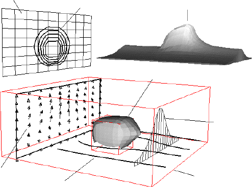
Figure 1-1
Various EnSight Part Types
Clip Plane Contours Elevated Surface
Isosurface
Profile
Vector Arrows
Particle Traces Model Part
1 Overview
1-4 EnSight 10.2 User Manual
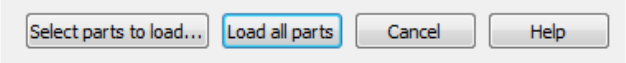
load all the parts or to select parts to load.
The “Load all parts” option will read the specified data (the “case”) and create
(i.e. “load”) all of the parts into EnSight. The other option - “Select parts to
load...” - will read the data but will not load any parts. This second option will
allow you to select on a per part basis which parts will be loaded into EnSight.
This “load” process is performed through the Part List.
The Part List contains all parts that have been read in (“loaded”) from your
specified data file as well as those created within EnSight. Additionally, it may
show model parts from the data that are not already loaded. These are referred to
as Loadable Parts or LPARTs.
LPARTs may be loaded zero or more times. You may choose not to load a
particular part from a data set if it is not needed for the visualization or analysis of
the case. This is advantageous to save memory and processing time. You may also
choose to load a part multiple times - so you could, for example, color the part by
multiple variables at the same time in multiple viewports.
LPARTs are shown as grayed out parts in the Part List. You can load a LPART by
selecting the part(s) and performing a right click operation to “Load part”
Part Attributes
Attributes define how a part appears and how it is created (in case of created
parts). All loaded parts have attributes.
The attributes that control how a part appears are referred to as “general” or
“visual” attributes. All part types have these same general attributes and include
settings such as visibility, line width, color, lighting parameters, etc.
Created parts have creation attributes, i.e., settings which specify how the part is
created. Each part type will have a different set of creation attributes.
Element
Representation
One of the general attributes that deserves some discussion in this overview is
“Element Representation”.
At the start of this chapter the EnSight architecture was briefly discussed,
indicating that the server has the data from the case you have loaded and the client
shows the extracts of data that you desire. The less data you extract to the client
the smaller the memory requirements and higher the performance. One way to
minimize the data sent to the client for visualization is to take advantage of the
“Element Representation” attribute.
Element Representation has no effect whatsoever on the data stored and used on
the EnSight server process. It only effects what is sent to the client for display.
Except for the “volume” representation, no 3D elements are ever sent to the client.
Even when a 3D element is viewed (“Full” representation) it is viewed on the
client as a set of 2d faces for the 3d element.
1 Overview
EnSight 10.2 User Manual 1-5
The choices for Element Representation are:
Full The client receives all of the vertices, as well as the definition
for all 0D, 1D, and 2D elements and all of the element faces
for 3D elements. It is usually a mistake to load parts
containing 3D element in this mode. 2D parts are usually best
loaded in this mode.
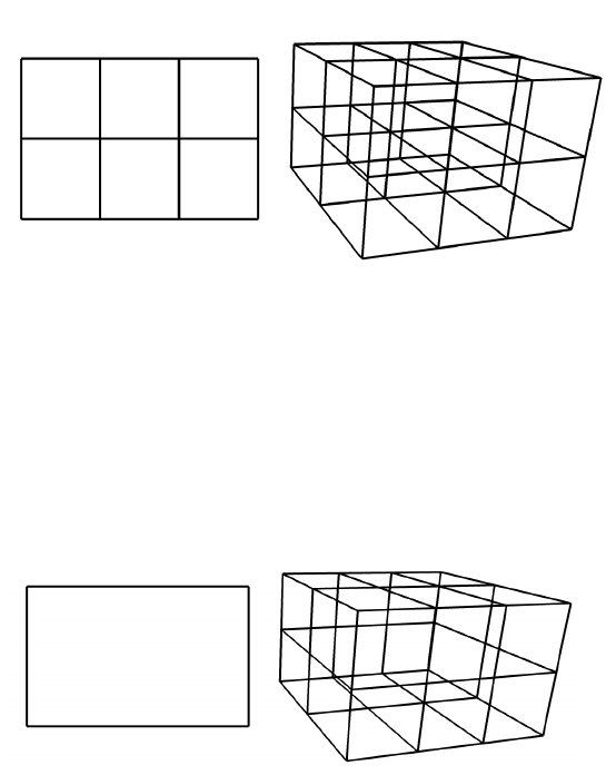
The image below shows two parts. The part on the left is
composed of quad (i.e., 2D) elements, while the part on the
right is composed of hexahedra (i.e., 3D) elements. The 3D
part is showing all of the faces of all of the 3D elements
resulting in “clutter” in the interior of the part.
Border The shared edges between 2D elements and the shared faces
between 3D elements are removed. Using the same geometry
from above, the figure below shows the result of this mode.
Note that the 3D part no longer contains interior lines. Border
mode is usually the best mode to use for loading 3D parts, and
not usually used for 2D parts.
Figure 1-2
Full Element Representation of 2D and 3D parts.
Figure 1-3
Border Element Representation of 2D and 3D parts.
1 Overview
1-6 EnSight 10.2 User Manual
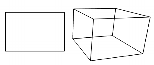
Feature angle This representation works on 2D elements, thus for 3D parts
the server first computes the Border representation. Then
given 2D elements, the edge between two elements is
removed if the normal between the two elements sharing the
edge is less than an angle (default 10 degrees) specified by the
user. The result is 1D information on the client that represents
“sharp” edges of the part. The figure below shows the result
of feature angle mode. Since the 2D part is planar all of the
interior edges are removed. Similarly for the 3D part - since
all the exterior bounds of the part are planar - all of the
interior edges of each face are removed, leaving just the sharp
edges of the box.
Nonvisual No data is sent to the client. Please note that this is entirely
different than loading the part with some other Element
Representation and then turning off the visible attribute. The
visible attribute simple turns off the rendering of a part. The
data has still been sent to the client! This is the recommended
mode for parts that do not need to be viewed but will be used
for extracting information such as a fluid field around a
geometry.
Bounding box Send only the bounding box geometry to the client for display.
Figure 1-4
Feature Angle Element Representation of 2D and 3D parts.
1 Overview
EnSight 10.2 User Manual 1-7
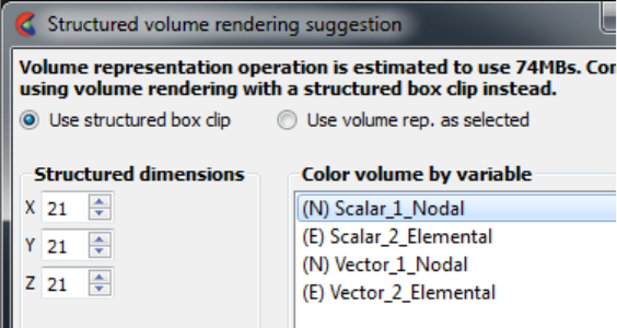
Volume Volume rendering displays all 3D elements at once, drawing
each element semi-transparently according to the value of a
variable.
Raw volume rendering (Use volume rep. as selected radio
button as shown in the figure below) will divide the elements
into tets and send them to the client and then adjust the
opacity per element based on the value of a variable.
Unstructured tet volume rendering uses 96 bytes per element
and 72 bytes per pixel. For example, if you have a 21x21x21
hex grid with roughly 10000 elements and each hex divides
into six tetrahedrons, you have 60k tet elements, using about
6MB. Suppose we have a 1K x 1K pixel screen, using about
72MB. This results in a combined estimate of about 6MB +
72MB for a total of 78MB. Note the estimate provided in the
dialog for this situation is 74MB, shown below.
A few million unstructured elements can easily overwhelm
the client and graphics card, so another, preferable option is
available to do a structured remesh (Use structured box clip
radio button shown in the figure below) using user-selected x,
y, and z dimensions to control the number of elements passed
up to the client. This structured, volume rendering uses up to
4 bytes/cell + 72 bytes per pixel on the client graphics card.
So a 21x21x21 structured grid (shown below) with 1kx1k
pixel screen, is roughly 40KB + 72 MB, or roughly 72MB.
So for small grid size, the bytes per pixel dominates and there
is little difference in the memory requirements between
structured and unstructured. But for large grids the bytes per
cell dominates (for a 1024x1024x1024 structured grid, this
takes 2GB for a structured and 100GB for unstructured) and
structured volume rendering is the only feasible way to go.
Figure 1-5
Volume Element Representation of a 3D part.
1 Overview
1-8 EnSight 10.2 User Manual
The default Element Representation used by EnSight, unless the data reader for
the format you have specified indicates otherwise, is “2D Full, 3D Border”.
Meaning 2D elements will be sent to the client in Full mode and 3D elements will
be sent in Border mode.
Created Parts
Parts that are created within EnSight are referred to as created (or dependent)
parts. The types of parts that you create depend on what features within EnSight
you choose to utilize. Any created part is derived from parts that already exist,
which is why created parts are sometimes called dependent parts—they depend on
the parts from which they were created. The parts that are used to create a
dependent part are referred to as parent parts. Any time that a parent part changes,
its dependent parts also change. A parent part will change when you change its
attributes, or modify the current time in the case of transient data.
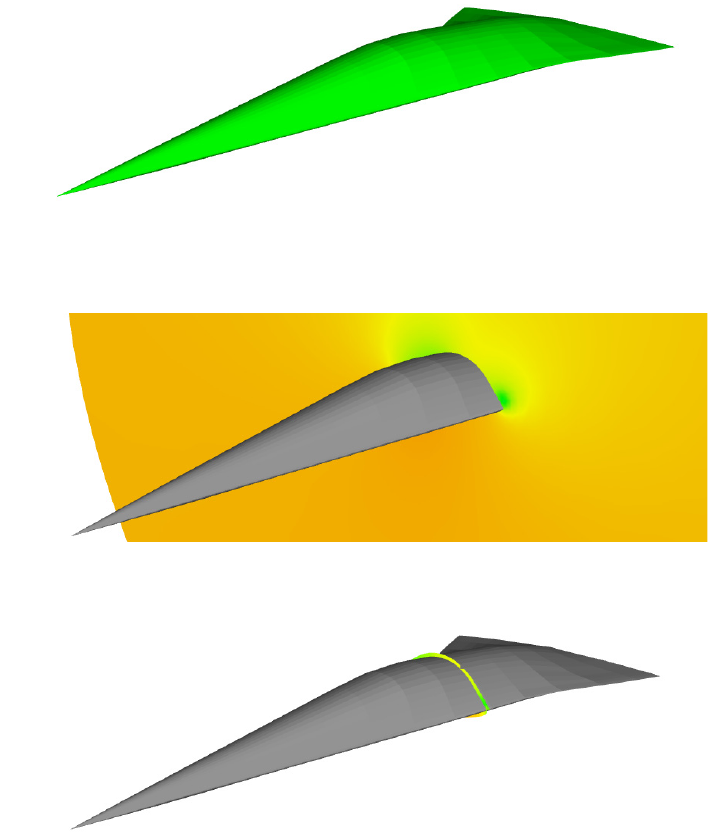
Failure to select the proper parent part(s) will result in an incorrect part being
created. For example, if I intend to create a clip through the flow field on the
geometry shown in the image below:
And I select the part representing the external flow field I will indeed see the clip I
intend.
But if I instead select the surface part as the parent I will get:
Figure 1-6
Clip example geometry
Figure 1-7
Clip through flow field part
Figure 1-8
Clip through surface part
1 Overview
EnSight 10.2 User Manual 1-9
Both model parts and created parts can be parent parts. For example in the clip
example above, if I wanted to view vector arrows on the clip part I would select
the clip part as the parent.
See Section 5.1, Parts for a complete list and description of derived parts that
EnSight can create.
Auxiliary
Geometry
Auxiliary geometry can be created around existing parts on which textures or
images can be mapped, or shadows from the existing parts can be cast when
exporting ray traced images. Various attributes of the geometry can be controlled
such as, visible components, outline, thickness, double walls, etc. (see Section
5.1.19, Auxiliary Geometry)
Clips A clip is a plane, line, box, ijk surface, xyz plane, rtz surface, quadric surface
(cylinder, sphere, cone, etc.), or revolution surface passing through specified
parent-parts. A clip can either be limited to a specific area (finite), or clip
infinitely through the model. You control the location of the various clips with an
interactive Tool or appropriate parameter or coefficient input.
A clip line or plane will either be a true clip through the model, or can be made to
be a grid where the grid density is under your control.
Clip surfaces can be animated as well as manipulated interactively.
In most cases you will create a clip which is the intersection of the clip tool and
the parent parts. This clip can either be a true intersection or all elements that
cross the intersection surface (a “crinkly” surface). You can also choose to cut the
parent parts into half spaces.
(see Section 5.1.3, Clip Parts)
Contours Contours are created by specifying which parts are to be contoured, and which
variable to use. The contour levels can be tied to those of the palette or can be
specified independently by the user.
(see Section 5.1.4, Contour Parts)
Developed
Surfaces
Developed Surfaces can be created from cylindrical, spherical, conical, or
revolution clip surfaces. You control the seam location and projection method that
will flatten the surface.
(see Section 5.1.5, Developed Surface Parts)
Elevated
Surfaces
Elevated Surfaces can be displayed using a scalar variable to elevate the displayed
surface of specified parts. The elevated surface can have side walls.
(see Section 5.1.6, Elevated Surface Parts)
Extrusions Parts can be extruded to their next higher order. Namely a line can be extruded
into a plane, a 2D surface into a 3D volume, etc. The extrusion can be rotational
(such as would be desired for an axi-symmetric part) or translational.
(see Section 5.1.7, Extruded Parts)
Isosurfaces Isosurfaces can be created using a scalar, vector component, vector magnitude, or
coordinate. Isosurfaces can be manipulated interactively or animated by
incrementing the isovalue.
(see Section 5.1.8, Isosurface Parts)
Particle Traces Particle traces—both streamlines (steady state) and pathlines (transient)—trace
the path of either a massless or massed particle in a vector field. You control
which parts the particle trace will be computed through, the duration of the trace,
1 Overview
1-10 EnSight 10.2 User Manual
which vector variable to use during the integration, and the integration time-step
limits. Like other parts, the resulting particle trace part has nodes at which all of
the variables are known, and thus it can be colored by a different variable than the
one used to create it. Components of the vector field can be eliminated by the user
to force the trace to, for example, lie in a plane. The particle trace can either be
displayed as a line, a ribbon, or a square tube showing the rotational components
of the flow field. Streamlines can be computed upstream, downstream, or both.
Streamline and pathline particle traces originate from emitters, which you create.
An emitter can be a point, rake, net, or can be the visible nodes of a part. Each
emitter has a particle trace emit time specified which you set, and a re-emit time
(if the data case is transient) can also be specified. Point, rake, and net emitters
can be interactively positioned with the mouse. For streamlines, the particle trace
continues to update as the emitter tool is positioned interactively by the user, or as
the emitter part element boundary representation is updated.
Another form of trace that is available is entitled node tracking. This trace is
constructed by connecting the locations of nodes through time. It is useful for
changing geometry or transient displacement models (including measured
particles) which have node ids.
A further type of trace that is available is a min or max variable track. This trace is
constructed by connecting the min or max of a chosen variable (for the selected
parts) though time. Thus, on transient models, one can follow where the min or
max variable location occurs.
(see Section 5.1.10, Particle Trace Parts)
Points Point parts are composed only of nodes. They can be created by reading an
external file containing the xyz coordinates of the nodes, and/or by placing the
cursor tool at desired locations and adding nodes. This feature can be used to
essentially place probes in the model at particular locations. It can also be used to
create parts that can be meshed with the 2D or 3D meshing capability within
EnSight.
(see Section 5.1.11, Point Parts)
Profiles Profile plots can be created by scalar, vector component, or vector magnitude. You
control the orientation of the resulting profile plot.
(see Section 5.1.12, Profile Parts)
Separation/
Attachment Lines
Separation and attachment lines show where flow abruptly leaves or returns to the
2D surface in 3D fields.
(see Section 5.1.13, Separation/Attachment Line Parts)
Shock Surfaces/
Regions
Shock surfaces or regions show the location and extent of shock waves in a
3Dflow field.
(see Section 5.1.14, Shock Regions/Surfaces Parts)
Subsets A subset Part can contain node and element ranges of any model Part.
(see Section 5.1.15, Subset Parts)
Tensor Glyphs Tensor glyphs show the direction of the principal eigenvectors. You specify which
eigenvectors you wish to view and how you wish to view compression and
tension.
(see Section 5.1.16, Tensor Glyph Parts)
Vector Arrows Vector arrows show the direction and magnitude of a vector field. Vector arrows
originate from element vertices, element nodes (including mid-side nodes), or

1 Overview
EnSight 10.2 User Manual 1-11
from element centers. You specify which parts are to have arrows and which
vector variable to use for the arrows, as well as a scale factor. You can eliminate
components of the vector, and can also filter the arrows to eliminate high, low,
low/high, or banded vector arrow magnitudes. The vector arrows can be either
straight or curved, and can have arrow heads. The arrow heads are either
proportional to the arrow or can be of fixed size.
(see Section 5.1.17, Vector Arrow Parts)
Vortex Cores Vortex cores show the center of swirling flow in a flow field.
(see Section 5.1.18, Vortex Core Parts)
Part creation occurs on either the server or the client. Since the data that is
available on the client and server are different, it is useful to understand where
Parts are created and where the resulting data is stored. By understanding this, you
will understand why some Parts can be created with certain parent Parts and
others cannot. For example, why you can’t clip through a particle trace part (clips
are created on the server and the particle trace part is not defined there). This
information can be gained by examining the following table.
Table 1–2 Part Creation and Data Location
(see Introduction to Part Creation)
Part Selection and Identification
In the process of creating a Part you will need to be able to select the parent
Part(s). This operation can be done from either the part list, the graphics window,
or by key words from a search dialog.
See How to Select Parts.
Part Type Where Created Data on
Server Data on Client
Clip Server Yes Depending on Element Rep
Contour Client No Yes
Developed
Surface
Server Yes Depending on Element Rep
Elevated Surface Server Yes Depending on Element Rep
Isosurface Server Yes Depending on Element Rep
Material Part Server Yes Depending on Element Rep
Particle Trace Server No Yes
Point Part Server Yes Depending on Element Rep
Profile Client No Yes
Separation/
Attachment Line
Server Yes Depending on Element Rep
Shock Surface/
Region
Server Yes Depending on Element Rep
Subset Server Yes Depending on Element Rep
Tensor Glyph Client No Yes
Vector Arrow Client. Server if
necessary.
No Yes
Vortex Core Server Yes Depending on Element Rep
1 Overview
1-12 EnSight 10.2 User Manual
Transformations
The standard transformations of rotate, translate, and scale are available, as well
as positioning of the Look-At and Look-From points and camera positions. The
transformation-state (the specific view in the Graphics Window and Viewports)
can be saved for later recall and use to a views manager. Transformations can be
performed with precision in a dialog, or interactively with the mouse.
(see Chapter 6, Transformation Control)
Frames
Normally transformations are performed on the entire scene. But they can also be
performed on a subset of the geometry (such as an “exploded” view). This is done
by creating a coordinate frame and assigning part(s) to the new frame definition.
The frame can be offset and rotated from the model axis system. Frames can have
rectangular, cylindrical, or spherical coordinates.
Frames, and therefore all parts attached to them, can be “periodic”. Rotational or
translational periodicity (as well as mirror symmetry) attributes are under user
control allowing, for example, an entire pie to be built from one slice of the pie.
Variables
While Parts are the fundamental entity in EnSight, the purpose of using EnSight is
nearly always the pursuit of understanding the simulation results, i.e., Variables.
Variables can either originate with the data file read or they can be computed
using provided variables and geometry.
Variables can be defined on all nodes/elements or can be declared “undefined” for
specified parts or node and element ranges.
Location A field variable can be defined on an element center or at the vertices of the part.
Constant Variable A Constant variable defines a single value and may or may not be associated with
any specific part. A Constant Variable may change value over time or be
recomputed based on its parent parts. Total Volume of a model is an example of a
constant variable. It is often referred to as a constant per case.
Constant Per Part
Variable
A Constant Per Part variable defines a single value for a given part. Each part can
have its own value for the variable. It can change overtime. Part Area would be a
good example of a constant per part variable. Note that created parts will only
inherit this variable if all parent parts have the same value.
Scalar Variable A Scalar variable defines a single value for each node or element on each part
where it is defined. It creates a “field” of data values. Temperature would be an
example of a Scalar variable.
Vector Variable A Vector variable defines three values - representing the x, y, and z components of
a vector - for each node or element on each part where it is defined. It creates a
“field” of data values. Velocity would be an example of a Vector variable.
Tensor Variable A Tensor variable defines nine values - representing the components of a tensor -
for each node or element on each part where it is defined. It creates a “field” of
data values. A stress tensor would be an example of a Tensor variable.
Complex Scalars/
Vectors
Scalar and Vector variables may have a real and imaginary portion.
1 Overview
EnSight 10.2 User Manual 1-13
Variable Creation New variables can be created either by specifying an equation via a calculator
dialog or a predefined definition can be used. Similar to creating new parts, you
will in most cases need to specify on what part(s) the new variable is computed. A
large number of functions are currently available.
(see Section 7.3, Variable Creation)
Queries
In addition to visualizing information, you can make numerical queries.
You can query on information for a node, point, element, or a part.
You can query on information for a data set (such as size, number of elements,
etc.)
You can query scalar and vector information for a point or node over time.
You can query scalar and vector information along a line. The line can either be a
defined line in space, or a logical line composed of multiple 1D elements for a
part (for example, query of a variable on a particle trace).
You can query to find the spatial or temporal mean as well as the min/max
information for a variable.
Where applicable, query information can be in the form of a Fast Fourier
Transform (FFT).
Plotting The plotter plots Y vs. X curves. The user controls line style, axis control, line
thickness and color. All query operations that result in multiple value output in
EnSight can be sent to the plotter for display. The user can control which curves to
plot. Multiple curve plots are possible. All plotable query information can be
saved to a disk file for use with other plotting packages.
(see Section 5.3, Query/Plotter and Section 5.8, Interactive Probe Query)
Transient Data
EnSight handles transient (time dependent) data, including changing connectivity
for the geometry. You can easily change between time steps via the user interface.
All parts and variables that are created, are updated to reflect the current display
time (you can override this feature for individual parts). You can change to a
defined time step, or change to a time between two defined steps (EnSight will
linearly interpolate between steps). Note that this “continuous” option is only
available for cases without changing connectivity.
CoProcessing EnSight has the ability to update the number of timesteps dynamically (that is,
perhaps if the solver is in the process of writing the data and you are loading it as
the solution proceeds: CoProcessing). The only caveat is that EnSight needs a
never-to-exceed, maximum number of timesteps. This can be achieved by putting
a maximum time steps keyword in a Case Gold file, or in a PLOT3D file, or by
inserting a special routine (USERD_get_max_time_steps) into your user-defined
reader, indicating dynamically updating the number of timesteps may occur. See
Advanced section of the Load Transient Data for details.
Animation
You can animate your model in four ways: particle trace animation, flipbook
1 Overview
1-14 EnSight 10.2 User Manual
animation, solution time streaming, and keyframe animation.
Particle Trace
Animation
Particle trace animation sends “tracers” down already created particle traces. You
control the color, line type, speed and length of the animated traces.
If transient data is being animated at the same time, animated traces will
automatically synchronize to the transient data time, unless you specifically
indicate otherwise.
Flipbook
Animation
A Flipbook animation reads in transient data, step by step, or moves a part
spatially through a series of increments and stores the animation in memory.
Playback is much faster as it requires no computation to move from frame to
frame.
However, the trade-off is that Flipbook Animation can fill up your client memory.
Flipbook animation is simpler to do than keyframe animation, while allowing four
common types of animation:
Sequential presentation of transient data
Mode shapes based on a nodal displacement variable
EnSight created parts with an animation delta that recreates the part at a new
location (i.e., moving isosurfaces and Clip surfaces).
Sequential displacement by linear interpolation from zero to maximum
vector value.
You can specify the display speed, and can step page-by-page through the
animation in either direction. You can load some, or all the desired data. If you
later load more data, you can choose to keep the already loaded data. With
transient data, you can create pages between defined time steps, with EnSight
linearly interpolating the data.
Flipbooks can be created in two formats: a) Object animation where new objects
are created for each frame. The user can then manipulate the model during
animation play back or b) Image animation where a bitmap image is created and
stored for each animation page. For large models, image animation can sometimes
take less memory - while trading off the capability to manipulate the model during
animation.
(see Section 5.7, Flipbook Animation)
Solution Time
Streaming
Solution time streaming accomplishes the same result as a flipbook animation of
transient data except the data is never loaded into memory: it is streamed directly
from disk one time step at a time. While you don’t see the animation speed of a
flipbook, you only need enough memory to load in one step.
Keyframe
Animation
Keyframe animation performs linearly interpolated transformations between
specified key frames to create animation frames. Command language can be
executed at key frames to script your animation. Some minimal editing is possible
by deleting back to defined key frames. Animation key frames can be saved and
restored from disk. Animation can be done on transient data and can automatically
synchronize with simultaneous flipbook animation and particle trace animation.
“Fly-around”, “rotate-objects”, and “exploded-view” quick animations are
predefined for easy use.
Keyframe animation can be recorded to disk files using a format of your choice.
(see Section 5.9, Keyframe Animation)
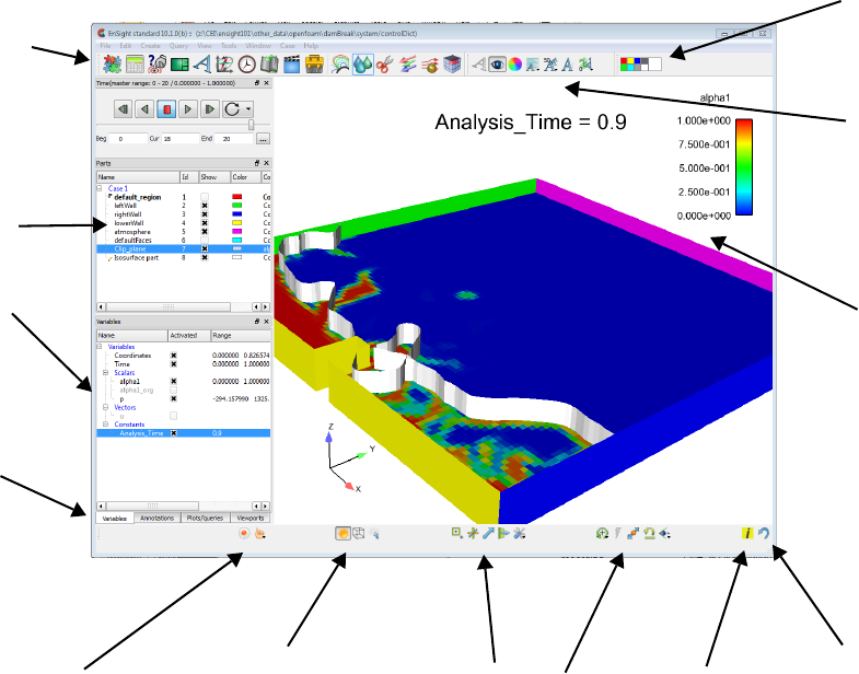
1 Overview
EnSight 10.2 User Manual 1-15
1.2 GUI Overview
This section gives an overview of the EnSight 10 user interface. Common terms
are described along with a brief summary of their purpose. References to other
sections of the documentation are noted for further details.
Figure 1-9 shows the EnSight user interface along with identification of several of
the major user interface elements. While EnSight typically follows the “look and
feel” guidelines for Microsoft Windows, Apple Macintosh, and Linux desktops, it
generally has a similar appearance on all of the platforms. Throughout this
document images of the interface may come from any of the three platforms;
nonetheless, the functionality is common to all three platforms in spite of minor
differences from the respective user interface guidelines.
The EnSight user interface is highly user configurable. For example, which icons
and where they’re displayed can be configured as can the scrolling lists to the left
of the graphics area. As such, the EnSight user interface may look significantly
different from what is shown in the documentation based on user preference.
Running EnSight with the command line option -no_prefs will revert EnSight
back to its default layout (see Command Line Start-up Options).
List
Variables
List
Transformation
Control
Quick
Action
Icons
Main
Window
Feature
Information
Button
“Desktop” - refers to the upper level of the GUI. It contains the following areas:
Undo / Redo
Object
List
Tab s
Icons
Parts
Picking and Line, & Highlighting
recording
Shading, Hidden
Figure 1-9
EnSight 10 Startup GUI
Transformation
Graphics
Icons
Secondary
Feature
1 Overview
1-16 EnSight 10.2 User Manual
1.2.1 Main Graphics Window
Contents This area shows a graphical representation of the currently loaded datasets’ visible
geometry. For example, a fluid dynamics dataset might show only boundary
surfaces, clips of fluid domains, and particle traces for flow fields but not the
entire fluid flow field; whereas FEA datasets might show all visible geometry for
a single time step from a transient simulation.
Mouse Usage Within this area of the user interface the user may use the computer mouse to
interact with the graphics in many ways. While clicking and holding down the left
or middle mouse buttons and moving the mouse, the graphics may be
transformed. By default, clicking and holding the left button while moving the
mouse controls the default transformation, typically rotation. Clicking and
holding the middle button while moving the mouse controls translation. EnSight
preferences, via the EnSight Preferences Dialog, may be set to indicate how the
mouse behaves in the Main Graphics Window. See How To Set or Modify
Preferences, section To Set Mouse and Keyboard Preferences: for further details.
Selection Clicking the left mouse button over an object drawn in the Main Graphics
Window while not moving the mouse selects the object beneath the mouse.
Holding down the Ctrl-key while performing this operation has the affect of
adding or removing the object below the mouse from the selection; thus, multiple
objects may be selected with the mouse. By default, the object selected in the
Main Graphics Window is highlighted. Additionally, the object is selected or
deselected in the appropriate list panel (described below).
Click-n-Go Selecting an object in the Main Graphics Window activates various hotspots on
the object. For example left clicking on an isosurface activates a multi-arrow
marker on the isosurface. Clicking and dragging on this marker will change the
value of the isosurface. Similarly, activating the multi-arrow marker on a clip part
allows that marker to be dragged to change the location of the clip part.
Annotations can be dragged around the graphics window, resized, and rescaled. In
general most objects drawn in the graphics window may be directly manipulated
with the mouse. (see Section 1.2.9, Click/Touch-n-Go)
Right-mouse click Clicking the right mouse button over an object in the Main Graphics Window will
display the popup context sensitive menu. The menu’s contents depend on the
object beneath the mouse pointer. If the mouse is over a clip plane, then a context
sensitive menu with options relevant to Parts, and in particular Clip Parts, will be
displayed containing applicable and common operations. Whereas if the mouse is
over a color legend, common operations applicable to legends are displayed.
Keyboard
interaction
Keystrokes may be used in the graphics window. The Del-key deletes the
currently selected object(s). The P-key is used by several different picking
operations. The function keys (F1-key through F12-key) are used for various
graphics transformations. See How To Rotate, Zoom, Translate, Scale and How
To Enable Stereo Viewing for further details. Additionally, EnSight Macros may
be defined to bind user-defined operations to other keys. See How To Define and
Use Macros for details.
Drag-n-Drop The Main Graphics Window also supports drag and drop from the various List
Panels. For example, a variable such as Pressure may be dragged from the
Variable List and dropped onto a clip part in the Main Graphics Window. This will
color the clip part by the pressure variable. (see Section 1.2.10, Drag-n-Drop)
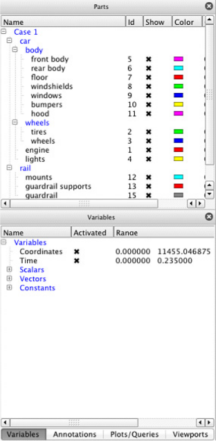
1 Overview
EnSight 10.2 User Manual 1-17
1.2.2 List Panels
List Panels show lists of commonly used EnSight Objects such as Parts, Variables,
Annotations, Queries, Plotters, Viewports, and Coordinate Frames. By default List
Panels are displayed to the left of the Main Graphics Window; but, because they
are a form of docking window, they may be moved to any edge of the main
EnSight Window, resized, undocked, or stacked on top of each other. Figure 1-10
shows the default layout of the list panels: the Parts list panel by itself and list
panels for Variables, Annotations, Queries/Plots, and Viewports stack atop of each
other in a tabbed layout. Chapter 3, List Panels of this document fully describes
the various List Panels.
Figure 1-10
List Panels
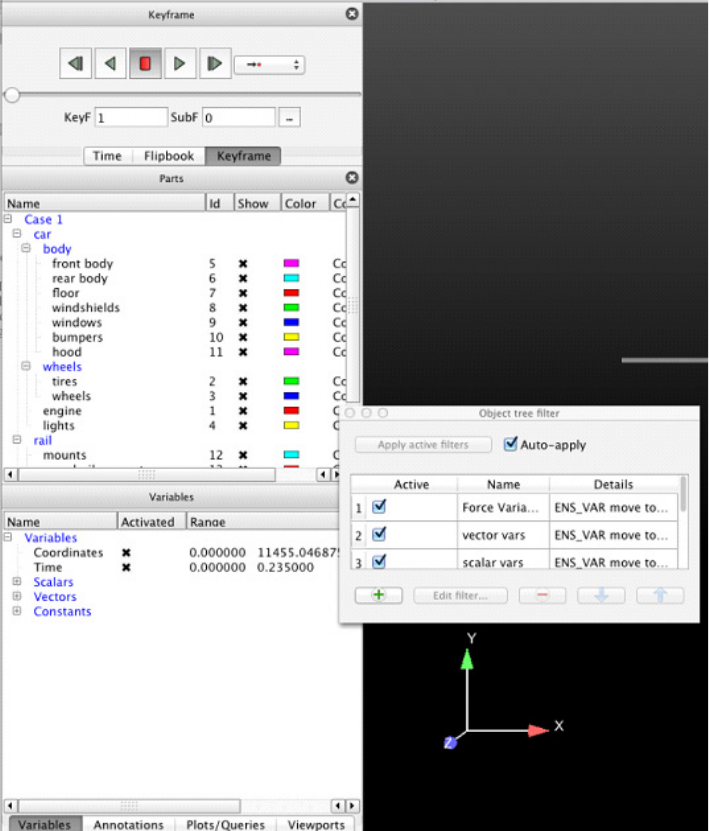
1 Overview
1-18 EnSight 10.2 User Manual
1.2.3 User Interface Panels
Other Panels Other User Interface Panels, such as the Time, Flipbook, Keyframe, and various
User Defined Tools, are also displayed in the same areas as the List Panels.
Similarly as with the List Panels, these panels are also dockable windows and may
be moved, resized, undocked, or stacked. Figure 1-11 shows an example of this.
Figure 1-11
Abbreviated Parts List
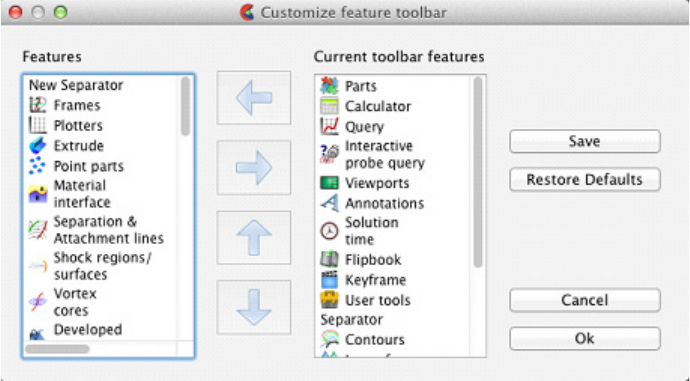
1 Overview
EnSight 10.2 User Manual 1-19
1.2.4 Feature and Quick Action Icon Bar
By default icons along the top edge of the EnSight user interface are arranged into
three clusters: Feature Icons, Secondary Feature Icons, and Quick Action Icons.
The Feature Icons and Secondary Feature Icons are organized into a single Icon
Bar with a simple delimiter between them. The Quick Action Icons are in their
own Icon Bar. Each Icon Bar may be repositioned along any of the edges of the
user interface or even undocked. This is done by grabbing and dragging the left
dimpled edge of the Icon Bar. All of these icons are fully described in Chapter 5,
Features.
Feature Icons The Feature Icons represent major functions of EnSight such as Part operations,
Calculator, Plotting, Queries, Viewports, Annotations, Time, Animation, and User
Defined Tools. Clicking on one of these icons activates the appropriate user
interface elements for that operation which may include displaying the
appropriate User Interface or List Panel, displaying the Feature Panel, and
displaying the relevant Secondary Feature Icons and Quick Action Icons.
Secondary Icons By default Secondary Feature Icons are displayed for common Part creation
including: Contours, Isosurfaces, Clips, Vector Arrows, and Particle Tracing.
Clicking on these displays the appropriate user interface in the Feature Panel.
Customize
Toolbar
The Customize Feature Toolbar Dialog (see Figure 1-12), activated via right
clicking on the Feature Icons context sensitive menu, allows the user to select
which Feature Icons to show and in what order. It may be advantageous to
customize these icons to show only those that are typically used by the user.
Quick Action
Icons
The Quick Action Icons provide common operations to modify the most recently
selected EnSight Object such as a Part or Annotation. Specifically, these icons
operate on the what ever is selected in the last updated List Panel. For example, if
two plots were last selected, then the Quick Action Icons operate on those two
plots. If all parts where last selected, then the Quick Action Icons operate on all
parts.
Figure 1-12
Customization of the Feature Toolbar
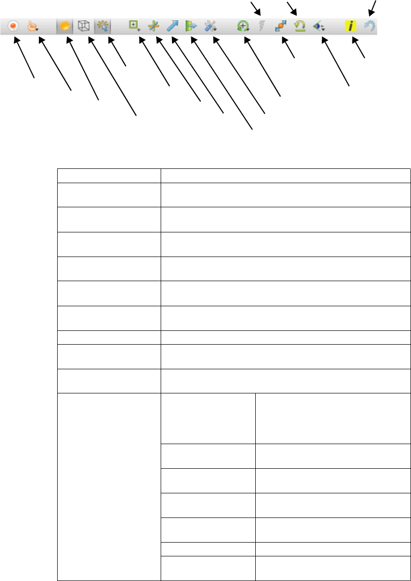
1 Overview
1-20 EnSight 10.2 User Manual
1.2.5 Tools Icon Bar
The Icon Bar along the lower edge of the EnSight user interface, shown in Figure
1-13 contains a variety of icons for commonly used operations. They are briefly
described here, see Section 5.11, Tools Icon Bar for further details.
Figure 1-13
Tools Icon Bar
Highlight
Pick Mode
Shade Surfaces
Hidden Line Display
Recording animations
Transformations
Cursor Tool
Line Tool
Selected
Tool Reset & Locate
Reinit Transforms
Fit View Information
Fast Display
Select View
dialogue
Undo / Redo
Plane Tool
Region Tool
Record animation Displays the Save Animation Dialog for recording animations.
Pick mode for the Main
Graphics Window
Submenu to set the type of pick operation performed by the P-
key.
Display shaded surfaces
toggle
Toggles shaded surface rendering.
Display hidden line
overlays toggle
Toggles hidden line overlays on the geometry.
Highlight selected parts
toggle
Toggles graphical highlighting of selected part(s).
Region tool visibility
toggle
Toggles the visibility of the region tool.
Cursor tool visibility
toggle
Toggles the visibility of the cursor tool.
Line tool visibility toggle Toggles the visibility of the line tool.
Plane tool visibility
toggle
Toggles the visibility of the plane tool.
Tool locations / Reset
dialog submenus
Options to display either the Tool Locations Dialog or the
Reset Tools / Viewports Dialog
Graphics window
transformations
submenu
Rotate Sets the Selected Transformation
operation to rotation. By default the
left mouse button is mapped to the
Selected Transformation.
Translate Sets the Selected Transformation
operation to translation.
Zoom Sets the Selected Transformation
operation to zoom.
Rubberband zoom Sets the Selected Transformation
operation to rubberband zoom.
Rubberband region Sets the Selected Transformation
operation to rubberband region.
Transformation editor Displays the transformation Editor.
Reset… Displays the Reset Tools / Viewports
Dialog.
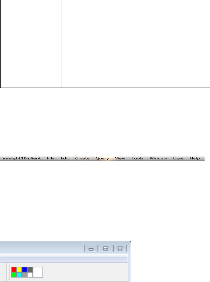
1 Overview
EnSight 10.2 User Manual 1-21
1.2.6 Main Menu Bar
The Main Menu Bar appears in the appropriate location for the operating system
in use. See Figure 1-14 for how it appears on the Apple Macintosh. Note that the
options are identical on all platforms. The Main Menu Bar options are described
in Chapter 4, Main Menu.
1.2.7 Quick Color Widget
The Quick Color Widget appears in the top right location in the EnSight window.
See Figure 1-15. The Quick Color Settings widget allows you to store your
favorite colors and drag/drop them onto objects (not viewports) that have a color
attribute. When any object with a constant color is selected, the large color patch
will show that object’s color. Drag and drop a color from any of the patches to any
single object to color that object by a constant color. Drag a color patch to any
other color patch. Right click on the patch to set its color. Currently parts, plotters,
queries, and all annotation types will accept a drag/drop color operation from the
widget.
Colors on the Quick Color Settings widget are stored as part of the user's
preferences and thus the colors on the widget are available between EnSight
sessions. For more details, see Use Quick Color Settings.
Fast display mode
toggle
Toggle for Fast display mode. When on, reduced geometry
representations may be used for some or all of the parts to
speed interactive transformations.
Fit view Reinitializes the graphics transformations so that all geometry
fits well within the Main Graphics Window while preserving the
current viewing orientation.
Reinitialize transforms Resets the graphics transformations to initial values.
Views orientation
submenu
Options to look up or down each of the three axes and an
option to display the Views Dialog.
Info dialog display Displays the EnSight Info Dialog.
Undo / redo last
transformation
Undo or Redo the last graphics transformation.
Figure 1-14
Main Menu Bar
Figure 1-15
Quick Color Widget
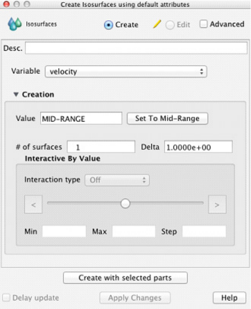
1 Overview
1-22 EnSight 10.2 User Manual
1.2.8 Feature Panel (FP)
While many common operations can be performed through direct interaction with
objects drawn in the Main Graphics Window, Icons, and various List and User
Interface Panels, more complex operations are typically found in the Feature
Panel (also known as the ‘FP’). Figure 1-16 shows the Feature Panel when used
for Isosurface Part Creation.
To avoid a proliferation of dialogs, EnSight typically reuses the Feature Panel for
many purposes. The Feature Panel will completely reconfigure itself
appropriately for the requested operation. The title bar of the Feature Panel will
indicate its current functionality. Common to most operations the Feature Panel
will also display its functionality in the upper left corner (‘Isosurfaces’ in Figure
1-16).
Simple and
Advanced
To simplify EnSight use while still providing a robust feature set, the Feature
Panel typically has a ‘Simple’ and an ‘Advanced’ view for most operations.
Toggling the ‘Advanced’ checkbox will display all options relevant to the current
operation. The Feature Panel also distinguishes, where appropriate, between
‘Create’ and ‘Edit’ mode. Create mode is used for creating new objects such as a
new Isosurface Part; whereas Edit mode is used to change attributes associated for
an existing object.
Figure 1-16
Isosurface Feature Panel (FP)
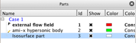
1 Overview
EnSight 10.2 User Manual 1-23
Selection and
Feature Panel
Selection
Figure 1-17 shows the Part List containing three parts. It is important to note three
visual metaphors shown. The blue highlighting around the ‘Isosurface part’
indicates that this part is the currently selected part. The pencil icon to the left of
the name ‘ami-x hypersonic body’ indicates that this part is the Feature Panel
selected part. The ‘P’ icon to the left of the ‘external flow field’ part indicates that
it is a parent part of the currently selected part(s). The concept between selected
and Feature Panel selected is important to understand and is common to all List
Panels. Selected objects are those that will be affected by operations in the main
user interface whereas Feature Panel selected objects are those that will be
affected by operations in the Feature Panel. This concept will be further
elaborated upon in Chapter 3, List Panels
Figure 1-17
Part List
1 Overview
1-24 EnSight 10.2 User Manual
1.2.9 Click/Touch-n-Go
Click-n-go is a way to grab a “handle” in the graphics window, using the mouse,
and drag it to affect the attribute attached to the handle. There are two methods
available, both of which perform the same operation and differ only in how the
handles appear. With click-n-go you use the left mouse button and click on an
object in the graphics window. If that objects has handles they will appear. With
touch-n-go the handles will automatically appear for the object found under the
mouse cursor (assuming your graphics hardware is capable of the function). With
either method, the next step is to “grab” a handle and modify its value by clicking
and dragging the handle.
Click-n-go is always active. Touch-n-go can be turned on/off via preferences. This
is done under Main Menu -> Edit -> Preferences -> View and using the “Set
Click-n-go preferences” button.
There are no touch-n-go handles on created parts – you must left click them to see
a handle (if it exists for the selected part type). The single handle will appear at the
picked location.
The following part types have a click-n-go handle with the function indicated:
Part Type Handle function tied to
Isosurfaces Isosurface value
Clip - XYZ X, Y, or Z clip value
Clip - Plane Translates the clip plane
Clip - Line Translates the clip line
Clip - Cylinder The radius
Clip - Cone The cone angle
Clip - Sphere The radius
Clip - IJK I, J, or K value
Particle traces - streamlines Translates emitter location
Vector arrows Arrow scale factor
Contours Number of sub-levels
Elevated Surface Scale factor
Profiles Scale factor
Click-n-go and Touch-n-go both show the same handles for the objects shown
in the figures below.
Text Annotation
The upper right handle performs a rotate of the text annotation. The other
handle performs a translate. It is not necessary to select the translate handle -
click/drag anywhere on the object (except the rotate handle) will perform a
translate.
1 Overview
EnSight 10.2 User Manual 1-25
Lines Annotation
The center handle translates the line annotation. The left/right handles move the
left/right end points. It is not necessary to select the translate handle - click/drag
anywhere on the object (except the other handles) will perform the translate.
Logo Annotation
The upper right handle will scale the logo. The other handle performs translate.
It is not necessary to select the translate handle - click/drag anywhere on the
object (except the other handles) will perform the translate.
Legend Annotation
The center handle will translate the legend. The upper right handle will resize.
The left top handle will modify the max value for the palette. Likewise, the
lower left handle will modify the min value. It is not necessary to select the
translate handle - click/drag anywhere on the object (except the other handles)
will perform the translate.
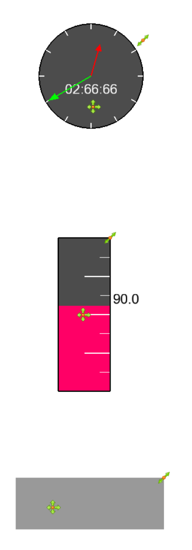
1 Overview
1-26 EnSight 10.2 User Manual
Dial Annotation
The upper right handle will size the dial while the other handle will translate. It
is not necessary to select the translate handle - click/drag anywhere on the
object (except the other handles) will perform the translate.
Gauge Annotation
The upper right handle will size the gauge dial while the other handle will
translate. It is not necessary to select the translate handle - click/drag anywhere
on the object (except the other handles) will perform the translate.
Shapes Annotation
The upper right handle will size the shape while the other handle will translate.
It is not necessary to select the translate handle - click/drag anywhere on the
object (except the other handles) will perform the translate.
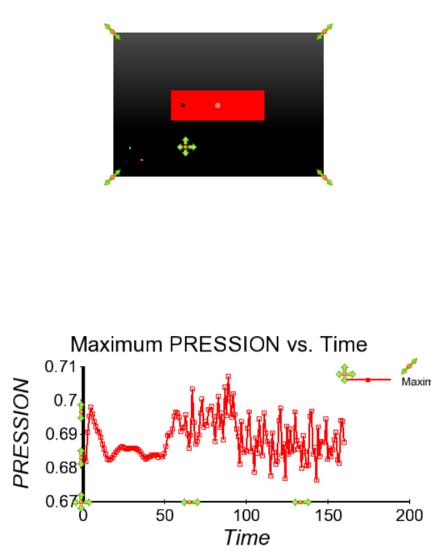
1 Overview
EnSight 10.2 User Manual 1-27
Viewports
The cross handle will translate the viewport while the corner handles will resize.
There are no touch and go handles for this object - you must use click-n-go.
Once the click-n-go handles are visible you may click/drag anywhere on the
object (except the other handles) to perform a translate.
Plotters
Upper right corner handle will scale the plotter. The marker on the plotter
legend will move the legend. The cross marker (that is not attached to the
legend) will translate the plotter. The up/down arrows on the y-axis will scale
the top/bottom values of the axis. Similarly, the left/right arrows on the x-axis
will scale the left/right values of the axis. It is not necessary to select the
translate handle - click/drag anywhere on the object (except the other handles)
will perform the translate.
1 Overview
1-28 EnSight 10.2 User Manual
1.2.10 Drag-n-Drop
You can drag (left click and hold the mouse button down, then move the mouse)
an object and drop (release the left mouse button) it onto a "target". The target can
be in the user interface (always available) or in the graphics window (will work
only if your graphics hardware supports the operation). The following drag and
drop actions are currently implemented:
Parts When dropped in a viewport (user interface or graphics window) will make the
part visible in the viewport.
When dropped onto a group in the Parts List will make the part belong to the
group.
Variables A constant variable dropped in the graphics window will create an annotation text
string with the value of the constant.
When scalars or vector variables are dropped in a viewport the parts with viewport
visibility True (regardless of their regular show/hide visibility status) will be
colored by the variable.
If you drop a scalar or vector onto a visible part the result will be that the part is
colored by the variable. Similarly, if you drop the variable onto a group in the
Parts list all the parts that belong to the group will be colored.
Plots and Queries You can assign a query to a plotter by dropping the query on the plotter
Styles From the Style manager you can drag/drop a style onto objects of the right type,
i.e., if you have a style that was saved for a curve you can drop it onto a curve on
a plotter.
1 Overview
EnSight 10.2 User Manual 1-29
1.3 Other Features
Server-of-Servers A special server-of-servers (SOS) can be used in place of a normal server if you
have partitioned data or utilize the auto-decompose feature. This SOS acts like a
normal server to the client, but starts and deals with multiple servers, each of
which handle their portion of the dataset. This provides significant parallel
advantage for large datasets.
(see Section 9.8, Server-of-Server Casefile Format)
Virtual Reality EnSight is fully capable of running multi-pipe display, virtual reality and
distributed rendering modes.
(see Section 11, Remote Display and Parallel Compositing)
Command
Language
Each action performed with the graphical user interface has a corresponding
EnSight command. A session file is always being saved to aid in recovery from a
mistake or a program crash. The user will be prompted upon restart, after a crash,
whether or not to use a recovery file to restore the session. The command
language is human-readable and can be modified. Command files can be played
all the way through, or you can choose to stop the file and step through it line-by-
line.
(See How To Record and Play Command Files)
Python For more powerful scripting, EnSight supports the Python programming
language. The EnSight Python implementation includes every EnSight command
as well as looping, conditionals, and a large library of standard utilities.
(see Chapter 7, EnSight Python Interpreter)
Batch Processing EnSight can be run in batch bringing up no visible windows (user interface or
graphics window) and producing output according to the command file processed
(see Use Batch)
Context Files You can define a “context” and apply it to similar datasets.
(See How To Save/Restore Context)
Graphics EnSight uses the OpenGL graphic libraries and is available on a multitude of
hardware platforms. The rendering can be done through the hardware or can be
performed in software.
Parallel
Computation
EnSight supports shared-memory parallel computation via POSIX threads.
Threads are used to accelerate the computation of streamlines, pathlines, clips,
isosurfaces, and other compute-intensive operations.
(See How To Setup For Parallel Computation)
Distributed
Memory Parallel
Computation
EnSight supports distributed memory parallel computations (clusters) via server-
of-server operations. The data decomposition may either be done by you or can be
done “on the fly”.
Macros You can define macros tied to mouse buttons or keyboard keys to automate
actions you frequently perform.
Saving and
Archiving
You can save the entire current status of EnSight for later use, and can save other
entities as well (including the geometry of created parts for use by your analysis
software).
(see Section 2.6, Archive Files)
Environment
Variables
You can control a number of aspects of EnSight (both client and server) with
environment variables.
1 Overview
EnSight 10.2 User Manual 1-31
1.4 Documentation
An Installation Guide is provided.
The on-line EnSight documentation consists of the EnSight Getting Started
Manual, How To Manual, User Manual, and Interface Manual. The online
documentation is available via the Help menu.
User Manual The EnSight User Manual is organized as follows:
User Manual Table of Contents
Chapter 1 - Overview
Chapter 2 - Input/Output. This chapter describes the reading of model data
(with internal or user-defined readers), command files, archive files, context files,
scenario files, and various other input and output operations.
Chapter 3 - GUI Overview. This chapter describes the EnSight Graphic User
Interface.
Chapter 4 - List Panels. This chapter describes the various list panels, for parts,
variables, annotations, plots/queries, viewports, frames, etc.
Chapter 5 - Main Menu. This chapter describes the features and functions
available through the buttons and pull-down menus of the Main Menu of the GUI.
Chapter 6 - Features. This chapter describes the features and functions available
through the Icon buttons of the GUI.
Chapter 7 - Transformation Control. This chapter describes the Global
transformation of all Frames and Parts, the transformation of selected Frames and
Parts as well as selected Frames alone, the transformation of the various Tools,
and the adjustment of the Z-Clip planes and the Look At and Look From Points.
Chapter 8 - Variables and EnSight Calculator. This chapter describes the
selection and activation of variables, color palettes, and the creation of new
variables.
Chapter 9 - Preference and Setup File Formats. This chapter describes the
format of various preference files which the uses can affect.
Chapter 10 - EnSight Data Formats. This chapter describes in detail the format
of the various EnSight data formats.
Chapter 11 - Utility Programs. This chapter describes a number of unsupported
utility programs distributed with EnSight.
Chapter 12 - Parallel and Distributed Rendering. This chapter describes how
to configure EnSight for various VR configurations and for parallel rendering.
Chapter 13 - CEIShell. This chapter describes the EnSight Virtual
Communications Utility.
Chapter 14 - EnSight Networking Considerations. This chapter describes
various things that should be considered when running EnSight on a network.
Chapter 15 - EULA. This chapter contains the User agreements.
Cross References in the User Manual will appear similar to:
(see Chapter __ or (see Section __
Clicking on these Cross References will automatically take you to the referenced
Chapter or Section.
1 Overview
1-32 EnSight 10.2 User Manual
How To... The various How To documents available on-line provide step-by-step, click by
click instructions explaining how to perform tasks within EnSight such as creating
an isosurface or reading in data.
Interface... This manual describes the various methods and API’s that exist for interfacing
with EnSight.
Ordering To order printed copies of EnSight documentation, go to our website at
www.ceisoftware.com and click on support and choose documentation and follow
the instructions.
Newsletter CEI periodically publishes an electronic EnSight newsletter. If you would like to
subscribe to the newsletter, see our website:
www.ceisoftware.com.
1.5 Contacting CEI
EnSight was created to make your work easier and more productive. If you have
any questions about or problems using EnSight, or have suggestions for
improvements, please contact CEI support:
Phone: (800) 551-4448 (USA)
(919) 363-0883 (Outside-USA)
Fax: (919) 363-0833
Email: support@ceisoftware.com
EnSight 10.2 User Manual 2-1
2 Input
This chapter provides information on data input and output for EnSight.
2.1 Reader Basics provides a detailed description of the basics for reading data.
This section is referenced by all formats, in that they all use some or all of these
basic procedures. The quick load, as well as the more flexible two step load
process is discussed for both unstructured and structured data formats.
2.2 Native EnSight Format Readers describes the specifics for reading the
EnSight formats.
2.3 Other Readers describes the specifics for reading many other formats into
Ensight. These can be internal or user-defined readers.
2.4 Other External Data Sources describes other ways in which model data can
be prepared to be read into EnSight.
2.5 Command Files provides a description of the files that can be saved for
operations such as automatic restarting, macro generation, archiving, hardcopy
output, etc.
2.6 Archive Files describes options for saving and restoring the entire current
state of the program.
2.7 Context Files describes the options for saving and restoring context files.
2.8 Session Files describes the options for saving and restoring session files.
2.9 Scenario Files describes the options for saving scenario files that can be
displayed in the EnVision program.
2.10 Saving Geometry and Results Within EnSight describes how to save
model data, from any format which can be read into EnSight, as EnSight gold
casefile format.
2.11 Saving and Restoring View States describes options for saving and
restoring given view orientations.
2.12 Saving Graphic Images describes options for saving and printing graphic
images.
2.13 Saving and Restoring Animations describes options for saving and
restoring flipbook and keyframe animation frames.
2.14 Saving Query Text Information describes options for saving query
information to a text file.
2.15 Saving Your EnSight Environment describes options for saving various
environment settings which affect EnSight.
2.16 Saving EnSight Graphics Rendering Window Size describes options for
precise resizing of your Graphics Rendering Window.
Note: Formats for EnSight related files are described in chapters 10 and 11.
Formats for the various Analysis codes are not described herein.
2.1 Reader Basics
2-2 EnSight 10.2 User Manual
2.1 Reader Basics
Dataset Format Basics
Reading and Loading Data Basics
Dataset Format Basics
EnSight is designed to be an engineering postprocessor, and supports data formats
for popular engineering simulation codes and generally used data formats. Yet its
many features can be used in other areas as well. EnSight has been used to
visualize and animate results from simulations of diesel combustion,
cardiovascular flow, petroleum reservoir migration, pollution dispersion,
meteorological flow, as well as results from many other disciplines.
EnSight reads node and element definitions from the geometry file and groups
elements into an entity called a Part. A Part is simply a group of nodes and
elements (the Part can contain different element types) which all behave the same
way within EnSight and share common display attributes (such as color, line
width, etc.).
EnSight allows you to read multiple datasets and work with them individually in
the same active session. Each dataset comprises a new “Case” and is handled by
its own Server process and can be added by using EnSight’s main menu Case >
Add... option. Note: if the client and the server are each on different computers,
then the data directory path is that seen from the server. Each server process has
its own console window and the output from the data read is directed to this
console. On Windows it is sometimes helpful to enlarge the default buffer size on
the server window to accommodate the sometimes large amount of output. Right-
click on the top left of the server window (named at top
C:\WINDOWS\System32\cmd.exe) and choose Screen Buffer size to be Width of
120 and Height of 9999, and Window size of Width 120 and Height of 40. Then
when you save it, save it for all windows of this name and every time the server
window is opened it will have these defaults and to see all of the server console
output.
Reading and Loading Data Basics
Reading and then Loading Data into EnSight can be done from “Simple” or
“Advanced” interface.
Simple Interface The simple interface allows you to select a dataset which is read by the EnSight
server and then have all parts loaded and displayed on the Client. This is quick but
it does not allow control of which parts to load, nor does it allow you to control
the visual representation. Also, the simple interface only works for files mapped
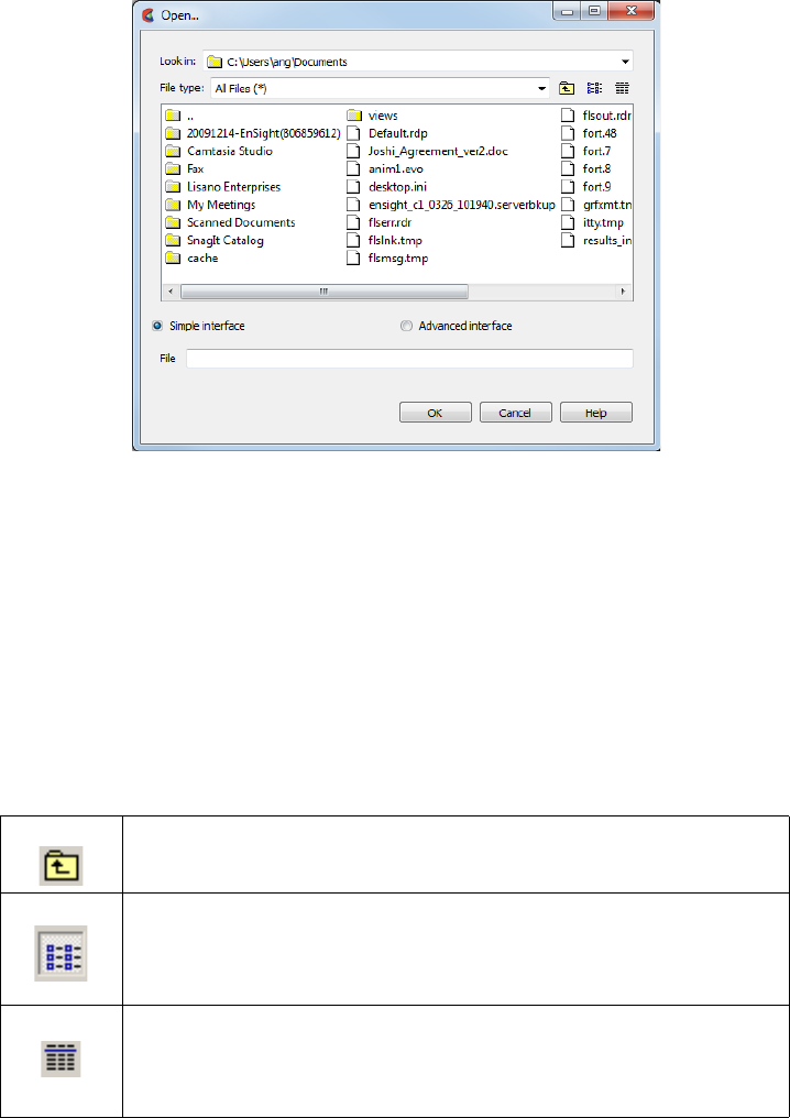
2.1 Reading and Loading Data Basics
EnSight 10.2 User Manual 2-3
in the
ensight_reader_extension.map
file found in the
$CEI_HOME/ensight102/
site_preferences
and/or in the EnSight Defaults Directory which is located
at %HOMEDRIVE%%HOMEPATH%\(username)\.ensight102 commonly
located at C:\Users\username\.ensight102 on Vista and Win7, C:\Documents and
Settings\yourusername\.ensight102 on older Windows, and ~/.ensight102 on
Linux, and in ~/Library/Application Support/EnSight102 on the Mac) directories.
Look in This field specifies the directory (or folder) name that is used to list the files and
directories in the list below.
File type Limits the directory content list to the file type chosen. The default is to show all files.
File/Directory
Manipulation
Buttons
Content List Shows the content of the Look in directory/folder. Single click to select a file. This will
insert the file name with full path as described in the Look in field in to the File field. If
you double click a file name, the file will be inserted into the File field and the Okay
button will execute. If you double click on a directory/folder name, you will change the
Look in filter.
File Specifies the file name that will be read once the Okay button is selected. As some file
formats require more than one file (geometry and results potentially) any associated files
will also be read according to the
ensight_reader_extension.map
file.
Okay Click to read the file (and associated files) specified in the File field and close the dialog.
Figure 2-1
File Open Dialog - Simple Interface
Changes the Look in directory to be one up from the current.
Show the content of the Look in directory in list view. In this view the
directory and file names are listed in alphabetical order. This is the
default.
Show the content of the Look in directory in detail view. This view will
show all directories and file names in alphabetical order and also show
size, type, date, and read/write attributes.
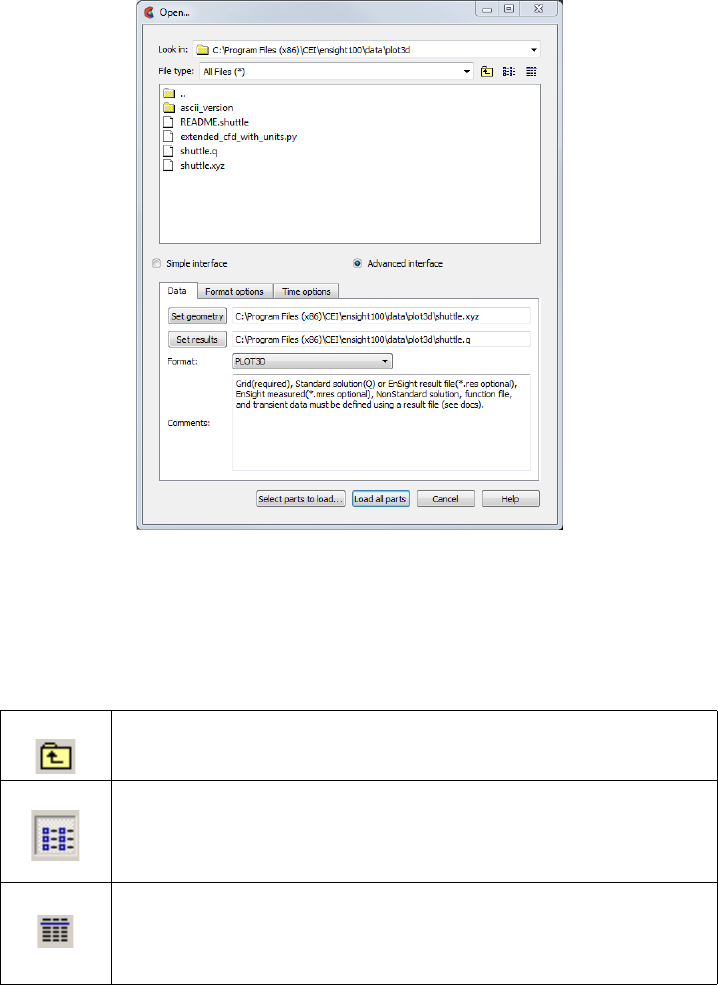
2.1 Reading and Loading Data Basics
2-4 EnSight 10.2 User Manual
Cancel Click to close the Open... dialog without reading any files.
(For a step-by-step tutorial please see How To Read Data).
Advanced
Interface
The advanced interface allows you to select a dataset which is read by the EnSight
server and then select which parts out of the dataset you wish to load and display
on the Client. You can control the format option, extra user interface options that
may be defined for your data file format and time settings.
Look in This field specifies the directory (or folder) name that is used to list the files and
directories in the list below.
File type Limits the directory content list to the file type chosen. The default is to show all files.
File/Directory
Manipulation
Buttons
Content List Shows the content of the Look in directory/folder. Single click to select a file. This will
insert the file name with full path as described in the Look in field in to the File field. If
you double click a file name, the file will be inserted into the File field and the Okay
button will execute. If you double click on a directory/folder name, you will change the
Look in filter.
Data Tab Contains settings for file format and file names.
Figure 2-2
File Open Dialog - Advanced Interface - Data Tab
Changes the Look in directory to be one up from the current.
Show the content of the Look in directory in list view. In this view the
directory and file names are listed in alphabetical order. This is the
default.
Show the content of the Look in directory in detail view. This view will
show all directories and file names in alphabetical order and also show
size, type, date, and read/write attributes.
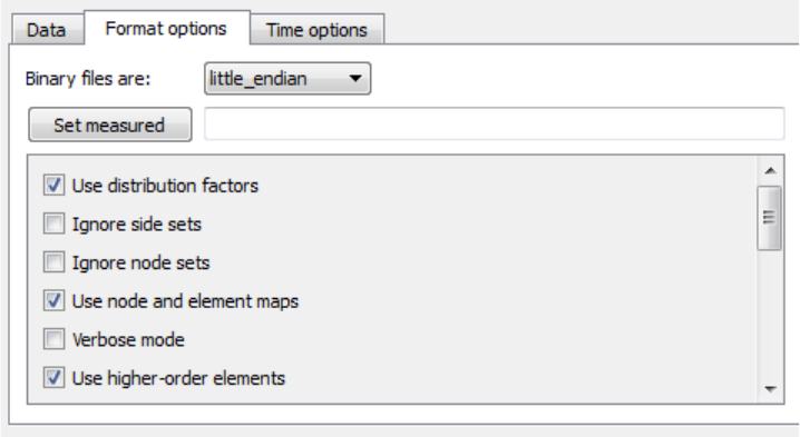
2.1 Reading and Loading Data Basics
EnSight 10.2 User Manual 2-5
Set The name for this field will depend on the file format. For example, for EnSight it is "Set
case" while for CTH it is "Set spcth*". This field describes the file name used to read the
dataset. Depending on the file format, there may be two (or possibly more) Set fields. The
use of the second (or third) set field depends on the file format and is described in the
Comments section of the dialog.
Format Specifies the Format of the dataset. This pulldown will vary depending upon what readers
are installed at your local site, and what readers are made visible in your preferences.
Note: you can start up ensight with the -readerdbg flag to view verbose information on the
readers as they are loaded into EnSight.
Comments Helpful information that is reader-specific will appear here, such as what file types are
entered into what fields.
Format Options
Tab
Contains format specific information.
Binary files are This is typically checked automatically by the reader, and thus usually there is no need to
use this toggle. If the file is binary, sets the byte order to the following:
Big-Endian - byte order used for HP, IBM, SGI, SUN, NEC, and IEEE Cray.
Little-Endian - byte order used for Intel and alpha based machines.
Native to Server Machine - sets the byte order to the same as the server machine.
Set measured Name of an EnSight 5 format measured results file (typically .mea file). Measured data is
read independently of the reader and is entered here for all readers except Case file format.
For Case file format, this field is not used and the measured data filename is entered into
the Case file. The measured data filename is always optional. Clicking the button inserts
the file name shown in Selection field and also inserts path information into Path field.
File names can alternatively be typed into the field.
Other Options Each data reader may have its own set of format options.
Figure 2-3
File Open Dialog - Advanced Interface - Format options Tab
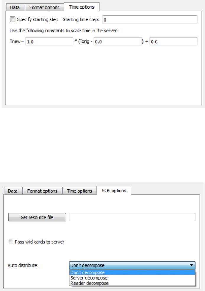
2.1 Reading and Loading Data Basics
2-6 EnSight 10.2 User Manual
Time Options
Tab
Contains Time specific information.
Time Settings Specify starting time step. If not specified, EnSight will load the last step (or whatever
step you have set in your preferences, see Edit>Preferences>Data). This section also
allows you to shift, scale and/or offset the original time values according to the values
entered into the equation.
SOS Options
Tab
If connected to an SOS server, this tab will be available and controls how the servers will
behave when handling data as well as what resources will be used.
Set resources Sets a filename to be used for SOS and Server resources.
Pass wild cards
to server
This toggle will pass wildcard filenames on to the server as opposed to resolving them on
the SOS. The usefulness of this toggle is entirely dependent on the specific reader in use.
Auto distribute How to decompose and distribute the data to each of the servers.
Don’t Data is already stored on disk decomposed.
Server Use the server to automatically partition the data
Reader Use the reader to automatically partition the data
Load All Parts Click to read and load all of the parts associated with the file names specified and close the
dialog.
Figure 2-4
File Open Dialog - Advanced Interface - Time options Tab
Figure 2-5
File Open Dialog - Advanced Interface - SOS options Tab
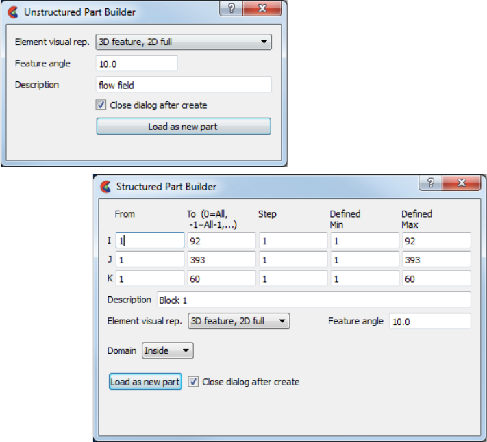
2.1 Reading and Loading Data Basics
EnSight 10.2 User Manual 2-7
Select Parts to
Load
Click to read the data files specified, close the dialog and show the parts in the Parts list as
loadable (grayed out) parts. These parts can be loaded by performing a right click
operation.
Cancel Click to close the Open... dialog without reading any files.
(For a step-by-step tutorial please see How To Read Data).
Data Part Loader If you right click on a grayed out part in the Parts list you can load (i.e., read it on
the server and show its element visual representation on the client). When you
load the part you can also specify the part description (if desired) as well as
specify the element visual representation. There are two basic part loader
windows. Details of these windows will be discussed below, and variants from
these windows will be discussed under each specific reader format.
All Parts or some of those available on the Server may be loaded to the Client and
their visual representation can be chosen. The Data Part Loader may be reopened
at a later time and additional or duplicate parts loaded as desired.
Unstructured Data If the part(s) in the Parts list is unstructured you will see the Unstructured Part Builder
dialog as shown above.
Structured Data If the part(s) in the Parts list is structured you will see the Structured Part Builder Dialog.
Element Visual
Rep.
Parts are defined on the server as a collection of 0, 1, 2, and 3D elements. EnSight can
show you all of the faces and edges of all of these elements, but this is usually a little
overwhelming, thus EnSight offers several different Visual Representations to simplify the
view in the graphics window. Note that the Visual Representation only applies to the
Figure 2-6
Typical File Data Part Loader dialogs
Unstructured Part Loader Dialog
Structured Part Loader Dialog
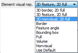
2.1 Reading and Loading Data Basics
2-8 EnSight 10.2 User Manual
EnSight client—it has no affect on the data for the EnSight server.
3D Border, 2D
Full
In this mode, load the designated parts, show all 1D and 2D elements, but show only the
unique (non-shared) faces of 3D elements.
3D Feature, 2D
Full
In this mode, load the designated parts, but show the 3D elements in Feature Angle mode
(see Feature below), and show all of the 1D and 2D elements.
3D nonvisual,
2D full
In this mode load the 3D parts but do not display them in the graphics window (see Non
Visual below) and load all the 1D and 2D elements.
Border In Border mode all 1D elements will be shown. Only the unique (non-shared) edges of 2D
elements and the unique (non-shared) faces of 3D elements will be shown.
Feature Angle When EnSight is asked to display a Part in this mode it first calculates the 3D Border, 2D
Full representation to create a list of 1D and 2D elements. Next it looks at the angle
between neighboring 2D elements. If the angle is above the Angle value specified in the
Feature Angle Field, the shared edge between the two elements is retained, otherwise it is
removed. Only 1D elements remain on the EnSight client after this operation.
Bounding Box All Part elements are replaced with a bounding box surrounding the Cartesian extent of
the elements of the Part.
Full In Full Representation mode all 1D and 2D elements will be shown. In addition, all faces
of all 3D elements will be shown.
Volume Volume render all 3D elements and ignore all other elements.
Non Visual This specifies that the loaded Part will not be visible in the Graphics Window because it is
only loaded on the Server. Visibility can be turned on later by changing the representation
(at which time the elements of the selected representation will be sent to the client).
Use Default This specifies that the part(s) should be loaded in the visual representation as defined by
the reader mapping file for the format specified.
Load Points and
normals only
If toggled on, only the vertices of the element representation, with normals, will be loaded
to the client.
Group these parts If more than one part is selected, they can be grouped into a single entity. The name of the
group will be according to the New Part Description filed and the individual parts will
receive the names shown in the part list.
New Part
Description
This allows the user to name the part. If nothing is entered here, then the part is named
from the partlist.
Load as New Part Loads Parts selected in the Parts List to the EnSight Server. The Parts are subsequently
loaded to the EnSight Client using the specified Visual Representation.
Structured Data
Domain Specifies the general iblanking option to use when creating a structured Part. If the model
does not have iblanking, InSide will be specified by default.
Inside Iblank value = 1 region
Outside Iblank value = 0 region
All Ignore iblanking and accept all nodes
Figure 2-7
Element Visual Representation pulldown
2.1 Reading and Loading Data Basics
EnSight 10.2 User Manual 2-9
Using Node Ranges:
From IJK Specifies the beginning I,J,K values to use when extracting the structured Part, or a
portion of it. Must be >= Min value.
To IJK Specifies the ending I,J,K values to use when extracting the structured Part, or a portion of
it. Must be <= Max value.
Valid values for the From and To fields can be positive or negative. Positive numbers are
the natural 1 through Max values. Negative values indicate surfaces back from the max, so
-1 would be the max surface, -2 the next to last surface etc. There are therefore two ways
to indicate any of the range values; the positive number from the min towards the max, or
the negative number from the max toward the min. The negative method is provided for
ease of use because of varying max values per part. (Zero will be treated like a -1, thus it is
another way to get the max surface)
1, 2, 3,... ---> <--- ...-3, -2 ,-1
|---|---|---|---|---|---|---|---|---|---|---|---|---|---|---|
min max
(always 1) (varies per zone)
Step IJK Specifies the step increment through I,J,K. A Step value of 1 extracts all original data. A
Step value of 2 extracts every other node, etc. Thus step values greater than 1 give a
coarser resolution.
Min IJK Minimum I,J,K values for Part chosen (for reference).
Max IJK Maximum I,J,K values for Part chosen (for reference).
Part Description Text field into which you can enter a description for the Part. If left blank a default will be
used.
Load as New Part Extracts the data from the data files and creates a Part on the Server (and on the Client
unless NonVisual has been specified for Representation) based on all information
specified in the dialog.
If only one part is highlighted, the values shown in the From and To fields (as well as the
Min and Max fields) are the actual values for the selected part. Using the From and To
fields you can control whether an EnSight part will be created using the entire ijk ranges
or some subset of them. The Step field allows you to sample at a more coarse resolution.
If more than one Part is highlighted, the values shown in the From and To fields are the
combined bounding maximums of the selected parts. The same basic functionality
described for a single part selection applies for multiple part selection, with one part being
created for each selected part in the dialog. If the specified ranges for the multiple
selection exceed the bounds of a given part, they are modified for that part so that its
bounds are not exceeded.
You use this portion of the Part Loader dialog to further extract iblanked regions from
structured parts which were created either as inside, outside, or all portions of the model.
(For step-by-step instructions see How To Read Data)
Loading Tips For large datasets, you should try to reduce the amount of information that is being
processed in order to minimize required memory. Here are some suggestions:
• When writing out data from your analysis software, consider what information will
actually be required for postprocessing. Any filtering operation you can do at this step
can greatly reduces the amount of time it takes to perform the postprocessing.
• For each Part you do load to the Client, a representation must be chosen. This visual
representation can be made very simple (through the use of the Bounding Box or
Feature Angle option, for example), or can be made more complex (by using the border
or full elements). The more you can reduce the visual representation, the faster the
graphics processing will occur on the Client (see Node, Element, and Line Attributes in
Section 5.1.1, Parts Quick Action Icons).

2.1 Reading and Loading Data Basics
2-10 EnSight 10.2 User Manual
• Load to the Client only those Parts that you need to see. For example, if you were
postprocessing the air flow around an aircraft you would normally not need to see the
flow field itself and could load it non-visual, but you would like to see the aircraft
surface and Parts created based on the flow field (which remains available on the
Server).
• If you have multiple variables in your result file, activate only those variables you want
to work with. When you finish using a variable, consider deactivating it to free up
memory and thereby speed processing (see Section 7.1, Variable Selection and
Activation).
Troubleshooting Loading Data
Problem Probable Causes Solutions
Data loads slowly Loading more Parts than needed For some models, especially
external fluid flow cases, there is a
flow field Part which does not need
to be visualized. Try loading this
Part non-visual.
Too many elements Make sure the default element
representation for Model Parts is set
to 3D Border/2D Full before
loading the data. In some cases it is
helpful to set the representation to
Feature Angle or 3D Feature 2D
Full, before loading.
Client is swapping because it does
not have enough memory to hold all
the Parts specified.
Try loading fewer Parts or installing
more memory to handle the dataset
size.
Server is swapping because it does
not have enough memory to hold all
of the Parts contained in the dataset.
Install more memory in your Server
host system, reduce the number of
variables activated, or somehow
reduce the geometry’s size. (If you
can get the data in, you can cut
away any area not now needed.
What is left can then be saved as a
geometric entity and that new
dataset used for future
postprocessing.)
Error reading data Incorrect path or filename Reenter the correct information.
Remember, the Path is on the server.
Incorrect file permissions Change the permissions of the
relevant directories and files to be
readable by you.
Temporary file space is full Temporary files are written to the
default temporary directory or the
directory specified by the
environment variable TMPDIR for
both the Client and Server. Check
file space by using the command
“df” and remove unnecessary files
from the temporary directory or
other full file systems.

2.1 Reading and Loading Data Basics
EnSight 10.2 User Manual 2-11
Format of the data is incorrect Recheck the data against the data
format definition. (Can use
ens_checker102 for Ensight6 or
EnSight Gold format checking.)
EnSight format scalar (or vector)
data loads, but appears incorrect.
Often range of values off by some
orders or magnitude.
Scalar (or vector) information not
formatted properly in data file
Format the file according to
examples listed under EnSight
Variable Files (see Chapter 9,
EnSight Data Formats) (Can use
ens_checker for Ensight6 or
EnSight Gold format checking.)
Extra white space appended to one
or more of the records
Check for and remove any extra
white space appended to each
record
Problem Probable Causes Solutions
2.2 Native EnSight Format Readers
2-12 EnSight 10.2 User Manual
2.2 Native EnSight Format Readers
EnSight’s native data format is useful as a general data format for unstructured or
structured grids. EnSight has three native data formats (from oldest to newest,
EnSight5, EnSight6 and EnSight Case Gold) which are well defined and well
documented so that they can be easily interfaced to your analysis code. All
licensed versions of EnSight read all three versions of Ensight formats, with the
exception of a special, bundled EnSight for Converge which reads only Converge
Case Gold translator output. EnSight 5, which is now considered a legacy format,
used a global coordinate array and supported unstructured meshes only. EnSight 6
format again used a global coordinate array but added support for structured
meshes. EnSight Case Gold (often just called Case format) is the most recent (and
recommended) format. Case Gold defines geometry on a part by part basis and
uses element index for connectivity. Case Gold format is tuned to the EnSight
internal data structure and is the fastest and most memory efficient format
available for EnSight.
A dramatic speed up in performance can sometimes be realized simply by reading
in data in the given format and saving it back out as Case Gold, then re-reading
the data back in using the native Case Gold reader. However, a number of solvers
now output data directly into the well-documented Case format. (see Chapter 9,
EnSight Data Formats). The application
ens_checker102
is included with EnSight to
enable error checking of the Case and EnSight 6 formats output by third-party
software.
Described below is the process for reading the latest (Case & EnSight 6) and the
legacy (EnSight 5) native formats:
EnSight Case Reader
EnSight5 Reader

2.2 EnSight Case Reader
EnSight 10.2 User Manual 2-13
EnSight Case Reader
In order to use this reader, you must be familiar with the basic data reader and part
loader dialogs discussed previously (see Chapter 2.1, Reader Basics).
EnSight6 and EnSight Gold are input using the exact same process. The data
consists of the following files:
• Case file (required)
• Geometry file (required)
• Variable files (optional)
• Measured/Particle files (optional)
- Measured/Particle geometry files
- Measured/Particle variable files
• Rigid body file (optional)
The Case file is a small ASCII file which points to all other files which pertain to
the model. The Case file names the geometry and variable files and records time
information. The geometry file is a general finite-element format describing nodes
and Parts, each Part being a collection of elements, and/or structured ijk blocks.
The variable file contains scalar (one value), vector (three values) or tensor (six or
9 values) data at each node and/or element. Measured/Particle files contain data
about discrete Particles in space from the simulation code or information directly
from experimental data.
EnSight data is based on Parts. The Parts defined in the data are always available
on the Server. However, all Parts do not have to be loaded to the Client for display.
Large flow fields for CFD problems, for example, are needed for computation by
the Server, but can be loaded non-visual.
EnSight data can be transient. The geometry as well as the variables can change
with each timestep. The casefile contains the filenames or filename patterns for
the transient data.
Simple Interface
Data Load
Load your casefile (typically named with a suffix
.case
) using the Simple Interface
method.
Advanced Interface
Data Load
Load your casefile (typically named with a suffix
.case
) using the Advanced
Interface method.
(see How To Read Data)
Data Tab
Format Use the Case format to read EnSight6 or EnSight Gold data.
Set Case Select the casefile (typically .case) and click this button
Format Options Tab
Endian Native, Big or Little-Endian. Since all modern platforms use the
Intel platform, which is little-endian we no longer automatically do
this check. Legacy files written from Unix platforms will need this
pulldown set to big-endian to read correctly.

2.2 EnSight5 Reader
2-14 EnSight 10.2 User Manual
EnSight5 Reader
EnSight5 input data consists of the following files:
• Geometry file (required)
• Result file (optional)
• Variable files (optional)
•Measured Particle Files (optional)
- Measured/Particle geometry files
- Measured/Particle results files
- Measured/Particle variable files
The geometry file is a general finite-element format describing nodes and Parts,
each Part being a collection of elements. The result file is a small ASCII file
allowing the user to name variables and provide time information. The result file
points to variable files which contain the scalar or vector information for each
node. Measured/Particle files contain data about discrete Particles in space from
the simulation code or information directly from actual experimental tests.
EnSight5 data is based on Parts. The Parts defined in the data are always available
on the Server. However, all Parts do not have to be loaded to the Client for display.
Large flow fields for CFD problems, for example, are needed for computation by
the Server, but do not generally need to be seen graphically.
EnSight5 data can have changing geometry, in which case the changing geometry
file names pattern is contained in the results file. However, it is still necessary to
specify an initial geometry file name in the (Set) Geometry field.
Simple Interface
Data Load
Load your geometry file (typically named with a suffix
.geo
) using the Simple
Interface method.
Advanced Interface
Data Load
Load your geometry and result files (typically named with a suffix
.geo and .res
)
using the Advanced Interface method.
(see How To Read Data)
Data Tab
Format Use the EnSight 5 format.
Set geometry Select the geometry file (typically .geo) and click this button
Set results Select the results file (typically .res), and click this button.
Format Options Tab
Set measured Select the measured file and click this button.
Endian Native, Big or Little-Endian. All modern platforms use the
Intel platform, which is little-endian. Legacy files from Unix
will be big-endian.
2.3 Other Readers
EnSight 10.2 User Manual 2-15
2.3 Other Readers
ABAQUS_ODB Reader
AcuSolve Reader
AUTODYN Reader
AIRPAK/ICEPAK Reader
ANSYS Reader
AV U S R e a d e r
CAD Reader
Barracuda Reader
CFF Reader
CFX4 Reader
CFX5 Reader
CGNS Reader
CGNS-XML Reader
Converge_Input Reader
CTH Reader
EXODUS II Reader
FAST UNSTRUCTURED Reader
FIDAP NEUTRAL Reader
FLOW3D-MULTIBLOCK Reader
FLUENT Direct Reader
Inventor Reader
LS-DYNA Reader
MSC.DYTRAN Reader
MSC.MARC Legacy Reader
NASTRAN OP2 Reader
Nastran Input Deck Reader
OpenFOAM Reader
OVERFLOW Reader
PLOT3D Reader
POLYFLOW Reader
RADIOSS Reader
SDRC Ideas Reader
SILO Reader
Software Cradle FLD Reader
STAR-CD and STAR-CCM+ Reader
STL Reader
Synthetic Reader
Tecp lo t R ea der
Vectis Reader
VTK Reader
XDMF Reader
EnSight includes a number of readers for non-native (non-EnSight) formats. This
section includes a description of each of these included readers and includes
instruction for their use. Some of the included readers are custom, internal
readers, and some of them are written using the standard, User Defined Reader
interface.
User Defined
Reader
Description
A user defined reader capability is included in EnSight which allows otherwise
unsupported structured or unstructured data to be read. In other words, the user
can create their own data readers. Each user defined reader utilizes a dynamic
2.3 Other Readers
2-16 EnSight 10.2 User Manual
shared library produced by the user. Once produced, these readers show up in the
list of data formats in the File Open Dialog just like the included readers.
User Defined
Reader
Implementation
The readers are produced by creating the routines documented in the user-defined
API. Three versions of the user defined API are available The 1.0 API (which has
been available since EnSight version 6) was designed to be friendly to those
producing it, but requires more manipulation internally by EnSight and
accordingly requires more memory and processing time. The 2.0 API (starting
with EnSight 7.2) was designed with efficiency in mind. It requires that all data be
provided on a part basis, and as such lends itself closely to the EnSight Gold type
format. A few of the advantages of the 2.0 API (Now at version 2.08) are:
* Less memory, more efficient, and faster - as indicated above.
* Model extents can be provided directly, such that EnSight need not read all the
coordinate data at load time.
* Tensor and complex variables are supported
* Exit routine provided, for cleanup operations at close of EnSight.
* Geometry and variables can be provided on different time lines (timesets).
* If your data format already provides boundary shell information, you can use it
instead of the “border” representation that EnSight would compute.
* Ghost cells (for both structured and unstructured data) are supported
* User specified node and/or element ids for structured parts are supported
* Material handling is supported
* Nsided and Nfaced elements are supported
* Structured ranges can be specified
* Filtered elements are supported
* Material Species is supported
* Rigid Body values can be supplied from the reader.
* Reader can be allowed to deal with block min, max, and stride within itself -
instead of having EnSight deal with it.
A 3.0 reader API is available in EnSight 9. The 3.0 API aims to provide the
flexibility of both of the previous versions while simplifying the reader
development processes. Contact CEI for more information on this API.
Creating Your Own
Custom User
Defined Reader
The process for creating and using a user-defined reader is explained in detail in
the EnSight Interface Manual. Samples, source code, makefiles, etc can be found
in the following location and its subdirectories:
On the CD: /CDROM/ensight102/src/readers
In installation
directory: $CEI_HOME/ensight102/src/readers
Start EnSight (or EnSight server) with the command line option (-readerdbg), for
a step-by-step echo of reader loading progress (see Command Line Start-up
Options).
ensight102 -readerdbg
The actual working user defined readers included in the EnSight distribution may
vary by hardware platform.
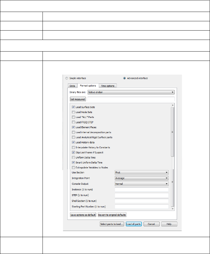
2.3 ABAQUS_ODB Reader
EnSight 10.2 User Manual 2-17
ABAQUS_ODB Reader
Overview
Because the reader is dependent upon the ABAQUS libraries, this reader is only
available for platforms supported by ABAQUS. See their website for more
details.
For updated information please see the file in the following directory:
$CEI_HOME/ensight102/src/readers/abaqus/README.txt
The ABAQUS odb reader is the recommended method of importing ABAQUS
data into EnSight.
Simple Interface
Data Load
Load your geometry/results file (typically named with a suffix
.odb
) using the
Simple Interface method.
Advanced Interface
Data Load
Load your geometry/result files (typically named with a suffix
.odb
) using the
Advanced Interface method.
Data Tab
Format Use the ABAQUS_ODB format.
Set geometry Select the geometry file (typically .odb) and click this button
Set results Not used
Format Options Tab
Set measured Select the measured file and click this button.
Reader GUI User controls as shown below are available:
Load Surface
Sets
Toggle ON (default) to load all Surface Sets

2.3 ABAQUS_ODB Reader
2-18 EnSight 10.2 User Manual
Load Node
Sets
Toggle ON to load all Node Sets (default OFF).
Load “*All*”
Parts
Often, ABAQUS parts that are simply the global element
matrix are redundant (e.g. E_ALL contains all elements).
Toggle OFF (default) to skip loading Parts with “all” in their
name, saving memory and time.
Load Freq
Step
Often, ABAQUS will include multiple steps in an ODB file
and the one desired is the modal analysis. Toggle this ON to
skip all other steps loading only the frequency step (Default is
OFF). If multiple frequencies, then each EnSight timestep
now becomes a different frequency.
Load
Element
Faces
Toggle ON to convert Surface Sets with 3D elements with
Face Sets into 2D elements using face specifications where
indicated by the ABAQUS dataset. (default ON).
Load internal
decomposition
parts
Toggle ON to load internal decomposition sets (that show the
parallel decomposition of the ABAQUS solver) as EnSight
parts.(default OFF).
Load
Analytical
Rigid Surface
parts
Toggle ON to load rigid surface parts as transient, rigid line
segments that can be extruded in 3 dimensions. This can be
done using a python script. Contact support@ensight.com for
details. (default OFF).
Load History
Data
Toggle ON to load History data which will load either as
constants or as queries over time (default ON). Some datasets
contain history data at extremely high sample rates with large
number of xy data pairs. EnSight is not structured to be able to
handle large numbers of queries with a large number of data
pairs, and will abort the loading of history data if it encounters
a data pair with more than 3000 samples. The reader will
output a warning that it has aborted the history data read and
that you can override this number; set the environmental
variable on the server as follows: set
ENSIGHT_READER_MAX_QUERY_PAIRS to the
maximum number of pairs that you wish to allow and restart
EnSight.
Interpolate
History to
Constants
History data is typically input to EnSight as queries (curves).
EnSight has the ability to use constant (single values at each
timestep) in ways that are not available to queries. If this is ON
then History variables will be interpolated as EnSight
Constants (if extrapolation is not necessary). If OFF then
History variables will be read in as constants only if there is an
exact one to one match of time values for each EnSight
timestep (Default OFF).

2.3 ABAQUS_ODB Reader
EnSight 10.2 User Manual 2-19
Skip Last
Frame if
Suspect
If the ABAQUS solver crashes, it can dump out a variety of
variable values for the last FRAME in the ODB file that may
be spurious. Toggle this ON (default) to check the last
FRAME in a STEP for an increase in the number of variables
and, if so, skip it. Toggle this OFF to ignore warning signs and
load the data from the last frame. If suspect values are found in
the last FRAME, then NAN checking of each variable value is
turned on, with NANs returned as zero (Default ON).
Smart
Uniform
Delta Time
Some ABAQUS STEPs have frame values that are constant
(and very small). Frame values are used by EnSight for time
steps and thus from this type of STEP are not monotonically
increasing in time and EnSight will skip these timesteps.
Toggle this ON, and EnSight will automatically convert time
values from selected ABAQUS STEPs into using a delta time
of 1.0 (default is ON).
Because EnSight is automatically changing the timestep
values, this will only be done to selected ABAQUS STEPs
(more may be added over time) The current list of these
includes only one ABAQUS STEP: "*STEP
PERTURBATION, *STATIC". As new STEPs are
encountered they may be added to this list and documented. If
a new STEP is encountered with non monotonically changing
time values that should be added to this list, please contact
EnSight support and send us an example dataset. And the
workaround is to toggle ON the other toggle “Uniform Delta
Time” which will make the delta time = 1.0 for ALL timesteps
for all ABAQUS Frames in all ABAQUS STEPs.
Because EnSight is automatically changing the ODB time
values, this Toggle has been added to allow the user to turn
this off and use the frame values as timestep time value in
EnSight.
Uniform
Delta Time
Some ABAQUS STEPs have Frame values that are constant
(and very small). Frame values are converted to float values
and are used by EnSight for time steps. Time values may
therefore become not monotonically increasing in time and
then EnSight will skip these timesteps.
Toggle this ON, and EnSight will automatically convert the
ABAQUS Frame time values from all ABAQUS STEPs into
using a uniform delta time of 1.0. Because this changes the
ABAQUS ODB time values for ALL of the ABAQUS STEPs
it is by default OFF.
Extrapolate
Variables to
Nodes
Variable values are extrapolated to the nodes using the
ABAQUS internal API from each element’s internal
integration points to the nodes from each element. The reader
then does a simple average of the nodal values from each
element. This has been demonstrated to give the same results
as ABAQUS CAE.

2.3 ABAQUS_ODB Reader
2-20 EnSight 10.2 User Manual
Older version ODB
files
The EnSight odb reader will be able to read .odb files from 6.1 to the current
version using the upgrade utility. If upgrade is needed, the original odb file is read
in and left unchanged, while an upgraded copy is automatically written in the
same directory (user must have write permission in this directory).
UPGRADE_6_* is added to end of filename prefix, where the * is the current
library version, for example UPGRADE_6_14 for ODB library version 6.14. The
current library version can be seen in the file open dialog under the Data Tab,
when you choose the ABAQUS_ODB reader in the reader selection pulldown.
The reader version will appear just below the pulldown in the reader description
box. The first numbers (for example, 6.14-1) indicate the API (which corresponds
to solver version 16) and the release (which corresponds to release 1).
Shell Elements In ABAQUS, many shell elements have sections and integration points. Sections
are regions such as top or bottom of a beam. Integration points are specified
locations on the sections. In contrast, EnSight elements have only one value per
element. So it is necessary to have a mapping scheme between the multiple
element values in ABAQUS and the single EnSight elemental value. Choose the
Format Options Tab in the data reader dialog to change the mapping of shell
elemental variable data from ABAQUS to EnSight.
Integration Point pulldown allows the choice of the max, min or average (default)
of the integration points at a shell element to use as the EnSight variable value.
The Use Section pulldown allows the choice of the first (default) or last section at
a shell element to use as the EnSight variable value.
To enter in a section number of your choosing (if there are more than two), simply
enter a value (1 to number of sections) into the Section field. Entering a value into
this field (default is empty) supersedes the choice in the pulldown.
Modal Data Sometimes the analysis will have transient/static STEPs along with
FREQUENCY STEPS. Ensight can handle either transient/static or frequency
Use Section Shell elements include variable data for each section. This
reader allows the use of the First (default) or the Last section.
Integration
Point
Shell elements include variable data for each of several
integration points. Choose max, min or average (default).
Console
Output
Normal - Informational and error output to the console.
Verbose - Detailed informational and error output to the
console.
Debug - Step by step progress through the reader with detail
numerical output for results to the console.
None - No console output
Instance Choose an instance (1 to the number of instances). Default is
to load them all.
Step Choose a step (1 to number of steps). Default is to load all
non-frequency steps.
Shell Section Which shell section to use (1 to number of shell sections).
Starting Part
Number
Which part to begin loading (1 to number of parts). Default is
1 (load all parts).
2.3 ABAQUS_ODB Reader
EnSight 10.2 User Manual 2-21
data, so by default, with mixed data, the FREQUENCY STEPs are skipped, and
only the transient/static STEPs are loaded.
If you want the only the modal data toggle ON the "Load FREQ STEP" toggle,
and the reader will use the first modal frequency STEP. Also, if, for example, you
know the modal FREQUENCY STEP, you can also select the step number by
entering it in the "STEP (1 to num)" field
Once your modal data is loaded, to visualize the modal displacement, select the
part(s) of interest, and displace by the displacement vector, U. Each modal
frequency is loaded in as a separate EnSight timestep, so step through EnSight
"times" to step through the frequencies. Similarly you can view the modal
velocity, V or the acceleration, A.
Each modal frequency is stored as a single value for a given EnSight
"timestep". You can access these EnSight constants as follows:
Modal Frequencies (single value constants) are stored in the constant, single value
variable, H_EIGFREQ. Modal Eigen values (single value constants) are stored in
the single value variable H_EIGVAL. Note for any given mode, H_EIGVAL is ( 2
* PI * H_EIGFREQ )^2 . These values are helpful, for example, to display the
frequency as an annotation that updates when the timestep is updated.
Modal Participation Factors (single value constants) are as follows:
H_PF1 - Participation factor, x-component
H_PF2 - Participation factor, y-component
H_PF3 - Participation factor, z-component
H_PF4 - Participation factor, x-rotation
H_PF5 - Participation factor, y-rotation
H_PF6 - Participation factor, z-rotation
Analytical Rigid
Surfaces
ABAQUS ODB data includes three Analytical Rigid Segments that do not have
variable data, do not deform, and only move rigidly in translation or rotation that
are of type
1. REVOLUTION - A rigid segment rotated about a point
2. CYLINDER - A rigid segment translated in a given direction
3. BSURF - A line segment used in 2D analysis
These parts are read in as line segments if the user toggles ON the Load
Analytical Rigid Surface parts toggle in the Format Options Tab in the data reader
dialog for the ABAQUS_ODB reader. These segments are translated and rotated
independently of the rest of the ABAQUS model using U and UR of the reference
node using EnSight's rigid body capability. These segments will displace and
rotate automatically according to their proscribed motion in the ODB file using
EnSight's rigid body implementation, so U and UR cannot be applied to the ARS
segments, and all variables are disabled for ARS segments. Conversely, you
cannot 'undisplace' an Analytical Rigid Segment. To get other parts to match the
automatic displacements / rotations of the ARS, you will need to turn on
displacements of your normal parts.
Analytical Rigid
Surfaces manual
creation
In order to turn the Analytical Rigid Segment into an Analytical Rigid Surface,
you can use EnSight's Extrude function. If the segment part has REV in the name,
then you'll want to rotate, and you can toggle ON to rotate about a part centroid,
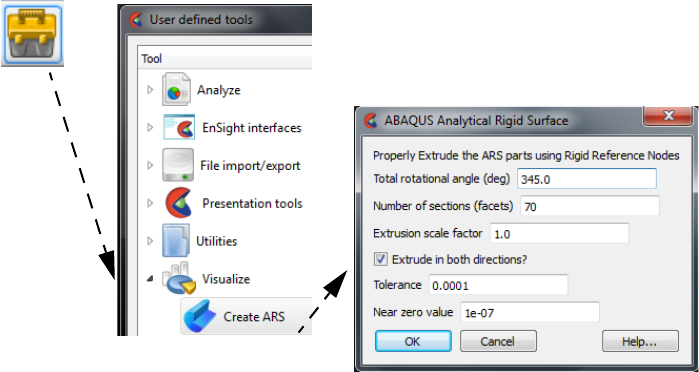
2.3 ABAQUS_ODB Reader
2-22 EnSight 10.2 User Manual
and choose the part id of the rigid reference node corresponding to this ARS part,
pick the rotational degrees and the axis, and click Create to construct the extruded
rotational surface. Note that since the ARS segment is moving automatically, and
the rigid reference node is not moving automatically, if you want to track the
actual motion of the rigid revolution part, you will want to turn on displacements
for the Rigid Reference point part, then toggle on Displace Computationally so
that the rigid reference node displacements are used in the calculations. If the
segment part has CYL in the name, then you'll want to extrude the part in a given
direction, with a total translation. This extruded part should automatically move
correctly without any other steps.
Analytical Rigid
Surfaces automatic
creation using
Python tool
Should you want all of this done for you automatically, there is a python tool
included with EnSight that will automatically create all of your Analytical Rigid
Surfaces. As shown in the Figure below, simply click on the tools icon at the top
and choose the Create ARS icon under the Visualize folder. Simply fill in the
GUI and it will turn on computational displacements of the rigid reference nodes
automatically and just create the rigid reference surfaces as expected.
Problems
If the default behavior of the reader is unexpected (that is, no parts loaded, too few
timesteps loaded, or variables not available) then reload the odb file and select the
Format Options Tab and choose Console Output: Debug. Then take a look at the
output in your server console.
Missing Parts Are you missing parts? By default, EnSight does not load the nodesets. Toggle
this ON to load the nodal parts. By default, EnSight does not load parts whose
names containing ALL or All because these are often duplicate parts that double
the required memory and slow down the operation of the reader. Toggle ON the
Load *all* toggle to load these parts. If you have no parts loaded, take a careful
look at the console output (see below) and notice that all of the nodesets are
skipped, as is the ALL_ELEMENTS part, thus you have no parts loaded.
-----------------------------------------------------------
EnSight ABAQUS Parts
Figure 2-8
Analytical Rigid Surface Python Tool
2.3 ABAQUS_ODB Reader
EnSight 10.2 User Manual 2-23
Total num Instances 1
Total num nodes 936
Total num elements 625
Choose 'Format options' tab in data reader dialog
To load or skip node or surface sets:
Toggle OFF 'Load Surface Sets'
Toggle OFF 'Load Node Sets'
To load or skip sets with ALL in their name:
Toggle OFF 'Load *ALL* Parts'
-----------------------------------------------------------------------------------
ABQ Ens Part Instance & Type Number Status
Num Num Name Elements
------- ------ --------------- --------- -------
1. 1. ALL NODES Assm 0 Nodeset 1 SKIPPED
2. 1. ALL NODES Assm 1 Nodeset 936 SKIPPED
3. 1. ASSEMBLY_CONSTRAINT-1_NODES Assm 1 Nodeset 36 SKIPPED
4. 1. ASSEMBLY_CONSTRAINT-1_POINT Assm 0 Nodeset 1 SKIPPED
5. 1. ALL ELEMENTS Assm 1 Elemset 625 SKIPPED
-----------------------------------------------------------
Number of regular ABAQUS parts = 5
Number of Analytical Rigid Surface parts = 0
Total number of Abaqus parts = 5
Total number of EnSight parts = 0
-----------------------------------------------------------
-----------------------------------------------------------
Missing Timesteps Are you missing timesteps? Each ABAQUS FRAME is an EnSight timestep. If
the change in time between two successive frames is too small to represent as a
float value, then EnSight will skip it.
ABAQUS data is loaded in STEPs. Since EnSight has only timesteps (transient) or one
timestep (static) there is a bit of mapping that goes on to read in an odb dataset.
ABAQUS STEPs of type "*STEP PERTURBATION, *STATIC" STEP” are now loaded
with their timesteps incremented by 1.0.And the Toggle "Smart Uniform Delta Time" has
been added to turn this off and use the frame values (which are 2E-16). This is ON by
default. Warning: this automatically changes timestep time values. Since other STEPs may
also have very small delta time, the Toggle "Uniform Delta Time" is included so that the
time values can be made to increment by 1.0 for ALL STEPs of the ODB data. (default
OFF).
To pick a given ABAQUS STEP, for example, STEP 4 (1- based), simply enter 4 into the
"STEP (1 to num)" field.
Here is the details on the load steps and "times" and is consistent with ABAQUS handling
of .fil
Abaqus STEP is an EnSight Case. Each Abaqus FRAME is a time increment to the final
STEP value. The EnSight total time is a unique cumulative value for each EnSight
timestep that is monotonically increasing.
Each odb STEP is like a sequential, but separate analysis
STEP3
\
|<--- STEP 1 --->|<--STEP 2 -->||<-------- STEP 4 ------->|
Tot |----------------+-------------++------------------------>|
time | 100s| 175s||175+delta 375s|
2.3 ABAQUS_ODB Reader
2-24 EnSight 10.2 User Manual
| | || |
STEP |--------------->|------------>||------------------------>|
time | 100s 75s||1e+36s 200s|
The ODB API reports data by STEP with each step having a series of FRAMES each
representing an EnSight timestep. EnSight use the Abaqus TOTAL TIME as our Solution
Time. Apparently, an Abaqus user can look at his status file and know what TOTAL
TIME relates to the STEP.
EXAMPLE
If we had a file with 3 ABAQUS STEPS, and 5 increments per step:
Notice the ABAQUS odb details in the left columns and the resulting
EnSight mapping on the right. The 'X' is a timestep that is
excluded from EnSight because there is no time change from the
previous step.
------------------- ABAQUS --------------------- | ---- EnSight ---
TOTAL "Time" STEP "Time" STEP # FRAME # | Step Sol. Time
----------- ---------- ------ ---------- | ---- ---------
0.0 0.0 0 0 | 0 0.0
0.1 0.1 0 1 | 1 0.1
0.3 0.3 0 2 | 2 0.3
0.3 1.0E-10 1 0 | 3 0.35
0.8 0.5 1 1 | 4 0.8
1.3 1.0 1 2 | 5 1.3
1.8 1.5 1 3 | 6 1.8
1.8 0.0 2 0 | X 1.8
3.8 2.0 2 1 | 7 3.8
5.8 4.0 2 2 | 8 5.8
7.8 6.0 2 3 | 9 7.8
............. etc ................
Therefore, if you wanted to look at:
The 1st load case (STEP 0): Look at Ensight times 0 - 0.3
or EnSight steps 0 - 2
The 2nd load case (STEP 1): Look at Ensight times 0.35 - 1.8
or EnSight steps 3 - 6
The 3rd load case (STEP 2): Look at Ensight times 1.8 - 7.8
or EnSight steps 6 - 9
NOTE: Times that have no total time increment are dropped from
EnSight.
Times that have an extremely small increment (e.g. 1E-10) are
incremented larger so that the time can be represented as a
float.
For example, when you see the X in the left hand column below, this timestep is skipped
because you can see that the increment is essentially zero. A number of steps are skipped
below for that reason.
-----------------------------------------------------------
EnSight to ABAQUS Temporal Mapping Table
------------------------------------------------------------
EnS EnS ABQ ABQ ABQ
STEP Soln STEP FRAME STEP
# Time # # Time
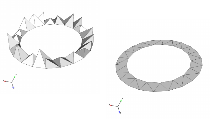
2.3 ABAQUS_ODB Reader
EnSight 10.2 User Manual 2-25
------ -------- -------- --------- -------
0 0 1 0 0
1 2.22E-16 1 1 2.22E-16
X 2.22E-16 1 2 2.22E-16
X 2.22E-16 1 3 2.22E-16
X 2.22E-16 1 4 2.22E-16
X 2.22E-16 1 5 2.22E-16
2 0.01 1 6 2.22E-16
-----------------------------------------------------------
-----------------------------------------------------------
Missing Variables When you choose Console Output Debug, you can see the list of variables in the
console output and that some of the variables are skipped. Skipped variables
include the _MAG variables, which are vector magnitude that EnSight auto-
calculates for vector variables from the components. You can see that some of the
contact variables, which are part-specific are combined into one, single value.
Odd Part Shapes When you read in your parts if the Surface Set parts seem to have full elements
showing and you only want the selected faces of the elements to be used to form
your parts, then reload your data and choose Load Element Faces in the Format
Options Tab of the Data Reader dialog.
(see How To Read Data)
Load Element Faces Toggle ON
Surface Set Part
Load Element Faces Toggle OFF
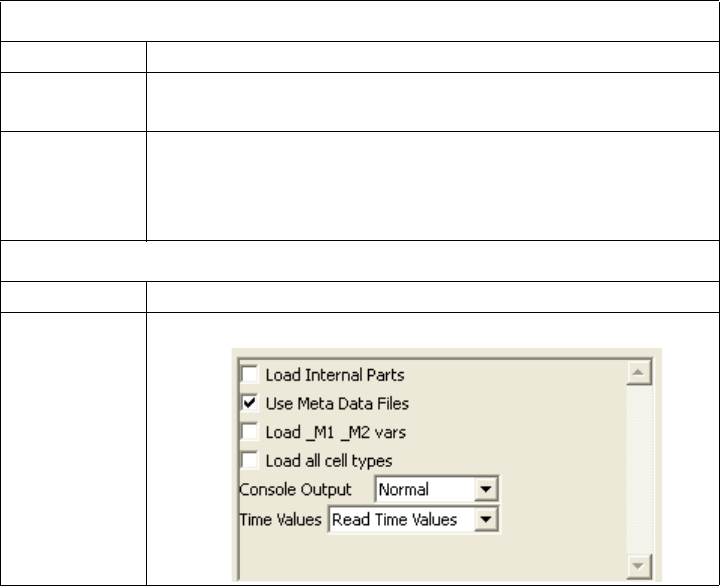
2.3 AIRPAK/ICEPAK Reader
2-26 EnSight 10.2 User Manual
AIRPAK/ICEPAK Reader
Overview
The current FLUENT Direct Reader also reads AIRPAK and ICEPAK data. The
Fluent Direct reader typically loads a Fluent Case (.cas) file and the matching data
(.dat) file. However, AIRPAK/ICEPAK writes out a .fdat file which doesn’t
automatically get recognized by the EnSight Fluent reader and some extra
understanding (and sometimes user-intervention) is necessary as described below.
See the following files for latest information on the Fluent reader.
$CEI_HOME/ensight102/src/readers/fluent/README.txt
The comments that follow are for the current Fluent reader. The reader loads
ASCII, binary single precision, or binary double precision. The files can be
uncompressed or compressed using gzip.
Data file
description
ICEPAK can generate files:
filename.cas
,
filename.dat
just like Fluent, but also if
the analysis uses a nonconformal mesh (not available in Fluent) then there will be
filename.fdat
, and
filename.nc.cas
files. The
filename.nc.cas
is a nonconformal
mesh geometry and its matching results file is the
filename.fdat
file.
Simple Interface
Data Load
Load your geometry file (typically named with a suffix
.cas
) using the Simple
Interface method. EnSight will automatically load the matching
.dat
file.
However, if you want to load the
filename.nc.cas
data file and its corresponding
filename.fdat
file, then you will either need to rename it to match exactly and have
the .dat extension (
filename.nc.dat
), or go to the advanced data load.
Advanced Interface
Data Load.
In EnSight if you don’t want to rename your files, then switch to the Advanced
Interface toggle in the data reader dialog and manually choose the *.nc.cas and the
*.fdat files as described below.
Data Tab
Format To use this reader, select the Fluent format.
Set cas Select the geometry file (typically .cas or .cas.gz) and click
this button. For transient data, use *.cas or *.cas.gz.
Set dat Note that the Fluent reader will automatically select the
matching .dat file. If you want to use the .fdat file, then select
the results file (typically .fdat or .fdat.gz), and click this Set
Dat button. For transient data, use *.fdat or *.fdat.gz .
Format Options Tab
Set measured Select the measured file and click this button.
Other
Options
using the
current
Fluent reader

2.3 AIRPAK/ICEPAK Reader
EnSight 10.2 User Manual 2-27
Load Internal
Parts
Toggle this ON to load the Fluent Internal Parts. This will
show all the internal walls forming all the cell volumes. If you
do toggle this on, then it is recommended that you click on the
'Choose Parts' button at the bottom of the data reader dialog,
rather than 'Load all', as you'll only want to load the interior
parts of interest to save memory and time. Default is OFF.
Use Meta
Files
Meta files are small summary files that contain highlights of
the important locations inside each of the Fluent files.
Allowing the EnSight reader to write out Meta Files that map
the locations of important data can provide a significant speed
up the next time you access that timestep. It is recommended
that you leave this toggle ON. If you have write permission in
the directory where your data is located, three types of binary
Meta Files will be written when you first access each file, with
extensions .EFC for the cas file, .EFD for the .dat file and
.EFG for the time-history data. They are optional, and if you
don't have write permission, the reader will take the extra time
to read the entire .CAS and .DAT file to find the relevant data
each time you come back to that timestep.
Load _M1
_M2 vars
Variables that end in '_M1' and '_M2' occur in Fluent unsteady
flow. They represent the value of the variable at the prior
iteration time and the time prior to that respectively. By
default this toggle is OFF and these variables are not loaded.
Toggle this ON to load these variables.
Load all cell
types
Fluent cells have a boundary condition flag. By default
(toggle OFF) EnSight loads only the cells with a boundary
condition flag equal to 1 (one). Toggle this option ON to load
all cells with a non-zero boundary condition. For example, if
you have a part with cells of boundary condition 32 (inactive),
EnSight will, by default not load this part. Toggle this option
ON and EnSight will load this part. Note: parts containing
cells with a boundary condition of zero are never loaded.
Console
Output
Use this flag to determine the amount of output to the console.
Normal - Usually only echo errors to console.
Verbose - Normal output plus an echo of every Fluent part
that is in the dataset, whether it is interior or not, whether it is
skipped, what variables are defined for which parts, and to
echo it's Ensight Part number.
Debug - Verbose output plus more detailed output and
progress through the reader routines often valuable for
understanding and reporting problems.

2.3 AIRPAK/ICEPAK Reader
2-28 EnSight 10.2 User Manual
(see How To Read Data)
Time Values Default is 'Calc Const Delta', to read a delta time from one file
and calculate the time values from that. If you choose 'Read
Time Values' then the reader will open each file and find the
exact time value. This will be stored in the EFG file if you've
not disabled Meta Files. Finally, the simplest is to 'Use File
Steps' which will just use the file step number as the time
value. This is quick, but is not a good idea if you need real
time for anything such as particle tracing.
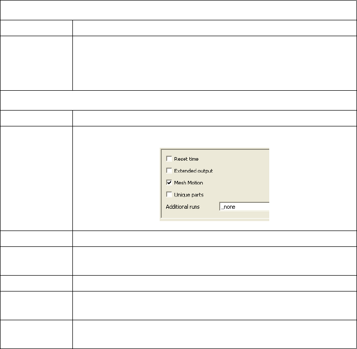
2.3 AcuSolve Reader
EnSight 10.2 User Manual 2-29
AcuSolve Reader
Overview
Description This reader from AcuSim will read results from Acusolve. Select the .log file
from the simple or advanced interface.
Data Reader
Main Menu > File > Data (reader)...
The File Selection dialog is used to specify which files you wish to read.
Main Menu > File > Data (Reader)...
Simple Interface
Data Load
Load your AcuSolve .log file using the Simple Interface method.
Advanced Interface
Data Load
Load your AcuSolve .log file using the Advanced Interface method.
Note: there is an older AcuSolve (v10 api) reader available from AcuSim.
(see How To Read Data)
Data Tab
Format Use the AcuSolve format.
Set file This field contains the first file name. For the first file you
should choose a file with extension .log. Clicking button
inserts file name shown into the field. Loading the .log file
will load all both geometry and results.
Format Options Tab
Set measured Select the measured file and click this button.
Other
Options
Reset time When toggle is on, time begins at 0.0 (default is off).
Extended
output
When toggle is on, console output will be verbose (default is
off).
Mesh Motion When toggle is on, moving meshes are visible (default is on).
Unique parts When toggle is on, a unique set of surfaces is shown in the part
list (default is off).
Additional
runs
Enter the comma separated list of runs (3, 5, 10, 10:20:2), or
_all. (default is _none).

2.3 ANSYS Reader
2-30 EnSight 10.2 User Manual
ANSYS Reader
Overview
Four Ansys
Readers
There are four ANSYS readers available in EnSight: three older, unsupported
legacy readers and the supported Ansys Results. Long-term, Ansys Results is the
reader of choice. This reader should read the latest Ansys results as well as older
versions. The other three, legacy readers will not show up in the reader list by
default and will not be documented in this manual.
Legacy Reader
Visibility Flag
The older readers, by default, are not loaded into the list of available readers, and
are not discussed in the remainder of this document. In the unlikely event you
need to enable these readers, go into the Menu, Edit > Preferences and click on
Data and toggle on the reader visibility flag. The legacy reader documentation is
found in
$CEI_HOME/ensight102/src/readers/ansys/README
and is not included
here.
Ansys Results
Reader
The Ansys Results reader supports scalar, vector and tensor variables, including
the capability to compute several common scalar variables derived from tensors
(such as the common failure theories) as well as local element result components
(such as axial stress in truss elements) when such element results are available.
Additionally, there is some control over the creation of variables from element-
based results. For example, they can be averaged to the nodes (with or without
geometry weighting) if desired. See the format options below for more details.
Results are always presented in the global coordinate system. Thus, any results in
local coordinate systems, or in non-cartesian coordinate systems are transformed
as needed into the model system.
For shell elements that have multiple layers (sections), the user can choose the
section that will be used. Additionally, the user can choose to have a different
variable be created for each section. See format options below for more details.
The user can control how parts are created. Parts can be created according to the
part id, the property id, or the material id.
Simple Interface
Data Load
Load your geometry/results file (typically named with a suffix
.rst
) using the
Simple Interface method.
Advanced Interface
Data Load
Load your geometry/result files (typically named with a suffix
.rst
) using the
Advanced Interface method.
Data Tab
Format Use the Ansys Results format.
Set file
(or results)
Select the geometry/results file (typically .rst, .rth, .rfl, or
.rmg) and click this button
Format Options Tab
Set measured Select the measured file and click this button.
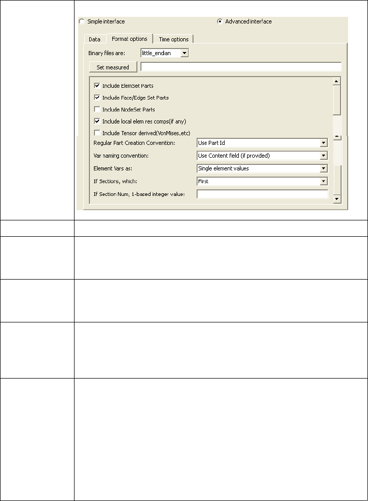
2.3 ANSYS Reader
EnSight 10.2 User Manual 2-31
Other
Options
Include any Element sets defined. These are sets of full
elements which are generally some logical subset of the total
number of elements. Default is on.
Include Face/
Edge Parts
Include any Face or Edge sets defined. These are some logical
set of particular faces and/or edges of full elements. Default is
off.
Include
NodeSet
Parts
Include any Node sets defined. These are generally the subset
of nodes needed for the Element, Face, or Edge sets above. As
such, they are generally not needed as separate parts, but can
be created if desired. Default is off.
Include local
elem res
comps (if
any)
Include the local stresses components, etc that are in the
element's local system.
A simple example is a bar (such as a truss element), which
only has tension or compression in the element's axial
orientation. Such an element would have an axial stress
variable.
Other elements would have appropriate result component
variables. Default is on

2.3 ANSYS Reader
2-32 EnSight 10.2 User Manual
Include
Tensor
derived
(VonMises,
etc.)
For tensor results, calculate scalars from the following derived
results (principal stress/strains, and common failure theories):
Mean Equal Direct
VonMises Min Principal
Octahedral Mid Principal
Intensity Max Principal
Max Shear
By default, all 9 of these will be derived. You can control
which are created by this toggle, with an environment variable.
Namely,
setenv ENSIGHT_VKI_DERIVED_FROM_TENSOR_FLAG n
where n = 1 for Mean only
2 for VonMises only
4 for Octahedral only
8 for Intensity only
16 for Max Shear only
32 for Equal Direct only
64 for Min Principal only
128 for Mid Principal only
256 for Max Principal only
512 for all
or any legal combination. example: for VonMises and Max
Shear only, use 18. Default is off
Regular Part
Creation
Convention
Parts will be created according to the following:
Use Part Id - Part Id (this is the default)
Use Property Id - Property Id
Use Material Id - Material Id
Var nam in g
convention
Use Content Field (if provided) - Variable names will be what
is in the Content field, if provided. If not provided, they willbe
the VKI dataset name. This is the default.
Use VKI dataset nameVariable names will be the VKI variable
dataset name (which are reasonably descriptive).

2.3 ANSYS Reader
EnSight 10.2 User Manual 2-33
(see How To Read Data)
Element Vars
as
Single element values - Element results (whether centroidal or
element nodal) will be presented as a single value per element.
Thus will be per_elem variables in EnSight.This is the default.
Averaged to node values - Element results (whether centroidal
or element nodal) will be averaged to the nodes without using
geometry weighting. Thus will be per_node variables in
EnSight. This is a global averaging, so shared nodes are
affected by all parts that share a node.
Geom weighted average to node values - Element results
(whether centroidal or element nodal) will be averaged to the
nodes using geometry weighting. Thus will be per_node
variables in EnSight. This is a global averaging, so shared
nodes are affected by all parts that share a node.
Ave to node values <by parts> - Element results (whether
centroidal or element nodal) will be averaged to the nodes
without using geometry weighting. Thus will be per_node
variables in EnSight. This is a local averaging, so all
averaging is contained within each part.
Geom weighted ave to node <by parts> - Element results
(whether centroidal or element nodal) will be averaged to the
nodes using geometry weighting. Thus will be per_node
variables in EnSight. This is a local averaging, so all averaging
is contained within each part.
If Sections,
which:
Which section will be used to create the variable
First - The first section will be used (this is the default)
Last - The last section will be used
Section Num (below) - The section number entered in the field
below will be used
Separate Vars per Section - A separate variable will be created
for each section.
Section Num If the previous option is chosen to be Section Num, then the
value in this field is the 1-based section number to use to
create the variable.
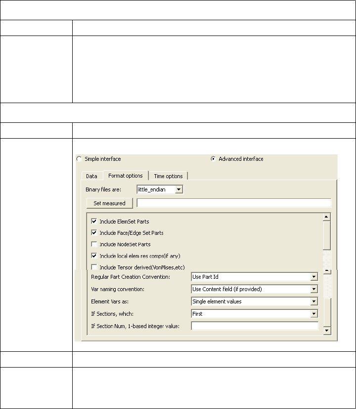
2.3 AUTODYN Reader
2-34 EnSight 10.2 User Manual
AUTODYN Reader
Overview
Description Reads a series of .adres files as a transient solution. Simply select one of the
.adres files and the sequence will be detected. Requires that the .adres_base files
exists in the same directory. Supported only on Windows.
Data Reader
Main Menu > File > Data (reader)...
The File Selection dialog is used to specify which files you wish to read.
Main Menu > File > Data (Reader)...
Simple Interface
Data Load
Load your AUTODYN .adres file using the Simple Interface method.
Advanced Interface
Data Load
Load your AUTODYN .adres file using the Advanced Interface method.
Data Tab
Format Use the Autodyn format.
Set file This field contains the first file name. For the first file you
should choose a file with extension .adres. Clicking button
inserts file name shown into the field. Loading any .adres file
will load all .adres files in the directory which includes both
geometry and results.
Format Options Tab
Set measured Select the measured file and click this button.
Other
Options
Include any Element sets defined. These are sets of full
elements which are generally some logical subset of the total
number of elements. Default is on.

2.3 AUTODYN Reader
EnSight 10.2 User Manual 2-35
Include Face/
Edge Parts
Include any Face or Edge sets defined. These are some logical
set of particular faces and/or edges of full elements. Default is
off.
Include
NodeSet
Parts
Include any Node sets defined. These are generally the subset
of nodes needed for the Element, Face, or Edge sets above. As
such, they are generally not needed as separate parts, but can
be created if desired. Default is off.
Include local
elem res
comps (if
any)
Include the local stresses components, etc that are in the
element's local system.
A simple example is a bar (such as a truss element), which
only has tension or compression in the element's axial
orientation. Such an element would have an axial stress
variable.
Other elements would have appropriate result component
variables. Default is on
Include
Tensor
derived
(VonMises,
etc.)
For tensor results, calculate scalars from the following derived
results (principal stress/strains, and common failure theories):
Mean Equal Direct
VonMises Min Principal
Octahedral Mid Principal
Intensity Max Principal
Max Shear
By default, all 9 of these will be derived. You can control
which are created by this toggle, with an environment
variable. Namely,
setenv ENSIGHT_VKI_DERIVED_FROM_TENSOR_FLAG n
where n = 1 for Mean only
2 for VonMises only
4 for Octahedral only
8 for Intensity only
16 for Max Shear only
32 for Equal Direct only
64 for Min Principal only
128 for Mid Principal only
256 for Max Principal only
512 for all
or any legal combination. example: for VonMises and Max
Shear only, use 18. Default is off
Regular Part
Creation
Convention
Parts will be created according to the following:
Use Part Id - Part Id (this is the default)
Use Property Id - Property Id
Use Material Id - Material Id
Var n am i ng
convention
Use Content Field (if provided) - Variable names will be what
is in the Content field, if provided. If not provided, they will
be the VKI dataset name. This is the default.
Use VKI dataset nameVariable names will be the VKI variable
dataset name (which are reasonably descriptive).

2.3 AUTODYN Reader
2-36 EnSight 10.2 User Manual
(see How To Read Data)
Element Vars
as
Single element values - Element results (whether centroidal or
element nodal) will be presented as a single value per element.
Thus will be per_elem variables in EnSight.This is the default.
Averaged to node values - Element results (whether centroidal
or element nodal) will be averaged to the nodes without using
geometry weighting. Thus will be per_node variables in
EnSight. This is a global averaging, so shared nodes are
affected by all parts that share a node.
Geom weighted average to node values - Element results
(whether centroidal or element nodal) will be averaged to the
nodes using geometry weighting. Thus will be per_node
variables in EnSight. This is a global averaging, so shared
nodes are affected by all parts that share a node.
Ave to node values <by parts> - Element results (whether
centroidal or element nodal) will be averaged to the nodes
without using geometry weighting. Thus will be per_node
variables in EnSight. This is a local averaging, so all
averaging is contained within each part.
Geom weighted ave to node <by parts> - Element results
(whether centroidal or element nodal) will be averaged to the
nodes using geometry weighting. Thus will be per_node
variables in EnSight. This is a local averaging, so all averaging
is contained within each part.
If Sections,
which:
Which section will be used to create the variable
First - The first section will be used (this is the default)
Last - The last section will be used
Section Num (below) - The section number entered in the field
below will be used
Separate Vars per Section - A separate variable will be created
for each section.
Section Num If the previous option is chosen to be Section Num, then the
value in this field is the 1-based section number to use to
create the variable.

2.3 AVUS Reader
EnSight 10.2 User Manual 2-37
AVUS Reader
Overview
The AVUS reader has been recently renamed, and was formerly called the
COBALT reader.
CEI provides the AVUS user-defined-reader on as "as-is" basis, and does not
warrant nor support its use.
There are two distinct readers for AVUS data (formerly Cobalt60) -- one for static
data, AVUS (formerly Cobalt60), and one for transient solution data, AVUS Case
(formerly Cobalt60 Case).
Both readers will read formatted and unformatted (single or double precision)
Cobalt60 grids, solution files (pix files), and Cobalt60 restart files. The file format
is determined automatically by the reader. The readers also support an enhanced
solution (pix) format that contains additional solution data beyond the normal six
fields.
See the following README file for current information on this reader and
contact the author as listed in the README file for further information.
$CEI_HOME/ensight102/src/readers/avus_cobalt_2/README
Simple Interface
Data Load
Load your geometry file (typically named with a suffix
.grd
) using the Simple
Interface method.
Advanced Interface
Data Load
Load your geometry and restart files (typically named with a suffix
.grd and .pix
)
using the Advanced Interface method.
Limitation This reader does not support restoring EnSight Context Files.
(see How To Read Data)
Data Tab
Format Use the AVUS or AVUS Case format.
Set grid
(or file)
Select the geometry file (typically .grd) and click this button
(or select the .case file for AVUS Case)
Set solution Select the restart file (typically .pix), and click this button.
Format Options Tab
Set measured Select the measured file and click this button.
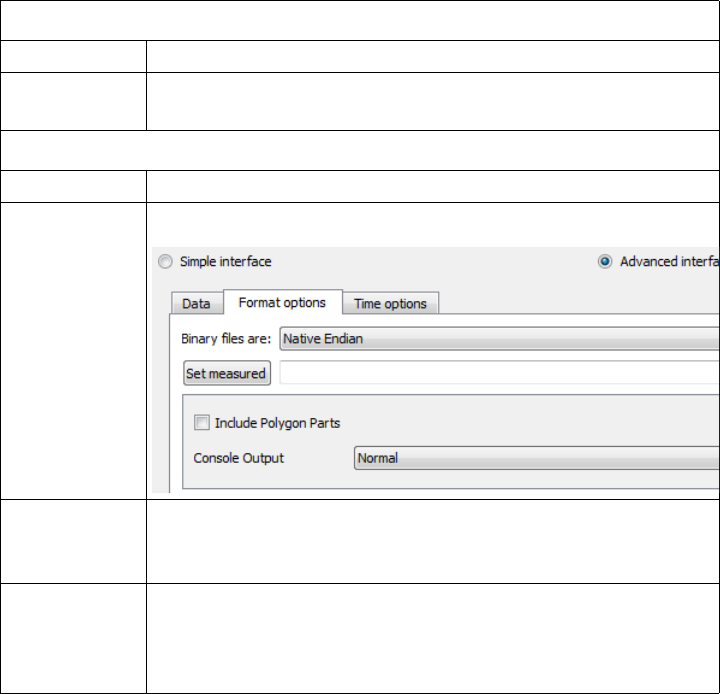
2.3 Barracuda Reader
2-38 EnSight 10.2 User Manual
Barracuda Reader
Overview
This reader inputs the format from the Barracuda solver by Computational
Particle Fluid Dynamics (CPFD). This data traditionally has a large number of
changing particle points within a static geometry composed of 2D walls and 3D
fluids. This reader optimizes the geometry to only reload the particles each
timestep, thus improving performance.
GMV.xxxxx files contain the transient data where x is a digit (0-9) representing
the timestep. In addition, there are a number of .gmv files, some of which must be
present in the folder with the GMV files: 00cells.gmv, 00drawcells.gmv,
00gridstl.gmv, 00mat.gmv, 00nodes.gmv, and 00poly.gmv. The 00gridstl.gmv file
can be read separately to view the STL geometry (no variable, fluids, nor discrete
particles), and the 00poly.gmv can be read separately as well to view the 2D
polygon geometry (no variable, fluids, nor discrete particles).
Please visit http://cpfd-software.com/ for more information about this solver.
Simple Interface
Data Load
Load your geometry file using the Simple Interface method and trust that the
translator will recognize the file type using the suffix.
Advanced Interface
Data Load
For more options, load your geometry using the Advanced Interface method and
click on the Format Options Tab as described below.
Data Tab
Format Use the Barracuda format.
Set File Select any one of the transient files (e.g. GMV.00000) and
click this button and all of them will be loaded.
Format Options Tab
Set measured Select the measured file and click this button.
Reader GUI
Include
Polygon
Parts
Include polygon parts will include parts with polyhedral and/
or polygon elements. Default is off.
Read Single
GMV File
Toggle this On to read only the file you have selected and only
the timestep represented by this file will be available. If off,
this will read all the Gmv files as a transient dataset, when you
select only one. Default is off.

2.3 Barracuda Reader
EnSight 10.2 User Manual 2-39
(see How To Read Data)
Console
Output
Normal - Minimal console output, only for errors.
Verbose - Normal output plus information about the model.
Debug - Full information for the developer to diagnose a
problem. Use this output to help to diagnose a problem or to
send it to CEI.
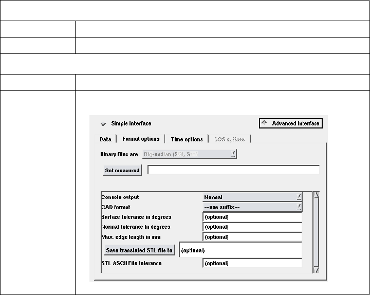
2.3 CAD Reader
2-40 EnSight 10.2 User Manual
CAD Reader
Overview
This reader uses an external translation program to get various CAD files into an
STL formatted temporary file which then read into EnSight. With the proper
licensing, the following CAD file formats can be read: IGES (.igs), STEP
(.STEP), CATIA V4 (.model, .dlv, .exp, .session), CATIA V5 (.CATPart,
.CATProduct, or .CATDrawing, on Windows 32/64-bit only), Pro/Engineer (.prt,
.asm), Unigraphics (.prt), and possibly others.To manually convert this ProE data
set into an STL using the CEI CAD translator, run this command:
ConvertSTL -i ./asm0002.asm.15 -o rs.stl
Additional licensing may be required. Please visit http://cad.ensight.com for more
information.
The CAD reader will also load STL files directly (either ASCII or binary) that
consist only of surfaces (triangles) and have no associated variables. See the STL
Reader.
See the following README file for current information on this reader in the
following directory.
$CEI_HOME/ensight102/src/readers/stl
Simple Interface
Data Load
Load your geometry file using the Simple Interface method and trust that the
translator will recognize the file type using the suffix.
Advanced Interface
Data Load
For more options, load your geometry using the Advanced Interface method and
click on the Format Options Tab as described below.
Data Tab
Format Use the CAD format.
Set File Select the CAD geometry file and click this button
Format Options Tab
Set measured Select the measured file and click this button.
Reader GUI

2.3 CAD Reader
EnSight 10.2 User Manual 2-41
(see How To Read Data)
Console
Output
Allows the user control of the amount and detail of the
console output. The allowable choices are as follows
Normal - Typically only error messages displayed (the
default)
Verbose - Normal messages plus informational messages
Debug - Messages indicating progress through the reader and
useful for diagnosing problems
CAD Format A pulldown to specify the format if the file name and
extension are not sufficient for automatic selection of the CAD
format. Allowable selections include CATIA v4, CATIA v5,
IGES, ProE, STEP, Unigraphics, and STL
Surface
Tolerance in
degrees
The maximum distance between a facet edge and the true
surface. It is a floating point value between 0 and 360 degrees,
with a default value: 15.0
Normal
Tolerance in
degrees
The maximum angle in degrees between two normals on two
adjacent facet nodes. Default value: 25. It is a floating point
value.
Max edge
length in mm
Maximum length of a side of a cell in world space in
millimeters. It is a floating point value with default of 0 (no
max)
Save
translated
STL file to
The name of the translated STL output file. If this name is
specified, then the STL output file is not automatically deleted
after processing. Default value: determined by system call
tempnam(). Example: /var/tmp/my_data.stl
STL ASCII
file tolerance
A positive floating point value used to round off coordinate
values read from ASCII STL files to compensate for the fact
that there is often a roundoff error on the last digit which leads
to discontinuity in the triangle facets.
Example: 1.0E-3 - Sets tolerance value to 1.0E-3
For example: If coordinate value is 147.3247 and Tolerance is
1.0E-3 then new coordinate is 147.324 If Tolerance is 1.0E-2
then new coordinate is 147.32
2.3 CFF Reader
2-42 EnSight 10.2 User Manual
CFF Reader
Overview
The CFF Reader is supplied compiled on Linux platforms on as "as-is" basis, and
CEI does not warrant nor support its use. A README file as well as the source
code is also supplied with the EnSight distribution in the directory below.
$CEI_HOME/ensight102/src/readers/cff

2.3 CFX4 Reader
EnSight 10.2 User Manual 2-43
CFX4 Reader
Overview
Reads a 3D Static Cbinary dump (.dmp) file.
See the following file for current information on this reader.
$CEI_HOME/ensight102/src/readers/cfx4/README.txt
Simple Interface
Data Load
Load your geometry/results file (typically named with a suffix
.dmp
) using the
Simple Interface method.
Advanced Interface
Data Load
Load your geometry/results file (typically named with a suffix
.dmp
) using the
Advanced Interface method.
(see How To Read Data)
Data Tab
Format Use the CFX-4 format.
Set cfx4 dmp Select the geometry/results file (typically .dmp) and click this
button
Format Options Tab
Set measured Select the measured file and click this button.
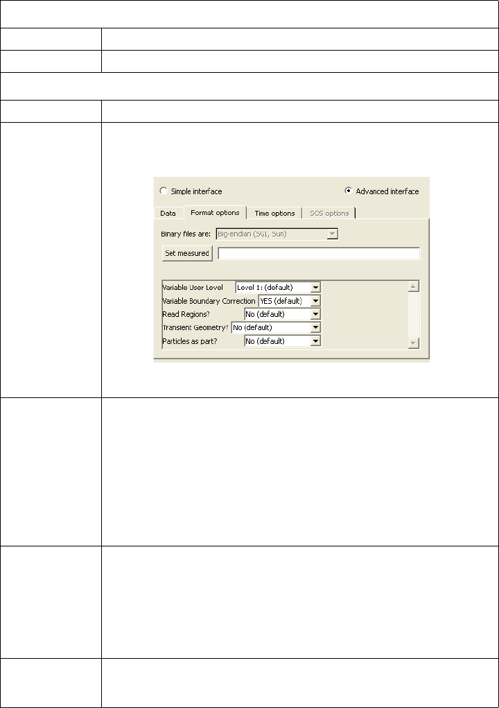
2.3 CFX5 Reader
2-44 EnSight 10.2 User Manual
CFX5 Reader
Overview
Reads a CFX results (.res) file. Currently reads version 16.1-0 and earlier.
Simple Interface
Data Load
Load your geometry/results file (typically named with a suffix
.res
) using the
Simple Interface method.
Advanced Interface
Data Load
Load your geometry/results file (typically named with a suffix
.res
) using the
Advanced Interface method to customize the read, for example to read transient
geometry (see below).
Data Tab
Format Use the CFX-5 format.
Set file Select the geometry/results file (.res) and click this button
Format Options Tab
Set measured Select the measured file and click this button.
Reader GUI
Variable User
Level
Allows the user control of number of variables read based on
a call into the CFX API. The allowable choices are as follows:
Level 0 - Read in all variables
Level 1 - (default)
Level 2 -
Level 3 -
Vari able
Boundary
Correction
Variable values are corrected using a boundary value
correction if this toggle is Yes.
YES - (default) Variable values adjusted using a boundary
value correction.
No - Variable values are not corrected.
Read
Regions?
No - (default) - Do not read Regions.
YES - Read Regions.

2.3 CFX5 Reader
EnSight 10.2 User Manual 2-45
The CFX solver does export to EnSight Case Gold format.
(see How To Read Data)
Transient
Geometry?
A flag to the reader if the data is transient. Note: by default, a
transient .res file will fail to load unless this is changed to Yes.
CFx transient data will have a .res file and a series of .trn files
(one for each timestep) located in a subdirectory. The res file
will have the names of the .trn files, the time value and path. If
the data is changing variables only then the .trn will not
contain the mesh. If the mesh is moving, then the user must
turn on the “Include Mesh” in the Transient Result options so
that the solver will write mesh information to each .trn file.
Failure to do this results in a static, unmoving mesh over time.
No - (default).
Yes - Coordinates only.
Particles as
Part?
If this is Yes, then EnSight reads in the particle data as a
separate EnSight point part.
No - (default) Do not read in particles as a separate EnSight
Part.
Yes - Read in the particles as a separate EnSight part
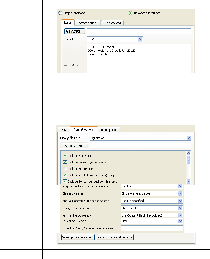
2.3 CGNS Reader
2-46 EnSight 10.2 User Manual
CGNS Reader
Overview
Legacy reader There are three CGNS readers in EnSight: this one (CGNS, which is a secondary reader),
the preferred CGNS-XML Reader which is the default for .cgns files and a legacy,
unsupported reader (CGNS-Legacy) which is unavailable by default, but can be made
visible in the list of readers in the data section of the preferences.
Some information on this reader is available at:
$CEI_HOME/ensight102/src/readers/cgns/README.txt
Simple Interface
Data Load
Load your geometry/results file (typically named with a suffix
.cgns
) using the
Simple Interface method.
Advanced Interface
Data Load
Load your geometry/results files (typically named with a suffix
.cgns)
using the
Advanced Interface method.
Data Tab
Format Use the CGNS format.
Set cgns Select the geometry/results file (typically .cgns) and click this
button. For models contained in multiple files, wildcards or a
special executive file can be used here. See the Special Notes
section below.
Format
Options
Tab
Set measured Select the measured file and click this button.

2.3 CGNS Reader
EnSight 10.2 User Manual 2-47
Include any Element sets defined. These are sets of full
elements which are generally some logical subset of the total
number of elements. Default is on.
Include Face/
Edge Set
Parts
Include any Face or Edge sets defined. These are some logical
set of particular faces and/or edges of full elements. Default is
on.
Include
NodeSet
Parts
Include any Node sets defined. These are generally the subset
of nodes needed for the Element, Face, or Edge sets above. As
such, they are generally not needed as separate parts, but can
be created if desired. Default is off.
Include local
elem res
comps (if
any)
Include the local stresses components, etc that are in the
element's local system.
A simple example is a bar (such as a truss element), which
only has tension or compression in the element's axial
orientation. Such an element would have an axial stress
variable.
Other elements would have appropriate result component
variables. Default is on
Include
Tensor
derived
(VonMises,
etc.)
For tensor results, calculate scalars from the following derived
results (principal stress/strains, and common failure theories):
Mean Equal Direct
VonMises Min Principal
Octahedral Mid Principal
Intensity Max Principal
Max Shear
By default, all 9 of these will be derived. You can control
which are created by this toggle, with an environment variable.
Namely,
setenv ENSIGHT_VKI_DERIVED_FROM_TENSOR_FLAG n
where n = 1 for Mean only
2 for VonMises only
4 for Octahedral only
8 for Intensity only
16 for Max Shear only
32 for Equal Direct only
64 for Min Principal only
128 for Mid Principal only
256 for Max Principal only
512 for all
or any legal combination. example: for VonMises and Max
Shear only, use 18. Default is on.
Regular Part
Creation
Convention
Parts will be created according to the following:
Use Part Id Part Id (this is the default)
Use Property Id Property Id
Use Material Id Material Id

2.3 CGNS Reader
2-48 EnSight 10.2 User Manual
Element Vars
as
Single element
values
Element results (whether centroidal or
element nodal) will be presented as a
single value per element. Thus will be
per_elem variables in EnSight.This is
the default.
Averaged to node
values
Element results (whether centroidal or
element nodal) will be averaged to the
nodes without using geometry
weighting. Thus will be per_node
variables in EnSight. This is a global
averaging, so shared nodes are affected
by all parts that share a node.
Geom weighted
average to node
values
Element results (whether centroidal or
element nodal) will be averaged to the
nodes using geometry weighting. Thus
will be per_node variables in EnSight.
This is a global averaging, so shared
nodes are affected by all parts that share
a node.
Ave to node values
<by parts>
Element results (whether centroidal or
element nodal) will be averaged to the
nodes without using geometry
weighting. Thus will be per_node
variables in EnSight. This is a local
averaging, so all averaging is contained
within each part.
Geom weighted
ave to node <by
parts>
Element results (whether centroidal or
element nodal) will be averaged to the
nodes using geometry weighting. Thus
will be per_node variables in EnSight.
This is a local averaging, so all
averaging is contained within each part.

2.3 CGNS Reader
EnSight 10.2 User Manual 2-49
Spatial
Decomp
Multiple File
Search
Normally, a single cgns file is specified and read. Namely, the
model is neither decomposed spatially into more than one file,
not temporally into more than one file. Thus the first option is
the default. However, when a model is spatially decomposed,
it can be read as long as it conforms to one of the other three
options below. (Note: this is not for temporally partitioned
data. See the Special Notes below this table for how to specify
that situation.)
Use file specified Opens only the file you specify. This is
the default.
Numbered in same
dir
Opens and combines data from all
filenames with the same pattern, but
different ending numbers, that are in the
same directory.
file.cgns.1 <= specify this one
file.cgns.2
...
file.cgns.9
Same name in
numbered dirs
Opens and combines data from all
filenames with the same name, but in
different numbered subdirectories.
dir1/file.cgns <= specify this one
dir2/file.cgns
...
dir9/file.cgns
Numbered in
numbered dirs
Opens and combines data from all
filenames with the same pattern, but
different ending numbers, that are in
different numbered subdirectories.
dir1/file.cgns.1 <= specify this one
dir2/file.cgns.2
...
dir9/file.cgns.3
Doing
Structured as:
Structured will cause originally structured parts to
be created as structured parts in
EnSight. This is the default.
Unstructured will cause originally structured parts to
be created as unstructured parts in
EnSight.
Var nam in g
convention
Use Content Field
(if provided)
Variable names will be what is in the
Content field, if provided. If not
provided, they willbe the VKI dataset
name. This is the default.
Use VKI dataset
name
Variable names will be the VKI variable
dataset name (which are reasonably
descriptive).

2.3 CGNS Reader
2-50 EnSight 10.2 User Manual
Special Notes: Special file input methods for temporally decomposed models. Namely, a file
per timestep. Possible file input methods:
1) Normally, a single .cgns file would be specified.
Thus for a non-decomposed model, or to view one particular time step, you
would enter the desired file.
2) If multiple .cgns files exist because of transient results, you can use a
wildcard (asterisk) in the name of the file, or subdirectory.
ex 1) For the situation where multiple .cgns files reside in the same directory:
/mydirectory/cfd_out.cgns.1
cfd_out.cgns.2
specify: /mydirectory/cfd_out.cgns.*
ex 2) For the situation where multiple .cgns files with the same name reside in
their own subdirectories:
/mydirectory/sub1a/cfd_out.cgns
/sub2a/cfd_out.cgns
specify: /mydirectory/sub*a/cfd_out.cgns
ex 3) For the situation where multiple .cgns files with different names reside in
their own subdirectories:
/mydirectory/sub1a/cfd_out.cgns.1
/sub2a/cfd_out.cgns.2
specify: /mydirectory/sub*a/cfd_out.cgns.*
Note that, in general, you can't have a mixture of these two examples with this
method. Namely, the following cannot be properly specified with this method:
/mydirectory/cfd_out.cgns.1
/sub2a/cfd_out.cgns.2
You would need to either copy the .cgns file in the subdirectory to the data
directory, or you will need to create a subdirectory for each .cgns file in the data
directory, and move the .cgns files into those subdirectories. You could
obviously take advantage of symbolic links to avoid actually moving any data.
Your other alternative is to use method 3) below.
HOWEVER, having said that, there is one special case where you can use this
method with the final file not being in the pattern subdirectories.
If Sections,
which:
Which section will be used to create the variable
First The first section will be used (this is the
default)
Last The last section will be used
Section Num
(below)
The section number entered in the field
below will be used
Separate Vars per
Section
A separate variable will be created for
each section.
Section Num If the previous option is chosen to be Section Num, then the
value in this field is the 1-based section number to use to
create the variable.
2.3 CGNS Reader
EnSight 10.2 User Manual 2-51
Special case requirements:
1. All but the last file is in the pattern subdirectories.
2. Each of the files in the subdirectories must have the same name, and it must
be the same as the one in the parent directory.
Example:
/mydirectory/sub1a/cfd_out.cgns
/sub2a/cfd_out.cgns
cfd_out.cgns
specify: /mydirectory/sub*a/cfd_out.cgns
and the
/mydirectory/sub1a/cfd_out.cgns,
/mydirectory/sub2a/cfd_out.out
files will be loaded.
Then the
/mydirectory/cfd_out.cgns
file will be loaded.
3) You can create a special executive file in which you list all of the .cgns files.
This would allow them to be placed in or anywhere below the data directory.
Thus, you could handle the mixture discussed in 2) above.
Rules for this special file:
a. The file must be named exactly: MULTILPLE_CGNS
b. The .cgns files must be one per line in this file.
c. They must NOT have a full path, because the path to the
MULTIPLE_CGNS file will be prepended to them.
d. There is no concept of comment lines, so no extraneous lines (even empty
lines) are allowed.
ex 1 above, specified in this manner:
/mydirectory/cfd_out.cgns.1
cfd_out.cgns.2
MULTIPLE_CGNS
where MULTIPLE_CGNS file would contain just 2 lines, like:
------------------ dashed lines are NOT in the file
cfd_out.cgns.1
cfd_out.cgns.2
------------------
ex_2 above, specified in the manner:
/mydirectory/sub1a/cfd_out.cgns
/sub2a/cfd_out.cgns
MULTIPLE_CGNS
where MULTIPLE_CGNS file would contain just 2 lines, like:
------------ dashed lines are NOT in the file
sub1a/cfd_out.cgns
sub2a/cfd_out.cgns
-------------
2.3 CGNS Reader
2-52 EnSight 10.2 User Manual
ex_3 above, specified in the manner)
/mydirectory/sub1a/cfd_out.cgns.1
/sub2a/cfd_out.cgns.2
MULTIPLE_CGNS
where MULTIPLE_CGNS file would contain just 2 lines, like:
------------- dashed lines are NOT in the file
sub1a/cfd_out.cgns.1
sub2a/cfd_out.cgns.2
-------------
And for the mixed mode situation:
/mydirectory/cfd_out.cgns.1
/sub2a/cfd_out.cgns.2
MULTIPLE_CGNS
where MULTIPLE_CGNS file would contain just 2 lines, like:
------------- dashed lines are NOT in the file
cfd_out.cgns.1
sub2a/cfd_out.cgns.2
-------------
(see How To Read Data)
2.3 CGNS-XML Reader
EnSight 10.2 User Manual 2-53
CGNS-XML Reader
Overview
There are three CGNS readers in EnSight: this one, the default CGNS Reader, and a
legacy, unsupported reader (CGNS-Legacy) which is unavailable by default, but can be
made visible in the list of readers in the data section of the preferences.
The CGNS-XML reader reads in a single .cgns file or a single.cgnsxml file. The cgnsxml
file is just an XML file is described below and defines various ways to read data, including
spatially decomposed .cgns files.
Limitations The reader has the following limitations.
See the following file for current information on this reader.
$CEI_HOME/ensight102/src/readers/cgns-xml/README
Data Reader
Simple Interface
Data Load
Load your .cgns file using the Simple Interface method.
Advanced Interface
Data Load
Load your .cgns file using the Advanced Interface method.
Data Tab
Format Use the CGNS-XML format.
Set cgns/xml Enter your
.cgns
filename or the .
cgnsxml
filename.
Format Options Tab
Set measured Select the measured file and click this button.
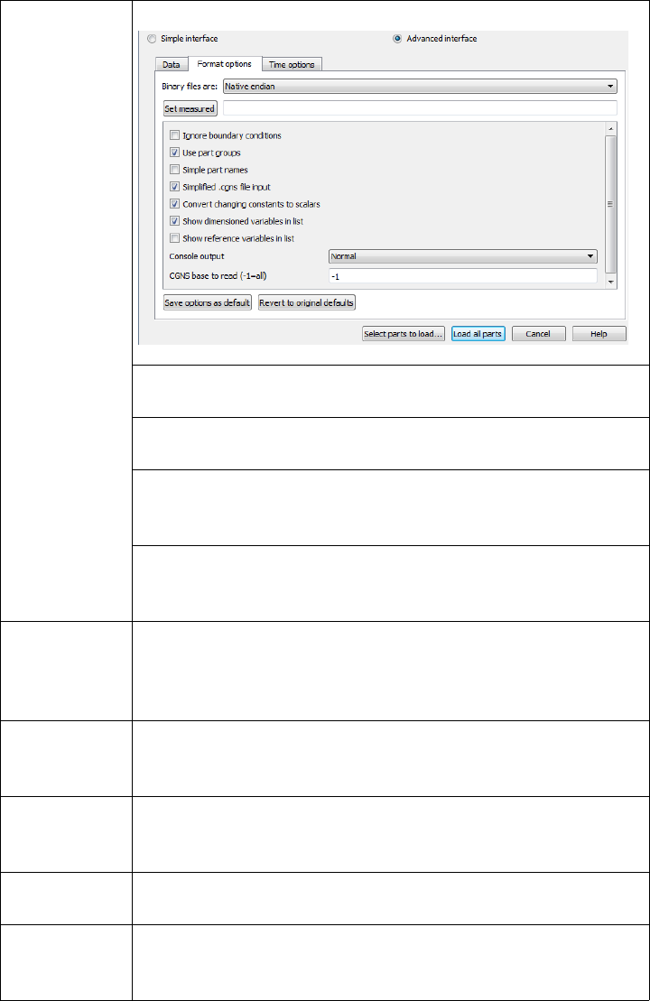
2.3 CGNS-XML Reader
2-54 EnSight 10.2 User Manual
Spatially
decomposed
EnSight can start up in a parallel mode where each server is responsible for a
portion of your CGNS file. If you have a single CGNS file, then the CGNS reader
does a round-robin assignment of parts to servers. If more servers than parts, then
some servers will have no parts. If less servers than parts, then some servers will
be responsible for multiple parts.
If you have multiple CGNS files (e.g. a spatially decomposed or partitioned
dataset), then the reader requires a
.cgnsxml
file which describes the relationships
Format
Options
The following options are customized for the reader:
Ignore boundary conditions - If toggled on, boundary
condition parts will not be loaded (default OFF).
Use part groups - If toggled on, parts will be placed into
groups (default ON).
Simple part names - If toggled on, parts will be named without
part number (ie. _00001, _00002, etc) appended. Default is
OFF.
Simplified .cgns file input - If toggled on, and a single .cgns
file is in use, the part grouping is turned off and simple part
names are turned on (default is ON).
Converge changing constants to scalars (default is ON). When
a zonal constant changes between zones, this "zonal constant"
is converted to a scalar variable (rather than per-case
constant).
Show dimensioned variables in list (default is ON). This will
show variables in the variable list that have been defined in the
cgnsxml file.
Show reference variables in list (default is OFF). This will
show reference variables in the variable list that have been
defined in the cgnsxml file.
Console Output - Can control amount of output that comes to
the console. Options are: Normal, Verbose, or Debug
CGNS base to read - If a CGNS file has more than one base
this allows specific bases to be read. The CGNS base is equal
to (1-#bases). By default, all are read (-1)
2.3 CGNS-XML Reader
EnSight 10.2 User Manual 2-55
between the individual blocks in the CGNS file and EnSight Parts and Groups.
The file itself is encoded in XML. The reader on each Server (in parallel SOS
mode) reads the
.xml
file and does a round-robin on the parts to assign to the
servers. The algorithm is biased such that each reader opens as few CGNS files as
possible. If a CGNS zone, section, or boundary condition is not specified in the
.xml file then it will not be read in.
The example below forms parts and groups from CGNS entities. A part can be a
simple CGNS entity (Zone, section, boundary condition surface-See part
name="Inlet_zone0) or it can be multiple entities combined into one (See part
name="blade1"). Parts can be grouped (See group name="Shroud") so that you
can select and operate on all grouped items within EnSight or you can expand the
group and operate on the parts individually within the group.
CGNSXML
example
<?xml version="1.0" encoding="UTF-8"?>
<CGNSmetafile version="1.0">
<parts>
<partlist>
<group name="Inlet">
<part name="Inlet_zone0" sym_axis = "X" sym_count = "64">
<zone base="1" zone="1" type="1" name="zone0001" file="SUB1/example.cgns.1" faces="i"/>
</part>
</group>
<group name="Outlet">
<part name="Outlet_zone18" sym_axis = "X" sym_count = "9">
<zone base="1" zone="1" type="1" name="zone0001" file="SUB8/example.cgns.8" faces="I"/>
</part>
</group>
<group name="Shroud">
<part name="shroud_zone0" sym_axis = "X" sym_count = "64">
<zone base="1" zone="1" type="1" name="zone0001" file="SUB1/example.cgns.1" faces="K"/>
</part>
<part name="shroud_zone2" sym_axis = "X" sym_count = "8">
<zone base="1" zone="1" type="1" name="zone0001" file="SUB2/example.cgns.2" faces="K"/>
</part>
<part name="shroud_zone1" sym_axis = "X" sym_count = "64">
<zone base="1" zone="2" type="1" name="zone0002" file="SUB1/example.cgns.1" faces="K"/>
</part>
<part name="shroud_zone3" sym_axis = "X" sym_count = "8">
<zone base="1" zone="2" type="1" name="zone0002" file="SUB2/example.cgns.2" faces="K"/>
</part>
</group>
<part name="pname" sym_axis="X" sym_count="10" autoload="1">
<zone base="1" zone="1" type="1" name="zone0001" file="example.cgns"/>
</part>
<part name="blade1" sym_axis="X" sym_count="7">
<zone base="1" zone="2" type="1" name="blade1_2_egv.cgns_j" file="egv.cgns" faces="j"/>
<zone base="1" zone="4" type="1" name="blade1_4_egv.cgns_j" file="egv.cgns" faces="j"/>
<zone base="1" zone="6" type="1" name="blade1_6_egv.cgns_j" file="egv.cgns" faces="j"/>
</part>
<group name="bc-symm-top">
<part name="bc-symm-top_00001" sect="3">
<zone base="1" zone="3" type="0" name="blk-3" file="example.cgns" sect="3"/>
</part>
<part name="bc-symm-top_00001" sect="2">
<zone base="1" zone="2" type="0" name="blk-2" file="example.cgns" sect="2"/>
</part>
</group>
<group name="bc-symm-top_BC">
<part name="bc-symm-top_BC_00001" boco="2">
<zone base="1" zone="1" type="0" name="blk-1" file="example.cgns" boco="2"/>
</part>
<part name="bc-symm-top_BC_00001" boco="1">
<zone base="1" zone="2" type="0" name="blk-2" file="example.cgns" boco="1"/>
</part>
</group>
</partlist>
</parts>
</CGNSmetafile>
XML Tags: <partlist> can contain <part> or <group> objects
<group> can contain <part> or <group> objects
<part> can contain <zone> objects
2.3 CGNS-XML Reader
2-56 EnSight 10.2 User Manual
Tag attributes: <part name="partname" [sym_axis="X"|"Y"|"Z"] [sym_count="N']
[autoload=”0”|”1"] [sect=”#”] [boco=”#”]>
name required and maps to the EnSight part name.
sym_axis optional and specifies an axis over which the part has
rotational symmetry.
sym_count optional and specifies the number of copies of the object that
make up 360 degrees.
autoload optional and if set to "0", specifies that the part should not be
autoloaded if the user selects "Load all parts".
sect optional and specifies that the part comes from a specific CGNS
zone section.
boco optional and specifies that the part comes from a specific CGNS
zone boundary condition.
<zonebase="#" zone="#" type="0”|”1" name="name"
file="cgnsfilename" [faces="iIjJkK"]/>
name required and is currently only used internally by the reader.
(for now just set to zone####, where #### is a 0 prefilled zone number
such as 0001)
base required and specifies the CGNS base number
zone required and specifies the CGNS zone number
type requried and specifies "1" = structured zone, "0" = unstructured zone
file required and specifies the CGNS file to extract information from
faces optional, but if specified and the zone is structured it specifies that
the zone should be read as the noted (2D) faces of the zone instead of the
volumetric elements. i=min I axis, I=max I axis, etc.
cgns2xml utility cgns2xml is a simple example xml file generation utility found in
$CEI_HOME/ensight102/machines/PLATFORM, where PLATFORM is the
hardware and os where you are running EnSight. This utility can be used to take a
list of .cgns files and generate a basic .xml file from them. The command line
looks like:
cgns2xml {infilelist} {outfile}
infilelist is the name of a file that contains the list of the .cgns files to
read. If the filename is '-', the list will be read from stdin, one filename per
line. If a filename of 'verbose' is given, verbose mode will be toggled on.
outfile is the name of the output
.xml
file. If the filename is '-', the
output will be sent to stdout.
(see How To Read Data)
2.3 Converge_Input Reader
2-58 EnSight 10.2 User Manual
Converge_Input Reader
Overview
Reads the input file (inputs.in) and other files in the same directory in order to
allow inspection, verification, and visualization of the input setup prior to the
ConvergeCFD solver. The reader will import the required files in order to create
the surfaces used for the Converge solver, along with a select number of variables,
such that user can visualize the boundary values and the movement of the surfaces
over time. The reader will generate the surface, movement, and boundary values
necessary for visualization.Also, if the model contains a spatially varying
variable, an additional point part will be created to visualize the spatially varying
boundary.
Details The reader looks for input.in file and if exists, it reads the crank_flag (1 time units
are in crank angle, and 0 time units in seconds).It reads start_time and end_time of
the simulation and chooses a time interval corresponding to a 0.5 degree crank
angle.These time steps in crank angles are converted into seconds and returned as
solution times which we see as Analysis_time in EnSight.
The reader then looks for the engine.in file. The presence of this file indicates that
it is IC engine case. The reader then gets the values of stroke, bore, connecting rod
length and rpm from the engine.in file and then finds the intake_lift and exhaust
lift.in files for intake and exhaust lift values (these are transient constants and are
used to make intake and exhaust translating parts to translate).
Note that if the engine.in file is missing, it indicates the analysis is a generic CFD
analysis.
The reader then looks for boundary.in file to get the boundary conditions for each
part, the number of parts and the part names. The boundary.in file also has rigid
body motion (for IC engine cases only translations for piston motion, intake and
exhaust lift) using rigid body flags. The boundary.in file contains the names of
other files containing other boundary conditions.
The reader then gets the geometry (nodes, elems, ids) from the surface*.dat file(s).
The boundary.in file specifies other files which contain variable information. The
reader must interpolate the variable start and end times in these variable files to
match the other timesteps. The reader does linear interpolation making use of the
720 degree cyclic nature in order to obtain variable values for all time steps.
Rigid body motion Piston motion is identified by the $ symbol in the boundary.in file. The piston and
crevice (if it exists) follow this motion. Translating intake parts and exhaust parts
translations are found using the file names intake_lift.in and exhaust_lift.in
respectively. Simple rigid body motion is created by algebraic sum of each
original coordinate value and the product of direction component and motion
value at particular time step (piston movement, intake lift or exhaust lift
depending on the kind of motion). More complex, general rigid body motion is
also available and it uses the supplied direction cosines converted into Euler
angles.
Limitations The reader uses the inputs.in file to determine the directory where the data files
are located. It expects that the names of inputs.in, boundary.in, engine.in,
intake_lift.in and exhaust_lift.in are unaltered.
The reader was built with the primary intention of visualizing In-cylinder engine
models. The reader is expected to read in arbitrary motion models, as well as

2.3 Converge_Input Reader
EnSight 10.2 User Manual 2-59
spatially varying boundary conditions. Currently, only Temperature, Pressure, and
Total Pressure spatial variables are imported into EnSight. For In-Cylinder
models, constants are imported for Bore, Stroke, Con_rod_length, RPM,
Intake_Lift, Exhaust_Lift, Piston_motion, Crank_angle, and Analysis_Time.
For more info, see
$CEI_HOME/ensight102/src/readers/converge_input/
Data Reader
Main Menu > File > Data (reader)...
The File Selection dialog is used to specify which files you wish to read.
Main Menu > File > Data (Reader)...
Simple Interface
Data Load
Load your geometry/results file (must be named
inputs.in
) using the Simple
Interface method.
Advanced Interface
Data Load
Load your geometry/results file (must be named
inputs.in
) using the Advanced
Interface method.
(see How To Read Data).
Data Tab
Format Use the Converge_input format.
Set .inputs.in
file
Select the Converge_input file (must be inputs.in) and click
this button
Format Options Tab
Moving
Liner
Default is OFF. If set, the liner will be defined as a changing
coordinates part, which effectively compresses and expands
the liner part in conjunction with the movement of the piston.
This option is valid only for In-cylinder engine models.
Console
Output
Use this flag to determine the amount of output to the console.
Normal - Usually only echo errors echoed to console.
Verbose - Normal plus high level output describing dataset and
progress while reading
Debug - Detailed output and progress through the reader
routines often valuable for understanding and reporting
problems.
Set measured Select the measured file and click this button.
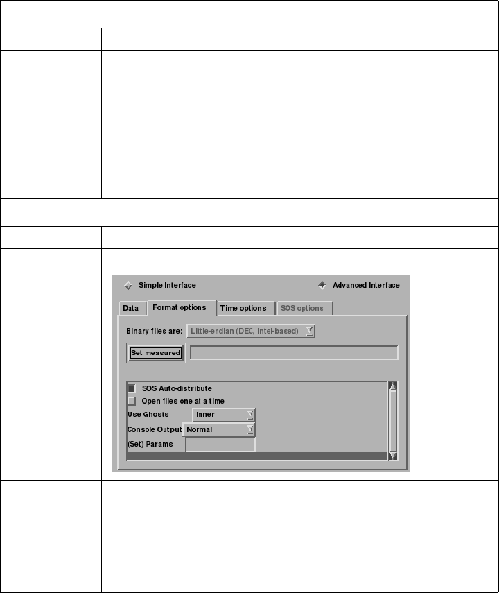
2.3 CTH Reader
2-60 EnSight 10.2 User Manual
CTH Reader
Overview
Reads a Spymaster .spcth file.
See the following file for current information on this reader.
$CEI_HOME/ensight102/src/readers/cth/README.txt
Simple Interface
Data Load
Load your geometry/results file(s) (typically named with a suffix
.spcth
) using the
Simple Interface method.
Advanced Interface
Data Load
Load your geometry/results files (typically named with a suffix
.spcth
) using the
Advanced Interface method.
Data Tab
Format Use the CTH format.
Set spcth* To read one Spymaster file, put the CTH Spymaster file
(typically named something filename.spcth) into the (Set)
Geometry field. To read in multiple, related CTH Spymaster
files (for example several files solved in parallel) as follows:
filename.spcth.0
filename.spcth.1
filename.spcth.2
Put an asterisk ‘*’ in the filename (filename.spcth.*).
Format Options Tab
Set measured Select the measured file and click this button.
Reader GUI User controls as shown below are available:
SOS Auto-
distribute
When running EnSight in SOS mode, turn this ON (default) to
tell the reader that you want it to intelligently distribute the
data among the servers. Turn it off if you have already
distributed the spcth files into different directories, or on
different machines and want to use a Case SOS file to assign
the spcth file(s) to EnSight Server(s) manually.

2.3 CTH Reader
EnSight 10.2 User Manual 2-61
Special Variables EnSight’s CTH reader has several special variables useful for understanding SOS
data. FILE_ID is the file ID number for each cell. BLOCK_ID is the block index.
And SERVER_ID is the server that has the data.
SOS details You can start up SOS using ceishell, or the legacy Case SOS file, or the legacy
resources file (.res) file, each discussed elsewhere in this manual.
Reader-distribute is the default behavior of EnSight. In Reader Distribute mode,
if you have more files than servers, files are distributed to servers in a round-robin
fashion according to file size to even the load. If you have more servers than files,
servers are allocated to files according to total file size per server. In Reader
Distribute mode, all files must be available to all servers.
Shown below are GUI images showing sample user input for a sample SOS read
of 8 spatially distributed spcth files into EnSight SOS using a resource (.res) file.
If you decide that you want to manually distribute the files, then you must move
the sets of files into separate directories, create the SOS casefile with different
directories and the filename* casefile, and toggle the reader SOS auto-distribute
OFF in the Format Options above.
See the Problems section of the Use Server of Servers for more tips problem-
solving your SOS visualization.
Open files
one at a time
When running EnSight in SOS mode, turn this ON to tell the
reader that you want it to only open one of the spcth files at a
time. When this is OFF (default) every server process may
open a number of the files simultaneously. This could be a
problem if you have a thousand files and a thousand servers
and your process reaches a limit with too many files opened at
once.
Use Ghosts Ghosts are invisible elements between the Server geometries
that allow for interpolation of data results rather than
extrapolation. Ghosts can be
inner (default) - use only the inner ghosts between blocks
all - use both inner as well as ghosts around blocks
none - no ghosts
normal - read in ghosts as normal cells.
outer zero - read in the inner and outer, but zero the variable
values on the outer locations. This is useful to create end caps
on the isosurfaces.
Console
Output
Normal - Normal console output
Verbose - Extra output useful to the user to understand their
data better.
Debug - Extra output often useful in debugging problems.
(Set) Params Allows user to enter parameters to change the behavior of the
reader, often for debugging purposes. For example to limit the
number of blocks in the part to 102, enter the following:
-numblocks 101
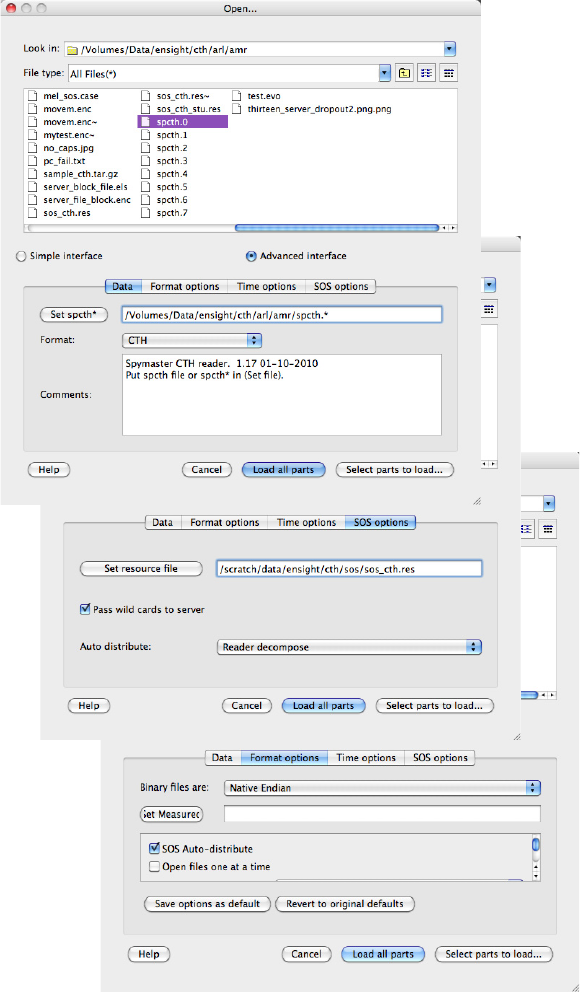
2.3 EXODUS II Reader
EnSight 10.2 User Manual 2-63
EXODUS II Reader
Overview
Misc Notes The Exodus reader links to the exodus routines in libexoIIc.a and the netcdf
routines in libnetcdf.a. You must have these libraries to compile and run the
ExodusII reader, and they are installed with EnSight.
Variable names that end in "x", "y", "z" will be treated as components of a vector.
For example, the variables "vel_x", "vel_y", "vel_z" will be treated as a vector
named "vel_vec". Case is ignored in matching variable names.
GUI control of
Reader
Note reader behavior can also be controlled in the Data Reader GUI via
checkboxes and fields. The environment variables, if set, are used to set the
default values for the GUI.
Loading Data
Summary Selecting the first file of any multi-file Exodus dataset will cause the reader to
load the entire dataset. Selecting a non-first file of a spatially decomposed or a
temporally decomposed dataset will cause the reader to load only that file. If the
user wishes to load only the first file, the “Read Selected File Only” toggle must
be turned ON and that file selected. If a dataset is both spatially and temporally
decomposed and a non-first file is selected, only the selected spatial
decomposition will be loaded and it will be loaded for all time steps.
Single file - no
decomposition
If the file is not decomposed spatially nor temporally, then you will have only one
Exodus file. Selecting this file will load all of the geometry and variables over all
time. The file will be named something like
file.e
.
Spatially
decomposed files
If the files are decomposed only spatially as shown below (each file contains a
portion of the geometry over all time), then EnSight will behave as follows:
a. To load all the files automatically, choose the first file.
b. To load a particular file, choose that file. If only the first file is desired toggle
ON the “Read Selected File Only” reader option.
file.e.4.0
file.e.4.1
file.e.4.2
file.e.4.3
Temporally
decomposed files
If the files are decomposed only temporally as shown below (each file contains all
the geometry but only for a subset of the total time), then EnSight will behave as
follows:
a. To load all the files automatically, choose the first file.
b. To load a particular file, choose that file. If only the first file is desired toggle
ON the “Read Selected File Only” reader option.
file.e
file.e-s0002
file.e-s0003

2.3 EXODUS II Reader
2-64 EnSight 10.2 User Manual
...Spatially and
Temporally
decomposed files
If the files are decomposed spatially and temporally, as shown below, then there is
a portion of the geometry in each file (indicated by 4.0, 4.1, 4.2, and 4.3) and a
portion of the total time range in each file (indicated by s0002, and s0003) as
shown below. EnSight will behave as follows:
a. To load all the files automatically, choose the first file.
b. To load only one portion of the geometry, choose any non-first file (for
example: choosing file.e.4.1 will load the .1 geometry over all time steps,
choosing file.e-s0002.4.0 will load the “.0” geometry over all time steps). Note
that EnSight loads all time steps of the selected spatial decomposition.
c. To read only one file, choose the file and toggle ON the “Read Selected File
Only” reader option.
file.e.4.0
file.e.4.1
file.e.4.2
file.e.4.3
file.e-s0002.4.0
file.e-s0002.4.1
file.e-s0002.4.2
file.e-s0002.4.3
file.e-s0003.4.0
file.e-s0003.4.1
file.e-s0003.4.2
file.e-s0003.4.3
Advanced Multiple
File Naming
This reader supports two extensions to the filename fields. The first supports
Exodus datasets where the geometry changes at some point in time. In this case, a
new Exodus file (or set of files), is used for each set of solution times. To support
this feature, insert wildcard characters (e.g. "*" and "?") in the filename that
expand to the name of the first files in each timeset.
The second extension allows for multiple files to be read as part of the same
timeset (e.g. domain decomposed files). This feature takes the form of a tag
(<X:Y>) appended to the filename. The value of "X" is the number of files in the
timeset and "Y" is the sprintf() format string on the integer (%d) formatting
options) for expanding an integer argument into a string. For example, if a dataset
consists of the following files:
Times 0-10 Times 11-15
foo.e.03.00 foo.e-s0002.03.00
foo.e.03.01 foo.e-s0002.03.01
foo.e.03.02 foo.e-s0002.03.02
Where the "foo.e.*" files contain timesteps 0 through 10 and the "foo.e-s0002.*"
files contain timesteps 11 through 15. Also, each timeset is spatially decomposed
into 3 subfiles, which each contain some portion of the dataset for the given
timesteps. For this dataset, use the file pattern "foo.*.03.<3:%0.2d>" to tell
EnSight there are multiple timesets and to generate the filenames for each timeset
by replacing the "<..>" substring with a number from 0 to 2 as generated using
sprintf() and "%0.2d". Note that the "<...>" marker must be the last part of the
filename. The ‘*’ will wildcard the timeset number and the “<...>” specifies the
spatial decomposition.

2.3 EXODUS II Reader
EnSight 10.2 User Manual 2-65
More info See the following file for current information on this reader.
$CEI_HOME/ensight102/src/readers/exodusII/README.exodus
Data Reader
Simple Interface
Data Load
Load your geometry/results file (typically named with suffix .ex, or .ex2, or .exo)
using the Simple Interface method.
Advanced Interface
Data Load
Load your geometry/results file (typically named with suffix .ex, or .ex2, or .exo)
using the Advanced Interface method.
Data Tab
Format Use the Exodus II format.
Set exo Select the geometry/results file (typically .ex, or .ex2, or .exo)
and click this button. If there are multiple Exodus files in the
solution set, select the first file to load all of the data.
Format Options Tab
Set measured Select the measured file and click this button.
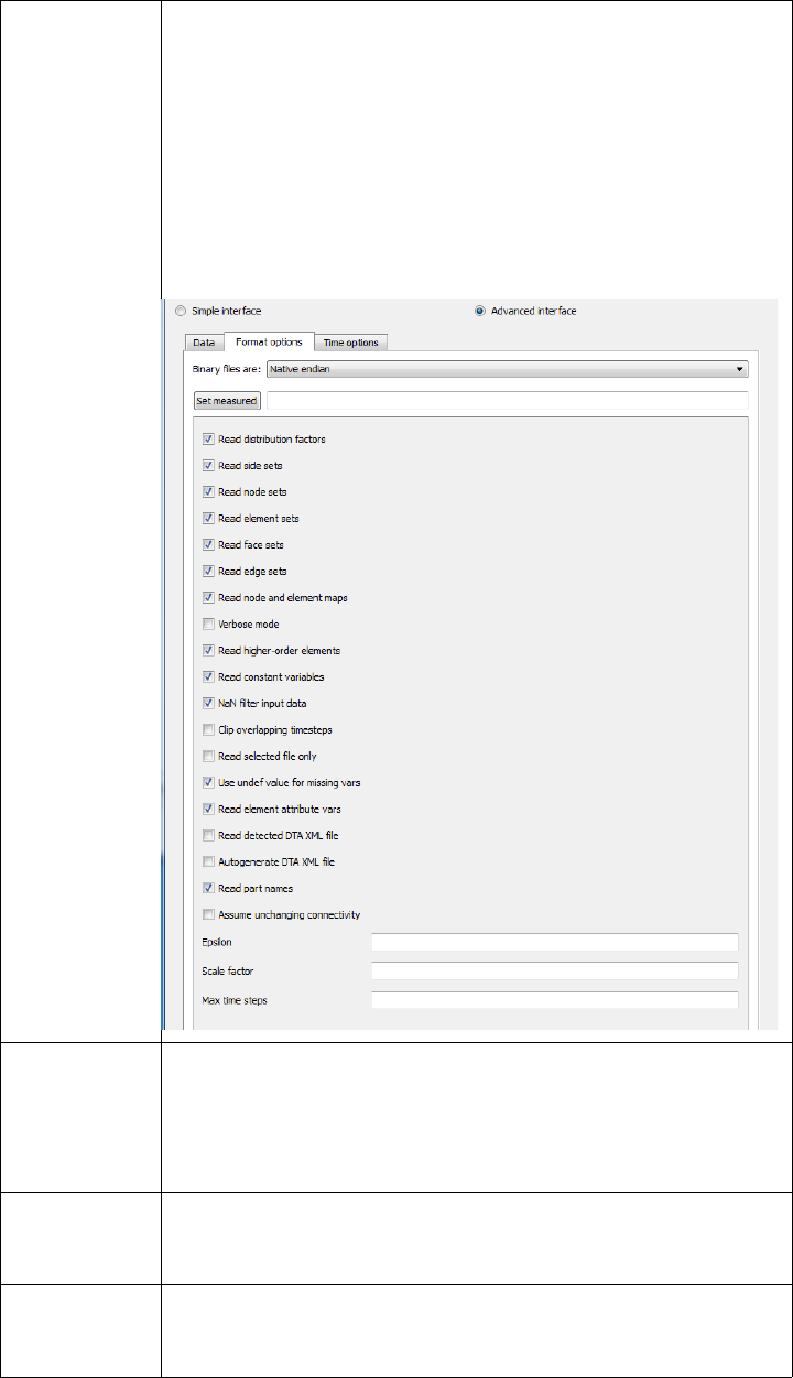
2.3 EXODUS II Reader
2-66 EnSight 10.2 User Manual
Reader GUI When you choose Exodus reader, and toggle on the Advanced
interface button, then click on the format options tab, you will
see a number of options for controlling the reader behavior.
Each of the choices in the data reader dialog has a
corresponding Environment variable described below that you
can set to control the default behavior. If you find yourself
repeatedly toggling on or off choices in the Format Options
tab of the data reader dialog, consider setting specific
Environment variables to change the default behavior of.the
reader.
Read
Distribution
Factors
Sets in Exodus can have distribution factor weights. If this is
ON (default ON) then distribution factors will be read in as
variables defined only on Set parts. The Environment variable
ENSIGHT_EXODUS_DF can be used to set the default value
(1 is ON, 0 is OFF).
Read Side
Sets
Toggle ON (default) to read Side set parts. The Environment
variable ENSIGHT_EXODUS_READ_SIDESETS can be
used to set the default value (1 is ON, 0 is OFF).
Read Node
Sets
Toggle ON (default) to read Node set parts. The Environment
variable ENSIGHT_EXODUS_READ_NODESETS can be
used to set the default value (1 is ON, 0 is OFF).

2.3 EXODUS II Reader
EnSight 10.2 User Manual 2-67
Read
Element Sets
Toggle ON (default) to read Element set parts. The
Environment variable
ENSIGHT_EXODUS_READ_ELEMENTSETS can be used
to set the default value (1 is ON, 0 is OFF).
Read Face
Sets
Toggle ON (default) to read Face set parts. The Environment
variable ENSIGHT_EXODUS_READ_FACESETS can be
used to set the default value (1 is ON, 0 is OFF).
Read Edge
Sets
Toggle ON (default) to read Edge set parts. The Environment
variable ENSIGHT_EXODUS_READ_EDGESETS can be
used to set the default value (1 is ON, 0 is OFF).
Read node
and element
maps
Toggle ON (default) to read node and element ids or labels
(referred to in Exodus as node maps or element maps). There
is no guarantee (particularly if using spatially decomposed
Exodus files) that the node and element labels will be unique.
If this option is toggled OFF then EnSight will ignore the
labels in Exodus file and generate an internal numbering
scheme guaranteed to have unique node and element ids. The
Environment variable
ENSIGHT_EXODUS_USE_NODEMAPS can be used to set
the default value (1 is ON, 0 is OFF).
Verbose
Mode
Toggle ON (default OFF) to output more detailed information
to the server console. The Environment variable
ENSIGHT_EXODUS_VERBOSE can be used to set the
default value (1 is ON, 0 is OFF).
Read higher
order
elements
Toggle ON (default ON) to preserve higher order elements.
Toggle OFF to down convert these elements to simpler
elements (e.g. convert a HEX20 into a HEX08). The
Environment variable
ENSIGHT_EXODUS_USE_HIGHERORDERELEMENTS
can be used to set the default value (1 to preserve higher order
elements and to 0 to convert these elements to simpler
elements.
Read
constant
variables
Toggle ON (default ON) to load the variables that have a
single value at each timestep (called Constants in EnSight).
The Environment variable
ENSIGHT_EXODUS_READ_CONSTANTS can be used to
set the default value (1 to load constant variables and 0 to not
load them).
NAN filter
input data
Toggle ON to check all floats (geometry as well as variables)
for IEEE nans and set to zero if nan (default ON). The
Environment variable ENSIGHT_EXODUS_CHECK_NANS
can be used to set the default value (1 to check all floats and 0
to not check floats).

2.3 EXODUS II Reader
2-68 EnSight 10.2 User Manual
Clip
Overlapping
timesteps
EnSight must have monotonically increasing time values in
each successive timestep. Exodus files sometimes have
overlapping timesteps. Toggle this ON, and when overlapping
times are encountered, EnSight will truncate the former values
and use the latter timesteps to construct the timeline.
If this is toggled OFF (default) and EnSight encounters
duplicate time values in subsequent timesteps it will apply the
epsilon value (see Epsilon below) and increment the latter
timestep so it remains monotonically increasing. With this
option toggled OFF, EnSight will retain all timesteps but
change the time values and is therefore not recommended. The
Environment variable
ENSIGHT_EXODUS_CLIP_TIMESTEP_OVERLAP can be
used to set the default value (1 to truncate the timesteps with
overlapping time ranges, and 0 to keep all timesteps).
Epsilon A delta time value (default 1.0) to be substituted when a non-
increasing delta time float value is encountered. If the reader
detects two sequential time values that are not increasing the
later solution time value will be set to the earlier time plus this
epsilon value. This will have a cascading effect, shifting other
solution times later as well. This is useful when the solution
times are all the same value in the Exodus dataset. Set the
Environment variable ENSIGHT_EPSILON to a positive float
value to change the default value.
Read
Selected File
Only
Toggle ON to read one and only one file which is the selected
file. Toggle OFF (default) to allow automatic pattern
recognition (and loading) of certain categories of file naming
schema as discussed in the beginning of this section.
ENSIGHT_EXODUS_READ_SELECTED_FILE_ONLY can
be used to set the default value ( 1 to read only one file and 0
to read all matching files in the schema).
Use Undef
value for
missing
variables
Toggle ON (default) to return EnSight’s undefined value
when missing variable values are encountered (see EnSight
Gold Undefined Variable Values Format). Toggle OFF to
return a value of 0.0 for missing variable values, which is the
behavior of the reader prior to reader version 2.72). The
Environment variable
ENSIGHT_EXODUS_USE_UNDEF_VALUE can be used to
set the default value ( 1 to return UNDEF and 0 to return 0.0
for missing variable values).
Read element
attribute vars
Some elements have unique attributes (such as thickness for
2D shell elements). Toggle ON (default) to read in element
attribute variables and OFF to not read these in. Use the
Environment variable
ENSIGHT_EXODUS_READ_ELEMENT_ATTRS to set the
default value ( 1 to read these values 0 to not read them).

2.3 EXODUS II Reader
EnSight 10.2 User Manual 2-69
Use detected
DTA XML
file
Toggle this ON (default is OFF) to check for the existence of a
.dta file (and read it in). The DTA file has extra metadata
more fully describing the parts. Set the Environment variable
ENSIGHT_EXODUS_USE_DTA_FILE to change the default
(1 is read .dta file, and 0 is do not check).
Auto
generate
DTA XML
file
Toggle this ON (default is OFF) to generate a ‘stub’ .dta file
from the Exodus datafile. Set the Environment variable
ENSIGHT_EXODUS_AUTOGEN_DTA to change the
default (1 generate ‘stub’ .dta file, 0 is do not generate .dta
file).
Read part
names
Toggle this ON (default is ON) to read in the part names from
the Exodus data file. Set the Environment variable
ENSIGHT_EXODUS_USE_FULL_NAMES to change the
default (1 to read in the part names from the Exodus data file,
0 to not read them in).
Assume
unchanging
connectivity
By default, with this Toggle OFF, when an Exodus dataset has
multiple temporal files, the reader assumes that this is a
changing connectivity file. Changing connectivity geometries
lose some capabilities within EnSight, such as the ability to
interpolate variable values between timesteps. If you know
your temporally decomposed dataset does not change
connectivity, then toggle this ON to tell EnSight to not make
this a changing connectivity dataset; the dataset will become a
changing coordinates geometry (which does allow
interpolation between timesteps). To change the default, set
the environment variable as follows:
ENSIGHT_EXODUS_ASSUME_UNCHANGING_CONNECTIVITY
to a value of 1 and the toggle will appear ON.
Scale Factor Enter a positive float value (default 1.0) to be used as a scale
factor for geometry and vectors (not for scalars). Set the
Environment variable ENSIGHT_EXODUS_SCALE to a
positive float value to change the default value.

2.3 EXODUS II Reader
2-70 EnSight 10.2 User Manual
SOS You can start up SOS using ceishell, or the legacy Case SOS file, or the legacy
resources file (.res) file, each discussed elsewhere in this manual.
There can be no more servers than the number of sub-files however (but fewer
servers are legal and in most cases, recommended). Finally, if there are sub-files,
the number and the naming convention must be the same over all timesets.
The Exodus reader does the decomposition automatically when running in Server
of Server (SOS) mode, which is called Reader-distribute mode. In Reader
Distribute mode, data is distributed to servers in a round-robin fashion. In Reader
Distribute mode, all files must be available to all servers.
If you decide that you want to manually distribute the files, then you must move
the sets of files into separate directories, create the SOS casefile with different
directories and the filename* casefile, and toggle the reader SOS auto-distribute
OFF in the Format Options above.
Shown below are GUI images showing sample user input for a sample read of
spatially distributed Exodus files (4 processors) into EnSight SOS using a simple
4-server resource (sos.res) file as follows. Also shown is the geometry colored by
the Server number calculated using the Calculator Function ServerNumber (which
is an excellent way of showing the allocation of the geometry among the EnSight
Servers. See the Problems section of the Use Server of Servers for more tips
problem-solving your SOS visualization.
#!CEIResourceFile 1.0
SOS:
host: localhost
SERVER:
host: localhost
Max time
steps
By default, EnSight can read from an Exodus file while the
simulation code is updating the Exodus file. For allocation
purposes, EnSight needs an absolute maximum number of
steps that will appear in the data file(s) during your EnSight
session. Currently, the maximum number of time steps that
EnSight will read is given here as 100000. Increase this value
if your solver may exceed this amount.
A value less than or equal to 1 will disable the ability to check
for new time steps. Note, this field is ignored on Exodus files
with HDF5 as the underlying format, as HDF5 files cannot
safely be read and written simultaneously.
Set the environment variable
ENSIGHT_EXODUS_MAX_TIMESTEPS to change the
default.
For details on how to use this capability in EnSight, see How
To Change Time Steps and the Advanced section in How To
Load Transient Data).
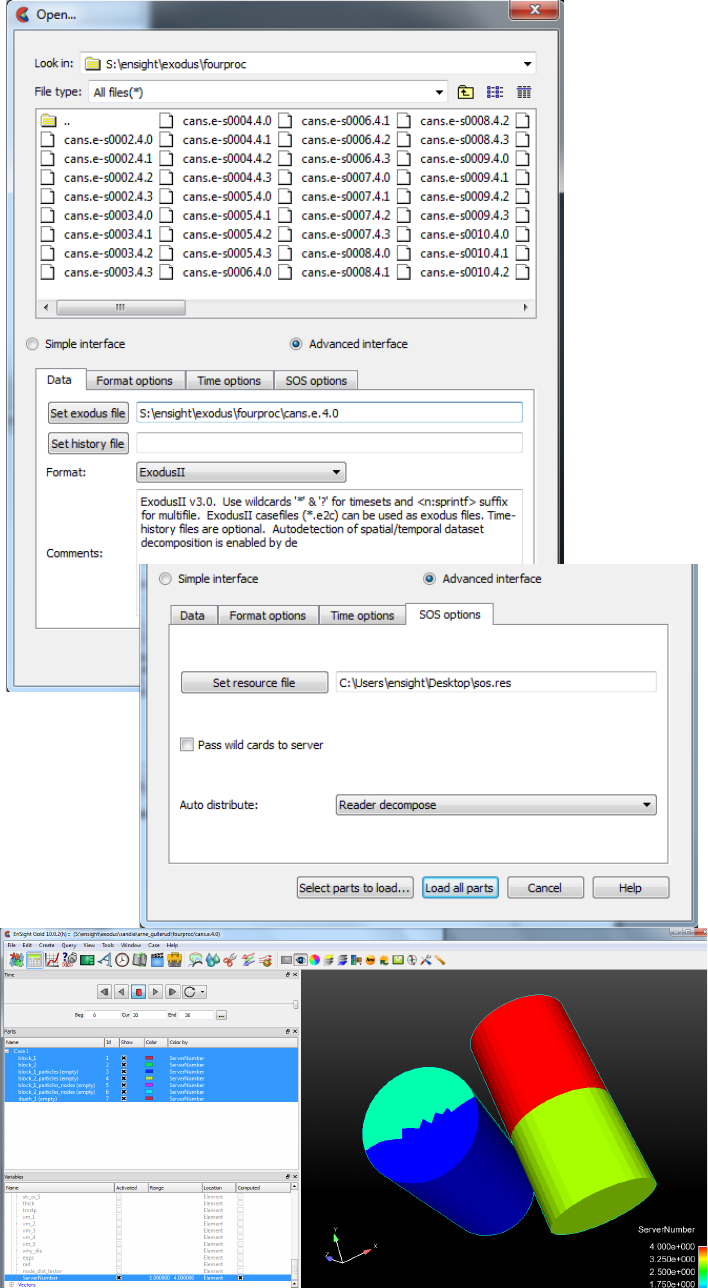

2.3 FAST UNSTRUCTURED Reader
EnSight 10.2 User Manual 2-73
FAST UNSTRUCTURED Reader
Overview
FAST UNSTRUCTURED is a format containing triangle and/or tetrahedron
elements. The triangles have tags indicating a grouping for specific purposes.
EnSight will read the unstructured single zone grid format for this data type,
placing all tetrahedral elements into the first Part, and the various triangle element
groupings into their own Parts.
Simple Interface
Data Load
Load your grid file using the Simple Interface method.
Advanced Interface
Data Load
Load your grid and solution files using the Advanced Interface method.
(see How To Read Data)
Data Tab
Format Use the FAST Unstructured format.
Set grid Select the grid file and click this button. This is the FAST
UNSTRUCTURED single zone grid file. Defines the
geometry as unstructured triangles and/or tetrahedrons.
Set solution Select the solution file and click this button. The Results file
can either be a Modified Result file which utilizes a modified
EnSight results file format, or can be variable files (optional)
which are either a PLOT3D solution file (Q-file) or FAST
function file with I = number of points and J=K=1. The
modified EnSight results file provides access to multiple
solution files that are produced by time dependent simulations.
FAST UNSTRUCTURED data can have changing geometry.
When this is the case, the changing geometry file names are
contained in the results file. However, it is still necessary to
specify an initial geometry file name.
WARNING: Do not use your solution file (e.g. file.q) here.
You must create a special results file to handle FAST variable
files.
Format Options Tab
Set measured Select the measured file and click this button.
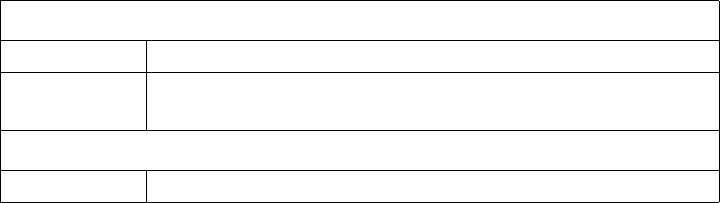
2.3 FIDAP NEUTRAL Reader
2-74 EnSight 10.2 User Manual
FIDAP NEUTRAL Reader
Overview
A FIDAP Neutral file contains all of the necessary geometry and result
information for use with EnSight.
A neutral file is produced by a separate procedure defined in the FIDAP
documentation. If the data is time dependent this information is also defined here.
Simple Interface
Data Load
Load your geometry/results file (typically named with a suffix
.fdneut
) using the
Simple Interface method.
Advanced Interface
Data Load
Load your geometry/results file (typically named with a suffix
.fdneut
) using the
Advanced Interface method.
(see How To Read Data)
Data Tab
Format Use the FIDAP Neutral format.
Set geometry Select the geometry/results file (typically .fdneut) and click
this button
Format Options Tab
Set measured Select the measured file and click this button.
2.3 FLOW3D-MULTIBLOCK Reader
EnSight 10.2 User Manual 2-75
FLOW3D-MULTIBLOCK Reader
Overview
This EnSight reader uses the FLSGRF READER API LIBRARY from
FlowScience in order to read data from a FLOW3D "flsgrf*" output data file as
well as the “prpgrf*” files written out in preprocessor mode (which contain only
one timestep). Flowscience is no longer supporting compressed formats with the
*.fgz and *.dat suffix.
Requirements If any extra FlowScience API debug files are desired from the EnSight session,
the FLSGRF API requires that the user have write permissions in the directory
where the flsgrf file resides.
THE FLSGRF API is only available for Windows 32-bit, 64-bit, Linux 32-bit, and
Linux 64-bit platforms.
EnSight attempts to implement the latest FLSGRF API and the FLSGRF API
should read flsgrf files written by older versions of FLOW3D.
Data Types There are several kinds of data available in a FLOW3D flsgrf output file, each
with its own EnSight timeset: Restart, Selected, Fixed, and Particle data.
Restart data By default, there are 11 restart timesteps per solution: t=0 and an additional ten
each spaced at 1/10th of the total simulation time. The user can change this
frequency in FLOW3D using the plotting interval (PLTDT) in the PREPIN input
file.
Selected data This consists of selected variables output at a higher number of timesteps. Restart
and selected data can both be available in the data file.
Fixed time group This data does not change over time. It consists of simulation parameters such as
binary flags used to activate physical models as well as mesh data.
Parallel Solution If multiple flsgrf files (flsgrf1.dat, flsgrf2.dat, ... flsgrfn.dat) from a parallel run
and the number of servers equals the number of files, then choose the first one
(flsgrf1.dat) and choose decomposition spatial and the remainder will be
automatically loaded. Each server reads only one of the spatially decomposed
files thus dividing up the memory requirements. For temporal decomposition,
load all the spatially decomposed files flsgrf*.dat and choose temporal
decomposition. In this mode, each server loads a separate timestep thus speeding
up transient postprocessing.
Particle data If particles are present in the simulation they will be present in the Restart data. If
the user requests particle information in the Selected data (from their project file
where anmtyp(i)='part') then particle information will also be available in the
Selected data timesets.
Particle data is not imported into EnSight by default. To import this data, Choose
the Multipart Flow3d reader then click on the Format Options Tab and select the
type of Particle data that you wish to import.
Geometry is STATIC in EnSight unless Particle data is imported and then the
geometry is CHANGING CONNECTIVITY because the number of particles can
change with each timestep.
Technical notes All block part variable data is cell-based (per element data). All particle variable
data is node-based (per node data). All FSI/TSE data is node-based (per node).
To visualize the fluid in the block try creating an isosurface of the Fluid Fraction

2.3 FLOW3D-MULTIBLOCK Reader
2-76 EnSight 10.2 User Manual
using an isosurface value of 0.51. Now to see the surrounding structure, make
another isosurface with a value of 0.51 using the Cell_Volume_Fraction_Fixed
variable. Click on the paint can icon and change your shading to smooth to
improve the isosurface look. To see the fluid as an isovolume, File>command and
type in ‘test: simple_isovolume_off’ then make an isovolume from 0.5001 to 1.0
using the Fluid Fraction and again change its shading to smooth.
To see detailed information about variables, blocks, boundary conditions, etc.
choose Console Output Debug as described below.
This reader makes use of Timesets. Each of the variable types has it's own
Timeset timeline and EnSight merges them all together. For details on using these
timesets see the advanced section of the Change Time Steps in the How To
Manual.
Ghost cells Ghost cells are invisible elements that help EnSight to interpolate variable values.
For example, Ghost cells between blocks allow for a smooth transition of the
isosurface of the fluid surface at part block boundaries. Ghosts that are not used
have a zero value for the variable, and must be removed: removal of ghosts at a
symmetry surface allows for smooth mirroring of the part(s).
Units If the units are specified in a known unit system in the data file, then EnSight can
convert them to any of the other known unit systems at read in. Also, EnSight can
annotate by the units for any of the variables (those not non-dimensionalized).
Updated info
$CEI_HOME/ensight102/src/readers/multi_flow3d/README.txt
Simple Interface
Data Load
Load your Flow3d file (typically named
flsgrf*
) using the Simple Interface
method.
Advanced Interface
Data Load
Load your Flow3d file (typically named
flsgrf*
) using the Advanced Interface
method.
Data Tab
Format Use the Flow3d-Multiblock format.
Set flsgrf This field should be an flsgrf or prpgrf file. If multiple flsgrf
files (flsgrf1.dat, flsgrf2.dat, ... flsgrfn.dat) from a parallel run,
then choose all using an asterisk (flsgrf*.dat) in place of the
numbers, or one by specifying the particular file (flsgrf1.dat).
Format Options Tab
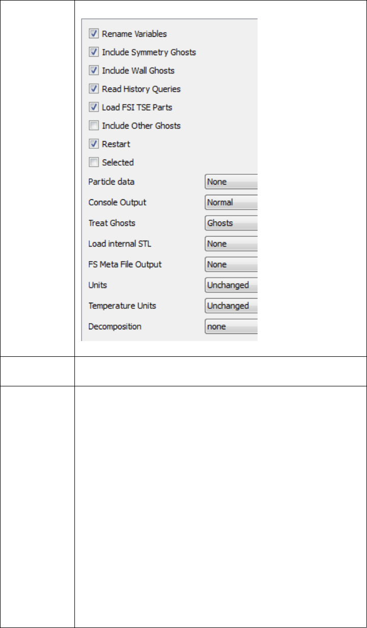
2.3 FLOW3D-MULTIBLOCK Reader
EnSight 10.2 User Manual 2-77
Format
Options
Rename
Vari ab les
Variables are renamed by default to be easier to interpret for
Flow3D users.
Include
Symmetry
Ghosts
Flow3d includes the following boundary conditions:
symmetry, wall, continuative, periodic, specified pressure,
specified velocity, grid overlay, outflow and interblock.
Ghosts are always included in periodic, specified pressure, and
inter-block boundary conditions.
Ghosts are optional (using a toggle) for the following
boundary conditions.
a. symmetry - include symmetry ghosts toggle
b. wall - include wall ghosts toggle
c. other - (continuative, specified velocity, grid overlay and
outflow) - include other ghosts toggle.
By default, symmetry ghosts are removed so that mirroring in
EnSight has no seam.
However toggling ON this flag will include the symmetry
ghosts for example for inviscid flow using the symmetry
condition to simulate a wall.

2.3 FLOW3D-MULTIBLOCK Reader
2-78 EnSight 10.2 User Manual
Include Wall
Ghosts
Flow3d includes the following boundary conditions:
symmetry, wall, continuative, periodic, specified pressure,
specified velocity, grid overlay, outflow and interblock.
Ghosts are always included in periodic, specified pressure, and
inter-block boundary conditions.
Ghosts are optional (using a toggle) for the following
boundary conditions.
a. symmetry - include symmetry ghosts toggle
b. wall - include wall ghosts toggle
c. other - (continuative, specified velocity, grid overlay and
outflow) - include other ghosts toggle.
By default, wall ghosts are removed so that the EnSight fluid/
wall interface does not show up using the isosurface of the
fluid fraction.
However toggling ON this flag will cause the fluid/wall
interface to show up using the isosurface of the fluid fraction.
Include Other
Ghosts
Flow3d includes the following boundary conditions:
symmetry, wall, continuative, periodic, specified pressure,
specified velocity, grid overlay, outflow and interblock.
Ghosts are always included in periodic, specified pressure, and
inter-block boundary conditions.
Ghosts are optional (using a toggle) for the following
boundary conditions.
a. symmetry - include symmetry ghosts toggle
b. wall - include wall ghosts toggle
c. other - (continuative, specified velocity, grid overlay and
outflow) - include other ghosts toggle.
By default, these other ghosts are removed so that the EnSight
fluid/wall interface does not show up using the isosurface of
the fluid fraction.
However toggling ON this flag will cause the fluid/wall
interface to show up using the isosurface of the fluid fraction.
Read History
Queries
The flsgrf file often includes xy plotting data in the form of
history data that is loaded into EnSight as pre-defined Queries
accessible by clicking on the Query/Plot icon or below the part
list in the Parts/queries tab. Default is ON.

2.3 FLOW3D-MULTIBLOCK Reader
EnSight 10.2 User Manual 2-79
Load FSI
TSE Parts
Fluid-Structure Interaction and Thermal Stress Evolution
unstructured parts (hexa8 and tet4’s) and their associated
stress, strain, temperature, displacement and blanking
(STATUS) nodal variables are loaded into EnSight by default.
A TSE (thermal stress evolution) component is a region in the
fluid, where the fluid solidified and a structural analysis is
performed in the solid in response to thermal gradients. An
FSI (fluid-structure interaction) components, is a solid region
in the fluid where the flow-induced structural deformations in
turn, influence the flow, requiring simultaneous structural and
fluid flow solution There can be only one TSE part in a
simulation.
Restart Load the variables on the Restart Timeline. Default ON.
Selected Load the variables on the Selected Timeline. Default OFF.
Particle Data By default, particle data is not read into EnSight. Choose the
appropriate timeline to read in the Particle data.
Console
Output
Use this flag to determine the amount of output to the console.
Normal - Usually only echo errors to console.
Verbose - Normal output plus an echo of every Fluent part
that is in the dataset, whether it is interior or not, whether it is
skipped, what variables are defined for which parts, and to
echo it's Ensight Part number.
Debug - Verbose output plus more detailed output and
progress through the reader routines often valuable for
understanding and reporting problems. Also detailed block
information, variable information, boundary condition
information, and timeset information
Treat Ghosts Ghost elements are invisible elements that help EnSight to
interpolate variable values. Ghosts can be read in as Ghost
cells, as normal (visible) cells, or they can be not read in at all.
1. Ghosts - include invisible ghost elements according to the
Flow3d boundary conditions (default) and user settings.
2. None - Use NO ghost elements. This will especially be
apparent in the gaps in the isosurface between data blocks due
to the lack of these invisible interpolating elements.
3. Normal - Use ALL ghost elements as NORMAL, visible
elements. This is useful for understanding boundary
conditions around part blocks.
Load Internal
STL
The flsgrf file sometimes includes surface, boundary
condition, or other important surface geometry on one or more
timelines. Default is to load None, but the pulldown allows the
user to choose Selected, Restart, or Static STL geometry
timelines.

2.3 FLOW3D-MULTIBLOCK Reader
2-80 EnSight 10.2 User Manual
FS Meta File
Output
The FlowScience reader API, optionally writes out optional
performance and debug files when a flsgrf file is opened if you
have write permission. These can help to speed up reading the
second time a file is opened or to understand the details of the
read or to diagnose a failed read. However, if multiple users
each with different file mask permissions attempt to open a
flsgrf file on a shared network hard drive, the writing and
overwriting of these files becomes problematic and can cause
a read to fail. The safest option, if others may follow your read
of a given file, is to choose to not write out these optional files.
The API offers four options on opening a file named, for
example, flsgrf:
None - write out no additional files
Performance - writes out c-flsgrf, flsgrdr, g_flsgrf, and t_flsgrf
files.
Debug - writes out the flsout.rdr file
All - writes out both Performance and Debug files.
Units Convert units to selected type. FlowScience reader API
allows the conversion of a known system units (CGS, SI or
English) to another known system (CGS, SI, or English).
EnSight will not convert from an unknown or unspecified unit
system.
Unchanged (default) - use the system of units in the data file
CGS - Uses grams, centimeters, and seconds.
SI - Uses kilograms, meters, and seconds.
English - Uses slugs, feet, and seconds.
Temperature
Units
Temperature units are always known (C, K, F, or R) and can
therefore always be converted to any other unit system.
Celsius - Convert to Celsius
Kelvin - Convert to Kelvin
Fahrenheit - Convert to Fahrenheit
Rankine - Convert to Rankine
Unchanged (default) use the temperature units in the data file
Decomposition If running in EnSight SoS mode, the type of decomposition to
use.
None -
Spatial - Traditional SOS mode in which each server is
assigned one of the spatially decomposed block files.
Temporal - Temporal SOS in which the data is not spatially
decomposed, but rather each of the available servers reads a
different timestep to speed up transient post processing.
Set measured Select the measured file and click this button.
2.3 FLOW3D-MULTIBLOCK Reader
EnSight 10.2 User Manual 2-81
Parallel post
processing (SOS)
The Flow3d solver can calculate its solution in parallel. This type of solution
writes out the data as separate files (flsgrf1.dat, flsgrf2.dat, flsgrf3.dat, ....), each
containing one structured block.EnSight can read each of these files onto a
separate server. Server 1 will read in the unstructured data plus block 1, server 2
will read in block 2, server 3 will read in block 3, etc.
You can create an SOS casefile (.sos), which maps out which server loads what
data and start EnSight up in SOS mode, and just load the sos casefile directly.
Alternatively, you can create a .res file to set up the servers, start up EnSight in
SOS mode, and load the data as flsgrf*.dat, and, in the data reader dialog, choose
the .res file and choose to allow sos to use the *. For more details (including a
sample resource file and sample SOS case file and how to use them, see How to
Use Server of Servers and search for Flow3d.
(see How To Read Data)

2.3 FLUENT Direct Reader
2-82 EnSight 10.2 User Manual
FLUENT Direct Reader
Overview
There are three methods to get Fluent data into EnSight. The first is to use the
current Fluent reader. This loads a Fluent Case (.cas) file and data (.dat or .fdat)
file. The second method to get data into EnSight is to use Fluent’s EnSight Case
Gold Export option and read the resulting .encas file directly into EnSight using
the Case reader. The third and last method is a little-used legacy reader for Fluent
Universal file and is described later under the FLUENT UNIVERSAL Reader.
See the following files for current information on the Fluent direct reader.
$CEI_HOME/ensight102/src/readers/fluent/README.txt
The comments that follow are for the current Fluent reader. The reader loads
ASCII, binary single precision, or binary double precision. The files can be
uncompressed or compressed using gzip. Note also, this reader is used to load
AIRPAK/ICEPAK .fdat data files (see AIRPAK/ICEPAK Reader).
Simple Interface
Data Load
Load your geometry file (typically named with a suffix
.cas
) using the Simple
Interface method.
Advanced Interface
Data Load
Load your geometry and result files (typically named with a suffix
.cas and .dat
)
using the Advanced Interface method.
Data Tab
Format To use this reader, select the Fluent format.
Set cas Select the geometry file (typically .cas or .cas.gz) and click
this button. For transient data, use a single asterisk to replace
the number (
*.cas
or
*.cas.gz
).
Set dat Select the results file (typically .dat or .dat.gz), and click this
button. For transient data, use a single asterisk to replace the
number (
*.dat
or
*.dat.gz
). Note that .fdat files (see Airpak /
Icepak reader) are also usable in place of the .dat file. Because
the .dat file is the automatic selection, if a .dat file is
collocated with a .fdat file, the user will have to manually
select the .fdat file and then click on the Set dat button to use a
.dat file variant.
Format Options Tab
Set measured Select the measured file (typically a .mea suffix) and click this
button. If you have fluent particle data you can translate it into
EnSight’s measured data format and import the particles as
measured data.
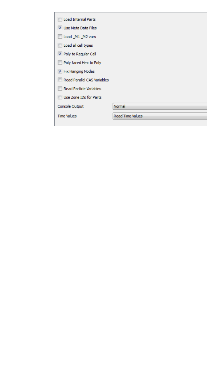
2.3 FLUENT Direct Reader
EnSight 10.2 User Manual 2-83
Other
Options
using the
current
Fluent reader
Load Internal
Parts
Toggle this ON to load the Fluent Internal Parts. This will
show all the internal walls forming all the cell volumes. If you
do toggle this on, then it is recommended that you click on the
'Choose Parts' button at the bottom of the data reader dialog,
rather than 'Load all', as you'll only want to load the interior
parts of interest to save memory and time. Default is OFF.
Use Meta
Files
Meta files are small summary files that contain highlights of
the important locations inside each of the Fluent files.
Allowing the EnSight reader to write out Meta Files that map
the locations of important data can provide a significant speed
up the next time you access that timestep. It is recommended
that you leave this toggle ON. If you have write permission in
the directory where your data is located, three types of binary
Meta Files will be written when you first access each file, with
extensions .EFC for the cas file, .EFD for the .dat file and
.EFG for the time-history data. They are optional, and if you
don't have write permission, the reader will take the extra time
to read the entire .CAS and .DAT file to find the relevant data
each time you come back to that timestep.
Load _M1
_M2 vars
Variables that end in '_M1' and '_M2' occur in Fluent unsteady
flow. They represent the value of the variable at the prior
iteration time and the time prior to that respectively. By
default this toggle is OFF and these variables are not loaded.
Toggle this ON to load these variables.
Load all cell
types
Fluent cells have a boundary condition flag. By default
(toggle OFF) EnSight loads only the cells with a boundary
condition flag equal to 1 (one). Toggle this option ON to load
all cells with a non-zero boundary condition. For example, if
you have a part with cells of boundary condition 32 (inactive),
EnSight will, by default not load this part. Toggle this option
ON and EnSight will load this part. Note: parts containing
cells with a boundary condition of zero are never loaded.

2.3 FLUENT Direct Reader
2-84 EnSight 10.2 User Manual
Poly to
Regular Cell
Fluent polyhedral cells when composed of the correct kind and
number of regular faces can be converted to regular cells
(tetrahedrons, hexahedrons, pyramids, or wedges) boosting
EnSight speed and decreasing memory requirements. Toggle
ON and reader checks each polyhedron to see if it can be
converted to a regular cell (default) and OFF to not convert
any polyhedral cells. There is very little slowdown during the
read to do this and a big payoff for some datasets with large
numbers of convertible polyhedra. Leave it on.
Poly faced
Hex to Poly
Fluent hex cells that transition to a more refined hex mesh will
sometimes have one or more of the quad4 faces subdivided
into four quad4 faces. For example a hexahedral cell with one
transition face will have the six full faces, and four subdivided
faces for a total of 10 faces. Toggle ON and the subdivided
faces are kept rather than the full face and the cell is changed
into a polyhedral which will slow down EnSight performance,
and greatly increase memory. The polyhedral also will have
hanging nodes (see the next toggle). Toggle OFF (default) to
convert the hex element to a six-sided hex which will be
adjacent to four smaller cells rather than completely connected
to them slowing down EnSight’s adjacency searching. The
default is thought to be the lesser of two evils.
Fix Hanging
Nodes
Some Fluent polyhedral cells and all transition hex cells
converted to polyhedrals will have hanging nodes. A hanging
node is a node not shared by at least 3 faces. A polyhedral
element with hanging nodes is not water tight and can cause
real problems in EnSight, so it is best to leave this toggle ON
(default) and only turn it OFF for experimental purposes.
Read Parallel
CAS
Vari ab les
For parallel investigation, if the user toggles on read cas
variables, this option creates two new elemental scalars:
ELEMENT_INDEX and PARTITION only if the data is
solved in parallel and has partition section(s). This is primarily
useful to visualize the Fluent geometric decomposition of
parallel solutions.
Read Particle
Vari ab les
This will read particle coordinates and variable data from the
DAT file. The number of particle parts is equal to the number
of injections.
Use Zone IDs
for Parts
A heterogenous mix of serial and parallel solution files will
result in a jumbled part ordering between CAS files. Toggle
this ON to use the part zone id to reorder the parts consistently
from CAS file to CAS file using the first file loaded as the
canonical order.
Read all files
to create
variable list
Some transient datasets have different variables in the
different DAT files. If this is OFF (default) then only the last
DAT file will be used to create the variable list. If ON, then all
DAT files will be used to create the master variable list.
Regardless of the option, a variable will be assigned the
EnSight Undefined value at time steps where it is undefined.

2.3 FLUENT Direct Reader
EnSight 10.2 User Manual 2-85
Node and Elem IDs Parts have node and element ids to enable querying your data. Node ids are
created from the coordinate global node. Element ids are created as follows. Face
part elements are uniquely numbered according to their zone index. Cell part
elements are uniquely numbered using their zone index added to the total number
of faces. So a dataset with 100 face elements and 300 cell elements would have
the face elements number 1-100 and the cell elements numbered 101-400. In
Verbose mode, the element id range for each part are written to the console.
Variable Location Variables that are cell-centered remain where they are found in the .dat file, that is
the reader does not interpolate the cell-centered variables to the nodes. Fluent can
export variable data to EnSight’s Case Gold format at either the nodes (default) or
Console
Output
Use this flag to determine the amount of output to the console.
Normal - Usually only echo errors to console.
Verbose - Normal output plus an echo of every Fluent part
that is in the dataset, whether it is interior or not, whether it is
skipped, what variables are defined for which parts, and to
echo it's Ensight Part number.
Debug - Verbose output plus more detailed output and
progress through the reader routines often valuable for
understanding and reporting problems.
Time Values 'Use Filename Numbers' will read the sequential numbers at
the tail of the filenames and adjust them by making the first
number 0 and shift all subsequent values. That is,
file4000001.cas, file4000004 ... file4000020 is as follows:
timestep 0 has time value 0.0, timestep 1 has time value 3.0,
and timestep n has time value 19.0.
‘Use Time Steps’ will make timestep and time value the same
for example: timestep 0 will have time value 0.0 and timestep
5 have time value 5.0.
'Read Time Values' (default) will open each file and find the
exact time value using the 'flow-time' keyword. Note that this
means that every file has to be opened and searched. Failing
that it defaults to the 'Calc Const Delta'.
'Calc Const Delta' reads a delta time from one file using
'physical-time-step' keyword, and calculates the time values
by multiplying the delta value by the adjusted filename
number. Failing that, it defaults to the ‘Use Filename
Numbers’ option.
It is essential that your time values are correct for some
calculations (for example, if you are going to do pathline
tracing). Keep in mind that if your timesteps are uniform then
you can use the ‘Use Time Steps’ option and just scale your
time values using the Time Options tab in the data reader
dialog. If your timesteps are not uniform, but your File
Numbers are proportional to your timesteps then you can
select ‘Use Filename Numbers’ and then scale the time values
using the Time Options Tab in the data reader dialog.
2.3 FLUENT Direct Reader
2-86 EnSight 10.2 User Manual
at the elements (same as .dat file). Unfortunately older versions of Fluent export
variables averaged to the nodes leading to flow into and out of walls which causes
particles to stop prematurely and skews mass flow calculations. Later versions of
Fluent consider boundary conditions prior to averaging the data to the nodes,
yielding a much more realistic representation of the physics.
Variables
Undefined
Not all variables exist on all parts in the dat file. If you select a part and color by
a variable and get undefined, then load the data using Verbose mode and take a
look at the console. Your variable is probably not defined for this part and EnSight
does not have the boundary conditions nor the solver physics algorithms to
extrapolate variable values to boundary parts. Create a clip on the location of an
interior part on a volume part if you want to see a plane with the values from the
volume.
Extra Variables EnSight will try to calculate extra CFD variables given the existing DAT variables
for your convenience.
gzipped files Files that are gzipped can be read by EnSight. However, with large numbers of
parts this can result in a substantial slow down in the access of variable
information in the DAT file because this involves non sequential access (seeking
around various places in the file rather than sequentially moving through the file
in order) which has been shown to result in dramatic slow downs. The
workaround is to simply ungzip your files prior to reading them into EnSight.
CAS Constants Extra CAS Single Value Variables - A number of single value variables are read
from the CAS file(s). These will show up in the EnSight Calculator named as
follows.
'PRESSURE_ABS' - operating pressure (absolute)
'PRESSURE_ABS_INIT'- initial operating pressure (absolute)
'GAMMA_REF' - reference gamma, ratio of specific heats
'VISCOSITY_REF' - reference viscosity
'TEMPERATURE_REF' - reference temperature
'PRESSURE_REF' - reference pressure
'DENSITY_REF' - reference density
'SPEED_SOUND_FAR' - far field speed of sound
'PRESSURE_FAR' - far field relative pressure
'DENSITY_FAR' - far field density
'R_ref' - Calculated reference gas constant = PRESSURE_ABS /
(DENSITY_REF * TEMPERATURE_REF)
'V_def' - Calculated default velocity magnitude from x, y and z-velocity default
values
'M_def' - Calculated from V_def / SPEED_SOUND_FAR
UDS, UDM
Variables
UDM and UDS variables now read in as UDM_0, UDM_1, UDM_2... and
UDS_0, UDS_1, .... Fluent differentiates between UDS (User defined scalar) and
UDM (user defined memory) as follows.
A UDS is a scalar variable for which a transport equation can be solved (e.g.
transport of a red color from an injection nozzle into the volume; convective
terms, diffusive terms,.) The single terms of this transport equation are
programmed via UDF (user defined functions) in C and are run time libraries.
A UDM is a node-based value which also is calculated using a UDF (e.g.viscosity
2.3 FLUENT Direct Reader
EnSight 10.2 User Manual 2-87
against local temperature and density). For UDMs transport equations are not
solved. Thus they require less memory compared to UDS.
UDMs and UDSs are available for additional physics which are not available in
Fluent (for example one can use a UDM for the calculation of dust concentration
in filter elements.
Polyhedral
elements
There are two methods to import polyhedral elements into EnSight. The first is to
try using the direct reader. This has the advantage that the direct reader will
attempt to convert polyhedral elements back to regular elements, saving memory
and speeding up EnSight. The second is to export EnSight Case Gold .encas file
from Fluent. Case Gold has the advantage of currently supporting automatic
Server of Server decomposition, which can distribute the many tasks to multiple
servers and speed up post processing.
Periodic elements The reader now supports rotational symmetry to provide continuous boundaries.
Particles The reader should attempt to read particles if they are present in the file(s).
Included with EnSight is a Fluent particle file translator to translate the Fluent
.part
file into an EnSight measured (
.mea
) data file. To get help with this
translator, type
$CEI_HOME/ensight102/machines/$CEI_ARCH/flupart -h
where $CEI_ARCH is your hardware/OS architecture (e.g. linux_2.6_64 or
apple_10.5, win32, etc.).
Source code and README for this translator are located
$CEI_HOME/ensight102/translators/fluent/Particles/
This measured data file is entered in the measured data field under the Format
Options tab of the data reader dialog.
(see How To Read Data)

2.3 Inventor Reader
2-88 EnSight 10.2 User Manual
Inventor Reader
Overview
Reads inventor (.iv) datasets for which there is a one-to-one correspondence in
Part, coordinate index, geometry index and element record. That is, there is one
set of coordinates, one geometry, one set of elements per inventor node. To read
in one inventor file, enter the .iv filename.
To read in multiple .iv files us a Case Inventor file (.civ). The user has the option
in the reader Format Options Tab to toggle off one part per file option (default on).
The .civ file is an ASCII file with the number of files on the first line, and the
filenames on the remaining. The filenames must be in quotes, and if they don't
include the path, the .civ file must be in the directory where the files are located. A
'.civ' filename cannot be in a '.civ' file: only '.iv' filenames are allowed.
Example Format:
numfiles: 2
"filename1.iv"
"filename2.iv"
For more info, see
$CEI_HOME/ensight102/src/readers/inventor
Data Reader
Main Menu > File > Data (reader)...
The File Selection dialog is used to specify which files you wish to read.
Main Menu > File > Data (Reader)...
Simple Interface
Data Load
Load your geometry/results file (typically named with a suffix
.iv
or
.civ
) using
the Simple Interface method.
Advanced Interface
Data Load
Load your geometry/results file (typically named with a suffix
.iv
or
.civ
) using
the Advanced Interface method.
(see How To Read Data).
Data Tab
Format Use the Inventor format.
Set .iv file Select the inventor file (typically .iv or .civ) and click this
button
Format Options Tab
One Part per
file
Makes one part out of each file.
Console
Output
Use this flag to determine the amount of output to the console.
Normal - Usually only echo errors echoed to console.
Verbose - Normal plus high level output describing dataset and
progress while reading
Debug - Detailed output and progress through the reader
routines often valuable for understanding and reporting
problems.
Set measured Select the measured file and click this button.
2.3 LS-DYNA Reader
EnSight 10.2 User Manual 2-89
LS-DYNA Reader
Overview
The LS-DYNA reader reads in a single or multiple unstructured C-binary d3plot files.
It supports bars, quads, bricks and thick shell elements.
Key File for Part
Naming
Can use of Key file to name parts as follows:
a. Works only if Material IDs are in the d3plot file
b. Put key file name into Params field
c. Looks for *PART keyword in keyfile
d. '$' in first column is a comment in keyfile
e. First non-comment line after *PART is used as partname if alpha or digit
f. Second non-comment line after *PART, 3rd integer is Material ID
g. If Mat'l ID in d3plot matches Mat'l ID in keyfile partname from key file is
substituted for Material ID in EnSight name.
FEMZIP The reader uses the publicly-available “femunzip” utility to unzip the compressed
files. This unzip utility can be downloaded for free. The user must set the
environmental variable “FEMUNZIP_UTILITY_PATH” to point to the location
of this executable. The reader will call this executable on the d3plot file(s) to
ensure that the file(s) are unzipped into a temporary folder prior to reading. A
“mapfile.txt” pointing to the unzipped files will be created which will be used in
subsequent runs avoid the need to unzip again.
CFD data The reader skips legacy CFDDATA sections, and reads instead the ICFD data
from the incompressible CFD and incompressible CFD surface solvers.
DEM/DES The reader now includes this particle data.
AMR The reader can read AMR data even if the expected, first d3plotaa is not available.
Duplicate
timesteps
The reader skips duplicate timesteps, caused perhaps by double precision to float
conversion.
Limitations The reader has the following limitations.
Does not read airbag particle data
Doesn't support PACKED data (3 integers per word)
Skips over Rigid Road Surface Data.
Coordinate System: Global vs. Local: Beam stresses and strains are always
output in the local r,s,t system. Per LSTC manual, stresses and strains of the other
elements are generally in the global system. However, shells & thick shells have
an option to output in local system (see LS-DYNA 960 keyword users manual
page 9.18. flag CMPFLG). The reader has no way of knowing whether stresses
and strains are output in the global or local system and just shows the values
contained in the files.
See the following file for current information on this reader.
$CEI_HOME/ensight102/src/readers/ls-dyna3d/README
Data Reader
Simple Interface
Data Load
Load your d3plot file using the Simple Interface method.
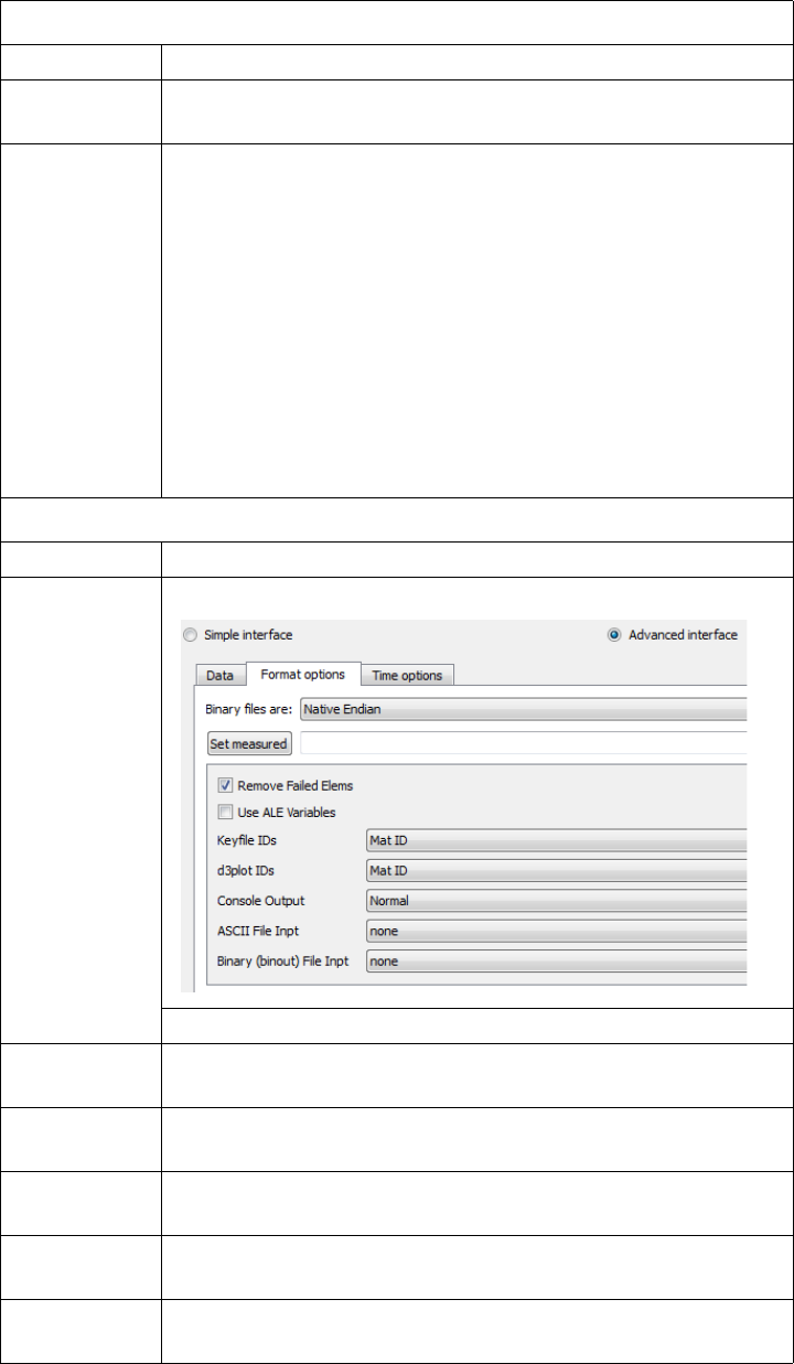
2.3 LS-DYNA Reader
2-90 EnSight 10.2 User Manual
Advanced Interface
Data Load
Load your d3plot file using the Advanced Interface method.
Data Tab
Format Use the LS-DYNA3D format.
Set d3plot This field should have the first d3plot file name. All of the
d3plot files will be loaded starting with this first one
Set key This field can be used to import parameters that modify the
behavior of the reader, or the Extra GUI section can be used to
choose which ids to use for naming and to name the keyfile
respectively.
keyfilename - Type the keyfile name into this field
-mid - use material id in keyfile to name parts in d3plot file.
-pid - use part id in keyfile to name parts in d3plot file.
example:
file.key -mid
This will use the material ids in keyfile named file.key to
name parts.
Format Options Tab
Set measured Select the measured file and click this button.
Format
Options
The following options are customized for the reader:
Remove
Failed Elems
Failed elements will not be shown (default)
Use ALE
Vari ab les
Include the ALE variables
Keyfile IDs This pulldown provides the choice of either Material IDs or
Part IDs from the keyfile to be used for part naming.
d3plot IDs Use either Material IDs (default) or Part IDs within the d3plot
file to read in the data.
Console
Output
Can control amount of output that comes to the console.
Options are: Normal, Verbose, or Debug

2.3 LS-DYNA Reader
EnSight 10.2 User Manual 2-91
(see How To Read Data)
ASCII File
Input
Can input glstat, abstat, matsum, rcforc, rwforc, nodout,
secforc, sleout, elout, dbfsi, and spcforc xy ascii files as
EnSight xy queries. These files must be in the same directory
as the d3plot file(s). Choose none (default) or all for all of the
available files. Choose filenames.txt if you wish to name a
subset of the files to read.
Binary
(binout) File
Input
Can input the binout file (default none) glstat, abstat, matsum,
rcforc, rwforc, nodout, secforc, sleout, elout, dbfsi, and
spcforc and nodfor, or all curve sets as EnSight xy queries.
The binout file must be in the same directory as the d3plot file.
This uses the LSTC binout API to read the xy data.
2.3 MSC.DYTRAN Reader
2-92 EnSight 10.2 User Manual
MSC.DYTRAN Reader
Overview
Reads any of the following (in preferred order):
1. The .dat file (which refers to .ARC files in the directory)
or 2. One of the .ARC files (which will get all .ARC files of the same pattern)
or 3. The modified case file (for specific control).
See the following file for current information on this reader.
$CEI_HOME/ensight102/src/readers/dytran/README.txt
Simple Interface
Data Load
Load your dytran file (typically named with a suffix
.dat or .arc
) using the Simple
Interface method.
Advanced Interface
Data Load
Load your dytran file (typically named with a suffix
.dat or .arc
) using the
Advanced Interface method.
Data Tab
Format Use the MSC/Dytran format.
Set dytran The preferred input is the file with .dat suffix. The root name
of this file will be used to find all .ARC files in the directory
which match the Dytran naming convention. And all parts of
the model will be made available to EnSight. Additionally,
this method allows for the most efficient setting for changing
geometry, because it can glean some pertinent information
thereto within the .dat file.
Alternatively, you can enter one of the .ARC files, and all
.ARC files in the directory which match the pattern will be
found and used. Note: no widcards are needed - just select one
of the .ARC filenames.
The third method is to enter a custom case file. This user
generated ascii file allows one to specify particular parts, etc.
Since one can accomplish the same thing by only loading
specific parts within EnSight, this method is probably
obsolete.
Format Options Tab
Set measured Select the measured file and click this button.
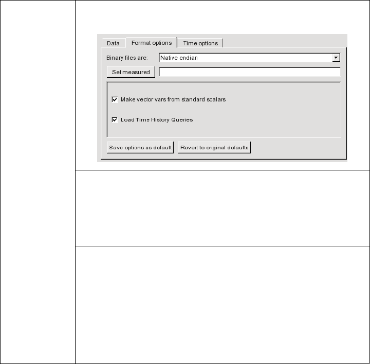
2.3 MSC.DYTRAN Reader
EnSight 10.2 User Manual 2-93
If you choose to not have the Dytran XY time-history data (from the .THS files)
loaded automatically, or if you are using a prior version of the reader, you can later
click on the XY Query/Plot icon and choose to load data from an external file in
the pulldown, and choose the desired .THS file(s). For details, see the How To
Manual section on Queries From External Sources.
(see How To Read Data)
Format
Options
The following options are customized for the reader, in
version 2.05 or later.
Make vector vars from standard scalars - Toggle on to have
vector variables automatically generated from known standard
scalar components. On is the default.
Example: If toggled on, a vector variable named VEL will be
created from the scalars XVEL, YVEL, ZVEL
Load Time History Queries - Toggle on to have all xy time-
history queries (contained in pattern matching .THS files in
the directory) loaded automatically into EnSight. On is the
default.
Note: These have traditionally been read into EnSight in the
Query/Plot feature, but reading each .THS file as an “external
file”. While this option still exists, it is not needed if this
toggle is on.
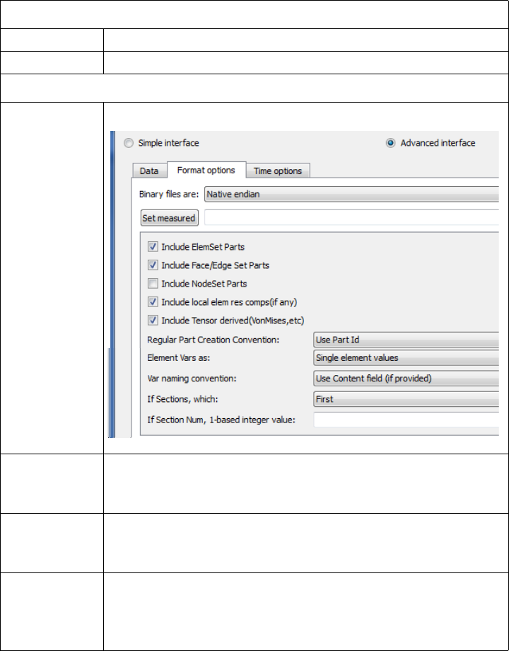
2.3 MSC.MARC Reader
2-94 EnSight 10.2 User Manual
MSC.MARC Reader
Overview
Reads a t16 or t19 file (which is the preferred method).
See the following file for current information on this reader.
Simple Interface
Data Load
Load your marc file (typically named with a suffix
.t16 or .t19
) using the Simple
Interface method.
Advanced Interface
Data Load
Load your marc file (typically named with a suffix
.t16 or .t19
) using the
Advanced Interface method.
Data Tab
Format Use the MSC.Marc format.
Set t16/t19 This field should have the .t16 or .t19 suffix file.
Format Options Tab
Format
Options
Include
ElemSet
Parts
Include any Element sets defined. These are sets of full
elements which are generally some logical subset of the total
number of elements. Default is on.
Include Face/
Edge Set
Parts
Include any Face or Edge sets defined. These are some logical
set of particular faces and/or edges of full elements. Default is
on.
Include
NodeSet
Parts
Include any Node sets defined. These are generally the subset
of nodes needed for the Element, Face, or Edge sets above. As
such, they are generally not needed as separate parts, but can
be created if desired. Default is off.

2.3 MSC.MARC Reader
EnSight 10.2 User Manual 2-95
Include local
elem res
comps (if
any)
Include the local stresses components, etc that are in the
element's local system.
A simple example is a bar (such as a truss element), which
only has tension or compression in the element's axial
orientation. Such an element would have an axial stress
variable.
Other elements would have appropriate result component
variables. Default is on
Include
Tensor
derived
(VonMises,
etc.)
For tensor results, calculate scalars from the following derived
results (principal stress/strains, and common failure theories):
Mean Equal Direct
VonMises Min Principal
Octahedral Mid Principal
Intensity Max Principal
Max Shear
By default, all 9 of these will be derived. You can control
which are created by this toggle, with an environment
variable. Namely,
setenv ENSIGHT_VKI_DERIVED_FROM_TENSOR_FLAG n
where n = 1 for Mean only
2 for VonMises only
4 for Octahedral only
8 for Intensity only
16 for Max Shear only
32 for Equal Direct only
64 for Min Principal only
128 for Mid Principal only
256 for Max Principal only
512 for all
or any legal combination. example: for VonMises and Max
Shear only, use 18. Default is on.
Regular Part
Creation
Convention
Parts will be created according to the following:

2.3 MSC.MARC Reader
2-96 EnSight 10.2 User Manual
Element Vars
as
Single element
values
Element results (whether centroidal or
element nodal) will be presented as a
single value per element. Thus will be
per_elem variables in EnSight.This is
the default.
Averaged to node
values
Element results (whether centroidal or
element nodal) will be averaged to the
nodes without using geometry
weighting. Thus will be per_node
variables in EnSight. This is a global
averaging, so shared nodes are affected
by all parts that share a node.
Geom weighted
average to node
values
Element results (whether centroidal or
element nodal) will be averaged to the
nodes using geometry weighting. Thus
will be per_node variables in EnSight.
This is a global averaging, so shared
nodes are affected by all parts that share
a node.
Ave to node values
<by parts>
Element results (whether centroidal or
element nodal) will be averaged to the
nodes without using geometry
weighting. Thus will be per_node
variables in EnSight. This is a local
averaging, so all averaging is contained
within each part.
Geom weighted
ave to node <by
parts>
Element results (whether centroidal or
element nodal) will be averaged to the
nodes using geometry weighting. Thus
will be per_node variables in EnSight.
This is a local averaging, so all
averaging is contained within each part.
Var naming
convention
Use Content Field
(if provided)
Variable names will be what is in the
Content field, if provided. If not
provided, they willbe the VKI dataset
name. This is the default.
Use VKI dataset
name
Variable names will be the VKI variable
dataset name (which are reasonably
descriptive).
If Sections,
which:
Which section will be used to create the variable
First The first section will be used (this is the
default)
Last The last section will be used
Section Num
(below)
The section number entered in the field
below will be used
Separate Vars per
Section
A separate variable will be created for
each section.

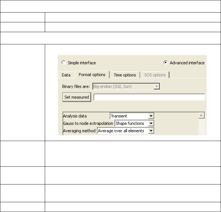
2.3 MSC.MARC Legacy Reader
2-98 EnSight 10.2 User Manual
MSC.MARC Legacy Reader
Overview
Reads a t16 or t19 file (which is the preferred method).
See the following file for current information on this reader.
$CEI_HOME/ensight102/src/readers/marc/README
Simple Interface
Data Load
Load your marc file (typically named with a suffix
.t16 or .t19
) using the Simple
Interface method.
Advanced Interface
Data Load
Load your marc file (typically named with a suffix
.t16 or .t19
) using the
Advanced Interface method.
Features 1. Can read both t16 binary result files and t19 formatted result files
2. Supports most analysis types (structural, thermal, magnetic, etc.)
3. Supports results for nodes (scalar / vector) and gauss-points (scalar, vector and
tensor). Gauss point results are extrapolated to nodes and averaged at the nodes.
4. Handles remeshing (global and local) and element activation / de-activation.
5. Can read results for DMP runs: If the main result file is selected, all domains
are imported. Domain result files can be selected individually
6. Can read static / transient results, modal results and buckling results.
7. Works on all Marc versions from Marc 2000 up to 2005r2.
Data Tab
Format Use the MSC.Marc Legacy format.
Set t16/t19 This field should have the .t16 or .t19 suffix file.
Format Options Tab
Format
Options
Analysis data: Transient, Modal, Buckling. Please choose the
type of data to be read. The "Transient" option supports any
time-dependent result types (static, quasi-static and transient).
Gauss to node extrapolation: Shape functions. Currently only
one choice.
Averaging method: Average over all elements. Currently only
one choice.
Set measured Select the measured file and click this button.
2.3 MSC.MARC Legacy Reader
EnSight 10.2 User Manual 2-99
8. In the past, Little-endian and Big-endian results were handled transparently in
the reader. A message "Not a native format file. May not work correctly!" will
appear if the reader suspects it is not in the native machine format, and automatic
conversion will start. This is becoming irrelevant as nearly all machines are using
Intel processors.
9. For Buckling and Modal results, a variable called "Load_Factor" or
"Frequency" is created respectively that gives the mode frequency or buckling
load factor.
10. Ensight does not support the ability for the time to move backwards as the
Arc-length methods will make happen. When the reader detects time that moves
backwards at any point in the results file, the times will be reset to be 0., 1., 2. etc.,
and an extra variable "Time" will be created that contains the actual time.
11. Reader supplies Stress as a Tensor (when available in the data)
a. To calculate Principal Stress, use EnSight's TensorEigenvalue calculator
function
b. To calculate VonMises Stress, use EnSight's TensorVonMises calc function
Limitations 1. Cannot read pre Marc 2000 results.
2. Rigid contact bodies and their results are not read.
3. Flow line data is not used.
4. Springs and Tyings are not used.
5. Only time-dependent results (static and / or transient), modal or buckling
results can be read at a time. If more than one of these exist in a single result file,
only the one selected on the options form will be read.
6. No Mentat sets (or Patran groups) are imported.
7. The t19 (formatted) results files read much slower than t16 (binary) result files.
It is faster to convert a t19 file to t16 (by using the "pldump2000" executable that
is always installed with Marc) than read t19 files directly in Ensight.
(see How To Read Data)
2.3 NASTRAN OP2 Reader
2-100 EnSight 10.2 User Manual
NASTRAN OP2 Reader
Overview
There are two Nastran readers: Nastran OP2, and Nastran OP2 (beta). This section
documents only the Nastran OP2. It reads .op2 suffix files including most PDA
Patran (PARAM POST = -1) and SDRC I-DEAS (PARAM POST = -2) files.
Limitations a) Binary format only. (If you need to read ASCII, convert using the Nastran
utility that will do this.)
b) Some non-linear and composite element types have not yet been implemented.
c) To read the NASTRAN input deck (.nas, .bdf, or .dat) there is a separate
reader: use the Nastran Input Deck Reader.
Recent
Enhancements
1. Extra GUI options were added to allow the user control over part creation and
variable extraction.
2. Location and displacement coordinate systems are now recognized and applied.
3. Multiple op2 files can be read by the reader, and thus will appear in the same
EnSight case. This is controlled by a simple ascii file (.mop file).
The format of the .mop file is:
----------------------------------
line 1: The word mop, in quotes
line 2: The number of files
line 3 and up: Each op2 filename, in quotes
example:
----------
mop
3
“boom.op2”
“bucket.op2”
“hframe_side.op2”
NOTE: The .mop file extension has been added to the Nastran reader section
of the ensight_reader_extension.map file (in site_preferences).
4. Rigid Body euler parameters are being read and passed to EnSight. (EnSight
has also been modified to apply these rigid body parameters to the geometry
and vector variables.) The specification of the rigid body file and the
registration of which parameters apply to what - is also done in the .mop
format.
The format of the .mop file, with rigid body information as well, is:
----------------------------------------------------------------------------
line 1: The word mop, in quotes
line 2: The number of files
line 3 and up: Each op2 filename, the euler parameter filename, the title of the
rigid body transformation in the euler parameter file that apply to
this .op2 file, and a unit conversion scale factor (if needed). All
on one line per file, and all in quotes.
example:
----------
2.3 NASTRAN OP2 Reader
EnSight 10.2 User Manual 2-101
mop
3
“boom.op2” “rigid.eet” “BOOM” “1000.0”
“bucket.op2” “rigid.eet” “BUCKET” “1000.0”
“hframe_side.op2” “motion.eet” “HFRAME” “1000.0”
NOTE: Since an euler parameter file contains the transformation information
for many different “parts”, the same file will generally be indicated for each
.op2 file. However, this can be a different file for each .op2 file.
Also, the last column is not required - but is provided in the case that unit
conversion is needed between the .op2 system and the euler parameter system.
In our example, the .op2 system was in millimeters, while the translations
values in the euler parameter file were given in meters.
NOTE: If there is an additional offset to the CG that is needed (other than that
specified in the euler parameter file), these offsets can also be placed in the
.mop file. Simply add three more columns containing the x, y, z offsets, like the
following:
example:
----------
mop
3
“boom.op2” “rigid.eet” “BOOM” “1000.0” “883.7” “207.4” “0.0”
“bucket.op2” “rigid.eet” “BUCKET” “1000.0” “-10.5” “67.2” “7.89”
“hframe_side.op2” “rigid.eet” “HFRAME” “1000.0” “367.5” “-12.45” “0.0”
5. You can also add a rotation order and yaw, pitch, and roll values on each of the
file lines if the coordinate system needs to be re-oriented. These additional
columns follow the same format as those in the EnSight Rigid Body (.erb) file.
(see Section 9.13, EnSight Rigid Body File Format)
6. The reader deals with timelines and needed interpolations between them.
Generally, EnSight readers need only provide data at the given timesteps of a
model. EnSight takes care of getting both ends of a time span and interpolating
between them if needed. However, if rigid body motion is provided, the
controlling timeline will be the rigid body timeline. Thus, for a given rigid
body timestep, we may fall between timesteps for the nastran model. This
reader can interpolate properly for this situation.
Also, if not using rigid body, but are using multiple files - with different
timelines - a combined timeline will be created and sent to EnSight. This also
can require interpolation within the different files - and this is handled as well.
7. How variables are handled has been completely redone. The old reader simply
presented the values of whatever was in the file. This lead to many different
variables, depending especially on which element types were used. It also did
not assure that some of the standard variables were available.
This reader now presents a standard list of the component and principal
stresses/strains, and the useful failure theories. These values are obtained either
by reading them from the file (if provided), or computing them from the data
that is provided. We believe it is much more friendly and useful.
8. Because of the way that element variable values now may lead to nodal

2.3 NASTRAN OP2 Reader
2-102 EnSight 10.2 User Manual
variables - requiring averaging, and because the way data is stored in a .op2 file
is not always conducive to being used efficiently by EnSight - various caching
schemes have been implemented to attempt to improve the efficiency of the
reader. Hopefully appropriate trade-offs between memory and speed have been
utilized. As such, it should be pointed out that one can color all parts by a
variable about as quickly as coloring only one.
9. Static models with multiple loadcases use the Solution Time dialog to switch
between loadcases. Thus, a “change of timestep” in EnSight will actually
change between loadcases.
NOTE: The preference within EnSight to have the Colo r P al ette up da te at ea ch
time step is especially nice to have set for this situation.
README See the following file for current information on this reader.
$CEI_HOME/ensight102/src/readers/nastran/README.txt
Simple Interface
Data Load
Load your geometry/results file (typically named with a suffix
.op2
) using the
Simple Interface method.
Advanced Interface
Data Load
Load your geometry/results file (typically named with a suffix
.op2
) using the
Advanced Interface method.
Data Tab
Format Use the Nastran OP2 format.
Set op2 Enter the .op2 filename if reading a single NASTRAN .op2
file, or a .mop filename if reading multiple .op2 files. The
.mop file is an ASCII file listing .op2 filenames. See the
description above or the README file indicated above for
more details. To read the NASTRAN input deck (.nas, .bdf, or
.dat) there is a separate reader: use the Nastran Input Deck
Reader.
Format Options Tab
Set measured Select the measured file and click this button.
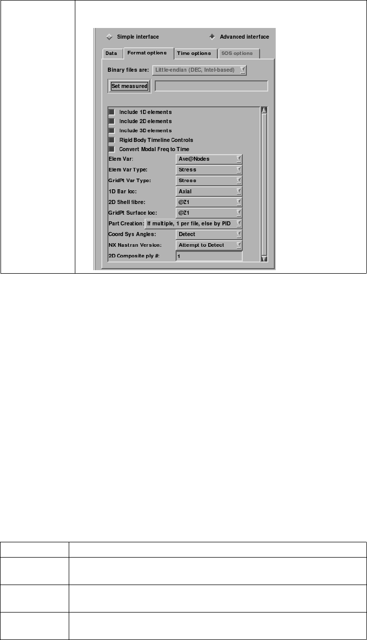
2.3 NASTRAN OP2 Reader
EnSight 10.2 User Manual 2-103
Extra GUI
Parameters
The toggles and fields below are customized for the Nastran OP2 reader. They allow the
user to specify basic options before the data is read. They may not all apply to any given
model.
Include 1D
elements
Toggle on to include any 1D (bar, rod, etc.) elements.
Include 2D
elements
Toggle on to include any 2D (tri, quad, etc.) elements.
Include 3D
elements
Toggle on to include any 3D (tet, hex, etc.) elements.
Rigid Body
Timeline Controls
Toggle on to have the geometry timeline controlled by the rigid body times (if
present). If off, the flex body times in the .op2 file will control.
Convert Modal
Freq to Time
Toggle on to compute solution time from the “frequency” field in the file for eigen
analysis (default is on). The is done with Time = (sqrt(freguency))/(2*PI). Toggle
off to no perform this computation and instead read the “frequency” value as the
time.
Elem Var: This pulldown provides control over the way Nastran element values will be
presented as variables within EnSight.
Elem Var Type: This pulldown provides the choice of extracting either Strain or Stress from
Nastran element values.
Extra GUI The following parameters are available. They are described
below.
Centroidal produces per_elem variables from the value at each element centroid
Ave@Nodes produces per_node variables, by averaging all vertex values at a given
node
Max@Nodes produces per_node variables, by taking the maximum vertex value at a
given node
Min@Nodes produces per_node variables, by taking the minimum vertex value at a
given node

2.3 NASTRAN OP2 Reader
2-104 EnSight 10.2 User Manual
GridPt Var Type: This pulldown provides the choice of extracting either Strain or Stress from
Nastran Grid Point values.
1D Bar loc: This pulldown provides the choice of where along the bar (EndA, EndB) or across
the cross-section (Pts 1-4), and what type of stress or strain to extract from
Nastran bar elements.
2D Shell Fibre: This pulldown provides the choice of which cross-sectional fibre (@Z1 or @Z2)
to extract from Nastran 2D Shell elements.
GridPt Surface loc: This pulldown provides the choice of which cross-sectional fibre (@Z1, @Z2, or
@MID) to extract from Nastran 2D Grid Point surfaces.
Part Creation: This pulldown provides part creation choices (which are most useful when a .mop
file is used to bring in multiple OP2 files together:
NX Nastran
Version:
This pulldown provides the user with some control over the changes that occurred
in the element record length at NX Nastran version 4.0. This is needed because
there is not a good way to determine the version used from the .op2 file itself.
2D Composite ply: This field allows the user to specify from which ply number to extract values from
Nastran 2D composite elements
(see How To Read Data)
Axial
Bend, EndA, Pt1 Combined, EndA, Pt1
Bend, EndA, Pt2 Combined, EndA, Pt2
Bend, EndA, Pt3 Combined, EndA, Pt3
Bend, EndA, Pt4 Combined, EndA, Pt4
Bend, EndB, Pt1 Combined, EndB, Pt1
Bend, EndB, Pt2 Combined, EndB, Pt2
Bend, EndB, Pt3 Combined, EndB, Pt3
Bend, EndB, Pt4 Combined, EndB, Pt4
One Per File One part for each file will be created. If a single OP2 file is being
read, all elements will be placed in a single part. If multiple OP2 files
are being read, one part per file will be produced.
By Property id Parts will be created by property id. According to how property ids
were used in the OP2 file, this will generally create several parts per
file.
Attempt to Detect Attempts to divine the version number, but may not always work
correctly. If it can’t tell, will default to less than version 4.
Declare as >= 4.0 Declares the version to be 4.0 or greater, so doesn’t go through
the detection process.

2.3 Nastran Input Deck Reader
EnSight 10.2 User Manual 2-105
Nastran Input Deck Reader
Overview
Description This reader will load Nastran input deck or bulk data files (typically .nas, .bdf,
.dat). These files contain the geometry for a Nastran run.
Usefulness Being able to read this format allows for the display of the original Nastran
geometry for verification as well as for use with rigid body motion.
Usage The Nastran input deck reader can read in and individual .nas/.dat/.bdf file, or it
can read in an exec file so that more than one file can be included in the same
case.
Limitations The current reader does not deal with local coordinate systems and only
recognizes the following elements:
Simple Exec file
format
An exec file is used to read in multiple Nastran input deck files into one case. This
exec file is a very simple ascii file that must conform to the following:
1. All lines must begin in column 1
2. No blank or comment lines allowed
3. If the stl filenames begin with a "/", it will be treated as absolute path.
Otherwise, the path for the exec file will be prepended to the name given in the
file. (Thus, relative paths should work).
line 0: numfiles: N (where N is the no. of files)
[line 1: version #] (optional line containing the
version number)
next N lines: nasfilename1
. . .
. . .
nasfilenameN
Example Simple
Exec file (without
version number)
numfiles: 3
CASTLE.DAT
bincastle.bdf
test.nas
1D Elements 2D Elements 3D Elements
CBAR CTRIA CTETRA
CBEAM CTRIAR CPENTA
CROD CTRIA6 CHEXA
CGAP CTRIAX
CTUBE CTRIA6X
CVISC CQUAD
CONROD CQUAD4
PLOTEL CQUADR
RROD CQUAD8
RBAR CQUADX
CELAS1 CSHEAR
CELAS2
2.3 Nastran Input Deck Reader
2-106 EnSight 10.2 User Manual
Example Simple
Exec file (with
version number)
numfiles: 3
version 1.1
CASTLE.DAT
bincastle.bdf
test.nas
Rigid Body Motion
Exec file
The reader includes the capability to link each input deck file with a rigid body
transformation file to allow the parts in each file to rigidly translate and rotate over time.
The rigid body motion Exec file has additional columns that contain the Euler Parameter
filename (see Section 9.14, Euler Parameter File Format), the transformation title in the
Euler Parameter file, and a units scale factor. The rigid body version of this Exec file
requires quotes as shown around the strings and values of the file lines.
example:
numfiles: 3
"CASTLE.DAT" "motion.dat" "CASTLE" "1000.0"
"bincastle.bdf" "motion.dat" "BCASTLE" "1000.0"
"test.nas" "motion.dat" "TEST" "1000.0"
And if an additional offset is needed to the CG, add these in 3 more columns
example:
numfiles: 3
"CASTLE.DAT" "motion.dat" "CASTLE" "1000.0" "1.35" "2.66" "0.0"
"bincastle.bdf" "motion.dat" "BCASTLE" "1000.0" "-2.45" "1.0" "-2.0"
"test.nas" "motion.dat" "TEST" "1000.0" "60.2" "23.4" "0.0"
You can also add a rotation order and yaw, pitch, and roll values on each of the file lines if
the coordinate system needs to be re-oriented. These additional columns follow the same
format as those in the EnSight Rigid Body (.erb) file.
(see Section 9.13, EnSight Rigid Body File Format)
README See the following file for current information on this reader.
$CEI_HOME/ensight102/src/readers/nas_input/README.txt
Simple Interface
Data Load
Load your geometry file (typically named with a suffix
.nas, .bdf, or .dat
) using
the Simple Interface method.
Advanced Interface
Data Load
Load your geometry file (typically named with a suffix
.nas, .bdf, or .dat
) using
the Advanced Interface method.
(see How To Read Data)
Data Tab
Format Use the Nastran Input Deck format.
Set geometry Select the geometry file (typically .nas, .bdf, or .dat) and
click this button
Format Options Tab
Set measured Select the measured file and click this button.

2.3 OpenFOAM Reader
EnSight 10.2 User Manual 2-107
OpenFOAM Reader
Overview
Description Reads OpenFOAM controlDict file found in modelname/system/controlDict.
Data Reader
Main Menu > File > Data (reader)...
The File Selection dialog is used to specify which file you wish to read.
Main Menu > File > Data (Reader)...
Handles steady state geometry with either steady state or transient variables. Steady state
variables with multiple iterations will use each iteration as an EnSight timestep.
Not yet supported:
a. Ongoing solution. The reader cannot handle newly available timesteps or iterations (for
example from an ongoing OpenFOAM solution) after the model has been read into
EnSight the first time. Should new iteration or timesteps become available after the model
was originally read into EnSight, the user must reload the dataset.
Command Line
Data Load
To automatically start EnSight and load the current directory’s OpenFOAM
dataset from the command line, type ‘ensight102 -Eensfoam’. This will trigger
EnSight to start up, look for the current directory’s “system/controlDict” file, and
automatically load the dataset into EnSight (using the default reader settings).
This reduces the number of steps to load the file into EnSight and thus the real
time required to load the data, and provides a level of integration with this data
format.
Sample Data A sample OpenFOAM dataset is included as a sample session with your install.
To access the welcome screen, at the top menu choose Window>Welcome To...
and load the Dam Break example session. Or, to load the same dataset manually,
find the controlDict file in $CEI_HOME/ensight/other_data/openfoam.
Simple Interface
Data Load
Load your OpenFOAM controlDict file using the Simple Interface method. Or
from the command line, simply run ensfoam.
Advanced Interface
Data Load
Load your OpenFOAM file using the Advanced Interface method.
Data Tab
Format Use the OpenFOAM format.
Set file This field contains the controlDict file. Clicking button
inserts the file name shown into the field.
Format Options Tab
Set measured Select the measured file and click this button.
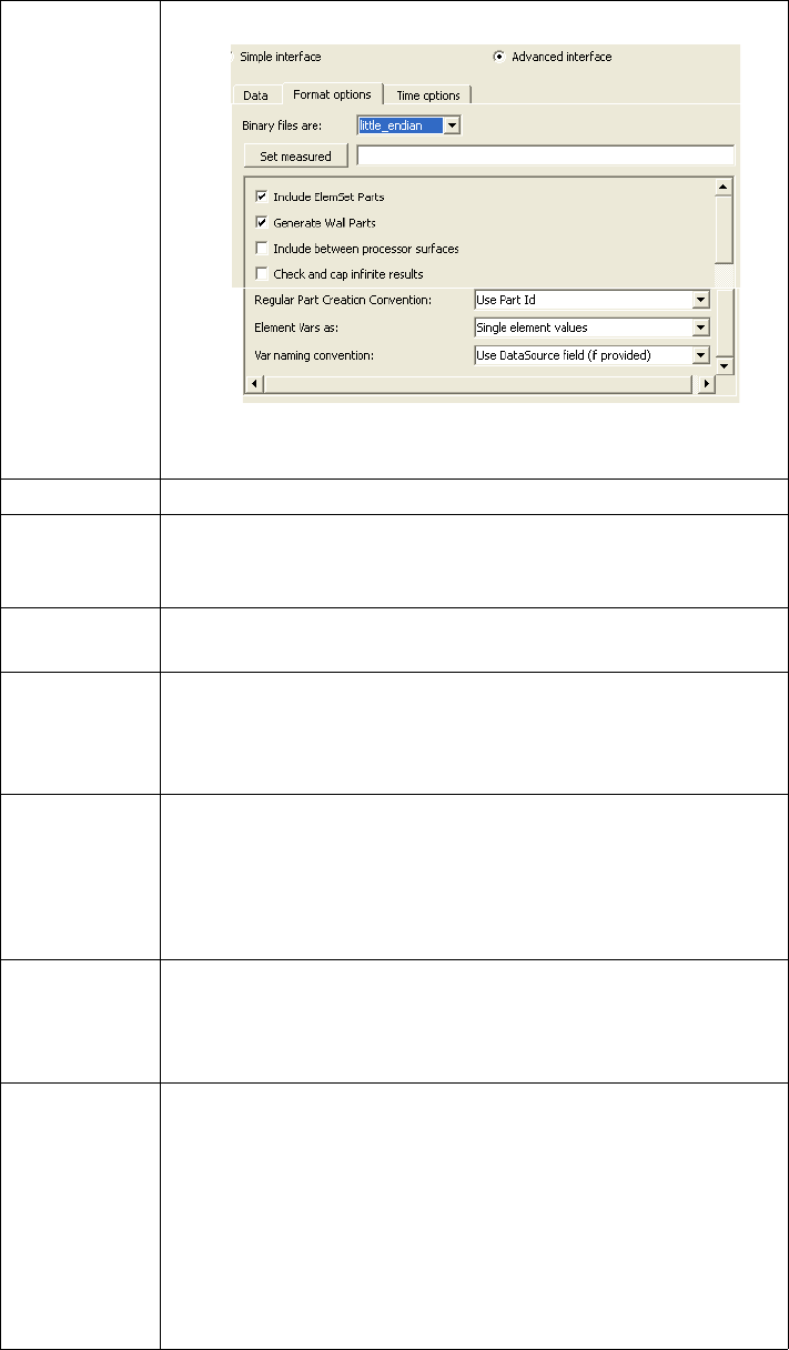
2.3 OpenFOAM Reader
2-108 EnSight 10.2 User Manual
Other
Options
Include
ElemSet
Parts
Include any Element sets defined. These are sets of full
elements which are generally some logical subset of the total
number of elements. Default is on.
Generate
Wall Parts
Generate 2D Face Sets. Default is on.
Include
between
processor
surfaces
If toggled ON and the data is from a parallel solution, then the
surfaces between the processors will be generated as parts.
Default is off.
Check and
cap infinite
results
If toggled ON and there exists values in the file that are
beyond the 32-bit size limit (thus creating ‘inf’ infinite
values), they will be capped at a value just below that limit
value.
Default is off
Regular Part
Creation
Convention
Parts will be created according to the following:
Use Part Id - Part Id (this is the default)
Use Property Id - Property Id
Use Material Id - Material Id
Var n am i ng
convention
Use DataSource field - By default variables are named using
the variable filename. For example, "U" is velocity, "p" is
pressure, etc.
Use Content Field (if provided) - Known variables are given
full, meaningful names, for example, "Velocity" or
"Pressure".
Use VKI dataset name - Long, hybrid variable name that is
guaranteed to be unique, but perhaps cryptic.

2.3 OpenFOAM Reader
EnSight 10.2 User Manual 2-109
(see How To Read Data)
Element Vars
as
Single element values - Element results (whether centroidal
or element nodal) will be presented as a single value per
element. Thus will be per_elem variables in EnSight.This is
the default.
Averaged to node values - Element results (whether
centroidal or element nodal) will be averaged to the nodes
without using geometry weighting. Thus will be per_node
variables in EnSight. This is a global averaging, so shared
nodes are affected by all parts that share a node.
Geom weighted average to node values - Element results
(whether centroidal or element nodal) will be averaged to the
nodes using geometry weighting. Thus will be per_node
variables in EnSight. This is a global averaging, so shared
nodes are affected by all parts that share a node.
Ave to node values <by parts> - Element results (whether
centroidal or element nodal) will be averaged to the nodes
without using geometry weighting. Thus will be per_node
variables in EnSight. This is a local averaging, so all
averaging is contained within each part.
Geom weighted ave to node <by parts> - Element results
(whether centroidal or element nodal) will be averaged to the
nodes using geometry weighting. Thus will be per_node
variables in EnSight. This is a local averaging, so all
averaging is contained within each part.
2.3 OVERFLOW Reader
2-110 EnSight 10.2 User Manual
OVERFLOW Reader
Simple Interface
Data Load
Load your geometry file using the Simple Interface method.
Advanced Interface
Data Load
Load your geometry and result files using the Advanced Interface method.
Limitation In order to automatically recognize the data as Overflow, the files must have the
format ‘
x.
’ and ‘
q.
’ format (For example
x.14000
,
x.14200
,
q.14000
, and
q.14200
would be appropriate filenames).
Note that the overflow reader can read in transient geometry files but these files
must have the same number of zones (EnSight parts) at each timestep. Each zone
can change in size (changing connectivity), but the total number of zones must
remain constant throughout time.
Example .res file For example, if you have files
x.14400
to
x.16000
and
q.14400
to
q.16000
, then an
example
q.res
file would be as follows. Then, put
x.14400
into the set geometry
and
q.res
into set results field and you will have transient geometry and variables.
2 1 1
10
1.0 2.0 3.0 4.0 5.0 6.0 7.0 8.0 9.0 10.0
14400 200
x.*****
q.***** S 1 Density
q.***** S 5 Energy
q.***** S 2 3 4 Momentum
Data Tab
Format Use the OVERFLOW format.
Set geometry Select the grid file (grid.in or single ‘x.’ file, e.g ‘x.14200’, see
details below) and click this button. This file is a structured
GRID file with FAST enhancements.
Set results Select the results file and click this button. The Results File is
either a modified EnSight Results file (q.res) or standard
plot3d Q-file (q.save or single ‘q.’ file, e.g. ‘q.14200’). The
standard plot3d Q-file is a variable file for a single timestep
and is optional.
The modified EnSight results file directs the reader to handle
multiple grid (x.) files and/or multiple variable (q.) files from
transient simulations. If using a .res file, then enter only the
first ‘x.’ file into the set geometry field, and the ‘.res’ into the
set results field.
Note: The Q-file(s) (and result file) may be located in a
different directory than the grid file.
Format Options Tab
Set bounds The optional boundary file defines boundary portions within
and/or across structured blocks. (Note: this can be EnSight’s
boundary file format or a .fvbnd file.)
Set measured Select the measured file and click this button.

2.3 OVERFLOW Reader
EnSight 10.2 User Manual 2-111
OVERFLOW Q FIle
Variables The variables of the flow information read by the OVERFLOW reader basically
conforms to those read by the PLOT3D reader, and includes additional flow
constants as well as additional Q variables such as and possible turbulence field
and species densities variables.
The 'Constant Variables' include (where the first 4 are the standard PLOT3D
constants):
The 'Q-Field Scalars' include (where the first 4 are the standard PLOT3D Q-
variables):
FSMACH =freestream Mach number Minf
ALPHA =angle-of-attack
RE =Reynolds number Re
TIME =iteration (file) number (in OVERFLOW; in PLOT3D,
time value)
GAMinf =freestream gamma inf
BETA =sideslip angle
Tinf =freestream temperature Tinf (in degrees Rankine)
IGAM =variable gamma option where:
0 = use constant value of GAMinf
1 = Single gas with variation of with temperature
computed using LT_A0-4, UT_A0-4 below
2 = Two gases, with variation of with temperature
computed using LT_A0-4, UT_A0-4 below all gas 1
below HT1, all gas 2 above HT2, linear mix in
between.
HTinf =freestream stagnation enthalpy h0*inf
RefMACH =reference mach number (Note: in OVERFLOW “restart”
files only)
Tvref =actual simulation time (Note: in OVERFLOW “restart”
files only)
DTvref =delta simulation time (Note: in OVERFLOW “restart”
files only)
RGAS1 =species gas constant 1
RGAS1_SMW =species gas constant 2
Density =Q1-field variable = dimensionless density, *
Momentum =dimensionless momentum vector with:
Momentum[X] = Q2-field variable = x component of
Momentum *u*
Momentum[Y] = Q3-field variable = y component of
Momentum *v*

2.3 OVERFLOW Reader
2-112 EnSight 10.2 User Manual
Assigning
Analysis_Time
By default, the Analysis_Time constant variable value is assigned the time values
listed in the q.res file. (see Section 9.7, PLOT3D Results File Format). In order to
use the TIME (or Tvref - if using an OVERFLOW restart q.file) value located in
the header of the q-file(s), edit the q.res file:
a) change the total number of time steps to a negative value, and
b) remove the list of time values in the q.res file.
(see How To Read Data, and Section 9.7, PLOT3D Results File Format)
Momentum[Z] = Q4-field variable = z component of
Momentum *w*
Energy =Q5-field variable = dimensionless total energy *e0*
Gamma_Q6_fiel
d
=Q6-field variable = gamma (constant field, unless
you use the gamma option of the code)
And for SA model:
Q7_field =Q7-field variable = turbulence variable
And for k-e model:
Q7_field,
Q8_field
=Q7-field and Q8-field variables which are the k and
epsilons

2.3 PLOT3D Reader
EnSight 10.2 User Manual 2-113
PLOT3D Reader
Supported Files The PLOT3D reader shipped with EnSight is an internal reader that supports C Binary,
Fortran Binary as well as ASCII formats. It will read double precision data, but will
convert it to single precision for use in EnSight.
Example Source The PLOT3D reader is an internal EnSight reader and the source code is
unavailable. But there is an example source code with limited functionality found
in the following directory that would be useful as a starting point for creating your
own user-defined implementation of this reader.
$CEI_HOME/ensight102/src/readers/plot3d/
Simple Interface
Data Load
Load your geometry file using the Simple Interface method.
Advanced Interface
Data Load
Load your geometry and result files using the Advanced Interface method.
Assigning
Analysis_Time
By default, the Analysis_Time constant variable value is assigned the time values
listed in the q.res file. (see Section 9.7, PLOT3D Results File Format). In order to
use the TIME value located in the header of the q-file(s), edit the q.res file:
a) change the total number of time steps to a negative value, and
b) remove the list of time values in the q.res file.
SOS Use of the Plot3D reader in parallel using EnSight’s Server of Server capability can be
done automatically using EnSight ceistart102 application, designating the number of
servers in the startup GUI and then just loading the file in auto distribute mode to let the
server do the allocation of file data to each server, or in a very controlled fashion using an
sos case file as discussed in the How To Manual (See How To Use Server of Servers).
(see How To Read Data)
Data Tab
Format Use the PLOT3D format.
Set geometry Select the grid file and click this button. This file is a
structured GRID file with FAST enhancements.
Set results Select the results file and click this button. The Results File is
either a modified EnSight Results file or standard plot3d Q-
file. Variable files (optional) are solution (PLOT3D Q-files) or
function (FAST) files. The modified EnSight results file
provides access to multiple solution files that are produced by
time dependent simulations.
Format Options Tab
Set bounds The optional boundary file defines boundary portions within
and/or across structured blocks. (Note: this can be EnSight’s
boundary file format or a .fvbnd file.)
Set measured Select the measured file and click this button.

2.3 RADIOSS Reader
2-114 EnSight 10.2 User Manual
RADIOSS Reader
Overview
Description Reads Radioss 4.x ANIM files.
Data Reader
Main Menu > File > Data (reader)...
The File Selection dialog is used to specify which files you wish to read.
Main Menu > File > Data (Reader)...
Simple Interface
Data Load
Load your radioss file using the Simple Interface method.
Advanced Interface
Data Load
Load your radioss file using the Advanced Interface method.
(see How To Read Data)
Data Tab
Format Use the RADIOSS_4.x format.
Set anim This field contains the first Radios file name in the series.
Clicking button inserts file name shown into the field. File
name can then be modified with an asterisk “*” or question
mark “??” to indicate the unique identifiers in the file series.
Format Options Tab
Set measured Select the measured file and click this button.
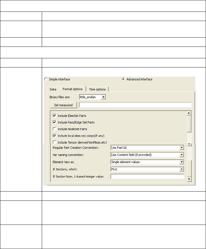
2.3 POLYFLOW Reader
EnSight 10.2 User Manual 2-115
POLYFLOW Reader
Overview
Description Reads Polyflow .msh and .res files.
Data Reader
Main Menu > File > Data (reader)...
The File Selection dialog is used to specify which files you wish to read.
Main Menu > File > Data (Reader)...
Simple Interface
Data Load
Load your Polyflow file using the Simple Interface method.
Advanced Interface
Data Load
Load your Polyflow file using the Advanced Interface method.
Data Tab
Format Use the Polyflow format.
Set .msh This field contains the mesh file. Clicking button inserts .msh
file name shown into the field.
Set .res This field contains the result file.
Format Options Tab
Set measured Select the measured file and click this button.
Other
Options
Include any Element sets defined. These are sets of full
elements which are generally some logical subset of the total
number of elements. Default is on.
Include Face/
Edge Parts
Include any Face or Edge sets defined. These are some logical
set of particular faces and/or edges of full elements. Default is
off.

2.3 POLYFLOW Reader
2-116 EnSight 10.2 User Manual
Include
NodeSet
Parts
Include any Node sets defined. These are generally the subset
of nodes needed for the Element, Face, or Edge sets above. As
such, they are generally not needed as separate parts, but can
be created if desired. Default is off.
Include local
elem res
comps (if
any)
Include the local stresses components, etc that are in the
element
Default is on
Include
Tensor
derived
(VonMises,
etc.)
For tensor results, calculate scalars from the tensors.
Default is off
Regular Part
Creation
Convention
Parts will be created according to the following:
Use Part Id - Part Id (this is the default)
Use Property Id - Property Id
Use Material Id - Material Id
Var n am i ng
convention
Use Content Field (if provided) - Variable names will be what
is in the Content field, if provided. If not provided, they will
be the VKI dataset name. This is the default.
Use VKI dataset name - Variable names will be the VKI
variable dataset name (which are reasonably descriptive).
Element Vars
as
Single element values - Element results (whether centroidal or
element nodal) will be presented as a single value per element.
Thus will be per_elem variables in EnSight.This is the default.
Averaged to node values - Element results (whether centroidal
or element nodal) will be averaged to the nodes without using
geometry weighting. Thus will be per_node variables in
EnSight. This is a global averaging, so shared nodes are
affected by all parts that share a node.
Geom weighted average to node values - Element results
(whether centroidal or element nodal) will be averaged to the
nodes using geometry weighting. Thus will be per_node
variables in EnSight. This is a global averaging, so shared
nodes are affected by all parts that share a node.
Ave to node values <by parts> - Element results (whether
centroidal or element nodal) will be averaged to the nodes
without using geometry weighting. Thus will be per_node
variables in EnSight. This is a local averaging, so all
averaging is contained within each part.
Geom weighted ave to node <by parts> - Element results
(whether centroidal or element nodal) will be averaged to the
nodes using geometry weighting. Thus will be per_node
variables in EnSight. This is a local averaging, so all averaging
is contained within each part.
If Sections,
which:
Not used

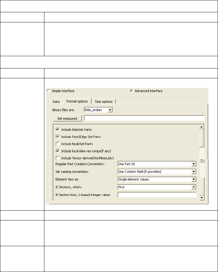
2.3 SDRC Ideas Reader
2-118 EnSight 10.2 User Manual
SDRC Ideas Reader
Overview
Description Reads SDRC/Ideas Universal files in Ascii and Binary format. Select the .unv file
and select "SDRC/Ideas" in the format pulldown on the Advanced reader tab.
Data Reader
Main Menu > File > Data (reader)...
The File Selection dialog is used to specify which files you wish to read.
Main Menu > File > Data (Reader)...
Simple Interface
Data Load
You cannot use the Simple Interface method to load your SDRC Ideas data
because the .unv extension is used by other formats.
Advanced Interface
Data Load
You must load your SDRC Ideas .unv file using the Advanced Interface method.
Data Tab
Format Use the SDRC Ideas format.
Set file This field contains the first file name. For the first file you
should choose a file with extension .unv. Clicking button
inserts file name shown into the field. Loading the .unv file
will load both geometry and results.
Format Options Tab
Set measured Select the measured file and click this button.
Other
Options
Include any Element sets defined. These are sets of full
elements which are generally some logical subset of the total
number of elements. Default is on.
Include Face/
Edge Parts
Include any Face or Edge sets defined. These are some
logical set of particular faces and/or edges of full elements.
Default is off.

2.3 SDRC Ideas Reader
EnSight 10.2 User Manual 2-119
Include
NodeSet
Parts
Include any Node sets defined. These are generally the subset
of nodes needed for the Element, Face, or Edge sets above.
As such, they are generally not needed as separate parts, but
can be created if desired. Default is off.
Include local
elem res
comps (if
any)
Include the local stresses components, etc that are in the
element's local system.
A simple example is a bar (such as a truss element), which
only has tension or compression in the element's axial
orientation. Such an element would have an axial stress
variable.
Other elements would have appropriate result component
variables. Default is on
Include
Tensor
derived
(VonMises,
etc.)
For tensor results, calculate scalars from the following
derived results (principal stress/strains, and common failure
theories):
Mean Equal Direct
VonMises Min Principal
Octahedral Mid Principal
Intensity Max Principal
Max Shear
By default, all 9 of these will be derived. You can control
which are created by this toggle, with an environment
variable. Namely,
setenv ENSIGHT_VKI_DERIVED_FROM_TENSOR_FLAG n
where n = 1 for Mean only
2 for VonMises only
4 for Octahedral only
8 for Intensity only
16 for Max Shear only
32 for Equal Direct only
64 for Min Principal only
128 for Mid Principal only
256 for Max Principal only
512 for all
or any legal combination. example: for VonMises and Max
Shear only, use 18. Default is off
Regular Part
Creation
Convention
Parts will be created according to the following:
Use Part Id - Part Id (this is the default)
Use Property Id - Property Id
Use Material Id - Material Id
Var nam in g
convention
Use Content Field (if provided) - Variable names will be what
is in the Content field, if provided. If not provided, they will
be the VKI dataset name. This is the default.
Use VKI dataset nameVariable names will be the VKI
variable dataset name (which are reasonably descriptive).

2.3 SDRC Ideas Reader
2-120 EnSight 10.2 User Manual
(see How To Read Data)
Element Vars
as
Single element values - Element results (whether centroidal
or element nodal) will be presented as a single value per
element. Thus will be per_elem variables in EnSight.This is
the default.
Averaged to node values - Element results (whether
centroidal or element nodal) will be averaged to the nodes
without using geometry weighting. Thus will be per_node
variables in EnSight. This is a global averaging, so shared
nodes are affected by all parts that share a node.
Geom weighted average to node values - Element results
(whether centroidal or element nodal) will be averaged to the
nodes using geometry weighting. Thus will be per_node
variables in EnSight. This is a global averaging, so shared
nodes are affected by all parts that share a node.
Ave to node values <by parts> - Element results (whether
centroidal or element nodal) will be averaged to the nodes
without using geometry weighting. Thus will be per_node
variables in EnSight. This is a local averaging, so all
averaging is contained within each part.
Geom weighted ave to node <by parts> - Element results
(whether centroidal or element nodal) will be averaged to the
nodes using geometry weighting. Thus will be per_node
variables in EnSight. This is a local averaging, so all
averaging is contained within each part.
If Sections,
which:
Which section will be used to create the variable
First - The first section will be used (this is the default)
Last - The last section will be used
Section Num (below) - The section number entered in the
field below will be used
Separate Vars per Section - A separate variable will be created
for each section.
Section Num If the previous option is chosen to be Section Num, then the
value in this field is the 1-based section number to use to
create the variable.
2.3 SILO Reader
EnSight 10.2 User Manual 2-121
SILO Reader
Overview
Description The Silo reader can read .silo files directly or can read them using a Casefile
which lists the geometry variable filenames, the timesteps and the constants all in
one ASCII file. The .silo file contains both the geometry and the results.
Library The Silo reader requires the Silo library version 4.2 or later. For information on
Silo please see the following website:
http://www.llnl.gov/bdiv/meshtv/software.html
SILO Casefile
format
The User Defined SILO Reader reads a restricted version of the EnSight Gold
ASCII casefile as described below.
1. FORMAT
type: - "silo" required
2. GEOMETRY
model:
3. VARIABLE
constant per case:
4. TIME (But only one of these!!!!)
number of steps: - required
time values: - required
# Use the following if transient and
# evenly spaced values
filename start number:
filename increment:
# Use the following if transient and
# list all values
filename numbers:
5. All commands and options must start in first
column. However, A space, newline, or # can
be used in first column to indicate a comment
line.
The following examples could be read by the user defined ensight gold reader
Example 1: A static model
-------------------------
FORMAT
type: silo
GEOMETRY
model: example1.silo
VARIABLE
constant per case: Density .5
TIME
number of steps: 1
time values: 0.0
2.3 SILO Reader
2-122 EnSight 10.2 User Manual
The following files would be needed for Example 1:
example1.silo
Example 2: A transient model
----------------------------
FORMAT
type: silo
GEOMETRY
model: example2.*.silo change_coords_only
VARIABLE
constant per case: Density .5
constant per case: Modifier 1.0 1.01 1.025 1.04
1.055
TIME
number of steps: 5
time values: .1 .2 .3 .4 .5
filename start number: 1
filename increment: 2
The following files would be needed for Example 2:
example2.1.silo
example2.3.silo
example2.5.silo
example2.7.silo
example2.9.silo
README See the following file for current information on this reader.
$CEI_HOME/ensight102/src/readers/silo/README.txt
Simple Interface
Data Load
Load your silo file (typically named with a suffix
.silo or .pdb or .case
) using the
Simple Interface method.
Advanced Interface
Data Load
Load your silo files (typically named with a suffix
.silo or .pdb or .case
) using the
Advanced Interface method.
(see How To Read Data)
Data Tab
Format Use the Silo format.
Set file This field should have the Silo Case file name or the .silo file.
Format Options Tab
Set measured Select the measured file and click this button.
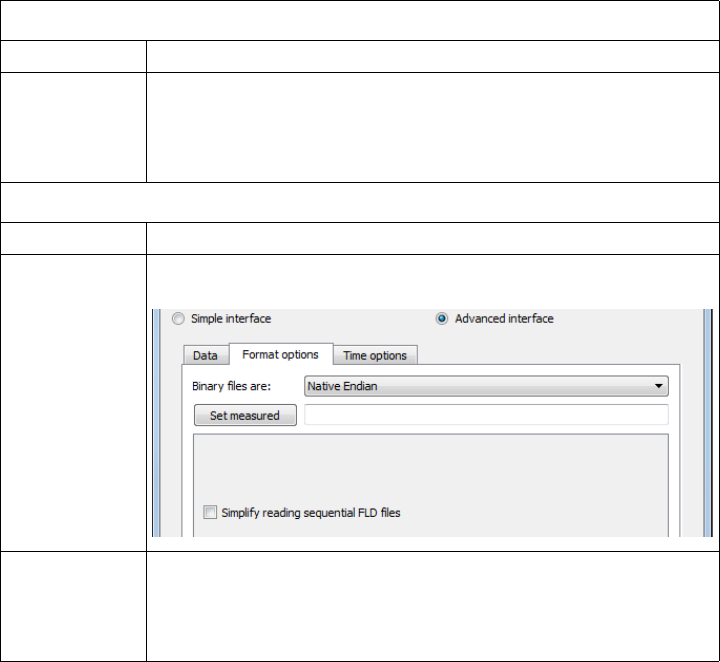
2.3 Software Cradle FLD Reader
EnSight 10.2 User Manual 2-123
Software Cradle FLD Reader
Overview
FLD File This reader imports a .fld file, which is a common file format of the solvers
developed by the Software Cradle Company. The following three solvers export
this format: scSTREAM, SC/Tetra, and HEAT Designer. This reader is designed
to work with version 4 of the FLD format, which is written by version 6 or later of
these solvers.
Platforms This reader was supplied only on Windows, and CEI compiled it on Linux and
Mac. Therefore, only the Windows version of the reader is officially supported by
Software Cradle.
Case Gold The SC/Tetra solver no longer exports EnSight Case Gold.
Undefined
variables
When a variable does not exist on a node or element, the EnSight undefined value
is set. Consider changing the display of the variable in the color palette editor and
choose Display Undefined as “By invisible” to avoid displaying undefined
regions.
Limitations Does not read measured data. Maximum material number is limited to 10000.
When timestep is changed, the material number of elements does not change.
Simple Interface
Data Load
Load your FLD file (typically named with a suffix
.fld
) using the Simple Interface
method.
Advanced Interface
Data Load
Load your FLD file (typically named with a suffix
.fld
) using the Advanced
Interface method.
Data Tab
Format Use the Software Cradle FLD format.
Set file Select the FLD file (typically .fld) and click this button. For
transient data, there will be one FLD file per timestep. Select
any one FLD file and the reader will automatically find all
other related files and load them as transient data.
Format Options Tab
Set measured Select the measured file and click this button.
Other
Options
Simplify
reading
sequential
FLD files
Creates a location map of the FLD file data that is used to
facilitate subsequent finding of data within the file.
2.3 STAR-CD and STAR-CCM+ Reader
EnSight 10.2 User Manual 2-125
STAR-CD and STAR-CCM+ Reader
Overview
Description This reader reads
.ccm
,
.ccmg
(geometry),
.ccmp
(variable),
.ccmt
(transient variable)
data exported from STAR-CD version 4.x or STAR-CCM+.
Export Case Gold STAR-CD version 3.x, STAR-CD version 4.x and STAR-CCM+ all export the
native format of EnSight (EnSight Case Gold). Prostar exports to EnSight Case
Gold Format. Use the 'automatic' export found with the NavCenter to export all
parts and all primary variables. Use the Prostar command line to export separate
parts, and/or any variable or combination of calculated variables. Both Steady
State and Transient Models can be exported in a similar manner, with options of
"automatic", or user controlled. The Case Gold format is likely to be more
efficient, robust and faster in EnSight.
Read .sim file This reader does not support
.sim
files written by STAR-CCM+. The
.sim
file
should be translated using STAR-CCM+ into EnSight Case Gold.
Read Version 3 file This reader does not support output from STAR-CD version 3.x. This data should
be translated using Prostar into EnSight Case Gold.
.ccmt input When there exists a single .ccmt file, and it exists in the same directory as the
other files, and especially if there is changing geometry, the .ccmt file should be
entered into the first field. It has pointers to the .ccmp/.ccmg files.
If there is no changing geometry, then one can still generally use the rule of
entering the .ccmt file if it exists, else the .ccmp file if it exists, else the .ccmg file
into the first field.
However sometimes there are multiple .ccmt files. And as long as the model is not
changing geometry, you can use the method described below to handle some
varied situations. Namely, enter the .ccm or .ccmp or .ccmg file into the first field.
And in the second field, enter the .ccmt file with an asterisk in the filename or the
directory to use pattern matching to read them all in: star*.ccmt or /mydir/run*/
star.ccm. If you have a mixture of different ccmt filenames and directory
locations that cannot be matched with one asterisk create a MULTIPLE_CCMT
text file with the relative path names (relative to MULTIPLE_CCMT file) and the
ccmt file names listed one to a line. See below for more details.
Particle data (.trk) Particle data is contained in the
.trk
file, which was formerly a
File.33
file. The
EnSight install includes a source file which can be compiled and run to translate
the
.trk
(or
File.33
) file into EnSight’s measured data format, which can be
loaded together with the .ccm file (as described below), or the EnSight
.case
file
can be edited to include the measured file name and it will automatically load.
The source file to the translator is found in the following location:
$CEI_HOME/ensight102/translators/starcd_file33
There is a
README
that guides you through compiling and using the translator. If
you have difficulty with this, contact support@ensight.com and we will supply
you with a compiled version for your hardware/OS. If you are using the translator
and have a case gold format file, the translator will automatically edit the case file
so that input of the measured data is automatic when your case file is loaded into
EnSight. If you are using this reader and a
.ccm
file, then choose the EnSight 5
option and you will get a
.res
file that you can use to load in the measured data

2.3 STAR-CD and STAR-CCM+ Reader
2-126 EnSight 10.2 User Manual
field described below.
Data Reader
Main Menu > File > Data (reader)...
The File Selection dialog is used to specify which files you wish to read.
Main Menu > File > Data (Reader)...
Simple Interface
Data Load
Load your
.ccm
file using the Simple Interface method.
Advanced Interface
Data Load
Load your STAR-CCM file using the Advanced Interface method.
Data Tab
Format Use the STAR-CD CCM format.
Set .ccm[t/p/g] Generally, one should enter one of the following in priority
order. The .ccmt file if it exists, else the .ccmp file if it exists,
else the .ccmg file. And nothing would be needed in the
second field.
Note:
A .ccmt file contains transient data. Generally just transient variable
data - but can contain transient geometry as well. It contains
pointers to needed .ccmp .ccmg files.
A .ccmp (or .ccm) file contains both geometry and results.
A .ccmg file contains geometry only.
Alternatively, if there is no changing geometry, for the first file
you should choose the file with extension
.ccmp
,
.ccm
, or .
ccmg
.
And then set the .ccmt file in the second field as described
below.
Set .ccmt Again, generally, you do not need this field, and should have
entered the .ccmt file in the first field.
However, if you chose to use the alternate method for time
varying variable data with no changing geometry, set the
.ccmt
file using this field. The file must only contain transient
variable data.
For multiple .ccmt files, star1.ccmt, star2.ccmt and star3.ccmt,
input star*.ccmt.
For multiple directories dir1/star.ccmt, dir2/star.ccmt, dir3/
star.ccmt specify full path as follows /mydir/dir*/star.ccmt.
Or, enter /mydir/MULTIPLE_CCMT and create a text file
named exactly MULTIPLE_CCMT in this directory
containing one ccmt file per line. The pathname location of the
MULTIPLE_CCMT will be prepended to each of the .ccmt
filenames so use relative pathnames to your .ccmt filenames
(or none). See below for details.
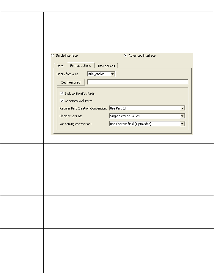
2.3 STAR-CD and STAR-CCM+ Reader
EnSight 10.2 User Manual 2-127
Format Options Tab
Set measured Select the measured file and click this button. This can be the
measured file obtained from the
File.33
or the
.trk
file using
the EnSight translator (see above).
Other
Options
Include any Element sets defined. These are sets of full
elements which are generally some logical subset of the total
number of elements. Default is on.
Generate
Wall Parts
Toggle on to create 2D Face set parts. Default is on.
Regular Part
Creation
Convention
Parts will be created according to the following:
Use Part Id - Part Id (this is the default)
Use Property Id - Property Id
Use Material Id - Material Id
Var n am i ng
convention
Use Content Field (if provided) - Variable names will be what
is in the Content field, if provided. If not provided, they will
be the VKI dataset name. This is the default.
Use VKI dataset name - Variable names will be the VKI
variable dataset name (which are reasonably descriptive).

2.3 STAR-CD and STAR-CCM+ Reader
2-128 EnSight 10.2 User Manual
Advanced .ccmt
alternate input
method
1) Normally, a single .ccmt file would be specified.
Thus, for: /mydirectory/star.ccmp
star.ccmt
In the second field, specify: /mydirectory/star.ccmt
2) However, if multiple .ccmt files exist because of restarts
of the solver, you can use a wildcard (asterisk) in
the name of the file, or subdirectory.
ex 1) For the situation where multiple .ccmt files reside
in the same directory: /mydirectory/star.ccmp
star_1.ccmt
star_2.ccmt
star_3.ccmt
In the second field, specify: /mydirectory/star_*.ccmt
ex 2) For the situation where multiple .ccmt files reside
in their own subdirectories: /mydirectory/star.ccmp
RESULTS.001d/star.ccmt
RESULTS.002d/star.ccmt
RESULTS.003d/star.ccmt
In the second field, specify: /mydirectory/RESULTS.*d/star.ccmt
Element Vars
as
Single element values - Element results (whether centroidal or
element nodal) will be presented as a single value per element.
Thus will be per_elem variables in EnSight.This is the default.
Averaged to node values - Element results (whether centroidal
or element nodal) will be averaged to the nodes without using
geometry weighting. Thus will be per_node variables in
EnSight. This is a global averaging, so shared nodes are
affected by all parts that share a node.
Geom weighted average to node values - Element results
(whether centroidal or element nodal) will be averaged to the
nodes using geometry weighting. Thus will be per_node
variables in EnSight. This is a global averaging, so shared
nodes are affected by all parts that share a node.
Ave to node values <by parts> - Element results (whether
centroidal or element nodal) will be averaged to the nodes
without using geometry weighting. Thus will be per_node
variables in EnSight. This is a local averaging, so all
averaging is contained within each part.
Geom weighted ave to node <by parts> - Element results
(whether centroidal or element nodal) will be averaged to the
nodes using geometry weighting. Thus will be per_node
variables in EnSight. This is a local averaging, so all averaging
is contained within each part.
2.3 STAR-CD and STAR-CCM+ Reader
EnSight 10.2 User Manual 2-129
Note that you can't have a mixture of these two examples with
this method. Namely, the following cannot be properly specified
with this method: /mydirectory/star.ccmp
star_1.ccmt
RESULTS.002d/star.ccmt
You would need to either copy (and rename) the .ccmt file in the
subdirectory to the data directory, or you will need to create
a subdirectory for each .ccmt file in the data directory, and move
the .ccmt files into those subdirectories. You could obviously
take advantage of symbolic links to avoid actually moving any data.
Your other alternative is to use method 3) below.
3) You can create a special file in which you list all of the .ccmt files
This would allow them to be placed in or anywhere below the data directory.
Thus, you could handle the mixture discussed in 2) above.
Rules for this special file:
a. The file must be named exactly: MULTILPLE_CCMT
b. The .ccmt files must be one per line in this file.
c. They must NOT have a full path, because the path to the
MULTIPLE_CCMT file will be prepended to them.
d. There is no concept of comment lines, so no extraneous lines (even
empty lines) are allowed.
ex 1 above, specified in this manner)
/mydirectory/star.ccmp
star_1.ccmt
star_2.ccmt
star_3.ccmt
MULTIPLE_CCMT
In the second field, specify: /mydirectory/MULTIPLE_CCMT
where MULTIPLE_CCMT file would contain just 3 lines, like:
------------- dashed lines are NOT in the file
star_1.ccmt
star_2.ccmt
star_3.ccmt
-------------
ex_2 above, specified in the manner)
/mydirectory/star.ccmp
RESULTS.001d/star.ccmt
RESULTS.002d/star.ccmt
RESULTS.003d/star.ccmt
MULTIPLE_CCMT
2.3 STAR-CD and STAR-CCM+ Reader
2-130 EnSight 10.2 User Manual
In the second field, specify: /mydirectory/MULTIPLE_CCMT
where MULTIPLE_CCMT file would contain just 3 lines, like:
------------- dashed lines are NOT in the file
RESULTS.001d/star.ccmt
RESULTS.002d/star.ccmt
RESULTS.003d/star.ccmt
-------------
And for the mixed mode situation:
/mydirectory/star.ccmp
star_1.ccmt
RESULTS.002d/star.ccmt
MULTIPLE_CCMT
In the second field, specify: /mydirectory/MULTIPLE_CCMT
where MULTIPLE_CCMT file would contain just 2 lines, like:
------------- dashed lines are NOT in the file
star_1.ccmt
RESULTS.002d/star.ccmt
-------------
(see How To Read Data)
2.3 STL Reader
EnSight 10.2 User Manual 2-131
STL Reader
Overview
Description Reads .stl files and .xct exec files.
Note: There is no longer an EnSight STL reader. this format is now read using the
CAD reader.
Overview
Description This reader will load STL files (either ASCII or binary). Note that STL files
consist only of surfaces (triangles) and have no associated variables.
Usefulness STL geometry format is widely compatible with a number of codes. Multiple STL
files geometries can be created to represent scenery or background, then read in
and scaled (using the -scaleg option) as a separate case to add to the presentation
of your existing model results in EnSight.
Usage The STL reader can read in an individual .stl file, or it can read in an exec file so
that more than one stl file can be included in the same case.
Limitations The current reader does not allow the coloring of each facet, nor does it allow
coloring of each part, and just skips over color statements in the file.
STL binary file
format
If the file is a binary STL (.stl) file, then it must contain exactly one part.
STL ASCII file
format
If the file is an ASCII STL (.stl) file, then it can contain one or multiple parts. If
you wish to read in multiple files
Single file multipart ASCII format is as follows:
solid part1
...
endsolid part1
solid part2
...
endsolid part2
Simple Exec file
format
An exec file (.xct) is used to read in multiple STL files into one case. Because
binary STL can contain only one part, if you wish to read in more than one binary
STL file into a single case, then you must use an exec file. ASCII STL files with
one or multiple parts can be read in to a single case using the exec file. An exec
file can read in binary and ASCII files together into a single case. This exec file is
a very simple ascii file that must conform to the following:
1. All lines must begin in column 1
2. No blank or comment lines allowed
3. If the stl filenames begin with a "/", it will be treated as absolute path.
Otherwise, the path for the exec file will be prepended to the name given in the
file. (Thus, relative paths should work).
line 0: numfiles: N (where N is the no. of files)
line 1-n: stlfilename1
. . .
. . .
stlfilenameN
Example Simple
Exec file
numfiles: 3
CASTLE.STL
bincastle.stl
test.slp

2.3 STL Reader
2-132 EnSight 10.2 User Manual
Rigid Body Motion
Exec file
Release 2.1 of the STL reader includes the added ability to link each STL part with a rigid
body transformation file to allow the STL part to rigidly translate and rotate over time.
The rigid body motion Exec file has additional columns that contain the Euler Parameter
filename (see Section 9.14, Euler Parameter File Format), the transformation title in the
Euler Parameter file, and a units scale factor (This is used to scale the translations, not the
geometry. Scaling of the geometry is accomplished in the Part Feature Panel.). The rigid
body version of this Exec file requires quotes as shown around the strings and values of
the file lines.
example:
numfiles: 3
"CASTLE.STL" "motion.dat" "CASTLE" "1000.0"
"bincastle.stl" "motion.dat" "BCASTLE" "1000.0"
"test.slp" "motion.dat" "TEST" "1000.0"
And if an additional offset is needed to the CG, add these in 3 more columns
example:
numfiles: 3
"CASTLE.STL" "motion.dat" "CASTLE" "1000.0" "1.35" "2.66" "0.0"
"bincastle.stl" "motion.dat" "BCASTLE" "1000.0" "-2.45" "1.0" "-2.0"
"test.slp" "motion.dat" "TEST" "1000.0" "60.2" "23.4" "0.0"
You can also add a rotation order and yaw, pitch, and roll values on each of the file lines if
the coordinate system needs to be re-oriented. These additional columns follow the same
format as those in the EnSight Rigid Body (.erb) file.
(see Section 9.13, EnSight Rigid Body File Format)
README See the following file for current information on this reader.
$CEI_HOME/ensight102/src/readers/stl/README
Simple Interface
Data Load
Load your geometry file (typically named with a suffix
.stl or .xct
) using the
Simple Interface method.
Advanced Interface
Data Load
Load your geometry file (typically named with a suffix
.stl or .xct
) using the
Advanced Interface method.
(see How To Read Data)
Data Tab
Format Use the STL format.
Set geometry Select the geometry file (typically .stl or .xct) and click this
button
Set results As of version 8.0.7(h) this field is activated to allow flags to
change reader behavior. In order to truncate the float values
put in a tolerance value and the reader will retain only to the
designated significant digit. This can be used to eliminate
duplicate node problems due to roundoff error. Put in the
keyword
-tol 1e-3
to eliminate the fourth and smaller decimal point values in the
nodal coordinates during data file read. See the README file
for more details.
Format Options Tab
Set measured Select the measured file and click this button.
2.3 Synthetic Reader
EnSight 10.2 User Manual 2-133
Synthetic Reader
Overview
Description This “reader” is unique in that it does not actually read geometry/variable data
from the disk. Rather, it is designed to synthesize geometry/variables based on
commands read in from a file or options chosen interactively in the Data Reader
dialog. The Synthetic reader can create transient or static geometry comprised of
spherical and/or cube parts(s) with an arbitrary, user-defined number of elements
(of user-chosen element type), that varies linearly over a user-chosen number of
timesteps as well as any number of scalar, vector, or constant variables. Note that
it may not appear in your pulldown list of readers by default: to see this reader, go
into preferences in the data section and make this reader available.
The most common usage is to interactively choose the Synthetic reader and to
enter a dummy filename in the data field (data reader dialog requires an entry in
this field), and to toggle on the Advanced interface, and to interactively choose
values in the Format Options. These interactive sessions can be saved as
command files to be rerun later, or session files to be reloaded later. More rare, is
to hand-edit a synthetic options (.svn) file with specific entries, and then the load
in the .syn file that will provide the input for generation of the dataset.
Usefulness Because the synthetic reader does not read the geometry nor variable data from
disk, it is useful for measuring EnSight performance separated from EnSight I/O.
Further, the Synthetic reader is compatible with all of EnSight’s parallel
capabilities (SOS, HPC+, threading). As such, it is useful for measuring graphics
hardware card performance by creating and controlling arbitrarily large numbers
of polygons to be rendered by the client graphics card. Also, it is useful for
supplying known models (size and element type) to quantify the benefits of
parallel computing (threading) performance, as well as parallel server (SOS)
performance, as well as parallel rendering performance. Further, in Compatibility
mode (one of the user options), the synthetic reader is useful for comparing
current versions of EnSight 10.2 to previous versions of EnSight. In addition,
with the power of the EnSight calculator and the simplicity of the geometry the
synthetic reader is a useful tool for verifying and validating the calculator
functions over the range of element types supported by EnSight.
Finally, the synthetic reader eliminates the need for transmitting extremely large
datasets for testing purposes. Since geometry is generated from commands,
arbitrarily large geometries for testing can be sent via email in the form of tiny
.syn files, or in .enc command files that contain the format options for creating the
gigantic dataset.
Usage The synthetic reader must have text in the file field, even if it is dummy text
because of EnSight requirements (in which case it will ignore the dummy text) or
it can read in a .syn file so which will contain a simple list of options for auto-
generating the geometry, timesteps, variables, etc.
Limitations The current reader only allows a subset of the EnSight element types, and all parts
currently contain only one element type. Elements of type TRI03 are used to
create a surface mesh on the outer boundary of the sphere or the cube part(s) or the
plane part(s). Volume elements create a 3D volume of the sphere or cube part(s).
And QUAD04 elements create a series of layers in the cube part(s).
Elements There are three part types: Spheres, Cubes and Planes. If you choose Tri 3 then
the surface of both the sphere and cube part(s) are meshed using this element type.

2.3 Synthetic Reader
2-134 EnSight 10.2 User Manual
If you choose another element type, then the sphere(s) are meshed using the Hex 8
element type, and the cubes are meshed using the element type. For example,
choose the Point element type and the Cube nodes become point elements.
Choose the Quad4 and the cube becomes a series of xy planes meshed in Quad 4
elements. Similarly choose Tet 4, Penta6, Nfaced Polyhedral, or Structured Hex
and the cube part’s hex elements are converted into these supported 3D element
types. Planes must use Tri 3 or Quad 4 elements only. Unfortunately a large
number of element types are still unsupported: Bar 2, Bar 3, Tri 6, Quad 8, Tet 10,
Pyr 5, Pyr 13, Penta 15, Hex 20, and Nsided Polygon. Choose an unsupported
element type and the cubes and spheres are meshed using Hex 8 elements and a
warning message is sent to the server console.
Plane Parts Plane parts are unique as follows. Each part has one plane. Plane parts are all
normal to the Z-axis and appear back to front uniformly distributed along the Z-
axis from Z=0 to Z=1. Planes interpolate between the beginning and ending
number of elements (which are elements per part). At earlier timesteps, parts with
higher part number are effectively given zero nodes and zero elements. As you
preoceed through time, parts are allowed to have elements. This allows the
appearance of parts as you proceed through time, from back to front, of
increasingly dense numbers of elements (when the ending number of elements is
higher than the beginning) resulting in an exponential increase in the number of
elements, for example, for graphics testing. If the Spread is set to Legacy, then the
planes x and y centers are exactly aligned. A different Spread will add some
random scatter to the x and y centers. If the number of plane parts is less than the
number of servers then the part will be assigned to the server by part number. If
there are more parts than servers, then a round-robin approach will apply.
Variables Scalar and vector variables alternate as nodal and elemental, respectively. The
first scalar variable (nodal) is a nodal deformation scalar, and the second variable
(elemental) is simply the element index. The first vector variable (nodal) is a
spiraling vector simulating a swirling flow spiraling inward and downward. The
first two constant variables are the number of nodes and the number of elements,
respectively. Other variables will be added as needed/requested. Finally user
variables can be added using the calculator (e.g. a quadric dependent on the
Coordinates).
Transient If one timestep is chosen the dataset is static. If more than one timestep is chosen,
and the dataset is in compatibility mode, then the dataset is changing connectivity.
If compatibility mode is off and the begin number of elements is the same as the
ending number of elements, then the dataset is changing coordinates only.
README See the following file for current information on this reader.
$CEI_HOME/ensight102/src/readers/synthetic/README.txt
Simple Interface
Data Load
For auto-generating a dataset, simply load a synthetic file (typically named with a
suffix
.syn
) using the Simple Interface method. For interactive use, toggle on the
Advanced Interface Data Load.
Advanced Interface
Data Load
Toggle on the Advanced Interface for interactive creation of your dataset. Then,
put a junk filename in the data file name field (e.g. “dd”) because the EnSight
dialog requires a filename (even a bogus one) and then go directly to the Format
Options tab to control your geometry and variable generation. Interactive creation
of your data requires the Advanced Interface method.
Data Tab

2.3 Synthetic Reader
EnSight 10.2 User Manual 2-135
Format Choose the Synthetic format. If this format is not available in
this pull down list, then go into your preferences under the
data tab and make this reader available.
Set
(Optional)
Optionally choose a .syn file. Or, for interactive use, enter a
bogus filename (required to be non-empty by the dialog) and
then toggle on the Advanced Interface and go to the Format
Options Tab to design your geometry, variables, etc.
Format Options Tab
Set measured Select the measured file and click this button.
Verbose
mode
Toggle this ON to get more output, useful for debugging
purposes, output to the console. Default is OFF.
Use ghost
elements
Toggle this on to create ghosts between the boundary shared
by SOS servers. If running EnSight in SOS mode, then the
geometry is automatically allocated evenly to each of the
servers. Toggle this ON to use ghost elements between the
servers. (Default is OFF).
Long names Toggle this OFF to use simple part and variable names. Toggle
ON to use long variable names. Default is ON.
Compatible
mode
Toggle this ON and new options will be limited to retain
compatibility with older versions of EnSight 10.0. Toggle this
OFF to take advantage of new variables and new names, and
other new features as they are added. Default is ON.
Element type Choose an element type. The following are allowable types
but not all are supported (see above for details): Point, Bar 2,
Bar 3, Tri 3, Tri 6, Quad 4, Quad 8, Tet 4, Tet 10, Pyr 5, Pyr
13, Penta 6, Penta 15, Hex 8, Hex 20, Nsided Polygon, Nfaced
Polyhedral, and Structured Hex. (Default is Tri 3). Over
time, more supported types will be added.
Boundary
ghosts
Choose None, Convert, or Add for controlling ghosts around
the outer perimeter of the cube(s) and sphere(s). Ghosts are
useful for allowing EnSight to interpolate variable values
rather than extrapolate them.
Choose None to use NO ghosts around the outer boundary.
Choose Convert to convert the outer boundary of cells to ghost
cells. Choose Add to add another layer of cells all around the
outer perimeter of the part(s) that are ghost cells.
Default is None, so legacy command files should work fine.
Spread out
parts
Created parts by default are created only slightly off center.
This has the effect of creating overlapping parts when multiple
parts are created which is not useful if you want to see each
part individually. This option spreads the parts out “Little”,
“Medium” or “Large” amounts in the XYZ directions
randomly so that the parts are overlapping a little bit, some
and are mostly spread out, respectively. This is useful, for
example, if you want to see the individual coloration on a large
number of parts.

2.3 Synthetic Reader
2-136 EnSight 10.2 User Manual
.syn file format The .syn file can contain the following text:
#!SYN_CASE 1.0
NUMBER_TIMESTEPS num
NUMBER_SPHERES num
NUMBER_CUBES num
NUMBER_ELEMENTS_START num
NUMBER_ELEMENTS_END num
PART_SCALE num
RAND_SEED num
USE_GHOSTS num
VERBOSE num
ELEM_TYPE {see list}
NUMBER_CONSTANTS num
NUMBER_VECTORS num
NUMBER_SCALARS num
LONG_NAMES num
Number of
spheres
Choose the number of spherical parts. Default 0
Number of
cubes
Choose the number of cube parts. Default 1.
Number of
planes
Choose the number of 2D plane parts. Default 0.
Number of
elements start
Starting number of elements at timestep 0 for each part.
Default 1000. The reader will attempt to create parts
containing roughly this number of elements using an odd
number of elements in each orthogonal direction. If you
choose 1000 and two cubes with Hex8 elements, and two
sphere parts then your total number of elements will be
roughly 4000 elements. In reality your cubes will be of
dimension 9x9x11 for a total of 891 elements and your spheres
will also have 891 elements because they are cubic elements
mapped onto a sphere resulting in 3564 total elements.
Number of
elements end
Ending number of elements at the last timestep for each part.
If you choose 10000 and two cube and two sphere parts then
your total number of elements will be 40000. Default 1000.
Number of
timesteps
Choose the number of timesteps. 0 means static data. Default
is 0.
Part scaling
factor
This is used for scaling the part. Default is 1.0
Random
number seed
This is for shifting parts randomly around so they don’t all
overlap each other. Default is 0.
Number of
scalars
Even scalars are nodal and odd scalars are elemental. Default
is 0.
Number of
vectors
Even scalars are nodal and odd scalars are elemental. Default
is 0.
Number of
constants
The first two constants are number of nodes in the dataset and
number of elements in the dataset. Default is 0.
2.3 Synthetic Reader
EnSight 10.2 User Manual 2-137
Valid values for
ELEM_TYPE
:
Point
Bar 2
Bar 3
Tri 3
Tri 6
Quad 4
Quad 8
Tet 4
Tet 10
Pyr 5
Pyr 13
Penta 6
Penta 15
Hex 8
Hex 20
Nsided Polygon
Nfaced Polyhedral
Structured Hex
For legacy reasons, the former 'tri' and 'hex' keywords are also still supported.
These options map 1 for 1 with the options found in the data reader dialog under
the Format Options Tab. Note: USE_GHOSTS, LONG_NAMES and VERBOSE
are true if <num> is non-zero.
.syn file example The following example creates a 20 timestep dataset with 3 spheres and 2 cubes.
Each sphere/cube will have 1M triangles. Each cube and sphere will have a
diameter of 0.2 (and the centroid will be randomly placed inside of a 1.0x1.0x1.0
box).
#!SYN_CASE 1.0
NUMBER_TIMESTEPS 20
NUMBER_SPHERES 3
NUMBER_CUBES 2
NUMBER_ELEMENTS_START 1000000
PART_SCALE 0.2
(see How To Read Data)
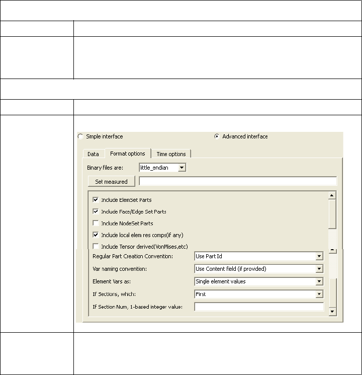
2.3 Tecplot Reader
2-138 EnSight 10.2 User Manual
Tecplot Reader
Overview
Description There are two Tecplot readers included with EnSight: Tecplot Binary and
Tecplot_ASCII which read binary and ASCII Tecplot data.
TECPLOT Binary
Reader Usage
The TECPLOT binary file format uses a Tecplot plt file.
Tecplot ASCII
Reader
A subset of the Tecplot 360 ASCII format is read using the Tecplot_ASCII reader.
This is discussed below. In the format options tab of the data reader dialog, choose
Debug to get extra output to the console if EnSight fails to read your ASCII file.
README See the following directory for current information on these readers.
$CEI_HOME/ensight102/src/readers/tecplot/
Simple Interface
Data Load
Load your Tecplot file (typically named with a suffix
.plt or .plot or .dat
) using
the Simple Interface method.
Advanced Interface
Data Load
Load your Tecplot file (typically named with a suffix
.plt or .plot or .dat
) using
the Advanced Interface method.
BINARY
Format Use the Tecplot Binary, or the legacy TECPLOT 7.x format.
Set plot
(or dat)
This field should have the .plt name for binary data. Use a
asterisk for transient multiple files (one timestep per file),
filename*.dat
Format Options Tab Tecplot BINARY
Set measured Select the measured file and click this button.
Tecplot
Binary Other
Options
Include any Element sets defined. These are sets of full
elements which are generally some logical subset of the total
number of elements. Default is on.

2.3 Tecplot Reader
EnSight 10.2 User Manual 2-139
Include Face/
Edge Parts
Include any Face or Edge sets defined. These are some logical
set of particular faces and/or edges of full elements. Default is
off.
Include
NodeSet
Parts
Include any Node sets defined. These are generally the subset
of nodes needed for the Element, Face, or Edge sets above. As
such, they are generally not needed as separate parts, but can
be created if desired. Default is off.
Include local
elem res
comps (if
any)
Include the local stresses components, etc that are in the
element's local system.
A simple example is a bar (such as a truss element), which
only has tension or compression in the element's axial
orientation. Such an element would have an axial stress
variable.
Other elements would have appropriate result component
variables. Default is on
Include
Tensor
derived
(VonMises,
etc.)
For tensor results, calculate scalars from the following derived
results (principal stress/strains, and common failure theories):
Mean Equal Direct
VonMises Min Principal
Octahedral Mid Principal
Intensity Max Principal
Max Shear
By default, all 9 of these will be derived. You can control
which are created by this toggle, with an environment
variable. Namely,
setenv ENSIGHT_VKI_DERIVED_FROM_TENSOR_FLAG n
where n = 1 for Mean only
2 for VonMises only
4 for Octahedral only
8 for Intensity only
16 for Max Shear only
32 for Equal Direct only
64 for Min Principal only
128 for Mid Principal only
256 for Max Principal only
512 for all
or any legal combination. example: for VonMises and Max
Shear only, use 18. Default is off
Regular Part
Creation
Convention
Parts will be created according to the following:
Use Part Id - Part Id (this is the default)
Use Property Id - Property Id
Use Material Id - Material Id
Var n am i ng
convention
Use Content Field (if provided) - Variable names will be what
is in the Content field, if provided. If not provided, they will
be the VKI dataset name. This is the default.
Use VKI dataset nameVariable names will be the VKI variable
dataset name (which are reasonably descriptive).

2.3 Tecplot Reader
2-140 EnSight 10.2 User Manual
Element Vars
as
Single element values - Element results (whether centroidal or
element nodal) will be presented as a single value per element.
Thus will be per_elem variables in EnSight.This is the default.
Averaged to node values - Element results (whether centroidal
or element nodal) will be averaged to the nodes without using
geometry weighting. Thus will be per_node variables in
EnSight. This is a global averaging, so shared nodes are
affected by all parts that share a node.
Geom weighted average to node values - Element results
(whether centroidal or element nodal) will be averaged to the
nodes using geometry weighting. Thus will be per_node
variables in EnSight. This is a global averaging, so shared
nodes are affected by all parts that share a node.
Ave to node values <by parts> - Element results (whether
centroidal or element nodal) will be averaged to the nodes
without using geometry weighting. Thus will be per_node
variables in EnSight. This is a local averaging, so all
averaging is contained within each part.
Geom weighted ave to node <by parts> - Element results
(whether centroidal or element nodal) will be averaged to the
nodes using geometry weighting. Thus will be per_node
variables in EnSight. This is a local averaging, so all averaging
is contained within each part.
If Sections,
which:
Which section will be used to create the variable
First - The first section will be used (this is the default)
Last - The last section will be used
Section Num (below) - The section number entered in the field
below will be used
Separate Vars per Section - A separate variable will be created
for each section.
Section Num If the previous option is chosen to be Section Num, then the
value in this field is the 1-based section number to use to
create the variable.
ASCII
Format Use the or Tecplot_ASCII.
Set plot
(or dat)
This field should have the .dat file name for ASCII data. Use a
asterisk for transient multiple files (one timestep per file),
filename*.dat
Format Options Tab Tecplot BINARY
Set measured Select the measured file and click this button.
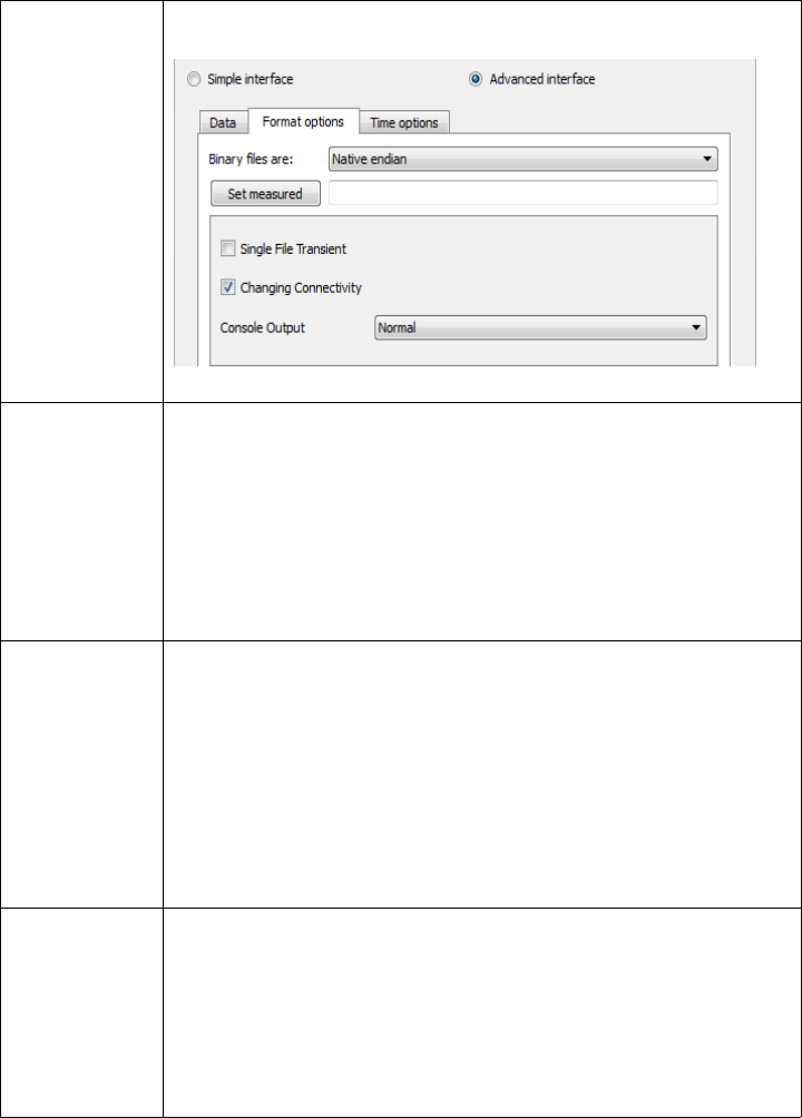
2.3 Tecplot Reader
EnSight 10.2 User Manual 2-141
(see How To Read Data)
Tecplot
ASCII Other
Options
Single File
Transient
Toggle this ON to load a single file as transient data (default is
OFF). If this toggle is ON, then the reader tries to find the
SOLUTIONTIME keyword to identify the time value of a
given part. If ZONE T= keyword is encountered prior to
finding a SOLUTIONTIME keyword, then the reader tries to
parse the Zone T contents to determine the time for that part.
So the ZONE T must contain a parseable time value if there is
no SOLUTIONTIME keyword.
Changing
Connectivity
There is no meta-data in the Tecplot ASCII file indicating
whether the connectivity changes over time. When this toggle
is ON, then transient data is loaded as changing connectivity
(coordinates and connectivity are read in at every timestep,
which is the safe (but slow) assumption (default ON). This
causes EnSight limitations, such as temporal calculations and
temporal queries. So if you know that your data doesn’t
change connectivity through time you can toggle this off. If
you are wrong then EnSight may crash.
Console
Output
If you want more information and detail about the file you are
reading, choose Console Output Verbose. If you are having
problems reading the file, choose Console Output Debug. The
Console output is generated at the Server console window.
Problem reports should include the Console output debug
information (note: default is Normal which includes very little
server console output).
2.3 Vectis Reader
2-142 EnSight 10.2 User Manual
Vectis Reader
Overview
Reader Visibility
Flag
By default, this reader is not loaded into the list of available readers. To enable
this reader go into the Menu, Edit > Preferences and click on Data and toggle on
the reader visibility flag.
Reader vs.
Translator
This reader is designed for files written before Vectis 3.6. For versions 3.6 or later,
we recommend using the Ricardo v2e translator to convert the Vectis POST file to
the Ensight format (for more details, see our FAQ on our website
www.ensight.com/
FAQ/faq.0024.html
).
Pre-version 3.6
Description
This reader inputs either .TRI or .POS datasets as follows
Single TRI file - Gives the CAD geometry, but no variables (If you must see this
along with your POST data, will have to read it as a second case), for example,
CYLINDER.TRI
Single POST file WITH NO *'s in the name - Gives the geometry and variables in
the post file, including surface patches and particles.
Multiple POST files - Enter a filename WITH *'s in the name
Gives the geometry and variables in the post files, which match the asterisks in a
sequentially increasing pattern (starts at 1, increases by 1). Note: If your naming/
numbering scheme is different than this, we require you to rename/renumber.
ex1) CYLINDER.POS.** matches:
CYLINDER.POS.01 CYLINDER.POS.02 CYLINDER.POS.03
ex2) myfile***.pos matches:
myfile001.pos myfile002.pos
Query over time Query node over time operation within EnSight will only work for cell variables
on the cell part. Patch and drop variables will currently return all zeros.
Cell Variables You may request cell variables on patch or droplet parts. The cell variable will be
mapped onto them. BUT, be aware that any portions of the patches which are
actually in the "external" cells will have zero values, because VECTIS doesn't
contain that info directly. This leads to slightly "streaked" or "blotched" models
which basically show the variable, but are probably not presentation quality. In
order to eliminate this effect, neighboring cell information will need to be
accessed - and at this time that work has not been done. Consider using Ensight's
Offset Variable capability - it might be useful for certain models.
README See the following file for current information on this reader.
$CEI_HOME/ensight102/src/readers/vectis/README.txt
Simple Interface
Data Load
Load your Vectis file (typically named with a suffix
.TRI or .POS
) using the Simple
Interface method.
Advanced Interface
Data Load
Load your Vectis file (typically named with a suffix
.TRI or .POS
) using the
Advanced Interface method.
Data Tab
Format Use the Vect is format.
Set tri/pos Select the vectis file (typically .TRI or .POS) and click this
button. This field should written by a Vectis version earlier
than 3.6
2.3 VTK Reader
2-144 EnSight 10.2 User Manual
VTK Reader
Overview
Description This reader is designed to read the VTM, VTU, VTS, and VTK file formats.
VTK The VTK format is a legacy format containing both geometry and variable data.
VTU and VTS The VTU and VTS formats are both a Serial Grid format using an XML-based
syntax containing both geometry and variable data. However, VTU uses an
Unstructured Grid, and VTS uses a Structured Grid.
VTM The VTM file enables the user to pass in one filename that points to many
spatially decomposed files, each containing a portion of the solution that was run
in parallel. For example, the VTM file can contain multiple serial VTK, VTU, or
VTS filenames, that were perhaps solved by multiple, parallel compute nodes.
And, each of the VTK, VTU, or VTK files contains its own geometry and
variables representing a spatial decomposition of the total solution at a given
timestep.
For example, suppose you have transient data with two timesteps solved on four
solver compute nodes. You might have the following files and sub folders:
file_0.vtm
file_1.vtm
./dir0/file_0_0.vtu, ./dir0/file_0_1.vtu, ./dir0/file_0_2.vtu, ./dir0/file_0_3.vtu
./dir1/file_1_0.vtu, ./dir1/file_1_1.vtu, ./dir1/file_1_2.vtu, ./dir1/file_1_3.vtu
Note that
file_0.vtm
and
file_1.vtm
each points to the geometry and variables at
timestep 0 and 1, respectively. It is important to remember that
file_0.vtm
contains
XML pointing to its four files using a local folder structure as shown below, so it
is critical that the subfolder and file structure be maintained if the data is moved.
Shown below are the spatially decomposed files for timestep 0 found in
dir0
.
dir0/file_0_0.vtu
dir0/file_0_1.vtu
dir0/file_0_2.vtu
dir0/file_0_3.vtu
Transient Since each file represents a single timestep, use an asterisk (*) to read in transient
data. Loading the transient VTM file in the example above would require picking
one of the
.vtm
files (so that it appears in the load field) and then typing in an
asterisk in place of the number:
file*.vtm
.
SoS The VTK reader supports parallel reading of the parallel VTM file(s) (see Use
Server of Servers). Suppose you are running EnSight in Server of Server (SoS)
mode and enter in
file*.vtm
to read in transient data.
If you have the same number of servers as files then each file is assigned to one
server. In the above example, if you have four servers, then at timestep 0, the first
server will read only the data contained in
dir0/file_0_0.vtu
. When you change
time to timestep 1, the first server will now read the data from
dir1/file_1_0.vtu
.
Similarly for the other servers, so that each server is reading spatially decomposed
data completely separately from the other servers.
If you have less servers than files, then some servers will be assigned more than
one file to read based on file sizes for efficient allocation of resources.
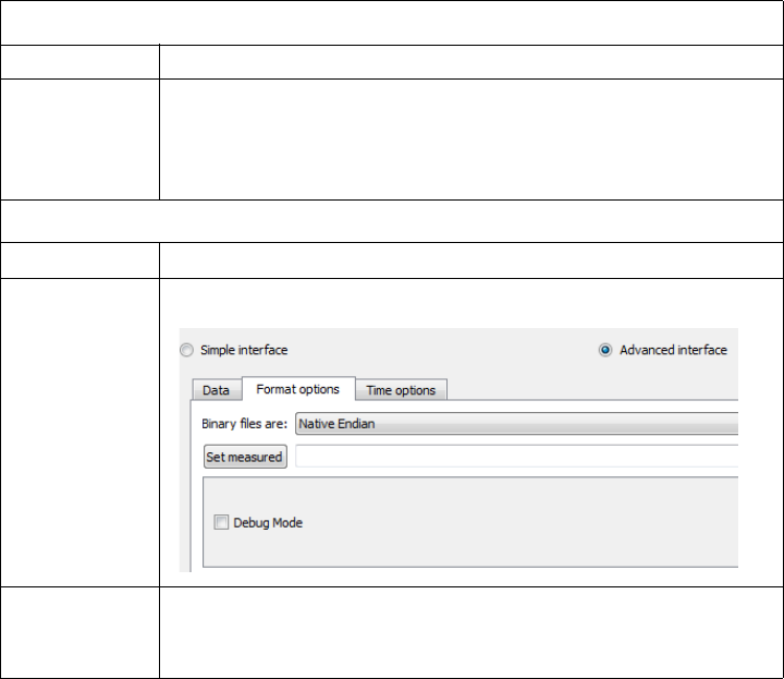
2.3 VTK Reader
EnSight 10.2 User Manual 2-145
Currently the VTK reader does not support more servers than files.
Limitations This reader does not read rectilinear grid (VTR) files, nor does it support polydata
files (VTP).
The reader does not support n-faced, 3D polyhedral elements in any of the formats
(they are simply skipped and will result in holes in your geometry), but does
support n-sided 2D polygon elements.
The reader does not read the parallel solution files (PVTK, PVTU, PVTS) which
contain extra information pertaining to the parallel solution.
Simple Interface
Data Load
Load your file (typically named with a suffix
.vtk
or
.vtu
or
.vtm
or
.vts
) using
the Simple Interface method.
Advanced Interface
Data Load
Load your file (typically named with one of the above suffixes ) using the
Advanced Interface method.
(see How To Read Data)
Data Tab
Format Use the VTK format.
Set vtm, vtu,
vts, vtk
Select the VTK file (typically .VTK, .VTS or .VTU or
.VTM) and click this button. Use file*.vtk, file*.vts, etc.
(where the asterisk (*) replaces the number) for transient
datasets. Each file will represent one timestep.
Format Options Tab
Set measured Select the measured file and click this button.
VTK Reader
Other
Options
Debug Mode Toggle this ON to get extra, debugging information printed to
the console in the event of problems reading the data. Note:
default is OFF.
2.3 XDMF Reader
2-146 EnSight 10.2 User Manual
XDMF Reader
Overview
Description Reads eXtensible Data Model and Format files (.xdmf files).
This reader is based on the xdmf library from:
pserver:anonymous@public.kitware.com:/cvsroot/Xdmf
The reader can handle all the element types in Xdmf except:
XDMF_MIXED
XDMF_POLYGON
Structured meshes are converted to unstructured form automatically by the reader.
The reader supports variables of type:
XDMF_ATTRIBUTE_TYPE_SCALAR
XDMF_ATTRIBUTE_TYPE_VECTOR
XDMF_ATTRIBUTE_TYPE_TENSOR
With centering:
XDMF_ATTRIBUTE_CENTER_CELL
XDMF_ATTRIBUTE_CENTER_NODE
The reader can handle 'Tree' grids. The reader does automatically decompose
datasets for server of server mode (SOS) based on 'Tree' grids. The various grid
blocks are distributed round-robin over the servers. Grids that are not 'Tree' grids
will all be read on the first server.
The reader allows the user to pass a filename using a wildcard (* or ?) to select a
collection of .xmf files. The reader assumes that each .xmf file contains a separate
timestep. Some checks are made to verify that each file has the same structure/
variables, but the checks are not complete. Likewise, some basic checks are made
for grids defined by reference. If all but one file has its grids geometry/topology
by reference, the reader will assume that they can be reused for other timesteps.
The reader can also be passed a file in the schema:
<?xml version="1.0" ?>
<Xdmf>
<Dataset>
<File Name=".xmf file" [Time="unknown"]/>
<Template Name="sprintf for .xmf files" [Start="1"] [Step="1"] [Count="1"]
[TimeStart="unknown"] [TimeStep="1.0"]/>
</Dataset>
</Xdmf>
This defines a collection of files by specific names. These can be via individual
names or via an sprintf() filename template and associated start, step and count
values. The file may also contain timestep values for each file (in the case of a
sprintf() template, the values are generated). Note: if a file has an <Information
Time=""/> element, that element will supercede the value specified here.
Simple Interface
Data Load
Load your geometry file (typically named with a suffix
.XDMF
) using the Simple
Interface method.

2.3 XDMF Reader
EnSight 10.2 User Manual 2-147
Advanced Interface
Data Load
Load your geometry and result files (typically named with a suffix
.XDM and .XDMF
)
using the Advanced Interface method.
(see How To Read Data)
Data Tab
Format Use the XDMF2 format.
Set xmf Select the geometry file (typically .XMF) and click this button
Format Options Tab
Verbose
mode
Provide more output to the console to track progress and
perhaps understand reader problems.
Enable Data
Freeing
Attempts to free memory as quickly as possible (default ON).
Flatten Grid
into Separate
Parts
Controls whether to use only the top level XDMF grids (which
can be a collection of grids) to create parts or to create a part
for each grid. When toggled ON, EnSight will make each grid
into a separate EnSight part (default OFF).
Set measured Select the measured file and click this button.
2.4 Other External Data Sources
2-148 EnSight 10.2 User Manual
2.4 Other External Data Sources
External Translators
Translators supplied with the EnSight application enable you to use data files
from many popular engineering packages. These translators are found in the
translators directory on the EnSight distribution CD. (Installed translators reside
in the $CEI_HOME/ensight102/translators directory.) A README file is
supplied for each translator to help you understand the operation of each
Particular translator. These translators are not supported by CEI, but are supplied
at no-cost and as source files, where possible, to allow user modification and
porting.
Exported from Analysis Codes
Several Analysis codes can export data in EnSight file formats. Examples of these
include Fluent, STAR-CD, CFX and others.
2.5 Command Files
EnSight 10.2 User Manual 2-149
2.5 Command Files
Command files contain EnSight command language as ASCII text that can be
examined and even edited. They can be saved starting at any point and ending at
any point during an EnSight session. They can be replayed at any point in an
EnSight session. However, some command sequences require a certain state to
exist, such as connection to the Server, the data read, or a Part created with a
Particular Part number.
There are a multitude of applications for command files in EnSight. They include
such things as being able to play back an entire EnSight session, easily returning
to a standard orientation, connecting to a specific host, creating Particle traces,
setting up a keyframe animation, etc. Anything that you will want to be able to
repeatedly do is a candidate for a command file. Further, if it is a task that you
frequently do, you can turn the command file into a macro (see To Use Macros
below).
Saving command
file
The command file which will repeat the entire current session can be saved from
the menu as follows: Main Menu> File > Save > Commands from this session...
This command file can then be replayed at startup of a new EnSight session and
will redo step by step each of the commands.
Documenting Bugs Command files are one of the best ways of documenting any bugs found in the
EnSight system. Hopefully that is a rare occasion, but if it occurs, a command file
provided to CEI will greatly facilitate the correction of the bug
Nested Command
Files
Command files can be nested, which means that if you have a command file that
does a specific operation, you can play that command file from any other
command file, as long as any prerequisite requirements are completed. This is
done by adding the command play: <filename> in the command file.
Default Command
File
EnSight is always saving a command file referred to as the default command file
(unless the you have turned off this feature with a Client command line option, see
Command Line Start-up Options). This command file can be saved (and renamed)
when exiting EnSight, as described later in this section. The default command file
is primarily intended to be a crash recovery aid. If something unforeseen were to
prematurely end your EnSight session, you can recover to the last successfully
completed command by restarting EnSight and running the default command file.
Saving the Default Command File for EnSight Session
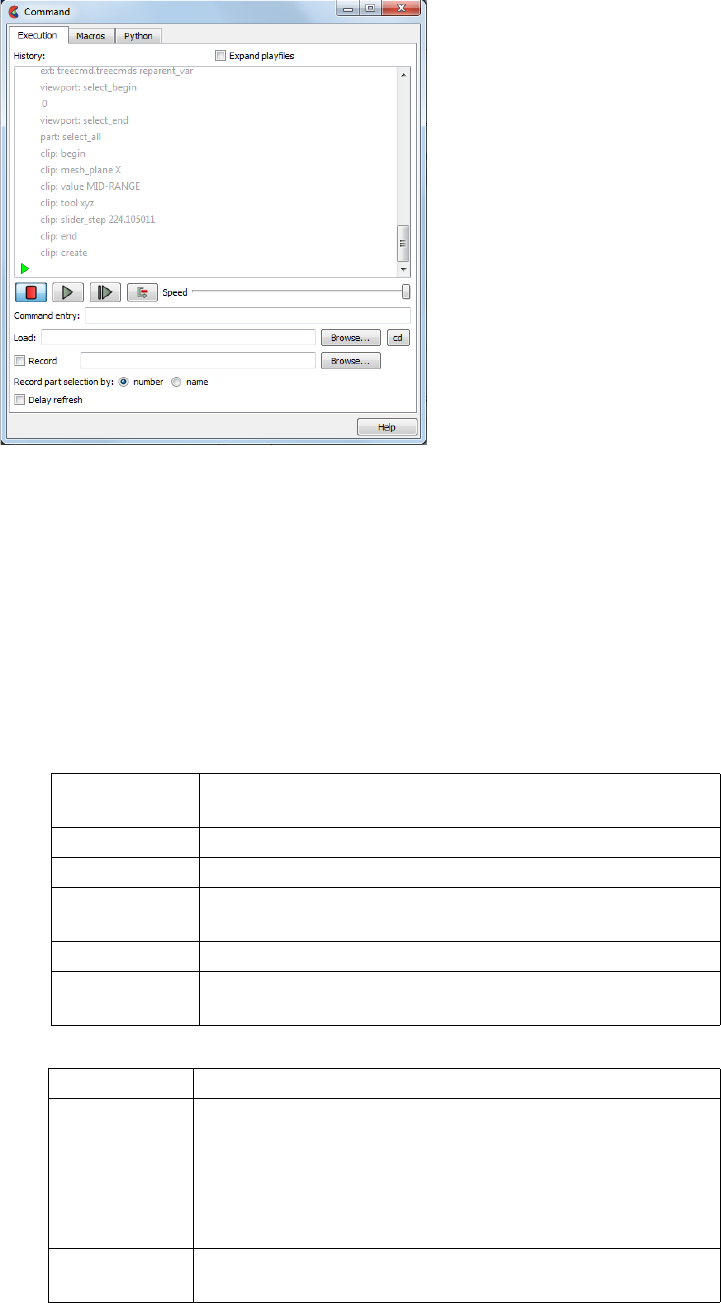
2.5 Command Files
2-150 EnSight 10.2 User Manual
Command dialog
You use the Command dialog to control the execution of EnSight command language. The
language can be entered by hand, or as is most often the case, played from a file. This
dialog also controls the recording of command files.
Main Menu > File > Command...
Execution Tab
History In the History window, commands to be executed will be shown in black below the green
current line indicator. As commands are executed, they will be show in gray above the
current line. Many operations can be preformed on the commands in the History window
by highlighting commands and clicking the right mouse button to bring up an action
menu. From this menu you can:
“VCR” buttons
Figure 2-9
Command dialog - Execution tab
Breakpoint set a breakpoint which will stop command execution at the
selected command.
Disable disable the selected command(s).
Copy copy the selected command(s) to the system clipboard.
Write/append write the selected command(s) to a new file or append them to
an existing file.
Execute execute the selected command(s).
Goto move the current line pointer to the selected command (Press
play or step to resume execution at this command).
Stop Stops command file playing.
Play Starts playing a command file. If you haven’t provided a
command file name (see Load, below), a File Selection dialog
will open for you to Select or enter the file name. Command
play continues as long as there are commands in the file, an
interrupt: command has not been processed, and the Stop
button has not been pressed.
Single Step Executes only the current (next) command, indicated by the
green current line pointer.
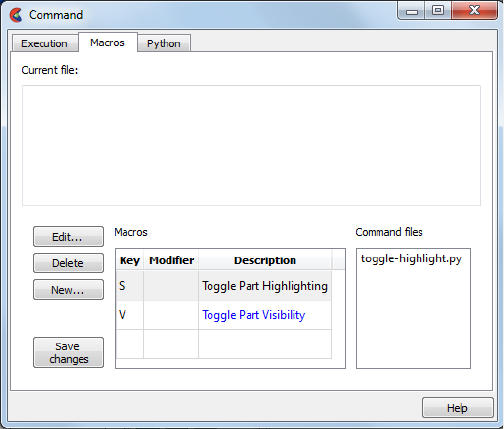
2.5 Command Files
EnSight 10.2 User Manual 2-151
Skip Skips over the current (next) command, indicated by the green current line pointer.
Speed Use the Speed slider to control the speed of command file play.
Command Entry Commands can be typed into this field for execution. Type the command and press return.
Load The name of a command file to be executed can be typed into this field. Press return to
load the file.
Or, you can use the associated Browse button to browse for a command file. A File
Selection dialog will open. Select or enter the file name. The file will be loaded when you
click “Open”.
The “Cd” button associated with the Load field can be used to change Ensight’s current
directory to the directory of the loaded command file. This can be useful for playing
command files that contain path information that assumes you’re starting from the
command file’s directory.
Record Check Record to start recording commands. If you have not typed a record filename in the
text field provided, A File Selection dialog will open for you to Select or enter the file
name. When Record is checked, all actions in EnSight are recorded to the specified file.
As long as the record filename stays the same, the record button may be toggled on and off
at any time, appending more commands to the file. When a new record file is selected, any
existing commands in the file will be overwritten. You can browse for a new record file or
directory at any time by clicking the browse button associated with this field.
Record Part
Selection By
Use this radio button to select the method by which part selection will be recorded in the
command language either by Number (default) or by Name.
Delay Refresh When checked, this will cause the EnSight graphics window to refresh only after the
playfile processing has completed or has been interrupted by the user.
Macros Tab
<filename> This window displays the contents of the currently selected file in the Command files list
(see below).
Macros A three-column table that lists all of the currently defined keystroke macros.
Keystroke macros are defined in a text file, macro.define. Macros can be defined at a site
or local level, with local macros overriding site macros that might be defined for the same
key. The
macro.define
file (if any) that resides in the
%CEI_HOME%/ensight102/
Figure 2-10
Command dialog - Macros tab
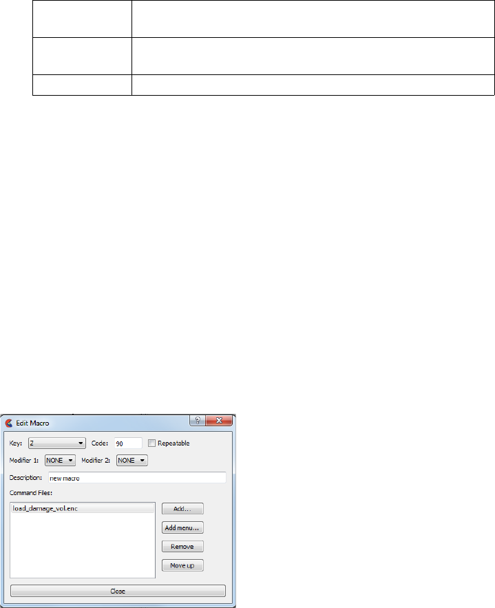
2.5 Command Files
2-152 EnSight 10.2 User Manual
site_preferences/macros
directory defines site-level macros, while the
macro.define
file
(if any) under the
macros
directory in the user’s EnSight Defaults directory (located at
%HOMEDRIVE%%HOMEPATH%\(username)\.ensight102
commonly located at
C:\Users\username\.ensight102
on Vista and Win7,
C:\Documents and
Settings\yourusername\.ensight102
on older Windows, and
~/.ensight102
on Linux, and
in
~/Library/Application Support/EnSight102
on the Mac) will define that user’s local
macros. Any command files referenced by macros must be located in these directories as
well.
In the Macros table, local macros are shown in black, site macros are shown in blue, and
local overrides of site macros are shown in red.
The table columns are:
The “Edit”, “Delete” and “New” buttons, below, operate on the macro selected in this
table.
Edit Opens The Edit Macro dialog. Change any of the values in this dialog to edit the currently
selected macro, then click “Close”. Your changes will not be written to the
macro.define
file until you either click “Save Changes” (see Below) or close the command dialog and
answer “Yes” to the Save Changes query message.
Delete Deletes the selected macro, provided it is not a site macro.
New Opens The New Macro dialog. Change any of the values in this dialog to define the new
macro, then click “Close”. Your changes will not be written to the
macro.define
file until
you either click “Save Changes” (see Below) or close the command dialog and answer
“Yes” to the Save Changes query message.
Save Changes Saves the changes from this Command Dialog session to the local
macro.define
file.
Command Files This list shows the command files that are associated with the currently selected macro.
New/Edit
Macros Dialog
Key A list of the key symbols supported for defining macros
Repeatable If checked, this causes the macro to be repeated while the specified key is held down.
Key a symbol representing the keyboard key on which a macro is
based
Modifier a symbol representing one of the modifier keys that may be
pressed along with the base key, (SHIFT, CTRL, or ALT)
Description a brief description of the macro
Figure 2-11
New/Edit Macro dialog

2.5 Saving the Default Command File for EnSight Session
EnSight 10.2 User Manual 2-153
Modifier 1 An optional modifier key (SHIFT, CTRL, or ALT) to be held down along with the base
key.
Modifier 2 A second optional modifier key.
Description A brief text description that allows you to quickly identify the macro.
Command Files Lists the command file(s) associated with a macro. Depending on how it is set up, a macro
can execute command files three different ways:
1. A single file is executed once for each key press.
2. The command file repeatedly executes as long as the key is held down.
3. Multiple command files execute in a cycle for each keystroke.
Add... To add a new command file to the list click “Add...”. A File Selection dialog will open.
Select or enter the desired file and click “Save”.
Add Menu... To add a menu selection to the list click “Add Menu...”. A dialog showing available menu
options will open. Select one of the menu options to be executed for this macro.
Remove To remove a command file from the list, select a file in the list, then click “Remove”.
Move up To change the order of execution of the command files listed, select a file, then click
“Move up” to change its position.
Python Tab The Interface Manual (see Chapter 7.1, Python EnSight module interface) contains a
description of this section.
Troubleshooting Command Files
This section describes some common errors when running commands. If an error
is encountered while playing back a command file you can possibly retype the
command or continue without the command.
(see How To Record and Play Command Files)
Saving the Default Command File for EnSight Session
EnSight is always saving a command file referred to as the default command file
(unless the you have turned off this feature with a Client command line option).
This default command file receives a default name starting with “ensigAAA” and
is written to your system temporary directory (e.g.
/usr/tmp
, unless you set your
TMPDIR environment variable is set to a valid pathname). This command file can
be saved (and renamed) when exiting EnSight. If you do not save this temporary
file in the manner explained below, it will be deleted automatically for you when
you quit normally from EnSight.
Problem Probable Causes Solutions
Error in command category Incorrect spelling in the command
category
Check and fix spelling
Command does not exist Incorrect spelling in the command Check and fix spelling
Error in parameter Incorrect integer, float, range, or
string value parameter
Fix spelling or enter a legal value
Commands do not seem to play Command file was interrupted by an
error or an interrupt command
Click continue in the Command
dialog
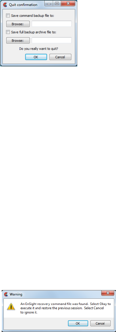
2.5 Auto recovery
2-154 EnSight 10.2 User Manual
Quit Confirmation dialog
You use the Quit Confirmation dialog to save either or both the default command file and
an archive file before exiting the program.
File-> Quit...
Save Command
Backup File To:
Toggle-on to save the default command file. Can also specify a new name for the
command file by typing it in or browsing to it. (see Section 2.5, Command Files for
more information on using command files.)
Save Full Backup
Archive File To
Toggle-on and specify a name (by typing it in or browsing to it) to create a Full Backup
archive file, which is a machine-dependent, binary dump of the current state of this
version of EnSight on this machine.
Yes Click to save the indicated files and terminate the program.
(see How To Record and Play Command Files)
Auto recovery
While EnSight is running, an auto recovery command file, recover.enc, is written
to the EnSight Defaults directory (located at
%HOMEDRIVE%%HOMEPATH%\(username)\.ensight102
commonly located at
C:\Users\username\.ensight102
on Vista and Win7,
C:\Documents and
Settings\username\.ensight102
on older Windows, and
~/.ensight102
on Linux, and
in
~/Library/Application Support/EnSight102
on the Mac). If EnSight crashes for
some reason, this temporary file is not deleted. When EnSight is restarted (without
using a play file) the user will be prompted with the option of using the auto
recover command file.
Auto recovery
dialog
Figure 2-12
Quit Confirmation dialog
Figure 2-13
Auto recovery dialog
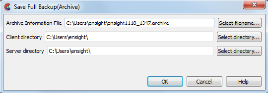
2.6 Archive Files
EnSight 10.2 User Manual 2-155
2.6 Archive Files
Saving and Restoring a Full backup
The current state of the EnSight Client and Server applications may be saved to
files. An EnSight session may then be restored to this saved state after restarting at
a later time. A Full Backup consists of the following files. First, a small archive
information file is created containing the location and name of the Client & Server
files that will be described next. Second, a file is created on the Client host system
containing the entire state of the Client. Third, a file is created on each Server
containing the entire state of the Server. You have control over the name and
location of the first file, but only the directories for the other files.
Restoring EnSight to a previously saved state will leave the system in exactly the
state EnSight was in at the time of the backup. For a restore to be successful, it is
important that EnSight be in a “clean” state. This means that no data can be read
in before performing a restore. During a restore, any auto connections to the
Server(s) will be made for you. If manual connections were originally used, you
will need to once again make them during the restore. (If more than one case was
present when the archive was saved, then connection to all the Servers is
necessary).
An alternative to a Full Backup is to record a command file up to the state the user
wishes to restore at a later date, and then simply replaying the command file.
However, this requires execution of the entire command file to get to the restart
point. A Full Backup returns you right to the restart point without having to
recompute any previous actions.
A Full Backup restores very quickly. If you have very large datasets that take a
significant time to read, consider reading them and then immediately writing a
Full Backup file. Then, use the Full Backup file for subsequent session instead of
reading the data.
Important Note: Archives are intended to facilitate rapid reload of data and
context and are NOT intended for long-term data storage. Therefore, archives are
likely NOT compatible between earlier EnSight versions and the current version
(see Release Notes for details). If EnSight fails to open an archive, it will state that
it failed and will write out a .enc file and echo its location. As command files ARE
often compatible between earlier and later versions, the .enc file can likely be
used to retrace the steps of the dataset.
Save Full Backup Archive dialog
Figure 2-14
Save Full Backup Archive dialog
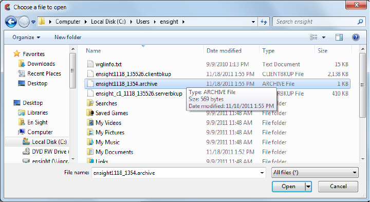
2.6 Saving and Restoring a Full backup
2-156 EnSight 10.2 User Manual
You use the Save Full Backup Archive dialog to control the files necessary to perform a
full archive on EnSight. This will save three files: a Archive Information file (suffix
.archive), a Client file (suffix .clientbkup) and a server file (suffix serverbkup). It is best
to specify the full path to each of these files so that you can find them.
File->Backup->Save->Full backup...
Archive Information
File
Specifies name of Full Backup control file.
Select filename... Click to bring up the file browser.
Click to display the file selection dialog for specifying the Archive Information File.
Client Directory... Specifies the directory for the Client archive file.
Select directory... Click to bring up a directory browser.
Server Directory... Specifies the directory for the Server archive file.
Select directory... Click to bring up a directory browser.
OK Click to perform the full backup.
NOTE: This command to create a backup is written to the command file, but is preceded
with a # (the comment character). To make the archive command occur when you play the
command file back, uncomment the #.
(see How To Save and Restore an Archive)
File Selection for Restarting from an Archive
You use the Restore Full Archive Backup dialog to read and restore a previously stored
archive file. Navigate to the directory where you saved the archive file (.archive suffix)
and choose open. It will direct EnSight to open the client backup file (.clientbkup suffix)
and the server backup file (.serverbkup suffix) and restore EnSight to its previous state.
File->Restore->Full backup...
Figure 2-15
File Selection for Restarting from an Archive

2.6 Saving and Restoring a Full backup
EnSight 10.2 User Manual 2-157
Troubleshooting Full Backup
Problem Probable Causes Solutions
Error message indicating that all
dialogs must be dismissed
When saving and restoring archives,
all EnSight dialogs, except for the
Client GUI, must be dismissed to
free up any temporary tables that are
in use. Temporary tables are not
written to the archive files.
Dismiss all the dialogs except the main
Client GUI.
Backup fails for any reason Ran out of disk space on the Client
or Server host system
Check the file system(s) you where you
are writing (both the Server and the
Client host systems) then remove any
unnecessary files to free up disk space.
Directory specified is not writable Change permissions of destination
directory or specify alternate location.
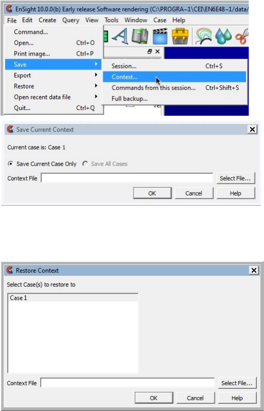
2.7 Context Files
2-158 EnSight 10.2 User Manual
2.7 Context Files
EnSight context files can be used to duplicate the current EnSight state with the
same or a different, but similar, dataset. The context file works best if the dataset
it is being applied to contains the same variable names and parts, but can also be
used when this is not the case.
Input and output of context files is described below as well as in How To Save or
Restore a Context File and under Save and Restore of File Menu Functions
Saving a Context File
To save the current context, simply entered the desired file name in the dialog
under: File > Save > Context...
(and if you have multiple cases to save, select Save All Cases)
Restoring a Context
If you are restoring a context file containing information for a single case, you can
select the case or cases that you wish to apply the context to. If you are restoring
a context file containing information about multiple cases, the selection list will
be ignored.
Figure 2-16
Saving a Context File
Figure 2-17
Restoring a Context File
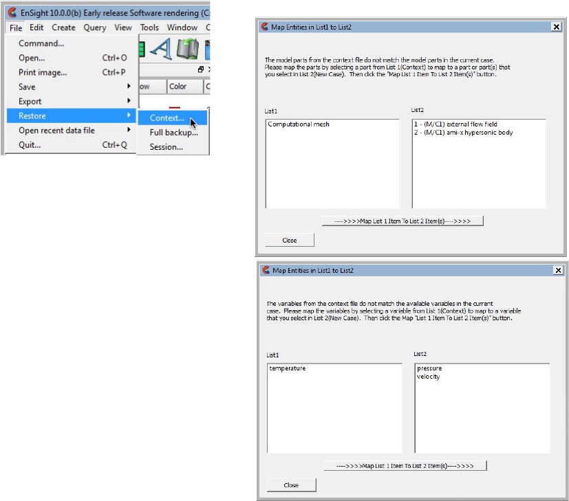
2.7 Restoring a Context
EnSight 10.2 User Manual 2-159
When restoring a context you can 1) read the new dataset and build the new parts
and then restore the context file, or 2) read the new dataset, close the part builder
without building any parts and restore the context file (whereupon the context file
will build the same parts as existed when it was saved) or 3) restore the context
before reading any data (whereupon the previous state with the same dataset will
be restored). The way you decide to do this depends upon whether the same parts
exist in the new dataset.
If the same parts do not exist, you would typically read the new dataset and build
the desired parts in the normal way. Then:
Flipbook animations are not restored using the context file because it is unknown
at the time the context file is created what state existed when the flipbook was
saved. Restoring a context file will fail if you have executed a python tool from
the User Defined Tools.
Part IDs may be different when you restore a context file.
Context files use EnSight’s command language and other state files (such as
palette, view, and keyframe animation).
Figure 2-18
Restoring a Context
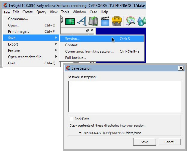
2.8 Session Files
2-160 EnSight 10.2 User Manual
2.8 Session Files
An EnSight session file records the state of the visualization utilizing the context
file capability along with a thumbnail of your graphics windows and a description
of the session. When you restart EnSight, your recent sessions are displayed in
the 'Welcome to EnSight' screen, complete with the thumbnail and description.
Saving a Session File
To save the current session, simply enter the desired file name in the dialog under:
File > Save > Session...
You will be prompted for a description for the session. The description is shown
on the Welcome screen, so this is a good place to make a note to remind yourself
of the particulars of this visualization.
You can check the toggle to pack the data into your session file. Packing allows
for true session file portability as it packs the original data directories as well as
the context information compressed into one session file. The directories that will
be compressed and saved are listed. The resulting single session file contains
everything EnSight needs to reproduce the exact visualization on any EnSight
installation that has the ability to read your data file. Your session file is a
portable way to share visualizations with other EnSight users. Keep in mind that
for a large data set, your session file can be quite large if you use the data packing
option.
Click 'Save' to open a file browser and choose a location for your session file.
If you have multiple cases, a single session file will be saved that includes all the
cases.
Figure 2-19
Saving a Session File
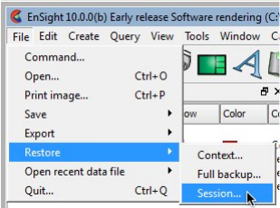
2.8 Restoring a Session
EnSight 10.2 User Manual 2-161
Restoring a Session
Restoring a session is simple. First, your most recent session files are available in
the 'Welcome to EnSight' screen on startup. Second, Mac and Windows users can
double click any EnSight session file (ending in .ens) and the file will restore.
Finally, you can browse for a session file from the EnSight menus as follows:
Main Menu > File > Restore > Session...
If you are restoring a session file containing information for multiple cases, all of
the cases will be restored. If you already have data loaded and restore a session,
EnSight will delete all the cases, start anew and then restore the session.
Figure 2-20
Restoring a Context File
2.9 Scenario Files
2-162 EnSight 10.2 User Manual
2.9 Scenario Files
Description A Scenario contains user-selected, client-based entities. These include parts,
annotations, plots, animations (i.e. flipbook, keyframe, and/or particle traces), and
transient client geometry with associated variable values.
Format A Scenario is saved using the new EnVision (.evsn) file format.
You may also save a scenario in the legacy Reveal (.csf) format, but do note that
this legacy format is readable only using Reveal, which is no longer included in
the current EnSight distribution (last distributed in EnSight 10.1).
Note also that saving in the EnLiten (.els) format is no longer an option, and
EnLiten is no longer included in the EnSight distribution.
Type A Scenario can be saved as a Single File or a Project. A single file (.evsn suffix)
contains one individual Scenario. A Project is a directory containing a context file,
an envision file a description file and a jpg image.
Since a Scenario Project can store more than one individual Scenario, you may
save a Scenario into an existing Project. This will append the new Scenario to any
prior data that has been stored in the Project.
EnVision Scenario files are designed to be viewed by CEI’s 3D geometry viewer EnVision.
EnVision can read a Single-File Scenario or the data within a Scenario Project
directory.
EnVision is similar to the EnSight Client without a Server attached. As such, it is
not capable of creating or modifying any new/existing variables.
EnVision Standard is free and installed with EnSight, while EnVision Pro is
licensed separately. EnVision Standard is used to visualize simple 3D geometry
animations, while EnVision Pro is useful for interactively exploring 3D transient
data.
Usage Flipbook, (non-transient) keyframe, and particle trace data can be played through
time without alteration. This can be visualized using EnVision Standard. When
this data is played, it will be loaded the first time from disk and then cached in
memory to speed up playback, similar to the EnSight Client.
However, transient data stored in a Scenario (including transient keyframe data)
has geometry and variables that can be interactively modified to a limited extent,
using EnVision Pro (but not EnVision Standard). The advantage of using
EnVision Pro to interactively visualize transient data is that it can create new
client parts such as vector arrows and contours and can displace geometry and
step through time. Note: if you play transient data through time, the data is
automatically cached (similar to a flipbook animation) to speed up playback.
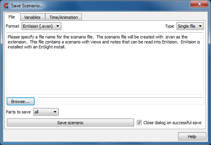
2.9 Scenario Files
EnSight 10.2 User Manual 2-163
You use the Save Scenario dialog to control the options of the scenario files to be saved in
EnSight for display in EnVision.
Main Menu > File > Export > Scenario...
File Tab
Format EnVision scenario files (.evsn) or Reveal CEI Scene Files (.csf) may be used.
EnVision Format Project - will save the scenario file plus files mentioned on the previous page.
Single file - will save only the scenario file.
File Name Enter the file name to be saved or use the Browse... button.
Save scenario Click to actually save the scenario.
Parts to Save all – All available parts.
visible – All parts currently visible.
selected – All parts currently selected.
Figure 2-21
Save Scenario Dialog - File Tab
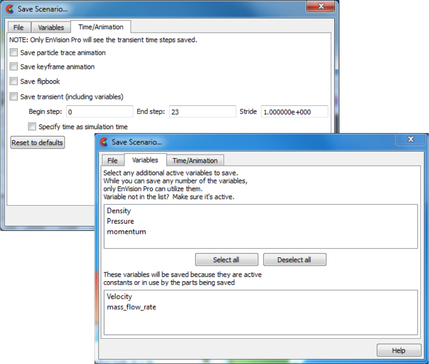
2.9 Scenario Files
2-164 EnSight 10.2 User Manual
Variables
Options Tab
Select Additional
Variables
Click, Ctrl-Click or Shift-Click to select variables in the list to save the optional, active
variables to save into the scenario for later use in EnVision Pro.There is no need to save
additional variables if you have EnVision Standard (which comes, by default with your
EnSight install).
Select all
Deselect all
Select or deselect all the optional, active variables to save into the scenario for later use in
EnVision Pro. There is no need to save additional variables if you have EnVision Standard
(which comes, by default with your EnSight install).
Time/Animation
Options Tab
Save keyframe
animation
Only available if keyframe animation is defined. Toggle on to save the keyframe
animation sequence to the scenario file.
Save Flipbook Only available if flipbook is defined and saving to an EnVision scenario file. Toggle on to
save the flipbook information to the scenario file.
Save particle
trace animation
Only available if animated particle traces exist. Toggle on to save the animated traces to
the scenario file.
Figure 2-22
Save Scenario Dialog - Variables and Time/Animation Options Tabs
2.9 Scenario Files
EnSight 10.2 User Manual 2-165
Save transient
(including
variables)
Only available if transient data exists. Toggle on to save transient data to the scenario file
for later use in EnVision Pro. There is no need to save transient data if you have EnVision
Standard (which comes, by default with your EnSight install).
Begin step - Beginning step to save.
End step - Ending step to save.
Stride - The step stride between Begin and End step
Specify time as simulation time - Use time value rather than default timestep
Reset to defaults Quick change back to all defaults.
(see How To Save Scenario)
2.10 Saving Geometry and Results Within EnSight
2-166 EnSight 10.2 User Manual
2.10 Saving Geometry and Results Within EnSight
Saving Geometric Entities
Sometimes you may wish to output geometric data or variable values from
EnSight to be included in a different analysis code, or to be used in a presentation.
EnSight has internal writers as well as external, user-defined writers, which use
the EnSight writer API (available to any EnSight user).
EnSight has five internal writers that allow saving geometric data and variable
values: 1) Brick of Values (used for volume rendering of variables for 3D Parts
only), 2) Case (EnSight Gold) 3) VRML, 4) Simple Client Output, or 5) PLY
Polygonal File Format. In addition to these five internal writers, EnSight also has
three user-defined writers that each use the EnSight user-defined writer API. Each
user-defined writer must be compiled into a dynamic shared library that is loaded
at runtime and listed in the Save Geometric Entities dialog with the internal writer
formats.
Both internal and user-defined writers have access only to the geometry of
selected parts and active variables. The VRML, Simple Client Output and PLY
Polygonal File Format writers save geometry and variable values only on the
client. The remaining writers save only parts located on the server and all active
variables. Server parts include all original model parts, and the following created
parts: 2D-clips, Elevated Surfaces, Developed Surfaces, and Isosurfaces. Note
that element filtering is ignored when saving out server parts; element filtering is
only used for VRML export. Client parts include the surface elements available on
the client.
The VRML internal writer saves all the parts on the client in their current visible
state except for Parts which have limit fringes set to transparent. The VRML 2.0
(.wrl file) will be saved on the client. The VRML output generally contains the
same visual features as the Reveal product. The VRML export supports nodal
variable coloring only. VRML does not support volume rendering therefore, none
of the parts can be rendered in Volume element representation. Parts colored using
element variables will be displayed in their EnSight constant color. An element
variable can be changed to a nodal variable (so that it can be written out in VRML
format) using the EnSight calculator function ElemToNode. The mechanism for
nodal color export is through texture mapping using an embedded texture map as
the color palette.
The Simple Client Output internal writer tesselates the elements on the client into
triangles and saves the tesselated elements of the selected part(s) into an ascii or
binary file containing first a list of the x, y, z coordinates followed by the
connectivity triplets, followed by the variable values of each of the selected,
active nodal variables at each of the coordinates. Note this format does not
support the saving of per-element variables.
The PLY Polygonal File Format internal writer tesselates the elements on the
client into triangles and saves the tesselated elements of the selected part(s) into
an ascii or binary file containing first a list of the x, y, z coordinates with their
respective color in RGB format, followed by the connectivity triplets. This format
does not save variable values, but merely color at each node in RGB format.
2.10 Saving Geometric Entities
EnSight 10.2 User Manual 2-167
The userd-defined writers can call the routines of an EnSight API to retrieve, to
get, for example, server side nodal coordinates, connectivities, node ids, and
element ids of parts as well as active variable values on those parts selected in the
Parts window to be passed by value to be used, manipulated and/or written out in
any format desired. User-defined writer dialog includes a Parameter field that
allows passing in a text field into the writer from the GUI for extra options.
Normally the active variables are all saved, but the following command tells the
user defined writers to save only the selected variables:
test: write selected vars
Several example user-defined writers (including source code header files,
Makefile and the corresponding shared library) are included to demonstrate this
capability.
The Case (Gold) Lite writer is included to demonstrate how to exercise most of
the API and output a subset of the Case (Gold) format. Complex numbers and
custom Gold format are not supported with this writer. While the writer is not
compiled, the source code of this writer, the required header files, and the
Makefile are included.
The Flatfile user-defined writer outputs coordinates and active variables (scalar
and/or vector only) for all selected parts. The format is ascii comma delimited so
it is easily imported into other applications. If any of the keywords ‘ANSYS’ or
‘force’ or ‘body’ is entered into the Parameter field, then Flatfile will output an
ANSYS body force file. If NODEID or nodeid is entered into the Parameter field
then node ids are written out. If SSCALE # is entered in the parameter field then
scalar variables will be scaled by the float value (for example SSCALE 3.1415
will multiply every value of the scalar by 3.1415). Similarly, VSCALE # will
scale each component of a vector variable and GSCALE # will scale each value of
the nodal coordinates. Only active nodal variables are exported unless CELLID is
entered into the Parameter field, and then only active element variables are written
out for each element id, including the element id (if it exists).
The STL user-defined writer is designed to write out the border geometry in the
form of triangular 2D elements of the selected part(s) at the beginning timestep.
The end time and the step time are ignored. The STL format does not support
multiple parts in a single binary file, but does support multiple parts in a single
ASCII file. Therefore, if multiple parts are selected and ascii is checked, the STL
writer outputs an ascii file with the border of each of the parts. If multiple parts
are selected and binary is checked, the STL writer outputs a binary file containing
a single border of the multiple parts.
Finally a user-defined writer is available for the Exodus II data format.
More user-defined writers may be distributed with EnSight in the future.
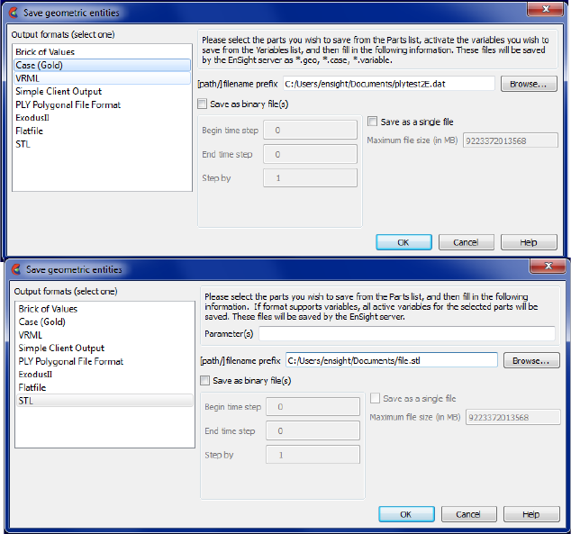
2.10 Saving Geometric Entities
2-168 EnSight 10.2 User Manual
Save Geometric Entities dialog
The Save Geometric Entities dialog is used to save Selected Model, 2D-Clip, Isosurface,
Elevated Surface, and Developed Surface Parts as EnSight Case (Gold) files. Thus
modified model Parts and certain classes of created Parts can become model Parts of a
new dataset.
Main Menu > File > Export > Save Geometric Entities...
Output Format Specify the desired format: Brick of Values, Case(EnSight Gold), VRML, Exodus,
Flatfile, STL, and possibly other user defined writers.
Parameter Allows passing a text field from the GUI to the writer for extra options. Some writers
make use of this field to modify their behavior (see Flatfile, for example) while others
ignore this field. See the README file(s) in the following directory
$CEI_HOME/
ensight102/src/writers.
[path]/filename
prefix
Specify path and filename prefix name for the saved files. For Case(Gold) the saved
geometry file will be named filename.geo, the casefile will be filename.case, and the
active variables will be filename.variablename. The VRML file will be filename.wrl. The
other writers will vary.
Save As Binary
File(s)
Save as Binary File(s) specifies whether to save the data in ASCII (button toggled off -
default) or binary (button toggled on) format. Writers vary in their handling of this.
Begin Time Step Begin Time Step field specifies the initial time step for which information will be
available to save for all selected Parts and activated variables. Writers may vary in their
usage of this information.
End Time Step End Time Step field specifies the final time step for which information will be saved for
all selected Parts and activated variables. Writers may vary in their handling of this.
Step By Step By field specifies the time step increment for which information will be saved for all
selected Parts and activated variables starting with Begin Time Step and finishing with
Figure 2-23
Save Geometric Entities dialog
(Showing Case (Gold) internal writer, and STL external writer)
2.10 If Rigid Body Transformations in Model
EnSight 10.2 User Manual 2-169
End Time Step. The Step By value MUST be an integer. Writers may vary in their
handling of this.
Save as a Single
File
Toggle on to have a single file per variable - containing all values for all time steps for that
variable. The default is to have a file per variable per time step. Writers may vary in their
handling of this.
Maximum file Size For Single File option, can specify the maximum file size. Continuation files are created if
the file size would exceed this maximum. Writers may vary in their handling of this.
Okay Click ok to pass the GUI values to the selected writer, and begin executing the writer
routine
If Rigid Body Transformations in Model
Since EnSight does something special with the model timeset when rigid body
information is read (via the rigid_body option in the casefile, or from a user-
defined reader with rigid_body reading capability), you need to be aware of a few
important issues. EnSight assumes that the rigid body timeset encompasses the
normal geometry timeset, and it replaces the normal geometry timeset with the
rigid body timeset - thus the following occurs when using this option.
1. If any created parts are in the list to be saved, EnSight will save as true
changing coordinates. Namely, a geometry file containing the coordinates for each
part will be saved at each time. Upon re-reading this model, you will be able to
duplicate all actions, but it will be done as a true changing coordinate model. In
other words, the original rigid_body file nature will not be duplicated.
2. If the original model had static geometry and rigid body file information - and
you do not have any created parts in the list to be saved - saving will preserve the
single static geometry and rigid_body file nature of the model. However, if the
original model had changing geometry, or if variables have been activated - the
number of geometry/variable files saved will be according to the rigid body
timeset. This timeset often has many more steps than the original timesets - so be
wise about the number of steps you write. It is often important to use the “Step
by” option to control this.
3. Because of the things mentioned in 1 and 2 above - if you want to use the save
geometric entities option in EnSight to “translate” a rigid body model from a
different format into the EnSight format, you may want to consider the following
process. First, read in the model without the rigid body transformations, activate
the desired variables, and save the model. Second, read in the model with the rigid
body transformations, do not activate any variables, and save the model (with a
different name). Edit the Casefile of the first model to use the model: and
rigid_body: lines of the second casefile instead of the first casefile.

2.10 If Rigid Body Transformations in Model
2-170 EnSight 10.2 User Manual
Troubleshooting Saving Geometric Entities
(see How To Save Geometric Entities)
Problem Probable Causes Solutions
A Part was not saved User attempted to save an
unsupported Part type.
Select only Model, Isosurface, 2D-
Clip, and Elevated Surface Parts.
Variable(s) not saved The variable was not activated or the
variable was a constant.
Activate all scalar and vector
variables you want saved.
Error saving File prefix indicates a directory that
is not writable or disk is out of space.
Re-specify a writable directory and
valid prefix name. Remove
unneeded files.
My custom user-defined writer
doesn’t show up on list of formats
Didn’t load at startup Start Ensight with -writerdbg option
EnSight loads user-defined writers at
startup from shared libraries found in
$CEI_HOME/ensight102/machines/
$CEI_ARCH/lib_writers
If your user-defined writer is not in
the default directory, tell EnSight
where to find it by:
setenv ENSIGHT10_UDW location
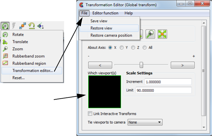
2.11 Saving and Restoring View States
EnSight 10.2 User Manual 2-171
2.11 Saving and Restoring View States
EnSight’s viewports provide a great deal of flexibility in how objects are
displayed in the Graphics Window. Given the complicated transformations that
can be performed, it is imperative that users be able to save and restore
accumulated viewport transforms.
View saving and restoring is accessed from the Transformations dialog.
Transformation Editor... > File > Save view
When either the Save View... or Restore View... selection is made, the user is
presented with the typical File Selection dialog from which the save or restore can
be accomplished. Save and Restore work on the one, selected viewport.
(see also How To Save and Restore Viewing Parameters)
Figure 2-24
View Saving and Restoring in Transformation Dialog
selected viewport
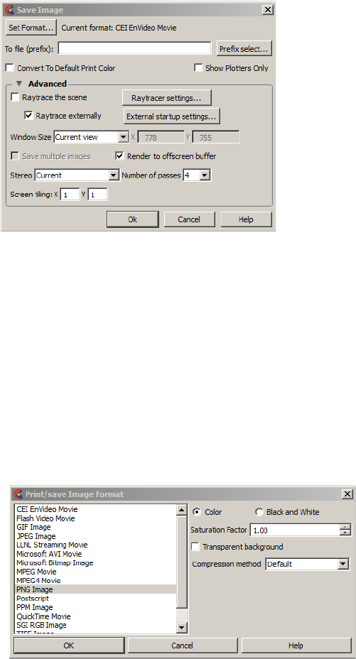
2.12 Saving Graphic Images
2-172 EnSight 10.2 User Manual
2.12 Saving Graphic Images
EnSight enables you to save an image of the Main View to a file.
Export Image dialog
You use the Save Image dialog to specify the format and destination of an image to save.
You also access the Image Format Options dialog for the various image types from this
dialog.
Main Menu > File > Export > Image...
Set Format... Click to select a format. Image formats: EnVideo, Flash, GIF, JPEG, LLNL Streaming,
Microsoft AVI, Microsoft Bitmap, MPEG, MPEG4, PNG, Postscript, PPM, QuickTime,
SGI RGB, TIFF, and XPixmap.
Note: the following are movie (animation) formats avi, evo, flash, mpeg, quicktime, and
LLNL streaming movie. If an animation format is selected for an image export, a single-
frame animation will be saved. The default format is evo, which is CEI’s image and
animation format which can be viewed using EnVideo.
Color/Black &
White
Color versus Black and White toggle selects either the normal color image or a black and
white image.
Saturation
Factor
At a value of 1.0, no change to the image. At lower values, a proportionate amount of
white is added to each pixel. At a value of 0.0, the image would be all white.
Transparent
background
Toggle saving of PNG images with transparent backgrounds.
Figure 2-25
Print/Save Image dialog
Figure 2-26
Output format and options dialogs
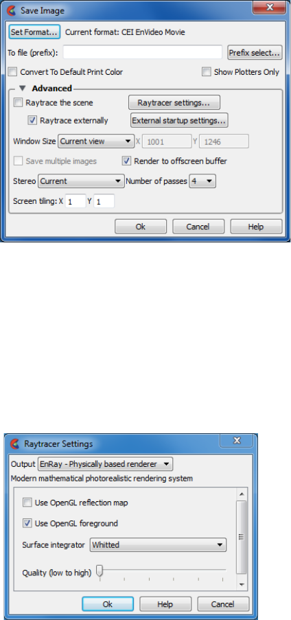
2.12 Saving Graphic Images
EnSight 10.2 User Manual 2-173
Note: Each format can have other options specific to that format.
To Fil e The image will be saved to this file name prefix. An appropriate suffix, according to the
file format chosen, will be added.
Convert to default
print colors
This is useful for making a white background for copying into a document or for printing.
Clicking this toggle on will convert all black to white and all white to black but will leave
all other colors as they are.
Show Plotters Only Clicking this toggle will cause the graphics window to only display plotters.
Raytrace the scene Toggle to raytrace the image. Raytracing is an advanced rendering technique in computer
graphics, where simulation of the light transport is performed between the image pixels,
objects in the scene, and the light sources. This technique is capable of generating high
realism images, but at a much higher cost than that of typical rasterization-based
techniques. Raytracing is suitable for rendering a wide variety of optical effects, such as
reflection, refraction, soft shadow, etc.
Raytracer settings Opens the Raytracer Settings dialog.
Output Specifies the resulting output type.
EnRay EnSight’s built-in raytracing renderer. It is tightly integrated, with support for many
visualization styles.
Use OpenGL
reflection map
Toggles use of reflection maps in rendering. EnSight provides a default material library,
where there are some reflection maps used for reflective materials when the graphics
hardware rendering engine is used. Although using these reflection images in the raytracer
does disable the real reflection computation between scene objects.
Figure 2-27
Print/Save Image Advanced dialog
Figure 2-28
Raytracer settings dialog
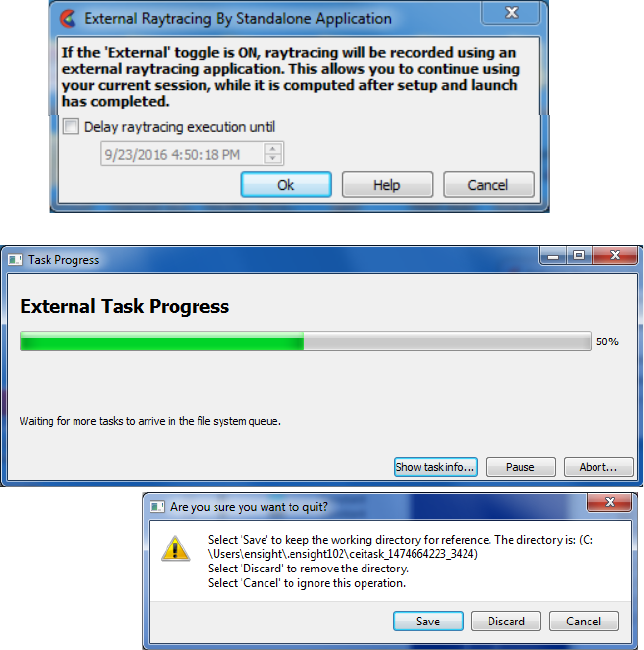
2.12 Saving Graphic Images
2-174 EnSight 10.2 User Manual
Use OpenGL
foreground
Toggles the 2D overlaying using the graphics hardware rendered result to the raytracer.
EnSight’s graphics window usually contains not only rendering results from 3D geometry,
but also 2D illustrations, such as palettes, plots, and tables. The raytracer does not have
the capability of rendering the 2D layer. Therefore, when we set this option on, the system
will output the hardware rendered 2D layer as an image and composite it with the
raytracing result.
Surface Integrator Choice of raytracing algorithms.
Whited Enables the Whittled style raytracer, which traces three types of rays: reflection,
refraction, and shadow. It is an efficient rendering algorithm for rendering highly
reflective scenes. It is not good at rendering diffusely reflective scenes.
Ambient
Occlusion
Enables the Ambient Occlusion technique which is suitable for scenes which are
dominated by ambient lights, and uses the local occlusion ratio to approximate the shading
effect.
Quality(low to high) Slider that specifies the image quality of the raytracing result. There are currently 6
levels, where 0 is the lowest quality and 5 is the highest quality. We hide the detailed
raytracing parameters from the user, such as number of samples per pixel, recursive depth,
etc.
Raytrace externally Toggles whether to externally process the raytracing. EnSight can use both the internal
EnRay raytracer or the external command line EnRay raytracer to perform the raytracing.
The benefit for external raytracing is that a user won’t be blocked by the time consuming
raytracing computation, and can continue using EnSight interactively.
External startup
settings
These settings allow you to schedule the startup of the raytracing later, perhaps when more
computational capability is available (e.g. nighttime), or after your session is complete to
avoid competition for your client machine resources.
Figure 2-29
External startup settings &
progress dialog
2.12 Saving Graphic Images
EnSight 10.2 User Manual 2-175
External Task
Progress
A progress bar to show ray/path tracing progress.
Show Task info This will open the reference working directory containing data files used in ray/path
tracing. This working directory is in your .ensight102 directory.
Pause Temporarily pause execution if, for example, the client becomes sluggish or unresponsive
Abort Delete the running ray/path tracing job
Close When finished, a close button will become available. Pressing close will bring up another
dialog, allowing you to save or discard the reference working directory.
Window Size Specifies the resulting image size in pixels.
Normal Use the current size of the graphics window
Full Use the size of a full screen window.
User Defined Enter a width and height in pixels in the X and Y fields.
NTSC Use the NTSC standard window size (704 x 480).
PAL Use the PALstandard window size (704 x 576).
Detached
Display
Uses the detached display (as specified with - dconfig option) as the source for the output.
DVD NTSC Use the DVD NTSC standard window size (720 x 480).
DVD PAL Use the DVD PALsize, (720 x 576).
HD 720p Use the HD 720p standard window size (1280 x 720).
HD 1080p Use the HD 1080p standard window size (1920 x 1080).
Save multiple
images
If using a detached display (as specified with a -dconfig option), you may save an image
from each display or a single image.
Render to
offscreen buffer
Controls where to render the image prior to saving. Toggle ON to render in an offscreen
buffer prior to saving the image, and toggle OFF to render on-screen prior to saving the
image. On screen rendering has the disadvantage that overlaid images, such as screen
savers, can interfere with the saved image. However, some platforms and graphics cards
do not support off-screen rendering.
Stereo Render two images from slightly different viewpoints to produce a stereo (3D) effect.
Current If the graphics window is mono, save a mono image. If stereo, save a stereo image.
Mono Save a mono image.
Interleaved Save a stereo interleaved image. Two full-color images will be generated. If the EnVideo
evo format is specified, both images will be saved in a single evo file. For other formats,
the images will be saved in separate files, e.g.
image_l.png
and
image_r.png
. In addition
an mtm (multi-tile movie) file will be generated, e.g.
image.mtm
. The mtm file can be read
by EnVideo to display
image_l.png
(left image) and
image_r.png
(right image) in stereo.
Interleaved stereo requires a specialized monitor with paired, polarized lenses; it uses
polarized lenses for the left and right eye and preserves the coloration of the parts.
Anaglyph Save a stereo color separated image with left/right eye color as specified. (Cyan/Red, Red/
Cyan, Blue/Red, or Red/Blue). This is not recommended if the parts are colored by a
variable as the coloration will distort the above color shift.
Number of passes The number of rendering passes. The higher the number, the better the quality (but
slower).
Screen tiling For powerwall environments, specify the number of images in x and y that will be
produced. For example, by selecting 2x2, a file prefix of “image”, and png format,
EnSight will save image_d00.png, image_d01.png, image_d02.png, image_d03.png, and
image.mtm. Each png file would have one fourth of the image, and the mtm file can be
used by EnVideo to view the images stitched together.
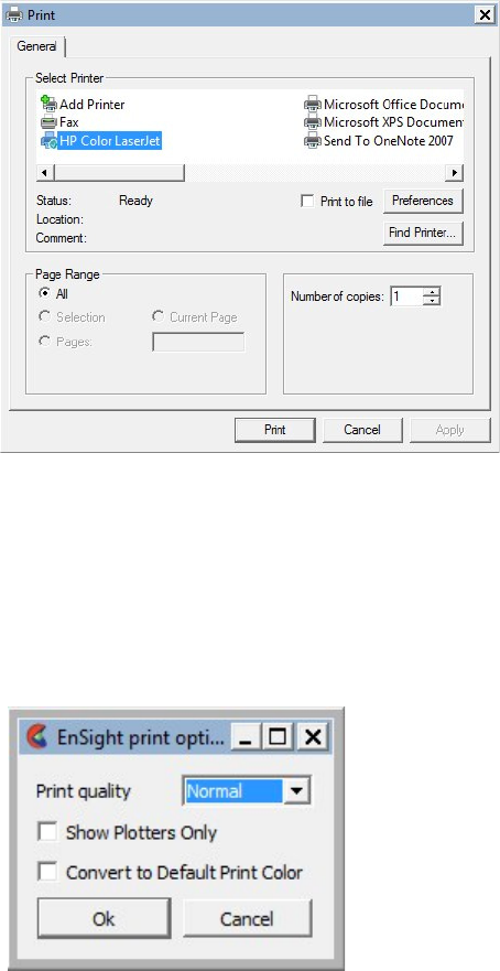
2.12 Saving Graphic Images
2-176 EnSight 10.2 User Manual
(see How To Print/Save an Image)
Print Image dialog
You use the Print Image dialog to specify the destination printer and options when
producing a hard copy of an image. When you choose to print an image, you will be
presented with the standard system print dialog.
File > Print Image…
After you choose your printer and options, you’ll see the EnSight print option dialog.
Print Quality Select the output quality – Draft, Normal, High, Best. Higher quality requires longer to
render.
Show Plotters Only Clicking this toggle will cause the graphics window to only display plotters.
Convert to Default
Print Colors
Clicking this toggle on will convert all black to white and all white to black but will leave
all other colors as they are.
Figure 2-30
Print Image dialog
Figure 2-31
Print Options dialog

2.12 Troubleshooting Saving an Image
EnSight 10.2 User Manual 2-177
Troubleshooting Saving an Image
(see How To Print/Save an Image)
Problem Probable Causes Solutions
Image has blotches or ghosts of other
windows in it
A viewport or menu was popped in
front of the Main Graphics Window
as the image was being saved.
Use offscreen rendering when
possible. Note that volume rendered
images on the Mac must be on
screen.
Error while saving image file Directory or file specified is not
writable
Rename the file or change the
permissions.
Ran out of disk space Check the file system you are using
then remove any unnecessary files to
free up disk space.
Image format not selected Select an image format before
saving.
Image looks bad when printed Original on-screen image has low
resolution
Select “user defined” size or a pre-
defined size such as “HD 1080p”
Image has been dithered during
processing
Do not enlarge or reduce the image
until it is in your word processor.
Non-integral ratio of printer
resolution to image resolution at
final size
The image is a pixel-map image. For
best results, the number of printer-
dots per image-dot should be an
integer. For example, if the original
image resolution is 72 dpi, reduced
to 48% the final-size resolution is
72/.48 = 150 dpi. On a 600 dpi
printer, each image pixel is exactly 4
printer-dots on a side.
Move/Draw PostScript output is
unavailable.
Move/Draw PostScript have been
disabled.
Image Pixel output is all that is
available.
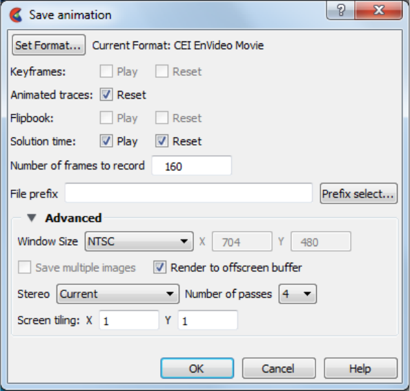
2.13 Saving and Restoring Animations
2-178 EnSight 10.2 User Manual
2.13 Saving and Restoring Animations
If you have transient data, animating traces, a flipbook saved, or a keyframe
animation, then you can save an animation. Do a File>Export Animation... to save
an animation. If you have no animations then the Export Animation will be greyed
out and unavailable. The options that are available will have active toggles. For
example, with a transient dataset with a animating particle trace, do a File>Export
Animation... and you will see the following dialog with Animated Traces and
Solution time toggles available. Choose Play to play the animation and Reset to
first reset to the first animation frame prior to recording the animation. Choose
the number of frames to record, and under the advanced tab choose your options.
Note that if you choose stereo interleaved and pick an image format such as png
you will get a file for the left and a file for the right eye at each timestep with a
mtm master file that can be used to play back your stereo animation in EnVideo. If
you choose a movie format such as mpeg then you will get a left and right movie
file each with all the respective frames in the one file and a mtm master file that
can be used to play back your animation in EnVideo.
Many of the animation options in the dialog below are the same as the options for
saving a graphic image (see Chapter 2.12, Saving Graphic Images).
Both Flipbook and Keyframe Animation processes have save and restore
capability. These are best described in the chapters devoted specifically to these
features.
For Flipbook Animations, see Section 5.7, Flipbook Animation and How To
Create a Flipbook Animation.
For Keyframe Animations, see Section 5.9, Keyframe Animation and How To
Create a Keyframe Animation.
Figure 2-32
Save Animation dialog
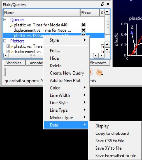
2.14 Saving Query Text Information
EnSight 10.2 User Manual 2-179
2.14 Saving Query Text Information
The data used for curves in EnSight’s plotter and any other information from a
query or otherwise which is presented in the EnSight Message Window can be
saved to a file suitable for printing.
By right-clicking on Query in the Plots/Queries panel, you can access the raw
information using the Data submenu.
Right-click on Query > Data
Copy to clipboard Put the data on the clipboard in a form suitable for pasting into another application, like
Microsoft Excel.
Save CSV to file Save the data to a text file in CSV (Comma Separated Values) format. One csv file will be
saved per selected query. If the query is over distance and the dataset is transient, then the
values of the query over distance will be saved in the file for each timestep from the
beginning timestep specified in the Beg field in the time dialog to the end timestep
specified in End field in the time slider dialog. Change both the Beg and End fields to the
same as the Cur field to save only the current timestep. This does not write command
language and thus does not play back using a command file.
Save XY to file Save the data to a text file in EnSight’s XY format. If the query is over distance then there
will be one file for each timestep from the beginning timestep specified in the Beg field in
the time dialog to the end timestep specified in End field in the time slider dialog. Change
both the Beg and End fields to the same as the Cur field to save only the current timestep.
(see Chapter 9.10, XY Plot Data Format).
Save Formatted to
file
Save the data to a generic ascii file. If the data is a query over distance along a 1D part or
query over distance on the line tool, then the data contains not just the distance and
variable values, but also x, y and z values used to calculate the distance value. If the
Figure 2-33
Saving or Loading XY Plot Data
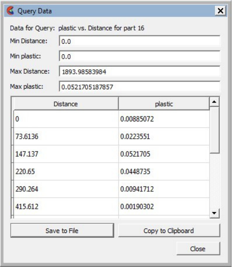
2.14 Saving Query Text Information
2-180 EnSight 10.2 User Manual
dataset is transient, then there will be one file for each timestep of the distance query from
the beginning timestep specified in the Beg field in the time dialog to the end timestep
specified in End field in the time slider dialog. Change both the Beg and End fields to the
same as the Cur field to save only the current timestep.
Display Display the data for the current timestep in two column form in a new window. Also show
the minimum and maximum value for each column.
Save to File Click this button to save the displayed data from the current timestep to a file in CSV
format.
Copy to Clipboard Put the data from the current timestep on the clipboard in a form suitable for pasting into
another application, like Microsoft Excel.
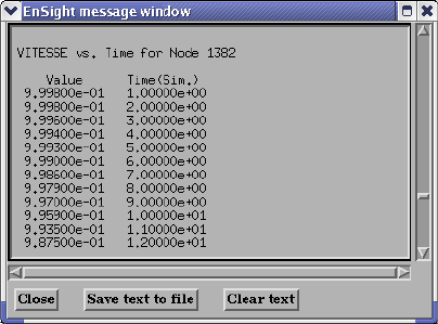
2.14 From EnSight Message Window
EnSight 10.2 User Manual 2-181
From EnSight Message Window
A file suitable for printing can be saved from any operation which places its
information into the EnSight Message Window, such as Show Information queries
and the Query/Plot Show Text... button described previously.
Save Text To File Brings up the typical File Selection dialog from which the information can be saved in the
file of your choice.
Figure 2-34
EnSight Message Window with Save Text To File Button
2.15 Saving Your EnSight Environment
2-182 EnSight 10.2 User Manual
2.15 Saving Your EnSight Environment
EnSight
Preferences
The first time EnSight is run by an individual user, a private preferences directory
is created for that user. A number of different files that control EnSight defaults
are stored in the preferences directory and are read as EnSight starts up. When
reading a preference file, EnSight first looks for the file in the user’s private
preferences directory, and failing that, it looks in the site_preferences directory.
The location of the user’s private preferences directory is shown in the ‘Help-
>Version’ dialog. The different preferences, their files and the file formats are
documented elsewhere in this manual (see Chapter 8, Preference and Setup File
Formats).
Disabling EnSight
Preferences
The command line flag (-no_prefs) can be used to force EnSight to ignore the files
in the user's private preferences directory for a single run of EnSight. This can be
useful to reset various files to their default values or to clear potentially corrupted
caches (see Command Line Start-up Options).
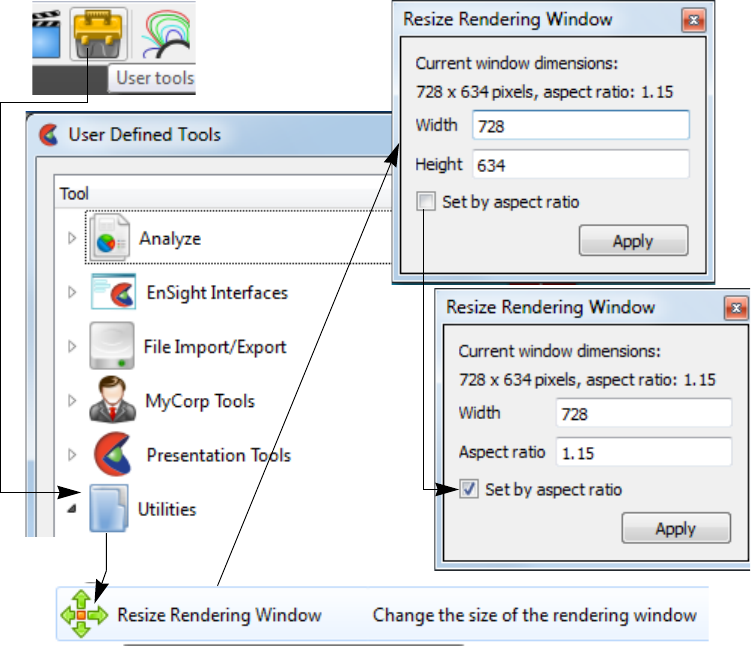
2.16 Saving EnSight Graphics Rendering Window Size
EnSight 10.2 User Manual 2-183
2.16 Saving EnSight Graphics Rendering Window Size
Save Window size
and position
When you exit EnSight, the status of many windows including their size, position
and docking status, are stored in the file {user_prefs_dir}/CEI/EnSight.ini. This
file is not generally editable by an end user. It is described here so that if a user
found a need to reset the window positions, deleting the file listed here would
force EnSight to revert back to its initial window defaults. The file stores the
location of the main window, the Feature Panel, the color editor, the palette editor
and any user-defined panels that were open when EnSight was closed. It also
stores the column names and widths for all of the object lists in EnSight.
Setting Precise
Graphics
Rendering Window
Size
If a user needs to be able to set a specific rendering window size, there is a user-
defined tool included to make it much simpler to specify this. Click on the toolbox
icon to open the User-defined Tools dialog then select: Utilities->Resize
Rendering Window. The Resize Rendering Window dialog is presented (and can
be docked in the main Window):
The dialog shows the current rendering window size in pixels along with the
current aspect ratio. The user can type in values for the width and height to tell
EnSight to resize the rendering portion of the window accordingly. If preferred,
the check box allows the window size to be set via width and aspect ratio.
Aspect ratio is important for preserving the arrangement of plots, labels,
Figure 2-35
Resize Rendering Window dialog
2.16 Saving EnSight Graphics Rendering Window Size
2-184 EnSight 10.2 User Manual
annotations, arrows, legends, etc in the graphics rendering window.
When you resize the window and then quit EnSight, your next session will open
with this size and location of the main window (thus preserving the rendering
window size) assuming you have the same configuration (hardware, OS, fonts,
language, etc).
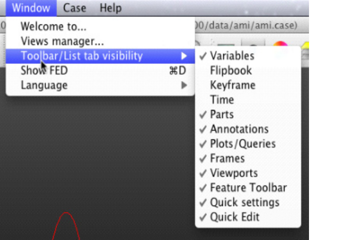
3.1 Overview
EnSight 10.2 User Manual 3-1
3 List Panels
3.1 Overview
The EnSight user interface by default shows several panels on the left side of the
main graphics area. These panels show the list of objects that EnSight knows
about. Panels may be displayed or hidden via the Window->Toolbar/List tab
visibility menu as shown in Figure 3-1. By default list panels are visible for
Parts, Variables, Annotations, Plots/Queries, and Viewports. A Frame list panel is
also available and activated via the menu option. Each of these list panels are
described in the following sections.
All of the list panels share common features and operate in a similar manner. List
panels show objects of a particular type, such as Parts, and list each object one per
line. Some list panels may also show objects arranged in a group hierarchy. For
example, Parts and Variables may be organized into user-defined groups (see
Figure 3-2). Other lists do not support grouping, such as Frames.
Figure 3-1
Window -> Toolbar/List tab visibility
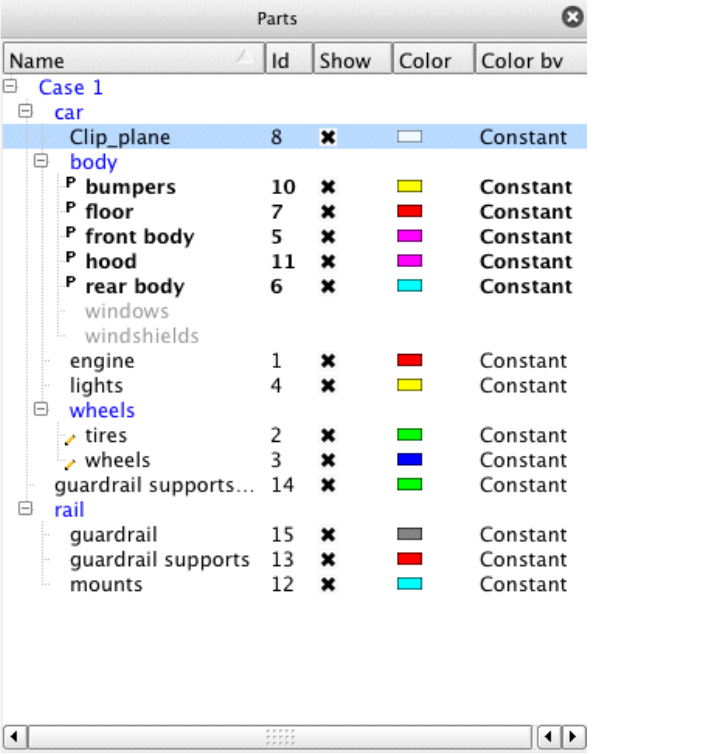
3.1 Overview
3-2 EnSight 10.2 User Manual
List panels can show a user selectable set of columns. Each column corresponds
to a particular object attribute. For example, the Part list panel by default shows
columns for Name, Id, Show, Color, and Color by. These correspond to the
associated Part attributes. Column headers may be clicked to change the sort
order of the list. A second click reverses the sort order for that column. The edge
between columns may be dragged to resize columns. Alternatively, right clicking
on a list panel's column header will display a context sensitive menu (see Figure
3-3) with an option Fit column widths that will resize all columns to an
appropriate size.
Figure 3-2
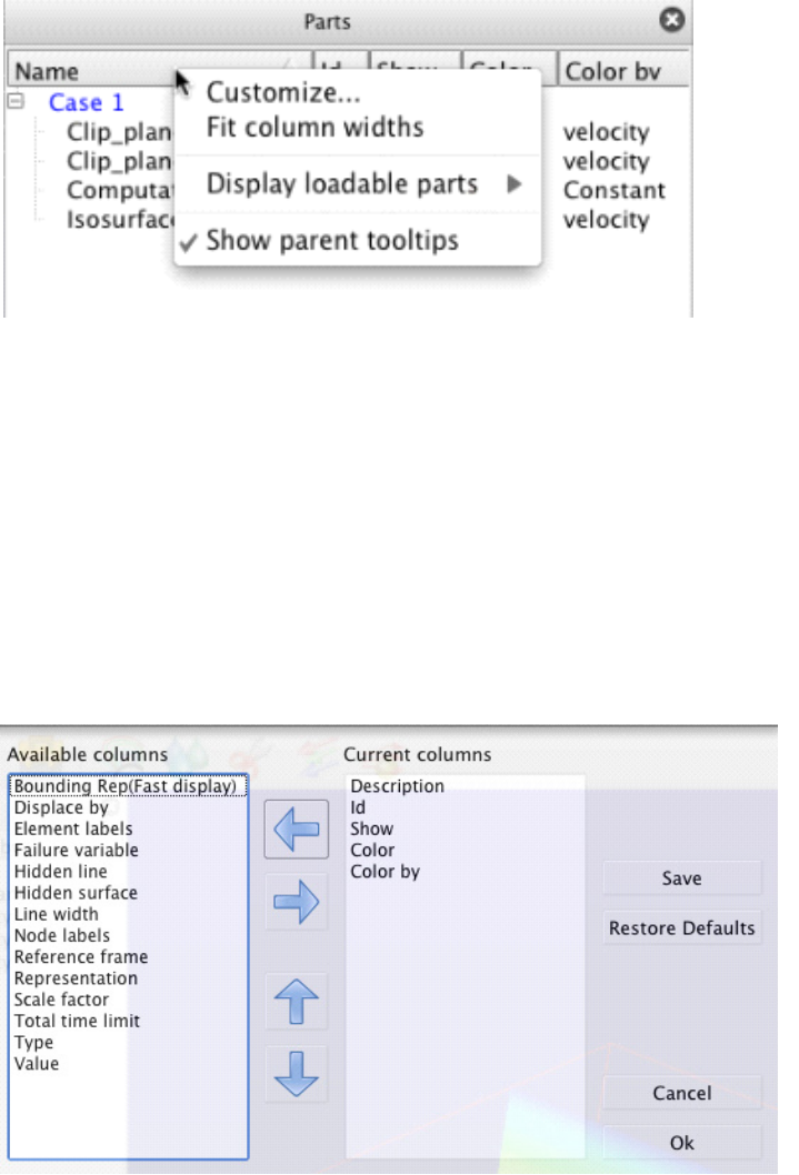
3.1 Overview
EnSight 10.2 User Manual 3-3
Which panel columns and their order are chosen from the same context sensitive
menu. Selecting the Customize… option displays a dialog (see Figure 3-4) for
choosing which columns are displayed and in what order. The dialog shows
available column attributes in the left list and displayed columns in the right list.
The left and right arrows move column attributes between the lists. The up and
down arrows are used to reorder the attributes in the right list. Clicking the Ok
button dismisses the dialog and resets the list panel's columns to the new set of
column attributes. Clicking the Cancel button dismisses the dialog with no
changes. Clicking the Save button operates the same as the Ok button and
additionally saves the changes for future EnSight sessions. The Restore Defaults
button will reset a list panel's attribute columns back to the application defaults.
List panels support drag and drop interaction. In panels that support grouping,
objects may be dragged from one group into another group. Variables support
drag and drop to the Part panel; this interaction causes a part to be colored by the
variable dropped onto it. Variables may also be dragged and dropped into the
main graphics window to color a part or all parts. These interactions are further
described in later sections.
Figure 3-3
Figure 3-4
3.1 Overview
3-4 EnSight 10.2 User Manual
Objects within a panel support two forms of selection: selection and Feature
Panel-selection. A blue background indicates which object or objects are selected
(see Figure 3-2). Selecting objects in a list panel operates very similarly to
making selections in a Microsoft Windows Explorer window or a Macintosh
Finder window. Objects are selected by clicking once on the object. Clicking on
a different object selects that object and deselects the former selection. Clicking
while holding down the Ctrl-key toggles selection. Clicking while holding down
the Shift-key extends a selection. Clicking while holding down the Alt- or Cmd-
key performs a disjoint selection. Lastly, clicking on an empty line of a list panel
deselects all objects.
Selected objects may be deleted by pressing the Del-key. A confirmation dialog
will appear to confirm the deletion.
An object or objects are made Feature Panel selected by either double clicking on
them or by choosing the context sensitive menu option Edit… The Feature Panel,
or Feature Editor Dialog, is used to perform or complicated interactions on
objects. It is described in detail in Chapter 6 of this manual. Feature Panel
selected objects are indicated by a little pencil icon drawn to the left of an object's
name as shown in Figure 3-2. It is important to distinguish between normal
selection and Feature Panel selection. The Feature Editor Dialog operates on
objects that are Feature Panel selected, those with the pencil icon next to their
name; whereas, the rest of the EnSight user interface operates on objects that are
normally selected.
List panels have a context sensitive menu that is displayed by right clicking on an
object or the background of a list panel. The contents of this pop-up menu depend
upon the particular list panel and what is selected. Typically, the pop-up menu
contains options for Edit…, Delete, and grouping (if the list panel supports
grouping). As previously mentioned, Edit… will make the current selection the
Feature Panel selection for that list panel and then display the Feature Editor
Dialog if it is not already displayed. Delete will simply delete the selected
object(s). If grouping is supported for the particular list panel, then options for
creating, deleting, and renaming groups will be available. The specific context
sensitive menus for each list panel type will be described in the following
sections.
List panels are a form of dockable panel. Dockable panels can be dragged and
placed elsewhere on the main user interface or even dragged off of the user
interface to make the panel a standalone window. Clicking a panel's 'x' button in
the upper right corner of the panel will hide the panel. Dragging and dropping a
panel onto another panel will stack the panels together thus making a tabbed
group with one tab per panel; this interaction is commenced by dragging on a
panel's header. Additionally, dragging a panel's edge will resize the panel or panel
group. These interactions allow the user to reorganize the user interface into a
more desirable configuration based on user preference.
Because list panels are a form of dockable panel, you may also see them stacked
with non-list panels such as the panels for Time, Flipbooks, and Keyframes.
Furthermore, User Defined Tools may also have a user interface that utilizes a
dockable panel.

3.2 Part List Panel
EnSight 10.2 User Manual 3-5
3.2 Part List Panel
The Part list panel displays four types of objects:
1. model parts - parts defined by the dataset;
2. cases - an object that represents a particular dataset;
3. LPARTS - parts that are not necessarily loaded from a dataset but could be;
4. derived parts - parts that are created within EnSight.
The Part list panel supports both user-defined groups as well as data set defined
groups (if the data format and reader supports groups). Figure 3-2 shows a single
dataset as indicated by Case 1. The dataset defines four groups: car, body, wheels,
rail. All other objects are model parts except for the groups, Case 1, windows,
windshields, and Clip_plane. Windows and windshields are LPARTs and are
indicated as such by their gray text. Clip_plane is a derived part and is indicated
as such by the 'P' icon to the left of its parent parts: bumpers, floor, front body,
hood, and rear_body. Clip_plane is also the selected part as indicated by its blue
background. Parts tires and wheels are the current Feature Panel selected parts as
indicated by the pencil icon to the left of their names.
Because the Part list panel supports grouping, objects within the list panel may be
drag and dropped between groups. The context sensitive menu also has
operations related to groups.
3.2.1 Default View
Figure 3-2 also shows the default view for the Part list panel. By default the list
panel has columns for Name, Id, Show, Color, and Color by as described in the
next section. Name is the default sort column. Clicking on a different column
header will change the sort.
The column header context sensitive menu has additional options for how
LPARTS should be displayed and an option for whether part-based tooltips should
be displayed (see Figure 3-3). LPARTS can be set to always be shown, never
shown, or only shown if the associated part is not loaded; this is the default. Part-
based tooltips are shown when the mouse is held stationary over a part name.
They indicate if the part is a model part or if it's a derived part; and, if it is a
derived part, what its parent parts are.
3.2.2 Attributes
Selecting the Customize… option from the column header context sensitive menu
displays a dialog for choosing which part attributes to display and in what order.
Table 3.1 lists the available attributes.
Tab le 3.1
Bounding Rep How the elements should be drawn while the scene is being
actively moved.
Color The part color when not colored by a variable.
Color by Whether the part is colored by a variable or a constant color.
Description The name of the part.
Displace by The name of the optional variable used to apply node
displacements.
Element labels Whether element labels are displayed for the part.
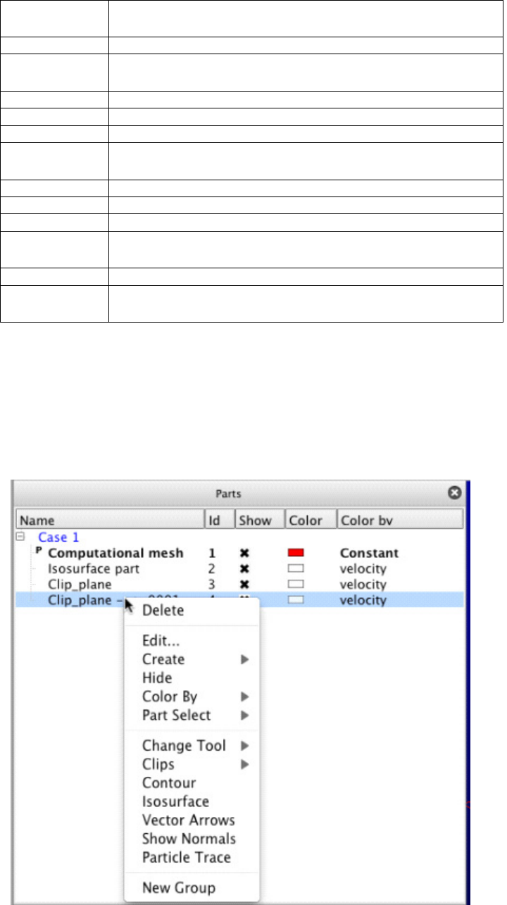
3.2 Part List Panel
3-6 EnSight 10.2 User Manual
3.2.3 Right Mouse Button Actions
The context sensitive menu for the Part list panel varies depending on what the
mouse is over in the Part list panel when the mouse is right-clicked. Figure 3-5
shows the menu when the context menu is displayed while over a part. The menu
shows an appropriate subset of options if the mouse is over the background, the
Case name, or a group name. Table 3.2 describes the various menu options that
may be available.
Failure
variable
The name of the optional variable used to indicate element
failure.
Hidden line Whether hidden line rendering applies to the part.
Hidden
surface
Whether hidden surface rendering applies to the part.
Id The part id number.
Line width The element line thickness (1-4).
Node labels Whether node labels are displayed for the part.
Reference
frame
The coordinate frame number the part belongs.
Representation How elements are drawn for the part.
Scale factor The scaling factor applied to elements.
Show The part visibility status.
Total time
limit
Total emission time for particle trace parts.
Type The part type (e.g. model, clip, particle trace).
Value The special value for certain part types (e.g. isosurface
value).
Figure 3-5

3.2 Part List Panel
EnSight 10.2 User Manual 3-7
Tab le 3.2
Delete Deletes the currently selected items. If the deleted
part(s) are model parts, they will be deleted and the list
will then show the associated LPART depending upon
the setting of the ‘Display loadable parts’ menu option
previously described.
Edit… Displays the Feature Panel with the current selection
marked for editing. Items marked for editing by the
Feature Panel will have a pencil icon displayed to the
left of their name.
Create The submenu lists the derived parts that may be created
using the currently selected parts as parent parts. See
Figure 3-6. Choosing one of the derived part types will
display the Feature Panel, if it is not already visible,
and place it in create mode for the selected type. The
currently selected part(s) will be used as the parent(s)
for the newly created part.
Hide / Show Toggles visibility off/on for the currently selected
part(s).
Color By Parts can be colored by a constant color (e.g. Red) or
false (pseudo) colored by a variable. Select Variable
will display the variable chooser dialog. Figure 3-7
shows this submenu. Figure 3-8 shows the variable
chooser dialog whereas Figure 3-9 shows the color
picker dialog. Choosing the menu option Make
Transparent will make the part 50% transparent.
Adjust Transparency… will display the
transparency adjustment slider dialog (see Figure 3-10).
Part Select Several menu options are available for setting the
current part selection. See Figure 3-11 for the submenu
and Table 3.3 for a description of the options.
Change Tool This menu item is only visible if the selected part is a
clip part. Selecting one of the items changes the type of
tool used to create the clip part. See Figure 3-15.
Clips Creates a clip part using the currently selected part(s) as
the parent part(s). It differs from the Create menu
option in that the Feature Panel is not displayed. See
Figure 3-16.
Contour Creates a contour part using the currently selected
part(s) as the parent part(s). The Variable Chooser
dialog is displayed to select the variable to use for the
contour calculation. It differs from the Create menu
option in that the Feature Panel is not displayed.

3.2 Part List Panel
3-8 EnSight 10.2 User Manual
Isosurface Creates an isosurface part using the currently selected
part(s) as the parent part(s). The Variable Chooser
dialog is displayed to select the variable to use for the
isosurface calculation. The midpoint value of the
selected variable is the value used for the isosurface.
This option differs from the Create menu option in that
the Feature Panel is not displayed.
Vector Arrows Creates a vector arrow part using the currently selected
part(s) as the parent part(s). The Variable Chooser
dialog is displayed to select the variable to use for the
vector arrows if there is more than one vector variable
available. It differs from the Create menu option in that
the Feature Panel is not displayed.
Show Normals Creates a vector arrow part where the arrows represent
part element normals.
Particle Trace Creates a particle trace part using the currently selected
part(s) as the parent part(s). The Variable Chooser
dialog is displayed to select the variable to use for the
part if there is more than one vector variable available.
It differs from the Create menu option in that the
Feature Panel is not displayed.
New Group Creates a new group is containing the currently selected
parts.
Create new group Creates a new empty group.
Rename group… A dialog is displayed to rename the currently selected
group.
Delete group Deletes the selected group. Contained parts are moved
to the group’s parent.
Rename case… A dialog is displayed to rename the case name.
Load part Depending on the selected LPART either the
Unstructured or the Structured Part Loader dialog will
display. These are describe later.
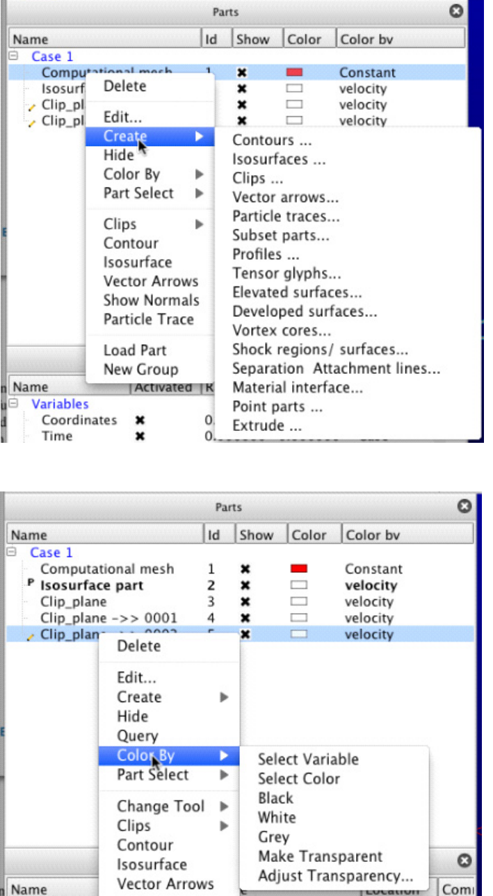
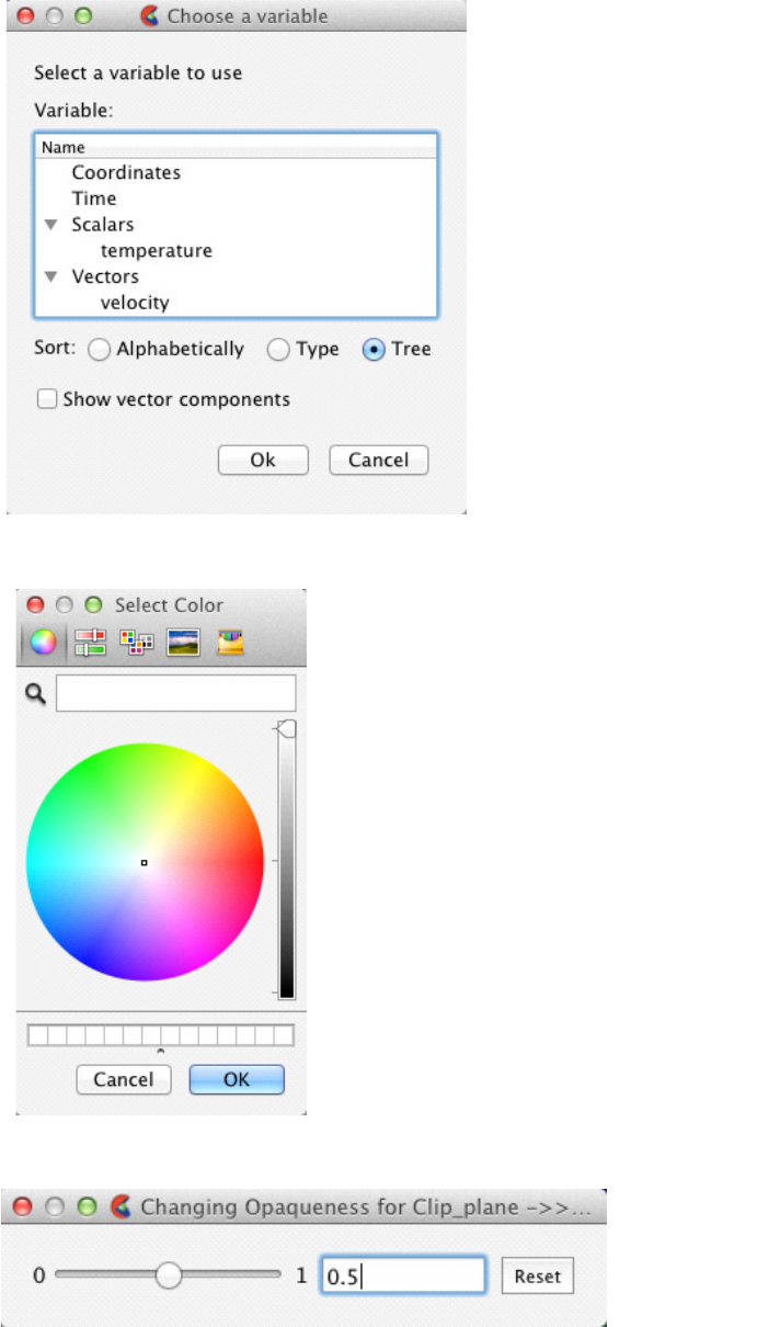
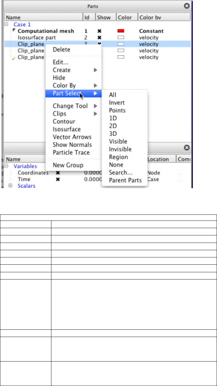
3.2 Part List Panel
EnSight 10.2 User Manual 3-11
Tab le 3.3
All Select all parts
Invert Inverts the current part selection
Points Selects only point parts
1D Selects only parts with 1D elements
2D Selects only parts with 2D elements
3D Selects only parts with 3D elements
Visible Select parts that are have their visibility attribute on
Invisible Select parts that are have their visibility attribute off
Region Selects parts underneath the region tool (see Figure 3-12).
If the region tool is not displayed in the graphics window,
then this option will display it and indicate that it must be
first visible via a message dialog. Once the region tool is
displayed, this option will then select all the parts,
overlapping or not, that are contained within the region tool.
None Deselects all parts
Search… Displays the Search Parts By Keyword dialog (see Figure
3-13). Parts are selected that match the specification
indicated in the dialog.
Parent Parts Selects the parent parts of the currently selected part(s). If
no parts are selected, then a Select Parent Parts dialog is
displayed (see Figure 3-14).
Figure 3-11
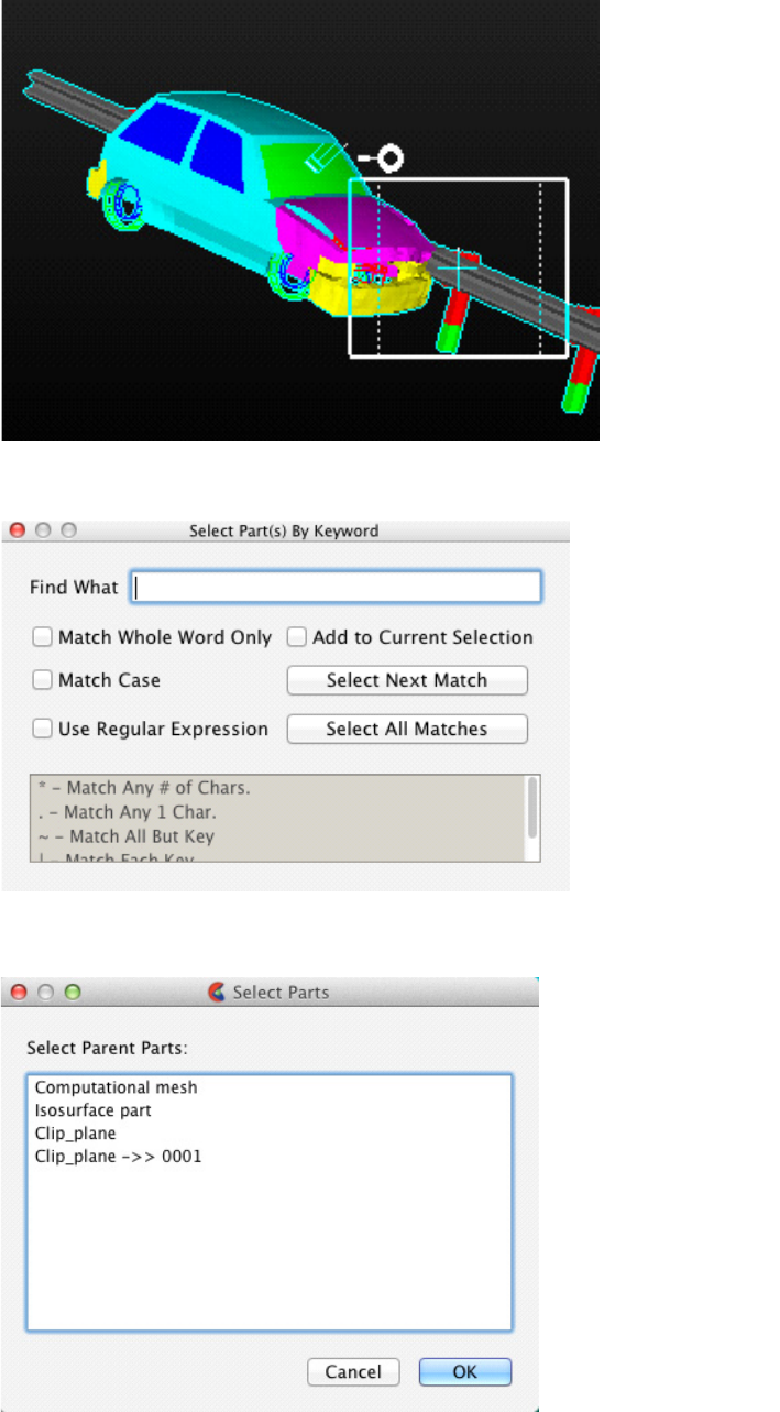
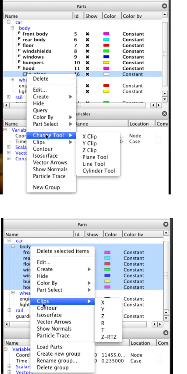
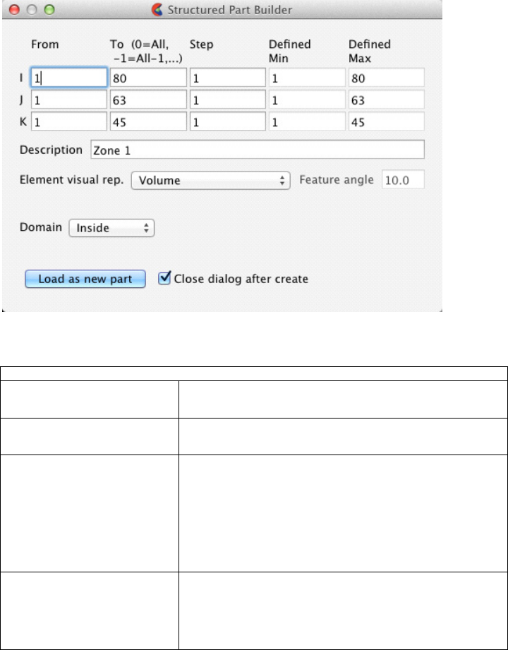
3.2 Part List Panel
3-14 EnSight 10.2 User Manual
If the Load Part option is selected over an unstructured LPART, the dialog shown
in Figure 3-17 is displayed to load the associated part. Table 3.4 describes the
fields in the dialog. If Load Part option is selected over a structured LPART, the
dialog shown in Figure 3-18 is displayed. Table 3.5 describes the fields for that
dialog.
Tab le 3.4
Element visual rep. The sets the element visual representation for the
part.
Feature angle The number of degrees for feature angle element
representation.
Description The name to use for the part once it is loaded.
This value is initialized with the name found in the
data set. If multiple parts are loaded
simultaneously, this input is inactive and the
loaded parts will use the names found in the data
set.
Close dialog after create If unchecked, the dialog stays open to allow
loading of the same part multiple times. This may
be useful if you wish to display the same part with
different attributes.
Figure 3-17
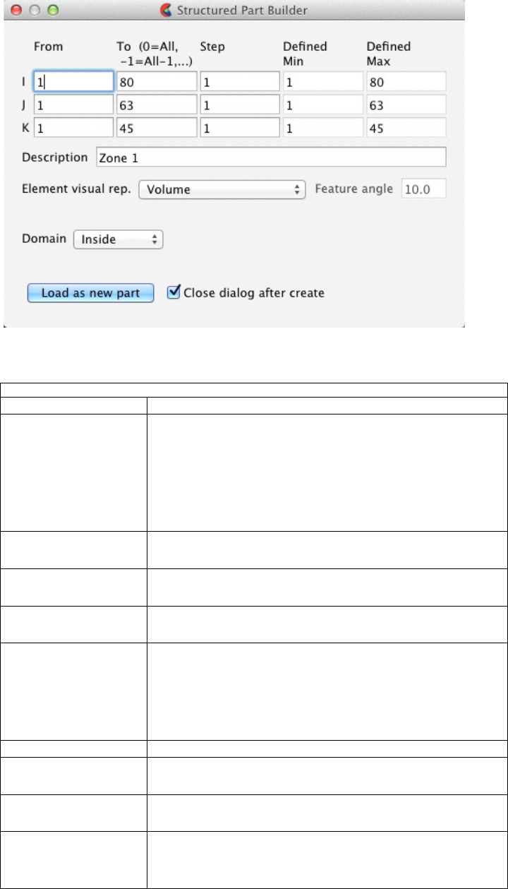
3.2 Part List Panel
EnSight 10.2 User Manual 3-15
Tab le 3.5
From (I,J,K) The starting values along the I,J,K axes.
To (I,J,K) The ending values along the I,J,K axes. For
convenience, zero may be specified to represent the
maximal value. Negative values indicate values N less
than the maximal values (e.g. -2 means 2 less than the
maximal value). Zero and negative values are useful
when loading multiple structured parts simultaneously.
Step (I,J,K) The I,J,K stride. Steps greater than 1 are useful for
loading reduced resolutions of the part(s).
Defined Min (I,J,K) The actual minimum values for the I,J,K axes as
defined by the dataset.
Defined Max (I,J,K) The actual maximum values for the I,J,K axes as
defined by the dataset.
Description The name to use for the part once it is loaded. This
value is initialized with the name found in the data set.
If multiple parts are loaded simultaneously, this input is
inactive and the loaded parts will use the names found
in the data set.
Element visual rep. The sets the element visual representation for the part.
Feature angle The number of degrees for feature angle element
representation.
Domain Ibanking domain to use, Inside (iblank value of 1), or
outside (iblank value of 0)
Close dialog after
create
If unchecked, the dialog stays open to allow loading of
the same part multiple times. This may be useful if you
wish to display the same part with different attributes.
Figure 3-18
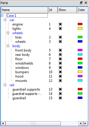
3.2 Part List Panel
3-16 EnSight 10.2 User Manual
3.2.4 Part Group Visual Transformations
EnSight part groups include the ability to apply a collection of rigid body
transforms to a group which, in turn, transforms the parts in that group.
Additionally, transformations for nested groups are applied in a hierarchical
fashion. This allows for a grouping in the part tree to apply local transformations
in local reference frames. For example, a group might specify the rotation of a tire
over its axle. While a higher level transform could specify motion relative to the
body of the car itself.
These transforms occur on the EnSight client and are visual only. Thus, for
example, they are not included in calculations done on the server.
Applying grouping to the car crash example part list may result in a display as
follows
A group transformation on the ‘wheels’ group will change the coordinates of parts
2-3 and a group transformation on the ‘body’ group will change the coordinates of
parts 5-12. A transformation applied to the ‘car’ group will be applied to parts 2-3
after the ‘wheels’ transformation and parts 5-12 after the ‘body’ transformation as
well as parts 1 and 4.
The group transformation can be modified using the transformation dialog that
can be accessed by right clicking on the group and selecting the
‘Edit group transform…’ option. If the user right clicks on the “car” group and
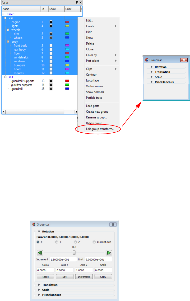
3.2 Part List Panel
EnSight 10.2 User Manual 3-17
chooses “Edit group transform...” then the dialog will look as follows:
The dialog is always connected to the group that was right clicked, and the dialog
does not change the target group based on selection. This allows for multiple
group dialogs to be open at the same time, each editing a different group. The title
of the dialog shows the group the dialog is transforming. For example, notice
above that the title of the dialog is Group: car.
There are three basic transformations: Rotation, Translation and Scale as well as
some additional options in the Miscellaneous category. Each section can be
opened by clicking on the associated section turn down. Unlike EnSight frames,
the individual transformations are maintained independently. This and the
hierarchical nature of groups makes it a simpler to modify individual
transformation.
Rotation section
3.2 Part List Panel
3-18 EnSight 10.2 User Manual
This section controls the rotation property of the group transformations. The
current rotation is always displayed at the top of the section as the axis of rotation
(the normal as nx, ny, nz) and the angle in degrees (default axis 0.0, 0.0, 1.0, and
default angle 0.0 degrees). The buttons below that value can be used to select the
specific axis that the slider below it controls “X”, “Y”, “Z” or “Current axis”. The
‘Current axis’ option will rotate over the axis listed at the top of the section. The
slider allows the user to interactively increment/decrement the angle over selected
axis. The slider will temporarily modify the rotation and apply the result when the
slider is released, at which point it will snap back to the center and the current
rotation will be updated at the top. The buttons on the right and left will
increment or decrement the angle by the ‘Increment’ value noted below.
Dragging the slider all the way to the right or left will result in the axis value
changing by the ‘Limit’ amount (the default is -90, +90 degrees).
The rotation can be explicitly set by entering values into the ‘Axis X’, ‘Axis Y’,
‘Axis Z’ and ‘Angle’ fields and clicking ‘Set’ or incremented by the fields by
clicking ‘Increment’. The ‘Copy’ button can be used to copy the current rotation
values into the fields, which can be useful with ‘Set’ to be an undo operation for
example. Finally, the ‘Reset’ button will set the rotation values back to their
default values of 0.0, 0.0, 1.0, 0.0.
By default, the rotation is applied about the global origin located at 0.0, 0.0, 0.0.
If another origin is desired, use the Centroid offset option in the Miscellaneous
section (discussed later, below).
For example, when you first open the dialog, you find the values Current: 0,0,1,0
This is the default value. It corresponds to a rotation around the axis (0,0,1) of an
angle 0. Every time you apply a rotation, the value of Current is updated. It gives
you the axis and angle of rotation that you should apply to the initial configuration
of the group in order to get the position of the group elements you are seeing now.
In other words, it gives you the composition of all the rotations that you have
applied to the group. Now, if you apply first a rotation of angle=90 degrees
around the axis (0,0,1) (that corresponds to axis Z) and then a rotation of angle =
90 degrees around the axis (0,1,0) (that corresponds to axis Y), the value of
Current is (0.5774, 0.5774, -0.5774) and angle = 120.0. If you now do "reset", so
that the group has no initial rotation, and make a rotation around axis (0.5774,
0.5774, -0.5774) of angle 120 by putting these values by hand, you see that the
result you obtain is the same.
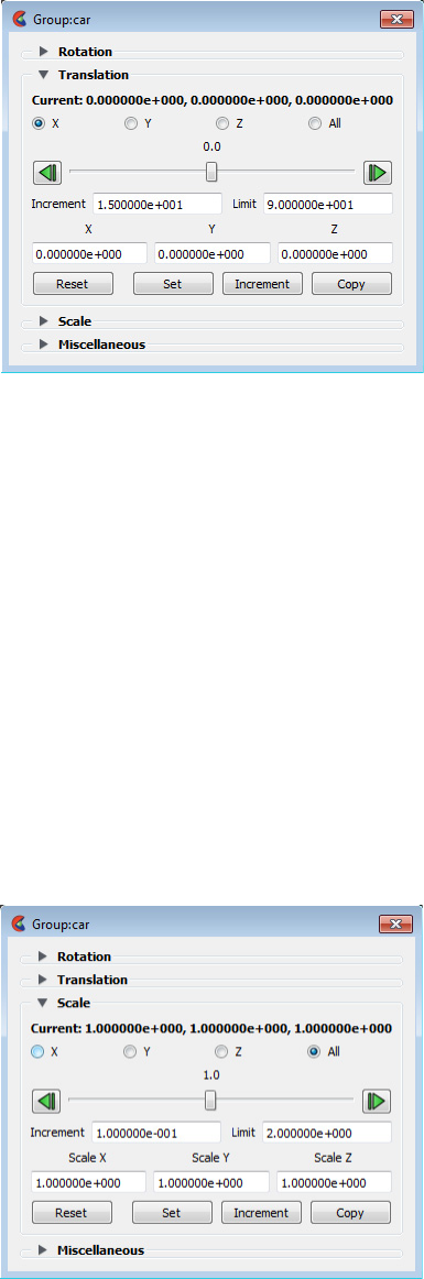
3.2 Part List Panel
EnSight 10.2 User Manual 3-19
Translation section
This section controls the translation property of the group transformations. The
current translation in X, Y, Z is always displayed at the top of the section. The
buttons below that value can be used to select the specific axis that the slider
below it controls. The slider allows the user to interactively modify the selected
axis. The slider will temporarily modify the translation and apply the result when
the slider is released, at which point the slider will snap back to the center. The
buttons on the right and left will increment or decrement the axis value by the
‘Increment’ value noted below. Dragging the slider all the way to the right or left
will result in the axis value changing by the ‘Limit’ amount.
The translation can be explicitly set by entering values into the ‘X’, ‘Y’ and ‘Z’
fields and clicking ‘Set’ or incremented by the ‘X’, ‘Y’ and ‘Z’ fields by clicking
‘Increment’. The ‘Copy’ button can be used to copy the current translation values
into the ‘X’, ‘Y’ and ‘Z’ fields, which can be useful with ‘Set’ to be an undo
operation for example. Finally, the ‘Reset’ button will set the translation to 0.0,
0.0, 0.0 .
Scale section
This section controls the scale property of the group transformations. The current
scaling factor in X, Y, Z is always displayed at the top of the section. The buttons
below that value can be used to select the specific axis that the slider below
controls. Selecting “All” scales all geometry uniformly. Selecting “X”, “Y” or “Z”
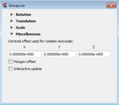
3.2 Part List Panel
3-20 EnSight 10.2 User Manual
will result in anisotropic scaling of the geometry only in that axis direction.
The slider allows the user to interactively modify the scaling. The slider will
temporarily modify the scale and apply the result when the slider is released, at
which point it will snap back to the center. The buttons on the right and left will
increment or decrement the axis value by the ‘Increment’ value noted below.
Dragging the slider all the way to the right or left will result in the axis value
changing by the ‘Limit’ amount.
The scale factor can be explicitly set by entering values into the ‘Scale X’, ‘Scale
Y’ and ‘Scale Z’ fields and clicking ‘Set’ or incremented by the ‘Scale X’, ‘Scale
Y’ and ‘Scale Z’ fields by clicking ‘Increment’. The ‘Copy’ button can be used to
copy the current scale values into the ‘Scale X’, ‘Scale Y’ and ‘Scale Z’ fields,
which can be useful with ‘Set’ to be an undo operation for example. Finally, the
‘Reset’ button will set the scale values to 1.0, 1.0, 1.0. By default, the scale is
applied about the global coordinate 0.0, 0.0, 0.0 . If another origin is desired, use
the Centroid offset option in the Miscellaneous section.
And this scaling occurs only on the EnSight Client and is visual only, and
therefore does not affect server calculations, such as, for example, volume.
Miscellaneous section
There are three options in this section.
Centroid offset
When the rotation and scale portions of the transformations are applied, by default
they are applied about the point 0.0, 0.0, 0.0 in model space. In the case of rotation
in particular, this can result in rotation about an undesirable location. Consider a
wheel with its center located at 2987, -1514, 266. The default rotation will be
about a point some distance from the center of the wheel. One option is that one
could put the wheel in its own group that translates -2987, 1514, -266 and then
apply a rotation transform to a group above that group. This scenario is fairly
common, so it has been built into the group transformation. In the Miscellaneous
section, one can specify a ‘Centroid offset used for rotation and scale’ (in our
example, enter 2987, -1514, 266). With this set, the rotation and translation will
be applied about this point instead.
Polygon offset
3.2 Part List Panel
EnSight 10.2 User Manual 3-21
Many models have coincident geometry, which are parts that have the exact same
nodes and polygons, for example a fluid inside of a container. The display of these
polygons can look rather odd in many cases, particularly when the one or more of
the parts are translucent (e.g. a translucent fluid inside a solid container). The
Polygon offset option specifies that parts which are children of this group will be
drawn slightly behind parts that are not in groups with polygon offset set.
It can be important to offset the correct part to get the desired behavior. For
example, in the case of a translucent fluid inside of a container, you would put the
fluid in a group and set this polygon offset to draw the fluid slightly behind
(inside) the container. Setting the container polygon offset would cause undesired
behavior as it would slightly offset the container inside of the fluid.
Surface restricted particle traces along the inside surface of the container should
be grouped and offset so that they are moved slightly behind (inside the
container). Conversely surface restricted particle traces along the outside of a
surface should not be offset: rather the surface itself should be offset in this case
so that it is moved slightly behind the external particle traces.
Or, consider two identical clips R and B colored red and blue respectively with R
placed in a group with Polygon offset enabled. Now, B will always be drawn in
front of R, no matter what the viewing angle. If B is made translucent, R will
become visible through B.
Interactive update
By default, the graphics rendering is only updated when the user releases the
mouse when dragging on the various sliders. This works well for large models,
but for smaller models, checking this box will update the graphics rendering
dynamically while the various manipulation sliders are dragged.
Other Options for Part Transformation
Please be aware that EnSight includes a number of Other Options for Part
Translation, Rotation and/or Scaling of EnSight geometry.
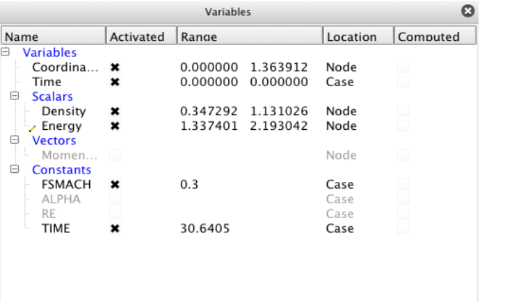
3.3 Variables List Panel
3-22 EnSight 10.2 User Manual
3.3 Variables List Panel
The Variables list panel displays both variables defined by the dataset and those
created within EnSight. Variables created within EnSight can either be calculated
using EnSight's calculators or by activating Extended CFD Variables or Boundary
Layer Variables.
The Variables list panel supports groups both defined by the dataset (if supported
by the dataset and data reader) as well as user-defined groups. Variables may be
drag and dropped between groups. By default the Variables list panel has groups
for Scalars, Vectors, and Constants. Variables are automatically placed into the
appropriate group based upon their type. Figure 3-19 shows the Variables list
panel.
The Variables list panel also supports drag and drop of variables from the
Variables list panel into the Parts list panel or main graphics window. Variables
that are dropped onto part(s) color those part(s) by the dragged variable. If the
variable is dropped onto the background of the Parts list panel or into the
background of the main graphics window, then all parts are colored by the
variable.
As with all list panels, selected variables have a blue background. Feature Panel
selected variables have a pencil icon to the left of their names.
3.3.1 Default View
Figure 3-19 shows the default view for the Variables list panel. By default it
shows columns for Name, Activated, Range, Location, and Computed. These
variable attributes are described in the following section.
The Variables list panel header context sensitive menu has only the standard two
options for Customize… and Fit column widths as described earlier in this
chapter.
3.3.2 Attributes
Selecting the Customize… option from the column header context sensitive menu
displays a dialog for choosing which variable attributes to display and in what
Figure 3-19
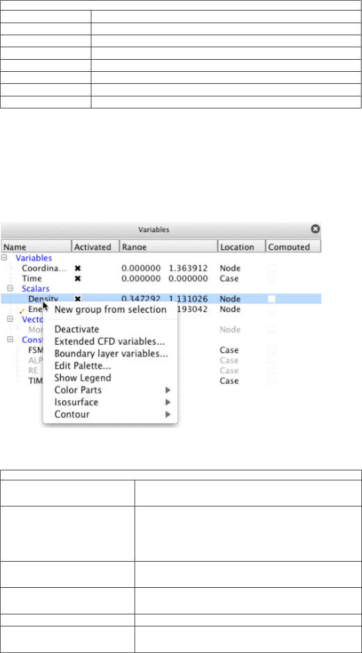
3.3 Variables List Panel
EnSight 10.2 User Manual 3-23
order. Table 3.6 lists the available attributes.
3.3.3 Right Mouse Button Actions
The context sensitive menu for the Variables list panel varies depending on what
the mouse is over in the Variables list panel when the mouse is right-clicked.
Figure 3-20 shows the menu when the context menu is displayed while over a
variable. The menu shows an appropriate subset of options if the mouse is over
the background, the Variable name, or a group name. Table 3.7 describes the
various menu options that may be available.
Tab le 3.6
Activated Indicates whether the variable is loaded into EnSight
Computed Indicates whether the variable is calculated by EnSight
Constant Value Displays the value for constants.
Description The name of the variable.
Exists in case Indicates which cases the variable exists.
Location Indicates whether the variable is node or element centered.
Range The value of constants or extrema for other variable types.
Type The type of the variable (e.g. Scalar, Vector).
Tab le 3.7
New group from selection Creates a new group containing the selected
variables.
Activate / Deactivate Loads or unloads the selected variables into
EnSight. Note that unloading a variable will
delete any part(s) or derived variables dependent
upon the deactivated variable.
Extended CFD variables… Displays the Extended CFD variables dialog (see
Figure 3-21 and the description below).
Boundary layer variables… Displays the Boundary layers variables dialog
(see Figure 3-22 and the description below).
Edit Palette… Displays the palette editor dialog.
Show Legend Displays a legend in the graphics window for the
selected variable(s).
Figure 3-20
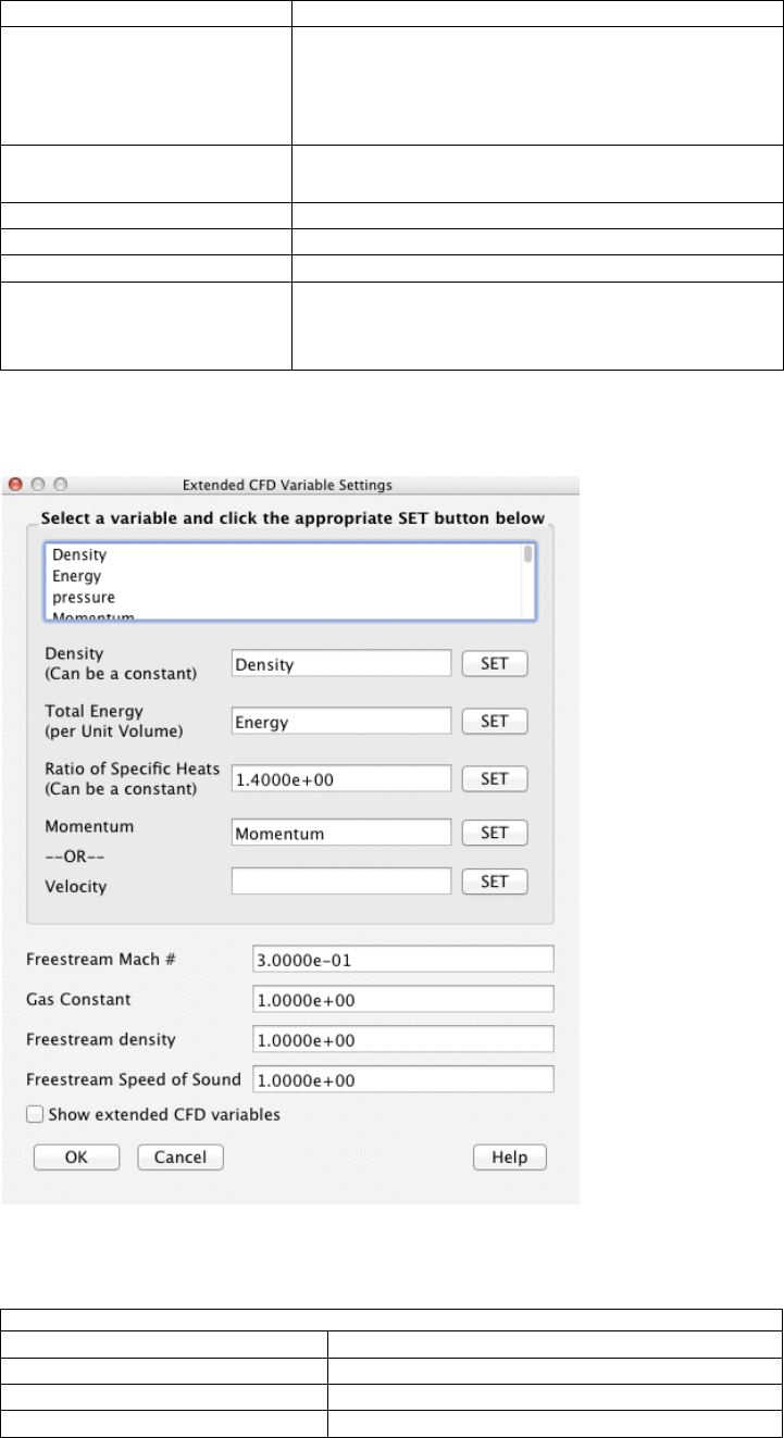
3.3 Variables List Panel
3-24 EnSight 10.2 User Manual
The Extended CFD variables dialog is used to…..GET TEXT AND TABLE
DESCRIPTIONS FROM MEL OR OLD DOC. (See Figure 3-21). Table 3.8
describes the fields in the dialog.
Color Parts Colors all parts by the selected variable.
Isosurface Creates an isosurface part for the selected
variable using all parts as the parent parts and
using the variable’s median value as the
isosurface value.
Contour Creates a contour part for the selected variable
using all parts as the parent parts.
New Group Creates a new group.
Delete Group Deletes the selected group.
Rename Group… Displays a dialog to rename the selected group.
Create Annotation Displays the selected Constant variable’s value
as a smart annotation in the main graphics
window.
Tab le 3.8
Density
Total Energy
Ratio of Specific Heats
Momentum
Figure 3-21
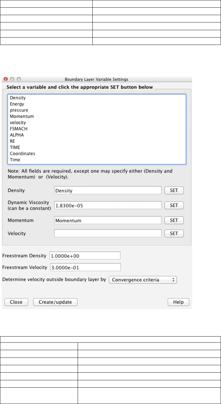
3.3 Variables List Panel
EnSight 10.2 User Manual 3-25
The Boundary Layer Variable dialog is used to…..GET TEXT AND TABLE
DESCRIPTIONS FROM MEL OR OLD DOC. (See Figure 3-22). Table 3.9
describes the fields in the dialog.
Velocity
Freestream Mach #
Gas Constant
Freestream density
Freestream Speed of Sound
Show extended CFD variables
Tab le 3.9
Density
Dynamic Viscosity
Momentum
Velocity
Freestream Density
Freestream Velocity
Determine velocity
outside boundary layer by
Figure 3-22
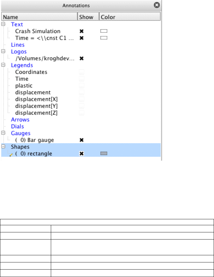
3.4 Annotations List Panel
3-26 EnSight 10.2 User Manual
3.4 Annotations List Panel
The Annotations list panel displays the various EnSight created annotations
including Arrows, Dials, Gauges, Legends, Lines, Logos, Shapes, and Text. The
Annotations list panel does not support drag and drop. As with all list panels,
selected annotations have a blue background. Feature Panel selected annotations
have a pencil icon to the left of their names.
3.4.1 Default View
Figure 3-23 shows the default view for the Annotations list panel. By default it
shows the columns for Name, Show, and Color.
The Annotations list panel header context sensitive menu has only the standard
two options for Customize… and Fit column widths as described earlier in this
chapter.
3.4.2 Attributes
Selecting the Customize… option from the column header context sensitive menu
displays a dialog for choosing which annotation attributes to display and in what
order. Table 3.10 lists the available attributes.
Table 3.10
Color A color swatch indicating the color of the annotation.
Description The name of the annotation.
Justification Left, center, or right justification indicator for Text
annotations.
Show Visibility toggle for annotations.
Size The size of the annotation.
Type The type of the annotation.
Figure 3-23
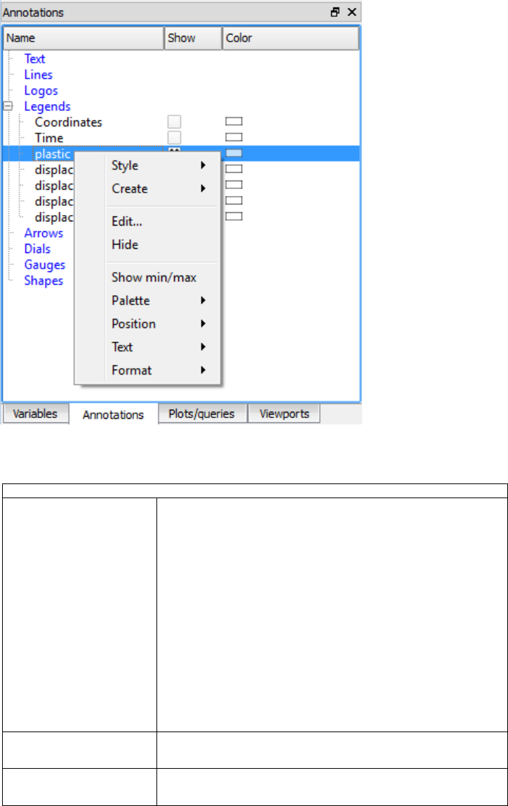
3.4 Annotations List Panel
EnSight 10.2 User Manual 3-27
3.4.3 Right Mouse Button Actions
The context sensitive menu for the Annotations list panel varies depending on
what the mouse is over in the Annotations list panel when the mouse is right-
clicked. Figure 3-24 shows the menu when the context menu is displayed while
over a legend. Table 3.11 describes the various menu options that may be
available.
Tab le 3.11
Style This allows you to manipulate the legend style. A
style is a collection of all the object attributes.
Create from Object - This will create a legend
style using all the attributes of the selected leg-
end.
Copy - This will copy the legend style from the
selected legend
Paste - This is used to paste the selected style onto
another legend to change many attributes
simultaneously to match the copied style.
Open Style Manager - Open the legend style man-
ager to see the styles that you have saved.
Create Options to create any of the annotation types: text,
line, logo, arrow, dial, gauge, or shape.
Edit… Makes the selected annotations Feature Panel selected
and opens the Feature Panel if not already displayed.
Figure 3-24

3.4 Annotations List Panel
3-28 EnSight 10.2 User Manual
Hide / Show Toggles the visibility of the annotation.
Delete Deletes the selected annotation.
Show Min/Max Displays visual markers and text on a legend to
indicate the current minimum and maximum values.
Palette Legend options; see Table 3.12.
Position Options to position a color legend near the top,
bottom, right, or left edges of the main graphics
window.
Text Legend options to adjust the text size, color, and
legend title.
Format Legend option for various numerical formats
explicitly listed in the pulldown.
Color Options to set the color for Line or Text annotations.
Black, White, or Grey may be chosen directly or the
Color Picker dialog may be selected.
Arrows Options to turn on/off arrows at either end of Line
annotations.
Line Width Options to set the line width of Line annotations.
Adjust size… Displays a size slider for Text annotations.
Justification Options for Left, Center, and Right justification for
Text annotations.
Rotate Options for +90, 180, -90 rotations for Text
annotations.
Font… Displays the Font Chooser dialog for Text
annotations.
Table 3.12
Banded Sets the legend’s colors to a banded format.
Continuous Sets the legend’s colors to a continuous format.
Clear Color Bands Deletes all color band markers from the legend. Color
band markers are added via the Palette dialog’s
Markers tab.
Set values to min/max Sets the legend’s range to match the minimum and
maximum values of the associated variable.
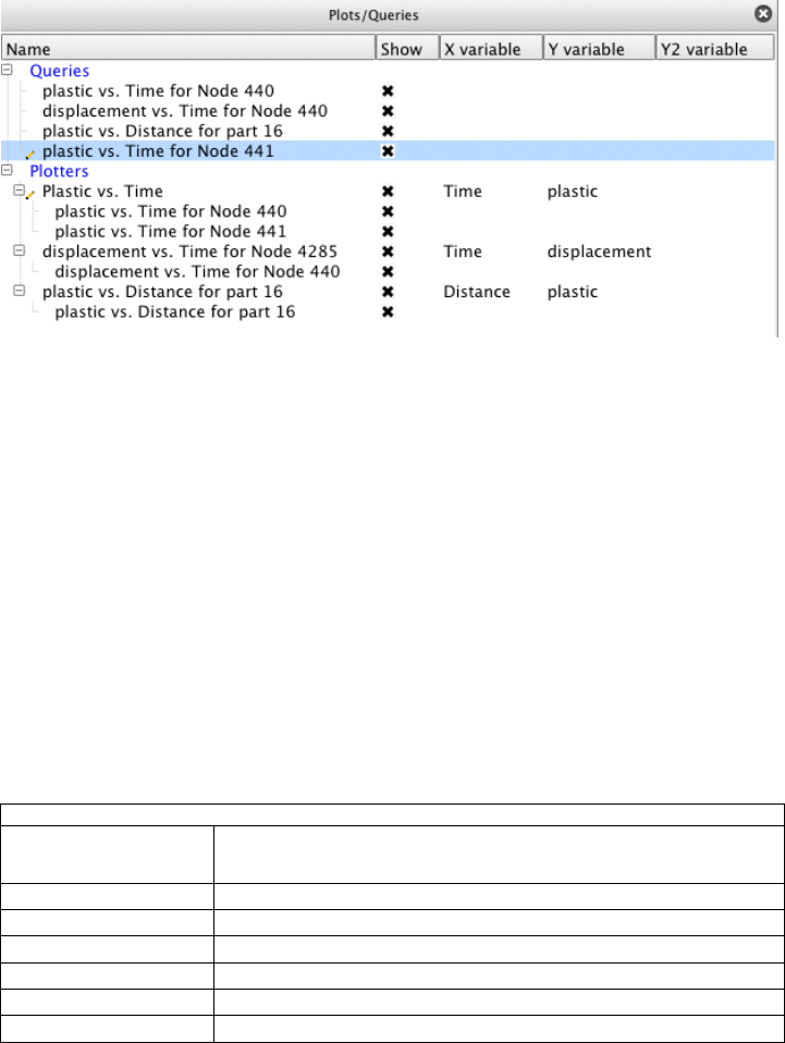
3.5 Queries/Plotters List Panel
EnSight 10.2 User Manual 3-29
3.5 Queries/Plotters List Panel
The Plots/Queries list panel shows both queries (XY data) and plotters (XY plots).
As shown in Figure 3-25 the list panel has groups for Queries and Plotters. All
queries are listed as children of the Queries group. The Plotters group lists all
plotters. Additionally, each plotter lists the queries it contains. Queries may or
may not be assigned to plotters. A query may also be assigned to multiple
plotters. The Plots/Queries list panel does not support further grouping. Queries
may be dragged and dropped onto plotters to assign and show the query on the
plotter.
As with all list panels, selected queries and plotters have a blue background.
Feature Panel selected queries and plotters have a pencil icon to the left of their
names.
3.5.1 Default View
Figure 3-25 shows the default view for Plots/Queries list panel. By default it
shows columns for Name, Show, X variable, Y variable, Y2 variable. These
attributes are described in the following section.
The Plots/Queries list panel header context sensitive menu has only the standard
two options for Customize… and Fit column widths as described earlier in this
chapter.
3.5.2 Attributes
Selecting the Customize… option from the column header context sensitive menu
displays a dialog for choosing which plotter and/or query attributes to display and
in what order. Table 3.13 lists the available attributes.
Table 3.13
Background color A color swatch indicating the background color of the
plotter.
Background type A background type (None or Solid color) of the plotter.
Description The name of the plotter or query.
Distance The length of the query if it is an over distance query.
Marker color A color swatch indicating the marker color on the query.
Marker scale The marker scaling factor for the query.
Marker visibility An indicator for marker visibility.
Figure 3-25
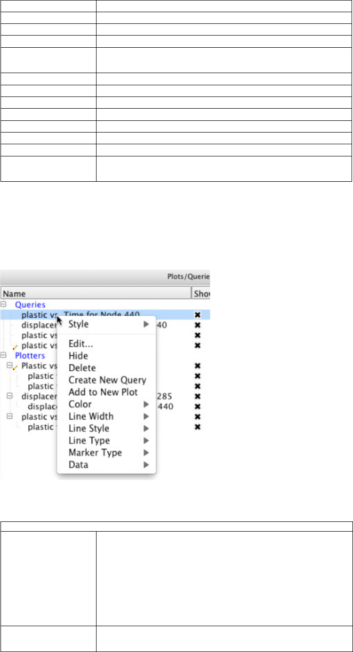
3.5 Queries/Plotters List Panel
3-30 EnSight 10.2 User Manual
3.5.3 Right Mouse Button Actions
The context sensitive menu for the Plots/Queries list panel depends on whether
the mouse is over a query (see Figure 3-26) or a plotter (see Figure 3-27). Table
3.14 describes the options for queries and Table 3.15 shows the options for the
Data submenus and Table 3.16 describes the options for plotters.
Normalize X An indicator if the X values have been normalized.
Normalize Y An indicator if the Y values have been normalized.
Query color A color swatch indicating the color of the query curve.
Query line style The query curve line style (Solid, Dotted, Dashed).
Query line type The query curve line type (None, Connect the dots,
Smooth).
Query offset X and Y offset values
Query scale X and Y values scale factor
Query width The width of the query curve.
Variable 1 The name of the Y variable
Variable 2 Name of second variable, if applicable
X variable The variable shown on the X axis of the plotter.
Y variable The variable shown on the Y axis of the plotter.
Y2 variable The variable shown on the opposite Y axis of the plotter
if two different Y types are plotted simultaneously.
Table 3.14
Style The style manager allows the user to copy a selection of
attributes (e.g. color, linestyle, etc) from one object and
apply them to another.
Create from object - create a style from this object
Copy - Copy this object’s style
Paste - Paste a previously copied style onto this object
Open Style Manager - Open manager
Edit… Makes the selected queries Feature Panel selected and
opens the Feature Panel if not already displayed.
Figure 3-26

3.5 Queries/Plotters List Panel
EnSight 10.2 User Manual 3-31
Hide / Show Toggles the visibility of the query.
Delete Deletes the query.
Create New Query Opens the Feature Panel to create a new query.
Add to New Plot Adds the selected queries to a new plotter.
Color Options to set the color for the query. Red, Green, or
Blue may be chosen directly or the Color Picker dialog
may be selected.
Line Width Sets the line width of the query curve.
Line Style Sets the line style of the query curve (Solid, Dotted, or
Dashed).
Line Type Sets the line type of the query curve (None, Connect the
dots, Smooth).
Marker Type Sets the marker type for the query curve (None, Dot,
Circle, Triangle, Square).
Data See table 3.15 for the options for the Data submenu.
Table 3.15
Display Displays a dialog containing the query data along with
useful metrics.
Copy to clipboard Copies the query XY data to the system clipboard so
the values may be pasted into another application such
as a spreadsheet.
Save to CSV file Writes the query XY data to a file in Comma
Separated Value (CSV) format.
Save to EnSight XY
file
Writes the query into EnSight’s XY format (see Chapter
9.10, XY Plot Data Format).
Save to ASCII file Writes the query data into a generic ascii format
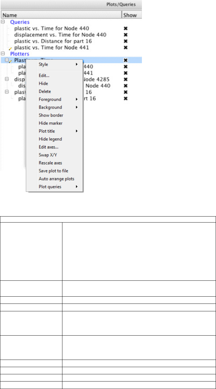
3.5 Queries/Plotters List Panel
3-32 EnSight 10.2 User Manual
Table 3.16
Style The style manager allows the user to copy a selection of
attributes (e.g. color, linestyle, etc) from one object and
apply them to another.
Create from object - create a style from this object
Copy - Copy this object’s style
Paste - Paste a previously copied style onto this object
Open Style Manager - Open manager
Edit… Makes the selected plotters Feature Panel selected and
opens the Feature Panel if not already displayed.
Hide / Show Toggles the visibility of the plotter.
Delete Deletes the plotter.
Foreground Options to set the foreground color for the plotter.
Black, White, or Grey may be chosen directly or the
Color Picker dialog may be selected.
Background Options to set the background color for the plotter.
None, Black, White, or Grey may be chosen directly or
the Color Picker dialog may be selected.
Hide/Show Border Toggles the visibility of the plotter border.
Hide/Show Marker Toggles the visibility of plotter markers.
Plot Title Options to set the plot title color and size via dialogs.
Hide/Show Legend Toggles the visibility of the plotter legend.
Figure 3-27

3.5 Queries/Plotters List Panel
EnSight 10.2 User Manual 3-33
Edit Axes… Makes the selected plotters Feature Panel selected and
then opens the Feature Panel to the appropriate panel
for adjusting axis attributes.
Swap X/Y Swaps the X and Y axes.
Rescale Axes Rescales the axes based upon current query data shown
in the plotter.
Save plot to file This is a quick save of only the selected plot(s) to a png
file(s) at the resolution of the graphics screen. This will
pop up a dialog to name the file (or to get a file prefix
name for a number of files) and a toggle to allow for a
white background. Use File>Export> Image for more
options.
Auto arrange plots This will automatically arrange all of the visible plots
into a uniform grid over the graphics screen area.
Plot queries This allows fast, simultaneous changes to all of the
queries in a single plot. The following sub-menus
are available:
Unique Colors - This will color each query a unique
color based on its index using a user-selected pal-
ette of colors. This selection will pop up a dialog
with a single pulldown of all of the available pal-
ettes in EnSight.
Toggle Markers - If markers are visible, this will tog-
gle markers visibility off. If markers are off then
this will toggle marker visibility on and it will
assign a list of markers to each query in a round-
robin fashion.
Toggle Linestyle - If lines are not all solid, then this
will toggle linestyle to all solid. If linestyles are all
solid then this will toggle a list of linestyles to each
query in a round-robin fashion.
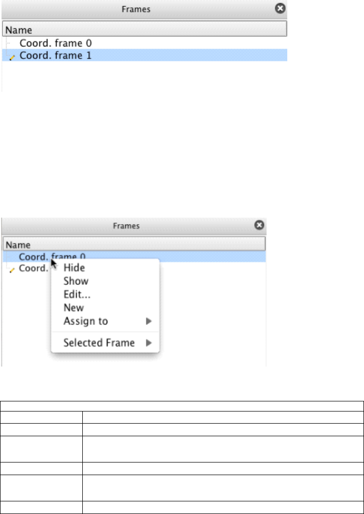
3.6 Frames List Panel
3-34 EnSight 10.2 User Manual
3.6 Frames List Panel
The Frames list panel shows the list of available coordinate frames within
EnSight. This list panel does not support groups nor drag and drop.
As with all list panels, selected frames have a blue background. Feature Panel
selected frames have a pencil icon to the left of their names.
3.6.1 Default View
Figure 3-28 shows the default view.
3.6.2 Attributes
The Frames list panel supports only a single frame attribute: Name.
3.6.3 Right Mouse Button Actions
Figure 3-29 shows the context sensitive menu for the Frames list panel and Table
3.17 describes its options.
Table 3.17
Hide Hides the frame in the graphics window.
Show Shows the frame in the graphics window.
Edit… Makes the selected frames Feature Panel selected and opens
the Feature Panel if not already displayed.
New Creates a new frame.
Assign to Options for adding the selected part(s) or all parts to the
selected frame.
Selected Frame DELETE THIS OPTION.
Figure 3-28
Figure 3-29
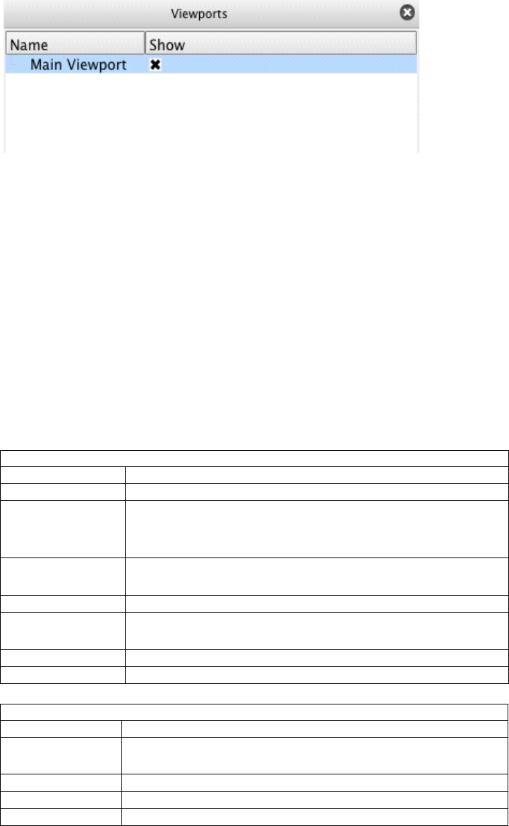
3.7 Viewports List Panel
EnSight 10.2 User Manual 3-35
3.7 Viewports List Panel
Figure 3-30 shows the Viewports list panel. It contains the default viewport
(Viewport 0) and any additional viewports created within EnSight. The Viewports
list panel does not support grouping. Parts may be dragged and dropped onto
viewports to assign and show the parts in the viewport.
3.7.1 Default View
Figure 3-30 shows the default view for Viewports list panel. By default it shows
columns for Name and Show. These attributes are described in the following
section.
The Viewports list panel header context sensitive menu has only the standard two
options for Customize… and Fit column widths as described earlier in this
chapter.
3.7.2 Attributes
Selecting the Customize… option from the column header context sensitive menu
displays a dialog for choosing which viewport attributes to display and in what
order. Table 3.13 lists the available attributes.
Table 3.13
Border visible Toggles the viewport’s border visibility.
Description The name of the viewport.
Dimension Indicates highest dimensionality of parts drawn: 2D or 3D.
If set to 2D, only 2D and lower dimensionality parts will be
visible.
Hidden line Toggles whether hidden line drawing applies to the
viewport.
Hidden surface Toggles whether shaded drawing applies to the viewport.
Perspective Toggles between whether perspective or orthographic
drawing will be used.
Show Toggles viewport visibility.
Track Indicates the type of viewport tracking (see Table 3.14).
Table 3.14
Off No camera tracking is used.
Node number The specified node number is kept in the center of the
viewport.
Part centroid The part centroid is kept in the center of the viewport.
Part xmin The viewport will follow the minimum x value.
Part xmax The viewport will follow the maximum x value.
Figure 3-30

3.7 Viewports List Panel
3-36 EnSight 10.2 User Manual
3.7.3 Right Mouse Button Actions
Table 3.15 describes the context sensitive menu options for viewports.
Part ymin The viewport will follow the minimum y value.
Part ymax The viewport will follow the maximum y value.
Part zmin The viewport will follow the minimum z value.
Part zmax The viewport will follow the maximum z value.
Table 3.15
Style The style manager allows the user to copy a selection
of attributes (e.g. color, linestyle, etc) from one object
and apply them to another.
Create from object - create a style from this object
Copy - Copy this object’s style
Paste - Paste a previously copied style onto this object
Open Style Manager - Open manager
Edit… Makes the selected viewports Feature Panel selected
and opens the Feature Panel if not already displayed.
Hide / Show Toggles the visibility of the viewport.
Delete Deletes the selected viewport(s).
New Creates a new viewport.
Copy Transformation Copies the current transformation values for the
selected viewport.
Paste Transformation Pastes the previously copied transformation values
into the selected viewport.
Link Links the selected viewports together so same
transformation (e.g. rotate, translate, scale) is applied
to all linked viewports.
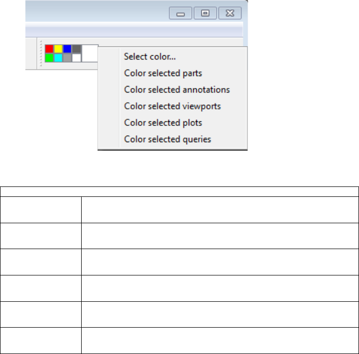
3.8 Quick Color Widget Panel
EnSight 10.2 User Manual 3-37
3.8 Quick Color Widget Panel
Figure 3-31 shows the Quick Color Widget. Right click on this widget and choose
an option from the pulldown as described in Table 3.17.
Table 3.17
Select color... Pops up a color selection dialog to allow you to customize a
patch color.
Color selected
parts
Color the selected part(s) by the constant color patch.
Color selected
annotations
Color the selected annotation(s) by the constant color patch.
Color selected
viewports
Color the selected viewport(s) by the constant color patch.
Color selected
plots
Color the selected plot(s) by the constant color patch.
Color selected
queries
Color the selected query(s) by the constant color patch.
Figure 3-31
EnSight 10.2 User Manual 4-1
4Main Menu
This chapter describes the functions available from the Main Menu.
4.1, File Menu Functions
4.2, Edit Menu Functions
4.3, Create Menu Functions
4.4, Query Menu Functions
4.5, View Menu Functions
4.6, Tools Menu Functions
4.7, Window Functions
4.8, Case Menu Functions
4.9, Help Menu Functions
Figure 4-1
EnSight Main Menu
Note that each of these menus, with the exception of the Case Menu,
has a shortcut pulldown using the Alt key and the first letter of the Menu:
that is Alt-f will pull down the Fle menu, Alt-e will pull down the Edit menu, etc.
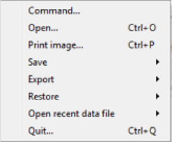
4.1 File Menu Functions
4-2 EnSight 10.2 User Manual
4.1 File Menu Functions
The Main Menu File menu provides access to basic file input and output
operations as well as the command language and Python interpreter tools.
Specifically, users can record and play command files, load data into the current
EnSight session/server, print and save images, record currently running
animations, save and restore various files, archives, and scenarios, and quit from
EnSight.
File Pull-down Menu
Command... Opens the Command dialog which is used to record and play Command Files or enter
command language directly
Main Menu > Command...
(see 2.5, Command Files and How To Record and Play Command Files and 7.1, Python
EnSight module interface in the Interface Manual)
Open... Opens the Open... dialog used to load a new dataset into the current EnSight session.
(see Reading and Loading Data Basics, in Section 2.1 and How to Read Data)
Print image... Opens the Print/save image dialog which is used to print the currently rendered image
through the platform specific printing system.
(see 2.12, Saving Graphic Images, and How To Print/Save an Image)
Save Allows the user to choose between the following sub-menu options: Session, Context,
Commands from this session, Full backup.
Session... Opens the Save current session dialog where you can specify the name
of a session file to be created. A session file is a single file that
incorporates a context file (see the ‘Context...’ menu option) and
potentially the dataset itself in a compressed datafile. Context files are
logged in the ‘Welcome’ screen for quick access and (if they include
the packed data option) allow an entire EnSight session to be
exchanged between EnSight users
(See How To Save and Restore a Session File).
(See How To Save or Restore a Context File)
Context... Opens the Save current context dialog where you can specify the name
of a context file to be created. This file saves information needed to
reproduce the same basic processing steps on a different set of data.
This is faster than replaying a command file because it skips the
intermediate steps and takes you directly to the end, but not all formats
restore a context properly.
(See How To Save or Restore a Context File)
Figure 4-2
File pull-down menu
4.1 File Menu Functions
EnSight 10.2 User Manual 4-3
Commands from
this session
Opens the File selection dialog where you can specify the name of a
file into which all the commands used up to this point in the session
will be placed.
(See How To Record and Play Command Files)
Full backup... Opens the Save full backup archive dialog which is used to save an
entire session as an archive file which can later be used to restore
EnSight to the same condition present when the archive file was made.
A full backup is a memory dump of the client and server to disk and is
suitable for a fast restore of the session the next day. It is not a good
option for long term archival purposes as the file format can change in
a non-backwardly compatible fashion with major EnSight releases.
Also, some data formats do not support backup and restoring archives
at all.
(see 2.6, Archive Files and How To Save and Restore an Archive)
Export Allows the user to export a file that is the choose between the following sub-menu
options: Animation, Scenario, Image, or Geometric entities.
Animation... Opens the Save animation dialog which is used to record the running
flipbook, animated trace animation, or record an animation of a
transient dataset by varying its solution time. It will not be available if
no animation is currently running and the current dataset is not
transient.
(See How to Animate Transient Data, How to Create a Flipbook
Animation, How To Animate Particle Traces, and How To Use
Raytrace Rendering)
Scenario... Opens the Save scenario dialog where you can create a scenario file
which can be viewed by CEI’s EnVision (.evsn) or Reveal (.csf)
products. EnVision and Reveal can display the geometry of scenes
created with EnSight in an interactive format. These tools are run
separately from EnSight. Users without EnSight license may
download EnVision separately as a free product.
(See How To Save Scenario)
Image.... Opens the Save image dialog used to save an image of the current
scene at any resolution and with various quality settings to any of the
supported image file formats.
Geometric
entities...
Opens the Export geometric entities dialog which is used to save
selected part geometry and active variable values from EnSight. One
common use of this function is to convert an existing dataset into
EnSight Gold format which can often be read more efficiently by
EnSight. Supported formats include: EnSight Gold, VRML 2.0, Brick
of Values (volume rendering of variables in 3D Part(s)), or User-
defined writer formats (e.g. flatfile, Exodus II, STL) can be selected
(see 2.10, Saving Geometry and Results Within EnSight and How To
Save Geometric Entities)
Restore Allows the user to choose between the following sub-menu options: restore a context, a
full backup archive file, or a session file.
Context... Opens the Restore context from file dialog where you can specify the
name of a context file to be read and which case to apply it to. First
read in your data then restore the context. The system will attempt to
create the same parts and variables as were present when the context
file was saved, using the data from the currently loaded dataset.
(See How To Save or Restore a Context File)
4.1 File Menu Functions
4-4 EnSight 10.2 User Manual
Full backup... Opens a file selection dialog which is used to specify the archive file to
be restored into EnSight. This will bring EnSight to the same condition
present when the archive file was saved.
(see 2.6, Archive Files and How To Save and Restore an Archive)
Session... Opens a file selection dialog that can be used to open a saved session
(.ens) format file. If the file contains a dataset, the dataset is extracted
to temporary disk space. The context in the session is then restored
(See How To Save and Restore a Session File).
Open recent data file This menu contains a sub-menu of the most recently loaded datasets. The menu is
specific to the server that is currently attached to the client. Selecting an item from the
sub-menu will cause the dataset to be reloaded. A dialog allows the user to replace the
currently loaded data or start a new case.
Quit... Opens the Quit confirmation dialog which allows you to save a command file or/and an
archive file before exiting EnSight.
(see Section 2.6, Archive Files)
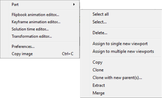
4.2 Edit Menu Functions
EnSight 10.2 User Manual 4-5
4.2 Edit Menu Functions
Clicking the Edit button in the Main Menu opens a pull-down menu which
provides access to the following features:
Part Opens a pull-down menu which allows you to choose between the following part
operations:
Select All Select all of the parts, see How To Select Parts)
Select... Bring up a dialog that allows for expression-based selection of
parts, see How To Select Parts)
Delete... Delete the currently selected parts. Note that deleted parts appear
as greyed out parts and disappear from the graphics window.
They can be reloaded using a right-click on the parts, see How
To Delete a Part)
Assign to single new
viewport
Create a new viewport and cause only the currently selected parts
to be visible in it.
Assign to multiple new
viewports
For each selected part, create a new viewport and make just that
individual part visible in the new viewport.
Copy Make a shallow copy of the selected part(s) that only exists on
the client for visualization purposes, (see How To Copy Parts)
Clone A cloned part is a replica of the selected part(s). A cloned model
part is an independent, reloaded model part with its attributes
updated to match the original. A cloned created part recreates the
created part with all of the attributes updated to match the
original, including the parentage (see How To Clone a Part).
A cloned part inherits model variables, but not calculated
variables from the selected part(s). If you wish to have calculated
variables available on the cloned part then you must perform this
step using the calculator.
Clone with new
parent(s)
Make a replica of the selected part(s) with a different set of
parent part(s) vs. the originals (see How To Clone a Part).
Extract Create a part from the current visual representation of the
selected part(s), see How To Extract Part Representations)
Figure 4-3
Edit pull-down menu
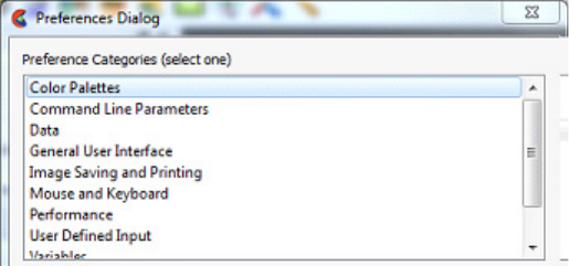
4.2 Edit Menu Functions
4-6 EnSight 10.2 User Manual
Merge Create a single part by merging the elements of the selected
part(s), see How To Merge Parts)
Flipbook animation
editor...
Opens the Flipbook animation editor in the Feature Panel which is used to load, run, and
modify Flipbook animation sequences.
(see 5.7, Flipbook Animation and How To Create a Flipbook Animation)
Keyframe animation
editor...
Opens the Keyframe animation editor in the Feature Panel which is used to create, save,
restore, run, and modify Keyframe animation sequences.
(see 5.9, Keyframe Animation and How To Create a Keyframe Animation)
Solution time editor... Opens the Solution time editor in the Feature Panel which is used to specify the currently
displayed time step in a transient dataset.
Main Menu > Edit > Solution time editor...
(see 5.10, Solution Time and How To Animate Transient Data)
Transformation editor... Opens the Transformation editor dialog which is used to precisely position parts, frames,
and tools in the Graphics Window and to Save and Restore Views.
(see Chapter 6, Transformation Control)
Copy Image Takes a snapshot of the contents of the graphics window and places it in the system
clipboard so that it may be pasted into other applications.
Preferences... Opens the Preferences dialog which is used to set or modify preferences within EnSight.
In this area you can set default attributes and preferences which will be used for the
current EnSight session. You may also save any of these to various preference file(s) so
that they will be the defaults for future invocations of EnSight. Preferences are divided
into several categories listed at the top of the dialog. Selecting one will change the lower
section of the dialog to reflect the selected category. Note that on the Macintosh computer,
the Edit menu does not have this entry because preferences on a Macintosh application are
found under the ensight10.client menu
The individual preferences categories are covered in more detail in the next few sections
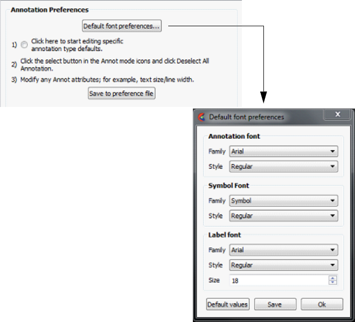
4.2 Edit Menu Functions
EnSight 10.2 User Manual 4-7
Annotation
Preferences
Default Font
preferences...
This option brings up the Font Preferences Dialog that allows for
several of the default font typefaces and styles to be set as shown
below:
Annotation font/style The ‘Annotation’ font is the font used for text annotations. The
dialog allows one to set the default font family and style, but the
actual font used can be change with each individual text
annotation.
Symbol font/style The ‘Symbol’ font is the font used for symbols.
Label font/style/size The ‘Label’ font is the font used for node and element labels,
contour labels, etc.
Default values Hitting this button will set things back to the default fonts.
Save Hitting this button will save your choices for future enSight
sessions.
Ok Hitting this button will use your choices for this session. It will
not save them for future sessions.
Click here to start Brings up the Feature Panel for the annotation feature. At this
point, any changes one makes to the various Feature Panel
options are actually editing the defaults for annotations and not
an actual annotation.
Save to preference file Once the defaults have been set, clicking this button will save
them for future invocations of EnSight
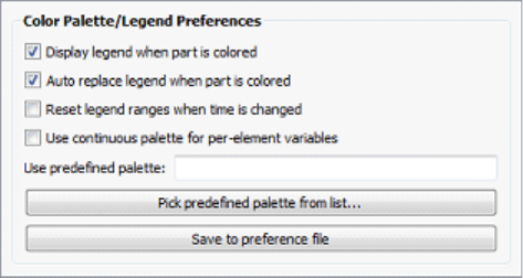
4.2 Edit Menu Functions
4-8 EnSight 10.2 User Manual
(see Setting Annotation Defaults)
Color Palettes
Preferences
Display legend when
part is colored
When this option is ON (default) EnSight will turn on legends
that are needed and turn off legends that are not needed. Does not
attempt to replace one legend with another.
Auto replace legend
when part is colored
When this option is ON (default) and user is coloring a part by a
variable, will find a legend that is not needed and replace it with
the legend for the new variable. The new variable legend will
utilize the display attributes from the legend not needed such as
location, size, layout, etc. If no legend can be found that is no
longer needed no action will be taken, thus this option is best
used with the "Display legend when part is colored" option
above.
Reset legend ranges Will cause legend ranges to be reset according to variable values
at the current time.
Use continuous
palette for per element
vars
By default the legend for Per Element variables has a “Type” set
to Constant. Toggle this on to change the default “Type” to
Continuous.
Use predefined palette Allows one to enter a predefined palette name if you have
predefined color palettes.
Pick predefined
palette from List...
Allows one to pick from your predefined palette list.
Save to preference file Will write the current legend and palette preferences to the
preference file for future EnSight sessions.
(see How To To Set Color Palette Defaults:)
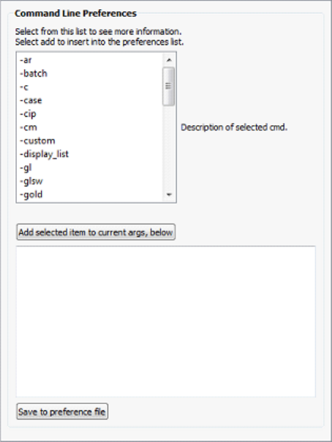
4.2 Edit Menu Functions
EnSight 10.2 User Manual 4-9
Command Line
Parameter
Preferences
In this panel, select some number of arguments and add them to the current args list. On
startup, EnSight will act as if the arguments in the list were added to the command line.
Select a command line argument from the list to see details for the argument to the right of
the list. Once selected, one may click the buttons below or edit the argument directly in
the text edit box (see Command Line Start-up Options).
Add selected item to
current args below
Add the selected argument to the list of default arguments.
Save to preference file Saves the command line preferences to the preference file for
future invocations of EnSight.
(see How To To Set Color Palette Defaults:)

4.2 Edit Menu Functions
4-10 EnSight 10.2 User Manual
Data Preferences These items control which readers are available to load data and allows for some control
over their default values.
Default data directory Specify the directory the server will start up in by default.
Binary files are Allows you to specify the default byte order for binary files. The
allowable settings are Big-endian, Little-endian, or Native
(default) to server machine. Note that virtually all machines have
gone to the Intel processor which is little-endian, so native or
little-endian will work on all recent files and big endian may be
necessary only for legacy files.
If starting time step is
not specified load
Can be set so that the default starting time step for transient data
can be either Last step or First step.
When reading data
automatically load
Allows you to have EnSight automatically load All parts, First
part, Last part, or No parts at startup.
N-faced
decomposition
Three methods are available for handling polyhedral cells, named
according to how they decompose the polyhedral into internal
regular tetrahedrons: centroid, convex clipper, concave clipper.
Each has a tradeoff for robustness, speed and memory.
Robustness is defined as how well poorly defined polyhedrals
(for example concave elements) are handled and how accurately
they are handled in calculations. The default decomposition
method is convex clipper because it has a good tradeoff in
robustness, speed, and memory usage. If you see gaps in your
mesh, switch Centroid if you have plenty of memory and are not
doing calculations using the mesh volume, or to Concave clipper
if you are willing to trade speed for memory or if you need to do
calculations with the mesh volume. Note that a switch from one
methodology to another may take some time as EnSight will treat
this as an update and will update the entire mesh, similar to a
time change with changing connectivity.
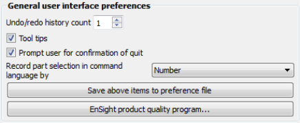
4.2 Edit Menu Functions
EnSight 10.2 User Manual 4-11
Note that clips of polyhedrals for all of these methods will show
the polyhedral outline, not the clip of the internal tetrahedral
mesh
Centroid Robust, Fast, but expensive in memory (2GB per million
polyhedrals). This methodology uses the centroid of the
polyhedral to remesh it into tetrahedral elements. This algorithm
stores the polyhedral element in addition to internal storage of
the tetrahedrals and the poly faces. A downside is that poorly
defined polys may cause inaccuracy in volumetric calculations.
Convex clipper (default) - Better memory usage (1.5GB per million
polyhedrals), Poor Robustness (poorly formed polyhedrals will
show up as gaps in the mesh) and Medium speed. A downside is
that poorly defined polys will show up with holes in the clip.
Poorly defined polyhedrals may adversely affect volumetric
calculations.
Concave Clipper This algorithm uses about the same memory as the convex
clipper, and is more robust in handling poorly defined
polyhedrals, but with the tradeoff that it is slower. Volumetric
calculations using poorly defined polyhedrals will be most
accurate with this algorithm.
New data notification Options for dealing with notification of a change in the model
dataset while EnSight is running. Please contact CEI support if
you have need of this.
Select below to toggle Allows you to specify which data formats will appear in the
“Format” pull-down of the File Open (Data Reader) dialog.
Clicking on the reader name will toggle the ‘*’ mark. Readers
marked with an ‘*’ will be available in the File Open dialog,
format pull-down.
Default reader Allows you to specify the default data reader format. This can be
useful if your format does not meet the extension mapping file
conventions (see 8.3, Data Format Extension Map File Format).
Save to preference file Will save the data preferences to the preference file for future
invocations of EnSight.
(see How To To Set Data Preferences:)
General User
Interface Preferences
Undo/redo history
count
Number of transformations that you can undo. Default is 1
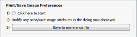
4.2 Edit Menu Functions
4-12 EnSight 10.2 User Manual
Prompt user for
confirmation of quit
Toggle on (default) and an ‘are you sure?’ prompt will come up if
you ask EnSight to quit. Toggle off to just quit without a warning.
Tool tips If checked, causes pop-up help information to appear when the
mouse is placed over icons, parts, etc while running EnSight.
Record part selection
in
Allows you to specify whether the part selections recorded in
command language will be by part Name or by part Number.
Command language recorded using part numbers can be difficult
to apply to datasets with different numbers of parts or that may
have other operations applied to them.
Save above items to
preference file
Will save the preferences above to the preference file for future
invocations of EnSight.
EnSight User
Feedback Program...
EnSight has a mechanism that will send information back to CEI
about the platform EnSight is run on and what dataset formats are
being used. This feedback is used to help guide development
efforts are CEI to more closely reflect common usage scenarios.
This button will allow the user to enable or disable participation
in this program.
Image Saving and
Printing Preferences
These setting allow the user to set things like the default output format for image saving,
etc.
Click here to start Clicking on this button will bring up the image saving dialog.
Once the dialog is visible, set all of the options that should be
used as the defaults. Once complete, select “Save to preference
file”.
Tool tips If checked, causes pop-up help information to appear when the
mouse is placed over icons, parts, etc while running EnSight.
Save to preference file Will write the current print/save preferences to the preference file
for future EnSight sessions.
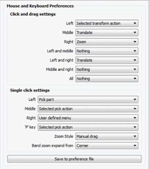
4.2 Edit Menu Functions
EnSight 10.2 User Manual 4-13
Mouse and Keyboard
Preferences
Many of the actions initiated by the mouse buttons and the keyboard ‘P’ key can be
customized to meet specific user needs. In the panel, select the option you wish to assign
to each button or combination of buttons. Note that these preferences are retained even if
you start EnSight with the -no_prefs option. There are two ways to reset the mouse button
preferences back to default. First delete the mouse preferences file (named
ensight.mouse.map3) which is stored in your local or site preferences. Second, manually
change them back in this dialog and resave them to the preferences
Click and drag settings can be assigned to the individual mouse buttons or any
combination (chording) of the buttons: Left, Middle, Right, Left and Middle, Left and
Right, Middle and Right, All. The specific actions can be one of the following:
Selected transform
action
When this option is chosen (it is the default for the left button),
depressing the button and moving the mouse will perform the
transformation (rotate, translate, zoom) currently selected in the
Transformation Control Area on the Tools Icon Bar.
Rotate When this option is chosen, depressing the button and moving
the mouse will perform a rotate transformation on the model.
Translate When this option is chosen, depressing the button and moving
the mouse will perform a translate transformation on the model.
Zoom When this option is chosen, depressing the button and moving
the mouse will perform a zoom transformation on the model.
Rubberband zoom When this option is chosen, depressing the button will cause the
rubberband zoom rectangle to appear and dragging it will modify
the zoom area.
Rubberband selection
tool
When this option is chosen, depressing the button will bring up
the rubberband selection tool that you can then manipulate.
Nothing When this option is chosen, no function is mapped to the mouse
button.
4.2 Edit Menu Functions
4-14 EnSight 10.2 User Manual
Note: One of the Mouse buttons must be assigned to Selected transform action. Macros
cannot be assigned to a mouse key which has a function assigned to it. (see How To
Customize Mouse Button Actions)
Single click settings can be assigned to individual mouse buttons and the ’p’ key. The
specific actions can be one of the following:
Selected pick action When this option is selected, the pick action selected via the pick
action pulldown will be performed.
Pick Part When this option is chosen, depressing the button will pick the
part in the part list.
Pick cursor tool
location
When this option is chosen, depressing the button will pick the
location for, and move the cursor tool.
Pick transf. center When this option is chosen, depressing the button will pick the
location for the new center of transformation. Subsequent
rotations, etc. will be about this picked location.
Pick elements to blank When this option is chosen, depressing the button will blank the
element under the pointer (if element blanking is enabled).
User defined menu When this function is chosen, the context sensitive action menu
will appear.
Nothing When this option is chosen, no function is mapped to the mouse
button
Other preferences include the following:
Zoom style Choose method to use for zoom action. For either option,
zooming stops when the mouse button is released.
Manual drag Zoom DISTANCE is based on the distance you move your
mouse when the mouse button is pressed.
Automatic slide Zoom Velocity is based on the distance the mouse is moved when
the mouse button is pressed.
Band zoom expand
from
Choose the method to use for rubber-band area manipulation. For
either option, area modification stops (and zooming will occur)
when the mouse button is released.
Center Zoom area will shrink and expand about the center of the
rectangle.
Corner Zoom area will shrink and expand about the selected corner of
the rectangle. The opposite corner will be fixed.
Save to preference file Will write the current mouse and keyboard preferences to the
preference file for future EnSight sessions.
(see How To To Set Mouse and Keyboard Preferences:)
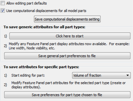
4.2 Edit Menu Functions
EnSight 10.2 User Manual 4-15
Parts Preferences
Allow editing part
defaults
Cause the fast representation to always be displayed. If this
option is disabled (the default), fast display will only be active
during a transformation.
Use computational
displacements for all
model parts
When toggled on (by default) this option causes the displacement
to show the computational displacement option to be ON and
greyed out (unchangeable) in the displacement dialog.EnSight
will then use computational (server-side, “deep”) displacements
which means that the displacements are added to the coordinates
on the server before any calculations are done. The calculator
function “Volume”, for example, will include the changing
coordinates in the volume calculation. Turn this off and the
displacement dialog will show computational displacements off
and thus displaced geometry will be visual only and calculations
will not include the displaced coordinates.
Save generic
attributes for all parts
This option allows you to modify any feature panel and it will
open up with the changes you have saved as the default.
Save general part
preferences to file
This option allows you to save your above options to a file so that
the next restart of EnSight will use these preferences. If you do
not save the above chosen preferences to a file, then your
preferences will only be in effect for this EnSight session.
Save attributes for
specific parts
This allows you to change the default attributes for specific part
types.
Save preferences for
part type chosen to
file
This option allows you to save your above options to a file so that
the next restart of EnSight will use these preferences. If you do
not save the above chosen preferences to a file, then your
preferences will only be in effect for this EnSight session.
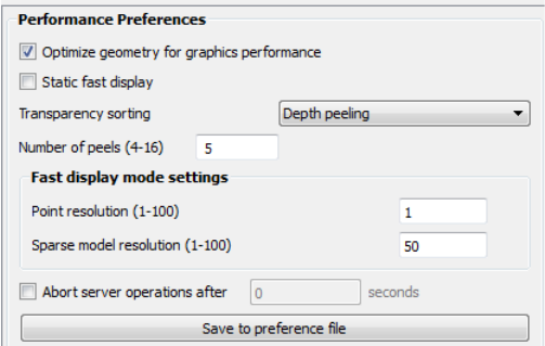
4.2 Edit Menu Functions
4-16 EnSight 10.2 User Manual
Performance
Preferences
Optimize geometry... Option (default ON) to optimize the geometry connectivity order
on the client to improve performance. This never occurs when
rendering only once; rather is used to optimize multi-rendering
situations. Only turn this off if your connectivity order should
never be changed.
Static fast display Cause the fast representation to always be displayed. If this
option is disabled (the default), fast display will only be active
during a transformation.
Transparency sorting This option controls the mechanism EnSight uses for displaying
transparent objects. The options are listed here. The default is
“Depth peeling”.
“Interactive” In this mode all of the transparent polygons are
sorted with each redraw. This option tends to be expensive
because of the sorting operation and the fact that it disables
display list rendering for transparent parts. The option may
reduce the ‘flimmering’ effect of coincident polygons if the scene
contains transparent polygons that are co-incident with opaque
polygons. It may still have a ‘flimmering’ effect with transparent
polygons that are coincident with other transparent polygons.
“Delayed” This mode is similar to “Interactive”, except that the
geometry is only resorted when the mouse button is released,
making it a bit faster, but less accurate.
“Depth peeling” This mode is only available on graphics cards
that support the OpenGL Shading Language. The sorting is pixel-
accurate and is performed as multi-pass rendering directly on the
graphics card. On modern cards, this option is almost always
faster and more accurate. There are two potential issues with this
mode. First, the number of properly resolved transparent surfaces
is limited to the number of depth peels (see the ‘Number of peels’
preference in this category). Second, depth peeling can have
display issues (‘flimmering’) when it encounters co-incident
geometry (geometry that does not have a strict proper order).
When encountering transparency issues, consider increasing the
number of depth peels or (in the co-incident geometry case)
changing the mode the “Interactive”.
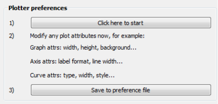
4.2 Edit Menu Functions
EnSight 10.2 User Manual 4-17
Number of Peels This option controls the number of surfaces that can be properly
depth resolved. This is also known as the “depth complexity” of
the scene or the number of transparent surfaces a ray from the
viewer to an individual pixel will intersect. This preference only
applies to “Depth peeling” sorting mode.
Point Allows specification of the fraction of nodes to display in Fast
Display, point representation. (“1” indicates all nodes, “2” would
be every other node, “3” every third node, etc.)
Sparse Model
Resolution
Allows specification of the percentage of the model geometry
that will be displayed. (immediate mode only)
Abort Server
Operations
Causes a timer to be set which will abort some of EnSight’s
CPU-intensive server operations (for example some calculator
options, clipping, isosurface, isovolume, particle tracing and
cuts) after the set amount of clock seconds have passed.
Optimize geometry for
graphics performance
When we make a new part, or update its connectivity, the user
can select to optimize its connectivity in order to improve
rendering performance. This reordering will be done if the client
mesh is bigger than 256 triangles, if the client mesh causes poor
performance, and if the mesh is used multiple times. Turn this off
to disable this feature.
Save to preference file Will write the current performance preferences to the preference
file for future EnSight sessions.
(see How To To Set Performance Preferences:)
Plotter Preferences
Click here to start Click then modify your plot attributes. These will be the default
attributes for this session.
Save to preference file Save your changes to a file so that the next time that you start
EnSight, these plotter preferences will be used.
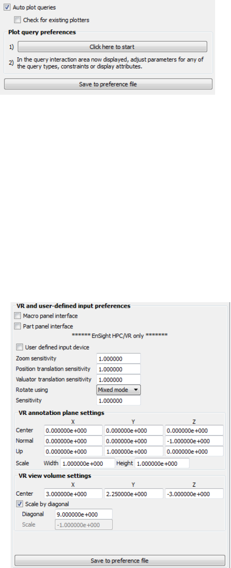
4.2 Edit Menu Functions
4-18 EnSight 10.2 User Manual
Query Preferences
Auto plot queries Newly created queries will be plotted if this is on (default).
Check for existing
plotters
This will not check for existing plotters if off (default). If on then
it will check for existing plotters.
Click here to start Click then modify your query attributes. These will be the default
attributes for this session.
Save to preference file Save your changes to a file so that the next time that you start
EnSight, these query preferences will be used.
VR and user defined
input Preferences
4.2 Edit Menu Functions
EnSight 10.2 User Manual 4-19
Macro panel interface Toggles on/off the user defined macro panel to the Main
Graphics window. The user defined macro panel is defined in
your EnSight preferences directory under the macros
subdirectory (8.2, Data Reader Preferences File Format) in the
hum.define file. (An example hum.define file is located at
$CEI_HOME/ensight102/src/cvf/udi/HUM/hum.define on your
client system.).
Part panel interface Display a part list in the graphics window. This is helpful when in
full screen mode or in a VR environment, to allow picking of
parts that can be operated on via macros.
HPC/VR only
User defined input
device
Toggles on/off the User Defined Input Device that is linked via a
runtime library. Use of the User Defined Input Device interface is
discussed in more detail under Tracking and Input Devices. The
next five preferences are only used if this toggle is on.
Zoom sensitivity Specifies a positive scalar value that adjusts the sensitivity of the
zoom input device. Values less than 1.0 cause the zoom to
happen more slowly, while values greater than 1.0 cause the
zoom to progress at a more rapid rate.
Position translation
sensitivity
Specifies a positive scalar value that adjusts the sensitivity of a
positional translation input device. Values less than 1.0 cause the
translation to happen more slowly, while values greater than 1.0
cause the translation to progress at a more rapid rate.
Valuator translation
sensitivity
Specifies a positive scalar value that adjusts the sensitivity of a
valuator translation input device. Values less than 1.0 cause the
translation to happen more slowly, while values greater than 1.0
cause the translation to progress at a more rapid rate.
Rotate using Opens a pull-down menu for selection of the type of input device
used to record rotation transformations.
Mixed mode A device that returns virtual angle values where the Z rotations
correspond to (literal) movement of the input device about its
local Z (or roll) axis; and where the X and Y rotations correspond
to translational movements of the input device with respect to its
local X and Y axes.
Direct mode A device that returns virtual angle values that correspond to
(literal) rotational movements of the input device about its local
X, Y, and Z axes.
Sensitivity Specifies a positive scalar value that adjusts the sensitivity of the
type of rotation input device selected in the Rotate Using
preference. Values less than 1.0 cause the rotation to happen
more slowly, while values greater than 1.0 cause the rotation to
progress at a more rapid rate
(see How To Enable User Defined Input Devices)
VR annotation plane
settings
Center Choose the center of the annotation plane using the VR
environment units (not your geometry units).
Normal Choose the normal of the annotation plane.
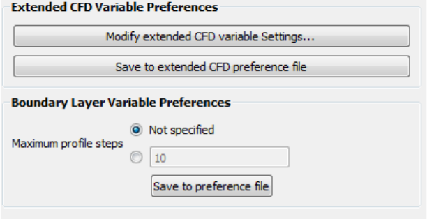
4.2 Edit Menu Functions
4-20 EnSight 10.2 User Manual
Up Choose the upward direction of the annotation plane.
Scale Choose the Width and Height scale of the annotation plane.
Acceptable range of values are greater than zero.
VR view volume
settings
Center Choose the center of your view volume in VR environment units
(not geometry units). Your data will be centered and scaled
around this point.
Scale by diagonal Toggle this on to fit your data into the VR environment.
Diagonal This is used if Scale by diagonal is toggled on. Use this to size
your virtual environment. For example, for a cave this defaults to
the diagonal of your cave.
Scale This is used if Scale by diagonal is toggled off. This would be
used to see your geometry in a virtual environment that this the
same as the geometry. For example, if both the geometry and the
virtual environment use meters, set this value to 1.0. If your
virtual environment is in millimeters and your geometry is in
meters, then use 1000.
Save to preference file Save your changes to a file so that the next time that you start
EnSight, these preferences will be used.
(see How To To Set User Defined Input Preferences:)
Variables
Preferences
Modify extended CFD
variable Settings...
Opens the Extended CFD variable settings dialog. If your data
defines variables or constants for density, total energy per unit
volume, and momentum (or velocity), it is possible to show
variables derived from these basic variables in the Main
Variables List of the GUI by utilizing the capabilities of this
dialog. See the Extended CFD Variable Setting dialog below.
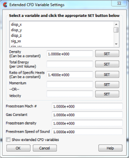
4.2 Edit Menu Functions
EnSight 10.2 User Manual 4-21
This dialog may be used to map the names of currently loaded variables to the
extended CFD variable types. It also allows for setting default constant values for
many of the types. In the dialog, one can select a variable name from the scrolling list
and then click on ‘SET’ to set the CFD variable to the selected variable.
Density Permits the selection of the density variable from the list (click
SET after selection) or the specification of a constant value in the
field provided.
Energy (Total) Per Unit
Volume
Permits the selection of the energy variable from the list. Click
SET after selection.
Ratio of Specific Heats Permits the selection of the ratio of specific heats variable from
the list (click SET after selection) or the specification of a
constant value in the field provided.
Momentum OR
Velocity
Permits the selection of the momentum or velocity variable from
the list. Click SET after selection.
Freestream Mach # Permits the specification of the freestream mach number in the
field provided.
Gas Constant Permits the specification of the gas constant in the field provided.
Freestream Density Permits the specification of the freestream density value in the
field provided.
Freestream Speed of
Sound
Permits the specification of the freestream speed of sound value
in the field provided.
Show Extended CFD
Variables
When selected, all of the variables that can be derived from the
information entered will be shown in the Main Variables List of
the GUI.
Figure 4-4
Extended CFD variable settings dialog
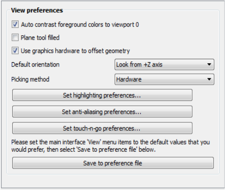
4.2 Edit Menu Functions
4-22 EnSight 10.2 User Manual
OK Clicking this button applies the changes made in the dialog.
(See How To Create New Variables)
Save to extended CFD
preferences file
Will write the current extended CFD preference to the extended
CFD preference file for future EnSight sessions.
(see How To To Set Variable Preferences:)
Boundary Layer
Variable Preferences
Maximum profile
steps
This value is used in Boundary Layer calculator functions.
EnSight will calculate the boundary layer profile normal to each
cell using values from the boundary fluid cell layer above each
surface element looking for the velocity gradient to change sign
or go to zero.
For user control (if for some reason, EnSight uses too many
values in the above boundary layer profile) you can limit the
maximum number of values to use in the boundary layer profile
calculation. A good maximum would be the maximum number of
fluid cells levels used to model the boundary layer anywhere
above the model surface. A poor maximum number would be one
that is too small: if the maximum is too small then EnSight may
stop within the boundary layer rather than finding the edge.
View Preferences The view category is focused on items related to the user interaction with graphics and the
quality of the graphical display. Note that the settings in the ‘View’ main window menu
will also be recorded when the settings for this category are saved. The options appear
like as follows:
Auto contrast
foreground colors to
viewport 0
Auto contrast will switch white and black colored foreground
objects (such as annotations, plotters, etc.) for maximum contrast
with viewport 0 (the default viewport). This feature works with
viewports that use a Constant or Blended background color. If
the viewport background is Blended it uses the color at the
bottom of the viewport. The typical usage is if you change the
background color to white in preparation for printing that the
objects that were white will turn to black. This is ON by default.
4.2 Edit Menu Functions
EnSight 10.2 User Manual 4-23
Plane tool filled By default, the EnSight plane tool is drawn as the border of a
rectangle. If checked, this option causes the plane tool to be
drawn as a solid, plane instead of just its outline.
Use graphics
hardware
There are two graphics part offsets employed in EnSight. This
one, hardware offset, is perpendicular to the monitor screen and
done in hardware if this toggle is on. This will allow, for
example, contour lines to appear closer to the viewer than their
parent part so they are visible no matter what orientation the part
is viewed from. The second offset is the display offset. The
display offset can be set in the feature panel for line parts such as
contour lines, particle trace lines, vector arrows, and separation/
attachment lines. The display offset is the distance in the
direction of the element normal (perpendicular to the surface).
Default orientation The default axis for viewing can be selected and set using this
preference.
Picking Method The default is to utilize the graphics hardware to give accelerated
part pick information. Should the graphics software drivers be
faulty, it may be desirable to instead to use software picking.
Set highlighting
preferences
This button opens the Highlighting preferences dialog where part
selection and targeting feedback can be adjusted for color and
intensity. To turn off highlighting completely, turn off the part
highlighting toggle located in the Tools Icon Bar or via the View
menu with the ‘Highlight selected parts’ menu. See ‘Highlighting
preferences’ below
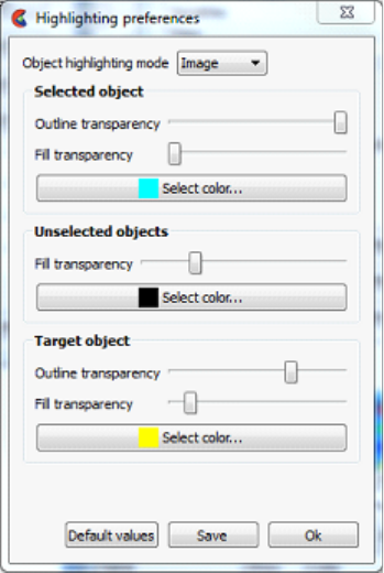
4.2 Edit Menu Functions
4-24 EnSight 10.2 User Manual
Highlighting Preferences
EnSight supports two highlighting methods. The default is ‘image’ mode. Image
mode is graphics card accelerated dynamic highlighting of objects as well as the
current selection. The advantage of this mode is that the highlighting can be updated
without re-rendering the graphics scene, making it very fast and efficient. The
system classifies all of the objects on the screen into a ‘selected’ object,
‘unselected’ objects and the object directly under the cursor (the ‘target’ object).
Each class of objects can be shaded by blending a ‘Fill’ color with the object color
itself. The ‘Selected’ and ‘Target’ object classes also support the display of a
silhouette ‘Outline’ around all of the visible pixels of objects in that class. The
outline is the same color as the fill color. This coloring is blended over the rendered
scene pixels. The user has control over the transparency of both the fill and outline
colors as well as the colors themselves, giving a measure of control over the
highlighting visuals.
The other mode is ‘Geometry’. In this mode, the selected geometry is rendered with
a ‘hatching’ pattern to differentiate the selected objects. This form of highlighting is
more compatible with older graphics cards, but it is much slower as the entire scene
must be re-rendered when the selection changes.
Object
Highlighting
Mode
If set to Geometry will display selected objects (currently parts)
by displaying selected geometry with a cross hatch pattern. This
method requires a redraw of the scene when new parts are
selected. If set to Image highlighting, the behavior is as outlined
in the previous paragraphs and the ‘object’ options for color and
transparency are active.
4.2 Edit Menu Functions
EnSight 10.2 User Manual 4-25
Selected
Objects
The selected objects are blended with a fill color as well as an
outline. Both use the same color specified. When the Outline
transparency slider is set to the left no outline will appear. When
the Outline transparency is set to the right a full intensity outline
of the color specified will appear around the object. If the Fill
transparency slider is set to the left, the color of the object is not
modified while if set to the right the full intensity of the color
specified will be used.
Unselected
Objects
Unselected objects will be blended with the color specified.
When the slider is set to the left no color modification will occur.
When the slider is set to the right the specified color will be
shown at full intensity on the unselected objects.
Target Objects The target object (the object under the mouse pointer) is blended
with a fill color as well as an outline. Both use the same color
specified. When the Outline transparency slider is set to the left
no outline will appear. When the Outline transparency is set to
the right a full intensity outline of the color specified will appear
around the target object. If the Fill transparency slider is set to the
left, the color of the target object is not modified while if set to
the right the full intensity of the color specified will be used.
Default Settings Will restore the highlighting preferences to the default values
Save
preferences
Will save the highlight preferences for the next session of
EnSight.
OK Closes the dialog.
Set anti-aliasing This button opens the Anti-aliasing preferences dialog used to
change parameters for on-screen smoothing jagged lines and
edges. These anti-aliasing options apply only to on-screen,
interactive use of EnSight. They do not apply to batch execution,
nor exporting of an image. For example, when saving an image
to file, anti aliasing is invoked separately from these preferences
in the advanced tab using the number of passes. See ‘Anti-
aliasing preferences’ below.
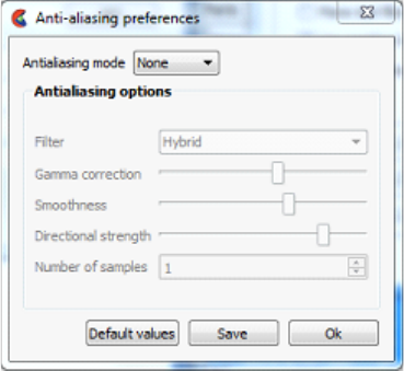
4.2 Edit Menu Functions
4-26 EnSight 10.2 User Manual
Anti-aliasing Preferences
EnSight provides some tools for reducing aliasing rendering artifacts caused by
digital sampling, especially of geometry in line or outline mode. This dialog allows
for some control over the anti-aliasing options.
antialiasing
mode
There are three antialiasing modes in decreasing order of speed
and increasing order of on-screen image quality: None, Filtered,
and Multipass. Filtered works only on modern graphics cards.
Multipass requires graphics hardware support, but will work on
older graphics cards. Therefore, anti-aliasing is disabled in
software rendering mode (starting EnSight with the -X option).
Additionally, setting the auxiliary buffers environmental variable
(setenv CEI_NUM_AUX_BUFFERS 0) will disable this feature.
None This is the default mode.
Multipass Each time the scene needs to be redrawn, it is drawn multiple
times from slightly different positions. The final image is a blend
of all the images. Rendering performance will slow down in
proportion to the number of samples
Filtered Each time the scene is drawn, an image filter is applied to the
result. The shape of the filter is a gaussian curve. Filtered anti-
aliasing has a very low performance cost, but is usually lower
quality than multipass anti-aliasing
Filter Used with the filtered option. A pulldown that can be Small,
Large, Hybrid
Small Used with filtered option. A symmetric 3x3 pixel filter.
Large Used with filtered option. A symmetric 5x5 pixel filter.
Hybrid Used with filtered option. A 5x5 pixel filter compressed in the
direction perpendicular to the image gradient
Gamma
Correction
Used with filtered option to correct for some monitor-dependent
artifacts. For example, without gamma correction, bright lines
against a dark background can appear dimmer after filtering, but
will appear to have the same overall brightness with the right
gamma correction.
Smoothness Changes the shape of the gaussian curve. High values make the
curve fall off slowly, making the image smoother and blurrier
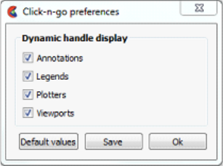
4.2 Edit Menu Functions
EnSight 10.2 User Manual 4-27
Directional
Strength
This option is used with the hybrid algorithm to control how
much the filter is compressed, perpendicular to the image
gradient.
Number of
Samples
Used with the Multipass option to specify the number of times to
redraw the scene. Rendering performance will slow down in
proportion to the number of samples.
Default Values Restores the anti-aliasing preferences to the default values.
Save Save the anti-aliasing preferences for subsequent EnSight
sessions.
OK Closes the dialog.
Set click-n-go
preferences...
Sets preferences for direct interaction with created parts in the
graphics window using graphical handles. See ‘Click-n-go
preferences’ below.
Click-n-go Preferences
Annotations,
Legends, etc
Toggle ON (default) ability to interact with these items in the
graphical user interface.
Default Values Restore selections back to default values.
Save Save settings to preferences file
OK Close dialog.
Save to preference file Writes the current view preferences to the preferences file for
future EnSight sessions.
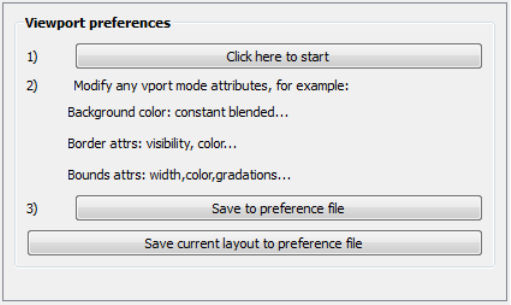
4.2 Edit Menu Functions
4-28 EnSight 10.2 User Manual
Viewports
Preferences
The viewports category is focused on items related to EnSight viewports. Note that the
settings in the ‘Viewports’ main window menu will also be recorded when the settings for
this category are saved. The options appear as follows:
Click here to start This will bring up the Viewports dialog with all the viewport
items selected.
Modify viewport
attributes
Set any viewport attribute (for example, background color to
blended).
Save to preference file This will save the changes you have made during the modify
viewport attributes in the previous step as defaults for future
sessions.
Save current layout to
preference file
This will save the current viewport layout and all the attributes to
your preference file.
(see How To To Set View Preferences:)
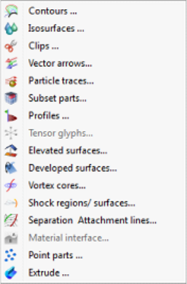
4.3 Create Menu Functions
EnSight 10.2 User Manual 4-29
4.3 Create Menu Functions
The create menu is used to bring up the Feature Panel in ‘create mode’ for all of
the various part types. The action for clicking on each menu item is the same as
clicking on the associated Feature icon, or by double clicking on a part in the Parts
List Panel, or by right- clicking on a part in the Parts List Panel and selecting
Edit...
The menu appears as:
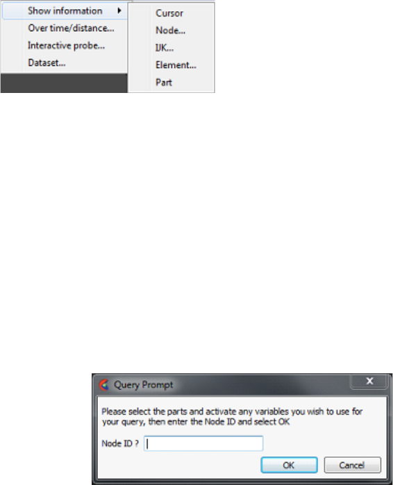
4.4 Query Menu Functions
4-30 EnSight 10.2 User Manual
4.4 Query Menu Functions
The Main Menu Query menu provides access to basic information querying
functions, the query generation dialogs and the interactive probe dialog.
Note: only parts with data residing on the Server host system may be queried.
Thus, parts that reside exclusively on the Client host system (i.e. contours, particle
traces, profiles, vector arrows) may NOT be queried, Table 1–2 Part Creation and
Data Location.
Show information Opens the following pull-down menu (see How To Get Point, Node, Element, and Part
Information).
Cursor Provides the following information in the Status History Area about a
Point inside of the selected Part(s) who’s position is specified with the
cursor tool (see How To Use the Cursor (Point) Tool):
x,y,z coordinates, Frame assignment of Point, the Part that the Point is
found in, the closest Node to the Point, the element id if it exists, and
the active Variable values at the Point.
Node... Opens the Query prompt dialog which is used to specify Node ID
number. When the Ok button is pressed, the following information about
the specified Node is shown in the Status History Area:
x,y,z coordinates, Frame assignment of Node, the Part that the Node is
found in, the element id if it exists, and all active nodal Variable values
at the Node.
Figure 4-5
Query pull-down menu
Figure 4-6
Show information Node... menu
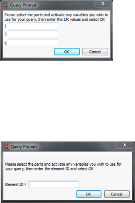
4.4 Query Menu Functions
EnSight 10.2 User Manual 4-31
IJK... Opens the Query Prompt dialog which is used to specify IJK values.
When the OK button is pressed, the following information about the
Node specified by the IJK values is shown in the Status History Area:
Node ID, Part in which the Node is located, x,y,z coordinates of the
Node, Frame assignment of the Node, and the specified Variable value
at the Node.
Element... Opens the Query Prompt for Element ID. When the Ok button is pressed,
the following information about the Element is shown in the Status
History Area:
Part in which Element is located, Type of Element, IJK bounds (if a
structured mesh), Number of Nodes, Node ID numbers, information
on neighboring Elements, and all active elemental Variable values at
the Element.
Part Causes the following information about the select Part to be shown in the
Status History Area:
Part type (structured or unstructured), number of Nodes in Part,
minimum and maximum x,y,z coordinates, Element type, min/max
node labels if exist, min/max element labels if exist, and the number of
Elements.
Over time/distance... Opens the Query/Plot Editor in the Feature Panel which is used to obtain information
about variables and to create plots of the information (see 5.3, Query/Plotter and How To
Query/Plot).
Interactive probe... Opens the Interactive Probe Query Editor in the Feature Panel which is used to obtain
information interactively about variables (5.8, Interactive Probe Query and How To Probe
Interactively).
Figure 4-7
Query Prompt for IJK Values
Figure 4-8
Query Prompt for Element ID
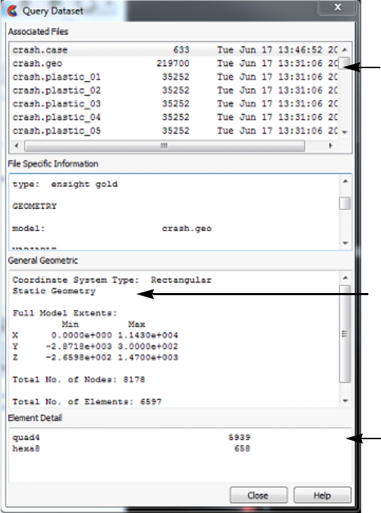
4.4 Query Menu Functions
4-32 EnSight 10.2 User Manual
Dataset... Opens the Query Dataset dialog, which provides information about the dataset loaded in
the current case. This can be useful to verify the files that you are using, whether the
geometry is static, changing coordinates, or changing connectivity, and the number of
each element type in your dataset. For the specified file, specific, general and detail
information is provided (see 5.3, Query/Plotter and How To Query Datasets).
For the specified file, specific, general and detail information is provided.
Main Menu > Query > Dataset...
(see 5.3, Query/Plotter and How To Query Datasets)
Figure 4-9
Query Dataset dialog
File details, sizes
and names
Number of each
element type
Dataset geometry type:
One of the following:
1. Static
2. Changing
Coordinates
3. Changing
Connectivity
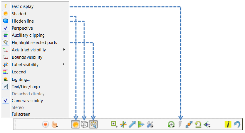
4.5 View Menu Functions
EnSight 10.2 User Manual 4-33
4.5 View Menu Functions
The Main Menu View menu allows the user to change overall rendering area view
features, including various visibility toggles, overall object display look and
extended visual capabilities such as stereo, fullscreen and detached display
modes. Some of the menu options are the same as the Tools Icon Bar global toggle
icons as indicated below:
Fast display Toggles the Fast display mode. By default, EnSight displays all of the lines and elements
for each part every time the rendering window redraws. If you have very large models (or
if you have slow graphics hardware), each redraw can take significant time. As a result,
interactive transformations become jerky and lag behind the motion of the mouse.
Ironically, the slower the graphics performance, the harder it is to perform precise
interactive transformations. To avoid this problem, you can tell EnSight to show a lesser
detailed part representation, e.g., a bounding box surrounding each Part, or the Part as a
point cloud. You can select to show the detail representation all the time, or only while
you are performing transformations. This obviously displays much less information, but
may be sufficient if you want to rotate a very large model.
A lesser detail display is also useful when experimenting with keyframe-animation rates.
Using lesser detail, the display rate can be adjusted to approximate the video rate, thus
you can see how your scene will transform on the video tape.
The default setting is off, indicating that all lines and elements of all visible parts will be
redrawn. When on, the redraw will show only the part’s Fast Display Representation (by
default a box). The fast display representation is only used while transformations are
being performed. The fast display representation will be continuously displayed if the
Static Fast Display option is turned on in: Main Menu > Edit > Preferences >
Performance > Static fast display.
Figure 4-10
View pull-down menu and corresponding Tools Icon Bar icons
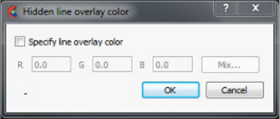
4.5 View Menu Functions
4-34 EnSight 10.2 User Manual
Shaded Toggle Toggles the Global Shaded mode for parts on and off. EnSight by default displays parts in
line mode. Shaded mode displays parts in a more realistic manner by making hidden
surfaces invisible while shading visible surfaces according to specified lighting
parameters. Parts in Shaded mode require more time to redraw than when in line mode, so
you may wish to first set up the Graphics Window as you want it, then turn on Shaded to
see the final result. Shaded can be toggled on/off for individual parts by using the Shaded
Toggle icon in the Tools Icon Bar. (see 5.1.1, Parts Quick Action Icons and How To Set
Drawing Style)
Hidden line Toggles the global Hidden line display for all parts on/off. This simplifies a line drawing
display by making hidden lines - lines behind surfaces - invisible while continuing to
display other lines. Hidden Line can be combined with Shaded to display both surfaces
and the edges of the visible surface elements. Hidden Line can be toggled on/off for
individual parts by using the Hidden Line Toggle icon in the Part Quick Action Icon Bar.
To have lines hidden behind surfaces, you must have surfaces (2D elements). If the
representation of the in-front parts consists of 1D elements, the display is the same
whether or not you have Hidden Lines mode toggled on (see 5.1.1, Parts Quick Action
Icons and How To Set Drawing Style). The Hidden line overlay dialog will be displayed if
the Shaded option is currently on and you then turn the Hidden Line option on. The
section Troubleshooting View Related Display Issues contains solution to common
hidden line display issues.
Hidden line overlay
dialog
This dialog is used to specify a color for the displayed lines. If this color is not different
from the surface color, the lines will not be visually distinguishable from the surfaces.
The default is the part-color of each part, which may be appropriate if the surfaces are
colored by a color palette instead of their part-color.
Specify line
overlay color
Toggle-on if you want to specify an overlay color. If off, the overlay line
color will be the same as the part color.
R, G, B The red, green, and blue components of the hidden line overlay. These
fields will not be accessible unless the ‘Specify line overlay color’ option
is on.
Mix... Click to interactively specify the constant color used for the hidden line
overlay using the system Color selector dialog (see Chapter 5.1.1, Parts
Quick Action Icons)
Okay Click to accept the hidden line overlay color options.
Perspective Toggles the view within each of the viewports within the Graphics Window between a
perspective view (the default) and an orthographic projection. Perspective is what
provides the sense of depth when viewing a three dimensional scene on a two dimensional
surface. Objects that are far away look smaller and parallel lines seem to meet at infinity.
Orthographic projection removes the sense of depth in a scene. Lines that are parallel will
never meet and objects of the same size all appear the same no matter how far away they
are from you. Orthographic projection mode often helps when you are positioning the
Cursor, Line, and Plane tools using multiple viewports. This is the Global toggle. Each
viewport also has a Perspective Toggle (see How To Set Global Viewing).
Figure 4-11
Hidden line overlay dialog
4.5 View Menu Functions
EnSight 10.2 User Manual 4-35
Auxiliary clipping Toggles the Auxiliary clipping feature on/off. (Default is Off). Like a Z-Clip plane,
Auxiliary clipping cuts-away a portion of the model. When Auxiliary clipping is On,
Parts (or portions of Parts) located on the back (negative-Z) side of the Plane Tool are
removed. Parts whose Clip attribute you have toggled off (in the General Attributes
section of the Feature Panel or with the Auxiliary clipping Toggle Icon in the Part Quick
Action Icon Bar) remain unaffected. Auxiliary clipping is interactive—the view updates
in real time as you move the Plane Tool around (see 4.6, Tools Menu Functions and How
To Use the Plane Tool).
Unlike a Z-Clip plane, Auxiliary clipping applies only to the parts you specify, and the
plane can be located anywhere with any orientation though it is always infinite in extent
(see 6.4, Z-Clip and How To Set Z Clipping). Auxiliary clipping is helpful, for example,
with internal flow problems since you can “peel” off the outside parts and look inside.
This capability is also often useful in animation. The position of the Plane Tool and the
status of Auxiliary clipping is the same for all displayed viewports. Do not confuse
Auxiliary clipping with a 2D-Clip plane, which is a created part whose geometry lies in a
plane cutting through its parent parts or with the Part operation of cutting a part.(see 5.1.3,
Clip Parts, How to Create Plane Clips, and How To Cut a Part). The section
Troubleshooting View Related Display Issues contains solution to common auxiliary
clipping issues. (See also How To Set Auxiliary Clipping)
Highlight selected
part(s)...
Highlight the selected parts in the graphics window. This often aids in the identification of
parts.
Axis triad visibility A sub-menu which allows you to toggle on/off the visibility of the Global axis triad, the
axis triads for all Frames, and the model axis triad.
Frame Toggles (default is On) the display of all coordinate Frame axis triads.
The visibility of individual coordinate Frame axes can be selectively
turned on/off by clicking on the Frame’s axis triad and then clicking on
the Frame Axis Triad Visibility Toggle in the Frame Quick Action Icon
Bar.
Global Toggles (default is Off) the display of the global coordinate frame axis.
The global coordinate frame axis triad represents the Look-At Point.
Model Toggles the display of the model axis triad in the lower left of the screen.
This triad is not at the origin of frame 0, but is aligned with it (see
Chapter 5.11, Tools Icon Bar).
Bounds visibility Toggles (default is Off) the extents box for all parts.
Label visibility A sub-menu which allows you to toggle the visibility of labels for Elements or Nodes.
Element
labeling
Toggles (default is Off) the global visibility of labels for elements in all
parts. Element labels will only be displayed if they are available in the
dataset. Visibility of element labels for individual parts can be controlled
via the Node/Element labeling icon in the Quick Action Icon Bar.
Node labeling Toggles (default is off) the global visibility of labels for nodes in all parts.
Node labels will only be displayed if they are available in the dataset.
Visibility of node labels for individual parts can be controlled via the
Node/Element labeling icon in the Quick Action Icon Bar.
Labeling
attributes...
Opens the Node/Element labeling dialog from which you can control the
labeling visibility, color, and filtering for selected parts. This same dialog
can also be reached from the Node/Element labeling icon in the Quick
Action Icon Bar.
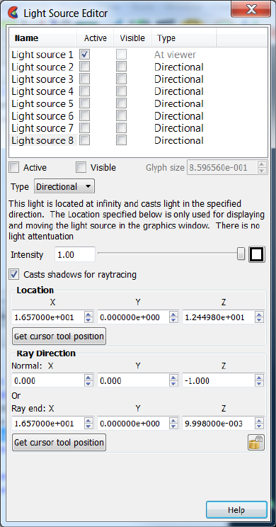
4.5 View Menu Functions
4-36 EnSight 10.2 User Manual
Legend Toggles (default is on) the global visibility of all legends. The visibility of individual
legends can be controlled by using the Legend tab in the Annotation Feature Panel (see
Chapter 7.2, Variable Summary & Palette) and How To Create Color Legends.
Lighting This dialog is used to specify the location, type, intensity, and color of up to eight light
sources. By default, a single directional light source exists, located at the user, pointing in
the direction of the view. This light source is always light source #1, and can not have it’s
type modified.
Light sources are defined in the model coordinate system and are shared among all
viewports, i.e., if a light source is defined, it is defined for all viewports.
Active Toggle on if you want the light source to cast light in the scene.
Visible Toggle on if you want to see a glyph representing the light source in the
scene.
Glyph Size If the light source is visible, this sets the size of the glyph.
Type Set the light source type. The light source types are:
Directional This light source is defined by a direction and does not attenuate with
distance. You will still have the option to specify a “ray end” location for
the light, but this is only used for the purpose of specifying a direction - it
has no effect on the lighting model.
Figure 4-12
Light Source Editor

4.5 View Menu Functions
EnSight 10.2 User Manual 4-37
Troubleshooting View Related Display Issues
Troubleshooting Hidden Surfaces and Shading
Spot Light is defined as a location, direction, and an angle for the spot. The
light attenuates such that the farther away the light is from the geometry,
the less effect the light will have.
Point Light emits from the location in all directions. Light attenuates based on
distance from the light source to the geometry (same attenuation as a spot
light). You still define a light direction and ray end location, but these are
only used for the purpose of defining the light attenuation distance.
Intensity Specifies, as a value from 0 to 1, the intensity of the light.
Color The color swatch next to the Intensity slider will bring up a color chooser
allowing you to set the color of the light.
Casts
shadows for
raytracing
Toggle on if you wish this light source to cast shadows in ray traced
image generation.
Location The location in model space of the light source.
Get cursor
tool position
To simplify source location setup, it is possible to use the current position
of the cursor tool (which has options of picking, dragging, and editing via
the transformation dialog) to specify either the location or the ray end
position.
Ray Normal
Direction
The direction of the light ray. For a point light source, the ray direction is
only used for the purpose of defining the Ray end location, which in turn
defines the distance to the light source for light attenuation.
Ray End The point the light is pointing towards and defines the light radius used
for light attenuation.
Text/Line/Logo Toggles global visibility for text strings and lines which have been created and logos
which have been imported. The visibility of individual Text strings, Lines, or Logos can
be controlled by selecting the item in the annotation list and selecting the context sensitive
Hide or Show menu items. It can also be toggled from the associated Annotation Feature
Panel (How To Create Lines and Arrows, How To Create Text Annotation, and How To
Load Custom Logos).
Detached display This menu item is disabled unless using a detached display. If you have a detached
display then it is automatically enabled and toggled on, and this menu item allows
toggling on/off this detached display. (see Chapter 12, Caves, Walls & Head-mounted
displays) for a discussion of detached displays.
Camera Visibility Toggles the global visibility for cameras. The visibility of individual cameras can be
controlled by selecting the camera in the Transformation editor (Camera) dialog. (see
Chapter 6.7, Camera).
Problem Probable Causes Solutions
Main View shows line drawing after
turning on the Shaded toggle
Shaded is toggled off for individual
parts
Toggle Shaded on for individual
parts with the Shaded Icon in the
Part Quick Action Icon Bar or in the
Feature Panel.

4.5 View Menu Functions
4-38 EnSight 10.2 User Manual
Troubleshooting Auxiliary Clipping
There are no surfaces to shade—all
parts have only lines.
If parts are currently in Feature
Angle representation, change the
representation. If model only has
lines, one cannot display shaded
images.
The Main View window shows
nothing other than the Plane Tool
after Clipping is toggled-on.
The element visibility attributes has
been toggled off for the part(s).
Toggle the element visibility on for
individual parts in the Feature Panel.
Problem Probable Causes Solutions
The Plane Tool does not appear to
clip anything
The Auxiliary Clipping toggle is off
for all parts.
Turn the Auxiliary Clipping toggle
on for individual parts in the Feature
Panel (Model) dialog General
Attributes section.
The Plane Tool is not intersecting the
model
Change the position of the Plane
Tool.
The Main View window shows
nothing other than the Plane Tool
after Clipping is toggled-on.
All of the part(s) is(are) on the back
side of the Plane Tool and is(are)
thus clipped
Change the position of the Plane
Tool.
Problem Probable Causes Solutions
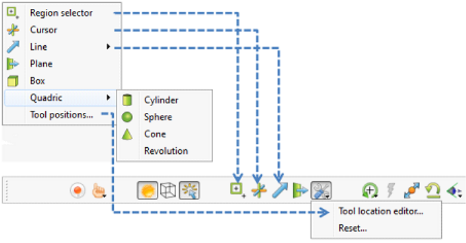
4.6 Tools Menu Functions
EnSight 10.2 User Manual 4-39
4.6 Tools Menu Functions
The Region selector, Cursor, Line, Plane, Box, and Quadric (cylinder, sphere,
cone, and revolution) Tools in EnSight are used for a variety of tasks, such as:
positioning of clipping planes and lines, query operations, particle trace emitters,
etc. Collectively these tools are referred to as Positioning Tools. Clicking Tools in
the Main Menu opens a pull-down menu which provides access to these tools.
Several of the tools have quick action icons below the Main Graphics Window, as
shown in Figure 4-13, to toggle their visibility.
Region selector Toggle Makes the Selection Tool (region selector) visible/invisible in the Graphics Window. The
Selection Tool appears as a white rectangle with two symbols at the upper left of the tool
(one is for zooming and the other for element blanking). It may be repositioned
interactively in the Graphics Window by selecting and dragging it or by selecting any
corner and rubber banding the corner. Note that a dotted rectangle, which stays at the
same aspect ratio of the screen, will indicate the actual selection area as it is manipulated.
Alternatively, you can reposition it precisely by specifying X and Y min/max coordinates
in the Transformation Editor dialog (described in Tool Positions...Region Tool below).
Main Menu > Tools > Region selector
or Tools Icon Bar > Selection tool
(see How to Use the Selection Tool)
Cursor Makes the Cursor Tool visible/invisible in the Graphics Window. The Cursor Tool
appears as a three-dimensional cross colored red, green, and blue. The red axis of the
cross corresponds to the X axis direction for the currently selected Frame, while green
corresponds to the Y axis and blue corresponds to the Z axis. The Cursor Tool is initially
located at the Look-At point and may be repositioned interactively in the Graphics
Window by left-clicking and dragging it or right-clicking on it and choosing ‘Edit’ on the
pulldown which opens the Tranformation Editor. If you have a specific location you want
to click on and have the cursor moved there, then select Pick Cursor Location from the
Pick Pull-down Icon menu in the Tools Icon Bar.
(see How to Use the Cursor (Point) Tool)
Figure 4-13
Tools pull-down menu and Pick Part pull-down menu
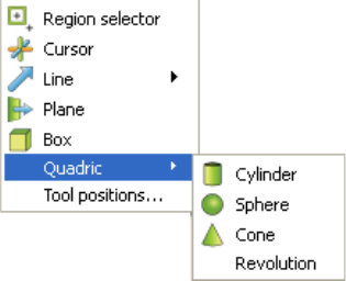
4.6 Tools Menu Functions
4-40 EnSight 10.2 User Manual
Line Opens a pull-down menu with options for toggling the visibility of the Line Tool as well
as options for restricting where the Line Tool is drawn. These options are described
below. The Line Tool appears as a white line with a dotted-line axis system at the center
point and an arrowhead on its 2nd endpoint. The Line Tool is initially centered about the
Look-At point and sized so that it fills approximately 10% of the default view. There are a
number of ways to manipulate the tools either interactively or via the transformation
dialog. You can change its length and orientation interactively in the Graphics Window
by selecting one of its end points. You can rotate the line tool by clicking and dragging on
the center axes. You can reposition it interactively in the Graphics Window by selecting
its center and dragging it or by selecting Pick Line Location from the Pick Pulldown Icon
menu in the Tools Icon Bar. Alternatively, you can reposition it precisely by rotating,
translating, or specifying coordinates in the Transformation Editor dialog by right-
clicking on the line tool and selecting ‘Edit’. If you have a precise location that you want
to locate the line tool you can select Pick Line Tool Location from the Pick Pull-down
Icon menu in the Tools Icon Bar.
(see How to Use the Line Tool)
Plane Makes the Plane Tool visible/invisible in the Graphics Window. (Note: Its appearance
(line or filled) is controlled under Main Menu > Edit > Preferences > View)
The Plane Tool is shown with an X, Y, Z axis system, is initially centered about the Look-
At point, and lies in the X-Y plane. You can reposition it interactively in the Graphics
Window by selecting its center point in the Graphics Window and dragging it. You can
change its orientation interactively in the Graphics Window by selecting the X, Y, or Z
letters at the ends of the axes. You can resize the Plane Tool interactively in the Graphics
Window by selecting any corner of the plane and dragging it. You can rubber-band any of
the corners by holding the Ctrl key while selecting and dragging. You can reposition it
precisely using the Tranformation Editor by right clicking on the plane tool center point
and choosing ‘Edit’. If you have a precise location that you want to locate the plane tool,
you can choose Pick Plane Tool Location from the Pick Pull-down Icon menu in the Tools
Icon Bar.
(see How to Use the Plane Tool)
Box Makes the Box Tool visible/invisible in the Graphics Window. The Box Tool is shown
with an X, Y, Z axis system and is initially centered about the Look-At point. You can
resize it interactively in the Graphics Window by selecting any of its corner points and
dragging. You can reposition it interactively in the graphics window by selecting the
origin of the box and dragging. You can reposition it precisely using the Transformation
Editor by right-clicking on the box tool origin and choosing ‘Edit’. You can perform
these types of operations as well as rotations, in the Transformation Editor dialog
(described in Tool Positions... Box Mode below). You can even reposition it precisely by
specifying coordinates in the Transformation Editor dialog.
(see How to Use the Box Tool)
Quadric Opens a pull-down menu which allows you to choose one of the Quadric Tools and make
it visible. Main Menu > Tools > Quadric
Figure 4-14
Quadric Tool pull-down menu
4.6 Tools Menu Functions
EnSight 10.2 User Manual 4-41
Cylinder Tool
Toggle
Makes the Cylinder Tool visible/invisible in the Graphics Window. The
Cylinder Tool appears as thick direction line with center point and
center tool axis system, and a circle around the line at the mid and two
end points. Thinner projection lines run parallel to the direction line
through the three circles outlining the surface of the cylinder. The
Cylinder Tool is initially centered about the Look-At point with the
direction line pointing in the X direction. There are a number of ways to
manipulate the tools either interactively or via the transformation
dialog. You can change its length and orientation interactively in the
Graphics Window by selecting one of its end points. You can rotate it in
the Graphics Window by selecting the end of one of the tool axes. You
can change its diameter by selecting the circle about the mid point. You
can reposition it interactively in the Graphics Window by selecting its
center. You can reposition it precisely using the Transformation Editor
by right-clicking on the cylinder tool origin and choosing ‘Edit’.
(see How to Use the Cylinder Tool)
Sphere Tool
Toggle
Makes the Sphere Tool visible/invisible in the Graphics Window. The
Sphere Tool appears as thick direction line with center point and center
tool axis system, and with several circles outlining the sphere. The
Sphere Tool is initially centered about the Look-At point with the
direction line pointing in the X direction. There are a number of ways to
manipulate the tools either interactively or via the transformation
dialog. You can change its radius and orientation interactively in the
Graphics Window by selecting one of the thick direction line end
points. You can rotate it in the Graphics Window by selecting the end of
one of the tool axes. You can reposition it interactively in the Graphics
Window by selecting its center. You can reposition it precisely using
the Transformation Editor by right-clicking on the sphere tool origin
and choosing ‘Edit’.
(see How to Use the Sphere Tool)
Cone Tool
Toggle
Makes the Cone Tool visible/invisible in the Graphics Window. The
Cone Tool appears as thick direction line with center point and a tool
axis system at the apex. It has a circle at the opposite end point. Thinner
projection lines run from the beginning point to the circle at the end
point outlining the surface of the cone. The Cone Tool is initially
centered about the Look-At point with the direction line pointing in the
X direction. There are a number of ways to manipulate the tools either
interactively or via the transformation dialog. You can change its length
and orientation interactively in the Graphics Window by selecting one
of the thick direction line end points. You can change its diameter by
selecting the largest circle about the end point. You can rotate it in the
Graphics Window by selecting the end of one of the tool axes. You can
reposition it interactively in the Graphics Window by selecting its
center. You can reposition it precisely using the Transformation Editor
by right-clicking on the cone tool origin and choosing ‘Edit’. Note: the
cone tool always operates as if the tool extends infinitely from the
origin at the half angle. The half angle of the cone tool is in degrees.
(see How to Use the Cone Tool)
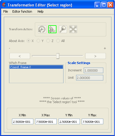
4.6 Tools Menu Functions
4-42 EnSight 10.2 User Manual
Revolution Tool
Toggle
Makes the Surface of Revolution Tool visible/invisible in the Graphics
Window. The Revolution Tool appears as thick direction line with
center point and center tool axis system, and with several circles
outlining each user defined point along the tool. Thinner projection
lines run through the circles to outline the revolution surface. The
Revolution Tool is initially centered about the Look-At point with the
direction line pointing in the X direction. There are a number of ways to
manipulate the tools either interactively or via the transformation
dialog. You can change its length and orientation interactively in the
Graphics Window by selecting one of the thick direction line end
points. You can rotate it in the Graphics Window by selecting the end of
one of the tool axes. You can reposition it interactively in the Graphics
Window by selecting its center or alternatively, you can reposition it
precisely by specifying coordinates in the Transformation Editor dialog
(described in Tool Positions... Quadric below).
Main Menu > Tools > Quadric
(see How to Use the Surface of Revolution Tool)
Transformation
Editor Tools Dialog
The Transformation Editor dialog is used for many types of transformation operations
including: global transformations, camera transformations, tool transformations, and
others. Tool transformations are described in this section of the documentation. Other
Transformation Editor functions are described fully (see Chapter 6, Transformation
Control).
Tool positions... Opens the Transformation Editor dialog which allows you to precisely position the
various tools within the Graphics Window in reference to the selected Frame.
Main Menu > Tools > Tool Positions...
Region Tool
(Selection region)
Click on Editor Function in the Transformation Editor dialog and then select Selecting
Tools >Region Selector from the Editor Function Menu Bar to display the dialog shown
below:
To precisely position the Selection tool, enter the desired normalized screen coordinate
values for X and Y minimum and maximum. The coordinates can be between 0.0 and 1.0.
Main Menu > Tools > Tool Positions... > Tools > Select region
Figure 4-15
Transformation Editor (Select region)
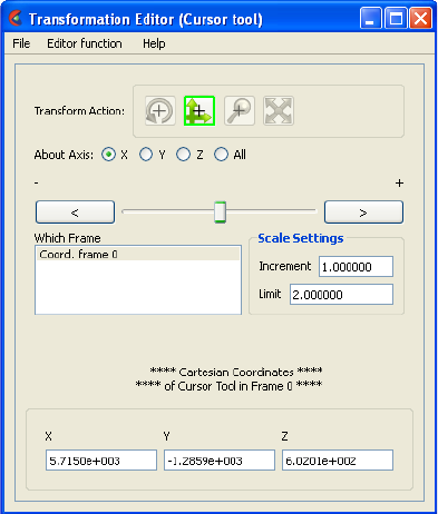
4.6 Tools Menu Functions
EnSight 10.2 User Manual 4-43
Cursor Tool Selecting Tools > Cursor from the Editor Function Menu Bar displays the dialog as
shown in Figure 4-16. Additionally, right-clicking on the cursor tool itself in the graphics
window and selecting Edit... from the Context Sensitive menu also displays this dialog
The Transformation Editor dialog provides three methods for the precise positioning of
the Cursor Tool. First, the Cursor Tool may be positioned within the Graphics Window by
entering coordinates in the X, Y, and Z fields. Pressing return causes the Cursor Tool to
relocate to the specified coordinates in the selected Frame (or, if more than one Frame is
selected, for Frame 0).
It is also possible to reposition the Cursor Tool from its present coordinate position by
specific increments. The Axis Button allows you to choose the axis of translation (X, Y,
Z, or All). The Slider Bar at Top allows you to quickly choose the increment by which to
move the position of the Cursor Tool. Dragging the slider in the negative (left) or positive
(right) directions and then releasing it will cause the X, Y, and Z coordinate fields to
increment as specified and the Cursor Tool to relocate to the new coordinates. The
number specified in the Limit field of the Scale Settings area determines the negative (-)
and positive (+) range of the slider. If the Limit is set to 1.0 as shown, then the numerical
range of the slider bar will be -1 to +1.
Alternatively, you can specify an increment for translation in the Increment field of the
Scale Settings area. Pressing return while the mouse pointer is in the Increment field will
cause the Cursor Tool to translate along the specified axis (or all axes) by the increment
specified.
Transformation Editor > Editor Function > Tools > Cursor
(see How to Use the Cursor (Point) Tool)
Figure 4-16
Transformation Editor (Cursor)
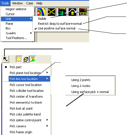
4.6 Tools Menu Functions
4-44 EnSight 10.2 User Manual
Line Tool From the menu Tools>Line there are three options as shown in Figure 4-17: Visible,
Restrict drag to surface+normal, and Use positive normal.
Visible Toggles the line tool visibility
Restrict drag to
surface +
normal
After choosing this option, click on the Pick icon and choose to pick
plane tool location using surface pick + normal and then put the cursor
tool on the part surface and pick using the ‘p’ key and the line tool will
appear aligned with the surface normal at the point picked with one end
attached to the surface at the point of the picking.
Use positive
surface normal
Same as above except the line tool will originate at the picked point
location, but will be in the direction of the positive normal.
Figure 4-17
Tools>Line Menu Options
Locks line parallel to selected
Line tool visibility
Locks line parallel to selected
part’s surface normal in
part’s surface normal
direction of surface normal
Choose Line tool
Click on Pick icon
Surface Pick + Normal
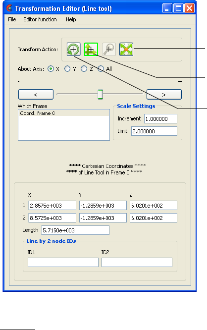
4.6 Tools Menu Functions
EnSight 10.2 User Manual 4-45
Selecting Tools>Line from the Editor Function Menu Bar displays the dialog as shown in
Figure 4-18. Additionally, right-clicking on the Line Tool in the graphics window and
selecting Edit... from the Context Sensitive menu also displays this dialog.
The Transformation Editor can control precisely the position and size of the line tool.
Position The Transformation Editor dialog provides several methods for the
precise positioning of the Line Tool. First, the Line Tool may be
positioned within the Graphics Window by entering coordinates for the
two endpoints in the X, Y, and Z fields. Pressing return after entering
each coordinate value causes the Line Tool to relocate to the specified
coordinates in the selected Frame (or if more than one Frame is
selected, in Frame 0). Enter all three X, Y, Z fields for a endpoint and
then press return once to cause the line tool to update its position to that
endpoint.
You can also specify the node ID labels to use for the line endpoints.
It is also possible to reposition the Line Tool from its present coordinate
position by specific increments. First click on the translate icon. The
Axis Button allows you to choose the axis of translation for the center
of the line (X, Y, Z, or All). The Slider Bar at Top allows you to quickly
choose the increment by which to move the position of the center point
of the Line Tool. Dragging the slider in the negative (left) or positive
(right) directions and then releasing it will cause the X, Y, and Z
coordinate fields to increment as specified and the Line Tool to relocate
to the new coordinates. The number specified in the Limit field of the
Scale Settings area determines the negative (-) and positive (+) range of
the slider. If the Limit is set to 1.0 as shown, then the numerical range of
the slider bar will be -1 to +1. The transformations are relative to the
line tool axis system.
Figure 4-18
Transformation Editor (Line Tool)
Translate Icon
Scale Icon
Rotate Icon
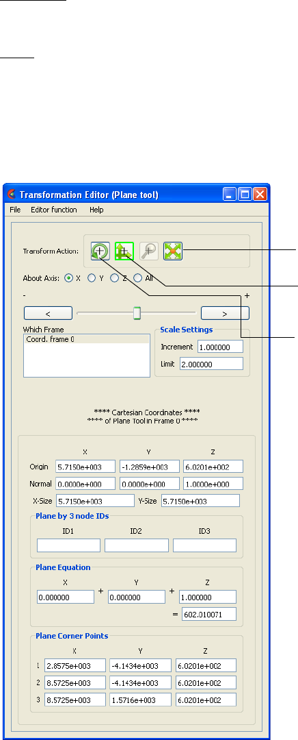
4.6 Tools Menu Functions
4-46 EnSight 10.2 User Manual
Alternatively, you can specify an increment for translation in the
Increment field of the Scale Settings area. Pressing return while the
mouse pointer is in the Increment field will cause the center point of the
Line Tool to translate along the specified axis (or all axes) by the
increment specified.
Orientation First click on the rotate icon. Next, pick an axis about which to rotate.
Next pick an increment and limit (in degrees) and slide the slider to
rotate the plane.
Scale First click on the scale icon. Next pick an increment and limit and slide
the slider to scale the line about its center, along its length.
Transformation Editor > Editor Function > Tools > Line
(see How to Use the Line Tool)
Plane Tool Selecting Tools > Plane from the Editor Function Menu Bar displays the dialog as shown
below. Additionally, right-clicking on the plane tool in the graphics area and selecting
Edit... from the Context Sensitive menu also displays this dialog.
The Transformation Editor can control precisely the position, orientation, and size of the
plane tool.
Figure 4-19
Transformation Editor (Plane Tool)
Scale Icon
Rotate Icon
Translate Icon

4.6 Tools Menu Functions
EnSight 10.2 User Manual 4-47
Position The Transformation Editor dialog provides several methods for the
precise positioning of the Plane Tool. First, the Plane Tool may be
positioned by entering the Origin, Normal and X- and Y-Size. Second,
the Plane Tool may be positioned by entering in 3 node IDs representing
3 corners (assuming unique node IDs). Third, the Plane Tool may be
positioned using the Algebraic Plane Equation. Finally, the Plane Tool
may be positioned within the Graphics Window by entering coordinates
for the three corners of the plane in the X, Y, and Z fields. Corner 1 is
defined as the -X, -Y corner of the plane, Corner 2 is defined as the +X,
-Y corner of the plane, and Corner 3 is defined as the +X, +Y corner of
the plane. Pressing return causes the Plane Tool to relocate to the
specified coordinates in the selected Frame (or if more than one Frame
is selected, in Frame 0). For your convenience, you can enter values
into all fields and then press return once to update the plane tool
position.
You can also position the Plane Tool be entering the id for three nodes.
The Plane Tool will then remain tied to these three nodes - even as the
nodes move in a transient geometry model.
You can also position the Plane Tool by entering a plane equation in the
form
Ax + By + Cz = D in the four fields and then pressing Return. For
convenience, enter in all four then press return. The coefficients may
then be normalized, but the equation of the plane will be the same as the
one you entered. The coefficients of the plane equation are in reference
to the selected Frame (or if more than one Frame is selected, to Frame
0).
As with the Cursor and Line Tools, it is possible to reposition the Plane
Tool from its present coordinate position by specific increments. First
click the translate icon at the top of the Transformation Editor. The
Axis Button allows you to choose the axis of translation (X, Y, Z, or
All) for the origin of the Plane Tool (intersection of the axes). The
Slider Bar at Top allows you to quickly choose the increment by which
to move the position of the origin. Dragging the slider in the negative
(left) or positive (right) directions and then releasing it will cause the X,
Y, and Z coordinate fields to increment as specified and the origin of the
Plane Tool to relocate to the new coordinates. The number specified in
the Limit field of the Scale Settings area determines the negative (-) and
positive (+) range of the slider. If the Limit is set to 1.0 as shown, then
the numerical range of the slider bar will be -1 to +1.
Alternatively, you can specify an increment for translation in the
Increment field of the Scale Settings area. Pressing return while the
mouse pointer is in the Increment field will cause the center of the Plane
Tool to translate along the specified axis (or all axes) by the increment
specified.
Orientation First click on the rotate icon. Next, pick an axis about which to rotate.
Next pick an increment and limit (in degrees) and slide the slider to
rotate the plane.
Scale First click on the scale icon. Next pick an axis direction to scale (X or
Y only). Finally pick an increment and limit and slide the slider to scale
the size of the plane.
Transformation Editor > Editor Function > Tools > Plane
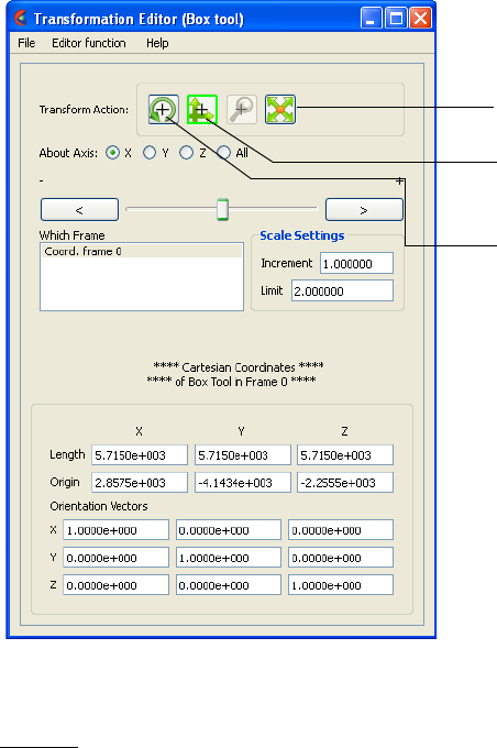
4.6 Tools Menu Functions
4-48 EnSight 10.2 User Manual
(see How to Use the Plane Tool)
Box Tool Selecting Tools > Box from the Editor Function Menu Bar displays the dialog shown
below. Additionally, right-clicking on the graphical Box Tool and selecting Edit... from
the Context Sensitive menu also displays this dialog.
The Transformation Editor can control precisely the position, orientation, and size of the
box tool.
Position The Transformation Editor dialog provides several methods for the
precise positioning of the Box Tool. First, the Box Tool may be
positioned within the Graphics Window by entering coordinates for the
origin of the box in the X, Y, and Z fields and the length of the each of
the X, Y, and Z sides. Pressing return causes the Box Tool to relocate to
the specified location in the selected Frame (or if more than one Frame
is selected, in Frame 0). For your convenience, you can enter in all of
the fields and then press return once to update the Box Tool position.
Additionally, you can modify the orientation of the Box Tool by
entering the X, Y, and Z orientation vectors of the box axis in regards to
Frame 0.
Figure 4-20
Transformation Editor (Box Tool)
Scale Icon
Rotate Icon
Translate Icon
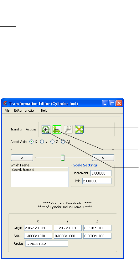
4.6 Tools Menu Functions
EnSight 10.2 User Manual 4-49
As with other Tools, it is possible to reposition the Box Tool from its
present coordinate position by specific increments. First click the
translate icon at the top of the Transformation Editor. The Axis Button
allows you to choose the axis of translation (X, Y, Z, or All) for the
origin of the Box Tool (intersection of the axes). The Slider Bar at Top
allows you to quickly choose the increment by which to move the
position of the origin. Dragging the slider in the negative (left) or
positive (right) directions and then releasing it will cause the X, Y, and
Z coordinate fields to increment as specified and the origin of the Box
Tool to relocate to the new coordinates. The number specified in the
Limit field of the Scale Settings area determines the negative (-) and
positive (+) range of the slider. If the Limit is set to 1.0 as shown, then
the numerical range of the slider bar will be -1 to +1.
Alternatively, you can specify an increment for translation in the
Increment field of the Scale Settings area. Pressing return while the
mouse pointer is in the Increment field will cause the origin of the Box
Tool to translate along the specified axis (or all axes) by the increment
specified.
Orientation First click on the rotate icon. Next, pick an axis about which to rotate.
Next pick an increment and limit (in degrees) and slide the slider to
rotate the Box Tool.
Scale First click on the scale icon. Next pick an axis direction to scale.
Finally pick an increment and limit and slide the slider to scale the size
of the Box Tool.
Transformation Editor > Editor Function > Tools > Box
(see How to Use the Box Tool)
Cylinder or Sphere
Too l s
Selecting Tools and then Cylinder or Sphere from the Editor Function Menu Bar displays
the dialog as shown below. Additionally, right-clicking on the Cylinder or Sphere tool in
the graphics area and selecting Edit... from the Context Sensitive menu also displays this
dialog.
Figure 4-21
Transformation Editor (Cylinder Tool) or
(Sphere Tool)
Translate Icon
Scale Icon
Rotate Icon

4.6 Tools Menu Functions
4-50 EnSight 10.2 User Manual
The Transformation Editor can control precisely the position and size of the cylinder tool.
Position The Transformation Editor dialog enables you to precisely control the
coordinates of the Cylinder or Sphere Tool origin (center point of the
thick direction line) by specifying them in the Orig. X, Y, and Z fields.
You control the direction vector for the Cylinder or Sphere Tool
direction axes by specifying the coordinates in the Axis X, Y, and Z
fields of the selected Frame (or if more than one Frame is selected, in
Frame 0). The Radius of each tool may be specified in the Radius Field.
It is possible to reposition the Cylinder or Sphere Tool origins by
specific increments. First click on the translate icon. The Axis Button
allows you to choose the axis of translation (X, Y, Z, or All) for the
origin of the tool. The Slider Bar at Top allows you to quickly choose
the increment by which to move the position of the origin. Dragging the
slider it in the negative (left) or positive (right) directions and then
releasing it will cause the X, Y, and Z coordinate fields to increment as
specified and the origin of the Cylinder or Sphere Tool to relocate to the
new coordinates. The number specified in the Limit field of the Scale
Settings area determines the negative (-) and positive (+) range of the
slider. If the Limit is set to 1.0 as shown, then the numerical range of the
slider bar will be -1 to +1.
Alternatively, you can specify an increment for translation in the
Increment field of the Scale Settings area. Pressing return while the
mouse pointer is in the Increment field will cause the origin of the
Cylinder or Sphere Tool to translate along the specified axis (or all
axes) by the increment specified.
Orientation First click on the rotate icon. Next, pick an axis about which to rotate.
Next pick an increment and limit (in degrees) and slide the slider to
rotate the plane.
Scale First click on the scale icon. Next pick an axis direction to scale. Can
only scale in the X (longitudinal) or Y (radial) directions. Finally pick
an increment and limit and slide the slider to scale the size of the
cylinder or sphere Tool.
Transformation Editor > Editor Function > Tools > Cylinder or Sphere
(see How To Use the Cylinder Tool and How To use the Sphere Tool)
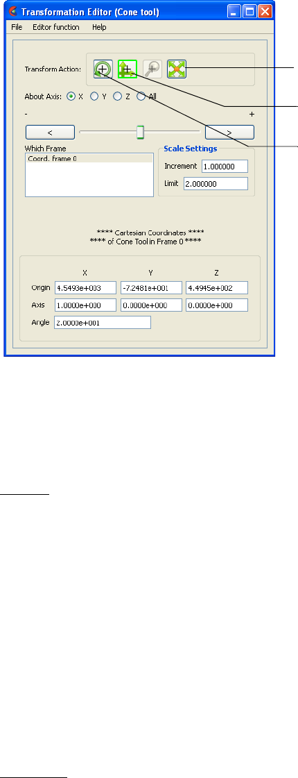
4.6 Tools Menu Functions
EnSight 10.2 User Manual 4-51
Cone Tool Selecting Tools>Cone from the Editor Function Menu Bar displays the dialog as shown
below. Additionally, right-clicking on the graphical Cone Tool and selecting Edit... from
the Context Sensitive menu also displays this dialog.
The Transformation Editor dialog enables you to precisely control the coordinates of the
Cone Tool origin (the point of the cone) by specifying them in the Orig. X, Y, and Z
fields. You control the direction vector for the Cone Tool direction axis by specifying the
coordinates in the Axis X, Y, and Z fields for the selected Frame (or if more than one
Frame is selected, in Frame 0). The conical half angle may be specified in degrees in the
Angle Field.
Position It is possible to reposition the Cone Tool origin by specific increments.
The Axis Button allows you to choose the axis of translation (X, Y, Z,
or All) for the origin of the tool. The Slider Bar at Top allows you to
quickly choose the increment by which to move the position of the
origin. Dragging the slider in the negative (left) or positive (right)
directions and then releasing it will cause the X, Y, and Z coordinate
fields to increment as specified and the origin of the Cone Tool to
relocate to the new coordinates. The number specified in the Limit field
of the Scale Settings area determines the negative (-) and positive (+)
range of the slider. If the Limit is set to 1.0 as shown, then the numerical
range of the slider bar will be -1 to +1.
Alternatively, you can specify an increment for translation in the
Increment field of the Scale Settings area. Pressing return while the
mouse pointer is in the Increment field will cause the center of the Cone
Tool to translate along the specified axis (or all axes) by the increment
specified.
Orientation First click on the rotate icon. Next, pick an axis about which to rotate.
Next pick an increment and limit (in degrees) and slide the slider to
rotate the plane.
Figure 4-22
Transformation Editor (Cone Tool)
Translate Icon
Scale Icon
Rotate Icon
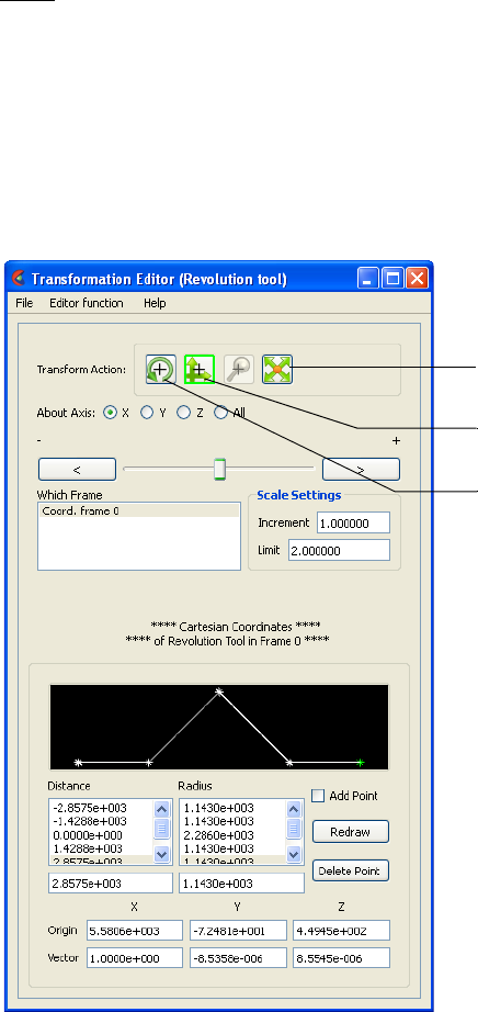
4.6 Tools Menu Functions
4-52 EnSight 10.2 User Manual
Scale First click on the scale icon. Next pick an axis direction to scale. Can
only scale in the X (longitudinal) or Y (half conical angle) directions.
Finally pick an increment and limit and slide the slider to scale the size
of the cone tool.
Transformation Editor > Editor Function > Tools > Cone
(see How to Use the Cone Tool)
Revolution Tool Selecting Tools>Revolution from the Editor Function Menu Bar displays the dialog as
shown below. Additionally, right-clicking on the graphical Revolution Tool and selecting
Edit... from the Context Sensitive menu also displays this dialog.
For the Revolution Tool, you not only control the origin and direction vector, but the
number of points and positions that are revolved about the axis.The desired coordinates of
the Revolution Tool origin (center point of the thick direction line) are specified in the
Orig. X, Y, and Z fields. The direction vector for the Revolution Tool direction axis is
specified by entering the desired coordinates in the Vect X, Y, and Z fields for the selected
Frame (or if more than one Frame is selected, in Frame 0).
Additional points may be added to the Revolution Tool by clicking on the Add Point(s)
toggle and then clicking at the desired location in the schematic for the tool. There is no
need to be overly precise in its placement since its location can be modified. Once you
have added all of the new points you wish, the Add Point(s) toggle should be turned off.
A point may be deleted by selecting it in the schematic area and then clicking the Delete
button.
Figure 4-23
Transformation Editor (Revolution Tool)
Translate Icon
Scale Icon
Rotate Icon

4.6 Tools Menu Functions
EnSight 10.2 User Manual 4-53
The position of any point may be modified interactively within the Revolution Tool
schematic window, Simply click on and drag the point to the desired location. The precise
location of any point may be specified by selecting the point in the schematic with the
mouse and then entering the desired Distance (from the Revolution Tool origin) or Radius
(from the axis) for the point in the text entry fields beneath the Distance and Radius Lists.
Pressing return will enter the new value in the list above for the selected point.
The Transformation Editor can control precisely the position and size of the revolution
tool.
Position It is possible to reposition the Revolution Tool origin by specific
increments. First click on the translate icon. The Axis Button allows
you to choose the axis of translation (X, Y, Z, or All) for the origin of
the tool. The Slider Bar at Top allows you to quickly choose the
increment by which to move the position of the origin. Dragging the
slider in the negative (left) or positive (right) directions and then
releasing it will cause the X, Y, and Z coordinate fields to increment as
specified and the origin of the Revolution Tool to relocate to the new
coordinates. The number specified in the Limit field of the Scale
Settings area determines the negative (-) and positive (+) range of the
slider. If the Limit is set to 1.0 as shown, then the numerical range of the
slider bar will be -1 to +1.
Alternatively, you can specify an increment for translation in the
Increment field of the Scale Settings area. Pressing return while the
mouse pointer is in the Increment field will cause the center of the
Revolution Tool to translate along the specified axis (or all axes) by the
increment specified.
Orientation First click on the rotate icon. Next, pick an axis about which to rotate.
Next pick an increment and limit (in degrees) and slide the slider to
rotate the plane.
Scale First click on the scale icon. Next pick an axis direction to scale. Can
only scale in the X (longitudinal) or Y (radial) directions. Finally pick
an increment and limit and slide the slider to scale the size of the
revolution tool.
Redraw This button will cause the Revolution Tool schematic window to re-
center to the currently defined points of the tool.
Transformation Editor > Editor Function > Tools > Revolution
(see How to Use the Surface of Revolution Tool)
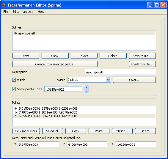
4.6 Tools Menu Functions
4-54 EnSight 10.2 User Manual
Spline Tool Selecting Tools>Spline from the Editor Function Menu Bar displays the dialog as shown
below. Additionally, right-clicking on the Spline tool in the graphics area and selecting
Edit... form the Context Sensitive menu also displays this dialog.
The Transformation Editor dialog enables you to create and edit the control points for a
spline. A spline is used for one of three functions (a) path for a camera, (b) the path for a
clip plane, and (c) the path for a distance vs. variable query.
New Creates a new spline
Copy Creates a new spline by copying the selected spline
Invert Inverts the control points for the selected spline
Delete Delete the selected spline(s)
Save to File Save the selected spline(s) to a file
Load from File Load splines from a file
Create from
selected part(s)
Create a new spline and use all of the coordinates in the selected parts
as the control points.
Description Description of the spline
Visible Toggles spline visibility
Width Line width for the spline
Color... Brings up the color chooser dialog to set the color for the spline
Show points Toggles the visibility of the control points.
Size The size of the control point markers in model coordinates
Points The list of control points for the spline. Right click operations in this
list include New, Copy, Paste, and Delete
Figure 4-24
Transformation Editor (Spline Tool)
4.6 Tools Menu Functions
EnSight 10.2 User Manual 4-55
New (at cursor) Inserts a new control point in the selected spline after the selected point
(or if no points are selected or exist at the end of the list) using the
cursor tool as the location.
Select All Selects all of the points in the list
Copy Stores the coordinates of the selected points in preparation for a Paste
operation
Paste Paste the copied points and insert them immediately after the selected
point (or if no points are selected or exist then at the end of the list).
Offset... Brings up a dialog where a xyz offset value can be specified. The offset
is added to the coordinates of the selected points.
Delete Delete the selected points.
XYZ fields Shows the XYZ values for the selected point. If modified will change
the control point location.
(see How to Use the Spline Tool)
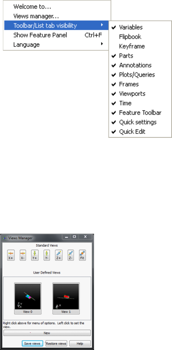
4.7 Window Functions
4-56 EnSight 10.2 User Manual
4.7 Window Functions
The Window menu in EnSight provides access to the EnSight ‘Welcome’ screen,
the ‘Views’ manager, language settings and the toolbars and dockable object list
dialogs. The menu appears like this:
Welcome to… Displays the Welcome dialog from which the user can reload previously loaded datasets and saved
session files.
Views manager Displays the Views Manager dialog. Note that you can also click on the Views button in the Tools
Icon Bar and select the ‘Views…’ menu to bring up the same dialog.
Views manager
dialog
This dialog allows the user to create, save, restore, and apply views interactively. A View
comprises all the viewing parameters and viewport parameters along with a thumbnail
image of the user’s data taken with the view.
Figure 4-25
Window pull-down menu
4.7 Window Functions
EnSight 10.2 User Manual 4-57
Along the top of the views manager are standard views down the major axes designed to
orient your model in the main graphics window. The center of the dialog contains a
collection of thumbnail images for the views defined interactively by the user. To create a
new view right click on an empty area in the User Defined Views area and select New or
click on the ‘New’ button. A new view will be created in the User Defined Views area
from your model viewing parameters in the main graphics window. To save your views to
a folder, click on the Save Views button. To load (restore) views from a file, click on the
Restore button. A view can be applied to the current scene by simply clicking on the
associated icon. There are a number of other options that can be accessed by right
clicking in the space containing the user-defined views or on the views themselves. For
more details, see How to Manage Views
Toolbar/List tab visibility The EnSight GUI consists of a number of toolbars and dockable object lists and other GUI panels.
This menu contains a list of all of the core dockable panels, the toolbars and any currently open
user-defined gui panel extensions. The visibility of these items can be toggled by selecting items
from the sub-menu under this menu option.
Show Feature Panel This menu is a quick way for the user to open up the Feature Panel with the currently selected
feature displayed.
Language This sub-menu allows the user to select the language to be used for the EnSight GUI. Various
languages may be listed, but English is the default. There will also be an option for ‘System Locale’.
This option will cause the language setting for EnSight to track the default system language (the
system ‘Locale’ setting). WelcomeDisplays the Welcome dialog.
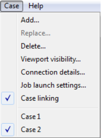
4.8 Case Menu Functions
4-58 EnSight 10.2 User Manual
4.8 Case Menu Functions
EnSight allows you to work concurrently with up to sixteen different sets of
results data (computational or experimental). Each set of results data is read in as
an EnSight “Case”. The Case Main Menu provides access to the mechanisms for
manipulating cases, controlling their visibility and for setting up and monitoring
their server connections.
Add... This menu option is used to add an additional case to the current EnSight session.
Selecting it opens a dialog which allows one to specify a name and other options for the
new Case. The name will appear in the list of active Cases at the bottom of the menu as
shown above. Adding a Case actually starts a new EnSight Server and connects it to the
EnSight Client. The File->Open... dialog will then open data files may be loaded for the
new Case. The geometry from the new case will be added to the geometry already present
in the EnSight Client. There are a number of options in the ‘New case’ dialog illustrated
below in the New Case Dialog section. The Open... dialog will then open and you can
read and load data for the new Case.
Replace... Replacing a Case causes all parts and variables associated with the active Case (selected
at the bottom of the Case menu) to be deleted. The Server will be restarted and assigned
the new Case name. Clicking the Replace... button opens a reduced version of the ‘New
case’ dialog which allows one to specify a name for the Case to be replaced and the server
launch configuration. The dialog also allows the user to click on ‘Keep currently loaded
data’ and convert the operation into an ‘Add case’ operation. The Open... dialog will then
open and you can read and load data for the new Case (see the New Case Dialog section
below)
Delete Deleting a Case causes all parts and variables associated with the Case to be deleted and
terminates the Server associated with the Case. Clicking the Delete button opens a
Warning Dialog which confirms that the case selected at the bottom of the menu should
be deleted (see How To Load Multiple Datasets (Cases)).
Viewport visibility... The visibility of the parts from an individual EnSight case can be limited to specific
Viewports. By default, the parts from all cases are visible in all viewports. This menu
option allows the user to select the specific viewport(s) that the geometry (parts)
associated with the case will be visible. Parts associated with the selected Case will be
visible in the green viewports and hidden in the back viewports. This operation simply
sets the individual part viewport visibility flags for all the parts in the current case (see
Part Visibility Toggle Icon in 5.1.1, Parts Quick Action Icons).
Figure 4-26
Case pull-down menu
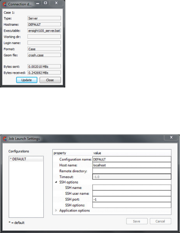
4.8 Case Menu Functions
EnSight 10.2 User Manual 4-59
Connection details... Opens the Connection details... dialog which gives information about the connection and
how many bytes have been transmitted.
Job Launch settings... Note: this dialog is deprecated and will be replaced with the CEIStart / CEIShell dialog in
a future release. This menu opens the Connection settings dialog. From this dialog users
can create and edit client-server or client-sos connection parameters. For example,
specific hostnames, network parameters and other setup options. You can control whether
automatic or manual connections will occur, and can manage and save this information
for future use (see How to Connect EnSight Client and Server).
Case Linking A toggle indicating Case Linking status: on or off. If case linking is on (as in Figure
4-26), you can turn it off using this toggle. Once turned off, you can not toggle it back on
in the current EnSight session. Case linking is optionally turned on at the load of the
second case (see How to Compare Cases), and then applies linking to all subsequent
cases. If case linking is not turned on before the second case is added, then it cannot be
turned on during the rest of the EnSight session. The goal of linking all the cases is to
quickly and uniformly perform the same operation over all of the cases. So
transformations, part attribute changes, part and variable creation and query operations
are performed automatically and uniformly across all of the loaded cases. When one case
is changed, all are changed in the same way (see How to Compare Cases). Please see the
Release Notes for a current list of limitations and capabilities.
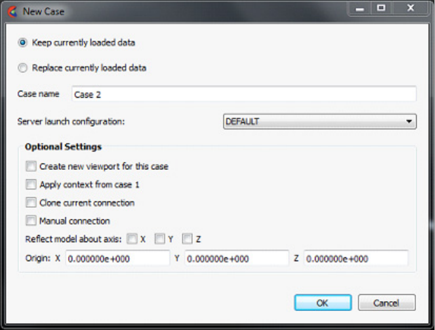
4.8 Case Menu Functions
4-60 EnSight 10.2 User Manual
Case 1, etc At the bottom of the Case menu, there is a list of the current cases. The current case is
checked in the menu. Selecting another case from the bottom of this list makes that case
the current case and the target of operations like the ‘Delete…’ or ‘Replace…’ from this
menu or query operations. Only one case can be current. In Figure 4-26 above, Case 2 is
the currently selected Case.
New case dialog This dialog is used to determine the new parameters for a new case.
Keep currently loaded data The new case can be added to the existing one. This
does not unload the current one and starts up a new
server to load the added dataset
Replace currently loaded data This deletes the existing dataset and loads the new data
in place of it
Case name The name that will appear at the bottom of the Case
menu.
Server launch configurations Choose a launch configuration for the server. A server
launch configuration is defined using the Case>Job
Launch Settings... menu.
Create new viewport for this
case
The new dataset can be placed in a new viewport or
added to the current
Apply context from case 1 The new dataset can have the context of case 1 applied
to it, which will cause it to basically inherit the
positioning etc. of case 1.
Clone current connection Use the same parameters to start up the new server as
the existing server used. This can be useful if one used a
complicated set of options to start up the server for the
original dataset and don’t want to have to repeat them
for this dataset.
Figure 4-27
Add Case Dialog
4.8 Case Menu Functions
EnSight 10.2 User Manual 4-61
Manual connection Check this option to cause the EnSight client to look for
a manual server connection. The client will wait for the
(remote) server to be launched once ‘Ok’ is clicked.
Reflect model about axis This option specifies that the dataset should be reflected
over one or more axis when loaded.
Origin Specify the origin of the data.
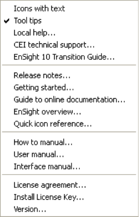
4.9 Help Menu Functions
4-62 EnSight 10.2 User Manual
4.9 Help Menu Functions
The Main Menu Help menu provides direct access to all of the EnSight
documentation products as well as version information, license control and the
direct technical support portal.
Icons with text Toggles the display of help text under the various toolbar icons. The option is disabled by
default.
Tool tips Toggles the display of tool-tip text help items. The option is enabled by default.
Local help... Opens an optional, site-specific local help document, if one exists. Simply place a .pdf file
in the $CEI_HOME/ensight102/site_preferences directory named “LocalHelp.pdf” or use
the Product extension mechanism (see Chapter 9.x for details on the product extension file
format). This is a hook for sites that want to provide site-specific help for their users. This
might include customized preferences, help manuals for local User-Defined Readers,
instructions for using customized macros, etc.
Figure 4-28
Help pull-down menu
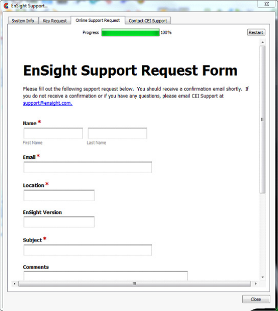
4.9 Help Menu Functions
EnSight 10.2 User Manual 4-63
CEI technical support... Opens the CEI Online Support tool for simplified problem reporting, key requests and
EnSight support contact information. The tool has four tabs: System Info, Key Request,
Online Support Request and Contact CEI Support.
System Info Click on this tab to review the information that has been
collected about the session. This tab collects information about
the EnSight Application in use, the license file, the graphics card,
environment variables and a screen shot of EnSight’s graphics
window. This information is useful for more rapid
troubleshooting of your EnSight issue.
Key Request Click on this tab to request a new or changed license key. Fill in
the information and click Submit Form.
Online Support
Request
Click this tab to send a problem report to your EnSight
Distributor. In this tab, fill out the form and click Submit Form.
Contact CEI Support This tab gives basic information on how to contact CEI technical
support including phone numbers, hours of service and email
addresses.
EnSight 10 transition
guide...
This menu opens a web-browser with information related to the transition from versions
prior to EnSight to 10.
Release notes... Provides an overview of changes made since the last major EnSight release.
Getting started... Opens the EnSight Getting Started Manual which provides an introduction to EnSight
designed for new users. Note that this document is not cross-referenced within itself or to
other documents.
Figure 4-29
Online support tool
4.9 Help Menu Functions
4-64 EnSight 10.2 User Manual
Guide to online
documentation...
Displays a guide to the use of the installed CEI documentation.
EnSight overview... Displays a PDF file which gives an overview of the operation of EnSight.
Quick icon reference... Provides a quick reference guide to all EnSight GUI icons, many of which have links to
appropriate How To documents.
How to manual... Opens the How To Manual.
User manual... Opens the User Manual.
Interface manual... Opens the Interface Manual. The Interface Manual covers the user-defined reader, writer
and math function APIs. It also documents the Command Driver and basic Python
interfaces.
License agreement... Opens the EnSight Version 10 End User License Agreement.
Install license key... Selecting this menu option causes EnSight to prompt the user for the location of a
slim8.key file obtained from CEI. It will install the key into the existing EnSight
installation.
Version... Opens up the EnSight version Information dialog. In it, is the version number of the
EnSight software currently running along with a listing of all of the user-defined
extensions and other versioning information.
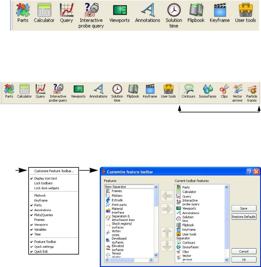
EnSight 10.2 User Manual 5-1
5Features
Overview
This chapter describes the functions available through the Feature ribbon, which
contains the Feature Icon Bar (including Secondary Feature Icons) and the Quick
Action Icon Bar.
Secondary “features” can be turned on as desired. These are not features in and of
themselves, but are accelerators into various settings of the main features. For
example, the Clip feature is really a shortcut to the clip settings of the Part feature.
By default you will see the five secondary features in the figure above. They are
attached to the feature ribbon by a separator. You can configure the Feature ribbon
by right-clicking anywhere on the ribbon and choosing “Customize Feature
Toolbar...”.
Selecting items and using the left or right arrows will allow you to move icons on
or off of the toolbar. Selecting and using the up or down arrows will change the
icon position in the toolbar. When you have made your changes you can hit the Ok
button to save them for the current session, or the Save button to save them for
this and future sessions.
Figure 5-1
EnSight Feature Icon Bar, with optional text labels
Figure 5-2
EnSight Secondary Features
Figure 5-3
Customizing the Feature Ribbon
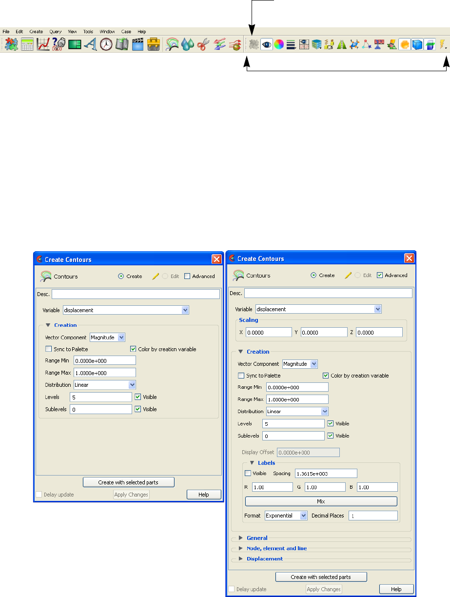
5-2 EnSight 10.2 User Manual
Quick Action Icons for easy manipulation of the major attributes of selected
features change in the Feature ribbon according to selection in the list panels. For
example, when a part is selected, you will see:
Just to the right of the separator, a greyed-out icon of the feature will be shown,
followed by the Quick Action Icons for the selection. These icons allow you to
change popular attributes without having to open the Feature Panel.
The Feature Panel (FP), is available for manipulation of a features attributes, for
both creation of new entities, as well as editing of existing entities. This editor can
be brought up in several different ways, including clicking on the feature icon
itself, double clicking on entities in the list panels, right-clicking on entities in the
list panels and selecting Edit..., etc. For ease of use, this editor can often have both
a basic and advanced mode. The following is an example of this editor for contour
parts.
Identifier icon
Quick Action Icons
Figure 5-4
Quick Action Icon Bar Example
Figure 5-5
Example of Feature Panel
EnSight 10.2 User Manual 5-3
Each feature in the chapter will discuss the associated Quick Action Icons and
Feature Panel options.
Quick links to the sections in this chapter:
Section 5.1, Parts
Section 5.1.1, Parts Quick Action Icons
Section 5.1.2, Model Parts
Section 5.1.3, Clip Parts
Section 5.1.4, Contour Parts
Section 5.1.5, Developed Surface Parts
Section 5.1.6, Elevated Surface Parts
Section 5.1.7, Extruded Parts
Section 5.1.8, Isosurface Parts
Section 5.1.9, Material Interface Parts
Section 5.1.10, Particle Trace Parts
Section 5.1.11, Point Parts
Section 5.1.12, Profile Parts
Section 5.1.13, Separation/Attachment Line Parts
Section 5.1.14, Shock Regions/Surfaces Parts
Section 5.1.15, Subset Parts
Section 5.1.16, Tensor Glyph Parts
Section 5.1.17, Vector Arrow Parts
Section 5.1.18, Vortex Core Parts
Section 5.1.19, Auxiliary Geometry
Section 5.2, Annotations
Section 5.2.1, Text Annotation
Section 5.2.2, Line Annotation
Section 5.2.3, Shape Annotation
Section 5.2.4, 3D Arrow Annotation
Section 5.2.5, Dial Annotation
Section 5.2.6, Gauge Annotation
Section 5.2.7, Logo Annotation
Section 5.2.8, Legend Annotation
Section 5.3, Query/Plotter
Section 5.3.1, At Line Tool Over Distance
Section 5.3.2, At 1D Part Over Distance
Section 5.3.3, At Spline Over Distance
Section 5.3.4, At Node Over Time
Section 5.3.5, At Element Over Time
Section 5.3.6, At IJK Over Time
Section 5.3.7, At XYZ Over Time
Section 5.3.8, At Minimum Over Time
Section 5.3.9, At Maximum Over Time
Section 5.3.10, By Scalar Value
Section 5.3.11, By Constant on Part Sweep
Parts
5-4 EnSight 10.2 User Manual
Section 5.3.12, By Operating on Existing Queries
Section 5.3.13, Read From an External File
Section 5.3.14, Read From a Server File
Section 5.3.15, Plotters
Section 5.4, Viewports
Section 5.4.1, Viewports Quick Action Icons & Feature Panel
Section 5.5, Frames
Section 5.5.1, Frames Quick Action Icons and Feature Panel
Section 5.5.2, Frame Definition
Section 5.5.3, Frame Transform
Section 5.6, Calculator
Section 5.7, Flipbook Animation
Section 5.8, Interactive Probe Query
Section 5.9, Keyframe Animation
Section 5.10, Solution Time
Section 5.11, Tools Icon Bar
Section 5.12, User Tools
5.0.1 Parts
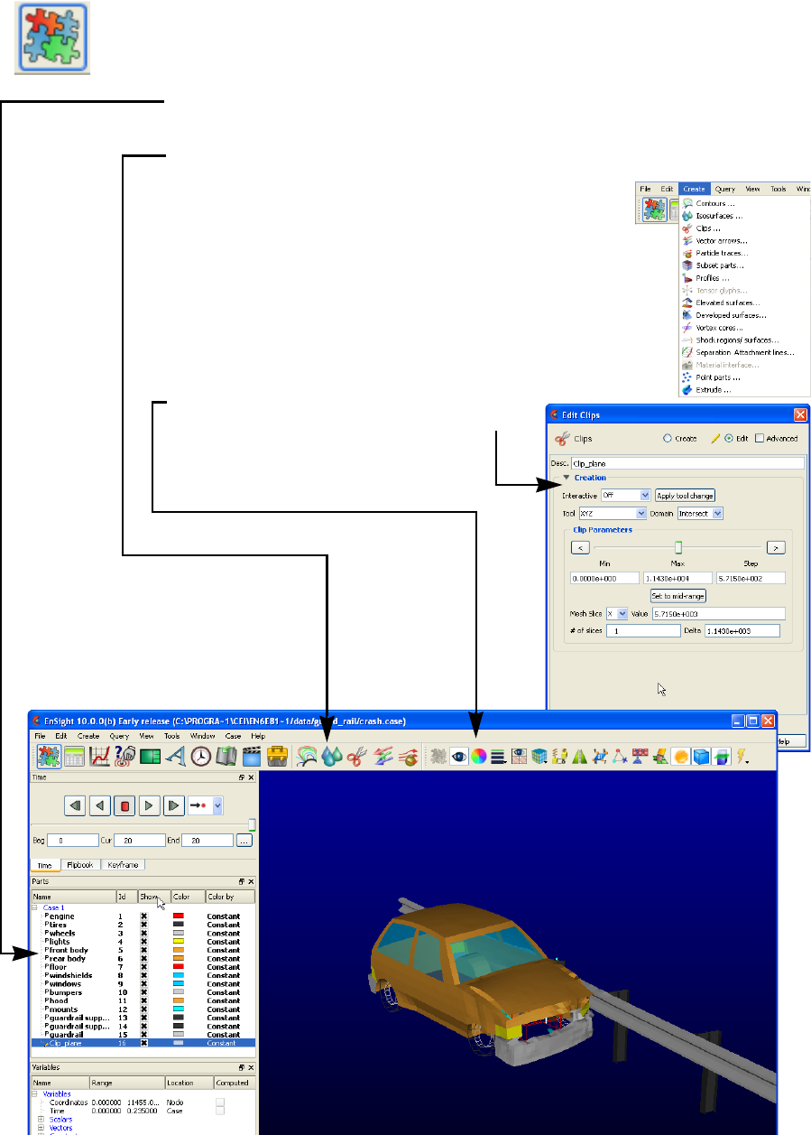
5.1 Parts
EnSight 10.2 User Manual 5-5
5.1 Parts
By default, the first icon on the Feature Icon Bar is the major feature entitled
“Parts”.
When model parts are loaded from data files, or created parts are produced
through the use of part features, they appear in the Parts list and are displayed in
the graphics window.
The secondary feature icons appear after the first separator. By default the ones
shown are those associated with parts and include
contours, isosurfaces, clips, vector arrows, and particle
traces. But as discussed above, these can be customized.
And the entire list is always available through the Create
menu.
The attributes of selected parts can be edited via the Quick
Action Icon Bar, which appears after the
second separator. Or in the Feature Panel
dialog, which can be opened by double-
clicking on the parts in the Parts list.
5.1 Parts
5-6 EnSight 10.2 User Manual
The actual process of reading data, loading model parts, and creating parts from
the various features, is discussed in many of the topics of the How To Manual.
Please refer to it for guidance.
The subsections which follow will discuss the various parts features.
Section 5.1.1, Parts Quick Action Icons
Section 5.1.2, Model Parts
Section 5.1.3, Clip Parts
Section 5.1.4, Contour Parts
Section 5.1.5, Developed Surface Parts
Section 5.1.6, Elevated Surface Parts
Section 5.1.7, Extruded Parts
Section 5.1.8, Isosurface Parts
Section 5.1.9, Material Interface Parts
Section 5.1.10, Particle Trace Parts
Section 5.1.11, Point Parts
Section 5.1.12, Profile Parts
Section 5.1.13, Separation/Attachment Line Parts
Section 5.1.14, Shock Regions/Surfaces Parts
Section 5.1.15, Subset Parts
Section 5.1.16, Tensor Glyph Parts
Section 5.1.17, Vector Arrow Parts
Section 5.1.18, Vortex Core Parts
Section 5.1.19, Auxiliary Geometry
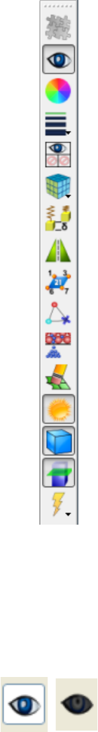
5.1 Parts Quick Action Icons
EnSight 10.2 User Manual 5-7
5.1.1 Parts Quick Action Icons
Each of the several different types of parts share the following Quick Action
Icons, which are used to adjust a number of attributes for individual parts.
These are discussed here, but apply to all 6.1.2 through 6.1.17 sections.
Part Visibility Icon Determines the global (in all viewports and in all Modes) visibility of the selected
Part(s). Note you can just right-click on the part and choose ‘Hide’ to make it invisible
Figure 5-6
Part Quick Action Icons
Part Visibility Toggle Icon
Part Visibility in Viewport Icon
Part Line Width Pulldown Icon
Element Representation Pulldown Icon
Visual Symmetry Icon
Part Shading Toggle Icon
Part Hidden Line Toggle Icon
Element/Node Label Toggle Icon
Part Auxiliary Clipping Toggle Icon
Node Representation Icon
Fast Display Representation Pulldown Icon
Part Element Blanking/Selection Icon
Part Color, Surface Properties (Lighting, Transparency) Icon
Part Displacement Element Icon
Part Filter Element Icon
When parts are selected
Figure 5-7
Part Visibility ON - OFF Icons
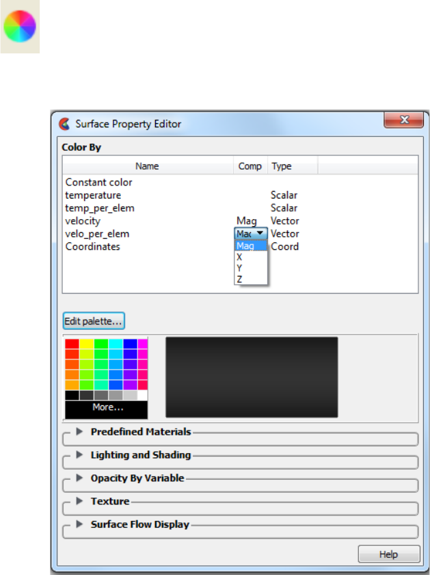
5.1 Parts Quick Action Icons
5-8 EnSight 10.2 User Manual
Part Color/Surface
Property Icon
Clicking once on the Part Color/Surface Property Icon opens a dialog which allows you
to assign color, lighting characteristics, transparency levels, textures, and display surface
flow to the individual Part(s) which has (have) been selected in the Parts List. If no Parts
are selected, modifications will affect the default Part color and all Parts subsequently
loaded or created will be assigned the new default color.
Note, you can just right-click on a part and choose how to color it.
Color By Allows you to choose whether to color the selected Part(s) by a Constant Color or by a
Var iab le .
Name Column containing the name of the surface property (Constant or Variable name).
Constant Color The selected Part(s) may be assigned a constant color by selecting it from the pre-
defined matrix of color cells.
Figure 5-8
Part Color/Surface Property Icon
Figure 5-9
Part Color/Surface Property dialog
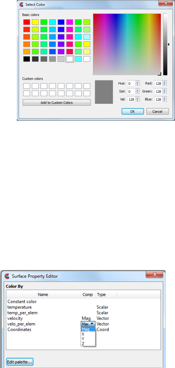
5.1 Parts Quick Action Icons
EnSight 10.2 User Manual 5-9
More... Alternatively, you can click on the More... area and the Select Color
dialog will open.
You can choose a color by entering RGB or HSV values directly,
picking a color from the matrix, or custom color lists, or by utilizing
the color square and slider. Regardless of which method you use to
define a color, it will not be applied to the selected Part(s) until you
click the OK button.
Variable Alternatively, the Part(s) may be colored by a variable selected in the pulldown list. The
color palette for each Variable associates a color with each value of the variable and
these colors are used to color the selected Part(s).
If coloring by a nodal variable, the default coloring will be continuously varying - even
within a given element. If you are coloring by a per-element variable, the coloring will
not vary within a given element. If you desire to see per-element variables in a
continuously varying manner, you can toggle on “Use continuous palette for per-element
variables” under Edit->Preferences... Color Palettes.
Comp Column containing the component description for vector variables. The default
component is Mag. If you are coloring by a vector variable clicking in its component
column allows selection of the magnitude or its components (e.g. X, Y, or Z).
Figure 5-10
Select Color dialog
Figure 5-11
Part Color/Surface Property Editor Color by Vector Component
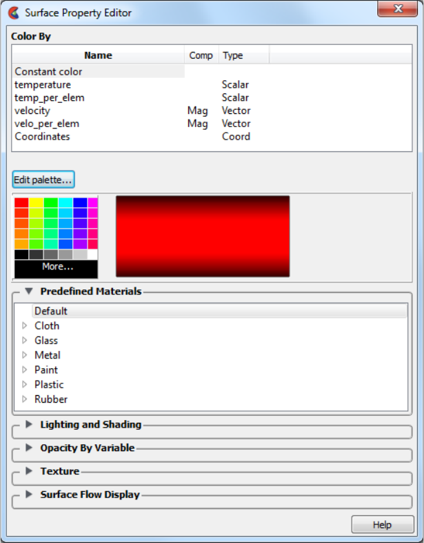
5.1 Parts Quick Action Icons
5-10 EnSight 10.2 User Manual
Type The type of variable (blank is constant, scalar is single value at every node or element,
vector is four values at every node or element, tensor is six or 9 values at every node or
element). Coordinates are a special client-side variable, with only magnitude available.
Edit Palette... The Palette is the mathematical mapping of variable values to colors and to color
opacity. Clicking on Edit Palette... will open the Palette Editor dialog and allow the
editing of this mapping. See How To Edit Color Palettes.
Predefined
Materials
Turn down exposes a number of predefined material models that allow you to quickly
assign realistic surface model to part(s) without going through the trouble of adjusting
the lighting and shading. Note that after you pick a predefined material, you can still go
to the lighting and shading turn down and further refine the settings. The lighting and
shading options are context-sensitive to the predefined material you have selected.
Default This is the legacy surface property model for backward-compatibility purposes.
Cloth Velvety cloth-like surface.
Glass Translucent glass-like properties: includes thin, clear, diamond and mirror glass-like
models.
Metal Includes Aluminum, Brass, Chrome, Copper, Gold, Iron & Silver metallic-like surfaces.
Figure 5-12
Part Color/Surface Property Editor Predefined Materials
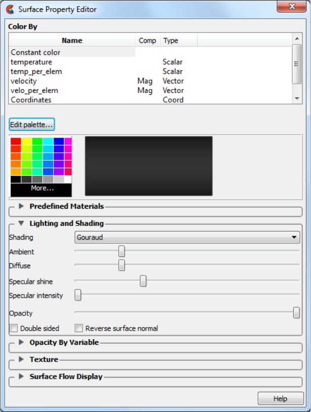
5.1 Parts Quick Action Icons
EnSight 10.2 User Manual 5-11
Paint Includes high-gloss, semi-gloss, satin, eggshell, and matte-like surface models.
Plastic Hard, Mid and Soft plastic-like models.
Rubber Hard, Mid and Soft rubber-like models.
Lighting and
Shading
Turn down exposes a number of detailed surface property controls that allow
modification of detailed surface property attributes.
Shading Selection of appearance of Part surface when Shaded Surface is on. Normally the mode
is set to Gouraud, meaning that the color and shading will interpolate across the polygon
in a linear scheme. You can also set the shading type to Flat, meaning that each polygon
will get one color and shade, or Smooth which means that the surface normals will be
averaged to the neighboring elements producing a “smooth” surface appearance. Not
valid for all Part types. Options are:
Flat Color and shading same for entire element.
Gouraud Color and shading varies linearly across element.
Figure 5-13
Part Color/Surface Property Editor Lighting and Shading
5.1 Parts Quick Action Icons
5-12 EnSight 10.2 User Manual
Smooth Normals averaged with neighboring elements to simulate smooth
surfaces.
Smooth High
Quality
Feature-based smoothing of adjacent elements within a fixed,
internal threshold angle (30o).
Ambient Controls the amount of natural surrounding light in an environment. A value toward 0.0
decreases (darkens) and toward 1.0 (floods) the amount of natural light.
Diffuse The incoming light that will be reflected in all directions equally. The part will reflect no
light if the value is 0.0, and will reflect maximum at 1.0 which diffuses the part surface
color.
Specular shine Shininess factor. This is the dispersion angle of the reflected light. The larger the factor
the smaller this angle. A large value of specular shine will therefore make the surface
darker and appear less smooth because it more closely shows the changing normal along
the surface.
Specular Intensity Highlight intensity (the amount of white light contained in the color of the Part which is
reflected back to the observer). Highlighting gives the Part a more realistic appearance
and reveals the shine of the surface. To change, use the slider.
Opacity This sets opacity as a constant percentage throughout the selected part(s).
The opaqueness of the selected Part(s) applied as a constant value over the part surface.
A value of 1.0 indicates that the Part is fully opaque, while a value of 0.0 indicates that it
is fully transparent. Setting this attribute to a value other than 1.0 will adversely affect
the graphics performance. Opacity is disabled for line parts.
Note that opacity can be varied by constant, OR by a variable value in the Opacity By
Variable turn down in this same dialog. This option will show up in the dialog only if you
have opacity by variable set to constant (which is the default). In other words, you can
use either this constant value of opacity OR you can set opacity by variable. You cannot
do both. See Opacity By Variable described just below.
The term used in the graphics community for opacity is alpha. Alpha is a graphics term
for the ‘density’ or opaqueness of the color. Anytime the alpha is less than 1.0, the
EnSight client calls into the graphics card’s rendering routines to perform complex
calculations for rendering the translucent part. Note that setting a part’s opacity to
transparent (0.0) will spend time and effort in the graphics card’s routines to render the
chosen level of opacity, and is not the same thing as turning its visibility off using the
visibility toggle (which simply does not render the part’s elements).
Double sided Applies the lighting and shading properties to both sides of the surface element.
Toggling OFF applies the lighting and shading properties only to the surface-normal side
of the model elements.
Reverse surface
normal
Reverses the surface normal on the surface element only on the client for lighting
calculations when the Double sided toggled OFF. It does not modify the part for
calculational purposes.
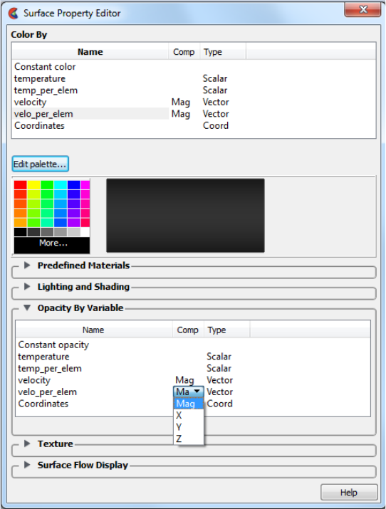
5.1 Parts Quick Action Icons
EnSight 10.2 User Manual 5-13
Opacity By
Variable
This turndown allows you to control the opacity using a variable value, which can help
to emphasize regions of importance, and de-emphasize uninteresting regions. This is an
expensive calculation routine best run on a client machine with a good graphics card.
Note: You can’t have opacity by a variable on a part while surface flow is being used on
that part. As soon as you turn on surface flow, the Opacity by a variable alpha
value will be reset to none.
Name If this is set to constant opacity (which is he default), then the constant opacity under the
Lighting and Shading dialog is enabled. In other words, you can use either this constant
value of opacity OR you can set opacity by variable. You cannot do both.
Choosing a variable name causes the opacity to vary according to the value of the
variable and disables constant opacity under the Lighting and shading turndown.
If you wish to further increase or decrease the variable opacity by variable value, use the
Palette Advanced Tab as shown in the How to Set Surface Properties in the section
Opacity by Variable (Transparency).
Comp Column containing the component description for vector variables. The default
component is Mag. If you are coloring by a vector variable clicking in its component
column allows selection of the magnitude or its components (e.g. X, Y, or Z).
Type The type of variable (blank is constant, scalar is single value at every node or element,
vector is four values at every node or element, tensor is six or 9 values at every node or
element). Coordinates are a special client-side variable, with only magnitude available.
Figure 5-14
Part Color/Surface Property Editor Opacity By Variable
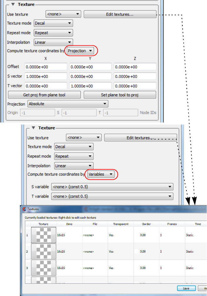
5.1 Parts Quick Action Icons
5-14 EnSight 10.2 User Manual
Texture Texture mapping is a mechanism for placing an image on a surface or modulating the
colors of a surface by various manipulations of the pixels via a texture map image.
EnSight supports the application of a texture onto a part and the combining of texture
effects with the normal EnSight coloring schemes. This can include animated textures
(e.g. EVO or MPEG files), which can be used to texture parts and 2D annotations.
Texture coordinates are computed via projection or using EnSight variables. Textures are
loaded into EnSight, then they are applied to parts. This powerful capability is best
explained using examples (see How To Map Textures).
Figure 5-15
Part Color/Surface Property Editor Texture Main Dialogs
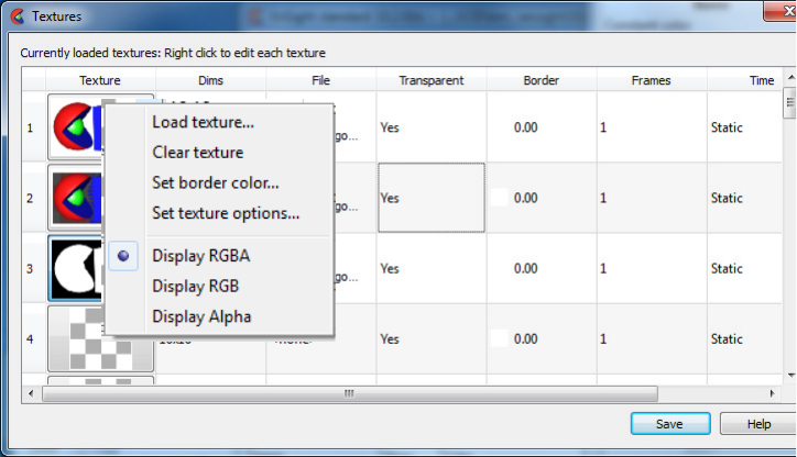
5.1 Parts Quick Action Icons
EnSight 10.2 User Manual 5-15
Use texture Pick the texture number to use on the selected part. The texture number is set using the
Edit textures... button just below.
Edit textures... Click on this button to open the Textures dialog. In the Textures dialog, right click on one
of the numbered textures in the Texture column and choose an option as follows.
Right click on a texture
Load texture... Load an image or a movie which can be used as a texture by
choosing it in the Use texture pulldown above.
Clear texture Clear the selected texture.
Set border
color...
Each texture has a border color that is used for colors outside of the
texture bounds. This color (RGB and opacity) can be set explicitly.
Note if Repeat mode is repeat, then border color is not used. If
Repeat mode is set to Clamp, then areas outside of the texture
bounds will be ‘clamped’ to the border color. If Repeat mode is set
to Clamp to texture, then regions outside of the texture bounds will
be clamped to the value just inside the texture.
Set texture
options...
Open a dialog allowing you to set movie parameters: the start and
end time, and the start and end frame, the compression
methodology, and whether to autoscale time. This is useful to match
up the movie end frames to the start and end of your timesteps which
will synchronize your movie texture playback to your data
timesteps.
Display RGBA All textures have both a color (RGB) and an opacity (A) component.
By default, the thumbnail is drawn using the full RGBA pixel value.
Display RGB Display only the RGB portion of the thumbnail.
Display Alpha Display only the alpha (opacity) of the thumbnail. Notice how the A
channel masks out the black and white pixels in the RGB image.
This masking can be used to place non-rectangular images/icons on
EnSight parts.
Columns Dims Dimension of the texture/movie in pixels.
Figure 5-16
Part Color/Surface Property Editor Texture Editor
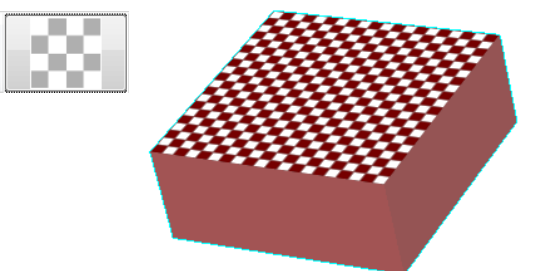
5.1 Parts Quick Action Icons
5-16 EnSight 10.2 User Manual
File Path and filename to the texture image/movie.
Transparent Yes/No indication of whether the texture uses transparency.
Border Choose the border color around the texture used for colors outside of
the texture bounds.
Frames Number of frames in the texture (1 for image, >1 for movie).
Time Static (image) or Transient (movie).
Save allows the user to save the currently loaded selection of textures and
their display mode into the user's preferences directory. These will
be automatically loaded every time EnSight is launched.
Texture mode The texture mode determines how a texture is combined with the natural coloring
scheme in EnSight. It has three values: "Replace", "Decal" and "Modulate".
Replace In replace mode, the base colors provided by EnSight are ignored
and the texture is used as the only source of color for the part (note,
this has the side effect of disabling any lighting).
Decal (default) In decal mode, the alpha channel of the texture is used to select
between the texture color and the base color of the part. If the
texture alpha value is 0, the base color of the part is displayed, while
locations where the texture alpha value is 255, the texture color will
be used exclusively. All alpha values in-between 0 and 255 will
result in an interpolation between the texture and base colors. Note
that the default, checkerboard texture uses an alpha channel with
values 255 and 80, which when applied to a reddish top surface will
show up as follows. For details, see How to place a logo on a part.
Modulate In modulate mode, the base color is multiplied by the texture color
and the resulting texture is used. Modulate mode is commonly used
with a texture that has a color of white and some pattern in the alpha
channel. This allows the base color to show through, but varies the
transparency of the part. Arbitrary clipping operations can be set up
this way. Modulation of the color channels can be confusing as the
operation tends to suppress colors, but it can be used with a
grayscale texture to attenuate. For details, see How to clip an object
with a texture.
Repeat mode Repeat (default), Clamp, and Clamp to texture. When the current texture projection
specifies texture coordinates outside of the texture [0,1], EnSight can either "repeat" the
coordinates (e.g. a texture coordinate of 2.3 is mapped to 0.3) or it can "clamp" to the
border color of the texture. Clamping is often used for logos and explicit texture
coordinates (see Texture projections).
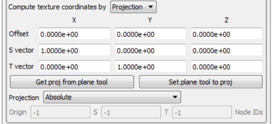
5.1 Parts Quick Action Icons
EnSight 10.2 User Manual 5-17
Repeat Repeat the texture if outside the texture range [0,1]. If repeat mode
is set to repeat, the border color of the texture is not used.
Clamp Regions outside the texture range are fixed to the border color.
Clamp to texture Regions outside the texture range are fixed to the texture just inside
the border.
Interpolation When the graphics hardware needs to access a pixel in the current texture it will either
use interpolation or nearest neighbor.
Nearest Nearest interpolation is more exact.
Linear Bilinear interpolation is smoother and slower.
Compute texture
coordinates by
Projection
Projection (default), In projection mode, think of the texture as a projected light-source,
like a presentation projector, only without divergence (i.e. the light lines are parallel).
The user places the light source to shine through the scene at some orientation centered
at some point. Textures are not limited to the exposed surface in EnSight, thus any
surface that intersects the beam of light is textured.
Offset The 'Offset' X,Y,Z values are considered to be relative to this node
ID. If it moves in time, the texture projection will appear to be
linked to it.
S vector An offset for the S vector.
T vector An offset for the T vector.
Get proj from
plane tool
Get the projection using the plane tool orientation.
Set plane tool to
proj
Set the plane tool position using the projection.
Projection Three options: Absolute (default), Offset relative to node ID, and
Offset and S/T vecs relative to node IDs.
Figure 5-17
Part Color/Surface Property Editor Texture Coordinates by Projection
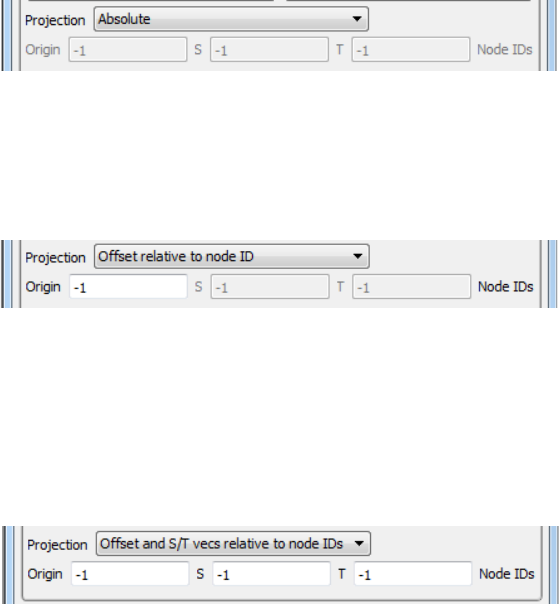
5.1 Parts Quick Action Icons
5-18 EnSight 10.2 User Manual
Absolute (default) mode requires no input thus the Origin, S, & T are
grayed out. This will fix the texture to its absolute position and
attitude in space. If the part geometry moves or deforms, the texture
remains fixed in the scene, thus it appears to slide along the part
surface.
Offset relative to node ID - The 'Offset relative to ID', allows the
user to specify a node ID in the 'Origin' field so the texture will
translate with the node id.
Offset and S/T vecs relative to node IDs - The Offset and S/T vecs
relative to node IDs allows the user to specify three node IDs that
will be used to translate and rotate the texture in 3D space as these
three nodes move: ‘Origin’, ‘S’ & ‘T’.
Figure 5-18
Part Color/Surface Property Editor Texture Projection Absolute
Figure 5-19
Part Color/Surface Property Editor Texture Projection Relative Node ID
Figure 5-20
Part Color/Surface Property Editor Texture Offset and S/T vecs Node IDs
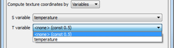
5.1 Parts Quick Action Icons
EnSight 10.2 User Manual 5-19
Compute texture
coordinates by
Variables
In Variables mode, the user must enter an S variable and a T variable and a pulldown for
each of these variables will appear. In this mode, one or two scalar variables are used to
provide explicit S and T texture coordinates for texturing. This is the most general
mechanism for texturing. The S-variable and T-variable option menus provide a list of
possible scalar variables. Users may also set the S and/or T value to the constant quantity
0.5. The variables are generally in the range [0,1], which map to the edges of the texture
map, just inside the border. Values outside this range will either be mapped to the texture
border color (in the case of clamp mode) or will be warped back into the range of [0,1]
by repeated subtraction/addition (in repeat mode). This form of projection is capable of
emulating the previous model. It also makes it relatively easy to create two dimensional
data palettes. Just like the existing palette in EnSight, some function of a variable is used
to select a color from a table. In this case, the table is a 2D texture, so this can be done for
two different variables at the same time, and the opacity can be varied as a function of
those variables.
S variable Default is constant value (0.5). Select a variable with a range of
[0,1],
T variable Default is constant value (0.5). Select a variable with a range of
[0,1],
Figure 5-21
Part Color/Surface Property Editor Texture Coordinates by Variables
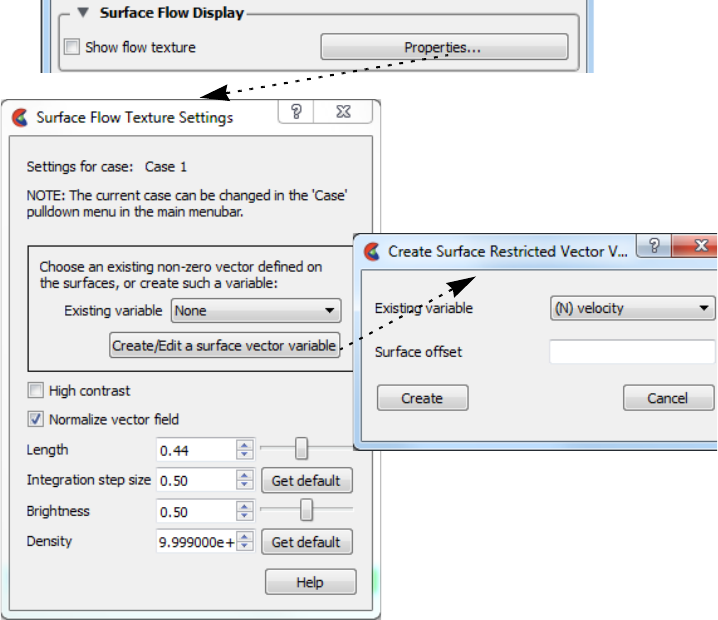
5.1 Parts Quick Action Icons
5-20 EnSight 10.2 User Manual
Surface Flow
Display
Toggles the display of Surface Flow Texture. This feature provides the capability to
visualize a vector (typically velocity) over a surface part, similar to tufts in a wind
tunnel. This is not the same as a particle trace part. It is a texture over the entire surface.
The properties of a surface flow are per-case.
Show flow texture This uses a Line Integral Convolution (LIC) algorithm to integrate a vector over a part
surface. Select the part(s) on which you desire to display the surface flow, and toggle this
ON (default OFF) to attempt to create a surface flow texture. If the chosen vector is zero
at the surface then the surface flow texture will just be noise (and you may need to create
a surface variable offset into the flow as described below). If the vector variable is per-
element, the surface flow texture may not be smooth. You can use the calculator
ElemToNode function to create a nodal variable and try again. Click the properties
button to open the Surface Flow Texture Settings dialog which will give you more
control of the result (see Surface Flow Display in How To Set Surface Properties ).
Properties Click this button to open the Surface Flow Texture Settings dialog which will give you
more control of the result.
Existing variable Choose an existing vector variable to display on the surface as flow
tufts.
Figure 5-22
Part Color/Surface Property Editor Surface Flow Display
5.1 Parts Quick Action Icons
EnSight 10.2 User Manual 5-21
Create/Edit a
surface vector
variable
If the vector variable is zero on the surface, then click this button to
create a new variable from the flow field that can be displayed on
the surface. Note, the first time you click this button, it will open the
Create Surface Restricted Vector Variable dialog shown above.
Choosing an existing variable and a Surface Offset will calculate a
vector variable on the surface by mapping from the flow field using
a pre-defined OffsetVar calculator function(see Section 7.3, Variable
Creation).
The second time you click on this button, it will open the calculator
and allow you to edit the variable parameters themselves. Note: you
can just as easily calculate a variable using the OffsetVar function
and use this variable in the Surface Flow display.
Existing variable - pick an existing variable to offset into the flow.
Surface Offset - pick a distance to offset into the flow, using the
surface normal to get vector variable value.
High Contrast Toggle this on to do a pass of image contrast enhancement. The
resulting tuft lines will look sharper.
Normalize Vector
Field
Toggle this on to normalize integration step length to the same unit
length prior to visualization. This will result in all the tufts being the
same length. With this off, the integration step length will be scaled
according to the vector magnitude and areas where the vector
magnitude is near-zero may contain algorithmic noise.
Length The Line Integral Convolution (LIC) algorithm will integrate a
maximum length of 20 pixel units in the positive and negative
directions. Length is a scaling factor of this 20 pixels. Range is 0 to
1.
Integration step
size
The step size in pixel units for each integration step. Range is 0 to 1.
Brightness This will brighten up the surface flow tuft display.
Density The density is a subjective value, related to the number of tufts on
the surface. This value is inversely proportional to the model size,
and is usually set to a very high initial value, which should create an
acceptable flow pattern and may not need to be adjusted. The
stepper will double and halve the step value. Note that above a
certain value, there are diminishing returns from increasing this
value.
Note: You can’t have opacity by a variable on a part while surface flow is being used on that part. As soon as you
turn on surface flow, the opacity by a variable alpha value will be reset to none.
LIC References: Brian Cabral and Leith (Casey) Leedon. Imaging vector fields using line integral
convolution. Proc of ISGGRAPH ‘93 (Anaheim, CA, Aug 1-6, 1993). In Computer
Graphics 27, Annual Conference Series, 1993, ACM SIGGRAPH, pp 263-272.
Detlev Stalling and Hans-Christian Hege. Fast and resolution independent line-integral
convolution. Proc of SIGGRAPH ‘95 (Los Angeles, CA, Aug 6-11, 1995). In Computer
Graphics 29, Annual Conference Series, 1995, ACM SIGGRAPH, pp 249-256.
see https://en.wikipedia.org/wiki/Line_integral_convolution
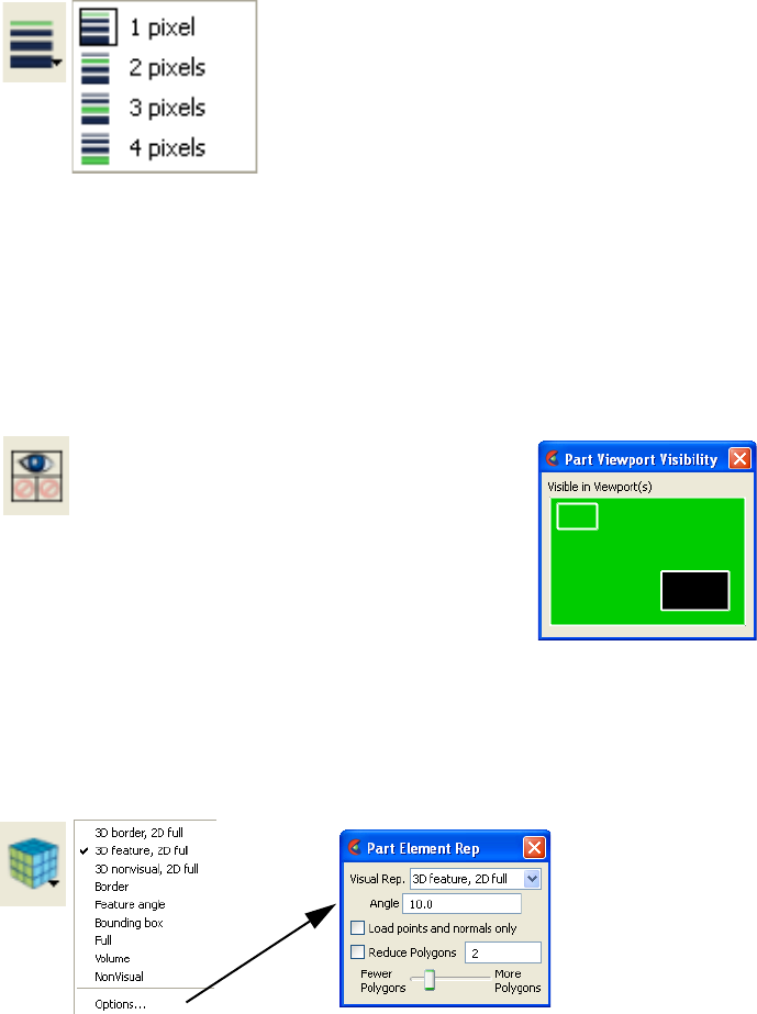
5.1 Parts Quick Action Icons
5-22 EnSight 10.2 User Manual
Part Line Width Icon Opens a pulldown menu for the specification of the desired display width for Part lines.
Performs the same function as the Line Representation Width field in the Node, Element,
and Line Attributes section of the Feature Panel (Model).
Part Visibility per
Viewport Icon
Opens the Part Viewport Visibility dialog. If the global visibility of a Part is on, this
dialog can be used to selectively turn on/off visibility of the selected Part(s) in different
viewports simply by clicking on a viewport’s border symbol within the dialog’s small
window. The selected Part(s) will be visible in the green viewports invisible in the black
viewports.
Part Element Settings
Icon
Opens a pulldown for the specification of the desired representation for elements of the
selected Part(s). Performs the same function as the Element Representation Visual Rep.
pulldown menu in the Node, Element, and Line Attributes section of the Feature Panel
(Model).
Figure 5-23
Part Line Width Icon
Figure 5-24
Part Visibility per Viewport Icon and Part Viewport
Visibility dialog
Figure 5-25
Part Element Settings Icon and Part Element Rep dialog
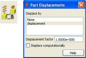
5.1 Parts Quick Action Icons
EnSight 10.2 User Manual 5-23
Part Displacements
Icon
Opens the Part Displacements dialog which allows you to choose the vector variable and
displacement factor. The model geometry is displaced by this variable vector value.
Displacement factor The vector variable can be scaled by this factor.
Each node of a Part is displaced by a distance and direction corresponding to the value of
a vector variable at the node. The new coordinate is equal to the old coordinate plus the
vector times the specified Factor, or:
Cnew = Corig + Factor * Vector,
where Cnew is the new coordinate location, Corig is the coordinate location as defined in
the data files, Factor is a scale factor, and Vector is the displacement vector. Note that a
value of 1.0 will give you “true” displacements.
You can greatly exaggerate the displacement vector by specifying a large Factor value.
Though you can use any vector variable for displacements, it certainly makes the most
sense to use a variable calculated for this purpose. Note that the variable value represents
the displacement from the original location, not the coordinates of the new location.
Displace
Computationally
Normally displacements are done on the client, and thus are done visually only. By
toggling this on, the displacements will be done on the server and thus will be taken into
account for any computations.
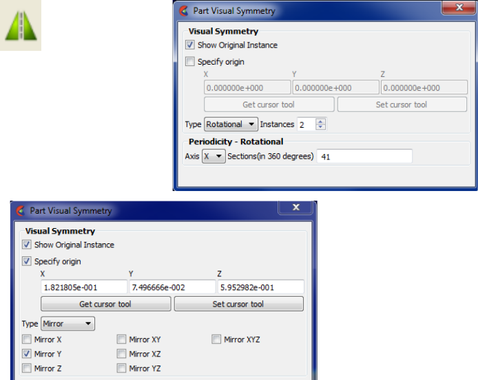
5.1 Parts Quick Action Icons
5-24 EnSight 10.2 User Manual
Visual Symmetry Icon Opens the Part Visual Symmetry dialog which allows you to control the display of
mirror images of the selected Part(s) or rotationally symmetric images about the Part’s
local frame axis and origin. This performs the same function as the Visual Symmetry
menu in the General Attributes section of the Feature Panel (Model).
Symmetry enables you to reduce the size of your analysis problem while still visualizing
the “whole thing.” Symmetry affects only the displayed image, not the data, so you
cannot query the image or use the image as a parent Part. However, you can get the
same effect by creating dependent Parts with the same symmetry attributes as the parent
Part.
Show Original
Instance
If toggled ON, the original instance will be visible. If toggled OFF, the original instance will not be
visible.
Specify origin You can specify the origin for the rotational or mirror symmetry. Note the default frame
for all parts is frame 0 (which is coincident with the global axis). To quickly and easily
modify the rotational origin, simply specify the origin in global coordinates. More
complicated symmetries about axes not aligned with the global axes require assigning a
new frame to the part(s) of interest.
Get/Set cursor tool Populate the visual symmetry origin fields using the cursor tool location by clicking the
get cursor tool button. Use the Set cursor tool button to assign the current origin field
values to the cursor location.
Figure 5-26
Visual Symmetry Icon & Dialogs

5.1 Parts Quick Action Icons
EnSight 10.2 User Manual 5-25
Type
Mirror 3D space split by three planes of a cartesian frame (xy, xz, and yz) defines 8 quadrants
(+x+y+z, +x+y-z, +x-y+z, +x-y-z, -x+y+z, -x+y-z, -x-y+z, -x-y-z). Mirroring can be
thought of as reflecting your model through these planes, or the origin, to get the proper
“mirrored” image of the data in the various quadrants.
You can mirror the Part to more than one quadrant. If the Part occupies more than one
quadrant, each portion of the Part mirrors independently. The images are displayed with
the same attributes as the Part. For each toggle, the Part is displayed as follows. The
default for all toggle buttons is OFF, except for the original representation - which is ON.
Mirror X quadrant on the other side of the YZ plane.
Mirror Y quadrant on the other side of the XZ plane.
Mirror Z quadrant on the other side of the XY plane.
Mirror XY diagonally opposite quadrant on the same side of the XY plane.
Mirror XZ diagonally opposite quadrant on the same side of the XZ plane.
Mirror YZ diagonally opposite quadrant on the same side of the YZ plane.
Mirror XYZ quadrant diagonally opposite through the origin.
Rotational Rotational visual symmetry allows for the display of a complete (or portion of a) “pie”
from one “slice” or instance. You control this option with:
Instances specifies the number of rotational instances to display.
Note that an additional section appears for rotational symmetry only. It is entitled
“Periodicity - Rotational”. While the Axis is used for both visual symmetry and
periodic traces, the Sections field is only needed/used when periodic traces are created.
See the Periodic Traces section of How To Create Particle Traces for instructions.
Axis specifies which rotational axis is to be used for rotational symmetry
and periodic traces.
Sections (in 360
degrees)
specifies the number of sections (instances) needed to make a full
360 degrees. Only used for periodic traces.
None No visual symmetry will be done.
Element Labeling Icon Opens the Part Node/Elem Labelling dialog. Toggles on/off the visibility of the element
and/or node labels (assuming the result file contains them) for the selected Part(s). The
global Element Labeling Toggle (Main Menu>View>Label Visibility) must be on in
order to see any element labels. Likewise, the global Node Labeling Toggle (Main
Menu>View>Label Visibility) must be on in order to see any element labels.
Figure 5-27
Element Labeling Icon
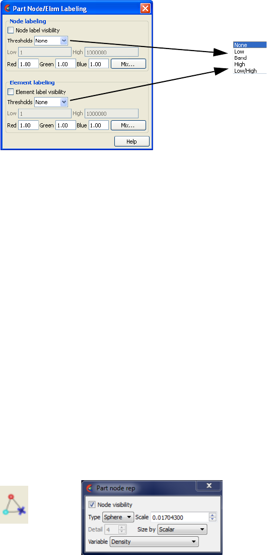
5.1 Parts Quick Action Icons
5-26 EnSight 10.2 User Manual
.
Element/Node Label
Visibility
Toggles on/off the visibility of the element or node labels (assuming the result file
contains them) for the selected Part(s). Performs the same function as the Label
Visibility Node toggle in the Node, Element, and Line Attributes section of the Feature
Panel (Model). Default is OFF. Note: if your part geometry occludes your node ids then
set the part opacity to transparent. To do this easily: Right click on the part in the
graphics area, or on the selected part(s) in the part list and choose Colorby>Make
Transparent. To change it back, right click and choose Colorby>Make Opaque.
Filter Thresholds A pulldown menu containing the following:
Low All element/node ids below the value in the low field are invisible
Band All element/node ids between the values in the low and high fields
are invisible.
High All element/node ids above the value in the high field are invisible.
Low/High All element/node ids below the low and above the high field values
are invisible.
Red, Green, Blue,
Mix
Enter the element/node id label color, or click on the Mix Button and pick your color.
Node Representation
Icon
Opens the Part Node Rep dialog. Performs the same function as the Node Representation
area in the Node, Element, and Line Attributes section of the Feature Panel (Model).
Node Visibility
Toggle
Toggles-on/off display of Part’s nodes whenever the Part is visible. Default is OFF.
Type Opens a pop-up menu for the selection of symbol to use when displaying the Part’s
nodes or point elements. Default is Dot. Options are:
Figure 5-28
Part Node/Elem Labeling Dialog
Filter Threshold
Val ues
Figure 5-29
Node Representation Icon and Part Node Rep dialog
5.1 Parts Quick Action Icons
EnSight 10.2 User Manual 5-27
Dot to display nodes as one-pixel dots.
Cross to display nodes as three-dimensional crosses whose size you
specify. If you want to render as spheres, first choose Cross and get
the Scale adjusted properly and then choose Sphere.
Sphere to display the nodes as spheres. If your graphics card supports
advanced GPU rendering of spheres (OpenGL version 3.3 or above)
then the spheres will be rendered extremely efficiently and the detail
box will be greyed out and unavailable. If your graphics hardware or
software driver does not support advanced rendering, then the
fallback is to render with less efficient polygons around each of the
nodes using a detail specified in the Detail pulldown. The detail
correlates to the number of polygons per sphere. Choose a detail that
is a trade off between rendering quality and speed.
Warning: when rendered using advanced rendering, we have found
that extremely large sphere sizes can cause greatly slow down
rendering or even hang your graphics card (due to a driver
limitation). Therefore, EnSight computes a safe sphere scale factor
automatically as a starting point, and best practice is to use the up or
down arrows to the right of the scale field to double or half the
scaling value incrementally, then type in an exact value for fine
adjustments.
Scale This field is used to specify scaling factor for size of node symbol. If Size By is
Constant, this field will specify the size of the marker in model coordinates. If Size By is
set to a variable, this field will be multiplied by the variable value. Not applicable when
node-symbol Type is Dot.
Note: use caution here if using advanced GPU rendering of spheres because a large size
relative to the size of the geometry can cause the graphics card to hang. Start out very
small relative to the model size and use a Cross instead of a sphere then increase your
size until the crosses are sufficiently large, then change them over to spheres.
Detail This field is only used if your graphics hardware or software driver do not support
advanced GPU rendering of spheres. This field is used to specify how round to draw the
spheres when the node-symbol type is Sphere. Ranges from 2 to 10, with 10 being the
most detailed (e.g., roundest spheres). Higher values take longer to draw, slowing
performance. Default is 4.
Size By Opens a pop-up menu for the selection of variable-type to use to size each node-symbol.
For options other than Constant, the node-symbol size will vary depending on the value
of the selected variable at the node. Not applicable when node-symbol Type is Dot. Get
this working using Cross, then switch to Sphere to avoid hanging your graphics card.
Default is Constant. Options are:
Constant sizes node using the Scale factor value.
Scalar sizes node using a scalar variable.
Vector Mag sizes node using magnitude of a vector variable.
Vector X-Comp sizes node using magnitude of X-component of a vector variable.
Vector Y-Comp sizes node using magnitude of Y-component of a vector variable.
Vector Z-Comp sizes node using magnitude of Z-component of a vector variable.
Variable Selection of variable to use to size the nodes. Activated variables of the appropriate Size
By type are listed. Not applicable when node-symbol Type is Dot or Size By is Constant.
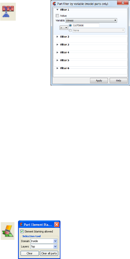
5.1 Parts Quick Action Icons
5-28 EnSight 10.2 User Manual
Filtered Elements icon Opens the Part Filter Elements dialog. Choose a variable (ideally a per-element variable,
but you can also use a per-node variable which EnSight will average to the elements).
This does a deep element removal of the elements from the selected model part on the
server based on logical operators on the variable. Since filtering only works on model
parts, filtering elements on a created part, can only be accomplished by filtering them on
the model part parent.
Six filters are available. Each filter can specify a variable to use in the filtering process
which can be compared against another variable or a constant value. The filters are
combined with "and" or "or" operators. The filtering occurs sequentially through the
filters, i.e., it is not possible, for example, to specify a filter operation of "variable1 < 0.5
OR (variable2 > 1.0 AND variable 3 < 0.0)"
See How To Filter Part Elements
Active Activate the filter by toggling it on. Notice that six filters can be toggled on.
Filter Operator Select a per-element scalar variable. Choose a pulldown threshold (<, >, = or !=).
And / Or If you toggle on a logical operator then choose second threshold.
Set to default To set the threshold values back to the default of 0.0.
Part Element
Blanking/Visibility Icon
Brings up the Part Element Blanking dialog. Element blanking is the visual removal of
elements on the graphics screen. The elements still remain on the server and are still used
in calculations, they are just not visible in the graphics window. Note that blanking is
done using element IDs as tags. If the element IDs change each timestep, this can result
in different elements becoming invisible each timestep.
See How To Do Element Blanking
Element blanking
allowed
Toggles on/off whether element blanking allowed
Selection tool Domain Controls whether inside or outside of selection tool will be used fro
the blanking
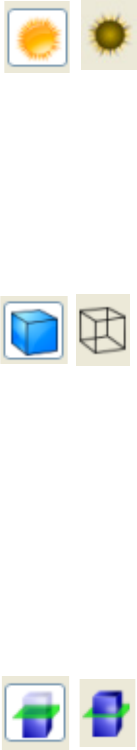
5.1 Parts Quick Action Icons
EnSight 10.2 User Manual 5-29
Layers Controls the “depth” of the blanking operation. Top will just blank
the first layer of elements encountered.at each invocation. While all
will blank elements at all depths.
Clear Clears blanked elements and restores them to visible for the selected Part(s)
Clear all parts Clears blanked elements and restores them to visible for all Part(s)
Part Shaded Surface
Icon
Toggles on/off Shaded display of surfaces for the selected Part(s) assuming that global
Shaded has been toggled ON in Main Menu > View > Shaded. Performs the same
function as the Hidden Surface Toggle in the General Attributes section of the Feature
Panel (Model). Default for all Parts is ON.
Part Hidden Line Icon Toggles on/off hidden line display of surfaces for the selected Part(s) assuming that the
global Hidden Line has been toggled ON in Main Menu > View > Hidden Line.
Performs the same function as the Hidden Line Toggle in the General Attributes section
of the Feature Panel (Model). Default for all Parts is ON.
Part Auxiliary Clipping
Icon
Toggles on/off whether the selected Part(s) will be affected by the Auxiliary Clipping
Plane feature. Performs the same function as the Aux Clip toggle in the General
Attributes section of the Feature Panel (Model). Default is ON. Auxiliary clipping is
simply a visual clipping that occurs only on the client and does not affect the underlying
model geometry, only its view on the screen.
Note: The global Auxiliary Clipping Toggle (in Main Menu > View) must be on in order
for any Parts to be affected by the Aux Clip Plane.
Figure 5-30
Part Shaded ON / OFF Icon
Figure 5-31
Part Hidden Line ON / OFF Icon
Figure 5-32
Part Auxiliary Clipping ON / OFF Icon
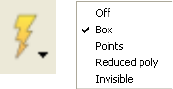
5.1 Parts Quick Action Icons
5-30 EnSight 10.2 User Manual
Fast Display
Representation Icon
Opens a pulldown menu for the specification of the desired fast display representation in
which a Part is displayed. The Part fast display representation corresponds to whether the
view Fast Display Mode (located in the View Menu) is on. The Fast Display pulldown
icon performs the same function as the Fast Display pulldown menu in the General
Attributes section of the Feature Panel (of all parts).
Box causes selected Part(s) to be represented by a bounding box of the
Cartesian extent of all Part elements (default)
Points causes selected Part(s) to be represented by a point cloud
Reduced poly causes selected Part(s) to be represented by reduced number of
polygons
Sparse Model decimates part elements by a factor determined in the Preferences.
Go to Edit>Preferences>Performance and enter in a factor from 1
(sparse) to 100 (full) in the Sparse model representation field. This
is only available when running in immediate mode using the -
no_display_list option at startup.
Invisible causes the selected Part(s) to be invisible
(see General Attributes in How To Set Global Viewing))
Figure 5-33
Fast Display Representation Icon
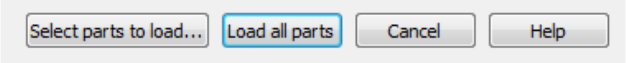
5.1 Model Parts
EnSight 10.2 User Manual 5-31
5.1.2 Model Parts
When you start EnSight, you either read directly or interactively extract parts
from the data files. Parts which come from the original dataset are referred to as
model parts. Model parts are defined by the data readers and are usually a logical
grouping of nodes and elements as defined by the solver. It might be a material or
property or perhaps a defined geometric entity such as a “wheel” or “inlet”
The computational grid (or mesh) used by EnSight is either an unstructured
definition (where each mesh element is defined) or a structured definition (an IJK
definition) defining a rectilinear or curvilinear space. It is also possible to have a
mixed definition where some parts are unstructured and other parts are structured.
When you read data you will choose the file name that will be read and set the
format and options for the file. Then you will choose one of two options - either to
load all the parts or to select parts to load.
The “Load all parts” option will read the specified data (the “case”) and create
(i.e. “load”) all of the parts into EnSight. The other option - “Select parts to
load...” - will read the data but will not load any parts. This second option will
allow you to select on a per part basis which parts will be loaded into EnSight.
This “load” process is performed through the Part List.
The Part List contains all parts that have been read in (“loaded”) from your
specified data file as well as those created within EnSight. Additionally, it may
show model parts from the data that are not already loaded. These are referred to
as Loadable Parts or LPARTs.
LPARTs may be loaded zero or more times. You may choose not to load a
particular part from a data set if it is not needed for the visualization or analysis of
the case. This is advantageous to save memory and processing time. You may also
choose to load a part multiple times - so you could, for example, color the part by
multiple variables at the same time in multiple viewports.
LPARTs are shown as grayed out parts in the Part List. You can load a LPART by
selecting the part(s) and performing a right click operation to “Load part”.
There are some creation attributes that affect model parts. These will be discussed
in this section.
There are also various attributes that affect the display of these parts, as well as all
created part types. These common attribute turndown sections of the Feature
Panel, will also be described in this section.
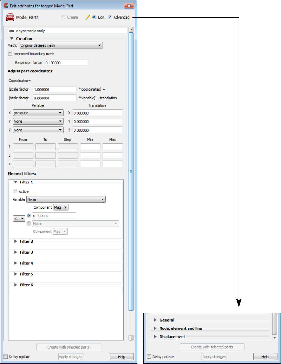
5.1 Model Parts
5-32 EnSight 10.2 User Manual
Since Model Parts are controlled by the loading process, they have neither a
specific Feature Icon in the Feature Icon Bar, nor an entry in the Main Menu >
Create menu. They do, however, have a Feature Panel associated with them. This
Feature Panel for Model Parts is opened by double-clicking (or right-clicking and
choosing Edit...) on a model part in the Part List.
Figure 5-34
Feature Panel - Model Parts
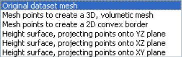
5.1 Model Parts
EnSight 10.2 User Manual 5-33
Edit Only the Edit mode is active, since all creation of model parts takes place with the
loading process. Note that when editing, the changes will be applied to those parts which
have the small “pencil” icon next to them in the Parts List.
Advanced Will open additional features for more advance control of the Part.
Desc The name of the part being edited. You can modify this description as desired.
Creation Creation Attributes for model parts consist of geometry scaling options (including
server-side displacements) for unstructured and structured parts, and updating of I,J,K
ranges for structured parts. Geometry scaling can be accomplished with a scale factor
which will be applied to the model coordinates and/or a scale factor times a nodal
variable. Updating the I,J,K node range attributes of the selected block structured Model
Parts or the geometry scaling will cause proper updating of all dependent parts and
variables.
Mesh: Opens pulldown menu for selection of model part re-meshing to use.
The default is to use the element connectivities described in the model data file(s). But a
remeshing can be done, utilizing the QHull library. This library can compute the convex
hull of point data, a 2D meshing. And since the convex hull of a 3D dataset lifted into 4
dimensional space turns out to be the volumetric tetrahedralization of the 3D data, it can
be used to do a 3D meshing as well. Please note that this remeshing can take
considerable memory and processing - so it needs to be used with that in mind. Also
note, that if the model part has been used to create other, children parts, remeshing is not
allowed. Only unstructured model parts are allowed to be remeshed. The following
model parts are allowed: model, extract, point, and measured parts.
Also, the worst case for QHull is a large number of co-planar points. In the higher-
dimensional lifting step, the planarity adds a singularity that is difficult to work around.
Using bounding boxes and planar projections can help. Accordingly, several options
exist, which can be used if your data exhibits problematic characteristics. The pulldown
menu options are:
Original dataset
mesh
The nodes and elements described in the model data file(s) is used.
No remeshing is done. This is the default.
Mesh points to
create a 3D,
volumetric mesh
The original element connectivities will be replaced with a
volumetric meshing of the nodes of the part, to produce tet elements.
Mesh points to
create a 2D
convex border
The original element connectivities will be replaced with a convex
hull meshing of the nodes of the part, to produce triangle elements.
Height surface,
projecting points
onto YZ plane
The original element connectivities will be replaced. The nodes of
the part will be projected to the YZ plane and then triangulated in
2D. The resulting triangle element connectivities will be used with
the original node data.
Height surface,
projecting points
onto XZ plane
The original element connectivities will be replaced. The nodes of
the part will be projected to the XZ plane and then triangulated in
2D. The resulting triangle element connectivities will be used with
the original node data.
5.1 Model Parts
5-34 EnSight 10.2 User Manual
Height surface,
projecting points
onto XY plane
The original element connectivities will be replaced. The nodes of
the part will be projected to the XY plane and then triangulated in
2D. The resulting triangle element connectivities will be used with
the original node data.
Note: There are a few formats that will not allow you to return to the input dataset
elements once you have meshed the part. Most do. For these few (ABAQUS fil, ansys,
ESTET, FIDAP Neutral, Fluent Universal, and N3S), you can change between the 2D
and 3D meshing options, but you need to delete the part and reload it, if you desire the
part back to the input elements.
Improved boundary
mesh
If one of the remeshing options is used, this toggle will employ a common “trick” that
often helps with the co-planar points problem described above. The “trick” consists of
adding 8 points (one at each corner of the bounding region) to the other points. This
basically embeds the original points inside of an 8-point box. Then compute the volume
tets and remove any tets connected to the non-original box points. Note that an offset
can be used for the bounding region to ensure that the bounding region is not collapsed
to 2D space (see Expansion factor below).
Expansion factor When adding the 8 points for the Improved boundary mesh trick above, an offset can be
used to expand the bounding region in all directions. This is that offset, or expansion
value.
Adjust part
coordinates:
The coordinates of the selected parts will be scaled and translated by the formula shown
in the dialog. It is possible to apply a simple scale factor, and/or to apply a scaled nodal
displacement vector variable (just choose the same vector variable for each pulldown
and it will use the correct component). In fact each coordinate direction can be scaled
according to a different model scalar variable if desired. This works only with model
variables, not computed variables. This is “server-side” scaling and displacement, having
the advantage of being able to properly query and compute on the displaced geometry of
the model.
Other options:
If you want to displace by a vector in which the resulting displacement is updated each
timestep then see How To Display Displacements.
If you want to scale the model coordinates visually only, then you can use the transform
editor and choose the scaling option and visually scale the geometry in the three
orthogonal directions, and do this separate for each direction (see How To Rotate, Zoom,
Translate, Scale).
If you want to scale, translate, or rotate a number of parts visually only consider
grouping them and doing a group transform (see Part Group Visual Transformations).
If you need to define your part(s) rotation or translation over time, consider rigid body
translations (see EnSight Rigid Body File Format).
If you need precise control of the rotation and translation of parts separately for
animation purposes, consider attaching a separate coordinate frame to each part (see
How To Create and Manipulate Frames).
Change structured
range and step
values
The creation range and step values for structured parts can be changed here.
IJK From These fields specify the desired minimum interval value in the
respective IJK component direction of the Model Part.
IJK To These fields specify the desired maximum interval value in the
respective IJK component direction of the Model Part.
5.1 Model Parts
EnSight 10.2 User Manual 5-35
IJK Step These fields specify the desired interval stride value in the
respective IJK component direction of the Model part.
IJK Min These fields verify the minimum interval limit in the respective IJK
component direction of the Model part.
IJK Max These fields verify the maximum interval limit in the respective IJK
component direction of the Model part.
(see How To Create IJK Clips)
Element Filters
Active Enables Element Filtering.
Variable Elements are removed from display on the client and from
calculation on the server for model parts only, using the named
variable (and component, if a vector) and the threshold operator(s) (
< , > , = , != ) as well as the value (either a single number or another
variable).
Note: multiple filters can be applied sequentially strung together
using logical ‘and’ or logical ‘or’.
Note: Filtered elements are not removed when the geometry is saved
in Case Gold format or as a Flatfile (see Saving Geometry and
Results Within EnSight).
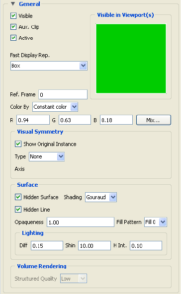
5.1 Model Parts
5-36 EnSight 10.2 User Manual
Feature Panel Turndowns Common To All Part Types
General General attributes are “general” in that: (a) all Parts have them, and (b) they can’t
be neatly categorized into any other attribute type. Like all Part attributes, they
are set individually for each Part.
Visible Toggles-on/off whether Part is visible on a global basis (in the Graphics Window or in all
viewports). (Performs the same function as the Visibility Quick Action Icon). Default is
ON.
Aux. Clip Toggles-on/off whether Part(s) selected in the Part List will be affected by the Auxiliary
Clipping Plane feature, which enables you to make invisible that portion of each
Part on the negative side of the current position of the Plane Tool. Performs the
same function as the Auxiliary Clipping Quick Action Icon. A Part with its Aux
Clip attribute toggled-off will not be cut away. Default is ON. (see Auxiliary
Clipping in (see Section 4.5, View Menu Functions).
Active Toggles-on/off whether or not display of the Part automatically updates as the solution
time changes. When visualizing transient data, you may wish to “freeze” a Part in time
while other Parts continue to update. For example, you can create two identical vector-
arrow Parts, toggle-off Active for one of them, change the time step of the display, and
see how the vector arrows change from one time step to the other. Only the EnSight
client Part is frozen, the EnSight server Part is kept current. Default is ON.
Visible in
Viewport(s)
This small window allows you to control the visibility of the selected Part(s) on a per
Viewport basis. Each visible viewport is shown. A green Viewport indicates that the
selected Part(s) will be visible in this Viewport, while a black Viewport indicates that the
selected Part(s) will not be visible. Change the visibility (black to green, green to black)
by selecting a viewport with the mouse.
5.1 Model Parts
EnSight 10.2 User Manual 5-37
Fast Display Rep. This pulldown menu allows for the selection of the fast display representation used to
display a part on the client. This attribute helps the display of complex data sets. The
part’s fast display representation displays according to whether the global Fast display
option (located in the View Menu) is on or off and on the state of the Static Fast Display
toggle located under Edit > Preferences..., Performance. For instance, when the Fast
Display is Off (default) the part displays according to its specified Element
Representation. When on, the parts are displayed by the fast display representation. The
fast display representation will only be used while performing transformations, unless
the Static Fast Display option has been selected. The part detail representations are:
Off display according to specified Element Representation.
Box a bounding (Cartesian extent) box of all part elements (default).
Points point cloud representation of the part.
Reduced poly polygon reduced representation of the part.
Sparse Model display a percentage of the model in each display box (only
available when running in immediate mode, using the -
no_display_list startup option). You control this percentage in the
performance preferences. Note, that it is useful for large models, but
should probably not be used for small models.
Invisible do not display at all while moving.
(see How To Set Global Viewing)
Ref. Frame This field specifies which frame the Part is assigned to. Default is the frame of the Part’s
parent Part (Frame 0 for original model Parts). Enter a different frame number in the
field to change the assignment. Changing a Part’s frame causes the Part to be drawn in
the new coordinate frame. Once assigned to a different frame, the Part will transform
with that frame. The choice of frame does not affect variable values. The interpolated
value of a variable at point 0,0,0 in Frame 0 is the same as at point 0,0,0 in Frame 1, even
though the points may appear at different locations in the Main View Window.
Color By A pulldown menu for the selection of the variable color palette by which you wish to
color the selected Part(s). Coloring a Part with a palette does not normally affect
graphics performance while in line drawing mode, but Shaded Surface mode
performance can be affected. If you do not color by a palette (Color By > Constant
color), the Part will be displayed according to the color specified in the R, G, B fields. If
you want to color Parts by palettes and want Shaded Surface mode, consider using the
Static Lighting option (see Static Lighting in (see Section 4.5, View Menu Functions).
RGB These fields allow you to specify a solid color for the selected Part(s) (applicable only if
Color By is Constant color). Enter a numerical value from 0 to 1 for each component
color (Red, Green, and Blue).
Mix... Opens the Select a color dialog for the selection of a solid color for the selected Part(s)
(applicable only if Color By is Constant color).
Visual Symmetry Allows you to control the display of mirror images of the selected Part(s) in each of the
seven other quadrants of the Part’s local frame or the rotationally symmetric instances of
the selected parts. This performs the same function as the Visual Symmetry Quick
Action Icon.
Symmetry enables you to reduce the size of your analysis problem while still visualizing
the “whole thing.” Symmetry affects only the displayed image, not the data, so you
cannot query the image or use the image as a parent Part. However, you can create the
same effect by creating dependent Parts with the same symmetry attributes as the parent
Part.
5.1 Model Parts
5-38 EnSight 10.2 User Manual
Show Original
Instance
Show the original instance or not
Type
Mirror You can mirror the Part to more than one quadrant. If the Part occupies more than one
quadrant, each portion of the Part mirrors independently. Symmetry works as if the local
frame is Rectangular, even if it is cylindrical or spherical. The images are displayed with
the same attributes as the Part. For each toggle, the Part is displayed as follows. The
default for all toggle buttons is OFF, except for the original representation - which is ON.
Symmetry Mirror X quadrant on the other side of the YZ plane.
Mirror Y quadrant on the other side of the XZ plane.
Mirror Z quadrant on the other side of the XY plane.
Mirror XY diagonally opposite quadrant on the same side of the XY plane.
Mirror XZ diagonally opposite quadrant on the same side of the XZ plane.
Mirror YZ diagonally opposite quadrant on the same side of the YZ plane.
Mirror XYZ quadrant diagonally opposite through the origin.
Rotational Rotational visual symmetry allows for the display of a complete (or portion of a) “pie”
from one “slice” or instance. You control this option with:
Axis rotates about the axis chosen.
Angle specifies the angle (in degrees) to rotate each instance from the
previous.
Instances specifies the number of rotational instances.
None No visual symmetry will be done.
Surface
Hidden Surface Toggles on/off surface shading for individual Parts. When global Hidden Surface has
been toggled on for the Graphics Window display (from Main Menu > View > Shaded or
the global Shaded Surfaces Tools Icon), individual Parts can be forced to stay in line
drawing mode using this toggle. Default is ON. (see Section 4.5, View Menu Functions)
Shading Pulldown menu for selection of appearance of Part surface when Hidden Surface is on.
Normally the mode is set to Gouraud, meaning that the color and shading will interpolate
across the polygon in a linear scheme. You can also set the shading type to Flat, meaning
that each polygon will get one color and shade, or Smooth which means that the surface
normals will be averaged to the neighboring elements producing a “smooth” surface
appearance.Not valid for all Part types. Options are:
Flat Color and shading same for entire element
Gouraud Color and shading varies linearly across element
Smooth Normals averaged with neighboring elements to simulate smooth
surfaces
Hidden Line Toggles on/off hidden line representation for individual Parts. When global Hidden Line
has been toggled on for the Graphics Window display (from Main Menu > View >
Hidden Line or via the global Hidden Line Tools Icon), individual Parts can be
forced not to appear as Hidden Line representation using this toggle. (To have lines
hidden behind surfaces, Parts must have surfaces, i.e. 2D elements) Default is ON. (see
Section 4.5, View Menu Functions)
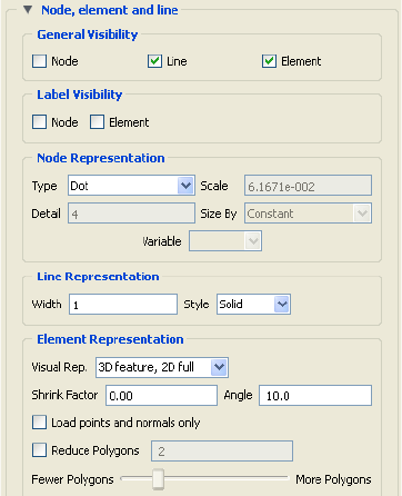
5.1 Model Parts
EnSight 10.2 User Manual 5-39
Opaqueness This field specifies the opaqueness of the selected Part(s). A value of 1.0 indicates that
the Part is fully opaque, while a value of 0.0 indicates that it is fully transparent. Setting
this attribute to a value other than 1.0 can seriously affect the graphics performance.
Fill Pattern Pulldown menu for selection of a fill pattern which can provide pseudo-transparency for
shaded surfaces. Default is Fill 0 which uses no pattern (produces a solid surface), while
Fill patterns 1 through 3 produce a EnSight defined fill pattern.
Lighting
Diff This field specifies diffusion (minimum brightness or amount of light that a Part
reflects). (Some applications refer to this as ambient light.) The Part will reflect no light
if value is 0.0. If value is 1.0, no lighting effects will be imposed and the Part will reflect
all light and be shown at full color intensity at every point. To change, enter a value from
0 to 1.
Shin This field specifies shininess.You can think of the shininess factor in terms of how
smooth the surface is. The larger the shininess factor, the smoother the object. A value of
0 corresponds to a dull finish and a value of 100 corresponds to a highly shiny finish. To
change, enter a value from 0 to 100.
H Int. This field specifies highlight intensity (the amount of white light contained in the color
of the Part which is reflected back to the observer). Highlighting gives the Part a more
realistic appearance and reveals the shine of the surface. To change, enter a value from 0
to 1 with larger values representing more white light. Will have no effect if Shin
parameter is zero.
(see How To Set Attributes)
Volume Rendering
Structured Quality This field controls the quality of volume rendering for a structured part. It allows a
tradeoff between rendering speed and image quality. The “Low”, “Medium”, and
“High” options provide this tradeoff by varying the number of samples. The “Best”
option provides the most precise rendering by performing exact ray/cell intersections.
Node, element and
line
Each Part’s Node, Element, and Line attributes control the representation of the Part on
the client, and how nodes, elements, and lines are displayed.
5.1 Model Parts
5-40 EnSight 10.2 User Manual
General Visibility Node Toggles-on/off display of Part’s nodes whenever the Part is visible.
Default is OFF.
Line Toggles-on/off display of line (1D) elements in the client-
representation whenever the Part is visible. Default is ON.
Element Toggles-on/off display of 2D elements in the client-representation
whenever the Part is visible. Note that 3D elements are always
represented as 2D elements on the client. Default is ON
Label Visibility Node Toggles-on/off display of Part’s node labels (if they exist) whenever
the Part is visible. Only model Parts may have node labels. Default
is OFF.
Element Toggles-on/off display of Part’s element labels (if they exist)
whenever the Part is displayed in Full visual representation. Only
model Parts may have element labels. Default is OFF.
Node
Representation
Type Opens a pop-up menu for the selection of symbol to use when displaying the Part’s
nodes. Default is Dot. Options are:
Dot to display nodes as one-pixel dots.
Cross to display nodes as three-dimensional crosses whose size you
specify.
Sphere to display the nodes as spheres whose size and detail you specify.
Scale This field is used to specify scaling factor for size of node symbol. Values between 0 and
1 reduce the size, factors greater than one enlarge the size. Not applicable when node-
symbol Type is Dot. Default depends on your model size.
Detail This field is used to specify how round to draw the spheres when the node-symbol type
is Sphere. Ranges from 2 to 10, with 10 being the most detailed (e.g., roundest spheres).
Higher values take longer to draw, slowing performance. Default is 2.
Size By Opens a pop-up menu for the selection of variable-type to use to size each node-symbol.
For options other than Constant, the node-symbol size will vary depending on the value
of the selected variable at the node. Not applicable when node-symbol Type is Dot.
Default is Constant. Options are:
Constant sizes node using the Scale factor value.
Scalar sizes node using a scalar variable.
Vector Mag sizes node using magnitude of a vector variable.
Vector X-Comp sizes node using magnitude of X-component of a vector variable.
Vector Y-Comp sizes node using magnitude of Y-component of a vector variable.
Vector Z-Comp sizes node using magnitude of Z-component of a vector variable.
Variable Selection of variable to use to size the nodes. Activated variables of the appropriate Size
By type are listed. Not applicable when node-symbol Type is Dot or Size By is Constant.
Line
Representation
Width Specification of width (in pixels) of line elements and edges of 2D elements whenever
they are visible. Range is from 1 to 20. Default is 1. Line widths other than 1 are not
available on all hardware. This performs the same function as the Part Line Width
Pulldown Icon in Part Mode.
5.1 Model Parts
EnSight 10.2 User Manual 5-41
Style Selection of style of line when lines are visible. Default is Solid. Options are:
Solid
Dotted
Dot-Dash
Element
Representation
Visual Rep.Selection of representation of Part’s elements on the client. Saves memory and time to
download.
3D border, 2D
full
represents the Part’s 3D elements in Border representation, the
Part’s 1 and 2D elements in Full representation. The result is the
outside surfaces of the Part are displayed along with all bar
elements.
3D feature, 2D
full
represents the Part’s 3D elements in Feature representation, the
Part’s 1 and 2D elements in Full representation. The result is the
outside sharp edges of the Part are displayed along with all bar
elements.
3D nonvisual,
2D full
represents the Part’s 3D elements in non visual representation, the
Part’s 1 and 2D elements in Full representation. The result is all the
1 and 2Delements from 2D parts are displayed.
Border represents the Part’s 3D elements with 2D elements corresponding
to unshared element faces, the Part’s 2D elements with 1D elements
corresponding to the unshared edges, and the Part’s 1D elements as
1D elements. The result is the outside faces and edges of the Part’s
elements.
Feature Angle first runs the 3D border, 2D full representation to get a list of 1 and
2D elements. The 1D elements and all non-shared 2D edges will be
shown, but only the shared edges above the Angle value will be
shown. The result consists of 1D elements visualizing the sharp
edges of the Part.
Bounding Box represents all Part elements as a bounding box surrounding the
Cartesian extent of the elements of the Part.
Full represents all faces of the Part’s 3D elements, and all the 1 and 2D
elements.
Non Visual means the Part exists on the server, but is not loaded on the client.
Not Loaded Parts may be used as parent Parts, but do not exist on
the client.
Vo l u m e Represents a variable spatially by varying the alpha transparency
according to the variable value throughout the spatial domain. This
requires a modern graphics card.
Shrink Factor Specification of scaling factor by which to shrink every element toward its centroid.
Enter the fraction to shrink by in range from 0 to 1. Default is 0.0 for no shrinkage.
Angle Specification of lower limit for not displaying shared edges in Feature Angle
Representation. Value is in degrees.
Load points and
normals only
Loads only vertex information and normals for the element representation given to the
client. Useful for very large models.
Reduce Polygons Lower the polygon density used to represent the part. Useful for very large models.
Toggle on, then type in a value to reduce by, or slide the slider.
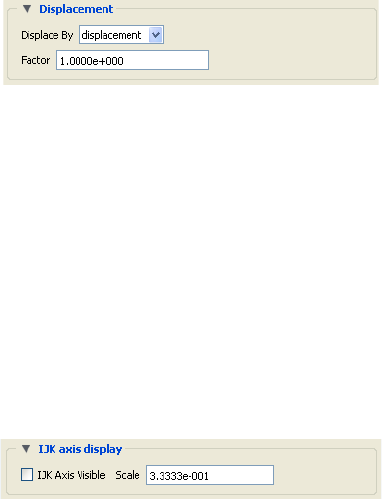
5.1 Model Parts
5-42 EnSight 10.2 User Manual
(see How To Set Attributes and How To Display Labels)
Displacement Displacement Attributes specify how to displace the Part nodes based on a nodal vector
variable. Each node of the Part is displaced by a distance and direction corresponding to
the value of a nodal vector variable at the node. The new coordinate is equal to the old
coordinate plus the vector times the specified Factor, or:
Cnew = Corig + Factor * Vector,
where:
Cnew is the new coordinate location,
Corig is the coordinate location as defined in the data files,
Factor is a scale factor, and
Vector is the displacement vector.
You can greatly exaggerate the displacement vector by specifying a large Factor value.
Though you can use any vector variable for displacements, it certainly makes the most
sense to use a variable calculated for this purpose. Note that the variable value represents
the displacement from the original location, not the coordinates of the new location.
Displace By Opens a pop-up menu for selection of vector variable to use for displacement (or None
for no displacement). Variable must be a nodal vector and be activated.
Factor This field is used to specify a scale factor for the displacement vector. New coordinates
are calculated as: Cnew = Corig + Factor*Vector, where Cnew is the new coordinate
location, Corig is the original coordinate location as defined in the data file, Factor is a
scale factor, and Vector is the displacement vector. Note that a value of 1.0 will give you
“true” displacements.
(see How To Display Displacements)
IJK axis display All Model and clip parts will have these attributes shown, but they only apply to those
model and clip parts which are structured.
IJK Axis Visible Toggle on to display an IJK axis triad for the part. IJK axis triad only visible when part
is visible.
Scale The scale factor for the IJK Axis triad.
(see How To Set Attributes)
5.1 Clip Parts
EnSight 10.2 User Manual 5-43
5.1.3 Clip Parts
A Clip is a slice through one or more parts. This "slice" can be defined by a
straight line; a plane; a quadric surface (cylinder, sphere, etc.); a constant x, y, or z
value; a constant i, j, or k value; or a box. The clip can be created in selected
model Parts or in previously created Clips, Isosurfaces, or Developed Surfaces.
EnSight calculates the values of variables at the nodes of the Clip. Clips can also
be parent Parts. For example, you can create a Clip Line passing through a vector
field, then create vector arrows originating from the nodes of the Clip Line. Clips
are created on the server, and so are not affected by the selected Representation(s)
of the parent Part(s). If you activate or create variables after creating a Clip, the
Clip automatically updates to include them.
You specify the location, orientation, and size of the Clip numerically in the
Transformations Editor dialog, or interactively using the Line, Plane, Box, or
Quadric surface tool. If you wish, EnSight will automatically extend the size of a
Clip Plane to include all the elements of the parent Part(s) that intersect the plane.
For a grid-type Clip Line, which is composed of bar elements, you specify how
many evenly spaced nodes are along the line. For a grid-type Clip Plane, which is
composed of rectangular elements, you specify the number of nodes in each
dimension, resulting in an evenly spaced grid of nodes across the plane.
If you request a mesh-type Clip Line EnSight finds the intersection of the
specified line with the selected parent Part(s) and creates bar elements that
correspond to the mesh of the parent Part(s).
If you request a mesh-type Clip Plane, an xyz clip, or any of the quadric surfaces,
EnSight finds the intersection of the specified plane or surface with the selected
parent Part(s) and creates elements of various dimensions, sizes, and shapes that
together form a cross-section of the parent Part(s). In this cross-section, three-
dimensional parent Part elements result in two-dimensional Clip Plane elements,
and two-dimensional parent Part elements result in one-dimensional Clip Plane
elements. Note that two-dimensional parent Part elements that are coplanar with
the cross-section are not included since they do not intersect the plane.
For line, XYZ, Plane, Quadric and Revolution Clips you can specify the resulting
part to be all elements that intersect the specified value - resulting in a “crinkly”
surface which can help analyze mesh quality.
For each Clip node on or inside an element of the selected parent Part(s), EnSight
calculates the value of each variable by interpolating from the variable’s values at
the surrounding nodes of the parent Part(s).
You can interactively manipulate the location of a clip Part by toggling on the
Interactive Tool button. When this toggle is on, the tool used to create the clip Part
will appear in the Graphics Window. Manipulation of this tool will cause the clip
Part to be recreated at the new location. This feature allows you to interactively
sweep a plane across your model or manipulate the size and location of the
cylinder, sphere, or cone.
You can animate a Clip by specifying an Animation Delta vector that moves the
Clip to a new location for each frame or page of the animation. The Clip updates
to appear as if it had been newly created at the new location and time.
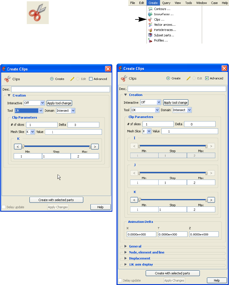
5.1 Clip Parts
5-44 EnSight 10.2 User Manual
For structured Parts, you can sweep through the Part with any of the i, j, or k
planes.
A Box Clip will create a part according to the Box Tool, and that can either be the
intersection of the Box Tool walls with the selected model parts (intersect), the
crinkly intersection of the Box Tool walls with the selected model parts (crinkly),
the portion of the selected model parts that lie within the Box Tool (inside), or the
portion of the selected model parts which lie outside the Box Tool (outside).
Clicking once on the Clip Feature Icon (which be default is in the Feature Ribbon)
or selecting Clips... in the Create menu, opens the Feature Panel for clip parts.
This editor is used to both create and edit clip parts.
Use Tool
IJK The IJK clip tool is used with structured mesh results.
Figure 5-35
Clip Icon
Figure 5-36
Feature Panel - Clips - IJK
5.1 Clip Parts
EnSight 10.2 User Manual 5-45
Create/Edit Toggles that control whether a new part will be created, or whether you are editing
existing part(s). Note that when editing, the changes will be applied to those parts which
have the small “pencil” icon next to them in the Parts List.
Advanced Will open additional features for more advance control of the Part.
Desc The name of the part to be created or being edited.
Creation
Interactive Opens pulldown menu for selection of type of interactive manipulation of the IJK clip.
Options are:
Off Interactive IJK clips are turned off.
Manual Value of the IJK clip selected are manipulated via the slider bar and
the IJK clip is interactively updated in the Graphics Window to the
new value.
Auto Value of the IJK clip is incremented by the Auto Delta value from
the minimum range value to the maximum value. When reaching the
maximum it starts again from the minimum.
Auto Cycle Value of the IJK clip is incremented by the Auto Increment value
from the minimum range value to the maximum value. When
reaching the maximum it decrements back to the minimum.
Apply Tool Change Recreates the Clip Part selected in the Parts List at the current position of and of the type
specified by Use Tool.
Domain Specification to extract the intersection of the specified mesh slice values. For IJK clips,
the only valid selection is “Intersect”.
Clip Parameters
# slices If you want more than one clip calculated at a Delta offset from each other, enter the
number of slices in this field. This number of clips is calculated then they are grouped
together. This field is only available at the first time the clip(s) are calculated. It is not
possible to change this value and recalculate the clips. To change the number or the
Delta, they must be deleted and recalculated.
Delta Offset value to use for creating a number of clips. The first clip is calculated at the
number entered in Value, and the next one is Delta + Value, etc. and they are all grouped
together in the Part List.
Mesh Slice Opens a pulldown menu for selecting which of the IJK dimensions you wish to allow to
change. You will then specify Min, Max and Step limits for the two remaining “fixed”
dimensions.
Value This field specifies the I, J, or K plane desired for the dimension selected in Mesh Slice.
Slider Bar(s) For IJK clips, the slider bar is used to increment / decrement the Mesh Slice Value
between its Minimum and Maximum value.
Min Specification of the minimum slice value for the range used with the
“Manual” slider bar and the “Auto” and “Auto Cycle” options.
Max Specification of the maximum slice value for the range used with the
“Manual” slider and the “Auto” and “Auto Cycle” options.
Step Specification of the increment/decrement the slider will move
within the min and max, each time the stepper buttons are clicked.
Animation Delta
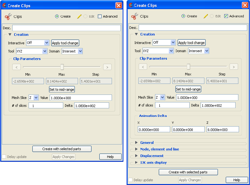
5.1 Clip Parts
5-46 EnSight 10.2 User Manual
See Feature Panel Turndowns Common To All Part Types for a detailed
discussion of the remaining Feature Panel turn-down sections which are the same
for all Parts.
(see How To Create IJK Clips)
Use Tool
XYZ The XYZ tool is used to create a planar Part at a constant Cartesian component value that
is referenced according to the local frame of the part.
This field specifies the incremental change in position of the clip for each page of
Flipbook or frame of Keyframe animation.
Create with selected
parts
Creates a Clip Part using the selected Part(s) in the Parts List.
Delay update Checking this box will cause EnSight to not apply any changes made until you hit the
Apply Changes button. When not checked, the changes are applied as you make them.
Apply Changes Applies any changes made. Only active when Delay update is on.
Create/Edit Toggles that control whether a new part will be created, or whether you are editing
existing part(s). Note that when editing, the changes will be applied to those parts which
have the small “pencil” icon next to them in the Parts List.
Advanced Will open additional features for more advance control of the Part.
Desc The name of the part to be created or being edited.
Creation
Figure 5-37
Feature Panel - Clips - XYZ
5.1 Clip Parts
EnSight 10.2 User Manual 5-47
Interactive Opens pulldown menu for selection of type of interactive manipulation of the XYZ clip.
Options are:
Off Interactive XYZ clips are turned off.
Manual Value of the XYZ clip selected are manipulated via the slider bar
and the XYZ clip is interactively updated in the Graphics Window
to the new value. For quick interactive control of the isosurface,
simply left-click on the isosurface and grab the resulting green,
cross-shaped click and go handle and drag left and right to see the
isosurface value interactively decrease and increase respectively.
Auto Value of the XYZ clip is incremented by the Auto Delta value from
the minimum range value to the maximum value. When reaching the
maximum it starts again from the minimum.
Auto Cycle Value of the XYZ clip is incremented by the Auto Increment value
from the minimum range value to the maximum value. When
reaching the maximum it decrements back to the minimum.
Apply Tool Change Recreates the Clip Part selected in the Parts List at the current position of and of the type
specified by Use Tool.
Domain Intersect will create the cross section of the selected parts at the specified X,
Y, or Z plane.
Crinkly will create a new part consisting of the parent part elements that
intersect the X, Y, or Z plane.
Clip Parameters
Slider Bar For XYZ clips, the slider bar is used to increment / decrement the Mesh Slice Value
between its Minimum and Maximum value.
Min Specification of the minimum interval value of the interactive XYZ
clip.
Max Specification of the maximum interval value of the interactive XYZ clip.
Step Specification of the interval step of the interactive XYZ clip.
Set to mid-range Clicking this button will put the value that is halfway between the minimum and the
maximum variable value.
Mesh Slice Opens a pulldown menu for selecting which of the XYZ components you wish to clip, i.e. the X,
the Y, or the Z component.
Value This field specifies the coordinate desired for the Mesh Slice component.
# slices If you want more than one clip calculated at a Delta offset from each other, enter the
number of slices in this field. This number of clips is calculated then they are grouped
together. This field is only available at the first time the clip(s) are calculated. It is not
possible to change this value and recalculate the clips. To change the number or the
Delta, they must be deleted and recalculated.
Delta Offset value to use for creating a number of clips. The first clip is calculated at the
number entered in Value, and the next one is Delta + Value, etc. and they are all grouped
together in the Part List.
Animation Delta
This field specifies the incremental change in position of the clip for each page of
Flipbook or frame of Keyframe animation.
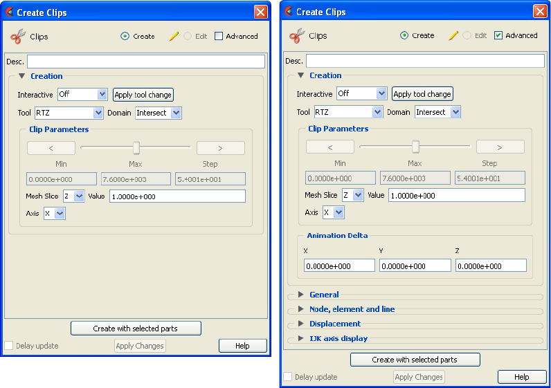
5.1 Clip Parts
5-48 EnSight 10.2 User Manual
See Feature Panel Turndowns Common To All Part Types for a detailed
discussion of the remaining Feature Panel turn-down sections which are the same
for all Parts.
(see How To Create XYZ Clips)
Use Tool
RTZ The RTZ tool is used to create a Part using cylindrical coordinates at a constant radius
about an axis, angle around that axis or height along an axis.
Create with selected
parts
Creates a Clip Part using the selected Part(s) in the Parts List.
Delay update Checking this box will cause EnSight to not apply any changes made until you hit the
Apply Changes button. When not checked, the changes are applied as you make them.
Apply Changes Applies any changes made. Only active when Delay update is on.
Create/Edit Toggles that control whether a new part will be created, or whether you are editing
existing part(s). Note that when editing, the changes will be applied to those parts which
have the small “pencil” icon next to them in the Parts List.
Advanced Will open additional features for more advance control of the Part.
Desc The name of the part to be created or being edited.
Creation
Interactive Opens pulldown menu for selection of type of interactive manipulation of the RTZ clip.
Options are:
Off Interactive RTZ clips are turned off.
Figure 5-38
Feature Panel - Clips - RTZ
5.1 Clip Parts
EnSight 10.2 User Manual 5-49
See Feature Panel Turndowns Common To All Part Types for a detailed
discussion of the remaining Feature Panel turn-down sections which are the same
for all Parts.
(see How To Create RTZ Clips)
Manual Value of the RTZ clip selected are manipulated via the slider bar and
the RTZ clip is interactively updated in the Graphics Window to the
new value.
Auto Value of the RTZ clip is incremented by the Auto Delta value from
the minimum range value to the maximum value. When reaching the
maximum it starts again from the minimum.
Auto Cycle Value of the RTZ clip is incremented by the Auto Increment value
from the minimum range value to the maximum value. When
reaching the maximum it decrements back to the minimum.
Apply Tool Change Recreates the Clip Part selected in the Parts List at the current position of and of the type
specified by Use Tool.
Domain Intersect Will create a cross section of the selected parts at the specified
radius, angle, or distance along the axis.
Crinkly Will create a new part consisting of the parent part elements that
intersect the specified radius, angle or distance.
Clip Parameters
Slider Bar For RTZ clips, the slider bar is used to increment / decrement the Slice Value between its
Minimum and Maximum value.
Min Specification of the minimum slice value for the range used with the
“Manual” slider bar and the “Auto” and “Auto Cycle” options.
Max Specification of the maximum slice value for the range used with the
“Manual” slider and the “Auto” and “Auto Cycle” options.
Step Specification of the increment/decrement the slider will move
within the min and max, each time the stepper buttons are clicked.
Mesh Slice Opens a pulldown menu for selecting which of the RTZ components to clip, i.e. the
radial (R), the angle theta (T) in degrees, or the distance along the longitudinal axis Z,
(Z).
Value This field specifies the magnitude desired for the Slice component, (theta in degrees).
Axis The global axis with which to align the longitudinal (Z) RTZ axis.
Animation Delta
This field specifies the incremental change in position of the clip for each page of
Flipbook or frame of Keyframe animation.
Create with selected
parts
Creates a Clip Part using the selected Part(s) in the Parts List.
Delay update Checking this box will cause EnSight to not apply any changes made until you hit the
Apply Changes button. When not checked, the changes are applied as you make them.
Apply Changes Applies any changes made. Only active when Delay update is on.
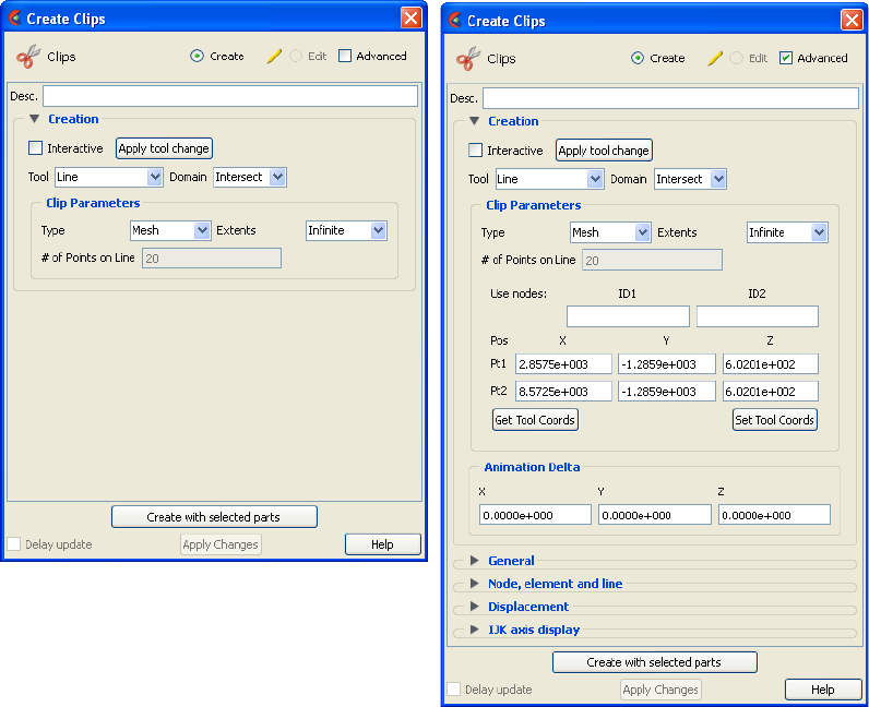
5.1 Clip Parts
5-50 EnSight 10.2 User Manual
Use Tool
Line The Line tool is used to create a clip line.
Create/Edit Toggles that control whether a new part will be created, or whether you are editing
existing part(s). Note that when editing, the changes will be applied to those parts which
have the small “pencil” icon next to them in the Parts List.
Advanced Will open additional features for more advance control of the Part.
Desc The name of the part to be created or being edited.
Creation
Interactive Toggles on/off interactive movement and updating of a clip Part. When toggled on, the
line tool used to create the 2D clip line will appear in the Graphics Window. Movement
of the tool will cause the Clip Part to be recreated at the new position. When
manipulation of the tool stops, the clip Part and any Parts that are dependent on it will be
updated. During movement, the Tool itself will not be visible, so as not to obscure the
Line Clip Part. The Tool will reappear when the mouse button is released.
Apply Tool Change Recreates the Clip Part selected in the Parts List at the current position of and of the type
specified by Use Tool.
Domain Specification to extract the intersection of the line tool with the selected part(s). For Line
clips, the only valid selections are “Intersect” and “Crinkly”.
Clip Parameters
Type Mesh Will create a Line Clip showing the intersection of the line tool with
the mesh elements of the parent Part.
Figure 5-39
Feature Panel - Clips - Line
5.1 Clip Parts
EnSight 10.2 User Manual 5-51
See Feature Panel Turndowns Common To All Part Types for a detailed
discussion of the remaining Feature Panel turn-down sections which are the same
for all Parts.
(see How To Create Line Clips)
Extents Opens a pull down menu for selection of the extent of the Line Clip.
Finite limits the Line Clip to the length specified by the Line
Tool endpoints.
Infinite Assumes the line tool defines an infinite line and uses
this to intersect the elements of the selected model Parts.
Grid Will create a Line Clip of evenly spaced bar elements along the line
tool.
# of Points on
Line
Specification of number of evenly spaced points on the line at which
to create a node.
Use nodes Allows for specification of the location of two node ids in the model from which to get
the line clip endpoints. If this method is used, the line clip will remain tied to these nodes
even if they move over time.
Pos of Pt1, Pt2 Specification of XYZ endpoint-coordinates of Line Clip. The position of a Line Clip Part
can be changed by manually entering values in the numeric fields and then pressing
Return.
Get Parameters
from Tool
The values in the numeric fields (and the position of a Line Clip Part, if selected in the
Feature Panel’s Parts List) can be updated after moving the Line tool interactively in the
Graphics Window by clicking Get Tool Coords. The Line Clip Part being edited will be
repositioned to the new coordinates after clicking Get Tool Coords. Coordinates are
always in the original model frame (Frame 0).
Apply Parameters
to Tool
The position of the Line Clip tool can be changed by entering values in the numeric
fields and then pressing Set Tool Coords.
Animation Delta
XYZ These X,Y,Z fields specify the incremental change in position of the clip for each page of
Flipbook or frame of Keyframe animation.
Create with selected
parts
Creates a Clip Part using the selected Part(s) in the Parts List.
Delay update Checking this box will cause EnSight to not apply any changes made until you hit the
Apply Changes button. When not checked, the changes are applied as you make them.
Apply Changes Applies any changes made. Only active when Delay update is on.
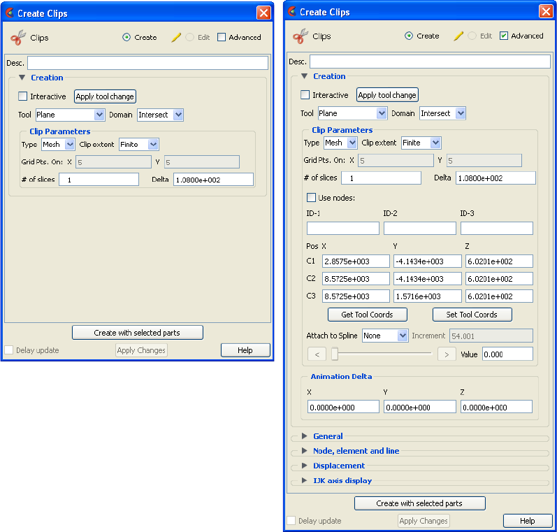
5.1 Clip Parts
5-52 EnSight 10.2 User Manual
Use Tool
Plane The Plane Tool is used to create a Plane Clip
Create/Edit Toggles that control whether a new part will be created, or whether you are editing
existing part(s). Note that when editing, the changes will be applied to those parts which
have the small “pencil” icon next to them in the Parts List.
Advanced Will open additional features for more advance control of the Part.
Desc The name of the part to be created or being edited.
Creation
Interactive Toggles on/off interactive movement and updating of the clip Part. When toggled on, the
Plane Tool used to create the clip Part will appear in the Graphics Window. Movement of
the Plane Tool will cause the Plane Clip to be recreated at the new position. When
manipulation of the tool stops, the clip Part and any Parts that are dependent on it will be
updated. During movement, the Tool itself will not be visible, so as not to obscure the
Line Clip Part. The Tool will reappear when the mouse button is released.
For quick interactive control of the clip plane, simply left-click on the plane tool origin
and grab the resulting green, cross-shaped click and go handle and drag to see the clip
location value interactively translate in the plane tool Z direction.
Apply Tool Change Recreates the Clip Part selected in the Parts List at the current position of and of the type
specified by Use Tool.
Figure 5-40
Feature Panel - Clips - Plane
5.1 Clip Parts
EnSight 10.2 User Manual 5-53
Domain Intersect will create the cross section of the selected parts where they intersect
the plane tool.
Crinkly will create a new part consisting of the parent part elements that
intersect the plane tool.
Inside will cut the parent parts and create a new part consisting of the
portion on the positive z side of the plane tool.
Outside will cut the parent parts and create a new part consisting of the
portion on the negative z side of the plane tool.
In/Out will cut the parent parts and create two new parts - namely an Inside
and Outside part.
Clip Parameters
Type Mesh Will create a Plane Clip showing the cross section of the parent Part.
Clip extent Opens a pull down menu for selection of the extent of the Plane
Clip.
Finite limits the Plane Clip to the area specified by the Plane
Tool corner coordinates.
Infinite extends the Plane Clip to include the intersection of the
plane with all elements of the selected model Parts.
Grid Will create a Line Clip of evenly spaced bar elements along the line
tool.
Grid Pts
on:XY
These fields specify the number of points on each edge of a Plane
Clip at which to create nodes. Additional nodes are located in the
interior of the plane to form an evenly spaced grid. The values must
be positive integers. Applicable only to grid-type Plane Clips. Grid
Pts in X correspond to the x-direction on the Plane tool, while the
number of Grid Pts in Y correspond to the y-direction of the Plane
tool.
# slices If you want more than one clip calculated at a Delta offset from each other, enter the
number of slices in this field. This number of clips is calculated then they are grouped
together. This field is only available at the first time the clip(s) are calculated. It is not
possible to change this value and recalculate the clips. To change the number or the
Delta, they must be deleted and recalculated.
Delta Offset value to use for creating a number of clips. The first clip is calculated at the
number entered in Value, and the next one is Delta + Value, etc. and they are all grouped
together in the Part List.
Use nodes Specification of three node ids which will be used to specify the plane of the clip. The
clip plane will be tied to these three nodes, even if they move in time.
Pos of C1,C2,C3 Specification of the location, orientation, and size of the Plane Clip using the coordinates
(in the Parts reference frame) of three corner points, as follows:
Corner 1 is corner located in negative-X negative-Y quadrant
Corner 2 is corner located in positive-X negative-Y quadrant
Corner 3 is corner located in positive-X positive-Y quadrant
Get Parameters
from Tool
Will update the C1, C2, and C3 fields to reflect the current position of the Plane Tool.
Apply Parameters
to Tool
Will reposition the Plane Tool to the position specified in C1, C2, and C3.
Animation Delta
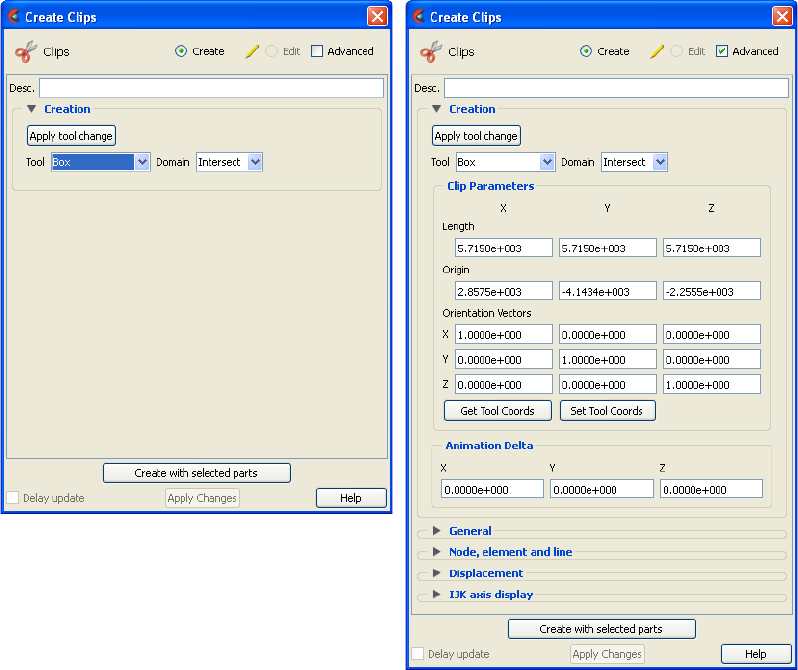
5.1 Clip Parts
5-54 EnSight 10.2 User Manual
See Feature Panel Turndowns Common To All Part Types for a detailed
discussion of the remaining Feature Panel turn-down sections which are the same
for all Parts.
(see How To Create Plane Clips)
Use Tool
Box This Clipping Tool extracts portions of the model that are inside, outside, or that intersect
a specified box.
Be aware that due to the algorithm used, this clip can (and most often does) have
chamfered edges, the size of which depends on the coarseness of the model elements
XYZ These X,Y,Z fields specify the incremental change in position of the clip for each page of
Flipbook or frame of Keyframe animation.
Create with selected
parts
Creates a Clip Part using the selected Part(s) in the Parts List.
Delay update Checking this box will cause EnSight to not apply any changes made until you hit the
Apply Changes button. When not checked, the changes are applied as you make them.
Apply Changes Applies any changes made. Only active when Delay update is on.
Create/Edit Toggles that control whether a new part will be created, or whether you are editing
existing part(s). Note that when editing, the changes will be applied to those parts which
have the small “pencil” icon next to them in the Parts List.
Figure 5-41
Feature Panel - Clips - Box
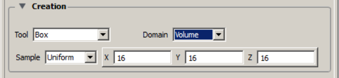
5.1 Clip Parts
EnSight 10.2 User Manual 5-55
Advanced Will open additional features for more advance control of the Part.
Desc The name of the part to be created or being edited.
Creation
Apply Tool Change Recreates the Clip Part selected in the Parts List at the current position of and of the type
specified by Use Tool.
Domain Intersect will create a new part consisting of the intersection of the box tool
sides and the selected parts.
Crinkly will create a new part consisting of the parent part elements that
intersect the box tool sides.
Inside will extract the volume portion of the parent parts that lie within the
box.
Outside will extract the volume portion of the parent parts that do not lie
within the box.
In/Out will create two new parts - namely the Inside and Outside parts.
Volume This option creates a client side volume rendering inside the box
tool using the number of samples specified in the dialog in the x, y,
and z directions. This allows volume rendering only in a specific
portion of the selected part inside the box tool. In contrast, if you
select the part and change its element representation to volume, then
the entire geometry will be volume rendered. See the Element
Representation section of Feature Panel Turndowns Common To All
Part Types.
Sample Type of sampling applied to the Box Tool:
Uniform - Create a volumetric grid with the specified number of
X, Y, and Z equally spaced divisions, or nodes along
each axis - creating a uniform grid.
X = The number of nodes along the x-axis of the box tool.
Y = The number of nodes along the y-axis of the box tool.
Z = The number of nodes along the z-axis of the box tool.
Clip Parameters
Length X,Y,Z These fields specify the extent of the clip in the X, Y and Z dimensions.
Origin X,Y,Z These fields specify the origin of the clip in the X, Y and Z dimensions.
Orientation
Vectors X,Y,Z
These fields contain the component values of the orthogonal box axis vectors.
Get Parameters
from Tool
Will update the Origin and Orientation Vector fields to reflect the current position of the
Box Tool.
Apply Parameters
to Tool
Will reposition the Box Tool to the position specified in the Origin and Orientation
Vector fields.
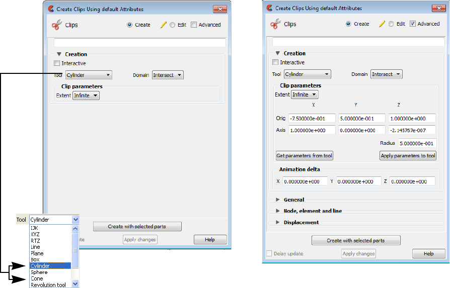
5.1 Clip Parts
5-56 EnSight 10.2 User Manual
See Feature Panel Turndowns Common To All Part Types for a detailed
discussion of the remaining Feature Panel turn-down sections which are the same
for all Parts.
(see How To Create Box Clips)
Use Tool
Cylinder, Sphere, Cone These Tools are used to create a quadric clip surface
Animation Delta
XYZ These X,Y,Z fields specify the incremental change in position of the clip for each page of
Flipbook or frame of Keyframe animation.
Create with selected
parts
Creates a Clip Part using the selected Part(s) in the Parts List.
Delay update Checking this box will cause EnSight to not apply any changes made until you hit the
Apply Changes button. When not checked, the changes are applied as you make them.
Apply Changes Applies any changes made. Only active when Delay update is on.
Create/Edit Toggles that control whether a new part will be created, or whether you are editing
existing part(s). Note that when editing, the changes will be applied to those parts which
have the small “pencil” icon next to them in the Parts List.
Advanced Will open additional features for more advance control of the Part.
Desc The name of the part to be created or being edited.
Figure 5-42
Feature Panel - Clips - Cylinder, Sphere, & Cone
5.1 Clip Parts
EnSight 10.2 User Manual 5-57
Creation
Interactive Toggles on/off interactive movement and updating of a clip Part. When toggled on, the
Quadric Tool used to create the Clip Part will appear in the Graphics Window at the
location of the Clip Part. Movement of the Quadric Tool will cause the Clip Part to be
recreated at the new position. When manipulation of the tool stops, the Clip Part and any
Parts that are dependent on it will be updated. During movement, the Tool itself will not
be visible, so as not to obscure the Line Clip Part. The Tool will reappear when the
mouse button is released.
Apply Tool Change Recreates the Clip Part selected in the Parts List at the current position of and of the type
specified by Use Tool.
Domain Intersect will create the cross section of the selected parts where they intersect
the quadric tool.
Crinkly will create a new part consisting of the parent part elements that
intersect the quadric tool.
Inside will cut the parent parts and create a new part consisting of the
portion on the inside of the quadric tool.
Outside will cut the parent parts and create a new part consisting of the
portion on the outside of the quadric tool.
In/Out will cut the parent parts and create two new parts - namely an Inside
and Outside part.
Note: if you clip through multiple parts, then you may not later change this domain.
Clip Parameters
Extent Opens a pulldown menu that allows for the selection of Finite or Infinite extents. It is
only present for cylinder and cone clips.
Clip Parameters
Cylinder Orig Specification of the origin (the center point) of the Cylindrical Clip.
Axis Specification of the longitudinal axis direction of the Cylindrical
Clip.
Radius Specification of the radius of the Cylindrical Clip.
Sphere Orig Specification of the origin (the center point) of the Spherical Clip.
Axis Specification of the axis direction of the Spherical Clip. (Note: Axis
is important if Developed Surface is created from the spherical clip.)
Radius Specification of the radius of the Spherical Clip.
Cone Orig Specification of the origin (the tip of the cone) of the Conical Clip.
Axis Specification of the axis direction of the Conical Clip. Axis
direction goes from tip to base.
Angle Specification of the conical half angle (in degrees) of the Conical
Clip.
Get Parameters
from Tool
Will update the parameter fields to reflect the current position of the Tool.
Apply Parameters
to Tool
Will reposition the Tool to the position specified in parameter fields.
Animation Delta
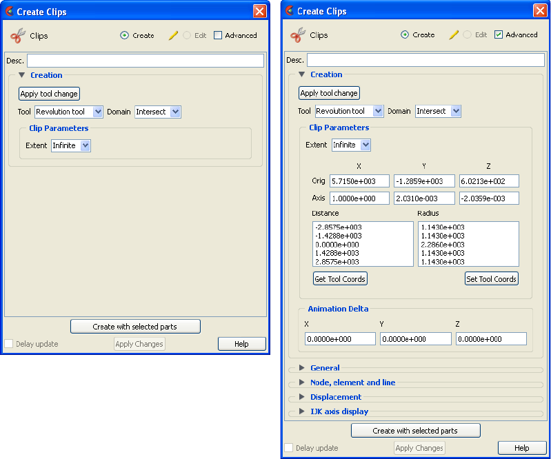
5.1 Clip Parts
5-58 EnSight 10.2 User Manual
See Feature Panel Turndowns Common To All Part Types for a detailed
discussion of the remaining Feature Panel turn-down sections which are the same
for all Parts.
(see How To Create Quadric Clips)
Use Tool
Revolution Tool This clipping Tool is used to create custom clip surfaces which are defined by revolving a
set of lines about a defined axis.
XYZ These X,Y,Z fields specify the incremental change in position of the clip for each page of
Flipbook or frame of Keyframe animation.
Create with selected
parts
Creates a Clip Part using the selected Part(s) in the Parts List.
Delay update Checking this box will cause EnSight to not apply any changes made until you hit the
Apply Changes button. When not checked, the changes are applied as you make them.
Apply Changes Applies any changes made. Only active when Delay update is on.
Create/Edit Toggles that control whether a new part will be created, or whether you are editing
existing part(s). Note that when editing, the changes will be applied to those parts which
have the small “pencil” icon next to them in the Parts List.
Advanced Will open additional features for more advance control of the Part.
Figure 5-43
Feature Panel - Clips - Revolution
5.1 Clip Parts
EnSight 10.2 User Manual 5-59
See Feature Panel Turndowns Common To All Part Types for a detailed
discussion of the remaining Feature Panel turn-down sections which are the same
for all Parts.
(see Section 4.6, Tools Menu Functions and How To Use the Surface of Revolution Tool)
Desc The name of the part to be created or being edited.
Creation
Apply Tool Change Recreates the Clip Part selected in the Parts List at the current position of and of the type
specified by Use Tool.
Domain Intersect will create the cross section of the selected parts where they intersect
the revolved surface.
Crinkly will create a new part consisting of the parent part elements that
intersect the revolved surface.
Inside will cut the parent parts and create a new part consisting of the
portion on the inside of the revolved surface.
Outside will cut the parent parts and create a new part consisting of the
portion on the outside of the revolved surface.
In/Out will cut the parent parts and create two new parts - namely an Inside
and Outside part.
Note: if you clip through multiple parts, then you may not later change this domain.
Clip Parameters
Extent Opens a pulldown menu that allows for the selection of Finite or Infinite extents.
Orig Specifies the XYZ coordinates of the origin (center point) of the Revolution Clip.
Axis These fields specify the XYZ coordinates of the axis direction of the Revolution Clip.
Distance/Radius These lists specify the distance (from the origin) and radius for each point that defines
the Revolution Clip. The points cannot be edited within this dialog. You must edit the
Revolution Tool in the Transformations dialog.
Get Parameters
from Tool
Will update the clip parameter fields to reflect the current position of the Revolution
Tool.
Apply Parameters
to Tool
Will reposition the Revolution Tool to the position specified in clip parameter fields.
Animation Delta
XYZ These X,Y,Z fields specify the incremental change in position of the clip for each page of
Flipbook or frame of Keyframe animation.
Create with selected
parts
Creates a Clip Part using the selected Part(s) in the Parts List.
Delay update Checking this box will cause EnSight to not apply any changes made until you hit the
Apply Changes button. When not checked, the changes are applied as you make them.
Apply Changes Applies any changes made. Only active when Delay update is on.
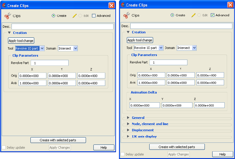
5.1 Clip Parts
5-60 EnSight 10.2 User Manual
Use Tool
Revolve 1D Part This option will create a clip surface by revolving a line, defined by a Part, about an axis.
Create/Edit Toggles that control whether a new part will be created, or whether you are editing
existing part(s). Note that when editing, the changes will be applied to those parts which
have the small “pencil” icon next to them in the Parts List.
Advanced Will open additional features for more advance control of the Part.
Desc The name of the part to be created or being edited.
Creation
Apply Tool Change Recreates the Clip Part selected in the Parts List at the current position of and of the type
specified by Use Tool.
Domain Intersect will create the cross section of the selected parts where they intersect
the revolved surface.
Crinkly will create a new part consisting of the parent part elements that
intersect the revolved surface.
Inside will cut the parent parts and create a new part consisting of the
portion on the inside of the revolved surface.
Outside will cut the parent parts and create a new part consisting of the
portion on the outside of the revolved surface.
In/Out will cut the parent parts and create two new parts - namely an Inside
and Outside part.
Note: if you clip through multiple parts, then you may not later change this domain.
Clip Parameters
Figure 5-44
Feature Panel - Clips - Revolve 1D Part
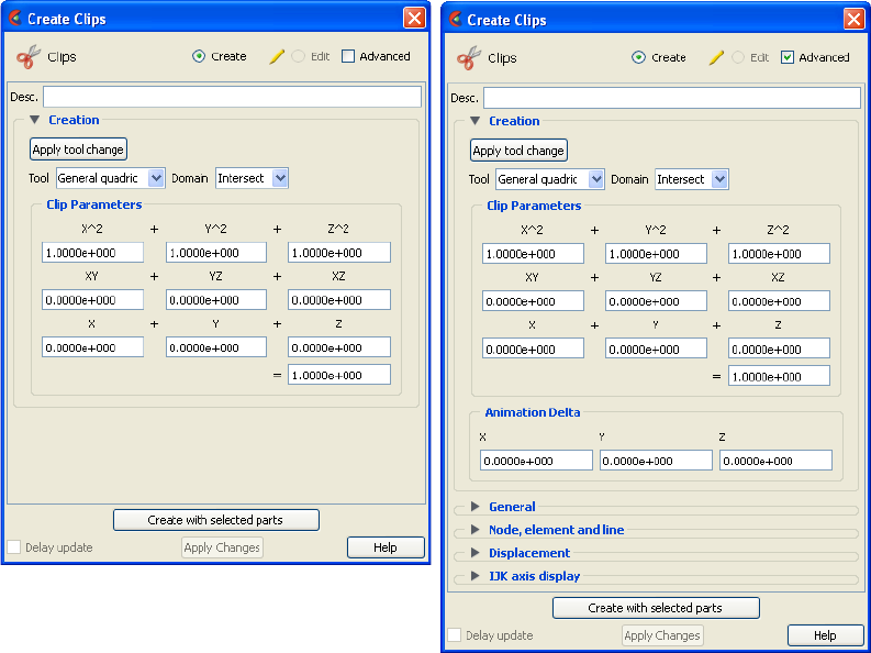
5.1 Clip Parts
EnSight 10.2 User Manual 5-61
See Feature Panel Turndowns Common To All Part Types for a detailed
discussion of the remaining Feature Panel turn-down sections which are the same
for all Parts.
Use Tool
General Quadric
Revolve Part This field specifies the Part number which will be revolved. The 1D Part must contain
only bar elements and must have only two free ends (i.e., there must be only one
“logical” line contained in the Part).
Orig These fields specify the XYZ coordinates of the axis line origin point.
Axis These fields specify the direction vector of the axis line. The “line” contained in the Part
specified by number in Revolve Part will be revolved about this axis to create the clip
surface Part.
Animation Delta
XYZ These X,Y,Z fields specify the incremental change in position of the clip for each page of
Flipbook or frame of Keyframe animation.
Create with selected
parts
Creates a Clip Part using the selected Part(s) in the Parts List.
Delay update Checking this box will cause EnSight to not apply any changes made until you hit the
Apply Changes button. When not checked, the changes are applied as you make them.
Apply Changes Applies any changes made. Only active when Delay update is on.
Figure 5-45
Feature Panel - Clips - General Quadric
5.1 Clip Parts
5-62 EnSight 10.2 User Manual
See Feature Panel Turndowns Common To All Part Types for a detailed
discussion of the remaining Feature Panel turn-down sections which are the same
for all Parts.
Create/Edit Toggles that control whether a new part will be created, or whether you are editing
existing part(s). Note that when editing, the changes will be applied to those parts which
have the small “pencil” icon next to them in the Parts List.
Advanced Will open additional features for more advance control of the Part.
Desc The name of the part to be created or being edited.
Creation
Apply Tool Change Recreates the Clip Part selected in the Parts List at the current position of and of the type
specified by Use Tool.
Domain Intersect will create the cross section of the selected parts where they intersect
the general quadric surface.
Crinkly will create a new part consisting of the parent part elements that
intersect the general quadric surface.
Inside will cut the parent parts and create a new part consisting of the
portion on the inside of the general quadric surface.
Outside will cut the parent parts and create a new part consisting of the
portion on the outside of the general quadric surface.
In/Out will cut the parent parts and create two new parts - namely an Inside
and Outside part.
Clip Parameters
10 Coefficient
Values
These coefficient values represent the general equation of a Quadric surface. They can
be hanged by modifying the values. No tool exists corresponding to this equation.
AX2+BY2+CZ2+DXY+EYZ+FXZ+GX+HY+IZ=J
Animation Delta
XYZ Not available for General Quadric Clips.
Create with selected
parts
Creates a Clip Part using the selected Part(s) in the Parts List.
Delay update Checking this box will cause EnSight to not apply any changes made until you hit the
Apply Changes button. When not checked, the changes are applied as you make them.
Apply Changes Applies any changes made. Only active when Delay update is on.
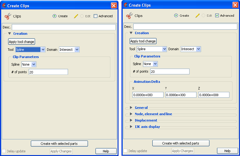
5.1 Clip Parts
EnSight 10.2 User Manual 5-63
Use Tool
Spline This option will create a clip along an existing spline using evenly spaced nodes along the
spline.
Create/Edit Toggles that control whether a new part will be created, or whether you are editing
existing part(s). Note that when editing, the changes will be applied to those parts which
have the small “pencil” icon next to them in the Parts List.
Advanced Will open additional features for more advance control of the Part.
Desc The name of the part to be created or being edited.
Creation
Apply Tool Change Recreates the Clip Part selected in the Parts List at the current position of and of the type
specified by Use Tool.
Domain Intersect will create the 1D part composed of bar elements using the selected
parts where they intersect the spline at an evenly spaced number of
points.
Clip Parameters
Spline This pulldown allows you to choose which spline to use as the clipping tool.
# of points Enter the number of evenly spaced points to use over the spline for the 1D clip creation.
Animation Delta
XYZ These X,Y,Z fields specify the incremental change in position of the clip for each page of
Flipbook or frame of Keyframe animation.
Create with selected
parts
Creates a Clip Part using the selected Part(s) in the Parts List.
Delay update Checking this box will cause EnSight to not apply any changes made until you hit the
Apply Changes button. When not checked, the changes are applied as you make them.
Figure 5-46
Feature Panel - Clips - Spline

5.1 Clip Parts
5-64 EnSight 10.2 User Manual
See Feature Panel Turndowns Common To All Part Types for a detailed
discussion of the remaining Feature Panel turn-down sections which are the same
for all Parts.
Troubleshooting Clips
Apply Changes Applies any changes made. Only active when Delay update is on.
Problem Probable Causes Solutions
Clip does not move during
animation
Animation deltas are not set, or
are too small.
Change the animation delta
values.
Clip results in an empty Part. Clip was taken outside of the
model.
Change the clip Tool location.
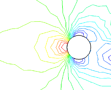
5.1 Contour Parts
EnSight 10.2 User Manual 5-65
5.1.4 Contour Parts
Contours are lines that trace out constant values of a variable across the surface(s)
of selected Part(s), just like contour lines on a topographical map.
The variable must be a scalar or vector variable. If it is a vector, the magnitude or
one of the components can be used. A Contour Part can consist of one contour
line, or a set of lines corresponding to the value-levels of the variable palette. A
Contour Part has its own attributes independent of those Parts used to create it (the
parent Part(s)).
Contours are drawn across the faces of parent Part elements (one-dimensional
elements are ignored). At each node along the edges of any one element face, the
contour’s variable has a value. If the range of these values includes the contour’s
value-level, the contour line crosses the face. EnSight draws the contour by
dividing the face into triangles each having the face’s centroid as one vertex. For
each triangle the contour crosses, it will cross only two sides. EnSight interpolates
to find the point on each of those two sides where the variable value equals the
contour value-level, then creates a bar element to connect the two points. Note
that a contour line can bend while crossing an element face.
Because Contour Parts are created on the EnSight Client, the Representation
attribute of the parent Part(s) greatly affects the result. Representations that reduce
Part elements to one-dimensional representations (Border applied to two-
dimensional Parts and Feature Angle), or do not download the Part (Not Loaded),
will eliminate those Part elements from the Contour creation process. On the other
hand, Full representation of three-dimensional elements will create contour lines
across hidden surfaces. Usually, you will want the Representation selection to be
3D Border, 2D Full.
Contour Parts are created on the Client, and so cannot be queried or used in
creating new variables. However, Contours can be used as parent Parts for Profiles
and Vector Arrows.
If you have synced the contours to the variable palette and you change the value-
levels in the Palette Editor, the Contour automatically regenerates using the new
value-levels.
Figure 5-47
Pressure Contours in a Flow Field around a Circular Obstruction
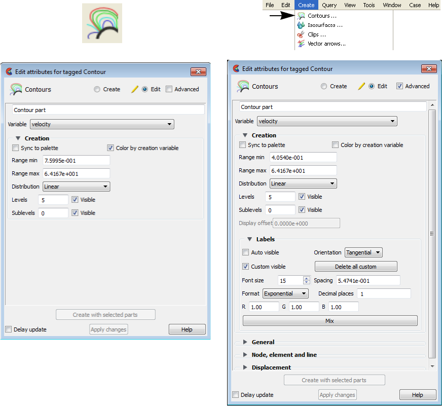
5.1 Contour Parts
5-66 EnSight 10.2 User Manual
Use care when simultaneously displaying contours based on different function
palettes so that you do not become confused as to which contours are which.
Coloring them differently and adding an on-screen legend can help.
Left-clicking once on the Contours Icon (or selecting Contours... from the Create
menu) opens the Feature Panel for Contours in create mode. This editor is used to
both create and edit contour Parts. Double-clicking on a part in the Parts list will
open the Feature Panel for Contours in edit mode. Left-clicking on the contour
part in the graphics window will pop up a green handle. Drag this cross left and
right to interactively change the contour density. Right-clicking on the contour
part will give you a number of quick options, one of which is to right click on a
contour level and choose Label>Add to Add a label at that location.
Create/Edit Toggles that control whether a new part will be created, or whether you are editing
existing part(s). Note that when editing, the changes will be applied to those parts which
have the small “pencil” icon next to them in the Parts List.
Advanced Will open additional features for more advance control of the Part.
Desc The name of the part to be created or being edited.
Figure 5-48
Contour Icon, and Create menu option
Figure 5-49
Feature Panel - Contours, basic and
advanced
5.1 Contour Parts
EnSight 10.2 User Manual 5-67
Variable Choose the variable to use for creating the contours from the pulldown.
Creation
Vector Component If the variable chosen is a vector, choose magnitude or one of the X, Y, or Z components.
Note that this is ignored if you use the advanced scaling option just described.
Sync To Palette Toggles on/off the contour line synchronization to the legend color palette.
Color by creation If toggled on at Contour part creation, then the Contour Part is colored by the variable.
Range Min This field is activated when Sync to Palette Toggle is Off.
Range Max This field is activated when Sync to Palette Toggle is Off.
Distribution This pop-up menu is activated when Sync to Palette Toggle is Off. Opens a pop-up menu
for the selection of a distribution function for the contour lines. Choices include Linear,
Logarithmic, and Quadratic.
Levels This field is activated when Sync to Palette Toggle is Off. This field determines the
number of contours between the Range Min and Range Max.
Visible Toggles whether the main level contours are visible or not.
Sublevels This field allows you to specify the number of sub-contours you wish to be drawn at
evenly spaced value-levels between the value-levels defined above if not syncing to the
palette, or defined in the Palette Editor if syncing to the palette. Leaving this field 0 will
produce exactly the number of contour lines for which value levels are specified.
Visible Toggles whether the sublevel contours are visible or not.
Display offset Available in advanced mode, this field specifies the normal distance away from a
surface to display the contours. A positive value moves the contours away from
the surface in the direction of the surface normal. A negative value moves in the
negative surface normal direction.
Please note that there is a hardware offset that will apply to contours, vector arrows,
separation/attachment lines, and surface restricted particle traces that can be turned on
or off in the View portion of Edit->Preferences. This preference (“Use graphics
hardware to offset line objects...”) is on by default and generally gives good images for
everything except move/draw printing. This hardware offset differs from the display
offset in that it is in the direction perpendicular to the computer screen monitor (Z-
buffer).
Thus, for viewing, you may generally leave the display offset at zero. But for printing, a
non-zero value may become necessary so the contours print cleanly.
Labels Available in advanced mode.
Auto Visible Toggles on/off the visibility of the automatic number labels for contour lines.
Custom Visible Toggles on/off the visibility of the custom number labels for contour lines. Custom
labels are created at user-selected locations on the contour lines, using right-click at the
desired contour location and choosing Labels>Add.
Delete all custom Removes all custom number labels (which were created using right-click at a contour
location and choosing Labels>Add).
Orientation Determines the orientation between number labels: Tangential or Horizontal.
Font Size Determines the number label font size.
Spacing Determines the spacing between number labels.
Format This pop-up menu allows selection of format of number labels. Choices include
Exponential, and Floating Point.

5.1 Contour Parts
5-68 EnSight 10.2 User Manual
See Feature Panel Turndowns Common To All Part Types for a detailed
discussion of the remaining Feature Panel turn-down sections which are the same
for all Parts.
Also see How to Create Contours)
Troubleshooting Contours
Decimal Places This field allows the specification of the number of decimal places of the number labels.
R,G,B Allows the specification of red, green, and blue values for the assignment of a color to
number labels.
Mix... Opens the Color Selector dialog for the assignment of a color to number labels.
Create with selected
parts
Creates a Contour Part using the selected Part(s) in the Parts List and the color palette
associated with the Variable currently selected in the Variables List.
Delay update Checking this box will cause EnSight to not apply any changes made until you hit the
Apply Changes button. When not checked, the changes are applied as you make them.
Apply Changes Applies any changes made. Only active when Delay update is on.
Problem Probable Causes Solutions
No contours created. Variable values on element faces are
outside range of palette function
value-levels.
Adjust palette function using the
Palette editor if syncing to palette.
Or adjust Range min and max in the
Feature Panel if not syncing
Parent Parts do not contain any 2D
elements.
Re-specify Parent Part list.
Parent Parts do not contain the
specified Variable.
Recreate the Variable for the selected
Parent Part(s).
Too many contours. Palette has too many function levels. Change the number of levels for the
palette using the Palette editor if
syncing to palette. Or adjust the
levels in the Feature Panel if not
syncing.
Specified too many sub-contours. Lower the sub-contour attribute.
Too few contours. The palette levels do not adequately
cover the function value range for
the Parent Parts.
Modify the palette using the Palette
editor (if syncing) or the Feature
Panel if not syncing.
Sub-contour attribute set to 0. Modify the Sub-contour attribute.
Contour Part created but (empty) Parent Part is in Feature Angle
representation.
Change Parent Part to 3D border, 2D
full representation.
Contours are fine at first, but later go
away.
Parent Parts representation changed
to Feature Angle, or Not Loaded.
The contours are created from the
Part representation on the EnSight
client. Modifying the representation
affects the Contour Parts.
Contour parts don’t print well See Display Offset above. Enter a display offset (may need to
be less than zero if viewed from
“backside”).
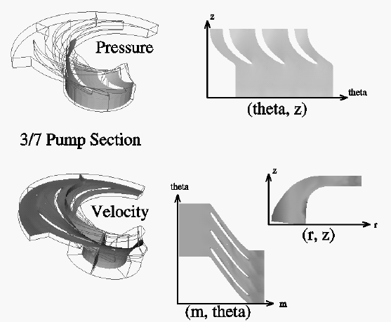
5.1 Developed Surface Parts
EnSight 10.2 User Manual 5-69
5.1.5 Developed Surface Parts
A Developed Surface is generated by treating any 2D Part (or parent Part) as a
surface of revolution, and mapping specific curvilinear coordinates of the
revolved surface into a planar representation.
A Developed Surface derives its name from the implied process that defines a
developable surface. A surface is considered “developable” if it can be unrolled
onto a plane without distortion. Although every 2D Part in EnSight is not by
definition a developable surface, each 2D Part can nevertheless be developed into
a planar surface which is distorted according to the type of developed projection
specified. For example, a Cylinder Clip Part is by definition a developable
surface, because it can be developed into planar surface without distortion.
Whereas, a Sphere Clip Part is not a developable surface, because it can not be
developed into a planar surface without distortion.
Parent Parts Only 2D Parts are developed. Also, only one Part is developed at a time. While all
2D Parts qualify as candidate parent Parts, only 2D Parts of revolution are
developed coherently. The current developed surface algorithm treats all parent
Parts as surfaces of revolution that are developed according to a local origin and
axis of revolution. These attributes are either inherited from the parent Part, or
must be specified according to the parent Part.
A developed surface permanently inherits the local origin and axis of revolution
information from any parent Part created via the cylinder, cone, sphere, or
revolution Clip tools. Whereas, surfaces developed from non-Clip Parts require
this information to be specified via the Orig. and Axis fields in the Attributes
(Developed Surfaces) dialog. The latter case is the only time the values in these
fields are used. Although default values are provided, it is up to you to make sure
that valid values are specified. In the former case, the Orig and Axis fields only
provide convenient feedback of the selected Clip Part. Note that developed
surfaces resulting from parent Parts of revolution created via the general quadric
Clip tool do not inherit the local origin and axis of revolution attributes from the
General Quadric Clip parent; rather, these attributes must be specified.
Figure 5-50
Developed
Surface
Examples
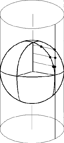
5.1 Developed Surface Parts
5-70 EnSight 10.2 User Manual
Developed Projections A parent Part is developed by specifying one of five curvilinear mappings called
developed projections; namely, an (r,z), (,z), (,r), (m,), or (m,r), projection.
The curvilinear coordinates r,, z, and m stand for the respective radius,, z, and
meridian (or longitude) directional components which are defined relative to the
local origin and axis of revolution of the parent Part. The meridian component is
defined as m = SQRT(r2 + z2).
Seam Line A surface of revolution is developed about its axis, starting at its “seam” line (or
zero meridian) where the surface is to be slit. Surface points along the seam are
duplicated on both ends of the developed Part. The seam line is specified via a
vector that is perpendicular to and originates from the axis of revolution, and
which points toward the seam which is located on the surface at a constant value.
This vector can be specified either manually or interactively. Interactive seam line
display and manipulation is provided via a slider in the Attributes (Developed
Surfaces) dialog.
Figure 5-51
Developed Equiareal Projection
Essentially, each topological projection first
surrounds the parent Part of revolution with a
virtual cylinder of constant radius. The
curvilinear coordinates of the parent Part are
then projected along the normals of (and thus
onto) the virtual cylinder. Finally, the virtual
cylinder is slit along a straight line, or
generator, and unwrapped into a plane. This
process yields an equiareal, or area
preserving, mapping which means that the
area of any enclosed curve on the surface of
the parent Part is equal to the area enclosed
by the image of the enclosed curve on the
developed plane. Although equiareal
mappings provide reduced shape distortion,
they do suffer from angular distortions of
local scale.
Vector fields of the parent Part (for all three
developed projections) are developed such
that a vector’s angle to its surface normal is
preserved. For example, a vector normal to
the parent surface remains normal when
developed onto the planar surface.
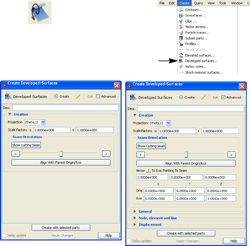
5.1 Developed Surface Parts
EnSight 10.2 User Manual 5-71
Clicking once on the Developed Surface Icon (if you have customized the Feature
Ribbon to have it visible) or selecting Developed Surfaces... in the Create menu,
opens the Feature Panel for Developed Surfaces. This editor is used to both create
and edit developed surface parts.
Create/Edit Toggles that control whether a new part will be created, or whether you are editing
existing part(s). Note that when editing, the changes will be applied to those parts which
have the small “pencil” icon next to them in the Parts List.
Advanced Will open additional features for more advance control of the Part.
Desc The name of the part to be created or being edited.
Figure 5-52
Developed Surface Icon, and Create menu option
Figure 5-53
Feature Panel - Developed Surfaces

5.1 Developed Surface Parts
5-72 EnSight 10.2 User Manual
See Feature Panel Turndowns Common To All Part Types for a detailed
discussion of the remaining Feature Panel turn-down sections which are the same
for all Parts.
Also (see How To Create Developed (Unrolled) Surfaces)
Troubleshooting Developed Surfaces
Creation
Projection Opens a pop-up dialog for the specification of which type of (u,v) projection, or
mapping, you wish to use for developing a surface of revolution; where u,v denotes
curvilinear components of the parent Part that are mapped into the xy-plane of reference
Frame 0. The options are:
(r,z) denotes the radial and z-directional components of the revolved surface.
(theta,z) denotes the theta and z-directional components of the revolved surface.
(theta,r) denotes the theta and radial components of the revolved surface.
(m,theta) denotes the meridian and theta components of the revolved surface. The
meridian component is the curvilinear component along a revolved surface
that runs in the direction of its axis of revolution (e.g. the meridonal and z-
directional components along a right cylinder are coincident, and for a
sphere the meridian is the longitude)
(m,r) denotes the meridian and radial components of the revolved surface.
Scale Factors (u,v) These fields specify the scaling factors which will be applied to the u and v projections.
Seam Orientation
Show Cutting
Seam
Click this button to display the current seam line location about the circumference of the
revolved surface. The seam line is manipulated interactively via the Slider Bar.
Align with Parent
Origin/Axis
Retrieves the Origin and Axis information from the Parent Part. Must be done if Parent
Part is a quadric clip.
Vector _|_ To Axis
Pointing To Seam
These fields allow you to precisely specify the position of the Cutting Seam Line by
specifying the direction of the vector perpendicular to the axis of revolution which points
in the direction of the seam line.
Orig X Y Z These fields specify a point on the axis of revolution.
Axis X Y Z These fields specify a vector, which when used with the Axis Origin defines the axis of
revolution.
Create with selected
parts
Creates a Developed surface part using the selected Part(s) in the Parts List.
Delay update Checking this box will cause EnSight to not apply any changes made until you hit the
Apply Changes button. When not checked, the changes are applied as you make them.
Apply Changes Applies any changes made. Only active when Delay update is on.
Problem Probable Causes Solutions
Error message is encountered while
creating a Developed Surface Part.
Parent Part is invalid. Only 2D Parts can be developed.

5.1 Developed Surface Parts
EnSight 10.2 User Manual 5-73
Developed Surface is created, but is
either not visible, Partially visible, or
obstructed by other Parts which may
be other developed Parts
Since all Developed Surfaces are
projected about the origin on the xy-
plane of the reference frame of the
parent Part, they may map outside
the viewport, intersect other Parts, or
pile up on each other.
Set the Developed Surface to be
viewed in its own viewport and
initialize the viewport.
Use different u/v scaling.
Assign the developed Part to its own
local reference frame and transform
it accordingly.
Developed Surface Part is a line. Wrong Projection type was
specified.
Select a different Projection.
Developed Surface Part does not
update to new Orig and/or Axis
values.
The Orig and Axis values can not be
specified if the Parent Part is created
from either a cylinder, sphere, cone,
or revolution quadric clip. These
values can only be specified if the
2D parent Part is not a quadric
clipped surface.
Since values entered for this
condition are not used, click the Get
Parent Part Defaults button to update
the fields based on the selected
parent Part in the Parts & Frames
list.
Problem Probable Causes Solutions
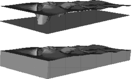
5.1 Elevated Surface Parts
5-74 EnSight 10.2 User Manual
5.1.6 Elevated Surface Parts
Elevated Surfaces visualize the value of a variable by creating a surface projected
away from the 2D elements of the parent Part. An Elevated Surface might be used
to show the pressure on a 2D surface representing the pressure as height above the
2D surface.
An Offset Surface projects an origin part into a 3D fluid domain using a single,
fixed, translation vector and then interpolates a variable from the 3D domain onto
the offset part. For example, an Offset Surface might be used to slightly offset the
roof of a car in the vertical direction into the flow field to visualize the flow field
velocity just outside of the boundary layer of the curved roof surface. Or, an
Offset Surface might be used to translate an origin part into a 3D parent domain
and ‘clip’ the 3D domain using the origin part. Creation of an offset surface that
results in a surface outside the 3D domain of the parent part(s) will result in
significant performance delays as compared to a surface inside the 3D domain.
Elevated Surface First let’s look at the Elevated Surface. It is easiest to describe this feature if you
think of a planar Part as the parent Part. Now warp this surface up out of plane
proportionally to the value of a variable. The resultant surface is an Elevated
Surface. Elevated surfaces are to surfaces what Profiles are to lines. While planar
surfaces are perhaps the most useful parent Parts to use, parents do not have to be
planar. Model Parts containing 2D elements, Clip Planes, Isosurfaces, and even
other elevated surfaces are all valid parent Parts.
The parent Part is not actually changed, a new surface is created. As this new
surface is “raised”, projection (Sidewall) elements can be created stretching from
the parent to the elevated surface around the boundary of the surfaces if desired.
Just the surface, just the sidewalls, or both can be created.
The projection from a node on the parent Part will be in the direction of the
normal at the node. If the node is shared by multiple elements, the average normal
is used.
The projected distance from a parent Part’s node to the corresponding elevated
surface node is calculated by adding to the variable’s value an Offset value, then
multiplying the sum by a Scaling value. Adding the Offset enables you to shift the
zero location of the plane. An Offset performs a “shift”, but does not change the
“shape” of the resulting elevated surface. The Scaling factor changes the distance
between parent and elevated surface, a “stretching” effect. EnSight will provide
default values for both factors based on the variable’s values at the parent Part’s
Figure 5-54
Elevated Surface example, with and without Sidewalls
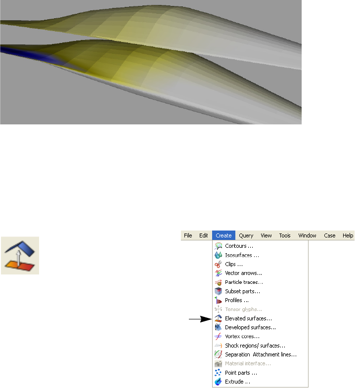
5.1 Elevated Surface Parts
EnSight 10.2 User Manual 5-75
nodes.
Offset Surface An offset surface requires two parts: an origin part and a 3D parent part. The
origin part is offset by a single scaled vector into the 3D part and the offset part
inherits the variable values of the 3D part at the intersection with the offset part.
An example will help. Imagine you have the upper surface of an aircraft
composed of 2D elements. The aircraft surface is enclosed within a 3D volume.
The origin surface of the aircraft is shifted by the value of a user-supplied constant
vector (and scale factor) into the 3D flowfield volume and becomes a new, Offset
Part. The new Offset Part now inherits the 3D flowfield volume’s variables at the
new location of the surface. Offset functionality is effectively clipping a 3D
volume using an origin part offset into the volume by a scaled, constant XYZ
vector. You cannot scale, warp, or rotate the origin part. You can only translate it.
To use this function you must change the Elevated Surface default pulldown to
Offset Surface. Then you must make sure you have selected the 3D volume parent
part in the part list, and then enter the origin part in the field in the Feature Panel.
Clicking once on the Elevated Surface Icon (if you have customized the Feature
Ribbon to have it visible) or selecting Elevated Surfaces... in the Create menu,
opens the Feature Panel for Elevated Surfaces. This editor is used to both create
and edit elevated surface parts.
Figure 5-55
Offset Surface example above main model
Figure 5-56
Elevated Surface Icon
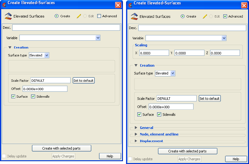
5.1 Elevated Surface Parts
5-76 EnSight 10.2 User Manual
Create/Edit Toggles that control whether a new part will be created, or whether you are editing
existing part(s). Note that when editing, the changes will be applied to those parts which
have the small “pencil” icon next to them in the Parts List.
Advanced Will open additional features for more advance control of the Part.
Desc The name of the part to be created or being edited.
Variable Choose the variable to use for creating the elevated surface from the pulldown.
Scaling
XYZ For vector-based or coordinate-based elevated surfaces, in advanced mode, specify
vector components used in creating the elevated surface. Not applicable to scalar-type
elevated surfaces. The scaling occurs according to the reference frame of the Elevated
Surface-Part. Letters labeling dialog data entry fields depend on type of the reference
frame (Rectangular, Spherical, or Cylindrical). If all components are 0.0, the vector or
coordinate magnitude will be used. These are applied as: xscale*xcomponent +
yscale*ycomponent + zscale*zcomponent.
Figure 5-57
Feature Panel - Elevated Surfaces, basic and advanced
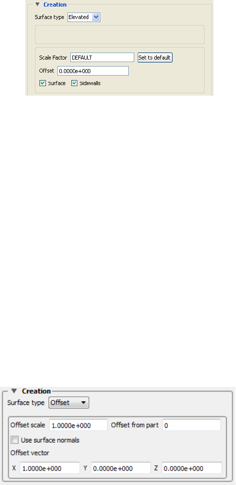
5.1 Elevated Surface Parts
EnSight 10.2 User Manual 5-77
Creation
Surface Type:
Elevated
This pulldown chooses between Elevated Surface and Offset surface. Shown below are
descriptions of the Elevated Surface options.
Scale Factor This field specifies the scaling for magnitude of distance between the parent Part node
and the corresponding elevated surface node. The Factor is multiplied times the value of
the variable. Values larger than one increase the size and values smaller than one decease
the size. A negative value will have the effect of switching the direction of the projected
surface
Set to Default Click to set Scale Factor and Offset values to the calculated defaults based on the
variable values for the parent Part.
Offset Value specified is added to the variable values before the Scale Factor is applied to
change the magnitude of projected distance. Default offset is magnitude of most-
negative projection distance (will cause the surface to be projected positively). Has the
effect of shifting the surface plot, but does not change the surface plot shape.
Surface Toggle Toggles on/off the creation of the actual elevated surface. The sidewalls alone will be
created if this toggle is off.
Sidewalls Toggle Toggles on/off the creation of the sidewalls of the Elevated Surface. Elements will
stretch from the parent Part to the Elevated surface around the boundary of the surfaces.
The Elevated Surface alone will be created if this toggle is off.
Surface Type:
Offset
This pulldown chooses between Elevated Surface and Offset surface.
To use the Offset Surface option, you need to select the 3D volume part(s) in the main
part window and set this pulldown surface type. Then set the options described below.
Offset Scale Scales the offset vector.
Offset Part This field picks the origin part number that will be used to clip the volume part selected
in the Part List.
Use Surface
Normals
Use Surface normals of each element to create the offset surface.
Offset Vector These fields are the rigid body translation vector for the entire offset origin part. The
origin part cannot be scaled, warped, or rotated. Note: Letters labeling dialog data entry
fields depend on type of the reference frame (Rectangular, Spherical, or Cylindrical).

5.1 Elevated Surface Parts
5-78 EnSight 10.2 User Manual
See Feature Panel Turndowns Common To All Part Types for a detailed
discussion of the remaining Feature Panel turn-down sections which are the same
for all Parts.
(see How to Create Elevated Surfaces)
Troubleshooting Elevated Surfaces
Create with selected
parts
Creates an elevated surface part using the selected Part(s) in the Parts List.
Delay update Checking this box will cause EnSight to not apply any changes made until you hit the
Apply Changes button. When not checked, the changes are applied as you make them.
Apply Changes Applies any changes made. Only active when Delay update is on.
Problem Probable Causes Solutions
The entire Elevated Surface is not
projected in the direction you
want.
Change the sign of the scale
factor.
You have a non-planar parent
Part and the elevated surface
seems to have strange
intersecting elements.
Sidewall elements are not
appropriate
Turn off sidewall toggle.
Scale factor too large. Lower the Scale Factor.
The Elevated Surface projection
appears to be “confused” at
various locations.
Inconsistently ordered elements,
such that the normals are not
“consistent”
Modify element ordering to be
consistent, if possible.
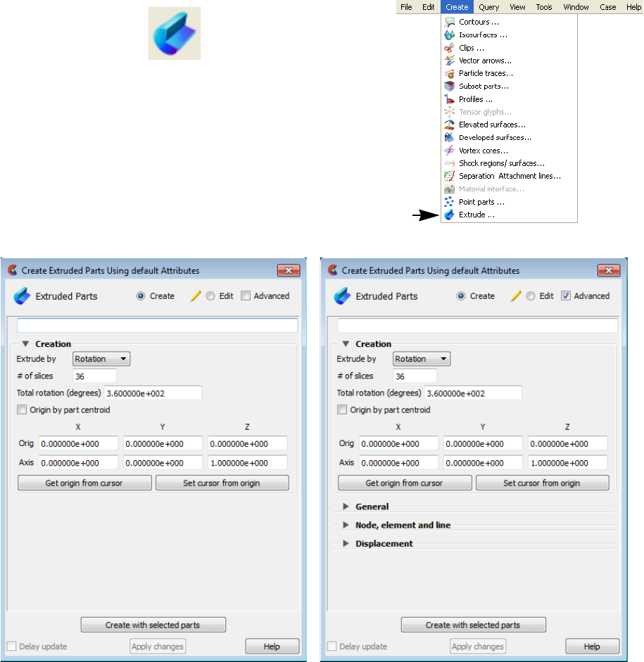
5.1 Extruded Parts
EnSight 10.2 User Manual 5-79
5.1.7 Extruded Parts
Extruded parts are created by “extruding” a part in a directional or rotational
manner to produce a part of next higher order. For example, a 2D axi-symmetric
surface can be extruded rotationally about the proper axis to produce a 3D
representation of the complete model. As another example, a 1D line can be
extruded in a direction to produce a 2D plane.
Clicking once on the Extrude Icon (if you have customized the Feature Ribbon to
have it visible) or selecting Extrude... in the Create menu, opens the Feature Panel
for Extruded parts. This editor is used to both create and edit extruded parts.
Figure 5-58
Extrusion Parts Icon
Figure 5-59
Feature Panel - Extruded Parts
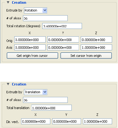
5.1 Extruded Parts
5-80 EnSight 10.2 User Manual
Create/Edit Toggles that control whether a new part will be created, or whether you are editing
existing part(s). Note that when editing, the changes will be applied to those parts which
have the small “pencil” icon next to them in the Parts List.
Advanced Will open additional features for more advance control of the Part.
Desc The name of the part to be created or being edited.
Creation
Extrude by Controls the type of extrusion to use.
Rotation To extrude the selected parts by revolving about an axis. This is what
you would choose for an axi-symmetric part.
Translation To extrude the selected parts by translating in a given direction.
# of slices Sets the number of elements that will be created in the “extrusion” direction. For
rotation, it would be the number of “slices” around the “pie”. For translation, it would be
the number of elements along the extrusion vector direction.
Total rotation
(degrees)
For rotation, sets the total number of degrees to rotate. It must be between -360 and
+360.
Origin by Part
Centroid
For rotation, sets x,y,z values for the origin of the axis of rotation using the part centroid
to the part chosen in the Part ID field.
Origin For rotation, sets x,y,z values for the origin of the axis of rotation.
Axis For rotation, sets the direction vector components for the axis of rotation.
Cursor Get/Set Can be used to get the origin values from the current cursor location, or to set the
location of the cursor to be at the origin location.
Total translation For translation, sets the total distance of extrusion travel.
Direction vector For translation, sets the direction vector components for the directional extrusion.
Create with selected
parts
Creates an extruded part using the selected Part(s) in the Parts List.
Delay update Checking this box will cause EnSight to not apply any changes made until you hit the
Apply Changes button. When not checked, the changes are applied as you make them.
Apply Changes Applies any changes made. Only active when Delay update is on.

5.1 Extruded Parts
EnSight 10.2 User Manual 5-81
See Feature Panel Turndowns Common To All Part Types for a detailed
discussion of the remaining Feature Panel turn-down sections which are the same
for all Parts.
(see Section 5.1.1, Parts Quick Action Icons and How to Extrude Parts)
Troubleshooting Extrusions
Problem Probable Causes Solutions
No extrusions created Parent Part is not a valid server-side
part.
Don’t try to extrude client-side parts
(particle traces, contours, etc.)
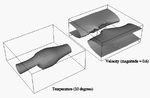
5.1 Isosurface Parts
5-82 EnSight 10.2 User Manual
5.1.8 Isosurface Parts
Isosurfaces are surfaces that follow a constant value of a variable through three-
dimensional elements. Hence, isosurfaces are to three-dimensional elements what
contour lines are to two-dimensional elements.
An isosurface may be based on a vector variable (magnitude or components), or a
scalar variable. If the variable is elemental, then a temporary internal nodal
variable is created by moving the elemental values to the nodes using simple
averaging from the surrounding elements.
At each node of a three-dimensional element, the isosurface’s variable has a value.
If the range of these values includes the isosurface’s isovalue, the isosurface cuts
through the element. EnSight draws the isosurface through that element by first
determining which edges the isosurface crosses, and then interpolating to find the
point on each of those edges corresponding to the isovalue. EnSight connects
these points with triangle elements passing through the parent Part elements. If the
Parent Part(s) contain two-dimensional elements, a line is created across the
elements - just like a contour.
All the triangle elements created inside all the three-dimensional elements of all
the parent Part(s) together with all the lines created across the two-dimensional
elements of all the Parent Part(s) constitute the isosurface. One-dimensional
elements of the parent Part(s) are ignored. Because isosurfaces are generated by
the server, the Representation of the parent Part(s) is not important.
You can interactively manipulate the value of an isosurface with a slider allowing
you to scan through the min/max range of a variable. This scanning can also be
done automatically. The isosurface will change shape as the value is changed.
If you are using animation, you can specify an Animation Delta value by which
the isovalue is incremented for each animation frame or page. The isosurface is
automatically updated to appear as if it had been newly created at the new location
and time.
Left-clicking on the isosurface part in the graphics window will pop up a green
handle in the shape of a cross. Drag this left and right to change the isosurface
value. Right-clicking on the results in a pulldown menu of quick options for your
Figure 5-60
Isosurface Illustration
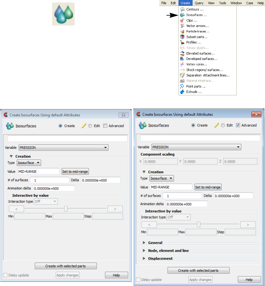
5.1 Isosurface Parts
EnSight 10.2 User Manual 5-83
isosurface.
Clicking once on the Isosurfaces Icon (which be default is in the Feature Ribbon)
or selecting Isosurfaces... in the Create menu, opens the Feature Panel for
Isosurface parts. This editor is used to both create and edit isosurface parts.
Create/Edit Toggles that control whether a new part will be created, or whether you are editing
existing part(s). Note that when editing, the changes will be applied to those parts which
have the small “pencil” icon next to them in the Parts List.
Advanced Will open additional features for more advance control of the Part.
Desc The name of the part to be created or being edited.
Figure 5-61
Isosurfaces Icon
Figure 5-62
Feature Panel - Isosurfaces
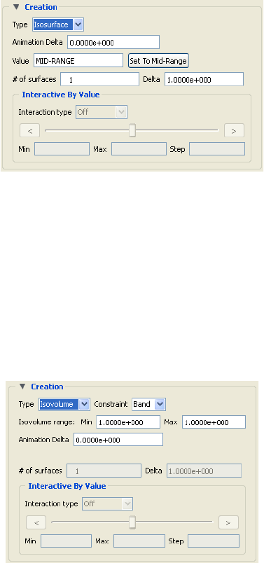
5.1 Isosurface Parts
5-84 EnSight 10.2 User Manual
Variable Choose the variable to use for creating the isosurface from the pulldown.
Scaling
XYZ For vector variables, in advanced mode, specify vector components used in creating the
isosurfaces. Not applicable to scalar variables. Scaling occurs in the reference frame of
the parent part. Letters labeling dialog data entry fields depend on type of the reference
frame (Rectangular, Spherical, or Cylindrical). If all components are 0.0, the vector
magnitude will be used. But, if any of these scaling factors is non-zero, the variable
value will be computed as xscale*xcomponent + yscale*ycomponent +
zscale*zcomponent.
Creation
Type
Isosurface Specification that an Isosurface type part created from the specified
Variable and selected parts will have the isovalue of Value for all its
elements.
Isovolume Specification that an Isovolume type part created from the specified
Variable and selected parts will consist of elements with isovalues
constrained to either below a Min, above a Max, or within the specified
interval of Min and Max. The isosurface and isovolume algorithms are
different. The isosurface algorithm defines the element intersection
along the element surfaces. In contrast, the isovolume algorithm
subdivides the 3D volume into tetrahedral elements and determines the
intersections along the edges of each subdivided basis element resulting
in more intersection points. For coarser meshes, the isosurface
algorithm will be a smoother surface, but as the mesh gets finer the two
algorithms should converge.
Animation Delta This field specifies the incremental change in isovalue for each frame or page of
animation. It can be negative.
5.1 Isosurface Parts
EnSight 10.2 User Manual 5-85
Value Specification of numerical isovalue of the isosurface. To avoid an empty Part, this value
must be in the range of the Variable within the Parent Parts. You can find this range using
the Variables dialog or by showing the Legend for the Variable. For vector-variable-
based isosurfaces, the vector magnitude is used.
Set to Mid-Range Clicking this button will put the value that is halfway between the minimum and the
maximum variable value.
# of surfaces If you want more than one isosurface calculated at a Delta offset from each other, enter
the number of surfaces in this field. This number of isosurfaces a1s calculated then
grouped together. This field is only available the first time the isosurface(s) are
calculated. It is not possible to change this value and recalculate the isosurfaces. To
change the number or the Delta, they must be deleted and recalculated.
Delta Offset value to use for creating a number of isosurfaces. The first isosurface is calculated
at the number entered in Value, and the next one is Delta + Value, etc.
Constraint Specification restricting the element isovalues of the Isovolume Part to an interval. The
Constraint options are:
Low all elements of Isovolume Part have isovalues below the specified Min
value.
Band all elements of Isovolume Part have isovalues within the specified Min
and Max interval values.
High all elements of Isovolume Part have isovalues above the specified Max
value.
Isovolume range
Min
Specification of the minimum isovalue limit for the Isovolume Part
Isovolume range
Max
Specification of the maximum isovalue limit for the Isovolume Part
Interactive By
Value
Interactive Type Opens pulldown menu for selection of type of interactive manipulation of the isosurface
value. Options are:
Off Interactive isosurfaces are turned off.
Manual Value of the isosurface(s) selected are manipulated via the slider bar
and the isosurface is interactively updated in the Graphics Window to
the new value. For quick interactive control of the isosurface, simply
left-click on the isosurface and grab the resulting green, cross-shaped
click and go handle and drag left and right to see the isosurface value
interactively decrease and increase respectively.
Auto Value of the isosurface is incremented by the Auto Delta value from the
minimum range value to the maximum value. When reaching the
maximum it starts again from the minimum. On some operating
systems this may require the cursor to be in the Main View.
Auto Cycle Value of the isosurface is incremented by the Auto Increment value
from the minimum range value to the maximum value. When reaching
the maximum it decrements back to the minimum.
Min Specification of the minimum isosurface value for the range used with the “Manual”
slider bar and the “Auto” and “Auto Cycle” options.
Max Specification of the maximum isosurface value for the range used with the “Manual”
slider and the “Auto” and “Auto Cycle” options.
5.1 Isosurface Parts
5-86 EnSight 10.2 User Manual
See Feature Panel Turndowns Common To All Part Types for a detailed
discussion of the remaining Feature Panel turn-down sections which are the same
for all Parts.
(see Section 5.1.1, Parts Quick Action Icons and How To Create Isosurfaces
Step Specification of the increment/decrement the slider will move within the min and max,
each time the stepper buttons are clicked.
Create with selected
parts
Creates an isosurface part using the selected Part(s) in the Parts List.
Delay update Checking this box will cause EnSight to not apply any changes made until you hit the
Apply Changes button. When not checked, the changes are applied as you make them.
Apply Changes Applies any changes made. Only active when Delay update is on.
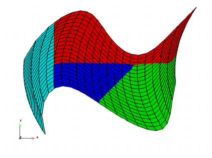
5.1 Material Interface Parts
EnSight 10.2 User Manual 5-87
5.1.9 Material Interface Parts
EnSight enables you to create and modify Material Parts from material
descriptions defined on model parts. The Material Parts feature allows you to
extract single or combined regions of specified materials, as well as boundary
interfaces between two or more specified materials.
Material Parts can only be created from model parts that have material ids
assigned to them. Therefore, Material Parts can not be created from any Measured
or Created Parts. In addition, material information is not transferred to Created
Parts.
Material Parts are created and reside on the server. They are Created Parts that
provide proper updating of all dependent parts and variables - except they do not
inherit any material data themselves.
Material Parts are created and modified by specifying parent model parts, as well
as selecting material descriptions listed in the Materials List. A Material Part is
extracted from only 2D and 3D elements. A Material Part is created as either a
Domain or an Interface.
Domain A material Domain defines a solid region composed of one or more specified
materials. Parts with 2D elements yield 2D material elements, and parts with 3D
elements yield 3D material elements.
Interface A material Interface defines a boundary region between at least two or more
adjacent specified materials. Parts with 2D elements yield 1D material elements,
and parts with 3D elements yield 2D material elements.
Null Materials Two categories of materials are reflected in the Materials List; namely, given
materials and a “null_material”. All given material descriptions correspond to a
material assigned a positive material number, or id. Any material that has an id
less than or equal zero (<= 0) is grouped under the “null_material” and assigned
the material id of zero (0). This allows the null material to act as a valid material.
The “null_material” description always appears in the Materials List whether or
not there are any null materials.
Formats Materials may be defined either by the three sparse files (i.e. material ids, mixed
ids, and mixed values), or materials may be designated as a set of per element
Figure 5-63
Material Parts Illustration
5.1 Material Interface Parts
5-88 EnSight 10.2 User Manual
scalar variable descriptions; but not by both. See Section 9.1, EnSight Gold
Casefile Format for format details.
Algorithm Two algorithms are implemented to compute the material part: the “smooth”
algorithm and the Young’s algorithm. The “smooth” algorithm is based on a
probability based approach to material interface reconstruction (see reference
below). Essentially volume fractions are averaged for every cell to its nodes,
edges/faces, and center. Each cell is then decomposed and/or subdivided into
subcells. Each subcell is then repeatedly assigned, compared, and appropriately
interpolated with volume fractions for each material. The resulting material cells
reflect the maximum volume fraction portion(s) of the interpolated subcells.
The Young’s algorithm partitions each mixed-material cell into regions which
exactly match the material fractions. The partitioning is based on an orientation
vector that determines the direction of the lines (or planes) used to subdivide the
cell. Materials are sliced off in the order assigned by the user.
Reference Meredith, Jeremy S. “A Probability Based Approach to Material Interface
Reconstruction for Visualization”, ECS277 Project 4, Spring 2001
D.L. Young, “Time-dependent multi-material flow with large fluid distortion,” in
Numerical Methods for Fluid Dynamics (K. W. Morton and J. J. Baines, eds.), pp.
273-285, Academic Press, 1982.
Caveats Material resolution tends to diminish (and at times distorts) at boundary cells that
lack adjacent ghost cells. The volume fractions at these cells simply lack the
proper weighting. This is remedied by providing material ghost cells.
Thus, materials that contribute half or less of the total portion on a boundary
element, typically do not appear without ghost cells.
Specie(s) Species may also be associated to a material (see MATERIAL Section under
EnSight Gold Case File Format and EnSight Gold Material Files Format ), but are
not involved in any of the computational aspects of creating/updating a material
part. Rather, a material species variable may be created via the new variable
calculator (see MatSpecies under 4.3 Variable Creation ).
Note: Species are only supported with the three sparse material files format, and
are not supported by the materials as scalars per element format.
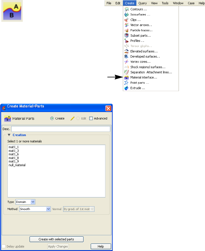
5.1 Material Interface Parts
EnSight 10.2 User Manual 5-89
Access Clicking once on the Material Interface Icon (if you have customized the Feature
Ribbon to have it visible) or selecting Material Interface... in the Create menu,
opens the Feature Panel for Material parts. This editor is used to both create and
edit Material interface parts.
Create/Edit Toggles that control whether a new part will be created, or whether you are editing
existing part(s). Note that when editing, the changes will be applied to those parts which
have the small “pencil” icon next to them in the Parts List.
Advanced Will open additional features for more advance control of the Part.
Desc The name of the part to be created or being edited.
Creation
Materials List List reflecting the available materials in the model parts. Any material that has an id less
than or equal to zero (<= 0) comprises the “null_material”.
Figure 5-64
Material Parts Icon
Figure 5-64
Feature Panel - Material Parts

5.1 Material Interface Parts
5-90 EnSight 10.2 User Manual
See Feature Panel Turndowns Common To All Part Types for a detailed
discussion of the remaining Feature Panel turn-down sections which are the same
for all Parts.
(See: How To Create Material Parts, and under Section 9.1, EnSight Gold Casefile
Format, see EnSight Gold Material Files Format)
Troubleshooting Material Parts
Type Opens a pulldown menu for specification of whether the Material Part results in a
Domain or Interface. Changing the Type of existing Material Parts will automatically
update them to the new specified type.
Domain Creates a solid region composed of one or more specified materials.
Parts with 2D elements yield 2D material elements, and parts with 3D
elements yield 3D material elements.
Interface Creates a boundary region between at least two or more specified
materials. Parts with 2D elements yield 1D material elements, and parts
with 3D elements yield 2D material elements.
Method Opens a pulldown menu for specification of the algorithm. Currently, use the Smooth to
compute the material part. Changing the method of existing Material Parts will
automatically update them to the new specified method.
Smooth Create/update a material part via the smooth algorithm (default)
Young’s Create/update a material part via the Young’s algorithm
Normal Not available for Smooth algorithm. Opens a pulldown menu to select the method for
computing the orientation vector for Young’s algorithm. The orientation can be
computed using the gradient of the first (non-droplet) material found in the cell (By grad.
of the 1st material), or it can be given an element-centered vector variable (vector)
Since the order of the materials is significant in the Young’s algorithm, it is important to
be able to change the order of the materials. Order of the materials can be changed by
right-clicking on the materials in the materials list and selecting Move Up, Move Down,
Move to Top, or Move to Bottom.
Create with selected
parts
Creates Material part using the selected Part(s) in the Parts List.
Delay update Checking this box will cause EnSight to not apply any changes made until you hit the
Apply Changes button. When not checked, the changes are applied as you make them.
Apply Changes Applies any changes made. Only active when Delay update is on.
Problem Probable Causes Solutions
No Type Domain Material Part
created for specified material
description(s)
Model part(s) not selected.
Model part(s) void of that material
Select only model part(s).
Nothing wrong.
No Type Interface Material Part
created for specified material
description(s)
Model parts not selected.
Two or more materials not selected.
Select only model part(s).
Select at least two (or more) materials.
Selected materials are not adjacent
across a 3D face or 2D edge.
Nothing wrong.

5.1 Material Interface Parts
EnSight 10.2 User Manual 5-91
No “null_material” Material Part
created for a specified
“null_material” selection.
Model parts do not contain any null
materials.
Nothing wrong.
There are no null materials, but
selecting “null_material” produces
a visible region.
Incorrect indexing in the material ids
file.
Material ids file possibly has a
negative index to an incorrect position
into the mixed-material id file.
Increasing the Subdivide level
does not increase the material
fraction detail
Increasing the Subdivide level
typically only increases the element
resolution.
Typically nothing wrong.
Changing the Type and/or Level as
well while simultaneously
changing the material selections
did not update the selected
Material Part to the new material
selections.
Material reselection is only updated
via the Apply New Material(s)
button.
Update the new materials first, then
change the type.
Delete the Material Part. Make new
material(s) selection and Type and/or
Subdivide specification. Then Create
a new Material Part.
Orientation does not appear
correct when using Young’s
algorithm.
Materials were not ordered correctly
prior to creation.
Order materials in list so that first
material gradient gives proper
orientation.
Problem Probable Causes Solutions
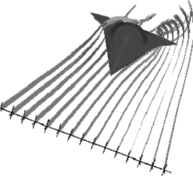
5.1 Particle Trace Parts
5-92 EnSight 10.2 User Manual
5.1.10 Particle Trace Parts
A streamline or pathline Particle trace visualizes a vector field by displaying the
path that a particle would follow if placed in that field. At each point on the
Particle trace, the direction of the trace is parallel to the vector field at that point
and time.
A streamline is a Particle trace in a steady-state vector field, while a pathline is a
Particle trace in a time-varying vector field. Particle traces can be lines or
“ribbons” (that additionally visualize the rotation of the vector field around the
path of the trace).
EnSight is capable of computing a pathline through a model with changing
coordinates and/or changing connectivity, but only on model parts. The variable
values are assumed to behave linearly between the known timesteps.
Symmetry For models with rotational periodic geometry, streamlines and pathlines can exit a
symmetry face and re-enter the corresponding symmetry face and continue.
Node Tracks Another form of trace that is available is entitled node tracking. This trace is
constructed by connecting the locations of nodes through time. It is useful for
changing geometry or transient displacement models (including measured
particles) which have node ids.
Min/Max Variable A further type of trace that is available is a min or max variable track. This trace
Tracks is constructed by connecting the min or max of a chosen variable (for the selected
parts) though time. Thus, on transient models one can follow where the min or
max variable location occurs.
Particle Trace Parts have their own attributes, so you can, for example, trace a
flow field using the velocity variable, and then color the resulting trace using the
temperature variable.
Emitters A streamline or pathline Particle Trace Part consists of one or more Particle traces
originating from points on one or more emitters. Each emitter is capable of
emitting a Particle starting at a specified time and continuing to emit Particles at
given intervals. When pathlines are generated with emitters emitting at multiple
time intervals and these traces are then animated, streaklines are displayed.
Emitters consist of single points, points along a line, points forming a grid in a
Figure 5-65
Particle Trace Illustration
5.1 Particle Trace Parts
EnSight 10.2 User Manual 5-93
plane, or points corresponding to the visible nodes of a Part. You can define
emitters using the Cursor tool, the Line tool, the Plane tool, or a Part. The traces
will be emitted from the visible nodes of the Part (which, for example, will be the
surface border nodes if the part element representation is border mode). In fact, if
you have a cursor, line or plane tool visible in a flow field, you can right-click on
the tool and choose ‘Particle Trace’ to immediately create a particle trace in the
flow field using all the default settings.
Emitters can be created using the cursor, line, and plane tools, using existing
visible Part nodes, or can be created in a surface restricted mode where the mouse
can be used to project points, rakes or nets directly onto the displayed surfaces of
the model.
Pathlines, of course, must be drawn forward in time, but streamlines can be drawn
forward in time, backward in time, or both. Each Particle trace terminates when
either (1) the Particle trace moves outside the space in which the vector field is
defined, (2) a user-specified time limit is reached, (3) the massless Particle
becomes stationary in a place where the vector field is zero, or (4) the last
transient-data time step is reached. (4 applies only to pathlines).
A Particle trace can pass through any point inside an element of the parent Part(s).
The vector field at any point is calculated from the shape function of the
containing element. Emitter points located outside the elements are ignored when
creating Particle traces.
Surface-Restricted A surface-restricted Particle trace is constrained to the surface of the selected
Traces Part(s) by using only the tangential component of the velocity. The velocity values
for this type of trace can be the velocity at the surface (if nonzero) or at some user
specified offset into the velocity field.
Interactive Traces A streamline Particle trace can be updated interactively by entering interactive
mode and moving the tool used to create the emitter. When a trace is selected and
interactive emitter is turned on, the tool will appear at the location of the emitter.
The user then manipulates the tool interactively in the Graphics Window or using
the transformations dialog. (This option is not available for surface-restricted
Particle traces, traces emitted from a Part nor in Server of Server mode).
Integration Method EnSight creates streamline and pathline Particle traces by integrating the vector
field variable over time using a Fourth Order Runge-Kutta method and utilizing a
time varying integration step. The integration step is lengthened or shortened
depending on the flow field, but you can control the minimum number of
integration steps performed in any element as well as other time step controls.
Normally, EnSight will perform the integration using all of the components of the
vector. However, it is possible to restrict the integration to a plane by specifying
which components of the vector to use. Typical uses of this feature would be to
restrict the Particle traces to a clip plane. Surface-restricted Particle traces provide
even greater flexibility in restricting a trace to planes or other surfaces.
Max # of Segments A trace will continue until it attempts to leave the flow field or until it reaches the
maximum time (Max Time, discussed later) or until it reaches the maximum
number of segments. Max Time and maximum number of segments exist because
sometimes a trace will continue indefinitely, for example when the trace is caught
in a vortex or recirculation area. Each trace has a maximum number of segments.
The maximum number of segments in each massless trace is by default 5000 for
5.1 Particle Trace Parts
5-94 EnSight 10.2 User Manual
surface-restricted traces, and 6000 for all other massless trace types. This default
can be changed by entering a command line entry (File>Command) into the
command dialog.
Surface restricted: test: max_skin_segments <value>
All other trace types: test: max_ptrace_segments <value>
A value of 0 disables the maximum segment check, and for massed particles the
value entered is automatically doubled.
Lines or Ribbons Line-type Particle traces consist of bar elements. Ribbons consist of 4-noded quad
elements and originate with their end-edge parallel to the Z-axis of the global
frame. Then, at each integration step, the leading edge is rotated around the
current direction of the path by the same amount the vector field has rotated
around the path since the previous time step. Ribbons are not available for
surface-restricted Particle traces.
Particle Trace Parts are created on the server, so the Representation-type of the
parent Parts has no effect. The algorithm that creates Particle traces initially sets
up a cross-referencing map of adjoining elements. Hence, the first Particle trace
takes longer to generate than subsequent traces.
If you calculate pathlines, consider calculating as many as possible at a time, since
the process can be very time consuming (most of the time is taken in reading time
step information). However, the data for the Trace Part is sent to and stored on the
Client. Thus, you cannot label nodes or elements, and some query options may be
limited. In such cases, it may be helpful to perform the labeling or query option on
the Particle Trace’s parent Part(s) instead. Line-type Particle Traces can be parent
Parts for Profiles. You can animate the motion of the massless Particles along their
Particle traces.
Transient Data By default the emission point is always set to emit the Particles at the current time
step. This can be a problem if you have a transient dataset with the current time set
at the last time step available. If you compute pathlines from this location, the
default emission time will be at the current time (last time step), thus no pathlines
will be generated. To solve this problem you will need to either change the current
time, or change the Start Time of the emitter.
The process of creating a streamline or pathline Particle trace is always to specify
an emission point (location and time), specify the Part(s) to trace the Particle
through and specify which vector variable to integrate. There are quick ways of
doing this process which assume that the correct defaults are set, or there are more
deliberate ways which give you more control. Particle trace Parts carry only one
set of attributes for all of the traces in the Part, thus it is not possible, for example,
to trace some of the emission points forward in time and others backward in time.
Particle trace Parts are different from all other created Parts in that when the
parent Parts change (such as at a time step change), the Particle trace Part does not
change. This is due to the fact that the Particle trace has been created at a specified
time (the emission time), making the Part independent of time (after the trace has
been created).
Regular pathline Particle traces can only be computed through a set of parent Parts
consisting of model Parts (to avoid the prohibitive cost of updating the non-model
part through time). In contrast, streamlines can be computed on non-model parts
(because the non-model parts do not have to be updated through time as the

5.1 Particle Trace Parts
EnSight 10.2 User Manual 5-95
streamline calculation proceeds). Surface-restricted Particle traces can be created
on model Parts, clip Parts, elevated surface Parts, and developed surface Parts.
If your dataset contains 3D elements, the Particles for regular traces will be traced
through 3D element fields only. Surface-restricted traces would have to be used to
trace along 2D elements of such a data set.
Trace Visibility & Color Each individual particle trace visibility status and color can be controlled via a
right mouse button selection of the particle trace in the graphics window. Note
that coloring individual traces only works if the trace part is a constant color.
Right-click on an individual trace and select "Set trace emission to constant
color..." to choose a color to set the selected emission. The standard color widget
will appear to allow you to select a color. Select "Set trace emission to random
colors" and EnSight will automatically assign a random color to each emission of
the particle trace part. To clear the per trace color simply color the part by a
constant color. The visibility of each individual trace can be turned invisible by
right-clicking on it and selecting "Hide this trace emission". Finally, reset all
traces to visible using "Show all trace emissions".
Massed-Particle Traces A particle trace can be created or updated from a massless-particle trace to a
massed-particle trace, or visa-versa. Massed-particle traces are specified via their
appended section in the Feature Detailed Editor (Traces) dialog. Massed particle
traces use an RK4(5) (Fehlberg) integration algorithm.
Definitions
Motion of a particle as a function of its velocity is defined as
d/dt(Xp) = Vp
with initial conditions Vp(t0)=Vp,0 and initial particle position
Xp(t0)=Xp,0 (capital letters denote vectors unless otherwise indicated).
For massless particles, the particle velocity is always identical to the local fluid
velocity, Vp=Vf. For massed particles, additional forces acting on them result in a
different velocity for the Vp than for the fluid, Vp not equal to Vf. This particle
velocity is determined from a momentum balance for the particle by
mp Ap = Fp,
or
mp d/dt(Vp) = Fg + Fb +Fp + Fd + Fe,
where
Ap = particle acceleration vector,
Fp = total (particle) force vector,
Fg = gravitational (body) force vector = mpG,
Fb = buoyancy (body) force vector = - mpG(f/p),
Fp = pressure (surface) force vector = - volppf,
Fd = drag (surface) force(s) vector = - ½ f ap cd |Vr| Vr,
Fe = additional forces vector, here = 0,

5.1 Particle Trace Parts
5-96 EnSight 10.2 User Manual
given the following definitions (Note: the underlined definitions are user
specified)
mp= spherical particle mass = p dp3 /6,
volp= volume of particle,
p= particle density,
dp= particle diameter,
f= fluid density (scalar or constant),
G= gravitational acceleration vector,
pf= fluid pressure gradient vector, (computed from pf = fluid
pressure scalar variable)
ap= particle reference area = dp2 /4,
Vp= particle velocity vector,
Vf= fluid velocity vector,
Vr= reference velocity vector = Vp – Vf,
cd= drag coefficient, typically given as a function of the local
relative Re, i.e. cd = cd(Re),
Re = Reynolds number = f |Vr| dp / f,
f= fluid dynamic viscosity (scalar or constant).
Thus, the total mass balance equation for massed particles may be defined by:
mp d/dt(Vp) = mpG -mpG(f/p) -(volppf) -(½fapcd|Vr|Vr)
Dividing through by the particle mass mp yields the following acceleration terms:
d/dt(Vp) = G - G(f/p) - pf/p - ½f|Vr|Vr(apcd/mp)
Note the following relation in the drag acceleration term:
(apcd/mp) = 1/cb
where: cb = ballistic parameter or coefficient = mp/(apcd) = 2pdp/(3cd)
Drag Coefficient
Currently, the following Drag Coefficient (Cd) table is provided as the default.
Re << 1 Cd = 24/Re
1 < Re << 500 Cd = 24/Re0.646
500 < Re << 3e5 Cd = 0.43
3e5 < Re << 2e6 Cd = 3.66E-4 Re.4275
2e6 < Re Cd = 0.18
This table is also coded as an example for your reference and access via the User-
Defined Math Function DragCoefTable1(Re) which is found in
5.1 Particle Trace Parts
EnSight 10.2 User Manual 5-97
$CEI_HOME/ensight102/src/math_functions/drag_coef_table1/libudmf-drag_coef_table1.c
In addition, two other drag coefficient functions are provided for your selection
via the User-Defined Math Function facility.
DragCoefPoly(Re) = (a + b Re + c Re2 + d/Re )
Where: {a,b,c,d} are polynomial coefficients with default values of {1.,0.,0.,0},
respectively.
DragCoefPower(Re) = (1 + .15 Re0.687) 24 / Re
Both of these functions are located respectively in
$CEI_HOME/ensight102/src/math_functions/drag_coef_poly/libudmf-drag_coef_poly.cf
$CEI_HOME/ensight102/src/math_functions/drag_coef_power/libudmf-drag_coef_power.c
You may also code your own. (See User Defined Math Functions, and/or the
Interface Manual: User Defined Math Functions.)
Rebound Massed Traces (Off a Boundary Wall)
Massed-particle traces can be toggled to rebound off boundary walls. The
rebounding massed traces are based on the following derivation. The derivation
assumes both the massed particle and boundary wall (or boundary) are both rigid
so that there is no deformation of the massed particle or boundary. Also rotational
considerations are ignored.
Starting with the initial impact particle velocity
Vp = Vp(VNi,VTi), (R0)
the tangential friction force opposing the massed particle is given by
FT = -mpdVT/dt = -mp(VTr-VTi)/dt, (R1)
and the normal reaction force is given by
FN = mpdVN/dt = mp(VNr-VNi)/dt, (R2)
The tangential friction force is proportional to the normal reaction force by the
coefficient of friction given by
FT = FN. (R3)
Equating R1 to R2, canceling out mp/dt, and taking into account R3 we have
-(VTr-VTi) = (VNr-VNi) (R4)
Solving for VTr we have
VTr = VTi-(VNr-VNi). (R5)
Now given that in the normal direction the final (reflected) velocity of the massed
particle is proportional to the initial (incident) velocity of the massed particle by
the coefficient of restitution , we have
VNr = VNi (R6)
which is the final normal component of the rebounding massed-particle velocity.
Subbing R6 into R5 and simplifying we have
5.1 Particle Trace Parts
5-98 EnSight 10.2 User Manual
VTr = VTi+(1+)VNi (R7)
which yields the final tangential component of the rebounding massed-particle
velocity. Combining these two components (R6 and R7) yield the final
rebounding particle velocity
Vp = Vp(VNr,VTr). (R8)
Where:
Particle-Mass Scalar on Boundaries
Information to compute a particle-mass scalar on boundaries (mP = mPi) is
provided each time massed-particle traces are created. This scalar is found and
computed via the New Computed Variables (NCV) functionality.
Massed Particle Scalar(massed-particle traced part(s))
This scalar creates a massed-particle per element scalar variable for each of the
parent parts of the massed-particle traces. This per element variable is the mass of
the particle times the sum of the number of times each element is exited by a
mass-particle trace.
References
The following references have contributed in part toward the development of the
massed-particle algorithm.
Donley, H. Edward
“The Drag Force on a Sphere”,
mp=the mass of the particle as defined above.
FT=the friction force tangent to the boundary "opposing" the particle
(thus the "-" sign on the right hand side of the equation assuming
the particle is traveling in the positive direction).
FN=the normal force on the boundary "opposing" the particle
(assuming the normal direction back into the field as positive).
VT=the tangential component of the particle velocity Vp.
VTi =The tangential component of the incident Vp impacting onto the
boundary.
VTr =The tangential component of the reflected Vp bouncing off the
boundary.
VN=The normal component of the particle velocity Vp.
VNi =The normal component of the incident Vp impacting onto the
boundary.
VNr =The normal component of the reflected Vp bouncing off the
boundary.
=The coefficient of restitution.
=The coefficient of friction.

5.1 Particle Trace Parts
EnSight 10.2 User Manual 5-99
http:\\www.ma.iup.edu/projects/CalcDEMma/drag/drag.html
Lund, Christoph
“Vorgaben für die Berechnung und Visualisierung der Bahnlinien
massebehafteter Partikel im Postprozessor EnSight”, Volkswagen AG,
27.07.2001. English translation by Kent Misegades.
Fluid Dynamics International, Inc.
FIDAP 7.0 Theory Manual”, April 1993, pp12-3+
Danby, J.M.A.
“Conputing Applications to Differential Equations”,
Restin Pub. Co., Inc. Restin, VA; 1985
Howard Brady, Rod Cross, Crawford Lindsey
“The Physics and Technology of Tennis”,
Raquet Tech Pub., Solana Beach, CA, 2002
Richard Burden, J. Douglas Faires, Albert C. Reynolds
“Numerical Analysis, 2nd Ed.”,
Prindle, Weber, & Schmidt, Boston, 1978
Paul Tipler
“Physics”,
Worth Pub. Inc.; NY, 1976
Clicking once on the Particle Trace Icon (which be default is in the Feature
Ribbon) or selecting Particle traces... in the Create menu, opens the Feature Panel
for particle trace parts. This editor is used to both create and edit particle trace
parts.
Figure 5-66
Particle Trace Icon
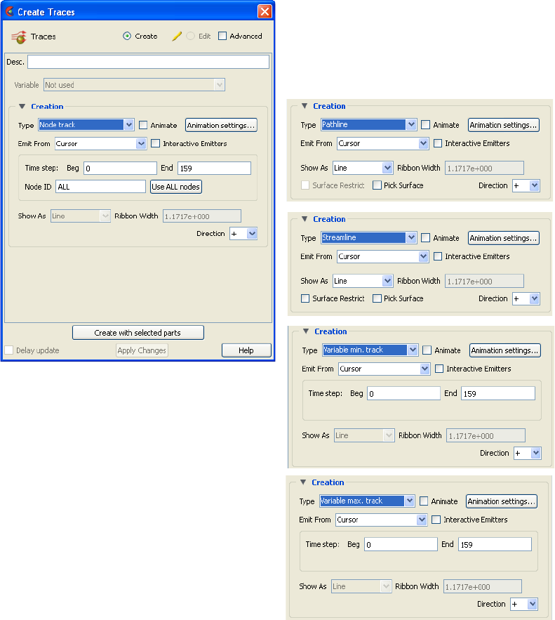
5.1 Particle Trace Parts
5-100 EnSight 10.2 User Manual
Create/Edit Toggles that control whether a new part will be created, or whether you are editing
existing part(s). Note that when editing, the changes will be applied to those parts which
have the small “pencil” icon next to them in the Parts List.
Advanced Will open additional features for more advance control of the Part.
Desc The name of the part to be created or being edited.
Creation
Type Opens a pulldown menu for specification of whether Particle trace calculation uses
steady-state data (streamlines), transient data (pathlines), or one of the tracking options.
Node Track Tracks one (or all) nodes of the selected part(s) through time.
Requires node ids and transient geometry or transient
displacements.
Figure 5-67
Feature Panel - Particle Traces - basic types
5.1 Particle Trace Parts
EnSight 10.2 User Manual 5-101
Pathline Traces a massless Particle through a time-varying vector field and
so is only available with transient results data and only allowed on
model parts.
Restriction to Model Parts
For even moderately-sized datasets, pathline trace calculations
consume significant quantities of CPU and can require substantial
I/O as the calculation labors to proceed through time. Restricting
this calculation only to model parts avoids the recompute of all the
dependent, non model parts through each timestep which can be
prohibitively slow.
Streamline Traces a massless Particle in a steady-sate vector field (for steady-
state data or the current time-step of transient data).
Variable min
track
Tracks the location of the minimum value of the chosen variable
through time.
Variable max
track
Tracks the location of the maximum value of the chosen variable
through time.
Emit From Opens a pulldown menu for the specification of the emitter type.
Cursor Creates Particle trace beginning from the position of the Cursor tool.
Line Creates Particle traces beginning from the position of the Line tool.
# Points This field specifies the number of evenly spaced traces you want to
emit from the Line tool.
Plane Create Particle traces beginning from the position of the Plane tool.
# Points These fields specify the number of traces you want to emit from the
Plane tool in the X and Y axes of the tool.
Part Creates particle traces beginning from visible nodes of the Part specified by the Part ID
Number field.
Part ID This field specifies the Part you wish to use as an emitter for the
creation of a particle trace. The Part ID number for a Part is found in
the Parts List. Limitation: once create a trace using a Part ID, this
ID can no longer be changed, nor can you change the emitter type.
Number of This field specifies the number of emitters desired. They will be
randomly selected from
Emitters the visible nodes of the part. (see Section , Created Parts)
File Creates particle traces from the locations specified in an external file.
(see Section 9.12, EnSight Particle Emitter File Format)
Time step: Beg, End For Tracking types, specifies the beginning and ending time steps to use for the track.
Node ID Field for specifying the desired node id of a Node Track. Note that a single node id can
be specified to track a single node, or ALL can be specified to track all nodes of the
selected part(s).
Use ALL nodes Clicking this button sets the value in the Node ID field to ALL.
Show As Opens a dialog for specification of trace representation for streamline and pathline
traces.
Line Depicts the trace as a line.
5.1 Particle Trace Parts
5-102 EnSight 10.2 User Manual
Ribbon Depicts trace as if it were a ribbon. The ribbon width is a specified
fixed value, while the twisting is determined by the rotation of the
flow about the path of the trace at any particular point on the trace.
Square Tubes Depicts trace as if it were a square tube. The tube width is a
specified fixed value, while the twisting is determined by the
rotation of the flow about the path of the trace at any particular point
on the trace.
Tubes Depicts trace as if it were a round tube. The tube width is a specified
fixed value. There is no indication of twisting when using tubes.
Ribbon Width This field only applies when Ribbon representation is chosen. Larger values in this field
produce wider ribbons. Only available for streamlines and pathlines.
Surface Restrict Toggles on/off surface restricted feature for streamlines. The streamline will be
constrained to stay on the surface of the selected Part(s) by using only the tangential
component of velocity. Be sure to use the Pick Surface feature in locating the emitter for
a surface restricted particle trace to ensure that the emitter is located on the surface of a
Part
Pick Surface Toggles on/off the feature which allows you to place the trace emitter at a point on a
surface directly below the mouse pointer by clicking the left mouse button.
Direction Trace the Particle in positive time, meaning to trace with the vector field, or trace the
Particle in negative time, meaning to trace the Particle upstream. Option only applies to
streamlines. Pathlines must be traced in + time.
(+) Positive time option traces Particle(s) forward in time. (This is the
only option for pathlines.)
(–) Negative time option traces Particle(s) backward in time.
(+/–) Positive/Negative time option traces Particle(s) both forward and
backward in time.
Animate Toggle Toggles on/off the animation of the motion of the Particles along the traces. In addition
to creating Particle traces based on vector variables, EnSight can also animate the motion
of the Particles along the Particle traces. To distinguish them from discrete Particles, we
call Particles moving along Particle traces “tracers.”
At any instant, each tracer consists of a portion of a Particle trace displayed with
attributes you specify separately from the attributes of the Particle trace. EnSight
animates each tracer by updating which portion of the Particle trace is currently
displayed. You specify the length of each tracer as a time value, so the tracer’s length
varies dynamically as it moves down the Particle trace (faster moving tracers are longer).
This option can add tremendously to the understanding of the flow field since relative
speed can be determined.
EnSight provides control over how the tracer looks and acts. You can animate one, some,
or all of the Particle traces you have created, but they are all animated in the one way you
specify. To help you get started, at the click of a button EnSight will suggest time-
specification values based on the Particle traces you have selected to animate. You can
specify the line width of the tracer, and choose to color it with a constant color or the
same calculated color used to color the Particle trace. If you wish to change the opacity
of the trace in the Color, Lighting and Transparency dialog, you cannot do it with the
opacity slider, but must instead use the “screen door” transparency in the Fill Pattern
pulldown. You can also display a spherical “head” on the leading-end of the tracer, and
dynamically size the head according to any active variable.
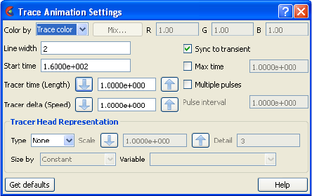
5.1 Particle Trace Parts
EnSight 10.2 User Manual 5-103
You control the speed of the motion and have the option to display multiple tracers on
the same Particle trace separated by a time interval. Hence, you can choose to view
rapid-fire pulses, slow moving “noodles,” or something in between. For steady-state
Particle traces (streamlines), “time” is the integration time with the emitters located at
time zero. For transient Particle traces (pathlines), you have the option to synchronize the
animation time to the solution time. The choice of whether a Particle trace is a streamline
or a pathline is made when you create the Particle trace.
You do not have to animate the entire Particle trace. You can specify where you want the
animation to start with a time value corresponding to a distance down the Particle trace
from the emitter, and where you want the animation to stop with a time value
corresponding to a distance farther down the Particle trace.
Tracers on all animated Particle traces are synchronized. If you combine Particle trace
animation with flipbook animation or keyframe animation, the animation time values are
automatically synchronized if you toggle-on Sync To Transient in the Trace Animation
Settings dialog.
Animation settings... Opens the Trace Animation Settings dialog.
Color By Opens a pulldown menu for selection of method by which to color the tracers.
Constant Displays tracers in the constant color specified in this dialog.
Mix… Opens the Color Selector dialog (see Section 5.1.19, Auxiliary
Geometry).
R,G,B Fields allow specification of constant color.
Trace Color Displays tracers in the same color as the Particle Trace Part from
which they originate.
Line Width Specification of displayed width (in pixels) of tracers. Note: Line Width specification
may not be available on some workstation platforms.
Start Time Specification of how far down each Particle trace to begin displaying tracers. A Particle
trace is made up of line segments. Each segment that makes up a Particle trace has an
associated time value. The start time indicates where on the Particle trace the tracers will
begin animation.
Tracer Time
(Length)
Specification of length of tracers which varies as the tracer speed varies along the
Particle trace. The Particle Time Length parameter scales the length of all tracers at all
times.
Figure 5-68
Trace Animation Settings dialog
5.1 Particle Trace Parts
5-104 EnSight 10.2 User Manual
Tracer Delta (Speed) Specification of how fast tracers move. Longer times result in faster moving tracers. This
parameter is not applicable when using Sync To Transient and displaying transient data
through flipbook or keyframe animation.
Sync to Transient Toggles on/off synchronization of tracer position to solution time of transient data. When
toggled-on, and transient data is in use (i.e. solution time, flipbook or keyframe
animations), each tracer is displayed with its leading-end at the correct location along the
Particle trace for the current solution time. Traces only move forward in time so cycling
through transient data is not applicable here.
Max Time Toggle Toggles on/off maximum lifetime for all tracers. If toggled-off, tracers continue to end of
Particle trace. If toggled-on, each tracer stops after moving down the Particle trace for a
distance corresponding to the specified Max Time (or until one of the other conditions
that stop a tracer occurs).
Max Time Field specifies lifetime of all tracers when Set Max Time is toggled-on.
Multiple Pulses
Toggle
Toggles on/off multiple emission of tracers. When toggled-off, a single tracer for each
Particle trace appears at the specified Start Time. When toggled-on, additional tracers
appear after each specified Pulse Interval. Not applicable to pathlines.
Pulse Interval Field specifies time delay between tracers. Not applicable when Multiple Pulses is
toggled-off.
Tracer Head Representation
Type Opens a pulldown menu for selection of type of head for each tracer.
None Specifies that no head will appear.
Spheres Specifies that a sphere will appear on the leading end of the tracer.
Scale Specification of scaling factor for head size. Values between 0 and 1
reduce the size, factors greater than one enlarge the size. Not
applicable when Head Type is None.
Detail Specification of detail-level of head in range from 2 to 10, with 10
being the most detailed (e.g., rounder spheres because more
polygons are used to create spheres). Higher values take longer to
draw, slowing performance. Not applicable when Head Type is
None.
Size By Opens a pulldown menu for the selection of variable-type to use to
size each tracer’s head. If you select a variable, the head size is
determined by multiplying the Scale factor times the variable value,
which will vary depending on the location of the tracer. Not
applicable when Head Type is None.
Constant Sizes head using just the Scale factor value.
Scalar Sizes head using a scalar variable.
Vector Mag Sizes head using magnitude a vector variable.
Vector X Sizes head using X-component of a vector
variable.
Vector Y Sizes head using Y-component of a vector
variable.
Vector Z Sizes head using Z-component of a vector
variable.
Variable Selection of variable to use to size the tracer
heads. Not applicable when Type is None or Size
By is Constant.

5.1 Particle Trace Parts
EnSight 10.2 User Manual 5-105
Troubleshooting Animated Particle Traces
Get Defaults Click to set time-value specifications in this dialog to values suggested by EnSight based
upon the characteristics of the selected Particle traces.
See Also: How To Animate Particle Traces
Problem Probable Causes Solutions
No motion. Can’t see
any tracers.
No Particle traces selected to
animate.
Select the traces you wish
to animate in the list at the
top of the Animated Trace
Setup dialog.
Tracers colored same as
Particle traces and have same
line width.
Change Color By or Line
Width.
Animate Traces not toggled-
on.
Toggle Animate on in the
Feature Panel.
Start Time > maximum
Particle trace time for all
traces selected.
Change settings in the Trace
Animation Settings dialog.
Delta Time (Speed) set too
high.
Change settings in the Trace
Animation Settings dialog.
Particle Time (Length) set too
small.
Change settings in the Trace
Animation Settings dialog.
Motion too fast. Delta Time (Speed) set too
high.
Change settings in the Trace
Animation Settings dialog.
Can’t get multiple
pulses at same time.
Pulse interval too high. Decrease to have pulses
start closer together.
Have one big tracer, no
pulses.
Pulse interval too small, pulses
start right after each other with
no separation.
Increase the interval.
Interactive Emitter Toggles on/off interactive Particle tracing. Manipulation of the Cursor, Line or Plane tool
will cause the Particle trace to be recreated at the new location and updated in the
Graphics Window. When manipulation of the tool stops, the Particle trace and any Parts
that are dependent on it will be updated. (Only available for non-surface-restricted
streamlines).
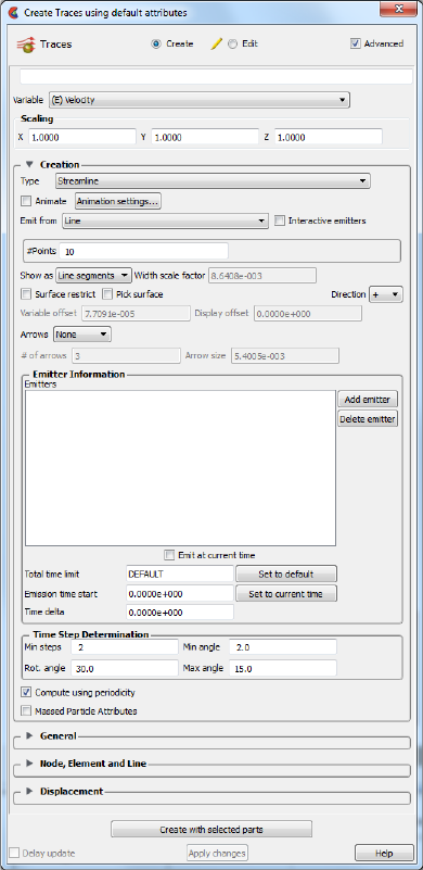
5.1 Particle Trace Parts
5-106 EnSight 10.2 User Manual
Scaling
XYZ For vector variables, in advanced mode, specify vector components used in creating the
particle traces. Not applicable to scalar variables. Are according to the reference frame
of the parent part. Letters labeling dialog data entry fields depend on type of the
reference frame (Rectangular, Spherical, or Cylindrical). If all components are 0.0, the
vector magnitude will be used. But, if any of these scaling factors is non-zero, the
variable value will be computed as xscale*xcomponent + yscale*ycomponent +
zscale*zcomponent.
Creation (Additional)
Variable offset This field specifies the distance into the flow field at which velocity (and other variables)
are to be sampled for the surface restricted trace(s). If velocity values are present at the
surface, this offset can be set to zero.
Figure 5-69
Feature Panel - Particle Traces - Advanced
5.1 Particle Trace Parts
EnSight 10.2 User Manual 5-107
Display offset This field specifies the normal distance away from a surface to display the surface
restricted traces. A positive value moves the traces away from the surface in the direction
of the surface normal.
Please note that there is a hardware offset that will apply to contours, vector arrows,
separation/attachment lines, and surface restricted particle traces that can be turned
on or off in the View portion of Edit->Preferences. This preference (“Use graphics
hardware to offset line objects...”) is on by default and generally gives good images
for everything except move/draw printing. This hardware offset differs from the
display offset in that it is in the direction perpendicular to the computer screen
monitor (Z-buffer).
Thus, for viewing, you may generally leave the display offset at zero. But for printing, a
non-zero value may become necessary so the traces print cleanly.
Arrows Controls whether the flow direction is indicated with arrows.
None option displays arrows as lines without tips.
Cone arrows have a tip composed of a 3D cone. Good for both 2D and 3D
fields.
Normal arrows have two short line tips, similar to the way many people
draw arrows by hand. The tip will lie in the X–Y, X–Z, or Y–Z plane
depending on the relative magnitudes of the X, Y, and Z components
of each individual vector. Suggested for 2D problems.
Triangles arrows have a tip composed of two intersecting triangles in the two
dominant planes. Good for both 2D and 3D fields.
# of Arrows Controls density of arrows. The trace with the longest dwell time will have this number
of arrowheads, and the other traces will get a number that corresponds to their dwell
time.
Arrow Size Scaling size of Arrowheads.
Emitter Information
Emitters List This section shows a list of all emitters created for the currently selected Particle Trace
Part.
Add Emitter Adds an emitter of the type specified by Emit From to the currently selected Particle
Trace Part.
Delete Emitter Deletes the emitter selected in the Emitters List from the selected Particle Trace Part.
Emit at current
time
Toggle on to set the emitter to the current time.
Total Time Limit This field specifies the maximum residence time of the trace, meaning the difference in
time between emission time and trace termination time. For pathlines the traces will also
be terminated once the end solution time (as defined in the Time Control Panel, see
Solution Time) is processed. Note: this limit is applied to each direction (+/-)
independently.
Set to default This button sets the Total Time Limit field to a reasonable default value using the vector
value and the geometry size.
Emission Time
Start
This field specifies the solution time at which to begin Particle emission. Enter value
between beginning and ending time available.
Time Delta This field specifies the time interval between emissions of Particles from the emitters. If
“0”, only one set of emissions will occur at start time
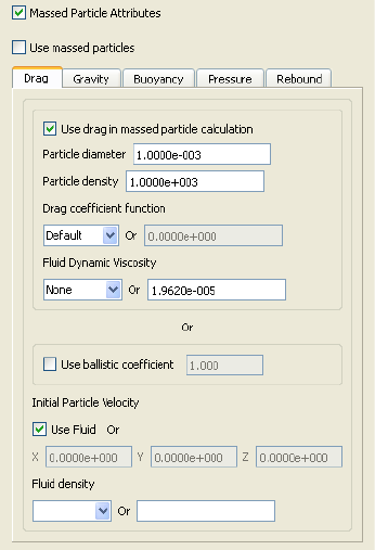
5.1 Particle Trace Parts
5-108 EnSight 10.2 User Manual
.
Time Step Determination Opens a turn-down area for the specification of time-step
parameters.
Min Steps This field is used to specify the minimum number of integration steps to perform in each
element.
Min Angle If angle between two successive line segments of the Particle trace is less than this value
EnSight will double the integration step.
Max Angle If angle between two successive line segments of the Particle trace is greater than this
value EnSight will half the integration step.
Rot Angle If the change in rotation angle at two successive points of the Particle trace is greater
than this value, the integration step is halved.
Periodicity Attributes Turns on/off the use of periodicity in the trace.
Compute using
Periodicity
Toggles on/off the periodicity feature. The default is OFF. If this toggle is ON and the
parent part has visual symmetry (see How to Set Symmetry) set to rotational, then the
particle tracer will attempt to trace the particle path out of a symmetry plane and back
into the other symmetry plane. This results in a somewhat confusing trace unless you
turn on instances of symmetry of the parent part and of the particle trace part, to see
clearly the traces as they move through the symmetry instances. For usage details, see
How to Create Particle Traces.
Massed Particle Attributes Opens the massed-particle attributes area.
Use massed
particles
Toggles on/off the massed-particle traces feature. The default is OFF
Note: Some dependent parameters are duplicated under multiple tabs for reference
convenience, i.e. Gravity under Gravity and Buoyancy tabs. Note that these parameters
are updated under all applicable tabs when changed under a particular tab
Drag term tab Showing dependent parameters for drag acceleration term (default selection)
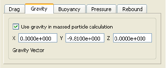
5.1 Particle Trace Parts
EnSight 10.2 User Manual 5-109
Use drag in
massed particle
calculation
Toggles on/off the inclusion of the drag term in the massed-particle computation. The
default is ON
Particle diameter This field specifies the diameter of all particles. The default is 1.e-3.
Particle density This field specifies the density value of all particles. The default is 1.e+3.
Drag coefficient
function
This field specifies the drag coefficient function to be called each time the drag
coefficient is calculated. This function defaults to “Default” which essentially defaults to
the table described above. Other functions may be accessed via the User-Defined Math
Function facility, i.e. DragCoefTable1(Re) (same as default), DragCoefPoly(Re),
DragCoefPower(Re). All functions must take the Reynolds Number as their only
argument. This parameter only works with the drag term.
Or This field specifies the drag coefficient value to be used in the computation if “None” is
specified as the variable name. The default value is 0. This parameter only works with the
drag term.
Fluid dynamic
viscosity
This field specifies the fluid dynamic viscosity variable to be used in the massed-particle
computation. The default is “None”.
Or This field specifies the fluid dynamic viscosity value to be used in the computation if
“None” is specified as the variable name. The default value is 1.9620e-5. This parameter
only works with the drag term.
Use ballistic
coefficient
Toggles on/off the use of the ballistic coefficient value (mp/(apcd))in place of the
above drag parameters which are greyed-out, i.e. particle diameter and density (used in
mp and ap), and drag coefficient and fluid dynamic viscosity (used in cd). The default
toggle is OFF. When toggled ON, the default value is 1.
Initial particle
velocity
Determines what initial velocity to use for all the particle emitters. The default is Use
fluid ON. This parameter only works with the drag term.
Use fluid Toggles on/off whether all particle emitters should use the fluid velocity at their
corresponding locations. The default is ON.
Or X, Y, Z These fields specify the initial velocity components of all particle emitters. Their default
is <0., 0., 0.>.
Fluid density This field specifies the fluid density variable to be used in the massed-particle
computation. The default is “None”. This parameter only works with the buoyancy term.
Or This field specifies the fluid density value to be used in the computation if “None” is
specified as the variable name. The default value is 1.
Gravity term tab Showing dependent parameters for gravity acceleration term
Use gravity in
massed particle
calculation
Toggles on/off the inclusion of the gravity term in the massed-particle computation. The
default is ON
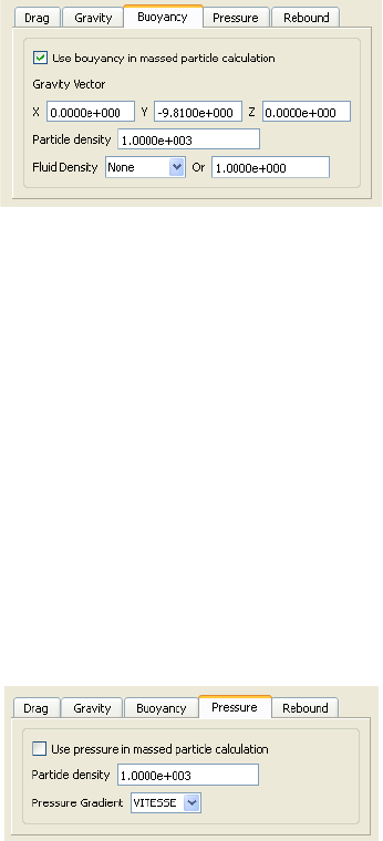
5.1 Particle Trace Parts
5-110 EnSight 10.2 User Manual
.
.
Gravity vector These fields specify the gravity vector to be applied in the massed-particle computation.
The default gravity components are <0., -9.81, 0.>. This parameter only works with the
gravity and buoyancy terms.
Buoyancy term
tab
Showing dependent parameters for buoyancy acceleration term
Use buoyancy in
massed particle
calculation
Toggles on/off the inclusion of the buoyancy term in the massed-particle computation.
The default is ON
Gravity vector These fields specify the gravity vector to be applied in the massed-particle computation.
The default gravity components are <0., -9.81, 0.>. This parameter only works with the
gravity and buoyancy terms.
Particle density This field specifies the density value of all particles. The default is 1.e+3.
Fluid density This field specifies the fluid density variable to be used in the massed-particle
computation. The default is “None”. This parameter only works with the buoyancy term.
Or This field specifies the fluid density value to be used in the computation if “None” is
specified as the variable name. The default value is 1.
Pressure gradient
term tab
Showing dependent parameters for pressure-gradient acceleration term
Use pressure in
massed particle
calculation
Toggles on/off the inclusion of the pressure-gradient term in the massed-particle
computation. The default is OFF
Particle density This field specifies the density value of all particles. The default is 1.e+3.
Pressure
gradient
This field specifies the fluid pressure gradient variable to be used in the massed-particle
computation. The default is “None”. This parameter only works with the pressure force
term.

5.1 Particle Trace Parts
EnSight 10.2 User Manual 5-111
.
See Feature Panel Turndowns Common To All Part Types for a detailed
discussion of the remaining Feature Panel turn-down sections which are the same
for all Parts.
(see How to Create Particle Traces)
Troubleshooting Particle Traces
Rebound term tab Showing dependent parameters for allowing rebound of massed traces
Use rebound in
massed particle
calculation
Toggles on/off the inclusion of rebound parameters to account for coefficient of
restitution and friction effects when massed traces contact boundaries. The default is OFF
Note: Rebound requires an active acceleration term, i.e. Drag, Gravity, Buoyancy, and/or
Pressure.
Coefficient of
restitution
This field specifies the coefficient of restitution value to be used for all massed trace
computations. The default value is 0. (no restitution - no rebound). The typical range for
this value is 0. to 1. (The value of 1. being full restitution, or a perfect elastic bounce off
the wall where the angle of reflection off the boundary into the field is equal to the angle
of incidence into the wall from the field.) This value is combined with the coefficient of
friction to determine the final rebound of the massed particle off the boundary wall.
Coefficient of
friction
This field specifies the coefficient of friction value of the boundary to be used for all
massed trace computations. The default value is 0. (no friction). The typical range for this
is 0. to <1. This value is combined with the coefficient of restitution to determine the final
rebound of the massed particle off the boundary wall.
Fraction of initial
impact velocity
This field specifies a fraction of the initial impact velocity (magnitude) value to be used
as a stopping criteria for a rebounding massed particle. The default is .01.
Maximum
number of wall
hits
This field specifies the maximum number of wall hits (per massed particle) value to be
used as a stopping criteria for a rebounding massed particle. The default value is 10 hits.
Create with selected
parts
Creates Material part using the selected Part(s) in the Parts List.
Delay update Checking this box will cause EnSight to not apply any changes made until you hit the
Apply Changes button. When not checked, the changes are applied as you make them.
Apply Changes Applies any changes made. Only active when Delay update is on.
Problem Probable Causes Solutions
Particle Trace Part is empty. Velocity is zero. Change time steps or change
location of emitters.

5.1 Particle Trace Parts
5-112 EnSight 10.2 User Manual
Emitter points are outside of flow
field.
Change location for emitter points.
Dataset is 3D and parent Parts are
2D, or dataset is 2D and parent Parts
are not planar.
Change parent Parts.
The created variable selected does
not exist for the parent Part(s)
Recreate the variable for the parent
Part(s) selected
The emitter part is non visual and
has no visible nodes
Make the emitter part element
representation 3D Border 2D Full to
obtain visible nodes
Streamline is OK, but pathline is
empty.
Creating pathline with the emitter
emitting at the last time step.
Modify emitter time for the emitter
groups.
Particle trace terminates prematurely Velocity has gone to zero. None
Particle has been traced out of the
flow field.
None
Stopping point is at the boundary
between two Parts.
Change the parent Parts for the
Particle trace to include neighbor
Part.
Particle getting lost and EnSight’s
search algorithm failing.
Call CEI hotline support.
Total Time Limit reached. Change Total Time Limit.
Particle trace exists, then is removed
after deleting Parts.
The parent Part for the Particle trace
was deleted.
None
Particle trace creation requested, but
Particles don’t come back.
Requested a large number of Particle
traces and/or doing pathlines in large
transient dataset.
Be patient.
Particles are stuck in a recirculation
area.
Process will finish when Total Time
Limit is reached. Consider
terminating job and starting over
with a smaller Total Time Limit.
Interactive tracing is slow. The size of the model and density of
the mesh will affect the performance
of an interactive trace.
If you can, run on a faster, larger
memory workstation. Also, limit if
possible the area of interest by
cutting the mesh into pieces with the
Cut & Split Part editing operation.
Interactive trace does not enter the
next Part
Interactive tracing is only done
through the Part the emitter resides
in.
When you let go of the emitter the
full trace will be shown
Surface restricted Particle trace does
not appear
Zero velocity at chosen variable
offset
Select a Variable offset distance that
will give nonzero velocity
Display offset causing trace to be on
opposite side of a surface (hidden
surface on)
Change sign of the Display offset.
Note offset is in the direction of the
surface element normal.
Emitter does not lie on the surface of
selected Parts
Create emitters that lie on the surface
Surface Restricted particle trace does
not print well
See Display Offset discussion above Enter a non-zero display offset.
Problem Probable Causes Solutions
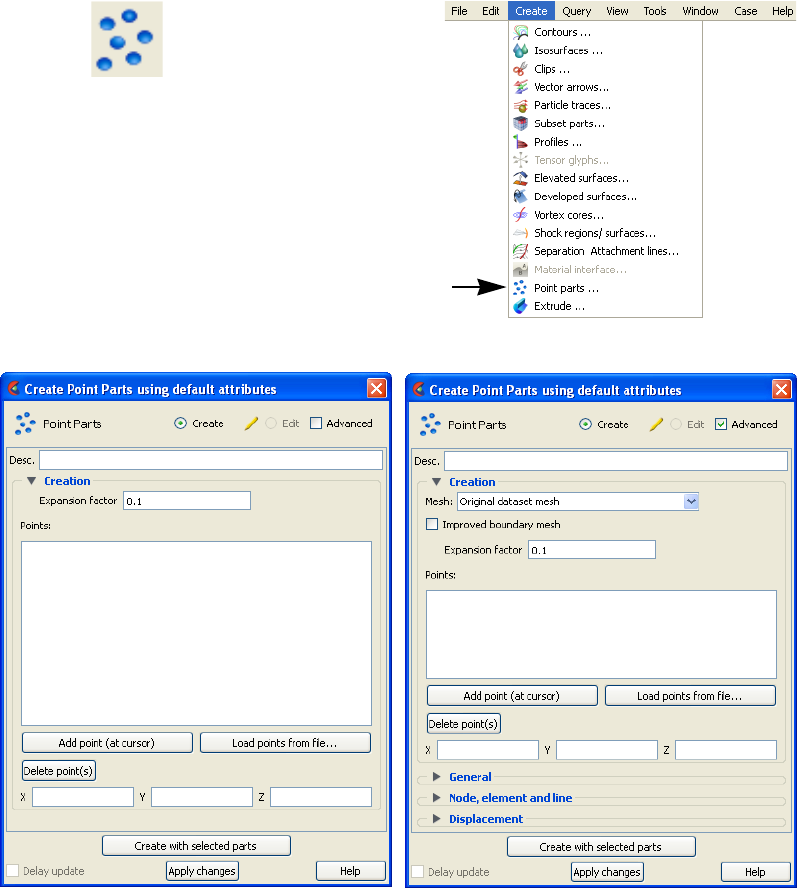
5.1 Point Parts
EnSight 10.2 User Manual 5-113
5.1.11 Point Parts
Point parts are composed only of nodes. They can be created by reading an
external file containing the xyz coordinates of the nodes, and/or by placing the
cursor tool at desired locations and adding nodes. This feature can be used to
essentially place probes in the model at particular locations. It can also be used to
create parts that can be meshed with the 2D or 3D meshing capability within
EnSight.
Clicking once on the Point parts Icon (if you have customized the Feature Ribbon
to have it visible) or selecting Point parts... in the Create menu, opens the Feature
Panel for Point parts. This editor is used to both create and edit Point parts.
Figure 5-70
Point Parts Icon
Figure 5-71
Feature Panel - Point Parts
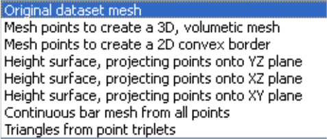
5.1 Point Parts
5-114 EnSight 10.2 User Manual
Create/Edit Toggle controls whether a new part will be created, or whether you are editing existing
part(s). Note that when editing, the changes will be applied to those parts which have the
small “pencil” icon next to them in the Parts List.
Advanced Will open additional features for more advance control of the Part.
Desc The name of the part to be created or being edited.
Creation
Mesh: Opens pulldown menu for selection of part meshing to use.
The default is to use the element connectivities described in the model data file(s). But a
remeshing can be done, utilizing the QHull library. This library can compute the convex
hull of point data, a 2D meshing. And since the convex hull of a 3D dataset lifted into 4
dimensional space turns out to be the volumetric tetrahedralization of the 3D data, it can
be used to do a 3D meshing as well. Please note that this remeshing can take
considerable memory and processing - so it needs to be used with that in mind.
Also, the worst case for QHull is a large number of co-planar points. In the higher-
dimensional lifting step, the planarity adds a singularity that is difficult to work around.
Using bounding boxes and planar projections can help. Accordingly, several options
exist, which can be used if your data exhibits problematic characteristics. The pulldown
menu options are:
Original dataset mesh The nodes and elements described in the model data file(s)
is used. No remeshing is done. This is the default.
Mesh points to create a 3D,
volumetric mesh
The original element connectivities will be replaced with a
volumetric meshing of the nodes of the part, to produce
tetrahedral elements.
Mesh points to create a 2D
convex border
The original element connectivities will be replaced with a
convex hull meshing of the nodes of the part, to produce
triangle elements.
Height surface, projecting
points onto YZ plane
The original element connectivities will be replaced. The
nodes of the part will be projected to the YZ plane and
then triangulated in 2D. The resulting triangle element
connectivities will be used with the original node data.
Height surface, projecting
points onto XZ plane
The original element connectivities will be replaced. The
nodes of the part will be projected to the XZ plane and
then triangulated in 2D. The resulting triangle element
connectivities will be used with the original node data.
Height surface, projecting
points onto XY plane
The original element connectivities will be replaced. The
nodes of the part will be projected to the XY plane and
then triangulated in 2D. The resulting triangle element
connectivities will be used with the original node data.
5.1 Point Parts
EnSight 10.2 User Manual 5-115
See Feature Panel Turndowns Common To All Part Types for a detailed
discussion of the remaining Feature Panel turn-down sections which are the same
for all Parts.
See also How To Use Point Parts
Note: There are a few formats that will not allow you to return to the input dataset
elements once you have meshed the part. Most do. For these few (ABAQUS fil, ansys,
ESTET, FIDAP Neutral, Fluent Universal, and N3S), you can change between the 2D
and 3D meshing options, but you need to delete the part and reload it, if you desire the
part back to the input elements.
Improved boundary
mesh
If one of the remeshing options is used, this toggle will employ a common “trick” that
often helps with the co-planar points problem described above. The “trick” consists of
adding 8 points (one at each corner of the bounding region) to the other points. This
basically embeds the original points inside of an 8-point box. Then compute the volume
tets and remove any tets connected to the non-original box points. Note that an offset
can be used for the bounding region to ensure that the bounding region is not collapsed
to 2D space (see Expansion factor below).
Expansion factor When adding the 8 points for the Improved boundary mesh trick above, an offset can be
used to expand the bounding region in all directions. This is that offset, or expansion
value.
Points: The list of points that will be used to create a point part, or that are in an already created
point part. When points are added, they will show up in this list. Use this list to select
points for modification or deletion
Add point (at cursor) Adds a point (at the xyz location of the cursor) to the list of points.
Load points from
file...
Brings up the file selection dialog, so a file which contains the xyz locations of points,
can be selected. Points in the file will be added to the Points list.
(see Section 9.17, Point Part File Format).
Delete point(s) Deletes any points selected in the Points list.
XYZ Shows the xyz coordinates of a selected point. Allows for editing of the values.
Create with selected
parts
Creates a Point part using the selected Part(s) in the Parts List.
Delay update Checking this box will cause EnSight to not apply any changes made until you hit the
Apply Changes button. When not checked, the changes are applied as you make them.
Apply Changes Applies any changes made. Only active when Delay update is on.
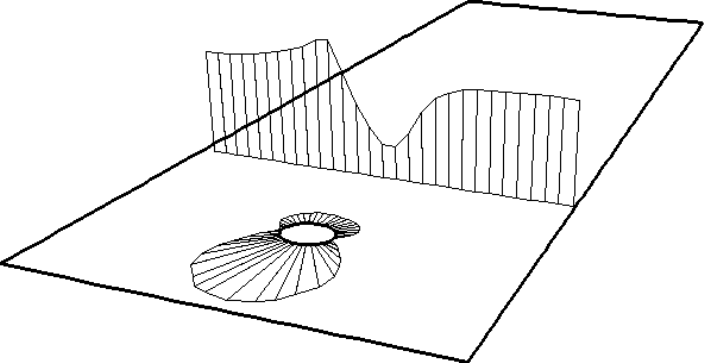
5.1 Profile Parts
5-116 EnSight 10.2 User Manual
5.1.12 Profile Parts
Profiles visualize values of a variable along a line with a plot projecting away
from the line. Projectors are parallel to a plane, but not necessarily in a plane.
Hence, Profile can follow the line.
You can scale and offset projectors. The positive direction is set as the From Point
as the origin point of the Plane Tool (away from center point is positive). Consider
a base-line (not necessarily straight) along which the value of a variable is known.
Moving along this base-line, you can “plot” the value of the variable on an “axis”
whose origin moves along the base-line and whose orientation varies so that it is
always both perpendicular to the base-line and parallel to a specified plane (but
not necessarily parallel to a line, enabling the plot-line to follow the curve of the
base-line in one dimension). A surface joining the base-line to the plot-line is
called a profile.
The parent Part of a Profile-Part can be a 1D-Clip Line, a Contour, a Particle
Trace, or a model Part consisting of a chain of bar elements. From each node of
the parent Part, EnSight draws a “projector” whose length is proportional to the
value of the variable at the node, and whose orientation makes it (1) parallel to a
specified plane, (2) pointing in a direction corresponding to the sign of the
variable’s value at the node (with the negative-direction determined by the
location of a specified point), and (3) perpendicular to the base-line elements
adjoining the node, or, if the base-line bends at the node, oriented so that its
projection into the plane defined by the base-line elements will bisect the angle
formed by the base-line elements. The outer-end of each projector is connected to
those of its neighbors, forming a series of four-sided polygons and hence a
surface.
The appearance of the profile depends greatly on the position of the location of the
plane tool origin (From Point) and the orientation of the specified plane, which
you can specify numerically or with the Plane tool. EnSight calculates the
projectors using the vector cross-product of the specified-plane’s normal (the Z-
axis) and each parent Part element, thus you should orient the plane so that its
normal is not parallel to the parent Part elements.
The projector length is calculated by adding to the variable’s value an Offset
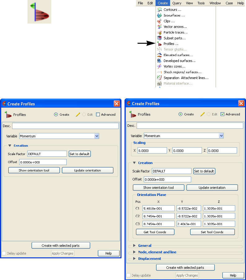
5.1 Profile Parts
EnSight 10.2 User Manual 5-117
value, then multiplying the sum by a Scaling value. Adding the Offset enables you
to shift the zero location of the projectors, which might be useful if you wanted to
make all the projectors have the same sign. An offset performs a “shift”, but does
not change the “shape” of the resulting profile. The Scaling factor changes the
displayed size of the profile, a “stretching” type of action. EnSight will provide
default values for both factors based on the variable’s values at the parent Part’s
nodes.
Clicking once on the Profiles Icon (if you have customized the Feature Ribbon to
have it visible) or selecting Profiles... in the Create menu, opens the Feature Panel
for Profile parts. This editor is used to both create and edit Profile parts.
.
Create/Edit Toggles that control whether a new part will be created, or whether you are editing
existing part(s). Note that when editing, the changes will be applied to those parts which
have the small “pencil” icon next to them in the Parts List.
Figure 5-72
Profile Icon
Figure 5-73
Feature Panel - Profiles
5.1 Profile Parts
5-118 EnSight 10.2 User Manual
See Feature Panel Turndowns Common To All Part Types for a detailed
discussion of the remaining Feature Panel turn-down sections which are the same
for all Parts.
(see How To Create Profile Plots)
Advanced Will open additional features for more advance control of the Part.
Desc The name of the part to be created or being edited.
Variable Choose the variable to use for creating the profile part from the pulldown.
Scaling
XYZ For vector variables, in advanced mode, specify vector components used in creating the
profiles. Not applicable to scalar variables. Scaling is in the reference frame of the parent
part. Letters labeling dialog data entry fields depend on type of the reference frame
(Rectangular, Spherical, or Cylindrical). If all components are 0.0, the vector magnitude
will be used. But, if any of these scaling factors is non-zero, the variable value will be
computed as xscale*xcomponent + yscale*ycomponent + zscale*zcomponent.
Creation
Scale Factor This field specifies the scaling for magnitude of the projector. The Scale Factor is
multiplied times the value of the variable. Values larger than one increase the size and
values smaller than one decrease the size.
Offset The value specified in this field is added to the variable values before the Scale Factor is
applied to change the magnitude of projectors. Default offset is magnitude of most-
negative projector (making them all positive). Has the effect of shifting the plot, but does
not change the plot shape.
Set to default Click to set Scale Factor and Offset values to the calculated defaults based on the
variable values for the parent Part.
Show Orientation
Tool
Causes the Plane Tool to become visible in the Graphics Window at the location
specified
Update Orientation Recreates the Profile Part at the current location and orientation of the Plane Tool.
Orientation Plane
Pos XYZ Specification of the location, orientation, and size of the Plane Clip using the coordinates
(in the Parts reference frame) of three corner points, as follows:
Pos of C1 Corner 1 is corner located in negative-X negative-Y quadrant
Pos of C2 Corner 2 is corner located in positive-X negative-Y quadrant
Pos of C3 Corner 3 is corner located in positive-X positive-Y quadrant
Set Tool Coords Will reposition the Plane Tool to the position specified in C1, C2, and C3.
Get Tool Coords Will update the C1, C2, and C3 fields to reflect the current position of the Plane Tool.
Create with selected
parts
Creates a Profile part using the selected Part(s) in the Parts List.
Delay update Checking this box will cause EnSight to not apply any changes made until you hit the
Apply Changes button. When not checked, the changes are applied as you make them.
Apply Changes Applies any changes made. Only active when Delay update is on.

5.1 Profile Parts
EnSight 10.2 User Manual 5-119
Troubleshooting Profiles
Problem Probable Causes Solutions
The entire profile is not projected the
direction you want.
The Plane is not oriented correctly. Turn on the Plane tool so you can see
its orientation. The projectors will be
parallel to this plane, so adjust its
orientation.
The From Point (plane tool origin) is
not in a good location
Turn on the Plane tool so you can see
the location of the center of the
plane. Positive projectors will go
away from this point, negative
towards.
Portions of the profile appear to be
projected in the wrong direction.
The From Point is not in a good
location.
Turn on the Plane tool so you can see
the location of the center of the
plane. Positive projectors will go
away from this point, negative
towards.
The normal to the Plane is parallel to
some of the elements of the parent
Part.
Turn on the Plane tool so you can see
its orientation. Try to make sure the
Z axis of the Plane tool does not lie
parallel to any portions of the parent
Part.
The Parent Part does not contain
elements which are consistently
ordered
None
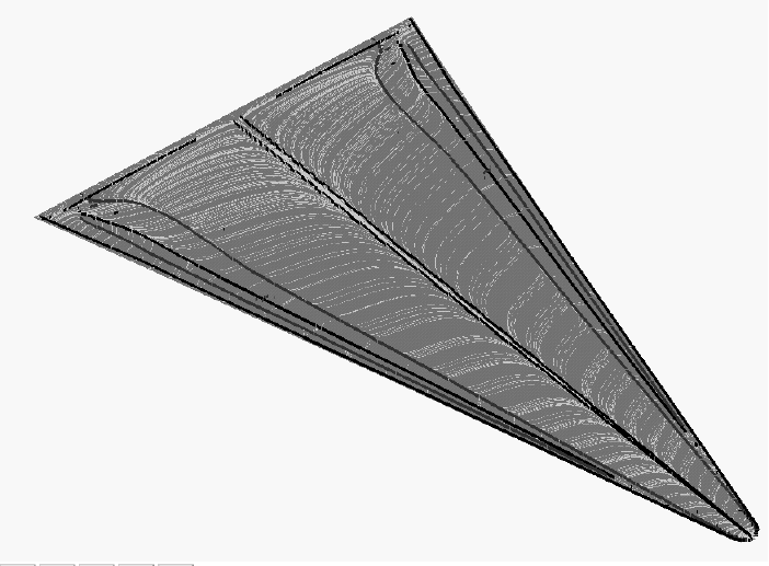
5.1 Separation/Attachment Line Parts
5-120 EnSight 10.2 User Manual
5.1.13 Separation/Attachment Line Parts
Separation and Attachment Lines exist on 2D surfaces and help visualize areas
where flow abruptly leaves or returns to the 2D surface in 3D flow fields. These
lines are topologically significant curves on the 2D surface where flow converges
and then separates (separation lines) from the surface into the 3D flow field, and
where flow attaches and then diverges (attachment lines) to the surface from the
3D flow field.
These line segments can be used as emitters for ribbon traces to help visualize
flow interaction from the 2D surface into the 3D field, or displayed along with
surface-restricted traces to help visualize the topology of the 2D surface.
EnSight creates separation and attachment lines as two distinct parts so that each
may be assigned their own attributes. Although both are updated computationally
when changes are made to either one via the Feature Panel.
Separation/Attachment lines can be created on any 2D part, whether it is a
boundary surface or internal surface to a 3D flow field. These lines can also be
created on 3D flow field parts. However, computation of the separation/
attachment lines is restricted to only the boundary surfaces of the 3D flow field.
Velocity Gradient Ensight creates separation and attachment lines from the velocity gradient
Tensor tensor of the 3D flow field part. EnSight automatically pre-computes the velocity
gradient tensor for all 3D model parts prior to creating the separation and
attachment lines. These values are then mapped to any corresponding 2D model
part, or inherited by any created part.
Since this variable is automatically created, all subsequent 3D model parts created
will also have this tensor variable computed.
Note: The velocity gradient tensor variable will continue to be created and
updated for all 3D model parts until it is deactivated.
5.1 Separation/Attachment Line Parts
EnSight 10.2 User Manual 5-121
This tensor variable behaves like any other created tensor variable, and may be
deactivated in the Variables List.
Thresholding Separation/Attachment lines may be filtered out according to the settings of a
threshold variable, value, and relational operator. Most active variables can be
used as threshold variables. Thresholding was implemented to help the user to
filter-out, or view portions of the line segments according to variable values.
When separation and attachment line parts are Created/Updated, the scalar
variable “fx_sep_att_strength” is created to help you threshold unwanted
core segments according to these scalar values.
Note: This scalar variable is currently set to the vorticity magnitude scalar, until a
better thresholding variable can be identified.
Since it has been observed that the current implementation of this algorithm may
produce additional lines that are not separation or attachment lines, the need for a
filtering mechanism that filters out segments according to different variables arose
and had been provided via thresholding options.
Algorithms Currently, separation and attachment lines are calculated according to the phase-
plane algorithm presented by Kenwright (see References below). This algorithm
detects both closed and open separation. Closed separation lines originate and
terminate at critical points, whereas open separation lines do not need to start or
end at critical points.
This technique is linear and nodal. That is, 2D elements are decomposed into
triangles, and then closed-form equations are solved to determine the velocity
gradient tensor values for eigen-analysis at the nodes. Also, any variables with
values at element centers are averaged to element nodes before processing.
References Please refer to the following references for more detailed explanations of pertinent
concepts and algorithms.
J. Helman, L. Hesselink
“Visualizing Vector Field Topology in Fluid Flows”,
IEEE CG&A, May 1991
D. Kenwright, “Automatic Detection of Open and Closed Separation and Attachment Lines”, IEEE
Visualization ‘98, 1998, pp. 151-158
R. Haimes and D. Kenwright, “On the Velocity Gradient Tensor and Fluid Feature Extraction”,
AIAA-99-88, Jan. 1999, pp. 315-4
S. Kenwright, C. Henze, C. Levit, “Feature Extraction of Separations and Attachment Liens”, IEEE
TVCG, Apr.-Jun. 1999, pp. 135-144
R. Peikert, M. Roth, “The ‘Parallel Vectors’ Operator - a vector field visualization primitive”, IEEE
Visualization ‘ 99, 1999
D. Kenwright, T. Sandstrom, GEL, NASA Ames Research Center, 1999
R. Haimes, D. Kenwright, The Fluid Extraction Tool Kit,
Massachusetts Institute of Technology, 2000
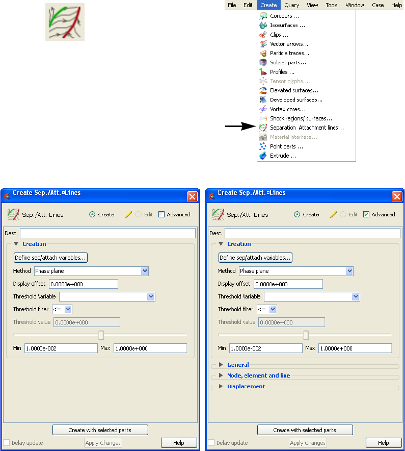
5.1 Separation/Attachment Line Parts
5-122 EnSight 10.2 User Manual
Access Clicking once on the Separation and Attachment lines icon (if you have
customized the Feature Ribbon to have it visible) or selecting Separation
Attachment lines... in the Create menu, opens the Feature Panel for Sep./Att. line
parts. This editor is used to both create and edit Separation and Attachment line
parts.
Create/Edit Toggles that control whether a new part will be created, or whether you are editing
existing part(s). Note that when editing, the changes will be applied to those parts which
have the small “pencil” icon next to them in the Parts List.
Advanced Will open additional features for more advance control of the Part.
Desc The name of the part to be created or being edited.
Figure 5-74
Separation/Attachment Lines Icon
Figure 5-75
Feature Panel - Separation/Attachment Lines
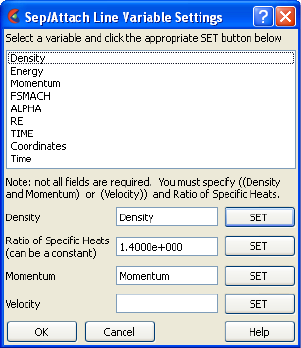
5.1 Separation/Attachment Line Parts
EnSight 10.2 User Manual 5-123
Creation
Define Sep/Attach
Variables...
Opens the Sep/Attach Line Variable Settings
dialog which allows the user to identify and set
the dependent variables used in computing
separation and attachment lines. This dialog
has a list of current accessible variables from
which to choose. Immediately below is a list of
dependent variables with corresponding text
field and SET button. The variable name in the
list is tied to a dependent variable below by
first highlighting a listed variable, and then
clicking the corresponding dependent
variable’s SET button, which inserts the listed
variable into its corresponding text field.
All text fields are required, except you may
specify either Density and Momentum (which
permits velocity to be computed on the fly), or
just Velocity. A default constant value is supplied for the Ratio of Specific Heats which
can be changed or specified by a scalar variable name.
Clicking Okay activates all specified dependent variables and closes the dialog.
Method Opens a pop-up dialog for the specification of which type of method, to use to compute
the separation and attachment lines on the 2D surface. There is currently only one
option:
Phase Plane Scheme that uses eigen-analysis on the velocity gradient tensor
along with phase plane analysis to compute the separation and
attachment line segments (see Algorithms).
Display offset This field specifies the normal distance away from a surface to display the separation/
attachment lines. A positive value moves the lines away from the surface in the direction
of the surface normal.
Please note that there is a hardware offset that will apply to contours, vector arrows,
separation/attachment lines, and surface restricted particle traces that can be turned on
or off in the View portion of Edit->Preferences. This preference (“Use graphics
hardware to offset line objects...”) is on by default and generally gives good images for
everything except move/draw printing. This hardware offset differs from the display
offset in that it is in the direction perpendicular to the computer screen monitor (Z-
buffer).
Thus, for viewing, you may generally leave the display offset at zero. But for printing, a
non-zero value may become necessary so the lines print cleanly.
Threshold Variable A list of possible variables that you may use to help filter out line segments. This list
includes the vorticity magnitude scalar variable (named fx_sep_att_strength) which gets
created when you Create/Update a separation and attachment part.
Threshold Filter Relational operators used to filter out line segments.
>= Filter out any line segments greater than or equal to the Threshold
Val ue.
<= Filter out any line segments less than or equal to the Threshold
Value (default).
Threshold Value The value at which to filter the line segments.

5.1 Separation/Attachment Line Parts
5-124 EnSight 10.2 User Manual
See Feature Panel Turndowns Common To All Part Types for a detailed
discussion of the remaining Feature Panel turn-down sections which are the same
for all Parts.
Note: Separation and Attachment Line feature extraction does not work with multiple cases.
Troubleshooting Separation/Attachment Lines
Threshold Slider Bar Used to change the Threshold Value in increments dependent on the Min and Max
settings. The stepper button on the left (and right) of the slide bar is used to decrement
(and increment) the Threshold value
Min The minimum value of the Threshold Variable. The stepper button
on the left (and right) side of the Min text filed is used to decrease
(and increase) the order of magnitude, or the exponent, of the min
value.
Max The maximum value of the Threshold Variable. The stepper button
on the left (and right) side of the Max text field is used to decrease
(and increase) the order of magnitude, or the exponent, of the Max
value.
Create with selected
parts
Creates a Separation and Attachments part using the selected Part(s) in the Parts List.
Delay update Checking this box will cause EnSight to not apply any changes made until you hit the
Apply Changes button. When not checked, the changes are applied as you make them.
Apply Changes Applies any changes made. Only active when Delay update is on.
Problem Probable Causes Solutions
Error creating separation and
attachment lines
Invalid part selected in part list Highlight 2D or 3D part
Undefined (colored by part color)
regions on sep/attach lines
Sep/Attach line segment node was
not mapped within a corresponding
3D field element
Make sure corresponding 3D field
part is defined.
Separation/attachment lines do not
print well.
See Display Offset discussion above Enter a non-zero Display Offset
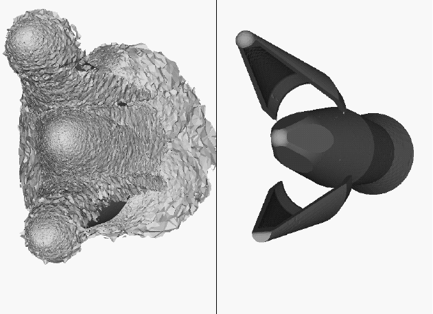
5.1 Shock Regions/Surfaces Parts
EnSight 10.2 User Manual 5-125
5.1.14 Shock Regions/Surfaces Parts
The Shock Region/Surface feature helps visualize shock waves in a 3D flow field.
Shock waves are characterized by an abrupt increase in density, energy, and
pressure gradients, as well as a simultaneous sudden decrease in the velocity
gradient.
EnSight creates candidate shock surfaces in 3D (trans/super-sonic) flow fields
using a creation scalar variable (i.e. density, pressure) along with the velocity
vector (see Algorithms below).
Thresholding Due to the nature of the shock algorithms, other surfaces with similar
characteristics may be produced besides shock surfaces, i.e. expansion regions,
etc. Therefore, a filtering mechanism is necessary to help filter out these non-
shock regions.
Shock surfaces may be filtered out according to the settings of a threshold
variable, value, and relational operator. Most active variables can be used as
threshold variables, but gradients of the density and energy related scalar variables
in the streamwise direction seem to work best.
When Shock parts are created via the Surface method, the scalar “SHK_*”
variable (where * is the appended name of the variable, i.e. SHK_Density) is
created to help threshold unwanted areas according to these scalar values. When
Shock parts are created via the Region method, the scalar “SHK_Threshold”
variable is created to help threshold respective unwanted areas.
Currently, these SHK_* variables consist of the gradient of an appropriate
creation variable (i.e. SHK_Density, SHK_Pressure, etc.) in the streamwise
direction. For the Region method, the creation variable is always pressure.
EnSight tries to compute a reasonable default threshold value each time one of
these threshold variables is applied. By default this value is half of one
exponential order less than the maximum value of the threshold variable on the
Figure 5-76
Shock Surface (Data Courtesy of Craft Technology)
5.1 Shock Regions/Surfaces Parts
5-126 EnSight 10.2 User Manual
shock part. This seems to produce a reasonable starting surface for the user to
threshold. By default, the smaller the threshold value, the larger the part.
The default threshold variable for non “SHK_” variables is the minimum of the
specified variable on the shock part.
The default Min/Max slider values try to bound the default threshold value by
appropriate orders of magnitude. Min/Max slider values floor/ceil the min/max
values of the threshold variable of the shock part when these ranges are exceeded
(see Threshold Slider Bar below).
Algorithms Shock parts are calculated according to two algorithms, or methods. The first
algorithm (referred to by EnSight as the Surface method) is based on the work of
Pagendarm et. al., and the second algorithm (referred to by EnSight as the Region
method) is based on the work by Haimes et. al. (See References below.)
The Surface method utilizes the maximal gradient of a quantity like density or
pressure in the streamwise direction. This yields a surface that requires
thresholding to distinguish significant portions of the shock patterns from weak
numerical artefacts.
The Region method utilizes flow physics to define shocks in steady state and
transient solutions. The steady state equation is based on developing a scalar field
based on combining the mach vector with the normalized pressure gradient field.
The transient solution combines this term with appropriate correction terms. The
Region method produces iso-shock surfaces that form regions that bound the
shock wave.
Note: Both methods use dependent variables (See Define Shock Variables below).
If some of the dependent variables do not exist and are required, they will be
temporarily calculated based on other defined dependent variables (as defined in
Variable Creation). The user has the responsibility to ensure these variables have
consistent units.
Both techniques have been implemented using linear interpolation to the nodes.
That is, their gradient calculations are based on decomposing finite elements into
tetrahedrons to approximate the gradient values at the nodes. Also, any variables
with values at element centers are averaged to element nodes before processing.
Other Notes Pre-filtering flow field elements by Mach Number.
The Surface Method allows the user to filter-out any flow field elements less than
a specified mach number, by issuing the following command via the command
line processor (See Section 2.5, Command Files):
test: shock_mach_prefilter #
Where # is the corresponding mach-number value (>=0.0) by which to filter.
(Zero is the default value - which means this option is turned-off until activated by
a value > 0.0.) Ideally this mach-number value would be 1; and thus, would
eliminate any subsonic regions from being processed via the Surface method’s
algorithm. In some transonic cases, this has doubled the efficiency of the
algorithm by eliminating the calculation of the second derivative on many
elements. Unfortunately, other cases have been observed (especially noticed in
regions with normal shack waves) where this option (due to the grid resolution
and/or the numerical dissipation inherent in the shock algorithm - see 1999
reference by D. Lovely and R. Haimes) has eliminated some valid shock regions.
Although care is taken to provide an appropriate stencil of elements for the
5.1 Shock Regions/Surfaces Parts
EnSight 10.2 User Manual 5-127
gradient calculations of values adjacent to these areas, it appears this value may
need to be < 1 to prevent these shock regions from being eliminated. This option
is therefore provided at the discretion and expertise of the user. This option only
takes effect when issued prior to a create or an update in shock method.
Post-filtering shock part elements by Mach Number.
Both methods allow the user to filter-out (prior to thresholding) any shock part
elements less than a specified mach number, by issuing the following command
via the command line processor (see Section 2.5, Command Files):
test: shock_mach_postfilter #
Where # is the corresponding mach-number value (>=0.0) by which to filter.
(Zero is the default value - which means this option is turned-off until activated by
a value > 0.0.) Ideally this mach number value would be 1; and thus, would
eliminate any subsonic regions from being displayed as part of the shock surface.
Unfortunately, some cases have been observed (especially noticed in regions with
normal shock waves) where this options (due to the grid resolution and/or the
numerical dissipation inherent in the shock algorithm - see 1999 reference by D.
Lovely and R. Haimes) has eliminated some valid shock regions. This option is
therefore provided at the discretion and expertise of the user. This option only
takes effect when issued prior to a create or an update in shock method.
Moving Shock.
Both methods compute the stationary shock based on the user specified
parameters. The Region Method has the capability of applying a correction term
to represent moving shocks in transient cases. This capability is toggled ON/OFF
by issuing the following command via the command line processor (see Section
2.5, Command Files).
test: toggle_moving_shock
Issuing the command a second time will toggle this option off. This option is
provided at the discretion and expertise of the user. This option only takes effect
when issued prior to a create or an update in shock method.
References Please refer to the following references for more detailed explanations of pertinent
concepts and algorithms.
H.G. Pagendarm, B. Seitz, S.I. Choudhry, “Visualization of Shock Waves in Hypersonic CFD
Solutions”, DLR, 1996
D. Lovely, R. Haimes, “Shock Detection from Computational Fluid Dynamics Results”,
AIAA-99-85, 1999, 14th AIAA Computational Fluid Dynamics Conference, Vol 1 technical papers.
R. Haimes and D. Kenwright, “On the Velocity Gradient Tensor and Fluid Feature Extraction”,
AIAA-99-88, Jan. 1999, 14th AIAA Computational Fluid Dynamics Conference, Vol 1 technical
papers.
D. Kenwright, T. Sandstrom, GEL, NASA Ames Research Center, 1999
R. Haimes, D. Kenwright, The Fluid Extraction Tool Kit,
Massachusetts Institute of Technology, 2000, 39th Aerospace Sciences Meeting and Exhibit, Reno.
R. Haimes, K. Jordan, “A Tractable Approach to Understanding the Results from Large-Scale 3D
Transient Simulations”, AIAA-2000-0918, Jan. 2001
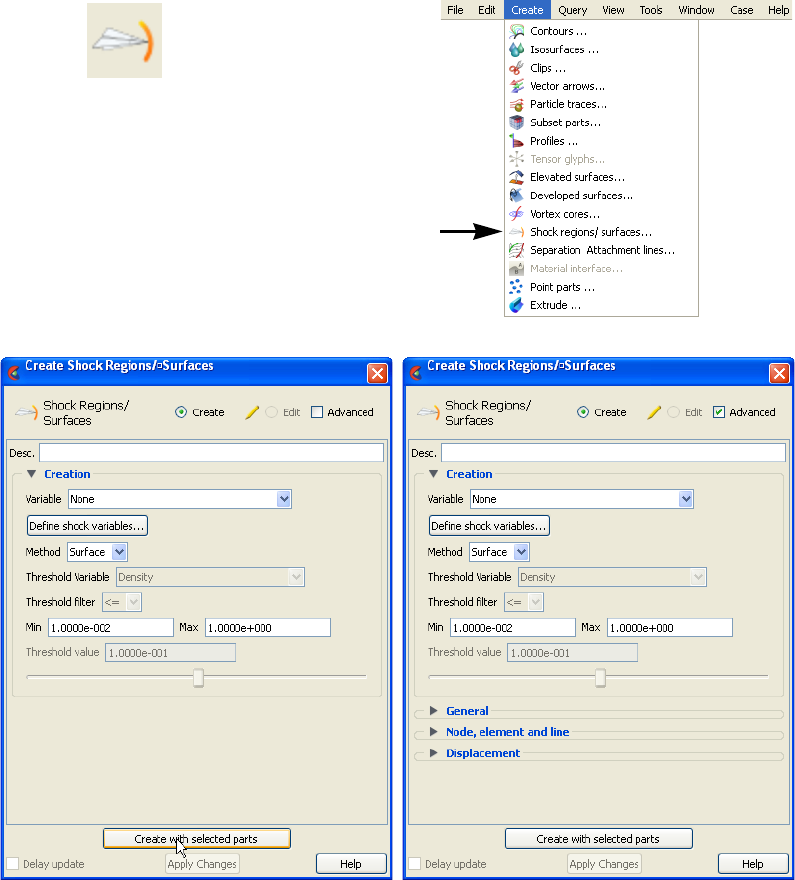
5.1 Shock Regions/Surfaces Parts
5-128 EnSight 10.2 User Manual
Access Clicking once on the Shock regions/surfaces icon (if you have customized the
Feature Ribbon to have it visible) or selecting Shock regions/surfaces... in the
Create menu, opens the Feature Panel for Shock regions/surfaces parts. This
editor is used to both create and edit Shock regions/surfaces parts.
Create/Edit Toggles that control whether a new part will be created, or whether you are editing
existing part(s). Note that when editing, the changes will be applied to those parts which
have the small “pencil” icon next to them in the Parts List.
Advanced Will open additional features for more advance control of the Part.
Desc The name of the part to be created or being edited.
Creation
Figure 5-77
Shock regions/surfaces icon
Figure 5-78
Feature Panel - Shock regions/surfaces
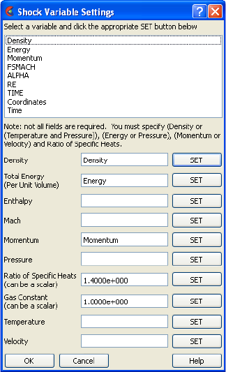
5.1 Shock Regions/Surfaces Parts
EnSight 10.2 User Manual 5-129
Variable A list of variables used to create the shock surface via Surface method. These variables
are specified via those SET in the Define Shock Variables list.
Note: This list is not used for the Region method. The Region method only uses pressure
as the creation variable.
Define Shock
Variables...
Opens the Shock Variable Settings dialog
which allows the user to identify and set the
dependent variables used in computing the
shock parts. This dialog has a list of current
accessible variables from which to choose.
Immediately below is a list of dependent
variables with corresponding text field and
SET button. The variable name in the list is
tied to a dependent variable below by first
highlighting the listed variable, and then
clicking the corresponding dependent
variable’s SET button, which inserts the
listed variable into its corresponding text
field.
Not all text fields are required. Although you
must specify either Density or Pressure,
Temperature, and Gas Constant; either
Energy or Pressure; either Velocity or
Momentum; and the Ratio of Specific Heats.
A default constant value is supplied for the
Ratio of Specific Heats and the Gas Constant
which may be changed or specified by a
scalar variable name.
Clicking Okay activates all specified dependent variables and closes the dialog.
Method Opens a pop-up dialog for the specification of which type of method, to use to compute
the vortex cores in the 3D field. These options are:
Surface Scheme that uses maximal density or pressure gradients in the
streamwise direction to locate candidate shock surfaces. (See
Algorithms above).
Region Scheme that uses flow physics based on the mach vector coupled
with pressure gradient to locate candidate shock regions. (See
Algorithms above.)
Threshold Variable A list of possible variables that you may use to help filter out unwanted areas. This list
includes the shock threshold variables “SHK_*” which gets created when you Create/
Update a shock part.
Threshold Filter Relational operators used to filter out shock areas.
>= Filter out any areas greater than or equal to the Threshold Value.
<= Filter out any areas less than or equal to the Threshold Value
(default).
Threshold Slider Bar Used to change the Threshold Value in increments dependent on the Min and Max
settings. The stepper button on the left (and right) of the slide bar is used to decrement
(and increment) the Threshold value

5.1 Shock Regions/Surfaces Parts
5-130 EnSight 10.2 User Manual
See Feature Panel Turndowns Common To All Part Types for a detailed
discussion of the remaining Feature Panel turn-down sections which are the same
for all Parts.
Note: Shock Surface feature extraction does not work with multiple cases.
Troubleshooting Shock Surfaces/Regions
Min The minimum value of the Threshold Variable. The stepper button
on the left (and right) side of the Min text field is used to decrease
(and increase) the order of magnitude, or the exponent, of the Min
value.
Max The maximum value of the Threshold Variable. The stepper button
on the left (and right) side of the Max text field is used to decrease
(and increase) the order of magnitude, or the exponent, of the Max
value.
Threshold Value The value at which to filter the shock areas.
Create with selected
parts
Creates a Shock regions/surfaces part using the selected Part(s) in the Parts List.
Delay update Checking this box will cause EnSight to not apply any changes made until you hit the
Apply Changes button. When not checked, the changes are applied as you make them.
Apply Changes Applies any changes made. Only active when Delay update is on.
Problem Probable Causes Solutions
Error creating shock part Non-3D part selected in part list Highlight 3D flow field part
No shock part created Flow field part subsonic No shock in subsonic regions
Shock dependent variables defined
with incorrect units, i.e. since
Region method uses density and
mach, if file variables are pressure,
temperature, and velocity, then
density (and thus mach) is
dependent on gas constant. By
default this value is 287 (Nm/KgK)
Make sure dependent variables have
correct units. i.e. gas constant may
need to be 1716(ft-lb/slugDegR), or
some other value rather than the
default
No to little shock part created Threshold value too large for <
operation
Decrease threshold value
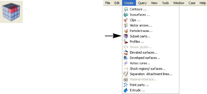
5.1 Subset Parts
EnSight 10.2 User Manual 5-131
5.1.15 Subset Parts
EnSight enables you to create and modify Subset Parts from ranges of node and/or
element labels of model parts. The Subset Parts feature allows you to isolate
contiguous and/or non-contiguous regions of large data sets, and apply the full-
range of feature applications and inspection provided by EnSight.
Subset Parts can only be created from parts that have node and/or element labels.
Therefore, Subset Parts can not be created from any Created Parts, because the
only parts that can have node and element labels are Model Parts such as parts
built from file data, Merged Model Parts, or Computational Mesh Model Parts
(parts created via the periodic computational symmetry Frame attribute). Model
Parts that do not have given or assigned node and/or element labels can not be
used to create Subset Parts.
Subset Parts are created and reside on the server. They are Created Parts that
provide proper updating of all dependent parts and variables.
Subset Parts are created and modified by specifying parent parts, as well as their
node and/or element labels. Node and/or element labels can be displayed and
filtered interactively according to global View and local Part attributes.
Clicking once on the Subset parts icon (if you have customized the Feature
Ribbon to have it visible) or selecting Subset parts... in the Create menu, opens the
Feature Panel for Subset parts. This editor is used to both create and edit Subset
parts.
Figure 5-79
Subset Parts Icon
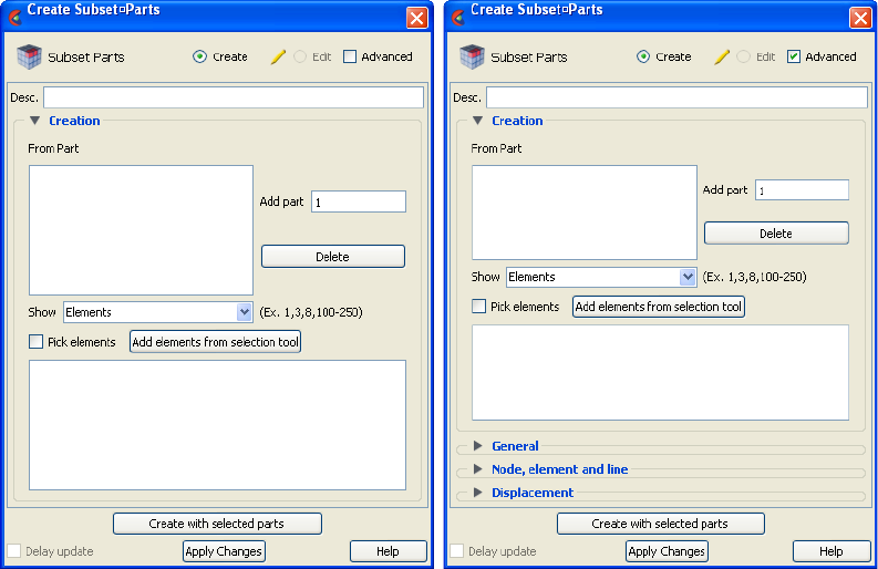
5.1 Subset Parts
5-132 EnSight 10.2 User Manual
Create/Edit Toggles that control whether a new part will be created, or whether you are editing
existing part(s). Note that when editing, the changes will be applied to those parts which
have the small “pencil” icon next to them in the Parts List.
Advanced Will open additional features for more advance control of the Part.
Desc The name of the part to be created or being edited.
Creation
From Part List reflecting the parent parts that have been added to the list. Selecting a part in this list
displays any corresponding element or node range specifications in the Show List.
Show Opens a pulldown menu for selecting which type of part entity you wish to include (or
have included) in your Subset Part. The Show options are:
Elements show any specified element label ranges
Nodes show any specified node label ranges
Add part This field specifies the GUI part number you wish to add to the From Part list.
Delete This button removes any selected entries in the From Part list along with any
corresponding element or node range specifications in the Show List.
Show List This field specifies the label ranges of Elements and/or Nodes wanted for the Subset Part
that correspond to the selected part in the From Part list. The Elements or Nodes are
specified as a range as the example indicates, i.e. (Ex. 1,3,8,9,100-250).
Pick elements This toggle enables element picking from the graphics window. Elements will be picked
using the pick selection which by default is the ‘p’ key.
Add Elements from
Selection Tool
Activate the selection tool, and adjust your selection window then click this button to
select all the elements within the window.
Figure 5-80
Feature Panel - Subset Parts
5.1 Subset Parts
EnSight 10.2 User Manual 5-133
See Feature Panel Turndowns Common To All Part Types for a detailed
discussion of the remaining Feature Panel turn-down sections which are the same
for all Parts.
Create with selected
parts
Creates a Profile part using the selected Part(s) in the Parts List.
Delay update Checking this box will cause EnSight to not apply any changes made until you hit the
Apply Changes button. When not checked, the changes are applied as you make them.
Apply Changes Applies any changes made. Only active when Delay update is on.
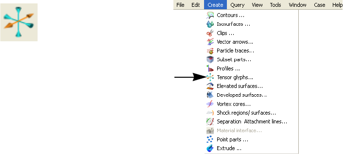
5.1 Tensor Glyph Parts
5-134 EnSight 10.2 User Manual
5.1.16 Tensor Glyph Parts
Tensor glyphs visualize the direction and tension/compression of the eigenvectors
at discrete points (at nodes or at element centers) for a given tensor variable.
Tensor glyph Parts are dependent Parts known only to the client. They cannot be
used as a parent Part for other Part types and cannot be used in queries. As
dependent Parts, they are updated anytime the parent Part and/or the creation
tensor variable changes (unless the general attribute Active flag is off).
Tensor glyphs can be filtered to show just the tensile or compressive eigenvectors.
Further, the visibility for each of the eigenvectors (Major, Middle, and Minor) can
be controlled.
Tensor glyphs will appear for each of the nodes/elements for the Parent part’s
visual Representation. Thus, for a border Representation of a Part, only the border
nodes/elements will be candidates for a tensor glyph.
The tensile and compressive eigenvectors can be visualized by modifying the
tensile/compressive component’s line width and color.
Clicking once on the Tensor glyphs icon (if you have customized the Feature
Toolbar to have it visible) or selecting Tensor glyphs... in the Create menu, opens
the Feature Panel for Tensor glyph parts. This editor is used to both create and edit
Tensor glyph parts.
Figure 5-81
Tensor Glyph Icon
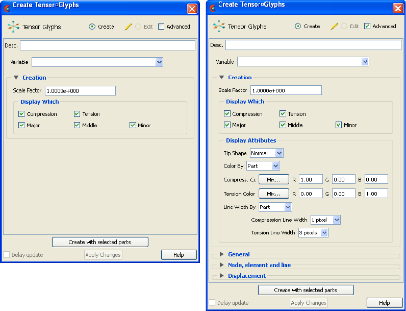
5.1 Tensor Glyph Parts
EnSight 10.2 User Manual 5-135
Create/Edit Toggles that control whether a new part will be created, or whether you are editing
existing part(s). Note that when editing, the changes will be applied to those parts which
have the small “pencil” icon next to them in the Parts List.
Advanced Will open additional features for more advance control of the Part.
Desc The name of the part to be created or being edited.
Variable The tensor variable used for the glyphs.
Creation
Scale Factor The size of the tensor glyph.
Display Which Controls which eigenvectors will be displayed.
Compression Show the eigenvectors that are in compression
Tension Show the eigenvectors that are in tension
Major Show the major eigenvector
Middle Show the middle eigenvector
Minor Show the minor eigenvector
Display Attributes
Tip Shape Opens a pop-up menu to select the tip shape.
None Displays eigenvectors as lines with no tips.
Normal Displays “classical” tips.
Figure 5-82
Feature Panel - Tensor Glyph

5.1 Tensor Glyph Parts
5-136 EnSight 10.2 User Manual
See Feature Panel Turndowns Common To All Part Types for a detailed
discussion of the remaining Feature Panel turn-down sections which are the same
for all Parts.
(see Section 5.1.1, Parts Quick Action Icons and How to Create Tensor Glyphs)
Troubleshooting Tensor Glyphs
Triangles Displays triangle tips.
Tip Size Controls the size of the tips.
Color By The tensor glyphs can be colored according to the part color, or have a separate color for
compression and tension.
Compression
Color
Specify the compressive color
Tension Color Specify the tensile color
Line Width By The tensor glyphs can use the part line width, or have a separate line width for
compression and tension.
Compression
Line Width
Specify the compressive line width
Tension Line
Width
Specify the tensile line width
Create with selected
parts
Creates a Profile part using the selected Part(s) in the Parts List.
Delay update Checking this box will cause EnSight to not apply any changes made until you hit the
Apply Changes button. When not checked, the changes are applied as you make them.
Apply Changes Applies any changes made. Only active when Delay update is on.
Problem Probable Causes Solutions
No tensor glyphs created No real eigenvectors exist. None
Scale Factor too small. Increase Scale Factor.
Parent parts have non-visual
attributes.
Re-specify parent parts or modify
parent part’s Element Representation.
Parent parts do not contain selected
tensor variable.
Re-specify parent parts.
Too many glyphs Parent parts have too many points at
which tensor glyphs are to be
displayed.
Consider using a grid clip as the
parent part.
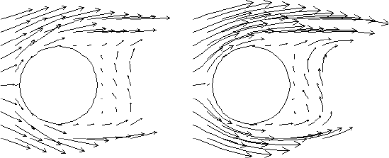
5.1 Vector Arrow Parts
EnSight 10.2 User Manual 5-137
5.1.17 Vector Arrow Parts
Vector Arrows visualize the magnitude and direction of a vector variable at
discrete points (at nodes, element vertices, or at the center of elements).
Other features can visualize magnitude, but Vector Arrows also show direction.
Vector arrow Parts are dependent Parts known only to the client. They cannot be
used as a parent Part for other Part types and cannot be used in queries. As
dependent Parts, they are updated anytime the parent Part and/or the creation
vector variable changes (unless the general attribute Active flag is off).
Vector arrows can be filtered according to low and/or high threshold values.
Vector arrows can emanate from the available nodes of the parent Part(s), the
available element vertex nodes of the parent Part(s), or the available element
centers of the parent Part(s) which pass through the filter successfully. The nodes
and elements available in the parent Part are based on the visual Representation of
the Part. Thus, for a border Representation of a Part, only the border elements and
associated nodes are candidates.
Vector arrows can have straight shafts representing the vector at the originating
location, or be the segment of a streamline emanating from the originating
location (curved). Straight vector arrows are displayed relatively quickly, while
curved vector arrows can be time consuming.
Different tip styles, sizes, and colors can be used to enhance vector arrow display.
To quickly create vector parts, right-click in the graphics window on a surface and
drag down to vector arrows, and vector arrows will automatically appear (if
there’s only one vector variable) or you will be prompted for which vector
variable to use to create vector variables and they will automatically appear. Left
click on the arrows and when a green, cross-shaped handle (click and go handle)
appears, drag it left and right to scale the arrows.
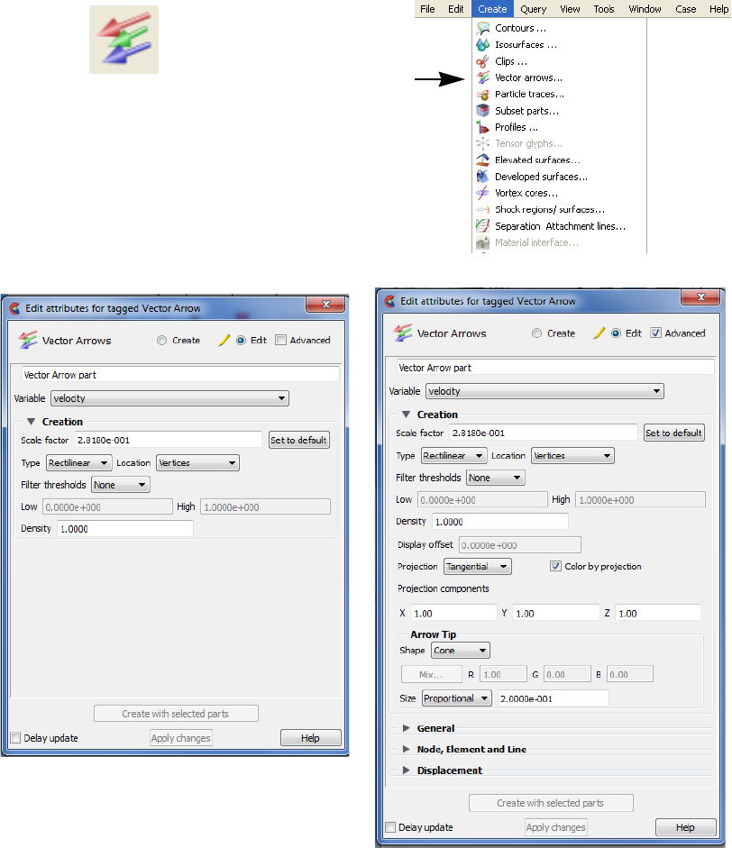
5.1 Vector Arrow Parts
5-138 EnSight 10.2 User Manual
Clicking once on the Vector arrows icon (which is in the Feature Ribbon by
default) or selecting Vector arrows... in the Create menu, opens the Feature Panel
for Vector arrow parts. This editor is used to both create and edit Vector arrow
parts.
Create/Edit Toggles that control whether a new part will be created, or whether you are editing
existing part(s). Note that when editing, the changes will be applied to those parts which
have the small “pencil” icon next to them in the Parts List.
Advanced Will open additional features for more advance control of the Part.
Desc The name of the part to be created or being edited.
Variable Choose the variable to use for creating the vector arrow part from the pulldown.
Figure 5-83
Vector Arrow Icon
Figure 5-84
Feature Panel - Vector Arrows
5.1 Vector Arrow Parts
EnSight 10.2 User Manual 5-139
Creation
Scale Factor / Time When Type is “Rectilinear”, this field specifies a scale factor to apply to the vector
values before displaying them. Scaling is usually necessary to control the visual length
of the vector arrows since the vector values may not relate well to the geometric
dimensions. Can be negative, causing the vector arrows to reverse direction.
When Type is “Rect. Fixed”, this field specifies the length of the arrows in units of the
model coordinate system. Can be negative, causing the vector arrows to reverse
direction.
When Type is “Curved”, this field specifies the duration time for streamlines forming the
shaft of curved vector arrows. Is an indication of the length of the curved vector arrow.
Set to Default Sets Scale Factor value to a computed reasonable value based on the vector variable
values and the geometry.
Type Opens a pop-up menu for selection of shaft-type of vector arrows. Options are:
Rectilinear arrows have straight shafts. The arrow points in the direction of the
vector at the originating location. The length of the arrow shaft is
determined by multiplying the vector magnitude by the scale factor.
Rect. Fixed arrows have straight shafts. The arrow points in the direction of the
vector at the originating location. The length of the arrow shaft is
determined by the scale factor. It is independent of the vector
variable.
Curved arrows have curved shafts. The arrow is actually a streamline
emanating from the originating location. It represents the path that a
massless Particle would follow if the flow field was steady state. For
this option, the “Scale Factor” changes to “Time”. Time is the
amount of time the streamline is allowed to take and is an indication
of how long the arrow will be. Hint: Since curved arrows can take a
significant amount of time (depending on the number of originating
locations), the setting of a proper “Time” value is critical. The best
way to do this is to first do a single Particle trace at a representative
location with the estimated “Time” value as the Max Time. A quick
iteration or two on the value here could save considerable time for
the curved vector arrow computation.
Location Opens a pop-up dialog for the selection of root-location of arrow shafts. The options are:
Node arrows originate from each node of the parent Part(s). Note: Discrete
Particles Parts must use Node option.
Vertices arrows originate only from those nodes at the vertices of each
element of the parent Part(s) (i.e., arrows are not displayed at free
nodes or mid-side nodes).
Element Center arrows originate from the geometric center of each element of the
parent Part(s).
Filter Thresholds Selection of pattern for filtering Vector Arrows according to magnitude. Options are:
None displays all the vector arrows. No filtering done.
Low displays only those arrows with magnitude above that specified in
the Low field. Filters low values out.
Band displays only those arrows with magnitude below that specified in
the Low field and above that specified in the High field. Filters the
band out.
5.1 Vector Arrow Parts
5-140 EnSight 10.2 User Manual
High displays only those arrows with magnitude below that specified in
the High field. Filters the high values out
Low_High displays only those arrows with magnitude between that specified in
the Low field and that specified in the High field. Filters out low and
high values.
Density The fraction of the parent’s nodes/elements which will show a vector arrow. A value of
1.0 will result in a vector arrow at each node/element, while a value of 0.0 will result in
no arrows. If between these two values, the arrows will be distributed randomly at the
specified density. There is no check for duplicates in the random distribution of arrows.
It is entirely possible that when you specify a density of 0.25 in a model containing 100
nodes you only get 15 unique locations with 10 duplicates. It will appear that only 15
arrows show up, but there are actually 25 with 10 duplicates.
Display offset This field specifies the normal distance away from a surface to display the vector arrows.
A positive value moves the vector arrows away from the surface in the direction of the
surface normal.
Please note that there is a hardware offset that will apply to contours, vector arrows,
separation/attachment lines, and surface restricted particle traces that can be turned on
or off in the View portion of Edit->Preferences. This preference (“Use graphics
hardware to offset line objects...”) is on by default and generally gives good images for
everything except move/draw printing. This hardware offset differs from the display
offset in that it is in the direction perpendicular to the computer screen monitor (Z-
buffer).
Thus, for viewing, you may generally leave the display offset at zero. But for printing, a
non-zero value may become necessary so the arrows print cleanly.
Projection Opens a pop-up menu to allow selection of which vector components to include when
calculating both the direction and magnitude of the vector arrows. The vector
components at the originating point are always first multiplied by the Projection
Components (see below). Then one of the following options is applied:
All to display a vector arrow composed of the Projection-Component-
modified X, Y, and Z components.
Normal to display a vector which is the projection of the All vector in the
direction of the normal at the originating location.
Tangential to display a vector which is the projection of the All vector into the
tangential plane at the originating location.
Component to display both the Normal and the Tangential vectors.
The All, Normal, and Tangential options produce a single vector per location, while the
Component option produces two vectors per location. If selection is not applicable to a
Particular element, that element’s vector arrow uses the All projection.
Color by Projection If the projection is Tangential or Normal and the vector arrow is colored by the vector,
then the vector arrow is colored by the Tangential or Normal, respectively.
Projection
Components X Y Z
These fields specify a scaling factor for each coordinate component of each vector arrow
used in calculating both the magnitude and direction of the vector arrow. Specify 1 to use
the full value of a component. Specify 0 to ignore the corresponding vector component
(and thus confine all the vector arrows to planes perpendicular to that axis). Values
between 0 and 1 diminish the contribution of the corresponding component, while values
greater than 1 exaggerate them. Negative values reverse the direction of the component.
Always applied before the Projection options above.
Arrow Tip

5.1 Vector Arrow Parts
EnSight 10.2 User Manual 5-141
See Feature Panel Turndowns Common To All Part Types for a detailed
discussion of the remaining Feature Panel turn-down sections which are the same
for all Parts.
(see How to Create Vector Arrows)
Troubleshooting Vector Arrows
Shape Opens a pop-up menu to select tip shape.
None option displays arrows as lines without tips.
Cone arrows have a tip composed of a 3D cone. Good for both 2D and 3D
fields
Normal arrows have two short line tips, similar to the way many people
draw arrows by hand. The tip will lie in the X–Y, X–Z, or Y–Z plane
depending on the relative magnitudes of the X, Y, and Z components
of each individual vector. Suggested for 2D problems.
Triangles arrows have a tip composed of two intersecting triangles in the two
dominant planes. Good for both 2D and 3D fields.
Tipped arrows display the tip of the arrow in any user specified color. Good
for both 2D and 3D fields. The color may be specified in the RGB
fields or chosen from the Color Selector dialog which is opened by
pressing the Mix... button
Size Lets you control a scale factor for tip size
Fixed sized arrows have tips for which the length is specified in the data
entry field to the right of the pop-up menu button. Units are in the
model coordinate system
Proportional sized arrow tips change proportionally to the change in the
magnitude of the vector arrows.
Create with selected
parts
Creates a vector arrow part using the selected Part(s) in the Parts List.
Delay update Checking this box will cause EnSight to not apply any changes made until you hit the
Apply Changes button. When not checked, the changes are applied as you make them.
Apply Changes Applies any changes made. Only active when Delay update is on.
Problem Probable Causes Solutions
Vector arrows do not match up with
their originating locations on one or
more of the parent Parts.
Displacements are on for some of the
parent Parts, but not others. Or the
parent Parts have been assigned to
different coordinate frames
Create separate vector arrow Parts
for the parents that will be displaced
(or assigned to different frame) and
the ones that will not be displaced
(or assigned to different frames).
You are displaying several different
vector arrow Parts at once and can’t
tell which is which.
Just too much similar information in
the same area.
Use different attributes for the
different vector arrow Parts, or better
yet, display the conflicting vector
arrow Parts on separate Part copies
which have been moved apart.
You are trying to display vector
arrows on a Discrete Particle Part,
but can’t get them to show up
Arrow Location set to Vertices (the
default).
Set the Arrow Location to Nodes.

5.1 Vector Arrow Parts
5-142 EnSight 10.2 User Manual
No vector data provided for the
Discrete Particle dataset, thus values
all set to zero when read into
EnSight.
Provide vector data for the particles.
Specify in the Measured results file.
See Section 3.7.
Vector arrows do not print well See Display Offset discussion above. Enter a non-zero Display Offset.
Problem Probable Causes Solutions
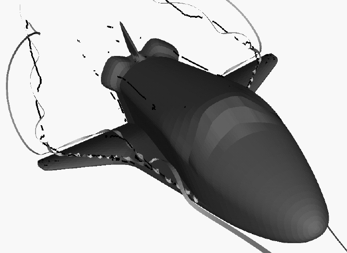
5.1 Vortex Core Parts
EnSight 10.2 User Manual 5-143
5.1.18 Vortex Core Parts
Vortex cores help visualize the centers of swirling flow in a flow field. EnSight
creates vortex core segments from the velocity gradient tensor of 3D flow field
part(s). Core segments can then be used as emitters for ribbon traces to help
visualize the strength and nature of the vortices.
Velocity Gradient EnSight automatically pre-computes the velocity gradient tensor for all 3D model
Tensor parts prior to creating the vortex cores. Since this variable is automatically
created, all subsequent 3D model parts created will also have this tensor
computed.
Note: The velocity gradient tensor variable will continue to be created and
updated for all 3D model parts until it is deactivated.
This tensor variable behaves like any other created tensor variable, and may be
deactivated in the Variables List.
Thresholding Core segments may be filtered out according to the settings of a threshold
variable, value, and relational operator. Most active variables can be used as
threshold variables. Thresholding was implemented to help the user filter-out, or
view portions of the core segments according to variable values.
When vortex core parts are Created/Updated, the vorticity magnitude scalar
variable “fx_vortcore_streng” is created to help you threshold unwanted
core segments according to these scalar values. (This is the magnitude (RMS) of
the vorticity as defined in chapter 4.)
Due to the difference in algorithms, some segments produced may not be vortex
cores (see Caveats). Thus, the need for a filtering mechanism that filters out
segments according to different variables arose and has been provided via
thresholding options.
Algorithms Currently, vortex cores are calculated according to two algorithms based on
5.1 Vortex Core Parts
5-144 EnSight 10.2 User Manual
techniques outlined by Sujudi, Haimes, and Kenwright (see References below).
Both techniques are linear and nodal. That is, they are based on decomposing
finite elements into tetrahedrons and then solving closed-form equations to
determine the velocity gradient tensor values at the nodes. Also, any variable with
values at element centers are first averaged to element nodes before processing.
The eigen-analysis algorithm uses classification of eigen-values and vectors to
determine whether the vortex core intersects any faces of the decomposed
tetrahedron. The vorticity based algorithm utilizes the fact of alignment of the
vorticity and velocity vectors to determine core intersection points.
References Please refer to the following references for more detailed explanations of pertinent
concepts and algorithms.
D. Banks, B. Singer, “Vortex Tubes in Turbulent Flows: Identification, Representation,
Reconstruction”, IEEE Visualization ‘94, 1994
D. Sujudi, R. Haimes, “Identification of Swirling Flow in 3-D Vector Fields”,
AIAA-95-1715, Jun. 1995
D. Kenwright, R. Haimes, “Vortex Identification - Applications in Aerodynamics”,
IEEE Visualization ‘97, 1997
M. Roth, R. Peikert, “A Higher-Order Method For Finding Vortex Core Lines”,
IEEE Visualization ‘98, 1998
R. Haimes and D. Kenwright, On the Velocity Gradient Tensor and Fluid Feature Extraction”,
AIAA-99-88, Jan. 1999
R. Peikert, M. Roth, “The ‘Parallel Vectors’ Operator - a vector field visualization primitive”, IEEE
Visualization ‘99, 1999
D. Kenwright, T. Sandstrom, GEL, NASA Ames Research Center, 1999
R. Haimes, D. Kenwright, The Fluid Extraction Toll Kit,
Massachusetts Institute of Technology, 2000
R. Haimes, K. Jordan, “A Tractable Approach to Understanding the Results from Large-Scale 3D
Transient Simulations”, AIAA-2000-0918, Jan. 2001
Caveats Due to the linear implementation of both the eigen-analysis and vorticity
algorithms, they both have problems finding cores of curved vortices. In addition,
testing has shown that both algorithms usually fail to predict vortex core segments
in regions of weak vortices. Note: for regions of weak vortices consider using the
Lambda2 or Q-criteria calculator functions (see Section 7.3, Variable Creation).
Since the eigen-analysis method finds patterns of swirling flow, it can also locate
swirling flow features that are not vortices (especially in the formation of
boundary layers). These non-vortex core type segments can sometimes be filtered
out via thresholding (see Thresholding). In addition, the eigen-analysis algorithm
may produce incorrect results when the flow is under more than one vortex, and
has a tendency to produce core locations displaced from the actual vortex core.
The vorticity based method does not seem to exhibit the problem of producing
core segments due to boundary layer formations, because the stress components
of the velocity gradient tensor have been removed in the formation of the vorticity
vector. Thus, the vorticity method seems to produce longer and more contiguous
cores - in most cases; and therefore, the reason for including both algorithms.
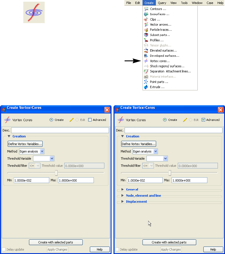
5.1 Vortex Core Parts
EnSight 10.2 User Manual 5-145
Access Clicking once on the Vortex cores icon (if you have customized the Feature
Ribbon to have it visible) or selecting Vortex cores... in the Create menu, opens
the Feature Panel for Vortex core parts. This editor is used to both create and edit
Vortex core parts.
Create/Edit Toggles that control whether a new part will be created, or whether you are editing
existing part(s). Note that when editing, the changes will be applied to those parts which
have the small “pencil” icon next to them in the Parts List.
Advanced Will open additional features for more advance control of the Part.
Desc The name of the part to be created or being edited.
Creation
Figure 5-85
Vortex Core Icon
Figure 5-86
Feature Panel - Vortex Cores
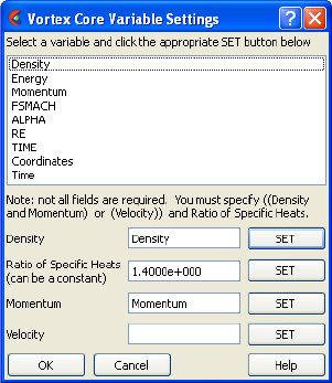
5.1 Vortex Core Parts
5-146 EnSight 10.2 User Manual
Define Vortex
Variables...
Opens the Vortex Core Variable Settings dialog
which allows the user to identify and set the
dependent variables used in computing the
vortex cores. This dialog has a list of current
accessible variables from which to choose.
Immediately below is a list of dependent
variables with corresponding text field and
SET button. The variable name in the list is
tied to a dependent variable below by first
highlighting a listed variable, and then clicking
the corresponding dependent variables’s SET
button, which inserts the listed variable into its
corresponding text field.
All text fields are required, except you may
specify either Density and Momentum (which
permits velocity to be computed on the fly), or
just Velocity. A default constant value is supplied for the Ratio of Specific Heats which
may be changed or specified by a scalar variable name.
Clicking Okay activates all specified dependent variables and closes the dialog.
Method Opens a pop-up dialog for the specification of which type of method to use to compute
the vortex cores in the 3D field. These options are:
Eigen Analysis Scheme that uses eigen-analysis on the Velocity gradient tensor to
compute the vortex core segments. (See Algorithms above).
Vorticity Scheme that uses the vorticity vector from the anti-symmetric
portions of the velocity gradient tensor to compute the vortex core
segments. (See Algorithms above).
Threshold Variable A list of possible variables that you may use to help filter out vortex core segments. This
list includes the vorticity magnitude scalar variable (named fx_vortcore_streng)
which gets created when you Create/Update a vortex core part.
Threshold Filter Relational operators used to filter out line segments.
>= Filter out any core segments greater than or equal to the Threshold
Val ue.
<= Filter out any core segments less than or equal to the Threshold
Value (default).
Threshold Value The value at which to filter the vortex core segments.
Threshold Slider Bar Used to change the Threshold Value in increments dependent on the Min and Max
settings. The stepper button on the left (and right) of the slide bar is used to decrement
(and increment) the Threshold value
Min The minimum value of the Threshold Variable. The stepper button
on the left (and right) side of the Min text filed is used to decrease
(and increase) the order of magnitude, or the exponent, of the min
value.
Max The maximum value of the Threshold Variable. The stepper button
on the left (and right) side of the Max text field is used to decrease
(and increase) the order of magnitude, or the exponent, of the Max
value.
Create with selected
parts
Creates a Separation and Attachments part using the selected Part(s) in the Parts List.

5.1 Vortex Core Parts
EnSight 10.2 User Manual 5-147
See Feature Panel Turndowns Common To All Part Types for a detailed
discussion of the remaining Feature Panel turn-down sections which are the same
for all Parts.
Note: Once a Vortex Core feature extraction calculation has been completed, it is no longer
possible to replace nor add case(s). However, if multiple cases have already been
loaded, then it is possible to use the Vortex Core feature extraction on each of the
cases.
Troubleshooting Vortex Cores
Delay update Checking this box will cause EnSight to not apply any changes made until you hit the
Apply Changes button. When not checked, the changes are applied as you make them.
Apply Changes Applies any changes made. Only active when Delay update is on.
Problem Probable Causes Solutions
Error creating vortex cores Non-3D part selected in part list Highlight 3D part
Undefined (colored by part color)
regions on vortex cores
Vortex core line segment node was
not mapped within a corresponding
3D field element
Make sure corresponding 3D field
part is defined.
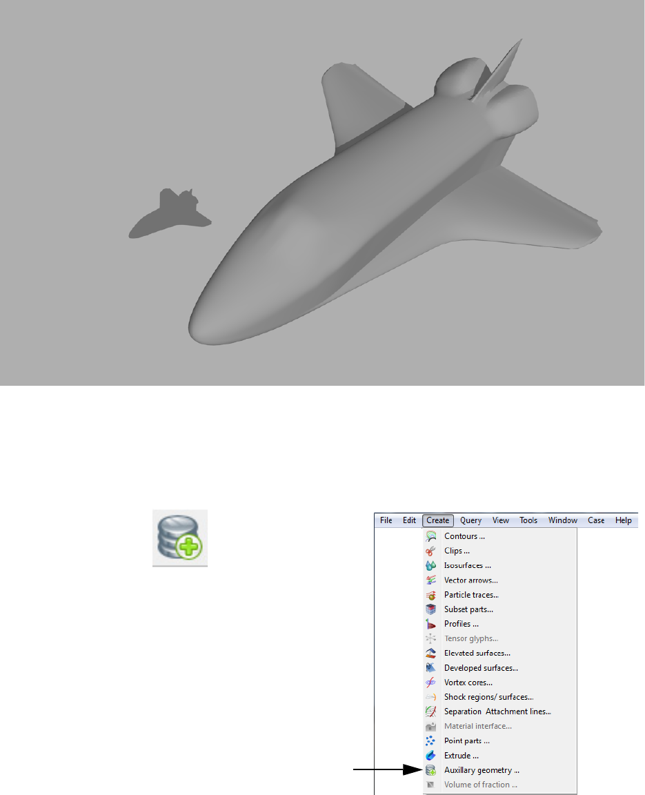
5.1 Auxiliary Geometry
5-148 EnSight 10.2 User Manual
5.1.19 Auxiliary Geometry
Auxiliary Geometry helps frame parts for visual effects. These geometries can be
texture-mapped for environmental reference, as well as display cast part shadows
when combined with directional lighting and ray-traced images.
Access Clicking once on the Auxiliary Geometry icon (if you have customized the
Feature Ribbon to have it visible) or selecting Auxiliary Geometry... in the Create
menu, opens the Feature Panel for Auxiliary Geometry parts. This editor is used to
both create and edit Auxiliary Geometry parts.
Figure 5-87
Auxiliary Geometry Icon
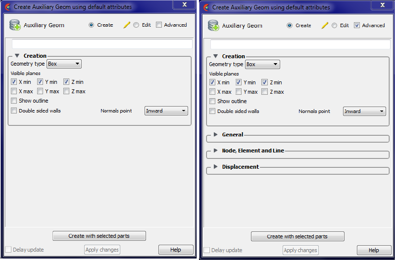
5.1 Auxiliary Geometry
EnSight 10.2 User Manual 5-149
Create/Edit Toggles that control whether a new part will be created, or whether you are editing
existing part(s). Note that when editing, the changes will be applied to those parts which
have the small “pencil” icon next to them in the Parts List.
Advanced Will open additional features for more advance control of the Part.
Desc [text field] The name of the part to be created or being edited.
Creation
Geometry Type To specify which type of geometry to be created/edited. The options are:
Box A box whose dimensions are the bounding box of the selected
part(s) with visible sides, top & bottom planes. Currently Box is the
only option, but it is a pulldown because more may be added in the
future.
Visible planes Controls which planes (sides of the box) that will be created.
X min Show the x-min plane
Y min Show the y-min plane
Z min Show the z-min plane
X max Show the x-max plane
Y max Show the y-max plane
X max Show the z-max plane
Show outline Show the outline of the specified geometry type.
Figure 5-88
Feature Panel - Auxiliary Geometry

5.1 Annotations
5-150 EnSight 10.2 User Manual
See Feature Panel Turndowns Common To All Part Types for a detailed
discussion of the remaining Feature Panel turn-down sections which are the same
for all Parts.
Troubleshooting Auxiliary Geometry
5.1.20 Annotations
Double sided
walls
Create two walls with opposing normals (an inside and an outside
surface for each wall). This is to overcome raytracing error
tolerance limitations. Double sided walls might be useful, for
example, to better compute the shadow effect on the edge or corner
of the box. If a single wall is used, the edge can be mistakenly bright
or dark. With an extra layer, the lighting is correct.
Normals point A pulldown menu for the specification of which direction to create
surface normals off the walls. Options are inward or outward. This
is usually not important for OpenGL rendering, and is primarily for
raytracing. If double sided walls is ON, then this option is ignored.
Inward (default) Normals off the wall point into the part.
Outward Normals off the wall point out from the part.
For a single layered box (Double sided walls off), the boundary
planes are created by default with normals pointing inward. For
most scenes where the auxilliary geometry is designed to provide a
backdrop to the model, an inward normal is the right choice for
raytracing. And outward normal is provided for rare situations
where the auxilliary geometry is not just a backdrop and you are
using less common backdrop geometry, for example, a glass
material, which needs to know the entry point and exit point
correctly. Flipping the normal direction may provide a better
raytrace rendering in this rare situation.
Create with selected
parts
Creates an Auxiliary geometry part using the selected Part(s) in the Parts List. Note: you
can still, click on a wall and drag it to a different location.
Problem Probable Causes Solutions
Error creating auxiliary geometry No parts selected in part list Must select existing part(s) in the
Parts List prior to creating auxiliary
geometry that will bound the part(s).
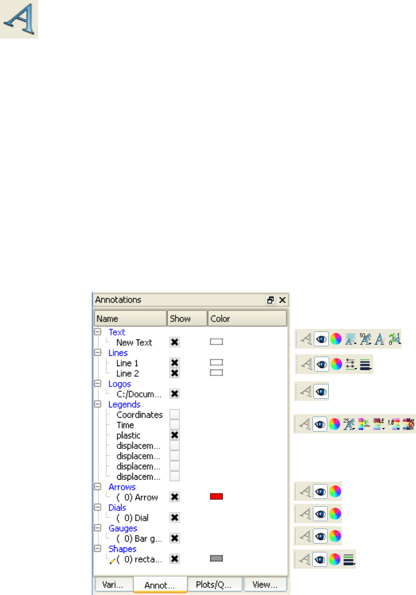
5.2 Annotations
EnSight 10.2 User Manual 5-151
5.2 Annotations
Overview
Annotations are provided to augment/mark up 3D/4D information contained in
the graphics window. Some examples of this are, current simulation time,
changing value of the volume or the area of an object, a variable's color legend,
company logo, text, arrows showing point(s) of interest, backdrop shapes, actual
experimental video footage, etc. Annotations can be selected in the graphics
window by left click and multiple items can be selected by holding the control key
down while left clicking. Selection is also available via the annotation list panel.
Upon selection of an annotation the Quick Action Icon Bar shows attributes that
can be edited. Right-click selection in both areas provide a menu of options for
editing, creating, and access to the full Feature Panel.
The annotation panel gives a user modifiable view of the annotation items that can
be created and already exist. The toggles, in the "Show" column, turn visibility on/
off, whereas the other column items are display only. Selection is accomplished
via right and left mouse buttons. Multiple disjoint items can be selected by
holding the control key as the mouse is clicked and multiple sequential items by
holding the Shift-key. Double-click displays the Feature Panel. Any item currently
in edit mode will display a pencil icon near it.
Figure 5-89
Annotation Panel
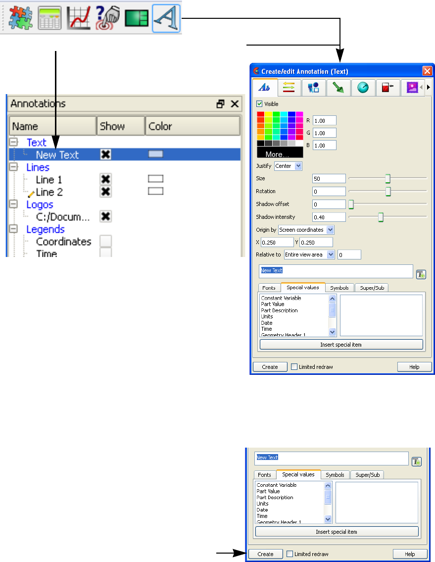
5.2 Text Annotation
5-152 EnSight 10.2 User Manual
5.2.1 Text Annotation
The annotation icon opens the annotation Feature Panel with the last tab selected
displayed. Text annotation can contain a mixture of a user's descriptive text along with
special values that access information from the current dataset. These annotations can be
positioned to a 2D or 3D location and tied to a specific viewport.
Create Clicking the Create button creates a text string called "New Text" that displays in the text
edit area of this dialog, in the annotations panel, and in the graphics window. This text
can then be modified simply by typing in the text edit, changing any of the attributes, or
by manipulation in the graphics window.
Figure 5-90
Text Annotation Feature Panel
Edit specific text by double clicking or right-click on item
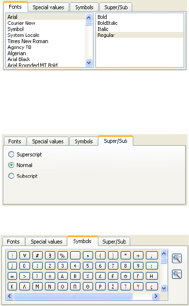
5.2 Text Annotation
EnSight 10.2 User Manual 5-153
Special Values Lists a number of different special strings that can be inserted into the annotation
currently being edited. These include information contained in results data or from other
dialogs.
Constant Variable inserts the value of the constant variable selected and displays
it in the selected format.
Date inserts the Day of Week, Month, Date, Time, Year.
Geometry Header inserts either the first or second header lines of the Case Gold
geometry file. User defined readers populate these values at
their own discretion.
Measured Header inserts the header line of the measured results file.
Variable Header inserts the header line of the selected variable data file.
Part Value inserts the value used to create the Isosurface or Clip Plane
Part. Works for Isosurface Parts, or some (XYZ, IJK, RTZ,
plane aligned with axis, or attached to a spline) Clip Plane
Parts.
Part Description inserts the description of the Part selected in a Parts List which
pops up within the Text Annotation Creation dialog.
Units inserts the units description for a specified variable if provided
by data reader.
Version inserts the EnSight version number, including the (letter).
For example, 10.2.0 (a) would be 10.2.0(a)
Fonts Allows selection of TrueType fonts and styles for your text.
See How To Manipulate Fonts for additional information on working with fonts
Super/Sub These toggles can be used to do superscripting and subscripting in your text string. They
place codes in the string (<no> for normal, <up> for superscript, and <dn> for subscript)
to delineate the desired mode.
Symbols Allows selection of special symbols to be inserted into your text.
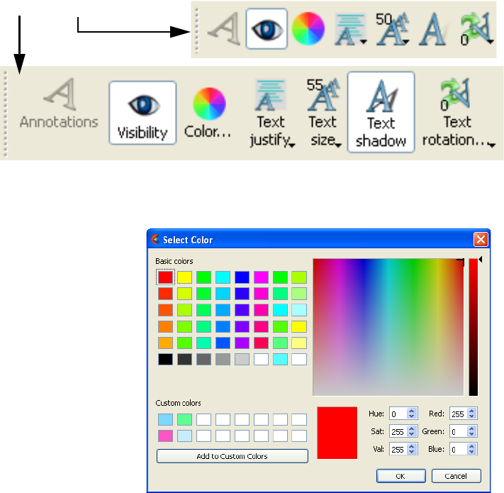
5.2 Text Annotation
5-154 EnSight 10.2 User Manual
Visible Toggles text visibility ON/OFF.
RGB Color of text.
Justify Pulldown for left, right, or center justification.
Size Field and slider for text size.
Rotation/Degrees Field and slider for rotation in degrees (-360 to 360).
Shadow offset Field and slider for an offset for a drop shadow.
Shadow intensity Field and slider for shadow intensity, where 0 is black and 1 is white.
Origin by Screen coordinates Indicates to locate the annotation in normalized screen space
3D coordinates Indicates to locate the annotation in world coordinates and thus
a X, Y, Z position must be specified.
Relative to If Origin is by 3D coordinates, this specifies which reference frame the X, Y, Z position
is in reference to.
Quick Action Icons
for Text
When a text annotation is selected, the following Quick Action Icons are available in the
tool ribbon:
Visibility Turn visibility of selected text ON or OFF
Color... Control color of selected text in color dialog that comes up.
With and without icon labels
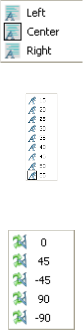
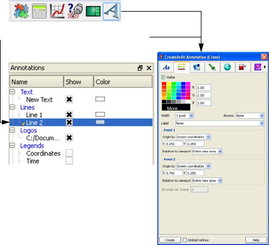
5.2 Line Annotation
5-156 EnSight 10.2 User Manual
5.2.2 Line Annotation
The annotation create/edit icon opens the annotation Feature Panel with the last tab
selected displayed. Line annotations can include arrows and can be attached to locations in
2D and/or 3D space. For example one endpoint attached to a 2D text annotation and the
other to a location in 3D space.
Create Clicking the Create button creates a line annotation that displays in the annotations
panel and in the graphics window. This line can then be modified simply by changing
any of the attributes or by manipulation in the graphics window.
Visible Toggles line visibility ON/OFF.
RGB Color of line.
Width Controls the line width in pixels
Arrows Allows placement of arrow on line
Label A text annotation can be used to label the line annotation. The text is aligned with the
line orientation.
Point 1, 2:
Figure 5-91
Line Annotation Feature Panel
Edit specific lines by double clicking or right-click on item
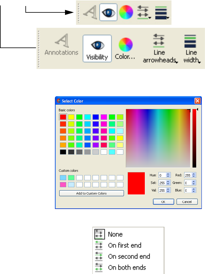
5.2 Line Annotation
EnSight 10.2 User Manual 5-157
Origin by Screen coordinates Indicates to locate the annotation in normalized screen space
3D coordinates Indicates to locate the annotation in world coordinates and thus
a X, Y, Z position must be specified.
Relative to If Origin is by 3D coordinates, this specifies which reference frame the X, Y, Z position
is in reference to.
3D origin ref.
frame
If either of the end point origins are in 3D coordinates then the reference frame is
specified here.
Quick Action Icons
for Lines
When a line annotation is selected, the following Quick Action Icons are available in the
tool ribbon:
Visibility Turn visibility of selected line ON or OFF
Color... Control color of selected line in color dialog that comes up.
Line arrowheads Set arrowhead situation of selected line.
With and without icon labels
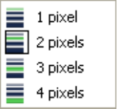
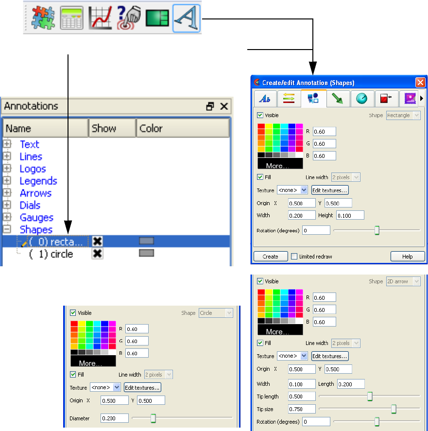
5.2 Shape Annotation
EnSight 10.2 User Manual 5-159
5.2.3 Shape Annotation
The annotation create/edit icon opens the annotation Feature Panel with the last tab
selected displayed. Shapes are often used as background for other annotations, to point to
other annotation information, and used as a panel to display actual experiment footage.
Create Clicking the Create button creates a shape annotation of the type selected in the "Shape"
option menu. The new shape displays in the annotations panel and in the graphics
window. This shape can then be modified simply by changing any of the attributes or by
manipulation in the graphics window.
Attributes common to all shapes:
Figure 5-92
Shape Annotation Feature Panel (Rectangles, 2D arrows, Circles
Edit specific shapes by double clicking or right-click on item
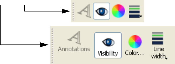
5.2 Shape Annotation
5-160 EnSight 10.2 User Manual
Visible Toggles shape visibility ON/OFF.
Shape Allows selection of the type of 2D shape that twill be created when the Create button is
selected.
RGB Color of shape.
Fill Toggles whether shape will be filled or just an outline.
Line width Controls the outline width in pixels
Origin XY Fields for setting the center of rectangles or spheres, or tip of arrows in normalized
coordinates - range 0 to 1.
Texture Allows specifying a texture to apply to the rectangle. Textures can be video and this
method allows actual video to be placed in the scene.
Edit textures... Click to display the texture dialog which allows adding more textures and modification
of texture attributes.
Attributes specific to Rectangles:
Width/Height Fields for setting the width and height of a rectangle shape in normalized coordinates -
range 0 to 1.
Rotation (degrees) Field and slider for rotation in degrees - range -360 to 360.
Attributes specific to 2D arrows:
Width/Length Fields for setting the width and length of a shape in normalized coordinates - range 0 to
1.
Tip: Length/Size Fields and sliders for setting the arrow tip length and size.
Rotation (degrees) Field and slider for rotation in degrees - range -360 to 360.
Attributes specific to Circles:
Diameter Field and slider for setting the diameter of a circle shape in normalized coordinates -
range 0 to 1.
Quick Action Icons
for Shapes
When a shape annotation is selected, the following Quick Action Icons are available in
the tool ribbon:
Visibility Turn visibility of selected shape ON or OFF
With and without icon labels
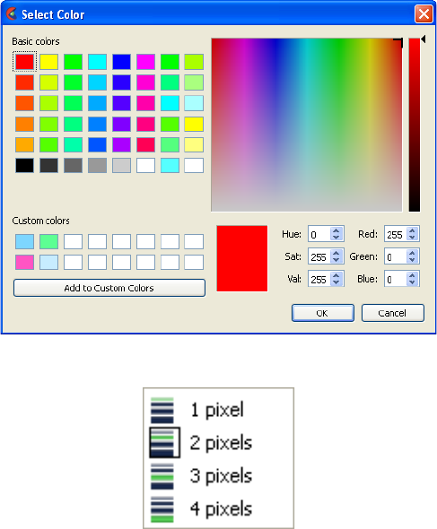
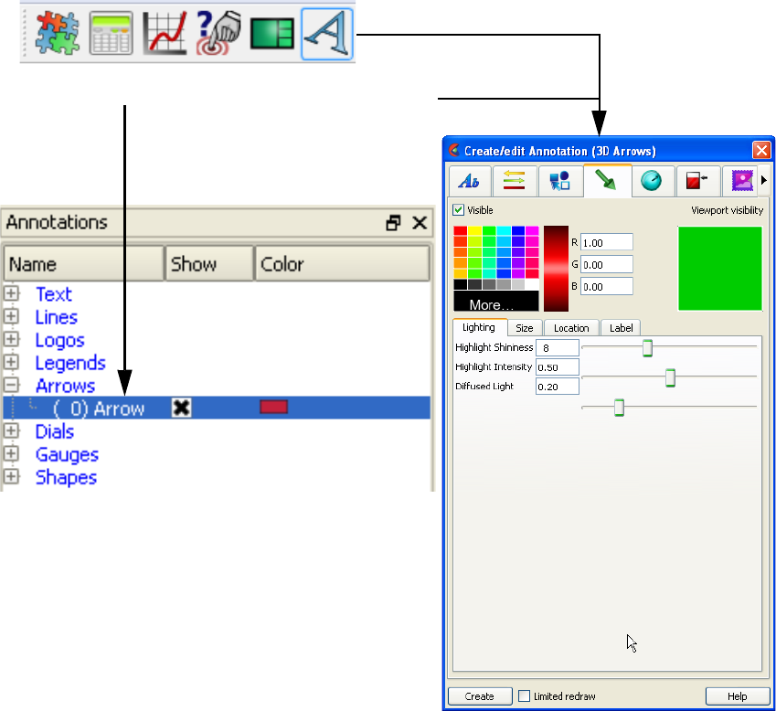
5.2 3D Arrow Annotation
5-162 EnSight 10.2 User Manual
5.2.4 3D Arrow Annotation
The annotation create/edit icon opens the annotation Feature Panel with the last tab
selected displayed. 3D arrows can be used to label areas of interest by attaching their
origin to an XYZ location, a probe query, a force, or a moment. The origin can be used to
locate specific nodes or elements interactively by snapping it to either of these. Snapping
the origin will not cause the annotation to follow the node or element however. To follow
the node or element, first create a probe query by node or element and then tie the 3D
arrow to the probe query.
Create Clicking the Create button creates a 3D arrow annotation. The new 3D arrow displays in
the annotations panel and in the graphics window. This 3D arrow can then be modified
simply by changing any of the attributes or by manipulation in the graphics window.
Visible Toggles arrow visibility ON/OFF.
Viewport visibility Toggles the visibility of the 3D arrow(s) in the viewport. Clicking on the viewport
toggles the visibility. Green indicates visible.
RGB Color of Line
Figure 5-93
3D Arrow Annotation Feature Panel
Edit specific shapes by double clicking or right-click on item
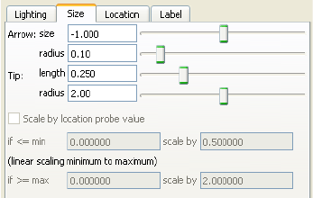
5.2 3D Arrow Annotation
EnSight 10.2 User Manual 5-163
Lighting Tab:
Highlight Shininess Shininess factor. You can think of the shininess factor in terms of how smooth the
surface is. The larger the shininess factor, the smoother the object. A value of 0
corresponds to a dull finish and larger values correspond to a more shiny finish. To
change, use the slider.
Highlight Intensity Highlight intensity (the amount of white light contained in the color of the arrow which
is reflected back to the observer). Highlighting gives the arrow a more realistic
appearance and reveals the shine of the surface. To change, use the slider. Will have no
effect if Highlight Shininess parameter is zero.
Diffused Light Diffusion (minimum brightness or amount of light that the arrow reflects). (Some
applications refer to this as ambient light.) The arrow will reflect no light if value is 0.0.
If value is 1.0, no lighting effects will be imposed and the arrow will reflect all light and
be shown at full color intensity at every point. To change, use the slider.
Size Tab:
Arrow: size Set the length of the arrow in global units.
radius Set the radius of the arrow as a percentage of the size.
Tip: length Set the length of the arrow tip as a percentage of the arrow size.
radius Set the radius of the arrow tip as a percentage of the arrow size.
Scale by location
probe/force/moment
value
(depends on which location method is used)
low value if below this value, scale by low scale factor
low value scale
factor
the scale factor to use if below the low value
high value if above this value, scale by high scale factor
high value scale
factor
the scale factor to use if above the high value
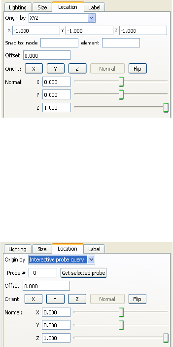
5.2 3D Arrow Annotation
5-164 EnSight 10.2 User Manual
Location Tab:
Origin by Interactive probe
query
Location set via the probe query capability
XYZ Location set by x,y,z coordinates
One or more forces Location set by external force vector glyph
One or more
moments
Location set by external moment vector glyph
If by Interactive
probe query:
Probe # The probe to use.
Offset This field specifies the distance away from the Arrow Location to display the arrow(s).
A positive value moves the arrow(s) in the opposite direction that the arrow is pointing
along the arrow axis.
Orient: X, Y, Z Orients the arrow direction parallel to the X, Y, or Z axis,
respectively.
Normal Orients the arrow normal to a surface. This is only available if
the Arrow Location has been picked on a 2D surface (see
below).
Flip Flips the arrow 180 degrees.
Normal X, Y, Z Rotates the arrow axis about the X, Y, or Z axis.
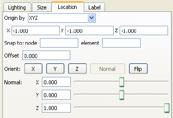
5.2 3D Arrow Annotation
EnSight 10.2 User Manual 5-165
If byXYZ:
X, Y, Z X,Y,Z - location of the arrow tip.
Snap to: node Enter the Node ID and press Enter and the arrow tip will be
located at the coordinates of this Node. This field will set the
Arrow Location X, Y, and Z values and is not used
subsequently. That is, the arrow location is specified by the X,
Y, and Z location and cannot be tied to a particular node
number as the node changes location due to transient data, etc.
element Enter the Element ID and press Return and the arrow tip will be
located at the centroid coordinates of this Element. This field
will set the Arrow Location X, Y, and Z values and is not used
subsequently. That is, the arrow location is specified by the X,
Y, and Z location and cannot be tied to a particular node
number as the node changes location due to transient data, etc.
Offset This field specifies the distance away from the Arrow Location to display the arrow(s).
A positive value moves the arrow(s) in the opposite direction that the arrow is pointing
along the arrow axis.
Orient: X, Y, Z Orients the arrow direction parallel to the X, Y, or Z axis,
respectively.
Normal Orients the arrow normal to a surface. This is only available if
the Arrow Location has been picked on a 2D surface (see
below).
Flip Flips the arrow 180 degrees.
Normal X, Y, Z Rotates the arrow axis about the X, Y, or Z axis.
If by one or more
forces:
Offset This field specifies the distance away from the Arrow Location to display the arrow(s).
A positive value moves the arrow(s) in the opposite direction that the arrow is pointing
along the arrow axis.
Selection list Description of loaded force vector glyphs from which to choose.
If by one or more
moments:
Offset This field specifies the distance away from the Arrow Location to display the arrow(s).
A positive value moves the arrow(s) in the opposite direction that the arrow is pointing
along the arrow axis.
Selection list Description of loaded moment vector glyphs from which to choose.
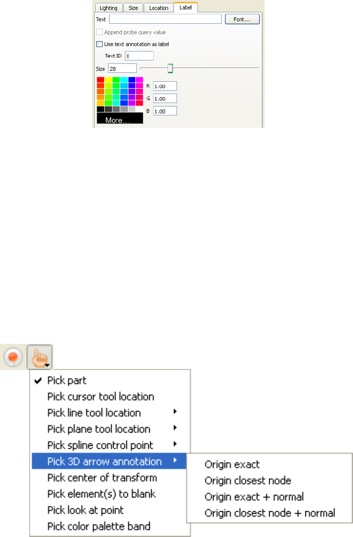
5.2 3D Arrow Annotation
5-166 EnSight 10.2 User Manual
Label Tab:
Text Enter the label to be displayed on the 3D arrow. Field is not used if the "Use text
annotation as label" toggle is on.
Font Pick the font for the label text.
Append probe
query value
If the Origin (Location tab) of the 3D arrow is set to "Interactive probe query" the probe
value can be appended onto the label.
Use text
annotation as label
A text annotation can be used as the 3D label. Specify the Text ID number in the field.
Size Size of the font used as the label
RGB Color for the label.
Picking the arrow location is accomplished using the pick icon below the graphics screen. Once your
pick method is chosen, move the cursor to the location you wish to pick and enter the 'p' key.
Origin exact Locate arrow tip at cursor
Origin closest node Snap arrow tip to closest node to cursor
Origin exact + normal Locate arrow tip at cursor & normal to surface
Origin closest node +
normal
Snap arrow tip to closest node to cursor &
normal to surface
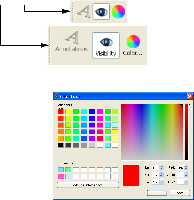
5.2 3D Arrow Annotation
EnSight 10.2 User Manual 5-167
Quick Action Icons
for 3D Arrows
When a 3D arrow annotation is selected, the following Quick Action Icons are available
in the tool ribbon:
Visibility Turn visibility of selected arrow ON or OFF
Color... Control color of selected arrow in color dialog that comes up.
With and without icon labels
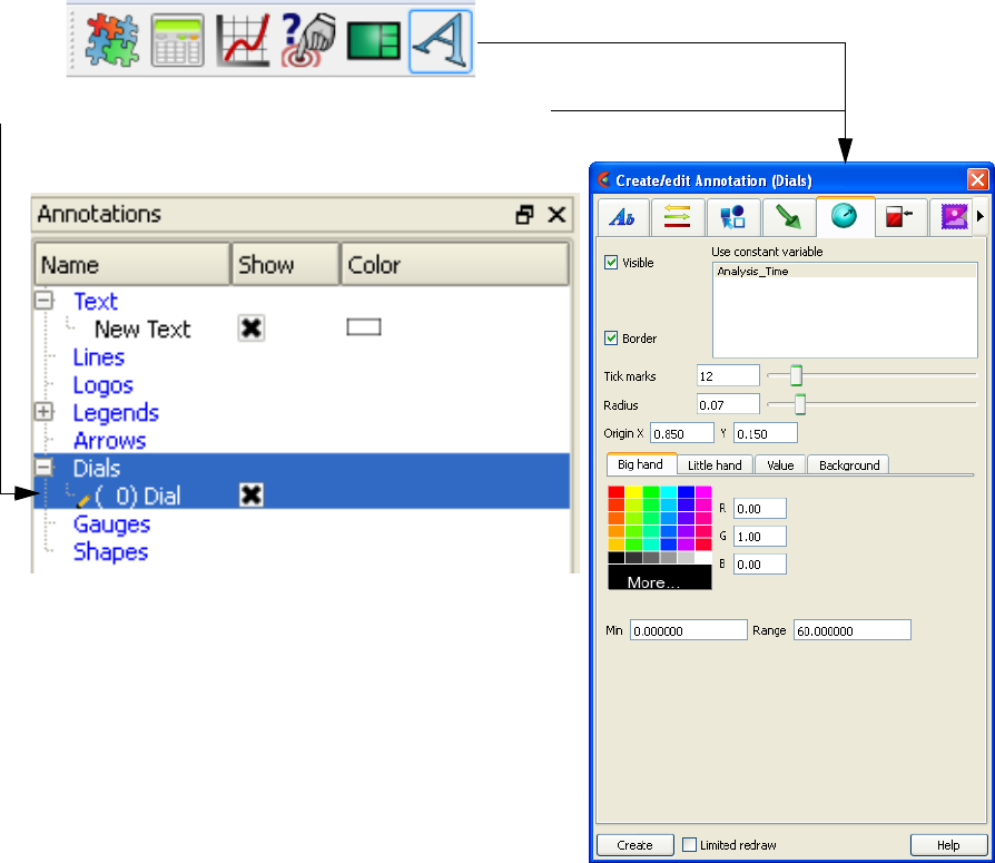
5.2 Dial Annotation
5-168 EnSight 10.2 User Manual
5.2.5 Dial Annotation
The annotation create/edit icon opens the annotation Feature Panel with the last tab
selected displayed. Dials can be used to show the current value of a constant variable in a
chosen range. In order to use this feature, you must have one or more constant variables.
Create Clicking the Create button creates a dial annotation using the constant variable selected.
The dial displays in the annotations panel and in the graphics window. This dial can then
be modified simply by changing any of the attributes or by manipulation in the graphics
window.
Visible Toggles dial visibility ON/OFF.
Use constant
variable
List of available constant variables.
Border Toggles border for the dial ON/OFF.
Tick marks Field and slider to control the number of tick marks around the dial.
Radius Field and slider to control the radius of the dial.
Origin Location of center of the dial in normalized X and Y coordinates.
Figure 5-94
Dial Annotation Feature Panel
Edit specific dials by double clicking or right-click on item
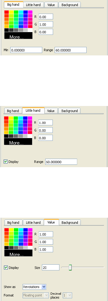
5.2 Dial Annotation
EnSight 10.2 User Manual 5-169
Big hand Tab:
RGB Color of the big hand on the dial.
Min Min value of the big hand on the dial.
Range Range for the big hand on the dial.
Little hand Tab:
RGB Color of the little hand on the dial.
Display Toggle controlling whether to show the little hand or not.
Range Range for the little hand on the dial.
Value Tab:
RGB Color of the value label in the dial.
Display Toggle controlling whether to show the value label or not.
Size Field and slider for size of the value label.
Show as Controls whether the value label is the actual value or the number of revolutions.
Format Controls the format of the displayed value label.
Decimal places Controls the number of decimal places of the displayed value label.
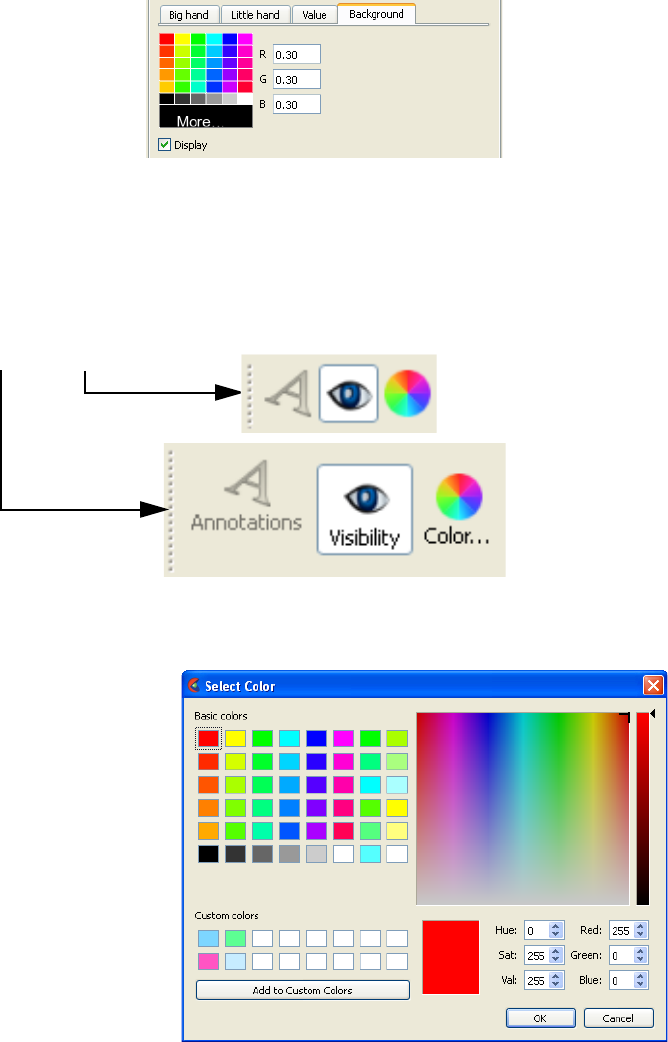
5.2 Dial Annotation
5-170 EnSight 10.2 User Manual
Background Tab:
RGB Color of the dial’s background.
Display Toggle controlling whether to have a background in the dial or not.
Quick Action Icons
for Dials
When a dial annotation is selected, the following Quick Action Icons are available in the
tool ribbon:
Visibility Turn visibility of selected dial ON or OFF
Color... Control color of selected dial in color dialog that comes up.
With and without icon labels
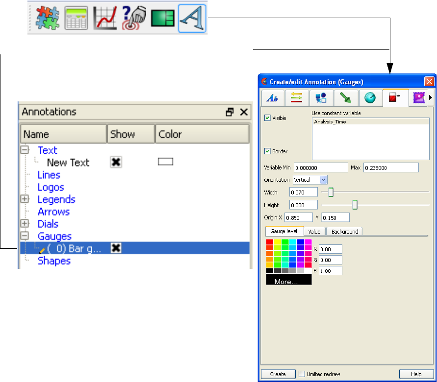
5.2 Gauge Annotation
EnSight 10.2 User Manual 5-171
5.2.6 Gauge Annotation
The annotation create/edit icon opens the annotation Feature Panel with the last tab
selected displayed. Gauges can be used to show the current value of a constant variable in
a chosen range. In order to use this feature, you must have one or more constant variables.
Create Clicking the Create button creates a gauge annotation using the constant variable
selected. The gauge displays in the annotations panel and in the graphics window. This
gauge can then be modified simply by changing any of the attributes or by manipulation
in the graphics window.
Visible Toggles gauge visibility ON/OFF.
Use constant
variable
List of available constant variables.
Border Toggles border for the gauge ON/OFF.
Variable Min/Max Fields for setting the min and max for the variable.
Orientation Pulldown for setting the gauge to be vertical or horizontal.
Width/Height Fields and sliders to control the size of the gauge.
Origin Location of the bottom left corner of the gauge in normalized X and Y coordinates.
Figure 5-95
Gauge Annotation Feature Panel
Edit specific gauges by double clicking or right-click on item
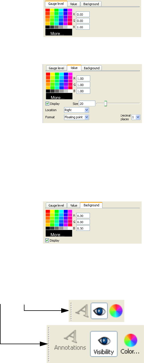
5.2 Gauge Annotation
5-172 EnSight 10.2 User Manual
Gauge level Tab:
RGB Color of the fluid in the gauge.
Value Tab:
RGB Color of the value label on the gauge.
Display Toggle controlling whether to show the value label or not.
Size Field and slider for size of the value label.
Location Controls whether the value label is to the left, right, or in the center of the gauge.
Format Controls the format of the displayed value label. (floating point or exponential)
Decimal places Controls the number of decimal places of the displayed value label.
Background Tab:
RGB Color of the gauge’s background.
Display Toggle controlling whether to have a background in the gauge or not.
Quick Action Icons
for Gauges
When a gauge annotation is selected, the following Quick Action Icons are available in
the tool ribbon:
With and without icon labels
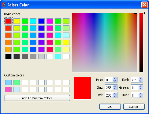
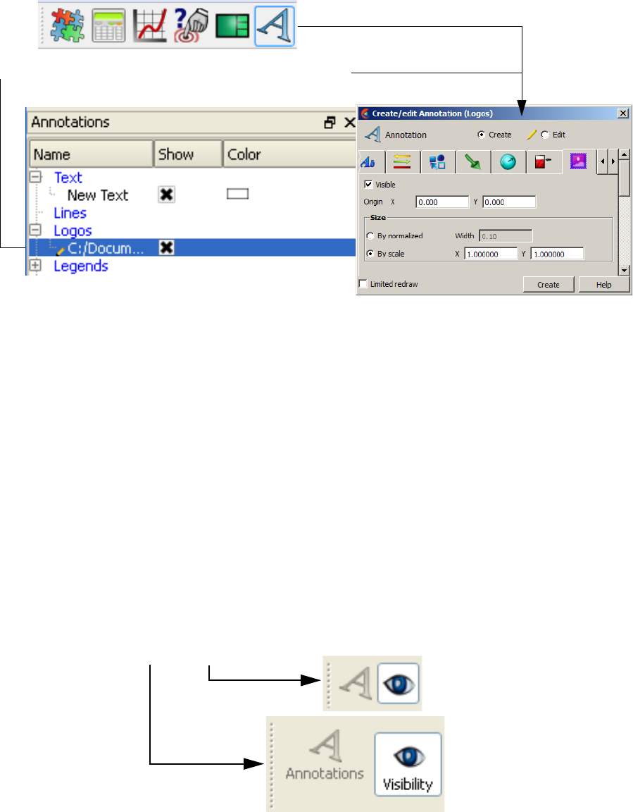
5.2 Logo Annotation
5-174 EnSight 10.2 User Manual
5.2.7 Logo Annotation
The annotation create/edit icon opens the annotation Feature Panel with the last tab
selected displayed.
Create Clicking the Create button opens a dialog to load a new logo. The new logo displays in
the annotations panel and in the graphics window. This logo can then be modified
simply by changing any of the attributes or by manipulation in the graphics window.
Visible Toggles logo visibility ON/OFF.
Origin Location of the bottom left corner of the logo in normalized X and Y coordinates.
Size By normalized width Changes the normalized width (value between 0.0 and 1.0)
which auto computes the height according to the aspect ratio of
the graphics window. This results in a logo that will
automatically scale (change size) relative to the size and aspect
ratio of the graphics window.
By scale X and Y scaling of the logo pixels. This default setting results
in the logo remaining a constant size when re-sizing the
graphics window.
Quick Action Icons
for Logos
When a logo annotation is selected, the following Quick Action Icons are available in
the tool ribbon:
Visibility Turn visibility of selected logo ON or OFF
Figure 5-96
Logo Annotation Feature Panel
Edit specific logos by double clicking or right-click on item
With and without icon labels
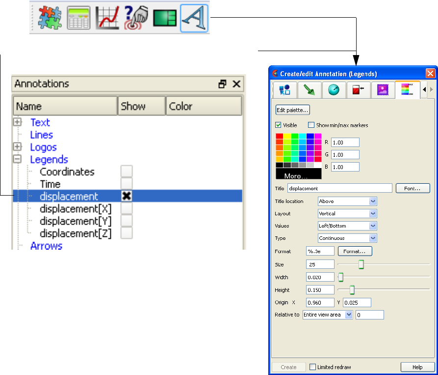
5.2 Legend Annotation
EnSight 10.2 User Manual 5-175
5.2.8 Legend Annotation
The annotation create/edit icon opens the annotation Feature Panel with the last tab
selected displayed.
Create Legends exist automatically for any variable that has been activated, therefore they
cannot be created via this dialog.
Edit Palettes Brings up the Palette Editor and allows you to edit palette attributes.
Visible Toggles Legend Visibility ON/OFF
Show min/max
markers
Toggles min/max markers on the right side of the legend color bar. These are the min/
max for the current time step.
RGB Color of the legend text.
Title Field for entering text for the legend title.
Font Brings up dialog for selecting font for legend title.
Title location Location of the Title: Above, Below or None
Layout Layout of the Legend Bar: Vertical or Horizontal.
Values Location of the legend values: Left/Bottom, Right/Top, or None.
Figure 5-97
Legend Annotation Feature Panel
Edit specific legends by double clicking or right-click on item
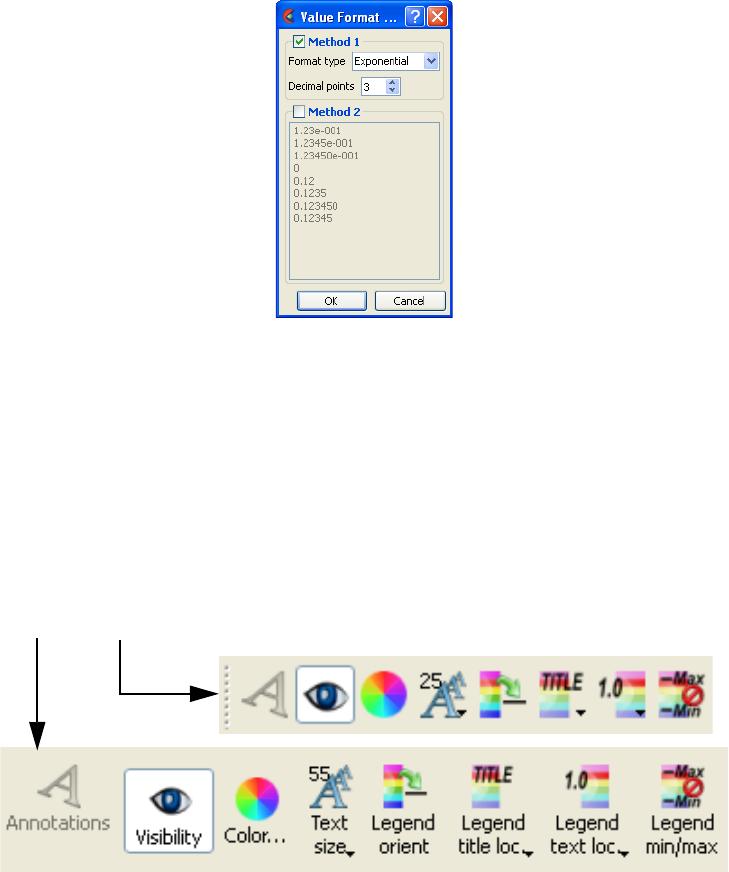
5.2 Legend Annotation
5-176 EnSight 10.2 User Manual
Type Color distribution: Continuous or Discrete.
Format Value format field, or use Format dialog:
Size Choose a Font Size
Width Legend width normalized.
Height Legend height normalized.
Origin Normalized X and Y coordinates of lower left of legend.
Relative to Ties the location values relative to the entire graphics window or a specific viewport.
Quick Action Icons
for Legends
When a legend annotation is selected, the following Quick Action Icons are available in
the tool ribbon:
Visibility Turn visibility of selected legend ON or OFF
With and without icon labels
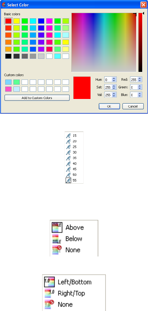
5.2 Query/Plotter
EnSight 10.2 User Manual 5-177
5.2.9 Query/Plotter
Color... Control color of selected legend in color dialog that comes up.
Text size Select common sizes for labels in selected legend.
Legend orient Toggle between vertical and horizontal orientation for selected
legend.
Legend title loc Select location of title for selected legend.
Legend text loc Select location of value labels for selected legend.
Legend min/max Toggle presence of min and max values for selected legend.

5.3 Query/Plotter
5-178 EnSight 10.2 User Manual
5.3 Query/Plotter
Overview
EnSight provides several ways to examine information about variable values.
You can, of course, visualize variable values with fringes, contours, vector arrows,
profiles, isosurfaces, etc. This section describes how to query variables
quantitatively:
Over Distance EnSight can query variables at points over distance for the following information:
• variable values inside Parts at evenly spaced points along a straight line
• variable values inside Parts at the nodes of a different 1D Part
Over Time EnSight can query variables over time for the following information:
• minimum and maximum variable values for Parts
• variable values at any number of sample times at any point inside of a Part or at
any labeled node or element.
Over-time queries can report actual variable values, or Fast Fourier Transform
(FFT) spectral values at the positive FFT frequencies.
Variable vs. EnSight can produce a scatter plot of one variable vs. another.
Va r i a b l e
Operations on EnSight can scale query values and/or combine one set of query values with
another set to produce a new set of values.
Importing EnSight can import query values from external files.
Query Candidates Only Parts with data residing on the Server host system may be queried. Thus,
Parts that reside exclusively on the Client host system (i.e. contours, particle
traces, profiles, vector arrows) may NOT be queried.
(see Section , Created Parts)
Clicking once on the Query Icon opens the Feature Panel for Query/Plots. This
editor is used to both create and edit queries and plots. Plots can be selected in the
graphics window by left click, and multiple items can be selected by holding the
control key down while left clicking. Selection is also available via the Plots/
Queries list panel. Upon selection of a query or plot, the Quick Action Icon Bar
shows attributes that can be edited. Right-click selection in both areas provide a
menu of options for editing, creating, and access to the full Feature Panel.
The Plots/Queries panel gives a user modifiable view of the plots and queries that
already exist. The toggles, in the "Show" column, turn visibility on/off, whereas
the other column items are display only. Selection is accomplished via right and
left mouse buttons. Multiple disjoint items can be selected by holding the control
key as the mouse is clicked and multiple sequential items by holding the Shift-
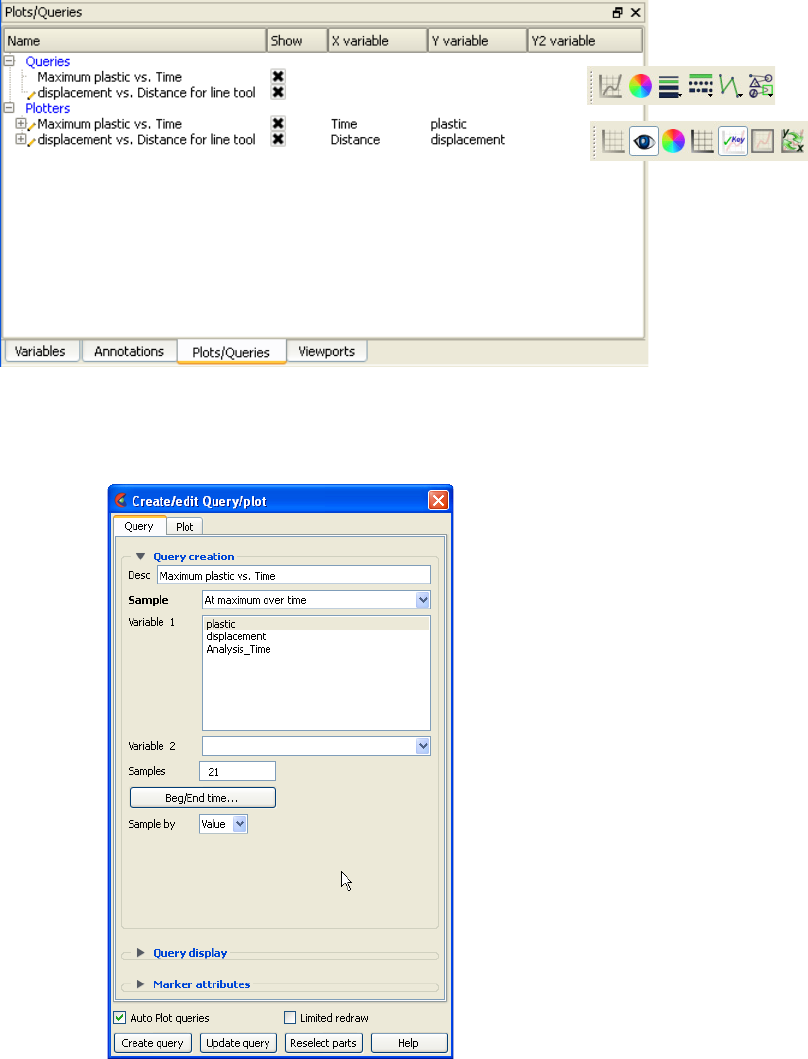
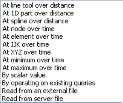
5.3 Query/Plotter
5-180 EnSight 10.2 User Manual
Query Tab
Query creation
Description This is the title for the query. You can provide it, edit it, etc. A default one is created if
you do not provide one.
Sample This menu contains the types of queries that can be created. Selecting one of these
changes the interface to display controls related to the type. These will be discussed
individually in subsequent sub-sections.
Please Select A
Query Style
is displayed until a Sample selection is made.
At Line Tool Over
Distance
queries at uniform points along the line tool.
At 1D Part Over
Distance
queries at the nodes of a 1D part.
At Spline Over
Distance
queries along an existing spline.
At Node Over
Time
queries at a node over a range of times.
At Element Over
Time
queries at an element over a range of times.
At IJK Over Time queries at an IJK location over a range of times.
At XYZ Over
Time
queries at the x, y, z location over a range of times.
At Minimum Over
Time
queries the minimum of a variable over a range of times.
At Maximum
Over Time
queries the maximum of a variable over a range of times.
By Scalar Value queries two variables at a given int(scalar variable value).
By Constant on
Part Sweep
queries a constant variable over the range, of the swept part.
By Operating on
Existing Queries
forms new query by scaling and/or combining existing ones.
Read From an
External File
imports previously saved or externally generated queries. (This can
be EnSight XY data format or MSC Dytran .ths files.)
Figure 5-100
Query Sample Types
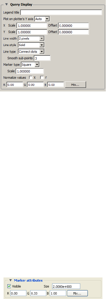
5.3 Query/Plotter
EnSight 10.2 User Manual 5-181
Read From a
Server File
imports any queries that the server knows about.
Query display
Legend title The title/name/description of the query legend. By default this
inherits the Query Creation Desc(ription). This text field allows the
query legend description to be changed.
X/Y Scale Scale factor for query values in X and or Y
X/Y Offset Offset for query values in X and or Y
Line width Line width for the query.
Line style Line style for the query, solid, dotted, or dashed.
Line type Line type for the query, none, connect the dots, or smooth.
Smooth sub-
points
When line type is smooth, this controls the smoothness.
Marker type The type of the marker along the query. None, dot, circle, triangle,
or square.
Scale Scale factor for the marker.
Normalize values
X/Y
Toggles to normalize the query values, or not.
RGB Color of the query line.
Mix... To use the color selector to set the color values.
Marker attributes
Visible Toggles the visibility of the marker showing the location for the
query. For distance queries, a sphere marker will be shown
indicating the beginning location for the query.
Size The size of the sphere marker. The value is a scale factor. Values
larger than 1.0 will scale the marker up, while values less than 1.0
(but greater than 0.0) will scale the marker down.
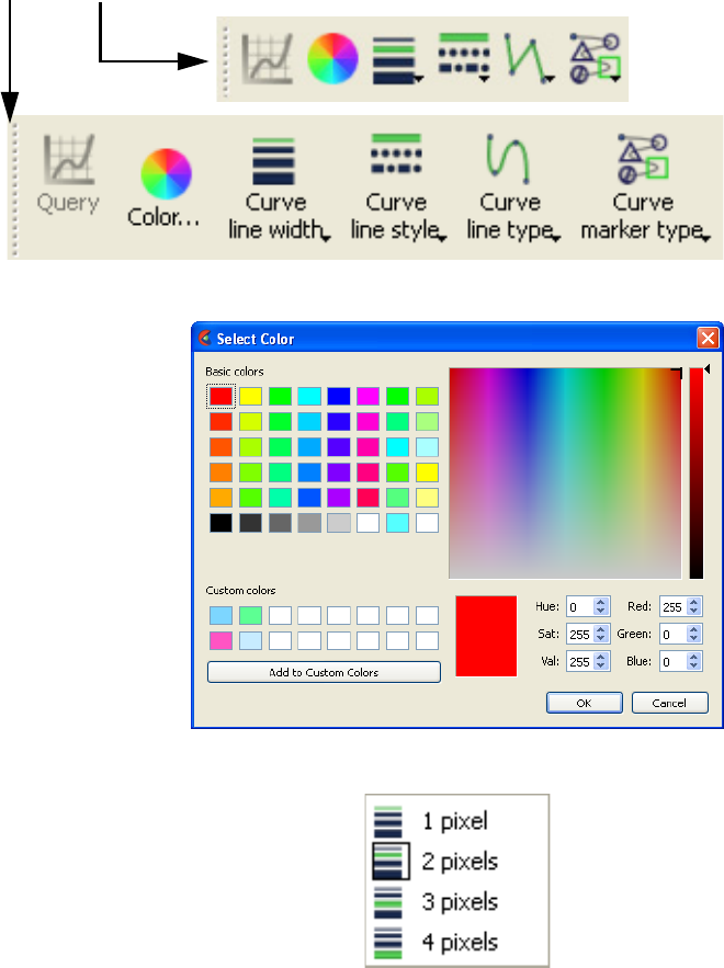
5.3 Query/Plotter
5-182 EnSight 10.2 User Manual
RGB The red, green, and blue color for the marker.
Mix... Opens the Color Selector to specify the color of the marker.
Auto Plot queries When toggled ON, newly created queries will automatically be plotted as well.
Limited redraw When toggled ON, all plots will be shown (invisible plots show translucently and will
not change).
Create Query Creates the query according to the specified options and values.
Update Query Updates the query according to the modified options and values.
Reselect parts Updates the query to use the currently selected parts in the Part list.
Quick Action Icons
for Queries
When a query is selected, the following Quick Action Icons are available in the tool
ribbon:
Color... Control color of selected query in color dialog that comes up.
Curve line
width
Select common line widths for selected curve.
With and without icon labels
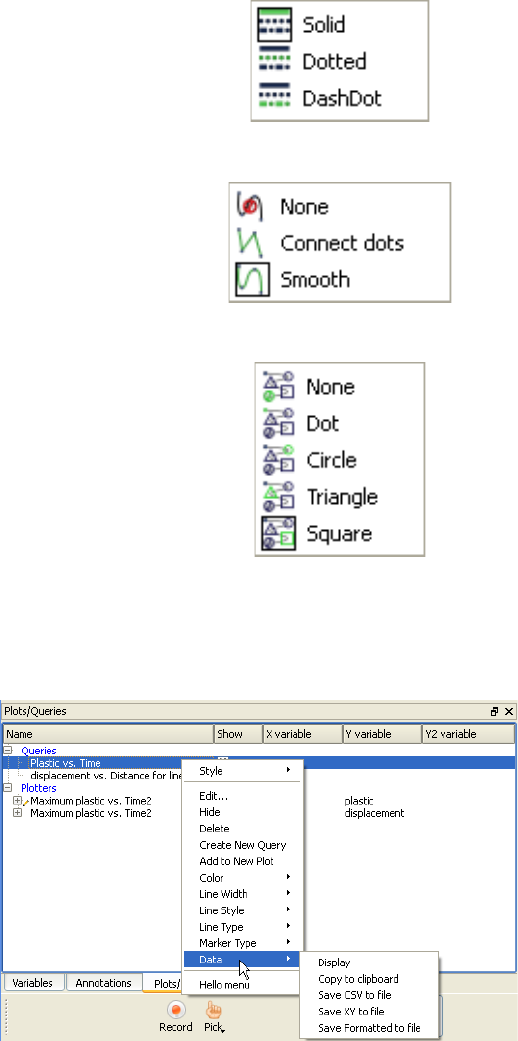
5.3 Query/Plotter
EnSight 10.2 User Manual 5-183
Curve line style Select the line style for the selected curve.
Curve line type Select the line type for the selected curve.
Curve marker
type
Select the marker type for the selected curve.
Right-click options
for Queries
Several things can be accomplished by right-clicking on a query in the Plots/
Queries panel. Many of them are duplicates of what can be done in other ways.
But a couple of them are worth noting here.
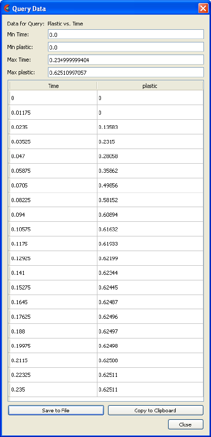
5.3 Query/Plotter
5-184 EnSight 10.2 User Manual
Data Display This will display the results (including the min and max values) of
the selected query in a window.
Copy to
Clipboard
Will copy the query data to the clipboard. (Same as hitting the Copy
to Clipboard button under Display).
Save CSV to File Opens the File Selection dialog for specification of filename to save
as a csv file.
Save XY to File Opens the File Selection dialog for specification of filename to save
in a generic format which could be used to export the information to
a different plotting system.
Save Formatted
to File
Opens the File Selection dialog for specification of filename to save
in the same format as the Display option shows.
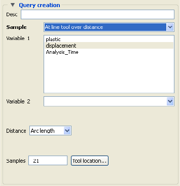
5.3 At Line Tool Over Distance
EnSight 10.2 User Manual 5-185
5.3.1 At Line Tool Over Distance
Variable: 1 A list of variables that can be chosen for the query. Choose one variable. If plotted, this
variable will be plotted along the Y-Axis.
Variable: 2 If you leave this as “None”, DISTANCE will be the default X- Axis variable. If you
choose a variable from the list, a “scatter plot” query will result, and the X-Axis will be
the variable you have chosen.
Distance A menu of choices that control the distance parameter.
Arc Length The distance along the part from the first node to each subsequent
node (i.e. the sum of the 1D element lengths).
X Arc Length The X coordinate value of each node accumulated from the start.
Y Arc Length The Y coordinate value of each node accumulated from the start
Z Arc Length The Z coordinate value of each node accumulated from the start.
From Origin The distance from the origin.
X from Origin The X distance from the origin.
Y from Origin The Y distance from the origin.
Z from Origin The Z distance from the origin.
Samples For queries over Distance using the Line Tool, this field specifies the number of equally
spaced points to query along the line.
Tool Location... Brings up the Transformation Editor (Line Tool) dialog for feedback and manipulation
of the location of the line tool.
Figure 5-101
Query/Plot Editor - At Line Tool Over Distance
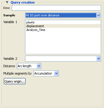
5.3 At 1D Part Over Distance
5-186 EnSight 10.2 User Manual
5.3.2 At 1D Part Over Distance
Note that the 1D part to use for the query must be selected from the Part’s list. The query
of the chosen variable will be created starting at the 1D part origin (or the lowest node ID
number, or the first node in the connectivity list) and will automatically proceed by
following the connectivity order. The order of the query cannot be changed, but it can be
reversed in the plotter, if desired.
Variable: 1 A list of variables that can be chosen for the query. Choose one variable. If plotted, this
variable will be plotted along the Y-Axis.
Variable: 2 If you leave this as “None”, DISTANCE will be the default X- Axis variable. If you
choose a variable form the list, a “scatter plot” query will result, and the X-Axis will be
the variable you have chosen.
Distance A menu of choices that control the distance parameter.
Arc Length The distance along the part from the first node to each subsequent
node (i.e. the sum of the 1D element lengths).
X Arc Length The X coordinate value of each node accumulated from the start.
Y Arc Length The Y coordinate value of each node accumulated from the start
Z Arc Length The Z coordinate value of each node accumulated from the start.
From Origin The distance from the origin.
X from Origin The X distance from the origin.
Y from Origin The Y distance from the origin.
Z from Origin The Z distance from the origin.
Multiple segments by When the selected 1D part contains more than one contiguous segment, these are
handled by:
Accumulation Each segment’s query is appended to the previous. Thus a plot of
this query will be one extended curve, but the extents of individual
segment may not be obvious.
Reset Each Each segment’s query is treated like it is independent. Thus a plot of
this query will appear as several curves.
Figure 5-102
Query/Plot Editor - At 1D Part Over Distance
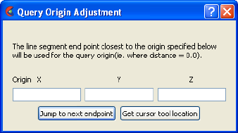
5.3 At 1D Part Over Distance
EnSight 10.2 User Manual 5-187
Query Origin... Brings up the Query Origin Adjustment dialog for feedback and manipulation of the
location of the query origin.
Orig XYZ Coordinates of the location to use for query origin determination. The endpoint closest to
the origin specified will be used as the “origin” of the query, i.e., where distance is zero.
If the 1D part is s closed loop (i.e. there are no end points), the closest point on the loop
is used as the “origin”.
Jump To Next
Endpoint
When multiple segments are present, clicking this button jumps to the beginning of the
next segment, placing that location in to the Orig XYZ fields.
Get Cursor Tool
Location
Places the current cursor tool location into the Orig XYZ fields so that point can be used
as the query origin.
Figure 5-103
Query Origin Adjustment dialog
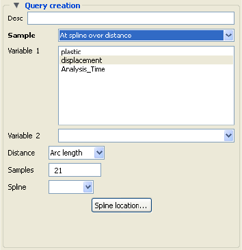
5.3 At Spline Over Distance
5-188 EnSight 10.2 User Manual
5.3.3 At Spline Over Distance
Note that the 1D part to use for the query must be selected from the Part’s list.
Variable: 1 A list of variables that can be chosen for the query. Choose one variable. If plotted, this
variable will be plotted along the Y-Axis.
Variable: 2 If you leave this as “None”, DISTANCE will be the default X- Axis variable. If you
choose a variable form the list, a “scatter plot” query will result, and the X-Axis will be
the variable you have chosen.
Distance A menu of choices that control the distance parameter.
Arc Length The distance along the part from the first node to each subsequent
node (i.e. the sum of the 1D element lengths).
X Arc Length The X coordinate value of each node accumulated from the start.
Y Arc Length The Y coordinate value of each node accumulated from the start
Z Arc Length The Z coordinate value of each node accumulated from the start.
From Origin The distance from the origin.
X from Origin The X distance from the origin.
Y from Origin The Y distance from the origin.
Z from Origin The Z distance from the origin.
Spline,
Spline location...
Pick a Spline. See Use the Spline Tool for more information on Spline Tools.
Figure 5-104
Query/Plot Editor - At Spline Over Distance
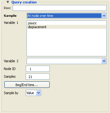
5.3 At Node Over Time
EnSight 10.2 User Manual 5-189
5.3.4 At Node Over Time
Variable: 1 A list of variables that can be chosen for the query. Pick one variable. If plotted, this
variable will be plotted along the Y-Axis.
Variable: 2 If you leave this as “None”, TIME will be the default X- Axis variable. If you choose a
variable form the list, a “scatter plot” query will result, and the X-Axis will be the
variable you have chosen.
Samples Specifies how many evenly timed moments over the specified range of time steps at
which to query (if left blank, you get a sample point at each time step). If you specify
more or fewer sample points than the number of time steps, EnSight linearly interpolates
between the adjoining time steps. If query is an FFT sampling, the number of
frequencies output will be less than or equal to the number of sample points.
Node ID Specifies a node ID.
Beg/End Time... Informs you that Begin/End time can be set in the solution time player panel.
Sample By Opens a pop-up menu for specification of how to report values for Over Time queries.
Options are:
Value reports values versus time.
FFT reports FFT spectral values versus FFT positive frequencies.
Figure 5-105
Query/Plot Editor - At Node Over Time
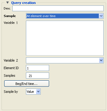
5.3 At Element Over Time
5-190 EnSight 10.2 User Manual
5.3.5 At Element Over Time
Variable: 1 A list of variables that can be chosen for the query. If plotted, this variable will be plotted
along the Y-Axis. (Note: only per_element variables can be used for this query type.)
Variable: 2 If you leave this as “None”, TIME will be the default X- Axis variable. If you choose a
variable form the list, a “scatter plot” query will result, and the X-Axis will be the
variable you have chosen.
Samples Specifies how many evenly timed moments over the specified range of time steps at
which to query (if left blank, you get a sample point at each time step). If you specify
more or fewer sample points than the number of time steps, EnSight linearly interpolates
between the adjoining time steps. If query is an FFT sampling, the number of
frequencies output will be less than or equal to the number of sample points.
Element ID Specifies an element ID.
Beg/End Time... Informs you that Begin/End time can be set in the solution time player panel.
Sample By Opens a pop-up menu for specification of how to report values for Over Time queries.
Options are:
Value reports values versus time.
FFT reports FFT spectral values versus FFT positive frequencies.
Figure 5-106
Query/Plot Editor - At Element Over Time
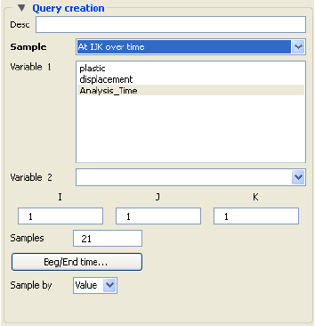
5.3 At IJK Over Time
EnSight 10.2 User Manual 5-191
5.3.6 At IJK Over Time
Variable: 1 A list of variables that can be chosen for the query. If plotted, this variable will be plotted
along the Y-Axis.
Variable: 2 If you leave this as “None”, TIME will be the default X- Axis variable. If you choose a
variable form the list, a “scatter plot” query will result, and the X-Axis will be the
variable you have chosen.
Samples Specifies how many evenly timed moments over the specified range of time steps at
which to query (if left blank, you get a sample point at each time step). If you specify
more or fewer sample points than the number of time steps, EnSight linearly interpolates
between the adjoining time steps. If query is an FFT sampling, the number of
frequencies output will be less than or equal to the number of sample points.
IJK Specifies the IJK planes of the desired location.
Beg/End Time... Informs you that Begin/End time can be set in the solution time player panel
Sample By Opens a pop-up menu for specification of how to report values for Over Time queries.
Options are:
Value reports values versus time.
FFT reports FFT spectral values versus FFT positive frequencies.
Figure 5-107
Query/Plot Editor - At IJK Over Time
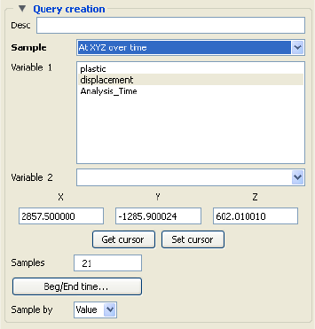
5.3 At XYZ Over Time
5-192 EnSight 10.2 User Manual
5.3.7 At XYZ Over Time
Variable: 1 A list of variables that can be chosen for the query. Choose one variable. If plotted, this
variable will be plotted along the Y-Axis.
Variable: 2 If you leave this as “None”, TIME will be the default X- Axis variable. If you choose a
variable form the list, a “scatter plot” query will result, and the X-Axis will be the
variable you have chosen.
Samples Specifies how many evenly timed moments over the specified range of time steps at
which to query (if left blank, you get a sample point at each time step). If you specify
more or fewer sample points than the number of time steps, EnSight linearly interpolates
between the adjoining time steps. If query is an FFT sampling, the number of
frequencies output will be less than or equal to the number of sample points.
Get/Set cursor Get will put the current coordinates of the cursor tool into the x, y and z fields. Set will
open up the Transformation Editor (Cursor Tool) dialog for specificationof the cursor
location. You can of course also set this location using interactive or picking methods.
Beg/End Time... Informs you that Begin/End time can be set in the solution time player panel
Sample By Opens a pop-up menu for specification of how to report values for Over Time queries.
Options are:
Value reports values versus time.
FFT reports FFT spectral values versus FFT positive frequencies.
Figure 5-108
Query/Plot Editor - At Cursor Over Time
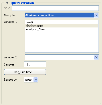
5.3 At Minimum Over Time
EnSight 10.2 User Manual 5-193
5.3.8 At Minimum Over Time
Variable: 1 A list of variables that can be chosen for the query. If plotted, this variable will be plotted
along the Y-Axis. Note that you can choose more than one variable in the list which is a
time-saving feature producing multiple queries at once as EnSight marches through time.
Variable: 2 If you leave this as “None”, TIME will be the default X- Axis variable. If you choose a
variable form the list, a “scatter plot” query will result, and the X-Axis will be the
variable you have chosen.
Samples Specifies how many evenly timed moments over the specified range of time steps at
which to query (if left blank, you get a sample point at each time step). If you specify
more or fewer sample points than the number of time steps, EnSight linearly interpolates
between the adjoining time steps. If query is an FFT sampling, the number of
frequencies output will be less than or equal to the number of sample points.
Beg/End Time... Informs you that Begin/End time can be set in the solution time player panel
Sample By Opens a pop-up menu for specification of how to report values for Over Time queries.
Options are:
Value reports values versus time.
FFT reports FFT spectral values versus FFT positive frequencies.
Figure 5-109
Query/Plot Editor - At Minimum Over Time
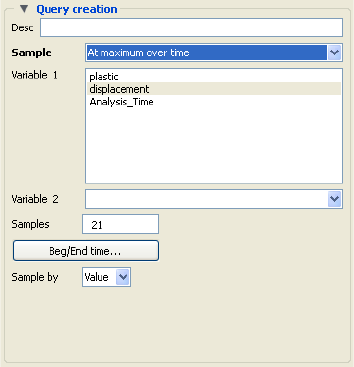
5.3 At Maximum Over Time
5-194 EnSight 10.2 User Manual
5.3.9 At Maximum Over Time
Variable: 1 A list of variables that can be chosen for the query. If plotted, this variable will be plotted
along the Y-Axis. Note that you can choose more than one variable in the list which is a
time-saving feature producing multiple queries at once as EnSight marches through time.
Variable: 2 If you leave this as “None”, TIME will be the default X- Axis variable. If you choose a
variable form the list, a “scatter plot” query will result, and the X-Axis will be the
variable you have chosen.
Samples Specifies how many evenly timed moments over the specified range of time steps at
which to query (if left blank, you get a sample point at each time step). If you specify
more or fewer sample points than the number of time steps, EnSight linearly interpolates
between the adjoining time steps. If query is an FFT sampling, the number of
frequencies output will be less than or equal to the number of sample points.
Beg/End Time... Informs you that Begin/End time can be set in the solution time player panel
Sample By Opens a pop-up menu for specification of how to report values for Over Time queries.
Options are:
Value reports values versus time.
FFT reports FFT spectral values versus FFT positive frequencies.
Figure 5-110
Query/Plot Editor - At Maximum Over Time
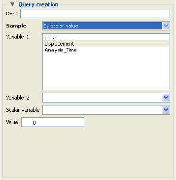
5.3 By Scalar Value
EnSight 10.2 User Manual 5-195
5.3.10 By Scalar Value
Variable: 1 A list of variables that can be chosen for the query. Choose one variable. If plotted, this
variable will be plotted along the Y-Axis. This is best plotted as a scatter plot.
Variable: 2 A list of variables that can be chosen for the query. If plotted, this variable will be plotted
along the X-Axis. This is best plotted as a scatter plot.
Scalar variable The scalar variable to use.
Value The value of the Scalar variable to use. Note that this does an integer compare of the
value you enter here to the integer of the variable. If int(value you enter) exactly equals
the int(variable value) then the Variable1, Variable 2 pair is selected. For example, if you
enter a Value of 0.0, then values of the Scalar variable from -0.5 to 0.5 will match.
Figure 5-111
Query/Plot Editor - By scalar value
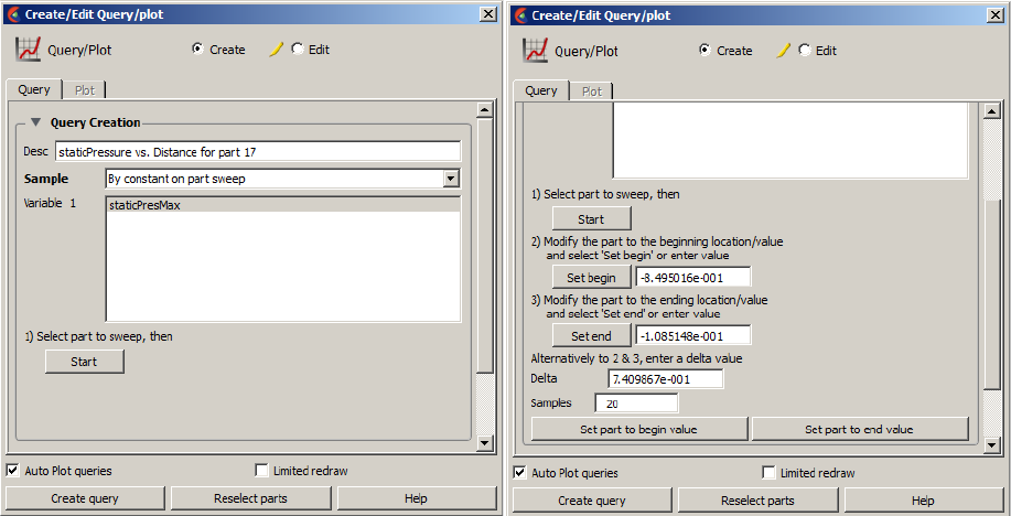
5.3 By Constant on Part Sweep
5-196 EnSight 10.2 User Manual
5.3.11 By Constant on Part Sweep
Variable: 1 A list of constant variables that can be chosen for the query. If plotted, this variable will
be plotted along the Y-Axis. Note that you can only choose one variable at time.
1) Select part to
sweep, then [Start]
Instructions to make sure you first select a part that has Variable 1. then clicking [Start]
lists the rest of the instructions 2-3, the Delta, Samples, etc.
2) Modify the part to
the beginning
location/value and
select [Set begin] or
enter value
Set Begin Select after moving the sweep part to the beginning location
- or - Enter the value of the beginning part location and click Enter.
3) Modify the part to
the ending location/
value and select
[Set end] or enter
value
Set end Select after moving sweep part to the ending location
- or - Enter the value of the ending part location and click Enter.
Alternatively to 2 & 3,
enter a delta value
Delta The delta value by which the part will increment(+) or decrement(-)
for the number of Samples
Samples Specifies how many evenly sampled increments over the range of the part location at
which to query. The number of Samples will either proceed:
Set parts to begin
value
Sets the parts at the begin value (useful for increment(+))
Set parts to end value Sets the parts at the end value (useful for decrement(-))
Figure 5-112
Query/Plot Editor - By Constant on Part Sweep
Before selecting Start After selecting Start
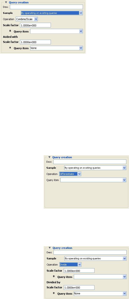
5.3 By Operating on Existing Queries
EnSight 10.2 User Manual 5-197
5.3.12 By Operating on Existing Queries
Operation: Combine/
Scale
A single query can be scaled, or two <scaled> queries can be combined.
Scale Factor Scale factor for the Query Item selected. The values of the selected
query will be multiplied by this factor either before it is added to the
second query or before the new query is created (if only operating
on a single query).
Query Item The existing query item(s) to operate on. A new query will be create
consisting of scaled values one query, or the scaled, algebraic sum of
two queries.
Operation:
Differentiate
You can differentiate an existing query using Romberg extrapolation on five central,
divided differences that minimize roundoff and truncation errors.
Query Item The existing query item(s) to operate on. A new query will be create
consisting of the differentiated values of the chosen query.
Operation: Divide One query can be divided by another.
Figure 5-113
Query/Plot Editor - By Operating On Existing Queries
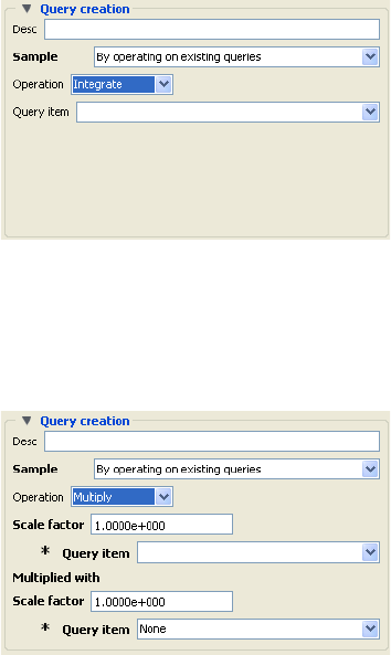
5.3 By Operating on Existing Queries
5-198 EnSight 10.2 User Manual
Scale Factor Scale factor for the Query Item selected. The values of the selected
query will be multiplied by this factor before it is divided by the
second query.
Query Item The existing query item(s) to operate on. A new query will be create
consisting of the scaled, division of two queries.
Operation: Integrate You can integrate an existing query using the Trapezoidal-Romberg method.
Query Item The existing query item(s) to operate on. A new query will be create
consisting of the integration of the values of the chosen query.
Operation: Multiply One query can be multiplied by another.
Scale Factor Scale factor for the Query Item selected. The values of the selected
query will be multiplied by this factor before it is multiplied by the
second query.
Query Item The existing query item(s) to operate on. A new query will be create
consisting of the scaled, multiplication of two queries.
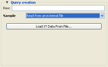
5.3 Read From an External File
EnSight 10.2 User Manual 5-199
5.3.13 Read From an External File
Load XY Data From
File
Opens the File Selection dialog from which a previously saved or externally generated
query can be retrieved. EnSight’s XY data format or MSC Dytran .ths files can be read.
Figure 5-114
Query/Plot Editor - Read From An External File
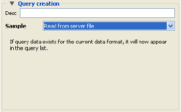
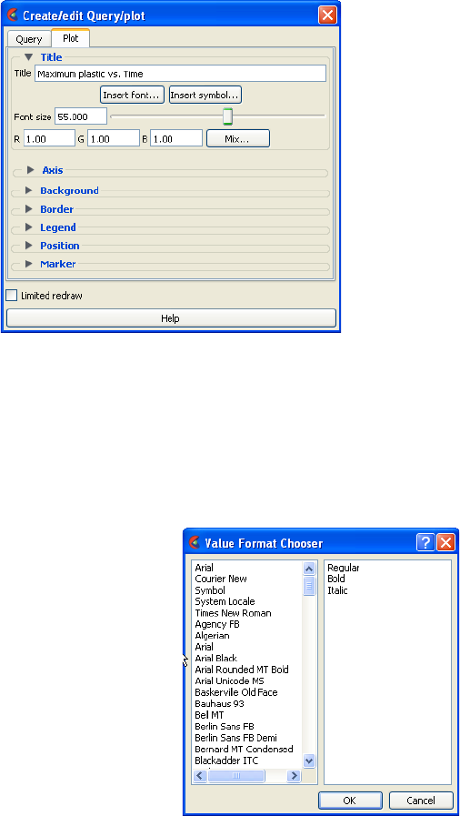
5.3 Plotters
EnSight 10.2 User Manual 5-201
5.3.15 Plotters
Plot Tab .
Title section
Title This field allows you to edit the existing plotter title.
Insert Font... This button brings up a dialog allowing you to pick the desired font. It inserts codes into
the text string at the location of the cursor.
Figure 5-116
Feature Panel - Plot
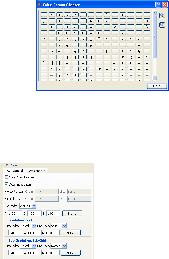
5.3 Plotters
5-202 EnSight 10.2 User Manual
Insert Symbol... This button brings up a matrix of symbols to pick from to allow you to insert symbols
into the plotter title.
Font Size This field allows you to specify the title text size.
RGB Mix... Color for the Title text may be specified using either the RBG fields or the Color
Selector dialog which is opened by clicking the Mix... button.
Axis section
Axis General Tab Clicking the Axis General tab causes the dialog to configure itself for General Plotter
Axis editing.
Swap X and Y
axes
Toggle on to swap the x and y axes.
Auto layout axes Toggle on to automatically layout the origin and size of the axes in the plotter region.
Horizontal/Vertical
axis Origin and
Size
If Auto layout not being used, you can control the origin and scale of the axes in the
plotter region. Values range from 0.0 to 1.0 and resulting distances are measured from
the left side (or bottom) of the Plotter.
Both Axes Line Width A pulldown menu for the specification of the desired line width (1 to
4 Pixels) for Plotter axes.
RGB Mix... Color for the axes may be specified using either the RBG fields or
the Color Selector dialog which is opened by clicking the Mix...
button.
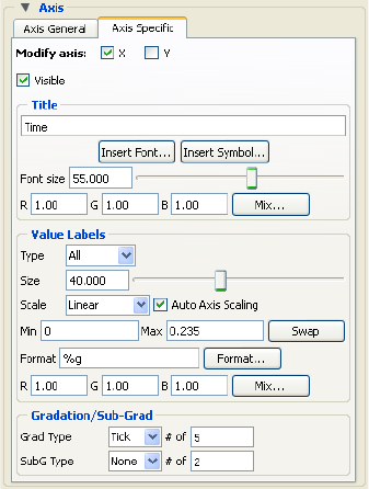
5.3 Plotters
EnSight 10.2 User Manual 5-203
Gradation/Grid Line Width A pulldown menu for the specification of the desired width (1-4
Pixels) for Gradation Lines or Ticks.
Line Style A pulldown menu for the specification of the style of line (Solid,
Dotted, or Dashed) desired for gradations. (The lines are normally
not visible and so this specification is only valid if Grad Type has
been selected to Grid in the X-Axis and/or Y-Axis configuration of
the Axis Specific Attributes dialog.)
RGB Mix... Color for the Gradation Lines or Ticks may be specified using either
the RBG fields or the Color Selector dialog which is opened by
clicking the Mix... button.
Sub-Gradation/Sub-Grid
Line Width A pulldown menu for the specification of the desired line width (1-4
Pixels) for Sub-Gradation Lines or Ticks (those between the
Gradation Lines or Ticks).
Line Style A pulldown menu for the specification of the style of line (Solid,
Dotted, or Dashed) desired for sub-gradations. (The lines are
normally not visible and so this specification is only valid if SubG
Type has been selected to Grid in the X-Axis and/or Y-Axis
configuration of the Axis Specific Attributes dialog.)
RGB Mix... Color for the Sub-Gradation Lines or Ticks may be specified using
either the RBG fields or the Color Selector dialog which is opened
by clicking the Mix... button
Axis Specific Tab Clicking the Axis Specific Axis tab causes the dialog to configure itself for editing of
Attributes specific to either the X or the Y Axis. If X-Axis toggle has been clicked, the
dialog will affect the X-Axis attributes only. Likewise for Y-Axis.
Visible Toggle Toggles on/off the visibility of the X (or Y) Axis line.
Title Title This field allows you to edit the existing X (or Y) Axis title.
Font Size This field allows you to specify the title text size.
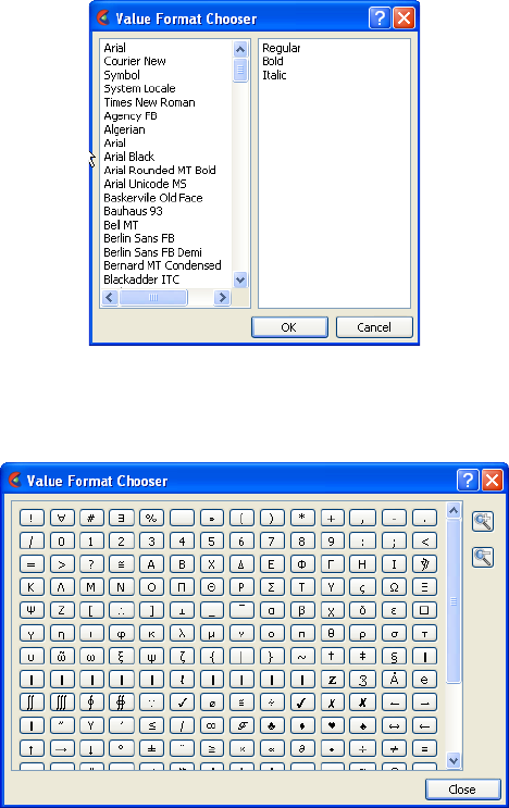
5.3 Plotters
5-204 EnSight 10.2 User Manual
Insert Font... This button brings up a dialog allowing you to pick the desired font.
It inserts codes into the text string at the location of the cursor.
Insert Symbol... This button brings up a matrix of symbols to pick from to allow you
to insert symbols into the plotter title.
RGB Mix... Color for the Title text may be specified using either the RBG fields
or the Color Selector dialog which is opened by clicking the Mix...
button.
Value Labels Type Opens a pop-up menu for selection of desired number (None, All, or
Beg/End) of X (or Y) Axis labels.
Size This field allows you to specify the size of X (or Y) Axis labels
Scale This field allows you to specify a linear or log10 scale for the Axis.
Min This field contains the minimum value of the X (or Y) Axis. If Auto
Axis Scaling is on, it is only an approximation to the value which
will be used.
Max This field contains the maximum value of the X (or Y) Axis. If Auto
Axis Scaling is on, it is only an approximation to the value which
will be used.
Format This field specifies the format used to display the X (or Y) Axis.
Any C language printf format is valid in this field.
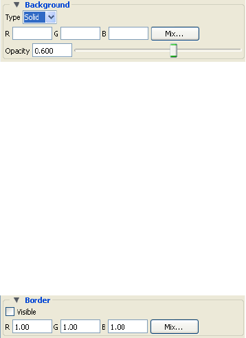
5.3 Plotters
EnSight 10.2 User Manual 5-205
Format... This button will open the Format dialog which allows you to select a
pre-defined format.
Gradation/Sub-Grad
Grad Type # of Opens a pop-up menu for selection of desired marker (None, Grid,
or Tick) for major gradations. # of field specifies the number of
major gradations you wish along the X (or Y) Axis. If Auto Axis
Scaling is on, it is only an approximation to the value which will be
used.
SubG Type # of Opens a pop-up menu for selection of desired marker (None, Grid,
or Tick) for sub gradations (between the major gradations. # of field
specifies the number of sub gradations you wish between each major
gradation along the X (or Y) Axis.
Background
section
Clicking the Background section causes the dialog to configure itself for Plotter
Background editing.
Type Opens a pop-up menu for the specification of plotter background color. Choices are:
None no background (the color of the Graphics Window or the viewport
underneath will show through the Plotter.
Solid allows a solid color to be specified for the Plotter Background
RGB Mix... Color for the Plotter background may be specified using either the RBG fields or the
Color Selector dialog which is opened by clicking the Mix... button.
Opacity Field or slider to set the opacity of the background.
Border section Clicking the Border section causes the dialog to configure itself for Plotter Border
editing.
Visible Toggle Toggles on/off the visibility in the other five Modes of the Border for the selected
Plotters.
RGB Mix... Color for the plotter border may be specified using either the RBG fields or the Color
Selector dialog which is opened by clicking the Mix... button. Note that the border color
is not shown while the plotter is selected - while selected the border is shown in green.
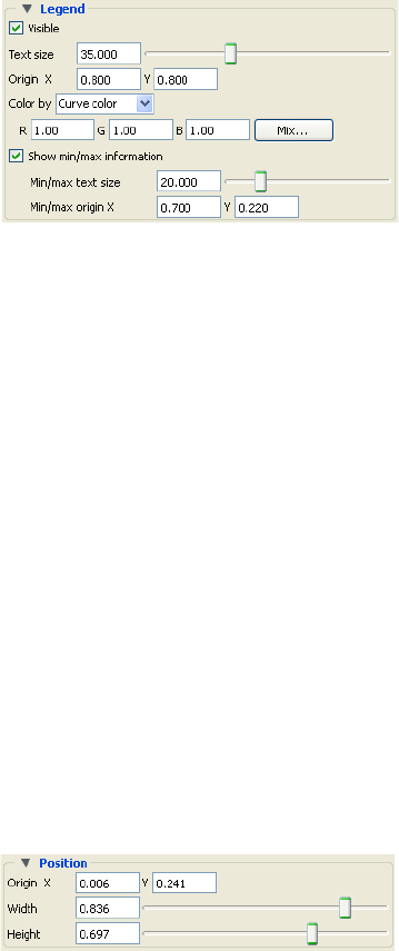
5.3 Plotters
5-206 EnSight 10.2 User Manual
Legend section Clicking the Legend section causes the dialog to configure itself for Plotter Legend
editing. The legend shows a line of the appropriate color, width, and marker next to the
name of the curve plotted using this line style.
Visible Toggle Toggles on/off the visibility of the legend for the selected Plotters.
Text Size This field specifies the desired size of the Legend text.
Origin X Y These fields specify the location of the Legend within a Plotter’s border. Values range
from 0.0 to 1.0 and resulting distances are measured from the Border origin (lower left
corner). These fields provide an alternative to interactively positioning the plotter
Legend
Color by Can choose to color by the color specified for the query curve, or by specifying the color
here.
RGB Mix... Color for the Legend text may be specified using either the RBG fields or the Color
Selector dialog which is opened by clicking the Mix... button.
Show min/max
information
Toggle on to have min and max text information added to the plot.
Min/max text size If displaying min/max information, can specify test size with the
field or the slider.
Min/max origin
XY
If displaying min/max information, can specify the xy normalized
origin location.
Position section Clicking the Position section causes the dialog to configure itself for Plotter Position.
Origin X Y These fields specify the location of the selected Plotter within the Graphics Window.
Values range from 0.0 to 1.0 and resulting distances are measured from the Graphics
Window origin (lower left corner). These fields provide an alternative to interactively
positioning the plotter which is done simply by clicking within the Plotter and dragging
it to the desired position.
Width, Height These fields specify the width and height of the Plotter. Resulting distances are measured
from the Border origin (lower left corner). These fields provide an alternative to
interactively resizing the plotter which is done simply by clicking on a side or corner and
dragging.
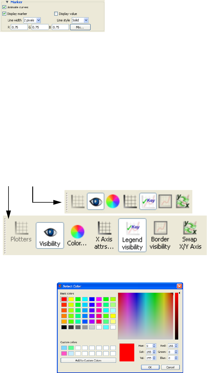
5.3 Plotters
EnSight 10.2 User Manual 5-207
Marker section This section is enabled only for plots with transient data.
Animate Curve When the solution time is changed or streamed (data loaded from disk one step after
another) or loaded in the flipbook, toggling this ON will cause the transient curve to plot
the data timestep by timestep.
Display Marker The Marker is a vertical time indicator line that appears only on a transient plot. When
the solution time is changed or streamed (data loaded from disk one step after another) or
loaded in the flipbook, toggling this ON will cause the vertical line Time Marker to
indicate the current timestep value on the plot. Click on the time indicator line and drag it
to change the time, and the time indicator line will jump to the next time value on your
plot.
Display value The value at the marker can be displayed by toggling this on.
Line Width Set the line width of the vertical time indicator line on the transient plot.
Line Style Set the line style of the vertical time indicator line on the transient plot.
RGB Set the color (RGB values) of the vertical time indicator line on the transient plot.
Quick Action Icons
for Plots
When a plot is selected, the following Quick Action Icons are available in the tool
ribbon:
Visibility Turn visibility of selected plot ON or OFF
Color... Control color of selected plot in color dialog that comes up.
With and without icon labels
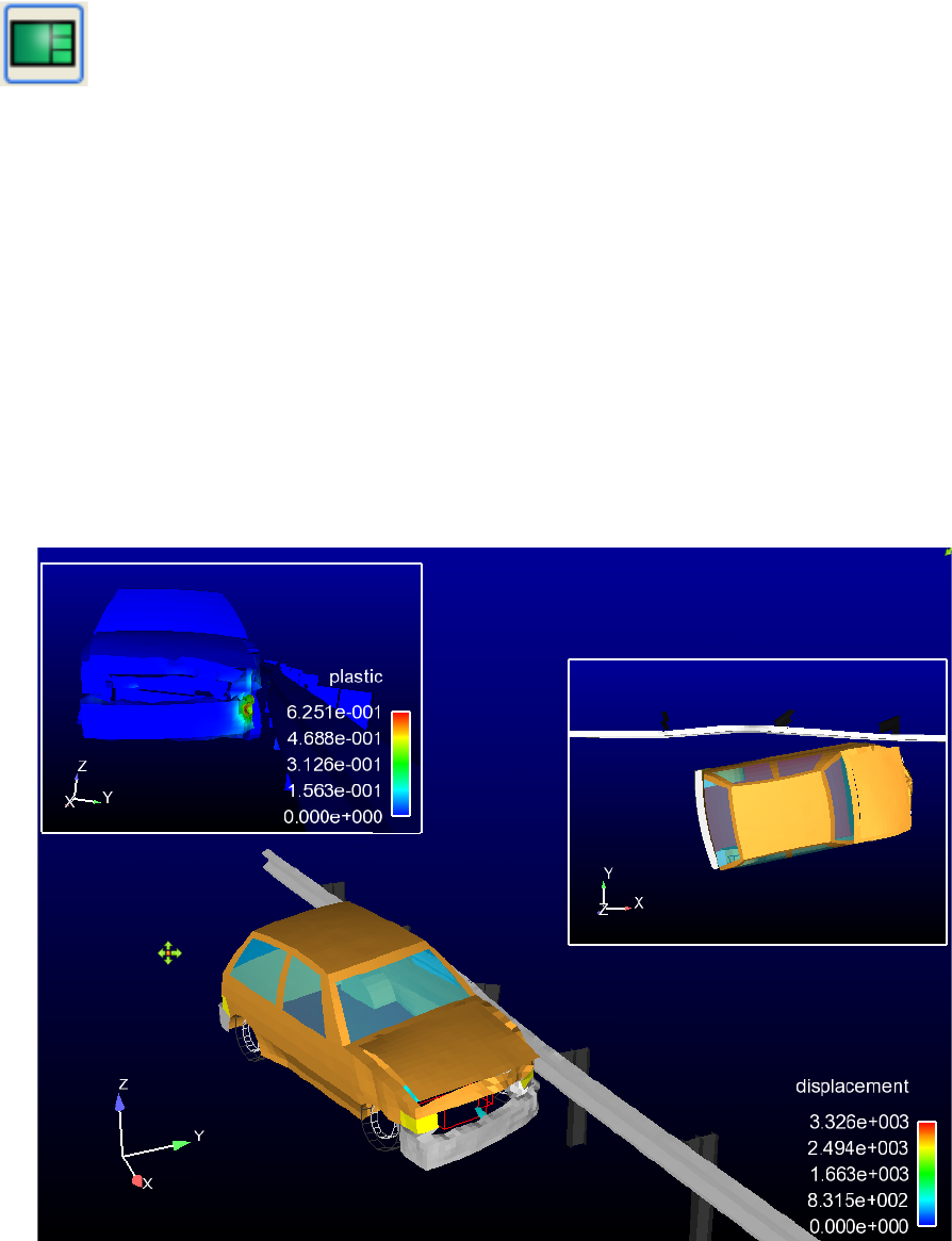
5.4 Viewports
EnSight 10.2 User Manual 5-209
5.4 Viewports
Overview
The default EnSight configuration shows one view of your model in the “main”
Graphics Window. This “initial viewport”, which covers the Graphics Window.
cannot be removed and is always used to clear (erase) the Graphics Window prior
to a redraw. You can create up to fifteen additional viewports that will overlay the
Graphics Window. These viewports can be interactively resized and relocated
within the Graphics Window using the mouse and the visibility of each Part can
be controlled on a per viewport basis. Transformations, and Z-clip location
settings can also be made independently in each viewport.
When in viewport mode, you are always modifying the viewports selected in the
Graphics Window. Selected viewports are outlined in the “selection color”, while
unselected objects are outlined in a white color.
Multiple viewports are helpful in showing the same object from multiple views,
showing different axes in each viewport, showing the same parts with different
attributes, etc. Max number of viewports is 16.
Figure 5-117
Viewport Example
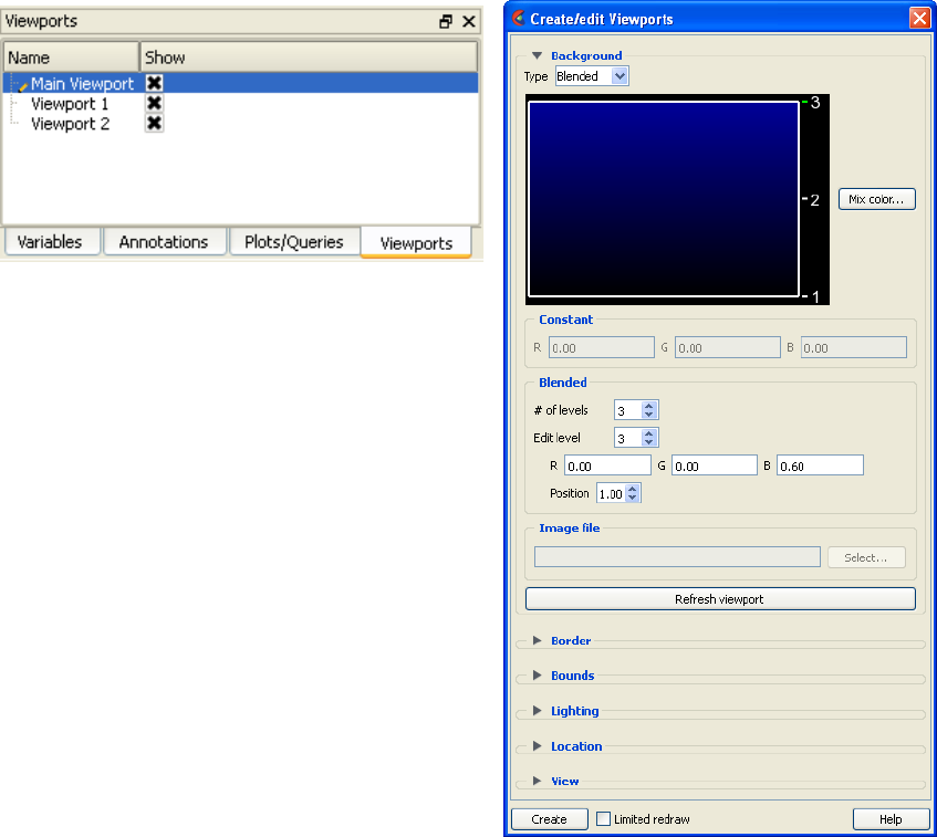
5.4 Viewports
5-210 EnSight 10.2 User Manual
You can get at the viewport attributes via the Quick Action Icons or through the
Feature Panel. Clicking once on the Viewports Icon opens the Feature Panel for
Viewports. This editor is used to both create and edit viewports. Plots can be
selected in the graphics window by left click, and multiple items can be selected
by holding the control key down while left clicking. Selection is also available via
the Viewports list panel. Upon selection of a viewport, the Quick Action Icon Bar
shows attributes that can be edited. Right-click selection in both areas provide a
menu of options for editing, creating, and access to the full Feature Panel.
The Viewports panel gives a user modifiable view of the viewports that already
exist. The toggles, in the "Show" column, turn visibility on/off. Selection is
accomplished via right and left mouse buttons. Multiple disjoint items can be
selected by holding the control key as the mouse is clicked and multiple sequential
items by holding the Shift-key. Double-click displays the Feature Panel. Any item
currently in edit mode will display a pencil icon near it.
Figure 5-118
Viewports Panel and Feature Panel
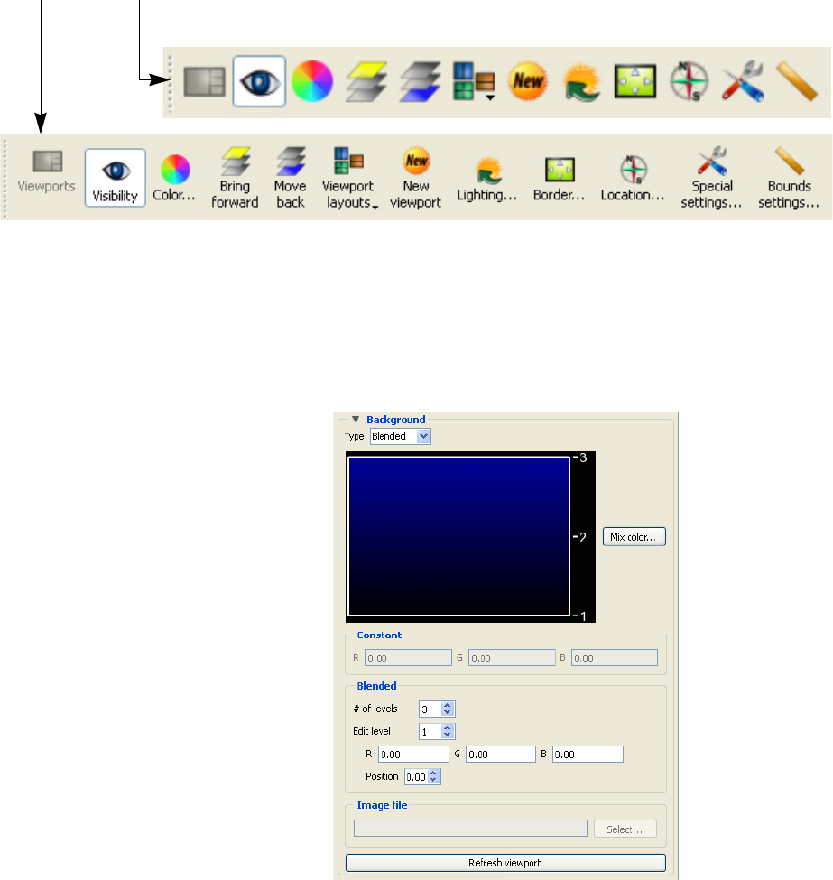
5.4 Viewports Quick Action Icons & Feature Panel
EnSight 10.2 User Manual 5-211
5.4.1 Viewports Quick Action Icons & Feature Panel
When a viewport is selected, the following Quick Action Icons become available.
Visibility Icon Sets the visibility of the selected viewport(s).
Color... Icon Opens the Background area of the Feature Panel for the specification of the color you
wish to assign to the background of the selected viewports.
Type Opens a pulldown menu for the specification of the type of background you wish to
assign to a viewport.
Blended In the Blended area, allows you to specify a background comprised
of 2 to 5 blended colors.
# of Levels This field specifies the number of levels (from 2 to 5) at which a
color will be specified. The default is 2.
With and without icon labels
Figure 5-119
Viewports Quick Action Icons
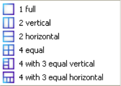
5.4 Viewports Quick Action Icons & Feature Panel
5-212 EnSight 10.2 User Manual
Edit Level This field specifies which of the levels you wish to edit. You may
select the desired level using the stepper buttons, by entering a value
in the field, or interactively by clicking on its number on the right
side of the Viewport Color window.
Position This field specifies the vertical position of the edit level as a fraction
(from 0 to 1) of the vertical height of the Viewport Color window,
where 0.0 is at the bottom and 1.0 is at the top. You may adjust a
level to the desired position using the stepper buttons, by entering a
value in the field, or interactively by selecting and dragging a level’s
number on the right side of the Viewport Color window. The
position of any level can not be below the position of the next lower
level.
Constant In the Constant area, allows you to specify a constant color using
the RGB fields or the Color Selector dialog which is accessed by
clicking the Mix Color... button.
Image In the Image file area, allows you to choose an image as a
background for your viewport.
Inherit Causes the viewport to display the same background color attributes
as the main Graphics Window. Only applicable for created
viewports, not the main Graphics Window.
Mix Color... Opens the Color Selector dialog.
Refresh Viewport Will redraw the selected viewport(s) with the defined viewport background settings.
Bring forward Icon Clicking this button moves the selected viewport(s) “forward” in the Graphics Window
to occlude any viewports which it (they) may overlap. Viewport 0 cannot be “popped”
Move back Icon Clicking this button moves the selected viewport(s) “back” in the Graphics Window to
be occluded by any viewports which may overlap it (them). Viewport 0 cannot be
“pushed”
Viewport Layouts
Icon
This icon opens a pulldown menu of icons which indicate standard viewport layouts.
New Viewport Icon Clicking this button creates a new Viewport within (and on top of) the “main” Graphics
Window. The location and size of the viewport can be modified interactively in the
Graphics Window by a) clicking and dragging within the viewport to move it of b)
clicking and dragging the edge or corner to resize it. More precise modifications may be
performed using the Location... Icon
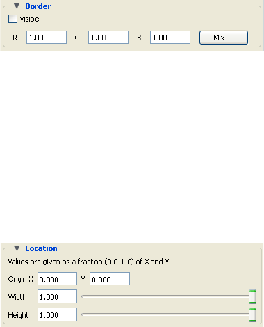
5.4 Viewports Quick Action Icons & Feature Panel
EnSight 10.2 User Manual 5-213
Lighting... Icon Opens the Light Source Editor dialog, where you can modify light sources and their
attributes. This is not a viewport specific operation - but this way of getting to it is has
been retained for now. You can also get there from the main menu View->Lighting.
Position Position of Light source 1 is either absolute or relative to the camera position.
Azimuth Azimuth Angle of Light source 1 (-180 to +180 degrees).
Elevation Elevation of Light source 1 (-90 to +90 degrees).
Convert to Absolute Converts a relative Azimuth and Elevation angle to Absolute Coordinates.
Set to Default Restores Light Source 1 values back to default.
Intensity Intensity of Light source 2 (0 to 1).
Set lights to default Click to set lights back to the default.
Border... Icon Opens the Border attributes area of the Feature Panel, for the specification of a constant
color for the border of the selected viewports.
Visible Toggle Toggles on/off visibility of a viewport’s border in the other five Modes. The border of
each viewport will always be visible in VPort Mode.
RGB These fields specify the RGB values for the color you wish to assign.
Mix... Opens the Color Selector dialog. See Section 7.1 Color.
Location... Icon Opens the Location area of the Feature Panel for the specification of the desired location
in the main Graphics Window for the selected viewports. This dialog provides a more
precise alternative to moving and resizing the viewports interactively.
Origin X Y These fields specify the location for the X and Y coordinates of the selected viewport’s
origin (lower left corner) in the main Graphics Window. Values range from 0.0 to 1.0.
Width, Height These fields specify the width and height of a selected viewport in X and Y coordinates
from the viewport’s origin. Values range from 0.0 to 1.0.
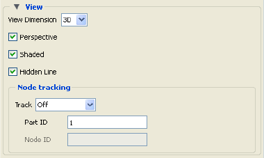
5.4 Viewports Quick Action Icons & Feature Panel
5-214 EnSight 10.2 User Manual
Special settings...
Icon
Opens the View area in the Feature Panel for the specification of whether the global
settings for Perspective versus Orthographic display, hidden surface display, and hidden
line display will apply in the selected viewport(s). In addition, a viewport can be
designated as 2D, in which case only planar 2D parts can be displayed in the viewport
Note, Once you designate a viewport as a 2D viewport, all 3D parts are no longer
visible in that viewport. To see the 3D parts in that viewport again, you will need to
make the viewport 3D, select the 3D parts in the parts list, and make them visible
again using the visibility per viewport icon.
Track In the Node tracking area, will do a global translate of the geometry to track the motion
with respect to one of the following:
Node number Enter the node id in the Node ID field
Part Centroid The geometric centroid of the part is used for tracking
Part xmin The minimum x coordinate of the part is used for tracking
Part xmax The maximum x coordinate of the part is used for tracking
Part ymin The minimum y coordinate of the part is used for tracking
Part ymax The maximum y coordinate of the part is used for tracking
Part zmin The minimum z coordinate of the part is used for tracking
Part zmax The maximum z coordinate of the part is used for tracking
Part ID ID number of Part used for camera tracking.
Node ID Node ID for the Part ID used for tracking if Node number selected in Track pulldown.
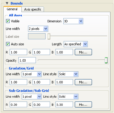
5.4 Viewports Quick Action Icons & Feature Panel
EnSight 10.2 User Manual 5-215
Bounds settings...
Icon
Opens the Bounds area of the Feature Panel for the specification of part bounding box
gradation and labeling.
General Tab Change the dialog to reflect overall extent grid attributes.
All Axes Section Contains parameters that affect attributes of all axes of the bounding extent.
Visible Toggle Toggles on/off visibility of the viewport 2D/3D extent axes.
Dimension Opens a menu for the specification of the desired dimension (2D or
3D) of the bounding extent axis. Default is 3D. 2D is only available
for 2D viewports and 3D viewports in orthographic mode.
Line Width Opens a menu for the specification of the desired line width (1 - 4
pixels) of the bounding extent axis. Default is 2.
RGB These fields specify the RGB values for the color you wish to
assign.
Mix Color... Opens the Color Selector dialog. See
Opacity Specifies the degree of opaqueness for the axes of the bounding
extent. This value may be adjusted by typing in a value from 0.0 to
1.0 in the field or by using the slider bar whose current value is
reflected in the field. A value of 0. or 1. will render the axes
completely transparent or completely opaque, respectively.
Auto Size Toggle Toggles on/off the scaling of the axis range to nice “round”
numbers.
Length Opens a menu for the specification of the desired type of length
gradation on the axes of the bounding extent.
As Specified Divides the gradations evenly along the length of the axis. (default)
Rounded Tries to round to the units of the common order of magnitude.
Gradation/Grid
Section
Controls the specification of the gradation/grid of the axes of the bounding extent
Line Width Opens a menu for the specification of the desired line width (1 - 4
pixels) for the gradation and grid of the bounding extent axis.
Default is 1.
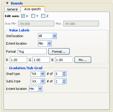
5.4 Viewports Quick Action Icons & Feature Panel
5-216 EnSight 10.2 User Manual
Line Style Opens a menu for the specification of the style of line (Solid,
Dotted, or Dashed) desired for the gradation and grid of the
bounding extent axis. Default is Solid.
RGB These fields specify the RGB values for the color you wish to
assign.
Mix Color... Opens the Color Selector dialog. See
Sub-Gradation/
Sub-Grid Section
Controls the specification of the subgradation/subgrid of the axes of the bounding extent.
Line Width Opens a menu for the specification of the desired line width (1 - 4
pixels) for the subgradation and subgrid of the bounding extent axis.
Default is 1.
Line Style Opens a menu for the specification of the style of line (Solid,
Dotted, or Dashed) desired for the subgradation and subgrid of the
bounding extent axis. Default is Solid.
RGB These fields specify the RGB values for the color you wish to
assign.
Mix Color... Opens the Color Selector dialog. See
Axis Specific Tab Change the dialog to reflect XY or Z-Axis extent attributes (see below)
X-, Y-, Z-Axis These toggles choose the axis.
Axis These fields reflect the Min and Max values of the selected axis.
Value Labels
Section
Controls attributes of the selected axis.
Grid Location Opens a menu for the specification of the desired location (None,
All (default), or Beg/End) to place the labels of the selected axis.
Extent Location Opens a menu for the specification of the desired extent (Min
(default), Max, or Both) on which to display the labels of the
selected axis.
Format This field specifies the format used to display the labels of the
selected axis. Any C language “printf” format is valid in this field.
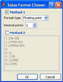
5.4 Frames
EnSight 10.2 User Manual 5-217
5.4.2 Frames
Format... Opens the Viewport Axis Text Format dialog which allows you to
select a pre-defined format.
Method 1
Format type Specify floating point, or exponential
Decimal
points
Specify the number of decimal points
Method 2
Format
Selection List
List of pre-defined formats.
RGB These fields specify the RGB values for the color you wish to
assign.
Mix Color... Opens the Color Selector dialog. See
Gradation/Sub-
Grad Section
Grad Type Opens a menu for the selection of desired marker (None, Grid, or
Tick (default)) for major gradations of the selected axis.
# of Specifies the number of major gradations you wish along the
selected axis. If Auto Size is on, it is only an approximation to the
value which will be used.
SubG Type Opens a menu for the selection of desired marker (None, Grid, or
Tick (default)) for sub-gradations (between the major gradations)
along the selected axis.
# of Specifies the number of sub-gradations you wish between each
major gradation along the selected extent axis
Extent Location Opens a menu for the specification of the desired extent (Min
(default), Max, or Both) on which to display the gradation/sub-
gradations of the selected axis.

5.5 Frames
5-218 EnSight 10.2 User Manual
5.5 Frames
Overview
As EnSight reads in model Parts, they are all initially assigned to the same
“Frame” of reference: Frame 0. Frame 0 corresponds to the model coordinate
system (defined when the model was created). Using the Frame Mode, you can
create additional frames, reassign Parts to different Frames, and specify various
attributes of the Frames.
Normally, transformations you make on parts (rotations, translations, etc.) are
performed globally; all Frames, Parts, and Tools are transformed with respect to
the Global Axis origin and orientation. The Frame feature, on the other hand,
allows you to perform transformations on selected Parts. This is useful if you
wish, for example, to create an animation with Parts moving in different directions
(such as a door or hood opening to reveal Parts within) or to move Part copies
away from each other in order to color the Parts by different variables (in fact, if
you make a copy of a Part, a new Frame is automatically created and the Part copy
is assigned to it). Note that the Frame feature coordinate transformations are
visual only and occur only on the client. That is, the transformed coordinates
cannot be used in the EnSight calculator.
In Frame Mode, transformations are always about the selected Frame’s definition,
that is, its origin position (with respect to Frame 0) and the orientation of its axes
(with respect to Frame 0). Since this is the case, the Frame’s orientation must be
adjusted (if necessary) before any transformations are applied. If transformations
are applied first, and the Frame’s definition adjusted at a later time, the
transformations will likely cause unexpected results (since the transformations
originally performed were about a different axis definition than that about which
transformations performed after the Frames definition changed occur). The
necessary order is 1) define frame location and orientation, 2) assign part to
frame, 3) perform transformations relative to the frame.
A Part can be assigned to only one Frame at a time. The Part will always be
transformed by the Frame’s transformation. A Part is not affected by a Frame’s
definition (other than transformations will be in reference to the definition). A
Part’s mirror symmetry operation (which can be thought of as a scaling
transformation) is always about the Frame to which the Part is assigned.
The Tools (Cursor, Line, Plane, etc.) are always shown in reference to the selected
Frame and are thus also transformed by the selected Frame’s transformations.
There are two transformation alternatives in Frame Mode: Frame Transform (the
default) and Frame Definition. As pointed out earlier, a frame should first be
defined (if necessary) before it is transformed.
A frame’s visibility in the Graphics Window can be toggled on or off. A Frame
may be selected by clicking on its axis triad or by selecting it in the Frames panel
list.
By default, the Frame feature icon is not shown in the Feature ribbon. As
discussed at the beginning of this chapter, it can be made to appear by right-
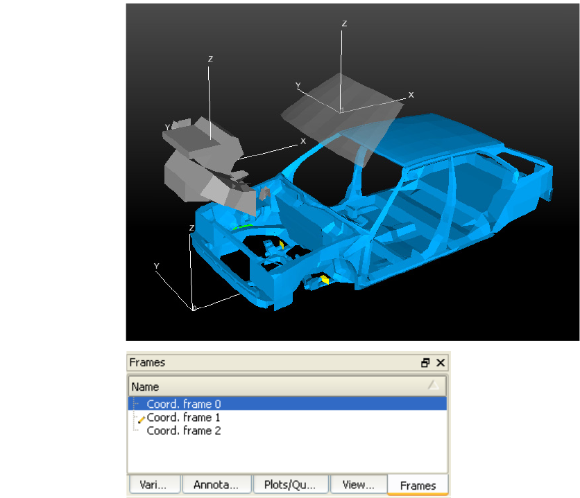
5.5 Frames
EnSight 10.2 User Manual 5-219
clicking in the Feature ribbon and toggling “Frames” on in the menu. Its location
in the ribbon can also be changed, by right-clicking in the Feature ribbon and
selecting “Customize Feature Toolbar”.
For further discussion concerning the transformation of Frames: See Section 6.2,
Tool Transform)
Three Frames exist in this
example.
Figure 5-120
Frame Example
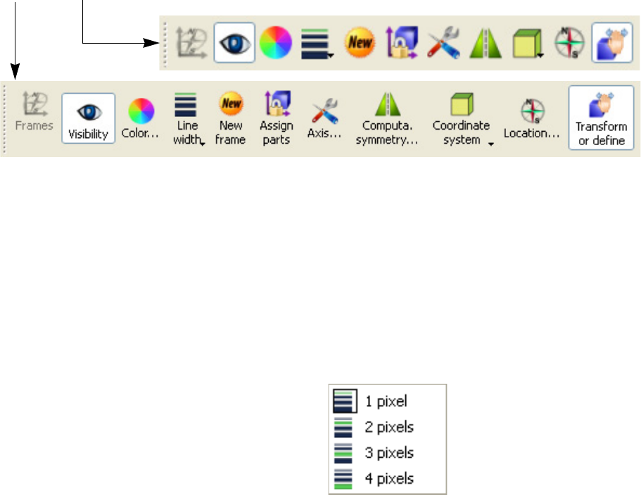
5.5 Frames Quick Action Icons and Feature Panel
5-220 EnSight 10.2 User Manual
5.5.1 Frames Quick Action Icons and Feature Panel
When a frame is selected, the following Quick Action Icons become available.
Visibility Icon Determines the visibility of the axis triad(s) of selected Frame(s). Default is Off
Color... Icon Opens the Color Selector dialog for the specification of the color you wish to assign to a
selected Frame’s axis triad.
Line width Icon Opens a pulldown menu for the specification of the width for Frame axis triad lines for
the selected Frame(s).
New frame Icon Creates a new Frame to which you can assign Parts. Be aware that each time you make a
copy of a Part EnSight creates a new Frame and assigns the copy to the new Frame. If
Parts are selected in the Parts List, the new Frame’s origin will be positioned at the center
of the selected Parts
Assign parts Icon Clicking this icon reassigns Part(s) selected in the Parts List to the currently selected
Frame.
With and without text labels
Figure 5-121
Frames Quick Action Icons
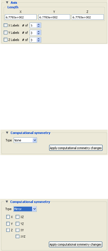
5.5 Frames Quick Action Icons and Feature Panel
EnSight 10.2 User Manual 5-221
Axis... Icon Opens the Axis area in the Feature Panel for the specification of axis triad line length and
labels for the selected Frame(s).
X Y Z These fields allow you to specify the desired length, in model coordinates, of each of the
three axes of the selected Frame’s axis triad
X Y Z Labels
Toggles
Toggles on/off the display of Labels on the respective line of a selected Frame’s axis
triad. Labels show distance along each axis.
X Y Z # of These fields specify the number of Labels which will appear on the respective axis.
Computational
symmetry... Icon
Opens the Computational symmetry area in the Feature Panel for the specification of
the type of periodic conditions which will be applied to all assigned Model Parts of the
selected Frame. (Note, computational symmetry does NOT work on created parts.
(see How To Set Symmetry)
Apply computational
symmetry changes
Changes made in the dialog will not be applied until this button is clicked.
Type Mirror If type Mirror symmetry is chosen.
Mirror In Specification of the type of mirror periodicity
Mirror X face-sharing quadrant on other side of the Y-Z plane
Mirror Y face-sharing quadrant on other side of the X-Z plane
Mirror Z face-sharing quadrant on other side of the X-Y plane
Mirror XY diagonally opposite quadrant on same side of the X-Y plane
Mirror XZ diagonally opposite quadrant on same side of the X-Z plane
Mirror YZ diagonally opposite quadrant on same side of the Y-Z plane
Mirror XYZ quadrant diagonally opposite through origin
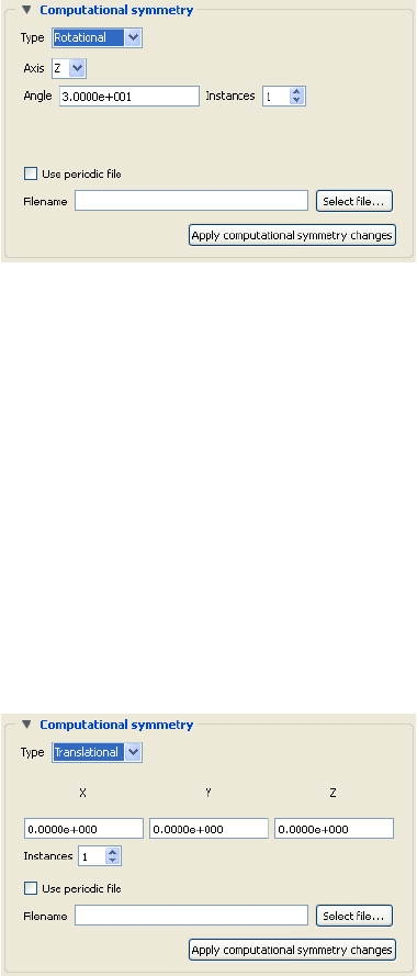
5.5 Frames Quick Action Icons and Feature Panel
5-222 EnSight 10.2 User Manual
Type Rotational If type Rotational symmetry is chosen.
Axis The Frame axis about which to rotate.
Angle This field specifies the rotational angle (in degrees) about the selected Frame’s z-axis for
rotational periodicity.
Instances This field specifies the number of periodic instances for rotational periodicity.
Use periodic file If toggled On, the periodic match file specified in Filename is used for rotational
symmetry. This is toggled on for non Case Gold format files. For case gold you must
enter the periodic match filename into the Case file.
Filename This field specifies the name of the periodic match file you wish to use.
Select File... Opens the File Selection dialog for the selection of a periodic match file.
(see Section 9.9, Periodic Matchfile Format)
Type Translational If type Translational symmetry is chosen.
X Y Z These fields specify the translational offset in reference to the selected Frame’s
orientation.
Instances This field specifies the number of periodic instances for translational periodicity.
Use periodic file If toggled On, the periodic match file specified in File Name is used for translational
symmetry. Note that this will be grayed out and unavailable for EnSight formatted data
because this information should be found in the GEOMETRY section of the Case (.case)
file (see Section 9.9, Periodic Matchfile Format).
Filename This field specifies the name of the periodic match file you wish to use. Note that this
will be grayed out and unavailable for EnSight formatted data because this filename
should be found in the GEOMETRY section of the Case (.case) file (see Section 9.9,
Periodic Matchfile Format).
Select File... Opens the File Selection dialog for the selection of a periodic match file.
(see Section 9.9, Periodic Matchfile Format)
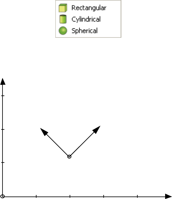
5.5 Frames Quick Action Icons and Feature Panel
EnSight 10.2 User Manual 5-223
Coordinate System
Icon
Opens a pulldown menu for the selection of the type of coordinate system (rectangular,
cylindrical, spherical) you wish to use for a selected Frame. All three are defined in
reference to Frame 0, which is rectangular. Note that each frame’s orientation vectors
(which describe its orientation to Frame 0) are rectangular (as is their on-screen
representation) no matter what the frame’s coordinate system type. However, functions
that access the frame will behave different depending on the frame’s coordinate system
type.
Rectangular The Figure below shows a rectangular frame. The origin is in reference to the Frame 0
origin, while the orientation is in reference to Frame 0’s orientation.
Y
3.0
2.0
1.0
1.0 2.0 3.0 4.0
Frame 0
Frame Orientation for Rectangular Frames
Origin: 2.0 1.0 0.0
Orientation Vectors:
X: .707 .707 0
Y: -.707 .707 0
Z: 0 0 1
X
Z
Z
X
Y
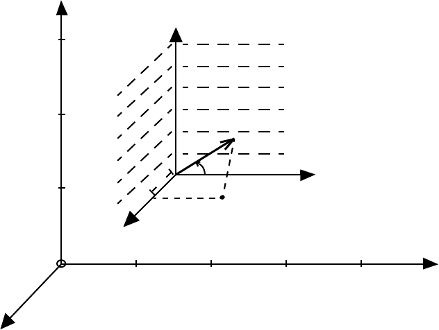
5.5 Frames Quick Action Icons and Feature Panel
5-224 EnSight 10.2 User Manual
Cylindrical The figure below shows a cylindrical frame. The origin is in reference to the Frame 0
origin, while the orientation is in reference to Frame 0’s orientation. Any function which
accesses a cylindrical frame will do so in cylindrical coordinates:
r The distance from the origin to projection point in the X–Y plane.
The angle from the X-axis to the projection point in the X–Y plane.
Z The Z-coordinate
Y
3.0
2.0
1.0
1.0 2.0 3.0 4.0Frame 0
Frame Orientation and Coordinate System Key for Cylindrical Frames
r = distance in x-y plane
= angle from x-axis to
projection pt. in x-y
Origin: 2.0 1.0 0.0
Orientation Vectors:
X: 1 0 0
Y: 0 1 0
Z: 0 0 1
X
Z
Z
Z
r
X
Y
P(r, ,z)
plane
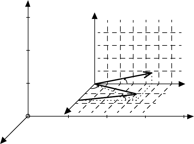
5.5 Frames Quick Action Icons and Feature Panel
EnSight 10.2 User Manual 5-225
Spherical The figure below shows a spherical frame. The origin is in reference to the Frame 0
origin, while the orientation is in reference to Frame 0’s orientation. Any function which
accesses a spherical frame will do so in spherical coordinates:
The distance from the origin to the point in question.
The angle measured from the Z-axis towards the projection point in the X–Z plane.
The angle from the X-axis to the projection point in the X–Y plane.
Location... Icon Opens the General area of the Feature Panel to permit precise definition of the selected
Frame(s). See Section 5.5.2, Frame Definition for a description of this dialog section.
Transform or define
Icon
Toggles between the transform and define methods.
Transform Transformations will cause the Parts assigned to the selected
Frame(s) to be transformed as well as the selected Frame’s axis
triad. Translations will move the Frames’ axis triad(s) and the
assigned Parts. Rotations of Parts will take place about the selected
Frame(s) axis origin.
See Section 5.5.3, Frame Transform
Definition User interaction in the Graphics Window or Feature Panel will
modify the selected Frame(s) origin location and/or axis orientation.
Note: Generally only want to use this mode before parts are
assigned to the frame.
See Section 5.5.2, Frame Definition
O
Frame Orientation and Coordinate System Key for Spherical Frames
= distance from origin
to point P
r = distance in x-y plane
= angle from z-axis to
line OP
= angle from x-axis to
projection point in
x-y plane
Origin: 2.0 1.0 0.0
Orientation Vectors
X: 1 0 0
Y: 0 1 0
Z: 0 0 1
X
Z
r
P
Y
3.0
2.0
1.0
Frame 0
Z
1.0 2.0 3.0 4.0
r
Y
X
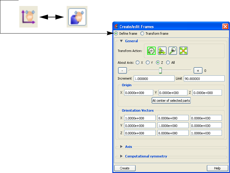
5.5 Frame Definition
5-226 EnSight 10.2 User Manual
5.5.2 Frame Definition
When Define frame has been chosen from the Transform or define icon or in the
Feature Panel for frames, then actions you make will affect only the definition
(origin and orientation) of the selected Frame(s). Frame 0’s definition however,
cannot be changed.
A Frame’s definition should be adjusted before it is transformed under Frame
Transform (as described in the previous pages). Transformations under Frame
Transform are always about the Frame’s origin and orientation. Failure to define
the proper origin position and orientation of a Frame will result in unexpected
transformation behavior.
You choose the type of transformation you wish to perform (rotate or translate)
from the Transformation Control Icons. Note that you cannot perform zoom,
scale, or reset operations under Frame Definition.
Transform Action:
Rotate
Interactive
Modification of
Orientation
When this toggle is on, clicking the left mouse button and dragging modifies the
orientation of the selected Frame(s). Clicking on the end of the X axis will limit the
rotation to be about the Y axis. Similarly, clicking on the end of the Y axis will limit the
rotation to be about the X axis.
Figure 5-122
Two ways to choose Frame Definition
Define Transform
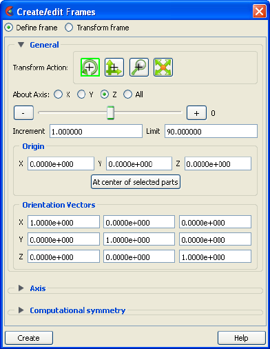
5.5 Frame Definition
EnSight 10.2 User Manual 5-227
Precise Modification
of Orientation
When the Feature Panel is opened under Frame Definition and the Rotate toggle is
selected, the dialog will be configured to permit precise rotation (modification of the
orientation) of the selected Frame(s).
You may rotate the selected Frame(s) precisely about their X, Y, Z, or All axes by
clicking on the desired axis and:
1. entering the desired rotation in (+ or -) degrees in the Increment field
and pressing Return, then
2. clicking the stepper buttons at each end of the slider bar (each click
will rotate the selected Frame(s) by the number of degrees specified
in the Increment field), or
3. dragging the slider in the positive or negative direction to the desired
number of degrees you wish to rotate the selected Frame(s) (the
Limit Field specifies the maximum number of degrees of rotation
performed when the slider is pulled to either end of the slider bar).
Origin XYZ
Orientation XYZ
You may precisely position both the origin and the axis of a selected Frame by entering
in the desired coordinates in the Origin and Orientation Vector X Y Z fields and then
pressing Return. These fields can be used regardless of whether the Rotate or the
Translate toggle is selected.
Transform Action:
Translate
Interactive
Translation of Origin
Position
When this toggle is on, clicking the left mouse button and dragging will translate the
selected Frame(s) (other than Frame 0) up, down, left, or right within the viewport.
Holding down the Control key while dragging will translate the selected Frame(s)
forward or backward.
Figure 5-123
Transformation Editor for Exact Rotation for Selected Frame(s) Only
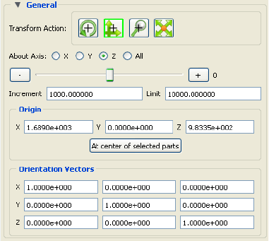
5.5 Frame Definition
5-228 EnSight 10.2 User Manual
Precise Translation
of Origin Position
When the Transformation Editor is open under Frame Definition and the Translate toggle
is selected, the dialog will be configured to permit precise Translation (modification of
the origin position) of the selected Frame(s).
You may translate the selected Frame(s) precisely along the X, Y, Z, or All axes by
clicking on the desired axis direction and:
1. entering the desired translation in (+ or -) model coordinate units in
the Increment field and pressing Return, then
2. clicking the stepper buttons at each end of the slider bar (each click
will translate the selected Frame(s) by the number of model
coordinate units specified in the Increment field), or
3. dragging the slider in the positive or negative direction to the desired
number of model coordinate units you wish to translate the selected
Frame(s) and then releasing the slider (the Limit Field specifies the
maximum number of model coordinate units that the Frame is
translated when the slider is pulled to either end of the slider bar).
Figure 5-124
Transformation Editor for Exact Translation of Selected Frames
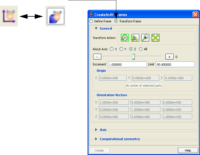
5.5 Frame Transform
EnSight 10.2 User Manual 5-229
5.5.3 Frame Transform
When Transform frame has been chosen from the Transform or define icon or in
the Feature Panel for frames, transformations you make will affect the selected
Frame(s) and the Parts assigned to them.
Note: Before any transformations are performed on a Frame, its definition should be
modified (if necessary) as described later in this section. Transformations always
occur about a Frame’s origin and orientation. Failure to define the proper
position and orientation of the Frame will result in unexpected transform
behavior. Thus, the order of dealing with things should be 1) define the frame, 2)
assign parts to the frame, 3) transform according to the frame.
You choose the type of transformation you wish to perform from among the
Transformation Control Icons in the Transformation Editor dialog. Note that
under Frame Transform, you cannot perform the zoom operation.
Transform Action:
Rotate
Interactive Rotation When this toggle is on, clicking the left mouse button and dragging causes the selected
Frame(s) and all Parts assigned to the Frame(s) to rotate about the Origins of each Frame
Axis. Holding down the Control key while dragging will rotate the selected Frame(s) and
all assigned Parts about a Z axis perpendicular to the screen.
Figure 5-125
Two ways to choose Frame Transform
Define Transform
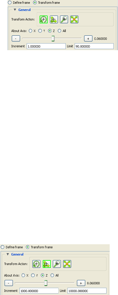
5.5 Frame Transform
5-230 EnSight 10.2 User Manual
Precise Rotation When the Transformation Editor is open under Frame Transform and the Rotate toggle is
selected, the dialog will be configured to permit precise Rotation.
You may rotate the selected Frame(s) and assigned Part(s) precisely about the X, Y, Z, or
All axes, as the orientation of the axes were defined when the Frame was first created by:
1. entering the desired rotation in (+ or -) degrees in the Increment field
and pressing Return, then
2. clicking the stepper buttons at each end of the slider bar (each click
will rotate the selected Frame(s) and assigned Part(s) by the number
of degrees specified in the Increment field), or
3. dragging the slider in the positive or negative direction to the desired
number of degrees you wish to rotate the selected Frame(s) and
assigned Part(s) (the Limit Field specifies the maximum number of
degrees of rotation performed when the slider is pulled to either end
of the slider bar).
Transform Action:
Translate
Interactive
Translation
When this toggle is on, you can transform objects interactively in the X-Y plane (or by
holding down the Control key, in Z). Clicking the left mouse button and dragging will
translate the selected Frame(s) and all assigned Part(s) up, down, left or right (or forward
or backward) within the selected viewport.
Precise Translation When the Transformation Editor is open under Frame Transform and the Translate
toggle is selected, the dialog will be configured to permit precise Translation.
You may translate the selected Frame(s) and all Parts assigned to them precisely along
the X, Y, Z, or All axes by:
1. entering the desired translation in (+ or -) model coordinate units in
the Increment field and pressing Return, then
Figure 5-126
Transformation Editor for Precise Rotation under Frame Transform
Figure 5-127
Transformation Editor for Precise Translation under Frame Transform
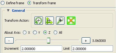
5.5 Calculator
EnSight 10.2 User Manual 5-231
5.5.4 Calculator
2. clicking the stepper buttons at each end of the slider bar (each click
will translate the selected Frame(s) and assigned Part(s) by the
number of model coordinate units specified in the Increment field),
or
3. dragging the slider in the positive or negative direction to the desired
number of model coordinate units you wish to translate the selected
Frame(s) and assigned Part(s) and then releasing the slider (the
Limit Field specifies the maximum number of model coordinate
units that the model is translated when the slider is pulled to either
end of the slider bar).
Transform Action:
Scale
When the Transformation Editor is open under Frame Transform and the Scale toggle is
selected, the dialog will be configured to permit precise scale.
You may precisely rescale the selected Frame(s) and assigned Part(s) in the X, Y, Z, or
All axes by:
1. entering in the Increment Field the desired rescale factor and
pressing Return (A value of .5 will reduce the scale of the selected
Frame(s) and assigned Part(s) in the chosen axis by half. A value of
2 will double the scale in the chosen axis. Be aware that entering a
negative number will invert the model coordinates in the chosen
axis.), then
2. clicking the stepper buttons at each end of the slider bar (Clicking
the left stepper button will apply 1/Increment value to the scale.
Clicking the right stepper button will apply the entire Increment
value to the scale), or
3. dragging the slider in the positive or negative direction to the desired
scale factor and then releasing the slider. (Dragging the slider to the
leftmost position will apply 1/Limit value to the scale. Dragging the
slider to the rightmost position will apply the entire Limit value to
the scale.)
Figure 5-128
Transformation Editor for Exact Scaling under Frame Transform


5.7 Flipbook Animation
EnSight 10.2 User Manual 5-233
5.7 Flipbook Animation
Overview
There are four common animation techniques which are easily accomplished with
Flipbook Animation. They are:
• animation of transient data, which can be any combination of scalar/
vector variables, geometry, and discrete Particles
• animation of mode shapes based on a mode-shape displacement variable
• animation of a Part moving or changing value during animation, such as
sweeping a 2D-Clip Plane or changing the value of an isosurface.
• animation applying a linear interpolation of a vector displacement field
value factor from 0 to 1.
You can combine any of these techniques with the animation of Particle traces.
The concept of a flipbook is similar to the stick figures you have probably seen in
books where each page contains a picture. When you flip through the pages
quickly you get the sense of motion. Flipbook animation stores a series of “pages”
in Client memory which are then rapidly played back to create the illusion of
motion. Pages can be loaded as graphic images, which may playback faster; or as
graphic objects, which can be transformed after creating the flipbook, even while
the flipbook is running.
For animation to be of interest, something must change from page to page. For
transient-data flipbooks, you must have visualized something about the model
that changes over time. For mode-shape flipbooks, you need to have set the
displacement attributes of the Parts for which you want to see mode shapes (see
Section 7.10 Displacement On Parts). For created-data flipbooks, you need to
have used the Start/Stop utility or specified Animation delta values for the Parts.
The number of pages in the flipbook determines the length and smoothness of the
animation. You directly or indirectly specify how many pages to create. While the
Server performs the calculations, the Client stores the flipbook pages in memory.
Just how many pages you can store depends on the amount of memory installed
on your Client workstation. Your choice to load graphic images or graphic objects
affects memory requirements, but the complexity of the model and the size of the
Graphics Window determine which will use less memory in any particular
situation.
You can control which original model Parts and created Parts will be updated for
each time increment as the user chooses. This feature takes all dependencies into
account. For example if an elevated surface was created from a 2D clip plane, the
clip plane would be updated first and then the elevated surface based on the new
clip. The ability to choose which Parts are or are not updated allows before and
after type comparisons of a Part.
After creating the flipbook, options for displaying it include: running all or only a
portion of it, adjusting the display speed, running under manual control or
5.7 Flipbook Animation
5-234 EnSight 10.2 User Manual
automatically, and running from the beginning or cycling back-and-forth between
the two ends.
It is important to know that objects in the flipbook cannot be edited. If you wish to
change something in the flipbook, you must reload it. If you decide to regenerate a
flipbook (after changing something), you can choose to discard all the old pages,
or keep any old page with the same page number as a new page.
This is very useful when you first load every tenth frame then decide to load them
all. EnSight will not have to reload every tenth frame that already exists. When
you are done with a flipbook, remember to click Delete All Pages. This will free
up memory for other uses.
Note that alpha transparency works with depth peel not sorted transparency.
Flipbook vs. Keyframe While you can implement any flipbook animation technique with keyframe
animation (described in the next section), flipbook animation has three
advantages. First, graphic-object-type flipbooks allow you to transform the model
interactively to see from many viewpoints. Second, graphic-image-type flipbooks
can be saved to a file and later replayed without having to have the dataset loaded,
or even being connected to the Server. Third, the speed of display can be more
interactive because the flipbook is in memory and can be flipped through
automatically or stepped through manually.
Flipbook animation has a few disadvantages. First, you cannot change any Part
attributes, except visibility and material properties, without regenerating the
flipbook. Second, each page is stored in Client memory, which limits the number
of pages and hence the duration of the animation.
Four Animation Techniques:
1.Transient Data Transient-data flipbooks have pages that correspond to particular solution times;
i.e. step or simulation. You specify at which time value to start and stop the
animation, and the time increment between each page. The time increment can be
more than one solution-time value; this is useful in finding a range of interest or
for a coarse review of the results. The increment can be a fraction, in which case
the data for a page is interpolated from the two adjoining solution-time values.
2. Mode Shapes Mode-shape flipbooks are used to show primary modes of vibration for a
structure. This is done by using a per node displacement, enabling the Part to
vibrate. While you can use any vector variable for a displacement, to see actual
mode shapes you need to have a Results-file vector variable corresponding to each
mode shape you wish to visualize. Note that you can create copies of Parts and
simultaneously display them with different mode-shape variables, or one at its
original state and the other with displacement for comparison.
The first page of a mode-shape flipbook shows the full displacement (as it is
normally shown in the Graphics Window). The last page shows the full
displacement in the opposite direction. The in-between pages show intermediate
displacements in proportion to the cosine of the elapsed-time of the animation.
3. Created Data Created-data flipbooks animate the motion of 2D-Clips and Isosurfaces according
to their animation attributes. This animation allows you to show clipping planes
sweeping through a model or to show a range of Isosurface values. The first page
shows the Part’s location as it appears in the normal Graphics Window. On each
subsequent page, each 2D-Clip is regenerated at the new location found by adding
the animation-delta displacement to the 2D-Clip’s location on the previous page.
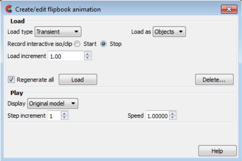
5.7 Flipbook Animation
EnSight 10.2 User Manual 5-235
Also, each Isosurface is regenerated with a new iso-value found by adding the
animation-delta increment to the iso-value of the previous page.
4.Linear Load Linear-loaded flipbooks are used to animate a displacement field of a part by
linearly interpolating the displacement field from its zero to its maximum value.
The variable by which the part is colored also updates according to the linearly
displaced values. Like Mode Shapes, this utilizes a per node displacement. The
function can be applied to any static vector variable.
Clicking once on the Flipbook Feature Icon opens the Feature Panel for flipbooks.
Load Area
Load Type A pulldown menu for the selection of type of flipbook animation to load. Options are:
Transient animates changes in data information resulting from changes in the
transient data. For example, changes in coloration resulting from
changes in variable values, or changes in displacement of Parts. See
discussion in the introduction section.
Mode shapes animates the mode shape resulting from a displacement variable.
See discussion in the introduction of this section.
Create data animates Parts having nonzero animation-delta values or which have
been recorded with the Start/Stop utility. See discussion in the
introduction of this section.
Linear load animates the Displacement (vector) variable of a part by linearly
interpolating the displacement field from its zero to its maximum
value. The Color variables of the part also update according to the
linearly displaced values.
Load As A pulldown menu for the selection of whether to load flipbook pages as Graphic Images
or Graphic Objects.
Graphic Objects flipbooks enable you to transform objects after creating the flipbook.
Playback performance depends on the complexity of the model.
Graphic Images flipbooks may be saved for later recall, but they cannot be
transformed, nor can the window be resized. Playback performance
depends on the Graphics Window size.
Figure 5-130
Flipbook Animation Editor
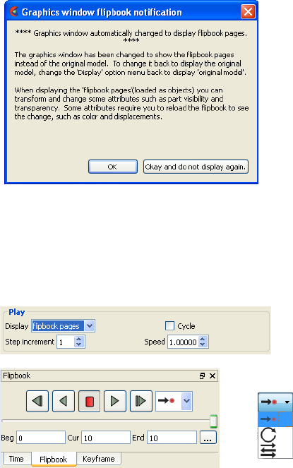
5.7 Flipbook Animation
5-236 EnSight 10.2 User Manual
Record Interactive
Iso/Clip
Allows you to define the change (isovalue change or clip plane movement) in an
isosurface or clip plane which will take place during the Flipbook load. Only isosurfaces
and clip planes which are modified in interactive mode are tracked.
Regenerate All Toggling this on reloads all flipbook pages. Toggling it off saves load time if some pages
have already been loaded, for example if you’ve just canceled the load, the pages already
created during the load remain in memory. Also, you can quickly load by increment of 2
just to see if your animation looks good, then you can change the increment to 1, toggle
off this toggle, and you’ll only load the odd pages that have not yet loaded.
Load Clicking this button starts the loading flipbook pages and opens a pop-up dialog which
reports the progress of the load and then closes to signal load is complete. If you cancel
the load, the pages already created during the load remain in memory. You may receive
an information message like the following indicating that the flipbook is now occupying
the graphics window.
Delete... Opens a pop-up warning dialog which asks you if you really wish to delete all loaded
pages. Click Okay to delete all loaded flipbook pages and free the memory for other use.
Play Area The Play area in the Feature Panel, along with the Flipbook panel in the animation area,
to control the animation.
Display A pulldown menu for selection and clarification of what is being viewed.
original model This is the original model.
flipbook pages These are the flipbook pages stored in memory.
Video Controls Click on the Video Playback control buttons to go back one timestep, to play in reverse,
to stop, to play forward and to step forward one timestep, respectively. You can also
control what happens as the end is reached, cycle back to the beginning or bounced back
and forth.
Figure 5-131
Flipbook Animation

5.7 Flipbook Animation
EnSight 10.2 User Manual 5-237
For step by step instructions, see the following:
Create a Flipbook Animation
Animate Transient Data
Troubleshooting Flipbook Animation
Speed This field specifies the playback-speed factor. Varies from 1.0 (full speed of your
hardware) to 0.0 (stopped). Change by entering a value or clicking the stepper buttons.
Beg Value for Beginning Time Step or Simulation Time. Type a value in the field, or the left
slider below the rail can be used to select the beginning value.
Cur Value for Current Time Step or Simulation Time. Type a value in the field, or the slider
above the rail can be used to select a value for the Current Time Step field.
End Value for Ending Time Step or Simulation Time. Type a value in the field or the right
slider below the rail can be used to select the ending value.
Step increment Specify the increment of each transient-data flipbook page.
Repeat Mode
Choose Play Once, Cycle or Bounce.
Record Button In order to save an active flipbook animation, click on the record button found in the tool
ribbon below the graphics window. See Record Animation Icon for details on how to
do the recording.
Problem Probable Causes Solutions
No motion No pages are loaded. Load flipbook pages.
All pages are the same visually. In order to see motion there must be
a difference between one page and
the next. Reload with differing Part
attributes, such as coloring by a
variable, using displacements, etc.
Run Type set to Step or Off Select Run Type to be Auto
Speed too fast Display Speed is set too fast. Change speed.
Speed too slow Display Speed is set too slow. Change speed.
Hardware bottleneck (computer
simply isn’t sufficiently powerful)
Reduce the number of pages.Load
pages as graphic images.
Speed erratic Virtual memory is swapping pages to
and from disk storage.
Only load the no.of pages that fit
into the workstation’s main memory.
Mode Shape(s) not visible Wrong Load Type setting Change Load Type to Mode Shapes
and reload.
Displacement attributes are
incorrect.
Change Displace by and Factor
attributes for the Part to animate.

5.7 Interactive Probe Query
5-238 EnSight 10.2 User Manual
5.7.1 Interactive Probe Query
2D Clip plane(s) not moving Wrong Load Type setting Change Load Type to Create Data
and reload.
Plane was not moved interactively
between Start and Stop.
Isosurface(s) not moving Wrong Load Type setting Change Load Type to Create Data
and reload.
Isosurface was not moved
interactively between Start and Stop.
Transient data ignored Wrong Load type
Solution time step specifications are
incorrect.
Change Load Type to Transient and
set Solution time values according to
available time steps.
Plays once then stops You are in play once mode. Change to Cycle or Bounce mode.
Pages lost Show From or Show To pages are
not at ends of flipbook.
Old pages are being regenerated. Toggle-off Regen. All Pages
Delete All Pages is clicked. Recover using the session command
file.
Transformations do not work Flipbook pages are loaded as graphic
images.
Reload flipbook pages as Graphic
Objects
Problem Probable Causes Solutions
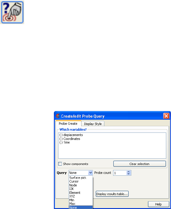
5.8 Interactive Probe Query
EnSight 10.2 User Manual 5-239
5.8 Interactive Probe Query
Overview
EnSight enables you to obtain scalar, vector, or coordinate information for the
model at a point directly under the mouse pointer, at the location of the cursor
tool, or at particular node, element, ijk, or xyz locations. The information is
normally displayed in the Results table, but it can also be displayed in the
Graphics Window. The performance of Interactive Query operations is dependent
on the refresh time of the Graphics Window. Interactive query values are not
echoed to EnSight command language files.
Clicking once on the Interactive Probe Query Icon opens the Feature Panel for
Probe Queries which is used to specify parameters for querying interactively.
Probe Create Tab
Which variables List of variables and their components (if vector and Show Components is toggles on).
Query Selection of whether interactive query is on, or which method to use to indicate input.
Surface Pick will query the location under the mouse in the Main View. The
query will be performed when the “p” keyboard key is pressed
(when “Pick Use ‘p’ ” is on) or whenever the mouse moves to a new
location in the Main View (when “Continuous” is on).
Cursor will query the location indicated by the Cursor Tool in the Main
View. The query will be performed when the “p” keyboard key is
pressed (when “Pick Use ‘p’ ” is on) or whenever the Cursor Tool
moves to a new location in the Main View (when “Continuous” is
on. You can do a quick query by right-clicking on the cursor and
choose ‘Query Variable over Time’.
Node will query the node as specified in the “Node ID” field (and will
show the node id in the query).
IJK will query the IJK node as specified in the “I J K” fields.
Figure 5-132
Interactive Probe Query Create tab
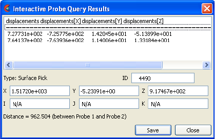
5.8 Interactive Probe Query
5-240 EnSight 10.2 User Manual
Element will query the element as specified in the “Element ID” field (and
will show the element id in the query).
XYZ will query the x, y, z location as specified in the “x y z” fields.
Min will query the min value.
Max will query the max value.
None indicates that interactive query is off.
Probe count Sets the number of query locations that are kept in memory and displayed to the user.
Search Selects the location for the query. (Only active for Surface Pick and Cursor queries.)
Exact indicates that the query will occur at the location of the mouse. Note
that this query will show the closest element id.
Closest Node indicates that the query will “snap” to the node closest to the mouse.
Note that this query will show the closest node id.
Pick (Use ‘p’) When the Action is Surface Pick or Cursor, controls whether the query will occur on a
keyboard ‘p’ key press (when on) or will occur continuously - tracking the mouse
location.
Node ID For Node Queries, specify the node id.
Element ID For Element Queries, specify the element id.
Clear Selection Clears all the selected variables.
Display Results
Table...
Opens the Interactive Probe Query Results Table dialog which shows a table of all
selected variables as well as the current query type, the latest xyz coordinates, the latest
ijk values (if applicable), and the latest node or element id (if applicable). Note that if
Exact is chosen, then the ID is the element ID and if Closest Node is chosen then the ID
is the Node ID. The contents of this dialog can be saved to a file by using the Save
button.
Figure 5-133
Interactive Probe Query Results Table
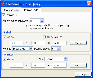
5.8 Keyframe Animation
EnSight 10.2 User Manual 5-241
5.8.1 Keyframe Animation
Probe Create Tab .
Display ID When toggled on, if an ID is appropriate for the type of search, will display the ID in the
query table and in the label on the model.
Display expansion
factor
If the model has element labels, this extracts the elements contained by the query locations
and creates a subset part from these elements. The factor is how many layers of elements will be
extracted, i.e., 1 is extract the element that contains the query while 2 means take the results from
the elements extracted at level 1 and find all of the neighbors to these elements. If the interactive
Query toggle is turned to None and the subset part has been created via the expansion factor
mechanism you will be prompted if you wish to save the subset part.
Label
Visible Toggle When toggled on, query information will be displayed in the
Graphics Window
Always on Top When on, query information in the Graphics Window will not be
hidden from view behind other geometry.
RGB These fields specify color values for the Labels.
Mix Opens the Color Selector dialog.
Marker
Visible When on, query location markers will be displayed in the Graphics
Window.
Size The size of the markers.
RGB These fields specify color values for the markers.
Mix Opens the Color Selector dialog.
Figure 5-134
Interactive Probe Query Display Style

5.9 Keyframe Animation
5-242 EnSight 10.2 User Manual
5.9 Keyframe Animation
Overview
Since its initial release in 1987, EnSight has been used extensively for animation,
due to its easy-to-use keyframe animator and ability to handle transient data. This
mechanism allows you to create your own movie sequence to present your results
more easily. There seems to be two mind sets when it comes to animation. The
first group of people believe animation to be totally trivial—something that can be
completely finished in an hour or two by anyone. The other group of people seem
to believe that animation is something that takes many days, if not weeks to finish
and requires an “animation expert” to get done. Well, neither of these ideas are
correct. While animation is not trivial, it is also not overly complicated. Most
animation produced by EnSight is setup during a day, and recorded the same day
or during the night to be complete by the next morning. Engineers create and
record their own animations. EnSight is intended to be used by end users—this
includes the animation module. We do acknowledge, however, that there is a
difference between animation, and animation done well. The latter comes with
time and experience.
EnSight uses a modified keyframe technique. This technique enables the user to
define what the scene should look like at certain times called Keyframe. Each
keyframe can be different from a previous keyframe by using any combination of
rotate, translate, scale, zoom, look-at, or look-from operations. A given keyframe
can also be the same as the previous frame (the purpose of which will be
explained shortly). The keyframe technique only works on transformations, and is
not used for other items related to what the scene looks like (i.e., when to turn on
Parts, do isosurfaces, shading changes, etc.). EnSight actually keeps track of the
transformation commands performed between keyframes and linearly interpolates
these commands when creating frames between the keyframes. These in-between
frames are referred to as subframes.
Each keyframe includes the following information: (1) a set of transformation
matrix values, specifying each local frame, the global frame and the Look-At and
Look-From Points; (2) the value of all isosurfaces and position of all clip Parts
using the plane tool; (3) the specific keyframe attributes; and (4) the
transformation commands and isosurface values to get the scene and clip Parts to
the next keyframe.
When running keyframe animation, EnSight performs the following actions for
each keyframe: (1) any command language commands associated with the
keyframe are executed, (2) the specified number of subframes are displayed in
sequence, interpolating the transformation commands to get to the next keyframe.
To begin the process of creating an animation sequence, first define the scene you
desire for the first keyframe. Then, turn on keyframe animation and create this
scene as your first keyframe. You can then proceed to modify the orientation of
the model and create your other keyframes.
If you make mistakes during the keyframe definition, click Delete Keyframe...
and enter the number of the last keyframe you were satisfied with. Then, proceed
5.9 Keyframe Animation
EnSight 10.2 User Manual 5-243
to define the subsequent keyframes again. As soon as you have at least two
keyframes defined, you may play back the animation to see what it looks like. To
do this, select the Play button in the Animation Panel. The animation process
generally proceeds with some keyframe definitions, running what you have so far
after some of those definitions, once in a while a delete back to operation, more
keyframe definitions, etc., until you are satisfied with the entire animation
sequence. You then set up the record information and set the process in motion to
produce the images.
Note, that when playing back the animation, you do not have to always play the
entire sequence. Run From, and To frame capability is provided. You also can
abort an animation run by entering the “a” key in the graphics window.
In order to get the length of animation you want on video, you will need to adjust
the number of sub-frames between keyframes in the Speed/Actions tab of the Run
Attributes dialog. The total number of frames displayed during animation is the
sum of the keyframes plus the sum of the subframes. The NTSC broadcasting
standard calls for 30 frames displayed per second. It can be difficult to get a feel
for how fast the animation will be once recorded. The speed of the playback on
the workstation is related both to its graphics capability and the complexity of the
scene, so reducing the complexity will speed things up. Accordingly, you might
consider options like making all but a representative Part invisible, use the feature
angle option to reduce the visual complexity of the Parts, and/or use the dynamic/
static box drawing modes.
Anything that is currently on will be on during the animation. That is, if contours,
vector arrows, Particle traces, shaded surfaces, flipbook animation, animated
traces, etc. are on, they will be on during animation. If any Parts have an
animation delta set or are dependent on a Part that has the delta set then they will
be regenerated and change through the animation. This enables you to do any of
the flipbook animation techniques within keyframe animation for recording
purposes, including the use of transient data (See Flipbook Animation). The
advantage for doing flipbook techniques within keyframe animation is that they
can be recorded and the amount of memory used is smaller because the whole
flipbook is not loaded into memory. This enables the recording of long sequences
of changing information that would not be able to be shown fully with flipbook
animation because of memory limits of the workstation. Short sequences that you
have already loaded into the flipbook can also be used by making sure that the
Flipbook Run toggle is on before running keyframe animation.
If dealing with transient data, you should set up the keyframes for display of the
model first, play it back, edit, etc. Then, after you are satisfied with the model
presentation, you can start dealing with displaying the transient data on the model.
You should be careful in doing movement of the model while transient data is
being displayed. It can be confusing to have the transient data changing at the
same time that the model in the scene is moving. When dealing with transient
data, we normally introduce the problem first with some keyframes, then run the
transient data without any transformations by defining two successive identical
keyframes. Between these two identical keyframes, we animate the transient data
using one of the several methods available.
We have attempted to create the animation module to be able to run in a set-up-
walk-away mode to create video. In order to do this, you can issue command
language lines at each keyframe (except the last one). For example, if you had a
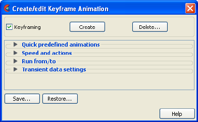
5.9 Keyframe Animation
5-244 EnSight 10.2 User Manual
case where you wanted to first show off some of the model, and then turn on
fringes to show results, you could issue a “view: fringes on” command at the
keyframe. It is also possible to play a command language file using this option.
Care should be taken to not issue an anim_keyframe: run command as Part of
this command language (which would cause an infinite loop).
When saving images to disk files, be aware that image files can take a great deal
of disk space. The file system that you are writing images to should be monitored
during the animation run to make sure it doesn’t run out of space.
Clicking once on the Keyframe Icon opens the Feature Panel for keyframe
animation.
Keyframing Toggle Toggles-on/off Keyframe animation feature. WARNING: If you toggle-off Keyframing,
all the keyframes previously created will be lost (see Save... below).
Create Click this button to create a keyframe. If Keyframing toggle is not turned on then
creating the first keyframe will turn it on automatically. Keyframes are automatically
numbered in sequence of their creation. As each keyframe is created, a message appears
in the Status History Area.
Delete… Opens the Delete Keyframes pop-up dialog which allows you to specify the number of
the last keyframe you wish to retain and then delete all keyframes back to that frame.
The keyframe whose number you specify is not deleted. To delete all keyframes enter 0
at the prompt.
Figure 5-135
Keyframe Animation Editor
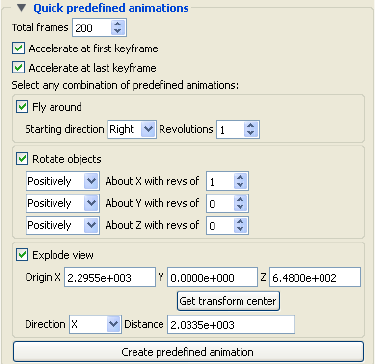
5.9 Keyframe Animation
EnSight 10.2 User Manual 5-245
Quick predefined
animations
turndown
Opens the Quick predefined animations area which allows you to add keyframes of
predefined movement to your animation. Currently implemented are "fly around",
"rotate objects", and "exploded view" One or a combination of these can be used.
Total Frames When the Create Keyframes button is pressed one or more keyframes will be created.
The total frames (keyframes plus subframes) will be the number specified here.
Accelerate at first
keyframe
If on, transformations will accelerate out of the first keyframe created when Create
Keyframes is pressed.
Accelerate at last
keyframe
If on, transformations will de-accelerate at the last keyframe created when Create
Keyframes is pressed.
Fly Around If on the look-from point will be revolved around the scene by the number of revolutions
specified. The viewer can either rotate to the Right or the Left. The keyframes will be
added when the Create Keyframes button is pressed.
Rotate Objects If on the objects will be rotated about the x, y, and/or z axis by the number of revolutions
specified. The keyframes will be added when the Create Keyframes button is pressed.
Explode View If on the objects will be assigned local axis systems and animated Distance units in the
Direction given about the origin specified. The global axis direction is used.
Origin XYZ The origin about which the explode will occur.
Get transform
center
Sets the About Origin to be at the current transform center.
Direction The direction of the explode transform. The choices are:
XTranslate in the x direction
YTranslate in the y direction
ZTranslate in the z direction
XYZ Translate in all three directions
Radial Translate in the direction defined by a vector from the given origin
through the part centroid.
For example, if the origin given is 0,0,0 and the explode direction is X, a part with a
centroid at X=1 will translate in the positive X direction while a part with a centroid at
X=-1 will translate in the negative X direction
Figure 5-136
Quick predefined animations
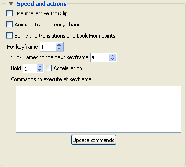
5.9 Keyframe Animation
5-246 EnSight 10.2 User Manual
Distance The total translation to be used.
Create predefined
animation
Creates the keyframe(s) given the selections in the dialog. If keyframe animation is
currently not on it will turn it on and create an initial keyframe, then add the predefined
transform indicated.
Speed and actions
turndown
Opens the Speed and actions turndown of the Keyframe Feature Panel.
Use interactive
Iso/Clip
By turning this toggle on, any clip or isosurface moved interactively during the keyframe
will animate.
Animate
transparency
change
By turning this toggle on, transparency changes to parts during the definition of the
keyframes will be part of the animation.
Spline the
translations and
Look-From points
By turning this toggle on, translations and look-at/from transforms will be interpolated
on a cubic spline.
For keyframe This field and the stepper buttons are used to select which keyframe to edit.
Sub-Frames to the
next keyframe
The Sub-Frames field specifies the number of subframes between that keyframe
specified and the next one. More subframes make the transformations to the next
keyframe smoother and slower.
Hold This field specifies the number of frames to hold at the keyframe.
Acceleration By turning on this toggle, acceleration will be used at the keyframe. If on for a previous
keyframe it will decelerate.
Figure 5-137
Speed and actions area of the Keyframe Feature Panel
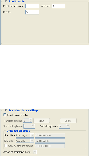
5.9 Keyframe Animation
EnSight 10.2 User Manual 5-247
Commands to
execute at
keyframe
This command text area is used to specify up to 20 commands to execute before
displaying the keyframe referenced in the For Keyframe field (this can be used for all
keyframes except the last one). You may use any command except commands
corresponding to nonpermitted actions, such as loading another dataset. Also, there is no
point in using view_transf commands that transform frames, change the Look At and
Look From points, or move the Plane Tool since the next thing EnSight does is update
the Graphics Window to match the transformation matrix information stored as Part of
the keyframe. You may use anim_keyframe commands, for example, to toggle-on
using transient data, but you should not use the anim_keyframe: run command since
then the animation will enter an infinite loop. Commands frequently used here would be
view: and annotation: commands. You may also play a command file (or a Python
script), so there is really no limit as to how many commands you can execute. The
shell: command is a special command to issue a UNIX command.
Update
Commands
This button will accept the commands entered above.
Run from/to
turndown
Opens the Run from/to turndown of the Keyframe Feature Panel.
Run from
keyframe / Run to
These fields specify the numbers of the keyframe to start from and the keyframe to run to
when Run button is pressed. Must be integer numbers of already created keyframes.
Default is Run From 1 and Run To number of keyframes you have created.
subframe Allows for the run to start at a finer, subframe level.
Transient data
settings turndown
Opens the Transient data settings turndown of the Keyframe Feature Panel.
Use Transient
Data
Toggles-on/off transient data as defined in the timelines (see below).
Figure 5-138
Run from/to area of Keyframe Feature Panel.
Figure 5-139
Transient data settings area of Keyframe Feature Panel.
5.9 Keyframe Animation
5-248 EnSight 10.2 User Manual
Transient timeline Transient data is always used according to the definitions of the transient timelines. In a
timeline you can specify the start and end time, how to increment time, etc.
By default a single timeline exists which spans the total number of keyframes. Only one
timeline can exist for each keyframe.
The timeline shown is the one being edited. The up/down arrows will advance/
decrement to the next/previous timeline if it exists.
New Will create a new timeline. If the previous timeline currently spans all available
keyframes a pop-up dialog will result and no new timeline will be created.
Delete Will delete the timeline indicated.
Start at keyframe Transient data will start at the keyframe indicated.
End at keyframe Transient data will end at the keyframe indicated.
Units Are In
Steps Area
Controls the time step to be shown at the Start Keyframe. The choices are:
Start time Controls the time step to be shown at the Start Keyframe. The choices are:
Use Begin: Use the Begin time as defined in the Solution Time Panel
Use End: Use the End time as defined in the Solution Time Panel
Use Current: Use the current time value
Specify: Set the time value using the input field
End time Controls the time step to be shown as the End Keyframe. The choices are the same as
Start Time.
Specify Time
Increment
If off, EnSight will interpolate time such that the Start/End Time values match up with
the Start/End keyframes specified. If on, you can specify the increment in time which
occurs for each frame during the timeline.
Action at start/end If you have specified a Time increment this option controls what will happen if you
arrive at the Start/End time. The choices are:
Loop Jump to the begin/end time
Swing Reverse direction
Record Button In order to save an active keyframe animation, click on the record button found in the
tool ribbon below the graphics window. See Record Animation Icon for details on how
to do the recording.
Window Size Brings up the Image/Movie Format and Options dialog.
NTSC - (704 x 480 pixels) format suitable for older recording media
PAL - (704 x 576 pixels) format suitable for older recording media
Detached display -
DVD NTSC - (720 x 480 pixels)
DVD PAL - (720 x 576 pixels)
HD 720p - (1280 x 720 pixels)
HD 1080p - (1920 x 1080 pixels)
Normal - (current graphics screen size) - machine/graphics/monitor dependent
User Defined - (user entered horizontal x vertical pixels) - not limited to screen size.
The keyframe animation will be recorded using the selected format. (see Section 2.12,
Saving Graphic Images and How to Print/Save an Image)

5.9 Solution Time
EnSight 10.2 User Manual 5-249
Troubleshooting Keyframe Animation
5.9.1 Solution Time
Save… Opens the File Selection dialog to allow you to save the specifications of the current
keyframe into a file. This saves only the keyframe specifications, not the animation
images or Part information. If you perform a Full Backup, the keyframe specifications
are saved as Part of the Backup.
Restore… Opens the File Selection dialog to allow you to restore keyframe specifications from a
file. This restores only the keyframe specifications; you must also load Part data and set
the Part attributes.
(see How To Create a Keyframe Animation)
Problem Probable Causes Solutions
Graphics Window flashes at start of
animation run.
New graphics window is opened to
display the animation.
Hardware specific. Does not affect
frames sent to recorder.
Lines “crawl” across the screen
when I play the animation.
Lines are only 1 pixel wide which
would cause crawling.
Use a line width greater than 1.
During playback the action of the
video starts as soon as the picture
comes up and it is hard to recognize
what is happening that quickly and
then it goes away.
When creating a video it is best to
have the model come up with a hold
of 3 seconds or more before starting
the animation. The animation should
run for a reasonable length of time
and then it should hold for 3 or more
seconds again at the end. On
complex models the hold may need
to be as much as 10.
Holding a video at the beginning and
the end and showing enough frames
in-between will allow your
audiences eyes to adjust and increase
comprehension of the video. Adding
annotation strings and pointers to
point out areas of interest also helps.
Also, showing the whole model with
a hold and then zooming way in on
the area of interest will help
comprehension.
Video is too fast when played back,
but it looked fine in EnSight.
Video playback speed is independent
of model complexity. Rendering
speed in EnSight is more dependent
on graphics hardware.
Increase the number of frames
recorded by adding more subframes
or use speed controls in video player.
Transformation of my object in the
animation is not smooth.
Not enough subframes. Adding more subframes will cause
more finely interpolated scene
between keyframes. For instance the
model should probably not rotate
more than 3 degrees between frames
being recorded.
Model is being clipped away as the
animation proceeds.
Running into the Z-Clip plane or the
regular plane tool with Clipping on.
Make sure the Z-Clip planes and the
plane tool are far enough away from
the model for the whole animation
sequence. NOTE: The distance
between the Z-Clip planes could
affect the clarity of the image. The
Z-Clip should be kept as close to the
model and as close to each other as
possible for better results.

5.10 Solution Time
5-250 EnSight 10.2 User Manual
5.10 Solution Time
Overview
Many analyses contain time dependent information, such as automobile crash
simulations and unsteady flow problems. The presence of time-dependent data is
indicated to EnSight through an EnSight result file, case file, or is determined
directly from the data files of other formats. EnSight has the capability of
displaying the model and results at any time provided for in the data. Linear
interpolation between given time steps is possible as long as the geometry does
not have changing connectivity over time.
EnSight keeps track of which variables and Parts have been created so that if you
change time steps, variables and Parts will update appropriately. For example,
assume you have created a clip plane through the combustion chamber of an
engine. From this clip plane you have created two constant variables Min
Temperature and Max Temperature and are displaying them in the Main View.
Now change time steps. First, the geometry updates to a new crank angle position.
Second, the clip plane will automatically be recalculated to fit the new geometry.
Third, the Min and Max values displayed in the Graphics Window are
recalculated and updated. This is all performed automatically by EnSight after
you change the current time value.
It is important to distinguish between time step and solution time. An example
will best illustrate this concept.
Consider a model with data for 5 different times:
Time Step Solution Time
01.0125
111.025
211.50
3 13.00
4 21.333
Note that the time steps coincide with the number of transient data files and are
integers. The solution time at each time step comes from the analysis, and does
not have to be at uniform intervals. The solution time can be in any units needed,
but must be consistent with the solution files. That is, if a velocity file was in
terms of meters per second, then the solution time must be in terms of seconds.
Hence it is not possible, for example, to have the solution time reported in degrees
crank angle for a combustion case unless the corresponding solution files were
also in terms of crank angle (otherwise velocity would be reported in the
meaningless units of meters-per-degree-crank-angle).
Important! EnSight will sort the solution time values and, after the sort, they
must be monotonically increasing. An error will occur if any time values
(represented as singe precision floats) are the same.
A Solution Time Panel gives you control over time and relates time step to
solution time. You can force the time information to conform to the actual time
data given at the steps, or you can allow interpolation to occur between time steps.
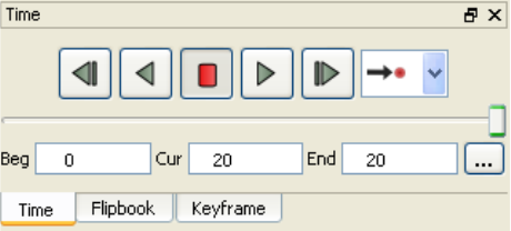
5.10 Solution Time
EnSight 10.2 User Manual 5-251
You must be aware of the implications of such an interpolation and choose the
method that is appropriate.
Also, you can see the ranges of time dependent data available and the current time
that is set for the Main View. You can change time steps by either entering a new
time to view, using the vcr-type single step buttons, or using the Solution Time
slider bar.
The Solution Time Panel by default shows a composite timeline of all timesets
from all cases. For any case, a number of different timesets can exist. Each timeset
can be attached to multiple variables and/or geometry. This makes it possible to,
for example, have one variable defined at t = 1.0, 2.0, 3.5 and another variable
defined at t = 1.5, 2.01, 4.0. For each timeline, controls exist to specify how
EnSight should interpolate the variables when time is set to a value not defined for
a given timeset. Also a convergence time value can be defined to merge timesteps
with time values that are very close, in the above example, 2.0 and 2.01 will be
merged if the master timeline convergence time is set to 0.01.
While the default is to show a composite timeline in the Solution Time Panel, it
can also display a timeline for any case loaded or the user can define his own time
values as a composite of time values available across the loaded cases.
There are other places within EnSight where time information is requested. These
include, traces, emitters, animated traces, flip book transient data, key frame
animation transient data, and Query/Plot. Each of these use the specified Beg/End
values. For functions which do not explicitly specify the time step the current
display time (as defined in the Solution Time Panel) is used.
For data that is transient, the Solution Time Icon will be visible. For static data
that does not change over time, there will be no Solution Time Icon on the Feature
Icon Bar. Clicking once on the Solution Time Icon opens the Solution Time Panel
which is used to specify time information.
Time Control Panel Contains the Video controls and the current step or solution time values.
Video Controls Click on the Video Playback control buttons to go back one timestep, to play in reverse,
to stop, to play forward and to step forward one timestep, respectively. You can also
control what happens when you reach the end - namely, the animation can, stop, can
cycle to the beginning, or can bounce back and forth. Note that this form of playing the
animation is a solution time stream of the data. That is, each timestep is read from the
data file without storing the animation in memory.
Beg Value for Beginning Time Step or Simulation Time.
Figure 5-140
Solution Time Panel Controls
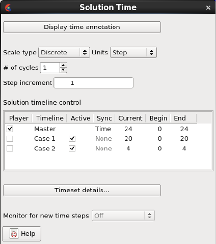
5.10 Solution Time
5-252 EnSight 10.2 User Manual
Cur Value for Current Time Step or Simulation Time. The slider can be used to select a value
for the Current Time Step field.
End Value for Ending Time Step or Simulation Time.
Solution Time Panel
Display time
annotation
Toggles an annotation in the graphics area of the Time value. Click on the Annot Tab to
the left of the graphics area to move, modify, etc. this annotation.
Scale Type A pulldown menu to specify use of existing time steps, or allow EnSight to linearly
interpolate to show any time step. Choices are:
Discrete Can only change time to defined steps.
Continuous Can change time to any time, including times between steps. Only
available if do not have changing geometry connectivity transient
case.
Units A pulldown menu to specify whether to use and display:
Step which will be an integer showing time as step data. Will show
NOSTEP if in Continuous mode and current time is not at a given
time step. Current time will automatically change to keep within
range Begin/End range. The default beginning and ending
simulation times correspond to the first and last time steps specified
in the results.
Simulation Time which will be a real number showing true simulation time. Current
time will automatically change to keep within the Begin/End range.
The default beginning and ending simulation times correspond to
the first and last times specified in the results.
# of Cycles For cyclic transient analysis, the solution is often computed for one cycle only. It is often
desirable to be able to visualize more than one cycle. This is possible only if the first and
last timesteps contain the same information. By default, EnSight assumes one cycle.
Figure 5-141
Solution Time Panel
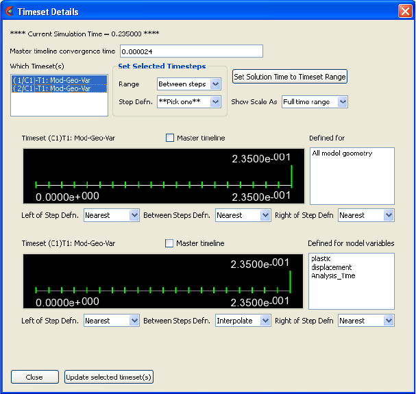
5.10 Solution Time
EnSight 10.2 User Manual 5-253
Step increment Specifies the incremental time which will be applied to the current time each time the
slider stepper buttons are used.
Solution timeline
control
This section of the dialog will exist only if multiple cases are loaded. It controls which
timeline will be shown in the Solution Time Panel and how a time change will effect
each loaded case.
Player One timeline can be designated the Player, which is the timeline
which will be shown in the Solution Time Panel
Timeline The name of the timeline. Cannot be edited by the user and is for
information purposes only.
Active Toggle on if the Case will be updated when a time change occurs.
Sync If the Master is the Player the Sync is always set to Time - meaning
the active cases will be updated to the time set by the user.
If the Player is set to one of the cases, Sync can be one of:
None - The other cases will not be modified when time changes
Time - The other active cases will be modified to the appropriate
time step when the user changes time
Relative - The other active cases will be modified to a new time
value but offset the current time difference
Timeset Details...
Tim sets Tab
will open the Timeset Details dialog which will contain two tabs.
Figure 5-142
Timeset Details Dialog - Timesets Tab
5.10 Solution Time
5-254 EnSight 10.2 User Manual
Master timeline
convergence time
A tolerance value used to determine if two different times should be treated as the same
time. For example 2.0 and 2.01 in two different timesets will be treated as the same time
if the convergence time is set to 0.01. Time values in the same timeset are not merged.
This is true for the default master timeline which is composed from all the time steps
across all the timesets as well as any user specified timeset from the 'Which timesets(s)'
list designated as the master time line by the 'Master timeline' toggle.
UserNote: The master timeline is by default the total number of unique time values
across all the timesets.
Which Timeset(s) Selects the timesets to be viewed.
Note, this is a list of both specified and composed time sets which include
a. all time sets as defined by the associated data set and corresponding reader (ie. for
EnSight Case format - as defined in the EnSight Gold Case file),
b. all time sets composed internally in EnSight such as when parts and variables of
different time sets are used to create a new part or variable.
Each time set selection indicates the order in which the it was created and referenced; the
case number to which it belongs (ie. C1 = the first case); and in general, which type of
part data (ie. Mod=Model or Mea=Measured) and geometry (Geo) and/or variables (Var)
with which it is associated. All other selections reflect the settings of this selection.
UserNote: Multiple selections display up to five multiple Timeset scales.
Set Selected
Timesteps
Allows modification of all selected timesets.
These settings are the multi-timeline way of setting the left/between/right settings. You
select all the timesets you want to edit in the "which timesets" list and then use this
interface.
Range Specified range affecting the entire time set interval Step definition,
i.e. step definition
a. Between steps: between the steps,
b. Left of: to the left of the entire time set interval,
c. Right of: to the right of the entire time set interval.
Applies to all timesets selected.
Step Defn. Specifies which time value to use in the specified Range, i.e.
**pick one***: directions to select an option below...
Right: Always use the Right time step value,
Left: Always use the Left time step value,
Interpolate: Always interpolate between left and right time step
values (when possible *),
Nearest: Always use the nearest time step value (when possible *),
Undefined: Always set the specified range as undefined.
UserNote: Applies to all timesets selected, as opposed to below 'Left
of Step Defn', 'Between steps defn.', and the 'Right of step defn'
buttons that apply to only one time scale. Some selections may be
'greyed-out' depending on definition.
Set Solution Time
To Timeset Range
Update solution time bar to selected timeset.
Show Scale As Specifies the markers (green tics) of the timeset scale shown to be time steps
a. Full time range: within the full range of the combined timeset intervals
b. Timeset's range: restricted to just the timeset range.
The change will not take effect until the “Update Selected Timeset(s)” button is pressed.
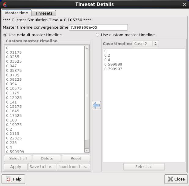
5.10 Solution Time
EnSight 10.2 User Manual 5-255
Timeset Scale Shows the time steps as defined for this timeset. The minimum and maximum time step
values are indicated at the bottom of the scale, and the current time 'value' is identified
above the scale. The tic marks indicate the time steps.
Master timeline Toggle ON the master timeline toggle above the timeline you wish to use then click on
the Update selected timesets button to use the selected timeset as the master (which will
use only the timesteps from the selected timeset in your time controls).
Defined For Lists all of the variables and/or geometry attached to the Timeset.
Left/Right of Step
Defn.
When the Current time is less than the Timeset’s minimum time, the attached variables
will use the Nearest values or become Undefined.
Between Steps
Defn.
When the Current time is between the Timeset’s minimum and maximum time values,
but not defined, the attached variables will use the Right/ Left, Interpolate, or Nearest
values, or become Undefined.
Update selected
timeset(s)
Must be selected in order to update any changed Timeset.
Timeset Details...
Master time Tab
Use default
master timeline
Toggle on if EnSight should create the composite timeline across the
loaded cases.
Use custom
master timeline
Toggle on if you wish to create your own master timeline. If
enabled, the two columns and other buttons will be active.
Custom master
timeline column
Any time values listed in the column can be selected, either
individually or by shift/control click operations.
Select all Select all of the time values in the Custom master timeline column.
Figure 5-143
Timeset Details Dialog - Master time Tab
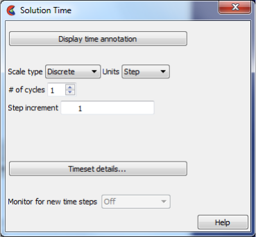
5.10 Solution Time
5-256 EnSight 10.2 User Manual
Delete Deletes the selected times from the Custom master timeline column.
Reset Resets the Custom master timeline values to be the default master
timeline.
Apply Creates the master timeline with the time values shown.
Save to file... Saves the time values to a file.
Load from file... Loads the time values from a file.
Case timeline Set the pulldown list to any case that exists. Once set, the time
values for that case will be shown in the column. And time value in
the column can be selected, either individually or by standard shift/
control click operations.
Select all Selects all of the time values in the Case timeline column
Left arrow icon Adds the time values selected in the Case timeline column to the
Custom master timeline column.
Monitor for new
timesteps
For transient solutions where EnSight is viewing the data as the solver is running, it is
possible that new timesteps can be added to the timeline while Ensight is viewing the
data. This option is only available if the data reader supports the capability. Thus, most
often, this pulldown will be grayed out, as this capability is unavailable for most data
formats.
EnSight has an ability to monitor for newly available timesteps, as a solution is
proceeding. This is a form of simulation co-processing and is referred to as simulation
monitoring, or simply, monitoring. It can be advantageous, for example, to monitor a
transient simulation to review ongoing results, or to terminate an errant simulation early,
rather than wait for the completion.
For ease of implementation, EnSight relies on a cooperative approach to determine when
new time steps are available (described later) rather than a post processing API
embedded within the solver because it is frequently impossible to modify the solver code
(especially for commercial solvers).
To inform EnSight that simulation monitoring is available for a given data set, the data
reader must simply tell EnSight that there are a maximum number of timesteps. For
EnSight Case Gold, this is accomplished simply by adding a line in the ascii text case file
as follows.
For EnSight Case format data, the Case file’s ‘TIME’ section needs to include the line:
maximum time steps: 100
Figure 5-144
Monitor for new timesteps
5.10 Solution Time
EnSight 10.2 User Manual 5-257
The line may appear anywhere within the ‘TIME’ section. Currently, the number
specified is not used. Indeed, the user may not know a priori how many times might be
generated by the solver. Simply the presence of this line, with a value of 1 or greater,
within the Case file indicates to EnSight that simulation monitoring should be offered as
an available option to the EnSight user.
For forward compatibility with future EnSight enhancements to simulation monitoring,
the user should specify the maximum number of time steps if known, or, otherwise, set it
to a sufficiently large value (e.g. 1000 or 10000). Since the number is used to allocate
modestly sized data structures in the EnSight Server (or EnSight SOS), it should not be
set to an unreasonably large value.
In a User Defined Reader, simply add another function as follows and return a value of 1
or greater.
int USERD_get_max_time_steps(void);
This function should return 1 or greater to indicate that simulation monitoring should be
made available for the particular data set. It should try to return the maximum number of
expected time steps for the data set or a value sufficiently large. The actual value may be
used at a later date.
You can turn on monitoring at the time that the data is loaded or you can turn it on later
in your session. To turn it on at loading, in the File>Open dialog, Advanced interface
toggle on, under the Time options tab, you will find a Monitor for new timesteps
pulldown (see Figure 5-145) with the following choices:
Off - Don’t monitor the data set for new time steps
Jump to end - Monitor for new time steps and jump to the last time step available
Stay at current - Monitor for new time steps but don’t change the current time step
Choose your option, but note that if the user defined reader does not support this option,
or if the.case file does not contain the proper keyword, then your choice will be ignored.
To turn it on during your session see Figure 5-141.
Cooperative Monitoring
As noted earlier EnSight’s implementation of simulation monitoring doesn’t require
modifications to the solver. Instead, EnSight monitors the specified data set for new time
steps. The advantage of this approach is that modifications aren’t needed to the solver.
However, for this to work reliably, the solver and/or data format must appropriately
update data files so that the data files are always available for reading and are
syntactically complete.
For example, if a user wishes to use EnSight Case format data, the .case file must be
“complete” and syntactically correct at all times; it can never be partially written, given
that EnSight may currently be trying to read it. Furthermore, any time steps referenced
in the .case file must exist. Since EnSight’s simulation monitoring is cooperative, the
preferred approach to guaranteeing the constraints on the data file is to first write any
geometry and/or variable files for the new time step(s), then create a new case file using
a temporary name containing the new time information, and finally replace the original
case file with the new case file. While EnSight is monitoring for new time steps, it will
periodically reopen the .case file, reread it, and then read any new geometry and/or
variable files. This approach guarantees that the data files are wholly intact and
available for reading at all times without needing special APIs or operating system file
locking.
The programmer may find the Linux/Mac OS X system function “rename(char
*oldName, char *newName)” useful for renaming a file. Similarly, the MS Windows
API includes the same rename() function or the MoveFile() native function can be used.
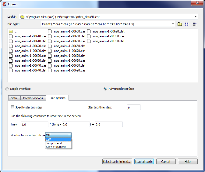
5.10 Solution Time
5-258 EnSight 10.2 User Manual
Other formats may have other appropriate approaches for amending data sets with new
data. For example, formats such as ExodusII may support simultaneous reading and
writing which can be used by the EnSight UDR API. Or, on a long solution, a given
reader may choose to only update the solution time if there has been a several minute
hiatus since the last file was last updated. Or a reader may choose to conservatively
remain ‘one timestep behind’ the last output timestep file, to avoid reading a partially
written solution file.
If you have questions about a specific format and this feature, please contact CEI
Support.
Batch Command File Playback
If EnSight is instructed to play a command file, it will handle time steps as it always has.
However, if the command file contains the command:
solution_time: monitor_for_new_steps jump_to_end
— or —
solution_time: monitor_for_new_steps stay_at_current
and a later EnSight command specifies a time step that currently doesn’t exist, EnSight
will wait until that time step becomes available. The EnSight console output indicates
this is happening.
Off Do not look for new timesteps
Jump to End When one or more new timesteps become available, automatically
change time to the last timestep.
Stay at Current When one or more new timesteps become available, update the
master timeline to indicate a new End time value, but do not change
timesteps.
Figure 5-145
File>Open dialog, Advanced interface, Time options tab
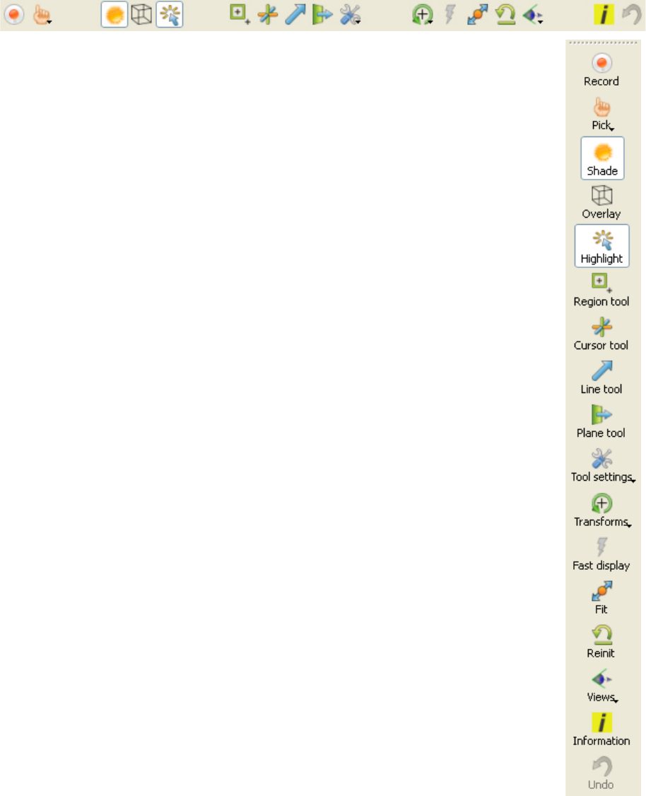
5.11 Solution Time
EnSight 10.2 User Manual 5-259
5.11 Tools Icon Bar
Tool icons are always available below the Graphics Window.
Figure 5-146
Tools Icon Bar
They can also be torn off and placed elsewhere and in a vertical
orientation if desired. Such is shown here to the right, with optional
icon text turned on (so we can reference them easily).
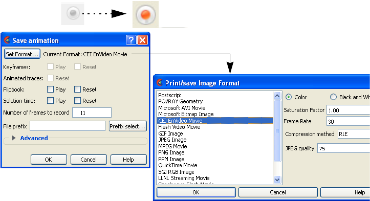
5.11 Solution Time
5-260 EnSight 10.2 User Manual
Record Animation
Icon
The Record Active Animation Icon will turn ON if you have an active animation
(flipbook, or keyframe, or streaming transient data via the clock icon, or animated
particle traces, or spin mode (where you press F4 and drag the cursor to spin the model),
or clip in auto or auto cycle interactive mode, or an isosurface in auto or auto cycle
interactive mode). In order to save an active transient animation, click on this record icon
found in the tool ribbon below the graphics window. See Record Animation Icon for
details on how to do the recording.
Record Button
Set Format... Brings up the Image/Movie Format and Options dialog. The animation will be recorded
using the selected format. (see Section 2.12, Saving Graphic Images and How to Print/
Save an Image)
Keyframes: Play This will play the keyframes.
Keyframes: Reset This will reset the keyframes to the beginning prior to starting the record.
Animated traces:
Reset
This will reset the animated traces to the beginning prior to starting the record. This
toggle is only active if you have animated traces.
Flipbook: Play This will play the flipbook.
Flipbook: Reset This will reset the flipbook to the beginning prior to starting the record.
Solution time: Play This will play through the solution time.
Solution time:
Reset
This will reset the solution time to the beginning prior to starting the record.
Number of frames Choose the number of frames to record.
File prefix The location and filename prefix for the recorded images. The appropriate suffix will be
added automatically.
Figure 5-147
Recording Transient Animation
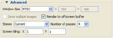
5.11 Solution Time
EnSight 10.2 User Manual 5-261
Advanced Area
Window Size Brings up the Image/Movie Format and Options dialog.
NTSC - (704 x 480 pixels) format suitable for older recording media
PAL - (704 x 576 pixels) format suitable for older recording media
Detached display -
DVD NTSC - (720 x 480 pixels)
DVD PAL - (720 x 576 pixels)
HD 720p - (1280 x 720 pixels)
HD 1080p - (1920 x 1080 pixels)
Normal - (current graphics screen size) - machine/graphics/monitor dependent
User Defined - (user entered horizontal x vertical pixels) - not limited to screen size.
The animation will be recorded using the selected format. (see Section 2.12, Saving
Graphic Images and How to Print/Save an Image)
Save multiple
images
If Type: Detached Display, will save an image per display
Render to
offscreen buffer
Render offscreen (if your card supports this feature). Toggle this on to avoid having the
image appear to your screen to be saved. This avoids the risk of saving overlapping
windows onto your image.
Stereo EnSight offers several options for saving stereo files.
Current Save according to the display settings
Mono Don’t save in stereo
Interleaved Left and right stereo saved together.
Anaglyph Cyan/
Red
Save two files for anaglyph stereo (colored glasses) using cyan in
the left eye and red in the right eye.
Anaglyph Blue/
Red
Save two files for anaglyph stereo (colored glasses) using blue in the
left eye and red in the right eye.
Anaglyph Red/
Blue
Save two files for anaglyph stereo (colored glasses) using red in the
left eye and blue in the right eye.
Number of passes Number of images to use in antialiasing algorithm. The higher the number, the smoother
that jagged lines will appear but the longer that your image will take to save.
Screen Tiling Graphics images can be saved in multiple sections called Tiles. These can be re-
rendered back onto multiple displays, using, for example, our free EnVideo application.
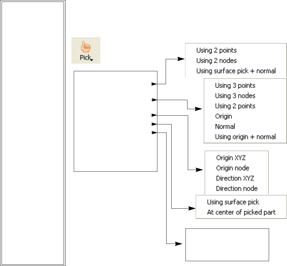
5.11 Solution Time
5-262 EnSight 10.2 User Manual
Pick Pulldown Icon Opens a pulldown menu for the specification of the desired type of Pick operation. The
actual Pick operation is normally assigned to the “P” key on the keyboard or the middle
mouse button, unless it has been reassigned under Main Menu: Edit > Preferences...
Mouse and Keyboard...
Pick part When the Pick operation is performed (by default, pressing the “P” key, or the middle
mouse button), the Part directly under the mouse cursor is selected. To select multiple
Parts, hold down the Control Key during the Pick operation.
Pick cursor tool
location
When the Pick operation is performed, the Cursor Tool will be positioned at the Picked
point.
Pick line tool
location
Using 2 points When the Pick operation is performed, the ends of the Line Tool will
be placed at the Picked points. Two points must be picked to
position the Line Tool.
Using 2 nodes When the Pick operation is performed, the ends of the Line Tool will
be placed at the nodes closest to the picked points. Two nodes must
be Picked to position the Line Tool. The line tool will continue to be
tied to these two nodes.
Using surface
pick + normal
When the Pick operation is performed, one end of the Line Tool will
be placed at the Picked points, while the other one will be placed out
in the normal to the surface direction.
Pick part
Pick cursor tool location
Pick line tool location
Pick plane tool location
Pick cylinder tool origin
Pick camera
Pick spline control point
Pick view
Pick contour label location
Pick element(s) to blank
Pick color palette band
Pick frame origin
Figure 5-148
Pick Pulldown Icon
Center of transform
Center
Center + direction
Look at point
5.11 Solution Time
EnSight 10.2 User Manual 5-263
Pick Plane Tool
Location
Using 3 points When the Pick operation is performed, the Plane Tool will be
positioned at the Picked points. Three points must be Picked to
position the Plane Tool.
Using 3 nodes When the Pick operation is performed, the Plane Tool will be
positioned at the nodes nearest the pick points. Three nodes must be
Picked to position the Plane Tool. The plane will continue to be tied
to these three nodes.
Using 2 points When the Pick operation is performed, you can click and drag the
mouse to define a line. The Plane Tool will be positioned parallel to
your current viewing angle through the defined line. Consider using
this option together with the F5, F6, F7, and F8 keys which will
transform the view to a standard orientation.
(see Section 6.1, Global Transform)
Using Origin When the Pick operation is performed, the location of origin of the
plane tool is chosen. Note that the orientation of the plane tool is
unchanged with this option.
Using Normal When the Pick operation is performed, the origin of the plane tool
remains unchanged, but the normal goes from the origin to the
picked point.
Using origin +
normal
When the Pick operation is performed, the location of origin of the
plane tool is chosen, and the normal of the plane tool is set to the
normal of the surface.
Pick cylinder tool
origin
When the Pick operation is performed, the location of origin of the
cylinder tool is chosen and the axis of the cylinder tool is set to the
normal of the surface.
Pick camera Origin XYZ When the Pick operation is performed on visible geometry the
selected camera origin will be updated to the picked position.
Origin node When the Pick operation is performed on visible geometry the
selected camera origin will be updated to the picked node id and it's
origin property will be updated to constrain itself to the node's
position.
Direction XYZ When the Pick operation is performed on visible geometry the
selected camera view direction will be updated to point to the picked
coordinate location and it's direction property will be updated to
constrain itself to point to the given location.
Direction node When the Pick operation is performed on visible geometry the
selected camera view direction will be updated to point to the picked
node id location and it's direction property will be updated to
constrain itself to the node's position.
Pick spline control
point
Using surface
pick
When the Pick operation is performed on visible geometry a control
point will be added to the currently selected spline at the insertion
point. If no spline is currently selected or one does not exist a new
spline will be created.
(see Section 4.6, Tools Menu Functions)
5.11 Solution Time
5-264 EnSight 10.2 User Manual
At center of
picked part
When the Pick operation is performed on visible geometry a control
point will be added to the currently selected spline at the center of
the picked part. If no spline is currently selected or one does not
exist a new spline will be created.
(see Section 4.6, Tools Menu Functions)
Pick view Center of
transform
When the Pick operation is performed, the center of global
transformation is positioned at the Picked point.
Center When the Pick operation is performed, the Picked point is centered
in the graphics window and the center of transform is set to the
Picked point.
Center +
direction
When the Pick operation is performed, the Picked point is centered
in the graphics window and then rotated so the surface normal is
parallel to the screen normal. The center of transform is also set to
the Picked point.
Look at Point When the Pick operation is performed, the Look At Point is
positioned at the Picked point. The Look From Point is also adjusted
to preserve the distance (between the two Points) and vector that
existed prior to the Pick operation. (see Section 6.5, Look At/Look
From)
Pick contour label
location
When the Pick operation is performed on a contour part, a contour
label is placed at the location of the Pick, or if a contour label exists
at the picked point, it will be removed.
Pick element(s) to
blank
When the Pick operation is performed, the Element that is chosen is visually removed
from the graphics screen. The element still remains in the Element Blanking selection in
Part Quick Action to enable / disable and restore visibility.
Pick color palette
band
When the Pick operation is performed on geometry colored by a variable or a color
palette visible in the graphics window, a color band will appear. (see Section 4.2, Edit
Menu Functions)
Pick frame origin When the Pick operation is performed, the origin of the selected frame will be positioned
at the Picked point.
Shade Icon Toggles on/off global Shaded (default is off) which displays all Parts in a more realistic
manner by making hidden surfaces invisible while shading visible surfaces according to
specified lighting parameters. Performs the same function as Main Menu > View >
Shaded item.
When toggled-off, all visible Parts are shown as line drawings. Shaded may be turned off
for individual Parts using the Shaded toggle in the Parts Quick Action Icon Bar or the
Feature Panel for each type of Part. It can also be turned off for a Particular viewport
with the Selected viewport(s) special attributes Icon, or in the View area of the
Viewports Panel.
Element Blanking Icon
Figure 5-149
Shaded Toggle Icon ON / OFF
5.11 Solution Time
EnSight 10.2 User Manual 5-265
Shaded requires more time to redraw than a line-mode display (the default), so you may
wish to first set up the Graphics Window as you want it, then turn on Shaded to see the
final result. To shade surfaces, a Part’s representation on the Client must include surfaces
- (2D elements). Any 1D elements of Parts displayed with Shaded on will continue to be
drawn as lines. Lighting parameters for brightness and reflectivity are specified
independently in the Feature Panel for each type of Part.
(see Section 4.5, View Menu Functions and How To Set Drawing Style)
Troubleshooting Hidden Surfaces
Problem Probable Causes Solutions
Graphics Window shows
line drawing after
toggling on Shaded.
Shaded is toggled off
for some or all
individual Parts.
Toggle Shaded on for individual
Parts with the Shaded Icon in
the Part Quick Action Icon bar
or in the Feature Panel dialog.
There are no surfaces to
shade—all Parts have
only lines.
If Parts are currently in Feature
Angle representation, change
the representation. If model
only has lines, you can not
display shaded images.
Element Visibility has
been toggled off for
some or all Parts.
Toggle Element Visibility on for
individual Parts in the Feature
Panel dialog.
Overlay Icon Toggles on/off global Hidden Line (default is off) which simplifies a line-drawing
display by making hidden lines—lines behind surfaces—invisible while continuing to
display other lines. Performs the same function as the Main Menu > View > Hidden Line
item.
Hidden Line can be combined with Shaded to display both shaded surfaces and the edges
of the visible surface elements. Hidden Line applies to all Parts displayed in the Graphics
Window but it can be toggled-on/off for individual Parts using the Feature Panel or the
Part Hidden Line Quick Action Icon. It can also be turned off for a Particular viewport
with the Selected viewport(s) special attributes Icon, or in the View area of the
Viewports Panel.
To have lines hidden behind surfaces, you must have surfaces (2D elements). If the
representation of the in-front Parts consists of 1D elements, the display is the same
whether or not you have Hidden Lines mode toggled-on.
During interactive transformations, the display reverts to displaying all lines. When you
release the mouse button, the Main View display automatically resumes Hidden Line
mode (assuming it is toggled on at that time).
The Hidden line option will not be active during playback of flipbook objects
animations.
Figure 5-150
Global Hidden Line Toggle Icon ON / OFF
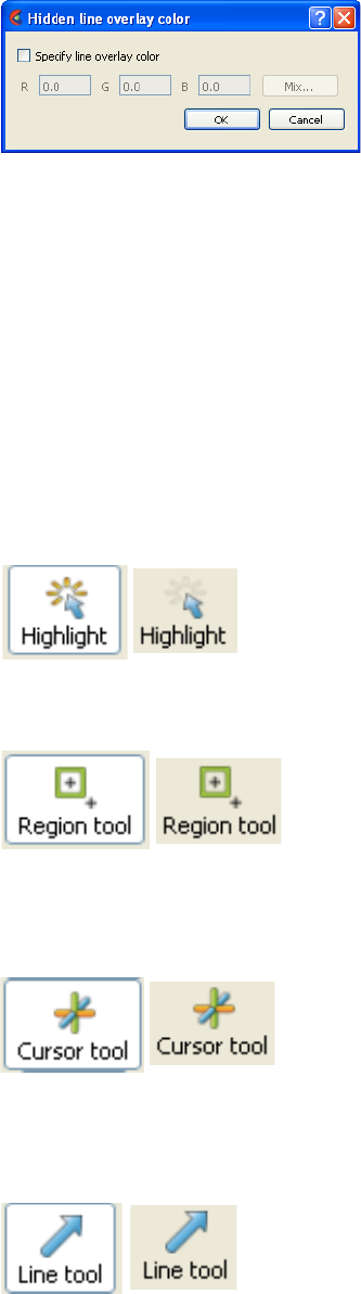
5.11 Solution Time
5-266 EnSight 10.2 User Manual
Hidden Line
Overlay
If you toggle Hidden Line on while Shaded is already on, the lines overlay the surfaces.
EnSight will prompt you to specify a color for the displayed lines (you do not want to
use the same color as the surfaces since they then will be indistinguishable from the
surfaces). The default is the Part-color of each Part, which may be appropriate if the
surfaces are colored by a color palette instead of their Part-color.
Specify line
overlay color
Toggle-on if you want to specify an overlay color. If off, the overlay line color will be the
same as the Part color.
R, G, B The red, green, and blue components of the hidden line overlay. These fields will not be
accessible unless the Specify Overlay option is on.
Mix... Click to interactively specify the constant color used for the hidden line overlay using
the Color Selector dialog. See How To Change Color)
(See How To Set Attributes)
Highlight Icon Toggles on/off the highlighting of selected parts in the graphics window. Parts selected in
the Part List are indicated in the graphics window.
Region Tool Icon Toggles on/off global visibility of the Region Tool (default is off)
Main Menu > Tools > Region Selector
Cursor Tool Icon Toggles on/off global visibility of the Cursor Tool (default is off)
Main Menu > Tools > Cursor
Line Tool Icon Toggles on/off global visibility of the Line Tool (default is off)
Figure 5-151
Hidden Line Overlay Color dialog
Figure 5-152
Highlight ON / OFF
Figure 5-153
Region Tool Visibility Toggle Icon ON / OFF
Figure 5-154
Cursor Tool Visibility Toggle Icon ON / OFF
Figure 5-155
Line Tool Visibility Toggle Icon ON / OFF
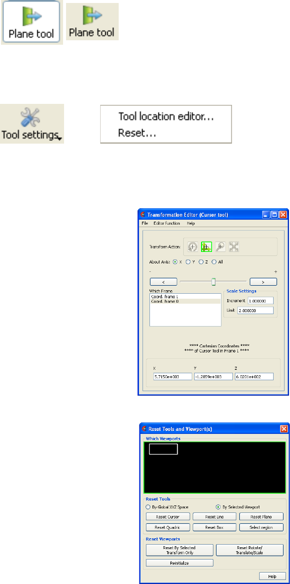
5.11 Solution Time
EnSight 10.2 User Manual 5-267
Main Menu > Tools > Line
Plane Tool Icon Toggles on/off global visibility of the Plane Tool (default is off)
Main Menu > Tools > Plane
Tool settings Icon Pulldown menu for opening the Feature Panel Tools area.
Tool location
editor...
Opens the Transformation Editor Panel in Tools mode, such as
below if most recent tool is cursor.
Reset... Opens up the Reset Tools and Viewports Panel.
Main Menu > Tools > Tool positions...
Figure 5-156
Plane Tool Visibility Toggle Icon ON / OFF
Figure 5-157
Tool settings Icon
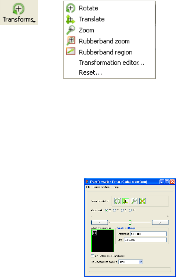
5.11 Solution Time
5-268 EnSight 10.2 User Manual
Transforms Icon Pulldown menu for dealing with transformations.
Rotate Sets left mouse button to global rotate.
Translate Sets left mouse button to global translate.
Zoom Sets left mouse button to global zoom.
Rubberband
zoom
Sets left mouse button to rubberband zoom.
Rubberband
region
Sets left mouse button to rubberband region.
Transformation
editor...
Opens the Transformation Panel in Global Transforms mode.
Figure 5-158
Transformations Icon
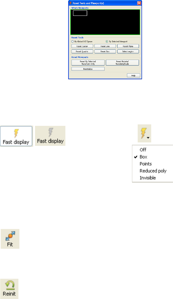
5.11 Solution Time
EnSight 10.2 User Manual 5-269
Reset... Opens up the Reset Tools and Viewports Panel.
Fast Display Icon This toggles on and off the Fast Display feature. This feature reduces a model to a simple
representation prior to doing a transformation such as rotate or translate in order to speed
up the rendering. Simple representations include Box, Points, Reduced Polygon,
Invisible, and Sparse model (if running in immediate mode) which can be chosen from
the Fast Display Representation Icon in Part Mode.
Fast Display allows faster model translation or rotation for large models.
Main Menu > View > Fast Display
Fit Icon The Fit icon will recenter the model and cause all visible parts to lie within the graphics
viewport selected.
Reinit Icon The Reint icon will perform a complete re initialization of the model in the graphics
viewport selected.
Figure 5-159
Fast Display Icon ON / OFF
and Part Quick Action Icon and pulldown
Part Fast Display Quick Action
Icon
Figure 5-160
Fit Icon
Figure 5-161
Fit Icon
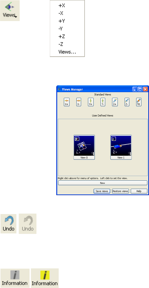
5.11 User Tools
5-270 EnSight 10.2 User Manual
5.11.1 User Tools
Views Icon The Views icon allows for selection of standard views.
+/- X Y Z Standard views down the selected axis toward the origin.
Views... Opens the Views Manager, for even better control and user defined
views can be created, saved and restored.
Undo Icon The Undo icon will undo the last transformation. It is gray if no transformation is
available to undo
Information Icon Click on this icon to see messages related to the most recent EnSight task that you’ve
completed. This icon is grey (no messages), yellow (non-error messages exist) or red
(error messages exist) depending upon the result of your most recent EnSight task.
Figure 5-162
Views Icon
Figure 5-163
Undo Icon
Figure 5-164
Information Icon
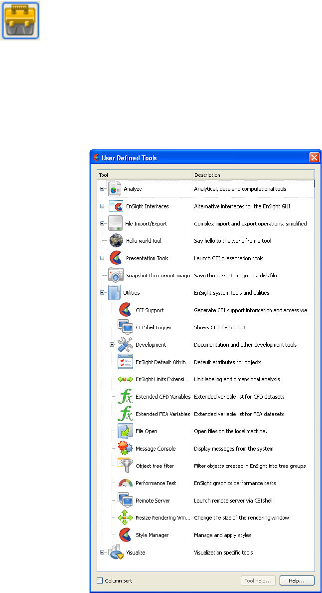
5.12 User Tools
EnSight 10.2 User Manual 5-271
5.12 User Tools
Overview
User defined tools can be produced for use in EnSight through the use of the
Ensight extension mechanisms provided, which utilize python and command
language. This is discussed in detail in the Interface Manual, see Section 7.3,
EnSight extension mechanism.
When the User Tools icon is clicked, a dialog comes up with currently recognized
user defined tools in categories, etc. Just navigate to and use them.
Figure 5-165
User Defined Tools dialog
General Description
EnSight 10.2 User Manual 6-1
6 Transformation Control
Included in this chapter:
Section 6.1, Global Transform
Section 6.2, Tool Transform
Section 6.3, Center Of Transform
Section 6.4, Z-Clip
Section 6.5, Look At/Look From
Section 6.6, Copy/Paste Transformation State
Section 6.7, Camera
General Description
An essential feature of postprocessing is the reorientation of the visualized model
in order to see it from a number of different vantage points. Basic transformations
include rotating (about an axis or axis origin point), translating (up, down, left,
right), and zooming (moving the model toward or away from you). When EnSight
reads in a geometry file, it assigns all model parts to the same Frame of reference:
Frame 0. Frame 0 corresponds to the model coordinate system (defined when the
model was created).
Two methods exist to transform a scene. In Global transform mode, the geometry
is transformed. In Camera transform mode, the scene does not move but instead a
camera is moved. A viewport can either use a global transform mode or can be
viewed through a camera.
Using the Frame Mode, it is possible to create additional frames and reassign parts
to them. In fact, when you copy a part, a new Frame is automatically created and
the part copy is assigned to the new Frame. (see Chapter 5.5, Frames)
Just after all parts of your model have been read in, EnSight centers the model in
the Graphics Window by placing the geometric center of the model at the Look At
Point which is always located in the center of the Graphics Window. Initially -
before any Global translations are made -the origin for the Global Axis is located
at the Look At Point.
There are nine Editor Functions available within the Transformation Editor,
Global Transform, Camera, Frame, Tools, Center of Transform, Z-Clip, Look At/
Look From, Copy Transformation State, and Paste Transformation State. (The
Transformation Editor dialog is opened by clicking the Transf Edit... button)
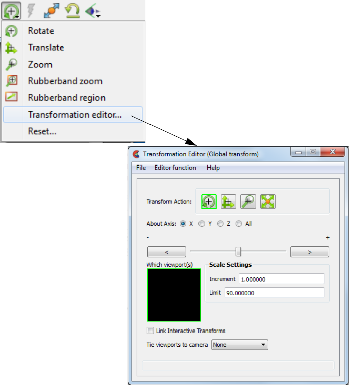
General Description
6-2 EnSight 10.2 User Manual
.
Transformations performed within the Editor affect the selected viewports and/or
frames. The transforms from one viewport can be copied to another by selecting
the viewport to be copied, selecting Copy Transformation State, selecting the
viewport(s) to be modified, and selecting Paste Transformation State.
Transformation Editor -> File Menu
File > Save View This opens the Save View dialog which allows you to save in a file the view (orientation)
of the model you have created in the Graphics Window and any Viewports by selecting
Save View and then entering the name of the file.
File > Restore View Opens the Restore View dialog which allows you to specify the name of a file in which
you previously stored a view. Clicking Okay in this dialog restores the view only in the
selected Viewports.
File > Restore
Camera Position
This will read from a Camera Orientation File which must be created manually
using the format description (see Chapter 9.20, Camera Orientation File Format)
because there is no File > Save Camera file format option.
Figure 6-1
Transforms Icon Transformation editor... selection and Transformation Editor dialog
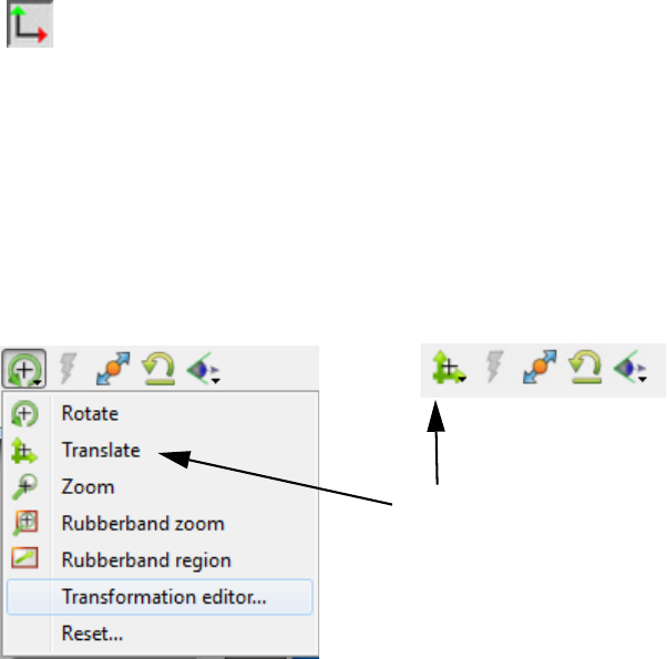
6.1 Global Transform
EnSight 10.2 User Manual 6-3
6.1 Global Transform
Normally transformations you make (rotations, translations, zoom, scale) are
performed globally. Global transformations affect the entire model as a unit and
move all Frames, parts, and visible tools relative to the Global Axis. If the
viewport is being viewed through a camera, the transformations move the camera.
If the viewport is not viewed through a camera, the geometry is transformed. You
can make the Global Axis triad (which pinpoints the Global Axis Origin) visible
by selecting Axis Visibility > Axis - Global from View in the Main Menu or by
clicking the Global Axis Visibility Toggle Icon on the Tools Icon Bar.
Most Global transformations you will make will be done interactively. Interactive
Transformations normally affect only the single, selected viewport (the one which
the mouse pointer is in when you click the left mouse button). The exception to
this is if when you toggle on Link Interactive Transforms, causing the selected
viewports in the Transformation Editor dialog to all transform together. You
choose the type of transformation you wish to perform from among the
Transformation Control Icons.
Rotate When you choose Rotate, clicking the left mouse button and dragging horizontally will
rotate the scene (including any tools that are visible) about the Global Y axis.
Clicking the left mouse button and dragging vertically will rotate the scene (including any
tools that are visible) about the Global X axis.
Holding the Control Key down and then clicking the left mouse button and dragging will
rotate the scene (including any tools that are visible) about the Global Screen Z Axis.
Rotation Using
Function Keys
Pressing the F1, F2, or F3 function keys will rotate the scene 45
degrees about the X, Y, or Z axis respectively. Holding the
Control Key down while pressing these keys will rotate the scene
by -45 degrees. The mouse must be located in the graphics
window for these keys to work.
Figure 6-2
Global Axis Visibility Toggle Icon and Global Axis triad
Figure 6-3
Transformation Control Area in View or Part Mode
Note that this icon changes to reflect
the current selection.
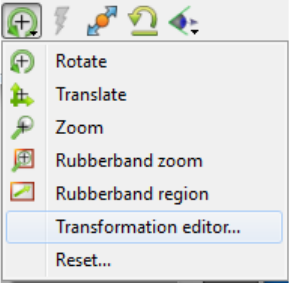
6.1 Global Transform
6-4 EnSight 10.2 User Manual
Translate When this toggle is on, you can transform objects interactively in the Global X-Y plane
(or by holding down the Control key, in Z). Clicking the left mouse button and dragging
will translate the scene (including any tools that are visible) up, down, left or right (or
forward or backward).
Zoom A Zoom transform while in Global Tranform Mode is really an adjustment of the Look
From Point, which you might also think of as the Camera Position. When this toggle is
on, clicking and dragging to the left or down will zoom-in, that is it will move the Look
From Point closer to the Look At Point. Clicking and dragging to the right or up will
zoom-out, that is it will move the Look From Point farther away from the Look At Point.
If you hold down the Control key while interactively zooming, you will “pan”, i.e. move
both the Look At and Look From Points in the direction of the mouse movement.
(see Section 6.5, Look At/Look From)
A Zoom transform while in Camera Mode is a movement of the camera in the camera Z
direction.
As you Zoom in or out, be aware that you may clip the model with the Front or Back Z-
Clip planes since they move in relationship to the Look From Point, always maintaining
the distance from the Look From Point specified in the Transformation Editor dialog:
Editor Function > Z-Clip.
(see Section 6.4, Z-Clip)
RubberBand Zoom You specify the area of interest by clicking and dragging the white rectangle (rubber
band) around the area you wish to zoom in on. Immediately after you perform the Band
Zoom operation however, EnSight will switch to the regular Zoom Transformation. So,
each time you click on the Band Zoom button, EnSight allows you to perform one Band
Zoom operation and subsequent clicking/dragging actions you make in the Graphics
Window perform regular Zoom transformations.
Band Zoom combines the functionality of a zoom-in transform as described above with a
panning operation. The effect of performing a Band Zoom is that the area of interest that
you specify will be centered in and will fill the selected viewport. EnSight adjusts the
transformation center to be in the center of the area you specified.
The Transformation Editor is inactive for the Band Zoom Operation.
RubberBand Region You specify the area of interest by clicking and dragging the white rectangle (rubber
band) around an area and the band zoom tool is located for you to blank out elements
(click on the eraser) or to zoom (click on the magnifying glass), or to use this as a tool for
other options.
Transformation Editor For more precise editing options, choose the Transformation Editor.
Figure 6-4
Transformation Control Area in View or Part Mode
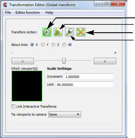
6.1 Global Transform
EnSight 10.2 User Manual 6-5
Precise Rotation When the Transformation Editor is open under Global Transform (the title bar will show
Global transform) and the Rotate toggle is selected, the dialog will be configured to
permit precise Rotation.
You may rotate the entire scene or camera (including any tools that are visible) precisely
about the X, Y, Z, or All axes by clicking on the appropriate axis of rotation toggle and:
entering the desired rotation in (+ or -) degrees in the Increment field and pressing
Return,
clicking the stepper buttons at each end of the slider bar (each click will rotate the
model by the number of degrees specified in the Increment field), or
dragging the slider in the positive or negative direction to the desired number of
degrees you wish to rotate the model (the Limit Field specifies the maximum number
of degrees of rotation performed when the slider is pulled to either end of the slider
bar).
Figure 6-5
Transformation Editor for Precise
Global Rotation
Rotate Toggle
Translate Toggle
Zoom Toggle
Scale Toggle
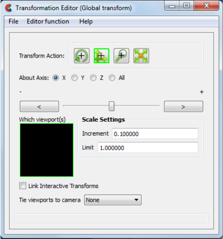
6.1 Global Transform
6-6 EnSight 10.2 User Manual
Precise Translation When the Transformation Editor is open under Global Transform and the Translate toggle
is selected, the dialog will be configured to permit precise Translation.
You may translate the entire scene or camera (including any tools that are visible)
precisely along the X, Y, Z, or All axes by clicking on the appropriate direction toggle
and:
entering the desired translation in (+ or -) model coordinate units in the Increment field
and pressing Return, then
clicking the stepper buttons at each end of the slider bar (each click will translate the
model by the number of model coordinate units specified in the Increment field), or
dragging the slider in the positive or negative direction to the desired number of
model coordinate units you wish to translate the model and then releasing the slider
(the Limit Field specifies the maximum number of model coordinate units that the
model is translated when the slider is pulled to either end of the slider bar).
Figure 6-6
Transformation Editor for Precise
Global Translation
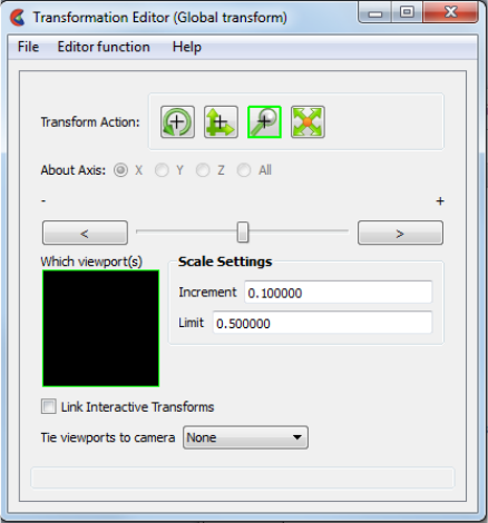
6.1 Global Transform
EnSight 10.2 User Manual 6-7
Precise Zooming When the Transformation Editor is open under Global Transform and the Zoom toggle is
selected, the dialog will be configured to permit precise Zoom.
You may precisely adjust the position of the Look From Point (with respect to the Look
At Point) or move the camera in the camera Z-direction by:
entering in the Increment Field the desired modification (+ or -) in the distance
between the two Points (a value of .5 will increase the distance to be equal to 1.5 the
current distance, a value of 1.0 will double the current distance), then
clicking the stepper buttons at each end of the slider bar (each click will increase or
decrease the distance between the two Points by the factor specified in the Increment
field), or
dragging the slider in the positive or negative direction to the desired modification
factor and then releasing the slider (the Limit Field specifies the maximum
modification factor for the distance between the two Points when the slider is pulled
to either end of the slider bar).
Figure 6-7
Transformation Editor for Precise
Global Zoom
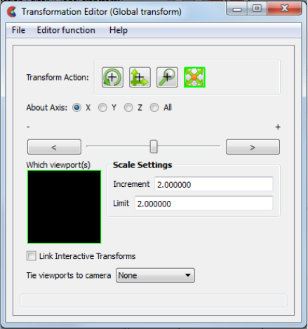
6.1 Global Transform
6-8 EnSight 10.2 User Manual
Precise Scaling Interactive modifications to scale are not permitted. When the Transformation Editor is
open under Global Transform and the Scale toggle is selected, the dialog will be
configured to permit precise adjustments to the scale of the scene. If in Global Transform
Mode the scene will be scaled. If in Camera Transform Mode the size of the camera
glyph will be changed.
You may precisely rescale the scene or camera in the X, Y, Z, or All axes by clicking on
the appropriate scaling direction and:
entering in the Increment Field the desired rescale factor and pressing Return (A value
of .5 will reduce the scale of the scene in the chosen axis by half. A value of 2 will
double the scale in the chosen axis. Be aware that entering a negative number will
invert the model coordinates in the chosen axis.), then
clicking the stepper buttons at each end of the slider bar (Clicking the left stepper
button will apply 1/Increment value to the scale. Clicking the right stepper button will
apply the entire Increment value to the scale), or
dragging the slider in the positive or negative direction to the desired scale factor and
then releasing the slider. (Dragging the slider to the leftmost position will apply 1/
Limit value to the scale. Dragging the slider to the rightmost position will apply the
entire Limit value to the scale.).
Link Interactive
Transforms
If you have multiple viewports you may link them together such that interactive (those
performed in the graphics window) transformation that occurs in one of the linked
viewports occurs in the other linked viewports. To link the viewports select all of the
viewports to be linked in the Which viewport(s) window and turn on the Link interactive
transforms button. An "L" will occur in the viewport outlines in the Which viewport(s)
window indicating which viewports are linked.
Tie viewport(s) to
camera
A viewport may either be in Global Transform Mode or in Camera Mode. In camera
mode the viewport is viewed through a camera. This pulldown makes this choice.
(see How to View a Viewport Through a Camera)
Figure 6-8
Transformation Editor for Precise
Global Scaling
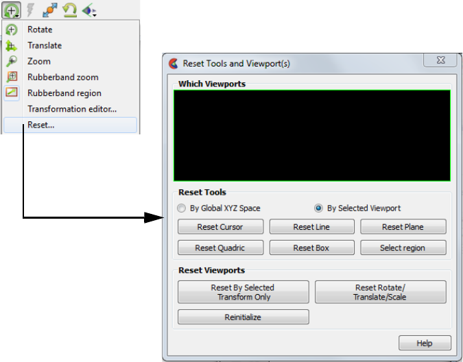
6.1 Global Transform
EnSight 10.2 User Manual 6-9
Reset... Clicking the Reset Tools and Viewport(s) button in the Transformation Control Area will
open the Reset Tools and Viewport(s) dialog
By Global XYZ Space
Toggle
When enabled, clicking a Reset button will cause the Cursor,
Line, Plane, or Quadric Tool to reset to its initial default position.
By Selected Viewport
Toggle
When enabled, clicking a Reset button will cause the Cursor,
Line, Plane, or Quadric Tool to be repositioned in the center of
the geometry for the selected viewport.
Reset Cursor Clicking this button will cause the Cursor Tool to reset according
to the “By” toggle.
Reset Line Clicking this button will cause the Line Tool to reset according
to the “By” toggle.
Reset Plane Clicking this button will cause the Plane Tool to reset according
to the “By” toggle.
Reset Quadric Clicking this button will cause the currently selected Quadric
Tool to reset according to the “By” toggle.
Reset Box Clicking this button will cause the Box Tool to reset according to
the “By” toggle.
Reset Select region Clicking this button will cause the selection Tool to reset
according to the “By” toggle.
Reset By Selected
Transform Only
Clicking this button will cause the transformation selected in the
Transformation Control Area to reset for the viewports selected
in the dialog’s Viewport(s) area.
Reset Rotate/
Translate/Scale
Clicking this button will cause the rotate, translate, and scale
transformations to reset for the viewports selected in the dialog’s
Viewport(s) area.
Figure 6-9
Reset Tools and Viewport(s) dialog
6.1 Global Transform
6-10 EnSight 10.2 User Manual
Reinitialize Clicking this button will cause the viewports selected in the
dialog’s Viewport(s) area to reset and recenter on the Parts which
are visible in the Viewport(s).
Reset using
Function Keys
Pressing the F5 button will change the scene in the current viewport to the standard “right
side” view. Similarly, pressing F6 will show a “top” view and F7 a “front” view. Pressing
F8 will restore the view to the one which existed before F5, F6, or F7 were pressed. If the
Control Key is pressed at the same time as F5, F6, or F7, then the current view will be
stored to the selected button.
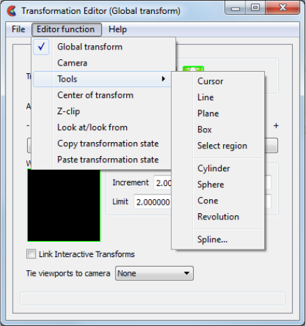
6.2 Tool Transform
EnSight 10.2 User Manual 6-11
6.2 Tool Transform
Transformation of the Cursor, Line, Plane, Box, Selection, and Quadric (cylinder,
sphere, cone, and revolution) Tools is covered in depth in Chapter 4.
(see Tool Positions in Section 4.6, Tools Menu Functions) specifically at
Transformation Editor Tools Dialog
Figure 6-10
Transformation Editor Tools Selections
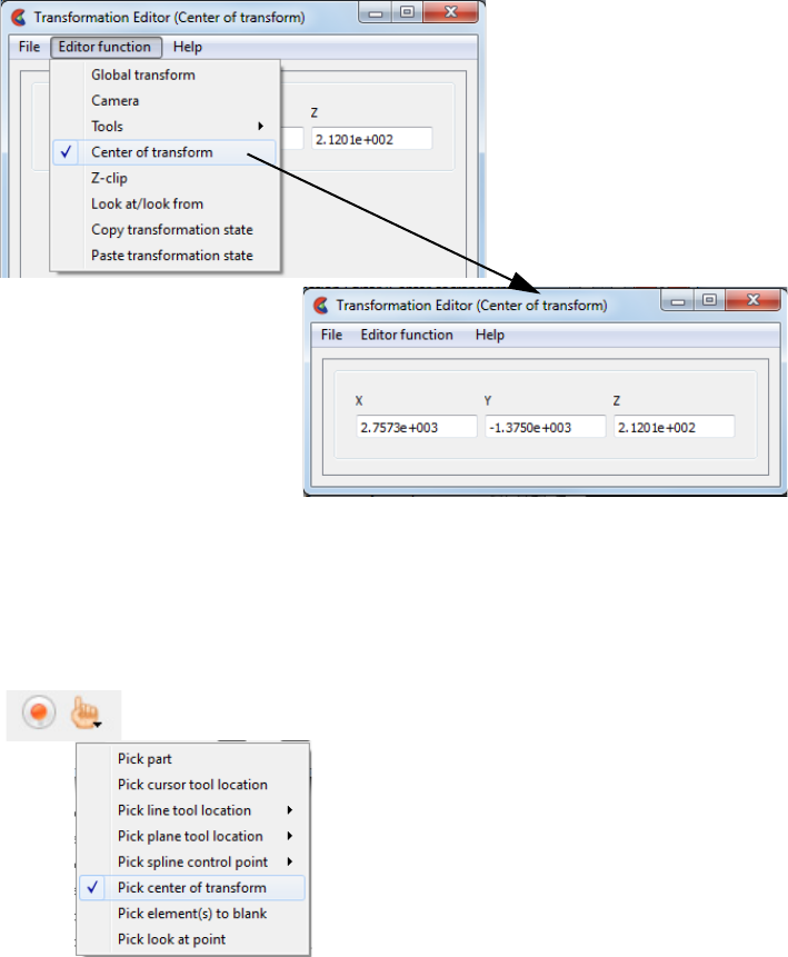
6.3 Center Of Transform
6-12 EnSight 10.2 User Manual
6.3 Center Of Transform
The point about which global transformations will occur can be specified exactly
if desired. Simply enter the model coordinates for the location of this point.
Alternatively you can click on the pick icon and pull down to ‘Pick center of
transform’, and then move the cursor over the part location (make sure the
EnSight graphics window is active) and pick using the ‘p’ key.
Alternatively, you can click on the Fit button which will reset the center of
transform to the geometric center of the visible parts.
Alternatively, you can right-click on a part in the graphics window and choose Set
Center of Transform and the location on the part will become the center of
transform.
Figure 6-11
Transformation Editor Center of Transform dialog
Figure 6-12
Pick Center of Transform pulldown
6.4 Z-Clip
EnSight 10.2 User Manual 6-13
6.4 Z-Clip
EnSight displays the scene in a three-dimensional, rectangular workspace that has
finite boundaries on all sides. Even if you rotate the model, you are always
looking into the workspace from the front side. The top-to-bottom and side-to-
side boundaries of the workspace are analogous to looking out a real window—
the window frame limits your view. In addition, since the memory of your
computer is finite, your workspace also has limits in the front-and-back direction.
The front boundary is the Front Clipping Plane (or the Near Plane) and the rear
boundary is the Back Clipping Plane (or the Far Plane). Only the portion of the
scene between these two planes is visible—the rest of the model (if any) is clipped
and therefore invisible. By convention, the front-to-back direction of the
workspace is the Z direction. Hence, the front and back clipping planes are
together called the Z-Clip Planes. Note that the Z-direction in the workspace is
always in-and-out of the screen and is completely independent of the Z-direction
of the model Frame (Frame 0).
Z-Clip Positions The position of the Z-Clip planes is specified in terms of their distance from the
Look From Point in the distance units implied by the model-geometry data. By
default, the planes automatically move as the model moves.
Initially, EnSight positions the Z-Clip Planes based on the dimensions of the
model parts read to the Client, with some extra space for you to perform
transformations. You can reposition the planes when doing so becomes necessary
or desirable.
Each viewport has its own independently adjustable set of Z-Clip Planes.
Using Z-Clip Planes You can use Z-Clip planes to deliberately clip-away portions of the model you are
not interested in, or which are getting in the way of what is of interest. For
example, you can clip-away both a front-portion and a back-portion of a model to
reduce the number of node and element labels displayed. Z-Clip Planes and
EnSight uses your workstation’s graphics hardware to perform all graphics
Hidden Surfaces manipulations, including the display of solid surfaces. The appearance of a solid
model is created by not displaying hidden surfaces—surfaces hidden behind
nearer surfaces. The algorithm used by the graphics hardware to do this task— Z-
buffering—is a simple algorithm which compares Z-values to calculate which
surfaces are closest to you and thus visible. Z-buffering is normally performed in
integer arithmetic, and on most graphics systems is confined to 24 bits of
resolution. Hence, the coordinates in Z must be mapped into this 24-bit space. To
achieve the maximum resolution possible in the 24 bits available, the graphics
hardware maps the Z-distance between the Front and Back Clipping Planes into
the 24 bits available. Hence, the larger the distance between the Z-Clip Planes, the
lower the Z resolution, which can affect image quality for solid images. If you see
problems with your solid images, move the front and back clipping planes in as
close as possible.
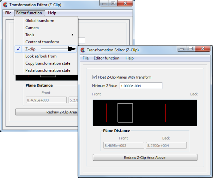
6.4 Z-Clip
6-14 EnSight 10.2 User Manual
The Transformation Editor (Z-Clip) is used to adjust the distances of the Front and Back
Clipping Planes from the Look-From Point.
Float Z Clip Planes
With Transform
When on, will automatically adjust the front and back Z-Clip
planes away from the model.
Minimum Z Value Minimum distance the Front Clipping Plane is allowed to float to
from the Look From Point (model coordinates). Used only if
Float Z Clip Planes with Transform toggle is on.
Z-Clip Area Display Displays position of Z-Clip planes relative to model-part Z-range
(shown as a rectangle) and allows interactive positioning (by
clicking and dragging) of the Z-Clip planes. If lines are inside
model rectangle, that part of model is clipped from the display.
Values update in data fields as you move sliders. Active
viewports of the Main View update automatically as you move
sliders.
Plane Distance
Front Distance of the Front Clipping Plane from Look From Point in
model coordinates. Precisely specify by typing in desired
distance and pressing Return. Not used if the Float Z Clip Planes
With Transform toggle is on.
Back Distance of the Back Clipping Plane from the Look From Point
in model coordinates. Precisely specify by typing in desired
distance and pressing Return. Not used if the Float Z Clip Planes
With Transform toggle is on
Figure 6-13
Transformation Editor for Z-Clip Plane Positions

6.4 Z-Clip
EnSight 10.2 User Manual 6-15
Troubleshooting Z-Clip Planes
Redraw Z-Clip
Area Above
The Plane Position Display does not automatically update if you
perform transformations in the active viewport. Click this button
to update the Plane Position Display.
Problem Probable Causes Solutions
Main View is empty No parts located between Front
and Back Z-Clip Planes.
Toggle off the Float Z-Clip
toggle and adjust Z-Clip plane
locations
Model degenerates to irregular
polygons or the front Z-Clip line
is locked in the model extent box
You have moved the front Z-Clip
plane too close to (or on) the
Look From Point.
Move the front Z-Clip plane
away from the Look From Point.
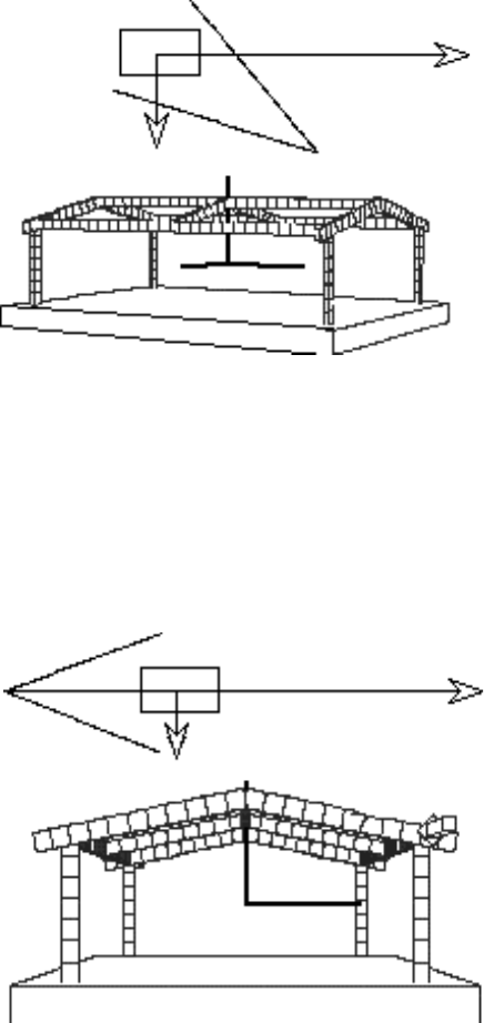
6.5 Look At/Look From
6-16 EnSight 10.2 User Manual
6.5 Look At/Look From
Using the Transformation Editor with Editor Function > Look At/Look From
chosen, you can reposition the point from which you are observing the model (the
Look From Point) and the point at which you are looking (the Look At Point).
Both the Look-From and Look-At points are specified in the coordinates of the
Model Frame (Frame 0).
Initially, the Look At Point is at the geometric center of the initial model parts
read by the EnSight Client. The Look From Point is on the positive Z-axis at a
distance appropriate to display the model in the Main View window.
If you increased only the X position of the Look From Point, in the Graphics
Window (or selected Viewport), it would appear that the model had rotated about
the Global Y axis. In fact, the model has not rotated at all, which is shown by the
visible Global Axis triad in the figure below. What has happened is that you are
now viewing the model from a position farther to the right than previously.
If the Y and Z coordinates of the Look From point were made to be the same as
those of the Look At point, but the X coordinate of Look From point was specified
as a much smaller value than that of the Look At point, it would appear in the
Graphics Window (or selected Viewport) that the model had rotated 90 degrees
about the Global Y axis. As before, the model has actually not rotated at all, which
is shown by the visible Global Axis triad in the figure below. What has happened
is that you are now viewing the model from a position on the negative Global X
axis looking in the positive X direction.
Figure 6-14
Image showing view of model from
negative X axis towards positive X axis
Eye Position
Model
Schematic
Plan View
X
Y
X
Z
ZG
(Look From Point)
Figure 6-15
Image showing view of model from
negative X axis towards positive X
axis
Eye Position
Model
Schematic
Plan View
X
Y
X
Z
Z
G
(Look From Point)
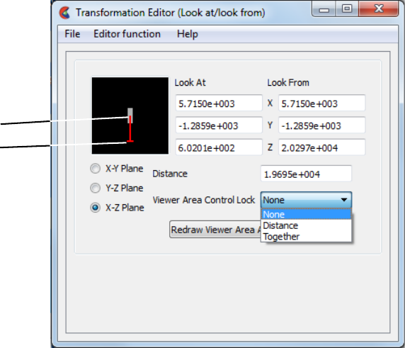
6.5 Look At/Look From
EnSight 10.2 User Manual 6-17
The position of the Look-At and Look-From points can be interactively or
precisely specified using the Transformation Editor dialog with Editor Function >
Look At/Look From.
Interactive The position of the Look At and Look From Points may be positioned interactively in the
Interactive Viewer Area by grabbing the Look At or Look From Point and dragging it to
the desired location. These interactive modifications can be made in the X-Z Plane, the X-
Y Plane, or the Y-Z Plane, depending upon which of the three toggles are selected. The
Graphics Window as well as the Look At and Look From coordinate fields updates as you
drag either Point to a new location.
Precise The position of the Look At and Look From Points may be positioned precisely by
specifying the desired coordinate values in the X Y Z fields and pressing Return.
Distance The distance in model coordinates may be precisely specified by
entering the desired value in this field and pressing Return.
Viewer Area Control
Lock
Opens a pop-up menu for the selection of how interactive actions taken in the Viewer
Area will be limited. Choices are:
None No locks are applied
Distance The distance between the two Points is locked
Together The distance and direction vector between the two Points is
locked
Redraw Viewer Area
Above
This button redraws the Viewer Area. This button should be clicked after a transformation
is performed in the selected viewport while this dialog is active.
Figure 6-16
Transformation Editor for Look At/Look From
Interactive Viewer
Area
Look At Point
Look From Point
6.6 Copy/Paste Transformation State
6-18 EnSight 10.2 User Manual
6.6 Copy/Paste Transformation State
This transformation option can be used to apply the transformation state of one
viewport to other viewports. Useful if you want multiple viewports to have the
model oriented the same, and you did not link the viewports for transformations
before applying any transformations.
The use of this option consists of:
1. Selecting the viewport (one only) containing the transformation state desired.
(You can do this with the Viewport Quick Action Icon, or under Editor Function ->
Global Transform in the Transformation Editor Dialog.)
2. Selecting Copy Transformation State under Editor Function in the
Transformation Editor dialog.
3. Selecting the one or more viewports to receive this transformation state.
(As in 1. above)
4. Selecting Paste Transformation State under Editor Function in the
Transformation Editor dialog.
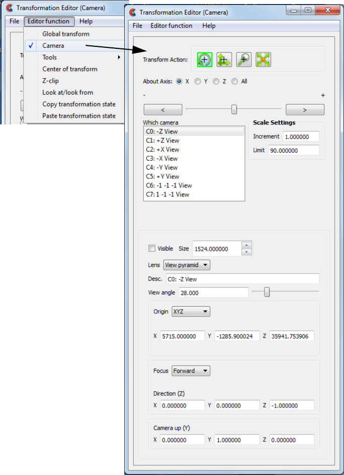
6.7 Camera
EnSight 10.2 User Manual 6-19
6.7 Camera
If a Viewport is in Camera Mode (see “Tie Viewports to Camera” in Section 6.1,
Global Transform) the viewport will be viewed through the camera chosen. Any
global transforms that have been created for the viewport are ignored and any
transforms performed will be for the camera selected.
(also see How to View a Viewport Through a Camera)
Figure 6-17
Transformation Editor for
Camera Rotation
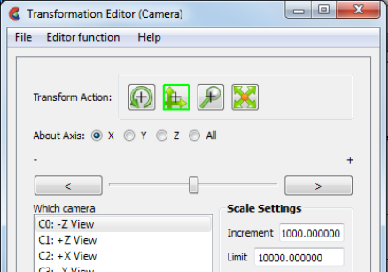
6.7 Camera
6-20 EnSight 10.2 User Manual
Rotate Toggle Interactive Rotation When transform action selected is rotate, then clicking the left
mouse button and dragging horizontally in a viewport that is
being viewed through a camera will rotate the camera about the
Camera Y axis. Holding the Control Key down and then clicking
the left mouse button and dragging will rotate the camera about
the Camera Z axis.
Precise Rotation When the Transformation Editor is open under Camera and the
Rotate toggle is selected, the dialog will be configured to permit
precise Rotation of the selected camera(s). You may rotate the
selected camera(s) selected precisely about the X, Y, Z, or All
camera axis by clicking on the appropriate axis of rotation toggle
and entering the desired rotation in (+ or -) degrees in the
Increment field and pressing Return, or by clicking the stepper
buttons at each end of the slider bar (each click will rotate the
camera by the number of degrees specified in the Increment
field), or by dragging the slider in the positive or negative
direction to the desired number of degrees you wish to rotate
(note: the Limit Field specifies the maximum number of degrees
of rotation performed when the slider is pulled to either end of
the slider bar).
Translate Toggle
Interactive Translation When the transform action is translate and the translate icon is
highlighted, then, clicking the left mouse button and dragging in
a viewport that is being viewed through a camera will translate
the camera left/right, or up/down (or by holding the Control key,
in/out).
Precise Translation When the Transformation Editor is open under Camera and the
Translate toggle is selected, the dialog will be configured to
permit precise Translation of the selected camera(s).
Figure 6-18
Transformation Editor for Camera Translation
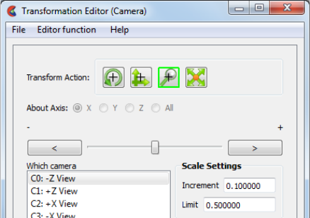
6.7 Camera
EnSight 10.2 User Manual 6-21
You may translate the camera(s) selected precisely about the X,
Y, Z, or All camera axis by clicking on the appropriate axis of
translation toggle and entering the desired translation in (+ or -)
model coordinate units in the Increment field and pressing
Return, or by clicking the stepper buttons at each end of the slider
bar (each click will translate the camera by the number of units
specified in the Increment field), or by dragging the slider in the
positive or negative direction to the desired number of units you
wish to translate (note: the Limit Field specifies the maximum
number of units in model coordinates performed when the slider
is pulled to either end of the slider bar).
Zoom Toggle
Interactive Zooming When the transform action is zoom then clicking the left mouse
button and dragging in a viewport that is being viewed through a
camera will move the camera in the camera z-direction. The
result is exactly the same as if you translated the camera in the z-
direction using the Translate Toggle.
Precise Zooming When the Transformation Editor is open under the Camera and
the Zoom toggle is selected, the dialog will be configured to
permit precise Zoom operations of the selected camera(s).
You may zoom the camera(s) (moving the camera in the camera
z-direction) selected precisely by entering the desired camera z-
axis movement in (+ or -) model coordinate units in the
Increment field and pressing Return, or by clicking the stepper
buttons at each end of the slider bar (each click will translate the
camera in the z camera axis direction by the number of units
specified in the Increment field), or by dragging the slider in the
positive or negative direction to the desired number of units you
wish to move (the Limit Field specifies the maximum number of
units in model coordinates performed when the slider is pulled to
either end of the slider bar).
Figure 6-19
Transformation Editor for Camera Zoom
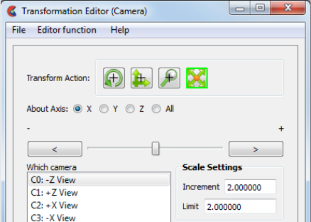
6.7 Camera
6-22 EnSight 10.2 User Manual
Scale Toggle When the Transformation Editor is open under Camera, and the Scale toggle is selected,
the dialog will be configured to permit Scale operations of the selected camera(s).
A Scale operation of a camera does not affect the transformations that are occurring in the
viewport - they affect the size of the camera glyph. You may modify the size of the camera
glyph by selecting the X, Y, Z, or All axis (they will all perform the same camera resize
operation) toggles and then entering the desired camera glyph scale factor in the
Increment field and pressing Return (values < 1 will make the camera glyph smaller while
values > 1. will make it larger), by clicking the stepper buttons at each end of the slider
bar (each click will scale the camera glyph up/down by the factor specified in the Limit
field), or dragging the slider in the positive or negative direction to scale the camera up or
down (the Limit Field specifies the maximum scale factor performed when the slider is
pulled to either end of the slider bar).
Figure 6-20
Transformation Editor for Camera Scale
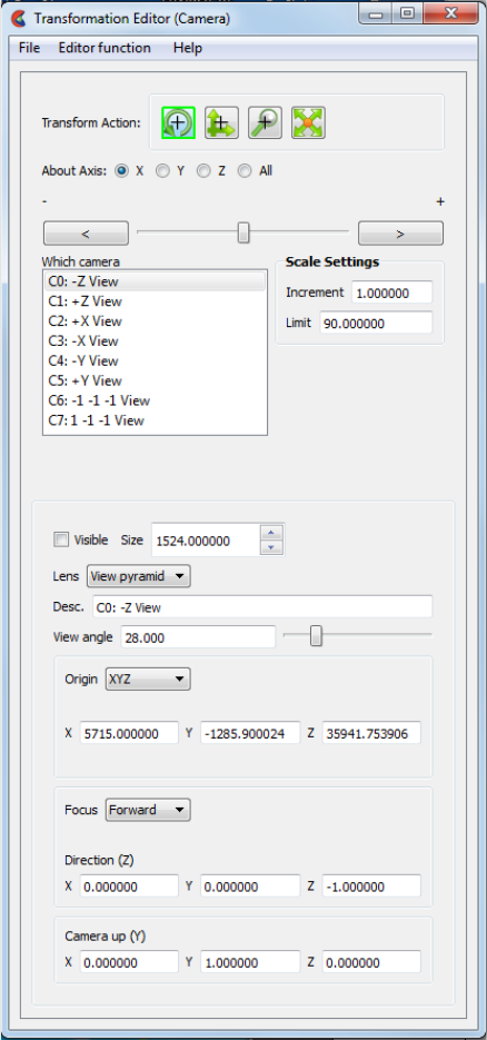
6.7 Camera
EnSight 10.2 User Manual 6-23
Which camera Selects the camera(s) being modified
File ->Restore Camera
Position
This opens the Restore camera dialog which allows you to specify the name of a file in
which a camera location and orientation is specified (see Chapter 9.20, Camera
Orientation File Format).
Visible Sets the visibility of the camera(s) selected
Size Sets the size of the camera glyph for the selected camera(s). Size is in model coordinates.
Desc Description of the camera.
Lens View pyramid will show the view constraints if the camera were used to view the
viewport. Classic shows a classical "lens" on the camera with no hint of the view volume.
View Angle The view angle in degrees that will be used with the camera. Small values decrease the
view angle and simulate a telephoto lens while large values increase the view angle and
simulate a wide angle lens. Current limitation is 5 < view angle < 120
Figure 6-21
Transformation Editor for Camera
Scale
6.7 Camera
6-24 EnSight 10.2 User Manual
Origin Sets the camera origin
XYZ The model coordinates of the camera
Node Sets the Camera origin at a specific part node id number
Spline Set the Camera origin to lie on a defined spline
Offset If the Origin is set to Node or Spline it is possible to offset the
origin from the node or spline by a XYZ value
Focus Defines the orientation of the camera
Forward If the origin is Spline then focus is "forward" on the spline. If the
origin is not Spline then the focus is defined by the Direction(Z)
fields.
Node Set the focus to a specified part and node id
XYZ Set the focus to a specific location
Camera up (Y) Sets the vector defining the "tilt" of the camera. Will be adjusted if the Focus is set to
Node or XYZ to form a right handed orthogonal coordinate system.
General Description
EnSight 10.2 User Manual 7-1
7 Variables and EnSight Calculator
Included in this chapter:
General Description
Section 7.1, Variable Selection and Activation
Section 7.2, Variable Summary & Palette
Section 7.3, Variable Creation
Section 7.4, Boundary Layer Variables
General Description
Variables are numerical values provided by your analysis software (model
variables) or created within EnSight (created variables). Variables can be
dependent on server part-geometry (for example, the area of a part), and a part’s
geometry can be dependent on its parent part’s variable values (for example, an
isosurface).
Va ri a bl e Ty pe s There are six types of variables: tensor, vector, scalar, constant, and constant per
part. Scalars and vectors can be real or complex. Symmetric tensors are defined
by six values, while asymmetric tensors are defined by nine values. Vectors, such
as displacement and velocity, have three values (the components of the vector) if
real, or six values if complex. Scalars, such as temperature or pressure, have a
single value if real, or two values if complex. Constants have a single value for
the model, such as analysis time or volume at each timestep. Constants per part
have a single value for each part, such as area at each timestep. All types can
change over time for transient models.
Note that constants per part, that are in model files and exist with the same value
in all parent parts of a created part - are inherited by said created parts. If the
value differs, they will become undefined in the created part. However,
computed constants per part are not automatically inherited by created
parts, and become undefined in the created parts. If a value is desired in the
created part(s) for the computed constant per part, one should include the created
part as one of the parent parts for the computed constant per part.
Activation Before using a variable, it must be loaded by EnSight, a process called activation.
EnSight normally activates variables as they are needed. Section 7.1, Variable
Selection and Activation describes how to select, activate, and deactivate
variables to make efficient use of your system memory.
(see Section 7.1, Variable Selection and Activation)
Creation In addition to using the variables given by your analysis software, EnSight can
create additional variables based on any existing variables and geometric
properties of server parts. EnSight provides approximately 100 functions to make
this process simpler. Because created variables may have dependencies on other
variables and possibly also on parts, they are more limited in their usage than
model variables. (see Section 7.3, Variable Creation)
Color Palettes Very often you will wish to color a part according to the values of a variable.
EnSight associates colors to values using a color palette. You have control over
the number of value-levels of the palette and the type of scale, as well as control
over colors and method of color gradation. You also use function palettes to
specify a set of levels for a variable, such as when creating contours.
General Description
7-2 EnSight 10.2 User Manual
(see Section 7.2, Variable Summary & Palette)
Queries You can make numerical queries about variables and geometric characteristics of
Server-based parts. These queries can be at points, nodes, elements, parts, along
lines, and along 1D parts. If you have transient data, you can query at one time
step or over a range of time steps, looking at actual variable values or a Fast
Fourier Transform (FFT) of the values. (see Section 4.4, Query Menu Functions)
Plotting Once you have queried a variable, you can plot the result.
(see Section 5.3, Query/Plotter)
From More than Variables can come from more than one case. If more than one case has a
One Case variable with the same name, this will be treated as one variable. If a variable does
not exist in one of the cases, it cannot be used in that case.
Parts When variables are activated or created, all parts except Particle Trace parts are
updated to reflect the new variable state. Particle Trace parts will always show
variables which are activated after the part’s creation as zero values.
Variable calculation occurs on the server. Therefore, the input to all of the
predefined functions includes some type of server based parts. Conversely, parts
which reside only on the client (contours, particle traces, profiles, vector arrows,
and tensor glyphs) cannot be used to calculate variables.
Location Variables can be defined at the vertices, at the element centers, or undefined. Face
and edge variables are not supported.
User Defined Math Functions
Users can write external variable calculator functions called User Defined Math
Functions (UDMF) that can be dynamically loaded by EnSight at startup. These
functions appear in EnSight’s calculator in the general function list and can be
used just as any other calculator function to derive new variables.
Several examples of UDMFs can be found in the directory
$CEI_HOME/ensight102/
src/math_functions/
.
When the EnSight server starts it will look in the following subdirectories for
UDMF dynamic shared libraries:
./libudmf-devel.so (.sl) (.dll)
$ENSIGHT10_UDMF/libudmf-*.so (.sl) (.dll)
$CEI_HOME/ensight102/machines/$ENSIGHT10_ARCH/lib_udmf/libudmf-*.so (.sl)
(.dll)
Depending on the server platform, the dynamic shared library must have the
correct suffix for that platform (e.g. .so, .sl, .dl
l
).
Currently, when a UDMF is used in the EnSight calculator, it is invoked for each
node in the specified part(s) if all the variables operated on for the specified
part(s) are node centered. If all of the variables are element centered, then the
UDMF is invoked for each element in the part(s). If the variables are a mix of
node and element centered values, then the node centered values are automatically
converted to element centered values and then the UDMF is invoked for each
element using element centered variables.
Arguments and the return type for the UDMF can be either scalar or vector
EnSight variables or constants. At this time, only variable quantities and constants
can be passed into UDMFs. There is no mechanism for passing in either part
geometry, neighboring variables, or other information. For more information, see
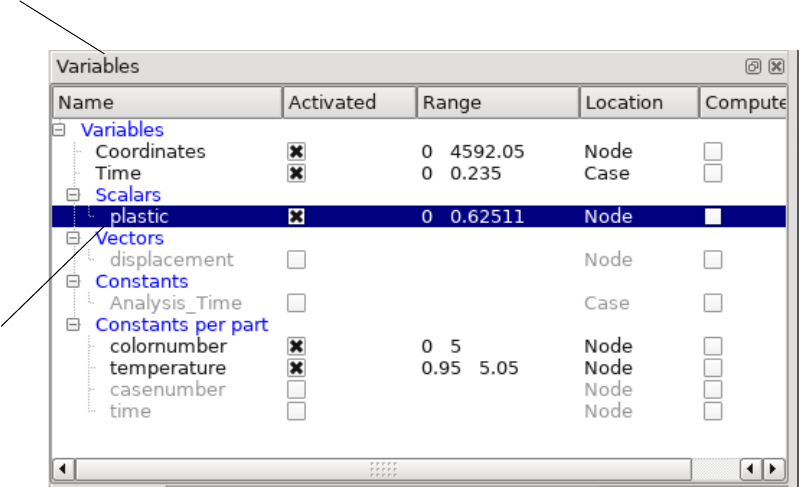
7.1 Variable Selection and Activation
7-4 EnSight 10.2 User Manual
7.1 Variable Selection and Activation
All available variables, both those read in and those created within EnSight, are
shown in the Variables Panel, whether they have been activated or not. In
addition, a variable list is included in each function requiring a variable. In this
case, only the appropriate variable types are shown.
Variable Panel This list shows all variables currently available, both those read from data and those you
have created within EnSight. Each column provides information about a variable. Right
click on the column header and choose customize to add columns of interest. Variables are
grouped by their type: constant, constant per part, scalar, vector or tensor.
Available Variable The description or name of the variable.
Grayed out Activation status. A deactivated variable has a grayed out name.
Name Var iab le N ame .
Range Min and max value of activated variable. Note that this does not update with time change.
For performance reasons, it only updates when you hover your mouse over these values.
Location Location of the variable:
Node Variable is located at geometry nodes.
Element Variable is located at geometry elements
Case Variable is a case variable
Computed Checkbox on indicates the variable is a computed variable
Activated Shows which variables are activated.
Figure 7-1
Variable Panel
Feature Panel
Vari ab les Li st
Edit Palette
Click here to
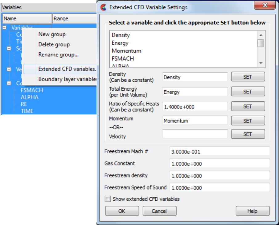
7.1 Variable Selection and Activation
EnSight 10.2 User Manual 7-5
Constant value Shows the value of an EnSight constant.
Exists in Case Shows which case(s) the variable belongs to, or “All” if available for all cases.
Type Constant, Constant per part, Scalar, Vector or Tensor.
Extended CFD Right click on the Variables folder and choose Extended CFD variables. These were
intended as a supplement to the OVERFLOW and PLOT3D readers. Opens
Variables... the Extended CFD Variable Settings dialog. If your data defines variables or constants for
density (SCALAR or CONSTANT), total energy per unit volume (SCALAR), and
momentum (or velocity) (VECTOR), it is possible to show new variables defined by these
basic variables in the Main Variables List of the GUI by utilizing the capabilities of this
dialog. (See Preferences... in Section 4.2, Edit Menu Functions).
WARNING: Modifications to this dialog will not affect extended CFD variables that have
already been activated - only future activated variables are affected. To modify an
existing variable you will need to modify the variable’s working expression in the
calculator and recalculate it.
WARNINGIf you deactivate a created variable or any of the variables used to define it,
both the values and the definition of the created variable are deleted. If you deactivate a
variable used to create a part’s geometry, the part will be deleted. If you deactivate a
variable who’s color palette has been used to color a part, the part’s appearance will
change.
(see How To Activate Variables)
Figure 7-2
Extended CFD Variable Settings
Dialog
7.2 Variable Summary & Palette
7-6 EnSight 10.2 User Manual
7.2 Variable Summary & Palette
You can visualize information about a model by representing variable values with
colors, often called fringes. Fringes are an extremely effective way to visualize
variable variations and levels. A variable color palette associates (or maps)
variable values to colors. Palettes are also used in the creation of contours. The
number of contour levels is based on the number of palette color levels, and the
contour values are based on the palette level values.
EnSight uses a variable’s color palette to convert numbers to colors, while you,
the viewer, use them in the opposite manner—to associate a visible color with a
number. If you wish, EnSight can display a color-value legend in the Main View
window.
Default Palettes At least one color palette—the Coordinate color palette—always exists, even if
your model has no variables. In addition, EnSight creates a color palette for each
constant per part, real scalar and real vector variable that you activate, giving the
color palette the same name as the variable. If the variable is a vector variable, the
default color palette uses the vector’s magnitude. Constant and Tensor variables
have no palette.
Default color palettes have five color levels. Ranging from low to high, the colors
are blue, cyan, green, yellow, and red (the spectral order). The numerical values
mapped to these five levels are determined by first finding the value-range for the
variable at the current time step when the variable is activated. The value for the
lowest level is set to the minimum value. The value for the highest level is set to
the maximum value. The three middle levels are spaced evenly between the
lowest and highest values. For datasets with only one time step, the scheme just
described works well because the variable’s value range is not changing over
time. However, if you have transient data, the range could vary widely at
different times and since the default was based on one time step, it may not be
appropriate for other time steps. EnSight can show you a histogram of the variable
values over time to assist you in setting a palette for transient cases.
The value range for the palette is defined when the variable is activated. The
range is initialized such that the min/max cover the variable range for the
currently defined parts. The range is not changed by EnSight if you add new parts
in the future but you do have the ability to initialize the palette based on the
variable extreme, the selected parts, and visible geometry in a specified viewport.
Value Levels A color palette can have up to 21 levels at which the variable value is specified.
Each color palette level’s value must be between the value at the adjoining levels.
You select whether the scale is linear (the default), quadratic (2x), or logarithmic
(log10).
Sometimes you may wish to only visualize areas whose palette-variable values are
in a limited range. You can choose to visualize other areas with a different,
uniform color, or to make those areas invisible.
Management The Palette Editor enables you to manage your color palettes. You can copy, save
to a file, and restore from a file existing palettes. You can also edit the palette. To
see the Palette Editor dialog, click on the Edit Palette... button in the Quick Action
Icon Bar at the top.
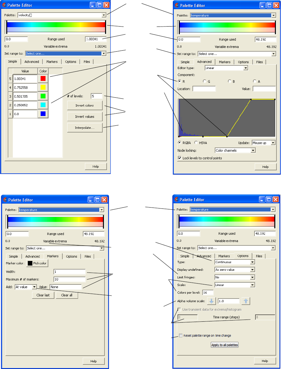
7.2 Variable Summary & Palette
EnSight 10.2 User Manual 7-7
Clicking the Edit Palette... button opens the Palette Editor dialog.
Figure 7-3
Palette Editor: Variables
Change # levels
Quick set of min/max using
Maximum & Minimum
Options
Simple Interface
Tab
Value Sliders
Palette
Select Palette to
Edit
Advanced Interface
Tab
color
Reverse Colors
and values
Interpolate values or
colors between 2 levels
parts, viewport or extrema
Variable Histogram
Tab
Markers
Tab
Color
Number
Location
Variable
Display
Scale and
Select Palette to
Edit
Banded or
Continuous
and fields
Level, value and
Blending Controls
Selection and
Color Channel
Blending Controls
Isovalue Line Markers
Volume Rendering
Opacity Scale
data over time range
Rescale with every timestep
change
Rescale using transient

7.2 Palette Editor Items Available on Every Tab
EnSight 10.2 User Manual 7-9
Palette Editor Items Available on Every Tab
Palette Select the variable palette to be edited
Color Palette This horizontal color legend shows the color range for the palette selected. The left and
right black vertical lines indicate the current min/max values in use in reference to the
variable extrema and can be clicked/dragged to adjust the minimum and maximum values
in use.
Range Used Specifies the minimum and maximum values to be used for the bottom and top levels in
the palette respectively
Set range to: The minimum and maximum values associated with the palette can be set to one of the
following
extrema Sets the minimum and maximum palette range values to a static value which is the
variable's minimum and maximum value at the current timestep. This is value can be set
using the variable’s minimum and maximum value over all time under the Options Tab by
toggling on “Use Transient Data for Extrema/Histogram”. The min and max can be reset
each timestep under the Options Tab by toggling on “Reset Palette Range on Time
Change”.
selected parts Does a one-time reset of the minimum and maximum palette range values using the
viewable elements on the screen of the selected parts (blanking and part element
representation affect this range). If you change time you will need to select this option
again to reset the min and max to the selected parts variable min and max.
current viewport Sets the minimum and maximum palette range values using the currently visible elements
in the current viewport (blanking, part element representation, and transformation will all
affect this range). If you change time you will need to select this option again to reset the
min and max to the current viewport variable min and max.
Palette Editor Simple Tab
Value/Color matrix You can type new values into each numeric field to adjust the value associated with a
color. If you click on the color swatch for any level a color selector dialog will appear
allowing you to set the color at the level indicated.
# of levels This field specifies the number of value levels for the selected palette. Each level will be
defined as a value and color in the field at the left of the dialog.
Invert colors Reverses the colors for the palette
Invert values Reverses the values for the palette
Interpolate... Brings up a dialog allowing you to interpolate values or colors between two levels.
Palette Editor Advanced Tab
Variable Palette The background of the middle graphic shows the relative number of nodes at which the
Histogram Value of the selected variable is within the range represented by a particular value band.
The small horizontal line at the far left of the graphic can be used to interactively adjust
the vertical scale of the histogram.
Control Points By default EnSight will create the same number of control points as there are levels in the
palette. Control points can be added or deleted by right clicking on a control point marker.
When adding a control point the point will be added half way between the selected point
and the one immediately to the right. To decouple the number of control points from the
number of palette levels see "Lock levels to control points" under the Options tab. To
adjust the component value at the control point click and drag the control point.
Editor Type The control points can control color by straight line interpolation (Linear) or by creating a
7.2 Palette Editor Markers Tab
7-10 EnSight 10.2 User Manual
spline.
Component Selects which color channel will be edited via the control points - Red, Green, Blue, or
Alpha, or Hue, Saturation, Value, or Alpha, depending on the state of the RGB/HSVA
toggle below.
Location Indicates the location (the x value) of the selected control point in the range 0 (left side) to
1.
Value Indicates the value of the component of the selected control point in the range 0 (off) to 1
(full value)
RGB/HSVA Toggle between Red/Green/Blue or Hue/Saturation/Value to represent color.
Update Specifies when the update to the scene will occur. Delayed will cause the update to occur
when you select the Apply Changes button at the bottom of the dialog. Mouse up
indicates that as you modify the control points or min/max range markers in the palette
editor that the update will occur when you release the mouse button. And finally,
Immediate will update the scene while you modify the control points.
Node locking By default the control points for the color and alpha channels are locked together, i.e., if a
node is added/deleted it is added to all channels and if the location of a control point is
moved it affects the location of all channels. "Color channels" indicates that only the
color is locked together and the alpha control points are independent. "None" indicates
that all color as well as alpha are independent. Warning: you can not make the node
locking more restrictive than the current setting, i.e., if you set the node locking to None
you will not be able to set it back to either of the two other choices. Also, once you have
set this to ‘None’, it cannot be set back to ‘Color Channel’ in the current session of
EnSight.
Lock levels to If turned on (the default), the number of control points for the palette will be the same as
control points the number of levels and they will be uniformly spaced. Turning this off allows you to
decouple the number and location of control points from the number of levels.
Palette Editor Markers Tab
It is possible to modify a texture entry in the color palette to show a particular
color. These inserted colors show up as regions (contours) of constant color in the
graphics window. The width of the resulting contour is a result of the marker
width as well as the number of colors per level (see Options tab).
A marker can be added by directly clicking on the horizontal legend in the dialog.
Marker Color Sets the color for all defined markers
Width Sets the number of texels covered by the marker
Maximum # of Sets the total number of marker objects that will be stored for the palette
markers
Add:
At Value Specify the variable value in the Value field which will be inserted as a marker into the
palette.
Uniformly Specify the number of uniformly spaced markers in the ‘How many’ field that will be
added into the palette
At levels Will add a marker at each level of the palette
Clear last Remove the last marker object created
Clear all Remove all markers from the palette
Palette Editor Options Tab
Type This pulldown allows for the selection of the desired type of color gradation. The options
are:
7.2 Palette Editor Files Tab
EnSight 10.2 User Manual 7-11
Continuous Displays graduated color variation across or along each element interpolating the color
across each element based on the value of the variable at the nodes. If the variable tied to
the palette is defined at the element centers the result will be a constant color across the
entire element (see also "Use continuous palette for per element vars" option under Edit-
>Preferences->Color Palettes).
Banded Displays discrete color bands across the elements the number of which is controlled by the
number of levels and the number of Colors per level.
Constant Displays a single color at each element without any blending.
Display undefined If the variable is not defined, the element can not be colored according to the color
palette. In this case the element will be colored by:
No Color associated with the value of 0. This is the default.
By part color Color associated with the constant part color.
By invisible The element will not be displayed.
Limit fringes This pulldown allows you to select how you wish to display elements with variable values
above or below the minimum and maximum of the color palette. Options are as follows:
No color scalar values that exceed the minimum or maximum of the palette by the same color
as associated with the minium or maximum of the palette. This is the default.
By part color Color scalar values that exceed the minium or maximum of the palette by the part's color.
By invisible Color scalar values that exceed the minimum or maximum of the palette using full
transparency
Scale This pulldown allows you to select the desired type of interpolation in the palette. The
options are:
Linear Interpolation in the palette is linear
Quadratic Interpolation in the palette is quadratic
Logarithmic Interpolation in the palette is log base 10
Colors per level Specifies the number of textels that will be used in the texture between each palette level.
Typically used with Banded type palettes to set the number of colors that are viewed or
with markers to create wider/thinner markers.
Alpha volume scale For volume rendered parts this factor will scale the control point alpha value by the factor
indicated.
Use Transient Toggle this on and enter the begin and end time in the Time range (steps) field, to use the
data for extrema variable data over the indicated time range to recalculate the histogram and the palette
histogram extrema.
Reset palette Toggle this on and the palette min and max will be reset each timestep using the current
range on time timestep min and max values of the variable.
change
Apply to all palettes This button will apply the reset palette range on time change to all palettes
Palette Editor Files Tab
EnSight includes over two hundred predefined palettes to help you display your
variable variation in a way that communicates your message more quickly and
effectively. Loading a Palette is done using the Restore button.You can create
your own palettes and save them using the Save button.
Restore Select a palette from the list and click the Restore button to set the colors and levels of the
current palette.
Save... Will save the current color and level information to a named palette for future use.
Predefined palettes can enable you to more efficiently communicate your message
from your data.
7.2 Palette Editor Files Tab
7-12 EnSight 10.2 User Manual
The human eye is drawn to vibrant colors. There are several predefined rainbow
palettes (EnSightDefaultPalette, ACFD_11_level_contours,
ACFD_21_level_contours, bobs_rainbow and reverse_rainbow). There are
several pastel and earthtone palettes (DEM_screen, earth,
saturn_pastelyellow_to_purple and morning_glory_blue_tan).
In contrast, dull colors such as gray are uninteresting. Several of the predefined
palettes are designed with a dull or uninteresting color in the middle (perhaps
representing a value near zero) with the vibrant colors at the positive and negative
extremes, thus highlighting the important values of your variable
(ACFD_21_Gray_Middle, ACFD_delta_13_level, and ACFD_delta_6_level).
The human eye sees contrast. Alternating dark and light hues, or alternating colors
with black provides a strong contrast showing the gradation of your data
(lava_waves, rainbow_banded, StarCDpalette15Band,
StarCDpaletteAlt20, and StarCDpaletteAlt20Band).
Finally, color deficiency is quite common. Some of the palettes below are useful
for various kinds of color deficiency (EnSightColorDef, grayscale,
grayscale_banded, grayscale_inverted).
(See How To Create Color Legends, How To Edit Color Palettes)
7.3 Variable Creation
EnSight 10.2 User Manual 7-13
7.3 Variable Creation
You can create additional variables based on existing data. Typical mathematical
operations, as well as many special built-in functions, enable you to produce
simple or complex equations for new variables. Some built-in functions enable
you to use values based on the geometric characteristics of server parts. In
general, created variables are available for any process, just like given variables.
If you have transient data, a time change will recompute the created variable
values.
Often an analysis program produces a set of basic results from which other results
can be derived. For example, if a computational fluid dynamics analysis gives you
density, momentum and total energy, you can derive pressure, velocity,
temperature, mach number, etc. EnSight provides many of these common
functions for you, or you can enter the equation(s) and build your own.
As another example, suppose you would like to normalize a given scalar or vector
variable according to its maximum value, or according to the value at a particular
node. Variable creation enables you to easily accomplish such a task. The more
familiar you become with this feature, the more uses you will discover.
EnSight allows variables to be defined at vertices (nodes) or element centers or a
single value per case (Case constant) or a single value for each part (Part
constant). If a new variable is created from a combination of nodal and element
based variables, such a new variable will always be element based. Variable
names are limited to 49 characters in length.
Note that part constants, that are in model files and exist with the same value in
all parent parts of a created part - are inherited by created parts. If the value
differs, they will become undefined in the created part. However, computed
constants per part are not automatically inherited by created parts, and become
undefined in the created parts. If a value is desired in the created part(s) for the
computed constant per part, one should include the created part as one of the
parent parts for the computed constant per part.
Note: Measured Variables are not supported by this functionality.
Note: you cannot select both measured and other parts in order to calculate
variables. Model part variable calculations must be handled separately from
measured parts.
7.3 Variable Creation
7-14 EnSight 10.2 User Manual
Building Expressions The Feature Panel (Variables) dialog Variable Creation turn-down section
provides function selection lists, calculator buttons, and feedback guidance to aid
you in building the working expression (or equation) for a new variable. You can
use three types of values in an expression: constants, scalars, and vectors.
Case Constants A Case constant is a single value for that case… for example…
• number 3.56
• constant variable from the Active Variables list Analysis_Time
• scalar variable at a particular node/element temperature[25]
(component and node/element number in brackets)
• vector variable component at a particular node velocity[Z][25]
/element (component and node/element number in brackets)
• coordinate component at a particular node/element coordinate[X][25]
(component and node/element number in brackets)
• any of the previous three at a particular time step temperature{15}[25]
(time step in braces right after the variable name) velocity{15}[Z][25]
(Note: This only works for model variables, not created ones) coordinate{15}[X][25]
• Math function COS(1.5708)
• General function that produces a constant AREA(plist)
Scalars A scalar in a variable expression can be a… for example…
• Scalar variable from the Active Variables list pressure
• vector variable component (component in brackets) velocity[Z]
• coordinate component (component in brackets) coordinate[Y]
• any of the previous three at a particular time step pressure{29}
(time step in braces right after the variable name) velocity{29}[Z]
(Note: This only works for model variables, not created ones) coordinate{29}[Y]
• General function that produces a scalar Divergence(plist,velocity)
Vectors A vector in a variable expression can be a… for example…
• vector variable from the Active Variables list velocity
• coordinate name from the Active Variables list coordinate
• any of the previous two at a particular time step velocity{9}
(time step in braces right after the variable name) coordinate{9}
(Note: This only works for model variables, not created ones)
• General function that produces a vector Vorticity(plist,velocity)
Part Constants A part constant is a single value for each part… for example…
• GUI part number part constant PartNumber()
• mass flow per part Flow()
• mass flow per part at timestep 3 mass_flow{3}

7.3 Variable Creation
EnSight 10.2 User Manual 7-15
Examples of Expressions and How To Build Them
The following are some example variable expressions, and how they can be built.
These examples assume Analysis_Time, pressure, density, and velocity are all
given variables.
Working
Expression Discussion and How To Build It
-13.5/3.5 A true constant since it does not change over time. To build it,
type on the keyboard or click on the Variable Creation dialog
calculator buttons -13.5/3.5
Analysis_Time/60.0 A simple example of modifying a given constant variable. If
Analysis_Time is in seconds, this expression would give you the
value in minutes. To build it, select Analysis_Time from the
Active variable list and then type or click /60.0.
velocity*density This expression is a vector * scalar, which is momentum, which
is a vector. To build it, select velocity from the Active Variables
list, type or click *, then select density from the Active Variable
list. Note that this means that all vector operations are
performed component-wise on each of the components.
SQRT(pressure[73] *
2.5)+ velocity[X][73]
This says, take the pressure at node (or element if pressure is an
element center based variable) number 73, multiply it by 2.5,
take the square root of the product, and then add to that the x-
component of velocity at node (or element) number 73. To build
it, select SQRT from the Math function list, select pressure from
the Active Variables list, type [73]*2.5)+, select velocity from
the Active Variable list, then type [X][73]
velocity^2 You have to be careful here. A vector * vector in EnSight is
performed component-wise (x-component * x-component, y-
component*y-component, and z-component*z-component).
The magnitude of this expression is SQRT(x-component^4 + y-
component^4 + z-component^4) which is NOT the square of the
magnitude. If you are looking for a scalar result, use
SQRT(DOT(velocity,velocity)), or RMS(velocity) or
SQRT(velocity[x]*velocity[x] +
velocity[y]*velocity[y]+velocity[z]*velocity[z])
pressure{19} This is a scalar, the value of pressure at time step 19. It does not
change with time. To build it, select pressure from the Active
Variables list, then type {19}. Note: variable must be a model variable,
not a computed variable. Also note: do not use a reference to two different
timesteps in one calculation as this will slow EnSight down exponentially as it
switches back and forth between the timesteps, element by element.
MAX(plist,pressure) MAX is one of the built-in General functions. This expression
calculates the maximum pressure value for all the nodes of the
selected parts. To build it, type or click (, select MAX from the
General function list and follow the interactive instructions that
appear in the Feedback area of this dialog (in this case, to select
the parts, click Okay, and select pressure from the Active
Variable list).
pressure^(1.0/3.0) The cube root of pressure

7.3 Variable Creation
7-16 EnSight 10.2 User Manual
Notice in the last example how a complex equation can be broken down into
several smaller expressions. This is necessary as EnSight can compute only one
variable at a time. Calculator limitations include the following:
1. The variable name cannot be used in the expression.
The following is invalid:
temperature = temperature + 100
Instead use new variable:
temperature2 = temperature + 100
2. The result of a function cannot be used in an expression.
The following is invalid:
norm_press_sqr = (pressure / MAX(plist,pressure))^2
Instead use two steps:
p_max = MAX(plist,pressure)
then:
norm_press_sqr = (pressure / p_max)^2
3. Neither created parts, changing geometry model parts, computed variables, nor
coordinates can be used with a time calculation (using {}). If one of these is
selected when you use {}, the calculation will fails with an error message.
If you need to reference a variable at two different times in an equation, do this
using temporary variables. This is because the calculator will compute these
values element by element and will find itself switching back and forth in time and
will slow down exponentially.
For example,
var{5} - var{0} will run exponentially slow as ensight switches back and forth
between timestep 0 and timestep 5, element by element.
Instead, use the following intermittent variables:
temp5 = var{5}
temp0 = var{0}
temp5 - temp0
4. Because calculations occur only on server based parts, client based parts are
ignored when included in the part list of the pre-defined functions, and variable
values may be undefined.
(pressure
/pressure_max)^2
This scalar is essentially the normalized pressure, squared. To
build it, first build the preceding MAX(plist,pressure)
expression and name it “pressure_max”. Then to build this
expression, select pressure from the Active Variables list, type or
click /, select pressure_max from the Active Variables list, then
type or click)^2.
Working
Expression Discussion and How To Build It
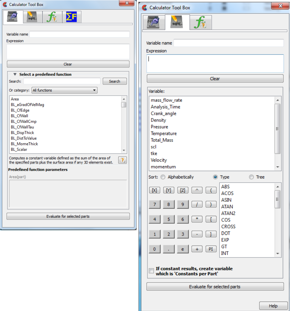
7.3 Variable Creation
EnSight 10.2 User Manual 7-17
Clicking the Calculator Icon opens the Feature Panel (Calculator) dialog.
Variable Name This field is used to specify the name for the variable being created. Built-in general
functions will provide a default, but they can be modified here. Variable names must not
start with a numeric digit and must not contain any of the following reserved characters:
([{+@ !*$
) ] }–space #^/
Working Expression The expression or equation for the new variable is presented in this area. Interaction with
the expression takes place here, either directly by typing in values and variable names,
etc., or indirectly by selecting built-in functions and clicking calculator buttons.
Clear Clicking this button clears the Variable name field, Working Expression area, Feedback
area, and deselects any built-in function.
Figure 7-5
Feature Panel (Calculator)
dialog
Predefined Functions Build Your Own Functions
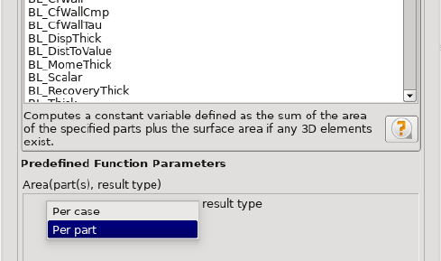
7.3 Threaded Calculator Functions
7-18 EnSight 10.2 User Manual
Constants per Part If the result is a single value (a Constant) then toggle this on to create a constant for each
of the selected parts at each timestep. Default is off, which will create a single value for
the case.
Evaluate Clicking this button produces the new variable defined in the working expression area.
Until you click this button, nothing is really created. The selection commands specify to
which parts the new variable should be applied.
Predefined functions Scroll this list of built-in functions provided for your convenience. Click on a function to
Tabinsert it into your Variable Name and Working Expression. For some functions,
dynamic instructions and fields will appear for you to follow. For example, when
computing area, you must select whether the resulting constant will be per part or pert
case.
Threaded Calculator Functions
The EnSight calculator functions are listed below. All of the calculator functions
are threaded except as follows. ElemToNode*, Lambda2, MassedParticle,
MatSpecies, MatToScalar, NormC, OffsetVar, Q_criteria, Radiograph_grid,
Radiograph_mesh, SOSConstant, StatRegVal1, StatRegVal2, TempMean,
TempMinmaxField. All of the Math functions are threaded. For more details on
this topic see Threading.
*The ElemToNode function can enable threading (see the function description
below for details).
Area Area (any part(s))
Computes a constant or constant per part variable whose value is the area of the
selected parts. If a part is composed of 3D elements, the area is of the border
representation of the part. The area of 1D elements is zero.
Boundary Layer BL_aGradOfVelMag(boundary part(s), velocity).
A Gradient Of Computes a vector variable which is the gradient of the magnitude of the specified
Velocity Magnitude velocity variable on the selected boundary part(s) defined as:
GRADBP |V| =
BP |V| =
|V|/
x i +
|V|/
y j +
|V|/
z k
where:
BP = on boundary part
V = V(x,y,z) = velocity vector
|V | = magnitude of velocity vector = SQRT(DOT(V,V))
x, y, z = coordinate directions
i, j, k = unit vectors in coordinate directions
Note1: For each boundary part, this function finds it corresponding field part (pfield),

7.3 Threaded Calculator Functions
EnSight 10.2 User Manual 7-19
computes the gradient of the velocity magnitude on the field part (Grad(pfield,velocity),
and then maps these computed values onto the boundary part.
Warning: The Boundary Layer Calculator functions (BL_*) are not supported for Server
of Server (SOS) decomposition (see Chapter , Section 7.4, Boundary Layer Variables).
Note2: Node or element ids are used if they exist. Otherwise the coordinate values
between the field part and boundary part are mapped and resolved via a floating-point
hashing scheme.
Note3: This velocity-magnitude gradient variable can be used as an argument for the fol-
lowing boundary-layer functions that require this variable.
Note: See Section 7.4, Boundary Layer Variables
Boundary Layer
BL_CfEdge
(boundary part(s), velocity, density, viscosity, ymax, flow comp(0,1,or2), grad)
Edge Skin-Friction Computes a scalar variable which is the edge skin-friction coefficient Cf(e) (that is, using
Coefficient the density e and velocity Ue values at the edge of the boundary layer – not the free-
stream density and velocity U values) defined as:
Component: 0 = Total tangential-flow (parallel) to wall:
Cf(e) = 2 w / (e Ue2)
Component: 1 = Stream-wise (flow) component tangent (parallel) to wall:
Cfs(e) = 2 ws / (e Ue2)
Component: 2 = Cross-flow component tangent (parallel) to wall:
Cfc(e) = 2 wc / (e Ue2)
where:
w = fluid shear stress magnitude at the boundary = (u/n)n=0 = (
ws2 +
wc2)
ws = (us/n)n=0 = stream-wise component of
w
wc = (uc/n)n=0 = cross-flow component of
w
= dynamic viscosity of the fluid at the wall
(u/n)n=0 = magnitude of the velocity-magnitude gradient in the normal direction
at the wall
(us/n)n=0 = stream-wise component of the velocity-magnitude gradient in the nor-
mal direction at the wall
(uc/n)n=0 = cross-flow component of the velocity-magnitude gradient in the nor-
mal direction at the wall
e = density at the edge of the boundary layer
Ue = velocity at the edge of the boundary layer
Boundary part 2D part
Velocity vector variable
boundary part 2D part
velocity vector variable
density scalar variable (compressible flow),
constant number (incompressible flow)
viscosity scalar variable, constant variable, or constant number

7.3 Threaded Calculator Functions
7-20 EnSight 10.2 User Manual
Provides a measure of the skin-friction coefficient in the tangent (parallel to surface)
direction, and in its tangent’s respective stream-wise and cross-flow directions, respective
to the decomposed velocity parallel to the surface at the edge of the boundary layer.
This is a non-dimensionalized measure of the fluid shear stress at the surface based on the
local density and velocity at the edge of the boundary layer. The following figure
illustrates the derivations of the computed ‘edge’ related velocity values Ue, us, uc &c.
Warning: The Boundary Layer Calculator functions (BL_*) are not supported for Server
of Server (SOS) decomposition (see Chapter , Section 7.4, Boundary Layer Variables).
ymax constant number
> 0 = Baldwin-Lomax-Spalart algorithm
0 = convergence algorithm
(See Algorithm Note under Boundary Layer Thickness)
flow comp constant number
0 = tangent flow parallel to surface
1 = stream-wise component tangent (parallel) to wall
2 = cross-flow component tangent (parallel) to wall
grad -1 = flags the computing of the velocity-magnitude gradient via
3-point interpolation.
vector variable = Grad(velocity magnitude), i.e. see BL_aGradOfVelMag
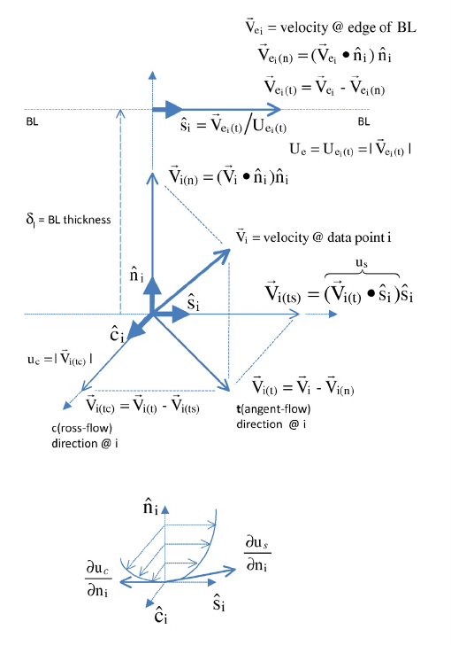
7.3 Threaded Calculator Functions
EnSight 10.2 User Manual 7-21
Note: See Section 7.4, Boundary Layer Variables
Boundary Layer BL_CfWall(boundary part(s), velocity, viscosity, free density, free velocity, grad).
Wall Skin Friction Computes a scalar variable which is the skin-friction coefficient Cf(), defined as:
Coefficient
Cf()
where:
=
fluid shear stress at the wall
=dynamic viscosity of the fluid at the wall
May be spatially and/or temporarily varying quantity (usually a
constant).
=distance profiled normal to the wall
=freestream density
Figure 7-6
Figure Illustrating Derivation of Edge Velocity Related Values and Components
w
0.5U
2
--------------------------------=
ww
u
n
-----
n0=
=
w
n

7.3 Threaded Calculator Functions
7-22 EnSight 10.2 User Manual
This is a non-dimensionalized measure of the fluid shear stress at the surface. An
important aspect of the Skin Friction Coefficient is:
Cf() , indicates boundary layer separation.
Warning: The Boundary Layer Calculator functions (BL_*) are not supported for Server
of Server (SOS) decomposition (see Chapter , Section 7.4, Boundary Layer Variables).
Boundary Layer BL_CfWallCmp(boundary part(s), velocity, viscosity, free-stream density, free-stream
velocity-mag., ymax, flow comp(1or2), grad).
Wall Skin-Friction Computes a scalar variable which is a component of the skin-friction coefficient Cf
Coefficient tangent (or parallel) to the wall, either in the stream-wise Cfs(•) or in the cross-flow Cfc(•)
Components direction defined as:
Component 1 = Steam-wise (flow) component tangent (parallel) to wall:
Cfs() = 2 ws / ( U2)
Component 2 = Cross-flow component tangent (parallel) to wall:
Cfc() = 2 wc / ( U2)
where:
ws = (us/n)n=0 = stream-wise component of
w
wc = (uc/n)n=0 = cross-flow component of
w
w = fluid shear stress magnitude at the wall = (u/n)n=0 = (
ws2 +
wc2)
= dynamic viscosity of the fluid at the wall
(us/n)n=0 = stream-wise component of the velocity-magnitude gradient in the nor-
mal direction at the wall
(uc/n)n=0 = cross-flow component of the velocity-magnitude gradient in the nor-
mal direction at the wall
= density at the edge of the boundary layer
U
= velocity at the edge of the boundary layer
=freestream velocity magnitude
= tangent (parallel to surface) component of the velocity-
magnitude gradient in the normal direction under the
“where:” list.
boundary part 2D part
velocity vector variable
viscosity scalar variable, constant variable, or constant number
free density constant number
free velocity constant number
grad -1 = flags the computing of the velocity-magnitude gradient via
3-point interpolation.
vector variable = Grad(velocity magnitude), i.e. see BL_aGradOfVelMag
boundary part 2D part
velocity vector variable
viscosity scalar variable, constant variable, or constant number
density scalar variable (compressible flow),
constant number (incompressible flow)
velocity mag constant variable, or constant number
U
w
u
n
-----
n0=
0=

7.3 Threaded Calculator Functions
EnSight 10.2 User Manual 7-23
Warning: The Boundary Layer Calculator functions (BL_*) are not supported for Server
of Server (SOS) decomposition (see Chapter , Section 7.4, Boundary Layer Variables).
Boundary Layer BL_CfWallTau(boundary part(s), velocity, viscosity, ymax, flow comp(0,1,or 2), grad).
Wall Fluid Computes a scalar variable which is the fluid’s shear-stress at the wall w or in its
Shear-Stress stream-wise ws, or cross-flow cs component direction defined as:
Component 0 = Total fluid shear-stress magnitude at the wall:
w = = (u/n)n=0 = (
ws2 +
wc2)
Component 1 = Steam-wise component of the fluid shear-stress at the wall:
ws = (us/n)n=0
Component 2 = Cross-flow component of the fluid shear-stress at the wall:
wc = (uc/n)n=0
where:
= dynamic viscosity of the fluid at the wall
(u/n)n=0 = magnitude of the velocity-magnitude gradient in the normal direction
at the wall
(us/n)n=0 = stream-wise component of the velocity-magnitude gradient in the nor-
mal direction at the wall
(uc/n)n=0 = cross-flow component of the velocity-magnitude gradient in the
normal direction at the wall
Warning: The Boundary Layer Calculator functions (BL_*) are not supported for Server
of Server (SOS) decomposition (see Chapter , Section 7.4, Boundary Layer Variables).
ymax constant number
> 0 = Baldwin-Lomax-Spalart algorithm
0 = convergence algorithm
(See Algorithm Note under Boundary Layer Thickness)
flow comp constant number
1 = stream-wise component tangent (parallel) to wall
2 = cross-flow component tangent (parallel) to wall
grad -1 = flags the computing of the velocity-magnitude gradient via
3-point interpolation.
vector variable = Grad(velocity magnitude), i.e. see BL_aGradOfVelMag
boundary part 2D part
velocity vector variable
viscosity scalar variable, constant variable, or constant number
ymax constant number
> 0 = Baldwin-Lomax-Spalart algorithm
0 = convergence algorithm
(See Algorithm Note under Boundary Layer Thickness)
flow comp constant number
0 = RMS of the stream-wise and cross-flow components
1 = stream-wise component at the wall
2 = cross-flow component at the wall
grad -1 = flags the computing of the velocity-magnitude gradient via
3-point interpolation.
vector variable = Grad(velocity magnitude), i.e. see BL_aGradOfVelMag

7.3 Threaded Calculator Functions
7-24 EnSight 10.2 User Manual
Boundary Layer BL_DispThick(boundary part(s), velocity, density, ymax, flow comp(0,1,or 2), grad).
Displacement Computes a scalar variable which is the boundary-layer displacement thickness *, *s, or
Thickness *c defined as:
Component: 0 = Total tangential-flow parallel to the wall
Component: 1 = Stream-wise flow component tangent (parallel) to the wall
Component: 2 = Cross-flow component tangent (parallel) to the wall
where:
Provides a measure for the effect of the boundary layer on the “outside” flow.
The boundary layer causes a displacement of the streamlines around the body.
n=distance profiled normal to the wall
=boundary-layer thickness (distance to edge of boundary
layer)
=density at given profile location
e=density at the edge of the boundary layer
u=magnitude of the velocity component parallel to the wall at a
given profile location in the boundary layer
us=stream-wise component of the velocity magnitude parallel to
the wall at a given profile location in the boundary layer
uc=cross-flow component of the velocity magnitude parallel to
the wall at a given profile location in the boundary layer
Ue =u at the edge of the boundary layer
ymax =distance from wall to freestream
comp =flow direction option
grad =flag for gradient of velocity magnitude
boundary part 2D part
velocity vector variable
density scalar variable (compressible flow),
constant number (incompressible flow)
ymax constant number
> 0 = Baldwin-Lomax-Spalart algorithm
0 = convergence algorithm
(See Algorithm Note under Boundary Layer Thickness)
flow comp constant number:
0 = total tangential flow direction parallel to wall
1 = stream-wise flow component direction parallel to wall
2 = cross-flow component direction parallel to wall
tot 1u
eUe
------------–
nd
0
=
s1us
eUe
------------–
nd
0
=
c
uc
eUe
------------
nd
0
=
7.3 Threaded Calculator Functions
EnSight 10.2 User Manual 7-25
Warning: The Boundary Layer Calculator functions (BL_*) are not supported for Server
of Server (SOS) decomposition (see Chapter , Section 7.4, Boundary Layer Variables).
Boundary Layer BL_DistToValue(boundary part(s), scalar, scalar value).
Distance to Value Computes a scalar variable which is the distance d from the wall to the specified value
from Wall defined as
where:
Warning: The Boundary Layer Calculator functions (BL_*) are not supported for Server
of Server (SOS) decomposition (see Chapter , Section 7.4, Boundary Layer Variables).
Boundary Layer BL_MomeThick(boundary part(s), velocity, density, ymax, flow compi(0,1,or2), flow
compj(0,1,or2), grad).
Momentum Computes a scalar variable which is the boundary-layer momentum thickness tot, ss, sc,
Thickness cs, or cc defined as:
Components: (0,0) = Total tangential-flow parallel to the wall
Components: (1,1) = stream-wise, stream-wise component
Components: (1,2) = Stream-wise, cross-flow component
grad -1 = flags the computing of the velocity-magnitude gradient via
4-point interpolation.
vector variable = Grad(velocity magnitude), i.e. see BL_aGradOfVelMag
n= distance profile d normal to boundary surface
= scalar field (variable)
= scalar field values
c= scalar value at which to assign d
boundary part 0D, 1D, or 2D part
scalar scalar variable
scalar value constant number or constant variable
dn
f c=
=
f
tot
1
eU2e
-------------- Ueu–und
0
=
ss
1
eU2e
-------------- Ueus
–usnd
0
=
sc
1
eU2e
-------------- Ueus
–ucnd
0
=

7.3 Threaded Calculator Functions
7-26 EnSight 10.2 User Manual
Components: (2,1) = cross-flow, stream-wise component
Components: (2,2) = cross-flow, cross-flow component
where:
Relates to the momentum loss in the boundary layer.
Warning: The Boundary Layer Calculator functions (BL_*) are not supported for Server
of Server (SOS) decomposition (see Chapter , Section 7.4, Boundary Layer Variables).
n= distance profiled normal to the wall
= boundary-layer thickness (or distance to edge of boundary layer)
= density at given profile location
= density at the edge of the boundary layer
u= magnitude of the velocity component parallel to the wall at a given
profile location in the boundary layer
us=stream-wise component of the velocity magnitude parallel to
the wall at a given profile location in the boundary layer
uc=cross-flow component of the velocity magnitude parallel to
the wall at a given profile location in the boundary layer
Ue =u at the edge of the boundary layer
ymax = distance from wall to freestream
compi= first flow direction option
compj= second flow direction option
grad = flag for gradient of velocity magnitude
boundary part 2D part
velocity vector variable
density scalar variable (compressible flow),
constant number (incompressible flow)
ymax constant number
> 0 = Baldwin-Lomax-Spalart algorithm
0 = convergence algorithm
(See Algorithm Note under Boundary Layer Thickness)
compiconstant number
0 = total tangential flow direction parallel to wall
1 = stream-wise flow component direction parallel to wall
2 = cross-flow component direction parallel to wall
compjconstant number
0 = total tangential flow direction parallel to wall
1 = stream-wise flow component direction parallel to wall
2 = cross-flow component direction parallel to wall
grad -1 = flags the computing of the velocity-magnitude gradient
via 4-point interpolation.
vector variable = Grad(velocity magnitude), i.e. see BL_aGradfVelMag
cs
1–
eU2e
-------------- ucusnd
0
=
cc
1–
eU2e
-------------- uc
2nd
0
=
e

7.3 Threaded Calculator Functions
EnSight 10.2 User Manual 7-27
Boundary Layer BL_Scalar(boundary part(s), velocity, scalar, ymax, grad).
Scalar Computes a scalar variable which is the scalar value of the corresponding scalar field at
the edge of the boundary layer. The function extracts the scalar value while computing the
boundary-layer thickness (see Boundary Layer Thickness).
where:
Warning: The Boundary Layer Calculator functions (BL_*) are not supported for Server
of Server (SOS) decomposition (see Chapter , Section 7.4, Boundary Layer Variables).
Boundary Layer BL_RecoveryThick(boundary part(s), velocity, total pressure, ymax, grad).
Recovery Thickness Computes a scalar variable which is the boundary-layer recovery thickness rec defined
as:
where:
This quantity does not appear in any physical conservation equations, but is sometimes
used in the evaluation of inlet flows.
Warning: The Boundary Layer Calculator functions (BL_*) are not supported for Server
of Server (SOS) decomposition (see Chapter , Section 7.4, Boundary Layer Variables).
ymax = distance from wall to freestream
grad = flag for gradient of velocity magnitude
boundary part 2D part
velocity vector variable
scalar scalar variable
ymax constant number
> 0 = Baldwin-Lomax-Spalart algorithm
0 = convergence algorithm
(See Algorithm Note under Boundary Layer Thickness)
grad -1 = flags the computing of the velocity-magnitude gradient
via 4-point interpolation.
vector variable = Grad(velocity magnitude)
n=distance profiled normal to the wall
=boundary-layer thickness (distance to edge of boundary layer)
pt=total pressure at given profile location
pte =pt at the edge of the boundary layer
ymax =distance from wall to freestream
grad =flag for gradient of velocity magnitude option
boundary part 2D part
velocity vector variable
total pressure scalar variable
ymax constant number
> 0 = Baldwin-Lomax-Spalart algorithm
0 = convergence algorithm
(See Algorithm Note under Boundary Layer Thickness)
grad -1 = flags the computing of the velocity-magnitude gradient
via 4-point interpolation.
vector variable = Grad(velocity magnitude), i.e. see BL_aGradfVelMag
rec 1pt
pte
------–
nd
0
=
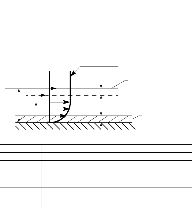
7.3 Threaded Calculator Functions
7-28 EnSight 10.2 User Manual
Boundary Layer BL_Shape is not explicitly listed in the general function list, but can be computed as a
Shape Parameter scalar variable via the calculator by dividing a displacement thickness by a momentum
thickness, i.e.
where:
Used to characterize boundary-layer flows, especially to indicate potential for separation.
This parameter increases as a separation point is approached, and varies rapidly near a
separation point.
Note: Separation has not been observed for H < 1.8, and definitely has been observed for
H = 2.6; therefore, separation is considered in some analytical methods to occur in
turbulent boundary layers for H = 2.0.
In a Blasius Laminar layer (i.e. flat plate boundary layer growth with zero pressure
gradient), H = 2.605. Turbulent boundary layer, H ~= 1.4 to 1.5, with extreme variations
~= 1.2 to 2.5.
Boundary Layer BL_Thick(boundary part(s), velocity, ymax, grad).
Thickness Computes a scalar variable which is the boundary-layer thickness defined as:
The distance normal from the surface to where u/U = 0.995,
where:
.
= boundary-layer displacement thickness
= boundary-layer momentum thickness
u=magnitude of the velocity component parallel to the wall at a
given location in the boundary layer
U=magnitude of the velocity just outside the boundary layer
boundary part 2D part
velocity vector variable
ymax constant number
> 0 = Baldwin-Lomax-Spalart algorithm
0 = convergence algorithm
(See Algorithm Note below)
grad -1 = flags the computing of the velocity-magnitude gradient
via 3-point interpolation.
vector variable = Grad(velocity magnitude), i.e. see BL_aGradfVelMag
H*/=
*
nu/U = 0.995
=
*
*
U
n
Streamline position without
boundary layer
Shifted streamline
Extra Thickness
Velocity Profile

7.3 Threaded Calculator Functions
EnSight 10.2 User Manual 7-29
Warning: The Boundary Layer Calculator functions (BL_*) are not supported for Server
of Server (SOS) decomposition (see Chapter , Section 7.4, Boundary Layer Variables).
Algorithm Note: The ymax argument allows the edge of the boundary layer to be
approximated by two different algorithms, i.e. the Baldwin-Lomax-Spalart and
convergence algorithms. Both schemes profile velocity data normal to the boundary
surface, or wall. Specifying ymax > 0 leverages results from both the Baldwin-Lomax and
vorticity functions over the entire profile to produce a fading function that approximates
the edge of the boundary layer. Whereas, specifying ymax = 0 uses velocity and velocity
gradient differences to converge to the edge of the boundary layer.
Please see the following references for more detailed explanations.
P.M. Gerhart, R.J. Gross, & J.I. Hochstein, Fundamentals of Fluid Mechanics, 2nd
Ed.,(Addison-Wesley: New York, 1992)
P. Spalart, A Reasonable Method to Compute Boundary-Layer Parameters from Navier-
Stokes Results, (Unpublished: Boeing, 1992)
H. Schlichting & K. Gersten, Boundary Layer Theory, 8th Ed., (Springer-Verlag: Berlin,
2003)
Boundary Layer BL_VelocityAtEdge(boundary part(s), velocity, ymax,comp(0,1,2),grad).
Velo ci ty At Edge Extracts a vector variable which is a velocity vector Ve, Vp, or Vn defined as:
Ve = Ve(x,y,z) = velocity vector at the edge of the boundary layer
Vn= Dot(Ve,N) = the decomposed velocity vector normal to the wall at the edge of
the boundary layer
Vp= Ve – Vn = the decomposed velocity vector parallel to the wall at the edge of the
boundary layer Computes a scalar variable which is the
boundary-layer thickness defined as:
Warning: The Boundary Layer Calculator functions (BL_*) are not supported for Server
of Server (SOS) decomposition (see Chapter , Section 7.4, Boundary Layer Variables).
boundary part 2D part
velocity vector variable
density scalar variable (compressible flow),
constant number (incompressible flow)
ymax constant number
> 0 = Baldwin-Lomax-Spalart algorithm
0 = convergence algorithm
(See Algorithm Note under Boundary Layer Thickness)
comp constant number
0 = velocity vector at edge of boundary layer
1 = decomposed velocity vector parallel to wall tangent to surface
2 = decomposed velocity vector normal to wall
grad -1 = flags the computing of the velocity-magnitude gradient
via 4-point interpolation.
vector variable = Grad(velocity magnitude), i.e. see BL_aGradfVelMag

7.3 Threaded Calculator Functions
7-30 EnSight 10.2 User Manual
Boundary Layer BL_Y1Plus(boundary part(s), density, viscosity, grad option, vector variable).
off Wall Computes a scalar variable which is the coefficient off the wall to the first field cell
centroid, defined as
where:
Normally is used to estimate or confirm the required 1st grid spacing
for proper capturing of viscous-layer properties. The values are
dependent on various factors including, what variables at the wall are
sought, the turbulent models used, and whether the law of the wall is
used or not. Consult a boundary-layer text for correct interpolation of
the values for your application.
Warning: The Boundary Layer Calculator functions (BL_*) are not supported for Server
of Server (SOS) decomposition (see Chapter , Section 7.4, Boundary Layer Variables).
Boundary Layer BL_Y1PlusDist(boundary part(s), velocity).
Distance off Wall Computes a scalar variable which is the off-the-wall distance, y1, which is the distance
off the wall to the first field cell centroid. The velocity variable is only used to determine
whether the variable is nodal or elemental to maintain consistency with the y1+ calculation
above.
Warning: The Boundary Layer Calculator functions (BL_*) are not supported for Server
n= distance profiled normal to the wall
= fluid shear stress at wall
= dynamic viscosity of fluid at wall
May be spatially and/or temporally varying quantity (usually a constant)
= density at the wall
= distance from first field element centroid to outer face, profiled normal
to wall
= fluid velocity vector
boundary part 2D (wall or surface) part
density scalar variable
viscosity scalar variable, constant variable, or constant number
gradient option 1. Use field velocity (will be used to calculate wall gradient)
2. Use gradient at boundary part (wall or surface)
3. Use gradient in corresponding field part
vector variable Will be one of three depending on gradient option
1. Use field velocity = velocity vector
2. Use gradient at boundary = Gradient variable on 2d boundary (wall or
surface) part
3. Use gradient in field = Gradient variable defined in 3d field part; or
could be gradient calculated using Grad(velocity magnitude), i.e. see
BL_aGradfVelMag
boundary part 2D part
velocity vector variable
y
1
+
y
1
+
y
1
+y
1w
w
---------- w
w
------=
ww
du
dn
------
n0=
=
w
w
y
1
u
y+
y
1

7.3 Threaded Calculator Functions
EnSight 10.2 User Manual 7-31
of Server (SOS) decomposition (see Chapter , Section 7.4, Boundary Layer Variables).
Case Map CaseMap (2D or 3D part(s), case to map from, scalar/vector/tensor, parts to map from,
search option flag)
For all locations on the selected part(s) this function finds the specified variable
value (scalar, vector, or tensor) from the ‘case to map from’ using a variety of user-
specified search options. If the variable in the ‘case to map from’ is located at the
nodes, then the casemapped variable will be defined on the nodes of the selected
part(s), and if the variable is located at the elements, then the casemapped variable
will be defined at the elements of the selected part(s).
The idea is to map onto the selected part(s), a variable from another case, usually for
comparison purposes. It does this by taking the location of the nodes or centroid of
the elements and looking at the other case to see if the variable in question is defined
at that location in the field. If so, the value is mapped to the parts nodes or element
value. The algorithm can be fairly expensive, so there are options to inform the
search that finds a matching variable location.
There are several options available in this function that can greatly impact the performance as follows.
Note: This function uses EnSight’s search capability to do the mapping. It is critical that
the nodes of the parts being mapped onto, lie within the geometry of all of the parts
case to map from constant number
scalar/vector/tensor scalar, vector, or tensor variable
search option If mapping search is successful, always assigns the exact value found.
If search mapping is not successful, because there is not an exact match
of node or element location, then the following occurs:
If search option is set to ‘search only’ (0), an undefined value will
be assigned.
If search option is set to ‘nearest value’ (1), the defined variable
value at the closest node or element will be assigned (so no
undefined values). This option will take time to search the ‘from
case’ according to the ‘parts to map from” selection outlined
below.
parts to map from The values for a location must be found by searching the geometry in
the ‘case to map from’. By setting this option you can hint to EnSight
where in the geometry it should search, which can vastly improve
performance.
Global search - This is the legacy scheme which will perform a
methodical, but uninformed search of the 3D, then 2D, then 1D,
then even 0D (point) elements to find the first defined variable
value. This works well for mapping onto a 3D or 2D that is
completely enclosed in a 3D ‘from’ volume. It works poorly if
the 2D is not fully enclosed (such as on the edge of a 3D part) or
if you want to map a 2D onto a 2D part and other 3D parts exist.
Dimensionality match - Only parts of the same dimension in the
from and to are searched. For example, only 3D “from” parts
will be used to map onto a 3D selected part. This is the option
that the user should use most often.
Part number match - The order of the parts is used, that is if you are
computing the case map on the third part then the third part is
used in the ‘case to map from’. This is best used if you have
exactly the same dataset in terms of the part list ordering, but
perhaps calculated differently so only the variable values differ.
Parts selected for case to map from - Select parts in the Case ‘From’
as well as the Case ‘To’. Only selected parts will be used in the
two cases.

7.3 Threaded Calculator Functions
7-32 EnSight 10.2 User Manual
of the case being mapped from. Mapping from a 2D surface to a 2D surface will
only work reliably if the surfaces are the same (or extremely close, and the flag=1
option is chosen). Mapping nodal variables is faster than mapping elemental
variables. This function is threaded so an hpc (formerly gold) license key may
improve performance. Select only the parts that you require, and use search option 0
if at all possible. For more details, see How To Compare Cases, and for detailed
pointers see Case Mapping Tips in that same How To write up.
Example: I have a 2D part in case 1 that I want to case map a variable from a similar 2D
part in case 2. First, select the 2D part in from case 1 in the Part List. Then set ‘case
to map from’ to ‘2’ and set the variable you want to map in the calculator pulldown.
Then use the search option ‘nearest value’ (=1) to mitigate tolerance issues between
the 2D part surfaces. Now the fourth option depends on the data in the two cases.
You should choose ‘Global search’ if you only have one 2D part in case 2 (because
there is only one part to search in the case). If, however, there are multiple parts
(with some 3D parts) in case 2, do not use the Global search because it will waste
time searching first in the 3D parts before it searches the 2D parts. Choose ‘Part
number match’ if the 2D parts are in the same location in the Part List for both cases
(e.g. both are second in their respective cases). Or, choose ‘Dimensionality match’
to limit the search to only the 2D parts in case 2. Or you could choose the option
‘Parts selected for case to map from’ and you would then select the 2D part in the
‘case to map from’ AND the 2D part in both case 1 and case 2, thereby limiting the
search to only the one 2D part.
Warning: Casemapping functions are not supported for Server of Server (SOS)
decomposition because SOS was designed to benefit from independent Servers
computations in parallel. The inter-dependent computational mapping of the field
results from the fluid part onto the boundary part violates this assumption. In other
words you cannot be sure that you will have all of the fluid information on one
server for the mapping, so this is disabled.
Case Map Diff CaseMapDiff (2D or 3D part(s), case to map from, scalar/vector/tensor, 0/1 0=search only
1=if search fails find closest)
This function is equivalent to Variable - CaseMap[Variable]. See CaseMap function
for details on how that function works.
See How To Compare Cases
Case Map Image CaseMapImage (2D or 3D part(s), part to map from, scalar, viewport number, Undefined
value limit)
This Function does a projection of a 2D part variable from a different case onto a 3D
geometry taking into account the view orientation from the specified viewport
number, similar to a texture mapping.The function in effect maps 2D results to a 3d
geometry taking into account view orientation and surface visibility.
part to map from Part number of the 2D part. This 2D part is usually data from an
infrared camera.
scalar scalar variable
viewport number The viewport number showing part(s) the variable is being
computed on, from the same camera view as part to map from
Undefined value
limit
Values on the 2D part that are under this value are considered
Undefined
7.3 Threaded Calculator Functions
EnSight 10.2 User Manual 7-33
Note: If the variable in the part to map from is located at the nodes, then the
casemapped variable will be at the nodes. If the variable is located at the elements
the casemapped variable will be at the elements. This function takes only a scalar
variable.
Coefficient Coeff (any 1D or 2D part(s), scalar, component)
Computes a constant or constant per part variable whose value is a coefficient Cx,
Cy, or Cz such that
where:
f = any scalar variable
S = 1D or 2D domain
= x component of normal
= y component of normal
= z component of normal
Specify [X], [Y], or [Z] to get the corresponding coefficient.
Note: Normal for a 1D part will be parallel to the plane of the plane tool.
Complex Cmplx(any part(s), scalar/vector(real portion), scalar/vector(complex portion), [optional
frequency(Degrees)])
Creates a complex scalar or vector from two scalar or vector variables. The
frequency is optional and is used only for reference.
Z = A + Bi
Complex CmplxArg (any part(s), complex scalar or vector)
Argument Computes the Argument of a complex scalar or vector. The resulting scalar is given
in degrees and will be in the range -180 and 180 degrees.
Arg = atan(Vi/Vr)
Complex CmplxConj (any part(s), complex scalar or vector)
Conjugate Computes the Conjugate of a complex scalar of vector. Returns a complex scalar or
vector where:
Nr = Vr
Ni = -Vi
Complex CmplxImag (any part(s), complex scalar or vector)
Imaginary Extracts imaginary portion of a complex scalar or vector into a real scalar or vector.
N = Vi
Complex CmplxModu (any part(s), complex scalar or vector)
Modulus Returns a real scalar/vector which is the modulus of the given scalar/vector
N = SQRT(Vr*Vr + Vi*Vi)
Complex CmplxReal(any part(s), complex scalar or vector)
Real Extracts the real portion of a complex scalar or vector into a real scalar or vector.
N = Vr
component [X], [Y], or [Z]
real portion scalar or vector variable
complex portion scalar or vector variable (but must be same as real portion)
[frequency] constant number (optional)
CxfnxSd
S
=CyfnySd
S
=CzfnzSd
S
=
nx
ny
nz
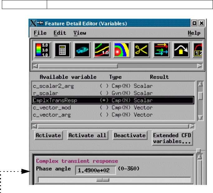
7.3 Threaded Calculator Functions
7-34 EnSight 10.2 User Manual
Complex CmplxTransResp(any part(s), complex scalar or vector, constant PHI(0.0-360.0 Degrees))
Transient Response Returns a real scalar or vector which is the real transient response:
Re(Vt) = Re(Vc)Cos(phi) - Im(Vc)Sin(phi)
which is a function of the transient phase angle “phi” defined by:
phi = 2 Pi f t
where
t = the harmonic response time parameter
f = frequency of the complex variable “Vc”
and the complex field “Vc”, defined as:
Vc = Vc(x,y,z) = Re(Vc) + i Im(Vc)
where
Vc = the complex variable field
Re(Vc) = the Real portion of Vc
Im(Vc) = the imaginary portion of Vc
i = Sqrt(-1)
Note, the transient complex function, was a composition of Vc and Euler’s
relation, namely:
Vt = Vt(x,y,z,t) = Re(Vt) + i Im(Vt) = Vc * e^(i phi)
where:
e^(i phi) = Cos(phi) + i Sin(phi)
The real portion Re(Vt), is as designated above:
Note: this function is only good for harmonic variations, thus fields with a
defined frequency!
phi angle constant number between 0 and 360 degrees.
Note: A special area becomes available in the Feature Panel (Variables) and
Feature Panel (Calculator) when you highlight a variable of this type -
allowing you to modify the phase angle (phi) easily with a slider.

7.3 Threaded Calculator Functions
EnSight 10.2 User Manual 7-35
ConstPerPart ConstPerPart (any part(s), constant)
This function is assigns a value to the selected part(s). The value can either be a
floating point value entered into the field, or it can be a case constant. This value
does not change over time. At a later point, any other part(s) can be selected and this
can be recalculated and these other part(s) will be assigned the new value and the
exisiting part(s) that were previously selected will retain their previously assigned
value. In other words, each successive time that this is recalculated for an existing
variable, values assigned to the most recently selected parts are updated without
removing previously assigned values.
Curl Curl (any part(s), vector)
Computes a vector variable which is the curl of the input vector
Defect Consider a mesh with a scalar per element variable representing the micro porosity of each cell,
where 0 means no porosity (the cell is completely full) and 100 means the cell is fully porous (the
cell is empty). Cells with a non zero porosity are considered to have defects. Defects that span
multiple cells may indicate an unacceptable defect. Six Defect functions are provided to help
calculate factors of interest in characterizing these defects that occur over multiple cells. To use the
Defect_ functions, you would create an isovolume of your porosity variable between desired ranges
(perhaps 5 to 100) and select this isovolume part then use these functions below.
Defect Defect_BulkVolume(2D or 3D part(s) )
BulkVolume Returns a per element scalar which is the sum of the volume of all the cells
comprising the defect, and then each cell with the defect is assigned this value.
Defect Defect_Count(2D or 3D part(s), Defect scalar per elem, min value, max value))
Count Returns a case constant which filters the count of the number of defects that exist
between the min value and the max value using a Defect scalar per element variable
that has been previously calculated by any of the other five Defect functions.
Defect Defect_LargestLinearExtent(2D or 3D part(s) )
LargestLinExtent Returns a per element scalar that is the largest linear extent of all the cells
comprising the defect, where each cell of the defect is assigned this value. The
largest linear extent is the root-mean-squared distance.
Defect Defect_NetVolume(2D or 3D part(s), scalar per elem, scale factor)
NetVolume Returns a per element scalar that is the sum of the cell volumes multiplied by the
scalar per element variable multiplied by the scale factor, of all the cells comprising
the defect, where each cell of the defect is assigned this value. The defect scalar per
element variable is usually porosity, but the user is free to use any per element scalar
variable. The scale factor adjusts the scalar per element variable values, i.e. if the
porosity range is from 0.0 to 100.0 then a scale factor of 0.01 can be used to
normalize the porosity values to volume fraction values ranging from 0.0 to 1.0.
Defect Defect_ShapeFactor(2D or 3D part(s) )
ShapeFactor Returns a per element scalar that is the Largest Linear Extent divided by the
diameter of the sphere with a volume equal to the Bulk Volume of the defect, where
each cell of the defect is assigned this value.
Defect Defect_SurfaceArea(2D or 3D part(s) )
SurfaceArea Returns a per element scalar that is the surface area of the defect, where each cell of
Curlfff3
y
-------f2
z
-------–
i
ˆf1
z
-------f3
x
-------–
j
ˆf2
x
-------f1
y
-------–
k
ˆ
++==
7.3 Threaded Calculator Functions
7-36 EnSight 10.2 User Manual
the defect is assigned this value.
Density Density(any part(s), pressure, temperature, gas constant).
Computes a scalar variable which is the density , defined as:
where: p = pressure
T = temperature
R = gas constant
Log of DensityLogNorm (any part(s), density, freestream density)
Normalized Computes a scalar variable which is the natural log of Normalized Density
Density defined as:
where: = density
= freestream density
Normalized DensityNorm (any part(s), density, freestream density)
Density Computes a scalar variable which is the Normalized Density defined as:
where: = density
= freestream density
Normalized DensityNormStag (any part(s), density, total energy, velocity, ratio of specific heats,
Stagnation freestream density, freestream speed of sound, freestream velocity magnitude)
Density Computes a scalar variable which is the Normalized Stagnation Density
defined as:
where: = stagnation density
where: = freestream stagnation density
pressure scalar variable
temperature scalar variable
gas constant scalar, constant, or constant per part variable, or constant number
density scalar variable, constant variable, or constant number
freestream density constant or constant per part variable or constant number
density scalar variable, constant variable, or constant number
freestream density constant or constant per part variable or constant number
density scalar, constant, or constant per part variable, or constant
number
total energy scalar variable
velocity vector variable
ratio of specific heats scalar, constant or constant per part variable, or constant
number
freestream density constant or constant per part variable or constant number
freestream speed of sound constant or constant per part variable or constant number
p
TR
-------=
n
ln
i
ln=
i
n
n
i
=
i
on
on ooi
=
o
oi

7.3 Threaded Calculator Functions
EnSight 10.2 User Manual 7-37
Stagnation DensityStag (any part(s), density, total energy, velocity, ratio of specific heats)
Density Computes a scalar variable which is the Stagnation Density defined as:
where: = density
= ratio of specific heats
= mach number
total energy must be a scalar
velocity must be a vector
Distance Dist2Nodes(any part(s), nodeID1,nodeID2).
Between Nodes Computes a constant, positive variable that is the distance between any two nodes.
Searches down the part list until it finds nodeID1, then searches until it finds nodeID2 and
returns Undef if nodeID1 or nodeID2 cannot be found. Nodes are designated by their node
id’s, so the part must have node ids. (Note that most created parts do not have node ids.)
Note also for transient results, that the geometry type is important for using this function.
There are three geometry types: static, changing coordinate, and changing connectivity.
You can find out your geometry type by doing a Query>Dataset and look in the General
Geometric section of the pop up window. If you have a static geometry with visual
displacement turned on then dis2nodes will not use the displacement in its calculations.
You will need to turn on server-side (computational) displacement (see How To use Server
Side Displacements). If you have changing coordinate geometry, then dist2node should
work fine, and if you have changing connectivity then dist2node should not be used as it
may give nonsensical results because connectivity is redone each timestep and node ids
may move around.
And finally, to find the distance between two nodes on different parts, or between two
nodes if one or both don’t have ids, or the ids are not unique for the model (namely, more
than one part has the same node id) use the line tool. See the Advanced Usage section of
How To Use the Line Tool.
Distance to parts Dist2Part(origin part + field part(s), origin part, origin part normal).
Node to nodes Computes a scalar variable on the origin part and field parts that is the minimum distance
at each node of the origin and field parts to any node in the origin part. This distance is
unsigned by default. The origin part is the origin of a Euclidean distance field. So, by
definition the scalar variable will always be zero at the origin part because the distance to
the origin part will always be zero.
The origin part normal vector must be a per node variable. If the origin part normal is
calculated using the Normal calculator function, then it is a per element variable and must
be moved to the nodes using the calculator ElemToNode function. If this per node, origin
part normal vector variable defined at the origin part is supplied then the normal vector is
used to return a signed distance function (with positive being the direction of the normal).
The signed distance is determined using the dot product of the vector from the given field
freestream velocity magnitude constant or constant per part variable or constant number
density scalar, constant, or constant per part variable, or constant number
total energy scalar variable
velocity vector variable
ratio of specific heats scalar, constant, or constant per part variable, or constant number
nodeID1 constant number
nodeID2 constant number
o
o11
–
2
-----------
+M2
11–
=
M

7.3 Threaded Calculator Functions
7-38 EnSight 10.2 User Manual
node and its closest node on the origin with the origin node’s normal vector.
Notes: The origin part must be included in the field part list (although, as discussed earlier,
the scalar variable will be zero for all nodes on the origin part). This algorithm has an
execution time on the order of the number of nodes in the field parts times the number of
nodes in the origin part. While the implementation is both SOS aware and threaded, the
run time is dominated by the number of nodes in the computation.
This function is computed between the nodes of the origin and field parts. As a result, the
accuracy of its approximation to the distance field is limited to the density of nodes
(effectively the size of the elements) in the origin part. If a more accurate approximation is
required, use the Dist2PartElem() function. It is slower, but is less dependent on the nodal
distribution in the origin part because it uses the nodes plus the element faces to calculate
the minimum distance.
Usage. A typical usage would be to use an arbitrary 2D part to create a clip in a 3D field.
Use the 2D part as your origin part, and select the origin part as well as your 3D field
parts. No need to have normal vectors. Create your scalar variable, called say
distTo2Dpart, then create an isosurface=0 in your field using the distTo2Dpart as your
variable.
Distance to parts Dist2PartElem(origin part + field part(s), origin part, origin part normal).
Node to elements Computes a scalar variable that is the minimum distance at each node of the origin part
and field parts and the closest point on any element in origin part. This distance is
unsigned (if the origin part normal vector is not supplied).
If the origin part normal vector is supplied, then the distance is signed. Note: the origin
part normal vector must be a per node variable. Note, if the origin part normal is
calculated using the Normal calculator function, then it is a per element variable and must
be moved to the nodes using the calculator ElemToNode function. If this per node, origin
part normal vector variable defined at the origin part is supplied, the direction of the
normal is used to return a signed distance function with distances in the direction of the
normal being positive.
Once the closest point in the origin part has been found for a node in an field part, the dot
product of the origin node normal and a vector between the two nodes is used to select the
sign of the result.
Notes: The origin part must be included in the field part list (although the output will be
zero for all nodes of the origin part because it is the origin of the Euclidean distance). This
algorithm has an execution time on the order of the number of nodes in the field parts
times the number of elements in the origin part. While the implementation is both SOS
aware and threaded, the run time is dominated by the number of nodes in the computation.
This function is a more accurate estimation of the distance field than Dist2Part() because it
allows for distances between nodes and element surfaces on the origin part. This improved
accuracy results in increased computational complexity and as a result this function can be
several times slower than Dist2Part(). See also the EnSight Tips and Tutorials on our
website.
origin part part number to compute the distance to
origin part normal a constant for unsigned computation or a nodal vector variable defined
on the origin part for a signed computation
origin part part number to compute the distance to
origin part normal a constant for unsigned computation or a nodal vector variable defined
on the origin part for a signed computation

7.3 Threaded Calculator Functions
EnSight 10.2 User Manual 7-39
Divergence Div (2D or 3D part(s), vector)
Computes a scalar variable whose value is the divergence defined as:
where u,v,w = velocity components in x,y,z directions.
Element Metric EleMetric (any part(s), metric_function).
Calculates an element mesh metric, at each element creating a scalar, element-based
variable depending upon the selected metric function. The various metrics are valid for
specific element types. If the element is not of the type supported by the metric function,
the value at the element will be the EnSight undefined value. Metrics exist for the
following element types: tri, quad, tet, and hex.A metric can be any one of the following:
# Name Elem types Description
0 Element type All EnSight element type number. See
the table below this one.
1 Condition hexa8, tetra4,
quad4, tria3
Condition number of the weighted
Jacobian matrix.
2 Scaled Jacobian hexa8, tetra4,
quad4, tria3
Jacobian scaled by the edge length
products.
3 Shape hexa8, tetra4,
quad4, tria3
Varies by element type.
4 Distortion hexa8, tetra4,
quad4, tria3
Distortion is a measure of how
well-behaved the mapping from
parameter space to world
coordinates is.
5 Edge ratio hexa8, tetra4,
quad4, tria3
Ratio of longest edge length over
shortest edge length.
6 Jacobian hexa8, tetra4, quad4 The minimum determinate of the
Jacobian computed at each vertex.
7Radius ratio tetra4, quad4, tria3 Normalized ratio of the radius of
the inscribed sphere to the radius
of the circumsphere.
8 Minimum angle tetra4, quad4, tria3 Minimum included angle in
degrees.
9 Maximum edge
ratio
hexa8, quad4 Largest ratio of principle axis
lengths.
10 Skew hexa8, quad4 Degree to which a pair of vectors
are parallel using the dot product,
maximum.
11 Taper hexa8, quad4 Maximum ratio of a cross-
derivative to its shortest associated
principal axis.
12 Stretch hexa8, quad4 Ratio of minimum edge length to
maximum diagonal.
13 Oddy hexa8, quad4 Maximum deviation of the metric
tensor from the identity matrix,
evaluated at the corners and
element center.
Div u
x
----- v
y
----- w
z
------++=

7.3 Threaded Calculator Functions
7-40 EnSight 10.2 User Manual
14 Max aspect
Frobenius
hexa8, quad4 Maximum of aspect Frobenius
computed for the element
decomposed into triangles.
15 Min aspect
Frobenius
hexa8, quad4 Minimum of aspect Frobenius
computed for the element
decomposed into triangles.
16 Shear hexa8, quad4 Scaled Jacobian with a truncated
range.
17 Signed volume hexa8, tetra4 Volume computed, preserving the
sign.
18 Signed area tria3, quad4 Area preserving the sign.
19 Maximum angle tria3, quad4 Maximum included angle in
degrees.
20 Aspect ratio tetra4, quad4 Maximum edge length over area.
21 Aspect
Frobenius
tetra4, tria3 Sum of the edge lengths squared
divided by the area and
normalized.
22 Diagonal hexa8 Ratio of the minimum diagonal
length to the maximum diagonal
length.
23 Dimension hexa8
24 Aspect beta tetra4 Radius ratio of a positively-
oriented tetrahedron.
25 Aspect gamma tetra4 Root-mean-square edge length to
volume.
26 Collapse ratio tetra4 Smallest ratio of the height of a
vertex above its opposing triangle
to the longest edge of that
opposing triangle across all
vertices of the tetrahedron.
27 Warpage quad4 Cosine of the minimum dihedral
angle formed by planes
intersecting in diagonals.
28 Centroid All Returns each element centroid as a
vector value at that element
29 Volume Test 3D elements Returns 0.0 for non-3D elements.
Each 3D element is decomposed
into Tet04 elements and this option
returns a scalar equal to 0.0, 1.0 or
2.0. It returns 0.0 if none of the
Tet04 element volumes is
negative, 1.0 if all of the Tet04
element volumes are negative, and
2.0 if some of the Tet04 element
volumes are negative.
# Name Elem types Description
V
2V
-----------

7.3 Threaded Calculator Functions
EnSight 10.2 User Manual 7-41
EnSight Element types:
30 Signed Volume 3D elements Returns 0.0 for non-3D elements.
Returns a scalar which is the sum
of the signed volumes of the Tet4
decomposition for 3D elements.
31 Part Number All Returns a scalar at each element
which is the EnSight part ID
number of that element.
Face Count All Returns a scalar which is the
number of faces in that element.
# Element type
0 Point
1 Point ghost
2 2 node bar
3 2 node bar ghost
4 3 node bar
5 3 node bar ghost
6 3 node triangle (tria3)
7 3 node triangle ghost
10 6 node triangle
11 6 node triangle ghost
12 4 node quadrilateral (quad4)
13 4 node quadrilateral ghost
14 8 node quadrilateral
15 8 node quadrilateral ghost
16 4 node tetrahedron (tetra4)
17 4 node tetrahedron ghost
20 10 node tetrahedron
21 10 node tetrahedron ghost
22 5 node pyramid
23 5 node pyramid ghost
24 13 node pyramid
25 13 node pyramid ghost
26 6 node pentahedron
27 6 node pentahedron ghost
28 15 node pentahedron
29 15 node pentahedron ghost
30 8 node hexahedron (hexa8)
31 8 node hexahedron ghost
20 node hexahedron
33 20 node hexahedron ghost
34 N-sided polygon
35 N-sided polygon ghost
38 N-faced polyhedron
39 N-faced polyhedron ghost
# Name Elem types Description
7.3 Threaded Calculator Functions
7-42 EnSight 10.2 User Manual
The implementation is based on the BSD implementation of the Sandia Verdict Library.
Please see the following links:
Verde User’s Manual
Verdict Mesh Verification Library
Detail of Elemetric Equations
For more detail on individual metrics, see the following reference:
C. J. Stimpson, C. D. Ernst, P. Knupp, P. P. Pebay, & D. Thompson, The Verdict Library
Reference Manual, May 8, 2007.
Element Size EleSize (any part(s)).
Calculates the Volume/Area/Length for 3D/2D/1D elements respectively, at each
element creating a scalar, element-based variable.
Warning: This will use the coordinates of the element to calculate the volume of each
element. If you wish to use displacement in the calculation of the volume, then you must
turn on computational (server-side) displacement, rather than visual only (client side)
displacement so that the displacement values will be applied to the coordinates on the
server prior to calculating the element size (see How to Display Displacements).
Warning 2: If you calculate the element size of a part and then use that part to create a
child part, the child part will inherit the values of the elesize calculation which are the size
of the parent elements not the size of the child elements. If you want the elesize of the child
part, then you must select the child part and recalculate a new elesize variable!
Element to Node ElemToNode (any part(s), element-based scalar or vector).
Averages an element based variable to produce a node-based variable.
For each node[i]->val += (elem[j]->val * elem[j]->wt) | node[i]
For each node[i]->wt += elem[j]->wt | node[i]
Results: node[i]->val /= node[i]->wt
where
wt = 1 for this algorithm and the weighting scalar in ElemtoNodeWeighted
j = iterator on all part elements
i = iterator on all part nodes (Note: node[i] must be on elem[j] to contribute)
| node[i] indicates node that is associated with elem[j]
By default, this uses all parts that share each node of the selected part(s). So, parts that are
not selected whose elements are shared by nodes of the selected part(s) will have their
element values averaged in with those of the selected parts.
Note: To turn the averaging across parts off and use only the elements of the each part at
each node, open up the command window (File>Command) and, in the Command Entry:
field, type test: across averaging off prior to using this function. The added
benefit of turning averaging between parts off, is that the function becomes threaded.
Element to Node Weighted ElemToNodeWeighted (any part(s), element-based scalar or vector, element-
based weighting scalar).
Same as ElementToNode, except that the value of the variable at the element is
weighted by an element scalar. That is, elem[j]->wt is the value of the weighting scalar in
the ElemToNode algorithm description above.
One use of this function might be to use the element size as a weighting factor so that
larger elements contribute more to the nodal value than smaller ones.
7.3 Threaded Calculator Functions
EnSight 10.2 User Manual 7-43
Energy:
Tota l Energy EnergyT (any part(s), density, pressure, velocity, ratio of specific heats).
Computes a scalar variable of total energy per unit volume
Kinetic Energy KinEn (any part(s), velocity, density)
Computes a scalar variable whose value is the kinetic energy defined as:
where = density
V = Velocity variable
Enthalpy Enthalpy (any part(s), density, total energy, velocity, ratio of specific heats)
Computes a scalar variable which is Enthalpy defined as:
where: E = total energy per unit volume
= density
V = velocity magnitude
= ratio of specific heats
Normalized EnthalpyNorm (any part(s), density, total energy, velocity, ratio of specific
Enthalpy heats, freestream density, freestream speed of sound)
Computes a scalar variable which is Normalized Enthalpy defined as:
where: h = enthalpy
= freestream enthalpy
density scalar, constant, or constant per part variable, or constant number
pressure scalar variable
velocity vector variable
ratio of specific heats scalar, constant, or constant per part variable, or constant number
velocity vector variable
density scalar, constant, or constant per part variable, or constant number
density scalar, constant, or constant per part variable, or constant number
total energy scalar variable
velocity vector variable
ratio of specific heats scalar, constant, or constant per part variable, or constant number
density scalar, constant, or constant per part variable, or constant
number
total energy scalar variable
velocity vector variable
eei
V2
2
------+
=
eie0
V2
2
------–=
e0
e
---=
Total E n e r gy
Internal Energy
Stagnation Energy
where: density=
VVelocity=
Or based on gamma, pressure and velocity:
ep
1
–
----------------V2
2
------
+=
Ek
Ek
1
2
---
V2
=
h
hE
--- V2
2
------–
=
hn
hnhh
i
=
hi

7.3 Threaded Calculator Functions
7-44 EnSight 10.2 User Manual
Stagnation EnthalpyStag (any part(s), density, total energy, velocity, ratio of specific heats)
Enthalpy Computes a scalar variable which is Stagnation Enthalpy defined as:
where: = enthalpy
V = velocity magnitude
Normalized EnthalpyNormStag (any part(s), density, total energy, velocity, ratio of
Stagnation specific heats, freestream density, freestream speed of sound, freestream velocity
Enthalpy magnitude)
Computes a scalar variable which is Normalized Stagnation Enthalpy
defined as:
where: = stagnation enthalpy
= freestream stagnation enthalpy
Entropy Entropy (any part(s), density, total energy, velocity, ratio of specific heats, gas
constant, freestream density, freestream speed of sound)
Computes a scalar variable which is Entropy defined as:
where:
= density
where: R = gas constant
= ratio of specific heats
= freestream speed of sound
= freestream density
ratio of specific heats scalar, constant, or constant per part variable, or constant
number
freestream density constant or constant per part variable or constant number
freestream speed of sound constant or constant per part variable or constant number
density scalar, constant, or constant per part variable, or constant number
total energy scalar variable
velocity vector variable
ratio of specific heats scalar, constant, or constant per part variable, or constant number
density scalar, constant, or constant per part variable, or constant
number
total energy scalar variable
velocity vector variable
ratio of specific heats scalar, constant, or constant per part variable, or constant
number
freestream density constant or constant per part variable or constant number
freestream speed of sound constant or constant per parts variable or constant number
freestream velocity magnitude constant or constant per part variable or constant number
ho
hohV
2
--- 2
+=
h
hon
hon hohoi
=
ho
hoi
s
s
p
p
------
------
--------------
R
1
–
-----------
ln=
a
7.3 Threaded Calculator Functions
EnSight 10.2 User Manual 7-45
where pressure, p is calculated from the total energy, e, and velocity V
and freestream pressure, =
density scalar, constant, or constant per part variable, or constant
number
total energy scalar variable
velocity vector variable
ratio of specific heats scalar, constant, or constant per part variable, or constant
number
gas constant scalar, constant, or constant per part variable or constant
number
freestream density constant or constant per part variable or constant number
freestream speed of sound constant or constant per part variable or constant number
p1–eV2
2
------
–=
p
a
2
---------------------
7.3 Threaded Calculator Functions
7-46 EnSight 10.2 User Manual
Flow Flow (any 1D or 2D part(s), velocity).
Computes a constant or constant per part variable whose value is the volume flow
rate defined as:
where = Velocity vector
= Unit vector normal to surface S
S = 1D or 2D domain
Note: Normal for a 1D part will be parallel to the plane of the plane tool.
Note also: To calculate mass flow rate, multiply Velocity vector by the Density scalar and
then substitute this vector value in for the velocity vector in the above equation.
Flow Rate FlowRate (any 1D or 2D part(s), velocity).
Computes a scalar Vn which is the component of velocity normal to the surface,
defined as:
where V = Velocity
= Unit vector normal to surface S
S = 1D or 2D domain
Note: This function is equivalent to calculating the dot product of the velocity vector and
the surface normal (using the Normal function).
Fluid Shear FluidShear(2D part(s), velocity magnitude gradient, viscosity)
Computes a scalar variable tau whose value is defined as:
tau = µ where tau = shear stress
µ = dynamic viscosity
= Velocity gradient in direction of surface normal
Hints: To compute fluid shear stress:
1. Use Gradient function on velocity to obtain “Velocity Grad” variable in
the 3D part(s) of interest.
2. Create a clip part or extract the outer surface of the part using part
extract (create a 2D part from the 3D part(s) used above) a surface on
which you wish to see the fluid shear stress.
3. Compute Fluid Shear variable (on the 2D surface).
velocity vector variable
velocity vector variable
velocity gradient vector variable
viscosity scalar, constant, or constant per part variable, or constant number
Qc
QcVn
ˆ
Sd
S
=
V
n
ˆ
VnVn
ˆ
=
n
ˆ
V
n
------
V
n
------
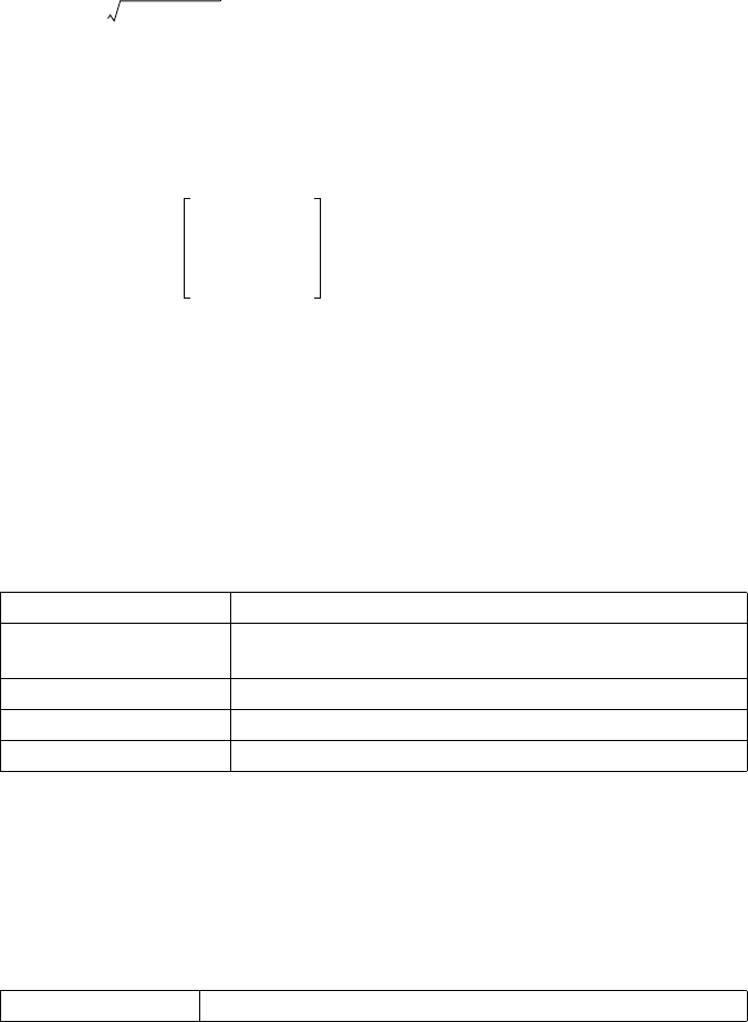
7.3 Threaded Calculator Functions
EnSight 10.2 User Manual 7-47
Fluid Shear FluidShearMax (2D or 3D part(s), velocity, density, turbulent kinetic energy, turbulent
Stress Max dissipation, laminar viscosity)
Computes a scalar variable defined as:
where F = force
A = unit area
= turbulent (eddy) viscosity
= laminar viscosity (treated as a constant)
E = local strain
The turbulent viscosity is defined as:
where = density
= turbulent kinetic energy
= turbulent dissipation
A measure of local strain E (i.e. local elongation in 3 directions) is given by
where
given the Euclidean norm defined by
;
and the rate of deformation tensor dij defined by
with = ¹u/¹x
= ¹v/¹y
= ¹w/¹z
= ¹u/¹y + ¹v/¹x =
= ¹u/¹z + ¹w/¹x =
= ¹v/¹z + ¹w/¹y =
given the strain tensor defined by
Force Force(2D part(s), pressure)
Computes a vector variable whose value is the force F defined as:
where p = pressure
A = unit area
Note: The force acts in the surface normal direction.
velocity vector variable
density scalar, constant, or constant per part variable, or constant
number
turbulent kinetic energy scalar variable
turbulent dissipation scalar variable
laminar viscosity constant or constant per part variable or constant number
pressure scalar variable
FAutul
+E==
ut
ul
ut
ut
0.09
2
--------------------=
E2trDD=
2tr D D2d
11
2d22
2d33
2
++d12
2d13
2d23
2
+++=
tr D Dd11 2d22
2d33
21
2
---d12
2d13
2d23
2
+++++=
Dd
ij
1
2
---
2d11 d12 d13
d21 2d22 d23
d31 d32 2d33
==
d11
d22
d33
d12
d21
d13
d31
d23
d32
eij
eij
1
2
---dij
=
FpA=

7.3 Threaded Calculator Functions
7-48 EnSight 10.2 User Manual
Force 1D Force1D(1D planar part(s), pressure, surface normal)
Computes a vector variable whose value is the force F defined as:
where p = pressure
L = unit length times 1
Note: The force acts in the part’s normal direction (in plane).
Gradient Grad (2D or 3D part(s), scalar or vector(Magnitude will be used))
Computes a vector variable whose value is the gradient defined as:
where f = any scalar variable (or the magnitude of the specified vector)
x, y, z = coordinate directions
i, j, k = unit vectors in coordinate directions
Algorithm: If the variable is at the element, then it is moved to the nodes. Then each
element is mapped to a normalized element and the Jacobian is calculated for the
transformation from the element to the normalized element; and then, its inverse Jacobian
is calculated for this transformation and used to compute the Jacobian for the scalar
variable. Thus, the chain rule is used with the inverse Jacobian of the transformation and
the Jacobian of the scalar variable to calculate the gradient for each node of each element.
The contributions of the gradient from all the elements are moved to all the nodes using an
unweighted average. Finally, if the original variable is per element, the gradient is moved
from the nodes to the elements using an unweighted average.
Gradient TensorGradTensor (2D or 3D part(s), vector)
Computes a tensor variable whose value is the gradient defined as:
where F = any vector variable
x, y, z = coordinate directions
i, j, k = unit vectors in coordinate directions
Helicity:
Helicity Density HelicityDensity(any part(s), velocity)
Computes a scalar variable whose value is:
where: V = Velocity
= Vorticity
pressure scalar variable
surface normal vector variable
velocity vector variable
FpL=
GRADf
GRADf
f
x
----- i
ˆf
y
----- j
ˆf
z
-----k
ˆ
++=
GRADF
GRADF
F
x
------ i
ˆF
y
------ j
ˆF
z
------ k
ˆ
++=
Hd
HdV=
7.3 Threaded Calculator Functions
EnSight 10.2 User Manual 7-49
Relative Helicity HelicityRelative(any part(s), velocity)
Computes a scalar variable whose value is:
where: = the angle between the velocity vector and the vorticity vector.
Filtered Relative HelicityRelFilter(any part(s), velocity, freestream velocity magnitude).
Helicity Computes a scalar variable whose value is:
, if
or , if
where = relative helicity (as described above)
= helicity density (as described above)
Iblanking Values IblankingValues (Any iblanked structured part(s))
Computes a scalar variable whose value is the iblanking flag of selected parts.
Returns undefined for unstructured part(s).
IJK Values IJKValues (Any structured part(s))
Computes a vector variable whose value is the I/J/K values of the selected parts.
Returns undefined for unstructured part(s).
Integrals:
Line Integral IntegralLine (1D part(s), scalar or (vector, component))
Computes a constant or constant per part variable whose value is the integral of the
input variable over the length of the specified 1D part(s). Nodal variables are first
converted to elemental variable using a weighted average of the shape function.
Surface Integral IntegralSurface (2D part(s), scalar or (vector, component))
Computes a constant or constant per part variable whose value is the integral of the
input variable over the surface of the specified 2D part(s). Nodal variables are first
converted to elemental variable using a weighted average of the shape function.
Volume Integral IntegralVolume (3D part(s), scalar or (vector, component))
Computes a constant or constant per part variable whose value is the integral of the
input variable over the volume of the specified 3D part(s). Nodal variables are first
converted to elemental variable using a weighted average of the shape function.
Kinetic Energy (See under Energy)
Length Length (any 1D part(s))
Computes a constant or constant per part variable whose value is the length of
selected parts. While any part can be specified, it will only return a nonzero length if
the part has 1D elements.
Line Integral See Line Integral under Integrals.
LineVectors LineVectors (any 1D part(s))
Computes a nodal, vector variable which is the vector beginning at each node to the next
velocity vector variable
velocity vector variable
freestream velocity magnitude constant or constant per part variable or constant number
Hr
Hr = V
V
--------------
cos=
Hrf
Hrf Hr
=
Hdfilter
Hrf 0=
Hdfilter
Hr
Hd
filter 0.1 V
2
=

7.3 Threaded Calculator Functions
7-50 EnSight 10.2 User Manual
node in the connectivity of the 1D part. This vector indicates the direction of the line segments.
where:
Vec i = Vector with origin at point i, with i from 1 to n-1.
(Pxi,Pyi,Pzi) = Coordinates of Point i of 1D part
n = Number of points in the 1D part
Lambda2 Lambda2 (any part(s), Grad_Vel_x, Grad_Vel_y, Grad_Vel_z)
Computes a scalar variable which is the second eigenvalue, or 82, of the second
invariant (or Q-criterion) of the velocity gradient tensor. Vortex shells may then be
visualized as an iso-surface of 82 = 0. The following describes the calculation of the
inputs to this function:
Explicitly calculate the three components of Velocity
Vel_x = Velocity[X] = x-component of the velocity vector
Vel_y = Velocity[Y] = y-component of the velocity vector
Vel_z = Velocity[Z] = z-component of the velocity vector
and then
Grad_Vel_x = Grad(any part(s), Vel_x) = gradient of x component Velocity
Grad_Vel_y = Grad(any part(s), Vel_y) = gradient of y component Velocity
Grad_Vel_z = Grad(any part(s), Vel_z) = gradient of z component Velocity
where
Velocity = velocity vector variable
Note: Common mistake is to try to calculate the Gradient from the component of the
velocity without using the intermediate Vel_x, Vel_y, and Vel_z variables. For example
this is wrong and will use only the velocity magnitude:
Grad_Vel_x = Grad(any part(s), Velocity[X])
Note: This is a User-Defined Math Function (UDMF) which may be modified and
recompiled by the user. For more details, see the Interface Manual, User Defined Math
Functions and see User Defined Math Functions, discussed above
Algorithm:
The three gradient vectors of the components of the velocity vector constitute the velocity
gradient tensor. Using the 9 components of this (anti-symmetric) velocity gradient tensor,
Lv, construct both the symmetric, S, and the anti-symmetric, , parts of the velocity
VeciPxi1+Pxi
–Pyi1+Pyi
–Pzi1+Pzi
–
=

7.3 Threaded Calculator Functions
EnSight 10.2 User Manual 7-51
gradient tensor,
where
then combine to compute the symmetric tensor
Next compute and sort the eigenvalues of Q (using Jacobi eigen analysis), and
assign the 2nd eigenvalue, or 82, as the scalar value at the node.
The vortex is to be visualized as an iso-surface with
See also the Q_criteria calculator function.
References
Haller, G., “An objective definition of a vortex,” Journal of Fluid Mechanics, 2005,
vol. 525, pp. 1-26.
Jeong, J. and Hussain, F., “On the identification of a vortex,” Journal of Fluid
Mechanics, 1995, vol. 285, pp. 69-94.
Mach Number Mach (any part(s), density, total energy, velocity, ratio of specific heats)
Computes a scalar variable whose value is the Mach number M defined as:
where m = momentum
= density
u = speed, computed from velocity input
= ratio of specific heats (1.4 for air)
p = pressure (see Pressure below)
c = speed of sound
See Total Energy in this section for a description.
density scalar, constant, or constant per part variable, or constant number
total energy scalar variable
velocity vector variable
ratio of specific heats scalar, constant, or constant per part variable, or constant number
vS+=
S1
2
---vv
T
+=
1
2
---vv
T
–=
QS
22
+=
-1-2-3
-20=
Mu
p
-----
----------u
c
---==
7.3 Threaded Calculator Functions
7-52 EnSight 10.2 User Manual
Make Scalar at MakeScalElem (any part(s), constant number or constant or constant per part variable)
Elements Assigns the specified constant value to each element, making a scalar variable.
Make Scalar at MakeScalNode (any part(s), constant number or constant or constant per part variable)
Nodes Assigns the specified constant value to each node, making a scalar variable.
Make Vector MakeVect (any part(s), scalar or zero, scalar or zero, scalar or zero)
Computes a vector variable formed from scalar variables. First scalar becomes the X
component of the vector, second scalar becomes the Y component, and the third
scalar becomes the Z component. A zero can be specified for some of the scalars,
creating a 2D or 1D vector field.
Massed Particle MassedParticle (massed particle trace part(s))
Scalar
This scalar creates a massed-particle per element scalar variable for each of the
parent parts of the massed-particle traces. This per element variable is the mass of
the particle times the sum of the number of times each element is exited by a mass-
particle trace. See Particle-Mass Scalar on Boundaries in Chapter 7
Mass-Flux MassFluxAvg (any 1D or 2D part(s), scalar, velocity, density)
Average Computes a constant or constant per part variable whose value is the mass flux average
bavg defined as:
where b = any scalar variable, i.e. pressure, mach, a vector component, etc.
= density (constant or scalar) variable
V = velocity (vector) variable
dA = area of some 2D domain
N = unit vector normal to dA
Note that the dot product (V*N), is positive when velocity is aligned with the unit normal
vector and is negative otherwise (see the FlowRate calculator function). This implies that
aligned flow contributes to the weighted average and otherwise subtracts from it. This
also presents the possibility that in recirculating flow, the denominator can tend toward
zero. Some prefer to use the absolute value of the dot product, which is a multi-step
process using the absolute value of the result from the EnSight FlowRate calculator
function.
scalar any scalar variable, i.e. pressure, mach, a vector component, etc
velocity a vector variable
density scalar, constant, or constant per part variable, or constant number
bavg
bV NdA
A
VNdA
A
------------------------------------ MassFluxOfScalar
MassFlux
-------------------------------------------------- Flow plist bV
Flow plist V
--------------------------------------------== =

7.3 Threaded Calculator Functions
EnSight 10.2 User Manual 7-53
MatSpecies MatSpecies (any model part(s), any material(s), any specie(s), scalar per element).
Computes a scalar per element variable whose value is the sum of all specified
material and species combinations multiplied by the specified element variable on
specified 'model' parts with defined material species.
where
This function only operates on model part(s) with pre-defined species. The
specified material(s) can either be a list of materials or a single material value. The
specified species can either be a list, a single specie, or no specie (i.e. a null species
list which then computes an element value based on only material fraction
contributions). The scalar per element value can either be an active variable, or a
scalar value (i.e. the value 1 would give pure material fraction and/or specie value
extraction).
Both material and specie names are selected from the context sensitive Active
Variables list which changes to a Materials list and then a Species List for their
respective prompts.
For more information on Species see Species under 7.19 Material Parts Create/
Update, and both MATERIAL Section under EnSight Gold Case File Format, and
Example Material Dataset (with Species) in User Manual section 11.1.
MatToScalar MatToScalar (any model part(s), a material).
Computes a scalar per element variable whose value s is the specified material’s
value m of the element on the specified part(s).
s = m
where
s = scalar per element variable value of each element
m = the corresponding material fraction value of each element
This function only operates on model part(s) with pre-defined materials that are given by
sparse mixed material definitions. Only one material may be converted into one per
element scalar variable at a time. The material cannot be the null material.
For more information on Materials,(see Chapter 5.1.9, Material Interface Parts), and both
MATERIAL Sections under EnSight Gold Case File Format, and Example Material
Dataset in User Manual section 11.1.
= e
s
ms
i
j
es = scalar per element variable value or value
msij = mi * sj
= The product of the material fraction mi
and its corresponding specie value sj
= 0,
if specie sj does not exist for material mi
=
m
i
,
if no species are specified.
7.3 Threaded Calculator Functions
7-54 EnSight 10.2 User Manual
Max Max (any part(s), scalar or (vector, component))
Computes a constant or constant per part variable whose value is the maximum
value of the scalar (or vector component) in the parts selected. The component is not
requested if a scalar is selected.
Min Min (any part(s), scalar or (vector, component))
Computes a constant or constant per part variable whose value is the minimum
value of the scalar (or vector component) in the parts selected.
Moment Moment (any part(s), vector, component).
Computes a constant or constant per part variable (the moment about the cursor tool
location) whose value is the x, y, or z component of Moment .
where = force vector component in direction i of vector F(x,y,z)
= (Fx,Fy,Fz)
= signed moment arm (the perpendicular distance from the
line of action of the vector component to the moment axis
(which is the current cursor tool position)).
MomentVector MomentVector (any part(s), force vector).
Computes a nodal vector variable (the moment is computed about each point of the
selected parts) whose value is the x, y, or z component of Moment .
where = force vector component in direction i of vector F(x,y,z)
= (Fx,Fy,Fz)
= signed moment arm (the perpendicular distance from the
line of action of the vector component to the moment axis
(model point position)).
Momentum Momentum(any part(s), velocity, density).
Computes a vector variable m, which is:
where = density
V = velocity
[component] if vector variable, magnitude is the default, or specify [x], [y], or [z]
[component] if vector variable, magnitude is the default, or specify [x], [y], or [z]
vector any vector variable
component [X], [Y], or [Z]
force vector any vector variable (per node or per element)
velocity a vector variable
density scalar, constant, constant per part variable, or constant number
M
MxFydzFzdy
–=
MyFzdxFxdz
–=
MzFxdyFydx
–=
Fi
di
Fi
M
MxFydzFzdy
–=
MyFzdxFxdz
–=
MzFxdyFydx
–=
Fi
di
Fi
mV=
7.3 Threaded Calculator Functions
EnSight 10.2 User Manual 7-55
Node Count NodeCount (any part(s))
Produces a constant or constant per part variable containing the node count of the
part(s) specified.
Node to Element NodeToElem (any part(s), node-based scalar or vector).
Averages a node based variable to produce an element based variable.
For each: elem[j]->val += node[i]->val | elem[j]
Results: elem[j]->val /= elem[j]->num_cell_nodes
where
j = iterator on all part elements
i = iterator on all part nodes (Note: elem[j] must contain node[i] to contribute)
| elem[j] indicates element that is associated with node[i]
Normal Normal (2D part(s) or 1D planar part(s))
Computes a vector variable which is the normal to the surface at each element for
2D parts, or for 1D planar parts - lies normal to the 1D elements in the plane of the
part.
Normal NormC (2D or 3D part(s), pressure, velocity, viscosity)
Constraints Computes a constant or constant per part variable whose value is the Normal
Constraints NC defined as:
where p = pressure
V = velocity
= dynamic viscosity
n = direction of normal
S = border of a 2D or 3D domain
Normalize Vector NormVect (any part(s), vector)
Computes a vector variable whose value is a unit vector of the given vector .
U =
where: V = vector variable field
=
Offset Field OffsetField (2D or 3D part(s))
Computes a scalar field of offset values. The values will be in model distance units
perpendicular to the boundary of the part. Note that an isosurface created in this
field would mimic the part boundary, but at the offset distance into the field.
Warning: This calculator function is not supported for Server of Server (SOS)
decomposition because SOS was designed to benefit from independent Servers
computations in parallel. The inter-dependent computational mapping of the field
results from the fluid part onto the boundary part violates this assumption. In other
words you cannot be sure that you will have all of the fluid information on one
server for the mapping, so this is disabled.
pressure scalar variable
velocity vector variable
viscosity scalar, constant, or constant per part variable, or constant number
NC p–
V
n
------ n
ˆ
+
Sd
S
=
U
V
VV
xVy
Vz
(,)
V
------------------------------
V
Vx
2Vy
2Vz
2
++
7.3 Threaded Calculator Functions
7-56 EnSight 10.2 User Manual
Offset Variable OffsetVar(2D or 3D part(s), scalar or vector, constant offset value)
Computes a scalar (or vector) variable defined as the offset value into the field of
that variable that exists in the normal direction from the boundary of the selected
part. This assigns near surface values of a variable to the surface of the selected
part(s) from the neighboring 3D field (which is found automatically using the
selected part(s) surface(s).
In other words, this function gets the value of a variable from surrounding field(s), a
fixed distance from the surface of the selected part(s) and assigns it to the surface fo
the selected part. For example, you might use this function to get the value of the
velocity in the flow field a slight distance above your vehicle surface and assign that
value to your vehicle surface.
To use this function, select part(s) in the part list that you want to use, enter a
variable and an offset. EnSight will auto detect the 3D field part(s) adjacent to your
selected part(s) surface(s) and reach into these fields by your offset in the normal
direction to obtain the variable value and then assign it to the surface of your
selected part(s). Note: choose a negative offset if your normals do not point into the
field.
Warning: This calculator function is not supported for Server of Server (SOS)
decomposition because SOS was designed to benefit from independent Servers
computations in parallel. Recall that EnSight must find the field adjacent to your
selected part(s) surfaces. And since some of these fields might be on other servers, it
will create dependencies that preclude independent Servers, so this is disabled.
Part Number PartNumber (any part(s))
Computes a constant per part variable which is the GUI part number, if the part is a
server-side part. Note: any client-side part (e.g. vector arrows, particle traces, profiles,
etc.) are assigned the undefined value. Model parts are always server-side parts and for a
listing of which Created parts are server-side or client-side, see Table 1–2 Part Creation
and Data Location. For a brief discussion of the undefined value, see EnSight Gold
Undefined Variable Values Format.
Pressure Pres (any part(s), density, total energy, velocity, ratio of specific heats)
Computes a scalar variable whose value is the pressure p defined as:
where: m = momentum
E = total energy
= density
V = velocity = m/
= ratio of specific heats (1.4 for air)
constant offset value constant number (constant variable is not valid)
density scalar, constant, or constant per part variable, or constant number
total energy scalar variable
velocity vector variable
ratio of specific heats scalar, constant, or constant per part variable, or constant number
p1–
E
--- 1
2
---V2
–
=

7.3 Threaded Calculator Functions
EnSight 10.2 User Manual 7-57
Pressure PresCoef (any part(s), density, total energy, velocity, ratio of specific heats, freestream
Coefficient density, freestream speed of sound, freestream velocity magnitude)
Computes a scalar variable which is Pressure Coefficient defined as:
where: p = pressure
= freestream pressure
= freestream density
= freestream velocity magnitude
Dynamic PresDynam (any part(s), density, velocity)
Pressure Computes a scalar variable which is Dynamic Pressure defined as:
where: = density
V = velocity magnitude
See also: Kinetic Energy
Normalized PresNorm (any part(s), density, total energy, velocity, ratio of specific heats,
Pressure freestream density, freestream speed of sound)
Computes a scalar variable which is Normalized Pressure defined as:
where: = freestream pressure =
= ratio of specific heats
= pressure
density scalar, constant, constant per part variable, or constant
number
total energy scalar variable
velocity vector variable
ratio of specific heats scalar, constant, or constant per part variable, or constant
number
freestream density constant or constant per part variable or constant number
freestream speed of sound constant or constant per part variable or constant number
freestream velocity magnitude constant or constant per part variable or constant number
density scalar, constant, or constant per part variable, or constant number
velocity vector variable
density scalar, constant, or constant per part variable, or constant
number
total energy scalar variable
velocity vector variable
ratio of specific heats scalar, constant, or constant per part variable, or constant
number
freestream density constant or constant per part variable or constant number
freestream speed of sound constant or constant per part variable or constant number
CP
CP
pp
i
–
iVi
2
2
-----------
--------------=
pi
i
Vi
q
qV2
2
---------=
pn
pnpp
i
=
pi
1
p

7.3 Threaded Calculator Functions
7-58 EnSight 10.2 User Manual
Log of PresLogNorm (any part(s), density, total energy, velocity, ratio of specific
Normalized heats, freestream density, freestream speed of sound)
Pressure Computes a scalar variable which is the natural log of Normalized Pressure
defined as:
where: = freestream pressure =
=ratio of specific heats
= pressure
Stagnation PresStag (any part(s), density, total energy, velocity, ratio of specific heats)
Pressure Computes a scalar variable which is the Stagnation Pressure defined as:
where: = pressure
= ratio of specific heats
= mach number
Note: In literature, stagnation pressure is used interchangeably with total pressure.
The stagnation pressure (or total pressure) use two different equations depending upon the
flow regime: compressible or incompressible. EnSight has chosen to define Stagnation
Pressure using the compressible flow equation (above), and Total Pressure using the
incompressible flow equation (see Total Pressure below).
Normalized PresNormStag (any part(s), density, total energy, velocity, ratio of specific heats,
Stagnation freestream density, freestream speed of sound, freestream velocity magnitude)
Pressure Computes a scalar variable which is Normalized Stagnation Pressure
defined as:
where: = stagnation pressure
= freestream stagnation pressure
density scalar, constant, or constant per part variable, or constant
number
total energy scalar variable
velocity vector variable
ratio of specific heats scalar, constant, or constant per part variable, or constant
number
freestream density constant or constant per part variable or constant number
freestream speed of sound constant or constant per part variable or constant number
density scalar, constant, or constant per part variable, or constant number
total energy scalar variable
velocity vector variable
ratio of specific heats scalar, constant, or constant per part variable, or constant number
density scalar, constant, or constant per part variable, or constant
number
total energy scalar variable
velocity vector variable
ratio of specific heats scalar, constant, or constant per part variable, or constant
number
freestream density constant or constant per part variable or constant number
pn
ln p pi
ln=
pi
1
p
po
pop1 1
–
2
-----------
+M2
1–
=
p
M
pon
pon popoi
=
po
poi

7.3 Threaded Calculator Functions
EnSight 10.2 User Manual 7-59
Stagnation PresStagCoef (any part(s), density, total energy, velocity, ratio of
Pressure specific heats, freestream density, freestream speed of sound, freestream velocity
Coefficient magnitude)
Computes a scalar variable which is Stagnation Pressure Coefficient
defined as:
where: = stagnation pressure
= freestream pressure =
= ratio of specific heats
= freestream density
= velocity magnitude
Pitot PresPitot (any part(s), density, total energy, velocity, ratio of specific heats)
Pressure Computes a scalar variable which is Pitot Pressure defined as:
=
where = ratio of specific heats
total energy per unit volume
= density
V = velocity magnitude
p = pressure
Note: For mach numbers less than 1.0, the Pitot Pressure is the same as the Stagnation
Pressure. For mach numbers greater than or equal to 1.0, the Pitot Pressure is
equivalent to the Stagnation Pressure behind a normal shock.
freestream speed of sound constant or constant per part variable or constant number
freestream velocity magnitude constant or constant per part variable or constant number
density scalar, constant, or constant per part variable, or constant
number
total energy scalar variable
velocity vector variable
ratio of specific heats scalar, constant, or constant per part variable, or constant
number
freestream density constant or constant per part variable or constant number
freestream speed of sound constant or constant per part variable or constant number
freestream velocity magnitude constant or constant per part variable or constant number
density scalar, constant, or constant per part variable, or constant number
total energy scalar variable
velocity vector variable
ratio of specific heats scalar, constant, or constant per part variable, or constant number
Cpo
Cpopopi
–
iV2
2
-----------
=
po
pi
1
i
V
pp
ppsp=
s
1+
2
-----------
V2
1–
E
--- V2
2
------–
-----------------------------------------
1–
2
1
+
-----------
V2
1–
E
--- V2
2
------–
-----------------------------------------
1
–
1+
-----------
–
11–
-------------------------------------------------------------------------------------------------------------------------
7.3 Threaded Calculator Functions
7-60 EnSight 10.2 User Manual
Pitot PresPitotRatio (any part(s), density, total energy, velocity, ratio of specific heats,
Pressure freestream density, freestream speed of sound)
Ratio Computes a scalar variable which is Pitot Pressure Ratio defined as:
where s = (defined above in Pitot Pressure)
= ratio of specific heats
total energy per unit volume
= density
V = velocity magnitude
Tota l PresT (any part(s), pressure, velocity, density)
Pressure Computes a scalar variable whose value is the total pressure defined as:
where = density
V = velocity
p = pressure
Note: In literature, total pressure is used interchangeably with stagnation pressure.
The total pressure (or stagnation pressure) use two different equations depending upon the
flow regime: incompressible or compressible. EnSight has chosen to define Total
Pressure using the incompressible flow equation (above), and Stagnation Pressure using
the compressible flow equation (see Stagnation Pressure above).
Q_criteria Q_criteria (any part(s), Grad_Vel_x, Grad_Vel_y, Grad_Vel_z)
Computes a scalar variable which is the second invariant, or Q-criterion, of the
velocity gradient tensor. Vortex shells may then be visualized as an iso-surface of Q-
criterion > 0. The following describes the calculation of the inputs to this function:
First you must calculate the intermediate variable:
Vel_x = Velocity[X] = x-component of the velocity vector
Vel_y = Velocity[Y] = y-component of the velocity vector
Vel_z = Velocity[Z] = z-component of the velocity vector
then calculate the gradient using the intermediate variable:
Grad_Vel_x = Grad(any part(s), Vel_x) = gradient of x component Velocity
Grad_Vel_y = Grad(any part(s), Vel_y) = gradient of y component Velocity
Grad_Vel_z = Grad(any part(s), Vel_z) = gradient of z component Velocity
with
density scalar, constant, or constant per part variable, or constant
number
total energy scalar variable
velocity vector variable
ratio of specific heats scalar, constant, or constant per part variable, or constant
number
freestream density constant or constant per part variable or constant number
freestream speed of sound constant or constant per part variable or constant number
pressure scalar variable
velocity vector variable
density scalar, constant, or constant per part variable, or constant number
ppr
ppr s1–EV2
2
---------–
=
pt
ptpV2
2
------
+=

7.3 Threaded Calculator Functions
EnSight 10.2 User Manual 7-61
Velocity = velocity vector variable
Note: A common mistake is to try to calculate the Gradient from the component of
the velocity without using the intermediate Vel_x, Vel_y, and Vel_z variables. For
example this is wrong and will use only the velocity magnitude:
Grad_Vel_x = Grad(any part(s), Velocity[X])
Note:
This is a User-Defined Math Function (UDMF) which may be modified and
recompiled by the user. Please see the EnSight Interface Manual for more details
(For more information, see the Interface Manual, User Defined Math Functions and
see User Defined Math Functions outlined above).
Algorithm
The three gradient vectors of the components of the velocity vector constitute the
velocity gradient tensor. Using the 9 components of this (anti-symmetric) velocity
gradient tensor, Lv, construct both the symmetric, S, and the anti-symmetric,
,,
parts of the velocity gradient tensor, the Q criteria is established as follows.
where
solving for Q (hence Q criteria) when
which (in terms of our EnSight variables) literally reduces to
Q = - 0.5 * ( Grad_Vel_x[X] * Grad_vel_x[X] + Grad_Vel_y[Y] * Grad_vel_y[Y]
+ Grad_Vel_z[Z] * Grad_Vel_z[Z] + 2 * (Grad_Vel_x[Y] * Grad_Vel_y[X] +
Grad_Vel_x[Z] * Grad_Vel_z[X] + Grad_Vel_y[Z] * Grad_Vel_z[Y] ) ) > 0
Now, to find the vortices, create an isosurface where Q is positive (Q > 0). This is
because an isosurface with positive Q isolates areas where the strength of the
rotation overcomes the strain, thus making those surfaces eligible as vortex
envelopes.
See also the Lambda2 calculator function.
References:
Dubief, Y and Delcayre, F., “On coherent-vortex identification in turbulence”,
Journal of Turbulence, (jot.iop.org) 1 (2000) 11, pp.1-22.
Haller, G., “An objective definition of a vortex,” Journal of Fluid Mechanics, 2005,
vol. 525, pp. 1-26.
Jeong, J. and Hussain, F., “On the identification of a vortex,” Journal of Fluid
Mechanics, 1995, vol. 285, pp. 69-94.
Radiograph_grid Radiograph_grid(1D or 2D part(s), dir X, dir Y, dir Z, num_points, variable,
[component]).
Computes a per element scalar variable on the designated 1D or 2D part(s), that is a
vS+=
S1
2
---vv
T
+=
1
2
---vv
T
–=
Q1
2
---2S2
–0=
7.3 Threaded Calculator Functions
7-62 EnSight 10.2 User Manual
directional integration from these parts of a scalar variable or vector component
through the model. Think of rays being cast from the center of each element of the
1D or 2D parents in the direction specified (and long enough to extend through the
model). Along each ray the desired variable is integrated and the integral value is
assigned to the element from which the ray was cast. This function integrates the ray
in a constant delta, grid-like fashion. You control the delta by the number of points
that is specified in the integration direction. (Please note that while this function is
not generally as time consuming as the Radiograph_mesh function (and you have
some resolution control with the num_points argument), it still may take some
computation time. You may want to set the Abort server operations performance
preference to avoid being stuck in a computation loop that exceeds your patience.)
The arguments are:
dir X = Integration direction vector x component
dir Y = Integration direction vector y component
dir Z = Integration direction vector z component
num_points = number of points along ray in the integration direction.
(integration delta will be ray length divided by num_points)
variable = Variable that is integrated along the ray.
component = If vector variable, component to be integrated.
[X] for x component
[Y] for y component
[Z] for z component
[] for magnitude
Note that this function will not work properly for Server of Servers (SOS). Each
portion will only give its local value.
Advanced usage: set the following environmental variable
ENSIGHT_RADIOGRAPH_OPTION to 0 which integrates the ray (default), or 1
which finds min along ray, or 2 which finds max along ray.
Radiograph_mesh Radiograph_mesh(1D or 2D part(s), dir X, dir Y, dir Z, variable, [component]).
Computes a per element scalar variable on the designated 1D or 2D part(s), that is a
directional integration from these parts of a scalar variable or vector component
through the model. Think of rays being cast from the center of each element of the
1D or 2D parents in the direction specified (and long enough to extend through the
model). Along each ray the desired variable is integrated and the integral value is
assigned to the element from which the ray was cast. This function integrates the ray
at each domain element face intersection. (Please note that this can be a very time
consuming process. You may want to set the Abort server operations performance
preference to avoid being stuck in a computation loop that exceeds your patience.
The Radiograph_grid function will generally be considerably quicker.)
The arguments are:
dir X = Integration direction vector x component
dir Y = Integration direction vector y component
dir Z = Integration direction vector z component
variable = Variable that is integrated along the ray.
component = If vector variable, component to be integrated.
[X] for x component
dir X constant number
dir Y constant number
dir Z constant number
num_points constant number
component [X], [Y], [Z], or []

7.3 Threaded Calculator Functions
EnSight 10.2 User Manual 7-63
[Y] for y component
[Z] for z component
[] for magnitude
Note that this function will not work properly for Server of Servers (SOS). Each
portion will only give its local value.
Advanced usage: set the following environmental variable
ENSIGHT_RADIOGRAPH_OPTION to 0 which integrates the ray (default), or 1
which finds min along ray, or 2 which finds max along ray.
Rectangular To RectToCyl (any part(s), vector)
Cylindrical Vector Produces a vector variable with cylindrical components according to frame 0.
(Intended for calculation purposes)
x = radial component, y = tangential component, z = z component
Server Number ServerNumber (any part(s))
Produces a per-element scalar variable that is the server number which contains
the element. Useful for decomposed models using Server-of-Servers, so the
distribution can be visualized.
Shock Plot3d ShockPlot3d(2D or 3D part(s), density, total energy, velocity, ratio of specific heats).
computes a scalar variable ShockPlot3d, whose value is:
where V = velocity
c = speed of sound
p = pressure
grad(p) = gradient of pressure
Note: to compute candidate shock surface(s), create an isosurface of the
calculated variable, shockplot3d = 1.0. These shock region(s) can
be verified by overlaying them with
Also consider comparing with the Shock Region/Surface feature visualization
(see Chapter 5.1.14, Shock Regions/Surfaces Parts).
Mesh Smoothing SmoothMesh(any 1D or 2D part(s), number of passes, weight)
Performs a mesh “smoothing” operation. The function returns a vector variable
which, when applied to the mesh as a displacement, will result in a “smoother” mesh
representation. The function computes new node locations resulting from a
“normalization” of the mesh elements. As a tendency it results in a mesh with equal
sized elements. The algorithm applies a form of convolution to the mesh edges
repeatedly (number of passes) using a weighting factor to control how much change
in position is allowed in each pass. In most cases, the weight is supplied as a
dir X constant number
dir Y constant number
dir Z constant number
component [X], [Y], [Z], or []
density scalar, constant, or constant per part variable, or constant number
total energy scalar variable
velocity vector variable
ratio of specific heats scalar, constant, or constant per part variable, or constant number
ShockPlot3d V
c
--- grad p
grad p
-----------------------
=
Mach 1.0
7.3 Threaded Calculator Functions
7-64 EnSight 10.2 User Manual
constant, but the weight can be specified as a nodal scalar array. This allows for
local control over the region of the mesh to be smoothed. The algorithm is fully
threaded. Note: nodes on the outer boundary of a mesh (or are bounded by ghost
elements) are not allowed to move. A good set of initial parameters might be 50
passes with a weight constant of 0.05.
For each pass, the following formula is applied:
where x = nodal position at pass (i)
w = nodal weight
n = edge connected nodes
SOS Constant SOSConstant(any part(s), variable, reduction operation (0-3))
(Note: generally this function should not be necessary. The SOSConstant
functionality has been pulled into the server/SOS infrastructure. It remains for
backward compatibility.) Computes a constant variable whose value is the result of
applying a reduction operation on that constant variable over the values on each of
the servers. If there is no SOS involved or only a single server, the result is the same
as the constant variable value on the single server. The selected part is used to select
the case from which the constant variable is used. The constant variable itself is
specified (this can be from the dataset or a computed value. The actual operation to
be performed is selected as an integer from 0 to 3. The operation can be a simple
summation of the values from each of the servers, an average of the values from the
servers (note that the weight given to each server in the average is the same, so this
is essentially the sum operation divided by the number of servers) or the minimum/
maximum of the values on each of the servers.
Spatial Mean SpaMean(any part(s), scalar or (vector, component))
Computes a constant or constant per part variable whose value is the volume (or
area or length) weighted mean value of a scalar (or vector component) at the current
time. This value can change with time. The component is not requested if a scalar
variable is used
The spatial mean is computed by summing the product of the volume (3D, or area
2D, or length 1D) of each element by the value of the scalar (or vector component)
taken at the centroid of the element (nodal variables are interpolated at each cell
centroid using cell shape blending or metric functions), for each element over the
entire part. The final sum is then divided by the total volume (or area) of the part.
where: = Scalar taken at centroid of element i
= Volume (or Area, or Length) of element i
number of passes the number of smoothing passes to be applied: constant
weight fraction of the length of a node’s edges a node is allowed to move
with each pass: nodal scalar variable or constant
variable constant variable (from the data or computed)
reduction operation value from 0 to 3 that selects from the following operations:
0=sum 1=average 2=minimum 3=maximum
[component] if vector variable, magnitude is the default, or specify [x], [y], or [z]
xi1+xiwx
jxi
–
j0=
n
+=
SpatialMean
sivoli
voli
---------------------=
si
voli
7.3 Threaded Calculator Functions
EnSight 10.2 User Manual 7-65
Spatial Mean SpaMeanWeighted(any part(s), scalar or (vector, component), weight, component)
Weighted Computes a constant or constant per part variable whose value is weighted both by
the volume (or area or length) AND a weighting variable. This value can change
with time. For both the variable itself and the weighting variable, the component is
not requested if a scalar variable is used.
The weighted, spatial mean is computed by summing the product of the volume
(3D, or area 2D, or length if 1D) of each element by the value of the scalar (or vector
component) taken at the centroid of the element (nodal variables are interpolated at
each cell centroid using cell shape blending or metric functions) with the product of
the weighting scalar/vector component taken at the centroid of the element (again, if
a nodal variable, similarly evaluated at the element centroid) for each element over
the entire part. The final sum is then divided by the total scalar/vector weighted
(again if nodal weighting variable is similarly evaluated at the element centroid)
volume (or area, or length) of the part as follows.
where: = Scalar or vector component taken at centroid of element i
where: = Scalar or vector component taken at centroid of element i
= Volume (or Area, or Length) of element i
Speed Speed (any part(s), velocity)
Computes a scalar variable whose value is the Speed defined as:
where: u,v,w = velocity components in the x,y,z directions.
Sonic Speed SonicSpeed(any part(s), density, total energy, velocity, ratio of specific heats).
Computes a scalar variable c, whose value is:
where = ratio of specific heats
= density
p = pressure
Statistics StatMoment (any part(s), v, function)
Moments Computes a constant or constant per part by which is the sum, mean, variance, skew,
or kurtosis by applying a selected statistical function over all of the nodes or
elements of the selected parts, given the selected scalar or constant variable. Five
functions are defined as:
[component] if vector variable, magnitude is the default, or specify [x], [y], or [z]
velocity vector variable
density scalar, constant, or constant per part variable, or constant number
total energy scalar variable
velocity vector variable
ratio of specific heats scalar, constant, or constant per part variable, or constant number
SpatialMeanWeighted
wisivoli
wivoli
--------------------------=
si
wi
voli
Speed u2v2w2
++=
cp
-----=
sum vi
i1=
N
=
7.3 Threaded Calculator Functions
7-66 EnSight 10.2 User Manual
The mean is the simple average (unweighted, arithmetic mean) of the all of the
samples. The var is the variance, which is an indication of the spread of a sample of
numbers out from the mean, and is the square of the standard deviation. The skew is an
indication of the degree of asymmetry about the mean. A positive skew indicates an
asymmetric tail toward more positive values, and a negative skew indicates an asymmetric
tail toward more negative values. The kurt is the kurtosis, which is an indication of the
peakness or flatness of the distribution compared to a normal distribution. A more positive
kurtosis indicates more peakness, and a negative kurtosis indicates a more flat
distribution.
If the variable (v) is a constant, the operation will be computed as if the variable
were a nodal variable with the given value at all nodes. If the computation is over an
element variable, the size of the element is not used in the computation. If volume or area
weighting is desired, the variable must be pre-weighted.
Note that StatMoment(plist,scalar,0) should be used in place of the example user-
defined math function, udmf_sum because StatMoment is threaded and properly handles
ghost cells. However, for parallel (SOS) computation, since nodes at the interface are
shared among servers, the values at the interface nodes are used in computations multiple
times. Therefore the StatMoment value computed using a nodal variable using SOS will
deviate from the true value calculated using just one server. Elemental variables do not
suffer from this issue as ghost elements are handled properly and elements are not shared
among servers. The function parameters are defined as:
Reference:
1. Numerical Recipes, Press et. al. Cambridge Univ. Press, 1997, pp. 454-459.
Statistics StatRegSpa (any part(s), y, x0, x1, x2, x3, x4, weight)
Regression Performs classical multivariate linear regression, predicting y = f(x0,x1,x2,x3,x4).
The regression is performed at the current timestep using all of the nodes/elements of the
selected parts. At each node/element, the input values y, x0, x1, x2, x3, x4 and weight are
evaluated and added as an observation to the regression with the supplied weight (in the
range [0.0-1.0]). If the model does not require 5 inputs, any of them can be specified as the
constant number 0.0 to drop it out. If the constant 1.0 is supplied as an input, an intercept
will be computed. One is cautioned to avoid co-linearity in the inputs (especially easy
when supplying constants as regressors). An example, to model simple linearity: y = Ax0
+ B, the function parameters would be: StatRegSpa(plist, yvar, xvar, 1., 0., 0., 0., 1.). The
example specifies that all observations be weighted the same. If weighting by element
v scalar variable, constant or constant per part variable, or constant
number
function constant number selecting the moment to compute
(0=sum, 1=mean, 2=variance, 3=skewness, 4=kurtosis)
mean 1
N
----vi
i1=
N
=
var 1
N1
–
-------------vimean–
2
i1=
N
=
skew 1
N
----vimean–
var
------------------------
3
i1=
N
=
kurt 1
N
----vimean–
var
------------------------
4
i1=
N
3
–=

7.3 Threaded Calculator Functions
EnSight 10.2 User Manual 7-67
volume were desired, compute a field variable of element volume, normalized by the
largest individual element volume and pass that variable as the weight. The function
returns a scalar constant whose value is the R-squared value for the regression.
The function parameters are defined as:
A full set of estimated values and statistical diagnostic output are available, see:
StatRegVal1, StatRegVal2
Statistics StatRegVal1 (any part(s), regression_variable, function)
Regression info This function returns basic statistical diagnostics for a regression computed using
StatRegSpa(). The function is passed the output variable of a previously computed
StatRegSpa() and the function number of a specific statistical quantity to return. The
values include the standard sum of squares values for the regression as well as the R-
squared value.
The function parameters are defined as:
See also: StatRegSpa, StatRegVal2
Statistics StatRegVal2 (any part(s), regression_variable, function, selection)
Regression info This function returns statistical diagnostics specific to individual input coefficients
for a regression computed using StatRegSpa(). The function is passed the output variable
of a previously computed StatRegSpa(), the function number of the specific statistical
quantity to return and the coefficient selected. The values include the sum of squares and
partial sum of squares for the individual coefficients as well as the estimated coefficient
itself and its standard error.
The function parameters are defined as:
See also: StatRegSpa, StatRegVal1
Surface Integral See Surface Integral under Integrals.
Computes a constant pr constant per part variable whose value is the integral of the
input variable over the surface of the specified 2D part(s).
y scalar, constant, or constant per part variable or constant number
x0, x1, x2, x3, x4 scalar, constant, or constant per part variable or constant number
weight scalar, constant, or constant per part variable or constant number
regression_variable a scalar variable which is the output of an earlier StatRegSpa()
function
function the statistical quantity to return (0=sum of squares error, 1=sum of
squares total, 2=sum of squares model, 3=R-squared)
regression_variable a scalar variable which is the output of an earlier StatRegSpa()
function
function the statistical quantity to return (0=the estimated coefficient, 1=sum
of squares for the variable, 2=partial sum of squares for the
variable, 3=standard error for the coefficient)
selection constant or constant per part variable or constant number which
selects the specific coefficient for which to retrieve the statistical
quantity (0=x0, 1=x1, 2=x2, 3=x3, 4=x4)
7.3 Threaded Calculator Functions
7-68 EnSight 10.2 User Manual
Swirl Swirl (any part(s), density, velocity).
Computes a scalar variable Swirl, whose value is:
where: = vorticity
= density
V = velocity
Temperature Temperature (any part(s), density, total energy, velocity, ratio of specific heats,
gas constant)
Computes a scalar variable whose value is the temperature T defined as:
where: m = momentum
E = total energy per unit volume
= density
V = velocity = m/
= ratio of specific heats (1.4 for air)
R = gas constant
Normalized Te mp e rN o r m (any part(s), density, total energy, velocity, ratio of specific heats,
Temperature freestream density, freestream speed of sound, gas constant)
Computes a scalar variable which is Normalized Temperature defined as:
where: = temperature
= freestream temperature
density scalar, constant, or constant per part variable, or constant number
velocity vector variable
density scalar, constant, or constant per part variable, or constant number
total energy scalar variable
velocity vector variable
ratio of specific heats scalar, constant, or constant per part variable, or constant number
gas constant constant or constant per part variable or constant number
density scalar, constant, or constant per part variable, or constant
number
total energy scalar variable
velocity vector variable
ratio of specific heats scalar, constant, or constant per part variable, or constant
number
freestream density constant or constant per part variable or constant number
freestream speed of sound constant or constant per part variable or constant number
gas constant constant or constant per part variable or constant number
Swirl V
V2
--------------=
T1
–
R
-----------E
--- 1
2
---V2
–
=
Tn
Tn
T
Ti
----=
T
Ti

7.3 Threaded Calculator Functions
EnSight 10.2 User Manual 7-69
Log of TemperLogNorm (any part(s), density, total energy, velocity, ratio of specific
Normalized heats, freestream density, freestream speed of sound, gas constant)
Temperature Computes a scalar variable which is the natural log of Normalized Temperature
defined as:
where: = temperature
= freestream temperature
Stagnation TemperStag (any part(s), density, total energy, velocity, ratio of specific heats, gas constant)
Temperature Computes a scalar variable which is the Stagnation Temperature
defined as:
where: = temperature
= ratio of specific heats
= mach number
Normalized TemperNormStag (any part(s), density, total energy, velocity, ratio of
Stagnation specific heats, freestream density, freestream speed of sound, freestream velocity
Temperature magnitude, gas constant)
Computes a scalar variable which is Normalized Stagnation Temperature
defined as:
where: = stagnation temperature
= freestream stagnation temperature
density scalar, constant, or constant per part variable, or constant
number
total energy scalar variable
velocity vector variable
ratio of specific heats scalar, constant, or constant per part variable, or constant
number
freestream density constant or constant per part variable or constant number
freestream speed of sound constant or constant per part variable or constant number
gas constant constant or constant per part variable or constant number
density scalar, constant, or constant per part variable, or constant number
total energy scalar variable
velocity vector variable
ratio of specific heats scalar, constant, or constant per part variable, or constant number
gas constant constant or constant per part variable or constant number
density scalar, constant, or constant per part variable, or constant
number
total energy scalar variable
velocity vector variable
ratio of specific heats scalar, constant, or constant per part variable, or constant
number
freestream density constant or constant per part variable or constant number
freestream speed of sound constant or constant per part variable or constant number
freestream velocity magnitude constant or constant per part variable or constant number
gas constant constant or constant per part variable or constant number
Tn
ln T Ti
ln=
T
Ti
To
ToT1 1
–
2
-----------
+M2
=
T
M
Ton
Ton ToToi
=
To
Toi
7.3 Threaded Calculator Functions
7-70 EnSight 10.2 User Manual
Temporal Mean Tem p Mean (any model part(s), scalar or vector, timestep1, timestep2)
Computes a scalar or vector variable, depending on which type was selected, whose
value is the mean value at each location (node or element) of a scalar or vector
variable over the interval from timestep1 to timestep2. Thus, the resultant scalar or
vector is independent of time. The temporal mean is the discrete integral of the
variable over time (using the Trapezoidal Rule) divided by the total time interval.
Because any derived parts may vary in size over time, this function is only allowed
on model parts. Model parts with changing connectivity are also not allowed.
Temporal Minmax TempMinmaxField (any model part(s), scalar or vector, timestep1, timestep2, 0 or 1, 0 =
compute minimum, 1 = compute maximum)
Field Computes a scalar or vector variable, depending on which type was selected, whose
value is the minimum or maximum at each location (node or element) of a scalar or
vector variable over the interval from timestep1 to timestep2. Thus, the resultant
scalar or vector is independent of time. If input variable is a vector then the max or
min is the max or min of each component of the vector. Because any derived parts
may vary in size over time, this function is only allowed on model parts. Model
parts with changing connectivity are also not allowed.
Tensor:
Tensor TensorComponent(any part(s), tensor, tensor row(1-3), tensor col(1-3))
Component Creates a scalar variable which is the specified row and column of a tensor variable.
S = Tij
i = given row (1 to 3)
j = given column (1 to 3)
Tensor TensorDeterminant(any part(s), Tensor or 3 Principals or 6 Tensor Components)
Determinate Computes the determinant of a tensor variable, three principal scalar variables, or
six tensor component scalar variables. The function will require either 1 or 6 entries
beyond the parts, as indicated below:
If computing from a tensor variable, a single tensor variable will be needed.
ex) TensorDeterminant(plist, Stress)
If computing from 3 principals, three scalar variables representing sigma_1,
sigma_2, and sigma_3 will be needed. Additionally, you must enter a -1 constant
for the last three entries.
ex) TensorDeterminant(plist, sigma_1, sigms_2, sigma_3, -1, -1, -1)
If computing from 6 tensor components, six scalar variables will be needed. They
must be the following (and must be in the order shown):
T11, T22, T33, T12, T13, T23.
ex) TensorDeterminant(plist, t_11, t_22, t_33, t_12, t_13, t_23)
Tensor TensorEigenvalue(any part(s), tensor, which number(1-3))
Eigenvalue Computes the number (1-3) eigenvalue of the given tensor. The first eigenvalue is
always the largest, while the third eigenvalue is always the smallest.
Tensor TensorEigenvector(any part(s), tensor, which number(1-3))
Eigenvector Computes the number (1-3) eigenvector of the given tensor.
timestep1 constant number
timestep2 constant number
timestep1 constant number
timestep2 constant number
tensor row constant number (1 to 3)
tensor col constant number (1 to 3)

7.3 Threaded Calculator Functions
EnSight 10.2 User Manual 7-71
Tensor Make TensorMake(any part(s), T11, T22, T33, T12, T13, T23)
Create a tensor from six scalars.
Tensor Make TensorMakeAsym(any part(s), T11,T12,T13, T21,T22,T23, T31,T,T33)
Asymmetric Create a tensor from 9 scalars.
Tensor TensorTresca(any part(s), Tensor or 3 Principals or 6 Tensor Components)
Tresca Computes Tresca stress/strain from a tensor variable, three principal scalar
variables, or six tensor component scalar variables. The function will require either
1 or 6 entries beyond the parts, as indicated below:
If computing from a tensor variable, a single tensor variable will be needed.
ex) TensorTresca(plist, Stress)
If computing from 3 principals, three scalar variables representing sigma_1,
sigma_2, and sigma_3 will be needed. Additionally, you must enter a -1 constant
for the last three entries.
ex) TensorTresca(plist, sigma_1, sigms_2, sigma_3, -1, -1, -1)
If computing from 6 tensor components, six scalar variables will be needed. They
must be the following (and must be in the order shown):
T11, T22, T33, T12, T13, T23.
ex) TensorTresca(plist, t_11, t_22, t_33, t_12, t_13, t_23)
The basic equation is shown below. If needed, the principal stresses/strains are first
computed from the tensor or its components.
where: = yield stress
= greatest principal stress/strain
= least principal stress/strain
Tensor TensorVonMises(any part(s), Tensor or 3 Principals or 6 Tensor Components)
Von Mises Computes Von Mises stress/strain from a tensor variable, three principal scalar
variables, or six tensor component scalar variables. The function will require either
1 or 6 entries beyond the parts, as indicated below:
If computing from a tensor variable, a single tensor variable will be needed.
ex) TensorVonMises(plist, Stress)
If computing from 3 principals, three scalar variables representing sigma_1,
sigma_2, and sigma_3 will be needed. Additionally, you must enter a -1 constant
for the last three entries.
ex) TensorVonMises(plist, sigma_1, sigms_2, sigma_3, -1, -1, -1)
If computing from 6 tensor components, six scalar variables will be needed. They
must be the following (and must be in the order shown):
T11, T22, T33, T12, T13, T23.
ex) TensorVonMises(plist, t_11, t_22, t_33, t_12, t_13, t_23)
The basic equation is shown below. If needed, the principal stresses/strains are first
computed from the tensor or its components.
yp 13
–=
yp
1
3
7.3 Threaded Calculator Functions
7-72 EnSight 10.2 User Manual
where: = yield stress
= greatest principal stress/strain
= middle principal stress/strain
= least principal stress/strain
udmf_sum This function has been replaced in EnSight by the StatMoment function (see StatMoment,
above). Note that StatMoment(plist,scalar,0) should be used in place of udmf_sum
because StatMoment is threaded and properly handles ghost cells.
Vector Cyl Projection VectorCylProjection (any part(s), vector, frame, axis)
Computes a new vector variable by projecting a vector onto a cylindrical coordinate
system. A coordinate frame is used as the basis for the system and can be frame 0 (the
center for the global coordinate system) or any other defined frame in any arbitrary
orientation. See How to Create and Manipulate Frames. The axial direction is defined to
be the frame's Z axis and the Radial direction is a vector from the Z axis to the position
being computed. The Theta direction is then Cross(Z,R). The resulting new vector
variable will be in the direction of the chosen axis (Z, R, or Theta) with a magnitude
computed by the dot product of the vector variable against the direction vector.
Vector Rect ProjectionVectorRectProjection (any part(s), vector, frame, axis)
Computes a new vector variable by projecting a vector onto a rectangular coordinate
system. A coordinate frame is used for the new rectangular system and can be frame 0
(the center for the global coordinate system) or any other defined frame in any arbitrary
orientation. See How to Create and Manipulate Frames. The resulting new vector
variable will be in the direction of the chosen axis (X, Y, or Z) with a magnitude computed
by the dot product of the vector variable against the direction vector.
Velocity Ve l o (any part(s), momentum, density)
Computes a vector variable whose value is the velocity V defined as:
where = density
m = momentum
Volume Vo l (3D part(s))
Computes a constant or constant per part variable whose value is the volume of 3D
vector model vector variable
frame frame number (0-based) with frame 0 being the global reference.
axis Radial (R), Angular (Theta) or Axial (Frame Z direction)
vector model vector variable
frame frame number (0-based) with frame 0 being the global reference.
axis X, Y, or Z Frame direction
momentum vector variable
density scalar, constant, or constant per part variable, or constant number
yp
1
2
---12
–
223
–
231
–
2
++=
yp
1
2
3
Vm
----=
7.3 Threaded Calculator Functions
EnSight 10.2 User Manual 7-73
parts.
Note: This will use the coordinates of the element to calculate the volume of each element.
If you wish to use displacement in the calculation of the volume, then you must turn on
computational (server-side) displacement, rather than visual only (client side)
displacement so that the displacement values will be applied to the coordinates on the
server prior to calculating each element size that is used to sum up the volume of the part.
Volume Integral See Volume Integral under Integrals.
Vorticity Vo r t (any 2D or 3D part(s), velocity)
Computes a vector variable that is the rotation of the flow in units of radians per
second with components x , y , z defined as:
where u,v,w = velocity components in the X, Y, Z directions
VorticityGamma VortGamma ( 2D clip part(s), velocity, gamma function number, k (1 or 2), proximity
radius, proximity option)
Computes a dimensionless scalar variable on a 2D clip part, whose value is the
vorticity-gamma function Gk(P), defined at each node (or element centroid for cell
centered data), P as follows:
where G1 = (gamma function number k=1) is a (non-Galilean invariant) vortex
center approximation method “...a dimensionless scalar, with |G1 |
bounded by 1. It can be shown that this bound is reached at the
location of the vortex centre if the vortex is axisymmetrical.
Thus, this scalar function provides a way to quantify the
streamline topology of the flow in the vicinity of P and the
rotation sign of the vortex. … Typically, near the vortex centre,
|G1| reaches values ranging from 0.9 to 1.0" [ref.2, 1424-5]
G2 = (gamma function number k=2) a (Galilean invariant) vortex
boundary approximation method resulting in a dimensionless
scalar, "… a local function depending only on W and µ, where W
is the rotation rate corresponding to the antisymmetrical part of
the velocity gradient at P and µ is the eigenvalue of the
symmetrical part of this tensor. (see Note below)" [ref.2, 1425]
k = Gamma function number, 1 or 2 used to determine VM.
P = Base node (or element centroid for per-element data) around which
the proximity area (or zone of influence) is being considered.
S = Proximity area (or zone of influence) surrounding P, determined
by a proximity radius measured from the base P and the proximity
option. The proximity option is used to determine which set of
elements to include in S as follows. If the proximity option is 0,
then S includes all elements with any nodes within the proximity
radius. If the proximity option is 1, then S includes only elements
with every node within the proximity radius. Both options also
include all elements which contain P.
M = A node (or element center) within S.
velocity vector variable
x
w
y
------ v
z
-----–= y
u
z
----- w
x
------–= z
v
x
----- u
y
-----–=
kP 1
S
---M
sin Sd
S
1
S
---PM VM
n
ˆ
PM VM
-----------------------------------
Sd
MS
==

7.3 Threaded Calculator Functions
7-74 EnSight 10.2 User Manual
PM = The vector from the base node P to M.
V(P) = Velocity vector at P.
V(M) = Velocity vector at each M.
VM = If the gamma function number k = 1, then VM = V(M).
If k=2, VM = V(M) - V(P).
n = A unit vector normal to the 2D clip plane parent part.
QM = The angle between VM and PM. Since -1 < sin(QM) < 1 (and n
is a unit vector), then -1 < Gk(P) < 1.
Note:
Recall that is the rotation rate for the antisymmetrical part of the velocity gradient
and that µ is the eigenvalue of the symmetric part of the tensor. The local character
of the flow may be classified for 2 in the following manner (based on figure 4 in
velocity vector variable
gamma function
number
single integer (k=1 or k= 2) which determines which value of VM
to use. A value of 1 is useful for finding vortex cores (centers) and
a value of 2 is useful for finding vortex boundaries.
proximity radius (greater than or equal to 0.0) Used to determine the proximity area
around each base node or element P over which the vorticity
gamma is calculated on the 2D clip part.
The larger the proximity radius, the more nodes (or elements) that
are used to calculate G and the slower the calculation. A proximity
radius less than or equal to 0.0 will always use a proximity area of
only elements that contain P and is the lower bound of this
parameter resulting in the smallest proximity area around P (and
the fastest calculation). A radius of 0.0 is a good value for the first
run.
WARNING: As the proximity radius approaches the parent plane
size this calculation approaches using every node (or element) in
the calculation for each node (or element) resulting in a n2
operation whose solution may be measured in calendar time rather
than wristwatch time.
The radius should be large enough to sample sufficient elements
for a meaningful average, but a small enough so the vortex result
remains a local calculation reported at each element. Again, a
radius of 0.0 is a good value for the first run, and a radius with a
small scaling of the element size is a good second run.
proximity option 0 to include all cells with any nodes in the proximity area, 1 to
include only cells entirely located in the proximity area. Use this
option along with the radius to control the number of nodes (or
elements) used in the calculation for each node (or element) P.
Consider using option 0 as the radius gets small relative to element
size, and 1 as the radius is enlarged. At a minimum, the proximity
area will always include elements that contain P.
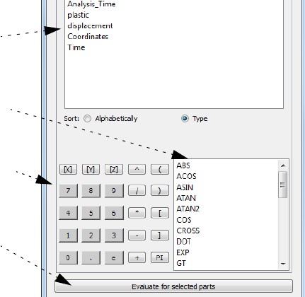
7.3 Threaded Calculator Functions
EnSight 10.2 User Manual 7-75
[ref.2, 1425] which plots 2 as a function of the ratio of /µ):
| /µ | < 1: flow locally dominated by strain, |2| < 2/
| /µ | = 1: pure shear, |2| = 2/
| /µ | > 1: flow locally dominated by rotation, |2| > 2/.
References:
1. Jeong, J. and Hussain, F., “On the identification of a vortex,” Journal of Fluid
Mechanics, 1995, vol. 285, pp. 69-94.
2. Laurent Graftieaux, Marc Michard, & Nathalie Grosjean "Combining PIV, POD
and vortex identification algorithms for the study of unsteady turbulent swirling
flows", Institute Of Physics Publishing Ltd in UK, Measurement Science &
Technology, 12 (2001) 1422-1429
3. PSA via Distene (personal communication).
Define equations Tab Under this tab, you are provided with a variable list, a calculator pad with math operators,
and a list of Math functions. These can be used to construct your own equations.
Var iab le L is t
Math Functions
Evaluate Expression
Math Operators

7.3 Threaded Calculator Functions
7-76 EnSight 10.2 User Manual
Math Functions Math functions use the syntax: function (value or expression). All angle arguments are in
radians. For most functions the value can be either a constant, constant per part, scalar, or
vector and the result of the function will be of corresponding type. When you select a math
function from the list, the function name and the opening “(“ appears in the Working
Expression for you. However, after defining the argument(s) for the function, you have to
manually provide any commas needed and a closing “)”. Note: any calculations involving
a vector are done on each component. For example:
GT(vector1,vector2) = (GT(vector1x, vector2x), GT(vector1y, vector2y), GT(vector1z, vector2z) )
The Math functions include the following:
Routines which accept argument(s) of type constant, scalar, or vector and produce the
corresponding type of result: (function works on each component of a vector)
ABS(constant) absolute value = constant
or (scalar) scalar
or (vector) vector
ACOS(constant) arccosine = radian constant
or (scalar) radian scalar
or (vector) radian vector
ASIN(constant) arcsine = radian constant
or (scalar) radian scalar
or (vector) radian vector
ATAN(constant) arctangent = radian constant
or (scalar) radian scalar
or (vector) radian vector
ATAN2(y, x) calculates ATAN(y/x) where the signs of both variables are used to determine the quadrant of the result.
Returns the result in radians which is between -PI and PI (inclusive). So:
ATAN2(constant, constant) = radian constant
or (constant, scalar) = radian scalar
or (constant, vector) = radian vector
or (scalar, scalar) = radian scalar
or (scalar, vector) = radian vector
or (vector, vector) = radian vector where:
ATAN2(vector1,vector2) = (ATAN2(vector1x/vector2x), ATAN2(vector1y/vector2y), ATAN2(vector1z/vector2z) )
TAN(radian constant) tangent = constant
or (radian scalar) scalar
or (radian vector) vector
CROSS(vector, vector) cross product = vector
COS(radian constant) cosine = constant
or (radian scalar) scalar
or (radian vector) vector
SIN(radian constant) sine = constant
or (radian scalar) scalar
or (radian vector) vector
CDF_CHISQU(v,k) evaluates the cumulative Chi-Squared distribution at the value v with k degrees of freedom.
CDF_CHISQU(constant, constant) = constant
or (constant, scalar) = scalar
or (scalar, scalar) = scalar
or (scalar, constant) = scalar
CDF_CHISQU(v,k) =
k
2
---v
2
---
k
2
---
-----------------
7.3 Threaded Calculator Functions
EnSight 10.2 User Manual 7-77
CDF_F(v, j, k) evaluates the cumulative F distribution at the value v with j and k degrees of freedom. If any input
value is a scalar then the result is a scalar.
CDF_F(scalar, constant, constant) = scalar
or (constant, scalar, constant) = scalar
or (constant, constant, scalar) = scalar
or (constant, constant, constant) = scalar
etc.
CDF_F(v, j, k) =
CDF_NORM(v) evaluates the cumulative normal distribution at the value v.
CDF_NORM(constant) = constant
or (scalar) = scalar
CDF_NORM(v) =
CDF_T(v, k) evaluates the cumulative Student’s T distribution at the value v with k degrees of freedom.
CDF_T(constant, constant) = constant
or (constant, scalar) = scalar
or (scalar, scalar) = scalar
or (scalar, constant) = scalar
CDF_T(v, k) =
DOT(vector, vector) dot product = scalar
Note: DOT(velocity,velocity ) is a scalar not equal to
velocity^2 which is a vector.
EXP(constant) e value = constant
or (scalar) scalar
or (vector) vector
GT(constant,constant) greater of = constant
or (constant,scalar) scalar
or (constant,vector) vector
or (scalar,scalar) scalar
or (scalar,vector) vector
or (vector,vector) vector where:
GT(vector1,vector2) = (GT(vector1x, vector2x), GT(vector1y, vector2y), GT(vector1z, vector2z) )
INT(variable) converts all values to signed integers by simply discarding the decimal portion.
Note: the decimal portion, FRAC, can be obtained as FRAC = var-INT(var).
LOG(constant) ln = constant
or (scalar) scalar
or (vector) vector
LOG10(constant) log10 = constant
or (scalar) scalar
or (vector) vector
LT(constant,constant) lesser of = constant
or (constant,scalar) scalar
or (constant,vector) vector
or (scalar,scalar) scalar
or (scalar,vector) vector
or (vector,vector) vector where:
LT(vector1,vector2) = (LT(vector1x, vector2x), LT(vector1y, vector2y), LT(vector1z, vector2z) )
Ijx
jx k+
-------------
j
2
---k
2
---(,)
1
2
---1erf
v
2
-------
+
1
2
---vk1
+
2
------------
1
2
---
n
k1+
2
------------
n
3
2
---
n
-------------------------------
v2
k
-----–
n
n!
----------------
n0=
k
2
---
k
-----------------------------------------------------------------------
+

7.3 Threaded Calculator Functions
7-78 EnSight 10.2 User Manual
MOD(var1,var2) modulo of int(var1) / (int(var2), (that is, the remainder of two integer divisions).
or (constant,scalar) scalar
or (constant,constant) constant
or (scalar,constant) scalar
or (scalar,scalar) scalar where:
Note: the first and second values are converted to integers by simply dropping fractional values (no rounding)
prior to the integer division. The result (that is, the remainder) is therefore always an integer
IF_CMP(var,var) compare the two values and return a
-1 or 0, where var can be same as LT above.
return value for IF_COMP(a,b):
(a < b) returns -1, (a = b) returns 0, (a > b) returns 1
IF_EQ(var,var)compare the two values and return a 1 or 0
where var can be same as LT above
return value for IF_EQ(a,b):
(a = b) returns 1, otherwise returns 0
IF_LT(var,var)compare the two values and return a 1 or
0 where var can be same as LT above
return value for IF_LT(a,b):
(a < b) returns 1, otherwise returns 0
IF_GT(var,var)compare the two values and return a 1 or 0
where var can be same as LT above
return value for IF_GT(a,b):
(a > b) returns 1, otherwise returns 0
PDF_CHISQU(v, k) evaluates the Chi-Squared probability density at the value v with k degrees of freedom.
PDF_CHISQU(constant, constant) = constant
or (constant, scalar) = scalar
or (scalar, scalar) = scalar
or (scalar, constant) = scalar
PDF_CHISQU(v, k) =
PDF_F(v, j, k) evaluates the F probability density at the value v with j and k degrees of freedom.
PDF_F(scalar, constant, constant) = scalar
or (constant, scalar, constant) = scalar
or (constant, constant, scalar) = scalar
or (constant, constant, constant) = scalar
etc.
PDF_F(v, j, k) =
PDF_NORM(v) evaluates the normal probability density at the value v.
PDF_NORM(constant) = constant
or (scalar) = scalar
PDF_NORM(v) =
PDF_T(v, k) evaluates the Student’s T probability density at the value v with k degrees of freedom.
PDF_T(constant, constant) = constant
or (constant, scalar) = scalar
or (scalar, scalar) = scalar
or (scalar, constant) = scalar
PDF_T(v, k) =
1
2
k
2
---
k
2
---
-----------------------v
k
21–
------------v
2
---–
exp
jv
jkk
jv k+
jk+
------------------------------
xB j
2
---k
2
---(,)
-----------------------------------
1
2
---------- v2
2
-----–
exp
1
B1
2
---k
2
---
k
--------------------------1v2
k
-----+
k1+
2
------------
–

7.3 Threaded Calculator Functions
EnSight 10.2 User Manual 7-79
RMS(vector) root-mean-square (magnitude) = scalar.
RMS(vector) is the same as
SQRT(vector[X]*vector[X] +
vector[Y]*vector[Y]+vector[Z]*vector[Z])
and the same as
SQRT(DOT(vector,vector))
but NOT the same as
SQRT(vector^2)
RND(constant) round to nearest = constant
or (scalar) scalar
or (vector) vector
LOOKUP(lookup table # (int), scalar)
or (lookup table # (int), vector)
finds the value of the scalar or vector using the x value
in the lookup table and returns the interpolated y value
of y. The lookup table x and y values must be defined in
advance in the proper case, using EnSight Python.
For example, if you define a table number 1, such that
x=[0,25,50] and y=[0,100,200] and you calculate as
follows:
myvar = LOOKUP(1,myscalar)
and the value of the variable myscalar is
0.0, 25.0, 50.0, and 37.5 at elements 1-4 respectively,
then the values for myvar will be
0.0, 100.0, 200.0, and 150. at elements 1-4 respectively.
Prior to this calculation, create lookup table 1 for this
example, with a min and max of 0 and 50 respectively,
using EnSight Python, using the following two EnSight
Python command lines.
from ensight.objs import *
# input values: (table#, xlist, ylist, minx,
maxx)
core.CASES[0].update_lookup_table(1,[0.,25.,50.]
,[0,100,200],0,50)
SQRT(constant) square root = constant
or (scalar) scalar
or (vector) vector
UNDEFINED
returns the Undefined value. This can be used as a test in
IF_EQ(var,UNDEFINED) will return 1 where the variable
is undefined and 0 where it is defined.

7.3 Threaded Calculator Functions
7-80 EnSight 10.2 User Manual
Calculator This on-screen calculator can usually be used in place of typing on your keyboard.
Button Function
0 to 9 number digits
. decimal
e e for exponential notation
+plus operator
– minus operator
* multiplication operator
/ division operator
^ exponentiation operator
PI value for
( opening parentheses. For function arguments and general grouping
) closing parentheses. For function arguments and general grouping
[ opening brackets. For components and node/element numbers
] closing brackets. For components and node/element numbers
[X] X component
[Y] Y component
[Z] Z component
(see How To Create New Variables)

7.4 Boundary Layer Variables
EnSight 10.2 User Manual 7-81
7.4 Boundary Layer Variables
EnSight creates the following Boundary Layer Variables simultaneously on a 2D
boundary part directly from velocity information of its corresponding 3D flow
field part. Their corresponding variable names are included in all appropriate
EnSight variable lists, i.e. Color Parts variable list, etc.
Warning: The Boundary Layer Variables capability as well as all the Boundary
Layer Calculator functions (BL_*) are not supported for Server of Server (SOS)
decomposition because SOS was designed to benefit from independent Servers
computations in parallel. The inter-dependent computational mapping of the field
results from the fluid part onto the boundary part violates this assumption.
Only nodal (values per node) variables are created. Any dependent elemental
variables (values per element) are averaged to nodal variables before processing.
(See Definitions below.)
Whether these variables are mapped onto the 2D boundary part, or used in
conjunction with other EnSight features (such as Elevated Surfaces of the
boundary layer thickness off the 2D boundary part, Vortex Cores, Separation and
Attachment Lines, Shock, etc.), these variables help provide valuable insight into
Variable Name Description Symbol
(N) bl_thickness Boundary layer thickness
(N) bl_disp_thickness Displacement thickness
(N) bl_momen_thickness Momentum thickness
(N) bl_shape_parameter Shape parameter
(N) bl_skin_friction_Cf Skin friction coefficient
*
H
Cf
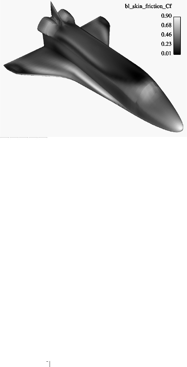
7.4 Boundary Layer Variables
7-82 EnSight 10.2 User Manual
the formation and location of possible boundary layers.
Boundary Layer A boundary layer is a relatively thin region that confines viscous diffusion near
the surface of a flow field, where the velocity gradient in the normal direction to
the surface goes through an abrupt change. Although multiple boundary layers
may be considered (especially in areas of flow separation), our current
implementation provides boundary layer parameters based on the former concept.
In these thin regions, the thickness of the boundary layer typically increases in the
downstream direction, and the velocity parallel to the surface is much larger than
the velocity normal to the surface.
Boundary Surfaces Boundary parts are typically 2D surface part(s) that correspond to a 3D field.
These surfaces may either be boundary parts defined directly from the data file, or
created parts (i.e. 2D IJK sweeps of a structured part, or an isosurface of zero
velocity of either an unstructured or structured part).
Velocity-Magnitude Changes of the velocity in the normal direction from the surface into the 3D flow
Gradient Vector field are utilized to determine the boundary layer. EnSight automatically creates a
velocity-magnitude gradient vector for all 3D model parts prior to creating the
boundary layer variables. These gradient values are then mapped to all
corresponding 2D model parts, and inherited by all created parts.
Note: The velocity-magnitude gradient vector variable will continue to be created
for all 3D model parts until it is deactivated.
This vector variable behaves like any other created variable, and may be
deactivated via the Feature Panel (Variables) dialog.
Definitions
Boundary Layer Thickness
The distance normal from the surface to where u/U = 0.995,
Figure 7-7
Skin Friction Coefficient
nu/U = 0.995
=
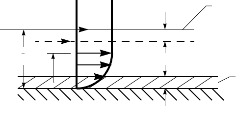
7.4 Boundary Layer Variables
EnSight 10.2 User Manual 7-83
where: u = magnitude of the velocity at a given location in the boundary layer,
U = magnitude of the velocity just outside the boundary layer.
Displacement Thickness
Provides a measure for the effect of the boundary layer on the “outside” flow. The
boundary layer causes a displacement of the streamlines around the body.
Momentum Thickness
Relates to the loss of momentum in the air in the boundary layer.
Shape Parameter
Used to characterize boundary layer flows, especially to indicate potential for
separation.
This parameter increases as a separation point is approached, and varies rapidly
near a separation point.
Note: Separation has not been observed for H < 1.8, and definitely has been
observed for H = 2.6; therefore, separation is considered in some analytical
methods to occur in turbulent boundary layers for H = 2.0.
In a Blasius Laminar layer (i.e. flat plate boundary layer growth with zero
pressure gradient), H = 2.605. Turbulent boundary layer, H ~= 1.4 to 1.5, with
extreme variations ~= 1.2 to 2.5.
Skin Friction Coefficient
where: = fluid shear stress at the wall.
= dynamic viscosity of the fluid.
May be spatially and/or temporarily varying quantity (usually a constant).
*
*
U
n
Streamline position without
boundary layer
Shifted streamline
Extra Thickness
*1
U
----Uu–nd
0
=
1
U2
------ Uu–und
0
=
*/
Cf
w
0.5V
2
-------------------------------=
wu
n
-----
n0=
=
7.4 Boundary Layer Variables
7-84 EnSight 10.2 User Manual
= distance normal to the wall.
= freestream density
= freestream velocity magnitude.
This is a non-dimensionalized measure of the fluid shear stress at the surface. An
important aspects of the Skin Friction Coefficient is:
, indicates boundary layer separation.
Other Notes: Factor Determining Velocity at Boundary-Layer Thickness ()
The factor (default = 0.995) which determines the velocity magnitude (u) at the
boundary-layer thickness () with respect to the velocity magnitude (U) just
outside the boundary layer (i.e. is the distance normal to the surface at which
u = 0.995U), may be changed by issuing the following command via the
command line processor Section 2.5, Command Files):
test: blt_factor #
where # is the corresponding factor ( > 0.).
References Please refer to the following texts for more detailed explanations.
P.M. Gerhart, R.J. Gross, & J.I. Hochstein, Fundamentals of Fluid Mechanics, 2nd Ed.,
(Addison-Wesley: New York, 1992),
C.A.J. Fletcher, Computational Techniques for Fluid Dynamics, Vol. 2, 2nd Ed.,
(Springer: New York, 1997)
n
V
Cf0=
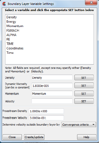
7.4 Boundary Layer Variables
EnSight 10.2 User Manual 7-85
Access Right-click on any variable in the variables list and choose “Boundary Layer
Variables” to create and update (make changes to) the boundary layer variables.
Define Boundary Opens the Boundary Layer Variable Settings dialog which allows the user to identify and
Layer Dependent set the dependent variables used in computing the boundary layer variables (see
Variables... Definitions above). This dialog has a list of current accessible variables to choose from.
Immediately below is a list of dependent variables with corresponding text field and SET
button. The variable name in the list is tied to a dependent variable below by first
highlighting a the listed variable, and then clicking the corresponding dependent variable’s
SET button, which inserts the listed variable into its corresponding text field.
All text fields are required, except you may specify either Density and Momentum (which
permits velocity to be computed on the fly), or Velocity. Default constant values are
provided which may be changed by editing the text field.
Clicking Okay activates all specified dependent variables and closes the dialog.
Freestream Density Constant ‘upstream’ density value (near flow inlet). Only used for skin-friction
coefficient, Cf.
Freestream Velocity Constant ‘upstream’ velocity magnitude value (near flow inlet). Only used for skin-
friction coefficient, Cf.
Determine Velocity Opens a pop-up dialog for the specification of which type of method to determine the
Outside Boundary constant velocity just outside the boundary layer (U) (see Definitions above). The
Layer By following options determine (U) at each node of the surface in the direction normal from
the surface into the 3D field by:
Convergence Criteria - monitoring the velocity profile until either the velocity magnitude
goes constant or its gradient goes to zero.
Distance From Surface - specifying the Normal Distance from the surface into the field at
which to extract the velocity and assign as U. Then monitor the velocity profile from the
surface into the field until U is obtained.
Normal Distance - Text field that contains the distance normal from the surface into
the 3D field at which to extract the velocity for U.
Figure 7-8
Boundary Layer Variable Settings Dialog

7.4 Boundary Layer Variables
7-86 EnSight 10.2 User Manual
Velocity Magnitude - specifying the Velocity Magnitude to assign as U. Then monitor the
velocity profile from the surface into the field until U is obtained.
Velocity Magnitude - Text field that contains the specified velocity magnitude to
assign as U.
Note: Boundary Layer Variable feature extraction does not work with multiple cases.
Troubleshooting Boundary Layer Variables
Problem Probable Causes Solutions
Error creating boundary layer
variables.
Non-2D part selected in part list. Select only 2D parts.
Undefined (colored by part color)
regions on boundary surface.
2D boundary surface node was not
mapped to corresponding 3D field
boundary node.
Make sure corresponding 3D field
part is defined.
EnSight 10.2 User Manual 8-1
8 Preference and Setup File Formats
This chapter provides information about the various file formats associated with
different preference options within EnSight. EnSight preferences are often
initialized from identically named files installed in the
%CEI_HOME%\site_preferences directory. The first time EnSight is run by an
individual user, a private preferences directory is created for that user. When
reading a preference file, EnSight first looks for the file in the user’s private
preferences directory, and failing that, it looks in the site_preferences directory.
The location of the user’s private preferences directory is shown in the ‘Help-
>Version’ dialog as shown here:
At the bottom of this dialog the 'Preferences' path is shown. Under Windows, the
path is often the user's home path, in the .ensight102 directory. If EnSight cannot
write to this directory, %HOMEDRIVE%%HOMEPATH%\.ensight102 will be
tried as well. Under Windows 7 and Vista, the path is commonly
C:\Users\{username}\.ensight102. Older versions of Windows tend to use
C:\Documents and Settings\{username}\.ensight102. Linux platforms use ~/
.ensight102. The OSX platform uses ~/Library/Application Support/EnSight102.
In all cases, the actual path used can be seen in the aforementioned dialog.
Figure 8-1
EnSight Help Version dialog
8-2 EnSight 10.2 User Manual
A number of different files are stored in the preferences directory and are read as
EnSight starts up. The command line flag (-no_prefs) can be used to force
EnSight to ignore the files in the user's private preferences directory for a single
run of EnSight. This can be useful to reset various files to their default values or to
clear potentially corrupted caches. For example, EnSight mains a cache of the
valid fonts on a system to speed up startup, if the user installs new fonts on a
system and EnSight does not recognize them immediately, running once with -
no_prefs will cause EnSight to ignore (and rebuild) the cache files, so the next
time it is run the cache will contain the new fonts (see Command Line Start-up
Options).
Specific files and their descriptions follow in the next sections.
Section 8.1, Palette/Color File Formats describes the format of the saved
function palettes, the default false color function palette and the default colors for
parts.
Section 8.2, Data Reader Preferences File Format describes the format for the
data reader preferences file.
Section 8.3, Data Format Extension Map File Format describes the format of
the ensight_reader_extension.map file.
Section 8.4, Parallel Rendering Configuration File points to the location where
the format of the parallel rendering configuration file is described.
Section 8.5, Resource File Format describes the format of the EnSight resources
file and points to the location where samples of its use are given.
Section 8.6, Other Preferences Files describes the format of various other files
EnSight generated in response to preference changes.
Section 8.7, Python Extension Files describes how user written EnSight Python
extensions can be scheduled for reading on startup.
8.1 Palette/Color File Formats
EnSight 10.2 User Manual 8-3
8.1 Palette/Color File Formats
The following palette formats are discussed in this section:
Palette Editor File Format
Predefined Function Palette
Default False Color Map File Format
Default Part Color File Format
Palette Editor File Format
A function palette file is saved using the Function Editor when you save (one or
more) function color palettes. The file stores the combination of a color table
along with its variable mapping. The following is an example function palette file:
palette 'velocity'
variable_type vector
variable 'velocity'
type continuous
limit_fringes no
scale linear
number_of_levels 5
colors
0.000000 0.000000 1.000000
0.000000 1.000000 1.000000
0.000000 1.000000 0.000000
1.000000 1.000000 0.000000
1.000000 0.000000 0.000000
values
0.100341
0.301022
0.501704
0.702385
0.903067
Many lines of the file consist of a descriptive keyword followed by an appropriate
value. In other areas the keyword is used to start a block of information. The
values are all free format real or integer numbers or string constants. The palette
name must have single quotes around each name. The string keywords and
constant values must match exactly.
Keyword Description
palette Name of the palette when one name is present. Name of the
subpalette when two names are present (e.g. palette 'velocity'
'xcomp')
variable Name of the variable used with the palette.
variable_type Type of the variable, scalar or vector.
limit_fringes Indicates if the palette is set up for limiting fringe. If it is, the
options are by_Part or by_invisible.
scale Indicates whether the palette scale is linear, logarithmic, or
quadratic.
8.1 Predefined Function Palette
8-4 EnSight 10.2 User Manual
Predefined Function Palette
When EnSight starts, it looks for user defined function color palettes located
under $CEI_HOME/ensight102/site_preferences/palettes and in the palettes
subdirectory under the user's EnSight private preferences directory (see the
section introduction for directory location specifics). These files must be named
palette_name.cpal, where the palette_name is the name of the color palette in the
'Files' area of the Palette editor dialog.
The format of the .cpal file is as follows:
• Line 1: The string “number_of_levels x”, where x is an integer <= 21.
• Line 2: The string “colors”
• Line 3 through x + 2: Three float values in range 0.0 to 1.0, indicating
red, green, and blue color components.
• Line x+3: has an optional keyword: undef_color
• Line x+4 has a float triplet of red, green, blue that is the undefined color.
• Line x+5 has an optional keyword: alpha
• Line x+6 through 2x+6 has one float between 0.0 and 1.0 inclusive
representing the alpha (opacity) value
An example color palette file without undefined color nor alpha values:
number_of_levels 5
colors
.008 0. 0.
.5 0. 0.
1. 0. 0.
1. 1. 0.
1. 0. 1.
An example color palette file with undefined color and alpha values:
number_of_levels 5
colors
.008 0. 0.
.5 0. 0.
1. 0. 0.
1. 1. 0.
1. 0. 1.
undef_color
0.7 0.7 0.7
alpha
1.0
0.25
0.1
0.25
1.0
number_of_levels Indicates the number of levels defined for the palette.
colors Indicates the start of a block of RGB triplets, 1 triplet per line.
There will be the same number of lines as there are levels.
values Indicates the start of a block of level values. There will be the
same number of values as there are levels.
8.1 Default False Color Map File Format
EnSight 10.2 User Manual 8-5
Default False Color Map File Format
This file defines the default false-color map color range that is assigned by
EnSight to each palette when variables are activated. If EnSight does not find a
definition file, it uses an internal default list. If, however, EnSight does find a file
at start-up, EnSight will read your colors as the default color palette colors. The
file must be called ensight.false_color.default and be located in the user's private
preferences directory (see the section introduction for path specifics).
The format of the
ensight.false_color.default
file is as follows:
• Line 1: "Version 6.0" (Note, this need not match EnSight’s version
number.)
• Line 2: One integer, the number default false color map colors
• Line 3 on: three floats (each ranging between 0. and 1.), the (red, green,
blue) color triplet of each color, each listed on separate lines.
An example default file can be found in:
$CEI_HOME/ensight102/site_preferences/ensight.false_color.default
on your client system.
The following is an example default false color map file with 5 colors; blue, cyan,
green, yellow, and red:
Version 6.0
5
0. 0. 1.
0. 1. 1.
0. 1. 0.
1. 1. 0.
1. 0. 0.
Default Part Color File Format
This file defines default Constant Colors that are assigned (and cycled through) by
EnSight when parts are built. If EnSight does not find a definition file it uses an
internal default list. If, however, EnSight does find a file it will be used instead.
The file must be called ensight.part.colors.default and be located in the user's
private preferences directory (see the section introduction for path specifics).
The format of the ensight.part.colors.default file is as follows:
• Line 1: "Version 6.0" (Note, this need not match EnSight's version
number.)
• Line 2: One integer, the number of default part colors
• Line 3 on: three floats (each ranging between 0. and 1.), the (red, green,
blue) color triplet of each color, each listed on separate lines.
An example default file can be found in:
$CEI_HOME/ensight102/site_preferences/ensight.part.colors.default
on your client system.
The following is an example default part colors file with 6 colors (blue, cyan,
green, yellow, red, and magenta):
Version 6.0
8.2 Data Reader Preferences File Format
EnSight 10.2 User Manual 8-7
8.2 Data Reader Preferences File Format
This is an optional file that will be created when the user saves preferences under
the Edit > Preferences... menu, the "Data" option. It contains two basic things: the
name of the reader desired to be the default format in the Data Reader dialog and
which reader names that the user wants to appear in the open dialog format list.
The file must be called ensight_reader_prefs.def and be located in the user's
private preferences directory (see the section introduction for path specifics).
The format of the
ensight_readers_prefs.def
file is as follows:
• Line 1: "VERSION 10.200000" (Note, this need not match EnSight’s
version number.)
• Line 2 (optional): “select readername” Where readername is the name
of the reader that will be used as the default
• Line 3 on: “remove readername” or “add readername” Where
readername is the name of a reader that will either be hidden (“remove”)
or shown (“add”) in the open dialog format list.
The following is an example data reader preferences file which hides a few of the
readers:.
VERSION 10.200000
remove ansys
remove Ansys Results (v10)
remove Ansys-Multi-Part
remove ESTET
remove Fluent Universal
remove MPGS 4.1
remove N3S
add ABAQUS fil
add ABAQUS_ODB
add AcuSolve
add Ansys Results
add Autodyn
add AVUS
add AVUS Case
add CAD
add Case
add CFF/WIND
add CFX-4
…
8.3 Data Format Extension Map File Format
8-8 EnSight 10.2 User Manual
8.3 Data Format Extension Map File Format
The ensight_reader_extension.map file is used to associate file naming
conventions with a reader within EnSight. This association allows EnSight to use
automatically select a reader for specific files. The Drag and Drop system uses
this mechanism to properly identify datasets for example. A default version of this
file is provided with the EnSight distribution and is placed in the $CEI_HOME/
ensight102/site_preferences directory. A user can override this file by placing
their own version of the file in their private EnSight preference directory (see the
section introduction for pathname details).
Historically, EnSight looked explicitly at the filename 'extension', hence the name
of the file, but limitations of this approach with modern filesystem and common
file naming schemes have required the use of more generic filename comparison
schemes. The extension map file uses filename wildcard matching known as
'globbing'. The EnSight wildcards include '*' for any number of character and '?'
for a single character.
A description of the format is contained in the file itself. A portion of the file is
given below (it contains only a few file formats, but it should be easy to see how
this file is formatted). The file begins with the line 'EnSight file extension to
format association file':
EnSight file extension to format association file
Version 1.0
#
# Comment lines start with a #
#
# The format of this file is as follows:
#
# READER_NAME: reader name as it appears in the Format chooser in the
# EnSight Data Reader dialog
#
# NUM_FILE_1: the number of file_1_ext lines to follow
#
# FILE_1_EXT: a 'glob' expression for the first filename
# There should be one definition after the :
# Multiple FILE_1_EXT lines may exist
#
# NUM_FILE_2: the number of file_2_ext lines to follow
#
# FILE_2_EXT: the 'glob' expression for a second file that will act as
# the result file. This is only used for formats that require
# two filenames. As with FILE_1_EXT, there may be multiple
# FILE_2_EXT lines.
#
# ELEMENT_REP: A keyword that describes how the parts will be
# loaded (all parts will be loaded the same way).
# One of the following:
# "3D border, 2D full"
# "3D feature, 2D full"
# "3D nonvisual, 2D full"
# "Border"
# "Feature angle"
# "Bounding Box"
# "Full"
# "Volume"
8.3 Data Format Extension Map File Format
EnSight 10.2 User Manual 8-9
# "Non Visual"
# If the ELEMENT_REP option is not set then
# "3D border, 2D" full is used
#
# READ_BEFORE: (optional) The name of a command file to play before reading
# the file(s)
#
# READ_AFTER: (optional) The name of a command file to read after loading
# the parts
# Definition for Case files
READER_NAME: Case
NUM_FILE_1: 3
FILE_1_EXT: *.case
FILE_1_EXT: *.encas
FILE_1_EXT: *.enc
ELEMENT_REP: 3D feature, 2D full
# Definition for EnSight5 files
READER_NAME: EnSight 5
NUM_FILE_1: 2
FILE_1_EXT: *.geo
FILE_1_EXT: *.geom
NUM_FILE_2: 4
FILE_2_EXT: *.res
FILE_2_EXT: *.RES
FILE_2_EXT: *.results
FILE_2_EXT: *.RESULTS
ELEMENT_REP: 3D border, 2D full
# Definition for Nastran files
READER_NAME: Nastran OP2
NUM_FILE_1: 2
FILE_1_EXT: *.op2
FILE_1_EXT: *.mop
ELEMENT_REP: 3D border, 2D full
# Definition for LS-Dyna files
READER_NAME: LS-DYNA3D
NUM_FILE_1: 2
FILE_1_EXT: *d3plot*
FILE_1_EXT: *.d3p
ELEMENT_REP: 3D border, 2D full
8.5 Resource File Format
EnSight 10.2 User Manual 8-11
8.5 Resource File Format
Resources are used to specify which computers are used for running the various
EnSight components, specifically the Server (ensight102.server), the SOS
(ensight102.sos), the CollabHub (ensight102.collabhub), and the distributed
renderers (ensight102.client). If you are running a single client and server on a
single computer, you may skip this document. Resources can be useful in simple,
relatively static environments. In EnSight 10, a more complete cluster
virtualization system called CEIShell may be used to support more complex
environments that might have cross-enterprise security and other concerns that
need to be abstracted.
Resources are an alternative way to specify these computers compared to SOS
case files, PRDIST files, Connection Settings, and command line options. While
these other ways are still valid, resources can simplify the specification of
computers in a dynamic network environment. For example, SOS Case files and
PRDIST files no longer need to be edited to reflect the current node allocation
from cluster batch schedulers. Resources coupled with native reader support in the
SOS even make SOS Case files unnecessary.
Resources files can be specified via command line arguments and environment
variables. Multiple resource files can be specified; precedence rules determine
which resources ultimately get used. This allows sites to specify defaults while
allowing them to be overridden. Here is an example of a resource file:
#!CEIResourceFile 1.0
SOS:
host: localhost
SERVER:
prologue: “setup_job”
epilogue: “cleanup_job”
host: server1
host: server2
host: server3
host: server4
COLLABHUB:
host: pc0
RENDERER:
prologue: “setenv DISPLAY :0.0”
# epilogue:
host: pc1
host: pc2
host: pc2
Resource files must begin with the '#!CEIResourceFile 1.0' line. subsequently,
they may have up to four optional sections: SOS, SERVER, COLLABHUB, and
RENDERER. Each of the four sections contains one or more 'host: hostname'
lines. These lines specify which computers to use for the corresponding section.
'hostname' must be an Internet/intranet routable host name or IP address. A given
host name may appear on multiple lines within a section or in different sections. If
it appears multiple times within a section, then that host will run multiple
instances of the corresponding EnSight component if needed.
Additionally, each section may have an optional 'prologue: cmd' line and/or an
8.5 Resource File Format
8-12 EnSight 10.2 User Manual
optional 'epilogue: cmd' line. These specify a command to execute on each host
before and after the corresponding EnSight component. Note that the cmd string
must be quoted, and may include appropriate job backgrounding symbols (e.g.
'&').
For examples, see How To Use Resource Management.
8.6 Other Preferences Files
EnSight 10.2 User Manual 8-13
8.6 Other Preferences Files
When a preference file is saved in EnSight, it is written to the user's private
preferences directory (see the section introduction for path details). The format of
these file is actually EnSight command language. In most cases, the files end with
the '.def' suffix. An example would be the file: ensight_performance_prefs.def.
After saving the preference, the file is created and contains:
VERSION 10.200000
prefs: minimize_redraw OFF
prefs: cull_lines OFF
prefs: static_fast_display OFF
prefs: transparency_sort depth_peel
prefs: number_of_peels 5
prefs: fastdisplay_point_res 1
prefs: fastdisplay_sparse_res 50
prefs: abort_server_time 0
prefs: abort_server_operations OFF
The details of specific commands can be found in the 'Command Language'
manual.
8.7 Python Extension Files
8-14 EnSight 10.2 User Manual
8.7 Python Extension Files
EnSight supports user-written extensions written in Python. See the "How to
Produce Customized Access to Tools & Features" section for details on this
process. Once the user has developed an extension, they need to place it in a
location where EnSight can find it. For user-specific extensions, one can place
them in a subdirectory of the user's private preferences directory named
'extensions/user_defined'. For example, if the private preferences directory is
~someuser/.ensight102 (under Linux), create a directory named ~someuser/
.ensight102/extensions/user_defined and place the Python extension files in that
directory (the files should use the 'CTOR' comment header convention outlined in
the HowTo section.
For enterprise/multi-user extension installations, users should use the 'Product
Extension' mechanism. To simplify the distribution and installation of extensions
and full GUI replacements, the "product" extension was introduced. Product
extensions are located in subdirectories of $CEI_HOME and the EnSight core
scans for them right after loading the extensions located in the $CEI_HOME/
ensight102/site_preferences/extensions/user_defined tree. EnSight looks for XML
files named 'product.xml' in the subdirectories of $CEI_HOME. An example from
EnSight 9.1 is EnSight CFD, which is defined through the file $CEI_HOME/
ensight91cfd/product.xml. A minimum product.xml would look like:
<?xml version="1.0" encoding="UTF-8"?>
<product>
<ensight_extension>
<loader>EnSightCFDGUI.py</loader>
<requires>
<ensight_core>
<minimum>9.1.0.0</minimum>
<maximum>9.2.0.-1</maximum>
</ensight_core>
</requires>
</ensight_extension>
<ensight_extension>
<loader>another_extension.py</loader>
<translation>path/*.qm</translation>
<documentation langid="">path/docs</documentation>
<documentation langid="is">path/docs/iceland</documentation>
<requires>
<ensight_core>
<minimum>9.1.0.0</minimum>
<maximum>9.2.0.-1</maximum>
</ensight_core>
</requires>
</ensight_extension>
</product>
This file defines two extensions to ensight (<ensight_extension>). The location of
the Direct Load bootstrap Python file is specified by <loader> and must be a
subdirectory of the directory where the product.xml file is located. This particular
extension has a single dependency (<requires>) on the EnSight core Python
interface (<ensight_core>). The allowed versions of the EnSight core are
specified by the <minimum> and <maximum> tags respectively. In the example,
this extension is allowed to load for all versions of EnSight number 9.1. Note that
8.7 Python Extension Files
EnSight 10.2 User Manual 8-15
numbers are substituted for the '(x)' version tags on EnSight (e.g. 9.1.0(c)
corresponds to 9.1.0.2). All version comparisons are fieldwise numeric and
matching the limits enables the extension. The second extension includes a pair of
Qt .qm translation files that go along with the extension. Note: an extension block
(<ensight_extension>) may have any number of <loader> and <translation> tags
and multiple <requires> blocks that apply to all of the <loader> and <translation>
tags in the block. Also, the <loader> and <translation> tags can include "glob"
wildcards to specify multiple translation and Python loader files.
The <documentation> tag allows the product XML file to specify a directory
where EnSight will look for it's documentation PDF files before it looks for them
under $CEI_HOME/ensight*/docs. The tag also supports the langid="" attribute.
This qualifies the path to a specific language. That path will only be used if
EnSight is currently using the specified language. In the above example, path/docs
will always be considered because the language id is "", but if the current EnSight
language is set to Icelandic ("is"), the path/docs/iceland will be searched first. In
all cases, the core EnSight docs directories will be searched, having failed all
other matches.

EnSight 10.2 User Manual 9-1
9 EnSight Data Formats
This section describes the format for all readable and writable files in EnSight
which you may need access to. The formats described are only for those files that
are specific to EnSight. We do not describe data formats not developed by CEI
(for example, data formats for various analysis codes). For information about
these formats, consult the applicable creator.
Note: If you are using this documentation to produce your own data translator, please make sure
that you follow the instructions exactly as specified. In many cases, EnSight reads data in
blocks to improve performance. If the format is not followed, the calculations of how much
to read for a block will be thrown off. EnSight does little in the way of error checking data
files when they are read. In this respect, EnSight sacrifices robustness for performance.
EnSight Formats
EnSight has three evolutionary file formats listed below from oldest to most
recent:
EnSight 5
- legacy format
- supported unstructured meshes only
- used a global nodal array
- used per node variables only
EnSight 6
- support for case file
- support for both unstructured and structured meshes
- uses a global nodal array
- use per node or per element variables
EnSight Case Gold (recommended format)
- is much faster than EnSight 6 and is more memory efficient (noticeable if you
have a large number of parts or for larger models)
- uses connectivity which can be separate from the node ids
- uses a part basis rather than a global array
Format illustration
Jump to Detailed Description of Formats
Ensight Case Gold EnSight 6
part 1
node coordinates
element connectivity by local node index
part 2
node coordinates
element connectivity by local node index
...
part n
node coordinates
element connectivity by local node index
global nodal ids & coordinates
part 1
element connectivity by global node ids
part 2
element connectivity by global node ids
...
part n
element connectivity by global node ids

EnSight Maximums
9-2 EnSight 10.2 User Manual
Saving Gold from EnSight
EnSight can export your model into Case Gold format (either ASCII or Binary).
Activate the variables of interest, select the parts in the main part window and
then go to the File menu: File->Save->Geometric Entities.
Tool to Check EnSight Format
There is another advantage to using Case Gold format in that there is a debugging
tool called ens_checker that can help you find mistakes in files as you write a
translator or exporter. Each version of EnSight has an improved ens_checker with
the version of EnSight as a suffix. For example with EnSight 10.2, use
ens_checker102. Just type
ens_checker102 file.case
and the code will echo its
progress and the problems it finds to the console. This tool will also check
EnSight 6 format.
EnSight Maximums
There are some maximums that you should be aware of when producing EnSight
data:
Maximum number of parts allowed. 1,073,741,824
(2^30)
Maximum number of variables allowed 10000
Maximum number of nodes in a part 2,147,483,647
(2^31)
Maximum number of elements in a part 2,147,483,647
(2^31)
Maximum file name length 1024
Maximum part name length visible in the GUI 79
Maximum variable name length visible in the GUI 49
Maximum number of Cases loaded 32
Maximum number of plots 25
Maximum number of viewports 16
EnSight Maximums
EnSight 10.2 User Manual 9-3
Detailed Description of Formats
Section 9.1, EnSight Gold Casefile Format describes in detail the EnSight Gold case,
geometry, and variable file formats. This format provides the best performance for
getting data into EnSight. It is readable by both EnSight and EnSight HPC
(formerly EnSight Gold).
Section 9.2, EnSight6 Casefile Format describes in detail the EnSight6 case, geometry,
and variable file formats. This format is still supported, but is a legacy format. It has
most, but not all, of the options of the gold format - and a bit lower in performance.
Section 9.3, EnSight5 Format describes in detail the EnSight5 geometry and variable
file formats. This format is still supported, but is a legacy format. It is for
unstructured data only.
Section 9.4, FAST UNSTRUCTURED Results File Format describes the “executive”
.res file that can be used with FAST unstructured solution and function files.
Section 9.5, FLUENT UNIVERSAL Results File Format describes the “executive”
.res file used with FLUENT Universal files for transient models.
Section 9.6, Movie.BYU Results File Format describes the “executive” .res file that
can be used with Movie.BYU files.
Section 9.7, PLOT3D Results File Format describes the “executive” .res file that can
be used with PLOT3D solution and function files.
Section 9.8, Server-of-Server Casefile Format describes the format of the casefile used
with the server-of-server capability of EnSight.
Section 9.9, Periodic Matchfile Format describes the file format used to explicitly
specify which nodes match from one periodic instance to the next.
Section 9.10, XY Plot Data Format describes the XY plot dat file format.
Section 9.11, EnSight Boundary File Format describes the format of the file which can
define unstructured boundaries of structured data.
Section 9.12, EnSight Particle Emitter File Format describes the format of the
optional file containing particle trace emitter time and location information.
Section 9.13, EnSight Rigid Body File Format describes the format of the optional
executive file that relates EnSight part names or numbers to rigid body
transformations.
Section 9.14, Euler Parameter File Format describes the format of a file that contains
translations and euler parameters for rigid body transformations.
Section 9.15, Vector Glyph File Format describes the format of the optional file
containing vector information such as forces or moments.
Section 9.16, Constant Variables File Format format of the constant variable file
Section 9.17, Point Part File Format describes the point part format.
Section 9.18, Spline Control Point File Format describes the spline file format.
Section 9.19, EnSight Embedded Python (EEP) File Format describes a portable
delivery mechanism for data and scripts.
Section 9.20, Camera Orientation File Format describes the file format for positioning
and orienting the Camera.
Section 9.21, Multi-Tiled Movie (MTM) File Format describes the file format for
9.1 EnSight Gold Casefile Format
EnSight 10.2 User Manual 9-5
9.1 EnSight Gold Casefile Format
Include in this section:
EnSight Gold General Description
EnSight Gold Geometry File Format
EnSight Gold Case File Format
EnSight Gold Wild Card Name Specification
EnSight Gold Variable File Format
EnSight Gold Per_Node Variable File Format
EnSight Gold Per_Element Variable File Format
EnSight Gold Undefined Variable Values Format
EnSight Gold Partial Variable Values Format
EnSight Gold Constant Per Part Variable Files
EnSight Gold Measured/Particle File Format
EnSight Gold Material Files Format
EnSight Gold General Description
EnSight Gold data consists of the following files:
• Case (required) (points to all other needed files including model
geometry, variables, and possibly measured geometry and variables - as
well as optionally a periodic match file, a structured boundary file, and a
rigid body file)
EnSight makes no assumptions regarding the physical significance of the scalar,
vector, 2nd order symmetric tensor, and complex variables. These files can be
from any discipline. For example, the scalar file can include such things as
pressure, temperature, and stress. The vector file can be velocity, displacement, or
any other vector data, etc.
In addition, EnSight Gold format handles "undefined" as well as "partial" variable
values. (See appropriate subsections later in this chapter for details.)
All variable results for EnSight Gold format are contained in disk files—one
variable per file. Additionally, if there are multiple time steps, there must either be
a set of disk files for each time step (transient multiple-file format), or all time
steps of a particular variable or geometry in one disk file each (transient single-file
format).
Sources of EnSight Gold format data include the following:
• Data that can be translated to conform to the EnSight Gold data format
(including being written from EnSight itself using the Save Geometric
Entities option under File->Save)
• Data that originates from one of the translators supplied with the EnSight
application
9.1 EnSight Gold General Description
9-6 EnSight 10.2 User Manual
The EnSight Gold format supports an unstructured defined element set as shown
in the figure on a following page. Unstructured data must be defined in this
element set. Elements that do not conform to this set must either be subdivided or
discarded.
The EnSight Gold format also supports the same structured block data format as
EnSight6, which is very similar to the PLOT3D format. Note that for this format,
the standard order of nodes is such that I’s advance quickest, followed by J’s, and
then K’s.
A given EnSight Gold model may have either unstructured data, structured data,
or a mixture of both.
This format is somewhat similar to the EnSight6 format, but differs enough to
allow for more efficient reading of the data. It is intended for 3D, binary, big data
models.
Note: While an ASCII format is available, it is not intended for use with large
models and is in fact subject to limitations such as integer lengths of 10 digits.
Use the binary format if your model will exceed 10 digits for node or element
numbers or labels.
Starting with version 7, EnSight writes out all model and variable files in EnSight
Gold format. Thus, it can be read by all subsequent EnSight licenses: standard,
hpc (formerly gold), and custom licenses.
ens_checker A program is supplied with EnSight which attempts to verify the integrity of the
format of EnSight 6 and EnSight Gold files. If you are producing EnSight
formatted data, this program can be very helpful, especially in your development
stage, in making sure that you are adhering to the published format. It makes no
attempt to verify the validity of floating point values, such as coordinates, variable
values, etc. This program takes a casefile as input. Thus, it will check the format
of the casefile, and all associated geometry and variable files referenced in the
casefile. See How To Use ens_checker.
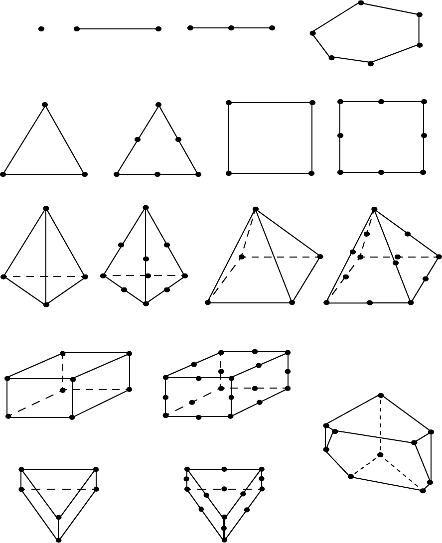
9.1 EnSight Gold General Description
EnSight 10.2 User Manual 9-7
Supported EnSight Gold Elements
The elements that are supported by the EnSight Gold format are:
eight node hexahedron twenty node hexahedron
six node pentahedron
9
10
7
8
12123
12
3
12
3
4
56
1
2
3
4
12
3
45 6
7
8
12
3
4
5
6
1
2
3
4
5
6
910
7
8
1
2
3
4
56
11
12
13 14
15
16
17 18
19
20
two node bar three node bar
three node triangle six node triangle four node quadrangle eight node quadrangle
four node tetrahedron ten node tetrahedron
1
point
12
3
4
1
4
8
2
3
5
6
7
5 node pyramid 13 node pyramid
11
22
33
44
55
6
7
8
9
10
11
12
13
fifteen node pentahedron (wedge)
1
2
3
4
5
6
78
9
10 11
12
13
14
15
(wedge)
Figure 9-1
Supported EnSight Gold Elements
1.
.
.
n
2
n-sided polygon
convex n-faced polyhedron
(described by n, n-sided faces)

9.1 EnSight Gold Case File Format
9-8 EnSight 10.2 User Manual
EnSight Gold Case File Format
The Case file is an ASCII free format file that contains all the file and name
information for accessing model (and measured) geometry, variable, and time
information. It is comprised of five sections (FORMAT, GEOMETRY, VARIABLE,
TIME, FILE) as described below:
Notes: If the case file name contains spaces it should load fine in the browser, but from
the command line it must be in quotes (e.g. ensight102 -case “file name.case”) or
on linux or mac can also use the backslash character (“\”) as follows:
ensight102 -case file\ name.case).
All lines in the Case file are limited to 1024 characters.
The titles of each section must be in all capital letters.
Anything preceded by a “#” denotes a comment and is ignored. Comments may
append information lines or be placed on their own lines.
Information following “:” may be separated by white spaces or tabs.
Specifications encased in “[]” are optional, as indicated.
Format Section This is a required section which specifies the type of data to be read.
Usage:
FORMAT
type: ensight gold
Geometry Section This is a required section which specifies the geometry information for the model
(as well as measured geometry if present, periodic match file (see Section 9.9,
Periodic Matchfile Format) if present, boundary file (see Section 9.11, EnSight
Boundary File Format) if present, rigid body file (see Section 9.13, EnSight Rigid
Body File Format) if present, and vector glyphs file (see Section 9.15, Vector
Glyph File Format) if present).
Usage:
GEOMETRY
model: [ts] [fs] filename [change_coords_only [cstep]]
OR
model: [ts] [fs] filename [changing_geometry_per_part]
measured: [ts] [fs] filename [change_coords_only]
match: filename [add_ghosts]
boundary: filename
rigid_body: filename [do_first]
Vector_glyphs: filename
where: ts = time set number as specified in TIME section. This is optional.
fs = corresponding file set number as specified in FILE section below.
(Note, if you specify fs, then ts is no longer optional and must also be
specified.)
filename = The filename of the appropriate file.
-> Model or measured filenames for a static geometry case (or single file
format), as well as match, boundary, and rigid_body filenames will not
contain “*” wildcards.
-> Model or measured filenames for a changing geometry case (unless single
file format) will contain “*” wildcards where each * represents one integer
with a maximum of 15 of the “*” wildcards per filename.
-> Model filenames for the structured block continuation option will contain
“%” wildcards.
-> filenames with spaces in them need to be enclosed in quotes.
9.1 EnSight Gold Case File Format
EnSight 10.2 User Manual 9-9
change_coords_only = The option to indicate that the changing geometry (as
indicated by wildcards in the filename) is coords only.
Otherwise, changing geometry connectivity will be
assumed.
cstep = the zero-based time step which contains the connectivity - only used for
change_coords_only option. This is an optional parameter. If all time steps
have the connectivity, then this is not needed and can be omitted. But if used,
the other time steps do not need to contain the connectivity - the parts need
only contain the coordinates, which can save considerably on file size.
changing_geometry_per_part = Signals the reader that the part lines in the geometry files
will have a manditory additional option The valid options are
part no_change
part coord_change
part conn_change
add_ghostsEnSight Case Gold allows the optional [add_ghosts] parameter after the
filename which will produce ghost cells across the match file boundary which
will provide continuity for variable calculations across the boundary, and for
computational symmetry/mirroring, etc. Only use the add_ghosts option if
you can afford the penalty of the additional ghost cells and you need the
computational continuity that they provide.
do_first If both periodic and rigid body data are present then the default is to do
periodic first then to do rigid body transforms. The do_first, does rigid body
transforms first, then periodic afterward.
Note: It is possible to use EnSight 5 measured data with a casefile. This is done by using
the Measured: line in the GEOMETRY section without any of the optional
portions, and with filename being an EnSight 5 measured results file (which
typically has a .mea extension). Also, since such information is contained in the
.mea file, do not use any measured variable lines in the VARIABLE section.
Variable Section This is an optional section which specifies the files and names of the variables (for
maximum number of variables, see EnSight Maximums). Per_Case and Per_Part
Constant variable values can also be set in this section.
Usage:
VARIABLE
constant per case: [ts] name const_value(s)
constant per case file: [ts] name cv_filename
constant per part: [ts] name cpp_filename [cpp_index_filename]
scalar per node: [ts] [fs] name filename
vector per node: [ts] [fs] name filename
tensor symm per node: [ts] [fs] name filename
tensor asym per node: [ts] [fs] name filename
scalar per element: [ts] [fs] name filename
vector per element: [ts] [fs] name filename
tensor symm per element: [ts] [fs] name filename
tensor asym per element: [ts] [fs] name filename
scalar per measured node: [ts] [fs] name filename
vector per measured node: [ts] [fs] name filename
complex scalar per node: [ts] [fs] name Re_fn Im_fn freq
complex vector per node: [ts] [fs] name Re_fn Im_fn freq
complex scalar per element
: [ts] [fs] name Re_fn Im_fn freq
complex vector per element
: [ts] [fs] name Re_fn Im_fn freq
9.1 EnSight Gold Case File Format
9-10 EnSight 10.2 User Manual
where:
ts
= The corresponding time set number (or index) as specified in TIME
section below. This is only required for transient constants and
variables.
fs
= The corresponding file set number (or index) as specified in FILE
section below.
(Note, if you specify fs, then ts is no longer optional and must
also be specified.)
name = The variable (GUI) name (ex. Pressure, Velocity, etc.)If the
variable name contains a space, it must be in quotes, and will be
renamed in EnSight, replacing the spaces with an underscore.
const_value(s) = The constant value. If constants change over time, then ns (see
TIME section below) constant values of ts.
cv_
filename
= The filename containing the per_case constant values, one value per
time step.
cpp_
filename
= The filename containing the per_part constant values.
cpp_index_filename
= The filename containing the offset indexes in the referenced cpp_filename.
filename
= The filename of the variable file. Note: only transient filenames
contain “*” wildcards where each * represents one integer with a
maximum of 15 of the “*” wildcards per filename. If the filename
contains a space, it must be in quotes.
Re_fn
= The filename for the file containing the real values of the complex
variable.
Im_fn
= The filename for the file containing the imaginary values of the
complex variable.
freq
= The corresponding harmonic frequency of the complex variable.
For complex variables where harmonic frequency is undefined,
simply use the text string: UNDEFINED.
Note: As many variable description lines as needed may be used.
Note: Variable descriptions have the following restrictions:
The maximum variable name length is documented at the beginning of this
chapter.
Duplicate variable descriptions are not allowed.
Leading and trailing white space will be eliminated.
Variable descriptions must not start with a numeric digit.
Variable descriptions must not contain any of the following reserved characters:
( [ + @ ! * $ : ,
) ] - space # ^ / .
Note: scalar or vector per measured node is necessary for EnSight Gold or EnSight 6
measured format data. For EnSight 5 format measured data, only the results file
(typically suffix .mea) is necessary in the geometry section because the EnSight 5
results file describes the geometry and variable files.
Time Section This is an optional section for steady state cases, but is required for transient
cases. It contains time set information. Shown below is information for one time
set. Multiple time sets (up to 16) may be specified for measured data as shown in
Case File Example 3 below. Time values can be one per line, all on one line, or
any combination of values per line (with a maximum limitation of 1024 characters
per line).
9.1 EnSight Gold Case File Format
EnSight 10.2 User Manual 9-11
Usage:
TIME
[maximum time steps: tm]
time set: ts [description]
number of steps: ns
filename start number: fs
filename increment: fi
time values: time_1 time_2 .... time_ns
or
TIME
[maximum time steps: tm]
time set: ts [description]
number of steps: ns
filename numbers: fn
time values: time_1 time_2 .... time_ns
or
TIME
[maximum time steps: tm]
time set: ts [description]
number of steps: ns
filename numbers file: fnfilename
time values file: tvfilename
where:
tm
= optional integer value, used only if the number of timesteps is to
be increasing over time. This keyword and value represents the never-
to-exceed, maximum number of timesteps (see the Advanced section of
the How To Load Transient Data ).
ts
= timeset number. This is the number referenced in the GEOMETRY
and VARIABLE sections.
description
= optional timeset description which will be shown in user
interface.
ns
= number of transient steps
fs
= the number to replace the “*” wildcards in the filenames, for the first step
fi
= the increment to fs for subsequent steps
time
= the actual time values for each step, each of which must be separated
by a white space and which may continue on the next line if needed
fn
= a list of numbers or indices, to replace the “*” wildcards in the filenames.
fnfilename
= name of file containing ns filename numbers (fn).
tvfilename
= name of file containing the time values (time_1 ... time_ns free
format one to a line or on multiple lines).
time values
= one time value for each timestep in free format on one or
multiple lines (with a maximum limit of 1024 characters per line).
File Section This section is optional for expressing a transient case with single-file formats.
This section contains single-file set information. This information specifies the
number of time steps in each file of each data entity, i.e. each geometry and each
variable (model and/or measured). Each data entity’s corresponding file set might
have multiple continuation files due to system file size limit, i.e. ~2 GB for -bit
and ~4 TB for 64-bit architectures. Each file set corresponds to one and only
one time set, but a time set may be referenced by many file sets. The following
information may be specified in each file set. For file sets where all of the time set
data exceeds the maximum file size limit of the system, both
filename index
and
9.1 EnSight Gold Case File Format
9-12 EnSight 10.2 User Manual
number of steps
are repeated within the file set definition for each continuation
file required. Otherwise
filename index
may be omitted if there is only one file.
File set information is shown in Case File Example 4 below.
Usage:
FILE
file set: fs
filename index: fi # Note: only used when data continues in other files
number of steps: ns
where:
fs
= file set number. This is the number referenced in the GEOMETRY
and VARIABLE sections above.
ns
= number of transient steps
fi
= file index number in the file name (replaces “*” in the filenames)
Material Section This is an optional section for material set information in the material interface
part case. For more details see the description in the Material Interface Parts
Feature Panel, or the MatSpecies calculator function in 4.3. Shown below is the
format for one material set. (Note, currently only one material set is supported.)
An example of this material set information is appended below as EnSight Gold
Material Files Format.
Usage:
MATERIAL
material set number: ms [description]
material id count: nm
material id numbers: matno_1 matno_2 ... matno_nm
material id names: matdesc_1 mat_2 ... mat_nm
# Either sparse file specifications:
material id per element [ts] [fs] filename
material mixed ids: [ts] [fs] filename
material mixed values: [ts] [fs] filename
# optional species parameters with sparse file specifications only
species id count:ns
species id numbers: spno_1 spno_2 … spno_ns
species id names: spdesc_1 spdesc_2 … spdesc_ns
species per material counts: spm_1 spm_2 … spm_nm
species per material lists: matno_1_sp_1 matno_1_sp_2 … matno_1_sp_spm_1
matno_2_sp_1 matno_2_sp_2 … matno_2_sp_spm_2
…
matno_nm_sp_1 matno_nm_sp2 … matno_nm_sp_spm_nm
(Note: above concatenated lists do not have to be on
separate lines.)
species element values: [ts] [fs] sp_filename
# Or materials defined by per element scalar variables:
material scalars per element: desc_esv_1 desc_esv_2 ... desc_esv_nm
where:
ts = The corresponding time set number (or index) as specified in TIME section
above. This is only required for transient materials.
fs = The corresponding file set number (or index) as specified in FILE section
above. (Note, if you specify fs, then ts is no longer optional and must also be
specified.)
9.1 EnSight Gold Case File Format
EnSight 10.2 User Manual 9-13
ms = Material set number. (Note, currently there is only one, and it must be a
positive number.)
description = Optional material set description which will be reflected in the file
names of exported material files.
nm = Number of materials for this set.
matno = Material number used in the material and mixed-material id files. There
should be nm of these. Non-positive numbers are grouped as the “null material”.
See EnSight Gold Material Files Format
matdesc = GUI material description corresponding to the nm matno’s.
filename = The filename of the appropriate material file. Note, only transient
filenames contain “*” wildcards with a maximum of 15 * wildcard characters.
The three required files are the material id per element, the mixed-material
ids, and the mixed-material values files.
ns = Number of species for this set.
spno = Specie number used in the "species per material lists:" specification. There
should be ns of these positive integers.
spdesc = GUI specie description corresponding to the ns spno's.
spm = Number of species per material number (matno). Enter 0 if no species exist for
a material.
matno_#_sp = Specie id number (spno) list member for this material number id
(matno). If no species for this material, then proceed to next material that
has species.
sp_filename = The filename of the appropriate “species element values:” file. Note,
only transient filenames contain "*" wildcards.
desc_esv = The description of each per element scalar variable to be a material.
The description listed must match the description listed under the VARIABLE
section for the per element scalar variable.
Note: Material and species descriptions are limited to 19 characters in the current
release. Material and species descriptions and file names must not start with a
numeric digit and must not contain any of the following reserved characters:
(
[ + @ ! * $
) ] - # ^ / space
Block Continuation
Section This section is optional for grouping partitioned structured blocks together. The
files containing blocks must conform to some restrictions in order for this to be
possible. Namely, the blocks in the files must be a continuation (in one of the
directions) from the blocks in the previous file. This purpose for this capability is
to be able to read N number of files using M number of cluster nodes, where N >
M. The filenames for the geometry and variables must contain “%” wildcards if
this option is used.
Usage:
BLOCK_CONTINUATION
number of sets: ns
filename start number: fs
filename increment: fi
9.1 EnSight Gold Case File Format
9-14 EnSight 10.2 User Manual
where:
ns
= The number of contiguous partitioned structured files to use
fs
= the number to replace the “%” wildcards in the geometry and
variable filenames, for the first set
fi
= the increment to
fs
for subsequent sets
Scripts Section This is an optional section which specifies the name of a Python script file or an
XML metadata file. The Python file is read when the dataset is loaded. The script
file contents are transferred to the client where they are executed in the running
client Python interpreter. The geometry pathname will be prepended to the Python
script filename before it is read if a fully qualified pathname is not provided.
The XML metadata file is used internal to EnSight, for example, to assign
material to the parts, or units to the variables or to put parts into folders in the part
list, etc.
Usage:
SCRIPTS
python: filename.py
metadata: filename.xml
Notes: An example showing the usage of the xml file is included with your Ensight install
in the directory shown below. To take advantage of this xml data, simply set the
environmental variable as follows and load the case file in this directory. Note
that setting this environmental variable will extensively customize your EnSight
user interface, in addition to making units available. Color by a variable to see
the units appear in the legend, and right click on a column header, such as Name,
in the variables window to Customize the columns and show Units (see below).
set ENSIGHT_ANSYS_VERSION=19.0
cd $CEI_HOME/ensight102/other_data/ensight/guard_rail_xml/
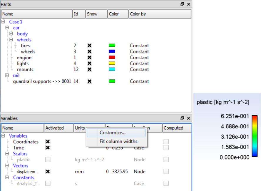
9.1 EnSight Gold Case File Format
EnSight 10.2 User Manual 9-15
Query Section This is an optional section which specifies query data filenames(s) each
containing xy data saved to the XY Plot Data Format using Right-Click on
query(ies) ((see Chapter 3.5.3, Right Mouse Button Actions)) or using the
command language curve:
save xy_data filename
. Each of the filename(s) must be
located in the same directory as the case file (you cannot use any path to point to
the query data file(s)).
Notes: The server passes the filename(s) up to the client where the EnSight formatted XY
data file(s) are read into EnSight queries (Warning: the client must have access to
the location of this file).
Also, the EnSight XY format contains a query that does not dynamically update in
time, that is, you cannot save a query along a line in a transient dataset and
expect to replicate the dynamically updating line query from a EnSight XY data
file.
Usage:
QUERY
xy_data: filename.exy
xy_data: filename2.exy
etc.
Case File Example 1 The following is a minimal EnSight Gold case file for a steady state model with some
results.
9.1 EnSight Gold Case File Format
9-16 EnSight 10.2 User Manual
Note: this (engold.case) file, as well as all of its referenced geometry and variable
files (along with a couple of command files) can be found under your installation directory
(path: $CEI_HOME/ensight102/data/user_manual). The EnSight Gold
Geometry File Example and the Variable File Examples are the contents of these files.
FORMAT
type: ensight gold
GEOMETRY
model: engold.geo
VARIABLE
constant per case: Cden .8
scalar per element: Esca engold.Esca
scalar per node: Nsca engold.Nsca
vector per element: Evec engold.Evec
vector per node: Nvec engold.Nvec
tensor symm per element: Eten engold.Eten
tensor symm per node: Nten engold.Nten
complex scalar per element: Ecmp engold.Ecmp_rengold.Ecmp_i2.
complex scalar per node: Ncmp engold.Ncmp_rengold.Ncmp_i4.
9.1 EnSight Gold Case File Format
EnSight 10.2 User Manual 9-17
Case File Example 2 The following is a Case file for a transient model. The connectivity of the geometry is also
changing. Note there are a maximum of 15 of the “*” wildcard characters per filename.
And there is a single EnSight XY query file. Note it is not currently possible to save and
restore transient query files (my_query**.exy is not currently supported).
FORMAT
type: ensight gold
GEOMETRY
model: 1 exgold2.geo**
VARIABLE
scalar per node: 1 Stress exgold2.scl**
vector per node: 1 Displacement exgold2.dis**
TIME
time set: 1
number of steps: 3
filename start number: 0
filename increment: 1
time values: 1.0 2.0 3.0
QUERY
xy_data: my_query.exy
The following files would be needed for Example 2:
exgold2.geo00 exgold2.scl00 exgold2.dis00
exgold2.geo01 exgold2.scl01 exgold2.dis01
exgold2.geo02 exgold2.scl02 exgold2.dis02
my_query.exy
9.1 EnSight Gold Case File Format
9-18 EnSight 10.2 User Manual
Case File Example 3 The following is a Case file for a transient model with measured data. Note there are a
maximum of 15 wildcard “*” characters per filename.
This example has pressure given per element.
FORMAT
type: ensight gold
GEOMETRY
model: 1 exgold3.geo*
measured: 2 exgold3.mgeo**
VARIABLE
constant per case: Gamma 1.4
constant per case: 1 Density .9 .9 .7 .6 .6
scalar per element 1 Pressure exgold3.pre*
vector per node: 1 Velocity exgold3.vel*
scalar per measured node: 2 Temperature exgold3.mtem**
vector per measured node: 2 Velocity exgold3.mvel**
TIME
time set: 1
number of steps: 5
filename start number: 1
filename increment: 2
time values: .1 .2 .3 # This example shows that time
.4 .5 # values can be on multiple lines
time set: 2
number of steps: 6
filename start number: 0
filename increment: 2
time values:
.05 .15 .25 .34 .45 .55
The following files would be needed for Example 3:
exgold3.geo1 exgold3.pre1 exgold3.vel1
exgold3.geo3 exgold3.pre3 exgold3.vel3
exgold3.geo5 exgold3.pre5 exgold3.vel5
exgold3.geo7 exgold3.pre7 exgold3.vel7
exgold3.geo9 exgold3.pre9 exgold3.vel9
exgold3.mgeo00 exgold3.mtem00 exgold3.mvel00
exgold3.mgeo02 exgold3.mtem02 exgold3.mvel02
exgold3.mgeo04 exgold3.mtem04 exgold3.mvel04
exgold3.mgeo06 exgold3.mtem06 exgold3.mvel06
exgold3.mgeo08 exgold3.mtem08 exgold3.mvel08
exgold3.mgeo10 exgold3.mtem10 exgold3.mvel10
9.1 EnSight Gold Case File Format
EnSight 10.2 User Manual 9-19
Case File Example 4 The following is two Case files for a simple static Block Continuation structured model
containing 5 files (sets). The first uses the first two sets, the second uses the last three sets.
FORMAT
type: ensight gold
GEOMETRY
model: ex_bc_%.geo
VARIABLE
scalar per node: temperature ex_bc_%.scl
BLOCK_CONTINUATION
number of sets: 2
filename start number: 1
filename increment: 1
---------------------------------------------------
FORMAT
type: ensight gold
GEOMETRY
model: ex_bc_%.geo
VARIABLE
scalar per node: temperature ex_bc_%.scl
BLOCK_CONTINUATION
number of sets: 3
filename start number: 3
filename increment: 1
The following files would be needed for Example 4:
ex_bc_1.geo ex_bc_1.scl used by first case
ex_bc_2.geo ex_bc_2.scl used by first case
ex_bc_3.geo ex_bc_3.scl used by second case
ex_bc_4.geo ex_bc_4.scl used by second case
ex_bc_5.geo ex_bc_5.scl used by second case
Case File Example 5 The following is Case File Example 3 expressed in transient single-file formats.
In this example, the transient data for the measured velocity data entity happens
to be greater than the maximum file size limit. Therefore, the first four time steps
fit and are contained in the first file, and the last two time steps are ‘continued’ in
a second file.
FORMAT
type: ensight gold
GEOMETRY
model: 1 1 exgold5.geo
measured: 2 2 exgold5.mgeo
VARIABLE
constant per case: Density .5
scalar per element: 1 1 Pressure exgold5.pre
vector per node: 1 1 Velocity exgold5.vel
scalar per measured node: 2 2 Temperature exgold5.mtem
vector per measured node: 2 3 Velocity exgold5.mvel*
TIME
time set: 1 Model
number of steps: 5
time values: .1 .2 .3 .4 .5
time set: 2 Measured
number of steps: 6
time values: .05 .15 .25 .34 .45 .55
FILE
file set: 1
9.1 EnSight Gold Case File Format
9-20 EnSight 10.2 User Manual
number of steps: 5
file set: 2
number of steps: 6
file set: 3
filename index: 1
number of steps: 4
filename index: 2
number of steps: 2
The following files would be needed for Example 5:
exgold5.geo exgold5.pre exgold5.vel
exgold5.mgeo exgold5.mtem exgold5.mvel1
exgold5.mvel2
Case File Example 6 The following is a Case file for a transient model. The connectivity of the geometry is not
changing, but the coordinates are. The connectivity is only present in step 1, but is not
present in steps 0, 2, 3, 4, or 5).
FORMAT
type: ensight gold
GEOMETRY
model: 1 aaa_coords.geo** change_coords_only 1
TIME
time set: 1
number of steps: 6
filename start number: 0
filename increment: 1
time values: 0.1 1.2 2.3 3.4 4.5 5.6
The following files would be needed for Example 6:
aaa_coords.geo00
aaa_coords.geo01 (contains the connectivity)
aaa_coords.geo02
aaa_coords.geo03
aaa_coords.geo04
aaa_coords.geo05
Case File Example 7 The following is a Case file for a static geometry, transient variable model with four
constant per part variables. See EnSight Gold Constant Per Part Variable Files section for
a description of the contents of constant per part files. There are a number of variations
possible. Note also, that the “temperature” constant per part also uses an optional constant
per part index file - which will make reading the constant per part file more efficient.
FORMAT
type: ensight gold
GEOMETRY
model: crash.geo
VARIABLE
scalar per node: 1 plastic crash.plastic_**
vector per node: 1 displacement crash.displacement_**
constant per part: 1 colornumber crash.colornumber
constant per part: 1 temperature crash.temperature crash.temperature.index
constant per part: 1 casenumber crash.casenumber
constant per part: 1 time crash.time
TIME
time set: 1
number of steps: 11
filename start number: 1
filename increment: 2
time values: 0.0 0.0235 0.047 0.0705
0.094 0.1175 0.141 0.1645
0.188 0.2115 0.235
9.1 EnSight Gold Case File Format
EnSight 10.2 User Manual 9-21
The following files would be needed for Case File Example 7 (which is in the data/
guard_rail directory of the Ensight 10.2 distribution):
crash_with_cpp.case crash.plastic_01
crash.casenumber crash.plastic_03
crash.colornumber crash.plastic_05
crash.displacement_01 crash.plastic_07
crash.displacement_03 crash.plastic_09
crash.displacement_05 crash.plastic_11
crash.displacement_07 crash.plastic_13
crash.displacement_09 crash.plastic_15
crash.displacement_11 crash.plastic_17
crash.displacement_13 crash.plastic_19
crash.displacement_15 crash.plastic_21
crash.displacement_17 crash.temperature
crash.displacement_19 crash.temperature.index
crash.displacement_21 crash.time
crash.geo
Contents of Each file contains transient data that corresponds to the specified number of time steps.
Transient The data for each time step sequentially corresponds to the simulation time values
Single Files
(time values)
found listed in the TIME section. In transient single-file format, the data for
each time step essentially corresponds to a standard EnSight gold geometry or variable
file (model or measured) as expressed in multiple file format. The data for each time step
is enclosed between two wrapper records, i.e. preceded by a BEGIN TIME STEP
record and followed by an END TIME STEP record. Time step data is not split
between files. If there is not enough room to append the data from a time step to the file
without exceeding the maximum file limit of a particular system, then a continuation file
must be created for the time step data and any subsequent time step. Any type of user
comments may be included before and/or after each transient step wrapper.
Note 1: If transient single file format is used, EnSight expects all files of a dataset
to be specified in transient single file format. Thus, even static files must be
enclosed between a BEGIN TIME STEP and an END TIME STEP wrapper.
This includes the condition where you have transient variables with static
geometry. The static geometry file must have the wrapper.
1. Note 2: For binary geometry files, the first BEGIN TIME STEP wrapper
must follow the <C Binary/Fortran Binary> line. Both BEGIN TIME STEP
and END TIME STEP wrappers are written according to type (1) in binary.
Namely: This is a write of 80 characters to the file:
in C: char buffer[80];
strcpy(buffer,”BEGIN TIME STEP”);
fwrite(buffer,sizeof(char),80,file_ptr);
in FORTRAN: character*80 buffer
buffer = ”BEGIN TIME STEP”
Note 3: Efficient reading of each file (especially binary) is facilitated by
appending each file with a file index. A file index contains appropriate
information to access the file byte positions of each time step in the file. (EnSight
automatically appends a file index to each file when exporting in transient single
file format.) If used, the file index must follow the last END TIME STEP
wrapper in each file.

9.1 EnSight Gold Case File Format
9-22 EnSight 10.2 User Manual
File Index Usage:
* Each file byte location is the first byte that follows the “BEGIN TIME STEP” record.
+ For Windows it is now ok to use “%20lld\n” for Visual Studio 2005 onward. Under
VS2003, use “20I64d\n”.
Shown below are the contents of each of the above files, using the data files from Case
File Example 3 for reference (without FILE_INDEX for simplicity).
Contents of file exgold4.geo_1:
BEGIN TIME STEP
Contents of file exgold3.geo1
END TIME STEP
BEGIN TIME STEP
Contents of file exgold3.geo3
END TIME STEP
BEGIN TIME STEP
Contents of file exgold3.geo5
END TIME STEP
BEGIN TIME STEP
Contents of file exgold3.geo7
END TIME STEP
BEGIN TIME STEP
Contents of file exgold3.geo9
END TIME STEP
Contents of file exgold4.pre_1:
BEGIN TIME STEP
Contents of file exgold3.pre1
END TIME STEP
BEGIN TIME STEP
Contents of file exgold3.pre3
END TIME STEP
BEGIN TIME STEP
Contents of file exgold3.pre5
END TIME STEP
BEGIN TIME STEP
Contents of file exgold3.pre7
END TIME STEP
BEGIN TIME STEP
Contents of file exgold3.pre9
END TIME STEP
Contents of file exgold4.vel_1:
BEGIN TIME STEP
Contents of file exgold3.vel1
END TIME STEP
BEGIN TIME STEP
Contents of file exgold3.vel3
END TIME STEP
BEGIN TIME STEP
Contents of file exgold3.vel5
END TIME STEP
BEGIN TIME STEP
Contents of file exgold3.vel7
END TIME STEP
BEGIN TIME STEP
Contents of file exgold3.vel9
END TIME STEP
Contents of file exgold4.mgeo_1:
BEGIN TIME STEP
Contents of file exgold3.mgeo00
END TIME STEP
BEGIN TIME STEP
ASCII+Binary Item Description
“%20lld\n” 4-byte integer n Total number of data time steps in the file.
“%20lld\n” 8-byte integer fb1File byte loc for contents of 1st time step*
“%20lld\n” 8-byte integer fb2File byte loc for contents of 2nd time step*
. . . . . . . . . . . .
“%20lld\n” 8-byte integer fbnFile byte loc for contents of nth time step*
“%20lld\n” 4-byte integer flag Miscellaneous flag (= 0 for now)
“%20lld\n” 8-byte integer fb of item n File byte loc for Item n above
“%s\n” 1-byte char*80 “FILE_INDEX” File index keyword
9.1 EnSight Gold Case File Format
EnSight 10.2 User Manual 9-23
Contents of file exgold3.mgeo02
END TIME STEP
BEGIN TIME STEP
Contents of file exgold3.mgeo04
END TIME STEP
BEGIN TIME STEP
Contents of file exgold3.mgeo06
END TIME STEP
BEGIN TIME STEP
Contents of file exgold3.mgeo08
END TIME STEP
BEGIN TIME STEP
Contents of file exgold3.mgeo10
END TIME STEP
Contents of file exgold4.mtem_1:
BEGIN TIME STEP
Contents of file exgold3.mtem00
END TIME STEP
BEGIN TIME STEP
Contents of file exgold3.mtem02
END TIME STEP
BEGIN TIME STEP
Contents of file exgold3.mtem04
END TIME STEP
BEGIN TIME STEP
Contents of file exgold3.mtem06
END TIME STEP
BEGIN TIME STEP
Contents of file exgold3.mtem08
END TIME STEP
BEGIN TIME STEP
Contents of file exgold3.mtem10
END TIME STEP
Contents of file exgold4.mvel1_1:
BEGIN TIME STEP
Contents of file exgold3.mvel00
END TIME STEP
BEGIN TIME STEP
Contents of file exgold3.mvel02
END TIME STEP
BEGIN TIME STEP
Contents of file exgold3.mvel04
END TIME STEP
BEGIN TIME STEP
Contents of file exgold3.mvel06
END TIME STEP
Contents of file exgold4.mvel2_1:
Comments can precede the beginning wrapper here.
BEGIN TIME STEP
Contents of file exgold3.mvel08
END TIME STEP
Comments can go between time step wrappers here.
BEGIN TIME STEP
Contents of file exgold3.mvel10
END TIME STEP
Comments can follow the ending time step wrapper.
Note: Each of these files could (and should for efficiency reasons) have the FILE_INDEX information following
the last END TIMESTEP. See the previous discussion for its usage.
EnSight Gold Wild Card Name Specification
If multiple time steps are involved, the file names must conform to the EnSight
wild-card specification. This specification is as follows:
• File names must include numbers that are in ascending order from
beginning to end.
• Numbers in the files names must be zero filled if there is more than one
significant digit.
• Numbers can be anywhere in the file name.
• When the file name is specified in the EnSight case file, you must replace
9.1 EnSight Gold Geometry File Format
9-24 EnSight 10.2 User Manual
the numbers in the file with an asterisk(*). The number of asterisks
specified is the number of significant digits. The asterisk must occupy the
same place as the numbers in the file names.
EnSight Gold Geometry File Format
The EnSight Gold format is part based for both unstructured and structured data.
There is no global coordinate array that each part references, but instead - each
part contains its own local coordinate array. Thus, the node numbers in element
connectivities refer to the coordinate array index, not a node id or label. This is
different than the EnSight6 format!
The EnSight Gold format consists of keywords followed by information. The
following items are important when working with EnSight Gold geometry files:
1. Node ids are optional. In this format they are strictly labels and are not used in
the connectivity definition. The element connectivities are based on the local
implied node number of the coordinate array in each part, which is sequential
starting at one. If you let EnSight assign node IDs, this implied internal
numbering is used. If node IDs are set to off, they are numbered internally,
however, you will not be able to display or query on them. If you have node
IDs given in your data, you can have EnSight ignore them by specifying
“node id ignore.” Using this option may reduce some of the memory taken up
by the Client and Server, but display and query on the nodes will not be
available. Note, prior to EnSight 7.4, node ids could only be specified for
unstructured parts. This restriction has been removed and user specified node
ids are now possible for structured parts.
2. Element ids are optional. If you specify element IDs, or you let EnSight
assign them, you can show them on the screen. If they are set to off, you will
not be able to show or query on them. If you have element IDs given in your
data you can have EnSight ignore them by specifying “element id ignore.”
Using this option will reduce some of the memory taken up by the Client and
Server. This may or may not be a significant amount, and remember that
display and query on the elements will not be available. Note, prior to EnSight
7.4, element ids could only be specified for unstructured parts. This restriction
has been removed and user specified element ids are now possible for
structured parts.
3. Model extents can be defined in the file so EnSight will not have to determine
these while reading in data. If they are not included, EnSight will compute
them, but will not actually do so until a dataset query is performed the first
time.
4. The format of integers and real numbers must be followed (See the Geometry
Example below).
5. ASCII Integers are written out using the following integer format:
From C:
10d
format
From FORTRAN:
i10
format
Note: this size of integer format limits the number of nodes as well as node
and element labels to 231 (2 GB) per part which is the same as a -bit

9.1 EnSight Gold Geometry File Format
EnSight 10.2 User Manual 9-25
integer.
ASCII Real numbers are written out using the following floating-point format:
From C:
12.5e
format
From FORTRAN:
e12.5
format
The number of integers or reals per line must also be followed!
6. By default, a Part is processed to show the outside boundaries. This
representation is loaded to the Client host system when the geometry file is
read (unless other attributes have been set on the workstation, such as feature
angle).
7. Coordinates for unstructured data must be defined within each part. This is
normally done before any elements are defined within a part, but does not
have to be. The different elements can be defined in any order (that is, you can
define a hexa8 before a bar2).
8. EnSight 10.2 and later use the part name as the unique designator. As such, a
given part name referring to a specific part, must remain the same in all
geometry files: a given part name must not change over time and it must not
be changed between spatially decomposed files.
9. A Part containing structured data cannot contain any unstructured element
types or more than one block. Each structured Part is limited to a single
block (or some subset of that block). A structured block is indicated by
following the Part description line with a ‘block’ line. By default, a block will
be curvilinear, non-iblanked, non-ghost, complete range. However, by
suppling one or more of the following options on the ‘block’ line, rectilinear
or uniform blocks can be specified, nodal iblanking for the block can be used,
cells within the block can be flagged as ghosts (used for computations, but not
displayed), subset ranges can be specified (useful for partitioned data). The
options include:
Only one of these can be used on the ‘block’ line
curvilinear
Indicates that coordinates of all ijk locations of the block will be
specified (default)
rectilinear
Indicates that i,j,k delta vectors for a regular block with possible
non-regular spacing will be specified
uniform
Indicates that i,j,k delta values for a regular block with regular
spacing will be specified
Any, none, or all of these can be used

9.1 EnSight Gold Geometry File Format
9-26 EnSight 10.2 User Manual
iblanked
An “iblanked” block must contain an additional integer array of
values at each node, traditionally called the iblank array. Valid iblank
values for the EnSight Gold format are:
0 for nodes which are exterior to the model, sometimes
called blanked-out nodes
1 for nodes which are interior to the model, thus in the
free stream and to be used
<0 or >1 for any kind of boundary nodes
In EnSight’s structured Part building dialog, the iblank option
selected will control which portion of the structured block is
“created”. Thus, from the same structured block, the interior flow
field part as well as a symmetry boundary part could be “created”.
Note: By default EnSight does not do any “partial” cell iblank
processing. Namely, only complete cells containing no “exterior”
nodes are created. It is possible to obtain partial cell processing by
issuing the “test:partial_cells_on” command in the Command
Dialog before reading the file.
with_ghost
A block with ghosts must contain an additional integer array of flags
for each cell. A flag value of zero indicates a non-ghost cell. A flag
value of non-zero indicates a ghost cell.

9.1 EnSight Gold Geometry File Format
EnSight 10.2 User Manual 9-27
Note that for structured data, the standard order of nodes is such that I’s advance
quickest, followed by J’s, and then K’s.
10. Maximum number of parts is 32769
Maximum number of variables is 10000
Maximum file name length is 1024
Maximum part name length is 79, but the GUI will only display 49
Maximum variable name length is 79, but the GUI will only display 49
range
A block with ranges will contain an extra line, following the ijk line,
which gives min and max planes for each of the ijk directions.
Thus, normally a 6 x 5 x 1 block part would start something like:
part
1
description
block
6 5 1
0.00000e+00
...
(The coordinate information for the 30 nodes of the block must
follow.)
But if only the top 6 x 3 x 1portion was to be represented in the file,
you can use “range” like:
part
1
description for top only
block range
6 5 1
1 6 3 5 1 1
0.00000e+00
...
(The coordinate information for the 18 nodes of the top portion of
the block must follow. Note that the ijk line following the block line
contains the size of the original block - which is needed to properly
deal with node and element numbering. The next line contains the
imin, imax, jmin, jmax, kmin, kmax defining the subset ranges. The
actual size of the block being defined is thus computed from these
ranges:
size_i = imax - imin + 1
size_j = jmax - jmin + 1
size_k = kmax - kmin + 1
9.1 EnSight Gold Geometry File Format
9-28 EnSight 10.2 User Manual
Generic Format Usage Notes:
In general an unstructured
part
can contain several different
element type
s.
#
=
a part number (maximum is 32769)
nn
= total number of nodes in a part
ne
= number of elements of a given type
np
= number of nodes per element for a given element type
nf
= number of faces per nfaced element
id_*
= node or element id number
x_*
= x component
y_*
= y component
z_*
= z component
n*_e*
= node number for an element
f*_e*
= face number for an nfaced element
ib_*
= iblanking value
gf_e*
= ghost flag for a structured cell
[ ]
contain optional portions
< >
contain choices
‘
indicates the beginning of an unformatted sequential FORTRAN binary write
’
indicates the end of an unformatted sequential FORTRAN binary write
element type
can be any of:
point g_point
bar2 g_bar2
bar3 g_bar3
tria3 g_tria3
tria6 g_tria6
quad4 g_quad4
quad8 g_quad8
tetra4 g_tetra4
tetra10 g_tetra10
pyramid5 g_pyramid5
pyramid13 g_pyramid13
penta6 g_penta6
penta15 g_penta15
hexa8 g_hexa8
hexa20 g_hexa20
nsided g_nsided
nfaced g_nfaced
9.1 EnSight Gold Geometry File Format
EnSight 10.2 User Manual 9-29
C Binary form:
C Binary 80 chars
description line 1 80 chars
description line 2 80 chars
node id <off/given/assign/ignore> 80 chars
element id <off/given/assign/ignore> 80 chars
[extents
80 chars
xmin xmax ymin ymax zmin zmax]
6 floats
part [conn_change/coord_change/no_change] 80 chars
# 1 int
description line this must be consistent in all files 80 chars
coordinates
80 chars
nn 1 int
[id_n1 id_n2 ... id_nn] nn ints
x_n1 x_n2 ... x_nn nn floats
y_n1 y_n2 ... y_nn nn floats
z_n1 z_n2 ... z_nn nn floats
element type 80 chars
ne 1 int
[id_e1 id_e2 ... id_ne] ne ints
n1_e1 n2_e1 ... np_e1
n1_e2 n2_e2 ... np_e2
.
.
n1_ne n2_ne ... np_ne ne*np ints
element type 80 chars
.
.
part [conn_change/coord_change/no_change] 80 chars
.
.
part [conn_change/coord_change/no_change] 80 chars
# 1 int
description line this must be consistent in all files 80 chars
block [iblanked] [with_ghost] [range] 80 chars
i j k # nn = i*j*k, ne = (i-1)*(j-1)*(k-1) 3 ints
[imin imax jmin jmax kmin kmax] # if range used: 6 ints
nn =
(imax-imin+1)*
(jmax-jmin+1)* (kmax-kmin+1)
ne = (imax-imin)*(jmax-jmin)*(kmax-kmin)
x_n1 x_n2 ... x_nn nn floats
y_n1 y_n2 ... y_nn nn floats
z_n1 z_n2 ... z_nn nn floats
[ib_n1 ib_n2 ... ib_nn] nn ints
[ghost_flags] 80 chars
[gf_e1 gf_e2 ... gf_ne] ne ints
[node_ids] 80 chars
[id_n1 id_n2 ... id_nn] nn ints
[element_ids] 80 chars
[id_e1 id_e2 ... id_ne] ne ints
part [conn_change/coord_change/no_change] 80 chars
# 1 int
description line this must be consistent in all files 80 chars
block rectilinear [iblanked] [with_ghost] [range] 80 chars
i j k # nn = i*j*k, ne = (i-1)*(j-1)*(k-1) 3 ints
[imin imax jmin jmax kmin kmax] # if range used: 6 ints
nn =
(imax-imin+1)*
(jmax-jmin+1)* (kmax-kmin+1)
ne = (imax-imin)*(jmax-jmin)*(kmax-kmin)
x_1 x_2 ... x_i i floats
y_1 y_2 ... y_j j floats
9.1 EnSight Gold Geometry File Format
9-30 EnSight 10.2 User Manual
z_1 z_2 ... z_k k floats
[ib_n1 ib_n2 ... ib_nn] nn ints
[ghost_flags] 80 chars
[gf_e1 gf_e2 ... gf_ne] ne ints
[node_ids] 80 chars
[id_n1 id_n2 ... id_nn] nn ints
[element_ids] 80 chars
[id_e1 id_e2 ... id_ne] ne ints
part [conn_change/coord_change/no_change] 80 chars
# 1 int
description line this must be consistent in all files 80 chars
block uniform [iblanked] [with_ghost] [range] 80 chars
i j k # nn = i*j*k, ne = (i-1)*(j-1)*(k-1) 3 ints
[imin imax jmin jmax kmin kmax] # if range used: 6 ints
nn =
(imax-imin+1)*
(jmax-jmin+1)* (kmax-kmin+1)
ne = (imax-imin)*(jmax-jmin)*(kmax-kmin)
x_origin y_origin z_origin 3 floats
x_delta y_delta z_delta 3 floats
[ib_n1 ib_n2 ... ib_nn] nn ints
[ghost_flags] 80 chars
[gf_e1 gf_e2 ... gf_ne] ne ints
[node_ids] 80 chars
[id_n1 id_n2 ... id_nn] nn ints
[element_ids] 80 chars
[id_e1 id_e2 ... id_ne] ne ints
Fortran Binary form:
‘Fortran Binary’ 80 chars
‘description line 1’ 80 chars
‘description line 2’ 80 chars
‘node id <off/given/assign/ignore>’ 80 chars
‘element id <off/given/assign/ignore>’ 80 chars
[‘extents’
80 chars
‘xmin xmax ymin ymax zmin zmax’]
6 floats
‘part [conn_change/coord_change/no_change]’ 80 chars
‘#’ 1 int
‘description line’ this must be consistent in all files 80 chars
‘coordinates’
80 chars
‘nn’ 1 int
[‘id_n1 id_n2 ... id_nn’] nn ints
‘x_n1 x_n2 ... x_nn’ nn floats
‘y_n1 y_n2 ... y_nn’ nn floats
‘z_n1 z_n2 ... z_nn’ nn floats
‘element type’ 80 chars
‘ne’ 1 int
[‘id_e1 id_e2 ... id_ne’] ne ints
‘n1_e1 n2_e1 ... np_e1
n1_e2 n2_e2 ... np_e2
.
.
n1_ne n2_ne ... np_ne’ ne*np ints
‘element type’ 80 chars
.
.
‘part [conn_change/coord_change/no_change]’ 80 chars
.
.
‘part [conn_change/coord_change/no_change]’ 80 chars
9.1 EnSight Gold Geometry File Format
EnSight 10.2 User Manual 9-31
‘#’ 1 int
‘description line’ 80 chars
‘block [iblanked] [with_ghost] [range]’ 80 chars
‘i j k’ # nn = i*j*k, ne = (i-1)*(j-1)*(k-1) 3 ints
[‘imin imax jmin jmax kmin kmax’] # if range used: 6 ints
nn =
(imax-imin+1)*
(jmax-jmin+1)* (kmax-kmin+1)
ne = (imax-imin)*(jmax-jmin)*(kmax-kmin)
‘x_n1 x_n2 ... x_nn’ nn floats
‘y_n1 y_n2 ... y_nn’ nn floats
‘z_n1 z_n2 ... z_nn‘ nn floats
[‘ib_n1 ib_n2 ... ib_nn’] nn ints
[‘ghost_flags’] 80 chars
[‘gf_e1 gf_e2 ... gf_ne’] ne ints
[‘node_ids’] 80 chars
[‘id_n1 id_n2 ... id_nn’] nn ints
[‘element_ids’] 80 chars
[‘id_e1 id_e2 ... id_ne’] ne ints
‘part [conn_change/coord_change/no_change]’ 80 chars
‘#’ 1 int
‘description line’ this must be consistent in all files 80 chars
‘block rectilinear [iblanked] [with_ghost] [range]’ 80 chars
‘i j k’ # nn = i*j*k, ne = (i-1)*(j-1)*(k-1) 3 ints
[‘imin imax jmin jmax kmin kmax’] # if range used: 6 ints
nn =
(imax-imin+1)*
(jmax-jmin+1)* (kmax-kmin+1)
ne = (imax-imin)*(jmax-jmin)*(kmax-kmin)
‘x_1 x_2 ... x_i’ i floats
‘y_1 y_2 ... y_j’ j floats
‘z_1 z_2 ... z_k’ k floats
[‘ib_n1 ib_n2 ... ib_nn’] nn ints
[‘ghost_flags’] 80 chars
[‘gf_e1 gf_e2 ... gf_ne’] ne ints
[‘node_ids’] 80 chars
[‘id_n1 id_n2 ... id_nn’] nn ints
[‘element_ids’] 80 chars
[‘id_e1 id_e2 ... id_ne’] ne ints
‘part [conn_change/coord_change/no_change]’ 80 chars
‘#’ 1 int
‘description line’ this must be consistent in all files 80 chars
‘block uniform [iblanked] [with_ghost] [range]’ 80 chars
‘i j k’ # nn = i*j*k, ne = (i-1)*(j-1)*(k-1) 3 ints
[‘imin imax jmin jmax kmin kmax’] # if range used: 6 ints
nn =
(imax-imin+1)*
(jmax-jmin+1)* (kmax-kmin+1)
ne = (imax-imin)*(jmax-jmin)*(kmax-kmin)
‘x_origin y_origin z_origin 3 floats
x_delta y_delta z_delta’ 3 floats
[‘ib_n1 ib_n2 ... ib_nn’] nn ints
[‘ghost_flags’] 80 chars
[‘gf_e1 gf_e2 ... gf_ne’] ne ints
[‘node_ids’] 80 chars
[‘id_n1 id_n2 ... id_nn’] nn ints
[‘element_ids’] 80 chars
[‘id_e1 id_e2 ... id_ne’] ne ints
ASCII form:
description line 1 A (max of 79 typ)
description line 2 A
node id <off/given/assign/ignore> A
element id <off/given/assign/ignore> A
9.1 EnSight Gold Geometry File Format
9-32 EnSight 10.2 User Manual
[extents
A
xmin xmax 2E12.5
ymin ymax 2E12.5
zmin zmax] 2E12.5
part [conn_change/coord_change/no_change] A
# I10
description line this must be consistent in all files A
coordinates
A
nn I10
[id_n1 I10 1/line (nn)
id_n2
.
.
id_nn]
x_n1 E12.5 1/line (nn)
x_n2
.
.
x_nn
y_n1 E12.5 1/line (nn)
y_n2
.
.
y_nn
z_n1 E12.5 1/line (nn)
z_n2
.
.
z_nn
element type A
ne I10
[id_e1 I10 1/line (ne)
id_e2
.
.
id_ne]
n1_e1 n2_e1 ... np_e1 I10 np/line
n1_e2 n2_e2 ... np_e2 (ne lines)
.
.
n1_ne n2_ne ... np_ne
element type A
.
.
part [conn_change/coord_change/no_change] A
.
.
part [conn_change/coord_change/no_change] A
# I10
description line this must be consistent in all files A
block [iblanked] [with_ghost] [range] A
i j k # nn = i*j*k, ne = (i-1)*(j-1)*(k-1) 3I10
[imin imax jmin jmax kmin kmax] # if range used: 6I10
nn =
(imax-imin+1)*
(jmax-jmin+1)* (kmax-kmin+1)
ne = (imax-imin)*(jmax-jmin)*(kmax-kmin)
x_n1 E12.5 1/line (nn)
x_n2
.
.
x_nn
y_n1 E12.5 1/line (nn)
9.1 EnSight Gold Geometry File Format
EnSight 10.2 User Manual 9-33
y_n2
.
.
y_nn
z_n1 E12.5 1/line (nn)
z_n2
.
.
z_nn
[ib_n1 I10 1/line (nn)
ib_n2
.
.
ib_nn]
[ghost_flags] 80 chars
[gf_e1 I10 1/line (ne)
gf_e2
.
.
gf_ne]
[node_ids] 80 chars
[id_n1 I10 1/line (nn)
id_n2
.
.
id_nn]
[element_ids] 80 chars
[id_e1 I10 1/line (ne)
id_e2
.
.
id_ne]
part [conn_change/coord_change/no_change] A
# I10
description line this must be consistent in all files A
block rectilinear [iblanked] [with_ghost] [range] A
i j k # nn = i*j*k, ne = (i-1)*(j-1)*(k-1) 3I10
[imin imax jmin jmax kmin kmax] # if range used: 6I10
nn =
(imax-imin+1)*
(jmax-jmin+1)* (kmax-kmin+1)
ne = (imax-imin)*(jmax-jmin)*(kmax-kmin)
x_1 E12.5 1/line (i)
x_2
.
.
x_i
y_1 E12.5 1/line (j)
y_2
.
.
y_j
z_1 E12.5 1/line (k)
z_2
.
.
z_k
[ib_n1 I10 1/line (nn)
ib_n2
.
.
ib_nn]
[ghost_flags] 80 chars
9.1 EnSight Gold Geometry File Format
9-34 EnSight 10.2 User Manual
[gf_e1 I10 1/line (ne)
gf_e2
.
.
gf_ne]
[node_ids] 80 chars
[id_n1 I10 1/line (nn)
id_n2
.
.
id_nn]
[element_ids] 80 chars
[id_e1 I10 1/line (ne)
id_e2
.
.
id_ne]
part [conn_change/coord_change/no_change] A
# I10
description line this must be consistent in all files A
block uniform [iblanked] [with_ghost] [range] A
i j k # nn = i*j*k, ne = (i-1)*(j-1)*(k-1) 3I10
[imin imax jmin jmax kmin kmax] # if range used: 6I10
nn =
(imax-imin+1)*
(jmax-jmin+1)* (kmax-kmin+1)
ne = (imax-imin)*(jmax-jmin)*(kmax-kmin)
x_origin E12/5
y_origin E12/5
z_origin E12/5
x_delta E12.5
y_delta E12.5
z_delta E12.5
[ib_n1 I10 1/line (nn)
ib_n2
.
.
ib_nn]
[ghost_flags] 80 chars
[gf_e1 I10 1/line (ne)
gf_e2
.
.
gf_ne]
[node_ids] 80 chars
[id_n1 I10 1/line (nn)
id_n2
.
.
id_nn]
[element_ids] 80 chars
[id_e1 I10 1/line (ne)
id_e2
.
.
id_ne]
9.1 EnSight Gold Geometry File Format
EnSight 10.2 User Manual 9-35
Notes:
• If
node id
is
given
or
ignore
, the [id] section must be there for each part.
• If
element id
is
given
or
ignore
, the [id] section must be there for each
element type
of each part
• If
iblanked
is there, the [ib] section must be there for the block.
• x, y, and z coordinates are mandatory, even if a 2D problem.
• If
block rectilinear
, then the x, y, z coordinates change to the x, y, and z
delta vectors.
• If
block uniform
, then the x, y, z coordinates change to the x, y, z
coordinates of the origin and the x, y, and z delta values.
• If
block range
, the ijk min/max range line must follow the ijk line. And the
number of nodes and elements is based on the ranges. The ijk line
indicates the size of the original block.
• If
with_ghost
is on the
block
line, then the
ghost_flag
section must be there
• Ids are just labels, the coordinate (or element) order is implied.
• The minimum needed for unstructured empty parts is the three lines (with
a given part name consistently unchanging in all geo files over time and/
or spatially decomposed):
part
# (use the actual part number)
description this must be consistent in all files
• The minimum needed for structured empty parts is the five lines:
part
# (use the actual part number)
description
block
0 0 0
• Element blocks for nsided elements contain an additional section - the
number of nodes in each element. See below.
• If the
GEOMETRY, model:
section contains the
changing_geometry_per_part
keyword, then the
part
keyword must be followed by one of the following
keywords in the geometry file:
conn_change/coord_change/no_change
. This is
useful when one or a few parts are changing connectivity (such as particle
parts) and others are static. Only the parts that are truly changing
connectivity will be updated by the reader on time change, avoiding
unnecessary duplicate reads of static geometry, and speeding up the
reading process.
part conn_change/coord_change/no_change
# (use the actual part number)
description
C Binary form of element block, if nsided:
9.1 EnSight Gold Geometry File Format
9-36 EnSight 10.2 User Manual
nsided 80 chars
ne 1 int
[id_n1 id_n2 ... id_ne] ne ints
np1 np2 ... npne This data is needed ne ints
e1_n1 e1_n2 ... e1_np1
e2_n1 e2_n2 ... e2_np2
.
.
ne_n1 ne_n2 ... ne_npne np1+np2+...+npne ints
Fortran Binary form of element block, if nsided:
‘nsided’ 80 chars
‘ne’ 1 int
[‘id_n1 id_n2 ... id_ne’] ne ints
‘np1 np2 ... npne’ This data is needed ne ints
‘e1_n1 e1_n2 ... e1_np1
e2_n1 e2_n2 ... e2_np2
.
.
ne_n1 ne_n2 ... ne_npne’ np1+np2+...+npne ints
Ascii form of element block, if nsided:
nsided A
ne I10
[id_n1 I10 1/line (ne)
id_n2
.
id_ne]
np1 This data is needed I10 1/line (ne)
np2 .
. .
npne .
e1_n1 e1_n2 ... e1_np1 I10 np*/line
e2_n1 e2_n2 ... e2_np2 (ne lines)
.
ne_n1 ne_n2 ... ne_npne
• Element blocks for nfaced elements are more involved since they are
described by their nsided faces. Thus, there is the optional section for ids
(id_e*), a section for the number of faces per element (nf_e*), a section
for number of nodes per face per element (np(f*_e*)), and a section for
the connectivity of each nsided face of each element (n*(f*_e*)). See
below.
C Binary form of element block, if nfaced:
nfaced 80 chars
ne 1 int
[id_e1 id_e2 ... id_ne] ne ints
nf_e1 nf_e2 ... nf_ne ne ints
np(f1_e1) np(f2_e1) ... np(nf_e1)
np(f1_e2) np(f2_e2) ... np(nf_e2)
.
.
np(f1_ne) np(f2_ne) ... np(nf_ne) nf_e1+nf_e2+...+nf_ne ints
n1(f1_e1) n2(f1_e1) ... n(np(f1_e1))
n1(f2_e1) n2(f2_e1) ... n(np(f2_e1))
.
n1(nf_e1) n2(nf_e1) ... n(np(nf_e1))
9.1 EnSight Gold Geometry File Format
EnSight 10.2 User Manual 9-37
n1(f1_e2) n2(f1_e2) ... n(np(f1_e2))
n1(f2_e2) n2(f2_e2) ... n(np(f2_e2))
.
n1(nf_e2) n2(nf_e2) ... n(np(nf_e2))
.
.
n1(f1_ne) n2(f1_ne) ... n(np(f1_ne))
n1(f2_ne) n2(f2_ne) ... n(np(f2_ne))
.
n1(nf_ne) n2(nf_ne) ... n(np(nf_ne)) np(f1_e1)+np(f2_e1)+...+np(nf_ne) ints
Fortran Binary form of element block, if nfaced:
‘nfaced’ 80 chars
‘ne’ 1 int
[‘id_e1 id_e2 ... id_ne’] ne ints
‘nf_e1 nf_e2 ... nf_ne’ ne ints
‘np(f1_e1) np(f2_e1) ... np(nf_e1)
np(f1_e2) np(f2_e2) ... np(nf_e2)
.
.
np(f1_ne) np(f2_ne) ... np(nf_ne)’ nf_e1+nf_e2+...+nf_ne ints
‘n1(f1_e1) n2(f1_e1) ... n(np(f1_e1))
n1(f2_e1) n2(f2_e1) ... n(np(f2_e1))
.
n1(nf_e1) n2(nf_e1) ... n(np(nf_e1))
n1(f1_e2) n2(f1_e2) ... n(np(f1_e2))
n1(f2_e2) n2(f2_e2) ... n(np(f2_e2))
.
n1(nf_e2) n2(nf_e2) ... n(np(nf_e2))
.
.
n1(f1_ne) n2(f1_ne) ... n(np(f1_ne))
n1(f2_ne) n2(f2_ne) ... n(np(f2_ne))
.
n1(nf_ne) n2(nf_ne) ... n(np(nf_ne))’ np(f1_e1)+np(f2_e1)+...+np(nf_ne) ints
Ascii form of element block, if nfaced:
nfaced A
ne I10
[id_e1 I10 1/line
id_e2 (ne lines)
.
id_ne]
nf_e1 I10 1/line
nf_e2 (ne lines)
.
nf_ne
np(f1_e1) I10 1/line
np(f2_e1) (nf_e1+nf_e2+...+nf_ne lines)
.
np(nf_e1)
np(f1_e2)
np(f2_e2)
.
np(nf_e2)
.
.
np(f1_ne)
np(f2_ne)
9.1 EnSight Gold Geometry File Format
9-38 EnSight 10.2 User Manual
.
np(nf_ne)
n1(f1_e1) n2(f1_e1) ... n(np(f1_e1)) I10 np*/line
n1(f2_e1) n2(f2_e1) ... n(np(f2_e1)) (nf_e1+nf_e2+...+nf_ne lines)
.
n1(nf_e1) n2(nf_e1) ... n(np(nf_e1))
n1(f1_e2) n2(f1_e2) ... n(np(f1_e2))
n1(f2_e2) n2(f2_e2) ... n(np(f2_e2)).
.
n1(nf_e2) n2(nf_e2) ... n(np(nf_e2))
.
.
n1(f1_ne) n2(f1_ne) ... n(np(f1_ne))
n1(f2_ne) n2(f2_ne) ... n(np(f2_ne))
.
n1(nf_ne) n2(nf_ne) ... n(np(nf_ne))
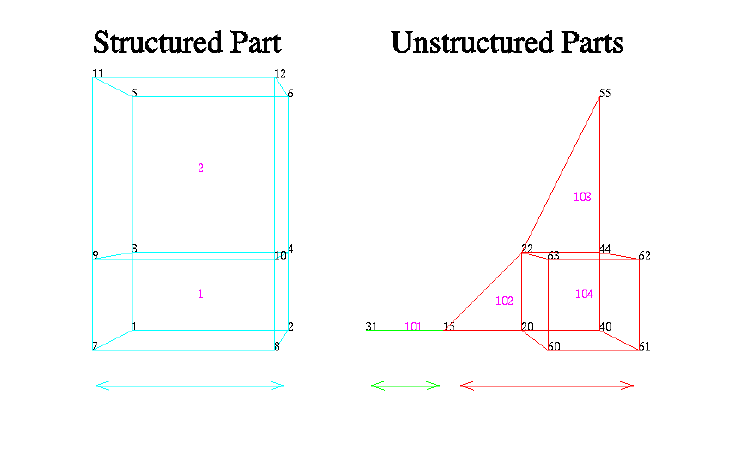
9.1 EnSight Gold Geometry File Format
EnSight 10.2 User Manual 9-39
EnSight Gold The following is an example of an ASCII EnSight Gold geometry file: This is the
Geometry File Example same example model as given in the EnSight6 geometry file section (only in Gold
format) with 11 defined unstructured nodes from which 2 unstructured parts are
defined, and a 2x3x2 structured part as depicted in the above diagram.
Note: The example file below (engold.geo) and all example variable files in the gold
section (also prefixed with engold) may be found under your EnSight installation
directory (path: $CEI_HOME/ensight102/data/user_manual).
Note: The appended “#” comment lines are for your reference only, and are not valid
format lines within a geometry file as appended below. Do NOT put these #
comments in your file!!!
This is the 1st description line of the EnSight Gold geometry example
This is the 2nd description line of the EnSight Gold geometry example
node id given
element id given
extents
0.00000e+00 6.00000e+00
0.00000e+00 3.00000e+00
0.00000e+00 2.00000e+00
part
1
2D uns-elements (unchanging description line for part 1)
coordinates
10 # nn
Do NOT put these # comments in your file!!
15 # node ids
20
40
22
44
55
60
61
62
63
4.00000e+00 # x components
5.00000e+00
6.00000e+00
part 2part 3 part 1
9.1 EnSight Gold Geometry File Format
9-40 EnSight 10.2 User Manual
5.00000e+00
6.00000e+00
6.00000e+00
5.00000e+00
6.00000e+00
6.00000e+00
5.00000e+00
0.00000e+00 # y components
0.00000e+00
0.00000e+00
1.00000e+00
1.00000e+00
3.00000e+00
0.00000e+00
0.00000e+00
1.00000e+00
1.00000e+00
0.00000e+00 # z components
0.00000e+00
0.00000e+00
0.00000e+00
0.00000e+00
0.00000e+00
2.00000e+00
2.00000e+00
2.00000e+00
2.00000e+00
tria3 # element type
2 # ne
102 # element ids
103
1 2 4
4 5 6
hexa8
1
104
2 3 5 4 7 8 9 10
part
2
1D uns-elements (unchanging, consistent description line for part 2)
coordinates
2
15
31
4.00000e+00
3.00000e+00
0.00000e+00
0.00000e+00
0.00000e+00
0.00000e+00
bar2
1
101
2 1
part
3
3D struct-part (unchanging, consistent description line fro part 3)
block iblanked
2 3 2
0.00000e+00 # i components
2.00000e+00
0.00000e+00
2.00000e+00
0.00000e+00
2.00000e+00
0.00000e+00
2.00000e+00
9.1 EnSight Gold Geometry File Format
EnSight 10.2 User Manual 9-41
0.00000e+00
2.00000e+00
0.00000e+00
2.00000e+00
0.00000e+00 # j components
0.00000e+00
1.00000e+00
1.00000e+00
3.00000e+00
3.00000e+00
0.00000e+00
0.00000e+00
1.00000e+00
1.00000e+00
3.00000e+00
3.00000e+00
0.00000e+00 # k components
0.00000e+00
0.00000e+00
0.00000e+00
0.00000e+00
0.00000e+00
2.00000e+00
2.00000e+00
2.00000e+00
2.00000e+00
2.00000e+00
2.00000e+00
1 # iblanking
1
1
1
1
1
1
1
1
1
1
1
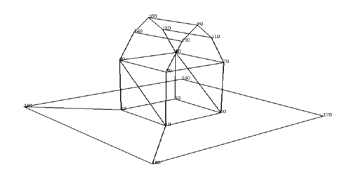
9.1 EnSight Gold Geometry File Format
9-42 EnSight 10.2 User Manual
Simple example The following is an example of an ASCII EnSight Gold geometry file with nsided
using nsided/ and nfaced data. It is a non-realistic, simple model which is intended only to
nfaced elements illustrate the format. Two nsided elements and three nfaced elements are used,
even though the model could have been represented with a single nsided and
single nfaced element.
Note: The appended “#” comment lines are for your reference only, and are not valid
format lines within a geometry file as appended below. Do NOT put these #
comments in your file!!!
simple example for nsided/nfaced
element types in EnSight Gold Format
node id given
element id given
extents
-2.00000e+00 4.00000e+00
0.00000e+00 3.50000e+00
-2.00000e+00 4.00000e+00
part
1
barn
coordinates
18 # nn Do NOT put these # comments in your file!!
10 # node ids
20
30
40
50
60
70
80
90
100
110
120
130
140
150
160
170
180
0.00000e+00 # x components
2.00000e+00
0.00000e+00
2.00000e+00
9.1 EnSight Gold Geometry File Format
EnSight 10.2 User Manual 9-43
0.00000e+00
2.00000e+00
0.00000e+00
2.00000e+00
0.00000e+00
2.00000e+00
0.00000e+00
2.00000e+00
0.00000e+00
2.00000e+00
4.00000e+00
4.00000e+00
-2.00000e+00
-2.00000e+00
0.00000e+00 # y components
0.00000e+00
2.00000e+00
2.00000e+00
0.00000e+00
0.00000e+00
2.00000e+00
2.00000e+00
3.50000e+00
3.50000e+00
3.00000e+00
3.00000e+00
3.00000e+00
3.00000e+00
0.00000e+00
0.00000e+00
0.00000e+00
0.00000e+00
0.00000e+00 # z components
0.00000e+00
0.00000e+00
0.00000e+00
2.00000e+00
2.00000e+00
2.00000e+00
2.00000e+00
1.00000e+00
1.00000e+00
1.50000e+00
1.50000e+00
0.50000e+00
0.50000e+00
-2.00000e+00
4.00000e+00
4.00000e+00
-2.00000e+00
nsided
2 # 2 nsided elements
101 # element ids
202
4 # 4 nodes in first element
8 # 8 nodes in second element
2 15 18 1 # connectivity of element 1
1 18 17 16 15 2 6 5 # connectivity of element 2
nfaced
3 # 3 nfaced polyhedra elements
1001 # element ids
1002
1003
5 # number of faces in element 1
5 # number of faces in element 2
7 # number of faces in element 3
3 # number of nodes in face 1 of element 1
9.1 EnSight Gold Geometry File Format
9-44 EnSight 10.2 User Manual
3 # face 2 of element 1
4 # face 3 of element 1
4 # face 4 of element 1
4 # face 5 of element 1
3 # number of nodes in face 1 of element 2
3 # face 2 of element 2
4 # face 3 of element 2
4 # face 4 of element 2
4 # face 5 of element 2
5 # number of nodes in face 1 of element 3
5 # face 2 of element 3
4 # face 3 of element 3
4 # face 4 of element 3
4 # face 5 of element 3
4 # face 6 of element 3
4 # face 7 of element 3
5 6 8 # connectivity of face 1 of element 1
2 1 4 # face 2 of element 1
6 2 4 8 # face 3 of element 1
8 4 1 5 # face 4 of element 1
1 2 6 5 # face 5 of element 1
5 8 7 # connectivity of face 1 of element 2
1 3 4 # face 2 of element 2
7 8 4 3 # face 3 of element 2
7 3 1 5 # face 4 of element 2
5 1 4 8 # face 5 of element 2
8 4 14 10 12 # connectivity of face 1 of element 3
7 11 9 13 3 # face 2 of element 3
7 8 12 11 # face 3 of element 3
11 12 10 9 # face 4 of element 3
9 10 14 13 # face 5 of element 3
13 14 4 3 # face 6 of element 3
7 3 4 8 # face 7 of element 3
Important note concerning use of nsided and nfaced element representations.
It is important to know that the execution time and memory use for nsided or nfaced elements is
significantly increased. It is not advisable to simply use the nsided/nfaced representations for all
elements, even those that could be represented with the simple basic elements. EnSight has no
problem with different element types begin used within a part.
If, for example, you have a model with triangles, quads and some nsided elements. You will be far
ahead to represent them in the EnSight data format as triangles, quads and the few nsided. Do not
represent them all as nsided.
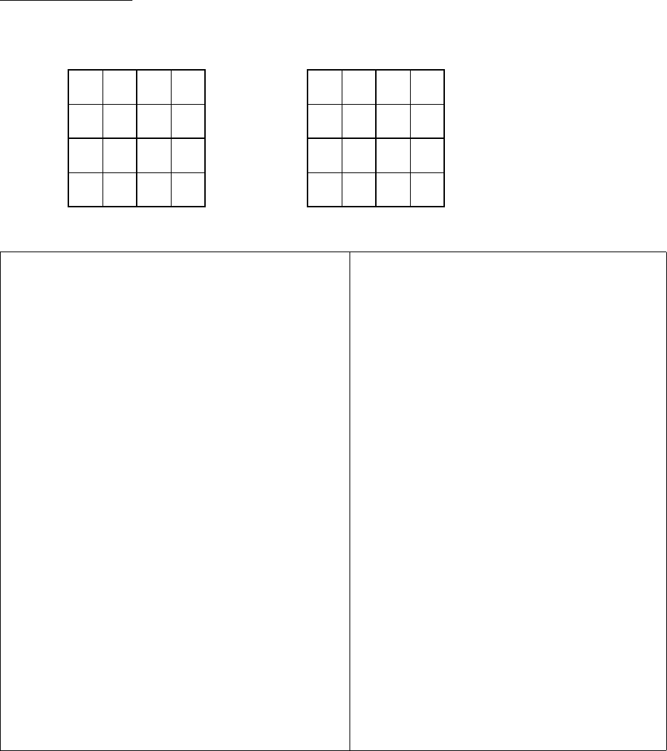
9.1 EnSight Gold Geometry File Format
EnSight 10.2 User Manual 9-45
Simple examples The following two ASCII EnSight Gold geometry file examples show use of
using ghost cells ghost cells in unstructured and structured models. First the geometry file for the
total model, composed of four parts, is given without any ghost cells. Then, two of
four separate geometry files – each containing just one of the original parts (and
appropriate ghost cells) will be given. This is supposed to simulate a decomposed
model, such as you might provide for EnSight’s Server-of-Servers.
Note: For unstructured models, ghost cells are simply a new element type. For
structured models, ghost cells are an “iblank”-like flag.
Unstructured model
Total Unstructured Model Geometry File:
EnSight Model Geometry File
EnSight 7.1.0
node id given
element id given
extents
0.00000e+00 4.00000e+00
0.00000e+00 4.00000e+00
0.00000e+00 0.00000e+00
part
1
bottom left
coordinates
9
1
2
3
6
7
8
11
12
13
0.00000e+00
1.00000e+00
2.00000e+00
0.00000e+00
1.00000e+00
2.00000e+00
0.00000e+00
1.00000e+00
2.00000e+00
0.00000e+00
0.00000e+00
0.00000e+00
1.00000e+00
1.00000e+00
1.00000e+00
2.00000e+00
2.00000e+00
2.00000e+00
0.00000e+00
0.00000e+00
0.00000e+00
0.00000e+00
0.00000e+00
0.00000e+00
0.00000e+00
0.00000e+00
0.00000e+00
quad4
4
1
2
5
6
1 2 5 4
2 3 6 5
4 5 8 7
5 6 9 8
part
2
bottom right
coordinates
9
3
4
5
8
12345
678910
11 12 13 14 15
16 17 18 19 20
21 22 23 24 25
Nodes Elements
part 1 part 2
part 3 part 4
1234
5678
9101112
13 14 15 16
part 3 part 4
part 1 part 2

9.1 EnSight Gold Geometry File Format
9-46 EnSight 10.2 User Manual
9
10
13
14
15
2.00000e+00
3.00000e+00
4.00000e+00
2.00000e+00
3.00000e+00
4.00000e+00
2.00000e+00
3.00000e+00
4.00000e+00
0.00000e+00
0.00000e+00
0.00000e+00
1.00000e+00
1.00000e+00
1.00000e+00
2.00000e+00
2.00000e+00
2.00000e+00
0.00000e+00
0.00000e+00
0.00000e+00
0.00000e+00
0.00000e+00
0.00000e+00
0.00000e+00
0.00000e+00
0.00000e+00
quad4
4
3
4
7
8
1 2 5 4
2 3 6 5
4 5 8 7
5 6 9 8
part
3
top left
coordinates
9
11
12
13
16
17
18
21
22
23
0.00000e+00
1.00000e+00
2.00000e+00
0.00000e+00
1.00000e+00
2.00000e+00
0.00000e+00
1.00000e+00
2.00000e+00
2.00000e+00
2.00000e+00
2.00000e+00
3.00000e+00
3.00000e+00
3.00000e+00
4.00000e+00
4.00000e+00
4.00000e+00
0.00000e+00
0.00000e+00
0.00000e+00
0.00000e+00
0.00000e+00
0.00000e+00
0.00000e+00
0.00000e+00
0.00000e+00
quad4
4
9
10
13
14
1 2 5 4
2 3 6 5
4 5 8 7
5 6 9 8
part
4
top right
coordinates
9
13
14
15
18
19
20
23
24
25
2.00000e+00
3.00000e+00
4.00000e+00
2.00000e+00
3.00000e+00
4.00000e+00
2.00000e+00
3.00000e+00
4.00000e+00
2.00000e+00
2.00000e+00
2.00000e+00
3.00000e+00
3.00000e+00
3.00000e+00
4.00000e+00
4.00000e+00
4.00000e+00
0.00000e+00
0.00000e+00
0.00000e+00
0.00000e+00
0.00000e+00
0.00000e+00
0.00000e+00
0.00000e+00
0.00000e+00
quad4
4
11
12
15
16
1 2 5 4
2 3 6 5
4 5 8 7
5 6 9 8
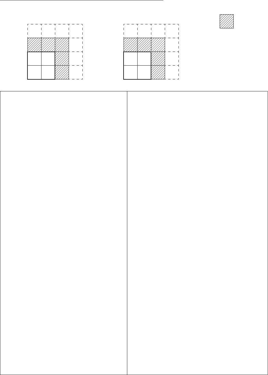
9.1 EnSight Gold Geometry File Format
EnSight 10.2 User Manual 9-47
Portion with part 1 containing ghost cells (other parts are empty)
EnSight Model Geometry File
part 1 portion
node id given
element id given
extents
0.00000e+00 4.00000e+00 0.00000e+00
4.00000e+00
0.00000e+00 0.00000e+00
part
1
bottom left
coordinates
16
1
2
3
4
6
7
8
9
11
12
13
14
16
17
18
19
0.00000e+00
1.00000e+00
2.00000e+00
3.00000e+00
0.00000e+00
1.00000e+00
2.00000e+00
3.00000e+00
0.00000e+00
1.00000e+00
2.00000e+00
3.00000e+00
0.00000e+00
1.00000e+00
2.00000e+00
3.00000e+00
0.00000e+00
0.00000e+00
0.00000e+00
0.00000e+00
1.00000e+00
1.00000e+00
1.00000e+00
1.00000e+00
2.00000e+00
2.00000e+00
2.00000e+00
2.00000e+00
3.00000e+00
3.00000e+00
3.00000e+00
3.00000e+00
0.00000e+00
0.00000e+00
0.00000e+00
0.00000e+00
0.00000e+00
0.00000e+00
0.00000e+00
0.00000e+00
0.00000e+00
0.00000e+00
0.00000e+00
0.00000e+00
0.00000e+00
0.00000e+00
0.00000e+00
0.00000e+00
quad4
4
1
2
5
6
1 2 6 5
2 3 7 6
5 6 10 9
6 7 11 10
g_quad4
5
1
1
1
1
1
3 4 8 7
7 8 12 11
9 10 14 13
10 11 15 14
11 12 16 15
part /* Empty part */
2
bottom right
part /* Empty part */
3
top left
part /* Empty part */
4
top right
1234
6789
11 12 13 14
16 17 18 19
Nodes Elements
part 1
123
567
91011
part 1
Ghost Cell
Note, the images are labeled
with node ids - but the
element connectivities are,
and must be, based on local
node indices.
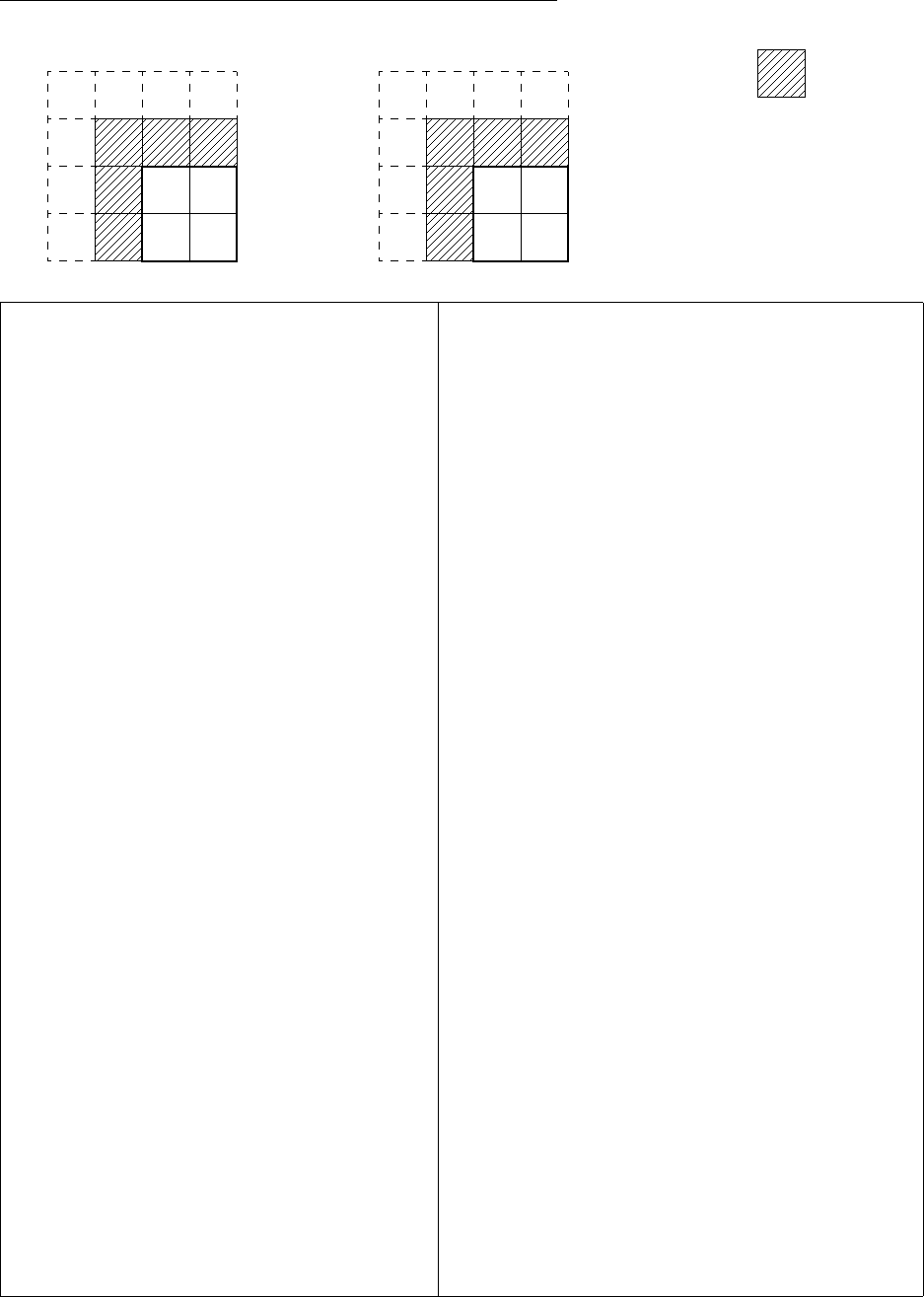
9.1 EnSight Gold Geometry File Format
9-48 EnSight 10.2 User Manual
Portion with part 2 containing ghost cells (other parts are empty)
EnSight Model Geometry File
part 2 portion
node id given
element id given
extents
0.00000e+00 4.00000e+00
0.00000e+00 4.00000e+00
0.00000e+00 0.00000e+00
part /* Empty part */
1
bottom left
part
2
bottom right
coordinates
16
2
3
4
5
7
8
9
10
12
13
14
15
17
18
19
20
1.00000e+00
2.00000e+00
3.00000e+00
4.00000e+00
1.00000e+00
2.00000e+00
3.00000e+00
4.00000e+00
1.00000e+00
2.00000e+00
3.00000e+00
4.00000e+00
1.00000e+00
2.00000e+00
3.00000e+00
4.00000e+00
0.00000e+00
0.00000e+00
0.00000e+00
0.00000e+00
1.00000e+00
1.00000e+00
1.00000e+00
1.00000e+00
2.00000e+00
2.00000e+00
2.00000e+00
2.00000e+00
3.00000e+00
3.00000e+00
3.00000e+00
3.00000e+00
0.00000e+00
0.00000e+00
0.00000e+00
0.00000e+00
0.00000e+00
0.00000e+00
0.00000e+00
0.00000e+00
0.00000e+00
0.00000e+00
0.00000e+00
0.00000e+00
0.00000e+00
0.00000e+00
0.00000e+00
0.00000e+00
quad4
4
3
4
7
8
2 3 7 6
3 4 8 7
6 7 11 10
7 8 12 11
g_quad4
5
1
1
1
1
1
1 2 6 5
5 6 10 9
9 10 14 13
10 11 15 14
11 12 16 15
part /* Empty part */
3
top left
part /* Empty part */
4
top right
2345
78910
12 13 15
17 18 19 20
Nodes Elements
part 2
1234
5678
9101112
13 14 15 16
Ghost Cell
14
part 2
Note, the images are labeled
with node ids - but the
element connectivities are,
and must be, based on local
node indices.

9.1 EnSight Gold Geometry File Format
EnSight 10.2 User Manual 9-49
Structured model
(using essentially the same model, but in structured format):
EnSight Model Geometry File
Total Structured Model
node id assign
element id assign
extents
0.00000e+00 4.00000e+00
0.00000e+00 4.00000e+00
0.00000e+00 0.00000e+00
part
1
left bottom
block uniform range
5 5 1
1 3 1 3 1 1
0.00000e+00
0.00000e+00
0.00000e+00
1.00000e+00
1.00000e+00
0.00000e+00
part
2
bottom right
block uniform range
5 5 1
3 5 1 3 1 1
2.00000e+00
0.00000e+00
0.00000e+00
1.00000e+00
1.00000e+00
0.00000e+00
part
3
top left
block uniform range
5 5 1
1 3 3 5 1 1
0.00000e+00
2.00000e+00
0.00000e+00
1.00000e+00
1.00000e+00
0.00000e+00
part
4
top right
block uniform range
5 5 1
3 5 3 5 1 1
2.00000e+00
2.00000e+00
0.00000e+00
1.00000e+00
1.00000e+00
0.00000e+00
12345
678910
11 12 13 14 15
16 17 18 19 20
21 22 23 24 25
Nodes Elements
part 1 part 2
part 3 part 4
1234
5678
9101112
13 14 15 16
part 3 part 4
part 1 part 2
5 x 5 x 1 Total Structured Model
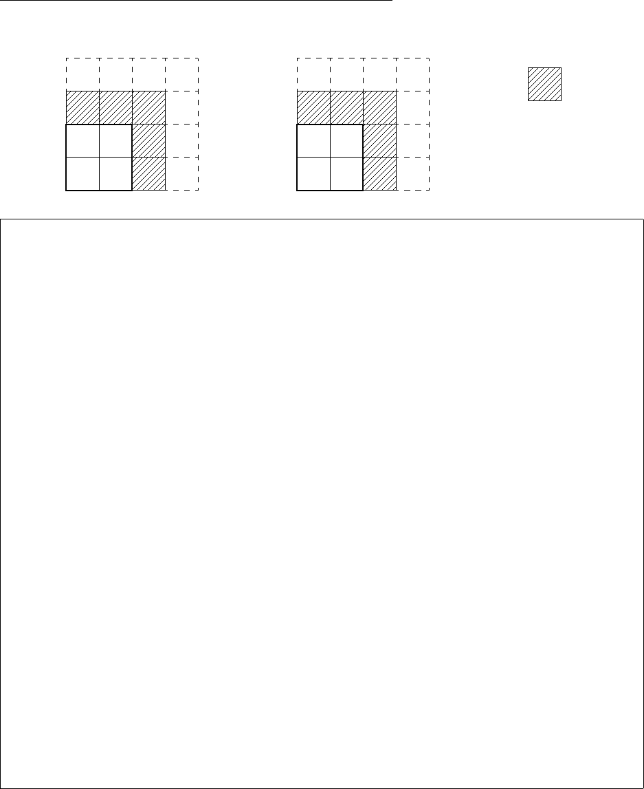
9.1 EnSight Gold Geometry File Format
9-50 EnSight 10.2 User Manual
Portion with part 1 containing ghost cells (other parts are empty)
EnSight Model Geometry File
part 1 portion only
node id assign
element id assign
extents
0.00000e+00 4.00000e+00
0.00000e+00 4.00000e+00
0.00000e+00 0.00000e+00
part
1
left bottom
block uniform range with_ghost
4 4 1
1 4 1 4 1 1
0.00000e+00
0.00000e+00
0.00000e+00
1.00000e+00
1.00000e+00
0.00000e+00
ghost_flags
0
0
1
0
0
1
1
1
1
Part /* Empty Part */
2
right bottom
block
0 0 0
part /* Empty Part */
3
left top
block
0 0 0
part /* Empty Part */
4
right top
block
0 0 0
1234
6789
11 12 13 14
16 17 18 19
Nodes Elements
part 1
123
567
91011
part 1
Ghost Cell
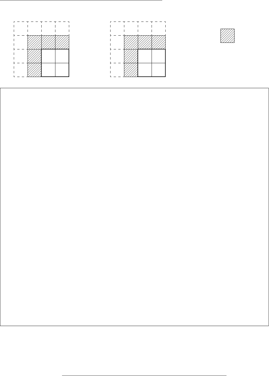
9.1 EnSight Gold Geometry File Format
EnSight 10.2 User Manual 9-51
Portion with part 2 containing ghost cells (other parts are empty)
Note: For both the unstructured and the structured model above, only the first two
files (parts 1 and 2) are given. The portion files for parts 3 and 4 are not given, but
would be similar to those for parts 1 and 2.
Example with part 2 containing ghost cells (other parts are empty
EnSight Model Geometry File
part 2 portion only
node id assign
element id assign
extents
0.00000e+00 4.00000e+00
0.00000e+00 4.00000e+00
0.00000e+00 0.00000e+00
part
1
left bottom
block
0 0 0
part
2
right bottom
block uniform range with_ghost
4 4 1
2 5 1 4 1 1
1.00000e+00
0.00000e+00
0.00000e+00
1.00000e+00
1.00000e+00
0.00000e+00
ghost_flags
1
0
0
1
0
0
1
1
1
part /* Empty Part */
3
left top
block
0 0 0
part /* Empty Part */
4
right top
block
0 0 0
2345
78910
12 13 15
17 18 19 20
Nodes Elements
part 2
1234
5678
9101112
13 14 15 16
Ghost Cell
14
part 2

9.1 Partial example of per-part connectivity usage
9-52 EnSight 10.2 User Manual
Partial example of per-part connectivity usage
sample.case
===========
FORMAT
type: ensight gold
GEOMETRY
model: 1 sample.geo**** changing_geometry_per_part
TIME
time set: 1
number of steps: 4
filename start number: 0
filename increment: 1
time values:
1.00000000e+00
2.00000000e+00
3.00000000e+00
4.00000000e+00
sample.geo0000
==============
EnSight Model Geometry File
EnSight 10.2.1
node id assign
element id assign
extents
0.00000e+00 4.00000e+00
0.00000e+00 1.00000e+00
0.00000e+00 0.00000e+00
part no_change
1
square 1
coordinates
4
0.00000e+00
1.00000e+00
1.00000e+00
0.00000e+00
0.00000e+00
0.00000e+00
1.00000e+00
1.00000e+00
0.00000e+00
0.00000e+00
0.00000e+00
0.00000e+00
quad4
1
1 2 3 4
part coord_change
2
square 2
coordinates
4
1.00000e+00
2.00000e+00
2.00000e+00
1.00000e+00
0.00000e+00
0.00000e+00
1.00000e+00
1.00000e+00
0.00000e+00
0.00000e+00
0.00000e+00
0.00000e+00
quad4
1
1 2 3 4
part conn_change
3
...

9.1 EnSight Gold Variable File Format
EnSight 10.2 User Manual 9-53
EnSight Gold Variable File Format
EnSight Gold variable files can either be per_node or per_element. They cannot
be both. However, an EnSight model can have some variables which are per_node
and others which are per_element.
EnSight Gold Per_Node Variable File Format
EnSight Gold variable files for per_node variables contain values for each
unstructured node and for each structured node. First comes a single description
line. Second comes a part line. Third comes a line containing the part number.
Fourth comes a ‘coordinates’ line or a ‘block’ line. If a ‘coordinates’ line, the
value for each unstructured node of the part follows. If it is a scalar file, there is
one value per node, while for vector files there are three values per node (output in
the same component order as the coordinates, namely, all x components, then all y
components, then all z components). If it is a ‘block’ line, the value(s) for each
structured node follows. The values for each node of the structured block are
output in the same IJK order as the coordinates. (The number of nodes in the part
are obtained from the corresponding EnSight Gold geometry file.)
Note: If the geometry of given part is empty, nothing for that part needs to be in
the variable file.
C Binary form:
SCALAR FILE:
description line 1 80 chars
part 80 chars
# 1 int
coordinates
80 chars
s_n1 s_n2 ... s_nn nn floats
part 80 chars
.
.
part 80 chars
# 1 int
block # nn = i*j*k 80 chars
s_n1 s_n2 ... s_nn nn floats
VECTOR FILE:
description line 1 80 chars
part 80 chars
# 1 int
coordinates
80 chars
vx_n1 vx_n2 ... vx_nn nn floats
vy_n1 vy_n2 ... vy_nn nn floats
vz_n1 vz_n2 ... vz_nn nn floats
part 80 chars
.
.
part 80 chars
# 1 int
block # nn = i*j*k 80 chars
vx_n1 vx_n2 ... vx_nn nn floats
vy_n1 vy_n2 ... vy_nn nn floats
9.1 EnSight Gold Per_Node Variable File Format
9-54 EnSight 10.2 User Manual
vz_n1 vz_n2 ... vz_nn nn floats
TENSOR FILE:
description line 1 80 chars
part 80 chars
# 1 int
coordinates
80 chars
v11_n1 v11_n2 ... v11_nn nn floats
v22_n1 v22_n2 ... v22_nn nn floats
v33_n1 v33_n2 ... v33_nn nn floats
v12_n1 v12_n2 ... v12_nn nn floats
v13_n1 v13_n2 ... v13_nn nn floats
v23_n1 v23_n2 ... v23_nn nn floats
part 80 chars
.
.
part 80 chars
# 1 int
block # nn = i*j*k 80 chars
v11_n1 v11_n2 ... v11_nn nn floats
v22_n1 v22_n2 ... v22_nn nn floats
v33_n1 v33_n2 ... v33_nn nn floats
v12_n1 v12_n2 ... v12_nn nn floats
v13_n1 v13_n2 ... v13_nn nn floats
v23_n1 v23_n2 ... v23_nn nn floats
TENSOR9 FILE:
description line 1 80 chars
part 80 chars
# 1 int
coordinates
80 chars
v11_n1 v11_n2 ... v11_nn nn floats
v12_n1 v12_n2 ... v12_nn nn floats
v13_n1 v13_n2 ... v13_nn nn floats
v21_n1 v21_n2 ... v21_nn nn floats
v22_n1 v22_n2 ... v22_nn nn floats
v23_n1 v23_n2 ... v23_nn nn floats
v31_n1 v31_n2 ... v31_nn nn floats
v_n1 v_n2 ... v_nn nn floats
v33_n1 v33_n2 ... v33_nn nn floats
part 80 chars
.
.
part 80 chars
# 1 int
block # nn = i*j*k 80 chars
v11_n1 v11_n2 ... v11_nn nn floats
v12_n1 v12_n2 ... v12_nn nn floats
v13_n1 v13_n2 ... v13_nn nn floats
v21_n1 v21_n2 ... v21_nn nn floats
v22_n1 v22_n2 ... v22_nn nn floats
v23_n1 v23_n2 ... v23_nn nn floats
v21_n1 v21_n2 ... v21_nn nn floats
v22_n1 v22_n2 ... v22_nn nn floats
v23_n1 v23_n2 ... v23_nn nn floats
COMPLEX SCALAR FILES (Real and/or Imaginary):
9.1 EnSight Gold Per_Node Variable File Format
EnSight 10.2 User Manual 9-55
description line 1 80 chars
part 80 chars
# 1 int
coordinates
80 chars
s_n1 s_n2 ... s_nn nn floats
part 80 chars
.
.
part 80 chars
# 1 int
block # nn = i*j*k 80 chars
s_n1 s_n2 ... s_nn nn floats
COMPLEX VECTOR FILES (Real and/or Imaginary):
description line 1 80 chars
part 80 chars
# 1 int
coordinates
80 chars
vx_n1 vx_n2 ... vx_nn nn floats
vy_n1 vy_n2 ... vy_nn nn floats
vz_n1 vz_n2 ... vz_nn nn floats
part 80 chars
.
.
part 80 chars
# 1 int
block # nn = i*j*k 80 chars
vx_n1 vx_n2 ... vx_nn nn floats
vy_n1 vy_n2 ... vy_nn nn floats
vz_n1 vz_n2 ... vz_nn nn floats
Fortran Binary form:
SCALAR FILE:
‘description line 1’ 80 chars
‘part’ 80 chars
‘#’ 1 int
‘coordinates’
80 chars
‘s_n1 s_n2 ... s_nn’ nn floats
‘part’ 80 chars
.
.
‘part’ 80 chars
‘#’ 1 int
‘block’ # nn = i*j*k 80 chars
‘s_n1 s_n2 ... s_nn’ nn floats
VECTOR FILE:
‘description line 1’ 80 chars
‘part’ 80 chars
‘#’ 1 int
‘coordinates’
80 chars
‘vx_n1 vx_n2 ... vx_nn’ nn floats
‘vy_n1 vy_n2 ... vy_nn’ nn floats
9.1 EnSight Gold Per_Node Variable File Format
9-56 EnSight 10.2 User Manual
‘vz_n1 vz_n2 ... vz_nn’ nn floats
‘part’ 80 chars
.
.
‘part’ 80 chars
‘#’ 1 int
‘block’ # nn = i*j*k 80 chars
‘vx_n1 vx_n2 ... vx_nn’ nn floats
‘vy_n1 vy_n2 ... vy_nn’ nn floats
‘vz_n1 vz_n2 ... vz_nn’ nn floats
TENSOR FILE:
‘description line 1‘ 80 chars
‘part’ 80 chars
‘#’ 1 int
‘coordinates‘
80 chars
‘v11_n1 v11_n2 ... v11_nn’ nn floats
‘v22_n1 v22_n2 ... v22_nn’ nn floats
‘v33_n1 v33_n2 ... v33_nn’ nn floats
‘v12_n1 v12_n2 ... v12_nn’ nn floats
‘v13_n1 v13_n2 ... v13_nn’ nn floats
‘v23_n1 v23_n2 ... v23_nn’ nn floats
‘part’ 80 chars
.
.
‘part’ 80 chars
‘#’ 1 int
‘block’ # nn = i*j*k 80 chars
‘v11_n1 v11_n2 ... v11_nn’ nn floats
‘v22_n1 v22_n2 ... v22_nn’ nn floats
‘v33_n1 v33_n2 ... v33_nn’ nn floats
‘v12_n1 v12_n2 ... v12_nn’ nn floats
‘v13_n1 v13_n2 ... v13_nn’ nn floats
‘v23_n1 v23_n2 ... v23_nn’ nn floats
TENSOR9 FILE:
‘description line 1‘ 80 chars
‘part’ 80 chars
‘#’ 1 int
‘coordinates‘
80 chars
‘v11_n1 v11_n2 ... v11_nn’ nn floats
‘v12_n1 v12_n2 ... v12_nn’ nn floats
‘v13_n1 v13_n2 ... v13_nn’ nn floats
‘v21_n1 v21_n2 ... v21_nn’ nn floats
‘v22_n1 v22_n2 ... v22_nn’ nn floats
‘v23_n1 v23_n2 ... v23_nn’ nn floats
‘v31_n1 v31_n2 ... v31_nn’ nn floats
‘v_n1 v_n2 ... v_nn’ nn floats
‘v33_n1 v33_n2 ... v33_nn’ nn floats
‘part’ 80 chars
.
.
‘part’ 80 chars
‘#’ 1 int
‘block’ # nn = i*j*k 80 chars
‘v11_n1 v11_n2 ... v11_nn’ nn floats
‘v12_n1 v12_n2 ... v12_nn’ nn floats
‘v13_n1 v13_n2 ... v13_nn’ nn floats
9.1 EnSight Gold Per_Node Variable File Format
EnSight 10.2 User Manual 9-57
‘v21_n1 v21_n2 ... v21_nn’ nn floats
‘v22_n1 v22_n2 ... v22_nn’ nn floats
‘v23_n1 v23_n2 ... v23_nn’ nn floats
‘v31_n1 v31_n2 ... v31_nn’ nn floats
‘v_n1 v_n2 ... v_nn’ nn floats
‘v33_n1 v33_n2 ... v33_nn’ nn floats
COMPLEX SCALAR FILES (Real and/or Imaginary):
‘description line 1’ 80 chars
‘part’ 80 chars
‘#’ 1 int
‘coordinates’
80 chars
‘s_n1 s_n2 ... s_nn’ nn floats
‘part’ 80 chars
.
.
‘part’ 80 chars
‘#’ 1 int
‘block’ # nn = i*j*k 80 chars
‘s_n1 s_n2 ... s_nn’ nn floats
COMPLEX VECTOR FILES (Real and/or Imaginary):
‘description line 1’ 80 chars
‘part’ 80 chars
‘#’ 1 int
‘coordinates’
80 chars
‘vx_n1 vx_n2 ... vx_nn’ nn floats
‘vy_n1 vy_n2 ... vy_nn’ nn floats
‘vz_n1 vz_n2 ... vz_nn’ nn floats
‘part’ 80 chars
.
.
‘part’ 80 chars
‘#’ 1 int
‘block’ # nn = i*j*k 80 chars
‘vx_n1 vx_n2 ... vx_nn’ nn floats
‘vy_n1 vy_n2 ... vy_nn’ nn floats
‘vz_n1 vz_n2 ... vz_nn’ nn floats
ASCII form:
SCALAR FILE:
description line 1 A (max of 79 typ)
part A
# I10
coordinates
A
s_n1 E12.5 1/line (nn)
s_n2
.
.
s_nn
part A
.
.
9.1 EnSight Gold Per_Node Variable File Format
9-58 EnSight 10.2 User Manual
part A
# I10
block # nn = i*j*k A
s_n1 E12.5 1/line (nn)
s_n2
.
.
s_nn
VECTOR FILE:
description line 1 A (max of 79 typ)
part A
# I10
coordinates
A
vx_n1 E12.5 1/line (nn)
vx_n2
.
.
vx_nn
vy_n1 E12.5 1/line (nn)
vy_n2
.
.
vy_nn
vz_n1 E12.5 1/line (nn)
vz_n2
.
.
vz_nn
part A
.
.
part A
# I10
block # nn = i*j*k A
vx_n1 E12.5 1/line (nn)
vx_n2
.
.
vx_nn
vy_n1 E12.5 1/line (nn)
vy_n2
.
.
vy_nn
vz_n1 E12.5 1/line (nn)
vz_n2
.
.
vz_nn
TENSOR FILE:
description line 1 A (max of 79 typ)
part A
# I10
coordinates
A
v11_n1 E12.5 1/line (nn)
9.1 EnSight Gold Per_Node Variable File Format
EnSight 10.2 User Manual 9-59
v11_n2
.
.
v11_nn
v22_n1 E12.5 1/line (nn)
v22_n2
.
.
v22_nn
v33_n1 E12.5 1/line (nn)
v33_n2
.
.
v33_nn
v12_n1 E12.5 1/line (nn)
v12_n2
.
.
v12_nn
v13_n1 E12.5 1/line (nn)
v13_n2
.
.
v13_nn
v23_n1 E12.5 1/line (nn)
v23_n2
.
.
v23_nn
part A
.
.
part A
# I10
block # nn = i*j*k A
v11_n1 E12.5 1/line (nn)
v11_n2
.
.
v11_nn
v22_n1 E12.5 1/line (nn)
v22_n2
.
.
v22_nn
v33_n1 E12.5 1/line (nn)
v33_n2
.
.
v33_nn
v12_n1 E12.5 1/line (nn)
v12_n2
.
.
v12_nn
v13_n1 E12.5 1/line (nn)
v13_n2
.
.
v13_nn
v23_n1 E12.5 1/line (nn)
9.1 EnSight Gold Per_Node Variable File Format
9-60 EnSight 10.2 User Manual
v23_n2
.
.
v23_nn
TENSOR9 FILE:
description line 1 A (max of 79 typ)
part A
# I10
coordinates
A
v11_n1 E12.5 1/line (nn)
v11_n2
.
.
v11_nn
v12_n1 E12.5 1/line (nn)
v12_n2
.
.
v12_nn
v13_n1 E12.5 1/line (nn)
v13_n2
.
.
v13_nn
v21_n1 E12.5 1/line (nn)
v21_n2
.
.
v21_nn
v22_n1 E12.5 1/line (nn)
v22_n2
.
.
v22_nn
v23_n1 E12.5 1/line (nn)
v23_n2
.
.
v23_nn
v31_n1 E12.5 1/line (nn)
v31_n2
.
.
v31_nn
v_n1 E12.5 1/line (nn)
v_n2
.
.
v_nn
v33_n1 E12.5 1/line (nn)
v33_n2
.
.
v33_nn
part A
.
.
part A
# I10
9.1 EnSight Gold Per_Node Variable File Format
EnSight 10.2 User Manual 9-61
block # nn = i*j*k A
v11_n1 E12.5 1/line (nn)
v11_n2
.
.
v11_nn
v12_n1 E12.5 1/line (nn)
v12_n2
.
.
v12_nn
v13_n1 E12.5 1/line (nn)
v13_n2
.
.
v13_nn
v21_n1 E12.5 1/line (nn)
v21_n2
.
.
v21_nn
v22_n1 E12.5 1/line (nn)
v22_n2
.
.
v22_nn
v23_n1 E12.5 1/line (nn)
v23_n2
.
.
v23_nn
v31_n1 E12.5 1/line (nn)
v31_n2
.
.
v31_nn
v_n1 E12.5 1/line (nn)
v_n2
.
.
v_nn
v33_n1 E12.5 1/line (nn)
v33_n2
.
.
v33_nn
COMPLEX SCALAR FILES (Real and/or Imaginary):
description line 1 A (max of 79 typ)
part A
# I10
coordinates
A
s_n1 E12.5 1/line (nn)
s_n2
.
.
s_nn
part A
.
9.1 EnSight Gold Per_Node Variable File Format
9-62 EnSight 10.2 User Manual
.
part A
# I10
block # nn = i*j*k A
s_n1 E12.5 1/line (nn)
s_n2
.
.
s_nn
COMPLEX VECTOR FILES (Real and/or Imaginary):
description line 1 A (max of 79 typ)
part A
# I10
coordinates
A
vx_n1 E12.5 1/line (nn)
vx_n2
.
.
vx_nn
vy_n1 E12.5 1/line (nn)
vy_n2
.
.
vy_nn
vz_n1 E12.5 1/line (nn)
vz_n2
.
.
vz_nn
part A
.
.
part A
# I10
block # nn = i*j*k A
vx_n1 E12.5 1/line (nn)
vx_n2
.
.
vx_nn
vy_n1 E12.5 1/line (nn)
vy_n2
.
.
vy_nn
vz_n1 E12.5 1/line (nn)
vz_n2
.
.
vz_nn

9.1 EnSight Gold Per_Node Variable File Format
EnSight 10.2 User Manual 9-63
The following variable file examples reflect scalar, vector, tensor, and complex
variable values per node for the previously defined EnSight6 Gold Geometry File
Example with 11 defined unstructured nodes and a 2x3x2 structured Part (Part
number 3). The values are summarized in the following table.
Note: These are the same values as listed in the EnSight6 per_node variable file section. Subsequently, the
following example files contain the same data as the example files given in the EnSight6 section -
only they are listed in gold format. (No asymmetric tensor example data given)
Per_node (Scalar) Variable Example 1: This shows an ASCII scalar file (engold.Nsca) for the gold
geometry example.
Per_node scalar values for the EnSight Gold geometry example
part
1
coordinates
1.00000E+00
3.00000E+00
4.00000E+00
5.00000E+00
6.00000E+00
7.00000E+00
8.00000E+00
9.00000E+00
1.00000E+01
1.10000E+01
part
2
coordinates
1.00000E+00
2.00000E+00
Complex Scalar
Node Node Scalar Vector Tensor (2nd order symm.) Real Imaginary
Index Id Value Values Values Value Value
Unstructured
1 15 (1.) (1.1, 1.2, 1.3) (1.1, 1.2, 1.3, 1.4, 1.5, 1.6) (1.1) (1.2)
2 31 (2.) (2.1, 2.2, 2.3) (2.1, 2.2, 2.3, 2.4, 2.5, 2.6) (2.1) (2.2)
3 20 (3.) (3.1, 3.2, 3.3) (3.1, 3.2, 3.3, 3.4, 3.5, 3.6) (3.1) (3.2)
4 40 (4.) (4.1, 4.2, 4.3) (4.1, 4.2, 4.3, 4.4, 4.5, 4.6) (4.1) (4.2)
5 22 (5.) (5.1, 5.2, 5.3) (5.1, 5.2, 5.3, 5.4, 5.5, 5.6) (5.1) (5.2)
6 44 (6.) (6.1, 6.2, 6.3) (6.1, 6.2, 6.3, 6.4, 6.5, 6.6) (6.1) (6.2)
7 55 (7.) (7.1, 7.2, 7.3) (7.1, 7.2, 7.3, 7.4, 7.5, 7.6) (7.1) (7.2)
8 60 (8.) (8.1, 8.2, 8.3) (8.1, 8.2, 8.3, 8.4, 8.5, 8.60 (8.1) (8.2)
9 61 (9.) (9.1, 9.2, 9.3) (9.1, 9.2, 9.3, 9.4, 9.5, 9.6) (9.1) (9.2)
10 62 (10.) (10.1,10.2,10.3) (10.1,10.2,10.3,10.4,10.5,10.6) (10.1) (10.2)
11 63 (11.) (11.1,11.2,11.3) (11.1,11.2,11.3,11.4,11.5,11.6) (11.1) (11.2)
Structured
1 1 (1.) (1.1, 1.2, 1.3) (1.1, 1.2, 1.3, 1.4, 1.5, 1.6) (1.1) (1.2)
2 2 (2.) (2.1, 2.2, 2.3) (2.1, 2.2, 2.3, 2.4, 2.5, 2.6) (2.1) (2.2)
3 3 (3.) (3.1, 3.2, 3.3) (3.1, 3.2, 3.3, 3.4, 3.5, 3.6) (3.1) (3.2)
4 4 (4.) (4.1, 4.2, 4.3) (4.1, 4.2, 4.3, 4.4, 4.5, 4.6) (4.1) (4.2)
5 5 (5.) (5.1, 5.2, 5.3) (5.1, 5.2, 5.3, 5.4, 5.5, 5.6) (5.1) (5.2)
6 6 (6.) (6.1, 6.2, 6.3) (6.1, 6.2, 6.3, 6.4, 6.5, 6.6) (6.1) (6.2)
7 7 (7.) (7.1, 7.2, 7.3) (7.1, 7.2, 7.3, 7.4, 7.5, 7.6) (7.1) (7.2)
8 8 (8.) (8.1, 8.2, 8.3) (8.1, 8.2, 8.3, 8.4, 8.5, 8.6) (8.1) (8.2)
9 9 (9.) (9.1, 9.2, 9.3) (9.1, 9.2, 9.3, 9.4, 9.5, 9.6) (9.1) (9.2)
10 10 (10.) (10.1,10.2,10.3) (10.1,10.2,10.3,10.4,10.5,10.6) (10.1) (10.2)
11 11 (11.) (11.1,11.2,11.3) (11.1,11.2,11.3,11.4,11.5,11.6) (11.1) (11.2)
12 12 (12.) (12.1,12.2,12.3) (12.1,12.2,12.3,12.4,12.5,12.6) (12.1) (12.2)
9.1 EnSight Gold Per_Node Variable File Format
9-64 EnSight 10.2 User Manual
part
3
block
1.00000E+00
2.00000E+00
3.00000E+00
4.00000E+00
5.00000E+00
6.00000E+00
7.00000E+00
8.00000E+00
9.00000E+00
1.00000E+01
1.10000E+01
1.20000E+01
Per_node (Vector) Variable Example 2: This example shows an ASCII vector file (engold.Nvec) for
the gold geometry example.
Per_node vector values for the EnSight Gold geometry example
part
1
coordinates
1.10000E+00
3.10000E+00
4.10000E+00
5.10000E+00
6.10000E+00
7.10000E+00
8.10000E+00
9.10000E+00
1.01000E+01
1.11000E+01
1.20000E+00
3.20000E+00
4.20000E+00
5.20000E+00
6.20000E+00
7.20000E+00
8.20000E+00
9.20000E+00
1.02000E+01
1.12000E+01
1.30000E+00
3.30000E+00
4.30000E+00
5.30000E+00
6.30000E+00
7.30000E+00
8.30000E+00
9.30000E+00
1.03000E+01
1.13000E+01
part
2
coordinates
1.10000E+00
2.10000E+00
1.20000E+00
2.20000E+00
1.30000E+00
2.30000E+00
part
3
block
1.10000E+00
9.1 EnSight Gold Per_Node Variable File Format
EnSight 10.2 User Manual 9-65
2.10000E+00
3.10000E+00
4.10000E+00
5.10000E+00
6.10000E+00
7.10000E+00
8.10000E+00
9.10000E+00
1.01000E+01
1.11000E+01
1.21000E+01
1.20000E+00
2.20000E+00
3.20000E+00
4.20000E+00
5.20000E+00
6.20000E+00
7.20000E+00
8.20000E+00
9.20000E+00
1.02000E+01
1.12000E+01
1.22000E+01
1.30000E+00
2.30000E+00
3.30000E+00
4.30000E+00
5.30000E+00
6.30000E+00
7.30000E+00
8.30000E+00
9.30000E+00
1.03000E+01
1.13000E+01
1.23000E+01
Per_node (Tensor) Variable Example 3: This example shows an ASCII 2nd order symmetric tensor file
(engold.Nten) for the gold geometry example.
Per_node symmetric tensor values for the EnSight Gold geometry example
part
1
coordinates
1.10000E+00
3.10000E+00
4.10000E+00
5.10000E+00
6.10000E+00
7.10000E+00
8.10000E+00
9.10000E+00
1.01000E+01
1.11000E+01
1.20000E+00
3.20000E+00
4.20000E+00
5.20000E+00
6.20000E+00
7.20000E+00
8.20000E+00
9.20000E+00
1.02000E+01
1.12000E+01
1.30000E+00
3.30000E+00
4.30000E+00
9.1 EnSight Gold Per_Node Variable File Format
9-66 EnSight 10.2 User Manual
5.30000E+00
6.30000E+00
7.30000E+00
8.30000E+00
9.30000E+00
1.03000E+01
1.13000E+01
1.40000E+00
3.40000E+00
4.40000E+00
5.40000E+00
6.40000E+00
7.40000E+00
8.40000E+00
9.40000E+00
1.04000E+01
1.14000E+01
1.50000E+00
3.50000E+00
4.50000E+00
5.50000E+00
6.50000E+00
7.50000E+00
8.50000E+00
9.50000E+00
1.05000E+01
1.15000E+01
1.60000E+00
3.60000E+00
4.60000E+00
5.60000E+00
6.60000E+00
7.60000E+00
8.60000E+00
9.60000E+00
1.06000E+01
1.16000E+01
part
2
coordinates
1.10000E+00
2.10000E+00
1.20000E+00
2.20000E+00
1.30000E+00
2.30000E+00
1.40000E+00
2.40000E+00
1.50000E+00
2.50000E+00
1.60000E+00
2.60000E+00
part
3
block
1.10000E+00
2.10000E+00
3.10000E+00
4.10000E+00
5.10000E+00
6.10000E+00
7.10000E+00
8.10000E+00
9.10000E+00
1.01000E+01
1.11000E+01
1.21000E+01
9.1 EnSight Gold Per_Node Variable File Format
EnSight 10.2 User Manual 9-67
1.20000E+00
2.20000E+00
3.20000E+00
4.20000E+00
5.20000E+00
6.20000E+00
7.20000E+00
8.20000E+00
9.20000E+00
1.02000E+01
1.12000E+01
1.22000E+01
1.30000E+00
2.30000E+00
3.30000E+00
4.30000E+00
5.30000E+00
6.30000E+00
7.30000E+00
8.30000E+00
9.30000E+00
1.03000E+01
1.13000E+01
1.23000E+01
1.40000E+00
2.40000E+00
3.40000E+00
4.40000E+00
5.40000E+00
6.40000E+00
7.40000E+00
8.40000E+00
9.40000E+00
1.04000E+01
1.14000E+01
1.24000E+01
1.50000E+00
2.50000E+00
3.50000E+00
4.50000E+00
5.50000E+00
6.50000E+00
7.50000E+00
8.50000E+00
9.50000E+00
1.05000E+01
1.15000E+01
1.25000E+01
1.60000E+00
2.60000E+00
3.60000E+00
4.60000E+00
5.60000E+00
6.60000E+00
7.60000E+00
8.60000E+00
9.60000E+00
1.06000E+01
1.16000E+01
1.26000E+01
9.1 EnSight Gold Per_Node Variable File Format
9-68 EnSight 10.2 User Manual
Per_node (Complex) Variable Example 4: This example shows ASCII complex real (engold.Ncmp_r)
and imaginary (engold.Ncmp_i) scalar files for the gold geometry example. (The
same methodology would apply for complex real and imaginary vector files.)
Real scalar File:
Per_node complex real scalar values for the EnSight Gold geometry example
part
1
coordinates
1.10000E+00
3.10000E+00
4.10000E+00
5.10000E+00
6.10000E+00
7.10000E+00
8.10000E+00
9.10000E+00
1.01000E+01
1.11000E+01
part
2
coordinates
1.10000E+00
2.10000E+00
part
3
block
1.10000E+00
2.10000E+00
3.10000E+00
4.10000E+00
5.10000E+00
6.10000E+00
7.10000E+00
8.10000E+00
9.10000E+00
1.01000E+01
1.11000E+01
1.21000E+01
Imaginary scalar File:
Per_node complex imaginary scalar values for the EnSight Gold geometry example
part
1
coordinates
1.20000E+00
3.20000E+00
4.20000E+00
5.20000E+00
6.20000E+00
7.20000E+00
8.20000E+00
9.20000E+00
1.02000E+01
1.12000E+01
part
2
coordinates
1.20000E+00
2.20000E+00
part
3
block

9.1 EnSight Gold Per_Element Variable File Format
EnSight 10.2 User Manual 9-69
1.20000E+00
2.20000E+00
3.20000E+00
4.20000E+00
5.20000E+00
6.20000E+00
7.20000E+00
8.20000E+00
9.20000E+00
1.02000E+01
1.12000E+01
1.22000E+01
EnSight Gold Per_Element Variable File Format
EnSight Gold variable files for per_element variables contain values for each
element of designated types of designated Parts. First comes a single description
line. Second comes a Part line. Third comes a line containing the part number.
Fourth comes an element type line and then comes the value for each element of
that type and part. If it is a scalar variable, there is one value per element, while
for vector variables there are three values per element. (The number of elements
of the given type are obtained from the corresponding EnSight Gold geometry
file.)
Note: If the geometry of given part is empty, nothing for that part needs to be in
the variable file.
C Binary form:
SCALAR FILE:
description line 1 80 chars
part 80 chars
# 1 int
element type
80 chars
s_e1 s_e2 ... s_ne ne floats
element type
80 chars
.
.
part 80 chars
.
.
part 80 chars
# 1 int
block # nn = (i-1)*(j-1)*(k-1) 80 chars
s_n1 s_n2 ... s_nn nn floats
VECTOR FILE:
description line 1 80 chars
part 80 chars
# 1 int
element type
80 chars
vx_e1 vx_e2 ... vx_ne ne floats
vy_e1 vy_e2 ... vy_ne ne floats
vz_e1 vz_e2 ... vz_ne ne floats
9.1 EnSight Gold Per_Element Variable File Format
9-70 EnSight 10.2 User Manual
element type
80 chars
.
.
part 80 chars
.
.
part 80 chars
# 1 int
block # nn = (i-1)*(j-1)*(k-1) 80 chars
vx_n1 vx_n2 ... vx_nn nn floats
vy_n1 vy_n2 ... vy_nn nn floats
vz_n1 vz_n2 ... vz_nn nn floats
TENSOR FILE:
description line 1 80 chars
part 80 chars
# 1 int
element type
80 chars
v11_e1 v11_e2 ... v11_ne ne floats
v22_e1 v22_e2 ... v22_ne ne floats
v33_e1 v33_e2 ... v33_ne ne floats
v12_e1 v12_e2 ... v12_ne ne floats
v13_e1 v13_e2 ... v13_ne ne floats
v23_e1 v23_e2 ... v23_ne ne floats
element type
80 chars
.
.
part 80 chars
.
.
part 80 chars
# 1 int
block # nn = (i-1)*(j-1)*(k-1) 80 chars
v11_n1 v11_n2 ... v11_nn nn floats
v22_n1 v22_n2 ... v22_nn nn floats
v33_n1 v33_n2 ... v33_nn nn floats
v12_n1 v12_n2 ... v12_nn nn floats
v13_n1 v13_n2 ... v13_nn nn floats
v23_n1 v23_n2 ... v23_nn nn floats
TENSOR9 FILE:
description line 1 80 chars
part 80 chars
# 1 int
element type
80 chars
v11_e1 v11_e2 ... v11_ne ne floats
v12_e1 v12_e2 ... v12_ne ne floats
v13_e1 v13_e2 ... v13_ne ne floats
v21_e1 v21_e2 ... v21_ne ne floats
v22_e1 v22_e2 ... v22_ne ne floats
v23_e1 v23_e2 ... v23_ne ne floats
v31_e1 v31_e2 ... v31_ne ne floats
v_e1 v_e2 ... v_ne ne floats
v33_e1 v33_e2 ... v33_ne ne floats
element type
80 chars
.
.
9.1 EnSight Gold Per_Element Variable File Format
EnSight 10.2 User Manual 9-71
part 80 chars
.
.
part 80 chars
# 1 int
block # nn = (i-1)*(j-1)*(k-1) 80 chars
v11_n1 v11_n2 ... v11_nn nn floats
v12_n1 v12_n2 ... v12_nn nn floats
v13_n1 v13_n2 ... v13_nn nn floats
v21_n1 v21_n2 ... v21_nn nn floats
v22_n1 v22_n2 ... v22_nn nn floats
v23_n1 v23_n2 ... v23_nn nn floats
v31_n1 v31_n2 ... v31_nn nn floats
v_n1 v_n2 ... v_nn nn floats
v33_n1 v33_n2 ... v33_nn nn floats
COMPLEX SCALAR FILES (Real and/or Imaginary):
description line 1 80 chars
part 80 chars
# 1 int
element type
80 chars
s_e1 s_e2 ... s_ne ne floats
element type
80 chars
.
.
part 80 chars
.
.
part 80 chars
# 1 int
block # nn = (i-1)*(j-1)*(k-1) 80 chars
s_n1 s_n2 ... s_nn nn floats
COMPLEX VECTOR FILES (Real and/or Imaginary):
description line 1 80 chars
part 80 chars
# 1 int
element type
80 chars
vx_e1 vx_e2 ... vx_ne ne floats
vy_e1 vy_e2 ... vy_ne ne floats
vz_e1 vz_e2 ... vz_ne ne floats
element type
80 chars
.
.
part 80 chars
.
.
part 80 chars
# 1 int
block # nn = (i-1)*(j-1)*(k-1) 80 chars
vx_n1 vx_n2 ... vx_nn nn floats
vy_n1 vy_n2 ... vy_nn nn floats
vz_n1 vz_n2 ... vz_nn nn floats
Fortran Binary form:
SCALAR FILE:
9.1 EnSight Gold Per_Element Variable File Format
9-72 EnSight 10.2 User Manual
‘description line 1’ 80 chars
‘part’ 80 chars
‘#’ 1 int
‘element type’
80 chars
‘s_e1 s_e2 ... s_ne’ ne floats
‘element type’
80 chars
.
.
‘part’ 80 chars
.
.
‘part’ 80 chars
‘#’ 1 int
‘block’ # nn = (i-1)*(j-1)*(k-1) 80 chars
‘s_n1 s_n2 ... s_nn’ nn floats
VECTOR FILE:
‘description line 1’ 80 chars
‘part’ 80 chars
‘#’ 1 int
‘element type‘
80 chars
‘vx_e1 vx_e2 ... vx_ne’ ne floats
‘vy_e1 vy_e2 ... vy_ne’ ne floats
‘vz_e1 vz_e2 ... vz_ne’ ne floats
‘element type’
80 chars
.
.
‘part’ 80 chars
.
.
‘part’ 80 chars
‘#’ 1 int
‘block’ # nn = (i-1)*(j-1)*(k-1) 80 chars
‘vx_n1 vx_n2 ... vx_nn’ nn floats
‘vy_n1 vy_n2 ... vy_nn’ nn floats
‘vz_n1 vz_n2 ... vz_nn’ nn floats
TENSOR FILE:
‘description line 1’ 80 chars
‘part’ 80 chars
‘#’ 1 int
‘element type‘
80 chars
‘v11_e1 v11_e2 ... v11_ne’ ne floats
‘v22_e1 v22_e2 ... v22_ne’ ne floats
‘v33_e1 v33_e2 ... v33_ne’ ne floats
‘v12_e1 v12_e2 ... v12_ne’ ne floats
‘v13_e1 v13_e2 ... v13_ne’ ne floats
‘v23_e1 v23_e2 ... v23_ne’ ne floats
‘element type’
80 chars
.
.
‘part’ 80 chars
.
.
‘part’ 80 chars
‘#’ 1 int
9.1 EnSight Gold Per_Element Variable File Format
EnSight 10.2 User Manual 9-73
‘block’ # nn = (i-1)*(j-1)*(k-1) 80 chars
‘v11_n1 v11_n2 ... v11_nn’ nn floats
‘v22_n1 v22_n2 ... v22_nn’ nn floats
‘v33_n1 v33_n2 ... v33_nn’ nn floats
‘v12_n1 v12_n2 ... v12_nn’ nn floats
‘v13_n1 v13_n2 ... v13_nn’ nn floats
‘v23_n1 v23_n2 ... v23_nn’ nn floats
TENSOR9 FILE:
‘description line 1’ 80 chars
‘part’ 80 chars
‘#’ 1 int
‘element type‘
80 chars
‘v11_e1 v11_e2 ... v11_ne’ ne floats
‘v12_e1 v12_e2 ... v12_ne’ ne floats
‘v13_e1 v13_e2 ... v13_ne’ ne floats
‘v21_e1 v21_e2 ... v21_ne’ ne floats
‘v22_e1 v22_e2 ... v22_ne’ ne floats
‘v23_e1 v23_e2 ... v23_ne’ ne floats
‘v31_e1 v31_e2 ... v31_ne’ ne floats
‘v_e1 v_e2 ... v_ne’ ne floats
‘v33_e1 v33_e2 ... v33_ne’ ne floats
‘element type’
80 chars
.
.
‘part’ 80 chars
.
.
‘part’ 80 chars
‘#’ 1 int
‘block’ # nn = (i-1)*(j-1)*(k-1) 80 chars
‘v11_n1 v11_n2 ... v11_nn’ nn floats
‘v12_n1 v12_n2 ... v12_nn’ nn floats
‘v13_n1 v13_n2 ... v13_nn’ nn floats
‘v21_n1 v21_n2 ... v21_nn’ nn floats
‘v22_n1 v22_n2 ... v22_nn’ nn floats
‘v23_n1 v23_n2 ... v23_nn’ nn floats
‘v31_n1 v31_n2 ... v31_nn’ nn floats
‘v_n1 v_n2 ... v_nn’ nn floats
‘v33_n1 v33_n2 ... v33_nn’ nn floats
COMPLEX SCALAR FILES (Real and/or Imaginary):
‘description line 1’ 80 chars
‘part’ 80 chars
‘#’ 1 int
‘element type’
80 chars
‘s_e1 s_e2 ... s_ne’ ne floats
‘element type’
80 chars
.
.
‘part’ 80 chars
.
.
‘part’ 80 chars
‘#’ 1 int
‘block’ # nn = (i-1)*(j-1)*(k-1) 80 chars
9.1 EnSight Gold Per_Element Variable File Format
9-74 EnSight 10.2 User Manual
‘s_n1 s_n2 ... s_nn’ nn floats
COMPLEX VECTOR FILES (Real and/or Imaginary):
‘description line 1’ 80 chars
‘part’ 80 chars
‘#’ 1 int
‘element type‘
80 chars
‘vx_e1 vx_e2 ... vx_ne’ ne floats
‘vy_e1 vy_e2 ... vy_ne’ ne floats
‘vz_e1 vz_e2 ... vz_ne’ ne floats
‘element type’
80 chars
.
.
‘part’ 80 chars
.
.
‘part’ 80 chars
‘#’ 1 int
‘block’ # nn = (i-1)*(j-1)*(k-1) 80 chars
‘vx_n1 vx_n2 ... vx_nn’ nn floats
‘vy_n1 vy_n2 ... vy_nn’ nn floats
‘vz_n1 vz_n2 ... vz_nn’ nn floats
ASCII form:
SCALAR FILE:
description line 1 A (max of 80 typ)
part A
# I10
element type
A
s_e1 12.5 1/line (ne)
s_e2
.
.
s_ne
element type
A
.
.
part A
.
.
part A
# I10
block # nn = (i-1)*(j-1)*(k-1) A
s_n1 E12.5 1/line (nn)
s_n2
.
.
s_nn
VECTOR FILE:
description line 1 A (max of 80 typ)
part A
# I10
element type
A
9.1 EnSight Gold Per_Element Variable File Format
EnSight 10.2 User Manual 9-75
vx_e1 E12.5 1/line (ne)
vx_e2
.
.
vx_ne
vy_e1 E12.5 1/line (ne)
vy_e2
.
.
vy_ne
vz_e1 E12.5 1/line (ne)
vz_e2
.
.
vz_ne
element type
A
.
.
part A
.
.
part A
# I10
block # nn = (i-1)*(j-1)*(k-1) A
vx_n1 E12.5 1/line (nn)
vx_n2
.
.
vx_nn
vy_n1 E12.5 1/line (nn)
vy_n2
.
.
vy_nn
vz_n1 E12.5 1/line (nn)
vz_n2
.
.
vz_nn
TENSOR FILE:
description line 1 A (max of 80 typ)
part A
# I10
element type
A
v11_e1 E12.5 1/line (ne)
v11_e2
.
.
v11_ne
v22_e1 E12.5 1/line (ne)
v22_e2
.
.
v22_ne
v33_e1 E12.5 1/line (ne)
v33_e2
.
.
v33_ne
9.1 EnSight Gold Per_Element Variable File Format
9-76 EnSight 10.2 User Manual
v12_e1 E12.5 1/line (ne)
v12_e2
.
.
v12_ne
v13_e1 E12.5 1/line (ne)
v13_e2
.
.
v13_ne
v23_e1 E12.5 1/line (ne)
v23_e2
.
.
v23_ne
element type
A
.
.
part A
.
.
part A
# I10
block # nn = (i-1)*(j-1)*(k-1) A
v11_n1 E12.5 1/line (nn)
v11_n2
.
.
v11_nn
v22_n1 E12.5 1/line (nn)
v22_n2
.
.
v22_nn
v33_n1 E12.5 1/line (nn)
v33_n2
.
.
v33_nn
v12_n1 E12.5 1/line (nn)
v12_n2
.
.
v12_nn
v13_n1 E12.5 1/line (nn)
v13_n2
.
.
v13_nn
v23_n1 E12.5 1/line (nn)
v23_n2
.
.
v23_nn
TENSOR9 FILE:
description line 1 A (max of 80 typ)
part A
# I10
element type
A
9.1 EnSight Gold Per_Element Variable File Format
EnSight 10.2 User Manual 9-77
v11_e1 E12.5 1/line (ne)
v11_e2
.
.
v11_ne
v12_e1 E12.5 1/line (ne)
v12_e2
.
.
v12_ne
v13_e1 E12.5 1/line (ne)
v13_e2
.
.
v13_ne
v21_e1 E12.5 1/line (ne)
v21_e2
.
.
v21_ne
v22_e1 E12.5 1/line (ne)
v22_e2
.
.
v22_ne
v23_e1 E12.5 1/line (ne)
v23_e2
.
.
v23_ne
v31_e1 E12.5 1/line (ne)
v31_e2
.
.
v31_ne
v_e1 E12.5 1/line (ne)
v_e2
.
.
v_ne
v33_e1 E12.5 1/line (ne)
v33_e2
.
.
v33_ne
element type
A
.
.
part A
.
.
part A
# I10
block # nn = (i-1)*(j-1)*(k-1) A
v11_n1 E12.5 1/line (nn)
v11_n2
.
.
v11_nn
v12_n1 E12.5 1/line (nn)
v12_n2
9.1 EnSight Gold Per_Element Variable File Format
9-78 EnSight 10.2 User Manual
.
.
v12_nn
v13_n1 E12.5 1/line (nn)
v13_n2
.
.
v13_nn
v21_n1 E12.5 1/line (nn)
v21_n2
.
.
v21_nn
v22_n1 E12.5 1/line (nn)
v22_n2
.
.
v22_nn
v23_n1 E12.5 1/line (nn)
v23_n2
.
.
v23_nn
v31_n1 E12.5 1/line (nn)
v31_n2
.
.
v31_nn
v_n1 E12.5 1/line (nn)
v_n2
.
.
v_nn
v33_n1 E12.5 1/line (nn)
v33_n2
.
.
v33_nn
COMPLEX SCALAR FILES (Real and/or Imaginary):
description line 1 A (max of 80 typ)
part A
# I10
element type
A
s_e1 12.5 1/line (ne)
s_e2
.
.
s_ne
element type
A
.
.
part A
.
.
part A
# I10
block # nn = (i-1)*(j-1)*(k-1) A
9.1 EnSight Gold Per_Element Variable File Format
EnSight 10.2 User Manual 9-79
s_n1 E12.5 1/line (nn)
s_n2
.
.
s_nn
COMPLEX VECTOR FILES (Real and/or Imaginary):
description line 1 A (max of 80 typ)
part A
# I10
element type
A
vx_e1 E12.5 1/line (ne)
vx_e2
.
.
vx_ne
vy_e1 E12.5 1/line (ne)
vy_e2
.
.
vy_ne
vz_e1 E12.5 1/line (ne)
vz_e2
.
.
vz_ne
element type
A
.
.
part A
.
.
part A
# I10
block # nn = (i-1)*(j-1)*(k-1) A
vx_n1 E12.5 1/line (nn)
vx_n2
.
.
vx_nn
vy_n1 E12.5 1/line (nn)
vy_n2
.
.
vy_nn
vz_n1 E12.5 1/line (nn)
vz_n2
.
.
vz_nn

9.1 EnSight Gold Per_Element Variable File Format
9-80 EnSight 10.2 User Manual
The following variable file examples reflect scalar, vector, tensor, and complex
variable values per element for the previously defined EnSight Gold Geometry
File Example with 11 defined unstructured nodes and a 2x3x2 structured Part
(Part number 3). The values are summarized in the following table
Note: These are the same values as listed in the EnSight6 per_element variable file section. Subsequently,
the following example files contain the same data as the example files in the EnSight6 section - only
they are listed in gold format. (No asymmetric tensor example data given)
Per_element (Scalar) Variable Example 1: This example shows an ASCII scalar file (engold.Esca) for
the gold geometry example.
Per_elem scalar values for the EnSight Gold geometry example
part
1
tria3
2.00000E+00
3.00000E+00
hexa8
4.00000E+00
part
2
bar2
1.00000E+00
part
3
block
5.00000E+00
6.00000E+00
Per_element (Vector) Variable Example 2: This example shows an ASCII vector file (engold.Evec) for
the gold geometry example.
Per_elem vector values for the EnSight Gold geometry example
part
1
tria3
2.10000E+00
3.10000E+00
2.20000E+00
3.20000E+00
Complex Scalar
Element Element Scalar Vector Tensor (2nd order symm.) Real Imaginary
Index Id Value Values Values Value Value
Unstructured
bar2
1 101 (1.) (1.1, 1.2, 1.3) (1.1, 1.2, 1.3, 1.4, 1.5, 1.6) (1.1) (1.2)
tria3
1 102 (2.) (2.1, 2.2, 2.3) (2.1, 2.2, 2.3, 2.4, 2.5, 2.6) (2.1) (2.2)
2 103 (3.) (3.1, 3.2, 3.3) (3.1, 3.2, 3.3, 3.4, 3.5, 3.6) (3.1) (3.2)
hexa8
1 104 (4.) (4.1, 4.2, 4.3) (4.1, 4.2, 4.3, 4.4, 4.5, 4.6) (4.1) (4.2)
Structured
block 1 1 (5.) (5.1, 5.2, 5.3) (5.1, 5.2, 5.3, 5.4, 5.5, 5.6) (5.1) (5.2)
9.1 EnSight Gold Per_Element Variable File Format
EnSight 10.2 User Manual 9-81
2.30000E+00
3.30000E+00
hexa8
4.10000E+00
4.20000E+00
4.30000E+00
part
2
bar2
1.10000E+00
1.20000E+00
1.30000E+00
part
3
block
5.10000E+00
6.10000E+00
5.20000E+00
6.20000E+00
5.30000E+00
6.30000E+00
Per_element (Tensor) Variable Example3: This example shows an ASCII 2nd order symmetric tensor
file (engold.Eten) for the gold geometry example.
Per_elem symmetric tensor values for the EnSight Gold geometry example
part
1
tria3
2.10000E+00
3.10000E+00
2.20000E+00
3.20000E+00
2.30000E+00
3.30000E+00
2.40000E+00
3.40000E+00
2.50000E+00
3.50000E+00
2.60000E+00
3.60000E+00
hexa8
4.10000E+00
4.20000E+00
4.30000E+00
4.40000E+00
4.50000E+00
4.60000E+00
part
2
bar2
1.10000E+00
1.20000E+00
1.30000E+00
1.40000E+00
1.50000E+00
1.60000E+00
part
3
block
9.1 EnSight Gold Per_Element Variable File Format
9-82 EnSight 10.2 User Manual
5.10000E+00
6.10000E+00
5.20000E+00
6.20000E+00
5.30000E+00
6.30000E+00
5.40000E+00
6.40000E+00
5.50000E+00
6.50000E+00
5.60000E+00
6.60000E+00
Per_element (Complex) Variable Example 4: This example shows ASCII complex real (engold.Ecmp_r)
and imaginary (engold.Ecmp_i) scalar files for the gold geometry example. (The
same methodology would apply for complex real and imaginary vector files.)
Real scalar File:
Per_elem complex real scalar values for the EnSight Gold geometry example
part
1
tria3
2.10000E+00
3.10000E+00
hexa8
4.10000E+00
part
2
bar2
1.10000E+00
part
3
block
5.10000E+00
6.10000E+00
Imaginary scalar File:
Per_elem complex imaginary scalar values for the EnSight Gold geometry example
part
1
tria3
2.20000E+00
3.20000E+00
hexa8
4.20000E+00
part
2
bar2
1.20000E+00
part
3
block
5.20000E+00
6.20000E+00
9.1 EnSight Gold Undefined Variable Values Format
EnSight 10.2 User Manual 9-83
EnSight Gold Undefined Variable Values Format
Undefined variable values are allowed in EnSight Gold scalar, vector, tensor and
complex variable file formats. Undefined values are specified on a “per section”
basis (i.e. coordinates, element_type, or block) in each EnSight Gold variable
file. EnSight first parses any undefined keyword “undef” that may follow the
sectional keyword (i.e. coordinates undef, element_type undef, or block
undef) on its line. This indicates that the next floating point value is the undefined
value used in that section. EnSight reads this undefined value, reads all
subsequent variable values for that section; and then converts any undefined (file
section) values to an internal undefined value (currently -1.2345e-10) recognized
computationally by EnSight (Note: the internal, or computational, undefined
value can be changed by the user via the “test: change_undef_value”
command before any data is read.)
Note: EnSight’s undefined capability is for variables only - not for geometry!
Also, in determining internally whether a vector or tensor variable is undefined at
a node or element, the first component is all that is examined. You cannot have
some components defined and others undefined.
The following per_node and per_element ASCII scalar files contain examples of
undefined values. For your comparison, these two files are the files engold.Nsca
and engold.Esca written with some undefined values specified. Note that the
undefined values per section need not be the same value; rather, it may be any
value - usually outside the interval range of the variable. The same methodology
applies to vector, tensor, and complex files.
C Binary form: (Per_node)
SCALAR FILE:
description line 1 80 chars
part 80 chars
# 1 int
coordinates undef 80 chars
undef_value
1 f
loat
s_n1 s_n2 ... s_nn nn floats
part 80 chars
.
.
part 80 chars
# 1 int
block undef # nn = i*j*k 80 chars
undef_value
1
float
s_n1 s_n2 ... s_nn nn floats
Fortran Binary form: (Per_node)
SCALAR FILE:
‘description line 1’ 80 chars
‘part’ 80 chars
‘#’ 1 int
‘coordinates undef’
80 chars
‘
undef_value
’ 1
float
‘s_n1 s_n2 ... s_nn’ nn floats
‘part’ 80 chars
9.1 EnSight Gold Undefined Variable Values Format
9-84 EnSight 10.2 User Manual
.
.
‘part’ 80 chars
‘#’ 1 int
‘block undef’ # nn = i*j*k 80 chars
‘
undef_value
’ 1
float
‘s_n1 s_n2 ... s_nn’ nn floats
ASCII form: (Per_node)
SCALAR FILE:
description line 1 A (max of 79 typ)
part A
# I10
coordinates undef
A
undef_value
E12.5
s_n1 E12.5 1/line (nn)
s_n2
.
.
s_nn
part A
.
.
part A
# I10
block undef # nn = i*j*k A
undef_value
E12.5
s_n1 E12.5 1/line (nn)
s_n2
.
.
s_nn
Undefined per_node (Scalar) Variable Example: This example shows undefined data in an ASCII scalar
file (engold.Nsca_u) for the gold geometry example.
Per_node undefined scalar values for the EnSight Gold geometry example
part
1
coordinates undef
-1.00000E+04
-1.00000E+04
3.00000E+00
4.00000E+00
5.00000E+00
6.00000E+00
7.00000E+00
8.00000E+00
9.00000E+00
1.00000E+01
1.10000E+01
part
2
coordinates
1.00000E+00
2.00000E+00
part
3
9.1 EnSight Gold Undefined Variable Values Format
EnSight 10.2 User Manual 9-85
block undef
-1.23450E-10
1.00000E+00
2.00000E+00
3.00000E+00
4.00000E+00
5.00000E+00
-1.23450E-10
7.00000E+00
8.00000E+00
9.00000E+00
1.00000E+01
1.10000E+01
1.20000E+01
C Binary form: (Per_element)
SCALAR FILE:
description line 1 80 chars
part 80 chars
# 1 int
element type undef
80 chars
undef_value
1
float
s_e1 s_e2 ... s_ne ne floats
element type undef
80 chars
undef_value
1
float
.
.
part 80 chars
.
.
part 80 chars
# 1 int
block undef # nn = (i-1)*(j-1)*(k-1) 80 chars
undef_value
1
float
s_n1 s_n2 ... s_nn nn floats
Fortran Binary form: (Per_element)
SCALAR FILE:
‘description line 1’ 80 chars
‘part’ 80 chars
‘#’ 1 int
‘element type undef’
80 chars
‘undef_value’
1
float
‘s_e1 s_e2 ... s_ne’ ne floats
‘element type undef’
80 chars
‘undef_value’
1
float
.
.
‘part’ 80 chars
.
.
9.1 EnSight Gold Undefined Variable Values Format
9-86 EnSight 10.2 User Manual
‘part’ 80 chars
‘#’ 1 int
‘block undef’ # nn = (i-1)*(j-1)*(k-1) 80 chars
‘undef_value’
1
float
‘s_n1 s_n2 ... s_nn’ nn floats
ASCII form: (Per_element)
SCALAR FILE:
description line 1 A (max of 80 typ)
part A
# I10
element type undef
A
undef_value
E12.5
s_e1 E12.5 1/line (ne)
s_e2
.
.
s_ne
element type undef
A
undef_value
E12.5
.
.
part A
.
.
part A
# I10
block undef # nn = (i-1)*(j-1)*(k-1) A
undef_value
E12.5
s_n1 E12.5 1/line (nn)
s_n2
.
.
s_nn
Undefined per_element (Scalar) Variable Example: This example shows undefined data in an ASCII
scalar file (engold.Esca_u) for the gold geometry example.
Per_elem undefined scalar values for the EnSight Gold geometry example
part
1
tria3 undef
-1.00000E+02
2.00000E+00
-1.00000E+02
hexa8
4.00000E+00
part
2
bar2
1.00000E+00
part
3
block undef
-1.23450E-10
-1.23450E-10
6.00000E+00
9.1 EnSight Gold Partial Variable Values Format
EnSight 10.2 User Manual 9-87
EnSight Gold Partial Variable Values Format
Partial variable values are allowed in EnSight Gold scalar, vector, tensor and
complex variable file formats. Partial values are specified on a “per section” basis
(i.e. coordinates, element_type, or block) in each EnSight Gold variable file.
EnSight first parses any partial keyword “partial” that may follow the sectional
keyword (i.e. coordinates partial, element_type partial, or block
partial) on its line. This indicates that the next integer value is the number of
partial values defined in that section. EnSight reads the number of defined partial
values, next reads this number of integer partial indices, and finally reads all
corresponding partial variable values for that section. Afterwords, any variable
value not specified in the list of partial indices is assigned the internal “undefined”
(see previous section) value. Values interpolated between time steps must be
defined for both time steps; otherwise, they are undefined.
The following per_node and per_element ASCII scalar files contain examples of
partial values. For your comparison, these two files are the files engold.Nsca and
engold.Esca written with some partial values specified. The same methodology
applies to vector, tensor, and complex files.
C Binary form: (Per_node)
SCALAR FILE:
description line 1 80 chars
part 80 chars
# 1 int
coordinates partial 80 chars
nn
1 int
i_n1 i_n2 ... i_nn nn ints
s_n1 s_n2 ... s_nn nn floats
part 80 chars
.
.
part 80 chars
# 1 int
block partial # nn = i*j*k 80 chars
nn 1 int
i_n1 i_n2 ... i_nn nn ints
s_n1 s_n2 ... s_nn nn floats
Fortran Binary form: (Per_node)
SCALAR FILE:
‘description line 1’ 80 chars
‘part’ 80 chars
‘#’ 1 int
‘coordinates partial’
80 chars
‘
nn’
1
int
‘
i_n1 i_n2 ... i_nn’ nn ints
‘s_n1 s_n2 ... s_nn’ nn floats
‘part’ 80 chars
.
9.1 EnSight Gold Partial Variable Values Format
9-88 EnSight 10.2 User Manual
.
‘part’ 80 chars
‘#’ 1 int
‘block partial’ # nn = i*j*k 80 chars
‘
nn’
1
int
‘
i_n1 i_n2 ... i_nn’ nn ints
‘s_n1 s_n2 ... s_nn’ nn floats
ASCII form: (Per_node)
SCALAR FILE:
description line 1 A (max of 79 typ)
part A
# I10
coordinates partial
A
nn I10
i_n1 I10 1/line (nn)
i_n2
.
.
i_nn
s_n1 E12.5 1/line (nn)
s_n2
.
.
s_nn
part A
.
.
part A
# I10
block partial # nn = i*j*k A
nn I10
i_n1 I10 1/line (nn)
i_n2
.
.
i_nn
s_n1 E12.5 1/line (nn)
s_n2
.
.
s_nn
Partial per_node (Scalar) Variable Example: This example shows partial data in an ASCII scalar file
(engold.Nsca_p) for the gold geometry example.
Per_node partial scalar values for the EnSight Gold geometry example
part
1
coordinates partial
9
2
3
4
5
6
7
8
9.1 EnSight Gold Partial Variable Values Format
EnSight 10.2 User Manual 9-89
9
10
3.00000E+00
4.00000E+00
5.00000E+00
6.00000E+00
7.00000E+00
8.00000E+00
9.00000E+00
1.00000E+01
1.10000E+01
part
2
coordinates
1.00000E+00
2.00000E+00
part
3
block
1.00000E+00
2.00000E+00
3.00000E+00
4.00000E+00
5.00000E+00
6.00000E+00
7.00000E+00
8.00000E+00
9.00000E+00
1.00000E+01
1.10000E+01
1.20000E+01
C Binary form: (Per_element)
SCALAR FILE:
description line 1 80 chars
part 80 chars
# 1 int
element type partial
80 chars
ne
1
int
i_n1 i_n2 ... i_ne ne ints
s_e1 s_e2 ... s_ne ne floats
element type partial
80 chars
ne
1
int
i_n1 i_n2 ... i_ne ne ints
.
.
part 80 chars
.
.
part 80 chars
# 1 int
block partial # me= (i-1)*(j-1)*(k-1) 80 chars
m
e
1
int
i_n1 i_n2 ... i_me me ints
s_n1 s_n2 ... s_me me floats
9.1 EnSight Gold Partial Variable Values Format
9-90 EnSight 10.2 User Manual
Fortran Binary form: (Per_element)
SCALAR FILE:
‘description line 1’ 80 chars
‘part’ 80 chars
‘#’ 1 int
‘element type partial’
80 chars
‘
ne’
1
int
‘
i_n1 i_n2 ... i_ne’ ne ints
‘s_e1 s_e2 ... s_ne’ ne floats
‘element type partial’
80 chars
‘
ne’
1 int
‘
i_n1 i_n2 ... i_ne’ ne ints
.
.
‘part’ 80 chars
.
.
‘part’ 80 chars
‘#’ 1 int
‘block partial’ # me = (i-1)*(j-1)*(k-1) 80 chars
‘
me’
1
int
‘
i_n1 i_n2 ... i_me’ me ints
‘s_n1 s_n2 ... s_me’ me floats
ASCII form: (Per_element)
SCALAR FILE:
description line 1 A (max of 80 typ)
part A
# I10
element type partial
A
ne I10
i_n1 I10 1/line (ne)
i_n2
.
.
i_ne
s_e1 E12.5 1/line (ne)
s_e2
.
.
s_ne
element type partial
A
ne I10
i_n1 I10 1/line (ne)
i_n2
.
.
i_ne
.
.
part A
.
.
part A
9.1 EnSight Gold Partial Variable Values Format
EnSight 10.2 User Manual 9-91
# I10
block partial # me = (i-1)*(j-1)*(k-1) A
me I10
i_n1 I10 1/line (me)
i_n2
.
.
i_me
s_n1 E12.5 1/line (me)
s_n2
.
.
s_me
Partial per_element (Scalar) Variable Example: This example shows partial data in an ASCII scalar file
(engold.Esca_p) for the gold geometry example.
Per_elem partial scalar values for the EnSight Gold geometry example
part
1
tria3 partial
1
1
2.00000E+00
hexa8
4.00000E+00
part
2
bar2
1.00000E+00
part
3
block partial
1
2
6.00000E+00
9.1 EnSight Gold Constant Per Part Variable Files
9-92 EnSight 10.2 User Manual
EnSight Gold Constant Per Part Variable Files
This section contains descriptions of the two EnSight Gold constant per part
variable files; i.e. constant per part file containing the values of the constant for
the different parts, which can vary over time or not - and the optional constant per
part index file containing the offset index for each time step in the constant per
part file. Sample files for the guard_rail dataset included in the EnSight
distribution are appended for an example (use crash_with_cpp.case in place of
crash.case).
EnSight constant per part file(s) are referenced on a variable line in the
VARIABLE section of an EnSight Case Gold casefile, like:
VARIABLE
constant per part: [ts] name cpp_filename [cpp_index_filename]
Constant Per Part File
This ascii file contains the values of the constant for listed parts, and affected
timesteps. The value can stay the same or vary over time. Some parts may be
assigned the constant value, while others are not. The layout of the file is as
follows:
ENSIGHT_CPP_VERSION 1.0 This must alway be the first line
obviously the version number could
change in the future.
TSTEP -1 -1 = apply to all time steps
Nparts -1 = apply to all parts
[part list] list of part ids to apply constant to,
required if Nparts is not -1
Note: measured part is indicated with
part id 0
constant per part value the constant value
-- OR --
TSTEP 0
Nparts
[part list]
constant per part value
Nparts
[part list]
constant per part value
...
TSTEP 1
Nparts
[part list]
constant per part value
...
TSTEP N-1
Nparts
[part list]
constant per part value
9.1 EnSight Gold Constant Per Part Variable Files
EnSight 10.2 User Manual 9-93
Note: any lines within the constant per part file which have a “#” in the first
column, will be treated as comments and ignored.
Constant Per Part Index File
This separate and optional ascii file contains the offset values to each TSTEP line
in the constant per part file. It exists to be able to more efficiently process the
constant per part file, by being able to jump directly to each time step, without
having to parse one’s way down. For large constant per part files - containing
many timesteps and many parts, the use of such a file should be considered. For
smaller file sizes, little is to be gained by its use.
Note: if one uses an index file, then one should avoid editing the constant per part
file, as it will invalidate the index values and have to resort to the slower parsing
method.
The file format consists simply of the version string on the first line, and one line
per timestep in the model. On each of those lines, in a fixed width of 16, is placed
the byte offset to the beginning of each TSTEP line in the constant per part file. A
sample for a 4 timestep model might look like:
ENSIGHT_CPPI_VERSION 1.0
12
246
340
434
where: Nparts = (int) number of parts which will be assigned the specified
constant value. A value of -1 indicates that it applies to all
parts (which will include the measured part if it exists).
[part list] = (int) list of parts assigned the specified constant value.
This must consist of space or comma delimited part numbers
(or part number ranges, which is two part numbers separated
by a dash). The part numbers are the part ids used in the
geometry file.
The part list will be absent if Nparts is set to -1
The part list can, and often must be on multiple lines.
The maximum character length of any given line is 1024
characters.
A few samples of part lists (these will accomplish the same
thing), are:
17,1,2,3,4,15,29,30,31,32,33,34,35
17 1 2 3 4 15 29 30 31 32
33 34 35
17,1-4,15,29,30-35
17 1-4 15
29-35
If you have a measured part, and want to include it in a part
list, use the number 0
constant per part value = (float) single scalar value assigned to all listed or implied
parts.
TSTEP # = Keyword tag pertaining to the respective time set’s time step.
A value of -1 indicates that the following Nparts, [part list]
sections will apply at all times - and thus will be the only
TSTEP line in the file.

9.1 EnSight Gold Constant Per Part Variable Files
9-94 EnSight 10.2 User Manual
Sample constant
per part files: For the guard_rail model included in the EnSight Distribution, which is made up
15 parts and 11 timesteps. This example will add four constant per part variables.
Each illustrates different effects that are possible.
First, note the additional lines (in red below) in the ensight casefile (which for this
sample is entitled crash_with_cpp.case) are:
FORMAT
type: ensight gold
GEOMETRY
model: crash.geo
VARIABLE
scalar per node: 1 plastic crash.plastic_**
vector per node: 1 displacement crash.displacement_**
constant per part: 1 colornumber crash.colornumber
constant per part: 1 temperature crash.temperature crash.temperature.index
constant per part: 1 casenumber crash.casenumber
constant per part: 1 time crash.time
TIME
time set: 1
number of steps: 11
filename start number: 1
filename increment: 2
time values: 0.0 0.0235 0.047 0.0705
0.094 0.1175 0.141 0.1645
0.188 0.2115 0.235
Contents of the crash.colornumber file assign different values (0.0 through 5.0) to
different parts, which will stay constant for all time steps:
ENSIGHT_CPP_VERSION 1.0
# apply to all time
TSTEP -1
# engine, tires, bumpers, mounts
4
1,2,10,12
0.0
# wheels, floor, guardrail
3
3,7,15
1.0
# lights
1
4
2.0
# front and read body, hood
3
5,6,11
3.0
# windshields, windows
2
8,9
4.0
# guardrail supports
2
13, 14,
5.0
9.1 EnSight Gold Constant Per Part Variable Files
EnSight 10.2 User Manual 9-95
Contents of the crash.casenumber file assign the value of 1.0 to all model and measured
parts for all time:
ENSIGHT_CPP_VERSION 1.0
# apply to all time steps
TSTEP -1
# apply to all parts
-1
1.0
Contents of crash.time assigns a changing time value, for the 11 time steps, to all parts:
ENSIGHT_CPP_VERSION 1.0
TSTEP 0
# apply to all parts
-1
0.0
TSTEP 1
-1
0.0235
TSTEP 2
-1
0.047
TSTEP 3
-1
0.0705
TSTEP 4
-1
0.094
TSTEP 5
-1
0.1175
TSTEP 6
-1
0.141
TSTEP 7
-1
0.1645
TSTEP 8
-1
0.188
TSTEP 9
-1
0.2115
TSTEP 10
-1
0.235

9.1 EnSight Gold Constant Per Part Variable Files
9-96 EnSight 10.2 User Manual
Contents of crash.temperature assigns transient temperature values to different parts:
Contents of crash.temperature.index file are:
Note that they are simply the byte offset to each TSTEP in the above file, with said offsets residing in
a fixed16 character field.
ENSIGHT_CPPI_VERSION 1.0
24
258
352
446
540
634
728
822
916
1010
1104
ENSIGHT_CPP_VERSION 1.0
TSTEP 0
4
1,2,10,12
0.0
3
3,7,15
1.0
1
4
2.0
3
5,6,11
3.0
2
8,9
4.0
2
13,14
5.0
TSTEP 1
4
1,2,10,12
0.1
3
3,7,15
1.1
1
4
2.1
3
5,6,11
3.1
2
8,9
4.1
2
13,14
5.1
TSTEP 2
4
1,2,10,12
0.2
3
3,7,15
1.2
1
4
2.2
3
5,6,11
3.2
2
8,9
4.2
2
13,14
5.2
TSTEP 3
4
1,2,10,12
0.3
3
3,7,15
1.3
1
4
2.3
3
5,6,11
3.3
2
8,9
4.3
2
13,14
5.3
TSTEP 4
4
1,2,10,12
0.4
3
3,7,15
1.4
1
4
2.4
3
5,6,11
3.4
2
8,9
4.4
2
13,14
5.4
TSTEP 5
4
1,2,10,12
0.5
3
3,7,15
1.5
1
4
2.5
3
5,6,11
3.5
2
8,9
4.5
2
13,14
5.5
TSTEP 6
4
1,2,10,12
0.6
3
3,7,15
1.6
1
4
2.6
3
5,6,11
3.4
2
8,9
4.4
2
13,14
5.4
TSTEP 7
4
1,2,10,12
0.7
3
3,7,15
1.7
1
4
2.7
3
5,6,11
3.3
2
8,9
4.3
2
13,14
5.3
TSTEP 8
4
1,2,10,12
0.8
3
3,7,15
1.8
1
4
2.8
3
5,6,11
3.2
2
8,9
4.2
2
13,14
5.2
TSTEP 9
4
1,2,10,12
0.9
3
3,7,15
1.9
1
4
2.9
3
5,6,11
3.1
2
8,9
4.1
2
13,14
5.1
TSTEP 10
4
1,2,10,12
0.95
3
3,7,15
1.95
1
4
2.95
3
5,6,11
3.05
2
8,9
4.05
2
13,14
5.05
9.1 EnSight Gold Measured/Particle File Format
EnSight 10.2 User Manual 9-97
EnSight Gold Measured/Particle File Format
Changes Measured/Particle file formats for both geometry and variables have remained
unchanged since EnSight 5. The only change is the contents of EnSight 5 results
file (.mea suffix) containing geometry and variable filenames and time values are
now entered directly into the EnSight Gold Case file.
While the format of a Measured/Particle geometry file is exactly the same as the
EnSight 5& 6 geometry file, it is repeated below for convenience:
•Line 1
This line is a description line.
•Line 2
Indicates that this file contains particle coordinates. The words “particle
coordinates” should be entered on this line without the quotes.
•Line 3
Specifies the number of Particles.
• Line 4 through the end of the file.
Each line contains the ID and the X, Y, and Z coordinates of each Particle.
The format of this line is “integer real real real” written out in the
following format:
From C:
%8d%12.5e%12.5e%12.5e
format
From FORTRAN:
i8, 3e12.5
format
A generic measured/Particle geometry file is as follows:
A description line
particle coordinates
#_of_Particles
id xcoord ycoord zcoord
id xcoord ycoord zcoord
id xcoord ycoord zcoord
.
.
.
Measured Geometry The following illustrates a measured/Particle file with seven points:
Example
This is a simple measured geometry file
particle coordinates
7
101 0.00000E+00 0.00000E+00 0.00000E+00
102 1.00000E+00 0.00000E+00 0.00000E+00
103 1.00000E+00 1.00000E+00 0.00000E+00
104 0.00000E+00 1.00000E+00 0.00000E+00
205 5.00000E-01 0.00000E+00 2.00000E+00
206 5.00000E-01 1.00000E+00 2.00000E+00
307 0.00000E+00 0.00000E+00-1.50000E+00
Measured Variable Measured variable files have remained unchanged since EnSight 5.
Files The particle variable file is also the same as EnSight6 case per_node variable
files.
Please note that they are NOT the same as the EnSight gold per_node variable
files. (see EnSight6 Per_Node Variable File Format, in Section 9.2)
9.1 EnSight Gold Material Files Format
9-98 EnSight 10.2 User Manual
EnSight Gold Material Files Format
This section contains descriptions of the three EnSight Gold material files; i.e.
material id file, mixed-material id file, and mixed-material values file. A simple
example dataset is also appended for quick reference.
All three EnSight Gold material files correlate to and follow the same syntax of
the other EnSight Gold file formats.
Material Id File
The material id file follows the same syntax as the per_element variable files,
except that its values are integers for each element of designated types of
designated parts. First comes a single description line. Second comes a Part line.
Third comes a line containing the part number. Fourth comes an element type line
(Note, this is the only material file that has an element type line). And then
comes the corresponding integer value for each element of that type and part (and
so on for each part).
The integer value is either positive or negative. A positive integer is the material
number/id for the entire element. A negative integer indicates that this element is
composed of multiple, or mixed, materials. The absolute value of this negative
number is a relative (1-bias) index into the mixed ids file that points to the mixed
material data for each element under its part (see example below).
Mixed (Material) Ids File
The mixed-material id file also contains integer values, and follows EnSight Gold
syntax with exceptions as noted below. First comes a single description line.
Second comes a Part line. Third comes a line containing the part number. Fourth
comes a “mixed ids” keyword line. Fifth comes the size of the total mixed id
array for all the mixed elements of this part. Next comes the mixed id element
data for each of the elements with mixed materials for this part (and so on for each
part).
The mixed id data for each of the “mixed elements” has the following order of
syntax. First comes the number of mixed materials. Second comes a list of
material ids that comprise that element. Next comes a negative number whose
absolute value is a relative (1-bias) index into the mixed values file that points to
the group of mixed-material fraction values that correspond to each listed material
of that element under its part (see example below).
Mixed (Material) Values File
The mixed-material values file contains float values, and also follows EnSight
Gold syntax with exceptions as noted below. First comes a single description line.
Second comes a Part line. Third comes a line containing the part number. Fourth
comes a “mixed values” keyword line. Fifth comes the size of the total mixed
values array for all the mixed elements of this part. Next comes the mixed
material fraction values whose order corresponds to the order of the material ids
listed for that element in the mixed ids file.
Species (Element) Values File
This is the same as the Mixed (Material) Values file except replace “mixed
values” with “species “values” and “mixval” with “spval.”
9.1 EnSight Gold Material Files Format
EnSight 10.2 User Manual 9-99
Materials via Per Element Scalar Variables
Materials defined by per element scalar variables are specified in the case file
under the MATERIAL section. The per element scalar files are the same format
as defined under the variable files subsection for scalar variable per element.
C Binary form:
MATERIAL ID FILE:
description line 1 80 chars
part 80 chars
# 1 int
element type 80 chars
matid_e1 matid_e2 ... matid_ne ne ints
element type 80 chars
.
.
part 80 chars
.
.
part 80 chars
# 1 int
block # nbe = (i-1)*(j-1)*(k-1) 80 chars
matid_e1 matid_e2 ... matid_nbe nbe ints
MIXED IDS FILE:
description line 1 80 chars
part 80 chars
# 1 int
mixed ids 80 chars
ni 1 int
mixid_1 mixid_2 ... mixid_ni ni ints
.
.
part 80 chars
.
.
part 80 chars
# 1 int
mixed ids 80 chars
ni 1 int
mixid_1 mixid_2 ... mixid_ni ni ints
MIXED VALUES FILE:
description line 1 80 chars
part 80 chars
# 1 int
mixed values 80 chars
nf 1 int
mixval_1 mixval_2 ... mixval_nf nf floats
.
.
part 80 chars
.
.
part 80 chars
# 1 int
mixed values 80 chars
nf 1 int
mixval_1 mixval_2 ... mixval_nf nf floats
SPECIES VALUES FILE:
same as Mixed Values File above except...
replace “mixed values” with “species values”
and “mixval” with “spval”
MATERIALS VIA PER ELEMENT SCALAR VARIABLES:
same as under EnSight Gold Per-Element Variable File Format
9.1 EnSight Gold Material Files Format
9-100 EnSight 10.2 User Manual
Fortran Binary form:
MATERIAL ID FILE:
‘description line 1’ 80 chars
‘part’ 80 chars
‘#’ 1 int
‘element type’ 80 chars
‘matid_e1 matid_e2 ... matid_ne’ ne ints
‘element type’ 80 chars
.
.
‘part’ 80 chars
.
.
‘part’ 80 chars
‘#’ 1 int
‘block’ # nbe = (i-1)*(j-1)*(k-1) 80 chars
‘matid_e1 matid_e2 ... matid_nbe’ nbe ints
MIXED IDS FILE:
‘description line 1’ 80 chars
‘part’ 80 chars
‘#’ 1 int
‘mixed ids’ 80 chars
‘ni’ 1 int
‘mixid_1 mixid_2 ... mixid_ni’ ni ints
.
.
‘part’ 80 chars
.
.
‘part’ 80 chars
‘#’ 1 int
‘mixed ids’ 80 chars
‘ni’ 1 int
‘mixid_1 mixid_2 ... mixid_ni’ ni ints
MIXED VALUES FILE:
‘description line 1’ 80 chars
‘part’ 80 chars
‘#’ 1 int
‘mixed values’ 80 chars
‘nf’ 1 int
‘mixval_1 mixval_2 ... mixval_nf’ nf floats
.
.
‘part’ 80 chars
.
.
‘part’ 80 chars
‘#’ 1 int
‘mixed values’ 80 chars
‘nf’ 1 int
‘mixval_1 mixval_2 ... mixval_nf’ nf floats
SPECIES VALUES FILE:
same as Mixed Values File above except...
replace “mixed values” with “species values”
and “mixval” with “spval”
MATERIALS VIA PER ELEMENT SCALAR VARIABLES:
same as under EnSight Gold Per-Element Variable File Format
9.1 EnSight Gold Material Files Format
EnSight 10.2 User Manual 9-101
ASCII form:
MATERIAL ID FILE:
description line 1 A (max of 79 typ)
part A
# I10
element type A
matid_e1 I10 1/line (ne)
matid_e2
...
matid_ne
element type A
.
.
part A
.
.
part A
# I10
block # nbe = (i-1)*(j-1)*(k-1) A
matid_e1 I10 1/line (nbe)
matid_e2
...
matid_nbe
MIXED IDS FILE:
description line 1 A (max of 79 typ)
part A
# I10
mixed ids A
ni I10
mixid_1 I10 1/line (ni)
mixid_2
...
mixid_ni . .
part A
.
.
part A
# I10
mixed ids A
ni I10
mixid_1 I10 1/line (ni)
mixid_2
...
mixid_ni
MIXED VALUES FILE:
description line 1 A (max of 80 typ)
part A
# I10
mixed values A
nf I10
mixval_1 E12.5 1/line (nf)
mixval_2
...
mixval_nf
.
.
part A
.
.
part A
# I10
mixed values A
nf I10
mixval_1 E12.5 1/line (nf)
mixval_2
...
mixval_nf
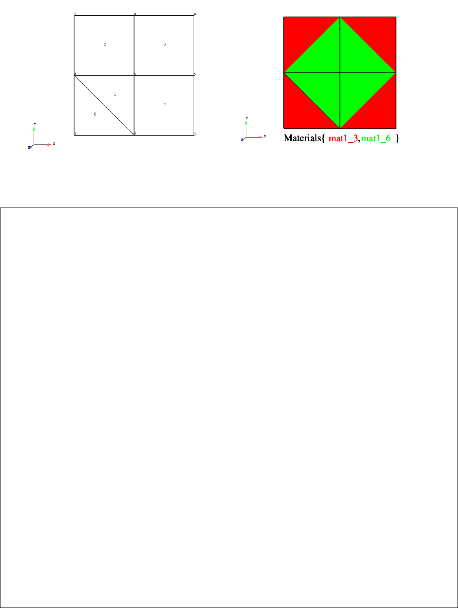
9.1 EnSight Gold Material Files Format
EnSight 10.2 User Manual 9-103
Example Material Dataset (without species)
The following example dataset of ASCII EnSight Gold geometry and material
files show the definition of material fractions for an unstructured model.
Case file
# Sample Case File for 2D Material Dataset
# Created: 03Apr03:mel
#
FORMAT
type: ensight gold
GEOMETRY
model: zmat2d.geo
VARIABLE
scalar per node: scalar zmat2d.sca
MATERIAL
material set number: 1 Mat1
material id count: 2
material id numbers: 3 6
material id names: matl_3 mat1_6 #Air H2O
material id per element: zmat2d.mati
material mixed ids: zmat2d.mixi
material mixed values: zmat2d.mixv
# y
#
# ^
# | Case Material ids = {3,6}
#
# 6. 7-----------8-----------9
# | /|\ |
# | / | \ |
# | e2 / | \ e3 |
# | / | \ |
# | / | \ |
# | q0 | q1 |
# | / | \ |
# | {.5,.5} | {.5,.5} |
# | / | \ |
# | / | \ |
# |/ | \|
# 3. 4-----------5-----------6
# |\ | /|
# | \ {0.,1.} | / |
# | \ | e4 / |
# | \ t1 | / |
# | \ | / |
# | e0 \ e1 | q2 |
# | \ | / |
# | t0 \ | {.5,.5} |
# | \ | / |
# | {1.,0.} \ | / |
# | \|/ |
# 0. 1-----------2-----------3 -> x
#
# 0. 3. 6.
#
Figure 9-2
Geometry for Example Material Dataset
Figure 9-2
Materials for Example Material Dataset

9.1 EnSight Gold Material Files Format
9-104 EnSight 10.2 User Manual
Geometry File (zmat2d.geo)
Geometry file
Example 2D Material Dataset
node id given
element id given
part
1
2d-mesh
coordinates
9
1
2
3
4
5
6
7
8
9
0.00000e+00
3.00000e+00
6.00000e+00
0.00000e+00
3.00000e+00
6.00000e+00
0.00000e+00
3.00000e+00
6.00000e+00
0.00000e+00
0.00000e+00
0.00000e+00
3.00000e+00
3.00000e+00
3.00000e+00
6.00000e+00
6.00000e+00
6.00000e+00
0.00000e+00
0.00000e+00
0.00000e+00
0.00000e+00
0.00000e+00
0.00000e+00
0.00000e+00
0.00000e+00
0.00000e+00
tria3
2
0
1
1 2 4
2 5 4
quad4
3
2
3
4
4 5 8 7
8 5 6 9
2 3 6 5
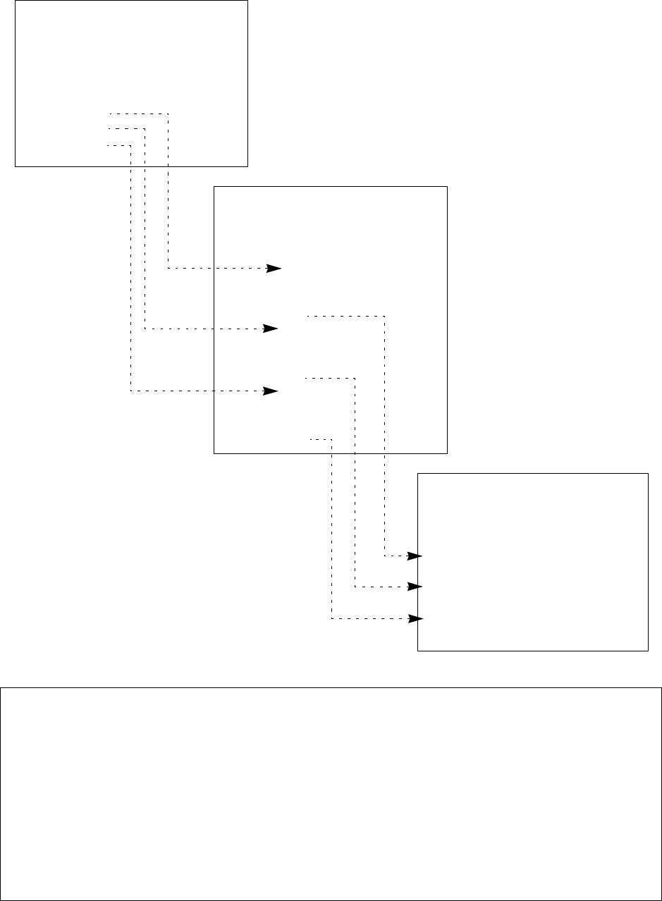
9.1 EnSight Gold Material Files Format
EnSight 10.2 User Manual 9-105
Scalar File (zmat2d.sca)
Scalar File
part
1
coordinates
0.00000e+00
1.00000e+00
2.00000e+00
1.00000e+00
2.00000e+00
3.00000e+00
2.00000e+00
3.00000e+00
4.00000e+00
Material Number/Id File
part
1
tria3
3
6
quad4
-1
-5
-9
Mixed Ids File
part
1
mixed ids
12
2
3
6
-1
2
3
6
-3
2
3
6
-5
Mixed Values File
part
1
mixed values
6
0.50000e+00
0.50000e+00
0.50000e+00
0.50000e+00
0.50000e+00
0.50000e+00
Material Number/ID File
(zmat2d.mati)
Mixed Material Ids File
(zmat2d.mixi)
Mixed Material Values File
(zmat2d.mixv)

9.1 EnSight Gold Material Files Format
9-106 EnSight 10.2 User Manual
Example Material Dataset (with Species)
Same as previous Material Dataset example except:
-append species information to MATERIAL section in case file, and
-add species element values file
(see example below).
Case file
Note: The following relationships are significant in the above case file.
material id numbers: 3 6
material id names: Air H20
species per material counts: 3 2
----^--- --^--
species per material lists: 12 13 14 11 13
N O Ar H O
where:
Case material ids (w/species) = {3,6} = {Air, H20} = {Air{ N, O, Ar), H20( H, O}}
Note: typical values " {Air(.78,.21.01), H20(.33,.67)}
# Sample Case File for 2D Material Dataset - with Species
# Created: 03Apr05:mel
#
FORMAT
type: ensight gold
GEOMETRY
Model: zmat2d.geo
VARIABLE
scalar per node: Nscalarzmat2d.sca
scalar per element: Escalarzmat2d.sca
MATERIAL
material set number: 1 Mat1
material id count: 2
material id numbers: 3 6
material id names: Air H2O
material id per element: zmat2d.mati
material mixed ids: zmat2d.mixi
material mixed values: zmat2d.mixv
# Optional Species data
species id count: 4
species id numbers: 11 12 13 14
species id names: Hydrogen Nitrogen Oxygen Argon
species per material counts: 3 2
species per material lists: 12 13 14 11 13
species element values: zmat2d.spv
9.1 EnSight Gold Material Files Format
EnSight 10.2 User Manual 9-107
M
a
t S
e p Species Element Values File (zmat2d.spv)
r e Species Element Values File
i c part
a i 1 0-bias Element Element by type in
l e species values Index Label the connectivity list
=== === 20 ===== ======= =====================
Air N 0.78000e+00 <--------------- 0 <---- e0 = t0 = 1st Triangle
" O 0.21000e+00 1
" Ar 0.01000e+00 2
H2O H 0.33000e+00 <--------------- 3 <---- e1 = t1 = 2nd Triangle
" O 0.67000e+00 4
Air N 0.78100e+00 <--------------- 5 <---- e2 = q0 = 1st Quad
" O 0.20900e+00 6
" Ar 0.01000e+00 6
H2O H 0.33300e+00 8
" O 0.66700e+00 9
Air N 0.78010e+00 <--------------- 10 <---- e3 = q1 = 2nd Quad
" O 0.20990e+00 11
" Ar 0.01000e+00 12
H2O H 0.33330e+00 13
" O 0.66670e+00 14
Air N 0.78001e+00 <--------------- 15 <---- e4 = q2 = 3rd Quad
" O 0.20999e+00 16
" Ar 0.01000e+00 17
H2O H 0.33333e+00 18
" O 0.66667e+00 19
Note: The above species element values are accessed via part-element connectivity (
zmat2d.geo
) and
material element data (
zmat2d.mati
and
zmat2d.mixi
) as illustrated above.
For more information on species see Species, located in Material Interface Parts, MATERIAL Section
under EnSight Gold Casefile Format, and MatSpecies function under 4.3 Va r ia bl e
Creation.
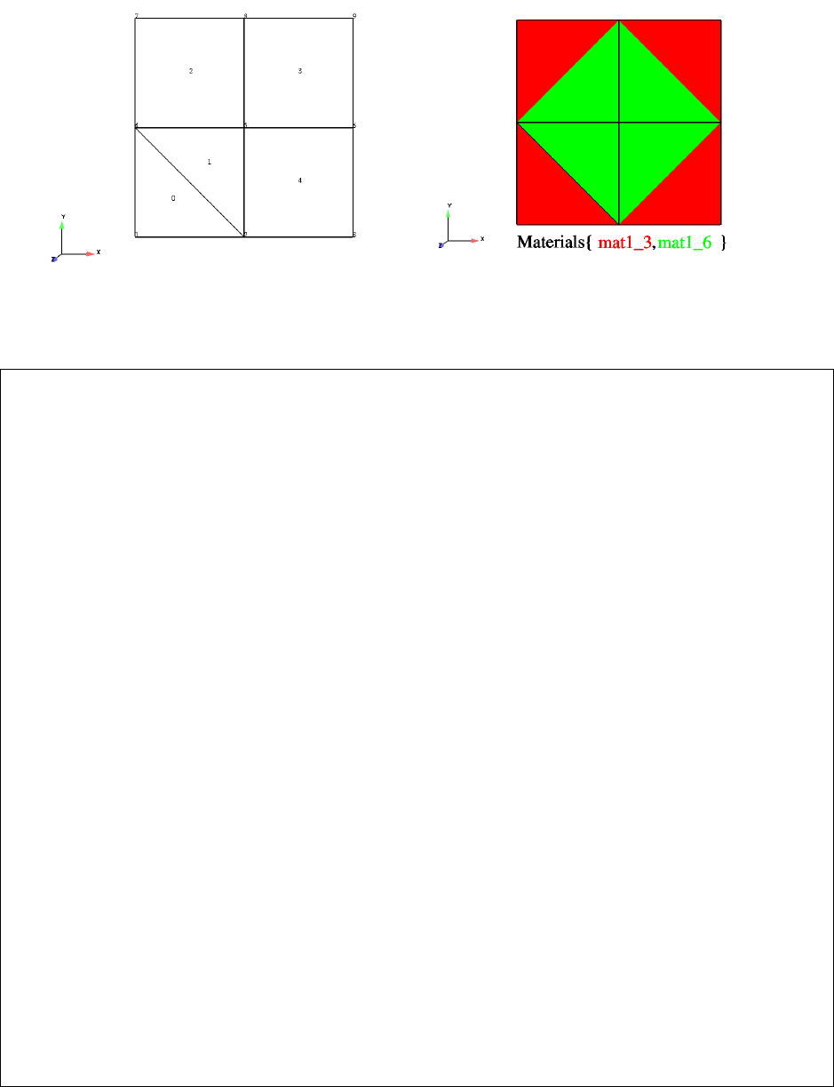
9.1 EnSight Gold Material Files Format
9-108 EnSight 10.2 User Manual
Example Material Dataset With Materials Defined By Per Element Scalar Variables
Note: Species are not supported under this format.
The following example dataset of ASCII EnSight Gold geometry and material
files show the definition of material fractions for an unstructured model.
Case file
# Sample Case File for 2D Material Dataset w/materials via per element scalars
# Created: 07Feb20:mel
#
FORMAT
type: ensight gold
GEOMETRY
model: zmat2d.geo
VARIABLE
scalar per node: scalarN zmat2d.sca
scalar per element: scal_E3 zmat2d.se3
scalar per element: scal_E6 zmat2d.se6
MATERIAL
material set number: 1 Mat1
material id count: 2
material id numbers: 3 6
material id names: matl_3 mat1_6 #Air H2O
material scalars per element: scal_E3 scal_E6
# y
#
# ^
# | Case Material ids = {3,6}
#
# 6. 7-----------8-----------9
# | /|\ |
# | / | \ |
# | e2 / | \ e3 |
# | / | \ |
# | / | \ |
# | q0 | q1 |
# | / | \ |
# | {.5,.5} | {.5,.5} |
# | / | \ |
# | / | \ |
# |/ | \|
# 3. 4-----------5-----------6
# |\ | /|
# | \ {0.,1.} | / |
# | \ | e4 / |
# | \ t1 | / |
# | \ | / |
# | e0 \ e1 | q2 |
# | \ | / |
# | t0 \ | {.5,.5} |
# | \ | / |
# | {1.,0.} \ | / |
# | \|/ |
# 0. 1-----------2-----------3 -> x
#
# 0. 3. 6.
Figure 9-3
Geometry for Example Material Dataset
Figure 9-3
Materials for Example Material Dataset
9.1 EnSight Gold Material Files Format
EnSight 10.2 User Manual 9-109
zmat2d.geo and zmat2d.sca are the same as in the Material Dataset (without species) example above.
zmat2d.se3 file contents:
zmat2d.se6 file contents:
Scalar3 File
part
1
tria3
1.00000e+00
0.00000e+00
quad4
5.00000e-01
5.00000e-01
5.00000e-01
Scalar6 File
part
1
tria3
0.00000e+00
1.00000e+00
quad4
5.00000e-01
5.00000e-01
5.00000e-01
9.2 EnSight6 Casefile Format
9-110 EnSight 10.2 User Manual
9.2 EnSight6 Casefile Format
Included in this section:
EnSight6 General Description
EnSight6 Geometry File Format
EnSight6 Case File Format
EnSight6 Wild Card Name Specification
EnSight6 Variable File Format
EnSight6 Per_Node Variable File Format
EnSight6 Per_Element Variable File Format
EnSight6 Measured/Particle File Format
Writing EnSight6 Binary Files
EnSight6 General Description
EnSight6 data consists of the following files:
• Case (required) (points to all other needed files including model
geometry, variables, and possibly measured geometry and variables)
EnSight6 supports constant result values as well as scalar, vector, 2nd order
symmetric tensor, and complex variable fields.
EnSight makes no assumptions regarding the physical significance of the variable
values in the files. These files can be from any discipline. For example, the scalar
file can include such things as pressure, temperature, and stress. The vector file
can be velocity, displacement, or any other vector data. And so on.
All variable results for EnSight6 are contained in disk files—one variable per file.
Additionally, if there are multiple time steps, there must either be a set of disk files
for each time step (transient multiple-file format), or all time steps of a particular
variable or geometry in one disk file (transient single-file format). Thus, all
EnSight6 transient geometry and variable files can be expressed in either multiple
file format or single file format.
Sources of EnSight6 data include the following:
• Data that can be translated to conform to the EnSight6 data format
• Data that originates from one of the translators supplied with the EnSight
application
The EnSight6 format supports an unstructured defined element set as shown in the
figure on the following page. Unstructured data must be defined in this element
set. Elements that do not conform to this set must either be subdivided or
discarded. The EnSight6 format also supports a structured block data format
which is very similar to the PLOT3D format. For the structured format, the
standard order of nodes is such that I’s advance quickest, followed by J’s, and then
K’s. A given EnSight6 model may have either unstructured data, structured data,
or a mixture of both.
9.2 EnSight6 General Description
EnSight 10.2 User Manual 9-111
ens_checker A program is supplied with EnSight which attempts to verify the integrity of the
format of EnSight 6 and EnSight Gold files. If you are producing EnSight
formatted data, this program can be very helpful, especially in your development
stage, in making sure that you are adhering to the published format. It makes no
attempt to verify the validity of floating point values, such as coordinates, variable
values, etc. This program takes a casefile as input. Thus, it will check the format
of the casefile, and all associated geometry and variable files referenced in the
casefile. See How To Use ens_checker.

9.2 EnSight6 General Description
9-112 EnSight 10.2 User Manual
Supported EnSight Elements
The elements that are supported by the EnSight6 format are:
eight node hexahedron twenty node hexahedron
six node pentahedron
9
10
7
8
12123
12
3
12
3
4
56
1
2
3
4
12
3
45 6
7
8
12
3
4
5
6
1
2
3
4
5
6
910
7
8
1
2
3
4
56
11
12
13 14
15
16
17 18
19
20
two node bar three node bar
three node triangle six node triangle four node quadrangle eight node quadrangle
four node tetrahedron ten node tetrahedron
1
point
12
3
4
1
4
8
2
3
5
6
7
5 node pyramid 13 node pyramid
11
22
33
44
55
6
7
8
9
10
11
12
13
fifteen node pentahedron (wedge)
1
2
3
4
5
6
78
9
10 11
12
13
14
15
(wedge)
Figure 9-4
Supported EnSight6 Elements

9.2 EnSight6 Case File Format
EnSight 10.2 User Manual 9-113
EnSight6 Case File Format
The Case file is an ASCII free format file that contains all the file and name
information for accessing model (and measured) geometry, variable, and time
information. It is comprised of five sections (FORMAT, GEOMETRY, VARIABLE,
TIME, FILE) as described below:
Notes: All lines in the Case file are limited to 79 characters.
The titles of each section must be in all capital letters.
Anything preceded by a “#” denotes a comment and is ignored. Comments may
append information lines or be placed on their own lines.
Information following “:” may be separated by white spaces or tabs.
Specifications encased in “[]” are optional, as indicated.
Format Section This is a required section which specifies the type of data to be read.
Usage:
FORMAT
type: ensight
Geometry Section This is a required section which specifies the geometry information for the model
(as well as measured geometry if present, and periodic match file (see Section 9.9,
Periodic Matchfile Format) if present).
Usage:
GEOMETRY
model: [ts] [fs] filename [change_coords_only]
measured: [ts] [fs] filename [change_coords_only]
match: filename
boundary: filename
where: ts = time set number as specified in TIME section. This is optional.
fs = corresponding file set number as specified in FILE section below.
filename = The filename of the appropriate file.
-> Model or measured filenames for a static geometry case, as well as match
and boundary filenames will not contain “*” wildcards.
-> Model or measured filenames for a changing geometry case will
contain “*” wildcards.
change_coords_only = The option to indicate that the changing geometry (as
indicated by wildcards in the filename) is coords only.
Otherwise, changing geometry connectivity will be
assumed.
Variable Section This is an optional section which specifies the files and names of the variables.
Constant variable values can also be set in this section.
Usage:
VARIABLE
constant per case: [ts] description
const_value(s)
scalar per node: [ts] [fs] description filename
vector per node: [ts] [fs] description filename
tensor symm per node: [ts] [fs] description filename
scalar per element: [ts] [fs] description filename
vector per element: [ts] [fs] description filename
tensor symm per element: [ts] [fs] description filename
scalar per measured node: [ts] [fs] description filename
vector per measured node: [ts] [fs] description filename
complex scalar per node: [ts] [fs] description
Re_fn Im_fn freq
complex vector per node: [ts] [fs] description
Re_fn Im_fn freq
9.2 EnSight6 Case File Format
9-114 EnSight 10.2 User Manual
complex scalar per element: [ts] [fs] description
Re_fn Im_fn freq
complex vector per element: [ts] [fs] description
Re_fn Im_fn freq
where:
ts
= The corresponding time set number (or index) as specified in TIME
section below. This is only required for transient constants and
variables.
fs
= The corresponding file set number (or index) as specified in FILE
section below.
description = The variable (GUI) name (ex. Pressure, Velocity, etc.)
const_value(s) = The constant value. If constants change over time, then ns (see
TIME section below) constant values of ts.
filename
= The filename of the variable file. Note: only transient filenames
contain “*” wildcards.
Re_fn
= The filename for the file containing the real values of the complex
variable.
Im_fn
= The filename for the file containing the imaginary values of the
complex variable.
freq
= The corresponding harmonic frequency of the complex variable.
For complex variables where harmonic frequency is undefined,
simply use the text string: UNDEFINED.
Note: As many variable description lines as needed may be used.
Note: Variable descriptions have the following restrictions:
The maximum variable name length is documented at the beginning of this
chapter.
Duplicate variable descriptions are not allowed.
Leading and trailing white space will be eliminated.
Variable descriptions must not start with a numeric digit.
Variable descriptions must not contain any of the following reserved characters:
( [ + @ ! * $
) ] - space # ^ /
Time Section This is an optional section for steady state cases, but is required for transient
cases. It contains time set information. Shown below is information for one time
set. Multiple time sets (up to 16) may be specified for measured data as shown in
Case File Example 3 below.
Usage:
TIME
time set: ts [description]
number of steps: ns
filename start number: fs
filename increment: fi
time values: time_1 time_2 .... time_ns
or
TIME
time set: ts [description]
number of steps: ns
filename numbers: fn
time values: time_1 time_2 .... time_ns
where:
ts
= timeset number. This is the number referenced in the GEOMETRY
9.2 EnSight6 Case File Format
EnSight 10.2 User Manual 9-115
and VARIABLE sections.
description
= optional timeset description which will be shown in user
interface.
ns
= number of transient steps
fs
= the number to replace the “*” wildcards in the filenames, for the first step
fi
= the increment to fs for subsequent steps
time
= the actual time values for each step, each of which must be separated
by a white space and which may continue on the next line if needed
fn
= a list of numbers or indices, to replace the “*” wildcards in the filenames.
File Section This section is optional for expressing a transient case with single-file formats. This
section contains single-file set information. This information specifies the number of time
steps in each file of each data entity, i.e. each geometry and each variable (model and/or
measured). Each data entity’s corresponding file set might have multiple continuation
files due to system file size limit, i.e. ~2 GB for -bit and ~4 TB for 64-bit architectures.
Each file set corresponds to one and only one time set, but a time set may be referenced by
many file sets. The following information may be specified in each file set. For file sets
where all of the time set data exceeds the maximum file size limit of the system, both
filename index
and
number of steps
are repeated within the file set definition for each
continuation file required. Otherwise
filename index
may be omitted if there is only one
file. File set information is shown in Case File Example 4 below.
Usage:
FILE
file set: fs
filename index: fi # Note: only used when data continues in other files
number of steps: ns
where:
fs
= file set number. This is the number referenced in the GEOMETRY
and VARIABLE sections above.
ns
= number of transient steps
fi
= file index number in the file name (replaces “*” in the filenames)
Case File Example 1 The following is a minimal EnSight6 case file for a steady state model with some results.
Note: this (en6.case) file, as well as all of its referenced geometry and variable files (along with a
couple of command files) can be found under your installation directory (path: $CEI_HOME/
ensight102/data/user_manual). The EnSight6 Geometry File Example and the Variable File
Examples are the contents of these files.
FORMAT
type: ensight
GEOMETRY
model: en6.geo
VARIABLE
constant per case: Cden .8
scalar per element: Esca en6.Esca
scalar per node: Nsca en6.Nsca
vector per element: Evec en6.Evec
vector per node: Nvec en6.Nvec
tensor symm per element: Eten en6.Eten
tensor symm per node: Nten en6.Nten
complex scalar per element: Ecmp en6.Ecmp_r en6.Ecmp_i 2.
complex scalar per node: Ncmp en6.Ncmp_r en6.Ncmp_i 4.
9.2 EnSight6 Case File Format
9-116 EnSight 10.2 User Manual
Case File Example 2 The following is a Case file for a transient model. The connectivity of the geometry is also
changing.
FORMAT
type: ensight
GEOMETRY
model: 1 example2.geo**
VARIABLE
scalar per node: 1 Stress example2.scl**
vector per node: 1 Displacement example2.dis**
TIME
time set: 1
number of steps: 3
filename start number: 0
filename increment: 1
time values: 1.0 2.0 3.0
The following files would be needed for Example 2:
example2.geo00 example2.scl00 example2.dis00
example2.geo01 example2.scl01 example2.dis01
example2.geo02 example2.scl02 example2.dis02
Case File Example 3 The following is a Case file for a transient model with measured data.
This example has pressure given per element.
FORMAT
type: ensight
GEOMETRY
model: 1 example3.geo*
measured: 2 example3.mgeo**
VARIABLE
constant per case: Gamma 1.4
constant per case: 1 Density .9 .9 .7 .6 .6
scalar per element 1 Pressure example3.pre*
vector per node: 1 Velocity example3.vel*
scalar per measured node: 2 Temperature example3.mtem**
vector per measured node: 2 Velocity example3.mvel**
TIME
time set: 1
number of steps: 5
filename start number: 1
filename increment: 2
time values: .1 .2 .3 # This example shows that time
.4 .5 # values can be on multiple lines
time set: 2
number of steps: 6
filename start number: 0
filename increment: 2
time values:
.05 .15 .25 .34 .45 .55
9.2 EnSight6 Case File Format
EnSight 10.2 User Manual 9-117
The following files would be needed for Example 3:
example3.geo1 example3.pre1 example3.vel1
example3.geo3 example3.pre3 example3.vel3
example3.geo5 example3.pre5 example3.vel5
example3.geo7 example3.pre7 example3.vel7
example3.geo9 example3.pre9 example3.vel9
example3.mgeo00 example3.mtem00 example3.mvel00
example3.mgeo02 example3.mtem02 example3.mvel02
example3.mgeo04 example3.mtem04 example3.mvel04
example3.mgeo06 example3.mtem06 example3.mvel06
example3.mgeo08 example3.mtem08 example3.mvel08
example3.mgeo10 example3.mtem10 example3.mvel10
Case File Example 4 The following is Case File Example 3 expressed in transient single-file formats.
In this example, the transient data for the measured velocity data entity happens
to be greater than the maximum file size limit. Therefore, the first four time steps
fit and are contained in the first file, and the last two time steps are ‘continued’ in
a second file.
FORMAT
type: ensight
GEOMETRY
model: 1 example4.geo
measured: 2 example4.mgeo
VARIABLE
constant per case: Density .5
scalar per element: 1 1 Pressure example4.pre
vector per node: 1 1 Velocity example4.vel
scalar per measured node: 2 2 Temperature example4.mtem
vector per measured node: 2 3 Velocity example4.mvel*
TIME
time set: 1 Model
number of steps: 5
time values: .1 .2 .3 .4 .5
time set: 2 Measured
number of steps: 6
time values: .05 .15 .25 .34 .45 .55
FILE
file set: 1
number of steps: 5
file set: 2
number of steps: 6
file set: 3
filename index: 1
number of steps: 4
filename index: 2
number of steps: 2

9.2 EnSight6 Case File Format
9-118 EnSight 10.2 User Manual
The following files would be needed for Example 4:
example4.geo example4.pre example4.vel
example4.mgeo example4.mtem example4.mvel1
example4.mvel2
Contents of Each file contains transient data that corresponds to the specified number of time steps.
Transient The data for each time step sequentially corresponds to the simulation time values
Single Files
(time values)
found listed in the TIME section. In transient single-file format, the data for
each time step essentially corresponds to a standard EnSight6 geometry or variable file
(model or measured) as expressed in multiple file format. The data for each time step is
enclosed between two wrapper records, i.e. preceded by a BEGIN TIME STEP record
and followed by an END TIME STEP record. Time step data is not split between files.
If there is not enough room to append the data from a time step to the file without
exceeding the maximum file limit of a particular system, then a continuation file must be
created for the time step data and any subsequent time step. Any type of user comments
may be included before and/or after each transient step wrapper.
Note 1: If transient single file format is used, EnSight expects all files of a dataset
to be specified in transient single file format. Thus, even static files must be
enclosed between a BEGIN TIME STEP and an END TIME STEP wrapper.
Note 2: For binary geometry files, the first BEGIN TIME STEP wrapper must
follow the <C Binary/Fortran Binary> line. Both BEGIN TIME STEP and END
TIME STEP wrappers are written according to type (1) in binary. (see Writing
EnSight6 Binary Files, in Section 9.2)
Note 3: Efficient reading of each file (especially binary) is facilitated by
appending each file with a file index. A file index contains appropriate
information to access the file byte positions of each time step in the file. (EnSight
automatically appends a file index to each file when exporting in transient single
file format.) If used, the file index must follow the last END TIME STEP
wrapper in each file.
File Index Usage:
* Each file byte location is the first byte that follows the BEGIN TIME STEP record.
Shown below are the contents of each of the above files, using the data files from Case
File Example 3 for reference (without FILE_INDEX for simplicity).
Contents of file example4.geo_1:
BEGIN TIME STEP
Contents of file example3.geo1
END TIME STEP
BEGIN TIME STEP
Contents of file example3.geo3
END TIME STEP
BEGIN TIME STEP
Contents of file example3.geo5
ASCII Binary Item Description
“%20d\n” sizeof(int) n Total number of data time steps in the file.
“%20d\n” sizeof(long) fb1File byte loc for contents of 1st time step*
“%20d\n” sizeof(long) fb2File byte loc for contents of 2nd time step*
. . . . . . . . . . . .
“%20d\n” sizeof(long) fbnFile byte loc for contents of nth time step*
“%20d\n” sizeof(int) flag Miscellaneous flag (= 0 for now)
“%20d\n” sizeof(long) fb of item n File byte loc for Item n above
“%s\n” sizeof(char)*80 “FILE_INDEX” File index keyword
9.2 EnSight6 Case File Format
EnSight 10.2 User Manual 9-119
END TIME STEP
BEGIN TIME STEP
Contents of file example3.geo7
END TIME STEP
BEGIN TIME STEP
Contents of file example3.geo9
END TIME STEP
Contents of file example4.pre_1:
BEGIN TIME STEP
Contents of file example3.pre1
END TIME STEP
BEGIN TIME STEP
Contents of file example3.pre3
END TIME STEP
BEGIN TIME STEP
Contents of file example3.pre5
END TIME STEP
BEGIN TIME STEP
Contents of file example3.pre7
END TIME STEP
BEGIN TIME STEP
Contents of file example3.pre9
END TIME STEP
Contents of file example4.vel_1:
BEGIN TIME STEP
Contents of file example3.vel1
END TIME STEP
BEGIN TIME STEP
Contents of file example3.vel3
END TIME STEP
BEGIN TIME STEP
Contents of file example3.vel5
END TIME STEP
BEGIN TIME STEP
Contents of file example3.vel7
END TIME STEP
BEGIN TIME STEP
Contents of file example3.vel9
END TIME STEP
Contents of file example4.mgeo_1:
BEGIN TIME STEP
Contents of file example3.mgeo00
END TIME STEP
BEGIN TIME STEP
Contents of file example3.mgeo02
END TIME STEP
BEGIN TIME STEP
Contents of file example3.mgeo04
END TIME STEP
BEGIN TIME STEP
Contents of file example3.mgeo06
END TIME STEP
BEGIN TIME STEP
Contents of file example3.mgeo08
END TIME STEP
BEGIN TIME STEP
Contents of file example3.mgeo10
END TIME STEP
Contents of file example4.mtem_1:
BEGIN TIME STEP
Contents of file example3.mtem00
END TIME STEP
BEGIN TIME STEP
Contents of file example3.mtem02
END TIME STEP
BEGIN TIME STEP
Contents of file example3.mtem04
END TIME STEP
BEGIN TIME STEP
Contents of file example3.mtem06
END TIME STEP
BEGIN TIME STEP
Contents of file example3.mtem08
END TIME STEP
BEGIN TIME STEP
Contents of file example3.mtem10
END TIME STEP
Contents of file example4.mvel1_1:
BEGIN TIME STEP
Contents of file example3.mvel00
END TIME STEP
9.2 EnSight6 Case File Format
9-120 EnSight 10.2 User Manual
BEGIN TIME STEP
Contents of file example3.mvel02
END TIME STEP
BEGIN TIME STEP
Contents of file example3.mvel04
END TIME STEP
BEGIN TIME STEP
Contents of file example3.mvel06
END TIME STEP
Contents of file example4.mvel2_1:
Comments can precede the beginning wrapper here.
BEGIN TIME STEP
Contents of file example3.mvel08
END TIME STEP
Comments can go between time step wrappers here.
BEGIN TIME STEP
Contents of file example3.mvel10
END TIME STEP
Comments can follow the ending time step wrapper.
EnSight6 Wild Card Name Specification
For transient data, if multiple time files are involved, the file names must conform
to the EnSight wild-card specification. This specification is as follows:
• File names must include numbers that are in ascending order from
beginning to end.
• Numbers in the files names must be zero filled if there is more than one
significant digit.
• Numbers can be anywhere in the file name.
• When the file name is specified in the EnSight result file, you must
replace the numbers in the file with an asterisk(*). The number of
asterisks specified is the number of significant digits. The asterisk must
occupy the same place as the numbers in the file names.
9.2 EnSight6 Geometry File Format
EnSight 10.2 User Manual 9-121
EnSight6 Geometry File Format
The EnSight6 format consists of keywords followed by information. The
following seven items are important when working with EnSight6 geometry files:
1. You do not have to assign node IDs. If you do, the element connectivities are
based on the node numbers. If you let EnSight assign the node IDs, the nodes
are considered to be sequential starting at node 1, and element connectivity is
done accordingly. If node IDs are set to off, they are numbered internally;
however, you will not be able to display or query on them. If you have node
IDs in your data, you can have EnSight ignore them by specifying “node id
ignore.” Using this option may reduce some of the memory taken up by the
Client and Server, but display and query on the nodes will not be available.
2. You do not need to specify element IDs. If you specify element IDs, or you let
EnSight assign them, you can show them on the screen. If they are set to off,
you will not be able to show or query on them. If you have element IDs in
your data you can have EnSight ignore them by specifying “element id
ignore.” Using this option will reduce some of the memory taken up by the
Client and Server. This may or may not be a significant amount, and
remember that display and query on the elements will not be available.
3. The format of integers and real numbers must be followed (See the Geometry
Example below).
4. Integers are written out using the following integer format:
From C:
8d
format
From FORTRAN:
i8
format
Real numbers are written out using the following floating-point format:
From C:
12.5e
format
From FORTRAN:
e12.5
format
The number of integers or reals per line must also be followed!
5. By default, a Part is processed to show the outside boundaries. This
representation is loaded to the Client host system when the geometry file is
read (unless other attributes have been set on the workstation, such as feature
angle).
6. Coordinates for unstructured data must be defined before any Parts can be
defined. The different elements can be defined in any order (that is, you can
define a hexa8 before a bar2).
7. A Part containing structured data cannot contain any unstructured element
types or more than one block. Each structured Part is limited to a single
block. A structured block is indicated by following the Part description line
with either the “block” line or the “block iblanked” line. An “iblanked” block
must contain an additional integer array of values at each node, traditionally
called the iblank array. Valid iblank values for the EnSight format are:
0 for nodes which are exterior to the model, sometimes called blanked-out nodes
1 for nodes which are interior to the model, thus in the free stream and to be used
<0 or >1 for any kind of boundary nodes
In EnSight’s structured Part building dialog, the iblank option selected will control
9.2 EnSight6 Geometry File Format
9-122 EnSight 10.2 User Manual
which portion of the structured block is “created”. Thus, from the same structured
block, the interior flow field part as well as a symmetry boundary part could be
“created”.
Note: By default EnSight does not do any “partial” cell iblank processing.
Namely, only complete cells containing no “exterior” nodes are created. It is
possible to obtain partial cell processing by issuing the “test:partial_cells_on”
command in the Command Dialog before reading the file.
Note also that for the structured format, the standard order of nodes is such that
I’s advance quickest, followed by J’s, and then K’s.
8. Maximum number of parts is 32769
Maximum number of variables is 10000
Maximum file name length is 1024
Maximum part name length is 79, but the GUI will only display 49
Maximum variable name length is 79, but the GUI will only display 49
Generic Format Not all of the lines included in the following generic example file are necessary:
description line 1 |
description line 2 |
node id <off/given/assign/ignore> |
All geometry files mus
t
element id <off/given/assign/ignore> |
contain these first six lines
coordinates |
# of unstructured nodes |
id x y z
id x y z
id x y z
.
.
.
part #
description line
point
number of points
id nd
id nd
id nd
.
.
.
bar2
number of bar2’s
id nd nd
id nd nd
id nd nd
.
.
.
bar3
number of bar3’s
id nd nd nd
id nd nd nd
id nd nd nd
.
.
.
tria3
number of three node triangles
9.2 EnSight6 Geometry File Format
EnSight 10.2 User Manual 9-123
id nd nd nd
id nd nd nd
id nd nd nd
.
.
.
tria6
number of six node triangles
id nd nd nd nd nd nd
.
.
.
quad4
number of quad 4’s
id nd nd nd nd
id nd nd nd nd
id nd nd nd nd
id nd nd nd nd
.
.
.
quad8
number of quad 8’s
id nd nd nd nd nd nd nd nd
id nd nd nd nd nd nd nd nd
id nd nd nd nd nd nd nd nd
id nd nd nd nd nd nd nd nd
.
.
.
tetra4
number of 4 node tetrahedrons
id nd nd nd nd
id nd nd nd nd
id nd nd nd nd
id nd nd nd nd
.
.
.
tetra10
number of 10 node tetrahedrons
id nd nd nd nd nd nd nd nd nd nd
id nd nd nd nd nd nd nd nd nd nd
id nd nd nd nd nd nd nd nd nd nd
id nd nd nd nd nd nd nd nd nd nd
.
.
.
pyramid5
number of 5 node pyramids
id nd nd nd nd nd
id nd nd nd nd nd
id nd nd nd nd nd
id nd nd nd nd nd
.
.
.
pyramid13
number of 13 node pyramids
id nd nd nd nd nd nd nd nd nd nd nd nd nd
id nd nd nd nd nd nd nd nd nd nd nd nd nd
9.2 EnSight6 Geometry File Format
9-124 EnSight 10.2 User Manual
id nd nd nd nd nd nd nd nd nd nd nd nd nd
id nd nd nd nd nd nd nd nd nd nd nd nd nd
.
.
.
hexa8
number of 8 node hexahedrons
id nd nd nd nd nd nd nd nd
id nd nd nd nd nd nd nd nd
id nd nd nd nd nd nd nd nd
id nd nd nd nd nd nd nd nd
.
.
.
hexa20
number of 20 node hexahedrons
id nd nd nd nd nd nd nd nd nd nd nd nd nd nd nd nd nd nd nd nd
id nd nd nd nd nd nd nd nd nd nd nd nd nd nd nd nd nd nd nd nd
id nd nd nd nd nd nd nd nd nd nd nd nd nd nd nd nd nd nd nd nd
id nd nd nd nd nd nd nd nd nd nd nd nd nd nd nd nd nd nd nd nd
id nd nd nd nd nd nd nd nd nd nd nd nd nd nd nd nd nd nd nd nd
.
.
.
penta6
number of 6 node pentahedrons
id nd nd nd nd nd nd
id nd nd nd nd nd nd
id nd nd nd nd nd nd
id nd nd nd nd nd nd
id nd nd nd nd nd nd
.
.
.
penta15
number of 15 node pentahedrons
id nd nd nd nd nd nd nd nd nd nd nd nd nd nd nd
id nd nd nd nd nd nd nd nd nd nd nd nd nd nd nd
id nd nd nd nd nd nd nd nd nd nd nd nd nd nd nd
id nd nd nd nd nd nd nd nd nd nd nd nd nd nd nd
id nd nd nd nd nd nd nd nd nd nd nd nd nd nd nd
.
.
.
part #
description line
block #nn=i*j*k
i j k
x_n1 x_n2 x_n3 ..... x_nn (6/line)
y_n1 y_n2 y_n3 ..... y_nn “
z_n1 z_n2 z_n3 ..... z_nn “
part #
description line
block iblanked #nn=i*j*k
i j k
x_n1 x_n2 x_n3 ..... x_nn (6/line)
y_n1 y_n2 y_n3 ..... y_nn “
z_n1 z_n2 z_n3 ..... z_nn “
ib_n1 ib_n2 ib_n3 .... ib_nn (10/line)
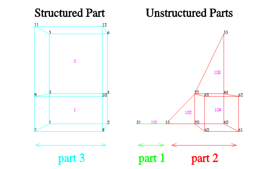
9.2 EnSight6 Geometry File Format
EnSight 10.2 User Manual 9-125
EnSight6 Geometry The following is an example of an ASCII EnSight6 geometry file with 11 defined
File Example unstructured nodes from which 2 unstructured parts are defined, and a 2x3x2
structured part as depicted in the above diagram. (See Case File Example 1 for
reference to this file.)
This is the 1st description line of the EnSight6 geometry example
This is the 2nd description line of the EnSight6 geometry example
node id given
element id given
coordinates
11
15 4.00000e+00 0.00000e+00 0.00000e+00
31 3.00000e+00 0.00000e+00 0.00000e+00
20 5.00000e+00 0.00000e+00 0.00000e+00
40 6.00000e+00 0.00000e+00 0.00000e+00
22 5.00000e+00 1.00000e+00 0.00000e+00
44 6.00000e+00 1.00000e+00 0.00000e+00
55 6.00000e+00 3.00000e+00 0.00000e+00
60 5.00000e+00 0.00000e+00 2.00000e+00
61 6.00000e+00 0.00000e+00 2.00000e+00
62 6.00000e+00 1.00000e+00 2.00000e+00
63 5.00000e+00 1.00000e+00 2.00000e+00
part 1
2D uns-elements (description line for part 1)
tria3
2
102 15 20 22
103 22 44 55
hexa8
1
104 20 40 44 22 60 61 62 63
part 2
1D uns-elements (description line for part 2)
bar2
1
101 31 15
part 3
9.2 EnSight6 Variable File Format
9-126 EnSight 10.2 User Manual
3D struct-part (description line for part 3)
block iblanked
2 3 2
0.00000e+00 2.00000e+00 0.00000e+00 2.00000e+00 0.00000e+00 2.00000e+00
0.00000e+00 2.00000e+00 0.00000e+00 2.00000e+00 0.00000e+00 2.00000e+00
0.00000e+00 0.00000e+00 1.00000e+00 1.00000e+00 3.00000e+00 3.00000e+00
0.00000e+00 0.00000e+00 1.00000e+00 1.00000e+00 3.00000e+00 3.00000e+00
0.00000e+00 0.00000e+00 0.00000e+00 0.00000e+00 0.00000e+00 0.00000e+00
2.00000e+00 2.00000e+00 2.00000e+00 2.00000e+00 2.00000e+00 2.00000e+00
1 1 1 1 1 1 1 1 1 1
1 1
EnSight6 Variable File Format
EnSight6 variable files can either be per_node or per_element. They cannot be
both. However, an EnSight model can have some variables which are per_node
and other variables which are per_element.
EnSight6 Per_Node Variable File Format
EnSight6 variable files for per_node variables contain any values for each
unstructured node followed by any values for each structured node.
First comes a single description line.
Second comes any unstructured node value. The number of values per node
depends on the type of field. An unstructured scalar field has one, a vector field
has three (order: x,y,z), a 2nd order symmetric tensor field has 6 (order: 11, 22, 33,
12, 13, 23), and a 2nd order asymmetric tensor field has 9 values per node (order:
11, 12, 13, 21, 22, 23, 31, , 33). An unstructured complex variable in EnSight6
consists of two scalar or vector fields (one real and one imaginary), with scalar
and vector values written to their separate files respectively.
Third comes any structured data information, starting with a part # line, followed
by a line containing the “block”, and then lines containing the values for each
structured node which are output in the same IJK component order as the
coordinates. Briefly, a structured scalar is the same as an unstructured scalar, one
value per node. A structured vector is written one value per node per component,
thus three sequential scalar field blocks. Likewise for a structured 2nd order
symmetric tensor, written as six sequential scalar field blocks, and a 2nd order
tensor, written as nine sequential scalar field blocks. The same methodology
applies for a complex variable only with the real and imaginary fields written to
separate structured scalar or vector files.
The values must be written in the following floating point format (6 per line as
shown in the examples below):
From C:
12.5e
format
From FORTRAN:
e12.5
format
The format of a per_node variable file is as follows:
•Line 1
This line is a description line.
• Line 2 through the end of the file contains the values at each node in the
model.

9.2 EnSight6 Per_Node Variable File Format
EnSight 10.2 User Manual 9-127
A generic example for per_node variables:
One description line for the entire file
*.*****E+** *.*****E+** *.*****E+** *.*****E+** *.*****E+** *.*****E+**
*.*****E+** *.*****E+** *.*****E+** *.*****E+** *.*****E+** *.*****E+**
*.*****E+** *.*****E+** *.*****E+** *.*****E+**
part #
block
*.*****E+** *.*****E+** *.*****E+** *.*****E+** *.*****E+** *.*****E+**
*.*****E+** *.*****E+**
*.*****E+** *.*****E+** *.*****E+** *.*****E+** *.*****E+** *.*****E+**
*.*****E+** *.*****E+**
*.*****E+** *.*****E+** *.*****E+** *.*****E+** *.*****E+** *.*****E+**
*.*****E+** *.*****E+**
Note that there is a format difference between the unstructured and structured
(block) portions of the vector and tensor data. For example a multiple component
unstructured vector appears as x y z triplets, while the structured counterpart lists
all x then all y and finally all z.
The following variable file examples reflect scalar, vector, tensor, and complex
variable values per node for the previously defined EnSight6 Geometry File
Example with 11 defined unstructured nodes and a 2x3x2 structured Part (Part
number 3). The values are summarized in the following table.
Complex Scalar
Node Node Scalar Vector Tensor (2nd order symm.) Real Imaginary
Index Id Value Values Values Value Value
Unstructured
1 15 (1.) (1.1, 1.2, 1.3) (1.1, 1.2, 1.3, 1.4, 1.5, 1.6) (1.1) (1.2)
2 31 (2.) (2.1, 2.2, 2.3) (2.1, 2.2, 2.3, 2.4, 2.5, 2.6) (2.1) (2.2)
3 20 (3.) (3.1, 3.2, 3.3) (3.1, 3.2, 3.3, 3.4, 3.5, 3.6) (3.1) (3.2)
4 40 (4.) (4.1, 4.2, 4.3) (4.1, 4.2, 4.3, 4.4, 4.5, 4.6) (4.1) (4.2)
5 22 (5.) (5.1, 5.2, 5.3) (5.1, 5.2, 5.3, 5.4, 5.5, 5.6) (5.1) (5.2)
6 44 (6.) (6.1, 6.2, 6.3) (6.1, 6.2, 6.3, 6.4, 6.5, 6.6) (6.1) (6.2)
7 55 (7.) (7.1, 7.2, 7.3) (7.1, 7.2, 7.3, 7.4, 7.5, 7.6) (7.1) (7.2)
8 60 (8.) (8.1, 8.2, 8.3) (8.1, 8.2, 8.3, 8.4, 8.5, 8.60 (8.1) (8.2)
9 61 (9.) (9.1, 9.2, 9.3) (9.1, 9.2, 9.3, 9.4, 9.5, 9.6) (9.1) (9.2)
10 62 (10.) (10.1,10.2,10.3) (10.1,10.2,10.3,10.4,10.5,10.6) (10.1) (10.2)
11 63 (11.) (11.1,11.2,11.3) (11.1,11.2,11.3,11.4,11.5,11.6) (11.1) (11.2)
Structured
1 1 (1.) (1.1, 1.2, 1.3) (1.1, 1.2, 1.3, 1.4, 1.5, 1.6) (1.1) (1.2)
2 2 (2.) (2.1, 2.2, 2.3) (2.1, 2.2, 2.3, 2.4, 2.5, 2.6) (2.1) (2.2)
3 3 (3.) (3.1, 3.2, 3.3) (3.1, 3.2, 3.3, 3.4, 3.5, 3.6) (3.1) (3.2)
4 4 (4.) (4.1, 4.2, 4.3) (4.1, 4.2, 4.3, 4.4, 4.5, 4.6) (4.1) (4.2)
5 5 (5.) (5.1, 5.2, 5.3) (5.1, 5.2, 5.3, 5.4, 5.5, 5.6) (5.1) (5.2)
6 6 (6.) (6.1, 6.2, 6.3) (6.1, 6.2, 6.3, 6.4, 6.5, 6.6) (6.1) (6.2)
7 7 (7.) (7.1, 7.2, 7.3) (7.1, 7.2, 7.3, 7.4, 7.5, 7.6) (7.1) (7.2)
8 8 (8.) (8.1, 8.2, 8.3) (8.1, 8.2, 8.3, 8.4, 8.5, 8.6) (8.1) (8.2)
9 9 (9.) (9.1, 9.2, 9.3) (9.1, 9.2, 9.3, 9.4, 9.5, 9.6) (9.1) (9.2)
10 10 (10.) (10.1,10.2,10.3) (10.1,10.2,10.3,10.4,10.5,10.6) (10.1) (10.2)
11 11 (11.) (11.1,11.2,11.3) (11.1,11.2,11.3,11.4,11.5,11.6) (11.1) (11.2)
9.2 EnSight6 Per_Node Variable File Format
9-128 EnSight 10.2 User Manual
Per_node (Scalar) Variable Example 1 This example shows ASCII scalar file (en6.Nsca) for the
geometry example.
Per_node scalar values for the EnSight6 geometry example
1.00000E+00 2.00000E+00 3.00000E+00 4.00000E+00 5.00000E+00 6.00000E+00
7.00000E+00 8.00000E+00 9.00000E+00 1.00000E+01 1.10000E+01
part 3
block
1.00000E+00 2.00000E+00 3.00000E+00 4.00000E+00 5.00000E+00 6.00000E+00
7.00000E+00 8.00000E+00 9.00000E+00 1.00000E+01 1.10000E+01
Per_node (Vector) Variable Example 2 This example shows ASCII vector file (en6.Nvec) for the
geometry example.
Per_node vector values for the EnSight6 geometry example
1.10000E+00 1.20000E+00 1.30000E+00 2.10000E+00 2.20000E+00 2.30000E+00
3.10000E+00 3.20000E+00 3.30000E+00 4.10000E+00 4.20000E+00 4.30000E+00
5.10000E+00 5.20000E+00 5.30000E+00 6.10000E+00 6.20000E+00 6.30000E+00
7.10000E+00 7.20000E+00 7.30000E+00 8.10000E+00 8.20000E+00 8.30000E+00
9.l0000E+00 9.20000E+00 9.30000E+00 1.01000E+01 1.02000E+01 1.03000E+01
1.11000E+01 1.12000E+01 1.13000E+01
part 3
block
1.10000E+00 2.10000E+00 3.10000E+00 4.10000E+00 5.10000E+00 6.10000E+00
7.10000E+00 8.10000E+00 9.10000E+00 1.01000E_01 1.11000E+01
1.20000E+00 2.20000E+00 3.20000E+00 4.20000E+00 5.20000E+00 6.20000E+00
7.20000E+00 8.20000E+00 9.20000E+00 1.02000E+01 1.12000E+01
1.30000E+00 2.30000E+00 3.30000E+00 4.30000E+00 5.30000E+00 6.30000E+00
7.30000E+00 8.30000E+00 9.30000E+00 1.03000E+01 1.13000E+01
Per_node (Tensor) Variable Example 3 This example shows an ASCII 2nd order symmetric tensor file
(en6.Nten) for the geometry example.
Per_node symmetric tensor values for the EnSight6 geometry example
1.10000E+00 1.20000E+00 1.30000E+00 1.40000E+00 1.50000E+00 1.60000E+00
2.10000E+00 2.20000E+00 2.30000E+00 2.40000E+00 2.50000E+00 2.60000E+00
3.10000E+00 3.20000E+00 3.30000E+00 3.40000E+00 3.50000E+00 3.60000E+00
4.10000E+00 4.20000E+00 4.30000E+00 4.40000E+00 4.50000E+00 4.60000E+00
5.10000E+00 5.20000E+00 5.30000E+00 5.40000E+00 5.50000E+00 5.60000E+00
6.10000E+00 6.20000E+00 6.30000E+00 6.40000E+00 6.50000E+00 6.60000E+00
7.10000E+00 7.20000E+00 7.30000E+00 7.40000E+00 7.50000E+00 7.60000E+00
8.10000E+00 8.20000E+00 8.30000E+00 8.40000E+00 8.50000E+00 8.60000E+00
9.10000E+00 9.20000E+00 9.30000E+00 9.40000E+00 9.50000E+00 9.60000E+00
1.01000E+01 1.02000E+01 1.03000E+01 1.04000E+01 1.05000E+01 1.06000E+01
1.11000E+01 1.12000E+01 1.13000E+01 1.14000E+01 1.15000E+01 1.16000E+01
part 3
block
1.10000E+00 2.10000E+00 3.10000E+00 4.10000E+00 5.10000E+00 6.10000E+00
7.10000E+00 8.10000E+00 9.10000E+00 1.01000E+01 1.11000E+01
1.20000E+00 2.20000E+00 3.20000E+00 4.20000E+00 5.20000E+00 6.20000E+00
7.20000E+00 8.20000E+00 9.20000E+00 1.02000E+01 1.12000E+01
1.30000E+00 2.30000E+00 3.30000E+00 4.30000E+00 5.30000E+00 6.30000E+00
7.30000E+00 8.30000E+00 9.30000E+00 1.03000E+01 1.13000E+01
1.40000E+00 2.40000E+00 3.40000E+00 4.40000E+00 5.40000E+00 6.40000E+00
7.40000E+00 8.40000E+00 9.40000E+00 1.04000E+01 1.14000E+01
1.50000E+00 2.50000E+00 3.50000E+00 4.50000E+00 5.50000E+00 6.50000E+00
7.50000E+00 8.50000E+00 9.50000E+00 1.05000E+01 1.15000E+01
1.60000E+00 2.60000E+00 3.60000E+00 4.60000E+00 5.60000E+00 6.60000E+00
7.60000E+00 8.60000E+00 9.60000E+00 1.06000E+01 1.16000E+01
Per_node (Complex) Variable Example 4 This example shows the ASCII complex real (en6.Ncmp_r)
and imaginary (en6.Ncmp_i) scalar files for the geometry example. (The same
methodology would apply for complex real and imaginary vector files.)
9.2 EnSight6 Per_Element Variable File Format
EnSight 10.2 User Manual 9-129
Real scalar File:
Per_node complex real scalar values for the EnSight6 geometry example
1.10000E+00 2.10000E+00 3.10000E+00 4.10000E+00 5.10000E+00 6.10000E+00
7.10000E+00 8.10000E+00 9.10000E+00 1.01000E+01 1.11000E+01
part 3
block
1.10000E+00 2.10000E+00 3.10000E+00 4.10000E+00 5.10000E+00 6.10000E+00
7.10000E+00 8.10000E+00 9.10000E+00 1.01000E+01 1.11000E+01 1.21000E+00
Imaginary scalar File:
Per_node complex imaginary scalar values for the EnSight6 geometry example
1.20000E+00 2.20000E+00 3.20000E+00 4.20000E+00 5.20000E+00 6.20000E+00
7.20000E+00 8.20000E+00 9.20000E+00 1.02000E+01 1.12000E+01
part 3
block
1.20000E+00 2.20000E+00 3.20000E+00 4.20000E+00 5.20000E+00 6.20000E+00
7.20000E+00 8.20000E+00 9.20000E+00 1.02000E+01 1.12000E+01 1.22000E+00
EnSight6 Per_Element Variable File Format
EnSight variable files for per_element variables contain values for each element
of designated types of designated Parts. First comes a single description line.
Second comes a Part line. Third comes an element type line and fourth comes the
value for each element of that type and part. If it is a scalar variable, there is one
value per element, while for vector variables there are three values per element.
(The number of elements of the given type are obtained from the corresponding
EnSight6 geometry file.)
The values must be written in the following floating point format (6 per line as
shown in the examples below):
From C:
12.5e
format
From FORTRAN:
e12.5
format
The format of a per_element variable file is as follows:
• Line 1 This line is a description line.
• Line 2 Part line, with part number corresponding to the geometry file.
• Line 3 Element type line ( example: tria3, hexa8, ... )
• Line 4 Repeats until next element type line, part line, or end of file is
reached. Lists values for each element of this part and type.
A generic example for per_element variables:
One description line for the entire file
part #
element type
*.*****E+** *.*****E+** *.*****E+** *.*****E+** *.*****E+** *.*****E+**
*.*****E+** *.*****E+**
part #
block
*.*****E+** *.*****E+** *.*****E+** *.*****E+** *.*****E+** *.*****E+**
*.*****E+** *.*****E+** *.*****E+** *.*****E+**
*.*****E+** *.*****E+** *.*****E+** *.*****E+** *.*****E+** *.*****E+**
*.*****E+** *.*****E+** *.*****E+** *.*****E+**
*.*****E+** *.*****E+** *.*****E+** *.*****E+** *.*****E+** *.*****E+**
*.*****E+** *.*****E+** *.*****E+** *.*****E+**

9.2 EnSight6 Per_Element Variable File Format
9-130 EnSight 10.2 User Manual
Note that there is a format difference between the unstructured and structured
(block) portions of the vector and tensor data. For example a multiple component
unstructured vector appears as x y z triplets, while the structured counterpart lists
all x then all y and finally all z.
The following variable file examples reflect scalar, vector, tensor, and complex
variable values per element for the previously defined EnSight6 Geometry File
Example with 11 defined unstructured nodes and a 2x3x2 structured Part (Part
number 3). The values are summarized in the following table.
Per_element (Scalar) Variable Example 1 This example shows an ASCII scalar file (en6.Esca) for the
geometry example.
Per_elem scalar values for the EnSight6 geometry example
part 1
tria3
2.00000E+00 3.00000E+00
hexa8
4.00000E+00
part 2
bar2
1.00000E+00
part 3
block
5.00000E+00 6.00000E+00 7.00000E+00 8.00000E+00 9.00000E+00 1.00000E+01
1.10000E+01 1.20000E+01
Per_element (Vector) Variable Example 2 This example shows an ASCII vector file (en6.Evec) for the
geometry example.
Per_elem vector values for the EnSight6 geometry example
part 1
tria3
2.10000E+00 2.20000E+00 2.30000E+00 3.10000E+00 3.20000E+00 3.30000E+00
hexa8
4.10000E+00 4.20000E+00 4.30000E+00
Complex Scalar
Element Element Scalar Vector Tensor (2nd order symm.) Real Imaginary
Index Id Value Values Values Value Value
Unstructured
bar2
1 101 (1.) (1.1, 1.2, 1.3) (1.1, 1.2, 1.3, 1.4, 1.5, 1.6) (1.1) (1.2)
tria3
1 102 (2.) (2.1, 2.2, 2.3) (2.1, 2.2, 2.3, 2.4, 2.5, 2.6) (2.1) (2.2)
2 103 (3.) (3.1, 3.2, 3.3) (3.1, 3.2, 3.3, 3.4, 3.5, 3.6) (3.1) (3.2)
hexa8
1 104 (4.) (4.1, 4.2, 4.3) (4.1, 4.2, 4.3, 4.4, 4.5, 4.6) (4.1) (4.2)
Structured
block 1 1 (5.) (5.1, 5.2, 5.3) (5.1, 5.2, 5.3, 5.4, 5.5, 5.6) (5.1) (5.2)
2 2 (6.) (6.1, 6.2, 6.3) (6.1, 6.2, 6.3, 6.4, 6.5, 6.6) (6.1) (6.2)
3 3 (7.) (7.1, 7.2, 7.3) (7.1, 7.2, 7.3, 7.4, 7.5, 7.6) (7.1) (7.2)
4 4 (8.) (8.1, 8.2, 8.3) (8.1, 8.2, 8.3, 8.4, 8.5, 8.6) (8.1) (8.2)
5 5 (9.) (9.1, 9.2, 9.3) (9.1, 9.2, 9.3, 9.4, 9.5, 9.6) (9.1) (9.2)
6 6 (10.) (10.1, 10.2, 10.3) (10.1, 10.2, 10.3, 10.4, 10.5, 10.6) (10.1) (10.2)
7 7 (11.) (11.1, 11.2, 11.3) (11.1, 11.2, 11.3, 11.4, 11.5, 11.6) (11.1) (11.2)
8 8 (12.) (12.1, 12.2, 12.3) (12.1, 12.2, 12.3, 12.4, 12.5, 12.6) (12.1) (12.2)
9.2 EnSight6 Per_Element Variable File Format
EnSight 10.2 User Manual 9-131
part 2
bar2
1.10000E+00 1.20000E+00 1.30000E+00
part 3
block
5.10000E+00 6.10000E+00 7.10000E+00 8.10000E+00 9.10000E+00 1.01000E+01
1.11000E+01 1.21000E+01
5.20000E+00 6.20000E+00 7.20000E+00 8.20000E+00 9.20000E+00 1.02000E+01
1.12000E+01 1.22000E+01
5.30000E+00 6.30000E+00 7.30000E+00 8.30000E+00 9.30000E+00 1.03000E+01
1.13000E+01 1.23000E+01
Per_element (Tensor) Variable Example 3 This example shows the ASCII 2nd order symmetric tensor file
(en6.Eten) for the geometry example.
Per_elem symmetric tensor values for the EnSight6 geometry example
part 1
tria3
2.10000E+00 2.20000E+00 2.30000E+00 2.40000E+00 2.50000E+00 2.60000E+00
3.10000E+00 3.20000E+00 3.30000E+00 3.40000E+00 3.50000E+00 3.60000E+00
hexa8
4.10000E+00 4.20000E+00 4.30000E+00 4.40000E+00 4.50000E+00 4.60000E+00
part 2
bar2
1.10000E+00 1.20000E+00 1.30000E+00 1.40000E+00 1.50000E+00 1.60000E+00
part 3
block
5.10000E+00 6.10000E+00 7.10000E+00 8.10000E+00 9.10000E+00 1.01000E+01
1.11000E+01 1.21000E+01
5.20000E+00 6.20000E+00 7.20000E+00 8.20000E+00 9.20000E+00 1.02000E+01
1.12000E+01 1.22000E+01
5.30000E+00 6.30000E+00 7.30000E+00 8.30000E+00 9.30000E+00 1.03000E+01
1.13000E+01 1.23000E+01
5.40000E+00 6.40000E+00 7.40000E+00 8.40000E+00 9.40000E+00 1.04000E+01
1.14000E+01 1.24000E+01
5.50000E+00 6.50000E+00 7.50000E+00 8.50000E+00 9.50000E+00 1.05000E+01
1.15000E+01 1.25000E+01
5.60000E+00 6.60000E+00 7.60000E+00 8.60000E+00 9.60000E+00 1.06000E+01
1.16000E+01 1.26000E+01
Per_element (Complex) Variable Example 4 This example shows the ASCII complex real (en6.Ecmp_r)
and imaginary (en6.Ecmp_i) scalar files for the geometry example. (The same
methodology would apply for complex real and imaginary vector files).
Real scalar File:
Per_elem complex real scalar values for the EnSight6 geometry example
part 1
tria3
2.10000E+00 3.10000E+00
hexa8
4.10000E+00
part 2
bar2
1.10000E+00
part 3
block
5.10000E+00 6.10000E+00 7.10000E+00 8.10000E+00 9.10000E+00 1.01000E+01
1.11000E+01 1.21000E+01
Imaginary scalar File:
Per_elem complex imaginary scalar values for the EnSight6 geometry example
part 1
tria3
2.20000E+00 3.20000E+00
hexa8
4.20000E+00
part 2
9.2 EnSight6 Measured/Particle File Format
EnSight 10.2 User Manual 9-133
EnSight6 Measured/Particle File Format
The format of a Measured/Particle geometry file is exactly the same as an EnSight
5 measured/particle geometry file and is repeated below as follows:
•Line 1
This line is a description line.
•Line 2
Indicates that this file contains particle coordinates. The words “particle
coordinates” should be entered on this line without the quotes.
•Line 3
Specifies the number of Particles.
• Line 4 through the end of the file.
Each line contains the ID and the X, Y, and Z coordinates of each Particle.
The format of this line is “integer real real real” written out in the
following format:
From C:
%8d%12.5e%12.5e%12.5e
format
From FORTRAN:
i8, 3e12.5
format
A generic measured/Particle geometry file is as follows:
A description line
particle coordinates
#_of_Particles
id xcoord ycoord zcoord
id xcoord ycoord zcoord
id xcoord ycoord zcoord
.
.
.
Measured Geometry The following illustrates a measured/Particle file with seven points:
Example
This is a simple measured geometry file
particle coordinates
7
101 0.00000E+00 0.00000E+00 0.00000E+00
102 1.00000E+00 0.00000E+00 0.00000E+00
103 1.00000E+00 1.00000E+00 0.00000E+00
104 0.00000E+00 1.00000E+00 0.00000E+00
205 5.00000E-01 0.00000E+00 2.00000E+00
206 5.00000E-01 1.00000E+00 2.00000E+00
307 0.00000E+00 0.00000E+00-1.50000E+00
Measured Variable Measured variable files use the same format as EnSight6 per_node variable files,
Files which is exactly the same as the EnSight 5 measured/particle variable files.
Writing EnSight6 Binary Files
This section describes the EnSight6 binary files. This format is used to increase
the speed of reading data into EnSight.
9.2 Writing EnSight6 Binary Files
9-134 EnSight 10.2 User Manual
For binary files, there is a header that designates the type of binary file. This
header is: “C Binary” or “Fortran Binary.” This must be the first thing in the
geometry file only. The format for the file is then essentially the same format as
the ASCII format, with the following exceptions:
The ASCII format puts the node and element ids on the same “line” as the
corresponding coordinates. The BINARY format writes all node id’s then
all coordinates.
The ASCII format puts all element id’s of a type within a Part on the same
“line” as the corresponding connectivity. The BINARY format writes all
the element ids for that type, then all the corresponding connectivities of
the elements.
FORTRAN binary files should be created as sequential access
unformatted files.
Float arrays (such as coordinates and variable values) must be single
precision. Double precision is not supported.
In all the descriptions of binary files that follow, the number on the left end of the
line corresponds to the type of write of that line, according to the following code:
1. This is a write of 80 characters to the file:
C example:
char buffer[80];
strcpy(buffer,”C Binary”);
fwrite(buffer,sizeof(char),80,file_ptr);
FORTRAN:
character*80 buffer
buffer = “Fortran Binary”
write(10) buffer
2. This is a write of a single integer:
C example:
fwrite(&num_nodes,sizeof(int),1,file_ptr);
FORTRAN:
write(10) num_nodes
3. This is a write of an integer array:
C example:
fwrite(node_ids,sizeof(int),num_nodes,file_ptr);
FORTRAN:
write(10) (node_ids(i),i=1,num_nodes)
4. This is a write of a float array:
C example:
fwrite(coords,sizeof(float),3*num_nodes,file_ptr);
FORTRAN:
write(10) ((coords(i,j),i=1,3),j=1,num_nodes)
Note: For EnSight6 format, when using Fortran binary, and writing arrays composed of
components, such as coordinates, or vector values, it is very important that they all be
written with a single Fortran write statement. If you instead were to write the coords in the
statement above with a loop per component, such that the write statement is executed three
times, like the following, EnSight will not be able to read it!
FORTRAN: do 200 i=1,3
write(10) (coords(i,j),j=1,num_nodes)
200 continue
9.2 Writing EnSight6 Binary Files
EnSight 10.2 User Manual 9-135
EnSight6 Binary An EnSight binary geometry file contains information in the following order:
Geometry
(1) <C Binary/Fortran Binary>
(1) description line 1
(1) description line 2
(1) node id <given/off/assign/ignore>
(1) element id <given/off/assign/ignore>
(1) coordinates
(2) #_of_points
(3) [point_ids]
(4) coordinate_array (For FORTRAN make sure only one write statement is used)
(1) part #
(1) description line
(1) element_type
(2) #_of_element_type
(3) [element_ids] for the element_type
(3) connectivities for the element_type
(1) element_type
(2) #_of_element_type
(3) [element_ids] for the element_type
(3) connectivities for the element_type
:
(1) part #
(1) description line
(1) element_type
(2) #_of_element_type
(3) [element_ids] for the element_type
(3) connectivities for the element_type
(1) element_type
(2) #_of_element_type
(3) [element_ids] for the element_type
(3) connectivities for the element_type
(1) part #
(1) description line
(1) block [iblanked]
(3) i j k
(4) all i coords, all j coords, all k coords (For FORTRAN make sure only one write
statement is used)
(3) [iblanking]
:
Per_node Binary Scalar An EnSight6 binary scalar file contains information in the following order:
(1) description line
(4) scalar_array for unstructured nodes
(1) part #
(1) block
(4) scalar_array for part’s structured nodes
Per_node Binary Vector An EnSight6 binary vector file contains information in the following order:
(1) description line
(4) vector_array for unstructured nodes (For FORTRAN make sure only one write
statement is used)
9.2 Writing EnSight6 Binary Files
9-136 EnSight 10.2 User Manual
(1) part #
(1) block
(4) vector_array for part’s structured nodes (For FORTRAN make sure only one write
statement is used)
Per_node Binary Tensor An EnSight6 binary tensor file contains information in the following order:
(1) description line
(4) tensor_array for unstructured nodes (For FORTRAN make sure only one write
statement is used)
(1) part #
(1) block
(4) tensor_array for part’s structured nodes (For FORTRAN make sure only one
write statement is used)
Per_node Binary Complex An EnSight6 binary complex real and imaginary scalar files contain
information in the following order: (The same methodology applies for the
complex real and imaginary vector files.)
Real scalar file:
(1) description line
(4) real scalar_array for unstructured nodes
(1) part #
(1) block
(4) real scalar_array for part’s structured nodes
Imaginary scalar file:
(1) description line
(4) imaginary scalar_array for unstructured nodes
(1) part #
(1) block
(4) imaginary scalar_array for part’s structured nodes
Per_element Binary Scalar An EnSight6 binary scalar file contains information in the following order:
(1) description line
(1) part #
(1) element type (tria3, quad4, ...)
(4) scalar_array for elements of part and type
(1) part #
(1) block
(4) scalar_array for structured elements of part
Per_element Binary Vector An EnSight6 binary vector file contains information in the following order:
(1) description line
(1) part #
(1) element type (tria3, quad4, ...)
(4) vector_array for elements of part and type (For FORTRAN make sure only one
write statement is used)
(1) part #
(1) block
(4) vector_array for structured elements of part (For FORTRAN make sure only one
write statement is used)
Per_element Binary Tensor An EnSight6 binary tensor file contains information in the following order:
9.2 Writing EnSight6 Binary Files
EnSight 10.2 User Manual 9-137
(1) description line
(1) part #
(1) element type (tria3, quad4, ...)
(4) tensor_array for unstructured elements of part and type (For FORTRAN make
sure only one write
statement is used)
(1) part #
(1) block
(4) tensor_array for structured elements of part and type (For FORTRAN make sure
only one write statement is
used)
Per_element Binary Complex EnSight6 binary complex real and imaginary scalar files contain
information in the following order: (The same methodology applies for the
complex real and imaginary vector files.)
Real scalar file:
(1) description line
(1) part #
(1) element type (tria3, quad4, ...)
(4) real scalar_array for unstructured elements of part and type
(1) part #
(1) block
(4) real scalar_array for structured elements of part and type
Imaginary scalar file:
(1) description line
(1) part #
(1) element type (tria3, quad4, ...)
(4) imaginary scalar_array for unstructured elements of part and type
(1) part #
(1) block
(4) imaginary scalar_array for structured elements of part and type
Binary Measured An EnSight6 binary measured/particle geometry file contains information in the
Geometry following order:
(1) <C Binary/Fortran Binary>
(1) description line 1
(1) particle coordinates
(2) #_of_points
(3) point_ids
(4) coordinate_array (For FORTRAN make sure only one write statement is used)
Binary Measured EnSight6 binary measured/discrete particle scalar and vector files follow the same
Variable Files binary formats as EnSight6 model per-node scalar and vector files.
9.3 EnSight5 Format
9-138 EnSight 10.2 User Manual
9.3 EnSight5 Format
Included in this section:
EnSight5 General Description
EnSight5 Geometry File Format
EnSight5 Result File Format
EnSight5 Wild Card Name Specification
EnSight5 Variable File Format
EnSight5 Measured/Particle File Format
Writing EnSight5 Binary Files
EnSight5 General Description
Note: The EnSight6 format replaces and includes all aspects of the older EnSight5 format.
This description is included for completeness but use of the EnSight6 format with
EnSight 6.x and later versions is encouraged!
EnSight5 data consists of the following files:
• Geometry (required)
• Results (optional) (points to other variable files and possibly to changing
geometry files)
• Measured (optional) (points to measured geometry and variable files)
The results file contains information concerning scalar and vector variables.
EnSight makes no assumptions regarding the physical significance of the scalar
and vector variables. These files can be from any discipline. For example, the
scalar file can include such things as pressure, temperature, and stress. The vector
file can be velocity, displacement, or any other vector data.
All variable results for EnSight5 are contained in disk files—one variable per file.
Additionally, if there are multiple time steps, there must be a set of disk files for
each time step.
Sources of EnSight5 data include the following:
• Data that can be translated to conform to the EnSight5 data format
• Data that originates from one of the translators supplied with the EnSight
application
The EnSight5 format supports a defined element set as shown below. The data
must be defined in this element set. Elements that do not conform to this set must
either be subdivided or discarded.
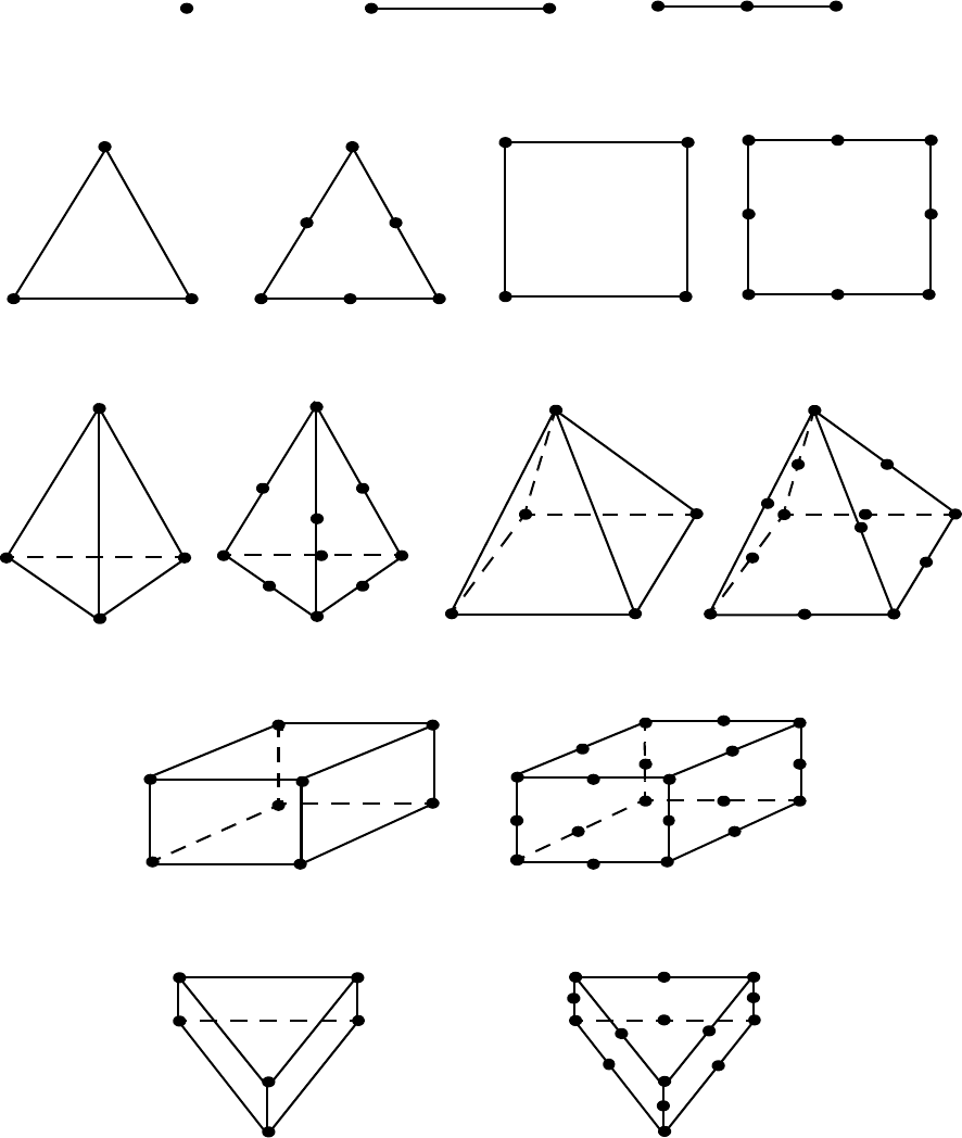
9.3 EnSight5 General Description
EnSight 10.2 User Manual 9-139
Supported EnSight5 Elements
The elements that are supported by the EnSight5 format are:
eight node hexahedron twenty node hexahedron
six node pentahedron
9
10
7
8
12123
12
3
12
3
4
56
1
2
3
4
12
3
45 6
7
8
12
3
4
5
6
1
2
3
4
5
6
910
7
8
1
2
3
4
56
11
12
13 14
15
16
17 18
19
20
two node bar three node bar
three node triangle six node triangle four node quadrangle eight node quadrangle
four node tetrahedron ten node tetrahedron
1
point
12
3
4
1
4
8
2
3
5
6
7
5 node pyramid 13 node pyramid
11
22
33
44
55
6
7
8
9
10
11
12
13
fifteen node pentahedron (wedge)
1
2
3
4
5
6
78
9
10 11
12
13
14
15
(wedge)
Figure 9-5
Supported EnSight5 Elements
9.3 EnSight5 Geometry File Format
9-140 EnSight 10.2 User Manual
EnSight5 Geometry File Format
The EnSight5 format consists of keywords followed by information. The
following items are important to remember when working with EnSight5
geometry files:
1. You do not have to assign node IDs. If you do, the element connectivities are
based on the node numbers. If you let EnSight assign the node IDs, the nodes
are considered to be sequential starting at node 1, and element connectivity is
done accordingly. If node IDs are set to off, they are numbered internally;
however, you will not be able to display or query on them. If you have node
IDs in your data, you can have EnSight ignore them by specifying “node id
ignore.” Using this option may reduce some of the memory taken up by the
Client and Server, but remember that display and query on the nodes will not
be available.
2. You do not need to specify element IDs. If you specify element IDs, or you let
EnSight assign them, you can show them on the screen. If they are set to off,
you will not be able to show or query on them. If you have element IDs in
your data you can have EnSight ignore them by specifying “element id
ignore.” Using this option will reduce some of the memory taken up by the
Client and Server. This may or may not be a significant amount, and
remember that display and query on the elements will not be available.
3. The format of integers and real numbers must be followed (See the Geometry
Example below).
4. Integers are written out using the following integer format:
From C:
8d
format
From FORTRAN:
i8
format
Real numbers are written out using the following floating-point format:
From C:
12.5e
format
From FORTRAN:
e12.5
format
The number of integers or reals per line must also be followed!
5. By default, a Part is processed to show the outside boundaries. This
representation is loaded to the Client host system when the geometry file is
read (unless other attributes have been set on the workstation, such as feature
angle).
6. Coordinates must be defined before any Parts can be defined. The different
elements can be defined in any order (that is, you can define a hexa8 before a
bar2).
Generic Format Not all of the lines included in the following generic example file are necessary:
description line 1
description line 2
node id <off/given/assign/ignore>
element id <off/given/assign/ignore>
coordinates
# of points
id x y z
id x y z
9.3 EnSight5 Geometry File Format
EnSight 10.2 User Manual 9-141
id x y z
.
.
.
part #
description line
point
number of points
id nd
id nd
id nd
.
.
.
bar2
number of bar2’s
id nd nd
id nd nd
id nd nd
.
.
.
bar3
number of bar3’s
id nd nd nd
id nd nd nd
id nd nd nd
.
.
.
tria3
number of three node triangles
id nd nd nd
id nd nd nd
id nd nd nd
.
.
.
tria6
number of six node triangles
id nd nd nd nd nd nd
.
.
.
quad4
number of quad 4’s
id nd nd nd nd
id nd nd nd nd
id nd nd nd nd
id nd nd nd nd
.
.
.
quad8
number of quad 8’s
id nd nd nd nd nd nd nd nd
id nd nd nd nd nd nd nd nd
id nd nd nd nd nd nd nd nd
id nd nd nd nd nd nd nd nd
.
.
9.3 EnSight5 Geometry File Format
9-142 EnSight 10.2 User Manual
.
tetra4
number of 4 node tetrahedrons
id nd nd nd nd
id nd nd nd nd
id nd nd nd nd
id nd nd nd nd
.
.
.
tetra10
number of 10 node tetrahedrons
id nd nd nd nd nd nd nd nd nd nd
id nd nd nd nd nd nd nd nd nd nd
id nd nd nd nd nd nd nd nd nd nd
id nd nd nd nd nd nd nd nd nd nd
.
.
.
pyramid5
number of 5 node pyramids
id nd nd nd nd nd
id nd nd nd nd nd
id nd nd nd nd nd
id nd nd nd nd nd
.
.
.
pyramid13
number of 13 node pyramids
id nd nd nd nd nd nd nd nd nd nd nd nd nd
id nd nd nd nd nd nd nd nd nd nd nd nd nd
id nd nd nd nd nd nd nd nd nd nd nd nd nd
id nd nd nd nd nd nd nd nd nd nd nd nd nd
.
.
.
hexa8
number of 8 node hexahedrons
id nd nd nd nd nd nd nd nd
id nd nd nd nd nd nd nd nd
id nd nd nd nd nd nd nd nd
id nd nd nd nd nd nd nd nd
.
.
.
hexa20
number of 20 node hexahedrons
id nd nd nd nd nd nd nd nd nd nd nd nd nd nd nd nd nd nd nd nd
id nd nd nd nd nd nd nd nd nd nd nd nd nd nd nd nd nd nd nd nd
id nd nd nd nd nd nd nd nd nd nd nd nd nd nd nd nd nd nd nd nd
id nd nd nd nd nd nd nd nd nd nd nd nd nd nd nd nd nd nd nd nd
id nd nd nd nd nd nd nd nd nd nd nd nd nd nd nd nd nd nd nd nd
.
.
.
penta6
number of 6 node pentahedrons
id nd nd nd nd nd nd
id nd nd nd nd nd nd
id nd nd nd nd nd nd
9.3 EnSight5 Geometry File Format
EnSight 10.2 User Manual 9-143
id nd nd nd nd nd nd
id nd nd nd nd nd nd
.
.
.
penta15
number of 15 node pentahedrons
id nd nd nd nd nd nd nd nd nd nd nd nd nd nd nd
id nd nd nd nd nd nd nd nd nd nd nd nd nd nd nd
id nd nd nd nd nd nd nd nd nd nd nd nd nd nd nd
id nd nd nd nd nd nd nd nd nd nd nd nd nd nd nd
id nd nd nd nd nd nd nd nd nd nd nd nd nd nd nd
.
.
.
EnSight5 Geometry The following is an example of an EnSight geometry file:
Example
this is an example problem
this is the second description line
node id given
element id given
coordinates
10
5 1.00000e+00 0.00000e+00 0.00000e+00
100 0.00000e+00 1.00000e+00 0.00000e+00
200 0.00000e+00 0.00000e+00 1.00000e+00
40 1.00000e+00 1.00000e+00 0.00000e+00
22 1.00000e+00 0.00000e+00 1.00000e+00
1000 2.00000e+00 0.00000e+00 0.00000e+00
55 0.00000e+00 2.00000e+00 0.00000e+00
44 0.00000e+00 0.00000e+00 2.00000e+00
202 2.00000e+00 2.00000e+00 0.00000e+00
101 2.00000e+00 0.00000e+00 2.00000e+00
part 1
This is Part 1, a pretty strange Part
tria3
2
101 100 200 40
201 101 5 1000
tetra4
1
102 100 202 101 1000
part 2
This is Part 2, it is pretty strange also
bar2
1
103 101 1000
9.3 EnSight5 Result File Format
9-144 EnSight 10.2 User Manual
EnSight5 Result File Format
The Result file is an ASCII free format file that contains variable and time step
information that pertains to a Particular geometry file. The following information
is included in this file:
• Number of scalar variables
• Number of vector variables
• Number of time steps
• Starting file number extension and skip-by value
• Flag that specifies whether there is changing geometry
• Names of the files that contain the values of scalar and vector variables
• The names of the geometry files that will be used for the changing
geometry.
The format of the EnSight5 result file is as follows:
•Line 1
Contains the number of scalar variables, the number of vector variables
and a geometry-changing flag. (If the geometry-changing flag is 0, the
geometry of the model does not change over time. If it is 1, then there is
connectivity changing geometry. If it is 2, then there is coordinate only
changing geometry.)
•Line 2
Indicates the number of time steps that are available.
•Line 3
Lists the time that is associated with each time step. There must be the
same number of values as are indicated in Line 2. This “line” can actually
span several lines in the file. You do not have to have one very long line.
•Line 4
Specified only if more than one time step is indicated in Line 2. The two
values on this line indicate the file extension value for the first time step
and the offset between files. If the values on this line are 0 5, the first time
step available has a subscript of 0, the second time step available has a
subscript of 5, the third time step has a subscript of 10, and so on.
•Line 5
Contains the names of the geometry files that will be used for changing
geometry. This line exists only if the flag on Line 1 is set to 1 or 2. The
geometry file name must follow the EnSight5 wild card specification.
• Line 6 through Line [5+N] where N is the number of scalar variables
specified in Line 1.
List BOTH the file names AND variable description that correspond to
each scalar variable. There must be a file name for each scalar variable
that is specified in Line 1.
9.3 EnSight5 Result File Format
EnSight 10.2 User Manual 9-145
If there is more than one time step, the file name must follow the
EnSight5 wild card specification. See Note below.
• Lines that follow the scalar variable files.
List the file names that correspond to each vector variable. There must be
a file name for each vector variable that is specified in Line 1. If there is
more than one time step, the file name must follow the EnSight5 wild
card specification. See Note below.
Note: Variable descriptions have the following restrictions:
The maximum variable name length is documented at the beginning of this
chapter.
Duplicate variable descriptions are not allowed.
Leading and trailing white space will be eliminated.
Variable descriptions must not start with a numeric digit.
Variable descriptions must not contain any of the following reserved characters:
( [ + @ ! * $
) ] - space # ^ /
The generic format of a result file is as follows:
#_of_scalars #_of_vectors geom_chang_flag
#_of_timesteps
time1 time2 time3 .....
start_file_# skip_by_value
geometry_file_name.geo**
scalar0_file_name** description (19 characters max)
scalar1_file_name** description
.
.
.
vector0_file_name** description (19 characters max)
vector1_file_name** description
.
EnSight5 Result
File Example 1 The following example illustrates a result file specified for a non-changing
geometry file with only one time step:
2 1 0
1
0.0
exone.scl0 pressure
exone.scl1 temperature
exone.dis0 velocity
EnSight5 Result
File Example 2 This example illustrates a result file that specifies a connectivity changing
geometry that has multiple time steps.
1 2 1
4
1.0 2.0 2.5 5.0
0 1
extwo.geom**
pres.scl** pressure
vel.dis** velocity
grad.dis** gradient
9.3 EnSight5 Variable File Format
9-146 EnSight 10.2 User Manual
The following files would be needed for example 2:
extwo.geom00 pres.scl00 vel.dis00 grad.dis00
extwo.geom01 pres.scl01 vel.dis01 grad.dis01
extwo.geom02 pres.scl02 vel.dis02 grad.dis02
extwo.geom03 pres.scl03 vel.dis03 grad.dis03
EnSight5 Wild Card Name Specification
If multiple time steps are involved, the file names must conform to the EnSight5
wild-card specification. This specification is as follows:
• File names must include numbers that are in ascending order from
beginning to end.
• Numbers in the files names must be zero filled if there is more than one
significant digit.
• Numbers can be anywhere in the file name.
• When the file name is specified in the EnSight5 result file, you must
replace the numbers in the file with an asterisk(*). The number of
asterisks specified is the number of significant digits. The asterisk must
occupy the same place as the numbers in the file names.
EnSight5 Variable File Format
Variables files have one description line followed by a value for each node. For a
scalar file there is one value per node, while for vector files there are three values
per node.
The values must be written in the following floating point format (6 per line as
shown in the examples below):
From C:
12.5e
format
From FORTRAN:
e12.5
format
The format of a variables file is as follows:
•Line 1
This line is a description line.
• Line 2 through the end of the file contains the values at each node in the
model. A generic example:
A description line
*.*****E+** *.*****E+** *.*****E+** *.*****E+** *.*****E+** *.*****E+**
*.*****E+** *.*****E+** *.*****E+** *.*****E+** *.*****E+** *.*****E+**
*.*****E+** *.*****E+** *.*****E+** *.*****E+** *.*****E+** *.*****E+**
EnSight5 Variable
File Example 1 This example shows a scalar file for a geometry with seven defined nodes.
These are the pressure values for a 7 node geometry
1.00000E+00 2.00000E+00 3.00000E+00 4.00000E+00 5.00000E+00 6.00000E+00
7.00000E+00
EnSight5 Variable
File Example 2 This example shows the vector file for a geometry with seven defined nodes.
These are the velocity values for a 7 node geometry
9.3 EnSight5 Measured/Particle File Format
EnSight 10.2 User Manual 9-147
1.00000E+00 1.00000E+00 1.00000E+00 2.00000E+00 2.00000E+00 2.00000E+00
3.00000E+00 3.00000E+00 3.00000E+00 4.00000E+00 4.00000E+00 4.00000E+00
5.00000E+00 5.00000E+00 5.00000E+00 6.00000E+00 6.00000E+00 6.00000E+00
7.00000E+00 7.00000E+00 7.00000E+00
EnSight5 Measured/Particle File Format
This file allows you to define Particle locations, sizes, etc. to display with the
geometry. Typical uses are fuel droplets for combustion analysis or data derived
from experiments on prototypes.
The measured/Particle files consist of the following:
• Measured/Particle geometry file (referenced by the measured results file)
• Measured/Particle results file (the filename, typically with a .mea suffix,
which is put into the Data Reader’s “(Set) Measured” field)
• Measured/Particle variables file (referenced by the measured results file)
which is the same format as an EnSight 5 variable file.
The format of the EnSight5 Measured/Particle geometry file is described below.
Note that there is only one description line and there must be an ID for each
measured point.
Note also that the number of Particles can be different in each of the geometry file
(if you have transient data), however, the number of values in each of the
corresponding variable files must coincide, and the IDs of the Particles must be
consistent in order to track the Particles at intermediate times or locations.
The format of an EnSight5 Measured/Particle geometry file is as follows:
•Line 1
This line is a description line.
•Line 2
Indicates that this file contains Particle coordinates. The words “particle
coordinates” should be entered on this line without the quotes.
•Line 3
Specifies the number of Particles.
• Line 4 through the end of the file.
Each line contains the ID and the X, Y, and Z coordinates of each Particle.
The format of this line is “integer real real real” written out in the
following format:
From C:
%8d%12.5e%12.5e%12.5e
format
From FORTRAN:
i8, 3e12.5
format
A generic measured/Particle geometry file is as follows:
A description line
particle coordinates
#_of_Particles
9.3 EnSight5 Measured/Particle File Format
9-148 EnSight 10.2 User Manual
id xcoord ycoord zcoord
id xcoord ycoord zcoord
id xcoord ycoord zcoord
.
.
.
EnSight5 Measured
Geometry/Particle The following illustrates an EnSight5 Measured Geometry/Particle file with seven
File Example points:
This is a simple ensight5 measured geometry/particle file
particle coordinates
7
101 0.00000E+00 0.00000E+00 0.00000E+00
102 1.00000E+00 0.00000E+00 0.00000E+00
103 1.00000E+00 1.00000E+00 0.00000E+00
104 0.00000E+00 1.00000E+00 0.00000E+00
205 5.00000E-01 0.00000E+00 2.00000E+00
206 5.00000E-01 1.00000E+00 2.00000E+00
307 0.00000E+00 0.00000E+00-1.50000E+00
EnSight5 Measured/ The format of the EnSight5 Measured/Particle results file (typically a .mea suffix)
is as follows:
Particle File Format
•Line 1
Contains the number of scalar variables, the number of vector variables,
and a measured geometry changing flag. If the measured geometry
changing flag is 0, only one time step is indicated.
•Line 2
Indicates the number of available time steps.
•Line 3
Lists the time that is associated with each time step. The time step
information does not have to coincide with the model time step
information. This “line” can actually span several lines in the file. You do
not have to have one very long line.
•Line 4
Specified only if Line 2 specifies more than one time step. The line
contains two values; the first value indicates the file extension value for
the first time step, and the second value indicates the offset between files.
If this line contains the values 0 and 5, the first time step has a subscript of
0, the second of 5, the third of 10, and so on.
•Line 5
Contains the name of the measured geometry file. If there is more than
one time step, the file name must follow the EnSight wild card
specification.
• Line 6 through Line [5+N] where N is the number of scalar variables
specified in Line 1.
9.3 EnSight5 Measured/Particle File Format
EnSight 10.2 User Manual 9-149
List the file names that correspond to each scalar variable. There must be
a file name for each scalar variable that is specified in Line 1. If there is
more than one time step, the file name must follow the EnSight wild card
specification.
• Lines that follow the scalar variable files.
List the names of the files that correspond to each vector variable. There
must be a file name for each vector variable that is specified in Line 1. If
there is more than one time step, the file name must follow the EnSight
wild card specification.
A generic EnSight5 Measured/Particle results file is as follows:
#_of_scalars #_of_vectors geom_chang_flag
#_of_timesteps
time1 time2 time3 .....
start_file_# skip_by_value
measured_geom_file_name**
scalar0_file_name** description
scalar1_file_name** description
.
.
.
vector0_file_name** description
vector1_file_name** description
.
.
.
Measured/Particle
Results File This example illustrates an EnSight5 Measured/Particle result file that specifies a
Example 1 non-changing geometry with only one time step:
2 1 0
1
0.0
exone.geom
exone.scl0 pressure
exone.scl1 temperature
exone.dis0 velocity
Measured/Particle
Results File This example illustrates an EnSight5 Measured/Particle result file that specifies a
Example 2 changing geometry with multiple time steps:
1 2 1
4
1.0 2.0 2.5 5.0
0 1
extwo.geom**
pres.scl** pressure
vel.dis** velocity
grad.dis** gradient
The following files are needed for Example 2:
extwo.geom00pres.scl00vel.dis00 grad.dis00
extwo.geom01pres.scl01vel.dis01 grad.dis01
extwo.geom02pres.scl02vel.dis02 grad.dis02
extwo.geom03pres.scl03vel.dis03 grad.dis03
9.3 Writing EnSight5 Binary Files
9-150 EnSight 10.2 User Manual
Measured /Particle The EnSight5 Measured/Particle variable files referred to in the measured Results
Results Variable files file follow the same format as EnSight5 Variable files. The number of values in
each of these variable files must correspond properly to the number of Particles in
the corresponding measured geometry files.
Writing EnSight5 Binary Files
This section describes the EnSight5 binary files. This format is used to increase
the speed of reading data into EnSight. A utility exists for converting EnSight5
ASCII files to EnSight5 binary files—it is called asciitobin5 and is found on the
release tape under ensight/server/utilities/asciitobin5.
For binary files, there is a header that designates the type of binary file. This
header is: “C Binary” or “Fortran Binary.” This must be the first thing in the file.
The format for the file is then essentially the same format as the ASCII format,
with the following exceptions:
The ASCII format puts the node and element ids on the same “line” as the
corresponding coordinates. The BINARY format writes all node id’s then
all coordinates.
The ASCII format puts all element id’s of a type within a Part on the same
“line” as the corresponding connectivity. The BINARY format writes all
the element ids for that type, then all the corresponding connectivities of
the elements.
In all the descriptions of binary files that follow, the number on the left end of the
line corresponds to the type of write of that line, according to the following code:
1. This is a write of 80 characters to the file:
C example:
char buffer[80];
strcpy(buffer,”C Binary”);
fwrite(buffer,sizeof(char),80,file_ptr);
FORTRAN:
character*80 buffer
buffer = “Fortran Binary”
write(10) buffer
2. This is a write of a single integer:
C example:
fwrite(&num_nodes,sizeof(int),1,file_ptr);
FORTRAN:
write(10) num_nodes
3. This is a write of an integer array:
C example:
fwrite(node_ids,sizeof(int),num_nodes,file_ptr);
FORTRAN:
write(10) (node_ids(i),i=1,num_nodes)
4. This is a write of a float array:
C example:
fwrite(coords,sizeof(float),3*num_nodes,file_ptr);
9.3 Writing EnSight5 Binary Files
EnSight 10.2 User Manual 9-151
FORTRAN:
write(10) ((coords(i,j),i=1,3),j=1,num_nodes)
(Note: Coords is a single precision array, double precision will not work!)
EnSight5 Binary
Geometry File Format An EnSight5 binary geometry file contains information in the following order:
(1) <C Binary/Fortran Binary>
(1) description line 1
(1) description line 2
(1) node id <given/off/assign/ignore>
(1) element id <given/off/assign/ignore>
(1) coordinates
(2) #_of_points
(3) [point_ids]
(4) coordinate_array
(1) part #
(1) description line
(1) element_type
(2) #_of_element_type
(3) [element_ids] for the element_type
(3) connectivities for the element_type
(1) element_type
(2) #_of_element_type
(3) [element_ids] for the element_type
(3) connectivities for the element_type
.
.
.
(1) part #
(1) description line
(1) element_type
(2) #_of_element_type
(3) [element_ids] for the element_type
(3) connectivities for the element_type
(1) element_type
(2) #_of_element_type
(3) [element_ids] for the element_type
(3) connectivities for the element_type
.
.
.
Binary Scalar An EnSight5 binary scalar file contains information in the following order:
(1) description line
(4) scalar_array
Binary Vector An EnSight5 binary vector file contains information in the following order:
(1) description line
9.3 Writing EnSight5 Binary Files
9-152 EnSight 10.2 User Manual
(4) vector_array
Binary Measured An EnSight5 binary measured/Particle geometry file contains information in the
following order:
(1) <C Binary/Fortran Binary>
(1) description line 1
(1) particle coordinates
(2) #_of_points
(3) point_ids
(4) coordinate_array
9.4 FAST UNSTRUCTURED Results File Format
EnSight 10.2 User Manual 9-153
9.4 FAST UNSTRUCTURED Results File Format
FAST UNSTRUCTURED input data consists of the following:
• Geometry file (required) (GRID file).
• Results file (optional).
•EnSight5 Measured/Particle Files (optional). The measured .res file
references the measured geometry and variable files.
FAST UNSTRUCTURED data files can be read as:
Workstation: ASCII, C Binary, or FORTRAN binary
Cray: ASCII, C Binary, or COS-Blocked FORTRAN binary
Due to the different number of representations on a Cray Research vector system
and workstations, binary files created on a Cray Research vector system can not
be read on the workstation, and visa versa.
EnSight reads the geometry (grid files) directly. However, an EnSight-like results
file is needed in order to read the results unless a “standard” Q-file is provided in
its place. See FAST UNSTRUCTURED Result File below.
FAST UNSTRUCTURED Geometry file notes
Only the single zone format can be read into EnSight. Any tetrahedral elements
will be placed into the first “domain” Part. Triangular elements are placed into
Parts based on their “tag” value.
The FAST UNSTRUCTURED solution file or function file formats can be used
for variable results. The I J K values need to be I=Number of points and J=K=1.
This does require the use of a modified EnSight results file as explained below.
Node and element numbers are assigned sequentially allowing for queries to be
made within EnSight. Tetrahedron elements will be assigned before triangular
elements.
FAST UNSTRUCTURED Result file format
The FAST UNSTRUCTURED result file was defined by CEI and is very similar
to the EnSight results file and contains information needed to relate variable
names to variable files, step information, etc. There is a slight variation from the
normal EnSight results file because of the differences between the solution (Q
file) and function files. The difference lies on the lines which relate variable
filenames to a description. These lines have the following format:
<filename> <type> <number(s)> <description>
See FAST UNSTRUCTURED Result File below for the definition of each.
The following information is included in a FAST UNSTRUCTURED result file:
• Number of scalar variables
• Number of vector variables
• Number of time steps
9.4 FAST UNSTRUCTURED Results File Format
9-154 EnSight 10.2 User Manual
• Starting file number extension and skip-by value
• Flag that specifies whether there is changing geometry.
• Names of the files that contain the values of scalar and vector variables.
An indication as to the type of the file being used for the variable, which
variable in the file and the name given to that variable.
• The names of the geometry files that will be used for the changing
geometry.
Generic FAST UNSTRUCTURED Result File Format
The format of the Result file is as follows:
•Line 1
Contains the number of scalar variables, the number of vector variables
and a geometry changing flag. If the geometry changing flag is 0, the
geometry of the model does not change over time. If the flag is 1, the
geometry can change connectivity. If the flag is 2, only coordinates can
change.
•Line 2
Indicates the number of time steps that are available. If this number is
positive, then line 3 information must be present. If this number is
negative, then Line 3 information must not be present and the times will
be read from the solution file. Thus, one must have a solution file in one
of the lines from Line 6 on.
•Line 3
Lists the time that is associated with each time step. There must be the
same number of values as are indicated in Line 2. This “line” can actually
span several lines in the file. Specify only if Line 2 value is positive.
•Line 4
Specified only if more than one time step is indicated in Line 2. The two
values on this line indicate the file extension value for the first time step
and the offset between files. If the values on this line are 0 5, the first time
step available has a subscript of 0, the second time step available has a
subscript of 5, the third time step has a subscript of 10, and so on.
•Line 5
This line exists only if the changing geometry flag on Line 1 has been set
to 1 or 2. Line contains name of the FAST UNSTRUCTURED grid file.
The file name must follow the EnSight wild card specification.
• Line 6 through Line [5+N] where N is the number of scalar variables
specified in Line 1.
List the file names that correspond to each scalar variable. There must be
a file name for each scalar variable that is specified in Line 1. If there is
more than one time step, the file name must follow the EnSight wild card
specification.
These lines also contain the type of file being used, solution or function,
and the location of the variable value in the file. The contents are:
9.4 FAST UNSTRUCTURED Results File Format
EnSight 10.2 User Manual 9-155
<filename> <type> <number> <description>
where filename is the name of solution file or function file containing the
variable; type is “S” for solution file, or “F” for function file; numberis
which variable in the file to use (specify just one number); and
description
is the Description of the variable.
The solution file (“s”) is the traditional .q file in which normally the first
variable is density, the second through fourth variables are the
components of momentum, and the fifth variable is total energy.
• Lines that follow the scalar variable files.
List the file names that correspond to each vector variable. There must be
a file name for each vector variable that is specified in Line 0. If there is
more than one time step, the file name must follow the EnSight wild card
specification.
These lines also contain the type of file being used, solution or function,
and the location(s) of the variable values in the file. The contents are:
<filename> <type> <numbers> <description>
where filename is the name of solution file or function file containing the
variable; type is “S” for solution file, or “F” for function file; numbersare
which variables in the file to use (specify just three numbers); and
description is the Description of the variable.
The generic format of the result file is as follows:
#_of_scalars #_of_vectors geom_chng_flag
#_of_timesteps
time1 time2 time3 .....
start_file_# skip_by_value
geometry_file_name.geo**
scalar0_file_name** type # description
scalar1_file_name** type # description
.
.
.
vector0_file_name** type # # # description
vector1_file_name** type # # # description
.
.
.
FAST UNSTRUCTURED This example illustrates a result file that specifies a non-changing geometry with
Example only one time step.
3 2 0
1
0.0
block.sol S 1 Density
block.sol S 5 Total_Energy
block.scl F 1 Temperature
block.var F 1 2 3 Displacement
block.sol S 2 3 4 Momentum
Thus, this model will get two scalars from the solution file (block.sol). The first is
Density in the first location in the file and the next is Total energy in the fifth
9.4 FAST UNSTRUCTURED Results File Format
9-156 EnSight 10.2 User Manual
location in the solution file. It will also get a Temperature scalar from the first
location in the function file (block.scl).
It will get a Displacement vector from the function file called block.var. The three
components of this vector are in the 1st, 2nd, and 3rd locations in the file. Finally,
a Momentum vector will be obtained from the 2nd, 3rd, and 4th locations of the
solution file.
Example 2 is somewhat similar, except that it is transient, with coordinate
changing geometry. Note also that the times will come from the solution file.
3 2 2
-10
0 1
block***.grid
block***.sol S 1 Density
block***.sol S 5 Total_Energy
block***.scl F 1 Temperature
block***.var F 1 2 3 Displacement
block***.sol S 2 3 4 Momentum
9.5 FLUENT UNIVERSAL Results File Format
EnSight 10.2 User Manual 9-157
9.5 FLUENT UNIVERSAL Results File Format
This section describes the FLUENT results file format and provides an example of
this file. For transient cases, you must supply this result file. For static models this
file is not required. The FLUENT result file is a slightly modified EnSight5
results file and provides a way to describe multiple time-step FLUENT Universal
files to EnSight.
When using multiple FLUENT files with this result file definition, you must make
sure that the files contain the same defined variables. In other words, any variable
that exists in one must exist in all.
The Result file is an ASCII free format file that contains time step and universal
file information for each available time step. The following information is
included in this file:
• Number of time steps
• Simulation Time Values
• Starting file number extension and skip-by value
• Name of the universal file with EnSight wild card specification.
The format of the Result file is as follows:
•Line 1
Indicates the number of time steps that are available.
•Line 2
Lists the time that is associated with each time step. There must be the
same number of values as are indicated in Line 1. This “line” can actually
span several lines in the file. You do not have to have one very long line.
•Line 3
Specified only if more than one time step is indicated in Line 1. The two
values on this line indicate the file extension value for the first time step
and the offset between files. If the values on this line are 0 5, the first time
step available has a subscript of 0, the second time step available has a
subscript of 5, the third time step has a subscript of 10, and so on.
•Line 4
Contains the names of the universal file that will be used for the changing
time step information. The universal file name must follow the EnSight5
wild card specification.
The generic format of the result file is as follows:
#_of_timesteps
time1 time2 time3 .....
start_file_# skip_by_value
universal_file_name***
9.6 Movie.BYU Results File Format
EnSight 10.2 User Manual 9-159
9.6 Movie.BYU Results File Format
For transient cases, you must supply an EnSight result file. The result file for the
Movie.BYU case is exactly the same as for EnSight5 (it is repeated below for
your ease).
The Result file is an ASCII free format file that contains variable and time step
information that pertains to a Particular geometry file. The following information
is included in this file:
• Number of scalar variables
• Number of vector variables
• Number of time steps
• Starting file number extension and skip-by value
• Flag that specifies whether there is changing geometry
• Names of the files that contain the values of scalar and vector variables
• The names of the geometry files that will be used for the changing
geometry.
The format of the Movie.BYU (EnSight5) result file is as follows:
•Line 1
Contains the number of scalar variables, the number of vector variables
and a geometry-changing flag. (If the geometry-changing flag is 0, the
geometry of the model does not change over time. If it is 1, then there is
connectivity changing geometry. If it is 2, then there is coordinate only
changing geometry.)
•Line 2
Indicates the number of time steps that are available.
•Line 3
Lists the time that is associated with each time step. There must be the
same number of values as are indicated in Line 2. This “line” can actually
span several lines in the file. You do not have to have one very long line.
•Line 4
Specified only if more than one time step is indicated in Line 2. The two
values on this line indicate the file extension value for the first time step
and the offset between files. If the values on this line are 0 5, the first time
step available has a subscript of 0, the second time step available has a
subscript of 5, the third time step has a subscript of 10, and so on.
•Line 5
Contains the names of the geometry files that will be used for changing
geometry. This line exists only if the flag on Line 1 is set to 1 or 2. The
geometry file name must follow the EnSight5 wild card specification.
• Line 6 through Line [5+N] where N is the number of scalar variables
specified in Line 1.
9.6 Movie.BYU Results File Format
9-160 EnSight 10.2 User Manual
List BOTH the file names AND variable description that correspond to
each scalar variable. There must be a file name for each scalar variable
that is specified in Line 1.
If there is more than one time step, the file name must follow the
EnSight5 wild card specification. See Note below.
• Lines that follow the scalar variable files.
List the file names that correspond to each vector variable. There must be
a file name for each vector variable that is specified in Line 1. If there is
more than one time step, the file name must follow the EnSight5 wild
card specification. See Note below.
Note: Variable descriptions have the following restrictions:
The maximum variable name length is documented at the beginning of this
chapter.
Duplicate variable descriptions are not allowed.
Leading and trailing white space will be eliminated.
Variable descriptions must not start with a numeric digit.
Variable descriptions must not contain any of the following reserved characters:
( [ + @ ! * $
) ] - space # ^ /
The generic format of a result file is as follows:
#_of_scalars #_of_vectors geom_chang_flag
#_of_timesteps
time1 time2 time3 .....
start_file_# skip_by_value
geometry_file_name.geo**
scalar0_file_name** description (19 characters max)
scalar1_file_name** description
.
.
.
vector0_file_name** description (19 characters max)
vector1_file_name** description
.
Movie.BYU Result
File Example 1 The following example illustrates a result file specified for a non-changing
geometry file with only one time step:
2 1 0
1
0.0
exone.scl0 pressure
exone.scl1 temperature
exone.dis0 velocity
Movie.BYU Result
File Example 2 This example illustrates a result file that specifies a connectivity changing
geometry that has multiple time steps.
1 2 1
4
1.0 2.0 2.5 5.0
0 1
9.6 Movie.BYU Results File Format
EnSight 10.2 User Manual 9-161
extwo.geom**
pres.scl** pressure
vel.dis** velocity
grad.dis** gradient
The following files would be needed for example 2:
extwo.geom00 pres.scl00 vel.dis00 grad.dis00
extwo.geom01 pres.scl01 vel.dis01 grad.dis01
extwo.geom02 pres.scl02 vel.dis02 grad.dis02
extwo.geom03 pres.scl03 vel.dis03 grad.dis03
9.7 PLOT3D Results File Format
9-162 EnSight 10.2 User Manual
9.7 PLOT3D Results File Format
PLOT3D input data consists of the following:
• Geometry file (required) (GRID file).
• Results file (optional).
•EnSight5 Measured/Particle Files (optional). The measured .res file
references the measured geometry and variable files.
PLOT3D data files can be read as:
Workstation: ASCII, C Binary, or FORTRAN binary
Cray: ASCII, C Binary, or COS-Blocked FORTRAN binary
(see PLOT3D Reader, in Section 2.3)
Due to the different number of representations on a Cray Research vector system
and workstations, binary files created on a Cray Research vector system can not
be read on the workstation, and visa versa.
EnSight attempts to ensure that the format of the file being read matches the
format you have selected in the Data Reader dialog. However, if you specify that
the file is C binary, and it is really FORTRAN binary, this will not be detected and
erroneous values will be loaded.
EnSight reads the geometry (xyz files) directly. However, an EnSight-like results
file (described below) is needed in order to read the results, unless a “standard” Q-
file is provided in its place.
PLOT3D Geometry file notes
The following information is required in order to read PLOT3D files correctly:
1. whether there is Iblanking information in the file
2. whether files are in ASCII, C Binary, or FORTRAN binary
3. whether the file is “Single Zone” or Multi-Zoned”
4. whether the model is 1D, 2D, or 3D in nature.
Iblanking can be one of the following:
0 = Outside (Blanked Out)
1 = Inside
2 = Interior boundaries
<0 = zone that neighbors
If single zone with Iblanking, you can build EnSight Parts from the inside
portions, blanked-out portions, or internal boundary portions. If single zone, you
can also specify I, J, K limiting ranges for Parts to be created.
If Multi-zoned with Iblanking, you can additionally build Parts that are the
boundary between two zones. (For boundary you must specify exactly two zones.)
If Multi-zoned and not using the “between boundary” option, a Part can span
several zones.
9.7 PLOT3D Results File Format
EnSight 10.2 User Manual 9-163
If Multi-zoned, the dimension of the problem is forced to be 3D.
There can be nodes in different zones which have the same coordinates. No
attempt has been made to merge these. Thus, on shared zone boundaries, there
will likely be nodes on top of nodes. One negative effect of this is that node labels
will be on top of each other.
Currently EnSight only prints out the global conditions in the solution file,
fsmach, alpha, re, and time. It does not do anything else with them.
Node and element numbers are assigned in a sequential manner. Queries can be
made on these node and element numbers or on nodes by I, J, and K.
PLOT3D Result file format
The PLOT3D result file was defined by CEI and is very similar to the EnSight
results file and contains information needed to relate variable names to variable
files, step information, etc. There is a slight variation from the normal EnSight
results file because of the differences between the solution (Q file) and function
files. The difference lies on the lines which relate variable filenames to a
description. These lines have the following format:
<filename> <type> <number(s)> <description>
See PLOT3D Result File below for the definition of each.
The following information is included in a PLOT3D result file:
• Number of scalar variables
• Number of vector variables
• Number of time steps
• Starting file number extension and skip-by value
• Flag that specifies whether there is changing geometry.
• Names of the files that contain the values of scalar and vector variables.
An indication as to the type of the file being used for the variable, which
variable in the file and the name given to that variable.
• The names of the geometry files that will be used for the changing
geometry.
Generic PLOT3D Result File Format
The format of the Result file is as follows:
• Optional first line, Line 0
Contains the maximum, never-to-exceed number of timesteps. This is
used if the number of timesteps is changing over time, perhaps being
written out by a solver. Your first load of the data might include a few of
the timesteps. The presence of this keyword indicates that the user may
request an update and the reader may update the number of timesteps
available in EnSight. The value entered is an integer number of timesteps.
9.7 PLOT3D Results File Format
9-164 EnSight 10.2 User Manual
•Line 1
Contains the number of scalar variables, the number of vector variables
and a geometry changing flag. If the geometry changing flag is 0, the
geometry of the model does not change over time. Only the coordinates
can change for a PLOT3D file at present time.
•Line 2
Indicates the number of time steps that are available.
Note: if this number is positive, then EnSight will assign the time values
listed in Line 3 to the Analysis_Time constant variable. If this value is
negative, the time values in Line 3 must be removed and EnSight will
assign the TIME (or Tvref for OVERFLOW restart q-file(s) ) value from
the header of the q-file(s) to the Analysis_Time constant variable. This is
noted under PLOT3D and/or OVERFLOW readers (see Section 2.3,
Other Readers).
•Line 3
Lists the time that is associated with each time step. There must be the
same number of values as are indicated in Line 2. This “line” can actually
span several lines in the file. (Exists if Line 2 is a positive, non-zero
value).
•Line 4
Specified only if more than one time step is indicated in Line 2. The two
values on this line indicate the file extension value for the first time step
and the offset between files. If the values on this line are 0 5, the first time
step available has a subscript of 0, the second time step available has a
subscript of 5, the third time step has a subscript of 10, and so on.
•Line 5
This line exists only if the changing geometry flag on Line 1 has been set
to 1. Line contains name of the PLOT3D xyz file. The file name must
follow the EnSight wild card specification.
• Line 6 through Line [5+N] where N is the number of scalar variables
specified in Line 1.
List the file names that correspond to each scalar variable. There must be
a file name for each scalar variable that is specified in Line 1. If there is
more than one time step, the file name must follow the EnSight wild card
specification.
These lines also contain the type of file being used, solution or function,
and the location of the variable value in the file. The contents are:
<filename> <type> <number> <description>
where filename is the name of solution file or function file containing the
variable; type is “S” for solution file, or “F” for function file; numberis
which variable in the file to use (specify just one number); and description
is the Description of the variable.
The solution file (“s”) is the traditional .q file in which normally the first
variable is density, the second through fourth variables are the
9.7 PLOT3D Results File Format
EnSight 10.2 User Manual 9-165
components of momentum, and the fifth variable is total energy.
• Lines that follow the scalar variable files.
List the file names that correspond to each vector variable. There must be
a file name for each vector variable that is specified in Line 1. If there is
more than one time step, the file name must follow the EnSight wild card
specification.
These lines also contain the type of file being used, solution or function,
and the location(s) of the variable values in the file. The contents are:
<filename> <type> <numbers> <description>
where filename is the name of solution file or function file containing the
variable; type is “S” for solution file, or “F” for function file; numbersare
which variables in the file to use (specify just three numbers); and
description is the Description of the variable.
The generic format of the result file is as follows:
maximum time steps: tm
#_of_scalars #_of_vectors geom_chng_flag
#_of_timesteps
time1 time2 time3 .....
start_file_# skip_by_value
geometry_file_name.geo**
scalar0_file_name** type # description
scalar1_file_name** type # description
.
.
.
vector0_file_name** type # # # description
vector1_file_name** type # # # description
.
.
.
PLOT3D Example This example illustrates a result file that specifies a non-changing geometry with
only one time step. You would not enter the max number of timesteps keyword as
the data is not transient.
3 2 0
1
0.0
block.sol S 1 Density
block.sol S 5 Total_Energy
block.scl F 1 Temperature
block.var F 1 2 3 Displacement
block.sol S 2 3 4 Momentum
Thus, this model will get two scalars from the solution file (block.sol). The first is
Density in the first location in the file and the next is Total energy in the fifth
location in the solution file. It will also get a Temperature scalar from the first
location in the function file (block.scl).
It will get a Displacement vector from the function file called block.var. The three
components of this vector are in the 1st, 2nd, and 3rd locations in the file. Finally,
9.7 PLOT3D Results File Format
9-166 EnSight 10.2 User Manual
a Momentum vector will be obtained from the 2nd, 3rd, and 4th locations of the
solution file.
Vectors can be 1D, 2D, or 3D. For a vector, always provide three numbers, but a
zero will indicate that a component is empty, thus:
block.var F 1 0 3 XZ_Displacement
would be a 2D vector variable with components only in the X–Z plane.
If the above example had transient variables (but not geometry), with 3 time steps,
it would appear as:
maximum time steps: 100
3 2 0
3
0.0 1.5 4.0
1 1
block.sol** S 1 Density
block.sol** S 5 Total_Energy
block.scl** F 1 Temperature
block.var** F 1 2 3 Displacement
block.sol** S 2 3 4 Momentum
The files needed would then be:
Note: because the maximum time steps keyword was entered, more files can be
written after postprocessing in EnSight as begun (here up to 100), and the user can
update and get the new timesteps as needed. See the Advanced section of How To
Load Transient Data. Leave this keyword out if you do not expect to add more
files and more timesteps during your EnSight session.
And if the geometry changed as well as the variables, it would appear as:
maximum time steps: 223
3 2 1
3
0.0 1.5 4.0
1 1
block.geo**
block.sol** S 1 Density
block.sol** S 5 Total_Energy
block.scl** F 1 Temperature
block.var** F 1 2 3 Displacement
block.sol** S 2 3 4 Momentum
The files needed would then be:
Note: because the maximum time steps keyword was entered, more files can be
written after postprocessing in EnSight as begun (here up to a total of 223
timesteps), and the user can update and get the new timesteps as needed. See the
Advanced section of How To Load Transient Data. Leave this keyword out if you
block.sol01 block.scl01 block.var01
block.sol02 block.scl02 block.var02
block.sol03 block.scl03 block.var03
block.sol01 block.scl01 block.var01 block.geo01
block.sol02 block.scl02 block.var02 block.geo02
block.sol03 block.scl03 block.var03 block.geo03
9.7 PLOT3D Results File Format
EnSight 10.2 User Manual 9-167
do not expect to add more files and more timesteps during your EnSight session.
Note: A “standard” Q-file can be substituted for PLOT3D result file format if
desired. A “standard” Q-file has 5 variable components (First is density, then the
three components of momentum, and last is energy).
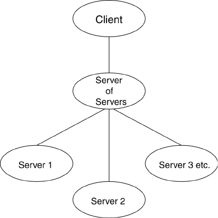
9.8 Server-of-Server Casefile Format
9-168 EnSight 10.2 User Manual
9.8 Server-of-Server Casefile Format
EnSight102, using an hpc (formerly gold) license key has the capability of dealing
with partitioned data in an efficient distributed manner by utilizing what we call a
server-of-servers (SOS for short). An SOS server resides between a normal client
and a number of normal servers. Thus, it appears as a normal server to the client,
and as a normal client to the various normal servers.
This arrangement allows for distributed parallel processing of the various portions
of a model, and has been shown to scale quite well.
Currently, EnSight SOS capability is only available for EnSight5, EnSight6,
EnSight Gold, Plot3d, and any EnSight User-Defined Reader data.
Please recognize that your data must be partitioned in some manner (hopefully in
a way that will be reasonably load balanced) in order for this approach to be
useful. The exception to this is the use of the auto_distribute capability for
structured or unstructured data. This option can be used if the data are readable by
all servers. It will automatically distribute each portion of the data over the
defined servers - without the user having to partition the data. Please note that
currently only EnSight Gold, Plot3d, and any 2.06 (or greater) user-defined readers
(which have implemented structured reader cinching) should be used for structured
auto_distribute - and that only EnSight Gold and any 2.08 (or greater) user-defined
readers (which have implemented the “*_in_buffers” routines ) should be used for
unstructured auto_distribute. Using an EnSight reader not written for SoS
autodistribute will result in each server loading the entire model.
Partition Utility
Included in the EnSight distribution is a command-line utility named
partition102
that will take most EnSight Case Gold binary unstructured datasets and partition
them for you. Simply type
partition102
at the command prompt to begin. This
command line program will prompt you for the name of the input case file and the
number of partitions in the x, y, and z and whether or not to use ghost elements,
etc. and will create (in a directory of your choosing) a case sos file (.sos) pointing
9.8 Partition Utility
EnSight 10.2 User Manual 9-169
to the partitioned case files ready for loading into EnSight server of server mode.
Note: If you do your own partitioning of data into EnSight6 or EnSight Gold
format, please be aware that each part must be in each partition - but, any given
part can be “empty” in any given partition. All that is required for an empty part is
the “part” line, the part number, and the “description” line. If you use CEISHELL
to start up your servers, and your format is EnSight Gold, then your SOS case file
can be greatly simplified to just list the case files (see Load Spatially Decomposed
Case Files).
You should place each partitioned portion of the model on the computer that will
access that portion. Each partitioned portion is actually a self contained set of
EnSight data files, which could typically be read by a normal client - server
session of EnSight. For example, if it were EnSight gold format, there will be a
casefile and associated gold geometry and variable results file(s). On the machine
where the EnSight SOS will be run, you will need to place the SOS casefile. This
is a simple ascii file which informs the SOS about pertinent information need to
run a server on each computer that will compute the various portions.
The format for the SOS casefile is as follows: (Note that [ ] indicates optional
information, and a blank line or a line with # in the first column are comments.)
FORMAT (Required)
type: master_server datatype (Required)
where: datatype is required and is one of the formats of EnSight’s
internal readers (which use the Part builder), namely:
gold ensight6 ensight5 plot3d
or it can be the string used to name any of the user-defined readers.
Note: For user-defined readers, the string must be exactly that which is
defined in the USERD_get_name_of_reader routine of the reader
(which is what is presented in the Format pulldown of the Data Reader
dialog).
If datatype is blank, it will default to EnSight6 data type.
[auto_distribute: server/reader/on/off] (Optional for structured or
unstructured data)
Set this option to “off” if you have moved the decomposed data file(s)
into separate directories or machines. Each server will simply read all
of the data as specified in its data_path and casefile below.
Set this option to “on” or “server” (these two options are the same) if
you want the EnSight server to automatically distribute data to the
servers specified below. This requires that each of the servers have
access to the same data (or identical copies of it). For structured data:
use the “ON” or “Server” option only if the datatype is gold, plot3d
or a 2.06 or greater user-defined reader (which has implemented
structured cinching). For unstructured data: use only if the
datatype is gold, or a 2.* user-defined reader (which has
implemented the “*_in_buffers” routines).
Set this option to “reader” if you want EnSight to allow the readers to do
the decomposition. This option requires that each of the servers have
access to the same data (or identical copies of it). This is prefered over
letting the server do the distribution. However the “reader” option
will only work if the reader has told EnSight that it can do the
9.8 Partition Utility
9-170 EnSight 10.2 User Manual
distribution by setting the return value to TRUE in the
USERD_prefer_auto_distribute reader routine.
[use_resources: on/off] (Optional, to use the specification of server
machines from EnSight resources; this will
override the machine names used in this file, see
How To Use Resource Management.)
[do_ghosts: on/off] (Optional for unstructured auto_distribute - default is off
starting with version 10.1.4(a).)
Allows user to control whether ghost cells will be produced between the
distributed portions.
This action can alternatively be set on by use of the -use_ghosts
command line argument, or by setting the
UNSTRUCT_AUTODISTRIBUTE_USE_GHOSTS environment
variable to 1.
[buffer_size: n] (Optional for unstructured auto_distribute and do_ghosts -
default is 100000)
Allows user to modify the default buffer size that is used when reading
node and element information of the model when producing ghost cells.
[want_metric: on/off] (Optional for unstructured auto_distribute and do_ghosts
- default is off starting with version 10.1.4(a))
If set on, a simple metric will be printed in the shell window that can
indicate the quality of the auto_distribution. The unstructured
auto_distribute method relies on some coherence in the element
connectivity - namely, that elements that lie next to each other are
generally listed close to each other in the data format.
The metric is simply the (#total_nodes / #nodes_needed_if_no_ghosts).
When no ghosts, the value will be 1.0. The more ghosts you must have,
the higher this metric will be. If the number gets much more than 2.0,
you may want to consider partitioning yourself.
This action can alternatively be set on by use of the -use_metric
command line argument, or by setting the
UNSTRUCT_AUTODISTRIBUTE_USE_METRIC environment
variable to 1.
NETWORK_INTERFACES (Note: this whole section is optional. It is
needed only when more than one network
interface to the sos host is available and it is
desired to use them. Thus distributing the
servers to sos communication over more than
one network interface)
number of network interfaces: num (Required - if section used)
where: num is the number of network interfaces to be used for the sos
host.
network interface: sos_network_interface_name1(Required - if section is used)
network interface: sos_network_interface_name2(Required - if section is used)
.
.
network interface: sos_network_interface_namenum(Required - if section used)
9.8 Partition Utility
EnSight 10.2 User Manual 9-171
SERVERS (Required)
number of servers: num (Required)
where: num is the number of servers that will be started and run
concurrently.
#Server 1 (Comment only)
machine id: mid (Required)
where: mid is the machine id of the server.
executable: /.../ensight102.server(Required, must use full path)
[directory: wd] (Optional)
where: wd is the working directory from which ensight102.server will
be
run
[login id: id] (Optional)
where: id is the login id. Only needed if it is different on this machine.
[data_path: /.../dd] (Optional)
where: dd is the data where the data resides. Full path must be provided
if you use this line.
casefile: yourfile.case (Required, but depending on format, may vary
as to whether it is a casefile, geometry file,
neutral file, universal file, etc. Relates to the
first data field of the Data Reader Dialog.)
[resfile: yourfile.res] (Depends on format as to whether required or
not. Relates to the second data field of the Data
Reader Dialog.)
[measfile: yourfile.mea] (Depends on format as to whether required or
not. Relates to the third data field of the Data
Reader Dialog.)
[bndfile: yourfile.bnd] (Depends on format as to whether required or
not. Relates to the fourth data field of the Data
Reader Dialog.)
#Server 2 (Comment only)
--- Repeat pertinent lines for as many servers as declared to be in this file ---
Example This example deals with a EnSight Gold dataset that has been partitioned into 3
portions, each running on a different machine. The machines are named joe, sally,
and bill. The executables for all machines are located in similar locations, but the
data is not. Note that the optional data_path line is used on two of the servers, but
not the third.
FORMAT
type: master_server gold
SERVERS
number of servers: 3
#Server 1
machine id: joe
executable: /usr/local/bin/ensight102/bin/ensight102.server
9.8 Spatially decomposed Case files
9-172 EnSight 10.2 User Manual
data_path: /usr/people/john/data
casefile: portion_1.case
#Server 2
machine id: sally
executable: /usr/local/bin/ensight102/bin/ensight102.server
data_path: /scratch/sally/john/data
casefile: portion_2.case
#Server 3
machine id: bill
executable: /usr/local/bin/ensight102/bin/ensight102.server
casefile: /scratch/temp/john/portion_3.case
If we name this example sos casefile “all.sos”, and we run it on yet another
machine, one named george, the data would be distributed as follows:
On george: all.sos
On joe (in /usr/people/john/data): portion_1.case, and all files referenced by it.
On sally (in /scratch/sally/john/data): portion_2.case, and all files referenced by it.
On bill (in /scratch/temp/john): portion_3.case, and all file referenced by it.
By starting EnSight with the -sos command line option (which will autoconnect
using ensight102.sos instead of ensight102.server), or by manually running
ensight102.sos in place of ensight102.server, and providing all.sos as the casefile
to read in the Data Reader dialog - EnSight will start three servers and compute
the respective portions on them in parallel (see Command Line Start-up Options).
For examples of structured and unstructured auto_distribute, see:
How To Use SOS.
Spatially decomposed Case files
If you choose to read spatially decomposed case files using the same number of
servers as case files, then this section is unnecessary. At some point you may
encounter case files that are spatially decomposed and wish to read them with less
servers than you have case files. At that point you will need to have this section
with a keyword MULTIPLE_CASEFILES. There are several ways to specify the
case files.
List them all by name:
MULTIPLE_CASEFILES
total number of cfiles: n
cfiles global path: global_path Optional
cfiles: partition_1.case
partition_2.case
.
partition_n.case
Specify number, pattern, start and increment
MULTIPLE_CASEFILES
total number of cfiles: n
cfiles global path: global_path Optional
9.8 Threading
EnSight 10.2 User Manual 9-173
cfiles pattern: partition_*.case
cfiles start number: #
cfiles increment: #
Use a separate file to containing the case filenames
MULTIPLE_CASEFILES
total number of cfiles: n
cfiles file: all_together_cfilenames.txt
Please see How To Load Spatially Decomposed Case Filesfor detailed usage
instructions.
Threading
By default, both the EnSight client and the server start up with an optimum
number of threads (depending on the number of processors available and within
the EnSight user license limits). Each executable of EnSight can be configured
individually to limit the number of threads used. The following environment
variables are used to specify the maximum number of threads that the executable
should use for computation. These environment variables should be set in your
shell startup script on the computers where the various EnSight executables run.
ENSIGHT10_MAX_THREADS
The maximum number of threads to use for each EnSight server. Server threads
are used to accelerate the computation of streamlines, clips, isosurfaces, shock
surfaces, most calculator functions (see Threaded Calculator Functions) and other
compute-intensive operations.
ENSIGHT10_MAX_CTHREADS
The maximum number of threads to use for each EnSight client. Client threaded
operations include transparency resort and display list creation.
ENSIGHT10_MAX_SOSTHREADS
The maximum number of threads to use on the server of server (SOS). The SOS
uses threads in order to start up server processes in parallel rather than serially.
The number of threads is limited to 1 (per client or server) with a Free or Desktop
license, 8 (per client or server) with a Standard license, while the upper limit for
an HPC (formerly Gold) license is 128. When setting these parameters it is a good
idea to take into account the number of processors on the system. In general, you
will not see benefit from setting the parameters higher than the number of total
processors. Because the server, server-of-servers and client operate in a pipelined
fashion, it is not necessary to limit one in order to apply more threads to another.
NETWORK_INTERFACES
If the machine named george had more than one network interface (say it had its
main one named george, but also had one named george2), we could add the
section shown below to our casefile example:
9.8 NETWORK_INTERFACES
9-174 EnSight 10.2 User Manual
number of network interfaces: 2
network interface: george
network interface: george2
This would cause machine joe to connect back to george, machine sally to connect
back to george2, and machine bill to connect back to george. This is because the
sos is cycling through its available interfaces as it connects the servers. Remember
that this is an optional section, and most users will probably not use it. Also, the
contents of this section will be ignored if the -soshostname command line
option is used (see Command Line Start-up Options).
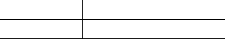
9.9 Periodic Matchfile Format
EnSight 10.2 User Manual 9-175
9.9 Periodic Matchfile Format
This is an optional file which can be used in conjunction with models which have
rotational or translational computational symmetry (or periodic boundary
conditions). It is invoked in the GEOMETRY section of the EnSight casefile,
using the “match: filename” line. EnSight 6 Case file allows the use of the
periodic matchfile which uses the matchfile in the border process to eliminate the
matched symmetry faces at the shared boundary between the faces. EnSight Case
Gold allows the optional [add_ghosts] parameter after the filename which will
produce ghost cells across the match file boundary which will provide continuity
for variable calculations across the boundary, and for computational symmetry/
mirroring, etc. Only use the add_ghosts option if you can afford the penalty of the
additional ghost cells and you need the computational continuity that they
provide.
When a model piece is created with periodic boundary conditions, there is usually
a built-in correspondence between two faces of the model piece. If you transform
a copy of the model piece properly, face 1 of the copy will be at the same location
as face 2 of the original piece. It is desirable to know the corresponding nodes
between face 1 and face 2 so border elements will not be produced at the matching
faces. This correspondence of nodes can be provided in a periodic match file as
indicated below. (Please note that if a periodic match file is not provided, by
default EnSight will attempt to determine this correspondence using a float
hashing scheme. This scheme has been shown to work quite well, but may not
catch all duplicates. The user has some control over the “capture” accuracy of the
hashing through the use of the command: “test: float_hash_digits”. If this
command is issued from the command dialog, the user can change the number of
digits, in a normalized scheme, to consider in the float hashing. The lower the
number of digits, the larger the “capture” distance, and thus the higher the number
of digits, the smaller the capture distance. The default is 4, with practical limits
between 2 and 7 or 8 in most cases.)
The transformation type and delta value are contained in the file. The periodic
match file is an ASCII free format file. For unstructured data, it can be thought of
as a series of node pairs, where a node pair is the node number of face 1 and its
corresponding node number on face 2. For structured blocks, all that is needed is
an indication of whether the i, j, or k planes contain the periodic face. The min
plane of this “direction” will be treated as face 1, and the max plane will be treated
as face 2.
The file format is as follows:
rotate_x/y/z / translate
The first line is either rotate_x, rotate_y, rotate_z
or translate
theta / dx dy dz
The second line contains rotation angle in degrees
or the three translational delta values.
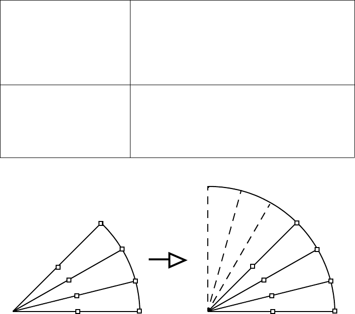
9.9 Periodic Matchfile Format
9-176 EnSight 10.2 User Manual
Simple unstructured rotational example:
The periodic match file for a rotation of this model about point 1 would be:
rotate_z
45.0
3
1 1
2 8
3 9
Thus, face 1 of this model is made up of nodes 1, 2, and 3 and face 2 of this model
is made up of nodes 1, 8, and 9. So there are 3 node pairs to define, with node 1
corresponding to node 1 after a copy is rotated, node 2 corresponding to node 8,
and node 3 corresponding to node 9.
np
n
11
n
21
n
12
n
22
. .
. .
. .
n
1np
n
2np
If any unstructured pairs, the third line contains
the number of these pairs (np).
And the node ids of each pair follow. (The first
subscript indicates face, the second is pair.)
blocks b
min
b
max
i/j/k
Last in the file comes as many of these “blocks”
lines as needed. bmin and bmax are a range of
block numbers. For a single block, bmin and bmax
would be the same. Only one of i, j, or k can be
specified for a given block.
2
45
8
3
7
9
6
1
8
6
4
2
Original
face 2
face 1
Figure 9-6
Model Duplication by rotational symmetry
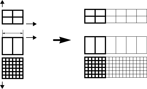
9.9 Periodic Matchfile Format
EnSight 10.2 User Manual 9-177
Simple structured translational model:
translate
2.0 0.0 0.0
blocks 1 1 i
blocks 2 3 j
Since block 1 is oriented differently than blocks 2 and 3 in terms of ijk space, two
“blocks” lines were needed in the match file.
Special Notes / Limitations:
1. This match file format requires that the unstructured node ids of the model be
unique. This is only an issue with EnSight Gold unstructured format, since it is
possible with that format to have non-unique node ids.
2. The model instance (which will be duplicated periodically) must have more
than one element of thickness in the direction of the duplication. If it has only one
element of thickness, intermediate instances will have all faces removed. If you
have this unusual circumstance, you will need to turn off the shared border
removal process, as explained in note 3.
3. The shared border removal process can be turned off, thereby saving some
memory and processing time, by issuing the “test: rem_shared_bord_off”
command in the command dialog. The effect of turning it off will be that border
elements will be left between each periodic instance on future periodic updates.
4. The matching and hashing processes actually occur together. Thus, matching
information does not have to be specified for all portions of a model. If no
matching information is specified for a given node, the hashing process is used.
By the same token, if matching information is provided, it is used explicitly as
specified - even if it is has been specified incorrectly.
Figure 9-7
Model Duplication by translational symmetry
of structured blocks (3 instances)
block 1
block 2
block 3
J
I
J
I
2.0
9.10 XY Plot Data Format
9-178 EnSight 10.2 User Manual
9.10 XY Plot Data Format
This file is saved using the Save section of the Query Entity dialog. The file can
contain one or more curves. The following is an example XY Data file:
Line Contents of Line
12
2 Distance vs. Temperature for Line Tool
3 Distance
4 Temperature
51
65
7 0.0 4.4
8 1.0 5.8
9 2.0 3.6
10 3.0 4.6
11 4.0 4.8
12 Distance vs. Pressure for Line Tool
13 Distance
14 Pressure
15 2
16 4
17 0.00 1.2
18 0.02 1.1
19 0.04 1.15
20 0.06 1.22
21 3
22 1.10 1.30
23 1.12 1.28
24 1.14 1.25
Line 1 contains the (integer) number of curves in the file.
Line 2 contains the name of the curve.
Line 3 contains the name of the X-Axis.
Line 4 contains the name of the Y-Axis.
Line 5 contains the number of curve segments in this curve.
9.10 XY Plot Data Format
EnSight 10.2 User Manual 9-179
Line 6 contains the number of points in the curve segment.
Lines 7-11 contain the X-Y information.
Line 12 contains the name of the second curve.
Line 13 contains the name of the X-Axis
Line 14 contains the name of the Y-Axis
Line 15 contains the number of curve segments in this curve. (For the second
curve, the first segment contains 4 points, the second 3 points.)

9.11 EnSight Boundary File Format
9-180 EnSight 10.2 User Manual
9.11 EnSight Boundary File Format
This file format can be used to represent boundary surfaces of structured data as
unstructured parts. The boundaries defined in this file can come from sections of
several different structured blocks. Thus, inherent in the file format is a grouping
and naming of boundaries across multiple structured blocks.
Additionally, a delta can be applied to any boundary section to achieve the
creation of repeating surfaces (such as blade rows in a jet engine).
Note: There is no requirement that the boundaries actually be on the surface of
blocks, but they must define either 2D surfaces or 1D lines. You may not use this
file to define 3D portions of the block.
The boundary file is read if referenced in the casefile of EnSight data models, or
in the boundary field of the Data Reader Dialog for other data formats. Any
boundaries successfully read will be listed in the Unstructured Data Part List of
the Data Part Loader Dialog.
The format of the EnSight Boundary File is as follows:
Line (1): Required header keyword and version number. ENSBND is required
exactly, but the version number could change in the future.
ENSBND 1.00
Line (2) through Line (NumBoundaries+1): The names of the boundaries to be
defined. (Each name must be no greater than 79 characters.)
For example:
inflow
wall
Chimera Boundary
outflow
Line (NumBoundaries+2): Required keyword indicating the end of the boundary
names and the beginning of the boundary section definitions.
BOUNDARIES
Line (NumBoundaries+3) through the end of the file: The boundary section
definitions. Each line will have the following information:
bnd_num blk_num imin imax jmin jmax kmin kmax [di dj dk n_ins]
where:
bnd_num
is the number of the boundary in the list of names above.
(For example: inflow is 1, wall is 2, Chimera Boundary is 3, etc.)
blk_num
is the parent structured block for this boundary section.
imin,imax, jmin,jmax, kmin,kmax
are the ijk ranges for the boundary section.
At least one of the min,max pairs must refer to the same plane. A wildcard (“$”)
can be used to indicate the maximum i, j, or k value of that block (the far plane).
Additionally, negative numbers can be used to indicate plane values from the far
side toward the near side. (-1 = far plane, -2 = one less than the far plane, etc.)
[di,dj,dk
and
n_ins]
are optional delta information which can be used to extract
repeating planes. The appropriate di, dj, or dk delta value should be set to the
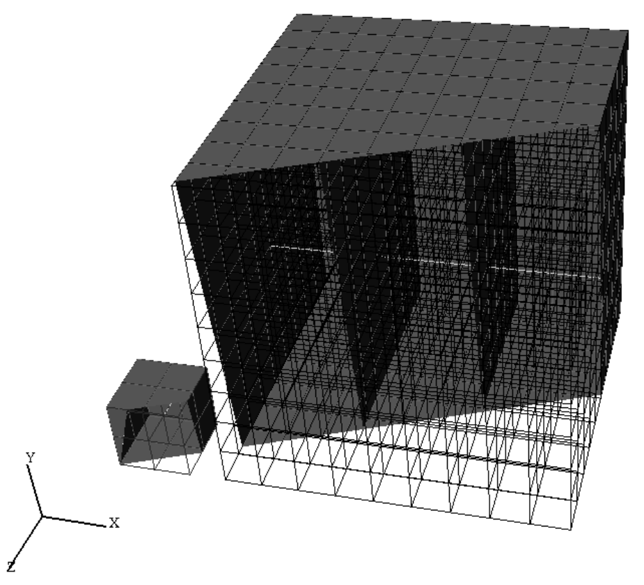
9.11 EnSight Boundary File Format
EnSight 10.2 User Manual 9-181
repeating plane offset value, and the other two delta values must be zero. The non-
zero delta must correspond to a min,max pair that are equal. The n_ins value is
used to indicate the number of repeating instances desired. A (“$”) wildcard can
be used here to indicate that the maximum number of instances that fit in the block
should be extracted.
All numbers on the line must be separated by spaces.
Finally, comment lines are allowed in the file by placing a “#” in the first column.
Below is a simple example of a boundary file for two structured blocks, the first of
which is a 3 x 3 x 3 block, and the second is a 10 x 10 x 10 block. We will define a
boundary which is the front and back planes of each block(K planes) and one that
is the top and bottom planes of each block(J planes). We will also define some
repeating x planes, namely, planes at i=1 and 3 for block one and at i=1, 4, 7, and
10 for block two. The image below shows the blocks in wire frame and the
boundaries shaded and slightly cut away, so you can see the interior x-planes.
9.11 EnSight Boundary File Format
9-182 EnSight 10.2 User Manual
The file to accomplish this looks like:
ENSBND 1.00
front_back
top_bottom
x-planes
middle lines
BOUNDARIES
#bnd blk imin imax jmin jmax kmin kmax di dj dk n_ins
#--- --- ---- ---- ---- ---- ---- ---- -- -- -- -----
1 1 1 3 1 3 $ $
1 2 1 $ 1 $ 10 10
2 1 1 $ $ $ 1 $
2 2 1 10 10 10 1 10
1 1 1 3 1 3 1 1
1 2 1 $ 1 $ 1 1
2 1 1 3 1 1 1 $
2 2 1 $ 1 1 1 $
3 1 1 1 1 $ 1 $ 2 0 0 2
3 2 1 1 1 $ 1 $ 3 0 0 $
4 1 2 2 2 2 1 3
4 2 1 10 5 5 5 5
Interpreting the 12 boundary definition lines:
1 1 1 3 1 3 $ $
defines a part of the boundary called front_back, on block 1, where I=1 to 3, J=1
to 3, and K=3. Thus, the far K plane of block 1.
1 2 1 $ 1 $ 10 10
defines another part of the front_back boundary, on block 2, where I=1 to 10, J=1
to 10, and K = 10. Thus, the far K plane of block 2.
2 1 1 $ $ $ 1 $
defines a part of the boundary called top_bottom, on block 1, where I=1 to 3, J=3,
and K=1 to 3. Thus, the far J plane of block 1.
2 2 1 10 10 10 1 10
defines another part of the top_bottom boundary, on block 2, where I=1 to 10,
J=10, and K=1 to 10. Thus, the far J plane of block 2.
1 1 1 3 1 3 1 1
defines another part of the front_back boundary, on block 1, where I=1 to 3, J=1 to
3, and K=1. Thus, the near K plane of block 1.
1 2 1 $ 1 $ 1 1
defines another part of the front_back boundary, on block 2, where I=1 to 10, J=1
to 10, and K=1. Thus the near K plane of block 2.
2 1 1 3 1 1 1 $
defines another part of the top_bottom boundary, on block 1, where I=1 to 3, J=1,
and K=1 to 3. Thus, the near J plane of block 1.
2 2 1 $ 1 1 1 $
defines another part of the top_bottom boundary, on block 2, where I=1 to 10,
J=1,and K=1 to 10. Thus, the near J plane of block 2.
9.11 EnSight Boundary File Format
EnSight 10.2 User Manual 9-183
3 1 1 1 1 $ 1 $ 2 0 0 2
defines a part of the boundary called x-planes, on block 1, where I=1, J=1 to 3,
K=1 to 3, then again where I=3, J=1 to 3, and K=1 to 3. Thus, both the near and
far I planes of block 1.
3 2 1 1 1 $ 1 $ 3 0 0 $
defines another part of the x-planes boundary, on block 2, where I=1, J=1 to 10,
and K=1 to 10, then again where I=4, J=1 to 10, and K=1 to 10, then again where
I=7, J=1 to 10, and K=1 to 10, then again where I=10, J=1 to 10, and K=1 to 10.
Thus, the I = 1, 4, 7, and 10 planes of block 2.
4 1 2 2 2 2 1 3
defines a part of the boundary called middle lines, on block 1, where I=2, J=2, and
K=1 to 3. Thus, line through the middle of block 1 in the K direction.
4 2 1 10 5 5 5 5
defines another part of the middle lines boundary, on block 2, where I=1 to 10,
J=5, and K=5. Thus a line through the middle of the block2 in the I direction.
Please note that the “$” wildcard was used rather randomly in the example, simply
to illustrate how and where it can be used.
The use of negative numbers for ijk planes is indicated below - again rather
randomly for demonstration purposes. This file will actually produce the same
result as the file above.
ENSBND 1.00
front_back
top_bottom
x-planes
middle lines
BOUNDARIES
#bnd blk imin imax jmin jmax kmin kmax di dj dk n_ins
#--- --- ---- ---- ---- ---- ---- ---- -- -- -- -----
1 1 1 3 1 3 -1 -1
1 2 -3 -1 1 -1 10 10
2 1 1 -1 -1 -1 1 -1
2 2 1 10 10 10 1 10
1 1 1 3 1 3 1 1
1 2 1 -1 1 -1 1 1
2 1 1 3 1 1 1 -1
2 2 1 -1 1 1 1 -1
3 1 1 1 1 -1 1 -1 2 0 0 2
3 2 1 1 1 -1 1 -1 3 0 0 $
4 1 2 -2 -2 2 1 3
4 2 1 10 5 5 -6 -6
9.12 EnSight Particle Emitter File Format
9-184 EnSight 10.2 User Manual
9.12 EnSight Particle Emitter File Format
This file can be used to specify the location of emitter points. It is most useful
when the user has specific (and many) emit points to use for particle traces.
Rather than type them all in one at a time as a cursor emitter, this file can be used.
Note the following:
1. The first two lines need to be exactly as shown.
Version 1.0
EnSight Particle Emitter File
2. #’s as the first character on a line, are comment lines. Comment lines can be
used anywhere in the file after the first two mandatory lines.
3.
Time
lines contain the emitter release time (floating point time value, NOT the
integer time step).
4.
Emit
lines contain the coordinates of an emitter. The emitter will be associated
with the previously specified
Time
.
There is one special case that may be useful to know. An option within EnSight is
to have traces emitted at the “current time”. You can use that option with an
emitter file if your number of emitters and their locations do not change over time.
Just omit the
Time
line in this file (and remember to set the emit at current time
toggle in EnSight).
If you use an emitter and choose the pathline option, then each emitter will emit a
particle trace at the indicated time.
However, if you use an emitter file and choose the streamline option, then
streamlines will be emitted at all of the Emit locations at once. Some might expect
this to operate as if streamlines are calculated at the ‘current time’ and as you
move through time, previous streamlines are removed and the new streamlines are
recalculated at the current timestep using the new emitter locations. This is not the
way this works when you use an emitter file with changing emitter locations. Each
streamline will emit at the time indicated in its Time keyword using the flowfield
corresponding to that Time keyword. You will end up with groups of streamlines
emitted at a common time and calculated at that common time all showing up at
once and all using a relative time value all starting from 0.0. It can be quite
confusing if you expect an ‘emit at current time’ behavior.
Sample File:
Version 1.0
EnSight Particle Emitter File
#
Time 0.249063
Emit 0.0669737 0.0134195 -0.013926
Emit 0.0669737 0.0131277 -0.0141079
Emit 0.0669737 0.0128642 -0.0143178
Emit 0.0669737 0.0155969 -0.0113572
Emit 0.0669737 0.0150344 -0.0122012
Emit 0.0669737 0.0146967 -0.0123587
9.12 EnSight Particle Emitter File Format
EnSight 10.2 User Manual 9-185
#
Time 0.249113
Emit 0.0669737 0.0137097 -0.0136404
Emit 0.0669737 0.0134218 -0.0138284
Emit 0.0669737 0.0131628 -0.0140438
Emit 0.0669737 0.01585 -0.0110264
Emit 0.0669737 0.0152879 -0.011882
Emit 0.0669737 0.0149536 -0.0120466
#
Time 0.249163
Emit 0.0669737 0.0139938 -0.0133488
Emit 0.0669737 0.01371 -0.0135428
Emit 0.0669737 0.0134555 -0.0137636
Emit 0.0669737 0.0160612 -0.0106906
Emit 0.0669737 0.0155347 -0.0115575
Emit 0.0669737 0.0152039 -0.0117291
#
Time 0.249213
Emit 0.0669737 0.0142718 -0.0130512
Emit 0.0669737 0.013992 -0.01511
Emit 0.0669737 0.0137423 -0.0134773
Emit 0.0669737 0.0162827 -0.0103501
Emit 0.0669737 0.0157745 -0.0112279
Emit 0.0669737 0.0154475 -0.0114064
#
Time 0.249263
Emit 0.0669737 0.0145433 -0.0127479
Emit 0.0669737 0.0142679 -0.0129536
Emit 0.0669737 0.014023 -0.013185
Emit 0.0669737 0.0164969 -0.0100051
Emit 0.0669737 0.0160074 -0.0108933
Emit 0.0669737 0.0156842 -0.0110787
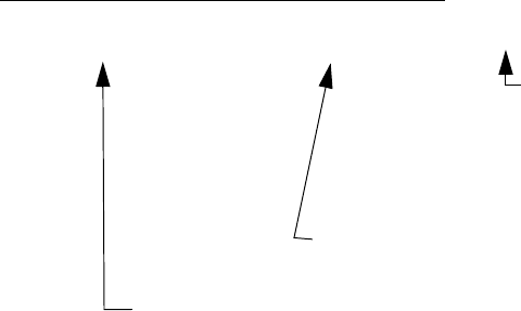
9.13 EnSight Rigid Body File Format
9-186 EnSight 10.2 User Manual
9.13 EnSight Rigid Body File Format
There are now two main versions for this file format. Version 1 is the original and
is still valid. It will be described first. Version 2, which is believed to be much
easier to understand and which has more capability and flexibility, will then be
described.
This file is used to link the transient transformations within the rigid body Euler
Parameter file (see Section 9.14, Euler Parameter File Format) with the parts in an
EnSight Gold format model. It also can be used to optionally specify non-transient
transformations for center of gravity offsets and orientation placements. Version 2
has more flexibility for the latter than does version 1. While not required,
.erb
is
the normal extension given to this file. The .erb file is referenced via the
rigid_body
line in an EnSight Gold Casefile
Version 1
In addition to linking EnSight parts to the transformations in the rigid body Euler
Parameter file (see Section 9.14, Euler Parameter File Format), version 1 of this
file can also be used to specify a units scaling factor, center of gravity offsets, and
initial yaw pitch roll rotations, if needed. Note that model vector variables will be
transformed as well. Please note that the order of transformations will first be the
yaw pitch roll rotations (if any specified) then second, the center of gravity offsets
(if any specified) and third, the euler parameter rotations and translations of the
euler parameter file. So:
The order of these transformations is:
Note the following:
1. The first line needs to be exactly as shown.
EnSight Rigid Body
2. The second line must be the .erb version number line. (Version is 1.1, previous
to EnSight 8.2 this line was not present and thus defaulted to version 1.0)
version 1.1
2. The third line must either be exactly
names
[xrot][yrot][zrot] [-xoff][-yoff][-zoff] [eet]
----optional----- ------optional------- -----
Note that this is
composed of the euler
parameter rotations and
then the associated
translations. So [rot][tran]
Note that the negative of these is what is
applied
The order of these is set by the rot_order, so they can be any of the
possible combinations.
9.13 Version 1
EnSight 10.2 User Manual 9-187
or
numbers
This indicates whether part names or part numbers will be used in the
association of ensight parts to the rigid body information in the Euler Parameter
File.
3. The fourth line must be a single integer
n
indicating the number of lines that
follow in the file.
4. The remaining
n
lines contain either 3, 4, 7, or 11 tokens which must each be
enclosed in quotes. When no unit scaling or center of gravity offset is needed
the lines have the form of either
“ens_part_name” “eet_filename” “eet_title”
or
“ens_part_#(s)” “eet_filename” “eet_title”
depending on the state of the second line in the file.
If unit scaling is specified, then the lines have the form of either
“ens_part_name” “eet_filename” “eet_title” “u_scale”
or
“ens_part_#(s)” “eet_filename” “eet_title” “u_scale”
If center of gravity offsets are needed (without rotations), the lines are either
“ens_part_name” “eet_filename” “eet_title” “u_scale” “xoff” “yoff” “zoff”
or
“ens_part_#(s)” “eet_filename” “eet_title” “u_scale” “xoff” “yoff” “zoff”
If yaw pitch roll rotations are needed (without offsets), the lines are either
“ens_part_name” “eet_filename” “eet_title” “u_scale” “rot_order” “xrot” “yrot” “zrot”
or
“ens_part_#(s)” “eet_filename” “eet_title” “u_scale” “rot_order” “xrot” “yrot” “zrot”
If both offsets and initial yaw pitch roll rotations are needed, the lines are either (note difference in order
of 3 offset offset columns and 4 rotation columns).
“ens_part_name” “eet_filename” “eet_title” “u_scale” “xoff” “yoff” “zoff” “rot_order” “xrot” “yrot” “zrot”
or
“ens_part_name” “eet_filename” “eet_title” “u_scale” “rot_order” “xrot” “yrot” “zrot” “xoff” “yoff” “zoff”
or
“ens_part_#(s)” “eet_filename” “eet_title” “u_scale” “xoff” “yoff” “zoff” “rot_order” “xrot” “yrot” “zrot”
or
“ens_part_#(s)” “eet_filename” “eet_title” “u_scale” “rot_order” “xrot” “yrot” “zrot” “xoff” “yoff” “zoff”
Where:
ens_part_name =
the actual part description given in the EnSight geometry file
ens_part_#(s) =
a single number, comma separated list, or list of dash separated
ranges of part numbers given in the EnSight geometry file
eet_filename =
the actual name of the Euler Parameter file
9.13 Version 1
9-188 EnSight 10.2 User Manual
Simple Sample File (using part numbers):
EnSight Rigid Body
version 1.1
numbers
3
“1,5” “my.eet” “BUCKET”
“2-4,6-9,11” “my.eet” “BOOM”
“10” “my.eet” “LINK”
Note, the above file would require that the ensight geometry file contain parts 1 thru 11
and that the my.eet file contain titles BUCKET, BOOM, and LINK.
Sample File (using part names and optional scaling and offsets - no initial
rotations):
EnSight Rigid Body
version 1.1
names
11
“bucket_property_1” “my.eet” “BUCKET” “1000.0” “383.7” “105.23” “0.0”
“bucket_property_2” “my.eet” “BUCKET” “1000.0” “383.7” “105.23” “0.0”
“boom_property_1” “my.eet” “BOOM” “1000.0” “-35.4” “76.85” “45.6”
“boom_property_2” “my.eet” “BOOM” “1000.0” “-35.4” “76.85” “45.6”
“boom_property_3” “my.eet” “BOOM” “1000.0” “-35.4” “76.85” “45.6”
“boom_enda” “my.eet” “BOOM” “1000.0” “-35.4” “76.85” “45.6”
“boom_endb” “my.eet” “BOOM” “1000.0” “-35.4” “76.85” “45.6”
“boom_top” “my.eet” “BOOM” “1000.0” “-35.4” “76.85” “45.6”
“boom_bot” “my.eet” “BOOM” “1000.0” “-35.4” “76.85” “45.6”
eet_title =
the actual name of the title in the columns of the Euler Parameter
File which correspond to the rigid body euler values to apply to
the ensight parts indicated
u_scale =
the optional units scaling value which can be applied to the
translation values in the Euler Parameter file. This is only needed
if the translations of the Euler Parameter file are not in the same
units as the EnSight geometry. (Note, if you use the xoff, yoff,
zoff offset below, you must use this value as well - but it can be
1.0) Note: this does not scale the geometry. This is used to scale
the translational values in the .eet file only. For example if your
.eet file has units of millimeters but your model is in meters,
putting a 1000 here will scale up all your translations
appropriately. This does not scale values in the .erb file.
xoff,yoff,zoff =
optional additional offsets to the center of gravity that can be
applied. These are applied before the rotation and translations
contained in the Euler Parameters file, and as such are generally
not needed
rot_order =
one of the following, indicating the order in which to apply the
rotation angles. xyz yxz zxy
xzy yzx zyx
xrot,yrot,zrot =
rotation angles (in degrees) about each axis. These will be
applied in the order specified with rot_order.
9.13 Version 1
EnSight 10.2 User Manual 9-189
“boom_cen” “my.eet” “BOOM” “1000.0” “-35.4” “76.85” “45.6”
“link” “my.eet” “LINK” “1000.0” “102.4” “80.0” “0.0”
Sample File (using part names and optional scaling and initial rotations - no
offsets):
EnSight Rigid Body
version 1.1
names
11
“bucket_property_1” “my.eet” “BUCKET” “1000.0” “yzx” “0.0” “90.0” “0.0”
“bucket_property_2” “my.eet” “BUCKET” “1000.0” “yzx” “0.0” “90.0” “0.0”
“boom_property_1” “my.eet” “BOOM” “1000.0” “yzx” “0.0” “90.0” “0.0”
“boom_property_2” “my.eet” “BOOM” “1000.0” “yzx” “0.0” “90.0” “0.0”
“boom_property_3” “my.eet” “BOOM” “1000.0” “yzx” “0.0” “90.0” “0.0”
“boom_enda” “my.eet” “BOOM” “1000.0” “yzx” “0.0” “90.0” “0.0”
“boom_endb” “my.eet” “BOOM” “1000.0” “yzx” “0.0” “90.0” “0.0”
“boom_top” “my.eet” “BOOM” “1000.0” “yzx” “0.0” “90.0” “0.0”
“boom_bot” “my.eet” “BOOM” “1000.0” “yzx” “0.0” “90.0” “0.0”
“boom_cen” “my.eet” “BOOM” “1000.0” “yzx” “0.0” “90.0” “0.0”
“link” “my.eet” “LINK” “1000.0” “yzx” “0.0” “90.0” “0.0”
Note, the two files above would require that the ensight geometry file contain parts
labeled bucket_property_1, bucket_property_2, boom_property_1, boom_property_2,
boom_property_3, boom_enda, boom_endb, boom_top, boom_bot, boom_cen, and
link, and that the my.eet file contain titles BUCKET, BOOM, and LINK.
Sample File (using part numbers and optional scaling, offsets and rotations - with
the offsets before the rotations. Also has some comments in the file):
# This is the same file as above, but has comments in it
EnSight Rigid Body
version 1.1
numbers
11
# Here come the parts registered against the labels in the motion file and
# assigned initial rotations and cg offsets
“1” “my.eet” “BUCKET” “1000.0” “383.7” “105.23” “0.0” “yzx” “0.0” “90.0” “0.0”
“2” “my.eet” “BUCKET” “1000.0” “383.7” “105.23” “0.0” “yzx” “0.0” “90.0” “0.0”
“3” “my.eet” “BOOM” “1000.0” “-35.4” “76.85” “45.6” “yzx” “0.0” “90.0” “0.0”
“4” “my.eet” “BOOM” “1000.0” “-35.4” “76.85” “45.6” “yzx” “0.0” “90.0” “0.0”
“5” “my.eet” “BOOM” “1000.0” “-35.4” “76.85” “45.6” “yzx” “0.0” “90.0” “0.0”
“6” “my.eet” “BOOM” “1000.0” “-35.4” “76.85” “45.6” “yzx” “0.0” “90.0” “0.0”
“7” “my.eet” “BOOM” “1000.0” “-35.4” “76.85” “45.6” “yzx” “0.0” “90.0” “0.0”
“8” “my.eet” “BOOM” “1000.0” “-35.4” “76.85” “45.6” “yzx” “0.0” “90.0” “0.0”
“9” “my.eet” “BOOM” “1000.0” “-35.4” “76.85” “45.6” “yzx” “0.0” “90.0” “0.0”
“10” “my.eet” “BOOM” “1000.0” “-35.4” “76.85” “45.6” “yzx” “0.0” “90.0” “0.0”
“11” “my.eet” “LINK” “1000.0” “102.4” “80.0” “0.0” “yzx” “0.0” “90.0” “0.0”
Sample File (using part numbers and optional scaling, offsets and rotations - with
the rotations before the offsets. Also has some comments in the file):
EnSight Rigid Body
version 1.1
numbers
11
“1” “my.eet” “BUCKET” “1000.0” “yzx” “0.0” “90.0” “0.0” “383.7” “105.23” “0.0”
“2” “my.eet” “BUCKET” “1000.0” “yzx” “0.0” “90.0” “0.0” “383.7” “105.23” “0.0”
“3” “my.eet” “BOOM” “1000.0” “yzx” “0.0” “90.0” “0.0”“-35.4” “76.85” “45.6”
“4” “my.eet” “BOOM” “1000.0” “yzx” “0.0” “90.0” “0.0”“-35.4” “76.85” “45.6”

9.13 Version 2
9-190 EnSight 10.2 User Manual
“5” “my.eet” “BOOM” “1000.0” “yzx” “0.0” “90.0” “0.0”“-35.4” “76.85” “45.6”
“6” “my.eet” “BOOM” “1000.0” “yzx” “0.0” “90.0” “0.0”“-35.4” “76.85” “45.6”
“7” “my.eet” “BOOM” “1000.0” “yzx” “0.0” “90.0” “0.0”“-35.4” “76.85” “45.6”
“8” “my.eet” “BOOM” “1000.0” “yzx” “0.0” “90.0” “0.0”“-35.4” “76.85” “45.6”
“9” “my.eet” “BOOM” “1000.0” “yzx” “0.0” “90.0” “0.0”“-35.4” “76.85” “45.6”
“10” “my.eet” “BOOM” “1000.0” “yzx” “0.0” “90.0” “0.0”“-35.4” “76.85” “45.6”
“11” “my.eet” “LINK” “1000.0” “yzx” “0.0” “90.0” “0.0”“102.4” “80.0” “0.0”
Note, the two files above would require that the ensight geometry file contain 11 parts
and that the my.eet file contain titles BUCKET, BOOM, and LINK.
Version 2
In addition to linking EnSight parts to the transformations in the rigid body Euler
Parameter file (see Section 9.14, Euler Parameter File Format), version 2 of this
file can also be used to specify any number of pre and post transformations. These
can range from the common translation, rotation, and scaling transformations, to
providing your own 4x4 matrices. Thus arranging portions of a model can be done
in a straight-forward manner.
First it is important to know the order that transformations will be applied.
Basically it will come in three stages:
[pre-transforms] x [euler-transforms] x [post-transforms]
where:
[pre-transforms] consists of concatenated T,S,R and M transforms in the user
specified order.
[euler-transforms] consists of the euler rotation, followed by the euler
translations.
[post-transforms] consists of concatenated T,S,R and M transforms in the user
specified order.
And the valid transformations are:
Command Description
Tx: value Translation in x
Ty: value Translation in y
Tz: value Translation in z
Sz: value Scaling in x
Sy: value Scaling in y
Sz: value Scaling in z
Rx: value (degrees) Rotation about x
Ry: value (degrees) Rotation about y
Rz: value (degrees) Rotation about z
Rxr: value (radians) Rotation about x
Ryr: value (radians) Rotation about y
Rzr: value (radians) Rotation about z
M: 16 values User supplied 4x4 matrix values (applied to geometry only):
a11,a12,a13,a14,
a21,a22,a23,a24,
a31,a32,a33,a34,
a41,a42,a43,a44
9.13 Version 2
EnSight 10.2 User Manual 9-191
1. The first line needs to be exactly as shown.
EnSight Rigid Body
2. The second line must be the .erb version number line.
version 2.0
2. The third line must either be exactly
names
or
numbers
This indicates whether part names or part numbers will be used in the
association of ensight parts to the rigid body information in the Euler Parameter
File.
3. The fourth line must be a single integer
n
indicating the number of “euler
transform” associations that follow in the file.
4. For each “euler transform”association indicated in 3. above:
There must be a line with:
“ens_part_name”
or
“ens_part_#(s)”
a) And a line with the number of transforms that will be used for this “euler
transform” association.
b) Then for each of the transforms declared in a), there must be one of the
valid transforms listed in the table above.
Note that blank lines are allowed. And anything beyond a “#” sign will ignore
everything else on that line.
Mv: 16 values User supplied 4x4 matrix values (applied to both geometry)
and vectors:
a11,a12,a13,a14,
a21,a22,a23,a24,
a31,a32,a33,a34,
a41,a42,a43,a44
Eul: “eet_fle” “eet_trans_title” <“units_scale”> Required reference to .eet file
and the specific transform
within that file. The units_scale
is optional.
Note that the quotes indicated
are required.
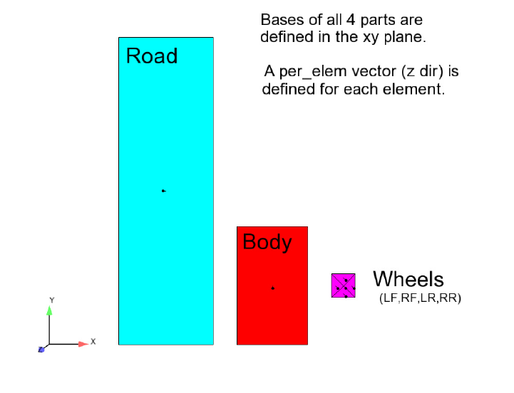
9.13 Version 2
9-192 EnSight 10.2 User Manual
An example is probably the best way to illustrate the use and flexibility of this file
format. Below is the image a simple set of parts that will be used to assemble a
vehicle with four wheels, and move it along a road, with the wheels turning.
Here is the contents of the Ensight Gold casefile, which references the veh.erb
file:
FORMAT
type: ensight gold
GEOMETRY
model: veh.geo
rigid_body: veh.erb
VARIABLE:
vector per element: evect veh.vec
And here is the contents of the veh.erb file, which will assemble the four wheels
onto the body, and onto the road, allow for the transient movement of the
assembled vehicle along the road, with the wheels turning, and have everything be
done in the xz plane instead of the xy plane:
EnSight Rigid Body
version 2.000000
names
6
“Body”
2
Eul: “veh.eet” “BODY” # .eet file only has forward trans for BODY
Mv:1.0 0.0 0.0 0.0 # A -90 rotation about x axis, matrix option
0.0 0.0 -1.0 0.0 # Since is Mv:, Will apply to vectors also.
0.0 1.0 0.0 0.0 # Note that a Rx: -90 would do the same.
0.0 0.0 0.0 1.0
9.13 Version 2
EnSight 10.2 User Manual 9-193
“LF_Wheel”
6
Tx: -4.5 # trans & rotate into position at origin
Ty: -2.5
Ry: -90.0 # Rx:,Ry:,Rz: are degrees.
Eul: “veh.eet” “WHEEL” # .eet has rot & forward trans for WHEEL
Ty: 4.5 # trans back to desired location
Rx: -90.0 # Use the simpler Rx: command
“RF_Wheel”
8
Tx: -4.5
Ty: -2.5
Ry: -90.0
Sx: -1.0 # Mirroring, keeps wheel outside outward
Eul: “veh.eet” “WHEEL”
Tx: 3.0
Ty: 4.5
Rx: -90.0
“LR_Wheel”
6
Tx: -4.5
Ty: -2.5
Ry: -90.0
Eul: “veh.eet” “WHEEL”
Ty: 0.5
Rx: -90.0
“RR_Wheel”
8
Tx: -4.5
Ty: -2.5
Ry: -90.0
Sx: -1.0
Eul: “veh.eet” “WHEEL”
Tx: 3.0
Ty: 0.5
Rx: -90.0
“Road”
4
Tx: 4.5
Tz: -0.5
Eul: “veh.eet” “ROAD”
M: 1.0 0.0 0.0 0.0 # Not transforming vector for this one.
0.0 0.0 -1.0 0.0 # orig vector was in +z, it stays such.
0.0 1.0 0.0 0.0
0.0 0.0 0.0 1.0
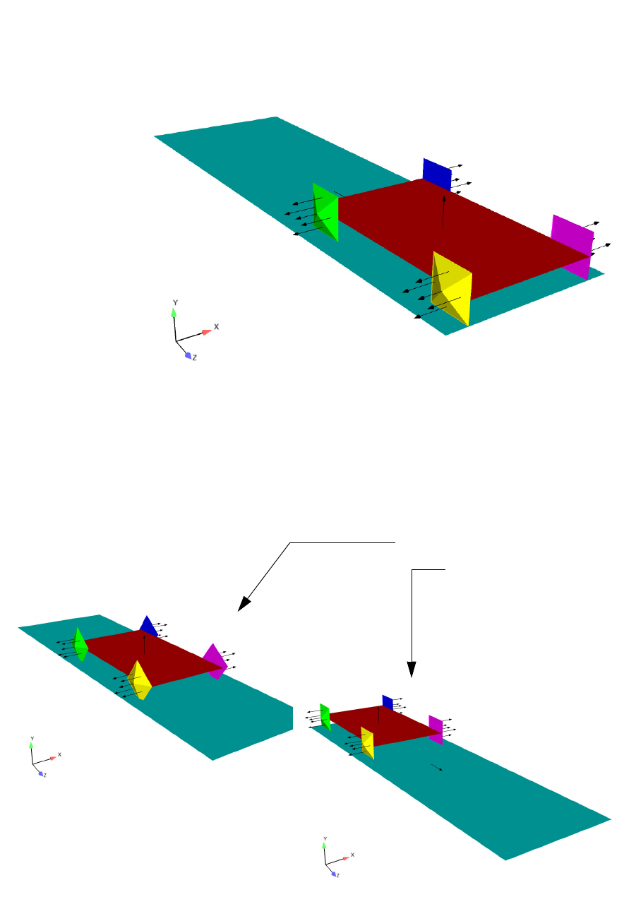
9.13 Version 2
9-194 EnSight 10.2 User Manual
So the model becomes:
Note: The assemblage has taken place, wheels are place properly on the body and
the vehicle is on the road, and it is all now in the xz plane. Note that the vectors
are also correct, including the one for the road - where we didn’t transform it - so
it is still in the z direction.
The model will be transient because the .eet file has 21 steps. So, if you step
through time, you will see the vehicle move with the wheels turning.
At step 9
At step 20
9.13 Version 2
EnSight 10.2 User Manual 9-195
For completeness, here are the contents of the other files used in this example.
Note that this model is included in the EnSight distribution (under .../data/
user_manual/rigid_body_example/erb2_example):
The veh.geo file:
EnSight vehicle example geometry
--------------------------------
node id given
element id given
extents
-5.00000e+00 5.00000e+00
0.00000e+00 1.30000e+10
-0.58000e+00 0.58000e+00
part
1
Body
coordinates
4
1
2
3
4
0.00000e+00
3.00000e+00
3.00000e+00
0.00000e+00
0.00000e+00
0.00000e+00
5.00000e+00
5.00000e+00
0.00000e+00
0.00000e+00
0.00000e+00
0.00000e+00
quad4
1
10
1 2 3 4
part
2
LF_Wheel
coordinates
5
1
2
3
4
5
4.00000e+00
5.00000e+00
5.00000e+00
4.00000e+00
4.50000e+00
2.00000e+00
2.00000e+00
3.00000e+00
3.00000e+00
2.50000e+00
0.00000e+00
0.00000e+00
9.13 Version 2
9-196 EnSight 10.2 User Manual
0.00000e+00
0.00000e+00
0.20000e+00
pyramid5
1
100
1 2 3 4 5
part
3
RF_Wheel
coordinates
5
1
2
3
4
5
4.00000e+00
5.00000e+00
5.00000e+00
4.00000e+00
4.50000e+00
2.00000e+00
2.00000e+00
3.00000e+00
3.00000e+00
2.50000e+00
0.00000e+00
0.00000e+00
0.00000e+00
0.00000e+00
0.20000e+00
pyramid5
1
200
1 2 3 4 5
part
4
LR_Wheel
coordinates
5
1
2
3
4
5
4.00000e+00
5.00000e+00
5.00000e+00
4.00000e+00
4.50000e+00
2.00000e+00
2.00000e+00
3.00000e+00
3.00000e+00
2.50000e+00
0.00000e+00
0.00000e+00
0.00000e+00
0.00000e+00
0.20000e+00
9.13 Version 2
EnSight 10.2 User Manual 9-197
pyramid5
1
300
1 2 3 4 5
part
5
RR_Wheel
coordinates
5
1
2
3
4
5
4.00000e+00
5.00000e+00
5.00000e+00
4.00000e+00
4.50000e+00
2.00000e+00
2.00000e+00
3.00000e+00
3.00000e+00
2.50000e+00
0.00000e+00
0.00000e+00
0.00000e+00
0.00000e+00
0.20000e+00
pyramid5
1
400
1 2 3 4 5
part
6
Road
coordinates
4
1
2
3
4
-5.00000e+00
-1.00000e+00
-1.00000e+00
-5.00000e+00
0.00000e+00
0.00000e+00
1.30000e+01
1.30000e+01
0.00000e+00
0.00000e+00
0.00000e+00
0.00000e+00
quad4
1
20
1 2 3 4
9.13 Version 2
9-198 EnSight 10.2 User Manual
The veh.vec file:
elemental vector
part
1
quad4
0.00000e+00
0.00000e+00
1.00000e+00
part
2
pyramid5
0.00000e+00
0.00000e+00
1.00000e+00
part
3
pyramid5
0.00000e+00
0.00000e+00
1.00000e+00
part
4
pyramid5
0.00000e+00
0.00000e+00
1.00000e+00
part
5
pyramid5
0.00000e+00
0.00000e+00
1.00000e+00
part
6
quad4
0.00000e+00
0.00000e+00
1.00000e+00
The veh.eet file:
Ens_Euler
NumTimes:
21
NumTrans:
3
Titles:
WHEEL
BODY
ROAD
Time Step:
0.0
0.0 0.0 0.0 1.0 0.0 0.0 0.0
0.0 0.0 0.0 1.0 0.0 0.0 0.0
0.0 0.0 0.0 1.0 0.0 0.0 0.0
Time Step:
6.00
0.0 0.4 0.0 9.510565e-01 -3.090170e-01 0.000000e+00
0.000000e+00
0.0 0.4 0.0 1.0 0.0 0.0 0.0
9.13 Version 2
EnSight 10.2 User Manual 9-199
0.0 0.0 0.0 1.0 0.0 0.0 0.0
Time Step:
12.00
0.0 0.8 0.0 8.090170e-01 -5.877853e-01 0.000000e+00
0.000000e+00
0.0 0.8 0.0 1.0 0.0 0.0 0.0
0.0 0.0 0.0 1.0 0.0 0.0 0.0
Time Step:
18.00
0.0 1.2 0.0 5.877853e-01 -8.090170e-01 0.000000e+00
0.000000e+00
0.0 1.2 0.0 1.0 0.0 0.0 0.0
0.0 0.0 0.0 1.0 0.0 0.0 0.0
Time Step:
24.00
0.0 1.6 0.0 3.090170e-01 -9.510565e-01 0.000000e+00
0.000000e+00
0.0 1.6 0.0 1.0 0.0 0.0 0.0
0.0 0.0 0.0 1.0 0.0 0.0 0.0
Time Step:
30.00
0.0 2.0 0.0 0.000000e+00 -1.000000e+00 0.000000e+00
0.000000e+00
0.0 2.0 0.0 1.0 0.0 0.0 0.0
0.0 0.0 0.0 1.0 0.0 0.0 0.0
Time Step:
36.00
0.0 2.4 0.0 -3.090170e-01 -9.510565e-01 0.000000e+00
0.000000e+00
0.0 2.4 0.0 1.0 0.0 0.0 0.0
0.0 0.0 0.0 1.0 0.0 0.0 0.0
Time Step:
42.00
0.0 2.8 0.0 -5.877853e-01 -8.090170e-01 0.000000e+00 0.000000e+00
0.0 2.8 0.0 1.0 0.0 0.0 0.0
0.0 0.0 0.0 1.0 0.0 0.0 0.0
Time Step:
48.00
0.0 3.2 0.0 -8.090170e-01 -5.877853e-01 0.000000e+00 0.000000e+00
0.0 3.2 0.0 1.0 0.0 0.0 0.0
0.0 0.0 0.0 1.0 0.0 0.0 0.0
Time Step:
54.00
0.0 3.6 0.0 -9.510565e-01 -3.090170e-01 0.000000e+00 0.000000e+00
0.0 3.6 0.0 1.0 0.0 0.0 0.0
0.0 0.0 0.0 1.0 0.0 0.0 0.0
Time Step:
60.00
0.0 4.0 0.0 -1.000000e+00 0.000000e+00 0.000000e+00 0.000000e+00
0.0 4.0 0.0 1.0 0.0 0.0 0.0
0.0 0.0 0.0 1.0 0.0 0.0 0.0
Time Step:
66.00
0.0 4.4 0.0 -9.510565e-01 3.090170e-01 0.000000e+00
0.000000e+00
0.0 4.4 0.0 1.0 0.0 0.0 0.0
0.0 0.0 0.0 1.0 0.0 0.0 0.0
Time Step:
72.00
0.0 4.8 0.0 -8.090170e-01 5.877853e-01 0.000000e+00
0.000000e+00
9.13 Version 2
9-200 EnSight 10.2 User Manual
0.0 4.8 0.0 1.0 0.0 0.0 0.0
0.0 0.0 0.0 1.0 0.0 0.0 0.0
Time Step:
78.00
0.0 5.2 0.0 -5.877853e-01 8.090170e-01 0.000000e+00
0.000000e+00
0.0 5.2 0.0 1.0 0.0 0.0 0.0
0.0 0.0 0.0 1.0 0.0 0.0 0.0
Time Step:
84.00
0.0 5.6 0.0 -3.090170e-01 9.510565e-01 0.000000e+00
0.000000e+00
0.0 5.6 0.0 1.0 0.0 0.0 0.0
0.0 0.0 0.0 1.0 0.0 0.0 0.0
Time Step:
90.00
0.0 6.0 0.0 0.000000e+00 1.000000e+00 0.000000e+00
0.000000e+00
0.0 6.0 0.0 1.0 0.0 0.0 0.0
0.0 0.0 0.0 1.0 0.0 0.0 0.0
Time Step:
96.00
0.0 6.4 0.0 3.090170e-01 9.510565e-01 0.000000e+00
0.000000e+00
0.0 6.4 0.0 1.0 0.0 0.0 0.0
0.0 0.0 0.0 1.0 0.0 0.0 0.0
Time Step:
102.00
0.0 6.8 0.0 5.877853e-01 8.090170e-01 0.000000e+00
0.000000e+00
0.0 6.8 0.0 1.0 0.0 0.0 0.0
0.0 0.0 0.0 1.0 0.0 0.0 0.0
Time Step:
108.00
0.0 7.2 0.0 8.090170e-01 5.877853e-01 0.000000e+00
0.000000e+00
0.0 7.2 0.0 1.0 0.0 0.0 0.0
0.0 0.0 0.0 1.0 0.0 0.0 0.0
Time Step:
114.00
0.0 7.6 0.0 9.510565e-01 3.090170e-01 0.000000e+00
0.000000e+00
0.0 7.6 0.0 1.0 0.0 0.0 0.0
0.0 0.0 0.0 1.0 0.0 0.0 0.0
Time Step:
120.0
0.0 8.0 0.0 1.0 0.0 0.0 0.0
0.0 8.0 0.0 1.0 0.0 0.0 0.0
0.0 0.0 0.0 1.0 0.0 0.0 0.0
Some additional comments:
1. Rotations, either in degrees or radians (Rx,Ry,Rz,Rxr,Ryr,Rzr) and scaling
(Sx,Sy,Sz) are applied to both geometry and vector variables. Translations
(Tx,Ty,Tz) are applied only to geometry. Note that the user can use the M: or Mv:
options if they want to supply their own 4x4 matrices. M: gets applied to
geometry only. Mv: gets applied to both geometry and vector fields. Thus, the
user has control. If the contents of the user-supplied matrix contains both
rotations and translations, and you have vector fields of interest, you may want to
9.13 Version 2
EnSight 10.2 User Manual 9-201
consider separating them into two separate matrices.
2. Pre- and post- transformations are separated by the Eul: transformation. Thus a
Eul: line is required for any of the “part(s)” that you call out in the .erb file.
Note: you do not have to reference any part(s) that do not have any rigidbody
motion or a need for a different orientation. If you need to orient a part that does
not have transient rigidbody euler transformations, simply include a transform in
the .eet file that has zero translation and rotation. The appropriate line(s) in the
.eet file would be:
0.0 0.0 0.0 1.0 0.0 0.0 0.0
And in fact, if the model had no transient rigidbody motion, but you wanted to use
the .erb file to orient the portions of the model, you could create a no-op.eet file
like:
Ens_Euler
Numtimes:
1
NumTrans3.
1
Titles:
NO-OP
Time Step:
0.0
0.0 0.0 0.0 1.0 0.0 0.0 0.0
And the Eul: line in the .erb file would be:
Eul: “no-op.eet” “NO-OP”
3. The example does not show the use of the units scaling factor. It is rarely
needed. If it is specified, the translations in the .eet file are multiplied by this
factor.
4. While the format allows for different .eet files, EnSight can only currently
handle one per model. So, place all transient euler transformations into the same
.eet file.
9.14 Euler Parameter File Format
9-202 EnSight 10.2 User Manual
9.14 Euler Parameter File Format
This contains rigid body transformation values (center of gravity translations and
euler parameters) over time. Please note that these transformations are applied
after any yaw pitch roll rotations and/or any center of gravity offsets specified in
the EnSight Rigid Body version 1 file, or any of the pre-transformations specified
in the EnSight RigidBody version 2 file. These transformations first do the euler
parameter rotations then the translations. While not required,
.eet,
is the normal
extension given to this file. It is referenced for EnSight parts via the EnSight
Rigid Body file. It can also be referenced from readers. The Nastran reader .mop
file, and the STL reader .xct are examples of this.
For a concise description of euler parameters, see the following, some of which is
discussed below.
Eric W. Weisstein. “Euler Parameter.” From MathWorld--A Wolfram Web Resource.
http://mathworld.wolfram.com/EulerParameters.html
Note the following:
1. The first line needs to be exactly as shown.
Ens_Euler
2. The second section consists of two lines. The first of which must be exactly:
NumTimes:
and the second of which must contain one integer indicating the number of
times,
nt
, contained in the file.
3. The third section consists of two lines. The first of which must be exactly:
NumTrans:
and the second of which must contain one integer indicating the number of
transformations,
ntx
, contained in the file.
4. The fourth section must begin with a line that is exactly:
Titles:
and must have
ntx
number of lines - each containing the title associated with a
transformation. These are the titles that .erb, .mob, and .xct files reference as
they associate parts with rigid body transformations.
5. The rest of the file consists of
nt
time step sections with the first line being
exactly:
Time Step:
the next line containing only a single float which represents the time value,
and the next
ntx
lines containing 7 floats representing the 3 translations in x, y,
z and the 4 euler parameters. So the way this would work is as follows. The
transformations from the Rigid Body File are applied: first the yaw pitch roll
rotations (if any specified) then second, the center of gravity offsets (if any
specified) and then the transformations from this Euler Parameter file: the euler
parameter rotations about 0,0,0 and then the translations.

9.14 Euler Parameter File Format
EnSight 10.2 User Manual 9-203
So, here is how you might use this. First put in any pre-rotations into the Rigid
Body File (if any alignment is needed, this is not normally needed), then put a
translation in the Rigid Body File in order to move the center of rotation of the
part to the origin (0,0,0) and then do the Euler rotation from the Euler Parameter
file, and then move the part back to its original location from the Euler Parameter
file. The net effect is to mathematically rotate the part about its center of rotation.
The euler parameters, eo, e1, e2, and e3 describe a finite rotation angle of
as
follows:
and a normalized, scaled unit vector, n, about which the rotation occurs.
and eo, e1, e2, and e3 form a quaternion in scalar-vector representation
and, since, Euler’s rotation theorem states that an arbitrary rotation may be
described by only three parameters, the four quantities must be related
Warning: If your four euler parameters don’t satisfy these equations you may get
odd non-linear rotational behavior and scaling of your geometry.
Suppose we want to rotate frame and base in the frame dataset (included in your
EnSight install at $CEI_HOME/ensight102/data/frame) about the Y-axis in
several timesteps. The frame dataset is static, that is, it has no timesteps. But,
e0
2
---
cos=
e
e1
e2
e3
n
ˆ
2
---
sin==
e0e(,) eo
2e1
2i
ˆe3
2j
ˆe3
2k
ˆ
+++=
eo
2ee+eo
2e1
2e3
2e3
2
+++ 1==
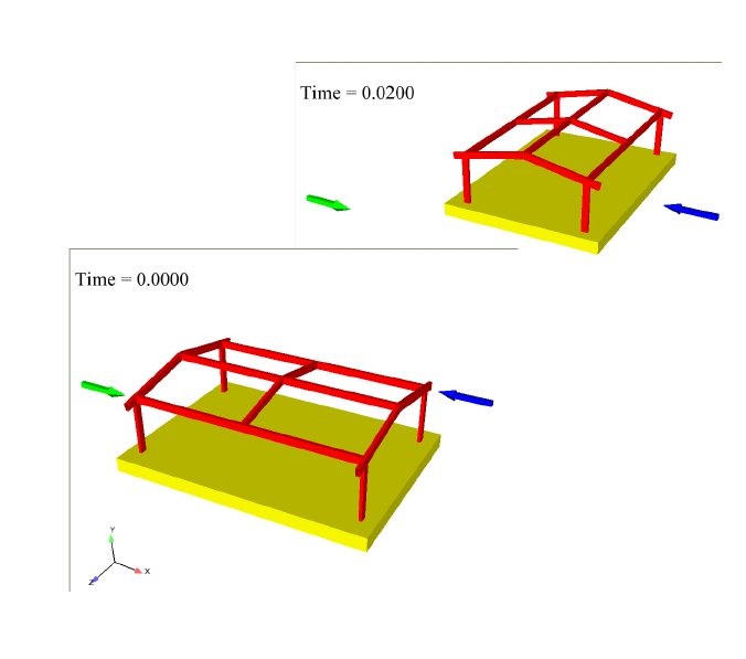
9.14 Euler Parameter File Format
9-204 EnSight 10.2 User Manual
using the rigid body rotation files, we will make the parts transient in time.
The frame case file is modified by adding one line after the model line which
indicates the EnSight rigid body (.erb) filename.
model: frame.geo
rigid_body: motion.erb
The motion.erb file might look as follows:
EnSight Rigid Body
version 1.1
names
2
"3d space frame" "simple_euler_y.eet" "Frame" "1.0" "0.0" "0.0" "0.0" "xyz" "0.0" "0.0" "0.0"
"frame base" "simple_euler_y.eet" "Frame" "1.0" "0.0" "0.0" "0.0" "xyz" "0.0" "0.0" "0.0"
This erb file names the euler (.eet) file: simple_euler_y.eet which is as follows:
Ens_Euler
NumTimes:
5
NumTrans:
1
Titles:
Frame
Time Step:
0.0
0.0 0.0 0.0 1.0 0.0 0.0 0.0
Time Step:
0.01
0.0 0.0 0.0 0.92388 0.0 0.38268 0.0
Time Step:
0.02
0.0 0.0 0.0 0.707 0.0 0.707 0.0
9.14 Euler Parameter File Format
EnSight 10.2 User Manual 9-205
Time Step:
0.03
0.0 0.0 0.0 0.3827 0.0 0.92390 0.0
Time Step:
0.04
0.0 0.0 0.0 0.0 0.0 1.0 0.0
Notice that the Euler parameters are for 5 rotations about the Y-axis, 0, 45, 90,
135, and 180 degrees. The four euler parameters are
cos(
/ 2 ), 0.0, 1.0*sin(
/ 2 ), 0.0
In this simple example we now have changed a static dataset into a transient
dataset with 5 timesteps. Notice that the .erb file has no translations. The frame
will rotate about one of the corners located at 0.,0.,0. If you want the Frame part
to rotate about the part centroid, then enter the centroid location (use a translation
of 190,56,148). The erb applies the negative of the values you enter to move it
over to the centroid prior to applying the Euler rotation.
EnSight Rigid Body
version 1.1
names
2
"3d space frame" "simple_euler_y.eet" "Frame" "1.0" "190." "56." "148." "xyz" "0.0" "0.0" "0.0"
"frame base" "simple_euler_y.eet" "Frame" "1.0" "0.0" "0.0" "0.0" "xyz" "0.0" "0.0" "0.0"
and each of the timesteps in the .eet file should translate back to the original
location by entering the same 190,56,148 values to move the part back to its
original location after the application of the Euler rotation, as follows.
Ens_Euler
NumTimes:
5
NumTrans:
1
Titles:
Frame
Time Step:
0.0
190.0 56.0 148.0 1.0 0.0 0.0 0.0
Time Step:
0.01
190.0 56.0 148.0 0.92388 0.0 0.38268 0.0
Time Step:
0.02
190.0 56.0 148.0 0.707 0.0 0.707 0.0
...
This is useful for showing the translational and rotational motion of a rigid body.
This is also useful for steady-state flows that include one solution that may have a
rotational part(s) that you wish to animate over time. You can create an euler file
that accurately rotates the part over time as well as the flow field around it, and
then trace pathlines through this rotating flowfield, because the velocity and other
vector variables are rotated along with the geometry.
9.14 Euler Parameter File Format
9-206 EnSight 10.2 User Manual
Another, more complex sample file might look like the following:
Ens_Euler
NumTimes:
6
NumTrans:
3
Titles:
Boom
Bucket
Link
Time Step:
0.0000
1600.5009 852.6449 -444.21389 0.9920 -0.0065 -0.05263 0.1144
3111.1418 -355.9743 -282.1282 0.0443 -0.5412 0.8391 -0.0291
-1463.1949 765.1186 -0.7573 0.9999 -0.0001 -0.0001 0.0035
Time Step:
0.1900
1600.6779 852.2065 -444.199 0.9920 -0.0065 -0.05263 0.1143
3093.7031 -378.0978 -284.0403 0.0454 -0.5085 0.8594 -0.0273
-1463.3661 765.2241 -0.7464 0.9999 -0.0001 -0.0001 0.0035
Time Step:
0.3900
1600.8939 852.2266 -444.23309 0.9920 -0.0065 -0.05268 0.1137
3065.6582 -404.1990 -286.7536 0.0471 -0.4527 0.8900 -0.0245
-1462.6159 765.4865 -1.4728 0.9999 -0.0002 -0.0003 0.0034
Time Step:
0.5900
1621.0400 808.7615 -446.20608 0.9947 -0.0054 -0.05139 0.0881
3053.7280 -510.7401 -292.5969 0.0464 -0.4105 0.9103 -0.0230
-1463.4859 765.3441 -3.0230 0.9999 -0.0003 -0.0002 0.0034
Time Step:
0.7901
1640.6300 771.1768 -500.67977 0.9974 -0.0017 -0.02703 0.0659
3135.5610 -562.3977 -420.8722 0.0245 -0.45 0.9012 -0.0112
-1464.9549 764.2155 -0.6192 0.9999 -0.0003 -0.0001 0.0037
Time Step:
0.9900
1654.2860 736.9480 -533.921 0.9988 -0.0004 -0.01302 0.0461
17.4958 -596.2341 -493.7609 0.0117 -0.4585 0.8885 -0.0057
-1464.9670 761.1839 -1.0681 0.9999 -0.0010 -0.0001 0.0051
9.15 Vector Glyph File Format
EnSight 10.2 User Manual 9-207
9.15 Vector Glyph File Format
This file contains vector glyph information. Vector glyphs can represent static or
transient forces or moments. These vectors can be located at a node id, an element
id, or an x,y,z location. Transient vector glyphs can change value and/or location
over time.
This file format is referenced from and EnSight Casefile, with a line in the
GEOMETRY
section, as such:
vector_glyphs: filename.vgf
See EnSight Gold Case File Format for more detail on the EnSight Casefile.
General Comments:
1. This is an ascii file.
2. Comment lines are allowed in the file. To be a comment, the line must begin
with a # sign, or be a blank line.
3. Each non-comment line begins with a keyword. When multiple lines are needed
for a given keyword entry, the keyword is repeated on each line.
4. The various tokens on a given line must be separated by spaces. Do NOT allow
the number of space separated tokens to exceed 15 on a line. Note: this restriction
really only applys to the TIMELINE times: line. All others have a set number of
tokens per line.
5. Transient timelines are specified separately, so they can easily be applied to
multiple vector glyphs. Static vector glyphs do not reference a timeline.

9.15 File description:
9-208 EnSight 10.2 User Manual
File description:
1. The first non-comment line must be exactly:
EnSight Vector Glyphs
2. The second line must be the version number, like:
Currently the only valid version is 1.0
Version 1.0
3. The third line must be the number of Vector Glyphs in the
file, like:
where
int
is the number of vector glyphs
NumVectorGlyphs: int
4. The fourth line should be the number of Transient
timelines in the file, if any. The line should look like:
where
int
is the number of vector glyph timelines.
(If all vector glyphs are static, the line is not needed, or
should indicate that the number is 0).
NumTimeLines: int
5. Each vector glyph will start with a line containing the
single capitalized word,
VECTOR
.
Under each
VECTOR
section, several lines are needed/
possible:
VECTOR
This is a required 2 token line, where
int
is an id
number. (Note: this must be first line of the
section.)
id: int
This is a required 2 (or more) token line.
description: string
This is a required 2 token line.
constant
must be
FORCE
or
MOMENT
type: constant
This is a required 2 token line.
constant
must be
STATIC
or
TRANSIENT
time_condition: constant
This is required if
TRANSIENT
time_condition. It is a 2
token line.
int
will be the id of the associated
timeline.
(Note: the
time_line
must be specified after the
time_condition
, and before any
xyzloc
or
values
lines)
time_line: int
This is a required 2 token line.
int
is the associated
part number
part: int
Use this 2 token line if attaching to a node id.
int
is
the node id to use.
nidloc: int
Use this 2 token line if attaching to an element id.
int
is the element id to use.
eidloc: int
Use this 4 token line(s) if specifying an xyz location
to act at. The three floats are the x,y,z locs. (There
must be one of these lines for each time. Thus, for a
STATIC glyph there will be just one line, but for a
TRANSIENT glyph, there will be multiple -
namely the
numtimes
of the associated timeline.)
xyzloc: float float float
(Note: one of the three location methods must be specified)

9.15 File description:
EnSight 10.2 User Manual 9-209
This is a required 4 token line(s). The three floats
are the x,y,z components of the vector. (There must
be one of these lines for each time. Thus, for a
STATIC glyph there will be just one line, but for a
TRANSIENT glyph, there will be multiple -
namely the
numtimes
of the associated timeline.)
values: float float float
6. Each vector glyph timeline (if any) will start with a line
containing the single capitalized word,
TIMELINE
.
Under each
TIMELINE
section, several lines are needed/
possible:.
TIMELINE
This is a required 2 token line.
int
is an id number,
and is the number that will be referenced by the
VECTOR
time_line
(Note: Must be first line of the section.)
id: int
This is a required 2 token line.
int
is the number of
time steps in the timeline.
(Note: Must follow the id line, and precede the
times line.)
numtimes: int
This is a required multi-token line. The
floats
are
the time values. We must read in
numtimes
floats,
however the number of these on a given line is
somewhat arbitrary. Just make sure that you do not
do more than 15 times per line.
times: float float ...
This is an optional 2 token line.
constant
is
UNDEF
or
NEAREST
. This controls what will happen if EnSight
specifies a time before the first time in this timeline.
UNDEF
will make the vector undefined.
NEAREST
will
treat it as if it is at the first time.
before: constant
This is an optional 2 token line.
constant
is
NEAREST
or
INTERPOLATE.
This controls what will happen if
EnSight specifies a time between times in this
timeline.
NEAREST
will cause the nearest time to be
used.
INTERPOLATE
will interpolate between the
bounding times.
amidst: constant
This is an optional 2 token line.
constant
is
UNDEF
or
NEAREST.
This controls what will happen if EnSight
specifies a time after the last time in this timeline.
UNDEF
will make the vector undefined.
NEAREST
will
treat it as if it is at the last time.
after: constant
(Note: The defaults for
before
,
amidst
, and
after
are:
before: UNDEF
amidst: INTERPOLATE
after: UNDEF
)
9.15 Example:
9-210 EnSight 10.2 User Manual
Example:
The following fictitious example shows a few variations for 4 vector glyphs, 2
static and 2 transient. Three are FORCE vectors, and one is a MOMENT vector.
You will note that one vector is located with a node id, one with an element id, and
2 with xyz locations.
We used some blank lines and some lines starting with #, for comments.
Note the use of the appropriate number of xyzloc and/or values lines.
Note that for the example, we did the TIMELINES
times
lines differently. The
first TIMELINE put all times on the same line - which we can easily do without
violating the 15 token limit because there are only 4 times. The second
TIMELINE put each time on its own
times
line.
In this case we did not re-use the transient timelines, but we easily could have
more than one vector glyph reference the same timeline.
EnSight Vector Glyphs
Version 1.0
#--------------------
NumVectorGlyphs: 4
NumTimeLines: 2
#--------------------
VECTOR
id: 1
description: dead load
type: FORCE
time_condition: STATIC
part: 1
nidloc: 173
values: 0.5 1.0 0.75
VECTOR
id: 2
description: wind load
type: FORCE
time_condition: TRANSIENT
time_line: 1
part: 1
eidloc: 13
values: 1.0 2.0 0.0
values: 0.0 2.0 1.0
values: 0.5 7.0 3.0
values: 2.0 5.0 8.0
VECTOR
id: 4
description: snow load
type: FORCE
time_condition: STATIC
part: 1
xyzloc: 1.5 1.5 1.0
values: 0.0 0.0 -5.25
VECTOR
id: 5
description: wrench
type: MOMENT
9.15 Example:
EnSight 10.2 User Manual 9-211
time_condition: TRANSIENT
time_line: 3
part: 72
xyzloc: 1.0 1.0 0.0
xyzloc: 1.1 1.8 0.2
xyzloc: 1.2 1.7 0.5
values: 10.0 15.0 2.0
values: 20.0 30.0 4.0
values: 100.0 150.0 20.0
#--------------------------
TIMELINE
id: 1
numtimes: 4
before: UNDEF
amidst: INTERPOLATE
after: NEAREST
times: 0.0 1.0 2.0 3.0
TIMELINE
id: 3
numtimes: 3
before: NEAREST
amidst: INTERPOLATE
after: UNDEF
times: 0.5
times: 1.5
times: 2.5
9.16 Constant Variables File Format
9-212 EnSight 10.2 User Manual
9.16 Constant Variables File Format
This file contains constant variables information. Constant variables
are defined two ways. One way is via the EnSight Gold Case file where
constant variables can be defined per case under the VARIABLE section,
i.e
VARIABLE
constant per case: [ts] Density 0.92
(see subsection EnSight Gold Case File Format under EnSight User Manual
Chapter 11.1).
The other way to define constant variables is by loading them using this Constant
Variables File Format. The advantage of this format is that all the constant
variables defined in this file will be created if they do not exist or updated if they
already exist, each time they are loaded at any stage during the EnSight session.
This file is saved or loaded via right click on a constant or constants and choosing
to save or load constants...
General Comments:
1. This is an ASCII file.
2. The file must start with the following two lines:
#Version 1.0
#EnSight Constant Variables
3. Any following line that begins with a "#" is recognized as a comment
line. Also, text following a "#" symbol is ignored as comments.
4. Each non-comment line has the following syntax
Constant_description1 Constant_value1
Constant_description2 Constant_value2
. . .
Constant_descriptionN Constant_valueN
where:
Constant_description = the variable name of the constant
Right click on a constant and choose to save
9.16 Example:
EnSight 10.2 User Manual 9-213
Constant_value = the value of the constant
5. This file format only supports static and not transient (or changing
time) constant variables. Although this file can be loaded at any
time step.
6. This file may also be loaded at anytime with no regard to data file format.
Example:
#Version 1.0
#EnSight Constant Variables
#
# Comment lines are supported and ignored during loading.
# But, the 1st two lines must be as indicated above.
#
Density .98
Pressure 1.66
Viscosity 1.965e-05 # comment appending text line is permitted
# and ignored during loading
Line 1: Required version line; verbatim as indicated above,
i.e. "#Version 1.0"
Line 2: Required file type line; verbatim as indicated above,
i.e. "EnSight Constant Variables"
Line 3 and on: Variable description, white-space, and variable value
(free format) for each variable.
9.17 Point Part File Format
9-214 EnSight 10.2 User Manual
9.17 Point Part File Format
This file format is for a series of points that can be used to specify a location to be
used as probes within a volume part (see Chapter 5.1.11, Point Parts). The point
data in this file is not loaded into EnSight as geometry. The format to load points
as geometry is a different section (see Chapter 9.1, EnSight Gold Casefile
Format).
Point part points can be loaded from a text file with the following format:
Line 1 is the version number in the form "#Version <version number>", where
version number is a floating point value. The version number is currently 1.0.
Line 2 is a keyword indicating the file type: “#EnSight Point Format”.
Lines 3 through n contain the floating point values for the x, y and z coordinates,
respectively, of each point. The values must be separated by commas or spaces
and each line may contain the x, y, and z values of only one point, terminated by a
carriage return. The number can be exponential (2 or 3 exponent values) or
floating. Any lines 3 through n that begin with a “#” are considered comments and
are ignored.
example:
#Version 1.0
#EnSight Point Format
0.00000e+00,0.00000e+00,0.00000e+00
# This is a comment line and is ignored
1.00000e-01,1.00000e-001,3.00000e-001
2.0,3.00000e-01,6.00000e-001
3.00000e+00,3.50000e-01,1.70000e+00
4.20000e+000,5.00000e-001,1.80000e+000
5.40000e+000,6.00000e-001,1.90000e+000
6.50000e+000,8.00000e-001,1.95000e+000
7.00000e+000,1.00000e+000,2.00000e+000
9.18 Spline Control Point File Format
EnSight 10.2 User Manual 9-215
9.18 Spline Control Point File Format
A Spline Control Point file is used to define one or more splines that can be used
in EnSight for positioning entities such as the camera or the plane tool. This file is
a text file with the following format:
Line 1 is the version number in the form "#Version <version number>", where
version number is a floating point value. The version number is currently 1.0.
Line 2 is a keyword indicating file type: “#EnSight Spline Control Points”.
Line 3 is the keyword to start a new spline and provide the text description of the
spline in the form “DESCRIPTION: <spline name text>” where the spline name
text is at most a 49 character text description.
lines 4 through n contain the floating point values for the x, y and z coordinates,
respectively, of each point. The values must be separated by commas and each
line may contain the x, y, and z values of only one point, terminated by a carriage
return. The number can be exponential (2 or 3 exponent values) or floating.
Lines beginning with a “#” are considered comments and ignored.
Multiple splines can be contained in one file. The keyword “DESCRIPTION:
<spline name>” begins a new spline point listing.
example:
#Version 1.0
#EnSight Spline Control Points
DESCRIPTION: First Spline
0.00000e+00,0.00000e+00,0.00000e+00
1.00000e-01,1.00000e-001,3.00000e-001
2.00000e-01,1.00000e-001,3.00000e-001
3.0,3.50000e-01,1.70000e+00
4.20000e+000,5.00000e-001,1.80000e+000
5.40000e+000,6.00000e-001,1.90000e+000
6.50000e+000,8.00000e-001,1.95000e+000
7.00000e+000,1.00000e+000,2.00000e+000
# This is a comment line and is ignored
DESCRIPTION: Second Spline
0.00000e+00,0.00000e+00,0.00000e+00
9.00000e-01,1.00000e-001,3.00000e-001
2.0,3.00000e-01,6.00000e-001
3.00000e+00,3.50000e-01,1.70000e+00
9.19 EnSight Embedded Python (EEP) File Format
9-216 EnSight 10.2 User Manual
9.19 EnSight Embedded Python (EEP) File Format
The EnSight Embedded Python file format is a mechanism that allows a user to
create portable archives of data files and scripts that can be opened and read by
EnSight through its Python interpreter. The file format itself is the standard ZIP
format used by many tools (e.g. WinZip, 7-Zip, PKZIP, zip, built into Windows
and OSX, etc). To change an existing ZIP file into a EEP file, simply change its
name to end in .eep. EnSight will recognize these files when passed on the
command line, dropped on the running application, run by the play: command or
opened via the command dialog. When presented with an EEP file, EnSight scans
its contents looking for the presence of a file named “__init__.py” or
“autoexec.py”. If files by both names are found in the EEP archive, it treats the
file as if only the “autoexec.py” file was found. The two cases are handled as
outlined below:
The “module” case (“__init__.py”):
If EnSight detects a file named “__init__.py”, it treats the contents of the file as an
EnSight module. It will extract all of the files in the EEP archive into a new,
temporary directory located in the same directory as the EEP file. If EnSight
cannot create a directory in that location, the operation will fail. Note: when
EnSight exits, the temporary directory and all of its contents will be deleted. The
directory which contains the temporary will be added to the EnSight Python
interpreter sys.path and the temporary directory will be imported as a module
using the ‘import’ command. As a result, the “__init__.py” file will be executed
by EnSight and the ‘__file__’ variable will point to the ‘__init__.py’ file. If the
same EEP file is opened a second time in a session, the files will not be re-
extracted, but reload() will be called on the module and “__init__.py” executed a
second time.
The “installer” case (“autoexec.py”):
If EnSight detects a file named “autoexec.py”, it will extract the contents of the
file as a string and execute it as Python code (similar to the exec() function). One
special variable will be set up before the string is executed. The Python variable
‘__file__’ will be set to the (string) name of the EEP file. Thus, the Python code in
“autoexec.py” can access the EEP file contents using the name in the ‘__file__’
variable and Python modules such as ‘zipfile’. An advantage of this approach is
that it does not require write access to the filesystem or the space to uncompress
the data. This approach requires a more complex user written Python script, but
should be used when the data in the EEP file is large, the filesystem is read only
(e.g. CDROM) or only a portion of the data in the file is needed.
Usage notes:
The EEP file is a very general mechanism for packaging data and scripts in a
portable fashion and getting EnSight to perform scripted operations. It can be
useful for creating demos, building installers for EnSight enhancements,
performing automated testing and other tasks. The use of the Python interpreter
inside of the EnSight application itself greatly simplifies the run-time
environment for such applications.
9.20 Camera Orientation File Format
EnSight 10.2 User Manual 9-217
9.20 Camera Orientation File Format
A camera orientation file is used to define the location, orientation, and lens field
of view angles. The orientation file can be restored in the Transformation Editor
(Camera) dialog via the File->Restore camera position option. The restored
values will apply to the camera selected and the aspect ratio information from the
field of view angles will be applied to modify any viewport using the camera.
The file is keyword delimited. The keywords can appear anywhere in the file.
Any line with a # sign in the first column is considered a comment line. Any
blank line is also considered a comment line.
FORMAT: Must be set to CAMERA_SETUP
VERSION: Must be set to 1.0
CAMERA LOCATION: Three space delimited floating point values indicating
the camera origin
CAMERA LOOK AT: Three space delimited floating point values indicating a
point along the camera view axis. The combination of the look at and the camera
location creates a camera view vector.
CAMERA ROTATION: Currently (version 1.0) ignored.
CAMERA FOV HORIZONTAL: A floating point value specifying the horizontal
field of view angle of the camera lens
CAMERA FOV VERTICAL: A floating point value specifying the vertical field
of view angle of the camera lens
Example:
FORMAT: CAMERA_SETUP
VERSION: 1.0
#
# camera location is the coordinate location of the camera
#
CAMERA LOCATION: -1500 50 150
#
# camera look at is the 3D coordinate of the center pixel of the IR image
#
CAMERA LOOK AT: 0. 50 150
#
# camera rotation in degrees about the axis from the camera location to the look at
point.
# Right hand rule.
#
CAMERA ROTATION: 0.
#
# field of view values in degrees for the horizontal and vertical axis of the lens
#
CAMERA FOV HORIZONTAL: 21.0
CAMERA FOV VERTICAL: 15.75
9.21 Multi-Tiled Movie (MTM) File Format
9-218 EnSight 10.2 User Manual
9.21 Multi-Tiled Movie (MTM) File Format
The multi-tiled movie (MTM) file format is designed to allow a single, large
movie to be subdivided into a grid array of movies for playback in a tiled
hardware setup using EnVideo. The mtm format also allows collections of images
that match a pattern to be read as a movie, as a stereo image, or as a stereo movie.
The mtm format also allows a pair of animations to be read as a stereo animation.
Finally, mtm format can be used to simply play two existing movies side by side.
Example Tiling of large movie by subdividing into two parts in the X:
MTM 1.0
#
# This is a Multi-Tile Movie file of full dimension (1400x600).
# with each sub movie containing half of the X dimension
# of dimension 700x600
fullresolution 1400 600
nummovies 2
movie
imageoffset 0 0
format EVO
file "test2_0000.evo"
movie
imageoffset 700 0
format EVO
file "test2_0001.evo"
Example Stereo movie using a series of left and right png files:
MTM 1.0
#
# MTM file written by EnSight 10.1.5(a)
# Stereo movie saved from EnSight into .png format
# which saved this mtm file as ens_stereo.mtm
# and a series of files named as follows:
#
# ens_stereo_0001_l.png, ens_stereo_0001_r.png
# ens_stereo_0002_l.png, ens_stereo_0002_r.png
# ens_stereo_0003_l.png, ens_stereo_0003_r.png
# ...
nummovies 1
fullresolution 700 600
movie
imageoffset 0 0
file "ens_stereo_####_@.png"
9.21 Example Tiling of two movies to play them side by side:
EnSight 10.2 User Manual 9-219
Example Tiling of two movies to play them side by side:
MTM 1.0
#
# This is a Multi-Tile Movie file of full dimension (1400 x 600).
# with the first sub movie containing 700 x 600
# and the second movie containing 700x500
# NOTE: because the second movie is not as large in the Y
# direction, there will be a black bar above the movie
# denoting the mismatched pixels.
#
# This allows you to play two movies of the same number of
# timesteps side by side.
#
fullresolution 1400 600
nummovies 2
movie
imageoffset 0 0
format EVO
file "movie1.evo"
movie
imageoffset 700 0
format EVO
file "movie2.evo"
EnSight 10.2 User Manual 10-1
10 Utility Programs
This chapter describes the utility programs that accompany EnSight. The Server
utility programs are located in $CEI_HOME/ensight102/server_utilities and
the Client utility programs are located in $CEI_HOME/ensight102/
client_utilities.
Utility programs are supplied on an “as is” basis and are unsupported. CEI will,
however, try to assist in problem resolution.
Each utility program is presented below and accompanied with a brief overview
that describes the function of the utility.
Section 10.1, EnSight Case Gold Writer
10.1 EnSight Case Gold Writer
10-2 EnSight 10.2 User Manual
10.1 EnSight Case Gold Writer
EnSight Case Gold Output API
The EnSight Case Gold Output API will allow users to make simple calls to our API to
write out EnSight’s Case Gold format.
In your installation directory, under $CEI_HOME/ensight102/src/
you will find the following directories
enout6_api - C output API for EnSight6 format
enoutg_api - C output API for EnSight Gold format
enout_py - Python output API for EnSight Gold format
Within each of these subdirectories is the API source code and a text help file. For any
other questions, please contact support@ensight.com for the latest information.
EnSight 10.2 User Manual 11-1
11 Remote Display and Parallel
Compositing
Remote Display
The EnSight architecture allows the compute and memory intensive operations
(server) to be located on a separate machine(s) than the user interface and graphics
display (client). There are times, however, when it is useful to also be able to
execute the client operations on a remote machine and "remote" the display back
to the desktop system. These situations may arise for a multitude of reasons
including:
(a) The desktop machine is "thin", meaning it does not have the capacity or
capability to act as an EnSight client, (b) The network bandwidth and/or latency is
such that the usual server to client communication results in low performance, (c)
EnSight software is only installed on remote machines and not on the desktop
machine. There is no single obvious solution for dealing with the multitude
various remote rendering situations but rather a number of different strategies that
may be examined and deployed.
Parallel Compositing
When the size of the data to render would overwhelm one client, EnSight HPC+
can distribute data between multiple remote clients. The remote clients each
render a portion of the data in parallel, and composite their images for display on
the main client.
Configuration File
formats
Proper settings for the various configurations are discussed throughout this
chapter.
Resource File
format
Details for the Resource file format, which is also discussed in this chapter can be
found in How To Use Resource Management.
11.1 Remote Display
11-2 EnSight 10.2 User Manual
11.1 Remote Display
Introduction
EnSight has always been a client / server based application by design to optimize
performance for analysis and visualization. For large enough data set sizes the
end-user (“user”) should make a conscious choice on where to run the EnSight
Client (“Client”) and EnSight Server (“Server”).
In most situations for best performance, it’s intended that the Client should be
used on the computer that the user is sitting in front of. This document will refer
to the computer that the user is sitting in front of as the “workstation” whether it is
a typical desktop or laptop computer or a high-end workstation. The reason that
the Client is intended to run on the workstation is because it is responsible for the
EnSight Graphical User Interface and OpenGL-based graphics rendering - both of
which perform better when they utilize the workstation’s graphics card.
Since the data to be analyzed may or may not reside on the same computer, the
user can choose to run the EnSight Server where the data are located. In many
situations this is the same workstation. Simply running the command
‘ensight102’ (or other versions) will start the Client and Server together on the
workstation. Various command line options, CEIStart, and other means can be
used to run the EnSight Server on a different computer.
Typically, running the Client on the workstation and the Server where the data are
located is the best approach for using EnSight in many cases. However, there are
situations where it makes sense to run the Client on a computer other than the
workstation while still displaying the Client via some remote display or remote
rendering mechanism back to the workstation.
One reason to run the Client on another computer is simply because the user’s IT
department does not install application software on the user’s workstation.
Another situation is when the workstation is relatively “thin” (underpowered)
compared to the needs of the EnSight Client and the data set being visualized.
Similarly, it may be advantageous to run the Client on another computer when the
network performance between the workstation and where the data are located is
undersized relative to the size of the data sent between the Server and Client.
It should be noted, however, that while it is possible to use EnSight with Remote
Rendering (or Remote Desktop), overall EnSight performance may still be better
in many cases running the Client on the workstation. Modern laptops, desktops,
and workstations tend to be extremely powerful. When compared to running a
graphical application remotely over typical networks, the native performance of a
modern workstation is difficult to beat in many cases.
The rest of the document presents the common approaches to using EnSight with
either remote desktop or remote rendering technologies. While there may be
other approaches not described here, these are the ones CEI Inc. uses and tests.
Remote Display using Microsoft’s Remote Desktop
If the user’s workstation and the computer intended run the EnSight Client are
both running Microsoft Windows, then it is advantageous to use Microsoft
11.1 Remote Display
EnSight 10.2 User Manual 11-3
Remote Desktop to control and view the EnSight Client on the remote computer.
It has the advantage of being completely supported by Microsoft without
requiring additional software to be installed. Furthermore, no modifications in
configuration nor use are needed by EnSight. The user simply starts the Microsoft
Remote Desktop application on their workstation and instructs it to connect to the
remote computer running Windows. The entire “display” of the remote computer
is transmitted to the user’s workstation. At this point the user simply runs the
EnSight Client.
The disadvantage of this approach is that the Remote Desktop application may not
take advantage of hardware assisted OpenGL rendering on the remote computer.
Falling back to software based rendering can be anywhere from 2 to 100 times
slower than hardware based rendering. Furthermore, Microsoft Remote Desktop
essentially takes over the entire desktop of the remote computer; multiple users
cannot typically use the same remote computer at the same time.
Remote Display using Apple’s Screen Sharing
Similar to Microsoft’s Remote Desktop application is Apple’s Screen Sharing
application. It, too, requires that both the workstation and remote computer are
running Apple’s MacOS X operating system. However, Apple Screen Sharing
does use the OpenGL graphics card in the remote computer. As of MacOS X
“Yosemite” multiple users may use the same remote computer.
Remote Display using VNC
VNC is the generic name for a remote display protocol that was initially created
for Unix and Linux operating systems. It is also supported by Apple’s MacOS X
operating system. Whereas Microsoft Desktop and Apple Screen Sharing are
specific applications provided by those operating systems, VNC requires
configuration of the remote computer’s display and/or graphics software and
installation of a client VNC application. Such client applications exist for
Windows, MacOS X, and Linux. Indeed, Apple’s Screen Sharing application
supports the VNC protocol as well as their own screen sharing protocol.
Depending upon the VNC implementation running on the remote computer, it
may or may not support multiple concurrent users. Similarly, it may or may not
support hardware based OpenGL support. Deploying and using VNC typically
requires IT support by the end-user due to the myriad of options and need for
operating system configuration of the remote computer. For this reason we (CEI)
do not support users with generic VNC installations such as TurboVNC. We
mention it here merely to suggest that solutions exist that may fulfill the
requirements of running EnSight entirely on a remote computer that may be
“blessed” solutions by the user’s IT department. If a VNC solution is not already
configured at your location we do not recommend using one of the VNC
solutions. We have tested several of them and find the setup, support, and
operation to be somewhat problematic. But of course technology changes over
time. Our examination was between February and November of 2014.
Remote Display using HPRGS
HP offers a remote desktop solution called RGS, which offers functionality
similar to VNC in that it allows a whole desktop to be displayed on a remote
machine. Linux and Windows are supported for both the workstation and remote
computer. It also supports hardware accelerated OpenGL. All OpenGL features
11.1 Remote Display
11-4 EnSight 10.2 User Manual
in EnSight 10.2 work under RGS, except for stereo displays. Its main drawback is
the somewhat difficult installation and configuration process, which is roughly as
difficult as the installation of other VNC software. The remote computer can run
one instance of the RGS sender. One or more RGS receivers can connect to it,
allowing collaboration. The cost starts at $200 for a node-locked RGS sender, and
the receivers are free (as of November 2014). We (CEI) have tested and continue
to use HPRGS. This is the recommended “remote desktop” solution for Linux
and mixed Windows, Mac, Linux installations.
EnSight’s “Remote Renderer”
Compared to the previous approaches which allow a workstation to share the
entire desktop of a remote computer, EnSight 10.1.3(a), and later, implements a
different approach called EnSight Remote Renderer. With this approach the
EnSight Client still runs on the user’s workstation but the actual graphics
rendering occurs on a remote computer with images automatically sent back to the
Client running on the workstation. Visually, the EnSight Client appears the same
as it does without Remote Renderer.
EnSight Remote Renderer has several advantages. It has the advantage of
working without additional software. Also, it can use hardware or software based
rendering on the remote computer with the user simply choosing which to use via
a checkbox. Another advantage is that remote desktop sharing software isn’t
needed. Remote Renderer can also be more efficient compared to desktop sharing
approaches since it doesn’t send images of the entire desktop - only the EnSight
graphics window is communicated to the workstation. Furthermore, it is the only
solution that supports stereo displays. One disadvantage compared to previous
approaches is that it requires EnSight to also be installed on the workstation as
well as the remote computer.
Installation with EnSight 10.1.3(a)
The initial release requires a small amount of site setup to enable EnSight Remote
Renderer. Specifically, the site needs to install three files into their CEI software
installation. The site needs to copy the files
‘run_ceishell_remote_renderer_fe.py’ and ‘run_ceishell_remote_renderer_be.py’
into $CEI_HOME/bin/ and ‘site_server_configs.py’ into $CEI_HOME/
ensight102/site_preferences/. If the site already has a file $CEI_HOME/
ensight102/site_preferences/site_server_configs.py then the CEI provided one
needs to be integrated into the site’s existing file. Contact CEI Support for
assistance if needed.
Future versions of EnSight Remote Renderer will be fully integrated into the
normal EnSight installation package and will not require any site manual
installation as described above.
Using EnSight Remote Renderer
Remote Renderer is started via ‘ceistart102’. When properly configured, the user
will see the ‘Remote Renderer’ option in the CEIStart dialog (see figure 1).
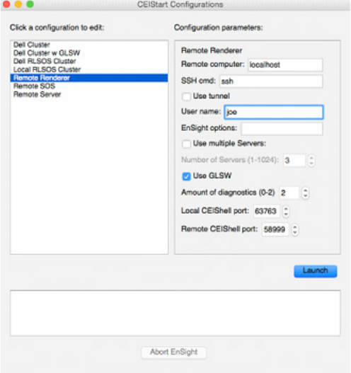
11.1 Remote Display
EnSight 10.2 User Manual 11-5
Selecting the ‘Remote Renderer’ option displays the list of options for the
CEIStart configuration described as follows:
‘Remote computer:’ is the computer where EnSight will run the Server, and
Remote Rendering components (SOS, CollabHub, and DRClient). The user is
required to have a valid account on that computer, working password-less SSH or
equivalent authentication, and a compatible version of EnSight installed.
‘SSH cmd:’ is the name of the SSH command - typically ‘ssh’ on Linux and
Macs. The application ‘plink.exe’ is recommended on Microsoft Windows. Note
that ‘pagent.exe’ needs to be configured and used to support password-less
authentication by plink.exe.
‘Use SSH tunnel.’ will enable SSH tunneling. This is typically required if the
user’s desktop computer, where ceistart102 is running, is not directly accessible
by the remote computer. This is common if the desktop computer sits on an
opposite side of a firewall or router from the remote computer.
‘User name:’ is the user’s login name on the remote computer.
‘EnSight options:’ can be used to specify any command line options normally
given on the ‘ensight102’ command line.
‘Use multiple servers:’ can be toggled on to use more than one EnSight Server
(i.e. SOS or EnSight HPC). Note that this requires that the site have an
appropriate license that enables EnSight HPC.
‘Number of Servers:’ specifies the number of EnSight Servers if using EnSight
HPC.
‘Use software rendering.’ toggles on/off OpenGL Software Rendering. If off,
11.1 Remote Display
11-6 EnSight 10.2 User Manual
EnSight will try to use hardware-enabled OpenGL rendering on the remote
computer. This requires that the remote computer be properly configured to
support applications using OpenGL remotely. Contact CEI Support if you require
guidance. If ‘Use GLSW’ is toggled on, then EnSight will use software rendering
on the remote computer. This does not require any special hardware nor system
support on the remote computer. However, rendering performance can vary
between 2x to 100x worse compared to hardware rendering.
‘Amount of diagnostics:’ indicates the amount of output generated by CEIStart.
‘0’ should be used for normal use since that greatly reduces the amount of output
thus improving performance. ‘1’ or ‘2’ should be used for debugging start up
issues or EnSight errors. If requiring support from CEI, please use ‘2’ to gather
helpful output. In such situations, please also specify the EnSight option ‘-v 3’.
This can be added to the ceistart102 command line.
‘Local CEIShell port:’ and ‘Remote CEIShell port:’ are auto generated random
numbers for TCP port numbers. These are used to prevent conflict with other
EnSight users on the same computers.
11.2 Parallel Compositing
EnSight 10.2 User Manual 11-7
11.2 Parallel Compositing
Parallel compositing is sometimes referred to as EnSight HPC+ or EnSight PC. It
enables users with an extremely large amount of visible geometry to distribute the
client-side computation and rendering among multiple CPUs and GPUs in a
cluster of workstations. The final result is an image in the EnSight rendering
window that is indistinguishable from a standard EnSight client running on a
single workstation, but at much higher performance.
Pros:
• very-high polygon rates (Billions of triangles / sec)
• scalable client memory and computation
• ability to render remotely and view locally
Cons:
• frame-rate upper-bound determined by network bandwidth
• resolution limited to single workstation display
Compositing is for users working in a desktop environment who have large data
which overwhelms the capability of a single workstation, in terms of memory,
processing power, and/or rendering performance. Note that compositing is not an
application for ganging together dozens of old workstations that have no other use
- compositing itself requires fast processors and a fast network in order to achieve
any measure of scalability.
EnSight HPC+ Configuration
A properly configured CEIShell network is required to use EnSight HPC+ (see
Chapter 13, CEIShell).
Given a running CEIShell network, EnSight HPC+ can be started by running the
command:
ensight102 -ceishell -prdist [optional_prdist_file]
The command line option '-ceishell' instructs EnSight to use the CEIShell
network. The '-prdist' option stands for ‘distributed parallel rendering’, and it
instructs EnSight to use parallel compositing. The -prdist option takes an optional
prdist file name although it is not usually needed (see Command Line Start-up
Options).
EnSight will run distributed rendering Clients on CEIShells that have the role
name 'DRCLIENTS'. If none have the role name 'DRCLIENTS', then any
CEIShells with role names 'SOS_SERVERS' will be used. If none have that role
name then 'SERVER' will be tried and then finally 'localhost'. You should use
either 'DRCLIENTS' or 'SOS_SERVERS' to be explicit as to which CEIShells
should be used.
EnSight will run the EnSight CollabHub on the CEIShell with the role name
'COLLABHUB'. If that can't be found, then role names 'SOS' or 'localhost' will be
used.
In EnSight 10.2 there are restrictions on the computers and their network
connectivity.
The DRCLIENTS must be on the same computer as the COLLABHUB
11.2 Parallel Compositing
11-8 EnSight 10.2 User Manual
computer or no more than one CEIShell connection away.
The DRCLIENT computers must be able to open a network connection to
each other.
The COLLABHUB must be on the same computer as the main EnSight
Client or one hop away.
The SOS must be on the same computer as the COLLABHUB or one hop
away.
The functioning CEIStart configuration "Remote SOS" shows how the entire
process can be fully automated including EnSight startup with optional one-click
invocation of parallel compositing. Many users may find that this configuration is
sufficient for real production use on a larger SMP type computer (for example, an
8 CPU or greater system with 8GB or more of memory).
The optional prdist file can be used to specify parallel compositing options;
although, it is frequently not needed. The format of the file looks like:
#
pc [options]
where [options] may include:
guicomposite = “NONE” “NOCOMP” “COMP”
compression = “NONE” “LOW” “MED” “HIGH” “AUTO”
guicompression = “{RAW|RLE|GZ} {final quality}
{interactive quality}” example: “RLE 0 2”
offscreen = “TRUE” “FALSE”
guicomposite
The parallel compositor (PC) needs to make a full set of TCP/IP connections
between all of the render processes to exchange data between them. The master
client (often called the GUI-client) is the EnSight client that actually displays a
GUI and with which the user interacts. The guicomposite option has three
possible values that determine the extent to which the master client participates in
the compositing.
• COMP: If the client is physically running on the same cluster as the other
rendering nodes, use guicomposite="COMP". This causes PC to use the
master node as part of the composite and as a side effect, leave the final
image on that node. It is the most efficient way to get an image from PC
to the screen, but the master node needs to be on the same high-
performance network as the other render nodes for this to work well as it
assumes symmetric bandwidth between the renderer clients and the
master client. "TRUE" is the same as "COMP".
• NOCOMP: The next level of performance is guicomposite="NOCOMP".
In this mode, the master still makes TCP/IP connections to each of the
renderer nodes, but it does not participate in the actual compositing. The
various pieces of the final image are sent back to the master node in
parallel over the N sockets to the render nodes. This mode works well if
11.2 Parallel Compositing
EnSight 10.2 User Manual 11-9
the master node is not located on the cluster interconnect, but can still
make N connections to the cluster over a fairly high performance
interface. (e.g. the asymmetric bandwidth situation). In practice, few
people use this mode as the number of off-cluster TCP/IP connections to
the master can be a problem for things like firewalls.
• NONE: The last level is guicomposite="NONE". In this mode, the PC
system runs entirely on the cluster and the final image is passed to the first
renderer node. That node can optionally compress the image and then
sends it via TCP/IP to the collabhub which then sends it to the master
client for display. This requires two network hops, but ensures that all of
the TCP/IP connections of PC remain inside the cluster. It is the most
firewall friendly mode as no new ports need to be opened up, but it is also
the slowest mode.
compression
The compression option determines how the render clients communicate
during compositing. If the rendered images are large and the CPUs are fast
enough, enabling compression can increase the frame rate. These compression
methods are all lossless. There are very few situations where the best value us not
“HIGH”.
guicompression
The guicompression option only has an effect when guicomposite is set
to “NONE”. This option allows you to specify a compression level for images
transmitted through the collaboration hub. This option is most useful when the
main client is remote from the rendering cluster, perhaps over a lower-bandwidth
and/or higher-latency network.
There are three compression methods each followed by two numbers: a final
quality number and an interactive quality number. The higher the number, the
lower the image quality. A quality value of 0 is lossless. The final number
represents the quality of the still image when no more transforms are occurring,
and the interactive number represents the quality of the image while undergoing
transforms (e.g. rotation or translation). Often the interactive number is higher
(lower quality) than the final to accelerate transformations.
RAW - uncompressed pixels. In this mode, the final and interactive quality
numbers represent spatial decomposition (elimination of some spatial fraction of
the pixels). The final and interactive quality numbers can range from 0 to 8,
where 0=all pixels, 1=every other pixel, 2=every third pixel, etc. Visually, this
effectively looks like larger pixels.
RLE - the evo RLE scheme, which has a nice balance of speed vs compression.
The final and interactive quality numbers represent the number of lower-order bits
of a color that are set to zero before the RLE scheme is applied. For example, the
value 2 means that the color of a pixel is first reduced to 6 (8-2) bits per pixel
before the compression. Therefore these quality numbers should ranges between 0
(highest quality) and 7 (lowest quality). Visually, this looks like quantized colors/
banding.
GZ - use the "gzip" algorithm is slower, but has good compression. The final and
transition quality numbers work as in the RLE case.
11.2 Parallel Compositing
11-10 EnSight 10.2 User Manual
offscreen
The offscreen option specifies that the render workers should create offscreen
(pbuffer) rendering windows. By default they will be onscreen, which is useful for
viewing and confirming the partial results. One advantage of using offscreen
windows is that your render nodes do not have to run at the same resolution as
your main client. Note: if guicompression = “NONE” and offscreen = “FALSE”
then the first renderer node in the prdist file may not display any image. It is
rendering and participating properly, however.
example
If the master client (where the GUI is) is on the cluster, use "COMP". In all other
situations, use "NONE". You can try "NOCOMP", but it is not always a win. In
house, we typically use the following pc line in our prdist files:
pc compression="HIGH" guicomposite="COMP" offscreen="TRUE"
guicompression="RLE 0 2" (all on one line).
If the master client is not on the cluster, change "COMP" to "NONE". For 99% of
the cases, that is the best setup.
See How To Use Resource Management for an example using resources
Trouble-shooting
For trouble-shooting problems like X server access, see Tips for Distributed
Rendering.
EnSight 10.2 User Manual 12-1
12 Caves, Walls & Head-mounted
displays
This chapter will discuss three kinds of displays (Caves, Walls and Head-
mounted) and the external input devices that used to navigate these displays.
A Cave is an immersive display with one or more screens often arranged in a
fashion to give the illusion of being in a virtual space, where you can walk into
and look inside of your simulation. The user’s head position and orientation are
tracked, and the screens are continuously redrawn, to maintain this illusion.
A Wall is a flat tiled display with multiple screens, usually rendered using
multiple machines. Walls can have a very high aggregate resolution, with a width
and height of tens of thousands of pixels. They are commonly referred to as
display walls, tiled displays, or power walls.
A Head-mounted display simulates a virtual environment much the same as a
Cave, except that the screens are mounted in front of the users eyes instead of
fixed to the walls.
Finally this chapter will discuss external input devices such as game controllers
that improve upon the traditional keyboard and mouse interface for navigation
within these custom environments.
12.1 CAVES
12-2 EnSight 10.2 User Manual
12.1 CAVES
This section discussions the creation, management, and navigation within a Cave
environment.
Configuration File (dconfig)
In order to configure a cave or a wall in EnSight, the user must create a display
configuration file. This file is specified on the command line using the argument -
dconfig <file> (see Command Line Start-up Options). If <file> is not a
fully-qualified path EnSight will search for the file in the following directories:
1. ~/.apex31/dconfig
2. $CEI_HOME/apex31/site_preferences/dconfig
These options allow for user-level and site-level configurations, respectively.
There are two logical displays that can be configured in EnSight. The file is used
to configure a detached display, which is external to the user-interface, and may
consist of 1-36 regions configured to form a large continuous display. The
configuration file also contains tracking calibration information and options for
using 6D input devices. The following sections will address each of the
capabilities related to parallel rendering and VR. The sample configurations
described in this chapter can be found in the directory $CEI_HOME/
ensight102/doc/dconfig. There are also examples of ‘simulated’
configuration files, which allow you to simulate display to multiple graphics pipes
on a single display.
Configuration File (dconfig) format
Configuration files are text-based beginning with the line:
CVFd 1.0
# after the first line, anything following a '#' is a comment
The remainder of the file consists of one or more sections describing the displays
and options. In describing the format of the file, portions which are optional will
be surrounded by [].
The key factors are that (1) immersive displays are often not flat and (2) the
rendered images must be co- registered with the coordinates of a 6d input tracking
system.
12.1 CAVES
EnSight 10.2 User Manual 12-3
Screen Layout
The basic syntax describing how screens are positioned in the cave:
display
[ stereo ]
screen
[ hostid <h> ]
displayid <p1>
resolution <x-res> <y-res>
[ displayorigin <xo> <yo> ]
[ bottomleft <x> <y> <z>
bottomright <x> <y> <z>
topleft <x> <y> <z>
]
[ lefteye
or
righteye
]
[ repeat 'screen' section for each additional screen
]
Note that all 3d coordinates given in the file are in the same frame of reference,
and use the same units, as the tracking system. We will refer to this as "display
coordinate space".
The keywords bottom/top refer to the minimum Y/maximum Y of the region, and
left/right refer to the minimum X/maximum X of the region. In some cases
'bottom' may be near the ceiling, and 'top' may be near the floor, such as when a
projector is mounted in an inverted position.
When determining the proper coordinates to use it is invaluable to sketch out the
display environment, label the corners of each screen, and mark the location of the
origin of the coordinate system. When using 6D input, the display coordinate
system and the tracking coordinate system must be the same.
Example 1
For the purpose of illustration consider the following example. Two projectors are
pointed at screens which form a right angle, as illustrated below. The projected
images are 10 feet wide by 7.5 feet high. The tracking system is calibrated in units
of feet with the origin on the floor in the middle of the room.
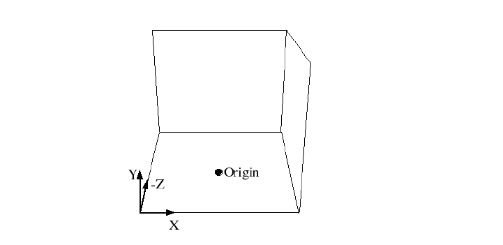
12.1 CAVES
12-4 EnSight 10.2 User Manual
CVFd 1.0
display
screen
displayid :0.2
resolution 1024 768
bottomleft -5 0.0 –5
bottomright 5 0.0 –5
topleft -5 7.5 –5
screen
displayid :0.1
resolution 1024 768
bottomleft 5 0.0 –5
bottomright 5 0.0 5
topleft 5 7.5 -5
Without head-tracking, this example is not yet very useful. The default position of
the viewer is at (0,0,0), which is on the floor in the chosen coordinate system.
There is an optional view section that can be inserted before the first screen of
the configuration file to change these defaults:
view
[ origin <x> <y> <z> ]
[ zaxis <nx> <ny> <nz> ]
[ yaxis <nx> <ny> <nz> ]
[ center <x> <y <z> ]
[ scale <factor> ]
[ eyesep <d> ]
The origin specifies the position of the viewer, and is only used if head-
tracking has not been enabled. The zaxis and yaxis are unit vectors that allow
the specification of a default orientation for objects placed in the scene. The
default values are (0,0,-1) for zaxis and (0,1,0) for yaxis. From the origin
vantage point, it is useful to think of zaxis as the direction that the viewer is
12.1 CAVES
EnSight 10.2 User Manual 12-5
looking and yaxis as the 'up' direction.
The center and scale parameters allow you to position and size the scene for
your display. If these parameters are not given, EnSight will compute a bounding
box from the 3d coordinates given in the bottomleft, bottomright, and
topleft parameters for the screens. The default center will be at the center of
this box and the default scale will be computed so that your EnSight scene will fill
the 3d space. Specifying a scale factor of 1.0 may be useful if your display
coordinates were designed to coincide with your model coordinates. This will
allow you to view your models life-sized. The values used to center and scale the
data can be adjusted at runtime. See the VR and user defined input Preferences for
more details.
The eyesep parameter allows an exact setting of the stereo separation between
the eyes. It is half the distance between the eyes in the units used by the head
tracker.
Example 2
Extending our example, we can position the viewer at the opposite corner of the
room at a height of 5.75 feet:
CVFd 1.0
display
view
origin -5 5.75 5
screen
displayid :0.2
resolution 1024 768
bottomleft -5 0.0 –5
bottomright 5 0.0 –5
topleft -5 7.5 –5
screen
displayid :0.1
resolution 1024 768
bottomleft 5 0.0 –5
bottomright 5 0.0 5
topleft 5 7.5 -5
Example 3
It is relatively straightforward to test large displays and VR environments on a
smaller system with a different number of graphics pipes. This can be
accomplished by creating a configuration file that maps the pipes to smaller
regions on a single monitor. As an example we will take the immersive
configuration from Example 2 and modify it to run on a single display, with the
modified regions shown in bold text.
CVFd 1.0
display
12.1 CAVES
12-6 EnSight 10.2 User Manual
view
origin -5 5.75 5
screen
displayid :0.0
resolution 0 240
bottomleft -5 0.0 –5
bottomright 5 0.0 –5
topleft -5 7.5 –5
screen
displayid :0.0
displayorigin 0 0
resolution 0 240
bottomleft 5 0.0 –5
bottomright 5 0.0 5
topleft 5 7.5 -5
Note that this method makes use of the displayorigin parameter so that the
resulting windows do not overlap. The default value for displayorigin is
(0,0) for each pipe. In a similar manner it is also possible to simulate large display
walls on a single pipe.
Tracking and Input Devices
EnSight supports tracking and input with 6 DOF devices through a defined API.
Pre-built libraries are provided to interface with VRPN or trackd ((C) Mechdyne,
Inc., www.mechdyne.com) on Windows and Linux, or the user may write a
custom interface to other devices or libraries. The tracking library is specified
with the CEI_INPUT environment variable.
The value of CEI_INPUT can either be a fully-qualified path and filename or
simply the name of the driver, in which case EnSight will load the library
libuserd_input-$(CEI_INPUT).so from directory:
$CEI_HOME/apex31/machines/$CEI_ARCH/udi/
Once any external programs are started, e.g. a trackd or VRPN server, you can
enable tracking in EnSight. From the ‘Preferences->VR and User
Defined Input’ menu, there is a toggle button which turns tracking on and
off (see VR and user defined input Preferences).
For information on the API which allows you to interface to other tracking
libraries or devices, please see the README file in $CEI_HOME/ensight102/
src/cvf/udi.
Trackd
To select trackd, use:
setenv CEI_INPUT trackd (for csh or equivalent users)
12.1 CAVES
EnSight 10.2 User Manual 12-7
For the trackd interface you will also need to set:
CEI_TRACKER_KEY <num>
CEI_CONTROLLER_KEY <num>
in order to specify the shared-memory keys for the input library to interact with
trackd. You can find the tracker and controller key values in your trackd.conf
configuration file.
With the environment variables set, you are ready to activate tracking. There are
two parts to this. First, trackd operates as a daemon that is run independent of
EnSight. If your input interface includes a separate program, you can run it at this
time. For trackd users, it is often useful during configuration to invoke trackd with
the –status option, so that you can see the information on your input devices.
The trackd driver shipped with EnSight also has a debug mode that can be
activated as follows:
setenv CEI_TRACKD_DEBUG 1
This is similar to the trackd -status option, but it reports the input as seen by the
EnSight trackd interface.
VRPN
To select VRPN, use:
setenv CEI_INPUT vrpn (for csh or equivalent users)
VRPN is set up using a configuration file. Specify the path to the vrpn
configuration file with an environment variable:
setenv CEI_VRPN_CONFIG [full path]/vrpn.cfg
The file is ASCII text and has the following format:
#VRPN 1.0
TRACKER (outnum) (vrpn_name) (sensor) (scale) (offset)
TRACKERVEC (outnum) dirx diry dirz upx upy upz
VALUATOR (outnum) (vrpn_name) (channel) (scale) (offset)
BUTTON (outnum) (vrpn_name) (button #)
DEBUG (0-4)
The file should start with the "#VRPN 1.0" string. Afterward, the various
commands follow. The text in parenthesis should be replaced by numbers. The
commands include
DEBUG (level)
string. Afterward, the various commands follow. The text in parenthesis should
be replaced by numbers. The commands include
TRACKER (outnum) (vrpn_name) (sensor) scale offset
Adds a tracker (numbered OUTNUM) to the UDI. The tracker input is from a vrpn
server using the name VRPN_NAME (in most cases, this string looks like an email
address). The specific sensor in the vrpn server is selected using SENSOR.
SCALE and OFFSET are a linear transformation applied to the tracker position
12.1 CAVES
12-8 EnSight 10.2 User Manual
before being presented to EnSight. Note: more than one VALUATOR line that
references the same VRPN_NAME may be specified for different OUTNUM values.
TRACKERVEC (outnum) dirx diry dirz upx upy upz
Refine the definition of the UDI tracker (numbered OUTNUM). The dir{x,y,z}
values define the vector that is transformed via the vrpn transform to produce the
EnSight UDI "forward" vector. The up{x,y,z} values define the vector that is
transformed via the vrpn transform to produce the EnSight UDI "up" vector. The
default values are: 0. 0. 1. 0. 1. 0. Note: the line must be preceded by a
TRACKER line with the same OUTNUM value.
VALUATOR (outnum) (vrpn_name) (channel) (scale) (offset)
Adds a valuator (numbered OUTNUM) to the UDI. The valuator input comes from
the vrpn remote "analog" server named VRPN_NAME. The specific channel in the
server is selected using CHANNEL. SCALE and OFFSET are a linear transformation
applied to the valuator before being presented to EnSight. Note: more than one
VALUATOR line that references the same VRPN_NAME may be specified for
different OUTNUM values.
BUTTON (outnum) (vrpn_name) (button_num)
Adds a virtual button (numbered OUTNUM) to the UDI. The button input comes
from the vrpn remote "button" server named VRPN_NAME. The specific button in
the server is numbered BUTTON_NUM. Note: more than one BUTTON line that
references the same VRPN_NAME may be specified for different OUTNUM values.
Example:
#VRPN 1.0
TRACKER 0 Tracker0@localhost 0 1.0 0.0
TRACKERVEC 0 0. 0. -1. 0. 1. 0.
TRACKER 1 Tracker0@localhost 1 1.0 0.0
TRACKERVEC 0 0. 0. -1. 0. 1. 0.
BUTTON 0 Mouse0@localhost 0
BUTTON 1 Mouse0@localhost 1
BUTTON 2 Mouse0@localhost 2
VALUATOR 0 Mouse0@localhost 0 1.0 0.0
VALUATOR 1 Mouse0@localhost 1 1.0 0.0
DEBUG 3
Config file (dconfig) tracking options
Once the EnSight client has been correctly interfaced to a tracking system you can
add a section to the configuration file in order to calibrate the tracking with the
display frame and customize the behavior of various interactions. The syntax for
the section is:
tracker
[ headtracker <i> ]
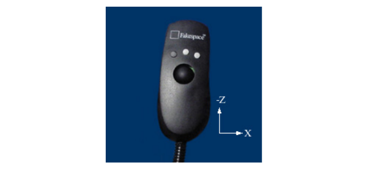
12.1 CAVES
EnSight 10.2 User Manual 12-9
[ cursortracker <i> ]
[ selectbutton <i> ]
[ rotatebutton <i> ]
[ transbutton <i> ]
[ zoombutton <i> ]
[ xformbutton <i> ]
[ xtransval <i> ]
[ ytransval <i> ]
[ ztransval <i> ]
[ auxbutton <i> <j> ]
[ motionfilter <i> <p> <r> ]
The headtracker and cursortracker parameters allow you to specify
which tracking device is tracking head position and which is tracking the
controller. Only two devices can be tracked by EnSight – one for the head position
and one for the position of the controller. All button/valuator input is interpreted
as having come from the controller. Note that the EnSight API for input devices
uses 0-based indices for trackers, buttons, and valuators. Trackd uses 1-based
indices, and other libraries may differ as well.
The remaining options allow you to customize the behavior of buttons and
valuators on the 6D input device. The input device can be used for:
1. Selecting items from the 3D GUI, which includes the heads-up macro (HUM)
panel, the part list, variable list, and value slider.
2. Performing transformations on the geometry in the scene.
3. Manipulating the cursor, line, plane, and quadric tools.
The input device has a local coordinate system which is relevant for some forms
of 6D interaction:
The default mode defines button 0 as the select button. When the 3D GUI is
visible, you can point at the 3D buttons and the item that you are pointing at will
be displayed in a highlight color. When you press the select button you will
activate the current selection. For the HUM panel, this means that you will
activate the macro that is defined for the selected button. See the “User Defined
Input Preferences” found in Section 4.2, Edit Menu Functions for more
12.1 CAVES
12-10 EnSight 10.2 User Manual
instructions on configuring and showing the HUM panel and part panel. Clicking
on an item in the part list will select or unselect the item in the list. Combined with
macros in the HUM, this will allow you to modify visibility or other attributes on
a part or collection of parts. If there are many parts in the part list, you can also
select the scrollbar and move the controller up and down to scroll through the list.
Similarly, the part-value slider can be used to modify part attributes for certain
part types. For isosurfaces you can select the part slider and move left to right to
change the isovalue. When no parts are selected, the part-value slider can be used
to modify the time in a transient simulation.
The rotatebutton, transbutton, and zoombutton allow you to
perform the selected transformations using gestures with the 6d input device. The
xformbutton allows you to link a button to the current transformation mode,
similar to the mouse button configurations for the main GUI interactions. You
may want to add buttons on the heads-up-macro (HUM) panel to switch between
modes. This is useful for 6D input devices with a smaller number of buttons. Note
that it is possible (and encouraged) to re-use the selectbutton for a
transformation. The selectbutton is only used when you are pointing at a
heads-up menu. When you are not pointing at a menu, the same button could be
used as the xformbutton, for example.
All 6d transformations have a ‘sensitivity’ which can be set to control the speed at
which the transformation occurs. These values can be set from the ‘Edit-
>Preferences->VR and User Defined Input’ dialog (see VR and user defined input
Preferences). There are also two forms of rotation available. In ‘Mixed Mode’, the
6d device acts similar to a mouse for rotation. Once you click the
rotatebutton, your movement is tracked in the X-Y plane of the input device.
Your translation in this space is mapped to a rotation in the 3D space. In ‘Direct
Mode’ it is the orientation of the device, rather than the position of the device,
which controls the rotation.
The xtransval, ytransval, and ztransval parameters configure the
valuators to allow for translation of the scene by pressing the valuator in a given
direction. The 'x', 'y', and 'z' designations refer to a local coordinate system which
is fixed to the controller input device. As you hold the device in your hand,
positive x is to the right, positive y is up, and positive z is toward the viewer. This
local coordinate system depends on the orientation of the tracking device attached
to the input device. It may be necessary to align the tracking device properly or
modify the trackd (or other tracking library) configuration to achieve the proper
orientation.
The auxbutton parameters configure additional buttons that can be used to control
various options. The first parameter "<i>" is the number of the auxbutton to
define. The second parameter "<j>" is the physical device button to bind to
auxbutton <i>. Currently, auxbutton 0 is used by EnSight as the "Menu" button.
This button can be used to bring up the "User defined menu" at the cursor point on
the annotation plane. Pressing the button a second time will either reposition the
menu or it will pop up to the next level of the menus if a submenu has been
selected.
The motionfilter parameter allows the user to select a filter threshold for each
12.1 CAVES
EnSight 10.2 User Manual 12-11
tracker (head or cursor). If the motion of the tracker exceeds this threshold, and
EnSight has the Fast Display mode global toggle enabled, it will display all the
parts using their fast representation until the motion drops below the threshold.
The <i> parameter selects the tracker to filter. The <p> value specifies a threshold
for the tracker position. This is computed as the variance of the distance between
the current position and the last 10 tracker positions. Similarly, the <r> value
specifies a threshold for the tracker direction vector. This is computed as the
variance of the angles between the current direction and the last 10 directions (in
radians).
Example 4
For the most basic configuration with head-tracking and a 6d input device, there
are only three lines added to Example 2 to create the tracker section:
CVFd 1.0
display
view
origin -5 5.75 5
tracker
headtracker 0
cursortracker 1
screen
displayid :0.2
resolution 1024 768
bottomleft -5 0.0 –5
bottomright 5 0.0 –5
topleft -5 7.5 –5
screen
displayid :0.1
resolution 1024 768
bottomleft 5 0.0 –5
bottomright 5 0.0 5
topleft 5 7.5 -5
Example 5
There are many different input devices available, and some have additional
buttons and valuators that can be used for navigation and selection in immersive
environments. In this example the configuration file is extended to use different
buttons for rotation, translation, zoom, and selection. We also configure a
‘thumbwheel’ input to provide translation in the X-Z plane.
CVFd 1.0
display
view
origin -5 5.75 5
tracker
headtracker 0
cursortracker 1
12.1 CAVES
12-12 EnSight 10.2 User Manual
selectbutton 4
rotatebutton 0
transbutton 1
zoombutton 2
xtransval 0
ztransval 1
screen
displayid :0.2
resolution 1024 768
bottomleft -5 0.0 –5
bottomright 5 0.0 –5
topleft -5 7.5 –5
screen
displayid :0.1
resolution 1024 768
bottomleft 5 0.0 –5
bottomright 5 0.0 5
topleft 5 7.5 -5
Annotations
Annotations in EnSight include the heads-up macro panel, text, lines, logos,
legends, and plots. In the GUI display these items appear as an overlay which is
fixed in screen space. In an immersive display environment it is useful to be able
to specify the locations of these objects. In EnSight, these items continue to
occupy a plane in the 3D world. By default, this plane will coincide with the first
pipe in the configuration file. The user may choose to specify the position and
orientation of this plane with the following addition to the configuration file:
Annot
[ screen <n> ]
OR
[
center <x> <y> <z>
zaxis <x> <y> <z>
yaxis <x> <y> <z>
xscale <float>
yscale <float>
]
Example 6
To continue with Example 5, suppose that the user would prefer for the
annotations to appear on the right wall instead of the left wall. The following
configuration file defines an annot section with the appropriate parameters to do
this:
CVFd 1.0
display
12.1 CAVES
EnSight 10.2 User Manual 12-13
view
origin -5 5.75 5
tracker
headtracker 0
cursortracker 1
selectbutton 4
rotatebutton 0
transbutton 1
zoombutton 2
xtransval 0
ztransval 1
annot
screen 1
screen
displayid :0.2
resolution 1024 768
bottomleft -5 0.0 –5
bottomright 5 0.0 –5
topleft -5 7.5 –5
screen
displayid :0.1
resolution 1024 768
bottomleft 5 0.0 –5
bottomright 5 0.0 5
topleft 5 7.5 -5
Fixing the annotations to a pipe is merely provided as a convenience. Internally
this is identical to using the explicit form:
annot
center 5 3.75 0
zaxis 1 0 0
yaxis 0 1 0
xscale 10
yscale 7.5
Cave Distributed Displays
Caves and walls can be driven by one or more machines. A single EnSight client
can draw all of the screens in the dconfig file, or a separate EnSight client can
draw each screen, typically on machines other than the one running the master
client. The examples up to now set up a cave on a single machine.
A ceishell network must be created to use distributed rendering. See Chapter 15.
The dconfig file must be slightly altered to specify on which machine a client
should run. In each screen section, a ‘hostid’ line can be added, indicating the
name of the machine to use, or indicating a ceishell ‘role’.
12.1 CAVES
12-14 EnSight 10.2 User Manual
Example 7
CVFd 1.0
display
screen
hostid clusternode01
displayid :0.2
resolution 1024 768
bottomleft -5 0.0 –5
bottomright 5 0.0 –5
topleft -5 7.5 –5
screen
hostid clusternode02
displayid :0.1
resolution 1024 768
bottomleft 5 0.0 –5
bottomright 5 0.0 5
topleft 5 7.5 -5
Once a CEIShell network is running, start EnSight in VR mode with the command
line:
ensight102 -ceishell -dconfig dconfig_file_name
Benefits of using a distributed system over a single machine:
- Rendering speed is higher because each client just draws one screen
- The number of screens is not limited to the number of display outputs on a
graphics card.
Drawbacks of using a distributed system
- A ceishell network must be created across all machines
- Some EnSight features are not supported in a distributed system, including
adding or replacing a case, and restoring a context or session.
Tips for Distributed Rendering
1. EnSight must be installed on each machine where a client or server will run.
2. The rendering nodes on linux computers must have OpenGL enabled X11
servers running on them and they must be configured for direct rendering by
remotely executed user processes. To test this, log into a rendering node
remotely and run "glxgears -display :0". If this does not bring up glxgears on
the display, the linux computer X11 server will need to be reconfigured.
3. On linux computers you may need to add options like '-ac' to the /etc/X11/
xmd/Xservers file or otherwise configure X11 authorization mechanisms (we
12.1 CAVES
EnSight 10.2 User Manual 12-15
know it will run with "-ac -s 0", but site security implications must be
carefully considered). It may be useful to check that the rendering is "direct"
as well (glxgears should run > 8000 fps on modern graphics cards with proper
hardware accelerated OpenGL drivers). The output of glxinfo on the
rendering node can be helpful in diagnosing issues as well. You may need to
modify the permissions of the /dev/nvidiactl file(s) to allow a non-console app
to access the graphics system.
4. All linux computers’ X11 screen savers and blanking functions should be
turned off on the rendering nodes for your PC to work properly.
5. On linux computers, ensure the DISPLAY environmental variable is set
correctly, typically to ':0.0', set CEI_HOME to the proper path, and put
$CEI_HOME/bin in the search path for remote connections (rsh or ssh).
6. Many clusters have multiple TPC/IP address and hostnames for each node.
Usually, one for the high-performance interconnect (e.g. InfiniBand) and one
for administration. For the highest performance EnSight needs to use the
TCP/IP addresses associated with the high-performance interconnect.
A cluster configured to use the highest performance interconnect as its default
is the simplest to configure for use with EnSight. For example, since by
default EnSight will use the TCP/IP address resolved by 'hostname', this name
should be the highest performance interconnect.
Once the above are working on your cluster, contact CEI Support if you run into
any problems running EnSight on it. Please send us your cluster(s) details and the
config files you have tried.
Some general advice:
To simplify debugging, start small and scale up.
For example, we have seen problems with some TCP/IP over IB implementations,
especially at scale, so start small (2-3 nodes) and if you have gigE in addition to
IB, try that as well. Also, implement HPC+ and VR with all the EnSight processes
running on rendering nodes of a single cluster. Configure one rendering node on
the cluster as an "interactive" node (with mouse/keyboard).
12.2 WALLS
12-16 EnSight 10.2 User Manual
12.2 WALLS
This section discussions the creation, management, and navigation within Wall
displays commonly referred to as a display wall, tiled display, or power wall.
A wall does not support head tracking or 6d input devices. If you have a wall and
wish to incorporate head tracking, you can configure it as a cave with all screens
positioned in the same plane (see Chapter 12.1, CAVES). See the Cave section.
In order to configure a cave or a wall in EnSight, the user must create a display
configuration file. See Configuration File (dconfig) for where to place the file.
The specification for a display wall consists of:
display
[ stereo ]
wallresolution
<x-res> <y-res>
screen
[ hostid <h> ]
displayid <p1>
resolution <x-res> <y-res>
wallorigin <wall-x> <wall-y>
[ displayorigin <xo> <yo> ]
[ lefteye
or
righteye
]
[ repeat 'screen' section for each additional screen ]
The wallresolution section gives the total pixel resolution of the display
wall. For each graphics pipe, there will be a screen section that describes the size
(resolution) and position (wallorigin) of the region within the global
display. The displayid parameter specifies the X display (i.e. :0.1). This
parameter is ignored on Windows, because there is only a single “screen”
regardless of the number of graphics cards or video outputs. The
displayorigin is an optional parameter to specify the origin of the window
on the given pipe (default (0,0)). Note that displayorigin is a position
relative to the origin of a given displayid, while wallorigin is a position
relative to the origin of the global display. Changing wallorigin will change
the region of the wall that is visible in a given window, while changes to
displayorigin simply move the window on the screen without changing the
contents. Example 1 will demonstrate a situation when the use of
displayorigin is useful. The lefteye/righteye optional designation
can be used for passive stereo displays, in which separate graphics pipes render
the left and right images.
Example 1
In this example there is one X server with five graphics pipes. The GUI is

12.2 WALLS
EnSight 10.2 User Manual 12-17
displayed on pipe :0.0, with the other four pipes used for the detached display.
Four projectors are configured in a 2x2 array to form a large continuous wall as
illustrated:
CVFd 1.0
#
# conference room display wall
#
display
wallresolution
2560 2048
screen # lower-left
displayid :0.1
resolution 1280 1024
wallorigin 0 0
screen # lower-right
displayid :0.2
resolution 1280 1024
wallorigin 1280 0
screen # upper-left
displayid :0.3
resolution 1280 1024
wallorigin 0 1024
screen # upper-right
displayid :0.4
resolution 1280 1024
wallorigin 1280 1024
Example 2
It is not uncommon for displays walls to use overlapping images with edge-
blending to smooth the otherwise sharp transition between projector images. The
edge-blending is performed by the projectors directly. This is easily configured as
a detached display by specifying pipes with overlapping pixel regions. Consider
an example of two pipes at 1280x1024 resolution each, with an overlap of 128
:0.3 :0.4
:0.1 :0.2
12.2 WALLS
12-18 EnSight 10.2 User Manual
pixels.
CVFd 1.0
#
# edge-blending example
#
display
wallresolution
2432 1024
screen # left
displayid :0.1
resolution 1280 1024
wallorigin 0 0
screen # right
displayid :0.2
resolution 1280 1024
wallorigin 1152 0
Note that in this case the total resolution of the wall in the x direction is decreased
by the amount of overlap.
Example 3
Passive stereo displays achieve stereo by projecting overlapping polarized images
from multiple projectors. This can be achieved using detached displays with a
distinct rendering region for each screen and eye. Consider for this example a
single screen with two projectors. For illustration purposes we will assume that
we have three graphics pipes. One pipe (:0.0) renders the GUI and is not listed.
CVFd 1.0
#
# passive stereo display
#
display
wallresolution
1280 1024
screen # left-eye
displayid :0.1
resolution 1280 1024
wallorigin 0 0
lefteye
screen # right-eye
displayid :0.2
resolution 1280 1024
wallorigin 0 0
righteye
Note that the lefteye/righteye parameters are NOT necessary when using
12.2 WALLS
EnSight 10.2 User Manual 12-19
traditional quad-buffered stereo to drive the projectors. Some systems have a
signal splitter which takes the frame-sequential stereo signal and generates
separate signals for left and right eye. In this case a conventional configuration
file without the “eye” designations will work fine. Passive stereo displays are
always in stereo mode.
Example 4
Active stereo displays achieve stereo by projecting alternating left and right eye
images from a single projector, with glasses that alternately block the left or right
eye. Adding the ‘stereo’ line enables active stereo for all screens.
CVFd 1.0
#
# active stereo display
#
display
stereo
wallresolution
1280 1024
screen
displayid :0.1
resolution 1280 1024
wallorigin 0 0
Wall Distributed Displays
Walls are commonly driven by more than one machine. A single EnSight client
can draw all of the screens in the dconfig file, or a separate EnSight client can
draw each screen. In the preceding examples, a single machine rendered all of the
screens.
See Cave Distributed Displays, which describes the addition of the ‘hostid’ line to
a dconfig file, the use of ceishell to launch the distributed processes, and pros and
cons of running distributed. For trouble-shooting tips, see Tips for Distributed
Rendering in the cave configuration section above.
12.3 Head-Mounted Displays
12-20 EnSight 10.2 User Manual
12.3 Head-Mounted Displays
This section discussions the creation, management, and navigation within a Head-
mounted display environment typically mounted in front of the users eyes instead
of fixed to the walls.
Canon MReal
EnSight supports the Canon Mixed Reality system, aka Canon MR or Canon
MReal. Mixed reality, sometimes called augmented reality, combines virtual and
real world images. The user feels that he or she is still in the normal workspace,
and able to walk around the simulation, or able to hold the simulation in hand and
examine it. Two front facing cameras capture live video feeds of the workspace,
from the user’s point of view, and the simulation results are drawn on top of that
video.
Once the Canon MR hardware and runtime are installed, use Canon MR by
launching it from a command prompt with a command line option
ensight102 -canonmr
Expectations
The user should see the 3D scene drawn within their workspace. By default this is
placed in the center of all the markers in the MREAL system. By default the
EnSight scene is scaled so that its bounding box is roughly the size of the bounds
around all of the markers.
There should also be a plane in space where annotations are drawn. By default it is
in the -X direction relative to the data.
Customization
The position and size of the scene, and the position, size, and orientation of the
annotation plane can be customized. See VR and user defined input Preferences
for more details.
Oculus Rift
EnSight supports the Oculus Rift virtual reality system.
Once the Oculus Rift hardware and runtime are installed, use the Oculus Rift by
launching it from a command prompt with a command line option
ensight102 -oculus
Expectations
The user should see the 3D scene drawn against a black background. By default,
the data is placed above the tracking camera, scaled so that the bounds around the
data are about a half meter in length. Annotations are drawn on a plane behind the
data.
Movements of the scene with a Gamepad or SpaceNavigator (see Chapter 12.4,
12.3 Head-Mounted Displays
EnSight 10.2 User Manual 12-21
SpaceNavigator and Gamepad) are reflected in both the Oculus display and the
main desktop view within EnSight. However, movements of the Oculus display
(look up/down, left/right, etc) are not replicated in main desktop view of EnSight.
Since the main desktop will not be visible while wearing the headset, it is helpful
to have a gamepad or SpaceNavigator available to navigate the scene.
Customization
The position and size of the scene, and the position, size, and orientation of the
annotation plane can be customized. See VR and user defined input Preferences
for more details.
12.4 SpaceNavigator and Gamepad
12-22 EnSight 10.2 User Manual
12.4 SpaceNavigator and Gamepad
Introduction
EnSight supports simple rotation and translation of the current view using external
input devices such as joysticks, game controllers and the 3DConnexion
SpaceNavigator ™ (http://www.3dconnexion.com). These devices are especially
helpful when used with a cave, wall, or head-mounted display, because you may
be away from, or unable to see, a keyboard and mouse.
SpaceNavigator
A SpaceNavigator is a 6-degree of freedom input device used to rotate and
translate a model. Note the 3DConnexion SpaceNavigator ™ is not supported on
Linux. This is controlled via the configuration file 'spacedevice.defaults' located
in the system site_preferences directory or users resource directory. EnSight will
automatically detect and use devices like the SpaceNavigator, but the
configuration file can be used to fine-tune the sensitivity of the device. The
default file looks something like:
VERSION 1.0
#
# Comments must have the '#' as the first character.
#
# ranges are xmin xmax ymin ymax zmin zmax
#
# these are the values for sensitivity of 50
translate_ranges -400 400 -400 400 -400 400
rotate_ranges -400 400 -400 400 -400 400
The values set the minimum and maximum ranges for the translation and
rotations. Adjusting them can correct for asymmetry in the output values from the
device and set the device's sensitivity. Narrowing the range has the effect of
increasing the sensitivity to smaller motions of the device.
Gamepad
On Windows and Linux platforms, EnSight also supports standard PC joysticks
and game controllers using native joystick APIs on those platforms. To use these
devices, three additional fields can be used: controller_id, controller_config and
single_axis.
single_axis {0|1}
By default, the spacedevice interface only allows transformation by a single axis
at a time. If this value is set to 0, transformations over multiple axes (either
translations or rotations) are allowed at the same time.
controller_id "name"
The presence of this field enables the use of joysticks/game controllers. The value
must be a string in quotes. Under Windows, the value is an integer (as a string)
which is the index of the game controller in the system. The first controller is "0".
Under Linux, this is the device name of the joystick in question. An example is "/
dev/input/jp0". The actual value is dependent on the specific Linux distribution.
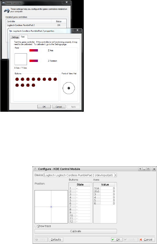
12.4 SpaceNavigator and Gamepad
EnSight 10.2 User Manual 12-23
control_config "configstring"
This field maps device controls (axes and buttons) to the transformation axes.
The configuration string consists of some number of axis transformation
expressions separated by spaces. Each expression is in the form {transformation
axis}={device axis}{u}{device button number}. The axes of transformation are:
X: translation in screen X, Y: translation in screen Y, Z: translation in screen Z, A:
rotation over the screen X axis, B: rotation over the screen Y axis and C: rotation
about the screen Z axis. The device axes follow the Windows game controller
naming conventions. The legal values are 'X', 'Y', 'Z', 'R', 'U', 'V'. The mapping of
various device controls to these axes varies from controller to controller. Under
Windows, the game controller control properties panel allows the user to see the
layout of the controls and see what buttons are mapped to which button numbers
interactively. The RumblePad uses the X, Y, Z and R axes.
Under Linux, the 'X', 'Y', 'Z', 'R', 'U', 'V' axes map to the first though sixth analog
axes respectively.
12.4 SpaceNavigator and Gamepad
12-24 EnSight 10.2 User Manual
If no button number is specified, the game controller always controls the selected
EnSight transformation. Each axis mapping can be qualified by a button state. For
example Y=Z5 means that EnSight translation in Y will be controlled by game
controller Z axis, but only while button 5 is pressed. Putting a lowercase 'u'
between the controller axis and the button number specifies the link is only made
when the named button is not pressed (up state). Thus, B=Ru6 specifies that
rotation over the screen Y axis is controlled by the game controller R axis, but
only when the button 6 is not pressed (up).
An example using a Logitech RumblePad 2 on a Windows system might be:
VERSION 1.0
#
# This is the SpaceDevice configuration for
# Logitech RumblePad or equivalent game pad
#
translate_ranges -400 400 -400 400 -400 400
rotate_ranges -400 400 -400 400 -400 400
#
controller_id "0"
controller_config "X=X Y=Yu5 Z=Y5 A=Ru6 B=Z C=R6"
single_axis 0
This file selects the first controller in the system (controller_id "0"), sets the
configuration string and enables transformations in multiple axes at the same
time. The configuration string maps translation in the X axis to the left stick
horizontal axis ("X=X"). It maps translation in the Y axis to the left stick vertical
axis, when button 5 is "up" ("Y=Yu5"). Translation in the Z axis is mapped to the
left stick vertical axis when button 5 is "down" ("Y=Y5"). Similarly, the right
stick axes (R and Z) are mapped to the rotation axes (A, B, C) conditioned by the
status of button 6.
Various game pads use different configurations of buttons and axes. The following
configuration file is suggested for use with an XBox style controller.
VERSION 1.0
#
# This is the SpaceDevice configuration for
# Microsoft XBox360 or XBoxOne game pad
#
translate_ranges -80 80 -80 80 -80 80
rotate_ranges -80 80 -80 80 -80 80
#
controller_id "0"
controller_config "X=X Y=Yu5 Z=Y5 A=R B=Uu6 C=U6"
single_axis 0
EnSight Virtual Communication Utility
EnSight 10.2 User Manual 13-1
13 CEIShell
EnSight Virtual Communication Utility
Who is this document for?
CEIShell is a technology that enables EnSight to run in diverse distributed
environments. An individual competent with Python and/or shell scripting
languages and who has a good technical understanding of the site’s computational
infrastructure must configure it for a particular site. End-users of EnSight
normally use a simple program,
ceistart102
for EnSight, to graphically start
EnSight using CEIShell once it has been properly configured. This document
gives a comprehensive overview of CEIShell along with details on configuring it
for a site. End-users can usually forgo reading this document and instead use
simple site-provided instruction on how to launch EnSight if CEIShell is
employed and properly configured.
Introduction
EnSight is used in numerous differing computational environments that make
distributed application launch challenging. Furthermore, EnSight has grown from
a basic client/server application into a multi-component application utilizing
anywhere from two to thousands of communicating processes. Historically, the
task of accessing and launching the various EnSight components has been built
into many of the EnSight components. This approach is no longer adequate.
Today’s computational environments tend to be far more complex. Secure login is
required to access remote computers. Firewalls may be used to restrict network
access. Queuing systems are used to manage and control access to changing
computational resources. Data may reside on computers several network hops
away from the user’s desktop workstation. Because of issues such as these,
CEIShell was developed to work easily and flexibly in such environments while at
the same time simplifying the core EnSight components. [Throughout this
document ‘EnSight components’ refers to the EnSight Client, Server, SOS,
CollabHub, and DR Client.]
CEIShell’s main purpose is to provide a virtualized environment for launching
EnSight components. Optionally, CEIShell can also provide communication
encapsulation and routing for EnSight components automatically and when
necessary. By focusing solely on launching and communication, CEIShell excels
in supporting complex, modern environments that entail remote and/or distributed
access, queuing systems, and firewall and tunneling issues. Furthermore, in such
environments CEIShell provides a more flexible, easier-to-use approach than is
possible with EnSight’s legacy methods.
While CEIShell provides numerous advantages, CEIShell support is entirely
optional today. EnSight 10 still supports all of the same legacy methods for
accessing and launching other EnSight components. Indeed, CEIShell is not of
much value when simply running just the EnSight Client and Server on the same
computer; running
ensight102
in such situations is completely appropriate.
However, given all of CEIShell’s strengths and improved usability, users should
plan to migrate to CEIShell for use in distributed environments. In a future
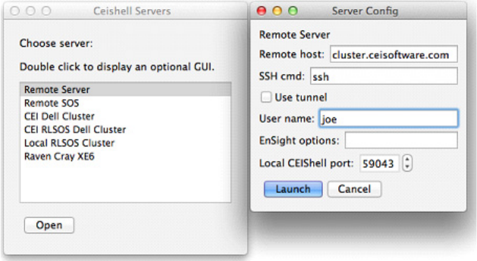
Operational Overview
13-2 EnSight 10.2 User Manual
version of EnSight, CEIShell will become the sole way of launching EnSight in
distributed environments (as a side note, removing the varying legacy methods
from EnSight will also result in better quality assurance for EnSight in these
areas).
Operational Overview
The concept is that a CEIShell process runs on each computer that is intended to
run an EnSight application component. If multiple computers will be used, then
each runs one or more CEIShells and the collection is called a CEIShell network.
Through command line options, the CEIShells are instructed on how to
communicate with each other. For example, if a user intends to run the EnSight
Client on her workstation named
bohr
, the EnSight SOS on a “login node” named
kepler
, and EnSight Servers on cluster nodes
n1-n8
, she would run 10 instances of
ceishell32
(EnSight 10.2, uses
ceishell32;
and recall EnSight 10.1 uses
ceishell31
)
on each of the computers
bohr
,
kepler
, and
n1
through
n8
. Once the CEIShell
network is running, she starts EnSight by running
ensight102
-
sos
-
ceishell
on
bohr
.
The EnSight Client communicates with the local CEIShell process to launch the
SOS and EnSight Servers on the appropriate computers.
To streamline start up of the CEIShell network as well as to launch EnSight, users
typically run the GUI based application
ceistart102
, referred to as CEIStart for the
remainder of this document. Using CEIStart a user can choose from one or more
site-configured CEIShell networks, each of which has its own set of
site-determined options (as shown below). The site can make each configuration
as flexible or concise as is appropriate for their computational environment.
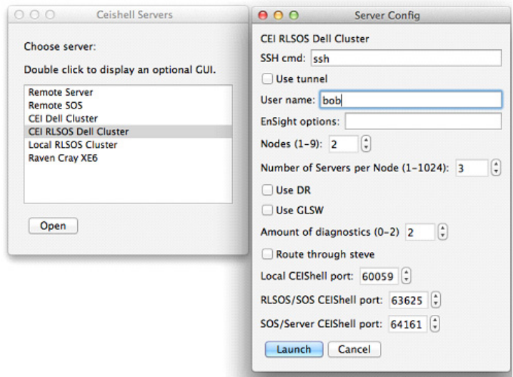
CEIShell
EnSight 10.2 User Manual 13-3
CEIShell
CEIShell is a simple application in that it only performs a few tasks: it knows how
to launch another application on the same computer; and, it knows how to
communicate with other CEIShells and applications linked with the CEIShell
library such as EnSight. Due to the complexities of remote computer access,
security controls, queuing system integration, network restrictions, and other
similar issues, CEIShell does not know how to launch an application on a different
computer. While a CEIShell can ask a remotely connected CEIShell to launch an
application, it cannot launch a remote application by itself. Therefore, since
CEIShell cannot launch a remote CEIShell by itself, it cannot start up a CEIShell
network by itself; this is the responsibility of the customer’s site. This is actually a
significant advantage since a site is free to launch a CEIShell network however is
appropriate for their environment.
Typically, one person at a site sets up the appropriate mechanisms for launching a
CEIShell network on a set of computers intended to run EnSight. Normally, this is
done with a scripting language such as Python or CSH while taking into account a
site’s methods for remote job launch, authentication, resource allocation, etc. Note
that while it is the site’s responsibility for determining how to launch a CEIShell
network, CEI Inc. and its distributors can advise on this task. Also, examples are
provided that show typical setups.
CEIShell Roles CEIShell has the concept of “roles” which are arbitrary names - strings - that are
used to identify a CEIShell. All CEIShells have multiple roles including
localhost
,
the computer’s network name, the computer’s short network name, and an
auto-generated unique name. For example a CEIShell running on a computer
ale.bigcompany.com
would have the roles:
localhost
,
ale.bigcompany.com
,
ale
, and
CEIShell
13-4 EnSight 10.2 User Manual
ceishell_000000
. In addition to these, a CEIShell may be assigned other roles by the
user via command line options.
While roles don’t signify anything special to the CEIShell other than to give it
specific names, they are used when determining where to launch a particular
program such as an EnSight component. Some roles have special meaning to
EnSight; specifically, names
SOS, SERVER, SOS_SERVERS, COLLABHUB
, and
DRCLIENTS
are
significant. These roles are typically used to indicate where to run the various
EnSight components. When EnSight needs to launch another EnSight component,
such as the EnSight Server, it queries the CEIShell network for a CEIShell that
has the appropriate role. The CEIShell that has the appropriate role is then asked
to launch the EnSight component.
All CEIShells have the role “localhost”. This acts as a fallback for when no other
roles match what has been requested by an application. The auto-generated unique
role, such as
ceishell_200002
, is unique within a particular instance of a CEIShell
network. It is used to reference a particular CEIShell. It is also noteworthy when
debugging CEIShell networks; the first digit indicates the CEIShell’s level below
the root CEIShell. The rest of the digits indicate the CEIShell instance at that
level.
Connecting CEIShells Together
CEIShells are connected together in a rooted tree without cycles meaning that
CEIShells have at most one parent and they can have zero or more children. The
CEIShell without a parent is the root CEIShell and CEIShells without children are
leaf CEIShells. Command line options
parent
and
child
can be used to indicate that
a CEIShell has a parent and/or one or more children, respectively. These two
options take a URL that indicates how to make the connection to the associated
parent and/or children.
URLs mimic syntax used by web URLs but with CEIShell they describe the
network connection parameters. They’re used by the
parent
and
child
options as
well as the
–app
and
–cmdurl
options (described later). URLs have many default
values thus minimizing what must be specified. Their syntax is:
method://host?option1=value1&option2&option3=value
where
method
is either
connect
or
listen
,
host
is a hostname, and
options/values
are
options recognized by the connection method.
For example, the URL
connect://kepler?port=8999&timeout=-1
indicates that a TCP/
IP connection should be made to host
kepler
on port
8999
and an infinite timeout
should be used; whereas
listen://
indicates that a TCP/IP listen() should be used
on the default port (port 1106 for
parent
and
child
connections or port 1109 for
app
and
cmdurl
connections) with a default timeout of 90 seconds. Note that the ‘?’ and
‘&’ characters may need to be escaped using the ‘\’ character and/or quoted
depending on the command interpreter shell (e.g.,
csh
,
sh
,
cmd.exe
, Python).
Connecting CEIShell and EnSight
A CEIShell that has the
app
option specified listens for connections from EnSight
(or any other application linked with the CEIShell library). While not a
requirement, this option is typically only specified to the CEIShell running on the
computer intended to run the EnSight Client. The
–app
option takes an optional
URL as previously described. Specifying the EnSight command line option
-ceishell
, which also takes an optional URL, instructs EnSight to connect to a
CEIShell
EnSight 10.2 User Manual 13-5
CEIShell that has the corresponding
–app
option (see Command Line Start-up
Options). It also tells EnSight to use CEIShell for all other component launching.
Furthermore, EnSight components will connect to each other using the same
network connection parameters specified to the associated CEIShells via their
–
child
and
–parent
options. These are in lieu of EnSight legacy connection
parameters. This allows the same TCP/IP tunneling (e.g., ssh tunnels) to be used
for both CEIShell and EnSight. Furthermore, EnSight has been enhanced to allow
TCP/IP connections in either direction when using CEIShell; the EnSight Client
can now connect to the EnSight Server as well as in the opposite direction, which
is the historical method.
Additionally, EnSight components can communicate with each other through
tunneled communication via the connected CEIShells. This happens
automatically when needed. An example of this would be running the EnSight
Client on a desktop that needs to connect via a “login” computer before
connecting to a remote cluster on an internal LAN where it is desired to run the
EnSight Server. By running CEIShells on these three computers, communication
can automatically be tunneled for the EnSight Client and Server through CEIShell
connections.
CEIShell
Command Line
CEIShell has the concept of “roles” which are arbitrary names - strings - that are
used to identify a CEIShell. All CEIShells have multiple roles including
localhost
,
the computer’s network name, the computer’s short network name, and an
auto-generated unique name. For example a CEIShell running on a computer
ale.bigcompany.com
would have the roles:
localhost
,
ale.bigcompany.com
,
ale
, and
ceishell_000000
. In addition to these, a CEIShell may be assigned other roles by the
user via command line options.
While roles don’t signify anything special to the CEIShell other than to give it
specific names, they are used when determining where to launch a particular
program such as an EnSight component. Some roles have special meaning to
EnSight; specifically, names
SOS, SERVER, SOS_SERVERS, COLLABHUB
, and
DRCLIENTS
are
significant. These roles are typically used to indicate where to run the various
EnSight components. When EnSight needs to launch another EnSight component,
such as the EnSight Server, it queries the CEIShell network for a CEIShell that
has the appropriate role. The CEIShell that has the appropriate role is then asked
to launch the EnSight component.
All CEIShells have the role “localhost”. This acts as a fallback for when no other
roles match what has been requested by an application. The auto-generated unique
role, such as
ceishell_200002
, is unique within a particular instance of a CEIShell
network. It is used to reference a particular CEIShell. It is also noteworthy when
debugging CEIShell networks; the first digit indicates the CEIShell’s level below
the root CEIShell. The rest of the digits indicate the CEIShell instance at that
level.
Connecting CEIShells Together
CEIShells are connected together in a rooted tree without cycles meaning that
CEIShells have at most one parent and they can have zero or more children. The
CEIShell without a parent is the root CEIShell and CEIShells without children are
leaf CEIShells. Command line options
parent
and
child
can be used to indicate that
a CEIShell has a parent and/or one or more children, respectively. These two
options take a URL that indicates how to make the connection to the associated
CEIShell
13-6 EnSight 10.2 User Manual
parent and/or children.
URLs mimic syntax used by web URLs but with CEIShell they describe the
network connection parameters. They’re used by the
parent
and
child
options as
well as the
–app
and
–cmdurl
options (described later). URLs have many default
values thus minimizing what must be specified. Their syntax is:
method://host?option1=value1&option2&option3=value
where
method
is either
connect
or
listen
,
host
is a hostname, and
options/values
are
options recognized by the connection method.
For example, the URL
connect://kepler?port=8999&timeout=-1
indicates that a TCP/
IP connection should be made to host
kepler
on port
8999
and an infinite timeout
should be used; whereas
listen://
indicates that a TCP/IP listen() should be used
on the default port (port 1106 for
parent
and
child
connections or port 1109 for
app
and
cmdurl
connections) with a default timeout of 90 seconds. Note that the ‘?’ and
‘&’ characters may need to be escaped using the ‘\’ character and/or quoted
depending on the command interpreter shell (e.g.,
csh
,
sh
,
cmd.exe
, Python).
Connecting CEIShell and EnSight
A CEIShell that has the
app
option specified listens for connections from EnSight
(or any other application linked with the CEIShell library). While not a
requirement, this option is typically only specified to the CEIShell running on the
computer intended to run the EnSight Client. The
–app
option takes an optional
URL as previously described. Specifying the EnSight command line option
-ceishell
, which also takes an optional URL, instructs EnSight to connect to a
CEIShell that has the corresponding
–app
option (see Command Line Start-up
Options). It also tells EnSight to use CEIShell for all other component launching.
Furthermore, EnSight components will connect to each other using the same
network connection parameters specified to the associated CEIShells via their
–
child
and
–parent
options. These are in lieu of EnSight legacy connection
parameters. This allows the same TCP/IP tunneling (e.g., ssh tunnels) to be used
for both CEIShell and EnSight. Furthermore, EnSight has been enhanced to allow
TCP/IP connections in either direction when using CEIShell; the EnSight Client
can now connect to the EnSight Server as well as in the opposite direction, which
is the historical method.
Additionally, EnSight components can communicate with each other through
tunneled communication via the connected CEIShells. This happens
automatically when needed. An example of this would be running the EnSight
Client on a desktop that needs to connect via a “login” computer before
connecting to a remote cluster on an internal LAN where it is desired to run the
EnSight Server. By running CEIShells on these three computers, communication
can automatically be tunneled for the EnSight Client and Server through CEIShell
connections.
Running ceishell32 without options shows CEIShell command line syntax along
with default values. The following output is displayed:
usage: /usr/local/CEI/apex31/machines/linux_2.6_64/ceishell32 [options]
-app [<url>] # connect to application
-child [<url>] # add child ceishell
-cmd <cmd> # quoted command to send to another ceishell
CEIShell
EnSight 10.2 User Manual 13-7
-cmdurl [<url>] # connect to ceishell's app url
-debug <logfile> # write debug output to logfile
-display <name> # display name to use with DRCLIENTS
-end_after_ensight# exit when ensight exits
-i # interactive mode
-parent <url> # connect to parent ceishell
-role <tag> # add new role tag
-security <n> # specify a security number
-v # # verbose output (1=low, 2=medium, 3=high)
-V # Version
url:
connect://host?option1&option2&option3
listen://?option1&option2&option3
options:
nconnections=N # default 1
port=N # default 1109 for app otherwise 1106
sockbufsize=N # default system dependent
timeout=N # default 90 seconds for connect;
# unlimited for listen
The set of commands that CEIShell supports for the
-cmd
command-line option
follows. Note: This set may change in future releases of CEIShell.
add_app
add_child
add_parent
add_role
add_role_to_child
allocate_vpn
allocate_vpn_internal
allocate_vpn_pseudo
allocate_vpn_pseudo_internal
allocate_vpn_pass2_nodes
update_vpn_route_internal
send_vpn_responses
flag_for_deallocation_vpn
deallocate_vpn_pass2_nodes
show_vpn_table
cd
change_role
delete_role
dump
dump_urls
exit
get_net
is_app_running
is_ceishell_running
list_app_tags
ls
ndescendants_internal
Basic CEIShell Examples
13-8 EnSight 10.2 User Manual
parent_name_internal
ping
play
pwd
quit
renumber_internal
run_cmd
run_cmd_xml
send_log
set_app_output_buffing
set_debug_log
set_display
set_no_reroute_log
set_software_rendering
show_jobs
show_net
show_roles
start_app
test_net
test_root_cmd
test_root_cmd_internal
terminate_all
terminate_app
terminate_ceishell
terminate_job
trace_route
update_tree_ids_internal
verbose
Basic CEIShell Examples
Example 1 Run the EnSight Client and Server on the same workstation using CEIShell:
Run: ceishell32 -app -v 3
Run: ensight102 -ceishell
Note that there isn’t much utility to this example other than to demonstrate
CEIShell for launch and to get an understanding of verbose command line output.
The app option to CEIShell indicates that it should listen for application
connections (i.e. EnSight). Also note that the CEIShell does not terminate when
EnSight completes. This allows a CEIShell network to be reused. If desired,
-
end_after_ensight
can be specified to the root CEIShell to indicate that the entire
network should terminate when EnSight terminates.
Example 2 Run the EnSight Client on workstation ale and the EnSight Server on computer
kepler using CEIShell:
On ale run: ceishell32 -app -child
On kepler run: ceishell32 -parent connect://ale -role SERVER
On ale run: ensight102 -ceishell
The -
child
and -
parent
options establish a parent/child relationship between the
two CEIShells. As with the previous example, only the CEIShell on
ale
listens for
an EnSight connection due to the -
app
option. The
-role SERVER
option indicates
that the CEIShell on
kepler
should have an additional role
SERVER
. EnSight will
look for a CEIShell with this role when asking the CEIShell network to start the
EnSight Server. See ‘Determining Where EnSight Components Run’ below for
details on where EnSight components are launched.
Using CEIStart
EnSight 10.2 User Manual 13-9
Example 3 Run the EnSight Client on workstation
ale
and the EnSight Server on computer
kepler
using CEIShell. Establish the TCP/IP connection from the Client to the
Server on TCP/IP port 7890 with no timeout:
On ale run: ceishell32 -app -child connect://kepler\?port=7890\&timeout=-1
On kepler run: ceishell32 -parent listen://\?port=7890\&timeout=-1 -role SERVER
On ale run: ensight102 -ceishell
Example 4 Run the EnSight Client on workstation
ale
and the EnSight SOS on computer
kepler
, a login node to a cluster managed by the batch queuing system SLURM,
and 8 EnSight Servers on the cluster as allocated by SLURM:
On ale run: ceishell32 -app -child
On kepler run: ceishell32 -parent connect://ale -role SOS -child listen://
\?nconnections=8\&timeout=-1
On kepler run: srun -N 8 ceishell32 -parent connect://kepler -role SOS_SERVERS
On ale run: ensight102 -sos -ceishell
Note that the CEIShell on kepler has a single parent and eight children. It listens
for eight child connections due to the
nconnections=8
URL option; and, it will not
time out. It will run the EnSight SOS due to its role. The
-sos
option to
ensight102
still needs to be specified to indicate to EnSight that SOS should be used and not
just an EnSight Server. As with the previous examples the CEIShell network
keeps running after EnSight terminates; thus the SLURM allocated nodes are
retained. Rerunning the last command will start another EnSight session while
reusing the same CEIShell network.
Passing arguments If you wish to pass arguments to EnSight, simply type them as normal when you
launch the application from the command line. Arguments unknown to ceishell
will simply be passed to EnSight.
ensight102 -ceishell -scalev 2.0
Using CEIStart
As can be seen from the previous examples, starting all the CEIShells by hand can
be tedious if more than a few are needed. A far more desirable approach is to use
CEIStart (
ceistart102
if using EnSight 10.2 or
ceistart102
if using EnSight 10.1 or
ceistart101
if using EnSight 10.1). It provides the user with a graphical interface
for launching the CEIShell network and then starting EnSight upon successful
launch of the network.
To use CEIStart a site must do a few things. It must write a script, or equivalent, to
launch the CEIShell network; and, it must write the configuration file for CEIStart
that indicates how to interface to the launch script. Typically, an individual does
this for a site whereas users of EnSight simply use CEIStart.
CEIStart supports multiple launch scripts -- each with its own CEIStart
configuration; and, the site can use these in anyway desired. For example, if a site
has two clusters, it may have two launch scripts and two configurations -- one for
each cluster. Each configuration can have an optional GUI control panel where
users can select a variety of options as needed by the launch script. Alternatively,
a site could decide to have just one launch script and configuration for both
clusters where the choice of which cluster to use is just an option. Either approach
works equally well.
Using CEIStart
13-10 EnSight 10.2 User Manual
Default CEIStart
configurations
EnSight 10.2 ships with two default configurations for ceistart102: 'Remote
Server' and 'Remote SOS'. These serve two purposes. First, they should work for
many sites "as-is"; and, second, they serve as simple examples to show how to
write a ceistart102 configuration and supporting CEIShell launch scripts.
The 'Remote Server' configuration is used to launch EnSight in Client / Server
mode with the EnSight Server running on a different computer than the Client
(although the same computer or 'localhost' may be specified). This configuration
prompts for the following: the remote computer name, the SSH command name,
whether or not to use SSH tunneling, the user name on the remote computer, any
additional options for EnSight, and a port number to use for communication. The
configuration assumes using SSH syntax for launching the remote CEIShell on
the specified computer (ie. 'ssh [-l username] remote_computer "remote
command"'). The actual command used is specified in the 'SSH cmd:' text box. On
Linux or Macintosh computers this command is typically 'ssh' whereas on
Windows computers a command such as 'plink.exe' must be specified. Note that
ssh (or plink.exe) must be properly installed and configured for password-less
authentication to the remote computer before using CEIStart. The 'Local CEIShell
port' number is an auto generated, random TCP/IP port number used by CEIShell
and EnSight. Typically, the user need not specify nor change this number. This is
used to prevent multiple users on the same computer from using the same TCP/IP
port number.
The 'Remote SOS' configuration operates very similarly to the 'Remote Server'
configuration except that it launches EnSight with the Client communicating to
the EnSight SOS running on the 'Remote computer'. This configuration prompts
for the number of EnSight Servers to use -- all of which run on the same computer
as the SOS. Even though all of the Servers will run on the same computer as the
EnSight SOS, this may be advantageous if the 'Remote computer' is a
multiprocessor computer. Optionally, EnSight HPC+ may be toggled on. If used,
EnSight runs in "parallel compositing" mode. The number of distributed Clients is
specified along with whether or not software rendering should be used (known to
EnSight as GLSW, or GL Software mode). Note that EnSight SOS and EnSight
HPC+ are separately licensed products.
The ‘Remote Server’ as well as the ‘Remote SOS’ configurations are specified via
the CEIStart configuration file. And if you wish to pass a server argument to
EnSight, then simply putt it on its command line. Any options not explicitly
known to ceistart are passed to the EnSight application for normal parsing.
$CEI_HOME/ensight102/site_preferences/cei_server_configs.py
Note that this file is overwritten each time EnSight is installed or updated.
Modifications to this file will not be preserved. If a site wishes to delete these two
CEIStart configurations, simply remove this file each time EnSight is installed or
updated. Should a site wish to modify these two configurations, the site should
provide new implementations via the following file.
$CEI_HOME/ensight102/site_preferences/site_server_configs.py
And remember to use the same configuration name(s).
Writing a Launch
Script
The details of writing a launch script along with the choice of scripting language
are entirely up to the site. However, CEI tends to prefer Python since it is used
Using CEIStart
EnSight 10.2 User Manual 13-11
extensively by CEI software. More importantly, Python tends to ease
cross-platform issues between Windows, Linux, and Mac OSX; with proper
coding, Python launch scripts can be written to run on all platforms.
A launch script can be as simple or complex as needed. Frequently, launch scripts
take optional parameters to customize their operation. Because CEIStart invokes
the script, optional parameters should be of the following types: integer, float,
string. Boolean values are represented by the integers 0 and 1.
A simple script that automates Example 2 from above would look like the
following, if written in CSH syntax (CSH is used here instead of Python for
brevity). Note the use of the verbosity flag (-v 3), which can aid in debugging.
#!/bin/csh –f
ceishell32 -v 3 -app –child &
ssh kepler “ceishell32 -parent connect://ale -role SERVER” &
exit 0
The script as written has several limitations. First, it assumes that the EnSight
Client (and first CEIShell) will always run on computer ale. Second, it assumes
that the EnSight Server (and second CEIShell) will run on computer kepler. If this
is all that is ever needed, then the script is adequate. However, with a bit of
parameterization, the script becomes more flexible:
#!/bin/csh -f
if ($#argv != 1) then
echo "usage: ${0} <remotehost>"
exit 1
endif
set remotehost = $argv[1]
set clienthost = `hostname`
ceishell32 -app -child &
set remotecmd = "ceishell32 -parent connect://$clienthost -role SERVER"
ssh $remotehost $remotecmd &
exit 0
The above script is better. It takes as a sole command line argument the name of
the remote computer. It also uses the system
hostname
command to determine the
name of the computer the script is running on and uses this as the hostname that
the second CEIShell should connect back to. However, this approach is
problematic if the computer the script is running on is not directly addressable by
the remote computer (as is typically the case if the first computer is running on an
external network behind a router). The following example improves this by
reversing the connection; it instructs the local computer to connect to the remote
computer.
#!/bin/csh
if ($#argv != 1) then
echo "usage: ${0} <remotehost>"
Debugging
13-12 EnSight 10.2 User Manual
exit 1
endif
set remotehost = $argv[1]
ceishell32 -app -child connect://$remotehost &
set remotecmd = "ceishell32 -parent listen:// -role SERVER"
ssh $remotehost $remotecmd &
exit 0
Finally, one more modification should be made. If two users execute the above
script at the same time and use the same remote host, then there is a chance that
their connections can get crossed. Using different TCP/IP port numbers instead of
the default will prevent this. The examples that ship with EnSight and CEIShell
show much more robust and comprehensive examples, written in Python, which
illustrate how to take this into account along with other issues. It is recommended
that a site either use “as-is” or start with the included examples.
Interfacing Launch
Scripts with
CEIStart
Once a launch script has been written and tested, CEIStart needs to be configured
to use it. CEIStart reads configurations from two files:
$CEI_HOME/ensight102/site_preferences/site_server_configs.py
and
~/.ensight102/user_server_configs.py (on Linux)
%HOME%\.ensight102\user_server_configs.py (on Windows)
~/Library/Application Support/EnSight102/user_server_configs.py (on Mac OS X)
If a configuration is identically named in both the site preference file and user
preference file, the one in the user preference file takes precedence. EnSight ships
and installs without either of these files to prevent overwriting site
customizations. However, example files can be found here:
$CEI_HOME/ensight102/ceistart_configs/
The files contain several working examples along with documentation on how to
create a configuration. Please see the files contained in that directory for details.
After the launch script has been written and tested, and after the CEIStart
configuration has been written, then it is time to run CEIStart (
ceistart102
) and test
everything together before deployment to end-users.
Debugging
Debugging Launch
Scripts
Launch scripts should be written and tested independently from EnSight. Be sure
to try running CEIShells by hand between computers with the proper command
line arguments. They should successfully connect. Knowing how to do this will
make certain that the details of the command line syntax are correct including
properly escaping characters such as ‘?’ and ‘&’ as used in URLs. Keep in mind
that different command shells (CSH, SH, cmd.exe, etc.) have different rules for
escaping and quoting.
Once a CEIShell network is running, a separate CEIShell can be used to query it.
On the computer that is running the root CEIShell, the one with the –app option,
run the following command in another window:
ceishell32 –cmd show_net
Determining Where EnSight Components Run
EnSight 10.2 User Manual 13-13
This will establish a connection to the CEIShell running with the
–app
option, the
root CEIShell, and display its list of connections properly indented to show levels
in the CEIShell network tree. It also shows each CEIShell’s roles. Make certain
that each CEIShell has the desired roles and is running on the intended computer.
When debugging CEIShell networks, it is helpful to specify the
–v
command line
option to increase verbosity from the CEIShell.
Once a CEIShell network is believed to be properly running, run EnSight on the
computer running the root CEIShell:
ensight102 –v 3 –ceishell [-sos]
Note that you need to specify the –sos option if you intend to run with SOS
otherwise just Client/Server mode will be used.
Debugging the
CEIStart
Configuration
The site and user CEIStart configuration files are simply Python scripts. Test the
validity of the syntax of the file(s) with running the command:
cpython31 site_server_configs.py
or
cpython31 user_server_configs.py
If the Python interpreter returns without error, then the syntax of the file is correct.
Running CEIStart will show semantic errors.
Miscellaneous
Debugging Advice
Frequently
ssh
is used to connect to remote computers. Be sure that
ssh
has been
properly configured to not prompt for a password. If the site requires prompting
for a password, utilize
ssh-agent
and
ssh-add
or equivalent.
On Windows platforms typically
Plink.exe
is used as an
ssh
substitute. Using
ssh
supplied with Cygwin can be problematic.
Connecting a pair CEIShells by hand on different computers is an excellent way
to test connectivity between the two computers especially if router and/or firewall
issues are involved.
CEIShell requires that the environment variable
CEI_HOME
be properly defined and
pointing to the EnSight installation. In limited circumstances CEIShell may be
able to divine this information but this can be problematic and error prone.
Feel free to contact CEI Support (support@ceisoftware.com) with any questions
or problems you encounter. Please note that Support typically requires copies of
any relevant output, launch scripts, CEIStart configurations, etc. to adequately
advise and debug.
Determining Where EnSight Components Run
When EnSight needs to launch any of its components (SOS, Servers, CollabHub,
and DRClients) while using CEIShell, it queries the CEIShell network for the
roles of all CEIShells running in the connected CEIShell network. Based upon
role names and possibly other details (described later), EnSight then instructs the
appropriate CEIShell to launch the EnSight component.
The role names SOS, SERVER, SOS_SERVERS, COLLABHUB, and
DRCLIENTS are special. Respectively, these indicate where the EnSight SOS, the
EnSight Server, the EnSight Servers for SOS use, the EnSight CollabHub, and the
EnSight rendering Clients should run. In other words when the EnSight Client
Determining Where EnSight Components Run
13-14 EnSight 10.2 User Manual
decides to launch the EnSight SOS (because
–sos
was specified on the EnSight
command line), the Client queries the CEIShell network for the roles assigned to
each CEIShell. It looks for the CEIShell closest to it in the CEIShell network that
has the role SOS; if found, the Client asks the CEIShell network to launch the
SOS on that particular CEIShell. If a CEIShell cannot be found with the role SOS,
then the SOS will be launched on the same computer as the Client. The ‘localhost’
is always the fallback should the appropriate role not be found.
Similarly, if the Client simply wishes to launch a Server, it looks for the closest
CEIShell with role SERVER. The Servers launched by the SOS are a bit different.
The SOS in this case will first query the CEIShell network starting at its
associated CEIShell for the list of CEIShells with the role SOS_SERVERS. If
found, those CEIShells will launch EnSight Servers for use by the SOS. If no
CEIShells have the role SOS_SERVERS, then it will look for CEIShells with the
role SERVER. If found, those CEIShells will launch Servers. If no CEIShells have
the role SERVER, then a single EnSight Server will be launched on the same
computer running the SOS.
The CollabHub and DRCLIENTS operate similarly as do the SOS and
SOS_SERVERS.
The logic is a bit more involved, though, due to support for EnSight legacy file
formats and options. If a specific name is requested for a component, then a
CEIShell that has the matching role name is used. For example, if EnSight is
started with
ensight102 -ceishell
, then the EnSight Server will start on computer
that has a CEIShell with role name ‘SERVER’. However, if EnSight is started
with
ensight102 -ceishell -c ale
, then the EnSight Server will start on the
computer that has a CEIShell with role name ‘ale’. Recall that all CEIShells have
at least four role names: localhost, their long Internet name, their short Internet
name, and an automatically assigned unique name. If a CEIShell is running on a
computer named ale.bigcompany.com, then its short Internet name is ale; and, this
will be computer that runs the Server. Furthermore, CEIShells can be given
additional role names. Any CEIShell could be given the role ‘ale’. This allows for
virtualization of hosts. Therefore, the complete search to find the correct CEIShell
consists of looking for a CEIShell with role ‘ale’ and if it cannot be found, then it
will look for a CEIShell with role name ‘SERVER’. If that cannot be found, then
it will fallback back to ‘localhost’ which always matches the local CEIShell.
The EnSight SOS uses a similar approach for determining where, and perhaps
how many, EnSight Servers to launch. If specific names are specified for where to
run EnSight Servers, such as via an EnSight .sos Case file, then CEIShells with
those roles are used (e.g., ‘ale’); otherwise the order of fallback is:
SOS_SERVERS, SERVER, localhost. If an EnSight .sos Case file is not used,
then the search order is: SOS_SERVERS, SERVER, localhost. If multiple
instances of SOS_SERVERS are found, then all will be used. If not, then multiple
instances of SERVER will be used. Finally, if none can be found, then a single
EnSight Server will be invoked on localhost.
The CollabHub uses the following search order for determining where and how
many rendering clients to use: DRCLIENTS, SOS_SERVERS, SERVER,
localhost. Parallel compositing based rendering (see the EnSight User Manual and
How To Manual), can be specified to EnSight by using the command line
ensight102 -ceishell -sos -prdist
. Note that no prdist file is specified with the
-prdist
command line option. This greatly simplifies distributed parallel rendering
Legacy Case SOS
EnSight 10.2 User Manual 13-15
as no prdist configuration file is needed. Parallel rendering based on dconfig files
still require the specification of the dconfig file even when using CEIShell. The
hostnames specified in the dconfig file are treated as role names. Recall that
CEIShells always have role names that match the hostnames that they are running
on.
See also
Use Server of Servers
Use Root Level Server of Servers
Connect EnSight Client & Server
Legacy Case SOS
The Case Server-of-Server file is a text file used to set up an EnSight SOS session.
It is a legacy format, but EnSight will startup up a ceishell network if the user
reads in a Case SOS file (see Chapter 9.8, Server-of-Server Casefile Format).
If the ‘machine id:’ line in the Case SOS file is missing (or commented out, or
exists but is empty), then CEIShells will start the Servers on the computers
running CEIShells with roles "SOS_SERVERS" (or "SERVER" if
"SOS_SERVERS" is not found; or, "localhost" if neither are found).
If the lines 'machine id: localhost' exist, then the above logic applies. NOTE that it
will not start the Servers on the same host as the SOS unless no CEIShells have
roles SOS_SERVERS or SERVER. This is CEIShell’s interpretation of the legacy
Case SOS file.
If the lines 'machine_id: foo' exist, then the CEIShells will start the Servers on the
computers running CEIShells with roles "foo" (or "SOS_SERVERS" if "foo" is
not found; or, "SERVER" if "SOS_SERVERS" is not found; or, "localhost" if
none are found).
Finally, if the 'machine id:' lines are missing or commented out, then 'data_path:'
and 'directory:' lines MUST come after 'casefile:' lines. This follows the same
constraint as resource files, which are also a legacy format (see How To Use
Resource Management). Deviance from these requirements will cause an error
message dialog to appear.
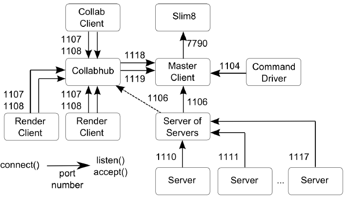
EnSight 10.2 User Manual 14-1
14 EnSight Networking Considerations
The EnSight application suite consists of a number of different applications
(Client, Server, Collabhub, Server of Servers, etc) that communicate over TCP/IP
(socket) connections. The collection of connections are fairly complex and in
secure environments, the specifics of those connections are critical for advanced
client/server usage of EnSight with remote components. In this section, we
document the various connections that can be made by the suite so that specific
firewall and VPN/tunnel configurations can be customized for use with EnSight.
Default TCP/IP Port Usage
The following diagram documents all of the TCP/IP connections that EnSight can
make as well as the default port numbers. In normal EnSight operation, the only
connections are between Slim8 (the license manager), the Master Client and a
single Server (which replaces the Server of Servers box in the diagram). EnSight
uses rsh or ssh to launch the various processes, but it does not use the rsh/ssh
channel for communication. Instead, the various processes make their own TCP/
IP connections after they have been launched. The arrows in the diagram
demonstrate the direction of the connection. The process at the arrow end of the
lines is making the accept() socket call while the other end is making the connect()
socket call. After the connection has been established, all communication is bi-
directional over the various socket connections.
By default, EnSight may use any of the ports in the range 1104 to 1119 (excepting
1105 and 1109) and port 7790 for bi-directional communication. Command line
options exist to change all of the default ports. It should be noted that these
connections may be within the same machine as ports usage has been constructed
to make it possible to run the entire system inside of a single computer. (see
Command Line Start-up Options)
At least one ‘Client’ and one ‘Server’ are necessary to run EnSight. The ‘Server of
Server’ (SOS) looks to the EnSight Client as a Server (it uses the same protocols
and ports as a Server does to talk to the client) and looks to the Server(s) as a
14-2 EnSight 10.2 User Manual
Client.
In standard collaboration mode, the “Master Client” launches a ‘Collabhub’
process and one or more external EnSight Clients (shown in the diagram as
‘Collab Client’s) can attach to the ‘Collabhub’. In EnSight HPC+ or VR mode,
there is a ‘Collabhub’ and one or more ‘Render Client’s (and there can be no
‘Collab Client’ components). The ‘Command Driver’is a seldom used
component, but is included here for the sake of completeness.
One connection not in this diagram is the connection between a Server and the
Master Client when the Server of Servers (SOS) is not being used. In this
situation, the server connects to the Master client over port 1106, using exactly the
same mechanism as the SOS uses to connect to the Master Client.
Connections between Clients and the Collabhub use two ports as data and control
channels. These connections are always made in the same direction, with the
connection from the Collabhub to the Master Client in the opposite direction than
the other Clients.
When running with the Server of Servers, the Servers may use ports from 1110 to
1117 depending on the number of threads specified for the SOS (up to 8 threads
maximum). For example if ENSIGHT10_MAX_SOSTHREADS is set to 2, then
ports 1110 and 1111 are used. These ports are re-used if more than two Servers are
specified. If ENSIGHT10_MAX_SOSTHREADS is set to 8 then ports 1110 to
1117 are used (and reused if more than 8 Servers is specified). By default, a single
thread and only port 1110 is used to establish all of the SOS to Server connections.
Initially, the Server (or SOS) attaches to the client on port 1106. If a Collabhub is
introduced (in Collaboration Mode or with HPC+ or VR), the SOS or Server
moves its connection to 1106 over to the collabhub.
CEIShell Connection Details
The previous section describes the connection details for EnSight's legacy
connection methods. While still valid in EnSight 10.2, EnSight is migrating to
using CEIShell for launch and network communication. See the details in the
CEIShell chapter elsewhere in this document.
With CEIShell, a user (or site) specifies the TCP/IP network names and port
numbers along with which direction the connect() / listen() occur. This allows a
site much greater flexibility to work within the network constraints of their
computational environment.
The default CEIStart configurations "Remote Server" and "Remote SOS" as
shipped use the same TCP/IP port numbers and connection directions as the
legacy methods (see the preceding section). However, a site could adapt these
configurations to use alternative connection details. Please contact CEI Support if
you need guidance.
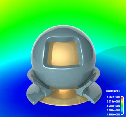
EnSight 10.2 User Manual 15-1
15 Raytracing
Starting from EnSight 10.2, an integrated raytracing engine, EnRay, is
incorporated into Ensight. Raytracing is an advanced rendering technique for
creating high quality visualization results. It generates global lighting effects
naturally by simulating physical transportation of photons. EnRay is based on
Physically Based Ray Tracer (http://www.pbrt.org), an open source raytracing
software, with integration of the Embree raytracing kernel from Intel (http://
embree.github.io), and many extensions implemented by CEI’s software
engineers. For a quick start on how to use the raytracer, see How To Use Raytrace
Rendering in the How To Manual.
In this chapter, we provide some in-depth discussions on the usage of the
Raytracer.
Understanding EnSight’s Materials
In this version of Ensight, we provide a predefined material library with some
commonly used material types. To maintain compatibility, Ensight sets the default
material to be of type “Default”, which is compatible with the lighting model used
in previous EnSight versions. For other material types, some different lighting
models will be used in the raytracer.
The materials are physically based. Their major differences come from the
individual microfacet representation. In computer graphics, we use a term
Bidirectional Reflectance Distribution Function (BRDF) to describe the
distribution of light scattering on the surface. Different materials have different
BRDFs. Some of the BRDFs are:
A Raytracing Example
Lambertian an ideal model that equally reflects in all directions.
OrenNayer a kind of diffuse reflection controlled by a smoothness
term. Can degenerate into Lambertian when
smoothness becomes zero.
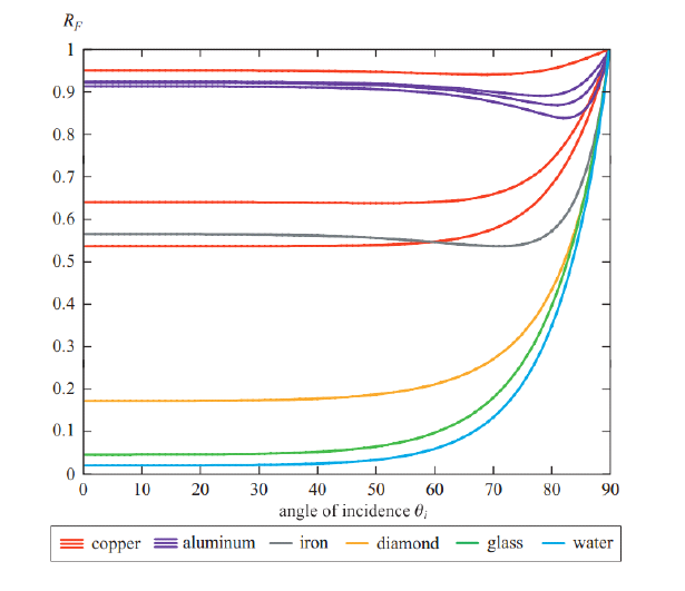
15-2 EnSight 10.2 User Manual
Another significant difference for the materials is their Fresnel terms. Note that
for some of the materials, their Fresnel reflection terms are fixed and hidden from
the user. When light moves from one media into another with different refraction
indices, both reflection and refraction may occur. The Fresnel equations describe
what fraction of the light is reflected, and what fraction is refracted. Fig. 1 shows
the reflection ratio according to the changes of incident angles for various
materials. It clearly indicates that differences between metals and non-metals are
significant. For example, at zero incidence angle, all the metals in the figure have
reflection ratio > 0.5, while the non metals have low reflection ratio < 0.2. Real
world perceptions substantiate this. However, note that at glancing angles, all
materials reflect almost all light.
Internally, the Fresnel terms are controlled by the factor of refraction index. For
metals, we assign default values for different metal types. A user thus does not
need to know anything about it. Once selecting a metal type, a user can freely
modify its appearance while EnSight will still use the same Fresnel terms for
computation. For non-metals, sometimes the refraction index is exposed. If it is
exposed to the user, a user can adjust this value to control the reflection and/or
refraction ratios for incident light.
GGX, Velvety,
BlinnPhong
are different specular highlighting models
Coated GGX a double-layer model, where the outer layer is
transparent with an index of refraction value
controlled by the user, and the inner layer is a normal
layer such as GGX or BlinnPhong
Figure courtesy of A. K. Peters, from “Realtime rendering”, 3rd Edition
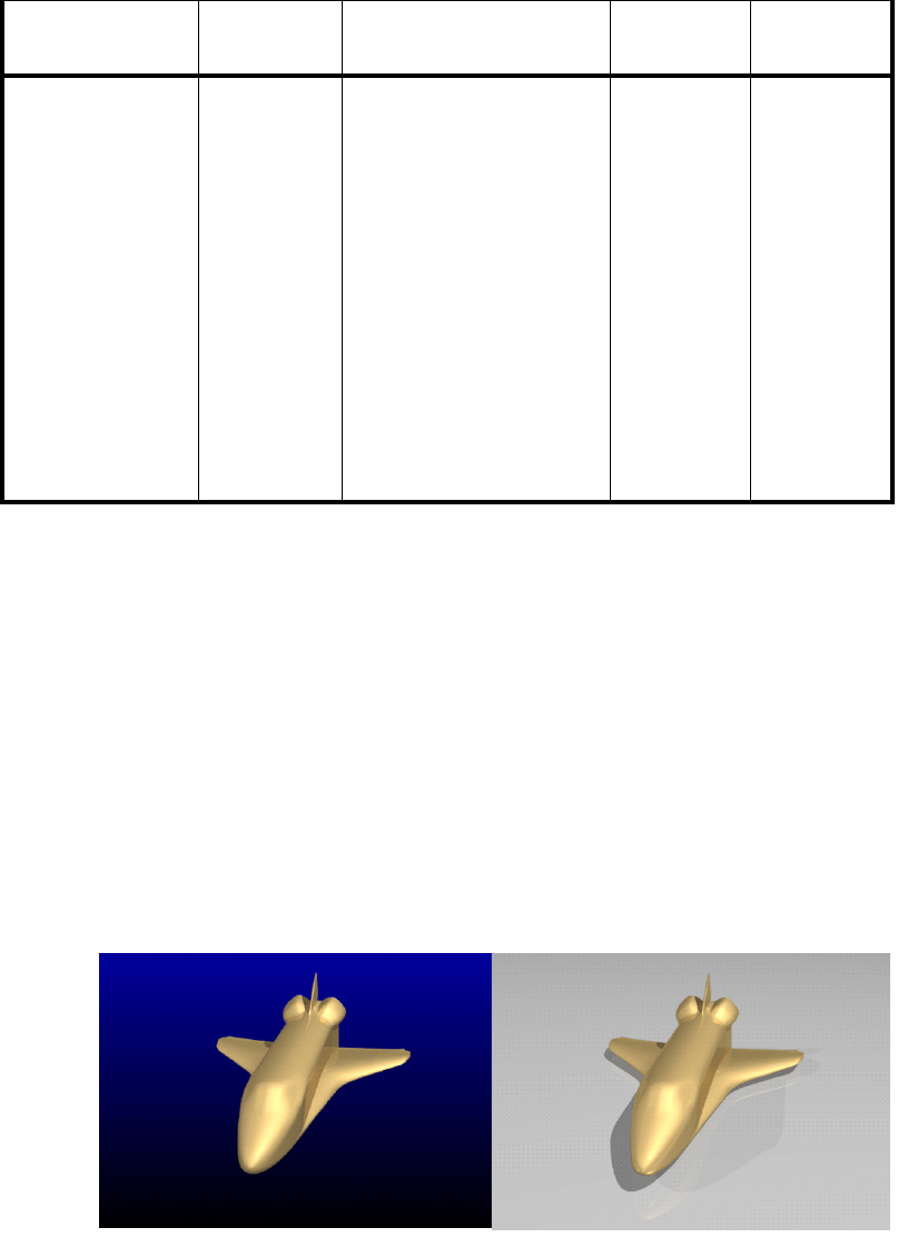
EnSight 10.2 User Manual 15-3
The materials are designed as shown in Table 1. You can see that some do not
have a diffuse component, while others do not have reflective highlights. Both the
graphics hardware rendering & raytracing implementations roughly follow the
same design. However, in the interactive graphics windows, they may look
similar. This is done for realtime performance reasons. Namely, we have to use a
simple implementation to handle several material types quickly.
Discussion on light sources
For a quick guide on how to use the light sources, see How To Set Light Sources.
Auxiliary geometry
Raytracing is a global illumination algorithm, where the interaction of photons
between neighboring objects plays an important role in enriching the realism of
the scene. Therefore, adding context to the current scene can greatly improve and
enhance the realism. Auxiliary geometry (being able to add floor, walls, and or
ceiling on which textures can be mapped, or shadows or reflections can be cast)
serves this purpose. Below is a comparison, where a floor is created for the right
image, while the left has no floor. Shadow and reflection make the shuttle image
on the right more realistic.
For a quick guide to how to use the auxiliary geometries, see How To Create
Material Diffuse Specular Reflective Transmitive
BRDF BRDF Fresnel
Default Lambertian BlinnPhong no n/a yes
Cloth Minnaert Velvety no n/a n/a
Glass n/a n/a n/a yes yes
Metal n/a GGX yes yes yes
Paint high-gloss Lambertian coated GGX yes yes yes
Paint semi-
gloss Lambertian coated GGX yes yes yes
Paint satin Lambertian Anisotropic yes n/a yes
Paint eggshell Lambertian Anisotropic yes n/a yes
Paint Matte OrenNayar n/a n/a n/a yes
Plastic Lambertian GGX yes n/a yes
Rubber OrenNayar n/a n/a n/a yes
Table 1: Material definition
15-4 EnSight 10.2 User Manual
Auxiliary Geometry.
Limitations
The current raytracer only supports rendering on a single machine. And not all
scene objects and rendering styles in the OpenGL rendering window can be
rendered using the raytracer. Below is a list of restrictions:
Multiple viewports
Volume rendering
Line elements
Hidden line (grid display on)
3D annotations (Text in 3d space or 3d glyphs)
Auxiliary Clipping
Contour parts
Profile parts
Tensor glyphs
Particle traces shown in a line representation, including Animated Traces
Vector arrows
Axis triad
Any part colored with Per Element Variables will be rendered as a single color.
Do not export flipbook animations.
So when the raytracer meets a scene with one or more limitations listed in the
above list, it will issue a warning message box. The user must confirm that the
limitations can be ignored, in order for the raytracing process to continue.
