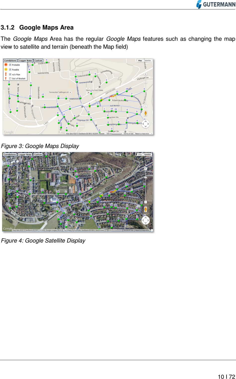
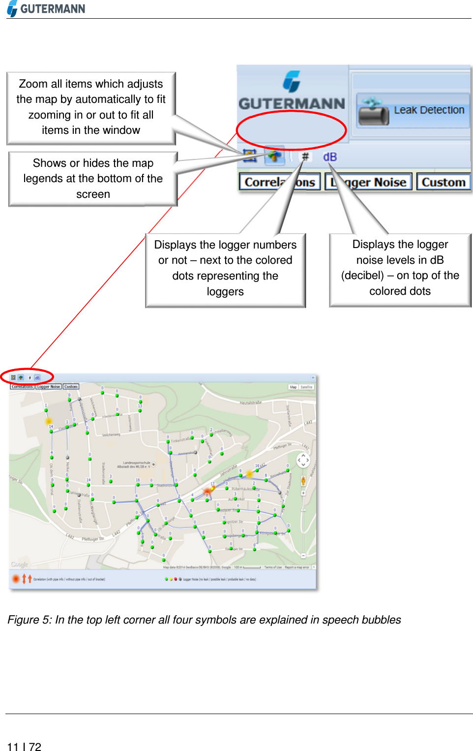
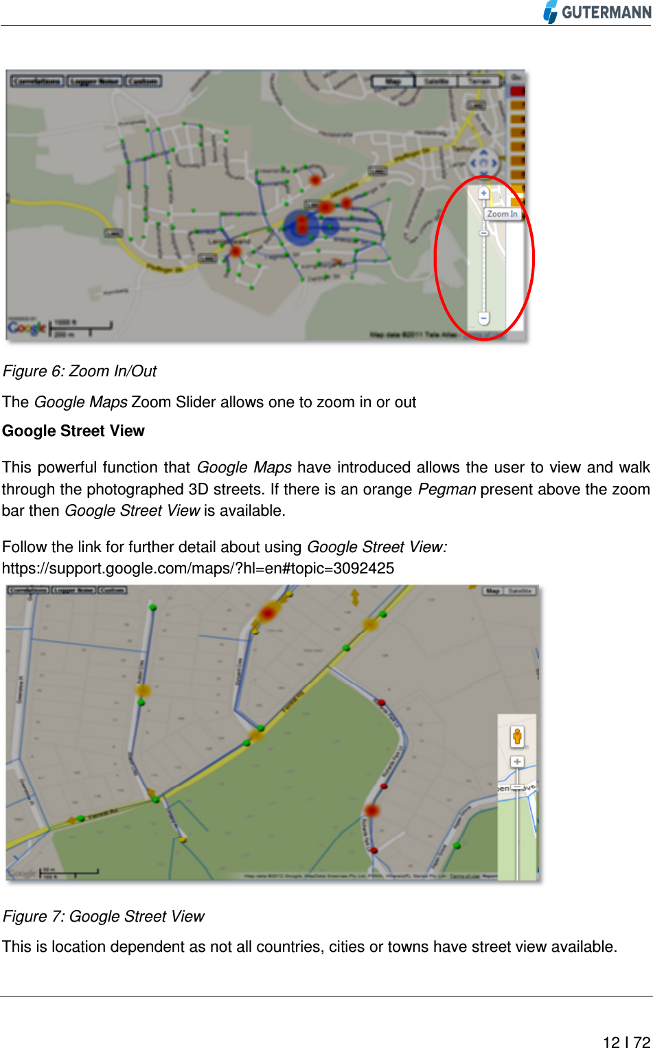
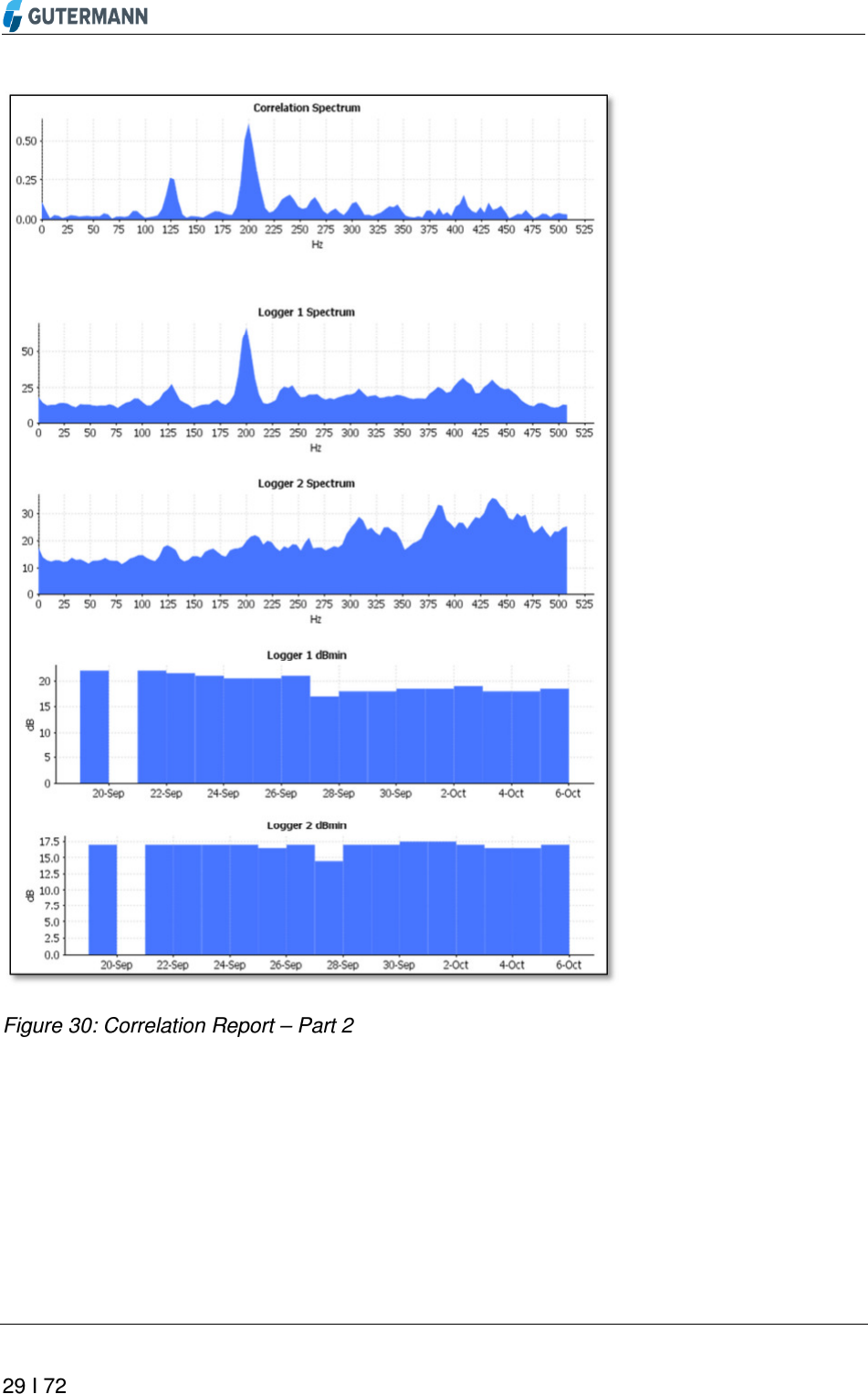
Gutermann Technology ZS820915AL2 Wireless Transceiver for data collection User Manual ZONESCAN NET Manual 2 1 Rev3 en
Gutermann Technology GmbH Wireless Transceiver for data collection ZONESCAN NET Manual 2 1 Rev3 en
Contents
- 1. user manual
- 2. user manual II
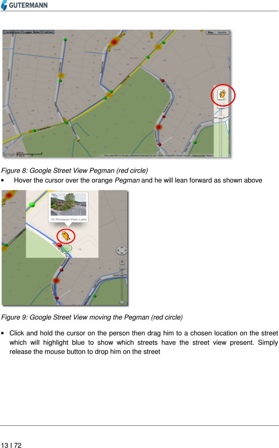
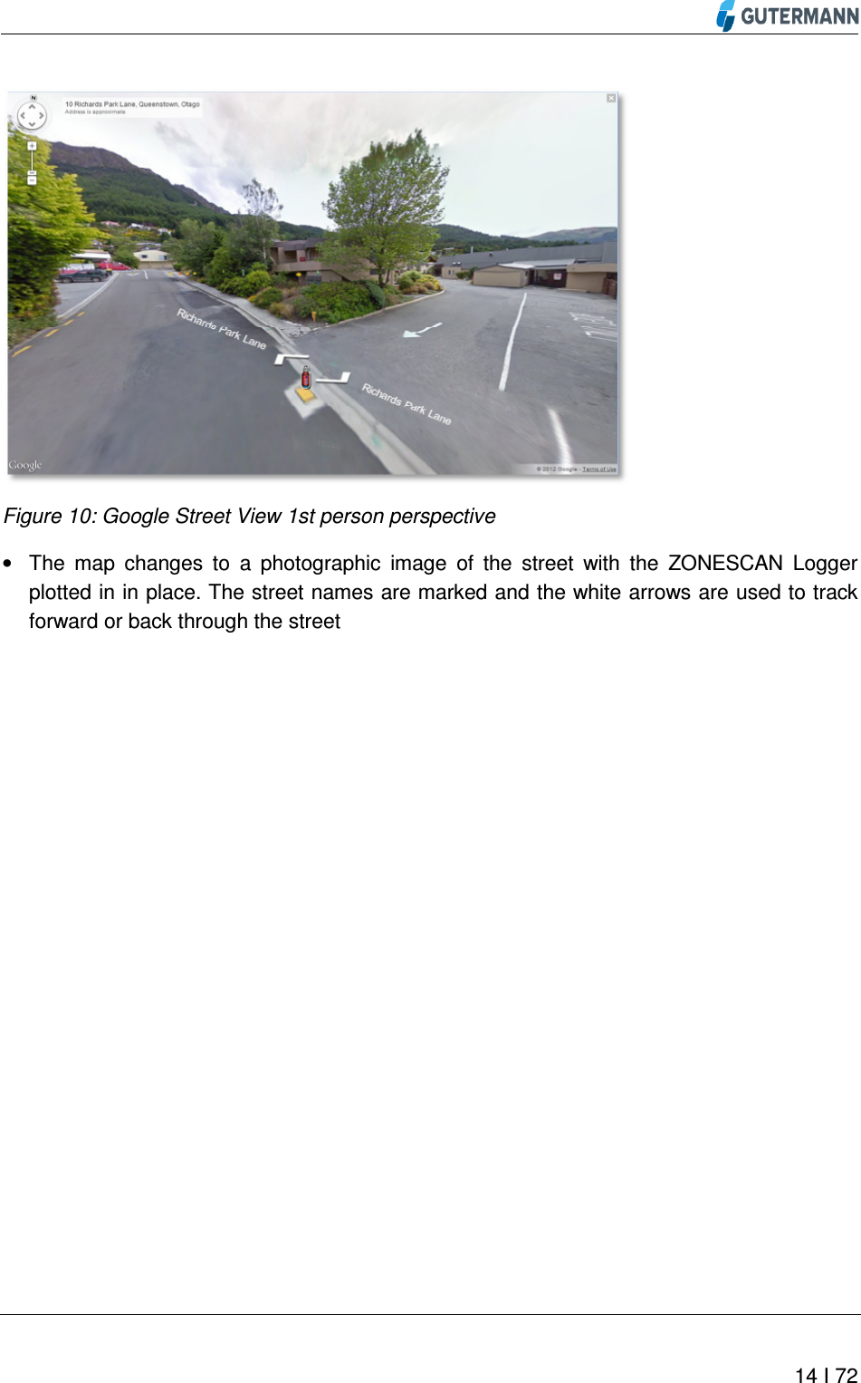
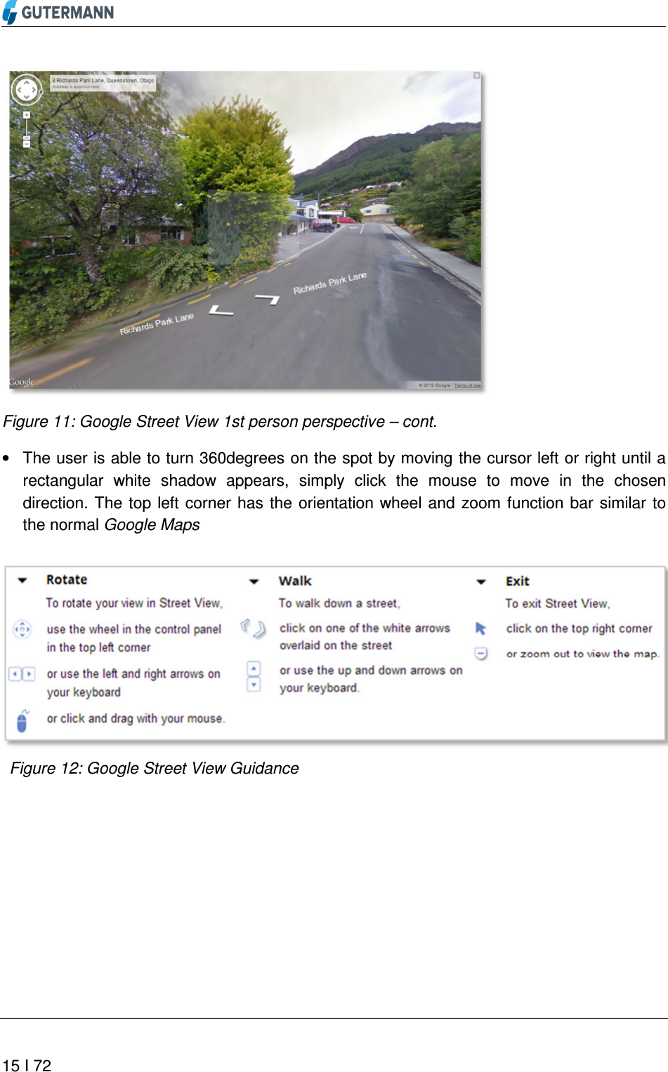
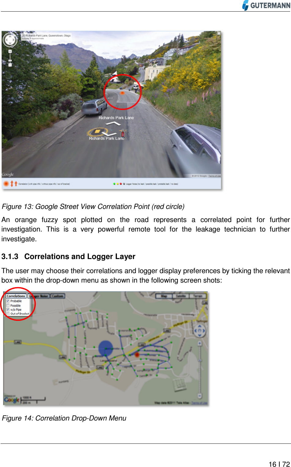
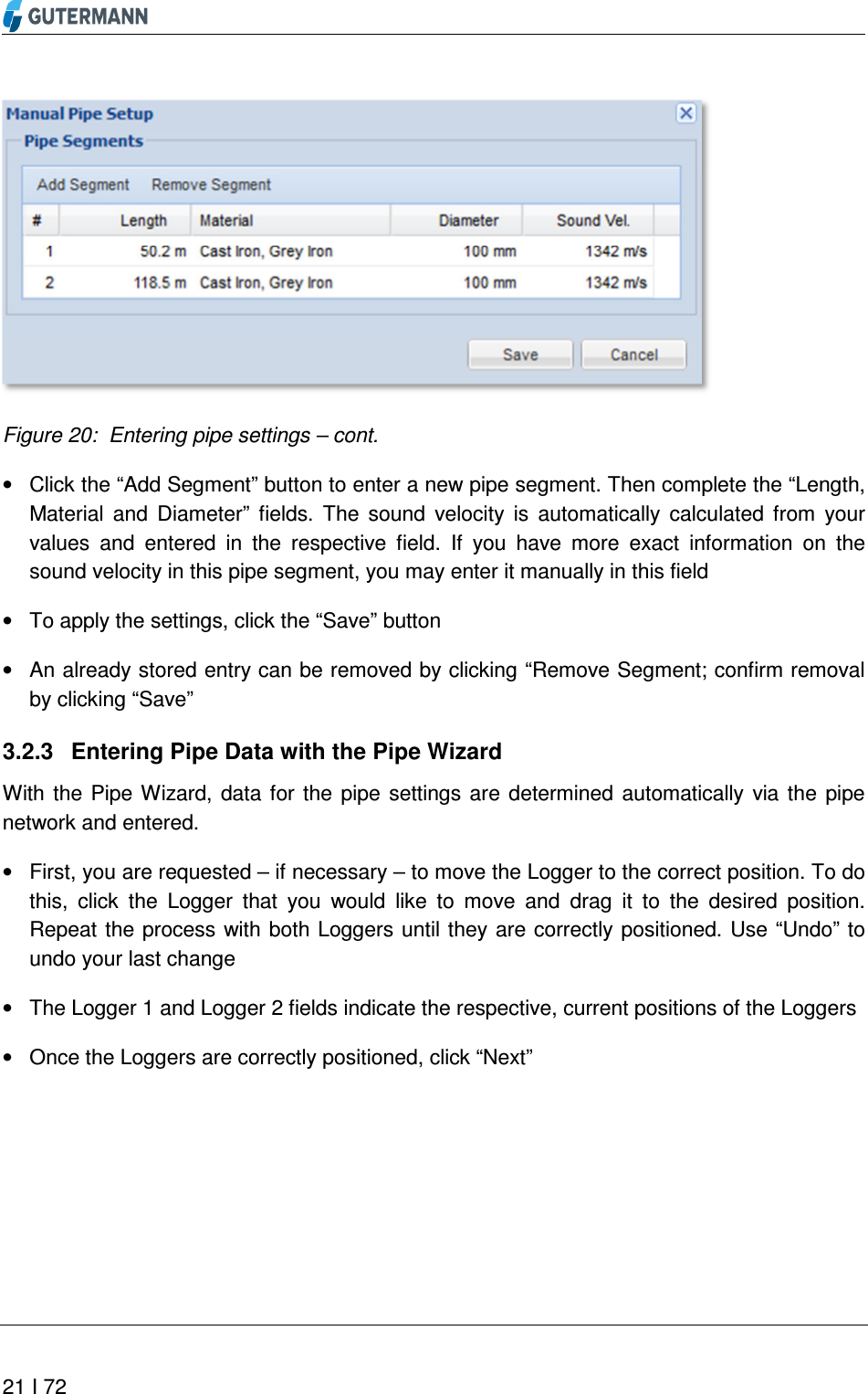
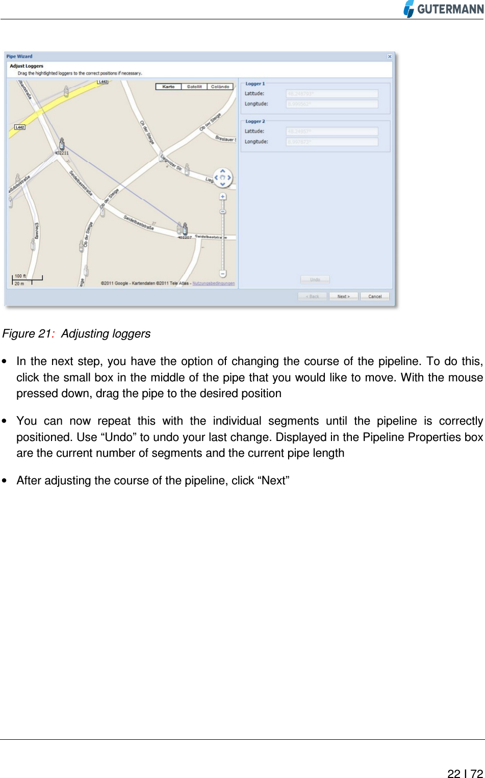
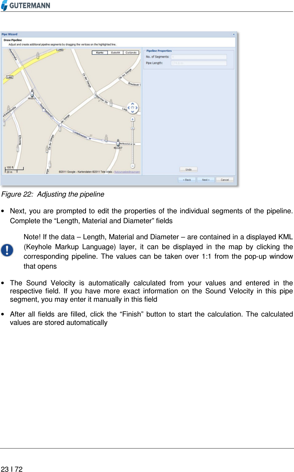
user manual