Ibm Water System Spss Complex Samples 19 Users Manual
SPSS COMPLEX SAMPLES 19 to the manual 4d32d40d-b1d4-4495-ad63-7160a22ee52d
2015-02-02
: Ibm Ibm-Ibm-Water-System-Spss-Complex-Samples-19-Users-Manual-431950 ibm-ibm-water-system-spss-complex-samples-19-users-manual-431950 ibm pdf
Open the PDF directly: View PDF ![]() .
.
Page Count: 288 [warning: Documents this large are best viewed by clicking the View PDF Link!]
- IBM SPSS Complex Samples 19
- Contents
- User's Guide
- 1. Introduction to Complex Samples Procedures
- 2. Sampling from a Complex Design
- Creating a New Sample Plan
- Sampling Wizard: Design Variables
- Sampling Wizard: Sampling Method
- Sampling Wizard: Sample Size
- Sampling Wizard: Output Variables
- Sampling Wizard: Plan Summary
- Sampling Wizard: Draw Sample Selection Options
- Sampling Wizard: Draw Sample Output Files
- Sampling Wizard: Finish
- Modifying an Existing Sample Plan
- Sampling Wizard: Plan Summary
- Running an Existing Sample Plan
- CSPLAN and CSSELECT Commands Additional Features
- 3. Preparing a Complex Sample for Analysis
- Creating a New Analysis Plan
- Analysis Preparation Wizard: Design Variables
- Analysis Preparation Wizard: Estimation Method
- Analysis Preparation Wizard: Size
- Analysis Preparation Wizard: Plan Summary
- Analysis Preparation Wizard: Finish
- Modifying an Existing Analysis Plan
- Analysis Preparation Wizard: Plan Summary
- 4. Complex Samples Plan
- 5. Complex Samples Frequencies
- 6. Complex Samples Descriptives
- 7. Complex Samples Crosstabs
- 8. Complex Samples Ratios
- 9. Complex Samples General Linear Model
- CSGLM Command Additional Features
- 10. Complex Samples Logistic Regression
- Complex Samples Logistic Regression Reference Category
- Complex Samples Logistic Regression Model
- Complex Samples Logistic Regression Statistics
- Complex Samples Hypothesis Tests
- Complex Samples Logistic Regression Odds Ratios
- Complex Samples Logistic Regression Save
- Complex Samples Logistic Regression Options
- CSLOGISTIC Command Additional Features
- 11. Complex Samples Ordinal Regression
- Complex Samples Ordinal Regression Response Probabilities
- Complex Samples Ordinal Regression Model
- Complex Samples Ordinal Regression Statistics
- Complex Samples Hypothesis Tests
- Complex Samples Ordinal Regression Odds Ratios
- Complex Samples Ordinal Regression Save
- Complex Samples Ordinal Regression Options
- CSORDINAL Command Additional Features
- 12. Complex Samples Cox Regression
- Examples
- 13. Complex Samples Sampling Wizard
- 14. Complex Samples Analysis Preparation Wizard
- 15. Complex Samples Frequencies
- 16. Complex Samples Descriptives
- 17. Complex Samples Crosstabs
- 18. Complex Samples Ratios
- 19. Complex Samples General Linear Model
- 20. Complex Samples Logistic Regression
- 21. Complex Samples Ordinal Regression
- 22. Complex Samples Cox Regression
- A. Sample Files
- B. Notices
- Bibliography
- Index

i
IBM SPSS Complex Samples 19
Note: Before using this information and the product it supports, read the general information
under Notices on p. 267.
This document contains proprietary information of SPSS Inc, an IBM Company. It is provided
under a license agreement and is protected by copyright law. The information contained in this
publication does not include any product warranties, and any statements provided in this manual
should not be interpreted as such.
When you send information to IBM or SPSS, you grant IBM and SPSS a nonexclusive right
to use or distribute the information in any way it believes appropriate without incurring any
obligationtoyou.
© Copyright SPSS Inc. 1989, 2010.

Preface
IBM® SPSS® Statistics is a comprehensive system for analyzing data. The Complex Samples
optional add-on module provides the additional analytic techniques described in this manual. The
Complex Samples add-on module must be used with the SPSS Statistics Core system and is
completely integrated into that system.
About SPSS Inc., an IBM Company
SPSS Inc., an IBM Company, is a leading global provider of predictive analytic software
and solutions. The company’s complete portfolio of products — data collection, statistics,
modeling and deployment — captures people’s attitudes and opinions, predicts outcomes of
future customer interactions, and then acts on these insights by embedding analytics into business
processes. SPSS Inc. solutions address interconnected business objectives across an entire
organization by focusing on the convergence of analytics, IT architecture, and business processes.
Commercial, government, and academic customers worldwide rely on SPSS Inc. technology as
a competitive advantage in attracting, retaining, and growing customers, while reducing fraud
and mitigating risk. SPSS Inc. was acquired by IBM in October 2009. For more information,
visit http://www.spss.com.
Technical support
Technical support is available to maintenance customers. Customers may contact
Technical Support for assistance in using SPSS Inc. products or for installation help
for one of the supported hardware environments. To reach Technical Support, see the
SPSS Inc. web site at http://support.spss.com or find your local office via the web site at
http://support.spss.com/default.asp?refpage=contactus.asp. Be prepared to identify yourself, your
organization, and your support agreement when requesting assistance.
Customer Service
If you have any questions concerning your shipment or account, contact your local office, listed
on the Web site at http://www.spss.com/worldwide. Please have your serial number ready for
identification.
Training Seminars
SPSS Inc. provides both public and onsite training seminars. All seminars feature hands-on
workshops. Seminars will be offered in major cities on a regular basis. For more information on
these seminars, contact your local office, listed on the Web site at http://www.spss.com/worldwide.
© Copyright SPSS Inc. 1989, 2010 iii
Additional Publications
The SPSS Statistics: Guide to Data Analysis,SPSS Statistics: Statistical Procedures Companion,
and SPSS Statistics: Advanced Statistical Procedures Companion, written by Marija Norušis and
published by Prentice Hall, are available as suggested supplemental material. These publications
cover statistical procedures in the SPSS Statistics Base module, Advanced Statistics module
and Regression module. Whether you are just getting starting in data analysis or are ready for
advanced applications, these books will help you make best use of the capabilities found within
the IBM® SPSS® Statistics offering. For additional information including publication contents
and sample chapters, please see the author’s website: http://www.norusis.com
iv

Contents
Part I: User’s Guide
1 Introduction to Complex Samples Procedures 1
PropertiesofComplexSamples .................................................. 1
UsageofComplexSamplesProcedures............................................ 2
PlanFiles................................................................ 2
FurtherReadings ............................................................. 3
2 Sampling from a Complex Design 4
Creating a NewSamplePlan .................................................... 4
Sampling Wizard:DesignVariables ............................................... 6
Tree ControlsforNavigatingtheSamplingWizard................................. 7
SamplingWizard:SamplingMethod............................................... 8
SamplingWizard:SampleSize...................................................10
DefineUnequalSizes.......................................................11
SamplingWizard:OutputVariables................................................12
SamplingWizard:PlanSummary .................................................13
SamplingWizard:DrawSampleSelectionOptions....................................14
SamplingWizard:DrawSampleOutputFiles.........................................15
SamplingWizard:Finish........................................................16
ModifyinganExistingSamplePlan................................................16
SamplingWizard:PlanSummary .................................................17
RunninganExistingSamplePlan .................................................18
CSPLANandCSSELECTCommandsAdditionalFeatures................................18
3 Preparing a Complex Sample for Analysis 19
CreatingaNewAnalysisPlan....................................................20
AnalysisPreparationWizard:DesignVariables.......................................20
TreeControlsforNavigatingtheAnalysisWizard..................................21
v
AnalysisPreparationWizard:EstimationMethod.....................................22
AnalysisPreparationWizard:Size ................................................23
DefineUnequalSizes.......................................................24
AnalysisPreparationWizard:PlanSummary ........................................25
AnalysisPreparationWizard:Finish...............................................26
ModifyinganExistingAnalysisPlan...............................................26
AnalysisPreparationWizard:PlanSummary ........................................27
4 Complex Samples Plan 28
5 Complex Samples Frequencies 29
Complex SamplesFrequenciesStatistics...........................................30
Complex SamplesMissingValues.................................................31
Complex SamplesOptions ......................................................32
6 Complex Samples Descriptives 33
ComplexSamplesDescriptivesStatistics...........................................34
ComplexSamplesDescriptivesMissingValues.......................................35
ComplexSamplesOptions ......................................................36
7 Complex Samples Crosstabs 37
ComplexSamplesCrosstabsStatistics.............................................39
ComplexSamplesMissingValues.................................................40
ComplexSamplesOptions ......................................................41
8 Complex Samples Ratios 42
ComplexSamplesRatiosStatistics................................................43
ComplexSamplesRatiosMissingValues ...........................................44
ComplexSamplesOptions ......................................................44
vi
9 Complex Samples General Linear Model 45
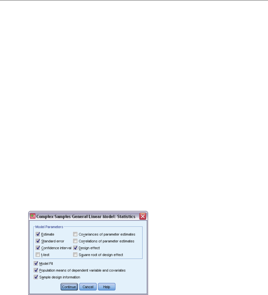
ComplexSamplesGeneralLinearModelStatistics....................................48
ComplexSamplesHypothesisTests ...............................................49
ComplexSamplesGeneralLinearModelEstimatedMeans..............................50
ComplexSamplesGeneralLinearModelSave .......................................51
ComplexSamplesGeneralLinearModelOptions .....................................52
CSGLMCommandAdditionalFeatures.............................................53
10 Complex Samples Logistic Regression 54
ComplexSamplesLogisticRegressionReferenceCategory .............................55
ComplexSamplesLogisticRegressionModel........................................56
ComplexSamplesLogisticRegressionStatistics......................................57
ComplexSamplesHypothesisTests ...............................................59
ComplexSamplesLogisticRegressionOddsRatios....................................60
ComplexSamplesLogisticRegressionSave.........................................61
ComplexSamplesLogisticRegressionOptions.......................................62
CSLOGISTICCommandAdditionalFeatures .........................................63
11 Complex Samples Ordinal Regression 64
Complex Samples Ordinal Regression Response Probabilities. . . . . . . . . . . . . . . . . . . . . . . . . . . . 66
ComplexSamplesOrdinalRegressionModel ........................................66
ComplexSamplesOrdinalRegressionStatistics......................................68
ComplexSamplesHypothesisTests ...............................................69
ComplexSamplesOrdinalRegressionOddsRatios....................................70
ComplexSamplesOrdinalRegressionSave .........................................71
ComplexSamplesOrdinalRegressionOptions .......................................72
CSORDINALCommandAdditionalFeatures..........................................73
12 Complex Samples Cox Regression 74
DefineEvent ................................................................77
vii
Predictors ..................................................................78
DefineTime-DependentPredictor.............................................79
Subgroups..................................................................80
Model .....................................................................81
Statistics ...................................................................82
Plots ......................................................................84
HypothesisTests .............................................................85
Save ......................................................................86
Export .....................................................................88
Options ....................................................................90
CSCOXREGCommandAdditionalFeatures..........................................91
Part II: Examples
13 Complex Samples Sampling Wizard 93
ObtainingaSamplefromaFullSamplingFrame......................................93
UsingtheWizard .........................................................93
PlanSummary........................................................... 103
SamplingSummary....................................................... 103
SampleResults.......................................................... 104
ObtainingaSamplefromaPartialSamplingFrame................................... 105
UsingtheWizardtoSamplefromtheFirstPartialFrame ........................... 105
SampleResults.......................................................... 118
UsingtheWizardtoSamplefromtheSecondPartialFrame......................... 118
SampleResults.......................................................... 123
Sampling with Probability Proportional to Size (PPS). . . . . . . . . . . . . . . . . . . . . . . . . . . . . . . . . . 123
UsingtheWizard ........................................................ 123
PlanSummary........................................................... 135
SamplingSummary....................................................... 135
SampleResults.......................................................... 137
RelatedProcedures.......................................................... 139
14 Complex Samples Analysis Preparation Wizard 140
Using the Complex Samples Analysis Preparation Wizard to Ready NHIS Public Data. . . . . . . . . 140
UsingtheWizard......................................................... 140
Summary............................................................... 143
viii
PreparingforAnalysisWhenSamplingWeightsAreNotintheDataFile................... 143
Computing Inclusion Probabilities and Sampling Weights . . . . . . . . . . . . . . . . . . . . . . . . . . 143
UsingtheWizard......................................................... 146
Summary............................................................... 154
RelatedProcedures.......................................................... 154
15 Complex Samples Frequencies 155
Using Complex Samples Frequencies to Analyze Nutritional Supplement Usage . . . . . . . . . . . . . 155
RunningtheAnalysis...................................................... 155
FrequencyTable ......................................................... 158
FrequencybySubpopulation................................................ 158
Summary............................................................... 159
RelatedProcedures.......................................................... 159
16 Complex Samples Descriptives 160
UsingComplexSamplesDescriptivestoAnalyzeActivityLevels......................... 160
RunningtheAnalysis...................................................... 160
UnivariateStatistics....................................................... 163
Univariate StatisticsbySubpopulation......................................... 163
Summary............................................................... 164
Related Procedures.......................................................... 164
17 Complex Samples Crosstabs 165
Using Complex Samples Crosstabs to Measure the Relative Risk of an Event . . . . . . . . . . . . . . . 165
RunningtheAnalysis...................................................... 165
Crosstabulation.......................................................... 168
RiskEstimate ........................................................... 169
RiskEstimatebySubpopulation.............................................. 170
Summary............................................................... 170
RelatedProcedures.......................................................... 170
ix
18 Complex Samples Ratios 171
UsingComplexSamplesRatiostoAidPropertyValueAssessment....................... 171
RunningtheAnalysis...................................................... 171
Ratios................................................................. 174
PivotedRatiosTable ...................................................... 174
Summary............................................................... 175
RelatedProcedures.......................................................... 175
19 Complex Samples General Linear Model 176
Using Complex Samples General Linear Model to Fit a Two-Factor ANOVA . . . . . . . . . . . . . . . . . 176
Running the Analysis...................................................... 176
ModelSummary ......................................................... 181
TestsofModelEffects..................................................... 181
Parameter Estimates...................................................... 182
EstimatedMarginalMeans ................................................. 183
Summary .............................................................. 185
RelatedProcedures.......................................................... 185
20 Complex Samples Logistic Regression 186
UsingComplexSamplesLogisticRegressiontoAssessCreditRisk....................... 186
RunningtheAnalysis...................................................... 186
PseudoR-Squares........................................................ 190
Classification............................................................ 191
TestsofModelEffects..................................................... 191
ParameterEstimates...................................................... 192
OddsRatios............................................................. 193
Summary............................................................... 194
RelatedProcedures.......................................................... 194
21 Complex Samples Ordinal Regression 195
UsingComplexSamplesOrdinalRegressiontoAnalyzeSurveyResults.................... 195
RunningtheAnalysis...................................................... 195
PseudoR-Squares........................................................ 200
TestsofModelEffects..................................................... 200
x
ParameterEstimates...................................................... 201
Classification............................................................ 202
OddsRatios............................................................. 203
GeneralizedCumulativeModel .............................................. 204
DroppingNon-SignificantPredictors.......................................... 205
Warnings............................................................... 207
ComparingModels ....................................................... 208
Summary............................................................... 209
RelatedProcedures.......................................................... 209
22 Complex Samples Cox Regression 210
Using a Time-Dependent Predictor in Complex Samples Cox Regression. . . . . . . . . . . . . . . . . . . 210
PreparingtheData ....................................................... 210
RunningtheAnalysis...................................................... 216
SampleDesignInformation................................................. 221
TestsofModelEffects..................................................... 222
TestofProportionalHazards................................................ 222
AddingaTime-DependentPredictor .......................................... 222
MultipleCasesperSubjectinComplexSamplesCoxRegression ........................ 226
PreparingtheDataforAnalysis.............................................. 227
CreatingaSimpleRandomSamplingAnalysisPlan ............................... 242
RunningtheAnalysis...................................................... 246
SampleDesignInformation................................................. 254
TestsofModelEffects..................................................... 255
ParameterEstimates...................................................... 255
PatternValues........................................................... 256
Log-Minus-LogPlot....................................................... 257
Summary............................................................... 257
xi
Part I:
User’s Guide

Chapter
1
Introduction to Complex Samples
Procedures
An inherent assumption of analytical procedures in traditional software packages is that the
observations in a data file represent a simple random sample from the population of interest. This
assumption is untenable for an increasing number of companies and researchers who find it both
cost-effective and convenient to obtain samples in a more structured way.
The Complex Samples option allows you to select a sample according to a complex design and
incorporate the design specifications into the data analysis, thus ensuring that your results are valid.
Properties of Complex Samples
A complex sample can differ from a simple random sample in many ways. In a simple random
sample, individual sampling units are selected at random with equal probability and without
replacement (WOR) directly from the entire population. By contrast, a given complex sample
can have some or all of the following features:
Stratification. Stratified sampling involves selecting samples independently within
non-overlapping subgroups of the population, or strata. For example, strata may be socioeconomic
groups, job categories, age groups, or ethnic groups. With stratification, you can ensure adequate
sample sizes for subgroups of interest, improve the precision of overall estimates, and use different
sampling methods from stratum to stratum.
Clustering. Cluster sampling involves the selection of groups of sampling units, or clusters. For
example, clusters may be schools, hospitals, or geographical areas, and sampling units may be
students, patients, or citizens. Clustering is common in multistage designs and area (geographic)
samples.
Multiple stages. In multistage sampling, you select a first-stage sample based on clusters. Then
you create a second-stage sample by drawing subsamples from the selected clusters. If the
second-stage sample is based on subclusters, you can then add a third stage to the sample. For
example, in the first stage of a survey, a sample of cities could be drawn. Then, from the selected
cities, households could be sampled. Finally, from the selected households, individuals could be
polled. The Sampling and Analysis Preparation wizards allow you to specify three stages in
adesign.
Nonrandom sampling. When selection at random is difficult to obtain, units can be sampled
systematically (at a fixed interval) or sequentially.
© Copyright SPSS Inc. 1989, 2010 1

2
Chapter 1
Unequal selection probabilities. When sampling clusters that contain unequal numbers of units,
you can use probability-proportional-to-size (PPS) sampling to make a cluster’s selection
probability equal to the proportion of units it contains. PPS sampling can also use more general
weighting schemes to select units.
Unrestricted sampling. Unrestricted sampling selects units with replacement (WR). Thus, an
individual unit can be selected for the sample more than once.
Sampling weights. Sampling weights are automatically computed while drawing a complex
sample and ideally correspond to the “frequency” that each sampling unit represents in the target
population. Therefore, the sum of the weights over the sample should estimate the population
size. Complex Samples analysis procedures require sampling weights in order to properly analyze
a complex sample. Note that these weights shouldbeusedentirelywithintheComplexSamples
option and should not be used with other analytical procedures via the Weight Cases procedure,
which treats weights as case replications.
Usage of Complex Samples Procedures
Your usage of Complex Samples procedures depends on your particular needs. The primary
types of users are those who:
Plan and carry out surveys according to complex designs, possibly analyzing the sample later.
The primary tool for surveyors is the Sampling Wizard.
Analyze sample data files previously obtained according to complex designs. Before using the
Complex Samples analysis procedures, you may need to use the Analysis Preparation Wizard.
Regardless of which type of user you are, you need to supply design information to Complex
Samples procedures. This information is stored in a plan file for easy reuse.
Plan Files
Aplanfile contains complex sample specifications. There are two types of plan files:
Sampling plan. The specifications given in the Sampling Wizard defineasampledesignthat
is used to draw a complex sample. The sampling plan file contains those specifications. The
sampling plan file also contains a default analysis plan that uses estimation methods suitable for
the specified sample design.
Analysis plan. This plan file contains information needed by Complex Samples analysis procedures
to properly compute variance estimates for a complex sample. The plan includes the sample
structure, estimation methods for each stage, and references to required variables, such as sample
weights. The Analysis Preparation Wizard allows you to create and edit analysis plans.
There are several advantages to saving your specifications in a plan file, including:
A surveyor can specify the first stage of a multistage sampling plan and draw first-stage
units now, collect information on sampling units for the second stage, and then modify the
sampling plan to include the second stage.

3
Introduction to Complex Samples Procedures
An analyst who doesn’t have access to the sampling plan file can specify an analysis plan and
refer to that plan from each Complex Samples analysis procedure.
A designer of large-scale public use samples can publish the sampling plan file, which
simplifies the instructions for analysts and avoids the need for each analyst to specify his
or her own analysis plans.
Further Readings
For more information on sampling techniques, see the following texts:
Cochran, W. G. 1977. Sampling Techniques, 3rd ed. New York: John Wiley and Sons.
Kish,L.1965. Survey Sampling. New York: John Wiley and Sons.
Kish, L. 1987. Statistical Design for Research. New York: John Wiley and Sons.
Murthy, M. N. 1967. Sampling Theory and Methods. Calcutta, India: Statistical Publishing
Society.
Särndal, C., B. Swensson, and J. Wretman. 1992. Model Assisted Survey Sampling.NewYork:
Springer-Verlag.

Chapter
2
Sampling from a Complex Design
Figure 2-1
Sampling Wizard, Welcome step
The Sampling Wizard guides you through the steps for creating, modifying, or executing a
sampling plan file. Before using the Wizard, you should have a well-defined target population, a
list of sampling units, and an appropriate sample design in mind.
Creating a New Sample Plan
EFrom the menus choose:
Analyze > Complex Samples > Select a Sample...
ESelect Design a sample and choose a plan filename to save the sample plan.
© Copyright SPSS Inc. 1989, 2010 4

5
Sampling from a Complex Design
EClick Next to continue through the Wizard.
EOptionally, in the Design Variables step, you can define strata, clusters, and input sample weights.
After you define these, click Next.
EOptionally, in the Sampling Method step, you can choose a method for selecting items.
If you select PPS Brewer or PPS Murthy, you can click Finish to draw the sample. Otherwise,
click Next and then:
EIn the Sample Size step, specify the number or proportion of units to sample.
EYou can now click Finish to draw the sample.
Optionally, in further steps you can:
Choose output variables to save.
Add a second or third stage to the design.
Set various selection options, including which stages to draw samples from, the random
number seed, and whether to treat user-missing values as valid values of design variables.
Choose where to save output data.
Paste your selections as command syntax.
6
Chapter 2
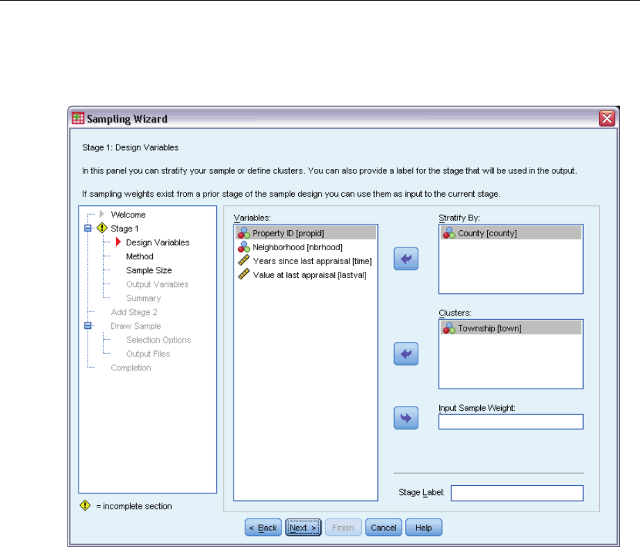
Sampling Wizard: Design Variables
Figure 2-2
Sampling Wizard, Design Variables step
This step allows you to select stratification and clustering variables and to define input sample
weights. You can also specify a label for the stage.
Stratify By. The cross-classification of stratification variables defines distinct subpopulations, or
strata. Separate samples are obtained for each stratum. To improve the precision of your estimates,
units within strata should be as homogeneous as possible for the characteristics of interest.
Clusters. Cluster variables define groups of observational units, or clusters. Clusters are useful
when directly sampling observational units from the population is expensive or impossible;
instead, you can sample clusters from the population and then sample observational units from
the selected clusters. However, the use of clusters can introduce correlations among sampling
units, resulting in a loss of precision. To minimize this effect, units within clusters should be as
heterogeneous as possible for the characteristics of interest. You must define at least one cluster
variable in order to plan a multistage design. Clusters are also necessary in the use of several
different sampling methods. For more information, see the topic Sampling Wizard: Sampling
Method on p. 8.

7
Sampling from a Complex Design
Input Sample Weight. If the current sample design is part of a larger sample design, you may have
sample weights from a previous stage of the larger design. You can specify a numeric variable
containing these weights in the first stage of the current design. Sample weights are computed
automatically for subsequent stages of the current design.
Stage Label. Youcanspecifyanoptionalstringlabelforeachstage.Thisisusedintheoutputto
help identify stagewise information.
Note: The source variable list has the same content across steps of the Wizard. In other words,
variables removed from the source list in a particular step are removed from the list in all steps.
Variables returned to the source list appear in the list in all steps.
Tree Controls for Navigating the Sampling Wizard
On the left side of each step in the Sampling Wizard is an outline of all the steps. You can navigate
theWizardbyclickingonthenameofanenabled step in the outline. Steps are enabled as
long as all previous steps are valid—that is, if each previous step has been given the minimum
required specifications for that step. See the Help for individual steps for more information on
whyagivenstepmaybeinvalid.
8
Chapter 2
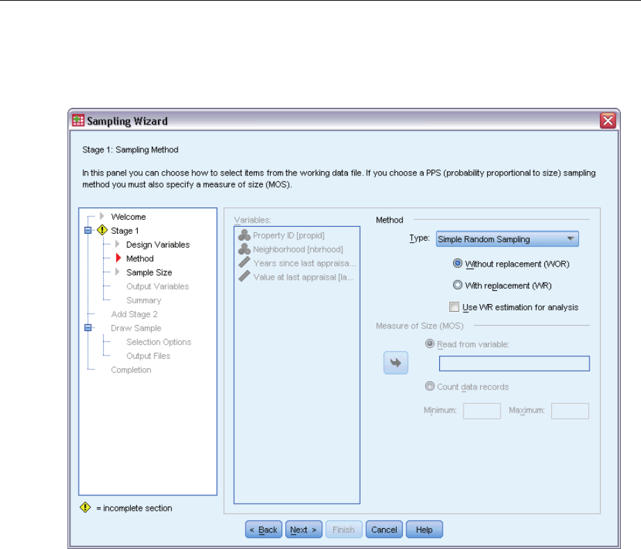
Sampling Wizard: Sampling Method
Figure 2-3
Sampling Wizard, Sampling Method step
This step allows you to specify how to select cases from the active dataset.
Method. Controls in this group are used to choose a selection method. Some sampling types allow
you to choose whether to sample with replacement (WR) or without replacement (WOR). See the
type descriptions for more information. Note that some probability-proportional-to-size (PPS)
types are available only when clusters have been defined and that all PPS types are available only
in the first stage of a design. Moreover, WR methods are available only in the last stage of a design.
Simple Random Sampling. Units are selected with equal probability. They can be selected
with or without replacement.
Simple Systematic. Units are selected at a fixed interval throughout the sampling frame (or
strata, if they have been specified) and extracted without replacement. A randomly selected
unit within the first interval is chosen as the starting point.
Simple Sequential. Units are selected sequentially with equal probability and without
replacement.
PPS. This is a first-stage method that selects units at random with probability proportional
to size. Any units can be selected with replacement; only clusters can be sampled without
replacement.

9
Sampling from a Complex Design
PPS Systematic. This is a first-stage method that systematically selects units with probability
proportional to size. They are selected without replacement.
PPS Sequential. This is a first-stage method that sequentially selects units with probability
proportional to cluster size and without replacement.
PPS Brewer. This is a first-stage method that selects two clusters from each stratum with
probability proportional to cluster size and without replacement. A cluster variable must be
specified to use this method.
PPS Murthy. This is a first-stage method that selects two clusters from each stratum with
probability proportional to cluster size and without replacement. A cluster variable must be
specified to use this method.
PPS Sampford. This is a first-stage method that selects more than two clusters from each
stratum with probability proportional to cluster size and without replacement. It is an
extension of Brewer’s method. A cluster variable must be specified to use this method.
Use WR estimation for analysis. By default, an estimation method is specified in the plan file
that is consistent with the selected sampling method. This allows you to use with-replacement
estimation even if the sampling method implies WOR estimation. This option is available
only in stage 1.
Measure of Size (MOS). If a PPS method is selected, you must specify a measure of size that defines
the size of each unit. These sizes can be explicitly defined in a variable or they can be computed
from the data. Optionally, you can set lower and upper bounds on the MOS, overriding any values
found in the MOS variable or computed from the data. These options are available only in stage 1.
10
Chapter 2
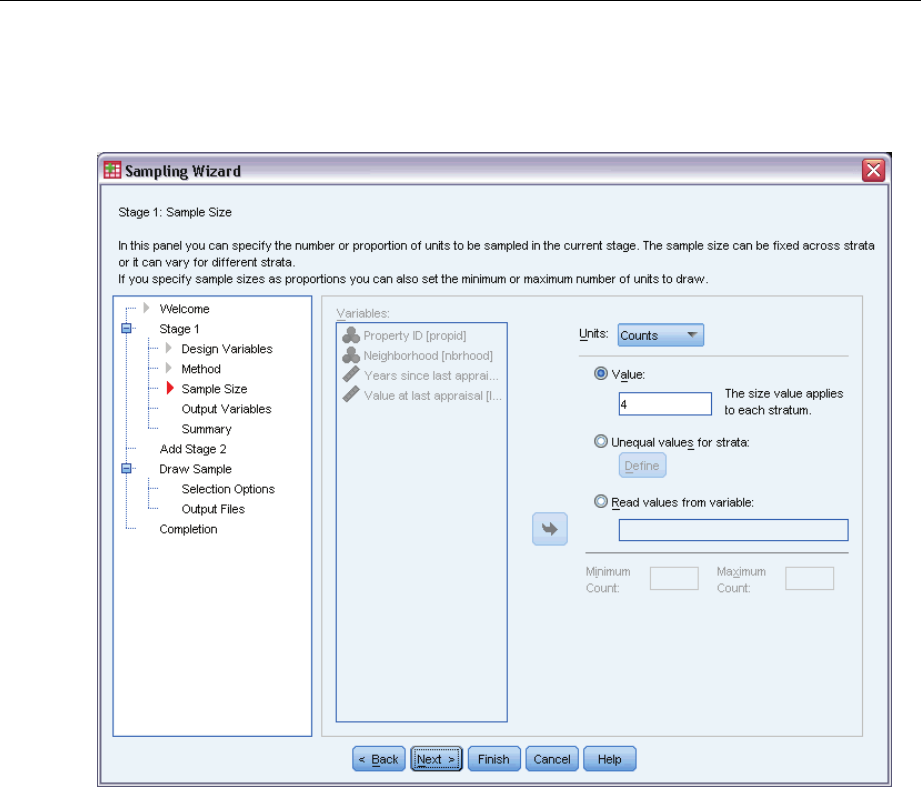
Sampling Wizard: Sample Size
Figure 2-4
Sampling Wizard, Sample Size step
This step allows you to specify the number or proportion of units to sample within the current
stage. The sample size can be fixed or it can vary across strata. For the purpose of specifying
sample size, clusters chosen in previous stages can be used to define strata.
Units. You can specify an exact sample size or a proportion of units to sample.
Value. A single value is applied to all strata. If Counts is selected as the unit metric, you should
enter a positive integer. If Proportions is selected, you should enter a non-negative value.
Unless sampling with replacement, proportion values should also be no greater than 1.
Unequal values for strata. Allows you to enter size values on a per-stratum basis via the Define
Unequal Sizes dialog box.
Read values from variable. Allows you to select a numeric variable that contains size values
for strata.
If Proportions is selected, you have the option to set lower and upper bounds on the number of
units sampled.

11
Sampling from a Complex Design
Define Unequal Sizes
Figure 2-5
Define Unequal Sizes dialog box
The Define Unequal Sizes dialog box allows you to enter sizes on a per-stratum basis.
Size Specifications grid. The grid displays the cross-classifications of up to five strata or
cluster variables—one stratum/cluster combination per row. Eligible grid variables include all
stratification variables from the current and previous stages and all cluster variables from previous
stages. Variables can be reordered within the grid or moved to the Exclude list. Enter sizes in the
rightmost column. Click Labels or Values to toggle the display of value labels and data values for
stratification and cluster variables in the grid cells. Cells that contain unlabeled values always
show values. Click Refresh Strata to repopulate the grid with each combination of labeled data
values for variables in the grid.
Exclude. To specify sizes for a subset of stratum/cluster combinations, move one or more variables
to the Exclude list. These variables are not used to define sample sizes.
12
Chapter 2
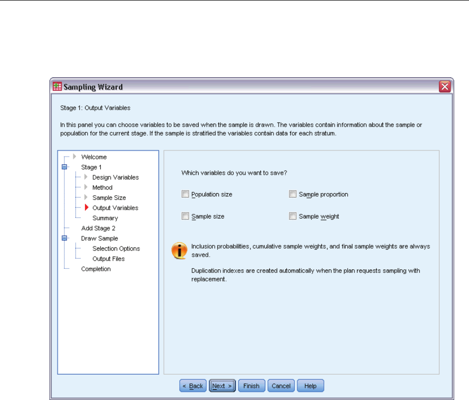
Sampling Wizard: Output Variables
Figure 2-6
Sampling Wizard, Output Variables step
This step allows you to choose variables to save when the sample is drawn.
Population size. The estimated number of units in the population for a given stage. The rootname
for the saved variable is PopulationSize_.
Sample proportion. The sampling rate at a given stage. The rootname for the saved variable is
SamplingRate_.
Sample size. The number of units drawn at a given stage. The rootname for the saved variable
is SampleSize_.
Sample weight. The inverse of the inclusion probabilities. The rootname for the saved variable is
SampleWeight_.
Some stagewise variables are generated automatically. These include:
Inclusion probabilities. The proportion of units drawn at a given stage. The rootname for the saved
variable is InclusionProbability_.
Cumulative weight. The cumulative sample weight over stages previous to and including the
current one. The rootname for the saved variable is SampleWeightCumulative_.
13
Sampling from a Complex Design
Index. Identifies units selected multiple times within a given stage. The rootname for the saved
variable is Index_.
Note: Saved variable rootnames include an integer suffixthatreflects the stage number—for
example, PopulationSize_1_ for the saved population size for stage 1.
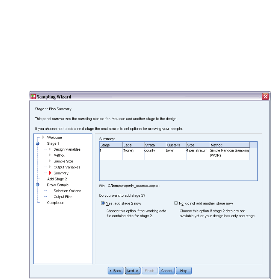
Sampling Wizard: Plan Summary
Figure 2-7
Sampling Wizard, Plan Summary step
This is the last step within each stage, providing a summary of the sample design specifications
through the current stage. From here, you can either proceed to the next stage (creating it, if
necessary) or set options for drawing the sample.
14
Chapter 2
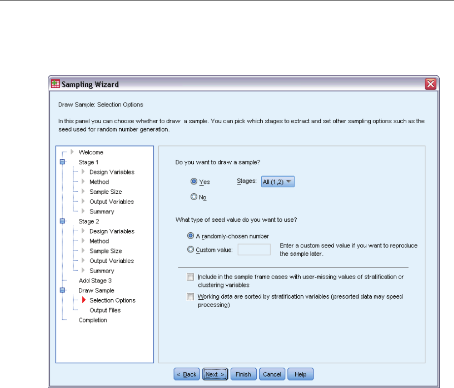
Sampling Wizard: Draw Sample Selection Options
Figure 2-8
Sampling Wizard, Draw Sample Selection Options step
This step allows you to choose whether to draw a sample. You can also control other sampling
options, such as the random seed and missing-value handling.
Draw sample. In addition to choosing whether to draw a sample, you can also choose to execute
part of the sampling design. Stages must be drawn in order—that is, stage 2 cannot be drawn
unless stage 1 is also drawn. When editing or executing a plan, you cannot resample locked stages.
Seed. This allows you to choose a seed value for random number generation.
Include user-missing values. This determines whether user-missing values are valid. If so,
user-missing values are treated as a separate category.
Data already sorted. If your sample frame is presorted by the values of the stratification variables,
this option allows you to speed the selection process.
15
Sampling from a Complex Design
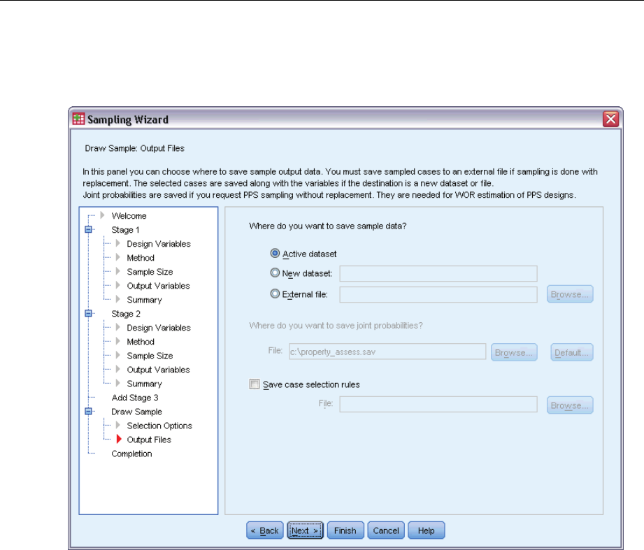
Sampling Wizard: Draw Sample Output Files
Figure 2-9
Sampling Wizard, Draw Sample Output Files step
This step allows you to choose where to direct sampled cases, weight variables, joint probabilities,
and case selection rules.
Sample data. These options let you determine where sample output is written. It can be added to
the active dataset, written to a new dataset, or saved to an external IBM® SPSS® Statistics data
file. Datasets are available during the current session but are not available in subsequent sessions
unless you explicitly save them as data files. Dataset names must adhere to variable naming rules.
If an external file or new dataset is specified, the sampling output variables and variables in the
active dataset for the selected cases are written.
Joint probabilities. These options let you determine where joint probabilities are written. They are
saved to an external SPSS Statistics data file. Joint probabilities are produced if the PPS WOR,
PPS Brewer, PPS Sampford, or PPS Murthy method is selected and WR estimation is not specified.
Case selection rules. If you are constructing your sample one stage at a time, you may want to
save the case selection rules to a text file. They are useful for constructing the subframe for
subsequent stages.
16
Chapter 2
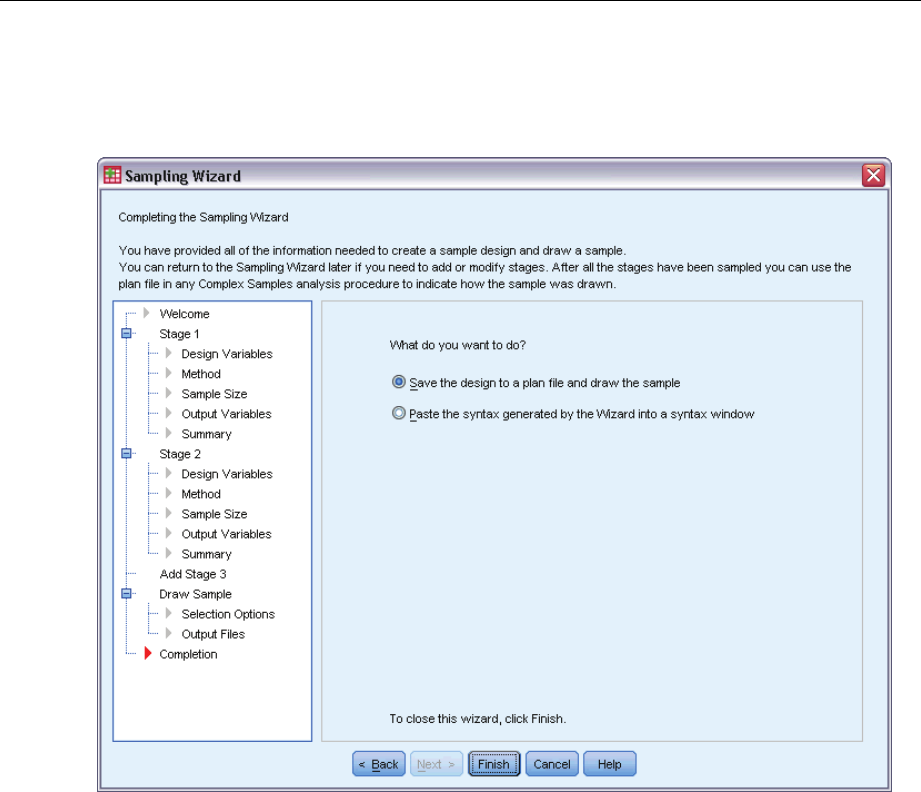
Sampling Wizard: Finish
Figure 2-10
Sampling Wizard, Finish step
This is the final step. You can save the plan file and draw the sample now or paste your selections
into a syntax window.
When making changes to stages in the existing plan file, you can save the edited plan to a
new file or overwrite the existing file. When adding stages without making changes to existing
stages, the Wizard automatically overwrites the existing plan file. If you want to save the plan
to a new file, select Paste the syntax generated by the Wizard into a syntax window and change the
filename in the syntax commands.
Modifying an Existing Sample Plan
EFrom the menus choose:
Analyze > Complex Samples > Select a Sample...
ESelect Editasampledesignand choose a plan file to edit.
EClick Next to continue through the Wizard.
17
Sampling from a Complex Design
EReviewthesamplingplaninthePlanSummarystep,andthenclickNext.
Subsequent steps are largely the same as for a new design. See the Help for individual steps
for more information.
ENavigate to the Finish step, and specify a new name for the edited plan file or choose to overwrite
the existing plan file.
Optionally, you can:
Specify stages that have already been sampled.
Remove stages from the plan.
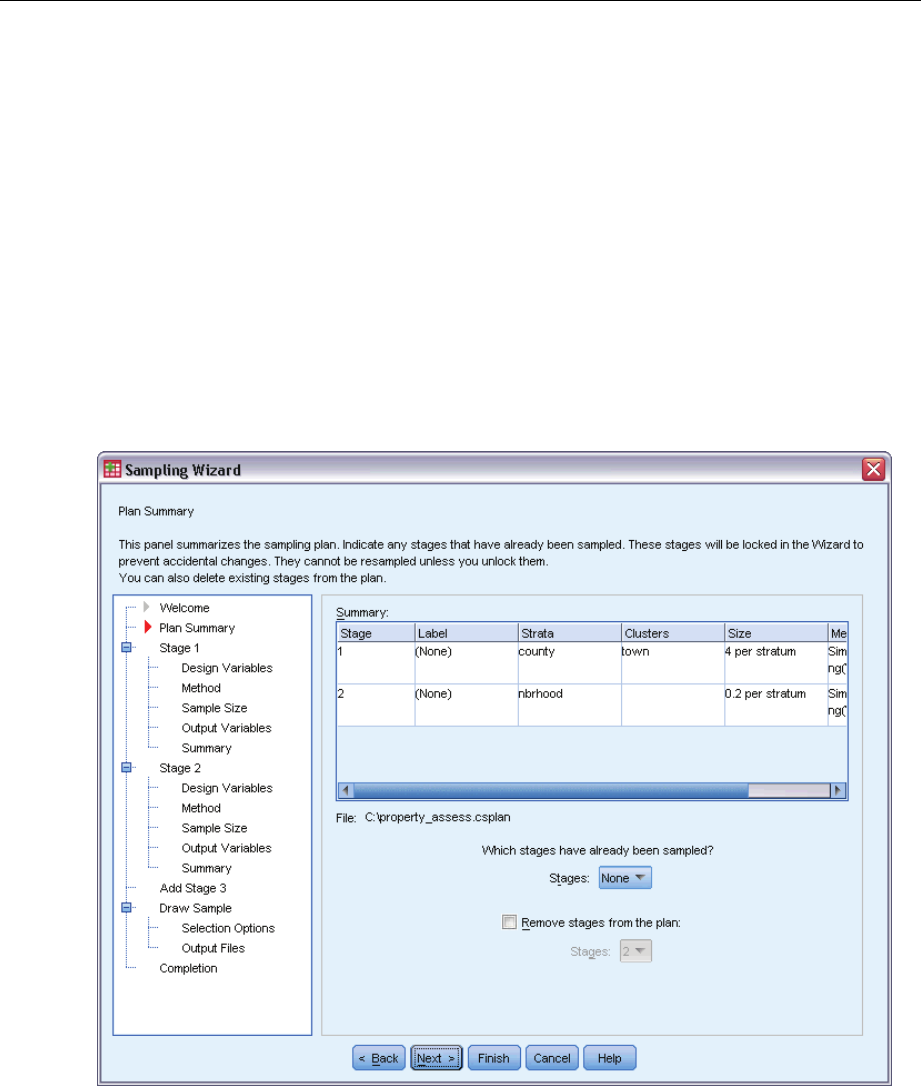
Sampling Wizard: Plan Summary
Figure 2-11
Sampling Wizard, Plan Summary step
This step allows you to review the sampling plan and indicate stages that have already been
sampled. If editing a plan, you can also remove stages from the plan.
Previously sampled stages. If an extended sampling frame is not available, you will have to execute
a multistage sampling design one stage at a time. Select which stages have already been sampled
from the drop-down list. Any stages that have been executed are locked; they are not available in
the Draw Sample Selection Options step, and they cannot be altered when editing a plan.

18
Chapter 2
Remove stages. You can remove stages 2 and 3 from a multistage design.
Running an Existing Sample Plan
EFrom the menus choose:
Analyze > Complex Samples > Select a Sample...
ESelect Draw a sample and choose a plan file to run.
EClick Next to continue through the Wizard.
EReviewthesamplingplaninthePlanSummarystep,andthenclickNext.
EThe individual steps containing stage information are skipped when executing a sample plan. You
can now go on to the Finish step at any time.
Optionally, you can specify stages that have already been sampled.
CSPLAN and CSSELECT Commands Additional Features
The command syntax language also allows you to:
Specify custom names for output variables.
Control the output in the Viewer. For example, you can suppress the stagewise summary of
the plan that is displayed if a sample is designed or modified, suppress the summary of the
distribution of sampled cases by strata that is shown if the sample design is executed, and
request a case processing summary.
Choose a subset of variables in the active dataset to write to an external sample file or to
a different dataset.
See the Command Syntax Reference for complete syntax information.
Chapter
3
Preparing a Complex Sample for
Analysis
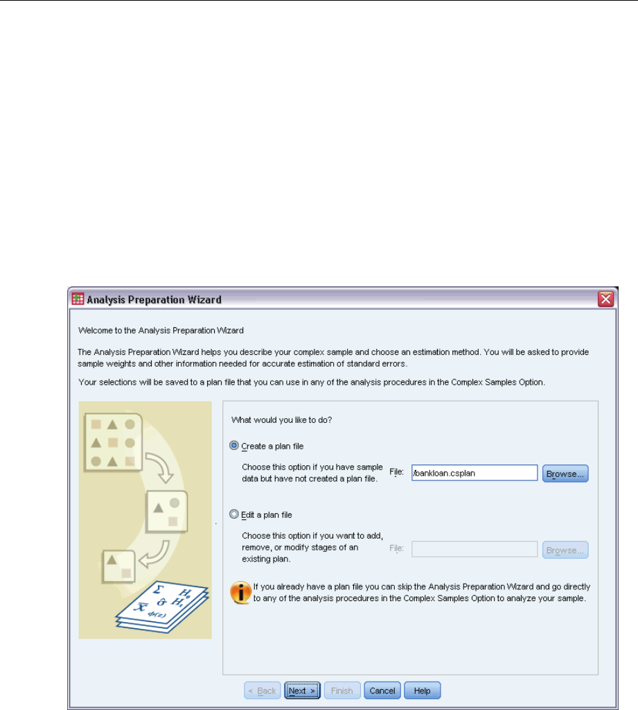
Figure 3-1
Analysis Preparation Wizard, Welcome step
The Analysis Preparation Wizard guides you through the steps for creating or modifying an
analysis plan for use with the various Complex Samples analysis procedures. Before using the
Wizard, you should have a sample drawn according to a complex design.
Creating a new plan is most useful when you do not have access to the sampling plan file used
to draw the sample (recall that the sampling plan contains a default analysis plan). If you do
have access to the sampling plan file used to draw the sample, you can use the default analysis
plan contained in the sampling plan file or override the default analysis specifications and save
your changes to a new file.
© Copyright SPSS Inc. 1989, 2010 19
20
Chapter 3
Creating a New Analysis Plan
EFrom the menus choose:
Analyze > Complex Samples > Prepare for Analysis...
ESelect Createaplanfile,andchooseaplanfilename to which you will save the analysis plan.
EClick Next to continue through the Wizard.
ESpecify the variable containing sample weights in the Design Variables step, optionally defining
strata and clusters.
EYou can now click Finish to save the plan.
Optionally, in further steps you can:
Select the method for estimating standard errors in the Estimation Method step.
Specify the number of units sampled or the inclusion probability per unit in the Size step.
Add a second or third stage to the design.
Paste your selections as command syntax.
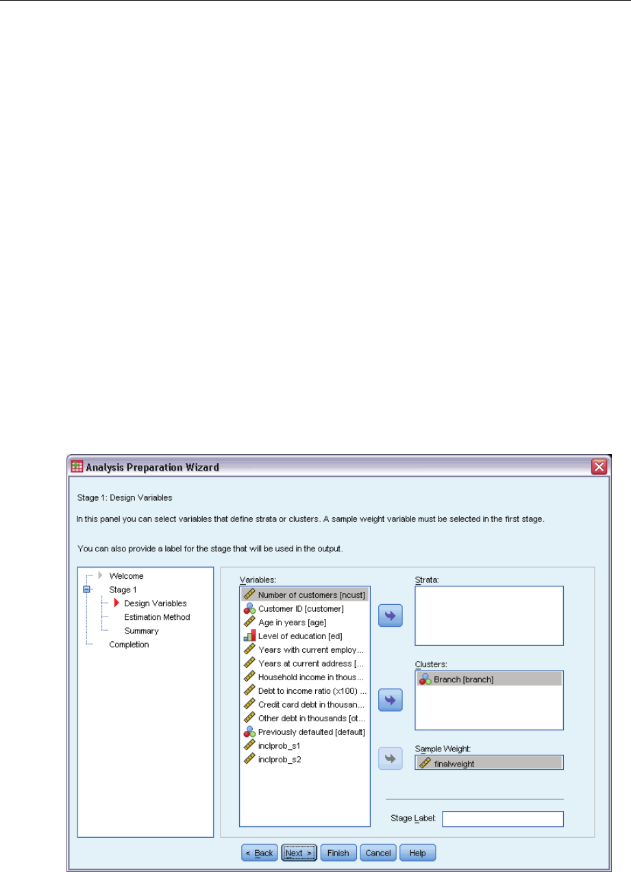
Analysis Preparation Wizard: Design Variables
Figure 3-2
Analysis Preparation Wizard, Design Variables step

21
Preparing a Complex Sample for Analysis
This step allows you to identify the stratification and clustering variables and define sample
weights. You can also provide a label for the stage.
Strata. The cross-classification of stratification variables defines distinct subpopulations, or strata.
Your total sample represents the combination of independent samples from each stratum.
Clusters. Cluster variables define groups of observational units, or clusters. Samples drawn in
multiple stages select clusters in the earlier stages and then subsample units from the selected
clusters. When analyzing a data file obtained by sampling clusters with replacement, you should
include the duplication index as a cluster variable.
Sample Weight. You must provide sample weights in the first stage. Sample weights are computed
automatically for subsequent stages of the current design.
Stage Label. Youcanspecifyanoptionalstringlabelforeachstage.Thisisusedintheoutputto
help identify stagewise information.
Note: The source variable list has the same contents across steps of the Wizard. In other words,
variables removed from the source list in a particular step are removed from the list in all steps.
Variables returned to the source list show up in all steps.
Tree Controls for Navigating the Analysis Wizard
At the left side of each step of the Analysis Wizard is an outline of all the steps. You can navigate
the Wizard by clicking on the name of an enabled step in the outline. Steps are enabled as long as
all previous steps are valid—that is, as long as each previous step has been given the minimum
required specifications for that step. For more information on why a given step may be invalid,
see the Help for individual steps.
22
Chapter 3
Analysis Preparation Wizard: Estimation Method
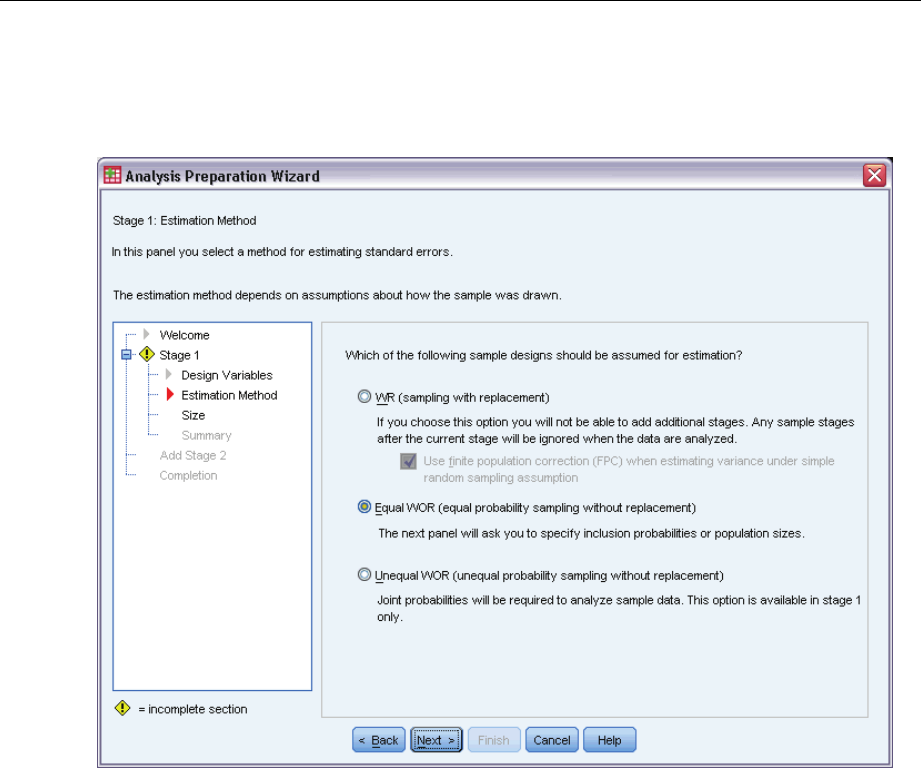
Figure 3-3
Analysis Preparation Wizard, Estimation Method step
This step allows you to specify an estimation method for the stage.
WR (sampling with replacement). WR estimation does not include a correction for sampling from a
finite population (FPC) when estimating the variance under the complex sampling design. You
can choose to include or exclude the FPC when estimating the variance under simple random
sampling (SRS).
Choosing not to include the FPC for SRS variance estimation is recommended when the
analysis weights have been scaled so that they do not add up to the population size. The SRS
variance estimate is used in computing statistics like the design effect. WR estimation can be
specified only in the final stage of a design; the Wizard will not allow you to add another stage if
you select WR estimation.
Equal WOR (equal probability sampling without replacement). Equal WOR estimation includes the
finite population correction and assumes that units are sampled with equal probability. Equal
WOR can be specified in any stage of a design.
Unequal WOR (unequal probability sampling without replacement). In addition to using the finite
population correction, Unequal WOR accounts for sampling units (usually clusters) selected with
unequal probability. This estimation method is available only in the first stage.
23
Preparing a Complex Sample for Analysis
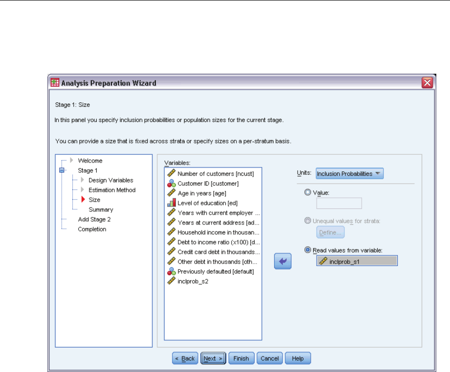
Analysis Preparation Wizard: Size
Figure 3-4
Analysis Preparation Wizard, Size step
This step is used to specify inclusion probabilities or population sizes for the current stage. Sizes
can be fixed or can vary across strata. For the purpose of specifying sizes, clusters specified in
previous stages can be used to define strata. Note that this step is necessary only when Equal
WOR is chosen as the Estimation Method.
Units. You can specify exact population sizes or the probabilities with which units were sampled.
Value. A single value is applied to all strata. If Population Sizes is selected as the unit metric,
you should enter a non-negative integer. If Inclusion Probabilities is selected, you should enter
avaluebetween 0 and 1, inclusive.
Unequal values for strata. Allows you to enter size values on a per-stratum basis via the Define
Unequal Sizes dialog box.
Read values from variable. Allows you to select a numeric variable that contains size values
for strata.
24
Chapter 3
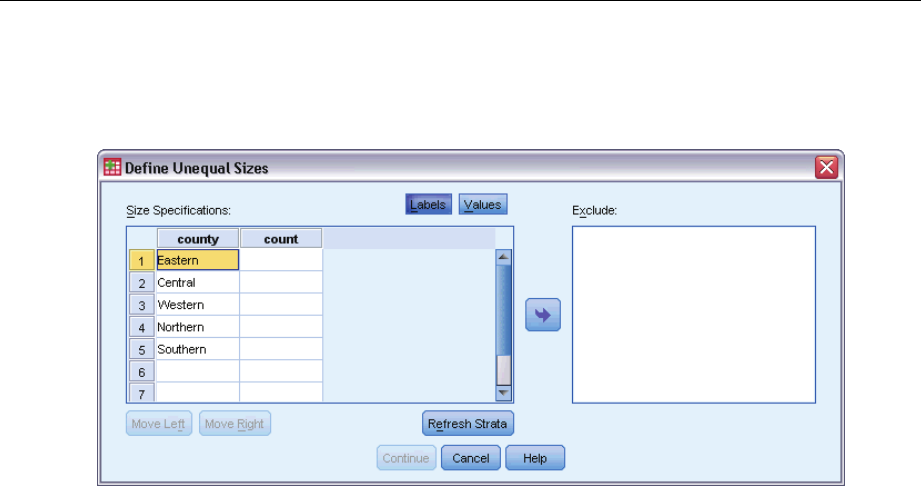
Define Unequal Sizes
Figure 3-5
Define Unequal Sizes dialog box
The Define Unequal Sizes dialog box allows you to enter sizes on a per-stratum basis.
Size Specifications grid. The grid displays the cross-classifications of up to five strata or
cluster variables—one stratum/cluster combination per row. Eligible grid variables include all
stratification variables from the current and previous stages and all cluster variables from previous
stages. Variables can be reordered within the grid or moved to the Exclude list. Enter sizes in the
rightmost column. Click Labels or Values to toggle the display of value labels and data values for
stratification and cluster variables in the grid cells. Cells that contain unlabeled values always
show values. Click Refresh Strata to repopulate the grid with each combination of labeled data
values for variables in the grid.
Exclude. To specify sizes for a subset of stratum/cluster combinations, move one or more variables
to the Exclude list. These variables are not used to define sample sizes.
25
Preparing a Complex Sample for Analysis
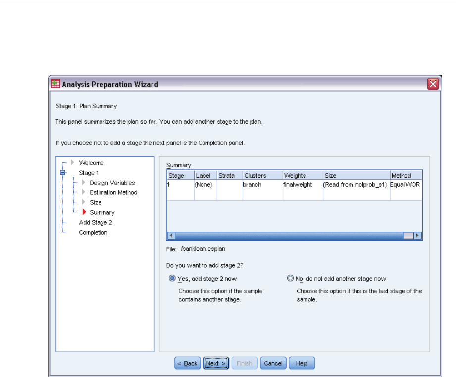
Analysis Preparation Wizard: Plan Summary
Figure 3-6
Analysis Preparation Wizard, Plan Summary step
This is the last step within each stage, providing a summary of the analysis design specifications
through the current stage. From here, you can either proceed to the next stage (creating it if
necessary) or save the analysis specifications.
If you cannot add another stage, it is likely because:
No cluster variable was specified in the Design Variables step.
You selected WR estimation in the Estimation Method step.
This is the third stage of the analysis, and the Wizard supports a maximum of three stages.
26
Chapter 3
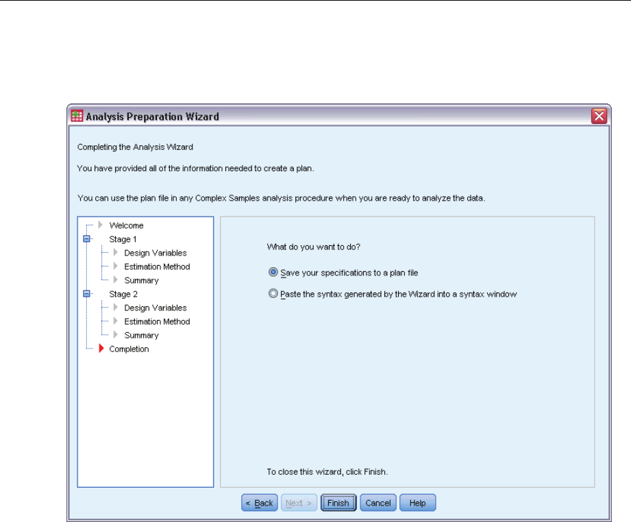
Analysis Preparation Wizard: Finish
Figure 3-7
Analysis Preparation Wizard, Finish step
This is the final step. You can save the plan file now or paste your selections to a syntax window.
When making changes to stages in the existing plan file,youcansavetheeditedplantoanew
file or overwrite the existing file. When adding stages without making changes to existing stages,
the Wizard automatically overwrites the existing plan file. If you want to save the plan to a
new file, choose to Paste the syntax generated by the Wizard into a syntax window and change the
filename in the syntax commands.
Modifying an Existing Analysis Plan
EFrom the menus choose:
Analyze > Complex Samples > Prepare for Analysis...
ESelect Edit a plan file, and choose a plan filename to which you will save the analysis plan.
EClick Next to continue through the Wizard.
27
Preparing a Complex Sample for Analysis
EReview the analysis plan in the Plan Summary step, and then click Next.
Subsequent steps are largely the same as for a new design. For more information, see the Help
for individual steps.
ENavigate to the Finish step, and specify a new name for the edited plan file, or choose to overwrite
the existing plan file.
Optionally, you can remove stages from the plan.
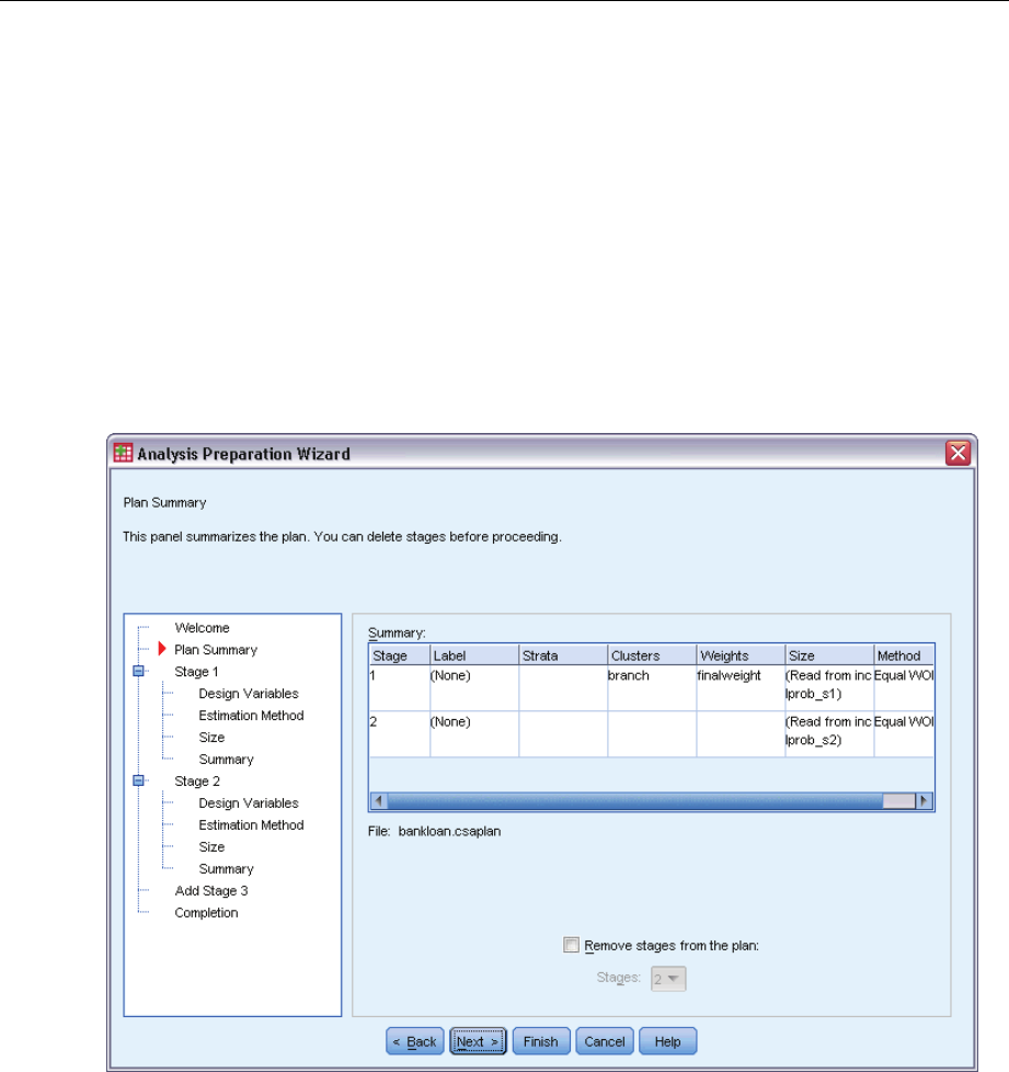
Analysis Preparation Wizard: Plan Summary
Figure 3-8
Analysis Preparation Wizard, Plan Summary step
This step allows you to review the analysis plan and remove stages from the plan.
Remove Stages. You can remove stages 2 and 3 from a multistage design. Since a plan must have
at least one stage, you can edit but not remove stage 1 from the design.
Chapter
4
Complex Samples Plan
Complex Samples analysis procedures require analysis specifications from an analysis or sample
plan file in order to provide valid results.
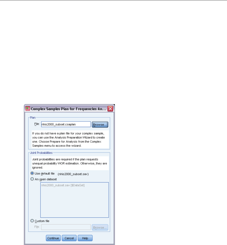
Figure 4-1
Complex Samples Plan dialog box
Plan. Specify the path of an analysis or sample plan file.
Joint Probabilities. In order to use Unequal WOR estimation for clusters drawn using a PPS WOR
method, you need to specify a separate file or an open dataset containing the joint probabilities.
This file or dataset is created by the Sampling Wizard during sampling.
© Copyright SPSS Inc. 1989, 2010 28

Chapter
5
Complex Samples Frequencies
The Complex Samples Frequencies procedure produces frequency tables for selected variables
and displays univariate statistics. Optionally, you can request statistics by subgroups, defined by
one or more categorical variables.
Example. Using the Complex Samples Frequencies procedure, you can obtain univariate tabular
statistics for vitamin usage among U.S. citizens, based on the results of the National Health
Interview Survey (NHIS) and with an appropriate analysis plan for this public-use data.
Statistics. The procedure produces estimates of cell population sizes and table percentages,
plus standard errors, confidence intervals, coefficients of variation, design effects, square roots
of design effects, cumulative values, and unweighted counts for each estimate. Additionally,
chi-square and likelihood-ratio statistics are computed for the test of equal cell proportions.
Data. Variables for which frequency tables are produced should be categorical. Subpopulation
variables can be string or numeric but should be categorical.
Assumptions. The cases in the data file represent a sample from a complex design that should
be analyzed according to the specifications in the file selected in the Complex Samples Plan
dialog box.
Obtaining Complex Samples Frequencies
EFrom the menus choose:
Analyze > Complex Samples > Frequencies...
ESelect a plan file. Optionally, select a custom joint probabilities file.
EClick Continue.
© Copyright SPSS Inc. 1989, 2010 29
30
Chapter 5
Figure 5-1
Frequencies dialog box
ESelect at least one frequency variable.
Optionally, you can specify variables to define subpopulations. Statistics are computed separately
for each subpopulation.
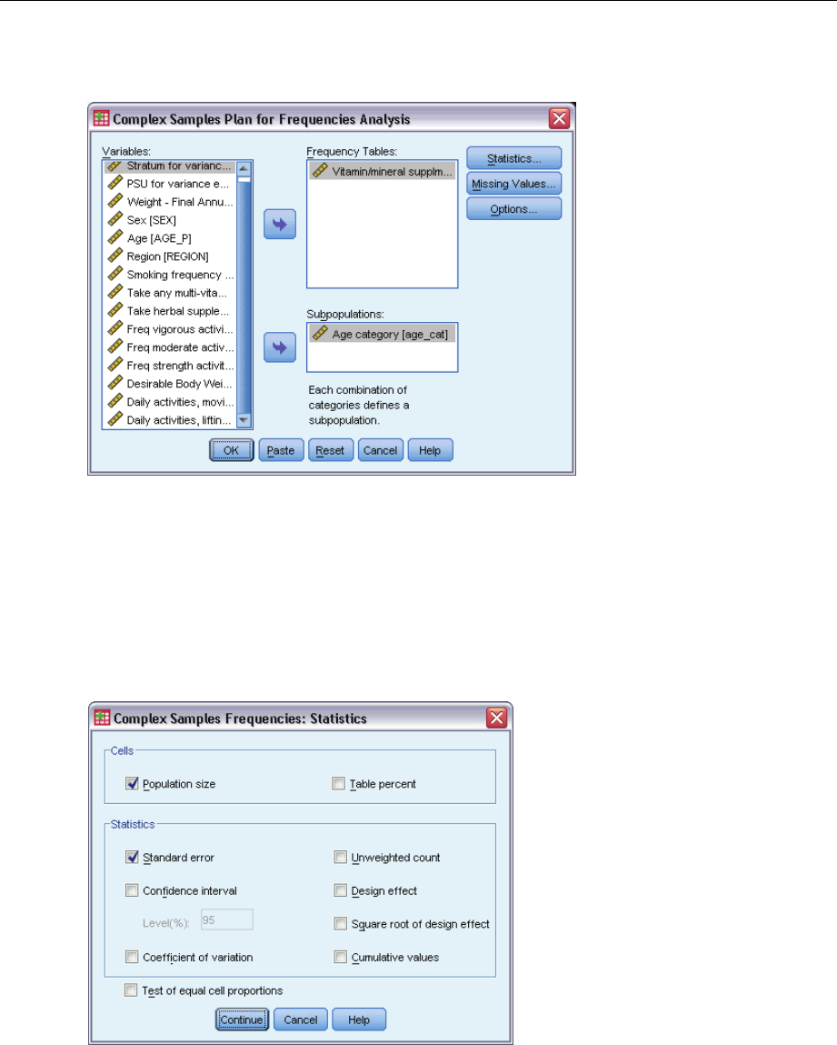
Complex Samples Frequencies Statistics
Figure 5-2
Frequencies Statistics dialog box
Cells. This group allows you to request estimates of the cell population sizes and table percentages.
Statistics. This group produces statistics associated with the population size or table percentage.
Standard error. The standard error of the estimate.
31
Complex Samples Frequencies
Confidence interval. Aconfidence interval for the estimate, using the specified level.
Coefficient of variation. The ratio of the standard error of the estimate to the estimate.
Unweighted count. The number of units used to compute the estimate.
Design effect. The ratio of the variance of the estimate to the variance obtained by assuming
that the sample is a simple random sample. This is a measure of the effect of specifying a
complex design, where values further from 1 indicate greater effects.
Square root of design effect. This is a measure of the effect of specifying a complex design,
where values further from 1 indicate greater effects.
Cumulative values. The cumulative estimate through each value of the variable.
Test of equal cell proportions. This produces chi-square and likelihood-ratio tests of the hypothesis
that the categories of a variable have equal frequencies. Separate tests are performed for each
variable.
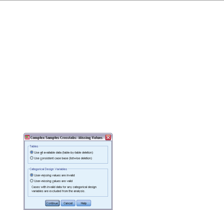
Complex Samples Missing Values
Figure 5-3
Missing Values dialog box
Tables. This group determines which cases are used in the analysis.
Use all available data. Missing values are determined on a table-by-table basis. Thus, the cases
used to compute statistics may vary across frequency or crosstabulation tables.
Use consistent case base. Missing values are determined across all variables. Thus, the cases
used to compute statistics are consistent across tables.
Categorical Design Variables. This group determines whether user-missing values are valid
or invalid.
32
Chapter 5
Complex Samples Options
Figure 5-4
Options dialog box
Subpopulation Display. You can choose to have subpopulations displayed in the same table or in
separate tables.

Chapter
6
Complex Samples Descriptives
The Complex Samples Descriptives procedure displays univariate summary statistics for several
variables. Optionally, you can request statistics by subgroups, defined by one or more categorical
variables.
Example. Using the Complex Samples Descriptives procedure, you can obtain univariate
descriptive statistics for the activity levels of U.S. citizens, based on the results of the National
Health Interview Survey (NHIS) and with an appropriate analysis plan for this public-use data.
Statistics. The procedure produces means and sums, plus ttests, standard errors, confidence
intervals, coefficients of variation, unweighted counts, population sizes, design effects, and square
roots of design effects for each estimate.
Data. Measures should be scale variables. Subpopulation variables can be string or numeric
but should be categorical.
Assumptions. The cases in the data file represent a sample from a complex design that should
be analyzed according to the specifications in the file selected in the Complex Samples Plan
dialog box.
Obtaining Complex Samples Descriptives
EFrom the menus choose:
Analyze > Complex Samples > Descriptives...
ESelect a plan file. Optionally, select a custom joint probabilities file.
EClick Continue.
© Copyright SPSS Inc. 1989, 2010 33
34
Chapter 6
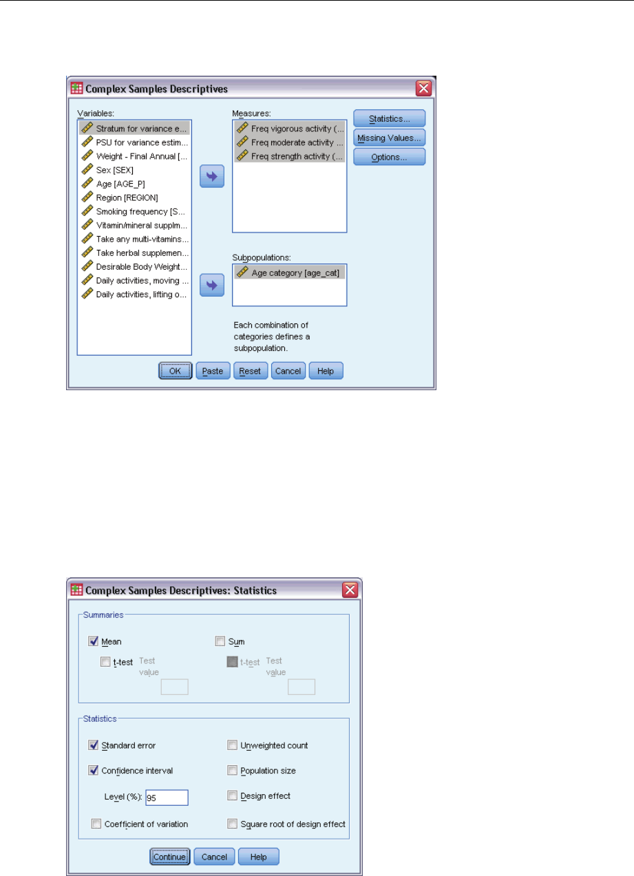
Figure 6-1
Descriptives dialog box
ESelect at least one measure variable.
Optionally, you can specify variables to define subpopulations. Statistics are computed separately
for each subpopulation.
Complex Samples Descriptives Statistics
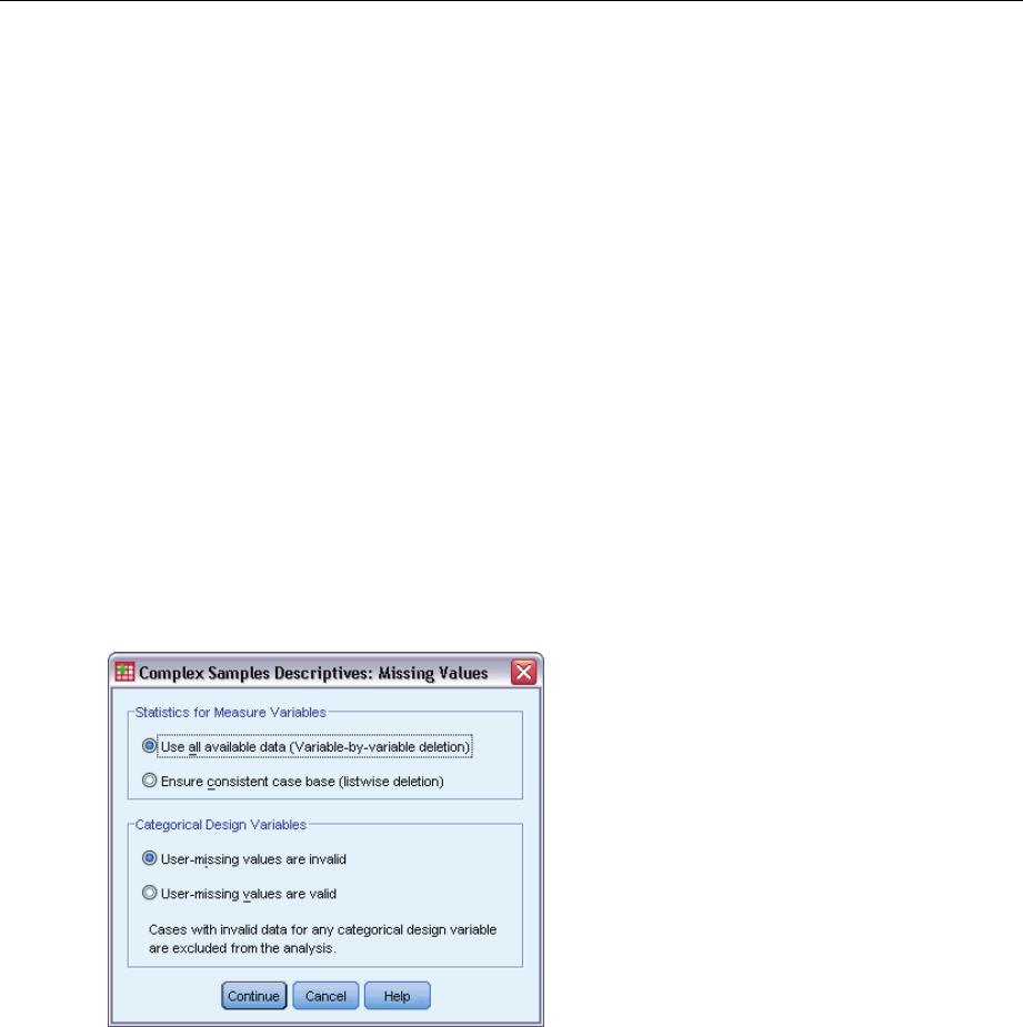
Figure 6-2
Descriptives Statistics dialog box
35
Complex Samples Descriptives
Summaries. This group allows you to request estimates of the means and sums of the measure
variables. Additionally, you can request ttests of the estimates against a specified value.
Statistics. This group produces statistics associated with the mean or sum.
Standard error. The standard error of the estimate.
Confidence interval. Aconfidence interval for the estimate, using the specified level.
Coefficient of variation. The ratio of the standard error of the estimate to the estimate.
Unweighted count. The number of units used to compute the estimate.
Population size. The estimated number of units in the population.
Design effect. The ratio of the variance of the estimate to the variance obtained by assuming
that the sample is a simple random sample. This is a measure of the effect of specifying a
complex design, where values further from 1 indicate greater effects.
Square root of design effect. This is a measure of the effect of specifying a complex design,
where values further from 1 indicate greater effects.
Complex Samples Descriptives Missing Values
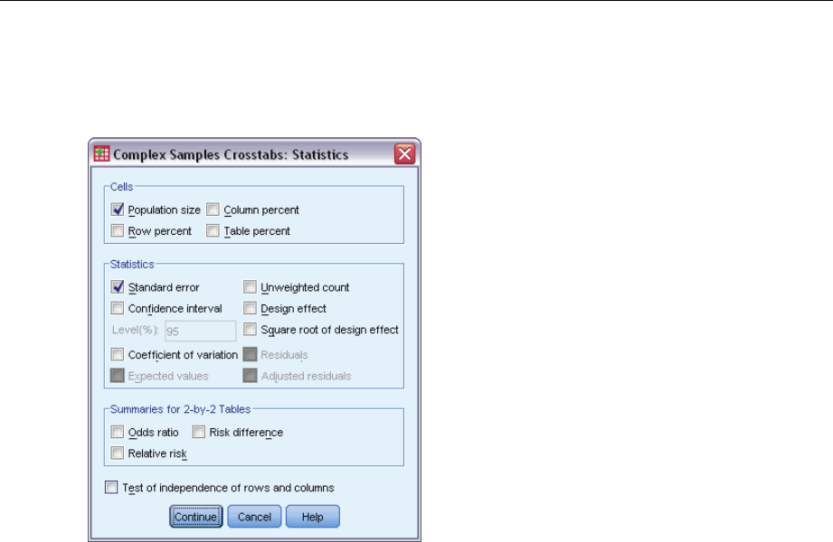
Figure 6-3
Descriptives Missing Values dialog box
Statistics for Measure Variables. This group determines which cases are used in the analysis.
Use all available data. Missing values are determined on a variable-by-variable basis, thus the
cases used to compute statistics may vary across measure variables.
Ensure consistent case base. Missing values are determined across all variables, thus the
cases used to compute statistics are consistent.
Categorical Design Variables. This group determines whether user-missing values are valid
or invalid.

36
Chapter 6
Complex Samples Options
Figure 6-4
Options dialog box
Subpopulation Display. You can choose to have subpopulations displayed in the same table or in
separate tables.

Chapter
7
Complex Samples Crosstabs
The Complex Samples Crosstabs procedure produces crosstabulation tables for pairs of selected
variables and displays two-way statistics. Optionally, you can request statistics by subgroups,
defined by one or more categorical variables.
Example. Using the Complex Samples Crosstabs procedure, you can obtain cross-classification
statistics for smoking frequency by vitamin usage of U.S. citizens, based on the results of the
National Health Interview Survey (NHIS) and with an appropriate analysis plan for this public-use
data.
Statistics. The procedure produces estimates of cell population sizes and row, column, and table
percentages, plus standard errors, confidence intervals, coefficients of variation, expected values,
design effects, square roots of design effects, residuals, adjusted residuals, and unweighted counts
for each estimate. The odds ratio, relative risk, and risk difference are computed for 2-by-2 tables.
Additionally, Pearson and likelihood-ratio statistics are computed for the test of independence of
the row and column variables.
Data. Row and column variables should be categorical. Subpopulation variables can be string or
numeric but should be categorical.
Assumptions. The cases in the data file represent a sample from a complex design that should
be analyzed according to the specifications in the file selected in the Complex Samples Plan
dialog box.
Obtaining Complex Samples Crosstabs
EFrom the menus choose:
Analyze > Complex Samples > Crosstabs...
ESelect a plan file. Optionally, select a custom joint probabilities file.
EClick Continue.
© Copyright SPSS Inc. 1989, 2010 37

38
Chapter 7
Figure 7-1
Crosstabs dialog box
ESelect at least one row variable and one column variable.
Optionally, you can specify variables to define subpopulations. Statistics are computed separately
for each subpopulation.
39
Complex Samples Crosstabs
Complex Samples Crosstabs Statistics
Figure 7-2
Crosstabs Statistics dialog box
Cells. This group allows you to request estimates of the cell population size and row, column,
and table percentages.
Statistics. This group produces statistics associated with the population size and row, column,
and table percentages.
Standard error. The standard error of the estimate.
Confidence interval. Aconfidence interval for the estimate, using the specified level.
Coefficient of variation. The ratio of the standard error of the estimate to the estimate.
Expected values. The expected value of the estimate, under the hypothesis of independence
of the row and column variable.
Unweighted count. The number of units used to compute the estimate.
Design effect. The ratio of the variance of the estimate to the variance obtained by assuming
that the sample is a simple random sample. This is a measure of the effect of specifying a
complex design, where values further from 1 indicate greater effects.
Square root of design effect. This is a measure of the effect of specifying a complex design,
where values further from 1 indicate greater effects.
Residuals. The expected value is the number of cases that you would expect in the cell if there
were no relationship between the two variables. A positive residual indicates that there are
more cases in the cell than there would be if the row and column variables were independent.
Adjusted residuals. The residual for a cell (observed minus expected value) divided by an
estimate of its standard error. The resulting standardized residual is expressed in standard
deviation units above or below the mean.

40
Chapter 7
Summaries for 2-by-2 Tables. This group produces statistics for tables in which the row and column
variable each have two categories. Each is a measure of the strength of the association between
the presence of a factor and the occurrence of an event.
Odds ratio. The odds ratio can be used as an estimate of relative risk when the occurrence
of the factor is rare.
Relative risk. The ratio of the risk of an event in the presence of the factor to the risk of the
event in the absence of the factor.
Risk difference. The difference between the risk of an event in the presence of the factor and
the risk of the event in the absence of the factor.
Test of independence of rows and columns. This produces chi-square and likelihood-ratio tests of
the hypothesis that a row and column variable are independent. Separate tests are performed
for each pair of variables.
Complex Samples Missing Values
Figure 7-3
Missing Values dialog box
Tables. This group determines which cases are used in the analysis.
Use all available data. Missing values are determined on a table-by-table basis. Thus, the cases
used to compute statistics may vary across frequency or crosstabulation tables.
Use consistent case base. Missing values are determined across all variables. Thus, the cases
used to compute statistics are consistent across tables.
Categorical Design Variables. This group determines whether user-missing values are valid
or invalid.

41
Complex Samples Crosstabs
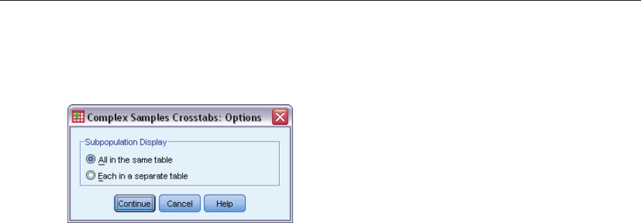
Complex Samples Options
Figure 7-4
Options dialog box
Subpopulation Display. You can choose to have subpopulations displayed in the same table or in
separate tables.

Chapter
8
Complex Samples Ratios
The Complex Samples Ratios procedure displays univariate summary statistics for ratios of
variables. Optionally, you can request statistics by subgroups, defined by one or more categorical
variables.
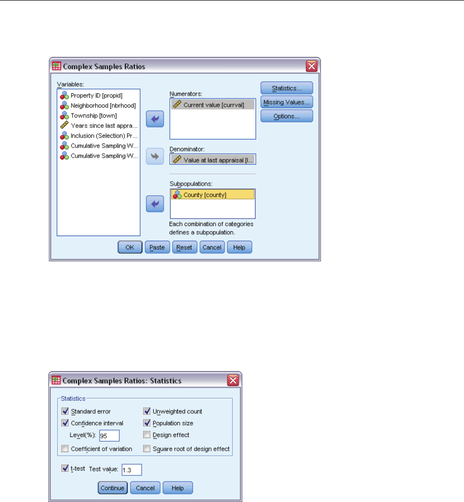
Example. Using the Complex Samples Ratios procedure, you can obtain descriptive statistics for
the ratio of current property value to last assessed value, based on the results of a statewide survey
carried out according to a complex design and with an appropriate analysis plan for the data.
Statistics. The procedure produces ratio estimates, ttests, standard errors, confidence intervals,
coefficients of variation, unweighted counts, population sizes, design effects, and square roots of
design effects.
Data. Numerators and denominators should be positive-valued scale variables. Subpopulation
variables can be string or numeric but should be categorical.
Assumptions. The cases in the data file represent a sample from a complex design that should
be analyzed according to the specifications in the file selected in the Complex Samples Plan
dialog box.
Obtaining Complex Samples Ratios
EFrom the menus choose:
Analyze > Complex Samples > Ratios...
ESelect a plan file. Optionally, select a custom joint probabilities file.
EClick Continue.
© Copyright SPSS Inc. 1989, 2010 42
43
Complex Samples Ratios
Figure 8-1
Ratios dialog box
ESelect at least one numerator variable and denominator variable.
Optionally, you can specify variables to define subgroups for which statistics are produced.
Complex Samples Ratios Statistics
Figure 8-2
Ratios Statistics dialog box
Statistics. This group produces statistics associated with the ratio estimate.
Standard error. The standard error of the estimate.
Confidence interval. Aconfidence interval for the estimate, using the specified level.
Coefficient of variation. The ratio of the standard error of the estimate to the estimate.
Unweighted count. The number of units used to compute the estimate.
Population size. The estimated number of units in the population.
44
Chapter 8
Design effect. The ratio of the variance of the estimate to the variance obtained by assuming
that the sample is a simple random sample. This is a measure of the effect of specifying a
complex design, where values further from 1 indicate greater effects.
Square root of design effect. This is a measure of the effect of specifying a complex design,
where values further from 1 indicate greater effects.
Ttest. You can request ttests of the estimates against a specified value.
Complex Samples Ratios Missing Values
Figure 8-3
Ratios Missing Values dialog box
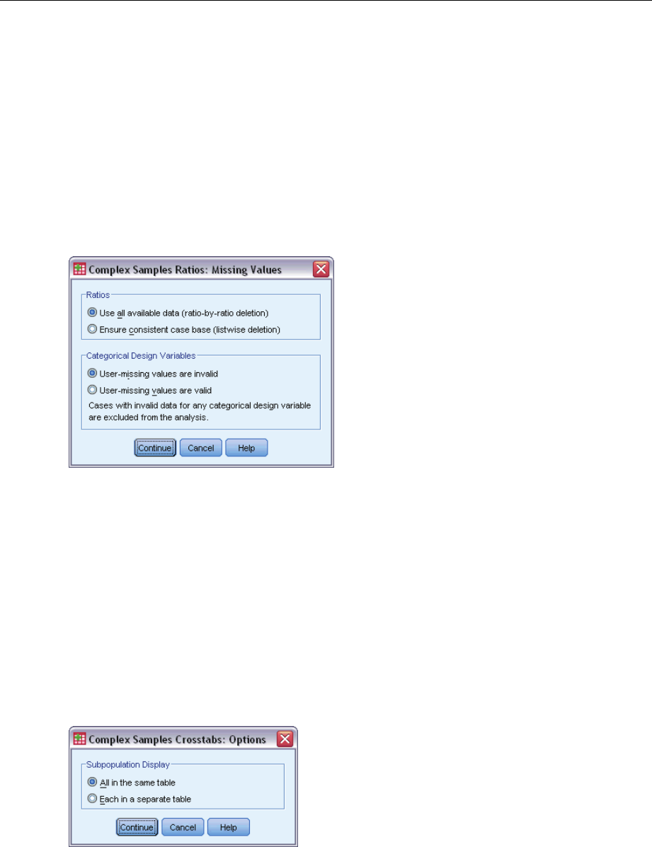
Ratios. This group determines which cases are used in the analysis.
Use all available data. Missing values are determined on a ratio-by-ratio basis. Thus, the cases
used to compute statistics may vary across numerator-denominator pairs.
Ensure consistent case base. Missing values are determined across all variables. Thus, the
cases used to compute statistics are consistent.
Categorical Design Variables. This group determines whether user-missing values are valid
or invalid.
Complex Samples Options
Figure 8-4
Options dialog box
Subpopulation Display. You can choose to have subpopulations displayed in the same table or in
separate tables.

Chapter
9
Complex Samples General Linear
Model
The Complex Samples General Linear Model (CSGLM) procedure performs linear regression
analysis, as well as analysis of variance and covariance, for samples drawn by complex sampling
methods. Optionally, you can request analyses for a subpopulation.
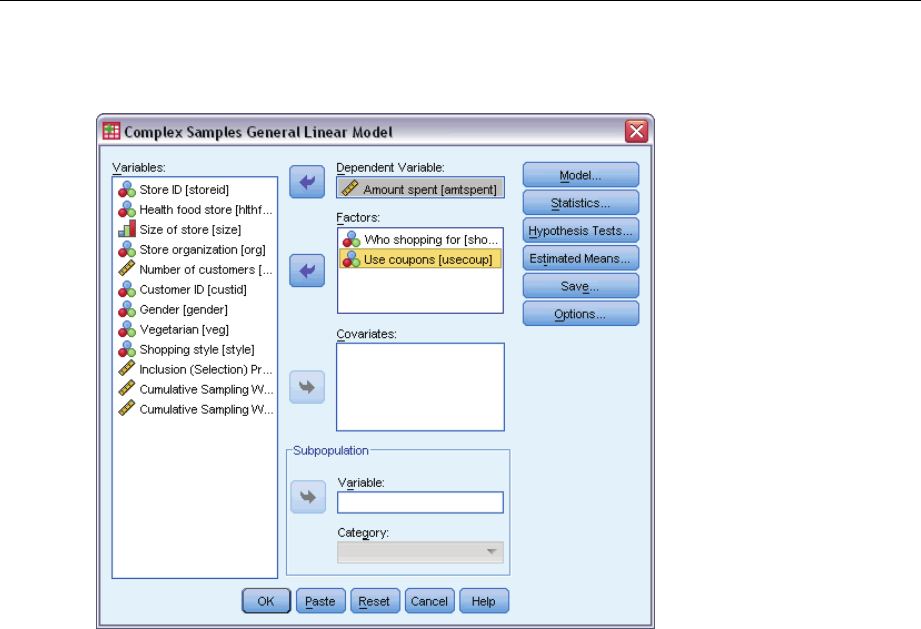
Example. A grocery store chain surveyed a set of customers concerning their purchasing habits,
according to a complex design. Given the survey results and how much each customer spent in the
previous month, the store wants to see if the frequency with which customers shop is related to
the amount they spend in a month, controlling for the gender of the customer and incorporating
the sampling design.
Statistics. The procedure produces estimates, standard errors, confidence intervals, ttests, design
effects, and square roots of design effects for model parameters, as well as the correlations and
covariances between parameter estimates. Measures of model fit and descriptive statistics for the
dependent and independent variables are also available. Additionally, you can request estimated
marginal means for levels of model factors and factor interactions.
Data. The dependent variable is quantitative. Factors are categorical. Covariates are quantitative
variables that are related to the dependent variable. Subpopulation variables can be string or
numeric but should be categorical.
Assumptions. The cases in the data file represent a sample from a complex design that should
be analyzed according to the specifications in the file selected in the Complex Samples Plan
dialog box.
Obtaining a Complex Samples General Linear Model
From the menus choose:
Analyze > Complex Samples > General Linear Model...
ESelect a plan file. Optionally, select a custom joint probabilities file.
EClick Continue.
© Copyright SPSS Inc. 1989, 2010 45
46
Chapter 9
Figure 9-1
General Linear Model dialog box
ESelect a dependent variable.
Optionally, you can:
Select variables for factors and covariates, as appropriate for your data.
Specify a variable to define a subpopulation. The analysis is performed only for the selected
category of the subpopulation variable.
47
Complex Samples General Linear Model
Figure 9-2
Model dialog box
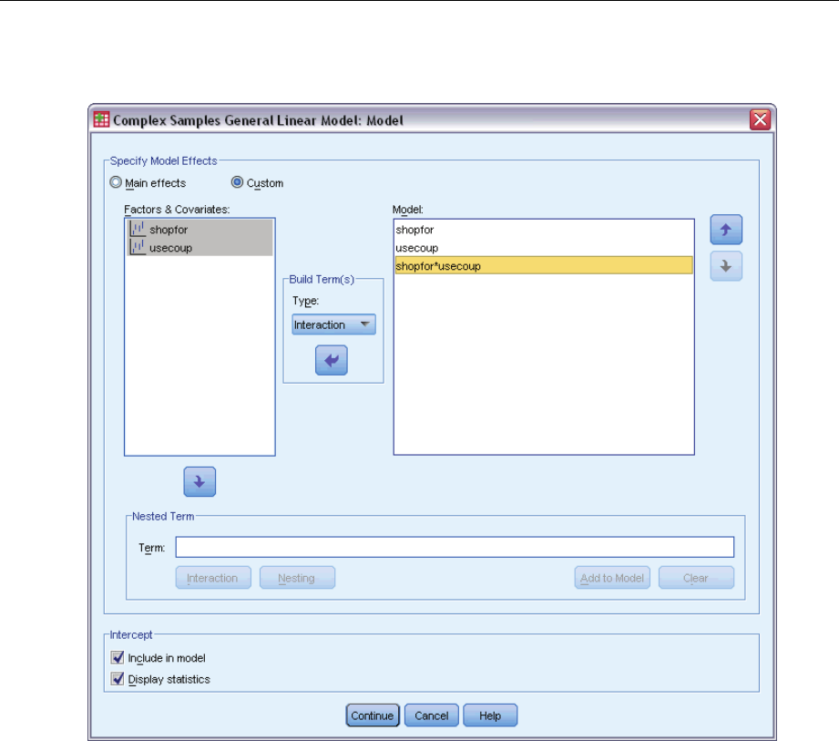
Specify Model Effects. By default, the procedure builds a main-effects model using the factors
and covariates specified in the main dialog box. Alternatively, you can build a custom model that
includes interaction effects and nested terms.
Non-Nested Terms
For the selected factors and covariates:
Interaction. Creates the highest-level interaction term for all selected variables.
Main effects. Creates a main-effects term for each variable selected.
All 2-way. Creates all possible two-way interactions of the selected variables.
All 3-way. Creates all possible three-way interactions of the selected variables.
All 4-way. Creates all possible four-way interactions of the selected variables.
All 5-way. Creates all possible five-way interactions of the selected variables.
48
Chapter 9
Nested Terms
You can build nested terms for your model in this procedure. Nested terms are useful for modeling
the effect of a factor or covariate whose values do not interact with the levels of another factor.
For example, a grocery store chain may follow the spending habits of its customers at several store
locations. Since each customer frequents only one of these locations, the Customer effect can be
said to be nested within the Store location effect.
Additionally, you can include interaction effects, such as polynomial terms involving the same
covariate, or add multiple levels of nesting to the nested term.
Limitations. Nested terms have the following restrictions:
All factors within an interaction must be unique. Thus, if Ais a factor, then specifying A*A
is invalid.
All factors within a nested effect must be unique. Thus, if Ais a factor, then specifying A(A)
is invalid.
No effect can be nested within a covariate. Thus, if Ais a factor and Xis a covariate, then
specifying A(X) is invalid.
Intercept. The intercept is usually included in the model. If you can assume the data pass through
the origin, you can exclude the intercept. Even if you include the intercept in the model, you
can choose to suppress statistics related to it.
Complex Samples General Linear Model Statistics
Figure 9-3
General Linear Model Statistics dialog box
Model Parameters. This group allows you to control the display of statistics related to the model
parameters.
Estimate. Displays estimates of the coefficients.
Standard error. Displays the standard error for each coefficient estimate.
Confidence interval. Displays a confidence interval for each coefficient estimate. The
confidence level for the interval is set in the Options dialog box.
Ttest. Displays a ttest of each coefficient estimate. The null hypothesis for each test is that
thevalueofthecoefficient is 0.
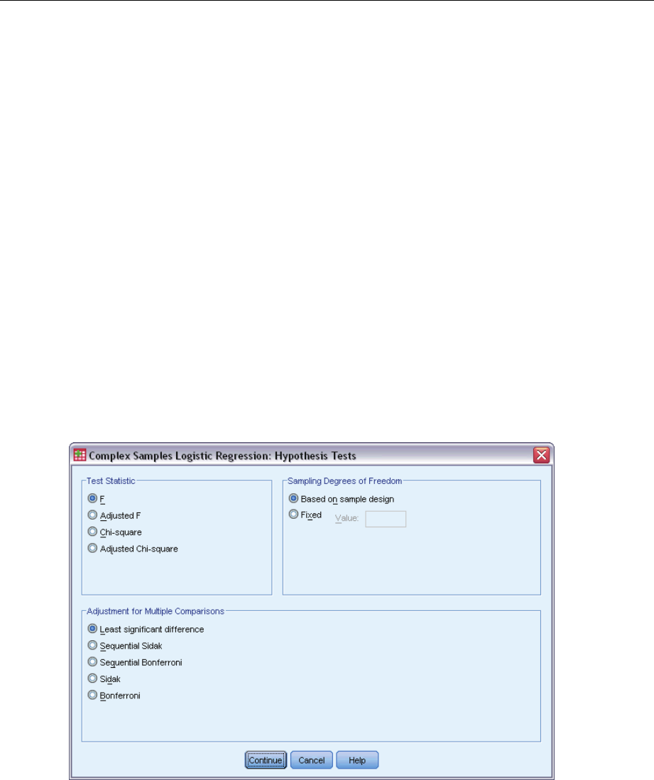
49
Complex Samples General Linear Model
Covariances of parameter estimates. Displays an estimate of the covariance matrix for the
model coefficients.
Correlations of parameter estimates. Displays an estimate of the correlation matrix for the
model coefficients.
Design effect. The ratio of the variance of the estimate to the variance obtained by assuming
that the sample is a simple random sample. This is a measure of the effect of specifying a
complex design, where values further from 1 indicate greater effects.
Square root of design effect. This is a measure of the effect of specifying a complex design,
where values further from 1 indicate greater effects.
Model fit. Displays R2and root mean squared error statistics.
Population means of dependent variable and covariates. Displays summary information about the
dependent variable, covariates, and factors.
Sample design information. Displays summary information about the sample, including the
unweighted count and the population size.
Complex Samples Hypothesis Tests
Figure 9-4
Hypothesis Tests dialog box
Test Statistic. This group allows you to select the type of statistic used for testing hypotheses. You
can choose between F,adjustedF, chi-square, and adjusted chi-square.
Sampling Degrees of Freedom. This group gives you control over the sampling design degrees of
freedomusedtocomputepvalues for all test statistics. If based on the sampling design, the value
is the difference between the number of primary sampling units and the number of strata in the
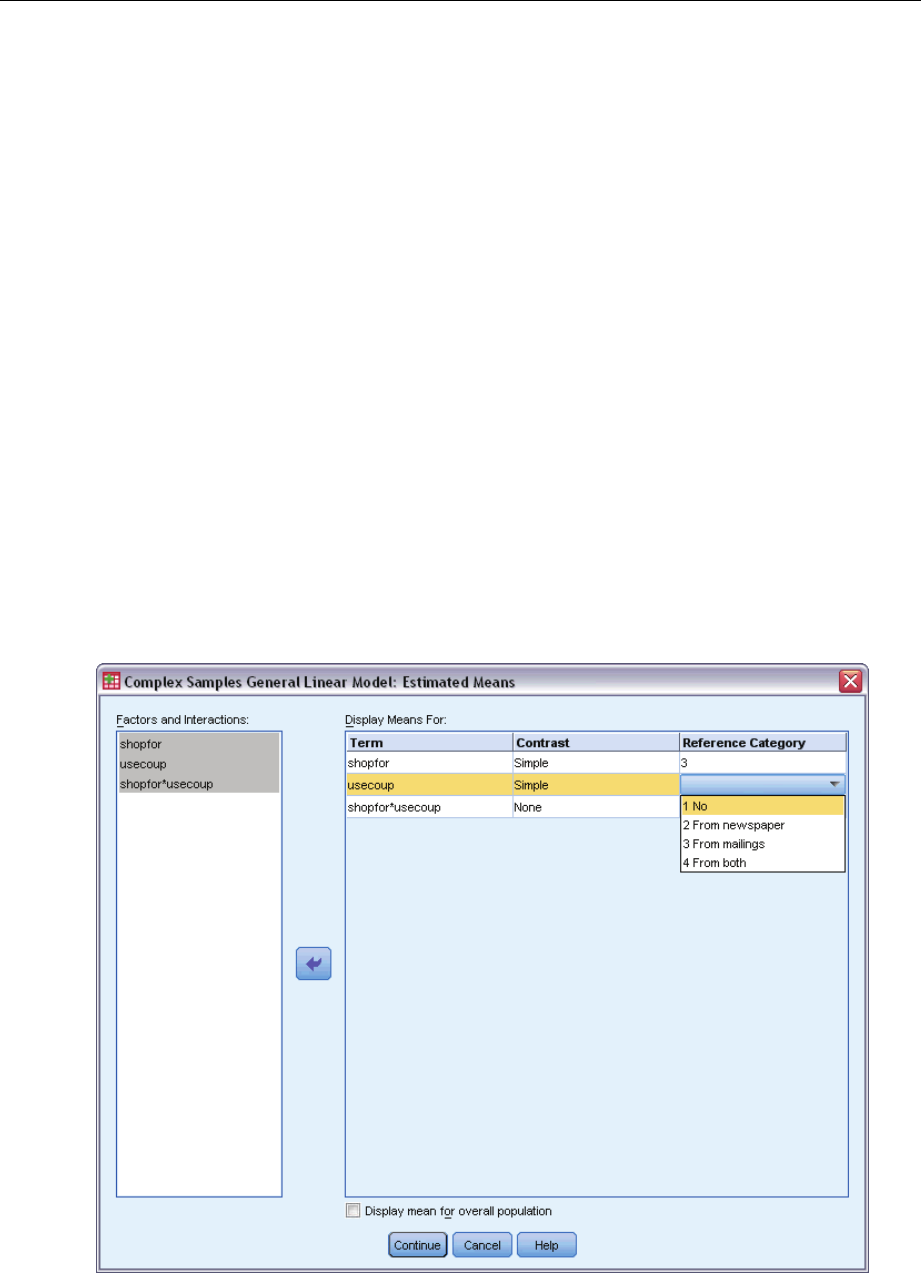
50
Chapter 9
first stage of sampling. Alternatively, you can set a custom degrees of freedom by specifying a
positive integer.
Adjustment for Multiple Comparisons. When performing hypothesis tests with multiple contrasts,
the overall significance level can be adjusted from the significance levels for the included
contrasts. This group allows you to choose the adjustment method.
Least significant difference. This method does not control the overall probability of rejecting
the hypotheses that some linear contrasts are different from the null hypothesis values.
Sequential Sidak. This is a sequentially step-down rejective Sidak procedure that is much
less conservative in terms of rejecting individual hypotheses but maintains the same overall
significance level.
Sequential Bonferroni. This is a sequentially step-down rejective Bonferroni procedure that is
much less conservative in terms of rejecting individual hypotheses but maintains the same
overall significance level.
Sidak. This method provides tighter bounds than the Bonferroni approach.
Bonferroni. This method adjusts the observed significance level for the fact that multiple
contrasts are being tested.
Complex Samples General Linear Model Estimated Means
Figure 9-5
General Linear Model Estimated Means dialog box
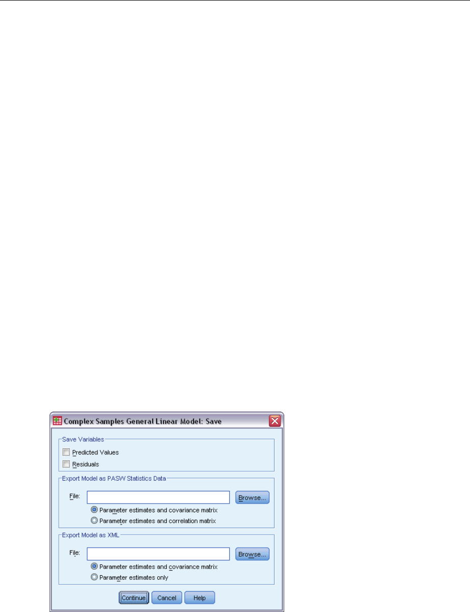
51
Complex Samples General Linear Model
The Estimated Means dialog box allows you to display the model-estimated marginal means for
levels of factors and factor interactions specified in the Model subdialog box. You can also request
that the overall population mean be displayed.
Term. Estimated means are computed for the selected factors and factor interactions.
Contrast. The contrast determines how hypothesis tests are set up to compare the estimated means.
Simple. Compares the mean of each level to the mean of a specified level. This type of contrast
is useful when there is a control group.
Deviation. Compares the mean of each level (except a reference category) to the mean of all of
the levels (grand mean). The levels of the factor can be in any order.
Difference. Compares the mean of each level (except the first) to the mean of previous levels.
They are sometimes called reverse Helmert contrasts.
Helmert. Compares the mean of each level of the factor (except the last) to the mean of
subsequent levels.
Repeated. Compares the mean of each level (except the last) to the mean of the subsequent
level.
Polynomial. Compares the linear effect, quadratic effect, cubic effect, and so on. The
first degree of freedom contains the linear effect across all categories; the second degree
of freedom, the quadratic effect; and so on. These contrasts are often used to estimate
polynomial trends.
Reference Category. The simple and deviation contrasts require a reference category or factor
level against which the others are compared.
Complex Samples General Linear Model Save
Figure 9-6
General Linear Model Save dialog box
Save Variables. This group allows you to save the model predicted values and residuals as new
variables in the working file.
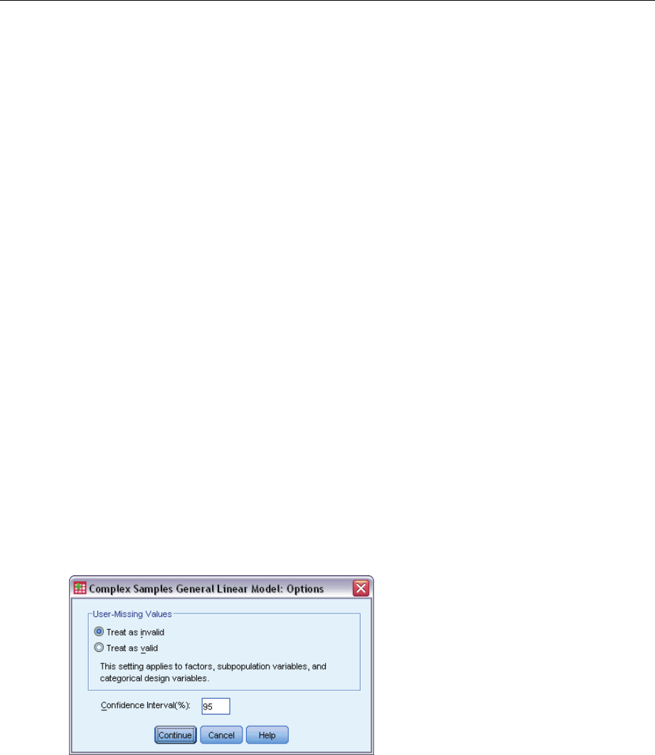
52
Chapter 9
Export model as SPSS Statistics data. Writes a dataset in IBM® SPSS® Statistics format containing
the parameter correlation or covariance matrix with parameter estimates, standard errors,
significance values, and degrees of freedom. The order of variables in the matrix file is as follows.
rowtype_. Takes values (and value labels), COV (Covariances), CORR (Correlations), EST
(Parameter estimates), SE (Standard errors), SIG (Significance levels), and DF (Sampling
design degrees of freedom). There is a separate case with row type COV (or CORR) for each
model parameter, plus a separate case for each of the other row types.
varname_. Takes values P1, P2, ..., corresponding to an ordered list of all model parameters,
for row types COV or CORR, with value labels corresponding to the parameter strings shown
in the parameter estimates table. The cells are blank for other row types.
P1, P2, ... These variables correspond to an ordered list of all model parameters, with variable
labels corresponding to the parameter strings shown in the parameter estimates table, and
take values according to the row type. For redundant parameters, all covariances are set
to zero; correlations are set to the system-missing value; all parameter estimates are set at
zero; and all standard errors, significance levels, and residual degrees of freedom are set to
the system-missing value.
Note:Thisfile is not immediately usable for further analyses in other procedures that read a matrix
file unless those procedures accept all the row types exported here.
Export Model as XML. Saves the parameter estimates and the parameter covariance matrix, if
selected, in XML (PMML) format. You can use this model file to apply the model information to
other data files for scoring purposes.
Complex Samples General Linear Model Options
Figure 9-7
General Linear Model Options dialog box
User-Missing Values. All design variables, as well as the dependent variable and any covariates,
must have valid data. Cases with invalid data for any of these variables are deleted from the
analysis. These controls allow you to decide whether user-missing values are treated as valid
among the strata, cluster, subpopulation, and factor variables.
Confidence Interval. This is the confidence interval level for coefficient estimates and estimated
marginal means. Specify a value greater than or equal to 50 and less than 100.

53
Complex Samples General Linear Model
CSGLM Command Additional Features
The command syntax language also allows you to:
Specify custom tests of effects versus a linear combination of effects or a value (using the
CUSTOM subcommand).
Fix covariates at values other than their means when computing estimated marginal means
(using the EMMEANS subcommand).
Specify a metric for polynomial contrasts (using the EMMEANS subcommand).
Specify a tolerance value for checking singularity (using the CRITERIA subcommand).
Create user-specified names for saved variables (using the SAVE subcommand).
Produce a general estimable function table (using the PRINT subcommand).
See the Command Syntax Reference for complete syntax information.

Chapter
10
Complex Samples Logistic Regression
The Complex Samples Logistic Regression procedure performs logistic regression analysis on
a binary or multinomial dependent variable for samples drawn by complex sampling methods.
Optionally, you can request analyses for a subpopulation.
Example. Aloanofficer has collected past records of customers given loans at several different
branches, according to a complex design. While incorporating the sample design, the officer
wants to see if the probability with which a customer defaults is related to age, employment
history, and amount of credit debt.
Statistics. The procedure produces estimates, exponentiated estimates, standard errors, confidence
intervals, ttests, design effects, and square roots of design effects for model parameters, as well as
the correlations and covariances between parameter estimates. Pseudo R2statistics, classification
tables, and descriptive statistics for the dependent and independent variables are also available.
Data. The dependent variable is categorical. Factors are categorical. Covariates are quantitative
variables that are related to the dependent variable. Subpopulation variables can be string or
numeric but should be categorical.
Assumptions. The cases in the data file represent a sample from a complex design that should
be analyzed according to the specifications in the file selected in the Complex Samples Plan
dialog box.
Obtaining Complex Samples Logistic Regression
From the menus choose:
Analyze > Complex Samples > Logistic Regression...
ESelect a plan file. Optionally, select a custom joint probabilities file.
EClick Continue.
© Copyright SPSS Inc. 1989, 2010 54
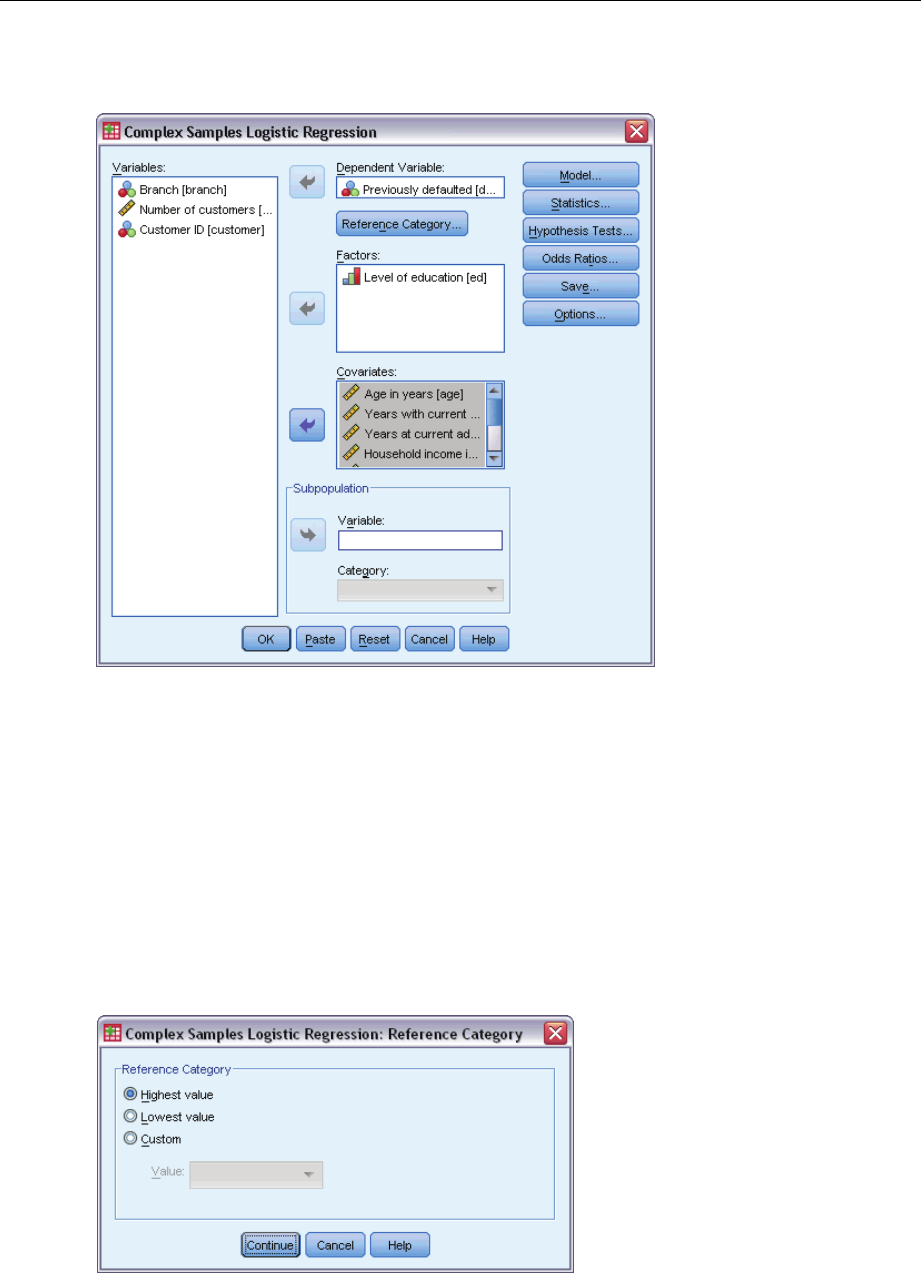
55
Complex Samples Logistic Regression
Figure 10-1
Logistic Regression dialog box
ESelect a dependent variable.
Optionally, you can:
Select variables for factors and covariates, as appropriate for your data.
Specify a variable to define a subpopulation. The analysis is performed only for the selected
category of the subpopulation variable.
Complex Samples Logistic Regression Reference Category
Figure 10-2
Logistic Regression Reference Category dialog box
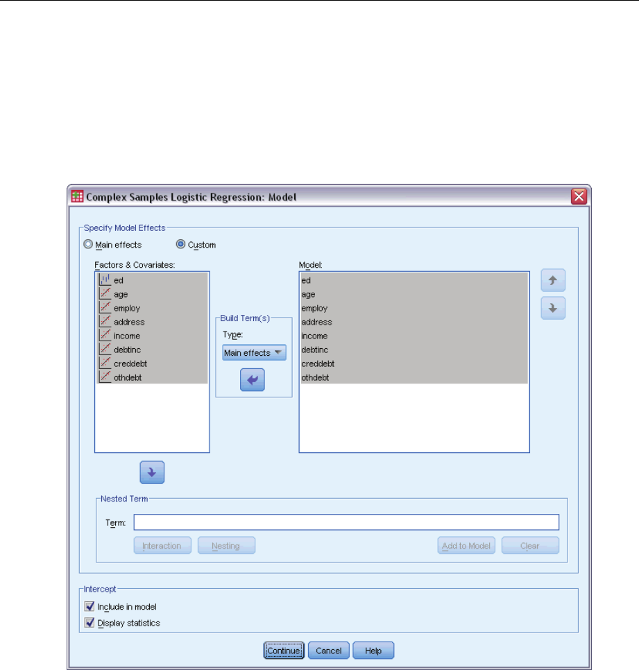
56
Chapter 10
By default, the Complex Samples Logistic Regression procedure makes the highest-valued
category the reference category. This dialog box allows you to specify the highest value, the
lowest value, or a custom category as the reference category.
Complex Samples Logistic Regression Model
Figure 10-3
Logistic Regression Model dialog box
Specify Model Effects. By default, the procedure builds a main-effects model using the factors
and covariates specified in the main dialog box. Alternatively, you can build a custom model that
includes interaction effects and nested terms.
Non-Nested Terms
For the selected factors and covariates:
Interaction. Creates the highest-level interaction term for all selected variables.
Main effects. Creates a main-effects term for each variable selected.
All 2-way. Creates all possible two-way interactions of the selected variables.
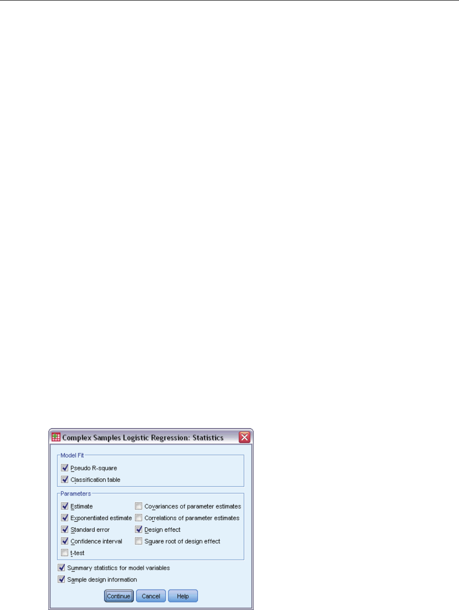
57
Complex Samples Logistic Regression
All 3-way. Creates all possible three-way interactions of the selected variables.
All 4-way. Creates all possible four-way interactions of the selected variables.
All 5-way. Creates all possible five-way interactions of the selected variables.
Nested Terms
You can build nested terms for your model in this procedure. Nested terms are useful for modeling
the effect of a factor or covariate whose values do not interact with the levels of another factor.
For example, a grocery store chain may follow the spending habits of its customers at several store
locations. Since each customer frequents only one of these locations, the Customer effect can be
said to be nested within the Store location effect.
Additionally, you can include interaction effects, such as polynomial terms involving the same
covariate, or add multiple levels of nesting to the nested term.
Limitations. Nested terms have the following restrictions:
All factors within an interaction must be unique. Thus, if Ais a factor, then specifying A*A
is invalid.
All factors within a nested effect must be unique. Thus, if Ais a factor, then specifying A(A)
is invalid.
No effect can be nested within a covariate. Thus, if Ais a factor and Xis a covariate, then
specifying A(X) is invalid.
Intercept. The intercept is usually included in the model. If you can assume the data pass through
the origin, you can exclude the intercept. Even if you include the intercept in the model, you
can choose to suppress statistics related to it.
Complex Samples Logistic Regression Statistics
Figure 10-4
Logistic Regression Statistics dialog box
Model Fit. Controls the display of statistics that measure the overall model performance.

58
Chapter 10
Pseudo R-square. The R2statistic from linear regression does not have an exact counterpart
among logistic regression models. There are, instead, multiple measures that attempt to mimic
the properties of the R2statistic.
Classification table. Displays the tabulated cross-classifications of the observed category by
the model-predicted category on the dependent variable.
Parameters. This group allows you to control the display of statistics related to the model
parameters.
Estimate. Displays estimates of the coefficients.
Exponentiated estimate. Displays the base of the natural logarithm raised to the power of the
estimates of the coefficients. While the estimate has nice properties for statistical testing, the
exponentiated estimate, or exp(B), is easier to interpret.
Standard error. Displays the standard error for each coefficient estimate.
Confidence interval. Displays a confidence interval for each coefficient estimate. The
confidence level for the interval is set in the Options dialog box.
Ttest. Displays a ttest of each coefficient estimate. The null hypothesis for each test is that
thevalueofthecoefficient is 0.
Covariances of parameter estimates. Displays an estimate of the covariance matrix for the
model coefficients.
Correlations of parameter estimates. Displays an estimate of the correlation matrix for the
model coefficients.
Design effect. The ratio of the variance of the estimate to the variance obtained by assuming
that the sample is a simple random sample. This is a measure of the effect of specifying a
complex design, where values further from 1 indicate greater effects.
Square root of design effect. This is a measure of the effect of specifying a complex design,
where values further from 1 indicate greater effects.
Summary statistics for model variables. Displays summary information about the dependent
variable, covariates, and factors.
Sample design information. Displays summary information about the sample, including the
unweighted count and the population size.
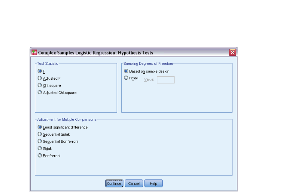
59
Complex Samples Logistic Regression
Complex Samples Hypothesis Tests
Figure 10-5
Hypothesis Tests dialog box
Test Statistic. This group allows you to select the type of statistic used for testing hypotheses. You
can choose between F,adjustedF, chi-square, and adjusted chi-square.
Sampling Degrees of Freedom. This group gives you control over the sampling design degrees of
freedomusedtocomputepvalues for all test statistics. If based on the sampling design, the value
is the difference between the number of primary sampling units and the number of strata in the
first stage of sampling. Alternatively, you can set a custom degrees of freedom by specifying a
positive integer.
Adjustment for Multiple Comparisons. When performing hypothesis tests with multiple contrasts,
the overall significance level can be adjusted from the significance levels for the included
contrasts. This group allows you to choose the adjustment method.
Least significant difference. This method does not control the overall probability of rejecting
the hypotheses that some linear contrasts are different from the null hypothesis values.
Sequential Sidak. This is a sequentially step-down rejective Sidak procedure that is much
less conservative in terms of rejecting individual hypotheses but maintains the same overall
significance level.
Sequential Bonferroni. This is a sequentially step-down rejective Bonferroni procedure that is
much less conservative in terms of rejecting individual hypotheses but maintains the same
overall significance level.
Sidak. This method provides tighter bounds than the Bonferroni approach.
Bonferroni. This method adjusts the observed significance level for the fact that multiple
contrasts are being tested.
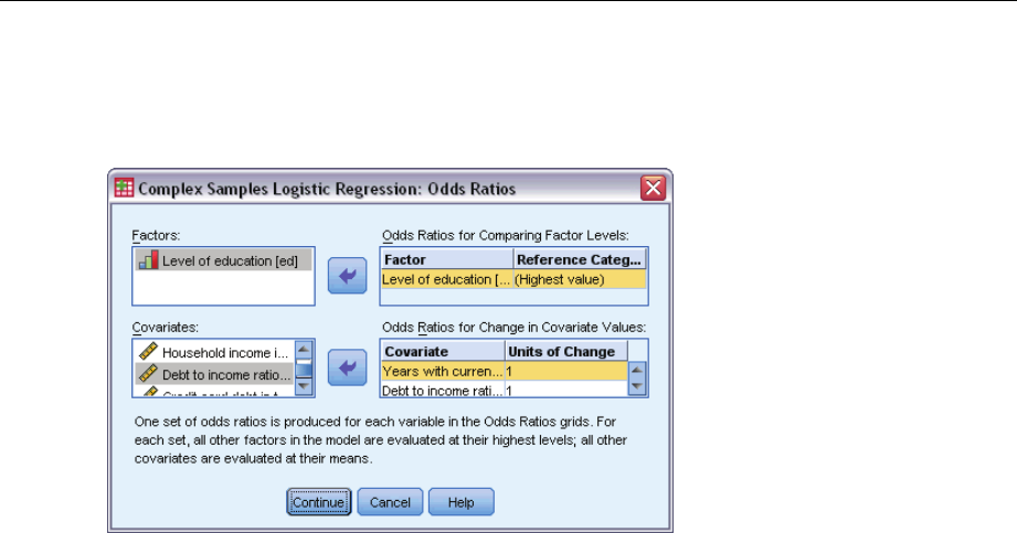
60
Chapter 10
Complex Samples Logistic Regression Odds Ratios
Figure 10-6
Logistic Regression Odds Ratios dialog box
The Odds Ratios dialog box allows you to display the model-estimated odds ratios for specified
factors and covariates. A separate set of odds ratios is computed for each category of the
dependent variable except the reference category.
Factors. For each selected factor, displays the ratio of the odds at each category of the factor to
the odds at the specified reference category.
Covariates. For each selected covariate, displays the ratio of the odds at the covariate’s mean value
plus the specified units of change to the odds at the mean.
When computing odds ratios for a factor or covariate, the procedure fixes all other factors at their
highest levels and all other covariates at their means. If a factor or covariate interacts with other
predictors in the model, then the odds ratios depend not only on the change in the specified
variable but also on the values of the variables with which it interacts. If a specified covariate
interacts with itself in the model (for example, age*age), then the odds ratios depend on both the
change in the covariate and the value of the covariate.
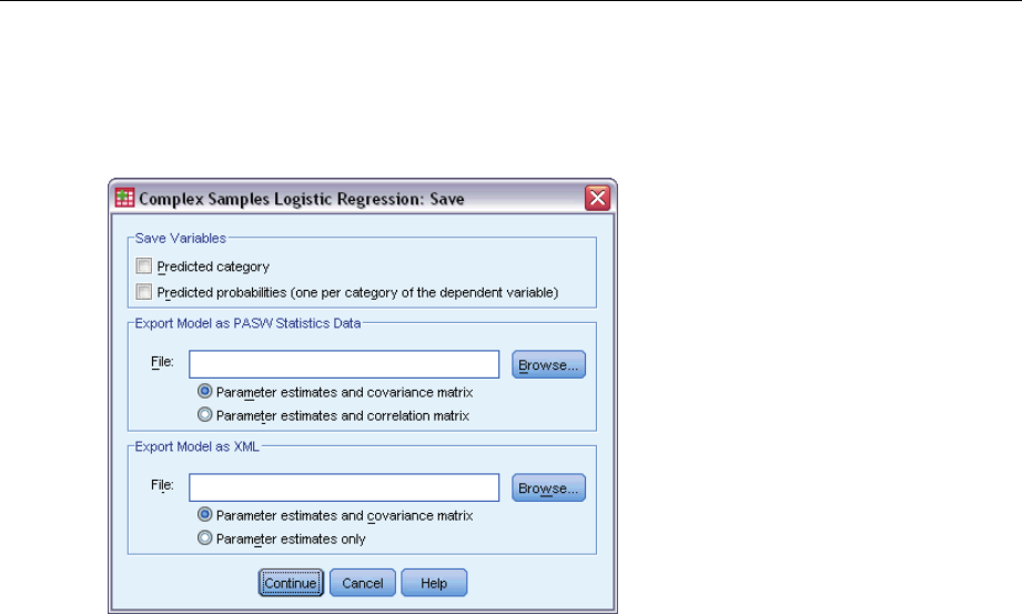
61
Complex Samples Logistic Regression
Complex Samples Logistic Regression Save
Figure 10-7
Logistic Regression Save dialog box
Save Variables. This group allows you to save the model-predicted category and predicted
probabilities as new variables in the active dataset.
Export model as SPSS Statistics data. Writes a dataset in IBM® SPSS® Statistics format containing
the parameter correlation or covariance matrix with parameter estimates, standard errors,
significance values, and degrees of freedom. The order of variables in the matrix file is as follows.
rowtype_. Takes values (and value labels), COV (Covariances), CORR (Correlations), EST
(Parameter estimates), SE (Standard errors), SIG (Significance levels), and DF (Sampling
design degrees of freedom). There is a separate case with row type COV (or CORR) for each
model parameter, plus a separate case for each of the other row types.
varname_. Takes values P1, P2, ..., corresponding to an ordered list of all model parameters,
for row types COV or CORR, with value labels corresponding to the parameter strings shown
in the parameter estimates table. The cells are blank for other row types.
P1, P2, ... These variables correspond to an ordered list of all model parameters, with variable
labels corresponding to the parameter strings shown in the parameter estimates table, and
take values according to the row type. For redundant parameters, all covariances are set
to zero; correlations are set to the system-missing value; all parameter estimates are set at
zero; and all standard errors, significance levels, and residual degrees of freedom are set to
the system-missing value.
Note:Thisfile is not immediately usable for further analyses in other procedures that read a matrix
file unless those procedures accept all the row types exported here.
Export Model as XML. Saves the parameter estimates and the parameter covariance matrix, if
selected, in XML (PMML) format. You can use this model file to apply the model information to
other data files for scoring purposes.
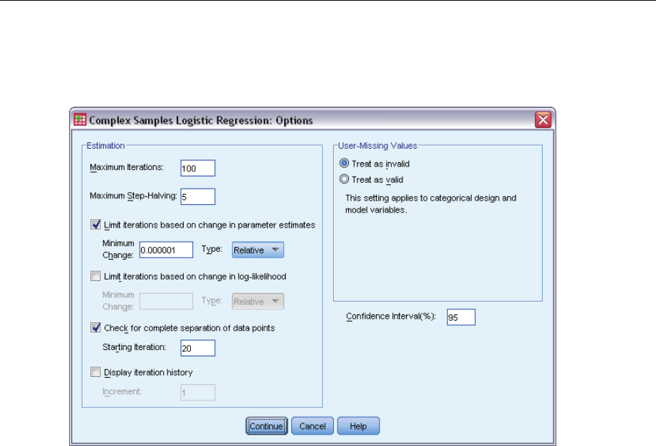
62
Chapter 10
Complex Samples Logistic Regression Options
Figure 10-8
Logistic Regression Options dialog box
Estimation. This group gives you control of various criteria used in the model estimation.
Maximum Iterations. The maximum number of iterations the algorithm will execute. Specify a
non-negative integer.
Maximum Step-Halving. At each iteration, the step size is reduced by a factor of 0.5 until the
log-likelihood increases or maximum step-halving is reached. Specify a positive integer.
Limit iterations based on change in parameter estimates. When selected, the algorithm stops
after an iteration in which the absolute or relative change in the parameter estimates is less
than the value specified, which must be non-negative.
Limit iterations based on change in log-likelihood. When selected, the algorithm stops after an
iteration in which the absolute or relative change in the log-likelihood function is less than the
value specified, which must be non-negative.
Check for complete separation of data points. When selected, the algorithm performs tests to
ensure that the parameter estimates have unique values. Separation occurs when the procedure
can produce a model that correctly classifies every case.
Display iteration history. Displays parameter estimates and statistics at every niterations
beginning with the 0th iteration (the initial estimates). If you choose to print the iteration
history, the last iteration is always printed regardless of the value of n.
User-Missing Values. All design variables, as well as the dependent variable and any covariates,
must have valid data. Cases with invalid data for any of these variables are deleted from the
analysis. These controls allow you to decide whether user-missing values are treated as valid
among the strata, cluster, subpopulation, and factor variables.

63
Complex Samples Logistic Regression
Confidence Interval. This is the confidence interval level for coefficient estimates, exponentiated
coefficient estimates, and odds ratios. Specify a value greater than or equal to 50 and less than 100.
CSLOGISTIC Command Additional Features
The command syntax language also allows you to:
Specify custom tests of effects versus a linear combination of effects or a value (using the
CUSTOM subcommand).
Fix values of other model variables when computing odds ratios for factors and covariates
(using the ODDSRATIOS subcommand).
Specify a tolerance value for checking singularity (using the CRITERIA subcommand).
Create user-specified names for saved variables (using the SAVE subcommand).
Produce a general estimable function table (using the PRINT subcommand).
See the Command Syntax Reference for complete syntax information.

Chapter
11
Complex Samples Ordinal Regression
The Complex Samples Ordinal Regression procedure performs regression analysis on a binary
or ordinal dependent variable for samples drawn by complex sampling methods. Optionally,
you can request analyses for a subpopulation.
Example. Representatives considering a bill before the legislature are interested in whether there
is public support for the bill and how support for the bill is related to voter demographics.
Pollsters design and conduct interviews accordingtoacomplexsamplingdesign.UsingComplex
Samples Ordinal Regression, you can fit a model for the level of support for the bill based upon
voter demographics.
Data. The dependent variable is ordinal. Factors are categorical. Covariates are quantitative
variables that are related to the dependent variable. Subpopulation variables can be string or
numeric but should be categorical.
Assumptions. The cases in the data file represent a sample from a complex design that should
be analyzed according to the specifications in the file selected in the Complex Samples Plan
dialog box.
Obtaining Complex Samples Ordinal Regression
From the menus choose:
Analyze > Complex Samples > Ordinal Regression...
ESelect a plan file. Optionally, select a custom joint probabilities file.
EClick Continue.
© Copyright SPSS Inc. 1989, 2010 64
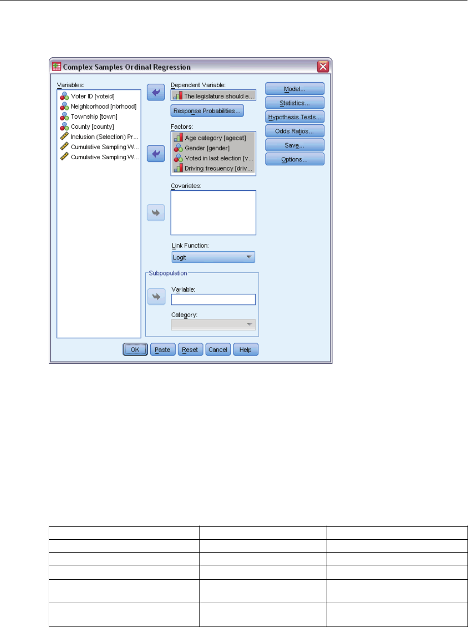
65
Complex Samples Ordinal Regression
Figure 11-1
Ordinal Regression dialog box
ESelect a dependent variable.
Optionally, you can:
Select variables for factors and covariates, as appropriate for your data.
Specify a variable to define a subpopulation. The analysis is performed only for the selected
category of the subpopulation variable, although variances are still properly estimated based
on the entire dataset.
Select a link function.
Link function. The link function is a transformation of the cumulative probabilities that allows
estimation of the model. Five link functions are available, summarized in the following table.
Function Form Typical application
Logit log( ξ/(1−ξ) ) Evenly distributed categories
Complementary log-log log(−log(1−ξ)) Higher categories more probable
Negative log-log −log(−log(ξ)) Lower categories more probable
Probit Φ−1(ξ) Latent variable is normally
distributed
Cauchit (inverse Cauchy) tan(π(ξ−0.5)) Latent variable has many extreme
values
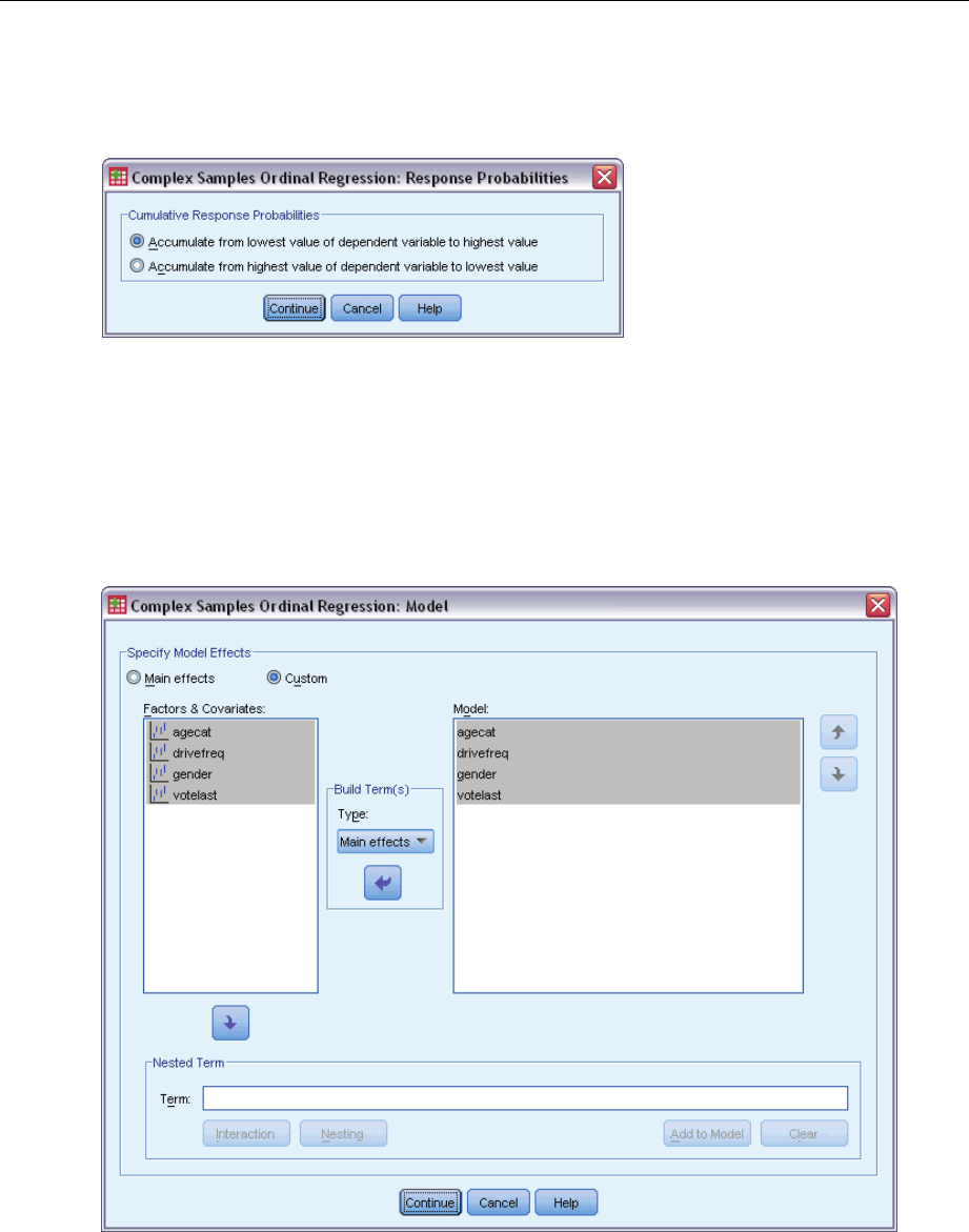
66
Chapter 11
Complex Samples Ordinal Regression Response Probabilities
Figure 11-2
Ordinal Regression Response Probabilities dialog box
The Response Probabilities dialog box allows you to specify whether the cumulative probability
of a response (that is, the probability of belonging up to and including a particular category of the
dependent variable) increases with increasing or decreasing values of the dependent variable.
Complex Samples Ordinal Regression Model
Figure 11-3
Ordinal Regression Model dialog box
Specify Model Effects. By default, the procedure builds a main-effects model using the factors
and covariates specified in the main dialog box. Alternatively, you can build a custom model that
includes interaction effects and nested terms.

67
Complex Samples Ordinal Regression
Non-Nested Terms
For the selected factors and covariates:
Interaction. Creates the highest-level interaction term for all selected variables.
Main effects. Creates a main-effects term for each variable selected.
All 2-way. Creates all possible two-way interactions of the selected variables.
All 3-way. Creates all possible three-way interactions of the selected variables.
All 4-way. Creates all possible four-way interactions of the selected variables.
All 5-way. Creates all possible five-way interactions of the selected variables.
Nested Terms
You can build nested terms for your model in this procedure. Nested terms are useful for modeling
the effect of a factor or covariate whose values do not interact with the levels of another factor.
For example, a grocery store chain may follow the spending habits of its customers at several store
locations. Since each customer frequents only one of these locations, the Customer effect can be
said to be nested within the Store location effect.
Additionally, you can include interaction effects, such as polynomial terms involving the same
covariate, or add multiple levels of nesting to the nested term.
Limitations. Nested terms have the following restrictions:
All factors within an interaction must be unique. Thus, if Ais a factor, then specifying A*A
is invalid.
All factors within a nested effect must be unique. Thus, if Ais a factor, then specifying A(A)
is invalid.
No effect can be nested within a covariate. Thus, if Ais a factor and Xis a covariate, then
specifying A(X) is invalid.
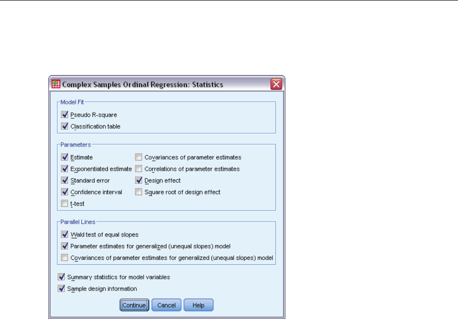
68
Chapter 11
Complex Samples Ordinal Regression Statistics
Figure 11-4
Ordinal Regression Statistics dialog box
Model Fit. Controls the display of statistics that measure the overall model performance.
Pseudo R-square. The R2statistic from linear regression does not have an exact counterpart
among ordinal regression models. There are, instead, multiple measures that attempt to mimic
the properties of the R2statistic.
Classification table. Displays the tabulated cross-classifications of the observed category by
the model-predicted category on the dependent variable.
Parameters. This group allows you to control the display of statistics related to the model
parameters.
Estimate. Displays estimates of the coefficients.
Exponentiated estimate. Displays the base of the natural logarithm raised to the power of the
estimates of the coefficients. While the estimate has nice properties for statistical testing, the
exponentiated estimate, or exp(B), is easier to interpret.
Standard error. Displays the standard error for each coefficient estimate.
Confidence interval. Displays a confidence interval for each coefficient estimate. The
confidence level for the interval is set in the Options dialog box.
Ttest. Displays a ttest of each coefficient estimate. The null hypothesis for each test is that
thevalueofthecoefficient is 0.
Covariances of parameter estimates. Displays an estimate of the covariance matrix for the
model coefficients.
Correlations of parameter estimates. Displays an estimate of the correlation matrix for the
model coefficients.
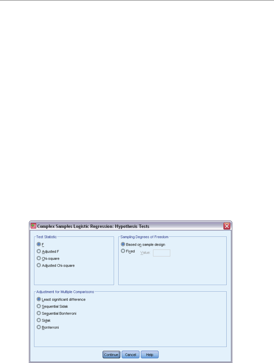
69
Complex Samples Ordinal Regression
Design effect. The ratio of the variance of the estimate to the variance obtained by assuming
that the sample is a simple random sample. This is a measure of the effect of specifying a
complex design, where values further from 1 indicate greater effects.
Square root of design effect. This is a measure, expressed in units comparable to those of
the standard error, of the effect of specifying a complex design, where values further from
1 indicate greater effects.
Parallel Lines. This group allows you to request statistics associated with a model with nonparallel
lines where a separate regression line is fitted for each response category (except the last).
Wald test. Produces a test of the null hypothesis that regression parameters are equal for all
cumulative responses. The model with nonparallel lines is estimated and the Wald test of
equal parameters is applied.
Parameter estimates. Displays estimates of the coefficients and standard errors for the model
with nonparallel lines.
Covariances of parameter estimates. Displays an estimate of the covariance matrix for the
coefficients of the model with nonparallel lines.
Summary statistics for model variables. Displays summary information about the dependent
variable, covariates, and factors.
Sample design information. Displays summary information about the sample, including the
unweighted count and the population size.
Complex Samples Hypothesis Tests
Figure 11-5
Hypothesis Tests dialog box
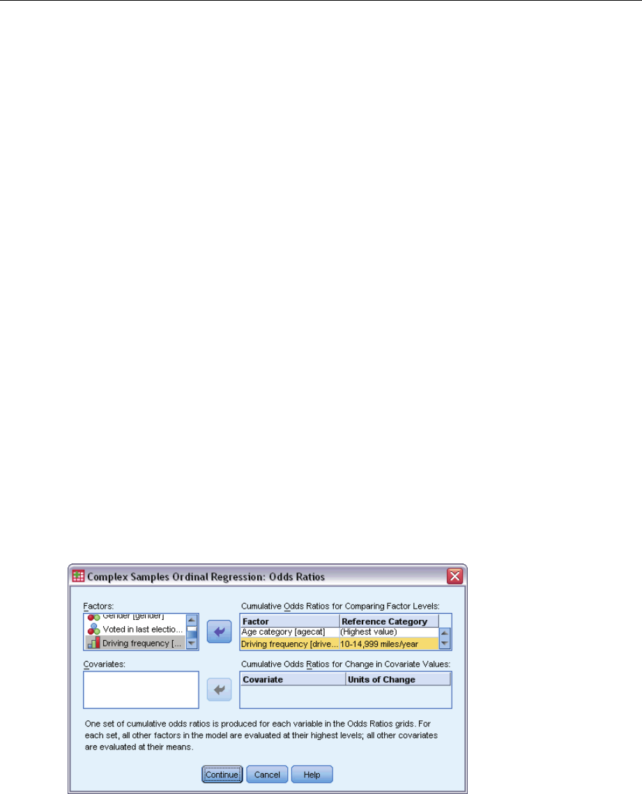
70
Chapter 11
Test Statistic. This group allows you to select the type of statistic used for testing hypotheses. You
can choose between F,adjustedF, chi-square, and adjusted chi-square.
Sampling Degrees of Freedom. This group gives you control over the sampling design degrees of
freedomusedtocomputepvalues for all test statistics. If based on the sampling design, the value
is the difference between the number of primary sampling units and the number of strata in the
first stage of sampling. Alternatively, you can set a custom degrees of freedom by specifying a
positive integer.
Adjustment for Multiple Comparisons. When performing hypothesis tests with multiple contrasts,
the overall significance level can be adjusted from the significance levels for the included
contrasts. This group allows you to choose the adjustment method.
Least significant difference. This method does not control the overall probability of rejecting
the hypotheses that some linear contrasts are different from the null hypothesis values.
Sequential Sidak. This is a sequentially step-down rejective Sidak procedure that is much
less conservative in terms of rejecting individual hypotheses but maintains the same overall
significance level.
Sequential Bonferroni. This is a sequentially step-down rejective Bonferroni procedure that is
much less conservative in terms of rejecting individual hypotheses but maintains the same
overall significance level.
Sidak. This method provides tighter bounds than the Bonferroni approach.
Bonferroni. This method adjusts the observed significance level for the fact that multiple
contrasts are being tested.
Complex Samples Ordinal Regression Odds Ratios
Figure 11-6
Ordinal Regression Odds Ratios dialog box
The Odds Ratios dialog box allows you to display the model-estimated cumulative odds ratios for
specified factors and covariates. This feature is only available for models using the Logit link
function. A single cumulative odds ratio is computed for all categories of the dependent variable
except the last; the proportional odds model postulates that they are all equal.
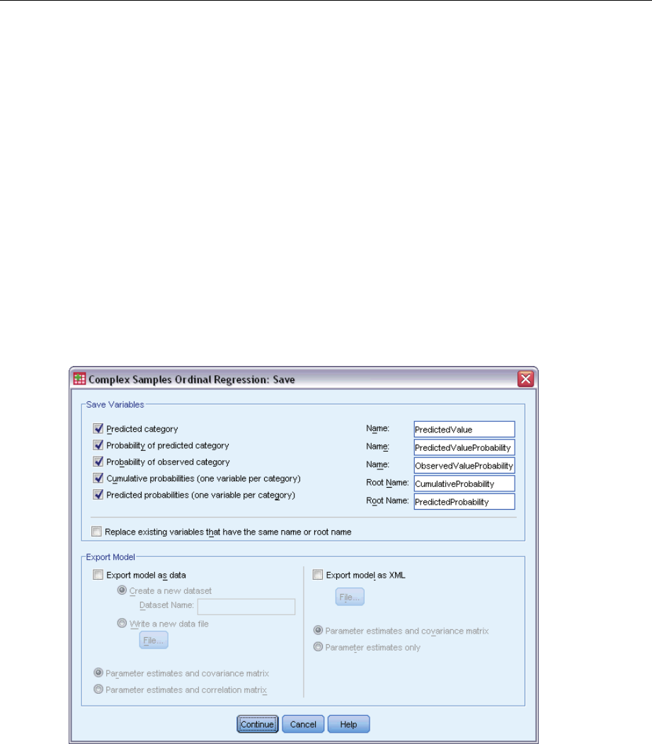
71
Complex Samples Ordinal Regression
Factors. For each selected factor, displays the ratio of the cumulative odds at each category of the
factor to the odds at the specified reference category.
Covariates. For each selected covariate, displays the ratio of the cumulative odds at the covariate’s
mean value plus the specified units of change to the odds at the mean.
When computing odds ratios for a factor or covariate, the procedure fixes all other factors at their
highest levels and all other covariates at their means. If a factor or covariate interacts with other
predictors in the model, then the odds ratios depend not only on the change in the specified
variable but also on the values of the variables with which it interacts. If a specified covariate
interacts with itself in the model (for example, age*age), then the odds ratios depend on both the
change in the covariate and the value of the covariate.
Complex Samples Ordinal Regression Save
Figure 11-7
Ordinal Regression Save dialog box
Save Variables. This group allows you to save the model-predicted category, probability of
predicted category, probability of observed category, cumulative probabilities, and predicted
probabilities as new variables in the active dataset.
Export model as SPSS Statistics data. Writes a dataset in IBM® SPSS® Statistics format containing
the parameter correlation or covariance matrix with parameter estimates, standard errors,
significance values, and degrees of freedom. The order of variables in the matrix file is as follows.
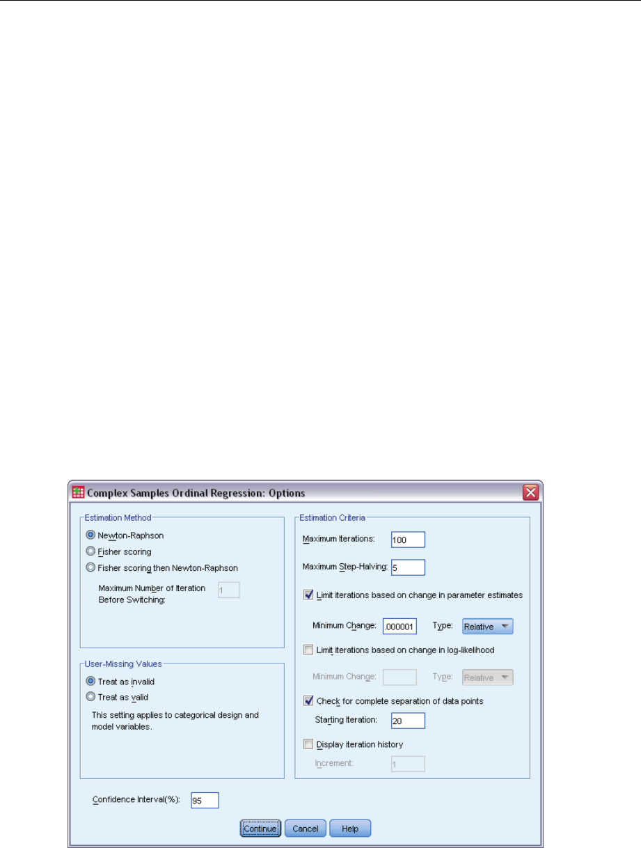
72
Chapter 11
rowtype_. Takes values (and value labels), COV (Covariances), CORR (Correlations), EST
(Parameter estimates), SE (Standard errors), SIG (Significance levels), and DF (Sampling
design degrees of freedom). There is a separate case with row type COV (or CORR) for each
model parameter, plus a separate case for each of the other row types.
varname_. Takes values P1, P2, ..., corresponding to an ordered list of all model parameters,
for row types COV or CORR, with value labels corresponding to the parameter strings shown
in the parameter estimates table. The cells are blank for other row types.
P1, P2, ... These variables correspond to an ordered list of all model parameters, with variable
labels corresponding to the parameter strings shown in the parameter estimates table, and
take values according to the row type. For redundant parameters, all covariances are set
to zero; correlations are set to the system-missing value; all parameter estimates are set at
zero; and all standard errors, significance levels, and residual degrees of freedom are set to
the system-missing value.
Note:Thisfile is not immediately usable for further analyses in other procedures that read a matrix
file unless those procedures accept all the row types exported here.
Export model as XML. Saves the parameter estimates and the parameter covariance matrix, if
selected, in XML (PMML) format. You can use this model file to apply the model information to
other data files for scoring purposes.
Complex Samples Ordinal Regression Options
Figure 11-8
Ordinal Regression Options dialog box

73
Complex Samples Ordinal Regression
Estimation Method. You can select a parameter estimation method; choose between
Newton-Raphson, Fisher scoring, or a hybrid method in which Fisher scoring iterations are
performed before switching to the Newton-Raphson method. If convergence is achieved during
the Fisher scoring phase of the hybrid method before the maximum number of Fisher iterations is
reached, the algorithm continues with the Newton-Raphson method.
Estimation. This group gives you control of various criteria used in the model estimation.
Maximum Iterations. The maximum number of iterations the algorithm will execute. Specify a
non-negative integer.
Maximum Step-Halving. At each iteration, the step size is reduced by a factor of 0.5 until the
log-likelihood increases or maximum step-halving is reached. Specify a positive integer.
Limit iterations based on change in parameter estimates. When selected, the algorithm stops
after an iteration in which the absolute or relative change in the parameter estimates is less
than the value specified, which must be non-negative.
Limit iterations based on change in log-likelihood. When selected, the algorithm stops after an
iteration in which the absolute or relative change in the log-likelihood function is less than the
value specified, which must be non-negative.
Check for complete separation of data points. When selected, the algorithm performs tests to
ensure that the parameter estimates have unique values. Separation occurs when the procedure
can produce a model that correctly classifies every case.
Display iteration history. Displays parameter estimates and statistics at every niterations
beginning with the 0th iteration (the initial estimates). If you choose to print the iteration
history, the last iteration is always printed regardless of the value of n.
User-Missing Values. Scale design variables, as well as the dependent variable and any covariates,
should have valid data. Cases with invalid data for any of these variables are deleted from the
analysis. These controls allow you to decide whether user-missing values are treated as valid
among the strata, cluster, subpopulation, and factor variables.
Confidence Interval. This is the confidence interval level for coefficient estimates, exponentiated
coefficient estimates, and odds ratios. Specify a value greater than or equal to 50 and less than 100.
CSORDINAL Command Additional Features
The command syntax language also allows you to:
Specify custom tests of effects versus a linear combination of effects or a value (using the
CUSTOM subcommand).
Fix values of other model variables at values other than their means when computing
cumulative odds ratios for factors and covariates (using the ODDSRATIOS subcommand).
Use unlabeled values as custom reference categories for factors when odds ratios are requested
(using the ODDSRATIOS subcommand).
Specify a tolerance value for checking singularity (using the CRITERIA subcommand).
Produce a general estimable function table (using the PRINT subcommand).
Save more than 25 probability variables (using the SAVE subcommand).
See the Command Syntax Reference for complete syntax information.

Chapter
12
Complex Samples Cox Regression
The Complex Samples Cox Regression procedure performs survival analysis for samples drawn
by complex sampling methods. Optionally, you can request analyses for a subpopulation.
Examples. A government law enforcement agency is concerned about recidivism rates in their area
of jurisdiction. One of the measures of recidivism is the time until second arrest for offenders. The
agency would like to model time to rearrest using Cox Regression but are worried the proportional
hazards assumption is invalid across age categories.
Medical researchers are investigating survival times for patients exiting a rehabilitation program
post-ischemic stroke. There is the potential for multiple cases per subject, since patient histories
change as the occurrence of significant nondeath events are noted and the times of these events
recorded. The sample is also left-truncated in the sense that the observed survival times are
“inflated” by the length of rehabilitation, because while the onset of risk starts at the time of the
ischemic stroke, only patients who survive past the rehabilitation program are in the sample.
Survival Time. The procedure applies Cox regression to analysis of survival times—that is, the
length of time before the occurrence of an event. There are two ways to specify the survival time,
depending upon the start time of the interval:
Time=0. Commonly, you will have complete information on the start of the interval for each
subject and will simply have a variable containing end times (or create a single variable with
end times from Date & Time variables; see below).
Varies by subject. This is appropriate when you have left-truncation, also called delayed
entry; for example, if you are analyzing survival times for patients exiting a rehabilitation
program post-stroke, you might consider that their onset of risk starts at the time of the stroke.
However, if your sample only includes patients who have survived the rehabilitation program,
then your sample is left-truncated in the sense that the observed survival times are “inflated”
by the length of rehabilitation. You can account for this by specifying the time at which they
exited rehabilitation as the time of entry into the study.
Date & Time Variables. Date & Time variables cannot be used to directly define the start and
end of the interval; if you have Date & Time variables, you should use them to create variables
containing survival times. If there is no left-truncation, simply create a variable containing end
times based upon the difference between the date of entry into the study and the observation date.
If there is left-truncation, create a variable containing start times, based upon the difference
between the date of the start of the study and the date of entry, and a variable containing end times,
based upon the difference between the date of the start of the study and the date of observation.
Event Status. You need a variable that records whether the subject experienced the event of interest
within the interval. Subjects for whom the event has not occurred are right-censored.
© Copyright SPSS Inc. 1989, 2010 74
75
Complex Samples Cox Regression
Subject Identifier. You can easily incorporate piecewise-constant, time-dependent predictors by
splitting the observations for a single subject across multiple cases. For example, if you are
analyzing survival times for patients post-stroke, variables representing their medical history
should be useful as predictors. Over time, they may experience major medical events that alter
their medical history. The following table shows how to structure such a dataset: Patient ID is the
subject identifier, End time defines the observed intervals, Status records major medical events,
and Prior history of heart attack and Prior history of hemorrhaging are piecewise-constant,
time-dependent predictors.
Patient ID End time Status Prior history of
heart attack
Prior history of
hemorrhaging
15Heart Attack No No
17Hemorrhaging Yes No
18
Died Yes Yes
224
Died No No
38
Heart Attack No No
315
Died Yes N o
Assumptions. The cases in the data file represent a sample from a complex design that should
be analyzed according to the specifications in the file selected in the Complex Samples Plan
dialog box.
Typically, Cox regression models assume proportional hazards—that is, the ratio of hazards
from one case to another should not vary over time. If this assumption does not hold, you may
need to add time-dependent predictors to the model.
Kaplan-Meier Analysis. If you do not select any predictors (or do not enter any selected predictors
into the model) and choose the product limit method for computing the baseline survival curve on
the Options tab, the procedure performs a Kaplan-Meier type of survival analysis.
To Obtain Complex Samples Cox Regression
EFrom the menus choose:
Analyze > Complex Samples > Cox Regression...
ESelect a plan file. Optionally, select a custom joint probabilities file.
EClick Continue.
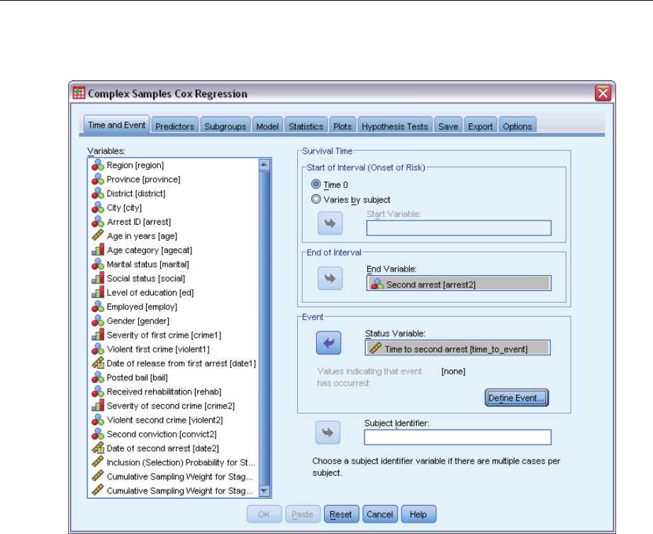
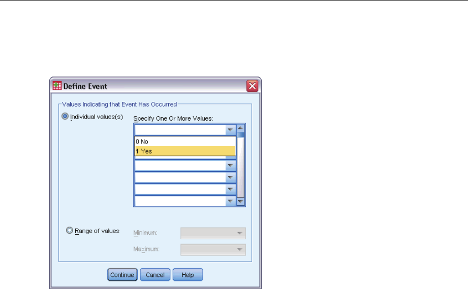
77
Complex Samples Cox Regression
Define Event
Figure 12-2
Define Event dialog box
Specify the values that indicate a terminal event has occurred.
Individual value(s). Specify one or more values by entering them into the grid or selecting them
from a listofvalueswithdefined value labels.
Range of values. Specify a range of values by entering the minimum and maximum values or
selecting values from a list with defined value labels.
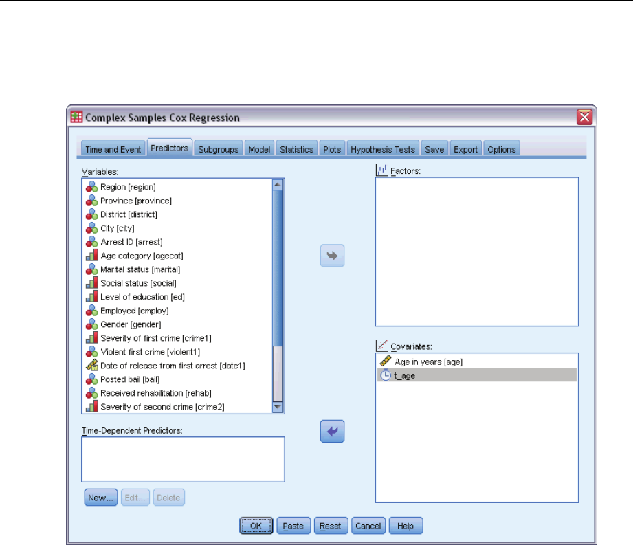
78
Chapter 12
Predictors
Figure 12-3
Cox Regression dialog box, Predictors tab
The Predictors tab allows you to specify the factors and covariates used to build model effects.
Factors.Factors are categorical predictors; they can be numeric or string.
Covariates. Covariates are scale predictors; they must be numeric.
Time-Dependent Predictors. There are certain situations in which the proportional hazards
assumption does not hold. That is, hazard ratios change across time; the values of one (or more)
of your predictors are different at different time points. In such cases, you need to specify
time-dependent predictors. For more information, see the topic Define Time-Dependent Predictor
on p. 79. Time-dependent predictors can be selected as factors or covariates.
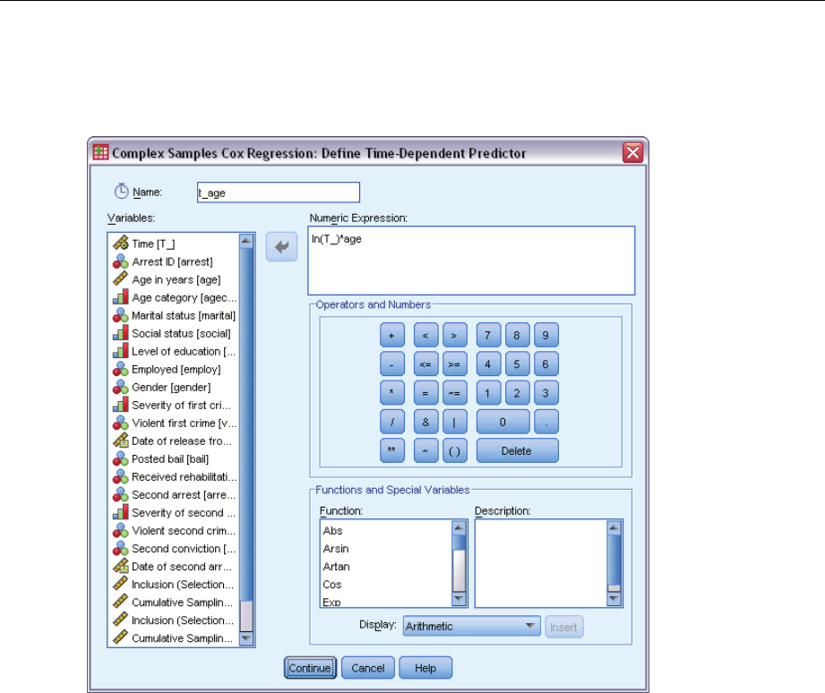
79
Complex Samples Cox Regression
Define Time-Dependent Predictor
Figure 12-4
Cox Regression Define Time-Dependent Predictor dialog box
The Define Time-Dependent Predictor dialog box allows you to create a predictor that is
dependent upon the built-in time variable, T_. You can use this variable to define time-dependent
covariates in two general ways:
If you want to estimate an extended Cox regression model that allows nonproportional
hazards, you can do so by defining your time-dependent predictor as a function of the time
variable T_ and the covariate in question. A common example would be the simple product of
the time variable and the predictor, but more complex functions can be specified as well.
Some variables may have different values at different time periods but aren’t systematically
relatedtotime.Insuchcases,youneedtodefine a segmented time-dependent predictor,
which can be done using logical expressions. Logical expressions take the value 1 if true
and 0 if false. Using a series of logical expressions, you can create your time-dependent
predictor from a set of measurements. For example, if you have blood pressure measured
once a week for the four weeks of your study (identified as BP1 to BP4), you can define your
time-dependent predictor as (T_ <1)*BP1 +(T_ >= 1 & T_ <2)*BP2 +(T_ >= 2 & T_ <3)
*BP3 +(T_ >= 3 & T_ <4)*BP4. Notice that exactly one of the terms in parentheses will
be equal to 1 for any given case and the rest will all equal 0. In other words, this function
meansthatiftimeislessthanoneweek,useBP1; if it is more than one week but less than
two weeks, use BP2; and so on.
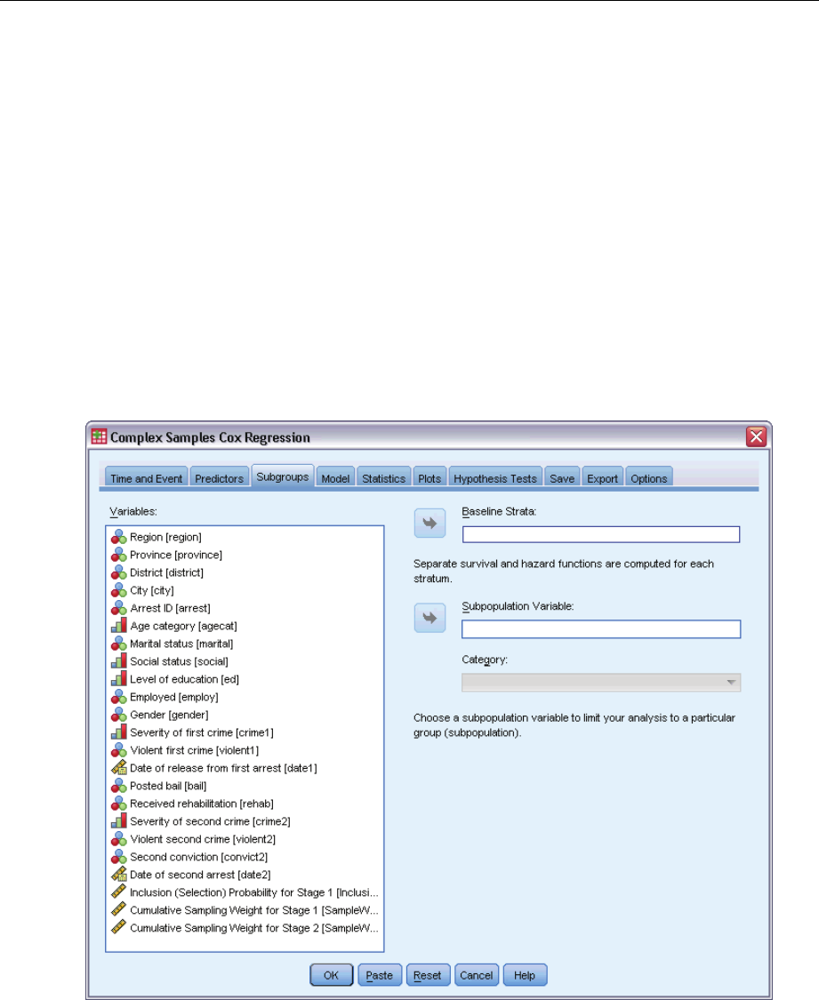
80
Chapter 12
Note: If your segmented, time-dependent predictor is constant within segments, as in the blood
pressure example given above, it may be easier for you to specify the piecewise-constant,
time-dependent predictor by splitting subjects across multiple cases. See the discussion on
Subject Identifiers in Complex Samples Cox Regression on p. 74 for more information.
In the Define Time-Dependent Predictor dialog box, you can use the function-building controls
to build the expression for the time-dependent covariate, or you can enter it directly in the
Numeric Expression text area. Note that string constants must be enclosed in quotation marks
or apostrophes, and numeric constants must be typed in American format, with the dot as the
decimal delimiter. The resulting variable is given the name you specify and should be included
as a factor or covariate on the Predictors tab.
Subgroups
Figure 12-5
Cox Regression dialog box, Subgroups tab
Baseline Strata. A separate baseline hazard and survival function is computed for each value of
this variable, while a single set of model coefficients is estimated across strata.
Subpopulation Variable. Specify a variable to define a subpopulation. The analysis is performed
only for the selected category of the subpopulation variable.
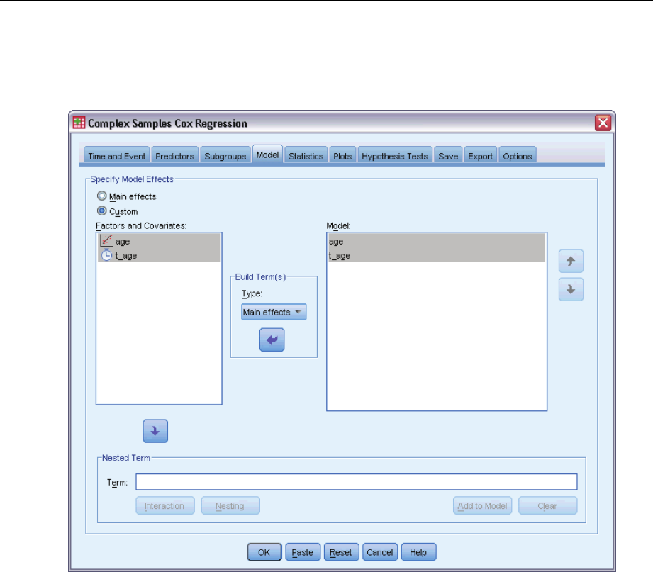
81
Complex Samples Cox Regression
Model
Figure 12-6
Cox Regression dialog box, Model tab
Specify Model Effects. By default, the procedure builds a main-effects model using the factors
and covariates specified in the main dialog box. Alternatively, you can build a custom model that
includes interaction effects and nested terms.
Non-Nested Terms
For the selected factors and covariates:
Interaction. Creates the highest-level interaction term for all selected variables.
Main effects. Creates a main-effects term for each variable selected.
All 2-way. Creates all possible two-way interactions of the selected variables.
All 3-way. Creates all possible three-way interactions of the selected variables.
All 4-way. Creates all possible four-way interactions of the selected variables.
All 5-way. Creates all possible five-way interactions of the selected variables.
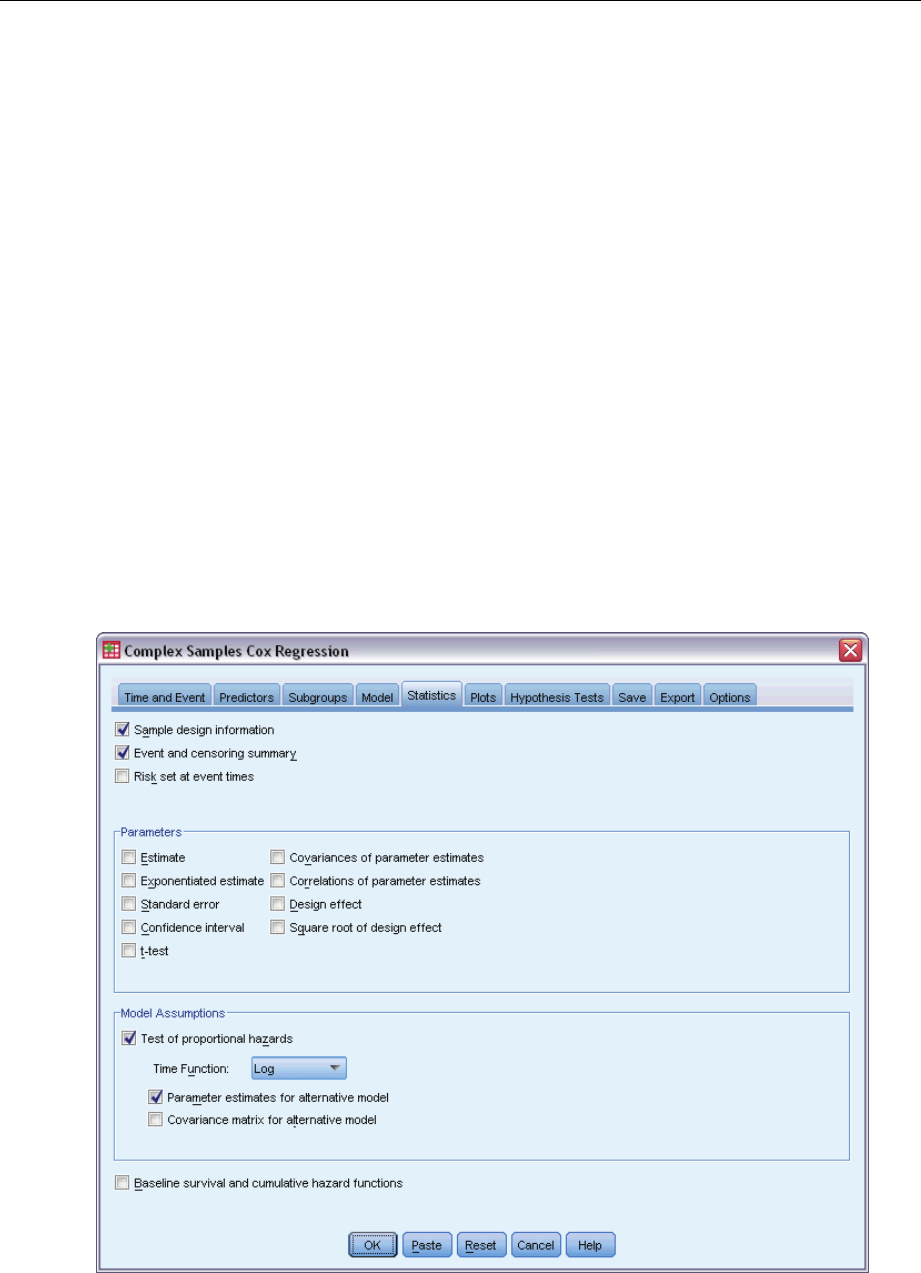
82
Chapter 12
Nested Terms
You can build nested terms for your model in this procedure. Nested terms are useful for modeling
the effect of a factor or covariate whose values do not interact with the levels of another factor.
For example, a grocery store chain may follow the spending habits of its customers at several store
locations. Since each customer frequents only one of these locations, the Customer effect can be
said to be nested within the Store location effect.
Additionally, you can include interaction effects, such as polynomial terms involving the same
covariate, or add multiple levels of nesting to the nested term.
Limitations. Nested terms have the following restrictions:
All factors within an interaction must be unique. Thus, if Ais a factor, then specifying A*A
is invalid.
All factors within a nested effect must be unique. Thus, if Ais a factor, then specifying A(A)
is invalid.
No effect can be nested within a covariate. Thus, if Ais a factor and Xis a covariate, then
specifying A(X) is invalid.
Statistics
Figure 12-7
Cox Regression dialog box, Statistics tab

83
Complex Samples Cox Regression
Sample design information. Displays summary information about the sample, including the
unweighted count and the population size.
Event and censoring summary. Displays summary information about the number and percentage of
censored cases.
Risk set at event times. Displays number of events and number at risk for each event time in
each baseline stratum.
Parameters. This group allows you to control the display of statistics related to the model
parameters.
Estimate. Displays estimates of the coefficients.
Exponentiated estimate. Displays the base of the natural logarithm raised to the power of the
estimates of the coefficients. While the estimate has nice properties for statistical testing, the
exponentiated estimate, or exp(B), is easier to interpret.
Standard error. Displays the standard error for each coefficient estimate.
Confidence interval. Displays a confidence interval for each coefficient estimate. The
confidence level for the interval is set in the Options dialog box.
t-test. Displays a ttest of each coefficient estimate. The null hypothesis for each test is that the
value of the coefficient is 0.
Covariances of parameter estimates. Displays an estimate of the covariance matrix for the
model coefficients.
Correlations of parameter estimates. Displays an estimate of the correlation matrix for the
model coefficients.
Design effect. The ratio of the variance of the estimate to the variance obtained by assuming
that the sample is a simple random sample. This is a measure of the effect of specifying a
complex design, where values further from 1 indicate greater effects.
Square root of design effect. This is a measure of the effect of specifying a complex design,
where values further from 1 indicate greater effects.
Model Assumptions. This group allows you to produce a test of the proportional hazards
assumption. The test compares the fittedmodeltoanalternative model that includes
time-dependentpredictorsx*_TF for each predictor x,where_TF is the specified time function.
Time Function.Specifies the form of _TF for the alternative model. For the identity function,
_TF=T_.Forthelog function, _TF=log(T_). For Kaplan-Meier,_TF=1−SKM(T_), where
SKM(.) is the Kaplan-Meier estimate of the survival function. For rank,_TF is the rank-order
of T_ among the observed end times.
Parameter estimates for alternative model. Displays the estimate, standard error, and confidence
interval for each parameter in the alternative model.
Covariance matrix for alternative model. Displays the matrix of estimated covariances between
parameters in the alternative model.
Baseline survival and cumulative hazard functions. Displays the baseline survival function and
baseline cumulative hazards function along with their standard errors.
Note: If time-dependent predictors defined on the Predictors tab are included in the model, this
option is not available.
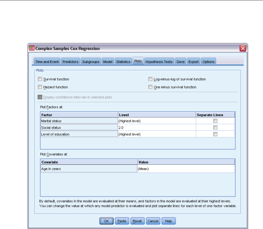
84
Chapter 12
Plots
Figure 12-8
Cox Regression dialog box, Plots tab
The Plots tab allows you to request plots of the hazard function, survival function, log-minus-log
of the survival function, and one minus the survival function. You can also choose to plot
confidence intervals along the specified functions; the confidence level is set on the Options tab.
Predictor patterns. You can specify a pattern of predictor values to be used for the requested plots
and the exported survival file on the Export tab. Note that these options are not available if
time-dependent predictors defined on the Predictors tab are included in the model.
Plot Factors at. By default, each factor is evaluated at its highest level. Enter or select a
different level if desired. Alternatively, you can choose to plot separate lines for each level
of a single factor by selecting the check box for that factor.
Plot Covariates at. Each covariate is evaluated at its mean. Enter or select a different value
if desired.
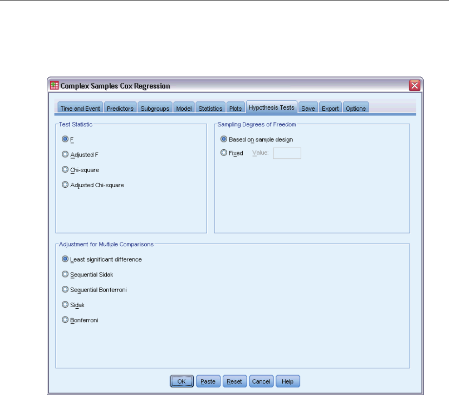
85
Complex Samples Cox Regression
Hypothesis Tests
Figure 12-9
Cox Regression dialog box, Hypothesis Tests tab
Test Statistic. This group allows you to select the type of statistic used for testing hypotheses. You
can choose between F,adjustedF, chi-square, and adjusted chi-square.
Sampling Degrees of Freedom. This group gives you control over the sampling design degrees of
freedomusedtocomputepvalues for all test statistics. If based on the sampling design, the value
is the difference between the number of primary sampling units and the number of strata in the
first stage of sampling. Alternatively, you can set a custom degrees of freedom by specifying a
positive integer.
Adjustment for Multiple Comparisons. When performing hypothesis tests with multiple contrasts,
the overall significance level can be adjusted from the significance levels for the included
contrasts. This group allows you to choose the adjustment method.
Least significant difference. This method does not control the overall probability of rejecting
the hypotheses that some linear contrasts are different from the null hypothesis values.
Sequential Sidak. This is a sequentially step-down rejective Sidak procedure that is much
less conservative in terms of rejecting individual hypotheses but maintains the same overall
significance level.
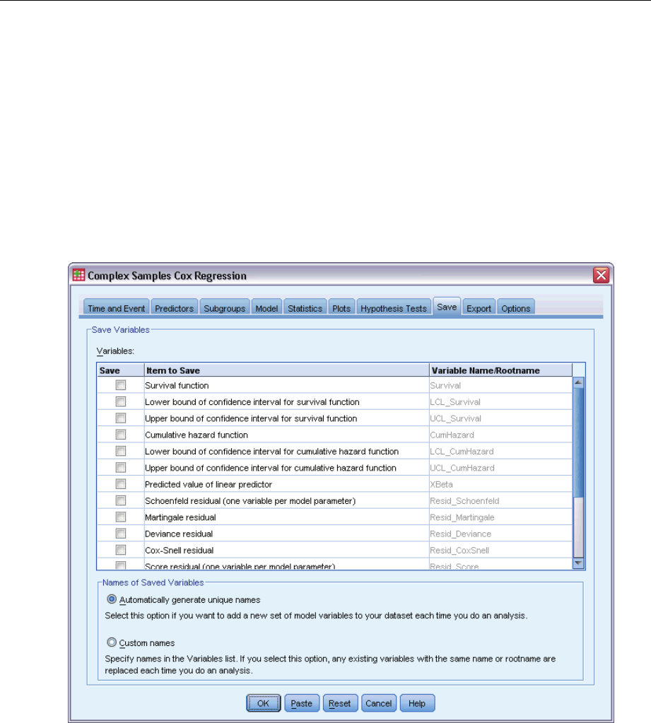
86
Chapter 12
Sequential Bonferroni. This is a sequentially step-down rejective Bonferroni procedure that is
much less conservative in terms of rejecting individual hypotheses but maintains the same
overall significance level.
Sidak. This method provides tighter bounds than the Bonferroni approach.
Bonferroni. This method adjusts the observed significance level for the fact that multiple
contrasts are being tested.
Save
Figure 12-10
Cox Regression dialog box, Save tab
Save Variables. This group allows you to save model-related variables to the active dataset for
further use in diagnostics and reporting of results. Note that none of these are available when
time-dependent predictors are included in the model.
Survival function. Saves the probability of survival (the value of the survival function) at the
observed time and predictor values for each case.
Lower bound of confidence interval for survival function. Saves the lower bound of the
confidence interval for the survival function at the observed time and predictor values for
each case.

87
Complex Samples Cox Regression
Upper bound of confidence interval for survival function. Saves the upper bound of the confidence
interval for the survival function at the observed time and predictor values for each case.
Cumulative hazard function. Saves the cumulative hazard, or −ln(survival), at the observed time
and predictor values for each case.
Lower bound of confidence interval for cumulative hazard function. Saves the lower bound of
the confidence interval for the cumulative hazard function at the observed time and predictor
values for each case.
Upper bound of confidence interval for cumulative hazard function. Saves the upper bound of
the confidence interval for the cumulative hazard function at the observed time and predictor
values for each case.
Predicted value of linear predictor. Saves the linear combination of reference value corrected
predictors times regression coefficients. The linear predictor is the ratio of the hazard function
to the baseline hazard. Under the proportional hazards model, this value is constant across
time.
Schoenfeld residual. For each uncensored case and each nonredundant parameter in the
model, the Schoenfeld residual is the difference between the observed value of the predictor
associated with the model parameter and the expected value of the predictor for cases in
the risk set at the observed event time. Schoenfeld residuals can be used to help assess the
proportional hazards assumption; for example, for a predictor x, plots of the Schoenfeld
residuals for the time-dependent predictor x*ln(T_) versus time should show a horizontal
line at 0 if proportional hazards holds. A separate variable is saved for each nonredundant
parameter in the model. Schoenfeld residuals are only computed for uncensored cases.
Martingale residual. For each case, the martingale residual is the difference between the
observed censoring (0 if censored, 1 if not) and the expectation of an event during the
observation time.
Deviance residual. Deviance residuals are martingale residuals “adjusted” to appear more
symmetrical about 0. Plots of deviance residuals against predictors should reveal no patterns.
Cox-Snell residual. For each case, the Cox-Snell residual is the expectation of an event during
the observation time, or the observed censoring minus the martingale residual.
Score residual. For each case and each nonredundant parameter in the model, the score
residual is the contribution of the case to the first derivative of the pseudo-likelihood. A
separate variable is saved for each nonredundant parameter in the model.
DFBeta residual. For each case and each nonredundant parameter in the model, the DFBeta
residual approximates the change in the value of the parameter estimate when the case is
removed from the model. Cases with relatively large DFBeta residuals may be exerting undue
influence on the analysis. A separate variable is saved for each nonredundant parameter in
the model.
Aggregated residuals. When multiple cases represent a single subject, the aggregated residual
for a subject is simply the sum of the corresponding case residuals over all cases belonging
to the same subject. For Schoenfeld’s residual, the aggregated version is the same as that of
the non-aggregated version because Schoenfeld’s residual is only defined for uncensored
cases. These residuals are only available when a subject identifier is specified on the Time
and Event tab.
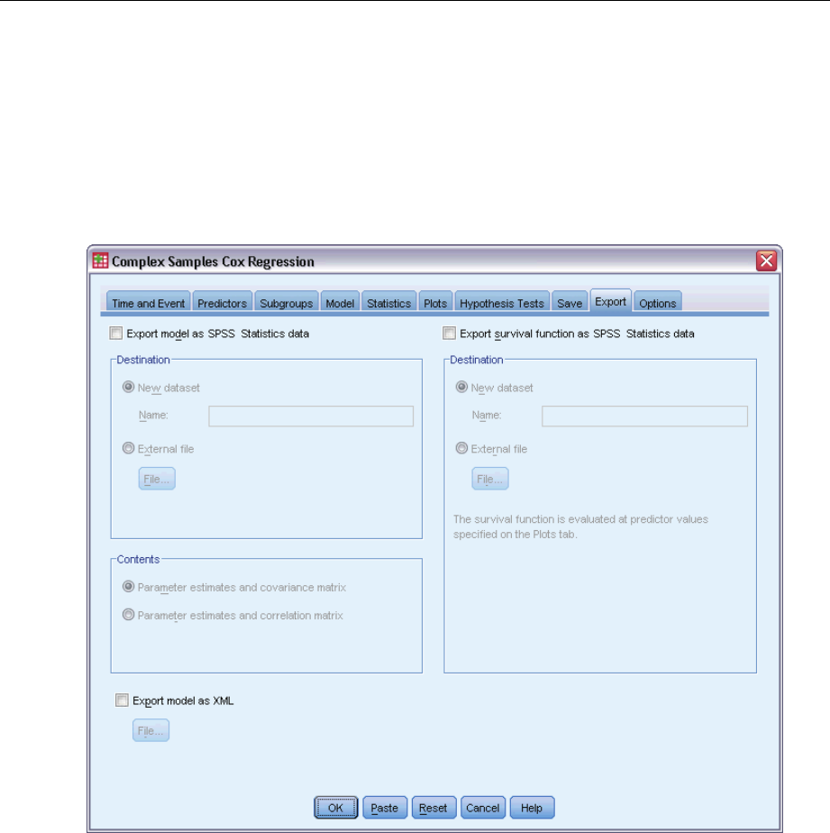
88
Chapter 12
Names of Saved Variables. Automatic name generation ensures that you keep all your work.
Custom names allow you to discard/replace results from previous runs without first deleting the
saved variables in the Data Editor.
Export
Figure 12-11
Cox Regression dialog box, Export tab
Export model as SPSS Statistics data. Writes a dataset in IBM® SPSS® Statistics format containing
the parameter correlation or covariance matrix with parameter estimates, standard errors,
significance values, and degrees of freedom. The order of variables in the matrix file is as follows.
rowtype_. Takes values (and value labels), COV (Covariances), CORR (Correlations), EST
(Parameter estimates), SE (Standard errors), SIG (Significance levels), and DF (Sampling
design degrees of freedom). There is a separate case with row type COV (or CORR) for each
model parameter, plus a separate case for each of the other row types.

89
Complex Samples Cox Regression
varname_. Takes values P1, P2, ..., corresponding to an ordered list of all model parameters,
for row types COV or CORR, with value labels corresponding to the parameter strings shown
in the parameter estimates table. The cells are blank for other row types.
P1, P2, ... These variables correspond to an ordered list of all model parameters, with variable
labels corresponding to the parameter strings shown in the parameter estimates table, and
take values according to the row type. For redundant parameters, all covariances are set
to zero; correlations are set to the system-missing value; all parameter estimates are set at
zero; and all standard errors, significance levels, and residual degrees of freedom are set to
the system-missing value.
Note:Thisfile is not immediately usable for further analyses in other procedures that read a matrix
file unless those procedures accept all the row types exported here.
Export survival function as SPSS Statistics data. Writes a dataset in SPSS Statistics format
containing the survival function; standard error of the survival function; upper and lower bounds
of the confidence interval of the survival function; and the cumulative hazards function for each
failure or event time, evaluated at the baseline and at the predictor patterns specified on the Plot
tab. The order of variables in the matrix file is as follows.
Baseline strata variable. Separate survival tables are produced for each value of the strata
variable.
Survival time variable. The event time; a separate case is created for each unique event time.
Sur_0, LCL_Sur_0, UCL_Sur_0. Baseline survival function and the upper and lower bounds
of its confidence interval.
Sur_R, LCL_Sur_R, UCL_Sur_R. Survival function evaluated at the “reference” pattern (see the
pattern values table in the output) and the upper and lower bounds of its confidence interval.
Sur_#.#, LCL_Sur_#.#, UCL_Sur_#.#, … Survival function evaluated at each of the predictor
patterns specified on the Plots tab and the upper and lower bounds of their confidence
intervals. See the pattern values table in the output to match patterns with the number #.#.
Haz_0, LCL_Haz_0, UCL_Haz_0. Baseline cumulative hazard function and the upper and lower
bounds of its confidence interval.
Haz_R, LCL_Haz_R, UCL_Haz_R. Cumulative hazard function evaluated at the “reference”
pattern (see the pattern values table in the output) and the upper and lower bounds of its
confidence interval.
Haz_#.#, LCL_Haz_#.#, UCL_Haz_#.#, … Cumulative hazard function evaluated at each of the
predictor patterns specified on the Plots tab and the upper and lower bounds of their confidence
intervals. See the pattern values table in the output to match patterns with the number #.#.
Export model as XML. Saves all information needed to predict the survival function, including
parameter estimates and the baseline survival function, in XML (PMML) format. You can use this
model file to apply the model information to other data files for scoring purposes.
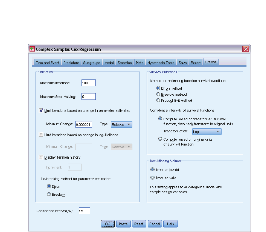
90
Chapter 12
Options
Figure 12-12
Cox Regression dialog box, Options tab
Estimation. These controls specify criteria for estimation of regression coefficients.
Maximum Iterations. The maximum number of iterations the algorithm will execute. Specify a
non-negative integer.
Maximum Step-Halving. At each iteration, the step size is reduced by a factor of 0.5 until the
log-likelihood increases or maximum step-halving is reached. Specify a positive integer.
Limit iterations based on change in parameter estimates. When selected, the algorithm stops
after an iteration in which the absolute or relative change in the parameter estimates is less
than the value specified, which must be positive.
Limit iterations based on change in log-likelihood. When selected, the algorithm stops after an
iteration in which the absolute or relative change in the log-likelihood function is less than
the value specified, which must be positive.
Display iteration history. Displays the iteration history for the parameter estimates and pseudo
log-likelihood and prints the last evaluation of the change in parameter estimates and pseudo
log-likelihood. The iteration history table prints every niterations beginning with the 0th

91
Complex Samples Cox Regression
iteration (the initial estimates), where nis the value of the increment. If the iteration history is
requested, then the last iteration is always displayed regardless of n.
Tie breaking method for parameter estimation. When there are tied observed failure times, one of
these methods is used to break the ties. The Efron method is more computationally expensive.
Survival Functions. These controls specify criteria for computations involving the survival function.
Method for estimating baseline survival functions. The Breslow (orNelson-Aalanorempirical)
method estimates the baseline cumulative hazard by a nondecreasing step function with
steps at the observed failure times, then computes the baseline survival by the relation
survival=exp(−cumulative hazard). The Efron method is more computationally expensive
and reduces to the Breslow method when there are no ties. The product limit method
estimates the baseline survival by a non-increasing right continuous function; when there are
no predictors in the model, this method reduces to Kaplan-Meier estimation.
Confidence intervals of survival functions. The confidence interval can be calculated in three
ways: in original units, via a log transformation, or a log-minus-log transformation. Only the
log-minus-log transformation guarantees that the bounds of the confidence interval will lie
between 0 and 1, but the log transformation generally seems to perform “best.”
User Missing Values. All variables must have valid values for a case to be included in the analysis.
These controls allow you to decide whether user-missing values are treated as valid among
categorical models (including factors, event, strata, and subpopulation variables) and sampling
design variables.
Confidence interval(%). This is the confidence interval level used for coefficient estimates,
exponentiated coefficient estimates, survival function estimates, and cumulative hazard function
estimates. Specify a value greater than or equal to 0, and less than 100.
CSCOXREG Command Additional Features
The command language also allows you to:
Perform custom hypothesis tests (using the CUSTOM subcommand and /PRINT LMATRIX).
Tolerance specification (using /CRITERIA SINGULAR).
General estimable function table (using /PRINT GEF).
Multiple predictor patterns (using multiple PATTERN subcommands).
Maximum number of saved variables when a rootname is specified (using the SAVE
subcommand). The dialog honors the CSCOXREG default of 25 variables.
See the Command Syntax Reference for complete syntax information.
Part II:
Examples

Chapter
13
Complex Samples Sampling Wizard
The Sampling Wizard guides you through the steps for creating, modifying, or executing a
sampling plan file. Before using the wizard, you should have a well-defined target population, a
list of sampling units, and an appropriate sample design in mind.
Obtaining a Sample from a Full Sampling Frame
A state agency is charged with ensuring fair property taxes from county to county. Taxes are based
on the appraised value of the property, so the agency wants to survey a sample of properties
by county to be sure that each county’s records are equally up to date. However, resources for
obtaining current appraisals are limited, so it’s important that what is available is used wisely. The
agency decides to employ complex sampling methodology to select a sample of properties.
A listing of properties is collected in property_assess_cs.sav.For more information, see the
topic Sample Files in Appendix A in IBM SPSS Complex Samples 19.Use the Complex Samples
Sampling Wizard to select a sample.
Using the Wizard
ETo run the Complex Samples Sampling Wizard, from the menus choose:
Analyze > Complex Samples > Select a Sample...
© Copyright SPSS Inc. 1989, 2010 93
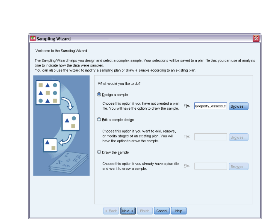
94
Chapter 13
Figure 13-1
Sampling Wizard, Welcome step
ESelect Design a sample,browsetowhereyouwanttosavethefile, and type property_assess.csplan
as the name of the plan file.
EClick Next.
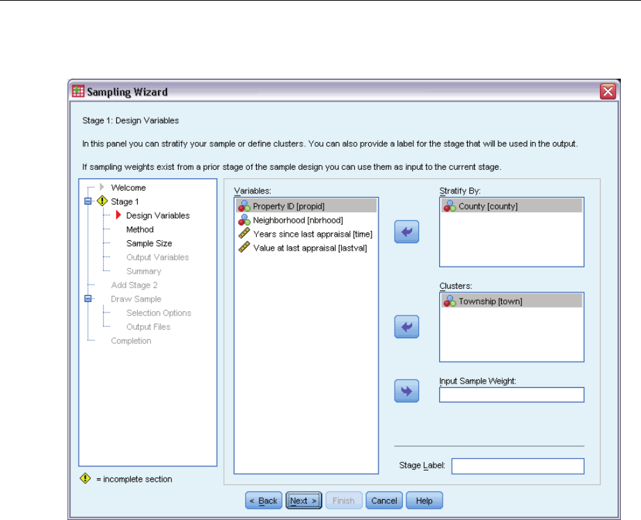
95
Complex Samples Sampling Wizard
Figure 13-2
Sampling Wizard, Design Variables step (stage 1)
ESelect County as a stratification variable.
ESelect Towns hip as a cluster variable.
EClick Next, and then click Next in the Sampling Method step.
This design structure means that independent samples are drawn for each county. In this stage,
townships are drawn as the primary sampling unit using the default method, simple random
sampling.
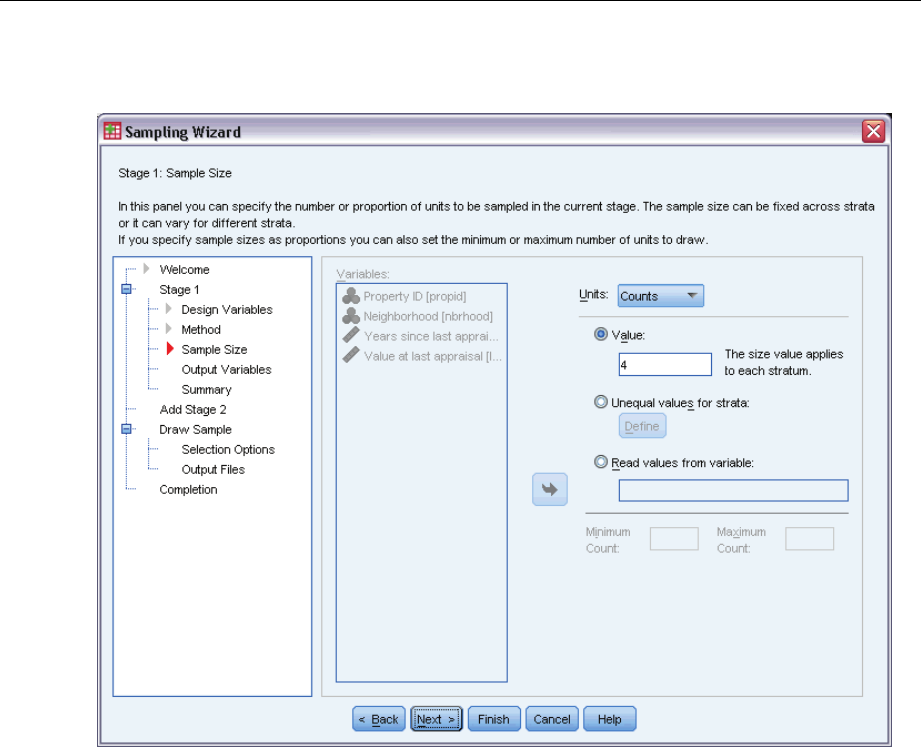
96
Chapter 13
Figure 13-3
Sampling Wizard, Sample Size step (stage 1)
ESelect Counts from the Units drop-down list.
EType 4as the value for the number of units to select in this stage.
EClick Next,andthenclickNext in the Output Variables step.
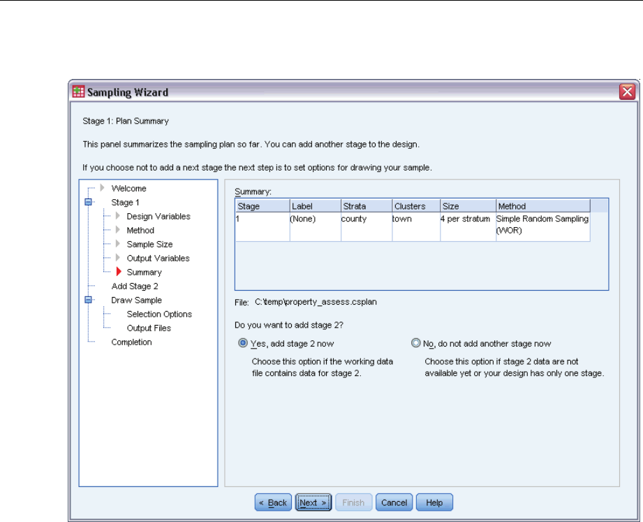
97
Complex Samples Sampling Wizard
Figure 13-4
Sampling Wizard, Plan Summary step (stage 1)
ESelect Yes,addstage2now.
EClick Next.
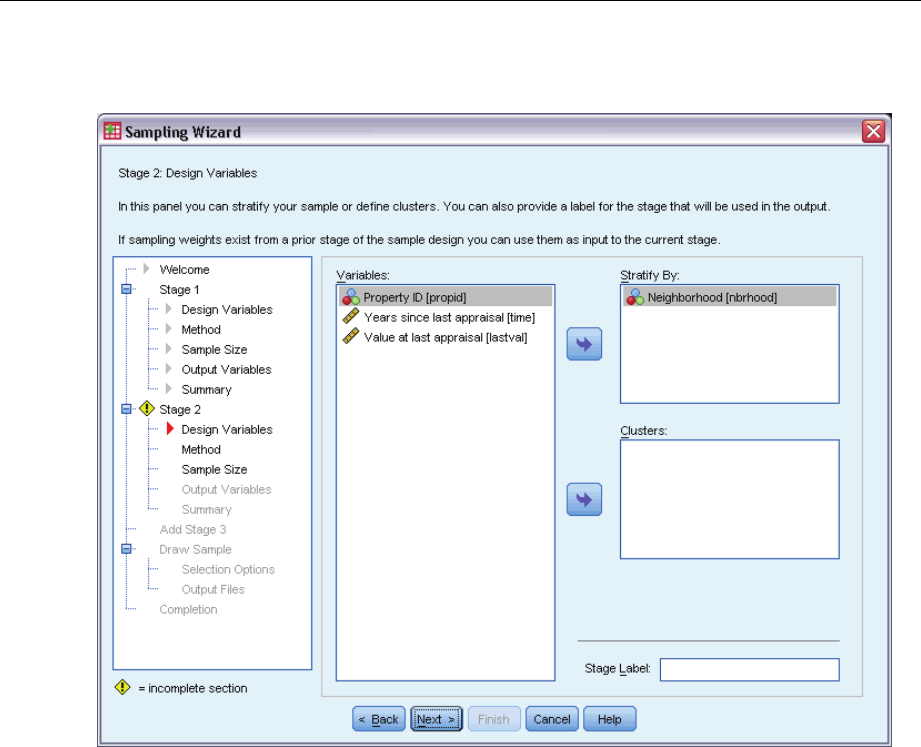
98
Chapter 13
Figure 13-5
Sampling Wizard, Design Variables step (stage 2)
ESelect Neighborhood as a stratification variable.
EClick Next, and then click Next in the Sampling Method step.
This design structure means that independent samples are drawn for each neighborhood of the
townships drawn in stage 1. In this stage, properties are drawn as the primary sampling unit using
simple random sampling.
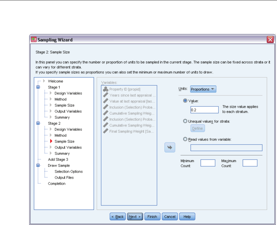
99
Complex Samples Sampling Wizard
Figure 13-6
Sampling Wizard, Sample Size step (stage 2)
ESelect Proportions from the Units drop-down list.
EType 0.2 as the value of the proportion of units to sample from each stratum.
EClick Next,andthenclickNext in the Output Variables step.
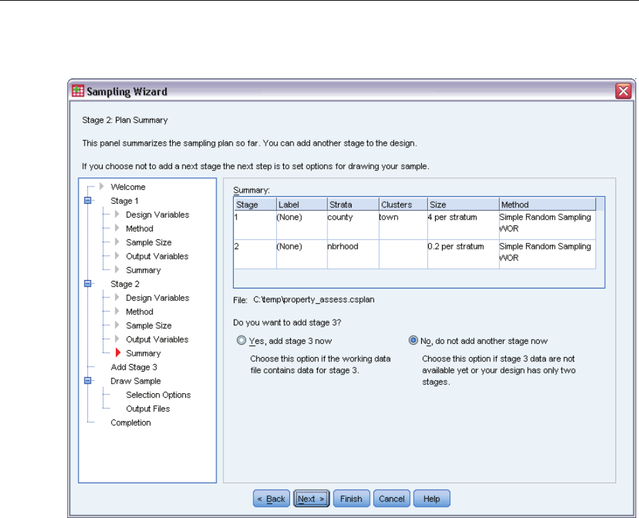
100
Chapter 13
Figure 13-7
Sampling Wizard, Plan Summary step (stage 2)
ELook over the sampling design, and then click Next.
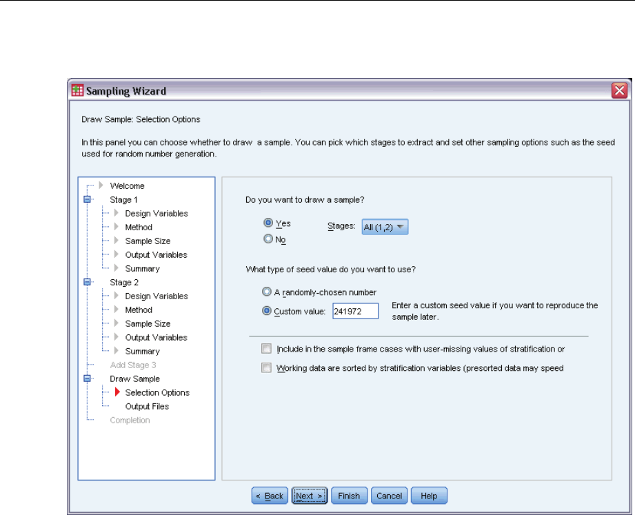
101
Complex Samples Sampling Wizard
Figure 13-8
Sampling Wizard, Draw Sample, Selection Options step
ESelect Custom value for the type of random seed to use, and type 241972 as the value.
Using a custom value allows you to replicate the results of this example exactly.
EClick Next, and then click Next intheDrawSampleOutputFilesstep.
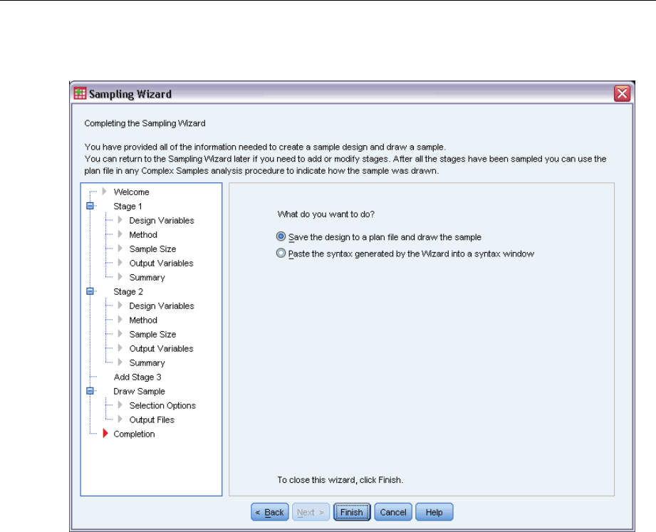
102
Chapter 13
Figure 13-9
Sampling Wizard, Finish step
EClick Finish.
These selections produce the sampling plan file property_assess.csplan and draw a sample
according to that plan.
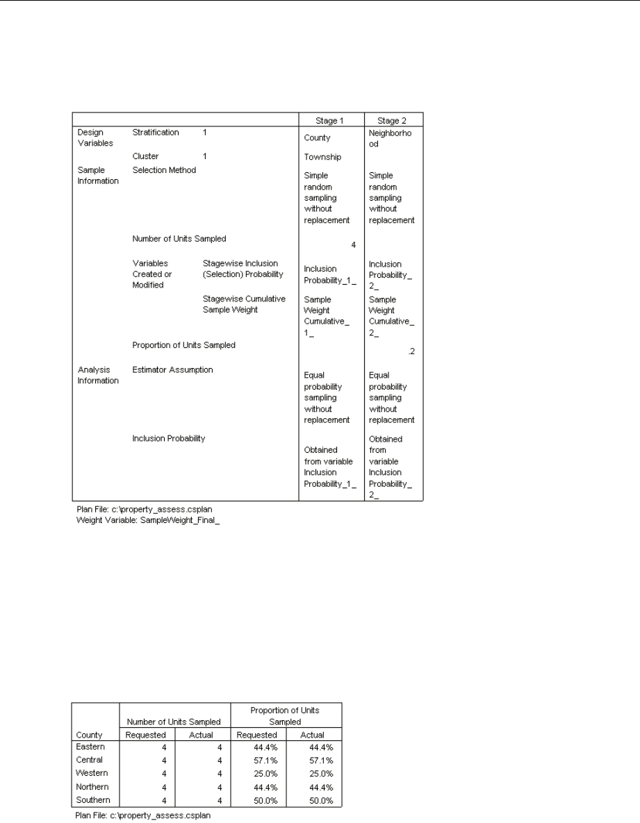
103
Complex Samples Sampling Wizard
Plan Summary
Figure 13-10
Plan summary
The summary table reviews your sampling plan and is useful for making sure that the plan
represents your intentions.
Sampling Summary
Figure 13-11
Stage summary
This summary table reviews the first stage of sampling and is useful for checking that the sampling
went according to plan. Four townships were sampled from each county, as requested.
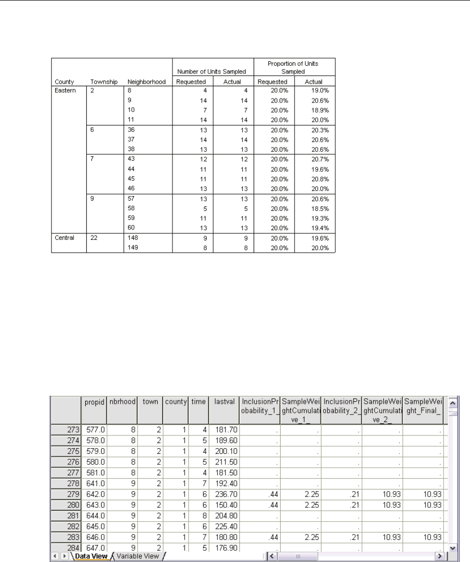
104
Chapter 13
Figure 13-12
Stage summary
This summary table (the top part of which is shown here) reviews the second stage of sampling.
It is also useful for checking that the sampling went according to plan. Approximately 20% of
the properties were sampled from each neighborhood from each township sampled in the first
stage, as requested.
Sample Results
Figure 13-13
Data Editor with sample results
You can see the sampling results in the Data Editor. Five new variables were saved to the working
file, representing the inclusion probabilities and cumulative sampling weights for each stage, plus
the final sampling weights.
Cases with values for these variables were selected to the sample.
Cases with system-missing values for the variables were not selected.

105
Complex Samples Sampling Wizard
The agency will now use its resources to collect current valuations for the properties selected in
the sample. Once those valuations are available, you can process the sample with Complex
Samples analysis procedures, using the sampling plan property_assess.csplan to provide the
sampling specifications.
Obtaining a Sample from a Partial Sampling Frame
A company is interested in compiling and selling a database of high-quality survey information.
The survey sample should be representative but efficiently carried out, so complex sampling
methods are used. The full sampling design calls for the following structure:
Stage Strata Clusters
1Region Province
2District City
3Subdivision
In the third stage, households are the primary sampling unit, and selected households will be
surveyed. However, since information is easily available only to the city level, the company plans
to execute the first two stages of the design now and then collect information on the numbers of
subdivisions and households from the sampled cities. The available information to the city level is
collected in demo_cs_1.sav.For more information, see the topic Sample Files in Appendix A in
IBM SPSS Complex Samples 19.Note that this file contains a variable Subdivision that contains
all 1’s. This is a placeholder for the “true” variable, whose values will be collected after the first
two stages of the design are executed, that allows you to specify the full three-stage sampling
design now. Use the Complex Samples Sampling Wizard to specify the full complex sampling
design, and then draw the first two stages.
Using the Wizard to Sample from the First Partial Frame
ETo run the Complex Samples Sampling Wizard, from the menus choose:
Analyze > Complex Samples > Select a Sample...
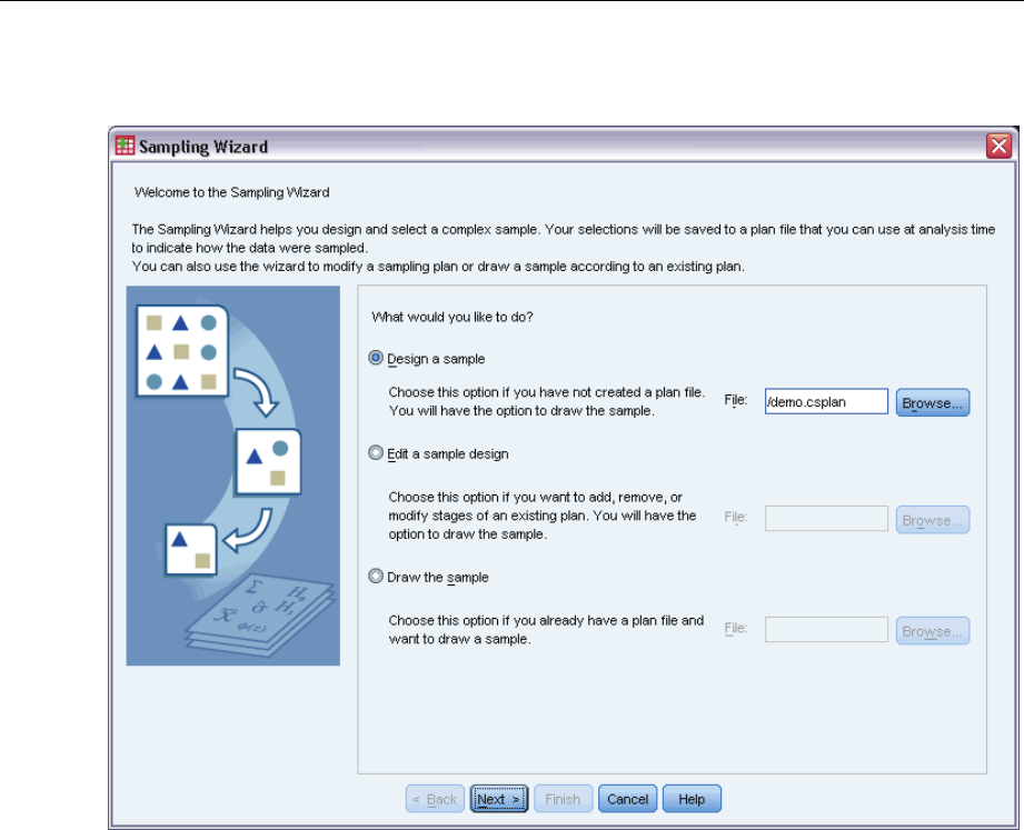
106
Chapter 13
Figure 13-14
Sampling Wizard, Welcome step
ESelect Designasample, browse to where you want to save the file, and type demo.csplan as
thenameoftheplanfile.
EClick Next.
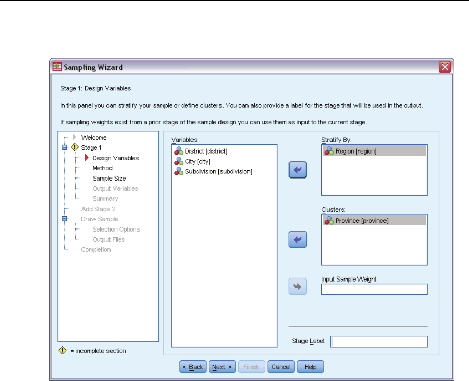
107
Complex Samples Sampling Wizard
Figure 13-15
Sampling Wizard, Design Variables step (stage 1)
ESelect Region as a stratification variable.
ESelect Province as a cluster variable.
EClick Next, and then click Next in the Sampling Method step.
This design structure means that independent samples are drawn for each region. In this stage,
provinces are drawn as the primary sampling unit using the default method, simple random
sampling.
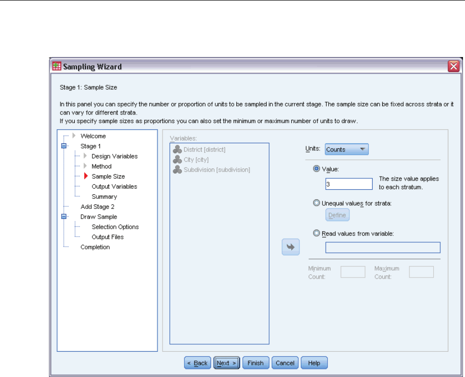
108
Chapter 13
Figure 13-16
Sampling Wizard, Sample Size step (stage 1)
ESelect Counts from the Units drop-down list.
EType 3as the value for the number of units to select in this stage.
EClick Next,andthenclickNext in the Output Variables step.

109
Complex Samples Sampling Wizard
Figure 13-17
Sampling Wizard, Plan Summary step (stage 1)
ESelect Yes,addstage2now.
EClick Next.
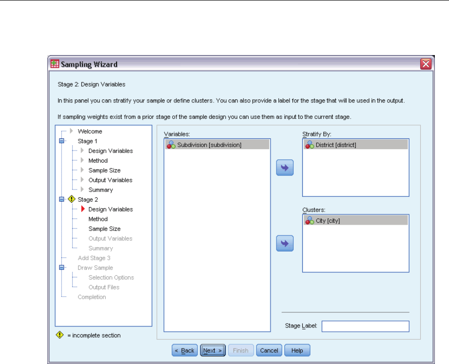
110
Chapter 13
Figure 13-18
Sampling Wizard, Design Variables step (stage 2)
ESelect District as a stratification variable.
ESelect City as a cluster variable.
EClick Next, and then click Next in the Sampling Method step.
This design structure means that independent samples are drawn for each district. In this stage,
cities are drawn as the primary sampling unit using the default method, simple random sampling.

111
Complex Samples Sampling Wizard
Figure 13-19
Sampling Wizard, Sample Size step (stage 2)
ESelect Proportions from the Units drop-down list.
EType 0.1 as the value of the proportion of units to sample from each strata.
EClick Next,andthenclickNext in the Output Variables step.
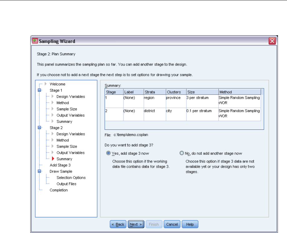
112
Chapter 13
Figure 13-20
Sampling Wizard, Plan Summary step (stage 2)
ESelect Yes,addstage3now.
EClick Next.
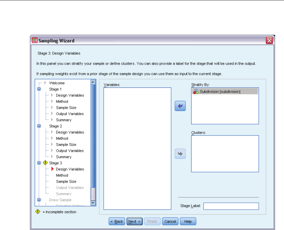
11 3
Complex Samples Sampling Wizard
Figure 13-21
Sampling Wizard, Design Variables step (stage 3)
ESelect Subdivision as a stratification variable.
EClick Next, and then click Next in the Sampling Method step.
This design structure means that independent samples are drawn for each subdivision. In this
stage, household units are drawn as the primary sampling unit using the default method, simple
random sampling.
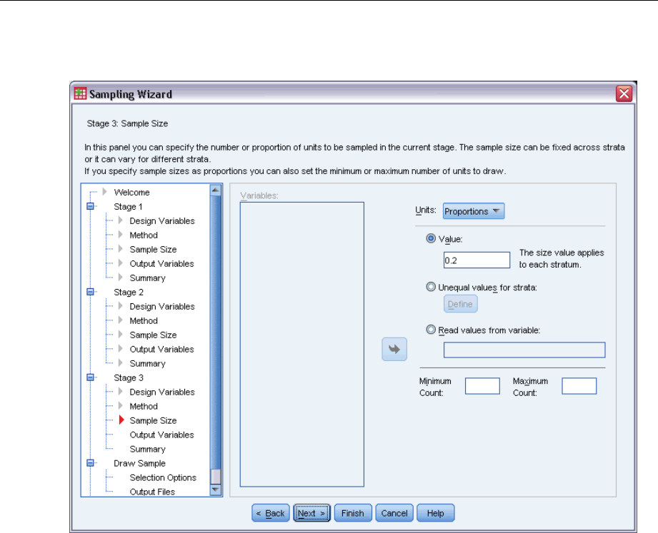
114
Chapter 13
Figure 13-22
Sampling Wizard, Sample Size step (stage 3)
ESelect Proportions from the Units drop-down list.
EType 0.2 as the value for the proportion of units to select in this stage.
EClick Next,andthenclickNext in the Output Variables step.
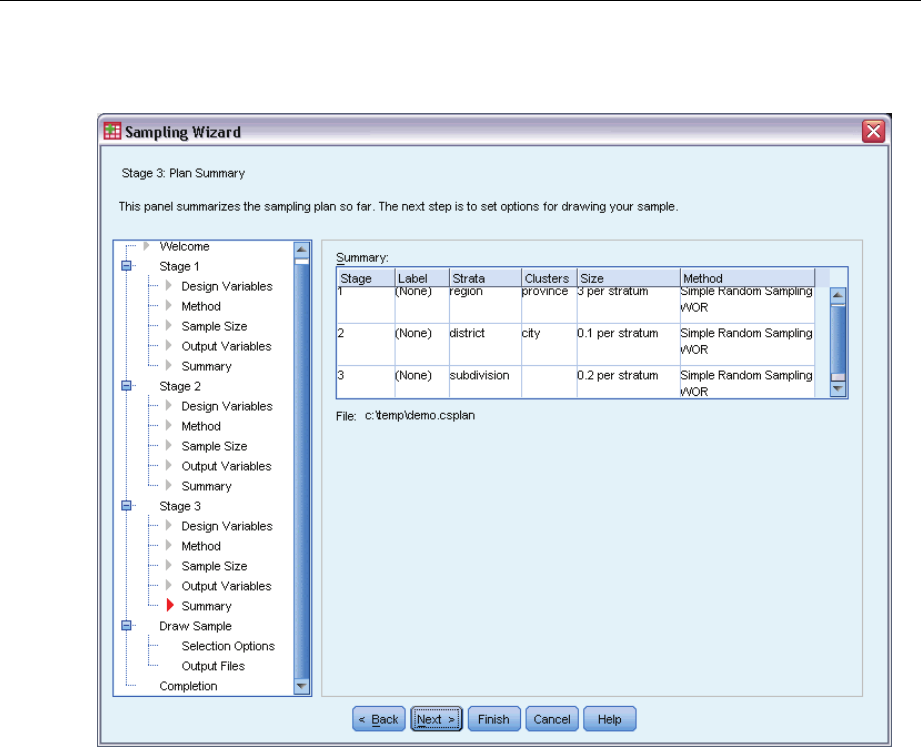
11 5
Complex Samples Sampling Wizard
Figure 13-23
Sampling Wizard, Plan Summary step (stage 3)
ELook over the sampling design, and then click Next.
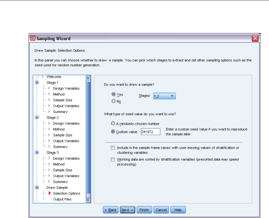
116
Chapter 13
Figure 13-24
Sampling Wizard, Draw Sample Selection Options step
ESelect 1, 2 as the stages to sample now.
ESelect Custom value for the type of random seed to use, and type 241972 as the value.
Using a custom value allows you to replicate the results of this example exactly.
EClick Next, and then click Next intheDrawSampleOutputFilesstep.
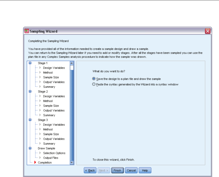
11 7
Complex Samples Sampling Wizard
Figure 13-25
Sampling Wizard, Finish step
EClick Finish.
These selections produce the sampling plan file demo.csplan and draw a sample according to the
first two stages of that plan.
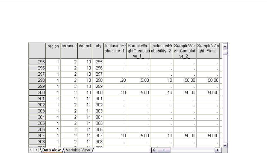
118
Chapter 13
Sample Results
Figure 13-26
Data Editor with sample results
You can see the sampling results in the Data Editor. Five new variables were saved to the working
file, representing the inclusion probabilities and cumulative sampling weights for each stage, plus
the “final” sampling weights for the first two stages.
Cities with values for these variables were selected to the sample.
Cities with system-missing values for the variables were not selected.
For each city selected, the company acquired subdivision and household unit information and
placed it in demo_cs_2.sav. Use this file and the Sampling Wizard to sample the third stage
of this design.
Using the Wizard to Sample from the Second Partial Frame
ETo run the Complex Samples Sampling Wizard, from the menus choose:
Analyze > Complex Samples > Select a Sample...
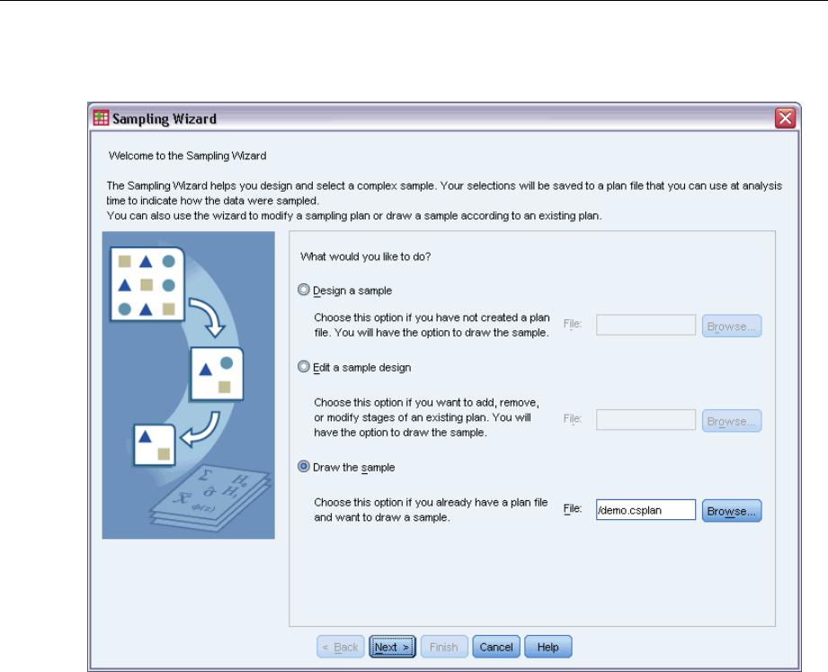
119
Complex Samples Sampling Wizard
Figure 13-27
Sampling Wizard, Welcome step
ESelect Draw a sample, browse to where you saved the plan file, and select the demo.csplan plan
file that you created.
EClick Next.
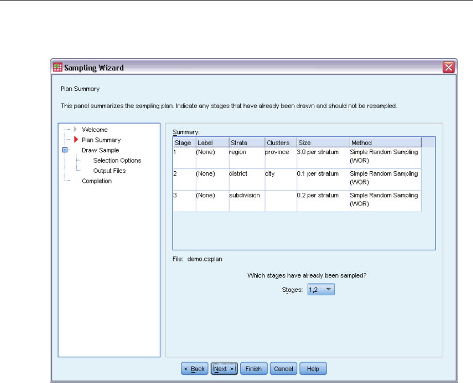
120
Chapter 13
Figure 13-28
Sampling Wizard, Plan Summary step (stage 3)
ESelect 1, 2 as stages already sampled.
EClick Next.
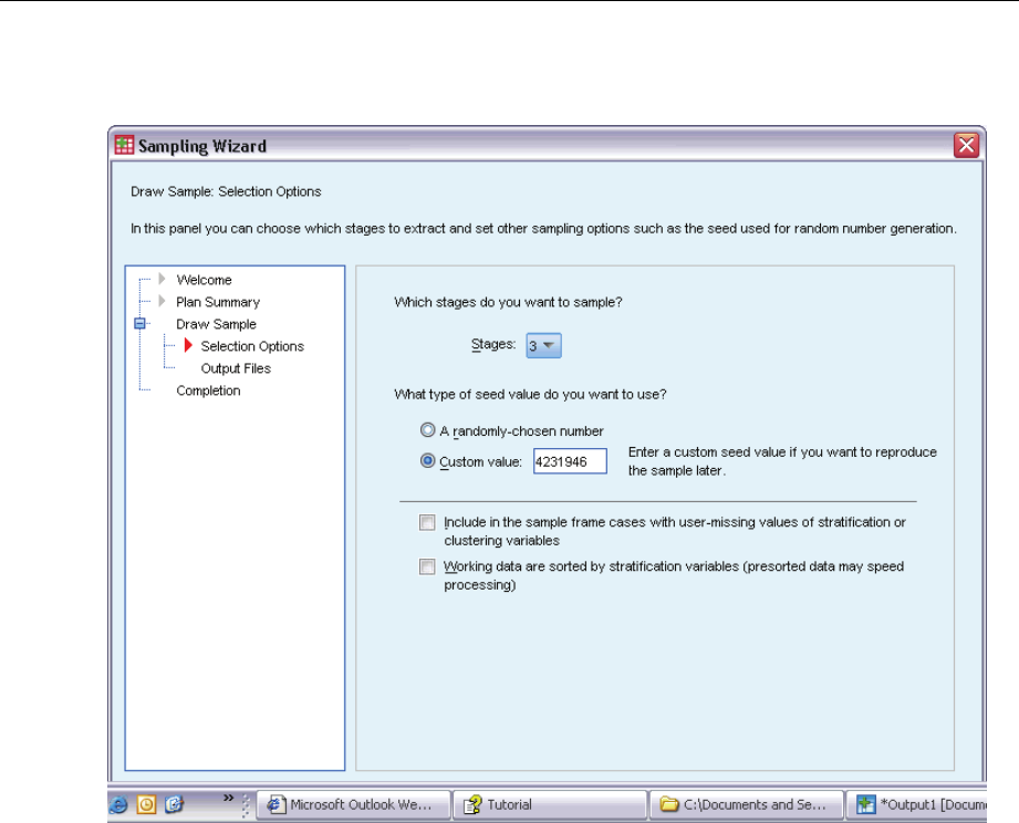
121
Complex Samples Sampling Wizard
Figure 13-29
Sampling Wizard, Draw Sample Selection Options step
ESelect Custom value for the type of random seed to use and type 4231946 as the value.
EClick Next, and then click Next intheDrawSampleOutputFilesstep.
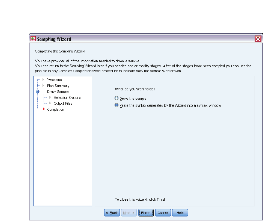
122
Chapter 13
Figure 13-30
Sampling Wizard, Finish step
ESelect Paste the syntax generated by the Wizard into a syntax window.
EClick Finish.
The following syntax is generated:
* Sampling Wizard.
CSSELECT
/PLAN FILE='demo.csplan'
/CRITERIA STAGES = 3 SEED = 4231946
/CLASSMISSING EXCLUDE
/DATA RENAMEVARS
/PRINT SELECTION.
Printing the sampling summary in this case produces a cumbersome table that causes problems in
the Output Viewer. To turn off display of the sampling summary, replace SELECTION with CPS in
the PRINT subcommand. Then run the syntax within the syntax window.
These selections draw a sample according to the third stage of the demo.csplan sampling plan.
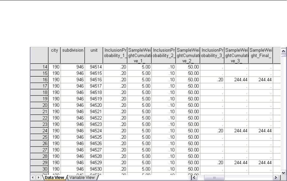
123
Complex Samples Sampling Wizard
Sample Results
Figure 13-31
Data Editor with sample results
You can see the sampling results in the Data Editor. Three new variables were saved to the
working file, representing the inclusion probabilities and cumulative sampling weights for the
third stage, plus the final sampling weights. These new weights take into account the weights
computed during the sampling of the first two stages.
Units with values for these variables were selected to the sample.
Units with system-missing values for these variables were not selected.
The company will now use its resources to obtain survey information for the housing units selected
in the sample. Once the surveys are collected, you can process the sample with Complex Samples
analysis procedures, using the sampling plan demo.csplan to provide the sampling specifications.
Sampling with Probability Proportional to Size (PPS)
Representatives considering a bill before the legislature are interested in whether there is public
support for the bill and how support for the bill is related to voter demographics. Pollsters design
and conduct interviews according to a complex sampling design.
A list of registered voters is collected in poll_cs.sav.For more information, see the topic
Sample Files in Appendix A in IBM SPSS Complex Samples 19.Use theComplexSamples
Sampling Wizard to select a sample for further analysis.
Using the Wizard
ETo run the Complex Samples Sampling Wizard, from the menus choose:
Analyze > Complex Samples > Select a Sample...
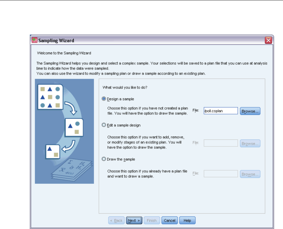
124
Chapter 13
Figure 13-32
Sampling Wizard, Welcome step
ESelect Designasample,browsetowhereyouwanttosavethefile, and type poll.csplan as the
name of the plan file.
EClick Next.
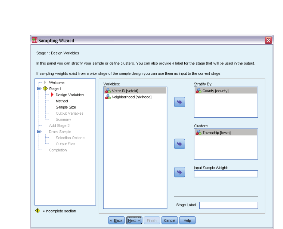
125
Complex Samples Sampling Wizard
Figure 13-33
Sampling Wizard, Design Variables step (stage 1)
ESelect County as a stratification variable.
ESelect Towns hip as a cluster variable.
EClick Next.
This design structure means that independent samples are drawn for each county. In this stage,
townships are drawn as the primary sampling unit.
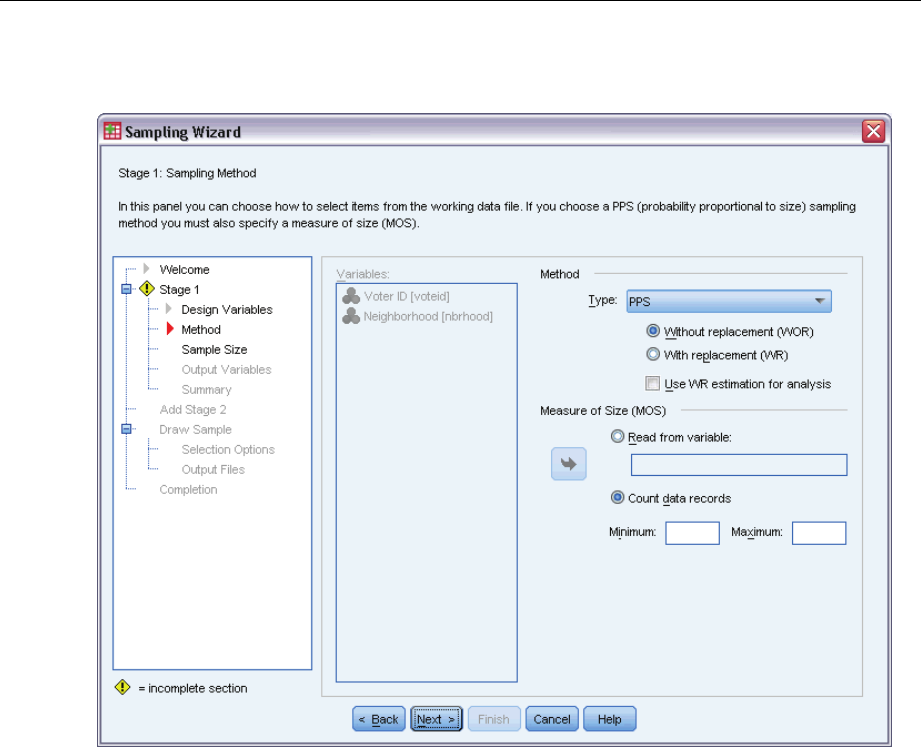
126
Chapter 13
Figure 13-34
SamplingWizard,SamplingMethodstep(stage1)
ESelect PPS as the sampling method.
ESelect Count data records as the measure of size.
EClick Next.
Within each county, townships are drawn without replacement with probability proportional to the
number of records for each township. Using a PPS method generates joint sampling probabilities
for the townships; you will specify where to save these values in the Output Files step.
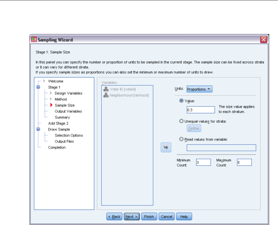
127
Complex Samples Sampling Wizard
Figure 13-35
Sampling Wizard, Sample Size step (stage 1)
ESelect Proportions from the Units drop-down list.
EType 0.3 as the value for the proportion of townships to select per county in this stage.
Legislators from the Western county point out that there are fewer townships in their county than
in others. In order to ensure adequate representation, they would like to establish a minimum of 3
townships sampled from each county.
EType 3as the minimum number of townships to select and 5as the maximum.
EClick Next,andthenclickNext in the Output Variables step.
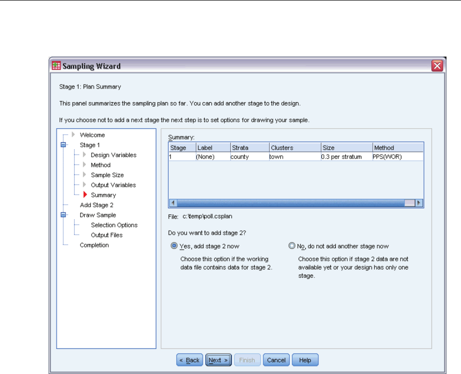
128
Chapter 13
Figure 13-36
Sampling Wizard, Plan Summary step (stage 1)
ESelect Yes,addstage2now.
EClick Next.
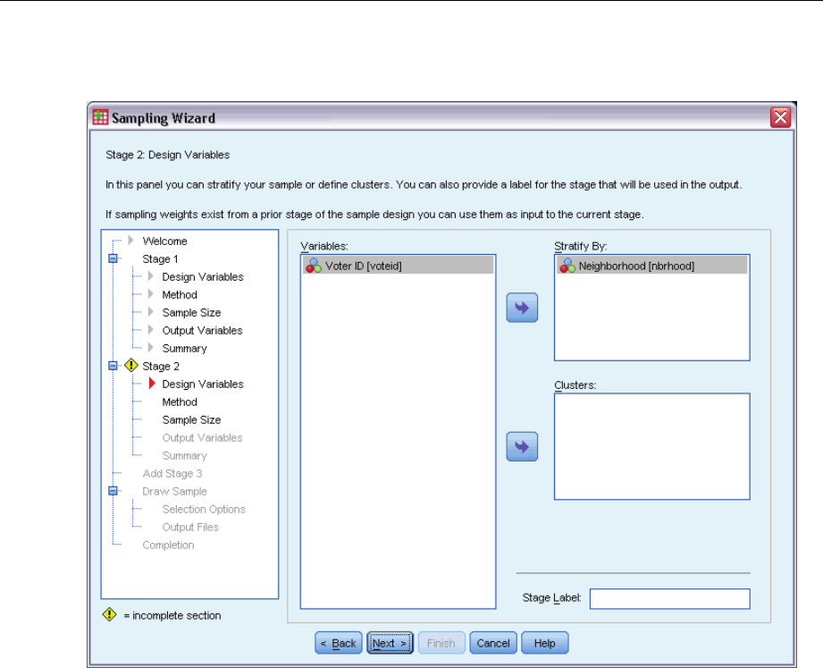
129
Complex Samples Sampling Wizard
Figure 13-37
Sampling Wizard, Design Variables step (stage 2)
ESelect Neighborhood as a stratification variable.
EClick Next, and then click Next in the Sampling Method step.
This design structure means that independent samples are drawn for each neighborhood of the
townships drawn in stage 1. In this stage, voters are drawn as the primary sampling unit using
simple random sampling without replacement.
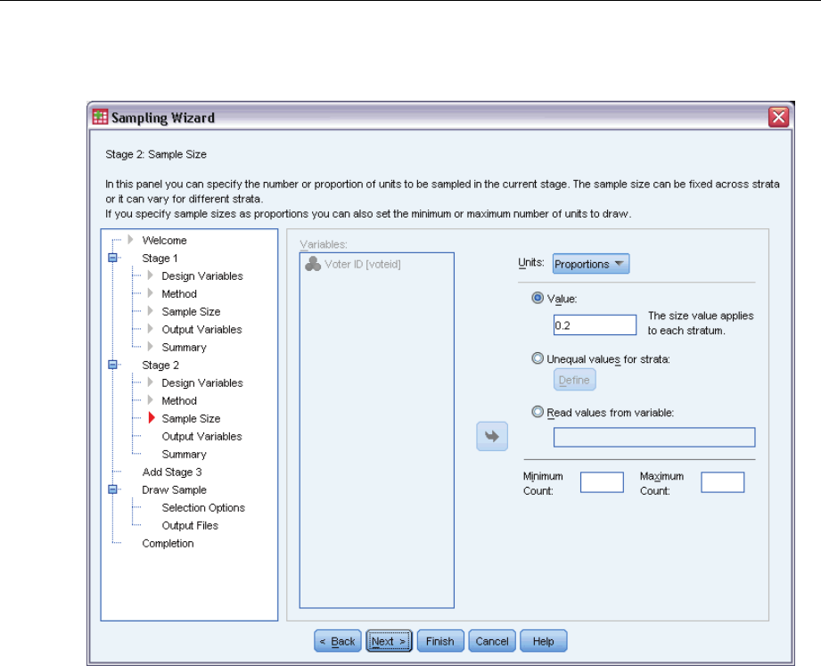
130
Chapter 13
Figure 13-38
Sampling Wizard, Sample Size step (stage 2)
ESelect Proportions from the Units drop-down list.
EType 0.2 as the value of the proportion of units to sample from each strata.
EClick Next,andthenclickNext in the Output Variables step.
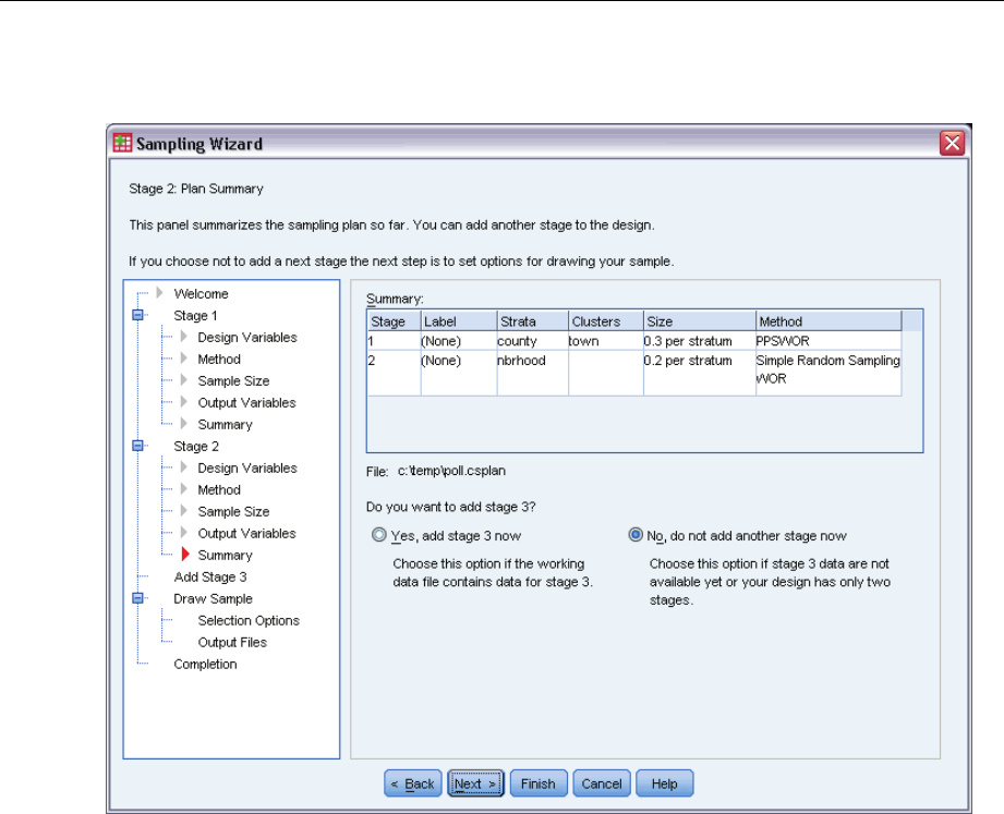
131
Complex Samples Sampling Wizard
Figure 13-39
Sampling Wizard, Plan Summary step (stage 2)
ELook over the sampling design, and then click Next.
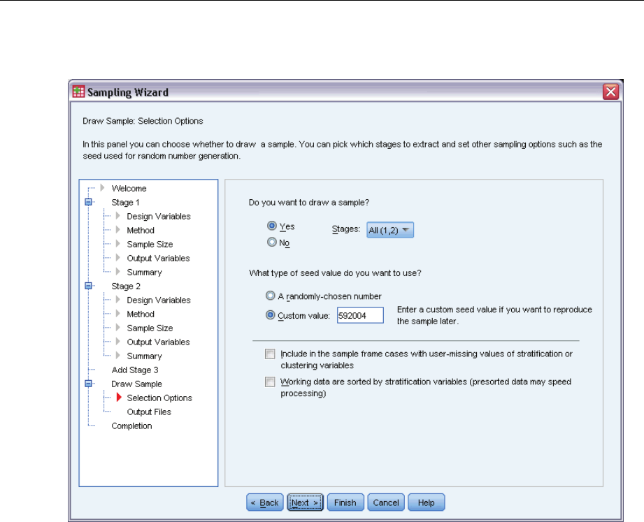
132
Chapter 13
Figure 13-40
Sampling Wizard, Draw Sample Selection Options step
ESelect Custom value for the type of random seed to use, and type 592004 as the value.
Using a custom value allows you to replicate the results of this example exactly.
EClick Next.
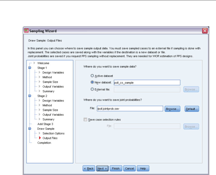
133
Complex Samples Sampling Wizard
Figure 13-41
Sampling Wizard, Draw Sample Selection Options step
EChoose to save the sample to a new dataset, and type poll_cs_sample as the name of the dataset.
EBrowse to where you want to save the joint probabilities and type poll_jointprob.sav as the name
of the joint probabilities file.
EClick Next.

134
Chapter 13
Figure 13-42
Sampling Wizard, Finish step
EClick Finish.
These selections produce the sampling plan file poll.csplan anddrawasampleaccordingtothat
plan, save the sample results to the new dataset poll_cs_sample, and save the joint probabilities
file to the external data file poll_jointprob.sav.
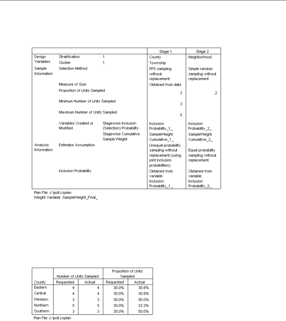
135
Complex Samples Sampling Wizard
Plan Summary
Figure 13-43
Plan summary
The summary table reviews your sampling plan and is useful for making sure that the plan
represents your intentions.
SamplingSummary
Figure 13-44
Stage summary
This summary table reviews the first stage of sampling and is useful for checking that the sampling
went according to plan. Recall that you requested a 30% sample of townships by county; the
actual proportions sampled are close to 30%, except in the Western and Southern counties. This is
because these counties each have only six townships, and you also specified that a minimum of
three townships should be selected per county.
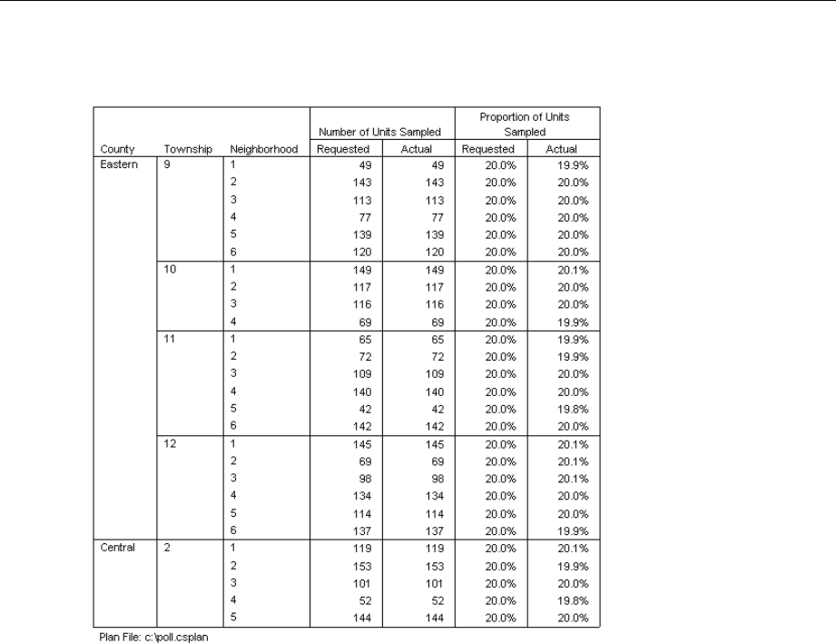
136
Chapter 13
Figure 13-45
Stage summary
This summary table (the top part of which is shown here) reviews the second stage of sampling.
It is also useful for checking that the sampling went according to plan. Approximately 20%
of the voters were sampled from each neighborhood from each township sampled in the first
stage, as requested.
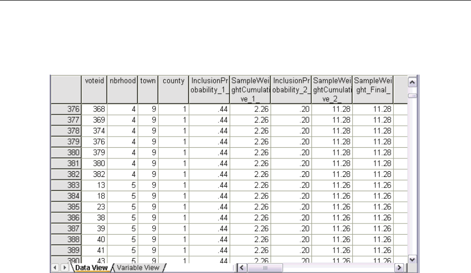
137
Complex Samples Sampling Wizard
Sample Results
Figure 13-46
Data Editor with sample results
You can see the sampling results in the newly created dataset. Five new variables were saved to
the working file, representing the inclusion probabilities and cumulative sampling weights for
each stage, plus the final sampling weights. Voters who were not selected to the sample are
excluded from this dataset.
The final sampling weights are identical for voters within the same neighborhood because they
are selected according to a simple random sampling method within neighborhoods. However, they
are different across neighborhoods within the same township because the sampled proportions are
not exactly 20% in all neighborhoods.
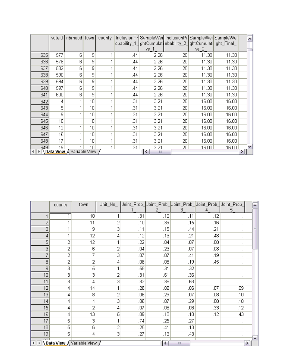
138
Chapter 13
Figure 13-47
Data Editor with sample results
Unlike voters in the second stage, the first-stage sampling weights are not identical for townships
within the same county because they are selected with probability proportional to size.
Figure 13-48
Joint probabilities file
The file poll_jointprob.sav contains first-stage joint probabilities for selected townships within
counties. County is a first-stage stratification variable, and Township is a cluster variable.
Combinations of these variables identify all first-stage PSUs uniquely. Unit_No_ labels PSUs
within each stratum and is used to match up with Joint_Prob_1_,Joint_Prob_2_,Joint_Prob_3_,
Joint_Prob_4_,andJoint_Prob_5_.Thefirst two strata each have 4 PSUs; therefore, the joint

139
Complex Samples Sampling Wizard
inclusion probability matrices are 4×4 for these strata, and the Joint_Prob_5_ column is left empty
for these rows. Similarly, strata 3 and 5 have 3×3 joint inclusion probability matrices, and stratum
4 has a 5×5 joint inclusion probability matrix.
The need for a joint probabilities file is seen by perusing the values of the joint inclusion
probability matrices. When the sampling method is not a PPS WOR method, the selection of a PSU
is independent of the selection of another PSU, and their joint inclusion probability is simply the
product of their inclusion probabilities. In contrast, the joint inclusion probability for Townships 9
and 10 of County 1 is approximately 0.11 (see the first case of Joint_Prob_3_ or the third case of
Joint_Prob_1_), or less than the product of their individual inclusion probabilities (the product of
the first case of Joint_Prob_1_ andthethirdcaseofJoint_Prob_3_ is 0.31×0.44=0.1364).
The pollsters will now conduct interviews for the selected sample. Once the results are
available, you can process the sample with Complex Samples analysis procedures, using the
sampling plan poll.csplan to provide the sampling specifications and poll_jointprob.sav to provide
the needed joint inclusion probabilities.
Related Procedures
The Complex Samples Sampling Wizard procedure is a useful tool for creating a sampling plan
file and drawing a sample.
To ready a sample for analysis when you do not have access to the sampling plan file, use
the Analysis Preparation Wizard.

Chapter
14
Complex Samples Analysis
Preparation Wizard
The Analysis Preparation Wizard guides you through the steps for creating or modifying an
analysis plan for use with the various Complex Samples analysis procedures. It is most useful
when you do not have access to the sampling plan file used to draw the sample.
Using the Complex Samples Analysis Preparation Wizard to Ready
NHIS Public Data
The National Health Interview Survey (NHIS) is a large, population-based survey of the U.S.
civilian population. Interviews are carried out face-to-face in a nationally representative sample
of households. Demographic information and observations about health behavior and status
are obtained for members of each household.
A subset of the 2000 survey is collected in nhis2000_subset.sav.For more information, see
the topic Sample Files in Appendix A in IBM SPSS Complex Samples 19.Use the Complex
Samples Analysis Preparation Wizard to create an analysis plan for this data file so that it can be
processed by Complex Samplesanalysisprocedures.
Using the Wizard
ETo prepare a sample using the Complex Samples Analysis Preparation Wizard, from the menus
choose:
Analyze > Complex Samples > Prepare for Analysis...
© Copyright SPSS Inc. 1989, 2010 140
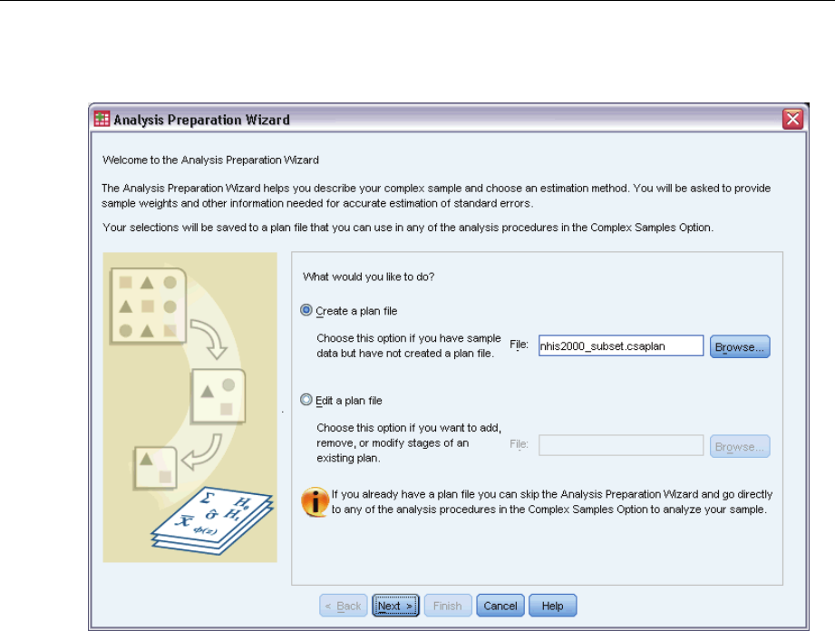
141
Complex Samples Analysis Preparation Wizard
Figure 14-1
Analysis Preparation Wizard, Welcome step
EBrowse to where you want to save the plan file and type nhis2000_subset.csaplan as the name for
the analysis plan file.
EClick Next.
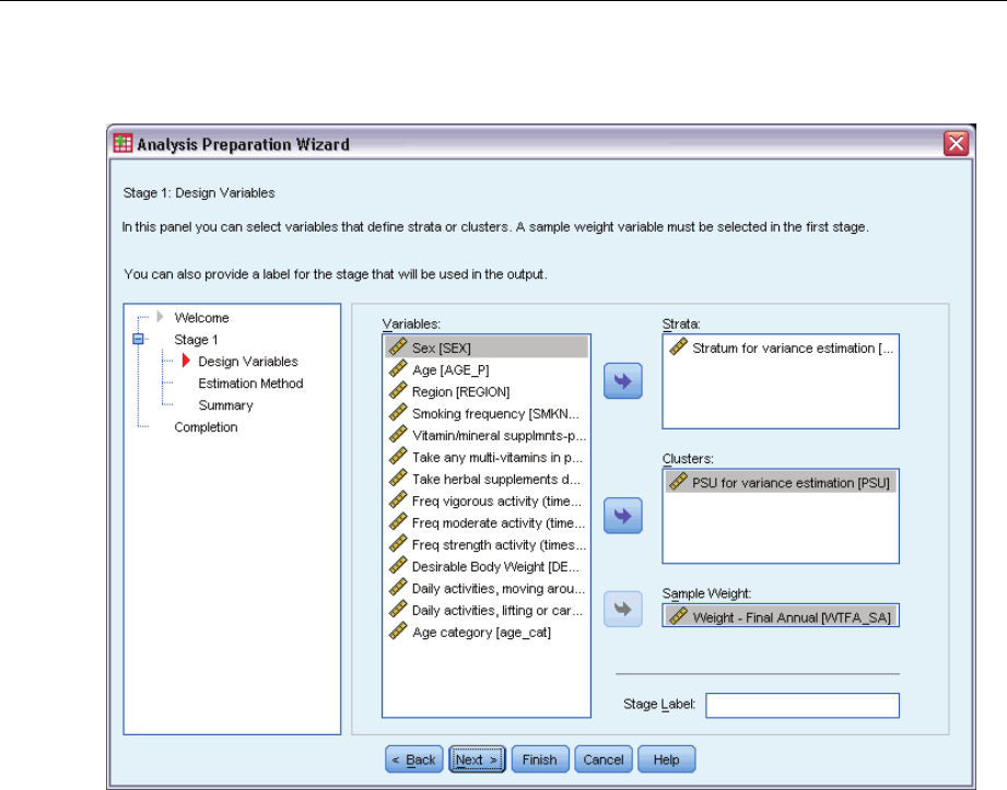
142
Chapter 14
Figure 14-2
Analysis Preparation Wizard, Design Variables step (stage 1)
The data are obtained using a complex multistage sample. However, for end users, the original
NHIS design variables were transformed to a simplified set of design and weight variables whose
results approximate those of the original design structures.
ESelectStratum for variance estimation asastratavariable.
ESelectPSU for variance estimation as a cluster variable.
ESelectWeight - Final Annual as the sample weight variable.
EClick Finish.
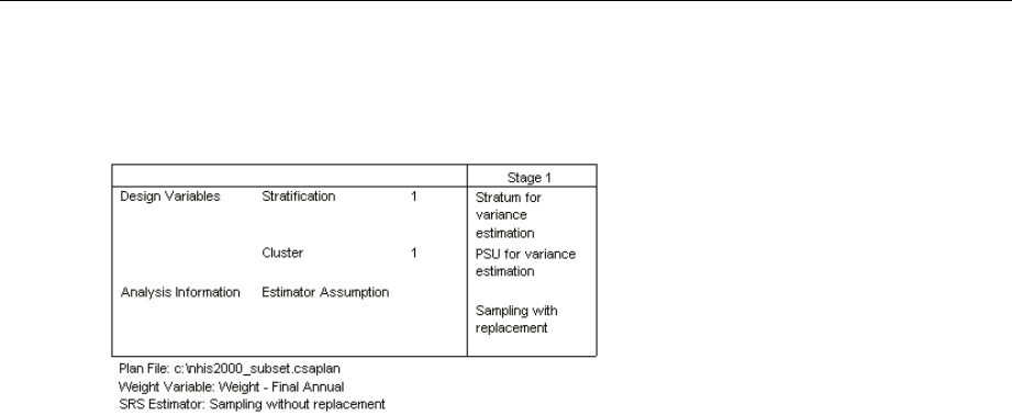
143
Complex Samples Analysis Preparation Wizard
Summary
Figure 14-3
Summary
The summary table reviews your analysis plan. The plan consists of one stage with a design of
one stratification variable and one cluster variable. With-replacement (WR) estimation is used,
and the plan is saved to c:\nhis2000_subset.csaplan. You can now use this plan file to process
nhis2000_subset.sav with Complex Samples analysis procedures.
Preparing for Analysis When Sampling Weights Are Not in the Data File
Aloanofficer has a collection of customer records, taken according to a complex design;
however, the sampling weights are not included in the file. This information is contained in
bankloan_cs_noweights.sav.For more information, see the topic Sample Files in Appendix A in
IBM SPSS Complex Samples 19.Starting with what she knows about the sampling design, the
officer wants to use the Complex Samples Analysis Preparation Wizard to create an analysis plan
for this data file so that it can be processed by ComplexSamplesanalysisprocedures.
The loan officer knows that the records were selected in two stages, with 15 out of 100 bank
branches selected with equal probability and without replacement in the first stage. One hundred
customers were then selected from each of those banks with equal probability and without
replacement in the second stage, and information on the number of customers at each bank is
included in the data file. The first step to creating an analysis plan is to compute the stagewise
inclusion probabilities and final sampling weights.
Computing Inclusion Probabilities and Sampling Weights
ETo compute the inclusion probabilities for the first stage, from the menus choose:
Transform > Compute Variable...
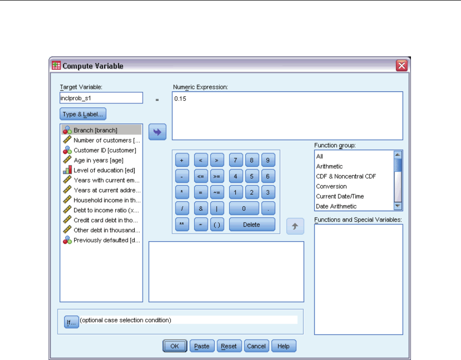
144
Chapter 14
Figure 14-4
Compute Variable dialog box
Fifteen out of one hundred bank branches were selected without replacement in the first stage;
thus, the probability that a given bank was selected is 15/100 = 0.15.
EType inclprob_s1 as the target variable.
EType 0.15 as the numeric expression.
EClick OK.
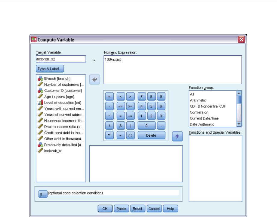
145
Complex Samples Analysis Preparation Wizard
Figure 14-5
Compute Variable dialog box
One hundred customers were selected from each branch in the second stage; thus, the stage
2 inclusion probability for a given customer at a given bank is 100/the number of customers at
that bank.
ERecall the Compute Variable dialog box.
EType inclprob_s2 as the target variable.
EType 100/ncust as the numeric expression.
EClick OK.
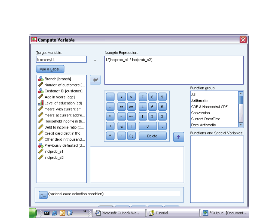
146
Chapter 14
Figure 14-6
Compute Variable dialog box
Now that you have the inclusion probabilities for each stage, it’s easy to compute the final
sampling weights.
ERecall the Compute Variable dialog box.
EType finalweight as the target variable.
EType 1/(inclprob_s1 * inclprob_s2) as the numeric expression.
EClick OK.
You are now ready to create the analysis plan.
Using the Wizard
ETo prepare a sample using the Complex Samples Analysis Preparation Wizard, from the menus
choose:
Analyze > Complex Samples > Prepare for Analysis...
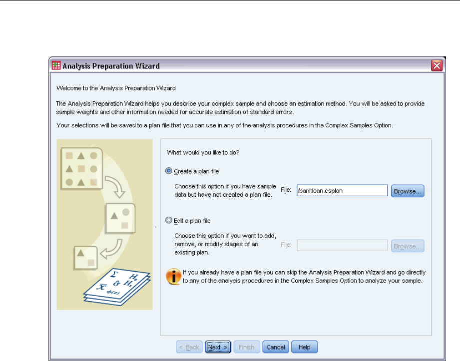
147
Complex Samples Analysis Preparation Wizard
Figure 14-7
Analysis Preparation Wizard, Welcome step
EBrowse to where you want to save the plan file and type bankloan.csaplan asthenameforthe
analysis plan file.
EClick Next.
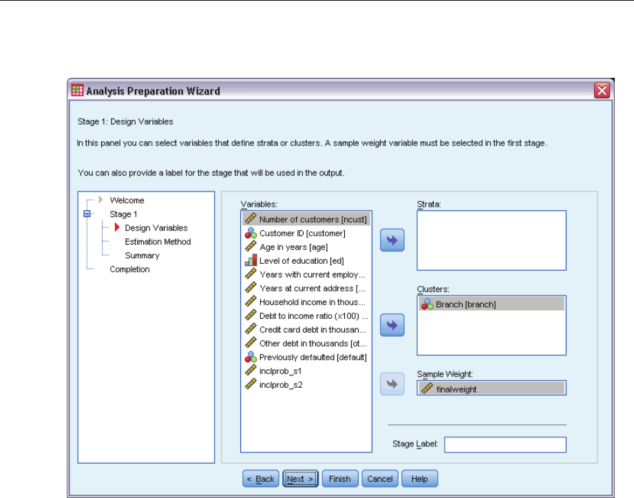
148
Chapter 14
Figure 14-8
Analysis Preparation Wizard, Design Variables step (stage 1)
ESelect Branch as a cluster variable.
ESelect finalweight as the sample weight variable.
EClick Next.
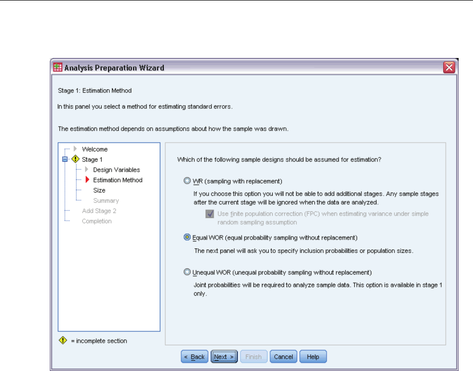
149
Complex Samples Analysis Preparation Wizard
Figure 14-9
Analysis Preparation Wizard, Estimation Method step (stage 1)
ESelect Equal WOR as the first-stage estimation method.
EClick Next.
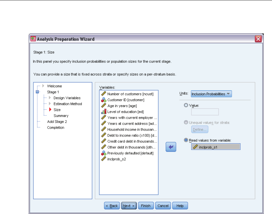
150
Chapter 14
Figure 14-10
Analysis Preparation Wizard, Size step (stage 1)
ESelect Read values from variable and select inclprob_s1 as the variable containing the first-stage
inclusion probabilities.
EClick Next.
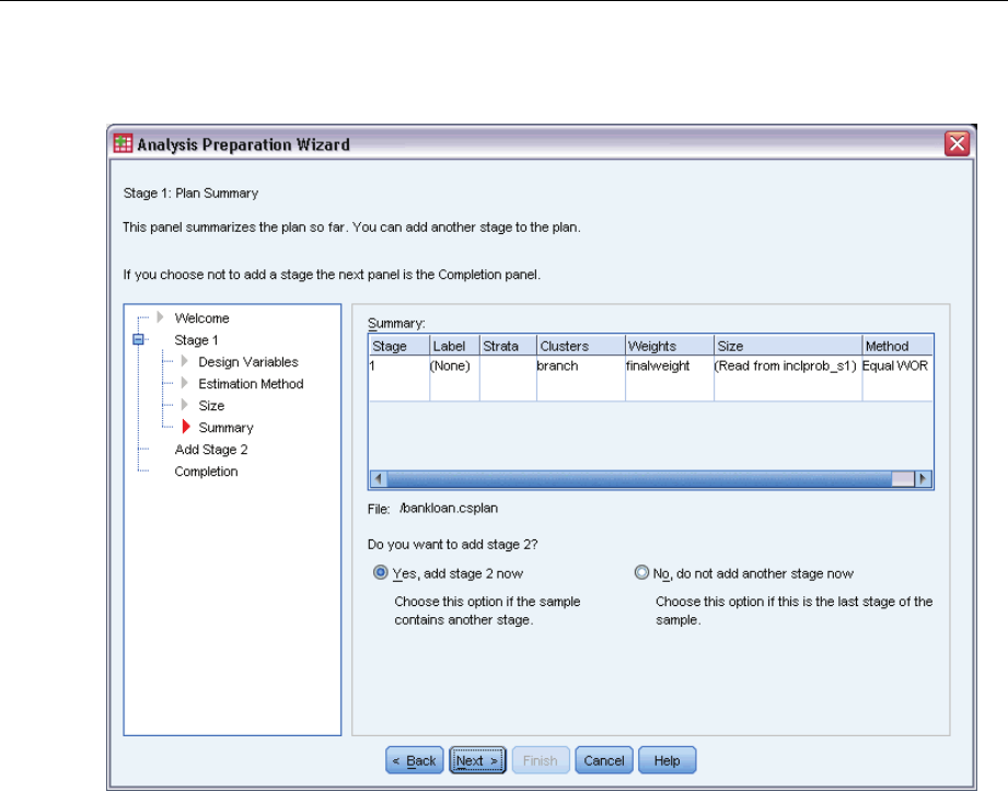
151
Complex Samples Analysis Preparation Wizard
Figure 14-11
Analysis Preparation Wizard, Plan Summary step (stage 1)
ESelect Yes,addstage2now.
EClick Next, and then click Next in the Design Variables step.
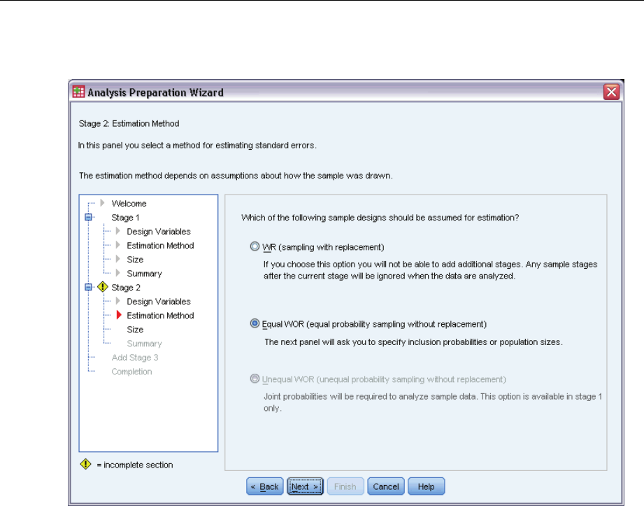
152
Chapter 14
Figure 14-12
Analysis Preparation Wizard, Estimation Method step (stage 2)
ESelect Equal WOR as the second-stage estimation method.
EClick Next.
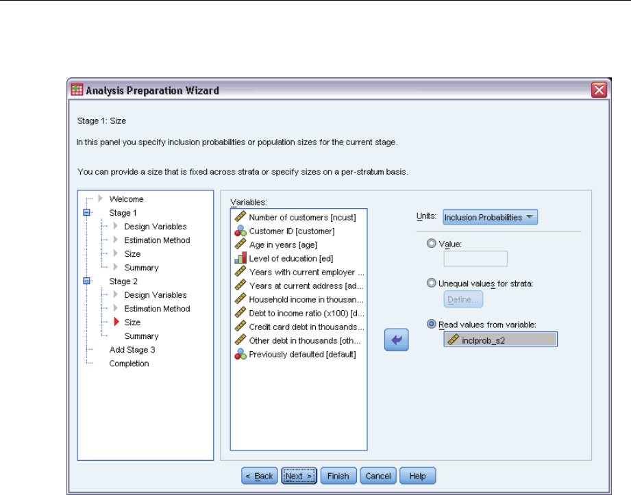
153
Complex Samples Analysis Preparation Wizard
Figure 14-13
Analysis Preparation Wizard, Size step (stage 2)
ESelect Read values from variable and select inclprob_s2 as the variable containing the second-stage
inclusion probabilities.
EClick Finish.
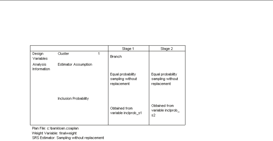
154
Chapter 14
Summary
Figure 14-14
Summary table
The summary table reviews your analysis plan. The plan consists of two stages with a design
of one cluster variable. Equal probability without replacement (WOR) estimation is used,
and the plan is saved to c:\bankloan.csaplan. You can now use this plan file to process
bankloan_noweights.sav (with the inclusion probabilities and sampling weights you’ve computed)
with Complex Samples analysis procedures.
Related Procedures
The Complex Samples Analysis Preparation Wizard procedure is a useful tool for readying a
sample for analysis when you do not have access to the sampling plan file.
To create a sampling plan file and draw a sample, use the Sampling Wizard.

Chapter
15
Complex Samples Frequencies
The Complex Samples Frequencies procedure produces frequency tables for selected variables
and displays univariate statistics. Optionally, you can request statistics by subgroups, defined by
one or more categorical variables.
Using Complex Samples Frequencies to Analyze Nutritional
Supplement Usage
A researcher wants to study the use of nutritional supplements among U.S. citizens, using the
results of the National Health Interview Survey (NHIS) and a previously created analysis plan.
For more information, see the topic Using the Complex Samples Analysis Preparation Wizard to
Ready NHIS Public Data in Chapter 14 on p. 140.
A subset of the 2000 survey is collected in nhis2000_subset.sav. The analysis plan is stored
in nhis2000_subset.csaplan.For more information, see the topic Sample Files in Appendix A
in IBM SPSS Complex Samples 19.Use Complex Samples Frequencies to produce statistics for
nutritional supplement usage.
Running the Analysis
ETo run a Complex Samples Frequencies analysis, from the menus choose:
Analyze > Complex Samples > Frequencies...
© Copyright SPSS Inc. 1989, 2010 155

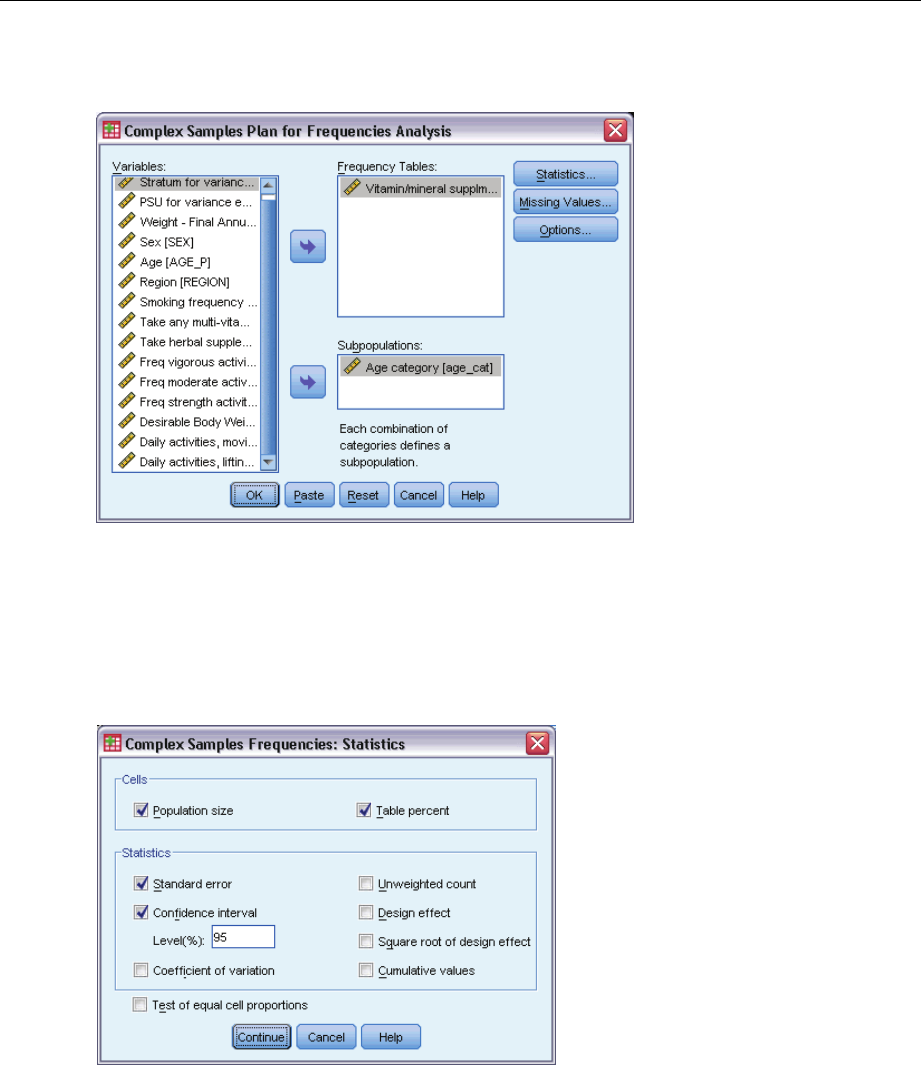
157
Complex Samples Frequencies
Figure 15-2
Frequencies dialog box
ESelect Vitamin/mineral supplmnts-past 12 m as a frequency variable.
ESelect Age category as a subpopulation variable.
EClick Statistics.
Figure 15-3
Frequencies Statistics dialog box
ESelect Ta bl e p e r c e n t in the Cells group.
ESelect Confidence interval in the Statistics group.
EClick Continue.
EClick OK in the Frequencies dialog box.
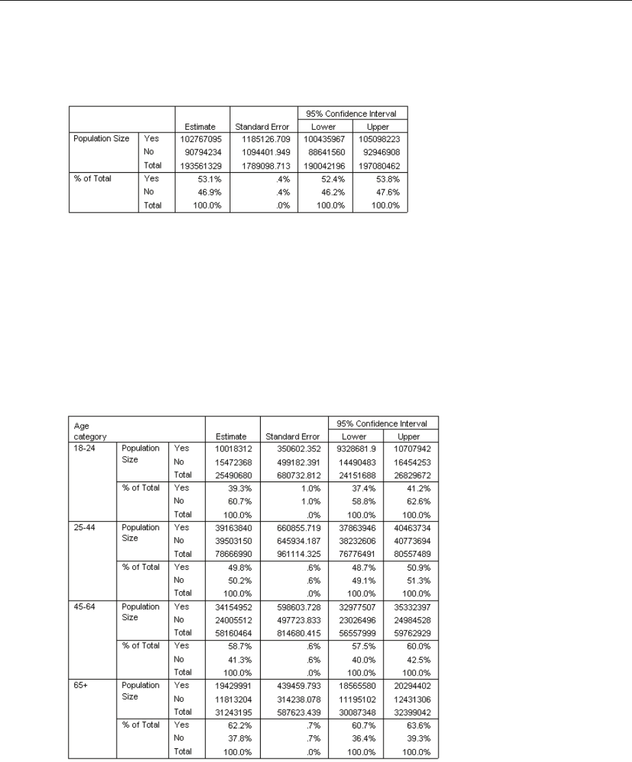
158
Chapter 15
Frequency Table
Figure 15-4
Frequency table for variable/situation
Each selected statistic is computed for each selected cell measure. The first column contains
estimates of the number and percentage of the population that do or do not take vitamin/mineral
supplements. The confidence intervals are non-overlapping; thus, you can conclude that, overall,
more Americans take vitamin/mineral supplements than not.
Frequency by Subpopulation
Figure 15-5
Frequency table by subpopulation
When computing statistics by subpopulation, each selected statistic is computed for each selected
cell measure by value of Age category.Thefirst column contains estimates of the number and
percentage of the population of each category that do or do not take vitamin/mineral supplements.
The confidence intervals for the table percentages are all non-overlapping; thus, you can conclude
that the use of vitamin/mineral supplements increases with age.

159
Complex Samples Frequencies
Summary
Using the Complex Samples Frequencies procedure, you have obtained statistics for the use of
nutritional supplements among U.S. citizens.
Overall, more Americans take vitamin/mineral supplements than not.
When broken down by age category, greater proportions of Americans take vitamin/mineral
supplements with increasing age.
Related Procedures
The Complex Samples Frequencies procedure is a useful tool for obtaining univariate descriptive
statistics of categorical variables for observations obtained via a complex sampling design.
The Complex Samples Sampling Wizard is used to specify complex sampling design
specifications and obtain a sample. The sampling plan file created by the Sampling Wizard
contains a default analysis plan and can be specified in the Plan dialog box when you are
analyzing the sample obtained according to that plan.
The Complex Samples Analysis Preparation Wizard is used to set analysis specifications for
an existing complex sample. The analysis plan file created by the Sampling Wizard can be
specified in the Plan dialog box when you are analyzing the sample corresponding to that plan.
The Complex Samples Crosstabs procedure provides descriptive statistics for the
crosstabulation of categorical variables.
The Complex Samples Descriptives procedure provides univariate descriptive statistics for
scale variables.

Chapter
16
Complex Samples Descriptives
The Complex Samples Descriptives procedure displays univariate summary statistics for several
variables. Optionally, you can request statistics by subgroups, defined by one or more categorical
variables.
Using Complex Samples Descriptives to Analyze Activity Levels
A researcher wants to study the activity levels of U.S. citizens, using the results of the National
Health Interview Survey (NHIS) and a previously created analysis plan. For more information,
see the topic Using the Complex Samples Analysis Preparation Wizard to Ready NHIS Public
Data in Chapter 14 on p. 140.
A subset of the 2000 survey is collected in nhis2000_subset.sav. The analysis plan is stored
in nhis2000_subset.csaplan.For more information, see the topic Sample Files in Appendix A
in IBM SPSS Complex Samples 19.Use Complex Samples Descriptives to produce univariate
descriptive statistics for activity levels.
Running the Analysis
ETo run a Complex Samples Descriptives analysis, from the menus choose:
Analyze > Complex Samples > Descriptives...
© Copyright SPSS Inc. 1989, 2010 160
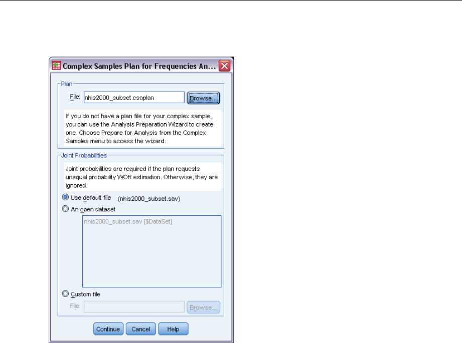
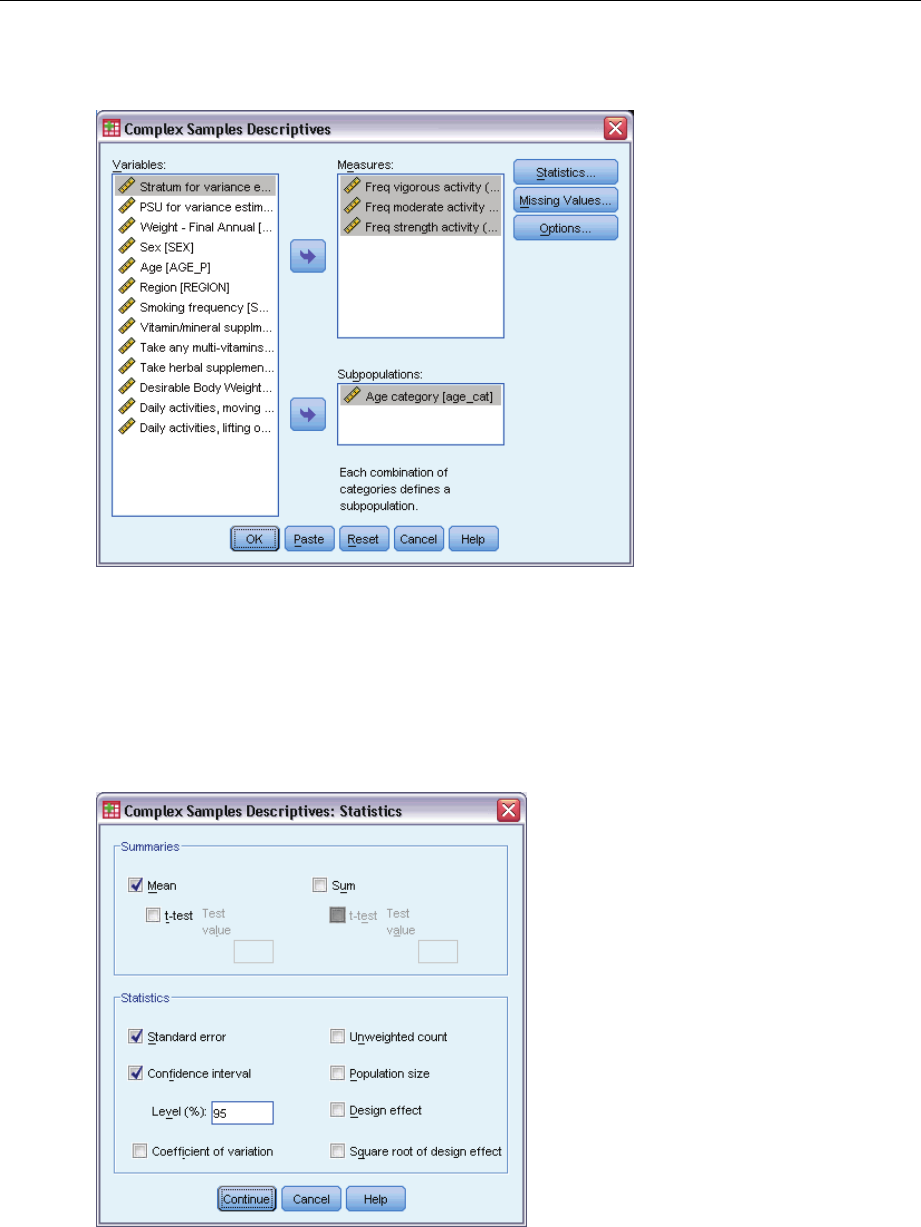
162
Chapter 16
Figure 16-2
Descriptives dialog box
ESelect Freq vigorous activity (times per wk) through Freq strength activity (times per wk) as
measure variables.
ESelect Age category as a subpopulation variable.
EClick Statistics.
Figure 16-3
Descriptives Statistics dialog box
ESelect Confidence interval in the Statistics group.
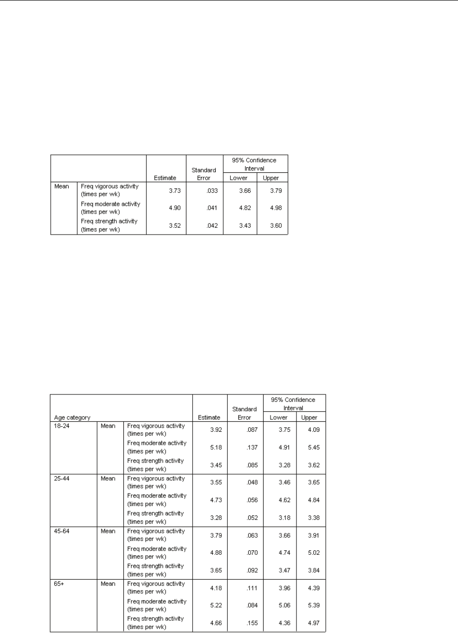
163
Complex Samples Descriptives
EClick Continue.
EClick OK in the Complex Samples Descriptives dialog box.
Univariate Statistics
Figure 16-4
Univariate statistics
Each selected statistic is computed for each measure variable. The first column contains estimates
of the average number of times per week that a person engages in a particular type of activity. The
confidence intervals for the means are non-overlapping. Thus, you can conclude that, overall,
Americans engage in a strength activity less often than vigorous activity, and they engage in
vigorous activity less often than moderate activity.
Univariate Statistics by Subpopulation
Figure 16-5
Univariate statistics by subpopulation

164
Chapter 16
Each selected statistic is computed for each measure variable by values of Age category.Thefirst
column contains estimates of the average number of times per week that people of each category
engage in a particular type of activity. The confidence intervals for the means allow you to make
some interesting conclusions.
In terms of vigorous and moderate activities, 25–44-year-olds are less active than those 18–24
and 45–64, and 45–64-year-olds are less active than those 65 or older.
In terms of strength activity, 25–44-year-olds are less active than those 45–64, and 18–24 and
45–64-year-olds are less active than those 65 or older.
Summary
Using the Complex Samples Descriptives procedure, you have obtained statistics for the activity
levels of U.S. citizens.
Overall, Americans spend varying amounts of time at different types of activities.
When broken down by age, it roughly appears that post-collegiate Americans are initially less
active than they were while in school but become more conscientious about exercising as
they age.
Related Procedures
The Complex Samples Descriptives procedure is a useful tool for obtaining univariate descriptive
statistics of scale measures for observations obtained via a complex sampling design.
The Complex Samples Sampling Wizard is used to specify complex sampling design
specifications and obtain a sample. The sampling plan file created by the Sampling Wizard
contains a default analysis plan and can be specified in the Plan dialog box when you are
analyzing the sample obtained according to that plan.
The Complex Samples Analysis Preparation Wizard is used to set analysis specifications for
an existing complex sample. The analysis plan file created by the Sampling Wizard can be
specified in the Plan dialog box when you are analyzing the sample corresponding to that plan.
The Complex Samples Ratios procedure provides descriptive statistics for ratios of scale
measures.
The Complex Samples Frequencies procedure provides univariate descriptive statistics of
categorical variables.

Chapter
17
Complex Samples Crosstabs
The Complex Samples Crosstabs procedure produces crosstabulation tables for pairs of selected
variables and displays two-way statistics. Optionally, you can request statistics by subgroups,
defined by one or more categorical variables.
Using Complex Samples Crosstabs to Measure the Relative Risk of
an Event
A company that sells magazine subscriptions traditionally sends monthly mailings to a purchased
database of names. The response rate is typically low, so you need to find a way to better
target prospective customers. One suggestion is to focus mailings on people with newspaper
subscriptions, on the assumption that people who read newspapers are more likely to subscribe to
magazines.
Use the Complex Samples Crosstabs procedure to test this theory by constructing a two-by-two
table of Newspaper subscription by Response and computing the relative risk that a person with a
newspaper subscription will respond to the mailing. This information is collected in demo_cs.sav
and should be analyzed using the sampling plan file demo.csplan.For more information, see the
topic Sample Files in Appendix A in IBM SPSS Complex Samples 19.
Running the Analysis
ETo run a Complex Samples Crosstabs analysis, from the menus choose:
Analyze > Complex Samples > Crosstabs...
© Copyright SPSS Inc. 1989, 2010 165

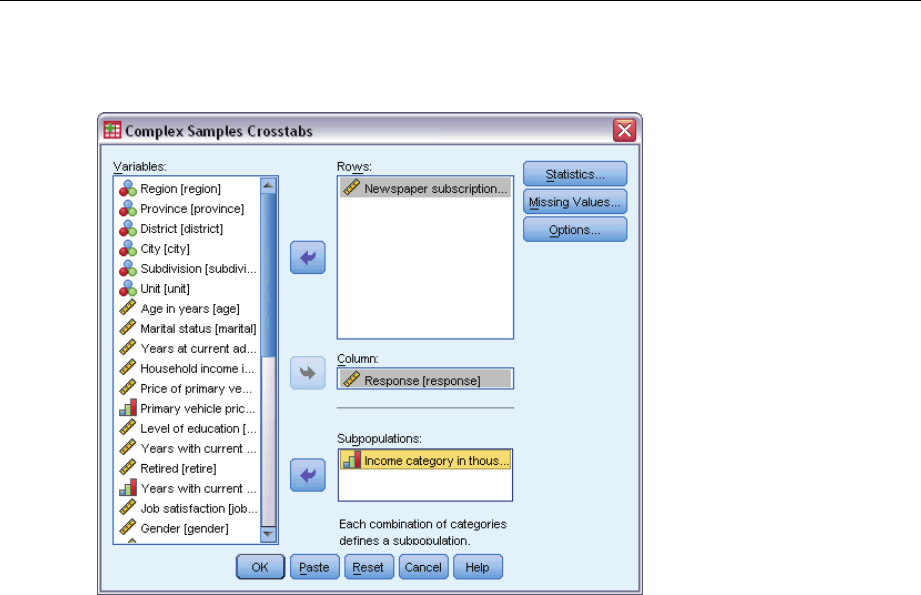
167
Complex Samples Crosstabs
Figure 17-2
Crosstabs dialog box
ESelect Newspaper subscription as a row variable.
ESelect Response as a column variable.
EThere is also some interest in seeing the results broken down by income categories, so select
Income category in thousands as a subpopulation variable.
EClick Statistics.
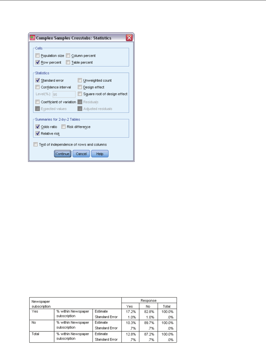
168
Chapter 17
Figure 17-3
Crosstabs Statistics dialog box
EDeselect Population size and select Row percent in the Cells group.
ESelect Odds ratio and Relative risk in the Summaries for 2-by-2 Tables group.
EClick Continue.
EClick OK in the Complex Samples Crosstabs dialog box.
These selections produce a crosstabulation table and risk estimate for Newspaper subscription by
Response. Separate tables with results split by Income category in thousands are also created.
Crosstabulation
Figure 17-4
Crosstabulation for newspaper subscription by response
The crosstabulation shows that, overall, few people responded to the mailing. However, a greater
proportion of newspaper subscribers responded.
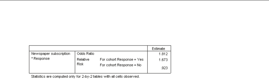
169
Complex Samples Crosstabs
Risk Estimate
Figure 17-5
Risk estimate for newspaper subscription by response
The relative risk is a ratio of event probabilities. The relative risk of a response to the mailing
is the ratio of the probability that a newspaper subscriber responds to the probability that a
nonsubscriber responds. Thus, the estimate of the relative risk is simply 17.2%/10.3% = 1.673.
Likewise, the relative risk of nonresponse is the ratio of the probability that a subscriber does not
respond to the probability that a nonsubscriber does not respond. Your estimate of this relative
risk is 0.923. Given these results, you can estimate that a newspaper subscriber is 1.673 times as
likely to respond to the mailing as a nonsubscriber, or 0.923 times as likely as a nonsubscriber
not to respond.
The odds ratio is a ratio of event odds. The odds of an event is the ratio of the probability that
the event occurs to the probability that the event does not occur. Thus, the estimate of the odds
that a newspaper subscriber responds to the mailing is 17.2%/82.8% = 0.208. Likewise, the
estimate of the odds that a nonsubscriber responds is 10.3%/89.7% = 0.115. The estimate of the
odds ratio is therefore 0.208/0.115 = 1.812 (note there is some rounding error in the intervening
steps). The odds ratio is also the ratio of the relative risk of responding to the relative risk of not
responding, or 1.673/0.923 = 1.812.
Odds Ratio versus Relative Risk
Since it is a ratio of ratios, the odds ratio is very difficult to interpret. The relative risk is easier
to interpret, so the odds ratio alone is not very helpful. However, there are certain commonly
occurring situations in which the estimate of the relative risk is not very good, and the odds ratio
can be used to approximate the relative risk of the event of interest. The odds ratio should be
used as an approximation of the relative risk of the event of interest when both of the following
conditions are met:
The probability of the event of interest is small (< 0.1). This condition guarantees that the
odds ratio will make a good approximation to the relative risk. In this example, the event of
interest is a response to the mailing.
The design of the study is case control. This condition signals that the usual estimate of the
relative risk will likely not be good. A case-control study is retrospective, most often used
when the event of interest is unlikely or when the design of a prospective experiment is
impractical or unethical.
Neither condition is met in this example, since the overall proportion of respondents was 12.8%
and the design of the study was not case control, so it’s safer to report 1.673 as the relative risk,
rather than the value of the odds ratio.
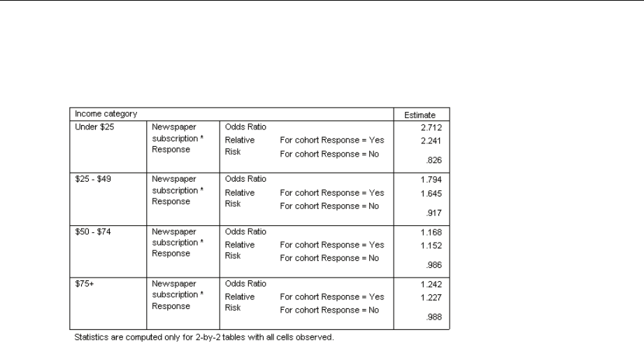
170
Chapter 17
Risk Estimate by Subpopulation
Figure 17-6
Risk estimate for newspaper subscription by response, controlling for income category
Relative risk estimates are computed separately for each income category. Note that the relative
risk of a positive response for newspaper subscribers appears to gradually decrease with increasing
income, which indicates that you may be able to further target the mailings.
Summary
Using Complex Samples Crosstabs risk estimates, you found that you can increase your response
rate to direct mailings by targeting newspaper subscribers. Further, you found some evidence that
the risk estimates may not be constant across Income category,soyoumaybeabletoincrease
your response rate even more by targeting lower-income newspaper subscribers.
Related Procedures
The Complex Samples Crosstabs procedure is a useful tool for obtaining descriptive statistics
of the crosstabulation of categorical variables for observations obtained via a complex sampling
design.
The Complex Samples Sampling Wizard is used to specify complex sampling design
specifications and obtain a sample. The sampling plan file created by the Sampling Wizard
contains a default analysis plan and can be specified in the Plan dialog box when you are
analyzing the sample obtained according to that plan.
The Complex Samples Analysis Preparation Wizard is used to set analysis specifications for
an existing complex sample. The analysis plan file created by the Sampling Wizard can be
specified in the Plan dialog box when you are analyzing the sample corresponding to that plan.
The Complex Samples Frequencies procedure provides univariate descriptive statistics of
categorical variables.

Chapter
18
Complex Samples Ratios
The Complex Samples Ratios procedure displays univariate summary statistics for ratios of
variables. Optionally, you can request statistics by subgroups, defined by one or more categorical
variables.
Using Complex Samples Ratios to Aid Property Value Assessment
A state agency is charged with ensuring that property taxes are fairly assessed from county to
county. Taxes are based on the appraised value of the property, so the agency wants to track
property values across counties to be sure that each county’s records are equally up-to-date.
Since resources for obtaining current appraisals are limited, the agency chose to employ complex
sampling methodology to select properties.
The sample of properties selected and their current appraisal information is collected in
property_assess_cs_sample.sav.For more information, see the topic Sample Files in Appendix A
in IBM SPSS Complex Samples 19.Use Complex Samples Ratios to assess the change in property
values across the five counties since the last appraisal.
Running the Analysis
ETo run a Complex Samples Ratios analysis, from the menus choose:
Analyze > Complex Samples > Ratios...
© Copyright SPSS Inc. 1989, 2010 171
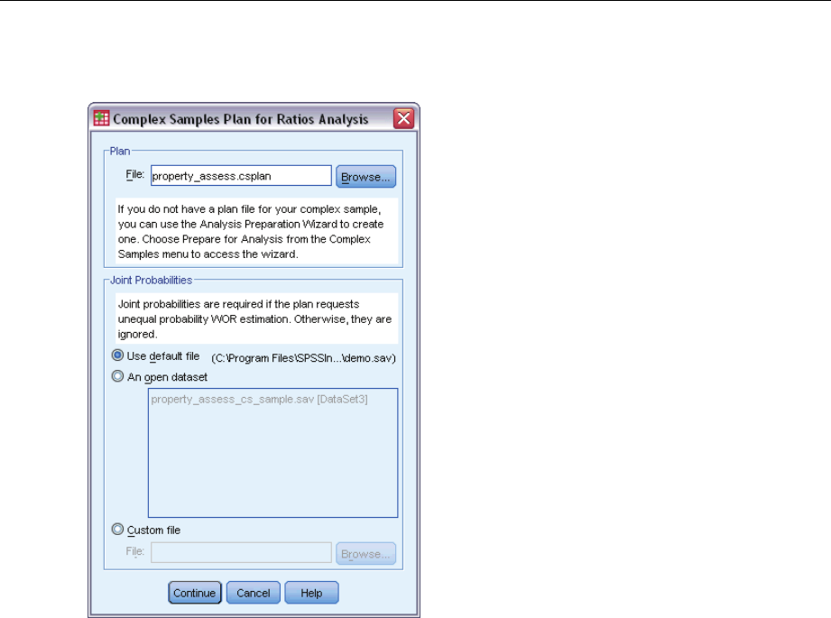
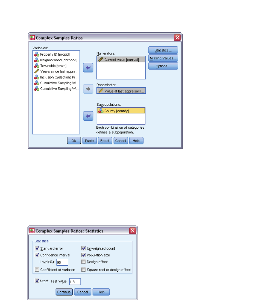
173
Complex Samples Ratios
Figure 18-2
Ratios dialog box
ESelect Current value as a numerator variable.
ESelect Value at last appraisal as the denominator variable.
ESelect County as a subpopulation variable.
EClick Statistics.
Figure 18-3
Ratios Statistics dialog box
ESelect Confidence interval,Unweighted count,andPopulation size in the Statistics group.
ESelect t-test and enter 1.3 as the test value.
EClick Continue.
EClick OK in the Complex Samples Ratios dialog box.
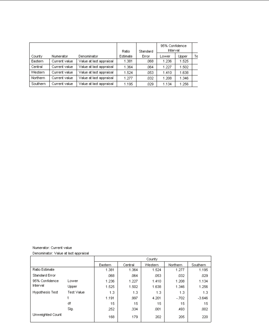
174
Chapter 18
Ratios
Figure 18-4
Ratios table
The default display of the table is very wide, so you will need to pivot it for a better view.
Pivoting the Ratios Table
EDouble-click the table to activate it.
EFrom the Viewer menus choose:
Pivot > Pivoting Trays
EDrag Numerator and then Denominator from the row to the layer.
EDrag County from the row to the column.
EDrag Statistics from the column to the row.
EClose the pivoting trays window.
Pivoted Ratios Table
Figure 18-5
Pivoted ratios table
The ratios table is now pivoted so that statistics are easier to compare across counties.
The ratio estimates range from a low of 1.195 in the Southern county to a high of 1.524 in
the Western county.
There is also quite a bit of variability in the standard errors, which range from a low of 0.029
in the Southern county to 0.068 in the Eastern county.

175
Complex Samples Ratios
Some of the confidence intervals do not overlap; thus, you can conclude that the ratios for the
Western county are higher than the ratios for the Northern and Southern counties.
Finally, as a more objective measure, note that the significance values of the ttests for the
Western and Southern counties are less than 0.05. Thus, you can conclude that the ratio for
the Western county is greater than 1.3 and the ratio for the Southern county is less than 1.3.
Summary
Using the Complex Samples Ratios procedure, you have obtained various statistics for the ratios
of Current value to Value at last appraisal. The results suggest that there may be certain inequities
in the assessment of property taxes from county to county, namely:
The ratios for the Western county are high, indicating that their records are not as up-to-date
as other counties with respect to the appreciation of property values. Property taxes are
probably too low in this county.
The ratios for the Southern county are low, indicating that their records are more up-to-date
than the other counties with respect to the appreciation of property values. Property taxes are
probably too high in this county.
The ratios for the Southern county are lower than those of the Western county but are still
within the objective goal of 1.3.
Resources used to track property values in the Southern county will be reassigned to the Western
county to bring these counties’ ratios in line with the others and with the goal of 1.3.
Related Procedures
The Complex Samples Ratios procedure is a useful tool for obtaining univariate descriptive
statistics of the ratio of scale measures for observations obtained via a complex sampling design.
The Complex Samples Sampling Wizard is used to specify complex sampling design
specifications and obtain a sample. The sampling plan file created by the Sampling Wizard
contains a default analysis plan and can be specified in the Plan dialog box when you are
analyzing the sample obtained according to that plan.
The Complex Samples Analysis Preparation Wizard is used to set analysis specifications for
an existing complex sample. The analysis plan file created by the Sampling Wizard can be
specified in the Plan dialog box when you are analyzing the sample corresponding to that plan.
The Complex Samples Descriptives procedure provides descriptive statistics for scale
variables.

Chapter
19
Complex Samples General Linear
Model
The Complex Samples General Linear Model (CSGLM) procedure performs linear regression
analysis, as well as analysis of variance and covariance, for samples drawn by complex sampling
methods. Optionally, you can request analyses for a subpopulation.
Using Complex Samples General Linear Model to Fit a Two-Factor
ANOVA
A grocery store chain surveyed a set of customers concerning their purchasing habits, according to
a complex design. Given the survey results and how much each customer spent in the previous
month, the store wants to see if the frequency with which customers shop is related to the amount
they spend in a month, controlling for the gender of the customer and incorporating the sampling
design.
This information is collected in grocery_1month_sample.sav.For more information, see the
topic Sample Files in Appendix A in IBM SPSS Complex Samples 19.Use the Complex Samples
General Linear Model procedure to perform a two-factor (or two-way) ANOVA on the amounts
spent.
Running the Analysis
ETo run a Complex Samples General Linear Model analysis, from the menus choose:
Analyze > Complex Samples > General Linear Model...
© Copyright SPSS Inc. 1989, 2010 176
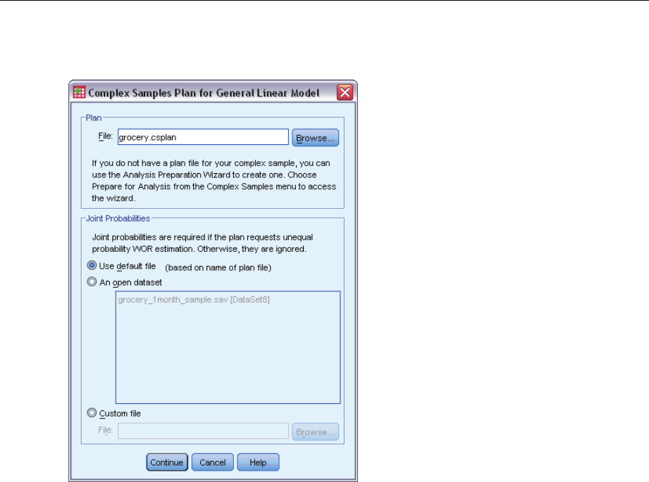

178
Chapter 19
Figure 19-2
General Linear Model dialog box
ESelect Amount spent as the dependent variable.
ESelect Who shopping for and Use coupons as factors.
EClick Model.

179
Complex Samples General Linear Model
Figure 19-3
Model dialog box
EChoose to build a Custom model.
ESelect Main effects as the type of term to build and select shopfor and usecoup as model terms.
ESelect Interaction as the type of term to build and add the shopfor*usecoup interaction as a model
term.
EClick Continue.
EClick Statistics in the General Linear Model dialog box.
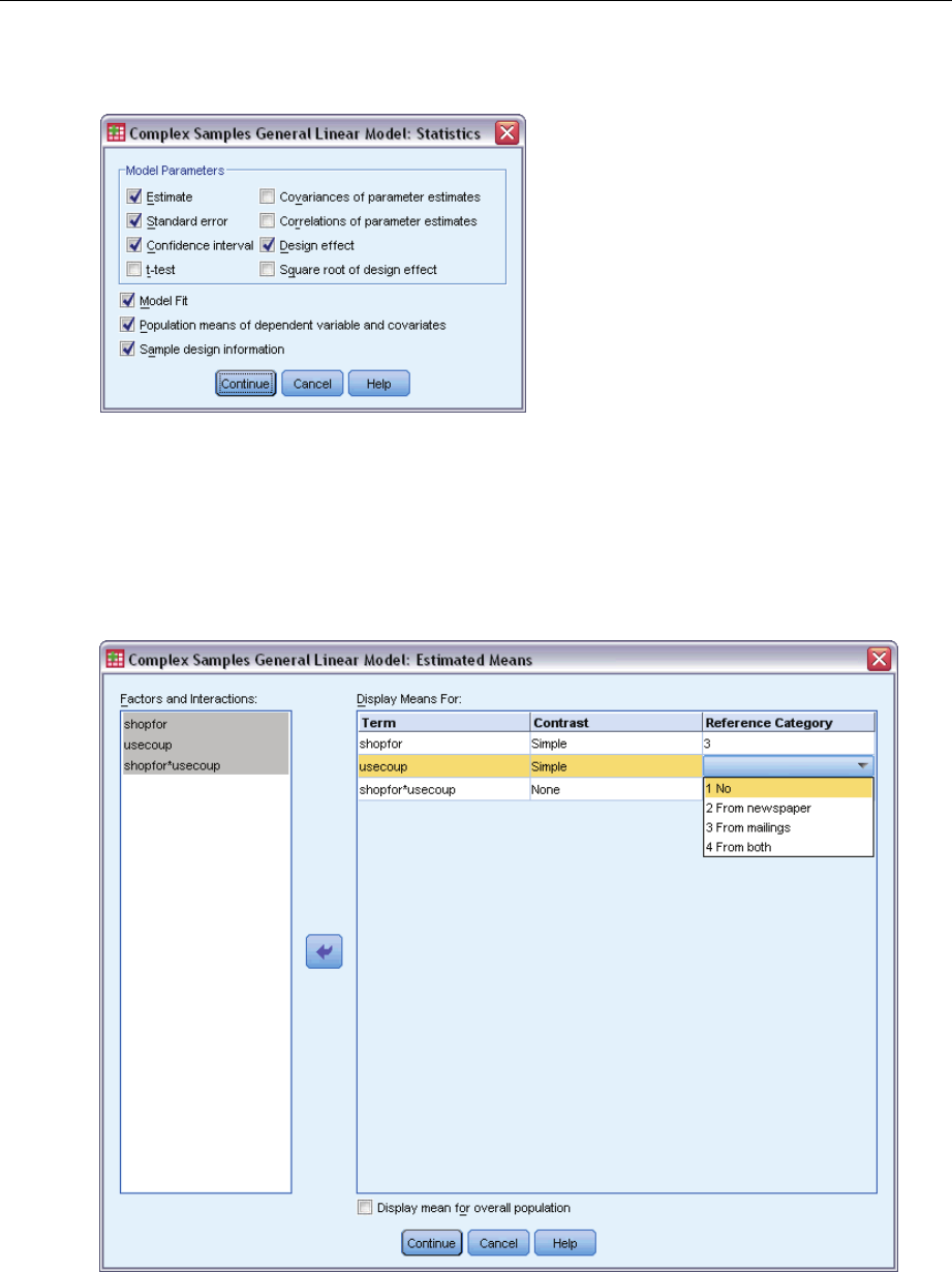
180
Chapter 19
Figure 19-4
General Linear Model Statistics dialog box
ESelect Estimate,Standard error,Confidence interval,andDesign effect in the Model Parameters
group.
EClick Continue.
EClick Estimated Means in the General Linear Model dialog box.
Figure 19-5
General Linear Model Estimated Means dialog box
EChoose to display means for shopfor,usecoup,andtheshopfor*usecoup interaction.
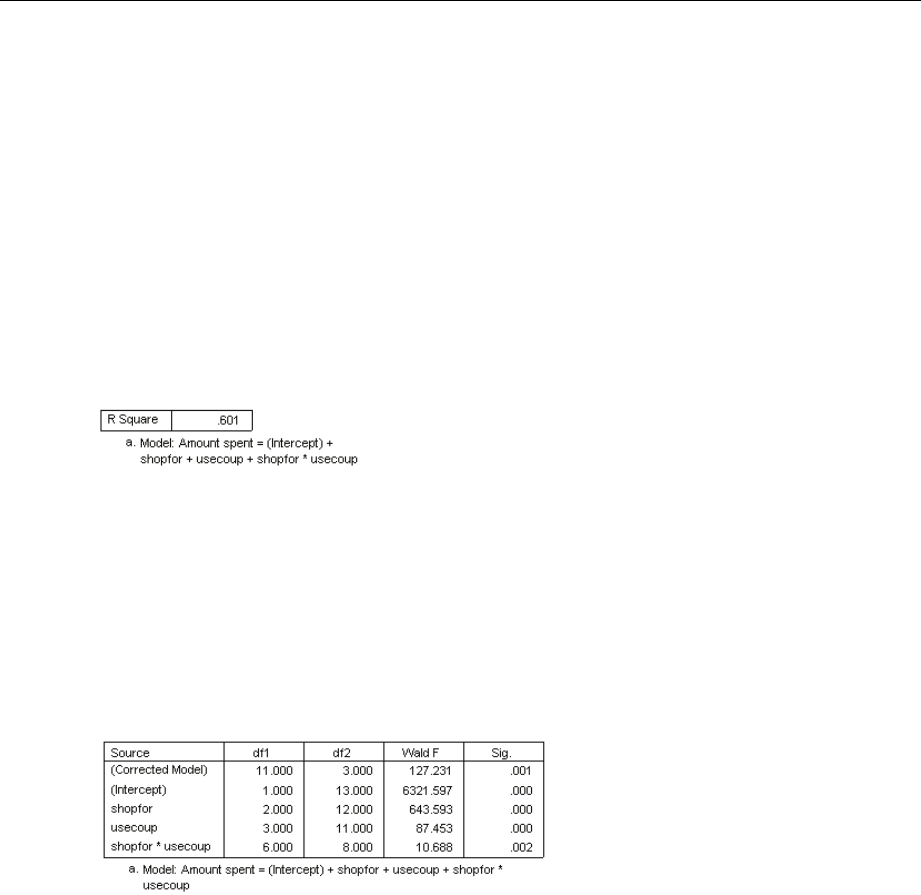
181
Complex Samples General Linear Model
ESelect a Simple contrast and 3 Self and family as the reference category for shopfor. Note that, once
selected, the category appears as “3” in the dialog box.
ESelect a Simple contrast and 1Noas the reference category for usecoup.
EClick Continue.
EClick OK in the General Linear Model dialog box.
Model Summary
Figure 19-6
R-square statistic
R-square, the coefficient of determination, is a measure of the strength of the model fit. It shows
that about 60% of the variation in Amount spent is explained by the model, which gives you
good explanatory ability. You may still want to add other predictors to the model to further
improve the fit.
Tests of Model Effects
Figure 19-7
Tests of between-subjects effects
Each term in the model, plus the model as a whole, is tested for whether the value of its effect
equals 0. Terms with significance values of less than 0.05 have some discernible effect. Thus, all
model terms contribute to the model.
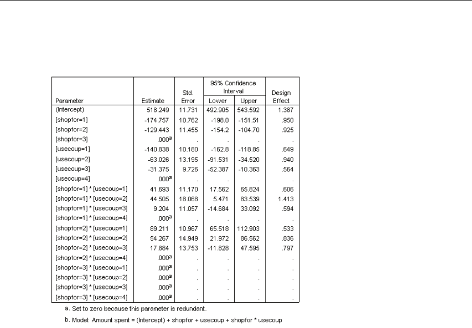
182
Chapter 19
Parameter Estimates
Figure 19-8
Parameter estimates
The parameter estimates show the effect of each predictor on Amount spent. The value of 518.249
for the intercept term indicates that the grocery chain can expect a shopper with a family who uses
coupons from the newspaper and targeted mailings to spend $518.25, on average. You can tell
that the intercept is associated with these factor levels because those are the factor levels whose
parameters are redundant.
The shopfor coefficients suggest that among customers who use both mailed coupons and
newspaper coupons, those without family tend to spend less than those with spouses, who in
turn spend less than those with dependents at home. Since the tests of model effects showed
that this term contributes to the model, these differences are not due to chance.
The usecoup coefficients suggest that spending among customers with dependents at home
decreases with decreased coupon usage. There is a moderate amount of uncertainty in the
estimates, but the confidence intervals do not include 0.
The interaction coefficients suggest that customers who do not use coupons or only clip from
the newspaper and do not have dependents tend to spend more than you would otherwise
expect. If any portion of an interaction parameter is redundant, the interaction parameter is
redundant.
The deviation in the values of the design effects from 1 indicate that some of the standard
errors computed for these parameter estimates are larger than those you would obtain if you
assumed that these observations came from a simple random sample, while others are smaller.
It is vitally important to incorporate the sampling design information in your analysis because
you might otherwise infer, for example, that the usecoup=3 coefficient is not different from 0!
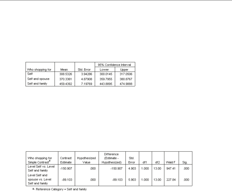
183
Complex Samples General Linear Model
The parameter estimates are useful for quantifying the effect of each model term, but the estimated
marginal means tables can make it easier to interpret the model results.
Estimated Marginal Means
Figure 19-9
Estimated marginal means by levels of Who shopping for
This table displays the model-estimated marginal means and standard errors of Amount spent at
the factor levels of Who shopping for. This table is useful for exploring the differences between
the levels of this factor. In this example, a customer who shops for him- or herself is expected
to spend about $308.53, while a customer with a spouse is expected to spend $370.34, and a
customer with dependents will spend $459.44. To see whether this represents a real difference or
is due to chance variation, look at the test results.
Figure 19-10
Individual test results for estimated marginal means of gender
The individual tests table displays two simple contrasts in spending.
The contrast estimate is the difference in spending for the listed levels of Who shopping for.
The hypothesized value of 0.00 represents the belief that there is no difference in spending.
The Wald Fstatistic, with the displayed degrees of freedom, is used to test whether the
difference between a contrast estimate and hypothesized value is due to chance variation.
Since the significance values are less than 0.05, you can conclude that there are differences in
spending.
The values of the contrast estimates are different from the parameter estimates. This is because
there is an interaction term containing the Who shopping for effect. As a result, the parameter
estimate for shopfor=1 is a simple contrast between the levels Self and Self and Family at the
level From both of the variable Use coupons. The contrast estimate in this table is averaged over
the levels of Use coupons.
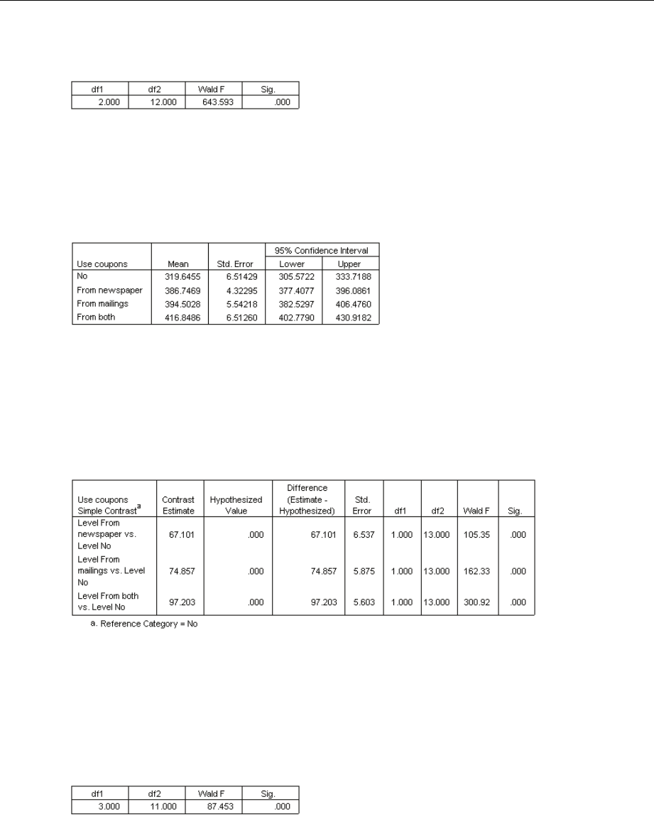
184
Chapter 19
Figure 19-11
Overall test results for estimated marginal means of gender
The overall test table reports the results of a test of all of the contrasts in the individual test table.
Its significance value of less than 0.05 confirms that there is a difference in spending among the
levels of Who shopping for.
Figure 19-12
Estimated marginal means by levels of shopping style
This table displays the model-estimated marginal means and standard errors of Amount spent at
the factor levels of Use coupons. This table is useful for exploring the differences between the
levels of this factor. In this example, a customer who does not use coupons is expected to spend
about $319.65, and those who do use coupons are expected to spend considerably more.
Figure 19-13
Individual test results for estimated marginal means of shopping style
The individual tests table displays three simple contrasts, comparing the spending of customers
who do not use coupons to those who do.
Since the significance values of the tests are less than 0.05, you can conclude that customers
who use coupons tend to spend more than those who don’t.
Figure 19-14
Overall test results for estimated marginal means of shopping style
The overall test table reports the results of a test of all the contrasts in the individual test table. Its
significance value of less than 0.05 confirms that there is a difference in spending among the levels
of Use coupons. Note that the overall tests for Use coupons and Who shopping for are equivalent
to the tests of model effects because the hypothesized contrast values are equal to 0.
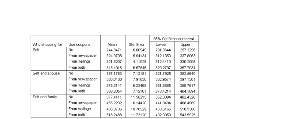
185
Complex Samples General Linear Model
Figure 19-15
Estimated marginal means by levels of gender by shopping style
This table displays the model-estimated marginal means, standard errors, and confidence intervals
of Amount spent at the factor combinations of Who shopping for and Use coupons.Thistable
is useful for exploring the interaction effect between these two factors that was found in the
tests of model effects.
Summary
In this example, the estimated marginal means revealed differences in spending between customers
at varying levels of Who shopping for and Use coupons. The tests of model effects confirmed this,
as well as the fact that there appears to be a Who shopping for*Use coupons interaction effect.
The model summary table revealed that the present model explains somewhat more than half of
the variation in the data and could likely be improved by adding more predictors.
Related Procedures
The Complex Samples General Linear Model procedure is a useful tool for modeling a scale
variable when the cases have been drawn according to a complex sampling scheme.
The Complex Samples Sampling Wizard is used to specify complex sampling design
specifications and obtain a sample. The sampling plan file created by the Sampling Wizard
contains a default analysis plan and can be specified in the Plan dialog box when you are
analyzing the sample obtained according to that plan.
The Complex Samples Analysis Preparation Wizard is used to specify analysis specifications
for an existing complex sample. The analysis plan file created by the Sampling Wizard can be
specified in the Plan dialog box when you are analyzing the sample corresponding to that plan.
The Complex Samples Logistic Regression procedure allows you to model a categorical
response.
The Complex Samples Ordinal Regression procedure allows you to model an ordinal response.

Chapter
20
Complex Samples Logistic Regression
The Complex Samples Logistic Regression procedure performs logistic regression analysis on
a binary or multinomial dependent variable for samples drawn by complex sampling methods.
Optionally, you can request analyses for a subpopulation.
Using Complex Samples Logistic Regression to Assess Credit Risk
If you are a loan officer at a bank, you want to be able to identify characteristics that are indicative
of people who are likely to default on loans and then use those characteristics to identify good
and bad credit risks.
Suppose that a loan officer has collected past records of customers given loans at
several different branches, according to a complex design. This information is contained in
bankloan_cs.sav.For more information, see the topic Sample Files in Appendix A in IBM SPSS
Complex Samples 19.The officer wants to see if the probability with which a customer defaults is
related to age, employment history, and amount of credit debt, incorporating the sampling design.
Running the Analysis
ETo create the logistic regression model, from the menus choose:
Analyze > Complex Samples > Logistic Regression...
© Copyright SPSS Inc. 1989, 2010 186
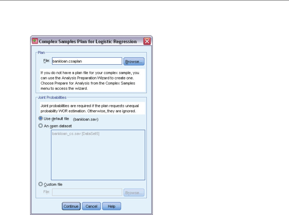
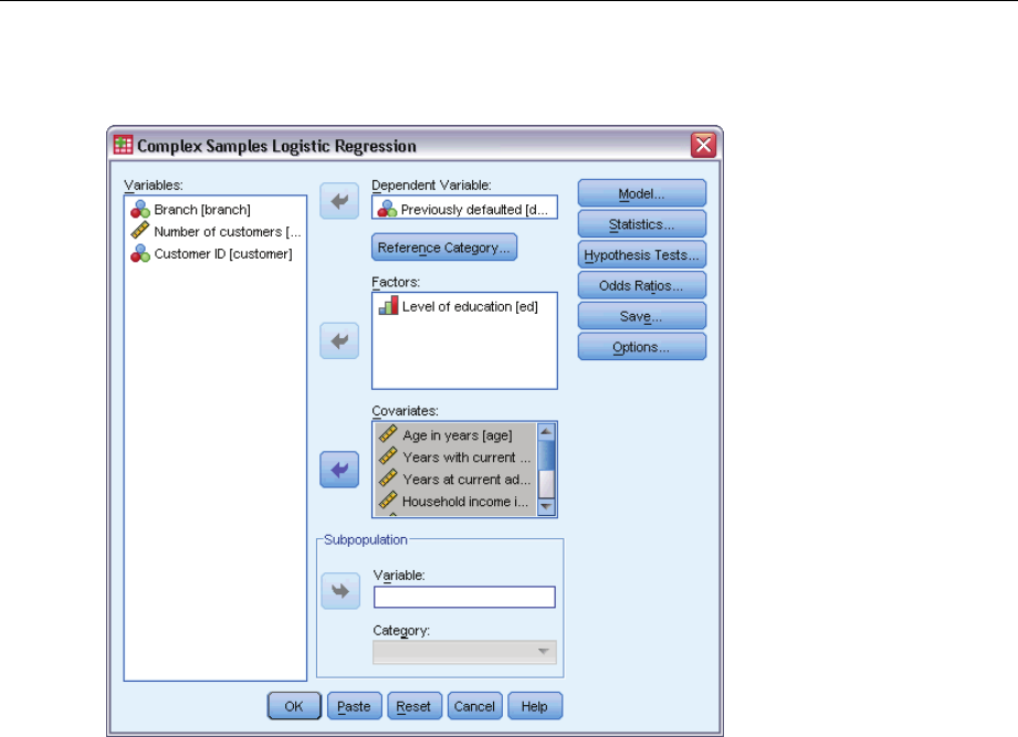
188
Chapter 20
Figure 20-2
Logistic Regression dialog box
ESelect Previously defaulted as the dependent variable.
ESelect Level of education as a factor.
ESelect Age in years through Other debt in thousands as covariates.
ESelect Previously defaulted and click Reference Category.
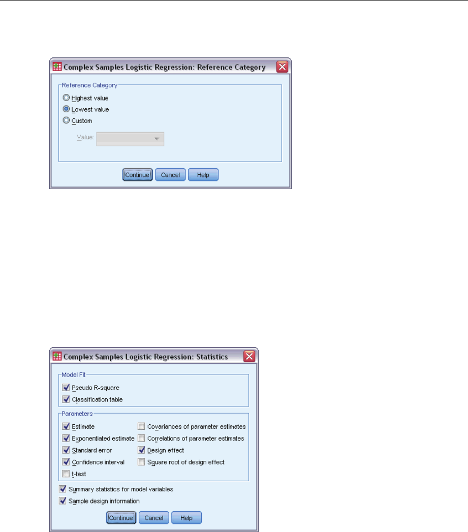
189
Complex Samples Logistic Regression
Figure 20-3
Logistic Regression Reference Category dialog box
ESelect Lowest value as the reference category.
This sets the “did not default” category as the reference category; thus, the odds ratios reported in
the output will have the property that increasing odds ratios correspond to increasing probability
of default.
EClick Continue.
EClick Statistics in the Logistic Regression dialog box.
Figure 20-4
Logistic Regression Statistics dialog box
ESelect Classification table in the Model Fit group
ESelect Estimate,Exponentiated estimate,Standard error,Confidence interval,andDesign effect in
the Parameters group.
EClick Continue.
EClick Odds Ratios in the Logistic Regression dialog box.
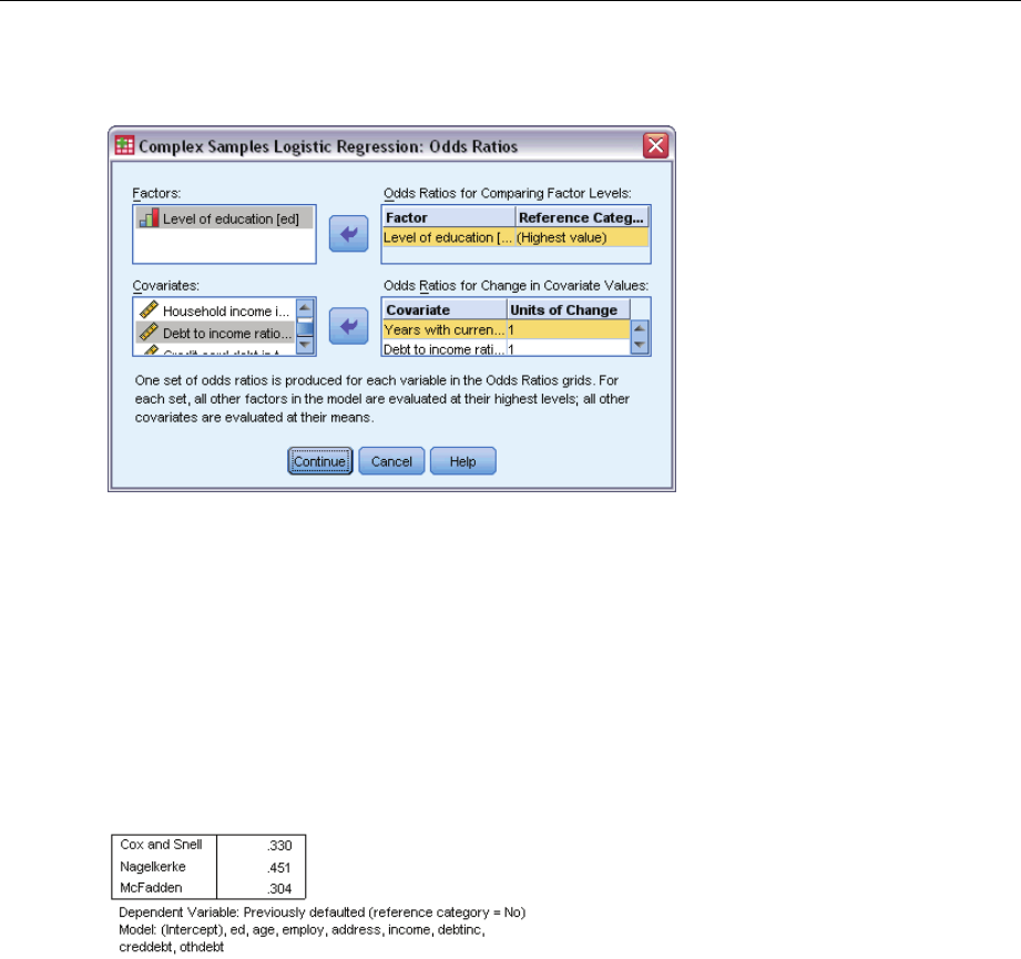
190
Chapter 20
Figure 20-5
Logistic Regression Odds Ratios dialog box
EChoose to create odds ratios for the factor ed and the covariates employ and debtinc.
EClick Continue.
EClick OK in the Logistic Regression dialog box.
Pseudo R-Squares
Figure 20-6
Pseudo R-square statistics
In the linear regression model, the coefficient of determination, R2, summarizes the proportion of
variance in the dependent variable associated with the predictor (independent) variables, with
larger R2values indicating that more of the variation is explained by the model, to a maximum
of 1. For regression models with a categorical dependent variable, it is not possible to compute
asingleR2statistic that has all of the characteristics of R2in the linear regression model, so
these approximations are computed instead. The following methods are used to estimate the
coefficient of determination.
Cox and Snell’s R2(Cox and Snell, 1989) is based on the log likelihood for the model
compared to the log likelihood for a baseline model. However, with categorical outcomes, it
has a theoretical maximum value of less than 1, even for a “perfect” model.
Nagelkerke’s R2(Nagelkerke, 1991) is an adjusted version of the Cox & Snell R-square that
adjusts the scale of the statistic to cover the full range from 0 to 1.
McFadden’s R2(McFadden, 1974) is another version, based on the log-likelihood kernels for
the intercept-only model and the full estimated model.
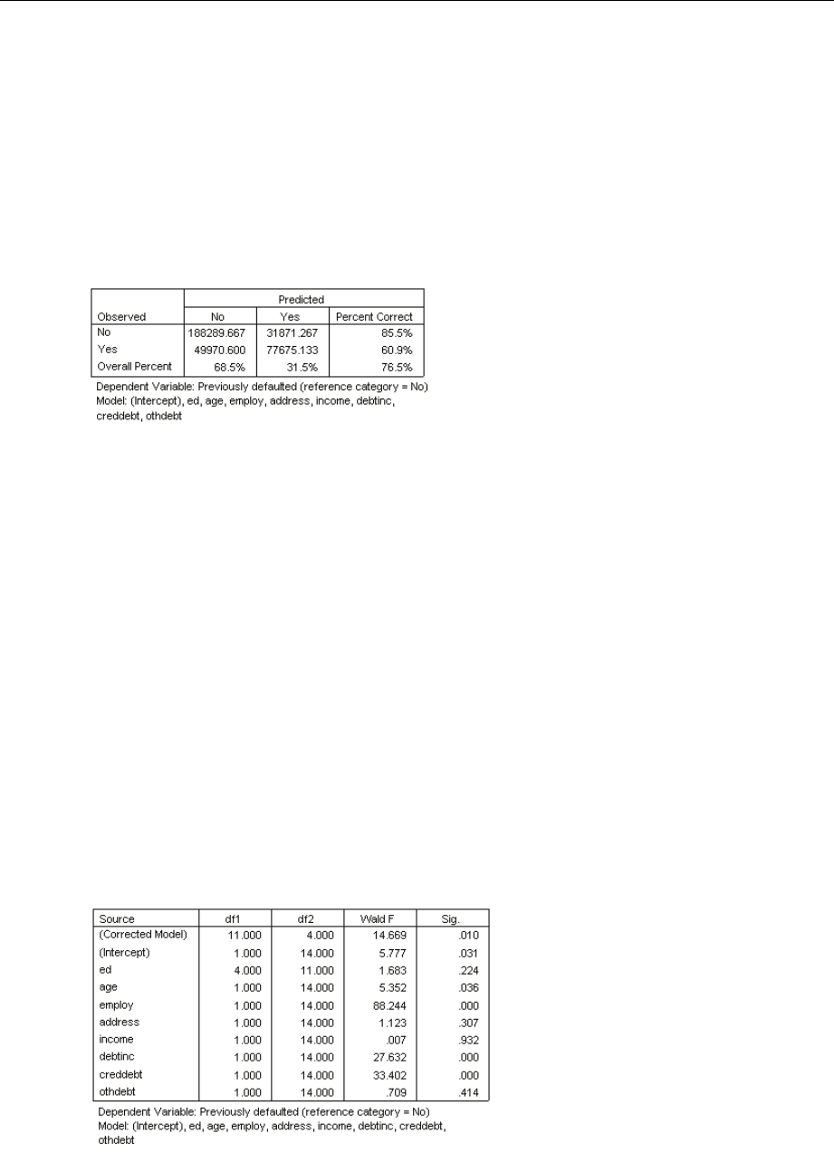
191
Complex Samples Logistic Regression
What constitutes a “good” R2value varies between different areas of application. While these
statistics can be suggestive on their own, they are most useful when comparing competing models
for the same data. The model with the largest R2statistic is “best” according to this measure.
Classification
Figure 20-7
Classification table
The classification table shows the practical results of using the logistic regression model. For each
case, the predicted response is Yes if that case’s model-predicted logit is greater than 0. Cases are
weighted by finalweight, so that the classification table reports the expected model performance in
the population.
Cells on the diagonal are correct predictions.
Cells off the diagonal are incorrect predictions.
Based upon the cases used to create the model, you can expect to correctly classify 85.5% of the
nondefaulters in the population using this model. Likewise, you can expect to correctly classify
60.9% of the defaulters. Overall, you can expect to classify 76.5% of the cases correctly; however,
because this table was constructed with the cases used to create the model, these estimates are
likely to be overly optimistic.
Tests of Model Effects
Figure 20-8
Tests of between-subjects effects
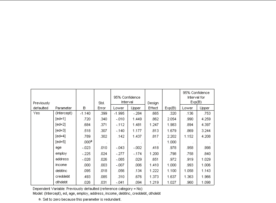
192
Chapter 20
Each term in the model, plus the model as a whole, is tested for whether its effect equals 0. Terms
with significance values less than 0.05 have some discernible effect. Thus, age,employ,debtinc,
and creddebt contribute to the model, while the other main effects do not. In a further analysis of
the data, you would probably remove ed,address,income,andothdebt from model consideration.
Parameter Estimates
Figure 20-9
Parameter estimates
The parameter estimates table summarizes the effect of each predictor. Note that parameter values
affect the likelihood of the “did default” category relative to the “did not default” category. Thus,
parameters with positive coefficients increase the likelihood of default, while parameters with
negative coefficients decrease the likelihood of default.
The meaning of a logistic regression coefficient is not as straightforward as that of a linear
regression coefficient. While Bis convenient for testing the model effects, Exp(B) is easier to
interpret. Exp(B) represents the ratio change in the odds of the event of interest attributable to a
one-unit increase in the predictor for predictors that are not part of interaction terms. For example,
Exp(B) for employ is equal to 0.798, which means that the odds of default for people who have
been with their current employer for two years are 0.798 times the odds of default for those who
have been with their current employer for one year, all other things being equal.
The design effects indicate that some of the standard errors computed for these parameter
estimates are larger than those you would obtain if you assumed that these observations came
from a simple random sample, while others are smaller. It is vitally important to incorporate the
sampling design information in your analysis because you might otherwise infer, for example,
that the age coefficient is no different from 0!
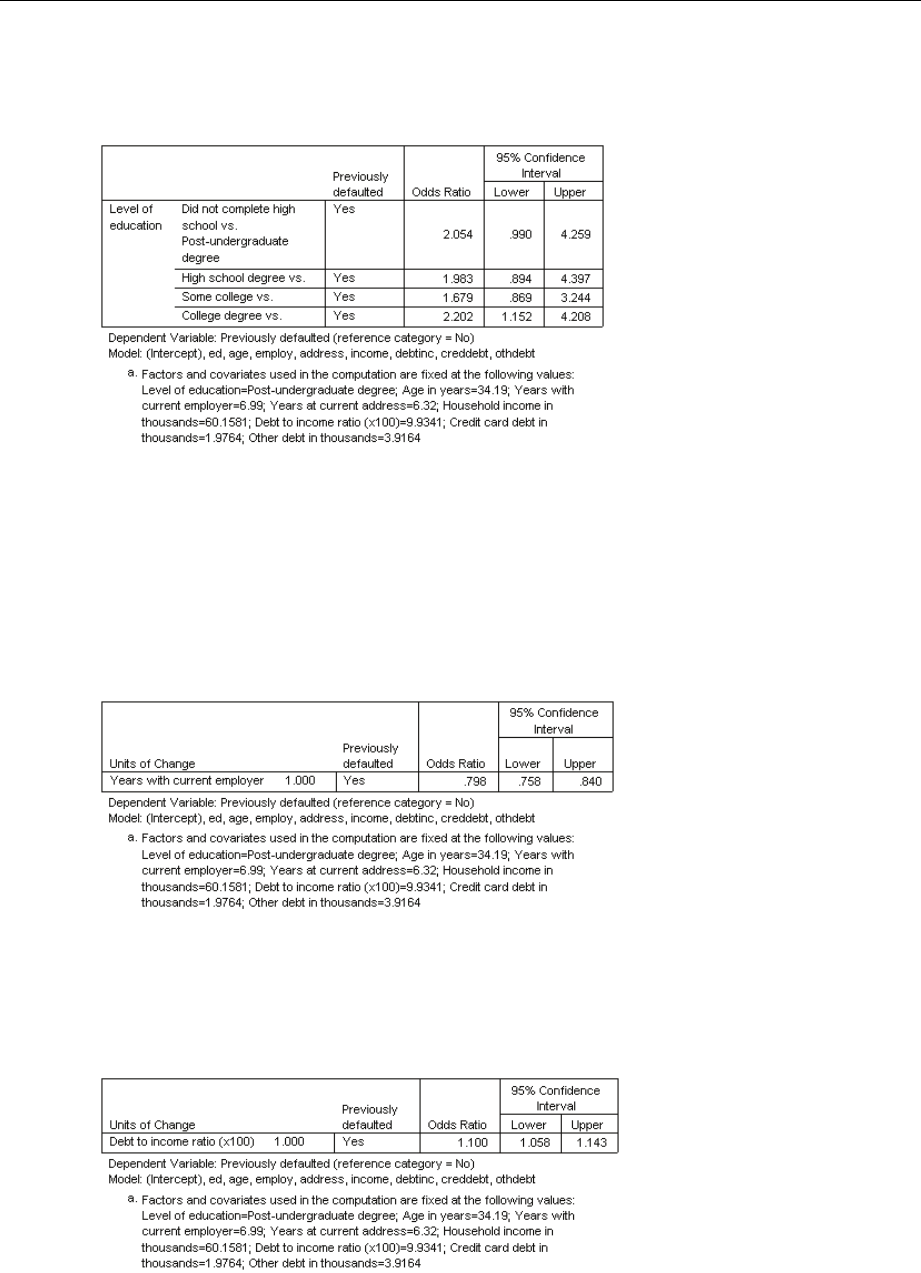
193
Complex Samples Logistic Regression
Odds Ratios
Figure 20-10
Odds ratios for level of education
This table displays the odds ratios of Previously defaulted at the factor levels of Level of
education. The reported values are the ratios of the odds of default for Did not complete high
school through College degree, compared to the odds of default for Post-undergraduate degree.
Thus, the odds ratio of 2.054 in the first row of the table means that the odds of default for a
person who did not complete high school are 2.054 times the odds of default for a person who has
a post-undergraduate degree.
Figure 20-11
Odds ratios for years with current employer
This table displays the odds ratio of Previously defaulted for a unit change in the covariate Years
with current employer. The reported value is the ratio of the odds of default for a person with 7.99
years at their current job compared to the odds of default for a person with 6.99 years (the mean).
Figure 20-12
Odds ratios for debt to income ratio

194
Chapter 20
This table displays the odds ratio of Previously defaulted for a unit change in the covariate Debt to
income ratio. The reported value is the ratio of the odds of default for a person with a debt/income
ratio of 10.9341 compared to the odds of default for a person with 9.9341 (the mean).
Note that because none of these predictors are part of interaction terms, the values of the odds
ratios reported in these tables are equal to the values of the exponentiated parameter estimates.
When a predictor is part of an interaction term, its odds ratio as reported in these tables will also
depend on the values of the other predictors that make up the interaction.
Summary
Using the Complex Samples Logistic Regression Procedure, you have constructed a model for
predicting the probability that a given customer will default on a loan.
A critical issue for loan officers is the cost of Type I and Type II errors. That is, what is
the cost of classifying a defaulter as a nondefaulter (Type I)? What is the cost of classifying a
nondefaulter as a defaulter (Type II)? If bad debt is the primary concern, then you want to lower
your Type I error and maximize your sensitivity. If growing your customer base is the priority,
then you want to lower your Type II error and maximize your specificity.Usually,bothare
major concerns, so you have to choose a decision rule for classifying customers that gives the
best mix of sensitivity and specificity.
Related Procedures
The Complex Samples Logistic Regression procedure is a useful tool for modeling a categorical
variable when the cases have been drawn according to a complex sampling scheme.
The Complex Samples Sampling Wizard is used to specify complex sampling design
specifications and obtain a sample. The sampling plan file created by the Sampling Wizard
contains a default analysis plan and can be specified in the Plan dialog box when you are
analyzing the sample obtained according to that plan.
The Complex Samples Analysis Preparation Wizard is used to specify analysis specifications
for an existing complex sample. The analysis plan file created by the Sampling Wizard can be
specified in the Plan dialog box when you are analyzing the sample corresponding to that plan.
The Complex Samples General Linear Model procedure allows you to model a scale response.
The Complex Samples Ordinal Regression procedure allows you to model an ordinal response.

Chapter
21
Complex Samples Ordinal Regression
The Complex Samples Ordinal Regression procedure creates a predictive model for an ordinal
dependent variable for samples drawn by complex sampling methods. Optionally, you can request
analyses for a subpopulation.
Using Complex Samples Ordinal Regression to Analyze Survey Results
Representatives considering a bill before the legislature are interested in whether there is public
support for the bill and how support for the bill is related to voter demographics. Pollsters design
and conduct interviews according to a complex sampling design.
The survey results are collected in poll_cs_sample.sav. The sampling plan used by the pollsters
is contained in poll.csplan; because it makes use of a probability-proportional-to-size (PPS)
method, there is also a file containing the joint selection probabilities (poll_jointprob.sav). For
more information, see the topic Sample Files in Appendix A in IBM SPSS Complex Samples 19.
Use Complex Samples Ordinal Regression to fit a model for the level of support for the bill based
upon voter demographics.
Running the Analysis
ETo run a Complex Samples Ordinal Regression analysis, from the menus choose:
Analyze > Complex Samples > Ordinal Regression...
© Copyright SPSS Inc. 1989, 2010 195
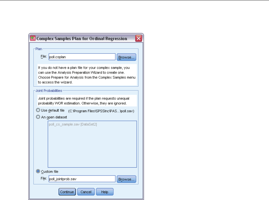
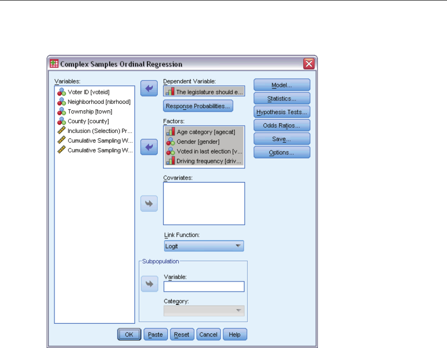
197
Complex Samples Ordinal Regression
Figure 21-2
Ordinal Regression dialog box
ESelect The legislature should enact a gas tax as the dependent variable.
ESelect Age category through Driving frequency as factors.
EClick Statistics.
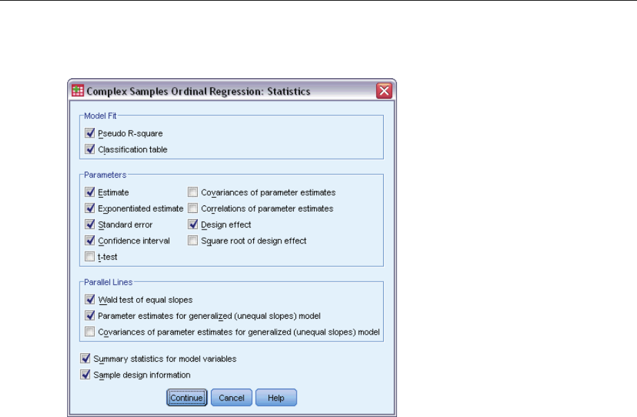
198
Chapter 21
Figure 21-3
Ordinal Regression Statistics dialog box
ESelect Classification table in the Model Fit group.
ESelect Estimate,Exponentiated estimate,Standard error,Confidence interval,andDesign effect in
the Parameters group.
ESelect Wald test of equal slopes and Parameter estimates for generalized (unequal slopes) model.
EClick Continue.
EClick Hypothesis Tests in the Complex Samples Ordinal Regression dialog box.
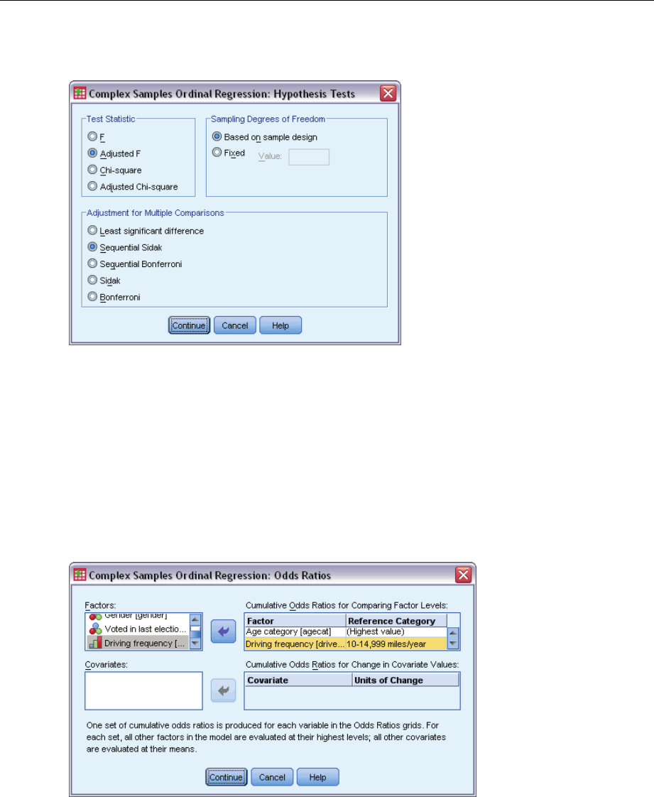
199
Complex Samples Ordinal Regression
Figure 21-4
Hypothesis Tests dialog box
Even for a moderate number of predictors and response categories, the Wald Ftest statistic can
be inestimable for the test of parallel lines.
ESelect Adjusted F in the Test Statistic group.
ESelect Sequential Sidak as the adjustment method for multiple comparisons.
EClick Continue.
EClick Odds Ratios in the Complex Samples Ordinal Regression dialog box.
Figure 21-5
Ordinal Regression Odds Ratios dialog box
EChoose to produce cumulative odds ratios for Age category and Driving frequency.
ESelect 10-14,999 miles/year, a more “typical” yearly mileage than the maximum, as the reference
category for Driving frequency.
EClick Continue.
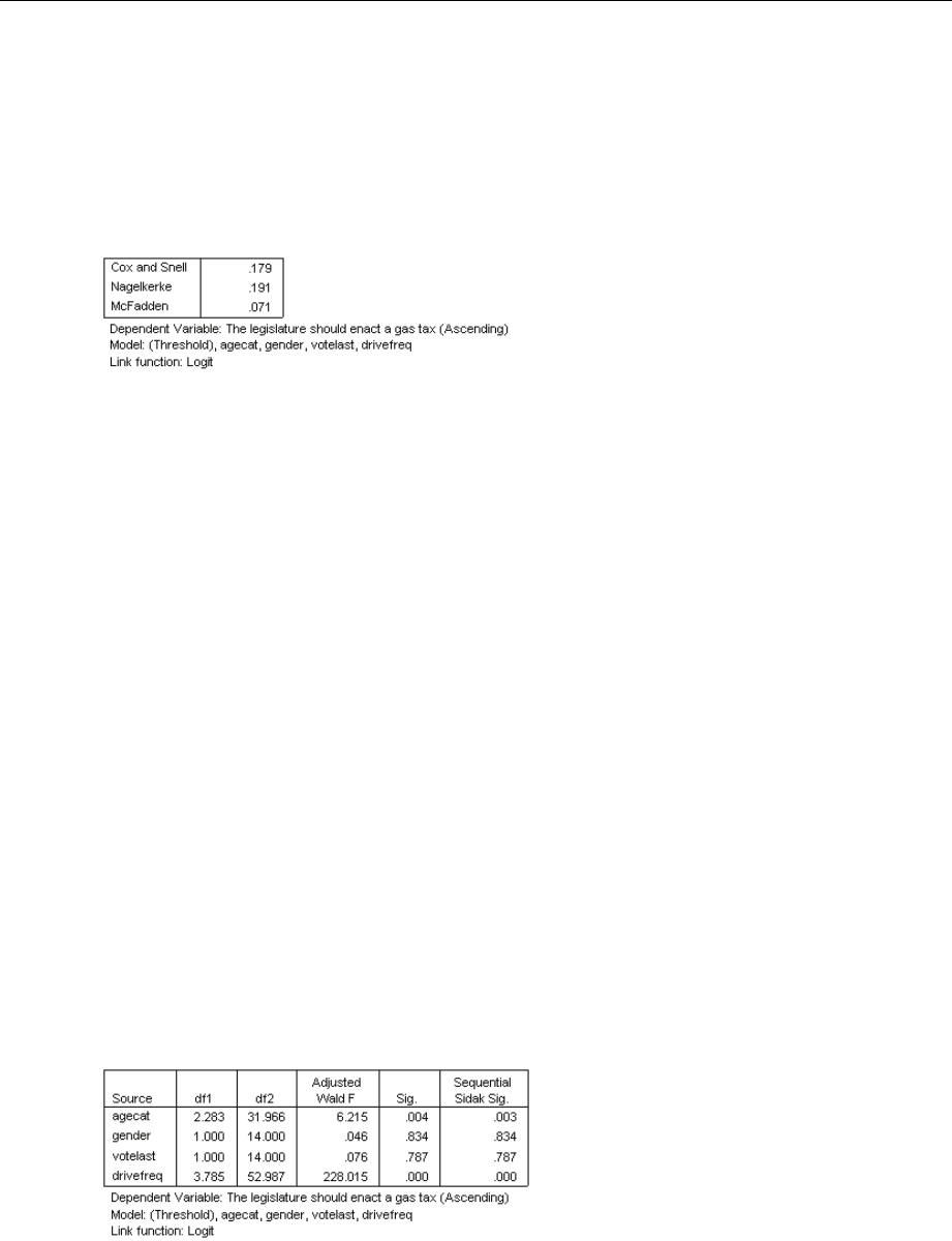
200
Chapter 21
EClick OK in the Complex Samples Ordinal Regression dialog box.
Pseudo R-Squares
Figure 21-6
Pseudo R-Squares
In the linear regression model, the coefficient of determination, R2, summarizes the proportion of
variance in the dependent variable associated with the predictor (independent) variables, with
larger R2values indicating that more of the variation is explained by the model, to a maximum
of 1. For regression models with a categorical dependent variable, it is not possible to compute
asingleR2statistic that has all of the characteristics of R2in the linear regression model, so
these approximations are computed instead. The following methods are used to estimate the
coefficient of determination.
Cox and Snell’s R2(Cox and Snell, 1989) is based on the log likelihood for the model
compared to the log likelihood for a baseline model. However, with categorical outcomes, it
has a theoretical maximum value of less than 1, even for a “perfect” model.
Nagelkerke’s R2(Nagelkerke, 1991) is an adjusted version of the Cox & Snell R-square that
adjusts the scale of the statistic to cover the full range from 0 to 1.
McFadden’s R2(McFadden, 1974) is another version, based on the log-likelihood kernels for
the intercept-only model and the full estimated model.
What constitutes a “good” R2value varies between different areas of application. While these
statistics can be suggestive on their own, they are most useful when comparing competing models
for the same data. The model with the largest R2statistic is “best” according to this measure.
Tests of Model Effects
Figure 21-7
Tests of model effects
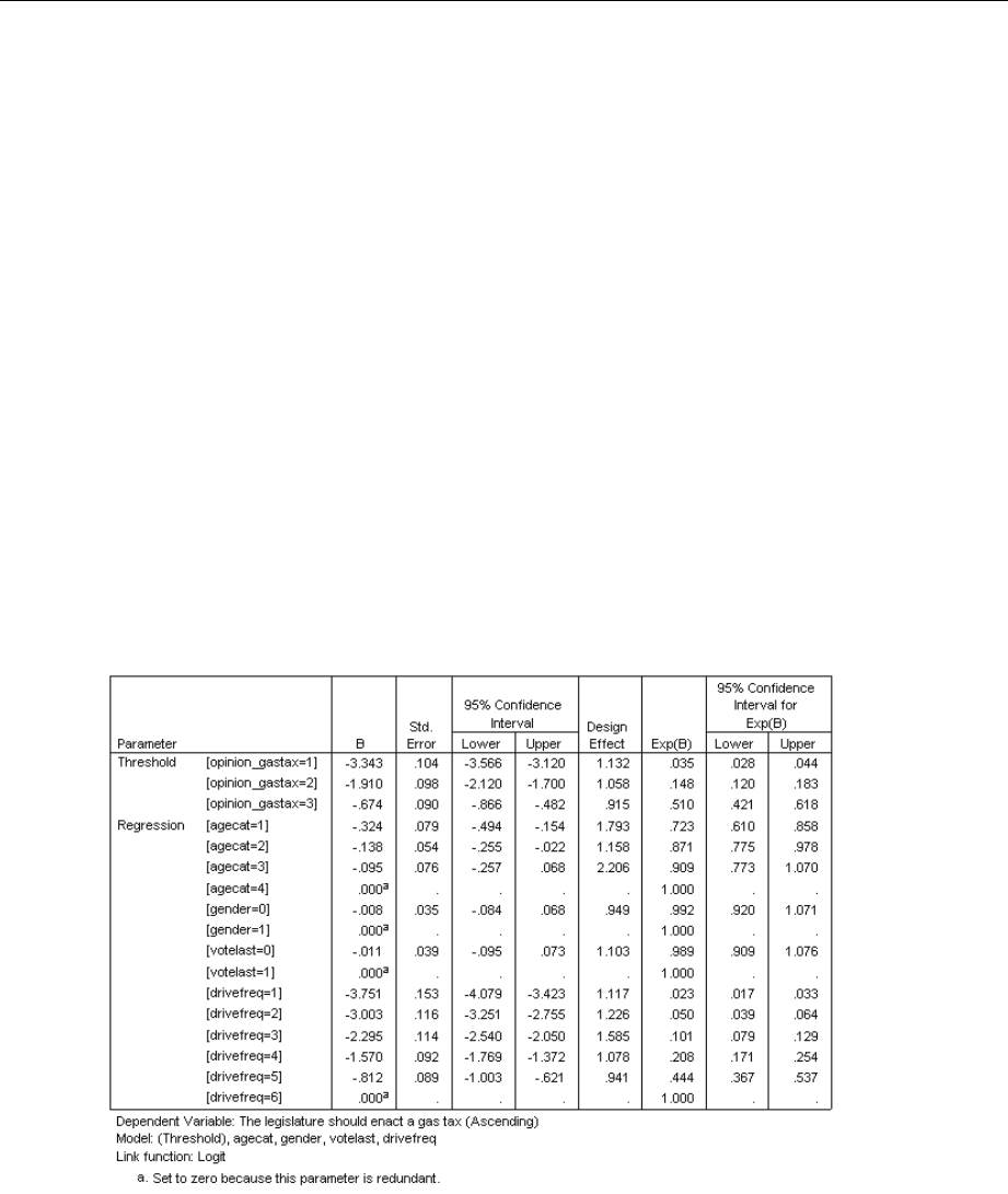
201
Complex Samples Ordinal Regression
Each term in the model is tested for whether its effect equals 0. Terms with significance values
less than 0.05 have some discernable effect. Thus, agecat and drivefreq contribute to the model,
while the other main effects do not. In a further analysis of the data, you would consider removing
gender and votelast from the model.
Parameter Estimates
The parameter estimates table summarizes the effect of each predictor. While interpretation
of the coefficients in this model is difficult due to the nature of the link function, the signs of
the coefficients for covariates and relative values of the coefficients for factor levels can give
important insights into the effects of the predictors in the model.
For covariates, positive (negative) coefficients indicate positive (inverse) relationships
between predictors and outcome. An increasing value of a covariate with a positive coefficient
corresponds to an increasing probability of being in one of the “higher” cumulative outcome
categories.
For factors, a factor level with a greater coefficient indicates a greater probability of being in
one of the “higher” cumulative outcome categories. The sign of a coefficient for a factor level
is dependent upon that factor level’s effect relative to the reference category.
Figure 21-8
Parameter estimates
You can make the following interpretations based on the parameter estimates:
Those in lower age categories show greater support for the bill than those in the highest age
category.
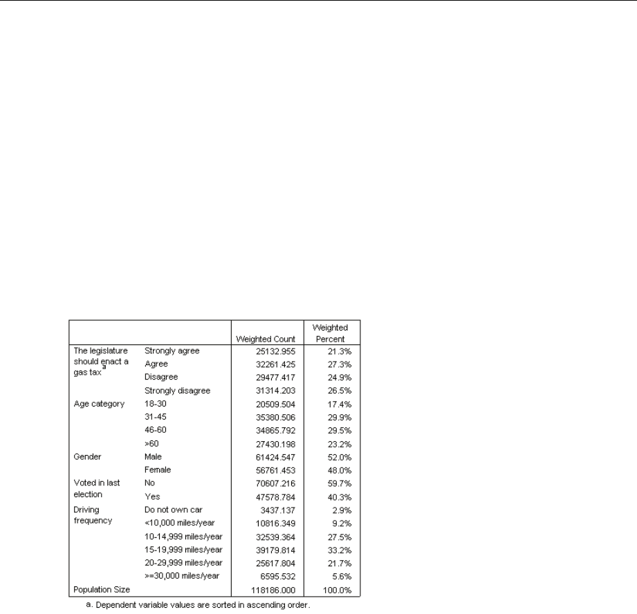
202
Chapter 21
Those who drive less frequently show greater support for the bill than those who drive more
frequently.
The coefficients for the variables gender and votelast, in addition to not being statistically
significant, appear to be small compared to other coefficients.
The design effects indicate that some of the standard errors computed for these parameter
estimates are larger than those you would obtain if you used a simple random sample, while
others are smaller. It is vitally important to incorporate the sampling design information in your
analysis because you might otherwise infer, for example, that the coefficient for the third level
of Age category,[agecat=3],issignificantly different from 0!
Classification
Figure 21-9
Categorical variable information
Given the observed data, the “null” model (that is, one without predictors) would classify all
customers into the modal group, Agree. Thus, the null model would be correct 27.3% of the time.
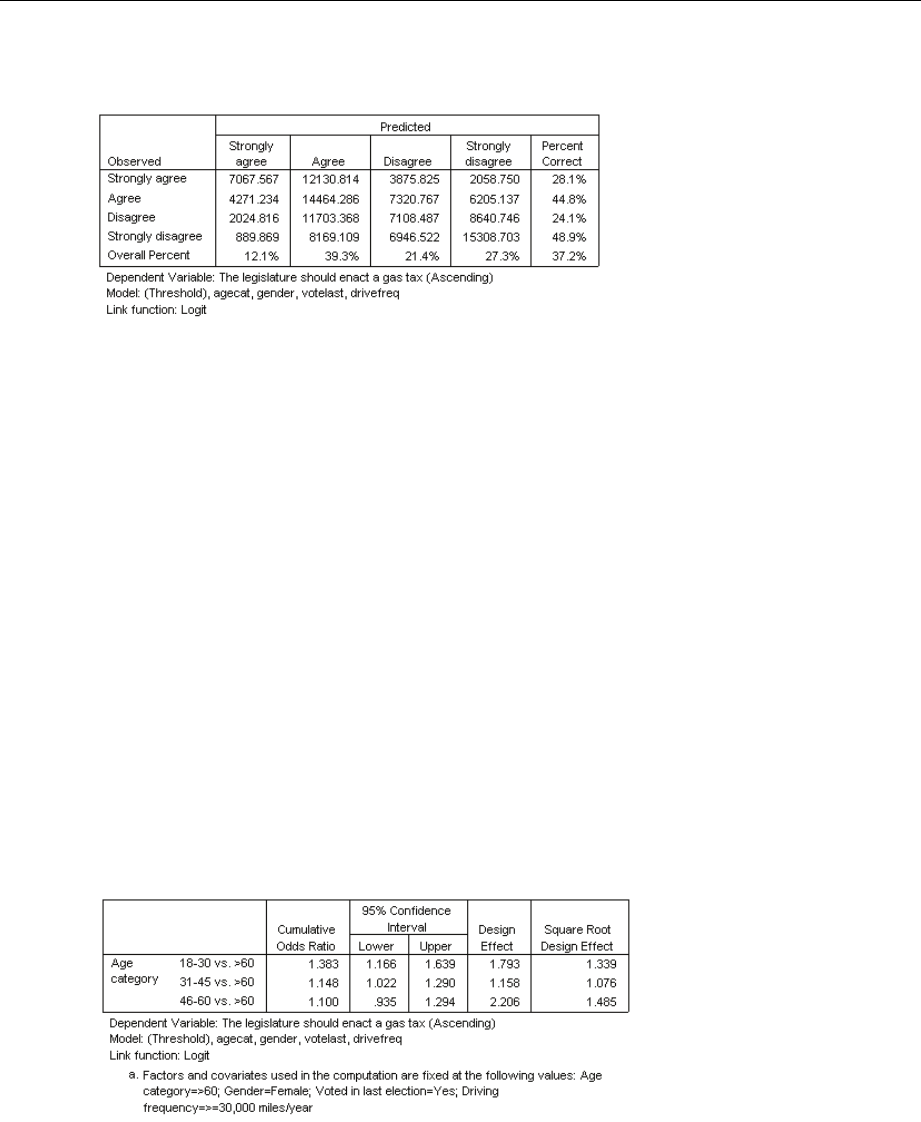
203
Complex Samples Ordinal Regression
Figure 21-10
Classification table
The classification table shows the practical results of using the model. For each case, the predicted
response is the response category with the highest model-predicted probability. Casesare
weighted by Final Sampling Weight, so that the classification table reports the expected model
performance in the population.
Cells on the diagonal are correct predictions.
Cells off the diagonal are incorrect predictions.
The model correctly classifies 9.9% more, or 37.2% of the cases. In particular, the model does
considerably better at classifying those who Agree or Strongly disagree, and slightly worse with
those who Disagree.
Odds Ratios
Cumulative odds are defined as the ratio of the probability that the dependent variable takes
a value less than or equal to a given response category to the probability that it takes a value
greater than that response category. The cumulative odds ratio is the ratio of cumulative odds
for different predictor values and is closely related to the exponentiated parameter estimates.
Interestingly, the cumulative odds ratio itself does not depend upon the response category.
Figure 21-11
Cumulative odds ratios for Age category
This table displays cumulative odds ratios for the factor levels of Age category. The reported
values are the ratios of the cumulative odds for 18–30 through 46–60,comparedtothecumulative
odds for >60. Thus, the odds ratio of 1.383 in the first row of the table means that the cumulative
odds for a person aged 18–30 are 1.383 times the cumulative odds for a person older than 60.
Note that because Age category is not involved in any interaction terms, the odds ratios are
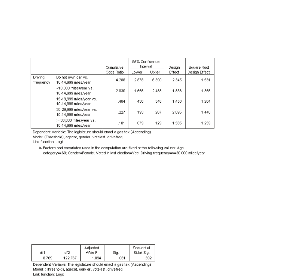
204
Chapter 21
merely the ratios of the exponentiated parameter estimates. For example, the cumulative odds
ratio for 18–30 vs. >60 is 1.00/0.723 = 1.383.
Figure 21-12
Odds ratios for driving frequency
This table displays the cumulative odds ratios for the factor levels of Driving frequency,using
10–14,999 miles/year as the reference category. Since Driving frequency is not involved in any
interaction terms, the odds ratios are merely the ratios of the exponentiated parameter estimates.
For example, the cumulative odds ratio for 20–29,999 miles/year vs. 10–14,999 miles/year is
0.101/0.444 = 0.227.
Generalized Cumulative Model
Figure 21-13
Test of parallel lines
The test of parallel lines can help you assess whether the assumption that the parameters are the
same for all response categories is reasonable. This test compares the estimated model with one
set of coefficients for all categories to a generalized model with a separate set of coefficients for
each category.
The Wald Ftest is an omnibus test of the contrast matrix for the parallel lines assumption that
provides asymptotically correct pvalues; for small to mid-sized samples, the adjusted Wald F
statistic performs well. The significance value is near 0.05, suggesting that the generalized model
maygiveanimprovementinthemodelfit; however, the Sequential Sidak adjusted test reports a
significance value high enough (0.392) that, overall, there is no clear evidence for rejecting the
parallel lines assumption. The Sequential Sidak test starts with individual contrast Wald tests to
provide an overall pvalue, and these results should be comparable to the omnibus Wald test result.
The fact that they are so different in this example is somewhat surprising but could be due to the
existence of many contrasts in the test and a relatively small design degrees of freedom.
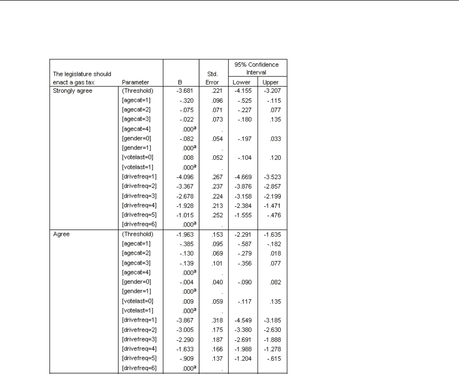
205
Complex Samples Ordinal Regression
Figure 21-14
Parameter estimates for generalized cumulative model (shown in part)
Moreover, the estimated values of the generalized model coefficients don’t appear to differ much
from the estimates under the parallel lines assumption.
Dropping Non-Significant Predictors
The tests of model effects showed that the model coefficients for Gender and Voted in last election
are not statistically significantly different from 0.
ETo produce a reduced model, recall the Complex Samples Ordinal Regression dialog box.
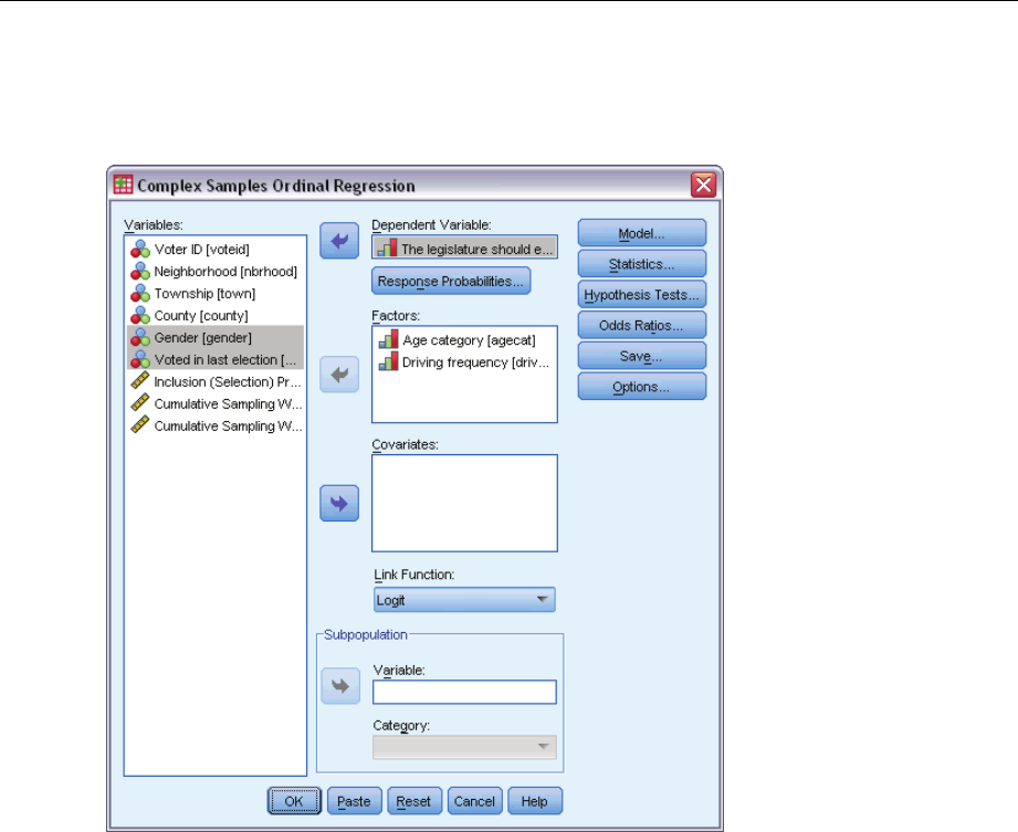
206
Chapter 21
EClick Continue in the Plan dialog box.
Figure 21-15
Ordinal Regression dialog box
EDeselect Gender and Voted in last election as factors.
EClick Options.
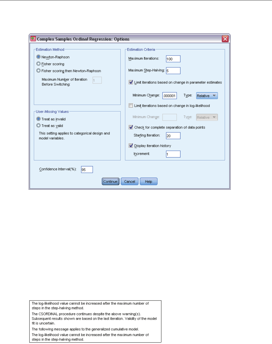
207
Complex Samples Ordinal Regression
Figure 21-16
Ordinal Regression Options dialog box
ESelect Display iteration history.
The iteration history is useful for diagnosing problems encountered by the estimation algorithm.
EClick Continue.
EClick OK in the Complex Samples Ordinal Regression dialog box.
Warnings
Figure 21-17
Warnings for reduced model
The warnings note that estimation of the reduced model ended before the parameter estimates
reached convergence because the log-likelihood could not be increased with any change, or “step,”
in the current values of the parameter estimates.
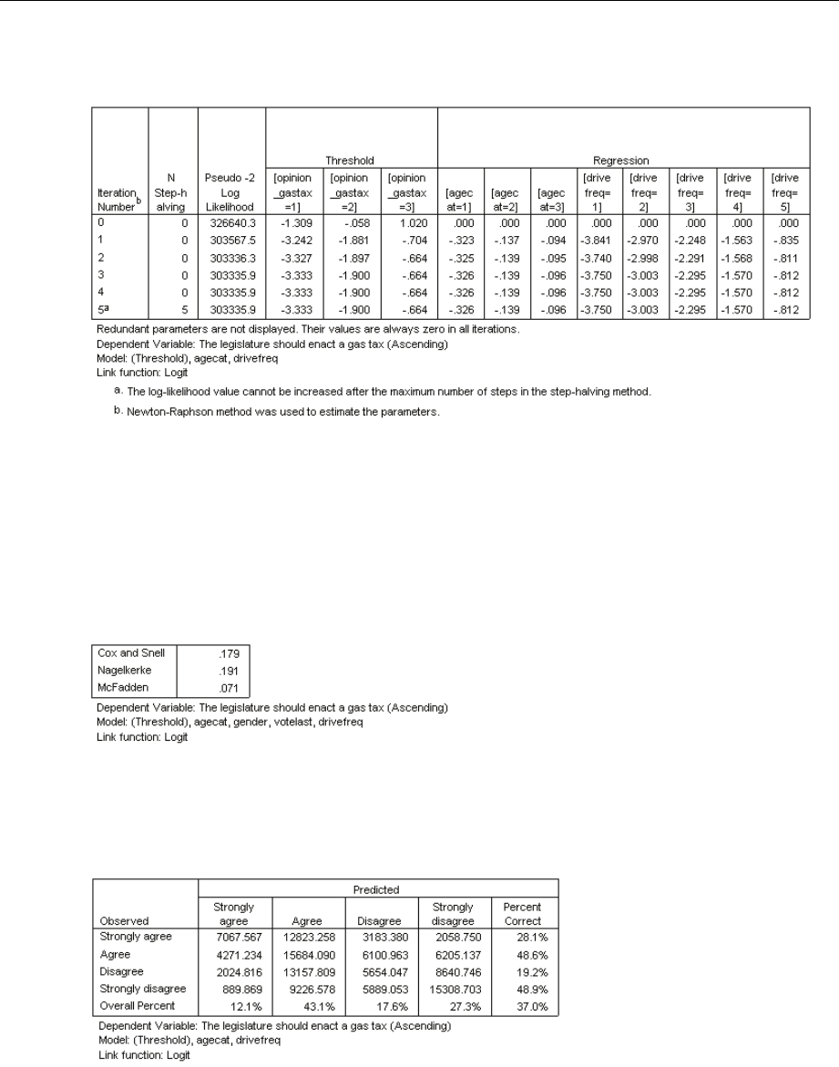
208
Chapter 21
Figure 21-18
Warnings for reduced model
Looking at the iteration history, the changes in the parameter estimates over the last few iterations
are slight enough that you’re not terribly concerned about the warning message.
Comparing Models
Figure 21-19
Pseudo R-Squares for reduced model
The R2values for the reduced model are identical to those for the original model. This is evidence
in favor of the reduced model.
Figure 21-20
Classification table for reduced model
The classification table somewhat complicates matters. The overall classification rate of 37.0%
for the reduced model is comparable to the original model, which is evidence in favor of the
reduced model. However, the reduced model shifts the predicted response of 3.8% of the voters

209
Complex Samples Ordinal Regression
from Disagree to Agree, more than half of whom were observed to respond Disagree or Strongly
disagree. This is a very important distinction that deserves careful consideration before choosing
the reduced model.
Summary
Using the Complex Samples Ordinal Regression Procedure, you have constructed competing
models for the level of support for the proposed bill based on voter demographics. The test of
parallel lines shows that a generalized cumulative model is not necessary. The tests of model
effects suggest that Gender and Votedinlastelectioncould be dropped from the model, and the
reduced model performs well in terms of pseudo-R2and overall classification rate compared to the
original model. However, the reduced model misclassifies more voters across the Agree/Disagree
split, so the legislators prefer to keep the original model for now.
Related Procedures
The Complex Samples Ordinal Regression procedure is a useful tool for modeling an ordinal
variable when the cases have been drawn according to a complex sampling scheme.
The Complex Samples Sampling Wizard is used to specify complex sampling design
specifications and obtain a sample. The sampling plan file created by the Sampling Wizard
contains a default analysis plan and can be specified in the Plan dialog box when you are
analyzing the sample obtained according to that plan.
The Complex Samples Analysis Preparation Wizard is used to specify analysis specifications
for an existing complex sample. The analysis plan file created by the Sampling Wizard can be
specified in the Plan dialog box when you are analyzing the sample corresponding to that plan.
The Complex Samples General Linear Model procedure allows you to model a scale response.
The Complex Samples Logistic Regression procedure allows you to model a categorical
response.

Chapter
22
Complex Samples Cox Regression
The Complex Samples Cox Regression procedure performs survival analysis for samples drawn
by complex sampling methods.
Using a Time-Dependent Predictor in Complex Samples Cox Regression
A government law enforcement agency is concerned about recidivism rates in their area of
jurisdiction. One of the measures of recidivism is the time until second arrest for offenders. The
agency would like to model time to rearrest using Cox Regression on a sample drawn by complex
sampling methods, but they are worried the proportional hazards assumption is invalid across
age categories.
Persons released from their firstarrestduringthemonthofJune2003wereselectedfrom
sampled departments, and their case history inspected through the end of June 2006. The
sample is collected in recidivism_cs_sample.sav. The sampling plan used is contained in
recidivism_cs.csplan; because it makes use of a probability-proportional-to-size (PPS) method,
there is also a file containing the joint selection probabilities (recidivism_cs_jointprob.sav). For
more information, see the topic Sample Files in Appendix A in IBM SPSS Complex Samples
19.Use Complex Samples Cox Regression to assess the validity of the proportional hazards
assumption and fit a model with time-dependent predictors, if appropriate.
Preparing the Data
The dataset contains the dates of release from first arrest and second arrest; since Cox regression
analyzes survival times, you need to compute the amount of time between these dates.
However, Date of second arrest [date2] contains cases with the value 10/03/1582, a missing
value for date variables. These are people who have not had a second offense, and we definitely
want to include them as right-censored cases in the model. The end of the follow-up period was
June 30, 2006, so we are going to recode 10/03/1582 to 06/30/2006.
ETo recode these values, from the menus choose:
Transform > Compute Variable...
© Copyright SPSS Inc. 1989, 2010 210
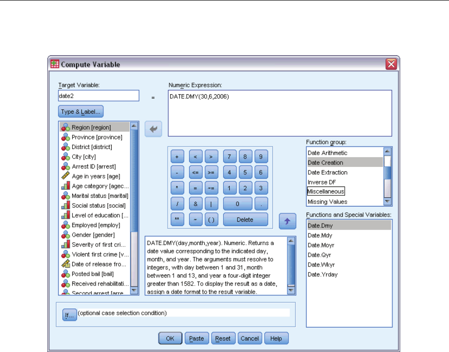
211
Complex Samples Cox Regression
Figure 22-1
Compute Variable dialog box
EType date2 as the target variable.
EType DATE.DMY(30,6,2006) as the expression.
EClick If.
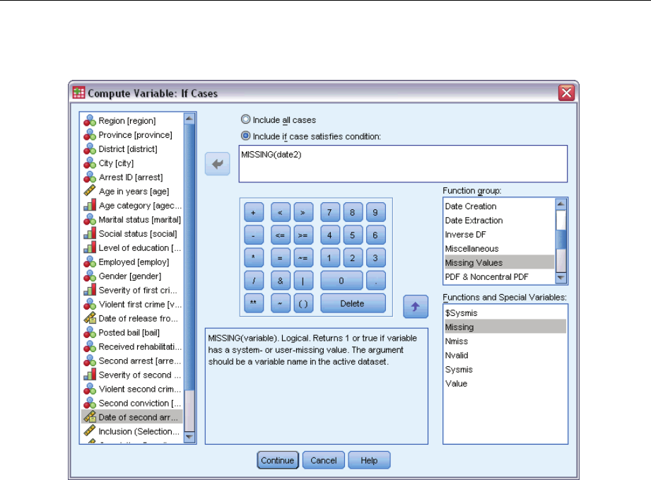
212
Chapter 22
Figure 22-2
ComputeVariableIfCasesdialogbox
ESelect Include if case satisfies condition.
EType MISSING(date2) as the expression.
EClick Continue.
EClick OK in the Compute Variable dialog box.
ENext, to compute the time between first and second arrest, from the menus choose:
Transform > Date and Time Wizard...
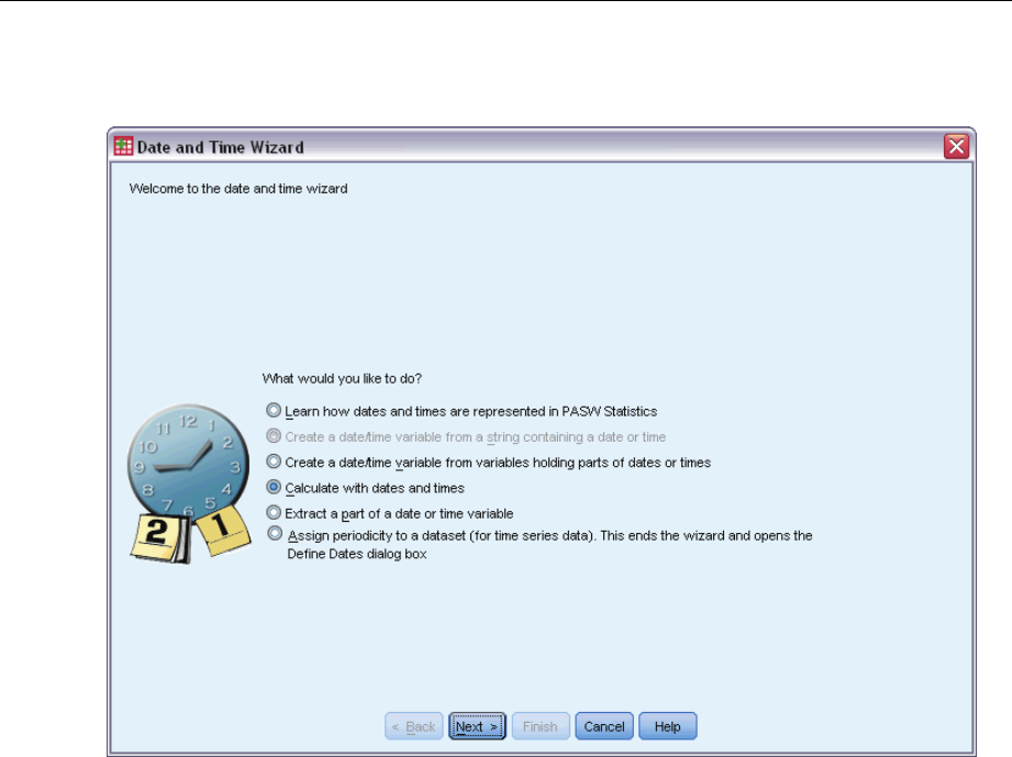
213
Complex Samples Cox Regression
Figure 22-3
DateandTimeWizard,Welcomestep
ESelect Calculate with dates and times.
EClick Next.
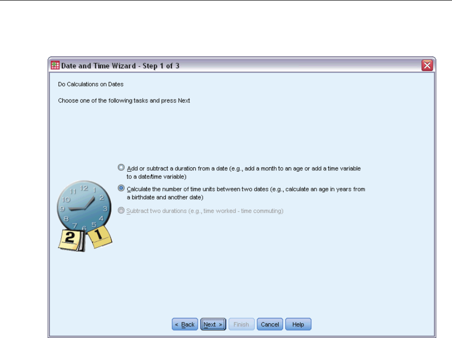
214
Chapter 22
Figure 22-4
Date and Time Wizard, Do Calculations on Dates step
ESelect Calculate the number of time units between two dates.
EClick Next.
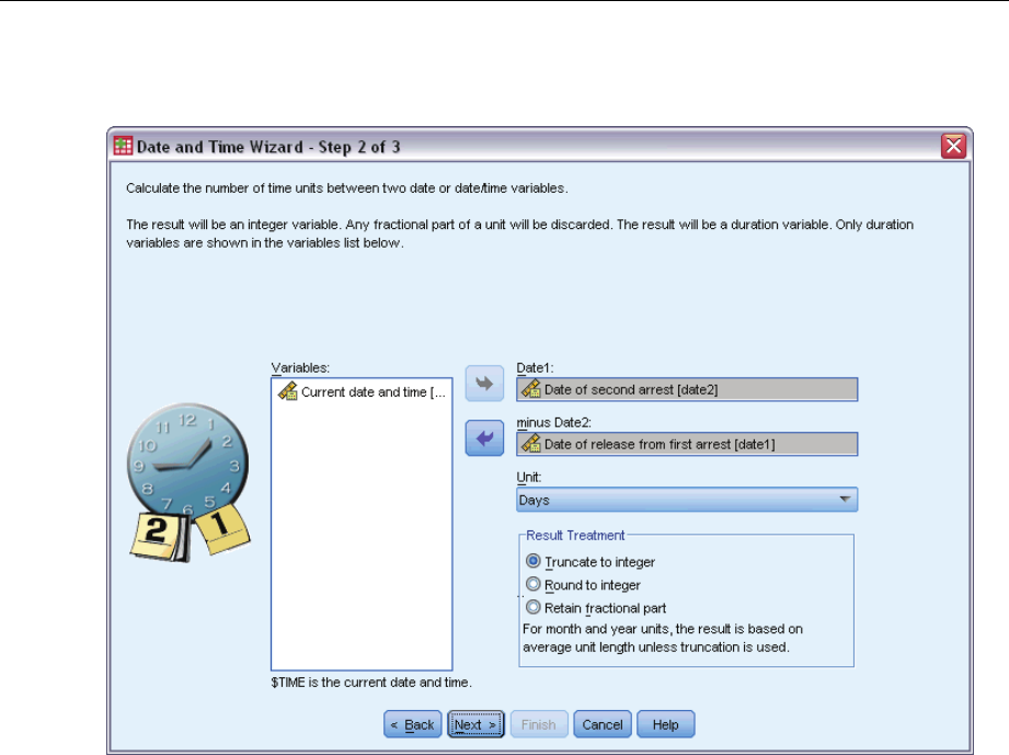
215
Complex Samples Cox Regression
Figure 22-5
Date and Time Wizard, Calculate the number of time units between two dates step
ESelect Date of second arrest [date2] as the first date.
ESelect Date of release from first arrest [date1] as the date to subtract from the first date.
ESelect Days as the unit.
EClick Next.
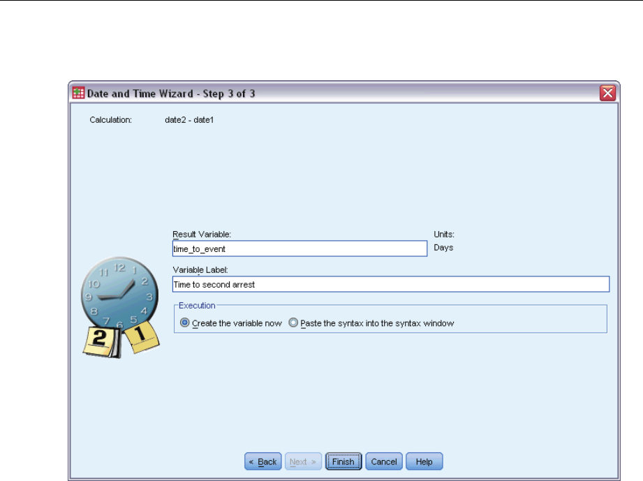
216
Chapter 22
Figure 22-6
Date and Time Wizard, Calculation step
EType time_to_event as the name of the variable representing the time between the two dates.
EType Time to second arrest as the variable label.
EClick Finish.
Running the Analysis
ETo run a Complex Samples Cox Regression analysis, from the menus choose:
Analyze > Complex Samples > Cox Regression...
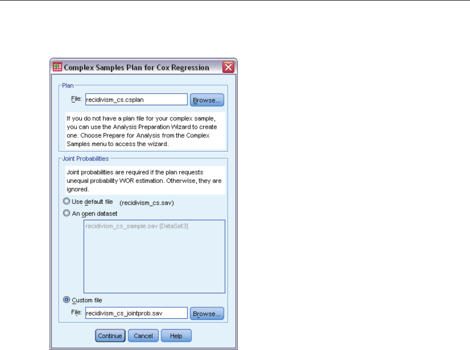
217
Complex Samples Cox Regression
Figure 22-7
Complex Samples Plan for Cox Regression dialog box
EBrowse to the sample files directory and select recidivism_cs.csplan as the plan file.
ESelect Custom file in the Joint Probabilities group, browse to the sample files directory, and select
recidivism_cs_jointprob.sav.
EClick Continue.

218
Chapter 22
Figure 22-8
Cox Regression dialog box, Time and Event tab
ESelect Time to second arrest [time_to_event] asthevariabledefining the end of the interval.
ESelect Second arrest [arrest2] as the variable defining whether the event has occurred.
EClick Define Event.
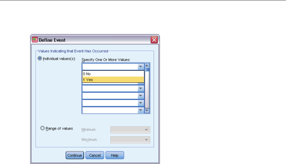
219
Complex Samples Cox Regression
Figure 22-9
Define Event dialog box
ESelect 1Yesas the value indicating the event of interest (rearrest) has occurred.
EClick Continue.
EClick the Predictors tab.
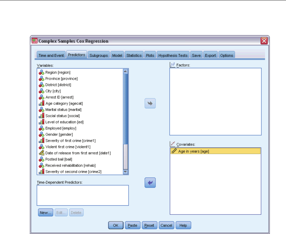
220
Chapter 22
Figure 22-10
Cox Regression dialog box, Predictors tab
ESelect Age in years [age] as a covariate.
EClick the Statistics tab.
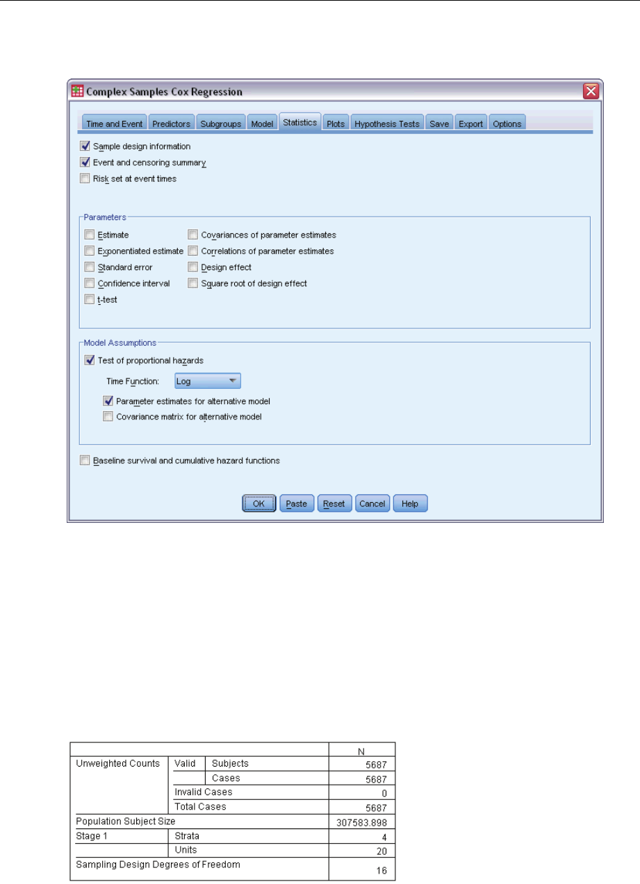
221
Complex Samples Cox Regression
Figure 22-11
Cox Regression dialog box, Statistics tab
ESelect Test of proportional hazards and then select Log as the time function in the Model
Assumptions group.
ESelect Parameter estimates for alternative model.
EClick OK.
Sample Design Information
Figure 22-12
Sample design information
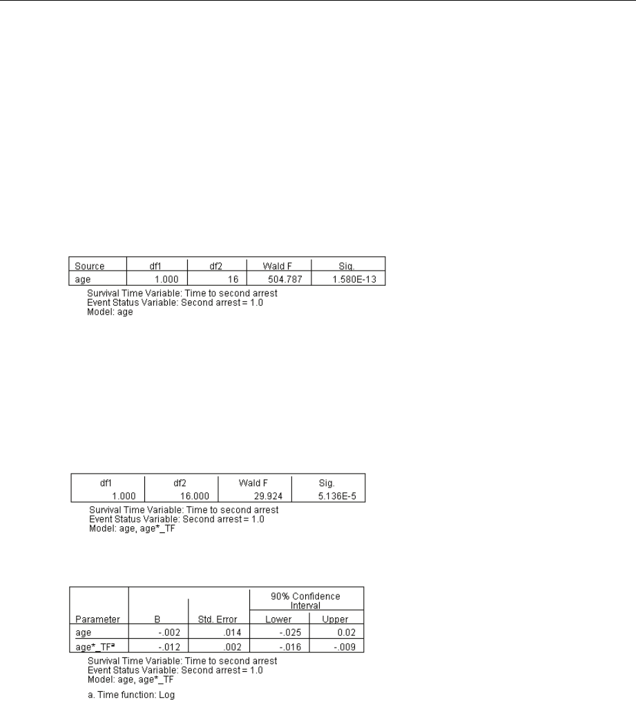
222
Chapter 22
This table contains information on the sample design pertinent to the estimation of the model.
There is one case per subject, and all 5,687 cases are used in the analysis.
The sample represents less than 2% of the entire estimated population.
Thedesignrequested4strataand5unitsperstrataforatotalof20unitsinthefirst stage of
the design. The sampling design degrees of freedom are estimated by 20−4=16.
Tests of Model Effects
Figure 22-13
Tests of model effects
In the proportional hazards model, the significance value for the predictor age is less than 0.05
and, therefore, appears to contribute to the model.
Test of Proportional Hazards
Figure 22-14
Overall test of proportional hazards
Figure 22-15
Parameter estimates for alternative model
The significance value for the overall test of proportional hazards is less than 0.05, indicating that
the proportional hazards assumption is violated. The log time function is used for the alternative
model, so it will be easy to replicate this time-dependent predictor.
Adding a Time-Dependent Predictor
ERecall the Complex Samples Cox Regression dialog box and click the Predictors tab.
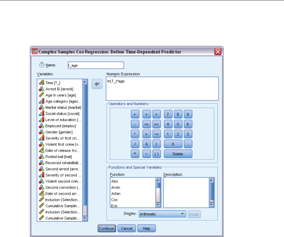
223
Complex Samples Cox Regression
EClick New.
Figure 22-16
Cox Regression Define Time-Dependent Predictor dialog box
EType t_age as the name of the time-dependent predictor you want to define.
EType ln(T_)*age as the numeric expression.
EClick Continue.
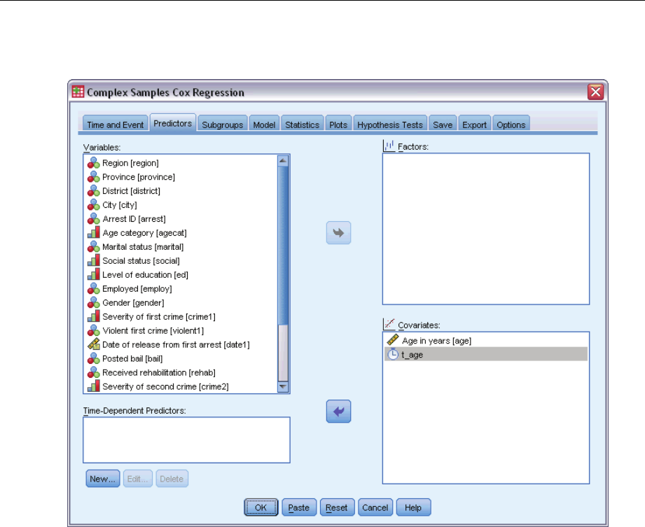
224
Chapter 22
Figure 22-17
Cox Regression dialog box, Predictors tab
ESelect t_age as a covariate.
EClick the Statistics tab.
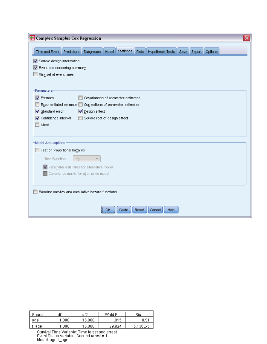
225
Complex Samples Cox Regression
Figure 22-18
Cox Regression dialog box, Predictors tab
ESelect Estimate,Standard error,Confidence interval,andDesign effect in the Parameters group.
EDeselect Test of proportional hazards and Parameter estimates for alternative model in the Model
Assumptions group.
EClick OK.
Tests of Model Effects
Figure 22-19
Tests of model effects
With the addition of the time-dependent predictor, the significance value for age is 0.91, indicating
that its contribution to the model is superseded by that of t_age.
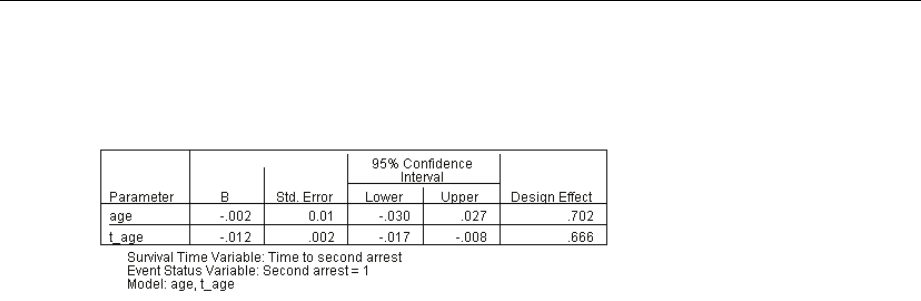
226
Chapter 22
Parameter Estimates
Figure 22-20
Parameter estimates
Looking at the parameter estimates and standard errors, you can see that you have replicated the
alternative model from the test of proportional hazards. By explicitly specifying the model, you
can request additional parameter statistics and plots. Here we have requested the design effect; the
value for t_age of less than 1 indicates that the standard error for t_age is smaller than what you
would obtain if you assumed that the dataset was a simple random sample. In this case, the effect
of t_age would still be statistically significant, but the confidence intervals would be wider.
Multiple Cases per Subject in Complex Samples Cox Regression
Researchers investigating survival times for patients exiting a rehabilitation program post-ischemic
stroke face a number of challenges.
Multiple cases per subject. Variables representing patient medical history should be useful as
predictors. Over time, patients may experience major medical events that alter their medical
history. In this dataset, the occurrence of myocardial infarction, ischemic stroke, or hemorrhagic
stroke is noted and the time of the event recorded. You could create computable time-dependent
covariates within the procedure to include this information in the model, but it should be more
convenient to use multiple cases per subject. Note that the variables were originally coded so that
the patient history is recorded across variables, so you will need to restructure the dataset.
Left-truncation. The onset of risk starts at the time of the ischemic stroke. However, the
sample only includes patients who have survived the rehabilitation program, thus the sample
is left-truncated in the sense that the observed survival times are “inflated” by the length of
rehabilitation. You can account for this by specifying the time at which they exited rehabilitation
as the time of entry into the study.
No sampling plan. The dataset was not collected via a complex sampling plan and is considered to
be a simple random sample. You will need to create an analysis plan to use Complex Samples
Cox Regression.
The dataset is collected in stroke_survival.sav.For more information, see the topic Sample
FilesinAppendixAinIBM SPSS Complex Samples 19.Use the Restructure Data Wizard to
prepare the data for analysis, then the Analysis Preparation Wizard to create a simple random
sampling plan, and finally Complex Samples Cox Regression to build a model for survival times.
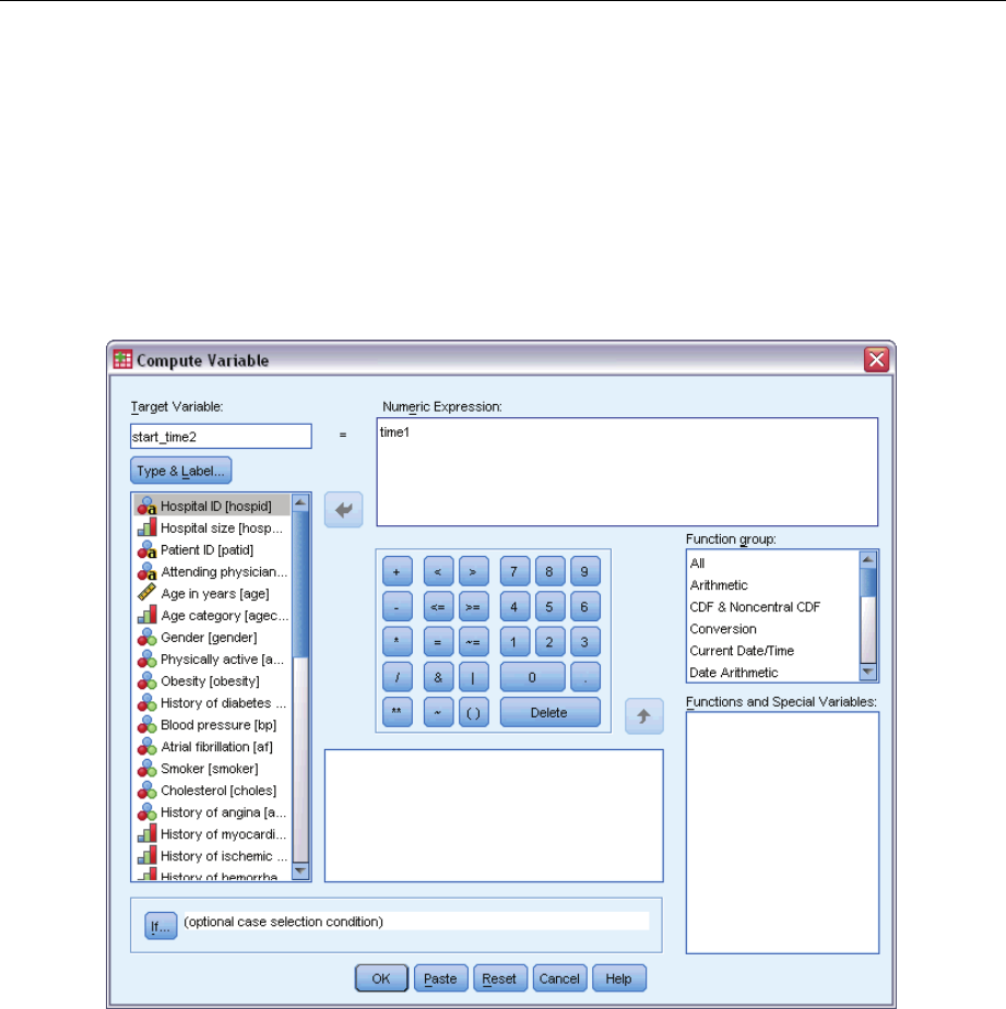
227
Complex Samples Cox Regression
Preparing the Data for Analysis
Before restructuring the data, you will need to create two ancillary variables to help with the
restructuring.
ETo compute a new variable, from the menus choose:
Transform > Compute Variable...
Figure 22-21
Compute Variable dialog box
EType start_time2 as the target variable.
EType time1 as the numeric expression.
EClick OK.
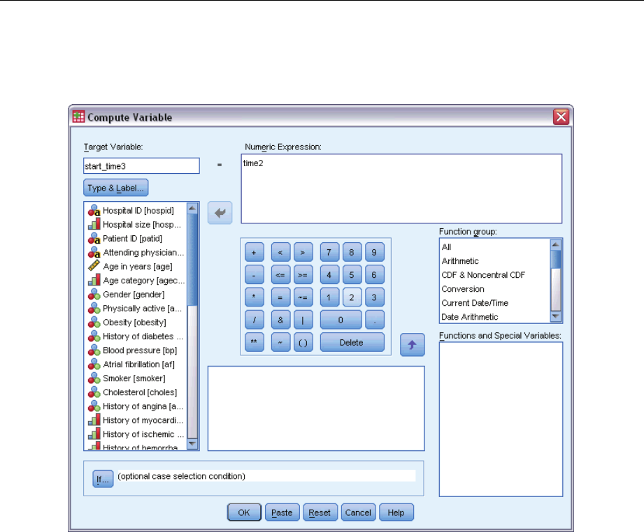
228
Chapter 22
ERecall the Compute Variable dialog box.
Figure 22-22
Compute Variable dialog box
EType start_time3 as the target variable.
EType time2 as the numeric expression.
EClick OK.
ETo restructure the data from variables to cases, from the menus choose:
Data > Restructure...
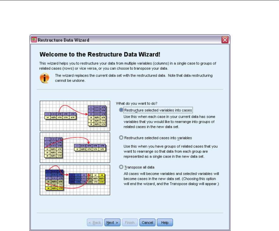
229
Complex Samples Cox Regression
Figure 22-23
Restructure Data Wizard, Welcome step
EMake sure Restructure selected variables into cases is selected.
EClick Next.
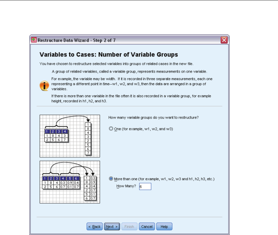
230
Chapter 22
Figure 22-24
Restructure Data Wizard, Variables to Cases Number of Variable Groups step
ESelect More than one variable group to restructure.
EType 6asthenumberofgroups.
EClick Next.
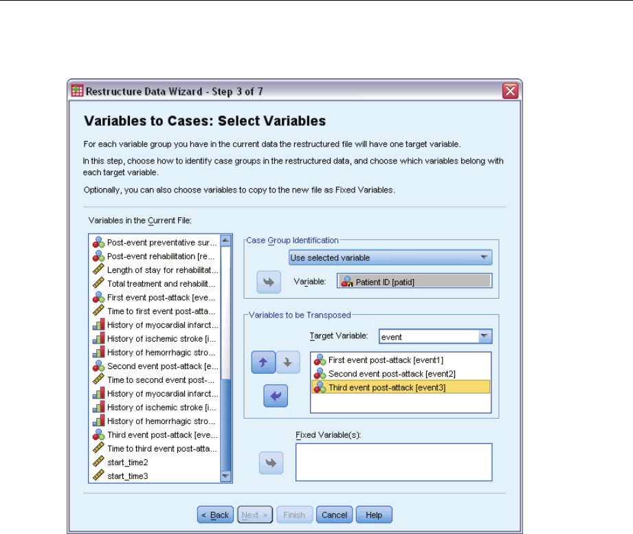
231
Complex Samples Cox Regression
Figure 22-25
Restructure Data Wizard, Variables to Cases Select Variables step
EIn the Case Group Identification group, select Use selected variable and select Patient ID [patid] as
the subject identifier.
EType event as the first target variable.
ESelectFirst event post-attack [event1],Second event post-attack [event2],andThird event
post-attack [event3] as variables to be transposed.
ESelect trans2 from the target variable list.
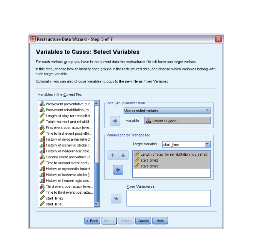
232
Chapter 22
Figure 22-26
Restructure Data Wizard, Variables to Cases Select Variables step
EType start_time as the target variable.
ESelect Length of stay for rehabilitation [los_rehab],start_time2,andstart_time3 as variables to be
transposed. Time to first event post-attack [time1] and Time to second event post-attack [time2]
will be used to create the end times, and each variable can only appear in one list of variables to be
transposed, thus start_time2 and start_time3 were necessary.
ESelect trans3 from the target variable list.
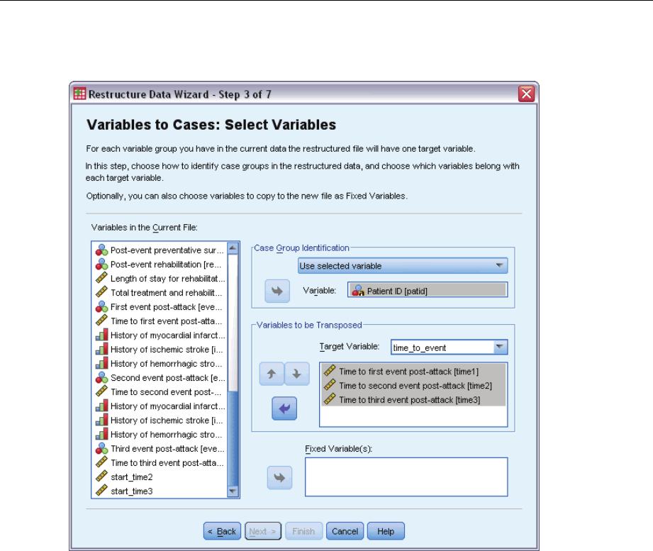
233
Complex Samples Cox Regression
Figure 22-27
Restructure Data Wizard, Variables to Cases Select Variables step
EType time_to_event as the target variable.
ESelect Time to first event post-attack [time1],Time to second event post-attack [time2],andTime
to third event post-attack [time3] as variables to be transposed.
ESelecttrans4 from the target variable list.
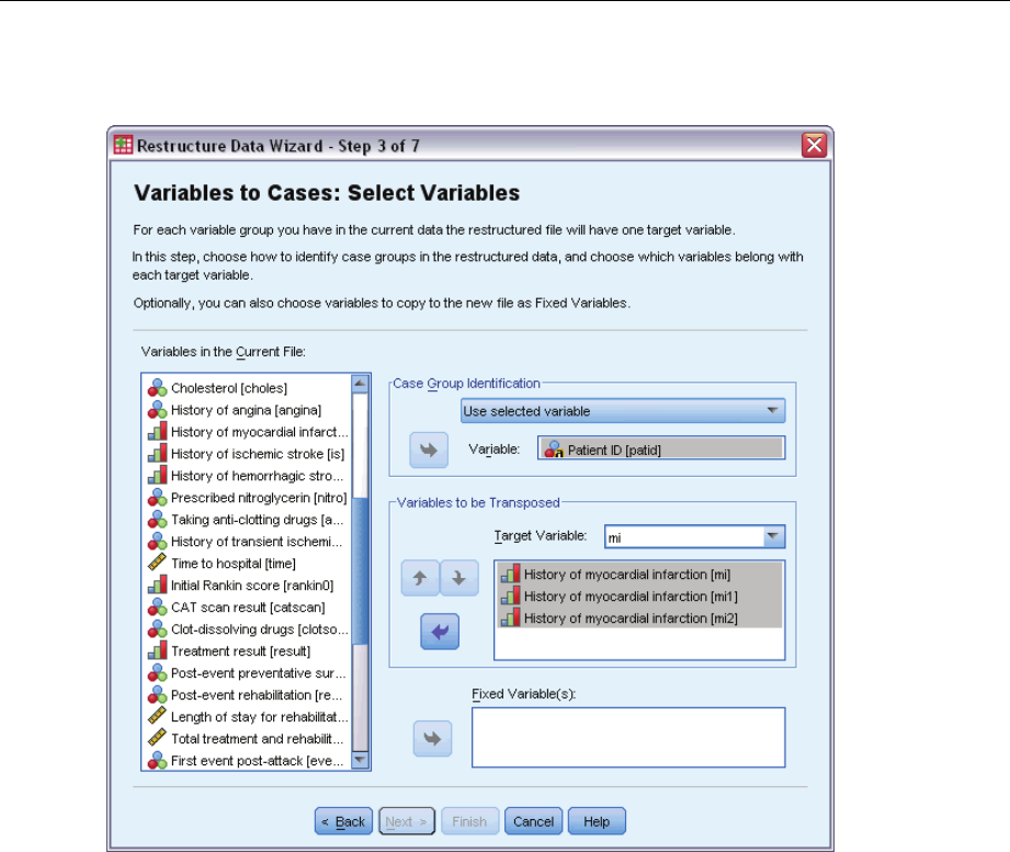
234
Chapter 22
Figure 22-28
Restructure Data Wizard, Variables to Cases Select Variables step
EType mi as the target variable.
ESelect History of myocardial infarction [mi],History of myocardial infarction [mi1],andHistory
of myocardial infarction [mi2] as variables to be transposed.
ESelecttrans5 from the target variable list.
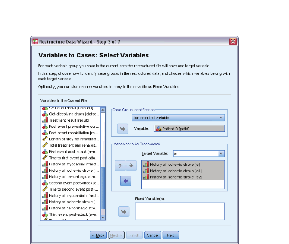
235
Complex Samples Cox Regression
Figure 22-29
Restructure Data Wizard, Variables to Cases Select Variables step
EType is as the target variable.
ESelect History of ischemic stroke [is],History of ischemic stroke [is1],andHistory of ischemic
stroke [is2] as variables to be transposed.
ESelecttrans6 from the target variable list.
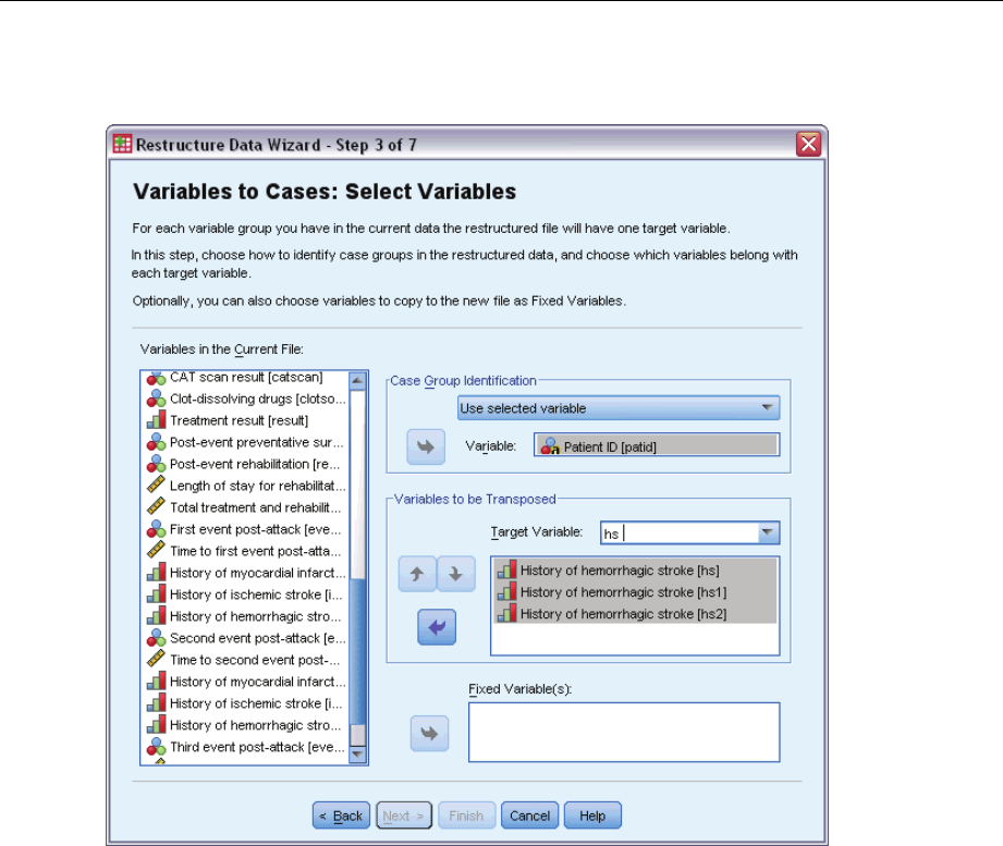
236
Chapter 22
Figure 22-30
Restructure Data Wizard, Variables to Cases Select Variables step
EType hs as the target variable.
ESelect History of hemorrhagic stroke [hs],History of hemorrhagic stroke [hs1],andHistory of
hemorrhagic stroke [hs2] as variables to be transposed.
EClick Next,thenclickNext in the Create Index Variables step.
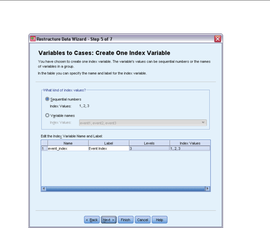
237
Complex Samples Cox Regression
Figure 22-31
Restructure Data Wizard, Variables to Cases Create One Index Variable step
EType event_index as the name of the index variable and type Event index as the variable label.
EClick Next.
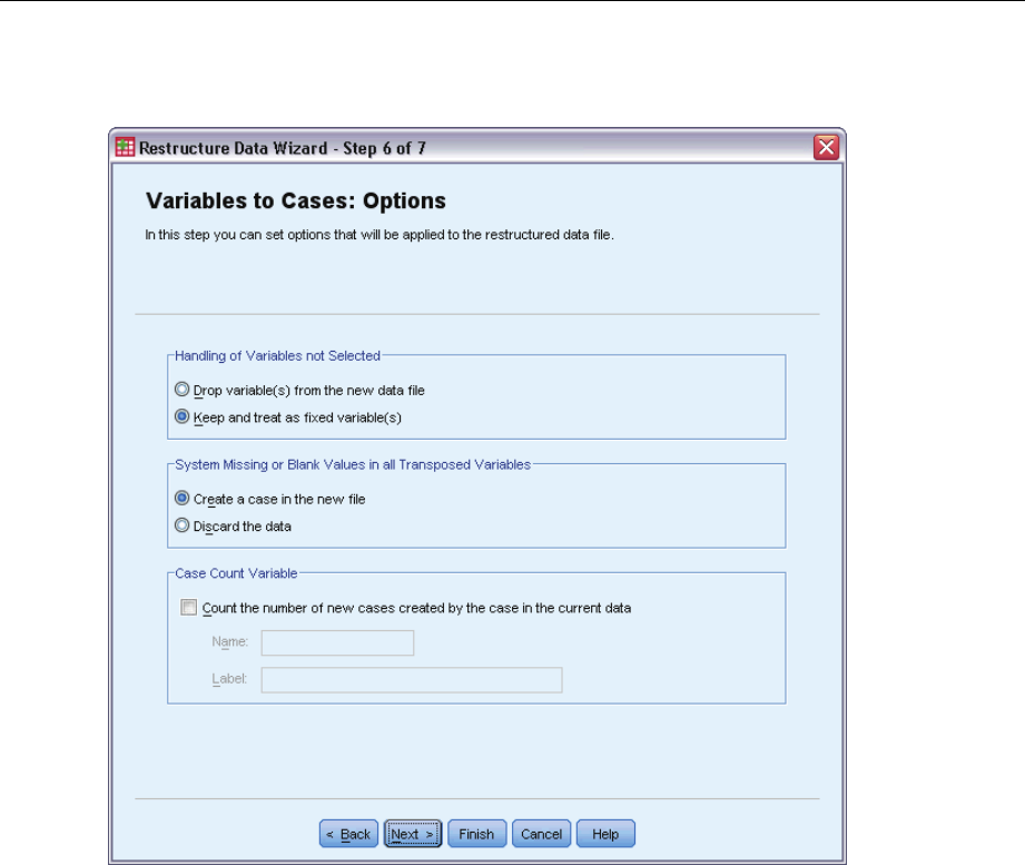
238
Chapter 22
Figure 22-32
Restructure Data Wizard, Variables to Cases Create One Index Variable step
EMake sure Keep and treat as fixed variable(s) is selected.
EClick Finish.
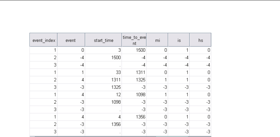
239
Complex Samples Cox Regression
Figure 22-33
Restructured data
The restructured data contains three cases for every patient; however, many patients experienced
fewer than three events, so there are many cases with negative (missing) values for event.Youcan
simply filter these from the dataset.
ETo filter these cases, from the menus choose:
Data > Select Cases...
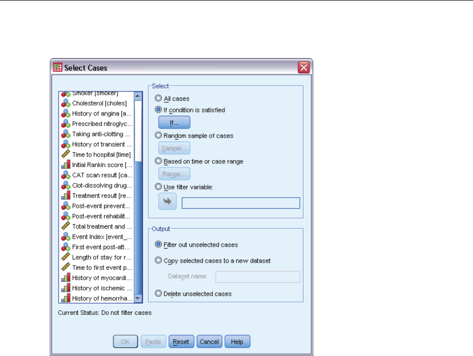
240
Chapter 22
Figure 22-34
Select Cases dialog box
ESelect If condition is satisfied.
EClick If.
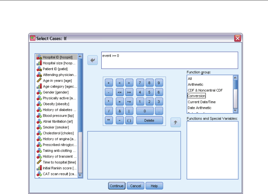
241
Complex Samples Cox Regression
Figure 22-35
Select Cases If dialog box
EType event >= 0 as the conditional expression.
EClick Continue.
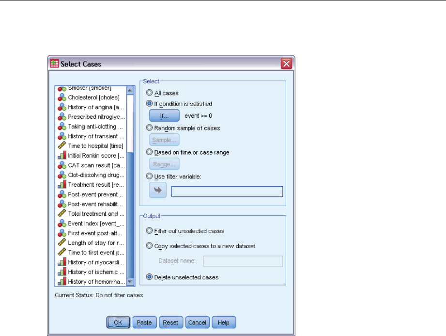
242
Chapter 22
Figure 22-36
Select Cases dialog box
ESelect Delete unselected cases.
EClick OK.
Creating a Simple Random Sampling Analysis Plan
Now you are ready to create the simple random sampling analysis plan.
EFirst, you need to create a sampling weight variable. From the menus choose:
Tr a n s fo rm > Compute Variable...
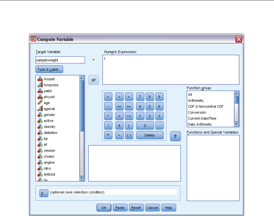
243
Complex Samples Cox Regression
Figure 22-37
Cox Regression main dialog box
EType sampleweight as the target variable.
EType 1as the numeric expression.
EClick OK.
You are now ready to create the analysis plan.
Note: There is an existing plan file, srs.csaplan,inthesamplefiles directory that you can use if
you want to skip the following instructions and proceed to analysis of the data.
ETo create the analysis plan, from the menus choose:
Analyze > Complex Samples > Prepare for Analysis...
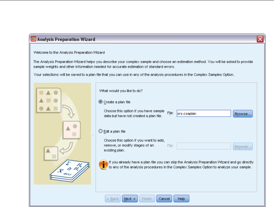
244
Chapter 22
Figure 22-38
Analysis Preparation Wizard, Welcome step
ESelect Createaplanfileand type srs.csaplan as the name of the file. Alternatively, browse to the
location you want to save it.
EClick Next.
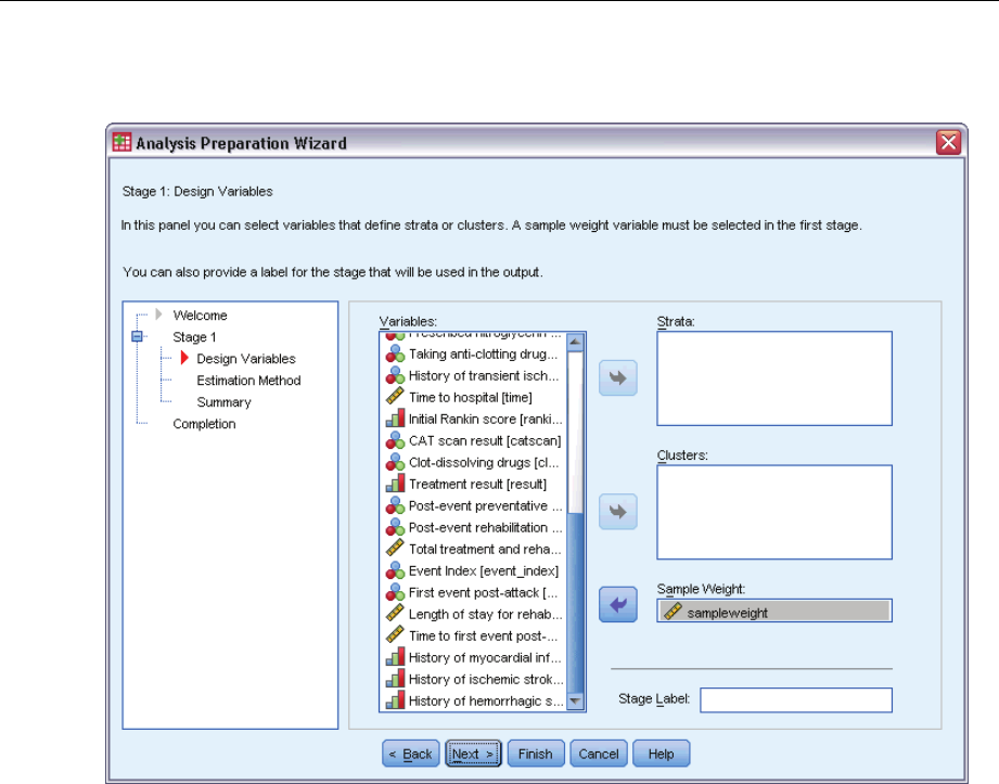
245
Complex Samples Cox Regression
Figure 22-39
Analysis Preparation Wizard, Design Variables
ESelect sampleweight as the sample weight variable.
EClick Next.
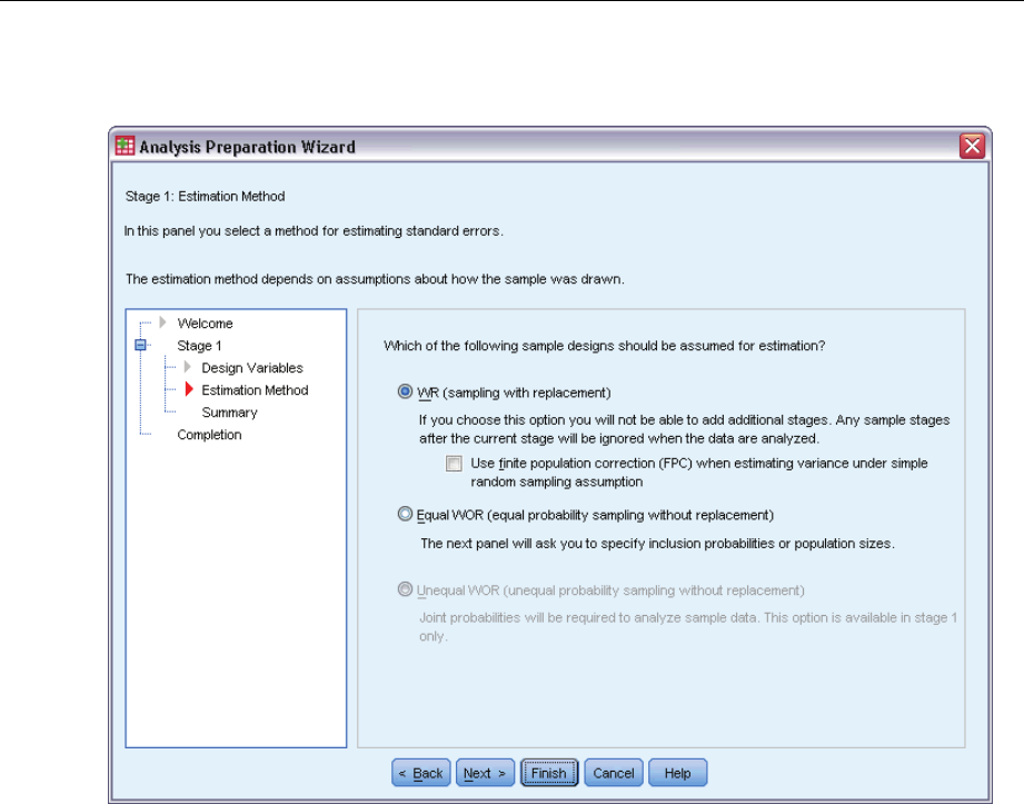
246
Chapter 22
Figure 22-40
Analysis Preparation Wizard, Estimation Method
EDeselect Use finite population correction.
EClick Finish.
You are now ready to run the analysis.
Running the Analysis
ETo run a Complex Samples Cox Regression analysis, from the menus choose:
Analyze > Complex Samples > Cox Regression...
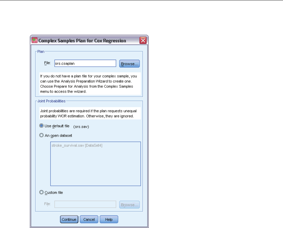
247
Complex Samples Cox Regression
Figure 22-41
Plan for Cox Regression dialog box
EBrowse to where you saved the simple random sampling analysis plan, or to the sample files
directory, and select srs.csaplan.
EClick Continue.
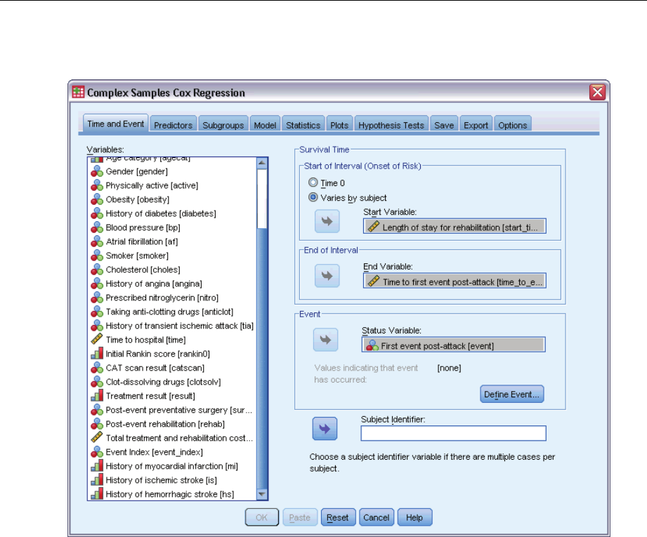
248
Chapter 22
Figure 22-42
Cox Regression dialog box, Time and Event tab
ESelect Varies by subject and select Length of stay for rehabilitation [los_rehab] as the start variable.
Note that the restructured variable has taken the variable label from the first variable used to
construct it, though the label is not necessarily appropriate for the constructed variable.
ESelect Time to first event post-attack [time_to_event] as the end variable.
ESelect First event post-attack [event] as the status variable.
EClick Define Event.
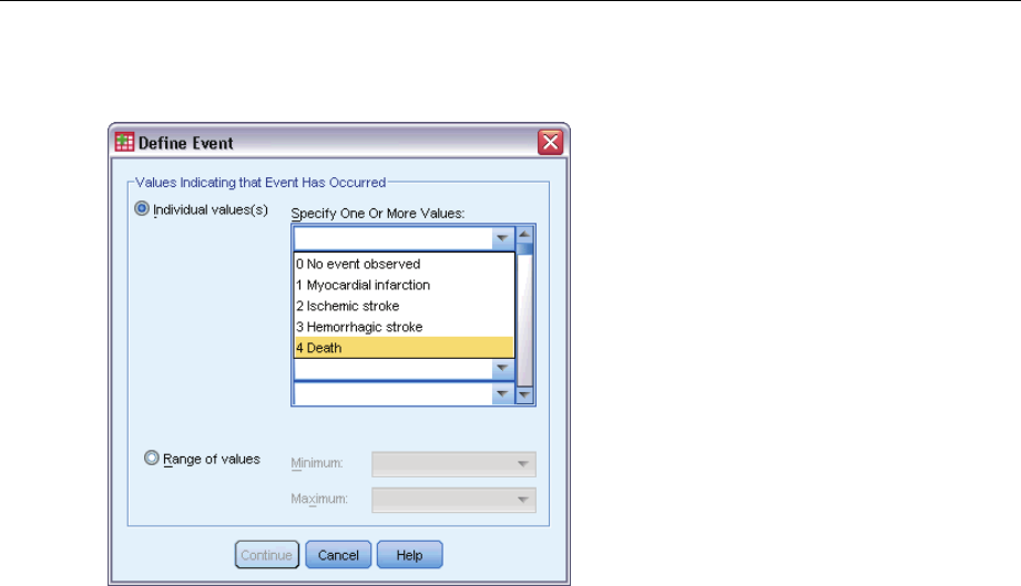
249
Complex Samples Cox Regression
Figure 22-43
Define Event dialog box
ESelect 4Deathas the value indicating the terminal event has occurred.
EClick Continue.
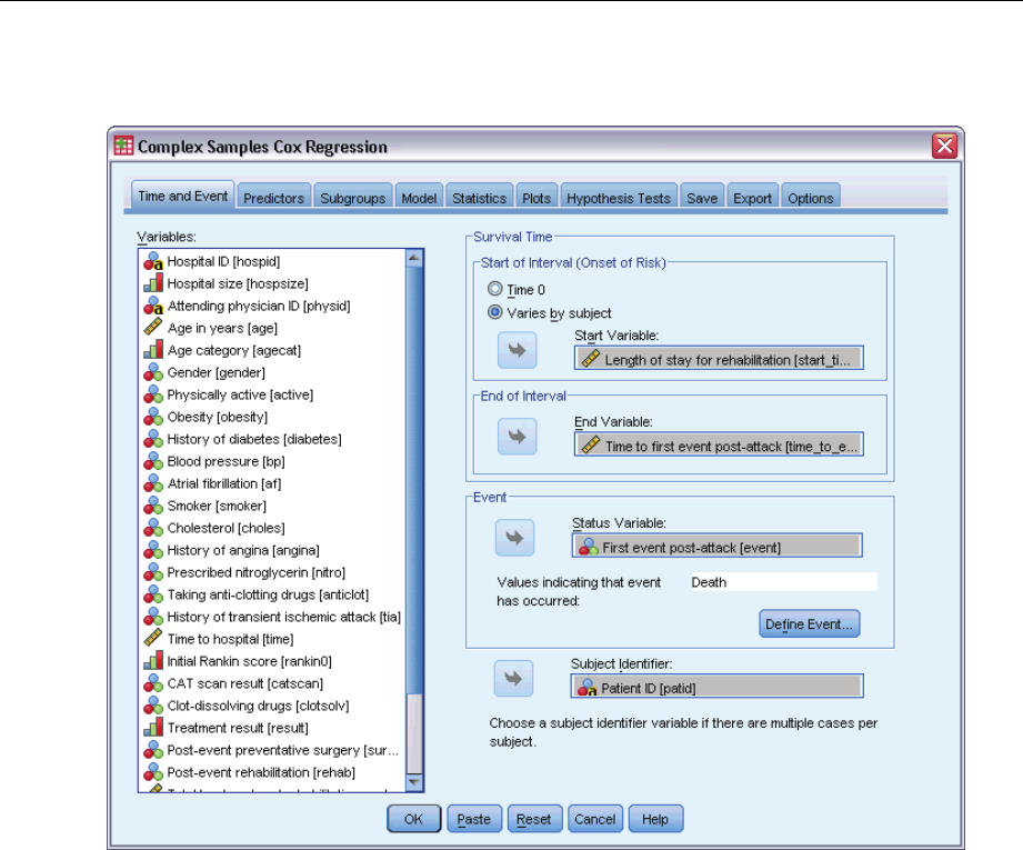
250
Chapter 22
Figure 22-44
Cox Regression dialog box, Time and Event tab
ESelect Patient ID [patid] as the subject identifier.
EClick the Predictors tab.
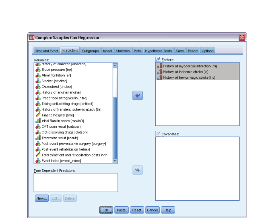
251
Complex Samples Cox Regression
Figure 22-45
Cox Regression dialog box, Predictors tab
ESelect History of myocardial infarction [mi] through History of hemorrhagic stroke [hs] as factors.
EClick the Statistics tab.
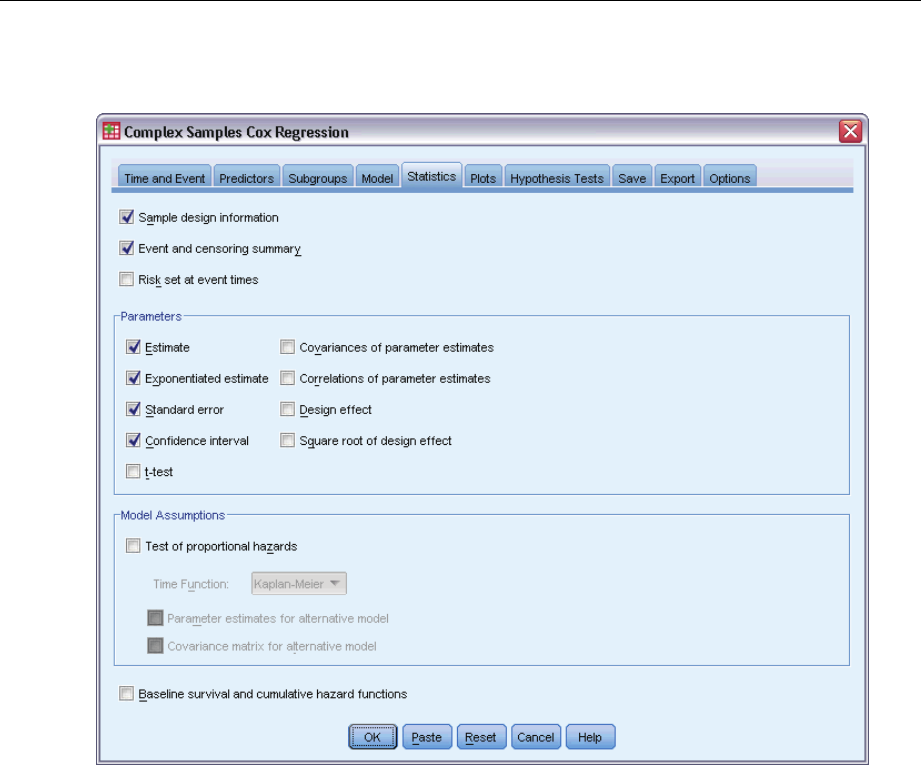
252
Chapter 22
Figure 22-46
Cox Regression dialog box, Statistics tab
ESelect Estimate,Exponentiated estimate,Standard error,andConfidence interval in the Parameters
group.
EClick the Plots tab.
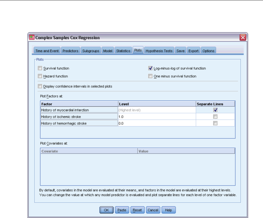
253
Complex Samples Cox Regression
Figure 22-47
Cox Regression dialog box, Statistics tab
ESelect Log-minus-log of survival function.
ECheck Separate Lines for History of myocardial infarction.
ESelect 1.0 as the level for History of ischemic stroke.
ESelect 0.0 as the level for History of hemorrhagic stroke.
EClick the Options tab.
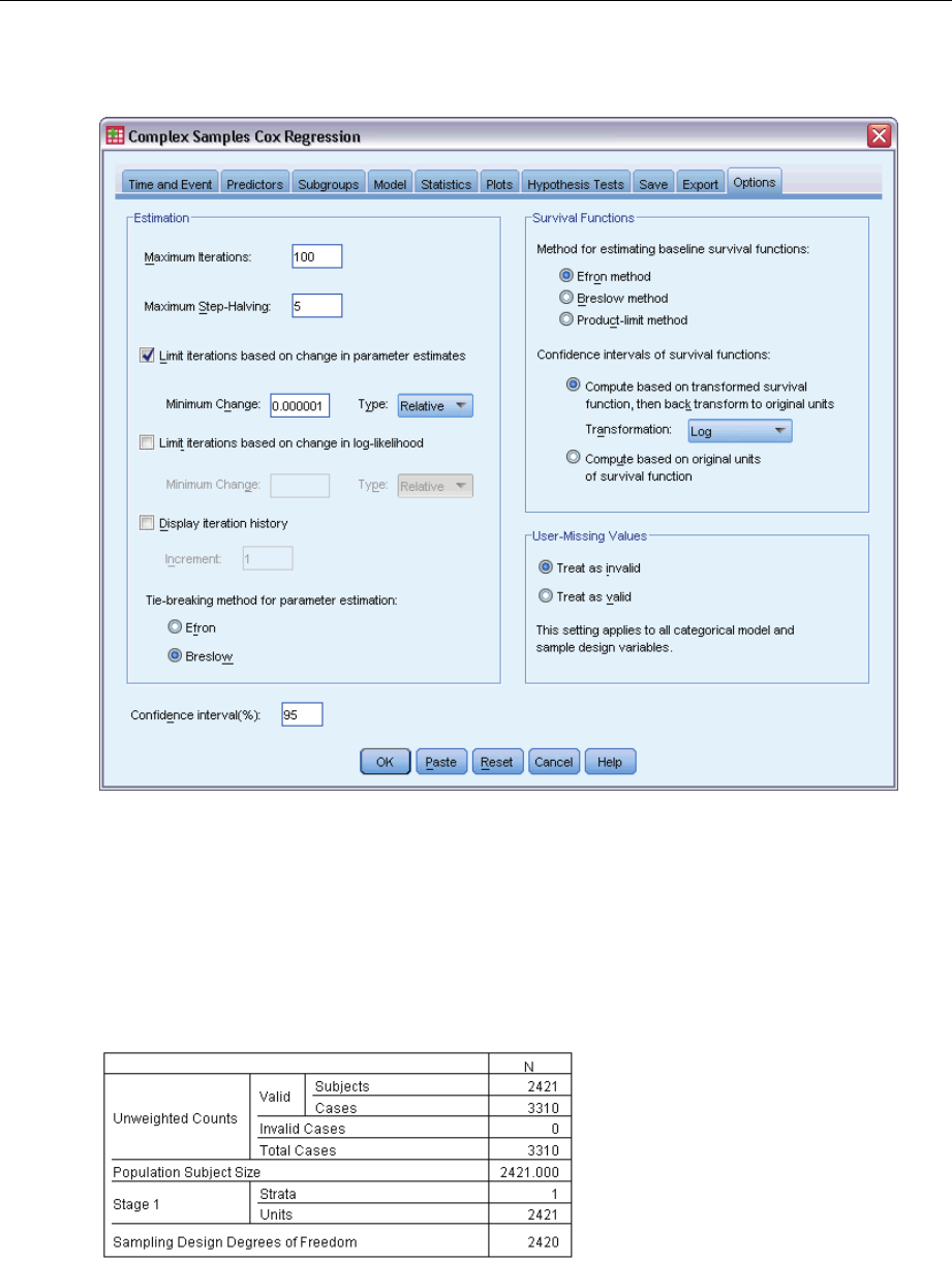
254
Chapter 22
Figure 22-48
Cox Regression dialog box, Options tab
ESelect Breslow as the tie-breaking method in the Estimation group.
EClick OK.
Sample Design Information
Figure 22-49
Sample design information
This table contains information on the sample design pertinent to the estimation of the model.
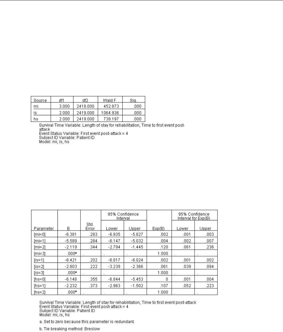
255
Complex Samples Cox Regression
There are multiple cases for some subjects, and all 3,310 cases are used in the analysis.
The design has a single stratum and 2,421 units (one for each subject). The sampling design
degrees of freedom are estimated by 2421−1=2420.
Tests of Model Effects
Figure 22-50
Tests of model effects
The significance value for each effect is near 0, suggesting that they all contribute to the model.
Parameter Estimates
Figure 22-51
Parameter estimates
The procedure uses the last category of each factor as the reference category; the effect of other
categories is relative to the reference category. Note that while the estimate is useful for statistical
testing, the exponentiated estimate, Exp(B), is more easily interpreted as the predicted change in
the hazard relative to the reference category.
The value of Exp(B) for [mi=0] means that the hazard of death for a patient with no prior
myocardial infarctions (mi) is 0.002 times that of a patient with three prior mi’s.
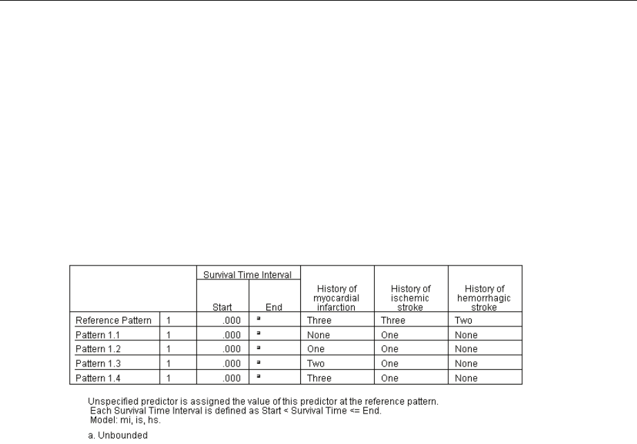
256
Chapter 22
The confidence intervals for [mi=0] and [mi=1] do not overlap with the interval for [mi=2],
and none of them include 0. Therefore, it appears that the hazard for patients with one or no
prior mi’s is distinguishable from the hazard for patients with two prior mi’s, which in turn is
distinguishable from the hazard for patients with three prior mi’s.
Similar relationships hold for the levels of is and hs, where increasing the number of prior
incidents increases the hazard of death.
Pattern Values
Figure 22-52
Pattern values
The pattern values table lists the values that define each predictor pattern. In addition to the
predictors in the model, the start and end times for the survival interval are displayed. For analyses
run from the dialogs, the start and end times will always be 0 and unbounded, respectively;
through syntax you can specify piecewise constant predictor paths.
The reference pattern is set at the reference category for each factor and the mean value of
each covariate (there are no covariates in this model). For this dataset, the combination of
factors shown for the reference model cannot occur, so we will ignore the log-minus-log plot
for the reference pattern.
Patterns 1.1 through 1.4 differ only on the value of History of myocardial infarction.A
separate pattern (and separate line in the requested plot) is created for each value of History of
myocardial infarction while the other variables are held constant.
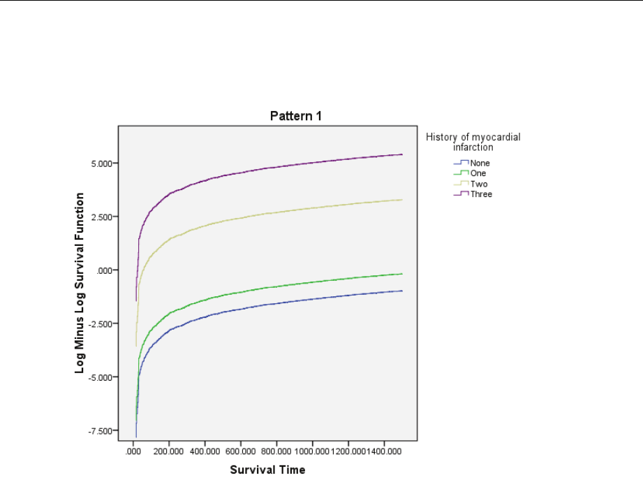
257
Complex Samples Cox Regression
Log-Minus-Log Plot
Figure 22-53
Log-minus-log plot
This plot displays the log-minus-log of the survival function, ln(−ln(suvival)), versus the survival
time. This particular plot displays a separate curve for each category of History of myocardial
infarction,withHistory of ischemic stroke fixed at One and History of hemorrhagic stroke fixed at
None, and is a useful visualization of the effect of History of myocardial infarction on the survival
function. As seen in the parameter estimates table, it appears that the survival for patients with
one or no prior mi’s is distinguishable from the survival for patients with two prior mi’s, which in
turn is distinguishable from the survival for patients with three prior mi’s.
Summary
You hav efit a Cox regression model for post-stroke survival that estimates the effects of the
changing post-stroke patient history. This is just a beginning, as researchers would undoubtedly
want to include other potential predictors in the model. Moreover, in further analysis of this
dataset you might consider more significant changes to the model structure. For example, the
current model assumes that the effect of a patient history-altering event can be quantified by a
multiplier to the baseline hazard. Instead, it may be reasonable to assume that the shape of the
baseline hazard is altered by the occurrence of a nondeath event. To accomplish this, you could
stratify the analysis based on Event index.

Appendix
A
Sample Files
The sample files installed with the product can be found in the Samples subdirectory of the
installation directory. There is a separate folder within the Samples subdirectory for each of
the following languages: English, French, German, Italian, Japanese, Korean, Polish, Russian,
Simplified Chinese, Spanish, and Traditional Chinese.
Not all sample files are available in all languages. If a sample file is not available in a language,
that language folder contains an English version of the sample file.
Descriptions
Following are brief descriptions of the sample files used in various examples throughout the
documentation.
accidents.sav. This is a hypothetical data file that concerns an insurance company that is
studying age and gender risk factors for automobile accidents in a given region. Each case
corresponds to a cross-classification of age category and gender.
adl.sav. This is a hypothetical data file that concerns efforts to determine the benefits of a
proposed type of therapy for stroke patients. Physicians randomly assigned female stroke
patients to one of two groups. The first received the standard physical therapy, and the second
received an additional emotional therapy. Three months following the treatments, each
patient’s abilities to perform common activities of daily life were scored as ordinal variables.
advert.sav. This is a hypothetical data file that concerns a retailer’s efforts to examine the
relationship between money spent on advertising and the resulting sales. To this end, they
have collected past sales figures and the associated advertising costs..
aflatoxin.sav. This is a hypothetical data file that concerns the testingofcorncropsfor
aflatoxin, a poison whose concentration varies widely between and within crop yields. A grain
processor has received 16 samples from each of 8 crop yields and measured the alfatoxin
levels in parts per billion (PPB).
anorectic.sav. While working toward a standardized symptomatology of anorectic/bulimic
behavior, researchers (Van der Ham, Meulman, Van Strien, and Van Engeland, 1997) made a
study of 55 adolescents with known eating disorders. Each patient was seen four times over
four years, for a total of 220 observations. At each observation, the patients were scored for
each of 16 symptoms. Symptom scores are missing for patient 71 at time 2, patient 76 at time
2, and patient 47 at time 3, leaving 217 valid observations.
bankloan.sav. This is a hypothetical data file that concerns a bank’s efforts to reduce the
rate of loan defaults. The file contains financial and demographic information on 850 past
and prospective customers. The first 700 cases are customers who were previously given
© Copyright SPSS Inc. 1989, 2010 258

259
Sample Files
loans. The last 150 cases are prospective customers that the bank needs to classify as good
or bad credit risks.
bankloan_binning.sav. This is a hypothetical data file containing financial and demographic
information on 5,000 past customers.
behavior.sav. In a classic example (Price and Bouffard, 1974), 52 students were asked to
rate the combinations of 15 situations and 15 behaviors on a 10-point scale ranging from
0=“extremely appropriate” to 9=“extremely inappropriate.” Averaged over individuals, the
values are taken as dissimilarities.
behavior_ini.sav. This data file contains an initial configuration for a two-dimensional solution
for behavior.sav.
brakes.sav. This is a hypothetical data file that concerns quality control at a factory that
produces disc brakes for high-performance automobiles. The data file contains diameter
measurements of 16 discs from each of 8 production machines. The target diameter for the
brakes is 322 millimeters.
breakfast.sav. In a classic study (Green and Rao, 1972), 21 Wharton School MBA students
and their spouses were asked to rank 15 breakfast items in order of preference with 1=“most
preferred” to 15=“least preferred.” Their preferences were recorded under six different
scenarios, from “Overall preference” to “Snack, with beverage only.”
breakfast-overall.sav. This data file contains the breakfast item preferences for the first
scenario, “Overall preference,” only.
broadband_1.sav. This is a hypothetical data file containing the number of subscribers, by
region, to a national broadband service. The data file contains monthly subscriber numbers
for 85 regions over a four-year period.
broadband_2.sav. This data file is identical to broadband_1.sav but contains data for three
additional months.
car_insurance_claims.sav. A dataset presented and analyzed elsewhere (McCullagh and
Nelder, 1989) concerns damage claims for cars. The average claim amount can be modeled
as having a gamma distribution, using an inverse link function to relate the mean of the
dependent variable to a linear combination of the policyholder age, vehicle type, and vehicle
age. Thenumberofclaimsfiled can be used as a scaling weight.
car_sales.sav. This data file contains hypothetical sales estimates, list prices, and physical
specifications for various makes and models of vehicles. The list prices and physical
specifications were obtained alternately from edmunds.com and manufacturer sites.
car_sales_uprepared.sav. This is a modified version of car_sales.sav that does not include any
transformed versions of the fields.
carpet.sav. In a popular example (Green and Wind, 1973), a company interested in
marketing a new carpet cleaner wants to examine the influence of five factors on consumer
preference—package design, brand name, price, a Good Housekeeping seal, and a
money-back guarantee. There are three factor levels for package design, each one differing in
the location of the applicator brush; three brand names (K2R,Glory,andBissell); three price
levels; and two levels (either no or yes) for each of the last two factors. Ten consumers rank
22 profiles defined by these factors. The variable Preference contains the rank of the average
rankings for each profile. Low rankings correspond to high preference. This variable reflects
an overall measure of preference for each profile.

260
Appendix A
carpet_prefs.sav. This data file is based on the same example as described for carpet.sav,butit
contains the actual rankings collected from each of the 10 consumers. The consumers were
asked to rank the 22 product profiles from the most to the least preferred. The variables
PREF1 through PREF22 contain the identifiers of the associated profiles, as defined in
carpet_plan.sav.
catalog.sav. This data file contains hypothetical monthly sales figures for three products sold
by a catalog company. Data for five possible predictor variables are also included.
catalog_seasfac.sav. This data file is the same as catalog.sav except for the addition of a set
of seasonal factors calculated from the Seasonal Decomposition procedure along with the
accompanying date variables.
cellular.sav. This is a hypothetical data file that concerns a cellular phone company’s efforts
to reduce churn. Churn propensity scores are applied to accounts, ranging from 0 to 100.
Accounts scoring 50 or above may be looking to change providers.
ceramics.sav. This is a hypothetical data file that concerns a manufacturer’s efforts to
determine whether a new premium alloy has a greater heat resistance than a standard alloy.
Each case represents a separate test of one of the alloys; the heat at which the bearing failed is
recorded.
cereal.sav. This is a hypothetical data file that concerns a poll of 880 people about their
breakfast preferences, also noting their age, gender, marital status, and whether or not they
have an active lifestyle (based on whether they exercise at least twice a week). Each case
represents a separate respondent.
clothing_defects.sav. This is a hypothetical data file that concerns the quality control process
at a clothing factory. From each lot produced at the factory, the inspectors take a sample of
clothes and count the number of clothes that are unacceptable.
coffee.sav. This data file pertains to perceived images of six iced-coffee brands (Kennedy,
Riquier, and Sharp, 1996) . For each of 23 iced-coffee image attributes, people selected all
brands that were described by the attribute. The six brands are denoted AA, BB, CC, DD, EE,
and FF to preserve confidentiality.
contacts.sav. This is a hypothetical data file that concerns the contact lists for a group of
corporate computer sales representatives. Each contact is categorized by the department of
the company in which they work and their company ranks. Also recorded are the amount of
the last sale made, the time since the last sale, and the size of the contact’s company.
creditpromo.sav. This is a hypothetical data file that concerns a department store’s efforts to
evaluate the effectiveness of a recent credit card promotion. To this end, 500 cardholders were
randomly selected. Half received an ad promoting a reduced interest rate on purchases made
over the next three months. Half received a standard seasonal ad.
customer_dbase.sav. This is a hypothetical data file that concerns a company’s efforts to use
the information in its data warehouse to make special offers to customers who are most
likely to reply. A subset of the customer base was selected at random and given the special
offers, and their responses were recorded.
customer_information.sav. A hypothetical data file containing customer mailing information,
such as name and address.
customer_subset.sav. A subset of 80 cases from customer_dbase.sav.

261
Sample Files
debate.sav. This is a hypothetical data file that concerns paired responses to a survey from
attendees of a political debate before and after the debate. Each case corresponds to a separate
respondent.
debate_aggregate.sav. This is a hypothetical data file that aggregates the responses in
debate.sav. Each case corresponds to a cross-classification of preference before and after
the debate.
demo.sav. This is a hypothetical data file that concerns a purchased customer database, for
the purpose of mailing monthly offers. Whether or not the customer responded to the offer
is recorded, along with various demographic information.
demo_cs_1.sav. This is a hypothetical data file that concerns the first step of a company’s
efforts to compile a database of survey information. Each case corresponds to a different city,
and the region, province, district, and city identification are recorded.
demo_cs_2.sav. This is a hypothetical data file that concerns the second step of a company’s
efforts to compile a database of survey information. Each case corresponds to a different
household unit from cities selected in the first step, and the region, province, district, city,
subdivision, and unit identification are recorded. The sampling information from the first
two stages of the design is also included.
demo_cs.sav. This is a hypothetical data file that contains survey information collected using a
complex sampling design. Each case corresponds to a different household unit, and various
demographic and sampling information is recorded.
dmdata.sav. This is a hypothetical data file that contains demographic and purchasing
information for a direct marketing company. dmdata2.sav contains information for a subset of
contacts that received a test mailing, and dmdata3.sav contains information on the remaining
contacts who did not receive the test mailing.
dietstudy.sav. This hypothetical data file contains the results of a study of the “Stillman diet”
(Rickman, Mitchell, Dingman, and Dalen, 1974). Each case corresponds to a separate
subject and records his or her pre- and post-diet weights in pounds and triglyceride levels
in mg/100 ml.
dvdplayer.sav. This is a hypothetical data file that concerns the development of a new DVD
player. Using a prototype, the marketing team has collected focus group data. Each case
corresponds to a separate surveyed user and records some demographic information about
them and their responses to questions about the prototype.
german_credit.sav. This data file is taken from the “German credit” dataset in the Repository of
Machine Learning Databases (Blake and Merz, 1998) at the University of California, Irvine.
grocery_1month.sav. This hypothetical data file is the grocery_coupons.sav data file with the
weekly purchases “rolled-up” so that each case corresponds to a separate customer. Some of
the variables that changed weekly disappear as a result, and the amount spent recorded is now
the sum of the amounts spent during the four weeks of the study.
grocery_coupons.sav. This is a hypothetical data file that contains survey data collected by
a grocery store chain interested in the purchasing habits of their customers. Each customer
is followed for four weeks, and each case corresponds to a separate customer-week and
records information about where and how the customer shops, including how much was
spent on groceries during that week.

262
Appendix A
guttman.sav. Bell (Bell, 1961) presented a table to illustrate possible social groups. Guttman
(Guttman, 1968) used a portion of this table, in which five variables describing such things
as social interaction, feelings of belonging to a group, physical proximity of members, and
formality of the relationship were crossed with seven theoretical social groups, including
crowds (for example, people at a football game), audiences (for example, people at a theater
or classroom lecture), public (for example, newspaper or television audiences), mobs (like a
crowd but with much more intense interaction), primary groups (intimate), secondary groups
(voluntary), and the modern community (loose confederation resulting from close physical
proximity and a need for specialized services).
health_funding.sav. This is a hypothetical data file that contains data on health care funding
(amount per 100 population), disease rates (rate per 10,000 population), and visits to health
care providers (rate per 10,000 population). Each case represents a different city.
hivassay.sav. This is a hypothetical data file that concerns the efforts of a pharmaceutical
lab to develop a rapid assay for detecting HIV infection. The results of the assay are eight
deepening shades of red, with deeper shades indicating greater likelihood of infection. A
laboratory trial was conducted on 2,000 blood samples, half of which were infected with
HIV and half of which were clean.
hourlywagedata.sav. This is a hypothetical data file that concerns the hourly wages of nurses
from office and hospital positions and with varying levels of experience.
insurance_claims.sav. This is a hypothetical data file that concerns an insurance company that
wants to build a model for flagging suspicious, potentially fraudulent claims. Each case
represents a separate claim.
insure.sav. This is a hypothetical data file that concerns an insurance company that is studying
the risk factors that indicate whether a client will have to make a claim on a 10-year term
life insurance contract. Each case in the data file represents a pair of contracts, one of which
recorded a claim and the other didn’t, matched on age and gender.
judges.sav. This is a hypothetical data file that concerns the scores given by trained judges
(plus one enthusiast) to 300 gymnastics performances. Each row represents a separate
performance; the judges viewed the same performances.
kinship_dat.sav. Rosenberg and Kim (Rosenberg and Kim, 1975) set out to analyze 15 kinship
terms (aunt, brother, cousin, daughter, father, granddaughter, grandfather, grandmother,
grandson, mother, nephew, niece, sister, son, uncle). They asked four groups of college
students (two female, two male) to sort these terms on the basis of similarities. Two groups
(one female, one male) were asked to sort twice, with the second sorting based on a different
criterion from the first sort. Thus, a total of six “sources” were obtained. Each source
corresponds to a proximity matrix, whose cells are equal to the number of people in a
source minus the number of times the objects were partitioned together in that source.
kinship_ini.sav. This data file contains an initial configuration for a three-dimensional solution
for kinship_dat.sav.
kinship_var.sav. This data file contains independent variables gender,gener(ation), and degree
(of separation) that can be used to interpret the dimensions of a solution for kinship_dat.sav.
Specifically, they can be used to restrict the space of the solution to a linear combination of
these variables.
marketvalues.sav. This data file concerns home sales in a new housing development in
Algonquin, Ill., during the years from 1999–2000. These sales are a matter of public record.

263
Sample Files
nhis2000_subset.sav. The National Health Interview Survey (NHIS) is a large, population-based
survey of the U.S. civilian population. Interviews are carried out face-to-face in a nationally
representative sample of households. Demographic information and observations about
health behaviors and status are obtained for members of each household. This data
file contains a subset of information from the 2000 survey. National Center for Health
Statistics. National Health Interview Survey, 2000. Public-use data file and documentation.
ftp://ftp.cdc.gov/pub/Health_Statistics/NCHS/Datasets/NHIS/2000/. Accessed 2003.
ozone.sav. The data include 330 observations on six meteorological variables for predicting
ozone concentration from the remaining variables. Previous researchers (Breiman and
Friedman, 1985), (Hastie and Tibshirani, 1990), among others found nonlinearities among
these variables, which hinder standard regression approaches.
pain_medication.sav. This hypothetical data file contains the results of a clinical trial for
anti-inflammatory medication for treating chronic arthritic pain. Of particular interest is the
time it takes for the drug to take effect and how it compares to an existing medication.
patient_los.sav. This hypothetical data file contains the treatment records of patients who were
admitted to the hospital for suspected myocardial infarction (MI, or “heart attack”). Each case
corresponds to a separate patient and records many variables related to their hospital stay.
patlos_sample.sav. This hypothetical data file contains the treatment records of a sample
of patients who received thrombolytics during treatment for myocardial infarction (MI, or
“heart attack”). Each case corresponds to a separate patient and records many variables
related to their hospital stay.
poll_cs.sav. This is a hypothetical data file that concerns pollsters’ efforts to determine the
level of public support for a bill before the legislature. The cases correspond to registered
voters. Each case records the county, township, and neighborhood in which the voter lives.
poll_cs_sample.sav. This hypothetical data file contains a sample of the voters listed in
poll_cs.sav. The sample was taken according to the design specified in the poll.csplan plan
file, and this data file records the inclusion probabilities and sample weights. Note, however,
that because the sampling plan makes use of a probability-proportional-to-size (PPS) method,
there is also a file containing the joint selection probabilities (poll_jointprob.sav). The
additional variables corresponding to voter demographics and their opinion on the proposed
bill were collected and added the data file after the sample as taken.
property_assess.sav. This is a hypothetical data file that concerns a county assessor’s efforts to
keep property value assessments up to date on limited resources. The cases correspond to
properties sold in the county in the past year. Each case in the data file records the township
in which the property lies, the assessor who last visited the property, the time since that
assessment, the valuation made at that time, and the sale value of the property.
property_assess_cs.sav. This is a hypothetical data file that concerns a state assessor’s efforts
to keep property value assessments up to date on limited resources. The cases correspond
to properties in the state. Each case in the data file records the county, township, and
neighborhood in which the property lies, the time since the last assessment, and the valuation
made at that time.
property_assess_cs_sample.sav. This hypothetical data file contains a sample of the properties
listed in property_assess_cs.sav. The sample was taken according to the design specified in
the property_assess.csplan plan file, and this data file records the inclusion probabilities

264
Appendix A
and sample weights. The additional variable Current value was collected and added to the
data file after the sample was taken.
recidivism.sav. This is a hypothetical data file that concerns a government law enforcement
agency’s efforts to understand recidivism rates in their area of jurisdiction. Each case
corresponds to a previous offender and records their demographic information, some details
of their first crime, and then the time until their second arrest, if it occurred within two years
of the first arrest.
recidivism_cs_sample.sav. This is a hypothetical data file that concerns a government law
enforcement agency’s efforts to understand recidivism rates in their area of jurisdiction. Each
case corresponds to a previous offender, released from their first arrest during the month of
June, 2003, and records their demographic information, some details of their first crime, and
the data of their second arrest, if it occurred by the end of June, 2006. Offenders were selected
from sampled departments according to the sampling plan specified in recidivism_cs.csplan;
because it makes use of a probability-proportional-to-size (PPS) method, there is also a file
containing the joint selection probabilities (recidivism_cs_jointprob.sav).
rfm_transactions.sav. A hypothetical data file containing purchase transaction data, including
date of purchase, item(s) purchased, and monetary amount of each transaction.
salesperformance.sav. This is a hypothetical data file that concerns the evaluation of two
new sales training courses. Sixty employees, divided into three groups, all receive standard
training. In addition, group 2 gets technical training; group 3, a hands-on tutorial. Each
employee was tested at the end of the training course and their score recorded. Each case in
the data file represents a separate trainee and records the group to which they were assigned
and the score they received on the exam.
satisf.sav. This is a hypothetical data file that concerns a satisfaction survey conducted by
a retail company at 4 store locations. 582 customers were surveyed in all, and each case
represents the responses from a single customer.
screws.sav. This data file contains information on the characteristics of screws, bolts, nuts,
and tacks (Hartigan, 1975).
shampoo_ph.sav. This is a hypothetical data file that concerns the quality control at a factory
for hair products. At regular time intervals, six separate output batches are measured and their
pH recorded. The target range is 4.5–5.5.
ships.sav. A dataset presented and analyzed elsewhere (McCullagh et al., 1989) that concerns
damage to cargo ships caused by waves. The incident counts can be modeled as occurring at
a Poisson rate given the ship type, construction period, and service period. The aggregate
months of service for each cell of the table formed by the cross-classification of factors
provides values for the exposure to risk.
site.sav. This is a hypothetical data file that concerns a company’s efforts to choose new
sites for their expanding business. They have hired two consultants to separately evaluate
the sites, who, in addition to an extended report, summarized each site as a “good,” “fair,”
or “poor” prospect.
smokers.sav. This data file is abstracted from the 1998 National Household
Survey of Drug Abuse and is a probability sample of American households.
(http://dx.doi.org/10.3886/ICPSR02934)Thus,thefirststepinananalysisofthisdatafile
should be to weight the data to reflect population trends.

265
Sample Files
stroke_clean.sav. This hypothetical data file contains the state of a medical database after it
has been cleaned using procedures in the Data Preparation option.
stroke_invalid.sav. This hypothetical data file contains the initial state of a medical database
and contains several data entry errors.
stroke_survival. This hypothetical data file concerns survival times for patients exiting a
rehabilitation program post-ischemic stroke face a number of challenges. Post-stroke, the
occurrence of myocardial infarction, ischemic stroke, or hemorrhagic stroke is noted and the
time of the event recorded. The sample is left-truncated because it only includes patients who
survived through the end of the rehabilitation program administered post-stroke.
stroke_valid.sav. This hypothetical data file contains the state of a medical database after the
values have been checked using the Validate Data procedure. It still contains potentially
anomalous cases.
survey_sample.sav. This data file contains survey data, including demographic data and
various attitude measures. It is based on a subset of variables from the 1998 NORC General
Social Survey, although some data values have been modified and additional fictitious
variables have been added for demonstration purposes.
telco.sav. This is a hypothetical data file that concerns a telecommunications company’s
efforts to reduce churn in their customer base. Each case corresponds to a separate customer
and records various demographic and service usage information.
telco_extra.sav. This data file is similar to the telco.sav data file, but the “tenure” and
log-transformed customer spending variables have been removed and replaced by
standardized log-transformed customer spending variables.
telco_missing.sav. This data file is a subset of the telco.sav data file, but some of the
demographic data values have been replaced with missing values.
testmarket.sav. This hypothetical data file concerns a fast food chain’s plans to add a new item
to its menu. There are three possible campaigns for promoting the new product, so the new
item is introduced at locations in several randomly selected markets. A different promotion
is used at each location, and the weekly sales of the new item are recorded for the first four
weeks. Each case corresponds to a separate location-week.
testmarket_1month.sav. This hypothetical data file is the testmarket.sav data file with the
weekly sales “rolled-up” so that each case corresponds to a separate location. Some of the
variables that changed weekly disappear as a result, and the sales recorded is now the sum of
the sales during the four weeks of the study.
tree_car.sav. This is a hypothetical data file containing demographic and vehicle purchase
price data.
tree_credit.sav. This is a hypothetical data file containing demographic and bank loan history
data.
tree_missing_data.sav This is a hypothetical data file containing demographic and bank loan
history data with a large number of missing values.
tree_score_car.sav. This is a hypothetical data file containing demographic and vehicle
purchase price data.
tree_textdata.sav. Asimpledatafile with only two variables intended primarily to show the
default state of variables prior to assignment of measurement level and value labels.

266
Appendix A
tv-survey.sav. This is a hypothetical data file that concerns a survey conducted by a TV studio
that is considering whether to extend the run of a successful program. 906 respondents were
asked whether they would watch the program under various conditions. Each row represents a
separate respondent; each column is a separate condition.
ulcer_recurrence.sav. This file contains partial information from a study designed to compare
the efficacy of two therapies for preventing the recurrence of ulcers. It provides a good
example of interval-censored data and has been presented and analyzed elsewhere (Collett,
2003).
ulcer_recurrence_recoded.sav. This file reorganizes the information in ulcer_recurrence.sav to
allow you model the event probability for each interval of the study rather than simply the
end-of-study event probability. It has been presented and analyzed elsewhere (Collett et
al., 2003).
verd1985.sav. This data file concerns a survey (Verdegaal, 1985). The responses of 15 subjects
to 8 variables were recorded. The variables of interest are divided into three sets. Set 1
includes age and marital,set2includespet and news,andset3includesmusic and live.
Pet is scaled as multiple nominal and age is scaled as ordinal; all of the other variables are
scaled as single nominal.
virus.sav. This is a hypothetical data file that concerns the efforts of an Internet service
provider (ISP) to determine the effects of a virus on its networks. They have tracked the
(approximate) percentage of infected e-mail traffic on its networks over time, from the
moment of discovery until the threat was contained.
wheeze_steubenville.sav. This is a subset from a longitudinal study of the health effects of
air pollution on children (Ware, Dockery, Spiro III, Speizer, and Ferris Jr., 1984). The data
contain repeated binary measures of the wheezing status for children from Steubenville, Ohio,
at ages 7, 8, 9 and 10 years, along with a fixed recording of whether or not the mother was
a smoker during the first year of the study.
workprog.sav. This is a hypothetical data file that concerns a government works program
that tries to place disadvantaged people into better jobs. A sample of potential program
participants were followed, some of whom were randomly selected for enrollment in the
program, while others were not. Each case represents a separate program participant.

Appendix
B
Notices
Licensed Materials – Property of SPSS Inc., an IBM Company. © Copyright SPSS Inc. 1989,
2010.
Patent No. 7,023,453
The following paragraph does not apply to the United Kingdom or any other country where such
provisions are inconsistent with local law: SPSS INC., AN IBM COMPANY, PROVIDES THIS
PUBLICATION “AS IS” WITHOUT WARRANTY OF ANY KIND, EITHER EXPRESS
OR IMPLIED, INCLUDING, BUT NOT LIMITED TO, THE IMPLIED WARRANTIES
OF NON-INFRINGEMENT, MERCHANTABILITY OR FITNESS FOR A PARTICULAR
PURPOSE. Some states do not allow disclaimer of express or implied warranties in certain
transactions, therefore, this statement may not apply to you.
This information could include technical inaccuracies or typographical errors. Changes are
periodically made to the information herein; these changes will be incorporated in new editions of
the publication. SPSS Inc. may make improvements and/or changes in the product(s) and/or the
program(s) described in this publication at any time without notice.
Any references in this information to non-SPSS and non-IBM Web sites are provided for
convenience only and do not in any manner serve as an endorsement of those Web sites. The
materials at those Web sites are not part of the materials for this SPSS Inc. product and use of
those Web sites is at your own risk.
When you send information to IBM or SPSS, you grant IBM and SPSS a nonexclusive right
to use or distribute the information in any way it believes appropriate without incurring any
obligationtoyou.
Information concerning non-SPSS products was obtained from the suppliers of those products,
their published announcements or other publicly available sources. SPSS has not tested those
products and cannot confirm the accuracy of performance, compatibility or any other claims
related to non-SPSS products. Questions on the capabilities of non-SPSS products should be
addressed to the suppliers of those products.
This information contains examples of data and reports used in daily business operations.
To illustrate them as completely as possible, the examples include the names of individuals,
companies, brands, and products. All of these names are fictitious and any similarity to the names
and addresses used by an actual business enterprise is entirely coincidental.
COPYRIGHT LICENSE:
This information contains sample application programs in source language, which illustrate
programming techniques on various operating platforms. You may copy, modify, and distribute
these sample programs in any form without payment to SPSS Inc., for the purposes of developing,
© Copyright SPSS Inc. 1989, 2010 267

268
Appendix B
using, marketing or distributing application programs conforming to the application programming
interface for the operating platform for which the sample programs are written. These examples
have not been thoroughly tested under all conditions. SPSS Inc., therefore, cannot guarantee or
imply reliability, serviceability, or function of these programs. The sample programs are provided
“AS IS”, without warranty of any kind. SPSS Inc. shall not be liable for any damages arising out
of your use of the sample programs.
Trademarks
IBM, the IBM logo, and ibm.com are trademarks of IBM Corporation, registered in many
jurisdictions worldwide. A current list of IBM trademarks is available on the Web at
http://www.ibm.com/legal/copytrade.shmtl.
SPSS is a trademark of SPSS Inc., an IBM Company, registered in many jurisdictions worldwide.
Adobe, the Adobe logo, PostScript, and the PostScript logo are either registered trademarks or
trademarks of Adobe Systems Incorporated in the United States, and/or other countries.
Intel, Intel logo, Intel Inside, Intel Inside logo, Intel Centrino, Intel Centrino logo, Celeron, Intel
Xeon, Intel SpeedStep, Itanium, and Pentium are trademarks or registered trademarks of Intel
Corporation or its subsidiaries in the United States and other countries.
Linux is a registered trademark of Linus Torvalds in the United States, other countries, or both.
Microsoft, Windows, Windows NT, and the Windows logo are trademarks of Microsoft
Corporation in the United States, other countries, or both.
UNIX is a registered trademark of The Open Group in the United States and other countries.
Java and all Java-based trademarks and logos are trademarks of Sun Microsystems, Inc. in the
United States, other countries, or both.
This product uses WinWrap Basic, Copyright 1993-2007, Polar Engineering and Consulting,
http://www.winwrap.com.
Other product and service names might be trademarks of IBM, SPSS, or other companies.
Adobe product screenshot(s) reprinted with permission from Adobe Systems Incorporated.
Microsoft product screenshot(s) reprinted with permission from Microsoft Corporation.

Bibliography
Bell,E.H.1961. Social foundations of human behavior: Introduction to the study of sociology.
New York: Harper & Row.
Blake, C. L., and C. J. Merz. 1998. "UCI Repository of machine learning databases." Available at
http://www.ics.uci.edu/~mlearn/MLRepository.html.
Breiman, L., and J. H. Friedman. 1985. Estimating optimal transformations for multiple
regression and correlation. Journal of the American Statistical Association, 80, 580–598.
Cochran, W. G. 1977. Sampling Techniques, 3rd ed. New York: John Wiley and Sons.
Collett, D. 2003. Modellingsurvivaldatainmedicalresearch, 2 ed. Boca Raton: Chapman &
Hall/CRC.
Cox, D. R., and E. J. Snell. 1989. The Analysis of Binary Data, 2nd ed. London: Chapman
and Hall.
Green, P. E., and V. Rao. 1972. Applied multidimensional scaling. Hinsdale, Ill.: Dryden Press.
Green, P. E., and Y. Wind. 1973. Multiattribute decisions in marketing: A measurement approach.
Hinsdale, Ill.: Dryden Press.
Guttman, L. 1968. A general nonmetric technique for finding the smallest coordinate space for
configurations of points. Psychometrika, 33, 469–506.
Hartigan,J.A.1975.Clustering algorithms.NewYork:JohnWileyandSons.
Hastie, T., and R. Tibshirani. 1990. Generalized additive models. London: Chapman and Hall.
Kennedy, R., C. Riquier, and B. Sharp. 1996. Practical applications of correspondence analysis
to categorical data in market research. Journal of Targeting, Measurement, and Analysis for
Marketing,5,56–70.
Kish,L.1965. Survey Sampling. New York: John Wiley and Sons.
Kish, L. 1987. Statistical Design for Research. New York: John Wiley and Sons.
McCullagh, P., and J. A. Nelder. 1989. Generalized Linear Models, 2nd ed. London: Chapman &
Hall.
McFadden, D. 1974. Conditional logit analysis of qualitative choice behavior. In: Frontiers in
Economics, P. Zarembka, ed. New York: AcademicPress.
Murthy, M. N. 1967. Sampling Theory and Methods. Calcutta, India: Statistical Publishing
Society.
Nagelkerke, N. J. D. 1991. A note on the general definition of the coefficient of determination.
Biometrika, 78:3, 691–692.
Price, R. H., and D. L. Bouffard. 1974. Behavioral appropriateness and situational constraints as
dimensions of social behavior. Journal of Personality and Social Psychology, 30, 579–586.
Rickman, R., N. Mitchell, J. Dingman, and J. E. Dalen. 1974. Changes in serum cholesterol
during the Stillman Diet. Journal of the American Medical Association,228,54–58.
© Copyright SPSS Inc. 1989, 2010 269

270
Bibliography
Rosenberg, S., and M. P. Kim. 1975. The method of sorting as a data-gathering procedure in
multivariate research. Multivariate Behavioral Research, 10, 489–502.
Särndal, C., B. Swensson, and J. Wretman. 1992. Model Assisted Survey Sampling.NewYork:
Springer-Verlag.
VanderHam,T.,J.J.Meulman,D.C.VanStrien,andH.VanEngeland.1997.Empiricallybased
subgrouping of eating disorders in adolescents: A longitudinal perspective. British Journal of
Psychiatry, 170, 363–368.
Verdegaal, R. 1985. Meer sets analyse voor kwalitatieve gegevens (in Dutch). Leiden: Department
of Data Theory, University of Leiden.
Ware,J.H.,D.W.Dockery,A.SpiroIII,F.E.Speizer,andB.G.FerrisJr.. 1984. Passive
smoking, gas cooking, and respiratory health of children living in six cities. American Review of
Respiratory Diseases, 129, 366–374.

Index
adjusted chi-square
in Complex Samples, 49, 59, 69
in Complex Samples Cox Regression, 85
adjusted Fstatistic
in Complex Samples, 49, 59, 69
in Complex Samples Cox Regression, 85
adjusted residuals
in Complex Samples Crosstabs, 39
aggregated residuals
in Complex Samples Cox Regression, 86
analysis plan,19
baseline strata
in Complex Samples Cox Regression, 80
Bonferroni
in Complex Samples, 49, 59, 69
in Complex Samples Cox Regression, 85
Breslow estimation method
in Complex Samples Cox Regression, 90
Brewer’s sampling method
in Sampling Wizard, 8
chi-square
in Complex Samples, 49, 59, 69
in Complex Samples Cox Regression, 85
classification tables
in Complex Samples Logistic Regression, 57, 191
in Complex Samples Ordinal Regression, 68, 202
clusters
in Analysis Preparation Wizard, 20
in Sampling Wizard, 6
coefficient of variation (COV)
in Complex Samples Crosstabs, 39
in Complex Samples Descriptives, 34
in Complex Samples Frequencies, 30
in Complex Samples Ratios, 43
column percentages
in Complex Samples Crosstabs, 39
Complex Samples
hypothesis tests, 49, 59, 69
missing values, 31, 40
options, 32, 36, 41, 44
Complex Samples Analysis Preparation Wizard, 140
public data, 140
related procedures, 154
sampling weights not available, 143
summary, 143, 154
Complex Samples Cox Regression, 210
date and time variables, 74
define event, 77
hypothesis tests, 85
Kaplan-Meier analysis, 74
log-minus-log plot, 257
model, 81
model export, 88
options, 90
parameter estimates, 226, 255
pattern values, 256
piecewise-constant, time-dependent predictors, 226
plots, 84
predictors, 78
sample design information, 221, 254
save variables, 86
statistics, 82
subgroups, 80
test of proportional hazards, 222
tests of model effects, 222, 225, 255
time-dependent predictor, 79, 210
Complex Samples Crosstabs, 37, 165
crosstabulation table, 168
related procedures, 170
relative risk, 165, 169–170
statistics, 39
Complex Samples Descriptives, 33, 160
missing values, 35
public data, 160
related procedures, 164
statistics, 34, 163
statistics by subpopulation, 163
Complex Samples Frequencies, 29, 155
frequency table, 158
frequency table by subpopulation, 158
related procedures, 159
statistics, 30
Complex Samples General Linear Model, 45, 176
command additional features, 53
estimated means, 50
marginal means, 183
model, 47
model summary, 181
options, 52
parameter estimates, 182
related procedures, 185
save variables, 51
statistics, 48
tests of model effects, 181
Complex Samples Logistic Regression, 54, 186
classification tables, 191
command additional features, 63
model, 56
odds ratios, 60, 193
options, 62
parameter estimates, 192
271

272
Index
pseudo R2statistics, 190
reference category, 55
related procedures, 194
save variables, 61
statistics, 57
tests of model effects, 191
Complex Samples Ordinal Regression, 64, 195
classification tables, 202
generalized cumulative model, 204
model, 66
odds ratios, 70, 203
options, 72
parameter estimates, 201
pseudo R2statistics, 200, 208
related procedures, 209
response probabilities, 66
save variables, 71
statistics, 68
tests of model effects, 200
warnings, 207
Complex Samples Ratios, 42, 171
missing values, 44
ratios, 174
related procedures, 175
statistics, 43
Complex Samples Sampling Wizard, 93
PPS sampling, 123
related procedures, 139
sampling frame, full, 93
sampling frame, partial, 105
summary, 103, 135
complex sampling
analysis plan, 19
sample plan, 4
confidence intervals
in Complex Samples Crosstabs, 39
in Complex Samples Descriptives, 34, 163
in Complex Samples Frequencies, 30, 158
in Complex Samples General Linear Model, 48, 52
in Complex Samples Logistic Regression, 57
in Complex Samples Ordinal Regression, 68
in Complex Samples Ratios, 43
confidence level
in Complex Samples Logistic Regression, 62
in Complex Samples Ordinal Regression, 72
contrasts
in Complex Samples General Linear Model, 50
correlations of parameter estimates
in Complex Samples General Linear Model, 48
in Complex Samples Logistic Regression, 57
in Complex Samples Ordinal Regression, 68
covariances of parameter estimates
in Complex Samples General Linear Model, 48
in Complex Samples Logistic Regression, 57
in Complex Samples Ordinal Regression, 68
Cox-Snell residuals
in Complex Samples Cox Regression, 86
crosstabulation table
in Complex Samples Crosstabs, 168
cumulative probabilities
in Complex Samples Ordinal Regression, 71
cumulative values
in Complex Samples Frequencies, 30
degrees of freedom
in Complex Samples, 49, 59, 69
in Complex Samples Cox Regression, 85
design effect
in Complex Samples Cox Regression, 82
in Complex Samples Crosstabs, 39
in Complex Samples Descriptives, 34
in Complex Samples Frequencies, 30
in Complex Samples General Linear Model, 48
in Complex Samples Logistic Regression, 57
in Complex Samples Ordinal Regression, 68
in Complex Samples Ratios, 43
deviance residuals
in Complex Samples Cox Regression, 86
deviation contrasts
in Complex Samples General Linear Model, 50
difference contrasts
in Complex Samples General Linear Model, 50
Efron estimation method
in Complex Samples Cox Regression, 90
estimated marginal means
in Complex Samples General Linear Model, 50
expected values
in Complex Samples Crosstabs, 39
Fstatistic
in Complex Samples, 49, 59, 69
in Complex Samples Cox Regression, 85
Fisher scoring
in Complex Samples Ordinal Regression, 72
generalized cumulative model
in Complex Samples Ordinal Regression, 204
Helmert contrasts
in Complex Samples General Linear Model, 50
inclusion probabilities
in Sampling Wizard, 12
input sample weights
in Sampling Wizard, 6
iteration history
in Complex Samples Logistic Regression, 62
in Complex Samples Ordinal Regression, 72

273
Index
iterations
in Complex Samples Logistic Regression, 62
in Complex Samples Ordinal Regression, 72
least significant difference
in Complex Samples, 49, 59, 69
in Complex Samples Cox Regression, 85
legal notices, 267
likelihood convergence
in Complex Samples Logistic Regression, 62
in Complex Samples Ordinal Regression, 72
log-minus-log plot
in Complex Samples Cox Regression, 257
marginal means
in GLM Univariate, 183
martingale residuals
in Complex Samples Cox Regression, 86
mean
in Complex Samples Descriptives, 34, 163
measure of size
in Sampling Wizard, 8
missing values
in Complex Samples, 31, 40
in Complex Samples Descriptives, 35
in Complex Samples General Linear Model, 52
in Complex Samples Logistic Regression, 62
in Complex Samples Ordinal Regression, 72
in Complex Samples Ratios, 44
Murthy’s sampling method
in Sampling Wizard, 8
Newton-Raphson method
in Complex Samples Ordinal Regression, 72
odds ratios
in Complex Samples Crosstabs, 39, 165
in Complex Samples Logistic Regression, 60, 193
in Complex Samples Ordinal Regression, 70, 203
parameter convergence
in Complex Samples Logistic Regression, 62
in Complex Samples Ordinal Regression, 72
parameter estimates
in Complex Samples Cox Regression, 82
in Complex Samples General Linear Model, 48, 182
in Complex Samples Logistic Regression, 57, 192
in Complex Samples Ordinal Regression, 68, 201
piecewise-constant, time-dependent predictors
in Complex Samples Cox Regression, 226
plan file, 2
polynomial contrasts
in Complex Samples General Linear Model, 50
population size
in Complex Samples Crosstabs, 39
in Complex Samples Descriptives, 34
in Complex Samples Frequencies, 30, 158
in Complex Samples Ratios, 43
in Sampling Wizard, 12
PPS sampling
in Sampling Wizard, 8
predicted categories
in Complex Samples Logistic Regression, 61
in Complex Samples Ordinal Regression, 71
predicted probability
in Complex Samples Logistic Regression, 61
in Complex Samples Ordinal Regression, 71
predicted values
in Complex Samples General Linear Model, 51
predictor patterns
in Complex Samples Cox Regression, 256
proportional hazards test
in Complex Samples Cox Regression, 222
pseudo R2statistics
in Complex Samples Logistic Regression, 57, 190
in Complex Samples Ordinal Regression, 68, 200, 208
public data
in Analysis Preparation Wizard, 140
in Complex Samples Descriptives, 160
R2statistic
in Complex Samples General Linear Model, 48, 181
ratios
in Complex Samples Ratios, 174
reference category
in Complex Samples General Linear Model, 50
in Complex Samples Logistic Regression, 55
relative risk
in Complex Samples Crosstabs, 39, 165, 169–170
repeated contrasts
in Complex Samples General Linear Model, 50
residuals
in Complex Samples Crosstabs, 39
in Complex Samples General Linear Model, 51
response probabilities
in Complex Samples Ordinal Regression, 66
risk difference
in Complex Samples Crosstabs, 39
row percentages
in Complex Samples Crosstabs, 39
Sampford’s sampling method
in Sampling Wizard, 8
sample design information
in Complex Samples Cox Regression, 82, 221, 254
sample files
location, 258
sample plan, 4
sample proportion
in Sampling Wizard, 12
sample size
in Sampling Wizard, 10, 12

274
Index
sample weights
in Analysis Preparation Wizard, 20
in Sampling Wizard, 12
sampling
complex design, 4
sampling estimation
in Analysis Preparation Wizard, 22
sampling frame,full
in Sampling Wizard, 93
sampling frame, partial
in Sampling Wizard, 105
sampling method
in Sampling Wizard, 8
Schoenfeld’s partial residuals
in Complex Samples Cox Regression, 86
score residuals
in Complex Samples Cox Regression, 86
separation
in Complex Samples Logistic Regression, 62
in Complex Samples Ordinal Regression, 72
sequential Bonferroni correction
in Complex Samples, 49, 59, 69
in Complex Samples Cox Regression, 85
sequential sampling
in Sampling Wizard, 8
sequential Sidak correction
in Complex Samples, 49, 59, 69
in Complex Samples Cox Regression, 85
Sidak correction
in Complex Samples, 49, 59, 69
in Complex Samples Cox Regression, 85
simple contrasts
in Complex Samples General Linear Model, 50
simple random sampling
in Sampling Wizard, 8
square root of design effect
in Complex Samples Cox Regression, 82
in Complex Samples Crosstabs, 39
in Complex Samples Descriptives, 34
in Complex Samples Frequencies, 30
in Complex Samples General Linear Model, 48
in Complex Samples Logistic Regression, 57
in Complex Samples Ordinal Regression, 68
in Complex Samples Ratios, 43
standard error
in Complex Samples Crosstabs, 39
in Complex Samples Descriptives, 34, 163
in Complex Samples Frequencies, 30, 158
in Complex Samples General Linear Model, 48
in Complex Samples Logistic Regression, 57
in Complex Samples Ordinal Regression, 68
in Complex Samples Ratios, 43
step-halving
in Complex Samples Logistic Regression, 62
in Complex Samples Ordinal Regression, 72
stratification
in Analysis Preparation Wizard, 20
in Sampling Wizard, 6
subpopulation
in Complex Samples Cox Regression, 80
sum
in Complex Samples Descriptives, 34
summary
in Analysis Preparation Wizard, 143, 154
in Sampling Wizard, 103, 135
systematic sampling
in Sampling Wizard, 8
ttest
in Complex Samples General Linear Model, 48
in Complex Samples Logistic Regression, 57
in Complex Samples Ordinal Regression, 68
table percentages
in Complex Samples Crosstabs, 39
in Complex Samples Frequencies, 30, 158
test of parallel lines
in Complex Samples Ordinal Regression, 68, 204
test of proportional hazards
in Complex Samples Cox Regression, 82
tests of model effects
in Complex Samples Cox Regression, 255
in Complex Samples General Linear Model, 181
in Complex Samples Logistic Regression, 191
in Complex Samples Ordinal Regression, 200
time-dependent predictor
in Complex Samples Cox Regression, 79, 210
trademarks, 268
unweighted count
in Complex Samples Crosstabs, 39
in Complex Samples Descriptives, 34
in Complex Samples Frequencies, 30
in Complex Samples Ratios, 43
warnings
in Complex Samples Ordinal Regression, 207
