JBL My TI Nspire™ Data Collection And Analysis Guidebook (UK English) Nspire EN GB

User Manual: JBL TI-Nspire™ Data Collection and Analysis Guidebook (UK English) TI-Nspire™ Data Collection and Analysis Guidebook

Open the PDF directly: View PDF .
Page Count: 78

Important Information
Data Collection
TI‑Nspire™ Lab Cradle
General Information
- Texas Instruments Support and Service
- Service and Warranty Information
Index

Data Collection and Analysis

Guidebook

This guidebook applies to TI-Nspire™ software version 4.4. To obtain the latest version

of the documentation, go to education.ti.com/guides.

Important Information

Except as otherwise expressly stated in the Licence that accompanies a program, Texas

Instruments makes no warranty, either express or implied, including but not limited to

any implied warranties of merchantability and fitness for a particular purpose,

regarding any programs or book materials and makes such materials available solely

on an "as-is" basis. In no event shall Texas Instruments be liable to anyone for special,

collateral, incidental, or consequential damages in connection with or arising out of the

purchase or use of these materials and the sole and exclusive liability of Texas

Instruments, regardless of the form of action, shall not exceed the amount set forth in

the licence for the program. Moreover, Texas Instruments shall not be liable for any

claim of any kind whatsoever against the use of these materials by any other party.

License

Please see the complete license installed in

C:\ProgramFiles\TIEducation\<TI-Nspire™ Product Name>\license.

Windows®, Mac®, Vernier EasyLink®, EasyTemp®, Go!Link®, Go!Motion®,

Go!Temp®and Vernier DataQuest™ are trademarks of their respective owners.

Contents

Important Information 2

Data Collection 5

What You Must Know 6

About Collection Devices 7

Connecting Sensors 11

Setting Up an Offline Sensor 12

Modifying Sensor Settings 13

Collecting Data 15

Using Data Markers to Annotate Data 19

Collecting Data Using a Remote Collection Unit 22

Setting Up the Sensor for Triggering 24

Collecting and Managing Data Sets 25

Using Sensor Data in Programmes 28

Collecting Sensor Data using RefreshProbeVars 29

Analysing Collected Data 30

Displaying Collected Data in Graph View 36

Displaying Collected Data in Table View 38

Customising the Graph of Collected Data 43

Striking and Restoring Data 52

Replaying the Data Collection 52

Adjusting Derivative Settings 54

Drawing a Predictive Plot 55

Using Motion Match 56

Printing Collected Data 56

TI-Nspire™ Lab Cradle 59

Exploring the Lab Cradle 59

Setting up the Lab Cradle for Data Collection 60

Using the Lab Cradle 61

Learning About the Lab Cradle 61

Viewing Data Collection Status 63

Managing Power 64

Charging the Lab Cradle 65

Upgrading the Operating System 66

General Information 72

Texas Instruments Support and Service 72

Service and Warranty Information 72

Index 73

Data Collection

The Vernier DataQuest™ application is built into the TI-Nspire™ software and the

operating system (OS) for handhelds. The application lets you:

• Capture, view, and analyse real-world data using a TI-Nspire™ handheld, a

Windows® computer, or a Mac® computer.

• Collect data from up to five connected sensors (three analogue and two digital)

using the TI-Nspire™ Lab Cradle.

Important: The TI-Nspire™ CM-C Handheld is not compatible with the Lab Cradle

and only supports the use of a single sensor at a time.

• Collect data either in the classroom or at remote locations using collection modes

such as time-based or event-based.

• Collect several data runs for comparison.

• Create a graphical hypothesis using the Draw Prediction feature.

• Play back the data set to compare the outcome to the hypothesis.

• Analyse data using functions such as interpolation, tangential rate or modelling.

• Send collected data to other TI-Nspire™ applications.

• Access sensor data from all connected sensor probes through your TI-Basic

program.

Adding a Vernier DataQuest™ Page

Note: The application is launched automatically when you connect a sensor.

Starting a new document or problem for each new experiment ensures that the

Vernier DataQuest™ application is set to its default values.

▶To start a new document containing a data collection page:

From the main File menu, click New Document, and then click Add Vernier

DataQuest™.

Handheld: Press c, and select Vernier DataQuest™ .

▶To insert a new problem with a data collection page into an existing document:

From the toolbar, click Insert > Problem>Vernier DataQuest™.

Handheld: Press ~and select Insert > Problem > Vernier DataQuest™.

Data Collection 5

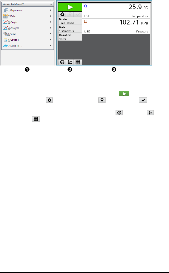
6 Data Collection

ÀVernier DataQuest™ Menu. Contains menu items for set-up, collection and

analysis of sensor data.

ÁDetails view. Contains buttons for starting data collection , changing

collection settings , marking collected data , storing data sets , and

tabs for managing multiple data runs.

View selection buttons let you choose from Meter view , Graph view , or

Table view .

ÂData work area. The information displayed here depends on the view.

Meter. Displays a list of sensors that are currently connected or set up in advance.

Graph. Displays collected data in a graphical representation, or displays the

prediction before a data collection run.

Table. Displays collected data in columns and rows.

What You Must Know

Basic Steps in Performing an Experiment

These basic steps are the same no matter which type of experiment you perform.

1. Start the Vernier DataQuest™ Application.

2. Connect sensors.

3. Modify sensor settings.

4. Select the collection mode and collection parameters.

5. Collect data.

6. Stop collecting data.

7. Store the data set.

8. Save the document to save all data sets in the experiment.

9. Analyse the data.

Sending Collected Data to Other TI-Nspire™ Applications

You can send collected data to the Graphs, Lists&Spreadsheet, and Data&Statistics

applications.

▶From the Send To menu, click the name of the application.

A new page showing the data is added to the current problem.

About Collection Devices

You can select from a variety of sensors and interfaces to collect data while running

the Vernier DataQuest™ application with TI-Nspire™ software.

Multi-Channel Sensor Interfaces

Multi-channel sensor interfaces let you connect more than one sensor at a time.

Sensor Interface Description

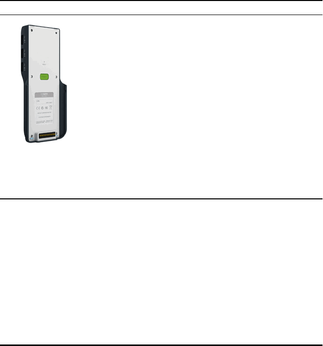
Texas

Instruments

TI-Nspire™ Lab

Cradle

This sensor can be used with a handheld, a computer, or as a

stand-alone sensor.

The sensor interface allows you to connect and use one to five

sensors at the same time. It can be used in the lab or at a

remote collection location.

The Lab Cradle supports two digital sensors and three analogue

sensors.

The Lab Cradle also supports high-sample data collection

sensors, such as a hand-grip heart rate or a blood pressure

monitor.

After using the Lab Cradle as a remote sensor, you can download

data to either a handheld or computer.

Single-Channel Sensor Interfaces

Single-channel sensor interfaces can only connect to one sensor at a time. These

sensors have either a mini-USB connector for a handheld or a standard USB connector

for a computer. For a complete list of compatible sensors, see Compatible Sensors.

Data Collection 7

8 Data Collection

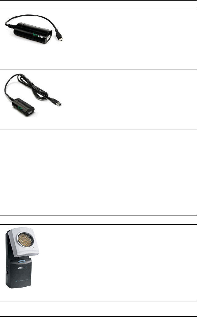
Sensor Interface Description

Vernier EasyLink®

This sensor interface is used with handhelds. It has a

mini-USB connector so it can be plugged directly into

the handheld.

Connect sensors to Vernier EasyLink® to:

• Measure barometric pressure.

• Measure the salinity of a solution.

• Investigate the relationship between pressure

and volume (Boyles’ Law).

Vernier Go!Link®

This sensor interface is used with computers. It has a

standard connector so it can be plugged into a

Windows® or Mac® computer.

Connect sensors to Vernier GoLink® to:

• Measure the acidity or alkalinity of a solution.

• Monitor greenhouse gases.

• Measure sound level in decibels.

Types of Sensors

•Analogue sensors. Temperature, light, pH and voltage sensors are analogue sensors

and require a sensor interface.

•Digital sensors. Photogates, radiation monitors and drop counters are digital

sensors. These sensors can only be used with the TI-Nspire™ Lab Cradle.

•Direct-connect USB sensors. These sensors connect directly to a handheld or

computer and do not require a sensor interface.

Sensors for Handhelds

The following lists some sensors you can use with a handheld.

Sensor Description

Texas Instruments

This analogue sensor connects directly to TI-Nspire™

handhelds through the mini-USB port. It is used to explore

and graph motion.

This sensor automatically launches the Vernier DataQuest™

application when you connect it to a handheld. Data

collection begins when you select the Motion Match

function.

This sensor collects up to 200 samples per second.

Use this sensor to:

• Measure position and speed of a person or object.

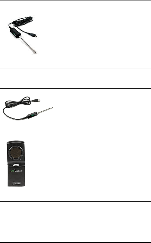
Sensor Description

CBR2™ • Measure the acceleration of an object.

Vernier EasyTemp®

temperature sensor

This analogue sensor connects directly to TI-Nspire™

handhelds through the mini-USB port and is used to collect

temperature ranges. You can design experiments to:

• Collect weather data.

• Record temperature changes due to chemical

reactions.

• Perform heat fusion studies.

Sensors for Computers

The following table lists some sensors you can use with a computer.

Sensor Description

Vernier Go!Temp®

temperature sensor

This analogue sensor connects to the computer’s USB

port and is used to collect temperature ranges.

You can use this sensor to:

• Collect weather data.

• Record temperature changes due to chemical

reactions.

• Perform heat fusion studies.

Vernier Go!Motion® motion

detector

This analogue sensor connects to the computer’s USB

port and is used to measure acceleration, speed and

velocity.

Use this sensor to:

• Measure position and speed of a person or

object.

• Measure the acceleration of an object.

Compatible Sensors

The following sensors can be used with the Vernier DataQuest™ application.

• 25-g Accelerometer

• 30-Volt Voltage Probe

Data Collection 9

10 Data Collection

• 3-Axis Accelerometer

• Low-g Accelerometer

• CBR 2™ - Connects directly to handheld USB port

• Go!Motion® - Connects directly to computer USB port

• Extra Long Temperature Probe

• Stainless Steel Temperature Probe

• Surface Temperature Sensor

• Ammonium Ion-Selective Electrode

• Anemometer

• Barometer

• Blood Pressure Sensor

• C02 Gas Sensor

• Calcium Ion-Selective Electrode

• Charge Sensor

• Chloride Ion-Selective Electrode

• Colorimeter

• Conductivity Probe

• High Current Sensor

• Current Probe

• Differential Voltage Probe

• Digital Radiation Monitor

• Dissolved Oxygen Sensor

• Dual-Range Force Sensor

• EasyTemp® - Connects directly to handheld USB port

• EKG Sensor

• Electrode Amplifier

• Flow Rate Sensor

• Force Plate

• Gas Pressure Sensor

• Go!Temp® - Connects directly to computer USB port

• Hand Dynamometer

• Hand-Grip Heart Rate Monitor

• Instrumentation Amplifier

• Light Sensor

• Magnetic Field Sensor

• Melt Station

• Microphone

• Nitrate Ion-Selective Electrode

• O2 Gas Sensor

• ORP Sensor

• pH Sensor

• Relative Humidity Sensor

• Respiration Monitor Belt (Requires Gas Pressure Sensor)

• Rotary Motion Sensor

• Salinity Sensor

• Soil Moisture Sensor

• Sound Level Meter

• Spirometer

• Thermocouple

• TI-Light - Sold only with the CBL 2™

• TI-Temp - Sold only with the CBL 2™

• TI-Voltage - Sold only with the CBL 2™

• Tris-Compatible Flat pH Sensor

• Turbidity Sensor

• UVA Sensor

• UVB Sensor

• Vernier Constant Current System

• Vernier Drop Counter

• Vernier Infrared Thermometer

• Vernier Motion Detector

• Vernier Photogate

• Voltage Probe

• Wide-Range Temperature Probe

Connecting Sensors

Direct-connect USB sensors, such as the Vernier Go!Temp® temperature sensor (for

computers) or the Vernier EasyLink® temperature sensor (for handhelds), connect

directly to the computer or handheld and do not need a sensor interface.

Other sensors require a sensor interface such as the TI-Nspire™ Lab Cradle.

Data Collection 11

12 Data Collection

Connecting Directly

▶Attach the cable on the sensor directly to the computer's USB port or to an

appropriate port on the handheld.

Connecting through a Sensor Interface

1. Attach the sensor to the sensor interface using either the mini-USB, USB or BT

connector and the appropriate cable.

2. Attach the interface to a computer or handheld using the appropriate connector

and cable.

Note: To attach a handheld to a TI-Nspire™ Lab Cradle, slide the handheld into the

connector at the bottom of the Lab Cradle.

Setting Up an Offline Sensor

You can pre-define meter settings for a sensor that is not currently attached to a

computer or handheld.

You cannot use the sensor offline, but you can prepare the experiment for it and then

attach it when ready to collect the data. This option makes it faster to share a sensor

during a lesson or lab in which there are not enough sensors for everyone.

1. From the Experiment menu, select Advanced Set Up > Configure Sensor > Add

Offline Sensor.

The Select Sensor dialogue box opens.

2. Select a sensor from the list.

3. Click the Meter View tab .

4. Click the sensor you have added, and modify its settings.

The settings will be applied when you attach the sensor.

Removing an offline sensor

1. From the Experiment menu, select Advanced Setup > Configure Sensor.

2. Select the name of the offline sensor to remove.

3. Click Remove.

Modifying Sensor Settings

You can modify how the sensor values are displayed and stored. For example, when

using a temperature sensor, you can change the unit of measure from Centigrade to

Fahrenheit.

Changing Sensor Measurement Units

Measurement units depend on the selected sensor. For example, units for the Vernier

Go!Temp® Temperature sensor are Fahrenheit, Celsius and Kelvin. Units for the

Vernier Hand Dynamometer (a specialised force sensor) are Newton, Pound and

Kilogramme.

You can change the units before or after you collect data. The collected data reflects

the new measurement unit.

1. Click Meter view to display the connected and offline sensors.

2. Click the sensor whose units you want to change.

3. In the Meter Settings dialogue box, select the unit type from the Measurement

Units menu.

Data Collection 13

14 Data Collection

Calibrating a Sensor

When the software or handheld detects a sensor, the calibration for that sensor

automatically loads. You can calibrate some sensors manually. Other sensors, such as

the Colorimeter and the Dissolved Oxygen Sensor, must be calibrated to provide useful

data.

There are three options for calibrating a sensor:

• Manual Entry

• Two Point

• Single Point

Refer to the sensor’s documentation for specific calibration values and procedures.

Setting a Sensor to Zero

You can set the standing value of some sensors to zero. You cannot set sensors in

which relative measurements such as force, motion and pressure are common to zero.

Sensors designed to measure specific environmental conditions, such as Temperature,

pH and CO2also cannot be set to zero.

1. Click Meter view to display the connected and offline sensors.

2. Click the sensor that you want to set to zero.

3. In the Meter Settings dialogue box, click Zero.

Reversing a Sensor's Readings

By default, pulling with a force sensor produces a positive force and pushing produces

a negative force. Reversing the sensor allows you to display pushing as a positive force.

1. Click Meter view to display the connected and offline sensors.

2. Click the sensor that you want to reverse.

3. In the Meter Settings dialogue box, click Reverse Readings.

The sensor display is now reversed. In Meter View, the reverse indicator

appears after the sensor name.

Collecting Data

Collecting Time-Based Data

The Time Based collection mode captures sensor data automatically at regular time

intervals.

1. Connect the sensor or sensors.

Sensor names are added to the sensor list automatically.

2. From the Experiment menu, select New Experiment.

This removes all data and restores all meter settings to their defaults.

3. From the Experiment menu, select Collection Mode > Time Based.

a) Select Rate or Interval from the drop-down list, and then type the Rate

(samples/second) or Interval (seconds/sample).

b) Type the Duration of the collection.

Data Collection 15

16 Data Collection

The Number of points is calculated and displayed, based on rate and duration.

Note that collecting too many data points can slow system performance.

c) Select Strip Chart if you want to collect samples continuously, retaining only the

last nsamples. (where “n” is the number shown in the Number of points field.)

4. Modify sensor settings as necessary.

5. Click Start Collection .

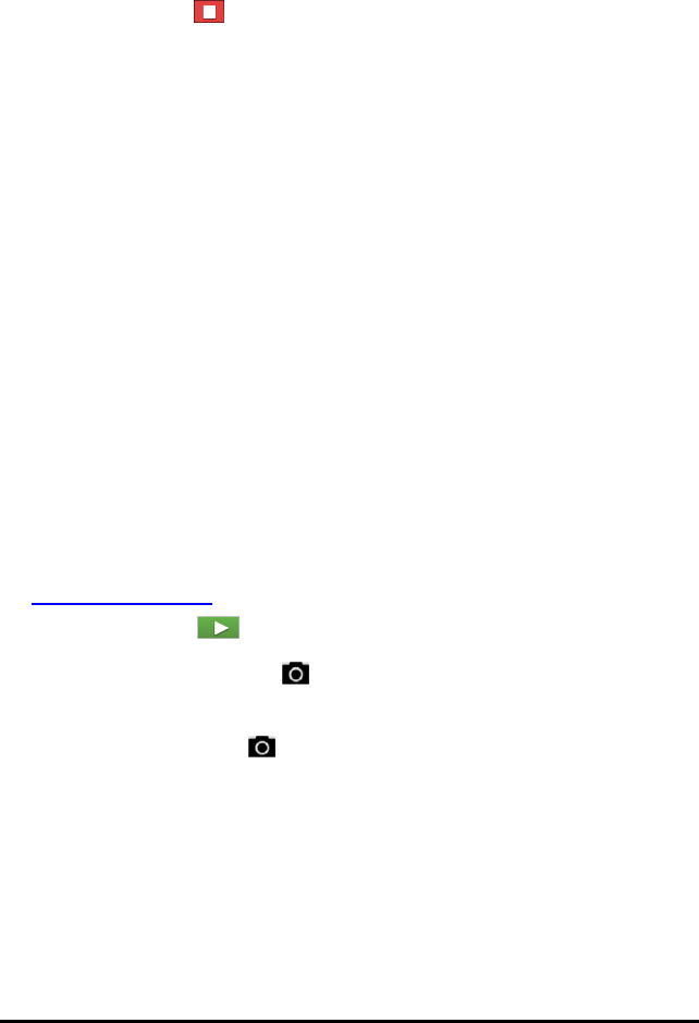
6. After the data has been collected, click Stop Collection .

The data set run is complete.

Collecting Selected Events

Use the Selected Events collection mode to capture samples manually. In this mode,

each sample is automatically assigned an event number.

1. Connect the sensor or sensors.

Sensor names are added to the sensor list automatically.

2. From the Experiment menu, select New Experiment.

This removes all data and restores all meter settings to their defaults.

3. From the Experiment menu, select Collection Mode > Selected Events.

The Selected Events Set-up dialogue box opens.

-Name. This text is visible in the Meter View. Its first letter is displayed as the

independent variable in the Graph view.

-Units. This text is displayed in Graph view alongside the Name.

-Average over 10 s. This option averages ten seconds of data for each point.

4. Modify sensor settings as necessary.

5. Click Start Collection .

The Keep Current Reading icon becomes active. The current sensor value

appears in the centre of the graph.

6. Click Keep Current Reading to capture each sample.

The data point is plotted, and the current sensor value appears in the centre of the

graph.

Note: If you selected the Averaging option, a countdown timer appears. When the

counter reaches zero, the system plots the average.

7. Continue capturing until you collect all of the desired data points.

8. Click Stop Collection .

The data set run is complete.

Collecting Events with Entry

Use the Events with Entry collection mode to capture samples manually. In this mode,

you define the independent value for each point you collect.

1. Connect the sensor or sensors.

Sensor names are added to the sensor list automatically.

2. From the Experiment menu, select New Experiment.

This removes all data and restores all meter settings to their defaults.

3. From the Experiment menu, select Collection Mode > Events with Entry.

The Events with Entry Set-up dialogue box opens.

-Name. This text is visible in the Meter View. Its first letter is displayed as the

independent variable in the Graph view.

-Units. This text is displayed in Graph view alongside the Name.

-Average over 10 s. This option averages ten seconds of data for each point.

4. Modify sensor settings as necessary.

5. Click Start Collection .

The Keep Current Reading icon becomes active. The current sensor value

appears in the centre of the graph.

6. Click Keep Current Reading to capture a sample.

The Events with Entry dialogue box opens.

Data Collection 17

18 Data Collection

7. Type a value for the independent variable.

8. Click OK.

The data point is plotted, and the current sensor value appears in the centre of the

graph.

Note: If you selected the Averaging option, a countdown timer appears. When the

counter reaches zero, the system plots the average.

9. Repeat steps 6 to 8 until you collect all of the desired data points.

10. Click Stop Collection .

The data set run is complete.

Collecting Photogate Timing Data

The Photogate Timing collection mode is available only when using the Vernier

Photogate sensor. This sensor can time objects that pass through the gates or objects

that pass outside of the gates.

1. Connect the Photogate sensor or sensors.

Sensor names are added to the sensor list automatically.

2. From the Experiment menu, select New Experiment.

This removes all data and restores all meter settings to their defaults.

3. From the Experiment menu, select Collection Mode > Photogate Timing.

4. Set the collection options.

5. Modify sensor settings as necessary.

6. Click Start Collection .

7. After the data has been collected, click Stop Collection .

The data set run is complete.

Collecting Drop Counter Data

The Drop Counting collection mode is available only when using the Vernier Drop

Counter optical sensor. This sensor can count the number of drops or record the

amount of liquid added during an experiment.

1. Connect the Drop Counter sensor or sensors.

Sensor names are added to the sensor list automatically.

2. From the Experiment menu, select New Experiment.

This removes all data and restores all meter settings to their defaults.

3. From the Experiment menu, select Collection Mode > Drop Counting.

4. Set the collection options.

5. Modify sensor settings as necessary.

6. Click Start Collection .

7. After the data has been collected, click Stop Collection .

The data set run is complete.

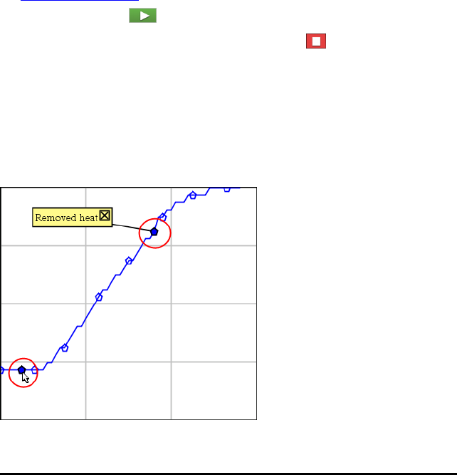
Using Data Markers to Annotate Data

Data markers give you a way to emphasise specific data points, such as when you

change a condition. For example, you might mark a point at which a chemical is added

to a solution or when heat is applied or removed. You can add a marker with or

without a comment, and you can hide a comment.

Two data markers, one with a comment displayed

Data Collection 19

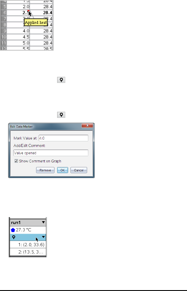
20 Data Collection

Marker shown as red triangle in Table view

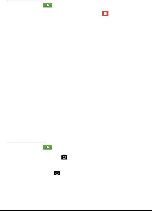
Adding a Marker During Data Collection

▶Click Add Data Marker to place a marker at the current data point.

Adding a Marker After Collecting Data

1. In Graph or Table view, click the point at which you want a marker.

2. Click Add Data Marker .

3. Complete the items in the dialogue box.

Adding a Comment to an Existing Marker

1. In the Detail view, click to expand the list of markers for the data set.

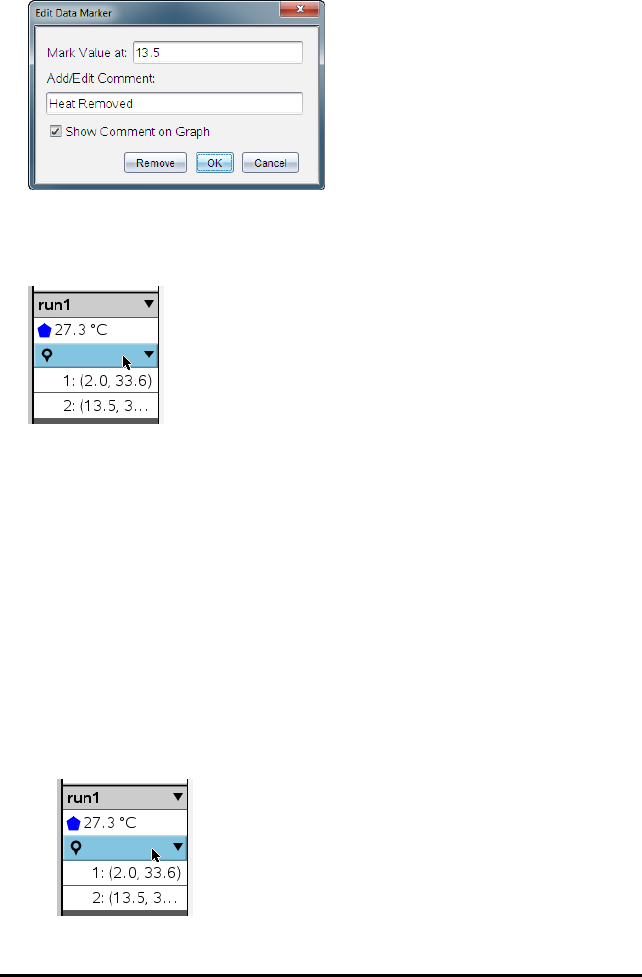
2. Click the entry for the marker that you want to change, and complete the items in

the dialogue box.

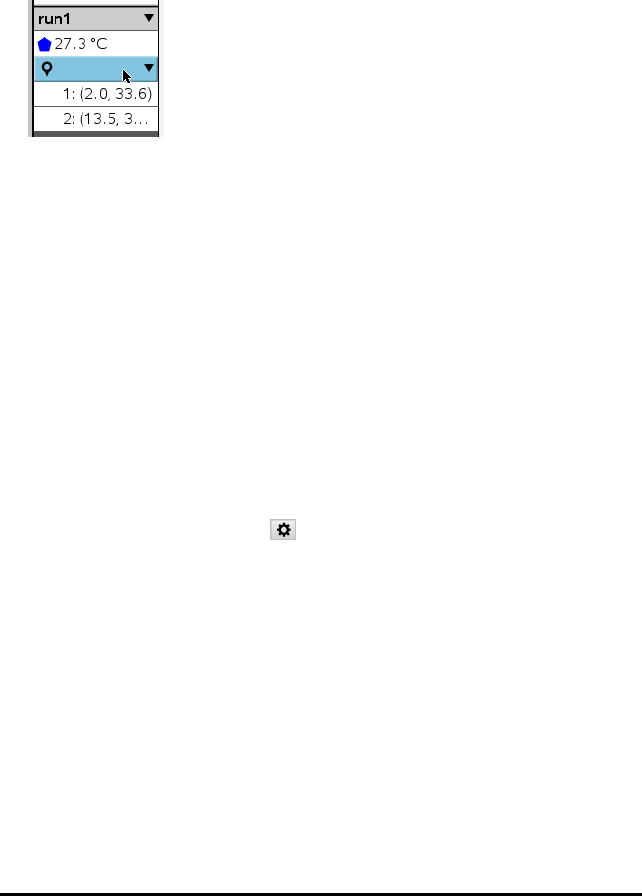
Repositioning a Data Marker

1. Click to expand the list of markers in the Detail view.

2. Click the entry for the marker that you want to change.

3. In the dialogue box, type a new value for Mark Value at.

Moving a Data Marker's Comment in the Graph View

▶Drag the comment to move it. The connecting line remains attached to the data

point.

Hiding/Showing a Data Marker's Comment

▶Hide a comment by clicking the Xat the end of the comment.

▶To restore a hidden comment:

a) Click to expand the list of markers in the Detail view.

Data Collection 21

22 Data Collection

b) Click the entry for the marker that you want to change, and tick

ShowCommentonGraph.

Removing a Data Marker

1. Click to expand the list of markers in the Detail view.

2. In the dialogue box, click Remove.

Collecting Data Using a Remote Collection Unit

To collect information from a sensor while it is disconnected, you can set it up as a

remote sensor. Only the TI-Nspire™ Lab Cradle, TI CBR2™, and Vernier Go!Motion®

support remote data collection.

You can set up a remote collection unit to start collecting:

• When you press a manual trigger on the unit, as on the TI-Nspire™ Lab Cradle

• When a delay countdown expires on a unit that supports a delayed start

Setting Up for Remote Collection

1. Save and close any open documents, and start with a new document.

2. Connect the remote collection unit to the computer or handheld.

3. Modifying Sensor Settings.

4. Click the Collection Setup button .

5. On the Collection Setup screen, click Enable Remote Collection.

6. Select the remote collection unit from the Devices list.

7. Specify the method for starting the collection:

• To start automatically after a specified delay (on supported units), type the

delay value.

• To start when you press the manual trigger (on supported units), type a delay

value of 0. When you use a delay, the manual trigger button on the TI-Nspire™

Lab Cradle has no effect on the start of the collection.

8. Click OK.

A message confirms that the unit is ready.

9. Disconnect the unit.

Depending on the device, LED lights may indicate its status.

Red. The system is not ready.

Amber. The system is ready but not collecting data.

Green. The system is collecting data.

10. If you are starting collection manually, press the trigger when ready. If you are

starting based on a delay, the collection will start automatically when the

countdown is complete.

Retrieving the Remote Data

After collecting data remotely, you transfer it to the computer or handheld for analysis.

Data Collection 23

24 Data Collection

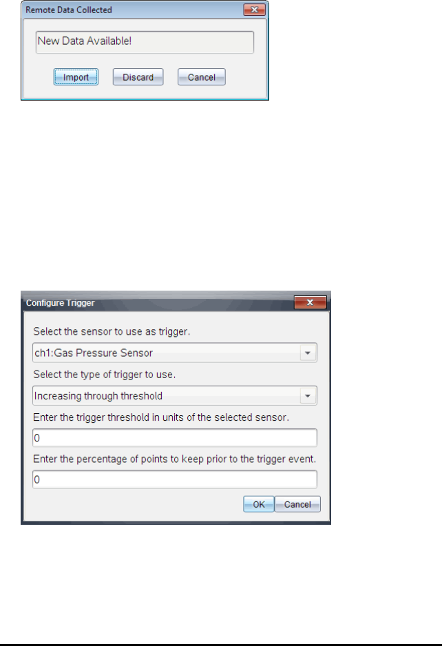
1. Open the Vernier DataQuest™ application.

2. Attach the TI-Nspire™ Lab Cradle to the handheld or computer.

The Remote Data Detected dialogue box opens.

3. Click Import.

The data transfers to the Vernier DataQuest™ application.

Setting Up the Sensor for Triggering

To start data collection based on a specific sensor reading, the TI-Nspire™ Lab Cradle

and sensor must be connected.

1. Connect the sensor.

2. Click Experiment > Advanced Set up > Triggering > Set Up.

The Configure Trigger dialogue box opens.

3. Select the sensor from the Select the sensor to use as trigger drop-down list.

Note: The menu displays the sensors connected to the TI-Nspire™ Lab Cradle.

4. Select one of the following from the Select the type of trigger to use drop-down

list.

•Increasing through threshold. Use to trigger on increasing values.

•Decreasing through threshold. Use to trigger on decreasing values.

5. Type the appropriate value in the Enter the trigger threshold in units of the selected

sensor field.

When entering the trigger value, enter a value within the range of the sensor.

If you change the unit type after setting the threshold, the value automatically

updates.

For example, if you use the Vernier Gas Pressure sensor with the units set as atm

and you later change the units to kPa, the settings are updated.

6. Type the number of data points to keep before the trigger value occurs.

7. Click OK.

The trigger is now set and enabled if values were entered.

8. (Optional) Select Experiment > Advanced Set up > Triggering to verify the active

indicator is set to Enabled.

Important: When the trigger is enabled, it stays active until it is disabled or you

start a new experiment.

Enabling a Disabled Trigger

If you set the trigger values in the current experiment, and then disable them, you can

enable the triggers again.

To enable a trigger:

▶Click Experiment > Advanced Set Up > Triggering > Enable.

Disabling an Enabled Trigger

To disable the active trigger.

▶Click Experiment > Advanced Set Up > Triggering > Disable.

Collecting and Managing Data Sets

By default, the Start Collection button overwrites collected data with data from

the next run. To preserve each run, you can store it as a data set. After collecting

multiple data sets, you can superimpose any combination of them on the Graph View.

Data Collection 25

26 Data Collection

Important: Stored data sets are lost if you close the document without saving it. If you

want stored data to be available later, make sure to save the document.

Storing Data as Sets

1. Collect the data from the first run. (See Collecting Data.)

2. Click the Store Data Set button .

The data is stored as run1. A new data set, run2, is created for collecting the next

run.

3. Click Start Collection to collect data for run2.

Comparing Data Sets

1. Click the Graph View icon to show the graph.

2. Click the Data Set Selector (near the top of the Detail View) to expand the list of

data sets.

ÀData Set Selector lets you expand or collapse the list.

ÁExpanded list shows available data sets. Scroll buttons appear as necessary

to let you scroll the list.

3. Choose which data sets to view by selecting or clearing the tickboxes.

The graph is rescaled as necessary to show all selected data.

Tip: To quickly select a single data set, hold down Shift while clicking its name in

the list. The graph shows only the selected set, and the list is collapsed

automatically to help you view details of the data.

Renaming a Data Set

By default, data sets are named run1,run2 and so on. The name of each data set is

displayed in the Table view.

1. Click the Table View icon to show the table.

2. Display the context menu for the table view, and select Data Set Options > [current

name].

3. Type the new Name.

Note: The maximum character limit is 30. The name cannot contain commas.

4. (Optional) Type Notes about the data.

Data Collection 27

28 Data Collection

Deleting a Data Set

1. Click the Graph View icon to show the graph.

2. Click the Data Set Selector (near the top of the Detail View) to expand the list of

data sets.

3. Scroll the list as necessary, and then click the Delete symbol (X) next to the name

of the data set.

4. Click OK on the confirmation message.

Expanding the View Details Area

▶Drag the boundary at the right edge of the Details area to increase or decrease its

width.

Using Sensor Data in Programmes

You can access sensor data from all connected sensor probes through your TI-Basic

programme by using this command:

RefreshProbeVars statusVar

• You must first launch the Vernier DataQuest™ application, or you will receive an

error.

Note: The Vernier DataQuest™ application will auto-launch when you connect a

sensor or a lab cradle to the TI-Nspire™ software or handheld.

• The RefreshProbeVars command will be valid only when Vernier DataQuest™ is in

'meter' mode.

•statusVar is an optional parameter that indicates the status of the command.

These are the statusVar values:

StatusVar

Value

Status

statusVar

Normal (continue with the programme)

statusVar

The Vernier DataQuest™ application is in data collection mode.

Note: The Vernier DataQuest™ application must be in meter mode for

this command to work.

statusVar

The Vernier DataQuest™ application is not launched.

statusVar

The Vernier DataQuest™ application is launched, but you have not

connected any probes.

Note: The RefreshProbeVars command will almost always return

statusVar=3 in the iOS, even if you have already launched the Vernier

DataQuest™ application

• Your TI-Basic programme will read directly from Vernier DataQuest™ variables in

the symbol table.

• The meter.time variable shows the last value of the variable; it does not update

automatically. If no data collection has occurred, meter.time will be 0 (zero).

• Use of variable names without corresponding probes being physically attached will

result in a "Variable not defined" error.

• The RefreshProbeVars command will be a NOP (null command) on iOS.

Collecting Sensor Data using RefreshProbeVars

1. Launch the Vernier DataQuest™ application.

2. Connect the sensor(s) you need to collect the data.

3. Run the programme you wish to use to collect data in the calculator application.

4. Manipulate the sensors and collect the data.

Note: You may create a programme to interact with the TI-Innovator Hub using b>

Hub > Send. (See Example 2, below.) This is optional.

Example 1

Define temp()=

Prgm

Data Collection 29

30 Data Collection

RefreshProbeVars status

If status=0 Then

Disp "ready"

For n,1,50

RefreshProbeVars status

temperature:=meter.temperature

Disp "Temperature: ",temperature

If temperature>30 Then

Disp "Too hot"

EndIf

Wait 1

EndFor

Else

Disp "Not ready. Try again later"

EndIf

EndPrgm

Example 2- with TI-Innovator™ Hub

Define tempwithhub()=

Prgm

RefreshProbeVars status

If status=0 Then

Disp "ready"

For n,1,50

RefreshProbeVars status

temperature:=meter.temperature

Disp "Temperature: ",temperature

If temperature>30 Then

Disp "Too hot"

Send "SET SOUND 440 TIME 2"

EndIf

Wait 1

EndFor

Else

Disp "Not ready. Try again later"

EndIf

EndPrgm

Analysing Collected Data

In the Vernier DataQuest™ application, use Graph View to analyse data. Start by

setting up graphs, and then use analysis tools such as integral, statistics and curve fit

to investigate the mathematical nature of the data.

Important: The Graph menu and Analyse menu items are only available when working

in Graph View.

Finding the Area Under a Data Plot

Use Integral to determine the area under a data plot. You can find the area under all of

the data or a selected region of the data.

To find the area under a data plot:

1. Leave the graph unselected to examine all the data, or select a range to examine a

specific area.

2. Click Analyse > Integral.

3. Select the plotted column name if you have more than a single column.

The data plot area is displayed in the View Details area.

Finding the Slope

Tangent displays a measure of the rate at which the data is changing at the point you

are examining. The value is labelled “Slope”.

To find the slope:

1. Click Analyse > Tangent.

A check mark appears in the menu next to the option.

2. Click the graph.

The examine indicator is drawn to the nearest data point.

The values of the plotted data are shown in the View details area and the All

Details for Graph dialogue box.

You can move the examine line by dragging, clicking another point or using the

arrow keys.

Interpolating the Value Between Two Data Points

Use Interpolate to estimate the value between two data points and to determine the

value of a Curve Fit between and beyond these data points.

The examine line moves from data point to data point. When Interpolate is on, the

examine line moves between and beyond data points.

To use Interpolate:

1. Click Analyse > Interpolate.

Data Collection 31

32 Data Collection

A check mark appears in the menu next to the option.

2. Click the graph.

The examine indicator is drawn to the nearest data point.

The values of the plotted data are shown in the View Details area.

You can shift the examine line by moving the cursor with the arrow keys or by

clicking on another data point.

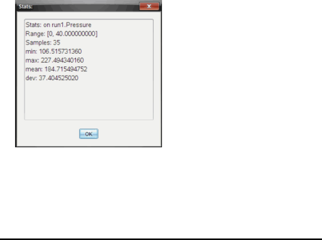
Generating Statistics

You can generate statistics (minimum, maximum, mean, standard deviation and

number of samples) for all the collected data or for a selected region. You can also

generate a curve fit based on one of several standard models or on a model that you

define.

1. Leave the graph unselected to examine all the data, or select a range to examine a

specific area.

2. Click Analyse > Statistics.

3. Select the plotted column name if you have more than a single column. For

example, run1.Pressure.

The Stats dialogue box opens.

4. Review the data.

5. Click OK.

For information on clearing the Statistics analysis, see Removing Analysis Options.

Generating a Curve Fit

Use Curve Fit to find the best curve fit to match the data. Select all of the data or a

selected region of data. The curve is drawn on the graph.

1. Leave the graph unselected to examine all the data, or select a range to examine a

specific area.

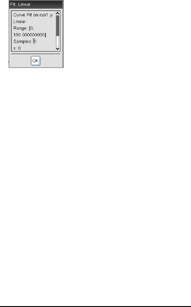
2. Click Analyse > Curve Fit.

3. Select a curve fit option.

Curve Fit option Calculated in the form:

Linear y=m*x+b

Quadratic y=a*x^2+b*x+c

Cubic y=a*x^3+b*x^2+c*x+d

Quartic y=a*x^4+b*x^3+c*x^2+d*x+e

Power (ax^b) y=a*x^b

Exponential (ab^x) y=a*b^x

Logarithmic y=a+b*ln(x)

Sinusoidal y=a*sin(b*x+c)+d

Logistic (d 0) y=c/(1+a*e^(-bx))+d

Natural Exponential y=a*e^(-c*x)

Proportional y=a*x

The Fit Linear dialogue box opens.

Data Collection 33

34 Data Collection

4. Click OK.

5. Review the data.

For information on clearing the Curve Fit analysis, see Removing Analysis Options.

Plotting a Standard or User-Defined Model

This option provides a manual method for plotting a function to fit data. Use one of the

predefined models or enter your own.

You can also set the spin increment to use in the View Details dialogue box. Spin

increment is the value by which the coefficient changes when you click the spin buttons

in the View Details dialogue box.

For example, if you set m1=1 as the spin increment, when you click the up spin button

the value changes to 1.1, 1.2, 1.3 and so on. If you click the down spin button, the value

changes to 0.9, 0.8, 0.7 and so on.

1. Click Analyse > Model.

The Model dialogue box opens.

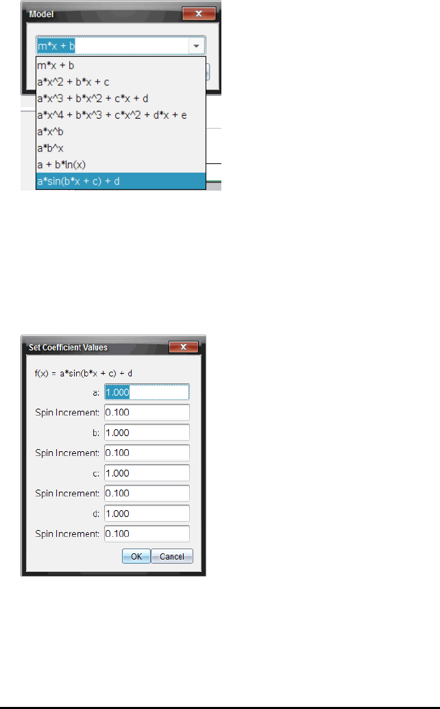
2. Type your own function.

—or—

Click to select a value from the drop-down list.

3. Click OK.

The Set Coefficient Values dialogue box opens.

4. Type the value for the variables.

5. Type the change in value in the Spin Increment fields.

6. Click OK.

Data Collection 35

36 Data Collection

Note: These values are the initial values. You can also adjust these values in the

View Details area.

The model is shown on the graph with adjustment options in the View Details area

and in the All Details for Graph dialogue box.

7. (Optional) Adjust the window setting for minimum and maximum axis values. For

more information, see Setting the Axis for One Graph.

For information on clearing the Model analysis, see Removing Analysis Options.

8. Click to make any desired adjustments to the coefficients.

—or—

Click the value in the View Details area.

This graphic is an example of a model with adjusted values.

Removing Analysis Options

1. Click Analyse > Remove.

2. Select the data display you want to remove.

The display you selected is removed from the graph and the View Details area.

Displaying Collected Data in Graph View

When you collect data, it is written in both the Graph and Table views. Use the Graph

view to examine the plotted data.

Important: The Graph menu and Analyse menu items are only active when working in

Graph View.

Selecting the Graph View

▶Click the Graph View tab .

Viewing Multiple Graphs

Use the Show Graph menu to show separate graphs when using:

• A sensor that plots more than one column of data.

• Multiple sensors with different defined units at the same time.

In this example, two sensors (the Gas Pressure sensor and the Hand Dynamometer)

were used in the same run. The following image shows the columns Time, Force and

Pressure in the Table view to illustrate why two graphs are shown.

Displaying One of Two Graphs

When two graphs are displayed, the top graph is Graph 1 and the bottom graph is

Graph 2.

To display only Graph 1:

▶Select Graph > Show Graph > Graph 1.

Only Graph 1 is displayed.

To display only Graph 2:

▶Select Graph > Show Graph > Graph 2.

Only Graph 2 is displayed.

Displaying Both Graphs

To display both Graph 1 and Graph 2 together:

▶Select Graph > Show Graph > Both.

Graph 1 and Graph 2 are displayed.

Displaying Graphs in the Page Layout View

Use the Page layout view when Show Graph is not the appropriate solution for

showing more than one graph.

The Show Graph option is not applicable for:

• Multiple runs using a single sensor.

• Two or more of the same sensors.

• Multiple sensors that use the same column(s) of data.

To use Page Layout:

1. Open the original data set you want to see in two graph windows.

2. Click Edit > Page Layout > Select Layout.

3. Select the type of page layout you want to use.

4. Click Click here to add an application.

Data Collection 37

38 Data Collection

5. Select Add Vernier DataQuest™.

The Vernier DataQuest™ application is added to the second view.

6. To see separate views, click the view you want to change, and then select View >

Table.

The new view is displayed.

7. To show the same view, click the view to change.

8. Click View > Graph.

The new view is displayed.

Displaying Collected Data in Table View

Table view provides another way to sort and view collected data.

Selecting the Table View

▶Click the Table View tab .

Defining Column Options

You can name columns and define the decimal points and the precision you want to

use.

1. from the Data menu, select Column Options.

Note: You can be in the Meter, Graph or Table view and still click these menu

options. The results will still be visible.

2. Click the name of the column you want to define.

The Column Options dialogue box opens.

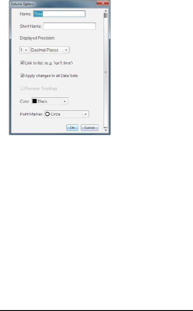
3. Type the long name for the column in the Name field.

4. Type the abbreviated name in the Short Name field.

Note: This name is displayed if the column cannot expand to display the full name.

5. Type the number of units in the Units field.

6. From the Displayed Precision drop-down list, select the precision value.

Note: The default precision is related to the precision of the sensor.

7. Select Link to list to link to the symbol table and make this information available to

other TI-Nspire™ applications.

Note: Linking is the default for most sensors.

Important: Heart rate and blood pressure sensors require a tremendous amount of

data to be useful, and the default for these sensors is to be unlinked to improve

system performance.

8. Select Apply changes to all Data Sets to apply these settings to all data sets.

9. Click OK.

The column settings are now defined with the new values.

Data Collection 39

40 Data Collection

Creating a Column of Manually Entered Values

To enter data manually, add a new column. Sensor columns cannot be modified, but

data entered manually can be edited.

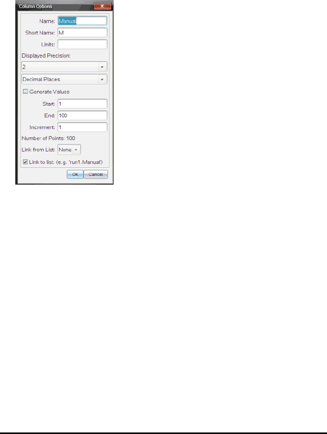
1. Click Data > New Manual Column.

The Column Options dialogue box opens.

2. Type the long name for the column in the Name field.

3. Type the abbreviated name in the Short Name field.

Note: This name is displayed if the column cannot expand to display the full name.

4. Type the units to be used.

5. From the Displayed Precision drop-down list, select the precision value.

Note: The default precision is related to the precision of the sensor.

6. (Optional) Select Apply changes to all Data Sets to apply these settings to all data

sets.

7. (Optional) Select Generate Values to automatically populate the rows.

If you select this option, complete these steps:

a) Type a starting value in the Start field.

b) Type an ending value in the End field.

c) Type the increase in value in the Increment field.

The number of points is calculated and shown in the Number of Points field.

8. Select Link from list to link to data in another TI-Nspire™ application.

Note: This list only populates when data exists in the other application and includes

a column label.

9. Select Link to list to link to the symbol table and make this information available to

other TI-Nspire™ applications.

Note: Linking is the default for most sensors.

Important: Heart rate and blood pressure sensors require a tremendous amount of

data to be useful, and the default for these sensors is to be unlinked to improve

system performance.

10. Click OK.

A new column is added to the table. This column can be edited.

Creating a Column of Calculated Values

You can add an additional column to the data set in which the values are calculated

from an expression using at least one of the existing columns.

Use a calculated column when finding the derivative for pH data. For more

information, see Adjusting Derivative Settings.

1. Click Data > New Calculated Column.

The Column Options dialogue box opens.

Data Collection 41

42 Data Collection

2. Type the long name for the column in the Name field.

3. Type the abbreviated name in the Short Name field.

Note: This name is displayed if the column cannot expand to display the full name.

4. Type the units to be used.

5. From the Displayed Precision drop-down list, select the precision value.

Note: The default precision is related to the precision of the sensor.

6. Type a calculation including one of the column names in the Expression field.

Note: The system-provided column names are dependent on the sensor(s) selected

and any changes made to the name field in Column Options.

Important: The Expression field is case-sensitive. (Example: “Pressure” is not the

same as “pressure”.)

7. Select Link to list to link to the symbol table and make this information available to

other TI-Nspire™ applications.

Note: Linking is the default for most sensors.

Important: Heart rate and blood pressure sensors require a tremendous amount of

data to be useful, and the default for these sensors is to be unlinked to improve

system performance.

8. Click OK.

The new calculated column is created.

Customising the Graph of Collected Data

You can customise the Graph view by adding a title, changing colours and setting

ranges for the axis.

Adding a Title

When you add a title to a graph, the title is displayed in the View Details area. When

you print the graph, the title prints on the graph.

1. Click Graph > Graph Title.

The Graph Title dialogue box opens.

If there are two graphs in the work area, the dialogue box has two title options.

2. Type the name of the graph in the Title field.

—or—

a) Type the name of the first graph in the Graph 1 field.

b) Type the name of the second graph in the Graph 2 field.

3. Select Enable to show the title.

Data Collection 43

44 Data Collection

Note: Use the Enable option to hide or show the graph title as needed.

4. Click OK.

The title is shown.

Setting Axis Ranges

Setting Axis Ranges for One Graph

To modify the minimum and maximum range for the x and y axis:

1. Click Graph > Window Settings.

The Window Settings dialogue box opens.

2. Type the new values in one or more of these fields:

- X Min

- X Max

- Y Min

- Y Max

3. Click OK.

The application uses the new values for the graph visual range until you modify the

range or change data sets.

Setting Axis Ranges for Two Graphs

When working with two graphs, enter two y axis minimum and maximum values, but

only one set of minimum and maximum values for the x axis.

1. Click Graph > Window Setting.

The Window Setting dialogue box opens.

2. Type the new values in one or more of these fields:

- X Min

- X Max

- Graph 1: Y Min

- Y Max

- Graph 2: Y Min

- Y Max

3. Click OK.

The application uses the new values for the graph visual range until you modify the

range or change data sets.

Setting the Axis Range on the Graph Screen

You can modify the minimum and maximum range for the x and y axes directly on the

graph screen.

▶Select the axis value that you want to change, and type a new value.

The graph is redrawn to reflect the change.

Data Collection 45

46 Data Collection

Selecting which Data Sets to Plot

1. In the Detail view on the left, click the tab immediately below the view selection

buttons.

2. The Detail view shows a list of available data sets.

3. Use the tick boxes to select the data sets to plot.

Autoscaling a Graph

Use the autoscale option to show all the points plotted. Autoscale Now is useful after

you change the x and y axis range or zoom in or out of a graph. You can also define the

automatic autoscale setting to use during and after a collection.

Autoscale Now Using the Application Menu

▶Click Graph > Autoscale Now.

The graph now displays all the points plotted.

Autoscale Now Using the Context Menu

1. Open the context menu in the graph area.

2. Click Window/Zoom > Autoscale Now.

The graph now displays all the points plotted.

Defining Autoscale During a Collection

There are two options for using the automatic autoscaling that occurs during a

collection. To choose an option:

1. Click Options > Autoscale Settings.

The Autoscale Settings dialogue box opens.

2. Click ►to open the During Collection drop-down list.

3. Select one of these options:

•Autoscale Larger - Expands the graph as needed to show all points as you

collect them.

•Do Not Autoscale - The graph is not changed during a collection.

4. Click OK to save the setting.

Defining Autoscale After a Collection

You have three options for setting the automatic autoscaling that occurs after a

collection. To set your choice:

1. Click Options > Autoscale Settings.

The Autoscale Settings dialogue box opens.

2. Click ►to open the After Collection drop-down list.

3. Select one of these options:

•Autoscale to Data. Expands the graph to show all data points. This option is the

default mode.

•Autoscale From Zero. Modifies the graph so all data points including the origin

point are displayed.

Data Collection 47

48 Data Collection

•Do Not Autoscale. The graph settings are not changed.

4. Click OK to save the setting.

Selecting a Range of Data

Selecting a range of data on the graph is useful in several situations, such as when

zooming in or out, striking and un-striking data and examining settings.

To select a range:

1. Drag across the graph.

The selected area is indicated by grey shading.

2. Perform one of these actions.

• Zoom in or out

• Strike or un-strike data

• Examine settings

To deselect a range:

▶Press the Esc key as necessary to remove the shading and the vertical trace line.

Zooming In on a Graph

You can zoom in on a subset of the collected points. You can also zoom out from a

previous zoom or expand the graph window beyond the data points collected.

To zoom in on a graph:

1. Select the area you want to zoom into, or use the current view.

2. Click Graph > Zoom In.

The graph adjusts to display only the area you selected.

The x range selected is used as the new x range. The y range autoscales to show all

graphed data points in the selected range.

Zooming Out of a Graph

▶Select Graph > Zoom Out.

The graph is now expanded.

If a Zoom In precedes a Zoom Out, the graph displays the original settings prior to

the Zoom In.

For example, if you Zoomed In twice, the first Zoom Out would display the window

of the first Zoom In. To display the full graph with all data points from multiple

zoom ins, use Autoscale Now.

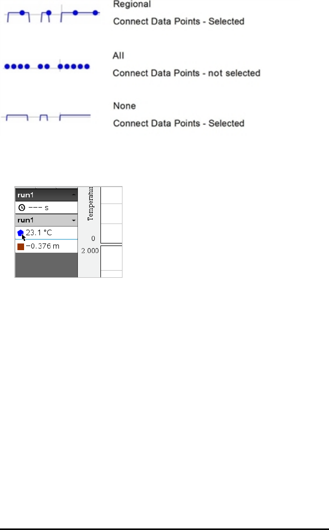
Setting Point Options

To indicate how often marks show on the graph and whether to use a connecting line:

1. Click Options > Point Options.

The Point Options dialogue box opens.

2. Select a Mark option from the drop-down list.

•None. No point protectors.

•Regional. Periodic point protectors.

•All. Every data point as a point protector.

3. Select Connect Data Points to display a line between points.

—or—

Clear Connect Data Points to remove the line between points.

The following graphics show examples of some of the Point Mark options.

Data Collection 49

50 Data Collection

Changing a Graph's Colour

1. Click the point indicator for the graph whose colour you want to change.

2. In the Column Options dialogue box, select the new Colour.

Selecting Point Markers

1. Right-click in the graph to open the menu.

2. Click Point Marker.

Note: If there is only one dependent variable column, the Point Marker option is

preceded by the data set name and column name. Otherwise, the Point Marker

option has a menu.

3. Select the column variable to change.

4. Select the point marker to set.

The Point Marker changes to the option selected.

Selecting an Independent Variable Column

Use the option Select X-axis Column to select the column used as the independent

variable when graphing the data. This column is used for all graphs.

1. Click Graph > Select X-axis Column.

2. Select the variable you want to change.

The x-axis label on the graph changes and the graph is reordered using the new

independent variable for graphing the data.

Selecting a Dependent Variable Column

Use the option Select Y-axis Column to select which dependent variable columns to

plot on the displayed graph(s).

1. Click Graph > Select Y-axis Column.

2. Select one of the following:

• A variable from the list. The list is a combination of dependent variables and

the number of data sets.

•More. Selecting More opens the Select dialogue box. Use this when you want

to select a combination of data set variables to graph.

Showing and Hiding Details

You can hide or show the Details view on the left side of the screen.

▶Click Options > Hide Details or Options > Show Details.

Data Collection 51

52 Data Collection

Striking and Restoring Data

Striking data omits it temporarily from the Graph view and from the analysis tools.

1. Open the data run that contains the data to be struck.

2. Click Table View .

3. Select the region by dragging from the starting row to the ending point.

The screen scrolls so you can see the selection.

4. Click Data > Strike Data.

5. Select one of the following:

•In Selected Region. Strike the data from the area you selected.

•Outside Selected Region. Strike all data except the area you selected.

The selected data is marked as struck in the table and is removed from the graph

view.

Restoring Struck Data

1. Select the range of data to restore or if restoring all struck data, start at step two.

2. Click Data > Restore Data.

3. Select one of the following:

•In Selected Region - Restore data in the selected area.

•Outside Selected Region - Restore data outside the selected area.

•All Data - Restore all data. No data selection necessary.

The data is restored.

Replaying the Data Collection

Use the Replay option to playback the data collection. This option lets you:

• Select the data set you want to replay.

• Pause the playback.

• Advance the playback by one point at a time.

• Adjust the playback rate.

• Repeat the playback.

Selecting the Data Set to Replay

You can replay one data set at a time. By default, the latest data set plays using the

first column as the base column (example: time reference).

If you have multiple data sets, and want a different data set or base column than the

default, you can select the data set to replay and the base column.

To select the data set to replay:

1. Click Experiment > Replay > Advanced Settings.

The Advanced Replay Settings dialogue box opens.

2. Select the data set to replay from the Data Set drop-down list.

Note: Changing the run in the Data Set selection tool does not affect the playback

choice. You must specify which data set in Experiment>Replay > AdvanceSettings.

3. (Optional) Select a new value from the Base Column drop-down list.

The selected column acts as the “Time” column for the replay.

Note: The base column should be a strictly increasing list of numbers.

4. Click Start to start the playback and save the settings.

Note: Data Set and Base Column options are based on the number of stored runs

and the sensor type used.

Starting and Controlling the Playback

▶Select Experiment > Replay > Start Playback.

Playback begins, and the Data Collection Control buttons change to:

Pause

Resume

Stop

Advance by One Point (enabled only during pause)

Data Collection 53

54 Data Collection

Adjusting the Playback Rate

To adjust the playback rate:

1. Select Experiment > Replay > Playback Rate.

The Playback Rate dialogue box opens.

2. In the Playback Rate field, click ▼to open the drop-down list.

3. Select the rate at which the playback will play.

Normal speed is 1.00. A higher value is faster and a lower value is slower.

4. Select one of the following options:

• Click Start to start the playback and save the settings.

• Click OK to save the settings for use on the next playback.

Repeating the Playback

1. Select Experiment > Replay > Start Playback.

2. Click Start to start the playback and save the settings.

Adjusting Derivative Settings

Use this option to select the number of points to use in derivative calculations. This

value affects the tangent tool, velocity and acceleration values.

Find pH derivative settings using a calculated column.

The Vernier DataQuest™ application can determine a numeric derivative from a list of

data with respect to another list of data. The data can be collected using sensors, input

manually, or linked with other applications. The numerical derivative is found using a

calculated column.

To determine the numerical 1st derivative of List B with respect to List A, enter the

following expression in the Column Options dialogue:

derivative(B,A,1,0) or derivative(B,A,1,1)

To determine the numerical 2nd derivative of List B with respect to List A, enter the

following expression:

derivative(B,A,2,0) or derivative (B,A,2,1)

The last parameter is either 0 or 1 depending on the method you are using. When it is

0, a weighted average is used. When it is 1, a time shifted derivative method is used.

Note: The first derivative calculation (weighted average) is what the Tangent tool uses

to display the slope at a data point when examining data. (Analyse > Tangent).

Note: The derivative calculation is completely row based. It is recommended that your

List A data be sorted in ascending order.

1. Click Options > Derivative Settings.

The Settings dialogue box opens.

2. Select the number of points from the drop-down list.

3. Click OK.

Drawing a Predictive Plot

Use this option to add points to the graph to predict the outcome of an experiment.

1. Click the Graph View tab .

2. From the Analyse menu, select Draw Prediction > Draw.

3. Click each area in which you want to place a point.

4. Press Esc to release the drawing tool.

Data Collection 55

56 Data Collection

5. To clear the drawn prediction, click Analyse > Draw Prediction > Clear.

Using Motion Match

Use this option to create a randomly generated plot when creating position-versus-time or

velocity-versus-time graphs.

This feature is only available when using a motion detector such as the CBR2™ sensor or

the Go!Motion® sensor.

Generating a Motion Match Plot

To generate a plot:

1. Attach the motion detector.

2. Click View > Graph.

3. Click Analyse > Motion Match.

4. Select one of the following options:

•New Position Match. Generates a random position plot.

•New Velocity Match. Generates a random velocity plot.

Note: Continue selecting a new position or a new velocity match to generate a new

random plot without removing the existing plot.

Removing a Motion Match Plot

To remove the generated plot:

▶Click Analyse > Motion Match > Remove Match.

Printing Collected Data

You can only print from the computer. You can print any single displayed active view, or

with the Print All option:

• One data view.

• All of the data views.

• A combination of the data views.

The Print All option has no effect on applications outside of the Vernier DataQuest™

application.

Printing Data Views

To print a data view:

1. On the main menu (top of the window), click File > Print.

The Print dialogue box opens.

2. Select Print All from the Print what drop-down list.

3. Select additional options, if needed.

4. Click Print to send the document to the printer.

Setting Options for the Print All Feature

1. Click Options > Print All Settings.

The Print All Settings dialogue box opens.

2. Select the views you want to print.

•Print Current View. The current view is sent to the printer.

•Print All Views. All three views (Meter, Graph and Table) are sent to the

printer.

•More. Only the views you select are sent to the printer.

Data Collection 57

58 Data Collection

3. Click OK.

The Print All Settings are now complete and can be used when printing.

TI-Nspire™ Lab Cradle

The TI-Nspire™ Lab Cradle is a device used with TI-Nspire™ handhelds, TI-Nspire™

software for computers or as a stand-alone tool to collect data.

The Lab Cradle supports all TI sensors. It also supports more than 50 analog and digital

Vernier DataQuest™ sensors, including motion detectors and photogate sensors. To see

the full list of supported sensors, go to education.ti.com/education/nspire/sensors.

Important: The TI-Nspire™ CM-C Handheld is not compatible with the Lab Cradle and

only supports the use of a single sensor at a time.

The Lab Cradle comes pre-loaded with its own operating system (OS). The TI-Nspire™

3.0 operating system for handheld and computer software has been preset to

recognise the Lab Cradle so you can start using it immediately.

Note: Any TI-Nspire™ OS earlier than 3.0 will not recognise the Lab Cradle. For more

information about upgrading a handheld OS, see Getting Started with the TI-Nspire™

CX Handheld or Getting Started with the TI-Nspire™ Handheld.

Exploring the Lab Cradle

The following graphic shows the front and back of the Lab Cradle.

TI-Nspire™ Lab Cradle 59

60 TI-Nspire™ Lab Cradle

Analog ports. The three BT analog ports used to connect analog sensors.

The other side of the cradle has two digital ports for digital sensors.

Battery panel and compartment area. The compartment is where the

rechargeable battery is located. Two cross-slotted screws are used to

secure the panel to the Lab Cradle.

Digital ports. The two digital ports used to connect digital sensors.

Reset button. Press this button to reboot the operating system if the Lab

Cradle does not respond to commands. Data may be lost when the Lab

Cradle reboots.

Trigger. Pressing this button is one method for capturing data from

attached sensors. Use this trigger when using the Lab Cradle as a stand-

alone data collection tool.

Label. Displays the serial number and other hardware information.

Handheld transfer connector. Used to connect the handheld and Lab

Cradle when collecting or transferring data.

Locking latch. Used to lock the Lab Cradle and handheld together.

Setting up the Lab Cradle for Data Collection

Before you can use the Lab Cradle to collect data, you must connect it to a handheld or

computer to define the collection parameters.

Attaching the Lab Cradle

To attach a handheld to a Lab Cradle, slide the handheld into the connector at the

bottom of the Lab Cradle. To lock the handheld to the Lab Cradle, push the lock up with

the handheld facing up. Push the lock down to release the handheld.

You can also connect to a handheld by plugging the handheld’s cable into the Lab

Cradle’s mini-USB port. This connection lets you transfer data from the Lab Cradle to

the handheld when you have collected data in the stand-alone mode.

To connect the Lab Cradle to a computer, plug the cable’s mini-USB connector into the

Lab Cradle’s mini-USB port. Then plug the cable’s standard USB connector into the

computer’s standard USB port.

Defining Collection Parameters

You must have the TI-Nspire™ software loaded on the computer or handheld. Use the

built-in Vernier DataQuest™ app to:

• Modify sensor settings.

• Set up data collection modes.

• Define triggering.

For more information, see the TI-Nspire™ Data Collection and Analysis Guidebook.

Using the Lab Cradle

The Lab Cradle can be used in the classroom or remotely. Collect the data with the Lab

Cradle, and then retrieve the data later. Store the data on the Lab Cradle until you

return to the classroom, and then transfer it to a handheld or computer for analysis.

Using the Lab Cradle with a Handheld

You can connect the Lab Cradle to your handheld to collect or retrieve data.

Using the Lab Cradle with a Computer

The Lab Cradle works with all Windows® and Mac® operating systems currently

supported by the TI-Nspire™ Teacher and Student computer software.

Using the Lab Cradle as a Stand-Alone Data Collection Tool

You can use the Lab Cradle in stand-alone mode to collect data either manually or

automatically. Press the trigger button to manually start and stop data collection when

in stand-alone mode.

Note: For long-term data collections TI recommends you use an AC adapter for a

handheld or a remote collection device such as the Lab Cradle.

Before collecting data, set up the data collection parameters using the Vernier

DataQuest™ app or use the sensor’s default settings. If you do not change the

parameters and use a single sensor, the Lab Cradle collects data using the sensor’s

default settings. If you use multiple sensors, the Lab Cradle collects samples beginning

with the sensor that has the shortest collection time requirement.

You do not have to reconnect the Lab Cradle to the same computer or handheld to

download the data. You can use any computer or handheld running a compatible OS

and TI-Nspire™ software to download the data.

Learning About the Lab Cradle

Portability

The Lab Cradle fits into the palm of most high school students' hands when connected

to the TI-Nspire™ handheld.

The Lab Cradle features an attachment point for a lanyard. Students can attach a

lanyard to wear the Lab Cradle around their neck. This feature lets students keep their

hands free to steady themselves in rough terrain during remote data collection

activities.

When collecting data for an experiment that subjects the Lab Cradle to intense

movement, TI recommends that students wear a Vernier Data Vest or zip-up jacket

with the sensor secured both around the student’s neck as well as to the student’s

TI-Nspire™ Lab Cradle 61

62 TI-Nspire™ Lab Cradle

chest. For example, if a student is measuring speed or motion on a roller coaster, the

Lab Cradle may bounce around due to the movement of the roller coaster. Wearing a

zip-up jacket or Vernier Data Vest limits the movement of the Lab Cradle.

Durability

The Lab Cradle is durable enough to withstand extensive use in the classroom and in

the field. It is designed to survive being dropped from a height of 36 inches, the height

of a standard lab table.

Storing/Operating Temperature Ranges

The Lab Cradle storage temperature range is between -40°C (-40° F) to 70°C (158° F).

The Lab Cradle, when used as a stand-alone data collection tool, operates in

temperatures from 10° C (50° F) to 45° C (113° F).

Triggering Methods

The Lab Cradle has two options for triggering data collection—automatic or manual.

To use automatic triggering, define the criteria in the Vernier DataQuest™ application

to start data collection. The Lab Cradle can trigger on either an increasing or

decreasing value.

Manual triggering is defined in the Vernier DataQuest™ app. By setting the trigger

delay value to zero, you can start data collection by pressing the trigger button on the

Lab Cradle when using it as a stand-alone data collection tool.

You can define a delay in triggering the data collection when using the Lab Cradle with

a computer or handheld. The Vernier DataQuest™ app starts a countdown based on the

time delay you define. When the countdown reaches zero, the Lab Cradle and its

connected sensors begin collecting data.

Multi-Channel Data Collection

You can connect up to five sensors to the Lab Cradle. It provides three analog BT

connectors and two digital BT connectors.

The Lab Cradle supports multi-channel data collection by allowing you to collect data

through all five sensors at the same time. When using all five sensors at the same

time, the time stamp is the same for all data collection streams.

Sampling Rate

The maximum sampling rate for a Lab Cradle using a single BT sensor is 100,000

samples per second. This sampling rate allows you to collect data for high-sample

sensors, such as microphones, blood pressure monitors and hand-grip heart rate

monitors.

If using more than one sensor at the same time, the 100,000 samples per second rate

is divided by the number of connected sensors. For example, when using:

• One sensor, data is collected at 100,000.

• Two sensors, data is collected at 50 kHz per sensor.

• Three sensors, data is collected at 33.3 kHz per sensor.

Some sensor’s maximum sample rates are less than the maximum sample rate of the

Lab Cradle. For example, with five sensors connected to the Lab Cradle, data may be

collected at 20 kHz per sensor; however, temperature sensors may only be capable of

collecting data at 1 kHz so it will only collect data at that rate.

Viewing Data Collection Status

The Lab Cradle has an LED light located on the top to indicate data collection status.

This light will be red, green or amber and use a variety of blink patterns.

TOP

Data collection

activity status

Red

• Red indicates that you need to wait until the system is ready.

•Slow blink: The Lab Cradle is updating experiment storage space. This is automatic

behaviour and does not impact active collections.

•Fast blink: Indicates one or more attached sensors are not warmed up. (You may

still collect data during the warm-up period but you risk the data being less

precise.)

Amber

• Amber indicates the system is ready but the collection has not yet started.

•One blink per second: The sensor is configured and set up for sampling.

•Slow blink: The Lab Cradle is connected to a computer or handheld running

TI-Nspire™ software but not set up for sampling.

•Fast blink: The Lab Cradle is ready for data collection when you press the trigger.

Green

• Green indicates the system is actively collecting data.

•Slow blink: Actively collecting data.

Note: There may be a slight variation in the duration of the blink depending on the

mode/rate of collection.

•Fast blink: Pre-storing data prior to a trigger.

Alternating Amber and Green

TI-Nspire™ Lab Cradle 63

64 TI-Nspire™ Lab Cradle

• The blinking pattern indicates the system is in trigger mode but has not yet

reached the trigger event.

Managing Power

When managing the power for the Lab Cradle, you must consider the power source

being used. The Lab Cradle can be powered by its rechargeable battery or a connected

power cord.

Batteries

The Lab Cradle runs on a rechargeable battery that supports one full day of high-use,

high-consumption sensor data collection before recharging. An example of high-use

data collection is an experiment requiring 150 total minutes of continuous data

collection with CO2(47mA) and O2 sensors at one sample every 15 seconds.

The battery recharges in less than 12 hours.

Viewing the Battery Status

There are two ways to view battery status: when attached to a handheld, or by looking

at the LED light. When the Lab Cradle is attached to a TI-Nspire™ handheld, you can

view the battery status for both. The first value is the handheld and the second value is

the Lab Cradle.

▶Press c 5 (Settings) 4(Status).

When you attach the Lab Cradle directly to a computer, you do not see a power

indicator. Use the LED light on the top of the Lab Cradle to determine battery status.

TOP

Battery

status

When the Lab Cradle is connected to a USB power source (either wall charger or

computer):

• Red - Slow blinking LED indicates the charge is low but charging.

• Amber - Slow blinking LED indicates the Lab Cradle is charging

• Green - Slow blinking LED indicates the Lab Cradle is fully charged.

When in the TI-Nspire™ Cradle Charging Bay:

• Red - Solid LED indicates the charge is low but is still charging.

• Amber - Solid LED indicates the Lab Cradle is charging.

• Green - Solid LED indicates the Lab Cradle is fully charged.

When running and not charging:

• Red - Blinking LED indicates the battery is below six percent.

• Amber - Blinking LED indicates the battery is below 30 percent.

• Green - Blinking LED indicates the battery is between 30 percent and 96 percent. Two

green blinks per second indicates the battery is over 96 percent.

Managing Battery Power

When the battery power reaches 30 percent, a yellow LED indicates the Lab Cradle

needs to be charged. The LED turns red when the battery power reaches five percent.

When managing battery power for the Lab Cradle, remember that some sensors need

to warm up before use. You can collect data while the sensor is warming up; however,

the data may not be as precise.

When you start a long-term or remote data collection, the system checks current

power sources to determine if the sources are adequate to support the sensors from

the beginning to the end of the experiment.

If the power is unable to support the experiment configuration, a warning indicates

that the power available is insufficient for the experiment. You either need to charge

the battery or plug the Lab Cradle into an external power source.

When using the wall charger, TI-Nspire™ Cradle Charging Bay or USB cable plugged

into a powered computer, the Lab Cradle can be fully charged from a dead state in less

than 12 hours when not being used.

The battery is capable of supporting one full day of high-use, high-consumption sensor

data collection or two full days of moderate to low consumption sensor data collection.

Charging the Lab Cradle

You can charge the Lab Cradle in a number of ways.

• Wall charger

• USB Cable connected to a computer

• TI-Nspire™ Navigator™ Cradle Charging Bay

TI-Nspire™ Lab Cradle 65

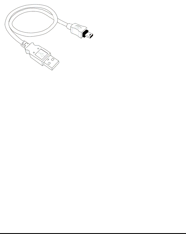
66 TI-Nspire™ Lab Cradle

Charging with an AC Wall Charger

Connect the plug to a standard AC wall outlet and the mini-B USB connector to the

TI-Nspire™ Lab Cradle.

Charging with a USB Cable

The Lab Cradle can be charged using a standard USB cable. Attach the mini-B

connector to the Lab Cradle and the USB type A connector into the computer.

The Lab Cradle will fully charge in less than 12 hours.

Charging with a Charging Bay

Use the TI-Nspire™ Navigator™ Cradle Charging Bay to charge five Lab Cradles at the

same time. A full charging bay with dead Lab Cradle units fully charges those units in

less than 12 hours.

You can leave the Lab Cradle in the charging bay even if fully charged. You can recharge

at any time regardless of the current charge level.

The charging bay is only included in certain bundled packages. The charging bay works

with Lab Cradles or with Lab Cradles connected to handhelds.

Upgrading the Operating System

Before You Begin

Before beginning an OS download, ensure that batteries are at least 25 percent

charged. If attached to a handheld, remove the handheld before updating the Lab

Cradle. You cannot update the OS with the handheld attached.

Finding Operating System Upgrades

For up-to-date information about available OS upgrades, check the Texas Instruments

website at education.ti.com.

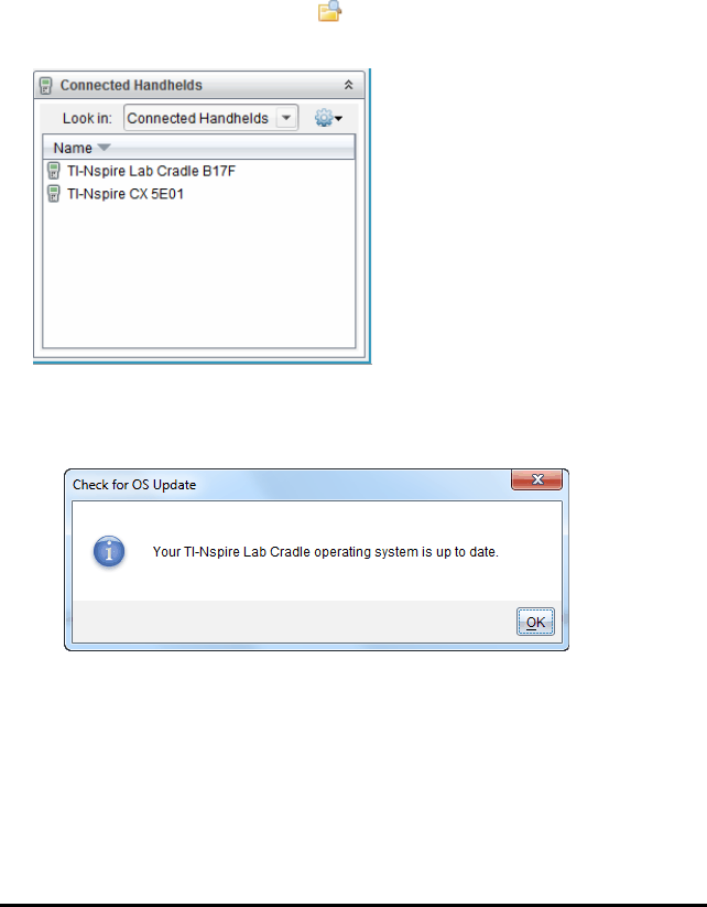
You can download an OS upgrade from the Texas Instruments website to a computer

and use a USB cable to install the OS on your TI-Nspire™ Lab Cradle. You will need an

Internet connection and the appropriate USB cable to download the updates.

Checking for Lab Cradle OS Updates

When using TI-Nspire™ software, you can quickly determine if your Lab Cradle OS is up

to date when the Lab Cradle is connected to a computer.

1. Open the TI-Nspire™ software and ensure the Lab Cradle is connected to your

computer.

2. In the Documents Workspace, click to open Content Explorer.

3. In the Connected Handhelds/Lab Cradle pane, select a connected Lab Cradle.

4. Select Help > Check for Handheld/Lab Cradle OS Update.

• If the operating system is current, the Check for Handheld OS dialogue box

opens indicating that the operating system on the Lab Cradle is up to date.

• If the operating system is not current, the dialogue box contains a message

indicating that a new version of the operating system is available.

5. Click OK to close the dialogue box.

Upgrading the Operating System

In the TI-Nspire™ software, you can select to upgrade the operating system on a

connected Lab Cradle from the following workspaces and menus:

TI-Nspire™ Lab Cradle 67

68 TI-Nspire™ Lab Cradle

• In all versions of the software, you can select Help > Check for Handheld/Lab Cradle

OS Update. Select a connected Lab Cradle in the Content Explorer to activate this

option. If the OS on the Lab Cradle is not current, the dialogue box indicates that

there is an updated version of the operating system. Follow the prompts to update

the operating system.

• In all versions of the TI-Nspire™ software, you can use options available in the

Documents Workspace:

- Open Content Explorer, select the Lab Cradle name, and then click and select

Install Handheld/Lab Cradle OS.

—or—

- Select Tools > Install Handheld/Lab Cradle OS.

• Those using teacher versions of the TI-Nspire™ software can use options available

in the Content Workspace:

- In the Resources pane, right-click the name of a connected Lab Cradle, and then

select Install Handheld/Lab Cradle OS.

—or—

- Select the Lab Cradle name in the Preview pane, click in the Preview pane,

and then select Install Handheld/Lab Cradle OS.

—or—

- Right-click the Lab Cradle name and select Install Handheld/Lab Cradle OS.

Completing the OS Upgrade

When you select to update the OS on a Lab Cradle, the Select Handheld/Lab Cradle OS

File dialogue box opens.

The file displayed for selection defaults to the file type required for the selected Lab

Cradle.

1. Select the OS file TI-Nspire.tlo.

2. Click Install OS to download the OS and update the Lab Cradle. The confirmation

message “You are about to upgrade your handheld/Lab Cradle operating system.

Any unsaved data will be lost. Do you want to continue?” is displayed.

3. Click Yes to continue.

The Installing OS dialogue box opens indicating the progress of the download. Do

not disconnect the Lab Cradle.

4. When the download is complete, the Information dialogue box opens indicating

that the OS file has been successfully transferred to the Lab Cradle. You can

disconnect the Lab Cradle.

5. Click OK.

Updating the OS on Multiple Lab Cradles

1. To view connected lab cradles:

• In the Content Workspace, view connected lab cradles in the Resources pane

under the Connected Handhelds heading.

• In the Documents Workspace, open the Content Explorer to view connected lab

cradles.

2. Click Tools > Install Handheld/Lab Cradle OS.

The Select Handheld OS File dialogue box opens.

TI-Nspire™ Lab Cradle 69

70 TI-Nspire™ Lab Cradle

3. Click Install OS for all connected handhelds/lab cradles.

Note: You can also update the OS on one lab cradle by clicking the radio button

next to the handheld name and then clicking Continue.

The OS Installation dialogue box opens.

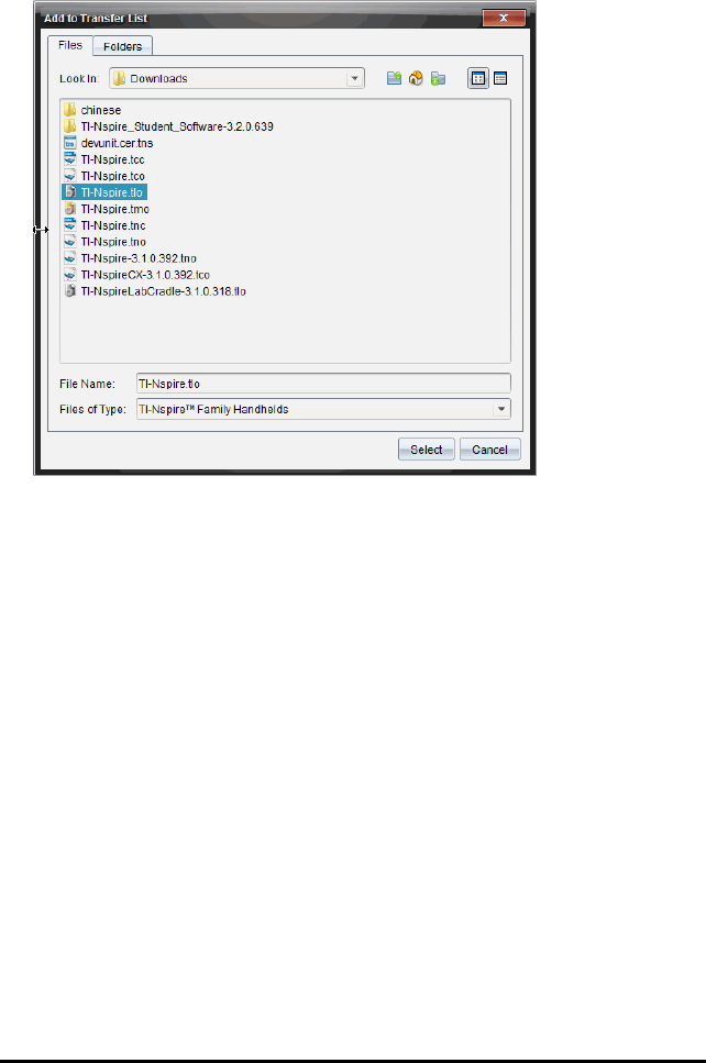
4. Click Add OS File.

The Add to Transfer List dialogue opens.

5. Navigate to the folder on your computer where the operating system file is

located.

6. Select the TI-Nspire.tlo file.

7. Click Select.

The OS Installation dialogue box is redisplayed showing the selected file.

8. Click Install OS.

The operating system is updated on the connected lab cradles. The status of the

update is shown on the Status tab in the OS Installation dialogue box.

9. When all lab cradles are updated, click Stop Transfer.

10. Click Close to close the OS Installation dialogue box.

TI-Nspire™ Lab Cradle 71

72 General Information

General Information

Texas Instruments Support and Service

Home Page: education.ti.com

E-mail inquiries: ti-cares@ti.com

KnowledgeBase and e-mail inquiries: education.ti.com/support

International information: education.ti.com/international

Service and Warranty Information

For information about the length and terms of the warranty or about product service,

refer to the warranty statement enclosed with this product or contact your local Texas

Instruments retailer/distributor.

Index

adding

titles to graphs 43

analysing data

integral 30

model 34

tangent 31

analysis options

removing 34

axis ranges

setting in graphs 44

calculations

derivative settings 54

collected data

deleting 28

viewing details 28

collecting and managing data sets 25

colours

changing for points 50

columns

defining options 38

selecting 51

comparing

data sets 26

comparing collected data sets 25

curve fit options 33

data

retrieving remote 23

selecting ranges 48

data analysis

interpolation 31

data collections

remote sensors 22

scaling graphs 47

setting sensor parameters 12

thresholds 24

Index 73

74 Index

data plots

finding curve fit 33

data sets

comparing 26

deleting collected 28

renaming 27

selecting for replays 53

selecting to plot 46

storing 26

data sets, collecting and managing 25

deleting

collected data sets 28

derivative settings

adjusting 54

displaying

Graph 1 37

graphs 36

graphs in Page Layout view 37

two graphs simultaneously 37

estimating

values between data points 31

expanding view details area 28

experiments

basic steps 6

finding

area under collected data 31

slope of collected data 31

finding upgrades 66

graphs

adding titles 43

displaying 36

displaying Graph 1 37

displaying in Page Layout view 37

displaying two simultaneously 37

position versus time 56

scaling 46

setting axis range 44

velocity versus time 56

importing

remote data 23

interfaces

multi-channel sensors 7

single-channel sensors 8

intervals 15

Lab Cradle

battery status 64

LEDs 63

overview 63

setting up 61

upgrading OS 66

LED lights

sensors 23

linking

columns to symbol table 38

managing collected data sets 25

measurement units

changing (Vernier DataQuest ™) 13

motion match

options 56

removing plots 56

naming columns 38

Operating System

upgrading 67

operating system upgrades 66

upgrading 67

Page Layout view 37

Index 75

76 Index

playbacks

adjusting rate 54

pausing 52

repeating 54

starting 53

plots

predictive 55

removing motion match 56

plotting

models 34

points

changing colours 50

setting markers 50

setting options 49

predictive plots

drawing and clearing 55

reducing view details area 28

RefreshProbeVars 28

remote data

retrieving 23

renaming

data sets 27

replays

starting 53

restoring data 52

sampling rate 62

scaling graphs 46

selecting

columns 51

data ranges 48

data sets for replays 53

data sets to plot 46

sensors

calibrating 14

changing measurement units 13

connecting 11

for computers 9

for handhelds 8

for remote data collections 22

interfaces 7-8

LED lights 23

multi-channel 62

reversing reading display 15

setting to zero 14

setting up offline 12

triggering 24

types 8

sets

renaming data sets 27

sets of data, comparing 26

sets, storing data as 26

showing screen details 51

slope 31

storing

data as sets 26

striking data 52

strip charts 16

symbol table

linking columns to 38

tables

restoring data 52

striking data 52

threshold values

increasing/decreasing 24

triggering

enabling 25

methods 62

Upgrading the OS 67

views

Graph 6

Page Layout 37

Table 6

Index 77

78 Index

zooming

in 48

out 48

JBL My TI Nspire™ Data Collection And Analysis Guidebook (UK English) Nspire EN GB

Navigation menu

Versions of this User Manual:

Views

Navigation