JBL My TI Nspire™ Navigator™ NC Teacher Software Guidebook (UK English) Nspire Navigator EN GB
User Manual: JBL TI-Nspire™ Navigator™ NC Teacher Software Guidebook (UK English) TI-Nspire™ Navigator™ NC Teacher Software Guidebook
Open the PDF directly: View PDF ![]() .
.
Page Count: 668 [warning: Documents this large are best viewed by clicking the View PDF Link!]
- Important Information
- Getting Started with TI‑Nspire™ Navigator NC Teacher Software
- Tracking and Reporting System Use
- Using the Content Workspace
- Using the Documents Workspace
- Working with TI‑Nspire™ Documents
- Creating a New TI‑Nspire™ Document
- Opening an Existing Document
- Saving TI‑Nspire™ Documents
- Deleting Documents
- Closing Documents
- Formatting Text in Documents
- Using Colours in Documents
- Setting Page Size and Document Preview
- Working with Multiple Documents
- Working with Applications
- Selecting and Moving Pages
- Working with Problems and Pages
- Printing Documents
- Viewing Document Properties and Copyright Information
- Working with PublishView™ Documents
- Creating a New PublishView™ Document
- Saving PublishView™ Documents
- Exploring the Documents Workspace
- Working with PublishView™ Objects
- Working with TI-Nspire™ Applications
- Working with Problems
- Organizing PublishView™ Sheets
- Using Zoom
- Adding Text to a PublishView™ Document
- Using Hyperlinks in PublishView™ Documents
- Working with Images
- Working with Video Files
- Converting Documents
- Printing PublishView™ Documents
- Working with Lesson Bundles
- Capturing Screens
- Accessing Screen Capture
- Using Capture Class
- Randomising Captured Screens
- Setting View Options in Capture Class
- Creating Stacks of Student Screens
- Comparing Selected Screens
- Using Make Presenter
- Saving Screens When Using Capture Class
- Printing Captured Screens
- Using Capture Page
- Viewing Captured Screens
- Saving Captured Pages and Screens
- Copying and Pasting a Screen
- Capturing Images in Handheld Mode
- Working with Images
- Using the Class Workspace
- Adding Classes
- Adding Students to Classes
- Removing Students from Classes
- Updating Class Rosters
- Managing Classes
- Beginning and Ending a Class Session
- Changing the Student View
- Arranging the Seating Chart
- Checking Student Login Status
- Sorting Student Information
- Changing the Classes Assigned to a Student
- Changing Student Names and Identifiers
- Moving Students to Another Class
- Copying Students to Another Class
- Exploring the Class Record
- Sending Files to a Class
- Collecting Files from Students
- Managing Unprompted Actions
- Saving Files to a Portfolio Record
- Deleting Files from Class Folders
- Checking the Status of File Transfers
- Cancelling File Transfers
- Viewing File Properties
- Resetting Student Passwords
- Understanding the File System
- Understanding File Transfers
- Using Live Presenter
- Using Question in the Teacher Software
- Responding to Questions
- Polling Students
- Using the Review Workspace
- Using the Portfolio Workspace
- Exploring the Assignments Pane
- Exploring the Workspace Views
- Saving an Item to the Portfolio Workspace
- Importing an Item to the Portfolio Workspace
- Editing Scores
- Exporting Results
- Sorting Information in the Portfolio Workspace
- Opening a Portfolio Item in Another Workspace
- Opening a Master Document
- Adding a Master Document
- Redistributing a Portfolio Item
- Collecting Missing Files from Students
- Sending Missing Files to Students
- Renaming a Portfolio Item
- Removing Columns from Portfolio
- Removing Individual Files from Portfolio
- Summary of File Type Options
- Calculator Application
- Using Variables
- Geometry Application
- What You Must Know
- Introduction to Geometric Objects
- Creating Points and Lines
- Creating Geometric Shapes
- Creating Shapes Using Gestures (MathDraw)
- Basics of Working with Objects
- Measuring Objects
- Transforming Objects
- Exploring with Geometric Construction Tools
- Using Geometry Trace
- Conditional Attributes
- Hiding Objects in the Geometry Application
- Customizing the Geometry Work Area
- Animating Points on Objects
- Adjusting Variable Values with a Slider
- Using the Calculate Tool
- Graphs Application
- What You Must Know
- Graphing Functions
- Manipulating Functions by Dragging
- Specifying a Function with Domain Restrictions
- Finding Points of Interest on a Function Graph
- Graphing a Family of Functions
- Graphing Equations
- Graphing Conic Sections
- Graphing Relations
- Graphing Parametric Equations
- Graphing Polar Equations
- Using the Text Tool to Graph Equations
- Graphing Scatter Plots
- Plotting Sequences
- Graphing Differential Equations
- Viewing Tables from the Graphs Application
- Editing Relations
- Accessing the Graph History
- Zooming/Rescaling the Graphs Work Area
- Customising the Graphs Work Area
- Hiding and Showing Items in the Graphs Application
- Conditional Attributes
- Calculating a Bounded Area
- Tracing Graphs or Plots
- Introduction to Geometric Objects
- Creating Points and Lines
- Creating Geometric Shapes
- Creating Shapes Using Gestures (MathDraw)
- Basics of Working with Objects
- Measuring Objects
- Transforming Objects
- Exploring with Geometric Construction Tools
- Animating Points on Objects
- Adjusting Variable Values with a Slider
- Labelling (Identifying) the Coordinates of a Point
- Displaying the Equation of a Geometric Object
- Using the Calculate Tool
- 3D Graphs
- Lists & Spreadsheet Application
- Creating and Sharing Spreadsheet Data as Lists
- Creating Spreadsheet Data
- Navigating in a Spreadsheet
- Working with Cells
- Working with Rows and Columns of Data
- Sorting Data
- Generating Columns of Data
- Graphing Spreadsheet Data
- Exchanging Data with Other Computer Software
- Capturing Data from Graphs & Geometry
- Using Table Data for Statistical Analysis
- Statistics Input Descriptions
- Statistical Calculations
- Distributions
- Confidence Intervals
- Stat Tests
- Working with Function Tables
- Data & Statistics Application
- Notes Application
- Using Templates in Notes
- Formatting Text in Notes
- Using Colour in Notes
- Inserting Images
- Inserting Items on a Notes Page
- Inserting Comments
- Inserting Geometric Shape Symbols
- Entering Maths Expressions in Notes Text
- Evaluating and Approximating Maths Expressions
- Using Maths Actions
- Graphing from Notes and Calculator
- Inserting Chemical Equations in Notes
- Deactivating Maths Expression Boxes
- Changing the Attributes of Maths Expression Boxes
- Using Calculations in Notes
- Exploring Notes with Examples
- Widgets
- Libraries
- Getting Started with the Programme Editor
- Defining a Program or Function
- Viewing a Program or Function
- Opening a Function or Program for Editing
- Importing a Program from a Library
- Creating a Copy of a Function or Program
- Renaming a Program or Function
- Changing the Library Access Level
- Finding Text
- Finding and Replacing Text
- Closing the Current Function or Program
- Running Programmes and Evaluating Functions
- Getting Values into a Program
- Displaying Information
- Using Local Variables
- Differences Between Functions and Programs
- Calling One Program from Another
- Controlling the Flow of a Function or Program
- Using If, Lbl and Goto to Control Program Flow
- Using Loops to Repeat a Group of Commands
- Changing Mode Settings
- Debugging Programs and Handling Errors
- Using the TI‑SmartView™ Emulator
- Writing Lua Scripts
- Data Collection
- What You Must Know
- About Collection Devices
- Connecting Sensors
- Setting Up an Offline Sensor
- Modifying Sensor Settings
- Collecting Data
- Using Data Markers to Annotate Data
- Collecting Data Using a Remote Collection Unit
- Setting Up the Sensor for Triggering
- Collecting and Managing Data Sets
- Using Sensor Data in Programmes
- Collecting Sensor Data using RefreshProbeVars
- Analysing Collected Data
- Displaying Collected Data in Graph View
- Displaying Collected Data in Table View
- Customising the Graph of Collected Data
- Striking and Restoring Data
- Replaying the Data Collection
- Adjusting Derivative Settings
- Drawing a Predictive Plot
- Using Motion Match
- Printing Collected Data
- Using the Help Menu
- General Information


Important Information
Except as otherwise expressly stated in the Licence that accompanies a program, Texas
Instruments makes no warranty, either express or implied, including but not limited to
any implied warranties of merchantability and fitness for a particular purpose,
regarding any programs or book materials and makes such materials available solely
on an "as-is" basis. In no event shall Texas Instruments be liable to anyone for special,
collateral, incidental, or consequential damages in connection with or arising out of the
purchase or use of these materials and the sole and exclusive liability of Texas
Instruments, regardless of the form of action, shall not exceed the amount set forth in
the licence for the program. Moreover, Texas Instruments shall not be liable for any
claim of any kind whatsoever against the use of these materials by any other party.
License
Please see the complete license installed in C:\Program Files\TI Education\<TI-Nspire™
Product Name>\license.
Adobe®, Adobe® Flash®, Apple®, Blackboard™, Chrome®, Excel®, Google®, Firefox®,
Internet Explorer®, Java™, JavaScript®, Mac®, Microsoft®, Mozilla®, OS X®,
PowerPoint®, Safari®, SMART® Notebook, Vernier DataQuest™, Vernier EasyLink®,
Vernier EasyTemp®, VernierGo!Link®, VernierGo!Motion®, VernierGo!Temp®, Vista®,
Windows®and Windows® XP are trademarks of their respective owners.
© 2011 - 2017 Texas Instruments Incorporated
ii

Contents
Important Information ii
Getting Started with TI-Nspire™ Navigator NC Teacher Software 1
Using the Welcome Screen 1
Exploring the Software 2
Exploring Workspaces 3
Understanding the Status Bar 4
Changing Language 5
Connecting to the Network 6
Helping Students Log In 7
Managing Available Seats 11
Tracking and Reporting System Use 14
Managing Session Logs 14
Packaging and Sending Session Logs 16
Using the Content Workspace 18
Exploring the Content Workspace 18
Exploring the Resources Pane 18
Using the Preview Pane 20
Accessing Computer Content 22
Using Shortcuts 24
Working with Links 25
Using Web Content 27
Sending Files to Class 31
Using the Documents Workspace 34
Exploring the Documents Workspace 34
Using the Documents Toolbox 34
Exploring Document Tools 35
Exploring the Page Sorter 35
Exploring the TI-SmartView™ Feature 36
Exploring Utilities 38
Exploring Content Explorer 39
Using the Work Area 40
Changing Document Settings 41
Changing Graphs & Geometry Settings 43
Working with TI-Nspire™ Documents 46
Creating a New TI-Nspire™ Document 46
iii

iv
Opening an Existing Document 47
Saving TI-Nspire™ Documents 48
Deleting Documents 49
Closing Documents 49
Formatting Text in Documents 50
Using Colours in Documents 51
Setting Page Size and Document Preview 51
Working with Multiple Documents 53
Working with Applications 54
Selecting and Moving Pages 57
Working with Problems and Pages 60
Printing Documents 62
Viewing Document Properties and Copyright Information 63
Working with PublishView™ Documents 66
Creating a New PublishView™ Document 66
Saving PublishView™ Documents 70
Exploring the Documents Workspace 72
Working with PublishView™ Objects 75
Working with TI-Nspire™ Applications 81
Working with Problems 84
Organizing PublishView™ Sheets 86
Using Zoom 91
Adding Text to a PublishView™ Document 91
Using Hyperlinks in PublishView™ Documents 93
Working with Images 99
Working with Video Files 101
Converting Documents 102
Printing PublishView™ Documents 104
Working with Lesson Bundles 106
Creating a New Lesson Bundle 106
Adding Files to a Lesson Bundle 107
Opening a Lesson Bundle 109
Managing Files in a Lesson Bundle 110
Managing Lesson Bundles 111
Packaging Lesson Bundles 114
Emailing a Lesson Bundle 114
Sending Lesson Bundles to Connected Handhelds 115
Capturing Screens 116
Accessing Screen Capture 116

Using Capture Class 116
Randomising Captured Screens 118
Setting View Options in Capture Class 119
Creating Stacks of Student Screens 122
Comparing Selected Screens 124
Using Make Presenter 124
Saving Screens When Using Capture Class 124
Printing Captured Screens 126
Using Capture Page 127
Viewing Captured Screens 128
Saving Captured Pages and Screens 129
Copying and Pasting a Screen 131
Capturing Images in Handheld Mode 131
Working with Images 134
Working with Images in the Software 134
Using the Class Workspace 138
Adding Classes 138
Adding Students to Classes 143
Removing Students from Classes 145
Updating Class Rosters 146
Managing Classes 148
Beginning and Ending a Class Session 150
Changing the Student View 151
Arranging the Seating Chart 152
Checking Student Login Status 152
Sorting Student Information 153
Changing the Classes Assigned to a Student 153
Changing Student Names and Identifiers 155
Moving Students to Another Class 156
Copying Students to Another Class 157
Exploring the Class Record 157
Sending Files to a Class 159
Collecting Files from Students 161
Managing Unprompted Actions 164
Saving Files to a Portfolio Record 165
Deleting Files from Class Folders 166
Checking the Status of File Transfers 167
Cancelling File Transfers 167
Viewing File Properties 168
Resetting Student Passwords 168
v

vi
Understanding the File System 170
Understanding File Transfers 170
Using Live Presenter 172
Starting Live Presenter 172
Viewing Live Presenter 173
Stopping Live Presenter 173
Using Question in the Teacher Software 174
Understanding the Question Tools 174
Using the Teacher Tool Palette 175
Understanding the Configuration Tool 177
Formatting Text and Objects 178
Adding Images to Questions 178
Adding Questions 179
Responding to Questions 194
Understanding the Question Toolbar 194
Types of Questions 194
Responding to Quick Poll Questions 195
Submitting Responses 197
Polling Students 198
Opening the Quick Poll Tool 199
Sending a Quick Poll 200
Stopping Polls 201
Resending Polls 201
Sending Polls to Missing Students 202
Saving Polls 202
Viewing Poll Results 203
Using the Review Workspace 206
Using the Review Toolbox 206
Exploring the Data View Pane 211
Opening Documents for Review 214
Viewing Data 216
Changing the Aspect Ratio 218
Organising Responses 218
Hiding and Showing Responses 223
Marking Responses as Correct or Incorrect 226
Adding Teacher Data 230
Saving to the Portfolio Workspace 233

Saving Data as a New Document 234
Using the Portfolio Workspace 236
Exploring the Assignments Pane 236
Exploring the Workspace Views 237
Saving an Item to the Portfolio Workspace 239
Importing an Item to the Portfolio Workspace 240
Editing Scores 241
Exporting Results 243
Sorting Information in the Portfolio Workspace 244
Opening a Portfolio Item in Another Workspace 244
Opening a Master Document 245
Adding a Master Document 246
Redistributing a Portfolio Item 246
Collecting Missing Files from Students 247
Sending Missing Files to Students 247
Renaming a Portfolio Item 247
Removing Columns from Portfolio 247
Removing Individual Files from Portfolio 248
Summary of File Type Options 248
Calculator Application 250
Entering and Evaluating Maths Expressions 251
CAS: Working with Measurement Units 258
Using the Unit Conversion Assistant 260
Conversion Categories and Units 263
Working with Variables 266
Creating User-defined Functions and Programmes 266
Editing Calculator Expressions 271
Financial Calculations 271
Working with the Calculator History 273
Using Variables 278
Linking Values on Pages 278
Creating Variables 278
Using (Linking) Variables 283
Naming Variables 285
Adjusting Variable Values with a Slider 286
Locking and Unlocking Variables 288
Removing a Linked Variable 291
vii

viii
Geometry Application 292
What You Must Know 292
Introduction to Geometric Objects 295
Creating Points and Lines 297
Creating Geometric Shapes 301
Creating Shapes Using Gestures (MathDraw) 307
Basics of Working with Objects 310
Measuring Objects 313
Transforming Objects 319
Exploring with Geometric Construction Tools 322
Using Geometry Trace 327
Conditional Attributes 328
Hiding Objects in the Geometry Application 329
Customizing the Geometry Work Area 330
Animating Points on Objects 331
Adjusting Variable Values with a Slider 332
Using the Calculate Tool 334
Graphs Application 338
What You Must Know 339
Graphing Functions 341
Manipulating Functions by Dragging 342
Specifying a Function with Domain Restrictions 344
Finding Points of Interest on a Function Graph 345
Graphing a Family of Functions 348
Graphing Equations 348
Graphing Conic Sections 349
Graphing Relations 352
Graphing Parametric Equations 355
Graphing Polar Equations 355
Using the Text Tool to Graph Equations 356
Graphing Scatter Plots 358
Plotting Sequences 359
Graphing Differential Equations 361
Viewing Tables from the Graphs Application 364
Editing Relations 365
Accessing the Graph History 367
Zooming/Rescaling the Graphs Work Area 368
Customising the Graphs Work Area 369
Hiding and Showing Items in the Graphs Application 371
Conditional Attributes 372
Calculating a Bounded Area 374

Tracing Graphs or Plots 375
Introduction to Geometric Objects 377
Creating Points and Lines 379
Creating Geometric Shapes 383
Creating Shapes Using Gestures (MathDraw) 389
Basics of Working with Objects 392
Measuring Objects 395
Transforming Objects 401
Exploring with Geometric Construction Tools 404
Animating Points on Objects 409
Adjusting Variable Values with a Slider 410
Labelling (Identifying) the Coordinates of a Point 412
Displaying the Equation of a Geometric Object 413
Using the Calculate Tool 414
3D Graphs 416
Graphing 3D Functions 416
Graphing 3D Parametric Equations 417
Rotating the 3D View 418
Editing a 3D Graph 419
Accessing the Graph History 419
Changing the Appearance of a 3D Graph 420
Showing and Hiding 3D Graphs 421
Customising the 3D Viewing Environment 421
Tracing in the 3D View 423
Example: Creating an Animated 3D Graph 424
Lists&Spreadsheet Application 426
Creating and Sharing Spreadsheet Data as Lists 427
Creating Spreadsheet Data 429
Navigating in a Spreadsheet 432
Working with Cells 433
Working with Rows and Columns of Data 437
Sorting Data 440
Generating Columns of Data 441
Graphing Spreadsheet Data 444
Exchanging Data with Other Computer Software 448
Capturing Data from Graphs&Geometry 450
Using Table Data for Statistical Analysis 453
Statistics Input Descriptions 454
Statistical Calculations 455
Distributions 460
ix

x
Confidence Intervals 466
Stat Tests 468
Working with Function Tables 472
Data&Statistics Application 474
Basic Operations in Data& Statistics 475
Overview of Raw and Summary Data 479
Working with Numeric Plot Types 480
Working with Categorical Plot Types 489
Exploring Data 496
Using Window/Zoom Tools 506
Graphing Functions 507
Using Graph Trace 512
Customising Your Workspace 513
Adjusting Variable Values with a Slider 514
Inferential Statistics 517
Notes Application 520
Using Templates in Notes 521
Formatting Text in Notes 522
Using Colour in Notes 523
Inserting Images 524
Inserting Items on a Notes Page 524
Inserting Comments 525
Inserting Geometric Shape Symbols 525
Entering Maths Expressions in Notes Text 526
Evaluating and Approximating Maths Expressions 527
Using Maths Actions 529
Graphing from Notes and Calculator 531
Inserting Chemical Equations in Notes 533
Deactivating Maths Expression Boxes 534
Changing the Attributes of Maths Expression Boxes 535
Using Calculations in Notes 535
Exploring Notes with Examples 537
Widgets 542
Creating a Widget 542
Adding a Widget 542
Saving a Widget 545
Libraries 546
What is a Library? 546

Creating Libraries and Library Objects 546
Private and Public Library Objects 547
Using Library Objects 548
Creating Shortcuts to Library Objects 549
Included Libraries 549
Restoring an Included Library 550
Getting Started with the Programme Editor 552
Defining a Program or Function 553
Viewing a Program or Function 556
Opening a Function or Program for Editing 556
Importing a Program from a Library 557
Creating a Copy of a Function or Program 557
Renaming a Program or Function 557
Changing the Library Access Level 558
Finding Text 558
Finding and Replacing Text 559
Closing the Current Function or Program 559
Running Programmes and Evaluating Functions 559
Getting Values into a Program 562
Displaying Information 564
Using Local Variables 565
Differences Between Functions and Programs 566
Calling One Program from Another 567
Controlling the Flow of a Function or Program 568
Using If, Lbl and Goto to Control Program Flow 568
Using Loops to Repeat a Group of Commands 571
Changing Mode Settings 574
Debugging Programs and Handling Errors 574
Using the TI-SmartView™ Emulator 576
Opening the TI-SmartView™ Emulator 576
Choosing a Keypad 577
Choosing Display Options 577
Working with the Emulated Handheld 578
Using the Touchpad 579
Using the Clickpad 579
Using Settings and Status 580
Changing TI-SmartView™ Options 580
Working with Documents 582
Using Screen Capture 582
xi

xii
Writing Lua Scripts 584
Overview of the Script Editor 584
Exploring the Script Editor Interface 584
Using the Toolbar 585
Inserting New Scripts 587
Editing Scripts 588
Changing View Options 589
Setting Minimum API Level 589
Saving Script Applications 589
Managing Images 590
Setting Script Permissions 592
Debugging Scripts 592
Data Collection 594
What You Must Know 595
About Collection Devices 596
Connecting Sensors 600
Setting Up an Offline Sensor 601
Modifying Sensor Settings 602
Collecting Data 604
Using Data Markers to Annotate Data 608
Collecting Data Using a Remote Collection Unit 611
Setting Up the Sensor for Triggering 613
Collecting and Managing Data Sets 614
Using Sensor Data in Programmes 617
Collecting Sensor Data using RefreshProbeVars 618
Analysing Collected Data 619
Displaying Collected Data in Graph View 625
Displaying Collected Data in Table View 627
Customising the Graph of Collected Data 632
Striking and Restoring Data 641
Replaying the Data Collection 641
Adjusting Derivative Settings 643
Drawing a Predictive Plot 644
Using Motion Match 645
Printing Collected Data 645
Using the Help Menu 648
Activating Your Software Licence 648
Registering Your Product 650
Downloading the Latest Guidebook 650
Exploring TI Resources 650

Getting Started with TI-Nspire™ Navigator NC Teacher
Software
The TI-Nspire™ Navigator™ NC system is a classroom management system that
enables connection between teacher and student computers through a wireless
networking connection. The software provides an integrated approach for delivering
and evaluating instruction, assessments, and content.
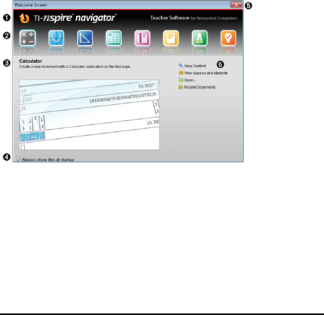
Using the Welcome Screen
To help you get started quickly, the Welcome Screen opens with some common task
options. You can choose to turn off the Welcome Screen.
To begin working with documents, click an icon or link or close this screen. Any normal
action that takes place automatically, such as upgrade prompts may appear after you
close the Welcome Screen.
Note: Depending on how your software was installed, you might see a Product
Improvement screen the first time you start the software.
ÀName. Shows software name.
ÁQuick Start icons. Click one of these icons to create a new document in the chosen
application. The applications are Calculator, Graphs, Geometry, Lists & Spreadsheet,
Data & Statistics, Question, Notes and the Vernier DataQuest™ application. The
Welcome Screen automatically closes and the chosen application opens in the
Documents Workspace.
ÂPreview area. When your mouse is hovering over an application icon or a link in
Teacher Tools, a preview of the application or tool is shown. A brief description of
the icon or link is also displayed at the top of the area.
Getting Started with TI-Nspire™ Navigator NC Teacher Software 1
2 Getting Started with TI-Nspire™ Navigator NC Teacher Software
ÃAlways show this at startup. Clear this tickbox to skip this screen when you open
the software.
ÄClose the Welcome Screen. Click here to close this screen and begin working in the
software.
ÅTeacher Tools. Click one of these links to close the Welcome Screen and open the
software in the chosen tool.
•View content. Opens the Content Workspace, where you can find content on
your computer, the web and links you have created.
•View classes and students. Opens the Class Workspace where you can see the
students in a class, or add new classes and students.
•Open. Opens a dialogue box where you can navigate to and open existing
documents.
Recent Documents. Lists the names of recently opened documents. As your mouse
hovers over each document name, the first page of that document is displayed in the
Preview pane. Click the name of a document to open that document.
Opening the Welcome Screen
The Welcome Screen opens automatically when you open the software if the Always
show this at start-up tickbox is selected. If this option is turned off or if you have closed
the Welcome Screen, click Help > Welcome Screen to open the Welcome Screen.
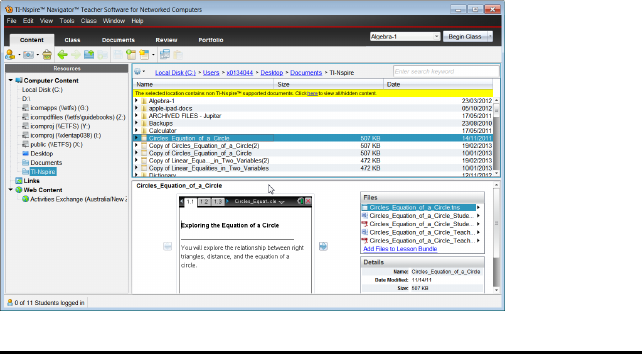
Exploring the Software
When you close the Welcome Screen, the TI-Nspire™ Navigator™ NC Teacher Software
opens the last workspace used. If you select one of the application icons, the software
opens a new document in the Documents Workspace.
When you open the software for the first time, the Content Workspace opens by
default. When you open a folder that contains documents other than TI-Nspire™
documents, the software lets you know there are additional documents in the folder
and provides the option to show all documents contained in the folder.
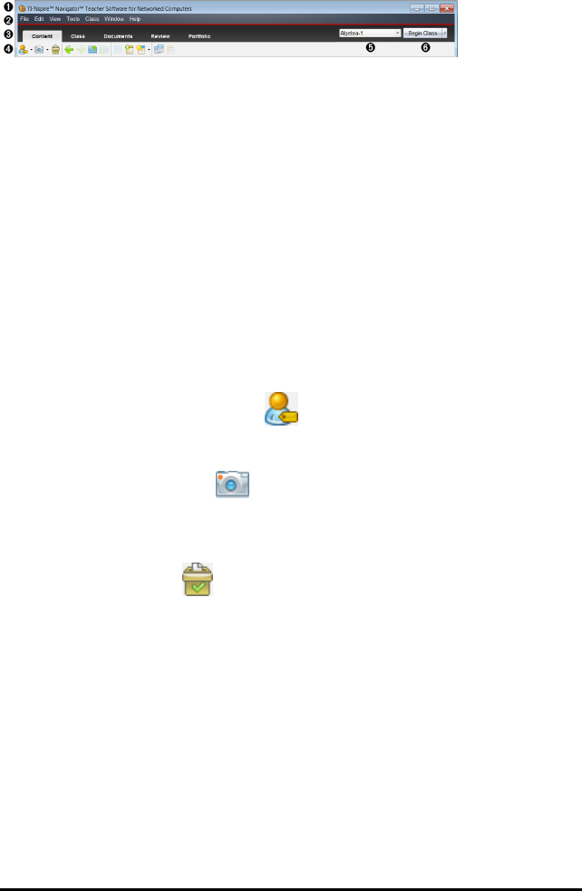
The options on the title bar, menu bar, and toolbars are available in all workspaces. For
more information, see the chapter for each workspace.
ÀTitle bar. Shows the name of the current document (if opened) and the name of the
software. The minimize, maximize, and close buttons are located in the right corner.
ÁMenu bar. Contains tools for working with documents in the current workspace and
contains options for modifying system settings. Click Help to access options for
opening the help file, performing online troubleshooting, and finding information
about software updates.
ÂWorkspace Selector. Use these tabs to switch between the Content, Class,
Documents, Review, and Portfolio Workspaces.
Note: Some tasks you perform may prevent you from immediately changing
workspaces. If a dialogue box awaits a response from you, type your response,
and then change workspaces.
ÃTools menu. Shows tools frequently used when working in each workspace. Every
workspace has the Quick Poll, Screen Capture, and Student Name Format icons.
Other tool menu options change depending on which workspace is open. Those tools
are covered in their respective chapters.
• Use the Student Name Format tool to choose how student names are
displayed, either by Last Name, First Name, User name, Display Name,
Student ID, or hidden.
• Use the Screen Capture tool to take a picture of an active document on
the computer, or capture screens on one or all connected student computers.
You can take several pictures, copy/paste the images in other documents, or
save the images. For more information, see Capturing Screens.
• Use the Quick Poll tool to immediately send a poll to students and
receive student responses. For more information, see Polling Students.
ÄClass list. Shows classes that are currently available.
ÅClass Actions button. Click this button to begin or end a class.
Exploring Workspaces
The TI-Nspire™ Navigator™ NC Teacher Software uses workspaces to help you easily
access the tasks you most commonly perform. The software has five predefined
workspaces.
•Content Workspace. Find and manage content on your computer and add and
manage links to websites.
Getting Started with TI-Nspire™ Navigator NC Teacher Software 3
4 Getting Started with TI-Nspire™ Navigator NC Teacher Software
•Class Workspace. Manage classes and students, use the Class Record panel, and
exchange files with students. This workspace is the only area where you can both
send and receive file types other than TI-Nspire™ (.tns) and PublishView™ (.tnsp)
documents.
•Documents Workspace. Author documents and demonstrate mathematical
concepts.
•Review Workspace. Review a collected set of documents; mark, show, or hide
student responses; switch data views; and organize data.
•Portfolio Workspace. Save, store, review, and manage class assignments from
students.
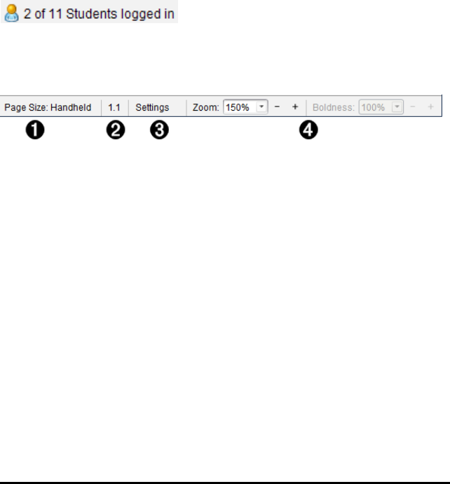
Understanding the Status Bar
Some information in the status bar changes, depending on which workspace is open.
In all workspaces, the status bar provides information about the student login status.
The student login status shows how many students are currently logged into class and
how many students are assigned to the current class.
In the Documents Workspace, the status bar gives additional information.
ÀPage Size. Shows whether the document is in Handheld or Computer page size. Click
here to view document properties. For more information on page size and document
preview, see Working with TI-Nspire™ Documents.
ÁProblem and page number. References the current document. In this example, 1.1
indicates problem 1, page 1 of the active document.
ÂSettings. Click here to view or change Document settings.
ÃZoom/Boldness. When working with a document in Handheld page size, use the
Zoom scale to zoom the active document in or out from 10% to 500%. To set a
zoom, type a specific number, use the + and - buttons to increase or decrease by
increments of 10%, or use the drop-down box to choose preset percentages.
When working with a document in Computer page size, use the Boldness scale to
increase or decrease the boldness of text and line thickness within applications. To
set the boldness, type a specific number, use the + and - buttons to increase or
decrease by increments of 10%, or use the drop-down box to choose preset
percentages.
In the Review Workspace, the status bar information changes, depending on the view
in the Page Sorter.
• If you are in the document view, the status bar provides the same information as
the Documents Workspace status bar.
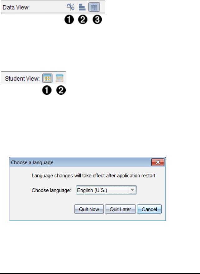
• If you are in the student response view, the status bar has Data View icons. Use
the icons to change between bar chart, table, and graph views. See Using the
Review Workspace for more information on the Data Views.
À
Á
Â
Graph
Bar Chart
Table
In the Class Workspace, the status bar has Student View icons. Use the icons to change
between Seating Chart view or Student List view. See Using the Class Workspace for
more information on the Student Views.
À
Á
Seating chart
Student List
Changing Language
Use this option to select a preferred language. You must restart the software for the
language to take effect.
1. Click File >Settings >Change Language.
The Choose a Language dialogue box opens.
2. Click ¤to open the Choose language drop-down list.
3. Select the desired language.
Getting Started with TI-Nspire™ Navigator NC Teacher Software 5
6 Getting Started with TI-Nspire™ Navigator NC Teacher Software
4. Click Quit Now to close the software immediately. You will be prompted to save
any open documents. When you restart the software, the language change is
effective.
—or—
Click Quit Later to continue your work. The language change is not applied until you
close and restart the software at a later time.
Note: If you select Simplified Chinese or Traditional Chinese as the language in the
TI-Nspire™ software, you should see Chinese characters in the menus and dialogues. If
your computer uses the Windows® XP operating system and you do not see Chinese
characters, you may need to install the Windows® XP East Asian Language Support
package.
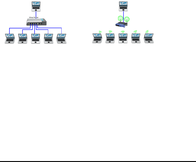
Connecting to the Network
Connection from student computers to teacher computers is through the school
network.
It’s best if the teacher computer has a wired connection, but the network administrator
will know which connection is best for your environment.
Student connections can be wired or wireless.
Teacher wired and students wired Teacher wired and students wireless
Once the school network administrator has provided network access, you are
automatically recognized and connected to the network when you open the software.
Verifying Connectivity
To verify your connection:
1. In the Class Workspace, click File > Settings > Teacher Preferences.
The Teacher Preferences dialogue box opens.
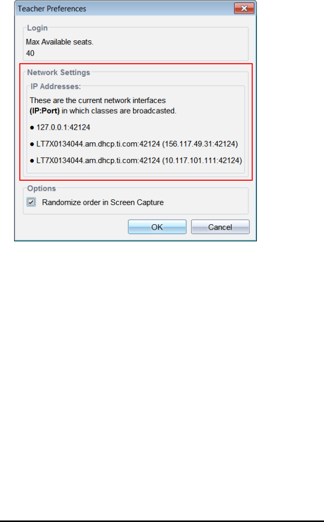
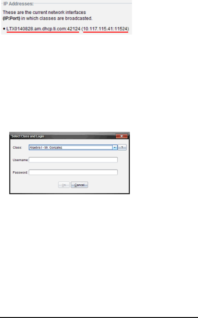
2. View the IP Addresses in the Network Settings area. If the host name and IP
address are present, you are connected and able to broadcast.
Note: If the IP address is missing, contact your Network Administrator.
Helping Students Log In
Students using TI-Nspire™ CX Student Software or TI-Nspire™ CX CAS Student Software
can log in to active classes if they have a user name and password.
Note: For information about how to create a class, start a class, build a class roster,
and create a user name and password for each student, see Using the Class
Workspace.
There are two ways for students to log in:
• Using the class name, which is the preferred method.
• Using the host name or IP address. Use this method when:
- Broadcasting multiple addresses (such as wired and wireless) and one address
is preferred. If your IT administrator has a preferred address, it will be
provided. Otherwise, the host name or any other available IP address can be
used.
- The class name does not appear in the Select Class and Login dialogue box.
This occurs when there is a timing issue between the network sending the
class name and software receiving it.
Getting Started with TI-Nspire™ Navigator NC Teacher Software 7
8 Getting Started with TI-Nspire™ Navigator NC Teacher Software
- If there are several classes running at the same time that have identical
names, such as "Algebra 1." The student will not know which class to select.
Best practice is to append a unique identifier such as the course ID or the
teacher name to the class name.
Providing Students with a Host Name or IP Address
Complete the following steps to locate host name or IP address.
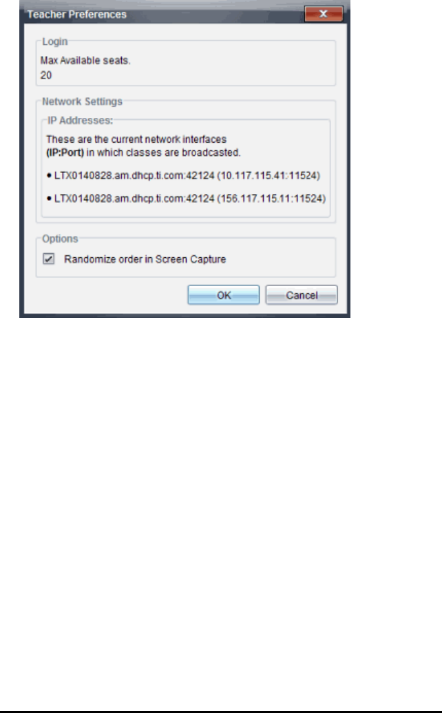
1. In the Class Workspace, click File > Settings > Teacher Preferences.
The Teacher Preferences dialogue box opens.
The host name and IP address are on the same line. You may be broadcasting several
addresses. If your network administrator has not specified a preference, use any
address.
2. Provide students either the host name or the IP address, but not both.
Host Name IP Address
3. Click OK.
The Teacher Preferences dialogue box closes.
Logging in Using Class Name
Ask students to complete the following steps to log in using a class name. Students
can log in after you start the class.
1. Click Tools > Login to a TI-Nspire Navigator Session.
The Select Class and Login dialogue box opens.
2. Click ¤to open the Class drop-down list, and then select a class.
3. Type your user name and password.
Note: User names and passwords are defined when a teacher creates the class
roster. Teachers can either provide a password or allow students to create their
own.
4. Click OK.
The "You are logged into class" confirmation message is displayed.
5. Click OK to close the dialogue box.
Getting Started with TI-Nspire™ Navigator NC Teacher Software 9
10 Getting Started with TI-Nspire™ Navigator NC Teacher Software
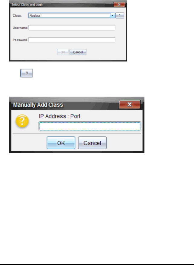
Logging In Using a Host Name or IP Address
Ask students to complete the following steps to log in using a host name or IP address.
1. Click Tools > Login to a TI-Nspire Navigator Session.
The Select Class and Login dialogue box opens.
2. Click , which is located at the end of the Class field.
The Manually Add Class dialogue box opens.
3. Type either the host name or IP address provided by the teacher.
• Example host name: LTXMyschool.network.edu:12345
• Example IP address: 10.111.222.333.12345
4. Click OK.
The Manually Add Class dialogue box closes and the Select Class and Login
dialogue box is active again.
5. Click ¤to open the Class drop-down list, and then select the class. The host name
or IP address is followed by the class name.
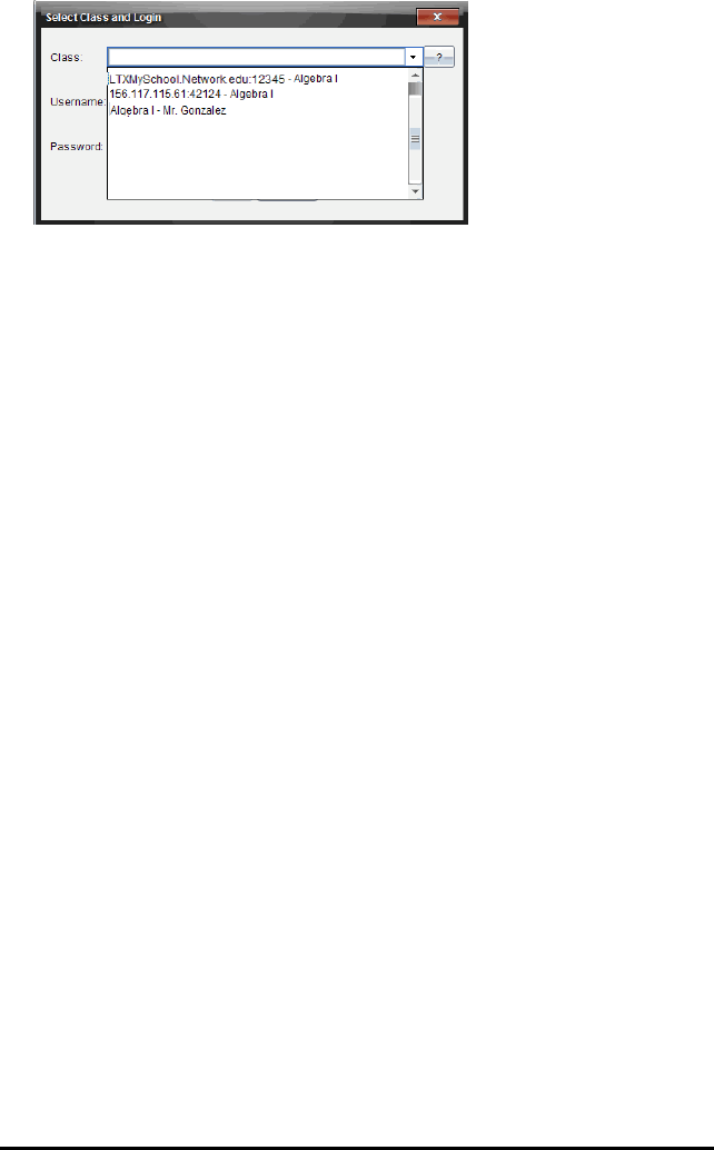
6. Type your user name and password.
7. Click OK.
The "You are logged into class" confirmation message is displayed.
8. Click OK to close the dialogue box.
Teachers will see the status bar increase as each student is logged in.
Managing Available Seats
If the maximum number of seats in a class has been exceeded, students receive the
error message:
"Cannot login to the selected class. The number of students allowed to login to this
class has been met. Contact your teacher for information."
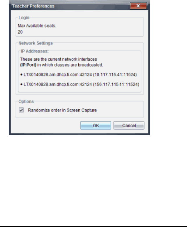
Finding Available Seats
To view the maximum number of seats:
1. In the Class Workspace, click File > Settings > Teacher Preferences.
The Teacher Preferences dialogue box opens.
Getting Started with TI-Nspire™ Navigator NC Teacher Software 11
12 Getting Started with TI-Nspire™ Navigator NC Teacher Software
If you have more students than seats available, students trying to log in will have to
wait until other students log out and seats become available.
Contact your school administrator to acquire more seat licenses. If you already have a
license for additional seats, you can update your license.
Updating a License for More Seats
When updating the license, the class session must be closed. For information about
starting and ending class sessions, see Using the Class Workspace.
Complete the following steps to activate your license:
1. Ensure the class session is closed.
2. Click Help > Update License.
The Texas Instruments Activation Wizard opens.
3. Select Activate your License.
4. Click Next.
5. Follow the screen prompts to activate your license.

Once you have activated the license, you will see an updated number of seats, which
are available when you restart the class.
Getting Started with TI-Nspire™ Navigator NC Teacher Software 13

Tracking and Reporting System Use
Schools participating in research-based programmes or schools receiving money from
funding initiatives must track student use of the TI-Nspire™ Navigator™ systems and
provide reports for auditing purposes.
To automatically track student usage of the TI-Nspire™ Navigator™ systems, a folder
named "SessionLogs" is created within the appropriate TI-Nspire™ Navigator™
software folder on the teacher's computer when the software is installed. The
software generates the files needed for tracking activity types, attendance, class
session information and activities that take place during a class session. The files are
dependent on each other and must be kept together in the SessionLogs folder so that
usage information is tracked and reported accurately.
The system automatically captures system usage data and appends the information for
each new class session in the appropriate file. If the system does not find a
SessionLogs folder, data is not tracked.
Managing Session Logs
The system automatically generates the following comma-separated variable (csv)
files and stores them in the SessionLogs folder. Each time you start the TI-Nspire™
software, logs are appended to the previous day’s log to keep a complete record.
•Activities.csv file. Activities that take place during class sessions are recorded in
this file.
•ActivityTypes.csv file. This file is the lookup table that the system references when
generating a usage report.
•Attendance.csv file. Information for each student who logs into a session is
recorded in this file.
•ClassSession.csv file. Information for all class sessions is recorded in this file.
Using the Activities File
The system records information about the activities that took place during the class
session in this file. Information includes:
•ClassSessionID. Class ID number unique to the funding programme.
•ClassName. Name of the class as defined in the software.
•ActivityTypeID. Type of activity that took place during the class. The ID correponds
to the activity types defined in the Activity Type file.
•ActivityDetail. Additional data about the activity type if available.
•ActivityStart. Time the activity started.
•ActivityEnd. Time the activity ended.
•NumStudent. Number of students who participated in this activity.
Tracking and Reporting System Use 14
15 Tracking and Reporting System Use
Using the ActivityTypes File
The ActivityTypes file is a look-up table that includes codes for identifying activity types
and a short description of each activity.
Activity ID Description
SC Screen Capture
CF Collect File
DF Delete File
SF Send File
RD Redistribute
SP Save to Portfolio
CM Collect Missing
SM Send Missing
US Umprompted Send
LP Live Presenter
QP-MC Quick Poll - Multiple Choice
QP-OR Quick Poll - Open Response
QP-EQ Quick Poll - Equations
QP-CE Quick Poll - Chemical Expression
QP-EX Quick Poll - Expressions
QP-IL Quick Poll - Image with labels
QP-IP Quick Poll - Image with point(s)
QP-CP Quick Poll - Coordinate Points
QP-LS Quick Poll - Lists & Spreadsheet
Using the Attendance File
The system records information for each student who logged into a session in the
Attendance file. Information includes:
•Class ID. The Class ID number unique to the funding programme.

•Class Name. Name of the class as defined in the software.
•Last Name. Last name of the student.
•First Name. First name of the student.
•Date and Time. Date and time when student logged in. Used to identify students
who logged in on time versus late.
•Student ID. The ID of the student.
Using the Class Session File
The system records information for each class session by Class ID. Information
includes:
•ClassSessionID. The Class ID number unique to the funding programme.
•ClassName. Name of the class as defined in the software.
•Start. Time the class started as recorded when the teacher clicks Begin Class.
•End. Time the class ended as recorded when the teacher clicks End Class.
•NumStudent. Number of students who logged in during the class session.
•ClassSectionName. Name of the class section.
•QuickPollTotalTime. Amount of time student spend on Quick Polls.
Managing Log Files
Session log files are managed automatically based upon their file size each time the
TI-Nspire™ is turned off. If the size of any one of the files is greater than 1 MB during
shutdown, a backup of each file is created in the SessionLogs folder with the following
names:
• Activities-bak.csv
• ActivityTypes-bak.csv
• Attendance-bak.csv
• ClassSession-bak.csv
Note: If a backup file already exists, it will be overwritten with a newer version.
The next time the TI-Nspire™ is turned on, four new, empty log files will be created.
Packaging and Sending Session Logs
The district administrator must report usage to the funding source for auditing
purposes at regular intervals. When files are requested, teachers can easily package
the session files into a zip file and send the file to the administrator. The zip file
preserves the format and dependencies of the activity files, and includes a default file
name that identifies the zip file for the administrator.
Complete the following steps to package the files in the SessionLogs folder into a zip
file and send the file to the administrator.
1. From the Content Workspace, click File > Package Session Logs.
Tracking and Reporting System Use 16
17 Tracking and Reporting System Use
Note: This menu item is only available if the SessionLogs folder was created.
The previous session log content is saved. Subsequent session data will append to
the existing files in the same folder as the previous sessions.
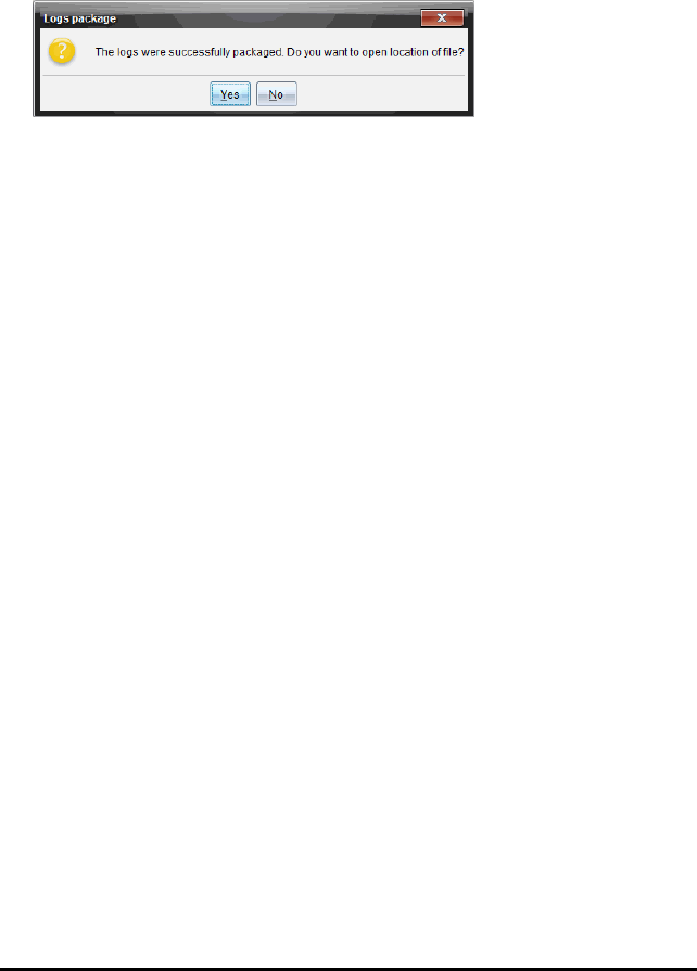
The software packages the files into a zip file and assigns a default name (TI_PKG_
SessionLogs_MMDDYYYY). The Logs package dialogue box opens.
2. Click Yes to go to the location where the zip file was saved.
Windows® Explorer (or Finder) opens. The zip file is saved in the same location as
the SessionLogs folder. For example, if you have TI-Nspire™ Navigator™ NC
Teacher Software, the SessionLogs folder is stored in the following location:
PC:
...\My Documents\My TI-Nspire™ Navigator™ NC Teacher Software\
Mac®:
.../Documents/My TI-Nspire™ Navigator™ NC Teacher Software/
3. Email the zip file to the administrator.
Data is appended to the existing file each time you start a new session. If you no
longer need the information after the files are sent to the administrator, remove
them from the SessionLogs folder and keep the zip file. The system will generate
new files the next time you start a new session.
Using the Content Workspace
The Content Workspace provides access and navigation to folders and files stored on
your computer, network, and external drives, allowing you to open, copy, and transfer
files to students.
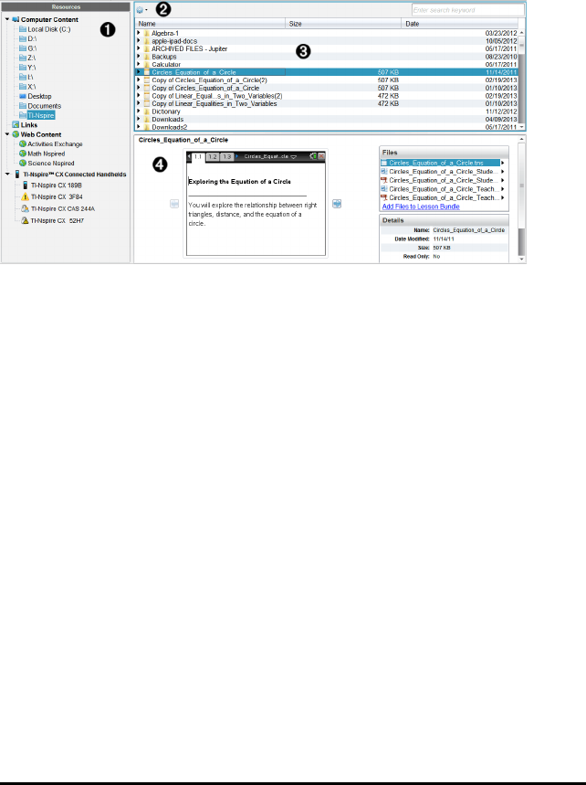
Exploring the Content Workspace
ÀResources pane. Select content here. You can select folders and shortcuts on
your computer, network drives, external drives, or web content. If you are
using software that supports TI-Nspire™ handhelds, the Connected Handhelds
heading is visible when handhelds are connected.
Note: You can add new links to your favourite Web sites in the Links section.
You can access these new links in the Content pane. New links may not be
added to the Web content section.
ÁNavigation bar. Navigate to any location on your computer by clicking an item
in the breadcrumb trail. When you select a resource, the options shown are
specific to that resource.
ÂContent pane. By default, the folders on your desktop are displayed. Use this
space to locate and view files on your computer. You can locate and access
files on a connected handheld if using software that supports handhelds. Use
the top half of the space as you would a file manager. The Content pane is able
to display the contents of only one selected item at a time. Avoid selecting
more than one item at a time.
ÃPreview pane. Shows details about the selected file or folder.
Exploring the Resources Pane
Use the Resources pane to locate documents on a computer, access web content, and
communicate with connected handhelds if using TI-Nspire™ software that supports
connected handhelds.
Using the Content Workspace 18
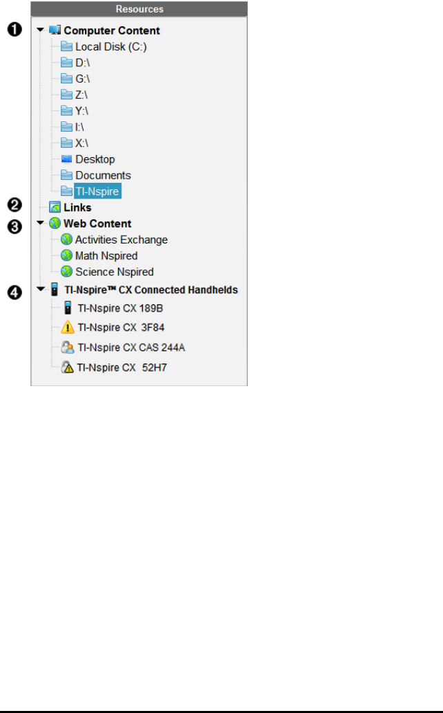
19 Using the Content Workspace
ÀComputer Content. Enables navigation to all files on a computer, network
drives and external drives. Computer Content expands and collapses to provide
access to the following default shortcuts:
• Local Disk
• External drives
• Network drives
• Desktop
• Documents or My Documents
When you select an item in Computer Content, the file structure appears in
the Content pane. When you select a folder or supported file, the detail is
displayed in the Preview pane.
ÁLinks. By default, links to Texas Instruments sites are listed. When you click
Links, it shows a list of links in the Content pane. Then when you click a link
there, it launches in your web browser. You can add your own links to this
section. Links from the latest version of the TI-Nspire™ software are added
when you upgrade.
Users located in the United States can search US standards or textbooks by
selecting the search option from Links.
ÂWeb Content. Lists links to Texas Instruments sites that contain TI-Nspire™-
supported activities. Web Content is available if you are connected to the
Internet. You can save material you find on these sites to your computer and
share items through the Computer Content pane or Connected Handhelds if
using software that supports handhelds. You cannot save links to websites in
the Web Content section.
Note: The web content that is available varies depending on region. If there
is no online content, this section is not visible in the Resources pane.
When you select an item in Web Content, the list of activities is displayed in
the Content pane and a preview of the selected activity is displayed in the
Preview pane.
ÃConnected Handhelds. Lists information about the handhelds connected to
your computer. To see folders and files on a specific handheld, click its name.
Each handheld name is shown with a status icon:
• A logged-in symbol ( ) indicates that a student is logged in to the
handheld and the handheld is not in Press-to-Test mode.
• A padlock symbol ( ) Shows that the handheld has been placed in
Press-to-Test mode by the Prepare Handhelds command. If the padlock
is combined with a warning symbol ( ), the handheld is in
Press-to-Test mode but was not placed in that mode by the Prepare
Handhelds command.
• A single warning symbol ( ) indicates that the version of the handheld
OS does not match the teacher's software version.
To open a tooltip containing status details, hover the mouse pointer over the
status icon.
Note:Connected Handhelds are not shown if there are no handhelds
connected or if you are using TI-Nspire™ Navigator™ NC Teacher Software.
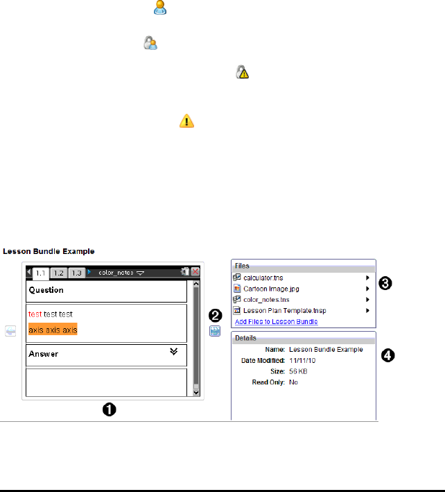
Using the Preview Pane
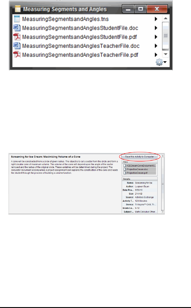
ÀA thumbnail preview of the selected folder, .tns file, file-type icon, or lesson
Using the Content Workspace 20
21 Using the Content Workspace
bundle. Double-click a file-type icon to open the file in its associated
application.
Note: If a lesson bundle is empty and this space is blank, you have the
option to add files.
ÁIf a TI-Nspire™ document has multiple pages, use the forward arrow to
preview the next page. The backward arrow becomes active so you can move
backward through the pages. If working with a lesson bundle, you can choose
to preview a TI-Nspire™ document within the bundle by this method.
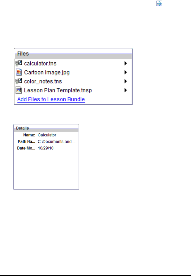
ÂIf a lesson bundle is selected, the Files dialogue box opens above the Details
window listing the files in the lesson bundle. Double-click any file in a lesson
bundle to open the file in its associated application.
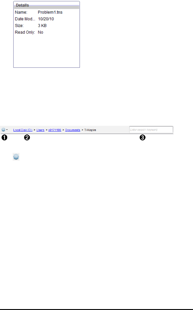
ÃIf a folder is selected, the Details window shows the name of the folder, the
path where the folder is located, and the date modified.
For document files and lesson bundle files, the Details window shows the
name, the date the file was modified, the file size, and whether or not the file
is read only.
Accessing Computer Content
Computer Content provides access to all information stored on your computer,
network, and external drives.
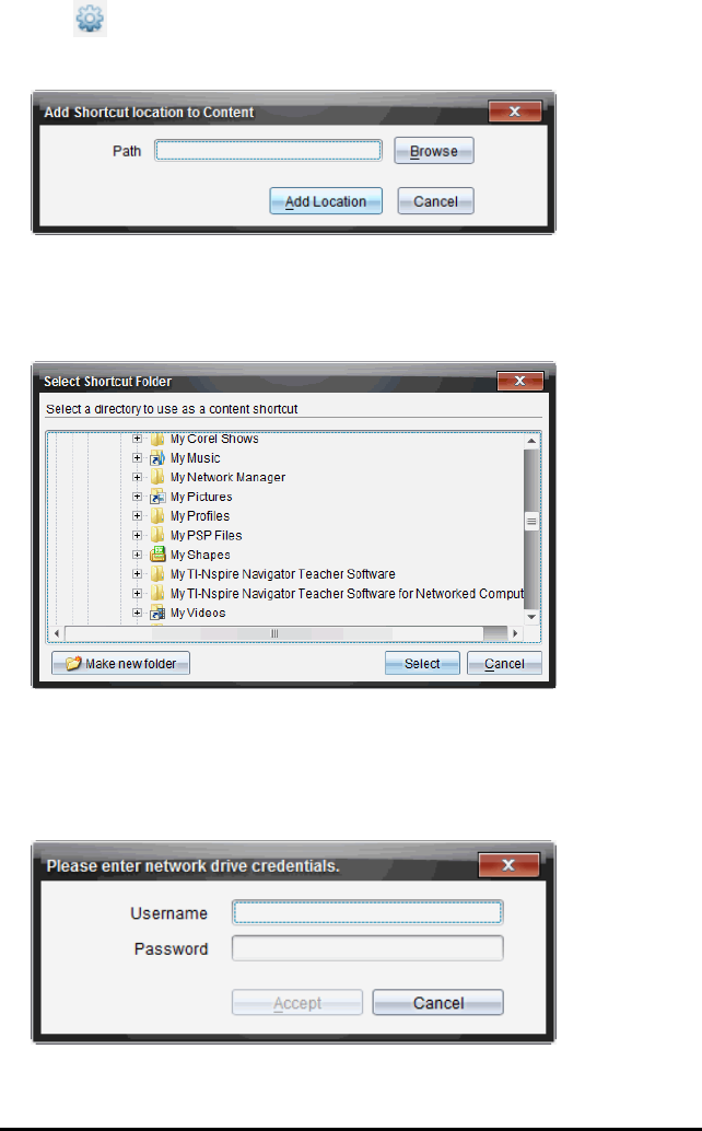
Using the Navigation bar
The Content pane Navigation bar provides tools needed to locate folders and files.
ÀOptions. Click ¤to open the menu to access options for working with files
and folders.
ÁCurrent path: Contains a clickable breadcrumb trail of the current location.
Click a breadcrumb to navigate to any section in the path.
ÂSearch. Enter a search keyword and press Enter to find all files within the
selected folder containing that word.
Filtering Computer Content
Use this filtering option for easy access and selection of your teaching content. You can
select show TI-Nspire™ content only or to show all content.
1. Select a folder in Computer Content in the Resources pane.
2. From the Menu bar, select View > Filter by.
3. Choose one of the following options.
•Show TI-Nspire™ content only
•Show all content
Mapping a Network Drive
Complete the following steps to map a network drive.
1. Select Computer Content from the Resources list.
Using the Content Workspace 22
23 Using the Content Workspace
2. Click , and then click Create Shortcut.
The Add Shortcut location to Content dialogue box opens.
3. Click Browse.
Note: You can also type the full path name for the network drive.
The Select Shortcut Folder dialogue box opens.
4. Navigate to the network drive.
5. Click Select.
6. Click Add Location.
The Please enter network drive credentials dialogue box opens.
7. Type the username and password given to you by your system administrator.
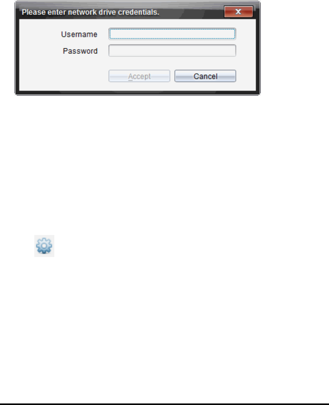
8. Click Accept.
The network drive is added to the list of folders under the Computer Content
heading in the Resources pane.
Accessing a Secured Network Drive
If access to a network drive requires authentication, complete the following steps to
access secured network.
1. Click the drive you want to access in the Resources pane.
The Please enter network drive credentials dialogue box opens.
2. Type your username and password.
3. Click Accept.
Using Shortcuts
Use this option to add folders or lesson bundles containing frequently used files to the
Computer Content list.
Adding a Shortcut
To add a shortcut to a folder containing files you access often:
1. Navigate to the folder where the files are located.
2. Click , and then click Create Shortcut.
The folder is added to the list of folders under Computer Content in the Resources
pane.
Deleting a Shortcut
To delete a shortcut:
1. From the Computer Content list, select the folder to be deleted.
2. Right-click the selected folder, and then click Remove Shortcut.
The folder is removed from the list of shortcuts.
Note: You cannot remove default shortcuts.
Using the Content Workspace 24
25 Using the Content Workspace
Working with Links
By default, the Links list contains a list of links to Texas Instruments websites. Click a
link to launch your web browser and access the website.
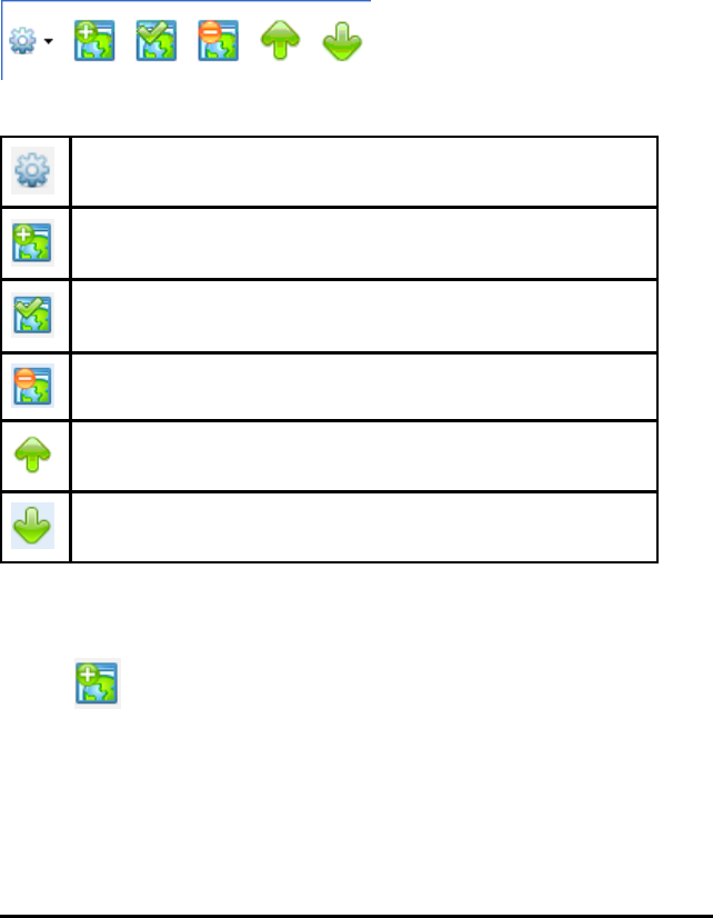
Using the Links Toolbar
When you select Links in the Resources pane, the tools on the navigation bar are
specific to working with links. Use these tools to add, edit, or delete links from the list.
You can also move a link up or down in the list.
Options. Click ¤to open the menu to access options for working with
links.
Click this icon to add a link to the list.
Select an existing link, and then click this icon to edit the link’s
attributes. You cannot edit a default link.
Click this icon to delete a link. You cannot delete a default link.
Select a link and click this icon to move the link up in the list.
Select a link and click this icon to move the link down in the list.
Adding a Link
Complete the following steps to add a link to the list of Links in the Resource pane.
1. Click .
The Add Link dialogue box opens.
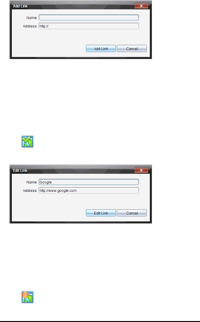
2. Type the name of the link.
3. Type the URL in the Address field.
4. Click Add Link.
The link is added to the bottom of the list of existing links.
Editing an Existing Link
Complete the following steps to edit an existing link.
1. Select the link you want to change.
2. Click .
The Edit Link dialogue box opens.
3. Make needed changes to the name of the link or to the URL.
4. Click Edit Link.
The changes are applied to the link.
Removing a Link
Complete the following steps to delete a link.
1. Select the link you want to delete.
2. Click .
Using the Content Workspace 26

27 Using the Content Workspace
The confirmation dialogue box opens.
3. Click Remove.
The link is removed from the list.
Note: You cannot delete a default link.
Moving Links Up or Down in the List
You can change the order of the links in the list to suit your needs.
▶Click to move a selected link up one place in the list.
▶Click to move a selected link down one place in the link.
▶Click , and then select Move to Top of List to relocate a selected link to the top
of the list.
▶Click , and then select Move to Bottom of List to relocate a selected link to the
bottom of the list.
Using Web Content
Web Content provides links to online materials on Texas Instruments websites. You can
save material found on these websites to your computer and share them using the
Computer Content pane and Connected Handhelds.
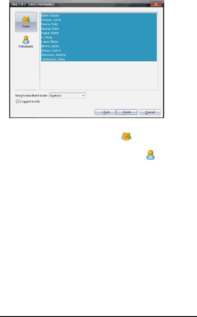
Information provided for each activity includes the name of the activity, the author, the
date the activity was posted, the size of the file, and the source.
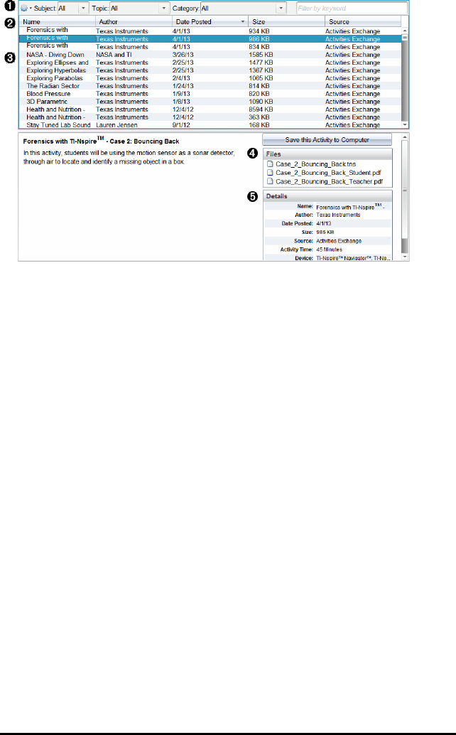
ÀNavigation toolbar.
ÁColumn headings.
ÂList of available activities.
ÃList of the files contained in the activity.
ÄDetails about the selected activity.
Note: An Internet connection is required to access Texas Instruments websites.
Sorting the List of Activities
Use the column headings to sort the information in the list of activities. By default the
list is displayed in alphabetical order by Name.
• Click the Name heading to list activities in reverse alphabetical order. Click the
heading again to return to A to Z order.
• Click the Author heading to list the activities in alphabetical order by author name.
• Click the Date Posted heading to list the activities in order from newest to oldest or
from oldest to newest.
• Click the Size heading to list the activities according to file size.
• Click the Source heading to list the activities in order by source.
• Right-click the column heading row to customize displayed column headings.
Using the Content Workspace 28

29 Using the Content Workspace
Filtering the List of Activities
By default, all available activities are listed in the Content pane. Options on the
Navigation bar enable you to filter the activities by subject, topic, and category. You
can also search for an activity using a keyword search.
To find all activities related to a particular subject:
1. In the Subject field, click ¤to open the drop-down list.
2. Select a subject.
All activities related to the selected subject are listed.
3. To narrow the search, click ¤in the Topic field to view and select a topic related
to the subject selected.
4. Use the Category field to narrow the search even further. Click ¤to select a
category related to the selected subject and topic.
Using Keywords to Search for an Activity
Complete the following steps to search for an activity using a keyword or phrase.
1. Type a keyword or phrase in the Filter by Keyword field.
2. Press Enter.
All activities that contain the keyword or phrase are listed.
Opening an Activity
1. Select the activity you want to open.
2. Click , and then select Open.
The Open Activity dialogue box opens with a list of all documents related to the
selected activity.
You can open a .tns or .tsnp file in the TI-Nspire™ software. Other files such as
Microsoft® Word and Adobe® PDF files open in their respective applications.
3. Select the file and click ¢, and then select Open.
• The .tns file opens in the Documents Workspace.
• The .doc or .pdf file opens in its associated application.
Saving an Activity to Your Computer
Complete the following steps to save an activity to your computer.
1. Select the activity you want to save. The file details are displayed in the bottom
half of the window.
2. Click Save this Activity to Computer in Preview pane, above Files.
Note: You can also right-click on the selected activity and choose Save to Computer.
The Save Selected files dialogue box opens.
3. Navigate to the folder where you want to save the file.
4. Click Save.
The activity is saved to your computer as a lesson bundle.
Using the Content Workspace 30

31 Using the Content Workspace
Copying an Activity
Complete the following steps to copy an activity. Once the activity is copied to the
Clipboard, you can paste the activity into a folder on your computer, and then drag the
activity to your list of shortcuts in the Local Content pane.
1. Click the activity you want to copy to select it.
2. Use one of the following methods to copy the activity to the Clipboard:
• Select the activity and drag it to a folder in the Local Content list.
• Click , and then click Copy.
• Right-click on a file in the Files list, and then click Copy.
• Click (Copy icon), which is located in the toolbar.
The activity is copied to the Clipboard.
3. Open a folder on your computer, and then click Edit > Paste to copy the activity to
the selected folder.
Sending Files to Class
You can send files and folders to your whole class, members of the class currently
logged in or to individual students. Class must be in session for you to send the files.
When you send a file to the whole class, all students currently logged in will receive
the file immediately. Students not logged in will receive the file when they log in.
Notes:
• Only TI-Nspire™ (.tns) and PublishView™ (.tnsp) file types open in the TI-Nspire™
software.
• Other file types (if supported) such as images, word processing or spreadsheet
files, open in the application the operating system has associated with the file
type.
Sending Files from the Content or Documents Workspaces
1. Select the file you want to send to the class.
• From the Content Workspace, click the file in the Content pane.
• From the Documents Workspace, click the file in the Content Explorer.
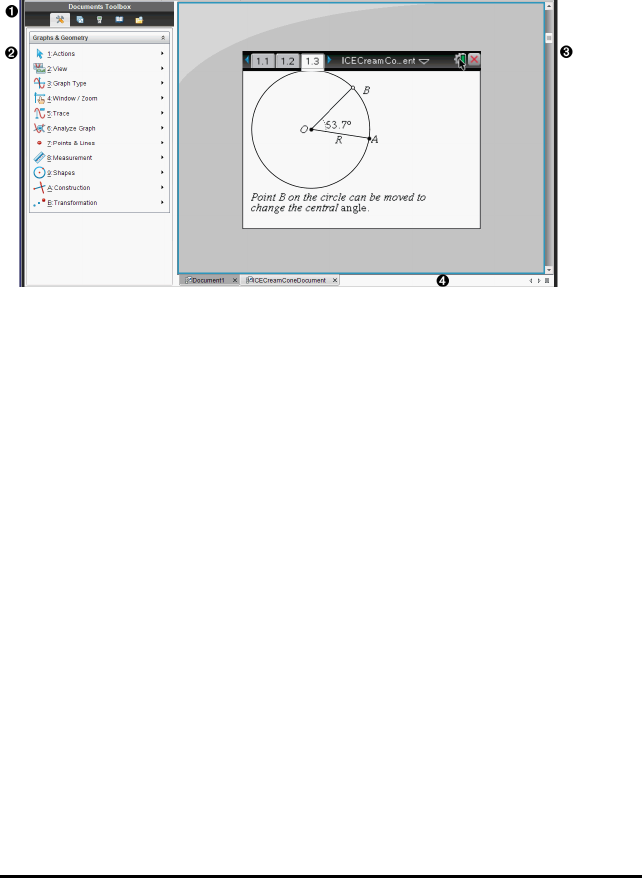
2. Click Send to Class , or click File>Send to> Send to Class.
The Select individual(s) dialogue box opens.
3. Select the student(s) to whom you want to send the file:
• To send the file to the whole class, click Class . To send the file only to
class members who are currently logged in, select the Logged in only check box.
• To send the file to an individual student, click Individuals and then click the
student.
Note: If you had any students selected in the classroom area, the software
already has them selected.
• Use the Send to handheld folder drop-down list to choose from the current
class folder, the top level folder on the handheld or the last 10 folders that files
were sent to. (Available only on TI-Nspire™ software that supports handhelds.)
4. Click Finish.
The file transfer appears in the Class Record in the Class Workspace.
Using the Content Workspace 32

33
Using the Documents Workspace
Use this workspace to create, modify, and view TI-Nspire™ and PublishView™
documents, and to demonstrate mathematical concepts.
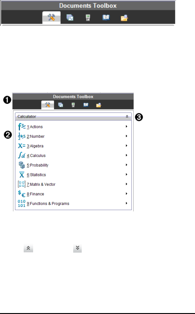
Exploring the Documents Workspace
ÀDocuments Toolbox. Contains tools such as the Document Tools menu, Page
Sorter, TI-SmartView™ emulator, Utilities, and Content Explorer. Click each
icon to access the available tools. When you are working in a TI-Nspire™
document, the tools available are specific to that document. When you are
working in a PublishView™ document, the tools are specific to that document
type.
ÁToolbox pane. Options for the selected tool are displayed in this area. For
example, click the Document Tools icon to access tools needed to work with
the active application.
Note: In the TI-Nspire™ CX Teacher Software, the tool for configuring questions
opens in this space when you insert a question. For more information, see
Using Question in the TI-Nspire™ Teacher Software.
ÂWork area. Shows the current document and enables you to perform
calculations, add applications, and add pages and problems. Only one document
at a time is active (selected). Multiple documents appear as tabs.
ÃDocument information. Shows the names of all open documents. When there
too many open documents to list, click the forward and backward arrows to
scroll through the open documents.
Using the Documents Toolbox
The Documents Toolbox, located on the left side of the workspace, contains tools
needed for working with both TI-Nspire™ documents and PublishView™ documents.
When you click a toolbox icon, the associated tools appear in the Toolbox pane.
Using the Documents Workspace 34
35 Using the Documents Workspace
Exploring Document Tools
In the following example, the Document Tools menu is open showing the options for the
Calculator application. In TI-Nspire™ documents, the Document Tools menu contains tools
available for working with an application. The tools are specific to the active application.
In PublishView™ documents, the Document Tools menu contains tools needed to insert
TI-Nspire™ applications and TI-Nspire™ documents, as well as multimedia objects such
as text boxes, images, and links to websites and files. For more information, see
Working with PublishView™ Documents.
ÀThe Documents Toolbox menu.
ÁTools available for the Calculator application. Click ¢to open the submenu for
each option.
ÂClick to close and click to open Document Tools.
Exploring the Page Sorter
The following example shows the Documents Toolbox with the Page Sorter open. Use
the Page Sorter to:
• See the number of problems in your document and where you are.
• Move from one page to another by clicking on the page you want.
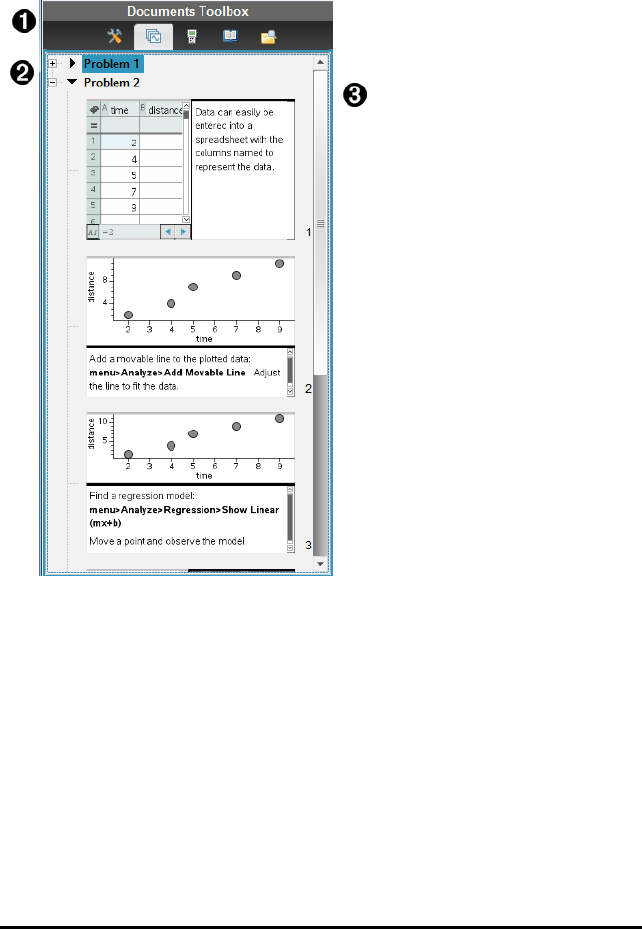
• Add, cut, copy, and paste pages and problems within the same document or
between documents.
Note: When you are working in a PublishView™ document, the Page Sorter is not
available in the Documents Toolbox.
ÀThe Documents Toolbox menu.
ÁClick the minus sign to collapse the view. Click the + sign to open the view and
show pages in the document.
ÂScroll bar. The scroll bar is only active when there are too many pages to show
in the pane.
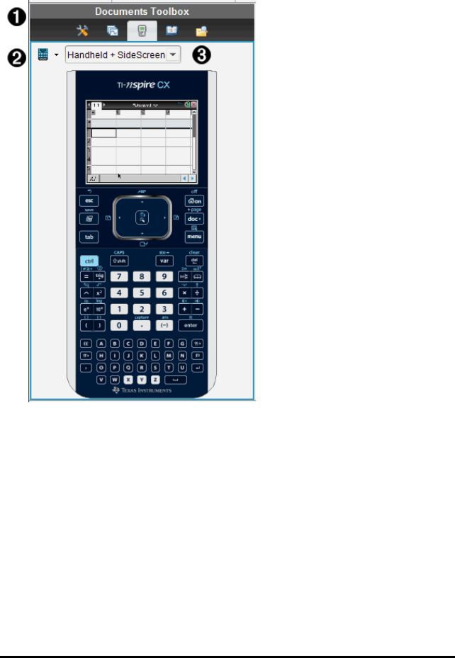
Exploring the TI-SmartView™ Feature
The TI-SmartView™ feature emulates how a handheld works. In the teacher software, the
emulated handheld facilitates classroom presentations. In the student software, the
emulated keypad gives students the ability to drive the software as if using a handheld.
Note: Content is displayed on the TI-SmartView™ small screen only when the document is
in Handheld view.
Using the Documents Workspace 36
37 Using the Documents Workspace
When working in a PublishView™ document, TI-SmartView™ emulator is not available.
Note: The following illustration shows the TI-SmartView™ panel in the teacher
software. In the Student Software, only the keypad is shown. For more information,
see Using the TI-SmartView™ Emulator.
ÀThe Documents Toolbox menu.
ÁHandheld Selector. Click ¤to select which handheld to show in the pane:
• TI-Nspire™ CX or TI-Nspire™ CX CAS
Then, select how to show the handheld:
• Normal
• High contrast
• Outline
ÂView selector. In the teacher software, click ¤to select the handheld view:
• Handheld only
• Keypad plus side screen
• Handheld plus side screen
Note: You can also change these options in the TI-SmartView™ Options
window. Click File> Settings > TI-Smartview™ Options to open the window.
Note: The view selector is not available in the student software.
When the Handheld Only display is active, select Always in Front to keep the
display in front of all other open applications. (Teacher software only.)
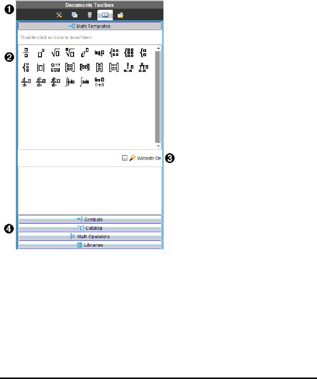
Exploring Utilities
Utilities provides access to the math templates and operators, special symbols,
catalogue items, and libraries that you need when working with documents. In the
following example, the Math templates tab is open.
ÀThe Documents Toolbox menu.
ÁMath Templates are open. Double-click a template to add it to a document.
Click the Math Template tab to close the template view.
To open the Symbols, Catalogue, Math Operators, and Libraries, click the tab.
ÂWizards On check box. Select this option to use a wizard to enter function
arguments.
ÃTabs for opening views where you can select and add symbols, catalogue items,
math operators, and library items to a document. Click the tab to open the
view.
Using the Documents Workspace 38
39 Using the Documents Workspace
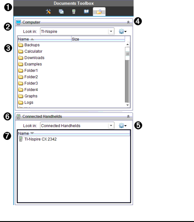
Exploring Content Explorer
Use Content Explorer to:
• See a list of files on your computer.
• Create and manage lesson bundles.
• If using software that supports connected handhelds, you can:
- See a list of files on any connected handheld.
- Update the OS on connected handhelds.
- Transfer files between a computer and connected handhelds.
Note: If you are using TI-Nspire™ software that does not support connected handhelds,
the Connected Handheld heading is not shown in the Content Explorer pane.

ÀThe Documents Toolbox menu.
ÁShows files on your computer and the name of the folder where the files are
located. Click ¤to navigate to another folder on the computer.
ÂThe list of folders and files within the folder named in the Look In: field. Right-click
on a highlighted file or folder to open the context menu listing available actions for
that file or folder.
ÃClick to close the list of files. Click to open the list of files.
ÄOptions menu. Click ¤to open the menu of actions you can perform on a
selected file:
• Open an existing file or folder.
• Move (navigate) up one level in the folder hierarchy.
• Create a new folder.
• Create a new lesson bundle.
• Rename a file or folder.
• Copy selected file or folder.
• Paste file or folder copied to Clipboard.
• Delete selected file or folder.
• Select all files in a folder.
• Package lesson bundles.
• Refresh the view.
• Install OS.
ÅConnected handhelds. Lists the connected handhelds. Multiple handhelds are listed
if more than one handheld is connected to the computer or when using the
TI-Nspire™ Docking Stations.
ÆThe name of the connected handheld. To show the folders and files on a handheld,
double-click the name.
Click ¤to navigate to another folder on the handheld.
Using the Work Area
The space on the right side of the workspace provides an area for creating and working
with TI-Nspire™ and PublishView™ documents. This work area provides a view of the
document so that you can add pages, add applications, and perform all work. Only one
document at a time is active.
When you create a document, you specify its page size as Handheld or Computer. This
is how the page is displayed in the work area.
Using the Documents Workspace 40
41 Using the Documents Workspace
•Handheld page size is optimized for the smaller screen of a handheld. This page
size can be viewed on handhelds, computer screens, and tablets. The content is
scaled when viewed on a larger screen.
•Computer page size takes advantage of the larger space of a computer screen.
These documents can show details with less scrolling required. The content is not
scaled when viewed on a handheld.
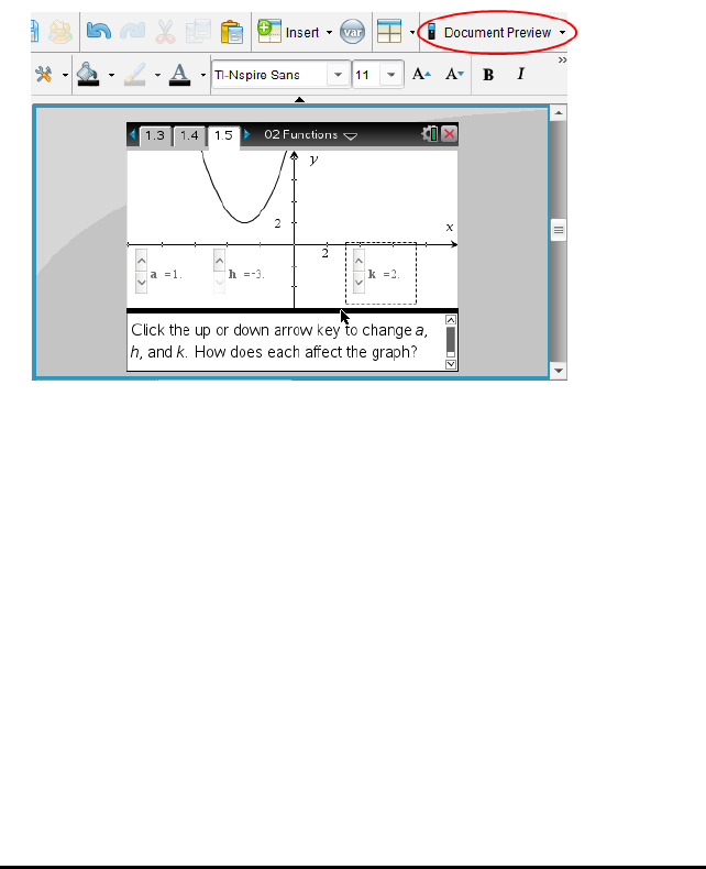
You can change the page preview to see how the document will look in a different
page size.
▶To change the page preview, click Document Preview on the toolbar, and then click
Handheld or Computer.
For more information on page size and document preview, see Working with
TI-Nspire™ Documents.
Changing Document Settings
Document settings control how all numbers, including elements or matrices and lists,
are displayed in TI-Nspire™ and PublishView™ documents. You can change the default
settings at anytime and you can specify settings for a specific document.
Changing Document Settings
1. Create a new document or open an existing document.
2. From the TI-Nspire™ File menu, select Settings>DocumentSettings.
The Document Settings dialogue box opens.
When you open Document Settings the first time, the default settings are
displayed.

3. Press Tab or use your mouse to move through the list of settings. Click ¤to open
the drop-down list to view the available values for each setting.
Field Value
Display Digits • Float
• Float1 - Float12
• Fix0 - Fix12
Angle • Radian
• Degree
• Gradian
Exponential Format • Normal
• Scientific
• Engineering
Real or Complex Format • Real
• Rectangular
• Polar
Calculation Mode • Auto
• CAS: Exact
• Approximate
Note: Auto mode shows an answer that is not a
whole number as a fraction except when a decimal is
used in the problem. Exact mode (CAS) shows an
answer that is not a whole number as a fraction or in
symbolic form, except when a decimal is used in the
problem.
Vector Format • Rectangular
• Cylindrical
• Spherical
Base • Decimal
• Hex
• Binary
Unit System (CAS) • SI
• Eng/U.S.
4. Click the desired setting.
5. Choose one of the following options:
• To apply the customized settings to ALL documents, click Make Default.
• To apply the settings to the open document only, click OK.
• To restore default settings, click Restore.
• Click Cancel to close the dialogue box without making changes.
Using the Documents Workspace 42
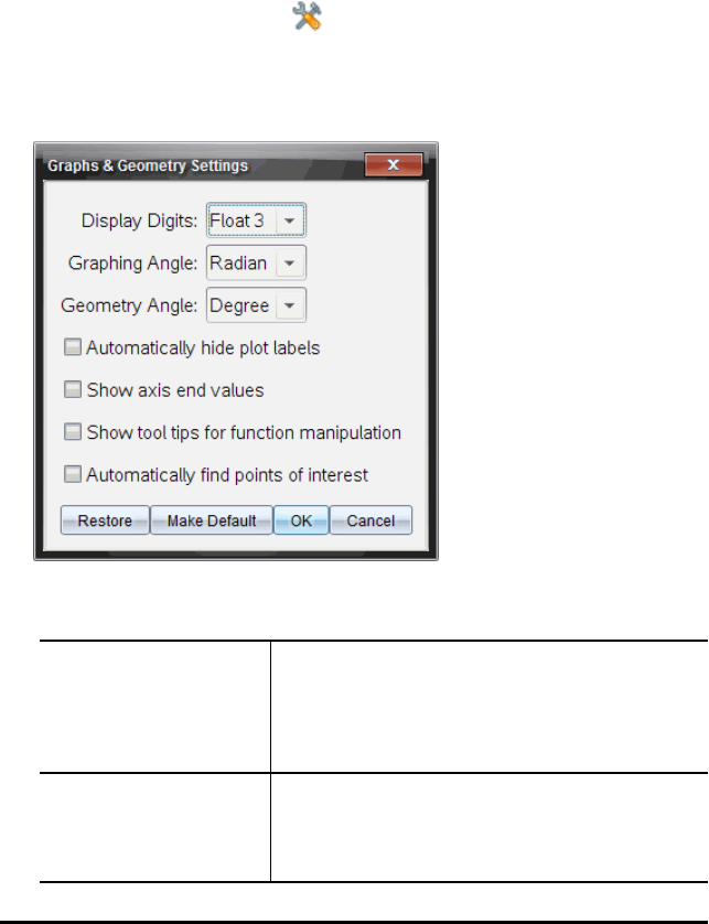
43 Using the Documents Workspace
Changing Graphs & Geometry Settings
Graphs & Geometry settings control how information is displayed in open problems
and in subsequent new problems. When you change the Graphs & Geometry settings,
the selections become the default settings for all work in these applications.
Complete the following steps to customize the application settings for graphs and
geometry.
1. Create a new graphs and geometry document or open an existing document.
2. In the Documents Toolbox, click to open the Graphs & Geometry application
menu.
3. Click Settings > Settings.
The Graphs & Geometry Settings dialogue box opens.
4. Press Tab or use your mouse to move through the list of settings. Click ¢to open
the drop-down list to view the available values for each setting.
Field Values
Display Digits • Auto
• Float
• Float1 - Float12
• Fix0 - Fix12
Graphing Angle • Auto
• Radian
• Degree
• Gradian
Field Values
Geometry Angle • Auto
• Radian
• Degree
• Gradian
5. Select the desired setting.
6. Select a check box to enable an option or clear a check box to disable an option.
Check box Operation when selected
Automatically hide
plot labels
Plot labels are displayed only when selected, grabbed,
or hovered.
Show axis end values A numeric label is displayed at the least and greatest
values visible on an axis
Show tool tips for
function manipulation
Shows helpful information as you manipulate function
graphs
Automatically find a
point of interest
Shows zeros, minima, and maxima for graphed functions
and objects while tracing function graphs.
7. Choose one of the following options:
• To apply the customized settings to ALL graphs and geometry documents, click
Make Default.
• To apply the settings to the open document only, click OK.
• To restore default settings, click Restore.
• Click Cancel to close the dialogue box without making changes.
Using the Documents Workspace 44

45

Working with TI-Nspire™ Documents
All work that you create and save using TI-Nspire™ applications is stored as a
document, which you can share with others using TI-Nspire™ software and with those
using handhelds. There are two types of documents:
• TI-Nspire™ document (.tns file)
• PublishView™ document (.tnsp file)
TI-Nspire™ Documents
A TI-Nspire™ document consists of one or more problems. Each problem can contain
one or more pages. A single page is displayed in the work area. All work occurs in the
applications within pages.
Because the TI-Nspire™ software and handhelds share the same functionality, you can
transfer TI-Nspire™ documents between computers and handhelds. When you create a
document, you select one of two page sizes.
•Handheld. Size: 320 ×217 pixels. This size allows documents to be viewed on all
platforms. The content will be scaled when viewed on a tablet or larger screen.
•Computer. Size: 640 ×434 pixels. The content will not be scaled when viewed on
smaller platforms. Some content may not be visible on a handheld device.
You can convert a document from one page size to the other any time.
PublishView™ Documents
PublishView™ documents can be printed on a standard piece of paper or published to a
website or blog. PublishView™ documents can include formatted text, images and
hyperlinks as well as all TI-Nspire™ applications.
For more information, see Working with PublishView™ Documents.
Creating a New TI-Nspire™ Document
When you open the software, the Documents Workspace opens with a blank document
containing one problem. You can add applications and content to this problem to
create a document.
Note: The Welcome Screen is displayed when you open the software if the "always
show this at startup" option is selected. Click an application icon to add a problem with
an active application to a new document.
To create a new document, complete the following steps:
1. On the TI-Nspire™ File menu,
• Select New TI-Nspire™ Document - Handheld Page Size.
-or-
• Select New TI-Nspire™ Document - Computer Page Size.
Working with TI-Nspire™ Documents 46
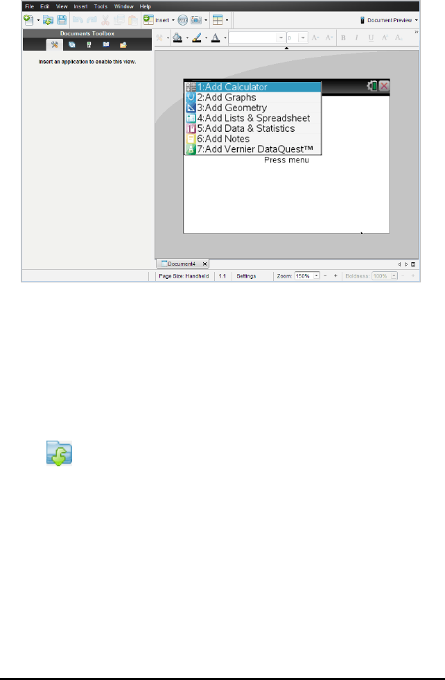
47 Working with TI-Nspire™ Documents
The new document opens in the Documents Workspace, and you are prompted to
select an application.
2. Select an application to add a problem to the document.
The problem is added to the document.
Opening an Existing Document
To open an existing document:
1. Click File > Open Document.
—or—
Click .
The Open dialogue box opens.
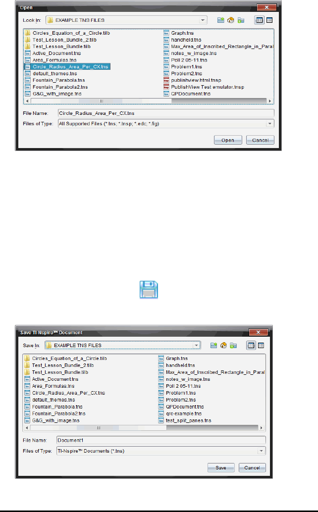
2. Use the file browser to locate the file you want to open and click the file to select
it.
3. Click Open.
The document opens in the work area.
Note: To select from your 10 most recent documents, click File > Recent Documents
and select a document from the drop-down list.
Saving TI-Nspire™ Documents
To save a new document:
1. Click File > Save Document or click .
The Save TI-Nspire™ Document dialogue box opens.
Working with TI-Nspire™ Documents 48
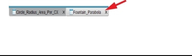
49 Working with TI-Nspire™ Documents
2. Navigate to the folder where you want to save the document or create a folder in
which to store the document.
3. Type a name for the new document.
4. Click Save to save the document.
The document closes and is saved with the extension .tns.
Note: When you save a file, the software looks in the same folder the next time you
open a file.
Saving a Document with a New Name
To save a previously saved document in a new folder and/or with a new name:
1. Click File > Save As.
The Save TI-Nspire™ Document dialogue box opens.
2. Navigate to the folder where you want to save the document or create a folder in
which to store the document.
3. Type a new name for the document.
4. Click Save to save the document with a new name.
Deleting Documents
File deletions on your computer are sent to the Recycle bin and can be retrieved if the
Recycle bin has not been emptied.
Note: File deletions on the handheld are permanent and cannot be undone, so be sure
that you want to delete the file that you select.
1. Select the document you want to delete.
2. Click Edit > Delete or press Delete.
The Warning dialogue box opens.
3. Click Yes to confirm the delete.
The document is deleted.
Closing Documents
▶To close a document, click File > Close or click the Close icon on the document tab
at the bottom of the document.
▶If working in tiled view, click the Close icon in the upper right corner of the
document window.
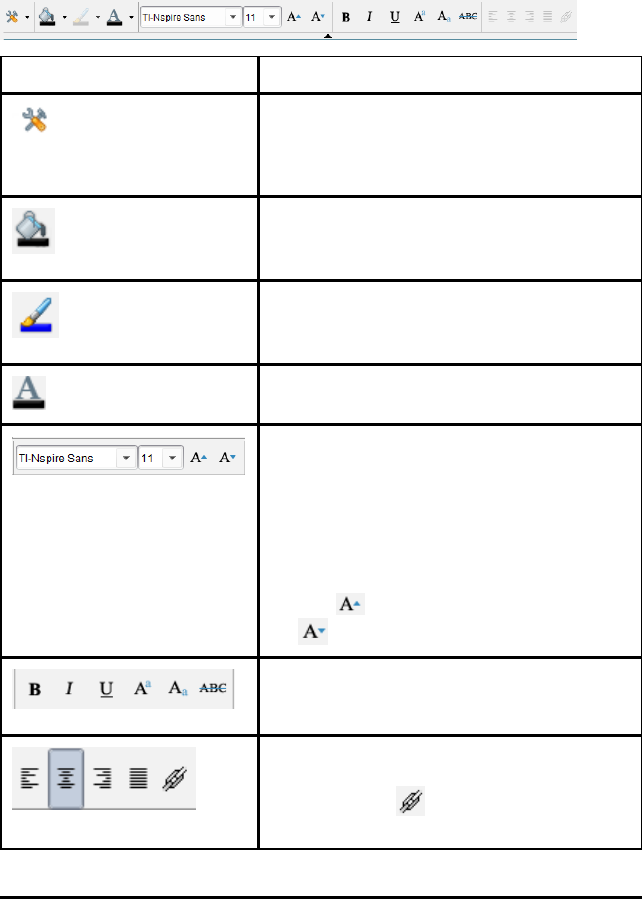
Formatting Text in Documents
Use the text formatting tools to format text in TI-Nspire™ applications that allow text
input, and to format text in PublishView™ documents. By default, the text formatting
toolbar opens in the area above an active document. Options on the toolbar are
enabled or disabled depending on the active application.
Option Function
Click ¤to open the menu for the active
application. This tool enables you to open an
application menu regardless of the option
selected in the Documents Toolbox.
Click ¤to select a background colour for
highlighting text or choose a fill colour for a
selected cell.
Click ¤to select the line colour for an object. For
example, in Graphs&Geometry, you can choose a
colour for a selected shape.
Click ¤to select a colour for selected text.
Use these tools to choose a font and set the size
of the font.
• Click ¤to select a different font from the
drop-down box.
• To select as specific font size, click ¤to
select a size from the drop-down box.
• Click to increase the font size or click
to decrease the font size incrementally.
Click the appropriate tool to apply bold, italics or
underlining; apply superscript or subscript; or
strike out text.
In a PublishView™ document, use these tools to
position text within the header or footer, or in
text box. Clicking opens the Hyperlink
dialogue box.
Working with TI-Nspire™ Documents 50

51 Working with TI-Nspire™ Documents
Option Function
For more information, see Working with
PublishView™ Documents.
Hiding and Showing the Formatting Toolbar
▶When the formatting toolbar is visible, click £(located under the toolbar) to hide
the toolbar.
▶Click ¤to show the toolbar when the formatting toolbar is hidden.
Using Colours in Documents
In the TI-Nspire™ applications that allow formatting, you can use colour in filled areas
of an object, or in lines or text, depending on the application you are using and how you
have selected the item. If the icon or menu item that you want to use is not available
(dimmed) after you have selected an item, colour is not an option for the selected
item.
Colours appear in documents opened on your computer and on the TI-Nspire™ CX
handheld.
Note: For more information about using colour in a TI-Nspire™ application, see the
chapter for that application.
Adding Colour from a List
To add colour to a fill area, line or text, complete the following steps:
1. Select the item.
2. Click Edit > Colour or select where you want to add colour (fill, line or text).
3. Select the colour from the list.
Adding Colour from a Palette
To add colour using the palette, complete the following steps:
1. Select the object.
2. Click the appropriate toolbar icon.
3. Select the colour from the palette.
Setting Page Size and Document Preview
When you create a document, you specify its page size as Handheld or Computer,
depending on how you expect the document to be used. Documents of both page sizes
can be opened on either platform, and you can convert the page size any time.
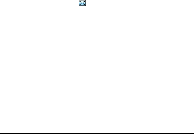
•Handheld. Size: 320 ×217 pixels, fixed. Handheld documents can be viewed on all
platforms. You can magnify (zoom) the content when viewing it on a tablet or
larger screen.
•Computer. Size: 640 ×434 pixels, minimum. Computer documents scale up
automatically to take advantage of higher resolution screens. The minimum size is
640×434, so some content may be clipped on handheld devices.
Note: You can view documents of either page size using Handheld or Computer
preview.
Converting the Current Document's Page Size
▶On the main TI-Nspire™ File menu, select Convert to, and then select the page size.
The software saves the current document and creates a copy that uses the
requested page size.
Viewing the Document in Handheld Preview
1. On the application toolbar, click DocumentPreview, and select Handheld.
The preview changes. This does not change the document's underlying page size.
2. (Optional) Adjust the viewing magnification:
- (Optional) Click the Zoom tool beneath the work area, and select a
magnification value for the preview.
—or—
- Click the Zoom to Fit button to make the handheld preview adjust
automatically to the window size.
Viewing the Document in Computer Preview
1. On the application toolbar, click DocumentPreview, and select Computer.
The preview changes. This does not change the document's underlying page size.
2. (Optional) Click the Boldness tool beneath the work area, and select a value to
increase or decrease the boldness of text and other items.
Setting a Default Preview
By default, when you open a document, it is automatically displayed using the preview
that matches its page size. You can override the rule and specify a preview that you
prefer.
Working with TI-Nspire™ Documents 52
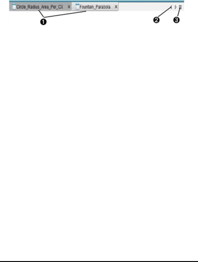
53 Working with TI-Nspire™ Documents
1. On the main TI-Nspire™ File menu, select Settings > Preview Settings.
2. Select the preview that you want documents to use when you open them.
Working with Multiple Documents
When multiple documents are open, document names are listed in tabs at the bottom
of the work area. Only one document is active at a time, and only the active document
is affected by commands from menus or tools.
To switch between documents:
ÀClick the tab to show a document in the work area. This document
becomes the active document. If the Show Documents in Tiles view is
open, these tabs are not shown.
ÁUse the right and left arrows to scroll through the list of documents.
These arrows are active only when there are too many documents to fit
in the window.
ÂClick the Show List icon to list all open documents. This is useful when
you have a large number of documents open and documents names on
the tabs may be truncated.
Working with Multiple Documents in Tiled View
When multiple documents are open, you can view thumbnails of the documents in the
work area. To change the view:
▶Click Window > Show Documents in Tiles.
Open documents are shown as thumbnails in the work area, and the scroll bar
becomes active.
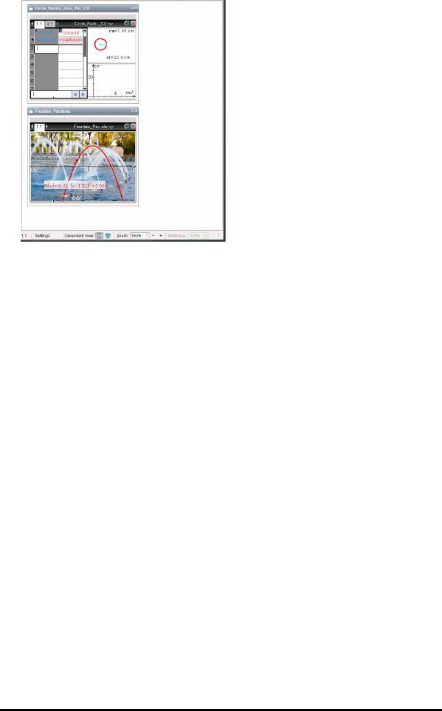
The status bar remains available; however, document names now appear in the
thumbnail view. Click Select Window > Show Documents in Tabs to view one document
at a time in the work area.
Working with Applications
When you first open a new document or add a new problem to a document, you select
an application from a menu.
The following illustration shows how a document containing the Lists& Spreadsheet
application appears in the work area.
Working with TI-Nspire™ Documents 54
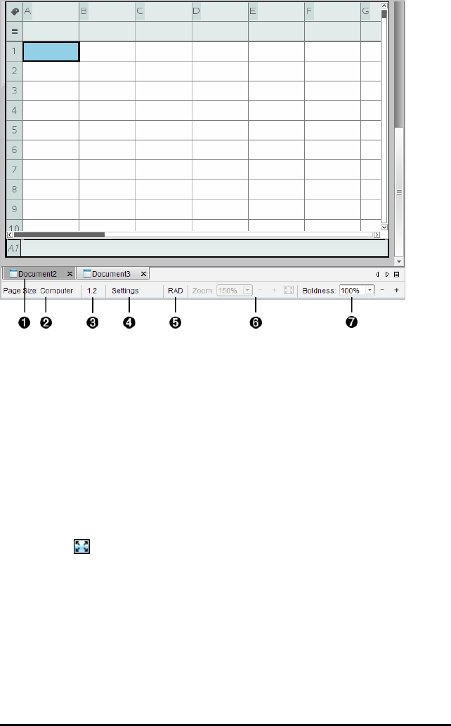
55 Working with TI-Nspire™ Documents
ÀDocument name. Tabs show the names of open documents. Click a name to make it
the active document.
ÁPage Size. Shows the document's page size as Handheld or Computer. You can use
the TI-Nspire™ File menu to convert a document from one page size to the other.
ÂProblem/Page counter. Labels the problem number and page number of the active
page. For example, a label of 1.2 identifies Problem1, Page2.
ÃSettings. Double-click to view or change the Document Settings for the active
document or to change the default Document Settings.
ÄAngle Mode. Shows an abbreviation of the angle mode (Degrees, Radians or Gradians)
in effect. Hover the pointer over the indicator to see the full name.
ÅZoom. Enabled in Handheld preview only (click DocumentPreview on the toolbar
and select Handheld). Click ▼and select a magnification value, or click the zoom-to-
fit button to make the preview adapt automatically to window size.
ÆBoldness. Enabled in Computer preview only (click Document Preview on the
toolbar and select Computer). Click ▼and select a value to increase or decrease the
boldness of text and other items.
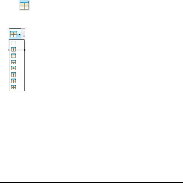
Working with Multiple Applications on a Page
You can add up to four applications to a page. When you have multiple applications on
a page, the menu for the active application is displayed in the Documents Toolbox.
Using multiple applications involves two steps:
• Changing the page layout to accommodate multiple applications.
• Adding the applications.
You can add multiple applications to a page even if an application is already active.
Adding Multiple Applications to a Page
By default, each page contains space to add one application. To add additional
applications to the page, complete the following steps.
1. Click Edit > Page Layout > Select Layout.
—or—
Click .
The page layout menu opens.
There are eight page layout options available. If an option is already selected, it is
dimmed.
2. Highlight the layout you want to add to the problem or page, then click to select it.
The new layout is displayed with the first application active.
Working with TI-Nspire™ Documents 56

57 Working with TI-Nspire™ Documents
3. In Handheld preview, click Press menu to select an application for each new section
in the problem or page. In Computer view, select Click here to add an application.
Swapping Applications
To change the position of applications on a page with multiple applications, “swap“
the positions of two applications.
1. Click Edit > Page Layout > Swap Application.
Note: The last active application you worked on is automatically selected as the
first application to be swapped.
2. Click the second application to swap.
This action performs the swap.
Note: When there are only two work areas, the selected application automatically
swaps position with the other application in the work area.
To cancel a swap, press Esc.
Selecting and Moving Pages
As you add problems and pages to a document, you can take advantage of features for
managing the parts.
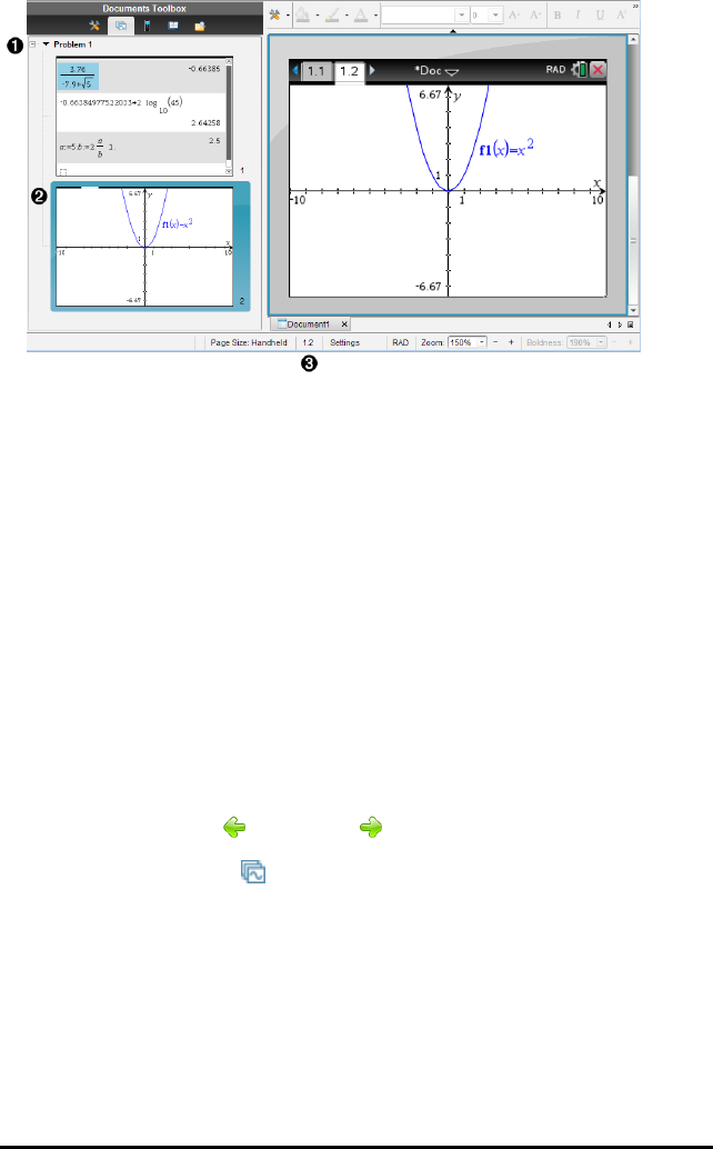
ÀPage Sorter. Lists the problems you have inserted in your document and shows
thumbnail images of the pages in each problem. The Page Sorter lets you rearrange,
copy and move both problems and pages. It also lets you rename problems.
ÁActive page. Indicates the current page by highlighting its thumbnail image.
Thumbnails let you easily scan the pages in a document and select a specific page to
work with.
ÂProblem/Page counter. Displays the problem number and page number of the
currently selected page.
Selecting Pages
Use any of these methods to move from page to page.
▶On the View menu, select PreviousPage or NextPage.
▶On the keyboard, press Ctrl+PgUp or Ctrl+PgDn.
(Mac®: Press Fn+UpArrow or Fn+DownArrow).
▶Click the Previous Page or Next Page button on the main toolbar.
▶Click the Page Sorter tool in the Documents Toolbox, and then click the
thumbnail of the page you want to work with.
Tip: To expand or collapse the list of thumbnails for a problem, double-click the
name of the problem.
Rearranging Pages with the Page Sorter
The Page Sorter makes it easy to reorder pages within a problem.
Working with TI-Nspire™ Documents 58

59 Working with TI-Nspire™ Documents
1. If necessary, click the Page Sorter tool in the Documents Toolbox.
2. In the Page Sorter, drag the thumbnail image of the page to the desired position.
Copying a Page
You can copy a page within the same problem or copy it to a different problem or
document.
1. If necessary, click the Page Sorter tool in the Documents Toolbox.
2. Select the thumbnail of the page to be copied.
3. On the Edit menu, click Copy.
4. Click the location at which you want to insert the copy.
5. On the Edit menu, click Paste.
Moving a Page
You can move a page within the same problem or move it to a different problem or
document.
1. If necessary, click the Page Sorter tool in the Documents Toolbox.
2. Select the thumbnail of the page to be moved.
3. On the Edit menu, click Cut.
4. Click the new location of the page.
5. On the Edit menu, click Paste.
Deleting a Page
1. Select the page in the work area or in the Page Sorter.
2. Click Edit > Delete.
Grouping Applications on a Page
You can combine as many as four consecutive application pages into a single page.
1. Select the first page in the series.
2. Click Edit > Page Layout > Group.
The next page is grouped with the first page. The page layout automatically adjusts
to display all the pages in the group.
Ungrouping Applications into Separate Pages
1. Select the grouped page.
2. Click Edit > Page Layout > Ungroup.
The applications are divided into individual pages.
Deleting an Application from a Page
1. Click the application to be deleted.
2. Click Edit > Page Layout > Delete Application.
Tip: To undo the delete, press Ctrl + Z (Mac®: “+Z).
Working with Problems and Pages
When you create a new document, it consists of a single problem with a single page.
You can insert new problems and add pages to each problem.
Adding a Problem to a Document
A document can contain up to 30 problems. Each problem's variables are unaffected by
the variables in other problems.
▶On the Insert menu, select Problem.
—or—
Click the Insert tool on the main toolbar, and select Problem.
A new problem with an empty page is added to your document.
Adding a Page to the Current Problem
Each problem can contain up to 50 pages. Each page has a work area, where you can
perform calculations, create graphs, collect and plot data, or add notes and
instructions.
1. Click Insert > Page.
—or—
Click the Insert tool on the main toolbar, and select Page.
An empty page is added to the current problem, and you are prompted to choose
an application for the page.
2. Select an application to add to the page.
Working with TI-Nspire™ Documents 60

61 Working with TI-Nspire™ Documents
Renaming a Problem
New problems are named automatically as Problem 1, Problem 2, and so on. To
rename a problem:
1. If necessary, click the Page Sorter tool in the Documents Toolbox.
2. Click the problem name to select it.
3. On the Edit menu, click Rename.
4. Type the new name.
Rearranging Problems with the Page Sorter
The Page Sorter lets you reorder problems within a document. If you move a problem
that you have not renamed, the numeric part of the default name changes to reflect
the new position.
1. If necessary, click the Page Sorter tool in the Documents Toolbox.
2. In the Page Sorter, arrange the problems by dragging each problem name to its
new position.
Tip: To collapse a problem's list of page thumbnails, double-click the name of the
problem.
Copying a Problem
You can copy a problem within the same document or copy it to a different document.
1. If necessary, click the Page Sorter tool in the Documents Toolbox.
2. Click the problem name to select it.
3. On the Edit menu, click Copy.
4. Click the location at which you want to insert the copy.
5. On the Edit menu, click Paste.
Moving a Problem
You can move a problem within the same document or move it to a different
document.
1. If necessary, click the Page Sorter tool in the Documents Toolbox.
2. Click the problem name to select it.

3. On the Edit menu, click Cut.
4. Click the new location of the problem.
5. On the Edit menu, click Paste.
Deleting a Problem
To delete a problem and its pages from the document:
1. If necessary, click the Page Sorter tool in the Documents Toolbox.
2. Click the problem name to select it.
3. On the Edit menu, click Delete.
Printing Documents
1. Click File > Print.
The Print dialogue box opens.
2. Set options for the print job.
• Printer — Select from your list of available printers
• Print What:
- Print All — prints each page on a separate sheet
- Viewable Screen — prints selected pages with additional layout options
(see Layout, below)
• Print Range — Click All Pages, or click Page range and set the starting and
ending pages.
• Layout:
- Orientation (portrait or landscape)
- The number of TI-Nspire™ pages (1, 2, 4 or 8) to be printed on each sheet
(available in Viewable Screen option only). The default is 2 pages per
sheet.
- Whether to allow space below each printed TI-Nspire™ page for comments
(available in Viewable Screen option only)
- Margins (from .25 inches to 2 inches) The default margin is .5 inches on all
edges.
• Documentation information to include:
- Problem name, including the option to group the pages physically by
problem
- Page label (such as 1.1 or 1.2) under each page
- Page header (up to two lines)
- Document name in the footer
3. Click Print, or click Save As PDF.
Working with TI-Nspire™ Documents 62
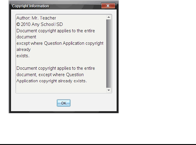
63 Working with TI-Nspire™ Documents
Note: To restore the Print defaults, click Reset.
Using Print Preview
• Click the Preview tickbox to toggle the preview pane.
• Click the arrows at the bottom of the preview pane to page through the preview.
Viewing Document Properties and Copyright Information
Note: Most of these instructions apply only to the Teacher Software.
Checking Page Size
1. In the Teacher Software, go to the TI-Nspire™ File menu and select Document
Properties.
2. Click the Page Size tab.
3. A tick indicates the document's current page size.
Viewing Copyright Information
The Teacher Software and Student Software let you view copyright information that
has been added to a document.
1. On the TI-Nspire™ File menu, select View Copyright Information.
The Copyright Information dialogue box opens.
2. Click OK to close the dialogue box.

Adding Copyright Information to a Document
Using the Teacher Software, you can add copyright information to individual
documents that you create, or you can apply the same copyright information to all new
documents.
1. Open the document.
2. On the TI-Nspire™ File menu, select Document Properties.
3. Click the Copyright tab.
4. Edit the following fields to define the copyright details:
• Author
• Copyright (select Public Domain or Copyright).
• Year (disabled if you selected Public Domain)
• Owner (disabled if you selected Public Domain)
• Comments
5. To add the supplied information to all new documents from this point forward,
select Apply this copyright to all new documents.
6. Click OK to apply the copyright information to the document.
Protecting a Document (making a document read-only)
Teachers can protect documents to create a document for distribution to your students
or for other use. A student who receives a read-only document and makes changes to it
will be prompted to save the document as a new file.
1. Open the document.
2. On the TI-Nspire™ File menu, select Document Properties.
3. Click the Protection tab.
4. Select the Make this document Read Only checkbox.
5. Click OK.
Working with TI-Nspire™ Documents 64

65

Working with PublishView™ Documents
Use the PublishView™ feature to create and share interactive documents with teachers
and students. You can create documents that include formatted text, TI-Nspire™
applications, images, hyperlinks, links to videos and embedded videos in a format that
is suitable for printing on a standard piece of paper, publishing to a website or blog, or
for use as an interactive worksheet.
PublishView™ features provide layout and editing features for presenting maths and
science concepts in a document where TI-Nspire™ applications can be interactively and
dynamically linked with supporting media, enabling you to bring the document to life.
Using the PublishView™ feature:
• Teachers can create interactive activities and assessments used on screen.
• Teachers can create printed materials to complement documents used on
TI-Nspire™ handhelds.
• When working with lesson plans, teachers can:
- Create lesson plans from existing handheld documents or convert lesson plans
to handheld documents.
- Link to related lesson plans or documents.
- Embed explanatory text, images, video and links to web resources.
- Build or interact with TI-Nspire™ applications directly from the lesson plan.
• Students can create reports or projects such as lab reports containing data
playback, curve fits, pictures and video—all on the same sheet.
• Students can print and turn in assignments on a standard piece of paper.
• Students taking exams can use one tool to create a document that contains: all
problems on the exam, text, images, hyperlinks, or videos, interactive TI-Nspire™
applications, screen shots and layout options needed to print a document.
Note: PublishView™ documents can be exchanged using the TI-Nspire™ Navigator™ NC
system. PublishView™ documents can reside in the Portfolio Workspace and TI-
Nspire™ questions within a PublishView™ document can be automatically graded by
the TI-Nspire™ Navigator™ system.
Creating a New PublishView™ Document
1. From the Documents Workspace, click File > New PublishView™ Document.
—or—
Click , and then click New PublishView™ Document.
• A blank letter-size document opens in the Documents Workspace. The
orientation is portrait, which cannot be changed.
• The default margin settings for the top and bottom margins are one-inch.
There are no settings for side margins.
• By default, a problem is added to the document.
Working with PublishView™ Documents 66
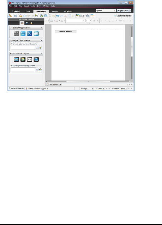
67 Working with PublishView™ Documents
• By default, the document contains the page number in a # of # format at the
bottom of the sheet.
• The scroll bars on the right side of the screen and at the bottom of the screen
are active.
2. Add TI-Nspire™ applications and PublishView™ objects as needed to complete the
document.
About PublishView™ Documents
When working with PublishView™ documents, it is important to keep the following
points in mind:
• PublishView™ documents are saved as .tnsp files, which distinguishes them from
TI-Nspire™ documents (.tns files).
• When inserting PublishView™ objects into a document, the text, image, hyperlink
or embedded video are contained in boxes that can be moved and resized.
• When you insert TI-Nspire™ applications, they work the same way as pages in a
TI-Nspire™ document.
• In a PublishView™ document, objects can overlap each other and you can control
which object is on top or bottom.
• Objects can be placed and positioned in a PublishView™ document in a free-form
fashion.
• You can convert an existing TI-Nspire™ document to a PublishView™ document
(.tnsp file).
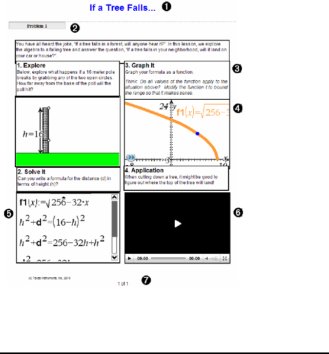
• When you convert a PublishView™ document to a TI-Nspire™ document (.tns file),
TI-Nspire™ applications are converted. PublishView™ objects containing text,
hyperlinks, videos and images are not converted.
• You cannot create or open a PublishView™ document on a handheld. You must
convert a PublishView™ document to a TI-Nspire™ document before sending it to a
handheld.
Exploring a PublishView™ Document
The following example shows how you might use TI-Nspire™ applications and
PublishView™ objects to build a PublishView™ document. In this example, borders are
turned on to show the boundaries around the objects. Showing borders enables you to
work with objects easily while building a document. When you are ready to print or
publish the document to the web, you can select to the hide borders.
ÀHeader. In this example, the header contains the title of the document. When the
Working with PublishView™ Documents 68

69 Working with PublishView™ Documents
header area is active, you can type and format text as needed.
ÁProblem break and name. In PublishView™ documents, use problem breaks to
control the page layout. You can select to hide or show problem breaks. Deleting a
problem removes the contents of the problem and removes the space between
problems when there are multiple problems. Problem breaks also enable you to use
variables in PublishView™ documents. Variables that have the same name are
independent of one another if they are used in different problems.
ÂText boxes. In this example, the introduction text and the text in boxes 1, 2, 3 and 4
is contained in text boxes. You can insert text and hyperlinks into a PublishView™
document using a text box. Text boxes can be resized and positioned as needed.
PublishView™ text boxes are not retained when you convert a PublishView™
document to a TI-Nspire™ document.
ÃTI-Nspire™ applications. In this example, the author uses Graphs & Geometry to
show the maths functions. When a TI-Nspire™ application is active in a PublishView™
document, the appropriate application menu opens in the Documents Toolbox. You
can work in a TI-Nspire™ application just as you would in a TI-Nspire™ document.
When you convert a PublishView™ document to a TI-Nspire™ document, applications
are retained.
ÄNotes application. You can also use the TI-Nspire™ Notes application to add text to a
PublishView™ document. Because Notes is a TI-Nspire™ application, it will be
retained when you convert the PublishView™ document to a TI-Nspire™ document.
Using the Notes application enables you to use an equation editor and can contain
TI-Nspire™ maths templates and symbols.
ÅVideo. This is an example of a video that is embedded in a PublishView™ document
within a frame. Users can start and stop the video using the controls. Frames
containing videos and images can be resized and positioned in the document as
needed.
ÆFooter. By default, the footer area contains the page number, which cannot be
edited. You can add other text above the page number if needed. Like the header,
you can format text as needed.
Using the Status Bar in a PublishView™ Document
When a PublishView™ document is open, options on the status bar are different than
when working in a TI-Nspire™ document.
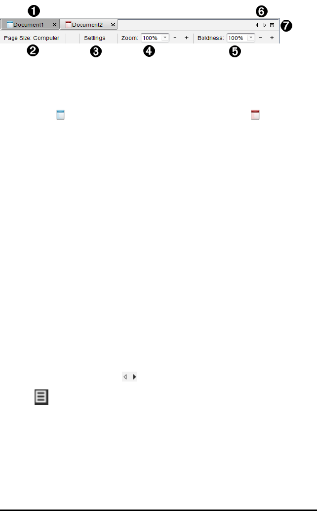
ÀDocument names are displayed in tabs. If multiple documents are open, the
document names are listed. You can have TI-Nspire™ and PublishView™ documents
open at the same time. In this example, Document 1 is an inactive TI-Nspire™
document ( ). Document 2 is the active PublishView™ document ( ). Click the X to
close a document.
ÁPage Size. Shows the document's page size as Handheld or Computer. You can use
the TI-Nspire™ File menu to convert a document from one page size to the other.
ÂClick Settings to change Document Settings. You can specify settings that are specific
to an active document or set default settings for all PublishView™ documents. When
you convert a TI-Nspire™ document into a PublishView™ document, the settings in
the TI-Nspire™ document convert to the settings defined for PublishView™
documents.
ÃUse the Zoom scale to zoom the active document in or out from 10% to 500%. To set
a zoom, type a specific number, use the + and - buttons to increase or decrease by
increments of 10%, or use the drop-down box to choose pre-set percentages.
ÄIn TI-Nspire™ applications, use the Boldness scale to increase or decrease the
boldness of text and line thickness within applications. To set the boldness, type a
specific number, use the + and - buttons to increase or decrease by increments of
10%, or use the drop-down box to choose pre-set percentages.
For PublishView™ objects, boldness is used to match text within TI-Nspire™
applications to other text on the PublishView™ sheet. It can also be used to increase
the visibility of TI-Nspire™ applications when presenting a document to a class.
ÅWhen there are too many open document names to show in the status bar, click the
forward and backward arrows ( ) to move through the documents.
ÆClick to see a list of all open documents.
Saving PublishView™ Documents
Saving a New Document
1. Click File > Save Document.
—or—
Working with PublishView™ Documents 70
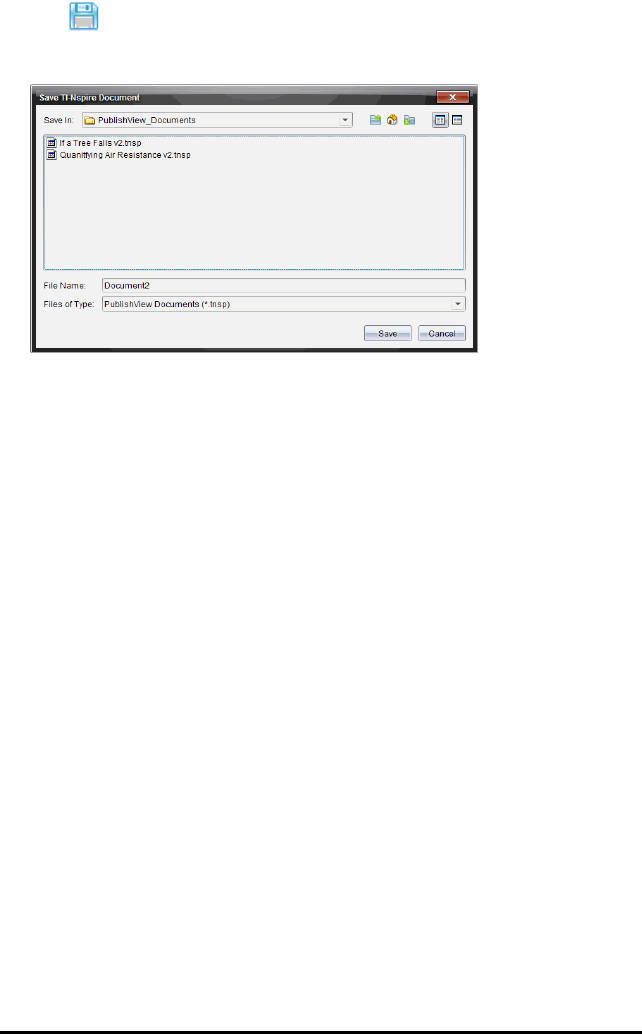
71 Working with PublishView™ Documents
Click .
The Save TI-Nspire™ Document dialogue box opens.
2. Navigate to the folder in which you want to save the document.
—or—
Create a folder in which to store the document.
3. Type a name for the new document.
4. Click Save.
The document closes and is saved with the extension .tnsp.
Note: When you save a file, the software first looks in the same folder the next time
you open a file.
Saving a Document with a New Name
To save a previously saved document in a new folder and/or with a new name:
1. Click File > Save As from the menu.
The Save TI-Nspire™ Document dialogue box opens.
2. Navigate to the folder in which you want to save the document.
—or—
Create a folder in which to store the document.
3. Type a new name for the document.
4. Click Save to save the document with a new name.
Note: You can also use the Save As option to convert documents from TI-Nspire™ files
to PublishView™ files or convert PublishView™ files to TI-Nspire™ files.

Exploring the Documents Workspace
When you create or open a PublishView™ document, it opens in the Documents
Workspace. Use the menu options and the toolbar just as you would when working
with a TI-Nspire™ document to:
• Navigate to existing folders and documents using Content Explorer
• Open existing documents
• Save documents
• Use the copy, paste, undo and redo options
• Delete documents
• Access TI-Nspire™ application-specific menus
• Open the Variables menu in TI-Nspire™ applications that allow variables
• Access and insert maths templates, symbols, catalogue items and library items
into a PublishView™ document
Note: For more information, see Using the Documents Workspace.
Exploring the Documents Toolbox
When a PublishView™ document is active, the Documents Toolbox contains tools
needed for working with PublishView™ documents. You can add TI-Nspire™
applications to a problem, insert parts of existing TI-Nspire™ documents into a
problem, and add PublishView™ objects.
The Documents Toolbox opens when you create a new PublishView™ document or
open an existing PublishView™ document. When working in a PublishView™ document,
Page Sorter and TI-SmartView™ emulator are not available.
Working with PublishView™ Documents 72
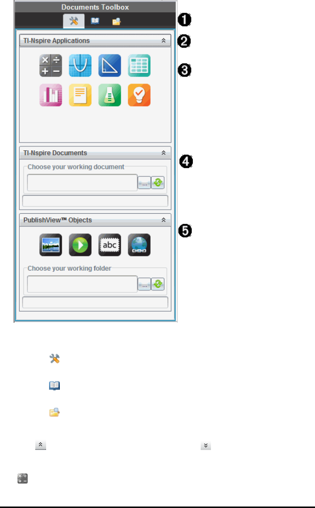
73 Working with PublishView™ Documents
ÀIn a PublishView™ document:
• Click to open the application menu and tools needed to work with
TI-Nspire™ applications and PublishView™ objects.
• Click to open the Utilities panel where you can access Maths Templates,
Symbols, the Catalogue, Maths Operators and Libraries.
• Click to open Content Explorer.
Note: For more information, see Using the Documents Workspace.
ÁClick to collapse a pane containing a menu. Click to expand a pane.
ÂTI-Nspire™ applications. Move an icon to a problem to insert an application:
Calculator
Graph
Geometry
Lists & Spreadsheet
Data & Statistics
Notes
Vernier DataQuest™
Question (Available in TI-Nspire™ CX Teacher Software, TI-Nspire™ CX
Navigator™ Teacher Software and TI-Nspire™ Navigator™ NC Teacher Software).
ÃTI-Nspire™ Documents. Use this tool to locate and insert existing TI-Nspire™
documents (.tns files) into a problem.
ÄPublishView™ Objects. Use this tool to move the following objects into a problem:
Image
Video
Text box
Hyperlink
Using Menus and the Toolbar
When working in a PublishView™ document, select options from the menus or the
toolbar in the Documents Workspace to work with content and objects. When you
insert an object into a PublishView™ document, you can manipulate it using the same
tools as you would when working with a TI-Nspire™ document. In PublishView™
documents, you can:
• Right-click on an object to open a context menu, which displays the actions that
can be performed on that object.
• Use add, insert and paste to add objects to a PublishView™ document.
• Use delete and cut to remove objects from a PublishView™ document.
• Move objects from one place to another within a PublishView™ document.
• Copy objects from one document and paste them into another PublishView™
document.
• Resize and scale objects such as text boxes and images.
• Change the font face and size and apply formatting such as italics, bold, underline
and colour to text.
Working with PublishView™ Documents 74
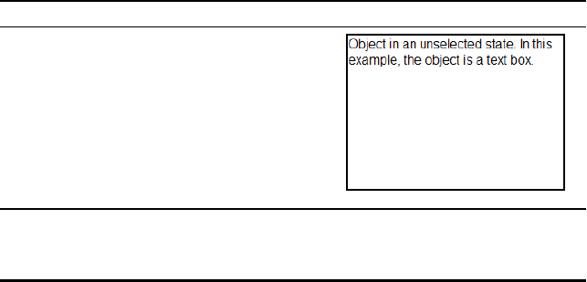
75 Working with PublishView™ Documents
Note: For more information, see Using the Documents Workspace.
Using Context Menus
In TI-Nspire™ applications and in PublishView™ documents, context menus provide a
list of options specific to the task you are working on. For example, when you right-
click a cell while working in the TI-Nspire™ Lists & Spreadsheet application, a context
menu opens providing a list of actions that you can perform on that cell. When you
right-click the border of a text box in a PublishView™ document, the context menu
provides actions that can be performed on the text box.
Context Menus in TI-Nspire™ Applications
When you insert a TI-Nspire™ application into a PublishView™ document, the
application menu and the context menus associated with that application are available
and work the same way they work in a TI-Nspire™ document.
Context Menus in PublishView™ Documents
In PublishView™ documents, context menus provide shortcuts to frequently performed
tasks. Context menus are specific to an object or area:
• The Sheet context menu provides options for working with the layout of the sheet
and document.
• Object context menus provide options for manipulating the object.
• Content-sensitive context menus provide options for working with the content
inside the object such as text or a video.
Working with PublishView™ Objects
In a PublishView™ document, text, hyperlinks, images and videos are contained in
PublishView™ objects. You can move, resize, copy and paste and delete an object
within a PublishView™ document. Objects can also be positioned so that one overlaps
the other.
Within a document, PublishView™ objects can exist in three states: unselected,
selected and interactive.
State Description
Unselected When unselected, an object does
not have handles for
repositioning and sizing. To
deselect an object, left-click or
right-click outside the object.
In this example, borders around
the object are showing.
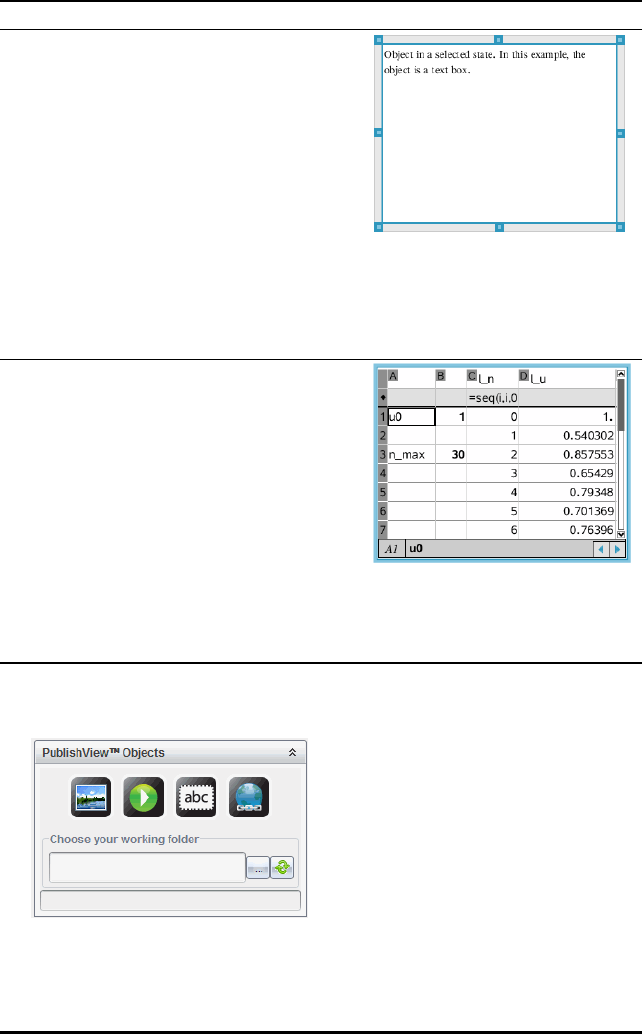
State Description
Selected When selected, an object will
have eight square handles
framing the object. To select an
object, click the object’s border.
When selected, objects can be
moved and resized.
• To move an object, click a
border and drag the object
to its new location.
• To resize an object, grab a
handle.
• Right-click the border to
open a context menu with
options for manipulating the
object.
Interactive An interactive state is indicated
by a blue frame around the
object. To enter interactive
state, left-click or right-click
anywhere in the body of the
object. When in an interactive
state, you can work with the
contents of the object. For
example, you can add or edit text
in a text box or complete maths
functions in a TI-Nspire™
application. When in an
interactive state, context menus
contain options specific to the
contents of an object.
Inserting an Object
1. In the Documents Toolbox, ensure the PublishView™ Objects menu is open.
2. Use your mouse to click an icon and drag it to the document.
3. Release the mouse button to drop the object into the document.
Working with PublishView™ Documents 76
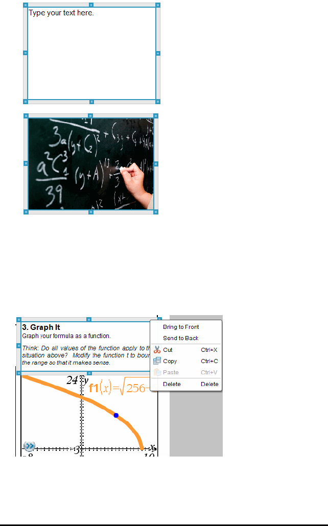
77 Working with PublishView™ Documents
Selected text boxes and
frames can be resized,
moved, copied, pasted
and deleted.
4. Using the mouse, grab the handles to resize the object and drag it to position the
object in the document as needed.
Opening Object Context Menus
▶Right-click the border of any object in a PublishView™ document.
The context menu opens to provide access to delete, copy/paste, cut and bring to
front/send to back actions.
Resizing an Object
1. Click any border around the object to select it. The border becomes a bold blue line
and the handles are active.
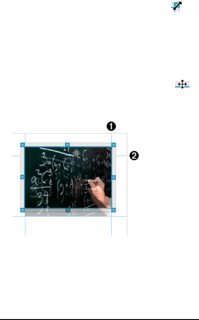
2. Move your mouse over one of the handles to activate the resizing tool .
3. Grab one of the handles and drag in the direction needed to make the object larger
or smaller.
4. Click outside the object to save the new size.
Moving an Object
To move an object to another location on the page:
1. Click any border around the object to select it. The border becomes a bold blue line
and the handles are active.
2. Move your cursor over one of the borders to activate the positioning tool .
3. Click to grab the object. The horizontal and vertical alignment guides are activated
at the top and bottom of the object. Use the grid lines to position the object on the
page.
Àvertical alignment guide
Áhorizontal alignment guide
4. Drag the object to a new location on the page.
5. Release the mouse button to drop the object in its new location.
Working with PublishView™ Documents 78
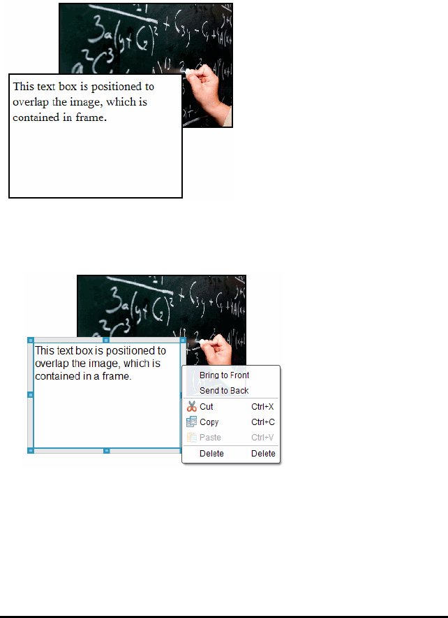
79 Working with PublishView™ Documents
Overlapping Objects
You can position objects so that one is on top of another. You can control the stacking
order to specify which object is positioned in front or behind the other. Overlapping
objects have many practical uses when presenting information in the classroom. For
example, you can create a "curtain control" by placing an empty text box over other
objects. Then, you can move the text box to reveal the items below it one at a time.
To change the position of an object in the stacking order:
1. Click the border of the object you want to position to select it, and then right-click
to open the context menu.
2. Click Send to back or Bring to front to move the selected object to the desired
position.
Deleting an Object
To delete an object from a sheet:
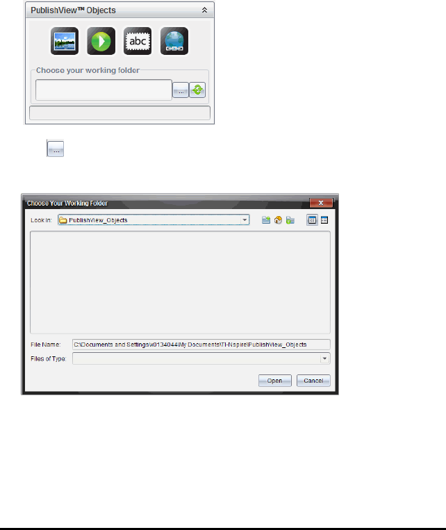
1. Click any border of the object to select it. When an object is selected, the border is
blue and the handles are active.
2. Press the Delete key to delete the text box.
—or—
Right-click a border, and then click Delete from the context menu.
Choosing a Working Folder for PublishView™ Objects
Use the Choose Your Working Folder field in the PublishView™ Objects pane to select a
folder for storing PublishView™ documents and related files.
1. Ensure the PublishView™ Objects pane is open.
2. Click .
The Choose Your Working Folder dialogue box opens.
3. Navigate to the folder where you want to store video and image files.
4. Click Open to choose the working folder.
The selected folder becomes the working folder and the folder name is displayed in
the Choose your working folder field. Previews of supported images and video files
in the folder are shown in the PublishView™ objects pane.
Working with PublishView™ Documents 80
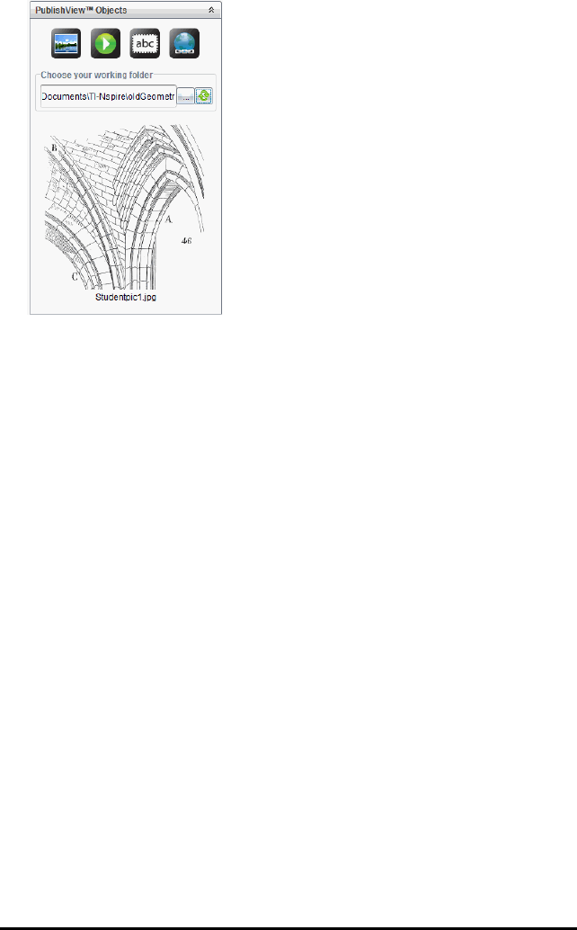
81 Working with PublishView™ Documents
5. To add an image or video file to a PublishView™ document, select the file and
move it onto the active sheet.
Working with TI-Nspire™ Applications
Note: For more information, see the appropriate chapter in this guidebook.
Adding an Application to a Problem
To add a TI-Nspire™ application to a problem in a PublishView™ document:
1. Choose one of the following actions to select an application:
• From the TI-Nspire™ Applications pane in the Documents Toolbox, use the
mouse pointer to point to the application and drag it to the problem.
• From the menu bar, click Insert and choose an application from the drop-down
menu.
• Right-click inside the sheet to open the context menu, click Insert and choose
an application from the menu.
The application is added to the sheet.
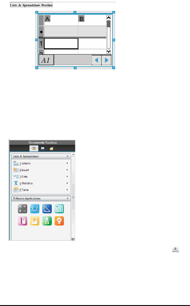
2. Using your mouse, grab the handles to resize or position the application object as
needed.
3. Click outside the application frame to accept the dimensions.
4. To open the menu for the active TI-Nspire™ application, click inside the application.
The menu opens in the Documents Toolbox above the TI-Nspire™ Applications
pane.
Right-click on an application element, such as a cell or function to open the context
menu for that item.
5. To work in the application, click an option from the application menu. Click to
collapse the application menu pane.
Adding Existing TI-Nspire™ Documents
Use the TI-Nspire™ Documents pane to open an existing TI-Nspire™ document to add
to a PublishView™ document. When you open an existing TI-Nspire™ document, all
Working with PublishView™ Documents 82
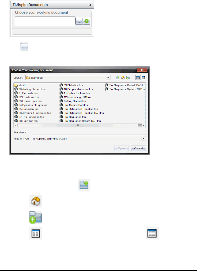
83 Working with PublishView™ Documents
pages of the document appear in the preview pane. You can move complete problems
or individual pages onto the PublishView™ sheet.
Choosing a Working TI-Nspire™ Document
To choose a working document:
1. In the Documents Toolbox, ensure the TI-Nspire™ Documents pane is open.
2. Click .
The Choose Your Working Document dialogue box opens.
3. Navigate to the folder in which the TI-Nspire™ document is stored:
• Click ¤in the Look in: field to use a file browser to locate a folder.
• From an open folder, click to move up a level in the folder hierarchy
• Click to return to the default home folder
• Click to add a new folder to open folder on your computer.
• Click to list folders and files. To show details, click .
4. Select the file, and then click Open.
The TI-Nspire™ document opens in the TI-Nspire™ Documents pane.
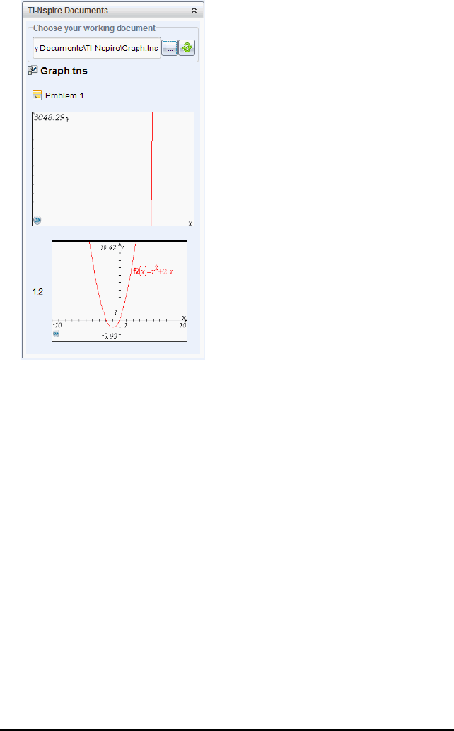
5. To add the TI-Nspire™ document to the PublishView™ document, move one page at
a time or one problem at a time to the PublishView™ sheet.
If you are adding a problem with multiple pages, the pages are stacked on top of
each other on the PublishView™ sheet. Move the top page to see the other pages.
Working with Problems
Like a TI-Nspire™ document, a PublishView™ document consists of one or more
problems.
Problems are used to control the layout of a PublishView™ document so that you can
isolate variables. When variables with the same name are used in multiple problems,
variables can have different values. To add problems to PublishView™ documents,
open the Sheet context menu or use the options on the Insert menu in the Documents
Workspace. When adding problems, keep the following guidelines in mind:
• By default, a new PublishView™ document contains one problem.
• You can insert a problem after any existing problem.
• You cannot insert a problem in the middle of an existing problem.
• A new problem break is always inserted after the selected problem.
• Inserting a problem break adds empty space below the break.
• Any object between two problem breaks is part of the problem above the break.
Working with PublishView™ Documents 84
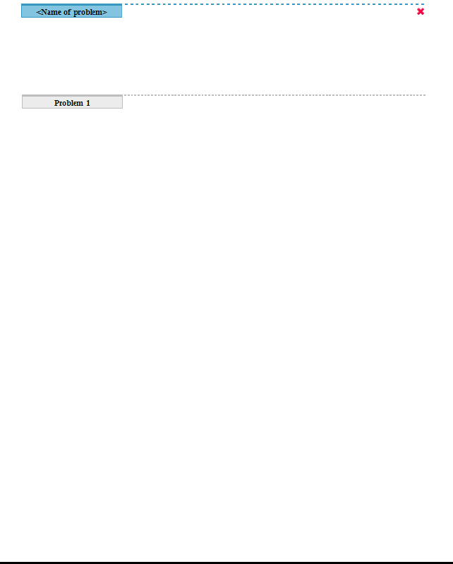
85 Working with PublishView™ Documents
• The last problem includes all sheets and objects below the last problem break.
• Problem breaks are not relative to any object, which lets you move objects within a
problem without affecting the problem break location.
Adding a Problem
To add a problem to an open PublishView™ document:
1. Right-click anywhere on the sheet, and then click Insert > Problem.
The problem is added to the document below any existing problems. The problem
break provides a visible divider between problems.
2. To name the problem, highlight the default text, type a name, and then click
outside the text box to save the name.
The problem break is saved.
If a document has multiple problems, use the scroll bar on the right side of the
document to move up and down through the problems.
Managing Problem Breaks
Problem breaks are used to separate problems and variable sets.
• Every problem has a problem break.
• A problem break becomes visible when a problem is added to a document.
• A problem break is represented by a dashed line with the name of the problem
positioned on the left side of the sheet.
• By default, the problem name is shown as <Name of problem>. Highlight the
default text to type a new name for the problem.
• Problem names do not have be unique. Two problems can have the same name.
Hiding and Showing Problem Breaks
You can select to hide or show problem breaks in a PublishView™ document. By
default, problem breaks are shown.
1. Right-click in any blank area of the document (outside of any object) to open the
sheet context menu.
2. Click Layout Options.
The Show/Hide Options dialogue box opens.
Note: You can also click View > PublishView™ Layout Options.
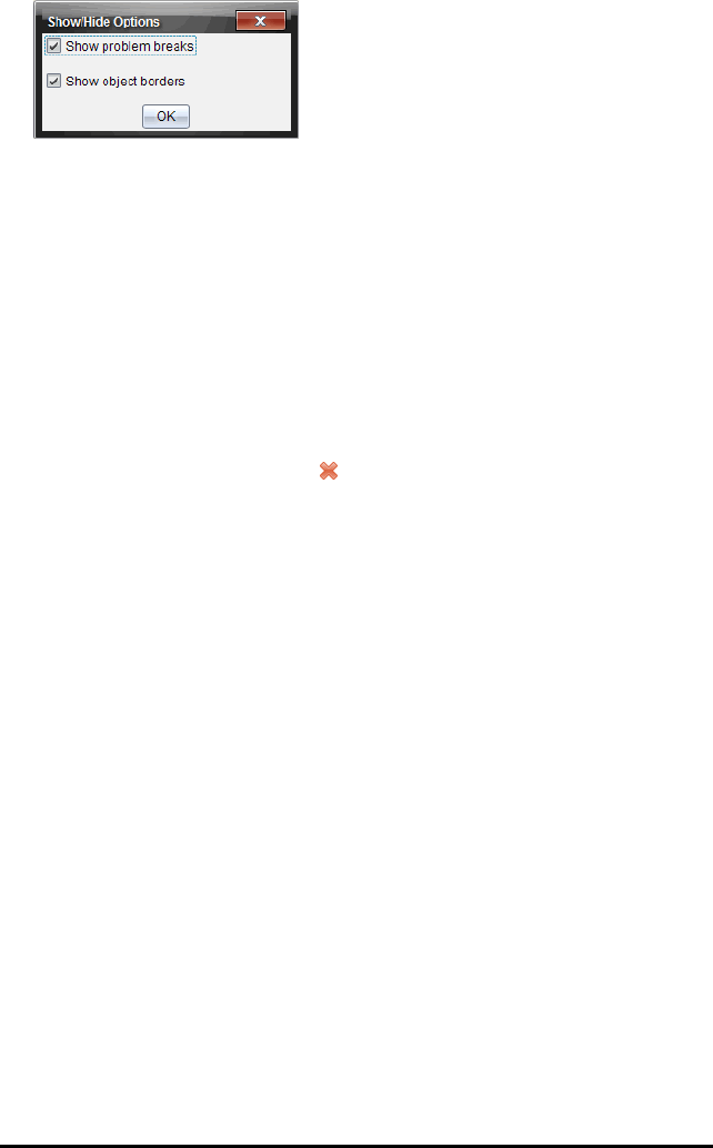
3. Clear the Show problem breaks option to hide problem breaks in the document.
Select the option to return to the default setting and show the problem breaks.
4. Click OK to close the dialogue box.
Renaming a Problem
1. Click the existing problem name on the problem break line.
2. Type a new name for the problem.
3. Click outside the text box to save the new name.
Deleting a Problem
To delete a problem, complete one of the following actions:
▶Select the problem break and click on the right side of the break.
▶Click Edit > Delete.
▶Right-click the problem break and click Delete.
▶Select the problem break and press the Delete or Backspace key.
When you delete a problem, all objects contained in the problem are removed and the
space between the selected problem break and the next problem break is removed.
Organizing PublishView™ Sheets
A PublishView™ document can have multiple sheets. A single sheet is displayed in the
workspace on your screen. All work occurs in the PublishView™ objects and TI-Nspire™
applications within sheets.
Adding Sheets to a Document
To add a sheet to a document:
▶Click Insert > Sheet.
The sheet is added to the document and the numbering increments by one.
Opening the Sheet Context Menu
▶Right-click in any blank area (outside of any object) in a PublishView™ sheet.
A context menu opens with options for inserting problems, pages, applications and
PublishView™ objects, edit options for removing space or deleting a page and
options for hiding and showing problem breaks and object borders.
Working with PublishView™ Documents 86
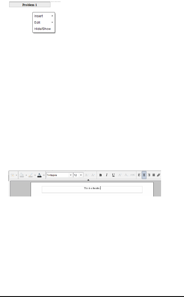
87 Working with PublishView™ Documents
Page Numbering
In a PublishView™ document, page numbering is displayed in the bottom margin
(footer). By default, numbering is placed in the centre of the PublishView™ sheet in a #
of # format. You cannot edit or delete page numbering.
Working with Headers and Footers
PublishView™ documents contain space at the top and bottom of a sheet to add a
header or a footer. Headers and footers can contain the date, the document name, the
lesson plan name, the class name, your school’s name, or any other information
needed to identify a document.
By default, headers and footers do not contain content and boundaries for the header
and footer are hidden. To activate a header or footer for editing, click inside the top or
bottom margin. When activated, a text box with a light grey border is displayed.
Inserting and Editing Text in Headers and Footers
1. Click inside the top or bottom margin.
The text box borders in the margin become visible and the object space is disabled.
The cursor is placed in the header or footer space and the formatting toolbar
becomes active.
2. Type the text.
• The default font is TI-Nspire™ true type, 12 pt, normal.
• By default, text is centreed horizontally and vertically.
• Text can be aligned: left, centre, right, or justified.
• Text that does not fit within the text box horizontally will wrap to the next line.
• Text that does not fit within the text box vertically will not be shown, but text is
retained. (If you delete text, the hidden text will appear.)
3. Complete one of the following actions to save the text:
• Single-click anywhere outside the header or footer text box to save the text.
• Press Esc to save the text.
The PublishView™ sheet becomes active and the formatting menu closes.
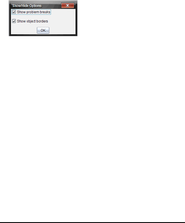
Showing and Hiding Borders
By default, borders are displayed when you insert an object into a problem. When you
select to hide borders, the selection applies to all objects in the document and to
objects that you add to the document. To hide the border:
1. Right-click in any blank area of the sheet (outside of any object) to open the
context menu.
2. Click Layout Options.
The Layout Options dialogue box opens.
Note: You can also click View > PublishView™ Layout Options.
3. Clear the Show object borders option to hide the borders around the objects in the
problem. Select the option to return to the default setting and show borders.
4. Click OK to close the dialogue box.
Adding and Removing Space
To manage how PublishView™ objects appear on a sheet, you may need to add or
delete space between objects.
Note: You can add and remove vertical space between objects using this method. To
add or remove horizontal space between objects, move the object.
Adding Space
1. Right-click in the area outside of any object where you want to add space. The
context menu opens.
2. Click Edit > Add/Remove Space. The Add/Remove Space tool becomes active.
Working with PublishView™ Documents 88
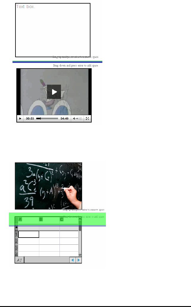
89 Working with PublishView™ Documents
Add/Remove Space
tool
3. Use your mouse to position the tool to the exact place where you want to add
space.
4. Click the tool, and then drag down to select the amount of space you want to add.
As you select the amount of space to be added, it is indicated in green.
5. Press the Enter key to add the space in between the objects. You can adjust the
amount of space by dragging up and down before you press Enter.
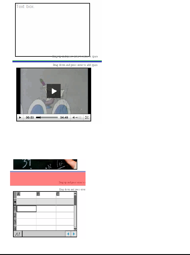
Removing Space
1. Right-click in the area outside of any object where you want to remove space.
The context menu opens.
2. Click Edit > Add/Remove Space.
The Add/Remove Space tool becomes active.
Add/Remove Space
tool
3. Use your mouse to position the tool to the exact place where you want to remove
space.
4. Click the tool, and then drag up to select the amount of space you want to remove.
As you select the amount of space to be removed, it is indicated in red.
Working with PublishView™ Documents 90

91 Working with PublishView™ Documents
5. Press the Enter key to remove the space in between the objects. You can adjust the
amount of space by dragging up and down before you press Enter.
Note: If there is not enough space on the sheet to accommodate the objects, the
objects won’t be moved when space is removed.
Deleting Blank Sheets from Problems
You can delete a sheet that does not contain any TI-Nspire™ applications or
PublishView™ objects from a problem. To delete a blank sheet from a problem:
1. Delete any TI-Nspire™ applications, PublishView™ objects, move or delete any
problem breaks from the sheet.
2. Place your cursor inside the sheet you want to delete.
3. Right-click inside the blank sheet to open the context menu.
4. Click Edit > Delete Sheet.
The blank sheet is removed from the problem.
Using Zoom
The zoom feature lets you zoom in on any object or area on the PublishView™
document for discussion, and zoom out to see an overview of the lesson. The zoom
uses the centre point of the viewable area to zoom in.
The default zoom setting is 100%.
▶To change the zoom percentage, do one of the following:
• Type the number in the box and press Enter.
• Use the - and + buttons to decrease or increase the percentage in 10%
increments.
• Use the drop-down arrow to choose a preset percentage.
The zoom settings are retained when you save the document.
Adding Text to a PublishView™ Document
In a PublishView™ document, there are three ways to add text:
• Insert a PublishView™ text box to enter free-form text or copy text from other
sources into the document. For example, you can place a PublishView™ text box
next to an image and type a description in a text box. You can also copy and paste
text from .doc, .txt and .rtf files. Use PublishView™ text boxes when you need
options for emphasizing and formatting text. PublishView™ text boxes are not
converted when you convert a PublishView™ document to a TI-Nspire™ document.
You may want to use a PublishView™ text box to add text that you don’t want
handheld users to see.
• Use the TI-Nspire™ Notes application. You should use the Notes application when
you need an advanced equation editor and when you need to use TI-Nspire™ maths
templates and symbols. Superscript and subscript are also easier to use in the
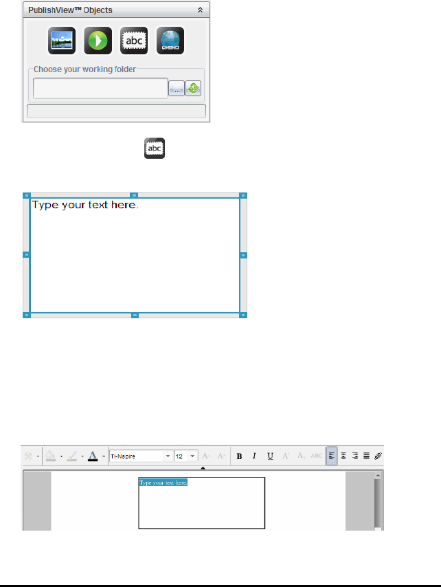
Notes application. You should also use Notes when you are planning to convert the
PublishView™ document to a TI-Nspire™ document for use on a handheld and you
want handheld users to see the text.
• Add text in TI-Nspire™ applications that allow text just as you would in a
TI-Nspire™ document.
Inserting Text into a Text Box
1. Ensure the PublishView™ Objects pane is open.
2. Use your mouse to click and drag it to the problem.
3. Release the mouse button to drop the text box into the problem.
4. Using the mouse, grab the handles to resize the text box or position in the problem
as needed.
5. Click outside the text box to save the size and position.
6. Click "Type your text here".
The formatting toolbar becomes active. The text box is in an interactive state for
adding or editing text.
7. Type the new text.
Working with PublishView™ Documents 92

93 Working with PublishView™ Documents
—or—
Copy and paste text from another file.
8. Apply formatting as needed.
9. Click outside the text box to save the text.
Formatting and Editing Text
The options for editing and formatting text are located on a formatting toolbar at the
top of the active document. Formatting options for editing text include:
• Changing the font, font size and font colour.
• Applying bold, italics and underline formatting.
• Applying the following text horizontal alignment options: left, right, centreed and
justified.
• Inserting hyperlinks.
Launching Edit Mode
▶Click inside a text box to launch edit mode.
• The formatting menu opens.
• The text is selectable for editing.
Opening the Content Context Menu
▶Right-click inside a text box containing text or a hyperlink.
The formatting menu and context menu open providing shortcuts to cut, copy and
paste.
Using Hyperlinks in PublishView™ Documents
In PublishView™ documents, use hyperlinks to:
• Link to a file
• Link to a website on the Internet
You can add a hyperlink to an open document or you can convert any text within a text
box to a hyperlink. When a hyperlink is added, the formatting of the text is underlined
and the font colour is blue. You can change the formatting of the hyperlinked text
without losing the hyperlink.
If a link is broken, an error message is displayed when you click the link:
• Cannot open the specified file
• Cannot open the specified web page
PublishView™ text boxes support both absolute and relative links.
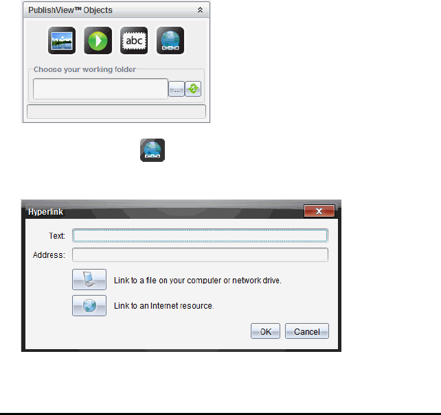
Absolute links contain the complete location of the linked file and do not depend on the
location of the main document.
Relative links contain the location of the linked file relative to the main document. If
you have multiple lessons in a single folder and they are all linked using relative
addressing, you can move the folder to any other location (another local folder,
datashare, flash drive, online) without breaking the links. The links also stay intact if
you bundle the documents into a lesson bundle or zip them into a zip file and share
them.
Note: The PublishView™ document must be saved before you can insert a relative
hyperlink.
Linking to a File
You can link to any file on your computer. If the file type is associated with an
application on your computer, it will launch when you click the link. There are two ways
to link to a file; by typing or pasting a file address into the Address field, or by browsing
to a file.
Linking to a File by Using an Address
1. Ensure the PublishView™ Objects pane is open.
2. Drag the hyperlink icon onto the document.
The Hyperlink dialogue box opens.
Working with PublishView™ Documents 94
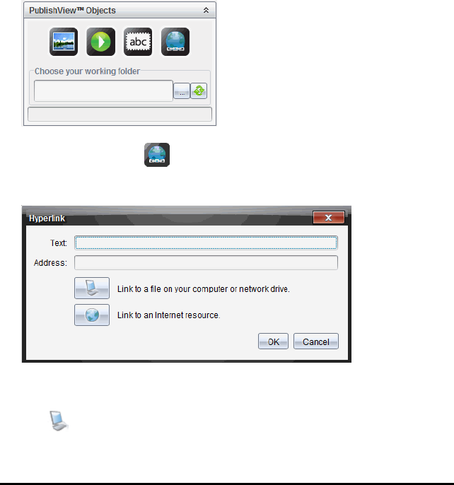
95 Working with PublishView™ Documents
3. Type the name of the link in the Text field. For example, this can be the name of
the document.
4. Copy the location of the file path you want to link to, and paste it in the Address
field.
—or—
Type the location of the file in the Address field.
Note: Type ../ to designate parent directories. For example:
../../lessons/mathlesson2.tns
5. Click OK to insert the link.
A text box containing the hyperlink is added to the PublishView™ document.
Linking to a File by Browsing
1. Ensure the PublishView™ Objects pane is open.
2. Drag the hyperlink icon onto the document.
The Hyperlink dialogue box opens.
3. Type the name of the link in the Text field. For example, this can be the name of
the document.
4. Click to select Link to a file on your computer or network drive.
The Select file to insert as hyperlink dialogue box opens.
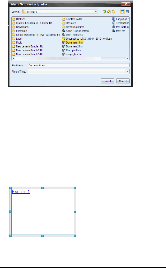
5. Navigate to and select the file you want to link to, and then click Insert.
The path name is inserted into the Address field in the Hyperlink dialogue box.
If the software is unable to determine if the link is a relative or absolute address,
the Hyperlink dialogue box opens with an option to change the type of link.
To change the link, click the appropriate option:
•Change to absolute address.
•Change to relative address.
6. Click OK to insert the link.
—or—
Click Start Over to go back to the Hyperlink dialogue box and choose a different file
to link, or to edit the Text or Address fields.
A text box containing the hyperlink is added to the PublishView™ document.
7. Using the mouse, grab the handles to resize the text box.
—or—
Working with PublishView™ Documents 96
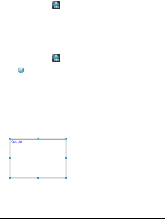
97 Working with PublishView™ Documents
Grab any border to position the text box in the document as needed.
Linking to a Website
There are two ways to link to a website; by typing or pasting the URL into the Address
field, or by browsing to a file.
Linking to a Website by Using an Address
1. Ensure the PublishView™ Objects menu is open.
2. Drag the hyperlink icon onto the document to open the Hyperlink dialogue box.
3. Type or paste the URL you want to link to in the Address field.
4. Click OK.
A text box containing the hyperlink is added to the PublishView™ document.
Linking to a Website by Browsing
1. Ensure the PublishView™ Objects menu is open.
2. Drag the hyperlink icon onto the document to open the Hyperlink dialogue box.
3. Click to select Link to an Internet resource.
The browser opens to your default website.
4. Navigate to the website or file on a website that you want to link to.
5. Copy the URL, and then paste it in the Address field in the Hyperlink dialogue box.
—or—
Type the URL in the Address field.
6. Click OK.
A text box containing the hyperlink is added to the PublishView™ document.
7. Using the mouse, grab the handles to resize the text box.
—or—
Grab any border to position the text box in the document as needed.
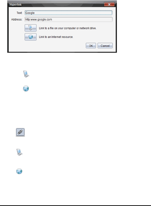
Editing a Hyperlink
To change the name of a hyperlink, change the path, or change the URL, complete the
following steps.
1. Using your mouse, right-click the hyperlink text, and then click Edit hyperlink.
The Hyperlink dialogue box opens.
2. Make corrections as needed:
• Type corrections to the hyperlink name in the Text field.
• Click to open the Select a file to add as a hyperlink dialogue box and use
the file browser to navigate to the folder where the file is located.
• Click to open a browser and navigate to a website to copy and paste the
correct the URL in the Address field.
3. Click OK to save the changes.
Converting Existing Text to a Hyperlink
1. Click inside the text box to activate edit mode and open the formatting menu.
2. Select the text you want to convert to a hyperlink.
3. Click .
The Hyperlink dialogue box opens with the selected text in the Text field.
4. Click to create a link to a file.
—or—
Click to create a link to page on a website.
Working with PublishView™ Documents 98
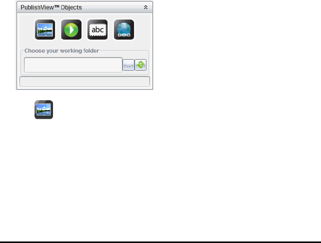
99 Working with PublishView™ Documents
Removing a Hyperlink
Use this process to remove a link from text inside a text box. The text remains in the
document.
1. Using your mouse, right-click the hyperlink text.
2. Click Remove hyperlink.
The hyperlink formatting is removed from the text and the text is no longer
clickable.
Note: To remove both the text and hyperlink, delete the text. If a text box contains only
the linked text, delete the text box.
Working with Images
Images can be added to PublishView™ documents as PublishView™ objects or can be
added inside TI-Nspire™ applications that support images. Supported files types are
.bmp, .jpg and .png files.
Note: If a TI-Nspire™ application is active in the PublishView™ document, the image is
added to the TI-Nspire™ page if you click Insert>Image from the menu bar or context
menu. If there is no TI-Nspire™ document active, the image is added as a
PublishView™ object. Only images inside TI-Nspire™ applications convert to TI-Nspire™
documents (.tns files).
Inserting an Image
1. Ensure the PublishView™ Objects pane is open.
2. Click , and then drag the icon to the document.
The Choose an image to insert into PublishView™ dialogue box opens.
Note: By default, the Texas Instruments preloaded images folder is displayed.
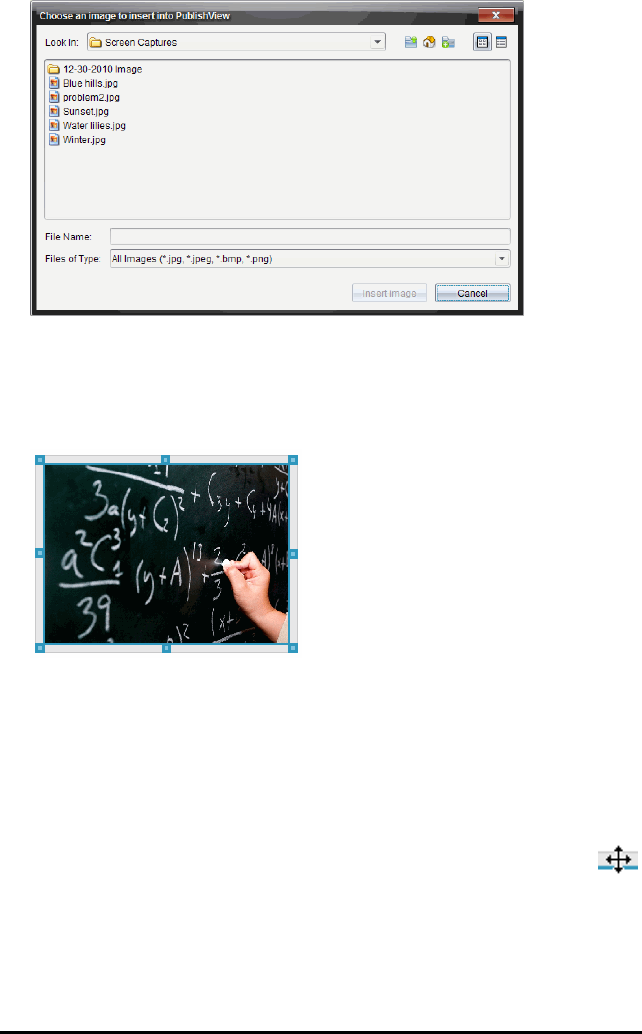
3. Navigate to the folder where the image file you want to insert is located, and then
highlight the file name.
4. Click Insert image.
The image is added to the PublishView™ sheet.
5. Using the mouse, grab the handles to resize the text box,
—or—
Grab any border to position the text box in the document as needed.
Moving Images
1. Click the frame containing the image to select it.
2. Move your cursor over the edge of the image to activate the positioning tool.
3. Move the image to its new location on the PublishView™ sheet.
Note: Objects can overlap each other on a PublishView™ sheet.
Working with PublishView™ Documents 100
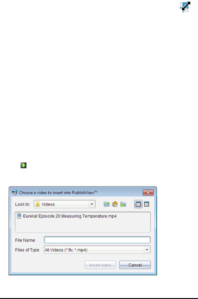
101 Working with PublishView™ Documents
Resizing Images
1. Click the frame containing the image to select it.
2. Move your cursor over one of the blue handles to activate the resizing tool.
3. Drag the handle to make the image smaller or bigger.
Deleting Images
▶Click the image to select it, and then press the Delete key.
—or—
▶Right-click a handle to open the context menu, and then click Delete.
Working with Video Files
You can embed video files in a PublishView™ document and play the videos directly
from the PublishView™ document. Supported video formats include:
• Flash® (.flv) video files with VP6 video and MP3 audio.
• MP4 (MPEG-4 multimedia container) with H264/AVC (Advanced Video Coding)
video compression and AAC audio.
Note: You can also insert a link to a video that will launch in a new browser window or
media player window. For more information, see Working with Hyperlinks.
Inserting a Video
1. Ensure the PublishView™ Objects pane is open.
2. Click , and then drag the icon to the document.
The Choose a video to insert into PublishView™ dialogue box opens.
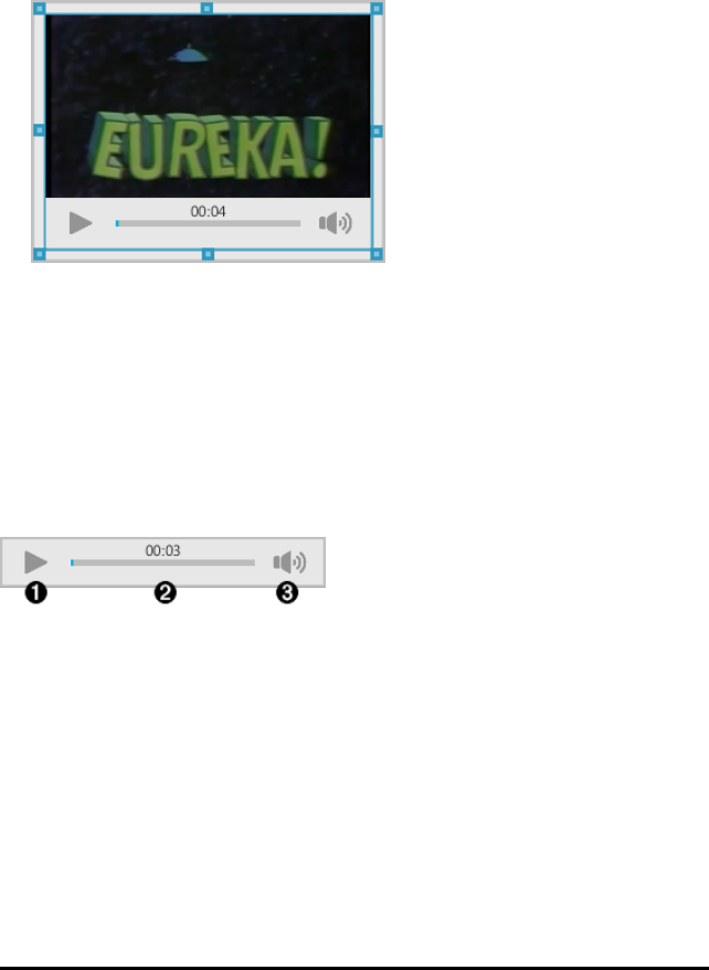
3. Navigate to the folder where the video file you want to insert is located, and select
the file name.
4. Click Insert video.
An object containing the embedded video is added to the PublishView™ sheet. By
default, the resizing and positioning handles are active.
5. Using the mouse, grab the handles to resize the object or grab any border to
position the object in the document as needed. For example, you may want to
position the object containing the video above or below a text box that contains
text introducing the video.
6. To play the video, click the forward arrow or click anywhere in the viewing window.
Using the Video Console
The video console lets users control the video.
ÀStarts or stops the video.
ÁShows the elapsed time as the video plays.
ÂMutes or unmutes the audio.
Converting Documents
You can convert PublishView™ documents (.tnsp files) to TI-Nspire™ documents (.tns
files) for display on handhelds. You can also convert TI-Nspire™ documents to
PublishView™ documents.
Working with PublishView™ Documents 102

103 Working with PublishView™ Documents
Converting a document creates a new document—the original document remains
intact and is not linked to the new document. If you make changes to one document,
the changes are not reflected in the other document.
Converting PublishView™ Documents to TI-Nspire™ Documents
You cannot open a PublishView™ document (.tnsp file) on a handheld. However, you
can convert the PublishView™ document to a TI-Nspire™ document that can be
transferred to and opened on a handheld. When you convert a PublishView™ document
to a TI-Nspire™ document:
• Only the TI-Nspire™ applications become part of the TI-Nspire™ document.
• PublishView™ objects such as text boxes, images, hyperlinks and videos are not
converted.
• Text contained in PublishView™ text boxes is not converted; however, text in a
TI-Nspire™ Notes application is converted.
• If images are contained in a TI-Nspire™ application, they are converted; however,
images contained in PublishView™ objects are not converted.
Complete the following steps to convert a PublishView™ document (.tnsp file) to a TI-
Nspire™ document (.tns file).
1. Open the PublishView™ document to be converted.
2. Click File > Convert to > TI-Nspire™ Document.
• The new TI-Nspire™ document opens in the Documents Workspace.
• All supported TI-Nspire™ applications are part of the new TI-Nspire™
document.
• Starting from top to bottom, and then left to right, the layout of the TI-Nspire™
document is based on the order of the TI-Nspire™ applications in the
PublishView™ document.
- Every TI-Nspire™ application in a PublishView™ document will appear as a
page in the converted TI-Nspire™ document. The order of the pages in the
TI-Nspire™ document is based on the layout of the TI-Nspire™ applications
in the PublishView™ document.
- If two or more problems are at the same level, the order is left to right.
• Problem breaks are maintained.
• The new TI-Nspire™ document is not linked to the PublishView™ document.
3. When work in the document is complete, click to save the document in the
current folder.
—or—
Click File > Save As to save the document in a different folder.
Note: If the document has never been saved, both the Save and Save as options
allow saving in a different folder.
Note: You can also use the Save as option to convert a PublishView™ document to a
TI-Nspire™ document.
Note: If you try to convert a PublishView™ document that does not contain TI-Nspire™
pages or applications, an error message is displayed.
Converting TI-Nspire™ Documents to PublishView™ Documents
You can convert existing TI-Nspire™ documents to PublishView™ documents, which
enables you to take advantage of the richer layout and editing features for printing,
generating student reports, creating worksheets and assessments and publishing
documents to a website or blog.
Complete the following steps to convert a TI-Nspire™ document to a PublishView™
document:
1. Open the TI-Nspire™ document you want to convert.
2. Click File > Convert to > PublishView™ Document.
• The new PublishView™ document opens in the Documents Workspace.
• By default, there are six objects per page.
• When converted, each problem from the TI-Nspire™ document will start a new
sheet in the PublishView™ document.
• Problem breaks are maintained.
3. When work in the document is complete, click to save the document in the
current folder.
—or—
Click File > Save As to save the document in a different folder.
Note: You can also use the Save as option to save a TI-Nspire™ document as a
PublishView™ document.
Printing PublishView™ Documents
You can print reports, worksheets and assessments created using the PublishView™
feature. To print a document:
1. Click File > Print.
The Print dialogue box opens. A preview of the document is shown on the right side
of the dialogue box.
2. Select a printer from the menu.
Note: The Print what field is disabled.
3. Select Paper Size from the menu. Options are:
• Letter (8.5 x 11 inches)
• Legal (8.5 x 14 inches)
Working with PublishView™ Documents 104

105 Working with PublishView™ Documents
• A4 (210 x 297 mm)
4. Select the number of Copies you want to print.
5. In the Print Range area, select to print all pages in the document, a range of pages,
or the current page only.
Note: By default, top and bottom margins are set to one-inch and are maintained
when printing a PublishView™ document. There are no side margins. PublishView™
sheets print just as they appear in the workspace.
6. If needed, select or clear the boxes to:
• Print Problem Breaks and Names.
• Print Headers
• Print Footers
• Show object borders
7. Click Print, or click Save As PDF.

Working with Lesson Bundles
Many lessons or activities contain multiple files. For example, teachers usually have a
teacher version of a file, a student version, assessments and sometimes supporting
files. A lesson bundle is a container that enables teachers to group all files needed for
a lesson together. Lesson bundles are used to:
• Add any type of file (.tns, .tnsp, .doc, .pdf, .ppt) to a lesson bundle.
• Send lesson bundles to connected handhelds or laptops; however, only the .tns files
are sent to the handheld.
• View all the files in a lesson bundle using the TI-Nspire™ software.
• Group all files associated with one lesson in one place.
• Email one lesson bundle file to teachers or students instead of looking for and
attaching multiple files.
Creating a New Lesson Bundle
Teachers and students can create new lesson bundles in the Documents Workspace.
Teachers can also create new lesson bundles in the Content Workspace.
Creating a Lesson Bundle in the Documents Workspace
Complete the following steps to create a new lesson bundle. By default, the new
lesson bundle does not contain files.
1. Click in the Documents Toolbox to open the Content Explorer.
2. Navigate to the folder where you want to save the lesson bundle file.
3. Click to open the menu, and then click New Lesson Bundle.
The new lesson bundle file is created with a default name and placed in your list of
files.
4. Type a name for your lesson bundle.
5. Press Enter to save the file.
Creating Lesson Bundles in the Content Workspace
In the Content Workspace, teachers have two options for creating lesson bundles:
• When files needed for a lesson bundle are located in different folders, create an
empty lesson bundle and then add files to the lesson bundle.
• If all needed files are located in the same folder, create a lesson bundle with
selected files.
Creating an Empty Lesson Bundle
Complete the following steps to create a lesson bundle that does not contain files.
Working with Lesson Bundles 106

107 Working with Lesson Bundles
1. Navigate to the folder on your computer where you want to save the lesson bundle.
Note: If you are using the software for the first time, you may need to create a
folder on your computer before creating a lesson bundle.
2. Click or click File > New Lesson Bundle.
The new lesson bundle file is created with a default name and placed in the list of
files.
3. Type a name for the lesson bundle and press Enter.
The lesson bundle is saved with the new name and details are shown in the
Preview pane.
Creating a Lesson Bundle Containing Files
You can select multiple files within a folder, and then create the lesson bundle. You
cannot add a folder to a lesson bundle.
1. Navigate to the folder that contains the files you want to bundle.
2. Select the files. To select multiple files, select the first file then hold down Shift
and click the last file in the list. To select random files, select the first file and then
hold down Ctrl and click the other files to select them.
3. Click , and then click Lesson Bundles > Create New Lesson Bundle from selected.
A new lesson bundle is created and placed in the open folder. The lesson bundle
contains copies of the selected files.
4. Type a name for the lesson bundle and press Enter.
The lesson bundle is saved in the open folder and the details are shown in the
Preview pane.
Adding Files to a Lesson Bundle
Use any of the following methods to add files to a lesson bundle:
• Drag any file into a selected lesson bundle. This method moves the file to the
lesson bundle. If you delete the lesson bundle, the file is deleted from your
computer. You can recover the file from the Recycle Bin.
• Copy and paste any file into a selected lesson bundle.
• Use the “Add files to lesson bundle” option. This method copies the selected files
into the lesson bundle. The file is not moved from its original location.
Using the Add Files to Lesson Bundle Option
Use this option to add files to an empty lesson bundle or add more files to an existing
lesson bundle.
1. Use one of the following options to select the lesson bundle file.
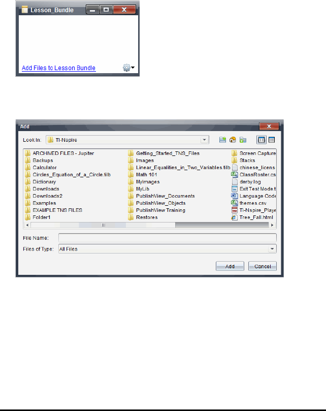
• When working in the Documents Workspace, open the Content Explorer and
then double-click the lesson bundle file name.
• When working in the Content Workspace, double-click the lesson bundle name.
Note: In the Content Workspace, you can also click the lesson bundle name to
open the Files dialogue box in the Preview pane. The Add Files to Lesson
Bundle option is available from the Files dialogue box. If the lesson bundle
already contains files, the first file in bundle is shown in the Files dialogue box.
The lesson bundle dialogue box opens. The name reflects the name of the lesson
bundle.
2. Click Add Files to Lesson Bundle.
The Add dialogue box opens.
3. Navigate to and select the file you want to add to the lesson bundle.
• You can select multiple files at one time if they are located in the same folder.
• If files are located in different folders, you can add them one at a time.
• You cannot create a folder within a lesson bundle or add a folder to a lesson
bundle.
4. Click Add to add the file to the bundle.
The file is added to the bundle and is now listed in the lesson bundle dialogue box.
Working with Lesson Bundles 108
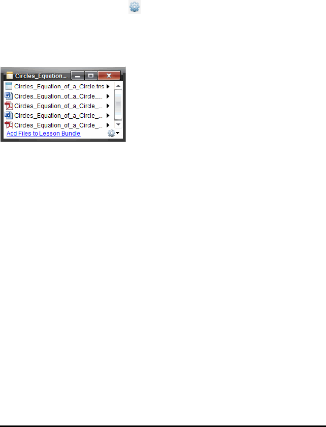
109 Working with Lesson Bundles
5. Repeat this process until all needed files are added to the lesson bundle.
Opening a Lesson Bundle
To view and work with files within a lesson bundle, complete one of the following
steps to open the lesson bundle file.
▶Double-click the lesson bundle name.
▶Select the lesson bundle, and then right-click and click Open.
▶Select the lesson bundle, click , and then click Open.
▶Select the lesson bundle, and then press Ctrl + O. (Mac®: “+ O).
When you open a lesson bundle, the files in the bundle are displayed in a separate
dialogue box.
Note: You cannot open a lesson bundle outside of the TI-Nspire™ software. For
example, if you open the folder using the file manager on your computer and double-
click the lesson bundle name, it does not automatically launch the TI-Nspire™
software.
Opening Files Within a Lesson Bundle
You can open any file within a lesson bundle on your computer if you have the
programme associated with the file type.
• When you open a .tns or .tnsp file, the file opens in the Documents Workspace in
the TI-Nspire™ software.
• When you open another file type, it launches the application or programme
associated with that file. For example, if you open a .doc file, it opens in
Microsoft® Word.
Use one of the following options to open a file within a lesson bundle:
▶Double-click the lesson bundle, and then double-click a file within the lesson
bundle.
▶Within a lesson bundle, select the file and then click ¢or right-click the file name
and select Open.
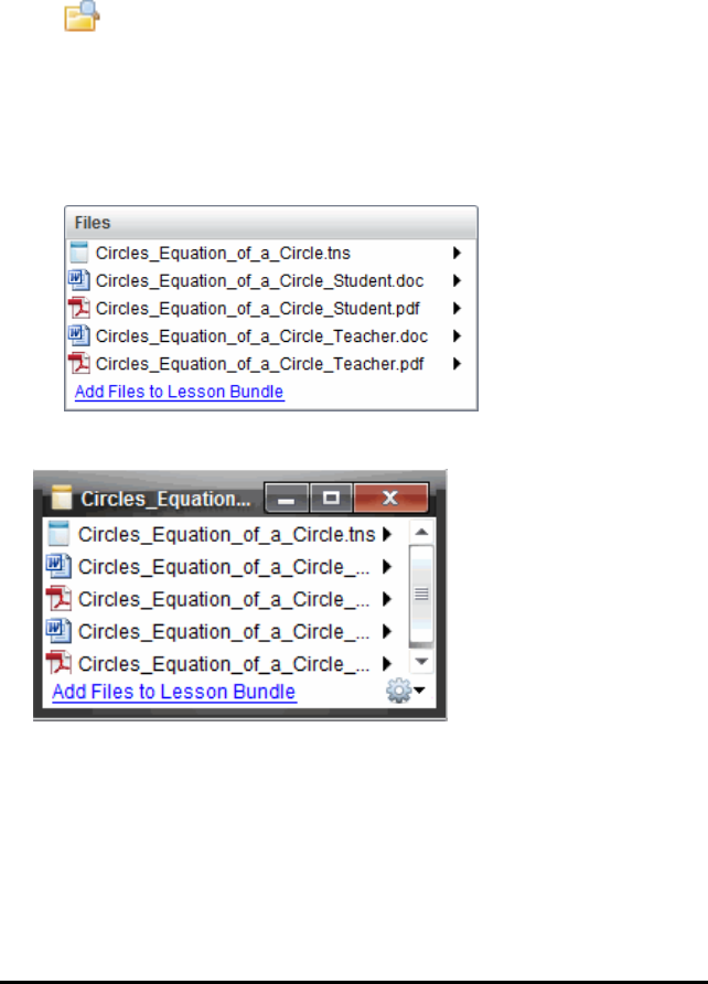
Managing Files in a Lesson Bundle
You can open, copy/paste, delete and rename files in an existing lesson bundle. To
locate and work with files in an existing lesson bundle:
1. Choose one of the following options to locate an existing lesson bundle.
• When working in the Documents Workspace, open the Content Explorer (click
in the Documents Toolbox), and then navigate to the folder where the
lesson bundle is located.
• When working in the Content Workspace, navigate to the folder where the
lesson bundle is located in Content pane.
Note: When you click a lesson bundle name in the Content pane, the Files
dialogue box opens in the Preview pane. Select a file and right-click to open the
context menu.
2. Double-click the lesson bundle name to open the Lesson Bundle dialogue box.
3. Select the file you want to work with and click ¢to open the context menu.
Working with Lesson Bundles 110
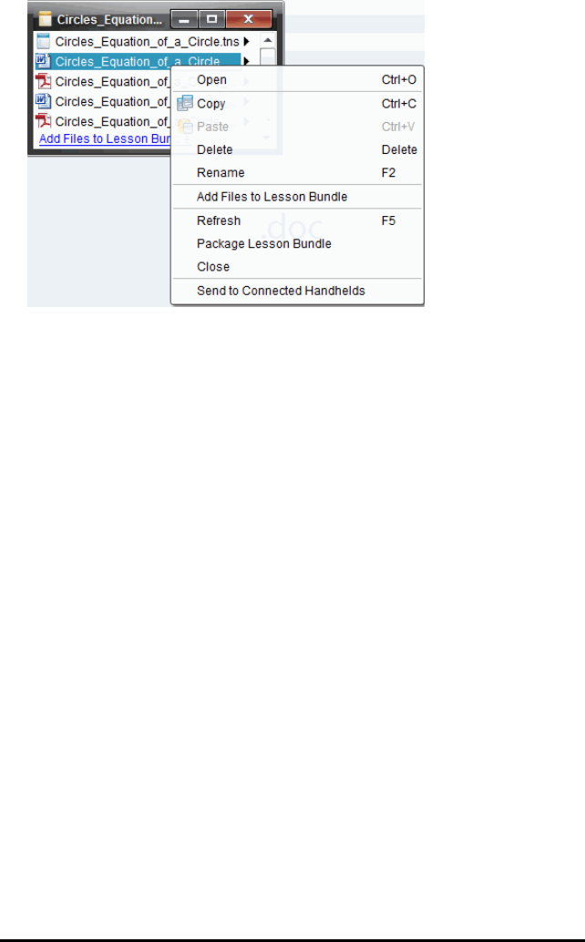
111 Working with Lesson Bundles
4. Click the action you want to perform:
• Click Open. TI-Nspire™ and PublishView™ documents open in the Documents
Workspace. When you open another file type, it launches the application or
programme associated with that file.
• Click Copy to place the file in the Clipboard.
• Navigate to a folder on your computer or select a connected handheld or
laptop, and then right-click and click Paste to place the copied file in a new
location.
• Click Delete to delete a file from the lesson bundle. Use caution when deleting
a file from a lesson bundle. You should ensure files contained in the bundle are
backed up if you need the files for future use.
• Click Rename to give the file a new name. To cancel this action, press Esc.
• Click Add Files to Lesson Bundle to select and add files to the bundle.
• Click Refresh to update the list of files in the bundle.
• Click Package Lesson Bundle to create a .tilb file
• Click Send to Connected Handhelds to open the Transfer Tool and send the
selected file to connected handhelds. You can send .tns files and OS files.
Note: This option is not available in the TI-Nspire™ Navigator™ NC Teacher
Software.
5. When finished, click Close to close the dialogue box.
Managing Lesson Bundles
Use the options menu or the context menu to copy, delete, rename or send a lesson
bundle to connected handhelds or laptops. You cannot add a folder to a lesson bundle.
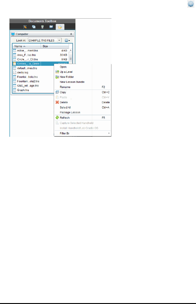
Managing Lesson Bundles in the Documents Workspace
1. Open the Content Explorer, and then right-click the lesson bundle name or click
to open the context menu.
2. Click the action you want to perform. If an action is not available, it is dimmed.
• Click Open to open the lesson bundle.
• Click Up One Level to navigate up a level in the folder hierarchy.
• You cannot add a folder to a lesson bundle. If you click New Folder, a new
folder is added to the folder where the lesson bundle is stored.
• Click New Lesson Bundle to create a new lesson bundle. The new lesson bundle
is not added to the existing lesson bundle—it is created in the same folder as
the existing lesson bundle.
• Click Rename to change the name of the lesson bundle. Press Esc to cancel this
action.
• Click Copy to copy the lesson bundle to the Clipboard.
• Navigate to another folder, and then click Paste to copy the lesson bundle in
another location.
• Click Delete to delete the lesson bundle. Use caution when deleting a lesson
bundle. You should ensure files contained in the bundle are backed up if you
need the files for future use.
•Select All highlights all files in the open folder. This action does not apply to
lesson bundles.
• Click Package Lesson to create a .tilb file.
• Click Refresh to update the list of files in the open folder.
Working with Lesson Bundles 112
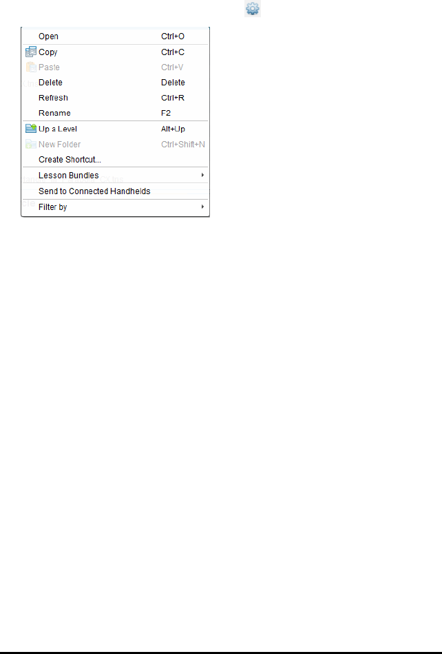
113 Working with Lesson Bundles
Managing Lesson Bundles in the Content Workspace
1. Click Local Content in the Resources pane.
2. In the Content pane, navigate to the lesson bundle you want to work with, and then
right-click to open the context menu or click to open the menu of options.
3. Select the action you want to perform:
• Click Open to open the lesson bundle.
• Click Copy to place the lesson bundle file in the Clipboard.
• Navigate to a folder on your computer or select a connected handheld, and
then right-click and click Paste to place the copied file in a new location.
• Click Delete to delete the lesson bundle. Use caution when deleting a lesson
bundle. You should ensure files contained in the bundle are backed up if you
need the files for future use.
• Click Refresh to update the list of files in the bundle.
• Click Rename to give the lesson bundle a new name. To cancel this action,
press Esc.
• To move up a level in the folder hierarchy, click Up a Level.
• To add the lesson bundle to the list of shortcuts in Local Content, click Create
Shortcut.
• To add more files to the lesson bundle, click Lesson Bundles >Add Files to
Lesson Bundle.
• Click Lesson Bundles > Package Lesson Bundle to create a .tilb file.
• Click Send to Connected Handhelds to open Transfer Tool and send the lesson
bundle to connected handhelds. (This option is not available in TI-Nspire™
Navigator™ NC Teacher Software.)
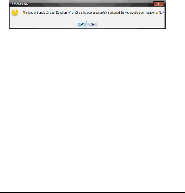
Packaging Lesson Bundles
Packaging lesson bundles creates a “package” folder with a .tilb file. This file contains
all files contained in the lesson bundle. You must package the lesson before you can
email the lesson bundle (.tilb file) to colleagues or students. By default, the lesson
bundle is saved in the following folder:
...\TI-Nspire\New Lesson Bundle1.tilb\package\...
Packaging a Lesson in the Documents Workspace
1. Open the Content Explorer.
2. Navigate to the folder where the lesson bundle is saved.
3. Select the lesson bundle you want to package.
4. Right-click to open the context menu, and then click Package Lesson.
The Lesson Bundle dialogue box opens confirming that the .tilb file was created
and the lesson bundle was successfully packaged.
5. Click Yes to open the folder where the lesson package is stored. Click No to close
the dialogue box.
Packaging a Lesson in the Contents Workspace
1. In Computer Content, navigate to the folder that contains the lesson bundle you
want to package.
2. Click the lesson bundle in the Content pane. The Lesson Bundle details are
displayed in the Preview pane.
3. Use one of the following methods to create the package:
• From the Preview pane, click ¢in the Files dialogue box, and then click Package
Lesson Bundle.
• From the Content pane, right-click the lesson bundle name, and then click
Lesson Bundles > Package Lesson Bundle.
The Lesson Bundle dialogue box opens confirming that the lesson bundle was
created.
4. Click Yes to open the folder where the lesson package is stored. Click No to close
the dialogue box.
Emailing a Lesson Bundle
After a lesson bundle is packaged, you can email the .tilb file to other teachers or
students. To attach the lesson bundle to an email:
Working with Lesson Bundles 114

115 Working with Lesson Bundles
1. In your email client, select the option needed to attach a file, and then navigate to
the .tilb folder.
2. Make sure you open the folder and select the .tilb file to attach to the email. You
cannot email the .tilb folder.
Sending Lesson Bundles to Connected Handhelds
Note: This option is not available in TI-Nspire™ Navigator™ NC Teacher Software.
1. Complete one of the following actions to select a lesson bundle:
• In the Documents Workspace, open the Content Explorer, and then select the
lesson bundle you want to send.
• In the Content Workspace, navigate to the lesson you want to send in the
Content pane.
2. Drag the lesson bundle file to a connected handheld. You can also copy the lesson
bundle, and then paste it to a connected handheld.
The lesson bundle is transferred to the handheld as a folder with the same name. Only
.tns files are transferred to the handheld.

Capturing Screens
Screen Capture enables you to:
•Capture Class
- View and monitor all student screens at one time, which allows you to ensure
all students are on track with an assignment.
- Capture one or several student screens for discussion in the classroom. You can
hide student names to focus the discussion on the lesson or concept, and not
on individuals.
- Select and display an individual student screen and view work as a live
presentation.
- Capture screen stacks that enable you to check student progress or collect
student assignments for later review.
- Save captured images as .jpg, .gif or .png files, which can be inserted into
TI-Nspire™ applications that allow images.
•Capture Page
- Capture the active page in a TI-Nspire™ document from the software or from
the TI-SmartView™ emulator as an image.
- Save captured images as .jpg, .gif, .png or .tif files, which can be inserted into
TI-Nspire™ applications that allow images.
- Copy and paste images into another application such as Microsoft® Word.
•Capturing Images in Handheld Mode
- In the Documents Workspace, use the DragScreen feature to capture the
emulator screen or side screen when the TI-SmartView™ Emulator is active.
- Teachers can use this feature to drag and paste an image to presentation tools
such as SMART® Notebook, Promethean’s Flipchart and Microsoft® Office
applications including Word and PowerPoint®.
Accessing Screen Capture
The Screen Capture tool is available from all workspaces. To access Screen Capture:
▶From the menu bar, click Tools >Screen Capture.
▶From the toolbar, click .
Using Capture Class
In the classroom, use the Screen Capture tool to view and capture student screens. You
can capture the screen of one selected student, of multiple selected students or of all
the students in the class.
Capturing Screens 116
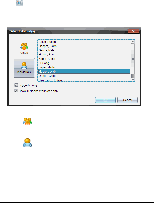
117 Capturing Screens
In the TI-Nspire™ Navigator™ NC Teacher Software, you can select to view only the
work area of the software on the student screens, or the entire computer screen,
which may include all applications the student has open at the time.
Note: To view and capture student screens, they must be logged in to class.
Capturing Student Screens
1. If you have not already done so, begin the class session and ask your students to
log in.
2. Click , and then click Capture Class.
The Select Individual(s) dialogue box opens. If you selected students in Class
Workspace, those student names are highlighted. If no students were selected, all
student names in the class are selected.
3. To change the selected student or add more students:
• Click to display the screens of all students in the class. If a student is not
logged in, the handheld display indicates "Not Logged In". As students log in,
click refresh to update your screen.
• Click , and then click the name of each student to display the screens of
individual students. To select multiple students, hold down the Shift key. To
select students in random order, hold down the Ctrl key (Mac®: “) and click
each student name.
• Select the Logged in only checkbox under the left pane to display screens from
only those students currently logged in. When you refresh your screen, any
students who log in after the initial screen capture will be listed at the end of
the Class Screen Capture window.
4. Click OK.
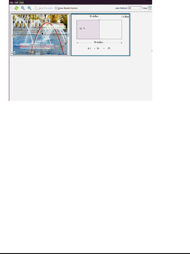
To view only the work area and not the entire student’s screen, select Show TI-
Nspire Work Area Only.
The screens of the selected students are displayed in the Class Screen Capture
window.
Note: The following example shows the screens from two selected students who
are logged in. The default view is Tiled, which shows all screens captured in the
window.
5. Decide if you want to display or hide the student names. To hide or show student
names, select the checkbox on the toolbar to toggle between hide and show or
click View > Show Student Names.
Note: Your selection to show or hide student names remains in effect until you
change it. For example, if you select to hide student names, the student names will
remain hidden when you close the Class Screen Capture window and return to the
Class Workspace. If you select to hide student names in the Class Workspace, they
will be hidden when the Class Screen Capture window opens.
Randomising Captured Screens
Use the Teacher Preferences option to set the randomise screen option.
1. From the Class Workspace, click File > Settings > Teacher Preferences.
The Teacher Preferences dialogue box opens.
Capturing Screens 118
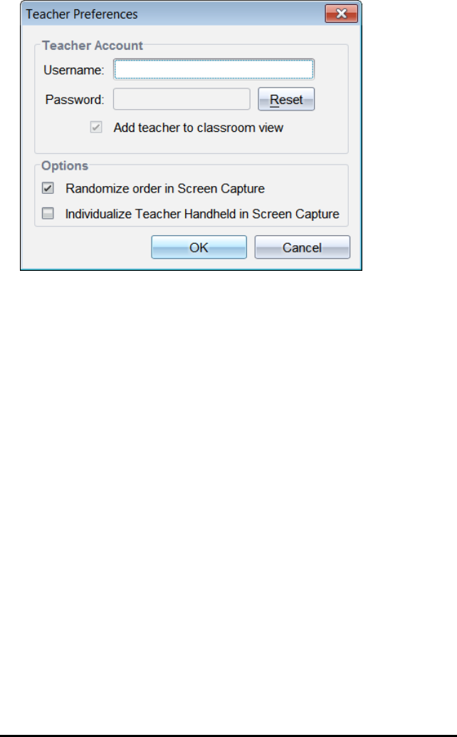
119 Capturing Screens
2. To randomise the order in which screens are captured, select Randomize order in
Screen Capture.
3. Click OK to save the settings.
Setting View Options in Capture Class
You have several options for optimising the view of captured class screens, including:
• Toggling between a tiled view and a gallery view.
• Comparing selected screens in a side-by-side view.
• Refreshing the view as needed or setting the auto-refresh feature to automatically
refresh the view at timed intervals.
• Zooming in or out to increase or decrease the size of the captured screens in the
window. You can also select the percentage at which the size of the screen will be
increased or decreased.
• Showing or hiding student names.
• Accessing Live Presenter options. For more information, see Using Live Presenter.
Toggling Between Tiled and Gallery Views
When you capture student screens, the default view for the Class Screen Capture
window is Tiled. Switch to Gallery view to show an enlarged view of a selected screen.
Thumbnail views of all the captured screens are shown in the left pane, enabling you
to find and select screens.
To toggle between Tiled and Gallery views:
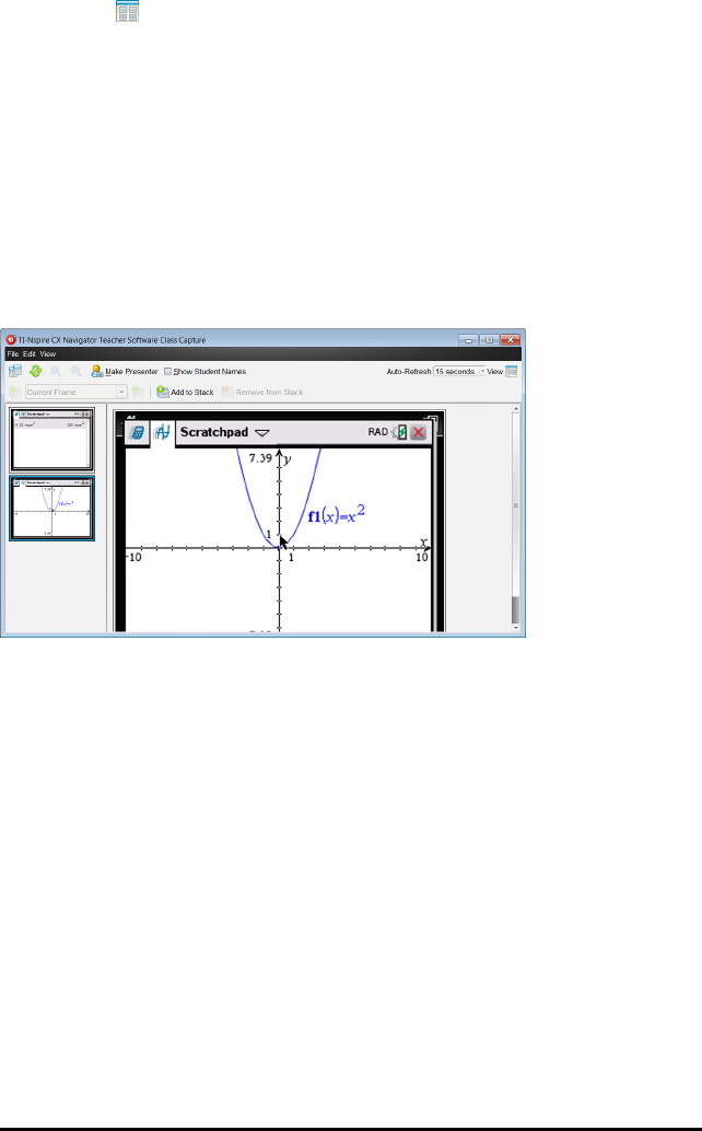
▶Click View , and then click Gallery or Tiled.
—or—
▶From the View menu, select Gallery or Tiled.
—or—
▶For Gallery view, press Ctrl + G. (Mac®: “+ G). For Tiled view, press Ctrl + T
(Mac®:“+T).
In Gallery view, thumbnail images of captured screens are displayed in a column in the
left pane of this view. An enlarged view of a selected screen is displayed in the right
pane.
• If you select multiple thumbnails to view in the left pane, they are displayed in the
right pane.
• If you select more than four thumbnails, view the additional screens by scrolling
down the right pane.
• If you selected to show student names, names are centred under each student’s
captured screen.
• Zoom functions are disabled in Gallery View.
• You can change the order of the screens in the Gallery View.
• The width of the thumbnail pane cannot be changed.
Rearranging Captured Screens
Changing the order of captured screens in one view (Tiled or Gallery) automatically
changes it in the other view.
Capturing Screens 120
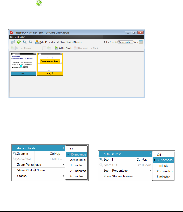
121 Capturing Screens
▶In Tiled view, drag the screen to its new position.
▶In Gallery view, drag the screen's thumbnail up or down to its new position.
As you drag, a vertical bar shows the point at which the screen will be inserted.
Note: To cancel the move before releasing the mouse button, press Esc.
Refreshing Captured Screens
As students log in to class and work on their screens, you might want to update the
captured screens.
Refreshing Screens Manually
▶Click Refresh .
Note: If a student has lost connection and a screen cannot be refreshed, it is
outlined in yellow.
Refreshing Screens Automatically
The auto-refresh feature recaptures class screens at timed intervals. The default
setting for the auto-refresh feature is Off. To enable auto-refresh:
▶On the View menu, click Auto Refresh, and select a time interval.
TI-Nspire™CX Navigator™
Teacher Software
TI-Nspire™Navigator™NC
Teacher Software
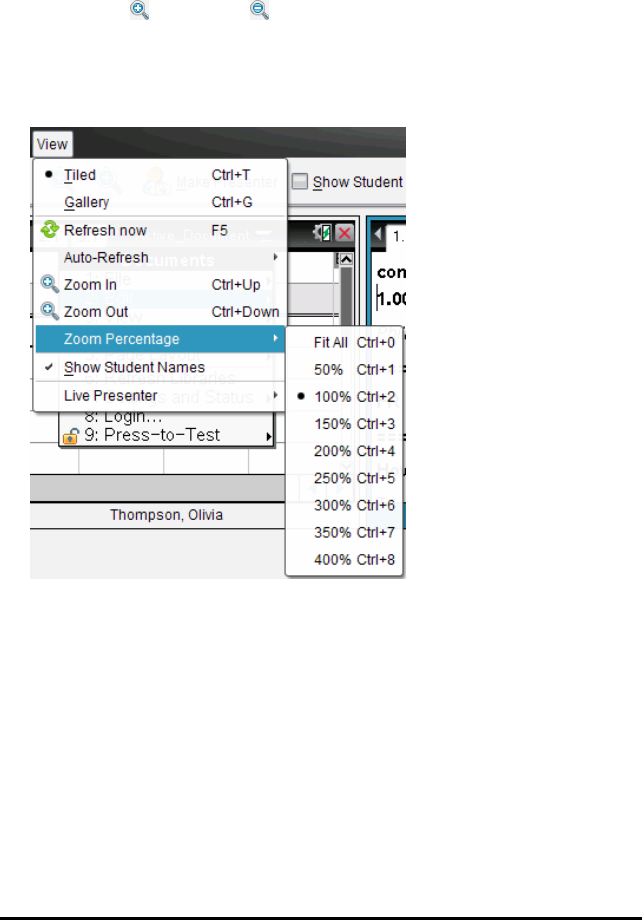
Zooming in and Zooming out
In the Tiled view only, you can magnify or shrink the views of the captured screens.
▶To zoom to levels between 50% and 400% in 50% increments:
Click Zoom In or Zoom Out on the toolbar.
–or–
Click View>ZoomIn or View>ZoomOut from the menu.
▶To zoom to a selected level, click View > Zoom Percentage, and select the level.
Creating Stacks of Student Screens
This feature enables you to collect a history of one or more students’ screens captured
in the Capture Class option. These collections are called stacks, and you can add or
remove screens from each student’s stack, as well as navigate within and through
student stacks. Using stacks is a convenient way to check progress in a lesson, collect
student presentations or assignments to review and mark later, or to show
performance and progress in parent/teacher meetings.
You add, remove, navigate and save stacks from the Class Capture window, which
becomes available when you use the Capture Class option.
▶To open the Class Capture window, click Window> Class Capture Window.
Capturing Screens 122
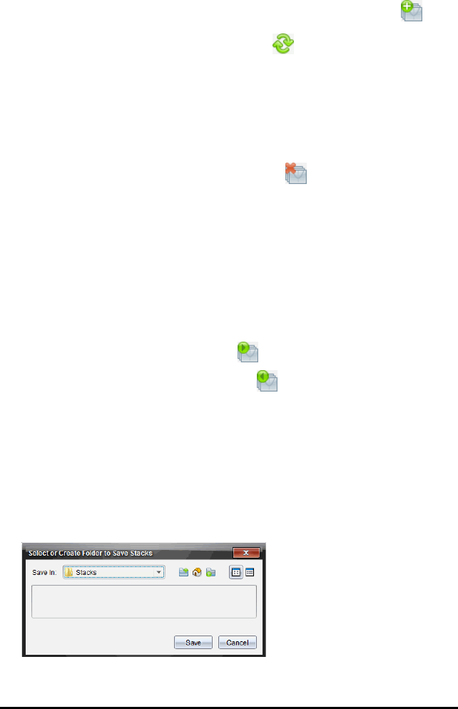
123 Capturing Screens
Adding Screens to a Stack
▶In the Class Capture window, click View> Stacks > Add to Stack, or click .
▶To add another set of screens, first click Refresh , and then add the stack.
When the first set of screens is added to a new stack, it is labelled Frame1. Each
subsequent addition increases the number by one; for example, Frame2, Frame3 and
so forth.
Removing Frames from a Stack
1. Select the frame you want to remove.
2. Click View> Stacks > Remove from Stack, or click .
As frames are removed from a stack, their names are adjusted to remain sequential
and reflect the deletion. For example, if Frame6 is deleted, Frame7 is renamed to
Frame6 and all subsequent frame numbers are adjusted downward by one digit.
Navigating Through Stacks
You can navigate a stack of frames from either the tiled or gallery view.
▶To view different frames in a stack, use one of these options:
• Click the drop-down arrow, and then click the desired frame from the list.
•View > Stacks > Next Frame, or click .
•View > Stacks > Previous Frame, or click .
Note: These options are available only if there is a next or previous frame to view.
Saving Stacks
When you close the Class Capture window, the software asks if you want to save the
stacks.
1. Click Yes to save the stacks.
The Select or Create Folder to Save Stacks dialogue box opens.

2. Click Save to save the stacks in the default folder, or create or navigate to another
folder, and then click Save.
The stacks are saved as individual screen captures with the student’s name, image
number, date and time. For example:
Laxmi Chopra_image1_10-21-2011_11-50
Laxmi Chopra_image2_10-21-2011_11-57
Use the Content Workspace or your computer’s file management system to locate and
open the saved screens.
The screens open in the default photo viewer on your computer.
Comparing Selected Screens
This feature enables you to compare student screens side-by-side.
1. Select the student screens you want to compare. To select multiple consecutive
screens, hold down the Shift key. To select screens in random order, hold down the
Ctrl key (Mac®: “) and click each image you want to save. When you select each
screen, the border changes colour.
Note: If you select more than four screens, scroll down the viewing pane to see
them.
2. Click Edit > Compare Selected.
If you are in Tiled view, the view switches to Gallery view and the selected screens
are listed in the order selected.
Note: This option is disabled when in Gallery view.
3. To exit comparison mode, click outside the screen in the left pane of the Gallery
view.
Using Make Presenter
Select a captured screen from the Class Screen Capture window, and then click the
Make Presenter option on the toolbar to launch Live Presenter and present a student
screen to the class. You can only choose one student at a time to be the Live Presenter.
For more information, see Using Live Presenter.
Saving Screens When Using Capture Class
You can save captured screens for use in other TI-Nspire™ documents that allow
images or for use in other application such as Microsoft® Word. You can save images
in the following formats: .jpg, .png or .gif. You can save one image at a time, select
multiple images to save or save all captured images.
Capturing Screens 124
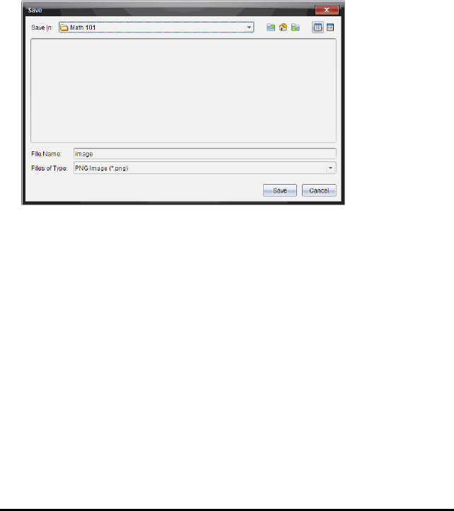
125 Capturing Screens
Saving Screen Images
To save screen images captured when using Capture Class, complete the following
steps.
1. In the Class Screen Capture window, select the screen or screens you want to save
as image files.
• To select multiple consecutive screens, click the first image, and then hold
down the Shift key and click the additional images. To select screens in random
order, hold down the Ctrl key (Mac®: “) and click each image you want to save.
• To select all captured screens, click Edit > Select All.
2. Click File > Save Selected Screen(s) or press Ctrl+S (Mac®:“+S).
The Save dialogue box opens.
3. Navigate to the folder on your computer where you want to save the file(s).
4. Type a name for the file or files in the File Name field.
The default file name is Image.
5. In the Files of Type field, click ¤, and then select the file type: .png, .jpg or .gif. The
default file type is .jpg.
6. Click Save.
The file or files are saved in the designated folder.
• If you saved one image, the file is saved with the name as specified in the File
Name field.
• If you saved multiple images, the files are saved with the name specified in the
File Name field with a number appended to the file name to make each file
name unique. For example, Image1, Image 2 and so on.
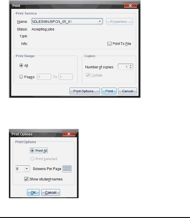
Printing Captured Screens
You can print screens captured using the Capture Class option. You can print one,
multiple or all captured screens. For each printed page, the class name is printed in the
page header and the date and page number are printed in the page footer.
Note: The print option is not available when using the Capture Page or Capture
Selected Handheld options.
To print a captured screen:
1. Select the screen you want to print.
2. Click File > Print.
The Print dialogue box opens.
3. If you selected more than one screen, click Print Options to select the number of
screen captures that you want per page.
The Print Options dialogue box opens.
Capturing Screens 126
127 Capturing Screens
4. Select options as needed. You can select to print one screen per page, six screens
per page or all screens on the page. You can also select whether to print student
names.
5. Click OK to return to the Print dialogue box.
6. Select the individual printer options for your printer.
7. Select the number of copies you want to print.
8. Click Print to send the print job to the selected printer.
Using Capture Page
Use the Capture Page option to capture an image of an active page in a TI-Nspire™
document. You can save images in the following file formats: .jpg, .gif, .png and .tif.
Saved images can be inserted into TI-Nspire™ applications that allow images. The
image is also copied to the Clipboard and can be pasted into other applications such as
Microsoft® Word or PowerPoint.
Capturing a Page
Complete the following steps to capture an image of an active page.
1. In the Documents Workspace, open a document and navigate to the page you want
to capture to make it active.
2. Click , and then click Capture Page.
The image of the active page is copied to the Clipboard and to the Screen Capture
window. The dialogue box opens in the lower right
corner of your desktop when the screen capture is complete.
3. Click View it.
The Screen Capture window opens.
You can also click Window > Screen Capture Window to open the Screen Capture
window.
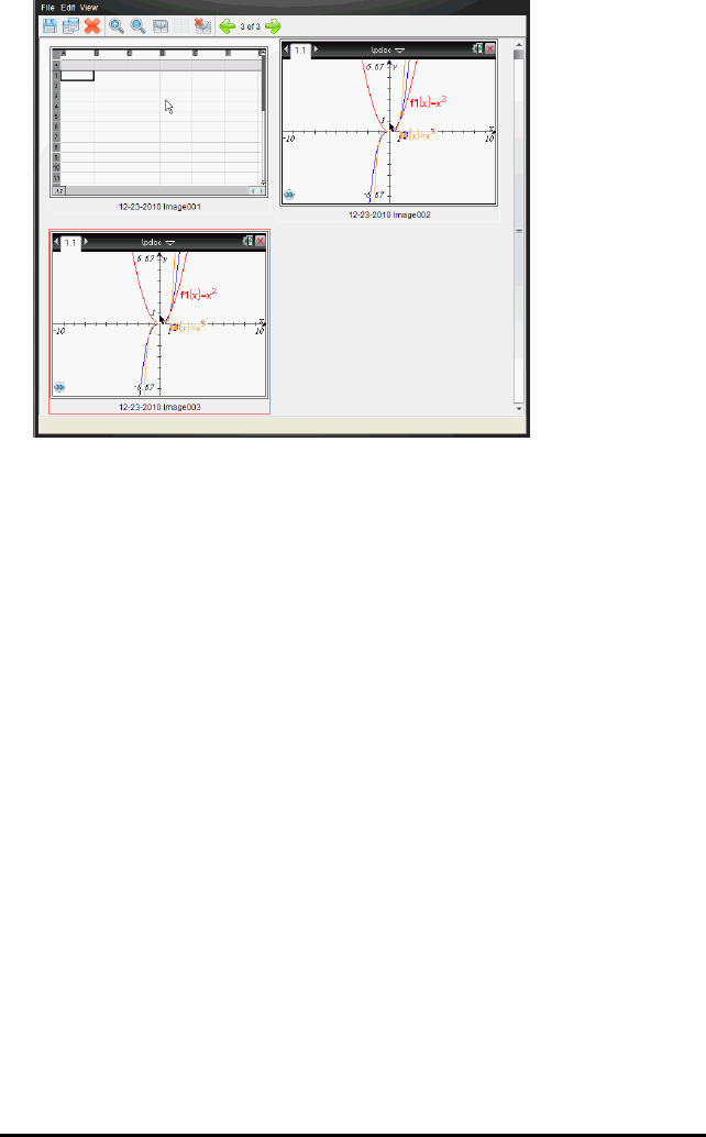
4. To capture additional pages, move to another page in the current document or
open a new document to select a page.
As you capture additional pages, the images are copied to the Screen Capture
window, which holds multiple images. The last page captured replaces the
contents of the Clipboard.
Viewing Captured Screens
When you capture a page or screen, it is copied to the Screen Capture window.
Capturing Screens 128
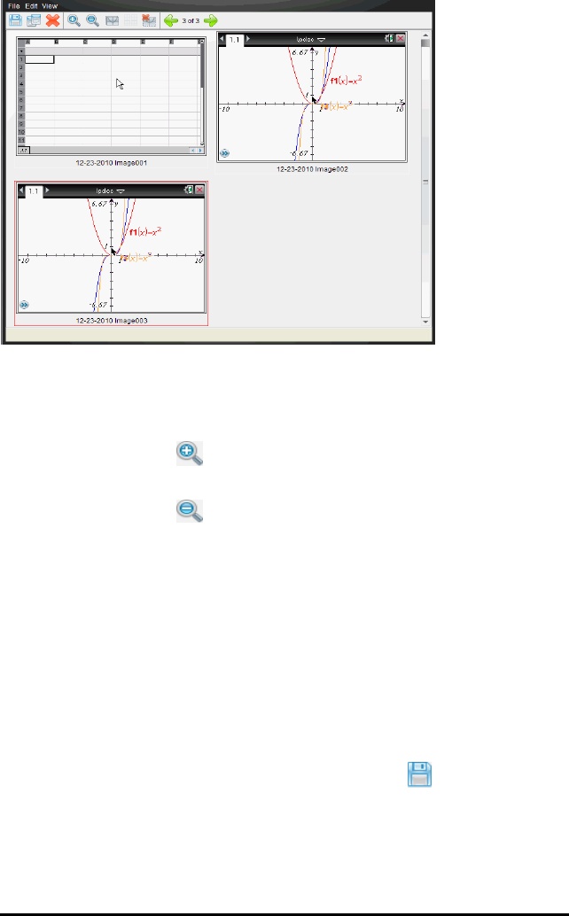
129 Capturing Screens
Zooming the View of Captured Screens
In the Screen Capture window, use the zoom in and zoom out options to increase or
decrease the size of the captured screens.
▶From the toolbar, click to increase the size of the screens in the view. You can
also click View > Zoom In from the menu.
▶From the toolbar, click to decrease the size of the screens in the view. You can
also click View > Zoom Out from the menu.
Saving Captured Pages and Screens
You can save captured pages and screens captured as images for use in other
TI-Nspire™ documents that allow images or for use in other applications such as
Microsoft® Word. You can save one image at a time, select multiple images to save or
save all captured images.
Saving Selected Screens
1. In the Screen Capture window, select the screen image you want to save.
2. Click File > Save Selected Screen(s).
Note: From the Screen Capture window, you can also click .
The Save as dialogue box opens.
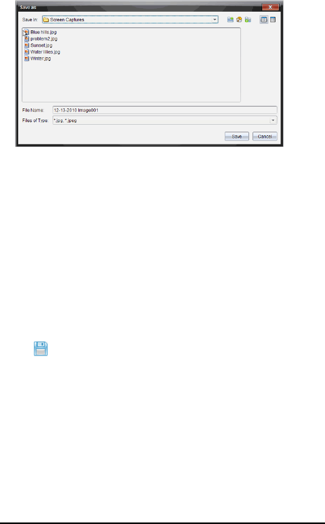
3. Navigate to the folder on your computer where you want to save the file.
4. Type a name for the file.
Note: The default file name is MM-DD-YYYY Image ###.
5. Select the file type for the image file. The default format is .jpg. Click¤to
select another format: .gif, .tif or .png.
6. Click Save.
The file is saved in the designated folder.
Saving Multiple Screens
1. In the Screen Capture window, select the screens you want to save.
To select multiple consecutive screens, click the first image, and then hold down
the Shift key and click the additional images. To select screens in random order,
press Ctrl (Mac®: “) and click each image you want to save.
2. Click or select File > Save Selected Screen(s). To save all captured screens,
select File > Save All Screens.
Note: The "Save All Screens" option is not available when using Capture Class.
The Save as dialogue box opens.
3. In the Save In field, navigate to the folder where you want to save the images.
4. In the File Name field, type a new folder name. The default folder name is MM-
DD-YYYY Image, where MM-DD-YYYY is the current date.
5. Select the file type for the image files. The default format is .jpg. Click¤to
select another format: .gif, .tif, or .png.
6. Click Save.
Capturing Screens 130
131 Capturing Screens
The images are saved in the specified folder with system-assigned names
reflecting the current date and a sequence number. For example, MM-DD-YYYY
Image 001.jpg,MM-DD-YYYY Image 002.jpg and so on.
Copying and Pasting a Screen
You can select a captured screen and copy it to the Clipboard for inclusion into other
documents or applications. You can also print copied screens. Copied screens are
captured at 100% zoom level, and they are copied in the order of selection.
Copying a Screen
1. Select the screen to copy.
2. Click or Edit > Copy.
The selected screen is copied to the Clipboard.
Pasting a Screen
Depending on the application you are pasting to, click Edit > Paste.
Note: You can also drag a screen capture to another application. This functions as a
copy and paste.
Capturing Images in Handheld Mode
In the Documents Workspace, use the DragScreen feature to capture the emulator
screen or side screen when the TI-SmartView™ Emulator is active.
Teachers can use this feature to drag and paste an image to presentation tools such as
SMART® Notebook, Promethean’s Flipchart and Microsoft® Office applications
including Word and PowerPoint®.
Capturing Images Using the DragScreen Feature
Complete the following steps to capture an image and copy it to a third-party
application.
1. From the Documents Workspace, click , which is located in the Documents
Toolbox.
The TI-SmartView™ Emulator opens.
• If the display selected is Handheld + SideScreen, the current document is shown
in the emulator and in the side screen.
• If the display selected is Keypad + SideScreen, the current document is shown in
the side screen.
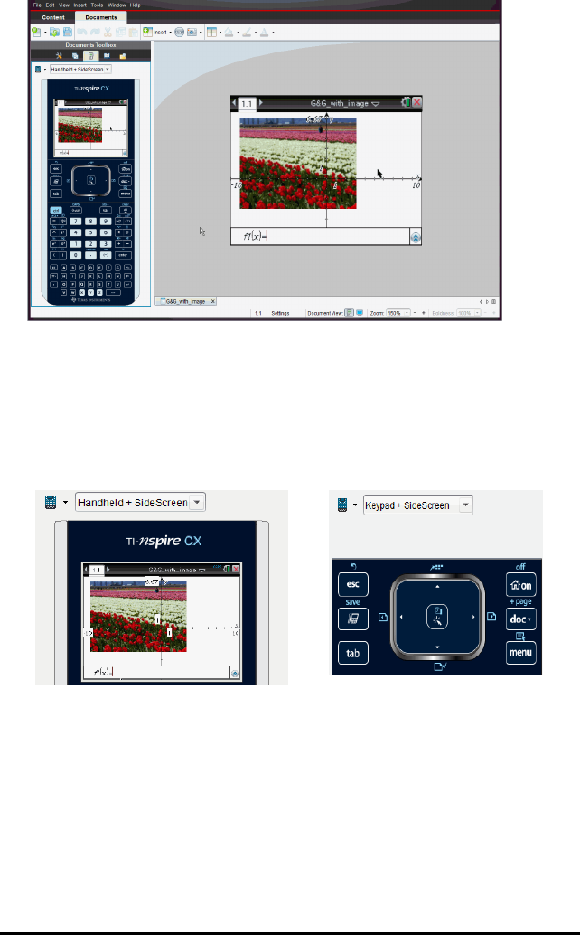
2. To start the screen capture, click the area above the emulator screen or above the
keypad. In the Handheld + SideScreen display, you can also click the area around the
emulator screen.
Do not release the mouse button. If the cursor is active or if you click inside the
emulator window, the screen capture is not started.
In Handheld + SideScreen view, click the area
above the emulator, click the area around the
emulator or click the border of the emulator
screen to start the screen capture.
In Keypad + SideScreen view, click the
area above the keypad to start the
screen capture.
3. Without releasing the mouse, drag the image.
A ghost image of the captured screen opens. The ghost image remains visible until
you release the mouse button.
Capturing Screens 132
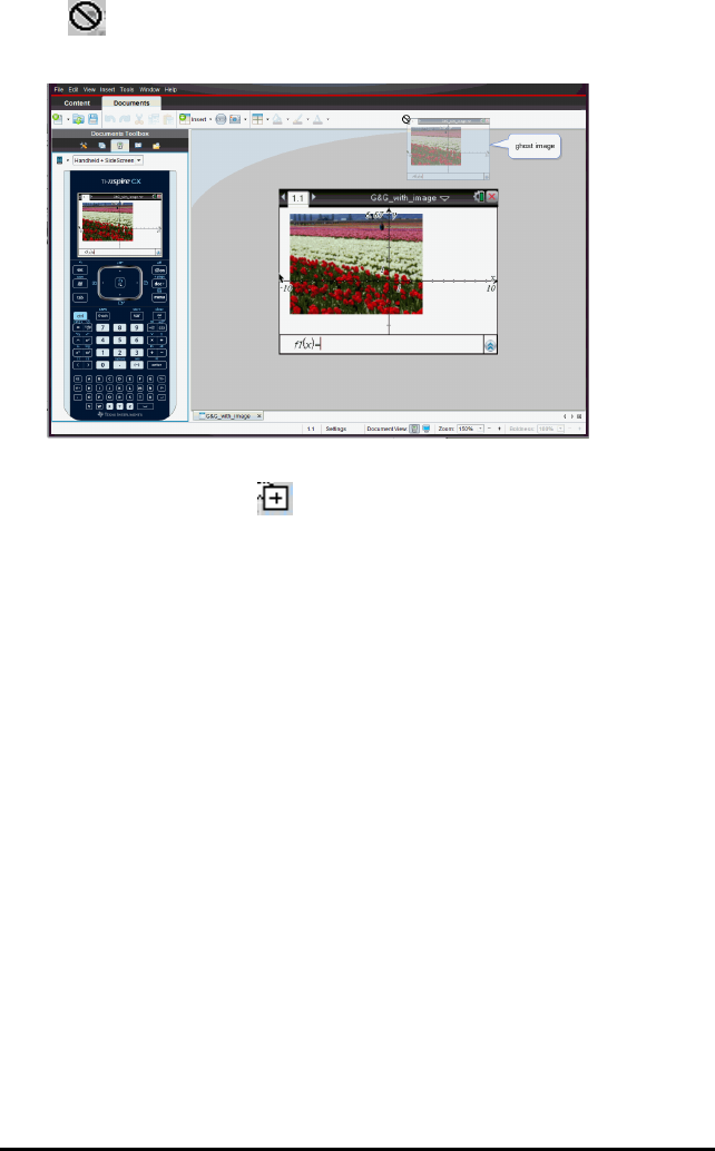
133 Capturing Screens
The in the corner of the ghost image indicates you cannot paste the image in
that location.
ghost
image
4. Drag the image to an open third-party application. When the image is on top of the
third-party application, the indicates you can drop the image.
5. Release the mouse button to drop the image into the selected application.
The image is also copied to the Clipboard and to the TI-Nspire™ Screen Capture
window.
To view captured images in the Screen Capture window, click Window > Screen
Capture Window.
You can capture additional screens as needed. As you capture additional screens,
the images are copied to the Screen Capture window, which holds multiple
images. The last screen captured replaces the contents of the Clipboard.

Working with Images
Images can be used in TI-Nspire™ applications for reference, assessment and
instructional purposes. You can add images to the following TI-Nspire™ applications:
• Graphs & Geometry
• Data & Statistics
• Notes
• Question, including Quick Poll
In the Graphs & Geometry and Data & Statistics applications, images are set in the
background behind the axis and other objects. In the Notes and Question applications,
the image is set at the cursor location in-line with the text (in the foreground).
You can insert the following image file types: .jpg, .png or .bmp.
Note: The transparency feature of a .png file type is not supported. Transparent
backgrounds are displayed as white.
Working with Images in the Software
When working in the TI-Nspire™ software, you can insert, copy, move and delete
images.
Inserting Images
In the Notes and Question applications, and in Quick Poll, you can insert more than one
image on a page. You can only insert one image on a page in the Graphs & Geometry
and Data & Statistics applications.
1. Open the document where you want to add an image.
2. Click Insert > Image.
The Insert Image dialogue box opens.
Working with Images 134
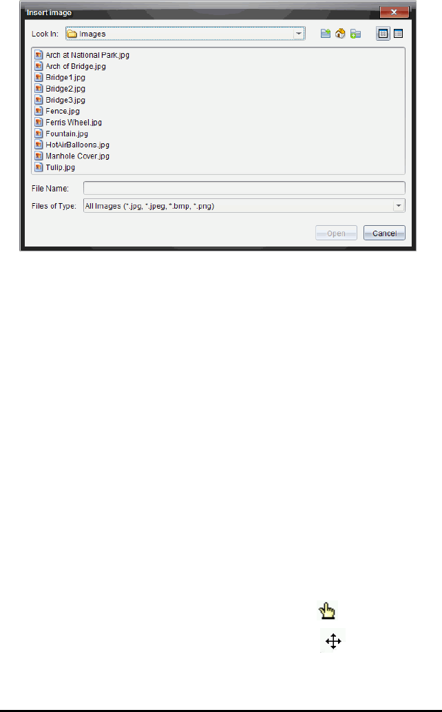
135 Working with Images
3. Navigate to the folder where the image is located and select the image.
4. Click Open.
• In the Graphs & Geometry and Data & Statistics applications, the image is
inserted in the background behind the axis.
• In Notes, Question and Quick Poll, the image is inserted at the cursor location.
You can type text above or below the image, and you can move the image up or
down on the page.
Note: You can also insert images by copying an image to the Clipboard and pasting it
into the application.
Moving Images
In applications such as Notes and Question where the image is set at the cursor
location, you can reposition the image by moving the image to a new line or blank
space, or by placing the image within a line of text. In the Graphs & Geometry and
Data & Statistics applications, images can be moved to any position on the page.
1. Select the image.
• In the Notes and Question applications, click the image to select it.
• In the Graphs & Geometry and Data & Statistics applications, right-click the
image and then click Select > Image.
2. Click the selected image and hold the mouse button.
• If an image is in the foreground, the cursor changes to .
• If an image is in the background, the cursor changes to .
3. Drag the image to the new location and release the mouse button to place the
image.
If an image is in the foreground, the cursor changes to when you hover your
mouse pointer over a location where there is a new line or space. Images in the
background can be moved and placed anywhere on the page.
Resizing Images
To retain the aspect ratio of an image, resize by grabbing the image at one of the four
corners.
1. Select the image.
• In the Notes and Question applications, click the image to select it.
• In the Graphs & Geometry and Data & Statistics applications, right-click the
image and then click Select > Image.
2. Move the cursor to one of the corners of the image.
The cursor changes to (a four-sided directional arrow).
Note: If you drag the cursor to an edge of the image, the cursor changes to (a
two-sided directional arrow). If you drag an image from one of its edges to resize
it, the image becomes distorted.
3. Click the corner or edge of the image.
The tool is enabled.
4. Drag in to make the image smaller or drag out to make the image larger.
5. Release the mouse when the image size is correct.
Deleting Images
To delete an image from an open document, complete the following steps.
1. Select the image.
• If an image is in the foreground, click the image to select it.
• If an image is in the background, right-click the image and then click Select >
Image.
2. Press Delete.
The image is removed.
Working with Images 136

137
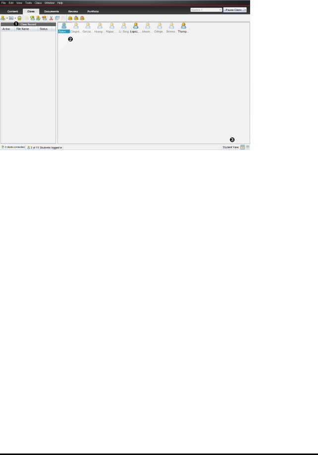
Using the Class Workspace
Use this workspace to add and manage classes and students, and to exchange files
with students.
ÀClass Record. Document actions are shown here. You can open a document in the
Review Workspace; save a document to the Portfolio Workspace; collect files from
the Class Record Workspace; send and delete files using the toolbar, and view
document properties in Record Item Properties.
ÁClassroom area. Shows the students in your class, which ones are logged in and the
status of file transfers for selected files in the Class Record. You can view the students
by Seating Chart or by Student List.
ÂStudent View. Lets you show the students in the classroom area in Seating Chart view
or Student List view.
Adding Classes
When you start using the TI-Nspire™ software, one of the first things you should do is
create your classes. Make sure you create a class for each of the class periods you plan
to teach.
If this is your first time using the TI-Nspire™ software, the classroom area may be
empty. You can complete the following steps at any time.
The Add Classes Wizard guides you through the process of setting up classes. The
software prompts you to add a class, and to add students to the class. You can choose
to add classes manually or using a CSV file.
Adding Classes Manually
1. Use the Workspace selector to select the Class Workspace.
Using the Class Workspace 138
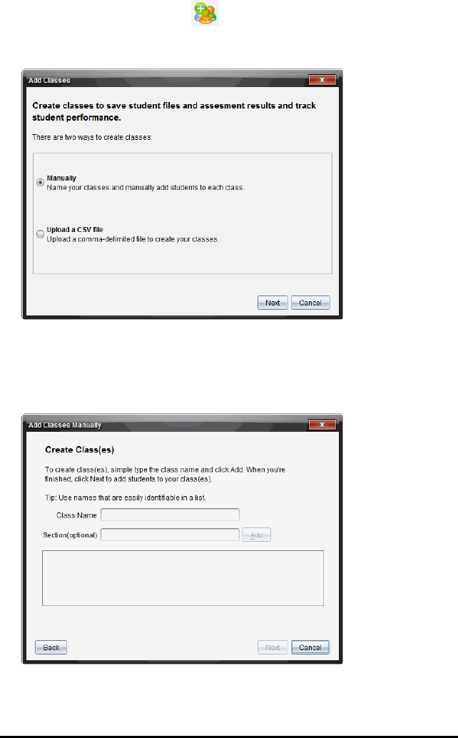
139 Using the Class Workspace
2. Click Class > Add Classes or click .
The Add Classes dialogue box opens.
3. Select Manually from the Add Classes dialogue box.
4. Click Next.
The Add Classes Manually dialogue box opens.
5. Type a Class Name. If needed, you can also provide a Section.
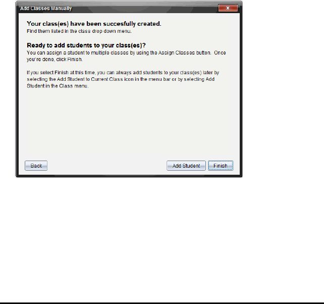
A class name must be between 3 and 32 alphanumeric characters. The class name
cannot contain the special characters / \ : " | * ? < > , and cannot contain these
words:
lpt1, lpt2, lpt3, lpt4, lpt5, lpt6, lpt7, lpt8, lpt9, com1, com2, com3, com4, com5,
com6, com7, com8, com9, aux, con, prn, nul.
Note: In the TI-Nspire™ Navigator™ NCTeacher Software, it is a good idea to
append a unique identifier such as the course ID or the teacher name to the class
name. This helps the student select the correct class if there are, for example,
multiple AlgebraI classes running.
6. Click Add.
The Add Classes Manually dialogue box shows the class listed.
7. Continue adding classes, and click Next when you are done.
A dialogue box displays showing successful class creation and asking if you want to
add students.
8. Click Add Student.
Note: Click Finish to Add Students later.
Using the Class Workspace 140
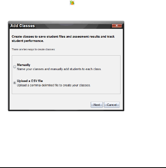
141 Using the Class Workspace
Adding Classes with a CSV Upload
You can add classes with a CSV upload, and import a list of students into the class. Use
the CSV upload option to import student information from a comma-separated values
(CSV) file or a text (.txt) file.
The CSV or .txt file should have this information:
Class Name
Section Name (optional)
Student First Name
Student Last Name
Student User Name
Student ID (optional)
Password (optional)
1. Use the Workspace selector to select the Class Workspace.
2. Click Class > Add Classes or click .
The Add Classes dialogue box opens.
3. Select Upload a CSV file from the Add Classes dialogue box.
4. Click Next.
The Add Classes by Uploading a CSV File dialogue box opens.
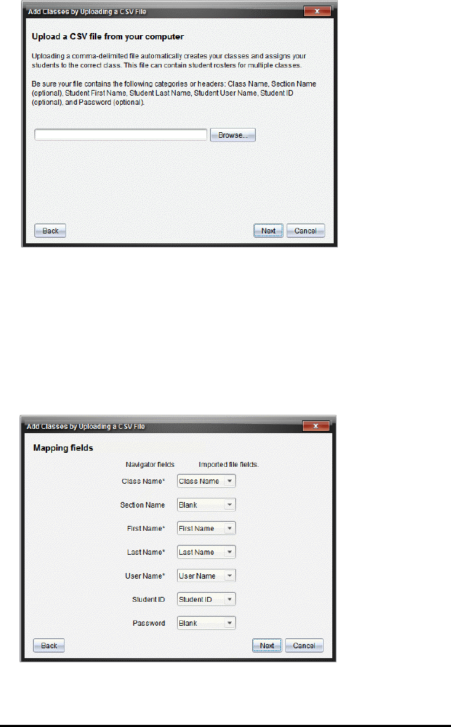
5. Click Browse to navigate to the file on your computer.
6. Select the file that contains the students you want to import.
7. Click Open.
The Add Classes by Uploading a CSV File dialogue box shows the file.
8. Click Next.
The Mapping fields dialogue box opens.
Using the Class Workspace 142
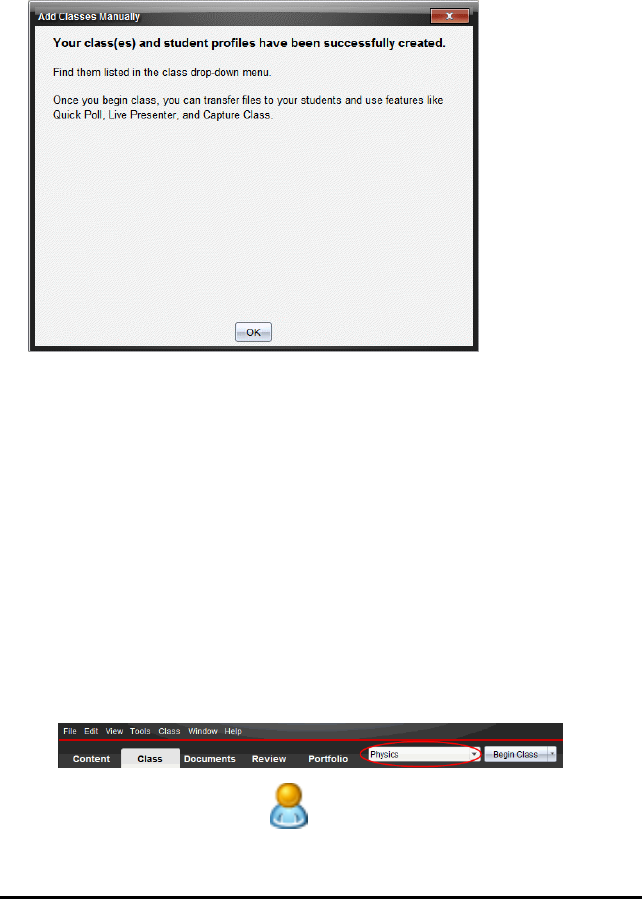
143 Using the Class Workspace
9. Click ¤and select a field from the drop-down lists to map the headings in your
comma-delimited file.
10. Click Next.
A dialogue box opens showing completion status.
11. Click OK to close
Note: If some students did not import successfully, click View Details to determine
the problem.
Adding Students to Classes
After you create classes, you need to add students to the classes. You can add students
to an active class session, or you can add students to any class at any time.
Note: These instructions explain how to add students after you create a class.
1. Select the class to which you want to add students.
• If class is in session, the student will be added to the current class. You have
the option of adding the student to other classes.
• If class is not in session, use the Class Session controls to select the class to
which you want to add the student.
2. Click Class > Add Student or click .
The Add Student dialogue box opens.
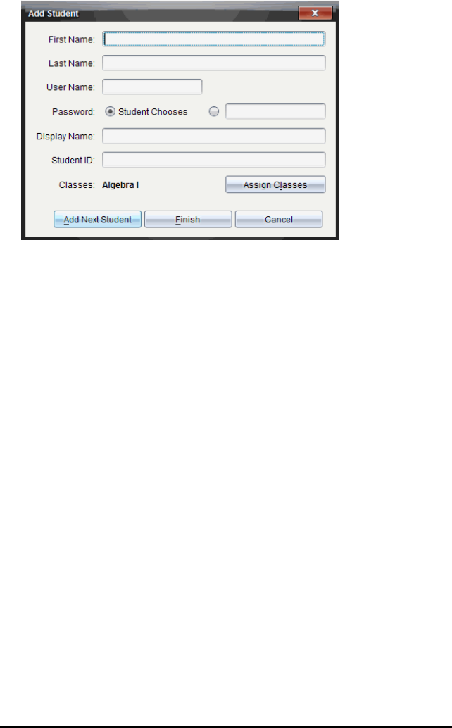
3. Type the student’s first name and last name.
4. Type a user name.
Note: The user name you choose must be unique. It cannot exist in the current
class or any other class.
5. If you want your student to create their own password, select Student Chooses.
—or—
If you want to create a password for your student, select the blank password entry
box and type a new password.
6. (Optional) Type a display name.
Note: If you leave the display name blank, the software uses the student’s first
name as the display name.
7. (Optional) Type a student ID.
8. (Optional) Assign the student to other classes:
• Click Assign Classes.
The Assign Classes dialogue box opens.
Using the Class Workspace 144
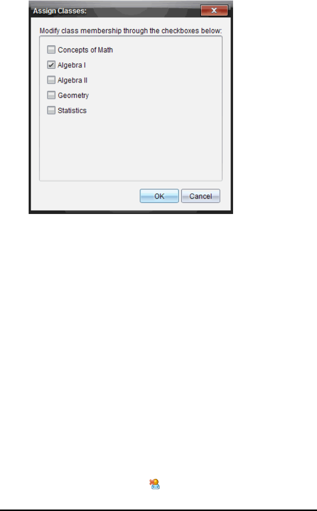
145 Using the Class Workspace
• Select the check boxes of the student’s classes.
• Clear the check boxes of the classes to which the student does not belong.
• Click OK.
The Add Student dialogue box opens.
9. If you need to add another student, click Add Next Student and repeat steps 3 – 8.
10. When all students are added, click Finish.
Removing Students from Classes
As necessary, you can remove students from your classes. When you remove students,
the TI-Nspire™ software only removes them from the selected class. If the students
are in other classes, they remain in those classes until you remove them.
Notes:
• You cannot remove students who are logged in to the TI-Nspire™ Navigator™
network.
• You cannot undo the removal of students.
• You can access many of the student account items by right-clicking the student icon
in the classroom area and choosing an action from the menu.
To remove a student from a class:
1. Click the student you want to remove.
2. Click Class > Remove Student, or click .
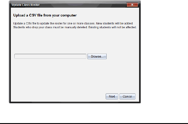
The software asks if you are sure you want to remove the student.
3. Click Yes.
The software removes the student.
Updating Class Rosters
You can update a single roster or multiple class rosters with new student information
by importing a CSV file with updates.
Note: You cannot change existing student information or remove students already in
the TI-Nspire™ Navigator™ database.
You can import a comma-separated value (CSV) file or a *.txt file. The CSV or .txt file
should have this information:
Class Name
Section Name (optional)
Student First Name
Student Last Name
Student User Name
Student ID (optional)
Password (optional)
1. Use the Workspace selector to select the Class Workspace.
2. Select the class for which you want to update the roster.
Note: Class cannot be started.
3. Click Class > Update Class Roster.
The Update Class Roster dialogue box opens.
4. Click Browse to navigate to the file on your computer.
Using the Class Workspace 146
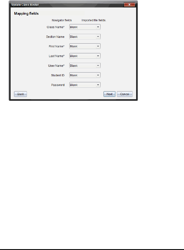
147 Using the Class Workspace
5. Select the file that contains the new students you want to import.
6. Click Open.
The Update Class Roster dialogue box shows the file.
7. Click Next.
The Mapping fields dialogue box opens.
8. Click ¤and select a field from the drop-down lists to map the headings in your
comma-delimited file.
9. Click Next.
A dialogue box displays showing completion status.
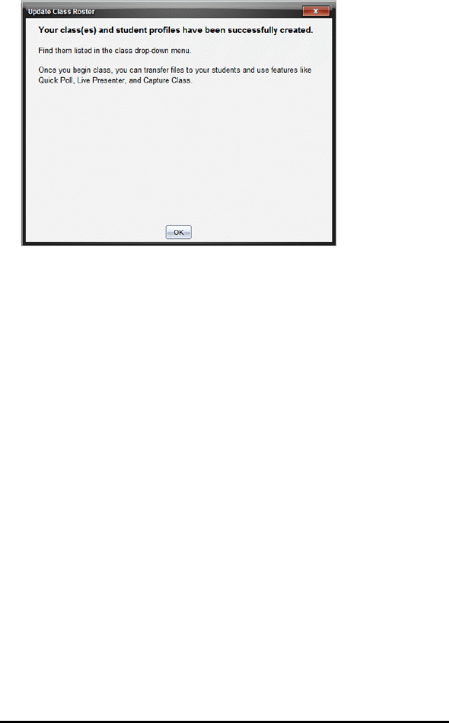
10. Click OK to close.
Note: If some students did not import successfully, click View Details to determine
the problem.
Managing Classes
You can delete classes and remove all class information from the TI-Nspire™
Navigator™ database. You can also choose to hide or show classes in menus and views.
Deleting a Class
When you delete a class, the software removes the class and removes the files on the
hard drive that correspond to that class.
Note: You cannot undo the removal of a class.
1. If you have a class session running, end it.
2. Click Class > Manage Classes.
The Manage Classes dialogue box opens.
Using the Class Workspace 148
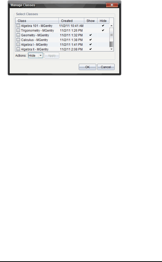
149 Using the Class Workspace
3. From the Class list, select the class you want to remove.
4. Select Delete from the Actions list.
5. Click Apply.
The software asks if you are sure you want to remove the class.
6. Click OK.
Hiding a Class
When you hide a class, the class is removed from all workspace views and menus
except for the Manage Classes dialogue box.
Note: Hidden classes are not deleted from the TI-Nspire™ Navigator™ database.
1. Click Class > Manage Classes.
The Manage Classes dialogue box opens.
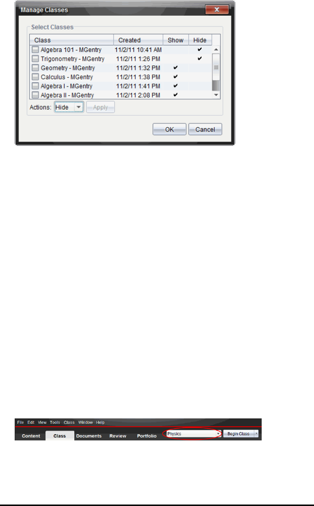
2. From the Class list, select the class you want to hide.
3. Select Hide from the Actions list.
4. Click Apply.
The software asks if you are sure you want to hide the class.
5. Click OK.
Note: Select Show from the Actions list when you want the class to show again.
Beginning and Ending a Class Session
A class session is the period of time the TI-Nspire™ software is active for a specific
class. While a class session is running, you can perform communication functions with
the selected class. You cannot use software to interact with your class until you begin a
class session, and you cannot begin another class until you end the current one.
Beginning a Class Session
1. Click Class> Select Class, or click the Classroom Session list.
A list of available classes opens.
2. Select the class you want to begin.
3. Click Begin Class.
Ending a Class Session
When class is over, or before you start another class, you need to end the current class
Using the Class Workspace 150
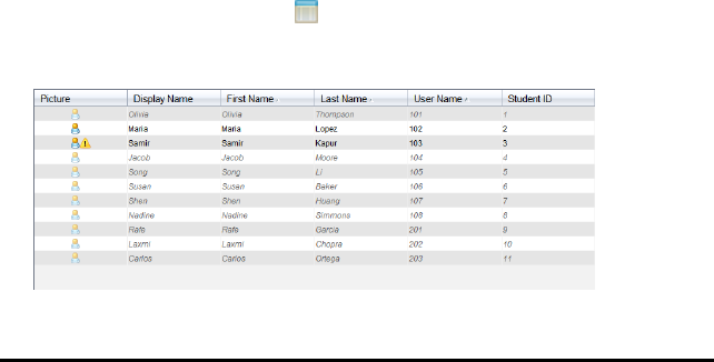
151 Using the Class Workspace
session. Ending a class stops all communication between your computer and student
handhelds or computers. When you end a class, students receive a message saying
class is ended, and students are automatically logged off.
▶To end a current class session, select End Class from the Class Actions drop down
list.
Pausing a Class Session
This function is available only on TI-Nspire™ software that supports handhelds. There
are times you may want to pause a class. If using TI-Nspire™ software that supports
handhelds, pausing a class suspends all activity on student handhelds, and they receive
a message telling them class is paused. When you resume class, the message clears
and students are able to use their handhelds. The students remain logged in when you
pause a class.
1. To pause a class in session, click Pause Class.
2. To resume the class, click Resume Class.
Changing the Student View
In the classroom area, you can view the students in the selected class in either the
Student List view or the Seating Chart view. The Student List view shows students in a
table that contains their display names, first name, last name, user name and student
ID. The Seating Chart view shows students as student icons with display names. You
can change the class view at any time.
In either view, the warning sign next to a student icon indicates that the OS on the
student's handheld does not match the software version on the teacher computer.
Moving your mouse over the warning sign opens a tool tip indicating that an OSupdate
is required.
Changing the Class View to Student List
▶Click View > Student List or click in the status bar.
The view changes to Student List.
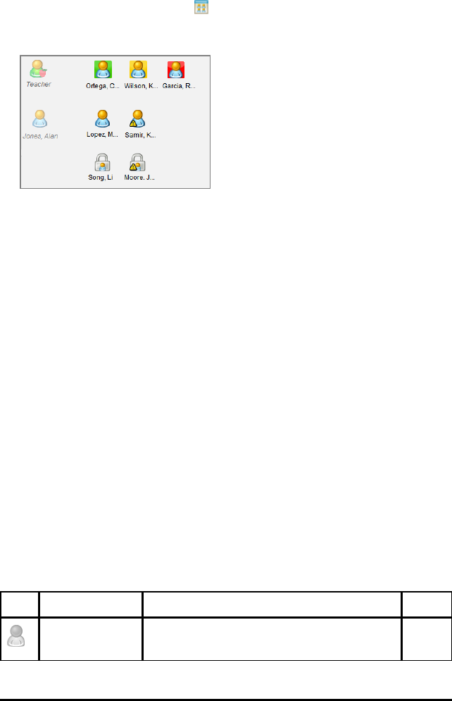
Changing the Class View to Seating Chart
▶Click View > Seating Chart or click in the status bar.
The view changes to Seating Chart view.
Arranging the Seating Chart
Initially, students are arranged in the Seating Chart view in the order that you added
them. However, you can rearrange the students so that they have the same seating
arrangement in the Class Workspace as they do in your actual classroom. You can
rearrange the seating chart at any time.
Arranging Students in the Seating Chart
1. Select the class from the Class Session list.
2. Click View > Seating Chart.
The classroom area shows your class in the Seating Chart view.
3. Within the classroom area, drag each student icon to the location that you want.
The software moves the student icons to the new locations.
The software remembers the student positions the next time you start the same
class.
Note: Do not place one student icon on top of another student icon. If you do this,
you will only be able to see one of the student’s icons.
Checking Student Login Status
You can view the students’ login status from the Seating Chart view. The colour of the
icon by the student display names indicates their login status as well as the class
status:
Icon Class status Student status Colour
Class session not
started.
N/A Grey
Using the Class Workspace 152
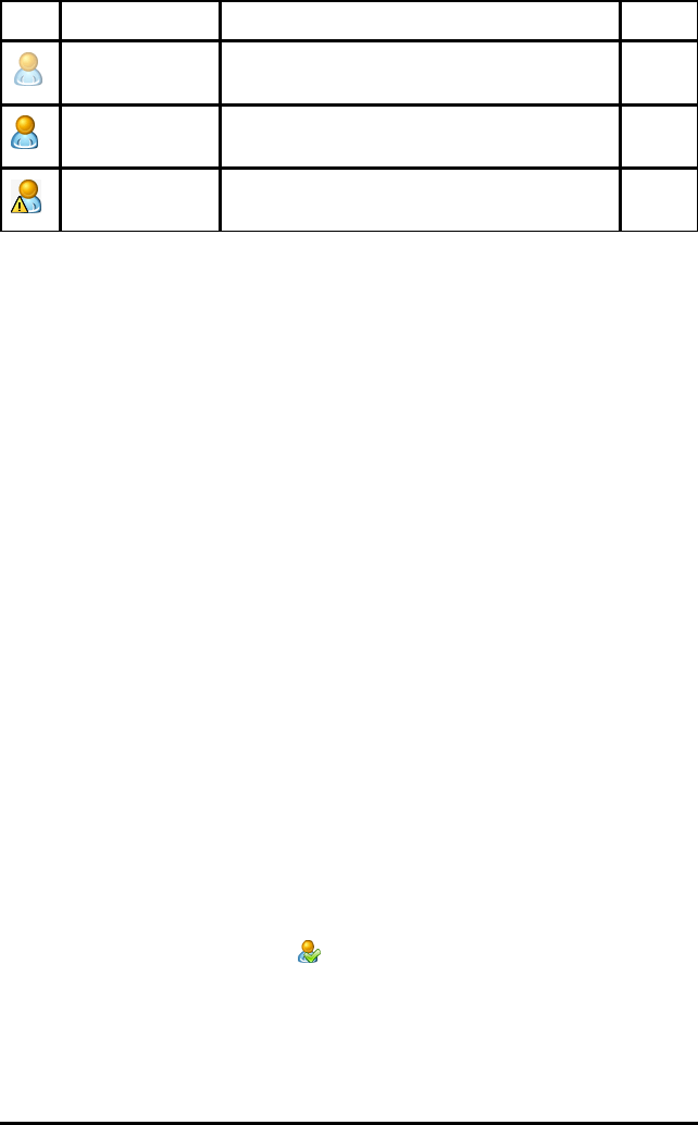
153 Using the Class Workspace
Icon Class status Student status Colour
Class session
started.
Student not logged in. Light
blue
Class session
started.
Student logged in. Dark
blue
Class session
started.
Student OS does not match software version on
teacher computer.
Dark
blue
Sorting Student Information
The Student List view in the classroom area shows the information for students in the
selected class. It includes display names, first names, last names, user names and
student IDs. In the Student List view, you can sort student information by each of these
categories. Information is sorted alphabetically from A-Z or Z-A and numerically from
1-9 or 9-1. You can sort student information at any time.
Sorting Student Information
1. Click Class >Select Class and select the class that contains the student information
you want to sort.
Note: If you have a class session running, you must end it to select the class.
2. In the menu, click View > Student List.
3. Click the column title of the list you want to sort.
The software sorts the selected list.
4. To sort the selected information in the opposite order, click the column title again.
Changing the Classes Assigned to a Student
Occasionally your students may move to a different class, or they may take more than
one of your classes. You can change student classes when necessary.
Note: You cannot change the classes of students who are logged in to the TI-Nspire™
Navigator™ network.
Changing a Student’s Class
1. Select a class to which the student belongs.
2. Click the student you want to edit.
3. Click Class > Edit Student, or click .
The Student Properties dialogue box opens.
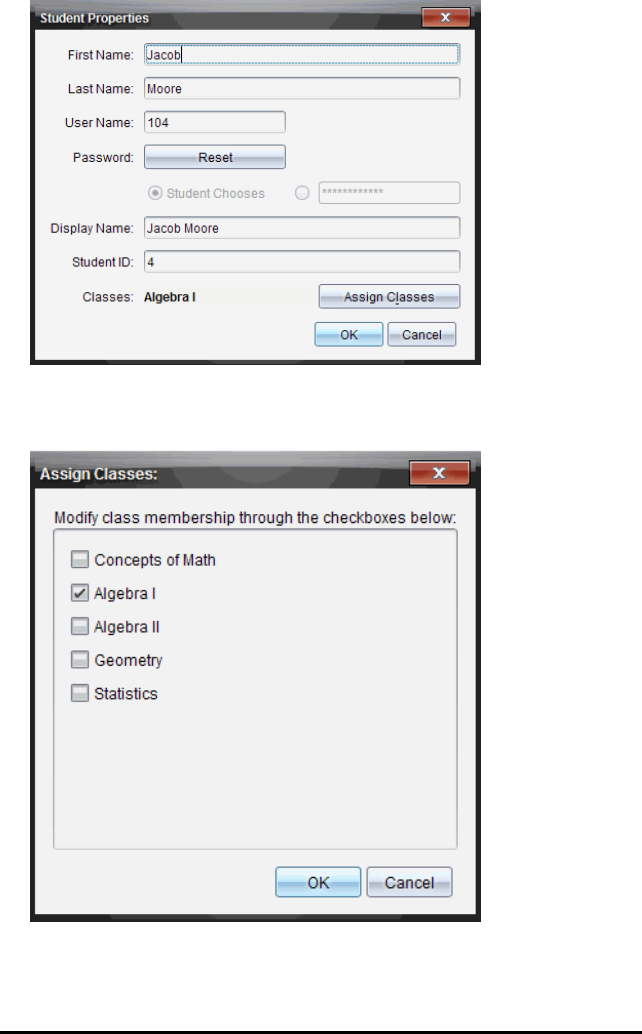
4. Click Assign Classes.
The Assign Classes dialogue box opens.
5. Select the check boxes of the student’s classes.
6. Clear the check boxes of the classes to which the student does not belong.
Using the Class Workspace 154

155 Using the Class Workspace
7. Click OK.
8. In the Student Properties dialogue box, click OK.
Changing Student Names and Identifiers
After you add students, you may find that you need to change one of their names or
identifiers. There are five different names and identifiers associated with your
students, including:
• First name
• Last name
• User name
• Display name
• Student ID
This section covers how to change any of these types of names and identifiers.
Note: You cannot change the account information of students who are logged in to the
TI-Nspire™ Navigator™ network.
Note: You can access many of the student account items by right-clicking the student
and choosing an action from the menu.
Changing Student Names or Identifiers
1. Select a class to which the student belongs.
Note: If you have a class session running, you must end it to select the class.
2. Click the student you want to edit.
3. Click Class > Edit Student, or click .
The Student Properties dialogue box opens.
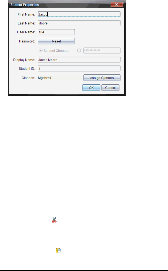
4. Click the field of the name or identifier you want to change.
5. Make the necessary changes.
6. Repeat steps 4 and 5 for any other names or identifiers you want to change.
7. Click OK.
Moving Students to Another Class
If any of your students move to a different class, you can move them within the
TI-Nspire™ software as well.
Note: You cannot move students who are logged in to the TI-Nspire™ Navigator™
network.
Note: You can access many of the student account items by right-clicking the student
and choosing an action from the menu.
Moving a Student to Another Class
1. Select a class to which the student belongs.
Note: If you have a class session running, you must end it to move the student.
2. Click the student you want to move.
3. Click Edit > Cut or click .
The software removes the student from the class and moves the student account
information to the Clipboard.
4. From the Class Session list, select the class where you want to move the student.
5. Click Edit > Paste or click .
The software moves the student to the selected class.
Using the Class Workspace 156

157 Using the Class Workspace
Copying Students to Another Class
When you have students in more than one of your classes, you may find it convenient
to copy them from one class to another. Copying students saves you the time of
entering all of their information again.
Note: You cannot copy students who are logged in to the TI-Nspire™ Navigator™
network.
Note: You can access many of the student account items by right-clicking the student
and choosing an action from the menu.
Copying a Student to Another Class
1. Select a class to which the student belongs.
Note: If you have a class session running, you must end it to select the class.
2. Click the student you want to copy.
3. Click Edit > Copy or click .
The software copies the student to the Clipboard.
4. From the Current Class dropdown list, select the class to which you want to copy
the student.
5. Click Edit > Paste or click .
The software copies the student to the selected class.
Exploring the Class Record
From the Class Record, you can open a document in the Review Workspace; save a
document to the Portfolio Workspace; collect files from the Class Record Workspace;
send and delete files using the toolbar; and view document properties in Record Item
Properties for all TI-Nspire™ documents, except Quick Poll files.
By default, 100 records are listed. To see additional records, click Load Next 100 or click
Load All Entries.
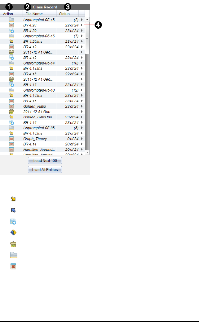
ÀFile action. The icons indicate the status of a file.
Sent to class
Collected from class
Saved to portfolio
Redistributed to class
Quick Poll
Unprompted
Deleted
ÁFile name. The names of files used in this class.
ÂStatus. The progress of an action. For example, "23 of 25" indicates that 23 out of 25
students have received a file.
ÃMenu options. Click ¢for quick access to certain menu items. This icon gives you the
Using the Class Workspace 158
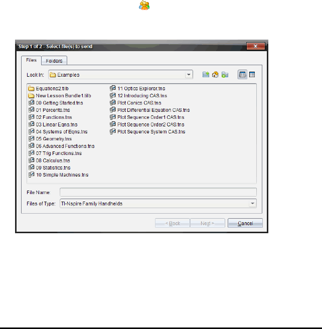
159 Using the Class Workspace
same options as a right-click.
Sending Files to a Class
You can send files and folders to your whole class, members of the class currently
logged in or to individual students. Class must be in session for you to send the files.
When you send a file to the whole class, all students currently logged in will receive
the file immediately. Students not logged in will receive the file when they log in.
Notes:
• Only TI-Nspire™ (.tns) and PublishView™ (.tnsp) file types open in the TI-Nspire™
software.
• Other file types (if supported) such as images, word processing or spreadsheet
files, open in the application the operating system has associated with the file
type.
Sending Files
1. Click Tools > Send to class or click .
The Select file(s) to send dialogue box opens.
2. Click the Files tab to choose files, or click the Folders tab to choose folders.
Note: You can send only files or folders, not a combination of files and folders.
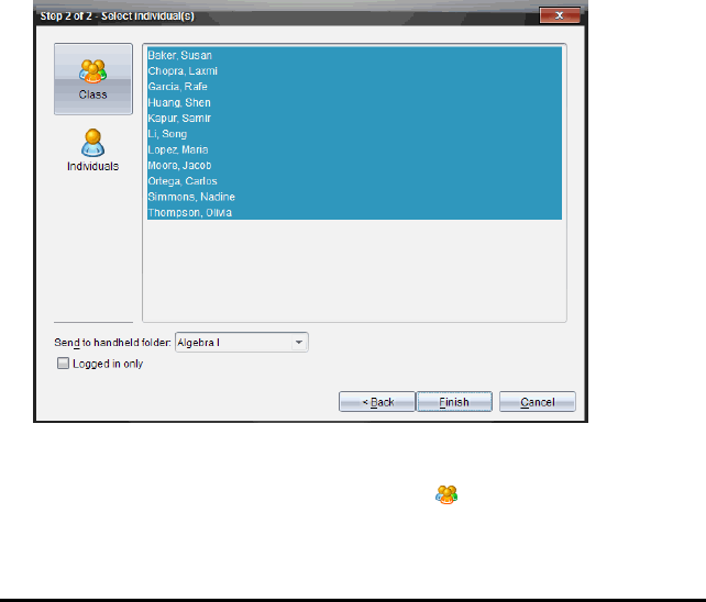
• TI-Nspire™ CX Navigator™ Teacher Software for handhelds transfers only .tns
files.
• TI-Nspire™ Navigator™ NC Teacher Software transfers all files.
3. To choose the files or folders you want to send, do one of the following:
• Navigate to the file or folder you want to send and click it. To select multiple
files or folders, press and hold the Ctrl key (Mac®: “) while clicking each file
name.
• Type the name of the file or folder in the File name or Folder name box. Folder
names may use alphanumeric characters, but cannot contain the special
characters / \ : " | * ? < > , and cannot contain these words:
lpt1, lpt2, lpt3, lpt4, lpt5, lpt6, lpt7, lpt8, lpt9, com1, com2, com3, com4, com5,
com6, com7, com8, com9, aux, con, prn, nul.
Note: You can also drag files from a file browser window to the Class Record to
send files.
4. Click Next.
The Select individual(s) dialogue box opens.
5. Select the student(s) to whom you want to send the file:
• To send the file to the whole class, click Class . To send the file only to class
members who are currently logged in, select the Logged in only check box.
Using the Class Workspace 160

161 Using the Class Workspace
• To send the file to an individual student, click Individuals , and then click the
student.
Note: If you had any students selected in the classroom area, the software
already has them selected.
• Use the Send to handheld folder drop-down list to choose from the current
class folder, the top level folder on the handheld or the last 10 folders that files
were sent to. (Available only in TI-Nspire™ software that supports handhelds.)
- You can also enter a folder name path in the drop-down list.
6. Click Finish.
The file transfer appears in the Class Record.
Sending Missing Files
The Send Missing function becomes active after you have completed the original
transfer. This function resends files to only those students who were not logged in or
targeted for the original transfer.
1. From the Class Record, select the send action of file that was sent to class.
Note: The send action cannot be active.
2. Click File > Send Missing.
Redistributing Selected Files to Class
The Redistribute Selected to Class function allows you to review, modify and send
selected assignments back to your students.
1. From the Class Record, select the collect action of the modified original file or
files.
2. Click File > Redistribute Selected to Class.
Note: It will only send files back to student’s collected from.
Collecting Files from Students
You can collect any previously sent files located in student class folders by using the
Class Record. You can also collect new files from students by typing the full file name.
When you collect files from the menu or icon, you have the option of deleting the
collected files from student class folders.
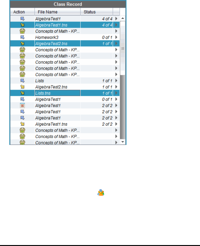
Note: If a student deleted a file, renamed a file, or stored it in another location, the file
cannot be collected.
To collect files, class must be in session. If any students are not logged in, files you
collect are automatically transferred when they log in.
Collecting Files from the Class Record
1. From the Class Record, choose the file or files that have been sent to class.
Note:By default, the first 100 records are listed. To display additional records, click
Load Next 100 or click Load AllEntries.
2. Click ¢next to any of the highlighted files and choose Collect Selected from Class.
The file transfer appears in the Class Record.
Collecting Files from the Menu or Icon
1. Click Tools > Collect from Class or click .
The Select file(s) to collect dialogue box opens.
2. To choose the files or folders you want to collect, do one of the following:
Using the Class Workspace 162
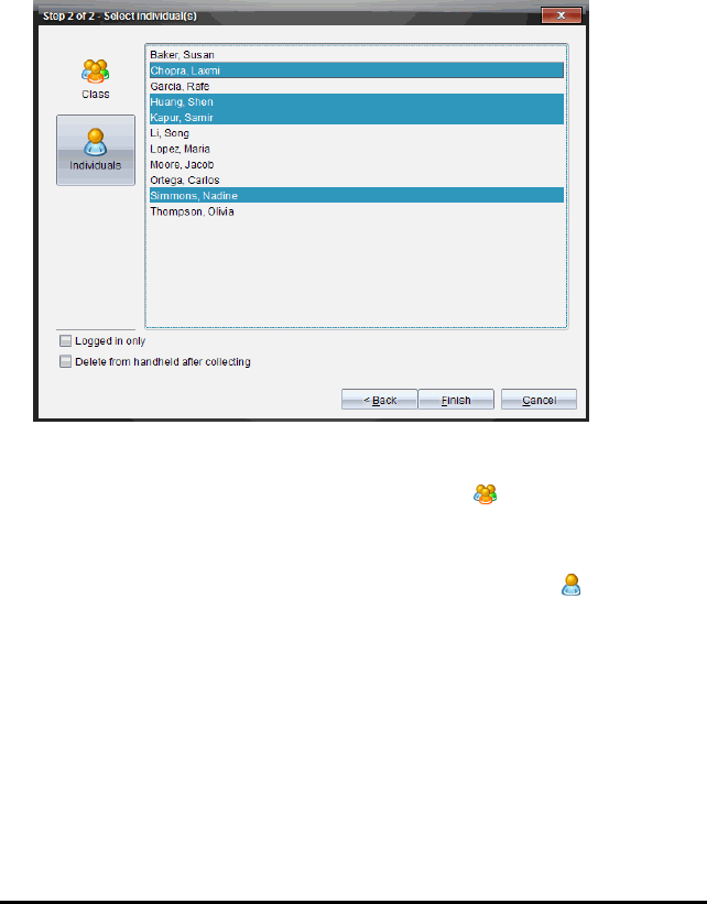
163 Using the Class Workspace
• Click Recent Files and navigate to the file you want to collect and click it. To
select multiple files or folders, press and hold the Ctrl key (Mac®: “) while
clicking each file name.
• Click Enter Filename and type the name of the file in the File name box, and
then click Add.
3. Click Next.
The Select individual(s) dialogue box opens.
4. Select the student(s) from whom you want to collect the file:
• To collect the file from the whole class, click Class . To collect the file only
from class members who are currently logged in, select the Logged in only
check box.
• To collect the file from an individual student, click Individuals , and then click
the student.
Note: If you had any students selected in the classroom area, the software
already has them selected.
5. If you want to remove the file from student class folders after you have collected
it, select the checkbox next to the option to delete the file after it has been
collected.
6. Click Finish.

The collected file appears in the Class Record.
Collecting Missing Files
The Collect Missing function becomes active for files that have not been received from
students.
1. From the Class Record, select the collect action of file that was sent to class.
2. Click File > Collect Missing.
Note: The collection action cannot be active.
Managing Unprompted Actions
When a student logged into a class session sends you a file outside of a collection, an
Unprompted action is created.
These files, which are stored in a database, are shown in the Class Record until they
are removed.
Reviewing and Opening Unprompted Actions
Unprompted actions are named "Unprompted" followed by the month and date. Each
class session contains all .tns and .tnsp files sent from students in one Unprompted
folder.
The latest Unprompted action appears at the top of the Class Record for the most
recent files sent by a student during a class session. During the next class session,
more recent Unprompted actions appear in the Class Record above the previous action.
To open the Unprompted action:
1. Double-click the action or right-click and choose Record Item Properties.
The Unprompted dialogue box opens. By default, no items in the Unprompted
action are selected.
2. In the Unprompted dialogue box, you can view one or more items, save the items
to the Portfolio Workspace, remove the items, export the items to another file
location, or do nothing.
Viewing Items in an Unprompted Action
1. From the Unprompted dialogue box, select the check box to the left of the item(s)
you want to view.
Note: You can also click the View icon beside an item to quickly access the item.
Using the Class Workspace 164

165 Using the Class Workspace
2. Click View.
The items open as read-only files.
Removing Individual Items from an Unprompted Action
Unprompted actions remain in the Class Record until you remove them. Even if you
have exported or saved items, its Unprompted action continues to show until you
remove it. To remove items from an Unprompted action:
1. In the Class Record, double-click the Unprompted action to open it.
2. From the Unprompted dialogue box, select the check box to the left of the item(s)
you want to remove.
3. Click Remove.
Exporting Unprompted Action Items
You can export items from the database to the file system. To export items from an
Unprompted action:
1. In the Class Record, double-click the Unprompted action to open it.
2. Select the files you want to export.
3. Click Export.
A file browser opens.
4. Select the location for the export.
5. Click Select Folder.
Saving Files to a Portfolio Record
You can save collected and unprompted files to a Portfolio record.
1. From the Class Record, select the files.
2. Click ¢and select Save selected to Portfolio.
The Save to Portfolio dialogue box opens.
3. Select to save the files to a new Portfolio column or add them to an existing
Portfolio column.
• To add the files to a new Portfolio column, click Add as new portfolio column
and type the name for the new Portfolio column.
• To save the files to an existing Portfolio column, click Add to existing portfolio
column and select the column name you want from the drop-down list.
4. Click Save.
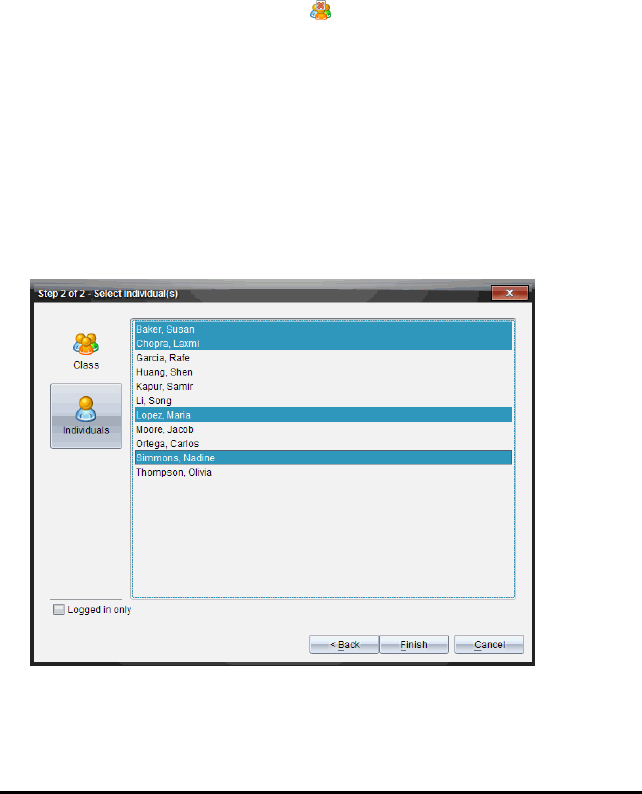
Note: The files you saved in the Portfolio Workspace are shown in the Class Record
until you remove them using the Remove command.
Deleting Files from Class Folders
When necessary, you can delete files from student class folders. You can delete files
that were sent to the class or collected from the class. Class must be in session for you
to delete files.
Note: Deleting a file only removes the specified file from the class folder. If the
student saved a copy with another name, or copied the file to another location, the
student still has access to the file.
1. Click Tools > Delete from class or click .
The Select file(s) to delete dialogue box opens.
2. To choose the files you want to delete, do one of the following:
• Click Recent Files and navigate to the file you want to delete and click it. To
select multiple files or folders, press and hold the Ctrl key (Mac®: “) while
clicking each file name.
• Click Enter Filename and type the name of the file in the File name box, and
then click Add.
3. Click Next.
The Select individual(s) dialogue box opens.
4. Select the student(s) whose files you want to delete.
Using the Class Workspace 166
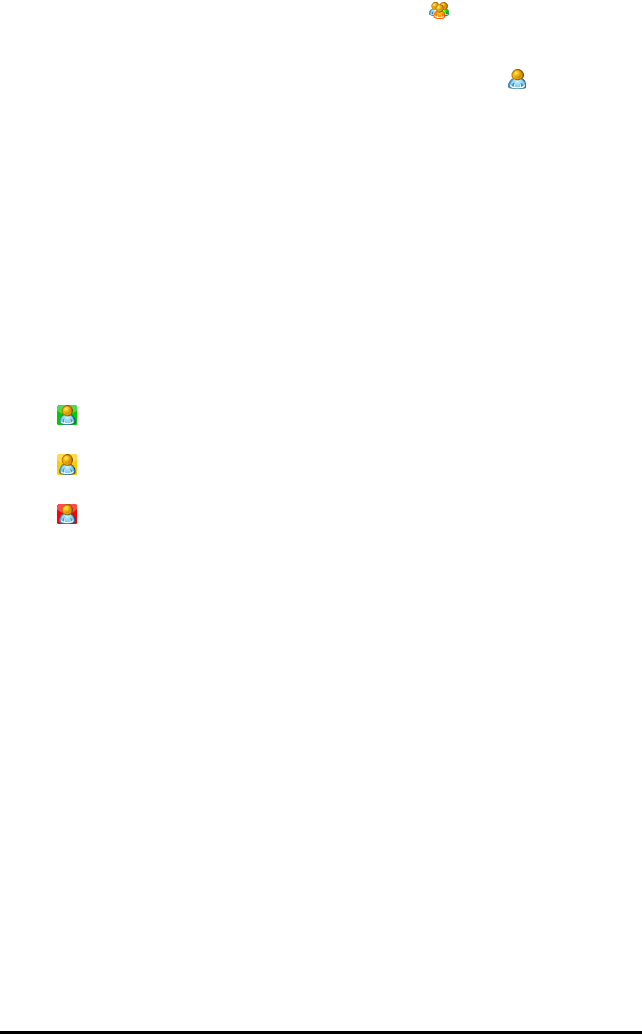
167 Using the Class Workspace
• To delete the file from the whole class, click Class . To delete the file only
from class members who are currently logged in, select the Logged in only
check box.
• To delete the file from an individual student, click Individuals , and then click
the student name.
Note: If you had any students selected in the classroom area, the software
already has them selected.
5. Click Finish.
The file deletion appears in the Class Record.
Checking the Status of File Transfers
When you send, collect, or delete files, you may want to check to see which of your
students have received or sent their files.
▶In the Class Record, click the file whose status you want to check.
In the classroom area, the software indicates the status of students as follows:
• A green background indicates that students have sent/received/deleted the
file.
• A yellow background indicates that students received the collect or delete
action, but they do not have the file in their class folder.
• A red background indicates that students have not yet
sent/received/deleted the file.
Note: You can also see the file transfer status in the file’s Properties dialogue box.
Cancelling File Transfers
If you change your mind about a file transfer, you can cancel the transfer in the Class
Record. Cancelling file transfers stops the software from transferring more files. Any
files that transfer before you cancel remain in student class folders.
1. In the Class Record, click the file whose transfer you want to cancel.
2. Click Edit > Remove from Class Record.
The software asks if you are sure you want to remove the action.
3. Click Remove.
The software stops the file transfer and removes the file from the Class Record
list.
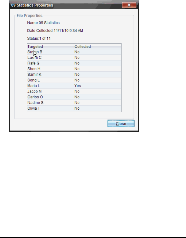
Viewing File Properties
Each file that you send or collect has a set of properties that you can view, except for
Quick Poll files. File properties include name, size, date sent and status. You can view
the file properties at any time.
1. Select the file in the Class Record.
2. Right-click the file name and select Record Item >Properties.
The Statistics Properties dialogue box opens showing the file properties.
Resetting Student Passwords
Because the TI-Nspire™ software maintains the privacy of student passwords, you
cannot retrieve passwords for your students if they forget them. However, you can
reset student passwords. You can reset passwords for all of the students in a class or
for individual students.
Note: You cannot reset the passwords of students who are currently logged in to the
TI-Nspire™ Navigator™ network.
Resetting Passwords for all Students in a Class
1. Select the class.
Note: Student(s) must be selected to perform a successful reset of the password.
Using the Class Workspace 168
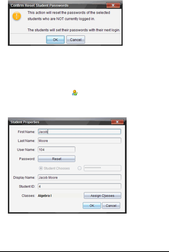
169 Using the Class Workspace
2. Click Class > Reset Student Password(s).
The Confirm Reset Student Passwords dialogue box opens.
3. Click OK.
4. The next time students log in, instruct them to type a new password.
Resetting Passwords for Individual Students
1. Click the student you want to edit.
2. Click Class > Edit Student, or click , or right-click the student name and choose
Edit Student from the menu.
The Student Properties dialogue box opens.
3. Click the Reset button next to Password.
4. If you want a student to create their own password, select Student Chooses.
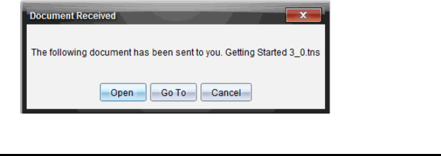
—or—
If you want to create a specific password for the student, select the blank
password entry box and type a new password.
5. Click OK.
The software resets the student’s password.
6. The next time the student logs in:
• If you selected Student Chooses, instruct the student to type a password.
• If you created a password for the student, tell the student the new password.
Understanding the File System
The TI-Nspire™ Student Software or TI-Nspire™ CAS Student Software sets up a file
system on the student’s computer when the software is installed. The student can
install the software anywhere, but once it is installed, the location cannot be changed.
The files are stored in the folder TI-Nspire\[Classname]. The system creates a new
class folder for each class.
The TI-Nspire™ Navigator™ NC Teacher Software automatically sends and collects files
to and from the current class folder on the student’s computer. Students are
responsible for keeping the files in this folder.
The teacher can send or collect any type of file.
Understanding File Transfers
During a class session, the teacher can send files to student computers and collect or
delete files from student computers.
Note: Before class starts, teachers can set up actions to send or collect files. When you
log in, the files are sent or collected. If the teacher set up actions to both send and
collect files, you will only see the dialogue box for the last action completed.
Opening Files
When the teacher sends a file to your computer, the Document Received dialogue box
opens.
Using the Class Workspace 170
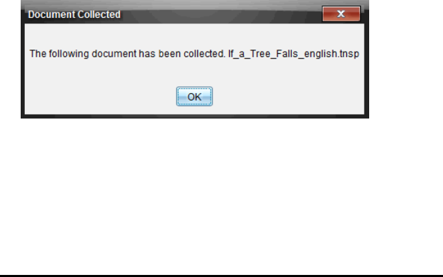
171 Using the Class Workspace
▶Click Open to open the file. If the teacher sent multiple files, this opens the last file
in the list.
Note: The files are received alphabetically by name, no matter which order the
teacher sent them in. The last file in the list is the last alphabetical file.
TI-Nspire™ documents (.tns) and TI-Nspire™ PublishView™ documents (.tnsp) open
directly within the TI-Nspire™ software.
Other file types (.doc, .pdf and so forth) open in their associated application, if the
application is installed on the computer.
▶Click Go To to go to the location the file was sent. The software automatically
opens the Content Explorer in the Documents Toolbox. The file name is highlighted.
You can open that file, or navigate to another file. If the teacher sent multiple files,
the last alphabetical file in the list is highlighted.
Note: If you cannot see the file location, you may have changed the default filter
from “Show all content” to “Show TI-Nspire™ content only.” Change the filter to
“Show all content” to view the files.
▶Click Cancel to dismiss the dialogue box without opening the file.
Collecting or Deleting Files
Your teacher may collect or delete files from your class folder during a class session.
For example, teachers can collect homework assignments or delete certain files prior
to a test. When the teacher collects or deletes files, the Document Collected dialogue
box opens.
▶Click OK to close the dialogue box.
Using Live Presenter
In the TI-Nspire™ Navigator™ NC Teacher Software, Live Presenter enables teachers to
project and present actions on a selected student computer in real-time. Teachers can
choose to project any student computer screen to show work as it is being performed,
and discuss the step-by-step process with the class.
While Live Presenter is active, all other student computers are unaffected by the
presentation and can be used.
Starting Live Presenter
You can start Live Presenter from the Class Workspace or from the Class Capture
window. For either method, make sure the student selected to be the presenter is
logged into an active class session. Although only one person can present at a time,
you can select anyone to present as long as they are logged in and the class session is
active.
Starting Live Presenter from the Class Workspace
To make a student the Live Presenter from the Class Workspace, use one of these
methods:
▶Select a student in the class, and then click Tools > Live Presenter.
—or—
▶Select a student in the class, right-click and then click Live Presenter.
Starting Live Presenter from the Class Capture Window
To make a student the Live Presenter from the Class Capture window, follow these
steps:
1. From the Class Workspace, click and then click Capture Class.
The Select Individual(s) dialogue box opens.
• Select the Logged in only checkbox to show screens only from those students
currently logged in. When you refresh your screen, any students who log in
after the initial screen capture will be added to the Class Screen Capture
window.
Note: If you selected a logged in student in the Class Workspace, that student’s
name is highlighted in the Select Individual(s) dialogue box. To select all students
in the class, click .
2. Click OK.
The Class Capture window opens.
Using Live Presenter 172
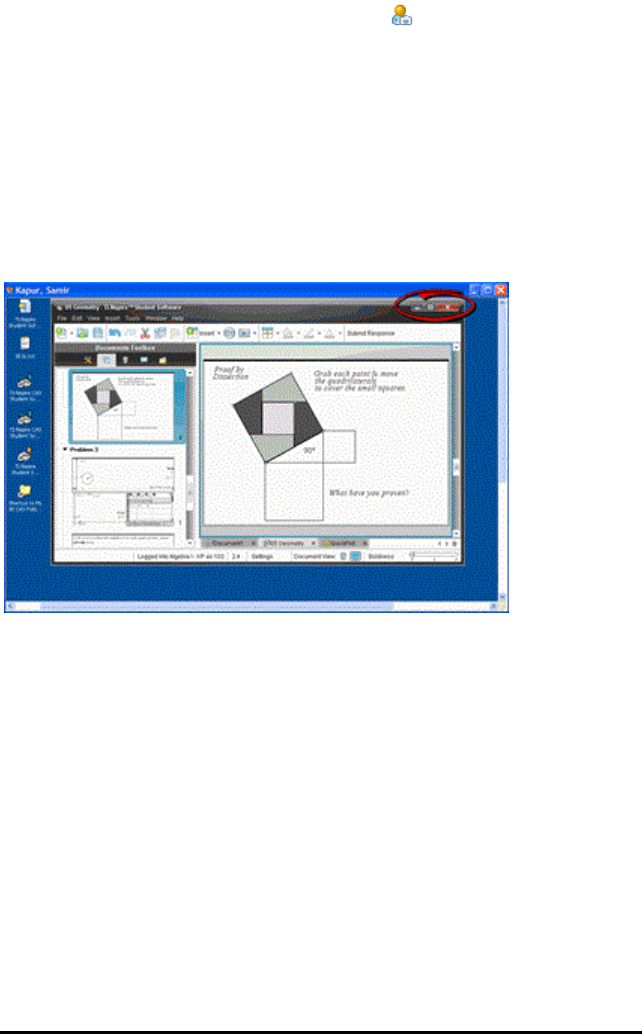
173 Using Live Presenter
3. Select a student who is logged in, and then click .
The Class Screen Capture window opens in Live Presenter mode.
Viewing Live Presenter
When you start Live Presenter from either the Class Workspace or the Class Capture
screen, the window opens in full-screen view by default. Use the minimise and
maximise buttons in the upper right corner to adjust the size of the window.
The name of the live presenter is shown in the upper left corner.
Student name
Buttons to minimise, maximise and close the
Live Presenter window.
Stopping Live Presenter
▶To stop Live Presenter, close the Live Presenter window.
The presentation window closes and the Class Workspace is displayed. The class is
still active.
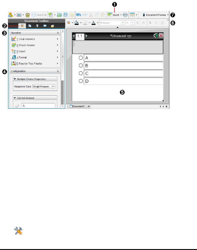
Using Question in the Teacher Software
The Question application in the Teacher Software allows you to author multiple choice,
open response, equation, expression, coordinate points, lists, image and chemistry
questions.
Although students cannot author questions, they can open documents containing
questions, answer these questions and, in Self-Check mode, check their work.
The Question application is located on the Insert menu in the Documents Workspace.
ÀInsert menu. Click Insert and select Question to add a question, or select Image to
add an image to a question.
ÁDocument Tools. Click this icon to open the toolbox pane.
ÂQuestion tool. Provides a menu of tools available for working with the Question
application.
ÃConfiguration tool. Allows you to set certain properties for each question you insert.
ÄQuestion area. This is where you type questions and view student responses.
ÅFormatting toolbar. Allows you to apply formatting to text.
ÆDocument Preview. View the document in Handheld or Computer mode. The
preview changes, but the page size does not. For more information on Document
Preview, see Working with TI-Nspire™ Documents.
Understanding the Question Tools
When you add a question, the Question application opens. If necessary, click Document
Tools to open the tools menu.
Using Question in the Teacher Software 174
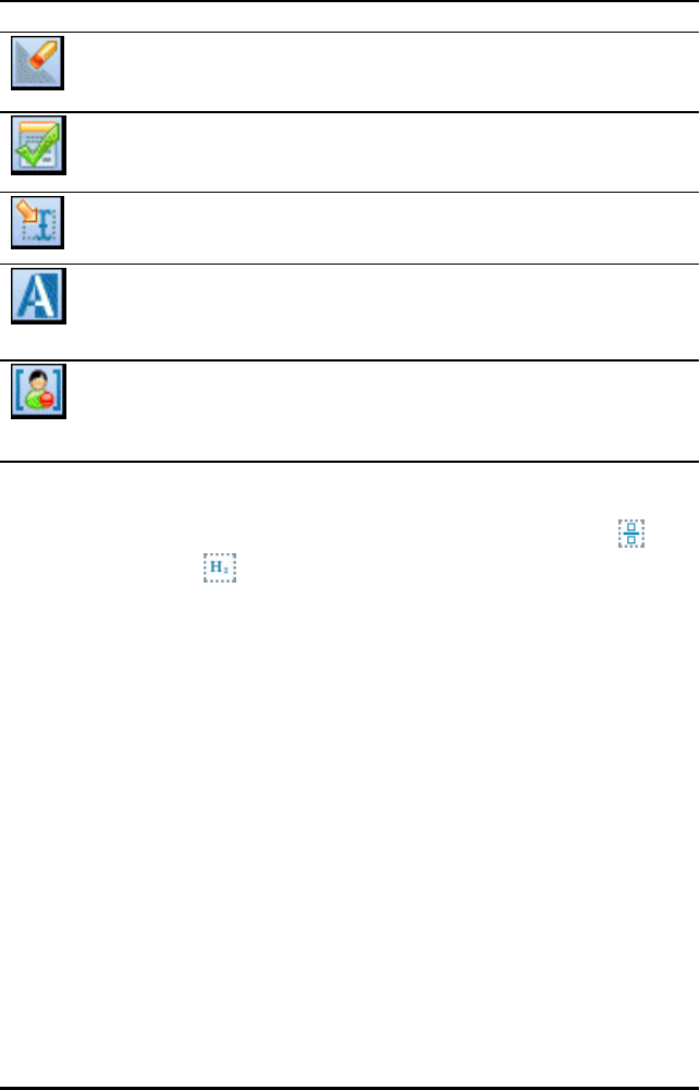
175 Using Question in the Teacher Software
Note: The Teacher Tool Palette is not available to students.
Tool name Tool function
Clear
Answers
Lets teachers or students clear the answers in the current
question or in the document.
Check
Answer
If you select Self-Check as the document type in the Question
Properties dialogueue box, students can check their answer to
the question.
Insert Lets teachers or students insert an expression box or chemical
equation box into the question or answer.
Format Lets teachers or students format the selected text as subscript or
superscript. (The chemical equation box uses its own formatting
tool, so this Format tool does not work in the chemical equation
box.)
Teacher
Tool
Palette
Lets you add copyright information and set the document type as
Self-Check or Exam.
Using the Insert Menu
The Insert menu in the Document Tools lets you add maths expression boxes and
chemical equation boxes to the Question area, Suggested Response area, or
Correct Answer area of some question types. When you are in question types that
allow maths expressions or chemical equations, place your cursor where you want to
insert the box, and then follow these steps.
1. Open the Question tool.
2. Click Insert > Expression Box or Chem Box.
The software inserts a blank box where your cursor is positioned.
3. Type the desired maths expression or chemical equation, and then click outside of
the box to continue typing text.
Using the Teacher Tool Palette
The Teacher Tool Palette allows you to add copyright information and set the
document type as Self-Check or Exam.
Adding Copyright Information
Use the Question Properties dialogue box to add copyright information to the current
question.
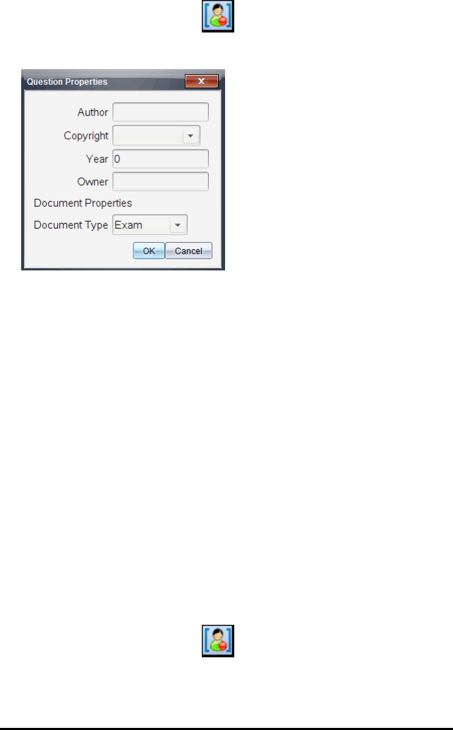
1. Click the Teacher Tool Palette icon > Question Properties.
The Question Properties dialogue box opens.
2. Type the author’s name and move to the Copyright field.
Note: TI-Nspire™ software allows you to use questions from more than one author
in the same document. Therefore, the information that you enter about the author
and copyright is not global. You must enter the relevant information for each
different question.
3. Select whether the question is public domain or has a copyright assigned to it and
move to the Year field.
4. Type the year the question was copyrighted and move to the Owner field. If you are
copyrighting a new question, type the current year (example: 2012).
5. Type the name of the person or entity that owns the copyright.
6. Click OK.
Setting Self-Check and Exam Document Types
When you define a document as Self-Check or Exam, all of the questions in that
document will be either Self-Check or Exam.
• When you define the document type as Self-Check, students can check the answers
against the answers provided by the teacher.
• In Exam mode, when you enter a suggested response to a question, students
cannot check the answers. You can use Exam mode to automatically grade student
responses.
1. Click the Teacher Tool Palette icon > Question Properties.
2. In the Document Type field, click Exam or Self-Check.
3. Click OK.
Using Question in the Teacher Software 176
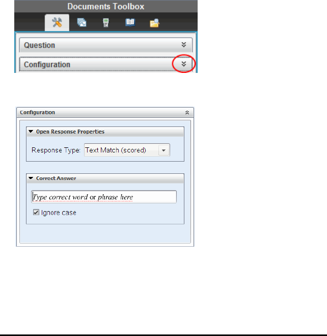
177 Using Question in the Teacher Software
Understanding the Configuration Tool
The Configuration tool allows you to set properties specific to each question type you
insert. Properties include the response type, the number of responses (if applicable),
the correct answer and other options.
For example, you can specify the correct answer to a question, and set the scale, axes
and grid on a graph. You can add a 2D maths expression on the question types that
contain a Correct Answer field.
Each question type has a unique set of options. The options are explained for each
question type in the Adding Questions section.
The configuration settings are retained when you copy and paste a question from one
document to another.
Adding Configuration Options
1. Click the down arrow on the Configuration bar in the Documents Toolbox to open
the Configuration tool.
2. Click the down arrow next to the choices you want to edit, and type the applicable
text.
3. Close the Configuration panel. The options you chose are saved when you save the
document.

Formatting Text and Objects
Use the text formatting tools to format text in sections of questions that allow text
input.
The formatting toolbar also contains the Document Tools icon to provide easy
access to the Question and Configuration tools.
For more information on formatting text and objects, see Working with TI-Nspire™
Documents.
Adding Images to Questions
You can add images to the Question Text Area of most questions. On some question
types, you can add an image in the Student Answer or Suggested Response Area of a
question.
Adding images provides a visual aid to help explain the context of the question, or as a
background on a graph.
Choose the image from a set of images on your computer, or copy and paste an image
from a different application into the Question Text Area. For more information, see
Working with Images.
Image Types Available
The following file types can be used in the Question application:
• .jpg
• .jpeg
• .bmp
• .png
Note: The transparency feature of .png is not supported. Any transparent .png
backgrounds will appear as white.
Adding Images Using the Insert Command
1. Click Insert > Image.
The Insert Image dialogue box opens.
2. Navigate to the location of the image and select it.
3. Click Open.
The image appears in the question.
Adding Images Using the Clipboard
To copy an image to the Clipboard from a TI-Nspire™ document, image file, or another
programme, press Ctrl+C (Mac®: “+C).
Using Question in the Teacher Software 178

179 Using Question in the Teacher Software
To paste the image into the question, press Ctrl+V (Mac®: “+V).
Adding Questions
You can add the following types of questions:
• Multiple Choice
- Custom
- ABCD
- True/False
- Yes/No
- Always/Sometimes/Never
- Agree/Disagree
- Strongly Agree...Strongly Disagree
• Open response
- Explanation (not auto-graded)
- Text Match (auto-graded)
• Equations and Expressions
- y=
- f(x)=
- Expression
• Coordinate Points and Lists
- (x,y) numerical input
- Drop Point(s)
- List(s)
• Image
- Label
- Point on
• Chemistry
When you select a question type, a brief explanation of the question is displayed at the
bottom of the Choose Question Type dialogue box.
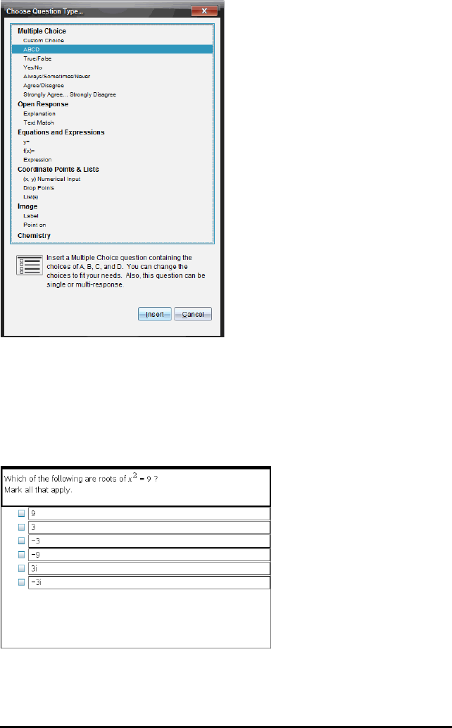
When you open a question template, the cursor is in the Question text area.
Adding a Multiple Choice Question
This example shows how to add a custom multiple choice question. A custom multiple
choice question allows you to specify answers your students can select. You can then
select one or more responses as correct to help you when grading or to help students
check questions that are in Self-Check mode.
To add a custom multiple-choice question:
1. Click Insert > Question.
Using Question in the Teacher Software 180
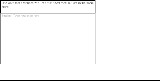
181 Using Question in the Teacher Software
The Choose Question Type dialogue box opens.
2. Click Custom Choice under the Multiple Choice heading.
3. Click Insert.
The Custom Choice template opens with the cursor in the Question text area.
Two response options exist in the template by default.
4. Type the question.
• You can type any combination of text, maths expressions and chemical
equations in the Question Area and Suggested Response area.
• You can add an image in the question text area.
5. Press Enter to add another question line, or press Tab to go to the first Correct
Answer button.
6. Type the response options. Add an image, if desired.
7. Press Enter to add other response options, and add the response text.
• Press Delete to clear or delete a response.
• Press Backspace to delete an empty response line.
8. Click the option next to a suggested response, if desired.
Note: In Self-Check mode, the student can check their answer against the
suggested response.
9. Open the Configuration tool. Choose the response type, and click the option that
corresponds to the correct answer.
Adding an Open Response Question
An open response question prompts the student to write a response. An explanation
question type allows students to respond without any predefined answers. A text
match question type allows the teacher to specify an answer for the student response.
Text match questions are automatically graded; open response questions are not
automatically graded.
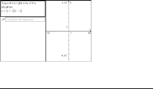
This example shows how to add an explanation question.
1. Click Insert > Question.
The Choose Question Type dialogue box opens.
2. Click Explanation under Open Response.
3. Click Insert.
The Open Response template opens with the cursor in the Question text area.
4. Type the question.
• You can type any combination of text, maths expressions and chemical
equations in the Question Area and Suggested Response area.
• You can add an image in the question text area.
• Press Tab or use the mouse pointer to navigate between fields.
5. Open the Configuration tool. Select the response type as Explanation or Text
Match, and type the correct answer.
• The Explanation response type allows students to give answers that closely
match your suggested response.
• The Text Match response type requires students to exactly match your
suggested response. Select the Ignore Case check box if capitalization is not
important.
• You can type any combination of text, maths expressions and chemical
equations in the Correct Answer area.
Adding an Equation Question
An equation question prompts the student to write an equation in the form of y= or f(x)
=, or to respond with a number or expression.
This example shows how to add a y= question.
1. Click Insert > Question.
The Choose Question Type dialogue box opens.
Using Question in the Teacher Software 182
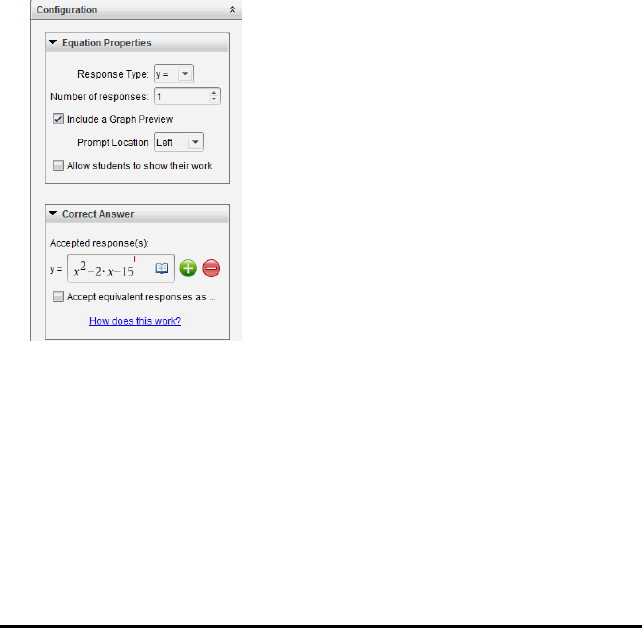
183 Using Question in the Teacher Software
2. Select y= under Equations and Expressions.
3. Click Insert.
The equation template opens with the cursor in the Question text area.
4. Type the question.
• You can type any combination of text, maths expressions and chemical
equations in the Question Area.
• You can add an image in the question text area.
• Press Tab or use the mouse pointer to navigate between fields.
5. Enter a suggested response, if desired.
6. Press Enter to add other response options, and add the response text.
• Press Delete to clear or delete a response.
• Press Backspace to delete an empty response line.
7. Open the Configuration tool to set the number of responses, the correct answer
and whether the students should show their work. You can also add a graph that
will show in the Question area.
• The number of responses can range from 1 to 5.
• The Show your work option includes areas for the students to write their
starting point, their steps and their final answer. The option to show work is
disabled if multiple responses are allowed.
• To add a graph in the Question area, check Include a Graph Preview. The
Question text area splits to show a graph on the right.
• When you are in the graph, the Graphs & Geometry toolbox is available to
allow you to add functions.
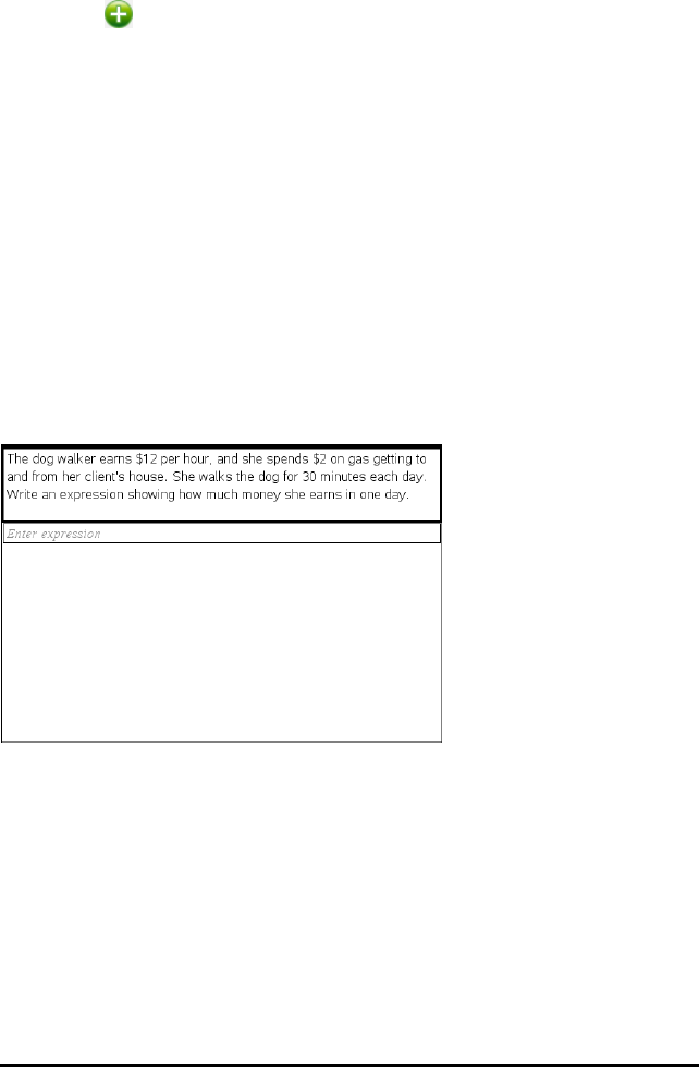
Note: Only the teacher can edit the graph. Students can only view and zoom
the graph.
• Click to add additional fields for multiple correct answers. For example,
you might want to accept both y=(x+1)(x+2) and y=(x+2)(x+1) as correct
answers.
• Select whether or not to accept equivalent responses as correct.
- If you do not check Accept equivalent responses as correct, the student
response is marked correct if it is an exact text match to one of the
accepted responses you entered.
- If you do check Accept equivalent responses as correct, the student
response is marked correct if it is equivalent to any accepted response you
entered. For example, if you typed x+2 as the correct answer, and the
student submits 2+x, this response is equivalent to the accepted response
and is automatically graded as correct. Spaces, case differences and extra
parentheses are ignored when the software evaluates student answers. For
example, y=2x+1 is evaluated the same as Y=2X+1.
Adding an Expression Question
An expression question prompts the student to respond with a number value or an
expression.
1. Click Insert > Question.
The Choose Question Type dialogue box opens.
2. Click Expression under Equations and Expressions.
3. Click Insert.
The expression template opens with the cursor in the Question text area.
4. Type the question.
• You can type any combination of text, maths expressions and chemical
equations in the Question area.
Using Question in the Teacher Software 184
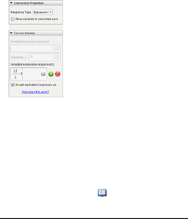
185 Using Question in the Teacher Software
• You can add an image in the Question area.
5. In the Expression type response, enter a starting expression, if desired. The student
sees the starting expression.
6. Enter a suggested response, if desired.
• If you set the response type as Number, the response fields are maths boxes
and accept only number values such as 1/3.
• If you set the response type as Expression, the response fields are expression
boxes and accept only expression inputs such as 2(3+5).
7. Open the Configuration tool to set the response type as Number or Expression, set
whether or not the students should show their work and enter a correct answer.
You can also set a tolerance for Number types, or equivalent responses for
Expression types.
• The Show your work option includes areas for the students to write their
starting point, their steps and their final answer.
• In the Number type response, enter the accepted numerical response and the
tolerance. Student responses are marked correct if they fall within the
tolerance interval you specify.
• Specifying a tolerance of zero indicates you are looking for the exact number
answer. Not specifying a tolerance is the same as specifying a tolerance of
zero.
• Student answers are considered correct if they are numerically equivalent to
the correct answer. Spaces, case differences and extra parentheses are ignored
when the software evaluates student answers.
• In the Expression type response, you can add additional fields (up to 10) for
multiple correct answers.
• In the Expression type response, click to open the Templates and Symbols
catalogue that allows you to enter 2D maths expressions.
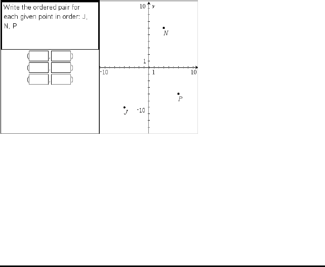
• In the Expression type response, you can select whether or not to accept
equivalent responses as correct.
- If you do not check Accept equivalent responses as correct, the student
response is marked correct if it is an exact text match to one of the
accepted responses you entered.
- If you do check Accept equivalent responses as correct, the student
response is marked correct if it is equivalent to any accepted response you
entered. For example, if you typed x+2 as the correct answer, and the
student submits 2+x, this response is equivalent to the accepted response
and is automatically graded as correct. Spaces, case differences and extra
parentheses are ignored when the software evaluates student answers. For
example, x+2 is evaluated the same as X+2.
Important: Students can enter the starting expression you supply and have
this response automatically graded as correct. For example, if you ask
students to factor x2-7x+12 and stipulate the correct answer is (x-3)(x-4),
the student can submit a response of x2-7x+12. This response is
automatically graded as correct because it is equivalent to the accepted
answer. You must manually mark this student response as incorrect in
either the Review or Portfolio Workspaces. See the chapters for those
workspaces for more information on marking and grading responses.
Adding an (x,y) Numerical Input Question
An (x,y) numerical input question prompts the student to respond with a coordinate.
1. Click Insert > Question.
The Choose Question Type dialogue box opens.
2. Click (x,y) Numerical Input under Coordinate Points & Lists.
3. Click Insert.
The template opens with the cursor in the Question text area.
4. Type the question.
Using Question in the Teacher Software 186
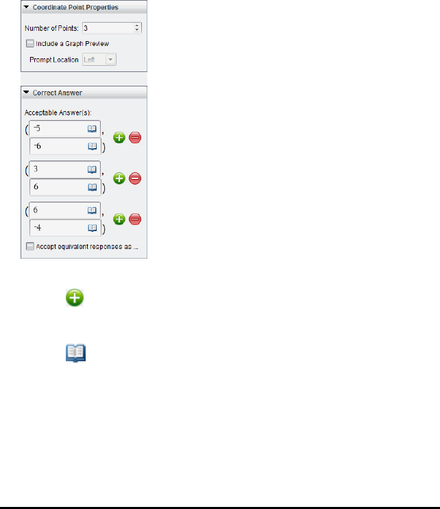
187 Using Question in the Teacher Software
• You can type any combination of text, maths expressions and chemical
equations in the Question area.
• You can add an image in the Question area.
• Press Tab or use the mouse pointer to navigate between fields.
5. Enter a suggested response, if desired.
• The response fields are expression boxes and accept only expression inputs.
6. Press Enter to add other response options (up to five), and add the response text.
• Press Delete to clear or delete a response.
• Press Backspace to delete an empty response line.
7. Open the Configuration tool to set the number of points, add a graph preview,
enter a correct answer, and set equivalent responses as correct.
• The number of points can range from 1 to 5.
• Click to add additional fields for multiple correct answers. You can type any
combination of text, maths expressions and chemical equations in the correct
answer fields.
• Click to open the Templates and Symbols catalogue that allows you to
enter 2D maths expressions.
• To add a graph in the Question area, select Include a Graph Preview. The
Question text area splits to show a graph on the right and the student prompt
area on the left. To change the location of the graph, click the down arrow next
to Prompt Location and choose the desired location for the graph in the student
prompt area.
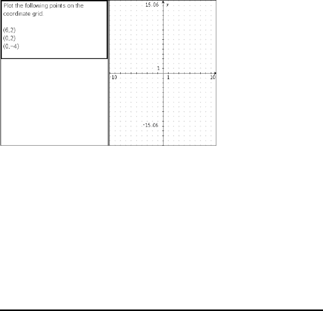
• When you are in the graph, the Graphs & Geometry tools are available to allow
you to add functions.
Note: Only the teacher can edit the graph. Students can only view and zoom
the graph.
• Select whether or not to accept equivalent responses as correct.
- If you do not check Accept equivalent responses as correct, the student
response is marked correct if it is an exact text match to one of the
accepted responses you entered.
- If you do check Accept equivalent responses as correct, the student
response is marked correct if it is equivalent to any accepted response you
entered. For example, if you typed (-0.5,.75) as the correct answer, and the
student submits (-.5,.75) or (-1/2,3/4) and so forth, the student response
is equivalent to the accepted response and is automatically graded as
correct.
Adding a Drop Points Question
A drop points question inserts a graph and prompts the student to drop points on the
graph in response to your question.
1. Click Insert > Question.
The Choose Question Type dialogue box opens.
2. Select Drop Points under Coordinate Points & Lists.
3. Click Insert.
The drop points template opens with the cursor in the Question text area.
The graph is in the Student answer area.
• When you are in the graph, the Graphs & Geometry tools are available to allow
you to add functions.
Using Question in the Teacher Software 188
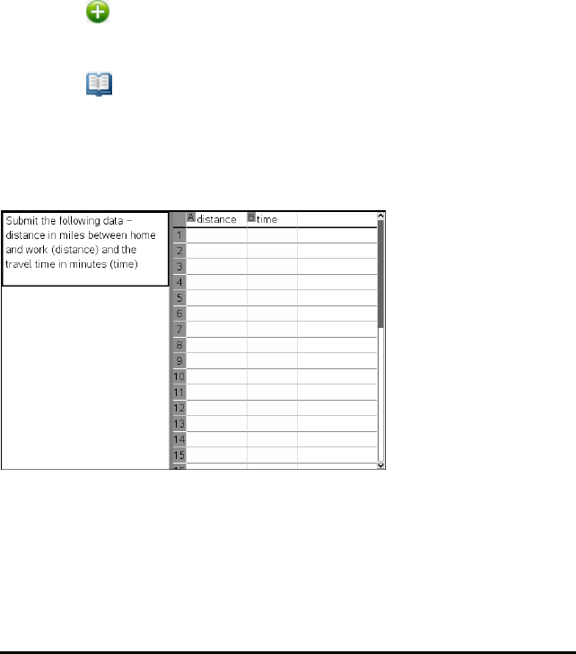
189 Using Question in the Teacher Software
Note: Only the teacher can edit the graph. Students can only view, zoom, or
place points on the graph.
4. Type the question.
• You can type any combination of text, maths expressions and chemical
equations in the Question area.
• You can add an image in the Question Area.
• Press Tab or use the mouse pointer to navigate between fields.
5. Open the Configuration tool to set the number of points, hide or show coordinates
and enter a correct answer.
• The number of points can range from 1 to 5.
• Showing coordinates is turned off by default. Select the check box to display
coordinate labels on the graph.
• Click to add additional fields for multiple correct answers. You can type any
combination of text, maths expressions and chemical equations in the correct
answer fields.
• Click to open the Templates and Symbols catalogue that allows you to
enter 2D maths expressions.
Adding a Lists Question
A Lists question inserts a list and prompts students to enter data in the lists in
response to your question.
1. Click Insert > Question.
The Choose Question Type dialogue box opens.
2. Select List(s) under the Coordinate Points & Lists question from the Choose
Question Type dialogue box.
3. Click Insert.
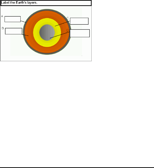
The List template opens with the cursor in the Question text area.
4. Type the question.
• You can add columns or rows, change the name of the lists and input data in
the lists, using the same functions allowed in the Lists & Spreadsheet
application.
5. Enter initial data in the lists, if desired.
6. Open the Configuration tool to set the number of lists for the student responses.
• The number of lists can range from 1 to 5.
• Lists must have names. The default names are List1,List2 and so forth.
Adding an Image: Label Question
An Image: Label question inserts an image. You can add blank fields to the image and
have students fill in the blanks in response to your question.
1. Click Insert > Question.
The Choose Question Type dialogue box opens.
2. Select Label under Image.
3. Click Insert.
The Image: Label template opens with a blank background and one label. This is
where the image for the question is inserted.
4. Type the question.
• You can type any combination of text, maths expressions and chemical
equations in the Question area.
• Press Tab or use the mouse pointer to navigate between fields.
5. Insert an image in the bottom portion of the question template.
6. Open the Configuration tool to set the number of responses and to enter answers
for each label.
Using Question in the Teacher Software 190
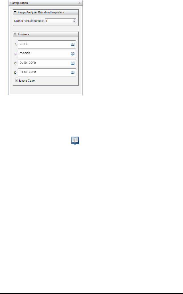
191 Using Question in the Teacher Software
• The number of responses determines the number of labels on the image. Each
new response gives the label a unique identifier, such as A, B, C and so forth.
Drag the labels to the desired location on the image.
Note: If you set more than 26 responses, the labels are identified with
numbers, starting with 1. You can insert a maximum of 35 labels.
• In the answers area, click to open the Templates and Symbols catalogue
that allows you to enter 2D maths expressions.
• If the label text is too large to fit in the default label size, grab and drag the
borders of the label to resize it.
7. Type a suggested response in the labels, if desired. Select the Ignore case check
box if capitalization is not important.
• You can type any combination of text, maths expressions and chemical
equations in the response area.
• As you type the suggested response, a ghosted image of your answer appears
in the respective label on the image. If the suggested response is too large for
the default label size, grab and drag the borders of the label to resize it.
Adding an Image: Point on Question
An Image: Point on question inserts an image. Add check boxes to the image and have
students place a check mark in the correct boxes in response to your question.
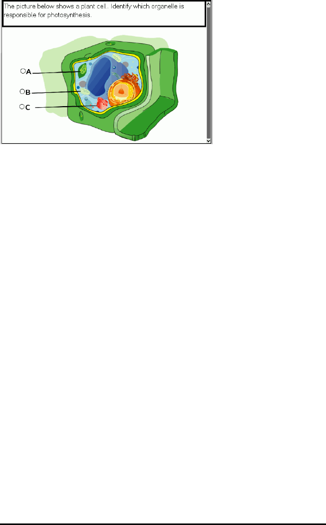
1. Click Insert > Question.
The Choose Question Type dialogue box opens.
2. Select Point on under Image.
3. Click Insert.
The Image: Point on template opens with a blank background and one point. This is
where the image for the question is inserted.
4. Type the question.
• You can type any combination of text, maths expressions and chemical
equations in the Question area.
• Press Tab or use the mouse pointer to navigate between fields.
5. Open the Configuration tool to set the response type, number of responses and
correct answer.
• The Response Type makes the point a circle for Single Reponse and changes to
a square for Multiple Responses to indicate students can select more than one
box.
• The number of responses determines the number of points on the image. Each
new response gives the point a unique identifier, such as A, B, C and so forth.
Drag the points to the desired location on the image.
Note: If you set more than 26 responses, the points are identified with
numbers, starting with 1. You can insert a maximum of 35 points.
6. Click a point or points as a suggested response, if desired.
Adding a Chemistry Question
When you add a Chemistry question, students respond with a chemical formula or
equation.
Using Question in the Teacher Software 192
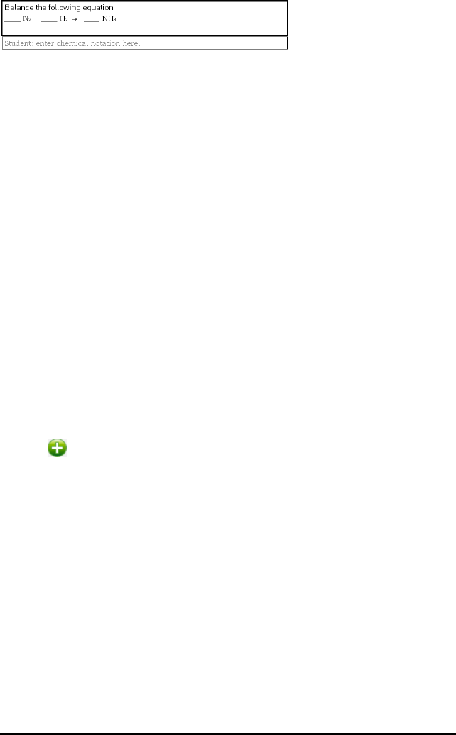
193 Using Question in the Teacher Software
1. Click Insert > Question.
The Choose Question Type dialogue box opens.
2. Click Chemistry.
3. Click Insert.
The Chemistry template opens with the cursor in the Question text area.
4. Type the question.
• You can type any combination of text, maths expressions and chemical
equations in the Question area.
• You can add an image in the Question area.
5. Enter a suggested response, if desired.
6. Open the Configuration tool to enter a correct answer.
Click to add additional fields for multiple correct answers. You should enter all
possible answers. The software does not evaluate equivalency for Chemistry
answers.
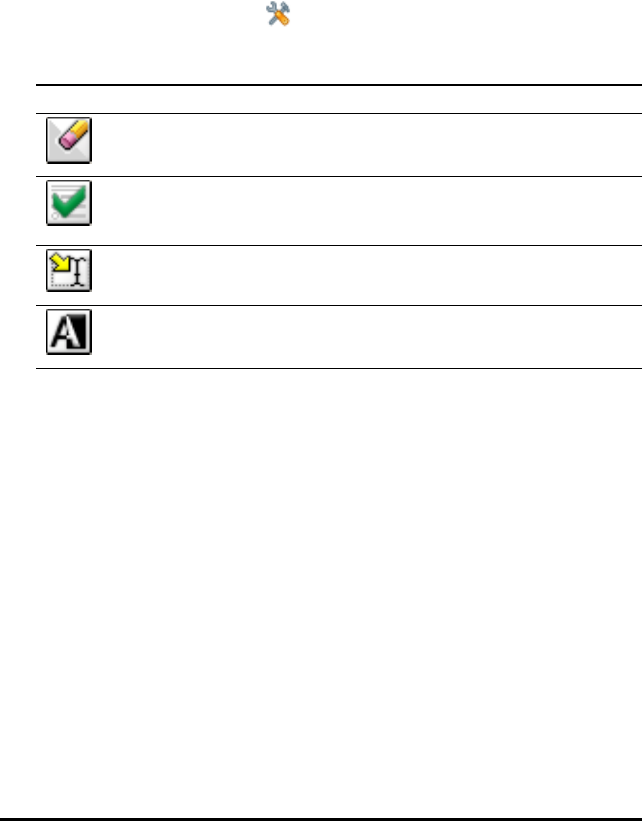
Responding to Questions
The teacher may send you a question in a variety of format types. This section shows
you how to answer the different question types.
Understanding the Question Toolbar
When you open a document with a question, a toolbar is available with four options.
Access the toolbar using the following method.
▶In the Documents Toolbox, click .
Handheld, press b.
Tool name Tool function
Clear
Answers
Lets you clear the answers in the current question or in the
document.
Check
Answer
If your document is in Self-Check mode, click here to view
the correct answer. You cannot check answers to exam-type
questions.
Insert Lets you insert an expression box in your answer.
Format Click this tool to format the selected text in your answer as
subscript or superscript.
Types of Questions
There are several types of questions you may be asked. There may be variations in a
type but how you answer the question is basically the same for each type.
•Multiple choice
- Custom
- ABCD
- True/False
- Yes/No
- Always/Sometimes/Never
- Agree/Disagree
- Strongly Agree…Strongly Disagree
•Open response
- Explanation
- Text match
Responding to Questions 194

195 Responding to Questions
•Equation
- y=
- f(x)=
•Coordinate points and list
- (x,y) numerical input
- Drop point(s)
- List(s)
Responding to Quick Poll Questions
When teachers send quick polls during class, the question opens as a new document on
top of any document you may currently have open. You can access other applications to
perform calculations, and check or clear answers before submitting your answer to the
question or quick poll.
Note: On TI-Nspire™ CX or TI-Nspire™ CX CAS handhelds, questions appear in colour if
the teacher applied colour when writing the question. Although you can see colour in
the questions you receive, you cannot add colour to the responses you submit.
Accessing Other Applications
If the teacher gives permission, the Quick Poll tool allows you to temporarily exit the
question to perform calculations or access other documents to determine the answer
to the question. For example, you can access the Scratchpad to perform a calculation,
or you can access the Lists & Spreadsheet application and copy data from there to a
List question type. In a List question, you can link to variables from the Vernier
DataQuest™ or Lists & Spreadsheet applications.
To access other applications while in the Quick Poll screen:
1. Open a new document.
Handheld: Press cto open the Home screen.
2. Choose an application.
Handheld:To return to the Quick Poll without accessing any documents, choose
C:Quick Poll.
3. When you are finished, click the Quick Poll icon.
When you respond to a poll, your response is immediately sent to the teacher’s
computer and teachers can track student responses in real time.
Showing Your Work
The teacher may request you to show work for your response. If so, the response area
has sections for you to write your starting point, your steps, and the final answer.

Responding to Different Question Types
▶For Multiple Choice questions, press Tab to navigate to a response. Press Enter to
mark a response.
▶For Open Response questions, type a response.
▶For Equation questions, type a response. If a graph is included in a question, the
graph updates when you press Enter. Any functions entered show up on the graph,
and the cursor remains in the answer box. You cannot manipulate the graph itself.
▶For Expression questions, type a response. If the response type is Number, your
response must be in the form of a number. If the response type is Expression, your
response must be in the form of an expression. For example, x+1.
▶For Coordinate Points: (x,y) questions, type an answer in the x-field box, and press
Tab to move to the y-field box. Type an answer.
If a graph is included with the question, the graph is updated when you enter a
function and press Enter.
You can access the Window and Zoom functions while you are working on the
graph.
▶For Coordinate Points: Drop Points questions, press Tab to move the cursor to a
point on the graph. Press Enter to drop a point at that location.
To delete a point, press Ctrl + Z to undo the action.
▶For Lists questions, press Tab if necessary to move the cursor to the first cell of the
list. Type an answer, and press Tab to move to the next cell. Type an answer.
To link a column to an existing variable, select the column and then click var. Click
Link To, and then click the variable you want to link to.
The behaviour in a Lists question closely matches the behaviour of the Lists &
Spreadsheet application, with the following exceptions. In a Lists question, you
cannot:
• Add, insert, or delete columns.
• Change the header row.
• Enter formulas.
• Switch to Table.
• Create plots.
▶For Chemistry questions, type a response.
▶For Image: Label questions, press Tab to move the cursor to a label on the image.
Type a response in the label field.
▶For Image: Point on questions, press Tab to move the cursor to a point on the
image. Press Enter to mark a response.
Responding to Questions 196

197 Responding to Questions
Checking Answers
If the teacher enables self-check on the question, the Check Answer option is available.
1. Click .
Handheld: Press b.
2. Click Check Answer.
Clearing Answers
After you answer a quick poll, you may decide you want to change the answer before
you submit it.
▶Click Menu > Clear Answers > Current Question or Document.
•Current Question clears answers for the active question.
•Document clears answers for all questions contained in the active document.
—or—
If you answered the question, you still have time to clear the answer before you submit
it to your teacher.
▶Click Clear Answer to clear your answer and try again.
Handheld: Press ~and choose Clear Answer.
Submitting Responses
To send a final answer to the teacher:
▶Click Submit Response.
Handheld: Press ~and choose Submit.
The response is sent to the teacher and the last screen you used is displayed.
Your response appears on the teacher’s computer. Your teacher may have set the poll
to allow you to submit more than one answer. If so, you can continue to respond to the
poll and submit answers until the teacher stops the poll.
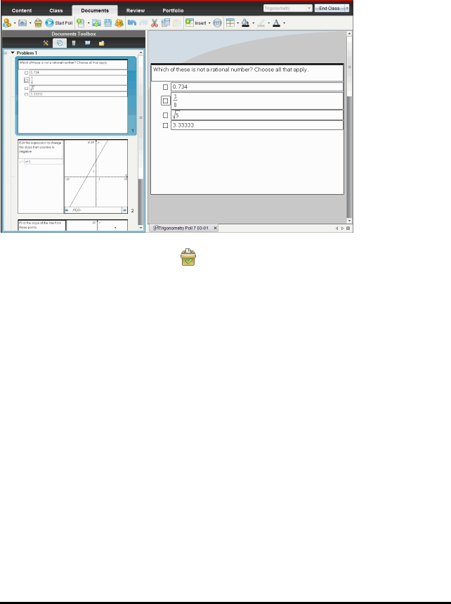
Polling Students
The Quick Poll tool lets you “poll” your students. A poll is a survey you send to students
that they immediately receive on their handhelds or laptops. After students receive the
poll, they can send responses back to your computer. Quick Poll is available from all
workspaces. As you receive student responses, use the Review Workspace to review
the responses.
When you click the Quick Poll icon from any workspace, the Documents Workspace
opens and you can start the Quick Poll. Starting the Quick Poll opens the Review
Workspace. You can switch to any workspace while a poll is in progress, but you can
only stop the poll from the Documents or Review Workspaces.
You can send the following types of questions:
• Multiple Choice
- Custom Choice
- ABCD
- True/False
- Yes/No
- Always/Sometimes/Never
- Agree/Disagree
- Strongly Agree...Strongly Disagree
• Open response
- Explanation (not auto-graded)
- Text Match (auto-graded)
• Equations and Expressions
Polling Students 198
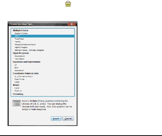
199 Polling Students
- y=
- f(x)=
- Expression
• Coordinate Points and Lists
- (x,y) Numerical Input
- Drop Points
- List(s)
• Image
- Label
- Point on
• Chemistry
When you select a question type, a brief explanation of the question is displayed at the
bottom of the Choose Question Type dialogue box.
Opening the Quick Poll Tool
You can open the Quick Poll tool from any workspace. You can send a poll from an
existing document or open a new document to start a poll.
Before you begin, make sure a class is in session.
1. Click Tools > Quick Poll or click .
The Choose Question Type dialogue box opens.
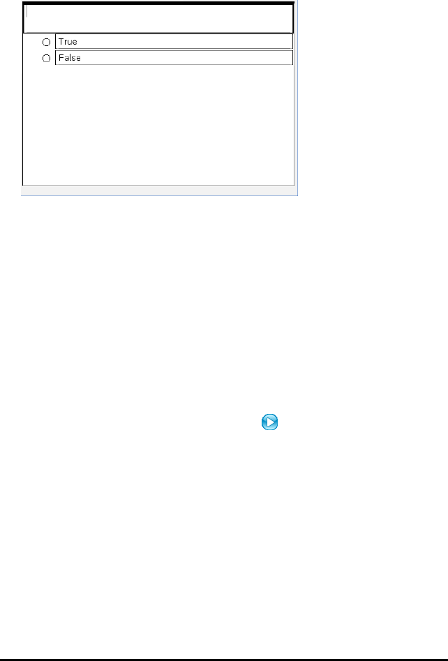
2. Select a question type and click Insert.
A new document opens with the question template open and the cursor in the
Question text area.
Quick Poll documents are named <Class name, Quick Poll Set#, mm-dd.tns>. For
example: Algebra1 - Mrs. Smith QP2 10-26.tns. You can rename the poll when you
save it.
Note: All Quick Polls for one class session are contained in one tab in the
Documents Workspace. A new tab is started when the number of questions in the
poll exceeds 30 or when you start a new class session.
Note: For more information about question types and about creating and
configuring questions, see Using Question in the Teacher Software.
Sending a Quick Poll
After you have selected the Quick Poll question, entered the information and selected
options, you are ready to send the poll to your students.
▶To send the Quick Poll question, click Start Poll .
The poll is immediately sent to students. The Quick Poll interrupts the active
TI-Nspire™ document and the poll becomes the active document.
You can stop a poll and restart it at any time.
Using Quick Poll Options
When Quick Poll is active, the Tools > Quick Poll Options menu is enabled. Available
options differ depending on whether you are using software that supports connected
handhelds or connected laptops. The Allow Document Access option is not available in
the TI-Nspire™ Navigator™ NC Teacher Software for Networked Computers.
Polling Students 200

201 Polling Students
•Allow Document Access. Allows you to grant or deny students access to the
Scratchpad and any documents on their handheld. The students may access a
document, do some maths and copy the results back into the poll.
Note: If a data collection sensor is attached to the computer or handheld during a
Quick Poll that does not have Allow Document Access turned on, the Quick Poll is
dismissed and the data collection console becomes active.
•Allow Resubmit. Allows the students to submit their responses several times.
Stopping Polls
You can stop polls at any time. Your students do not need to do anything on their
handhelds or computers to stop the poll. When you stop a poll, the students can no
longer submit answers.
▶To stop a poll, click Stop Poll .
Note: If you pause a class while a Quick Poll is running, the Quick Poll remains on the
students’ handhelds, but students are not able to answer or submit the poll until you
resume the class. Pausing class is not available in TI-Nspire™ Navigator™ NC Teacher
Software for Networked Computers.
Resending Polls
You can resend a poll from the Review Workspace, without switching workspaces or
starting a new question.
The software treats the resent poll like a new poll. Students receive a new poll on top
of the open document on their handheld or laptop.
The data from the poll is treated as new data and does not overwrite any data from
the original poll.
▶To resend the same poll you just sent, click Start Poll .
▶To resend a previous poll, click the poll in the page sorter and then click Start Poll
.
The poll is added to the page sorter in the order it was sent. The page sorter indicates
it was resent.
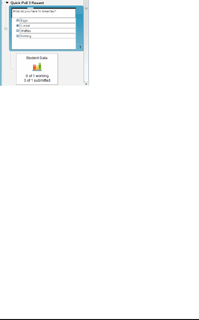
Sending Polls to Missing Students
You can send the most recent poll to students who were not logged in before the poll
was stopped.
Note: The Send to Missing option can only be used with the last poll that was sent.
1. In the page sorter, click the last poll that was sent.
2. Click File> Send to Missing.
The poll is immediately sent to students who were not logged in when the poll was
sent previously, but are currently logged in.
The data gathered from the missing students is added to the data from the last poll.
Saving Polls
You can save Quick Poll results to the Portfolio Workspace while the poll is still in
progress, or you can save a completed set of Quick Poll documents as a .tns file.
You can save to the Portfolio Workspace from either the Class Workspace or the
Review Workspace.
When you save the results to the Portfolio Workspace, the polls sent in one class
session are saved in one column.
A new column is started when a poll exceeds 30 questions, or when you start a new
class session.
▶To save a Quick Poll to the Portfolio Workspace, click File > Save to Portfolio.
Note: After the first save, subsequent changes to the poll are automatically
updated in the Portfolio Workspace until you stop the poll.
You can also save a set of Quick Polls as a Master Document (.tns file). A Master
Document contains information that can be used as the answer key for evaluating
responses collected from students.
Polling Students 202
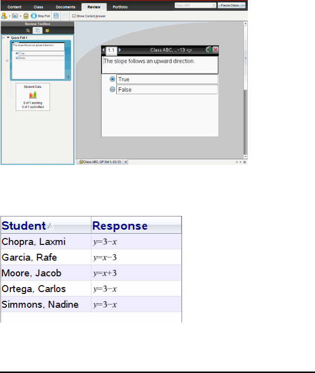
203 Polling Students
▶To save a Quick Poll as a Master Document, click File > Save Quick Poll Set as
Document.
Note: After you save as a .tns file, any subsequent changes to the poll are not
updated in the .tns document.
Viewing Poll Results
Review Quick Poll results in the Review Workspace.
Polls sent in one class session are contained in a Quick Poll tab in the Review
Workspace. Each new question is added as a new problem in the page sorter, and the
software automatically opens to the last question that was sent. A new tab is started
when a poll exceeds 30 questions.
You can view the results as a bar chart, graph or table. The results automatically
update as students send their responses, until you stop the poll.
The following example shows the poll results listed in a table.

For more information about viewing and sorting poll results, see Using the Review
Workspace.
Polling Students 204

205
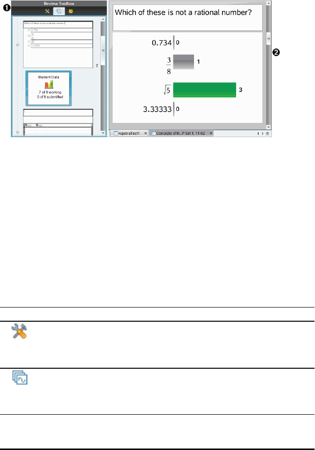
Using the Review Workspace
Use this workspace to review a collected set of documents, manage student
responses, run live activities and organise data.
ÀReview toolbox. Contains the Review Tools, Page Sorter and Student Response tools.
Click each icon to access the available tools. Options for the selected tool are
displayed in the toolbox pane.
ÁData View pane. Shows the data and options from the poll or document you have
selected in the Review Toolbox. You can switch the data view between bar chart,
table and graph (if available).
The software retains the data view that was set for each question when you close and
reopen the Review Workspace. All hidden and unhidden data, settings in graph view,
table view, bar chart view and Show Your Work are retained when you close the
Review Workspace.
Using the Review Toolbox
The Review toolbox contains tools needed for working with collected documents,
Question results and Quick Poll results.
Icon What you can do
Review
tools
The Review tools let you organise the response data, use graph tools, hide
or show responses and mark Question and Quick Poll responses as correct
or incorrect.
Page
sorter
Displays all the problems in a document or Quick Poll, all the pages in each
problem and the student responses for each question in the document.
Using the Review Workspace 206
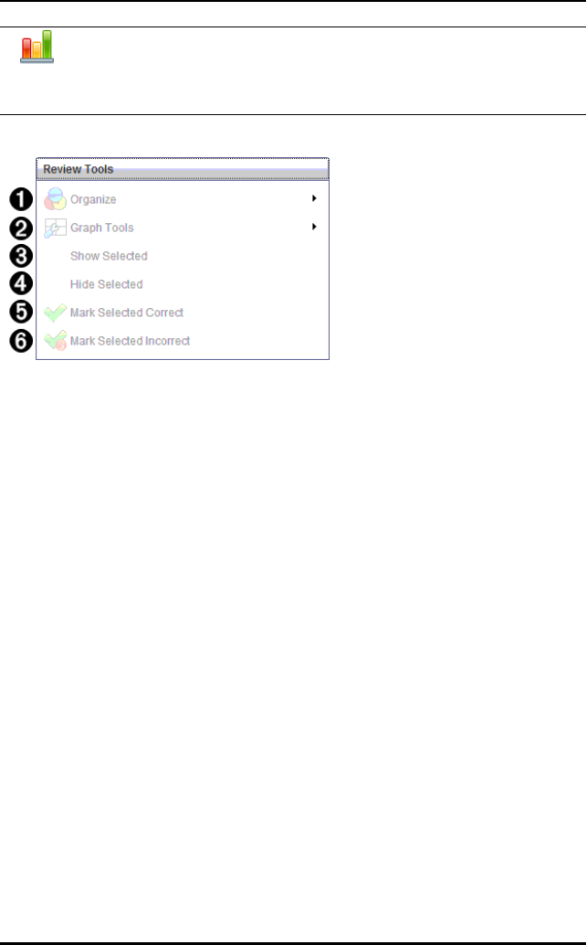
207 Using the Review Workspace
Icon What you can do
Student
pane
Displays the student names and responses in the Data View pane.
Exploring the Review Tools
ÀOrganise. Click ¢to organise the data in different views.
ÁGraph Tools. Click ¢to access the graph tools when you are in coordinate graph
view.
ÂShow Selected. Shows selected responses for review in the Data View pane.
ÃHide Selected. Hides selected responses in the Data View pane.
ÄMark Selected Correct. Select a response from the Data View pane and click Mark
Selected Correct to mark that response as the correct answer. You can mark more
than one answer as a correct answer.
ÅMark Selected Incorrect. Select a response from the Data View pane and click Mark
Selected Incorrect to mark that response as an incorrect answer. You can mark more
than one answer as an incorrect answer.
Exploring the Page Sorter
Use the Page Sorter to view student responses to any questions in a document.
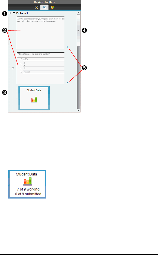
ÀClick the minus sign (–) to collapse the view. Click the plus sign (+) to expand the
view and show all the pages in a problem, and all the problems in a document.
ÁThe pages in a problem. Click a page to open it in the Data View pane.
ÂStudent responses. A student data icon follows each question in the document. Click
the icon to view the student responses for the question in the Data View pane.
In Quick Polls, the icon shows the number of students who were logged in when the
poll was started, the number who have responded and the number who have
submitted their answer. In the example below, nine students received the poll,
seven students responded to the poll and no students have submitted their answer.
Note: If you send a poll to students who were missing, the numbers may change.
ÃScroll bar. The scroll bar is active when there are too many pages to show in the
panel.
ÄPage numbers. Click a page number to open the page in the Data View pane.
Exploring the Student Pane
Use the Student pane to:
Using the Review Workspace 208
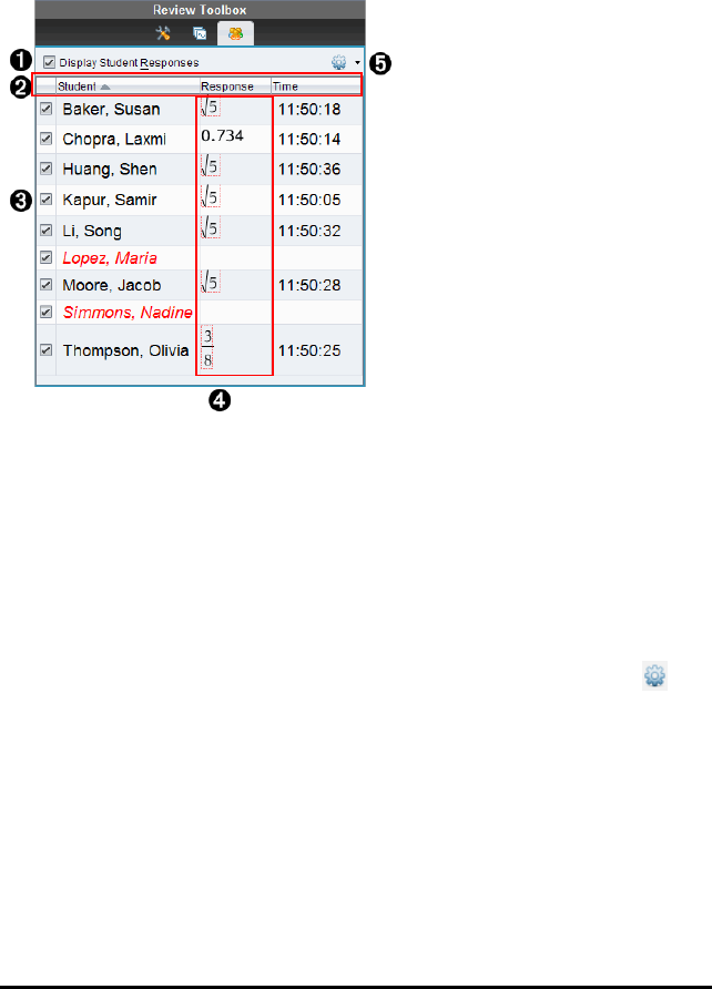
209 Using the Review Workspace
• Display the students to whom the file was sent
• View the students who responded
• View student responses
• Mark responses as correct or incorrect
• Sort the responses by student or response, or by time in Quick Polls
ÀDisplay Student Responses. Select this checkbox to show the responses of each
student. Clear the checkbox to hide the student responses.
ÁStudent, Response, and Time columns. The Time column is available only in Quick
Poll reviews.
• Click the Student column to list the students in alphabetical order. Click again
to list in reverse alphabetical order.
• Click the Response column to list the responses in alphabetical or numerical
order. Click again to list the responses in reverse order.
• To add the Time column in Quick Poll reviews, click the Options menu ,
and then click Time.
• Click the Time column to list the responses in order of the time they were
answered (first response on top). Click again to list the responses with the
first response on the bottom.
ÂStudent names. Lists all students in the class associated with the document currently
opened for review. The student names are displayed as chosen in the Class>Student
Name Format menu.
Student names in red text indicate students who did not receive the file or respond
to the Quick Poll.
Clear the checkbox next to a name to hide that student’s response.

ÃResponses. Lists all responses next to the student’s name. A student may be listed
several times if they gave multiple responses. The Response column may change if
the review document is an active Quick Poll or a question document that has not
been saved yet.
• A response is shown if the student responded.
• The response area is blank if the student did not respond.
• "Responded" is displayed if the student responded and the responses are
hidden.
• "No Response" is displayed if the student has not yet responded to the open
question or active Quick Poll.
• "Working" is displayed if the student has modified their response to a Quick
Poll, but has not submitted it.
ÄOptions menu. Click ¤to open the menu of options you can perform on the student
responses:
• Display student responses.
• Display student names only.
• Display responses only.
• Display a Time column for Quick Poll results.
• Select all items in the list.
• Show the selected item.
• Hide the selected item.
• Mark one or more responses as correct.
• Mark one or more responses as incorrect.
Using the Review Workspace 210
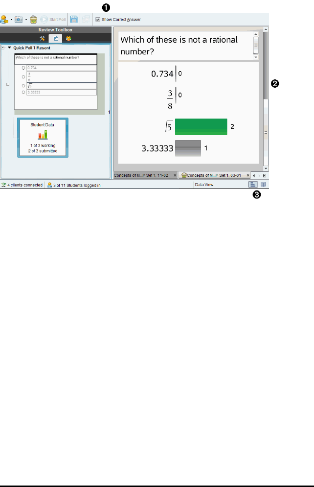
211 Using the Review Workspace
Exploring the Data View Pane
ÀShow Correct Answer. Select this checkbox to display the answer you marked as the
correct answer in the Data View pane. The correct answer is highlighted in green.
ÁResponses. Shows the information chosen in the Page Sorter. This example shows
the responses from a selected Student Response icon. You can show or hide
responses and mark responses as correct or incorrect.
ÂData View. Click an icon to view the data in different formats: bar chart, graph or
table. A "Show Your Work" option is available for expression and equation questions.
Understanding the Data View
The Data View pane displays the question in the open document, as well as the
responses to that question. You can view live results in the Data View pane. The data is
updated in real time as students respond to Quick Poll and Open Response questions,
graph functions or move points on a graph.
The Data View icons allow you to view responses in the Data View pane as a bar chart,
graph or table. Each view shows the student responses and the frequency of each
response.
The bar chart and table views are available for all question types and Quick Poll
documents. The graph view is available in equation, coordinate points and list
questions.
Expression and equation questions have an additional "Show Your Work" data view
available, if you marked the question for students to show their work. The "Show Your
Work" data view is retained when you close and reopen the Review Workspace.
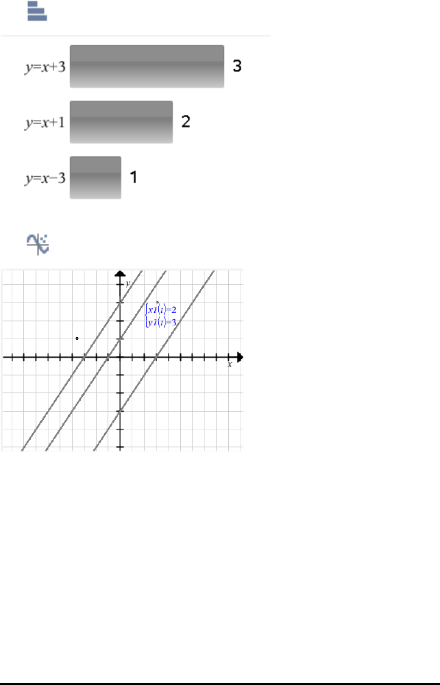
The following examples show the same data displayed in different data views.
Click to view the data in bar chart form.
Click to view the data in graph form.
When you are in graph view, the Graph Tools are available to allow you to work with
the graph. The settings in the graph are retained when you close and reopen the
Review Workspace.
In the bar chart and graph views, hover your mouse pointer over a response to see a
list of students who gave that response.
Using the Review Workspace 212
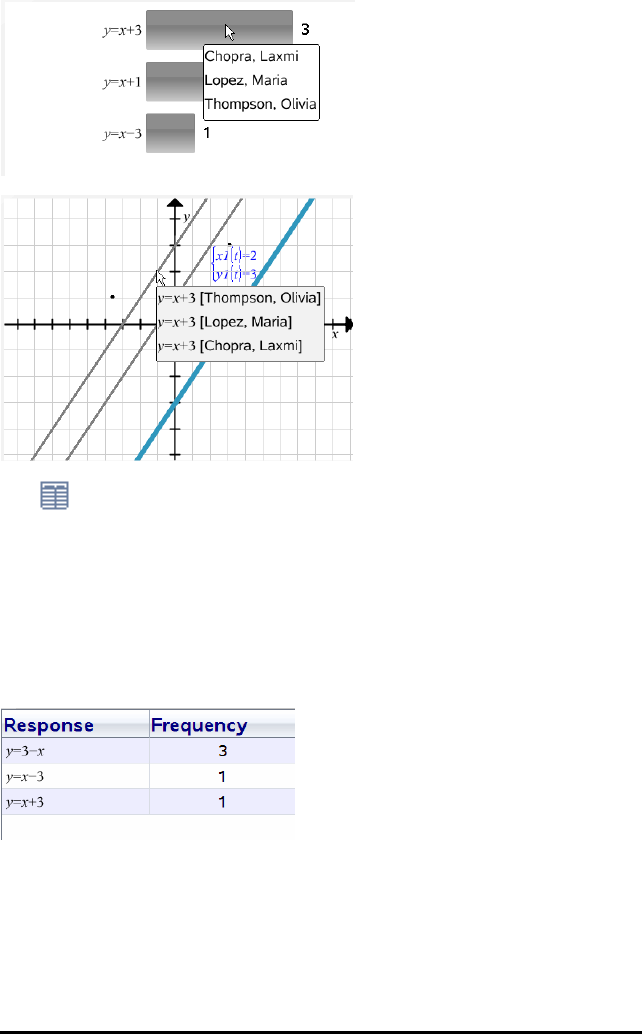
213 Using the Review Workspace
Click to view the data in table form.
The table view is available as a frequency table or as a student table.
▶To view data in different table views, click the Organise tool in the Review toolbox,
and then click Frequency Table or Student Table.
A frequency table shows the responses with the number of times the response
occurred. Click the Response heading to sort the responses in ascending order,
descending order or question order. Click the Frequency heading to sort by frequency of
response.
A student table shows the student names with their responses. Click the Student
heading to sort the responses in ascending or descending alphabetical order. Click the
Response heading to sort the responses in ascending order, descending order or
question order.
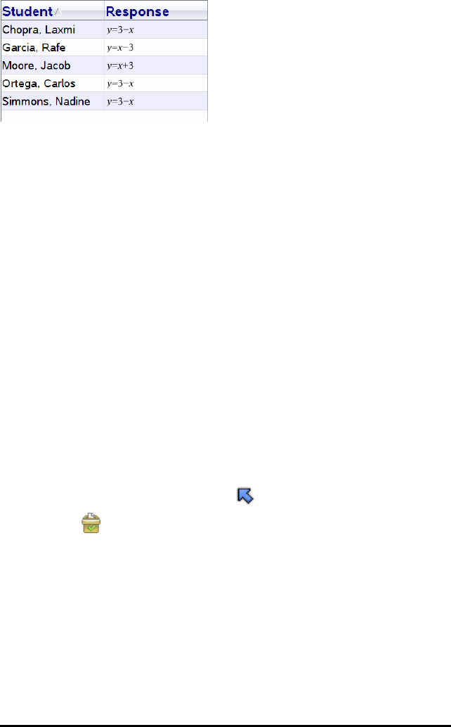
The settings for sorting and sizing columns are retained for each document when you
close and reopen the Review Workspace.
Opening Documents for Review
You can review a document that has been collected from the class, a Quick Poll in
progress or a saved Quick Poll. You cannot review a document that does not have
questions.
When you start a Quick Poll, the software automatically switches to the Review
Workspace and you can review the data as the students are responding. When you stop
and save the poll, you can open it in the Review Workspace to review the saved
responses.
If this is your first time using the software, the Data View pane may be empty.
Complete the following steps to open a document for review.
Opening a Document from the Class Workspace
To open a document for review from the Class Workspace:
1. Use the Workspace selector to select the Class Workspace.
2. Right-click a file from the Class Record, then click Open in Review workspace.
The software automatically switches to the Review Workspace with the selected
document open.
Note: You can open collected documents that contain questions and
QuickPolls for review in the Class Record.
Using the Review Workspace 214
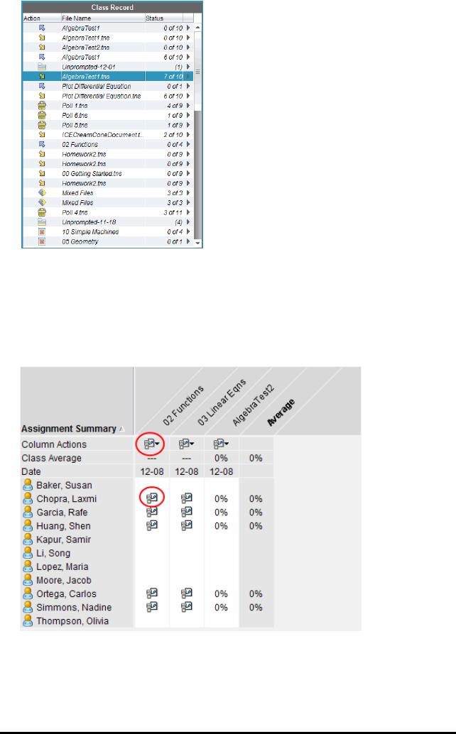
215 Using the Review Workspace
Opening a Document from the Portfolio Workspace
To open a document for review from the Portfolio Workspace, follow these steps:
1. Use the Workspace selector to select the Portfolio Workspace.
2. Right-click a column cell or a cell in a student row, then click Open in Review
workspace.
The software automatically switches to the Review Workspace with the selected
document open.
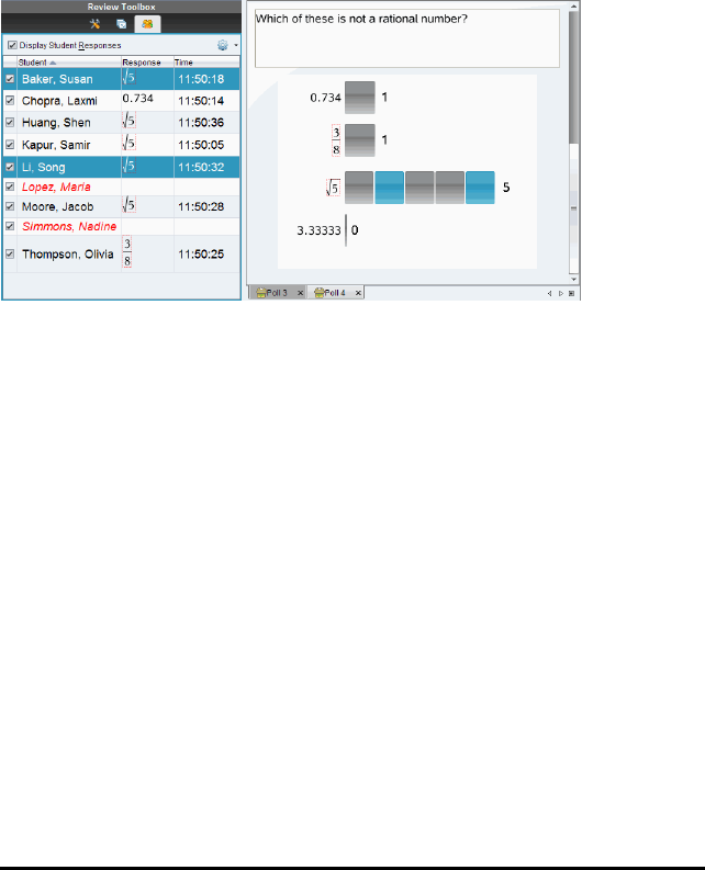
Viewing Data
You can view data in the Student pane or in the Data View pane. You can choose a
student to view their answer, or you can choose an answer to view which students
gave that answer.
Viewing Data from the Student Pane
▶Click a student name in the Student pane to view that answer in the Data View
pane. You can select more than one student at a time.
The software highlights the selected student’s answer in blue.
If you switch between bar chart, table and graph views, the software retains the
selected information and highlights the responses from the selected students.
Note: Since student responses can vary for List questions, the software does not show
List answers for selected students in the Data View pane.
Viewing Data from the Data View Pane
▶Click a response in the Data View pane to view the students who gave that
response in the Student pane. You can select more than one response at a time.
The software highlights the corresponding student names in blue.
Using the Review Workspace 216
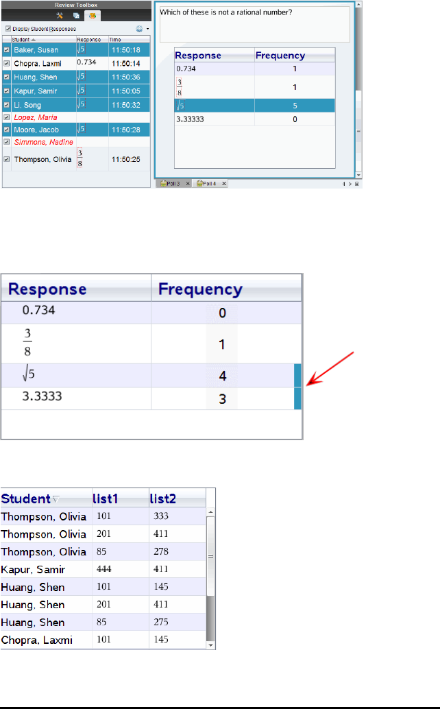
217 Using the Review Workspace
If you switch between bar chart, table and graph views, the software retains the
selected information and highlights the students who answered the selected response.
Note: If Multiple Choice questions have multiple responses, a blue area is displayed
next to all responses from the selected student.
Note: For List questions, right-click anywhere in the table view and then click Show
Student Column to show student names next to their responses.
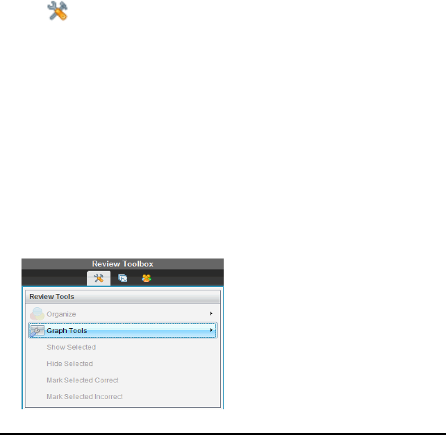
Changing the Aspect Ratio
The Review Workspace displays graphs in a question application as they appear on the
students’ handhelds or computers. At times, the graphs may appear stretched, since
the graph may have changed the aspect ratio to fit on the handheld.
You can select to view the graphs as they come in from students, or you can preserve
the aspect ratio of the graph as it appeared when it was inserted in the question
application.
By default, the Review Workspace displays graphs in a question application as they
appear when the students submit them.
To preserve the aspect ratio of a graph as it appeared when it was inserted in the
question, follow these steps:
1. View the data in graph view.
2. Right-click on the graph in the Data View pane, then click Graph Tools> Aspect
Ratio.
— or —
3. Click in the Review Toolbox, then click Graph Tools> Aspect Ratio.
When the Aspect Ratio box is ticked, the aspect ratio is preserved. When the box is
not ticked, the aspect ratio may change.
Organising Responses
You can configure a plot list for List questions, organise bar chart data and table views,
individualise student responses and organise Multiple Choice questions that have
multiple responses into separate, group or equivalent responses.
Configuring a Plot List
The plot list settings let you set different shapes for the different plots to help you
follow separate lines or responses on a graph.
To set the plot list settings, follow these steps.
1. While in graph view, click Graph Tools in the Review toolbox.
Using the Review Workspace 218
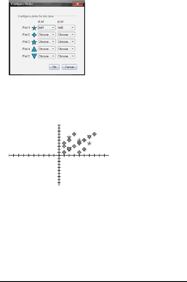
219 Using the Review Workspace
2. Click Plot List Settings.
The Configure Plot(s) dialogue box opens.
3. Click the down arrow next to a shape to choose which list to represent (list1, list2
and so forth) for the xList and yList.
Note: You can choose more than one shape for each list.
4. Click OK.
The graph view is updated with the shapes you selected.
When you change plot list settings in the graph view, and then change to bar chart
view, the software asks you to choose which lists to show in the bar chart. You can
choose an individual list, or a list for the Category and Frequency.
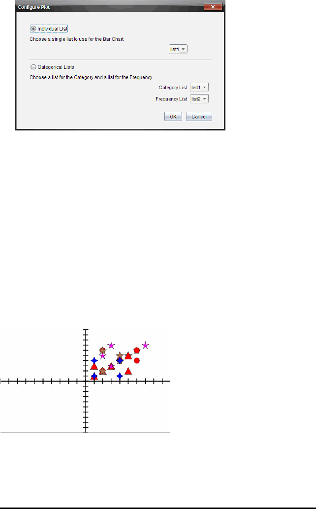
5. Select the applicable options and click OK.
If you click Cancel, the software shows the bar chart as an individual list, using list1
as the default.
You can configure the plot list at any time while in bar chart view.
Note: To configure the plot list from the bar chart view, click Organise in the
Review toolbox and click Plot List Settings.
Individualising Student Responses
You can change the colours of each student response in a graph so you can identify the
separate responses. This is useful when you are running a live activity; you can view
the progress of individual students as they graph functions, move points on a graph or
respond to Quick Poll questions.
▶To change the colour of student responses, click Graph Tools in the Review toolbox
and then click Individualise Student Responses.
The responses are displayed in different colours in the Data View pane.
Organising List Data
In bar chart view, you can organise list data by Frequency, Numeric Value or
Alphabetically.
Using the Review Workspace 220
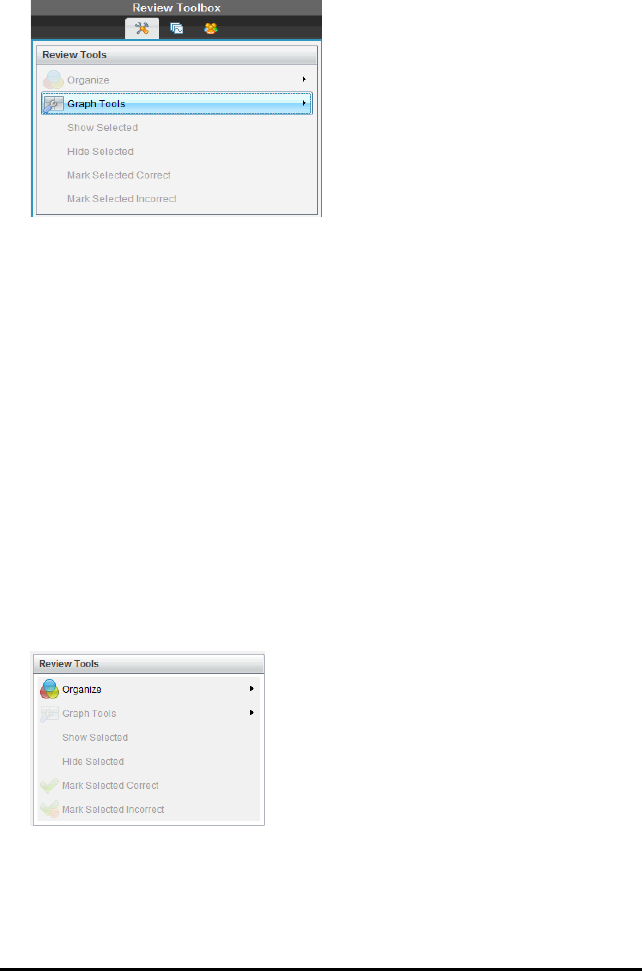
221 Using the Review Workspace
To organise list data, follow these steps.
1. In bar chart view, click Graph Tools.
2. Select to sort the bars by Frequency, Numeric Value or Alphabetically.
The bar chart view is updated in the Data View pane.
Organising Bar Chart Data
Organising by separate responses shows the results for each individual response. For
example, all of the A responses, all of the Bs, all of the Cs and so forth. Organising by
group responses shows all multiple responses from the students. For example, all of
the A plus B responses, all of the A plus C responses and so forth.
Organising by equivalency combines similar results into one bar. For example, y=4Mx,
y=Mx+4 and y=M(xM4) would all be combined into one bar or table row.
By default, Multiple Response questions are displayed as separate responses in the bar
chart view.
Settings for organising by separate or group responses and for organising by
equivalency are retained when you close and reopen the Review Workspace.
To organise by grouped responses, follow these steps.
1. Click the Organise tool in the Review toolbox.
2. Click Show Student Responses Grouped Together.
The Data View pane shows the grouped responses.
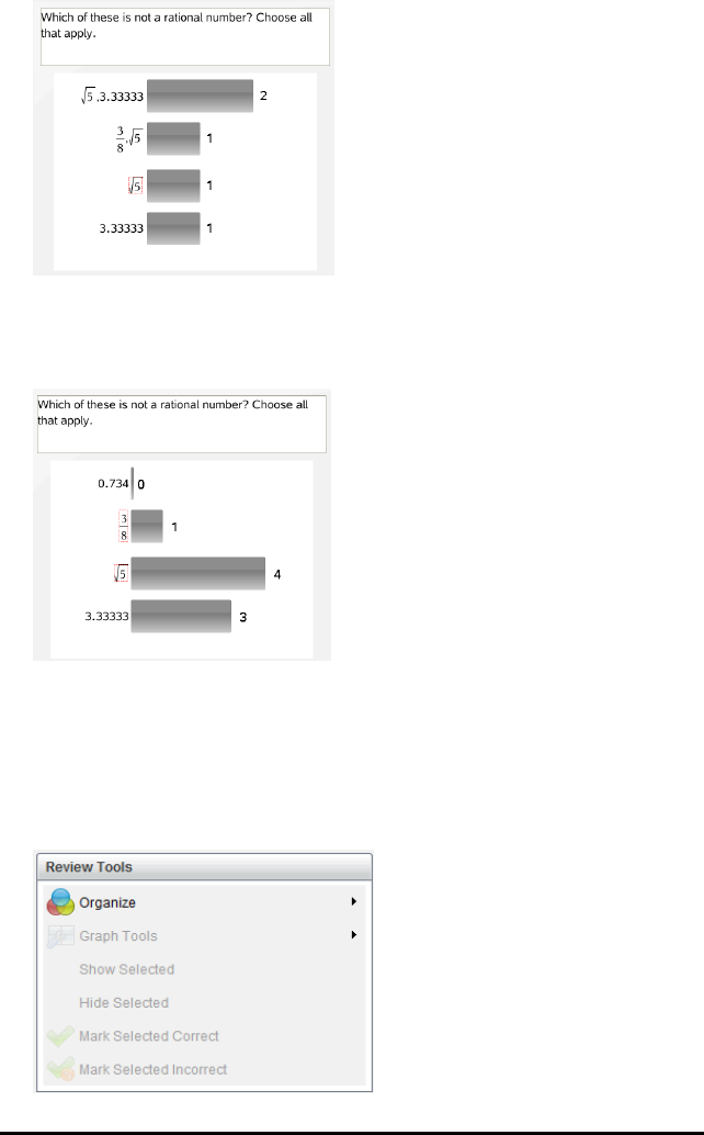
3. To return to the default view, click the Organise tool and then click Show Student
Responses Separated.
The Data View pane shows the data as separate responses.
Organising by Equivalency
Organising by equivalency groups all similar responses together in one bar or row. In
bar chart view, you can still see separate responses by clicking on the bar.
To organise by equivalency, follow these steps.
1. Click the Organise tool in the Review toolbox.
Using the Review Workspace 222
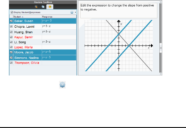
223 Using the Review Workspace
2. Click Group Responses by Equivalence.
The Data View pane shows the grouped responses.
3. To return to the default view, click the Organise tool and then click Group
Responses by Exact Matches.
The Data View pane shows the data as separate responses.
Hiding and Showing Responses
You can hide one or more student responses in the Student pane or in the Data View
pane. When you hide a response, the corresponding data updates and the Data View
pane does not show the hidden data. Settings for hiding or showing data are retained
when you close and reopen the Review Workspace.
When you hide responses, the following actions occur in the different views.
•Bar chart view. The bar chart is updated and re-sorted using the current data.
•Table view. The table is updated and re-sorted using the current data.
•Graph view. The graph is updated using the current data. Any regression that was
added is automatically recalculated and the new values are displayed.
•Show your work. The selected student’s work is hidden from view.
Hiding Responses from the Student Pane
To hide responses, follow these steps.
1. In the Student pane, select the students whose responses you want to hide.
The selected student responses are highlighted in blue in the Data View pane.
2. Click the Options menu , then click Hide Selected or clear the checkbox next to
the student name.
The Data View pane hides the responses of the students you selected and shows
the responses of the remaining students.
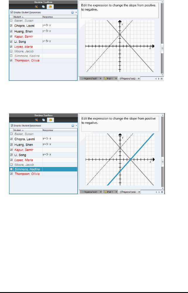
The student names you selected are displayed in grey text.
Note: If a response is hidden, click a student name to show the response. The
response is displayed in blue in the Data View pane. All bar chart, table and graph
views are updated with the selected data. The response stays in view until you
select a different student.
Hiding Responses from the Data View Pane
You can hide responses in the bar chart, graph or table views. When you hide
responses, the Data View pane updates the data and does not show the hidden
responses. In the Student View, student names are displayed in grey. In Page Sorter
view, the software does not change the documents or icons.
To hide responses, follow these steps.
1. In the Data View pane, select the responses you want to hide.
The selected students are highlighted in blue in the Student pane.
Using the Review Workspace 224
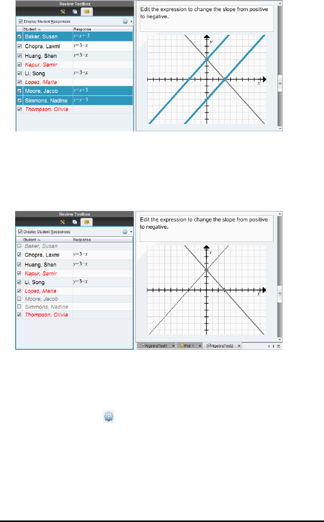
225 Using the Review Workspace
2. Right-click the response and click Hide Selected.
The Data View pane hides the responses you selected and shows the responses of
the remaining students.
The student names that correspond with the responses you selected are displayed
in grey text.
Showing Responses
To show the hidden responses, follow these steps.
1. In the Student pane, select the students whose responses you want to show.
2. Click the Options menu , and then click Show Selected.
The student names are displayed in black and student responses are shown in the
Data View pane.
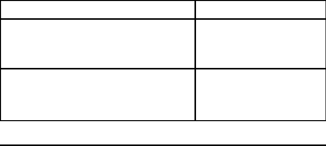
Marking Responses as Correct or Incorrect
You can use the Review Workspace to mark selected answers as correct or incorrect. If
you are reviewing a document with a correct answer already marked, you can change
the correct answer. In a Multiple Choice question with multiple responses, you can add
additional correct answers.
If the Show Correct Answer box is ticked, answers marked as correct are highlighted in
green.
The software re-evaluates the data based on the correct responses and the Data View
pane updates the view to reflect the changes.
To mark a response as correct:
▶In the Student pane, right-click a student and click Mark as Correct.
▶In the Data View pane, right-click a response and click Mark Selected Correct.
▶In the Data View pane, click a response and click Mark Selected Correct in the
Review Tools pane.
In Multiple Choice questions with multiple answers, check marks are displayed next to
the responses.
▶Click a tick mark to mark a response as correct.
When you mark a response as incorrect, the software removes the green highlight.
To mark a response as incorrect:
▶In the Student pane, right-click a student and click Remove as Correct.
▶In the Data View pane, right-click a response and click Mark Selected Incorrect.
▶In Multiple Choice questions with multiple answers, click the green tick mark.
Note: If you change an answer to correct or incorrect, any points you already manually
awarded students for correct or incorrect answers will not be changed.
When you mark responses, the following actions occur in the different question types.
Question Types Action
Multiple Choice, Single Response
Image: Label, Single Response
Image: Point on, Single Response
Adding a new answer replaces
the current answer. Removing
an answer leaves the question
with no correct answers.
Multiple Choice, Multiple Responses
Image: Label, Multiple Responses
Image: Point on, Multiple Responses
Adding a new answer increases
the correct answer set. For
example, an answer of "A and B"
becomes "A and B and C."
Using the Review Workspace 226
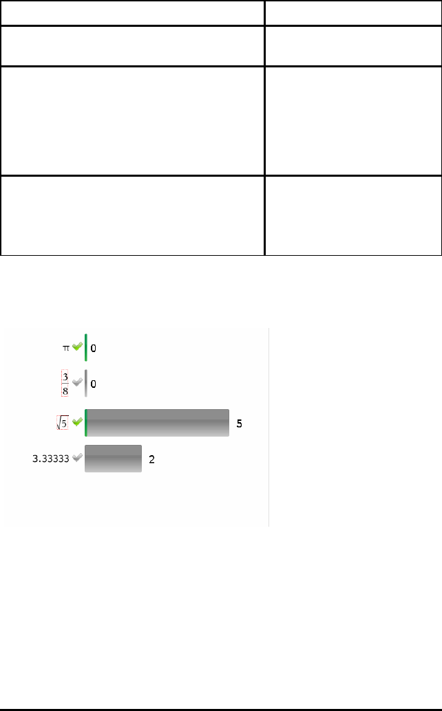
227 Using the Review Workspace
Question Types Action
Removing an answer decreases
the correct answer set.
Open Response: Explanation
Open Response: Text Match
Equation: f(x) and y=
Coordinate Points
Expression: Variable
Chemical
Adding a new answer increases
the correct answer set.
Removing an answer leaves the
question with no correct
answers.
Expression: Numerical Adding a new answer, with or
without tolerance, replaces the
current answer. Removing an
answer leaves the question with
no correct answers.
The following examples show answers marked as correct in different data views.
Bar chart view, Multiple Choice question with multiple responses and two correct
answers, organised by Show Student Responses Separate and no student selected
in the Student pane.
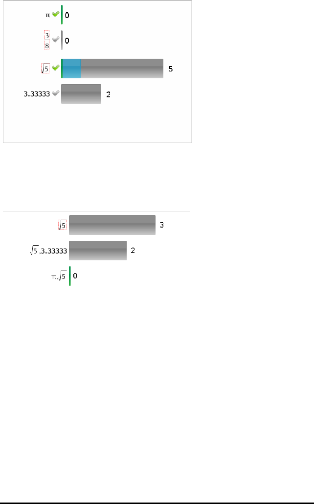
Bar chart view, Multiple Choice question with multiple responses and two correct
answers, organised by Show Student Responses Separate and one student
selected in the Student pane.
Bar chart view, Multiple Choice question with multiple responses and two correct
answers, organised by Show Student Responses Grouped Together and no
students selected in the Student pane.
Using the Review Workspace 228
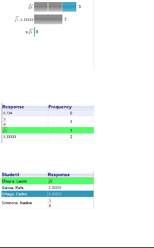
229 Using the Review Workspace
Bar chart view, Multiple Choice question with multiple responses and two correct
answers, organised by Show Student Responses Grouped Together and one
student selected in the Student pane.
Frequency table view, Multiple Choice question with one correct answer and no
student selected in the Student pane.
Student table view, Multiple Choice question with one correct answer and one
student selected in the Student pane.
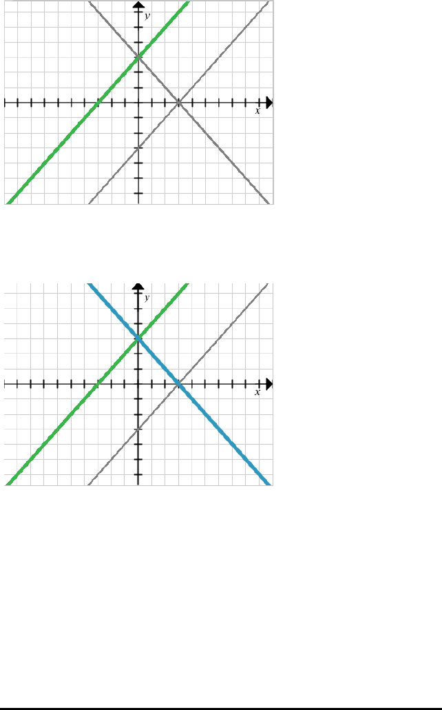
Graph view, Equation y= question with one correct answer and no student
selected in the Student pane.
Graph view, Equation y= question with one correct answer and one student
selected in the Student pane.
Adding Teacher Data
There may be times you want to add your own data to a graph you are reviewing in
class. The Graph Tools allow you to add teacher points and teacher equations to a
graph and to set the plot list settings and individualise student responses.
Teacher data is displayed larger than student data and in a different colour.
When you add teacher data, the software re-evaluates the data and the Data View
pane updates the view to reflect the changes.
Using the Review Workspace 230
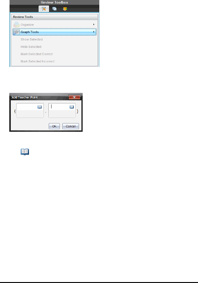
231 Using the Review Workspace
You can hide and show teacher data, but you cannot mark a teacher response as
correct or incorrect.
Adding Teacher Points
1. Click Graph Tools in the Review toolbox.
2. Click Add Teacher Point.
The Add Teacher Point dialogue box opens.
3. Type your information in the fields.
Click to open maths templates and symbols that you can add to the fields.
4. Click OK.
Your point is displayed on the graph and the name Teacher is added to the list of
names in the Student pane.
Note: The teacher may have multiple entries.
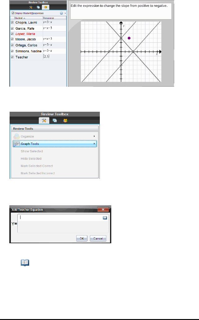
Adding Teacher Equations
1. Click Graph Tools in the Review toolbox.
2. Click Add Teacher Equation.
The Add Teacher Equation dialogue box opens.
3. Type your information in the field.
Click to open maths templates and symbols that you can add to the fields.
4. Click OK.
Your line is displayed on the graph and the name Teacher is added to the list of
names in the Student pane.
Note: The teacher may have multiple entries.
Using the Review Workspace 232
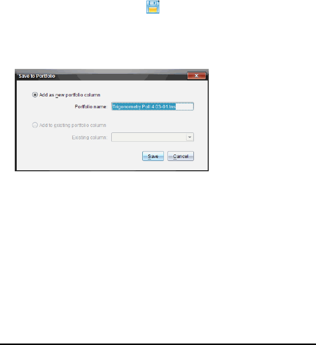
233 Using the Review Workspace
Saving to the Portfolio Workspace
You can save documents that contain questions and Quick Polls to the Portfolio
Workspace, where you can review and analyse individual responses and assign or
change a student’s grade.
When you save Quick Polls to Portfolio, students can continue to submit answers to the
Quick Poll until you stop the poll. The saved Quick Poll in Portfolio automatically
updates without you having to save it again.
Note: If you opened the file from the Portfolio Workspace, or if you have already saved
the file to Portfolio, the software does not ask you for a file name. The software saves
the file to the Portfolio Workspace with the existing file name and updates any grades
you had given students. You can go to the Portfolio Workspace and change a grade at
any time.
To save a file to the Portfolio Workspace:
1. Click File> Save to Portfolio, or click .
The Save to Portfolio dialogue box opens. By default, the name of the file is shown
in the Portfolio name box. If the file is a Quick Poll you have not saved yet, the
default name is <Class name, Quick Poll Set#, mm-dd.tns>. For example: Algebra1 -
Mrs. Smith, QP Set 2, 10-26.tns.
• To add a new Portfolio column, select Add as new portfolio column. You can
use the existing name or type a new name.
• To add the file to an existing portfolio column, select Add to existing portfolio
column. Click the down arrow to select the column.
Note: Quick Polls cannot be added to existing columns.
2. Click Save.
The file is saved in the Portfolio Workspace.

Saving Data as a New Document
You can take data collected from students, view it in table form and save it as a Lists &
Spreadsheet document. This document can be used as an instructional aid or be sent to
the students for further analysis.
Note: If the data comes from a Lists question, the column titles in the Table View are
used as the names for the list variables. If the variable names are not usable, the
software renames them. For instance, if the name has a space, the software replaces
it with an underscore.
1. To save data to a new Lists & Spreadsheet document, make sure you are viewing
the data in table view.
2. Right-click anywhere in the table, and then click Send Table to New Document.
Note: Hidden data is not sent. If data is sorted, the sort order is retained in the new
document.
The Lists & Spreadsheet document opens in the Documents Workspace.
Using the Review Workspace 234

235
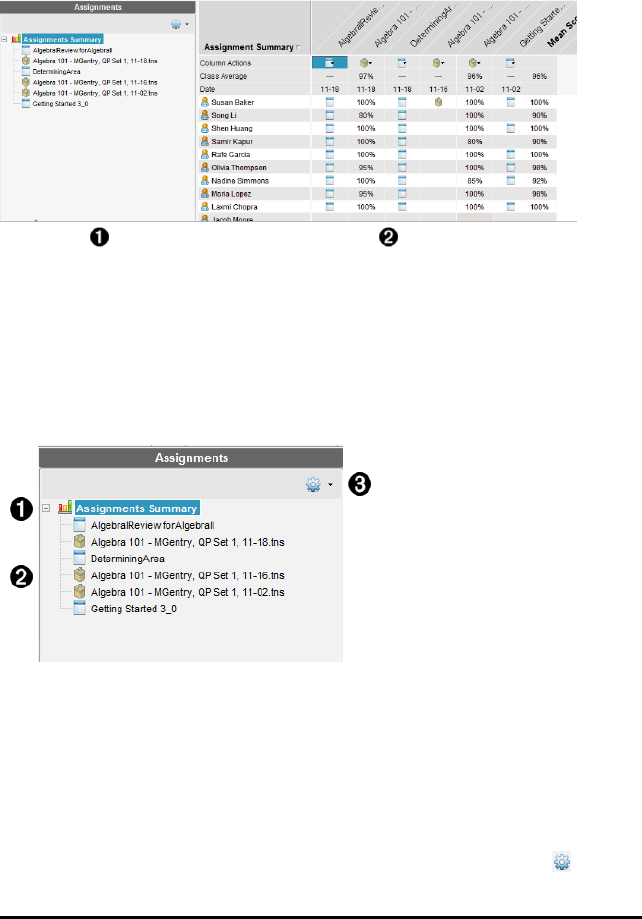
Using the Portfolio Workspace
Use this workspace to save, review, modify grades, and manage class assignments
from students.
ÀAssignments pane. Select assignments to view student information and scores. You
can redistribute, rename, or remove an assignment.
ÁWork area. Lists the students in the selected class and shows the scores received for
each assignment. Enables you to view class or student assignments; sort by
assignment, score or student; and edit assignment scores.
Exploring the Assignments Pane
ÀAssignments Summary. Lists the names of the assignments that you saved to the
Portfolio Workspace. Shows a class and student average in the workspace.
• Click the minus sign (–) to collapse the list of individual assignments and view
only the Assignments Summary.
• Click the plus sign (+) to show the list of individual assignments.
ÁIndividual assignments. Click an assignment to see the student scores for
that assignment.
ÂOptions menu. Available when you select an individual assignment. Click to open
Using the Portfolio Workspace 236
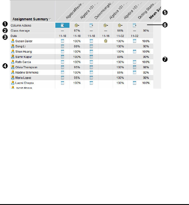
237 Using the Portfolio Workspace
a menu that allows you to:
• Open the document in the Review Workspace.
• Redistribute the assignment to the current class.
• Remove the assignment from the Portfolio Workspace. The assignment still
exists in other workspaces.
• Rename the assignment.
Exploring the Workspace Views
The appearance of the workspace changes depending on what you selected in the
Assignments pane.
Assignments Summary View
This work area opens when you select Assignments Summary in the Assignments pane.
ÀColumn Actions. Lets you perform certain actions on a column. Click a file icon
anywhere in this row to:
• Open an assessment for review in the Review Workspace.
• Sort assignments in ascending or descending order by student.
• Open the Master in the Review Workspace.
• Remove from Portfolio.
• Rename the assignment.
ÁClass Average. Shows the average score of the class for the assignment
in that column.
ÂDate. Shows the date the file was collected. The date the last file was collected is
shown in the first column on the left.
ÃStudents. Lists all students in the class.
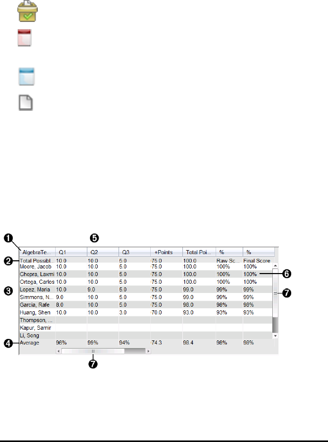
ÄColumn Header. Shows the name of the assignment saved to the Portfolio
Workspace. You can perform the same actions on the column header as you can on
the column actions. Right-click the column header to open the menu.
The column header Mean Score shows the mean score for all assignments and the
mean score for all assignments per student. Right-click the Mean Score column to
sort by ascending or descending scores.
ÅFile icon. Shows the type of file. The file types shown are:
Quick Poll
PublishView™ file
(Shown only in the TI-Nspire™ Navigator™ NC Teacher Software)
TI-Nspire™ file
Other file types
(Shown only in the TI-Nspire™ Navigator™ NC Teacher Software)
ÆStudent scores. If questions are automatically graded, the scores are shown. You can
change a student’s score for an assignment.
Individual Assignment View
This work area opens when you select a single assignment in the Assignments pane.
To view this work area, the assignment you select must be a .tns file that contains one
or more questions.
Note: In the TI-Nspire™ Navigator™ NC Teacher Software, you can also open .tnsp files.
ÀName of the selected assignment.
ÁTotal Possible. This row shows the points for these categories:
Using the Portfolio Workspace 238

239 Using the Portfolio Workspace
• Total possible points for each question in the assignment. You can edit this
number.
• Total number of extra points possible for the assignment. You can edit this
number.
• Total points for the assignment.
• Raw score based on the number of points the student received divided by
total possible points.
• Final percentage. This number updates when you edit possible points or extra
points. You can edit this score. The final score is the same as the raw score,
unless you change it.
If you edit the final score, it no longer updates if the other points change.
ÂStudent names. All students who received the selected assignment. Right-click to
open and edit the document in the Documents Workspace, or to open the document
for review in the Review Workspace.
ÃAverage. Shows the average score for all students, as well as average total points, raw
score, and final score.
ÄQuestions in the assignment. If the document contained multiple questions, each
question is displayed here, along with the total possible score for that question.
ÅScores. Lists the score each student received for the selected assignment. Each page
in an assignment may have a separate score. Right-click to edit the score, open the
assignment in the Documents Workspace, or open the document in the Review
Workspace.
ÆScroll bar. Appears when there are more questions in the assignment to view, or
more students to view.
Saving an Item to the Portfolio Workspace
If you are using the TI-Nspire™ software for the first time, the Portfolio Workspace
may be empty. You need to save files to the Portfolio Workspace to view and edit
scores, and perform other work on the files.
You can save collected, unprompted, and Quick Poll files to the Portfolio Workspace.
You can save to the Portfolio Workspace from the Class and Review Workspaces.
When you save Quick Polls to Portfolio, students can continue to submit answers to the
Quick Poll until you stop the poll. The saved Quick Poll automatically updates without
you having to save it again.
Note: If you opened the file from the Portfolio Workspace, or if you have already saved
the file to the Portfolio Workspace, the software does not ask you for a file name. The
software saves the file to the Portfolio Workspace with the existing file name, and
updates any grades you had given students. You can change a grade in the Portfolio
Workspace at any time.
To save a file to the Portfolio Workspace, follow these steps.
1. Select the files you want to save.
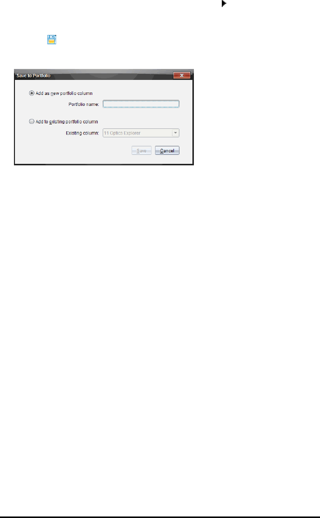
• From the Class Record in the Class Workspace, click , and then click Save
selected to Portfolio.
• From an open file in the Review Workspace, click File> Save to Portfolio, or
click .
The Save to Portfolio dialogue box opens.
2. Save the files to a new Portfolio column or add them to an existing Portfolio
column.
• To add the files to a new Portfolio column, select Add as new portfolio column.
You can use the existing name, or type a new name.
• To save the files to an existing Portfolio column, select Add to existing portfolio
column. Click the down arrow to select the desired column from the drop-down
list.
Note: Quick Polls cannot be added to existing columns.
3. Click Save.
The file is saved in the Portfolio Workspace.
Note: The files you saved in the Portfolio Workspace remain in the Class Record until
you remove them using the Remove command.
If a file is deleted from the Class Record, that delete action does not affect the file
copy in the Portfolio Workspace. The copy remains in the Portfolio Workspace until it is
deleted.
Importing an Item to the Portfolio Workspace
You can import a .tns file from your computer to a student’s Portfolio entry.
1. Click Assignments Summary.
2. Highlight a cell in the student row where you want to import the file.
Note: You can import a file for only one student at a time.
3. Click File> Import Item.
The Open dialogue box is displayed.
4. Navigate to the file you want to import and click it.
Using the Portfolio Workspace 240
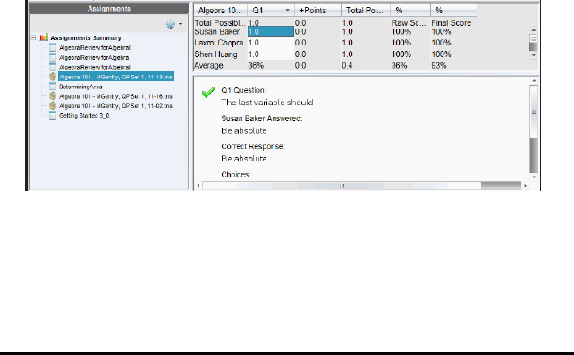
241 Using the Portfolio Workspace
5. Click Import.
If a file already exists in that cell, you are prompted to confirm the file
replacement.
• Click Replace to save your imported file over the existing file.
• Click Keep Existing to keep the existing file and cancel the import file function.
Editing Scores
There may be times when you want to edit a student’s score. For example, an Open
Response assignment contains a question that requires the word “Autumn” as the
correct answer. One student has entered “Fall.” If you want to give the student full or
partial credit, you can do so by changing the student’s score for the question.
In addition to editing an individual student score, you can edit the total possible points
for each question, the extra points, and the final percentage.
▶Use whole numbers to edit the scores. For example, type 75 to give a score of 75%,
type 100 to give a score of 100%, and so forth.
Note: If you type a score and do not press Enter, the change is not made, and the
previous score remains in place.
Previewing a Student’s Answer
You can preview a student’s answer to an individual assignment question in the
Preview Pane. This provides a quick, easy, and efficient method for the review of
questions, answers, and the modification of scores.
Note: The assignment must contain at least one question to be previewed.
1. Click an individual assignment in the Assignments Summary list.
2. Select the question cell you want to preview.
The following information is shown in the Preview Pane.
•Q#Question. Original question with icon showing correct or incorrect response
•Student’s Answer. Student’s response
•Correct Response. Teacher’s correct response (blank if there is no correct
response)
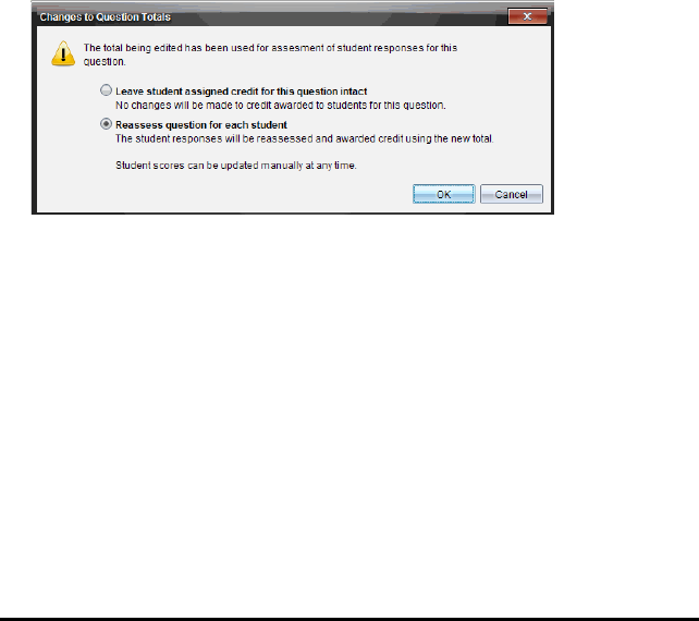
Note: Depending on the question posted, additional information may be displayed.
Modifying a Student’s Score for an Assignment
You can edit the score for an assignment from the Assignments Summary view, or you
can edit the score for individual questions in an assignment from the Individual
Assignments view. These steps describe how to change a score from either view.
1. In the student row, select the score you want to edit.
2. Right-click the cell and click Edit Score.
3. Type the replacement score, and press Enter. To cancel, press Esc.
Changing the Total Possible Points for a Question
You can edit the total possible score for individual questions or extra points.
1. Select a cell in the Total Possible row.
2. Right-click the cell and click Edit Score.
3. Type the points for the question or for extra points, and press Enter.
The software asks if you want to keep the student scores for the question, or
reassess the scores for each student. The default setting is to reassess the scores
for each student.
• To keep the student scores without making changes, select Leave student
assigned credit for this question intact.
• To reassess the score for each student, select Reassess question for each
student.
4. Click OK.
Changing the Final Percentage Score
1. In the Individual Assignments view, select the student whose score you want to
edit.
2. Right-click the cell in the Final column, and click Edit Score.
3. Type the replacement score and press Enter. To cancel, press Esc.
Note: If you edit the final score, it retains the edited value and no longer updates if you
edit other values in the row.
Using the Portfolio Workspace 242
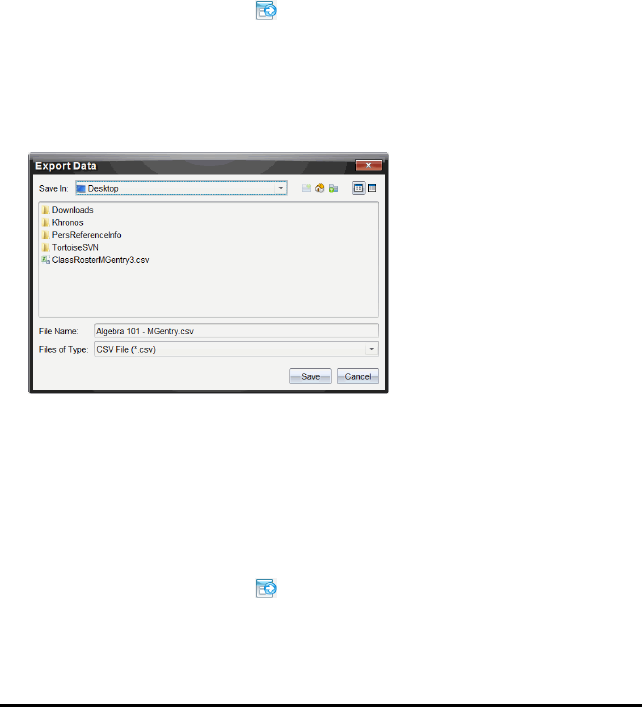
243 Using the Portfolio Workspace
Exporting Results
If you or your school district use electronic gradebook software and reporting, you may
want to export scores to these programs. You can export scores from Portfolio
Workspace as a .csv formatted file. The export action includes all scores for all
students on the selected assignment, or for all assignments.
The .csv file contains all the columns and rows in the workspace except for the Column
Actions row. If a student had an empty cell with no score, the .cvs file displays a cell
that is empty.
Exporting the Current View
This allows you to export all data shown in the Portfolio Workspace for a single
assignment.
1. Choose an assignment from the list.
2. Click File > Export Data or click .
3. Select Export Current View.
The Export Data dialogue box opens.
• The default location is the My Documents folder.
• The default name is the name of the assignment.
4. Navigate to the location where you want to save the file.
5. Click Save.
Customizing an Export
Custom Export allows you to export the final scores for one or more assignments. This
is useful for reporting scores over a date range with only the student name and final
score exporting.
1. Click File > Export Data or click .
2. Select Custom Export.
The Custom Export dialogue box opens.
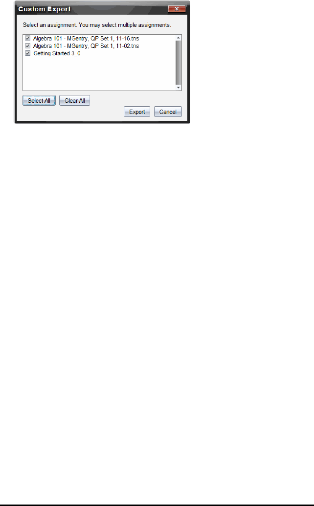
3. Choose the assignments you want to export.
• Select the check box by assignment name.
• Click Select All to select all assignments.
• Click Clear All to clear selections.
4. Click Export.
The Export Data dialogue box opens.
• The default location is the My Documents folder.
• The default name is the name of the assignment.
5. Navigate to the location where you want to save the file.
6. Click Save.
Sorting Information in the Portfolio Workspace
1. Click the column header of the list you want to sort.
The selected list can be sorted in ascending, descending, or student name order.
2. Click the column header again to sort in another order.
Opening a Portfolio Item in Another Workspace
You can open a .tns file in the Documents Workspace to edit it; or you can open a .tns
or Quick Poll file in the Review Workspace to view student responses in bar chart,
table, or graph views.
Note: In the TI-Nspire™ Navigator™ NC Teacher Software, you can also open .tnsp files.
Opening an Item in the Documents Workspace
1. Click the file you want to open.
To open a file for all students:
• From the Assignments Summary list, click the file.
Using the Portfolio Workspace 244

245 Using the Portfolio Workspace
• From the Assignments Summary view, click the icon in the Column Actions
row, or click the Column Header.
To open a file for selected students:
• From the Assignments Summary view, select a cell in a selected student’s row.
You can open more than one file in a column, but you cannot open multiple
files from different columns.
• From the Individual Assignments view, select a cell in the selected student’s
row.
2. Click File> Open for Editing or right-click and click Open for Editing.
The file opens in the Documents Workspace.
Opening an Item in the Review Workspace
1. Click the file you want to open using one of these methods:
• From the Assignments Summary list, select the file.
• From the Assignments Summary view, click the icon in the Column Actions
row, or click the Column Header.
• From the Assignments Summary view, click a cell in a selected student’s row.
You can open more than one file in a column, but you cannot open multiple
files from different columns.
• From the Individual Assignments view, click a cell in the selected student’s
row.
Note: Any method you choose in the Review Workspace opens the file with all
student responses. You cannot open a file for just one student. However, you can
select review responses for an individual student in the Review Workspace.
2. Click File> Open in Review Workspace or right-click and click Open in Review
Workspace.
The file opens in the Review Workspace.
Opening a Master Document
A Master Document is the original document that was sent to students, and it contains
the answer key for evaluating the responses collected from students. When you save a
document to a column in the Portfolio Workspace, there is usually a Master Document
associated with that file.
You can open the Master Document from the Portfolio Workspace in the Assignments
Summary view. When you open the Master Document, it opens in the Documents
Workspace as a read-only file.
1. In the Column Actions row, click the icon corresponding to the file you want to
open.
2. Right-click the icon and click Open Master Document.
The document opens in the Documents Workspace as a read-only file.

Adding a Master Document
There may be times when you want to replace an existing Master Document, or add a
Master Document to an assignment that does not have one. For example, a question
was marked with an incorrect answer and students did not receive credit for that
answer. You can give students credit by changing the answer to that question, and
retain the Master Document as a permanent record of the correct answer key.
Note: You can add or replace a Master Document for a .tns file, but not for a Quick Poll
file.
The new Master Document is used to evaluate student scores. The evaluation works as
follows:
• If a question changed, student answers are evaluated for the new question.
• If the new Master Document has questions that were not in the old Master
Document, those questions are evaluated. Students may receive zero credit for
those questions if they have not seen them.
To add or replace a Master Document, follow these steps:
1. In the Column Actions row, click the icon corresponding to the .tns file you want to
open.
2. Click File> Add Master Document.
A dialogue box opens where you can select a file.
3. Navigate to the .tns file you want to use as the new Master Document and click
Open.
The software displays a message warning that replacing the Master Document will
cause the software to reevaluate the student scores.
4. Click Add/Replace Master to assign the new Master Document, or click Cancel to
cancel the action.
Redistributing a Portfolio Item
Redistributing a file to the class is a useful way to return graded assignments or to
return assignments for additional work. Class must be in session to redistribute a file.
Note: You cannot redistribute a Quick Poll file.
1. Right-click the item you want to redistribute.
2. Click Redistribute to Class, or click .
The system sends the file to each student logged onto the TI-Nspire™ Navigator™
network.
Using the Portfolio Workspace 246

247 Using the Portfolio Workspace
Collecting Missing Files from Students
There may be times when you store a set of student files to the Portfolio Workspace
and the collection is incomplete because not all students were present, had the file
ready for collection, or were not logged on. Class must be in session to collect a file.
1. Select an individual file, or click a file icon on the Column Actions row to select all
files in that column.
Note: You can collect only one column of files at a time.
2. Click Collect Missing.
Missing files are collected from those students who are logged onto the network
and whose files were not initially collected.
Sending Missing Files to Students
There may be times when you send a set of files to students and the send is
incomplete because not all students were present, or logged on, or a new student was
added to the class. Class must be in session to send a missing file.
1. Select an individual file, or click a file icon on the Column Actions row to select all
files in that column.
Note: You can only send files contained in one column at a time.
2. Click Send Missing.
Missing files are sent to those students who are logged onto the network and who
did not initially receive the files.
Renaming a Portfolio Item
You can rename an assignment from the Assignments pane or from the column
header.
1. Click the assignment name or column header you want to rename.
2. Right-click and click Rename.
The Rename Portfolio Column dialogue box opens.
3. Type the new name.
4. Click Rename. Click Cancel to cancel the request.
The column appears in the column header and in the Assignments pane with the
new name.
Removing Columns from Portfolio
There may be times you want to delete files from Portfolio. For example, an incorrect
file was sent to or collected from a class. You can remove an assignment from the
Assignments pane or from the column header.

1. Click the assignment name or column header you want to remove.
2. Right-click and click Remove From Portfolio.
The Remove from Portfolio dialogue box opens.
3. Click Remove to delete the file. Click Cancel to cancel the request.
Note: If a file is saved to the Portfolio Workspace and later deleted from the Class
Record, that delete action does not affect the file copy in the Portfolio. The copy
remains in the Portfolio Workspace until it is deleted.
Removing Individual Files from Portfolio
There may be times you want to delete a single file or a few files from a column list,
but not all of the files. For example, an incorrect file was collected from a student.
Remove individual files from the work area in the Assignments Summary view.
1. Click the file or files within a single column that you want to delete.
2. Press Delete.
The Remove Selected Document(s) dialogue box opens.
3. Click Remove to delete the files. Click Don’t Remove to cancel the request.
Summary of File Type Options
.tns .tns with
questions
.tnsp Quick
Poll
Other file
types
Save to Portfolio Ÿ Ÿ Ÿ Ÿ Ÿ
Save Selected to
Portfolio
Ÿ Ÿ Ÿ Ÿ Ÿ
Edit Score Ÿ Ÿ Ÿ Ÿ
Open in Review
Workspace
Ÿ Ÿ
Open for Editing Ÿ Ÿ Ÿ Ÿ*
Redistribute to class Ÿ Ÿ Ÿ Ÿ
Open Master
Document
Ÿ Ÿ Ÿ Ÿ Ÿ
Add Master
Document
Ÿ Ÿ
Export Data Ÿ** Ÿ** Ÿ** Ÿ** Ÿ**
Send/Collect Missing Ÿ Ÿ Ÿ Ÿ
Rename Portfolio
Column of files
Ÿ Ÿ Ÿ Ÿ Ÿ
Using the Portfolio Workspace 248

249 Using the Portfolio Workspace
Remove Portfolio
Column of Files
Ÿ Ÿ Ÿ Ÿ Ÿ
Ÿ*The file opens in the program the operating system has associated with the file
type.
Ÿ**Empty, non-graded, and “Other file types” show “No score” in the cell when
exported.
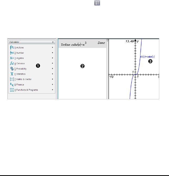
Calculator Application
The Calculator application lets you:
• Enter and evaluate maths expressions
• Define variables, functions, and programmes that become available to any
TI-Nspire™ application—such as the Graphs application—residing in the same
problem.
• Define library objects, such as variables, functions, and programmes, which are
accessible from any problem of any document. For information on creating library
objects, see Libraries.
Adding a Calculator Page
▶To start a new document with a blank Calculator page:
From the main File menu, click New Document, and then click Add Calculator.
Handheld: Press c, and select Calculator .
▶To add a Calculator page in the current problem of an existing document:
From the toolbar, click Insert > Calculator.
Handheld: Press ~and select Insert > Calculator.
ÀCalculator menu. This menu is available anytime you are in the Calculator work area
using the Normal view mode. The menu in this screen snapshot may not exactly
match the menu on your screen.
ÁCalculator work area
• Enter a maths expression on the entry line, and then press Enter to evaluate
the expression.
• Expressions are displayed in standard mathematical notation as you enter
them.
• Entered expressions and results show in the Calculator history.
Calculator Application 250
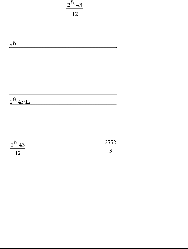
251 Calculator Application
ÂExample of Calculator variables used in another application.
Entering and Evaluating Maths Expressions
Entering Simple Maths Expressions
Note: To enter a negative number on the handheld, press v. To enter a negative
number on a computer keyboard, press the hyphen key (-).
Suppose you want to evaluate
1. Select the entry line in the Calculator work area.
2. Type 2^8 to begin the expression.
3. Press ¢to return the cursor to the baseline.
4. Complete the expression:
Type *43/12.
Handheld: Type r43 p12.
5. Press ·to evaluate the expression.
The expression is displayed in standard mathematical notation, and the result is
displayed on the right side of the Calculator.
Note: If a result does not fit on the same line with the expression, it is displayed on the
next line.
Controlling the Form of a Result
You might expect to see a decimal result instead of 2752/3 in the preceding example.
A close decimal equivalent is 917.33333..., but that’s only an approximation.
By default, Calculator retains the more precise form: 2752/3. Any result that is not a
whole number is shown in a fractional or (CAS) symbolic form. This reduces rounding
errors that could be introduced by intermediate results in chained calculations.
You can force a decimal approximation in a result:
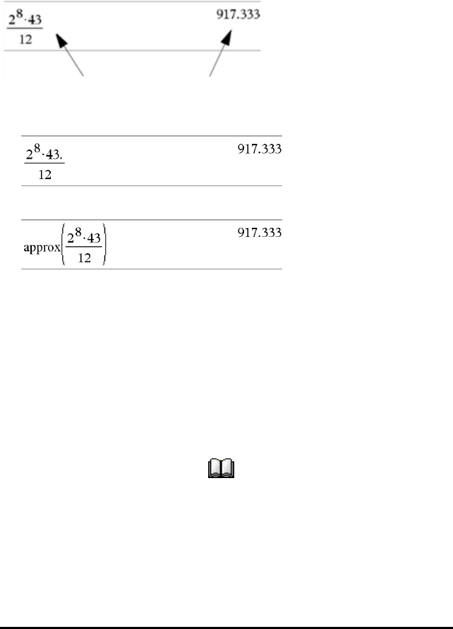
• By pressing shortcut keys.
Windows®: Press Ctrl +Enter to evaluate the expression.
Mac®: Press “ +Enter to evaluate the expression.
Handheld: Press / · instead of ·to evaluate the expression.
Pressing / · forces the approximate result.
• By including a decimal in the expression (for example, 43. instead of 43).
• By wrapping the expression in the approx() function.
• By changing the document’s Auto or Approximate mode setting to Approximate.
From the File menu, click Settings >Document Settings.
Handheld: Press ~ 1 7.
Note that this method forces all results in all of the document’s problems to
approximate.
Inserting Items from the Catalogue
You can use the Catalogue to insert system functions and commands, symbols and
expression templates into the Calculator entry line.
1. Click the Utilities tab, and then click to open the Catalogue.
Handheld: Press k1.
Calculator Application 252
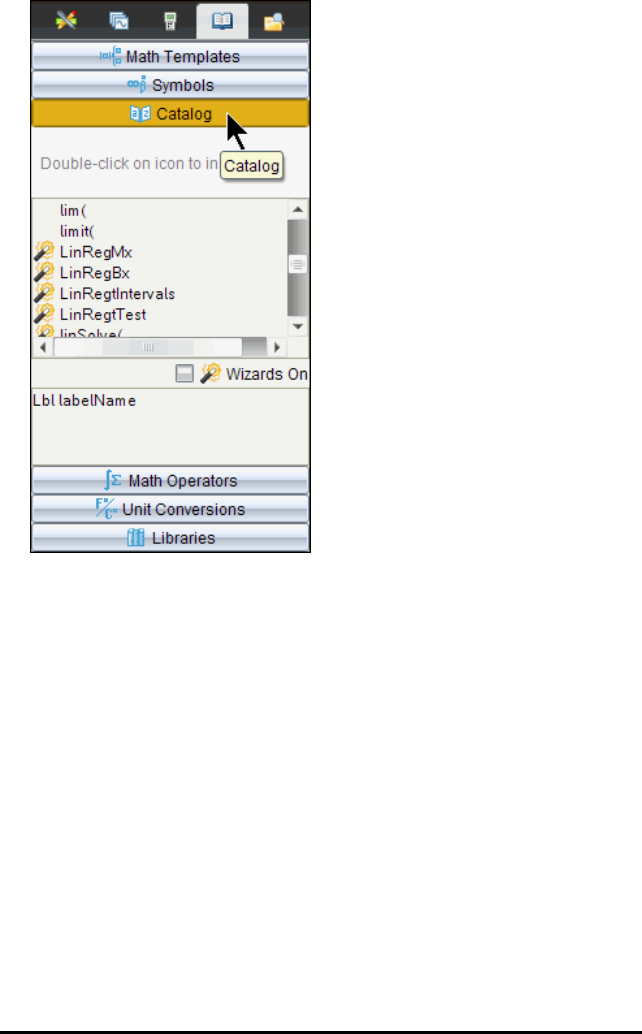
253 Calculator Application
Note: Some functions have a wizard that prompts you for each argument. Those
functions are shown with an indicator. To receive the prompts, select Wizards On.
2. If the item you are inserting is visible in the list, select it and press ·to insert
it.
3. If the item is not visible:
a) Click inside the list of functions, and then press a letter key to jump to the
entries that begin with that letter.
b) Press ¤or£as necessary to highlight the item you are inserting.
Help, such as syntax information or a short description of the selected item,
appears at the bottom of the Catalogue.
c) Press ·to insert the item into the entry line.
Using an Expression Template
The Calculator has templates for entering matrices, piecewise functions, systems of
equations, integrals, derivatives, products and other maths expressions.
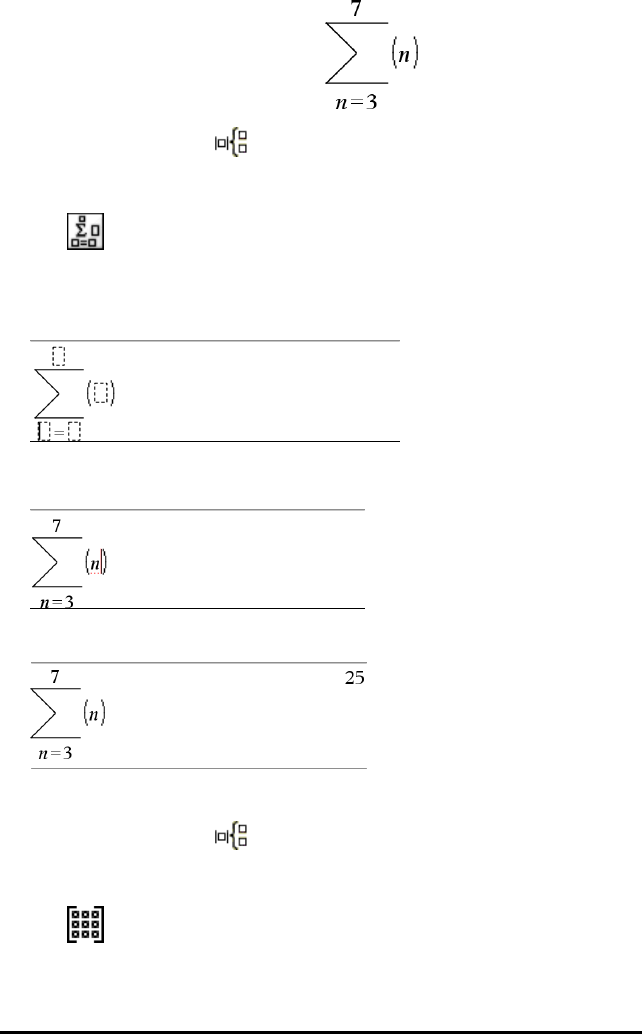
For example, suppose you want to evaluate
1. On the Utilities tab, click to open the templates.
Handheld: Press t.
2. Click to insert the algebraic sum template.
The template appears on the entry line with small blocks representing elements
that you can enter. A cursor appears next to one of the elements to show that you
can type a value for that element.
3. Use the arrow keys to move the cursor to each element’s position, and type a value
or expression for each element.
4. Press ·to evaluate the expression.
Creating Matrices
1. On the Utilities tab, click to open the templates.
Handheld: Press t.
2. Click .
The Create a Matrix dialogue box opens.
Calculator Application 254

255 Calculator Application
3. Type the Number of rows.
4. Type the Number of columns, and then click OK.
Calculator opens a template with spaces for the rows and columns.
Note: If you create a matrix with a large number of rows and columns, it may take
a few moments to appear.
5. Type the matrix values into the template, and then press ·to define the
matrix.
Inserting a Row or Column into a Matrix
▶To insert a new row, hold down Alt and press Enter.
▶To insert a new column, hold down Shift and press Enter.
Handheld:
▶To insert a new row, press @.
▶To insert a new column, press g ·.
Inserting Expressions Using a Wizard
You can use a wizard to simplify entering some expressions. The wizard contains
labeled boxes to help you enter the arguments in the expression.
For example, suppose you want to fit a y = mx + b linear regression model to the
following two lists:
{1,2,3,4,5}
{5,8,11,14,17}
1. On the Utilities tab, click to open the Catalogue.
Handheld: Press k1.
2. Click an entry in the Catalogue, and then press Lto jump to the entries that begin
with “L.”
Handheld: Press L.
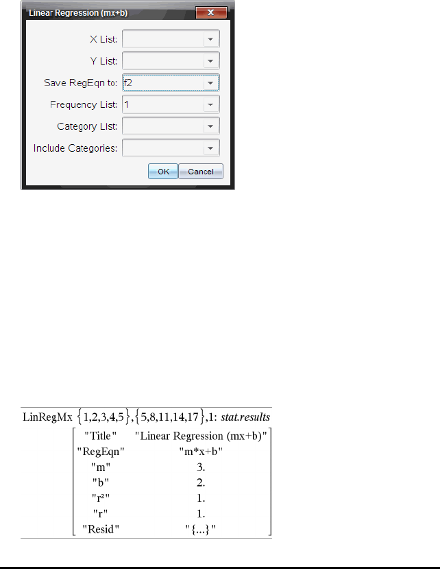
3. Press ¤as necessary to highlight LinRegMx.
4. Select the Wizards On option, if it is not already selected:
Handheld: Press eeto highlight Wizards On, press ·to change the
setting and then press eeto highlight LinRegMx again.
5. Press ·.
A wizard opens, giving you a labeled box to type each argument.
6. Type {1,2,3,4,5} as X List.
7. Press eto move to the Y List box.
8. Type {5,8,11,14,17} as Y List.
9. If you want to store the regression equation in a specific variable, press e, and
then replace Save RegEqn To with the name of the variable.
10. Click OK to close the wizard and insert the expression into the entry line.
Calculator inserts the expression and adds statements to copy the regression
equation and show the variable stat.results, which will contain the results.
LinRegMx {1,2,3,4,5},{5,8,11,14,17},1: CopyVar stat.RegEqn,f2: stat.results
Calculator then shows the stat.results variables.
Calculator Application 256
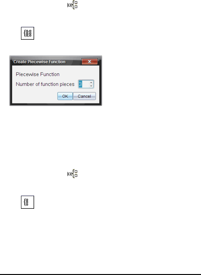
257 Calculator Application
Note: You can copy values from the stat.results variables and paste them into the
entry line.
Creating a Piecewise Function
1. Begin the function definition. For example, type the following expression:
Define f(x,y)=
2. On the Utilities tab, click to open the templates.
Handheld: Press t.
3. Click .
The Create Piecewise Function dialogue box opens.
4. Type the Number of Function Pieces, and click OK.
Calculator opens a template with spaces for the pieces.
5. Type the expressions into the template, and press ·to define the function.
6. Enter an expression to evaluate or graph the function. For example, type the
expression f(1,2) on the Calculator entry line.
Creating a System of Equations
1. On the Utilities tab, click to open the templates.
Handheld: Press t.
2. Click .
The Create a System of Equations dialogue box opens.
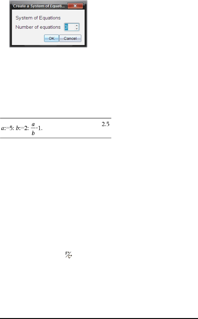
3. Type the Number of Equations, and click OK.
Calculator opens a template with spaces for the equations.
4. Type the equations into the template, and press ·to define the system of
equations.
Entering Multiple Statements on the Entry Line
To enter several statements on a single line, separate them with a colon (“:”). Only the
result of the last expression is shown.
CAS: Working with Measurement Units
A list of pre-defined constants and measurement units is available in the Catalog. You
can also create your own units.
Note: If you know a unit’s name, you can type the unit directly. For example, you can
type _qt to specify quarts. To type the underscore symbol on the handheld, press
/ _.
CAS: Converting Between Measurement Units
You can convert a value between any two units within the same category (such as
length).
Example: Using the Catalog, convert 12 metres to feet. The desired expression is 12·_
m¢_ft.
1. Type 12 on the entry line.
2. On the Utilities tab, click to show the unit conversions.
Handheld: Press k3.
Calculator Application 258
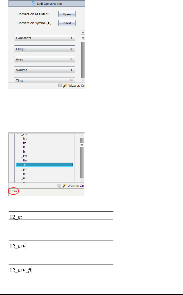
259 Calculator Application
3. Click the Length category to expand the list of pre-defined length units.
Handheld: Scroll to the Length category, and press ·.
4. Scroll to metre.
Handheld: Scroll to _m (noting the metre hint in the Help window).
5. Press ·to paste _m to the entry line.
6. Click the Conversion Operator (¢) at the top of the Units list, and press ·to
paste it to the entry line.
7. Select _ft from the Length category, and press ·.
8. Press ·to evaluate the expression.
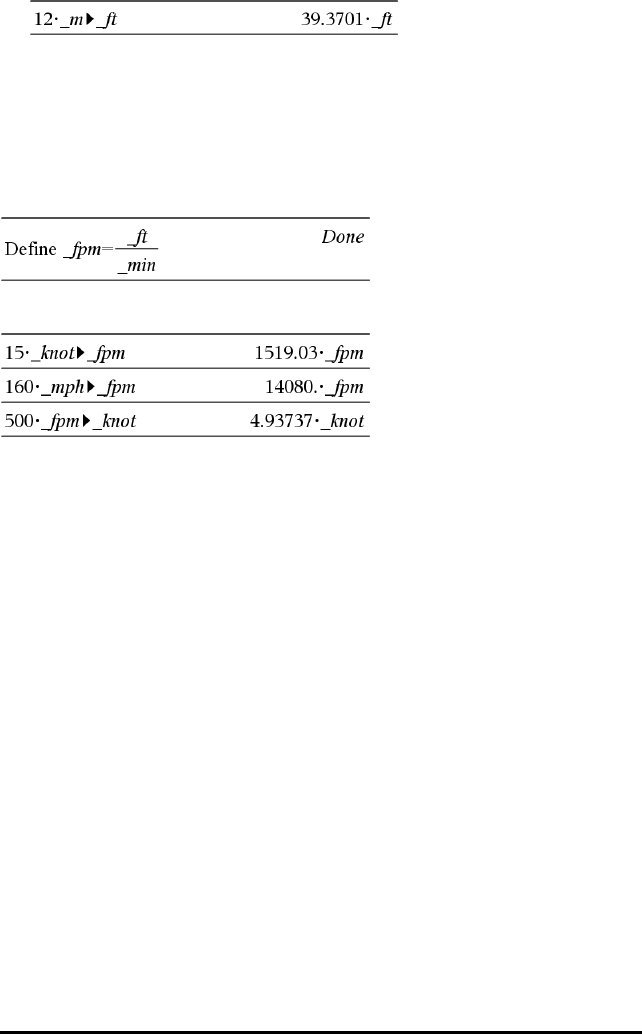
CAS: Creating a User-defined Unit
As with the pre-defined units, user-defined unit names must begin with an underscore
symbol.
Example: Using the pre-defined units _ft and _min, define a unit named _fpm that lets
you enter velocity values in feet per minute and convert velocity results to feet per
minute.
Now you can use the new velocity unit _fpm.
Using the Unit Conversion Assistant
In any application where maths input is allowed, you can generate unit conversions
using the Unit Conversion Assistant. This can help reduce syntax errors by
automatically entering the units for you.
Example: Convert 528 minutes to hours. The desired expression is 528•_min►_hr.
1. Type 528 on the entry line.
2. On the Utilities tab, click the Unit Conversions bar.
Handheld: Press k3.
Calculator Application 260
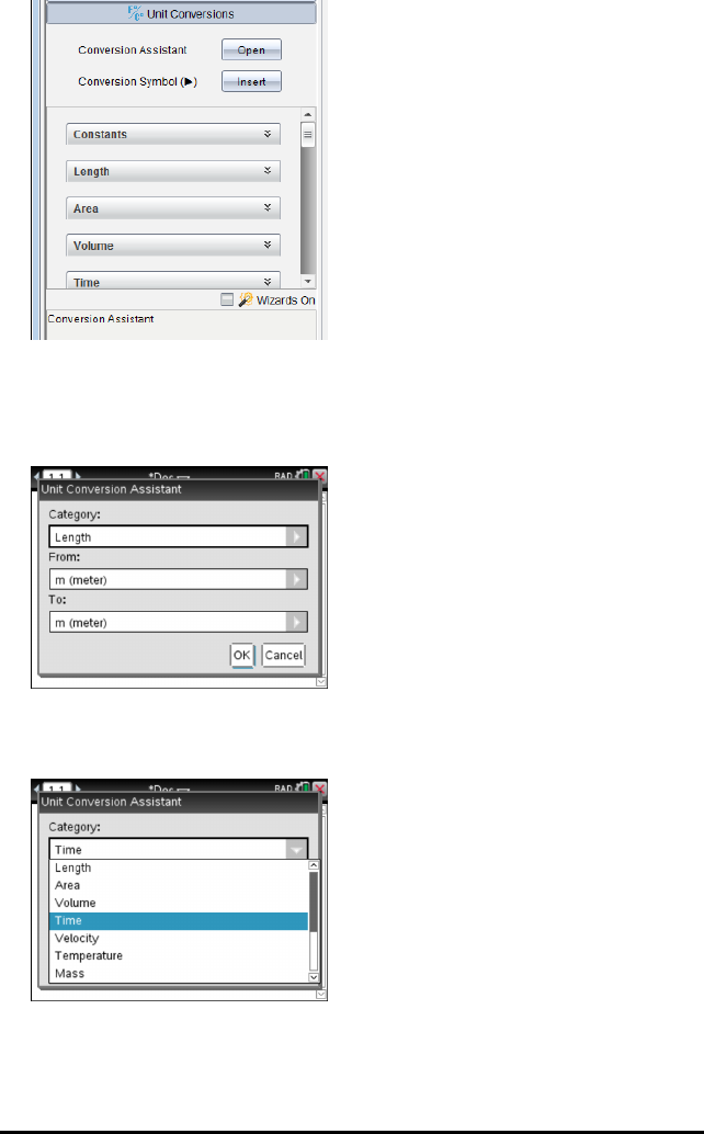
261 Calculator Application
3. Click the Open button next to Conversion Assistant.
Handheld: Press ·.
The Unit Conversion Assistant dialogue box displays:
4. Click the Category list and select Time.
Handheld: Scroll to the Time category and press ·.
5. Click the From list and select min (minute).
Handheld: Scroll to min (minute) and press ·.
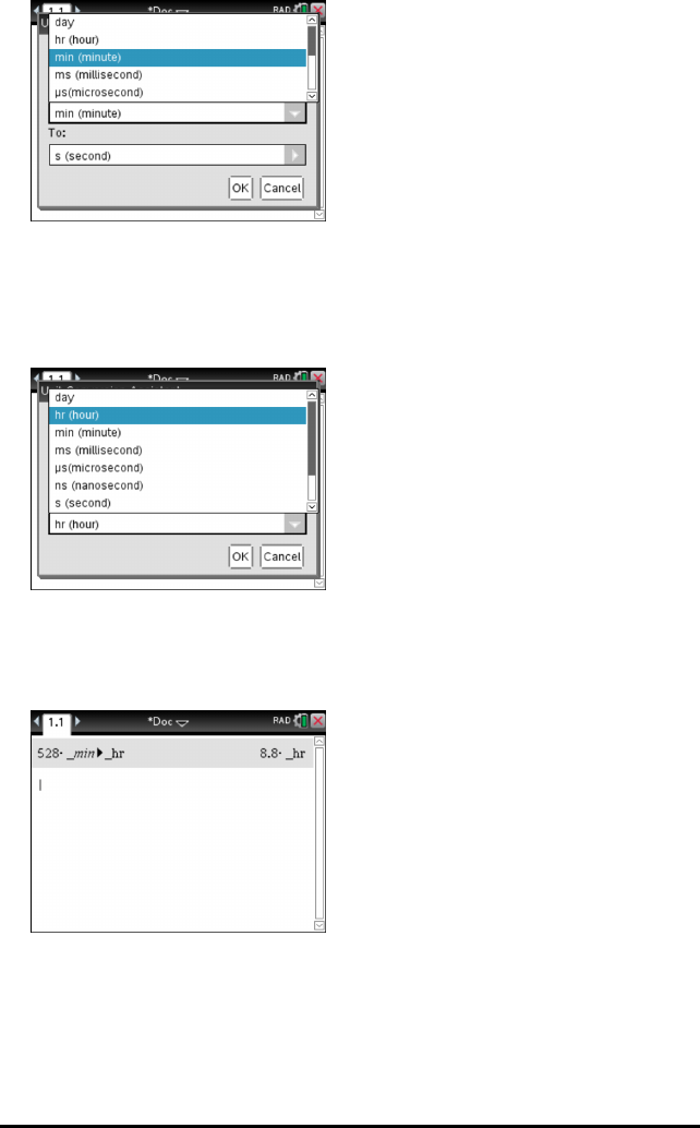
Note: You can select Use existing unit at the bottom of the list if you have already
entered a unit. In this example, you might have already entered 528•_min.
6. Click the To list and select hr (hour).
Handheld: Scroll to hr (hour) and press ·.
7. Click OK to paste _min►_hr to the entry line.
8. Press Enter to evaluate the expression.
Handheld: Press ·.
Note:
• The last Category, From, and To selections will be retained until:
- the software is closed and re-opened (Desktop)
- the device is reset (Handheld)
Calculator Application 262

263 Calculator Application
- the language is changed, or the app is uninstalled or upgraded (iPad)
• Inserting a conversion into a Notes text field will automatically create a Maths Box.
• Inserting a conversion into an empty line in the Calculator will automatically insert
Ans before the conversion.
Conversion Categories and Units
The following table lists categories and their respective units that are available in the
Unit Conversion Assistant. When the units are pasted to the entry line, underscores (_)
are added before the name of each unit to differentiate them from other variables. For
example:
• _cm►_m
• _km/_hr►_m/_s
• _¡C►_¡F
Category Units
Length Å (Angstrom)
au (astronomical unit)
cm (centimetre)
dm (decimetre)
fath (fathom)
fm (fermi)
ft (foot)
in (inch)
km (kilometre)
ltyr (light-year)
m (metre)
mm (micron)
mi (mile)
mil (1/1000 inch)
mm (millimetre)
nm (nanometre)
Nmi (nautical mile)
pc (parsec)
rod (rod)
yd (yard)
Area acre (acre)
cm2
dm2
ft2

Category Units
ha (hectare)
in2
km2
m2
mi2
mm2
yd2
Volume cm3
cup (cup)
dm3
ft3
floz (US fluid ounce)
flozUK (British fluid ounce)
gal (US gallon)
galUK (British gallon)
in3
l (litre)
m3
ml (millilitre)
pt (pint)
qt (quart)
tbsp (tablespoon)
tsp (teaspoon)
yd3
Time day (day)
hr (hour)
min (minute)
ms (millisecond)
ms (microsecond)
ns (nanosecond)
s (second)
week (week)
yr (year)
Velocity ft/min
ft/s
knot (knot)
km/h
km/min
Calculator Application 264
265 Calculator Application
Category Units
km/s
m/s
mi/h
mi/min
mi/s
Temperature ¡C (Celsius)
¡F (Fahrenheit)
K (kelvin)
¡R (Rankine)
Mass amu (atomic mass unit)
gm (gram)
kg (kilogram)
lb (pound)
mg (milligram)
mton (metric ton)
oz (ounce)
slug (slug)
ton (ton)
tonUK (long ton)
Force dyne (dyne)
kgf (kilogram force)
lbf (pound force)
N (newton)
tonf (ton force)
Energy BTU (British thermal unit)
cal (calorie)
erg (erg)
eV (electron volt)
ftlb (foot-pound)
J (joule)
kcal (kilocalorie)
kJ (kilojoule)
kgf*m
kWh (kilowatt-hour)
latm (liter-atmosphere)
Power hp (horsepower)
kW (kilowatt)

Category Units
PS (metric horsepower)
W (watt)
Pressure atm (atmosphere)
bar (bar)
inH2O (inches of water)
inHg (inches of mercury)
kPa (kilopascal)
kgf/cm2
lbf/in2
mbar (millibar)
mmH2O (millimetres of water)
mmHg (millimetres of mercury)
N/m2
Pa (pascal)
psi (pounds per square inch)
torr (millimetres of mercury)
Working with Variables
When you first store a value in a variable, you give the variable a name.
• If the variable does not already exist, Calculator creates it.
• If the variable already exists, Calculator updates it.
Variables within a problem are shared by TI-Nspire™ maths and science learning
technology applications. For example, you can create a variable in Calculator and then
use or modify it in Graphs & Geometry or Lists & Spreadsheet within the same
problem.
For more information, see UsingVariables.
Creating User-defined Functions and Programmes
You can use the Define command to create your own functions and programmes. You
can create them in the Calculator application or in the Programme Editor and then use
them in other TI-Nspire™ applications.
For more information, see Overview of the Programme Editor and Libraries.
Defining a Single-line Function
Suppose you want to define a function named cube() that calculates the cube of a
number or variable.
1. On the Calculator entry line, type Define cube(x)=x^3 and press Enter.
Calculator Application 266
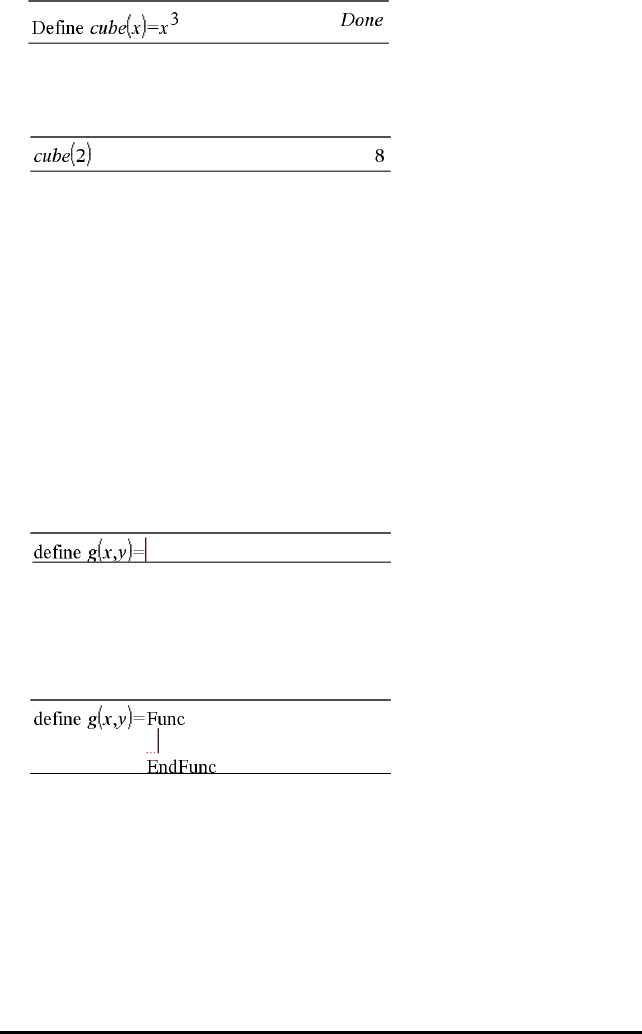
267 Calculator Application
The message “Done” confirms that the function has been defined.
2. Type cube(2) and press Enter to test the function.
Defining a Multiple-line Function Using Templates
You can define a function consisting of multiple statements entered on separate lines.
A multiple-line function may be easier to read than one with multiple statements
separated by colons.
Note: You can create multiple-line functions only by using the Define command. You
cannot use the := or →operators to create multiple-line definitions. The
Func...EndFunc template serves as a container for the statements.
As an example, define a function named g(x,y)that compares two arguments xand y.
If argument x> argument y, the function should return the value of x. Otherwise, it
should return the value of y.
1. On the Calculator entry line, type Define g(x,y)=. Do not press Enter yet.
2. Insert the Func...EndFunc template.
From the Functions&Programmes menu, select Func...EndFunc.
Calculator inserts the template.
3. Insert the If...Then...Else...EndIf template.
From the Functions&Programmes menu, select Control, and then select
If...Then...Else...EndIf.
Calculator inserts the template.
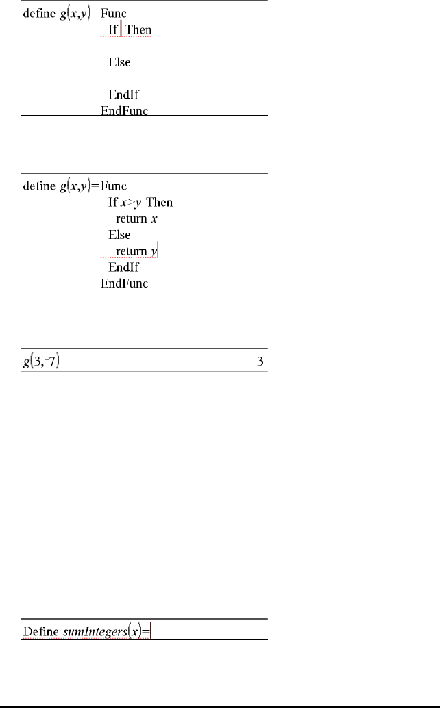
4. Type the remaining parts of the function, using the arrow keys to move the cursor
from line to line.
5. Press Enter to complete the definition.
6. Evaluate g(3,-7) to test the function.
Defining a Multiple-line Function Manually
Within a multi-line template such as Func...EndFunc or If...EndIf, you can start a new
line without completing the definition.
•Handheld: Press @instead of ·.
•Windows®: Hold Alt and press Enter.
•Macintosh®: Hold Option and press Enter.
As an example, define a function sumIntegers(x)that calculates the cumulative sum of
integers from 1 to x.
1. On the Calculator entry line, type Define sumIntegers(x)=. Do not press
Enter yet.
2. Insert the Func...EndFunc template.
Calculator Application 268
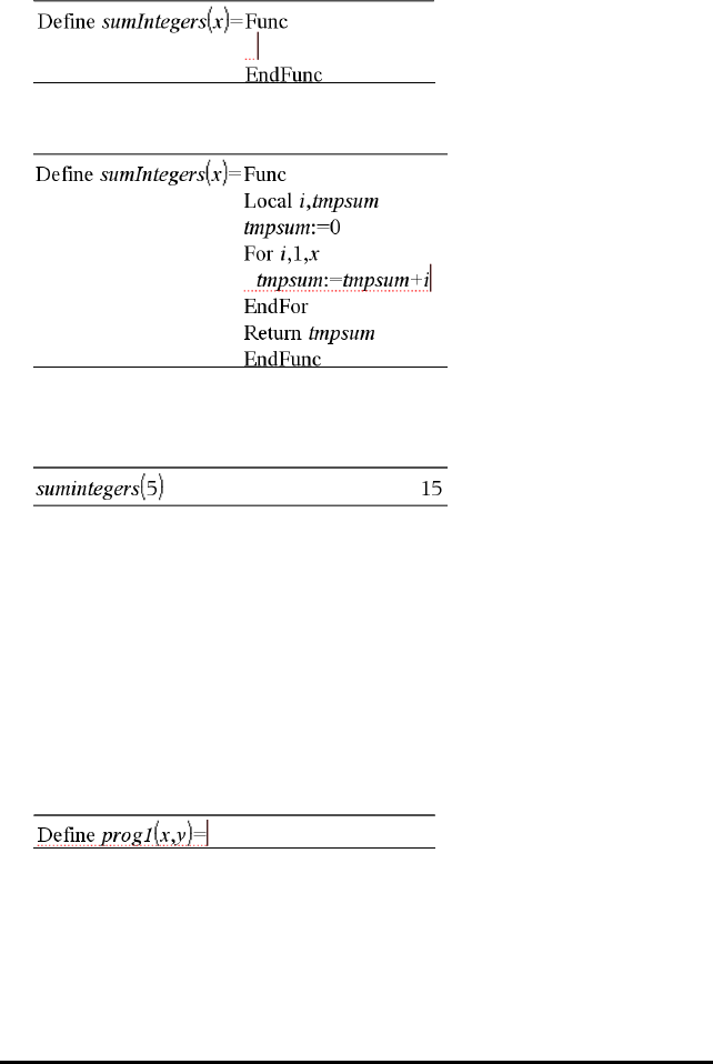
269 Calculator Application
From the Functions&Programmes menu, select Func...EndFunc.
Calculator inserts the template.
3. Type the following lines, pressing @or Alt+Enter at the end of each line.
4. After typing Return tmpsum, press Enter to complete the definition.
5. Evaluate sumIntegers(5) to test the function.
Defining a Programme
Defining a programme is similar to defining a multiple-line function. The
Prgm...EndPrgm template serves as a container for the programme statements.
As an example, create a programme named g(x,y)that compares two arguments.
Based on the comparison, the programme should show the text “x>y” or “x≤y”
(showing the values of xand yin the text).
1. On the Calculator entry line, type Define prog1(x,y)=. Do not press Enter
yet.
2. Insert the Prgm...EndPrgm template.
From the Functions&Programmes menu, select Prgm...EndPrgm.
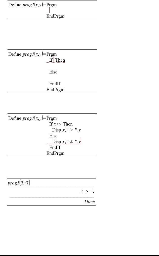
3. Insert the If...Then...Else...EndIf template.
From the Functions&Programmes menu, select Control, and then select
If...Then...Else...EndIf.
4. Type the remaining parts of the function, using the arrow keys to move the cursor
from line to line. Use the Symbol Palette to select the "≤“symbol.
5. Press Enter to complete the definition.
6. Execute prog1(3,-7)to test the programme.
Recalling a Function or Programme Definition
You might want to reuse or modify a function or programme that you have defined.
1. Show the list of defined functions.
Calculator Application 270

271 Calculator Application
From the Actions menu, select Recall Definition.
2. Select the name from the list.
The definition (for example, Define f(x)=1/x+3) is pasted into the entry
line for editing.
Editing Calculator Expressions
Although you cannot edit an expression in the Calculator history, you can copy all or
part of an expression from the history and paste it to the entry line. You can then edit
the entry line.
Positioning the Cursor in an Expression
▶Press e,¡,¢,£or ¤to move the cursor through the expression. The cursor
moves to the closest valid position in the direction that you press.
Note: An expression template may force the cursor to move through its parameters,
even though some parameters may not be exactly in the path of the cursor movement.
For example, moving upward from the main argument of an integral always moves the
cursor to the top limit.
Inserting into an Expression in the Entry Line
1. Position the cursor at the point where you want to insert additional elements.
2. Type the elements that you want to insert.
Note: When you insert an open parenthesis, Calculator adds a temporary close
parenthesis, displayed in gray. You can override the temporary parenthesis by typing
the same parenthesis manually or by entering something past the temporary
parenthesis (thereby implicitly validating its position in the expression). After you
override the temporary gray parenthesis, it is replaced with a black parenthesis.
Selecting Part of an Expression
1. Position the cursor at the starting point in the expression.
Handheld: Press ¡,¢,£or ¤to move the cursor.
2. Press and hold g, and then press ¡,¢,£or ¤to select.
Deleting all or part of an expression on the entry line
1. Select the part of the expression to delete.
2. Press ..
Financial Calculations
Several TI-Nspire™ functions provide financial calculations, such as time value of
money, amortisation calculations, and return on investment calculations.
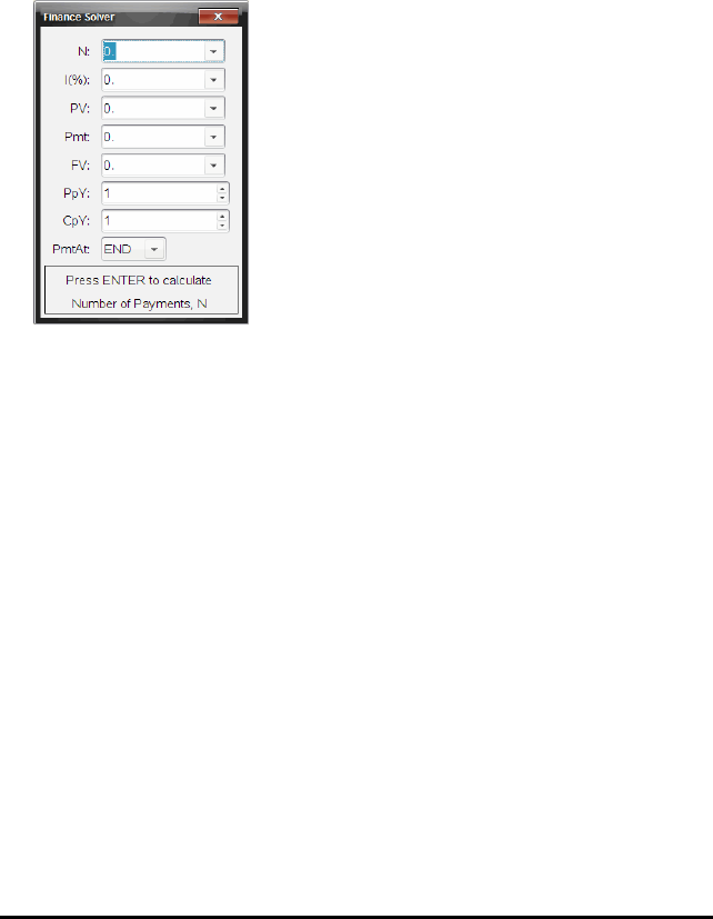
The Calculator application also includes a Finance Solver. It lets you dynamically solve
several types of problems, such as loans and investments.
Using the Finance Solver
1. Open the Finance Solver.
From the Finance menu, click Finance Solver.
The Finance Solver displays its default values (or previous values, if you have
already used the solver in the current problem).
2. Enter each known value, using eto cycle through the items.
• The help information at the bottom of the Finance Solver describes each item.
• You might need to temporarily skip the value that you want to calculate.
• Make sure to set PpY,CpY and PmtAt to the correct settings (12, 12 and END in
this example).
3. Press eas necessary to select the item that you want to calculate, and then
press ·.
The Finance Solver calculates the value and stores all the values in “tvm.”
variables, such as tvm.n and tvm.pmt. These variables are accessible to all
TI-Nspire™ applications within the same problem.
Calculator Application 272
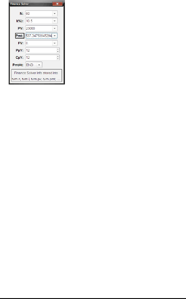
273 Calculator Application
Finance Functions Included
In addition to the Finance Solver, TI-Nspire™ built-in finance functions include:
• TVM functions for calculating future value, present value, number of payments,
interest rate and payment amount.
• Amortisation information such as amortisation tables, balance, sum of interest
payments and sum of principal payments.
• Net present value, internal rate of return and modified rate of return.
• Conversions between nominal and effective interest rates, and calculation of days
between dates.
Notes:
• Finance functions do not automatically store their argument values or results to
the TVM variables.
• For a complete list of TI-Nspire™ functions, see the Reference Guide.
Working with the Calculator History
As you enter and evaluate expressions in the Calculator application, each entry/result
pair is saved in the Calculator history. The history gives you a way to review your
calculations, repeat a set of calculations, and copy expressions for reuse in other pages
or documents.
Viewing the Calculator History
Note: You may notice a processing slowdown when the history contains a large
number of entries.
▶Press ▲or ▼to scroll through the history.
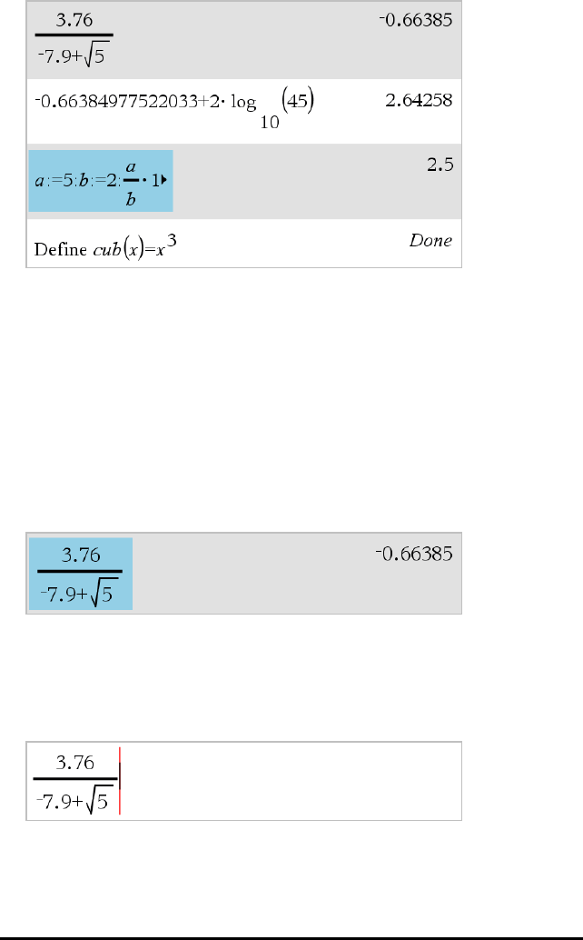
Copying a Calculator History Item to the Entry Line
You can quickly copy an expression, subexpression, or result from the history into the
entry line.
1. Press ▲or ▼to move through the history and select the item that you want to
copy.
—or—
Select part of the expression or result by using Shift in combination with the arrow
keys.
Note: The float setting for the current document may limit the number of decimal
places displayed in a result. To capture the result in its full precision, select it
either by scrolling with the up and down arrow keys or by triple-clicking it.
2. Press Enter to copy the selection and insert it into the entry line.
Calculator Application 274
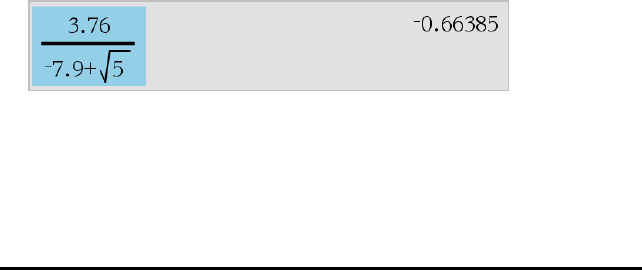
275 Calculator Application
Copying a History Item to Another Application
1. Press ▲or ▼to move through the history and select the item that you want to
copy.
2. Optionally, select part of the expression or result by pressing Shift in combination
with the arrow keys.
3. Use the standard key shortcut for copying a selection.
Windows®: Press Ctrl+C.
Mac®: Press “+C.
Handheld: Press / C.
4. Place the cursor at the location where you want the copy.
5. Paste the copy.
Windows®: Press Ctrl+V.
Mac®: Press “+V.
Handheld: Press / V.
Note: If you copy an expression that uses variables into a different problem, the values
of those variables are not copied. You must define the variables in the problem where
you paste the expression.
Deleting an Expression from the History
When you delete an expression, all variables and functions defined in the expression
retain their current values.
1. Drag or use the arrow keys to select the expression.
Handheld: Use the arrow keys.
2. Press Del.
The expression and its result are removed.

Clearing the Calculator History
When you clear the history, all variables and functions defined in the history retain
their current values. If you clear the history by mistake, use the undo feature.
▶From the Actions menu, select Clear History.
All expressions and results are removed from the history.
Calculator Application 276

277

Using Variables
A variable is a defined value that can be used multiple times in a problem. You can
define a value or function as a variable within each application. Within a problem,
variables are shared by TI-Nspire™applications. For example, you can create a variable
in Calculator, and then use or modify it in Graphs & Geometry or Lists & Spreadsheet
within the same problem.
Each variable has a name and a definition and the definition can be changed. When
you change the definition, all occurrences of the variable in the problem are updated to
use the new definition. In the TI-Nspire™ software, a variable has four attributes:
• Name - User-defined name assigned when the variable is created.
• Location - Variables are stored in memory.
• Value - Number, text, mathematical expression or function.
• Type - Type of data that can be stored as a variable.
Note: Variables created with the Local command within a user-defined function or
programme are not accessible outside that function or programme.
Linking Values on Pages
Values and functions created or defined in one application can interact with other
applications (within the same problem) to share data.
When using linked items, keep in mind:
• Values can be linked between applications on one page or between different pages
of the same problem.
• All applications are linked to the same data.
• If the linked value is changed in the original application, the change is reflected in
all linked usages.
Defining a variable is the first step in linking values.
Creating Variables
Any portion or attribute of an object or function created within an application can be
stored as a variable. Examples of attributes that can become variables are the area of
a rectangle, the radius of a circle, the value contained in a spreadsheet cell or the
contents of a row or column or a function expression. When you create a variable, it is
stored in memory.
Types of Variables
You can store the following data types as variables:
Using Variables 278
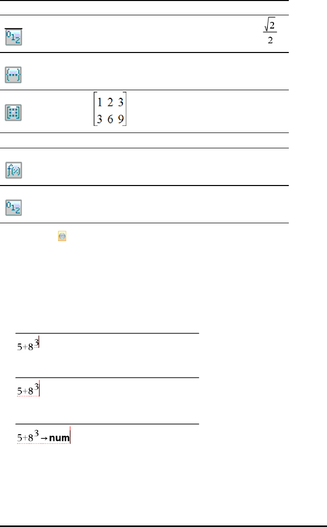
279 Using Variables
Data type Examples
Expression
2.541.25E62pxmin/102+3i(xN2)2
List {2, 4, 6, 8} {1, 1, 2} {"red", "blue", "green"}
Matrix
This can be entered as: [1,2,3;3,6,9]
Character string “Hello”“xmin/10”“The answer is:”
Function, programme myfunc(arg )ellipse(x, y, r1, r2 )
Measurement area, perimeter, length, slope, angle
When you click or press hon a handheld to open the list of stored variables, a
symbol indicates the type.
Creating a Variable from a Calculator Value
This example shows how to create a variable using a handheld. Complete the following
steps to create a variable named num and store the result of the expression 5+83in
that variable.
1. On the Calculator entry line, type the expression 5+8^3.
2. Press ¢to expand the cursor to the baseline.
3. Press / h and then type the variable name num.
This means: Calculate 5+83and store the result as a variable named num.
4. Press ·.
Calculator creates the variable num and stores the result there.
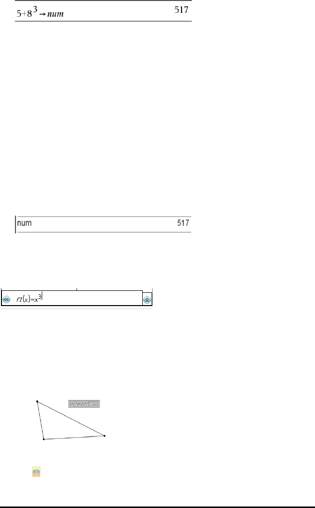
Creating a Variable in the Computer Software
When creating a variable in the computer software, use the following conventions. As
alternatives to using &(store), you can use “:=” or the Define command. All of the
following statements are equivalent.
5+83&num
num := 5+83
Define num=5+83
Checking a Variable’s Value
You can check the value of an existing variable by entering its name on the Calculator
entry line. When you type the name of a stored variable, it appears in bold type.
▶On the Calculator entry line, type the variable name num and press ·.
The value most recently stored in num is displayed as the result.
Automatically Creating Variables in Graphs & Geometry
In the Graphs and Geometry applications, functions defined on the entry line are
automatically stored as variables.
In this example, f1(x)=x3is a variable definition, which allows it to be displayed in
other applications including a table in the Lists & Spreadsheet application.
Creating a Variable from a Graphs & Geometry Value
1. Click the value to store as a variable.
2. Click .
Handheld: Press h.
Using Variables 280
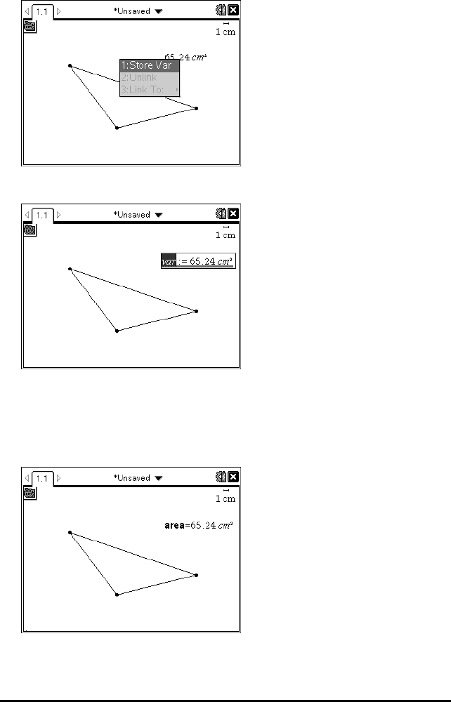
281 Using Variables
The Variables options are displayed with Store Var highlighted.
3. Press ·. VAR := appears before the selected value. This is the default name.
4. Replace the default name VAR with the variable name you want to give the value.
5. When the variable name is typed, press ·.
The value is saved to that variable name and the stored value or its name appears
in bold text to indicate it is a stored value.
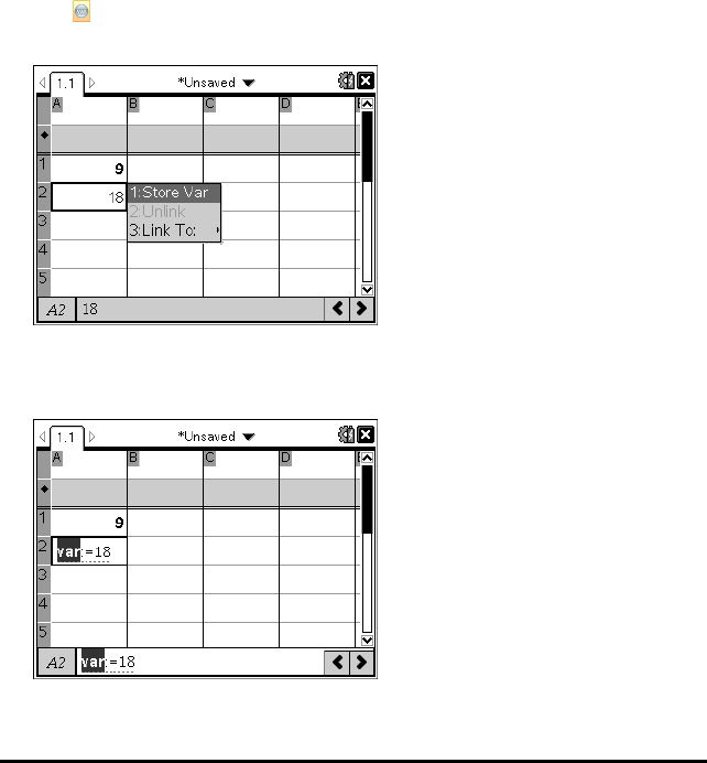
Note: You can also share a Graphs & Geometry axis end value with other applications.
If necessary, click Actions,Show/Hide Axes End Values to display the end values on the
horizontal and vertical axes. Click the number for an end value to highlight it in the
entry field. Name the variable and store it for use with other applications by using any
method described in Step 2.
Automatically Creating Variables in Lists & Spreadsheet
Naming a list at the top of a Lists & Spreadsheet column automatically stores that
value as a list variable. This variable can be used in other applications including Data &
Statistics.
Creating a Variable from a Lists & Spreadsheet Cell Value
You can share a cell value with other applications. When defining or referring to a
shared cell in Lists & Spreadsheet, precede the name with an apostrophe (‘).
1. Click the cell that you want to share.
2. Click to open the Variables menu.
Handheld: Press h.
3. Click Store Var.
A formula is inserted into the cell with var as a placeholder for a variable name.
4. Replace the letters “var” with a name for the variable and press ·.
Using Variables 282

283 Using Variables
The value is now available as a variable to other applications within the same
problem.
Note: If a variable with the name you specified already exists in the current problem
space, Lists & Spreadsheet displays an error message.
Using (Linking) Variables
Sharing, or linking, the variables you create is a powerful tool for maths exploration.
The display of linked variables is automatically updated when the variable’s value
changes.
Linking to Shared Variables
To use a stored variable:
1. Display the page and select the location or object to which you want to link a
variable.
2. Select the Variables tool h.
The Variables options are displayed. The software knows which types of variables
will work in the location or with the object selected and will only display those
variables.
3. Use 9and :to scroll the list.
—or—
Type part of the variable name.
As you type, the system displays a list of variables that begin with the letters you
typed. Typing part of the name enables you to locate a variable more quickly if the
list is long.
4. When you locate and highlight the name of the variable you want to use, click the
name.
—or—
Press ·.
The selected variable value is linked.
Linking a Lists & Spreadsheet Cell to a Variable
When you link a cell to a variable, Lists & Spreadsheet keeps the cell value updated to
reflect the current value of the variable. The variable can be any variable in the current
problem and can be defined in Graphs & Geometry, Calculator or any instance of Lists
& Spreadsheet.
Note: Do not link to a system variable. Doing so could prevent the variable from being
updated by the system. System variables include ans,StatMatrix and statistics results
(such as RegEqn,dfError and Resid).
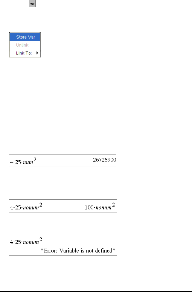
1. Click the cell that you want to link to the variable.
2. Open the VarLink menu:
- Click , and then click Cell.
- Handheld: Press h.
The VarLink menu is displayed.
3. Under Link To, scroll to the name of the variable and click it.
The cell shows the value of the variable.
Using a Variable in a Calculation
After storing a value in a variable, you can use the variable name in an expression as a
substitute for the stored value.
1. Enter the expression:
- Type 4*25*num^2 on the entry line and press Enter.
- Handheld: Type 4r25 rnum^2 on the entry line and press ·.
Calculator substitutes 517, the value currently assigned to num and evaluates the
expression.
2. Enter the expression:
- Type 4*25*nonum^2 and press Enter.
- Handheld: Type 4r25 rnonum^2 on the entry line and press ·.
CAS: Because the variable nonum has not been defined, it is treated algebraically in
the result.
Because the variable nonum has not been defined, the expression returns an error
message.
Using Variables 284
285 Using Variables
Naming Variables
Variable and function names that you create must meet the following naming rules.
Note: In the unlikely event that you create a variable with the same name as one used
for statistical analysis or by the Finance Solver, an error condition could occur. If you
begin entering a variable name that is already in use in the current problem, the
software shows the entry in bold to let you know.
• Variable names must be in one of the forms xxx or xxx.yyy. The xxx part can have
1 to 16 characters. The yyy part, if used, can have 1 to 15 characters. If you use the
xxx.yyy form, both xxx and yyy are required; you cannot start or end a variable
name with a period “.”.
• Characters can consist of letters, digits and the underscore character (_). Letters
can be U.S. or Greek letters (but not Πor p), accented letters and international
letters.
• Do not use cor nfrom the symbol palette to construct a variable name such as c1
or n12. These may appear to be letters, but they are treated internally as special
symbols.
• You can use uppercase or lowercase letters. The names AB22,Ab22,aB22 and
ab22 all refer to the same variable.
• You cannot use a digit as the first character of xxx or yyy.
• You can use digits 0 through 9, U.S. letters, a - z, Latin and Greek letters (but not p)
as subscripts (for example, a2,qa, or h2o). To enter a subscript while typing a
variable name, select in the Math Templates or on the formatting toolbar.
• Do not use spaces.
• If you want a variable to be treated as a complex number, use an underscore as the
last character of the name.
• CAS: If you want a variable to be treated as a type of unit (such as _m or _ft), use
an underscore as the first character of the name. You cannot use subsequent
underscores in the name.
• You cannot use an underscore as the first character of the name.
• You cannot use a preassigned variable, function or command name, such as Ans,
min or tan.
Note: For more information about TI-Nspire™ functions, see the Reference Guide.
• Library documents and library objects are subject to additional naming restrictions.
For more information, see Libraries.
Here are some examples:
Variable names Valid?
Myvar, my.var Yes
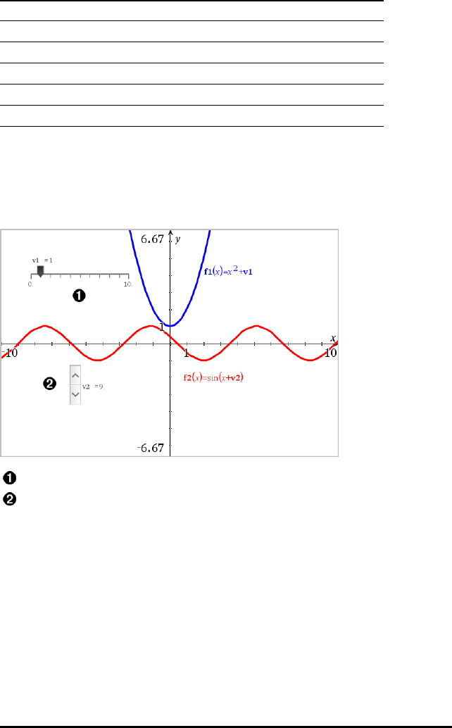
Variable names Valid?
My var, list 1 No. Contains a space.
a, b, b12, b12, c, d Yes. Note that variables b12 and b12 are distinct.
Log, Ans No. Preassigned to a system function or variable.
Log1, list1.a, list1.b Yes
3rdTotal, list1.1 No. xxx or yyy starts with a digit.
Adjusting Variable Values with a Slider
A slider control lets you interactively adjust or animate the value of a numeric variable.
You can insert sliders in the Graphs, Geometry, Notes and Data&Statistics
applications.
Horizontal slider for adjusting variable v1.
Minimised vertical slider for adjusting variable v2.
Note: TI-Nspire™ version 4.2 or higher is required for opening .tns files containing
sliders on Notes pages.
Inserting a Slider Manually
1. From a Graphs, Geometry or Data&Statistics page, select Actions > Insert Slider.
—or—
From a Notes page, make sure the cursor is not in a maths box or chem box, and
then select Insert > InsertSlider.
The Slider Settings screen opens.
Using Variables 286
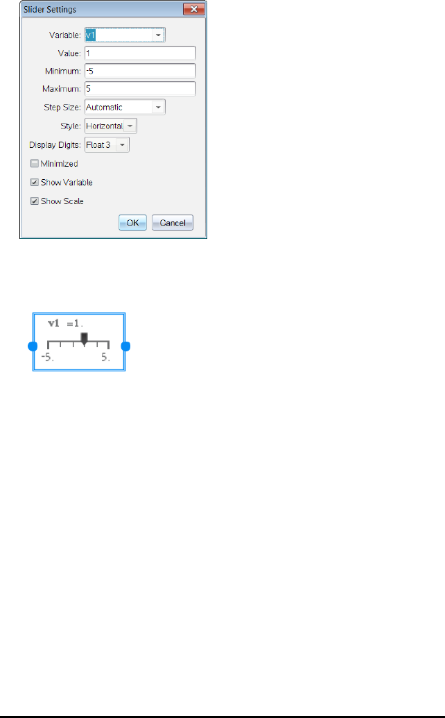
287 Using Variables
2. Enter the desired values, and click OK.
The slider is displayed. On a Graphs, Geometry or Data&Statistics page, handles
are displayed to let you move or stretch the slider.
To remove the handles and use the slider, click an empty
space in the work area. You can show the handles any time by
selecting Move from the slider's context menu.
3. To adjust the variable, slide the pointer (or click the arrows on a minimised slider).
- You can use the Tab key to move the focus to a slider or to move from one
slider to the next. The colour of the slider changes to show you when it has the
focus.
- When a slider has the focus, you can use the arrow keys to change the value of
the variable.
Working with the Slider
Use the options on the context menu to move or delete the slider, and to start or stop
its animation. You can also change the slider's settings.
1. Display the slider's context menu.
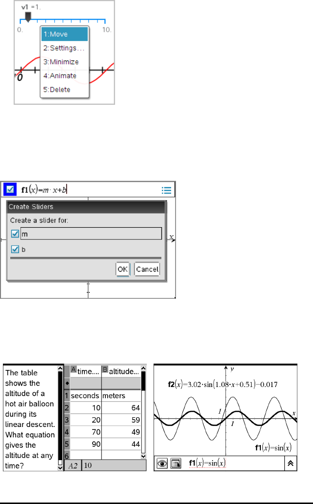
2. Click an option to select it.
Automatic Sliders in Graphs
Sliders can be created for you automatically in the Graphs application and in the
analytic window of the Geometry application. You are offered automatic sliders when
you define certain functions, equations or sequences that refer to undefined variables.
Locking and Unlocking Variables
Locking lets you protect variables from modification or deletion. Locking prevents
unintended changes to a variable.
Using Variables 288

289 Using Variables
Time and altitude lists can be locked to ensure
problem fidelity
Reference function f1 can be locked to prevent
unintended change
Variables you Cannot Lock
• System variable Ans
•stat. and tvm. variable groups
Important Information About Locked Variables
• To lock variables, use the Lock command.
• To modify or delete a locked variable, you must first unlock the item.
• Locked variables display a lock icon on the variable menu list.
• The Lock command clears the Redo/Undo history when applied to unlocked
variables.
Examples of Locking
Lock a,b,c Locks variables a,band cfrom the Calculator application.
Lock mystats.Locks all members of variable group mystats.
UnLock func2 Unlocks variable func2.
lm:=getLockInfo
(var2)
Retrieves the current lock status of var2 and assigns that
value to lm in the Calculator application.
For more information, see the Reference Guide.
Updating a Variable
If you want to update a variable with the result of a calculation, you must store the
result explicitly.
Entry Result Comment
a := 2 2
a38 Result not stored in
variable a.
a2
a := a38Variable aupdated
with result.
a8
a2&a64 Variable aupdated
with result.
a64
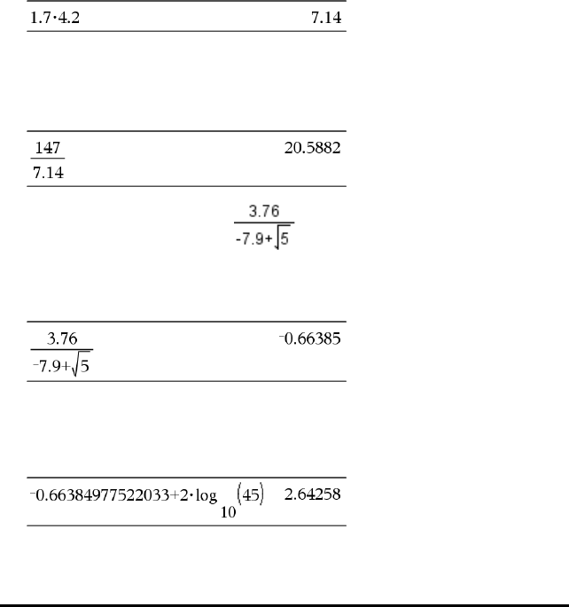
Reusing the Last Answer
Each instance of Calculator automatically stores the last calculated result as a variable
named Ans. You can use Ans to create a chain of calculations.
Note: Do not link to Ans or any system variable. Doing so could prevent the variable
from being updated by the system. System variables include statistics results (such as
Stat.RegEqn,Stat.dfError and Stat.Resid) and Finance Solver variables (such as
tvm.n,tvm.pmt and tvm.fv).
As an example of using Ans, calculate the area of a garden plot that is 1.7 meters by
4.2 meters. Then use the area to calculate the yield per square meter if the plot
produces a total of 147 tomatoes.
1. Calculate the area:
- On the Calculator entry line, type 1.7*4.2 and press Enter.
- Handheld: On the Calculator entry line, type 1.7 r4.2 and press ·.
2. Reuse the last answer to calculate the yield per square meter:
- Type 147/ans and press Enter to find the yield.
- Handheld: Type 147 pans and press ·to find the yield.
3. As a second example, calculate and then add 2*log(45).
- Type 3.76/(-7.9+sqrt(5)) and press Enter.
- Handheld: Type 3.76 p(v7.9+sqrt(5)) and press ·.
4. Reuse the last answer:
- Type ans+2*log(45) and press Enter.
- Handheld: Type ans+2 rlog(45) and press ·.
Using Variables 290

291 Using Variables
Temporarily Substituting a Value for a Variable
Use the “|” (such that) operator to assign a value to a variable for just a single
execution of the expression.
Removing a Linked Variable
1. Select the linked variable.
2. Press h.
The Variables options are displayed.
3. Select Unlink.
The link is removed from the value and the value is displayed without any bold
formatting.
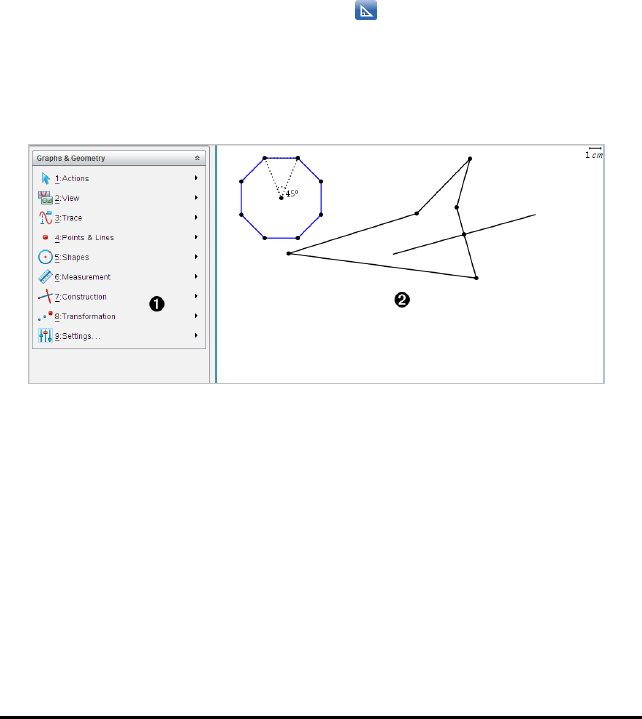
Geometry Application
The Geometry application lets you:
• Create and explore geometric objects and constructions.
• Manipulate and measure geometric objects.
• Animate points on objects and explore their behaviour.
• Explore object transformations.
Adding a Geometry Page
▶To start a new document with a blank Geometry page:
From the main File menu, click New Document, and then click Add Geometry.
Handheld: Press c, and select Geometry .
▶To add a Geometry page in the current problem of an existing document:
From the toolbar, click Insert > Geometry.
Handheld: Press ~and select Insert > Geometry.
ÀGeometry menu – Available anytime you are viewing a Geometry page.
ÁGeometry work area -- The area where you create and explore geometric objects.
What You Must Know
Changing the Graphs and Geometry Settings
1. From the Settings menu in the Documents Toolbox, select Settings.
2. Select the settings that you want to use.
Geometry Application 292

293 Geometry Application
-Display Digits. Sets the display format for numbers as Floating or Fixed
decimal.
-Graphing Angle. Sets the angle unit for all Graphs and 3D Graphing applications
in the current document. The default setting is Radian. Set this to Auto if you
want graphing angles to follow the Angle setting in the main File>Settings
menu. An angle mode indicator shows the resulting mode in Graphs and 3D
Graphing applications.
-Geometry Angle. Sets the angle unit for all Geometry applications in the current
document. The default setting is Degree. Set this to Auto if you want geometry
angles to follow the Angle setting in the main File>Settings menu. An angle
mode indicator shows the resulting mode in Geometry applications.
-Automatically hide plot labels. In the Graphs application, hides the label that
normally appears next to a graphed relation.
-Show axis end values. Applies only in the Graphs application.
-Show tool tips for function manipulation. Applies only in the Graphs application.
-Automatically find points of interest. In the Graphs application, shows zeros,
minima and maxima while tracing function graphs.
-Force Geometric Triangle Angles to Integers. Restricts the angles of a triangle to
integer values as you create or edit the triangle. This setting applies only in the
Geometry View with the Geometry Angle unit set to Degree or Gradian. It does
not apply to analytic triangles in Graphing View or to analytic triangles in the
Analytic Window of the Geometry View. This setting does not affect existing
angles, and it does not apply when constructing a triangle based on previously
inserted points. By default, this setting is deselected.
-Automatically Label Points. Applies labels (A,B, ..., Z,A1,B1, and so on) to
points, lines, and vertices of geometric shapes as you draw them. The labelling
sequence starts at Afor each page in a document. By default, this setting is
deselected.
Note: If you create a new object that uses existing un-labelled points, those
point are not automatically labelled in the completed object.
- Click Restore to restore all settings to their factory defaults.
- Click Make Default to apply the current settings to the open document and save
them as the default for new Graphs and Geometry documents.
Using Context Menus
Context menus provide quick access to commonly used commands and tools that apply
to a specific object. For example, you can use a context menu to change an object's
line colour or to group a set of selected objects.
▶Display the context menu for an object in one of the following ways.
- Windows®: Right-click the object.
- Mac®: Hold “and click the object.
- Handheld: Move the pointer to the object, and then press / b.
Finding Hidden Objects in the Graphs or Geometry Application
You can hide and show individual graphs, geometric objects, text, labels,
measurements and axis end-values.
To temporarily view hidden graphs or objects or to restore them as shown objects:
1. From the Actions menu, select Hide/Show.
The Hide/Show tool appears in the work area, and all hidden objects become
visible in dimmed colours.
2. Click a graph or object to toggle its Hide/Show state.
3. To apply the changes and close the Hide/Show tool, press ESC.
Inserting a Background Image
You can insert an image as a background for a GraphsorGeometry page. The file
format of the image can be .bmp, .jpg or .png.
1. From the Insert menu, click Image.
2. Navigate to the image you want to insert, select it and then click Open.
For information on moving, resizing, and deleting a background image, see Working
with Images in the Software.
Adding Text to the Graphs or Geometry Work Area
1. From the Actions menu, select Text.
The Text tool appears in the work area.
2. Click the location for the text.
Geometry Application 294
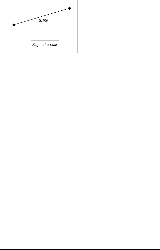
295 Geometry Application
3. Type the text in the box that appears, and then press Enter.
4. To close the Text tool, press ESC.
5. To edit the text, double-click it.
Deleting a Relation and its Graph
1. Select the relation by clicking its graph.
2. Press Backspace or DEL.
The graph is removed from both the work area and the graph history.
Introduction to Geometric Objects
Geometry tools are accessible in both the Graphs and Geometry applications. You can
use these tools to draw and investigate objects such as points, lines, and shapes.
• The Graphing view shows the Graphs work area superimposed on the Geometry
work area. You can select, measure, and alter objects in both work areas.
• The Plane Geometry view shows only the objects created in the Geometry
application.
Objects Created in the Graphs Application
Points, lines, and shapes created in the Graphs application are analytic objects.
• All points that define these objects reside on the x,y graph plane. Objects created
here are visible only in the Graphs application. Changing the axes scale affects the
appearance of the objects.
• You can display and edit the coordinates of any point on an object.
• You can display the equation of a line, tangent line, circle shape, or geometric conic
created in the Graphs application.
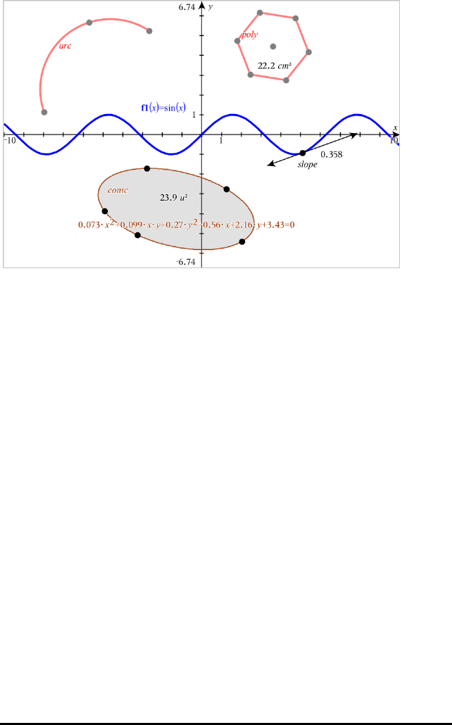
The circle arc and polygon were created in the Geometry application. The sine wave and conic
were created in the Graphs application.
Objects Created in the Geometry Application
Points, lines, and shapes created in the Geometry application are not analytic objects.
• Points that define these objects do not reside on the graph plane. Objects created
here are visible in both the Graphs and Geometry applications, but they are
unaffected by changes to the Graphs x,y axes.
• You cannot obtain the coordinates of an object’s points.
• You cannot display the equation of a geometric object created in the Geometry
application
Geometry Application 296
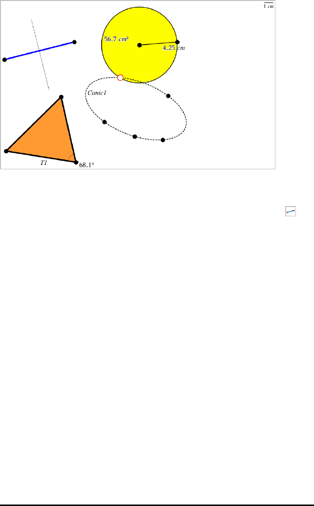
297 Geometry Application
Creating Points and Lines
As you create an object, a tool appears in the work area (for example, Segment ). To
cancel, press ESC. To enable automatic labelling of certain objects, see What You Must
Know in this chapter.
Creating a Point on the Work Area
1. From the PointsandLines menu, select Point. (In the Graphs application, click
Geometry > PointsandLines > Point.)
2. Click a location to create the point.
3. (Optional) Label the point.
4. To move a point, drag it.
Creating a Point on a Graph or Object
You can create a point on a line, segment, ray, axis, vector, circle, graph or axis.
1. From the PointsandLines menu, select Point On. (In the Graphs application, click
Geometry > PointsandLines > Point On.)
2. Click the graph or object on which you want to create the point.
3. Click a location on the object to place the point.

Identifying Points of Intersection
1. From the PointsandLines menu, select Intersection Points. (In the Graphs
application, click Geometry > PointsandLines > Intersection Points.)
2. Click two intersecting objects to add points at their intersections.
Creating a Line
1. From the PointsandLines menu, select Line. (In the Graphs application, click
Geometry > PointsandLines > Line.)
2. Click a location to define one point on the line.
3. Click a second location to define the direction of the line and the length of its
visible portion.
Geometry Application 298

299 Geometry Application
4. To move a line, drag its identifying point. To rotate it, drag any point except the
identifying point or ends. To extend its visible portion, drag from either end.
Creating a Segment
1. From the PointsandLines menu, select Segment. (In the Graphs application, click
Geometry > PointsandLines > Segment.)
2. Click two locations to define the endpoints of the segment.
3. To move a segment, drag any point other than an endpoint. To manipulate the
direction or length, drag either endpoint.
Creating a Ray
1. From the PointsandLines menu, select Ray. (In the Graphs application, click
Geometry > PointsandLines > Ray.)
2. Click a location to define the endpoint of the ray.
3. Click a second location to define the direction.

To move a ray, drag its identifying point. To rotate it, drag any point except the
identifying point or end. To extend its visible portion, drag from the end.
Creating a Tangent
You can create a tangent line at a specific point on a geometric object or function
graph.
1. From the PointsandLines menu, select Tangent. (In the Graphs application, click
Geometry > PointsandLines > Tangent.)
2. Click the object to select it.
3. Click a location on the object to create the tangent.
4. To move a tangent, drag it. It remains attached to the object or graph.
Creating a Vector
1. From the PointsandLines menu, select Vector. (In the Graphs application, click
Geometry > PointsandLines > Vector.)
Geometry Application 300

301 Geometry Application
2. Click a location to establish the vector's initial point.
3. Click a second location to specify direction and magnitude and complete the vector.
4. To move a vector, drag any point other than the endpoints. To manipulate the
magnitude and/or direction, drag either end point.
Note: If you create an endpoint on an axis or another object, you can move the
endpoint only along that object.
Creating a Circle Arc
1. From the PointsandLines menu, select Circle Arc. (In the Graphs application, click
Geometry > PointsandLines > Circle Arc.)
2. Click a location or point to establish the starting point of the arc.
3. Click a second point to establish an intermediate point through which the arc will
pass.
4. Click a third point to set the ending point and complete the arc.
5. To move an arc, drag its perimeter. To manipulate it, drag any of its three defining
points.
Creating Geometric Shapes
The Shape tools let you explore circles, polygons, conics and other geometric objects.
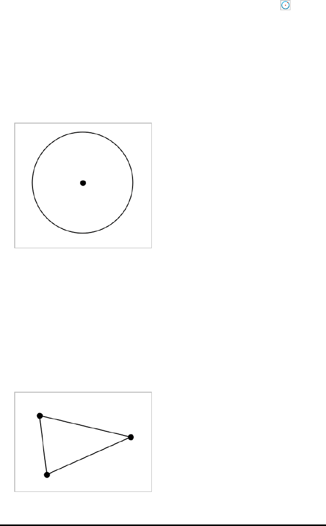
As you create a shape, a tool appears in the work area (for example,Circle ). To
cancel the shape, press ESC. To enable automatic labelling of certain objects, see What
You Must Know, in this chapter.
Creating a Circle
1. From the Shapes menu, select Circle. (In the Graphs application, click Geometry >
Shapes > Circle.)
2. Click a location or point to position the circle’s centre point.
3. Click a location or point to establish the radius and complete the circle.
4. To resize a circle, drag its perimeter. To move it, drag its centre point.
Creating a Triangle
Note: To ensure that the total of the angles of a triangle equals 180°or 200 gradians,
you can force integer angles in the Geometry view. Refer to What You Must Know, in
this chapter.
1. From the Shapes menu, select Triangle. (In the Graphs application, click Geometry >
Shapes > Triangle.)
2. Click three locations to establish the vertices of the triangle.
Geometry Application 302

303 Geometry Application
3. To manipulate a triangle, drag any point. To move it, drag any side.
Creating a Rectangle
1. From the Shapes menu, select Rectangle. (In the Graphs application, click Geometry
> Shapes > Rectangle.)
2. Click a location or point to establish the first corner of the rectangle.
3. Click a location for the second corner.
One side of the rectangle is displayed.
4. Click to establish the distance to the opposite side and complete the rectangle.
5. To rotate a rectangle, drag one of its first two points. To extend it, drag one of the
last two points. To move it, drag any side.
Creating a Polygon
1. From the Shapes menu, select Polygon. (In the Graphs application, click Geometry >
Shapes > Polygon.)
2. Click a location or point to establish the first vertex of the polygon.
3. Click to establish each additional vertex.
4. To complete the polygon, click the first vertex.
5. To manipulate a polygon, drag any vertex. To move it, drag any side.
Creating a Regular Polygon
1. From the Shapes menu, select Regular Polygon. (In the Graphs application, click
Geometry > Shapes > Regular Polygon.)
2. Click once on the work area to establish the centre point.
3. Click a second location to establish the first vertex and radius.
A 16-sided regular polygon is formed. The number of sides is displayed in brackets;
for example, {16}.
4. Drag any vertex in a circular motion to set the number of sides.
- Drag clockwise to reduce the number of sides.
- Drag counter-clockwise to add diagonals.
5. To resize or rotate a regular polygon, drag any of its points. To move it, drag any
side.
Creating an Ellipse
1. From the Shapes menu, select Ellipse. (In the Graphs application, click Geometry >
Shapes > Ellipse.)
2. Click two locations or points to establish the foci.
3. Click to establish a point on the ellipse and complete the shape.
Geometry Application 304
305 Geometry Application
4. To manipulate an ellipse, drag any of its three defining points. To move it, drag its
perimeter.
Creating a Parabola (from focus and vertex)
1. From the Shapes menu, select Parabola. (In the Graphs application, click Geometry
> Shapes > Parabola.)
2. Click a location to establish the focus.
3. Click a location to establish the vertex and complete the parabola.
4. To manipulate a parabola, drag its focus or its vertex. To move it, drag it from any
other point.
Creating a Parabola (from focus and directrix)
1. Create a line to serve as the directrix.
2. From the Shapes menu, select Parabola. (In the Graphs application, click Geometry
> Shapes > Parabola.)
3. Click a location to establish the focus.
4. Click the line to establish it as the directrix.

5. To manipulate a parabola, rotate or move its directrix or drag its focus. To move it,
select both the directrix and the focus, and then drag either object.
Creating a Hyperbola
1. From the Shapes menu, select Hyperbola. (In the Graphs application, click
Geometry > Shapes > Hyperbola.)
2. Click two locations to establish the foci.
3. Click a third location to complete the hyperbola.
4. To manipulate a hyperbola, drag any of its three defining points. To move it, drag it
from any other place on the shape.
Creating a Conic by Five Points
1. From the Shapes menu, select ConicbyFivePoints. (In the Graphs application, click
Geometry > Shapes > ConicbyFivePoints.)
2. Click five locations to establish the five points on the shape.
Depending on the pattern of the points, the conic can be a hyperbola or an ellipse.
Geometry Application 306
307 Geometry Application
3. To manipulate a conic, drag any of its five defining points. To move it, drag it from
any other place on the shape.
Creating Shapes Using Gestures (MathDraw)
The MathDraw tool lets you use touchscreen or mouse gestures to create points, lines,
circles and other shapes.
MathDraw is available in:
• Geometry view without the analytic window displayed.
• Graphing view when the x scale and y scale are identical. This avoids non-circular
ellipses and non-square rectangles appearing as circles and squares.
MathDraw is not available in the 3D Graphing view or in the Geometry view with the
analytic window displayed.
Activating MathDraw
1. If using the Geometry view with the analytic window visible, use the View menu to
hide the window.
2. On the Actions menu, select MathDraw.
The MathDraw icon appears. You can begin using the tool.
Cancelling MathDraw
▶When you have finished using the MathDraw tool, press Esc.
The tool also closes if you select a different tool or change views.
Creating Points
To create a labelled point, tap or click in an open area.
• If the point is close to an existing line, segment, ray, geometric conic (including
circles) or polygon, the point snaps to that object. You can also place a point on the
intersection of any two of those types of objects.

• If the point is close to a visible grid location in a Graphs view or the analytic
window of a Geometry view, it snaps to the grid.
Drawing Lines and Segments
To create a line or segment, touch or click the initial position, and then drag to the end
position.
• If the drawn line passes near an existing point, the line snaps to the point.
• If the drawn line starts close to an existing point and ends next to another existing
point , it becomes a segment defined by those points.
• If the drawn line is nearly parallel or perpendicular to an existing line, segment or
side of a polygon, it aligns to that object.
Note: The default tolerance for detecting parallel/perpendicular lines is 12.5
degrees. This tolerance can be redefined using a variable named
ti_gg_fd.angle_tol. You can change the tolerance in the current problem by setting
this variable in the calculator app to a value in the range 0 through 45 (0=no
parallel/perpendicular detection).
Drawing Circles and Ellipses
To create a circle or ellipse, use the touchscreen or mouse to draw the approximate
shape.
• If the drawn shape is sufficiently circular, a circle is created.
• If the shape is elongated, an ellipse is created.
• If the virtual centre of the drawn shape is near an existing point, the circle or
ellipse is centred on that point.
Drawing Triangles
To create a triangle, draw a triangle-like shape.
• If a drawn vertex is close to an existing point, the vertex snaps to the point.
Drawing Rectangles and Squares
To create a rectangle or square, use the touchscreen or mouse to draw the perimeter.
• If the drawn shape is nearly square, a square is created.
• If the drawn shape is elongated, a rectangle is created.
Geometry Application 308

309 Geometry Application
• If the centre of a square is close to an existing point, the square snaps to that
point.
Drawing Polygons
To create a polygon, tap or click a succession of existing points, ending on the first
point you tapped.
Using MathDraw to Create Equations
In the Graphs view, MathDraw attempts to recognise certain gestures as functions for
analytic parabolas.
Note: The default step value for quantisation of the parabola coefficients is 1/32. The
denominator of this fraction can be redefined using a variable named ti_gg_fd.par_
quant. You can change the step value in the current problem by setting this variable to
a value greater or equal to 2. A value of 2, for example, produces a step value of 0.5.
Using MathDraw to Measure an Angle
To measure the angle between two existing lines, use the touchscreen or mouse to
draw a circle arc from one of the lines to the other.
• If the intersection point between the two lines does not exist, it is created and
labelled.
• The angle is not a directed angle.
Using MathDraw to Find a Mid-point
To create a point midway between two points, tap or click point1, point2, and then
point1 again.
Using MathDraw to Erase
To erase objects, use the touchscreen or mouse to drag left and right, similar to the
motion of erasing a whiteboard.
• The erasure area is the bounding rectangle of the erasure gesture.
• All point objects and their dependents inside the erasure area are removed.

Basics of Working with Objects
Selecting and Deselecting Objects
You can select an individual object or multiple objects. Select multiple objects when
you want to quickly move, colour, or delete them together.
1. Click an object or graph to select it.
The object flashes to indicate selection.
2. Click any additional objects to add them to the selection.
3. Perform the operation (such as moving or setting colour).
4. To deselect all objects, click an empty space in the work area.
Grouping and Ungrouping Geometric Objects
Grouping objects gives you a way to reselect them as a set, even after you have
deselected them to work with other objects.
1. Click each object to add it to the current selection.
The selected objects flash.
2. Display a context menu of the selected object or objects.
3. Click Group. You can now select all the items in the group by clicking any of its
members.
4. To split a group into individual objects, display a context menu of any of its
member objects, and click Ungroup.
Deleting Objects
1. Display the context menu of the object or objects.
2. Click Delete.
You cannot delete the origin, the axes, or points representing locked variables, even
if those items are included in the selection.
Moving Objects
You can move an object, group, or combination of selected objects and groups.
Geometry Application 310
311 Geometry Application
Note: If an immovable object (such as the graph axes or a point with locked
coordinates) is included in a selection or group, you cannot move any of the objects.
You must cancel the selection and then select only movable items.
To move this... Drag this
A multiple-object
selection or group
Any of its objects
A point The point
A segment or
vector
Any point other than an endpoint
A line or ray The identifying point
A circle The centre point
Other geometric
shapes
Any position on the object except one of its defining points. For
example, move a polygon by dragging any of its sides.
Constraining Object Movement
Holding down the SHIFT key before dragging lets you constrain how certain objects are
drawn, moved, or manipulated.
Use the constraint feature to:
• Rescale only a single axis in the Graphs application.
• Pan the work area horizontally or vertically, depending on which direction you drag
initially.
• Limit object movement to horizontal or vertical.
• Limit point placement to 15°increments as you draw a triangle, rectangle, or
polygon.
• Limit angle manipulations to 15°increments.
• Limit the radius of a resized circle to integer values.

Pinning Objects
Pinning objects prevents accidental changes as you move or manipulate other objects.
You can pin graphed functions, geometric objects, text objects, the graph axes, and the
background.
1. Select the object or objects to pin, or click an empty area if you are pinning the
background.
2. Display the context menu, and select Pin.
A pinned object displays a pin icon when you point to it.
3. To unpin an object, display its context menu, and select Unpin.
Notes:
• Although you cannot drag a pinned point, you can reposition it by editing its x and y
coordinates.
• You cannot pan the work area while the background is pinned.
Changing the Line or Fill Colour of an Object
Colour changes made in the software are displayed in shades of grey when you work
on documents using a TI-Nspire™ handheld that does not support colour. Colour is
preserved when you move documents back to the software.
1. Select the object or objects.
2. Display the object’s context menu, click Colour, and then click LineColour or
FillColour.
3. Select the colour to apply to the objects.
Changing the Appearance of an Object
1. From the Actions menu, select Attributes.
2. Click the object that you want to change. You can change shapes, lines, graphs, or
graph axes.
The list of the attributes for the selected object are displayed.
3. Press 9and:to move through the list of attributes.
4. At each attribute icon, press 7or8to move through the options. For example,
select Thick, Thin, or Medium for the Line Weight attribute.
Geometry Application 312

313 Geometry Application
5. Press Enter to apply the changes.
6. Press ESC to close the Attributes tool.
Labelling Points, Geometric Lines, and Shapes
1. Display the context menu of the object.
2. Click Label.
3. Type the text of the label, and then press Enter.
The label attaches itself to the object and follows the object as you move it. The
label's colour matches the object's colour.
Measuring Objects
Measurement values update automatically as you manipulate the measured object.
Note: Measurements of objects created in the Graphs application are displayed in
generic units namedu. Measurements of objects created in the Geometry application
are displayed in centimetres (cm).
Measuring Length of a Segment, Circle Arc or Vector
1. From the Measurement menu, select Length. (In the Graphs application, click
Geometry > Measurement > Length.)
2. Click the object to display its length.

Measuring Distance Between Two Points, a Point and a Line, or a Point and a Circle
1. From the Measurement menu, select Length. (In the Graphs application, click
Geometry > Measurement > Length.)
2. Click the first point.
3. Click the second point or a point on the line or circle.
In this example, length is measured from the centre of the
circle to the upper leftvertex of the polygon.
Measuring Circumference of a Circle or Ellipse or the Perimeter of a Polygon,
Rectangle or Triangle
1. From the Measurement menu, select Length. (In the Graphs application, click
Geometry > Measurement > Length.)
2. Click the object to display its circumference or perimeter.
Geometry Application 314

315 Geometry Application
Measuring a Side of a Triangle, Rectangle or Polygon
1. From the Measurement menu, select Length. (In the Graphs application, click
Geometry > Measurement > Length.)
2. Click two points on the object that form the side you want to measure.
Note: You must click two points to measure a side. Clicking the side measures the
entire length of the object's perimeter.
Measuring Area of a Circle, Ellipse, Polygon, Rectangle orTriangle
Note: You cannot measure the area of a polygon constructed using the Segment tool.
1. From the Measurement menu, select Area. (In the Graphs application, click
Geometry > Measurement > Area.)
2. Click the object to display its area.

Measuring Slope of a Line, Ray, Segment or Vector
1. From the Measurement menu, select Slope. (In the Graphs application, click
Geometry > Measurement > Slope.)
2. Click the object to display its slope.
The value is updated automatically when you manipulate the object.
Measuring Angles
Measured angles in the Geometry application range from 0°to 180°. Measured angles
in the Graphs application range from 0 radians to πradians. To change the angle unit,
use the Settings menu.
1. From the Measurement menu, select Angle. (In the Graphs application, click
Geometry > Measurement > Angle.)
2. Click three locations or points to define the angle. The second click defines the
vertex.
Geometry Application 316

317 Geometry Application
Measuring Angles using the Directed Angle Tool
1. From the Measurement menu, select DirectedAngle. (In the Graphs application,
click Geometry > Measurement > DirectedAngle.)
2. Click three locations or existing points to define the angle. The second click defines
the vertex.
3. To reverse the measurement orientation,
a) On the Actions menu, select Attributes.
b) Click the angle text. For example, click 300°.
c) Select the orientation attribute, and use the right or left arrow key to change it.
d) Press Esc to close the Attributes tool.

Moving a Measured Value
▶Drag the measurement to the desired location.
Note: If you move a measurement too far from its object, it stops following the
object. However, its value continues to be updated as you manipulate the object.
Editing a Measured Length
You can set the length of a side of a Triangle, Rectangle or Polygon by editing its
measured value.
▶Double-click the measurement, and then enter the new value.
Storing a Measured Value as a Variable
Use this method to create a variable and assign a measured value to it.
1. Display the item's context menu, and select Store.
2. Type a variable name for the stored measurement.
Linking a Measured Length to an Existing Variable
Use this method to assign a measured length value to an existing variable.
1. Display the measurement's context menu, and select Variables > Link to.
The menu shows the list of currently defined variables.
2. Click the name of the variable you want to link to.
Deleting a Measurement
▶Display the measurement's context menu, and select Delete.
Geometry Application 318

319 Geometry Application
Locking or Unlocking a Measurement
1. Display the measurement's context menu, and select Attributes.
2. Use the up/down arrow keys to highlight the Lock attribute.
3. Use the left/right arrow keys to close or open the lock.
As long as the value remains locked, manipulations are not allowed that would
require the measurement to change.
Transforming Objects
You can apply transformations to drawn objects in both the Graphs and Geometry
applications. If the object's points are labelled, the corresponding points in the
transformed object are labelled using prime notation (A→A'). To enable automatic
labelling of certain objects, see What You Must Know in this chapter.
Exploring Symmetry
1. From the Transformation menu, select Symmetry. (In the Graphs application, click
Geometry > Transformation > Symmetry.)
2. Click the object whose symmetry you want to explore.
3. Click a location or existing point to establish the point of symmetry.
A symmetrical image of the object is displayed.
4. Manipulate the original object or the point of symmetry to explore the symmetry.
Exploring Reflection
1. Create a line or segment to predefine the line about which the object will be
reflected.
2. From the Transformation menu, select Reflection. (In the Graphs application, click
Geometry > Transformation > Reflection.)
3. Click the object whose reflection you want to explore.
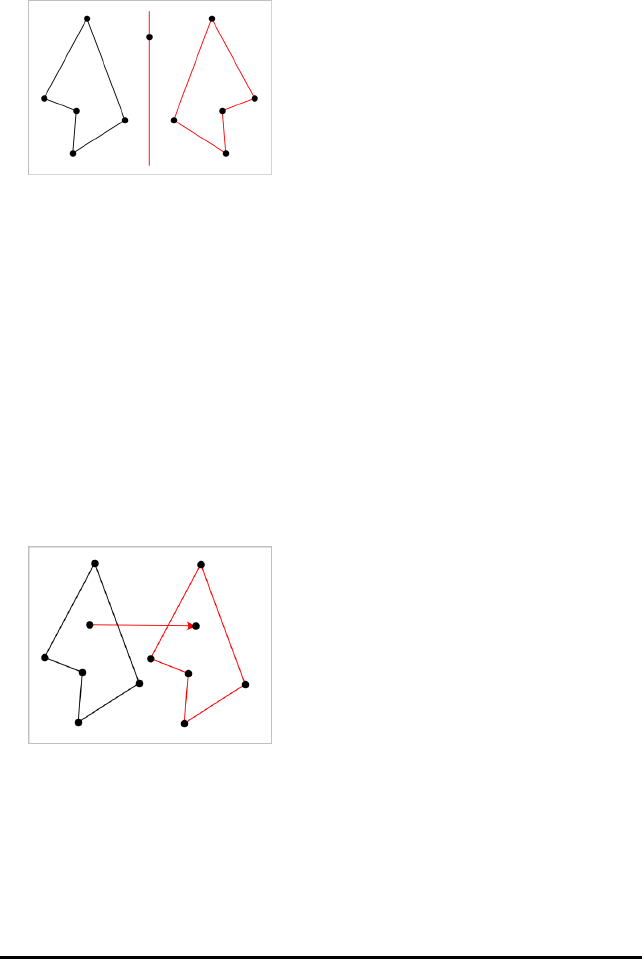
4. Click the predefined reflection line or segment.
A reflected image of the object is displayed.
5. Manipulate the original object or the line of symmetry to explore the reflection.
Exploring Translation
1. (Optional) Create a vector to predefine the distance and direction of translation.
2. From the Transformation menu, select Translation. (In the Graphs application, click
Geometry > Transformation > Translation.)
3. Click the object whose translation you want to explore.
4. Click the predefined vector.
—or—
Click two locations on the work area to indicate the direction and distance of
translation.
A translated image of the object is displayed.
5. Manipulate the original object or the vector to explore the translation.
Exploring Rotation
1. (Optional) Create an angle measurement to serve as a predefined angle of
rotation.
Geometry Application 320
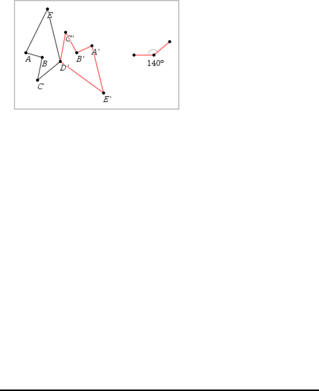
321 Geometry Application
2. From the Transformation menu, select Rotation. (In the Graphs application, click
Geometry > Transformation > Rotation.)
3. Click the object whose rotation you want to explore.
4. Click a location or point to define the point of rotation.
5. Click the points of the predefined angle.
—or—
Click three locations to define an angle of rotation.
A rotated image of the object is displayed.
6. Manipulate the original object or the point of rotation to explore the rotation.
Exploring Dilation
1. Create a Text object containing a numeric value to serve as a predefined dilation
factor.
Note: You can also use a measured length value as the dilation factor. Keep in
mind that if you use a large value, you may have to pan the display to view the
dilated object.
2. From the Transformation menu, select Dilation. (In the Graphs application, click
Geometry > Transformation > Dilation.)
3. Click the object whose dilation you want to explore.
4. Click a location or existing point to define the centre point of dilation.
5. Click the Text object or measurement that defines the dilation factor.
A dilated image of the object is displayed.

6. Manipulate the original object or the centre point of dilation to explore the dilation.
You can also edit the dilation factor.
Exploring with Geometric Construction Tools
You can investigate scenarios by adding objects from the Construction tools. The
constructions are dynamic. The midpoint of a line segment, for example, is updated
automatically when you manipulate the endpoints.
While a construction is in progress, a tool appears in the work area (for example,
Parallel ). To cancel, press ESC.
Creating a Midpoint
This tool lets you bisect a segment or define a midpoint between any two points. The
points can be on a single object, on separate objects, or on the work area.
1. From the Construction menu, select Midpoint. (In the Graphs application, click
Geometry > Construction > Midpoint.)
2. Click a point or location to define the first point.
3. Click a second point or location to complete the midpoint.
Geometry Application 322

323 Geometry Application
Creating a Parallel Line
This tool creates a parallel line with respect to any existing line. The existing line can
be a Graphs axis or any side of a triangle, square, rectangle, or polygon.
1. From the Construction menu, select Parallel. (In the Graphs application, click
Geometry > Construction > Parallel.)
2. Click the object that will serve as the reference line.
3. Click a location to create the parallel line.
You can drag the parallel line to move it. If you manipulate the reference object,
the line remains parallel.
Creating a Perpendicular Line
You can create a line that is perpendicular to a reference line. The reference can be an
axis, an existing line, a segment, or one side of a triangle, rectangle, or polygon.
1. From the Construction menu, select Perpendicular. (In the Graphs application, click
Geometry > Construction > Perpendicular.)
2. Click a location or existing point through which the perpendicular line should pass.
3. Click the item that will serve as the reference line.
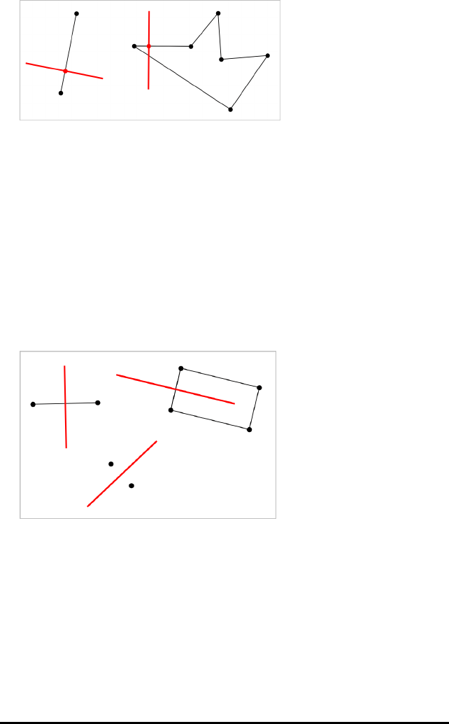
You can drag the intersection point to move the perpendicular. If you manipulate
the reference object, the line remains perpendicular.
Creating a Perpendicular Bisector
You can create a perpendicular bisector on a segment, on one side of a triangle,
rectangle, or polygon, or between any two points.
1. From the Construction menu, select PerpendicularBisector. (In the Graphs
application, click Geometry > Construction > PerpendicularBisector.)
2. Click the item that will serve as the reference line.
—or—
Click two points to create a perpendicular bisector between them.
Bisecting an Angle
This tool creates an angle bisector. The points of the angle can be on existing objects,
or they can be locations on the work area.
1. From the Construction menu, select AngleBisector. (In the Graphs application, click
Geometry > Construction > AngleBisector.)
2. Click three locations or points to define the angle. The second click defines the
vertex of the angle.
Geometry Application 324
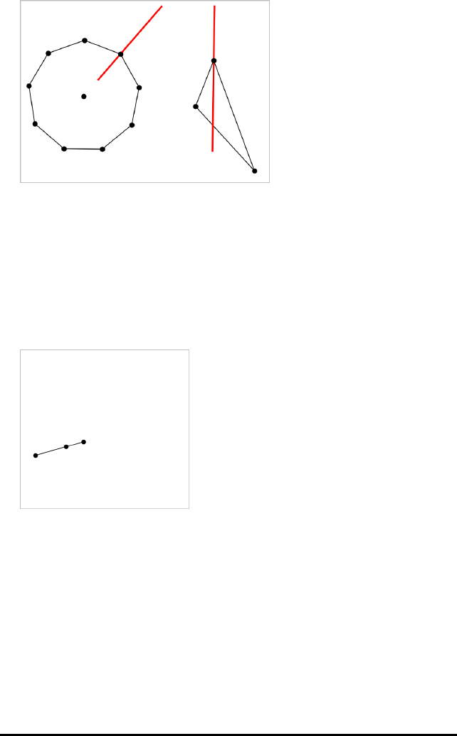
325 Geometry Application
The angle bisector adjusts automatically as you manipulate its defining points.
Creating a Locus
The Locus tool enables you to explore the range of motion of one object with respect to
another object as constrained by a shared point.
1. Create a segment, line, or circle.
2. Create a point on the segment, line, or circle.
3. Create another object that uses the point created in the previous step.
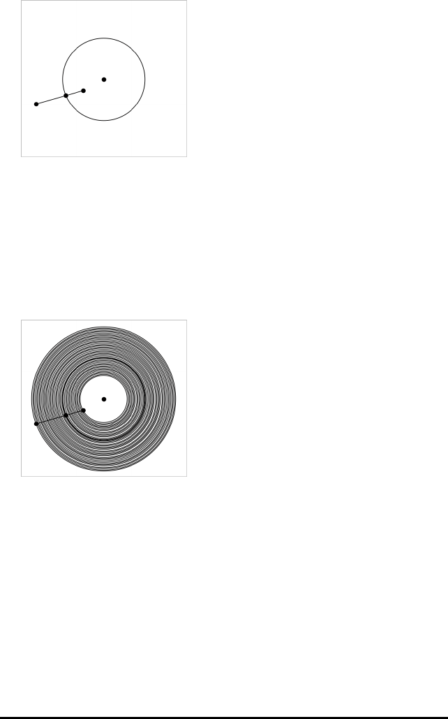
Circle created to use the defined point on
the segment.
4. From the Construction menu, select Locus. (In the Graphs application, click
Geometry > Construction > Locus.)
5. Click the point shared by the objects.
6. Click the object defined to share the point (this is the object to vary).
The continuous locus is displayed.
Creating a Compass
This tool operates similarly to a geometric compass used for drawing circles on paper.
1. From the Construction menu, select Compass. (In the Graphs application, click
Geometry > Construction > Compass.)
2. To set the width (radius) of the compass:
Click a segment.
—or—
Click any side of a triangle, rectangle, polygon, or regular polygon.
Geometry Application 326
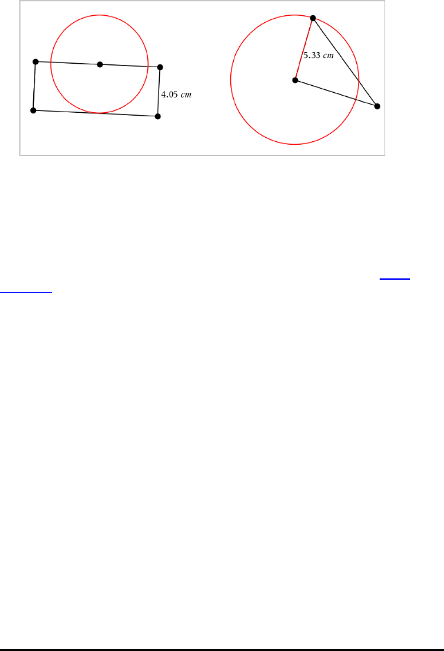
327 Geometry Application
—or—
Click any two existing points or locations on the work area.
3. Click a location to establish the centre of the circle and complete the construction.
The radius adjusts automatically as you manipulate the original segment, side, or
points used to define the radius.
Using Geometry Trace
The Geometry Trace tool leaves a visible trail of a geometric object or function graph
as it is moved or manipulated. The movement can be done manually or by using
animation. This tool is accessible in both the Graphs and Geometry applications.
1. From the Trace menu, select GeometryTrace.
The Geometry Trace tool appears.
2. Click the object or function that you want to trace to select it.
3. Drag the object, or play the animation.
This example shows traces of a graphed function manipulated by dragging and a
triangle manipulated by animation.
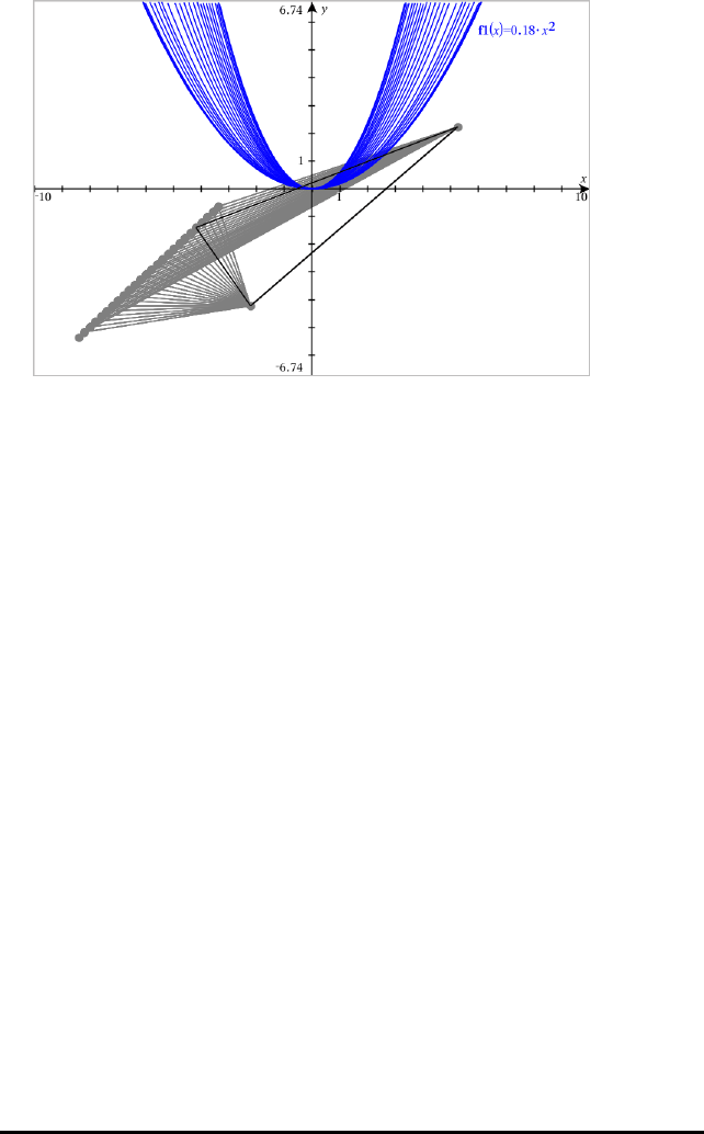
Note: You cannot select or manipulate the trace trail.
4. To erase all trails, select EraseGeometryTrace from the Trace menu.
5. To stop tracing, press Esc.
Conditional Attributes
You can cause objects to hide, show, and change colour dynamically, based on
specified conditions such as "r1<r2" or "sin(a1)>=cos(a2)."
For example, you might want to hide an object based on a changing measurement that
you have assigned to a variable, or you might want an object’s colour to change based
on a "Calculate" result assigned to a variable.
Conditional behaviours can be assigned to objects or groups in the Graphing, Plane
Geometry, and 3D Graphing views.
Setting Conditional Attributes of an Object
You can set conditions of a selected object either by using its context menu or by
activating the Set Conditions tool from the Actions menu and then selecting the object.
These instructions describe using the context menu.
1. Select the object or group.
2. Display the object’s context menu, and click Conditions.
The conditional attributes are displayed.
Geometry Application 328
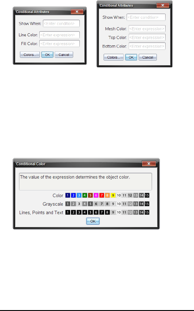
329 Geometry Application
For 2D objects For 3D objects
3. (Optional) In the Show When field, enter an expression specifying the conditions
during which the object will be shown. Anytime the condition is not satisfied, the
object will be hidden.
You can specify tolerance by using compound conditionals in the Show When input
field. For example, area>=4andarea<=6.
Note: If you need to see conditionally hidden objects temporarily, click
Actions>Hide/Show. To return to normal viewing, press ESC.
4. (Optional) Enter numbers or expressions that evaluate to numbers in the applicable
colour fields, such as Line Colour or Mesh Colour. To see a map of colour values,
click the Coors button.
Map of conditional colour values
5. Click OK in the Conditional Attributes dialogue box to apply the conditions.
Hiding Objects in the Geometry Application
The Hide/Show tool reveals objects you have previously selected as hidden and lets you
select which objects to show or hide.
1. From the Actions menu, select Hide/Show.
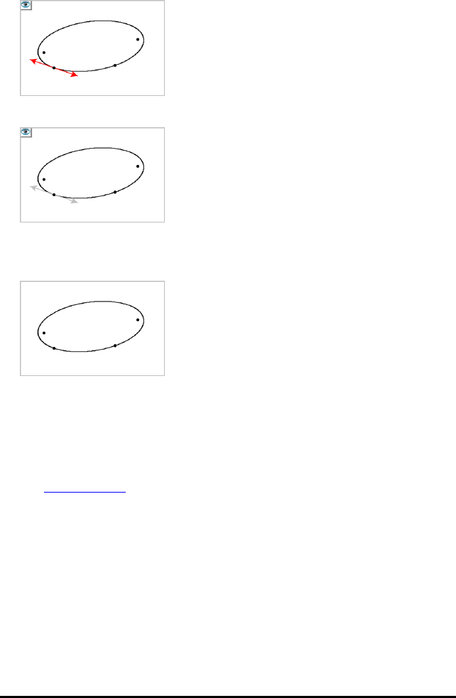
The Hide/Show tool appears, and currently hidden items (if any) are shown
dimmed.
2. Click objects to toggle their hide/show status.
3. Press Esc to complete your selections and close the tool.
All objects you selected as hidden objects disappear.
4. To view the hidden objects temporarily or restore them as shown objects, open the
Hide/Show tool.
Customizing the Geometry Work Area
Inserting a Background Image
You can insert an image as a background for any Graphs or Geometry page.
1. From the Insert menu, click Image.
2. Navigate to the image you want to insert, select it, and then click Open.
Adding a Text Object to the Work Area
Use the Text tool to add numeric values, formulas, observations, or other explanatory
information to the Geometry work area.
1. From the Actions menu, select Text.
2. Click the location for the text.
3. Type the text in the box that appears, and then press Enter.
Geometry Application 330
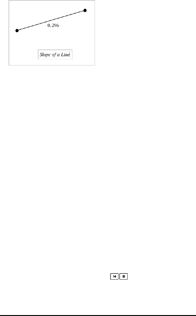
331 Geometry Application
To move a text object, drag it. To edit the text, double-click it. To delete a text object,
display its context menu, and select Delete.
Changing the Attributes of Numeric Text
If you enter a numeric value as text, you can lock it or set its format and displayed
precision.
1. From the Actions menu, select Attributes.
2. Click the numeric text to display its list of attributes.
3. Press 9and:to move through the list.
4. At each attribute icon, press 7or8to move through the options. For example,
select 0through 9as the precision.
5. Press Enter to apply the changes.
6. Press Esc to close the Attributes tool.
Animating Points on Objects
You can animate any point created as a point on an object or graph. Multiple points can
be animated simultaneously.
Animating a Point
1. From the Actions menu, select Attributes.
2. Click the point to display its attributes.
3. Press ▼to select the animation attributes.
4. Press ◄or►to choose either unidirectional or alternating animation.
5. Type a value to set the animation speed. Any nonzero speed begins the animation.
To reverse the direction, enter a negative value.
6. Press Enter to display the animation controls .
7. Press ESC to close the Attributes tool.
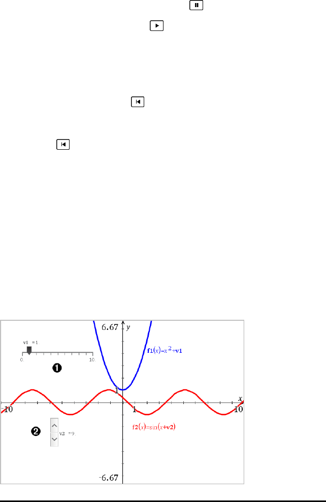
Pausing and Resuming All Animations
▶To pause all animations on a page, click Pause .
▶To resume all animations, click Play .
Resetting All Animations
Resetting pauses all animations and returns all animated points to the positions they
occupied when they were first animated.
▶To reset animation, click Reset .
Changing or Stopping the Animation of a Point
1. Click Reset to stop all animation.
2. From the Actions menu, select Attributes.
3. Click the point to display its attributes.
4. Select the animation attribute, and type a new animation speed. To stop the
point’s animation, enter zero.
Note: If other animated points exist, the animation controls remain in the work
area.
Adjusting Variable Values with a Slider
A slider control lets you interactively adjust or animate the value of a numeric variable.
You can insert sliders in the Graphs, Geometry, Notes and Data&Statistics
applications.
Geometry Application 332
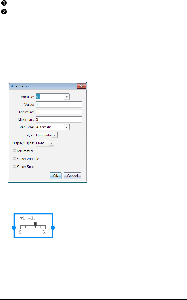
333 Geometry Application
Horizontal slider for adjusting variable v1.
Minimised vertical slider for adjusting variable v2.
Note: TI-Nspire™ version 4.2 or higher is required for opening .tns files containing
sliders on Notes pages.
Inserting a Slider Manually
1. From a Graphs, Geometry or Data&Statistics page, select Actions > Insert Slider.
—or—
From a Notes page, make sure the cursor is not in a maths box or chem box, and
then select Insert > InsertSlider.
The Slider Settings screen opens.
2. Enter the desired values, and click OK.
The slider is displayed. On a Graphs, Geometry or Data&Statistics page, handles
are displayed to let you move or stretch the slider.
To remove the handles and use the slider, click an empty
space in the work area. You can show the handles any time by
selecting Move from the slider's context menu.
3. To adjust the variable, slide the pointer (or click the arrows on a minimised slider).
- You can use the Tab key to move the focus to a slider or to move from one
slider to the next. The colour of the slider changes to show you when it has the
focus.
- When a slider has the focus, you can use the arrow keys to change the value of
the variable.
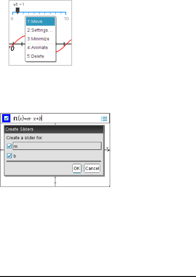
Working with the Slider
Use the options on the context menu to move or delete the slider, and to start or stop
its animation. You can also change the slider's settings.
1. Display the slider's context menu.
2. Click an option to select it.
Automatic Sliders in Graphs
Sliders can be created for you automatically in the Graphs application and in the
analytic window of the Geometry application. You are offered automatic sliders when
you define certain functions, equations or sequences that refer to undefined variables.
Using the Calculate Tool
The Calculate tool is available in the Graphs and Geometry applications. It lets you
evaluate a maths expression you have entered as a text object.
The following example uses the Calculate tool to calculate the measured angles of a
triangle.
1. Using the Shapes menu, create a triangle and then measure its angles.
Geometry Application 334
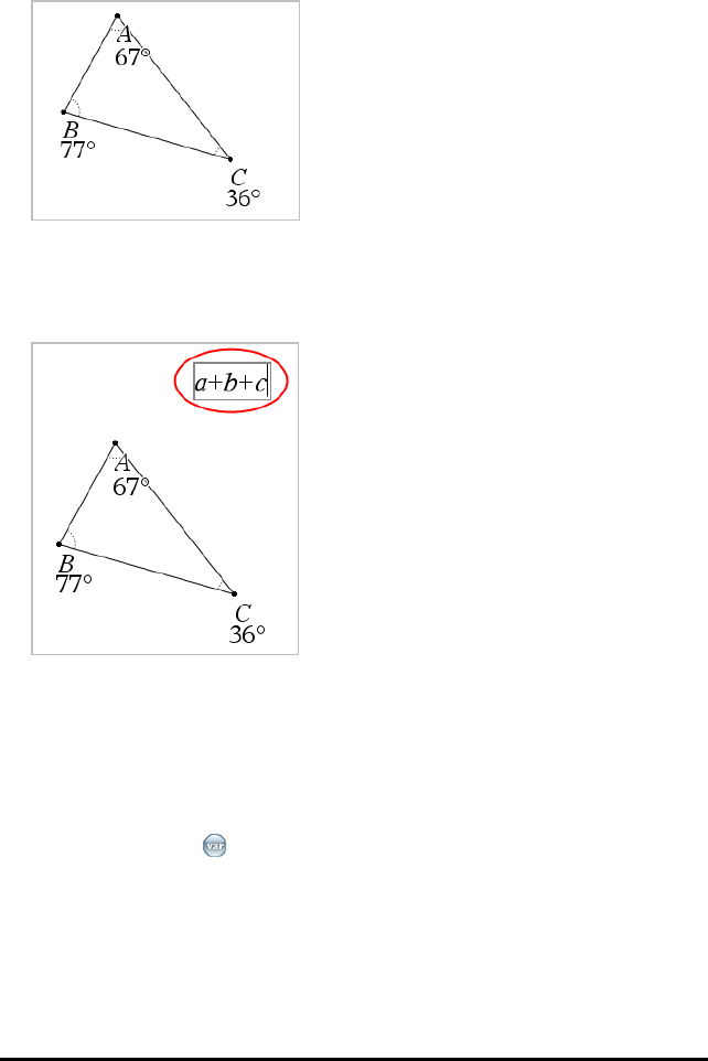
335 Geometry Application
Tip: You can enable options to automatically label points and to force geometric
triangle angles to integers. For more information, see What You Must Know, in this
chapter.
2. From the Actions menu, click Text.
3. Click a location for the text, and type the formula for the calculation.
In this example, the formula calculates three terms.
4. From the Actions menu, click Calculate.
5. Click the formula you created.
You are prompted to select a value for each term in the formula.
6. Click each angle measurement when prompted.
Note: If you have stored a measurement as a variable, you can select it when
prompted by clicking . If the name of a stored measurement matches a term in
the formula, you can press “L” when prompted for that term.
After you have selected the third term, the calculation result attaches itself to the
pointer.

7. Position the result, and press Enter to anchor it as a new text object.
Geometry Application 336

337
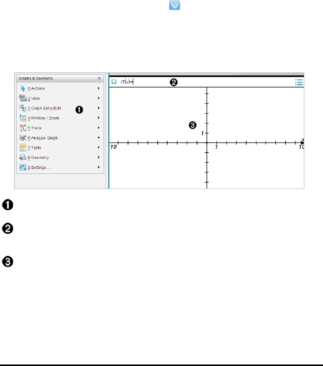
Graphs Application
The Graphs application lets you:
• Graph and explore functions and other relations, such as inequalities, parametrics,
polars, sequences, differential equation solutions, and conics.
• Animate points on objects or graphs and explore their behaviour.
• Link to data created by other applications.
Adding a Graphs Page
▶To start a new document with a blank Graphs page:
From the main File menu, click New Document, and then click Add Graphs.
Handheld: Press c, and select Graphs .
▶To add a Graphs page in the current problem of an existing document:
From the toolbar, click Insert > Graphs.
Handheld: Press ~and select Insert > Graphs.
Graphs &Geometry menu. Contains tools for defining, viewing, and investigating
relations.
Entry line. Lets you define the relations that you want to graph. The default graph
type is Function, so the form f1(x)= is displayed initially. You can define multiple
relations for each of several graph types.
Graphs Work Area
• Shows graphs of relations that you define on the entry line.
• Shows points, lines, and shapes that you create with geometry tools.
• Drag the area to pan (affects only those objects created in the Graphs
application).
Graphs Application 338

339 Graphs Application
What You Must Know
Changing the Graphs and Geometry Settings
1. From the Settings menu in the Documents Toolbox, select Settings.
2. Select the settings that you want to use.
-Display Digits. Sets the display format for numbers as Floating or Fixed
decimal.
-Graphing Angle. Sets the angle unit for all Graphs and 3D Graphing applications
in the current document. The default setting is Radian. Set this to Auto if you
want graphing angles to follow the Angle setting in the main File>Settings
menu. An angle mode indicator shows the resulting mode in Graphs and 3D
Graphing applications.
-Geometry Angle. Sets the angle unit for all Geometry applications in the current
document. The default setting is Degree. Set this to Auto if you want geometry
angles to follow the Angle setting in the main File>Settings menu. An angle
mode indicator shows the resulting mode in Geometry applications.
-Automatically hide plot labels. In the Graphs application, hides the label that
normally appears next to a graphed relation.
-Show axis end values. Applies only in the Graphs application.
-Show tool tips for function manipulation. Applies only in the Graphs application.
-Automatically find points of interest. In the Graphs application, shows zeros,
minima and maxima while tracing function graphs.
-Force Geometric Triangle Angles to Integers. Restricts the angles of a triangle to
integer values as you create or edit the triangle. This setting applies only in the
Geometry View with the Geometry Angle unit set to Degree or Gradian. It does
not apply to analytic triangles in Graphing View or to analytic triangles in the
Analytic Window of the Geometry View. This setting does not affect existing
angles, and it does not apply when constructing a triangle based on previously
inserted points. By default, this setting is deselected.
-Automatically Label Points. Applies labels (A,B, ..., Z,A1,B1, and so on) to
points, lines, and vertices of geometric shapes as you draw them. The labelling
sequence starts at Afor each page in a document. By default, this setting is
deselected.
Note: If you create a new object that uses existing un-labelled points, those
point are not automatically labelled in the completed object.
- Click Restore to restore all settings to their factory defaults.
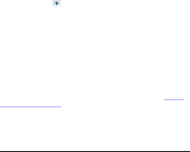
- Click Make Default to apply the current settings to the open document and save
them as the default for new Graphs and Geometry documents.
Using Context Menus
Context menus provide quick access to commonly used commands and tools that apply
to a specific object. For example, you can use a context menu to change an object's
line colour or to group a set of selected objects.
▶Display the context menu for an object in one of the following ways.
- Windows®: Right-click the object.
- Mac®: Hold “and click the object.
- Handheld: Move the pointer to the object, and then press / b.
Finding Hidden Objects in the Graphs or Geometry Application
You can hide and show individual graphs, geometric objects, text, labels,
measurements and axis end-values.
To temporarily view hidden graphs or objects or to restore them as shown objects:
1. From the Actions menu, select Hide/Show.
The Hide/Show tool appears in the work area, and all hidden objects become
visible in dimmed colours.
2. Click a graph or object to toggle its Hide/Show state.
3. To apply the changes and close the Hide/Show tool, press ESC.
Inserting a Background Image
You can insert an image as a background for a GraphsorGeometry page. The file
format of the image can be .bmp, .jpg or .png.
1. From the Insert menu, click Image.
2. Navigate to the image you want to insert, select it and then click Open.
For information on moving, resizing, and deleting a background image, see Working
with Images in the Software.
Adding Text to the Graphs or Geometry Work Area
1. From the Actions menu, select Text.
Graphs Application 340
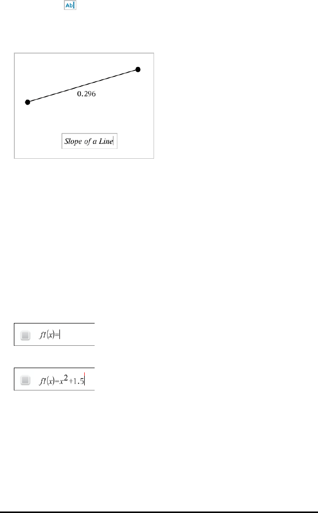
341 Graphs Application
The Text tool appears in the work area.
2. Click the location for the text.
3. Type the text in the box that appears, and then press Enter.
4. To close the Text tool, press ESC.
5. To edit the text, double-click it.
Deleting a Relation and its Graph
1. Select the relation by clicking its graph.
2. Press Backspace or DEL.
The graph is removed from both the work area and the graph history.
Graphing Functions
1. From the GraphEntry/Edit menu, select Function.
2. Type an expression for the function.
3. Press Enter to graph the function.
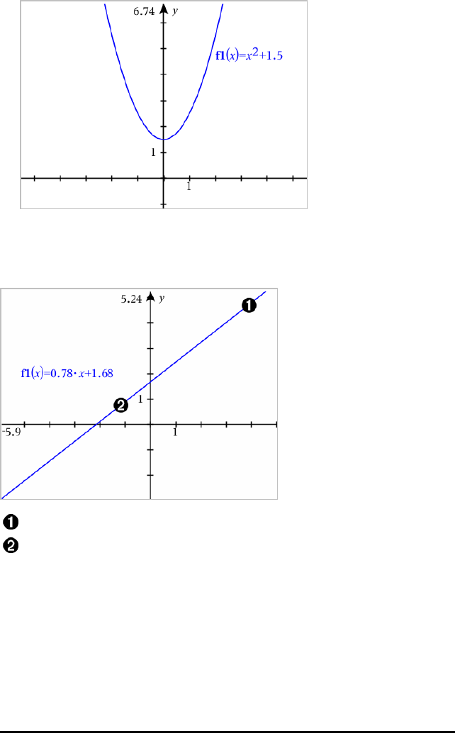
Manipulating Functions by Dragging
Some types of functions can be translated, stretched, and/or rotated by dragging parts
of the graph. As you drag, the expression for the graph updates to reflect the change.
Drag graph from the ends to rotate.
Drag graph near the middle to translate.
Manipulating a Linear Function
▶To translate, grab near the middle of the graph, and then drag.
Graphs Application 342
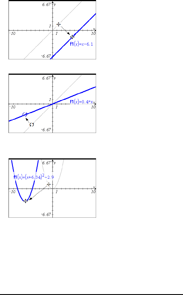
343 Graphs Application
▶To rotate, grab near the ends of the graph, and then drag.
Manipulating a Quadratic Function
▶To translate, grab near the vertex of the graph, and then drag.
▶To stretch, grab away from the vertex of the graph, and then drag.
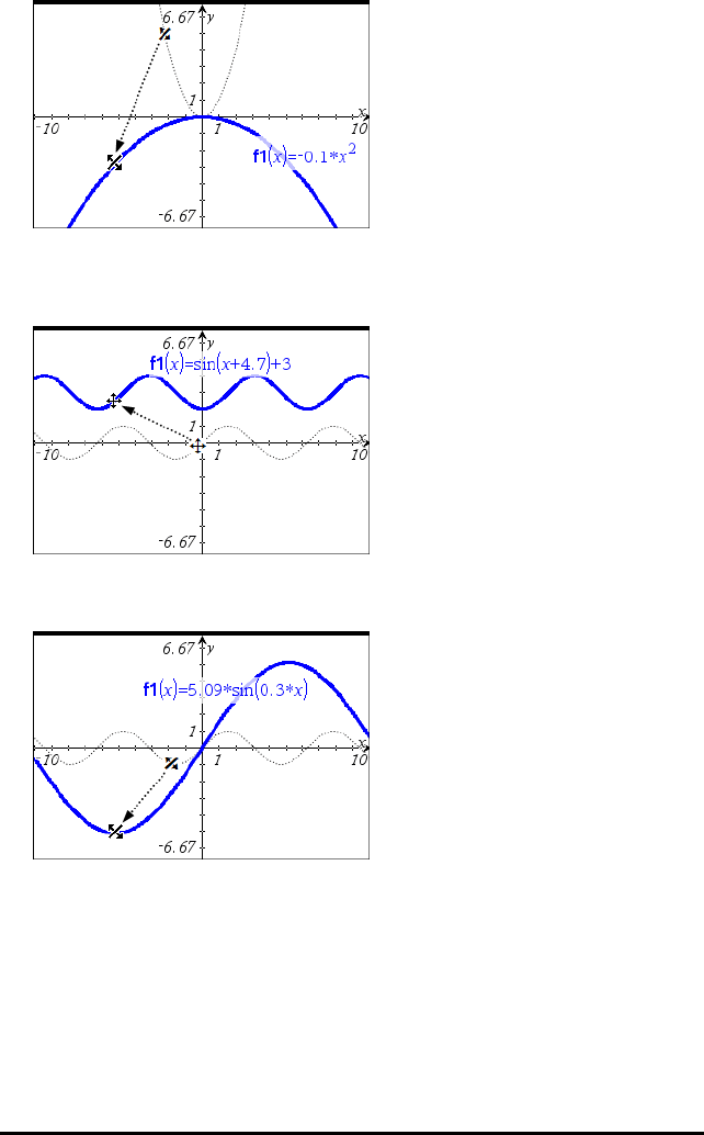
Manipulating a Sine or Cosine Function
▶To translate, grab near the axis of vertical symmetry of the graph, and then drag.
▶To stretch, grab away from the axis of vertical symmetry of the graph, and then
drag.
Specifying a Function with Domain Restrictions
You can use the entry line or the Calculator application to specify a function with
domain restrictions. For multiple domain restrictions on a function, use the piecewise()
function.
In the following example, a function with a domain that is less than 2 and greater than
-2 is specified on the entry line:
1. From the GraphEntry/Edit menu, select Function.
Graphs Application 344
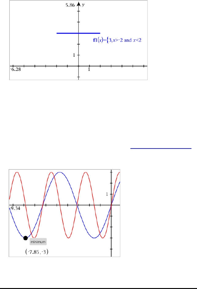
345 Graphs Application
2. Type the following on the entry line, using spaces to separate the "and" operator:
piecewise(3,x>-2 and x<2)
3. Tap Enter to graph the function.
Finding Points of Interest on a Function Graph
The Graphs application helps you find zeros, minimums, maximums, intersections,
derivatives (dy/dx), or integrals. For Graphs defined as conic sections, you can also find
foci, directrix, and other points.
(CAS): You can also find the point of inflection.
Identifying Points of Interest by Dragging a Point
▶To quickly identify maximums, minimums, and zeros, create a point on the graph
and then drag the point.
Temporary signposts appear as you drag through points of interest.
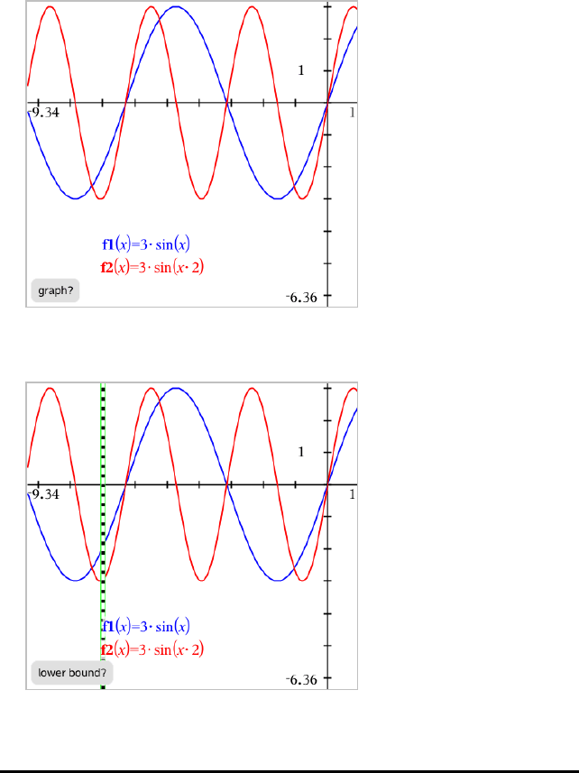
Identifying Points of Interest with Analysis Tools
This example illustrates using the Minimum tool. Other analysis tools operate
similarly.
1. From the AnalyseGraph menu, select Minimum.
The Minimum icon is displayed at the top left on the work area, and a graph?
prompt appears in the work area.
2. Click the graph on which you want to find the minimum.
A dotted line appears, representing the lower bound of the range to search.
Graphs Application 346
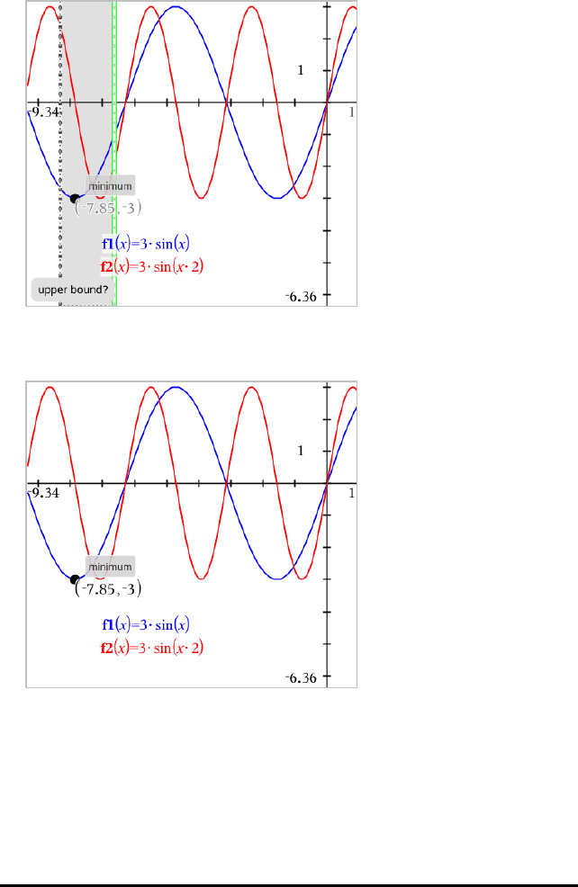
347 Graphs Application
3. Drag the line or click a location to set the lower bound and display a proposed
upper bound.
4. Drag the line representing the upper bound, or click a location to set it.
The minimum is displayed, along with a text object showing its coordinates.
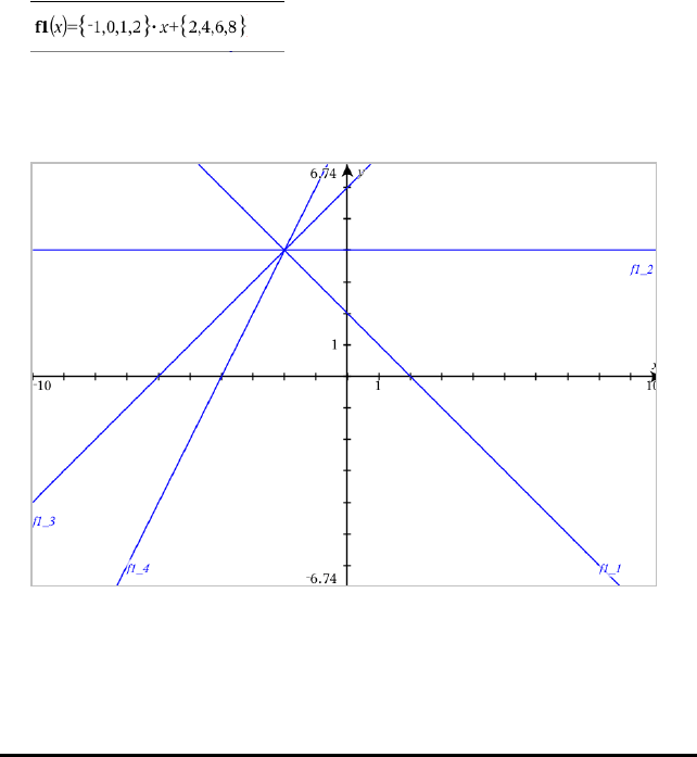
Graphing a Family of Functions
In a family of functions, each member has its own value for one or more of the
parameters. By entering the parameters as lists, you can use a single expression to
graph a family of up to 16 functions.
For example, the expression f1(x) = {-1,0,1,2} •x + {2,4,6,8} denotes the following four
functions:
f1_1(x)=-1•x+2
f1_2(x) = 0•x+4
f1_3(x) = 1•x+6
f1_4(x) = 2•x+8
To Graph a Family of Functions
1. From the GraphEntry/Edit menu, select Function.
2. Type the expression, using lists to represent the members of the family.
3. Press Enter to graph the functions.
Each member is labelled separately (f1_1,f1_2, and so on) to indicate its sequence
in the expression.
Note: You cannot edit a single function graph to change it to a family of functions.
Graphing Equations
1. From the GraphEntry/Edit menu, select Equation.
Graphs Application 348
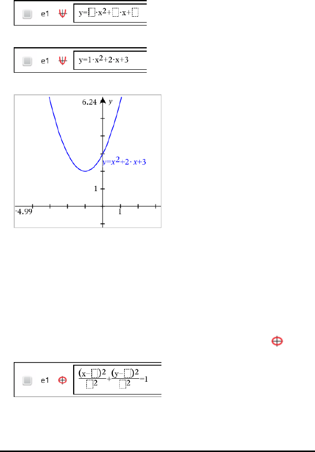
349 Graphs Application
2. Click the type of equation (Line,Parabola,Circle,Ellipse,Hyperbola, or Conic).
3. Click the specific template for the equation. For example, tap y=a•x2+b•x+c to
define a parabola.
The entry line includes a symbol to indicate the type of equation.
4. Type the coefficients into the equation template.
5. Press Enter.
Graphing Conic Sections
The Graphing view lets you graph and explore linear and conic equations analytically in
a two-dimensional coordinate system. You can create and analyse lines, circles,
ellipses, parabolas, hyperbolas, and general conic equations.
The entry line makes it easy to enter the equation by displaying a template for the type
of equation you choose.
Example: Creating a conic ellipse
1. From the GraphEntry/Edit menu, select Equation>Ellipse, and tap the
equation type.
2. Type initial values for the coefficients in the provided spaces. Use the arrow keys to
move among the coefficients.
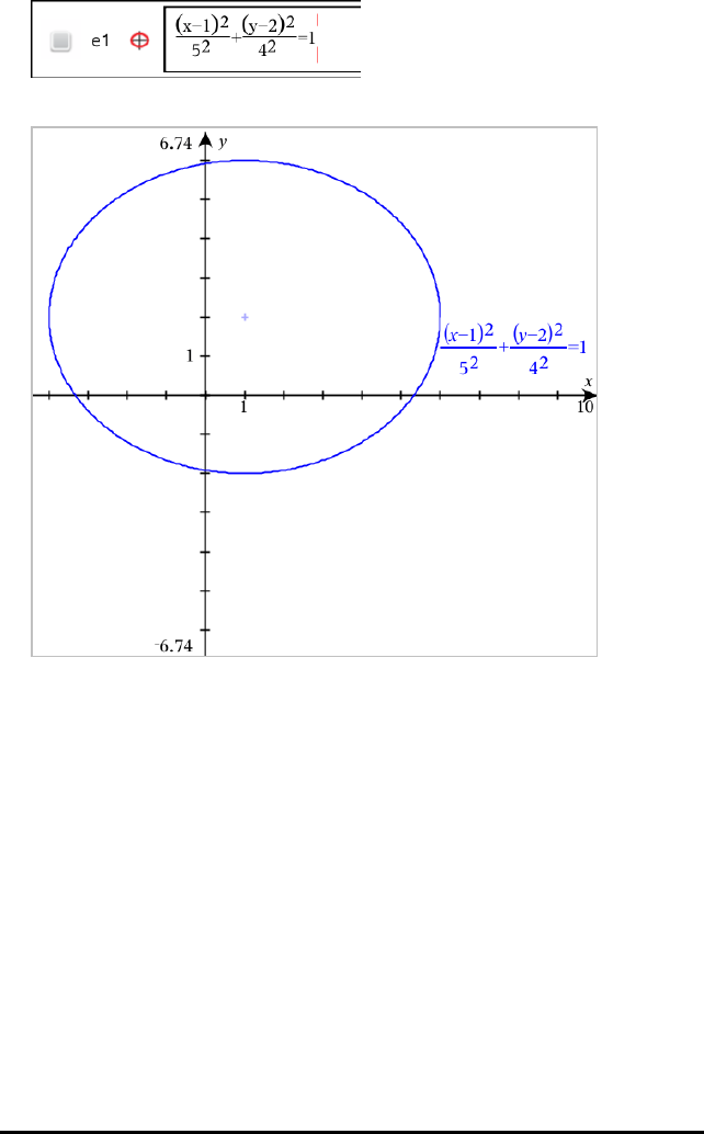
3. Press Enter to graph the equation.
Exploring the sample ellipse
1. Drag the ellipse from its centre to explore the effect of translation on the equation.
Graphs Application 350
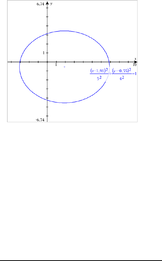
351 Graphs Application
2. Use the analysis tools, such as AnalyseGraph >AnalyseConics>Foci to further
explore the graph.
Note: The type of conic determines which analysis tools you can use. In the case of
the ellipse, you can obtain its centre, vertices, foci, axes of symmetry, directrices,
eccentricity, and latera recta.
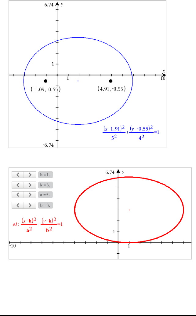
3. To explore translation and dilation interactively, define a conic ellipse that uses
variables for the h,k,a, and bcoefficients. Insert sliders to vary the parameters.
Graphing Relations
Relation graphing is available on Graphs pages and in the Analytic Window of
Geometry pages.
Graphs Application 352
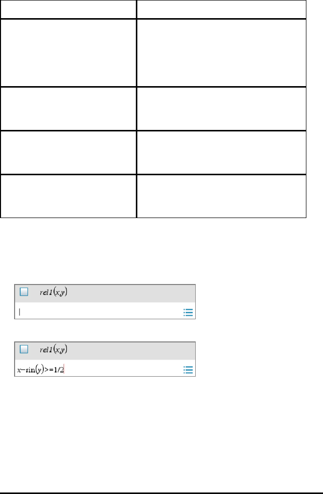
353 Graphs Application
You can define relations using ≤,<,=,>or ≥. The inequality operator (≠) is not
supported in relation graphing.
Relation type Examples
Equations and inequalities
equivalent to y=f(x)
• y = sqrt(x)
• y-sqrt(x) = 1/2
• -2*y-sqrt(x) = 1/2
• y-sqrt(x) ≥1/2
• -2*y-sqrt(x) ≥1/2
Equations and inequalities
equivalent to x=g(y)
• x = sin(y)
• x-sin(y) = 1/2
• x-sin(y) ≥1/2
Polynomial equations and
inequalities
• x^2+y^2 = 5
• x^2-y^2 ≥ 1/2+y
• x3+y3-6*x*y=0
The above relations on domains
restricted by rectangles
• y=sin(x) and -2π<x≤2π
• y≤x2|y≥-2 and 0≤x≤3
• {x2+y2≤3, y≥0 and x≤0
Note: Restrictions imposed by an active Press-to-Test session may limit the types of
relations you can graph.
To Graph a Relation:
1. From the GraphEntry/Edit menu, select Relation.
2. Type an expression for the relation.
3. Press Enter to graph the relation.
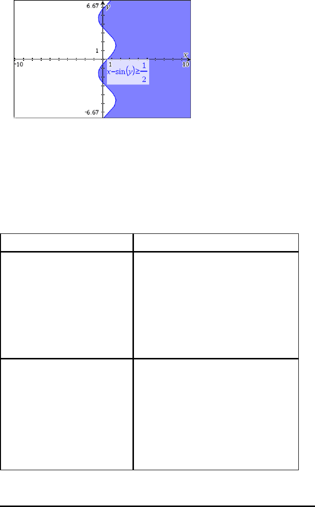
Tips for Graphing Relations
▶You can quickly define a relation from the Function entry line. Position the cursor to
the immediate right of the = sign, and then press the Backspace key. A small menu
appears with the relation operators and a Relation option. Choosing from the menu
places the cursor in the Relation entry line.
▶You can type a relation as text on a Graphs page and then drag the text object over
either axis. The relation is graphed and added to the relation history.
Warning and Error Message
Error Condition Additional Information
Relation input not supported Relation input not supported
Note: The following relation inputs are
supported:
• Relations using ≤, <, =, >, or ≥.
• Polynomial relations in x and y
• Relations equivalent to y=f(x) or x=g(y)
or corresponding inequalities
• The above relations on domains
restricted by rectangles
Domain Restrictions not supported
for certain classes of relations
equivalent to y=f(x) or x=g(y) or
corresponding inequalities.
• Relations equivalent to y=f(x) and
corresponding inequalities can only
have constraints on x
• For example: y=√(x) and 0≤x≤1 will
work but y=√(x) and 0≤y≤1 will not
• Relations equivalent to x=g(y) and
corresponding inequalities can only
have constraints on y
• For example: x=sin(y)|−1≤y≤1 will work
but x=sin(y)|−1≤x≤1 will not
Graphs Application 354
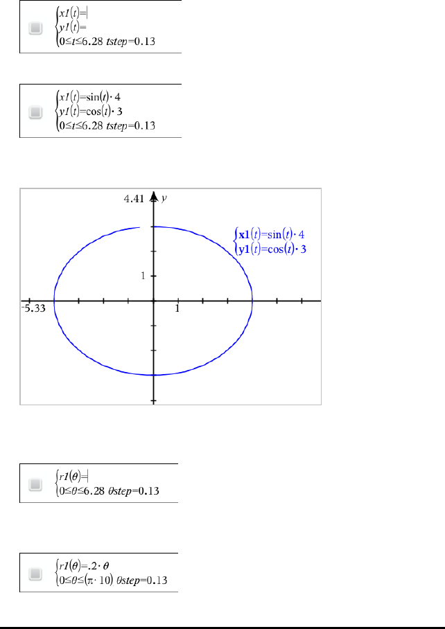
355 Graphs Application
Graphing Parametric Equations
1. From the GraphEntry/Edit menu, select Parametric.
Use the up and down arrow keys to move among the fields in the Parametric entry
line.
2. Type expressions for xn(t) and yn(t).
3. (Optional) Edit the default values for tmin,tmax, and tstep.
4. Press Enter.
Graphing Polar Equations
1. From the GraphEntry/Edit menu, select Polar.
2. Type an expression for rn(θ).
3. (Optional) Edit the default values for θmin,θmax, and θstep.
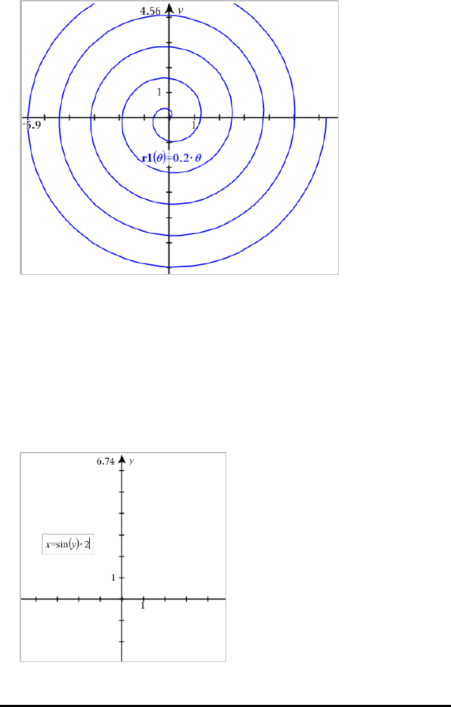
4. Press Enter.
Using the Text Tool to Graph Equations
You can graph an "x=" or "y=" equation by typing it into a text box and dragging the
text to an axis. You can edit the equation text (for example, change it to an inequality),
but you cannot change it between x= and y=.
Graphing a Trigonometry Relation from Text
1. From the Actions menu, select Text.
2. Click the work area to place the text box.
3. Type the equation for the trigonometry relation, such as x=sin(y)*2.
Graphs Application 356
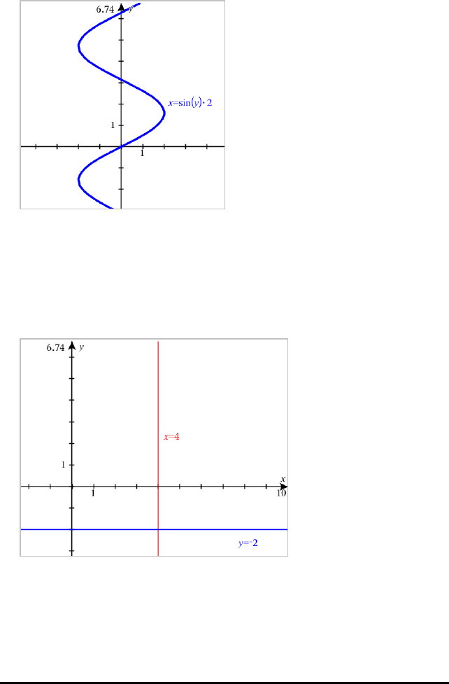
357 Graphs Application
4. Press Enter to complete the text object.
5. Drag the text object to either axis to graph the equation.
Graphing a Vertical or Horizontal Line from Text
1. From the Actions menu, select Text.
2. Click the work area to place the text box.
3. Type the equation for a vertical line, such as x=4, or a horizontal line, such as
y=-2. Click Enter to complete it.
4. Drag the text object to either axis to graph the equation.
After plotting a line, you can drag to translate or rotate it.
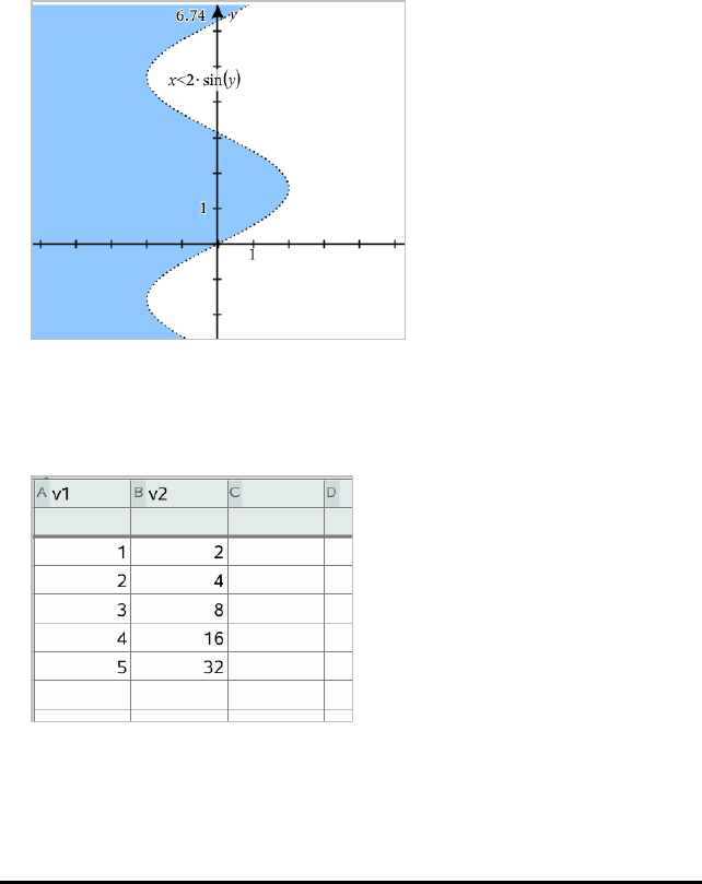
Graphing an Inequality from Text
You can graph inequalities that use the >, <, ≤, or ≥operators. Areas that satisfy the
inequality are shown with shading. If the shaded areas of two or more inequalities
overlap, the area of overlap is shaded darker.
1. From the Actions menu, select Text.
2. Click the work area to place the text box.
3. Type the inequality expression, such as x<2*sin(y). Click Enter to complete it.
4. Drag the text object to either axis to graph the inequality.
Graphing Scatter Plots
1. (Optional) Create two predefined list variables containing the x and y values to
plot. You can use the Lists&Spreadsheet, Calculator, or Notes application to create
the lists.
2. From the GraphEntry/Edit menu, select Scatter Plot.
Use the up and down arrow keys to move between the x and y fields.
Graphs Application 358
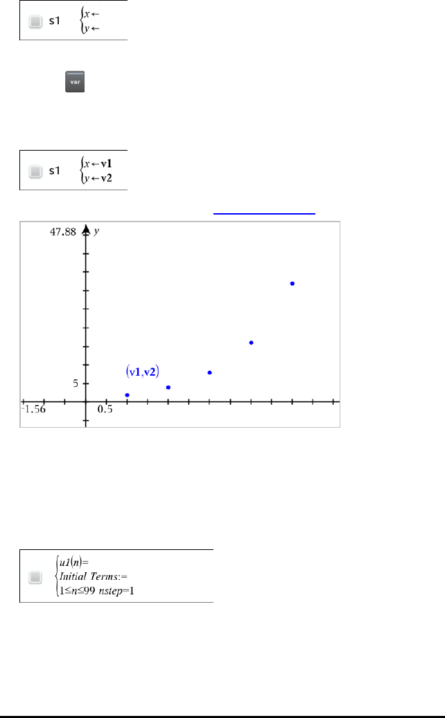
359 Graphs Application
3. Use one of the following methods to specify lists to plot as x and y.
- Click to select names of the predefined list variables.
- Type the names of the variables, such as v1.
- Type lists as comma-separated elements enclosed within brackets, for
example: {1,2,3}.
4. Press Enter to plot the data, and then zoom the work area to view the plotted data.
Plotting Sequences
The Graphs application lets you plot two types of sequences. Each type has a separate
template for defining the sequence.
Defining a Sequence
1. From the GraphEntry/Edit menu, select Sequence > Sequence.
2. Type the expression to define the sequence. Update the independent variable field
to m+1, m+2, etc., if necessary.
3. Type an initial term. If the sequence expression references more than one prior
term, such as u1(n-1) and u1(n-2), (or u1(n) and u1(n+1)), separate the terms with
commas.
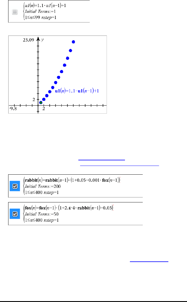
4. Press Enter.
Defining a Custom Sequence
A custom sequence plot shows the relationship between two sequences by plotting
one on the xaxis and the other on the yaxis.
This example simulates the Predator-Prey model from biology.
1. Use the relations shown here to define two sequences: one for a rabbit population,
and another for a fox population. Replace the default sequence names with rabbit
and fox.
.05 = the growth rate of rabbits if there are no foxes
.001 = the rate at which foxes can kill rabbits
.0002 = the growth rate of foxes if there are rabbits
.03 = the death rate of foxes if there are no rabbits
Note: If you want to see the plots of the two sequences, zoom the window to the
Zoom-Fit setting.
2. From the GraphEntry/Edit menu, select Sequence > Custom.
3. Specify the rabbit and fox sequences to plot on the x and y axes, respectively.
Graphs Application 360
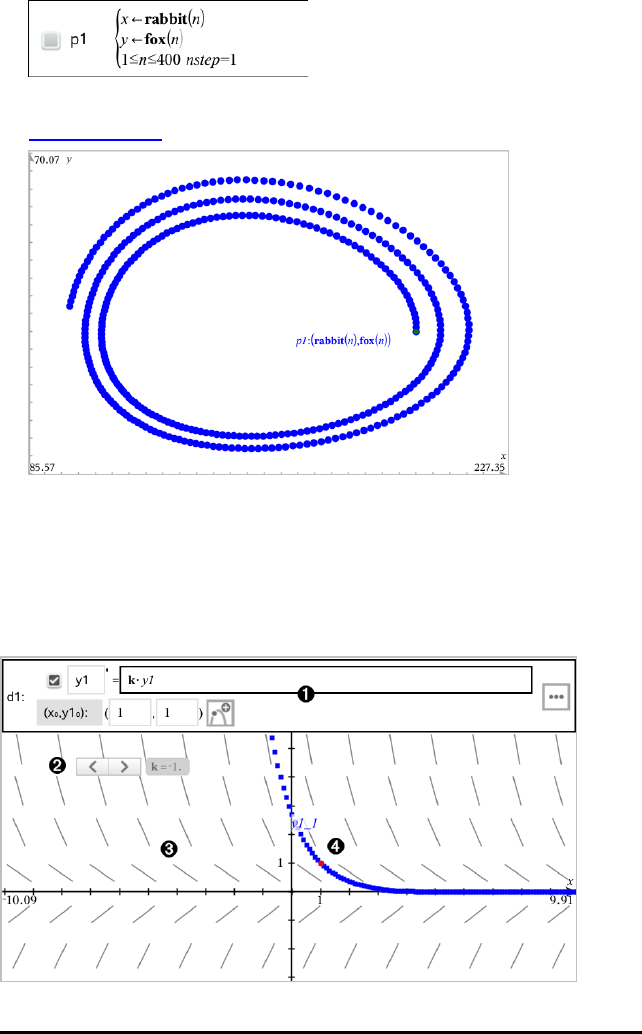
361 Graphs Application
4. Press Enter to create the custom plot.
5. Zoom the window to the Zoom-Fit setting.
6. Explore the custom plot by dragging the point that represents the initial term.
Graphing Differential Equations
You can study linear and non-linear differential equations and systems of ordinary
differential equations (ODEs), including logistic models and Lotka-Volterra equations
(predator-prey models). You can also plot slope and direction fields with interactive
implementations of Euler and Runge-Kutta methods.
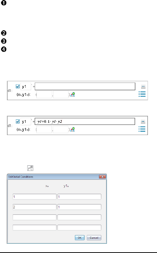
ODE entry line:
•y1 ODE identifier
• Expression k·y1 defines the relation
• Fields (1,1) for specifying initial condition
• Buttons for adding initial conditions and setting plot parameters
Slider to vary coefficient kof the ODE
Slope field
A solution curve passing through the initial condition
To Graph a Differential Equation:
1. From the GraphEntry/Edit menu, select DiffEq.
The ODE is automatically assigned an identifier, such as “y1.”
2. Move to the relation field and enter the expression that defines the relation. For
example, you might enter -y1+0.1*y1*y2.
3. Enter the initial condition for the independent value x0and for y10.
Note: The x0value(s) are common to all the ODEs in a problem but can be entered
or modified only in the first ODE.
4. (Optional) To study multiple initial conditions for the current ODE, click Add Initial
Conditions and enter the conditions.
Graphs Application 362
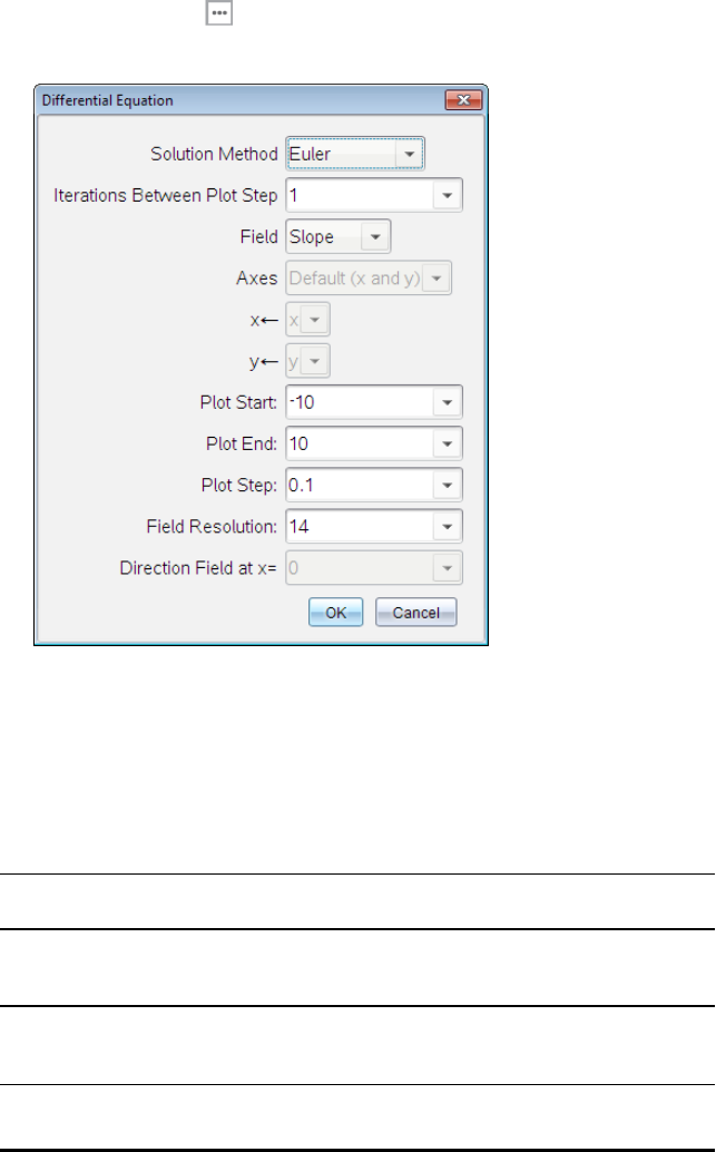
363 Graphs Application
5. Tap Edit Parameters to set the plot parameters. Select a numerical Solution
Method, and then set any additional parameters. You can change these parameters
anytime.
6. Click OK.
7. To enter additional ODEs, press the down arrow to display the next ODE edit field.
As you move among defined ODEs, the graph is updated to reflect any changes.
One solution to the ODE is graphed for each IC specified for each shown ODE
(selected by check box).
Summary of Differential Equation Settings
Solution
Method
Selects Euler or Runge-Kutta as the numerical solution method.
Iterations
Between
Plot Step
Computational accuracy for Euler solution method only. Must be an
integer value>0. To restore the default, select the down-arrow and
select Default.
Error
Tolerance
Computational accuracy for Runge-Kutta solution method only. Must be a
floating-point value|1×10-14. To restore the default, select the down-
arrow and select Default.
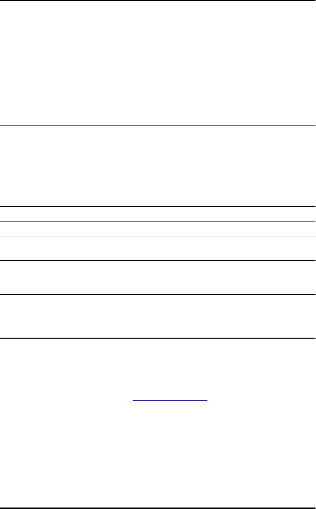
Field None - No field is plotted. Available for any number of ODEs, but
required if three or more 1st-order ODEs are active. Graphs a
combination of the solution and/or values of one or more ODEs
(according to user-configured Axes settings).
Slope - Plots a field representing the family of solutions to a single 1st-
order ODE. Exactly one ODE must be active. Sets Axes to Default
(xandy). Sets Horizontal axis to x (the independent variable). Sets
Vertical axis to y (the solution to the ODE).
Direction - Graphs a field in the phase plane representing the
relationship between a solution and/or values of a system of two
1st-order ODEs (as specified by the CustomAxes setting). Exactly two
ODEs must be active.
Axes Default (x and y) - Plots x on the x axis and y (the solutions to the active
differential equations) on the y axis.
Custom - Lets you select the values to be plotted on the x and y axes
respectively. Valid entries include:
•x(the independent variable)
•y1,y2, and any identifiers defined in the ODE editor
•y1’,y2’, and any derivatives defined in the ODE editor
Plot Start Sets the independent variable value at which the solution plot starts.
Plot End Sets the independent variable value at which the solution plot stops.
Plot Step Sets the increment of the independent variable at which values are
plotted.
Field
Resolution
Sets the number of columns of field rendering elements (line segments)
used to draw a slope or direction field. You can change this parameter
only if Field =Direction or Slope.
Direction
Field at x=
Sets the independent variable value at which a direction field is drawn
when plotting non-autonomous equations (those that refer to x). Ignored
when plotting autonomous equations. You can change this parameter
only if Field =Direction.
Viewing Tables from the Graphs Application
You can show a table of values for any relation defined in the current problem.
Note: For details about using tables and instructions for accessing tables from the
Lists&Spreadsheet application, see Working with Tables.
Showing a Table
▶From the Table menu, select Split-screenTable.
The table is displayed with columns of values for the currently defined relations.
Graphs Application 364
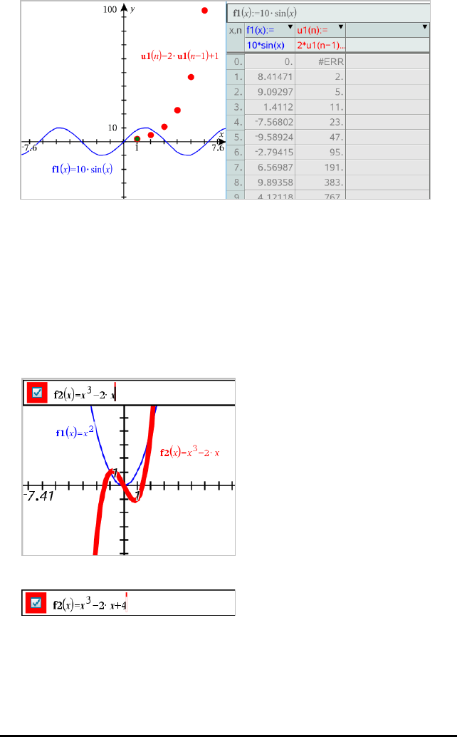
365 Graphs Application
To change which relation is displayed in a column, click the arrow in the top cell of
the column, and then select the relation name.
Hiding the Table
▶From the Table menu, select RemoveTable.
Editing Relations
1. Double-click the graph to show its expression in the entry line.
—or—
Display the graph’s context menu, and then click EditRelation.
2. Modify the expression as needed.
3. Press ·to graph the revised function.
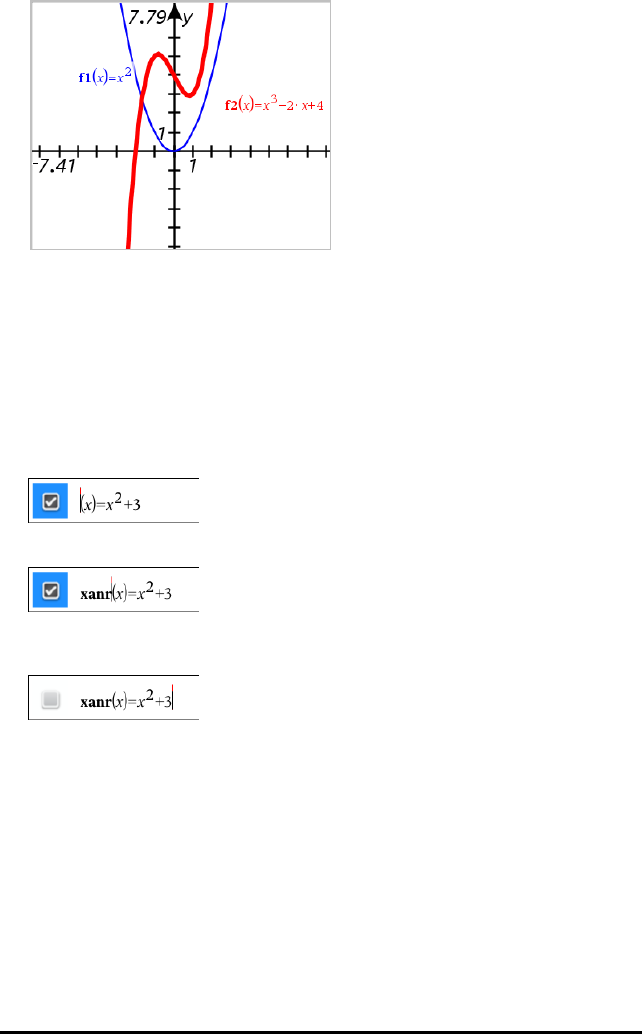
Renaming a Relation
Each relation type has a default naming convention. For example, the default name for
functions is fn(x). (The number represented by nincreases as you create more
functions.) You can replace the default name with a name of your choice.
Note: If you want to use a custom name as a convention, you must enter it manually
for each function.
1. In the entry line, delete the existing name. For example, delete the "f1" from "f1
(x)". You can use the right and left arrow keys to position the cursor.
2. Type the replacement name.
3. If you are defining a new relation, position the cursor after the = sign and type the
expression.
4. Press Enter to graph the relation with its new name.
Graphs Application 366
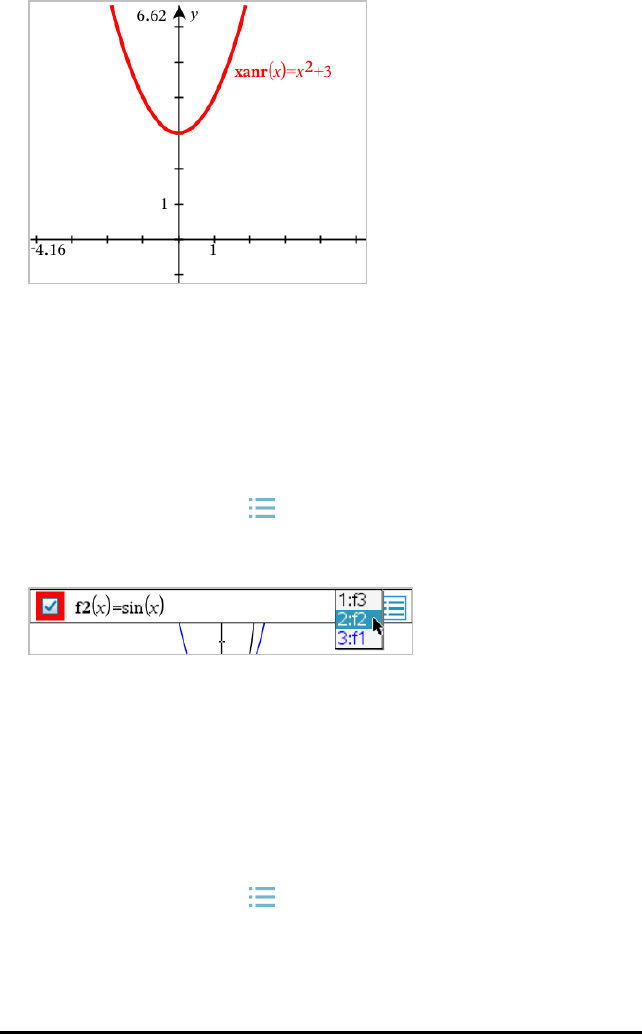
367 Graphs Application
Accessing the Graph History
For each problem, the software stores a history of relations defined in the Graphs
application and 3D Graphing view, such as function graphs f1 through f99 and 3D
function graphs z1 through z99. You can view and edit these items using a button on
the entry line.
Viewing the History
1. Press Ctrl+G to show the entry line.
2. Clickthe History Menu button on the entry line.
The menu is displayed. As you point to the name of each item, its expression
appears in the entry line.
3. Select the name of the relation you want to view or edit.
4. (Optional) From the entry line, use the up and down arrow keys to scroll through
the defined relations of the same type.
Viewing the History of Specific Relation Types
Use this method if you want to view or edit a defined relation that does not appear in
the History menu.
1. On the GraphEntry/Edit menu, click the relation type. For example, click Polar to
show the entry line for the next available Polar relation.
2. Clickthe History Menu button , or use the up and down arrow keys to scroll
through the defined relations of the same type.

Zooming/Rescaling the Graphs Work Area
Rescaling in the Graphs application affects only the graphs, plots and objects that
reside in the Graphing view. It has no effect on objects in the underlying Plane
Geometry view.
Rescaling by Dragging Along an Axis
▶To rescale the x and y axes proportionally, drag a k mark on either axis.
▶To rescale only one axis, hold down Shift and drag a k mark on the axis.
Zooming Using a Zoom Tool
▶From the Window/Zoom menu, select one of the tools.
-Zoom-Box (Click two corners of a box to define the area to show.)
-Zoom-In
-Zoom-Out
Zooming to Predefined Settings
▶From the Window/Zoom menu, select one of the predefined Zoom settings.
-Zoom - Standard
-Zoom - Quadrant 1
-Zoom - Standard User
-Zoom - Standard Trig
-Zoom - Standard Data
-Zoom - Fit
Entering Custom Window Settings
1. From the Window/Zoom menu, select WindowSettings.
2. Enter a value for each setting. You can use expressions for exact input, as shown
below.
Graphs Application 368
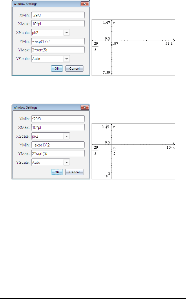
369 Graphs Application
On TI-Nspire™ products, fractional input is preserved as-is. Other exact inputs are replaced with
the evaluated result.
On TI-Nspire™ CAS products, fractional and other exact inputs are preserved.
Customising the Graphs Work Area
Inserting a Background Image
You can insert an image as a background for any Graphs or Geometry page.
1. From the Insert menu, click Image.
2. Navigate to the image you want to insert, select it and then click Open.
Adding a Text Object to the Work Area
Use the Text tool to add numeric values, formulas, observations or other explanatory
information to the Graphs work area. You can graph an equation entered as text (such
as "x=3").
1. From the Actions menu, select Text.
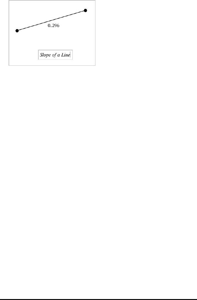
2. Click the location for the text.
3. Type the text in the box that appears, and then press Enter.
To move a text object, drag it. To edit the text, double-click it. To delete a text object,
display its context menu, and select Delete.
Changing the Attributes of Numeric Text
If you enter a numeric value as text, you can lock it or set its format and displayed
precision.
1. From the Actions menu, select Attributes.
2. Click the numeric text to display its list of attributes.
3. Press ▲and▼to move through the list.
4. At each attribute icon, press◄or►to move through the options. For example,
select 0through 9as the precision.
5. Press Enter to apply the changes.
6. Press Esc to close the Attributes tool.
Displaying the Grid
By default, the grid is not displayed. You can choose to display it as dots or lines.
▶From the View menu, select Grid, and then select DotGrid,LinedGrid or NoGrid.
Changing the Grid Colour
1. From the Actions menu, choose Select > Grid (available only when the grid is
displayed).
The grid flashes to show it is selected.
2. Click the down arrow next to the Colour button, and select a colour for the grid.
Graphs Application 370
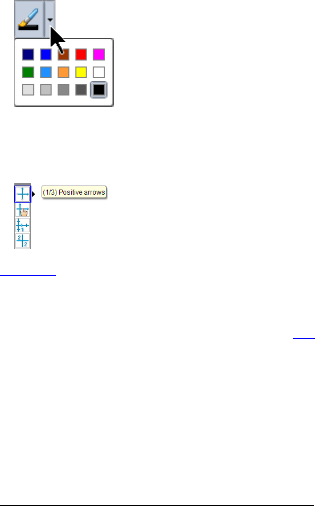
371 Graphs Application
Changing the Appearance of the Graph Axes
1. From the Actions menu, click Attributes.
2. Click either axis.
3. Press ▲and▼to move to the desired attribute, and then press ◄and►to
choose the option to apply.
Note: To hide the axes or selectively hide or show an individual axis end-value, use the
Hide/Show tool.
Hiding and Showing Items in the Graphs Application
The Hide/Show tool reveals objects you have previously selected as hidden and lets you
select which objects to show or hide.
Note: If you hide a graph, its expression is automatically marked as hidden in the graph
history.
1. From the Actions menu, select Hide/Show.
The Hide/Show tool appears at the top of the work area, and currently hidden
items (if any) are shown dimmed.
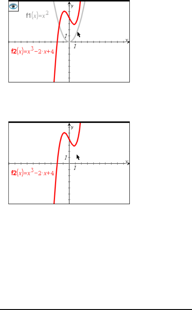
2. Click objects to toggle their hide/show status. You can hide graphs, geometric
objects, text, labels, measurements, and individual axis end-values.
3. Press Esc to complete your selections and close the tool.
All objects you selected as hidden objects disappear.
4. To view the hidden objects temporarily or restore them as shown objects, open the
Hide/Show tool.
Conditional Attributes
You can cause objects to hide, show, and change colour dynamically, based on
specified conditions such as "r1<r2" or "sin(a1)>=cos(a2)."
For example, you might want to hide an object based on a changing measurement that
you have assigned to a variable, or you might want an object’s colour to change based
on a "Calculate" result assigned to a variable.
Conditional behaviours can be assigned to objects or groups in the Graphing, Plane
Geometry, and 3D Graphing views.
Graphs Application 372
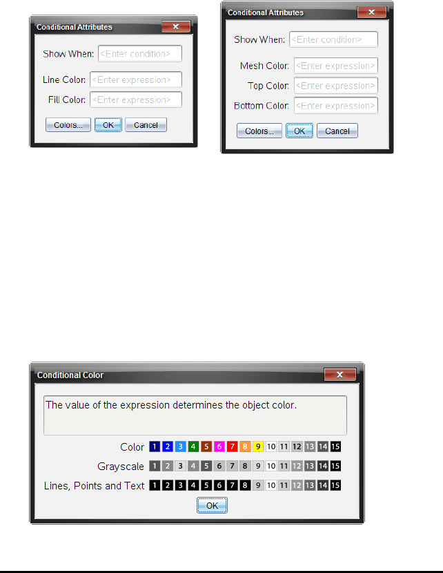
373 Graphs Application
Setting Conditional Attributes of an Object
You can set conditions of a selected object either by using its context menu or by
activating the Set Conditions tool from the Actions menu and then selecting the object.
These instructions describe using the context menu.
1. Select the object or group.
2. Display the object’s context menu, and click Conditions.
The conditional attributes are displayed.
For 2D objects For 3D objects
3. (Optional) In the Show When field, enter an expression specifying the conditions
during which the object will be shown. Anytime the condition is not satisfied, the
object will be hidden.
You can specify tolerance by using compound conditionals in the Show When input
field. For example, area>=4andarea<=6.
Note: If you need to see conditionally hidden objects temporarily, click
Actions>Hide/Show. To return to normal viewing, press ESC.
4. (Optional) Enter numbers or expressions that evaluate to numbers in the applicable
colour fields, such as Line Colour or Mesh Colour. To see a map of colour values,
click the Coors button.
Map of conditional colour values
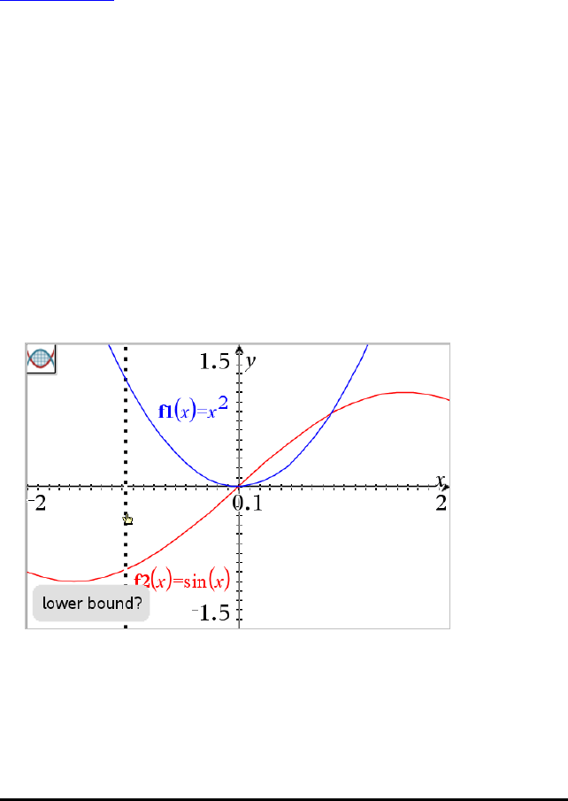
5. Click OK in the Conditional Attributes dialogue box to apply the conditions.
Calculating a Bounded Area
Note: To avoid unexpected results when using this feature, make sure the
documentsetting for "RealorComplexFormat" is set to Real.
When you calculate the area between curves, each curve must be:
• A function with respect to x.
- or -
• An equation in the form y=, including y= equations defined through a text box or a
conicequation template.
Defining and Shading the Area
1. From the Analyse Graph menu, select Bounded Area.
If exactly two appropriate curves are available, they are selected automatically,
and you can skip to step 3. Otherwise, you are prompted to select two curves.
2. Click two curves to select them.
– or –
Click one curve and the x axis.
You are prompted to set the lower and upper bounds.
3. Click two points to define the bounds. Optionally, you can type numeric values.
The area becomes shaded, and the area value is displayed. The value is always
non-negative, regardless of the interval direction.
Graphs Application 374
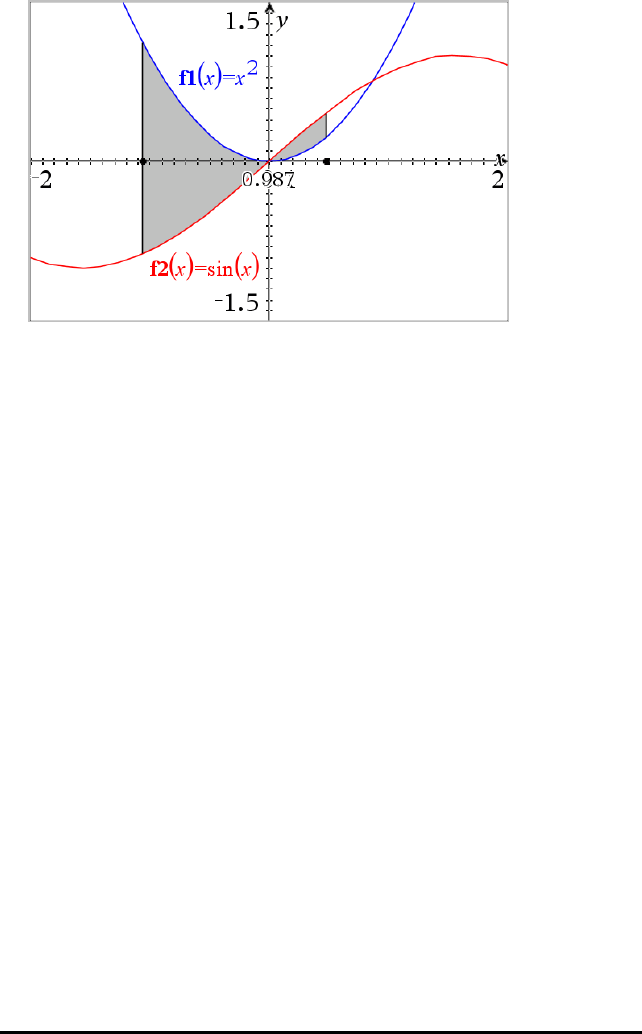
375 Graphs Application
Working with Shaded Areas
As you change the bounds or redefine the curves, the shading and the area value are
updated.
• To change the lower or upper bound, drag it or type new coordinates for it. You
cannot move a bound that resides on an intersection. However, the point moves
automatically as you edit or manipulate the curves.
• To redefine a curve, either manipulate it by dragging or edit its expression in the
entry line.
If an endpoint resided originally on an intersection, and the redefined functions no
longer intersect, the shading and area value disappear. If you redefine the function
(s) so that there is an intersection point, the shading and area value reappear.
• To delete or hide the shaded area, or to change its colour and other attributes,
display its context menu.
- Windows®: Right-click the shaded area.
- Mac®: Hold “and click the shaded area.
- Handheld: Move the pointer to the shaded area and press / x.
Tracing Graphs or Plots
Graph Trace lets you move a trace cursor over the points of a graph or plot and displays
value information.
Tracing Specific Graphs
1. From the Trace menu, select Graph Trace.
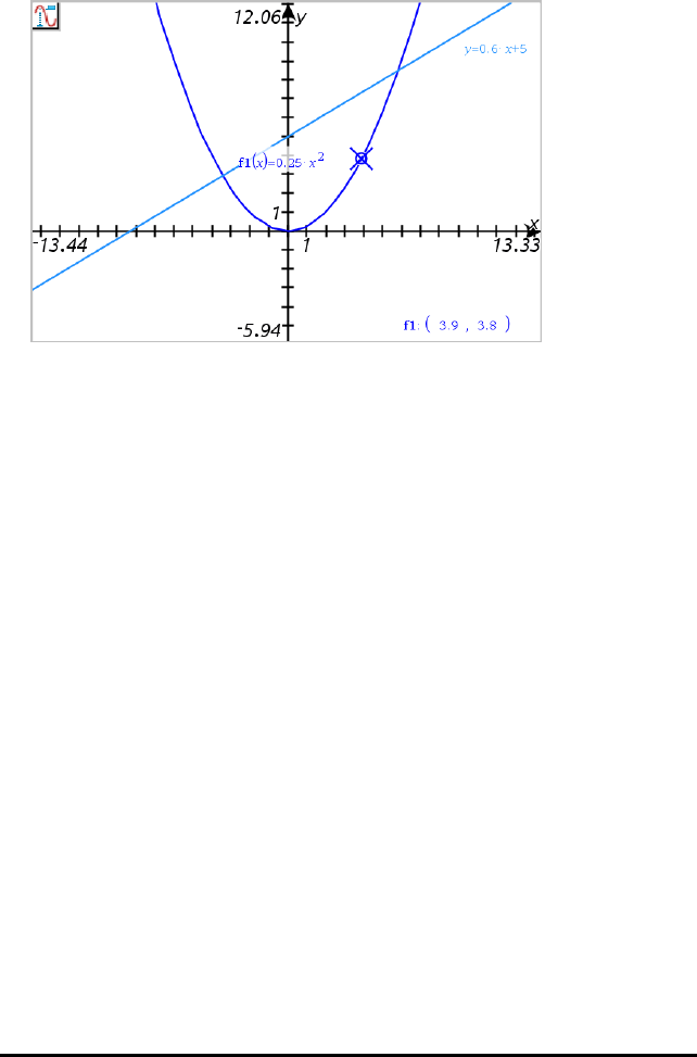
The Graph Trace tool appears at the top of the work area, the trace cursor appears,
and the cursor coordinates are displayed in the lower right corner.
2. Explore a graph or plot:
- Point to a position on a graph or plot to move the trace cursor to that point.
- Press ◄or ►to step the cursor along the current graph or plot. The screen
pans automatically to keep the cursor in view.
- Press ▲or ▼to cycle among the displayed graphs.
- Click the trace cursor to create a persistent point. Optionally, enter a specific
independent value to move the trace cursor to that value.
3. To stop tracing, press Esc.
Tracing All Graphs
The Trace All tool allows tracing multiple functions simultaneously. With several
functions graphed on the work area, perform the following steps:
Note: The Trace All tool traces only function graphs, not plots of other relations (polar,
parametric, scatter, sequence).
1. From the Trace menu, select TraceAll.
The Trace All tool appears in the work area, a vertical line indicates the x value of
the trace, and the coordinates for each traced point are displayed in the lower right
corner.
Graphs Application 376
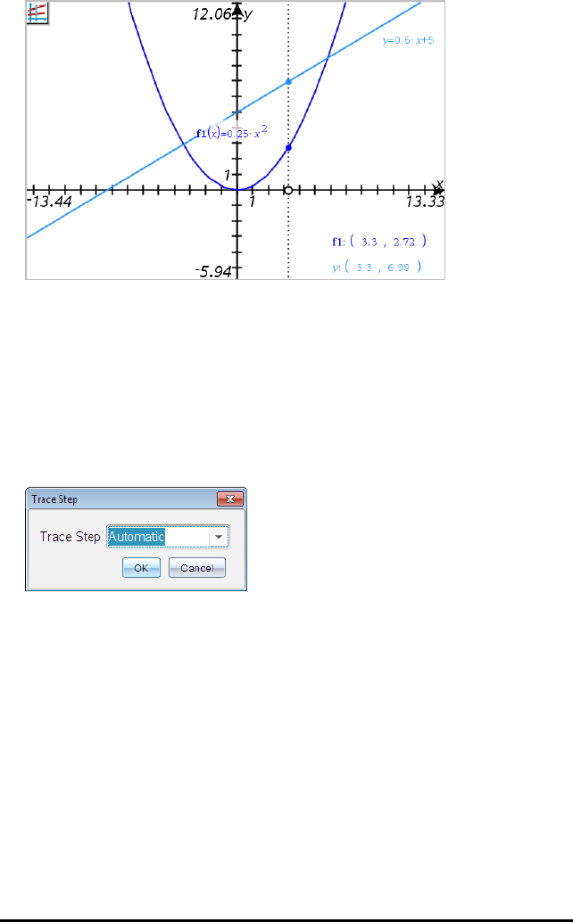
377 Graphs Application
2. Explore the graphs:
- Click a point on the x axis to move all the trace points to that x value.
- Press ◄or ►to step the trace points along all the graphs.
3. To stop tracing, press Esc.
Changing the Trace Step
1. From the Trace menu, select Trace Step.
2. Choose Automatic or enter a specific step size for tracing.
Introduction to Geometric Objects
Geometry tools are accessible in both the Graphs and Geometry applications. You can
use these tools to draw and investigate objects such as points, lines, and shapes.
• The Graphing view shows the Graphs work area superimposed on the Geometry
work area. You can select, measure, and alter objects in both work areas.
• The Plane Geometry view shows only the objects created in the Geometry
application.
Objects Created in the Graphs Application
Points, lines, and shapes created in the Graphs application are analytic objects.
• All points that define these objects reside on the x,y graph plane. Objects created
here are visible only in the Graphs application. Changing the axes scale affects the
appearance of the objects.
• You can display and edit the coordinates of any point on an object.
• You can display the equation of a line, tangent line, circle shape, or geometric conic
created in the Graphs application.
The circle arc and polygon were created in the Geometry application. The sine wave and conic
were created in the Graphs application.
Objects Created in the Geometry Application
Points, lines, and shapes created in the Geometry application are not analytic objects.
• Points that define these objects do not reside on the graph plane. Objects created
here are visible in both the Graphs and Geometry applications, but they are
unaffected by changes to the Graphs x,y axes.
• You cannot obtain the coordinates of an object’s points.
• You cannot display the equation of a geometric object created in the Geometry
application
Graphs Application 378

379 Graphs Application
Creating Points and Lines
As you create an object, a tool appears in the work area (for example, Segment ). To
cancel, press ESC. To enable automatic labelling of certain objects, see What You Must
Know in this chapter.
Creating a Point on the Work Area
1. From the PointsandLines menu, select Point. (In the Graphs application, click
Geometry > PointsandLines > Point.)
2. Click a location to create the point.
3. (Optional) Label the point.
4. To move a point, drag it.
Creating a Point on a Graph or Object
You can create a point on a line, segment, ray, axis, vector, circle, graph or axis.
1. From the PointsandLines menu, select Point On. (In the Graphs application, click
Geometry > PointsandLines > Point On.)
2. Click the graph or object on which you want to create the point.
3. Click a location on the object to place the point.
Identifying Points of Intersection
1. From the PointsandLines menu, select Intersection Points. (In the Graphs
application, click Geometry > PointsandLines > Intersection Points.)
2. Click two intersecting objects to add points at their intersections.
Creating a Line
1. From the PointsandLines menu, select Line. (In the Graphs application, click
Geometry > PointsandLines > Line.)
2. Click a location to define one point on the line.
3. Click a second location to define the direction of the line and the length of its
visible portion.
Graphs Application 380
381 Graphs Application
4. To move a line, drag its identifying point. To rotate it, drag any point except the
identifying point or ends. To extend its visible portion, drag from either end.
Creating a Segment
1. From the PointsandLines menu, select Segment. (In the Graphs application, click
Geometry > PointsandLines > Segment.)
2. Click two locations to define the endpoints of the segment.
3. To move a segment, drag any point other than an endpoint. To manipulate the
direction or length, drag either endpoint.
Creating a Ray
1. From the PointsandLines menu, select Ray. (In the Graphs application, click
Geometry > PointsandLines > Ray.)
2. Click a location to define the endpoint of the ray.
3. Click a second location to define the direction.
To move a ray, drag its identifying point. To rotate it, drag any point except the
identifying point or end. To extend its visible portion, drag from the end.
Creating a Tangent
You can create a tangent line at a specific point on a geometric object or function
graph.
1. From the PointsandLines menu, select Tangent. (In the Graphs application, click
Geometry > PointsandLines > Tangent.)
2. Click the object to select it.
3. Click a location on the object to create the tangent.
4. To move a tangent, drag it. It remains attached to the object or graph.
Creating a Vector
1. From the PointsandLines menu, select Vector. (In the Graphs application, click
Geometry > PointsandLines > Vector.)
Graphs Application 382
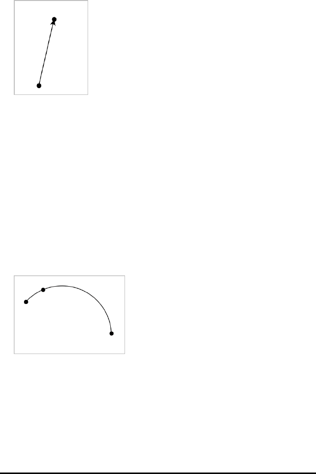
383 Graphs Application
2. Click a location to establish the vector's initial point.
3. Click a second location to specify direction and magnitude and complete the vector.
4. To move a vector, drag any point other than the endpoints. To manipulate the
magnitude and/or direction, drag either end point.
Note: If you create an endpoint on an axis or another object, you can move the
endpoint only along that object.
Creating a Circle Arc
1. From the PointsandLines menu, select Circle Arc. (In the Graphs application, click
Geometry > PointsandLines > Circle Arc.)
2. Click a location or point to establish the starting point of the arc.
3. Click a second point to establish an intermediate point through which the arc will
pass.
4. Click a third point to set the ending point and complete the arc.
5. To move an arc, drag its perimeter. To manipulate it, drag any of its three defining
points.
Creating Geometric Shapes
The Shape tools let you explore circles, polygons, conics and other geometric objects.

As you create a shape, a tool appears in the work area (for example,Circle ). To
cancel the shape, press ESC. To enable automatic labelling of certain objects, see What
You Must Know, in this chapter.
Creating a Circle
1. From the Shapes menu, select Circle. (In the Graphs application, click Geometry >
Shapes > Circle.)
2. Click a location or point to position the circle’s centre point.
3. Click a location or point to establish the radius and complete the circle.
4. To resize a circle, drag its perimeter. To move it, drag its centre point.
Creating a Triangle
Note: To ensure that the total of the angles of a triangle equals 180°or 200 gradians,
you can force integer angles in the Geometry view. Refer to What You Must Know, in
this chapter.
1. From the Shapes menu, select Triangle. (In the Graphs application, click Geometry >
Shapes > Triangle.)
2. Click three locations to establish the vertices of the triangle.
Graphs Application 384
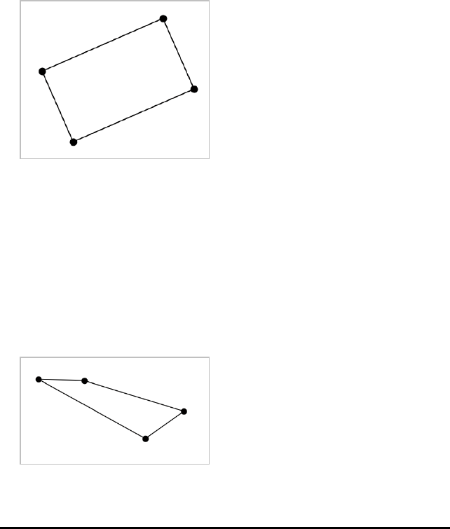
385 Graphs Application
3. To manipulate a triangle, drag any point. To move it, drag any side.
Creating a Rectangle
1. From the Shapes menu, select Rectangle. (In the Graphs application, click Geometry
> Shapes > Rectangle.)
2. Click a location or point to establish the first corner of the rectangle.
3. Click a location for the second corner.
One side of the rectangle is displayed.
4. Click to establish the distance to the opposite side and complete the rectangle.
5. To rotate a rectangle, drag one of its first two points. To extend it, drag one of the
last two points. To move it, drag any side.
Creating a Polygon
1. From the Shapes menu, select Polygon. (In the Graphs application, click Geometry >
Shapes > Polygon.)
2. Click a location or point to establish the first vertex of the polygon.
3. Click to establish each additional vertex.
4. To complete the polygon, click the first vertex.
5. To manipulate a polygon, drag any vertex. To move it, drag any side.

Creating a Regular Polygon
1. From the Shapes menu, select Regular Polygon. (In the Graphs application, click
Geometry > Shapes > Regular Polygon.)
2. Click once on the work area to establish the centre point.
3. Click a second location to establish the first vertex and radius.
A 16-sided regular polygon is formed. The number of sides is displayed in brackets;
for example, {16}.
4. Drag any vertex in a circular motion to set the number of sides.
- Drag clockwise to reduce the number of sides.
- Drag counter-clockwise to add diagonals.
5. To resize or rotate a regular polygon, drag any of its points. To move it, drag any
side.
Creating an Ellipse
1. From the Shapes menu, select Ellipse. (In the Graphs application, click Geometry >
Shapes > Ellipse.)
2. Click two locations or points to establish the foci.
3. Click to establish a point on the ellipse and complete the shape.
Graphs Application 386

387 Graphs Application
4. To manipulate an ellipse, drag any of its three defining points. To move it, drag its
perimeter.
Creating a Parabola (from focus and vertex)
1. From the Shapes menu, select Parabola. (In the Graphs application, click Geometry
> Shapes > Parabola.)
2. Click a location to establish the focus.
3. Click a location to establish the vertex and complete the parabola.
4. To manipulate a parabola, drag its focus or its vertex. To move it, drag it from any
other point.
Creating a Parabola (from focus and directrix)
1. Create a line to serve as the directrix.
2. From the Shapes menu, select Parabola. (In the Graphs application, click Geometry
> Shapes > Parabola.)
3. Click a location to establish the focus.
4. Click the line to establish it as the directrix.
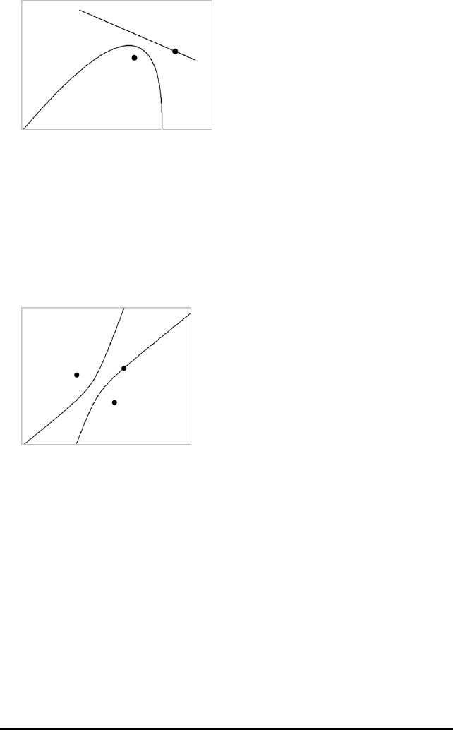
5. To manipulate a parabola, rotate or move its directrix or drag its focus. To move it,
select both the directrix and the focus, and then drag either object.
Creating a Hyperbola
1. From the Shapes menu, select Hyperbola. (In the Graphs application, click
Geometry > Shapes > Hyperbola.)
2. Click two locations to establish the foci.
3. Click a third location to complete the hyperbola.
4. To manipulate a hyperbola, drag any of its three defining points. To move it, drag it
from any other place on the shape.
Creating a Conic by Five Points
1. From the Shapes menu, select ConicbyFivePoints. (In the Graphs application, click
Geometry > Shapes > ConicbyFivePoints.)
2. Click five locations to establish the five points on the shape.
Depending on the pattern of the points, the conic can be a hyperbola or an ellipse.
Graphs Application 388

389 Graphs Application
3. To manipulate a conic, drag any of its five defining points. To move it, drag it from
any other place on the shape.
Creating Shapes Using Gestures (MathDraw)
The MathDraw tool lets you use touchscreen or mouse gestures to create points, lines,
circles and other shapes.
MathDraw is available in:
• Geometry view without the analytic window displayed.
• Graphing view when the x scale and y scale are identical. This avoids non-circular
ellipses and non-square rectangles appearing as circles and squares.
MathDraw is not available in the 3D Graphing view or in the Geometry view with the
analytic window displayed.
Activating MathDraw
1. If using the Geometry view with the analytic window visible, use the View menu to
hide the window.
2. On the Actions menu, select MathDraw.
The MathDraw icon appears. You can begin using the tool.
Cancelling MathDraw
▶When you have finished using the MathDraw tool, press Esc.
The tool also closes if you select a different tool or change views.
Creating Points
To create a labelled point, tap or click in an open area.
• If the point is close to an existing line, segment, ray, geometric conic (including
circles) or polygon, the point snaps to that object. You can also place a point on the
intersection of any two of those types of objects.

• If the point is close to a visible grid location in a Graphs view or the analytic
window of a Geometry view, it snaps to the grid.
Drawing Lines and Segments
To create a line or segment, touch or click the initial position, and then drag to the end
position.
• If the drawn line passes near an existing point, the line snaps to the point.
• If the drawn line starts close to an existing point and ends next to another existing
point , it becomes a segment defined by those points.
• If the drawn line is nearly parallel or perpendicular to an existing line, segment or
side of a polygon, it aligns to that object.
Note: The default tolerance for detecting parallel/perpendicular lines is 12.5
degrees. This tolerance can be redefined using a variable named
ti_gg_fd.angle_tol. You can change the tolerance in the current problem by setting
this variable in the calculator app to a value in the range 0 through 45 (0=no
parallel/perpendicular detection).
Drawing Circles and Ellipses
To create a circle or ellipse, use the touchscreen or mouse to draw the approximate
shape.
• If the drawn shape is sufficiently circular, a circle is created.
• If the shape is elongated, an ellipse is created.
• If the virtual centre of the drawn shape is near an existing point, the circle or
ellipse is centred on that point.
Drawing Triangles
To create a triangle, draw a triangle-like shape.
• If a drawn vertex is close to an existing point, the vertex snaps to the point.
Drawing Rectangles and Squares
To create a rectangle or square, use the touchscreen or mouse to draw the perimeter.
• If the drawn shape is nearly square, a square is created.
• If the drawn shape is elongated, a rectangle is created.
Graphs Application 390

391 Graphs Application
• If the centre of a square is close to an existing point, the square snaps to that
point.
Drawing Polygons
To create a polygon, tap or click a succession of existing points, ending on the first
point you tapped.
Using MathDraw to Create Equations
In the Graphs view, MathDraw attempts to recognise certain gestures as functions for
analytic parabolas.
Note: The default step value for quantisation of the parabola coefficients is 1/32. The
denominator of this fraction can be redefined using a variable named ti_gg_fd.par_
quant. You can change the step value in the current problem by setting this variable to
a value greater or equal to 2. A value of 2, for example, produces a step value of 0.5.
Using MathDraw to Measure an Angle
To measure the angle between two existing lines, use the touchscreen or mouse to
draw a circle arc from one of the lines to the other.
• If the intersection point between the two lines does not exist, it is created and
labelled.
• The angle is not a directed angle.
Using MathDraw to Find a Mid-point
To create a point midway between two points, tap or click point1, point2, and then
point1 again.
Using MathDraw to Erase
To erase objects, use the touchscreen or mouse to drag left and right, similar to the
motion of erasing a whiteboard.
• The erasure area is the bounding rectangle of the erasure gesture.
• All point objects and their dependents inside the erasure area are removed.

Basics of Working with Objects
Selecting and Deselecting Objects
You can select an individual object or multiple objects. Select multiple objects when
you want to quickly move, colour, or delete them together.
1. Click an object or graph to select it.
The object flashes to indicate selection.
2. Click any additional objects to add them to the selection.
3. Perform the operation (such as moving or setting colour).
4. To deselect all objects, click an empty space in the work area.
Grouping and Ungrouping Geometric Objects
Grouping objects gives you a way to reselect them as a set, even after you have
deselected them to work with other objects.
1. Click each object to add it to the current selection.
The selected objects flash.
2. Display a context menu of the selected object or objects.
3. Click Group. You can now select all the items in the group by clicking any of its
members.
4. To split a group into individual objects, display a context menu of any of its
member objects, and click Ungroup.
Deleting Objects
1. Display the context menu of the object or objects.
2. Click Delete.
You cannot delete the origin, the axes, or points representing locked variables, even
if those items are included in the selection.
Moving Objects
You can move an object, group, or combination of selected objects and groups.
Graphs Application 392

393 Graphs Application
Note: If an immovable object (such as the graph axes or a point with locked
coordinates) is included in a selection or group, you cannot move any of the objects.
You must cancel the selection and then select only movable items.
To move this... Drag this
A multiple-object
selection or group
Any of its objects
A point The point
A segment or
vector
Any point other than an endpoint
A line or ray The identifying point
A circle The centre point
Other geometric
shapes
Any position on the object except one of its defining points. For
example, move a polygon by dragging any of its sides.
Constraining Object Movement
Holding down the SHIFT key before dragging lets you constrain how certain objects are
drawn, moved, or manipulated.
Use the constraint feature to:
• Rescale only a single axis in the Graphs application.
• Pan the work area horizontally or vertically, depending on which direction you drag
initially.
• Limit object movement to horizontal or vertical.
• Limit point placement to 15°increments as you draw a triangle, rectangle, or
polygon.
• Limit angle manipulations to 15°increments.
• Limit the radius of a resized circle to integer values.

Pinning Objects
Pinning objects prevents accidental changes as you move or manipulate other objects.
You can pin graphed functions, geometric objects, text objects, the graph axes, and the
background.
1. Select the object or objects to pin, or click an empty area if you are pinning the
background.
2. Display the context menu, and select Pin.
A pinned object displays a pin icon when you point to it.
3. To unpin an object, display its context menu, and select Unpin.
Notes:
• Although you cannot drag a pinned point, you can reposition it by editing its x and y
coordinates.
• You cannot pan the work area while the background is pinned.
Changing the Line or Fill Colour of an Object
Colour changes made in the software are displayed in shades of grey when you work
on documents using a TI-Nspire™ handheld that does not support colour. Colour is
preserved when you move documents back to the software.
1. Select the object or objects.
2. Display the object’s context menu, click Colour, and then click LineColour or
FillColour.
3. Select the colour to apply to the objects.
Changing the Appearance of an Object
1. From the Actions menu, select Attributes.
2. Click the object that you want to change. You can change shapes, lines, graphs, or
graph axes.
The list of the attributes for the selected object are displayed.
3. Press 9and:to move through the list of attributes.
4. At each attribute icon, press 7or8to move through the options. For example,
select Thick, Thin, or Medium for the Line Weight attribute.
Graphs Application 394
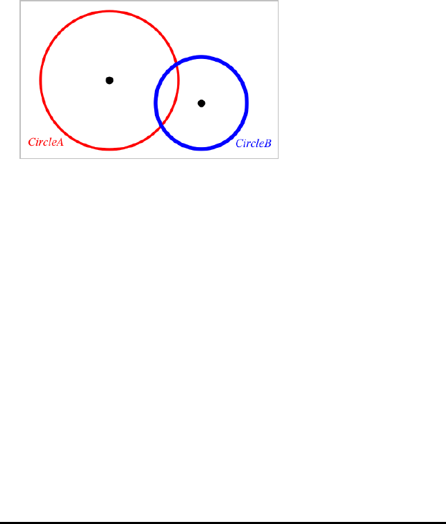
395 Graphs Application
5. Press Enter to apply the changes.
6. Press ESC to close the Attributes tool.
Labelling Points, Geometric Lines, and Shapes
1. Display the context menu of the object.
2. Click Label.
3. Type the text of the label, and then press Enter.
The label attaches itself to the object and follows the object as you move it. The
label's colour matches the object's colour.
Measuring Objects
Measurement values update automatically as you manipulate the measured object.
Note: Measurements of objects created in the Graphs application are displayed in
generic units namedu. Measurements of objects created in the Geometry application
are displayed in centimetres (cm).
Measuring Length of a Segment, Circle Arc or Vector
1. From the Measurement menu, select Length. (In the Graphs application, click
Geometry > Measurement > Length.)
2. Click the object to display its length.
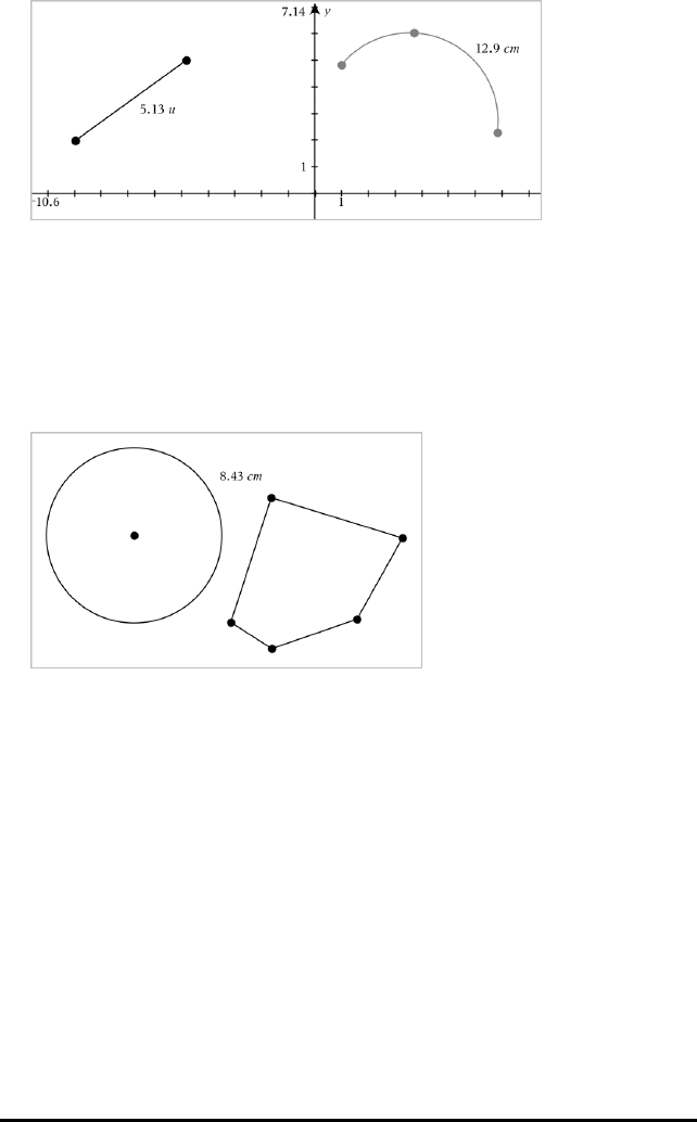
Measuring Distance Between Two Points, a Point and a Line, or a Point and a Circle
1. From the Measurement menu, select Length. (In the Graphs application, click
Geometry > Measurement > Length.)
2. Click the first point.
3. Click the second point or a point on the line or circle.
In this example, length is measured from the centre of the
circle to the upper leftvertex of the polygon.
Measuring Circumference of a Circle or Ellipse or the Perimeter of a Polygon,
Rectangle or Triangle
1. From the Measurement menu, select Length. (In the Graphs application, click
Geometry > Measurement > Length.)
2. Click the object to display its circumference or perimeter.
Graphs Application 396
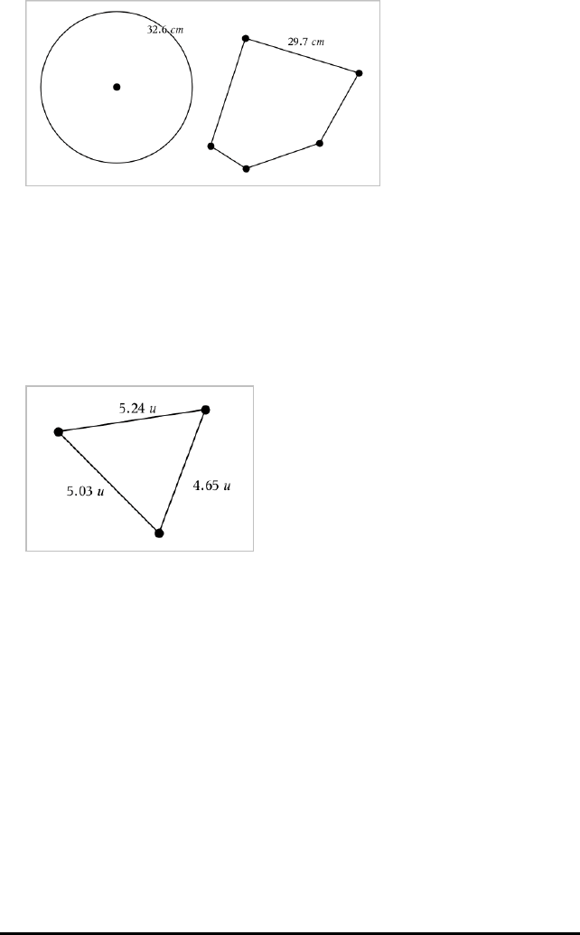
397 Graphs Application
Measuring a Side of a Triangle, Rectangle or Polygon
1. From the Measurement menu, select Length. (In the Graphs application, click
Geometry > Measurement > Length.)
2. Click two points on the object that form the side you want to measure.
Note: You must click two points to measure a side. Clicking the side measures the
entire length of the object's perimeter.
Measuring Area of a Circle, Ellipse, Polygon, Rectangle orTriangle
Note: You cannot measure the area of a polygon constructed using the Segment tool.
1. From the Measurement menu, select Area. (In the Graphs application, click
Geometry > Measurement > Area.)
2. Click the object to display its area.
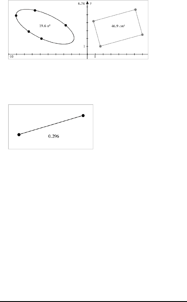
Measuring Slope of a Line, Ray, Segment or Vector
1. From the Measurement menu, select Slope. (In the Graphs application, click
Geometry > Measurement > Slope.)
2. Click the object to display its slope.
The value is updated automatically when you manipulate the object.
Measuring Angles
Measured angles in the Geometry application range from 0°to 180°. Measured angles
in the Graphs application range from 0 radians to πradians. To change the angle unit,
use the Settings menu.
1. From the Measurement menu, select Angle. (In the Graphs application, click
Geometry > Measurement > Angle.)
2. Click three locations or points to define the angle. The second click defines the
vertex.
Graphs Application 398
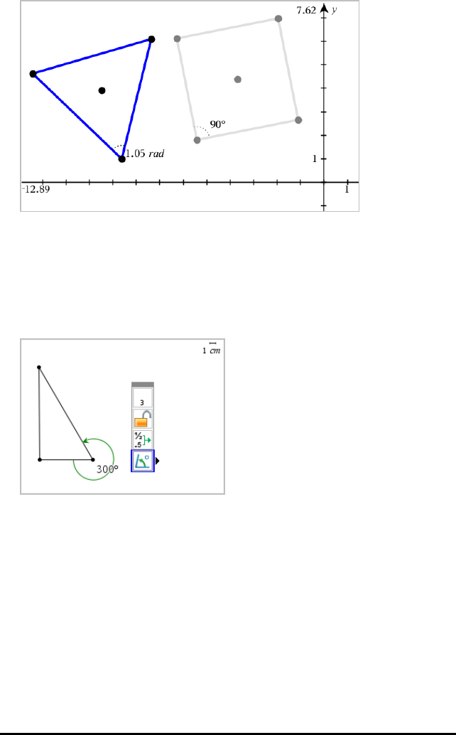
399 Graphs Application
Measuring Angles using the Directed Angle Tool
1. From the Measurement menu, select DirectedAngle. (In the Graphs application,
click Geometry > Measurement > DirectedAngle.)
2. Click three locations or existing points to define the angle. The second click defines
the vertex.
3. To reverse the measurement orientation,
a) On the Actions menu, select Attributes.
b) Click the angle text. For example, click 300°.
c) Select the orientation attribute, and use the right or left arrow key to change it.
d) Press Esc to close the Attributes tool.
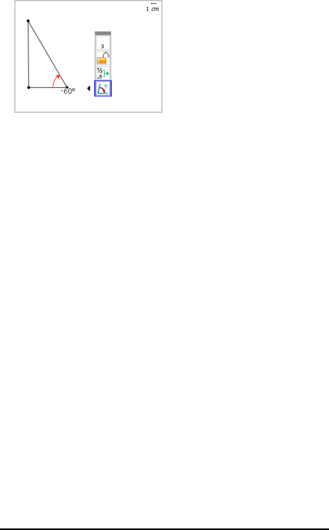
Moving a Measured Value
▶Drag the measurement to the desired location.
Note: If you move a measurement too far from its object, it stops following the
object. However, its value continues to be updated as you manipulate the object.
Editing a Measured Length
You can set the length of a side of a Triangle, Rectangle or Polygon by editing its
measured value.
▶Double-click the measurement, and then enter the new value.
Storing a Measured Value as a Variable
Use this method to create a variable and assign a measured value to it.
1. Display the item's context menu, and select Store.
2. Type a variable name for the stored measurement.
Linking a Measured Length to an Existing Variable
Use this method to assign a measured length value to an existing variable.
1. Display the measurement's context menu, and select Variables > Link to.
The menu shows the list of currently defined variables.
2. Click the name of the variable you want to link to.
Deleting a Measurement
▶Display the measurement's context menu, and select Delete.
Graphs Application 400
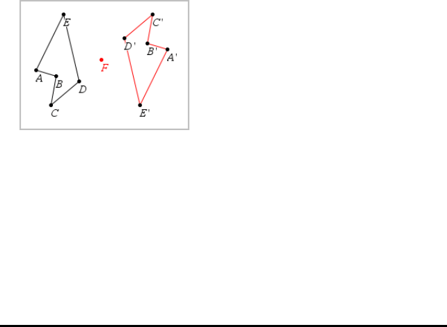
401 Graphs Application
Locking or Unlocking a Measurement
1. Display the measurement's context menu, and select Attributes.
2. Use the up/down arrow keys to highlight the Lock attribute.
3. Use the left/right arrow keys to close or open the lock.
As long as the value remains locked, manipulations are not allowed that would
require the measurement to change.
Transforming Objects
You can apply transformations to drawn objects in both the Graphs and Geometry
applications. If the object's points are labelled, the corresponding points in the
transformed object are labelled using prime notation (A→A'). To enable automatic
labelling of certain objects, see What You Must Know in this chapter.
Exploring Symmetry
1. From the Transformation menu, select Symmetry. (In the Graphs application, click
Geometry > Transformation > Symmetry.)
2. Click the object whose symmetry you want to explore.
3. Click a location or existing point to establish the point of symmetry.
A symmetrical image of the object is displayed.
4. Manipulate the original object or the point of symmetry to explore the symmetry.
Exploring Reflection
1. Create a line or segment to predefine the line about which the object will be
reflected.
2. From the Transformation menu, select Reflection. (In the Graphs application, click
Geometry > Transformation > Reflection.)
3. Click the object whose reflection you want to explore.

4. Click the predefined reflection line or segment.
A reflected image of the object is displayed.
5. Manipulate the original object or the line of symmetry to explore the reflection.
Exploring Translation
1. (Optional) Create a vector to predefine the distance and direction of translation.
2. From the Transformation menu, select Translation. (In the Graphs application, click
Geometry > Transformation > Translation.)
3. Click the object whose translation you want to explore.
4. Click the predefined vector.
—or—
Click two locations on the work area to indicate the direction and distance of
translation.
A translated image of the object is displayed.
5. Manipulate the original object or the vector to explore the translation.
Exploring Rotation
1. (Optional) Create an angle measurement to serve as a predefined angle of
rotation.
Graphs Application 402

403 Graphs Application
2. From the Transformation menu, select Rotation. (In the Graphs application, click
Geometry > Transformation > Rotation.)
3. Click the object whose rotation you want to explore.
4. Click a location or point to define the point of rotation.
5. Click the points of the predefined angle.
—or—
Click three locations to define an angle of rotation.
A rotated image of the object is displayed.
6. Manipulate the original object or the point of rotation to explore the rotation.
Exploring Dilation
1. Create a Text object containing a numeric value to serve as a predefined dilation
factor.
Note: You can also use a measured length value as the dilation factor. Keep in
mind that if you use a large value, you may have to pan the display to view the
dilated object.
2. From the Transformation menu, select Dilation. (In the Graphs application, click
Geometry > Transformation > Dilation.)
3. Click the object whose dilation you want to explore.
4. Click a location or existing point to define the centre point of dilation.
5. Click the Text object or measurement that defines the dilation factor.
A dilated image of the object is displayed.
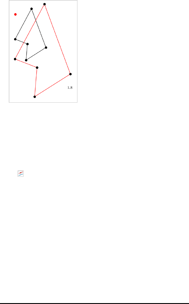
6. Manipulate the original object or the centre point of dilation to explore the dilation.
You can also edit the dilation factor.
Exploring with Geometric Construction Tools
You can investigate scenarios by adding objects from the Construction tools. The
constructions are dynamic. The midpoint of a line segment, for example, is updated
automatically when you manipulate the endpoints.
While a construction is in progress, a tool appears in the work area (for example,
Parallel ). To cancel, press ESC.
Creating a Midpoint
This tool lets you bisect a segment or define a midpoint between any two points. The
points can be on a single object, on separate objects, or on the work area.
1. From the Construction menu, select Midpoint. (In the Graphs application, click
Geometry > Construction > Midpoint.)
2. Click a point or location to define the first point.
3. Click a second point or location to complete the midpoint.
Graphs Application 404
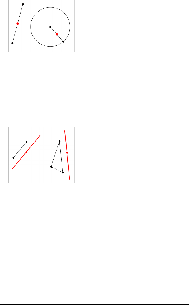
405 Graphs Application
Creating a Parallel Line
This tool creates a parallel line with respect to any existing line. The existing line can
be a Graphs axis or any side of a triangle, square, rectangle, or polygon.
1. From the Construction menu, select Parallel. (In the Graphs application, click
Geometry > Construction > Parallel.)
2. Click the object that will serve as the reference line.
3. Click a location to create the parallel line.
You can drag the parallel line to move it. If you manipulate the reference object,
the line remains parallel.
Creating a Perpendicular Line
You can create a line that is perpendicular to a reference line. The reference can be an
axis, an existing line, a segment, or one side of a triangle, rectangle, or polygon.
1. From the Construction menu, select Perpendicular. (In the Graphs application, click
Geometry > Construction > Perpendicular.)
2. Click a location or existing point through which the perpendicular line should pass.
3. Click the item that will serve as the reference line.

You can drag the intersection point to move the perpendicular. If you manipulate
the reference object, the line remains perpendicular.
Creating a Perpendicular Bisector
You can create a perpendicular bisector on a segment, on one side of a triangle,
rectangle, or polygon, or between any two points.
1. From the Construction menu, select PerpendicularBisector. (In the Graphs
application, click Geometry > Construction > PerpendicularBisector.)
2. Click the item that will serve as the reference line.
—or—
Click two points to create a perpendicular bisector between them.
Bisecting an Angle
This tool creates an angle bisector. The points of the angle can be on existing objects,
or they can be locations on the work area.
1. From the Construction menu, select AngleBisector. (In the Graphs application, click
Geometry > Construction > AngleBisector.)
2. Click three locations or points to define the angle. The second click defines the
vertex of the angle.
Graphs Application 406

407 Graphs Application
The angle bisector adjusts automatically as you manipulate its defining points.
Creating a Locus
The Locus tool enables you to explore the range of motion of one object with respect to
another object as constrained by a shared point.
1. Create a segment, line, or circle.
2. Create a point on the segment, line, or circle.
3. Create another object that uses the point created in the previous step.

Circle created to use the defined point on
the segment.
4. From the Construction menu, select Locus. (In the Graphs application, click
Geometry > Construction > Locus.)
5. Click the point shared by the objects.
6. Click the object defined to share the point (this is the object to vary).
The continuous locus is displayed.
Creating a Compass
This tool operates similarly to a geometric compass used for drawing circles on paper.
1. From the Construction menu, select Compass. (In the Graphs application, click
Geometry > Construction > Compass.)
2. To set the width (radius) of the compass:
Click a segment.
—or—
Click any side of a triangle, rectangle, polygon, or regular polygon.
Graphs Application 408
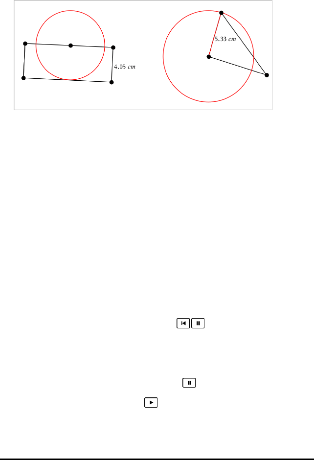
409 Graphs Application
—or—
Click any two existing points or locations on the work area.
3. Click a location to establish the centre of the circle and complete the construction.
The radius adjusts automatically as you manipulate the original segment, side, or
points used to define the radius.
Animating Points on Objects
You can animate any point created as a point on an object or graph. Multiple points can
be animated simultaneously.
Animating a Point
1. From the Actions menu, select Attributes.
2. Click the point to display its attributes.
3. Press ▼to select the animation attributes.
4. Press ◄or►to choose either unidirectional or alternating animation.
5. Type a value to set the animation speed. Any nonzero speed begins the animation.
To reverse the direction, enter a negative value.
6. Press Enter to display the animation controls .
7. Press ESC to close the Attributes tool.
Pausing and Resuming All Animations
▶To pause all animations on a page, click Pause .
▶To resume all animations, click Play .
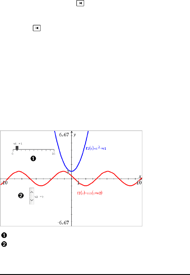
Resetting All Animations
Resetting pauses all animations and returns all animated points to the positions they
occupied when they were first animated.
▶To reset animation, click Reset .
Changing or Stopping the Animation of a Point
1. Click Reset to stop all animation.
2. From the Actions menu, select Attributes.
3. Click the point to display its attributes.
4. Select the animation attribute, and type a new animation speed. To stop the
point’s animation, enter zero.
Note: If other animated points exist, the animation controls remain in the work
area.
Adjusting Variable Values with a Slider
A slider control lets you interactively adjust or animate the value of a numeric variable.
You can insert sliders in the Graphs, Geometry, Notes and Data&Statistics
applications.
Horizontal slider for adjusting variable v1.
Minimised vertical slider for adjusting variable v2.
Graphs Application 410
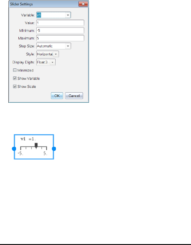
411 Graphs Application
Note: TI-Nspire™ version 4.2 or higher is required for opening .tns files containing
sliders on Notes pages.
Inserting a Slider Manually
1. From a Graphs, Geometry or Data&Statistics page, select Actions > Insert Slider.
—or—
From a Notes page, make sure the cursor is not in a maths box or chem box, and
then select Insert > InsertSlider.
The Slider Settings screen opens.
2. Enter the desired values, and click OK.
The slider is displayed. On a Graphs, Geometry or Data&Statistics page, handles
are displayed to let you move or stretch the slider.
To remove the handles and use the slider, click an empty
space in the work area. You can show the handles any time by
selecting Move from the slider's context menu.
3. To adjust the variable, slide the pointer (or click the arrows on a minimised slider).
- You can use the Tab key to move the focus to a slider or to move from one
slider to the next. The colour of the slider changes to show you when it has the
focus.
- When a slider has the focus, you can use the arrow keys to change the value of
the variable.
Working with the Slider
Use the options on the context menu to move or delete the slider, and to start or stop
its animation. You can also change the slider's settings.
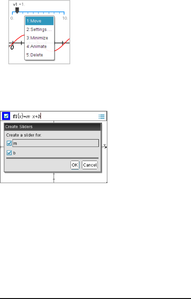
1. Display the slider's context menu.
2. Click an option to select it.
Automatic Sliders in Graphs
Sliders can be created for you automatically in the Graphs application and in the
analytic window of the Geometry application. You are offered automatic sliders when
you define certain functions, equations or sequences that refer to undefined variables.
Labelling (Identifying) the Coordinates of a Point
The Graphs application can identify and label the coordinates of any existing point,
provided the point was created in the Graphs application.
1. From the Actions menu, select Coordinates and Equations.
The tool appears at the top of the work area
2. Tap the point whose coordinates you want to show.
Graphs Application 412

413 Graphs Application
3. Press Esc to close the tool.
If you later move the point to a different location, the coordinates follow the point and
update automatically.
Displaying the Equation of a Geometric Object
You can display the equation of a line, tangent line, circle shape, or geometric conic,
provided the object was constructed in the Graphing View or within the Analytic
Window of the Plane Geometry View.
Note: Due to differences in the numerical representations of analytic and geometric
conics, the capability to convert a geometric conic to an analytic template may
sometimes be unavailable. This is done in order to avoid a situation where the
template-based conic would be different from the geometric one.
1. From the Actions menu, click CoordinatesandEquations.
2. Move the pointer to the object.
The equation for the object appears.
Note: If you approach a defined point on the line or the centre point of a circle, the
coordinates of that point are displayed instead of the equation. Move the pointer
away from the defined point to obtain the equation of the object.
3. Click to attach the equation to the pointer.
4. Move the equation to the desired location, and click to anchor it.

5. Press Esc to exit the tool.
Using the Calculate Tool
The Calculate tool is available in the Graphs and Geometry applications. It lets you
evaluate a maths expression you have entered as a text object.
The following example uses the Calculate tool to calculate the measured angles of a
triangle.
1. Using the Shapes menu, create a triangle and then measure its angles.
Tip: You can enable options to automatically label points and to force geometric
triangle angles to integers. For more information, see What You Must Know, in this
chapter.
2. From the Actions menu, click Text.
3. Click a location for the text, and type the formula for the calculation.
In this example, the formula calculates three terms.
Graphs Application 414
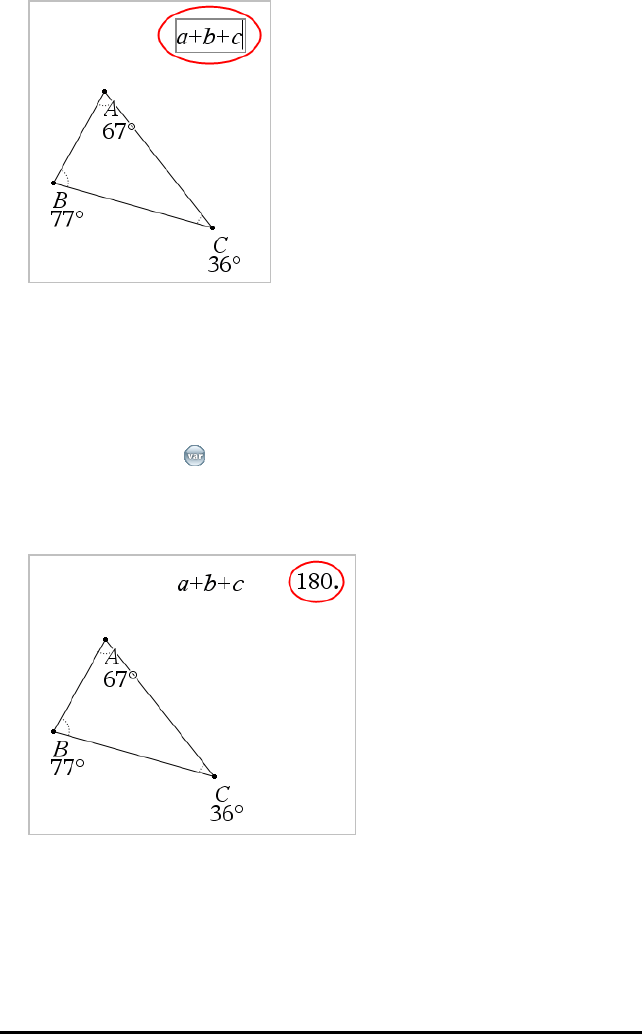
415 Graphs Application
4. From the Actions menu, click Calculate.
5. Click the formula you created.
You are prompted to select a value for each term in the formula.
6. Click each angle measurement when prompted.
Note: If you have stored a measurement as a variable, you can select it when
prompted by clicking . If the name of a stored measurement matches a term in
the formula, you can press “L” when prompted for that term.
After you have selected the third term, the calculation result attaches itself to the
pointer.
7. Position the result, and press Enter to anchor it as a new text object.
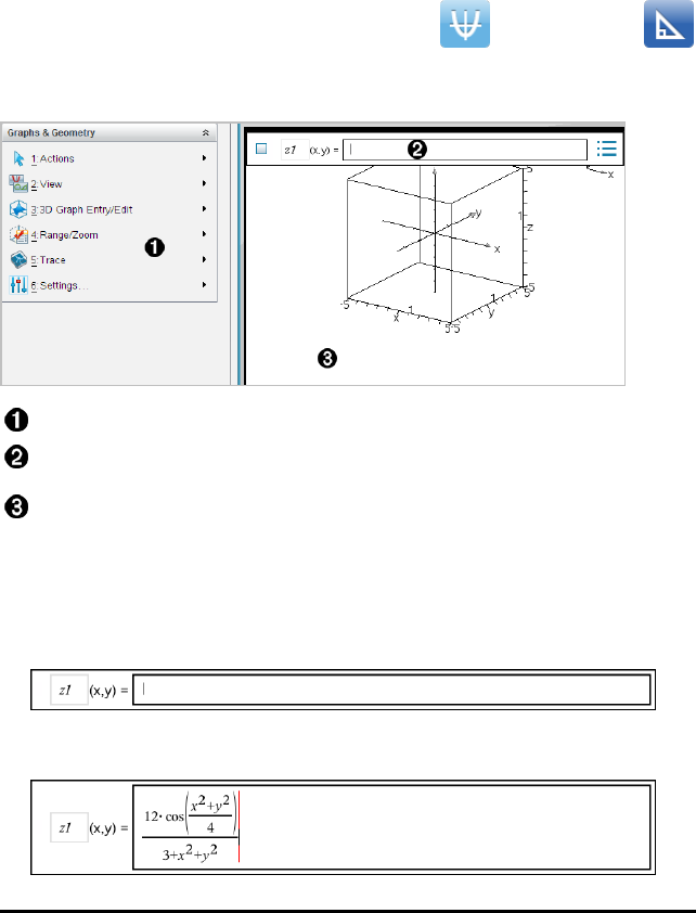
3D Graphs
The 3D Graphing view lets you create and explore three-dimensional graphs of:
• 3D functions of the form z(x,y)
• 3D parametric plots
Selecting the 3D Graphing View
The 3D Graphing View is available on any Graphs page or Geometry page
.
▶From the View menu, select 3DGraphing.
3D Graphs Menu
Entry line. Lets you define 3D graphs. The default graph type is 3D Function,
indicated by z1(x,y)=.
3D Graphs Work Area. Shows a 3D box containing graphs that you define. Drag to
rotate the box.
Graphing 3D Functions
1. In the 3D Graphing view, select 3DGraphEntry/Edit > Function.
The entry line appears.
2. Enter the expression that defines the graph. You can type the expression or build it
using expression templates.
3D Graphs 416
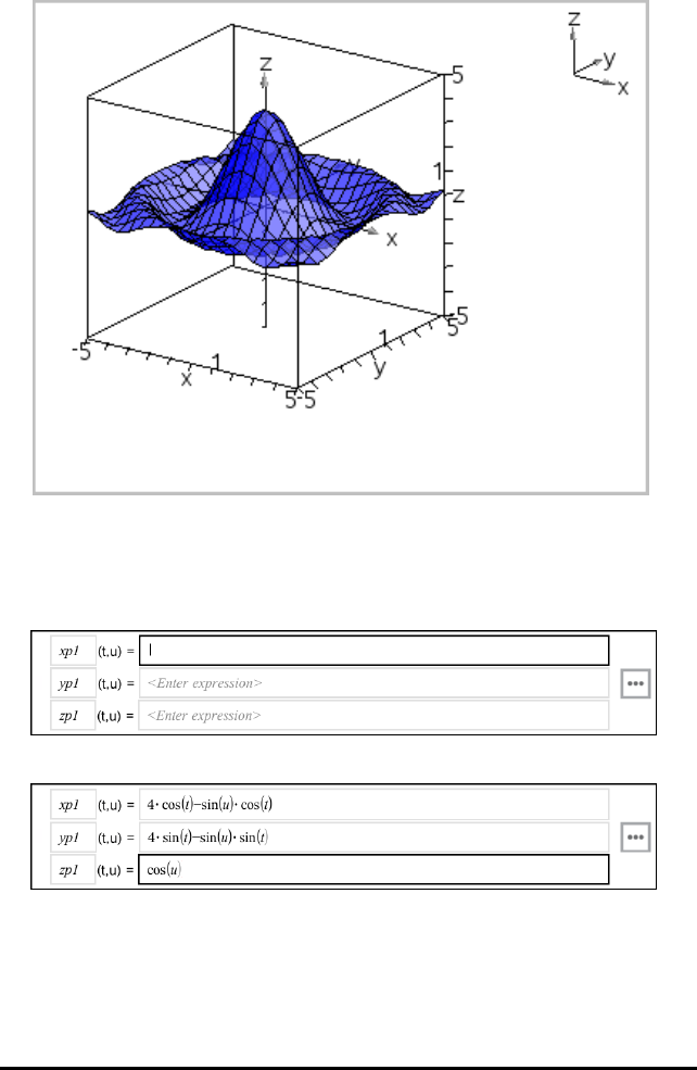
417 3D Graphs
3. Press Enter to create the graph and hide the entry line. You can show or hide the
entry line anytime by pressing Ctrl+G.
Graphing 3D Parametric Equations
1. In the 3D Graphing view, select 3DGraphEntry/Edit > Parametric.
The entry line appears.
2. Type the equations that define the graph.
3. Press Enter to draw the graph and hide the entry line and keyboard. You can show
or hide the entry line anytime by pressing Ctrl+G.
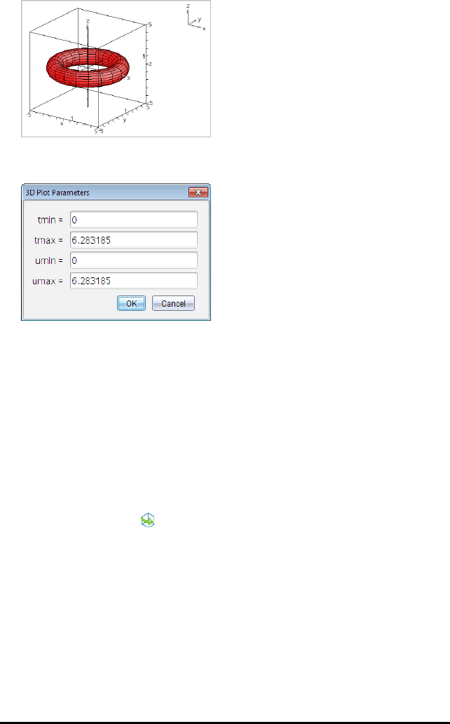
4. To set the graphing parameters tmin,tmax,umin, and umax, display the graph's
context menu, and select EditParameters.
Rotating the 3D View
Rotating Manually
1. Press Rto activate the Rotation tool (required only for the TI-Nspire™ handheld
with Clickpad).
2. Press any of the four arrow keys to rotate the graph.
Rotating Automatically
Auto rotation is equivalent to holding down the right arrow key.
1. Press A.
The Auto Rotation icon appears, and the graph rotates.
2. (Optional) Use the up and down arrow keys to explore the rotating graph.
3. To stop the rotation and return to the Pointer tool, press Esc.
Viewing from Specific Orientations
1. If necessary, press Esc to return to the Pointer tool.
2. Use letter keys to select the orientation:
- Press Z,Y, or Xto view along the z, y, or x axis.
- Press letter Oto view from the default orientation.
3D Graphs 418
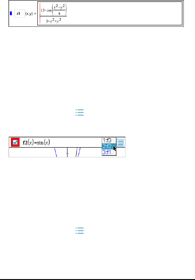
419 3D Graphs
Editing a 3D Graph
1. Double-click the graph to show its expression in the entry line.
—or—
Display the graph’s context menu, and then click EditRelation.
2. Modify the existing expression, or type a new expression in the entry line.
3. Press Enter.
Accessing the Graph History
For each problem, the software stores a history of relations defined in the Graphs
application and 3D Graphing view, such as function graphs f1 through f99 and 3D
function graphs z1 through z99. You can view and edit these items using a button on
the entry line.
Viewing the History
1. Press Ctrl+G to show the entry line.
2. Clickthe History Menu button on the entry line.
The menu is displayed. As you point to the name of each item, its expression
appears in the entry line.
3. Select the name of the relation you want to view or edit.
4. (Optional) From the entry line, use the up and down arrow keys to scroll through
the defined relations of the same type.
Viewing the History of Specific Relation Types
Use this method if you want to view or edit a defined relation that does not appear in
the History menu.
1. On the GraphEntry/Edit menu, click the relation type. For example, click Polar to
show the entry line for the next available Polar relation.
2. Clickthe History Menu button , or use the up and down arrow keys to scroll
through the defined relations of the same type.
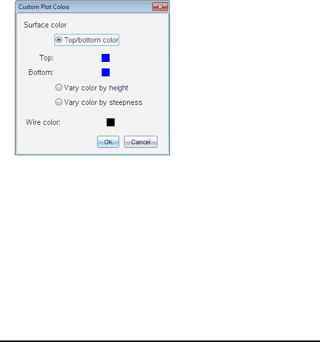
Changing the Appearance of a 3D Graph
Setting Wire and Surface Colour:
1. Display the graph’s context menu, click Colour, and then click LineColour or
FillColour.
2. Click a colour swatch to apply it.
Setting Custom Plot Colours:
You can assign different colours to a graph's top and bottom surfaces or choose to
have the graph coloured automatically, based on height or steepness. You can also set
the wire colour.
1. Display the graph’s context menu, and then click Colour >CustomPlotColour.
2. Select one of the three Surface colour options: Top/bottom colour,Vary colour by
height, or Vary colour by steepness.
- If you choose Top/bottom colour, click the colour swatches to select colours for
the top and bottom surfaces.
- If you choose to vary colour by height or steepness, colours are determined
automatically.
3. To set the Wire colour, click the colour swatch and select a colour.
Setting Other Attributes of a Graph:
1. Display the graph’s context menu, and then click Attributes. You can set the
following attributes for the selected graph.
3D Graphs 420
421 3D Graphs
- format: surface+wire, surface only, or wire only
- x resolution (enter a value in range 2-200*, default=21)
- y resolution (enter a value in range 2-200*, default=21)
- transparency (enter a value in range 0-100, default=30)
* Handhelds are limited to a maximum display resolution of 21, regardless of the
value entered.
2. Set the attributes as you like, and then press Enter to accept the changes.
Showing or Hiding a Graph’s Label
▶Display the graph’s context menu, and then click Hide Label or Show Label.
Showing and Hiding 3D Graphs
1. In the 3D Graphing view, select Actions > Hide/Show.
The Hide/Show tool appears, and all hidden items are displayed in grey.
2. Tap a graph to change its hide/show state.
3. To apply the changes and dismiss the tool, press Esc.
Note: If you want to show or hide only the graph's label, see Showing or Hiding a
Graph’s Label.
Customising the 3D Viewing Environment
Setting the Background Colour
▶Display the context menu for the work area, and then click Background Colour.
Showing or Hiding Specific View Elements
▶From the View menu, click the item to show or hide. You can choose items such as
the 3D box, axes, box end values and legend.
Changing the 3D Projection
▶From the View menu, click OrthographicProjection or PerspectiveView.
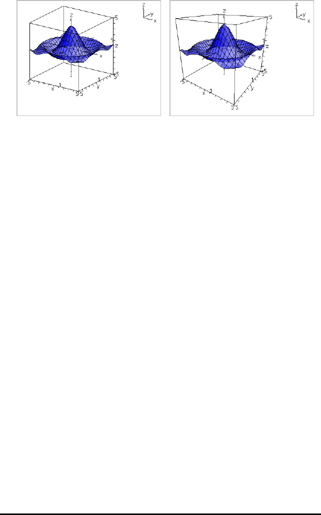
Orthographic Projection (default) Perspective View
Setting the Visual Attributes of the Box and Axes
1. Display the context menu for the box, and then click Attributes. You can set the
following attributes.
- Show or hide tic labels
- Show or hide end values
- Show or hide arrows on axes
- Show 3D or 2D arrow heads
2. Set the attributes as you like, and then press Enter to accept the changes.
Shrinking or Magnifying the 3D View
▶From the Range/Zoom menu, click ShrinkBox or MagnifyBox.
Changing the 3D Aspect Ratio
1. From the Range/Zoom menu, click Aspect Ratio.
2. Enter values for the x, y and z axes. The default value for each axis is1.
Changing the Range Settings
▶On the Range/Zoom menu, click RangeSettings. You can set the following
parameters.
- XMin (default=-5)
XMax (default=5)
XScale (default=Auto) You can enter a numeric value.
3D Graphs 422
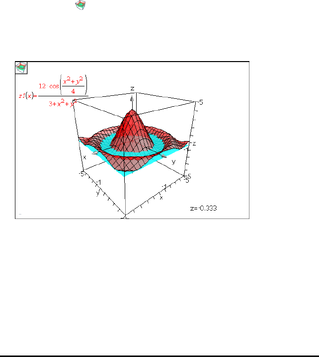
423 3D Graphs
- YMin (default=-5)
YMax (default=5)
YScale (default=Auto) You can enter a numeric value.
- ZMin (default=-5)
ZMax (default=5)
ZScale (default=Auto) You can enter a numeric value.
- eye q¡ (default=35)
eye f¡ (default=160)
eye distance (default=11)
Tracing in the 3D View
1. From the Trace menu, select zTrace.
The z Trace icon and the trace plane appear, along with a text line showing the
current "z=" trace value.
2. To move the trace, hold down Shift and press the up or down arrow key.
The "z=" text is updated as you move.
3. (Optional) Use the four arrow keys to rotate the view and see how the trace plane
and the graph intersect.
4. To stop tracing and return to the Pointer tool, press Esc.
Changing the Trace Settings
1. From the Trace menu, select TraceSetup.
The 3D Trace Setup dialogue box opens.
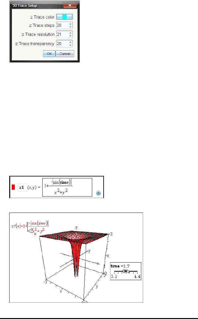
2. Enter or select the settings, and click OK to apply them.
3. If you are not already tracing, your new settings take effect the next time you
trace.
Example: Creating an Animated 3D Graph
1. Insert a new problem and select the 3D Graphing view.
2. From the Actions menu, select InsertSlider, click to position it, and type time as
the variable name.
3. Display the slider’s context menu, click Settings, and enter the following values.
Value: 3.8
Minimum: 3.2
Maximum: 4.4
Step Size: 0.1
4. In the entry line, define the function shown here:
5. Drag the slider thumb to see the effect of varying time.
3D Graphs 424
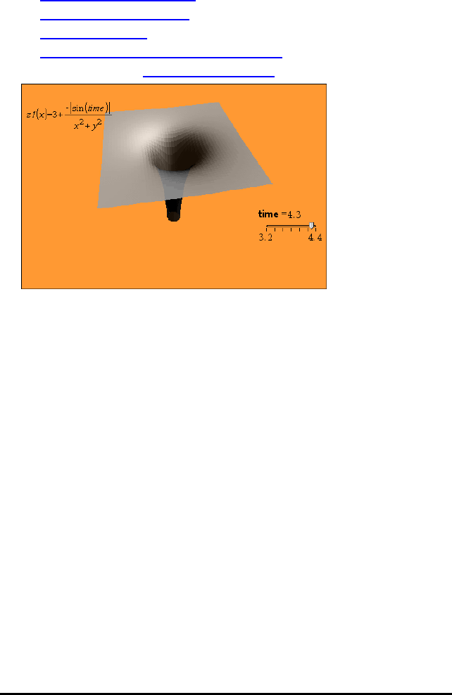
425 3D Graphs
6. Add visual interest. For example:
-Change the background colour of the work area.
-Hide the box, axes, or legend.
-Automatically rotate the graph.
-Change the graph's fill colour and hide its lines.
- Change the graph’s transparency and shading.
7. To animate the graph, display the slider’s context menu, and click Animate. (To
stop, click StopAnimate from the context menu.)
You can combine manual or auto rotation with the slider animation. Experiment
with the x and y resolution to balance curve definition against animation
smoothness.
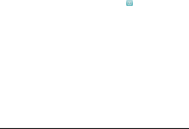
Lists&Spreadsheet Application
The Lists&Spreadsheet application gives you a place to work with tabular data. It lets
you:
• Store numeric data, text or maths expressions.
• Define a table cell in terms of the contents of other cells.
• Define an entire column based on the contents of another column.
• Share columns of data as list variables with other TI-Nspire™ applications. Also
share individual cells as variables.
• Work with variables created in the Graphs&Geometry and Calculator applications.
• Collect tables of real-world data from sensors.
• Generate columns of data-based sequences that you define.
• Plot table data using the Data&Statistics application.
• Generate a table of values for a function.
• Copy and paste table data from the Lists&Spreadsheet application to other
computer applications, such as TI Connect™ software and Excel® spreadsheet
software.
• Perform statistical analysis on lists of data.
Adding a Lists&Spreadsheet Page
▶To start a new document with a blank Lists&Spreadsheet page:
From the main File menu, click New Document and then click Lists&Spreadsheet.
Handheld: Press c, and select Lists&Spreadsheet .
▶To add a Lists&Spreadsheet page in the current problem of an existing document:
From the toolbar, click Insert > Lists&Spreadsheet.
Handheld: Press ~and select Insert >Lists&Spreadsheet.
Lists&Spreadsheet Application 426
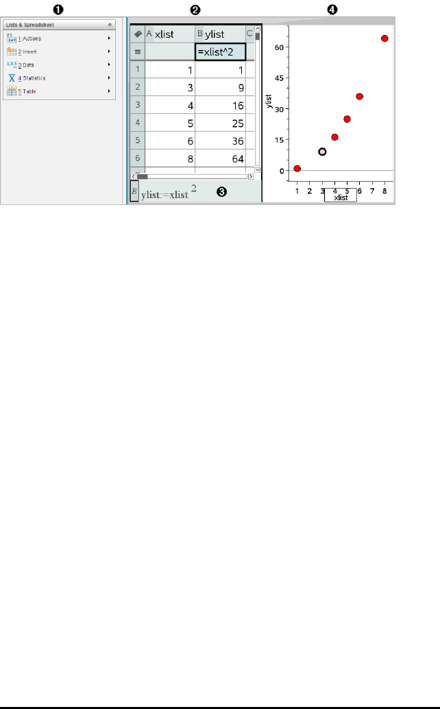
427 Lists&Spreadsheet Application
ÀLists&Spreadsheet tools (available when a Lists&Spreadsheet work area is
active)
ÁSample Lists&Spreadsheet work area
ÂLists&Spreadsheet entry line
ÃLists&Spreadsheet data plotted in the Data&Statistics application
Creating and Sharing Spreadsheet Data as Lists
You can define a column as a named list of elements of the same type of data. After
defining a list, you can link to it from the Graphs&Geometry, Calculator or
Data&Statistics applications, and from other instances of the Lists&Spreadsheet
application within the current problem.
Note: Lists&Spreadsheet can display a maximum of 2500 elements in a list.
Sharing a Spreadsheet Column as a List Variable
You share a column of data by naming it as a list variable.
Note: Avoid defining variables that use the same names as those used for statistical
analysis. In some cases, an error condition could occur.
Variable names used for statistical analysis are listed in the TI-Nspire™ Reference
Guide, under the stat.results entry.
1. Click the cell to move to the column’s name cell (the top cell of the column).
—or—
Press ▲as necessary.
2. Type a name for the list variable, and press Enter.

The column is now available as a list variable to other TI-Nspire™ applications.
3. Create elements in the list the same as you would create data in spreadsheet cells.
For example, you can type the data into each cell or use a formula to generate a
column of data.
Notes:
• If a variable with the name you specified already exists in the current problem,
Lists&Spreadsheet displays an error message.
• When you select the column formula cell of a list, it displays the list name in an
expression similar to width:=.
• Lists can contain empty elements (denoted by “_”) .
• You can refer to a specific element in a named list from the Calculator application.
Use the list name and the element’s position within the list. In a list named
Heights, for example, refer to the first element as Heights[1]. The expression
Heights[2] refers to the second element, and so on.
Linking to an Existing List Variable
Linking a column to an existing list variable lets you easily view and edit the values in
the list. The list can be any shared list in the current problem and can be defined in
Graphs&Geometry, Calculator or any instance of Lists&Spreadsheet.
After you link a column to a list, Lists&Spreadsheet automatically shows any changes
that you make to the list with other TI-Nspire™ applications.
1. Click the column formula cell (the second cell from the top) of the column that you
want to link to the variable.
2. Type the name of the list variable you want to link to.
—or—
Click on the toolbar (press hon the handheld), click Link To and click the
variable you want to link to.
3. Press Enter.
The column shows the list elements.
Notes:
• You cannot link to the same variable multiple times on the same page.
Lists&Spreadsheet Application 428
429 Lists&Spreadsheet Application
• Use caution if you link to a system variable. Doing so could prevent the variable
from being updated by the system. System variables include ans and statistics
results (such as stat.results,stat.RegEqn and stat.Resid).
Inserting an Element in a List
When you insert an element in a list, the remaining elements shift downward to
create space. No other columns are affected.
▶Click Insert > Insert Cell.
Deleting an Element from a List
When you delete an element, the remaining list elements shift upward to close the
gap. The upward shift affects only the selected column.
1. Click the cell of the element to delete.
2. Open the context menu for the cell, and click Delete Cell.
Note: If you press Del or Backspace to clear the contents of the cell instead of
deleting the list element, the element is assigned a value of 0 (zero). The
remaining list elements do not shift.
Creating Spreadsheet Data
You can type numeric values, text or formulas into body cells. Column formula cells can
contain formulas only. (For more information, see Generating Columns of Data.)
Data Examples
Entry Remarks
1.234 Simple numeric entry
“Green” Text - Enclose categorical data (such as the names of colours used in a
study) within quotes to distinguish them from variable names.
Handheld: Press / r to enter quoted data.
=a3*length Formula - Consists of an “=” symbol followed by an expression.
You can type the expression or use the Catalogue and expression
templates to build it. For more information, see the Calculator section.
To ensure a decimal result instead of a fraction, type one of the integers
in the expression as a decimal. For example, type 1.0 instead of 1.

Typing a Maths Expression, Text or Spreadsheet Formula
1. Double-click the cell to select it and put it in edit mode.
Note: If the cell is already selected, you can press Enter or click the entry line.
2. Type the expression, text or formula. Be sure to enclose text entries in quotes and
start formula entries with an “=” symbol.
As you type the data, it appears in the cell and on the entry line simultaneously.
3. Press Enter to complete the entry and move down to the next cell.
—or—
Press Tab to complete the entry and move right to the next cell.
The Lists&Spreadsheet application automatically recalculates any cells that are
dependent on the cell you entered. If you have shared the cell, and other
TI-Nspire™ applications are linked to the cell, the other applications are also
updated.
Note: Empty cells in a spreadsheet display as a void represented by an underscore
(_). The underscore is automatically added to empty cells when a list is named or
when an empty cell is referenced in a formula. When you plan to perform
calculations on a range of cells, be sure to notice the location of void cells. Cells
without a value can affect calculations. For example, if you include a void cell in
the range for a sum such as “=b2+c2,” the result of the calculation is void(_).
Inserting a Cell Range into a Formula
The Select Range feature lets you insert a cell range (such as a1:b3) into a formula by
selecting the range instead of typing cell addresses into an argument.
Suppose you want to calculate the mean of a range of cells.
1. Select the cell that will contain the result.
2. From the Data menu, click ListMaths>Mean.
An editable formula appears in the cell.
Lists&Spreadsheet Application 430
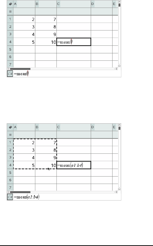
431 Lists&Spreadsheet Application
3. Click Actions>Select>Select Formula Range.
4. Drag a selection rectangle around the range of values for which you want to
calculate the mean.
Handheld: Move to the first cell in the range, hold g, and press the arrow keys.
The formula is updated as you select the cells.
5. Press Enter to complete the formula and display the result.
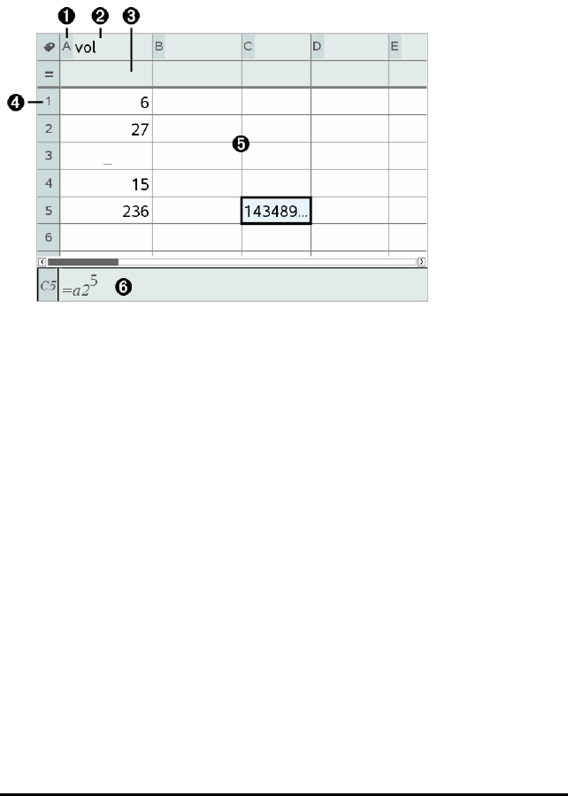
Navigating in a Spreadsheet
A spreadsheet includes a column letter at the top of each column and a row number on
the left of each row. The top two rows and the row numbers remain in place as you
scroll. You can name a column of data to make it available as a list variable in
TI-Nspire™ applications.
ÀColumn reference letter
ÁColumn name cell for defining a column as a list variable
ÂColumn formula cell for generating a column of data
ÃRow reference number
ÄBody Cells - Any empty (void) element in a list is displayed as an underscore (“_”).
Any value that cannot fit in a cell’s width is truncated (143489...). Hover over the
cell to display the complete value.
ÅEntry line (includes cell reference for current cell)
You can select any cell to view or edit its contents. When a spreadsheet is larger than
the Lists&Spreadsheet work area, you can move to different parts of the spreadsheet
by using the Tab key and by pressing short-cut keys.
▶Press Tab to move between the body of the spreadsheet (data zone) and the
column names and formulas (naming zone).
▶Press ◄,►,▲and ▼to move through the spreadsheet one cell at a time (move
between cells within a zone). The arrow keys move the cursor from cell to cell and
scroll as necessary to keep the selected cell in view.
▶Move across several cells at a time by pressing Page up,Page Dn,Home and End.
Lists&Spreadsheet Application 432

433 Lists&Spreadsheet Application
Handheld: Press / 9(Pageup), / 3 (PageDn), / 7 (Home) and
/ 1 (End) keys.
▶Use the Go To command on the Actions menu to select a specific cell. Type the
cell’s column letter and row number (such as G16).
▶Press Enter to put the selected cell in Edit mode.
▶Drag the scroll bar to move vertically without changing the cell or block of cells
selected.
Working with Cells
Working with Colour
The Lists&Spreadsheet application displays black text and cells with a white
background by default. You can change the colour of cells and text to emphasize or
distinguish data. The colours and the order in which colour is assigned is based on the
TI-Nspire™ colour palette.
Changing the Fill Colour of Cells
1. Select the cells to fill with colour. You can choose one or more cells in any adjacent
cells, columns or rows.
2. Access the context menu and click Colour > Fill Colour.
3. Click the colour to apply to the cells.
Note: If you combine colour text and colour cells, choose colours carefully to ensure
visibility as you work with documents in the software and on the handheld.
Changing the Colour of Text
1. Select the cells that contain the text to change. You can choose one or more cells in
any adjacent cells, columns or rows.
2. Access the context menu and click Colour > Text Colour.
3. Click the colour to apply to the text. Empty cells in the selection area show the
colour change when text is added.
Understanding Cell References in Formulas
Use a cell reference to use data from a cell or range of cells in a formula. The
calculation results update automatically when values in cells change.

Relative references include only the cell’s column letter and row number (for example,
E7). A relative reference describes where a cell is in relation to other cells of the
spreadsheet. The Lists&Spreadsheet application keeps track of relative cell references
and adjusts the reference automatically when surrounding cells shift (because of
actions you perform, such as column deletions or cell insertions).
Follow these guidelines to specify cell references:
• Include a column letter and row number in a relative reference.
• Include the $symbol before both the column letter and the row number to specify
an absolute reference.
• Include a colon (:) between a two cell reference to specify a range of cells.
Absolute references include the $symbol before the column letter and before the row
number (for example, $B$16). Absolute references always refer to the cell in a specific
position in the spreadsheet. The application does not automatically adjust the cell
reference when cell positions change.
Typing a Cell Reference in a Formula
1. Double-click the cell and type the formula. For more information, see the
Calculator section.
2. Move to the appropriate position in the formula and type the cell reference. Use
the format for a relative reference (B3), absolute reference ($B$2) or range of cells
(A1:A4).
Note: You can click Recalculate on the Actions menu to update all references and
formula results in a spreadsheet.
Deleting the Contents of Cells
1. Click a cell to select it.
—or—
Use the arrow keys to move to the cell.
Note: If you are deleting a range of cells, select a cell at one end or corner of the
range, and then use Shift with the arrow keys to select the remaining cells in the
range.
2. Press Del.
Lists&Spreadsheet Application 434

435 Lists&Spreadsheet Application
Note: Any cell that uses a formula with an absolute reference to deleted data
shows an error. A cell that uses a formula with a relative reference to deleted data
is updated to use the data currently in the referenced position.
Copying Cells
When you copy cells, any formulas in the original cells are copied to the destination
cells.
1. Click the cell to copy.
—or—
Use the arrow keys to move to the cell.
Note: If you are copying a range of cells, select a cell at one end or corner of the
range, and then use Shift with the arrow keys to select the remaining cells in the
range.
2. Use the standard key short-cut for copying a selection.
Windows®: Press Ctrl+C.
Mac®: Press “+C.
Handheld: Press / C.
3. Click the cell where you want to duplicate the copied cell. If you are copying a block
of data, click the cell that will become the upper left corner of the copied block.
4. Paste the selected cells:
Windows®: Press Ctrl+V.
Mac®: Press “+V.
Handheld: Press / V.
Important: Paste copied data into a cell that is in the same mode as the cell from
which the data was originally copied. Otherwise, a formula could paste as a string
enclosed in quotes instead of a formula.
Filling Adjacent Cells
You can repeat a cell’s formula or value throughout adjacent cells within the row or
column. You can also repeat a range of cells horizontally or vertically. If you fill from a

range that contains a simple sequence (such as 2, 4, 6), the sequence continues in the
filled cells.
1. Click the cell that contains the value or formula to repeat.
Note: If you are repeating a range of cells, drag to select the range, or select a cell
at one end of the range, and then use Shift with the arrow keys to select the
remaining cells.
2. Click Data > Fill.
3. Use the arrow keys, or drag to select the range that will hold the repetitions.
4. Press Enter.
The value, formula or pattern that you selected for duplication is repeated over the
selected range.
Sharing a Cell Value as a Variable
You can share the value of a cell with other TI-Nspire™ applications by storing it as a
variable. When you define or refer to a shared cell or variable in Lists&Spreadsheet,
the name is preceded with an apostrophe(‘).
1. Click the cell that you want to share.
2. Click on the toolbar, and click Store Var to store the cell’s value.
Handheld: Press / h or press hand select Store Var).
A formula is inserted into the cell with var as a placeholder for a variable name.
3. Type over the letters “var” with a name for the variable, and press Enter. Use a
variable name that does not exist in the current problem.
The value is shown in bold to indicate that it is now available as a variable to other
TI-Nspire™ applications.
Linking a Cell to a Variable
When you link a cell to a variable, Lists&Spreadsheet keeps the cell value updated to
reflect the current value of the variable. The variable can be any variable in the current
problem and can be defined in Graphs&Geometry, Calculator, Data&Statistics or any
instance of Lists&Spreadsheet.
1. Click the cell that you want to link to a variable.
2. Click on the toolbar, and click Link to.
Lists&Spreadsheet Application 436

437 Lists&Spreadsheet Application
Handheld: Press / h or press hand select Link to.
The VarLink menu opens.
3. Under Link To, press ▲, and ▼to scroll to the name of the variable.
4. Press Enter.
The cell shows the value of the variable.
Note: Use caution if you link to a system variable. Linking could prevent the variable
from being updated by the system. System variables include statistics results (such as
Stat.RegEqn,Stat.dfError and Stat.Resid) and finance-solver variables (such as tvm.n,
tvm.pmt and tvm.fv).
Working with Rows and Columns of Data
Selecting a row or column
▶To select a column, move to the top of the column and click the column reference
letter. To select a row, move to the leftmost cell of the row and click the row
reference number. Press Esc to cancel the selection.
Handheld: Hold down ▲to move past the top cell, or hold down ◄to move past
the leftmost cell.
▶To extend a selection to adjacent rows or columns, hold down Shift and press ◄,
►,▲or ▼.
Resizing a Row or Column
1. Click the row or column that you want to resize.
2. From the Actions menu, select Resize and then select an option.
3. Choose a resizing option for a column or row.
- For a column, choose Resize Column Width,Maximize Column Width or
Minimise Column Width.
- For a row, you can choose Resize Row Height.
The tools that minimise and maximise the column width work automatically. You
must manually adjust the size to use the Resize Column Width and Resize Row
Height tools.
4. To resize manually, use ◄and ►to resize the column, or use ▲and ▼to resize
the row, and then press Enter.

Inserting an Empty Row or Column
1. Click a column or row where you want to insert the new data.
2. From the Insert menu, select either Row or Column.
- If you are inserting a row, the remaining rows shift down to create space for
the new row.
- If you are inserting a column, the remaining columns shift right to create
space.
Note: If other cells contain formulas with relative references to a displaced row or
column, those references adjust accordingly.
Deleting Entire Rows or Columns
You can delete a row, column, group of rows or group of columns. When you delete a
row or column, the remaining rows or columns move up or left to fill the gap.
1. Click the column or row that you want to delete.
2. (Optional) To select adjacent rows or columns to delete, hold down Shift and press
◄,►,▲or ▼.
3. Display the context menu.
- Windows®: Right-click the selected row.
- Mac®: Hold the “key, and click the selected row.
- Handheld: Press / b.
4. On the context menu, select Delete Row.
The selected rows or columns are deleted.
Note: If other cells contain formulas that refer to the deleted row or column, those
cells show an error. Relative references to cells whose positions have changed
because of a deletion adjust accordingly.
Copying Rows or Columns
1. Click the row number to copy a row, or click the column letter to copy a column.
2. (Optional) To select adjacent rows or columns to copy, hold down Shift and press
◄,►,▲or ▼.
3. Copy the row or column:
Windows®: Press Ctrl+C.
Lists&Spreadsheet Application 438

439 Lists&Spreadsheet Application
Mac®: Press “+C.
Handheld: Press / C.
4. Move to any cell in the row or column where you want to place the copied items.
5. Paste the row or column:
Windows®: Press Ctrl+V.
Mac®: Press “+V.
Handheld: Press / V.
The copied row or column is pasted in place, replacing the previous contents.
Note: If you copy a named column, it is pasted with the name removed to prevent
a variable conflict.
Moving a Column
1. Click the column that you want to move.
2. From the Actions menu, select Move Column.
An insertion bar appears.
3. Press ◄and ►to place the insertion bar at the column’s new position, and then
press Enter.
Note: Relative references to any cell in a position is affected by the move adjust
accordingly.
Displaying Results as Exact or Approximate
You can choose to display a column’s calculated results in Exact (fraction) or
Approximate (decimal) form. This affects only the values calculated from a formula.
1. Select the column by clicking the reference letter at the top of the column.
Handheld: Hold down ▲to move past the top cell.
2. Display the context menu for the column.
3. On the context menu, click either Data>Exact or Data>Approximate.
Note: To restore the column results to the document’s default setting, select the
column and click Data>Restore Document Setting.
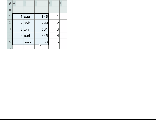
Clearing Column Data
The Clear Data command lets you remove the data from selected columns. Clear Data
does not delete the column, and it does not clear a column’s name or formula.
After clearing the data, Lists&Spreadsheet recalculates column formulas for the
selected columns. This makes Clear Data useful for capturing a fresh set of data from
another application or selectively generating a fresh column of random numbers.
1. Click the column or columns that you want to clear.
2. From the Data menu, select Clear Data.
Note: If a recalculated formula produces the same data as before, it may appear
that the Clear Data command has failed.
Sorting Data
You can sort a selected area of the spreadsheet in ascending or descending order. You
select which column in the selected area will be used as the key for the sort. When the
sort moves data up or down in the key column, the corresponding data in the other
selected columns is also moved up or down. This preserves the integrity of each row.
Note: Sorting is based on numeric values. If you select a key column that contains text,
you could get unexpected results.
1. Select the range of cells.
2. From the Actions menu, select Sort.
The Sort dialogue box opens.
3. Click the column letter to use for ordering.
4. Click Descending or Ascending as the sort method, and then click OK.
Lists&Spreadsheet Application 440
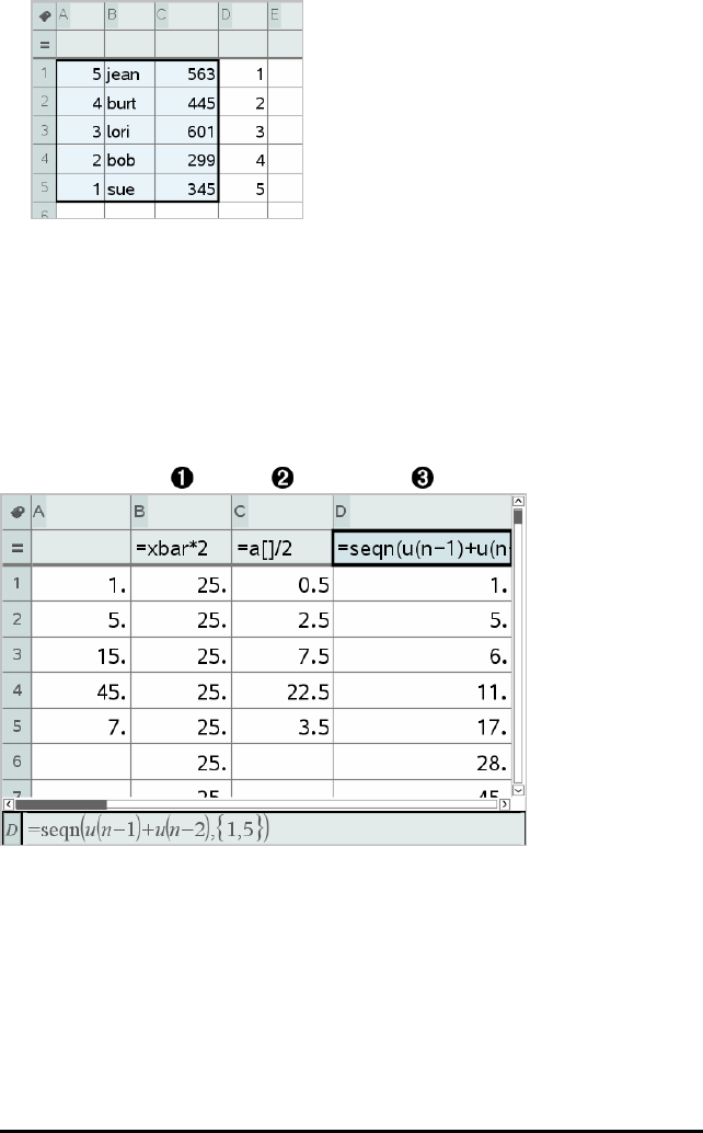
441 Lists&Spreadsheet Application
Note: Sorting a column that is defined by a formula will remove the formula, because
it may not be valid after the sort.
Generating Columns of Data
You can create a column of values based on the contents of another column. You can
also create a column based on any of several types of sequential data.
Entering a formula in a column’s formula cell tells the Lists&Spreadsheet application
that you want to apply the formula to all cells in the column, not just to a single cell.
ÀColumn formula based on a variable
ÁColumn formula based on another column (column A)
ÂColumn formula that generates a sequence
Notes:
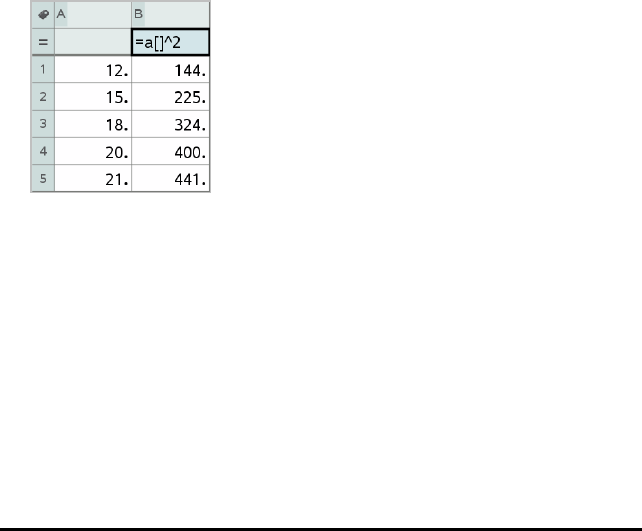
• If you generate data in a column that already contains one or more cell values,
Lists&Spreadsheet asks for confirmation before replacing the existing values.
Proceeding removes all of the existing values in the column.
• If you edit a cell manually in a column of generated data, Lists&Spreadsheet asks
for confirmation before replacing the generated data. Proceeding removes the
generated data for the entire column.
Creating Column Values Based on Another Column
1. Click the column formula cell (the second cell from the top) of the column where
you want to use a formula.
Lists&Spreadsheet inserts the leading equal sign (=) for the formula. If the
column is a named list, Lists&Spreadsheet inserts listname:= followed by the
cursor.
2. Type the expression for the formula after the = and press Enter Use brackets ([])
after any column letter you include in the formula. For example, type =a[]^2 to
create a column of values in which each cell is the square of the corresponding cell
of column A.
Lists&Spreadsheet shows the formula in the formula cell and fills the column
with the results.
Generating a Column of Random Numbers
This example generates a column of 20 random integers in the range 1 to 6.
1. Click the column formula cell (the second cell from the top) of the column.
Lists&Spreadsheet inserts the leading equal sign (=) for the formula. If the
column is a named list, Lists&Spreadsheet inserts listname:= followed by the
cursor.
2. After the equal sign, type RandInt(1,6,20).
Lists&Spreadsheet Application 442
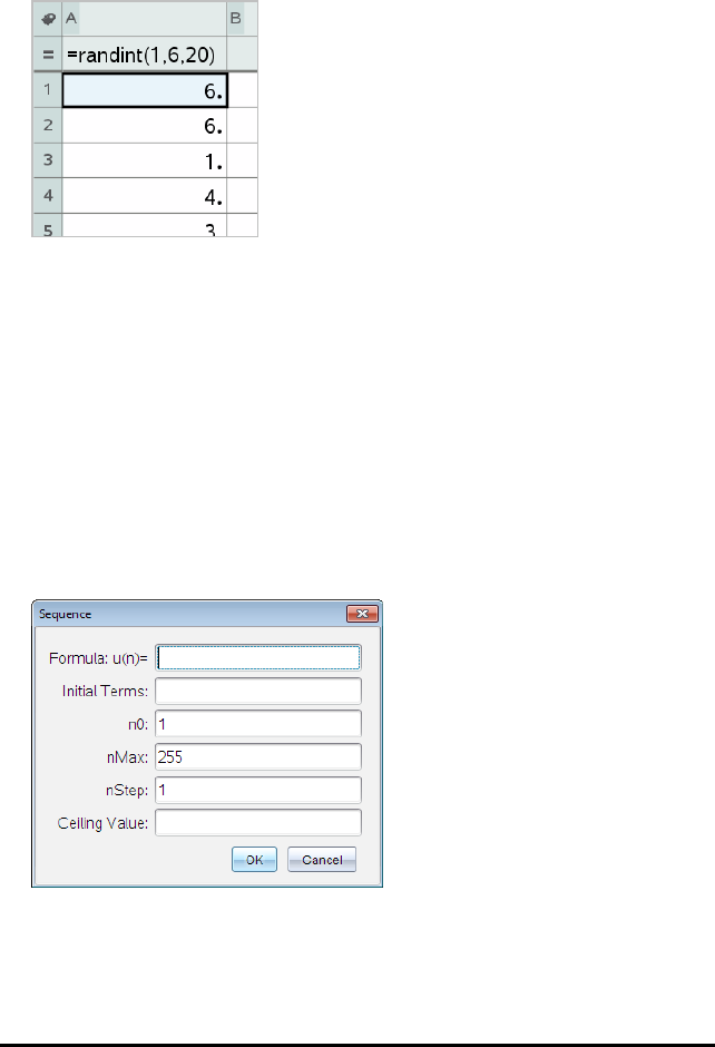
443 Lists&Spreadsheet Application
Note: You can also use the Catalogue or click Data > Random > Integer to insert the
RandInt() function.
3. Press Enter to generate the numbers.
4. Generate (Recalculate) a new set of random numbers:
Windows®: Press Ctrl+R.
Mac®: Press “+R.
Handheld: Press / R.
Generating a Numerical Sequence
1. Click any cell in the column in which you want to generate the sequence.
2. From the Data menu, select Generate Sequence.
The Sequence dialogue box opens.
3. Type the Formula that will be applied to the column values.
4. Type any Initial Terms required by the sequence. Separate them with commas.
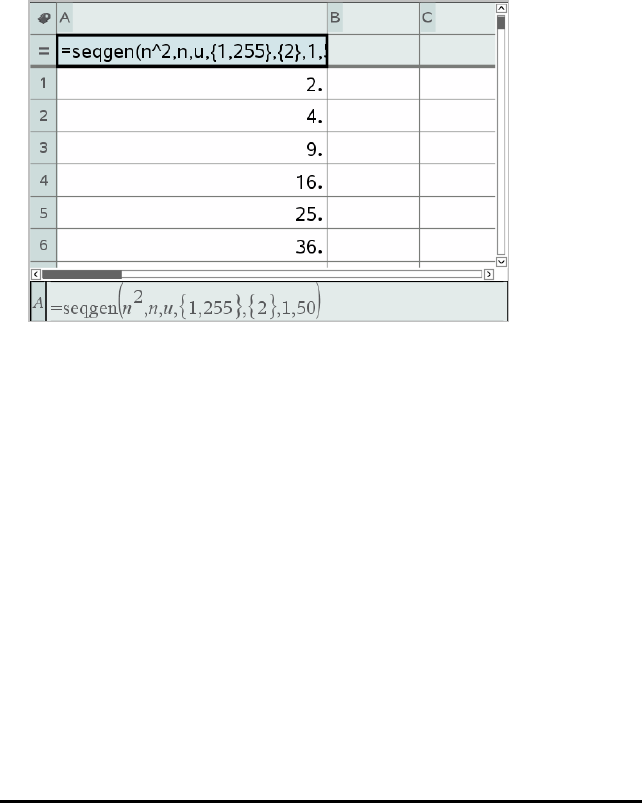
5. Type a starting value for the independent variable (n0).
6. Type a maximum number of values to be generated (nMax).
7. Type the step value (nStep).
8. (Optional) Type a maximum value for the sequence in the Ceiling Value field.
9. Click OK.
Lists&Spreadsheet shows the formula in the formula cell and fills the column
with the results.
Graphing Spreadsheet Data
You can graph the data in a spreadsheet using Quick Graph or Summary Plot.
Lists&Spreadsheet cells that contain no data are not represented by data points on
graphs.
Using Quick Graph
You can easily create a dot plot of the data in one column or a scatter plot of two
adjacent columns by using the Quick Graph feature. This feature displays the graphed
data using the Data&Statistics application.
To create a scatter plot:
1. Name both of the columns to declare them as lists.
Lists&Spreadsheet Application 444
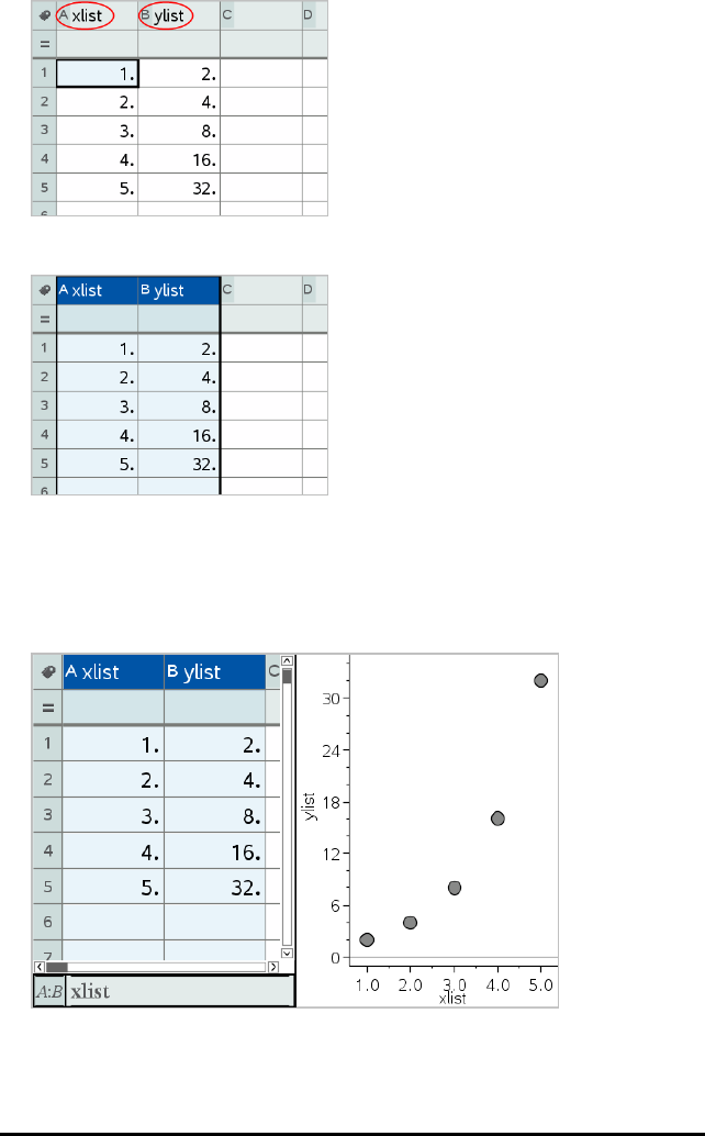
445 Lists&Spreadsheet Application
2. Select both columns.
3. From the Data menu, select Quick Graph.
A Data&Statistics application is added to the page with the plotted data. The
leftmost of the two lists is plotted on the x axis, and the other list is plotted on the
y axis.
4. (Optional) Use the Data&Statistics features to analyse or visually enhance the
graph.
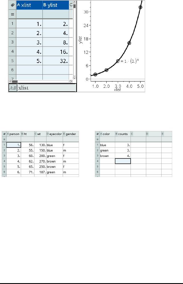
Note: For more information, see Using Data and Statistics.
Creating a Summary Plot from a Summary Table
In this example, you create a summary table from raw data, and then use the table to
generate a summary plot. For more information, see Using Data&Statistics.
raw data summary table for eye colour based on raw data
A summary table contains an X (or Y) List and a Summary List.
• The X (or Y) List contains numeric or string values (such as 1999 or “colour”).
Numeric values result in a histogram. String values identify the categories for a bar
chart.
• The Summary List contains numeric values (such as count, frequency, or
probability) for each element in the other list.
To Create a Summary Plot:
Note: For situations in which you already have a summary table, you can skip the first
two steps.
Lists&Spreadsheet Application 446
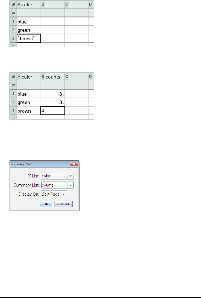
447 Lists&Spreadsheet Application
1. Create a list that holds the category identifiers. For this example, name the list
“colour” and type strings for eye colour. Enclose category names in quotes to
prevent them from being interpreted as variables.
2. Create the summary list. For this example, name the list “counts” and type the
total count for each of the eye colours.
3. Select either list by clicking the top cell of the column and pressing▲.
4. From the Data menu, select Summary Plot.
The Summary Plot dialogue box opens.
5. If necessary, use Tab and the arrow keys to select the correct lists for X List and
Summary List.
6. In the Display On field, select how to display the summary plot in the
Data&Statistics application.
• Select Split Page to place the chart on half of the current page.
• Select New Page to add the chart on a new page.
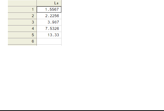
The summary plot is displayed with the list names along the axes and a summary
plot symbol in the lower left corner of the chart window.
Note: In this example, the XList contains string data, so the summary plot displays
as a bar chart. The category strings from the list display beneath the bars.
Exchanging Data with Other Computer Software
You can use the TI-Nspire™ desktop software to copy table data to and from software
outside the TI-Nspire™ applications, such as TIDataEditor (in the TIConnect™
software) and Excel® spreadsheet software.
For example, you can copy:
• The values of individual cells, a range of cells or an entire list from TIDataEditor.
• The values (not the underlying formulas) of individual cells, a range of cells or an
entire column from an Excel® spreadsheet.
• A number from TIDataEditor.
• The value of a matrix from TIDataEditor.
Example - Copying Data from TIDataEditor
1. Open the TIConnect™ software.
2. Display the TIDataEditor.
3. If necessary, open the file containing the number, list or matrix that you want to
copy.
4. Drag to select the values that you want to copy. To copy an entire list, click the top
cell in the list.
Lists&Spreadsheet Application 448
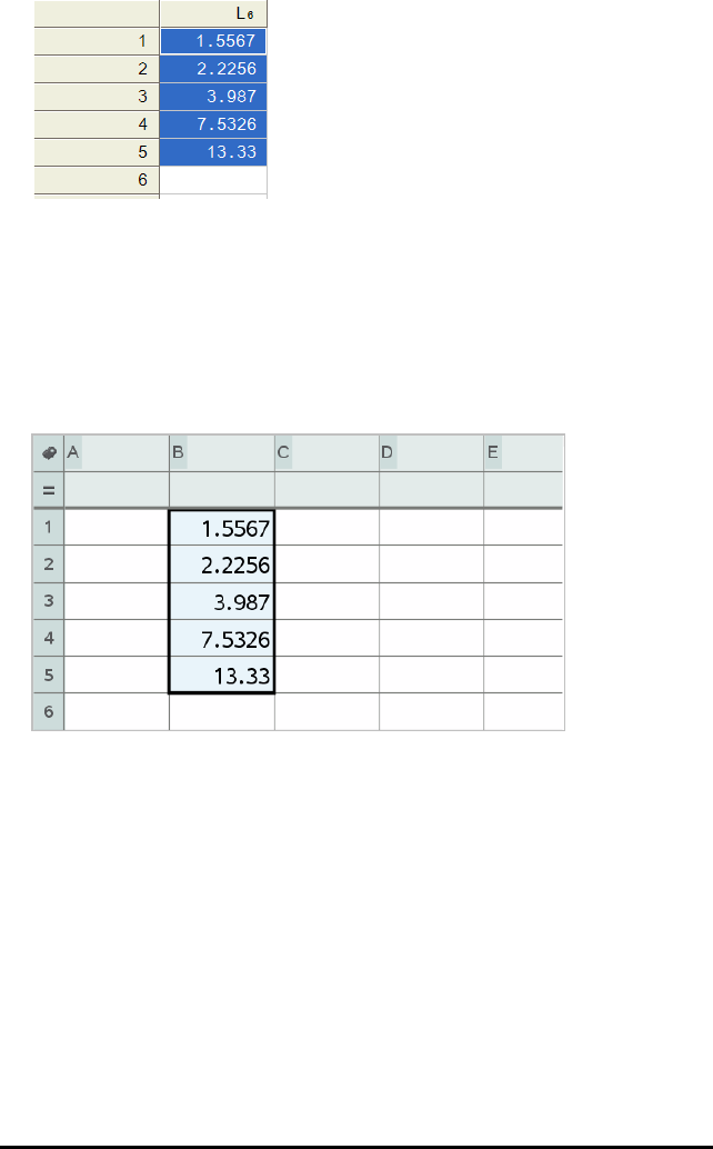
449 Lists&Spreadsheet Application
5. Click Edit > Copy.
6. In Lists&Spreadsheet, click the cell where you want the data to be pasted.
If you have copied a range of cells, they will be pasted so that the upper-left corner
of the range is positioned at the selected cell. Any data in those cells will be
overwritten.
7. Click Edit > Paste.
Copying Cells from an Excel® Spreadsheet
You can copy up to 26 columns and 2500 rows from an Excel® spreadsheet to a
Lists&Spreadsheet application.
1. Drag to select the values that you want to copy from the Excel® spreadsheet. To
copy an entire column, click the column identifier at the top of the column.
Note: If you select non-contiguous columns in the Excel® spreadsheet, they will be
pasted as contiguous columns in Lists&Spreadsheet.
2. Use the standard key short-cut for copying a selection.
Windows®: Press Ctrl+C.

Mac®: Press “+C.
3. In Lists&Spreadsheet, click the cells where you want the data to be pasted.
If you are copying a range of cells, they will be pasted so that the upper-left corner
of the range is positioned at the selected cell. Any data in those cells in will be
overwritten.
4. Paste the data.
Windows®: Press Ctrl+V.
Mac®: Press “+V.
Handheld: Press / V.
Note: Categorical data must be enclosed in quotes (““) after the data is pasted.
Capturing Data from Graphs&Geometry
You can use Lists&Spreadsheet application to capture information about objects in
the Graphs&Geometry application. For example, you could track changes in the area
of a triangle as you change the length of a side in the Graphs&Geometry application.
Captured values replace values in the column. If you prefer, you can remove all data
from a column before starting a new capture by clicking Clear Data on the Data menu.
Capturing Data Manually
1. Make sure the data value that you want to capture is linked to a variable name.
2. Click the column formula cell (the second cell from the top) of the column in which
you want to capture the values.
Note: Captured values replace values in the column.
3. Click Data > Data Capture >Manual.
A capture expression is inserted into the column formula cell with var as a
placeholder for the name of the variable you are capturing.
Lists&Spreadsheet Application 450
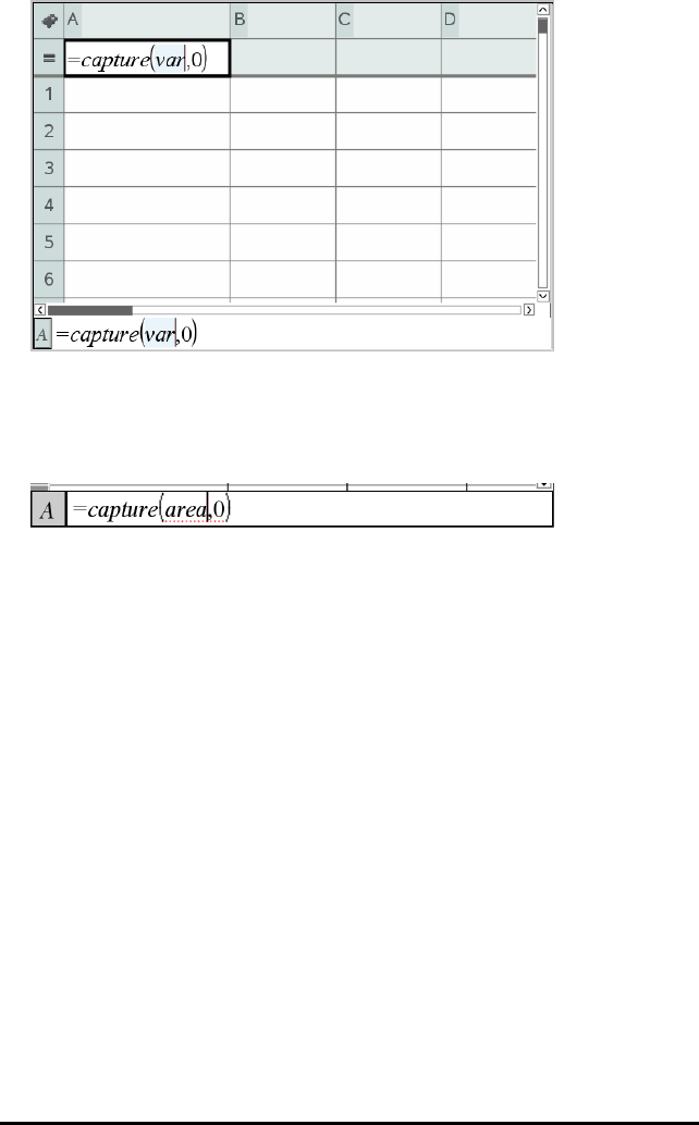
451 Lists&Spreadsheet Application
4. Replace the letters “var” with the name of the variable to capture from
Graphs&Geometry. For example, type area.
The formula cell now contains an expression similar to =capture(area,0).
Note: The argument “0” tells Lists&Spreadsheet that you want to trigger each
capture manually.
5. Press Enter.
6. From the Graphs&Geometry application, change the object with a measured
value stored as the variable (area, in this example) referenced in the data capture
expression.
7. Each time you are ready to capture the current value of area, press the capture
keys.
Windows®: Press Ctrl+.(the full stop key).
Mac®: Hold down “and press .(the full stop key).
Handheld: Press / ^.
The current area value is added to the end of the list as a list element.
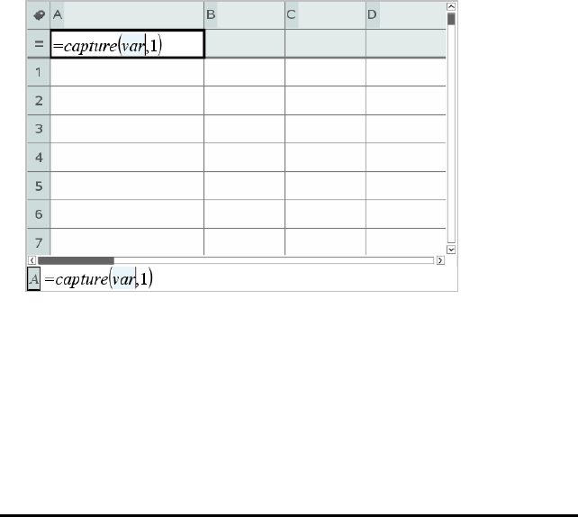
Capturing Data Automatically
When you capture data automatically, you can specify that you want the captures to be
triggered by:
• Changes in the captured variable only.
• Changes in the captured variable or additional variables.
This lets you set up multiple columns of synchronised captures, such as the x and y
coordinates of a moving object.
1. Clear all columns that you will be using for the captured data.
2. Make sure any data values that you want to capture are linked to variable names.
3. Click the column formula cell (the second cell from the top) of the column in which
you want to capture the values.
4. Click Data >Data Capture >Automatic.
A capture expression is inserted into the column formula cell with var as a
placeholder for the name of the variable you are capturing.
5. Replace the letters “var” with the name of the variable to capture. For example,
type objpathX. Alternatively, you can select the variable name from the
Variables menu.
The formula cell now contains an expression similar to =capture
(objpathX,1).
Lists&Spreadsheet Application 452
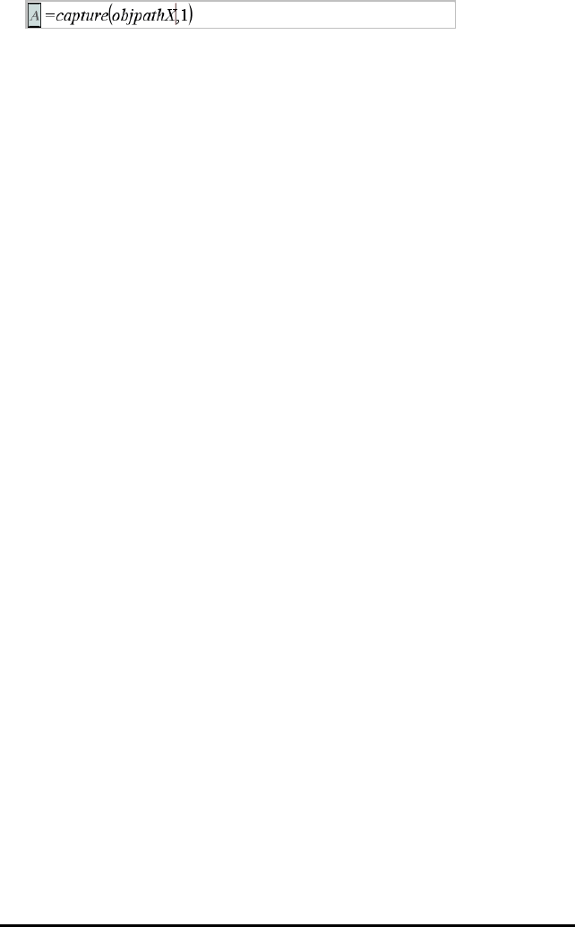
453 Lists&Spreadsheet Application
Note: The argument “1” tells Lists&Spreadsheet that you want the captures to be
triggered by the variable change.
6. If you want the capture to also be triggered by changes in an additional variable or
variables, type a comma after the 1, and then type the variable name or the name
of a list that itemises the variables.
The formula cell will contain an expression similar to =capture
(objpathX,1,objpathY).
7. Press Enter to complete the formula.
8. If you are capturing multiple columns of synchronised data, set up the additional
columns. For example, you might set up a second capture variable using
=capture(objpathY,1,objpathX).
9. When you are ready to capture the values, begin moving the object or start the
animation that affects it in Graphs&Geometry.
Each captured value is added to the end of the list.
Using Table Data for Statistical Analysis
Tools on the Statistics menu provide access to wizards that help you perform statistical
analyses on the data in table columns. You specify the location of the data, and
Lists&Spreadsheet stores the results in two columns: one for the result names, and
one for the corresponding values.
Plotting Statistical Data
Some statistics wizards include a Draw box. By default, the box is not selected.
Selecting this box creates a Data&Statistics work area on the page, displays the
calculated results in Lists&Spreadsheet, and draws the results of the statistical
analysis in the Data&Statistics work area.
Note: For functions that support the Draw option, the option is available only if you
type the function in a column formula cell.
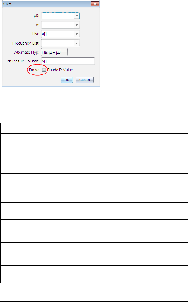
Draw box (as shown in the zTest wizard).
Statistics Input Descriptions
The following table describes the different inputs used in Lists&Spreadsheet wizards.
Input Description
m0Hypothesized value of the population mean that you are testing.
sThe known population standard deviation; must be a real
number >0.
List The name of the list containing the data you are testing.
Frequency List The name of the list containing the frequency values for the
data in List. Default=1. All elements must be integers |0. The
frequency values can also be typed as a list, in the format {1, 1,
3, 2}.
v, Sx, n Summary statistics (mean, standard deviation and sample size)
for the one-sample tests and intervals.
s1 The known population standard deviation from the first
population for the two-sample tests and intervals. Must be a
real number>0.
s2 The known population standard deviation from the second
population for the two-sample tests and intervals. Must be a
real number>0.
List1, List2 The names of the lists containing the data you are testing for
the two-sample tests and intervals.
Lists&Spreadsheet Application 454
455 Lists&Spreadsheet Application
Input Description
Frequency1,
Frequency2
The names of the lists containing the frequencies for the data in
List1 and List2 for the two-sample tests and intervals.
Defaults=1. All elements must be integers |0.
v1, Sx1, n1,
v2, Sx2, n2
Summary statistics (mean, standard deviation, and sample size)
for sample one and sample two in two-sample tests and
intervals.
Pooled Specifies whether variances are to be pooled for
2-SampletTest and 2-SampletInterval.
p0The expected sample proportion for 1-PropzTest. Must be a
real number, such that0<p0<1.
x The count of successes in the sample for the 1-PropzTest and
1-PropzInterval. Must be an integer|0.
n The count of observations in the sample for the 1-PropzTest
and 1-PropzInterval. Must be an integer>0.
x1 The count of successes from sample one for the 2-PropzTest
and 2-PropzInterval. Must be an integer|0.
x2 The count of successes from sample two for the 2-PropzTest
and 2-PropzInterval. Must be an integer|0.
n1 The count of observations in sample one for the 2-PropzTest
and 2-PropzInterval. Must be an integer >0.
n2 The count of observations in sample two for the 2-PropzTest
and 2-PropzInterval. Must be an integer >0.
C-Level The confidence level for the interval instructions. Must be |0
and <100. If it is |1, it is assumed to be given as a percent and
is divided by 100. Default=0.95.
RegEQ The prompt for the name of the function where the calculated
regression equation is to be stored.
Statistical Calculations
Performing a Statistical Calculation
You can perform statistical calculations to analyse data. The following example fits a
y=mx+b linear regression model to the two lists in columns A and B.
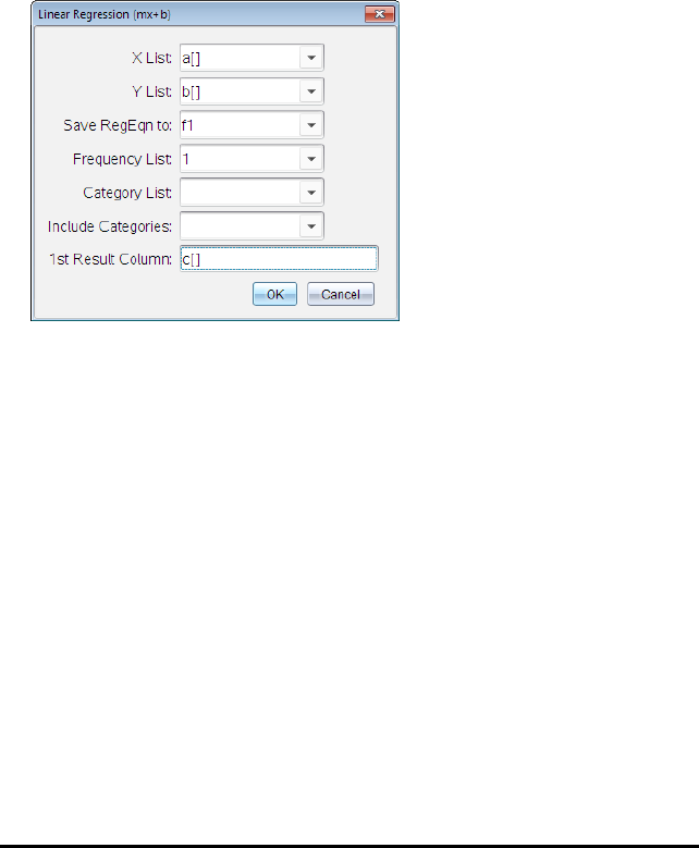
1. From the Statistics menu, select Stat Calculation > LinearRegression (mx+b) to
choose the regression model.
The Linear Regression (mx+b) dialogue box opens.
2. Type a[] as the column for the X List.
3. Type b[] as the column for the Y List.
4. To store the regression equation in a specified variable, replace Save RegEqn To
with the name of the variable.
5. Type c[] as the column for the 1st Result.
6. Click OK.
Lists&Spreadsheet inserts two columns: one containing the names of the results,
and one containing the corresponding values.
Lists&Spreadsheet Application 456
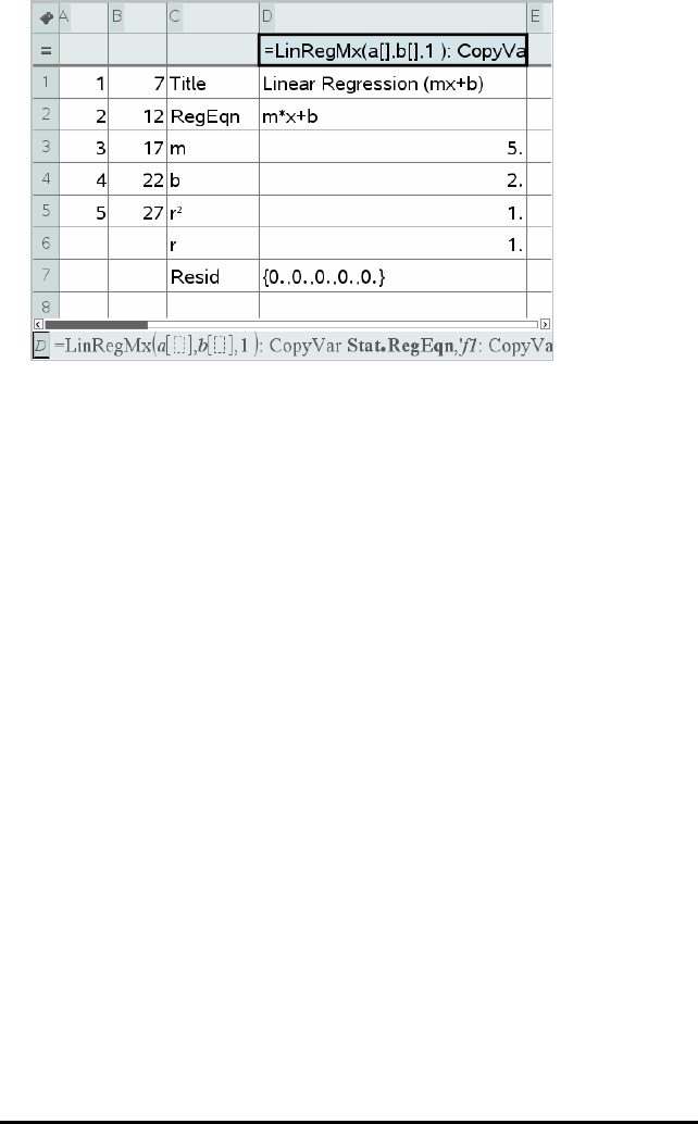
457 Lists&Spreadsheet Application
Note: The results are linked to the source data. For example, if you change a value
in column A, the regression equation is updated automatically.
Storing Statistical Results
Lists&Spreadsheet stores statistical results using a variable-group name with the
format stat.nnn, where nnn is the result name (for example, stat.RegEqn and
stat.Resid). The use of standard names for variables makes it easier to identify and use
the statistical variables later. If you want to use a custom variable group instead of the
standard name, you can edit the formula in the column formula cell.
You could use the following formula to store the results in the variable group MystatsB.
=LinRegMx(a[],b[],1 ): CopyVar Stat., MystatsB.
Later, you could view the results by entering the following expression inthe Calculator
application or in another column of the Lists&Spreadsheet application:
MystatsB.results
Supported Statistical Calculations
The Stat Calculations menu lets you select from the calculations described below. For
more information, see the TI-Nspire™ReferenceGuide.
One-Variable Statistics (OneVar)
Analyses data with one measured variable. You can specify an optional frequency list.
The statistical data returned using this analysis technique are:

• Sample mean, x
• Sum of the data, Gx
• Sum of the squared data, Gx2
• Sample standard deviation, sx
• Population standard deviation, sx
• Sample size, n
• X-min
• First quartile, Q1
• Median
• Third quartile, Q3
• X-max
• Sum of squared deviations, SSx = G(xNx)2
Two-Variable Statistics (TwoVar)
Analyses paired data. List 1 is the independent variable. List 2 is the dependent
variable. You can specify an optional frequency list. The statistical data returned using
this analysis technique are:
For each list:
• Sample mean, xor y
• Sum of the data, Gxor Gy
• Sum of the squared data, Gx2or Gy2
• Sample standard deviation, sx = sn-1x or sy = sn-1y
• Population standard deviation, sx = snx or sy = sny
• X-min or Y-min
• First quartile, Q1X or Q1Y
• Median
• Third quartile, Q3X or Q3Y
• X-max or Y-max
• Sum of squared deviations, SSx = G(xNx)2or SSy = G(yNy)2
Additional data:
• Sample size for each data set, n
Lists&Spreadsheet Application 458

459 Lists&Spreadsheet Application
•Gxy
• Correlation coefficient, R.
Linear Regression (mx+b) (LinRegMx)
Fits the model equation y=ax+b to the data using a least-squares fit. It displays values
for m(slope) and b(y-intercept).
Linear Regression (a+bx) (LinRegBx)
Fits the model equation y=a+bx to the data using a least-squares fit. It displays values
for a(y-intercept), b(slope), r2, and r.
Median-Median Line (MedMed)
Fits the model equation y=mx+b to the data using the median-median line (resistant
line) technique, calculating the summary points x1, y1, x2, y2, x3 and y3.
Median-MedianLine displays values for m(slope) and b(y-intercept).
Quadratic Regression (QuadReg)
Fits the second-degree polynomial y=ax2+bx+c to the data. It displays values for a,b,c,
and R2. For three data points, the equation is a polynomial fit; for four or more, it is a
polynomial regression. At least three data points are required.
Cubic Regression (CubicReg)
Fits the third-degree polynomial y=ax3+bx2+cx+d to the data. It displays values for a,b,
c,d, and R2. For four points, the equation is a polynomial fit; for five or more, it is a
polynomial regression. At least four points are required.
Quartic Regression (QuartReg)
Fits the fourth-degree polynomial y=ax4+bx3+cx2+dx+e to the data. It displays values
for a,b,c,d,eand R2. For five points, the equation is a polynomial fit; for six or more,
it is a polynomial regression. At least five points are required.
Power Regression (PowerReg)
Fits the model equation y=axb to the data using a least-squares fit on transformed
values ln(x) and ln(y). It displays values for a,b,r2and r.
Exponential Regression (ExpReg)
Fits the model equation y=abxto the data using a least-squares fit on transformed
values x and ln(y). It displays values for a,b,r2and r.

Logarithmic Regression (LogReg)
Fits the model equation y=a+bln(x) to the data using a least-squares fit on
transformed values ln(x) and y. It displays values for a,b,r2and r.
Sinusoidal Regression (SinReg)
Fits the model equation y=asin(bx+c)+d to the data using an iterative least-squares fit.
It displays values for a,b,cand d. At least four data points are required. At least two
data points per cycle are required to avoid aliased frequency estimates.
Note: The output of SinReg is always in radians, regardless of the Radian/Degree mode
setting.
Logistic Regression (d=0) (Logistic)
Fits the model equation y=c/(1+a*e⁻bx) to the data using an iterative least-squares fit.
It displays values for a,band c.
Logistic Regression (dƒ0) (LogisticD)
Fits the model equation y=c(1+a*e(⁻bx))+d to the data using an iterative least-squares
fit. It displays values for a,b,cand d.
Multiple Linear Regression (MultReg)
Calculates multiple linear regression of list Y on lists X1, X2, …, X10.
Distributions
Calculating a Distribution
Example: Calculate a distribution to fit the Normal Pdf distribution model.
1. Click the column formula cell (second cell from the top) in columnA.
2. Click Statistics > Distributions > Normal Pdf to choose the Distribution model.
The Normal Pdf dialogue box opens and displays fields for typing or selecting the
arguments for the calculation.
3. Press Tab as necessary to move from field to field and provide each argument. You
can type values, or select them from the drop-down list:
-X Value: Click the drop-down arrow to choose any list in the problem to provide
the x values for the calculation.
-Mean: Type a value for the mean or click the drop-down arrow to choose a
variable that contains the mean.
Lists&Spreadsheet Application 460
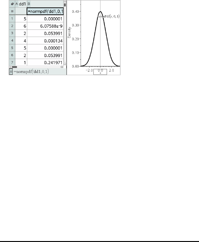
461 Lists&Spreadsheet Application
-Standard Deviation: Type a value for the standard deviation or choose a variable
that contains the standard deviation.
4. Click the Draw tick box to see the distribution plotted in Data& Statistics.
Note: The Draw option is not available for all distributions.
5. Click OK.
Lists& Spreadsheet inserts two columns: one containing the names of the results,
and one containing the corresponding values. The results are plotted in Data&
Statistics.
Note: The results are linked to the source data. For example, you can change a
value in Column A, and the equation updates automatically.
Supported Distribution Functions
The following distributions are available from the Lists& Spreadsheet application. For
more information regarding these functions, see the TI-Nspire™ Reference Guide.
• To return a single distribution result based on a single value, type the function in a
single cell.
• To return a list of distribution results based on a list of values, type the function in
a column formula cell. In this case, you specify a list (column) that contains the
values. For each value in the list, the distribution returns a corresponding result.
Note: For distribution functions that support the draw option (normPdf,tPdf,
χ²Pdf, and FPdf), the option is available only if you type the distribution function
in a formula cell.
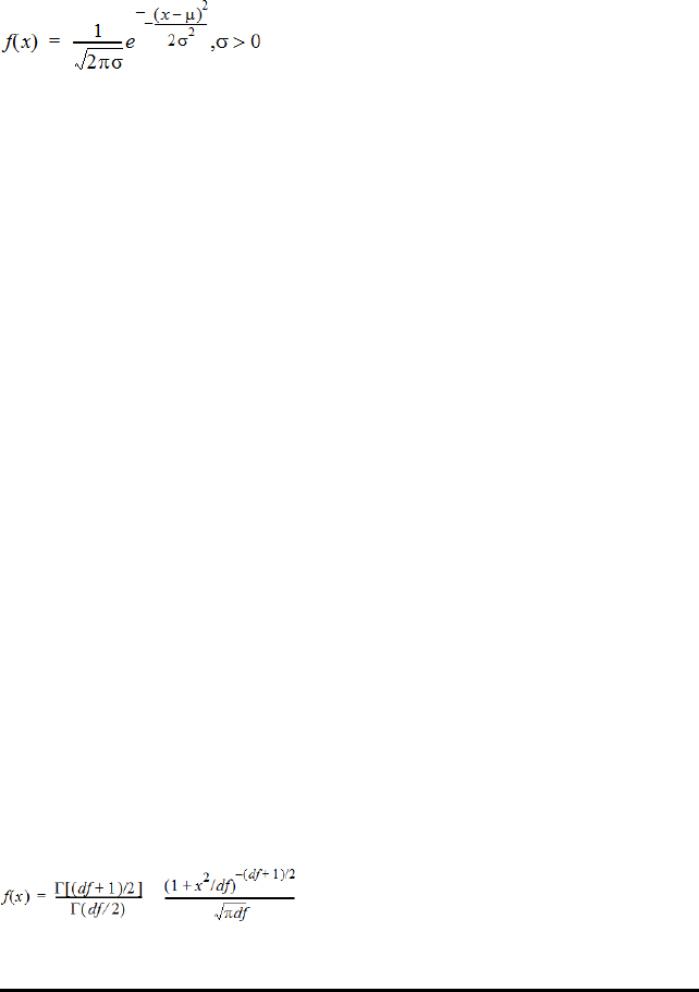
Normal Pdf (normPdf)
Computes the probability density function (Pdf) for the normal distribution at a
specified xvalue. The defaults are mean μ=0 and standard deviation σ=1. The
probability density function (Pdf) is:
This distribution is used to determine the probability of the occurrence of a certain
value in a normal distribution. The draw option is available when Normal Pdf is invoked
from a formula cell.
When you access distributions from the formula cell, you must select a valid list from
the drop-down list to avoid unexpected results. If accessed from a cell, you must
specify a number for the x-value. The distribution returns the probability that the value
you specify will occur.
Normal Cdf (normCdf)
Computes the normal distribution probability between LowerBound and
UpperBound for the specified mean, μ(default=0) and the standard deviation, s
(default=1). You can click the Draw (Shade area) box to shade the area between the
lower and upper bounds. Changes to the initial LowerBound and UpperBound
automatically update the distribution.
This distribution is useful in determining the probability of an occurrence of any value
between the lower and upper bounds in the normal distribution. It is equivalent to
finding the area under the specified normal curve between the bounds.
Inverse Normal (invNorm)
Computes the inverse cumulative normal distribution function for a given area under
the normal distribution curve specified by mean, μand standard deviation, s.
This distribution is useful in determining the x-value of data in the area from 0 to x<1
when the percentile is known.
tPdf (tPdf)
Computes the probability density function (Pdf) for the tdistribution at a specified x
value. df (degrees of freedom) must be 0. The probability density function (Pdf) is:
Lists&Spreadsheet Application 462
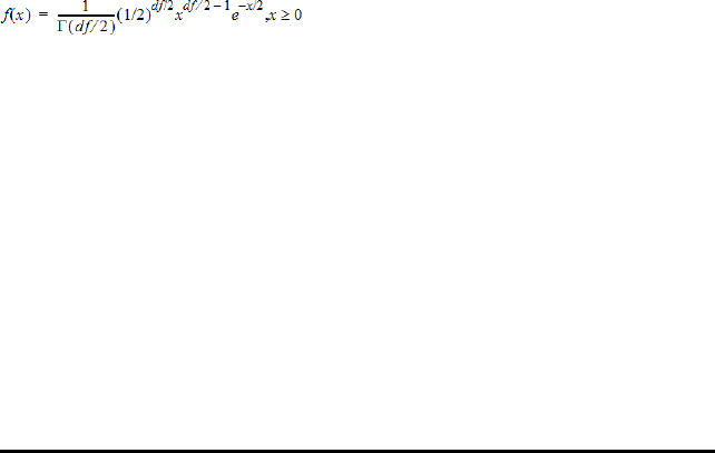
463 Lists&Spreadsheet Application
This distribution is useful in determining the probability of the occurrence of a value
when the population standard deviation is not known and the sample size is small. The
draw option is available when tPdf is invoked from a formula cell.
tCdf (tCdf)
Computes the Student-t distribution probability between LowerBound and
UpperBound for the specified df (degrees of freedom). You can click the Draw (Shade
area) box to shade the area between the bounds. Changes to the initial LowerBound
and UpperBound automatically update the distribution.
This distribution is useful in determining the probability of the occurrence of a value
within an interval defined by the lower and upper bound for a normally distributed
population when the population standard deviation is not known.
Inverset (invt)
Computes the inverse cumulative t-distribution probability function specified by
Degrees of Freedom, df, for a given area under the curve.
This distribution is useful in determining the probability of an occurrence of data in the
area from 0 to x<1. This function is used when the population mean and/or population
standard deviation is not known.
c2Pdf (c2Pdf())
Computes the probability density function (Pdf) for the c2(chi-square) distribution at a
specified xvalue. df (degrees of freedom) must be an integer >0. The probability
density function (Pdf) is:
This distribution is useful in determining the probability of the occurrence of a given
value from a population with a c2distribution. The draw option is available when c2
Pdf is invoked from a formula cell.
c2Cdf (c2Cdf())
Computes the c2(chi-square) distribution probability between lowBound and upBound
for the specified df (degrees of freedom). You can click the Draw Shade area box to
shade the area between the lower and upper bounds. Changes to the initial lowBound
and upBound automatically update the distribution.
This distribution is useful in determining the probability of the occurrence of value
within given boundaries of a population with a c2distribution.
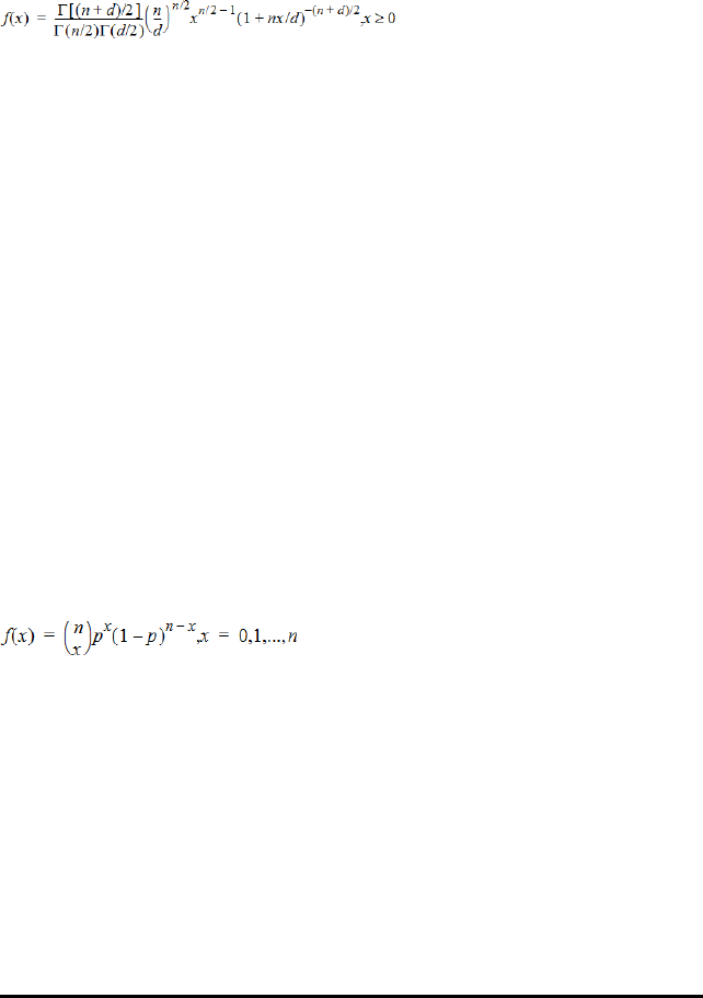
FPdf (FPdf())
Computes the probability density function (Pdf) for the Fdistribution at a specified x
value. numerator df (degrees of freedom) and denominator df must be integers >0.
The probability density function (Pdf) is:
where n= numerator degrees of freedom
d= denominator degrees of freedom
This distribution is useful in determining the probability that two samples have the
same variance. The draw option is available when FPdf is invoked from a formula cell.
FCdf (FCdf())
Computes the Fdistribution probability between lowBound and upBound for the
specified dfnumer (degrees of freedom) and dfDenom. You can click the Draw (Shade
area) box to shade the area between the lower and upper bounds. Changes to the
initial lowBound and upBound automatically update the distribution.
This distribution is useful in determining the probability that a single observation falls
within the range between the lower bound and upper bound.
Binomial Pdf (binomPdf())
Computes a probability at xfor the discrete binomial distribution with the specified
numtrials and probability of success (p) on each trial. The xparameter can be an
integer or a list of integers. 0{p{1 must be true. numtrials must be an integer >0. If
you do not specify x, a list of probabilities from 0 to numtrials is returned. The
probability density function (Pdf) is:
where n = numtrials
This distribution is useful in determining the probability of success in a success/failure
trial, at trial n. For example, you could use this distribution to predict the probability of
getting heads in a coin toss on the fifth toss.
Binomial Cdf (binomCdf())
Computes a cumulative probability for the discrete binomial distribution with n number
of trials and probability p of success on each trial.
Lists&Spreadsheet Application 464
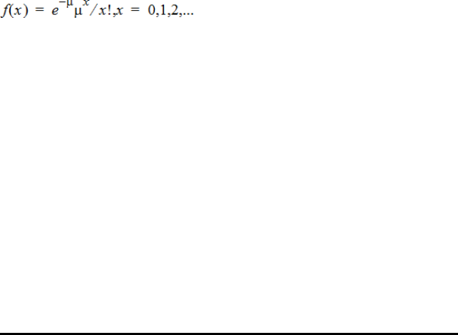
465 Lists&Spreadsheet Application
This distribution is useful in determining the probability of a success on one trial before
all trials are completed. For example, if heads is a successful coin toss and you plan to
toss the coin 10 times, this distribution would predict the chance of obtaining heads at
least once in the 10 tosses.
Inverse Binomial (invBinom())
Given the number of trials (NumTrials) and the probability of success of each trial
(Prob), this function returns the minimum number of successes, k, such that the
cumulative probability of ksuccesses is greater than or equal to the given cumulative
probability (CumulativeProb).
Inverse Binomial with respect to N (invBinomN())
Given the probability of success of each trial (Prob), and the number of successes
(NumSuccess), this function returns the minimum number of trials, N, such that the
cumulative probability of xsuccesses is less than or equal to the given cumulative
probability (CumulativeProb).
Poisson Pdf (poissPdf())
Computes a probability at xfor the discrete Poisson distribution with the specified
mean, μ, which must be a real number >0. xcan be an integer or a list of integers.
The probability density function (Pdf) is:
This distribution is useful in determining the probability of obtaining a certain number
of successes before a trial begins. For example, you could use this calculation to
predict the number of heads that would occur in eight tosses of a coin.
Poisson Cdf (poissCdf())
Computes a cumulative probability for the discrete Poisson distribution with specified
mean, x.
This distribution is useful in determining the probability that a certain number of
successes occur between the upper and lower bounds of a trial. For example, you could
use this calculation to predict the number of heads displayed between coin toss No.3
and toss No.8.

Geometric Pdf (geomPdf())
Computes a probability at x, the number of the trial on which the first success occurs,
for the discrete geometric distribution with the specified probability of success p. 0{p
{1 must be true. xcan be an integer or a list of integers. The probability density
function (Pdf) is:
This distribution is useful in determining the likeliest number of trials before a success
is obtained. For example, you could use this calculation to predict the number of coin
tosses that would be made before a heads resulted.
Geometric Cdf (geomCdf())
Computes a cumulative geometric probability from lowBound to upBound with the
specified probability of success, p.
This distribution is useful in determining the probability associated with the first
success occurring during trials 1 through n. For example, you could use this calculation
to determine the probability that heads display on toss No.1, No.2, No.3, ..., No.n.
Confidence Intervals
Supported Confidence Intervals
The following confidence intervals are available from the Lists&Spreadsheets
application. For more information regarding these functions, see the TI-Nspire™
Reference Guide.
z Interval (zInterval)
Computes a confidence interval for an unknown population mean, m, when the
population standard deviation, s, is known. The computed confidence interval depends
on the user-specified confidence level.
This test is useful in determining how far from a population mean a sample mean can
get before indicating a significant deviation.
t Interval (tInterval)
Computes a confidence interval for an unknown population mean, m, when the
population standard deviation, s, is unknown. The computed confidence interval
depends on the user-specified confidence level.
This test is useful in examining whether the confidence interval associated with a
confidence level contains the value assumed in the hypothesis. Like the z Interval, this
test helps you determine how far from a population mean a sample mean can get
before indicating a significant deviation when the population mean is unknown.
Lists&Spreadsheet Application 466

467 Lists&Spreadsheet Application
2-Sample z Interval (zInterval_2Samp)
Computes a confidence interval for the difference between two population means
(m1Nm2) when both population standard deviations (s1and s2) are known. The
computed confidence interval depends on the user-specified confidence level.
This test is useful in determining if there is statistical significance between the means
of two samples from the same population. For example, this test could determine
whether there is significance between the mean college entrance test score of female
students and the mean of college entrance test score of male students at the same
school.
2-Sample t Interval (tInterval_2Samp)
Computes a confidence interval for the difference between two population means
(m1Nm2) when both population standard deviations (s1and s2) are unknown. The
computed confidence interval depends on the user-specified confidence level.
This test is useful in determining if there is statistical significance between the means
of two samples from the same population. It is used instead of the 2-sample z
confidence interval in situations where the population is too large to measure to
determine the standard deviation.
1-Prop z Interval (zInterval_1Prop)
Computes a confidence interval for an unknown proportion of successes. It takes as
input the count of successes in the sample xand the count of observations in the
sample n. The computed confidence interval depends on the user-specified confidence
level.
This test is useful in determining the probability of a given number of successes that
can be expected for a given number of trials. For instance, casino examiners would use
this test to determine if observed payouts for one slot machine demonstrate a
consistent pay out rate.
2-Prop z Interval (zInterval_2Prop)
Computes a confidence interval for the difference between the proportion of successes
in two populations (p1-p2). It takes as input the count of successes in each sample
(x1andx2) and the count of observations in each sample (n1andn2). The computed
confidence interval depends on the user-specified confidence level.
This test is useful in determining if two rates of success differ because of something
other than sampling error and standard deviation. For example, a gambler could use
this test to determine if there is an advantage in the long run by playing one game or
machine versus playing another game or machine.
Linear Reg t Intervals (LinRegtIntervals)
Computes a linear regression t confidence interval for the slope coefficient b. If the
confidence interval contains 0, this is insufficient evidence to indicate that the data
exhibits a linear relationship.

Multiple Reg Intervals (MultRegIntervals)
Computes multiple regression prediction confidence interval for the calculated y and a
confidence for y.
Stat Tests
Supported Statistical Tests
Hypothesis tests are available from the Lists&Spreadsheets application. For more
information regarding these functions, see the TI-Nspire™ Reference Guide.
Some of the wizards for Stat Tests display a Draw box. By default, the box is not
selected. Selecting the box creates a Data&Statistics work area on the page and plots
the results in that work area.
ztest (zTest)
Performs a hypothesis test for a single unknown population mean, m, when the
population standard deviation,s, is known. It tests the null hypothesis H0:m=m0
against one of the alternatives below.
• Ha:mƒm0
• Ha:m<m0
• Ha:m>m0
This test is used for large populations that are normally distributed. The standard
deviation must be known.
This test is useful in determining if the difference between a sample mean and a
population mean is statistically significant when you know the true deviation for a
population.
ttest (tTest)
Performs a hypothesis test for a single unknown population mean, m, when the
population standard deviation, s, is unknown. It tests the null hypothesis H0:m=m0
against one of the alternatives below.
• Ha:mƒm0
• Ha:m<m0
• Ha:m>m0
This test is similar to a z-test, but is used when the population is small and normally
distributed. This test is used more frequently than the z-test because small sample
populations are more frequently encountered in statistics than are large populations.
This test is useful in determining if two normally distributed populations have equal
means, or when you need to determine if a sample mean differs from a population
mean significantly and the population standard deviation is unknown.
Lists&Spreadsheet Application 468

469 Lists&Spreadsheet Application
2-Sample z Test (zTest_2Samp)
Tests the equality of the means of two populations (m1and m2) based on independent
samples when both population standard deviations (s1and s2) are known. The null
hypothesis H0:m1=m2is tested against one of the alternatives below.
• Ha:m1ƒm2
• Ha:m1<m2
• Ha:m1>m2
2-Sample t Test (tTest_2Samp)
Tests the equality of the means of two populations (m1and m2) based on independent
samples when neither population standard deviation (s1or s2) is known. The null
hypothesis H0:m1=m2is tested against one of the alternatives below.
• Ha:m1ƒm2
• Ha:m1<m2
• Ha:m1>m2
1-Prop z Test (zTest_1Prop)
Computes a test for an unknown proportion of successes (prop). It takes as input the
count of successes in the sample xand the count of observations in the sample n.
1-Prop z Test tests the null hypothesis H0:prop=p0against one of the alternatives
below.
• Ha: propƒp0
• Ha: prop<p0
• Ha: prop>p0
This test is useful in determining if the probability of the success seen in a sample is
significantly different from the probability of the population or if it is due to sampling
error, deviation or other factors.
2-Prop z Test (zTest_2Prop)
Computes a test to compare the proportion of successes (p1and p2) from two
populations. It takes as input the count of successes in each sample (x1and x2) and
the count of observations in each sample (n1and n2). 2-Prop z Test tests the null
hypothesis H0:p1=p2(using the pooled sample proportion Ç) against one of the
alternatives below.
• Ha: p1ƒp2
• Ha: p1<p2
• Ha: p1>p2
This test is useful in determining if the probability of success seen in two samples is
equal.
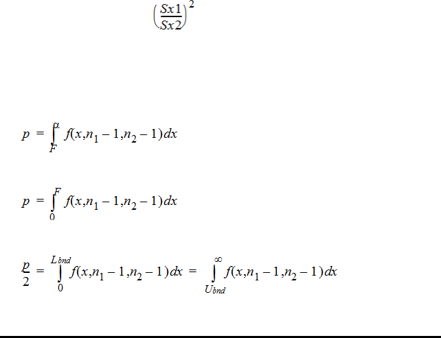
c2GOF (c2GOF)
Performs a test to confirm that sample data is from a population that conforms to a
specified distribution. For example, c2GOF can confirm that the sample data came
from a normal distribution.
c22-way Test (c22way)
Computes a chi-square test for association on the two-way table of counts in the
specified Observed matrix. The null hypothesis H0for a two-way table is: no
association exists between row variables and column variables. The alternative
hypothesis is: the variables are related.
2-Sample FTest (FTest_2Samp)
Computes an F-test to compare two normal population standard deviations (s1and
s2). The population means and standard deviations are all unknown. 2-Sample FTest,
which uses the ratio of sample variances Sx12/Sx22, tests the null hypothesis
H0:s1=s2against one of the alternatives below.
• Ha:s1ƒs2
• Ha:s1<s2
• Ha:s1>s2
Below is the definition for the 2-SampleFTest.
Sx1,Sx2 = Sample standard deviations having n1N1 and n2N1 degrees of
freedom df, respectively.
F=F-statistic =
df(x, n1N1,
n2N1)
=Fpdf() with degrees of freedom df, n1N1, and n2N1
p= reported pvalue
2-Sample FTest for the alternative hypothesis s1>s2.
2-Sample FTest for the alternative hypothesis s1<s2.
2-Sample FTest for the alternative hypothesis s1ƒs2. Limits must satisfy the following:
Lists&Spreadsheet Application 470

471 Lists&Spreadsheet Application
where: [Lbnd,Ubnd]=lower and upper limits
The F-statistic is used as the bound producing the smallest integral. The remaining
bound is selected to achieve the preceding integral’s equality relationship.
Linear Reg t Test (LinRegtTest)
Computes a linear regression on the given data and a ttest on the value of slope band
the correlation coefficient rfor the equation y=a+bx. It tests the null hypothesis
H0:b=0 (equivalently, r=0) against one of the alternatives below.
• Ha:bƒ0 and rƒ0
• Ha:b<0 and r<0
• Ha:b>0 and r>0
Multiple Reg Tests (MultRegTest)
Computes a linear regression on the given data, and provides the F test statistic for
linearity.
For more information, see the TI-Nspire™ Reference Guide.
ANOVA (ANOVA)
Computes a one-way analysis of variance for comparing the means of 2 to 20
populations. The ANOVA procedure for comparing these means involves analysis of the
variation in the sample data. The null hypothesis H0:m1=m2=...=mkis tested against the
alternative Ha: not all m1...mkare equal.
The ANOVA test is a method of determining if there is a significant difference
between the groups as compared to the difference occurring within each group.
This test is useful in determining if the variation of data from sample-to-sample shows
a statistically significant influence of some factor other than the variation within the
data sets themselves. For example, a box buyer for a shipping firm wants to evaluate
three different box manufacturers. He obtains sample boxes from all three suppliers.
ANOVA can help him determine if the differences between each sample group are
significant as compared to the differences within each sample group.
ANOVA 2-Way (ANOVA2way)
Computes a two-way analysis of variance for comparing the means of two to 20
populations. A summary of results is stored in the stat.results variable.
The two-way ANOVA analysis of variance examines the effects of two independent
variables and helps to determine if these interact with respect to the dependent
variable. (In other words, if the two independent variables do interact, their combined
effect can be greater than or less than the impact of either independent variable
additively.)
This test is useful in evaluating differences similar to the ANOVA analysis but with the
addition of another potential influence. To continue with the ANOVA box example, the
two-way ANOVA might examine the influence of box material on the differences seen.

Selecting an Alternative Hypothesis (ƒ< >)
Most of the inferential stat editors for the hypothesis tests prompt you to select one of
three alternative hypotheses.
• The first is a ƒalternative hypothesis, such as mƒm0 for the zTest.
• The second is a <alternative hypothesis, such as m1<m2 for the 2-SampletTest.
• The third is a >alternative hypothesis, such as p1>p2 for the 2-PropzTest.
To select an alternative hypothesis, move the cursor to the appropriate alternative, and
then press Enter.
Selecting the Pooled Option
Pooled (2-SampletTest and 2-SampletInterval only) specifies whether the variances
are to be pooled for the calculation.
• Select No if you do not want the variances pooled. Population variances can be
unequal.
• Select Yes if you want the variances pooled. Population variances are assumed to
be equal.
To select the Pooled option, select Yes from the drop-down list.
Working with Function Tables
The Lists&Spreadsheet application lets you show a table of function values for any
function in the current problem. You can change the settings for the table, delete
columns, add values for multiple functions, and edit the expression that defines a
function without leaving the Lists&Spreadsheet application.
Switching to a Table
1. While working in the Lists&Spreadsheet application:
Windows: Press Ctrl+T.
Mac®: Press “+T.
Handheld: Press / T.
The Lists&Spreadsheet application disappears and an empty table is displayed
with a list of the functions that are available in the problem.
Note: If you have previously shown a table for a function from the
Lists&Spreadsheet application, the table includes that function by default.
2. Choose the name of the function for which you want to display values.
Values for the function you selected are displayed in the first column of the table.
Lists&Spreadsheet Application 472

473 Lists&Spreadsheet Application
3. To move through adjacent cells of the table, press ▲or ▼. Press Tab to move
from the body of the table (cells) to the top two rows (cells for column names and
formulas).
4. To hide the table of values and return to the Lists&Spreadsheet application,
repeat Step 1.
Making Changes from a Table
You can change the table of function values using the tools on the Table menu.
▶To remove a column from the table, click any cell and click Delete Column.
▶To display the list of functions, click a cell in a column and click Choose. Select a
cell in an empty column unless you are replacing values already displayed. Click a
function in the list to add its values to the column.
Note: You can also click the drop-down arrow on the top cell of a column to display
the list of functions in the problem.
▶To change the expression that defines a function, click Edit Expression. You can also
edit the expression directly on the entry line beneath the table.
Note: When you edit the expression for a function, that function automatically
changes in the application used to define the function. For example, if you edit a
Graphs&Geometry function in the table, the table values and graph of the
function are both updated.
▶To change the default table settings, choose Edit Table Settings.
The Table dialogue box opens. Press Tab to move from field to field and type or
select new values for the default table settings:
-Table Start: Type the value to use as the first value in the table of values.
-Table Step: Type a value for the interval between values.
-Independent and Dependent: Click the drop-down arrow to choose Auto or Ask
as the method for populating a column with the values of the independent and
dependent variables. Auto populates the table starting at the defined table
start value and displays an independent and dependent value for each step. Ask
lets you select a cell and press Enter to generate a value for a cell.
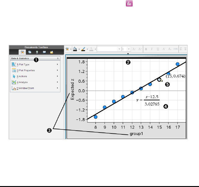
Data&Statistics Application
The Data&Statistics application provides tools to:
• Visualise sets of data in different types of plots.
• Directly manipulate variables to explore and visualise data relationships. Data
changes in one application are dynamically applied to all linked applications.
• Explore central tendency and other statistical summary techniques.
• Fit functions to data.
• Create regression lines for scatter plots.
• Graph hypothesis tests and results (z- and t-tests) based on summary statistics
definitions or data.
Adding a Data&Statistics Page
▶To start a new document with a blank Data&Statistics page:
From the main File menu, click New Document, and then click Add
Data&Statistics.
Handheld: Press c, and select Data&Statistics .
▶To add a Data&Statistics page in the current problem of an existing document:
From the toolbar, click Insert > Data&Statistics.
Handheld: Press ~and select Insert > Data&Statistics.
ÀData&Statistics menu
ÁWork area
ÂAdd Variable regions on x-axis and y-axis
Data&Statistics Application 474

475 Data&Statistics Application
ÃNormal Probability Plot with expression
ÄData point with coordinates
Basic Operations in Data& Statistics
The Data& Statistics application lets you explore and visualise data and graph
inferential statistics. The Lists& Spreadsheet application can work in conjunction with
the Data& Statistics application. The Lists& Spreadsheet Summary Plot and Quick
Graph tools automatically add a Data& Statistics application to show plots. A list that
you create in a problem (using the Lists& Spreadsheet or Calculator applications) can
be accessed as a variable in any TI-Nspire™ application in that problem.
Changing Data& Statistics Settings
1. From the Settings menu, select Settings.
2. Select the settings that you want to use.
•Display Digits. Lets you select the display format for numeric labels in the
current document. Select Auto to automatically follow the setting in the
Document Settings dialogue box.
•Diagnostics. Displays the value of the r2or R2statistic (when available) under
certain regression equations.
-r2is displayed for Linear (mx+b), Linear (a+bx), Power, Exponential and
Logarithmic regressions.
-R2is displayed for Quadratic, Cubic and Quartic regressions.
Using the Default Caseplot
The Data& Statistics application plots numeric and string (categorical) data from
variables. When you add a Data& Statistics application to a problem that includes
lists, a default caseplot displays on the work area.
The caseplot is like having a stack of cards with information on them and scattering
the cards randomly on a table. You can click a dot to see the information on that
“card”. You can drag a dot to “group” the “cards” by the caption variable.
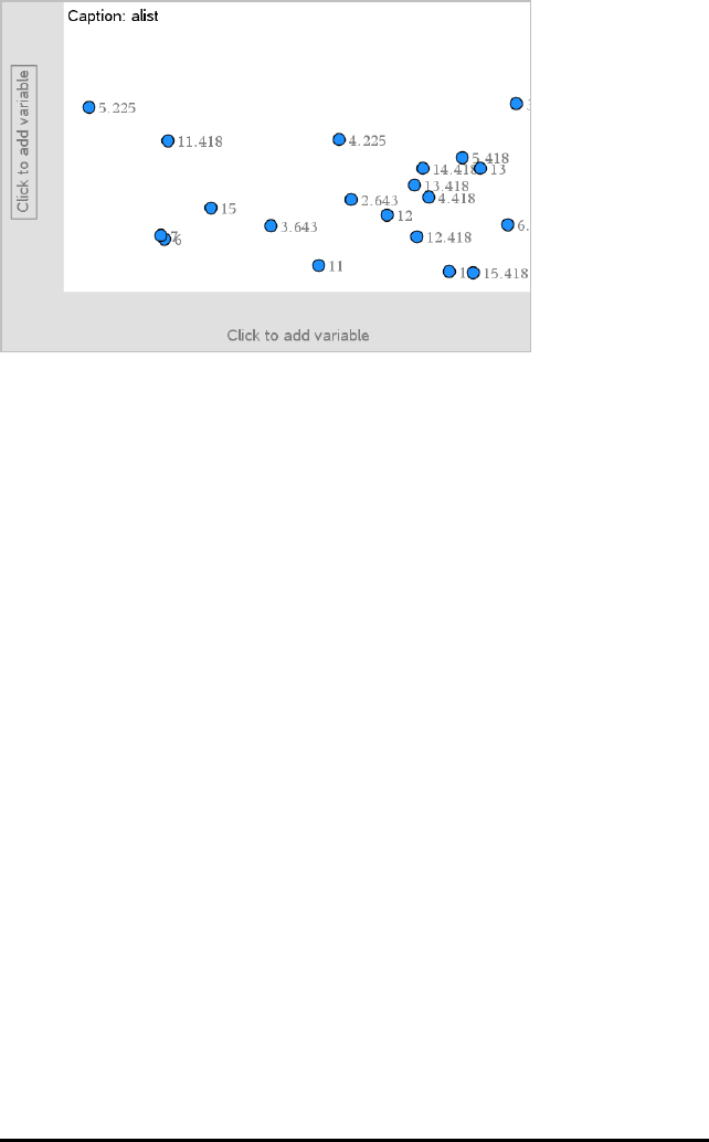
▶Click the variable name displayed after Caption to use the caseplot.
- Choose <None> to remove the default caseplot.
- Choose the name of a variable to have it replace the current caseplot variable.
- Hover over any data point to see the summary information.
- Drag any data point toward an axis to see how the points group.
- Activate the Graph Trace tool and press ◄or►to move across points.
When you add a variable to either axis, the plot for that variable replaces the default
caseplot. The default caseplot redisplays if you remove the plotted variable from each
axis.
Using the Context Menu
The context menu provides access to the tools most commonly used with the selected
object. The context menu displays different options depending on the active object and
the task you are performing.
▶To open the context menu for an object.
Windows®: Right-click the object.
Mac®: Hold “and click the object.
Handheld: Point to the object and press / b.
The context menu includes the Colour option. You can use the Colour option to change
the data to the colour of your choice.
Data&Statistics Application 476
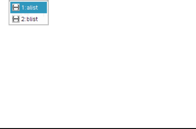
477 Data&Statistics Application
Other options that are appropriate for various plots also appear on the context menu.
Selecting Data and Displaying Summary Information
When you hover over part of a plot, the Data& Statistics application displays summary
information for the data it represents.
1. Hover at an area of interest in a plot to display data values or summary
information. For example, you can hover over the centre of a box plot to display the
median summary data.
2. Click once to select a representation of data in a plot.
Data points are shown with a bold outline to indicate selection. You can click a
point a second time to deselect it, or click additional points to add to the selection.
Plotting Variables
To plot variables, start with a problem that includes a Data& Statistics application and
lists created in the Lists& Spreadsheet application or the Calculator application.
1. Click the Add Variable region near the centre of an axis.
If no variable is plotted on the axis, the tooltip Click or Enter to add variable
displays.
2. Click the tooltip Click or Enter to add variable.
A list displays the names of available variables.
3. Click the name of the variable to plot.
Note: By convention, the independent variable is shown on the x-axis.
The default plot for one variable is a dot chart. The data points in the default
caseplot reposition to represent the elements of the selected variable in a dot
chart.
4. (Optional) Click the Add Variable region near the centre of the remaining axis to
plot a second variable.
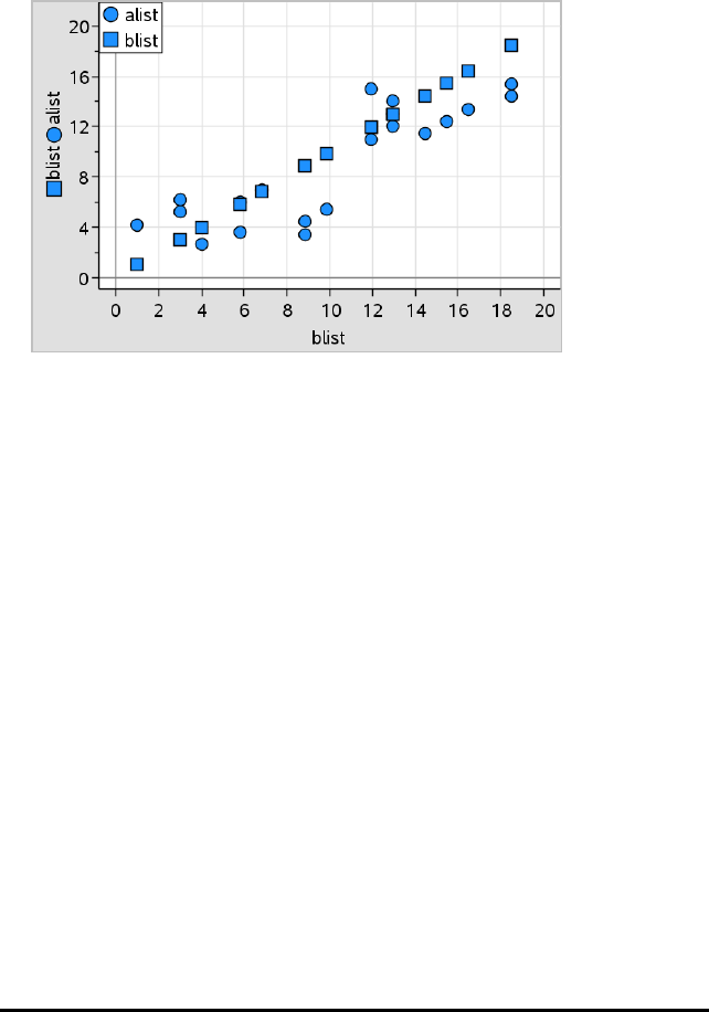
The default plot for two variables is a scatter plot. The data points shift to
represent the elements of both variables as a scatter plot.
5. (Optional) Repeat Steps 1-3 to choose additional variables to plot on the vertical
axis.
The name of each variable that you add is appended to the label on the axis. The
default data point shape changes to help you distinguish data, and a legend is
displayed to identify the shapes.
6. Change, analyse or explore the plotted data.
- Remove or change the variable on an axis by clicking the Add Variable region
again.
- View the plotted data in another supported plot type by selecting a tool from
the Plot Typesmenu.
- Choose the Graph Trace tool on the Analyse menu and press ◄or►to move
across the data points in the plot.
- The lists that you plot as variables can include incomplete or missing cases. (A
case is the data contained in a row of cells in the Lists& Spreadsheet
application.) The Lists& Spreadsheet application displays a void as an
underscore (“_”), and Data& Statistics plots no data point for a void cell.
Manipulating Plotted Data
You can manipulate data points on the Data& Statistics work area to explore their
effects. For example, you could explore how a specific group of values affects the
median.
Data&Statistics Application 478
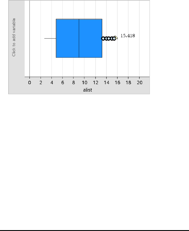
479 Data&Statistics Application
You can move a data point only in directions allowed by its definition. If a list is defined
with a formula in Lists& Spreadsheet, the points in Data& Statistics may not move
because of the formula’s restrictions. For example, you can manipulate a plot that
represents the result of y=x, but you can only move along a line.
You cannot move points that represent data in a locked variable or data that represents
a categorical value.
1. On the Data& Statistics work area, click a representation of data—such as a
histogram bin or a whisker of a box plot—that is not locked or restricted by a
formula.
The pointer changes to an open hand to show that the data can be moved.
2. Drag the selection to explore how different values of the point affect the plot.
Handheld: Press / a to grab, and then swipe or use the arrow keys to drag.
As you drag, the changing value displays on the work area.
Overview of Raw and Summary Data
You can create plots directly from raw data or from a summary table.
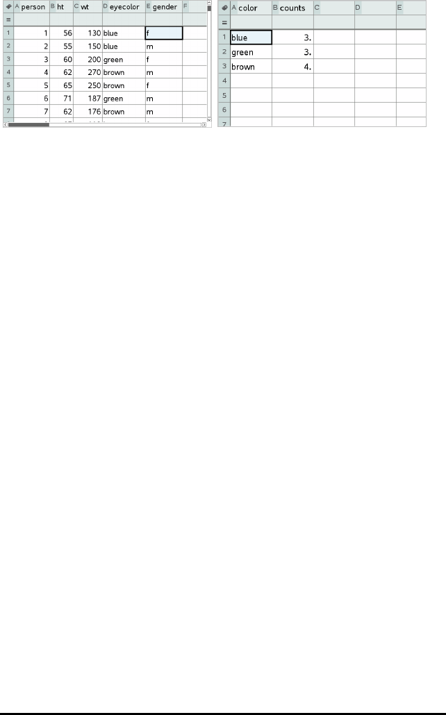
Raw data Summary table for eye colour based on raw data
• Raw data consists of a single list, such as a list of eye colours. When you create a
plot of raw data, Data&Statistics counts the occurrences for you. Plotting raw
data directly gives you flexibility in analysing it.
• A summary table consists of two lists, such as eye colours (the XorYList) and
counts of eye-colour occurrences (the Summary List). For more information, see
Using Lists&Spreadsheet chapter.
Working with Numeric Plot Types
Plots can represent the data from a variable in a variety of ways. Choosing the
appropriate plot can help you visualise the data. For example, you may be able to
observe the shape and spread of the data in one plot type and another type may be
useful for determining the best method for statistically evaluating data.
Creating Dot Plots
Dot plots, also known as dot-frequency plots, represent one-variable data. Dot plots are
the default plot type for numeric data. When you plot a variable as a dot plot, one dot
represents each value in the list. Each dot displays on the axis at a point that
correspond to the value.
1. To create a dot plot, click the Add Variable region in the center of an axis and click
the name of a numeric variable. For more information, see Plotting Variables.
2. (Optional) To split a dot plot by category, click the Add Variable region on the other
axis and choose the list that contains the corresponding category data.
3. (Optional) To plot multiple dot plots, choose Add X Variable on the Plot Properties
menu and click a numeric variable from the list that displays.
A second dot plot appears on the work area and the name of the plotted variable is
added to both axis labels.
4. Explore the plotted data.
- Hover over a data point to display data values.
Data&Statistics Application 480
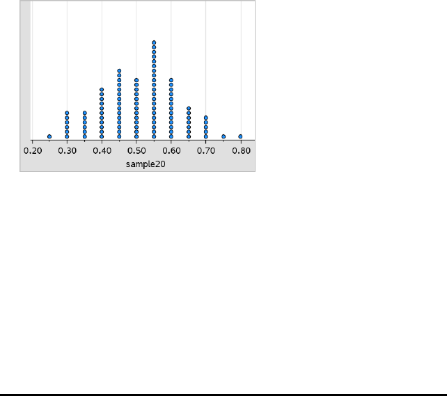
481 Data&Statistics Application
- Drag a dot to move it. As you move a point, the values associated with it
change on the work area display and in the list for the variable.
- Activate the Graph Trace tool and press ◄or►to move across the data
points in the plot in list order. Points enlarge and display a bold outline as you
move across them in Trace mode.
Creating Box Plots
The Box Plot Tool plots one-variable data in a modified box plot. “Whiskers” extend
from each end of the box, either to 1.5 times the interquartile range or to the end of
the data, whichever comes first. Points that are a width of 1.5*Interquartile Range
past the quartiles plot individually, beyond the whiskers. These points are the potential
outliers. When no outliers exist, x-min and x-max are the prompt for the end of each
whisker.
Box plots are useful for comparing two or more sets of data that use the same scale. If
a dataset is large, a box plot can also be useful in exploring data distribution.
1. Click the Add Variable region in the centre of an axis. The default plot for one
numeric variable is a dot plot. For more information, see Plotting Variables.
Note: If two variables are plotted in the work area, you can create a dot plot by
removing one variable. Choose RemoveXVariable or RemoveYVariable from the
Plot Types menu.
2. On the Plot Types menu, click Box Plot.
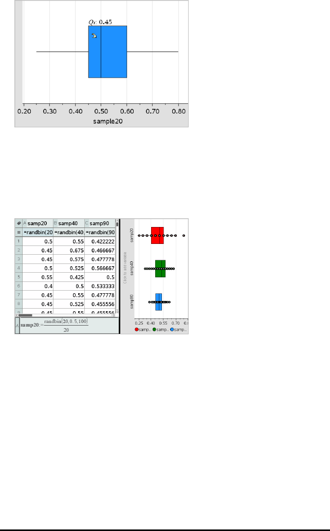
A modified box plot displays on the Data&Statistics work area.
Note: You can split a box plot by category by adding a list that contains
corresponding categorical data to the y-axis.
3. (Optional) To add additional variables for comparing box plots on the same axis,
click Add X Variable on the Plot Properties menu.
For example, you can use multiple box plots to compare the distributions of sample
proportions. In the example, true proportion is .5 and sample size varies from n=20
to n=40 to n=90.
Notes:
- You can create a box plot with frequency by choosing Add X Variable or Add Y
Variable on the Plot Properties menu.
- You can specify a variable multiple times as you choose variables to plot as box
plots.
- The variable used to provide frequency information is added to the label on the
horizontal axis in the format: x_variablename{frequencylist_name}.
Data&Statistics Application 482

483 Data&Statistics Application
4. Point and click the regions of the box plot to explore and analyse the data it
represents.
- Hover over a region or over a whisker to display the details for the portion of
the plot that interests you. The label for the quartile that corresponds to your
selection is displayed.
- Click a region of the box plot to select the data points or whiskers. Click again
to remove the selection.
- You can select any box plot that does not include frequency data and choose
Dot Plot on the context menu to change the plot type.
- Drag a selection to move it and explore other possibilities for the data.
- Use the arrow keys to move a data point one pixel at a time.
- Activate the Graph Trace tool and press ◄or►to move across dots and
regions of the plot. As the trace cursor moves, the values for Q1, the median,
Q3 and whisker ends/outliers are displayed.
5. Change the plot from a modified box plot to a standard box plot by choosing Extend
Box Plot Whiskers on the Plot Properties menu.
The box plot is redrawn as a standard box plot with extended whiskers.
The standard box plot’s whiskers use the minimum and maximum points in the
variable and outliers are not identified. The whiskers on the plot extend from the
minimum data point in the set (x-min) to the first quartile (Q1) and from the third
quartile (Q3) to the maximum point (x-max). The box is defined by Q1, Med
(median), and Q3.
Note: You can click Show Box Plot Outliers on the Plot Properties menu to return to
the modified box plot.
Plotting Histograms
A histogram plots one-variable data and depicts the distribution of data. The number
of bins displayed depends on the number of data points and the distribution of these
points. A value that occurs on the edge of a bin is counted in the bin to the right.
Creating a Histogram from Raw Data
1. Create the list that you want to plot as a histogram. For example, you can enter or
collect data as a named list on a Lists&Spreadsheet page.
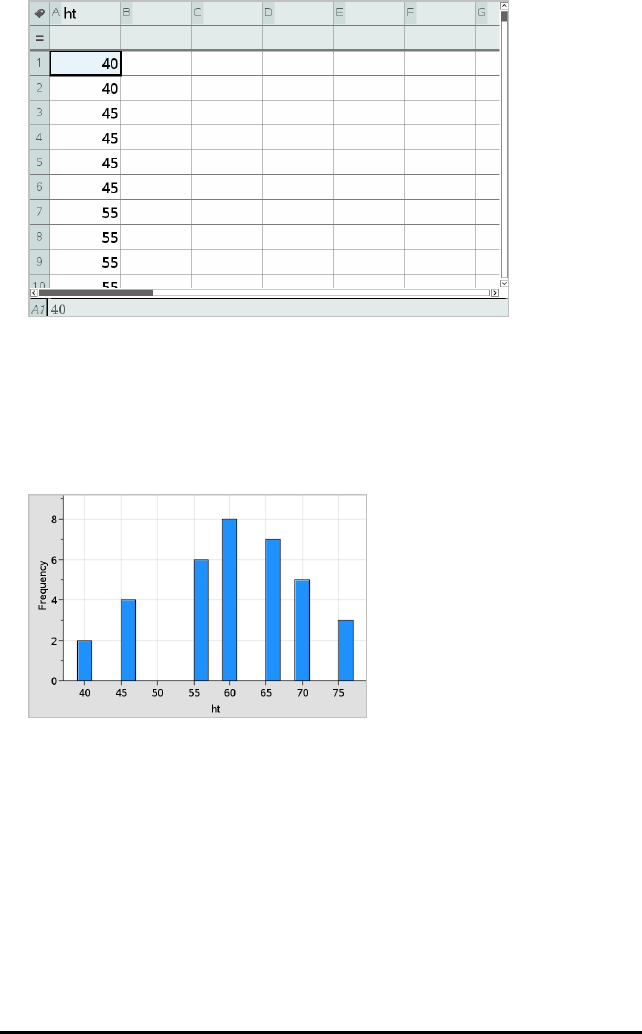
2. On a Data&Statistics page, click the x or y axis, and select your list as the data to
plot.
3. From the Plot Types menu, click Histogram.
The data forms the bins of a histogram, with Frequency plotted by default on the
unselected axis.
4. Explore the data.
- Hover over a bin to see the information for that bin.
- Click a bin to select it. Click the bin again to deselect it.
- Drag the side of a bin to adjust bin width and number of bins.
Note: The bins are not adjustable in categorical plots or plots in which you
choose variable bin widths.
- On the Analyse menu, click Graph Trace and press ◄or►to cycle through the
bins and display their values.
Data&Statistics Application 484
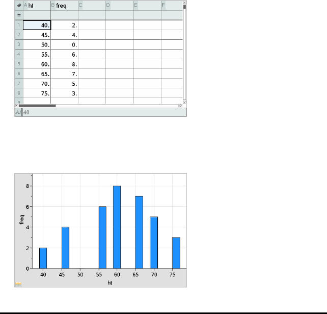
485 Data&Statistics Application
Adjusting the Histogram Scale of Raw Data
1. On the Plot Properties menu, click Histogram Properties and choose Histogram
Scale.
2. Choose the format for the scale of the histogram.
-Frequency - displays data based upon the number of values that occur within
each bin. This is the default data representation.
-Percent - displays data in the histogram by each group’s percent value of the
whole data set.
-Density - displays data based upon the density of each group within the data
set.
Creating a Histogram with Frequency or Summary Data
1. On a Lists&Spreadsheet page, create two lists: one containing the “bins”, such as
heights in a population (ht), and the other containing the frequencies of those
heights (freq).
2. On a Data&Statistics page, access the context menu on the x axis, and click Add X
Variable with Summary List.
3. Select ht as the X List and freq as the Summary List.
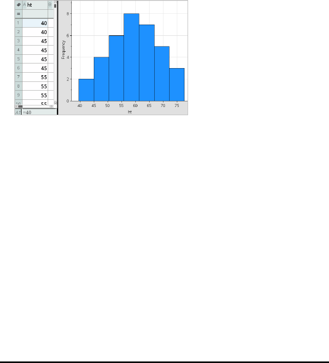
Note: It is up to you to set the data and bins in a meaningful way when using
summary data.
Setting Equal Bin Widths
By default, bin widths are set to equal. You can specify the width and alignment of
equal-width bins.
1. On the Plot Properties menu, click HistogramProperties > BinSettings and choose
Equal Bin Width.
The Equal Bin Width Settings dialogueue box opens.
2. Type values to set Width and Alignment of the bins.
3. Click OK to apply the changes and redraw the bins.
Both the data represented by the bins and the value you type for the alignment
affect the placement of bins on the scale.
Setting Variable Bin Widths
You can set variable bin widths based on a list of bin boundaries.
1. Create a named list containing boundary values.
For example, a boundary list defined as {60,70,100,110} will create bins at 60 to
70, 70 to 100 and 100 to 110.
Note: The data must fall within the specified bin widths. For example, a data point
of 115 would be outside the bins in the above list, and you would receive a
Data/Bin Location Mismatch error.
2. On the Plot Properties menu, click HistogramProperties > BinSettings and choose
Variable Bin Width.
The Variable Bin Width Settings dialogue box opens.
Data&Statistics Application 486
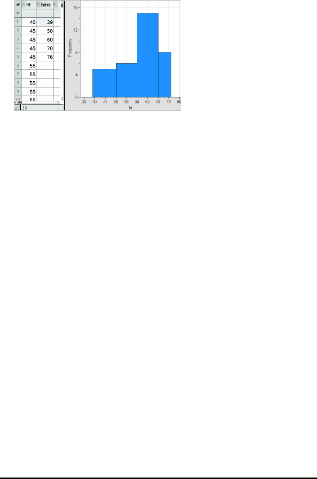
487 Data&Statistics Application
3. Select your boundary list as the List of Bin Boundaries.
4. Click OK to apply the changes and redraw the bins.
Note: You cannot change variable bin widths by dragging their boundaries; you
must edit the list of boundaries or restore equal-width bins.
Creating a Normal Probability Plot
A normal probability plot shows one set of data against the corresponding quartile (z)
of the standard normal distribution. You can use normal probability plots to judge the
appropriateness of the normal model for your data.
1. Choose or create the data you want to use for a normal probability plot. Use a
named list from Lists&Spreadsheet or Calculator.
2. Plot the data in one of the following ways:
- Create a dot plot by selecting a column and choosing QuickGraph.
- Add a Data&Statistics work area. Click the Add Variable region on an axis and
click the data list name to plot the variable.
3. On the Plot Types menu, click Normal Probability Plot.
The data graphs in the Data&Statistics work area. You can examine the graph to
compare the normal variable against the quartile.
4. Explore the data represented in the normal probability plot.
- Hover over a data point to display its value.
- Click to select a data point. Click again to deselect it.
- Click multiple data points to select them.
- Activate the Graph Trace tool and press ◄or►to move across the data
points and display values.
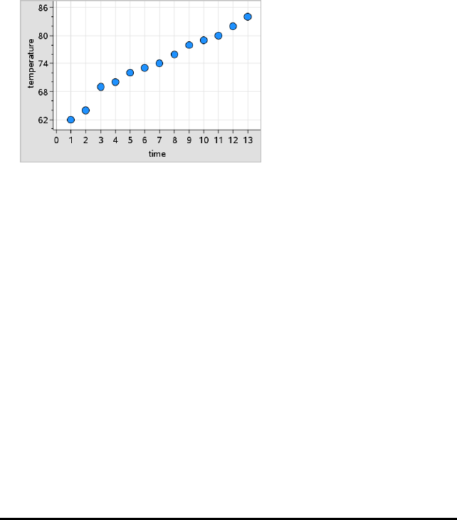
Creating a Scatter Plot
A scatter plot shows the relationship between two sets of data. You can also plot a
scatter plot by using the Quick Graph tool in the Lists&Spreadsheet application.
1. In the Data&Statistics work area, click the Add Variable region and select the
variable that contains the data you want to see represented on an axis.
The plot of the selected variable displays on the axis.
2. Click the Add Variable region of the other axis and select the variable containing
the data you want to plot.
The data points shift to represent the data in the selected variable.
3. Analyse and explore the data in the plot.
- Click a point to select it.
- Hover over a data point to view the summary data.
- Work with the data using the available tools on the Analyse menu. For
example, choose the Graph Trace tool and press ◄or►to move across the
plot.
4. Optional: To plot additional lists against the x-axis, right-click the y-axis and click
Add Variable.
Creating an X-Y Line Plot
An X-Y line plot is a scatter plot in which the data points are plotted and connected in
order of appearance in the two variables. Like scatter plots, these plots depict the
relationship between two sets of data.
By convention, the left-most column of data is represented on the horizontal axis.
1. Create a scatter plot. For more information, see Creating a Scatter Plot.
Data&Statistics Application 488
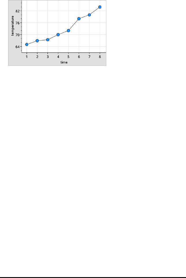
489 Data&Statistics Application
2. On the Plot Types menu, click the XY Line Plot tool.
The data points within each set are connected to each other by a line.
Note: The dots are connected in the order that they appear in the list variable on
the horizontal axis. To change the order, use the sort tool in Lists&Spreadsheet.
3. Analyse and explore the data in the plot.
- Hover over a data point to view the summary data.
- Work with the data using the available tools on the Analyse menu. For
example, choose the Graph Trace tool and press the arrow keys to move across
the dots in the plot and view the values.
Working with Categorical Plot Types
You can sort and group data using the categorical plot types:
• Dot Chart
• Bar Chart
• Pie Chart
The categorical plot types can be used to compare the representations of data across
different plots. When the same variable (list) is used for a dot chart and a bar chart or
pie chart in a problem, selecting a data point or segment in one of the plots selects the
corresponding data point, segment or bar in all other plots that include the variable.
Creating a Dot Chart
The default plot type for categorical data is the dot chart.
When one variable is plotted, the value of each cell is represented as one dot, and the
dots are stacked at the point on the axis that corresponds to the cell value.
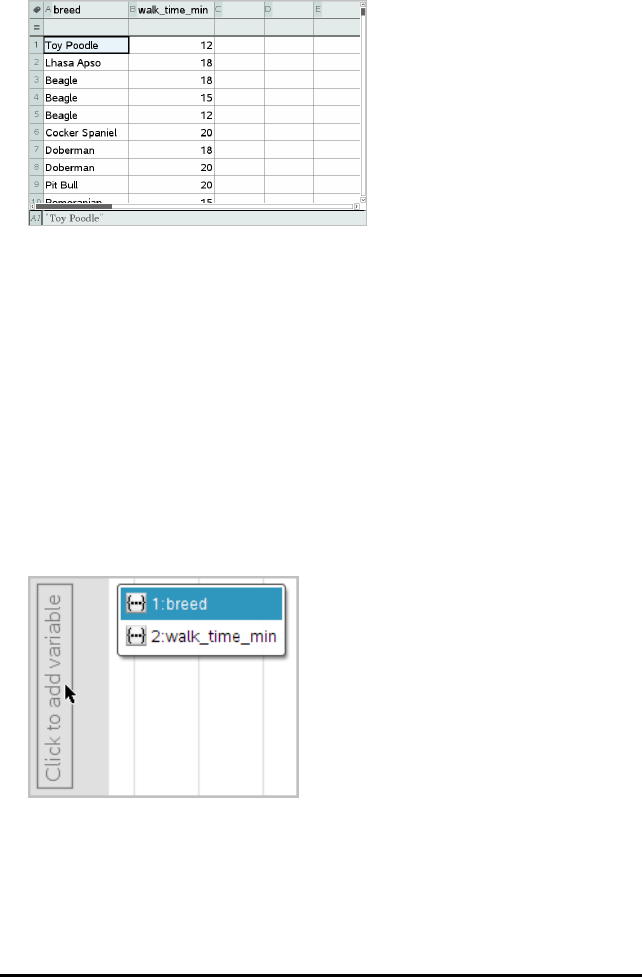
1. In Lists&Spreadsheet, create a spreadsheet that includes at least one column of
string values that can be used as categories for data.
Note: To type a string in Lists&Spreadsheet, enclose the characters in quotes.
2. Add a Data&Statistics page to the problem.
Notes:
- You can also use the Lists&Spreadsheet Quick Graph tool to automatically add
a Data&Statistics page and plot the selected column.
- The new Data&Statistic work area displays a default caseplot with a caption,
variable name and unplotted data points for the variable. You can click the
variable name in the caption to choose another variable for previewing, or drag
a default data point toward an axis to plot the current variable.
3. Move near the centre of either axis and click the Add List region. The list of
variables displays.
4. Click the list that contains the categories you want to use for sorting data.
Data&Statistics Application 490
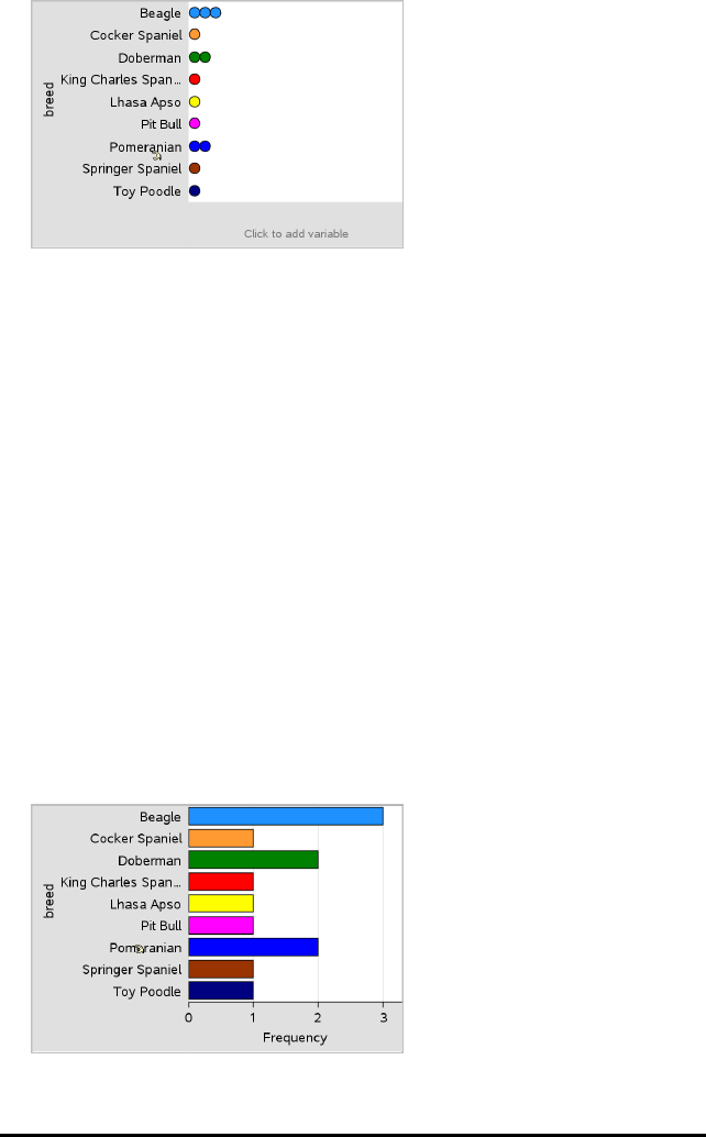
491 Data&Statistics Application
A dot chart plots in the work area. The application labels the axis with the variable
name and shows a dot for each instance of a category.
5. Explore the plotted data.
- Hover over a dot in the plot to display data values.
- Click a dot to select it. Click the dot a second time to deselect it or remove it
from a selection of multiple dots.
- Activate the Graph Trace tool and press ◄or ►to move across the points in
list order. Dots display a bold outline as you move across them in Trace mode.
Creating a Bar Chart
Like dot charts, bar charts display categorical data. The length of a bar represents the
number of cases in the category.
1. Click the Add Variable region of either axis and choose the name of a categorical
variable. For more information, see Creating a Dot Chart.
2. On the Plot Types menu, click Bar Chart.
The dot chart changes to a bar representation of the data.
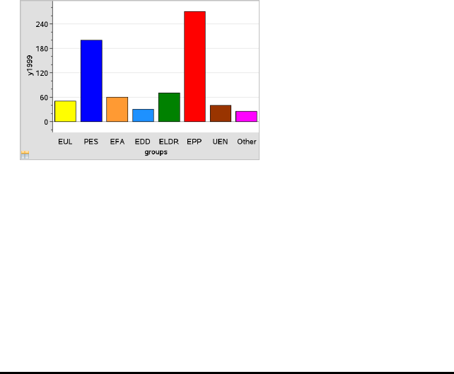
3. Explore the data in the plot.
- Hover over a bar to see a category summary (the number of cases and
percentage among all categories).
- Activate the Graph Trace tool and press ◄or ►move across the bars and
view summary information.
Creating a Bar Chart from a Frequency Table or Summary Data
1. On a new Data&Statistics page, create a bar chart with frequency or summary
data by choosing Add X Variable on the Plot Properties menu.
Note: You can also create a bar chart with frequency by selecting Add Variable with
Summary List from the context menu of the Add Variable region of an axis.
2. Select the desired variable from the pop-up choices.
3. Set the height of the bars with the summary variable by selecting Add Summary
List from the Plot Properties menu.
4. Select the summary list from the pop-up choices.
The bar chart plots on the work area. The icon in the lower left corner indicates
that this plot was generated from summary data.
5. Hover over a bar to see a category summary, or use the Graph Trace tool on the
Analyse menu to move across all of the bars displaying the summaries.
6. (Optional) Add summary lists to create a comparative bar chart.
Data&Statistics Application 492
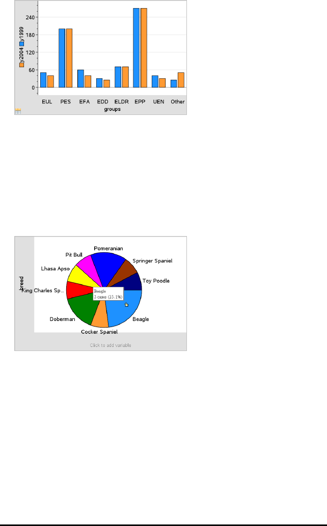
493 Data&Statistics Application
Creating a Pie Chart
A pie chart represents categorical data in a circular layout and uses an appropriately
proportioned segment for each category.
1. Create a dot chart on the work area.
2. On the Plot Types menu, click Pie Chart.
The dots move by category into the segments of the pie chart.
3. Hover over a segment to see the summary for the category, or use the Graph Trace
tool on the Analyse menu to move across each segment displaying all of the
summaries. The summary shows the number of cases for the category and the
percentage among all cases.
Note: You can switch to a pie chart from a bar chart generated from summary data.
Creating a Comparative Bar Chart
This might be used to explore data in a two-way table.
1. Type the raw data on a Lists&Spreadsheet page.
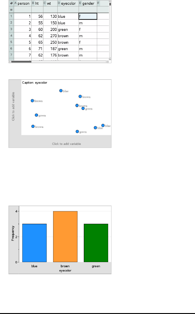
2. From the Insert menu in the toolbar, click Data&Statistics.
Note: Your screen may differ, depending on the data you entered.
3. Select the Click to add variable field, and select eye colour as the variable for the x
axis.
4. On the Plot Type menu, click Bar Chart.
The frequency of the eye colour data is plotted.
5. To split the eye colour data by gender, click the Plot Properties menu, click Split
Categories by Variable and then click gender.
Data&Statistics Application 494
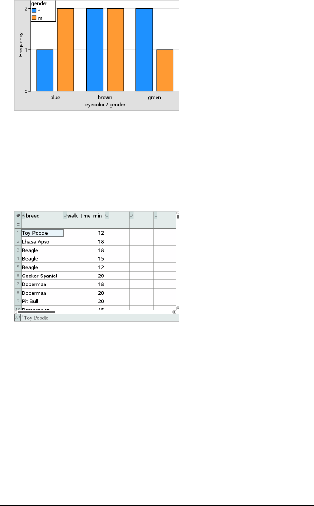
495 Data&Statistics Application
Splitting a Numeric Plot by Categories
You can use a categorical split to sort the values plotted on an axis.
1. Open a problem that includes a Lists&Spreadsheet page, or create data to be
plotted in the Lists&Spreadsheet application.
In this example, lists contain dog breed and daily walk information.
2. Click column letter (B).
3. On the Lists&Spreadsheet Data menu, click the Quick Graph tool.
The Quick Graph tool adds a Data&Statistics page. Data&Statistics plots the
variable and labels the horizontal axis.
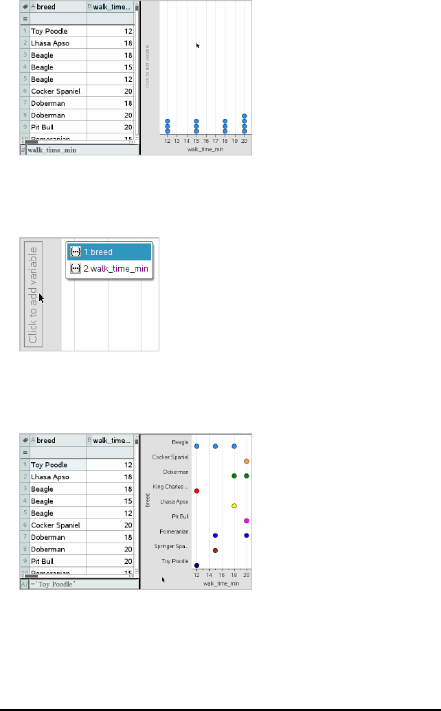
4. To plot the numeric data for each category, hover on the Add Variable region near
the centre of the vertical axis and click the tooltip Click or Enter to add variable.
The list of available variables displays.
5. On the list of variables, click the name of the category variable.
Data&Statistics labels the vertical axis and plots the numeric data for each
category.
Exploring Data
You can manipulate and explore plotted data.
Data&Statistics Application 496
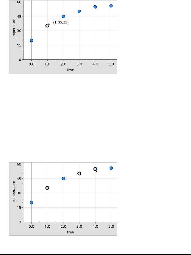
497 Data&Statistics Application
Moving Points or Bins of Data
1. Click and hold the desired point or bin.
The pointer changes to an open hand ÷.
2. Drag the point or bar to the new location and release it. Moving the point changes
the values for x and y.
If you are working with data from Lists&Spreadsheet, the data that corresponds
to the original point or bar automatically updates in the original column(s) in
Lists&Spreadsheet as you move the point.
You can also move points or bins by changing the numbers in the
Lists&Spreadsheet or Calculator applications. Data will update in all of the
representations.
Moving Multiple Points
1. Position the pointer over each data point that you want to select. When the pointer
changes to an open hand ÷, click to add the point to the selection.
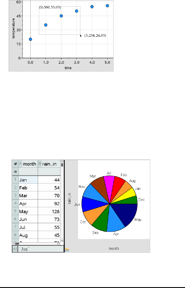
Alternatively, you can drag a selection rectangle around the points to select them.
2. Drag any of the selected points to move them all.
Note: When a list is defined in Lists&Spreadsheet as a formula, the movement of
points is restricted to positions that satisfy the formula.
Sorting Plotted Categories
You can sort plotted categories in list order, value order or alphabetically by category
name.
1. Click the work area that contains the plotted data.
2. On the Actions menu, click Sort and then click the type of sort.
Months listed chronologically but sorted by value (amount of rainfall)
Note: You can customise the order of the categories by clicking a label and dragging it.
Data&Statistics Application 498
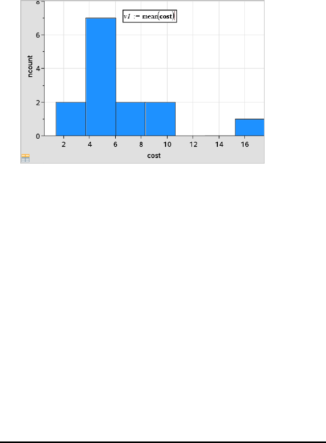
499 Data&Statistics Application
Plotting a Value
You can plot a value on an existing plot. It displays as a vertical line in the work area.
1. From the Analyse menu, click Plot Value.
A text box with a default expression opens in the work area.
2. Type the value you want to plot, and press Enter. In this example, the value is v1:=
mean(cost).
The line is drawn at that value, perpendicular to the axis. If you have multiple plots
on the work area, a plot value segment displays for each plot.
Note: If you use a frequency table to generate a histogram, reference the
frequency list in your expression. For example, type the expression "v1:= mean(List,
FreqList)" in the plot value entry box.
3. Click the line to display the value.
Note: Double-click the value to edit the expression.
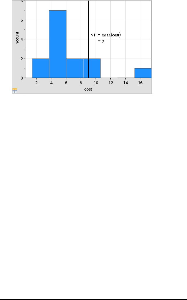
Plot value with value displayed
You can use Plot value for a single number or any expression that evaluates to a
number. If the value is dependent on the data, like mean, when you drag a point or
make changes in the Lists&Spreadsheet application, the line updates to reflect
the change, allowing for investigation of the influence of points on the calculation.
Removing a Plotted Value
1. Select the plotted value line.
2. From the Actions menu, click Remove Plotted Value.
Changing the Plot Type
You can change the plot type, to view different representations of data.
▶On the Plot Type menu, click a new plot type. Only the supported plot types are
available. For example, only univariate plot types are available when a single
variable plotted on an axis.
The data representation changes to the new plot format.
Note: Options are unavailable on the menu if the plotted data cannot be
represented by the plot type. For example, if a scatter plot is displayed in the work
area, you cannot create a box plot without first removing the variable from the y-
axis.
Data&Statistics Application 500
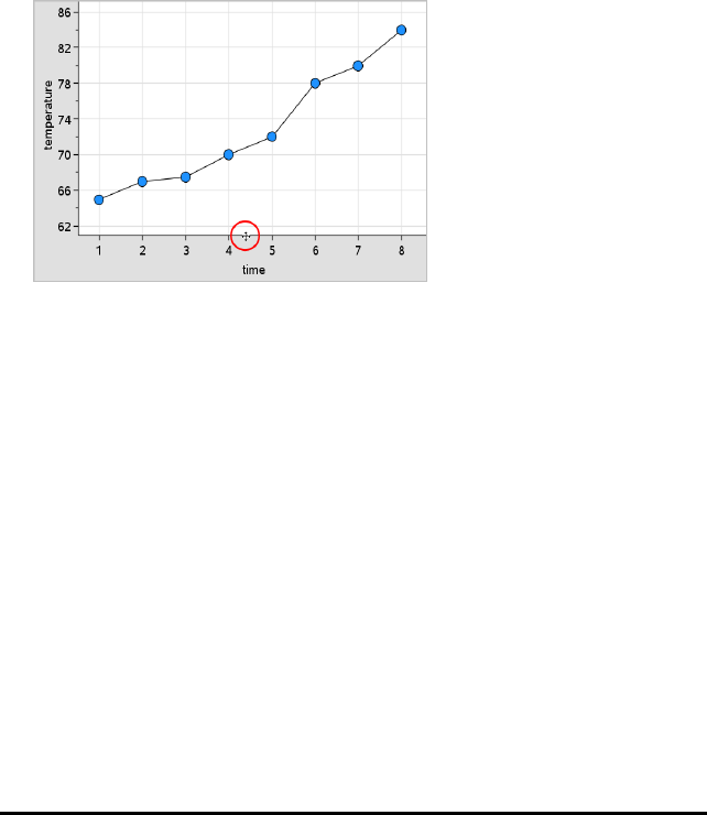
501 Data&Statistics Application
Rescaling a Graph
You can change the scale of the axes by using Translation and Dilation. The pointer
changes to indicate whether Translation (ö) or Dilation (ô) is available in zones on the
axes.
Translation
A translation slides a set of axes a fixed distance in a given direction. The original axes
have the same shape and size.
1. Position the pointer over a tick mark or label in the middle third of the axis. The
pointer changes to ö.
2. Click to grab. The pointer changes to a grasping hand ù. Drag to the desired
position and release.
Dilation
Dilation retains the shape of the axes, but enlarges or reduces the size.
1. Position the pointer over a tick mark or label near the ends of the axis. The pointer
changes to óon the vertical axis or ôon the horizontal axis.
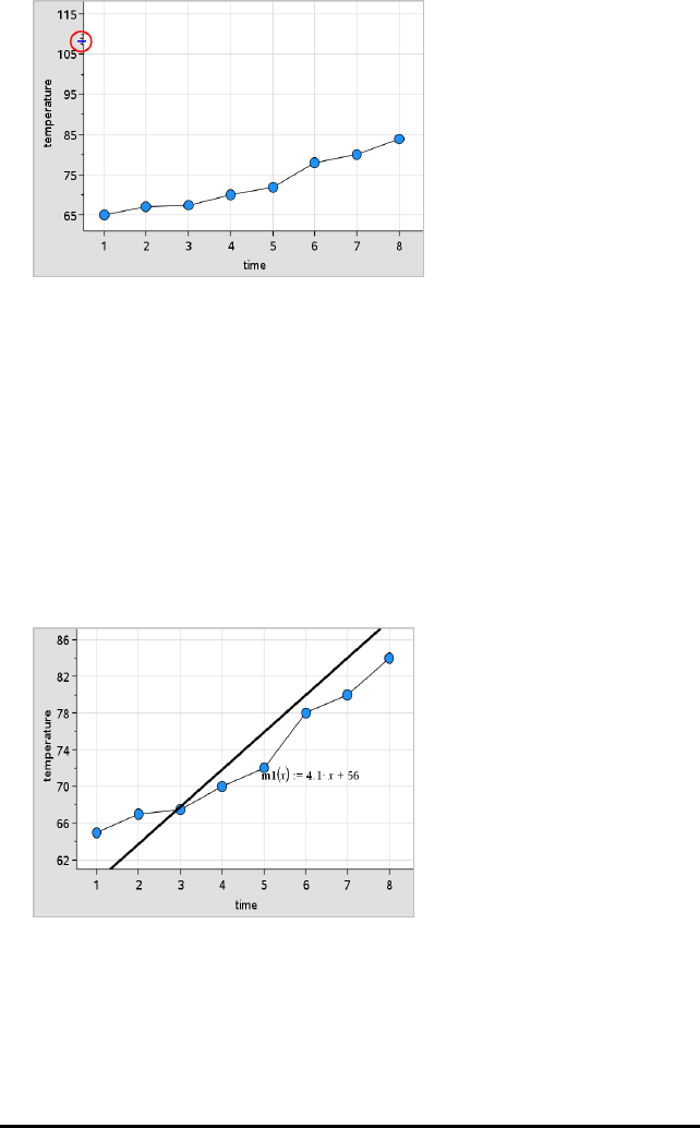
2. Click to grab. The pointer changes to an open hand ÷. Drag to the desired position
and release.
Adding a Movable Line
You can add a movable line to a plot. Moving and rotating the line on the work area
changes the function that describes it.
▶From the Analyse menu, click Add Movable Line.
The movable line displays and is labelled with a function that describes it. For this
example, Data&Statistics stores the expression for the movable line in the
variable m1.
Rotating a Movable Line
1. Click and grab either end of the line.
The pointer changes to é.
Data&Statistics Application 502
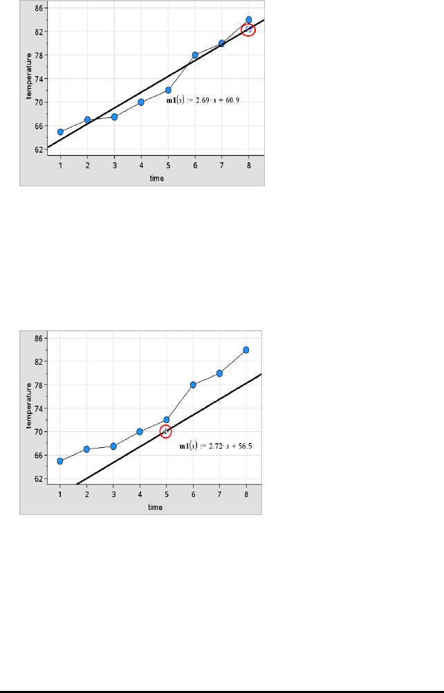
503 Data&Statistics Application
2. Drag to rotate and change the slope of the line.
The function m1(x) is updated for the changes in the position of the movable line.
Changing the Intercept
1. Click in the middle of the movable line.
The pointer changes to ö.
2. Drag to change the intercept.
The number at the end of the equation changes to show the change in the
intercept.
Note: The movable line is stored as a function that can be used for prediction in the
Calculator application.
Locking the Intercept at Zero
You can lock the intercept of the movable line at zero.
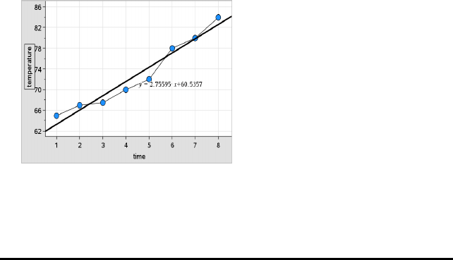
▶From the Analyse menu, click Lock Intercept at Zero.
You can unlock the intercept by choosing Unlock Movable Line Intercept on the
Analyse menu.
Tracing a Movable Line
You can trace a movable line to predict and analyse values.
1. Click the line.
The pointer changes.
2. From the Analyse menu, click Graph Trace to enable Trace mode for the line.
Rotation of the line is not supported in Trace mode.
3. Press ◄or►(left or right arrow keys) to trace the movable line.
If the plotted variables change, points on the graph and the line are updated
automatically.
Showing a Line of Regression
You can show a line of regression when you have a scatter plot or an X-Y line plot on
the work area. Studying the line of regression can help you understand the relationship
between two variables.
1. With a scatter plot or X-Y line plot of two variables on the work area, click the
Analyse menu, choose Regression and view the list of regressions.
2. Click the type of regression line to show. For example, choose Show Linear (mx+b)
to plot a linear regression line as shown in the following example.
When the line of regression is selected, the expression for the line displays.
Data&Statistics Application 504
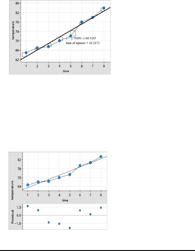
505 Data&Statistics Application
Showing Residual Squares
You can display residual squares on a plot. Residual squares can help you assess the
appropriateness of the model for your data.
Note: This tool is only available when a regression or movable line is present in the
work area.
▶From the Analyse menu, click Residuals >Show Residual Squares.
The sum of squares is updated as the line or data changes.
Showing a Residual Plot
You can show a residual plot to determine how well a line fits data. The work area
must include a scatter plot and one or more movable lines, regressions or plotted
functions for Show Residual Plot to be available.
▶With a scatter plot, line of regression and/or movable line in the work area, click
the Analyse menu and click Show Residual Plot > Residuals.

Notes:
• With multiple regressions or functions and movable lines plotted, you can select
each by clicking the line to show its residual plot.
• Click and hold a dot on the residual plot to see the residual.
• The residual plot for the selected regression or function displays in the work area.
• For consistency in comparing sets of data, residual plots do not rescale when you
move from one function or regression to another.
• Select a function or regression before a showing residual plot. If no function or
regression is selected and there are several plotted, Data&Statistics arbitrarily
selects the function or regression for showing the residual plot.
• Axes can be adjusted by clicking and dragging.
Removing a Residual Plot
▶With a scatter plot, line of regression and/or movable line in the work area, click
the Analyse menu, and click Hide Residual Plot.
Using Window/Zoom Tools
Use the Window/Zoom tools to redefine the graph to better view points of interest.
The Window/Zoom tools include:
• Window Settings: displays a Window Settings dialogue box that lets you type the
x-min, x-max, y-min, and y-max values for the axes.
• Zoom - Data: adjusts the zoom factor to display all plotted data.
• Zoom - In: lets you define the centre point of the zoom in location. The Zoom In
factor is approximately 2.
• Zoom - Out: lets you define the centre point of the zoom out location. The Zoom
Out factor is approximately 2.
Using the Window Settings Tool
1. On the Window/Zoom menu, click Window Settings.
The Window Settings dialogue box opens. The current values for x-min, x-max,
y-min and y-max are displayed in the fields.
Note: Only the appropriate boxes are editable, depending on whether there are one
or two axes in the work area.
2. Type the new values over the old values.
3. Click OK to apply the changes and redraw the plot.
Data&Statistics Application 506

507 Data&Statistics Application
Using the Zoom Data Tool
▶On the Window/Zoom menu, click Zoom Data.
The work area rescales to display all plotted data.
Using the Zoom In Tool
1. On the Window/Zoom menu, click Zoom In.
2. In the work area, click the centre point of the area of interest. This will be the
centre of the zoom in action.
The plot redraws to focus and enlarge the portion of the plot centred about the
point you selected in the previous step.
Using the Zoom Out Tool
1. On the Window/Zoom menu, click Zoom Out.
2. In the work area, click the centre point of the area of interest. This will be the
centre of the zoom out action.
The plot redraws to display a larger portion of the plot, centred about the point you
selected in the previous step.
Graphing Functions
You can graph functions by typing them in Data&Statistics, or you can graph functions
defined in other applications.
Graphing Functions Using the Plot Function Tool
You can use the Plot Function tool to plot functions in a work area that already includes
a plot on the axes. Plot Function lets you specify and graph a function for comparison
to an existing plot.
To use the Plot Function tool:
1. Create or open a problem that includes variables (from Lists&Spreadsheet) that
are plotted on a Data&Statistics work area. Ensure that your work area contains
both a horizontal axis and a vertical axis scale.
2. From the Analyse menu, click Plot Function.
A function entry field displays in the work area.
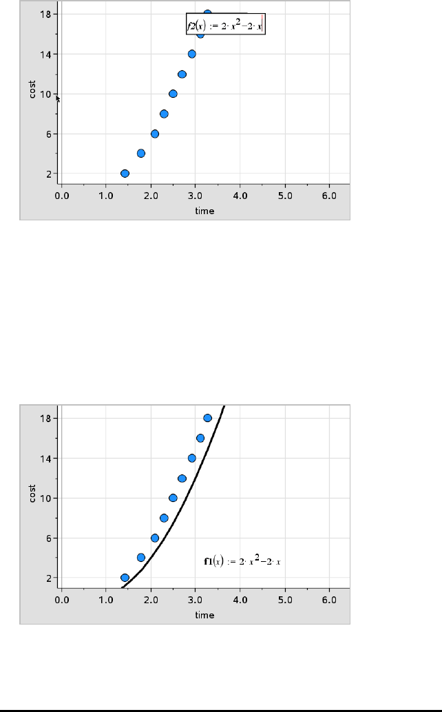
Note: You can edit the function’s expression typed in the entry field. However, the
function graphed in Data&Statistics cannot be manipulated or moved around the
work area. To do that, use Graphs&Geometry.
3. Type the function in the entry field, and press Enter.
Note: You can rename the function by typing over f1(x): with another name, if you
choose.
The function graphs in the work area and is saved as a variable for use in other
applications.
Data&Statistics Application 508
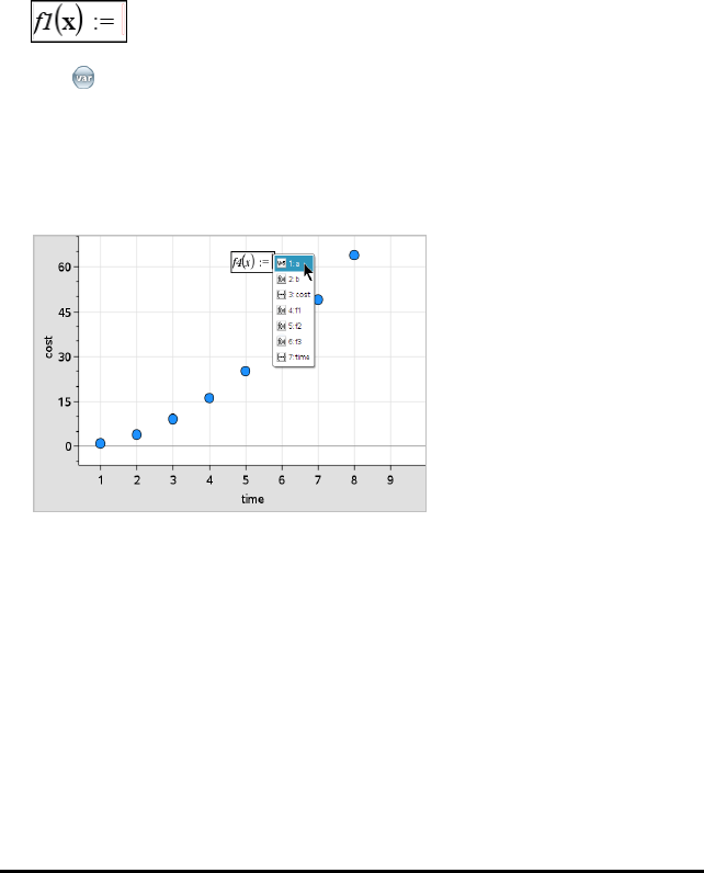
509 Data&Statistics Application
Entering Functions from Other Applications
You can enter a function that has been defined as a variable in another application,
such as Lists&Spreadsheet, Graphs&Geometry or Calculator.
1. Add a variable to each axis. You can access any variables defined in a
Lists&Spreadsheet or Calculator application in your problem from the variable list.
2. From the Analyse menu, click Plot Function.
A function entry field displays in the work area.
3. Click on the toolbar.
Handheld: Press h.
A list of variables available in the problem displays.
4. Click to select the variable containing the function you want to plot.
In the example below, the variable acontains the function f(x)=x2.
5. Press Enter.
The function plots in the work area.
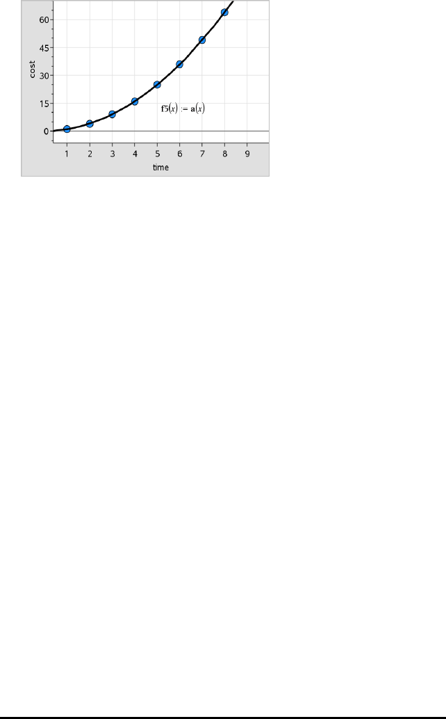
Editing a Function
You can edit a function and update it in the work area.
1. You can edit a function by double-clicking the equation and then making changes as
required.
2. Press Enter after making all changes and the updates are displayed in the work
area.
Using Data&Statistics Functions in other Applications
Data&Statistics functions are stored as variables, and may be used in other
applications, in the same manner as any other variable. Support for all function types is
included.
Note: Function numbers increment to use the next available. If you have defined f1(x)
and f2(x) in Graphs&Geometry, the first function you create in Data&Statistics will
be f3(x).
Using Show Normal PDF
You can approximate data plotted in the Data&Statistics work area against the
normal probability density function. The tool overlays the normal probability density
function using the mean and the standard deviation of the data in the histogram.
To show the normal probability density function for plotted data:
1. Add a variable to the x-axis.
2. On the Plot Types menu, click Histogram.
Data&Statistics Application 510
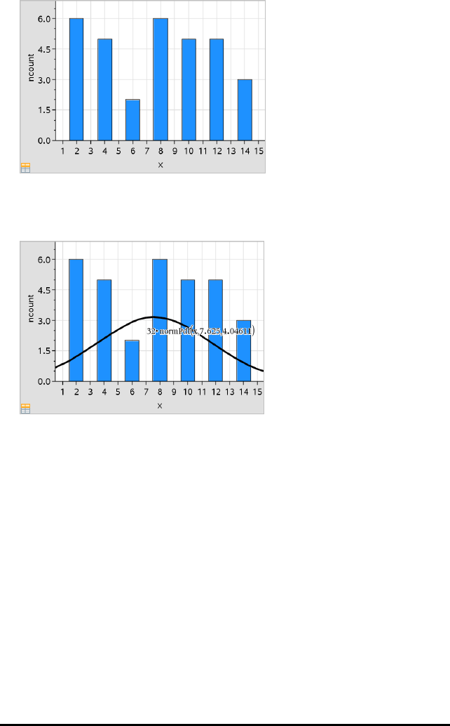
511 Data&Statistics Application
Note:Show Normal PDF is available only when histogram is the plot type.
3. From the Analyse menu, click Show Normal PDF.
The normal PDF for the graph plots in the work area. The expression used to
calculate the PDF displays when selected.
You can click Hide Normal PDF on the Analyse menu to remove the PDF.
Using Shade Under Function
Use Shade Under Function to find the area of a selected region under a function
graphed in the work area.
1. Select any function graphed in the Data&Statistics work area. For example, select
a previously graphed normal PDF.
2. From the Analyse menu, click Shade Under Function.
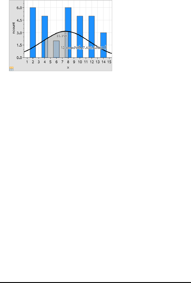
The pointer becomes a dotted vertical line and the boundary +/- ˆdisplays when
you position the mouse near the boundary on the left or right. You can click when ˆ
displays to set it as a boundary.
3. Select a point on the curve and click to indicate where to start shading under the
function. The direction in which you move next determines whether the region
shaded is on the left, right or centre of the curve.
4. Select a point on the curve and click to indicate the end boundary of the shaded
area. A region under the function is shaded based on the points you selected.
You can work with Shade Under Function in the following ways:
• Select the region to display the values for data points in the shaded area.
• To remove the shading, right-click or Ctrl-click the shaded region and choose
Remove Shaded Region.
• To change the fill colour of the shaded area, right-click or Ctrl-click the shaded
region, choose Colour, choose Fill and click a colour.
• Use plot value to set the boundary to an exact number. When a boundary for
shading is set to a plotted value, you can change the plotted value to update
the shading.
• Edit a shaded region by clicking and dragging the edge at the starting or ending
boundary.
Using Graph Trace
Graph Trace lets you move from one point on a graph to another to analyse variations
in the data. You can use Graph Trace mode to explore the data for the following
graphs.
• Graphs from Plot Function and Show Normal PDF
• Distribution curves (created in the Lists&Spreadsheet application)
• Movable Lines
Data&Statistics Application 512

513 Data&Statistics Application
• Regressions
• Caseplots
• Dot plots
• Scatter plots and X-Y line plots
• Box plots
• Histograms
• Bar charts
• Pie charts
To use Graph Trace
1. From the Analyse menu, click Graph Trace.
2. Press ◄or►to move across the plot.
The data representations enlarge and appear with a bold outline as you move
across them in Trace mode.
Customising Your Workspace
Working with Colour
All data points for a plotted variable display in the same colour to distinguish them
from the data points of other variables. Data plotted by category and split plots are
automatically displayed in different colours to help you distinguish the data.
To emphasise or distinguish certain parts of your work, you can change the default
colour for a variable’s data.
• Apply fill colours to objects, such as shading, or change the colour for a variable’s
data points.
• Apply colour to plotted lines (such as lines of regression) or movable lines.
Inserting a Background Image
When using the computer software, you can insert an image as a background for a
Data&Statistics page. The file format of the image can be .bmp, .jpg or .png.
1. From the Insert menu, click Image.
2. Navigate to the image that you want to insert.
3. Select it, and then click Open.
The image is inserted as a background.
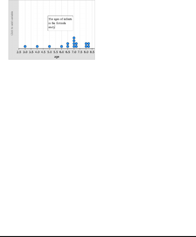
For more information, see the Working with Images chapter.
Working with Text
The Insert Text tool lets you type text to describe details related to plots on the work
area.
1. From the Actions menu, click Insert Text.
A text box opens.
2. Type notes or descriptions in the text box.
3. Customise the text to suit your needs.
• Move the pointer over the edges of the text box to drag the borders and change
the width or height.
• Click and grab the text box to move it near objects that relate to the text.
• Scroll to view additional text in a box by clicking the arrows at the top and
bottom edge.
• Click outside of the text entry box to exit the Text tool.
• Hide text by clicking the Actions menu and clicking Hide Text.
• Change the colour of text.
Adjusting Variable Values with a Slider
A slider control lets you interactively adjust or animate the value of a numeric variable.
You can insert sliders in the Graphs, Geometry, Notes and Data&Statistics
applications.
Data&Statistics Application 514
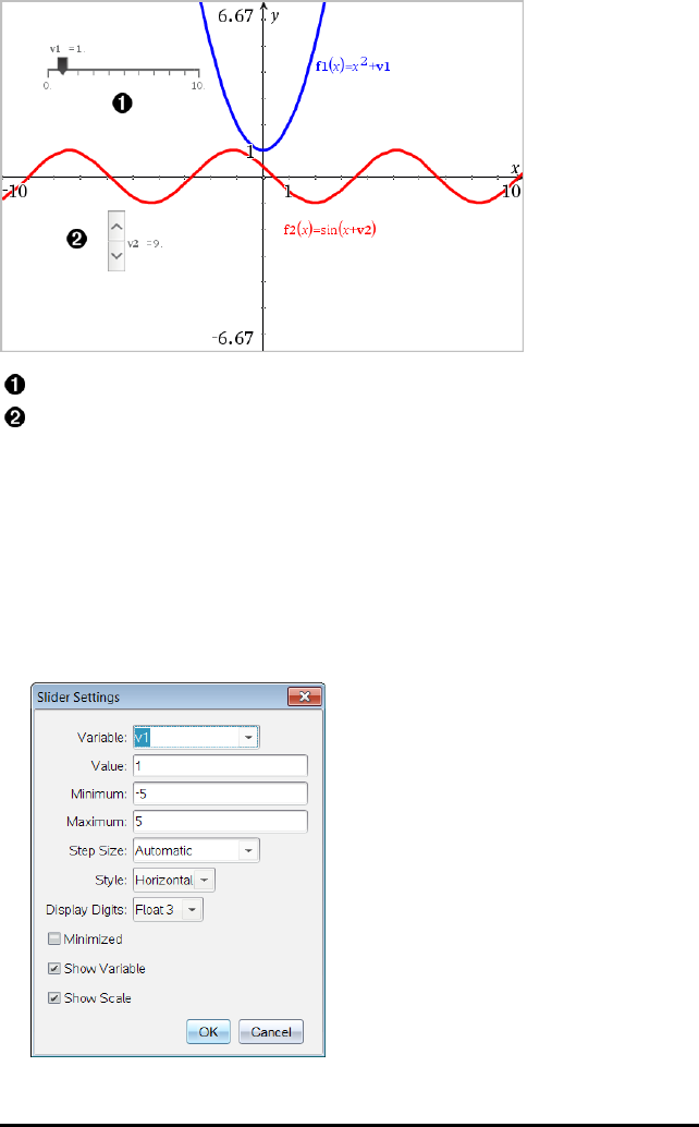
515 Data&Statistics Application
Horizontal slider for adjusting variable v1.
Minimised vertical slider for adjusting variable v2.
Note: TI-Nspire™ version 4.2 or higher is required for opening .tns files containing
sliders on Notes pages.
Inserting a Slider Manually
1. From a Graphs, Geometry or Data&Statistics page, select Actions > Insert Slider.
—or—
From a Notes page, make sure the cursor is not in a maths box or chem box, and
then select Insert > InsertSlider.
The Slider Settings screen opens.
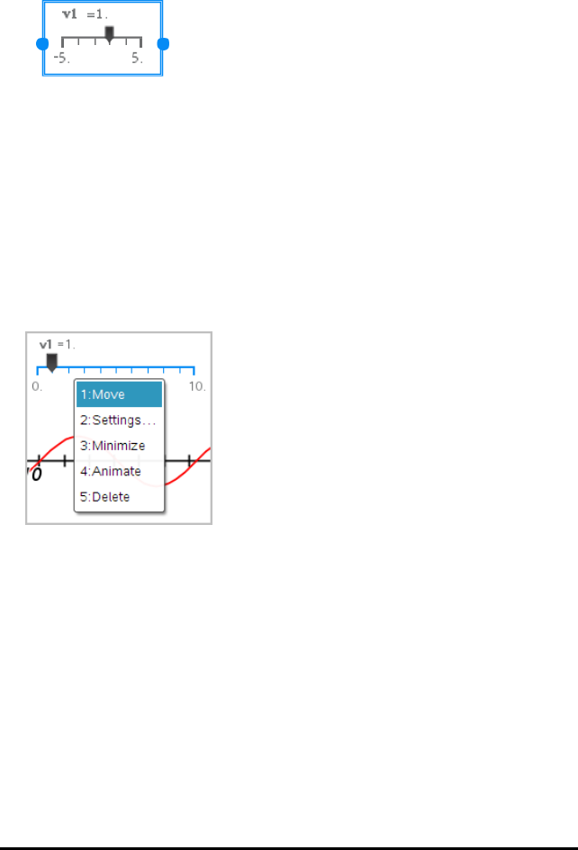
2. Enter the desired values, and click OK.
The slider is displayed. On a Graphs, Geometry or Data&Statistics page, handles
are displayed to let you move or stretch the slider.
To remove the handles and use the slider, click an empty
space in the work area. You can show the handles any time by
selecting Move from the slider's context menu.
3. To adjust the variable, slide the pointer (or click the arrows on a minimised slider).
- You can use the Tab key to move the focus to a slider or to move from one
slider to the next. The colour of the slider changes to show you when it has the
focus.
- When a slider has the focus, you can use the arrow keys to change the value of
the variable.
Working with the Slider
Use the options on the context menu to move or delete the slider, and to start or stop
its animation. You can also change the slider's settings.
1. Display the slider's context menu.
2. Click an option to select it.
Automatic Sliders in Graphs
Sliders can be created for you automatically in the Graphs application and in the
analytic window of the Geometry application. You are offered automatic sliders when
you define certain functions, equations or sequences that refer to undefined variables.
Data&Statistics Application 516
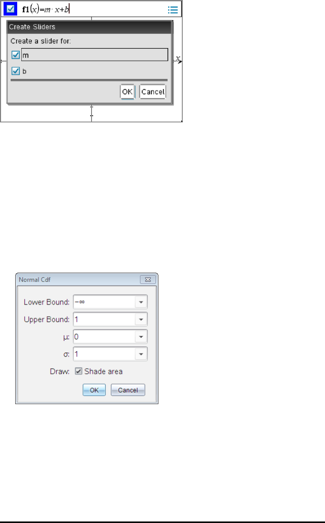
517 Data&Statistics Application
Inferential Statistics
You can explore hypothesis tests and probability distributions in the Data&Statistics
application after entering the data on a Lists&Spreadsheet page.
Drawing Inferential Statistics Plots
The following example uses the Draw option of the normCdf() function to plot a
distribution model.
1. On a Lists&Spreadsheet page, select the column-formula cell (second cell from
the top) in columnA.
2. From the Statistics menu, click Distributions, and click NormalCdf.
3. Type the plot parameters into the NormalCdf wizard.
4. Select the Draw box to see the distribution plotted and shaded in Data&Statistics.
Note: The Draw option is not available for all distributions.
5. Click OK.
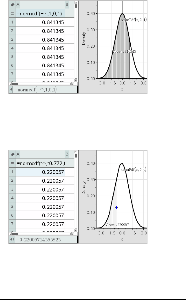
Exploring Inferential Statistics Plots
After drawing the plot in the previous example, you can explore the effect of changing
the upper bound.
▶On the Data&Statistics plot, drag the vertical line that represents the upper bound
toward the left or right.
As you drag, the formula is updated and the shaded area is recalculated.
Data&Statistics Application 518

519
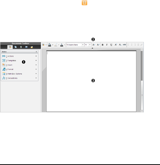
Notes Application
The Notes application lets you create and share text documents using the TI-Nspire™
handheld and computer software. Use Notes to:
• Create study notes to reinforce learning, demonstrate your understanding of
classroom concepts and review for exams.
• Edit collaboratively by assigning different roles to individuals using your document
so that any edits appear in a different text format.
• Create and evaluate maths expressions.
• Create correctly formatted chemical formulas and equations.
Adding a Notes Page
▶To start a new document with a blank Notes page:
From the main File menu, click New Document and then click Add Notes.
Handheld: Press c, and select Notes .
▶To add a Notes page in the current problem of an existing document:
From the toolbar, click Insert > Notes.
Handheld: Press ~and select Insert > Notes.
ÀNotes tools – Available any time you are in the Notes work area.
ÁText formatting toolbar - Lets you change size, colour, bold and other text
properties.
ÂNotes work area - The area where you type and format text.
Notes Application 520
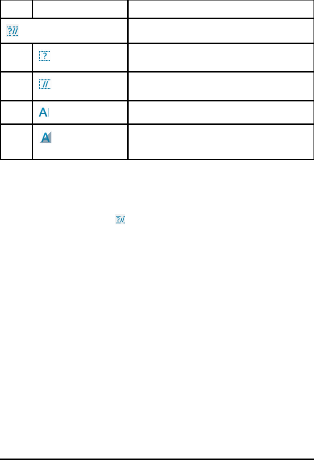
521 Notes Application
Using Templates in Notes
Use the options on the Templates menu to select a format for your Notes page.
Menu Option Function
2: Templates
1: Q&A Creates a template to enter question and answer
text.
2: Proof Creates a template to enter statement and reason
text.
3: Default Lets you type freeform text.
4:Hide Answer
(Q&A)
Toggles to show or hide the Answer in a Q&A
format.
Selecting a Template
Complete the following steps to select and apply a template:
1. From the Notes menu, click .
2. From the menu, click the template you want to apply.
Handheld: From the Notes work area, press b, and then press ►to display the
menu options.
The Notes page is displayed in the format you selected.
Using the Q&A Template
Use the Q&A template to create questions and answers. You can show or hide the
answer so you can create questions for review and hide the answers. When you use
the document as a study aid, you can verify that your answers are correct.
Press Tab to move the text cursor between the Question and Answer areas of the
template.
Using the Proof Template
The proof template provides an outline structure for statements and corresponding
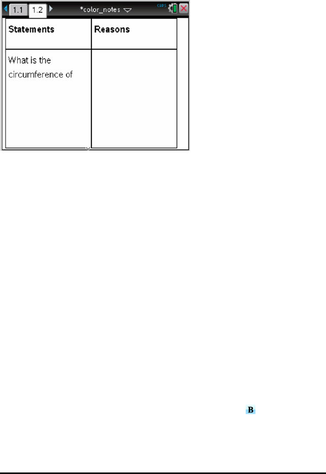
reasons.
Press Tab to move the text cursor between the Statements and Reasons areas of the
template.
Formatting Text in Notes
Text formatting lets you apply visual properties, such as bold and italic, to your text.
•Ordinary text. Apply most combinations of bold, italic, underline, superscript,
subscript, and strikethrough formatting. Select font and font size for any character.
•Text in a maths expression box. Apply formatting and enter maths exponents and
maths subscripts for variable names. Select font and font size. Font size affects all
text in the box.
•Text in a chemical equation box. Apply formatting. Select font and font size. Font
size affects all text in the box. Superscript and subscript are handled automatically.
Selecting Text
▶Drag from the starting point to the ending point to select the text.
Handheld: If you are using the Q&A or Proof template, press eto place the
cursor in the area containing the text. Use the Touchpad to place the cursor at the
start or end of the text to be selected. Hold down g, and use the Touchpad to
select the text.
Applying a Text Format
1. Select the text that you want to format.
2. On the formatting toolbar, click the formatting icons (such as for bold) to toggle
them, or click to select a font and font size.
Handheld: Click b, and then select Format >Format Text.
Notes Application 522
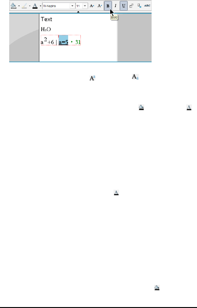
523 Notes Application
The changes are applied to the text as you make selections.
Note: The toolbar shows only the icons that are applicable to the type of text
selected. For example, superscript ( ) and subscript ( ) are shown only for
ordinary text.
Using Colour in Notes
When working in the Notes application on a desktop, use the (fill colour) or the
(text colour) options on the Documents Workspace toolbar to emphasise words,
calculations and formulas.
You can also apply colour to text when working in the Notes application on the
TI-Nspire™ CX handheld.
Changing Text Colours
1. Select the text you want to change to another colour. You can select a sentence,
phrase, word or a single letter. You can also select a maths expression box, a
chemical equation box or individual characters in a calculation, formula, chemical
equation or maths template.
2. From the Documents Workspace toolbar, click .
Handheld: Press ~, and then click Edit > Text Colour.
The Text Colour palette opens.
3. Click a colour to apply it to the selected text.
Applying a Background Colour
You can apply a background colour to highlight selected characters in ordinary text, text
in a maths expression or text in a chemical equation box.
1. Select the text.
2. From the Documents Workspace toolbar, click the arrow next to .
Handheld: Press ~, and then press Edit > Fill Colour.
The Fill Colour palette opens.
3. Click a colour to apply it to the selected text.
Inserting Images
When working in the Notes application on a desktop, use the Images option on the
Insert menu to add an image to a Notes page.
Note: The option for inserting an image is not available when working on a handheld.
However, you can transfer a file containing an image from your computer to a TI-
Nspire™ CX handheld and colours are retained.
1. Click Insert > Image from the Documents Toolbar.
The Insert Image window opens.
2. Navigate to the folder where the image is located.
3. Select the image, and then click Open to insert the image into the Notes work
area. Valid files types are .jpg, .png or .bmp.
4. To type text around the image, place the cursor in front of the image or after the
image, and then type the text.
Resizing an Image
Complete the following steps to resize an image.
1. Click the image to select it.
2. Move the cursor to the edge of the image.
The cursor changes to a left-right arrow symbol.
3. Click the mouse and hold to enable the {tool, and then drag the image to make it
smaller or larger.
4. Release the mouse button when the image is sized correctly.
For more information, see Working with Images.
Inserting Items on a Notes Page
When working with the Notes application, open the Insert menu to insert a maths
expression, chemical equation, shape symbol or a comment.
Menu
Name
Menu Option Function
3: Insert
1: Maths Box Lets you insert a maths expression.
Notes Application 524
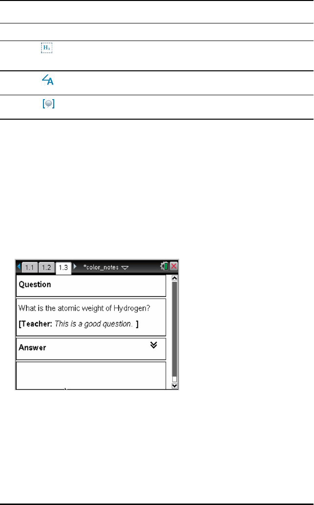
525 Notes Application
Menu
Name
Menu Option Function
-/M
2: Chem box -
/E
Lets you insert a chemical formula or equation.
2: Shape Marks the selected text as an angle, triangle, circle,
line, segment, ray or vector.
3: Comment Lets you type text that is italicised and prefaced with
Teacher or Reviewer.
Inserting Comments
You can insert Teacher or Reviewer comments into a Notes application. Comments are
easy to distinguish from the original text.
1. Define the type of comments you’re inserting (Teacher or Reviewer):
- On the Insert menu, click Comment, and then click Teacher or Reviewer.
- Handheld: While in the Notes work area, press bto display the Notes
menu. Press Insert > Comment, and then either Teacher or Reviewer.
2. Type your text.
Text that you type appears in italics.
Inserting Geometric Shape Symbols
You can use geometric shape symbols to designate selected text as geometric objects,
such as an angle, circle or line segment.
To insert a shape symbol, position the cursor where you want it, and then do the
following:
• On the Insert menu, click Shapes, and then select the shape to apply.
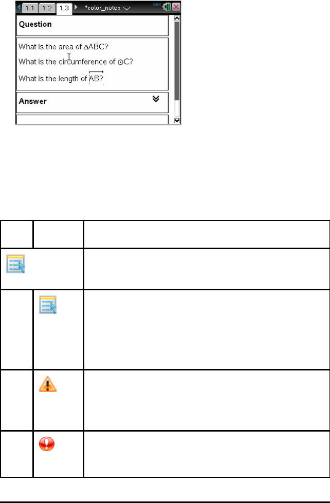
• Handheld: Press bto display the Notes menu. On the Insert menu, press
Shapes, and then press the shape to apply.
Entering Maths Expressions in Notes Text
You can include maths expressions in Notes text, using the same tools as in other
TI-Nspire™ applications.
Maths expression boxes have attributes that allow you to control how the expression is
displayed.
Menu
Name
Menu
Option
Function
5: Maths Box
Options
1:
Maths
Box
Attributes
When a maths box is selected, this option opens a dialogue box
allowing you to customise the maths box. You can hide or show
input or output, turn off calculation for the box, insert symbols,
change display and angle settings, and allow or disallow the
wrapping of expressions and the display of warning indicator
after they have been dismissed. You can change the attributes
of multiple selected maths boxes at the same time.
2:
Show
Warning
Info
Displays a warning indicator after the warning has been
dismissed.
3:
Show
Error
Displays an error after the error has been dismissed.
Notes Application 526
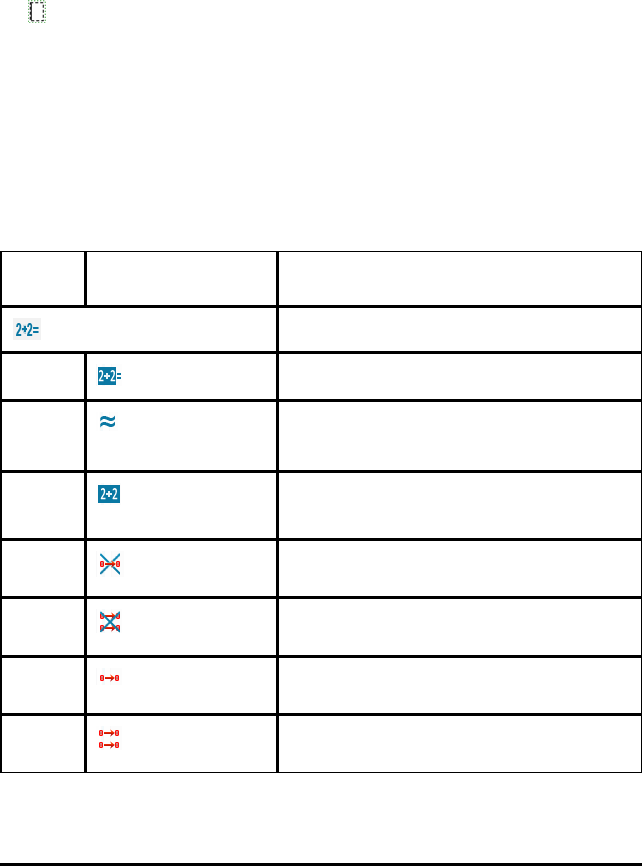
527 Notes Application
Entering an Expression
1. In the Notes work area, position the cursor where you want the expression.
2. From the Insert menu, select Maths Box.
—or—
Press Ctrl+M (Mac®: Press “+M).
An empty maths expression box is displayed.
3. Type the expression in the box. You can use the Catalogue, if necessary, to insert a
function, command, symbol or expression template.
4. To exit the maths box, click anywhere outside it.
Evaluating and Approximating Maths Expressions
You can evaluate or approximate one or more expressions and display the results. You
can also convert selected text and multiple maths expression boxes into a single maths
expression box. Notes automatically updates expressions and any variables used.
Menu
Name
Menu Option Function
1: Actions
1: Evaluate - ·Evaluates the expression.
2: Approximate
/ ·
Approximates the expression.
3: Evaluate and
replace
Replaces the selected part of the expression
with the result.
4: Deactivate Deactivates the current or selected item (box
or boxes)
5: Deactivate All Deactivates all boxes in the current Notes
application.
6: Activate Activates the current or selected previously
deactivated item.
7: Activate All Activates all boxes in the current Notes
application.

Evaluating or Approximating an Expression
To evaluate or approximate an expression, place the cursor anywhere in the maths
expression box and then do the following:
• Windows®: On the Actions menu, click Evaluate or Approximate. You can also use
Enter to evaluate or Ctrl+Enter to approximate.
• Mac®: Press “+ Enter to approximate.
• Handheld: Press bto display the Notes menu. On the Actions menu, select
Evaluate.
The result replaces the expression.
Evaluating Part of an Expression
To evaluate part of an expression, select the text or part of the maths expression. Then
do the following:
▶On the Actions menu, click Evaluate and Replace.
Handheld: Press bto open the Notes menu. Select Actions, and then select
Evaluate Selection.
The result replaces the selected part only.
Breaking Long Calculations
Some calculations may take a long time. Notes indicates that the handheld is
performing a long calculation by displaying a busy icon. If a calculation is taking more
time than you want to spend, you can end the calculation.
To stop the function or programme in progress, do the following:
• Windows®: Hold down the F12 key and press Enter repeatedly.
• Mac®: Hold down the F5 key and press Enter repeatedly.
• Handheld: Hold down the ckey and press ·repeatedly.
Showing Warnings and Errors
If a calculation in Notes results in a warning or error, you can view the warning or error
again even after you have dismissed the dialogue box.
Notes Application 528
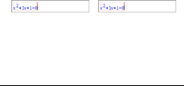
529 Notes Application
To display a warning or error in Notes after you have dismissed the dialogue box, do
one of the following:
• Windows®: Right-click and select Show warning info or Show error.
• Mac®: “+click and select Show warning info or Show error.
Note: You can change your settings so that warnings do not appear at all. The showing
of warning indicators is controlled by the Maths Box Attributes dialogue box. See
Changing the Attributes of Maths Expression Boxes.
Converting Selected Items to Maths Expression Boxes
To convert items to maths expression boxes:
1. Select the text, or combination of text and existing maths expression box, that you
want to evaluate.
2. From the Actions menu, click Convert to Maths Expression Box.
Using Maths Actions
Maths Actions are available on Notes, Scratchpad and Calculator pages.
When you display the context menu for a selected expression or equation, the menu
may include a Maths Actions submenu that lists the available actions. Each action
might prompt you for any needed parameters.
The specific maths actions listed depend on:
• The type of expression or relation.
• The operating system in use (numeric or CAS).
• Any restrictions imposed by an active Press-to-Test session.
Example of Maths Actions in Notes
1. Insert a maths box, and type the equation x2+3x+1=0, but don't press Enter yet.
Numeric OS CAS OS
2. Display the context menu of the equation, and select Maths Actions.
Windows®: Right-click the equation.
Mac®: Hold “, and click the equation.
Handheld: Point to the equation, and press / b.
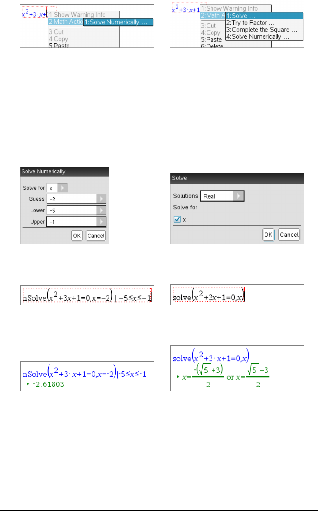
Numeric OS CAS OS
3. Select the action to perform:
-Solve Numerically for numeric OS.
-Solve for CAS OS.
You are prompted to enter parameters. For example, Numeric Solve prompts for
the variable of interest, initial guess, lower bound and upper bound.
4. Type a value for each parameter. When options are available, you can click an
arrow to make a selection.
Numeric OS CAS OS
5. Click OK to construct the completed expression and place it in the maths box.
Numeric OS CAS OS
6. Press Enter to complete the action.
Numeric OS CAS OS
7. As a further exploration, drag through the maths box to select x2+3·x+1. Do not
include the "=0" portion.
Notes Application 530
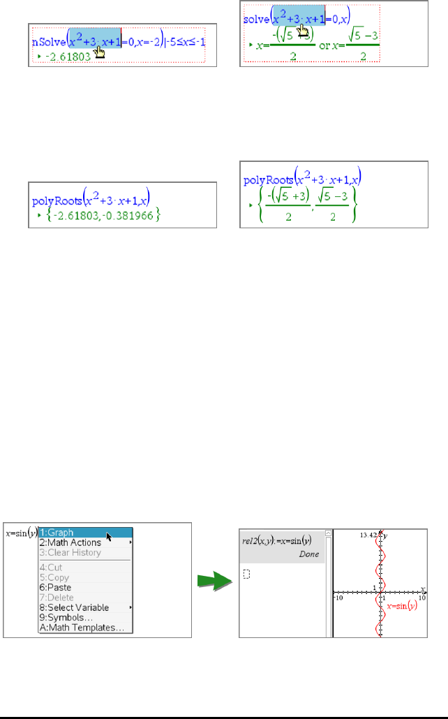
531 Notes Application
Numeric OS CAS OS
8. Display the context menu for the selected text, select MathsActions >
FindRootsofPolynomial, and press Enter to complete the action.
The action and its result are shown in a new maths box.
Numeric OS CAS OS
Tips for Using Maths Actions in Notes
▶For a previously evaluated expression, click in the expression and then display its
context menu.
When you select an action, it replaces the expression.
▶For a displayed result, click in the result and then display its context menu.
When you select an action, it appears in a new maths box.
▶For a portion of an expression or result, select the portion and then display the
context menu.
When you select an action, it appears in a new maths box.
Graphing from Notes and Calculator
You can graph a function or relation directly from its context menu. This feature is
available for many functions and relations on Notes, Scratchpad and Calculator pages.
If page layout options allow, the graph appears on the same page as the function or
relation. Otherwise, the graph appears on a separate Graphs page.
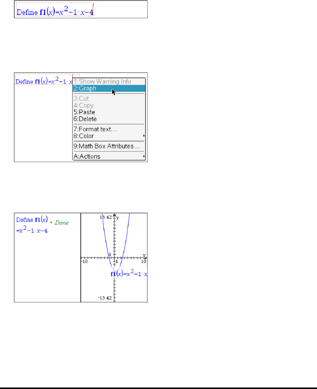
The type of graph created depends on:
• The type of function or relation.
• Any restrictions imposed by an active Press-to-Test session.
Example of Graphing from Notes
This example uses a Notes page to explore a quadratic function interactively.
1. Insert a maths box on a new Notes page, and enter the following function
definition:
Define f1(x)=x2-1·x-4
2. Display the context menu of the Define statement.
Windows®: Right-click the statement.
Mac®: Hold “, and click the statement.
Handheld: Point to the statement, and press / b.
3. Select Graph from the context menu.
The graph appears. The graph and the maths box are linked so that any adjustment
to one affects the other.
4. Explore the relationship between the defined function and its graph:
- Drag the ends or centre of the graph to manipulate it, and observe the changes
to the function definition.
—or—
Notes Application 532
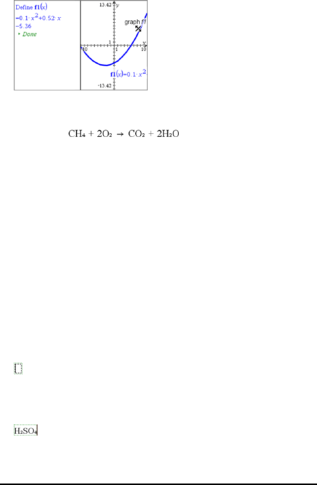
533 Notes Application
- Edit the defined function in the maths box, and observe the changes to the
graph.
Inserting Chemical Equations in Notes
Chemical equation boxes (chem boxes) make it easy to type chemical formulas and
equations, such as .
As you type in a chem box, most of the formatting work is handled automatically:
• Correct capitalisation of most element symbols, such as Ag and Cl, is automatic.
• Leading digits are treated as coefficients and are shown at full size. Numbers that
follow an element or a closed parenthesis are converted to subscripts.
• The equals “=” symbol is converted to a yields “&” symbol.
Notes:
• Equations in a chem box cannot be evaluated or balanced.
• Element capitalisation may not work in every situation. For example, to enter
carbon dioxide, CO2, you must manually capitalise theO. Otherwise, typing “co”
would result in“Co”, the symbol for cobalt.
Entering a chemical equation
1. In the Notes work area, position the cursor where you want the equation.
2. From the Insert menu, select Chem Box.
—or—
Press Ctrl+E (Mac®: Press “+E).
An empty chemical equation box is displayed.
3. Type the equation in the box. For example, to represent sulphuric acid, type
h2sO4, capitalising the O manually.
The chem box automatically formats the text as you type:
4. If you need superscripts for ionic equations, type a caret symbol (^) and then the
text.

5. Use parentheses to indicate whether a compound is solid(s), liquid(l), gas(g), or
aqueous(aq).
6. To exit the chem box, click anywhere outside it.
Deactivating Maths Expression Boxes
Calculations are by default activated, which means that results automatically update
when you evaluate or approximate an expression. If you don’t want results to
automatically update, you can deactivate a maths expression box, group of boxes or
the entire application.
Deactivating a Box or a Group of Boxes
To deactivate a box or a group of boxes:
1. Select the box or boxes that you want to deactivate.
2. Deactivate the selected box or boxes:
• Windows®: Click Actions > Deactivate (or right-click and then click Actions >
Deactivate).
• Mac®: Click Actions > Deactivate (or “+click and then click Actions >
Deactivate).
• Handheld: Press bto open the Notes menu. From the Actions menu, select
Deactivate.
Note: You can manually update a deactivated box or boxes by selecting the box or
boxes and using the process described in Evaluating and Approximating Maths
Expressions.
Deactivating All Boxes in the Notes Application
To deactivate all boxes in the Notes application:
▶With a document open, place your cursor in the Notes application that you want to
deactivate and select Deactivate All.
• Windows®: Click Actions > Deactivate All or right-click and click Actions >
Deactivate All.
• Mac®: Click Actions > Deactivate or “+click and click Actions > Deactivate.
Notes Application 534

535 Notes Application
• Handheld: Press bto display the Notes menu. On the Actions menu, click
Deactivate.
Note: When you use this option in Q&A and Proof templates, Deactivate All
deactivates only the maths boxes in the current work area.
Changing the Attributes of Maths Expression Boxes
You can change attributes in one or more maths expression boxes at the same time.
Controlling the attributes in maths expression boxes allows you to do the following:
• Show or hide the input or output or prevent calculation in the box.
• Select a symbol separator using Insert Symbol.
• Choose the number of digits to display in the output of a maths expression.
• Select angle settings so you can use both radian/degree and gradian angle
measures in the same Notes application.
• Select whether to allow maths expressions to wrap.
• Select whether to show or hide warning indicators.
To change the attributes of one or more boxes, do the following:
1. Select the box or boxes that you want to change.
2. On the Maths Box Options menu, click Maths Box Attributes.
3. Use the menus or selection boxes to make your selections.
4. Click OK to save or Cancel to abandon the change.
Note: Maths expression boxes recalculate automatically after you have made attribute
changes and saved the changes.
Undoing Changes to Maths Expression Boxes
▶To undo changes you have made to a maths expression box, click / Z.
Using Calculations in Notes
In the Notes application, the options on the Calculations menu enable you to perform
calculations. The calculations are described in the following table.
Important Information to Know
• Notes does not support editing programmes. Use Programme Editor instead.
• Notes does not support executing Lock or Unlock commands. Use Calculator
instead.
• Notes does not display intermediate results obtained via "Disp" command. Use
Calculator instead.
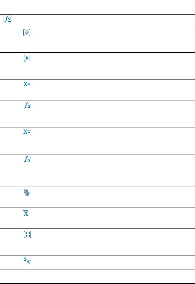
• Notes does not support user-defined dialogue boxes obtained via "Request,"
"RequestStr," or "Text" commands. Use Calculator instead.
• Notes does not support the execution of multiple statistics commands that produce
stat. variables.
Menu
Name
Menu
Option
Function
6: Calculations
1:
Define
Variables
Define a variable in a Note using the Calculator application.
2:
Number
Use tools from the Calculator Number menu, including Convert
to Decimal, Approximate to Fraction, Factorise, Least Common
Multiple, Highest Common Factor, Remainder, Fraction Tools,
Number Tools and Complex-Number Tools.
3:
Algebra
Use tools from the Calculator Algebra menu, including
Numerical Solve, Solve System of Linear Equations, Polynomial
Tools.
4:
Calculus
Use tools from the Calculus menu including Numerical
Derivative at a Point, Numerical Definite Integral, Sum, Product,
Numerical Function Minimum and Numerical Function
Maximum.
3
(CAS):
Algebra
Use tools from the Calculator Algebra menu, including Solve,
Factorise, Expand, Zeroes, Numerical Solve, Solve System of
Equations, Polynomial Tools, Fraction Tools, Convert
Expressions, Trigonometry, Complex and Extract.
4
(CAS):
Calculus
Use tools from the Calculus menu including Derivative,
Derivative at a Point, Integral, Limit, Sum, Product, Function
Minimum, Function Maximum, Tangent Line, Normal Line, Arc
Length, Series, Differential Equation Solver, Implicit
Differentiation and Numerical Calculations
5:
Probability
Use tools from the Calculator Probability menu, including
Factorial, Permutations, Combinations, Random and
Distributions.
6:
Statistics
Use tools from the Calculator Statistics menu, including Stats
Calculations, Stats Results, List Maths, List Operations and
others.
7:
Matrix &
Vector
Use tools from the Calculator Matrix & Vector menu, including
Create, Transpose, Determinant, Row-Echelon Form, Reduced
Row-Echelon Form, Simultaneous, and others.
8: Use tools from the Calculator Finance menu, including Finance
Notes Application 536
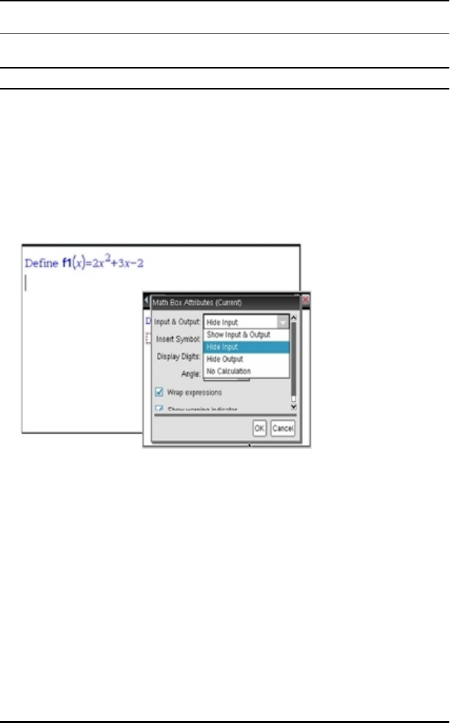
537 Notes Application
Menu
Name
Menu
Option
Function
Finance Solver, TVM Functions, Amortization, Cash Flows, Interest
Conversions and Days between Dates.
Note: For more information, see the Calculator documentation.
Exploring Notes with Examples
This section shows you how the Notes application works with other applications to
automatically update results.
Example #1: Using Notes to Explore Roots of a Quadratic Function
1. Open a new document and start the Notes application.
2. Define a function in a maths box, evaluate, and hide the output using the Maths
Box attributes.
3. Type some more text; for example: “Real Roots of f1(x) are:”
4. In a new maths box, type: polyRoots(f1(x),x).
5. Press ·and hide the input of this maths box by using the Maths Box attributes
dialogue box.
6. Use the Page Layout toolbar icon to select the split layout.
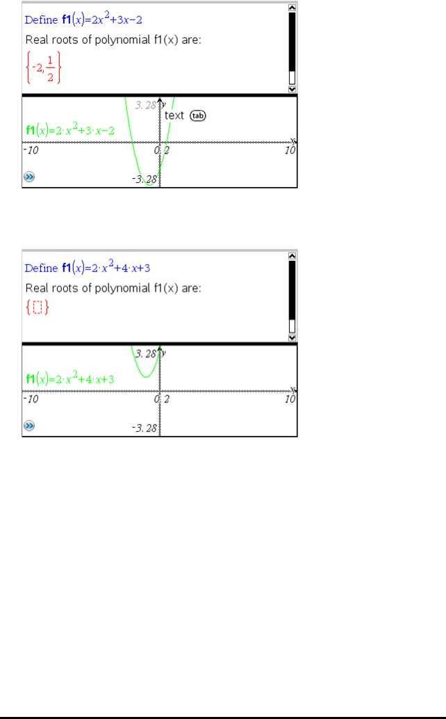
7. Add the Graph application and plot f1(x).
See how the roots of f1 change when the function is modified in Graph.
Example #2: Using Notes to Explore Data Sampling
In this example, we create a sampling distribution of sample means drawn from a
given population. We will be able to watch the sampling distribution take shape for a
given sample size and describe its characteristics. You can change the population and
the sample size.
1. Set up the population and the sample size.
a) Type "Create sample data:"
b) Insert a maths expression box and define the population. For example, type
"population:=seq(n,n,1,50)".
c) Press ·and hide the output using the Maths Expression Box Attributes
dialogue box.
d) Insert a maths expression box and define the sample size. For example, type
"size:=5".
Notes Application 538
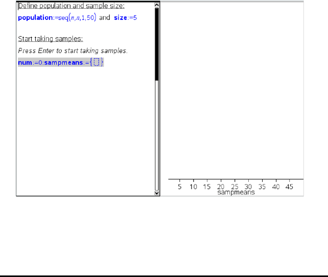
539 Notes Application
e) Press ·and hide the output using the Maths Expression Box Attributes
dialogue box.
2. Set up the initialization.
a) Type "Start taking samples:"
b) Insert a maths expression box and set the initial values for the number of
samples (num) and the list of sample means (sampmeans). Type:
"num:=0:sampmeans:={}"
c) Press ·and hide the output using the Maths Expression Box Attributes
dialogue box.
d) Deactivate the maths expression box using Actions > Deactivate. The
deactivation will prevent the content of that maths box from being overwritten
when the values for num and sampmeans change. The deactivated maths box
will be shown with the light colour background.
3. Set up Data & Statistics for the sampling.
a) Change the page layout and insert Data & Statistics.
b) Click on the horizontal axis and add sampmeans list.
c) Change the window setting: XMins=1 and XMax = 50.
d) You can also set up the plot of the mean of sample means using Analyse > Plot
Value.
4. Enter the instructions to add data.
a) Type "Create new samples:"
b) Insert a maths expression to define the sample (sample) and update the
number of samples and the list of sample means. Type:
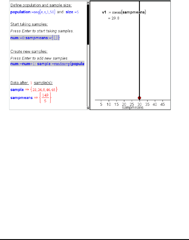
"num:=num+1:sample:=randsamp(population,size):
sampmeans:=augment(sampmeans,{mean(sample)})"
c) Press ·, hide the output, and turn off the expression wrapping using the
Maths Expression Box Attributes dialogue box.
d) Deactivate the maths expression box using Actions > Deactivate to prevent the
content of the maths box to be overwritten when num and sampmeans values
are reinitialized.
e) Create maths expression boxes that display the current number of experiments
(num), sample (sample) and the list of sample means (sampmeans).
5. Now you are ready to explore. Add more samples by simply pressing ·when
you are in the maths expression box in the "Create new samples" section.
Note: You can also automate the sampling process by using a For...EndFor loop.
Notes Application 540
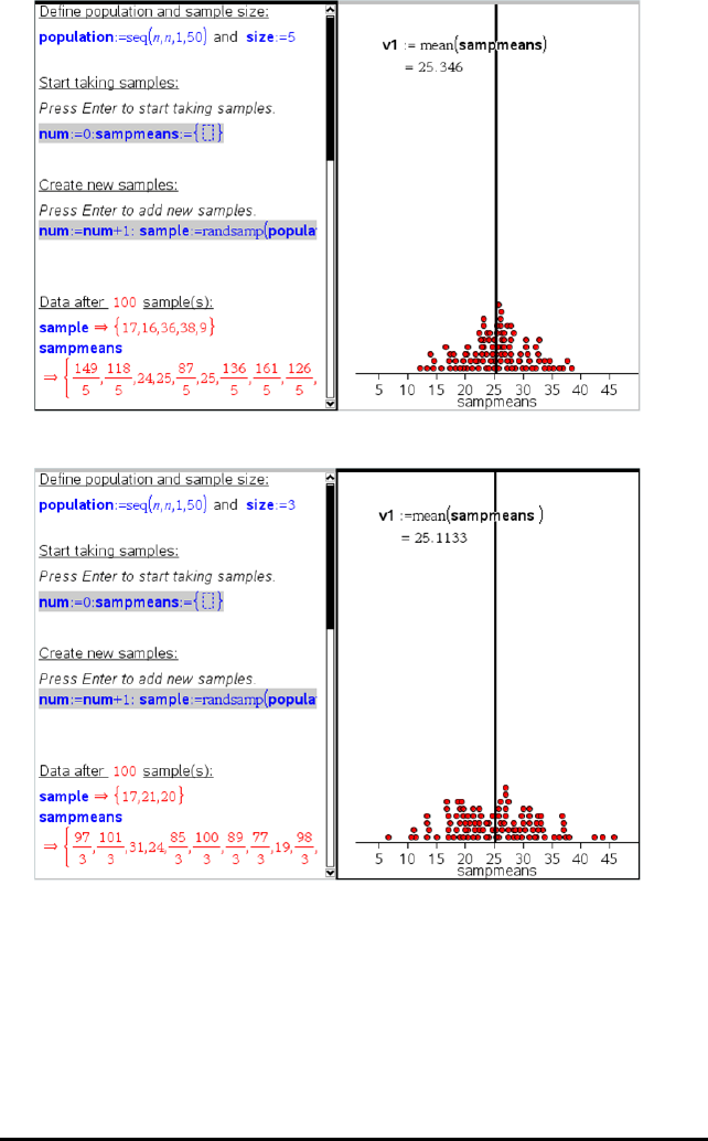
541 Notes Application
You can also change the sample size and restart the sampling.

Widgets
All work that you create and save using TI-Nspire™ applications is stored as a
document, which you can share with others using TI-Nspire™ software, a TI-Nspire™
handheld, or the TI-Nspire™ App for iPad®. You save these TI-Nspire™ documents as
.tns files.
A Widget is a .tns document that is stored in your MyWidgets folder.
You can use Widgets to:
• Easily access text files
• Insert and run scripts (such as the pre-loaded widget example: Stopwatch.tns)
• Quickly insert a saved problem into a document
When you add a Widget, TI-Inspire™ CX extracts only the first page of the selected .tns
file, and inserts it into your open document.
Creating a Widget
A document is regarded as a Widget when it is saved or copied to the designated
MyWidgets folder. The default location is:
• Windows®: MyDocuments\TI-Nspire\MyWidgets.
• Mac®: Documents/TI-Nspire/MyWidgets.
• Handheld: MyWidgets
• TI-Nspire™ App for iPad® and TI-Nspire™ CASApp for iPad®: MyWidgets
If the MyWidget folder has been inadvertently deleted, you must create it before
attempting to use a Widget.
Note: When you add a Widget, TI-Inspire™ CX extracts only the first page of the
selected .tns file, and inserts it into your open document.
Adding a Widget
Adding a Widget to a New Document
1. Open a new document.
Widgets 542
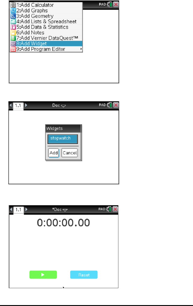
543 Widgets
2. Click Add Widget.
3. Scroll to select a .tns file from the box.
4. Click Add.
Note: Stopwatch is a preloaded .tns file. Any saved .tns file will show up in this list.
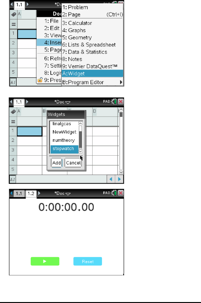
Adding a Widget to an Existing Document
1. Click the ¤on Doc¤>Insert >Widget.
2. Click Add.
Note: You can also add a Widget to a new or existing document using the Insert menu.
Widgets 544
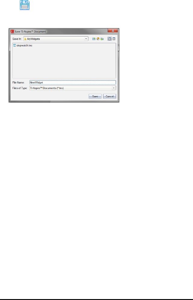
545 Widgets
Saving a Widget
1. Click .
2. Navigate to MyDocuments > MyWidgets.
3. Type in a name for your Widget.
4. Click Save.
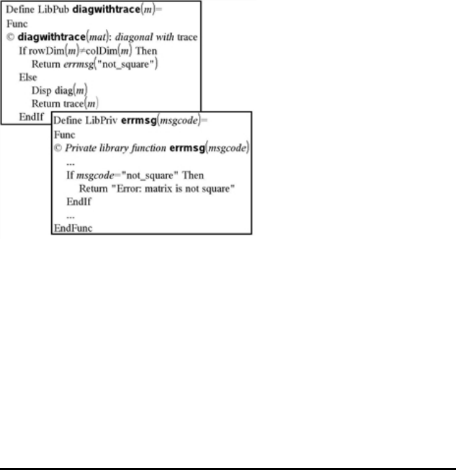
Libraries
What is a Library?
A library is a TI-Nspire™ document that contains a collection of variables, functions
and/or programmes that have been defined as library objects.
Unlike ordinary variables, functions and programmes, which can be used only within a
single problem (the problem in which they are defined), library objects are accessible
from any document. You can even create public library objects that appear in the
TI-Nspire™ Catalogue.
For example, suppose you have created library document matrix containing public
library function diagwithtrace() and a private library function errmsg().
Function diagwithtrace() displays the diagonal of a square matrix and calculates the
trace of the matrix. If its input is not a square matrix, the function calls errmsg(), which
should then return an appropriate error string.
You could then use the following syntax to display the diagonal and calculate the trace
of matrix mdefined in the current problem:
matrix\diagwithtrace(m)
Creating Libraries and Library Objects
A document is regarded as a library when it is saved or copied to the designated library
folder. The default location is:
• Windows®: MyDocuments\TI-Nspire\MyLib.
• Mac®: Documents/TI-Nspire/MyLib.
• Handheld: MyLib
Libraries 546

547 Libraries
If the folder has been inadvertently deleted, you must create it before attempting to
use libraries.
You can define library objects using either the Programme Editor or the Calculator
application. Library objects must be defined with a Define command and must reside
in the first problem of a library document.
Note: If you use the Programme Editor to define a library function or programme, you
must store the object and also save the document. Saving the document does not
automatically store the object. For more information, see Programming.
Naming restrictions apply to library documents and library objects.
• A library document name must be a valid variable name between 1 and 16
characters long, and it must not contain a period or begin with an underscore.
• A library object name must be a valid variable name between 1 and 15 characters
long. It must not contain a period and must not begin with an underscore.
Private and Public Library Objects
When you define a library object, you designate it as private (LibPriv) or public (LibPub).
Define a=5
a is not a library object.
Define LibPriv b={1,2,3}
b is a private library object.
Define LibPub func1(x)=x^2 - 1
func1 is a public library object.
APrivate library object does not appear in the Catalogue, but you can access it by
typing its name. Private objects serve well as building blocks that perform basic, low-
level tasks. Typically, private library objects are called upon by the public functions and
programmes.
APublic library object appears in the Catalogue’s library tab after you refresh the
libraries. You can access a public library object through the Catalogue or by typing its
name.
Mac® only: In version 1.4 of the software, a library document name cannot contain
extended characters, such as Ö, á or ñ.
Note: In library programmes and functions defined as public, a comment line (©)
immediately following the Prgm or Func line is automatically displayed as help in the
Catalogue. You could, for example, show a syntax reminder there.

Using Short and Long Names
Anytime you are in the same problem where an object is defined, you can access it by
entering its short name (the name given in the object’s Define command). This is the
case for all defined objects, including private, public and non-library objects.
You can access a library object from any document by typing the object’s long name. A
long name consists of the name of the object’s library document followed by a
backslash “\” followed by the name of the object. For example, the long name of the
object defined as func1 in the library document lib1 is lib1\func1. To type the “\”
character on the handheld, press g p.
Note: If you cannot remember the exact name or the order of arguments required for a
private library object, you can open the library document or use the Programme Editor
to view the object. You also can use getVarInfo to view a list of objects in a library.
Using Library Objects
Before using a library variable, function or programme, make sure that these steps
have been followed:
• The object has been defined with the Define command, and the command
specifies either the LibPriv or LibPub attribute.
• The object resides in the first problem of a library document. The document must
reside in the designated library folder and must meet the naming requirements.
• If you defined the object using the Programme Editor, it has been stored using
Check Syntax & Store from the Programme Editor menu.
• The libraries have been refreshed.
Refreshing the Libraries
▶Refresh libraries to make the library objects available to your documents.
- From the Tools menu, click Refresh Libraries.
Handheld: Press / b and click Refresh Libraries.
Using a Public Library Object
1. Refresh the libraries.
2. Open the TI-Nspire™ application in which you want to use the variable, function or
programme.
Note: All applications can evaluate functions, but only the Calculator and Notes
applications can run programmes.
3. Open the Catalogue and use the library tab to find and insert the object.
4. If arguments are required, type them inside the parentheses.
Using a Private Library Object
1. Refresh the libraries.
Libraries 548

549 Libraries
2. Open the TI-Nspire™ application in which you want to use the variable, function or
programme.
Note: All applications can evaluate functions, but only the Calculator and Notes
applications can run programmes.
3. Type the name of the object, such as lib1\func1().
In case of a function or programme, always follow the name with parentheses. To
type the “\” character on the handheld, press g p.
4. If arguments are required, type them inside the parentheses.
Creating Shortcuts to Library Objects
You can make the objects in a library more easily accessible by using libShortcut() to
create shortcuts to them. This creates a variable group in the current problem that
contains references to all the objects in the specified library document. You can choose
to include or exclude the private library objects.
For example, suppose the library document linalg contains functions named clearmat,
cofactor, gausstep, help, inversestep, kernelbasis, rank and simultstep. Executing
libShortcut(“linalg”,“la”)would create a variable group containing the following
members:
la.clearmat
la.cofactor
la.gausstep
la.help
la.inversestep
la.kernelbasis
la.rank
la.simultstep
You can refer to those library objects from within the current problem by typing their
variable names or by selecting them from the Variables menu.
For more details about using libShortcut(), see the Reference Guide.
Included Libraries
To help you get started with libraries, the TI-Nspire™ Software installation includes a
library document with useful Linear Algebra functions. The library is named linalg or
linalgCAS and is installed in the designated library folder.
Note: Updating the handheld’s operating system or reinstalling the computer software
places all included libraries in the default folder. If you have edited an object in an
included library or replaced an included library with your own document of the same
name, updating or reinstalling will overwrite your changes. This could also happen
after batteries are replaced or the handheld system is reset.

Restoring an Included Library
If you inadvertently delete or overwrite an included library, you can restore it from the
installation DVD.
1. Open the DVD, and navigate to the libs folder.
2. Identify the library file to restore, such as linalg.tns or linalgCAS.tns for the linear
algebra library.
3. Copy the file.
- Windows®: Copy the file to your designated library folder. The default location
is MyDocuments\TI-Nspire\MyLib.
- Mac®: Copy the file to your designated library folder. The default location is
Documents/TI-Nspire/MyLib.
- Handheld: Connect the handheld to your computer, open the TI-Nspire™
software, and copy the library file to the handheld’s MyLib folder.
4. Activate the new library objects.
- From the TI-Nspire™ Software Tools menu, click Refresh Libraries.
Handheld:Press / b, and click Refresh Libraries.
Libraries 550

551
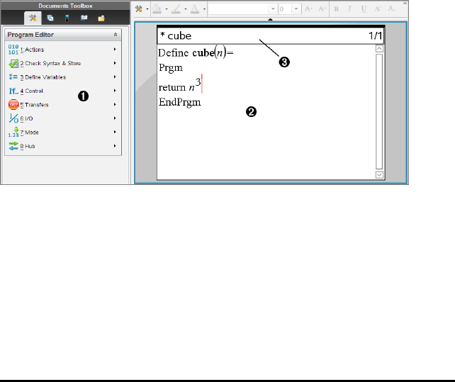
Getting Started with the Programme Editor
You can create user-defined functions or programmes by typing definition statements
on the Calculator entry line or by using the Programme Editor. The Programme Editor
offers some advantages, and it is covered in this section. For more information, see
Calculator.
• The editor has programming templates and dialogue boxes to help you define
functions and programmes using correct syntax.
• The editor lets you enter multiple-line programming statements without requiring
a special key sequence to add each line.
• You can easily create private and public library objects (variables, functions and
programmes). For more information, see Libraries.
Launching the Programme Editor
▶To add a new Programme Editor page in the current problem:
From the toolbar, click Insert > Programme Editor > New.
Handheld: Press ~and select Insert > ProgrammeEditor > New.
Note: The editor is also accessible from the Functions & Programmes menu of a
Calculator page.
ÀProgramme Editor menu – This menu is available any time you are in the Programme
Editor work area using the Normal view mode.
ÁProgramme Editor work area
ÂStatus line shows line-number information and the name of the function or
programme being edited. An asterisk (*) indicates that this function is “dirty”, which
means that it has changed since the last time its syntax was checked and it has been
stored.
Getting Started with the Programme Editor 552
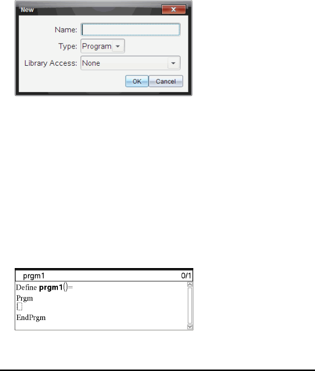
553 Getting Started with the Programme Editor
Defining a Program or Function
Starting a new Program Editor
1. To start the editor from a Calculator page,
- From the Insert menu, click ProgramEditor, and click New.
Handheld: Press b 9 1 1.
2. To start the editor when not on a Calculator page,
- From the Insert menu, click ProgramEditor, and click New.
Handheld: Press / b 4 8 1.
3. Type a name for the function or program you are defining.
4. Select the Type (Program or Function).
5. Set the Library Access:
- To use the function or program only from the current document and problem,
select None.
- To make the function or program accessible from any document but not visible
in the Catalogue, select LibPriv.
- To make the function or program accessible from any document and also
visible in the Catalogue, select LibPub (Show in Catalogue). For more
information, see Libraries.
6. Click OK.
A new instance of the Program Editor opens, with a template matching the
selections you made.
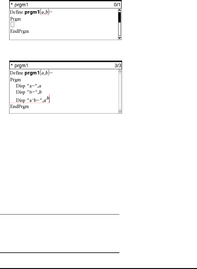
Entering Lines into a Function or Program
The Program Editor does not execute the commands or evaluate expressions as you
type them. They are executed only when you evaluate the function or run the program.
1. If your function or program will require the user to supply arguments, type
parameter names in the parentheses that follow the name. Separate parameters
with a comma.
2. Between the Func and EndFunc (or Prgm and EndPrgm) lines, type the lines of
statements that make up your function or program.
- You can either type the names of functions and commands or insert them from
the Catalogue.
- A line can be longer than the width of the screen; if so, you might have to scroll
to view the entire statement.
- After typing each line, press ·. This inserts a new blank line and lets you
continue entering another line.
- Use the ¡,¢,£and ¤arrow keys to scroll through the function or program for
entering or editing commands.
Inserting Comments
A comment symbol (©) lets you enter a remark. Comments can be useful to someone
viewing or editing the program. Comments are not displayed when the program runs
and they have no effect on program flow.
Define LibPub volcyl(ht,r) =
Prgm
©volcyl(ht,r) => volume of cylinderÀ
Disp “Volume =”, approx(p ¦ r2¦ht)
©This is another comment.
EndPrgm
Getting Started with the Programme Editor 554
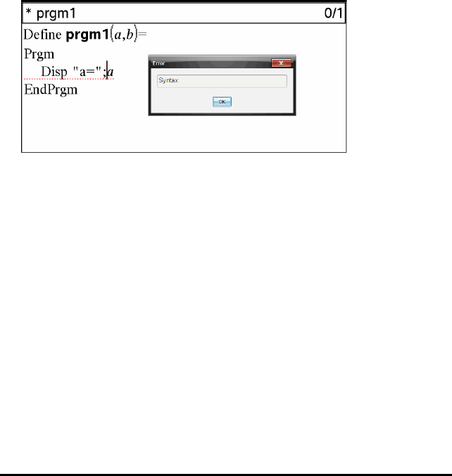
555 Getting Started with the Programme Editor
ÀComment showing required syntax. Because this library object is public and this
comment is the first line in a Func or Prgm block, the comment is displayed in the
Catalogue as help. For more information, see Libraries.
To insert a comment:
1. Position the cursor at the end of the line in which you want to insert a comment.
2. From the Actions menu, click Insert Comment.
3. Type the text of the comment after the © symbol.
Checking Syntax
The Program Editor lets you check the function or program for correct syntax.
▶From the CheckSyntax&Store menu, click Check Syntax.
If the syntax checker finds any syntax errors, it displays an error message and tries
to position the cursor near the first error so you can correct it.
Storing the Function or Program
You must store your function or program to make it accessible. The Program Editor
automatically checks the syntax before storing.
An asterisk (*) is displayed in the upper left corner of the Program Editor to indicate
that the function or program has not been stored.
▶From the CheckSyntax&Store menu, click CheckSyntax&Store.
If the syntax checker finds any syntax errors, it displays an error message and tries
to position the cursor near the first error.
If no syntax errors are found, the message “Stored successfully“is displayed in the
status line at the top of the Program Editor.
Note: If the function or program is defined as a library object, you must also save the
document in the designated library folder and refresh libraries to make the object
accessible to other documents. For more information, see Libraries.
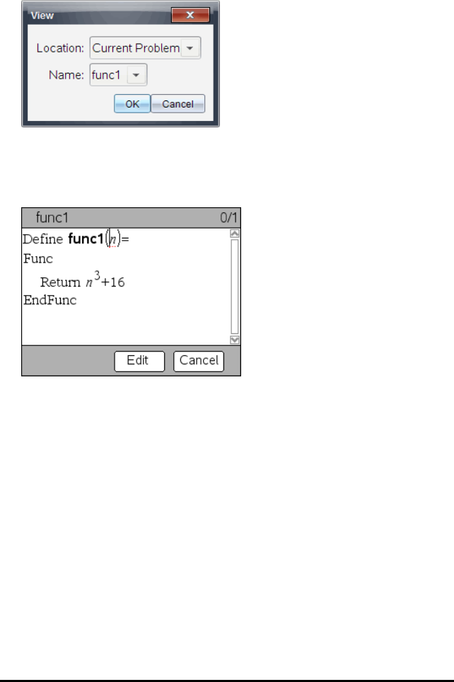
Viewing a Program or Function
1. From the Actions menu, click View.
2. If the function or program is a library object, select its library from the Location list.
3. Select the function or program name from the Name list.
The function or program is displayed in a viewer.
4. Use the arrow keys to view the function or program.
5. If you want to edit the program, click Edit.
Note: The Edit selection is available only for functions and programs defined in the
current problem. To edit a library object, you must first open its library document.
Opening a Function or Program for Editing
You can open a function or program from the current problem only.
Note: You cannot modify a locked program or function. To unlock the object, go to a
Calculator page and use the unLock command.
1. Display the list of available functions and programs.
- From the Actions menu, click Open.
Getting Started with the Programme Editor 556
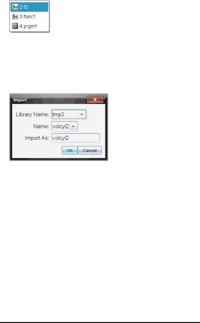
557 Getting Started with the Programme Editor
2. Click the item to open.
Importing a Program from a Library
You can import a function or program defined as a library object into a Program Editor
within the current problem. The imported copy is not locked, even if the original is
locked.
1. From the Actions menu, click Import.
2. Select the Library Name.
3. Select the Name of the object.
4. If you want the imported object to have a different name, type the name under
Import As.
Creating a Copy of a Function or Program
When creating a new function or program, you might find it easier to start with a copy
of the current one. The copy that you create is not locked, even if the original is locked.
1. From the Actions menu, click Create Copy.
2. Type a new name or click OK to accept the proposed name.
3. If you want to change the access level, select Library Access and select a new level.
Renaming a Program or Function
You can rename and (optionally) change the access level of the current function or
program.
1. From the Actions menu, click Rename.
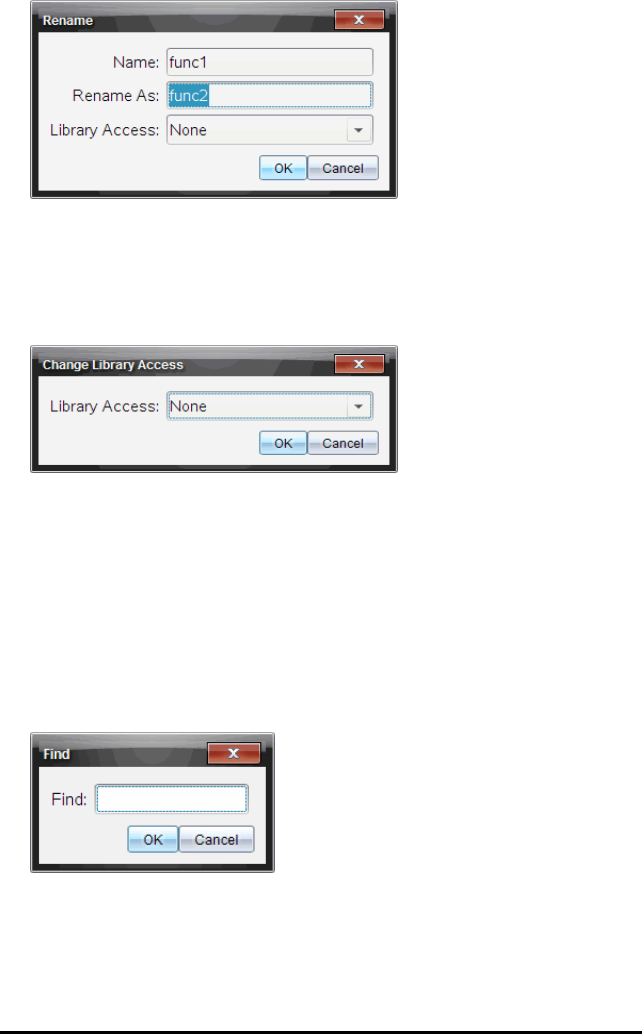
2. Type a new name or click OK to accept the proposed name.
3. If you want to change the access level, select Library Access and select a new level.
Changing the Library Access Level
1. From the Actions menu, click Change Library Access.
2. Select the Library Access:
- To use the function or program only from the current Calculator problem, select
None.
- To make function or program accessible from any document but not visible in
the Catalogue, select LibPriv.
- To make the function or program accessible from any document and also
visible in the Catalogue, select LibPub.
Finding Text
1. From the Actions menu, click Find.
2. Type the text that you want to find, and click OK.
- If the text is found, it is highlighted in the program.
- If the text is not found, a notification message is displayed.
Getting Started with the Programme Editor 558
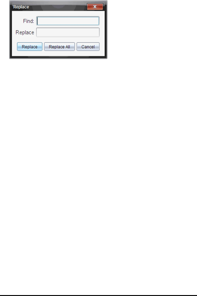
559 Getting Started with the Programme Editor
Finding and Replacing Text
1. From the Actions menu, click Find and Replace.
2. Type the text that you want to find.
3. Type the replacement text.
4. Click Replace to replace the first occurrence after the cursor position.
—or—
Click Replace All to replace every occurrence.
Note: If the text is found in a maths template, a message is displayed to warn you
that your replacement text will replace the whole template—not just the found
text.
Closing the Current Function or Program
▶From the Actions menu, click Close.
If the function or program has unstored changes, you are prompted to check syntax
and store before closing.
Running Programmes and Evaluating Functions
After defining and storing a programme or function, you can use it from an application.
All the applications can evaluate functions, but only the Calculator and Notes
applications can run programmes.
The programme statements are executed in sequential order (although some
commands alter the programme flow). The output, if any, is displayed in the
application’s work area.
• Programme execution continues until it reaches the last statement or a Stop
command.
• Function execution continues until it reaches a Return command.
Running a Programme or Function from the Programme Editor
1. Make sure you have defined a programme or function and the Programme Editor is
the active pane (computer) or page (handheld).
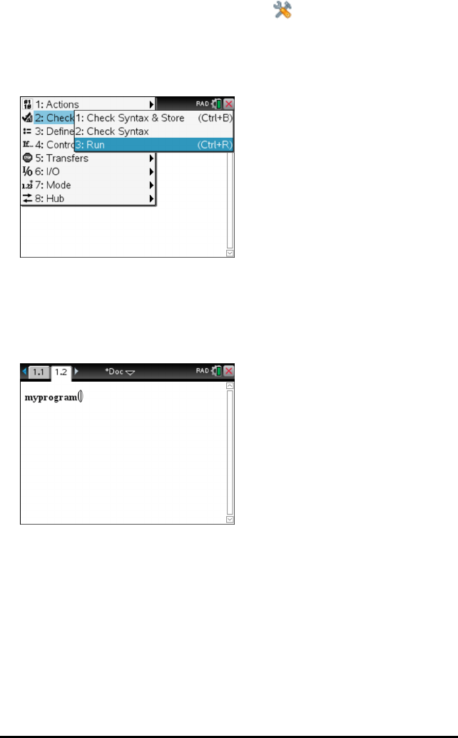
2. On the toolbar, click the Document Tools button and select Check Syntax &
Store > Run.
—or—
Press Ctrl+R.
Handheld: Press b 2 3, or press / R.
This will automatically:
• check the syntax and store the programme or function,
• paste the programme or function name on the first available line of the
Calculator application immediately following the Programme Editor. If no
Calculator exists in that position, a new one is inserted.
3. If the programme or function requires you to supply one or more arguments, type
the values or variable names inside the parentheses.
4. Press ·.
Note: You can also run a programme or function in Calculator or Notes applications by
typing the name of the programme with parentheses and any required arguments and
pressing ·.
Getting Started with the Programme Editor 560

561 Getting Started with the Programme Editor
Using Short and Long Names
Anytime you are in the same problem where an object is defined, you can access it by
entering its short name (the name given in the object’s Define command). This is the
case for all defined objects, including private, public and non-library objects.
You can access a library object from any document by typing the object’s long name. A
long name consists of the name of the object’s library document followed by a
backslash “\” followed by the name of the object. For example, the long name of the
object defined as func1 in the library document lib1 is lib1\func1. To type the “\”
character on the handheld, press g p.
Note: If you cannot remember the exact name or the order of arguments required for a
private library object, you can open the library document or use the Programme Editor
to view the object. You also can use getVarInfo to view a list of objects in a library.
Using a Public Library Programme or Function
1. Make sure you have defined the object in the document’s first problem, stored the
object, saved the library document in the MyLib folder, and refreshed the libraries.
2. Open the TI-Nspire™ application in which you want to use the programme or
function.
Note: All applications can evaluate functions, but only the Calculator and Notes
applications can run programmes.
3. Open the Catalogue and use the library tab to find and insert the object.
—or—
Type the name of the object. In the case of a programme or function, always
follow the name with parentheses.
libs2\func1()
4. If the programme or function requires you to supply one or more arguments, type
the values or variable names inside the parentheses.
libs2\func1(34,power)
5. Press ·.
Using a Private Library Programme or Function
To use a Private library object, you must know its long name. For example, the long
name of the object defined as func1 in the library document lib1 is lib1\func1.
Note: If you cannot remember the exact name or the order of arguments required for a
private library object, you can open the library document or use the Programme Editor
to view the object.
1. Make sure you have defined the object in the document’s first problem, stored the
object, saved the library document in the MyLib folder, and refreshed the libraries.

2. Open the TI-Nspire™ application in which you want to use the programme or
function.
Note: All applications can evaluate functions, but only the Calculator and Notes
applications can run programmes.
3. Type the name of the object. In the case of a programme or function, always
follow the name with parentheses.
libs2\func1()
4. If the object requires you to supply one or more arguments, type the values or
variable names inside the parentheses.
libs2\func1(34,power)
5. Press ·.
Interrupting a Running Programme or Function
While a programme or function is running, the busy pointer }is displayed.
▶To stop the programme or function,
- Windows®: Hold down the F12 key and press Enter repeatedly.
- Mac®: Hold down the F5 key and press Enter repeatedly.
- Handheld: Hold down the ckey and press ·repeatedly.
A message is displayed. To edit the programme or function in the Programme
Editor, select GoTo. The cursor appears at the command where the break occurred.
Getting Values into a Program
You can choose from several methods to supply the values that a function or program
uses in calculations.
Embedding the Values Within the Program or Function
This method is useful primarily for values that must be the same each time the
program or function is used.
1. Define the program.
Define calculatearea()=
Prgm
w:=3
h:=23.64
area:=w*h
EndPrgm
2. Run the program.
calculatearea() :area70.92
Getting Started with the Programme Editor 562

563 Getting Started with the Programme Editor
Letting the User Assign the Values to Variables
A program or function can refer to variables created beforehand. This method requires
users to remember the variable names and to assign values to them before using the
object.
1. Define the program.
Define calculatearea()=
Prgm
area:=w*h
EndPrgm
2. Supply the variables, and then run the program.
w:=3 : h:=23.64
calculatearea() :area70.92
Letting the User Supply the Values as Arguments
This method lets users pass one or more values as arguments within the expression
that calls the program or function.
The following program, volcyl, calculates the volume of a cylinder. It requires the user
to supply two values: height and radius of the cylinder.
1. Define the volcyl program.
Definevolcyl(height,radius) =
Prgm
Disp "Volume =", approx(p ¦ radius2¦height)
EndPrgm
2. Run the program to display the volume of a cylinder with a height of 34 mm and a
radius of 5 mm.
volcyl(34,5)Volume = 534.071
Note: You do not have to use the parameter names when you run the volcyl
program, but you must supply two arguments (as values, variables or expressions).
The first must represent the height and the second must represent the radius.
Requesting the Values from the User (Programs Only)
You can use the Request and RequestStr commands in a program to make the program
pause and display a dialogue box prompting the user for information. This method
does not require users to remember variable names or the order in which they are
needed.
You cannot use the Request or RequestStr command in a function.
1. Define the program.

Define calculatearea()=
Prgm
Request "Width: ",w
Request "Height: ",h
area:=w*h
EndPrgm
2. Run the program and respond to the requests.
calculatearea() : area
Width: 3 (3 entered as a response)
Height: 23.64(23.64 entered as a response)
70.92
Use RequestStr instead of Request when you want the program to interpret the user’s
response as a character string rather than a maths expression. This avoids requiring
the user to enclose the response in quotation marks (““).
Displaying Information
A running function or program does not display intermediate calculated results unless
you include a command to display them. This is an important difference between
performing a calculation on the entry line and performing it in a function or program.
The following calculations, for example, do not display a result in a function or
program (although they do from the entry line).
©
x:=12¦6
cos(p/4)&n
©
Displaying Information in the History
You can use the Disp command in a program or function to display information,
including intermediate results, in the history.
©
Disp 12¦6
Disp "Result:",cos(p/4)
©
Displaying Information in a Dialogue Box
You can use the Text command to pause a running program and display information in
a dialogue box. The user clicks OK to continue or clicks Cancel to stop the program.
You cannot use the Text command in a function.
©
Text "Area=" & area
©
Getting Started with the Programme Editor 564

565 Getting Started with the Programme Editor
Note: Displaying a result with Disp or Text does not store that result. If you expect to
refer later to a result, store it to a global variable.
©
cos(p/4)&maximum
Disp maximum
©
Using Local Variables
A local variable is a temporary variable that exists only while a user-defined function is
being evaluated or a user-defined program is running.
Example of a Local Variable
The following program segment shows a For...EndFor loop (which is discussed later in
this module). The variable iis the loop counter. In most cases, the variable iis used
only while the program is running.
Local iÀ
For i,0,5,1
Disp i
EndFor
Disp i
ÀDeclares variable ias local.
Note: When possible, declare as local any variable that is used only within the program
and does not need to be available after the program stops.
What Causes an Undefined Variable Error Message?
An Undefined variable error message is displayed when you evaluate a user-defined
function or run a user-defined program that references a local variable that is not
initialized (assigned a value).
For example:
Define fact(n)=Func
Local mÀ
While n>1
n¦m&m: n–1&n
EndWhile
Return m
EndFunc
ÀLocal variable mis not assigned an initial value.
Initialize Local Variables
All local variables must be assigned an initial value before they are referenced.

Define fact(n)=Func
Local m: 1&mÀ
While n>1
n¦m&m: n–1&n
EndWhile
Return m
EndFunc
À1 is stored as the initial value for m.
Note (CAS): Functions and programs cannot use a local variable to perform symbolic
calculations.
CAS: Performing Symbolic Calculations
If you want a function or program to perform symbolic calculations, you must use a
global variable instead of a local. However, you must be certain that the global variable
does not already exist outside of the program. The following methods can help.
• Refer to a global variable name, typically with two or more characters, that is not
likely to exist outside of the function or program.
• Include DelVar within a program to delete the global variable, if it exists, before
referring to it. (DelVar does not delete locked or linked variables.)
Differences Between Functions and Programs
A function defined in the Program Editor is similar to the functions built into the
TI-Nspire™ Software.
• Functions must return a result, which can be graphed or entered in a table.
Programs cannot return a result.
• You can use a function (but not a program) within an expression. For example: 3¦
func1(3) is valid, but not 3¦prog1(3).
• You can run programs from Calculator and Notes applications only. However, you
can evaluate functions in Calculator, Notes, Lists & Spreadsheet, Graphs &
Geometry and Data & Statistics.
• A function can refer to any variable; however, it can store a value to a local variable
only. Programs can store to local and global variables.
Note: Arguments used to pass values to a function are treated as local variables
automatically. If you want to store to any other variables, you must declare them
as Local from within the function.
• A function cannot call a program as a subroutine, but it can call another user-
defined function.
• You cannot define a program within a function.
• A function cannot define a global function, but it can define a local function.
Getting Started with the Programme Editor 566
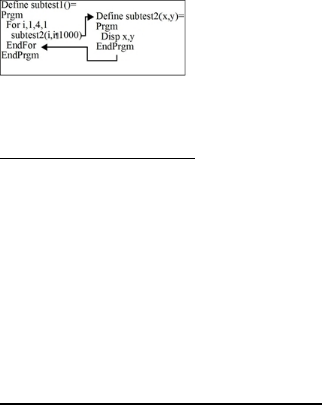
567 Getting Started with the Programme Editor
Calling One Program from Another
One program can call another program as a subroutine. The subroutine can be external
(a separate program) or internal (included in the main program). Subroutines are
useful when a program needs to repeat the same group of commands at several
different places.
Calling a Separate Program
To call a separate program, use the same syntax that you use to run the program from
the entry line.
Defining and Calling an Internal Subroutine
To define an internal subroutine, use the Define command with Prgm...EndPrgm.
Because a subroutine must be defined before it can be called, it is a good practice to
define subroutines at the beginning of the main program.
An internal subroutine is called and executed in the same way as a separate program.
Define subtest1()=
Prgm
local subtest2À
Define subtest2(x,y)=Á
Prgm
Disp x,y
EndPrgm
©Beginning of main program
For i,1,4,1
subtest2(i,I*1000) Â
EndFor
EndPrgm
ÀDeclares the subroutine as a local variable.
ÁDefines the subroutine.
ÂCalls the subroutine.
Note: Use the Program Editor’s Var menu to enter the Define and Prgm...EndPrgm
commands.
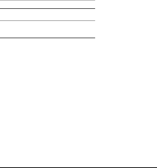
Notes about Using Subroutines
At the end of a subroutine, execution returns to the calling program. To exit a
subroutine at any other time, use Return with no argument.
A subroutine cannot access local variables declared in the calling program. Likewise,
the calling program cannot access local variables declared in a subroutine.
Lbl commands are local to the programs in which they are located. Therefore, a Goto
command in the calling program cannot branch to a label in a subroutine or vice versa.
Avoiding Circular-Definition Errors
When evaluating a user-defined function or running a program, you can specify an
argument that includes the same variable that was used to define the function or
create the program. However, to avoid circular-definition errors, you must assign a
value for variables that are used in evaluating the function or running the program.
Forexample:
x+1&xÀ
– or –
For i,i,10,1
Disp iÀ
EndFor
ÀCauses a Circular definition error message if x or i does not have a value. The error
does not occur if x or i has already been assigned a value.
Controlling the Flow of a Function or Program
When you run a program or evaluate a function, the program lines are executed in
sequential order. However, some commands alter the program flow. For example:
• Control structures such as If...EndIf commands use a conditional test to decide
which part of a program to execute.
• Loop commands such as For...EndFor repeat a group of commands.
Using If, Lbl and Goto to Control Program Flow
The If command and several If...EndIf structures let you execute a statement or block
of statements conditionally, that is, based on the result of a test (such as x>5). Lbl
(label) and Goto commands let you branch or jump, from one place to another in a
function or program.
The If command and several If...EndIf structures reside on the Program Editor’s Control
menu.
When you insert a structure such as If...Then...EndIf, a template is inserted at the
cursor location. The cursor is positioned so that you can enter a conditional test.
Getting Started with the Programme Editor 568

569 Getting Started with the Programme Editor
If Command
To execute a single command when a conditional test is true, use the general form:
If x>5
Disp "x is greater than 5"À
Disp xÁ
ÀExecuted only if x>5; otherwise, skipped.
ÁAlways displays the value of x.
In this example, you must store a value to x before executing the Ifcommand.
If...Then...EndIf Structures
To execute one group of commands if a conditional test is true, use the structure:
If x>5 Then
Disp "x is greater than 5"À
2¦x&xÀ
EndIf
Disp xÁ
ÀExecuted only if x>5.
ÁDisplays the value of:
2x if x>5
x if x{5
Note: EndIf marks the end of the Then block that is executed if the condition is true.
If...Then...Else...EndIf Structures
To execute one group of commands if a conditional test is true and a different group if
the condition is false, use this structure:
If x>5 Then
Disp "x is greater than 5"À
2¦x&xÀ
Else
Disp "x is less than or equal to 5"Á
5¦x&xÁ
EndIf
Disp xÂ
ÀExecuted only if x>5.
ÁExecuted only if x{5.

ÂDisplays value of:
2x if x>5
5x if x{5
If...Then...ElseIf... EndIf Structures
A more complex form of the If command lets you test for multiple conditions. Suppose
you want a program to test a user-supplied argument that signifies one of four
options.
To test for each option (IfChoice=1, If Choice=2 and so on), use the
If...Then...ElseIf...EndIf structure.
Lbl and Goto Commands
You can also control the flow by using Lbl (label) and Goto commands. These
commands reside on the Program Editor’s Transfers menu.
Use the Lbl command to label (assign a name to) a particular location in the function
or program.
Lbl labelName name to assign to this location (use the
same naming convention as a variable
name)
You can then use the Goto command at any point in the function or program to branch
to the location that corresponds to the specified label.
Goto labelName specifies which Lbl command to branch
to
Because a Goto command is unconditional (it always branches to the specified label),
it is often used with an If command so that you can specify a conditional test. For
example:
If x>5
Goto GT5À
Disp x
--------
-------- Á
Lbl GT5
Disp "The number was > 5"
ÀIf x>5, branches directly to label GT5.
ÁFor this example, the program must include commands (such as Stop) that prevent
Lbl GT5 from being executed if x{5.
Getting Started with the Programme Editor 570
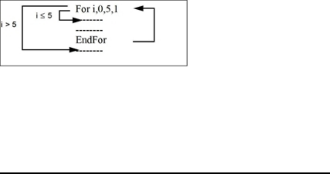
571 Getting Started with the Programme Editor
Using Loops to Repeat a Group of Commands
To repeat the same group of commands successively, use one of the loop structures.
Several types of loops are available. Each type gives you a different way to exit the
loop, based on a conditional test.
Loop and loop-related commands reside on the Program Editor’s Control and Transfers
menus.
When you insert one of the loop structures, its template is inserted at the cursor
location. You can then begin entering the commands that will be executed within the
loop.
For...EndFor Loops
AFor...EndFor loop uses a counter to control the number of times the loop is repeated.
The syntax of the For command is:
Note: The ending value can be less than the beginning value, provided the increment is
negative.
For variable,begin,end [, increment]
À Á Â Ã
ÀVariable used as a counter
ÁCounter value used the first time For is executed
ÂExits the loop when variable exceeds this value
ÃAdded to the counter each subsequent time For is executed (If this optional value is
omitted, the increment is 1.)
When For is executed, the variable value is compared to the end value. If variable
does not exceed end, the loop is executed; otherwise, control jumps to the command
following EndFor.
Note: The For command automatically increments the counter variable so that the
function or program can exit the loop after a certain number of repetitions.
At the end of the loop (EndFor), control jumps back to the For command, where the
variable is incremented and compared to end.
For example:
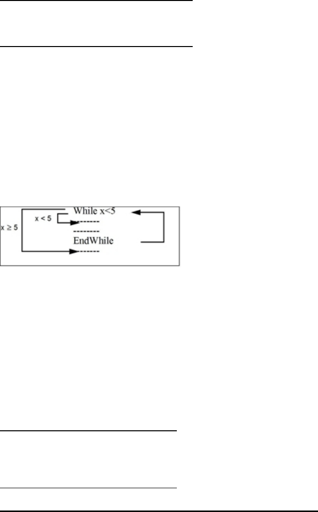
For i,0,5,1
Disp iÀ
EndFor
Disp iÁ
ÀDisplays 0, 1, 2, 3, 4, and 5.
ÁDisplays 6. When variable increments to 6, the loop is not executed.
Note: You can declare the counter variable as local if it does not need to be saved after
the function or program stops.
While...EndWhile Loops
AWhile...EndWhile loop repeats a block of commands as long as a specified condition
is true. The syntax of the While command is:
While condition
When While is executed, condition is evaluated. If condition is true, the loop is
executed; otherwise, control jumps to the command following EndWhile.
Note: The While command does not automatically change the condition. You must
include commands that allow the function or program to exit the loop.
At the end of the loop (EndWhile), control jumps back to the While command, where
condition is re-evaluated.
To execute the loop the first time, the condition must initially be true.
• Any variables referenced in the condition must be set before the While command.
(You can build the values into the function or program, or you can prompt the user
to enter the values.)
• The loop must contain commands that change the values in the condition,
eventually causing it to be false. Otherwise, the condition is always true and the
function or program cannot exit the loop (called an infinite loop).
For example:
0&xÀ
While x<5
Disp xÁ
x+1&xÂ
EndWhile
Getting Started with the Programme Editor 572
573 Getting Started with the Programme Editor
Disp xÃ
ÀInitially sets x.
ÁDisplays 0, 1, 2, 3, and 4.
ÂIncrements x.
ÃDisplays 5. When x increments to 5, the loop is not executed.
Loop...EndLoop Loops
ALoop...EndLoop creates an infinite loop, which is repeated endlessly. The Loop
command does not have any arguments.
Typically, you insert commands in the loop that let the program exit from the loop.
Commonly used commands are: If,Exit,Goto and Lbl (label). For example:
0&x
Loop
Disp x
x+1&x
If x>5À
Exit
EndLoop
Disp xÁ
ÀAn If command checks the condition.
ÁExits the loop and jumps to here when xincrements to 6.
Note: The Exit command exits from the current loop.
In this example, the If command can be anywhere in the loop.
When the If command is: The loop is:
At the beginning of the
loop
Executed only if the condition is true.
At the end of the loop Executed at least once and repeated only if the condition
is true.
The If command could also use a Goto command to transfer program control to a
specified Lbl (label) command.

Repeating a Loop Immediately
The Cycle command immediately transfers program control to the next iteration of a
loop (before the current iteration is complete). This command works with For...EndFor,
While...EndWhile and Loop...EndLoop.
Lbl and Goto Loops
Although the Lbl (label) and Goto commands are not strictly loop commands, they can
be used to create an infinite loop. For example:
As with Loop...EndLoop, the loop should contain commands that let the function or
program exit from the loop.
Changing Mode Settings
Functions and programs can use the setMode() function to temporarily set specific
calculation or result modes. The Program Editor’s Mode menu makes it easy to enter
the correct syntax without requiring you to memorise numeric codes.
Note: Mode changes made within a function or program definition do not persist
outside the function or program.
Setting a Mode
1. Position the cursor where you want to insert the setMode function.
2. From the Mode menu, click the mode to change, and click the new setting.
The correct syntax is inserted at the cursor location. For example:
setMode(1,3)
Debugging Programs and Handling Errors
After you write a function or program, you can use several techniques to find and
correct errors. You can also build an error-handling command into the function or
program itself.
If your function or program allows the user to select from several options, be sure to
run it and test each option.
Getting Started with the Programme Editor 574
575 Getting Started with the Programme Editor
Techniques for Debugging
Run-time error messages can locate syntax errors but not errors in program logic. The
following techniques may be useful.
• Temporarily insert Disp commands to display the values of critical variables.
• To confirm that a loop is executed the correct number of times, use Disp to display
the counter variable or the values in the conditional test.
• To confirm that a subroutine is executed, use Disp to display messages such as
“Entering subroutine” and “Exiting subroutine” at the beginning and end of the
subroutine.
• To stop a program or function manually,
- Windows®: Hold down the F12 key and press Enter repeatedly.
- Mac®: Hold down the F5 key and press Enter repeatedly.
- Handheld: Hold down the ckey and press ·repeatedly.
Error-handling Commands
Command Description
Try...EndTry Defines a block that lets a function or program execute a command and,
if necessary, recover from an error generated by that command.
ClrErr Clears the error status and sets system variable errCode to zero. For an
example of using errCode, see the Try command in the Reference
Guide.
PassErr Passes an error to the next level of the Try...EndTry block.
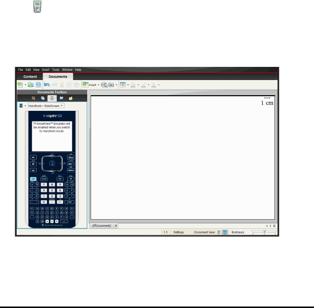
Using the TI-SmartView™ Emulator
With three layout options to choose from, teachers will find that the emulator
facilitates classroom presentations. In the teacher software, layout options are:
• Handheld only
• Keypad plus side screen
• Handheld plus side screen
In the student software, the TI-SmartView™ emulates the keypad, which along with
the handheld view, gives students the ability to drive the software as if using a
handheld.
Opening the TI-SmartView™ Emulator
The TI-SmartView™ emulator is located in the Documents Workspace. To open the
emulator view:
1. Open the Documents Workspace.
2. Click , which is located in the Documents Toolbox.
In the teacher software, the handheld is displayed with Handheld and SideScreen
panels open in computer mode as shown in the following illustration. You can use
the keypad on the emulated handheld, but the document won’t appear on the
emulated handheld screen until you switch to Handheld mode.
In the student software, the TI-Nspire™ CX keypad is displayed with the side screen
open in computer mode. You can use the keypad on the emulated handheld to work
with the document in the side screen in either computer mode or handheld mode.
Using the TI-SmartView™ Emulator 576
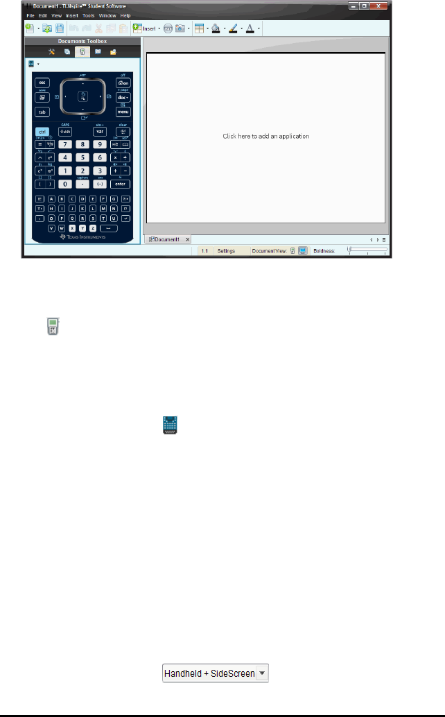
577 Using the TI-SmartView™ Emulator
3. Click View > Handheld.
—or—
Click in the status bar to switch to handheld mode.
Choosing a Keypad
An open document is not affected by changing the keypad. You can switch between
keypads anytime you want. To select a keypad:
1. In the emulator panel, click to open the menu and select one of the following
options:
• TI-Nspire™ CX
• TI-Nspire™ with Touchpad
• TI-Nspire™ with Clickpad
2. Click ¢to select a faceplate option:
• Normal
• High Contrast
• Outline
Choosing Display Options
In the teacher software, use this option to choose how to display the emulator in the
software window.
1. In the emulator panel, click .
—or—
Click File > Settings > TI-SmartView™.
2. Select one of the following options:
•Handheld Only. Displays the emulated handheld and hides the workspace and
other panels.
Note: To keep the Handheld Only display in front of other application windows,
click Always in Front at the top right of the TI-SmartView™ panel.
•Keypad + SideScreen. Opens a larger view of the keypad along with the side
screen.
•Handheld + SideScreen. Opens the entire emulated handheld along with the
side screen.
Changing the Width of the TI-SmartView™ Panel
To change the width of the TI-SmartView™ emulator panel:
▶Click the right edge of the panel and drag it until it is the width you want.
Changing the Size of the Screen in the Workspace
When in handheld mode, use the Scale to change the size of the screen.
▶Drag the slider to the appropriate scale percentage. The scale slider is located on
the far right side of the status bar, at the bottom of the TI-Nspire™ window. Scale
percentages range from 100% to 200%. The default scale is 150%.
Note: If computer mode is selected, you cannot change the size of the workspace.
Working with the Emulated Handheld
To input data and work with files on the emulator, you can use the computer keyboard,
TI-SmartView™ keypad, TI-Nspire™ menus and icons or any combination of these.
Note: Within one command, you cannot use a combination of both the keypad and the
keyboard. For example, you cannot press Ctrl on the keyboard and click bon the
emulator to open a context menu.
For the most part, you can perform any function in the TI-SmartView™ emulator that
you can perform on the handheld. Keys and applications operate the same way.
Note: If you switch to Computer mode, you can still use most of the keys on the
emulated handheld or keypad and all keystrokes are reflected in the workspace.
However, some key combinations may only work in Handheld mode.
Using the TI-SmartView™ Emulator 578
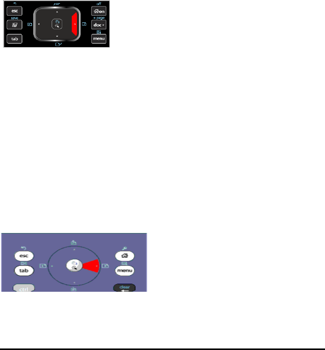
579 Using the TI-SmartView™ Emulator
As you click keys on the emulator or press keys on the keyboard that activate keys on
the emulator, those keys change colour, making it easy for your audience to follow
along. The last key selected stays highlighted.
In the teacher software, the emulator screen and the side screen are both interactive.
You can click on icons and menu items on both screens. You can also right-click to
display menus on both screens.
All handheld shortcuts and arrow functionality work from the computer keyboard. For
example, to save a document, you can click / S on the emulator keypad or you can
press Ctrl + S on the computer keyboard. When using a Mac®, press “+S.
Using the Touchpad
You can operate the Touchpad on the TI-Nspire™ Touchpad keypad using either the
touchpad on a laptop or by using the mouse to click the Touchpad. Areas of the
Touchpad are highlighted as you click the arrow zones.
An arrow is highlighted when you press
or tap it.
• Clicking the ¡,¢,£or ¤keys on the Touchpad moves through menus one item at
a time.
• Clicking and holding down an arrow on the Touchpad causes continual movement
in the selected direction.
• Clicking and sliding the mouse across the Touchpad area enables you to move the
mouse pointer.
• Clicking the middle of the Touchpad selects the highlighted menu option.
Using the Clickpad
You can use the Clickpad on the TI-Nspire™ Clickpad keypad using either the touchpad
on a laptop or by using the mouse to click the Clickpad. Areas of the Clickpad are
highlighted as you click the arrow zones.
• Clicking the ¡,¢,£or ¤keys on the Clickpad moves through menus one item at a
time.

• Clicking and holding down an arrow on the Clickpad causes continual movement in
the selected direction.
• Clicking the middle of the Clickpad selects the highlighted menu option.
Using Settings and Status
When working with the TI-SmartView™ emulator, you can change General Settings
and Document Settings. For more information, see Using the Documents Workspace.
You can view all other settings, but you cannot change them in the TI-SmartView™
emulator. However, the ability to view these options provides teachers with an
instructional tool when they need to show students how to set up a handheld.
To view settings and status:
1. Click cto access the Home screen.
2. Click Settings.
Setting or
Settings
Description
Language You can open the languages menu and select a language, but you
cannot save changes. To change the language, use the TI-Nspire™
menu File > Settings > Change Language option.
Handheld
Setup
You can open the menus and select items to demonstrate which
items to choose, but you cannot save any changes.
Handheld
Status
You can access the screen. The # symbol replaces any numeric values
that would be displayed on the handheld.
About You can open the About screen and view the software version. Other
information that pertains only to the handheld hardware is marked as
"Not Applicable".
Login You can display the Login to Class screen and type in the User Name
and Password fields. Login is not available.
Changing TI-SmartView™ Options
You can change the emulator options, even when the emulator panel is closed.
1. In the teacher software, click File> Settings> TI-SmartView™ Options.
The TI-SmartView™ Options dialogue box opens.
Using the TI-SmartView™ Emulator 580
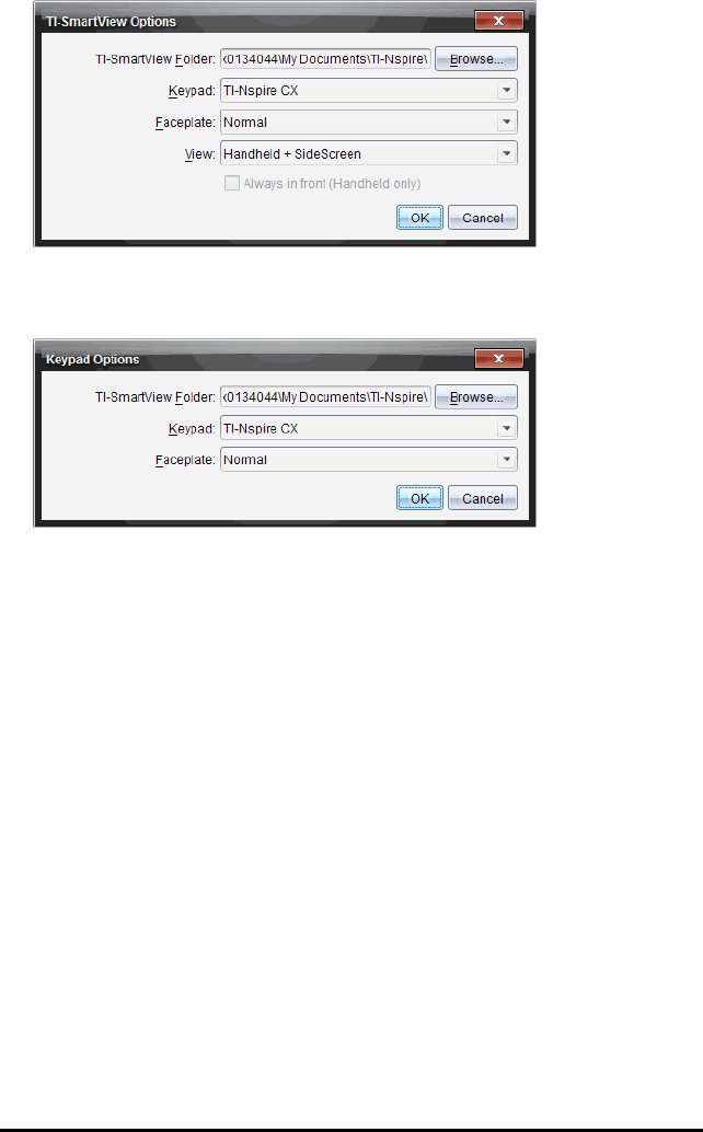
581 Using the TI-SmartView™ Emulator
In the student software, click File > Settings > Keypad Options.
The Keypad Options dialogue box opens.
2. Click Browse to change the folder where documents are saved and accessed in the
My Documents folder when using the emulator.
Important: If you change the TI-SmartView™ location, you must also copy or move
the MyLib folder and paste it to the new location to see library objects.
The default location of MyLib is:
• Windows®: Documents\TI-Nspire\MyLib.
• Mac®: Documents/TI-Nspire/MyLib.
Note: Close and reopen the TI-Nspire™ application for the libraries to reflect the
change.
3. Click ¤to open the menu and select a keypad.
4. Click ¤to open the menu and select a faceplate.
5. In the teacher software, click ¤to open the menu and select a view. If selecting
Handheld only, select Always in Front to keep this window on top of all other open
applications.
6. Click OK to save the settings.

Working with Documents
You can open multiple documents in the workspace by selecting File>Open Document
from the menu or using keyboard shortcuts. When you switch between these
documents, the emulated handheld shows only the current document. You can insert
pages and problems using either the TI-Nspire™ menus or icons, keyboard shortcuts or
TI-SmartView™ menus or shortcuts.
Opening a Document
You can open a document by navigating to it on the emulator, the same way you open
a document on the handheld, or you click File>OpenDocument.
When you open a document using the emulator, you can only open documents that are
in the folder displayed on the emulator (usually the My Documents folder, unless you
specified a different folder in your TI-SmartView™ settings). When you open a
document using the menu path, you can browse to find any TI-Nspire™ document on
your computer or network. If you open a document using the emulated handheld, it
replaces the document that was previously open.
Note: If the number of characters in the document’s file path name exceeds 256
characters, the document cannot be opened and an error message is displayed. To
avoid this error, keep file and folder names short or move files up in the file path.
Saving a Document
When you save a document using the File>Save Document menu or icon, keyboard
shortcuts, keypad shortcuts or emulator menus, the document is saved in the same
location where the file was opened. To save the file in another location or with a
different name, click File>Save As.
Using Screen Capture
To capture the current page, press Ctrl+J (Mac®: ì“ +J) on your keyboard or on the
emulated handheld. The image is automatically placed in the Clipboard and in the
TI-Nspire™ Screen Capture window. You can paste the image into another application
without having to take additional steps. This feature is only available when the
TI-SmartView™ panel is active and the workspace is in Handheld mode.
All other screen capture features work the same way they do in other areas of
TI-Nspire™ software. For more information, see Capturing Screens.
Using the TI-SmartView™ Emulator 582

583

Writing Lua Scripts
The Script Editor allows you to create and deliver dynamically linked simulations,
powerful and flexible utilities and other educational content for exploring maths and
science concepts. When you open a document containing a script, the script runs
automatically as programmed. To see the running script application, the page
containing the script application must be active.
The Script Editor is directed toward teachers and other authors who are comfortable
working in a Lua scripting environment. Lua is a powerful, fast, lightweight scripting
language that is fully supported in TI-Nspire™ and PublishView™ documents.
Documents containing script applications can be opened on TI-Nspire™ handhelds. The
script application runs on a handheld, but you cannot view or edit the script.
Note these resources for using the Script Editor and creating scripts:
• Press F1 to access the TINspire™ help, which includes the Script Editor help.
• Press F2 for additional TI-Nspire™ resources such as scripting samples and a link to
the TI-Nspire™ Scripting API library. (This information is also available at
education.ti.com/nspire/scripting.)
• Go to lua.org for more information about Lua.
Overview of the Script Editor
With the Script Editor, you can insert, edit, save, run, and debug script applications
inTI-Nspire™ (.tns files) and Publishview™ (.tnsp files) documents.
• Script applications function within documents, problems, and pages the same way
that other TI-Nspire™ applications do.
• When you create a new document or open an existing document, you can insert or
edit a script application within a page or within a work area of a split page.
• In a split page layout, you can add a script application to each work area of a page.
A page can be split into a maximum of four quadrants.
• Images can be added to script applications. See the Inserting Images section.
• All work done in the Script Editor is lost if you close the TI-Nspire™ or
PublishView™ document without saving it.
Exploring the Script Editor Interface
The Script Editor window opens when you insert a new script application or edit an
existing script application in a TI-Nspire™ or PublishView™ document.
Select options for creating new scripts or editing scripts from the Insert menu in the
Documents Workspace when a document is open.
Note: Although not labeled, the Documents Workspace is the default workspace in the
TI-Nspire™ CX Student Software and TI-Nspire™ CX CAS Student Software.
The following figure shows the Script Editor with an existing script.
Writing Lua Scripts 584
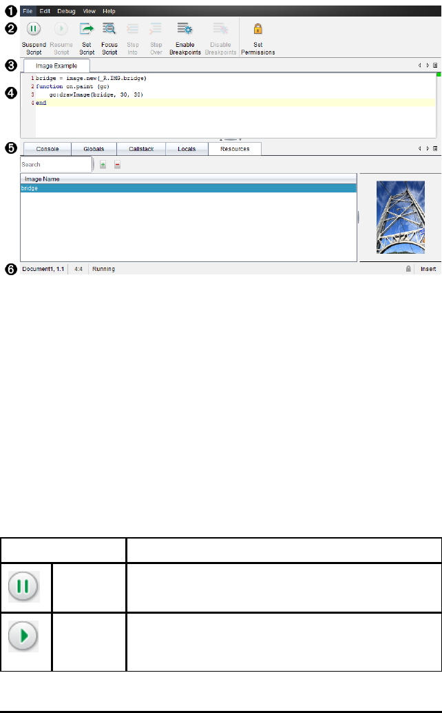
585 Writing Lua Scripts
ÀMenu bar. Contains options for working with the Script Editor.
ÁToolbar. Provides tools for common Script Editor functions. See the Using the
Toolbar section.
ÂScript title. Shows script title. Right-click the title to change it or by clicking Edit >
Set Script Title.
ÃText box. Provides a space to type script text.
ÄTools panel. Shows script data. See the Using the Tools Panel section.
ÅStatus bar. Displays the operational state of the script. See the Using the Status Bar
section.
Using the Toolbar
The following table describes the toolbar options.
Tool name Tool function
Suspend
Script
Pauses the script execution.
Resume
Script
Resumes the script execution.
While debugging, the script continues to execute until the
next breakpoint or the end of the script.
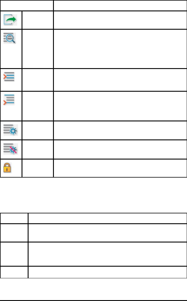
Tool name Tool function
Set Script Starts the script execution.
Focus
Script
Sets the focus to the page in the document where the script
application is attached:
• In a TI-Nspire™ document, sets the focus to the page.
• In a PublishView™ document, sets the focus to the
frame on the page.
Step Into While debugging, executes the current statement. If the
statement calls any functions, the debugger stops at the first
line of each function.
Step Over While debugging, executes the current statement.
If the statement calls any functions, the debugger does not
stop within the function unless the function contains a
breakpoint.
Enable
Breakpoints
Switches from normal mode to debugging mode.
Disable
Breakpoints
Switches back from debugging mode to normal mode and
resumes the script.
Set
Permissions
Sets permission levels to Protected, View Only, or
Unprotected and allows you to set a password for the script.
Using the Tools Panel
At the bottom of the window, the Tools panel shows the scripting data. For more
information, see the Debugging Scripts section.
Tab Window Display
Console Script errors are printed here.
Print statements embedded in the script also print here.
Globals Selected global variables are displayed.
To select a global variable for display, select Click to add new watch
variable at the bottom of the Tools panel.
Call Stack Displays the call tree for the currently executing function.
Writing Lua Scripts 586

587 Writing Lua Scripts
Tab Window Display
Locals Local variables in the current function’s scope are displayed.
Resources Upload, insert, and manage images here.
Using the Status Bar
The status bar at the bottom of the window shows basic script data, as described in
this example: stopwatch, 1.1,4:1,Running.
• Name of the document that the script application is attached to (stopwatch)
• Problem and page number (1.1)
• Script line and character, (4:1 describing line 4 and character 1)
• Operational state of the script (Running). Note the possible states:
- Normal mode: Running, Paused, or Error
- Debugging mode: Running (debugging), Paused, or Error
Inserting New Scripts
To insert a new script application and script, follow these steps.
1. Open the document where you want to insert the script. It can be a new or existing
document.
2. Click Insert > Script Editor > Insert Script.
A script application is inserted, and the Script Title dialogue box opens.
Note: The TI-Nspire™ CX Student Software and the TI-Nspire™ CX CAS Student
Software open automatically within the Documents Workspace.
3. Type a script title. (The maximum number of characters is 32.)
4. Click OK.
The Script Editor window opens showing a blank script.
5. Type your text in the script lines.
Note: Some non-standard UTF-8 wide characters may not be displayed correctly.
For these characters, it is highly recommended that you use the string.uchar
function.
6. When the script is complete, click Set Script to execute it.
• In a TI-Nspire™ document, the script application is inserted in a new page.
When the page containing the script application is active, the Documents
Toolbox is empty.
• In a PublishView™ document, a frame containing the script application is added
to the active page. You can move or size this frame just as you would any other
PublishView™ object, and you can add other PublishView™ objects to the page.

7. To view the script application, click Focus Script.
Zooming Text in the Script Editor
You can adjust the size of the text in your script and in any of the tool panels.
Menu Method
1. Click in the area of the text to zoom.
2. On the View menu, select Zoom, and then select Zoom In,Zoom Out, or Restore.
Note that the menu also displays keyboard shortcuts for the Zoom commands.
Mouse Method
1. Position the mouse pointer over the area to zoom.
2. Hold Ctrl, and roll the mouse wheel forward or back.
Editing Scripts
To edit an existing script, follow these steps.
1. Open the TI-Nspire™ or PublishView™ document that contains the script. The page
containing the script must be active.
2. Select the page and the work area that contains the script.
3. Click Insert > Script Editor > EditScript.
The Script Editor opens showing the script. If the selected work area on the page
does not contain a script, Edit Script is dimmed.
If the script is password protected, the Password Protected dialogue box opens
prompting for a password.
4. Make any desired changes.
• To designate comments, use double hyphens (--) at the start of each comment
line.
• To change the title, click Edit >Set Script Title or right-click the title and click
Set Script Title.
Notes:
• Some nonstandard UTF-8 characters may not be displayed correctly. For these
characters, it is highly recommended that you use the string.uchar function.
• The print function may yield unexpected results for non–UTF-8 characters.
• Some nonprintable characters returned by the on.save function will be
discarded.
5. To execute the script, click Set Script.
Any errors are displayed in the Console area in the Tools panel.
6. To view the script application (running script), click Focus Script.
Writing Lua Scripts 588

589 Writing Lua Scripts
Changing View Options
To change viewing options:
▶To clear the scripting data in the Tools panel and restore the editor defaults, click
View >Restore Editor to Defaults.
▶To view the script title in the document and before each print statement in the
Console, click View >Title in Document View.
▶To hide or show toolbar labels, click View >Toolbar Text Labels.
▶To show or hide the Tools panel or its areas, click View >Tools Panel and click the
appropriate option.
▶To create tab groups when multiple scripts are open, right-click one of the titles
and click New Horizontal Group or New Vertical Group.
Setting Minimum API Level
Each release of the T-Nspire™ software includes API support for a specific set of Lua
scripting features. Setting the minimum API level for a script lets you specify a
minimum set of features that you require for your script.
If a user tries to run the script on a system that does not meet the script's minimum
API level, a message notifies the user and prevents the script from running.
To Set the Minimum API Level for a Script:
1. Determine the minimum level that you want your script to require.
- Setting the level too low for the script's feature set can result in a script error
on older software.
- Setting the level too high can result in the script refusing to start on older
software that supports the feature set.
2. On the Script Editor File menu, select Set Minimum API Level.
3. In the dialogue box, type the minimum level using the format major.minor. For
example, you might type 2.3.
This API level or higher will be required for running the script.
Saving Script Applications
Clicking Set Script resets (updates) a script application in a TI-Nspire™ or PublishView™
document. However, the script and script application are not saved until you save the
document. If you close the document or close the TI-Nspire™ software without saving,
work on the script is lost.
To ensure the script application is saved after all work is complete, follow these steps.
1. From the Script Editor window, click Set Script to reset (update) the script
application in the document.
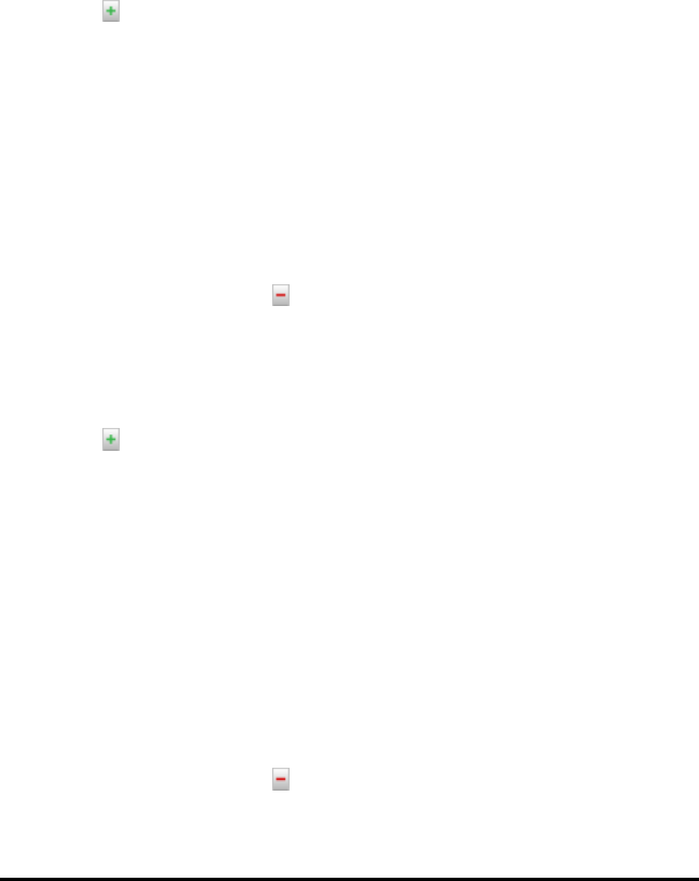
2. From an open document, click File > Save Document to save changes to the
TI-Nspire™ or PublishView™ document.
Note: To ensure work is backed up, set the script and save the document frequently.
Managing Images
To insert an image into a script application, follow these steps.
Add an Image to Resources
1. Click the Resource tab.
2. Click the button.
3. Click on an image file name.
4. Click Open.
5. Accept the default image name or rename the image by typing a new name into
the box. (Ex: newimage)
6. Click OK.
Note: You will see the image thumbnail in the bottom-right corner of your screen.
Your image file name will appear in a list of images at the bottom-left of your
screen.
7. Right-click an image name to Rename, Copy Name, Preview, or Remove the
image. You may also click the button to remove an image.
Add Multiple Images to Resources
1. Click the Resource tab.
2. Click the button.
3. Select Comma Separated Values (*.csv) from the Files of Type menu.
4. Select your .csv file.
Note: The .csv format consists of two comma-separated columns. The first column
is the local name of the image resource used in the code. The second column is the
absolute path to the image on the current system.
Example for Windows:
bridge,C:\images\bridge.jpg
house,C:\images\house.jpg
5. Click Open.
6. Right-click an image name to Rename, Copy Name, Preview, or Remove the
image. You may also click the button to remove an image.
Writing Lua Scripts 590

591 Writing Lua Scripts
Create a Script to Call Up an Image
1. Type a script in the script line box as follows:
myimage = image.new(_R.IMG.img_1)
function on.paint (gc)
gc:drawImage (myimage, 30, 30)
end
Note: Replace img_1 (above) with the name of your image.
2. Click Set Script to save the script. You will see your image in the Document Preview
screen.
3. Click Focus Script to set the focus to the page in the document where you want to
attach the script application.
Note: A TI-Nspire document sets the focus to the page; A PublishView™ document
sets the focus to the frame on the page.
Create a Script to Call Up Multiple Images
1. Type a script in the script line box as follows:
myimg = {}
for name, data in pairs (_R.IMG)
myimg [name] = image.new(data)
end
function on.paint (gc)
gc:drawImage (myimg[imagename], 30, 30)
end
2. Click Set Script to save the script. You will see your image in the Document Preview
screen.
3. Click Focus Script to set the focus to the page in the document where you want to
attach the script application.
Note: A TI-Nspire document sets the focus to the page; A PublishView™ document
sets the focus to the frame on the page.

Setting Script Permissions
You can set permission levels for a script and specify a password to protect a script.
Follow these steps.
1. In the Script Editor window, click File >Set Permissions.
The Set Permissions dialogue box opens.
2. In the Permissions Level area, select the appropriate security level:
•Protected. The script can be run, but not viewed or edited.
•View only. The script can be viewed, but not edited.
•Unprotected. The script can be viewed and edited.
3. To secure a script, designate a password in the Security area.
Note: Use caution when setting passwords because they cannot be recovered.
4. Click OK.
The next time you click Insert > Script Editor > EditScript, a Password Protected
dialogue box opens prompting for the password. Choose one of these options:
• To edit the script, enter the password and click OK.
• To view the script only, do not enter the password and click View.
Debugging Scripts
You can debug your script to investigate runtime errors and trace the execution flow.
While debugging, data is displayed in the Tools panel.
▶To enable debugging mode or disable it and return to normal mode, click Debug >
Enable Breakpoints or Disable Breakpoints.
Note: Disabling breakpoints always resumes the script execution.
▶While debugging, click Step Into and Step Over as appropriate. See the Exploring
the Script Editor interface section.
▶To set breakpoints, double-click in the space to the far left of the line number.
Breakpoints are disabled until you click EnableBreakpoints.
▶Note these factors when debugging:
• Breakpoints in coroutines are not supported.
• If a breakpoint is set in a function that is a callback, the debugger may not stop
at the breakpoint.
• The debugger may not stop at functions such as on.save, on.restore, and
on.destroy.
On the toolbar, Step Into and Step Over are enabled when breakpoints are enabled.
Writing Lua Scripts 592

593 Writing Lua Scripts
▶To suspend and resume the script execution, click Suspend Script and Resume
Script. When the script resumes, it runs until the next breakpoint is encountered or
to the end of the script. A script can be suspended in normal mode or debugging
mode.

Data Collection
The Vernier DataQuest™ application is built into the TI-Nspire™ software and the
operating system (OS) for handhelds. The application lets you:
• Capture, view, and analyse real-world data using a TI-Nspire™ handheld, a
Windows® computer, or a Mac® computer.
• Collect data from up to five connected sensors (three analogue and two digital)
using the TI-Nspire™ Lab Cradle.
Important: The TI-Nspire™ CM-C Handheld is not compatible with the Lab Cradle
and only supports the use of a single sensor at a time.
• Collect data either in the classroom or at remote locations using collection modes
such as time-based or event-based.
• Collect several data runs for comparison.
• Create a graphical hypothesis using the Draw Prediction feature.
• Play back the data set to compare the outcome to the hypothesis.
• Analyse data using functions such as interpolation, tangential rate or modelling.
• Send collected data to other TI-Nspire™ applications.
• Access sensor data from all connected sensor probes through your TI-Basic
program.
Adding a Vernier DataQuest™ Page
Note: The application is launched automatically when you connect a sensor.
Starting a new document or problem for each new experiment ensures that the
Vernier DataQuest™ application is set to its default values.
▶To start a new document containing a data collection page:
From the main File menu, click New Document, and then click Add Vernier
DataQuest™.
Handheld: Press c, and select Vernier DataQuest™ .
▶To insert a new problem with a data collection page into an existing document:
From the toolbar, click Insert > Problem>Vernier DataQuest™.
Handheld: Press ~and select Insert > Problem > Vernier DataQuest™.
Data Collection 594
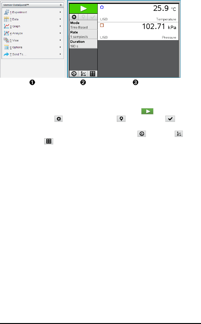
595 Data Collection
ÀVernier DataQuest™ Menu. Contains menu items for set-up, collection and
analysis of sensor data.
ÁDetails view. Contains buttons for starting data collection , changing
collection settings , marking collected data , storing data sets , and
tabs for managing multiple data runs.
View selection buttons let you choose from Meter view , Graph view ,
or Table view .
ÂData work area. The information displayed here depends on the view.
Meter. Displays a list of sensors that are currently connected or set up in
advance.
Graph. Displays collected data in a graphical representation, or displays the
prediction before a data collection run.
Table. Displays collected data in columns and rows.
What You Must Know
Basic Steps in Performing an Experiment
These basic steps are the same no matter which type of experiment you perform.
1. Start the Vernier DataQuest™ Application.
2. Connect sensors.
3. Modify sensor settings.
4. Select the collection mode and collection parameters.
5. Collect data.
6. Stop collecting data.
7. Store the data set.
8. Save the document to save all data sets in the experiment.
9. Analyse the data.
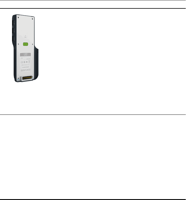
Sending Collected Data to Other TI-Nspire™ Applications
You can send collected data to the Graphs, Lists&Spreadsheet, and Data&Statistics
applications.
▶From the Send To menu, click the name of the application.
A new page showing the data is added to the current problem.
About Collection Devices
You can select from a variety of sensors and interfaces to collect data while running
the Vernier DataQuest™ application with TI-Nspire™ software.
Multi-Channel Sensor Interfaces
Multi-channel sensor interfaces let you connect more than one sensor at a time.
Sensor Interface Description
Texas
Instruments
TI-Nspire™ Lab
Cradle
This sensor can be used with a handheld, a computer, or as a
stand-alone sensor.
The sensor interface allows you to connect and use one to five
sensors at the same time. It can be used in the lab or at a
remote collection location.
The Lab Cradle supports two digital sensors and three analogue
sensors.
The Lab Cradle also supports high-sample data collection
sensors, such as a hand-grip heart rate or a blood pressure
monitor.
After using the Lab Cradle as a remote sensor, you can download
data to either a handheld or computer.
Single-Channel Sensor Interfaces
Single-channel sensor interfaces can only connect to one sensor at a time. These
sensors have either a mini-USB connector for a handheld or a standard USB connector
for a computer. For a complete list of compatible sensors, see Compatible Sensors.
Data Collection 596
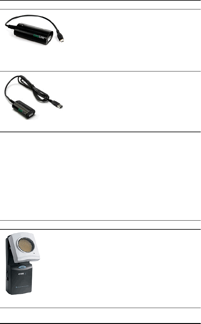
597 Data Collection
Sensor Interface Description
Vernier EasyLink®
This sensor interface is used with handhelds. It has a
mini-USB connector so it can be plugged directly into
the handheld.
Connect sensors to Vernier EasyLink® to:
• Measure barometric pressure.
• Measure the salinity of a solution.
• Investigate the relationship between pressure
and volume (Boyles’ Law).
Vernier Go!Link®
This sensor interface is used with computers. It has a
standard connector so it can be plugged into a
Windows® or Mac® computer.
Connect sensors to Vernier GoLink® to:
• Measure the acidity or alkalinity of a solution.
• Monitor greenhouse gases.
• Measure sound level in decibels.
Types of Sensors
•Analogue sensors. Temperature, light, pH and voltage sensors are analogue sensors
and require a sensor interface.
•Digital sensors. Photogates, radiation monitors and drop counters are digital
sensors. These sensors can only be used with the TI-Nspire™ Lab Cradle.
•Direct-connect USB sensors. These sensors connect directly to a handheld or
computer and do not require a sensor interface.
Sensors for Handhelds
The following lists some sensors you can use with a handheld.
Sensor Description
Texas Instruments
This analogue sensor connects directly to TI-Nspire™
handhelds through the mini-USB port. It is used to explore
and graph motion.
This sensor automatically launches the Vernier DataQuest™
application when you connect it to a handheld. Data
collection begins when you select the Motion Match
function.
This sensor collects up to 200 samples per second.
Use this sensor to:
• Measure position and speed of a person or object.
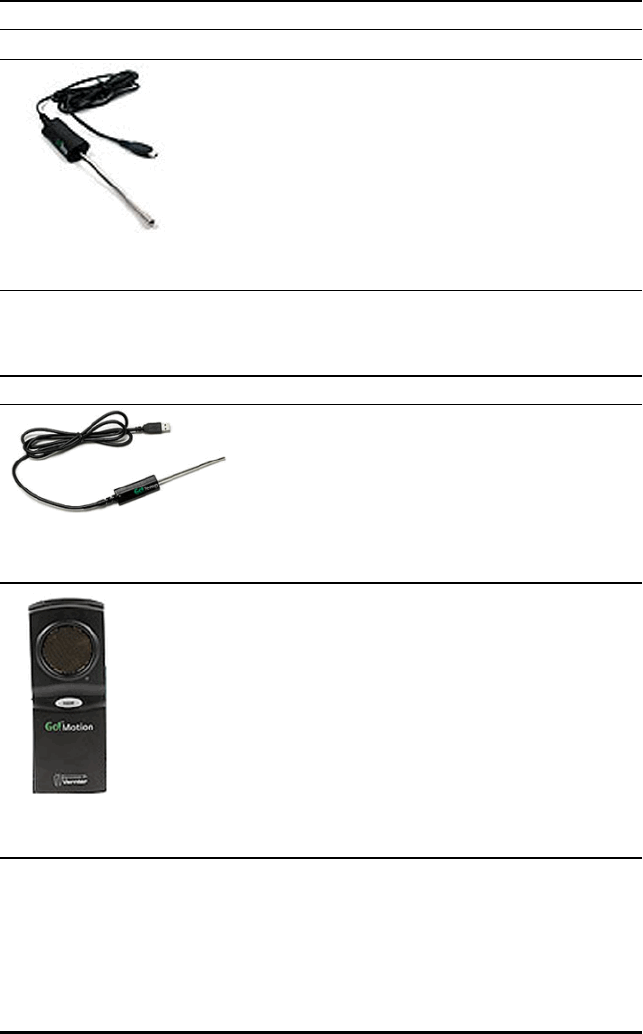
Sensor Description
CBR2™ • Measure the acceleration of an object.
Vernier EasyTemp®
temperature sensor
This analogue sensor connects directly to TI-Nspire™
handhelds through the mini-USB port and is used to collect
temperature ranges. You can design experiments to:
• Collect weather data.
• Record temperature changes due to chemical
reactions.
• Perform heat fusion studies.
Sensors for Computers
The following table lists some sensors you can use with a computer.
Sensor Description
Vernier Go!Temp®
temperature sensor
This analogue sensor connects to the computer’s USB
port and is used to collect temperature ranges.
You can use this sensor to:
• Collect weather data.
• Record temperature changes due to chemical
reactions.
• Perform heat fusion studies.
Vernier Go!Motion® motion
detector
This analogue sensor connects to the computer’s USB
port and is used to measure acceleration, speed and
velocity.
Use this sensor to:
• Measure position and speed of a person or
object.
• Measure the acceleration of an object.
Compatible Sensors
The following sensors can be used with the Vernier DataQuest™ application.
• 25-g Accelerometer
• 30-Volt Voltage Probe
Data Collection 598

599 Data Collection
• 3-Axis Accelerometer
• Low-g Accelerometer
• CBR 2™ - Connects directly to handheld USB port
• Go!Motion® - Connects directly to computer USB port
• Extra Long Temperature Probe
• Stainless Steel Temperature Probe
• Surface Temperature Sensor
• Ammonium Ion-Selective Electrode
• Anemometer
• Barometer
• Blood Pressure Sensor
• C02 Gas Sensor
• Calcium Ion-Selective Electrode
• Charge Sensor
• Chloride Ion-Selective Electrode
• Colorimeter
• Conductivity Probe
• High Current Sensor
• Current Probe
• Differential Voltage Probe
• Digital Radiation Monitor
• Dissolved Oxygen Sensor
• Dual-Range Force Sensor
• EasyTemp® - Connects directly to handheld USB port
• EKG Sensor
• Electrode Amplifier
• Flow Rate Sensor
• Force Plate
• Gas Pressure Sensor
• Go!Temp® - Connects directly to computer USB port
• Hand Dynamometer
• Hand-Grip Heart Rate Monitor
• Instrumentation Amplifier
• Light Sensor
• Magnetic Field Sensor

• Melt Station
• Microphone
• Nitrate Ion-Selective Electrode
• O2 Gas Sensor
• ORP Sensor
• pH Sensor
• Relative Humidity Sensor
• Respiration Monitor Belt (Requires Gas Pressure Sensor)
• Rotary Motion Sensor
• Salinity Sensor
• Soil Moisture Sensor
• Sound Level Meter
• Spirometer
• Thermocouple
• TI-Light - Sold only with the CBL 2™
• TI-Temp - Sold only with the CBL 2™
• TI-Voltage - Sold only with the CBL 2™
• Tris-Compatible Flat pH Sensor
• Turbidity Sensor
• UVA Sensor
• UVB Sensor
• Vernier Constant Current System
• Vernier Drop Counter
• Vernier Infrared Thermometer
• Vernier Motion Detector
• Vernier Photogate
• Voltage Probe
• Wide-Range Temperature Probe
Connecting Sensors
Direct-connect USB sensors, such as the Vernier Go!Temp® temperature sensor (for
computers) or the Vernier EasyLink® temperature sensor (for handhelds), connect
directly to the computer or handheld and do not need a sensor interface.
Other sensors require a sensor interface such as the TI-Nspire™ Lab Cradle.
Data Collection 600
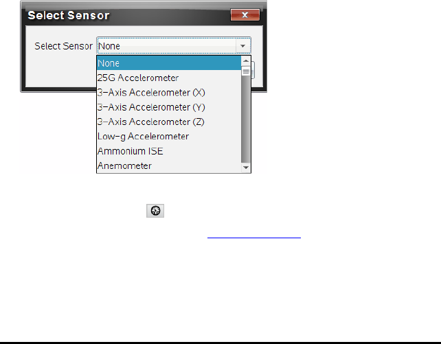
601 Data Collection
Connecting Directly
▶Attach the cable on the sensor directly to the computer's USB port or to an
appropriate port on the handheld.
Connecting through a Sensor Interface
1. Attach the sensor to the sensor interface using either the mini-USB, USB or BT
connector and the appropriate cable.
2. Attach the interface to a computer or handheld using the appropriate connector
and cable.
Note: To attach a handheld to a TI-Nspire™ Lab Cradle, slide the handheld into the
connector at the bottom of the Lab Cradle.
Setting Up an Offline Sensor
You can pre-define meter settings for a sensor that is not currently attached to a
computer or handheld.
You cannot use the sensor offline, but you can prepare the experiment for it and then
attach it when ready to collect the data. This option makes it faster to share a sensor
during a lesson or lab in which there are not enough sensors for everyone.
1. From the Experiment menu, select Advanced Set Up > Configure Sensor > Add
Offline Sensor.
The Select Sensor dialogue box opens.
2. Select a sensor from the list.
3. Click the Meter View tab .
4. Click the sensor you have added, and modify its settings.
The settings will be applied when you attach the sensor.
Removing an offline sensor
1. From the Experiment menu, select Advanced Setup > Configure Sensor.

2. Select the name of the offline sensor to remove.
3. Click Remove.
Modifying Sensor Settings
You can modify how the sensor values are displayed and stored. For example, when
using a temperature sensor, you can change the unit of measure from Centigrade to
Fahrenheit.
Changing Sensor Measurement Units
Measurement units depend on the selected sensor. For example, units for the Vernier
Go!Temp® Temperature sensor are Fahrenheit, Celsius and Kelvin. Units for the
Vernier Hand Dynamometer (a specialised force sensor) are Newton, Pound and
Kilogramme.
You can change the units before or after you collect data. The collected data reflects
the new measurement unit.
1. Click Meter view to display the connected and offline sensors.
2. Click the sensor whose units you want to change.
3. In the Meter Settings dialogue box, select the unit type from the Measurement
Units menu.
Data Collection 602
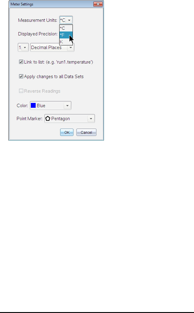
603 Data Collection
Calibrating a Sensor
When the software or handheld detects a sensor, the calibration for that sensor
automatically loads. You can calibrate some sensors manually. Other sensors, such as
the Colorimeter and the Dissolved Oxygen Sensor, must be calibrated to provide useful
data.
There are three options for calibrating a sensor:
• Manual Entry
• Two Point
• Single Point
Refer to the sensor’s documentation for specific calibration values and procedures.
Setting a Sensor to Zero
You can set the standing value of some sensors to zero. You cannot set sensors in
which relative measurements such as force, motion and pressure are common to zero.
Sensors designed to measure specific environmental conditions, such as Temperature,
pH and CO2also cannot be set to zero.
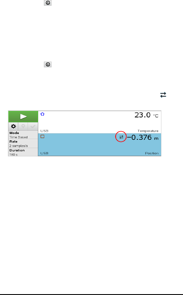
1. Click Meter view to display the connected and offline sensors.
2. Click the sensor that you want to set to zero.
3. In the Meter Settings dialogue box, click Zero.
Reversing a Sensor's Readings
By default, pulling with a force sensor produces a positive force and pushing produces
a negative force. Reversing the sensor allows you to display pushing as a positive force.
1. Click Meter view to display the connected and offline sensors.
2. Click the sensor that you want to reverse.
3. In the Meter Settings dialogue box, click Reverse Readings.
The sensor display is now reversed. In Meter View, the reverse indicator
appears after the sensor name.
Collecting Data
Collecting Time-Based Data
The Time Based collection mode captures sensor data automatically at regular time
intervals.
1. Connect the sensor or sensors.
Sensor names are added to the sensor list automatically.
2. From the Experiment menu, select New Experiment.
This removes all data and restores all meter settings to their defaults.
3. From the Experiment menu, select Collection Mode > Time Based.
a) Select Rate or Interval from the drop-down list, and then type the Rate
(samples/second) or Interval (seconds/sample).
b) Type the Duration of the collection.
Data Collection 604
605 Data Collection
The Number of points is calculated and displayed, based on rate and duration.
Note that collecting too many data points can slow system performance.
c) Select Strip Chart if you want to collect samples continuously, retaining only the
last nsamples. (where “n” is the number shown in the Number of points field.)
4. Modify sensor settings as necessary.
5. Click Start Collection .
6. After the data has been collected, click Stop Collection .
The data set run is complete.
Collecting Selected Events
Use the Selected Events collection mode to capture samples manually. In this mode,
each sample is automatically assigned an event number.
1. Connect the sensor or sensors.
Sensor names are added to the sensor list automatically.
2. From the Experiment menu, select New Experiment.
This removes all data and restores all meter settings to their defaults.
3. From the Experiment menu, select Collection Mode > Selected Events.
The Selected Events Set-up dialogue box opens.
-Name. This text is visible in the Meter View. Its first letter is displayed as the
independent variable in the Graph view.
-Units. This text is displayed in Graph view alongside the Name.
-Average over 10 s. This option averages ten seconds of data for each point.
4. Modify sensor settings as necessary.
5. Click Start Collection .
The Keep Current Reading icon becomes active. The current sensor value
appears in the centre of the graph.
6. Click Keep Current Reading to capture each sample.
The data point is plotted, and the current sensor value appears in the centre of the
graph.
Note: If you selected the Averaging option, a countdown timer appears. When the
counter reaches zero, the system plots the average.
7. Continue capturing until you collect all of the desired data points.
8. Click Stop Collection .
The data set run is complete.
Collecting Events with Entry
Use the Events with Entry collection mode to capture samples manually. In this mode,
you define the independent value for each point you collect.
1. Connect the sensor or sensors.
Sensor names are added to the sensor list automatically.
2. From the Experiment menu, select New Experiment.
This removes all data and restores all meter settings to their defaults.
3. From the Experiment menu, select Collection Mode > Events with Entry.
The Events with Entry Set-up dialogue box opens.
-Name. This text is visible in the Meter View. Its first letter is displayed as the
independent variable in the Graph view.
-Units. This text is displayed in Graph view alongside the Name.
-Average over 10 s. This option averages ten seconds of data for each point.
4. Modify sensor settings as necessary.
5. Click Start Collection .
The Keep Current Reading icon becomes active. The current sensor value
appears in the centre of the graph.
6. Click Keep Current Reading to capture a sample.
The Events with Entry dialogue box opens.
Data Collection 606
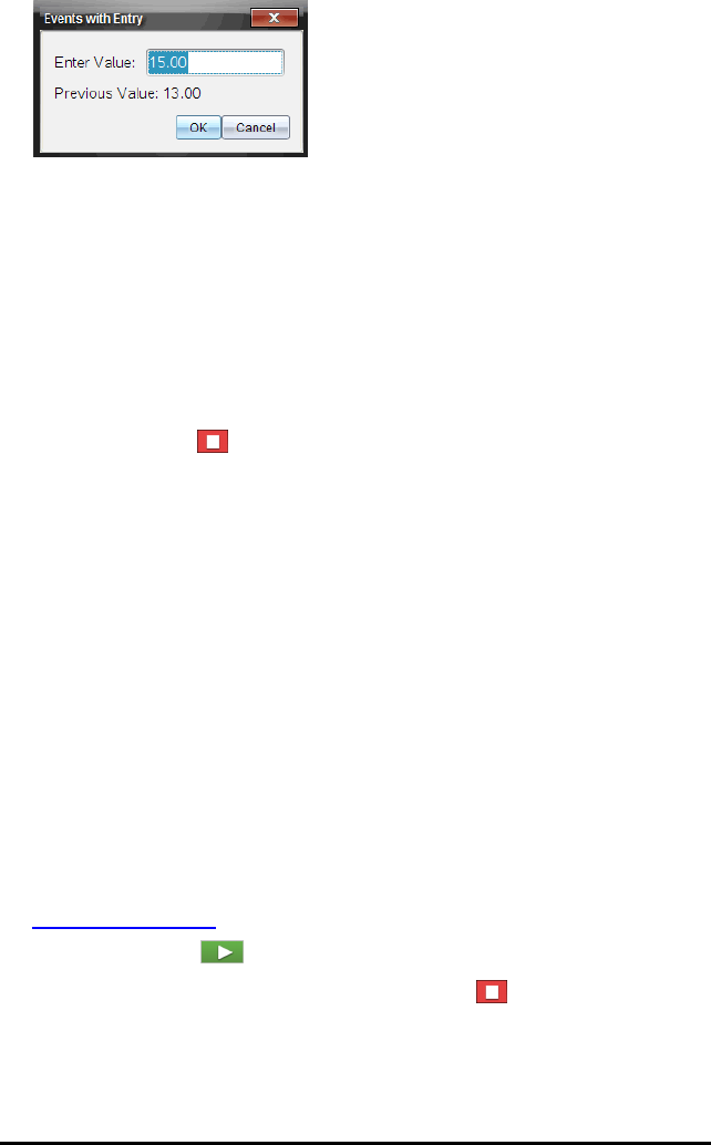
607 Data Collection
7. Type a value for the independent variable.
8. Click OK.
The data point is plotted, and the current sensor value appears in the centre of the
graph.
Note: If you selected the Averaging option, a countdown timer appears. When the
counter reaches zero, the system plots the average.
9. Repeat steps 6 to 8 until you collect all of the desired data points.
10. Click Stop Collection .
The data set run is complete.
Collecting Photogate Timing Data
The Photogate Timing collection mode is available only when using the Vernier
Photogate sensor. This sensor can time objects that pass through the gates or objects
that pass outside of the gates.
1. Connect the Photogate sensor or sensors.
Sensor names are added to the sensor list automatically.
2. From the Experiment menu, select New Experiment.
This removes all data and restores all meter settings to their defaults.
3. From the Experiment menu, select Collection Mode > Photogate Timing.
4. Set the collection options.
5. Modify sensor settings as necessary.
6. Click Start Collection .
7. After the data has been collected, click Stop Collection .
The data set run is complete.
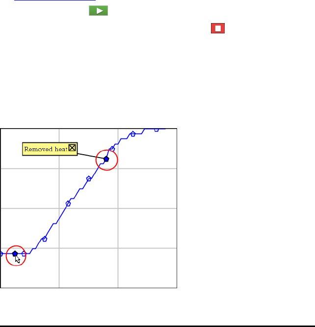
Collecting Drop Counter Data
The Drop Counting collection mode is available only when using the Vernier Drop
Counter optical sensor. This sensor can count the number of drops or record the
amount of liquid added during an experiment.
1. Connect the Drop Counter sensor or sensors.
Sensor names are added to the sensor list automatically.
2. From the Experiment menu, select New Experiment.
This removes all data and restores all meter settings to their defaults.
3. From the Experiment menu, select Collection Mode > Drop Counting.
4. Set the collection options.
5. Modify sensor settings as necessary.
6. Click Start Collection .
7. After the data has been collected, click Stop Collection .
The data set run is complete.
Using Data Markers to Annotate Data
Data markers give you a way to emphasise specific data points, such as when you
change a condition. For example, you might mark a point at which a chemical is added
to a solution or when heat is applied or removed. You can add a marker with or
without a comment, and you can hide a comment.
Two data markers, one with a comment displayed
Data Collection 608
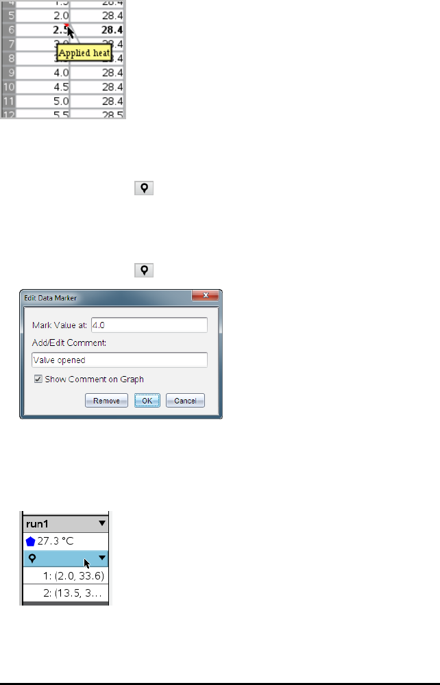
609 Data Collection
Marker shown as red triangle in Table view
Adding a Marker During Data Collection
▶Click Add Data Marker to place a marker at the current data point.
Adding a Marker After Collecting Data
1. In Graph or Table view, click the point at which you want a marker.
2. Click Add Data Marker .
3. Complete the items in the dialogue box.
Adding a Comment to an Existing Marker
1. In the Detail view, click to expand the list of markers for the data set.
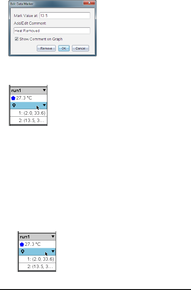
2. Click the entry for the marker that you want to change, and complete the items in
the dialogue box.
Repositioning a Data Marker
1. Click to expand the list of markers in the Detail view.
2. Click the entry for the marker that you want to change.
3. In the dialogue box, type a new value for Mark Value at.
Moving a Data Marker's Comment in the Graph View
▶Drag the comment to move it. The connecting line remains attached to the data
point.
Hiding/Showing a Data Marker's Comment
▶Hide a comment by clicking the Xat the end of the comment.
▶To restore a hidden comment:
a) Click to expand the list of markers in the Detail view.
Data Collection 610
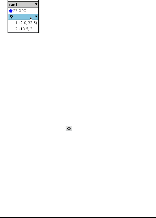
611 Data Collection
b) Click the entry for the marker that you want to change, and tick
ShowCommentonGraph.
Removing a Data Marker
1. Click to expand the list of markers in the Detail view.
2. In the dialogue box, click Remove.
Collecting Data Using a Remote Collection Unit
To collect information from a sensor while it is disconnected, you can set it up as a
remote sensor. Only the TI-Nspire™ Lab Cradle, TI CBR2™, and Vernier Go!Motion®
support remote data collection.
You can set up a remote collection unit to start collecting:
• When you press a manual trigger on the unit, as on the TI-Nspire™ Lab Cradle
• When a delay countdown expires on a unit that supports a delayed start
Setting Up for Remote Collection
1. Save and close any open documents, and start with a new document.
2. Connect the remote collection unit to the computer or handheld.
3. Modifying Sensor Settings.
4. Click the Collection Setup button .
5. On the Collection Setup screen, click Enable Remote Collection.
6. Select the remote collection unit from the Devices list.
7. Specify the method for starting the collection:
• To start automatically after a specified delay (on supported units), type the
delay value.
• To start when you press the manual trigger (on supported units), type a delay
value of 0. When you use a delay, the manual trigger button on the TI-Nspire™
Lab Cradle has no effect on the start of the collection.
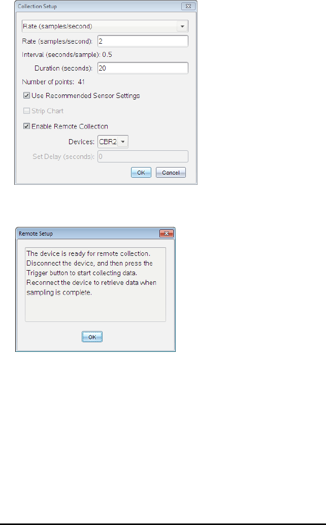
8. Click OK.
A message confirms that the unit is ready.
9. Disconnect the unit.
Depending on the device, LED lights may indicate its status.
Red. The system is not ready.
Amber. The system is ready but not collecting data.
Green. The system is collecting data.
10. If you are starting collection manually, press the trigger when ready. If you are
starting based on a delay, the collection will start automatically when the
countdown is complete.
Retrieving the Remote Data
After collecting data remotely, you transfer it to the computer or handheld for analysis.
Data Collection 612
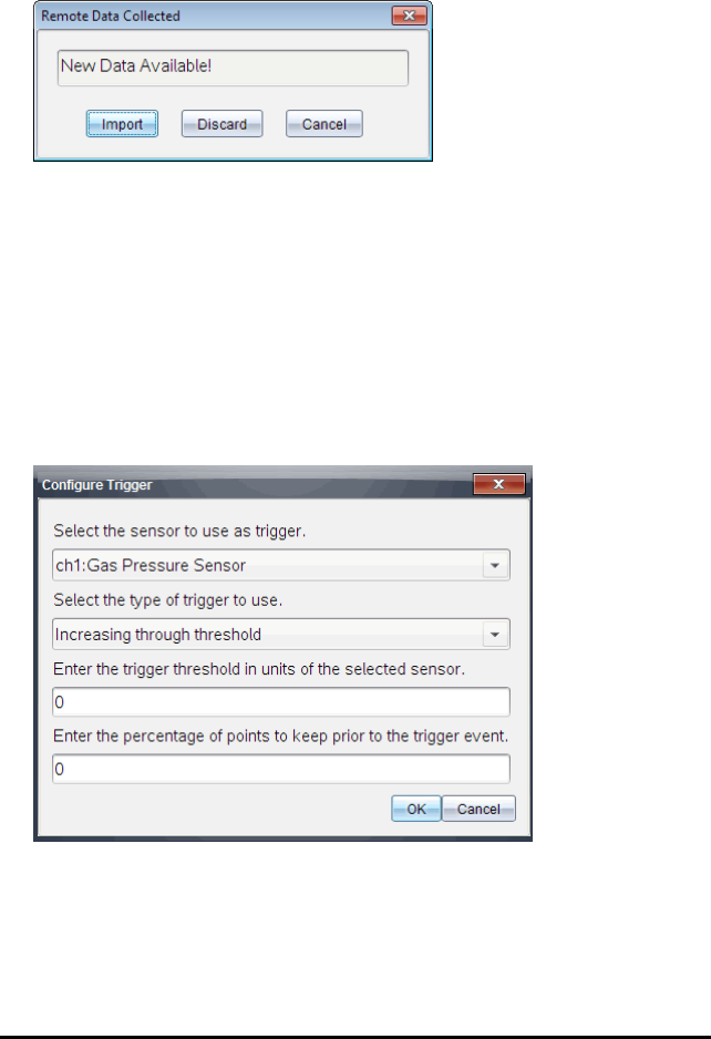
613 Data Collection
1. Open the Vernier DataQuest™ application.
2. Attach the TI-Nspire™ Lab Cradle to the handheld or computer.
The Remote Data Detected dialogue box opens.
3. Click Import.
The data transfers to the Vernier DataQuest™ application.
Setting Up the Sensor for Triggering
To start data collection based on a specific sensor reading, the TI-Nspire™ Lab Cradle
and sensor must be connected.
1. Connect the sensor.
2. Click Experiment > Advanced Set up > Triggering > Set Up.
The Configure Trigger dialogue box opens.
3. Select the sensor from the Select the sensor to use as trigger drop-down list.
Note: The menu displays the sensors connected to the TI-Nspire™ Lab Cradle.
4. Select one of the following from the Select the type of trigger to use drop-down
list.
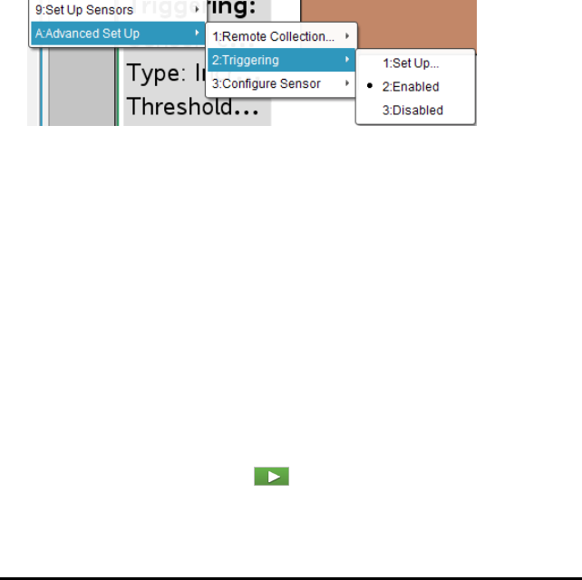
•Increasing through threshold. Use to trigger on increasing values.
•Decreasing through threshold. Use to trigger on decreasing values.
5. Type the appropriate value in the Enter the trigger threshold in units of the selected
sensor field.
When entering the trigger value, enter a value within the range of the sensor.
If you change the unit type after setting the threshold, the value automatically
updates.
For example, if you use the Vernier Gas Pressure sensor with the units set as atm
and you later change the units to kPa, the settings are updated.
6. Type the number of data points to keep before the trigger value occurs.
7. Click OK.
The trigger is now set and enabled if values were entered.
8. (Optional) Select Experiment > Advanced Set up > Triggering to verify the active
indicator is set to Enabled.
Important: When the trigger is enabled, it stays active until it is disabled or you
start a new experiment.
Enabling a Disabled Trigger
If you set the trigger values in the current experiment, and then disable them, you can
enable the triggers again.
To enable a trigger:
▶Click Experiment > Advanced Set Up > Triggering > Enable.
Disabling an Enabled Trigger
To disable the active trigger.
▶Click Experiment > Advanced Set Up > Triggering > Disable.
Collecting and Managing Data Sets
By default, the Start Collection button overwrites collected data with data from
the next run. To preserve each run, you can store it as a data set. After collecting
multiple data sets, you can superimpose any combination of them on the Graph View.
Data Collection 614
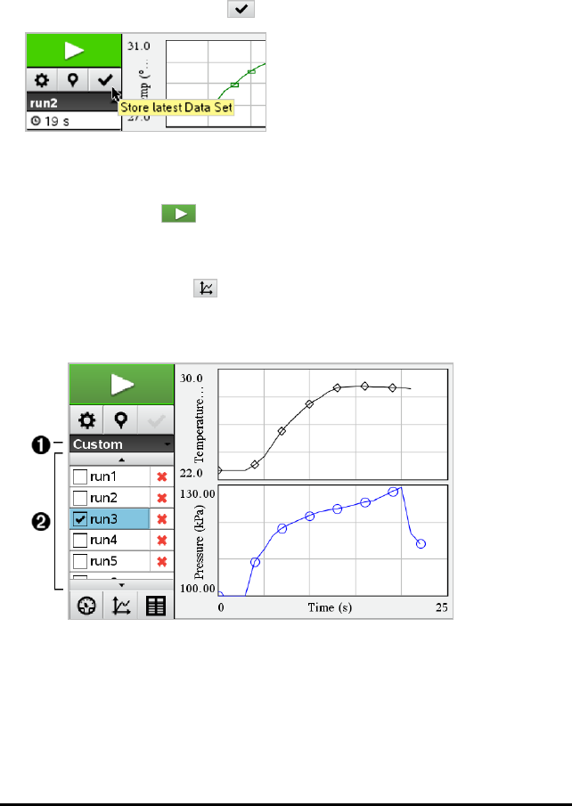
615 Data Collection
Important: Stored data sets are lost if you close the document without saving it. If you
want stored data to be available later, make sure to save the document.
Storing Data as Sets
1. Collect the data from the first run. (See Collecting Data.)
2. Click the Store Data Set button .
The data is stored as run1. A new data set, run2, is created for collecting the next
run.
3. Click Start Collection to collect data for run2.
Comparing Data Sets
1. Click the Graph View icon to show the graph.
2. Click the Data Set Selector (near the top of the Detail View) to expand the list of
data sets.
ÀData Set Selector lets you expand or collapse the list.
ÁExpanded list shows available data sets. Scroll buttons appear as necessary
to let you scroll the list.
3. Choose which data sets to view by selecting or clearing the tickboxes.
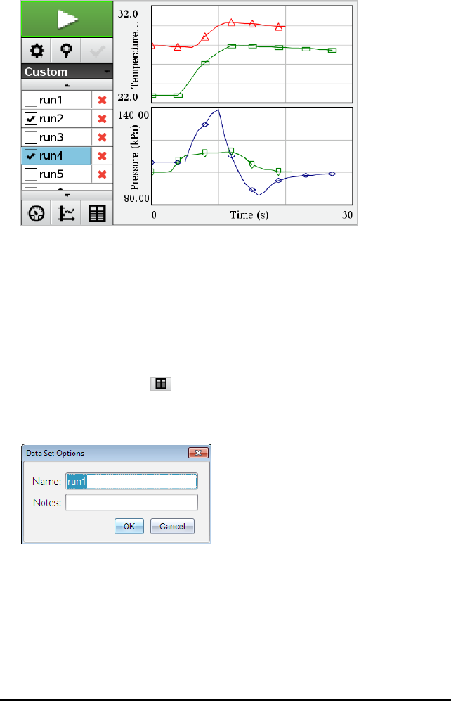
The graph is rescaled as necessary to show all selected data.
Tip: To quickly select a single data set, hold down Shift while clicking its name in
the list. The graph shows only the selected set, and the list is collapsed
automatically to help you view details of the data.
Renaming a Data Set
By default, data sets are named run1,run2 and so on. The name of each data set is
displayed in the Table view.
1. Click the Table View icon to show the table.
2. Display the context menu for the table view, and select Data Set Options > [current
name].
3. Type the new Name.
Note: The maximum character limit is 30. The name cannot contain commas.
4. (Optional) Type Notes about the data.
Data Collection 616
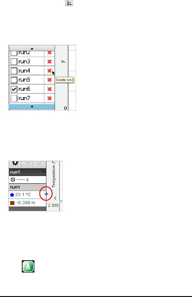
617 Data Collection
Deleting a Data Set
1. Click the Graph View icon to show the graph.
2. Click the Data Set Selector (near the top of the Detail View) to expand the list of
data sets.
3. Scroll the list as necessary, and then click the Delete symbol (X) next to the name
of the data set.
4. Click OK on the confirmation message.
Expanding the View Details Area
▶Drag the boundary at the right edge of the Details area to increase or decrease its
width.
Using Sensor Data in Programmes
You can access sensor data from all connected sensor probes through your TI-Basic
programme by using this command:
RefreshProbeVars statusVar
• You must first launch the Vernier DataQuest™ application, or you will receive an
error.
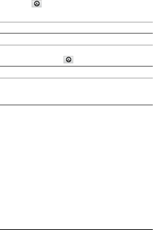
Note: The Vernier DataQuest™ application will auto-launch when you connect a
sensor or a lab cradle to the TI-Nspire™ software or handheld.
• The RefreshProbeVars command will be valid only when Vernier DataQuest™ is in
'meter' mode.
•statusVar is an optional parameter that indicates the status of the command.
These are the statusVar values:
StatusVar
Value
Status
statusVar
=0
Normal (continue with the programme)
statusVar
=1
The Vernier DataQuest™ application is in data collection mode.
Note: The Vernier DataQuest™ application must be in meter mode for
this command to work.
statusVar
=2
The Vernier DataQuest™ application is not launched.
statusVar
=3
The Vernier DataQuest™ application is launched, but you have not
connected any probes.
Note: The RefreshProbeVars command will almost always return
statusVar=3 in the iOS, even if you have already launched the Vernier
DataQuest™ application
• Your TI-Basic programme will read directly from Vernier DataQuest™ variables in
the symbol table.
• The meter.time variable shows the last value of the variable; it does not update
automatically. If no data collection has occurred, meter.time will be 0 (zero).
• Use of variable names without corresponding probes being physically attached will
result in a "Variable not defined" error.
• The RefreshProbeVars command will be a NOP (null command) on iOS.
Collecting Sensor Data using RefreshProbeVars
1. Launch the Vernier DataQuest™ application.
2. Connect the sensor(s) you need to collect the data.
3. Run the programme you wish to use to collect data in the calculator application.
4. Manipulate the sensors and collect the data.
Note: You may create a programme to interact with the TI-Innovator Hub using b>
Hub > Send. (See Example 2, below.) This is optional.
Example 1
Define temp()=
Prgm
© Check if system is ready
Data Collection 618

619 Data Collection
RefreshProbeVars status
If status=0 Then
Disp "ready"
For n,1,50
RefreshProbeVars status
temperature:=meter.temperature
Disp "Temperature: ",temperature
If temperature>30 Then
Disp "Too hot"
EndIf
© Wait for 1 second between samples
Wait 1
EndFor
Else
Disp "Not ready. Try again later"
EndIf
EndPrgm
Example 2- with TI-Innovator™ Hub
Define tempwithhub()=
Prgm
© Check if system is ready
RefreshProbeVars status
If status=0 Then
Disp "ready"
For n,1,50
RefreshProbeVars status
temperature:=meter.temperature
Disp "Temperature: ",temperature
If temperature>30 Then
Disp "Too hot"
© Play a tone on the Hub
Send "SET SOUND 440 TIME 2"
EndIf
© Wait for 1 second between samples
Wait 1
EndFor
Else
Disp "Not ready. Try again later"
EndIf
EndPrgm
Analysing Collected Data
In the Vernier DataQuest™ application, use Graph View to analyse data. Start by
setting up graphs, and then use analysis tools such as integral, statistics and curve fit
to investigate the mathematical nature of the data.
Important: The Graph menu and Analyse menu items are only available when working
in Graph View.

Finding the Area Under a Data Plot
Use Integral to determine the area under a data plot. You can find the area under all of
the data or a selected region of the data.
To find the area under a data plot:
1. Leave the graph unselected to examine all the data, or select a range to examine a
specific area.
2. Click Analyse > Integral.
3. Select the plotted column name if you have more than a single column.
The data plot area is displayed in the View Details area.
Finding the Slope
Tangent displays a measure of the rate at which the data is changing at the point you
are examining. The value is labelled “Slope”.
To find the slope:
1. Click Analyse > Tangent.
A check mark appears in the menu next to the option.
2. Click the graph.
The examine indicator is drawn to the nearest data point.
The values of the plotted data are shown in the View details area and the All
Details for Graph dialogue box.
You can move the examine line by dragging, clicking another point or using the
arrow keys.
Interpolating the Value Between Two Data Points
Use Interpolate to estimate the value between two data points and to determine the
value of a Curve Fit between and beyond these data points.
The examine line moves from data point to data point. When Interpolate is on, the
examine line moves between and beyond data points.
To use Interpolate:
1. Click Analyse > Interpolate.
Data Collection 620
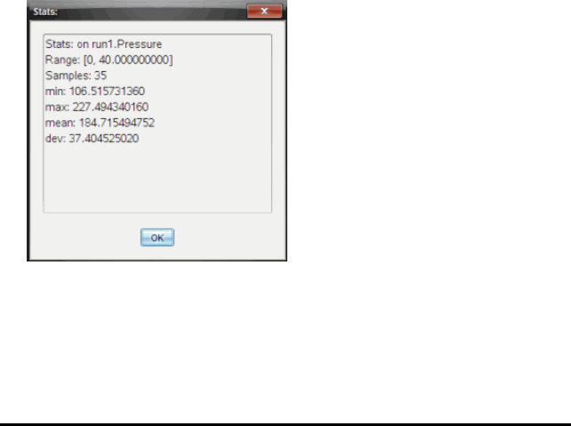
621 Data Collection
A check mark appears in the menu next to the option.
2. Click the graph.
The examine indicator is drawn to the nearest data point.
The values of the plotted data are shown in the View Details area.
You can shift the examine line by moving the cursor with the arrow keys or by
clicking on another data point.
Generating Statistics
You can generate statistics (minimum, maximum, mean, standard deviation and
number of samples) for all the collected data or for a selected region. You can also
generate a curve fit based on one of several standard models or on a model that you
define.
1. Leave the graph unselected to examine all the data, or select a range to examine a
specific area.
2. Click Analyse > Statistics.
3. Select the plotted column name if you have more than a single column. For
example, run1.Pressure.
The Stats dialogue box opens.
4. Review the data.
5. Click OK.
For information on clearing the Statistics analysis, see Removing Analysis Options.
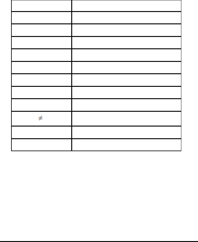
Generating a Curve Fit
Use Curve Fit to find the best curve fit to match the data. Select all of the data or a
selected region of data. The curve is drawn on the graph.
1. Leave the graph unselected to examine all the data, or select a range to examine a
specific area.
2. Click Analyse > Curve Fit.
3. Select a curve fit option.
Curve Fit option Calculated in the form:
Linear y=m*x+b
Quadratic y=a*x^2+b*x+c
Cubic y=a*x^3+b*x^2+c*x+d
Quartic y=a*x^4+b*x^3+c*x^2+d*x+e
Power (ax^b) y=a*x^b
Exponential (ab^x) y=a*b^x
Logarithmic y=a+b*ln(x)
Sinusoidal y=a*sin(b*x+c)+d
Logistic (d 0) y=c/(1+a*e^(-bx))+d
Natural Exponential y=a*e^(-c*x)
Proportional y=a*x
The Fit Linear dialogue box opens.
Data Collection 622
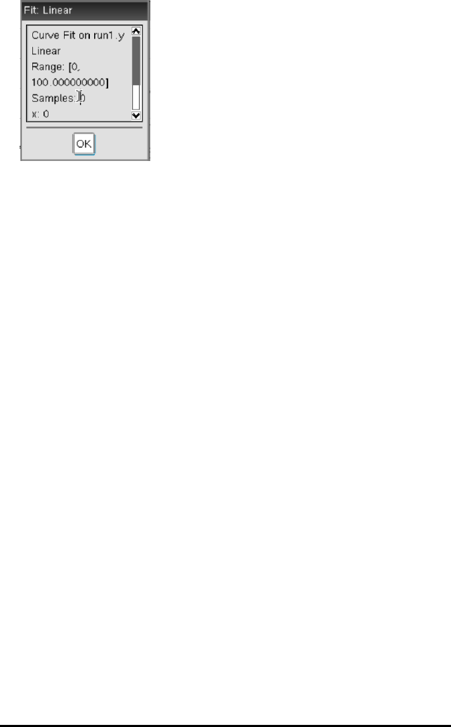
623 Data Collection
4. Click OK.
5. Review the data.
For information on clearing the Curve Fit analysis, see Removing Analysis Options.
Plotting a Standard or User-Defined Model
This option provides a manual method for plotting a function to fit data. Use one of the
predefined models or enter your own.
You can also set the spin increment to use in the View Details dialogue box. Spin
increment is the value by which the coefficient changes when you click the spin buttons
in the View Details dialogue box.
For example, if you set m1=1 as the spin increment, when you click the up spin button
the value changes to 1.1, 1.2, 1.3 and so on. If you click the down spin button, the value
changes to 0.9, 0.8, 0.7 and so on.
1. Click Analyse > Model.
The Model dialogue box opens.
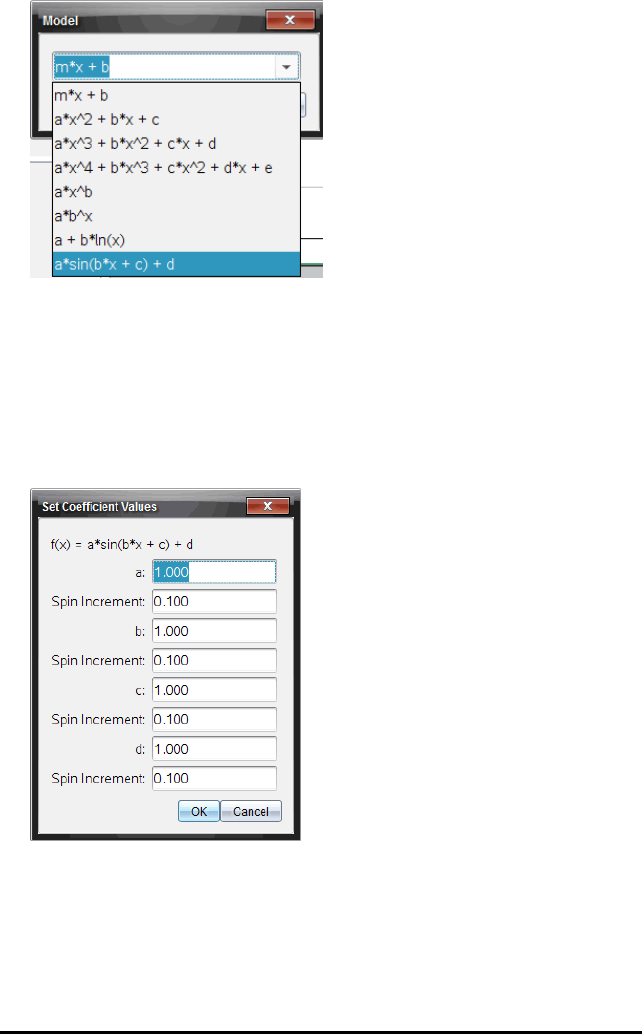
2. Type your own function.
—or—
Click to select a value from the drop-down list.
3. Click OK.
The Set Coefficient Values dialogue box opens.
4. Type the value for the variables.
5. Type the change in value in the Spin Increment fields.
6. Click OK.
Data Collection 624

625 Data Collection
Note: These values are the initial values. You can also adjust these values in the
View Details area.
The model is shown on the graph with adjustment options in the View Details area
and in the All Details for Graph dialogue box.
7. (Optional) Adjust the window setting for minimum and maximum axis values. For
more information, see Setting the Axis for One Graph.
For information on clearing the Model analysis, see Removing Analysis Options.
8. Click to make any desired adjustments to the coefficients.
—or—
Click the value in the View Details area.
This graphic is an example of a model with adjusted values.
Removing Analysis Options
1. Click Analyse > Remove.
2. Select the data display you want to remove.
The display you selected is removed from the graph and the View Details area.
Displaying Collected Data in Graph View
When you collect data, it is written in both the Graph and Table views. Use the Graph
view to examine the plotted data.
Important: The Graph menu and Analyse menu items are only active when working in
Graph View.
Selecting the Graph View
▶Click the Graph View tab .
Viewing Multiple Graphs
Use the Show Graph menu to show separate graphs when using:
• A sensor that plots more than one column of data.
• Multiple sensors with different defined units at the same time.

In this example, two sensors (the Gas Pressure sensor and the Hand Dynamometer)
were used in the same run. The following image shows the columns Time, Force and
Pressure in the Table view to illustrate why two graphs are shown.
Displaying One of Two Graphs
When two graphs are displayed, the top graph is Graph 1 and the bottom graph is
Graph 2.
To display only Graph 1:
▶Select Graph > Show Graph > Graph 1.
Only Graph 1 is displayed.
To display only Graph 2:
▶Select Graph > Show Graph > Graph 2.
Only Graph 2 is displayed.
Displaying Both Graphs
To display both Graph 1 and Graph 2 together:
▶Select Graph > Show Graph > Both.
Graph 1 and Graph 2 are displayed.
Displaying Graphs in the Page Layout View
Use the Page layout view when Show Graph is not the appropriate solution for
showing more than one graph.
The Show Graph option is not applicable for:
• Multiple runs using a single sensor.
• Two or more of the same sensors.
• Multiple sensors that use the same column(s) of data.
To use Page Layout:
1. Open the original data set you want to see in two graph windows.
2. Click Edit > Page Layout > Select Layout.
3. Select the type of page layout you want to use.
4. Click Click here to add an application.
Data Collection 626

627 Data Collection
5. Select Add Vernier DataQuest™.
The Vernier DataQuest™ application is added to the second view.
6. To see separate views, click the view you want to change, and then select View >
Table.
The new view is displayed.
7. To show the same view, click the view to change.
8. Click View > Graph.
The new view is displayed.
Displaying Collected Data in Table View
Table view provides another way to sort and view collected data.
Selecting the Table View
▶Click the Table View tab .
Defining Column Options
You can name columns and define the decimal points and the precision you want to
use.
1. from the Data menu, select Column Options.
Note: You can be in the Meter, Graph or Table view and still click these menu
options. The results will still be visible.
2. Click the name of the column you want to define.
The Column Options dialogue box opens.
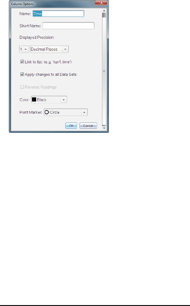
3. Type the long name for the column in the Name field.
4. Type the abbreviated name in the Short Name field.
Note: This name is displayed if the column cannot expand to display the full name.
5. Type the number of units in the Units field.
6. From the Displayed Precision drop-down list, select the precision value.
Note: The default precision is related to the precision of the sensor.
7. Select Link to list to link to the symbol table and make this information available to
other TI-Nspire™ applications.
Note: Linking is the default for most sensors.
Important: Heart rate and blood pressure sensors require a tremendous amount of
data to be useful, and the default for these sensors is to be unlinked to improve
system performance.
8. Select Apply changes to all Data Sets to apply these settings to all data sets.
9. Click OK.
The column settings are now defined with the new values.
Data Collection 628
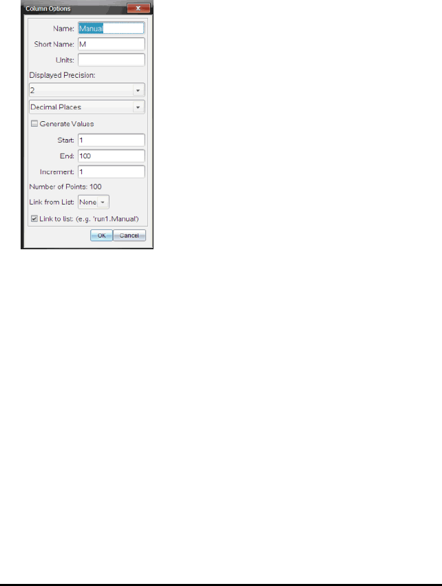
629 Data Collection
Creating a Column of Manually Entered Values
To enter data manually, add a new column. Sensor columns cannot be modified, but
data entered manually can be edited.
1. Click Data > New Manual Column.
The Column Options dialogue box opens.
2. Type the long name for the column in the Name field.
3. Type the abbreviated name in the Short Name field.
Note: This name is displayed if the column cannot expand to display the full name.
4. Type the units to be used.
5. From the Displayed Precision drop-down list, select the precision value.
Note: The default precision is related to the precision of the sensor.
6. (Optional) Select Apply changes to all Data Sets to apply these settings to all data
sets.
7. (Optional) Select Generate Values to automatically populate the rows.
If you select this option, complete these steps:
a) Type a starting value in the Start field.
b) Type an ending value in the End field.

c) Type the increase in value in the Increment field.
The number of points is calculated and shown in the Number of Points field.
8. Select Link from list to link to data in another TI-Nspire™ application.
Note: This list only populates when data exists in the other application and includes
a column label.
9. Select Link to list to link to the symbol table and make this information available to
other TI-Nspire™ applications.
Note: Linking is the default for most sensors.
Important: Heart rate and blood pressure sensors require a tremendous amount of
data to be useful, and the default for these sensors is to be unlinked to improve
system performance.
10. Click OK.
A new column is added to the table. This column can be edited.
Creating a Column of Calculated Values
You can add an additional column to the data set in which the values are calculated
from an expression using at least one of the existing columns.
Use a calculated column when finding the derivative for pH data. For more
information, see Adjusting Derivative Settings.
1. Click Data > New Calculated Column.
The Column Options dialogue box opens.
Data Collection 630
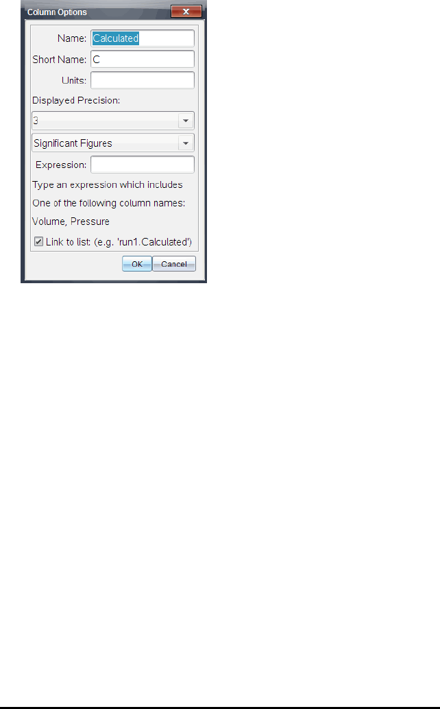
631 Data Collection
2. Type the long name for the column in the Name field.
3. Type the abbreviated name in the Short Name field.
Note: This name is displayed if the column cannot expand to display the full name.
4. Type the units to be used.
5. From the Displayed Precision drop-down list, select the precision value.
Note: The default precision is related to the precision of the sensor.
6. Type a calculation including one of the column names in the Expression field.
Note: The system-provided column names are dependent on the sensor(s) selected
and any changes made to the name field in Column Options.
Important: The Expression field is case-sensitive. (Example: “Pressure” is not the
same as “pressure”.)
7. Select Link to list to link to the symbol table and make this information available to
other TI-Nspire™ applications.
Note: Linking is the default for most sensors.
Important: Heart rate and blood pressure sensors require a tremendous amount of
data to be useful, and the default for these sensors is to be unlinked to improve
system performance.
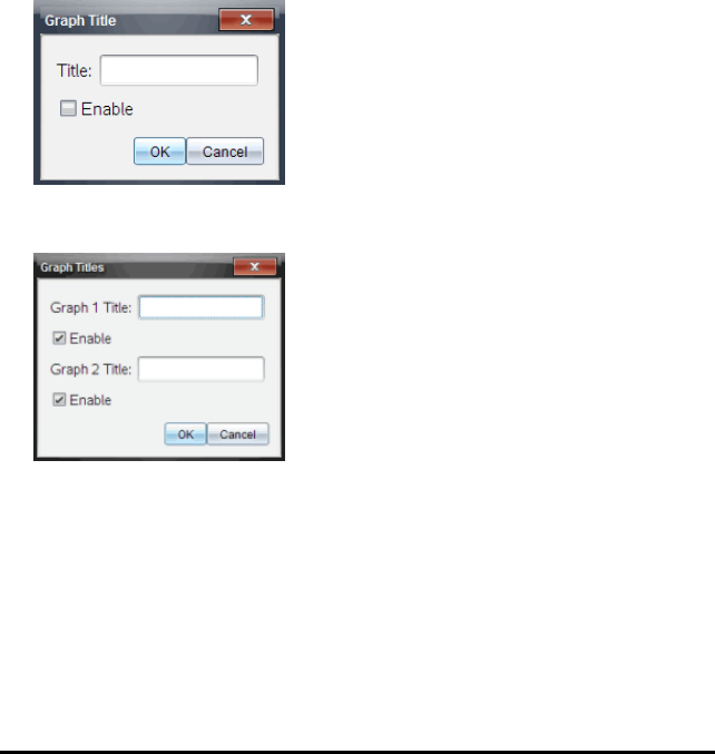
8. Click OK.
The new calculated column is created.
Customising the Graph of Collected Data
You can customise the Graph view by adding a title, changing colours and setting
ranges for the axis.
Adding a Title
When you add a title to a graph, the title is displayed in the View Details area. When
you print the graph, the title prints on the graph.
1. Click Graph > Graph Title.
The Graph Title dialogue box opens.
If there are two graphs in the work area, the dialogue box has two title options.
2. Type the name of the graph in the Title field.
—or—
a) Type the name of the first graph in the Graph 1 field.
b) Type the name of the second graph in the Graph 2 field.
3. Select Enable to show the title.
Data Collection 632
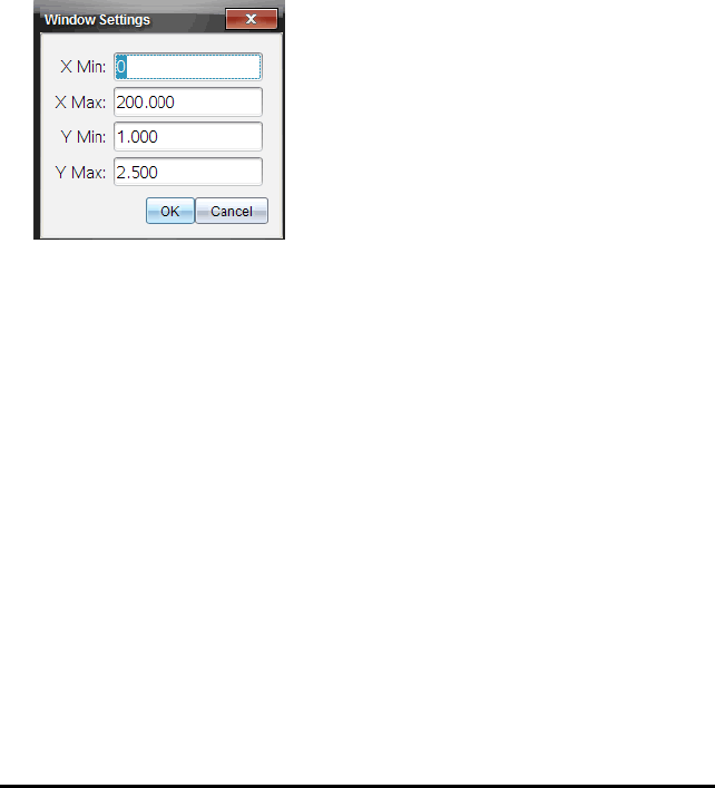
633 Data Collection
Note: Use the Enable option to hide or show the graph title as needed.
4. Click OK.
The title is shown.
Setting Axis Ranges
Setting Axis Ranges for One Graph
To modify the minimum and maximum range for the x and y axis:
1. Click Graph > Window Settings.
The Window Settings dialogue box opens.
2. Type the new values in one or more of these fields:
- X Min
- X Max
- Y Min
- Y Max
3. Click OK.
The application uses the new values for the graph visual range until you modify the
range or change data sets.
Setting Axis Ranges for Two Graphs
When working with two graphs, enter two y axis minimum and maximum values, but
only one set of minimum and maximum values for the x axis.
1. Click Graph > Window Setting.
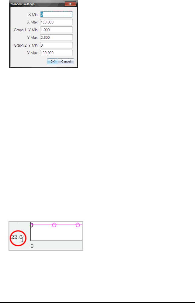
The Window Setting dialogue box opens.
2. Type the new values in one or more of these fields:
- X Min
- X Max
- Graph 1: Y Min
- Y Max
- Graph 2: Y Min
- Y Max
3. Click OK.
The application uses the new values for the graph visual range until you modify the
range or change data sets.
Setting the Axis Range on the Graph Screen
You can modify the minimum and maximum range for the x and y axes directly on the
graph screen.
▶Select the axis value that you want to change, and type a new value.
The graph is redrawn to reflect the change.
Data Collection 634
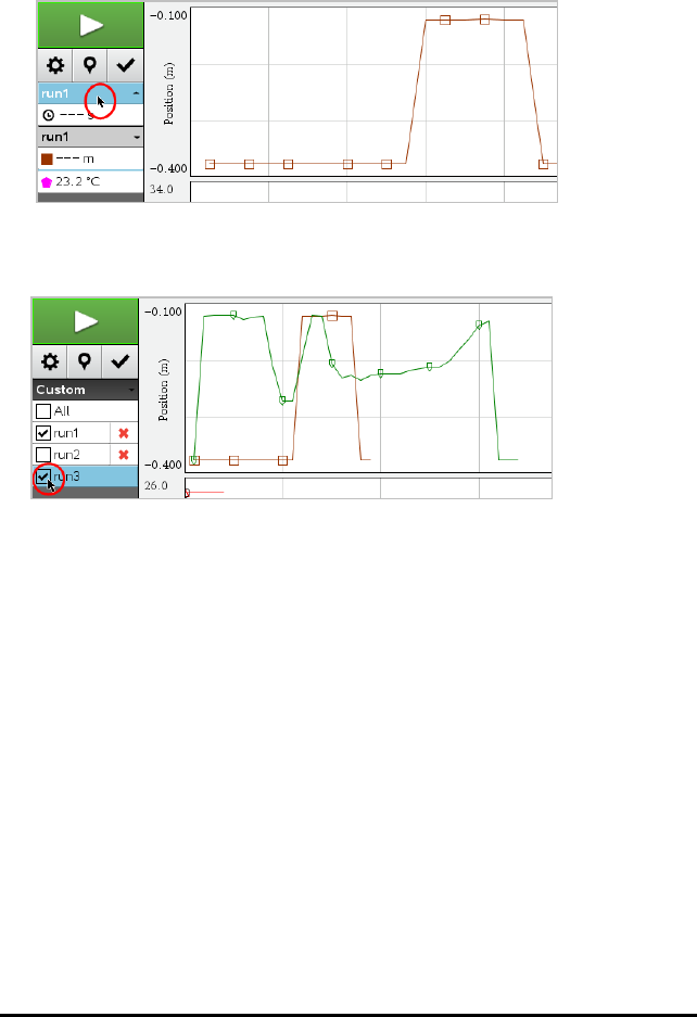
635 Data Collection
Selecting which Data Sets to Plot
1. In the Detail view on the left, click the tab immediately below the view selection
buttons.
2. The Detail view shows a list of available data sets.
3. Use the tick boxes to select the data sets to plot.
Autoscaling a Graph
Use the autoscale option to show all the points plotted. Autoscale Now is useful after
you change the x and y axis range or zoom in or out of a graph. You can also define the
automatic autoscale setting to use during and after a collection.
Autoscale Now Using the Application Menu
▶Click Graph > Autoscale Now.
The graph now displays all the points plotted.
Autoscale Now Using the Context Menu
1. Open the context menu in the graph area.
2. Click Window/Zoom > Autoscale Now.
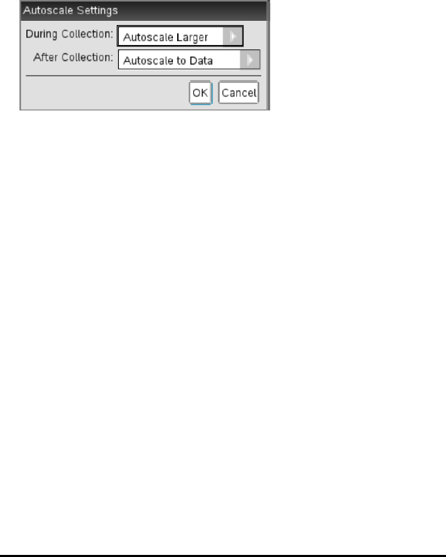
The graph now displays all the points plotted.
Defining Autoscale During a Collection
There are two options for using the automatic autoscaling that occurs during a
collection. To choose an option:
1. Click Options > Autoscale Settings.
The Autoscale Settings dialogue box opens.
2. Click ►to open the During Collection drop-down list.
3. Select one of these options:
•Autoscale Larger - Expands the graph as needed to show all points as you
collect them.
•Do Not Autoscale - The graph is not changed during a collection.
4. Click OK to save the setting.
Defining Autoscale After a Collection
You have three options for setting the automatic autoscaling that occurs after a
collection. To set your choice:
1. Click Options > Autoscale Settings.
The Autoscale Settings dialogue box opens.
2. Click ►to open the After Collection drop-down list.
3. Select one of these options:
•Autoscale to Data. Expands the graph to show all data points. This option is the
default mode.
•Autoscale From Zero. Modifies the graph so all data points including the origin
point are displayed.
Data Collection 636

637 Data Collection
•Do Not Autoscale. The graph settings are not changed.
4. Click OK to save the setting.
Selecting a Range of Data
Selecting a range of data on the graph is useful in several situations, such as when
zooming in or out, striking and un-striking data and examining settings.
To select a range:
1. Drag across the graph.
The selected area is indicated by grey shading.
2. Perform one of these actions.
• Zoom in or out
• Strike or un-strike data
• Examine settings
To deselect a range:
▶Press the Esc key as necessary to remove the shading and the vertical trace line.
Zooming In on a Graph
You can zoom in on a subset of the collected points. You can also zoom out from a
previous zoom or expand the graph window beyond the data points collected.
To zoom in on a graph:
1. Select the area you want to zoom into, or use the current view.
2. Click Graph > Zoom In.
The graph adjusts to display only the area you selected.
The x range selected is used as the new x range. The y range autoscales to show all
graphed data points in the selected range.
Zooming Out of a Graph
▶Select Graph > Zoom Out.
The graph is now expanded.
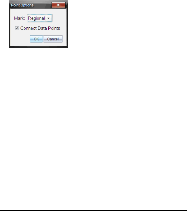
If a Zoom In precedes a Zoom Out, the graph displays the original settings prior to
the Zoom In.
For example, if you Zoomed In twice, the first Zoom Out would display the window
of the first Zoom In. To display the full graph with all data points from multiple
zoom ins, use Autoscale Now.
Setting Point Options
To indicate how often marks show on the graph and whether to use a connecting line:
1. Click Options > Point Options.
The Point Options dialogue box opens.
2. Select a Mark option from the drop-down list.
•None. No point protectors.
•Regional. Periodic point protectors.
•All. Every data point as a point protector.
3. Select Connect Data Points to display a line between points.
—or—
Clear Connect Data Points to remove the line between points.
The following graphics show examples of some of the Point Mark options.
Data Collection 638
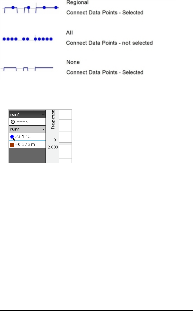
639 Data Collection
Changing a Graph's Colour
1. Click the point indicator for the graph whose colour you want to change.
2. In the Column Options dialogue box, select the new Colour.
Selecting Point Markers
1. Right-click in the graph to open the menu.
2. Click Point Marker.
Note: If there is only one dependent variable column, the Point Marker option is
preceded by the data set name and column name. Otherwise, the Point Marker
option has a menu.
3. Select the column variable to change.
4. Select the point marker to set.
The Point Marker changes to the option selected.
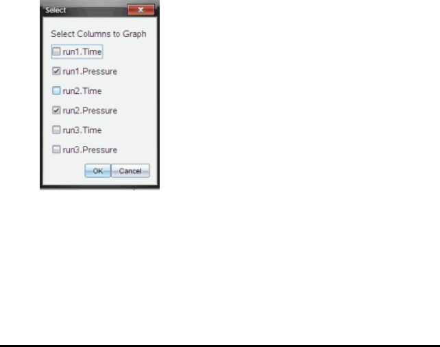
Selecting an Independent Variable Column
Use the option Select X-axis Column to select the column used as the independent
variable when graphing the data. This column is used for all graphs.
1. Click Graph > Select X-axis Column.
2. Select the variable you want to change.
The x-axis label on the graph changes and the graph is reordered using the new
independent variable for graphing the data.
Selecting a Dependent Variable Column
Use the option Select Y-axis Column to select which dependent variable columns to
plot on the displayed graph(s).
1. Click Graph > Select Y-axis Column.
2. Select one of the following:
• A variable from the list. The list is a combination of dependent variables and
the number of data sets.
•More. Selecting More opens the Select dialogue box. Use this when you want
to select a combination of data set variables to graph.
Showing and Hiding Details
You can hide or show the Details view on the left side of the screen.
▶Click Options > Hide Details or Options > Show Details.
Data Collection 640

641 Data Collection
Striking and Restoring Data
Striking data omits it temporarily from the Graph view and from the analysis tools.
1. Open the data run that contains the data to be struck.
2. Click Table View .
3. Select the region by dragging from the starting row to the ending point.
The screen scrolls so you can see the selection.
4. Click Data > Strike Data.
5. Select one of the following:
•In Selected Region. Strike the data from the area you selected.
•Outside Selected Region. Strike all data except the area you selected.
The selected data is marked as struck in the table and is removed from the graph
view.
Restoring Struck Data
1. Select the range of data to restore or if restoring all struck data, start at step two.
2. Click Data > Restore Data.
3. Select one of the following:
•In Selected Region - Restore data in the selected area.
•Outside Selected Region - Restore data outside the selected area.
•All Data - Restore all data. No data selection necessary.
The data is restored.
Replaying the Data Collection
Use the Replay option to playback the data collection. This option lets you:
• Select the data set you want to replay.
• Pause the playback.
• Advance the playback by one point at a time.
• Adjust the playback rate.
• Repeat the playback.
Selecting the Data Set to Replay
You can replay one data set at a time. By default, the latest data set plays using the
first column as the base column (example: time reference).
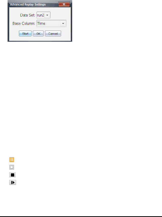
If you have multiple data sets, and want a different data set or base column than the
default, you can select the data set to replay and the base column.
To select the data set to replay:
1. Click Experiment > Replay > Advanced Settings.
The Advanced Replay Settings dialogue box opens.
2. Select the data set to replay from the Data Set drop-down list.
Note: Changing the run in the Data Set selection tool does not affect the playback
choice. You must specify which data set in Experiment>Replay > AdvanceSettings.
3. (Optional) Select a new value from the Base Column drop-down list.
The selected column acts as the “Time” column for the replay.
Note: The base column should be a strictly increasing list of numbers.
4. Click Start to start the playback and save the settings.
Note: Data Set and Base Column options are based on the number of stored runs
and the sensor type used.
Starting and Controlling the Playback
▶Select Experiment > Replay > Start Playback.
Playback begins, and the Data Collection Control buttons change to:
Pause
Resume
Stop
Advance by One Point (enabled only during pause)
Data Collection 642
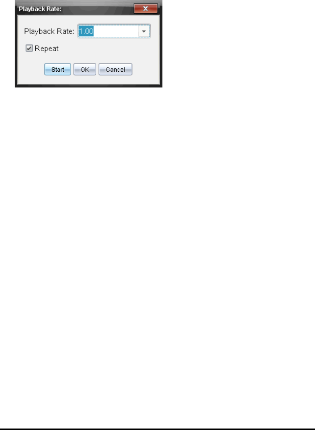
643 Data Collection
Adjusting the Playback Rate
To adjust the playback rate:
1. Select Experiment > Replay > Playback Rate.
The Playback Rate dialogue box opens.
2. In the Playback Rate field, click ▼to open the drop-down list.
3. Select the rate at which the playback will play.
Normal speed is 1.00. A higher value is faster and a lower value is slower.
4. Select one of the following options:
• Click Start to start the playback and save the settings.
• Click OK to save the settings for use on the next playback.
Repeating the Playback
1. Select Experiment > Replay > Start Playback.
2. Click Start to start the playback and save the settings.
Adjusting Derivative Settings
Use this option to select the number of points to use in derivative calculations. This
value affects the tangent tool, velocity and acceleration values.
Find pH derivative settings using a calculated column.
The Vernier DataQuest™ application can determine a numeric derivative from a list of
data with respect to another list of data. The data can be collected using sensors, input
manually, or linked with other applications. The numerical derivative is found using a
calculated column.
To determine the numerical 1st derivative of List B with respect to List A, enter the
following expression in the Column Options dialogue:
derivative(B,A,1,0) or derivative(B,A,1,1)
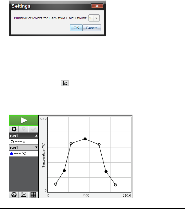
To determine the numerical 2nd derivative of List B with respect to List A, enter the
following expression:
derivative(B,A,2,0) or derivative (B,A,2,1)
The last parameter is either 0 or 1 depending on the method you are using. When it is
0, a weighted average is used. When it is 1, a time shifted derivative method is used.
Note: The first derivative calculation (weighted average) is what the Tangent tool uses
to display the slope at a data point when examining data. (Analyse > Tangent).
Note: The derivative calculation is completely row based. It is recommended that your
List A data be sorted in ascending order.
1. Click Options > Derivative Settings.
The Settings dialogue box opens.
2. Select the number of points from the drop-down list.
3. Click OK.
Drawing a Predictive Plot
Use this option to add points to the graph to predict the outcome of an experiment.
1. Click the Graph View tab .
2. From the Analyse menu, select Draw Prediction > Draw.
3. Click each area in which you want to place a point.
4. Press Esc to release the drawing tool.
Data Collection 644

645 Data Collection
5. To clear the drawn prediction, click Analyse > Draw Prediction > Clear.
Using Motion Match
Use this option to create a randomly generated plot when creating position-versus-time or
velocity-versus-time graphs.
This feature is only available when using a motion detector such as the CBR2™ sensor or
the Go!Motion® sensor.
Generating a Motion Match Plot
To generate a plot:
1. Attach the motion detector.
2. Click View > Graph.
3. Click Analyse > Motion Match.
4. Select one of the following options:
•New Position Match. Generates a random position plot.
•New Velocity Match. Generates a random velocity plot.
Note: Continue selecting a new position or a new velocity match to generate a new
random plot without removing the existing plot.
Removing a Motion Match Plot
To remove the generated plot:
▶Click Analyse > Motion Match > Remove Match.
Printing Collected Data
You can only print from the computer. You can print any single displayed active view, or
with the Print All option:
• One data view.
• All of the data views.
• A combination of the data views.
The Print All option has no effect on applications outside of the Vernier DataQuest™
application.
Printing Data Views
To print a data view:
1. On the main menu (top of the window), click File > Print.
The Print dialogue box opens.
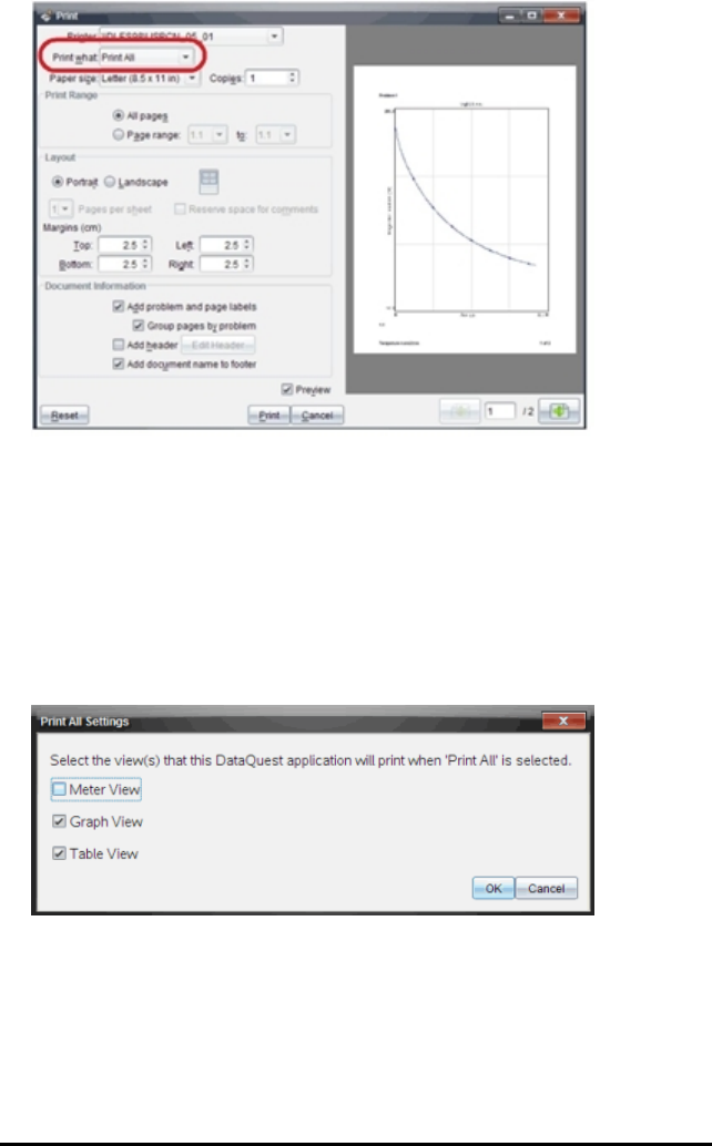
2. Select Print All from the Print what drop-down list.
3. Select additional options, if needed.
4. Click Print to send the document to the printer.
Setting Options for the Print All Feature
1. Click Options > Print All Settings.
The Print All Settings dialogue box opens.
2. Select the views you want to print.
•Print Current View. The current view is sent to the printer.
•Print All Views. All three views (Meter, Graph and Table) are sent to the
printer.
•More. Only the views you select are sent to the printer.
Data Collection 646

647 Data Collection
3. Click OK.
The Print All Settings are now complete and can be used when printing.
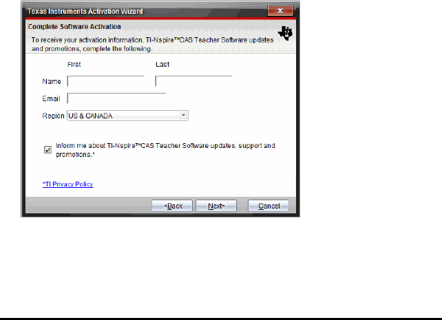
Using the Help Menu
Use the Help menu to find useful information to help you use the software more
productively. You can:
• Open the PDFhelp file (press F1 or click Help).
• Open the web-based help file (press F2 or click Online Help).
• Activate your software license.
• Register your TI product.
• Explore TI resources such as Activities Exchange, where you can find lessons,
quizzes and other instructive activities shared by teachers.
• Explore online troubleshooting.
• Check for updates to the software or updates to operating systems for TI-Nspire™
handhelds and the TI-Nspire™ Lab Cradle.
• Check to see which version of the software you are using.
Activating Your Software Licence
1. Ensure that your computer is connected to the Internet.
2. From the Help menu, select Activate to open the Texas Instruments Activation
Wizard.
3. Click Activate your Licence, and then click Next.
The Complete Software Activation dialogue box opens.
4. Complete the name and email fields, and then select the region where you live if
different from the default entry. If you want to receive emails from TI about
updates, support and promotions, ensure the tick box is selected.
5. Click Next.
Using the Help Menu 648
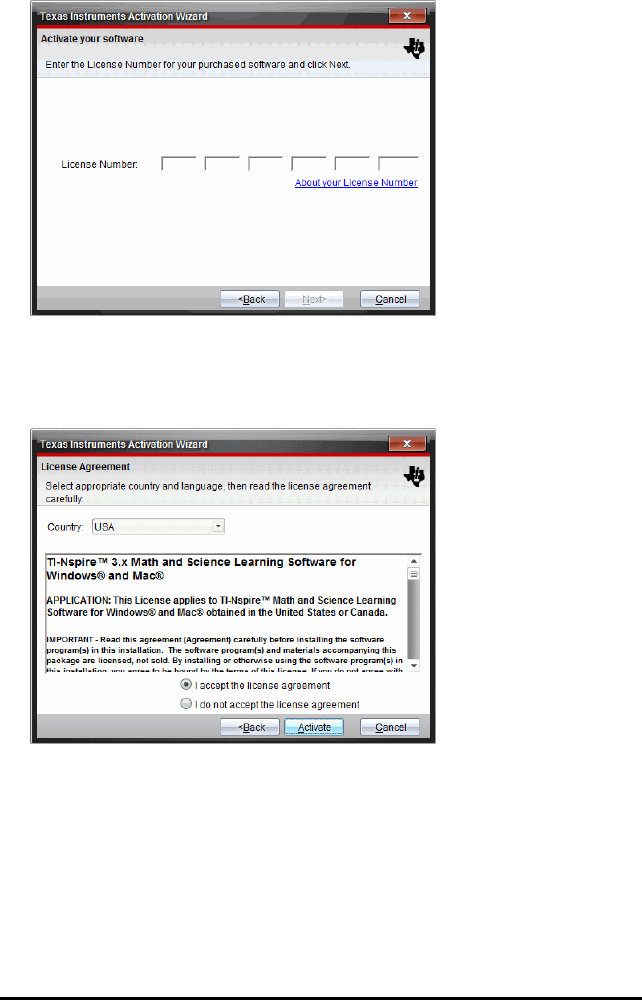
649 Using the Help Menu
The Activate your software dialogue box opens.
6. Type the licence number.
7. Click Next.
The Licence Agreement dialogue box opens.
8. In the Country field, select your country from the drop-down list if it is different
from the default entry.
9. Review the licence agreement, and then select to accept the agreement.
10. Click Activate. The licence number is validated against the TI database to ensure it
is valid.
If the licence number is valid, the Successful Activation dialogue box opens. If the
licence number is not valid, check to make sure the numbers are entered correctly.
If the problem persists, contact TI Support.
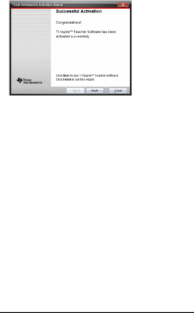
11. Click Next to continue, or select Finish to complete the installation with default
settings.
12. When prompted, click OK to accept the default location for your TI-Nspire™ folder.
If needed, navigate to the location on your computer where you want to store your
TI-Nspire™ documents and files.
13. Select whether or not to replace any documents that have the same name.
The software launches and the Welcome Screen opens.
Registering Your Product
1. Ensure that your computer is connected to the Internet.
2. From the Help menu, select Register to access the TI Product Registration site.
3. Follow the instructions on the website.
Downloading the Latest Guidebook
1. Ensure that your computer is connected to the Internet.
2. From the Help menu, select Download latest Guidebook.
The Education Technology website opens with the Guidebooks tab active.
3. Click the title of the Guidebook that you want to download.
A PDF version of the Guidebook opens on your desktop.
Exploring TI Resources
The Help menu also provides links to TI resources and websites.
▶Select Help > Visit education.ti.com to access the Texas Instruments Education
Technology website.
Using the Help Menu 650

651 Using the Help Menu
▶Select Help > Visit Activities Exchange to access the Texas Instruments Activities
Exchange, site, a forum where you can browse by subject to find ready-to-use
maths and science learning activities appropriate for secondary school to college.
Note: Activities available for download may vary depending on your geographical
region.
▶Select Help > Explore Online Troubleshooting to access the TI Knowledge Base
where you can find general information, troubleshooting help, product usage tips
and information specific to TI products.
Updating the TI-Nspire™ Software
Update the Software
1. Ensure that your computer is connected to the Internet.
2. Close any open documents.
3. From the Help menu, select Check for Upgrades and Notifications.
• If your software is current, a confirmation message appears.
• If your software is not current, you are prompted to update.
4. Click Update to download and install the update, or click Close to cancel.
A progress indicator shows the download progress. If you receive a connection
error, check your Internet connection and try again.
Note for users updating TI-Nspire™ Navigator™ Teacher Software or TI-Nspire™
Navigator™NC Teacher Software: Your portfolio and class records reside on your
computer as a database. Because the new software might have features that are not
supported in the old database structure, the old data might need to be converted.
When conversion is necessary, a Database Update tool helps you make a backup of the
old database. The tool appears during the first startup of the updated software.
Manage Automatic Checking
Automatic checking uses the Internet to check for upgrades each time you open the
TI-Nspire™ software. If your system is not up-to-date, you receive a notification. You
can turn automatic checking on or off.
1. From the Help menu, select Check for Upgrades and Notifications.
2. Tick or clear the Automaticallycheckforupdates tickbox.
3. Click Close.
Updating the OS on a Connected Handheld
Note: To avoid losing unsaved data, close all documents on the handheld before
updating its operating system.
1. Ensure that your computer is connected to the Internet.
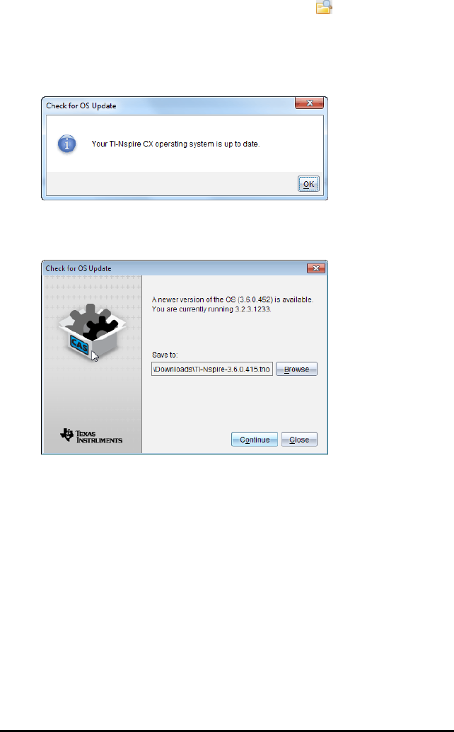
2. In the Documents Toolbox, click the Content Explorer tab to show connected
handhelds.
3. Select the handheld that you are updating.
4. From the Help menu, select Check for OSUpdates.
• If the operating system is current, a confirmation message appears.
• If the operating system is not current, the TI-Nspire™ software prompts you to
install the latest OS now. If the updated OS file is not already available on your
computer, you can choose a location for it.
5. Click Continue and follow the prompts to install the OS on the handheld, or click
Close to cancel.
When the update is complete, the handheld restarts automatically.
Viewing Software Version and Legal Information
1. From the Help menu, select About TI-Nspire™ <Product Name>Software.
Note: You do not need an Internet connection to open this screen.
Using the Help Menu 652
653 Using the Help Menu
2. Click OK to close the window.
Helping Improve the Product
This product includes a feature that can help TI improve the product by automatically
collecting anonymous information about product usage and reliability.
Note: Depending on how your software was installed, you might see the following
screen the first time you start the software. You also can access the feature manually.
1. From the Help menu, select Product Improvements.
2. Read the information on the screen, and click one of the buttons:
- To allow information to be collected, click Yes, I want to help.
- To prevent collection, click No thanks.

General Information
Texas Instruments Support and Service
Home Page: education.ti.com
E-mail inquiries: ti-cares@ti.com
KnowledgeBase and e-mail inquiries: education.ti.com/support
International information: education.ti.com/international
Service and Warranty Information
For information about the length and terms of the warranty or about product service,
refer to the warranty statement enclosed with this product or contact your local Texas
Instruments retailer/distributor.
General Information 654

655
