Motorola Solutions 89FT7622 5.7GHz Fixed Wireless (ISM) User Manual Exhibit D Users Manual Part 1 per 2 1033 b3
Motorola Solutions, Inc. 5.7GHz Fixed Wireless (ISM) Exhibit D Users Manual Part 1 per 2 1033 b3
Contents
- 1. Exhibit D Users Manual Part 1 per 2 1033 b3
- 2. Exhibit D Users Manual Part 2 per 2 1033 b3
- 3. Exhibit D Users Manual Part 3 per 2 1033 b3
- 4. Exhibit D Users Manual Part 4 per 2 1033 b3
- 5. Exhibit D Users Manual Part 5 per 2 1033 b3
- 6. Exhibit D Users Manual Part 6 per 2 1033 b3
- 7. Exhibit D Users Manual Part 7 per 2 1033 b3
- 8. Exhibit D Users Manual Part 8 per 2 1033 b3
- 9. Exhibit D Users Manual Part 9 per 2 1033 b3
- 10. Users Manual
Exhibit D Users Manual Part 1 per 2 1033 b3

Release 8 Planning Guide
March 200 Through Software Release 6.
Issue 2, December 2006 Draft for Regulatory Review 127
P
PLANNING
LANNING G
GUIDE
UIDE

Release 8 Planning Guide
March 200 Through Software Release 6.
Issue 2, December 2006 Draft for Regulatory Review 129
12 ENGINEERING YOUR RF COMMUNICATIONS
Before diagramming network layouts, the wise course is to
◦ anticipate the correct amount of signal loss for your fade margin calculation
(as defined below).
◦ recognize all permanent and transient RF signals in the environment.
◦ identify obstructions to line of sight reception.
12.1 ANTICIPATING RF SIGNAL LOSS
The C/I (Carrier-to-Interference) ratio defines the strength of the intended signal relative
to the collective strength of all other signals. Canopy modules typically do not require a
C/I ratio greater than
◦ 3 dB or less at 10-Mbps modulation and −65 dBm for 1X operation. The C/I ratio
that you achieve must be even greater as the received power approaches the
nominal sensitivity (−85 dBm for 1X operation).
◦ 10 dB or less at 10-Mbps modulation and −65 dBm for 2X operation. The C/I ratio
that you achieve must be even greater as the received power approaches the
nominal sensitivity (−79 dBm for 2X operation).
◦ 10 dB or less at 20-Mbps modulation.
12.1.1 Understanding Attenuation
An RF signal in space is attenuated by atmospheric and other effects as a function of the
distance from the initial transmission point. The further a reception point is placed from
the transmission point, the weaker is the received RF signal.
12.1.2 Calculating Free Space Path Loss
The attenuation that distance imposes on a signal is the free space path loss.
PathLossCalcPage.xls calculates free space path loss.
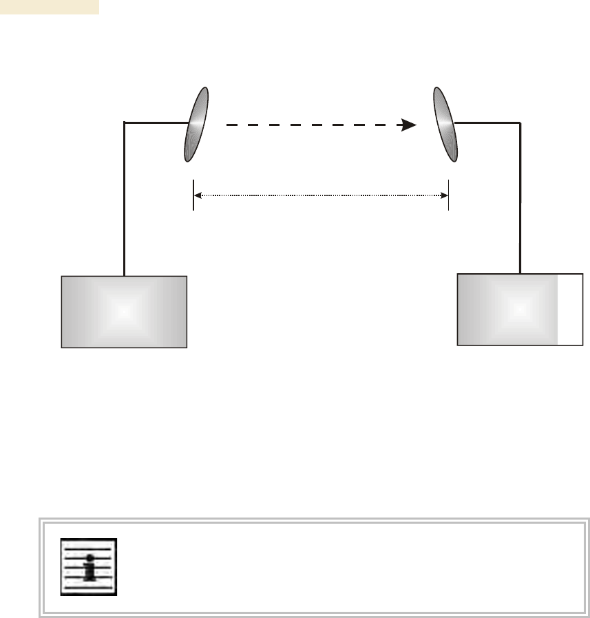
12.1.3 Calculating Rx Signal Level
The Rx sensitivity of each module is provided at
http://motorola.canopywireless.com/prod_specs.php. The determinants in Rx signal level
are illustrated in Figure 37.
Planning Guide Release 8
130 Draft for Regulatory Review Issue 2, December 2006
Tx
power
Tx antenna
gain
Tx
cable
loss
Rx antenna
gain
Rx
cable
loss
Rx
signal
level
Transmitter
or Amplifier
receiver
or amplifier
distance
free space signal
transmitter
or amplifier
Figure 37: Determinants in Rx signal level
Rx signal level is calculated as follows:
Rx signal level dB =
Tx power
−
Tx cable loss
+
Tx antenna gain
−
free space path loss
+
Rx antenna gain
−
Rx cable loss
NOTE:
This Rx signal level calculation presumes that a clear line of sight is established
between the transmitter and receiver and that no objects encroach in the
Fresnel zone.
12.1.4 Calculating Fade Margin
Free space path loss is a major determinant in Rx (received) signal level. Rx signal level,
in turn, is a major factor in the system operating margin (fade margin), which is calculated
as follows:
system operating margin (fade margin)
dB =
Rx signal level
dB −
Rx sensitivity
dB
Thus, fade margin is the difference between strength of the received signal and the
strength that the receiver requires for maintaining a reliable link. A higher fade margin is
characteristic of a more reliable link.
Release 8 Planning Guide
March 200 Through Software Release 6.
Issue 2, December 2006 Draft for Regulatory Review 131
12.2 ANALYZING THE RF ENVIRONMENT
An essential element in RF network planning is the analysis of spectrum usage and the
strength of the signals that occupy the spectrum you are planning to use. Regardless of
how you measure and log or chart the results you find (through the Spectrum Analyzer in
SM and BHS feature or by using a spectrum analyzer), you should do so
◦ at various times of day.
◦ on various days of the week.
◦ periodically into the future.
As new RF neighbors move in or consumer devices in your spectrum proliferate, this will
keep you aware of the dynamic possibilities for interference with your network.
12.2.1 Mapping RF Neighbor Frequencies
Canopy modules allow you to
◦ use an SM or BHS (or a BHM reset to a BHS), or an AP that is temporarily
transformed into an SM, as a spectrum analyzer.
◦ view a graphical display that shows power level in RSSI and dBm at 5-MHz
increments throughout the frequency band range, regardless of limited selections
in the Custom Radio Frequency Scan Selection List parameter of the SM.
◦ select an AP channel that minimizes interference from other RF equipment.
The SM measures only the spectrum of its manufacture. So if, for example, you wish to
analyze an area for both 2.4- and 5.7-GHz activity, take both a 2.4- and 5.7-GHz SM to
the area. To enable this functionality, perform the following steps:
CAUTION!
The following procedure causes the SM to drop any active RF link. If a link is
dropped when the spectrum analysis begins, the link can be re-established
when either a 15-minute interval has elapsed or the spectrum analyzer feature is
disabled.
Procedure 2: Analyzing the spectrum
1. Predetermine a power source and interface that will work for the SM or BHS in
the area you want to analyze.
2. Take the SM or BHS, power source, and interface device to the area.
3. Access the Tools web page of the SM or BHS.
RESULT: The Tools page opens to its Spectrum Analyzer tab. An example of this
tab is shown in Figure 143.
4. Click Enable.
RESULT: The feature is enabled.
5. Click Enable again.
RESULT: The system measures RSSI and dBm for each frequency in the
spectrum.
Planning Guide Release 8
132 Draft for Regulatory Review Issue 2, December 2006
6. Travel to another location in the area.
7. Click Enable again.
RESULT: The system provides a new measurement of RSSI and dBm for each
frequency in the spectrum.
NOTE: Spectrum analysis mode times out 15 minutes after the mode was
invoked.
8. Repeat Steps 6 and 7 until the area has been adequately scanned and logged.
=========================== end of procedure ======================
As with any other data that pertains to your business, a decision today to put the data into
a retrievable database may grow in value to you over time.
RECOMMENDATION:
Wherever you find the measured noise level is greater than the sensitivity of the
radio that you plan to deploy, use the noise level (rather than the link budget) for
your link feasibility calculations.
12.2.2 Anticipating Reflection of Radio Waves
In the signal path, any object that is larger than the wavelength of the signal can reflect
the signal. Such an object can even be the surface of the earth or of a river, bay, or lake.
The wavelength of the signal is approximately
◦ 2 inches for 5.2- and 5.7-GHz signals.
◦ 5 inches for 2.4-GHz signals.
◦ 12 inches for 900-MHz signals.
A reflected signal can arrive at the antenna of the receiver later than the non-reflected
signal arrives. These two or more signals cause the condition known as multipath. When
multipath occurs, the reflected signal cancels part of the effect of the non-reflected signal
so, overall, attenuation beyond that caused by link distance occurs. This is problematic at
the margin of the link budget, where the standard operating margin (fade margin) may be
compromised.
12.2.3 Noting Possible Obstructions in the Fresnel Zone
The Fresnel (pronounced fre·NEL) Zone is a theoretical three-dimensional area around
the line of sight of an antenna transmission. Objects that penetrate this area can cause
the received strength of the transmitted signal to fade. Out-of-phase reflections and
absorption of the signal result in signal cancellation.
The foliage of trees and plants in the Fresnel Zone can cause signal loss. Seasonal
density, moisture content of the foliage, and other factors such as wind may change the
amount of loss. Plan to perform frequent and regular link tests if you must transmit
though foliage.
12.2.4 Radar Signature Detection and Shutdown
With Release 8.1, Canopy meets ETSI EN 301 893 v1.2.3 for Dynamic Frequency
Selection (DFS). DFS is a requirement in certain countries of the EU for systems like
Canopy to detect interference from other systems, notably radar systems, and to avoid
co-channel operation with these systems. All 5.4 GHz modules and all 5.7 GHz
Connectorized modules running Release 8.1 have DFS. Other modules running Release

Release 8 Planning Guide
March 200 Through Software Release 6.
Issue 2, December 2006 Draft for Regulatory Review 133
8.1 do not. With Release 8.1, Canopy SMs and BHSs as well as Canopy APs and BHMs
will detect radar systems.
When an AP or BHM enabled for DFS boots, it receives for 1 minute, watching for the
radar signature, without transmitting. If no radar pulse is detected during this minute, the
module then proceeds to normal beacon transmit mode. If it does detect radar, it waits for
30 minutes without transmitting, then watches the 1 minute, and will wait again if it
detects radar. If while in operation, the AP or BHM detects the radar signature, it will
cease transmitting for 30 minutes and then begin the 1 minute watch routine. Since an
SM or BHS only transmits if it is receiving beacon from an AP or BHM, the SMs in the
sector or BHS are also not transmitting when the AP or BHM is not transmitting.
When an SM or BHS with DFS boots, it scans to see if an AP or BHM is present (if it can
detect a Canopy beacon). If an AP or BHM is found, the SM or BHS receives on that
frequency for 1 minute to see if the radar signature is present. For an SM, if no radar
pulse is detected during this 1 minute, the SM proceeds through normal steps to register
to an AP. For a BHS, if no radar pulse is detected during this 1 minute, it registers, and
as part of registering and ranging watches for the radar signature for another 1 minute. If
the SM or BH does detect radar, it locks out that frequency for 30 minutes and continues
scanning other frequencies in its scan list.
Note, after an SM or BHS has seen a radar signature on a frequency and locked out that
frequency, it may connect to a different AP or BHM, if color codes, transmitting
frequencies, and scanned frequencies support that connection.
For all modules, the module displays its DFS state on its General Status page. You can
read the DFS status of the radio in the General Status tab of the Home page as one of
the following:
◦ Normal Transmit
◦ Radar Detected Stop Transmitting for n minutes, where n counts
down from 30 to 1.
◦ Checking Channel Availability Remaining time n seconds, where
n counts down from 60 to 1. This indicates that a 30-minute shutdown has
expired and the one-minute re-scan that follows is in progress.
DFS can be enabled or disabled on a module’s Radio page: Configuration > Radio >
DFS.
Operators in countries with regulatory requirements for DFS must not disable the feature
and must ensure it is enabled after a module is reset to factory defaults.
Operators in countries without regulatory requirements for DFS will most likely not want
to use the feature, as it adds no value if not required, and adds an additional 1 minute to
the connection process for APs, BHMs, and SMs, and 2 minutess for BHSs.
−
RECOMMENDATION:
Where regulations require that radar sensing and radio shutdown is enabled, you
can most effectively share the spectrum with satellite services if you perform
spectrum analysis and select channels that are distributed evenly across the
frequency band range.

Planning Guide Release 8
134 Draft for Regulatory Review Issue 2, December 2006
A connectorized 5.7-GHz module provides an Antenna Gain parameter. When you
indicate the gain of your antenna in this field, the algorithm calculates the appropriate
sensitivity to radar signals, and this reduces the occurrence of false positives (wherever
the antenna gain is less than the maximum).
12.3 USING JITTER TO CHECK RECEIVED SIGNAL QUALITY
The General Status tab in the Home page of the Canopy SM and BHS displays current
values for Jitter. This is an index of overall received signal quality. Interpret the jitter
value as indicated in Table 32.
Table 32: Signal quality levels indicated by jitter
Correlation of Highest Seen
Jitter to Signal Quality
Signal
Modulation
High
Quality
Questionable
Quality
Poor
Quality
1X operation
(2-level FSK)
0 to 4
5 to 14
15
2X operation
(4-level FSK)
0 to 9
10 to 14
15
In your lab, an SM whose jitter value is constant at 14 may have an incoming packet
efficiency of 100%. However, a deployed SM whose jitter value is 14 is likely to have
even higher jitter values as interfering signals fluctuate in strength over time. So, do not
consider 14 to be acceptable. Avoiding a jitter value of 15 should be the highest priority in
establishing a link. At 15, jitter causes fragments to be dropped and link efficiency to
suffer.
Canopy modules calculate jitter based on both interference and the modulation scheme.
For this reason, values on the low end of the jitter range that are significantly higher in 2X
operation can still be indications of a high quality signal. For example, where the amount
of interference remains constant, an SM with a jitter value of 3 in 1X operation can
display a jitter value of 7 when enabled for 2X operation.
However, on the high end of the jitter range, do not consider the higher values in 2X
operation to be acceptable. This is because 2X operation is much more susceptible to
problems from interference than is 1X. For example, where the amount of interference
remains constant, an SM with a jitter value of 6 in 1X operation can display a jitter value
of 14 when enabled for 2X operation. As indicated in Table 32, these values are
unacceptable.
12.4 USING LINK EFFICIENCY TO CHECK RECEIVED SIGNAL QUALITY
A link test, available in the Link Capacity Test tab of the Tools web page in an AP or BH,
provides a more reliable indication of received signal quality, particularly if you launch
tests of varying duration. However, a link test interrupts traffic and consumes system
capacity, so do not routinely launch link tests across your networks.
12.4.1 Comparing Efficiency in 1X Operation to Efficiency in 2X Operation
Efficiency of at least 98 to 100% indicates a high quality signal. Check the signal quality
numerous times, at various times of day and on various days of the week (as you

Release 8 Planning Guide
March 200 Through Software Release 6.
Issue 2, December 2006 Draft for Regulatory Review 135
checked the RF environment a variety of times by spectrum analysis before placing
radios in the area). Efficiency less than 90% in 1X operation or less than 60% in 2X
operation indicates a link with problems that require action.
12.4.2 When to Switch from 2X to 1X Operation Based on 60% Link Efficiency
In the above latter case (60% in 2X operation), the link experiences worse latency (from
packet resends) than it would in 1X operation, but still greater capacity, if the link remains
stable at 60% Efficiency. Downlink Efficiency and Uplink Efficiency are measurements
produced by running a link test from either the SM or the AP. Examples of what action
should be taken based on Efficiency in 2X operation are provided in Table 33.
Table 33: Recommended courses of action based on Efficiency in 2X operation
Module Types
Further Investigation
Result
Recommended Action
Check the General Status tab
of the Advantage SM.1 See
Checking the Status of 2X
Operation on Page 93.
Uplink and
downlink are both
≥60% Efficiency.2
Rerun link tests.
Advantage AP
with
Advantage SM
Rerun link tests.
Uplink and
downlink are both
≥60% Efficiency.
Optionally, re-aim SM, add a
reflector, or otherwise mitigate
interference. In any case, continue
2X operation up and down.
Check the General Status tab
of the Canopy SM.1 See
Checking the Status of 2X
Operation on Page 93.
Uplink and
downlink are both
≥60% Efficiency.2
Rerun link tests.
Uplink and
downlink are both
≥60% Efficiency.
Optionally, re-aim SM, add a
reflector, or otherwise mitigate
interference. In any case, continue
2X operation up and down.
Rerun link tests.
Results are
inconsistent and
range from 20% to
80% Efficiency.
Monitor the Session Status tab in
the Advantage AP.
Monitor the Session Status tab
in the Advantage AP.
Link fluctuates
between 2X and
1X operation.3
Optionally, re-aim SM, add a
reflector, or otherwise mitigate
interference. Then rerun link tests.
Rerun link tests.
No substantial
improvement with
consistency is
seen.
On the General tab of the SM,
disable 2X operation. Then rerun
link tests.
Advantage AP
with
Canopy SM
Rerun link tests.
Uplink and
downlink are both
≥90% Efficiency.
Continue 1X operation up and
down.
NOTES:
1. Or check Session Status page of the Advantage AP, where a sum of greater than 7,000,000 bps for the
up- and downlink indicates 2X operation up and down (for 2.4- or 5.x-GHz modules.
2. For throughput to the SM, this is equivalent to 120% Efficiency in 1X operation, with less capacity used at
the AP.
3. This link is problematic.
Planning Guide Release 8
136 Draft for Regulatory Review Issue 2, December 2006
12.5 CONSIDERING FREQUENCY BAND ALTERNATIVES
For 5.2-, 5.4-, and 5.7-GHz modules, 20-MHz wide channels are centered every 5 MHz.
For 2.4-GHz modules, 20-MHz wide channels are centered every 2.5 MHz. This allows
the operator to customize the channel layout for interoperability where other Canopy
equipment is collocated.
Cross-band deployment of APs and BH is the recommended alternative (for example,
a 5.2-GHz AP collocated with 5.7-GHz BH).
IMPORTANT!
Regardless of whether 2.4-, 5.2-, 5.4-, or 5.7-GHz modules are deployed,
channel separation between modules should be at least 20 MHz for 1X operation
or 25 MHz for 2X.
12.5.1 900-MHz Channels
900-MHz Single AP Available Channels
A single 900-MHz AP can operate with the 8-MHz wide channel centered on any of the
following frequencies:
(All Frequencies in MHz)
906
909
912
915
918
922
907
910
913
916
919
923
908
911
914
917
920
924
900-MHz AP Cluster Recommended Channels
Three non-overlapping channels are recommended for use in a 900-MHz AP cluster:
(All Frequencies in MHz)
906
915
924
This recommendation allows 9 MHz of separation between channel centers. You can use
the Spectrum Analysis feature in an SM, or use a standalone spectrum analyzer, to
evaluate the RF environment. In any case, ensure that the 8-MHz wide channels you
select do not overlap.
12.5.2 2.4-GHz Channels
2.4-GHz BH and Single AP Available Channels
A BH or a single 2.4-GHz AP can operate in the following channels, which are separated
by only 2.5-MHz increments.
(All Frequencies in GHz)
2.4150
2.4275
2.4400
2.4525
2.4175
2.4300
2.4425
2.4550
2.4200
2.4325
2.4450
2.4575
2.4225
2.4350
2.4475
2.4250
2.4375
2.4500
The channels of adjacent 2.4-GHz APs should be separated by at least 20 MHz.

Release 8 Planning Guide
March 200 Through Software Release 6.
Issue 2, December 2006 Draft for Regulatory Review 137
IMPORTANT!
In the 2.4-GHz frequency band, an SM can register to an AP that transmits on a
frequency 2.5 MHz higher than the frequency that the SM receiver locks when
the scan terminates as successful. This establishes a poor-quality link. To
prevent this, select frequencies that are at least 5 MHz apart.
2.4-GHz AP Cluster Recommended Channels
Three non-overlapping channels are recommended for use in a 2.4-GHz AP cluster:
(All Frequencies in GHz)
2.4150
2.4350
2.4575
This recommendation allows 20 MHz of separation between one pair of channels and
22.5 MHz between the other pair. You can use the Spectrum Analysis feature in an SM
or BHS, or use a standalone spectrum analyzer, to evaluate the RF environment. Where
spectrum analysis identifies risk of interference for any of these channels, you can
compromise this recommendation as follows:
◦ Select 2.4375 GHz for the middle channel
◦ Select 2.455 GHz for the top channel
◦ Select 2.4175 GHz for the bottom channel
In any case, ensure that your plan allows at least 20 MHz of separation between
channels.
12.5.3 5.2-GHz Channels
Channel selections for the AP in the 5.2-GHz frequency band range depend on whether
the AP is deployed in cluster.
5.2-GHz BH and Single AP Available Channels
A BH or a single 5.2-GHz AP can operate in the following channels, which are separated
by 5-MHz increments.
(All Frequencies in GHz)
5.275
5.290
5.305
5.320
5.280
5.295
5.310
5.325
5.285
5.300
5.315
The channels of adjacent APs should be separated by at least 20 MHz. However,
25 MHz of separation is advised.
Planning Guide Release 8
138 Draft for Regulatory Review Issue 2, December 2006
5.2-GHz AP Cluster Recommended Channels
Three non-overlapping channels are recommended for use in a 5.2-GHz AP cluster:
(All Frequencies in GHz)
5.275
5.300
5.325
12.5.4 5.4-GHz Channels
Channel selections for the AP in the 5.4-GHz frequency band range depend on whether
the AP is deployed in cluster.
5.4-GHz BH and Single AP Available
A BH or single 5.4-GHz AP can operate in the following channels, which are separated
by 5-MHz.
(All Frequencies in GHz)
5495
5515
5535
5555
5575
5595
5615
5635
5655
5675
5695
5500
5520
5540
5560
5580
5600
5620
5640
5660
5680
5700
5505
5525
5545
5565
5585
5605
5625
5645
5665
5685
5705
5510
5530
5550
5570
5590
5610
5630
5650
5670
5690
The channels of adjacent APs should be separated by at least 20 MHz.
5.4-GHz AP Cluster Recommended Channels
The fully populated cluster requires only three channels, each reused by the module that
is mounted 180° opposed. In this frequency band range, the possible sets of three non-
overlapping channels are numerous. As many as 11 non-overlapping 20-MHz wide
channels are available for 1X operation. Fewer 25-MHz wide channels are available for
1X operation, where this greater separation is recommended for interference avoidance.
5.4-GHz AP Cluster Limit Case
In the limit, the 11 channels could support all of the following, vertically stacked on the
same mast:
◦ 3 full clusters, each cluster using 3 channels
◦ a set of 4 APs, the set using the 2 channels that no AP in any of the 3 full
clusters is using
IMPORTANT!
Where regulations require you to have Dynamic Frequency Selection (DFS)
enabled, analyze the spectrum, then spread your channel selections as evenly
as possible throughout this frequency band range, appropriately sharing it with
satellite services.

Release 8 Planning Guide
March 200 Through Software Release 6.
Issue 2, December 2006 Draft for Regulatory Review 139
12.5.5 5.7-GHz Channels
Channel selections for the AP in the 5.7-GHz frequency band range depend on whether
the AP is deployed in cluster.
5.7-GHz BH and Single AP Available ISM/U-NII Channels
A BH or a single 5.7-GHz AP enabled for ISM/U-NII frequencies can operate in the
following channels, which are separated by 5-MHz increments.
(All Frequencies in GHz)
5.735
5.765
5.795
5.825
5.740
5.770
5.800
5.830
5.745
5.775
5.805
5.835
5.750
5.780
5.810
5.840
5.755
5.785
5.815
5.760
5.790
5.820
The channels of adjacent APs should be separated by at least 20 MHz. However,
25 MHz of separation is advised.
5.7-GHz AP Cluster Recommended ISM/U-NII Channels
Six non-overlapping ISM/U-NII channels are recommended for use in a 5.7-GHz AP
cluster:
(All Frequencies in GHz)
5.735
5.775
5.815
5.755
5.795
5.835
The fully populated cluster requires only three channels, each reused by the module that
is mounted 180° offset. The six channels above are also used for backhaul point-to-point
links.
As noted above, a 5.7-GHz AP enabled for ISM/U-NII frequencies can operate on a
frequency as high as 5.840 GHz. Where engineering plans allow, this frequency can be
used to provide an additional 5-MHz separation between AP and BH channels.
12.5.6 Channels Available for OFDM Backhaul Modules
Channel selections for BHs in the OFDM series are quoted in the user guides that are
dedicated to those products. However, these BHs dynamically change channels when
the signal substantially degrades. Since the available channels are in the 5.4- and
5.7-GHz frequency band ranges, carefully consider the potential effects of deploying
these products into an environment where traffic in this range pre-exists.
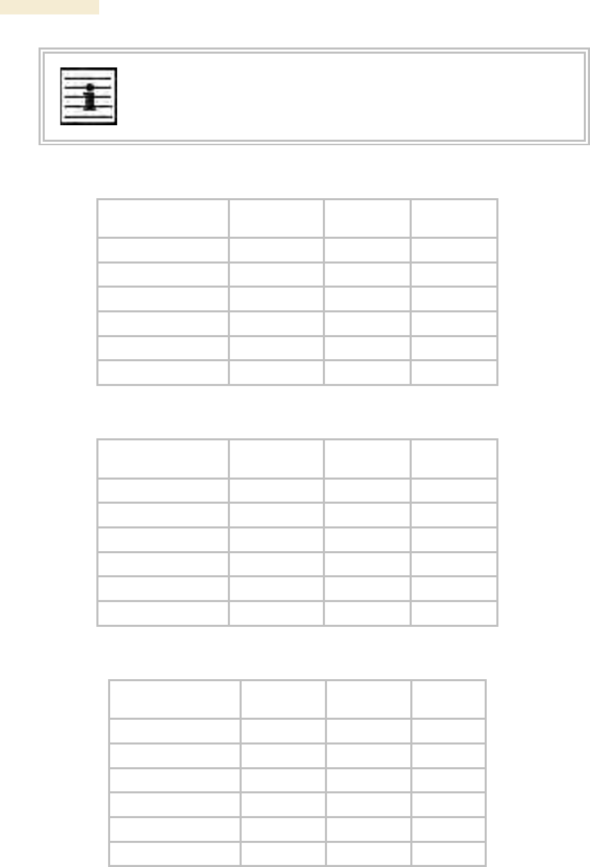
12.5.7 Example Channel Plans for AP Clusters
Examples for assignment of frequency channels and sector IDs are provided in the
following tables. Each frequency is reused on the sector that is at a 180° offset. The entry
in the Symbol column of each table refers to the layout in Figure 38 on Page 142.
Planning Guide Release 8
140 Draft for Regulatory Review Issue 2, December 2006
NOTE:
The operator specifies the sector ID for the module as described under Sector
ID on Page 439.
Table 34: Example 900-MHz channel assignment by sector
Direction of Access
Point Sector
Frequency
Sector ID
Symbol
North (0°)
906 MHz
0
A
Northeast (60°)
915 MHz
1
B
Southeast (120°)
924 MHz
2
C
South (180°)
906 MHz
3
A
Southwest (240°)
915 MHz
4
B
Northwest (300°)
924 MHz
5
C
Table 35: Example 2.4-GHz channel assignment by sector
Direction of Access
Point Sector
Frequency
Sector ID
Symbol
North (0°)
2.4150 GHz
0
A
Northeast (60°)
2.4350 GHz
1
B
Southeast (120°)
2.4575 GHz
2
C
South (180°)
2.4150 GHz
3
A
Southwest (240°)
2.4350 GHz
4
B
Northwest (300°)
2.4575 GHz
5
C
Table 36: Example 5.2-GHz channel assignment by sector
Direction of Access
Point Sector
Frequency
Sector ID
Symbol
North (0°)
5.275 GHz
0
A
Northeast (60°)
5.300 GHz
1
B
Southeast (120°)
5.325 GHz
2
C
South (180°)
5.275 GHz
3
A
Southwest (240°)
5.300 GHz
4
B
Northwest (300°)
5.325 GHz
5
C

Release 8 Planning Guide
March 200 Through Software Release 6.
Issue 2, December 2006 Draft for Regulatory Review 141
Table 37: Example 5.4-GHz channel assignment by sector
Direction of Access
Point Sector
Frequency
Sector ID
Symbol
North (0°)
5.580 GHz
0
A
Northeast (60°)
5.620 GHz
1
B
Southeast (120°)
5.660 GHz
2
C
South (180°)
5.580 GHz
3
A
Southwest (240°)
5.620 GHz
4
B
Northwest (300°)
5.660 GHz
5
C
Table 38: Example 5.7-GHz channel assignment by sector
Direction of Access
Point Sector
Frequency
Sector ID
Symbol
North (0°)
5.735 GHz
0
A
Northeast (60°)
5.755 GHz
1
B
Southeast (120°)
5.775 GHz
2
C
South (180°)
5.735 GHz
3
A
Southwest (240°)
5.755 GHz
4
B
Northwest (300°)
5.775 GHz
5
C
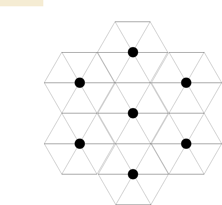
12.5.8 Multiple Access Points Clusters
When deploying multiple AP clusters in a dense area, consider aligning the clusters as
shown in Figure 38. However, this is only a recommendation. An installation may dictate
a different pattern of channel assignments.
Planning Guide Release 8
142 Draft for Regulatory Review Issue 2, December 2006
A
B
C
A
B
C
A
B
C
A
B
C
A
B
C
A
B
C
A
B
C
A
B
C
A
B
C
A
B
C
A
B
C
A
B
C
A
B
C
A
B
C
Figure 38: Example layout of 7 Access Point clusters
12.6 SELECTING SITES FOR NETWORK ELEMENTS
The Canopy APs must be positioned
◦ with hardware that the wind and ambient vibrations cannot flex or move.
◦ where a tower or rooftop is available or can be erected.
◦ where a grounding system is available.
◦ with lightning arrestors to transport lightning strikes away from equipment.
◦ at a proper height:
− higher than the tallest points of objects immediately around them (such as
trees, buildings, and tower legs).
− at least 2 feet (0.6 meters) below the tallest point on the tower, pole, or roof
(for lightning protection).
◦ away from high-RF energy sites (such as AM or FM stations, high-powered
antennas, and live AM radio towers).
◦ in line-of-sight paths
− to the SMs and BH.
− that will not be obstructed by trees as they grow or structures that are later
built.
Release 8 Planning Guide
March 200 Through Software Release 6.
Issue 2, December 2006 Draft for Regulatory Review 143
NOTE:
Visual line of sight does not guarantee radio line of sight.
12.6.1 Resources for Maps and Topographic Images
Mapping software is available from sources such as the following:
◦ http://www.microsoft.com/streets/default.asp
− Microsoft Streets & Trips (with Pocket Streets)
◦ http://www.delorme.com/software.htm
− DeLorme Street Atlas USA
− DeLorme Street Atlas USA Plus
− DeLorme Street Atlas Handheld
Topographic maps are available from sources such as the following:
◦ http://www.delorme.com/software.htm
− DeLorme Topo USA
− DeLorme 3-D TopoQuads
◦ http://www.usgstopomaps.com
− Timely Discount Topos, Inc. authorized maps
Topographic maps with waypoints are available from sources such as the following:
◦ http://www.topografix.com
− TopoGrafix EasyGPS
− TopoGrafix Panterra
− TopoGrafix ExpertGPS
Topographic images are available from sources such as the following:
◦ http://www.keyhole.com/body.php?h=products&t=keyholePro
− keyhole PRO
◦ http://www.digitalglobe.com
− various imagery
12.6.2 Surveying Sites
Factors to survey at potential sites include
◦ what pre-existing wireless equipment exists at the site. (Perform spectrum
analysis.)
◦ whether available mounting positions exist near the lowest elevation that satisfies
line of site, coverage, and other link criteria.
◦ whether you will always have the right to decide who climbs the tower to install
and maintain your equipment, and whether that person or company can climb at
any hour of any day.
Planning Guide Release 8
144 Draft for Regulatory Review Issue 2, December 2006
◦ whether you will have collaborative rights and veto power to prevent interference
to your equipment from wireless equipment that is installed at the site in the
future.
◦ whether a pre-existing grounding system (path to Protective Earth
) exists, and
what is required to establish a path to it.
◦ who is permitted to run any indoor lengths of cable.
12.6.3 Assuring the Essentials
In the 2.4-, 5.2-, 5.4-, and 5.7-GHz frequency band ranges, an unobstructed line of sight
(LOS) must exist and be maintainable between the radios that are involved in each link.
Line of Sight (LOS) Link
In these ranges, a line of sight link is both
◦ an unobstructed straight line from radio to radio.
◦ an unobstructed zone surrounding that straight line.
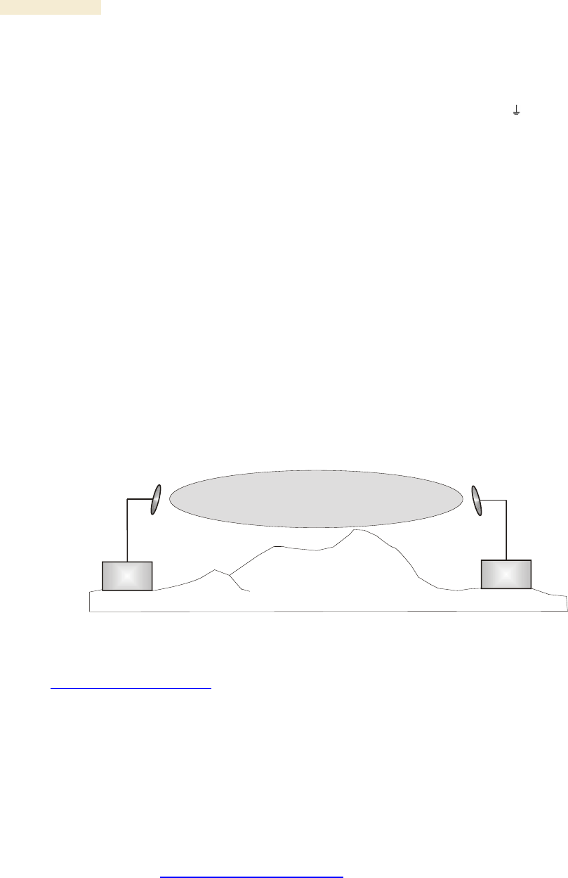
Fresnel Zone Clearance
An unobstructed line of sight is important, but is not the only determinant of adequate
placement. Even where the path has a clear line of sight, obstructions such as terrain,
vegetation, metal roofs, or cars may penetrate the Fresnel zone and cause signal loss.
Figure 39 illustrates an ideal Fresnel zone.
Transmitter
or Amplifier receiver
transmitter
Fresnel zone
Figure 39: Fresnel zone
FresnelZoneCalcPage.xls calculates the Fresnel zone clearance that is required between
the visual line of sight and the top of an obstruction that would protrude into the link path.
Non-Line of Sight (NLOS) Link
The Canopy 900-MHz modules have a line of sight (LOS) range of 40 miles (more than
64 km) and greater non-line of sight (NLOS) range than Canopy modules of other
frequency bands. NLOS range depends on RF considerations such as foliage,
topography, obstructions.
12.6.4 Finding the Expected Coverage Area
The transmitted beam in the vertical dimension covers more area beyond than in front of
the beam center. BeamwidthRadiiCalcPage.xls calculates the radii of the beam coverage
area.
Release 8 Planning Guide
March 200 Through Software Release 6.
Issue 2, December 2006 Draft for Regulatory Review 145
12.6.5 Clearing the Radio Horizon
Because the surface of the earth is curved, higher module elevations are required for
greater link distances. This effect can be critical to link connectivity in link spans that are
greater than 8 miles (12 km). AntennaElevationCalcPage.xls calculates the minimum
antenna elevation for these cases, presuming no landscape elevation difference from one
end of the link to the other.
12.6.6 Calculating the Aim Angles
The appropriate angle of AP downward tilt is derived from both the distance between
transmitter and receiver and the difference in their elevations. DowntiltCalcPage.xls
calculates this angle.
The proper angle of tilt can be calculated as a factor of both the difference in elevation
and the distance that the link spans. Even in this case, a plumb line and a protractor can
be helpful to ensure the proper tilt. This tilt is typically minimal.
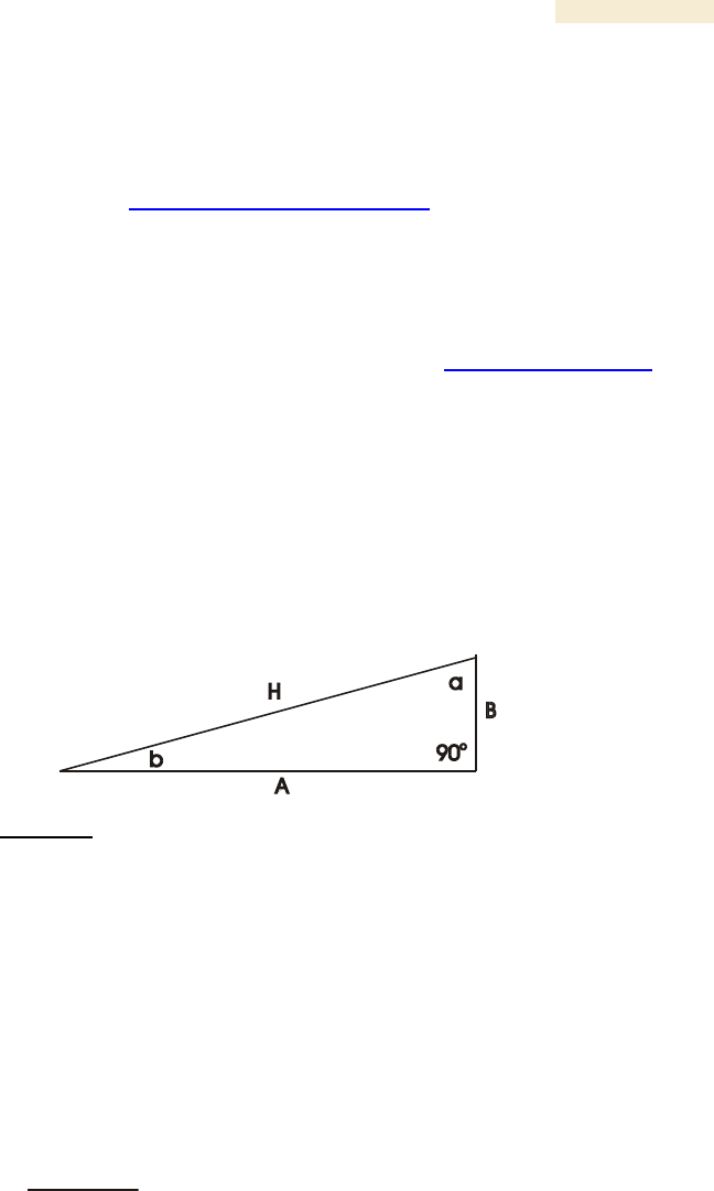
The number of degrees to offset (from vertical) the mounting hardware leg of the support
tube is equal to the angle of elevation from the lower module to the higher module (<B in
the example provided in Figure 40).
LEGEND
b Angle of elevation.
B Vertical difference in elevation.
A Horizontal distance between modules.
Figure 40: Variables for calculating angle of elevation (and depression)
Calculating the Angle of Elevation
To use metric units to find the angle of elevation, use the following formula:
tan b =
B
1000A
where
B is expressed in meters
A is expressed in kilometers.
Planning Guide Release 8
146 Draft for Regulatory Review Issue 2, December 2006
To use English standard units to find the angle of elevation, use the following formula:
tan b =
B
5280A
where
B is expressed in feet
A is expressed in miles.
The angle of depression from the higher module is identical to the angle of elevation from
the lower module.
12.7 COLLOCATING CANOPY MODULES
A BH and an AP or AP cluster on the same tower require a CMM. The CMM properly
synchronizes the transmit start times of all Canopy modules to prevent interference and
desensing of the modules. At closer distances without sync from a CMM, the frame
structures cause self interference.
Furthermore, a BH and an AP on the same tower require that the effects of their differing
receive start times be mitigated by either
◦ 100 vertical feet (30 meters) or more and as much spectral separation as
possible within the same frequency band range.
◦ the use of the frame calculator to tune the Downlink Data parameter in each,
so that the receive start time in each is the same. See Using the Frame
Calculator Tool (All) on Page 440.
Canopy APs and a BHS can be collocated at the same site only if they operate in
different frequency band ranges.
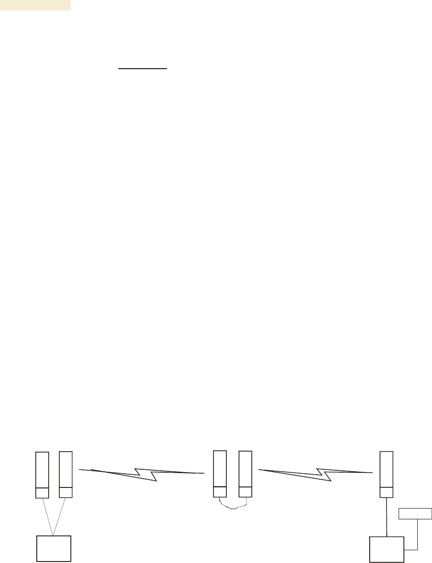
Where a single BH air link is insufficient to cover the distance from an AP cluster to your
point of presence (POP), you can deploy two BHSs, connected to one another by
Ethernet, on a tower that is between a BHM collocated with the AP cluster and another
BHM collocated with the POP. This deployment is illustrated in Figure 41.
CMM
BH
-M-
AP BH
-S-
CMM
BH
-S-
CMM
BH
-M-
CMM
POP
Figure 41: Double-hop backhaul links
Release 8 Planning Guide
March 200 Through Software Release 6.
Issue 2, December 2006 Draft for Regulatory Review 147
However, the BHSs can be collocated at the same site only if one is on a different
frequency band range from that of the other or one of the following conditions applies:
◦ They are vertically separated on a structure by at least 100 feet (30 m).
◦ They are vertically separated on a structure by less distance, but either
− an RF shield isolates them from each other.
− the uplink and downlink data parameters and control channels match (the
Downlink Data parameter is set to 50%).
The constraints for collocated modules in the same frequency band range are to avoid
self-interference that would occur between them. Specifically, unless the uplink and
downlink data percentages match, intervals exist when one is transmitting while the other
is receiving, such that the receiving module cannot receive the signal from the far end.
The interference is less a problem during low throughput periods and intolerable during
high. Typically, during low throughput periods, sufficient time exists for the far end to
retransmit packets lost because of interference from the collocated module.
12.8 DEPLOYING A REMOTE AP
In cases where the subscriber population is widely distributed, or conditions such as
geography restrict network deployment, you can add a Remote AP to
◦ provide high-throughput service to near LoS business subscribers.
◦ reach around obstructions or penetrate foliage with non-LoS throughput.
◦ reach new, especially widely distributed, residential subscribers with broadband
service.
◦ pass sync to an additional RF hop.
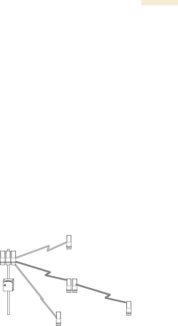
In the remote AP configuration, a Canopy AP is collocated with a Canopy SM. The
remote AP distributes the signal over the last mile to SMs that are logically behind the
collocated SM. A remote AP deployment is illustrated in Figure 42.
C A N O P Y
C A N O P Y
C A N O P Y
C A N O P Y
Canopy
SM
Canopy
SM with
Remote AP
Canopy
SM
C A N O P Y
AP
C A N O P Y C A N O P Y C A N O P Y
C A N O P Y
Canopy
SM
C A N O P YC A N O P YC A N O P YC A N O P Y
C A N O P YC A N O P Y
C A N O P YC A N O P Y
C A N O P YC A N O P Y
Canopy
SM
Canopy
SM with
Remote AP
Canopy
SM
C A N O P YC A N O P Y
AP
C A N O P Y C A N O P Y C A N O P YC A N O P YC A N O P Y C A N O P YC A N O P Y C A N O P YC A N O P Y
C A N O P YC A N O P Y
Canopy
SM
Figure 42: Remote AP deployment
Planning Guide Release 8
148 Draft for Regulatory Review Issue 2, December 2006
The collocated SM receives data in one frequency band, and the remote AP must
redistribute the data in a different frequency band. Base your selection of frequency band
ranges on regulatory restrictions, environmental conditions, and throughput requirements.
IMPORTANT!
Each relay hop (additional daisy-chained remote AP) adds latency to the link as
follows:
◦ approximately 6 msec where hardware scheduling is enabled.
◦ approximately 15 msec where software scheduling is enabled.
12.8.1 Remote AP Performance
The performance of a remote AP is identical to the AP performance in cluster.
Throughputs, ranges, and patch antenna coverage are identical. Canopy Advantage and
Canopy modules can be deployed in tandem in the same sector to meet customer
bandwidth demands.
As with all equipment operating in the unlicensed spectrum, Motorola strongly
recommends that you perform site surveys before you add network elements. These will
indicate that spectrum is available in the area where you want to grow. Keep in mind that
◦ non-LoS ranges heavily depend on environmental conditions.
◦ in most regions, not all frequencies are available.
◦ your deployments must be consistent with local regulatory restrictions.
12.8.2 Example Use Case for RF Obstructions
A remote AP can be used to provide last-mile access to a community where RF
obstructions prevent SMs from communicating with the higher-level AP in cluster. For
example, you may be able to use 900 MHz for the last mile between a remote AP and the
outlying SMs where these subscribers cannot form good links to a higher-level 2.4-GHz
AP. In this case, the short range of the 900-MHz remote AP is sufficient, and the ability of
the 900-MHz wavelength to be effective around foliage at short range solves the foliage
penetration problem.
An example of this use case is shown in Figure 43.
Release 8 Planning Guide
March 200 Through Software Release 6.
Issue 2, December 2006 Draft for Regulatory Review 149
C A N O P Y
C A N O P Y
2.4 GHz SM
2.4 GHz SM
with
Remote 900 MHz AP
C A N O P Y
2.4 GHz AP
C A N O P Y
C A N O P Y
C A N O P Y
C A N O P Y
900 MHz SM
4 Mbps Maximum Throughput
NLoS
Range ~2 miles
14 Mbps Maximum Aggregate Throughput
LoS
Range 2.5 miles
7 Mbps Maximum Aggregate Throughput
LoS
Range 5 miles
C A N O P Y
C A N O P Y
C A N O P Y
900 MHz SM
2 Mbps Maximum Throughput
NLoS
Range ~4 miles
C A N O P Y
900 MHz SM
4 Mbps Maximum Throughput
LoS
Range 20 miles
C A N O P Y
900 MHz SM
2 Mbps Maximum Throughput
LoS
Range 40 miles
C A N O P Y C A N O P Y C A N O P Y C A N O P Y
C A N O P Y C A N O P Y
2.4 GHz SM
2.4 GHz SM
with
Remote 900 MHz AP
C A N O P Y C A N O P Y
2.4 GHz AP
C A N O P Y
C A N O P Y
C A N O P Y
C A N O P Y C A N O P Y
C A N O P Y C A N O P Y
C A N O P Y C A N O P Y
C A N O P Y C A N O P Y
900 MHz SM
4 Mbps Maximum Throughput
NLoS
Range ~2 miles
14 Mbps Maximum Aggregate Throughput
LoS
Range 2.5 miles
7 Mbps Maximum Aggregate Throughput
LoS
Range 5 miles
C A N O P Y C A N O P Y
C A N O P Y C A N O P Y
C A N O P Y C A N O P Y
900 MHz SM
2 Mbps Maximum Throughput
NLoS
Range ~4 miles
C A N O P Y C A N O P Y
900 MHz SM
4 Mbps Maximum Throughput
LoS
Range 20 miles
C A N O P Y C A N O P Y
900 MHz SM
2 Mbps Maximum Throughput
LoS
Range 40 miles
Figure 43: Example 900-MHz remote AP behind 2.4-GHz SM
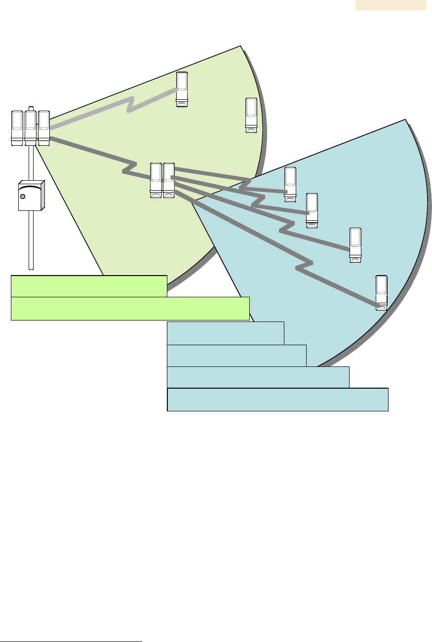
The 2.4 GHz modules provide a sustained aggregate throughput of up to 14 Mbps to the
sector. One of the SMs in the sector is wired to a 900-MHz remote AP, which provides
NLoS sustained aggregate throughput5 of
◦ 4 Mbps to 900-MHz SMs up to 2 miles away in the sector.
◦ 2 Mbps to 900-MHz SMs between 2 and 4 miles away in the sector.
12.8.3 Example Use Case for Passing Sync
All Canopy radios support the remote AP functionality. The BHS and the SM can reliably
pass the sync pulse, and the BHM and AP can reliably receive it. Examples of passing
sync over cable are shown under Passing Sync in an Additional Hop on Page 97. The
sync cable is described under Cables on Page 59.
5 NLoS ranges depend on environmental conditions. Your results may vary from these.
Planning Guide Release 8
150 Draft for Regulatory Review Issue 2, December 2006
The sync is passed in a cable that connects Pins 1 and 6 of the RJ-11 timing ports of the
two modules. When you connect modules in this way, you must also adjust configuration
parameters to ensure that
◦ the AP is set to properly receive sync.
◦ the SM will not propagate sync to the AP if the SM itself ceases to receive sync.
Perform Procedure 35: Extending network sync on Page 369.
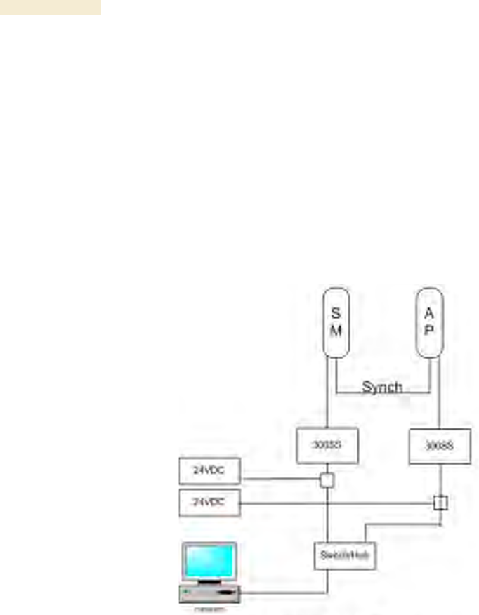
12.8.4 Physical Connections Involving the Remote AP
The SM to which you wire a remote AP can be either an SM that serves a customer or an
SM that simply serves as a relay. Where the SM serves a customer, wire the remote AP
to the SM as shown in Figure 44.
Figure 44: Remote AP wired to SM that also serves a customer
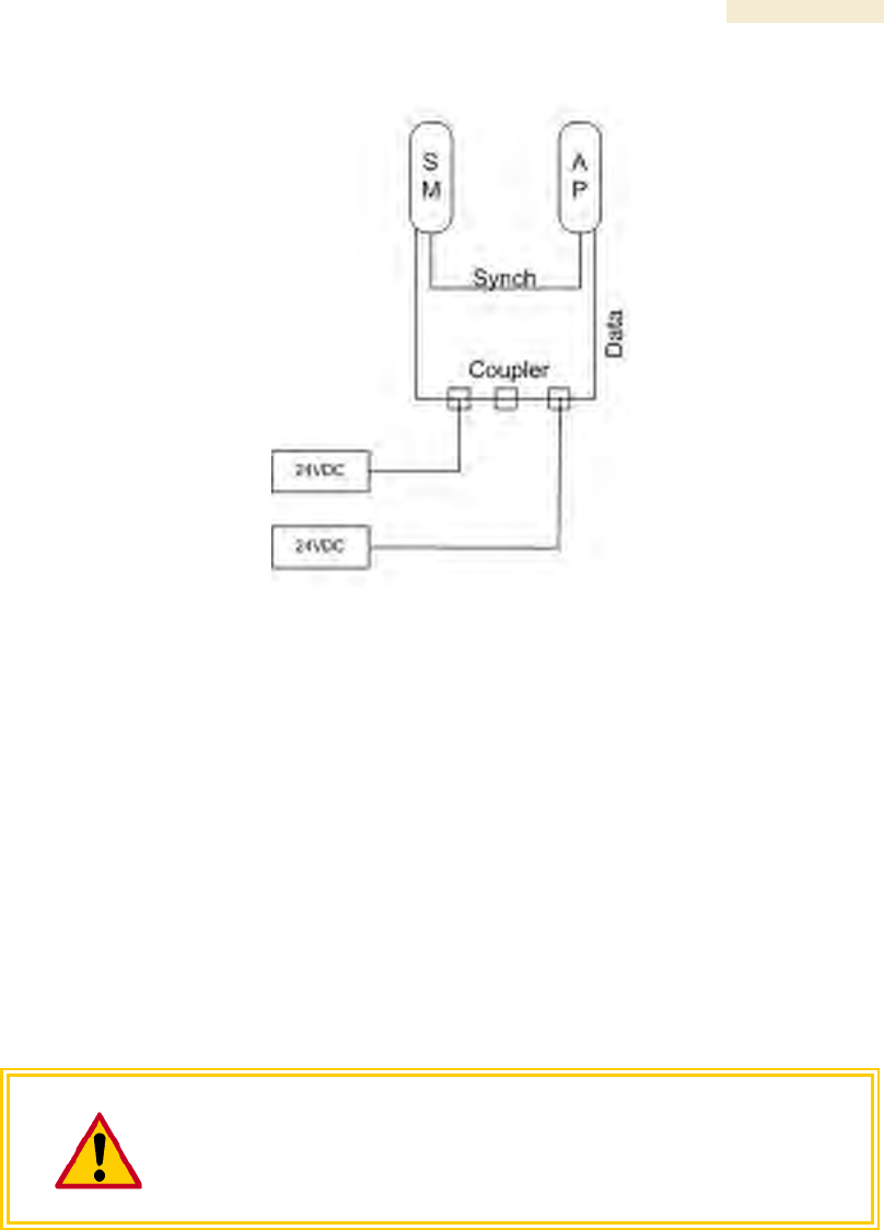
Where the SM simply serves as a relay, you must use a straight-through RJ-45
female-to-female coupler, and wire the SM to the remote AP as shown in Figure 45.
Release 8 Planning Guide
March 200 Through Software Release 6.
Issue 2, December 2006 Draft for Regulatory Review 151
Figure 45: Remote AP wired to SM that serves as a relay
12.9 DIAGRAMMING NETWORK LAYOUTS
12.9.1 Accounting for Link Ranges and Data Handling Requirements
For aggregate throughput correlation to link distance in both point-to-multipoint and
point-to-point links, see
◦ Link Performance and Encryption Comparisons on Page 63.
◦ all regulations that apply in your region and nation(s).
12.9.2 Avoiding Self Interference
For 5.2-, 5.4-, and 5.7-GHz modules, 20-MHz wide channels are centered every 5 MHz.
For 2.4-GHz modules, 20-MHz wide channels are centered every 2.5 MHz. This allows
you to customize the channel layout for interoperability where other Canopy equipment is
collocated.
CAUTION!
Regardless of whether 2.4-, 5.2-, 5.4-, or 5.7-GHz modules are deployed,
channel separation between modules should be at least 20 MHz for 1X
operation or 25 MHz for 2X.
Physical Proximity
A BH and an AP on the same tower require a CMM. The CMM properly synchronizes the
transmit start times of all Canopy modules to prevent interference and desensing of the
modules. At closer distances without sync from a CMM, the frame structures cause self
interference.
Furthermore, a BH and an AP on the same tower require that the effects of their differing
receive start times be mitigated by either
Planning Guide Release 8
152 Draft for Regulatory Review Issue 2, December 2006
◦ 100 vertical feet (30 meters) or more and as much spectral separation as
possible within the same frequency band range.
◦ the use of the frame calculator to tune the Downlink Data % parameter in each,
so that the receive start time in each is the same. See Using the Frame
Calculator Tool (All) on Page 440.
Spectrum Analysis
You can use an SM or BHS as a spectrum analyzer. See Mapping RF Neighbor
Frequencies on Page 131. Through a toggle of the Device Type parameter, you can
temporarily transform an AP into an SM to use it as a spectrum analyzer.
Power Reduction to Mitigate Interference
Where any module (SM, AP, BH timing master, or BH timing slave) is close enough to
another module that self-interference is possible, you can set the SM to operate at less
than full power. To do so, perform the following steps.
CAUTION!
A low setting of the Transmitter Output Power parameter can cause a link to a
distant module to drop. A link that drops for this reason can be re-established
by only Ethernet access.
Procedure 3: Invoking the low power mode
1. Access the Radio tab of the module.
2. In the Transmitter Output Power parameter, reduce the setting.
3. Click Save Changes.
4. Click Reboot.
5. Access the Session Status tab in the Home web page of the SM.
6. Assess whether the link achieves good Power Level and Jitter values.
NOTE: The received Power Level is shown in dBm and should be maximized.
Jitter should be minimized. However, better/lower jitter should be favored over
better/higher dBm. For historical reasons, RSSI is also shown and is the unitless
measure of power. The best practice is to use Power Level and ignore RSSI,
which implies more accuracy and precision than is inherent in its measurement.
7. Access the Link Capacity Test tab in the Tools web page of the module.
8. Assess whether the desired links for this module achieve
◦ uplink efficiency greater than 90%.
◦ downlink efficiency greater than 90%.
9. If the desired links fail to achieve any of the above measurement thresholds, then
a. access the module by direct Ethernet connection.
b. access the Radio tab in the Configuration web page of the module.
c. in the Transmitter Output Power parameter, increase the setting.
d. click Save Changes.
e. click Reboot.
=========================== end of procedure ======================

Release 8 Planning Guide
March 200 Through Software Release 6.
Issue 2, December 2006 Draft for Regulatory Review 153
12.9.3 Avoiding Other Interference
Where signal strength cannot dominate noise levels, the network experiences
◦ bit error corrections.
◦ packet errors and retransmissions.
◦ lower throughput (because bandwidth is consumed by retransmissions) and high
latency (due to resends).
Be especially cognitive of these symptoms for 900-MHz links. Where you see these
symptoms, attempt the following remedies:
◦ Adjust the position of the SM.
◦ Deploy a band-pass filter at the AP.
◦ Consider adding a remote AP closer to the affected SMs. (See Deploying a
Remote AP on Page 147.)
Certain other actions, which may seem to be potential remedies, do not resolve high
noise level problems:
◦ Do not deploy an omnidirectional or vertically polarized antenna.
◦ Do not set the antenna gain above the recommended level.
◦ Do not deploy a band-pass filter in the expectation that this can mitigate
interband interference.
Release 8 Planning Guide
March 200 Through Software Release 6.
Issue 2, December 2006 Draft for Regulatory Review 155
13 ENGINEERING YOUR IP COMMUNICATIONS
13.1 UNDERSTANDING ADDRESSES
A basic understanding of Internet Protocol (IP) address and subnet mask concepts is
required for engineering your IP network.
13.1.1 IP Address
The IP address is a 32-bit binary number that has four parts (octets). This set of four
octets has two segments, depending on the class of IP address. The first segment
identifies the network. The second identifies the hosts or devices on the network. The
subnet mask marks a boundary between these two sub-addresses.
13.2 DYNAMIC OR STATIC ADDRESSING
For any computer to communicate with a Canopy module, the computer must be
configured to either
◦ use DHCP (Dynamic Host Configuration Protocol). In this case, when not
connected to the network, the computer derives an IP address on the 169.254
network within two minutes.
◦ have an assigned static IP address (for example, 169.254.1.5) on the 169.254
network.
IMPORTANT!
If an IP address that is set in the module is not the 169.254.x.x network address,
then the network operator must assign the computer a static IP address in the
same subnet.
13.2.1 When a DHCP Server is Not Found
To operate on a network, a computer requires an IP address, a subnet mask, and
possibly a gateway address. Either a DHCP server automatically assigns this
configuration information to a computer on a network or an operator must input these
items.
When a computer is brought on line and a DHCP server is not accessible (such as when
the server is down or the computer is not plugged into the network), Microsoft and Apple
operating systems default to an IP address of 169.254.x.x and a subnet mask of
255.255.0.0 (169.254/16, where /16 indicates that the first 16 bits of the address range
are identical among all members of the subnet).

Planning Guide Release 8
156 Draft for Regulatory Review Issue 2, December 2006
13.3 NETWORK ADDRESS TRANSLATION (NAT)
13.3.1 NAT, DHCP Server, DHCP Client, and DMZ in SM
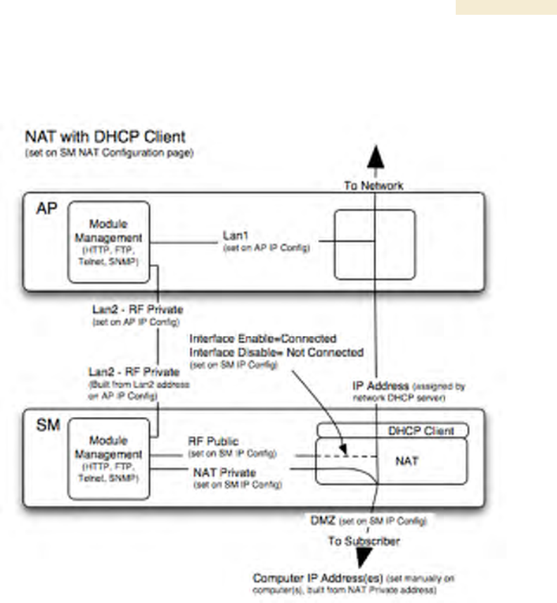
The Canopy system provides NAT (network address translation) for SMs in the following
combinations of NAT and DHCP (Dynamic Host Configuration Protocol):
◦ NAT Disabled (as in earlier releases)
◦ NAT with DHCP Client and DHCP Server
◦ NAT with DHCP Client
◦ NAT with DHCP Server
◦ NAT without DHCP
NAT
NAT isolates devices connected to the Ethernet/wired side of an SM from being seen
directly from the wireless side of the SM. With NAT enabled, the SM has an IP address
for transport traffic (separate from its address for management), terminates transport
traffic, and allows you to assign a range of IP addresses to devices that are connected
to the Ethernet/wired side of the SM.
In the Canopy system, NAT supports many protocols, including HTTP, ICMP (Internet
Control Message Protocols), and FTP (File Transfer Protocol). For virtual private network
(VPN) implementation, L2TP over IPSec (Level 2 Tunneling Protocol over IP Security) is
supported, but PPTP (Point to Point Tunneling Protocol) is not supported. See NAT and
VPNs on Page 161.
DHCP
DHCP enables a device to be assigned a new IP address and TCP/IP parameters,
including a default gateway, whenever the device reboots. Thus DHCP reduces
configuration time, conserves IP addresses, and allows modules to be moved to a
different network within the Canopy system.
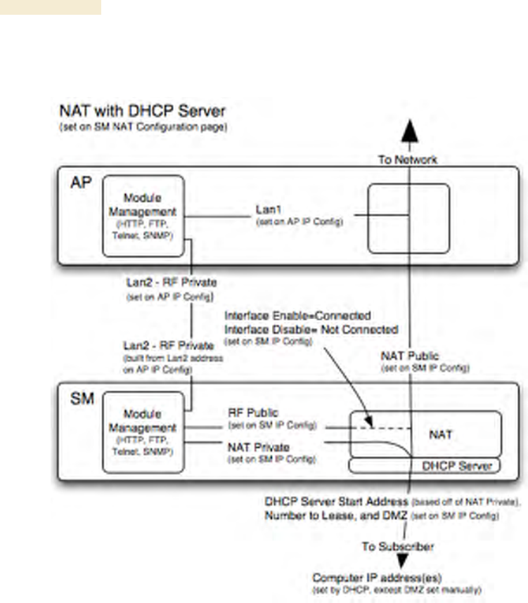
In conjunction with the NAT features, each SM provides
◦ a DHCP server that assigns IP addresses to computers connected to the SM by
Ethernet protocol.
◦ a DHCP client that receives an IP address for the SM from a network DHCP
server.
DMZ
In conjunction with the NAT features, a DMZ (demilitarized zone) allows the assignment
of one IP address behind the SM for a device to logically exist outside the firewall and
receive network traffic. The first three octets of this IP address must be identical to the
first three octets of the NAT private IP address.
Release 8 Planning Guide
March 200 Through Software Release 6.
Issue 2, December 2006 Draft for Regulatory Review 157
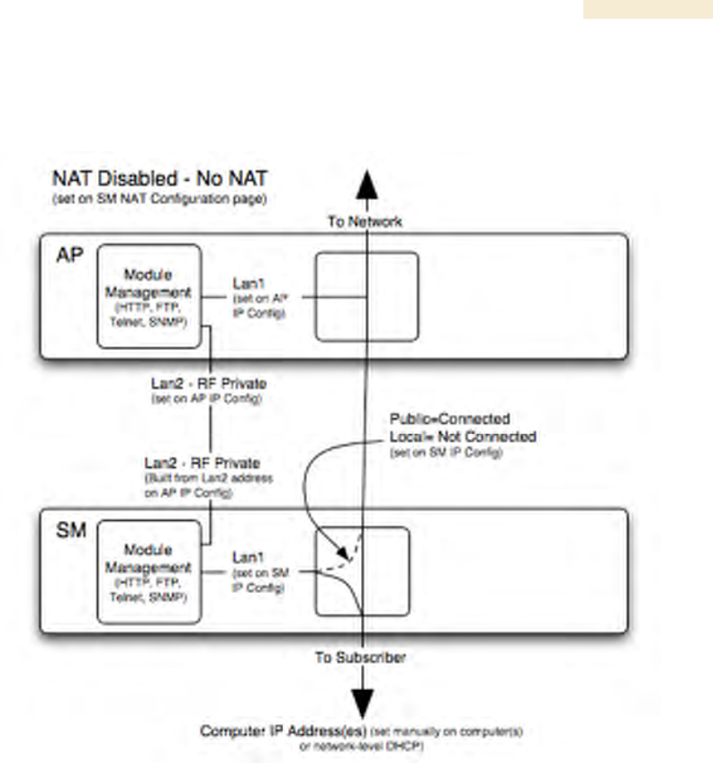
NAT Disabled
The NAT Disabled implementation is illustrated in Figure 46.
Figure 46: NAT Disabled implementation
Planning Guide Release 8
158 Draft for Regulatory Review Issue 2, December 2006
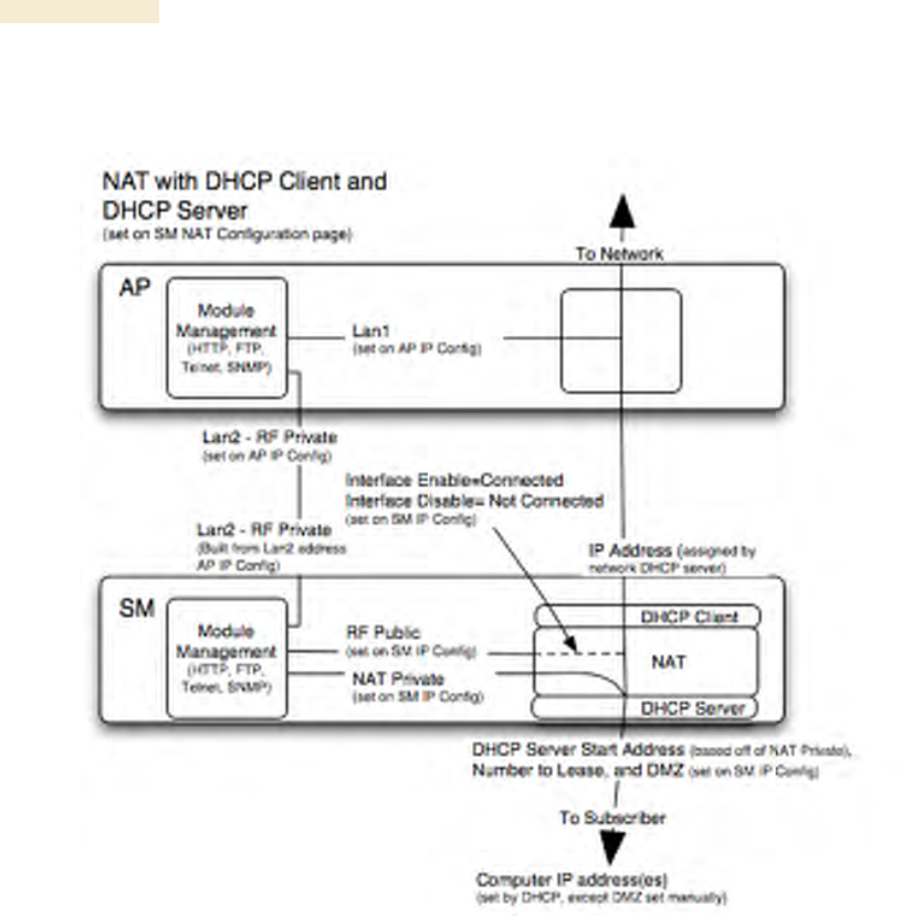
NAT with DHCP Client and DHCP Server
The NAT with DHCP Client and DHCP Server implementation is illustrated in Figure 47.
Figure 47: NAT with DHCP Client and DHCP Server implementation
Release 8 Planning Guide
March 200 Through Software Release 6.
Issue 2, December 2006 Draft for Regulatory Review 159
NAT with DHCP Client
The NAT with DHCP Client implementation is illustrated in Figure 48.
Figure 48: NAT with DHCP Client implementation
Planning Guide Release 8
160 Draft for Regulatory Review Issue 2, December 2006
NAT with DHCP Server
The NAT with DHCP Server implementation is illustrated in Figure 49.
Figure 49: NAT with DHCP Server implementation
Release 8 Planning Guide
March 200 Through Software Release 6.
Issue 2, December 2006 Draft for Regulatory Review 161
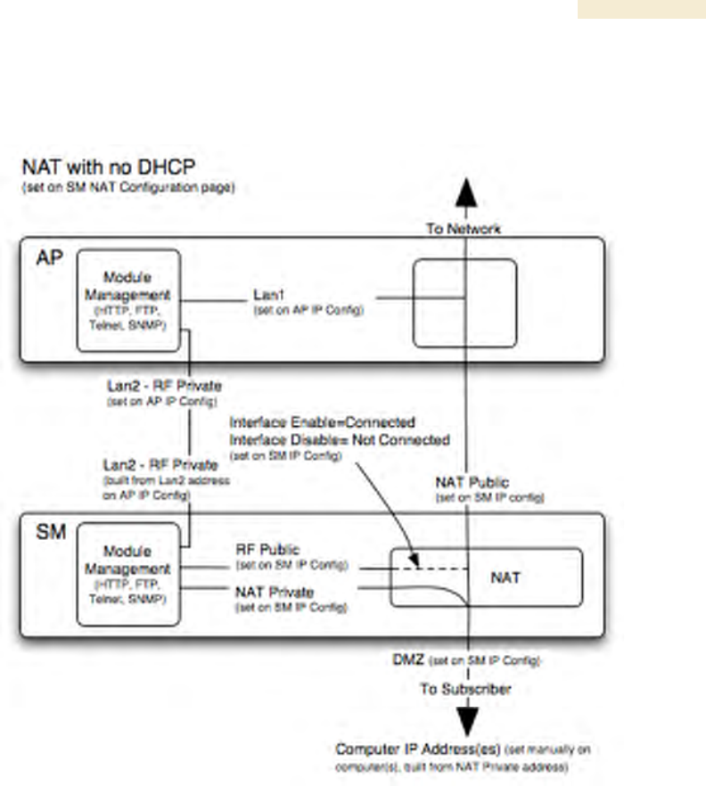
NAT without DHCP
The NAT without DHCP implementation is illustrated in Figure 50.
Figure 50: NAT without DHCP implementation
13.3.2 NAT and VPNs
VPN technology provides the benefits of a private network during communication over a
public network. One typical use of a VPN is to connect remote employees, who are at
home or in a different city, to their corporate network over the public Internet. Any of
several VPN implementation schemes is possible. By design, NAT translates or changes
addresses, and thus interferes with a VPN that is not specifically supported by a given
NAT implementation.
With NAT enabled, SMs support L2TP over IPSec (Level 2 Tunneling Protocol over IP
Security) VPNs, but do not support PPTP (Point to Point Tunneling Protocol) VPNs.
With NAT disabled, SMs support all types of VPNs.
13.4 DEVELOPING AN IP ADDRESSING SCHEME
Canopy network elements are accessed through IP Version 4 (IPv4) addressing.
A proper IP addressing method is critical to the operation and security of a Canopy
network.

Planning Guide Release 8
162 Draft for Regulatory Review Issue 2, December 2006
Each Canopy module requires an IP address on the network. This IP address is for only
management purposes. For security, you should either
◦ assign an unroutable IP address.
◦ assign a routable IP address only if a firewall is present to protect the module.
You will assign IP addresses to computers and network components by either static or
dynamic IP addressing. You will also assign the appropriate subnet mask and network
gateway to each module.
13.4.1 Address Resolution Protocol
As previously stated, the MAC address identifies a Canopy module in
◦ communications between modules.
◦ the data that modules store about each other.
◦ the data that BAM or Prizm applies to manage authentication and bandwidth.
The IP address is essential for data delivery through a router interface. Address
Resolution Protocol (ARP) correlates MAC addresses to IP addresses.
For communications to outside the network segment, ARP reads the network gateway
address of the router and translates it into the MAC address of the router. Then the
communication is sent to MAC address (physical network interface card) of the router.
For each router between the sending module and the destination, this sequence applies.
The ARP correlation is stored until the ARP cache times out.
13.4.2 Allocating Subnets
The subnet mask is a 32-bit binary number that filters the IP address. Where a subnet
mask contains a bit set to 1, the corresponding bit in the IP address is part of the network
address.
Example IP Address and Subnet Mask
In Figure 51, the first 16 bits of the 32-bit IP address identify the network:
Octet 1
Octet 2
Octet 3
Octet 4
IP address 169.254.1.1
10101001
11111110
00000001
00000001
Subnet mask 255.255.0.0
11111111
11111111
00000000
00000000
Figure 51: Example of IP address in Class B subnet
In this example, the network address is 169.254, and 216 (65,536) hosts are addressable.
13.4.3 Selecting Non-routable IP Addresses
The factory default assignments for Canopy network elements are
◦ unique MAC address
◦ IP address of 169.254.1.1, except for an OFDM series BHM, whose IP address
is 169.254.1.2 by default
◦ subnet mask of 255.255.0.0
◦ network gateway address of 169.254.0.0

Release 8 Planning Guide
March 200 Through Software Release 6.
Issue 2, December 2006 Draft for Regulatory Review 163
For each Canopy radio and CMMmicro, assign an IP address that is both consistent
with the IP addressing plan for your network and cannot be accessed from the Internet.
IP addresses within the following ranges are not routable from the Internet, regardless of
whether a firewall is configured:
◦ 10.0.0.0 – 10.255.255.255
◦ 172.16.0.0 – 172.31.255.255
◦ 192.168.0.0 – 192.168.255.255
You can also assign a subnet mask and network gateway for each CMMmicro.

Release 8 Planning Guide
March 200 Through Software Release 6.
Issue 2, December 2006 Draft for Regulatory Review 165
14 ENGINEERING VLANS
Canopy radios support VLAN functionality as defined in the 802.1Q (Virtual LANs)
specification, except for the following aspects of that specification:
◦ the following protocols:
− Generic Attribute Registration Protocol (GARP) GARV
− Spanning Tree Protocol (STP)
− Multiple Spanning Tree Protocol (MSTP)
− GARP Multicast Registration Protocol (GMRP)
◦ priority encoding (802.1P) before Release 7.0
◦ embedded source routing (ERIF) in the 802.1Q header
◦ multicast pruning
◦ flooding unknown unicast frames in the downlink
As an additional exception, the Canopy AP does not flood downward the unknown
unicast frames to the Canopy SM.
A VLAN configuration in Layer 2 establishes a logical group within the network. Each
computer in the VLAN, regardless of initial or eventual physical location, has access to
the same data. For the network operator, this provides flexibility in network segmentation,
simpler management, and enhanced security.
14.1 SM MEMBERSHIP IN VLANS
With the supported VLAN functionality, Canopy radios determine bridge forwarding on
the basis of not only the destination MAC address, but also the VLAN ID of the
destination. This provides flexibility in how SMs are used:
◦ Each SM can be a member in its own VLAN, whose other members can be APs
in other sectors. This case would allow movement of the SM from sector to
sector without requiring a reconfiguration of the VLAN.
◦ Each SM can be in its own broadcast domain, such that only the radios that are
members of the VLAN can see multicast traffic to and from the SM. In most
cases, this can significantly conserve bandwidth at the SMs.
◦ The network operator can define a work group of SMs, regardless of the AP(s)
to which they register.
Canopy point-to-multipoint modules provide the VLAN frame filters that are described in
Table 39.
Planning Guide Release 8
166 Draft for Regulatory Review Issue 2, December 2006
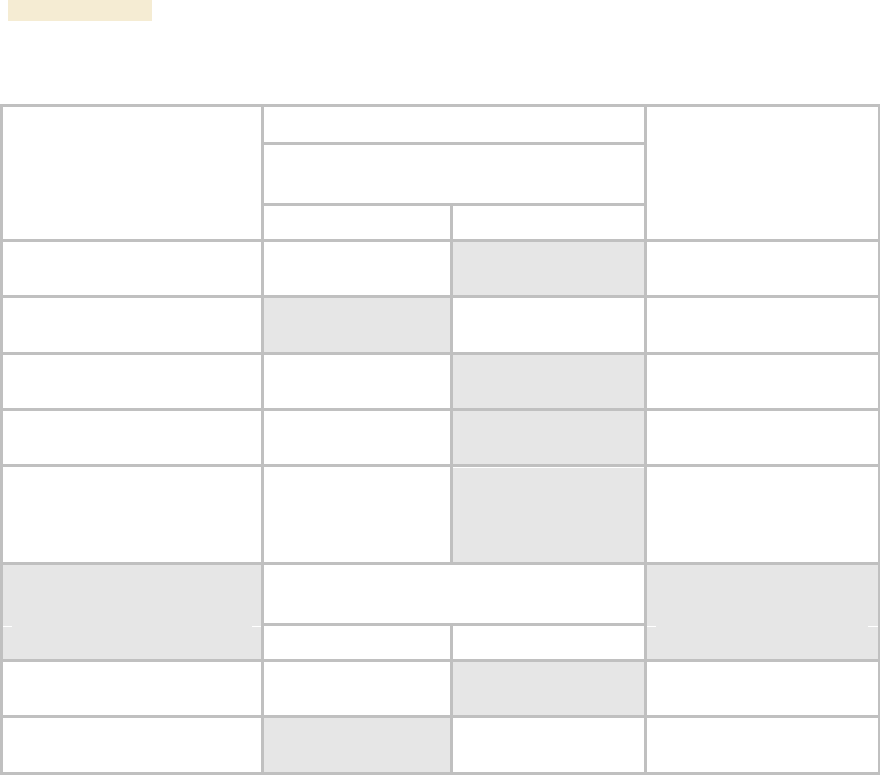
Table 39: VLAN filters in point-to-multipoint modules
then a frame is discarded if…
entering the bridge/
NAT switch through…
Where VLAN is active,
if this parameter value
is selected …
Ethernet…
TCP/IP…
because of this VLAN
filter in the Canopy
software:
any combination of VLAN
parameter settings
with a VID not in the
membership table
Ingress
any combination of VLAN
parameter settings
with a VID not in the
membership table
Local Ingress
Allow Frame Types:
Tagged Frames Only
with no 802.1Q tag
Only Tagged
Allow Frame Types:
Untagged Frames Only
with an 802.1Q tag,
regardless of VID
Only Untagged
Local SM Management:
Disable in the SM, or
All Local SM Management:
Disable in the AP
with an 802.1Q tag
and a VID in the
membership table
Local SM Management
leaving the bridge/
NAT switch through…
Ethernet…
TCP/IP…
any combination of VLAN
parameter settings
with a VID not in the
membership table
Egress
any combination of VLAN
parameter settings
with a VID not in the
membership table
Local Egress
14.2 PRIORITY ON VLANS (802.1p)
Canopy radios can prioritize traffic based on the eight priorities described in the IEEE
802.1p specification. When the high-priority channel is enabled on an SM, regardless of
whether VLAN is enabled on the AP for the sector, packets received with a priority of
4 through 7 in the 802.1p field are forwarded onto the high-priority channel.
VLAN settings in a Canopy module can also cause the module to convert received non-
VLAN packets into VLAN packets. In this case, the 802.1p priority in packets leaving the
module is set to the priority established by the DiffServ configuration.
If you enable VLAN, immediately monitor traffic to ensure that the results are as desired.
For example, high-priority traffic may block low-priority.
For more information on the Canopy high priority channel, see High-priority Bandwidth on
Page 88.