Openoffice Org 3 2 Calc Guide OpenOffice.org 3.x
OpenOffice - 3.2 - Calc Guide OOo_3.2_CalcG Free User Guide for OpenOffice Software, Manual
2015-07-27
: Openoffice-Org Openoffice-Org-Openoffice-3-2-Calc-Guide-777740 openoffice-org-openoffice-3-2-calc-guide-777740 openoffice-org pdf
Open the PDF directly: View PDF ![]() .
.
Page Count: 497 [warning: Documents this large are best viewed by clicking the View PDF Link!]
- Chapter 1
Introducing Calc
- What is Calc?
- Spreadsheets, sheets, and cells
- Parts of the main Calc window
- Starting new spreadsheets
- Opening existing spreadsheets
- Opening CSV files
- Saving spreadsheets
- Navigating within spreadsheets
- Selecting items in a sheet or spreadsheet
- Working with columns and rows
- Working with sheets
- Viewing Calc
- Using the Navigator
- Chapter 2
Entering, Editing, and Formatting Data
- Introduction
- Entering data using the keyboard
- Speeding up data entry
- Sharing content between sheets
- Validating cell contents
- Editing data
- Formatting data
- Autoformatting cells and sheets
- Formatting spreadsheets using themes
- Using conditional formatting
- Hiding and showing data
- Sorting records
- Finding and replacing in Calc
- Chapter 3 Creating Charts and Graphs
- Chapter 4
Using Styles and Templates in Calc
- What is a template?
- What are styles?
- Types of styles in Calc
- Accessing styles
- Applying cell styles
- Applying page styles
- Modifying styles
- Creating new (custom) styles
- Copying and moving styles
- Deleting styles
- Creating a spreadsheet from a template
- Creating a template
- Editing a template
- Adding templates using the Extension Manager
- Setting a default template
- Associating a spreadsheet with a different template
- Organizing templates
- Chapter 5 Using Graphics in Calc
- Chapter 6 Printing, Exporting, and E-mailing
- Chapter 7 Using Formulas and Functions
- Chapter 8
Using the DataPilot
- Introduction
- Examples with step by step instructions
- DataPilot functions in detail
- The database (preconditions)
- Start
- Data source
- The DataPilot dialog
- Working with the results of the DataPilot
- Start the dialog
- Change layout by using drag and drop
- Grouping rows or columns
- Grouping of categories with scalar values
- Grouping of categories with date or time values
- Grouping without the automatic creation of intervals
- Sorting the result
- Drilling (showing details)
- Filtering
- Updating (refreshing) changed values
- Cell formatting
- Multiple data fields
- Shortcuts
- Function GETPIVOTDATA
- Chapter 9 Data Analysis
- Chapter 10 Linking Calc Data
- Chapter 11 Sharing and Reviewing Documents
- Chapter 12 Calc Macros
- Chapter 13
Calc as a Simple Database
- Introduction
- Associating a range with a name
- Sorting
- Filters
- Calc functions similar to database functions
- Count and sum cells that match conditions: COUNTIF and SUMIF
- Ignore filtered cells using SUBTOTAL
- Using formulas to find data
- ADDRESS returns a string with a cell’s address
- INDIRECT converts a string to a cell or range
- OFFSET returns a cell or range offset from another
- INDEX returns cells inside a specified range
- Database-specific functions
- Conclusion
- Chapter 14
Setting up and Customizing Calc
- Introduction
- Choosing options that affect all of OOo
- Choosing options for loading and saving documents
- Choosing options for Calc
- Controlling Calc’s AutoCorrect functions
- Customizing the user interface
- Adding functionality with extensions
- Appendix A Keyboard Shortcuts
- Appendix B Description of Functions
- Appendix C Calc Error Codes
- Index

Calc Guide
Using Spreadsheets in OpenOffice.org
This PDF is designed to be read onscreen, two pages at a
time. If you want to print a copy, your PDF viewer should
have an option for printing two pages on one sheet of
paper, but you may need to start with page 2 to get it to
print facing pages correctly. (Print this cover page
separately.)

Copyright
This document is Copyright © 2005–2010 by its contributors as listed
in the section titled Authors. You may distribute it and/or modify it
under the terms of either the GNU General Public License, version 3 or
later, or the Creative Commons Attribution License, version 3.0 or
later. Note that Chapter 8, Using the DataPilot, is licensed under the
Creative Commons Attribution-Share Alike License, version 3.0.
All trademarks within this guide belong to their legitimate owners.
Authors
Rick Barnes Peter Kupfer
James Andrew Krishna Aradhi
Andy Brown Stephen Buck
Bruce Byfield Martin J. Fox
T. J. Frazier Stigant Fyrwitful
Spencer E. Harpe Regina Henschel
Peter Hillier-Brook John Kane
Kirk Emma Kirsopp
Jared Kobos Sigrid Kronenberger
Shelagh Manton Alexandre Martins
Kashmira Patel Anthony Petrillo
Andrew Pitonyak Iain Roberts
Hazel Russman Gary Schnabl
Rob Scott Sowbhagya Sundaresan
Nikita Telang Barbara M Tobias
John Viestenz Jean Hollis Weber
Stefan Weigel Sharon Whiston
Claire Wood Linda Worthington
Michele Zarri Magnus Adielsson
Sandeep Samuel Medikonda
Feedback
Please direct any comments or suggestions about this document to:
authors@documentation.openoffice.org
Publication date and software version
Published 8 September 2010. Based on OpenOffice.org 3.2.
You can download
an editable version of this document from
http://oooauthors.org/english/userguide3/published/

Contents
Chapter 1
Introducing Calc.........................................................................9
What is Calc?....................................................................................10
Spreadsheets, sheets, and cells........................................................10
Parts of the main Calc window..........................................................11
Starting new spreadsheets...............................................................16
Opening existing spreadsheets.........................................................17
Opening CSV files.............................................................................18
Saving spreadsheets.........................................................................19
Navigating within spreadsheets........................................................23
Selecting items in a sheet or spreadsheet........................................27
Working with columns and rows.......................................................30
Working with sheets..........................................................................32
Viewing Calc.....................................................................................33
Using the Navigator..........................................................................38
Chapter 2
Entering, Editing, and Formatting Data...................................41
Introduction......................................................................................42
Entering data using the keyboard.....................................................42
Speeding up data entry.....................................................................45
Sharing content between sheets.......................................................48
Validating cell contents.....................................................................49
Editing data......................................................................................51
Formatting data................................................................................53
Autoformatting cells and sheets........................................................59
Formatting spreadsheets using themes............................................60
Using conditional formatting............................................................61
Hiding and showing data..................................................................63
Sorting records.................................................................................65
Finding and replacing in Calc...........................................................67
OpenOffice.org 3.x Calc Guide 3

Chapter 3
Creating Charts and Graphs.....................................................72
Introduction......................................................................................73
Creating a chart................................................................................73
Editing charts...................................................................................78
Formatting charts.............................................................................84
Formatting 3D charts........................................................................87
Formatting the chart elements.........................................................91
Resizing and moving the chart..........................................................93
Gallery of chart types........................................................................95
Chapter 4
Using Styles and Templates in Calc........................................105
What is a template?........................................................................106
What are styles?..............................................................................106
Types of styles in Calc.....................................................................107
Accessing styles..............................................................................108
Applying cell styles.........................................................................109
Applying page styles.......................................................................111
Modifying styles..............................................................................111
Creating new (custom) styles..........................................................116
Copying and moving styles.............................................................117
Deleting styles................................................................................119
Creating a spreadsheet from a template.........................................119
Creating a template........................................................................120
Editing a template...........................................................................121
Adding templates using the Extension Manager.............................123
Setting a default template..............................................................124
Associating a spreadsheet with a different template......................125
Organizing templates......................................................................126
Chapter 5
Using Graphics in Calc...........................................................129
Graphics in Calc..............................................................................130
Adding graphics (images)...............................................................130
4 OpenOffice.org 3.x Calc Guide

Modifying images............................................................................136
Using the picture context menu......................................................142
Using Calc’s drawing tools..............................................................145
Positioning graphics........................................................................148
Creating an image map...................................................................151
Chapter 6
Printing, Exporting, and E-mailing........................................154
Quick printing.................................................................................155
Controlling printing........................................................................155
Using print ranges..........................................................................159
Page breaks.....................................................................................163
Headers and footers........................................................................164
Exporting to PDF............................................................................167
Exporting to XHTML.......................................................................173
Saving as Web pages (HTML).........................................................174
E-mailing spreadsheets...................................................................174
Digital signing of documents..........................................................175
Removing personal data.................................................................176
Chapter 7
Using Formulas and Functions...............................................177
Introduction....................................................................................178
Setting up a spreadsheet................................................................178
Creating formulas...........................................................................180
Understanding functions.................................................................197
Strategies for creating formulas and functions...............................203
Finding and fixing errors................................................................205
Examples of functions.....................................................................210
Using regular expressions in functions...........................................215
Advanced functions.........................................................................217
Chapter 8
Using the DataPilot................................................................218
Introduction....................................................................................219
Examples with step by step instructions.........................................219
OpenOffice.org 3.x Calc Guide 5

DataPilot functions in detail............................................................241
Function GETPIVOTDATA...............................................................267
Chapter 9
Data Analysis..........................................................................271
Introduction....................................................................................272
Consolidating data..........................................................................272
Creating subtotals...........................................................................275
Using “what if” scenarios...............................................................277
Using other “what if” tools.............................................................281
Working backwards using Goal Seek..............................................288
Using the Solver.............................................................................290
Chapter 10
Linking Calc Data....................................................................294
Why use multiple sheets?................................................................295
Setting up multiple sheets..............................................................295
Referencing other sheets................................................................299
Referencing other documents.........................................................301
Hyperlinks and URLs......................................................................303
Linking to external data..................................................................307
Linking to registered data sources.................................................312
Embedding spreadsheets................................................................316
Chapter 11
Sharing and Reviewing Documents.........................................322
Introduction....................................................................................323
Sharing documents (collaboration).................................................323
Recording changes..........................................................................326
Adding comments to changes.........................................................329
Adding other comments..................................................................330
Reviewing changes.........................................................................332
Merging documents........................................................................335
Comparing documents....................................................................337
Saving versions...............................................................................337
6 OpenOffice.org 3.x Calc Guide

Chapter 12
Calc Macros...........................................................................340
Introduction....................................................................................341
Using the macro recorder...............................................................341
Write your own functions................................................................345
Accessing cells directly...................................................................353
Sorting............................................................................................354
Conclusion......................................................................................356
Chapter 13
Calc as a Simple Database......................................................357
Introduction....................................................................................358
Associating a range with a name....................................................359
Sorting............................................................................................365
Filters.............................................................................................367
Calc functions similar to database functions..................................375
Database-specific functions............................................................387
Conclusion......................................................................................388
Chapter 14
Setting up and Customizing Calc...........................................389
Introduction....................................................................................390
Choosing options that affect all of OOo..........................................390
Choosing options for loading and saving documents......................396
Choosing options for Calc...............................................................400
Controlling Calc’s AutoCorrect functions.......................................409
Customizing the user interface.......................................................410
Adding functionality with extensions..............................................420
Appendix A
Keyboard Shortcuts................................................................422
Introduction....................................................................................423
Navigation and selection shortcuts.................................................423
Function and arrow key shortcuts..................................................425
Cell formatting shortcuts................................................................426
DataPilot shortcuts.........................................................................427
OpenOffice.org 3.x Calc Guide 7

Appendix B
Description of Functions........................................................428
Functions available in Calc.............................................................429
Mathematical functions..................................................................430
Financial analysis functions............................................................435
Statistical analysis functions...........................................................449
Date and time functions..................................................................458
Logical functions.............................................................................462
Informational functions...................................................................463
Database functions.........................................................................466
Array functions...............................................................................468
Spreadsheet functions....................................................................470
Text functions..................................................................................475
Add-in functions..............................................................................479
Appendix C
Calc Error Codes.....................................................................484
Introduction to Calc error codes.....................................................485
Error codes displayed within cells..................................................486
General error codes........................................................................487
Index.........................................................................................490
8 OpenOffice.org 3.x Calc Guide

Chapter 1
Introducing Calc
Using Spreadsheets in OpenOffice.org
What is Calc?
Calc is the spreadsheet component of OpenOffice.org (OOo). You can
enter data (usually numerical) in a spreadsheet and then manipulate
this data to produce certain results.
Alternatively, you can enter data and then use Calc in a ‘What if...’
manner by changing some of the data and observing the results
without having to retype the entire spreadsheet or sheet.
Other features provided by Calc include:
•Functions, which can be used to create formulas to perform
complex calculations on data
•Database functions, to arrange, store, and filter data
•Dynamic charts; two new types of charts—Bubble Charts and
Filled Net Charts—have been introduced in OOo 3.2
•Macros, for recording and executing repetitive tasks; scripting
languages supported include OpenOffice.org Basic, Python,
BeanShell, and JavaScript
•Ability to open, edit, and save Microsoft Excel spreadsheets
•Import and export of spreadsheets in multiple formats, including
HTML, CSV, PDF, and PostScript
Note
If you want to use macros written in Microsoft Excel using the
VBA macro code in OOo, you must first edit the code in the
OOo Basic IDE editor.
Spreadsheets, sheets, and cells
Calc works with elements called spreadsheets. Spreadsheets consist of
a number of individual sheets, each sheet containing cells arranged in
rows and columns. A particular cell is identified by its row number and
column letter.
Cells hold the individual elements—text, numbers, formulas, and so on
—that make up the data to display and manipulate.
Each spreadsheet can have many sheets, and each sheet can have
many individual cells. In Calc 3.x, each sheet can have a maximum of
65,536 rows and a maximum of 1024 columns, for a total of over 67
million cells.
10 OpenOffice.org 3.x Calc Guide
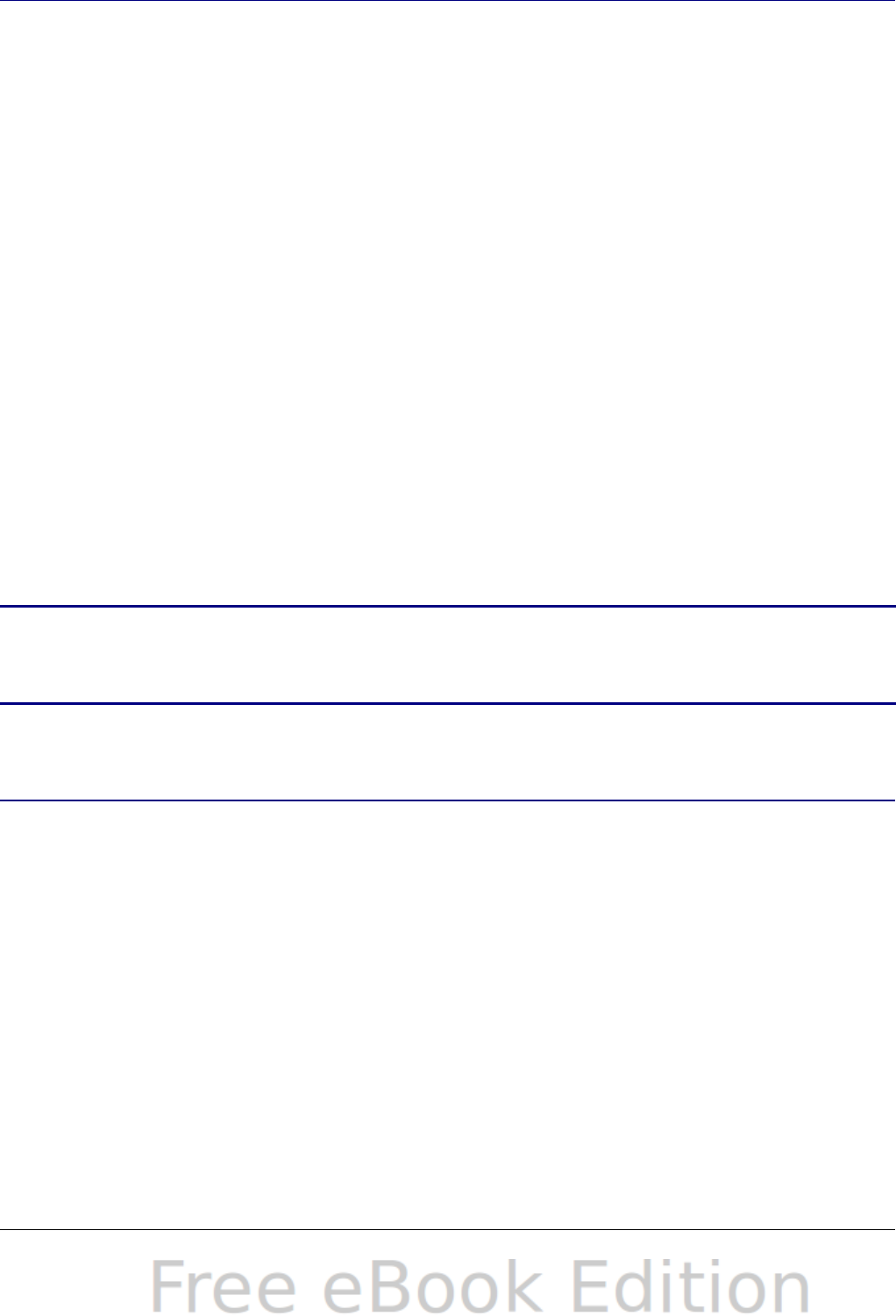
Parts of the main Calc window
When Calc is started, the main window looks similar to Figure 1.
Figure 1: Parts of the Calc window
Note
If any part of the Calc window in Figure 1 is not shown, you can
display it using the View menu. For example, View > Status
Bar will toggle (show or hide) the Status Bar. It is not always
necessary to display all the parts, as shown; show or hide any of
them, as desired.
Title bar
The Title bar, located at the top, shows the name of the current
spreadsheet. When the spreadsheet is newly created, its name is
Untitled X, where X is a number. When you save a spreadsheet for the
first time, you are prompted to enter a name of your choice.
Menu bar
Under the Title bar is the Menu bar. When you choose one of the
menus, a submenu appears with other options. You can modify the
Menu bar, as discussed in Chapter 14 (Setting up and Customizing
Calc).
Chapter 1 Introducing Calc 11

•File contains commands that apply to the entire document such
as Open, Save, Wizards, Export as PDF, and Digital
Signatures.
•Edit contains commands for editing the document such as Undo,
Changes, Compare Document, and Find and Replace.
•View contains commands for modifying how the Calc user
interface looks such as Toolbars, Full Screen, and Zoom.
•Insert contains commands for inserting elements such as cells,
rows, columns, sheets, and pictures into a spreadsheet.
•Format contains commands for modifying the layout of a
spreadsheet such as Styles and Formatting, Paragraph, and
Merge Cells.
•Tools contains functions such as Spelling, Share Document,
Cell Contents, Gallery, and Macros.
•Data contains commands for manipulating data in your
spreadsheet such as Define Range, Sort, Filter, and DataPilot.
•Window contains commands for the display window such as New
Window, Split, and Freeze.
•Help contains links to the Help file bundled with the software,
What's This?, Support, Registration, and Check for Updates.
Toolbars
Three toolbars are located under the Menu bar by default: the
Standard toolbar, the Formatting toolbar, and the Formula Bar.
The icons (buttons) on these toolbars provide a wide range of common
commands and functions. You can also modify these toolbars, as
discussed in Chapter 14 (Setting up and Customizing Calc).
Placing the mouse pointer over any of the icons displays a small box,
called a tooltip. It gives a brief explanation of the icon’s function. For a
more detailed explanation, choose Help > What’s This? and hover
the mouse pointer over the icon. To turn this feature off again, click
once or press the Esc key twice. Tips and extended tips can be turned
on or off from Tools > Options > OpenOffice.org > General.
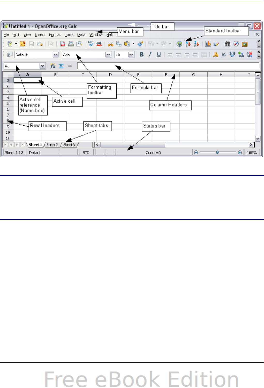
In the Formatting toolbar, the three boxes on the left are the Apply
Style, Font Name, and Font Size lists (see Figure 2). They show the
current settings for the selected cell or area. (The Apply Style list may
not be visible by default.) Click the down-arrow to the right of each box
to open the list.
12 OpenOffice.org 3.x Calc Guide
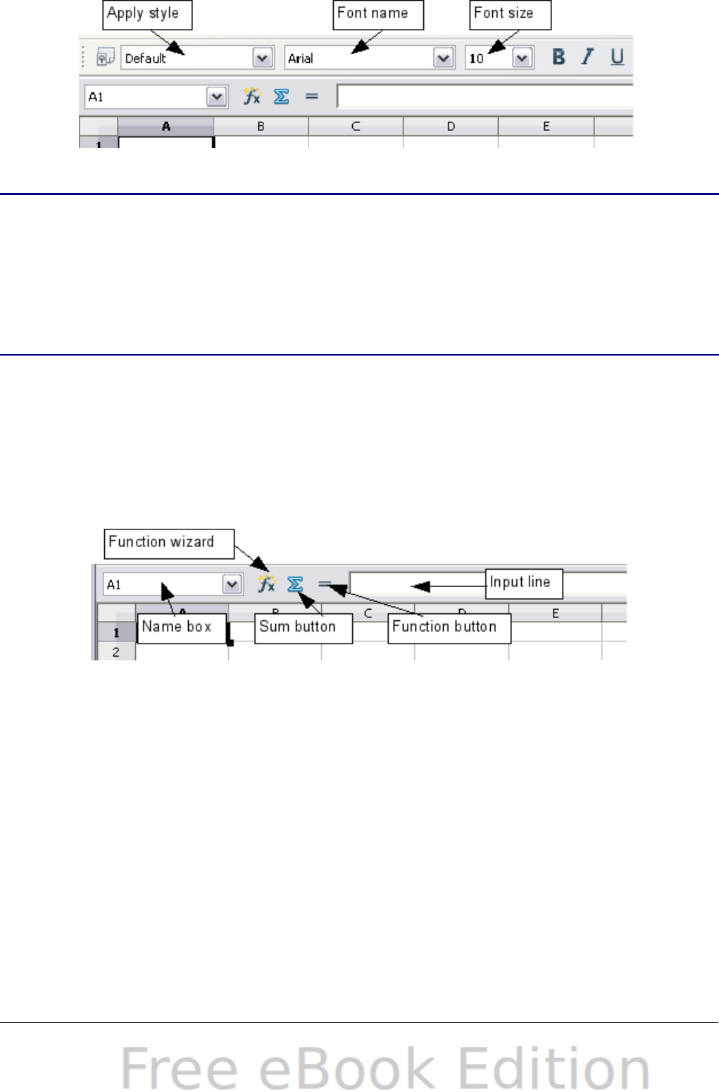
Figure 2: Apply Style, Font Name and Font Size lists
Note
If any of the icons (buttons) in Figure 2 is not shown, you can
display it by clicking the small triangle at the right end of the
Formatting toolbar, selecting Visible Buttons in the drop-
down menu, and selecting the desired icon (for example, Apply
Style) in the drop-down list. It is not always necessary to display
all the toolbar buttons, as shown; show or hide any of them, as
desired.
Formula Bar
On the left hand side of the Formula Bar is a small text box, called the
Name Box, with a letter and number combination in it, such as D7. This
combination, called the cell reference, is the column letter and row
number of the selected cell.
Figure 3: Formula Bar
To the right of the Name Box are the the Function Wizard, Sum, and
Function buttons.
Clicking the Function Wizard button opens a dialog from which you
can search through a list of available functions. This can be very useful
because it also shows how the functions are formatted.
In a spreadsheet the term function covers much more than just
mathematical functions. See Chapter 7 for more details.
Clicking the Sum button inserts a formula into the current cell that
totals the numbers in the cells above the current cell. If there are no
numbers above the current cell, then the cells to the left are placed in
the Sum formula.
Chapter 1 Introducing Calc 13
Clicking the Function button inserts an equals (=) sign into the
selected cell and the Input line, thereby enabling the cell to accept a
formula.
When you enter new data into a cell, the Sum and Equals buttons
change to Cancel and Accept buttons .
The contents of the current cell (data, formula, or function) are
displayed in the Input line, which is the remainder of the Formula Bar.
You can either edit the cell contents of the current cell there, or you
can do that in the current cell. To edit inside the Input line area, click
in the area, then type your changes. To edit within the current cell, just
double-click the cell.
Individual cells
The main section of the screen displays the cells in the form of a grid,
with each cell being at the intersection of a column and a row.
At the top of the columns and at the left end of the rows are a series of
gray boxes containing letters and numbers. These are the column and
row headers. The columns start at A and go on to the right, and the
rows start at 1 and go down.
These column and row headers form the cell references that appear in
the Name Box on the Formula Bar (see Figure 3). You can turn these
headers off by selecting View > Column & Row Headers.
Sheet tabs
At the bottom of the grid of cells are the sheet tabs. These tabs enable
access to each individual sheet, with the visible (active) sheet having a
white tab. Clicking on another sheet tab displays that sheet, and its tab
turns white. You can also select multiple sheet tabs at once by holding
down the Control key while you click the names.
Status bar
The Calc status bar provides information about the spreadsheet and
convenient ways to quickly change some of its features.
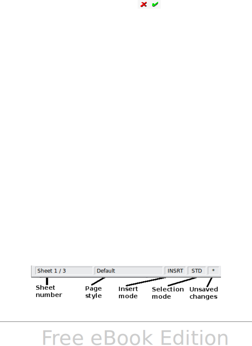
Figure 4: Left end of Calc status bar
14 OpenOffice.org 3.x Calc Guide
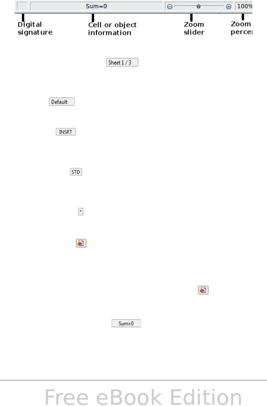
Figure 5: Right end of Calc status bar
Sheet sequence number ( )
Shows the sequence number of the current sheet and the total
number of sheets in the spreadsheet. The sequence number may not
correspond with the name on the sheet tab.
Page style ( )
Shows the page style of the current sheet. To edit the page style,
double-click on this field. The Page Style dialog opens.
Insert mode ( )
Click to toggle between INSRT (Insert) and OVER (Overwrite)
modes when typing. This field is blank when the spreadsheet is not
in a typing mode (for example, when selecting cells).
Selection mode ( )
Click to toggle between STD (Standard), EXT (Extend), and ADD
(Add) selection. EXT is an alternative to Shift+click when selecting
cells. See page 27 for more information.
Unsaved changes ( )
An asterisk (*) appears here if changes to the spreadsheet have not
been saved.
Digital signature ( )
If the document has not been digitally signed, double-clicking in this
area opens the Digital Signatures dialog, where you can sign the
document. See Chapter 6 (Printing, Exporting, and E-mailing) for
more about digital signatures.
If the document has been digitally signed, an icon shows in this
area. You can double-click the icon to view the certificate. A
document can be digitally signed only after it has been saved.
Cell or object information ( )
Displays information about the selected items. When a group of cells
is selected, the sum of the contents is displayed by default; you can
right-click on this field and select other functions, such as the
average value, maximum value, minimum value, or count (number of
items selected).
Chapter 1 Introducing Calc 15
When the cursor is on an object such as a picture or chart, the
information shown includes the size of the object and its location.
Zoom ( )—new in OOo 3.1
To change the view magnification, drag the Zoom slider or click on
the + and – signs. You can also right-click on the zoom level
percentage to select a magnification value or double-click to open
the Zoom & View Layout dialog.
Starting new spreadsheets
You can create a new, blank spreadsheet from the Start Center
(Welcome to OpenOffice.org), from within Calc, or from any other
component of OOo such as from Writer or Draw.
From the Start Center
Click the Spreadsheet icon.
From the Menu bar
Choose File > New > Spreadsheet.
From a toolbar
If a document is open in any component of OOo (for example,
Writer), you can use the New Document icon on the Standard
toolbar. If you already have a spreadsheet open, clicking this button
opens a new spreadsheet in a new window. From any other
component of OOo (for example, Writer), click the down-arrow and
choose spreadsheet.
From the keyboard
If you already have a spreadsheet open, you can press Control+N to
open a new spreadsheet in a new window.
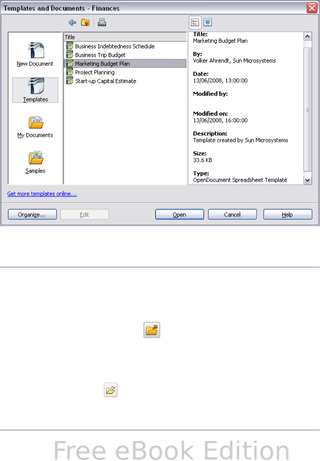
From a template
Calc documents can also be created from templates. Follow the
above procedures, but instead of choosing Spreadsheet, choose the
Templates icon from the Start Center or File > New >Templates
and Documents from the Menu bar or toolbar. On the Templates
and Documents window, navigate to the appropriate folder and
double-click on the required template. A new spreadsheet, based on
the selected template, opens.
A new OpenOffice.org installation does not contain many templates,
but you can add more by downloading them from
16 OpenOffice.org 3.x Calc Guide
http://extensions.services.openoffice.org/ and installing them as
described in Chapter 14 (Customizing Calc).
Figure 6: Starting a new spreadsheet from a template
Opening existing spreadsheets
You can open an existing spreadsheet from the Start Center or from
any component of OOo. Calc can open spreadsheets in a wide range of
file formats, including Microsoft Excel (*.xls and *.xlsx).
From the Start Center
Click the Open a document icon.
From the Menu bar
Choose File > Open.
From a toolbar
Click the Open icon on the Standard toolbar.
Chapter 1 Introducing Calc 17
From the keyboard
Press the key combination Control+O.
Each of these options displays the Open dialog, where you can locate
the spreadsheet that you want to open.
Tip
You can also use the Recent Documents list to open a
spreadsheet. This list is located on the File menu, directly
below Open. The list displays the last 10 files that were
opened in any of the OOo components.
Opening CSV files
Comma-separated-values (CSV) files are text files that contain the cell
contents of a single sheet. Each line in a CSV file represents a row in a
spreadsheet. Commas, semicolons, or other characters are used to
separate the cells. Text is put in quotation marks; numbers are written
without quotation marks.
To open a CSV file in Calc:
1) Choose File > Open.
2) Locate the CSV file that you want to open.
3) If the file has a *.csv extension, select the file and click Open.
4) If the file has another extension (for example, *.txt), select the
file, select Text CSV (*csv;*txt;*xls) in the File type box (scroll
down into the spreadsheet section to find it) and then click Open.
5) On the Text Import dialog (Figure 7), select the Separator options
to divide the text in the file into columns.
You can preview the layout of the imported data at the bottom of
the dialog. Right-click a column in the preview to set the format
or to hide the column.
If the CSV file uses a text delimiter character that is not in the
Text delimiter list, click in the box, and type the character.
6) Click OK to open the file.
Caution If you do not select Text CSV (*csv;*txt;*xls) as the file type
when opening the file, the document opens in Writer, not Calc.
18 OpenOffice.org 3.x Calc Guide
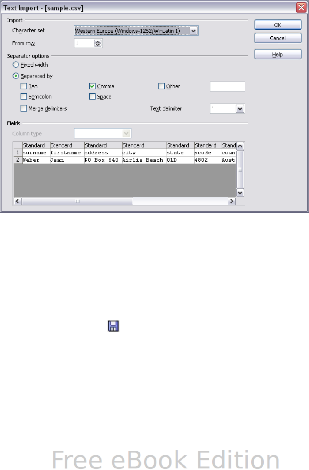
Figure 7: Text Import dialog, with Comma (,) selected as the separator
and double quotation mark (“) as the text delimiter.
Saving spreadsheets
Spreadsheets can be saved in three ways.
From the Menu bar
Choose File > Save (or Save All or Save As).
From the toolbar
Click the Save button on the Standard toolbar. If the file has
been saved and no subsequent changes have been made, this button
is grayed-out and not clickable.
From the keyboard
Press the key combination Control+S.
If the spreadsheet has not been saved previously, then each of these
actions will open the Save As dialog. There you can specify the
spreadsheet name and the location in which to save it.
Chapter 1 Introducing Calc 19

Note
If the spreadsheet has been previously saved, then saving it
using the Save (or Save All) command will overwrite an
existing copy. However, you can save the spreadsheet in a
different location or with a different name by selecting File >
Save As.
Password protection
To protect an entire document from being viewable without a
password, use the option on the Save As dialog to enter a password.
This option is only available for files saved in OpenDocument formats
or the older OpenOffice.org 1.x formats.
On the Save As dialog, select the Save with password option, and
then click Save. You will be prompted to type the same password in
two fields. If the passwords match, the OK button becomes active.
Click OK to save the document as password-protected. If the
passwords do not match, you will be prompted to type the password
again.
OOo uses a very strong encryption mechanism that makes it almost
impossible to recover the contents of a document in case you lose the
password.
Saving a document automatically
You can choose to have Calc save your spreadsheet automatically at
regular intervals. Automatic saving, like manual saving, overwrites the
last saved state of the file. To set up automatic file saving:
1) Choose Tools > Options > Load/Save > General.
2) Click on Save AutoRecovery information every. This enables
the box to set the interval. The default value is 15 minutes. Enter
the value you want by typing it or by pressing the up or down
arrow keys.
Saving as a Microsoft Excel document
If you need to exchange files with users of Microsoft Excel, they may
not know how to open and save *.ods files. Only Microsoft Excel 2007
with Service Pack 2 (SP2) can do this. Users of Microsoft Excel 2007,
2003, XP, and 2000 can also download and install a free
OpenDocument Format (ODF) plugin from Sun Microsystems.
20 OpenOffice.org 3.x Calc Guide
Some users of Microsoft Excel may be unwilling or unable to receive
*.ods files. (Perhaps their employer does not allow them to install the
plug-in.) In this case, you can save a document as a Excel file (*.xls or
*.xlsx).
1) Important—First save your spreadsheet in the file format used
by OpenOffice.org, *.ods. If you do not, any changes you may have
made since the last time you saved it will only appear in the
Microsoft Excel version of the document.
2) Then choose File > Save As.
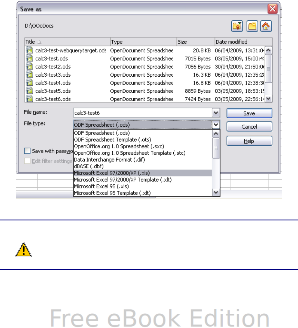
3) On the Save As dialog (Figure 8), in the File type (or Save as
type) drop-down menu, select the type of Excel format you need.
Click Save.
Figure 8. Saving a spreadsheet in Microsoft Excel format
Caution
From this point on, all changes you make to the spreadsheet
will occur only in the Microsoft Excel document. You have
actually changed the name of your document. If you want to go
back to working with the *.ods version of your spreadsheet, you
must open it again.
Chapter 1 Introducing Calc 21
Tip
To have Calc save documents by default in a Microsoft Excel
file format, go to Tools > Options > Load/Save > General.
In the section named Default file format and ODF settings,
under Document type, select Spreadsheet, then under Always
save as, select your preferred file format.
Saving as a CSV file
To save a spreadsheet as a comma separate value (CSV) file:
1) Choose File > Save As.
2) In the File name box, type a name for the file.
3) In the File type list, select Text CSV (*.csv;*.txt;*.xls) and click
Save.
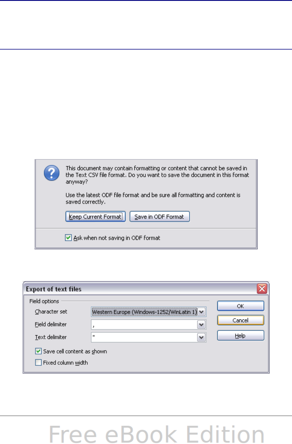
You may see the message box shown below. Click Keep Current
Format.
4) In the Export of text files dialog (Figure 9), select the options you
want and then click OK.
Figure 9: Choosing options when exporting to Text CSV
22 OpenOffice.org 3.x Calc Guide

Saving in other formats
Calc can save spreadsheets in a range of formats, including HTML
(Web pages), through the Save As dialog. Calc can also export
spreadsheets to the PDF and XHTML file formats. See Chapter 6
(Printing, Exporting, and E-mailing) for more information.
Navigating within spreadsheets
Calc provides many ways to navigate within a spreadsheet from cell to
cell and sheet to sheet. You can generally use whatever method you
prefer.
Going to a particular cell
Using the mouse
Place the mouse pointer over the cell and click.
Using a cell reference
Click on the little inverted black triangle just to the right of the
Name Box (Figure 3). The existing cell reference will be highlighted.
Type the cell reference of the cell you want to go to and press Enter.
Cell references are case insensitive: a3 or A3, for example, are the
same. Or just click into the Name Box, backspace over the existing
cell reference, and type in the cell reference you want and press
Enter.
Using the Navigator
Click on the Navigator button in the Standard toolbar (or press F5)
to display the Navigator. Type the cell reference into the top two
fields, labeled Column and Row, and press Enter. In Figure 22 on
page 39, the Navigator would select cell A7. For more about using
the Navigator, see page 38.
Moving from cell to cell
In the spreadsheet, one cell normally has a darker black border. This
black border indicates where the focus is (see Figure 10). The focus
indicates which cell is enabled to receive input. If a group of cells is
selected, they have a highlight color (usually gray), with the focus cell
having a dark border.
Chapter 1 Introducing Calc 23
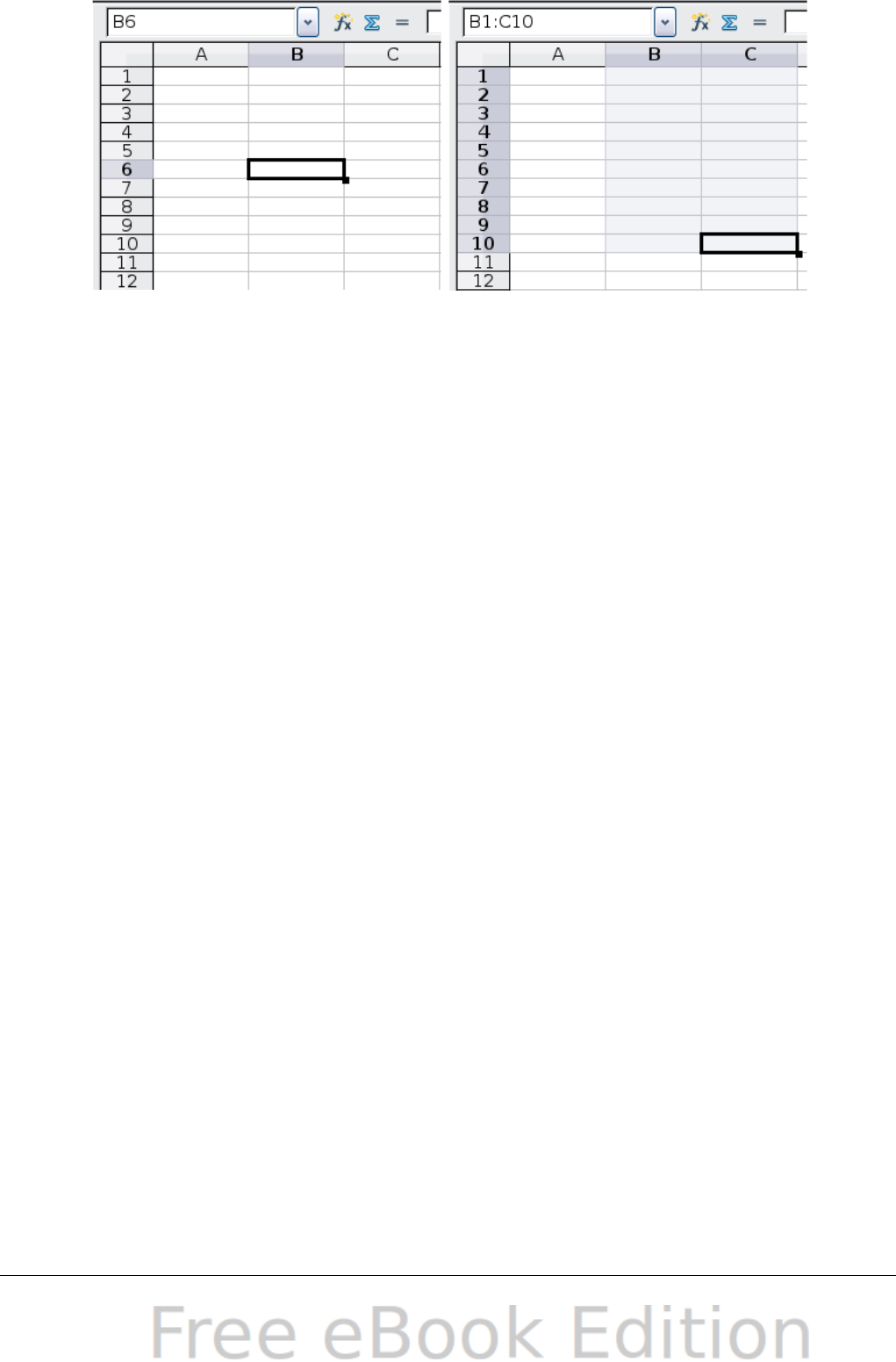
Figure 10. (left) One selected cell and (right) a group of
selected cells
Using the mouse
To move the focus using the mouse, simply move the mouse pointer
to the cell where you want the focus to be and click the left mouse
button. This action changes the focus to the new cell. This method is
most useful when the two cells are a large distance apart.
Using the Tab and Enter keys
•Pressing Enter or Shift+Enter moves the focus down or up,
respectively.
•Pressing Tab or Shift+Tab moves the focus to the right or to the
left, respectively.
Using the arrow keys
Pressing the arrow keys on the keyboard moves the focus in the
direction of the arrows.
Using Home, End, Page Up and Page Down
•Home moves the focus to the start of a row.
•End moves the focus to the column furthest to the right that
contains data.
•Page Down moves the display down one complete screen and
Page Up moves the display up one complete screen.
•Combinations of Control (often represented on keyboards as Ctrl)
and Alt with Home, End, Page Down (PgDn), Page Up (PgUp), and
the arrow keys move the focus of the current cell in other ways.
Table 1 describes the keyboard shortcuts for moving about a
spreadsheet.
24 OpenOffice.org 3.x Calc Guide
Tip
Use one of the four Alt+Arrow key combinations to resize the
height or width of a cell. (For example: Alt+↓ increases the
height of a cell.)
Table 1. Moving from cell to cell using the keyboard
Key Combination Movement
→Right one cell
←Left one cell
↑Up one cell
↓Down one cell
Control+→To the next column to the right containing data in
that row or to Column AMJ
Control+←To the next column to the left containing data in that
row or to Column A
Control+↑To the next row above containing data in that
column or to Row 1
Control+↓To the next row below containing data in that
column or to Row 65536
Control+Home To Cell A1
Control+End To lower right-hand corner of the rectangular area
containing data
Alt+Page Downn One screen to the right (if possible)
Alt+Page Up One screen to the left (if possible)
Control+Page Down One sheet to the right (in sheet tabs)
Control+Page Up One sheet to the left (in sheet tabs)
Tab To the next cell on the right
Shift+Tab To the next cell on the left
Enter Down one cell (unless changed by user)
Shift+Enter Up one cell (unless changed by user)
Chapter 1 Introducing Calc 25
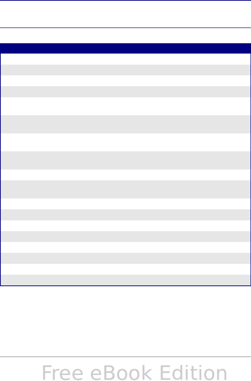
Customizing the effects of the Enter key
You can customize the direction in which the Enter key moves the
focus, by selecting Tools > Options > OpenOffice.org Calc >
General.
The four choices for the direction of the Enter key are shown on the
right hand side of Figure 11. It can move the focus down, right, up, or
left. Depending on the file being used or on the type of data being
entered, setting a different direction can be useful.
Figure 11: Customizing the effect of the Enter key
The Enter key can also be used to switch into and out of the editing
mode. Use the first two options under Input settings in Figure 11 to
change the Enter key settings.
Moving from sheet to sheet
Each sheet in a spreadsheet is independent of the others, though they
can be linked with references from one sheet to another. There are
three ways to navigate between different sheets in a spreadsheet.
Using the keyboard
Pressing Control+Page Down moves one sheet to the right and
pressing Control+Page Up moves one sheet to the left.
Using the mouse
Clicking on one of the sheet tabs at the bottom of the spreadsheet
selects that sheet.
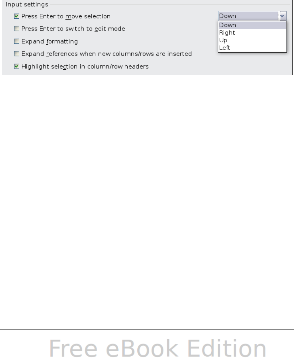
If you have a lot of sheets, then some of the sheet tabs may be
hidden behind the horizontal scroll bar at the bottom of the screen.
If this is the case, then the four buttons at the left of the sheet tabs
can move the tabs into view. Figure 12 shows how to do this.
26 OpenOffice.org 3.x Calc Guide
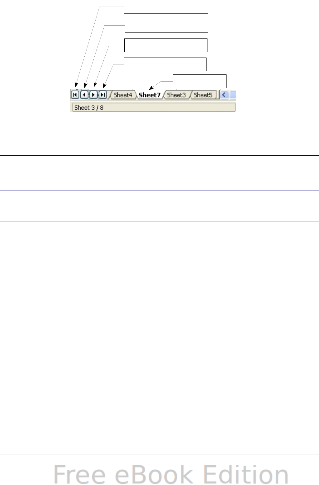
Figure 12. Sheet tab arrows
Notice that the sheets here are not numbered in order. Sheet
numbering is arbitrary; you can name a sheet as you wish.
Note
The sheet tab arrows that appear in Figure 12 only appear if
you have some sheet tabs that can not be seen. Otherwise,
they appear faded as in Figure 1.
Selecting items in a sheet or spreadsheet
Selecting cells
Cells can be selected in a variety of combinations and quantities.
Single cell
Left-click in the cell. The result will look like the left side of Figure 10.
You can verify your selection by looking in the Name Box.
Range of contiguous cells
A range of cells can be selected using the keyboard or the mouse.
To select a range of cells by dragging the mouse:
1) Click in a cell.
2) Press and hold down the left mouse button.
3) Move the mouse around the screen.
4) Once the desired block of cells is highlighted, release the left
mouse button.
To select a range of cells without dragging the mouse:
1) Click in the cell which is to be one corner of the range of cells.
2) Move the mouse to the opposite corner of the range of cells.
Chapter 1 Introducing Calc 27
Move to the first sheet
Move left one sheet
Move right one sheet
Move to the last sheet
Sheet tabs

3) Hold down the Shift key and click.
Tip
You can also select a contiguous range of cells by first clicking
in the STD field on the status bar and changing it to EXT,
before clicking in the opposite corner of the range of cells in
step 3 above. If you use this method, be sure to change EXT
back to STD or you may find yourself extending the selection
unintentionally.
To select a range of cells without using the mouse:
1) Select the cell that will be one of the corners in the range of cells.
2) While holding down the Shift key, use the cursor arrows to select
the rest of the range.
The result of any of these methods looks like the right side of Figure
10.
Tip
You can also directly select a range of cells using the Name
Box. Click into the Name Box as described in “Using a cell
reference” on page 23. To select a range of cells, enter the cell
reference for the upper left-hand cell, followed by a colon (:),
and then the lower right-hand cell reference. For example, to
select the range that would go from A3 to C6, you would enter
A3:C6.
Range of noncontiguous cells
1) Select the cell or range of cells using one of the methods above.
2) Move the mouse pointer to the start of the next range or single
cell.
3) Hold down the Control key and click or click-and-drag to select
another range of cells to add to the first range.
4) Repeat as necessary.
Tip
You can also select a noncontiguous range of cells by first
clicking twice in the STD field on the status bar to change it to
ADD, before clicking on a cell that you want to add to the
range of cells in step 3 above. This method works best when
adding single cells to a range. If you use this method, be sure
to change ADD back to STD or you may find yourself adding
more selections unintentionally.
28 OpenOffice.org 3.x Calc Guide
Selecting columns and rows
Entire columns and rows can be selected very quickly in OOo.
Single column or row
To select a single column, click on the column identifier letter (see
Figure 1).
To select a single row, click on the row identifier number.
Multiple columns or rows
To select multiple columns or rows that are contiguous:
1) Click on the first column or row in the group.
2) Hold down the Shift key.
3) Click the last column or row in the group.
To select multiple columns or rows that are not contiguous:
1) Click on the first column or row in the group.
2) Hold down the Control key.
3) Click on all of the subsequent columns or rows while holding
down the Control key.
Entire sheet
To select the entire sheet, click on the small box between the A column
header and the 1 row header.
Figure 13. Select All box
You can also press Control+A to select the entire sheet.
Selecting sheets
You can select either one or multiple sheets. It can be advantageous to
select multiple sheets at times when you want to make changes to
many sheets at once.
Single sheet
Click on the sheet tab for the sheet you want to select. The active sheet
becomes white (see Figure 12).
Chapter 1 Introducing Calc 29
Select All
Multiple contiguous sheets
To select multiple contiguous sheets:
1) Click on the sheet tab for the first desired sheet.
2) Move the mouse pointer over the sheet tab for the last desired
sheet.
3) Hold down the Shift key and click on the sheet tab.
All the tabs between these two sheets will turn white. Any actions that
you perform will now affect all highlighted sheets.
Multiple noncontiguous sheets
To select multiple noncontiguous sheets:
1) Click on the sheet tab for the first desired sheet.
2) Move the mouse pointer over the sheet tab for the second desired
sheet.
3) Hold down the Control key and click on the sheet tab.
4) Repeat as necessary.
The selected tabs will turn white. Any actions that you perform will
now affect all highlighted sheets.
All sheets
Right-click any one of the sheet tabs and choose Select All Sheets
from the pop-up menu.
Working with columns and rows
Inserting columns and rows
Columns and rows can be inserted individually or in groups.
Note
When you insert a single new column, it is inserted to the left
of the highlighted column. When you insert a single new row, it
is inserted above the highlighted row.
Cells in the new columns or rows are formatted like the
corresponding cells in the column or row before (or to the left
of) which the new column or row is inserted.
Single column or row
Using the Insert menu:
1) Select the cell, column, or row where you want the new column or
row inserted.
30 OpenOffice.org 3.x Calc Guide

2) Choose either Insert > Columns or Insert > Rows.
Using the mouse:
1) Select the cell, column, or row where you want the new column or
row inserted.
2) Right-click the header of the column or row.
3) Choose Insert Rows or Insert Columns.
Multiple columns or rows
Multiple columns or rows can be inserted at once rather than inserting
them one at a time.
1) Highlight the required number of columns or rows by holding
down the left mouse button on the first one and then dragging
across the required number of identifiers.
2) Proceed as for inserting a single column or row above.
Deleting columns and rows
Columns and rows can be deleted individually or in groups.
Single column or row
A single column or row can be deleted by using the mouse:
1) Select the column or row to be deleted.
2) Choose Edit > Delete Cells from the menu bar.
Or,
1) Right-click on the column or row header.
2) Choose Delete Columns or Delete Rows from the pop-up menu.
Multiple columns or rows
Multiple columns or rows can be deleted at once rather than deleting
them one at a time.
1) Highlight the required columns or rows by holding down the left
mouse button on the first one and then dragging across the
required number of identifiers.
2) Proceed as for deleting a single column or row above.
Tip
Instead of deleting a row or column, you may wish to delete
the contents of the cells but keep the empty row or column.
See Chapter 2 (Entering, Editing, and Formatting Data) for
instructions.
Chapter 1 Introducing Calc 31
Working with sheets
Like any other Calc element, sheets can be inserted, deleted, and
renamed.
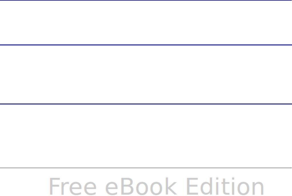
Inserting new sheets
There are several ways to insert a new sheet. The first step for all of
the methods is to select the sheets that the new sheet will be inserted
next to. Then any of the following options can be used.
•Choose Insert > Sheet from the menu bar.
•Right-click on the sheet tab and choose Insert Sheet.
•Click in an empty space at the end of the line of sheet tabs.
Figure 14. Creating a new sheet
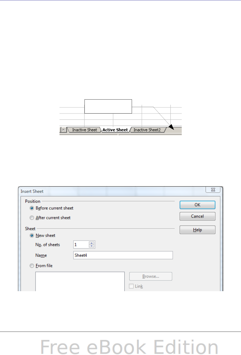
Each method will open the Insert Sheet dialog. Here you can select
whether the new sheet is to go before or after the selected sheet and
how many sheets you want to insert. If you are inserting only one
sheet, there is the opportunity to give the sheet a name.
Figure 15: Insert Sheet dialog
32 OpenOffice.org 3.x Calc Guide
Click here to insert
a new sheet
Deleting sheets
Sheets can be deleted individually or in groups.
Single sheet
Right-click on the tab of the sheet you want to delete and choose
Delete Sheet from the pop-up menu, or choose Edit > Sheet >
Delete from the Menu bar. Either way, an alert will ask if you want
to delete the sheet permanently. Click Yes.
Multiple sheets
To delete multiple sheets, select them as described earlier, then
either right-click over one of the tabs and choose Delete Sheet
from the pop-up menu, or choose Edit > Sheet > Delete from the
Menu bar.
Renaming sheets
The default name for the a new sheet is SheetX, where X is a number.
While this works for a small spreadsheet with only a few sheets, it
becomes awkward when there are many sheets.
To give a sheet a more meaningful name, you can:
•Enter the name in the Name box when you create the sheet, or
•Right-click on a sheet tab and choose Rename Sheet from the
pop-up menu; replace the existing name with a different one.
•(New in OOo3.1) Double-click on a sheet tab to pop up the
Rename Sheet dialog.
Note
Sheet names must start with either a letter or a number; other
characters including spaces are not allowed. Apart from the
first character of the sheet name, allowed characters are
letters, numbers, spaces, and the underscore character.
Attempting to rename a sheet with an invalid name will
produce an error message.
Viewing Calc
Using zoom
Use the zoom function to change the view to show more or fewer cells
in the window.
Chapter 1 Introducing Calc 33
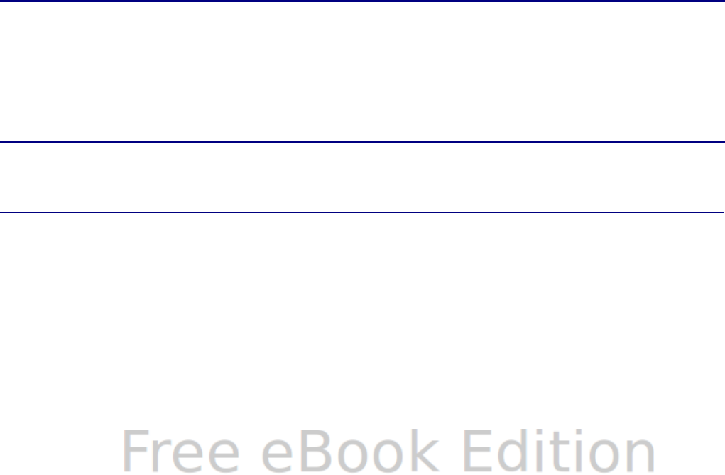
In addition to using the Zoom slider (new in OOo 3.1) on the Status bar
(see page 16), you can open the Zoom dialog and make a selection on
the left-hand side.
•Choose View > Zoom from the Menu bar, or
•Double-click on the percentage figure in the Status bar at the
bottom of the window.
Figure 16. Zoom dialog
Optimal
Resizes the display to fit the width of the selected cells. To use this
option, you must first highlight a range of cells.
Fit Width and Height
Displays the entire page on your screen.
Fit Width
Displays the complete width of the document page. The top and
bottom edges of the page may not be visible.
100%
Displays the document at its actual size.
Variable
Enter a zoom percentage of your choice.
Freezing rows and columns
Freezing locks a number of rows at the top of a spreadsheet or a
number of columns on the left of a spreadsheet or both. Then when
scrolling around within the sheet, any frozen columns and rows remain
in view.
34 OpenOffice.org 3.x Calc Guide
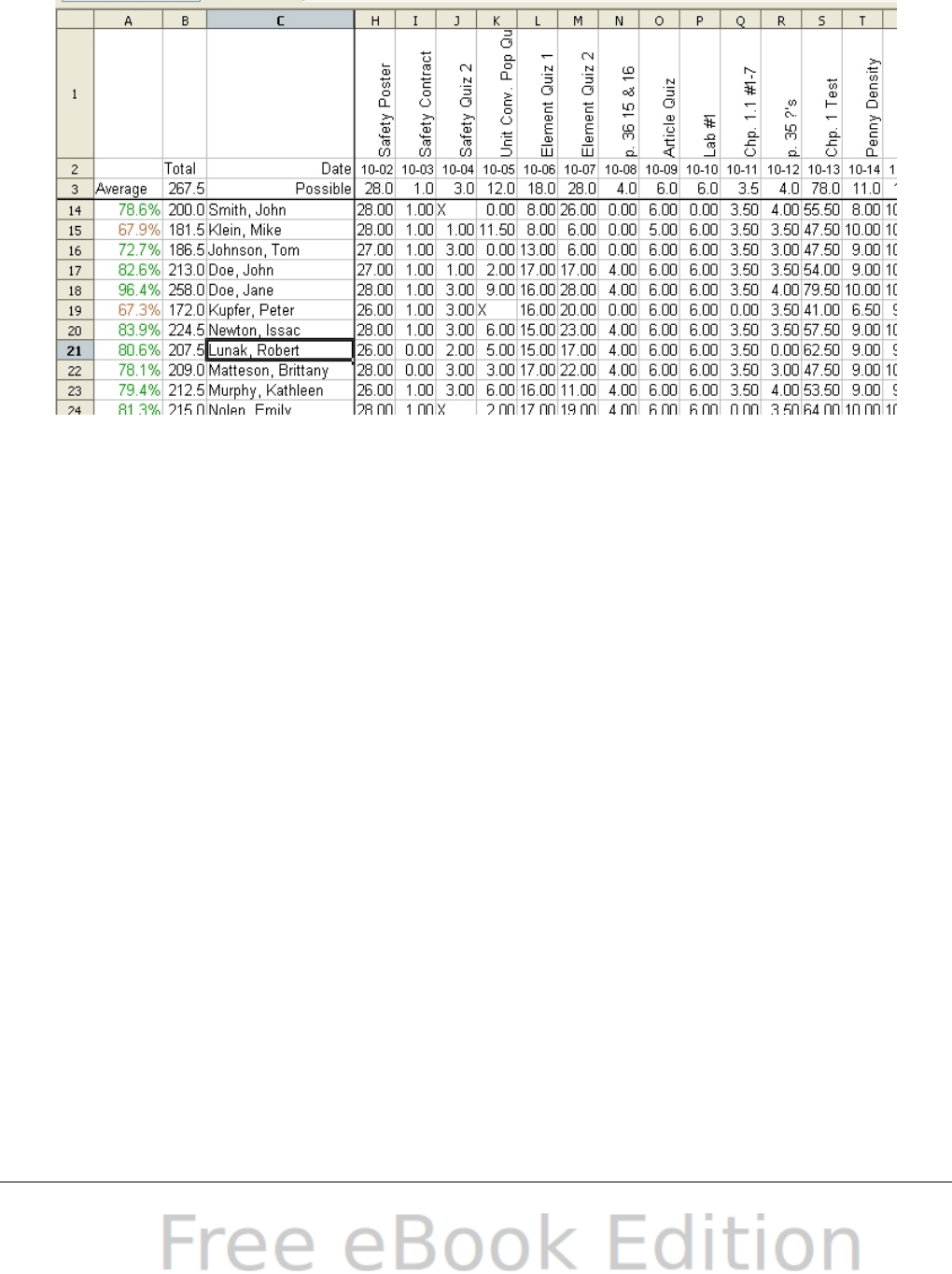
Figure 17 shows some frozen rows and columns. The heavier horizontal
line between rows 3 and 14 and the heavier vertical line between
columns C and H denote the frozen areas. Rows 4 through 13 and
columns D through G have been scrolled off the page. The first three
rows and columns remained because they are frozen into place.
Figure 17. Frozen rows and columns
You can set the freeze point at one row, one column, or both a row and
a column as in Figure 17.
Freezing single rows or columns
1) Click on the header for the row below where you want the freeze
or for the column to the right of where you want the freeze.
2) Choose Window > Freeze.
A dark line appears, indicating where the freeze is put.
Freezing a row and a column
1) Click into the cell that is immediately below the row you want
frozen and immediately to the right of the column you want
frozen.
2) Choose Window > Freeze.
Two lines appear on the screen, a horizontal line above this cell
and a vertical line to the left of this cell. Now as you scroll around
the screen, everything above and to the left of these lines will
remain in view.
Unfreezing
To unfreeze rows or columns, choose Window > Freeze. The check
mark by Freeze will vanish.
Chapter 1 Introducing Calc 35
Splitting the screen
Another way to change the view is by splitting the window, also known
as splitting the screen. The screen can be split horizontally, vertically,
or both. You can therefore have up to four portions of the spreadsheet
in view at any one time.
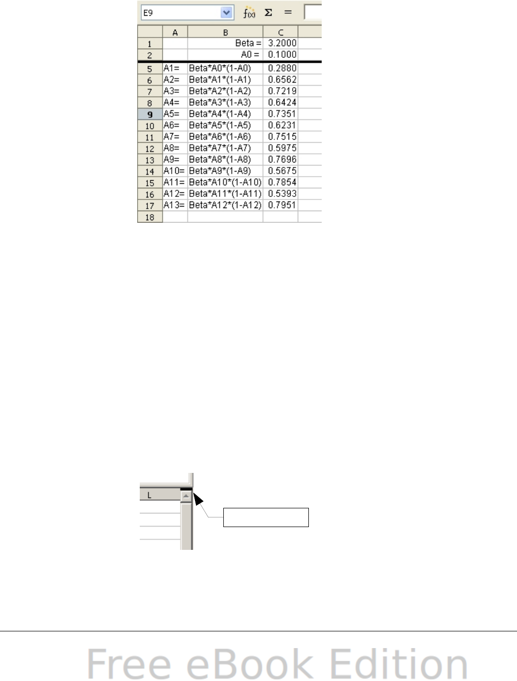
Figure 18. Split screen example
Why would you want to do this? Imagine you have a large spreadsheet
and one of the cells has a number in it that is used by three formulas in
other cells. Using the split-screen technique, you can position the cell
containing the number in one section and each of the cells with
formulas in the other sections. Then you can change the number in the
cell and watch how it affects each of the formulas.
Splitting the screen horizontally
To split the screen horizontally:
1) Move the mouse pointer into the vertical scroll bar, on the right-
hand side of the screen, and place it over the small button at the
top with the black triangle.
Figure 19. Split screen bar on
vertical scroll bar
36 OpenOffice.org 3.x Calc Guide
Split screen bar
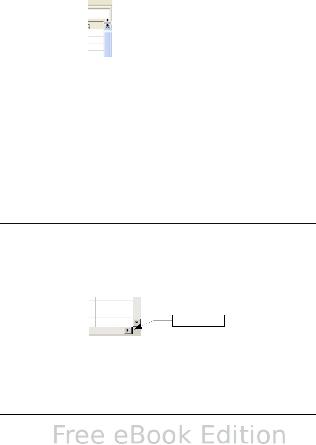
2) Immediately above this button, you will see a thick black line
(Figure 19). Move the mouse pointer over this line, and it turns
into a line with two arrows (Figure 20).
Figure 20. Split-screen bar on
vertical scroll bar with cursor
3) Hold down the left mouse button. A gray line appears, running
across the page. Drag the mouse downwards and this line follows.
4) Release the mouse button and the screen splits into two views,
each with its own vertical scroll bar. You can scroll the upper and
lower parts independently.
Notice in Figure 18, the Beta and the A0 values are in the upper part
of the window and other calculations are in the lower part. Thus, you
can make changes to the Beta and A0 values and watch their effects on
the calculations in the lower half of the window.
Tip
You can also split the screen using a menu command. Click in a
cell immediately below and to the right of where you wish the
screen to be split, and choose Window > Split.
Splitting the screen vertically
To split the screen vertically:
1) Move the mouse pointer into the horizontal scroll bar at the
bottom of the screen and place it over the small button on the
right with the black triangle.
Figure 21: Split bar on
horizontal scroll bar
2) Immediately to the right of this button is a thick black line (Figure
21). Move the mouse pointer over this line and it turns into a line
with two arrows.
Chapter 1 Introducing Calc 37
Split screen bar
3) Hold down the left mouse button, and a gray line appears,
running up the page. Drag the mouse to the left and this line
follows.
4) Release the mouse button, and the screen is split into two views,
each with its own horizontal scroll bar. You can scroll the left and
right parts of the window independently.
Removing split views
To remove a split view, do any of the following:
•Double-click on each split line.
•Click on and drag the split lines back to their places at the ends of
the scroll bars.
•Choose Window > Split to remove all split lines at the same
time.
Using the Navigator
In addition to the cell reference boxes (labeled Column and Row), the
Navigator provides several other ways to move quickly through a
spreadsheet and find specific items.
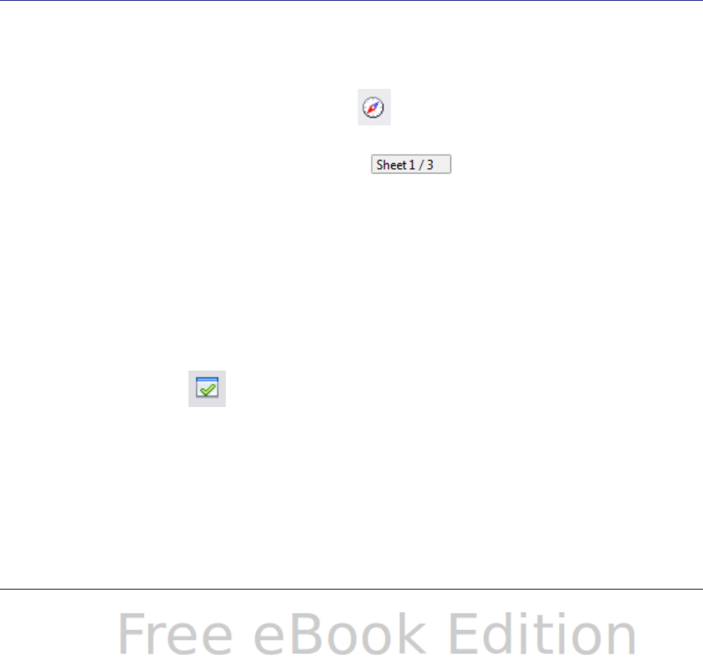
To open the Navigator, click its icon on the Standard toolbar, or
press F5, or choose View > Navigator on the Menu bar, or double-
click on the Sheet Sequence Number in the Status Bar. You
can dock the Navigator to either side of the main Calc window or leave
it floating. (To dock or float the Navigator, hold down the Control key
and double-click in an empty area near the icons at the top.)
The Navigator displays lists of all the objects in a spreadsheet
document, grouped into categories. If an indicator (plus sign or arrow)
appears next to a category, at least one object of this kind exists. To
open a category and see the list of items, click on the indicator.
To hide the list of categories and show only the icons at the top, click
the Contents icon . Click this icon again to show the list.
Table 2 summarizes the functions of the icons at the top of the
Navigator.
38 OpenOffice.org 3.x Calc Guide
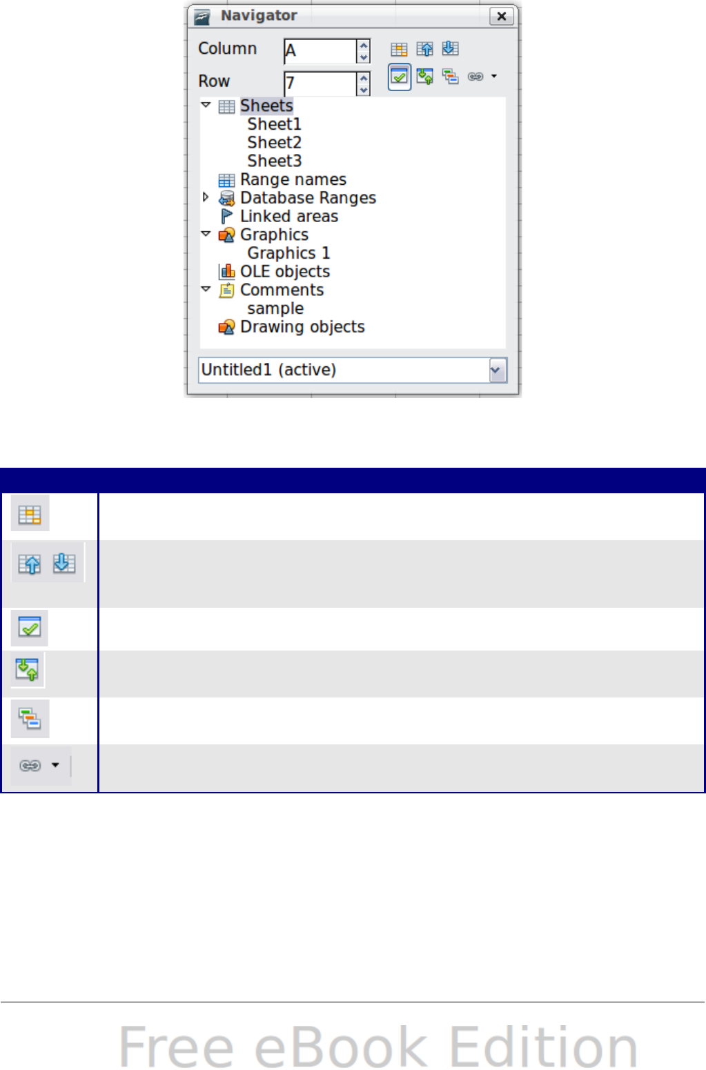
Figure 22: The Navigator in Calc
Table 2: Function of icons in the Navigator
Icon Action
Data Range. Specifies the current data range denoted by the
position of the cell cursor.
Start/End. Moves to the cell at the beginning or end of the
current data range, which you can highlight using the Data
Range button.
Contents. Shows or hides the list of categories.
Toggle. Switches between showing all categories and showing
only the selected category.
Displays all available scenarios. Double-click a name to apply that
scenario. See Chapter 7 (Data Analysis) for more information.
Drag Mode. Choose hyperlink, link, or copy. See “Choosing a drag
mode” for details.
Chapter 1 Introducing Calc 39

Moving quickly through a document
The Navigator provides several convenient ways to move around a
document and find items in it:
•To jump to a specific cell in the current sheet, type its cell
reference in the Column and Row boxes at the top of the
Navigator and press the Enter key; for example, in Figure 22 the
cell reference is A7.
•When a category is showing the list of objects in it, double-click
on an object to jump directly to that object’s location in the
document.
•To see the content in only one category, highlight that category
and click the Toggle icon. Click the icon again to display all the
categories.
•Use the Start and End icons to jump to the first or last cell in the
selected data range.
Tip
Ranges, scenarios, pictures, and other objects are much easier
to find if you have given them informative names when creating
them, instead of keeping Calc’s default Graphics 1, Graphics 2,
Object 1, and so on, which may not correspond to the position of
the object in the document.
Choosing a drag mode
Sets the drag and drop options for inserting items into a document
using the Navigator.
Insert as Hyperlink
Creates a hyperlink when you drag and drop an item into the
current document.
Insert as Link
Inserts the selected item as a link where you drag and drop an
object into the current document.
Insert as Copy
Inserts a copy of the selected item where you drag and drop in the
current document. You cannot drag and drop copies of graphics,
OLE objects, or indexes.
40 OpenOffice.org 3.x Calc Guide

Chapter 2
Entering, Editing, and
Formatting Data

Introduction
You can enter data into Calc in several ways: using the keyboard, the
mouse (dragging and dropping), the Fill tool, and selection lists. Calc
also provides the ability to enter information into multiple sheets of the
same document at the same time.
After entering data, you can format and display it in various ways.
Entering data using the keyboard
Most data entry in Calc can be accomplished using the keyboard.
Entering numbers
Click in the cell and type in the number using the number keys on
either the main keyboard or the numeric keypad.
To enter a negative number, either type a minus (–) sign in front of it or
enclose it in parentheses (brackets), like this: (1234).
By default, numbers are right-aligned and negative numbers have a
leading minus symbol.
Entering text
Click in the cell and type the text. Text is left-aligned by default.
Entering numbers as text
If a number is entered in the format 01481, Calc will drop the leading
0. (Exception: see Tip below.) To preserve the leading zero, for example
for telephone area codes, type an apostrophe before the number, like
this: '01481.
The data is now treated as text and displayed exactly as entered.
Typically, formulas will treat the entry as a zero and functions will
ignore it.
Tip
Numbers can have leading zeros and still be regarded as
numbers (as opposed to text) if the cell is formatted
appropriately. Right-click on the cell and chose Format Cells
> Numbers. Adjust the leading zeros setting to add leading
zeros to numbers.
42 OpenOffice.org 3.x Calc Guide
Note
When a plain apostrophe is used to allow a leading 0 to be
displayed, it is not visible in the cell after the Enter key is
pressed. If “smart quotes” are used for apostrophes, the
apostrophe remains visible in the cell.
To choose the type of apostrophe, use Tools > AutoCorrect
Options > Custom Quotes. The selection of the apostrophe
type affects both Calc and Writer.
Caution When a number is formatted as text, take care that the cell
containing the number is not used in a formula because Calc
will ignore the value.
Entering dates and times
Select the cell and type the date or time. You can separate the date
elements with a slash (/) or a hyphen (–) or use text such as 10 Oct 03.
Calc recognizes a variety of date formats. You can separate time
elements with colons such as 10:43:45.
Entering special characters
A “special” character is one not found on a standard English keyboard.
For example, © ¾ æ ç ñ ö ø ¢ are all special characters. To insert a
special character:
1) Place the cursor in your document where you want the character
to appear.
2) Click Insert > Special Character to open the Special
Characters dialog (Figure 23).
3) Select the characters (from any font or mixture of fonts) you wish
to insert, in order; then click OK. The selected characters are
shown in the bottom left of the dialog. As you select each
character, it is shown alone at the bottom right, along with the
numerical code for that character.
Note
Different fonts include different special characters. If you do
not find a particular special character you want, try changing
the Font selection.
Chapter 2 Entering, Editing, and Formatting Data 43
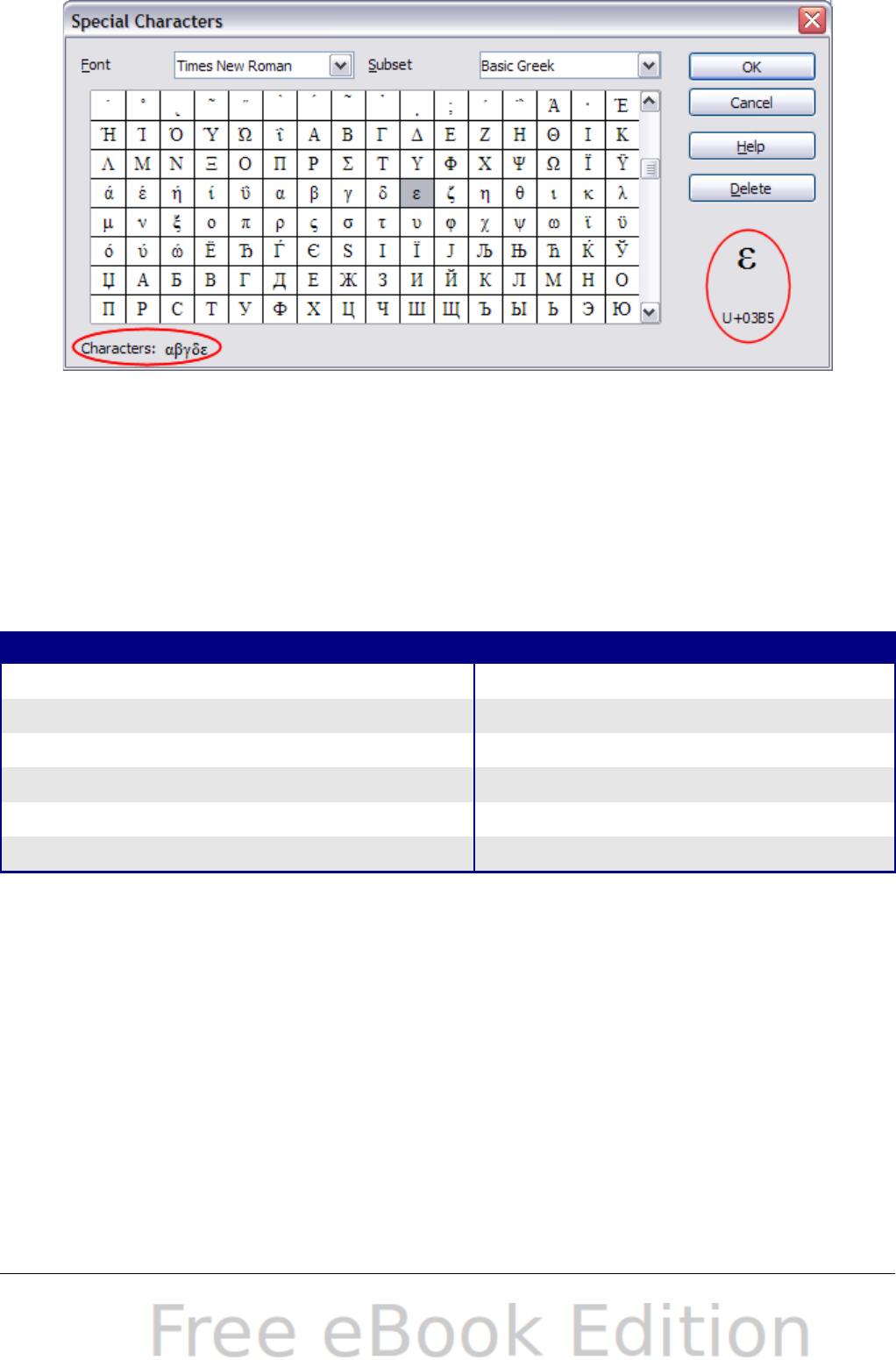
Figure 23: The Special Characters dialog
Inserting dashes
To enter en and em dashes, you can use the Replace dashes option
under Tools > AutoCorrect Options. This option replaces two
hyphens, under certain conditions, with the corresponding dash.
In the following table, the A and B represent text consisting of letters A
to z or digits 0 to 9.
Text that you type: Result
A - B (A, space, minus, space, B) A – B (A, space, en-dash, space, B)
A -- B (A, space, minus, minus, space, B) A – B (A, space, en-dash, space, B)
A--B (A, minus, minus, B) A—B (A, em-dash, B)
A-B (A, minus, B) A-B (unchanged)
A -B (A, space, minus, B) A -B (unchanged)
A --B (A, space, minus, minus, B) A –B (A, space, en-dash, B)
Deactivating automatic changes
Calc automatically applies many changes during data input, unless you
deactivate those changes. You can also immediately undo any
automatic changes with Ctrl+Z.
AutoCorrect changes
Automatic correction of typing errors, replacement of straight
quotation marks by curly (custom) quotes, and starting cell content
with an uppercase (capital) letter are controlled by Tools >
AutoCorrect Options. Go to the Custom Quotes, Options, or
Replace tabs to deactivate any of the features that you do not want.
44 OpenOffice.org 3.x Calc Guide
On the Replace tab, you can also delete unwanted word pairs and
add new ones as required.
AutoInput
When you are typing in a cell, Calc automatically suggests matching
input found in the same column. To turn the AutoInput on and off,
set or remove the check mark in front of Tools > Cell Contents >
AutoInput.
Automatic date conversion
Calc automatically converts certain entries to dates. To ensure that
an entry that looks like a date is interpreted as text, type an
apostrophe at the beginning of the entry. The apostrophe is not
displayed in the cell.
Speeding up data entry
Entering data into a spreadsheet can be very labor-intensive, but Calc
provides several tools for removing some of the drudgery from input.
The most basic ability is to drop and drag the contents of one cell to
another with a mouse. Many people also find AutoInput helpful. Calc
also includes several other tools for automating input, especially of
repetitive material. They include the Fill tool, selection lists, and the
ability to input information into multiple sheets of the same document.
Using the Fill tool on cells
At its simplest, the Fill tool is a way to duplicate existing content. Start
by selecting the cell to copy, then drag the mouse in any direction (or
hold down the Shift key and click in the last cell you want to fill), and
then choose Edit > Fill and the direction in which you want to copy:
Up, Down, Left or Right.
Caution Choices that are not available are grayed out, but you can still
choose the opposite direction from what you intend, which
could cause you to overwrite cells accidentally.
Tip
A shortcut way to fill cells is to grab the “handle” in the lower
right-hand corner of the cell and drag it in the direction you
want to fill. If the cell contains a number, the number will fill in
series. If the cell contains text, the same text will fill in the
direction you chose.
Chapter 2 Entering, Editing, and Formatting Data 45

Figure 24: Using the Fill tool
Using a fill series
A more complex use of the Fill tool is to use a fill series. The default
lists are for the full and abbreviated days of the week and the months
of the year, but you can create your own lists as well.
To add a fill series to a spreadsheet, select the cells to fill, choose Edit
> Fill > Series. In the Fill Series dialog, select AutoFill as the Series
type, and enter as the Start value an item from any defined series. The
selected cells then fill in the other items on the list sequentially,
repeating from the top of the list when they reach the end of the list.
Figure 25: Specifying the start of a fill series (result is in Figure 26)
46 OpenOffice.org 3.x Calc Guide

Figure 26: Result of fill series
selection shown in Figure 25
You can also use Edit > Fill > Series to create a one-time fill series
for numbers by entering the start and end values and the increment.
For example, if you entered start and end values of 1 and 7 with an
increment of 2, you would get the sequence of 1, 3, 5, 7.
In all these cases, the Fill tool creates only a momentary connection
between the cells. Once they are filled, the cells have no further
connection with one another.
Defining a fill series
To define your own fill series, go to Tools > Options >
OpenOffice.org Calc > Sort Lists. This dialog shows the previously-
defined series in the Lists box on the left, and the contents of the
highlighted list in the Entries box.
Figure 27: Predefined fill series
Click New. The Entries box is cleared. Type the series for the new list
in the Entries box (one entry per line), and then click Add.
Chapter 2 Entering, Editing, and Formatting Data 47
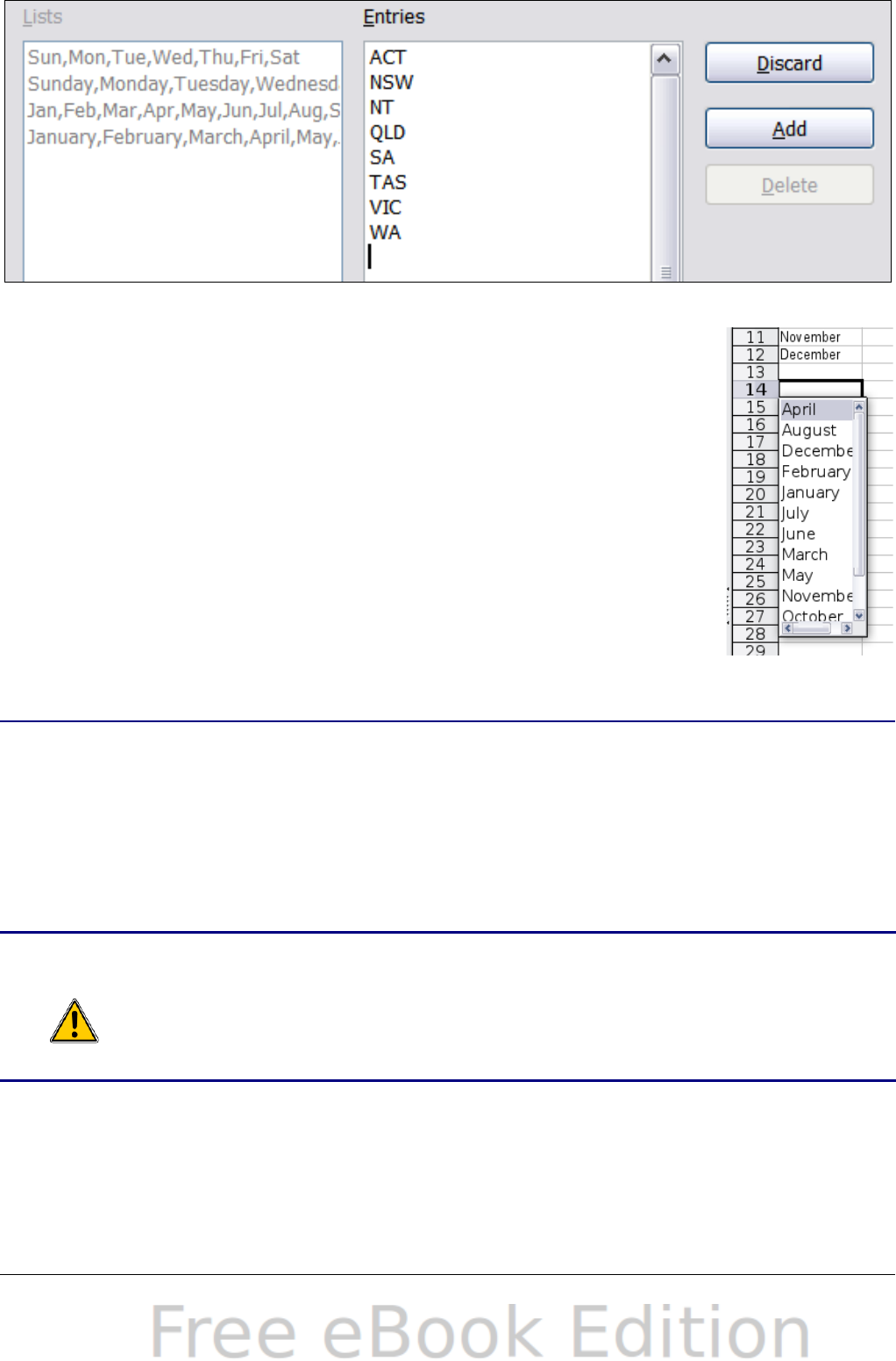
Figure 28: Defining a new fill series
Using selection lists
Selection lists are available only for text, and are
limited to using only text that has already been entered
in the same column.
To use a selection list, select a blank cell and press
Ctrl+D. A drop-down list appears of any cell in the same
column that either has at least one text character or
whose format is defined as Text. Click on the entry you
require.
Sharing content between sheets
You might want to enter the same information in the same cell on
multiple sheets, for example to set up standard listings for a group of
individuals or organizations. Instead of entering the list on each sheet
individually, you can enter it in all the sheets at once. To do this, select
all the sheets (Edit > Sheet > Select), then enter the information in
the current one.
Caution
This technique overwrites any information that is already in
the cells on the other sheets—without any warning. For this
reason, when you are finished, be sure to deselect all the
sheets except the one you want to edit. (Ctrl+click on a sheet
tab to select or deselect the sheet.)
48 OpenOffice.org 3.x Calc Guide

Validating cell contents
When creating spreadsheets for other people to use, you may want to
make sure they enter data that is valid or appropriate for the cell. You
can also use validation in your own work as a guide to entering data
that is either complex or rarely used.
Fill series and selection lists can handle some types of data, but they
are limited to predefined information. To validate new data entered by
a user, select a cell and use Data > Validity to define the type of
contents that can be entered in that cell. For example, a cell might
require a date or a whole number, with no alphabetic characters or
decimal points; or a cell may not be left empty.
Depending on how validation is set up, the tool can also define the
range of values that can be entered and provide help messages that
explain the content rules you have set up for the cell and what users
should do when they enter invalid content. You can also set the cell to
refuse invalid content, accept it with a warning, or—if you are
especially well-organized—start a macro when an error is entered.
Validation is most useful for cells containing functions. If cells are set
to accept invalid content with a warning, rather than refusing it, you
can use Tools > Detective > Mark Invalid Data to find the cells with
invalid data. The Detective marks with a circle any cells containing
invalid data.
Note that a validity rule is considered part of a cell’s format. If you
select Format or Delete All from the Delete Contents window, then it
is removed. (Repeating the Detective’s Mark Invalid Data command
then removes the invalid data circle, because the data is no longer
invalid.) If you want to copy a validity rule with the rest of the cell, use
Edit > Paste Special > Paste Formats or Paste All.
Figure 29 shows the choices for a typical validity test. Note the Allow
blank cells option under the Allow list.
Chapter 2 Entering, Editing, and Formatting Data 49
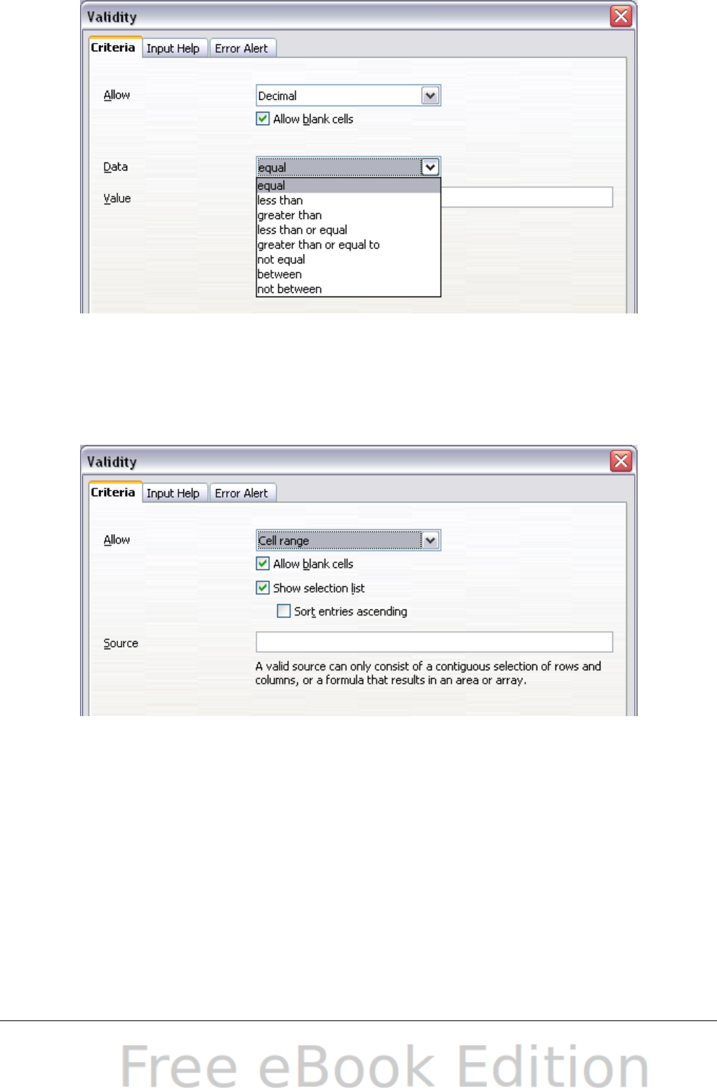
Figure 29: Typical validity test choices.
The validity test options vary with the type of data selected from the
Allow list. For example, Figure 30 shows the choices when a cell must
contain a cell range.
Figure 30: Validity choices for a cell range.
To provide input help for a cell, use the Input Help page of the Validity
dialog (Figure 31). To show an error message when an invalid value is
entered, use the Error Alert page (Figure 32). Be sure to write
something helpful, explaining what a valid entry should contain—not
just “Invalid data—try again” or something similar.
50 OpenOffice.org 3.x Calc Guide
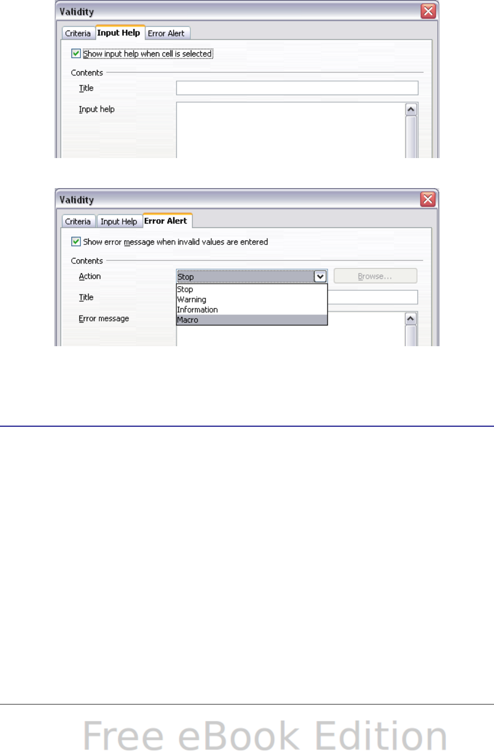
Figure 31: Defining input help for a cell
Figure 32: Defining an error message for a cell with
invalid data
Editing data
Editing data is done is in much the same way as entering it. The first
step is to select the cell containing the data to be edited.
Removing data from a cell
Data can be removed (deleted) from a cell in several ways.
Removing data only
The data alone can be removed from a cell without removing any of
the formatting of the cell. Click in the cell to select it, and then press
the Backspace key.
Removing data and formatting
The data and the formatting can be removed from a cell at the same
time. Press the Delete key (or right-click and choose Delete
Contents, or use Edit > Delete Contents) to open the Delete
Contents dialog (Figure 33). From this dialog, different aspects of
Chapter 2 Entering, Editing, and Formatting Data 51
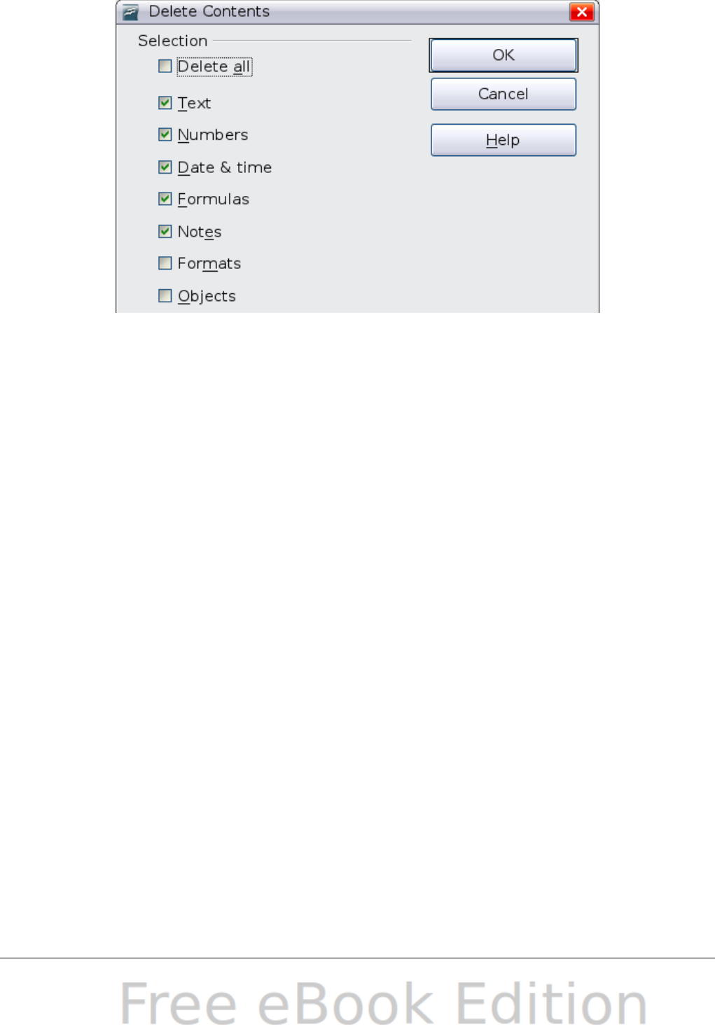
the cell can be deleted. To delete everything in a cell (contents and
format), check Delete all.
Figure 33: Delete Contents dialog
Replacing all the data in a cell
To remove data and insert new data, simply type over the old data. The
new data will retain the original formatting.
Changing part of the data in a cell
Sometimes it is necessary to change the contents of cell without
removing all of the contents, for example if the phrase “See Dick run”
is in a cell and it needs to be changed to “See Dick run fast.” It is often
useful to do this without deleting the old cell contents first.
The process is the similar to the one described above, but you need to
place the cursor inside the cell. You can do this in two ways.
Using the keyboard
After selecting the appropriate cell, press the F2 key and the cursor
is placed at the end of the cell. Then use the keyboard arrow keys to
move the cursor through the text in the cell.
Using the mouse
Using the mouse, either double-click on the appropriate cell (to
select it and place the cursor in it for editing), or single-click to
select the cell and then move the mouse pointer up to the input line
and click into it to place the cursor for editing.
52 OpenOffice.org 3.x Calc Guide
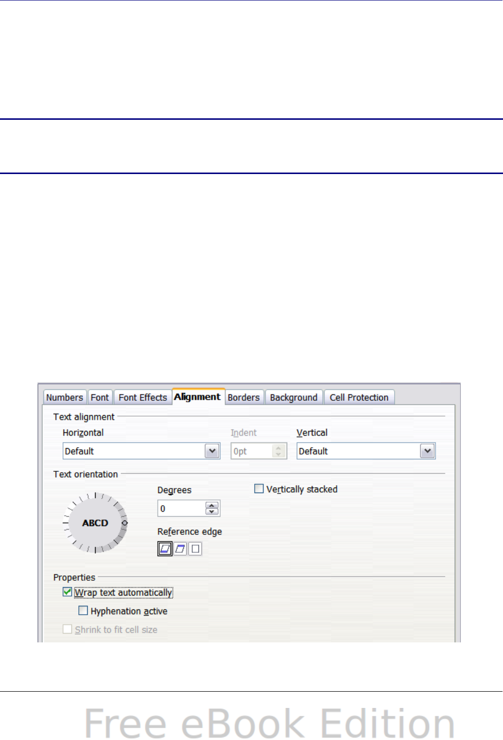
Formatting data
The data in Calc can be formatted in several ways. It can either be
edited as part of a cell style so that it is automatically applied, or it can
be applied manually to the cell. Some manual formatting can be
applied using toolbar icons. For more control and extra options, select
the appropriate cell or cells range, right-click on it, and select Format
Cells. All of the format options are discussed below.
Note
All the settings discussed in this section can also be set as a
part of the cell style. See Chapter 4 (Using Styles and
Templates) for more information.
Formatting multiple lines of text
Multiple lines of text can be entered into a single cell using automatic
wrapping or manual line breaks. Each method is useful for different
situations.
Using automatic wrapping
To set text to wrap at the end of the cell, right-click on the cell and
select Format Cells (or choose Format > Cells from the menu bar, or
press Ctrl+1). On the Alignment tab (Figure 34), under Properties,
select Wrap text automatically. The results are shown in Figure 35.
Figure 34: Format Cells > Alignment dialog
Chapter 2 Entering, Editing, and Formatting Data 53
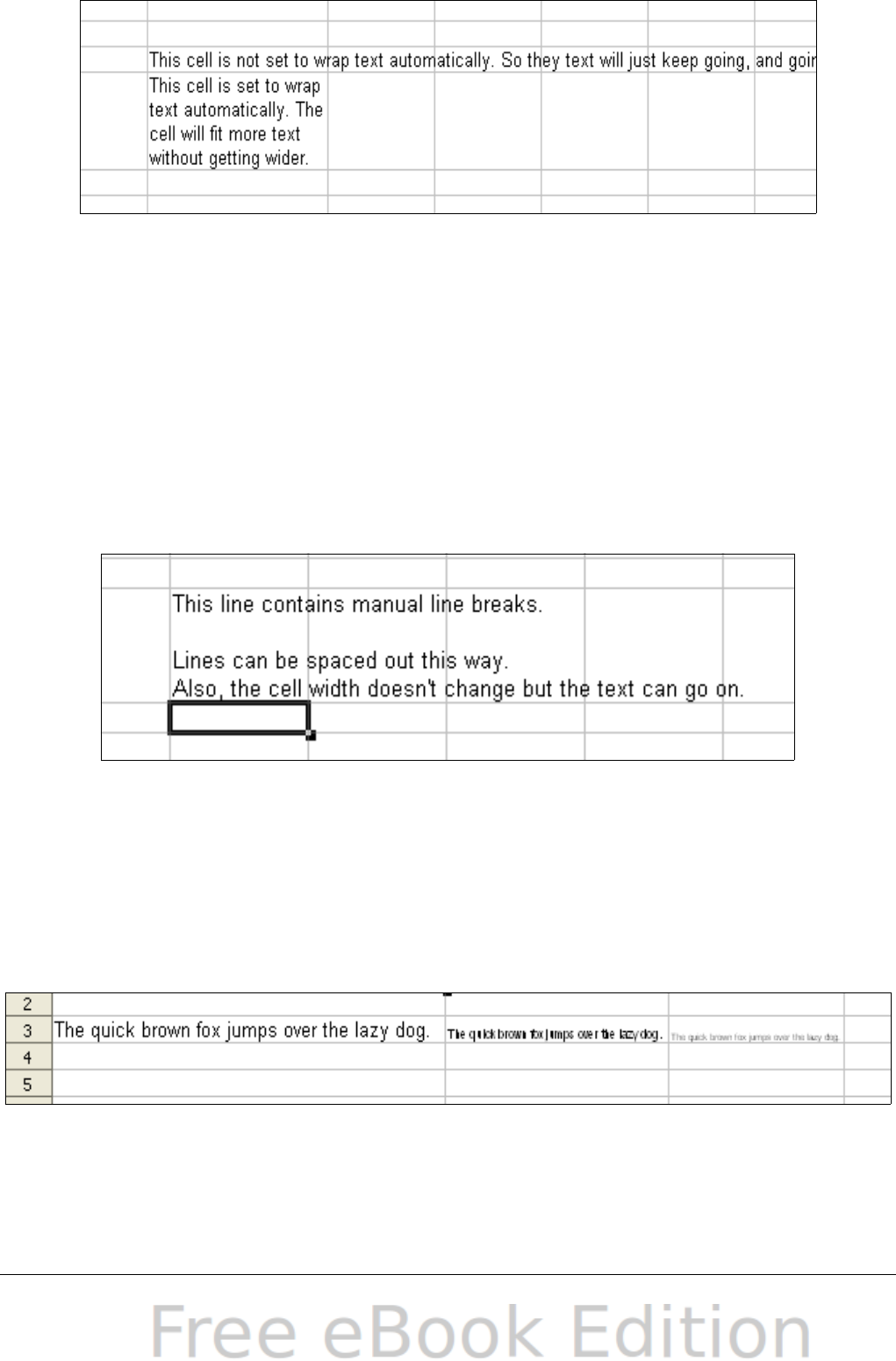
Figure 35: Automatic text wrap
Using manual line breaks
To insert a manual line break while typing in a cell, press Ctrl+Enter.
This method does not work with the cursor in the input line. When
editing text, first double-click the cell, then single-click at the position
where you want the line break.
When a manual line break is entered, the cell width does not change.
Figure 36 shows the results of using two manual line breaks after the
first line of text.
Figure 36: Cell with manual line breaks
Shrinking text to fit the cell
The font size of the data in a cell can automatically adjust to fit in a
cell. To do this, select the Shrink to fit cell option in the Format Cells
dialog (Figure 34). Figure 37 shows the results.
Figure 37: Shrinking font size to fit cells
54 OpenOffice.org 3.x Calc Guide
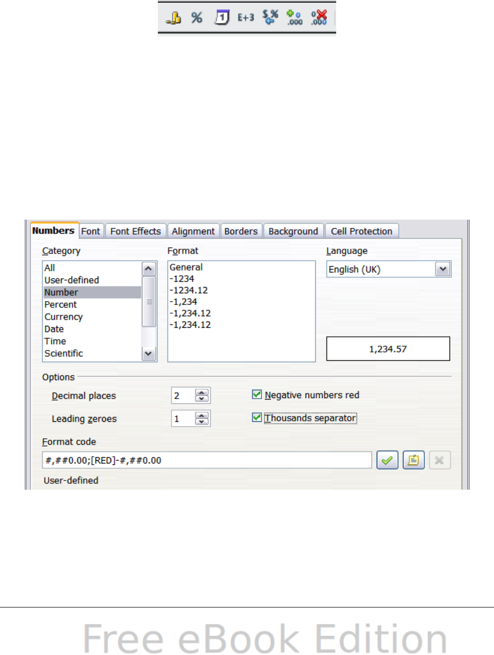
Formatting numbers
Several different number formats can be applied to cells by using icons
on the Formatting toolbar. Select the cell, then click the relevant icon.
Some icons may not be visible in a default setup; click the down-arrow
at the end of the Formatting bar and select other icons to display.
Figure 38: Number format icons. Left to right: currency, percentage,
date, exponential, standard, add decimal place, delete decimal place.
For more control or to select other number formats, use the Numbers
tab (Figure 39) of the Format Cells dialog.
•Apply any of the data types in the Category list to the data.
•Control the number of decimal places and leading zeros.
•Enter a custom format code.
The Language setting controls the local settings for the different
formats such as the date order and the currency marker.
Figure 39: Format Cells > Numbers
Chapter 2 Entering, Editing, and Formatting Data 55
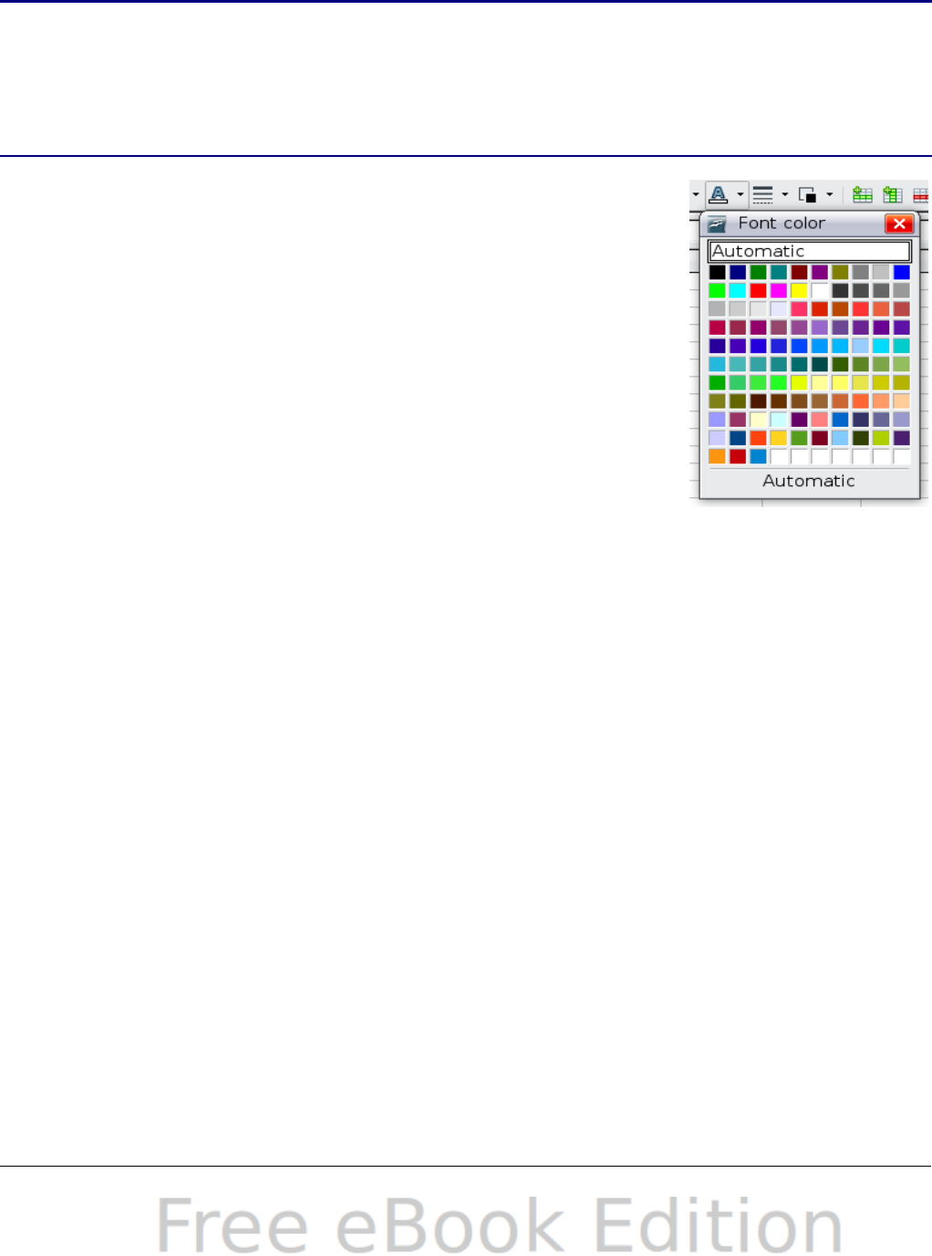
Formatting the font
To quickly choose the font used in a cell, select the cell, then click the
arrow next to the Font Name box on the Formatting toolbar and choose
a font from the list.
Tip
To choose whether to show the font names in their font or in
plain text, go to Tools > Options > OpenOffice.org > View
and select or deselect the Show preview of fonts option in the
Font Lists section. For more information, see Chapter 14
(Setting Up and Customizing Calc).
To choose the size of the font, click the arrow next
to the Font Size box on the Formatting toolbar. For
other formatting, you can use the Bold, Italic, or
Underline icons.
To choose a font color, click the arrow next to the
Font Color icon to display a color palette. Click on
the required color.
(To define custom colors, use Tools > Options >
OpenOffice.org > Colors. See Chapter 14 for
more information.)
To specify the language of the cell (useful because it allows different
languages to exist in the same document and be spell checked
correctly), use the Font tab of the Format Cells dialog. See Chapter 4
for more information.
Choosing font effects
The Font Effects tab (Figure 40) of the Format Cells dialog offers more
font options.
Overlining and underlining
You can choose from a variety of overlining and underlining options
(solid lines, dots, short and long dashes, in various combinations)
and the color of the line.
Strikethrough
The strikethrough options include lines, slashes, and Xs.
Relief
The relief options are embossed (raised text), engraved (sunken
text), outline, and shadow.
56 OpenOffice.org 3.x Calc Guide
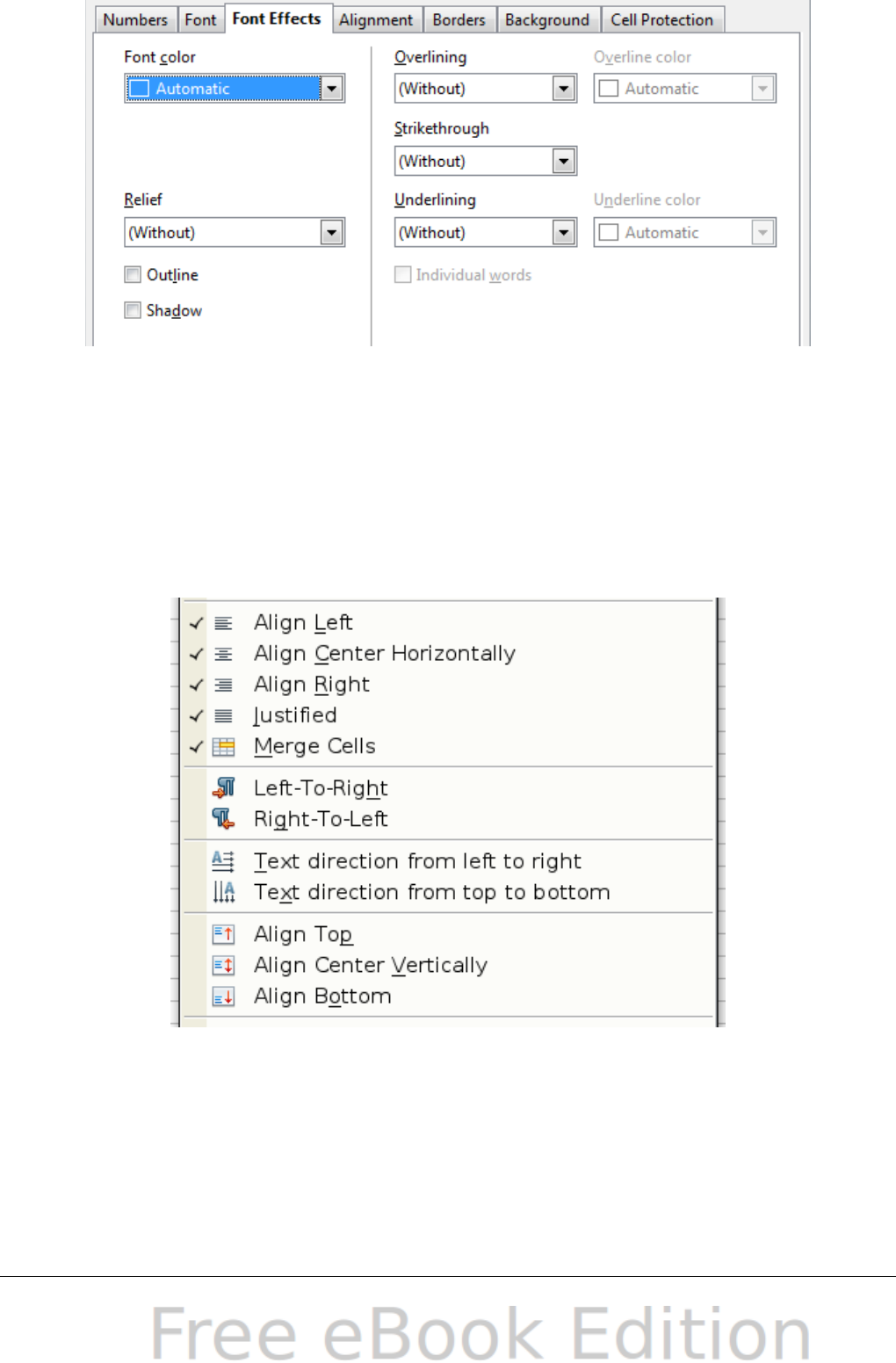
Figure 40: Format Cells > Font Effects
Setting cell alignment and orientation
Some of the cell alignment and orientation icons are not shown by
default on the Formatting toolbar. To show them, click on the small
arrow at the right-hand end of the toolbar and select them from the list
of icons.
Figure 41: Cell alignment and orientation
Some of the alignment and orientation icons are available only if you
have Asian or CTL (Complex Text Layout) languages enabled (in Tools
> Options > Language Settings > Languages). If you choose an
unavailable icon from the list, it does not appear on the toolbar.
Chapter 2 Entering, Editing, and Formatting Data 57

For more control and other choices, use the Alignment tab (Figure 34)
of the Format Cells dialog to set the horizontal and vertical alignment
and rotate the text. If you have Asian languages enabled, then the Text
orientation section shows an extra option (labeled Asian layout
mode) under the Vertically stacked option, as shown in Figure 41.
Figure 42: Asian layout mode option
The difference in results between having Asian layout mode on or off
is shown in Figure 43.
Figure 43: Types of vertical stacking
Formatting the cell borders
To quickly choose a line style and color for the borders of a cell, click
the small arrows next to the Line Style and Line Color icons on the
Formatting toolbar. If the Line Style and Line Color icons are not
displayed in the formatting toolbar, select the down arrow on the right
side of the bar, then Visible Buttons. In each case, a palette of
choices is displayed.
For more control, including the spacing between the cell borders and
the text, use the Borders tab of the Format Cells dialog. There you can
also define a shadow. See Chapter 4 for details.
58 OpenOffice.org 3.x Calc Guide
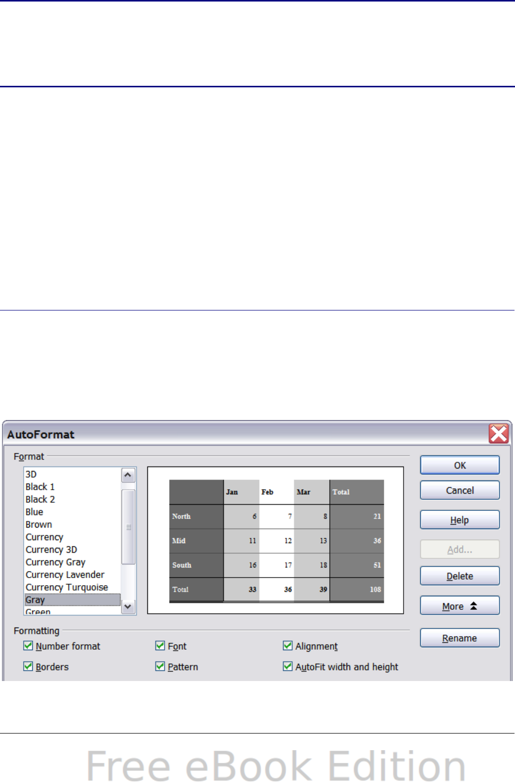
Note
The cell border properties apply to a cell, and can only be
changed if you are editing that cell. For example, if cell C3 has
a top border (which would be equivalent visually to a bottom
border on C2), that border can only be removed by selecting
C3. It cannot be removed in C2.
Formatting the cell background
To quickly choose a background color for a cell, click the small arrow
next to the Background Color icon on the Formatting toolbar. A palette
of color choices, similar to the Font Color palette, is displayed.
(To define custom colors, use Tools > Options > OpenOffice.org >
Colors. See Chapter 14 for more information.)
You can also use the Background tab of the Format Cells dialog. See
Chapter 4 for details.
Autoformatting cells and sheets
You can use the AutoFormat feature to quickly apply a set of cell
formats to a sheet or a selected cell range.
1) Select the cells that you want to format, including the column and
row headers.
2) Choose Format > AutoFormat.
Figure 44: Choosing an AutoFormat
Chapter 2 Entering, Editing, and Formatting Data 59
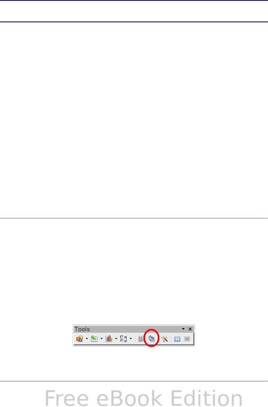
Note If the selected cell range does not have column and row
headers, AutoFormat is not available.
3) To select which properties (number format, font, alignment,
borders, pattern, autofit width and height) to include in an
AutoFormat, click More. Select or deselect the required options.
4) Click OK.
If you do not see any change in color of the cell contents, choose View
> Value Highlighting from the menu bar.
Defining a new AutoFormat
You can define a new AutoFormat that is available to all spreadsheets.
1) Format a sheet.
2) Choose Edit > Select All.
3) Choose Format > AutoFormat. The Add button is now active.
4) Click Add.
5) In the Name box of the Add AutoFormat dialog, type a meaningful
name for the new format.
6) Click OK to save. The new format is now available in the Format
list in the AutoFormat dialog.
Formatting spreadsheets using themes
Calc comes with a predefined set of formatting themes that you can
apply to your spreadsheets.
It is not possible to add themes to Calc, and they cannot be modified.
However, you can modify their styles after you apply them to a
spreadsheet.
To apply a theme to a spreadsheet:
1) Click the Choose Themes icon in the Tools toolbar. If this toolbar
is not visible, you can show it using View > Toolbars > Tools.
The Theme Selection dialog appears. This dialog lists the
available themes for the whole spreadsheet.
2) In the Theme Selection dialog, select the theme that you want to
apply to the spreadsheet.
60 OpenOffice.org 3.x Calc Guide

As soon as you select a theme, some of the properties of the
custom styles are applied to the open spreadsheet and are
immediately visible.
3) Click OK. If you wish, you can now go to the Styles and
Formatting window to modify specific styles. These modifications
do not change the theme; they only change the appearance of this
specific spreadsheet document.
Using conditional formatting
You can set up cell formats to change depending on conditions that you
specify. For example, in a table of numbers, you can show all the values
above the average in green and all those below the average in red.
Note To apply conditional formatting, AutoCalculate must be
enabled. Choose Tools > Cell Contents > AutoCalculate.
Conditional formatting depends upon the use of styles. If you are not
familiar with styles, please refer to Chapter 4. An easy way to set up
the required styles is to format a cell the way you want it and click the
New Style from Selection icon in the Styles and Formatting window.
After the styles are set up, here is how to use them.
1) In your spreadsheet, select the cells to which you want to apply
conditional formatting.
2) Choose Format > Conditional Formatting from the menu bar.
3) On the Conditional Formatting dialog (Figure 45), enter the
conditions. Click OK to save. The selected cells are now
formatted in the relevant style.
Cell value is / Formula is
Specifies whether conditional formatting is dependent on a cell
value or on a formula. If you select cell value is, the Cell Value
Condition box is displayed, as shown in the example. Here you can
choose from conditions including less than, greater than, between,
and others.
Parameter field
Enter a reference, value, or formula in the parameter field, or in
both parameter fields if you have selected a condition that requires
two parameters. You can also enter formulas containing relative
references.
Chapter 2 Entering, Editing, and Formatting Data 61
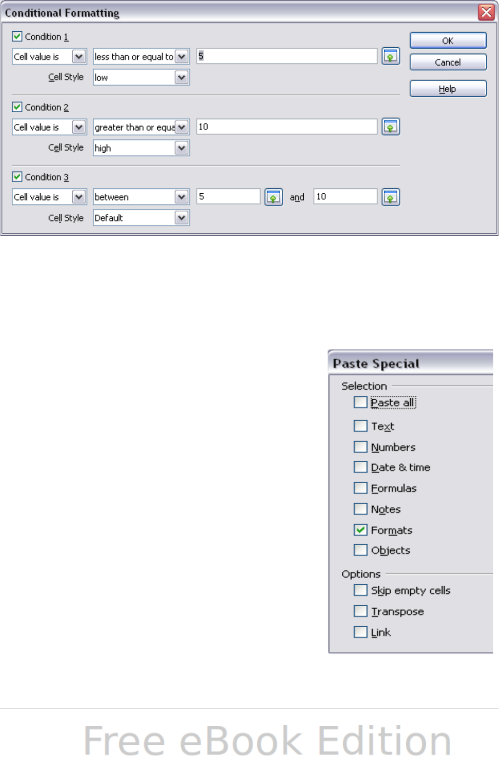
Figure 45: Conditional formatting dialog
Cell style
Choose the cell style to be applied if the specified condition
matches. The style must have been defined previously.
See the Help for more information and examples of use.
To apply the same conditional formatting
later to other cells:
1) Select one of the cells that has been
assigned conditional formatting.
2) Copy the cell to the clipboard.
3) Select the cells that are to receive this
same formatting.
4) Choose Edit > Paste Special.
5) On the Paste Special dialog, in the
Selection area, select only the Formats
option. Make sure all other options are
not selected. Click OK.
62 OpenOffice.org 3.x Calc Guide
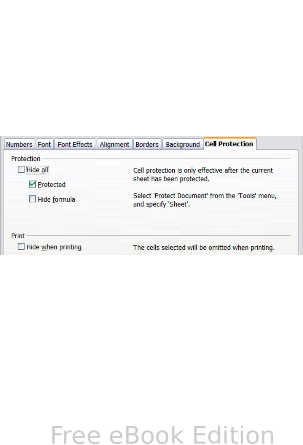
Hiding and showing data
When elements are hidden, they are neither visible nor printed, but
can still be selected for copying if you select the elements around
them. For example, if column B is hidden, it is copied when you select
columns A and C. When you need a hidden element again, you can
reverse the process, and show the element.
To hide or show sheets, rows, and columns, use the options on the
Format menu or the right-click (context) menu. For example, to hide a
row, first select the row, and then choose Format > Row > Hide (or
right-click and choose Hide).
To hide or show selected cells, choose Format > Cells from the menu
bar (or right-click and choose Format Cells). On the Format Cells
dialog, go to the Cell Protection tab.
Figure 46: Hiding or showing cells
Outline group controls
If you are continually hiding and showing the same cells, you can
simplify the process by creating outline groups, which add a set of
controls for hiding and showing the cells in the group that are quick to
use and always available.
If the contents of cells falls into a regular pattern, such as four cells
followed by a total, then you can use Data > Group and Outline >
AutoOutline to have Calc add outline controls based on the pattern.
Otherwise, you can set outline groups manually by selecting the cells
for grouping, then choosing Data > Group and Outline > Group. On
the Group dialog, you can choose whether to group the selected cells
by rows or columns.
Chapter 2 Entering, Editing, and Formatting Data 63

When you close the dialog, the outline group controls are visible
between either the row or column headers and the edges of the editing
window. The controls resemble the tree-structure of a file-manager in
appearance, and can be hidden by selecting Data > Group and
Outline > Hide Details. They are strictly for online use, and do not
print.
The basic outline controls have plus or minus signs at the start of the
group to show or hide hidden cells. However, if outline groups are
nested, the controls have numbered buttons for hiding the different
levels.
If you no longer need a group, place the mouse cursor in any cell in it
and select Data > Group and Outline > Ungroup. To remove all
groups on a sheet, select Data > Group and Outline > Remove.
Figure 47: Outline group controls
Filtering which cells are visible
A filter is a list of conditions that each entry has to meet in order to be
displayed. You can set three types of filters from the Data > Filter
sub-menu.
Automatic filters add a drop-down list to the top row of a column that
contains commonly used filters. They are quick and convenient and
almost as useful with text as with numbers, because the list includes
every unique entry in the selected cells.
In addition to these unique entries, automatic filters include the option
to display all entries, the ten highest numerical values, and all cells
that are empty or not empty, as well as a standard filterthat you can
customize (see below). However, they are somewhat limited. In
particular, they do not allow regular expressions, so you cannot use
them to display cell contents that are similar but not identical.
64 OpenOffice.org 3.x Calc Guide
Standard filters are more complex than automatic filters. You can set
as many as three conditions as a filter, combining them with the
operators AND and OR. Standard filters are mostly useful for numbers,
although a few of the conditional operators, such as = and < > can
also be used for text.
Other conditional operators for standard filters include options to
display the largest or smallest values, or a percentage of them. Useful
in themselves, standard filters take on added value when used to
further refine automatic filters.
Advanced filters are structured similarly to standard filters. The
differences are that advanced filters are not limited to three
conditions, and their criteria are not entered in a dialog. Instead,
advanced filters are entered in a blank area of a sheet, then referenced
by the advanced filter tool in order to apply them.
Sorting records
Sorting rearranges the visible cells on the sheet. In Calc, you can sort
by up to three criteria, which are applied one after another. Sorts are
handy when you are searching for a particular item, and become even
more powerful after you have filtered data.
In addition, sorting is often useful when you add new information.
When a list is long, it is usually easier to add new information at the
bottom of the sheet, rather than inserting rows in the proper places.
After you have added the information, you can sort it to update the
sheet.
Highlight the cells to be sorted, then select Data > Sort to open the
Sort dialog (Figure 48) or click the Sort Ascending or Sort
Descending toolbar buttons. Using the dialog, you can sort
the selected cells using up to three columns, in either
ascending (A-Z, 1-9) or descending (Z-A, 9-1) order.
Tip
You can define a custom sort order if the supplied
alphanumeric ones do not fit your requirements. See “Defining
a fill series” on page 47 for instructions.
On the Options tab of the Sort dialog (Figure 49), you can choose the
following options.
Chapter 2 Entering, Editing, and Formatting Data 65
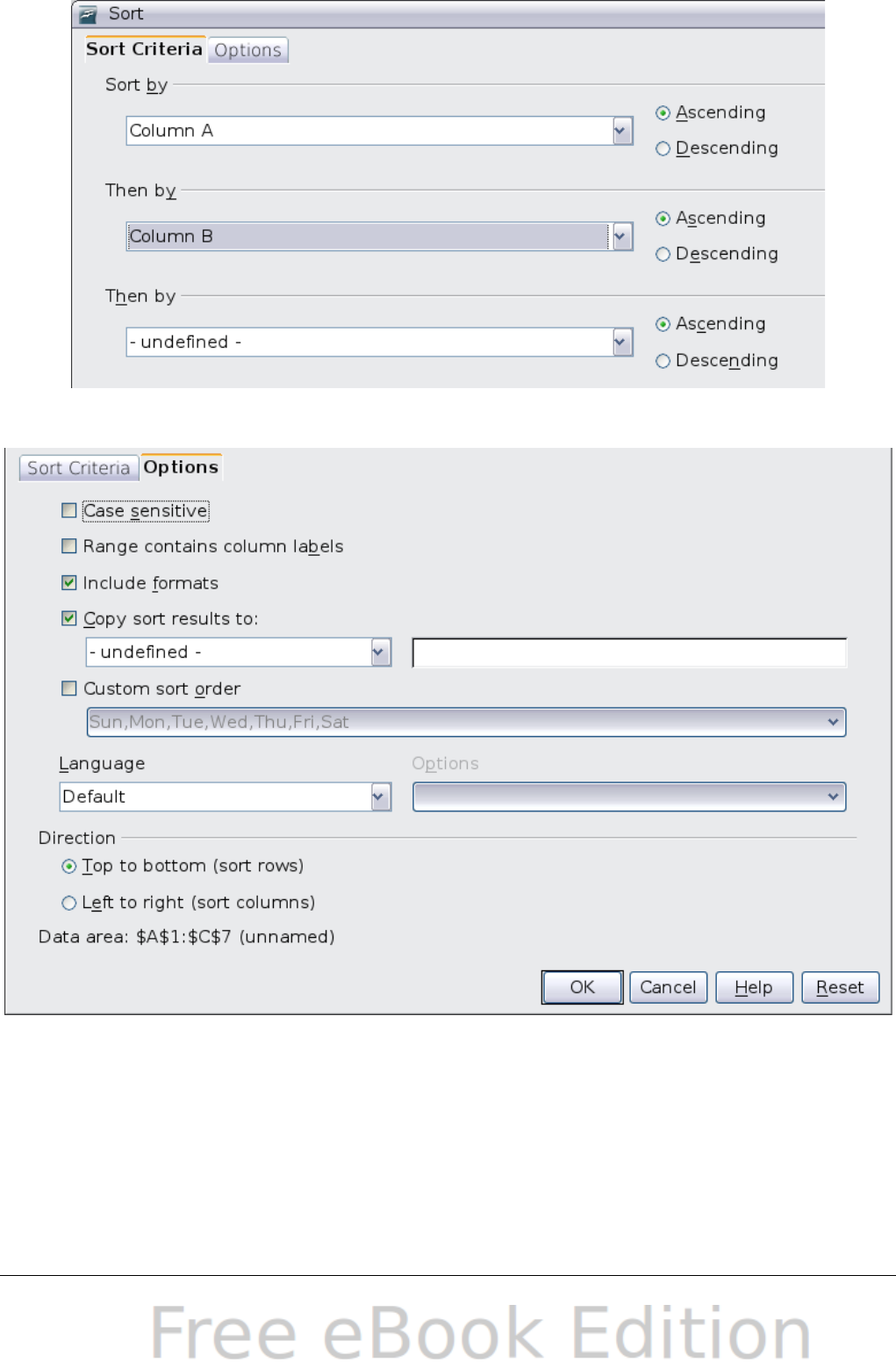
Figure 48: Choosing the criteria and order of sorting
Figure 49: Options for sorting
Case sensitive
If two entries are otherwise identical, one with an upper case letter
is placed before one with a lower case letter in the same position if
the sort is descending; if the sort is ascending, then the entry with
an upper case letter is placed after one with a lower case letter in
the same position.
66 OpenOffice.org 3.x Calc Guide
Range contains column labels
Does not include the column heading in the sort.
Include formats
A cell's formatting is moved with its contents. If formatting is used
to distinguish different types of cells, then use this option.
Copy sort results to
Sets a spreadsheet address to which to copy the sort results. If a
range is specified that does not have the necessary number of cells,
then cells are added. If a range contains cells that already have
content, then the sort fails.
Custom sort order
Select the box, then choose from the drop-down list one of the sort
orders defined in Tools > Options > OpenOffice.org Calc >
Sort Lists.
Direction
Sets whether rows or columns are sorted. The default is to sort by
columns unless the selected cells are in a single column.
Finding and replacing in Calc
In spreadsheet documents you can search for text, formulas, and
styles. You can navigate from one occurrence to the next using Find,
or you can highlight all matching cells at once using Find All, then
apply another format or replace the cell contents by other content.
Text and numbers in cells may have been entered directly or may be
the result of a calculation. The search method you use depends on the
type of data you are searching for.
Tip
Cell contents can be formatted in different ways. For example,
a number can be formatted as a currency, to be displayed with
a currency symbol. You see the currency symbol in the cell, but
you cannot search for it.
By default, Calc searches the current sheet. To search through all
sheets of the document, click More Options, then select Search in all
sheets option.
Chapter 2 Entering, Editing, and Formatting Data 67
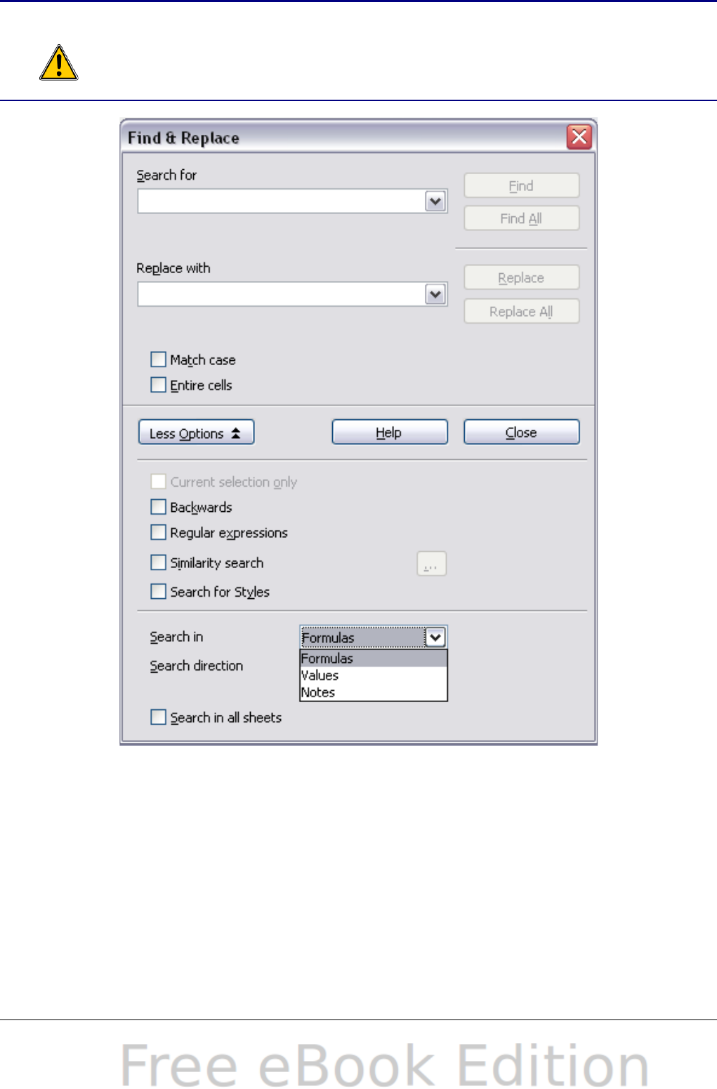
Caution Use Replace All with caution; otherwise, you may end up with
some highly embarrassing mistakes. A mistake with Replace
All might require a manual, word-by-word search to fix, if it is
not discovered in time to undo it.
Figure 50: Expanded Find & Replace dialog
Finding and replacing formulas or values
You can use the Find & Replace dialog to search in formulas or in the
displayed values that result from a calculation.
1) To open the Find & Replace dialog, use the keyboard shortcut
Control+F or select Edit > Find & Replace.
2) Click More Options to expand the dialog.
68 OpenOffice.org 3.x Calc Guide

3) Select Formulas or Values in the Search in drop-down list.
•Formulas finds parts of the formulas.
•Values finds the results of the calculations.
4) Type the text you want to find in the Search for box.
5) To replace the text with different text, type the new text in the
Replace with box.
6) When you have set up your search, click Find. To replace text,
click Replace instead.
Finding and replacing text
1) Open the Find & Replace dialog, click More Options to expand
the dialog, and select Values or Notes in the Search in drop-down
list.
2) Type the text you want to find in the Search for box.
3) To replace the text with different text, type the new text in the
Replace with box.
4) Click Find, Find All, Replace, or Replace All.
When you click Find, Calc selects the next cell that contains your text.
You can edit the text, then click Find again to advance to the next
found cell. If you closed the dialog, you can press Ctrl+Shift+F to find
the next cell without opening the dialog.
When you click Find All, Calc selects all cells that contain your entry.
Now you can, for example, apply a cell style to all of them at once.
Finding and replacing cell styles
To quickly change all the paragraphs of one (unwanted) style to
another (preferred) style:
1) On the expanded Find & Replace dialog, select Search for
Styles. The Search for and Replace with boxes now contain a list
of styles.
2) Select the styles you want to search for and replace.
3) Click Find, Find All, Replace, or Replace All.
Using wildcards (regular expressions)
Wildcards (also known as regular expressions) are combinations of
characters that instruct OOo how to search for something. Regular
expressions are very powerful but not very intuitive. They can save
time and effort by combining multiple finds into one.
Chapter 2 Entering, Editing, and Formatting Data 69

To use wildcards and regular expressions when searching and
replacing:
1) On the Find & Replace dialog, click More Options to see more
choices. On this expanded dialog, select the Regular
expressions option.
2) Type the search text, including the wildcards, in the Search for
box and the replacement text (if any) in the Replace with box.
3) Click Find, Find All, Replace, or Replace All (not
recommended).
Tip The online help describes many of the regular expressions and
their uses.
The following points are interesting to Calc users:
•In Calc, regular expressions are applied separately to each cell.
So a search for r.d will match red in cell A1 but will not match r
in cell A2 and d (or ed) in cell A3. (The regular expression r.d
means “try to match r followed by any other character followed
by d.”)
•When a match is found, the whole cell is shown highlighted, but
only the text found will be replaced. For example, searching for
brown will highlight a cell containing redbrown clay, and
replacing with nothing will leave the cell containing red clay.
•If Find is used twice in a row, the second time with Current
selection only activated, then the second search will evaluate
the whole of each selected cell, not just the strings found which
caused the cells to be selected in the first search. For example,
searching for joh?n, then activating Current selection only and
searching for sm.th will find cells containing Jon Smith and
Smythers, Johnathon.
•If a cell contains a hard line break (entered by Ctrl+Enter), this
may be found by \n. For example if a cell contains red
hard_line_break clay then searching for d\nc and replacing with
nothing leaves the cell containing relay.
•The hard line break acts to mark “end of text” as understood by
the regular expression special character $ (in addition of course
to the end of text in the cell). For example, if a cell contains red
hard_line_break clay then a search for d$ replacing with al
leaves the cell with real hard_line_break clay. Note that with
this syntax the hard line break is not replaced—it simply marks
the end of text.
70 OpenOffice.org 3.x Calc Guide

•Using \n in the Replace with box will replace with the literal
characters \n, not a hard line break.
•The Find & Replace dialog has an option to search Formulas,
Values, or Notes. This applies to any search, not just one using
regular expressions. Searching with the Formulas option would
find SUM in a cell containing the formula =SUM(A1:A6). If a cell
contains text instead of a function, the text will still be found - so
that the simple text SUMMARY in a cell would also give a match
to SUM using the Formulas option.
•Searching for the regular expression ^$ will not find empty cells.
This is intentional—the rationale being to avoid performance
issues when selecting a huge number of cells. Note that empty
cells will not be found even if you are only searching a selection.
•Find .+ (or similar) and Replace with & effectively re-enters the
contents of cells. This can be used to strip formatting
automatically applied by Calc (often needed to clean data
imported from the clipboard or badly formatted files), for
example, to convert text strings consisting of digits into actual
numbers (the cells must first be correctly formatted numbers).
The leading apostrophes, telling Calc to treat the numbers as text,
are removed.
See Chapter 7 (Using Formulas and Functions) for the use of regular
expressions within formulas.
Chapter 2 Entering, Editing, and Formatting Data 71

Chapter 3
Creating Charts and
Graphs
Presenting information visually
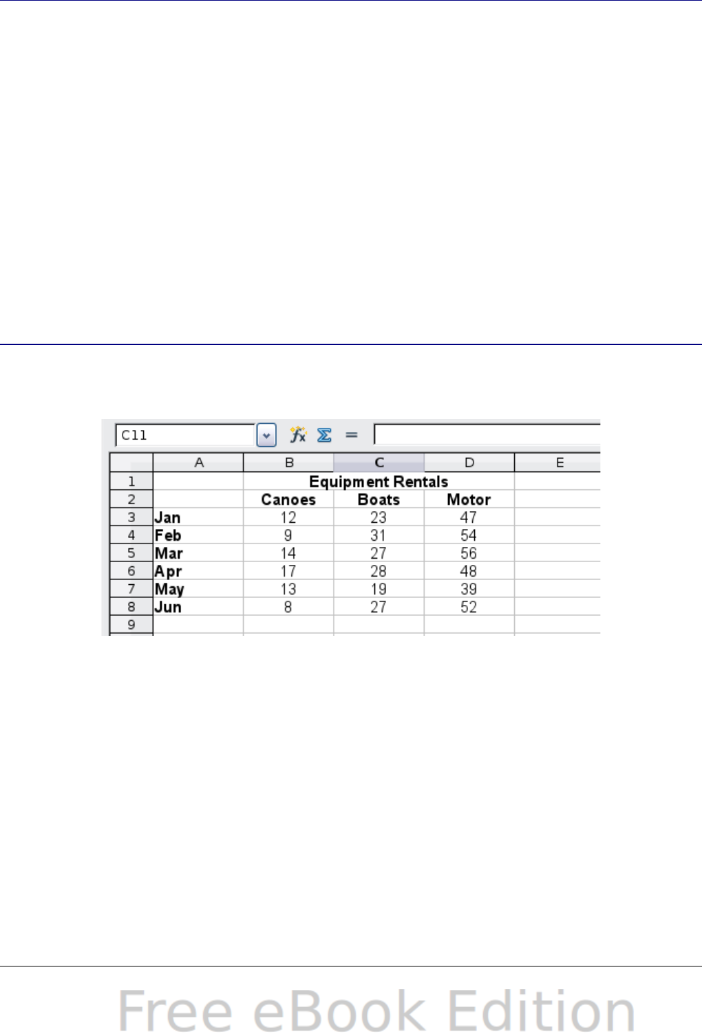
Introduction
Charts and graphs can be powerful ways to convey information to the
reader. OpenOffice.org Calc offers a variety of different chart and
graph formats for your data.
Using Calc, you can customize charts and graphs to a considerable
extent. Many of these options enable you to present your information
in the best and clearest manner.
For readers who are interested in effective ways to present information
graphically, two excellent introductions to the topic are William S.
Cleveland’s The elements of graphing data, 2nd edition, Hobart Press
(1994) and Edward R. Tufte’s The Visual Display of Quantitative
Information, 2nd edition, Graphics Press (2001).
Creating a chart
To demonstrate the process of making charts and graphs in Calc, we
will use the small table of data in Figure 51.
Figure 51: Table of data for charting examples
To create a chart, first highlight (select) the data to be included in the
chart. The selection does not need to be in a single block, as shown in
Figure 52; you can also choose individual cells or groups of cells
(columns or rows). See Chapter 1 (Introducing Calc) for more about
selecting cells and ranges of cells.
Chapter 3 Creating Charts and Graphs 73
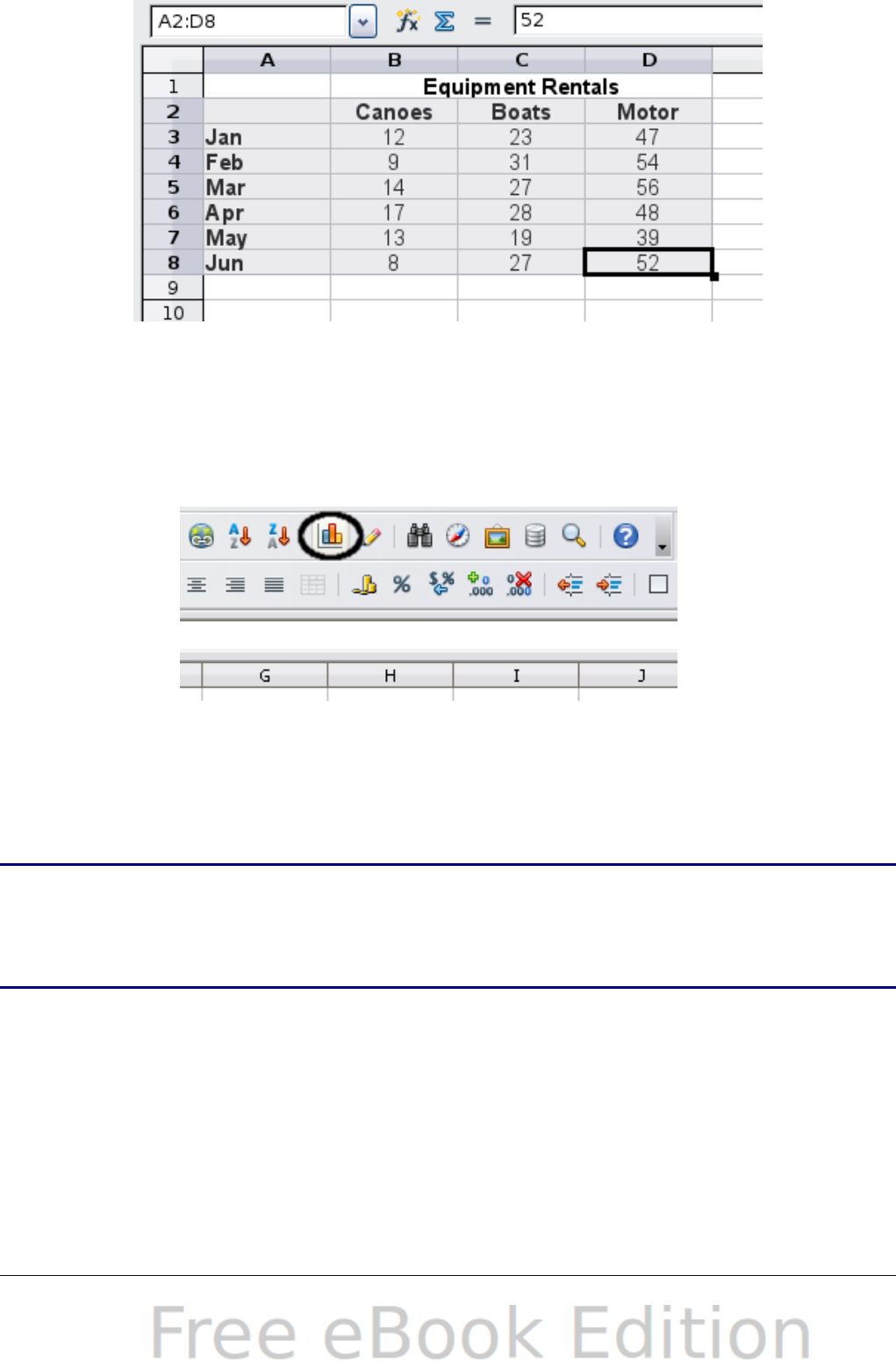
Figure 52: Selecting data for plotting
Next, open the Chart Wizard dialog using one of two methods.
•Choose Insert > Chart from the menu bar.
•Or, click the Chart icon on the main toolbar.
Figure 53: Insert chart from main toolbar
Either method inserts a sample chart on the worksheet, opens the
Formatting toolbar, and opens the Chart Wizard, as shown in Figure
54.
Tip
Before choosing the Chart Wizard, place the cursor anywhere in
the area of the data. The Chart Wizard will then do a fairly good
job of guessing the range of the data. Just be careful that you
have not included the title of your chart.
74 OpenOffice.org 3.x Calc Guide

Figure 54: Chart Wizard, Step 1—Choose a chart type
Choosing a chart type
The Chart Wizard includes a sample chart with your data. This sample
chart updates to reflect the changes you make in the Chart Wizard.
The Chart Wizard has three main parts: a list of steps involved in
setting up the chart, a list of chart types, and the options for each
chart type. At any time you can go back to a previous step and change
selections.
Calc offers a choice of 10 basic chart types, with a few options for each
type of chart. The options vary according to the type of chart you pick.
The first tier of choice is for two-dimensional (2D) charts. Only those
types which are suitable for 3D (Column, Bar, Pie, and Area) give you
an option to select a 3D look.
On the Choose a chart type page (Figure 54), select a type by clicking
on its icon. The preview updates every time you select a different type
of chart, and provides a good idea of what the finished chart will look
like.
The current selection is highlighted (shown with a surrounding box) on
the Choose a chart type page. The chart’s name is shown just below
Chapter 3 Creating Charts and Graphs 75
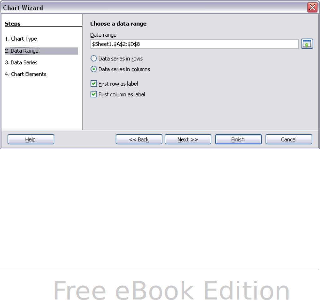
the icons. For the moment, we will stick to the Column chart and click
on Next again.
Changing data ranges and axes labels
In Step 2, Data Range, you can manually correct any mistakes you
have made in selecting the data.
On this page you can also change the way you are plotting the data by
using the rows—rather than the columns—as data series. This is useful
if you use a style of chart such as Donut or Pie to display your data.
Lastly, you can choose whether to use the first row or first column, or
both, as labels on the axes of the chart.
You can confirm what you have done so far by clicking the Finish
button, or click Next to change some more details of the chart.
We will click Next to see what we can do to our chart using the other
pages of the Wizard.
Figure 55: Changing data ranges and axes labels
76 OpenOffice.org 3.x Calc Guide
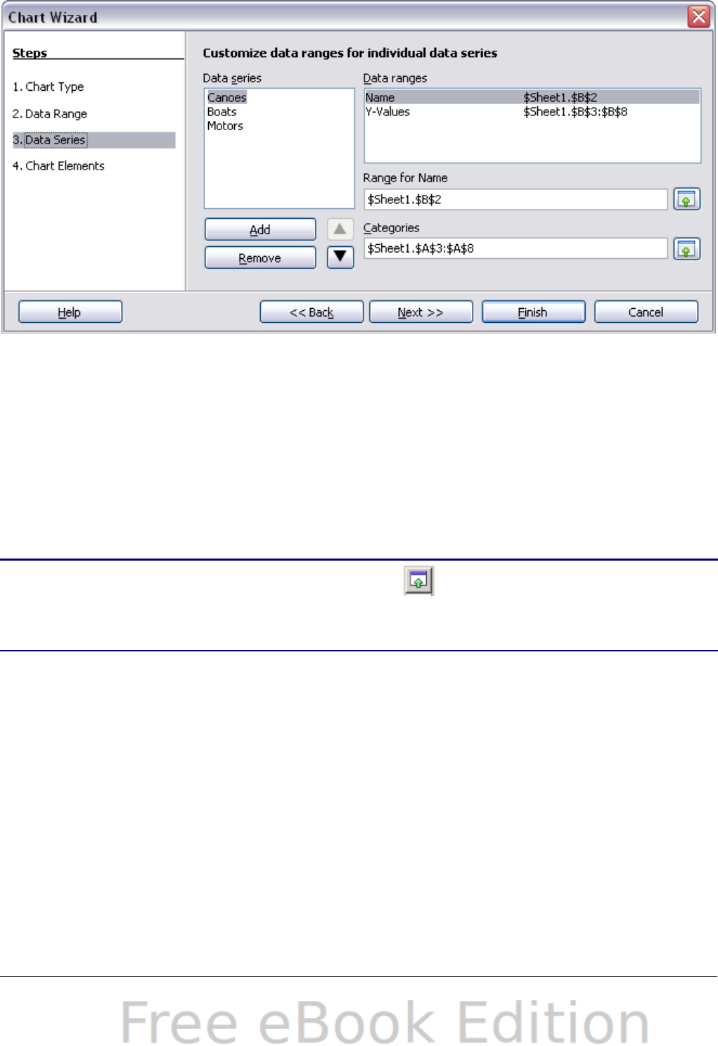
Selecting data series
Figure 56: Amending data series and ranges
On the Data Series page, you can fine tune the data that you want to
include in the chart. Perhaps you have decided that you do not want to
include the data for canoes. If so, highlight Canoes in the Data series
box and click on Remove. Each named data series has its ranges and
its individual Y-values listed. This is useful if you have very specific
requirements for data in your chart, as you can include or leave out
these ranges.
Tip You can click the Shrink button next to the Range for Name
box to work on the spreadsheet itself. This is handy if your data
ranges are larger than ours and the Chart Wizard is in the way.
Another way to plot any unconnected columns of data is to select the
first data series and then select the next series while holding down the
Ctrl key. Or you can type the columns in the text boxes. The columns
must be separated by semi-colons. Thus, to plot B3:B11 against
G3:G11, type the selection range as B3:B11;G3:G11.
The two data series you are selecting must be in separate columns or
rows. Otherwise Calc will assume that you are adding to the same data
series.
Click Next to deal with titles, legend and grids.
Chapter 3 Creating Charts and Graphs 77
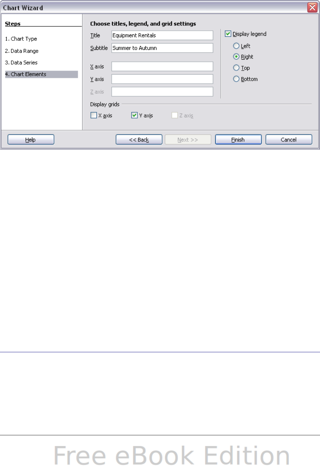
Adding or changing titles, legend, and grids
Figure 57: Titles, legend and grids
On the Chart Elements page, you can give your chart a title and, if
desired, a subtitle. Use a title that draws the viewers’ attention to the
purpose of the chart: what you want them to see. For example, a better
title for this chart might be The Performance of Motor and Other
Rental Boats.
It may be of benefit to have labels for the x axis or the y axis. This is
where you give viewers an idea as to the proportion of your data. For
example, if we put Thousands in the y axis label of our graph, it
changes the scope of the chart entirely. For ease of estimating data you
can also display the x or y axis grids by selecting the Display grids
options.
You can leave out the legend or include it and place it to the left, right,
top or bottom.
To confirm your selections and complete the chart, click Finish.
Editing charts
After you have created a chart, you may find things you would like to
change. Calc provides tools for changing the chart type, chart
elements, data ranges, fonts, colors, and many other options, through
the Insert and Format menus, the right-click (context) menu, and the
Chart toolbar.
78 OpenOffice.org 3.x Calc Guide

Changing the chart type
You can change the chart type at any time. To do so:
1) First select the chart by double-clicking on it. The chart should
now be surrounded by a gray border.
2) Then do one of the following:
•Choose Format > Chart Type from the menu bar.
•Click the chart type icon on the Formatting toolbar.
•Right-click on the chart and choose Chart Type.
In each case, a dialog similar to the one in Figure 54 opens. See page
75 for more information.
Adding or removing chart elements
Figures 58 and 59 show the elements of 2D and 3D charts.
The default 2D chart includes only two of those elements:
•Chart wall contains the graphic of the chart displaying the data.
•Chart area is the area surrounding the chart graphic. The
(optional) chart title and the legend (key) are in the chart area.
The default 3D chart also has the chart floor, which is not available in
2D charts.
Figure 58: Elements of 2D chart
Chapter 3 Creating Charts and Graphs 79
Chart area
Chart wall
Chart title
Legend
Axis labels
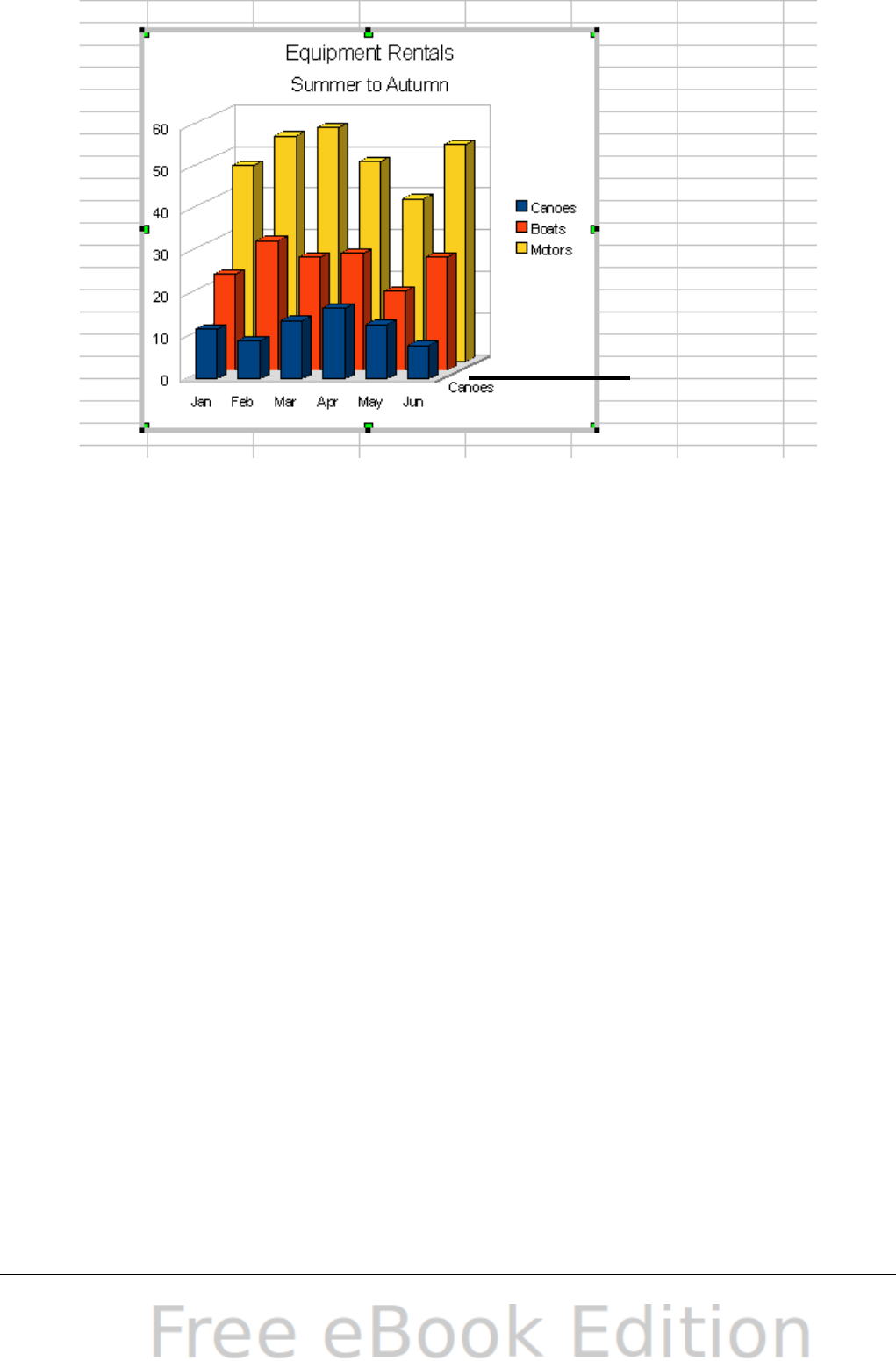
Figure 59: Elements of 3D chart
You can add other elements using the commands on the Insert menu.
The various choices open dialogs in which you can specify details.
First select the chart so the green sizing handles are visible. This is
done with a single click on the chart.
The dialogs for Titles, Legend, Axes, and Grids are self-explanatory.
The others are a bit more complicated, so we’ll take a look at them
here.
Data labels
Data labels put information about each data point on the chart. They
can be very useful for presenting detailed information, but you need to
be careful to not create a chart that is too cluttered to read.
Choose Insert > Data Labels. The options are as follows.
Show value as number
Displays the numeric values of the data points. When selected, this
option activates the Number format... button.
Number format...
Opens the Number Format dialog, where you can select the number
format. This dialog is very similar to the one for formatting numbers
in cells, described in Chapter 2 (Entering, Editing, and Formatting
Data).
80 OpenOffice.org 3.x Calc Guide
Chart floor
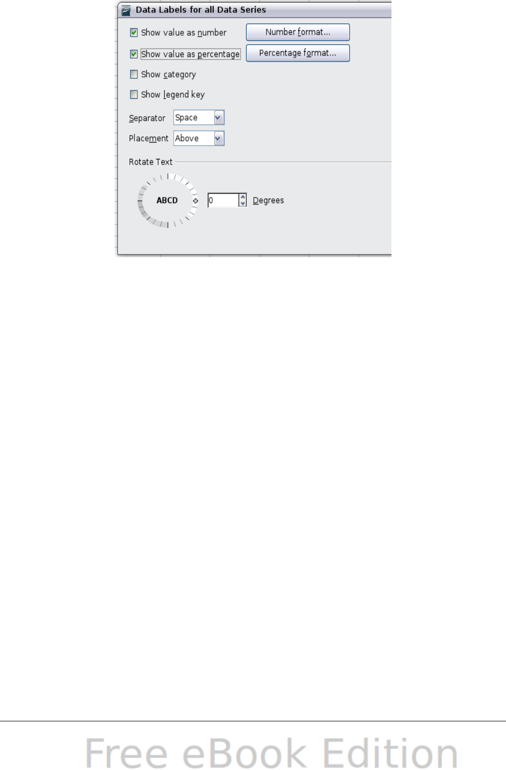
Figure 60: Data Labels dialog
Show value as percentage
Displays the percentage value of the data points in each column.
When selected, this option activates the Percentage format...
button.
Percentage format...
Opens the Number Format dialog, where you can select the
percentage format.
Show category
Shows the data point text labels.
Show legend key
Displays the legend icons next to each data point label.
Separator
Selects the separator between multiple text strings for the same
object.
Placement
Selects the placement of data labels relative to the objects.
Figure 71 on page 95 shows examples of values as text (neither Show
value as number nor Show value as percentage selected) and values as
percentages, as well as when data values are used as substitutes for
legends or in conjunction with them.
Chapter 3 Creating Charts and Graphs 81
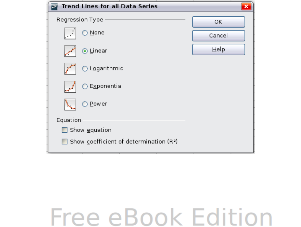
Trend lines
When you have a scattered grouping of points in a graph, you may
want to show the relationship of the points. A trend line is what you
need. Calc has a good selection of regression types you can use for
trend lines: linear, logarithm, exponential, and power. Choose the type
that comes closest to passing through all of the points.
To insert trend lines for all data series, double-click the chart to enter
edit mode. Choose Insert > Trend Lines, then select the type of trend
line from None, Linear, Logarithmic, Exponential, or Power. You can
also choose whether to show the equation for the trend line and the
coefficient of determination (R2).
To insert a trend line for a single data series, first select the data series
in the chart, and then right-click and choose Insert > Trend Line
from the context menu. The dialog for a single trend line is similar to
the one below but has a second tab (Line), where you can choose
attributes (style, color, width, and transparency) of the line.
To delete a single trend line or mean value line, click the line, then
press the Del key.
To delete all trend lines, choose Insert > Trend Lines, then select
None.
A trend line is shown in the legend automatically.
Figure 61: Trend Lines dialog
82 OpenOffice.org 3.x Calc Guide

If you insert a trend line on a chart type that uses categories, such as
Line or Column, then the numbers 1, 2, 3, … are used as x-values to
calculate the trend line.
The trend line has the same color as the corresponding data series. To
change the line properties, select the trend line and choose Format
Trend Line. This opens the Line tab of the Trend Lines dialog.
To show the trend line equation, select the trend line in the chart,
right-click to open the context menu, and choose Insert Trend Line
Equation.
When the chart is in edit mode, OpenOffice.org gives you the equation
of the trend line and the correlation coefficient. Click on the trend line
to see the information in the status bar. To show the equation and the
correlation coefficient, select the line and choose Insert R2 and
Trend Line Equation.
For more details on the regression equations, see the topic Trend lines
in charts in the Help.
Mean value lines
If you select mean value lines, Calc calculates the average of each
selected data series and places a colored line at the correct level in the
chart.
Y error bars
If you are presenting data that has a known possibility of error, such as
social surveys using a particular sampling method, or you want to show
the measuring accuracy of the tool you used, you may wish to show
error bars on the chart. Select the chart and choose Insert > Y Error
Bars.
Several options are provided on the Y Error Bars dialog (Figure 62).
You can only choose one option at a time. You can also choose whether
the error indicator shows both positive and negative errors, or only
positive or only negative.
•Constant value – you can have separate positive and negative
values.
•Percentage – choose the error as a percentage of the data points.
•In the drop-down list:
–Standard error
–Variance – shows error calculated on the size of the biggest and
smallest data points
Chapter 3 Creating Charts and Graphs 83
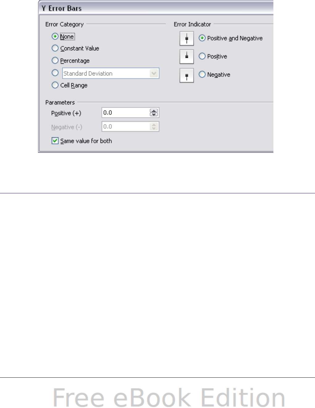
–Standard deviation – shows error calculated on standard
deviation
–Error margin – you designate the error
•Cell range – calculates the error based on cell ranges you select.
The Parameters section at the bottom of the dialog changes to
allow selection of the cell ranges.
Figure 62: Specifying the parameters of error bars
Formatting charts
The Format menu has many options for formatting and fine-tuning the
appearance of your charts.
Double-click the chart so that it is enclosed by a gray border indicating
edit mode; then, select the chart element that you want to format.
Choose Format from the menu bar, or right-click to display a pop-up
(context) menu relevant to the selected element. The formatting
choices are as follows.
Format Selection
Opens a dialog in which you can specify the area fill, borders,
transparency, characters, font effects, and other attributes of the
selected element of the chart (see page 91).
Position and Size
Opens a dialog (see page 94).
84 OpenOffice.org 3.x Calc Guide

Arrangement
Provides two choices: Bring Forward and Send Backward, of
which only one may be active for some items. Use these choices to
arrange overlapping data series.
Title
Formats the titles of the chart and its axes.
Legend
Formats the location, borders, background, and type of the legend.
Axis
Formats the lines that create the chart as well as the font of the text
that appears on both the X and Y axes.
Grid
Formats the lines that create a grid for the chart.
Chart Wall, Chart Floor, Chart Area
Described in the following sections.
Chart Type
Changes what kind of chart is displayed and whether it is two- or
three-dimensional.
Data Ranges
Explained on page 76 (Figure 55 and Figure 56).
3D View
Formats 3D charts (see page 87).
Note
Chart Floor and 3D View are only available for a 3D chart.
These options are unavailable (grayed out) if a 2D chart is
selected.
In most cases you need to select the exact element you want to format.
Sometimes this can be tricky to do with the mouse, if the chart has
many elements, especially if some of them are small or overlapping. If
you have Tooltips turned on (in Tools > Options > OpenOffice.org >
General > Help, select Tips), then as you move the mouse over each
element, its name appears in the Tooltip. Once you have selected one
element, you can press Tab to move through the other elements until
you find the one you want. The name of the selected element appears
in the Status Bar.
Chapter 3 Creating Charts and Graphs 85
Moving chart elements
You may wish to move or resize individual elements of a chart,
independent of other chart elements. For example, you may wish to
move the legend to a different place. Pie charts allow moving of
individual wedges of the pie (in addition to the choice of “exploding”
the entire pie).
1) Double-click the chart so that it is enclosed by a gray border.
2) Double-click any of the elements—the title, the legend, or the
chart graphic. Click and drag to move the element. If the element
is already selected, then move the pointer over the element to get
the move icon (small hand), then click, drag and move the
element.
3) Release the mouse button when the element is in the desired
position.
Note
If your graphic is 3D, round red handles appear which control
the three-dimensional angle of the graphic. You cannot resize or
reposition the graphic while the round red handles are showing.
With the round red handles showing, Shift + Click to get the
green resizing handles. You can now resize and reposition your
3D chart graphic. See the following tip.
Tip
You can resize the chart graphic using its green resizing handles
(Shift + Click, then drag a corner handle to maintain the
proportions). However, you cannot resize the title or the key.
Changing the chart area background
The chart area is the area surrounding the chart graphic, including the
(optional) main title and key.
1) Double-click the chart so that it is enclosed by a gray border.
2) Choose Format > Chart Area.
3) On the Chart Area dialog (Figure 63), choose the desired format
settings.
On the Area tab, you can change the color, or choose a hatch pattern,
bitmap or some preset gradients. Click on the drop-down box to see
the options. Patterns are probably more useful than color if you have to
print out your chart in black and white.
You can also use the Transparency tab to change the area’s
transparency. If you used a preset gradient from the Area tab, you can
see the different parameters of which it is composed.
86 OpenOffice.org 3.x Calc Guide

Figure 63: Chart Area dialog
Changing the chart graphic background
The chart wall is the area that contains the chart graphic.
1) Double-click the chart so that it is enclosed by a gray border.
2) Choose Format > Chart Wall. The Chart Wall dialog has the
same formatting options as described in “Changing the chart area
background” above.
3) Choose your settings and click OK.
Changing colors
If you need a different color scheme from the default for the charts in
all your documents, go to Tools > Options > Charts > Default
Colors, which has a much wider range of colors to choose from.
Changes made in this dialog affect the default chart colors for any
chart you make in future.
Formatting 3D charts
Use Format > 3D View to fine tune 3D charts. The 3D View dialog has
three pages, where you can change the perspective of the chart,
whether the chart uses the simple or realistic schemes, or your own
custom scheme, and the illumination which controls where the
shadows will fall.
Chapter 3 Creating Charts and Graphs 87
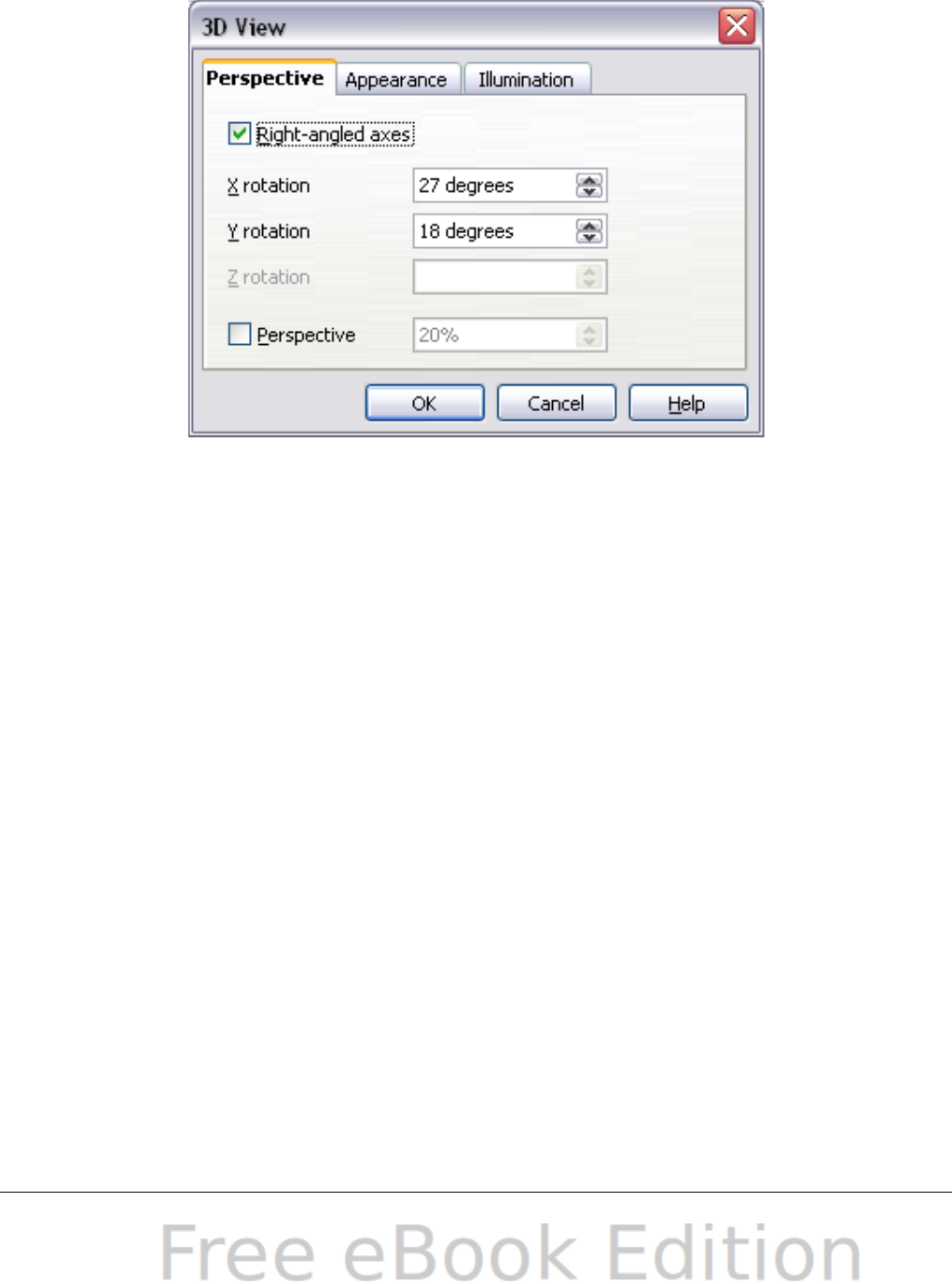
Rotation and perspective
To rotate a 3D chart or view it in perspective, enter the required values
on the Perspective page of the 3D View dialog. You can also rotate 3D
charts interactively; see page 90.
Figure 64: Rotating a chart
Some hints for using the Perspective page:
•Set all angles to 0 for a front view of the chart. Pie charts and
donut charts are shown as circles.
•With Right-angled axes enabled, you can rotate the chart contents
only in the X and Y direction; that is, parallel to the chart borders.
•An x value of 90, with y and z set to 0, provides a view from the
top of the chart. With x set to –90, the view is from the bottom of
the chart.
•The rotations are applied in the following order: x first, then y,
and z last.
•When shading is enabled and you rotate a chart, the lights are
rotated as if they are fixed to the chart.
•The rotation axes always relate to the page, not to the chart’s
axes. This is different from some other chart programs.
•Select the Perspective option to view the chart in central
perspective as through a camera lens instead of using a parallel
projection.
Set the focus length with the spin button or type a number in the
box. 100% gives a perspective view where a far edge in the chart
looks approximately half as big as a near edge.
88 OpenOffice.org 3.x Calc Guide
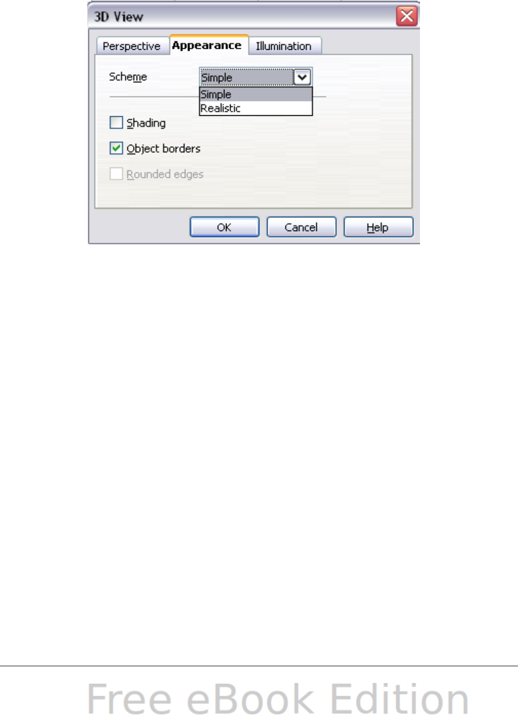
Appearance
Use the Appearance page to modify some aspects of a 3D chart’s
appearance.
Figure 65: Modifying appearance of 3D chart
Select a scheme from the list box. When you select a scheme, the
options and the light sources are set accordingly. If you select or
deselect a combination of options that is not given by the Realistic or
Simple schemes, you create a Custom scheme.
Select Shading to use the Gouraud method for rendering the surface.
Otherwise, a flat method is used. The flat method sets a single color
and brightness for each polygon. The edges are visible, soft gradients
and spot lights are not possible. The Gouraud method applies gradients
for a smoother, more realistic look. Refer to the Draw Guide for more
details on shading.
Select Object Borders to draw lines along the edges.
Select Rounded Edges to smooth the edges of box shapes. In some
cases this option is not available.
Illumination
Use the Illumination page (Figure 66) to set the light sources for the
3D view. Refer to the Draw Guide for more details on setting the
illumination.
Click any of the eight buttons to switch a directed light source on or
off. By default, the second light source is switched on. It is the first of
Chapter 3 Creating Charts and Graphs 89
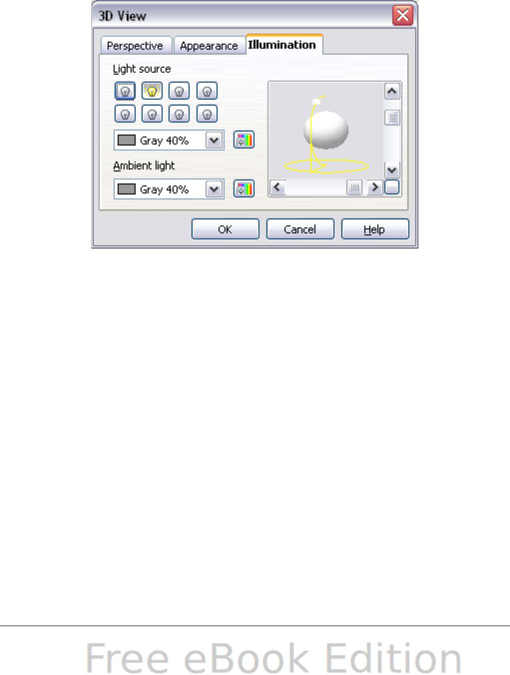
seven normal, uniform light sources. The first light source projects a
specular light with highlights.
For the selected light source, you can then choose a color and intensity
in the list just below the eight buttons. The brightness values of all
lights are added, so use dark colors when you enable multiple lights.
Figure 66: Setting the illumination
Each light source always points at the middle of the object initially. To
change the position of the light source, use the small preview inside
this page. It has two sliders to set the vertical and horizontal position
of the selected light source.
The button in the corner of the small preview switches the internal
illumination model between a sphere and a cube.
Use the Ambient light list to define the ambient light which shines with
a uniform intensity from all directions.
Rotating 3D charts interactively
In addition to using the Perspective page of the 3D View dialog to
rotate 3D charts, you can also rotate them interactively.
Select the Chart Wall, then hover the mouse pointer over a corner
handle or the rotation symbol found somewhere on the chart. The
cursor changes to a rotation icon.
Press and hold the left mouse button and drag the corner in the
direction you wish. A dashed outline of the chart is visible while you
drag, to help you see how the result will look.
90 OpenOffice.org 3.x Calc Guide
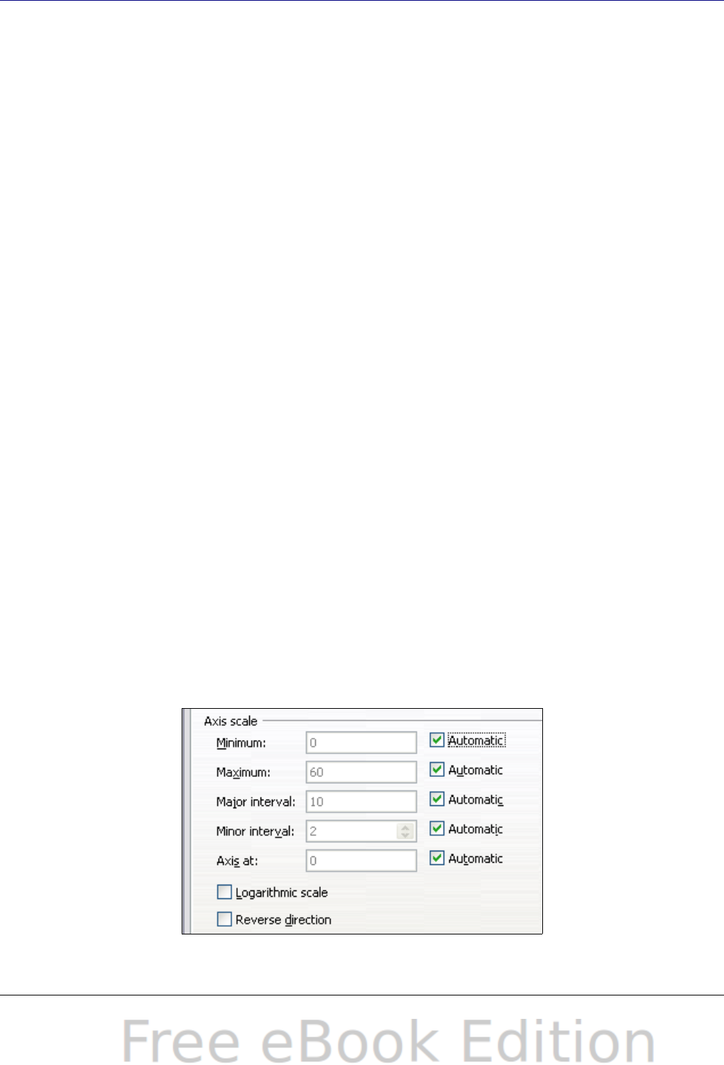
Formatting the chart elements
Depending on the purpose of your document, for example a screen
presentation or a printed document for a black and white publication,
you might wish to use more detailed control over the different chart
elements to give you what you need.
To format an element, left-click on the element that you wish to
change, for example one of the axes. The element will be highlighted
with green squares. Then, right-click and choose an item from the
context menu. Each chart element has its own selection of items. In the
next few sections we explore some of the options.
Formatting axes and inserting grids
Sometimes you need to have a special scale for one of the axes of your
chart, or you need smaller grid intervals, or you want to change the
formating of the labels on the axis. After highlighting the axis you wish
to change, right-click and choose one of the items from the pop-up
menu.
Choosing Format Axis opens the dialog shown in (Figure 67). On the
Scale tab, you can choose a logarithmic or linear scale (default), how
many marks you need on the line, where the marks are to appear, and
the increments (intervals) of the scale. You must first deselect the
Automatic option in order to modify the value for any scale.
On the Label tab (Figure 68), you can choose whether to show or hide
the labels and how to handle them when they won’t all fit neatly into
one row (for example, if the words are too long).
Not shown here are the tab with options for choosing a font,
formatting the lines, and positioning the elements of the line and
interval marks.
Figure 67: Formatting axis scales
Chapter 3 Creating Charts and Graphs 91
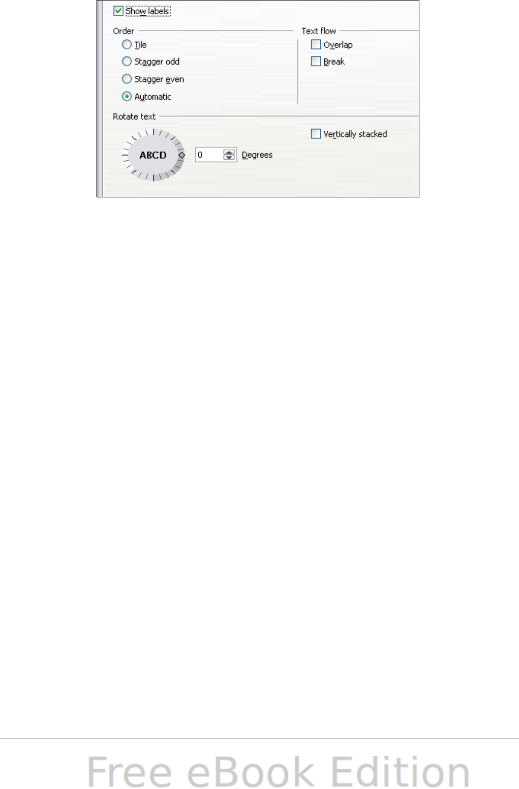
Figure 68: Formatting axis labels
Formating data labels
You can choose properties for the labels of the data series. Carefully
click on the chart element, then right-click and choose the property
you want to change. This opens a dialog with several tabs where you
can change the color of the label text, the size of the font, and other
attributes. The Label tab is shown in Figure 68.
On the Data Labels tab, you can choose whether to:
•Show the labels as text
•Show numeric values as a percentage or a number
•Include the legend box as part of the label
These choices are the same as those shown in Figure 60 on page 81.
The text for labels is taken from the column labels and it cannot be
changed here. If the text needs to be abbreviated, or if it did not label
your graph as you were expecting, you need to change it in the original
data table.
Choosing and formatting symbols
In line and scatter charts the symbols representing the points can be
changed to a different symbol shape or color through the object
properties dialog. Select the data series you wish to change, right-
click, and choose Format > Data Series from the context menu.
On the Line tab of the Data Series dialog, in the Icon section, choose
from the drop-down list Select > Symbols. Here you can choose no
symbol, a symbol from an inbuilt selection, a more exciting range from
92 OpenOffice.org 3.x Calc Guide
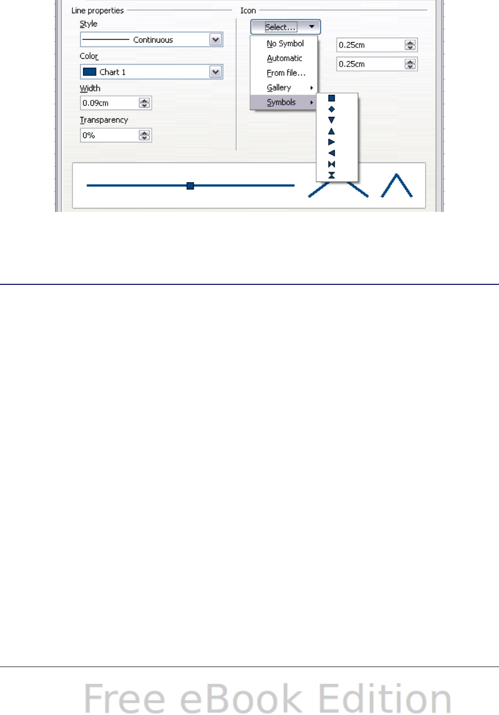
the gallery, or if you have pictures you need to use instead, you can
insert them using Select > From file.
Figure 69: Symbol selection
Resizing and moving the chart
You can resize or move all elements of a chart at the same time, in two
ways: interactively, or by using the Position and Size dialog. You may
wish to use a combination of both methods: interactive for quick and
easy change, then the dialog for precise sizing and positioning.
To resize a chart interactively:
1) Click once on the chart to select it. Green sizing handles appear
around the chart.
2) To increase or decrease the size of the chart, click and drag one
of the markers in one of the four corners of the chart. To maintain
the correct ratio of the sides, hold the Shift key down while you
click and drag.
To move a chart interactively:
1) Click on the chart to select it. Green sizing handles appear around
the chart.
2) Hover the mouse pointer anywhere over the chart. When it
changes to the move icon, click and drag the chart to its new
location.
3) Release the mouse button when the element is in the desired
position.
Chapter 3 Creating Charts and Graphs 93
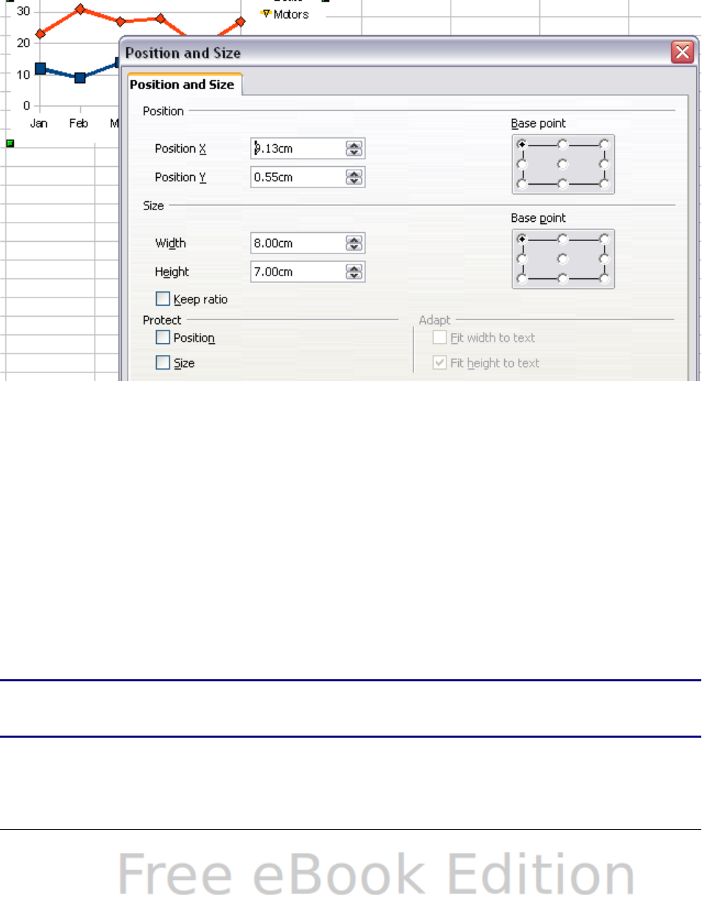
Using the Position and Size dialog
To resize or move a chart using the Position and Size dialog:
1) Click on the chart to select it. Green sizing handles appear around
the chart.
2) Right-click and choose Position and Size from the pop-up menu.
3) Make your choices on this dialog.
Figure 70: Defining the position and size of an object
Position is defined as an X,Y coordinate relative to a fixed point (the
base point), typically located at the upper left of the document. You can
temporarily change this base point to make positioning or
dimensioning simpler (click on the spot corresponding to the location
of the base point in either of the two selection windows on the right
side of the dialog—upper for positioning or lower for dimensioning).
The possible base point positions correspond to the handles on the
selection frame plus a central point. The change in position lasts only
as long as you have the dialog open; when you close this dialog, Calc
resets the base point to the standard position.
Tip The Keep ratio option is very useful. Select it to keep the ratio
of width to height fixed while you change the size of an object.
Either or both the size and position can be protected so that they
cannot be accidentally changed. Select the appropriate options.
94 OpenOffice.org 3.x Calc Guide

Tip If you cannot move an object, check to see if its position is
protected.
Gallery of chart types
Its important to remember that while your data can be presented with
a number of different charts, the message you want to convey to your
audience dictates the chart you ultimately use. The following sections
present examples of the types of charts that Calc provides, with some
of the tweaks that each sort can have and some notes as to what
purpose you might have for that chart type. For details, see the Help.
Column charts
Column charts are commonly used for data that shows trends over
time. They are best for charts that have a relatively small number of
data points. (For large time series a line chart would be better.) It is
the default chart type, as it is one of the most useful charts and the
easiest to understand.
Bar charts
Figure 71: Three bar graph treatments.
Bar charts are excellent for giving an immediate visual impact for data
comparison in cases when time is not an important factor, for example,
when comparing the popularity of a few products in a marketplace.
•The first chart is achieved quite simply by using the chart wizard
with Insert > Grids, deselecting y-axis, and using Insert >
Mean Value Lines.
Chapter 3 Creating Charts and Graphs 95
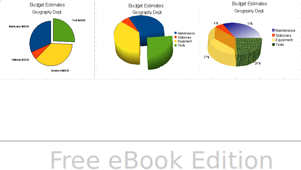
•The second chart is the 3D option in the chart wizard with a
simple border and the 3D chart area twisted around.
•The third chart is an attempt to get rid of the legend and put
labels showing the names of the companies on the axis instead.
We also changed the colors to a hatch pattern.
Pie charts
Pie charts are excellent when you need to compare proportions. For
example, comparisons of departmental spending: what the department
spent on different items or what different departments spent. They
work best with smaller numbers of values, about half a dozen; more
than this and the visual impact begins to fade.
As the Chart Wizard guesses the series that you wish to include in your
pie chart, you might need to adjust this initially on the Wizard’s Data
Ranges page if you know you want a pie chart, or by using the Format
> Data Ranges > Data Series dialog.
You can do some interesting things with a pie chart, especially if you
make it into a 3D chart. It can then be tilted, given shadows, and
generally turned into a work of art. Just don’t clutter it so much that
your message is lost, and be careful that tilting does not distort the
relatively size of the segments.
You can choose in the Chart Wizard to explode the pie chart, but this is
an all or nothing option. If your aim is to accentuate one piece of the
pie, you can separate out one piece by carefully highlighting it after
you have finished with the Chart Wizard, and dragging it out of the
group. When you do this you might need to enlarge the chart area
again to regain the original size of the pieces.
Figure 72: Pie charts
The effects achieved in Figure 72 are explained below:
•2D pie chart with one part of the pie exploded: Choose Insert >
Legend and deselect the Display legend box. Choose Insert >
96 OpenOffice.org 3.x Calc Guide
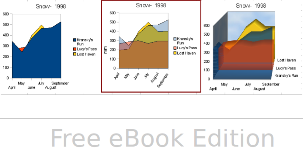
Data Labels and choose Show value as number. Then carefully
select the piece you wish to highlight, move the cursor to the
edge of the piece and click (the piece will have nine green
highlight squares to mark it), and then drag it out from the rest of
the pieces. The pieces will decrease in size, so you need to
highlight the chart wall and drag it at a corner to increase the
size.
3D pie chart with realistic schema and illumination: Choose
Format > 3D view > Illumination where you can change the
direction of the light, the color of the ambient light, and the depth
of the shade. We also adjusted the 3D angle of the disc in the
Perspective dialog on the same set of tabs.
The chart updates as you make changes, so you can immediately
see the effects.
If you want to separate out one of the pieces, click on it carefully;
you should see a wire frame highlight. Drag it out with the mouse
and then, if necessary, increase the size of the chart wall.
•3D pie chart with different fill effects in each portion of the pie:
Choose Insert > Data labels and select show value as
percentage. Then carefully select each of the pieces so that it has
a wire frame highlight and right-click to get the object properties
dialog; choose the Area tab. For one we chose a bitmap, for
another a gradient and for the third we used the Transparency
tab and adjusted the transparency to 50%.
Area charts
An area chart is a version of a line or column graph. It may be useful
where you wish to emphasize volume of change. Area charts have a
greater visual impact than a line chart, but the data you use will make
a difference.
Figure 73: Area charts—the good, the bad, and the ugly
Chapter 3 Creating Charts and Graphs 97
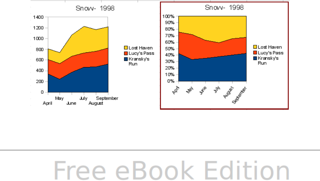
As shown in Figure 73, an area chart is sometimes tricky to use. This
may be one good reason to use transparency values in an area chart.
After setting up the basic chart using the Chart Wizard, do this:
•Right-click on the Y axis and choose Delete Major Grid. As the
data overlaps, some of it is missing behind the first data series.
This is not what you want. A better solution is shown in Chart 2.
•After deselecting the Y axis grid, right-click on each data series in
turn and choose Format Data Series. On the Transparency tab,
set Transparency to 50%. The transparency makes it easy to see
the data hidden behind the first data series. Now, right-click on
the X axis and choose Format Axis. On the Label tab, choose Tile
in the Order section and set the Text orientation to 55 degrees.
This places the long labels at an angle.
•To create the third variation, after doing the steps above, right-
click and choose Chart Type. Choose the 3D Look option and
select Realistic from the drop-down list. We also twisted the
chart area around and gave the chart wall a picture of the sky. As
you can see, the legend turns into labels on the z-axis. But overall,
though it is visually more appealing, it is more difficult to see the
point you are trying to make with the data.
Other ways of visualizing the same data series are represented by the
stacked area chart or the percentage stacked area chart. The first does
what it says: each number of each series is added to the others so that
it shows an overall volume but not a comparison of the data. The
percentage stacked chart shows each value in the series as a part of
the whole. For example in June all three values are added together and
that number represents 100%. The individual values are a percentage
of that. Many charts have varieties which have this option.
Figure 74: Stacked and percentage stacked area charts
98 OpenOffice.org 3.x Calc Guide
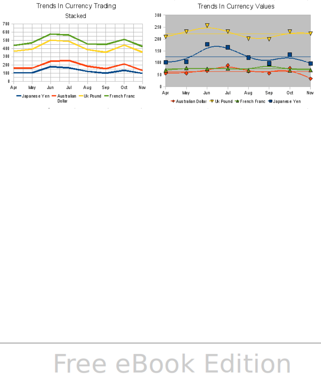
Line charts
A line chart is a time series with a progression. It is ideal for raw data,
and useful for charts with plentiful data that show trends or changes
over time where you want to emphasize continuity. On line charts, the
x-axis is ideal to represent time series data.
Things to do with lines: thicken them, make them 3D, smooth the
contours, just use points.
3D lines confuse the viewer, so just using a thicker line often works
better.
Figure 75: Line charts
Scatter or XY charts
Scatter charts are great for visualizing data that you have not had time
to analyze, and they may be the best for data when you have a constant
value against which to compare the data; for example, weather data,
reactions under different acidity levels, conditions at altitude, or any
data which matches two series of numeric data. In contrast to line
charts, the x-axis are the left to right labels, which usually indicate a
time series.
Scatter charts may surprise those unfamiliar with how they work.
While constructing the chart, if you choose Data Range > Data
series in rows, the first row of data represents the x-axis. The rest of
the rows of data are then compared against the first row data. Figure
76 shows a comparison of three currencies with the Japanese Yen.
Even though the table presents the monthly series, the chart does not.
In fact the Japanese Yen does not appear; it is merely used as the
constant series that all the other data series are compared against.
Chapter 3 Creating Charts and Graphs 99
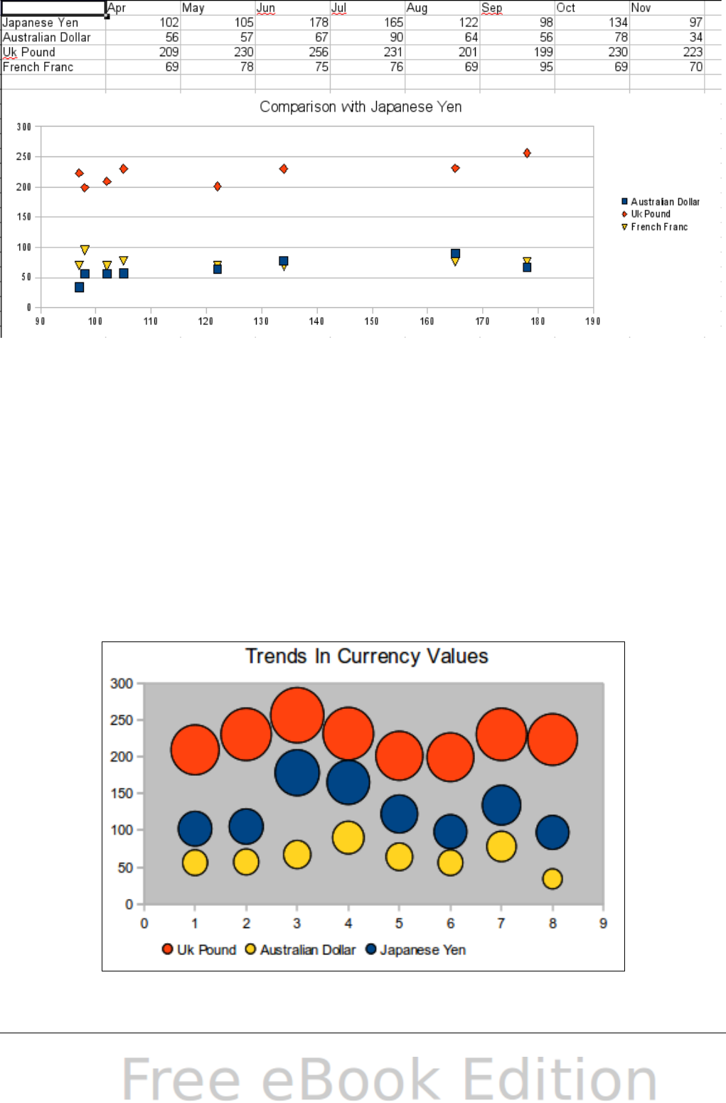
Figure 76: A particularly volatile time in the world currency market.
Bubble charts
A bubble chart is a variation of a scatter chart in which the data points
are replaced with bubbles. It shows the relations of three variables in
two dimensions. Two variables are used for the position on the X-axis
and Y-axis, while the third is shown as the relative size of each bubble.
One or more data series can be included in a single chart.
Bubble charts are often used to present financial data. The data series
dialog for a bubble chart has an entry to define the data range for the
bubbles and their sizes.
Figure 77: Bubble chart showing three data series
100 OpenOffice.org 3.x Calc Guide

Net charts
A net chart is similar to a polar or radar chart. They are useful for
comparing data that are not time series, but show different
circumstances, such as variables in a scientific experiment or
direction. The poles of the net chart are equivalent to the y-axes of
other charts. Generally, between three and eight axes are best; any
more and this type of chart becomes confusing. Before and after values
can be plotted on the same chart, or perhaps expected and real results,
so that differences can be compared.
Types of net charts:
•Figure 78 - Part 1: Plain net chart without grids and with just
points, no lines.
•Figure 79 - Part 2: Net chart with lines, points and grid. Axes
colors and labels changed. Chart area color = gradient. Points
changed to fancy 3D ones.
Figure 78: Two net diagrams showing totally fabricated data from
totally fictional experiments.
Other varieties of net chart show the data series as stacked numbers
or stacked percentages. The series can also be filled with a color.
Partial transparency is often best for showing all the series.
Chapter 3 Creating Charts and Graphs 101
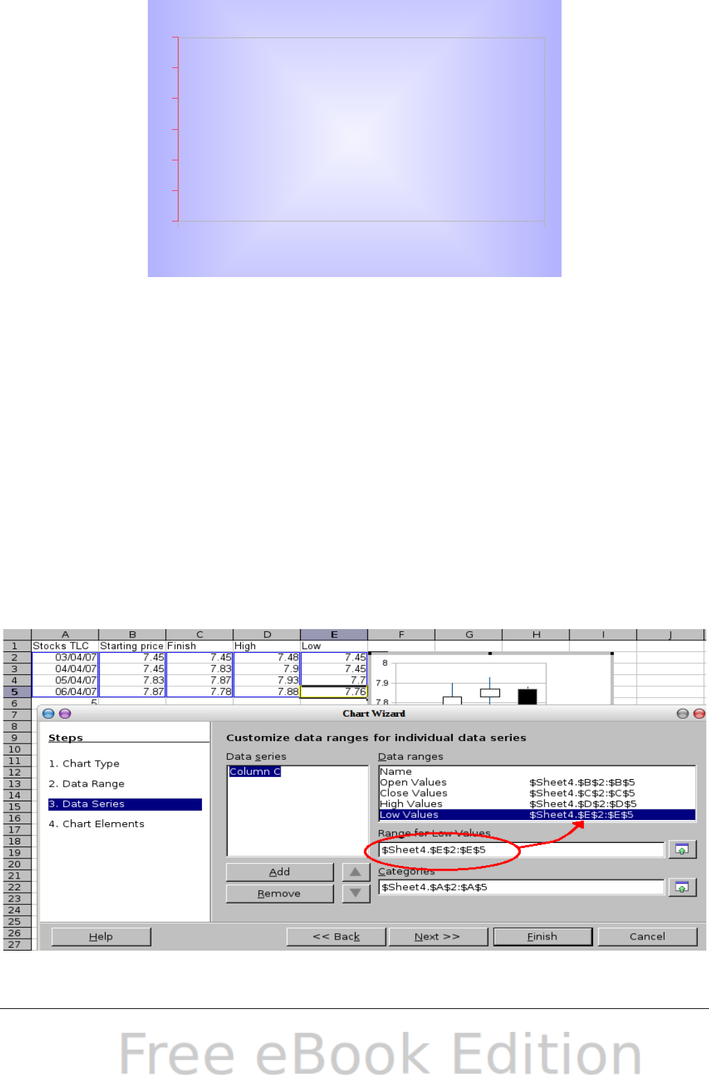
green
0
2
4
6
8
10
12
Coloured light on mood
Figure 79: Filled net or radar chart
Stock charts
A stock chart is a specialized column graph specifically for stocks and
shares. You can choose traditional lines, candlestick, and two-column
type charts. The data required for these charts is quite specialized,
with series for opening price, closing price, and high and low prices. Of
course the x-axis represents a time series.
When you set up a stock chart in the Chart Wizard, the Data Series
dialog is very important. You need to tell it which series is for the
opening price, closing price, high and low price of the stock and so on.
Otherwise the chart may be indecipherable. The sample table for this
chapter needed to be changed to fit the data series.
Figure 80: Adjusting data series for stock charts.
102 OpenOffice.org 3.x Calc Guide
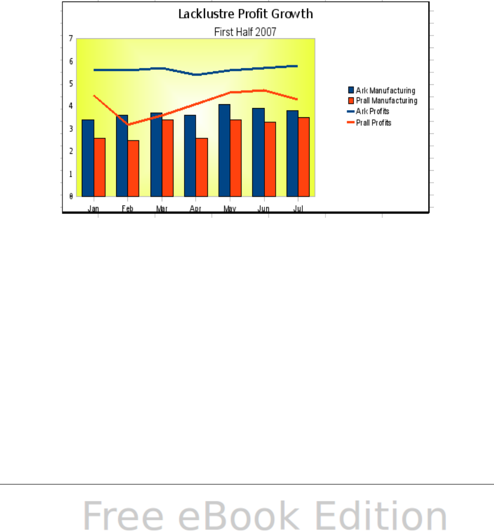
A nice touch is that OpenOffice.org Chart color-codes the rising and
falling shares: white for rising and black for falling in the candlestick
chart, and red and blue in the traditional line chart.
Column and line charts
A column and line chart is a combination of two other chart types. It is
useful for combining two distinct but related data series, for example
sales over time (column) and the profit margin trends (line).
You can choose the number of columns and lines in the Chart Wizard.
So for example you might have two columns with two lines to
represent two product lines with the sales figures and profit margins of
both.
Figure 81: Column and line chart
This chart has manufacturing cost and profit data for two products,
over a period of time (six months in 2007). To create this chart, first
highlight the table and start the Chart Wizard. Choose Column and
Line chart type with two lines and the data series in rows. Then give it
a title to highlight the aspect you want to show. The lines are different
colors at this stage and don’t reflect the product relationships. When
you finish with the Chart Wizard, highlight the chart, click on the line,
right-click and chose Format Data Series.
On this tab there are a few things to change: The colors should match
the products. So both Ark Manufacturing and profit are blue and Prall
is red. The lines need to be more noticeable so make the lines thicker
by increasing the width to 0.08.
Chapter 3 Creating Charts and Graphs 103

For the background, highlight the chart wall, right-click and choose
Format Wall. On the Area tab, change the drop-down box to show
Gradient. Choose one of the preset gradient patterns and make it
lighter by going to the Transparency tab and making the gradient 50%
transparent.
To make the chart look cleaner without the grid, go to Insert > Grids
and deselect the X-axis option.
104 OpenOffice.org 3.x Calc Guide

Chapter 4
Using Styles and
Templates in Calc
Bringing uniformity to your spreadsheets

What is a template?
A template is a model that you use to create other documents. For
example, you can create a template for invoices that has your
company’s logo and address at the top of the page. New spreadsheets
created from this template will all have your company’s logo and
address on the first page.
Templates can contain anything that regular documents can contain,
such as text, graphics, styles, and user-specific setup information such
as measurement units, language, the default printer, and toolbar and
menu customization.
All documents—text, spreadsheets, presentations, drawings—in
OpenOffice.org are based on templates. You can create, or download
and install, as many templates as you wish. When you start a new
spreadsheet without choosing a specific template (as described in
“Creating a spreadsheet from a template“ on page 119), the new
spreadsheet is based on the default template for spreadsheets. If you
have not specified a default template, OOo uses the blank spreadsheet
template that is installed with OOo. See “Setting a default template”
on page 124.
This chapter describes how to create, use, modify, and organize
templates. We begin by describing styles and their use, as styles are a
major component of templates.
What are styles?
A style is a set of formats that you can apply to selected elements in a
document to quickly change their appearance. When you apply a style,
you apply a whole group of formats at the same time.
Many people manually format spreadsheet cells and pages without
paying any attention to styles. They are used to formatting documents
according to physical attributes. For example, for the contents of a cell
you might specify the font family, font size, and any formatting such as
bold or italic.
Styles are logical attributes. Using styles means that you stop saying
“font size 14pt, Times New Roman, bold, centered”, and you start
saying “Title” because you have defined the “Title” style to have those
characteristics. In other words, styles means that you shift the
emphasis from what the text (or page, or other element) looks like, to
what the text is.
106 OpenOffice.org 3.x Calc Guide

Styles help improve consistency in a document and can greatly speed
up formatting. They also make major formatting changes easy. For
example, you may decide to change the appearance of all subtotals in
your spreadsheet to be 10 pt. Arial instead of 8 pt. Times New Roman
after you have created a 15-page spreadsheet; you can change all of
the subtotals in the document by simply changing the properties for
the subtotal style.
Page styles assist with printing, so you don’t need to define margins,
headers and footers, and other printing attributes each time you print
a spreadsheet.
This chapter describes the styles OOo Calc offers, what they might be
used for, and how to apply styles, change existing styles, and create
new styles.
Types of styles in Calc
While some components of OOo offer many style types, Calc offers only
two:
•Cell styles include fonts, alignment, borders, background, number
formats (for example, currency, date, number), and cell
protection.
•Page styles include margins, headers and footers, borders and
backgrounds, and the sequence for printing sheets. The page size,
orientation, and other attributes of a page style apply only when a
spreadsheet is printed; they are not displayed onscreen.
Cell styles
Similar to paragraph styles in OOo Writer, cell styles are the most
basic type of style in Calc. You can apply a cell style to a cell and that
cell will follow the formatting rules of the style. Five cell styles are
supplied with OOo: Default, Heading, Heading1, Result, and Result2.
Initially, the styles are configured so that if you change the font family
of Default, then all of the other styles will change to match. We will
discuss how to set this up in “Creating new (custom) styles” on page
116. The five standard styles can be seen in use in Figure 82.
Chapter 4 Using Styles and Templates in Calc 107
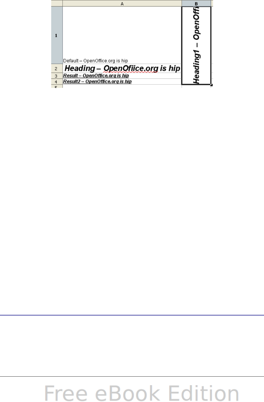
Figure 82: Calc cell style types
Page styles
Page styles in Calc are applied to sheets. Although one sheet may print
on several pages (pieces of paper), only one page style can be applied
to a sheet. If a spreadsheet file contains more than one sheet, the
different sheets can have different page styles applied to them. So, for
example, a spreadsheet might contain one sheet to be printed in
landscape orientation (using the Default page style) and another sheet
to be printed in portrait orientation (using the Report page style).
Two page styles are supplied with Calc: Default and Report. The major
difference between these two styles is that Report is portrait-oriented
and Default is landscape-oriented. You can adjust many settings using
page styles. You can also define as many page styles as you wish.
Because spreadsheets are primarily used onscreen and not printed,
Calc does not display the page style on the screen. If you want a
spreadsheet to fit on a certain page size, you have to carefully control
the column width and row height, with only File > Page Preview to
guide you.
Despite this limitation, it’s well worth defining page styles for any
spreadsheets that you are likely to print. Otherwise, if a need for
printing does arise, you may lose time to trial and error.
Accessing styles
The main way to access styles is through the Styles and Formatting
window (shown in Figure 83). You can open this window in several
ways.
•Keyboard: Press the F11 key.
•Menu: Choose Format > Styles and Formatting.
108 OpenOffice.org 3.x Calc Guide
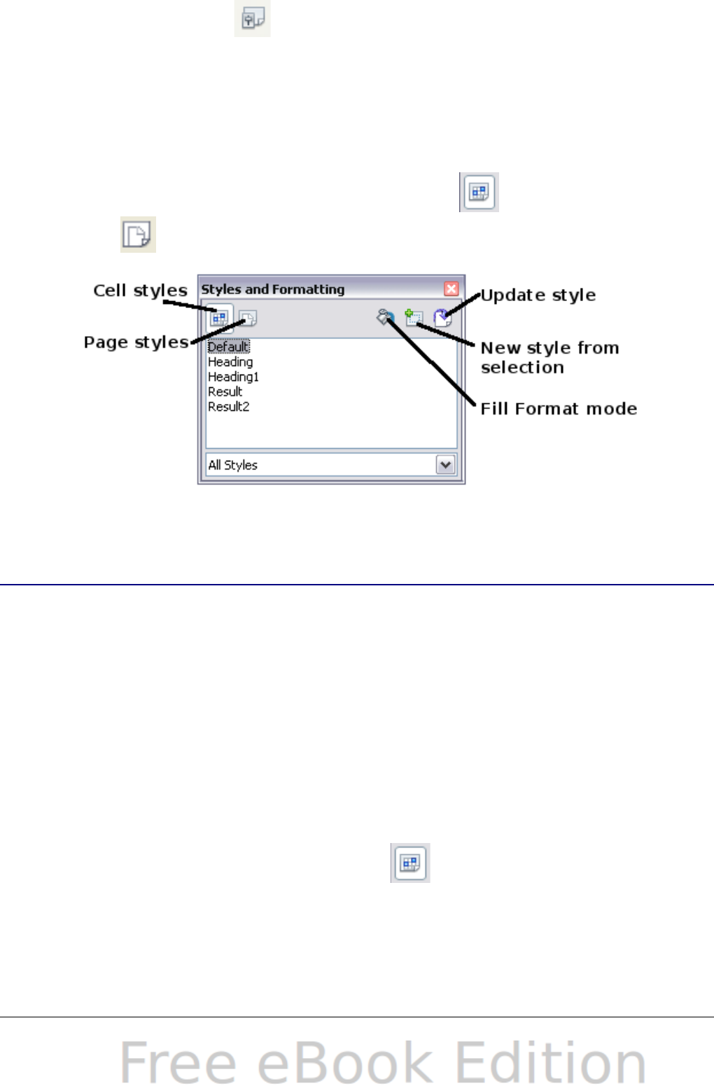
•Toolbar: Click the icon on the far left of the Formatting
toolbar.
The Styles and Formatting window can be docked at the left or right of
the main Calc window. To dock or undock the window, hold down the
Ctrl key and double-click a gray part of the window next to the icons at
the top.
The first button on the top left of the window, , is for cell styles and
the second, , is for page styles.
Figure 83: Styles and Formatting window
Applying cell styles
Calc provides several ways to apply cell styles:
•Using the Styles and Formatting window
•Using Fill Format mode
•Using the Apply Style list
•Assigning styles to shortcut keys
Using the Styles and Formatting window
1) Ensure the Styles and Formatting window is open by pressing
F11 or by selecting Format > Styles and Formatting. Choose
the Cell Styles list by clicking the icon.
2) Highlight the cell or group of cells to which the styles should be
applied.
3) Double-click on the cell style name.
Chapter 4 Using Styles and Templates in Calc 109
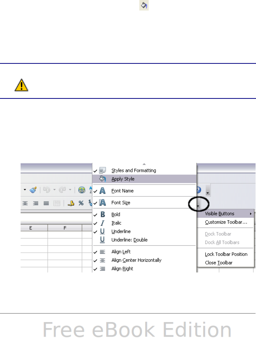
Using Fill Format mode
This method is quite useful when you need to apply the same style to
many scattered cells.
1) Open the Styles and Formatting window and select the style you
want to apply.
2) Click the Fill Format mode icon . The mouse pointer changes
to this icon.
3) Position the moving icon on the cell to be styled and click the
mouse button.
4) To quit Fill Format mode, click the Fill Format mode icon again
or close the Styles and Formatting window.
Caution When this mode is active, a right-click anywhere in the
document undoes the last Fill Format action. Be careful not to
accidentally right-click and thus undo actions you want to
keep.
Using the Apply Style list
You can also add an Apply Style drop-down list to the Formatting
toolbar and select a style from the list to apply it to the selected cells:
1) Click the down-arrow at the right-hand end of the Formatting
toolbar. On the drop-down menu, click Visible Buttons.
Figure 84: Adding an Apply Style list to the Formatting toolbar
110 OpenOffice.org 3.x Calc Guide
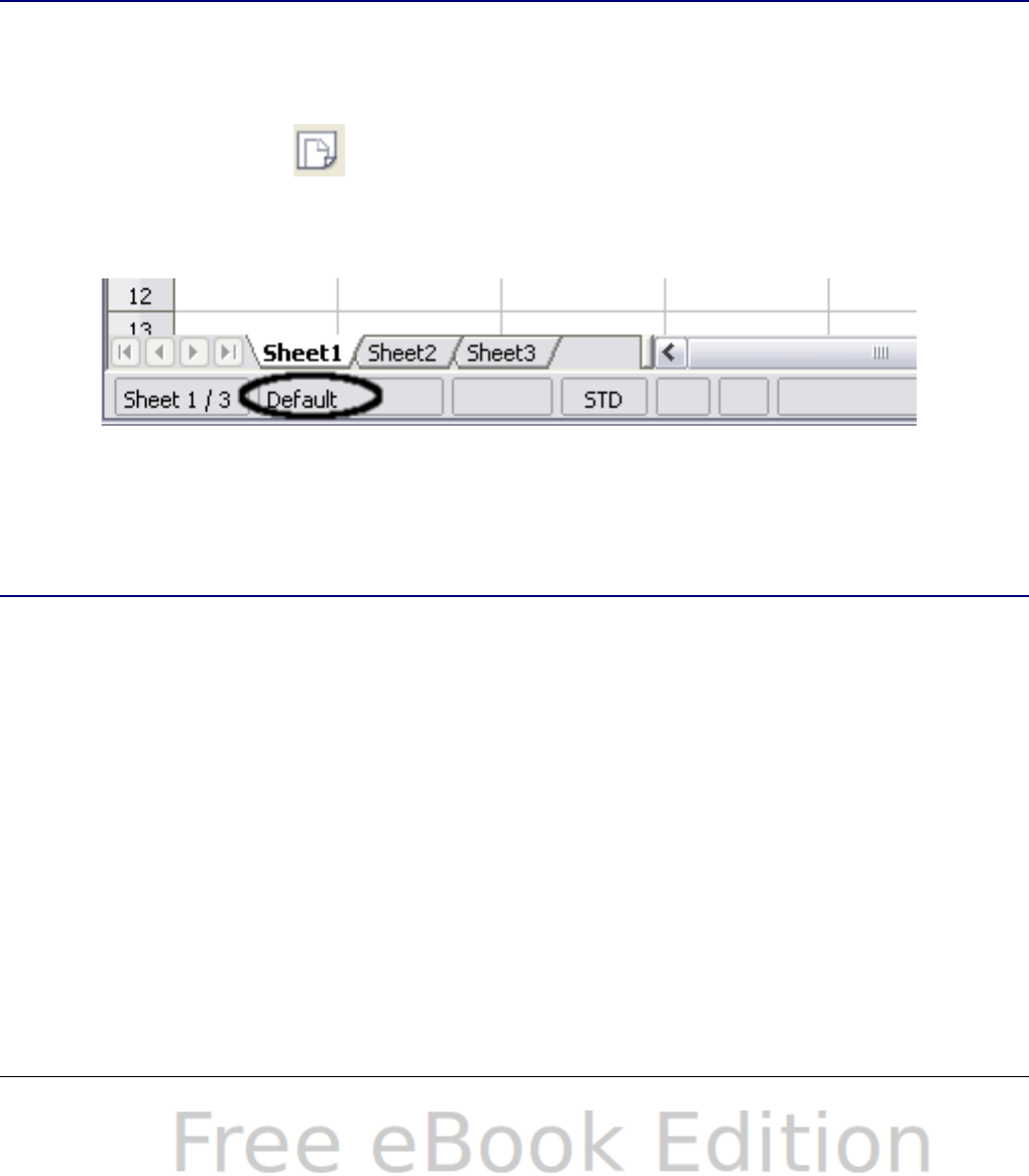
2) On the submenu, click Apply Style. The menus close and the
Apply Style list now appears on the toolbar between the Styles
and Formatting icon and the Font Name list.
Assigning styles to shortcut keys
You can create keyboard shortcuts to apply commonly-used cell or
page styles, including custom styles that you have created. See
Chapter 14 (Setting up and Customizing Calc) for instructions.
Applying page styles
1) Select the sheet to be styled (click on its sheet tab at the bottom
of the screen).
2) In the Styles and Formatting window, choose the Page Styles list
by clicking the icon. Double-click on the required page style.
To find out which page style is in use for a selected sheet, look in
status bar.
Figure 85: Status bar showing location of page style
information below the sheet tabs.
Modifying styles
To modify a style, right-click on its name in the Styles and Formatting
window and choose Modify. Make the changes in the Style dialog and
click OK to save the changes.
You can also modify a current cell style by selecting an already
formatted cell and clicking the Update Style button on the top right
hand corner of the Styles and Formatting window.
Style organizer
Right click on the name of a style in the Styles and Formatting window
and click Modify to open a Style dialog similar to the one shown in
Figure 86.
Chapter 4 Using Styles and Templates in Calc 111
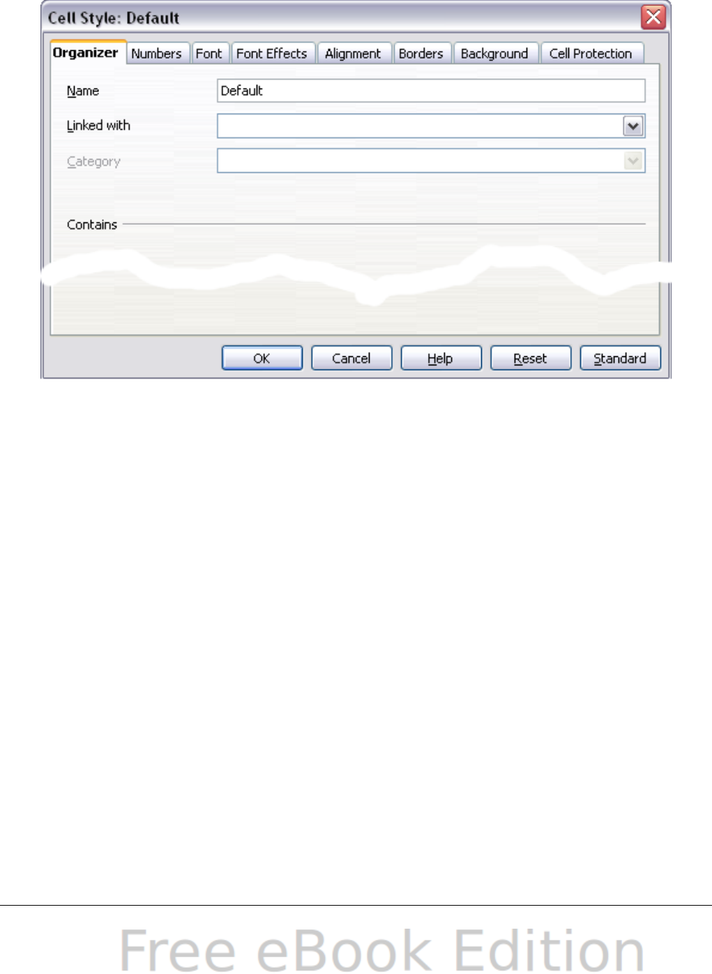
The Style dialog has several tabs. The Organizer tab, shown in Figure
86 for cell styles, is found in all components of OOo. It provides basic
information about the style. The Organizer tab for page styles is similar
to the one shown for cell styles.
Figure 86: Organizer tab of Cell Style dialog
Name
This is the style’s name. You cannot change the name of a built-in
style, but you can change the name of a custom style.
Linked with
This option is only available for cell styles; page styles cannot be
linked. If you link cell styles, then when you change the base style
(for example, by changing the font from Times to Helvetica), all the
linked styles will change as well. Sometimes this is exactly what you
want; other times you do not want the changes to apply to all the
linked styles. It pays to plan ahead.
For example, you can make a new style called red, in which the only
change you want to make is for the cell text to be red. In order to
make sure that the rest of the text characteristics are the same as
the default style, you can link red with default. Then, any changes
you make to default will be automatically applied to red.
Category
In Calc, the only option in this drop-down box is Custom styles.
112 OpenOffice.org 3.x Calc Guide

Cell style options
When editing or creating cell styles, you can set several options, which
are similar to those for directly formatting cells. A more detailed
coverage of cell formatting is given in Chapter 2 (Entering, Editing,
and Formatting Data). A brief summary is provided here.
Numbers
On the Numbers tab, you can control the behavior of the data in a cell
with this style. This includes specifying the type of data, the number of
decimal places, and the language.
Font
Use the Font tab to choose the font for the cell’s contents..
Font effects
The Font Effects tab offers more font options including underlining,
strikethrough, and color.
Alignment
Use the Alignment tab to set the horizontal and vertical alignment for
the data in the cells, and rotate the text.
Borders
Use the Borders tab to set the borders for the cells, along with a
shadow.
Background
Use the Background tab to choose the background color for a cell.
Cell protection
Use the Cell Protection options to protect cells against certain types of
editing.
Page style options
Several of the page style options are described in more detail in
Chapter 6 (Printing, Exporting, and E-mailing), because manually
formatting a sheet at print time (using Format > Page) actually
modifies the page style.
Chapter 4 Using Styles and Templates in Calc 113
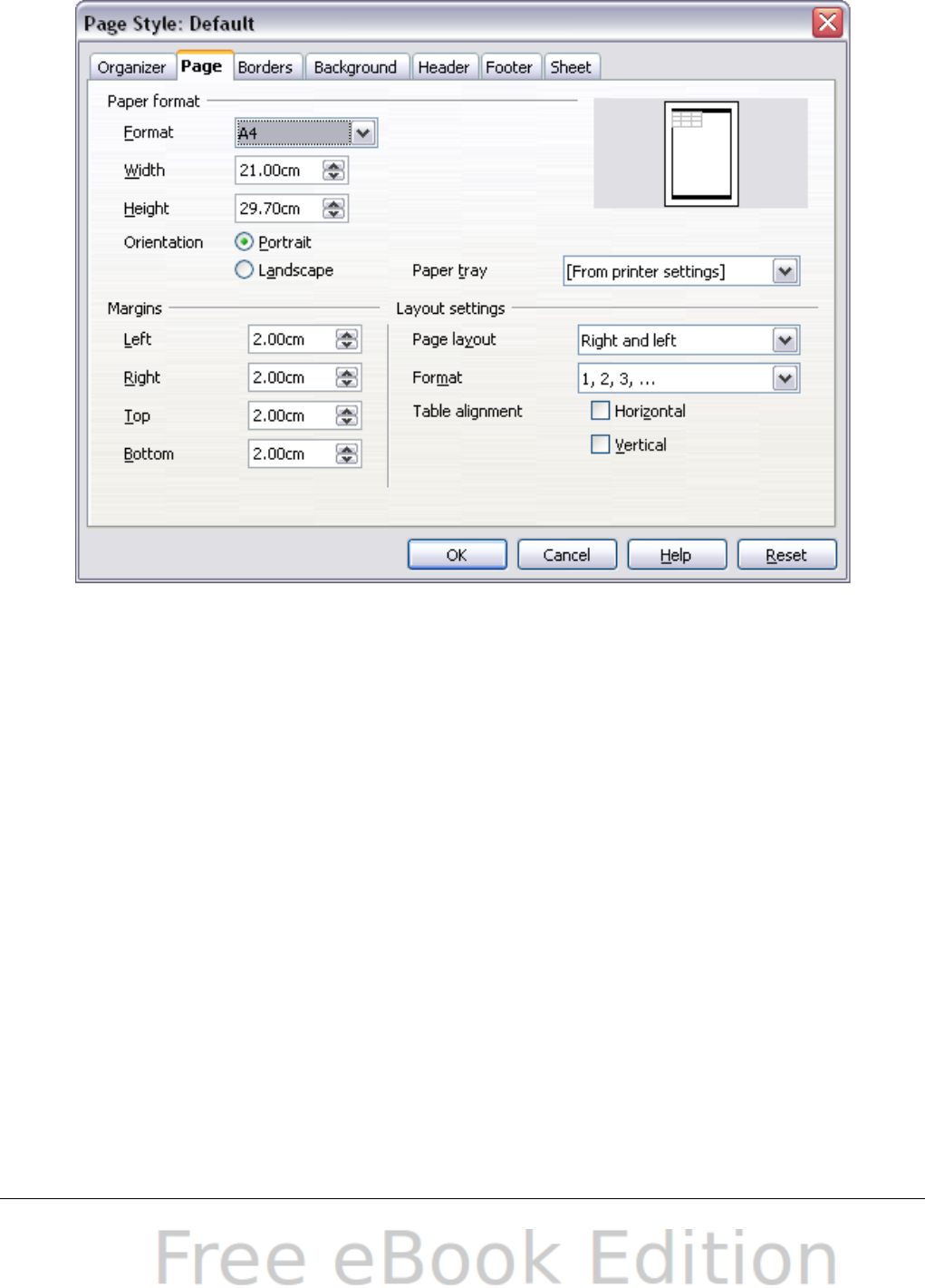
Page
Use the Page tab to edit the overall appearance of the page and its
layout. The available options are shown in Figure 87.
Figure 87: Page Style: Page tab
Paper format
Here you can set a generic paper type to be used. Letter or A4 are
most common, but you can also use legal, tabloid, envelope sizes, or
user-defined paper types. You can also define the orientation of the
page and which print tray for the paper to come from (if your printer
has more than one tray).
Margins
Here you can set the margins for the page.
Layout settings: Page layout
Here you can specify whether to apply the formatting to right (odd)
pages only, left (even) pages only, or both right and left pages that
use the current page style.
Mirrored formats the pages as if you want to bind the printed pages
like a book.
The first page of a document is assumed to be an odd page.
114 OpenOffice.org 3.x Calc Guide

Layout settings: Format
This area specifies the page numbering style for this page style.
Layout settings: Table alignment
This option specifies the alignment options for the cells on a printed
page, either horizontal or vertical.
Borders
The Border and Background tabs for pages duplicate the tabs of the
same name on cell styles, and are over-ridden by the cell style or
manual settings. You may choose to ignore the Border and Background
tabs altogether in page styles. Both tabs are illustrated with helpful
diagrams.
Similar to formatting a cell style, use the Borders tab to choose
whether the page should have borders, how large the borders should
be, and how far the text will be from the borders.
Background
Use this tab to specify the background for this page style. You can
apply either a solid color or a picture as a background.
Header
Use this tab to design and apply the header for this page style. For
more detailed instructions on how to format the header, see Chapter 6
(Printing, Exporting, and E-mailing).
Footer
Use this tab to design and apply the footer for this page style. For more
detailed instructions on how to format the footer, see Chapter 6.
Sheet
By far the most important settings for Calc page styles are on the
Sheet tab. Although the Sheet tab includes an option that sets the first
page option, most of its settings involve exactly how your spreadsheet
will print. See Chapter 6.
Chapter 4 Using Styles and Templates in Calc 115

Creating new (custom) styles
You may want to add some new styles. You can do this in two ways:
•Creating a new style using the Style dialog
•Creating a new style from a selection
Note
New styles apply only to this document; they are not be saved
in the template. To save new styles in a template, see
“Copying and moving styles“ on page 117 and “Creating a
template” on page 120.
Creating a new style using the Style dialog
To create a new style using the Style dialog, right-click in the Styles
and Formatting window and choose New from the pop-up menu.
(Cell styles only) If you want your new style to be linked with an
existing style, first select that style and then right-click and choose
New.
If you link styles, then when you change the base style (for example, by
changing the font from Times to Helvetica), all the linked styles will
change as well. Sometimes this is exactly what you want; other times
you do not want the changes to apply to all the linked styles. It pays to
plan ahead.
The dialogs and choices are the same for defining new styles and for
modifying existing styles.
Creating a new style from a selection
You can create a new cell style by copying an existing manual format.
1) Open the Styles and Formatting window and choose the type of
style you want to create.
2) In the document, select the formatted cell that you want to save
as a style.
3) In the Styles and Formatting window, click on the New Style
from Selection icon .
4) In the Create Style dialog, type a name for the new style. The list
shows the names of existing custom styles of the selected type.
Click OK to save the new style.
116 OpenOffice.org 3.x Calc Guide
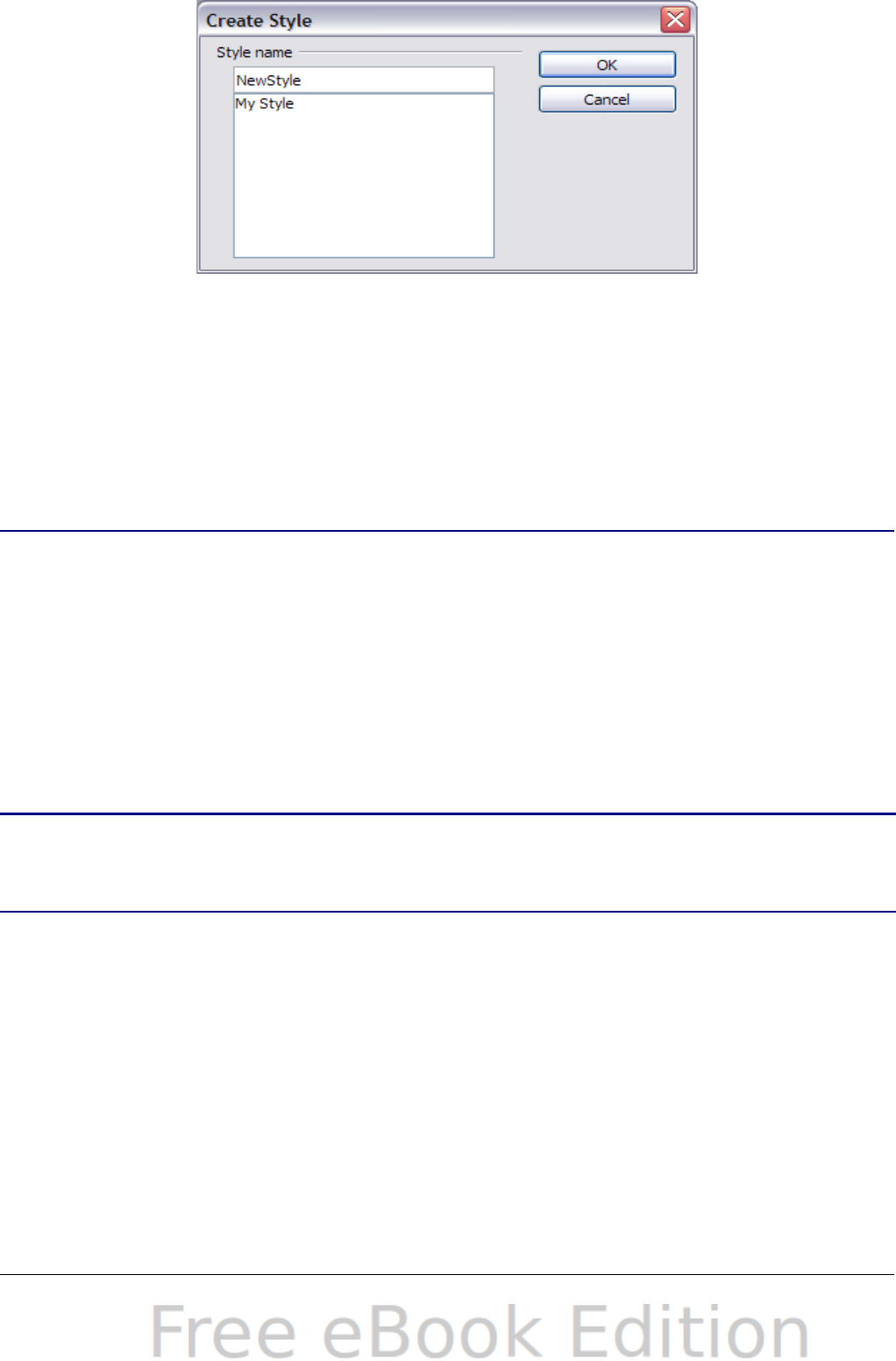
Figure 88: Naming a new style created
from a selection.
Creating a new style by dragging and dropping
Select a cell and drag it to the Styles and Formatting window.
Copying and moving styles
Occasionally you may want to copy a style from one spreadsheet to
another, or between a spreadsheet and a template, instead of
recreating it in the second spreadsheet. You can do this using the
Template Management dialog.
1) Click File > Templates > Organize.
2) In the Template Management dialog (Figure 89), set the lists at
the bottom to either Templates or Documents, as needed. The
default is Templates on the left and Documents on the right.
Tip
To copy styles from a file that is not open, click the File button.
When you return to this dialog, both lists show the selected file
as well as all the currently open documents.
3) Open the folders and find the templates from and to which you
want to copy. Double-click on the name of the template or
document, and then double-click the Styles icon to show the list of
individual styles (Figure 90).
4) To copy a style, hold down the Ctrl key and drag the name of the
style from one list to the other.
5) Repeat for each style you want to copy. If the receiving template
or document has many styles, you may not see any change unless
you scroll down in the list. When you are finished, click Close.
Chapter 4 Using Styles and Templates in Calc 117
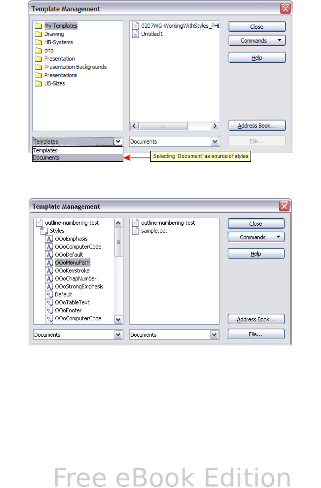
Figure 89: Choosing to copy styles from a document, not a
template.
Figure 90: Copying a style from one document to another.
118 OpenOffice.org 3.x Calc Guide

Deleting styles
You cannot remove (delete) any of Calc’s predefined styles, even if you
are not using them.
You can remove any user-defined (custom) styles; but before you do,
you should make sure the styles are not in use. If an unwanted style is
in use, you will want to replace it with a substitute style.
Replacing styles (and then deleting the unwanted ones) can be very
useful if you are dealing with a spreadsheet that has been worked on
by several people.
To delete unwanted styles, right-click on them (one at a time) in the
Styles and Formatting window and click Delete on the pop-up menu.
Choose Yes in the confirmation pop-up.
Creating a spreadsheet from a template
To create a spreadsheet from a template:
1) From the main menu, choose File > New > Templates and
Documents. The Templates and Documents dialog opens. (See
Figure 91 for the Windows version of this dialog.)
2) In the box on the left, click the Templates icon if it is not already
selected. A list of template folders appears in the center box.
3) Double-click the folder that contains the template that you want
to use. A list of all the templates contained in that folder appears
in the center box.
4) Select the template that you want to use. You can preview the
selected template or view the template’s properties:
•To preview the template, click the Preview icon. A preview of
the template appears in the box on the right.
•To view the template’s properties, click the Document
Properties icon. The template’s properties appear in the box
on the right.
5) Click Open. The Templates and Documents dialog closes and a
new document based on the selected template opens in Calc. You
can then edit and save the new document just as you would any
other document.
Chapter 4 Using Styles and Templates in Calc 119
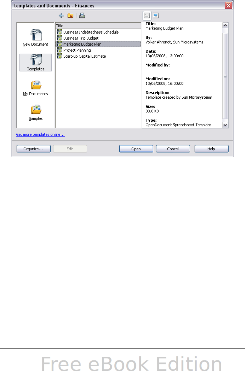
Figure 91: Templates and Documents dialog.
Creating a template
You can create a template from a document:
1) Open a new or existing document of the type you want to make
into a template (text document, spreadsheet, drawing,
presentation).
2) Add the content and styles that you want.
3) From the main menu, choose File > Templates > Save. The
Templates dialog opens (see Figure 92).
4) In the New template field, type a name for the new template.
5) In the Categories list, click the category to which you want to
assign the template. The category you choose has no effect on the
template itself; it is simply the folder in which you save the
template. Choosing an appropriate folder (category) makes it
easier to find the template when you want to use it. You may wish
to create a folder for Calc templates.
To learn more about template folders, see “Organizing templates”
on page 126.
6) Click OK to save the new template.
120 OpenOffice.org 3.x Calc Guide
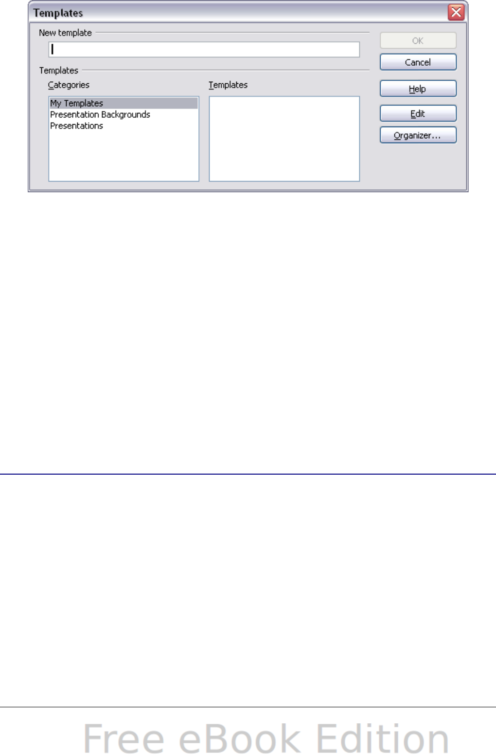
Figure 92: Saving a new template
Any settings that can be added to or modified in a document can be
saved in a template. For example, below are some of the settings
(although not a full list) that can be included in a Calc document and
then saved as a template for later use:
•Printer settings: which printer, single sided / double sided, and
paper size, and so on
•Cell and page styles to be used
Templates can also contain predefined text, saving you from having to
type it every time you create a new document. For example, an invoice
template might contain your company’s name, address and logo.
You can also save menu and toolbar customizations in templates; see
Chapter 14 (Setting up and Customizing Calc) for more information.
Editing a template
You can edit a template’s styles and content, and then, if you wish, you
can reapply the template’s styles to documents that were created from
that template. (Note that you can only reapply styles. You cannot
reapply content.)
To edit a template:
1) From the main menu, choose File > Templates > Organize. The
Template Management dialog opens.
Chapter 4 Using Styles and Templates in Calc 121
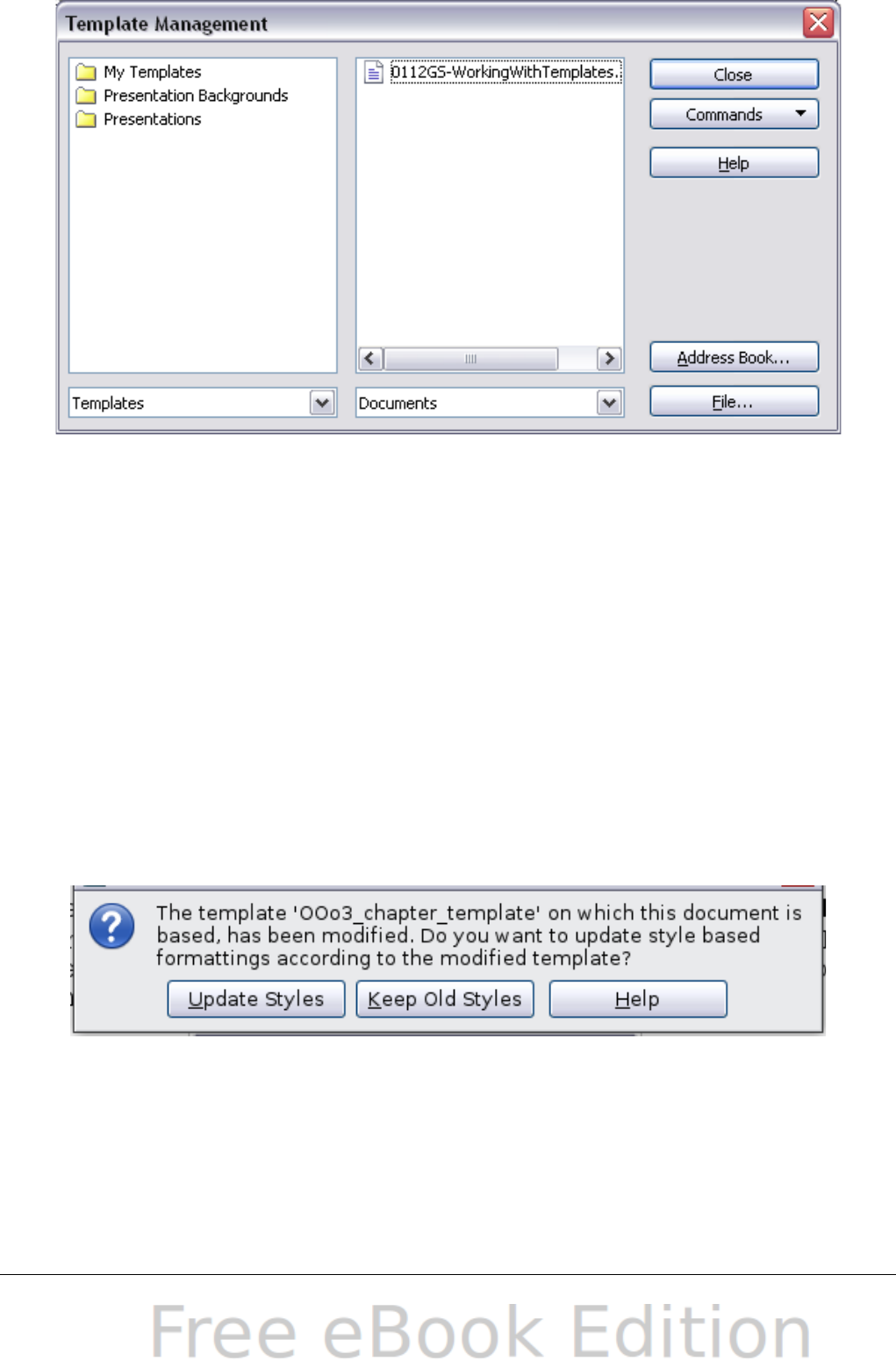
Figure 93: Template management dialog
2) In the box on the left, double-click the folder that contains the
template that you want to edit. A list of all the templates
contained in that folder appears underneath the folder name.
3) Select the template that you want to edit.
4) Click the Commands button and choose Edit from the drop-
down menu.
5) Edit the template just as you would any other document. To save
your changes, choose File > Save from the main menu.
Updating a spreadsheet from a changed template
The next time you open a spreadsheet that was created from the
changed template, the following message appears.
Figure 94: Update styles message
Click Update Styles to apply the template’s changed styles to the
spreadsheet. Click Keep Old Styles if you do not want to apply the
template’s changed styles to the spreadsheet (but see Caution notice
below).
122 OpenOffice.org 3.x Calc Guide
Caution
If you choose Keep Old Styles in the message box shown in
Figure 94, that message will not appear again the next time you
open the document after changing the template it is based on.
You will not get another chance to update the styles from the
template, although you can use the macro given in the Note
below to re-enable this feature.
Note To re-enable updating from a template:
1) Use Tools > Macros > Organize Macros >
OpenOffice.org Basic. Select the document from the list,
click the +, and select Standard. If Standard has a + beside
it, click that and select a module.
2) Name the macro. For example, you could call it
FixDocument. If the Edit button is active, click it. If the Edit
button is not active, click New, type a module name in the
pop-up dialog, and click OK.
3) In the Basic window, enter the following:
Sub FixDocV3
' set UpdateFromTemplate
oDocSettings = ThisComponent.createInstance( _
"com.sun.star.document.Settings" )
oDocSettings.UpdateFromTemplate = True
End Sub 'FixDocV3
4) Click the Run BASIC icon, then close the Basic window.
5) Save the document.
Next time when you open this document you will have the
update from template feature back.
Adding templates using the Extension
Manager
The Extension Manager provides an easy way to install collections of
templates, graphics, macros, or other add-ins that have been
“packaged” into files with a .OXT extension. See Chapter 14 (Setting
Up and Customizing Calc) for more about the Extension Manager.
This Web page lists many of the available extensions:
http://extensions.services.openoffice.org/.
To install an extension, follow these steps:
1) Download an extension package and save it anywhere on your
computer.
Chapter 4 Using Styles and Templates in Calc 123
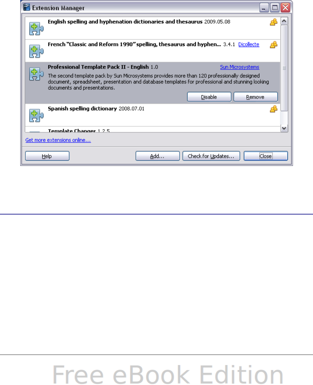
2) In OOo, choose Tools > Extension Manager from the menu bar.
In the Extension Manager dialog, click Add.
3) A file browser window opens. Find and select the package of
templates you want to install and click Open. The package begins
installing. You may be asked to accept a license agreement.
4) When the package installation is complete, the templates are
available for use through File > New > Templates and
Documents and the extension is listed in the Extension Manager.
Figure 95: Newly-added package of templates.
Setting a default template
If you create a document by choosing File > New > Text Document
(or Spreadsheet, Presentation, or Drawing) from the main menu,
OOo creates the document from the Default template for that type of
document. You can, however, set a custom template to be the default.
You can reset the default later if you choose.
Setting a custom template as the default
You can set any template to be the default, as long as it is in one of the
folders displayed in the Template Management dialog.
124 OpenOffice.org 3.x Calc Guide

To set a custom template as the default:
1) From the main menu, choose File > Templates > Organize. The
Template Management dialog opens.
2) In the box on the left, select the folder containing the template
that you want to set as the default, then select the template.
3) Click the Commands button and choose Set As Default
Template from the drop-down menu.
The next time that you create a document by choosing File > New, the
document will be created from this template.
Although many important settings can be changed in the Options
dialog (see Chapter 14), for example default fonts and page size, more
advanced settings (such as page margins) can only be changed by
replacing the default template with a new one.
Resetting the default template
To re-enable OOo’s default template for a document type as the
default:
1) In the Template Management dialog, click any folder in the box on
the left.
2) Click the Commands button and choose Reset Default
Template > Spreadsheet from the drop-down menu.
The next time that you create a spreadsheet by choosing File > New,
it will be created from OOo’s default template for spreadsheets.
Associating a spreadsheet with a different
template
At times you might want to associate a spreadsheet with a different
template, or perhaps you’re working with a spreadsheet that did not
start from a template but you now want it associated with a template.
One of the major advantages of using templates is the ease of updating
styles in more than one document, as described on page 122. If you
update styles by copying them from a different template (as described
on page 117), the document has no association with the template from
which the styles were loaded—so you cannot use this method. What
you need to do is associate the document with the different template.
For best results, the names of styles should be the same in the existing
document and the new template. If they are not, you will need to use
Search and Replace to replace the old styles with new ones. See
Chapter 4 Using Styles and Templates in Calc 125

Chapter 2 (Entering, Editing, and Formatting Data) for more about
replacing styles using Find and Replace.
1) Use File > New > Templates and Documents. Choose the
template you want. A new file, based on the template, opens. If
the template has unwanted text or graphics in it, delete them.
2) Open the spreadsheet you want to change. (It opens in a new
window.) Press Control+A to select everything in the spreadsheet.
3) Switch to the window containing the blank spreadsheet created in
step 1, and paste the content into that spreadsheet.
4) Save the file under a new name.
Organizing templates
OOo can only use templates that are in OOo template folders. You can
create new OOo template folders and use them to organize your
templates, and import templates into those folders. For example, you
might have one template folder for report templates and another for
letter templates. You can also export templates.
To begin, choose File > Templates > Organize from the main menu.
The Template Management dialog opens.
Note
All the actions made by the Commands button in the Template
Management dialog can be made as well by right-clicking on
the templates or the folders.
Creating a template folder
To create a template folder:
1) In the Template Management dialog, click any folder.
2) Click the Commands button and choose New from the drop-
down menu. A new folder called Untitled appears.
3) Type a name for the new folder, and then press Enter. OOo saves
the folder with the name that you entered.
Deleting a template folder
You cannot delete template folders supplied with OOo or installed
using the Extension Manager; you can only delete template folders that
you have created.
126 OpenOffice.org 3.x Calc Guide

To delete a template folder:
1) In the Template Management dialog, select the folder that you
want to delete.
2) Click the Commands button and choose Delete from the drop-
down menu. A message box appears and asks you to confirm the
deletion. Click Yes.
Moving a template
To move a template from one template folder to another template
folder:
1) In the Template Management dialog, double-click the folder that
contains the template you want to move. A list of the templates
contained in that folder appears underneath the folder name.
2) Click the template that you want to move and drag it to the
desired folder. If you do not have the authority to delete templates
from the source folder, this action copies the template instead of
moving it.
Deleting a template
You cannot delete templates supplied with OOo or installed using the
Extension Manager; you can only delete templates that you have
created or imported.
To delete a template:
1) In the Template Management dialog, double-click the folder that
contains the template you want to delete. A list of the templates
contained in that folder appears underneath the folder name.
2) Click the template that you want to delete.
3) Click the Commands button and choose Delete from the drop-
down menu. A message box appears and asks you to confirm the
deletion. Click Yes.
Importing a template
If the template that you want to use is in a different location, you must
import it into an OOo template folder.
To import a template into a template folder:
1) In the Template Management dialog, select the folder into which
you want to import the template.
Chapter 4 Using Styles and Templates in Calc 127

2) Click the Commands button and choose Import Template from
the drop-down menu. A standard file browser window opens.
3) Find and select the template that you want to import and click
Open. The file browser window closes and the template appears
in the selected folder.
4) If you want, type a new name for the template, and then press
Enter.
Exporting a template
To export a template from a template folder to another location:
1) In the Template Management dialog, double-click the folder that
contains the template you want to export. A list of the templates
contained in that folder appears underneath the folder name.
2) Click the template that you want to export.
3) Click the Commands button and choose Export Template from
the drop-down menu. The Save As window opens.
4) Find the folder into which you want to export the template and
click Save.
128 OpenOffice.org 3.x Calc Guide

Chapter 5
Using Graphics in Calc
Graphics in Calc
Calc is often used to present data and make forecasts and predictions.
Graphics can turn an average document into a memorable one. Calc
can import various vector (line drawing) and raster (bitmap) file
formats. The most commonly used graphic formats are GIF, JPG, PNG,
and BMP. See the Help for a full list of the formats OOo can import.
Graphics in Calc are of three basic types:
•Image files, such as photos, drawings, and scanned images
•Diagrams created using OOo’s drawing tools
•Charts and graphs created using OOo’s Chart facility
This chapter covers images and diagrams. Charts are described in
Chapter 3 (Creating Charts and Graphs).
Although using graphics in Calc is very similar to using graphics in any
other component of OOo, this chapter explains some of the differences
in their use. It also covers some of the more advanced graphics
functions and how they can further enhance your spreadsheet.
Note
The term graphics refers to both pictures and drawing objects.
Often the word images is used when referring to pictures and
other graphics that are not drawing objects.
Adding graphics (images)
Images (also called pictures in OOo), such as corporate logos and
photographs of people and products, are probably the most common
types of graphics added to a Calc document. They may be downloaded
from the Internet, scanned, or created with a graphics program; or
they may be photos taken with a digital camera.
Images can be inserted in four ways:
•Using the Insert File dialog
•By dragging and dropping a supported file
•From the gallery
•From the clipboard by copying and pasting
Inserting an image file
Perhaps the most common way to insert graphics is to use an existing
file.
130 OpenOffice.org 3.x Calc Guide
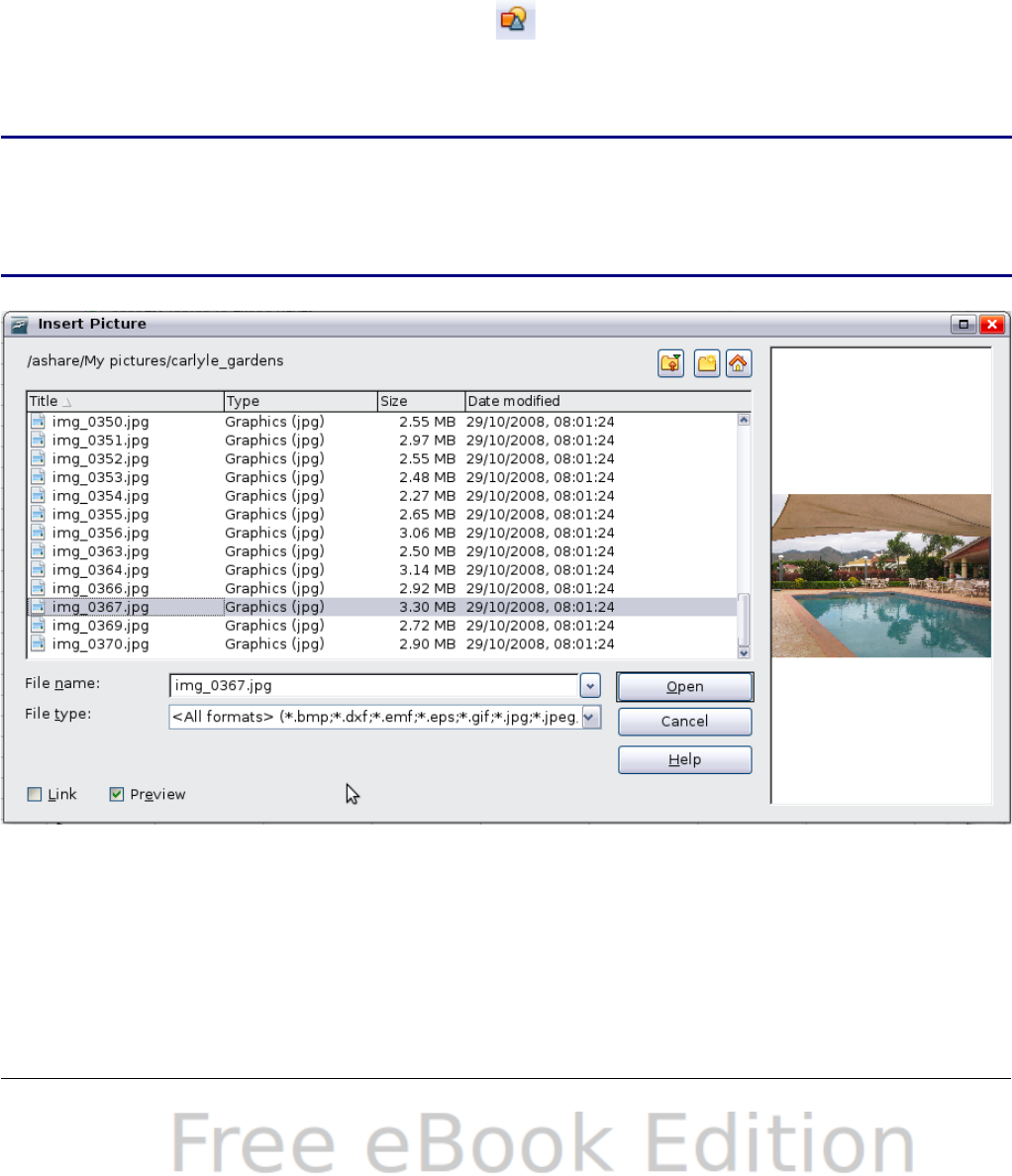
To insert an image from a file, use either of the following methods:
•Insert Picture dialog
•Drag and drop
Insert Picture dialog
1) Click in the location in the Calc document where you want the
image to appear. Do not worry too much about the exact
placement of the image at this stage; placement can be changed
easily as described in “Positioning graphics” on page 148.
2) Choose Insert > Picture > From File from the menu bar, or
click the Insert Picture icon on the Picture toolbar).
3) On the Insert Picture dialog, navigate to the file to be inserted,
select it, and click Open.
Note
The picture is inserted into Calc floating above the cells and
anchored to the cell in which the cursor was placed. See
“Positioning graphics” on page 148 for more about positioning
and anchoring graphics.
Figure 96: Inserting a picture from a file
At the bottom of the dialog are two options, Preview and Link. Select
Preview to view a thumbnail of the selected image on the right, so you
can verify that you have the correct file. The Link option is discussed
on page 132. When the Link option is not selected, the picture is
embedded in the Calc document.
Chapter 5 Using Graphics in Calc 131

Note
Your Insert Picture dialog may look quite different from the one
shown here, depending on your operating system and your
choice in Tools > Options > OpenOffice.org > General of
whether to use the OOo Open and Save dialogs.
Drag and drop
1) Open a file browser window and locate the image you want to
insert.
2) Drag the image into the Calc document and drop it where you
want it to appear. A faint vertical line marks where the image will
be dropped. The picture will be anchored to the cell where it was
dropped.
This method always embeds (saves a copy of) the image file in the Calc
document.
Linking an image file
To create a link to the file containing the image instead of saving a
copy of the image in the Calc document, use the Insert picture dialog
and select the Link option. The image is then displayed in the
document, but when the document is saved, it contains only a
reference to the image file—not the image itself. The document and the
image remain as two separate files, which are merged temporarily only
when you open the document again.
Linking an image has two advantages and one disadvantage:
•Advantage – Linking can reduce the size of the document when it
is saved, because the image file itself is not included. The file size
is usually not a problem on a modern computer with a reasonable
amount of memory, unless the document includes many large
graphics files. Calc can handle quite large files.
•Advantage – You can modify the image file separately without
changing the document because the link to the file remains valid,
and the modified image will appear when you next open the
document. This can be a big advantage if you (or someone else,
perhaps, a graphic artist) is updating images.
•Disadvantage – If you send the document to someone else, or
move it to a different computer, you must also send the image
files, or the receiver will not be able to see the linked images. You
need to keep track of the location of the images and make sure
the recipient knows where to put them on another machine, so
the Calc document can find them. For example, you might keep
132 OpenOffice.org 3.x Calc Guide

images in a subfolder named Images (under the folder containing
the Writer document); the recipient of the Calc file needs to put
the images in a subfolder with the same name (under the folder
containing the Writer document).
Note
When inserting the same image several times in the document,
it might appear beneficial to create links. However, this is not
necessary, as OOo embeds in the document only one copy of
the image file. (Deleting one or more of the copies does not
affect the others.)
Embedding linked images
If you originally linked the images, you can easily embed (save in the
Calc document) one or more of them later if you wish. To do so:
1) Open the document in Calc.
2) Choose Edit > Links from the menu bar.
The Edit Links dialog shows all the linked files. In the Source file
list, select the files you want to change from linked to embedded.
3) Click the Break Link button.
4) Save the Calc document.
Figure 97: The Edit Links dialog
Note
Going the other way, from embedded to linked, is not so easy—
you must delete and reinsert each image, one at a time,
selecting the Link option when you do so.
Chapter 5 Using Graphics in Calc 133
Inserting an image from the clipboard
Using the clipboard, you can copy images into a Calc document from
another Calc document, from another component of OOo (Writer, Draw,
and so on), and from other programs.
To do this:
1) Open both the source document and the Calc document into
which you want to copy the image.
2) In the source document, select the image to be copied.
3) Press Control+C to copy the image to the clipboard.
4) Switch to the Calc window.
5) Click to place the cursor where the graphic is to be inserted.
6) Press Control+V to insert the image.
Caution If the application from which the graphic was copied is closed
before the graphic is pasted into Calc, the image stored on the
clipboard could be lost from the clipboard.
Inserting an image from the Gallery
The Gallery provides a convenient way to group reusable objects such
as graphics and sounds that you can insert into your documents.
The Gallery is available in all components of OOo. It does not come
with many graphics, but you can add your own pictures or find
extensions containing more graphics. The Gallery is explained in more
detail in Chapter 11 (Graphics, the Gallery, and Fontwork) in the
Getting Started guide. For more about extensions, see Chapter 14
(Setting Up and Customizing Calc) in this book.
This section explains the basics of inserting a Gallery image into a Calc
document.
1) To open the Gallery (Figure 98), click on the Gallery icon
(located in the right side of the Standard toolbar) or choose Tools
> Gallery from the menu bar.
2) Navigate through the Gallery to find the desired picture.
3) To insert the picture, either right-click on the picture and choose
Insert > Copy or click and drag the picture from the Gallery into
the Calc document.
134 OpenOffice.org 3.x Calc Guide
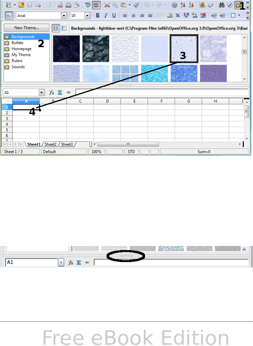
By default, the Gallery is docked above the Calc workspace. To expand
the Gallery, position the pointer over the line that divides it from the
top of the workspace. When the pointer changes to parallel lines with
arrows, click and drag downward. The workspace resizes in response.
Figure 98: Gallery in Calc
To expand the Gallery without affecting the workspace, undock it so it
floats over the workspace. To do so, hold down the Control key and
double-click on the upper part of the Gallery next to the View icons.
Double-click in the same area while holding down the Control key to
dock it again (restore it to its position over the workspace).
When the Gallery is docked, to hide it and view the full Calc
workspace, click the Hide/Show button in the middle of the thin bar
separating the Gallery from the workspace.
To close the Gallery, choose Tools > Gallery to uncheck the Gallery
entry, or click on the Gallery icon again.
Chapter 5 Using Graphics in Calc 135
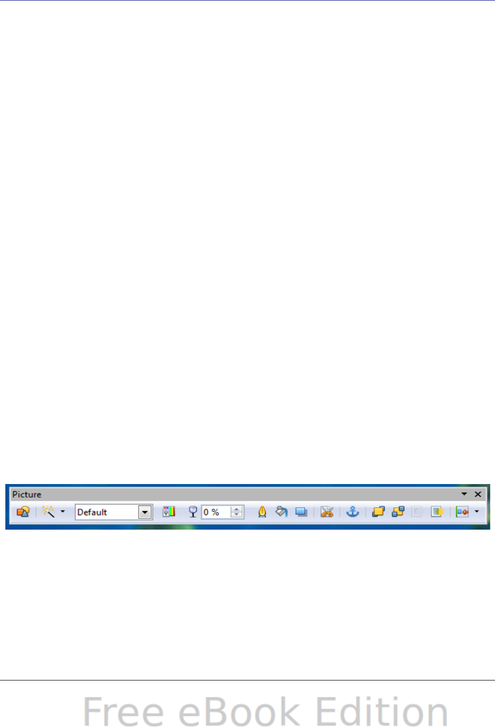
Modifying images
When you insert a new image, you may need to modify it to suit the
document. This section describes the use of the Picture toolbar,
resizing, cropping, and a workaround for rotating a picture. Changes
made in Calc do not affect the original picture, whether it is embedded
or linked.
Calc provides many tools for working with images. These tools are
sufficient for most people’s everyday requirements. However, for
professional results it is generally better to use an image manipulation
program such as GIMP to modify images (for example, to crop, resize,
rotate, and change color values) and then insert the result into Calc.
GIMP is an open-source graphics program that can be downloaded
from http://www.gimp.org/downloads/.
Using the Picture toolbar
When you insert an image or select one already present in the
document, the Picture toolbar appears. You can set it to always be
present (View > Toolbars > Picture). Picture control buttons from
the Picture toolbar can also be added to the Standard Toolbar. See
Chapter 14 (Setting Up and Customizing Calc) for more information.
This toolbar can be either floating or docked. Figure 99 shows the
Picture toolbar when it is floating. A brief explanation of the tools is
given in Table 3. See the Draw Guide for a more detailed explanation.
Two other toolbars can be opened from this one: the Graphic Filter
toolbar, which can be torn off and placed elsewhere on the window,
and the Color toolbar, which opens as a separate floating toolbar.
From these three toolbars, you can apply small corrections to the
graphic or obtain special effects.
Figure 99: The Picture Toolbar
136 OpenOffice.org 3.x Calc Guide
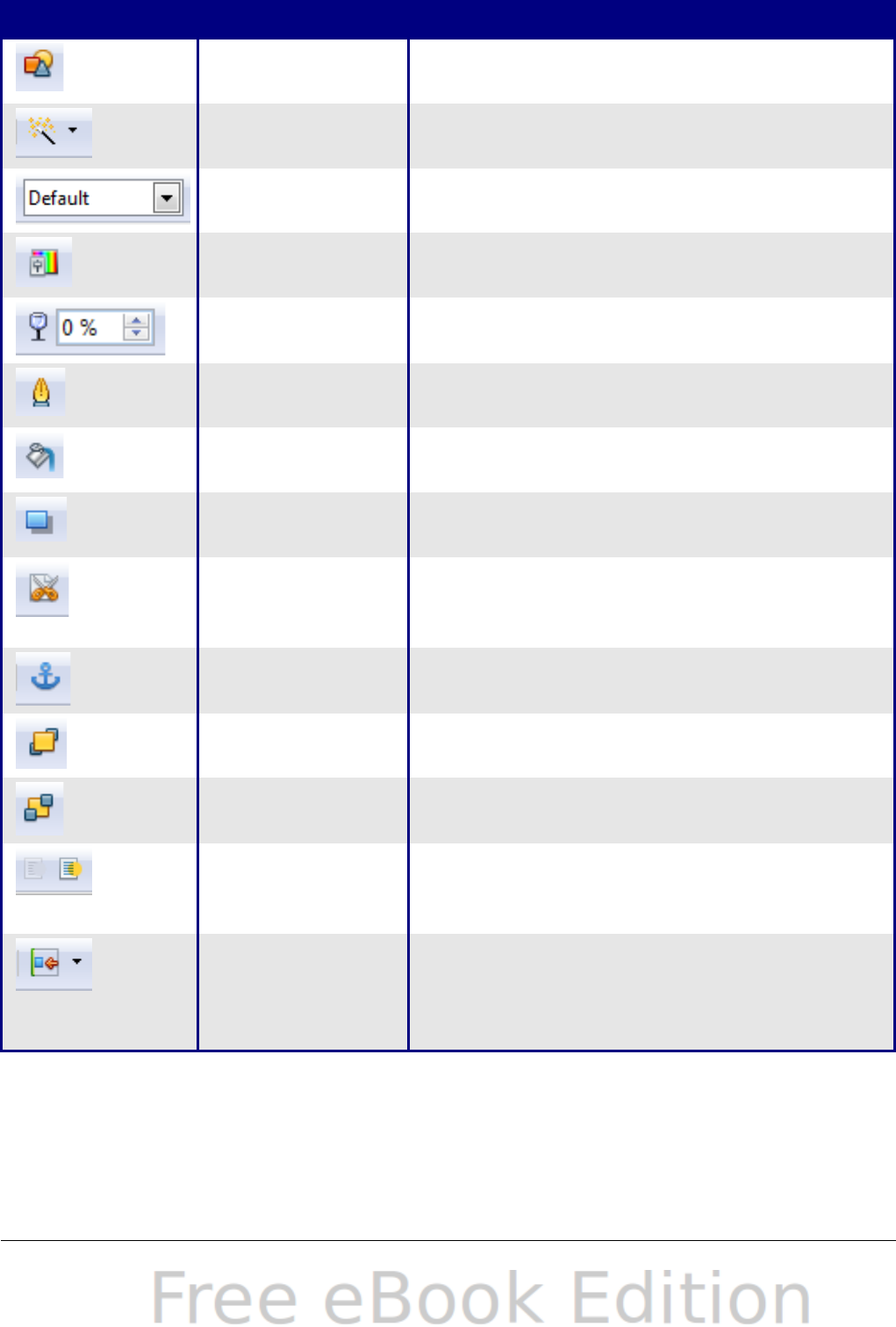
Table 3: Picture toolbar functions (from left to right)
Icon Name Behavior
From File Use of this icon is described in
“Inserting an image file” on page 130.
Filter Displays the Graphic Filter toolbar. See
page 138.
Graphics Mode Provides several color modes in the
drop-down list. See page 138.
Color Opens the Color toolbar, described on
page 139.
Transparency Sets the transparency of the selected
image. See page 139.
Line Adjusts the border style of the selected
image.
Area Fills an area with the selected color or
pattern.
Shadow Adds a drop shadow to the edges of the
picture.
Crop Opens the Crop dialog, where you can
remove a selected part of the picture.
See page 140.
Anchor Toggles between anchoring the image
to the cell or to the page. See page 150.
Bring to Front Brings the selected image to the front
of the stack. See page 149.
Send to Back Pushes the selected image to the rear of
the stack. See page 149.
To Foreground /
Background
Allows image to float in the foreground
or makes it part of the background
(behind the cells). See page 149.
Alignment If two or more pictures are selected,
adjusts the horizontal and vertical
alignment of the pictures in relation to
each other. See page 151.
Chapter 5 Using Graphics in Calc 137
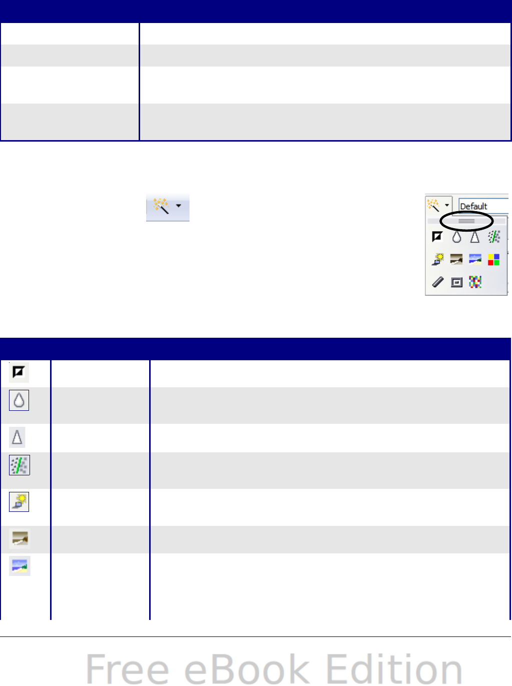
Choosing a graphics mode
You can change color images to grayscale by selecting the image and
then selecting Grayscale from the Graphics mode list.
Table 4: Graphics modes
Graphics mode Behavior
Default Keeps the picture the same as it was inserted.
Grayscale Shows the picture in gradual shades of gray.
Black / White Converts the picture into a monochromatic black and
white image.
Watermark Makes the picture into a watermark that blends into
the background.
Using graphic filters
Click the Filter icon to display the Graphic Filter
toolbar, which provides options for applying basic
photographic and effect filters to images from within
Calc. To “tear off” this toolbar and place it anywhere on
the screen, click on the three parallel lines and drag it
away.
Table 5: Graphic filters and their effects
Icon Name Behavior
Invert Inverts the colors in the picture like a negative.
Smooth Applies a Gaussian Blur to the image which softens
edges.
Sharpen Sharpens the image.
Remove
Noise
Applies crude noise reduction.
Solarization Reverses a portion of the tones, then produces
pronounced outlines of the highlights.
Aging Applies a Sepia filter.
Posterize Opens a dialog to determine the number of poster
colors. This effect is based on the reduction of the
number of colors. It makes photos look like
paintings.
138 OpenOffice.org 3.x Calc Guide
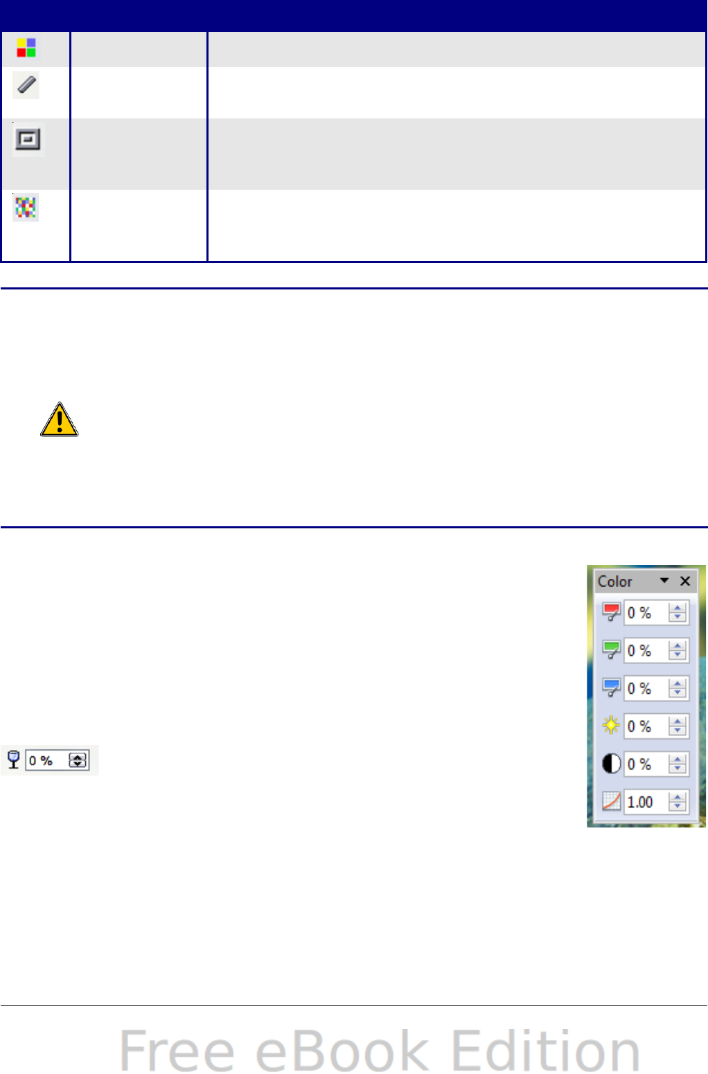
Icon Name Behavior
Pop Art Applies a Pop Art style to the image.
Charcoal
Sketch
Applies a Charcoal Sketch look to the image.
Relief Displays a dialog for creating reliefs. The position of
the imaginary light source that determines the type
of shadow can be chosen.
Mosaic Joins small groups of pixels into rectangular areas of
the same color. The larger the individual rectangles
are, the fewer details the graphic image has.
Caution
Applying OOo picture filters to any image consecutively will
progressively degrade the quality of the image. The picture
filters used in Calc utilize what is known as a Destructive
Editing algorithm, whereby each filter is applied to the image
immediately, changing the original data of the image.
Successive transformations result in less and less original data
remaining, thus compromising the quality of the inserted
picture. While this might be acceptable for use in simple
documents, it is still recommended that dedicated photo or
image editing software be used to perform anything but the
simplest of manipulations.
Adjusting colors
Use the Color toolbar to adjust an image’s red, green,
and blue channels independently, as well as its
brightness, contrast and gamma.
Setting transparency
Modify the percentage value in the Transparency box
on the Picture toolbar to make the image more
transparent. This is particularly useful when creating a
watermark or when wrapping an image in the
background.
Customizing lines, areas, and shadows
The Line, Area, and Shadow icons open dialogs where you can
customize these elements. Details are in the Draw Guide.
Chapter 5 Using Graphics in Calc 139
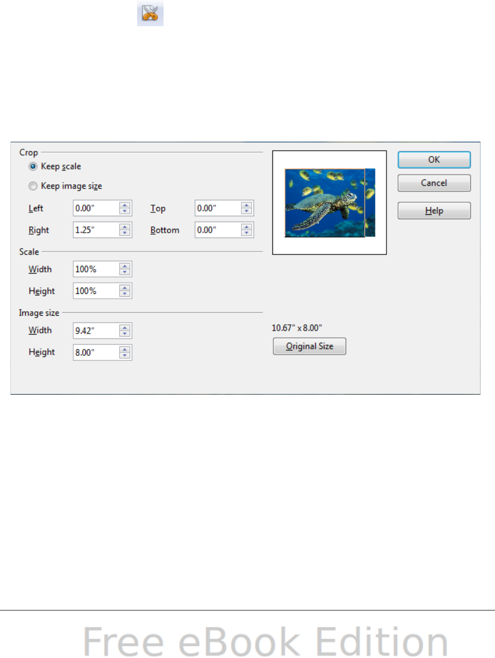
Cropping pictures
When you are only interested in a section of the image for the purpose
of your document, you may wish to crop (cut off) parts of it. The user
interface in Calc for cropping an image is not very friendly, so it may
be a better choice to use a graphics package.
Click the Crop icon to open a dialog where you can select which
portion of the image you want to remove.
It is not possible to use the mouse to select the area to be cropped, as
you can in Draw. Instead, in the Crop dialog, specify how far from the
top, bottom, left and right borders of the image the crop should be, as
illustrated in Figure 100. On the thumbnail in the figure, notice that
the cropped selection is highlighted with an inner rectangle.
Figure 100: The Crop dialog
On the Crop dialog, you can control the following parameters:
Keep scale / Keep image size
When Keep scale is selected (default), cropping the image does not
change the scale of the picture.
When Keep image size is selected, cropping enlarges (for positive
cropping values), shrinks (for negative cropping values), or distorts
of the image so that the image size remains constant.
140 OpenOffice.org 3.x Calc Guide
Left, Right, Top, and Bottom
The image is cropped by the amount entered in these boxes. For
example, a value of 3cm in the Left box cuts 3 cm from the left side
of the picture.
•When Keep scale is selected, the size of the image also changes,
so in this example the width will be reduced by 3 cm.
•When Keep image size is selected, the remaining part of the
image is enlarged (when you enter positive values for cropping)
or shrunk (when you enter negative values for cropping) so that
the width and height of the image is not changed.
Width and Height
The Width and Height fields under either Scale or Image size
change as you enter values in the Left, Right, Top, and Bottom
fields. Use the thumbnail next to these fields to determine the
correct amount by which to crop.
The cropped shape is always a rectangle; more complex cropped
shapes are not possible in Calc. Instead, use a dedicated photo or
image editing software for the job, then import the image into Calc.
Note
If you crop an image in Calc, the picture itself is not changed.
If you export the document to HTML, the original image is
exported, not the cropped image.
Resizing an image
To resize an image.
1) Click the picture, if necessary, to show the green resizing handles.
2) Position the pointer over one of the green resizing handles. The
pointer changes shape giving a graphical representation of the
direction of the resizing.
3) Click and drag to resize the picture.
4) Release the mouse button when satisfied with the new size.
The corner handles resize both the width and the height of the graphic
object simultaneously, while the other four handles only resize one
dimension at a time.
Tip
To retain the original proportions of the graphic, Shift+click
one of the corner handles, then drag. Be sure to release the
mouse button before releasing the Shift key.
Chapter 5 Using Graphics in Calc 141
Resizing a bit-mapped (raster) image such as a photograph adversely
affects the resolution, causing some degree of blurring. It is better to
use a graphics package to size your picture correctly before inserting it
into your document, if possible.
For more accurate resizing, use the Position and Size dialog, described
on page 143.
Rotating a picture
Calc does not provide a tool for rotating a picture, but you can use this
workaround:
1) Open a new Draw or Impress document.
2) Insert the image you want to rotate.
3) Select the image, then in the Drawing toolbar (shown by default
at the bottom of the window in Impress and Draw), select the
Rotate icon .
4) Rotate the image as desired. Use the red handles at the corners of
the picture and move the mouse in the direction you wish to
rotate. By default the picture rotates around its center (indicated
by a black crosshair), but you can change the pivot point by
moving the black crosshair to the desired rotation center.
Tip To restrict the rotation angle to multiples of 15 degrees keep
the Shift key pressed while rotating the image.
5) Select the rotated picture by pressing Ctrl+A, then copy the
image to the clipboard with Ctrl+C.
6) Finish by going back to the Calc document, place the cursor
where the image is to be inserted, and press Ctrl+V.
Using the picture context menu
Many of the options accessible from the Picture toolbar can also be
reached by right-clicking on an image to pop up a context menu. Some
additional options are only available from the context menu; these are
described in this section.
Text
Opens a dialog where you can set the options for text that goes over a
picture. To write text over a graphic, click on the graphic to select it,
and then press Enter. There should be a cursor inside the graphic. Any
142 OpenOffice.org 3.x Calc Guide
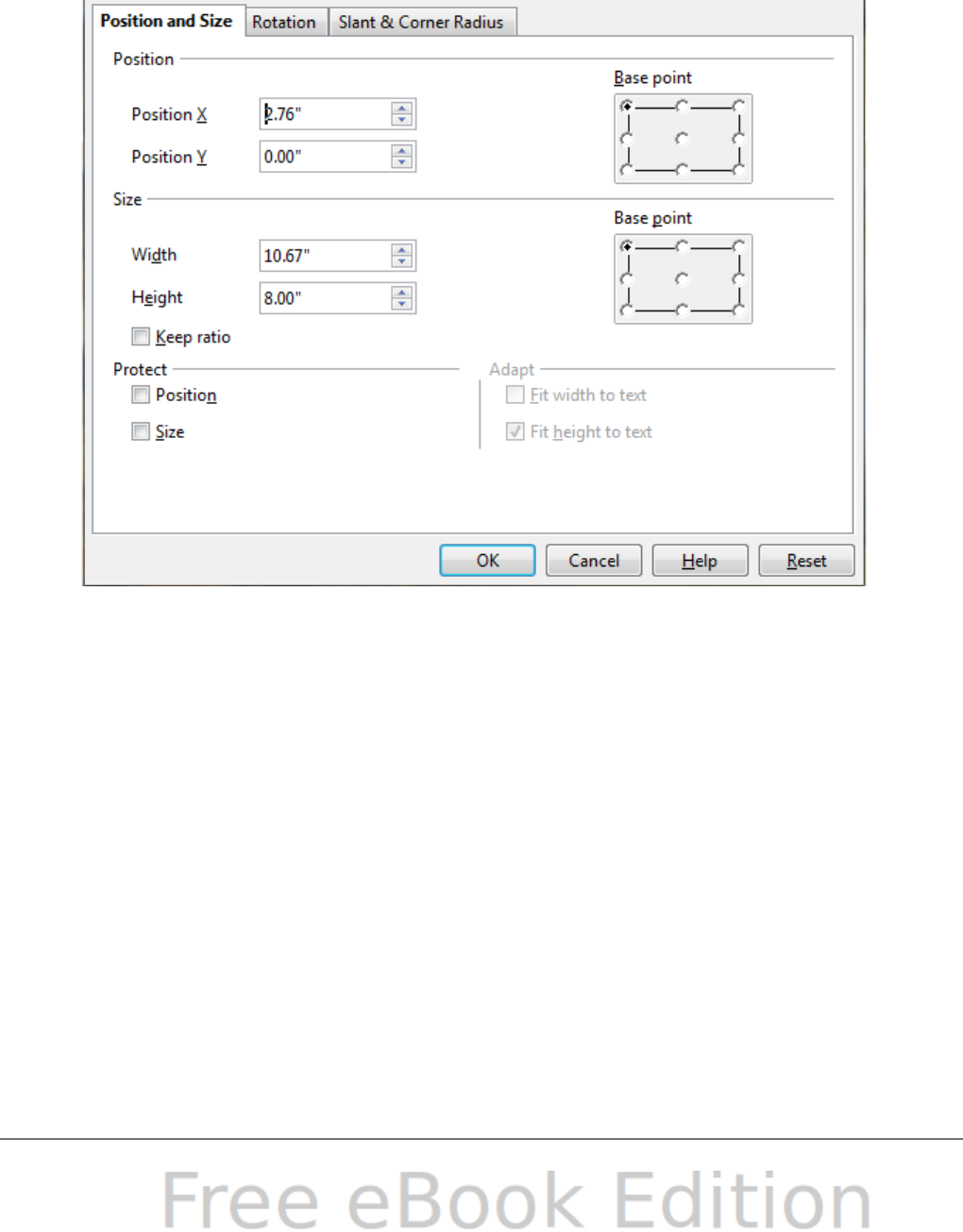
text entered is part of the graphic, so if the graphic is moved the text
will move with it.
Position and Size
Opens the dialog shown below where you can change the size, location,
rotation, slant and corner radius of the image.
Figure 101: Position and Size Dialog
Original Size
Resets the dimensions of the image to the values when it was originally
inserted into the document.
Description
You can add metadata in the form of a title and description to the
image. This information is used by accessibility tools (such as screen
reader software) and as ALT (alternative) attributes if you export the
document to HTML.
Chapter 5 Using Graphics in Calc 143

Name
You can add a custom name to be assigned to the image, to make it
easier to find in the Navigator.
Tip
When collaborating with a team on a large, multi-page
publication, it may be beneficial to give graphics, figures, and
other objects meaningful names and descriptions to aid in clear
communication.
Flip
Flips the image either horizontally or vertically.
Assign Macro
Adds programmable functionality to the image. Calc provides rich
macro functionality. Macros are introduced in Chapter 12 (Calc
Macros).
Group
To group images:
1) Select one image, then hold down the Shift key and click in turn
on each of the others that you want to include in the group. The
invisible “bounding box” (with the 8 green handles) expands to
include all the selected images.
2) With the images selected, choose Format > Group > Group
from the menu bar.
Or hover the mouse pointer over one of the images. When the
pointer changes shape from an arrow to a hand, right-click and
choose Group > Group from the pop-up menu.
Note You cannot include drawing objects in a group with pictures.
After images are grouped, the context menu provides other choices
(Ungroup and Edit Group) and the Format > Group menu includes
Ungroup and Enter Group. For more information about grouping, see
the Draw Guide.
144 OpenOffice.org 3.x Calc Guide
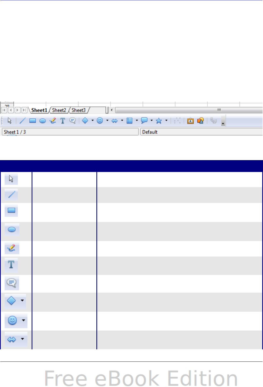
Using Calc’s drawing tools
Calc, like the other components of OOo, has a range of tools to create
custom drawings. This chapter covers the default options in Calc. For a
more detailed explanation of the drawing tools and their uses, see the
Draw Guide.
In general, if you need to create complex drawings, it is recommended
to use OpenOffice.org Draw or another drawing program.
To begin using the drawing tools, choose View > Toolbars >
Drawing. The Drawing toolbar appears at the bottom of the screen.
You can tear off this toolbar and move it to a convenient place on the
window.
Figure 102: The Drawing toolbar showing default icons
Table 6: Drawing toolbar functions (from left to right)
Icon Name Behavior
Select Selects objects.
Line Draws a line.
Rectangle Draws a rectangle. To draw a square, hold
down Shift while you drag.
Ellipse Draws an ellipse. To draw a circle, hold down
Shift while you drag.
Freeform Line Draws a freeform line.
Text Draws a text box with no border.
Callouts Draws a line that ends in a rectangular callout.
Basic Shapes Opens the Basic Shapes toolbar.
Symbol Shapes Opens the Symbol Shapes toolbar.
Block Arrows Opens the Block Arrows toolbar of shapes.
Chapter 5 Using Graphics in Calc 145
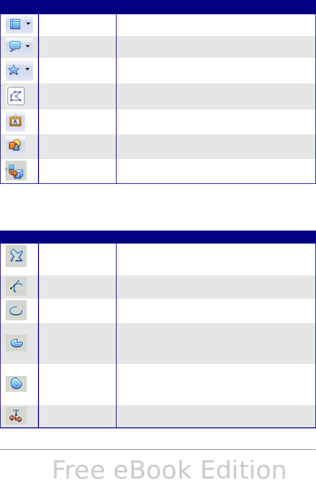
Icon Name Behavior
Flowcharts Opens the Flowchart toolbar of shapes.
Callouts Opens the Callouts toolbar of shapes.
Stars Opens the Stars toolbar of shapes.
Points Allows editing of the points of a selected
polygon.
Fontwork
Gallery Opens the Fontwork Gallery.
From File Inserts a picture using the Insert Picture
dialog.
Extrusion On/Off Opens the 3-D Setting toolbar and converts the
selected shape (if any) to 3-D.
To display other icons, click the down-arrow at the right-hand end of
the toolbar, select Visible Buttons, and then choose the tools you
want to appear on the toolbar.
Icon Name Behavior
Polygon
Draws a line composed of a series of straight
line segments. Hold down the Shift key to
position new points at 45 degree angles.
Curve Draws a smooth Bézier curve.
Arc Draws an arc.
Ellipse Pie
Draws a filled shape that is defined by the arc
of an oval and two radius lines in the current
document. To draw a circle pie, hold down
Shift while you drag.
Circle Segment
Draws a filled shape that is defined by the arc
of a circle and a diameter line in the current
document. To draw an ellipse segment, hold
down Shift while you drag.
Text Animation Inserts animated text.
146 OpenOffice.org 3.x Calc Guide

If support for Asian languages has been enabled (in Tools > Options
> Language Settings > Languages), two more tools can be added to
the Drawing toolbar: Vertical Text and Vertical Callouts.
To use a drawing tool:
1) Click in the document where you want the drawing to be
anchored. You can change the anchor later, if necessary.
2) Select the tool from the Drawing toolbar (Figure 102). The mouse
pointer changes to a cross-hair pointer.
3) Move the cross-hair pointer to the place in the document where
you want the graphic to appear and then click-and-drag to create
the drawing object. Release the mouse button. (Some tools have
other requirements; see the Help or the Draw Guide for details.)
The selected drawing function remains active, so you can draw
another object of the same type.
4) To cancel the selected drawing function, press the Esc key or
click on the Select icon (the arrow) on the Drawing toolbar.
5) You can now change the properties (fill color, line type and
weight, anchoring, and others) of the drawing object using either
the Drawing Object Properties toolbar (Figure 103) or the choices
and dialog boxes reached by right-clicking on the drawing object.
Set or change properties for drawing objects
To set the properties for a drawing object before you draw it:
1) On the Drawing toolbar (Figure 102), click the Select tool.
2) On the Drawing Object Properties toolbar (Figure 103), click on
the icon for each property and select the value you want for that
property.
3) For more control, or to define new attributes, you can click on the
Area or Line icons on the toolbar to display detailed dialogs.
These default properties are applied only to the current document and
session. They are is not retained when you close the document, and
they do not apply to any other document. The defaults apply to all the
drawing objects except text objects.
To change the properties for an existing drawing object, select the
object and continue as described above.
Other tools and methods for modifying and positioning graphics are
described in “Positioning graphics” below.
Chapter 5 Using Graphics in Calc 147
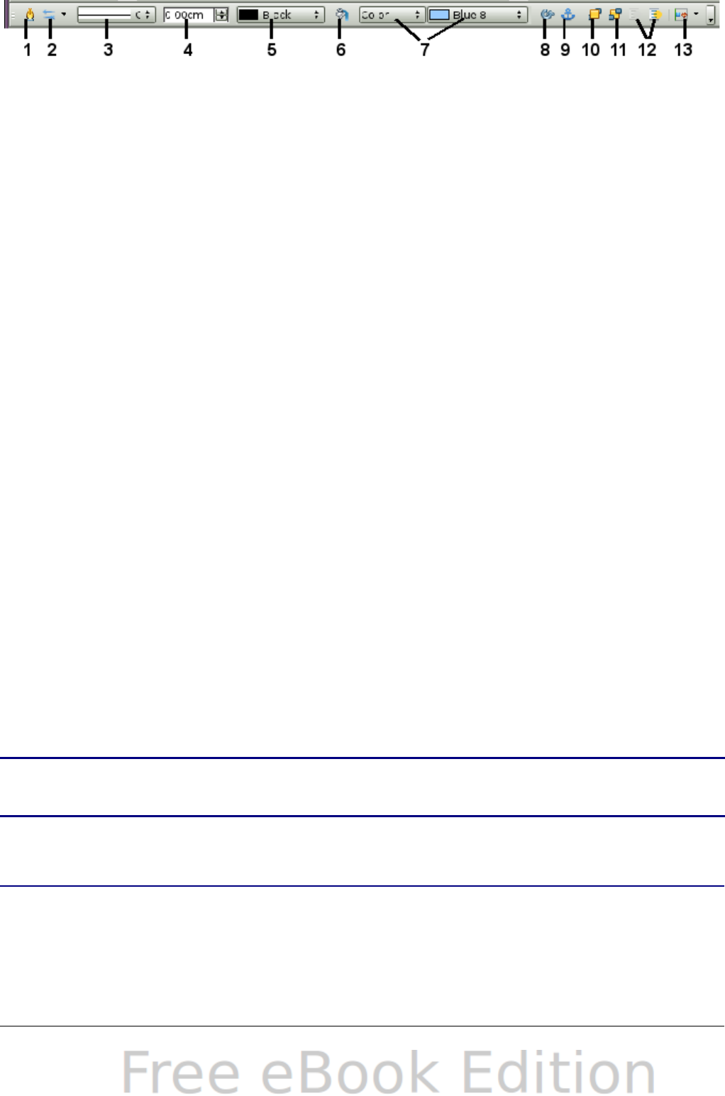
1Line 5Line Color 9Change Anchor 13 Alignment
2Arrow Style 6Area 10 Bring to Front
3Line Style 7Area Style / Filling 11 Send to Back
4Line Width 8Rotate 12 To Foreground / To Background
Figure 103. Drawing Object Properties toolbar
Resizing a drawing object
Select the object, click on one of the eight handles around it and drag
it to its new size. For a scaled resizing, select one of the corner handles
and keep the Shift key pressed while dragging the handle.
For more control of the size of the object, use the Position and Size
dialog (see “Position and Size” on page 143) to set the width and
height independently. If the Keep ratio option is selected, then the
two dimensions change so that the proportion is maintained, allowing
for a scaled resizing.
Grouping drawing objects
To group drawing objects:
1) Select one object, then hold down the Shift key and select the
others you want to include in the group. The bounding box
expands to include all the selected objects.
2) With the objects selected, hover the mouse pointer over one of
the objects and choose Format > Group > Group from the menu
bar or right-click and choose Group > Group from the pop-up
menu.
Note You cannot include an embedded or linked graphic in a group
with drawing objects.
Positioning graphics
Graphics can be positioned in OOo Calc to work together and build
more complex features.
148 OpenOffice.org 3.x Calc Guide

Arranging graphics
Graphics in a Calc document are maintained in a similar manner to a
deck of cards. As you add more images to the document, each image
occupies a new layer at the top of the stack. To arrange graphics, you
tell Calc to change the order of layers in the stack.
Figure 104: Layering effect
Calc provides four basic options to re-arrange the order of images.
These options can be accessed from both the Picture toolbar and the
picture context menu:
Bring to Front
Places the image on top of any other graphics or text.
Bring Forward
Brings the image one level up in the stack (z-axis). Depending on the
number of overlapping objects, you may need to apply this option
several times to obtain the desired result.
Send Backward
The opposite of Bring Forward; sends the selected image one level
down in the object stack.
Send to Back
Sends the selected graphic to the bottom of the stack, so that other
graphics and text cover it.
Chapter 5 Using Graphics in Calc 149
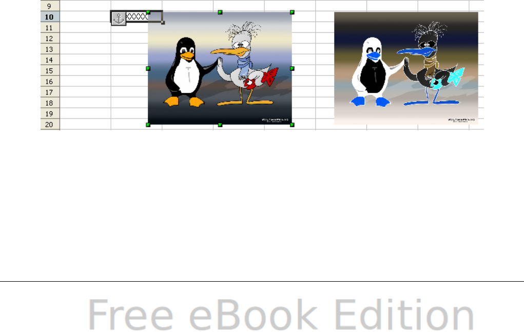
To Background and To Foreground
An image or a drawing object can be sent to the background as well.
This is not the same as Bring Forward and Send Backward, which
set the order of a number of overlapping graphics. This feature
pushes a graphic behind the cells, allowing cells to be edited without
affecting the graphic.
A graphic in the background will have To Foreground as a menu
item, instead of To Background.
Anchoring graphics
Anchors tell a graphic where to stay in relation to other items.
Anchor to page
Anchoring a graphic to the page allows it to be positioned in a
specific place on the page. The graphic does not move when cells
are added or deleted. This is equivalent to an absolute reference.
The graphic will always stay by cell B10 if that is where it is placed.
Anchor to cell
Anchoring a graphic to a cell ensures that the graphic always stays
with the content it is originally anchored to. If a graphic is anchored
to cell B10, and a new row is inserted, the graphic will then be
anchored to cell B11. This is equivalent to a relative reference.
For example, in Figure 105 the normal Otto and Tux picture is
anchored To Cell B10 (XXX shows where the picture is anchored). The
inverse Otto and Tux picture is anchored to the page.
Figure 105: Anchoring 1
If two rows are inserted above the pictures, the normal picture
(anchored to cell) will shift down two rows and the anchor will change.
The inverse picture (anchored to page) will not move. This is illustrated
in Figure 106. Note that the anchor symbol and the XXX have moved
down to cell B12.
150 OpenOffice.org 3.x Calc Guide
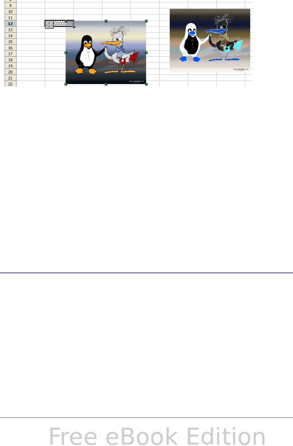
.
Figure 106: Anchoring 2
Aligning graphics
You can align several graphics relative to each other. To do this:
1) Select all of the graphics to be aligned (Shift+click on each in
turn). The graphics will be surrounded by an invisible bounding
box with 8 green handles.
2) On the Picture toolbar, click on the Alignment icon and select one
of the six options.
Or, position the mouse pointer over any of the graphics. When the
pointer changes shape from an arrow to a hand, right-click and
choose Alignment, then select from the six options.
The six options include three for aligning the graphics horizontally
(left, center, right) and three for aligning the graphics vertically (top,
center, bottom).
Creating an image map
An image map defines areas of an image (called hotspots) with
hyperlinks to web addresses, other files on the computer, or parts of
the same document. Hotspots are the graphic equivalent of text
hyperlinks. Clicking on a hotspot causes Calc to open the linked page
in the appropriate program (for example, the default browser for an
HTML page; OOo Calc for a .ODS file; a PDF viewer for a PDF file). You
can create hotspots of various shapes, and include several hotspots in
the same image.
To use the image map editor:
1) In your OOo document, select the picture where you want to
define the hotspots.
2) Choose Edit > ImageMap from the menu bar. The ImageMap
Editor (Figure 107) opens.
Chapter 5 Using Graphics in Calc 151

3) Use the tools and fields in the dialog (described on the next page)
to define the hotspots and links necessary.
4) Click the Apply icon to apply the settings.
5) When done, click the Save icon to save the imagemap to a file,
then click the X in the upper right corner to close the dialog.
Figure 107: The dialog to create or edit an image map
The main part of the dialog shows the image on which the hotspots are
defined. A hotspot is identified by a line indicating its shape.
The toolbar at the top of the dialog contains the following tools:
•Apply button: click this button to apply the changes.
•Load, Save, and Select icons.
•Tools for drawing a hotspot shape: these tools work in exactly the
same way as the corresponding tools in the Drawing toolbar.
•Edit, Move, Insert, Delete Points: advanced editing tools to
manipulate the shape of a polygon hotspot. Select the Edit Points
tool to activate the other tools.
•Active icon: toggles the status of a selected hotspot between
active and inactive.
•Macro: associates a macro with the hotspot instead of just
associating an hyperlink.
152 OpenOffice.org 3.x Calc Guide

•Properties: sets the hyperlink properties and adds the Name
attribute to the hyperlink.
Below the toolbar, specify for the selected hotspot:
•Address: the address pointed by the hyperlink. You can also point
to an anchor in a document; to do this, write the address in this
format: file:///<path>/document_name#anchor_name
•Text: type the text that you want to be displayed when the mouse
pointer is moved over the hotspot.
•Frame: where the target of the hyperlink will open: pick among
_blank (opens in a new browser window), _self (opens in the
active browser window), _top or _parent.
Tip
The value _self for the target frame will work just fine in the vast
majority of occasions. It is therefore not recommended to use
the other choices unless absolutely necessary.
Chapter 5 Using Graphics in Calc 153

Chapter 6
Printing, Exporting, and
E-mailing

Quick printing
Click the Print File Directly icon to send the entire document to
the default printer defined for your computer.
Note
You can change the action of the Print File Directly icon to
send the document to the printer defined for the document
instead of the default printer for the computer. Choose Tools >
Options > Load/Save > General and the Load printer
settings with the document option.
Controlling printing
For more control over printing, use File > Print.
Figure 108. The Print dialog
On the Print dialog, you can choose:
•Which printer to use (if more than one are installed on your
system) and the properties of the printer—for example, page
orientation (portrait or landscape), which paper tray to use, and
Chapter 6 Printing, Exporting, and E-mailing 155
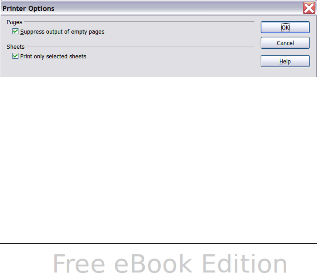
what paper size to print on. The properties available depend on
the selected printer; consult the printer’s documentation for
details.
•What sheets and pages to print, how many copies to print, and in
what order to print them. Use dashes to specify page ranges and
commas or semicolons to separate ranges; for example: 1, 5, 11–
14, 34–40. Selection refers to the highlighted part of a page or
pages.
•Whether to print to a printer or to a file.
Printer options
You can set printer options for the current document only or for all
spreadsheets.
•To select options for the current document, click the Options
button on the bottom left of the Print dialog (Figure 108).
•To set print options permanently, go to Tools > Options >
OpenOffice.org Calc > Print. The dialogs for both are very
similar.
Figure 109. Printer Options dialog
Selecting sheets to print
You can select one or more sheets for printing. This can be useful if
you have a large spreadsheet with multiple sheets and only want to
print certain sheets. For example, an accountant might record costs
over time with one sheet for each month. To print the November and
December sheets, follow this procedure.
1) Go to the November sheet. Hold down the Control key and click
on the tab of the December sheet.
2) If you wish to print all of the sheets, choose File > Print and
click the Options button.
156 OpenOffice.org 3.x Calc Guide
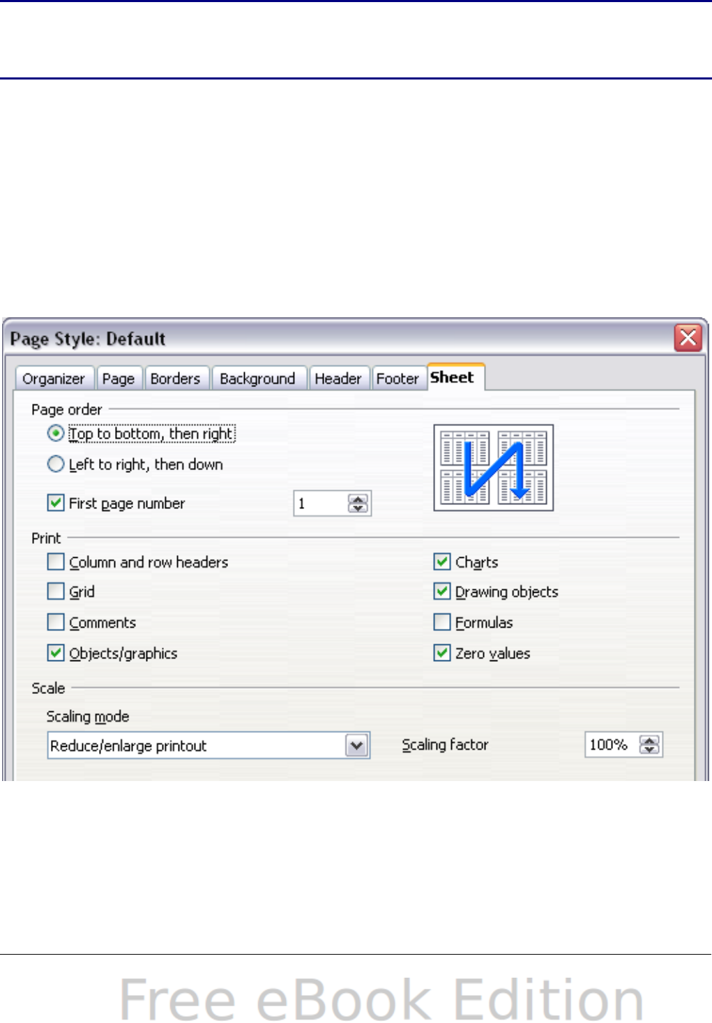
3) Deselect Print only selected sheets. This affects the print
preview, export, and printing of your spreadsheet. Click OK.
Note
The Options button is different from the Properties button.
Properties deals with the settings of the printer, whereas
Options deals with OOo’s settings.
Selecting the page order, details, and scale
To select the page order, details, and scale to be printed:
1) Choose Format > Page from the main menu. The Page Style
dialog opens; any changes made here are saved in the page style
for this spreadsheet.
2) Choose the Sheet tab (Figure 110).
3) After making your selections (see next page), click OK.
Figure 110. The Sheet tab of the Page Style dialog
Page Order
You can set the order in which pages print. This is especially useful in a
large document; for example, controlling the print order can save time
if you have to collate the document a certain way.
Chapter 6 Printing, Exporting, and E-mailing 157
Where a sheet prints to more than one page of paper, it can be printed
either by column, where the first column of pages prints, and then the
second column and so on, or by row as shown in the graphic on the top
right of the dialog in Figure 110.
Print
You can specify which details to print. These details include:
•Row and column headers
•Sheet grid—prints the borders of the cells as a grid
•Comments—prints the comments defined in your spreadsheet on
a separate page, along with the corresponding cell reference
•Objects and graphics
•Charts
•Drawing objects
•Formulas—prints the formulas contained in the cells, instead of
the results
•Zero Values—prints cells with a zero value
Note
Remember that since the print detail options are a part of the
page’s properties, they are also a part of the page style’s
properties. Therefore, different page styles can be set up to
quickly change the print properties of the sheets in the
spreadsheet.
Scale
Use the scale features to control the number of pages the data will
print on. This can be useful if a large amount of data needs to be
printed compactly or, if the reader has poor eyesight, text can be
enlarged when it prints.
•Reduce/Enlarge printout—scales the data in the printout either
larger or smaller. For example, if a sheet would normally print out
as four pages (two high and two wide), a scaling of 50% would
print as one page (both width and height are halved).
•Fit print range(s) on number of pages—defines exactly how many
pages the printout will take up. This option will only reduce a
printout, it will not enlarge it. To enlarge a printout, the
reduce/enlarge option must be used.
•Fit print range(s) to width/height—defines how high and wide the
printout will be, in pages.
158 OpenOffice.org 3.x Calc Guide
Using print ranges
Print ranges have several uses, including printing only a specific part
of the data or printing selected rows or columns on every page.
Defining a print range
To define a new print range or modify an existing print range:
1) Highlight the range of cells that comprise the print range.
2) Choose Format > Print Ranges > Define.
The page break lines display on the screen.
Tip You can check the print range by using File > Page Preview.
OOo will only display the cells in the print range.
Adding to the print range
After defining a print range, you can add more cells to it. This allows
multiple, separate areas of the same sheet to be printed, while not
printing the whole sheet. After you have defined a print range:
1) Highlight the range of cells to be added to the print range.
2) Choose Format > Print Ranges > Add. This adds the extra cells
to the print range.
The page break lines no longer display on the screen.
Note The additional print range will print as a separate page, even if
both ranges are on the same sheet.
Removing a print range
It may become necessary to remove a defined print range, for example
if the whole sheet needs to be printed later.
Choose Format > Print Ranges > Remove. This removes all defined
print ranges on the sheet. After the print range is removed, the default
page break lines will appear on the screen.
Editing a print range
At any time, you can directly edit the print range, for example to
remove or resize part of the print range. Choose Format > Print
Chapter 6 Printing, Exporting, and E-mailing 159
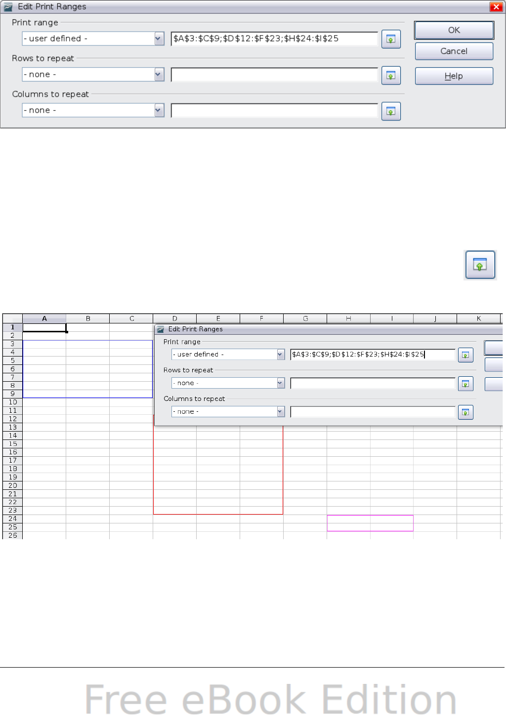
Ranges > Edit. If you have already selected a print range, the Edit
Print Ranges dialog looks something like Figure 111.
Figure 111: Edit a print range
In this example, three rectangles are selected, each separated by a
semicolon. The first is bounded by cell A3 ($A$3) in the top left and
cell C9 ($C$9) in the bottom right corners. Clicking anywhere in the
text entry box shows the currently selected print range on the screen,
with each rectangle in a different color, as in Figure 112.
After making any changes, click the Shrink icon next to the text
entry box to redisplay the rectangles with their new values.
To re-expand the Edit Print Ranges dialog, click the Shrink icon again.
Figure 112: Print range marked by colored boxes
Printing rows or columns on every page
If a sheet is printed on multiple pages, you can set up certain rows or
columns to repeat on each printed page.
160 OpenOffice.org 3.x Calc Guide
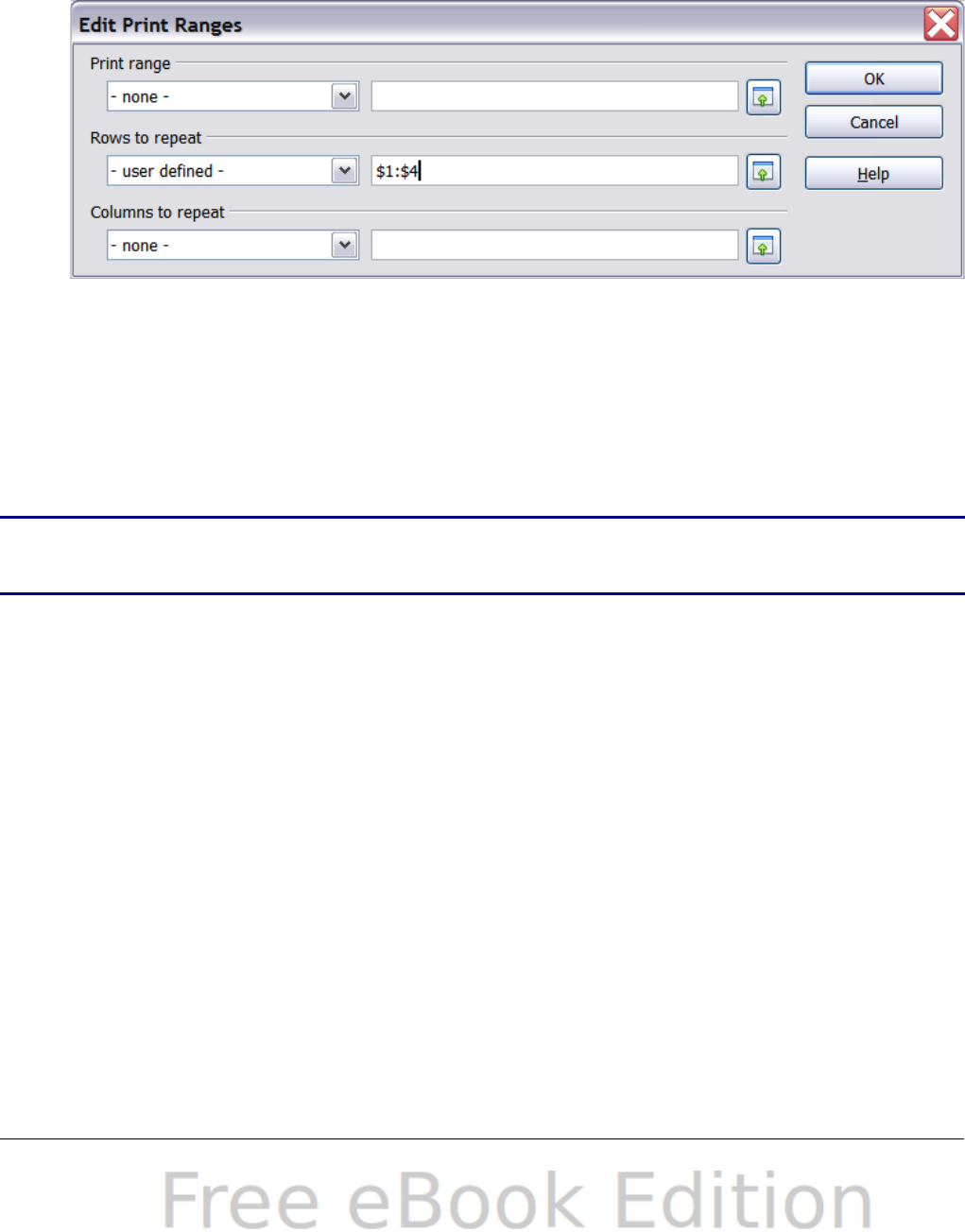
For example, if the top two rows of the sheet as well as column A need
to be printed on all pages, do the following:
1) Choose Format > Print Ranges > Edit. On the Edit Print
Ranges dialog, type the rows in the text entry box under Rows to
repeat. For example, to repeat rows 1 and 2, type $1:$2. This
automatically changes Rows to repeat from - none - to
- user defined -.
Figure 113: Specifying repeating rows
2) To repeat columns, type the columns in the text entry box under
Columns to repeat. For example, to repeat column A, type $A.
This automatically changes Columns to repeat from - none - to
- user defined -.
3) Click OK.
Note You do not need to select the entire range of the rows to be
repeated; simply select one cell in each row.
Defining a custom print range
In addition to highlighting a print range for each print job, you can
define a range of cells to be used repeatedly. This may be useful if
there are different areas of a large spreadsheet that need to be printed
for different reports. Several different print ranges can be defined to
meet this need.
1) To define a print range, use the same procedure as labeling an
area of the sheet. Highlight the cells you want to define as a print
range and select Insert > Names > Define. (The cells can be
highlighted after opening the Define Names dialog as well.)
2) On the Define Names dialog (Figure 114), type a name for the
range in the text box with the blinking cursor. The name of the
range cannot contain any spaces.
Chapter 6 Printing, Exporting, and E-mailing 161
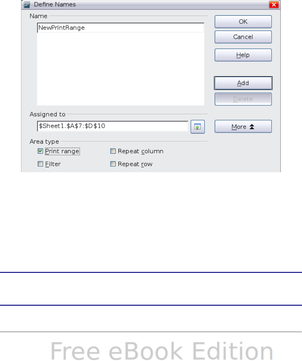
3) Click the More button in the dialog and then select the Print
range option. Click the Add button.
4) To include more than one group of cells in the selection, type in
the additional ranges. For example, to select the rectangle with
A3 as the top left cell and F20 as the bottom right cell, enter
;$A$3:$F$20 or ;A3:F20 (both work and are equivalent) after
the initial selection. Make sure that each group of cells is
separated with a semicolon.
5) Click OK.
Figure 114: Define Names dialog
To print this range:
1) Choose Format > Print Ranges > Edit (Figure 111). The
previously defined area now appears in the drop-down box under
Print range.
2) Select the defined print range and click OK.
This method can be useful to quickly change the print range without
highlighting a large area of cells every time.
Note
If the cell range name refers to more than one group of cells, it
will not appear in the drop-down list. You will need to type it in
or highlight and select it.
162 OpenOffice.org 3.x Calc Guide

Page breaks
While defining a print range can be a powerful tool, it may sometimes
be necessary to manually adjust Calc’s printout. To do this, you can use
a manual break. A manual break helps to ensure that your data prints
properly. You can insert a horizontal page break above, or a vertical
page break to the left of, the active cell.
Inserting a page break
To insert a page break:
1) Navigate to the cell where the page break will begin.
2) Select Insert > Manual Break.
3) Select Row Break or Column Break depending on your need.
The break is now set.
Row break
Selecting Row Break creates a page break above the selected cell. For
example, if the active cell is H15, then the break is created between
rows 14 and 15.
Column break
Selecting Column Break creates a page break to the left of the selected
cell. For example, if the active cell is H15, then the break is created
between columns G and H.
Tip
To see page break lines more easily on screen, you can change
their color. Choose Tools > Options > OpenOffice.org >
Appearance and scroll down to the Spreadsheet section.
Deleting a page break
To remove a page break:
1) Navigate to a cell that is next to the break you want to remove.
2) Select Edit > Delete Manual Break.
3) Select Row Break or Column Break depending on your need.
The break is now removed.
Chapter 6 Printing, Exporting, and E-mailing 163

Note
Multiple manual row and column breaks can exist on the same
page. When you want to remove them, you have to remove
each one individually. This may be confusing at times, because
although there may be a column break set on the page, when
you go to Edit > Manual Break, the Column break choice
may not be available (grayed out).
In order to remove the break, you have to be in the cell next to
the break. For example, if you set the column break while you
are in H15, you can not remove it if you are in cell D15.
However, you can remove it from any cell in column H.
Headers and footers
Headers and footers are predefined pieces of text that are printed at
the top or bottom of a sheet outside of the sheet area. Headers are set
the same way as footers.
Headers and footers are assigned to a page style. You can define more
than one page style for a spreadsheet and assign different page styles
to different sheets. For more about page styles, see Chapter 4.
Setting a header or a footer
To set a header or footer:
1) Navigate to the sheet that you want to set the header or footer
for. Select Format > Page.
2) Select the Header (or Footer) tab. See Figure 115.
3) Select the Header on option.
From here you can also set the margins, the spacing, and height for
the header or footer. You can check the AutoFit height box to
automatically adjust the height of the header or footer.
Margin
Changing the size of the left or right margin adjusts how far the
header or footer is from that side of the page.
Spacing
Spacing affects how far above or below the sheet the header or
footer will print. So, if spacing is set to 1.00", then there will be 1
inch between the header or footer and the sheet.
Height
Height affects how big the header or footer will be.
164 OpenOffice.org 3.x Calc Guide
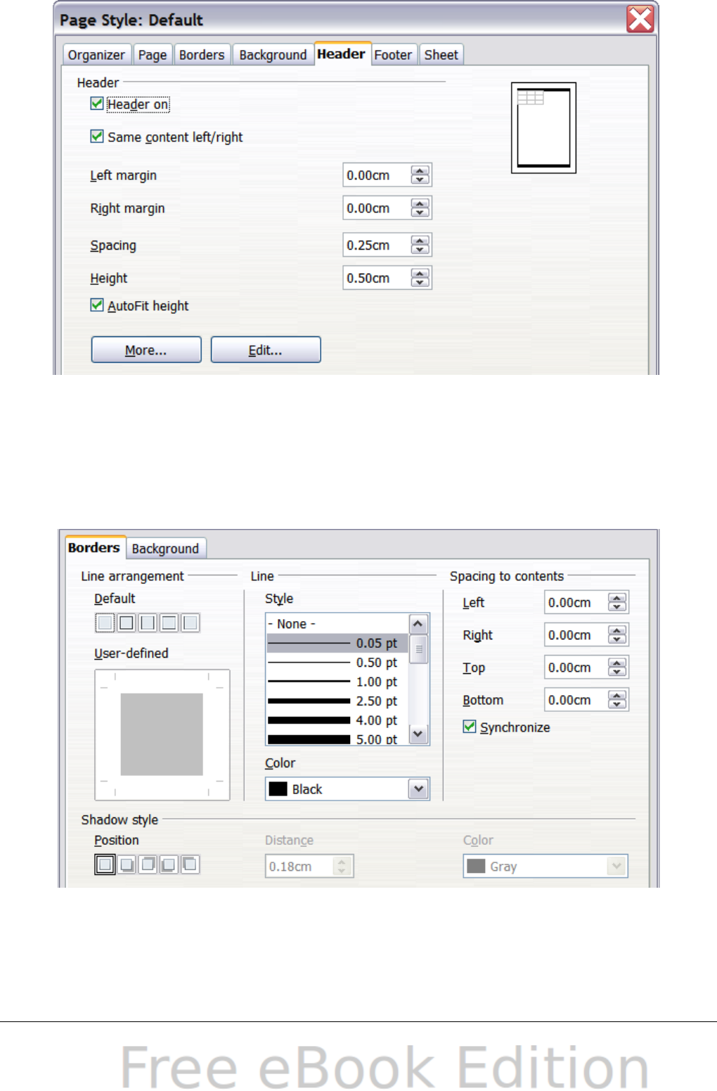
Figure 115: Header dialog
Header or footer appearance
To change the appearance of the header or footer, click the More
button in the dialog. This opens the Border/Background dialog.
Figure 116: Header/Footer Border/Background dialog
From this dialog you can set the background and border style of the
header or footer. See Chapter 4 (Using Styles and Templates) for more
information.
Chapter 6 Printing, Exporting, and E-mailing 165
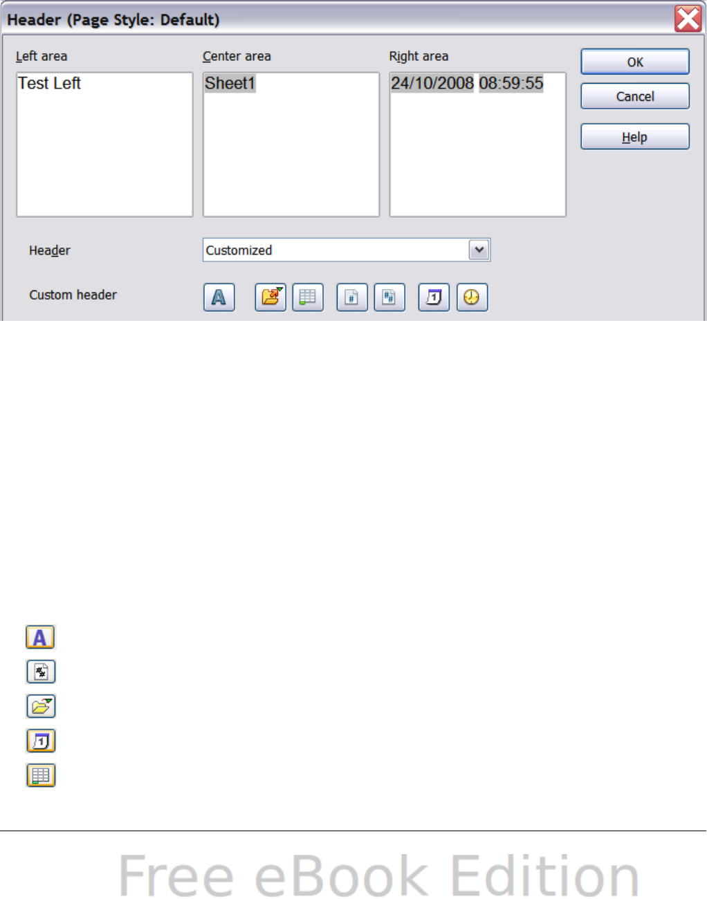
Setting the contents of the header or footer
The header or footer of a Calc spreadsheet has three columns for text.
Each column can have different contents.
To set the contents of the header or footer, click the Edit button in the
header or footer dialog shown in Figure 115 to display the dialog
shown in Figure 117.
Figure 117: Edit contents of header or footer
Areas
Each area in the header or footer is independent and can have
different information in it.
Header
You can select from several preset choices in the Header drop-down
list, or specify a custom header using the buttons below the area
boxes. (To format a footer, the choices are the same.)
Custom header
Click in the area (Left, Center, Right) that you want to customize,
then use the buttons to add elements or change text attributes.
Opens the Text Attributes dialog.
Inserts the total number of pages.
Inserts the File Name field.
Inserts the Date field.
Inserts the Sheet Name field.
166 OpenOffice.org 3.x Calc Guide

Inserts the Time field.
Inserts the current page number.
Exporting to PDF
Calc can export documents to PDF (Portable Document Format). This
industry-standard file format is ideal for sending the file to someone
else to view using Adobe Reader or other PDF viewers.
Quick export to PDF
Click the Export Directly as PDF icon to export the entire
document using your default PDF settings. You are asked to enter the
file name and location for the PDF file, but you do not get to choose a
page range, the image compression, or other options.
Controlling PDF content and quality
For more control over the content and quality of the resulting PDF, use
File > Export as PDF. The PDF Options dialog opens. This dialog has
five pages (General, Initial View, User Interface, Links, and Security).
Make your selections and click Export. Enter the location and file
name of the PDF to be created. Click Save to export the file.
General page of PDF Options dialog
On the General page, you can choose which pages to include in the
PDF, the type of compression to use for images (which affects the
quality of images in the PDF), and other options.
Range section
•All: Exports the entire document.
•Pages: To export a range of pages, use the format 3-6 (pages 3 to
6). To export single pages, use the format 7;9;11 (pages 7, 9, and
11). You can also export a combination of page ranges and single
pages, by using a format like 3-6;8;10;12.
•Selection: Exports whatever content is selected.
Chapter 6 Printing, Exporting, and E-mailing 167
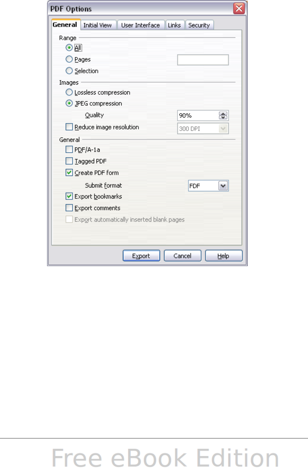
Figure 118: General page of PDF Options dialog
Images section
•Lossless compression: Images are stored without any loss of
quality. Tends to make large files when used with photographs.
Recommended for other kinds of images or graphics.
•JPEG compression: Allows for varying degrees of quality. A
setting of 90% works well with photographs (small file size, little
perceptible loss).
•Reduce image resolution: Lower-DPI (dots per inch) images
have lower quality. For viewing on a computer screen a resolution
of 72dpi (for Windows) or 96dpi (GNU/Linux) is sufficient, while
for printing it is generally preferable to use at least 300 or 600
dpi, depending on the capability of the printer. Higher dpi
settings greatly increase the size of the exported file.
168 OpenOffice.org 3.x Calc Guide

Note
EPS images with embedded previews are exported only as
previews. EPS images without embedded previews are
exported as empty placeholders.
General section
•PDF/A-1: PDF/A is an ISO standard established in 2005 for long-
term preservation of documents, by embedding all the pieces
necessary for faithful reproduction (such as fonts) while
forbidding other elements (including forms, security, encryption,
and tagged PDF). If you select PDF/A-1, the forbidden elements
are greyed-out (not available).
•Tagged PDF: Exports special tags into the corresponding PDF
tags. Some tags that are exported are table of contents,
hyperlinks, and controls. This option can increase the file size
significantly.
•Create PDF form - Submit format: Choose the format for
submitting forms from within the PDF file. This setting overrides
the control’s URL property that you set in the document. There is
only one common setting valid for the whole PDF document: PDF
(sends the whole document), FDF (sends the control contents),
HTML, and XML. Most often you will choose the PDF format.
•Export bookmarks: Exports sheet names in Calc documents as
“bookmarks” (a table of contents list displayed by some PDF
readers, including Adobe Reader).
•Export comments: Exports comments in Calc documents as PDF
notes. You may not want this!
•Export automatically inserted blank pages: Not available in
Calc.
Initial View page of PDF Options dialog
On the Initial View page (Figure 119), you can choose how the PDF
opens by default in a PDF viewer. The selections are self-explanatory.
User Interface page of PDF Options dialog
On the User Interface page (Figure 120), you can choose more settings
to control how a PDF viewer displays the file. Some of these choices
are particularly useful when you are creating a PDF to be used as a
presentation or a kiosk-type display.
Chapter 6 Printing, Exporting, and E-mailing 169
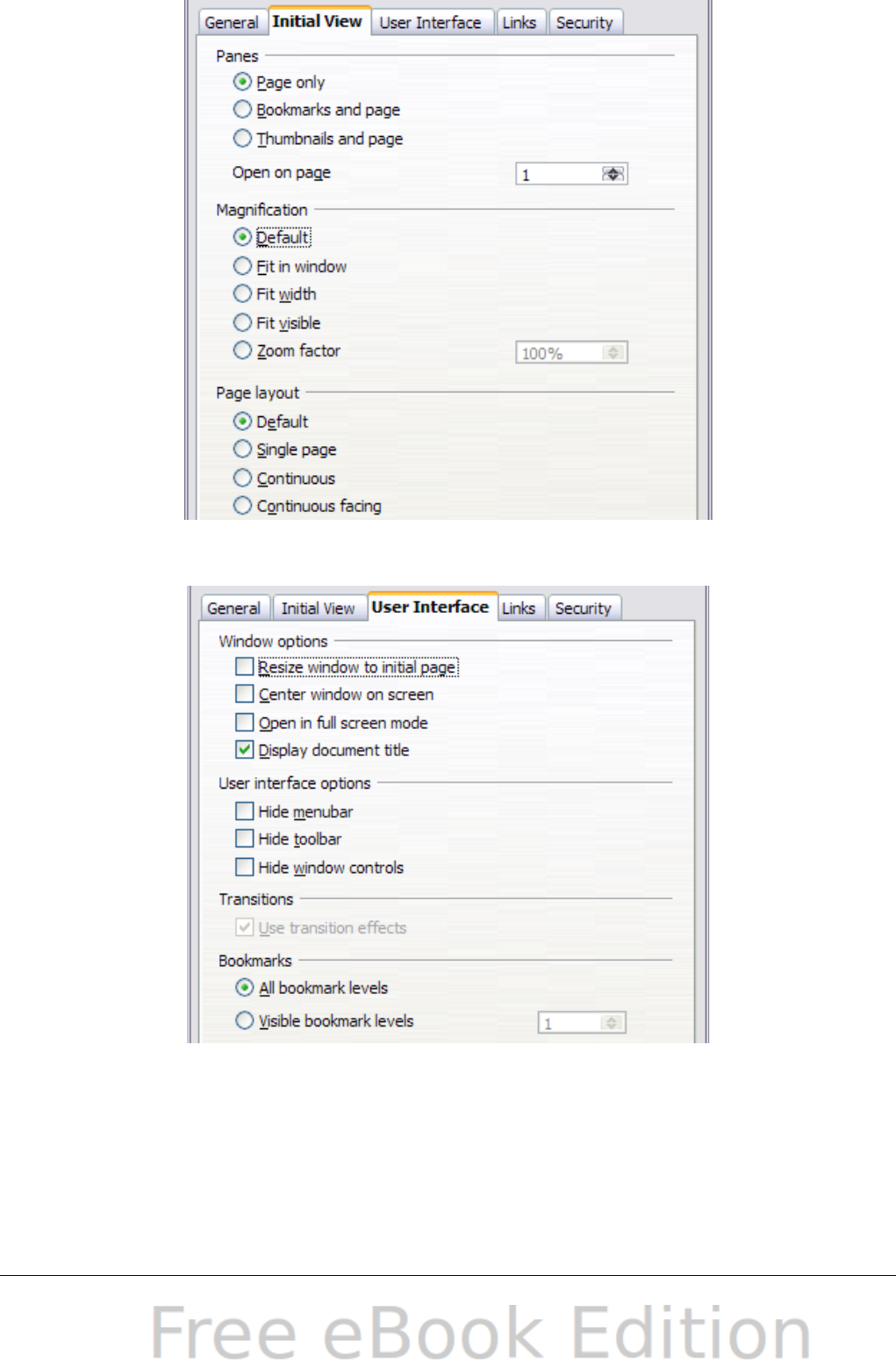
Figure 119: Initial View page of PDF Options dialog
Figure 120: User Interface page of PDF Options dialog
Window options section
•Resize window to initial page: Causes the PDF viewer window
to resize to fit the first page of the PDF.
170 OpenOffice.org 3.x Calc Guide
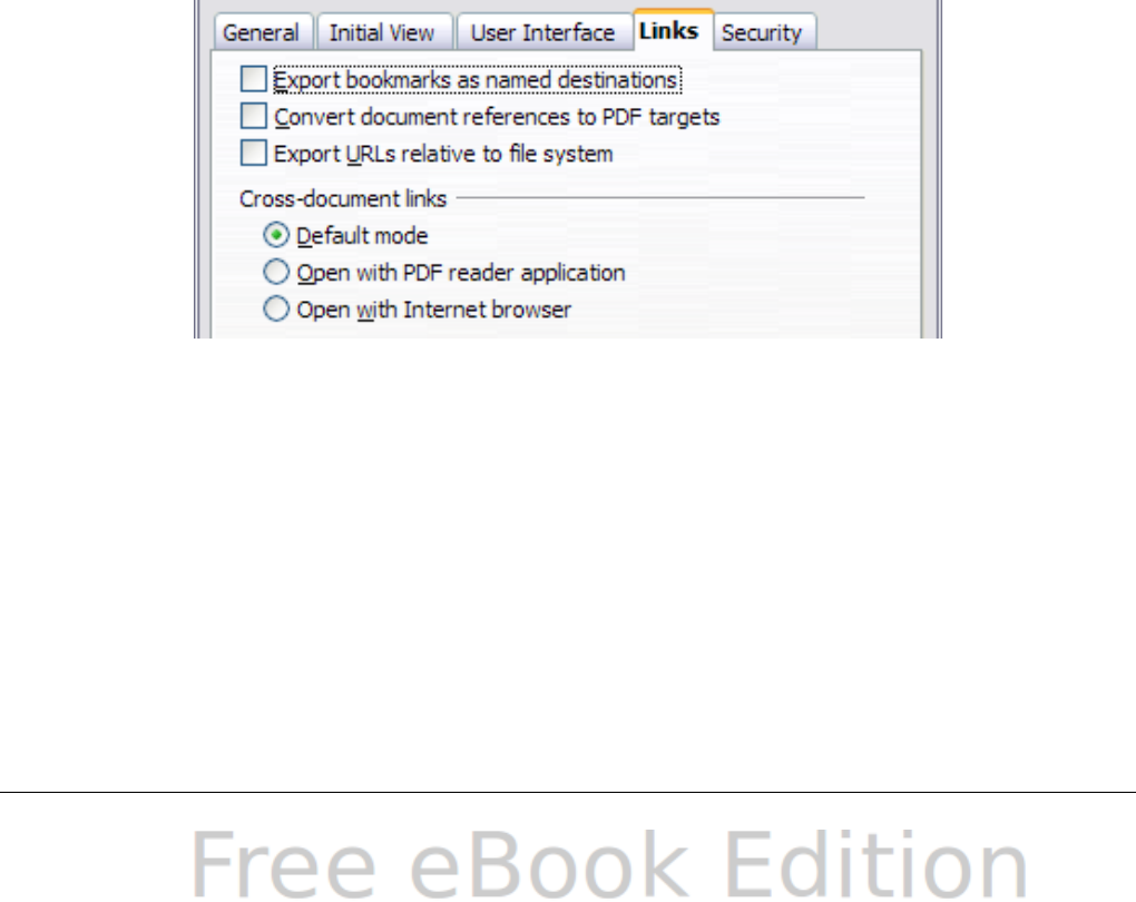
•Center window on screen: Causes the PDF viewer window to be
centered on the computer screen.
•Open in full screen mode: Causes the PDF viewer to open full-
screen instead of in a smaller window.
•Display document title: Causes the PDF viewer to display the
document’s title in the title bar.
User interface options section
•Hide menubar: Causes the PDF viewer to hide the menu bar.
•Hide toolbar: Causes the PDF viewer to hide the toolbar.
•Hide window controls: Causes the PDF viewer to hide other
window controls.
Transitions
Not available in Calc.
Bookmarks
Select how many heading levels are displayed as bookmarks, if
Export bookmarks is selected on the General page.
Links page of PDF Options dialog
On this page you can choose how links are exported to PDF.
Figure 121: Links page of PDF Options dialog
Export bookmarks as named destinations
If you have defined Writer bookmarks, Impress or Draw slide names,
or Calc sheet names, this option exports them as “named
destinations” to which Web pages and PDF documents can link.
Convert document references to PDF targets
If you have defined links to other documents with OpenDocument
extensions (such as .ODT, .ODS, and .ODP), this option converts the
file names to .PDF in the exported PDF document.
Chapter 6 Printing, Exporting, and E-mailing 171
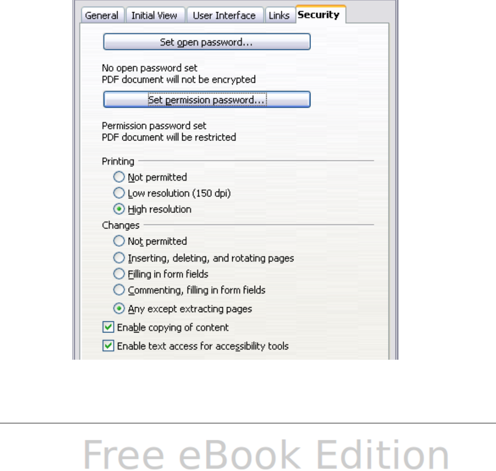
Export URLs relative to file system
If you have defined relative links in a document, this option exports
those links to the PDF.
Cross-document links
Defines the behavior of links clicked in PDF files.
Security page of PDF Options dialog
PDF export includes options to encrypt the PDF (so it cannot be
opened without a password) and apply some digital rights management
(DRM) features.
•With an open password set, the PDF can only be opened with the
password. Once opened, there are no restrictions on what the
user can do with the document (for example, print, copy, or
change it).
•With a permissions password set, the PDF can be opened by
anyone, but its permissions can be restricted. See Figure 122.
Figure 122: Security page of PDF Options dialog.
172 OpenOffice.org 3.x Calc Guide
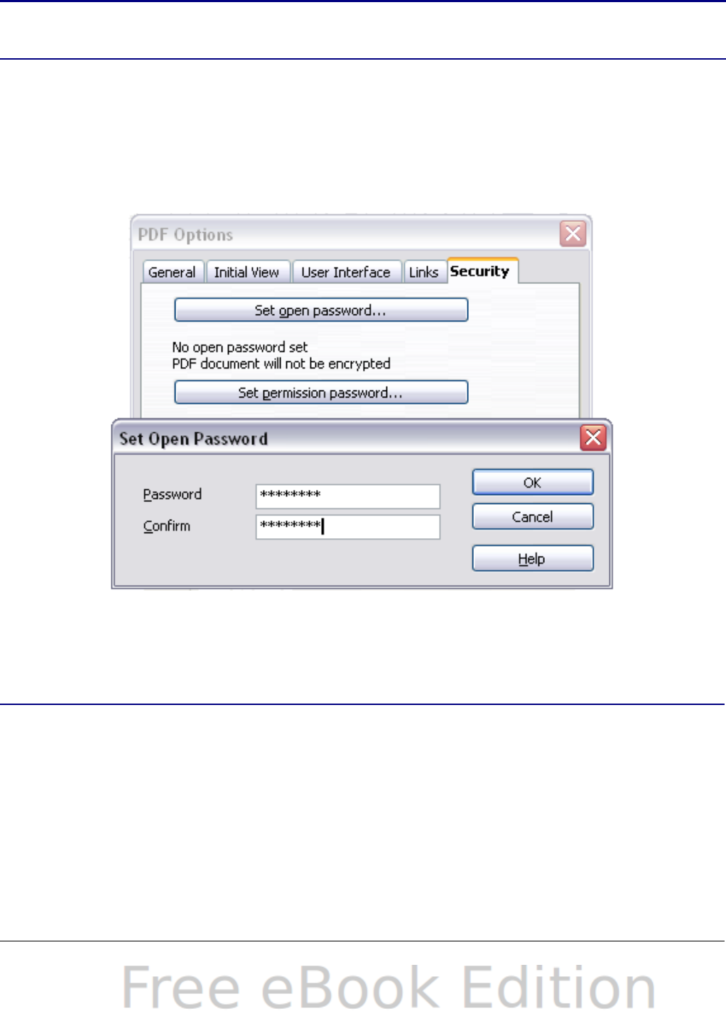
•With both the open password and permission password set, the
PDF can only be opened with the correct password, and its
permissions can be restricted.
Note Permissions settings are effective only if the user’s PDF viewer
respects the settings.
Figure 123 shows the dialog displayed when you click the Set open
password button on the Security page of the PDF Options dialog.
After you set a password for permissions, the other choices on the
Security page (shown in Figure 122) become available. These
selections are self-explanatory.
Figure 123: Setting a password to encrypt a PDF
Exporting to XHTML
Calc can export spreadsheets to XHTML. Choose File > Export. On
the Export dialog, specify a file name for the exported document, then
select the XHTML in the File format list and click the Export button.
Chapter 6 Printing, Exporting, and E-mailing 173

Saving as Web pages (HTML)
Calc can save files as HTML documents. Use File > Save As and
select HTML Document, or File > Wizards > Web Page.
If the file contains more than one sheet, the additional sheets will
follow one another in the HTML file. Links to each sheet will be placed
at the top of the document. Calc also allows the insertion of links
directly into the spreadsheet using the Hyperlink dialog.
E-mailing spreadsheets
OOo provides several quick and easy ways to send spreadsheets as an
e-mail attachment in one of three formats: OpenDocument Spreadsheet
(OOo’s default format), Microsoft Excel, or PDF.
To send the current document in OpenDocument format:
1) Choose File > Send > Document as E-mail. OpenOffice.org
opens your default e-mail program with the spreadsheet (*.ODS)
document attached.
2) In your e-mail program, enter the recipient, subject, and any text
you want to add, then send the e-mail.
File > Send > E-mail as OpenDocument Spreadsheet has the
same effect.
If you choose E-mail as Microsoft Excel, OOo first creates a file in
Excel format and then opens your e-mail program with the *.XLS file
attached.
Similarly, if you choose E-mail as PDF, OOo first creates a PDF using
your default PDF settings (as when using the Export Directly as PDF
toolbar button) and then opens your email program with the *.PDF file
attached.
E-mailing a spreadsheet to several recipients
To e-mail a document to several recipients, you can use the features in
your e-mail program or you can use OOo Writer’s mail merge facilities
to extract email addresses from an address book.
For details, see Chapter 10 (Printing, Exporting, and E-mailing) in the
Getting Started guide.
174 OpenOffice.org 3.x Calc Guide

Digital signing of documents
To sign a document digitally, you need a personal key, the certificate. A
personal key is stored on your computer as a combination of a private
key, which must be kept secret, and a public key, which you add to your
documents when you sign them. You can get a certificate from a
certification authority, which may be a private company or a
governmental institution.
When you apply a digital signature to a document, a checksum is
computed from the document’s content plus your personal key. The
checksum and your public key are stored together with the document.
When someone later opens the document on any computer with a
recent version of OpenOffice.org, the program will compute the
checksum again and compare it with the stored checksum. If both are
the same, the program will signal that you see the original, unchanged
document. In addition, the program can show you the public key
information from the certificate. You can compare this key with the
public key that is published on the web site of the certificate authority.
Whenever someone changes something in the document, this change
breaks the digital signature.
On Windows operating systems, the Windows features of validating a
signature are used. On Solaris and Linux systems, files that are
supplied by Thunderbird, Mozilla or Firefox are used. For a more
detailed description of how to get and manage a certificate, and
signature validation, see “Using Digital Signatures” in the OOo Help.
To sign a document:
1) Choose File > Digital Signatures.
2) If you have not saved the document since the last change, a
message box appears. Click Yes to save the file.
3) After saving, you see the Digital Signatures dialog. Click Add to
add a public key to the document.
4) In the Select Certificate dialog, select your certificate and click
OK.
5) You see again the Digital Signatures dialog, where you can add
more certificates if you want. Click OK to add the public key to
the saved file.
A signed document shows an icon in the status bar. You can double-
click the icon to view the certificate.
Chapter 6 Printing, Exporting, and E-mailing 175

Removing personal data
You may wish to ensure that personal data, versions, notes, hidden
information, or recorded changes are removed from files before you
send them to other people or create PDFs from them.
In Tools > Options > OpenOffice.org > Security > Options, you
can set Calc to remind (warn) you when files contain certain
information and remove personal information automatically on saving.
To remove personal and some other data from a file, go to File >
Properties. On the General tab, uncheck Apply user data and then
click the Reset button. This removes any names in the created and
modified fields, deletes the modification and printing dates, and resets
the editing time to zero, the creation date to the current date and time,
and the version number to 1.
To remove version information, either go to File > Versions, select the
versions from the list and click Delete, or use Save As and save the
file with a different name.
176 OpenOffice.org 3.x Calc Guide

Chapter 7
Using Formulas and
Functions

Introduction
In previous chapters, we have been entering one of two basic types of
data into each cell: numbers and text. However, we will not always
know what the contents should be. Often the contents of one cell
depends on the contents of other cells. To handle this situation, we use
a third type of data: the formula. Formulas are equations using
numbers and variables to get a result. In a spreadsheet, the variables
are cell locations that hold the data needed for the equation to be
completed.
A function is a predefined calculation entered in a cell to help you
analyze or manipulate data in a spreadsheet. All you have to do is add
the arguments, and the calculation is automatically made for you.
Functions help you create the formulas needed to get the results that
you are looking for.
Setting up a spreadsheet
If you are setting up more than a simple one-worksheet system in Calc,
it is worth planning ahead a little. Avoid the following traps:
•Typing fixed values into formulas
•Not including notes and comments describing what the system
does, including what input is required and where the formulas
come from (if not created from scratch)
•Not incorporating a system of checking to verify that the formulas
do what is intended
The trap of fixed values
Many users set up long and complex formulas with fixed values typed
directly into the formula.
For example, conversion from one currency to another requires
knowledge of the current conversion rate. If you input a formula in cell
C1 of =0.75*B1 (for example to calculate the value in Euros of the USD
dollar amount in cell B1), you will have to edit the formula when the
exchange rate changes from 0.75 to some other value. It is much
easier to set up an input cell with the exchange rate and reference that
cell in any formula needing the exchange rate. What-if type
calculations also are simplified: what if the exchange rate varies from
0.75 to 0.70 or 0.80? No formula editing is needed and it is clear what
rate is used in the calculations. Breaking complex formulas down into
178 OpenOffice.org 3.x Calc Guide
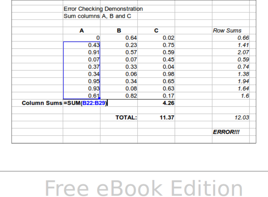
more manageable parts, described below, also helps to minimise errors
and aid troubleshooting.
Lack of documentation
Lack of documentation is a very common failing. Many users prepare a
simple worksheet which then develops into something much more
complicated over time. Without documentation, the original purpose
and methodology is often unclear and difficult to decipher. In this case
it is usually easier to start again from the beginning, wasting the work
done previously. If you insert comments in cells, and use labels and
headings, a spreadsheet can be later modified by you or others and
much time and effort will be saved.
Error-checking formulas
Adding up columns of data or selections of cells from a worksheet often
results in errors due to omitting cells, wrongly specifying a range, or
double-counting cells. It is useful to institute checks in your
spreadsheets. For example, set up a spreadsheet to calculate columns
of figures, and use SUM to calculate the individual column totals. You
can check the result by including (in a non-printing column) a set of
row totals and adding these together. The two figures—row total and
column total—must agree. If they do not, you have an error
somewhere.
Figure 124: Error checking of formulas
Chapter 7 Using Formulas and Functions 179

You can even set up a formula to calculate the difference between the
two totals and report an error in case a non-zero result is returned (see
Figure 124).
Creating formulas
You can enter formulas in two ways, either directly into the cell itself,
or at the input line. Either way, you need to start a formula with one of
the following symbols: =, + or –. Starting with anything else causes the
formula to be treated as if it were text.
Operators in formulas
Each cell on the worksheet can be used as a data holder or a place for
data calculations. Entering data is accomplished simply by typing in
the cell and moving to the next cell or pressing Enter. With formulas,
the equals sign indicates that the cell will be used for a calculation. A
mathematical calculation like 15 + 46 can be accomplished as shown
in Figure 125.
While the calculation on the left was accomplished in only one cell, the
real power is shown on the right where the data is placed in cells and
the calculation is performed using references back to the cells. In this
case, cells B3 and B4 were the data holders, with B5 the cell where the
calculation was performed. Notice that the formula was shown as
=B3+B4. The plus sign indicates that the contents of cells B3 and B4
are to be added together and then have the result in the cell holding
the formula. All formulas build upon this concept. Other ways of
entering formulas are shown in Table 7.
These cell references allow formulas to use data from anywhere in the
worksheet being worked on or from any other worksheet in the
workbook that is opened. If the data needed was in different
worksheets, they would be referenced by referring to the name of the
worksheet, for example =SUM(Sheet2.B12+Sheet3.A11).
Note
To enter the = symbol for a purpose other than creating a
formula as described in this chapter, type an apostrophe or
single quotation mark before the =. For example, in the entry '=
means different things to different people, Calc treats everything
after the single quotation mark—including the = sign—as text.
180 OpenOffice.org 3.x Calc Guide
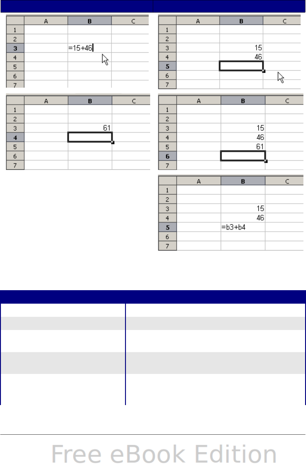
Simple Calculation in 1 Cell Calculation by Reference
Figure 125: A simple calculation
Table 7: Common ways to enter formulas
Formula Description
=A1+10 Displays the contents of cell A1 plus 10.
=A1*16% Displays 16% of the contents of A1.
=A1*A2 Displays the result of the multiplication of
A1 and A2.
=ROUND(A1;1) Displays the contents of cell A1 rounded to
one decimal place.
=EFFECTIVE(5%;12) Calculates the effective interest for 5%
annual nominal interest with 12 payments a
year.
Chapter 7 Using Formulas and Functions 181
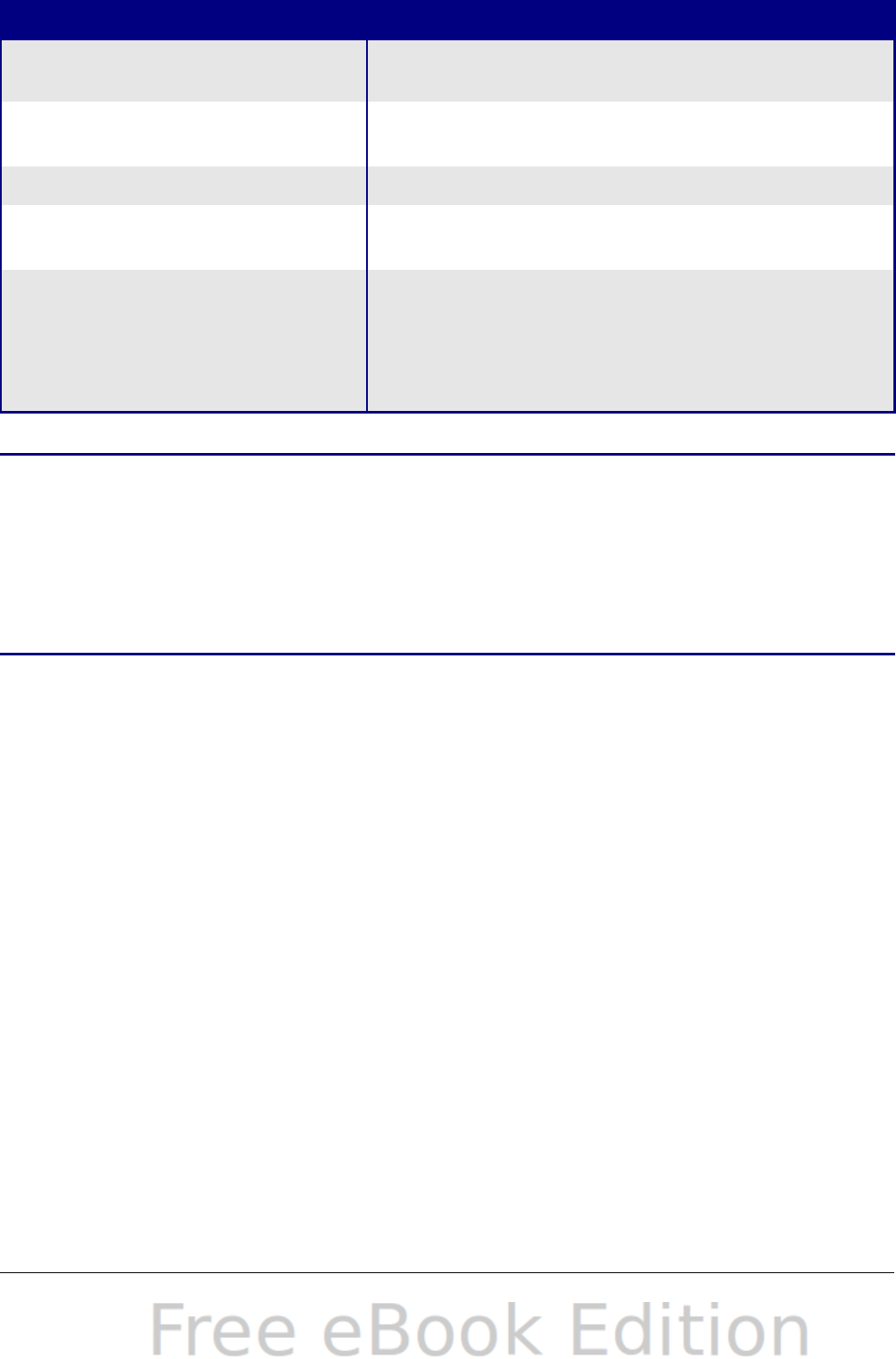
Formula Description
=B8-SUM(B10:B14) Calculates B8 minus the sum of the cells
B10 to B14.
=SUM(B8;SUM(B10:B14)) Calculates the sum of cells B10 to B14 and
adds the value to B8.
=SUM(B1:B65536) Sums all numbers in column B.
=AVERAGE(BloodSugar) Displays the average of a named range
defined under the name BloodSugar.
=IF(C31>140; "HIGH"; "OK") Displays the results of a conditional
analysis of data from two sources. If the
contents of C31 is greater than 140, then
HIGH is displayed, otherwise OK is
displayed.
Note
Users of Lotus 1-2-3®, Quattro Pro® and other spreadsheet
software may be familiar with formulas that begin with +, -, =,
(, @, ., $, or #. A mathematical formula would look like
+D2+C2 or +2*3. Functions begin with the @ symbol such as
@SUM(D2..D7), @COS(@DEGTORAD(30)) and
@IRR(GUESS;CASHFLOWS). Ranges are identified such as
A1..D3.
Functions can be identified in Table 7 with a word, for example
ROUND, followed by parentheses enclosing references or numbers.
It is also possible to establish ranges for inclusion by naming them
using Insert > Names, for example BloodSugar representing a range
such as B3:B10. Logical functions can also be performed as
represented by the IF statement which results in a conditional
response based upon the data in the identified cell, for example
=IF(A2>=0;"Positive";"Negative")
A value of 3 in cell A2 would return the result Positive, –9 the result
Negative.
Operator types
You can use the following operators in OpenOffice.org Calc: arithmetic,
comparative, descriptive, text, and reference.
Arithmetic operators
The addition, subtraction, multiplication and division operators return
numerical results. The Negation and Percent operators identify a
182 OpenOffice.org 3.x Calc Guide
characteristic of the number found in the cell, for example -37. The
example for Exponentiation illustrates how to enter a number that is
being multiplied by itself a certain number of times, for example 23 =
2*2*2.
Table 8: Arithmetical operators
Operator Name Example
+ (Plus) Addition =1+1
– (Minus) Subtraction =2–1
– (Minus) Negation –5
* (asterisk) Multiplication =2*2
/ (Slash) Division =10/5
% (Percent) Percent 15%
^ (Caret) Exponentiation 2^3
Comparative operators
Comparative operators are found in formulas that use the IF function
and return either a true or false answer; for example, =IF(B6>G12;
127; 0) which, loosely translated, means if the contents of cell B6 are
greater than the contents of cell G12, then return the number 127,
otherwise return the number 0.
A direct answer of TRUE or FALSE can be obtained by entering a
formula such as =B6>B12. If the numbers found in the referenced
cells are accurately represented, the answer TRUE is returned,
otherwise FALSE is returned.
Table 9: Comparative operators
Operator Name Example
= (equal sign) Equal A1=B1
> (Greater than) Greater than A1>B1
< (Less than) Less than A1<B1
>= (Greater than or equal to) Greater than or equal to A1>=B1
<= (Less than or equal to) Less than or equal to A1<=B1
<> (Inequality) Inequality A1<>B1
Chapter 7 Using Formulas and Functions 183
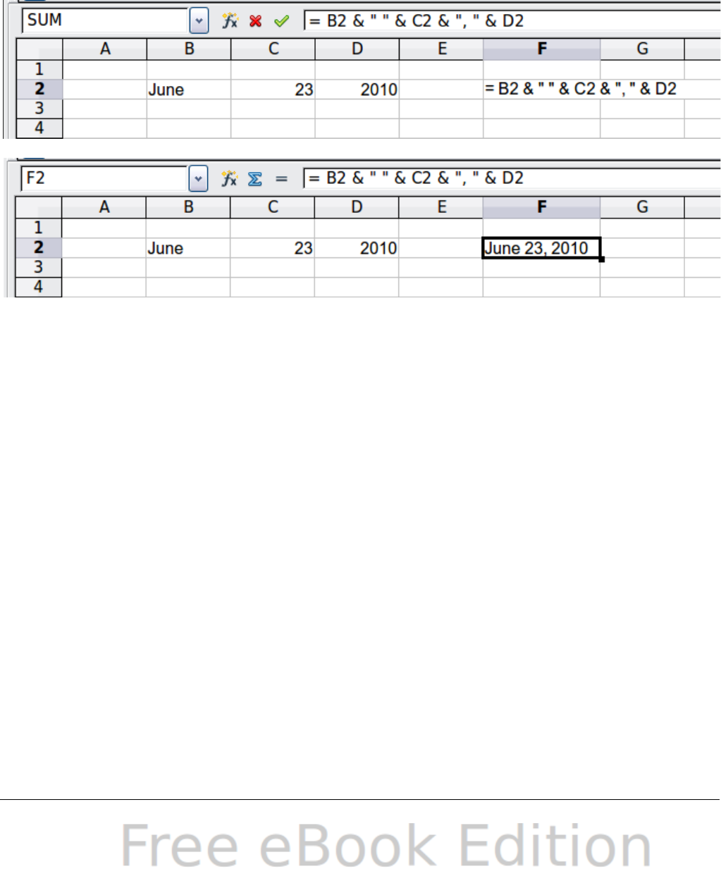
If cell A1 contains the numerical value 4 and cell B1 the numerical
value 5, the above examples would yield results of FALSE, FALSE,
TRUE, FALSE, TRUE, and TRUE.
Text operators
It is common for users to place text in spreadsheets. To provide for
variability in what and how this type of data is displayed, text can be
joined together in pieces coming from different places on the
spreadsheet. Figure 126 shows an example.
Figure 126: Text concatenation
In this example, specific pieces of the text were found in three
different cells. To join these segments together, the formula also adds
required spaces and punctuation enclosed within quotation marks,
resulting in a formula of =B2 & " " & C2 & ", " & D2. The result is
the concatenation into a date formatted in a particular sequence.
Taking this example further, if the result cell is defined as a name, then
text concatenation is performed using this defined name. Calc has a
CONCATENATE function which performs the same operation.
184 OpenOffice.org 3.x Calc Guide
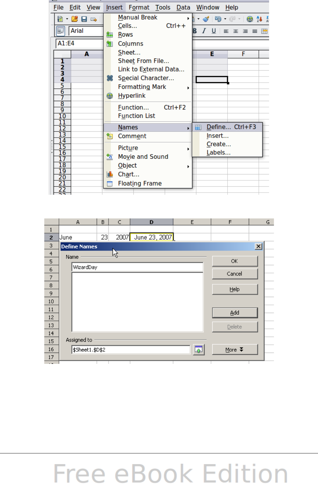
Figure 127: Defining a name for a range of cells
Figure 128: Naming a cell or range of cells for
inclusion in a formula
Chapter 7 Using Formulas and Functions 185
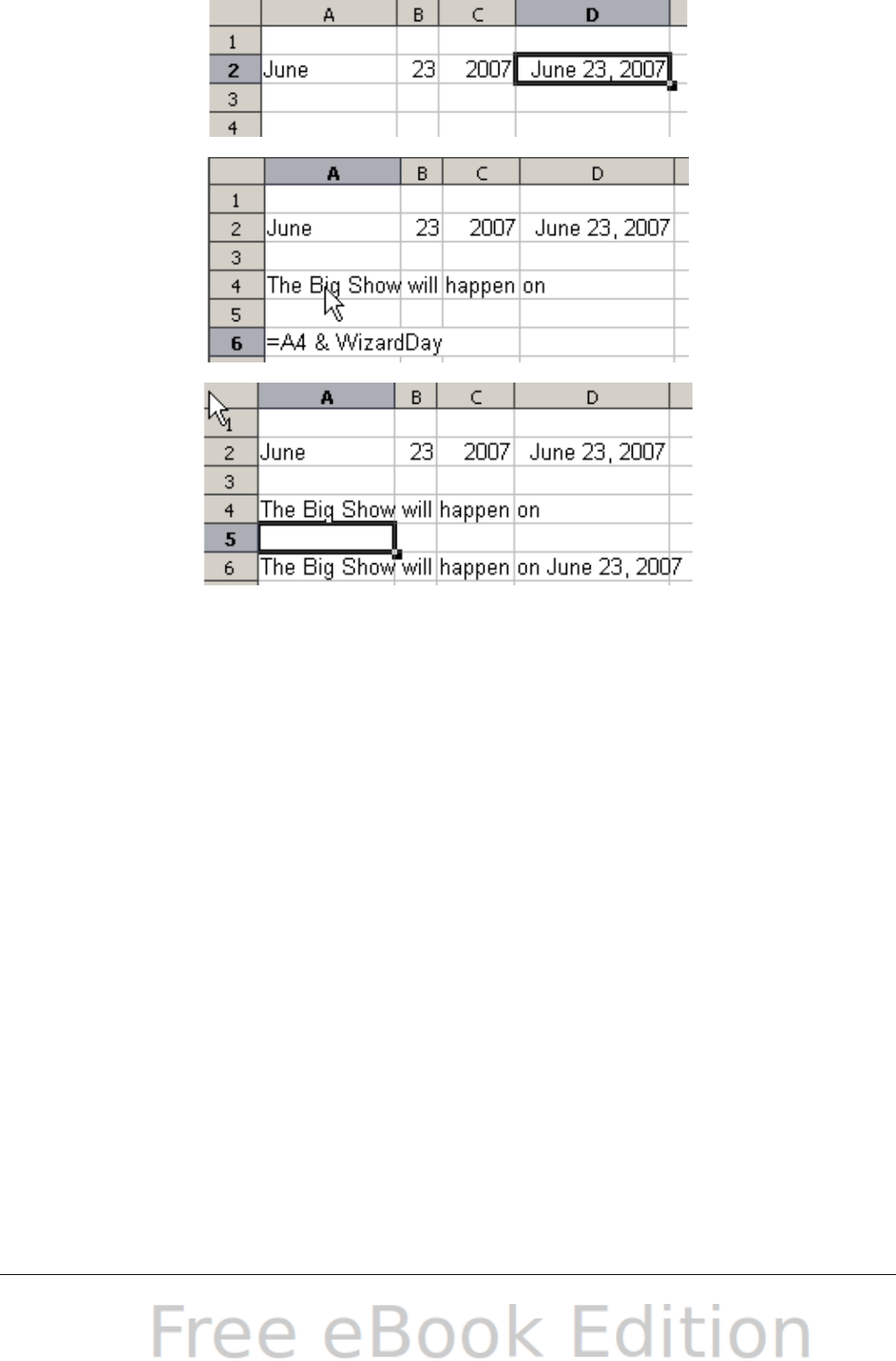
Figure 129: Defining Names on a worksheet
Reference operators
In its simplest form a reference refers to a single cell, but references
can also refer to a rectangle or cuboid range or a reference in a list of
references. To build such references you need reference operators.
An individual cell is identified by the column identifier (letter) located
along the top of the columns and a row identifier (number) found along
the left-hand side of the spreadsheet. On spreadsheets read from left to
right, the upper left cell is A1.
Range operator
The range operator is written as colon. An expression using the range
operator has the following syntax:
reference left : reference right
The range operator builds a reference to the smallest range including
both the cells referenced with the left reference and the cells
referenced with the right reference.
186 OpenOffice.org 3.x Calc Guide
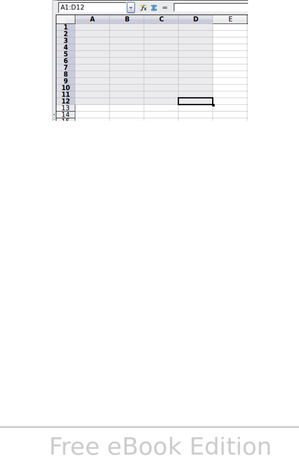
Figure 130: Reference Operator for a range
In the upper left corner of Figure 130 the reference A1:D12 is shown,
corresponding to the cells included in the drag operation with the
mouse to highlight the range.
Examples
A2:B4 Reference to a rectangle range with 6 cells, 2
column width × 3 row height. When you click on
the reference in the formula in the input line, a
border indicates the rectangle.
(A2:B4):C9 Reference to a rectangle range with cell A2 top
left and cell C9 bottom right. So the range
contains 24 cells, 3 column width × 8 row
height.
Sheet1.A3:Sheet3.D4 Reference to a cuboid range with 24 cells, 4
column width × 2 row height × 3 sheets depth.
When you enter B4:A2 or A4:B2 directly, then Calc will turn it to
A2:B4. So the left top cell of the range is left of the colon and the
bottom right cell is right of the colon. But if you name the cell B4 for
example with '_start' and A2 with '_end', you can use _start:_end
without any error.
Calc can not reference a whole column of unspecified length via A:A or
a whole row via 1:1 yet as you might know from other spreadsheet
programs. See Issue 20495.
Chapter 7 Using Formulas and Functions 187

Reference concatenation operator
The concatenation operator is written as a tilde. An expression using
the concatenation operator has the following syntax:
reference left ~ reference right
The result of such an expression is a reference list, which is an ordered
list of references. Some functions can take a reference list as an
argument, SUM, MAX or INDEX for example.
The reference concatenation is sometimes called 'union'. But it is not
the union of the two sets 'reference left' and 'reference right' as
normally understood in set theory. COUNT(A1:C3~B2:D2) returns 12
(=9+3), but it has only 10 cells when considered as the union of the
two sets of cells.
Notice that SUM(A1:C3;B2:D2) is different from SUM( A1:C3~B2:D2)
although they give the same result. The first is a function call with 2
parameters, each of them is reference to a range. The second is a
function call with 1 parameter, which is a reference list.
Intersection operator
The intersection operator is written as an exclamation mark. An
expression using the intersection operator has the following syntax:
reference left ! reference right
If the references refer to single ranges, the result is a reference to a
single range, containing all cells, which are both in the left reference
and in the right reference.
If the references are reference lists, then each list item from the left is
intersected with each one from the right and these results are
concatenated to a reference list. The order is to first intersect the first
item from the left with all items from the right, then intersect the
second item from the left with all items from the right, and so on.
Examples
A2:B4 ! B3:D6
This results in a reference to the range B3:B4, because these cells
are inside A2:B4 and inside B3:D4.
(A2:B4~B1:C2) ! (B2:C6~C1:D3)
First the intersections A2:B4!B2:C6, A2:B4!C1:D3, B1:C2!B2:C6 and
B1:C2!C1:D3 are calculated. This results in B2:B4, empty, B2:C2,
and C1:C2. Then these results are concatenated, dropping empty
parts. So the final result is the reference list B2:B4 ~ B2:C2 ~
C1:C2.
188 OpenOffice.org 3.x Calc Guide

You can use the intersection operator to refer a cell in a cross
tabulation in an understandable way. If you have columns labeled
'Temperature' and 'Precipitation' and the rows labeled 'January',
'February', 'March', and so on, then the following expression
'February' ! !Temperature'
will reference to the cell containing the temperature in February.
The intersection operator (!) should have a higher precedence than the
concatenation operator (~), but do not rely on precedence.
Tip Always put in parentheses the part that is to be calculated first.
Relative and absolute references
References are the way that we refer to the location of a particular cell
in Calc and can be either relative (to the current cell) or absolute (a
fixed amount).
Relative referencing
An example of a relative reference will illustrate the difference
between a relative reference and absolute reference using the
spreadsheet from Figure 131.
1) Type the numbers 4 and 11 into cells C3 and C4 respectively of
that spreadsheet.
2) Copy the formula in cell B5 to cell C5. You can do this by using a
simple copy and paste or click and drag B5 to C5 as shown below.
The formula in B5 calculates the sum of values in the two cells B3
and B4.
3) Click in cell C5. The formula bar shows =C3+C4 rather than
=B3+B4 and the value in C5 is 15, the sum of 4 and 11 which are
the values in C3 and C4.
In cell B5 the references to cells B3 and B4 are relative references.
This means that Calc interprets the formula in B5 and applie it to the
cells in the B column and puts the result in the in the cell holding the
formula. When you copied the formula to another cell, the same
procedure was used to calculate the value to put in that cell. This time
the formula in cell C5 referred to cells C3 and C4.
Chapter 7 Using Formulas and Functions 189
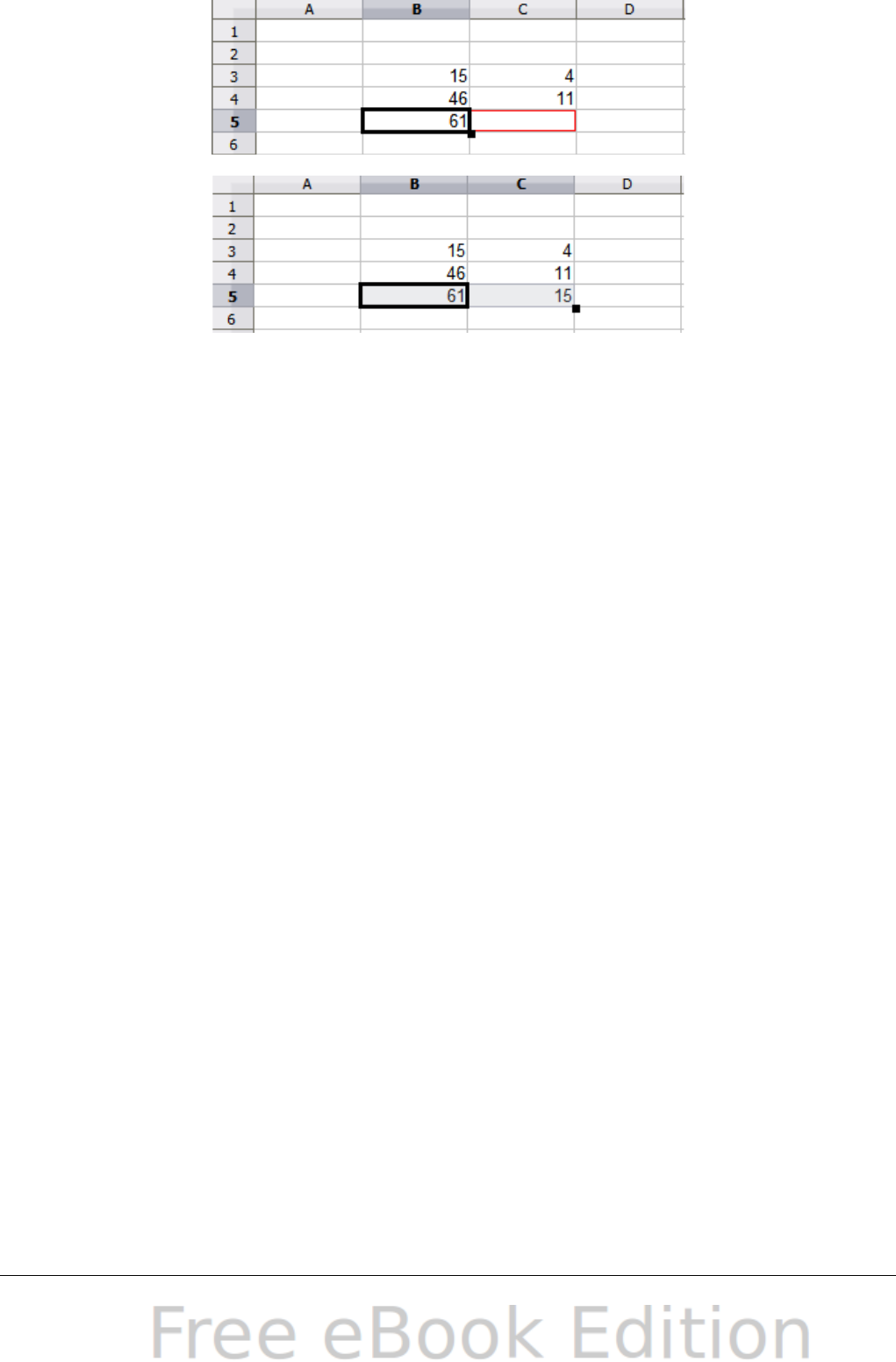
Figure 131: Relative references
You can think of a relative address as a pair of offsets to the current
cell. Cell B1 is 1 column to the left of Cell C5 and 4 rows above. The
address could be written as R[-1]C[-4]. In fact earlier spreadsheets
allowed this notation method to be used in formulas.
Whenever you copy this formula from cell B5 to another cell the result
will always be the sum of the two numbers taken from the two cells
one and two rows above the cell containing the formula.
Relative addressing is the default method of referring to addresses in
Calc.
Absolute referencing
You may want to multiply a column of numbers by a fixed amount. A
column of figures might show amounts in US Dollars. To convert these
amounts to Euros it is necessary to multiply each dollar amount by the
exchange rate. $US10.00 would be multiplied by 0.75 to convert to
Euros, in this case Eur7.50. The following example shows how to input
an exchange rate and use that rate to convert amounts in a column
form USD to Euros.
1) Input the exchange rate Eur:USD (0.75) in cell D1. Enter amounts
(in USD) into cells D2, D3 and D4, for example 10, 20, and 30.
2) In cell E2 type the formula =D2*D1. The result is 7.5, correctly
shown.
3) Copy the formula in cell E2 to cell E3. The result is 200, clearly
wrong! Calc has copied the formula using relative addressing -
the formula in E3 is =D3*D2 and not what we want which is
=D3*D1.
4) In cell E2 edit the formula to be =D2*$D$1. Copy it to cells E3
and E4. The results are now 15 and 22.5 which are correct.
190 OpenOffice.org 3.x Calc Guide
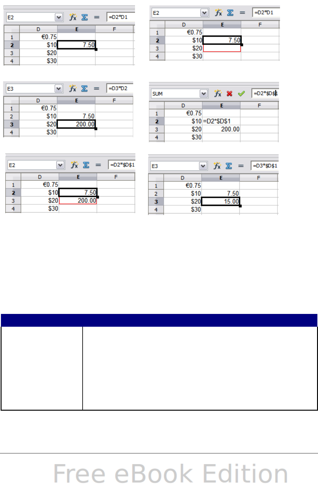
Steps 2: Setting the exchange rate of Eur at 7.5, then copying it to E3
Copying formula from E2 to E3 & changing the formula to read absolute reference
Applying the correct formula from E2 to E3
Figure 132: Absolute References
The $ signs before the D and the 1 convert the reference to cell D1
from relative to absolute or fixed. If the formula is copied to another
cell the second part will always show $D$1. The interpretation of this
formula is “take the value in the cell one column to the left in the same
row and multiply it by the value in cell D1”.
Cell references can be shown in four ways:
Reference Explanation
D1 Relative, from cell E3: the cell one column to the left
and two rows above
$D$1 Absolute, from cell E3: the cell D1
$D1 Partially absolute, from cell E3: the cell in column D
and two rows above
D$1 Partially absolute, from cell E3: the cell one column to
the left and row 1
Chapter 7 Using Formulas and Functions 191
Hint
To change references in formulas highlight the cell and press
Shift-F4 to cycle through the four different types of references.
This is of limited value in more complicated formulas, it is
usually quicker to edit the formula by hand.
Knowledge of the use of relative and absolute references is essential if
you want to copy and paste formulas and to link spreadsheets.
Order of calculation
Order of calculation refers to the sequence in which numerical
operations are performed. Division and multiplication are performed
before addition or subtraction. There is a common tendency to expect
calculations to be made from left to right as the equation would be
read in English. Calc evaluates the entire formula, then based upon
programming precedence breaks the formula down executing
multiplication and division operations before other operations.
Therefore, when creating formulas you should test your formula to
make sure that the correct result is being obtained. Following is an
example of the order of calculation in operation.
Table 10 – Order of Calculation
Left To Right Calculation Ordered Calculation
1+3*2+3 = 11
1+3=4, then 4 X 2 = 8, then 8 + 3 = 11
=1+3*2+3 result 10
3*2=6, then 1 + 6 + 3 = 10
Another possible intention could be:
1+3*2+3 = 20
The program resolves the
multiplication of 3 X 2 before
dealing with the numbers being
added.
If you intend for the result to be either of the two possible solutions on
the left, the way to achieve these results would be to order the formula
as:
((1+3) * 2)+3 = 11 (1+3) * (2+3) = 20
Note Use parentheses to group operations in the order you intend; for
example, =B4+G12*C4/M12 might become =((B4+G12)*C4)/M12.
Calculations linking sheets
Another powerful feature of Calc is the ability to link data through
several worksheets. The naming of worksheets can be helpful to
192 OpenOffice.org 3.x Calc Guide
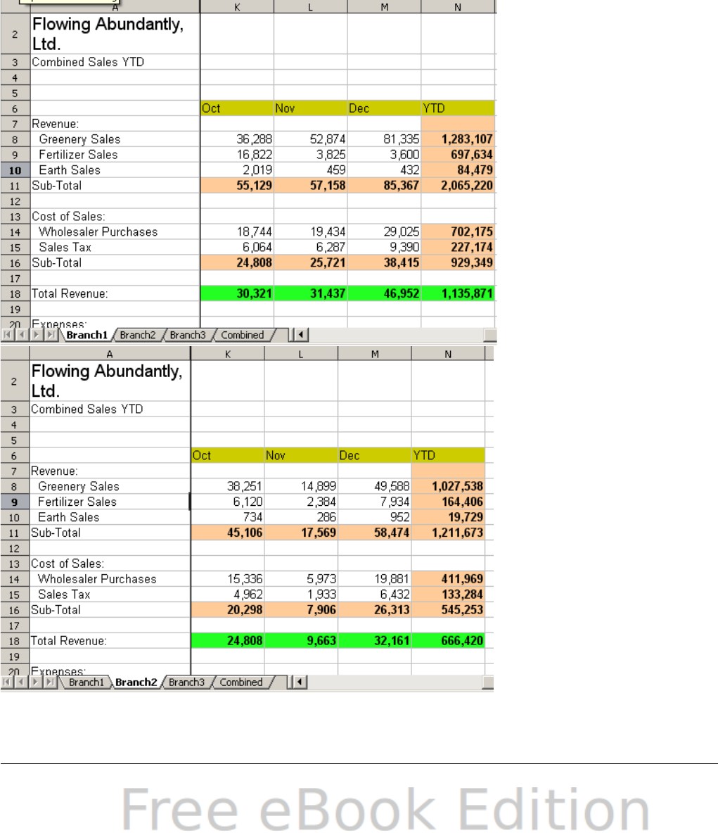
identify where specific data may be found. A name such as Payroll or
Boise Sales is much more meaningful than Sheet1. The function named
SHEET() returns the sheet number in the collection of spreadsheets.
There are several worksheets in each book and they are numbered
from the left: Sheet1, Sheet2, and so forth. If you drag the worksheets
around to different locations among the tabs, the function returns the
number referring to the current position of this worksheet.
An example of calculations obtaining data from other work can be seen
in a business setting where a business combines revenues and costs of
each of its branch operations into a single combined worksheet.
Sheet containing data
for Branch 1.
Sheet containing data
for Branch 2.
Chapter 7 Using Formulas and Functions 193
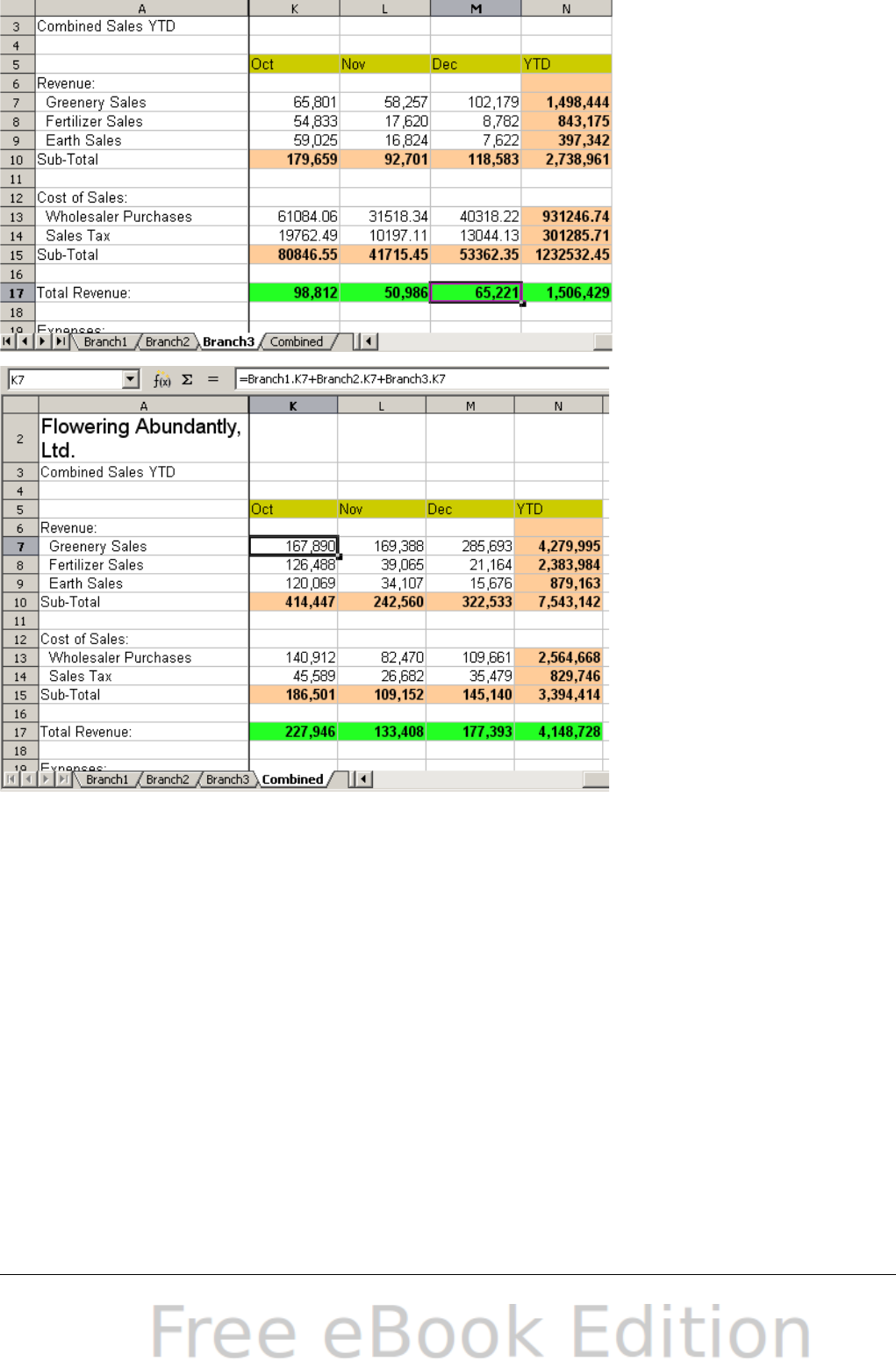
Sheet containing data
for Branch 3.
Sheet containing
combined data for all
branches.
Figure 133: Combining data from several sheets into a single sheet
The spreadsheets have been set up with identical structures. The
easiest way to do this is to set up the first Branch spreadsheet, input
data, format cells, and prepare the formulas for the various sums of
rows and columns.
1) On the worksheet tab, right-click and select Rename Sheet....
Type Branch1. Right-click on the tab again and select Move/Copy
Sheet...
2) In the Move/Copy Sheet dialog, select the Copy option and select
Sheet 2 in the area Insert before. Click OK, right-click on the tab
of the sheet Branch1_2 and rename it to Branch2. Repeat to
produce the Branch3 and Combined worksheets.
194 OpenOffice.org 3.x Calc Guide
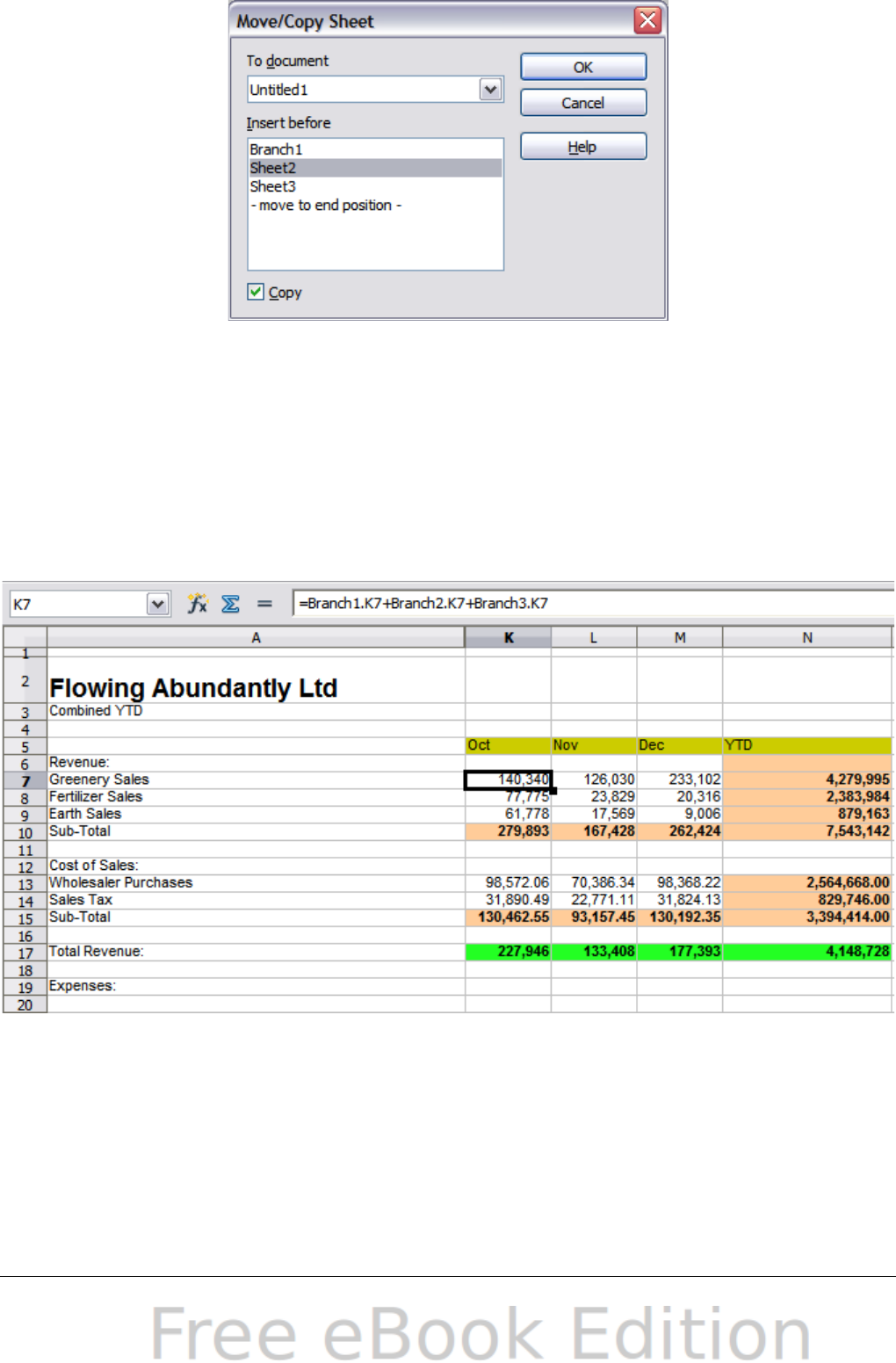
Figure 134: Copying a worksheet
3) Enter the data for Branch 2 and Branch 3 into the respective
sheets. Each sheet stands alone and reports the results for the
individual branches.
4) In the Combined worksheet, click on cell K7. Type =, click on the
tab Branch1, click on cell K7, press +, repeat for sheets Branch2
and Branch3 and press Enter. You now have a formula in cell K1
which adds the revenue from Greenery Sales for the 3 Branches.
Figure 135: Linking sheets—the Combined worksheet showing linking
between branch sheets
5) Copy the formula, highlight the range K7..N17, click Edit >
Paste Special, uncheck the Paste all and Formats boxes in the
Selection area of the dialog box and click OK. You will see the
following message:
Chapter 7 Using Formulas and Functions 195

Figure 136: Linking sheets: pasting a formula to
a cell range
6) Click Yes. You have now copied the formulas into each cell while
maintaining the format you set up in the original worksheet. Of
course, in this example you would have to tidy the worksheet up
by removing the zeros in the non-formatted rows.
Figure 137: Linking Sheets: Copy Paste Special from K7...N17
Note OOo default is to paste all the attributes of the original cell(s) -
formats, notes, objects, text strings and numbers.
The Function Wizard can also be used to accomplish the linking. Use of
this Wizard is described in detail in the section on Functions.
196 OpenOffice.org 3.x Calc Guide

Understanding functions
Calc includes over 350 functions to help you analyze and reference
data. Many of these functions are for use with numbers, but many
others are used with dates and times, or even text. A function may be
as simple as adding two numbers together, or finding the average of a
list of numbers. Alternatively, it may be as complex as calculating the
standard deviation of a sample, or a hyperbolic tangent of a number.
Typically, the name of a function is an abbreviated description of what
the function does. For instance, the FV function gives the future value
of an investment, while BIN2HEX converts a binary number to a
hexadecimal number. By tradition, functions are entered entirely in
upper case letters, although Calc will read them correctly if they are in
lower or mixed case, too.
A few basic functions are somewhat similar to operators. Examples:
+ This operator adds two numbers together for a result. SUM() on
the other hand adds groups of contiguous ranges of numbers
together.
* This operator multiplies two numbers together for a result.
PRODUCT() does the same for multiplying that SUM() does for
adding.
Each function has a number of arguments used in the calculations.
These arguments may or may not have their own name. Your task is to
enter the arguments needed to run the function. In some cases, the
arguments have predefined choices, and you may need to refer to the
online help or Appendix B (Description of Functions) in this book to
understand them. More often, however, an argument is a value that
you enter manually, or one already entered in a cell or range of cells on
the spreadsheet. In Calc, you can enter values from other cells by
typing in their name or range, or—unlike the case in some
spreadsheets—by selecting cells with the mouse. If the values in the
cells change, then the result of the function is automatically updated.
For compatibility, functions and their arguments in Calc have almost
identical names to their counterparts in Microsoft Excel. However,
both Excel and Calc have functions that the other lacks. Occasionally,
functions with the same names in Calc and Excel have different
arguments, or slightly different names for the same argument—neither
of which can be imported to the other. However, the majority of
functions can be used in both Calc and Excel without any change.
Chapter 7 Using Formulas and Functions 197
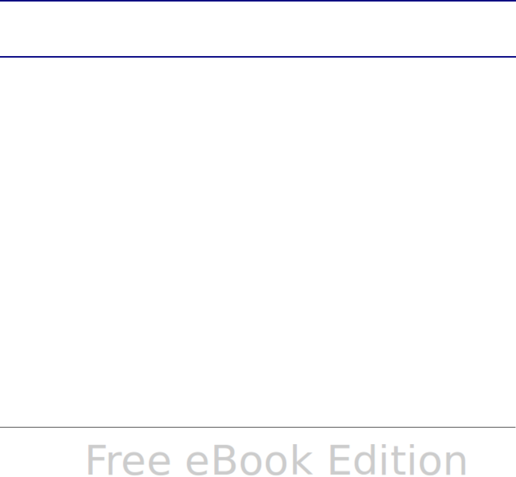
Understanding the structure of functions
All functions have a similar structure. If you use the right tool for
entering a function, you can escape learning this structure, but it is
still worth knowing for troubleshooting.
To give a typical example, the structure of a function to find cells that
match entered search criteria is:
= DCOUNT (Database;Database field;Search_criteria)
Since a function cannot exist on its own, it must always be part of a
formula. Consequently, even if the function represents the entire
formula, there must be an = sign at the start of the formula.
Regardless of where in the formula a function is, the function will start
with its name, such as DCOUNT in the example above. After the name
of the function comes its arguments. All arguments are required,
unless specifically listed as optional.
Arguments are added within the parentheses and are separated by
semicolons, with no space between the arguments and the semicolons.
Note
OOo uses the semicolon as an argument list separator, unlike
Excel which uses a comma. This is a common mistake made by
users accustomed to entering Excel formulas.
Many arguments are a number. A Calc function can take up to thirty
numbers as an argument. That may not sound like much at first.
However, when you realize that the number can be not only a number
or a single cell, but also an array or range of cells that contain several
or even hundreds of cells, then the apparent limitation vanishes.
Depending on the nature of the function, arguments may be entered as
follows:
"text data" The quotes indicate text or string data is being entered.
9 The number nine is being entered as a number.
"9" The number nine is being entered as text
A1 The address for whatever is in Cell A1 is being entered
Nested functions
Functions can also be used as arguments within other functions. These
are called nested functions.
=SUM(2;PRODUCT(5;7))
198 OpenOffice.org 3.x Calc Guide

To get an idea of what nested functions can do, imagine that you are
designing a self-directed learning module. During the module, students
do three quizzes, and enter the results in cells A1, A2, and A3. In A4,
you can create a nested formula that begins by averaging the results of
the quizzes with the formula =AVERAGE(A1:A3). The formula then uses
the IF function to give the student feedback that depends upon the
average grade on the quizzes. The entire formula would read:
=IF(AVERAGE(A1:A3) >85; "Congratulations! You are ready to
advance to the next module"; "Failed. Please review the
material again. If necessary, contact your instructor for
help")
Depending on the average, the student would receive the message for
either congratulations or failure.
Notice that the nested formula for the average does not require its own
equal sign. The one at the start of the equation is enough for both
formulas.
If you are new to spreadsheets, the best way to think of functions is as
a scripting language. We've used simple examples to explain the
concept more clearly, but, through nesting of functions, a Calc formula
can quickly become complex.
Note Calc keeps the syntax of a formula displayed in a tool tip next
to the cell as a handy memory aid as you type.
A more reliable method is to use the Function List (Figure 135).
Available from the Insert menu, the Function List automatically docks
as a pane on the right side of the Calc editing window. If you wish, you
can Control+double-click on a blank space at the top of the pane to
undock this pane and make it a floating window.
The Function List includes a brief description of each function and its
arguments; highlight the function and look at the bottom of the pane to
see the description. If necessary, hover the cursor over the division
between the list and the description; when the cursor becomes a two-
headed arrow, drag it upwards to increase the space for the
description. Double-click on a function’s name to add it to the current
cell, together with placeholders for each of the function’s arguments.
Using the Function List is almost as fast as manual entry, and has the
advantage of not requiring that you memorize a formula that you want
to use. In theory, it should also be less error-prone. In practice, though,
some users may fumble when replacing the placeholders with values.
Another feature is the ability to display the last formulas used.
Chapter 7 Using Formulas and Functions 199
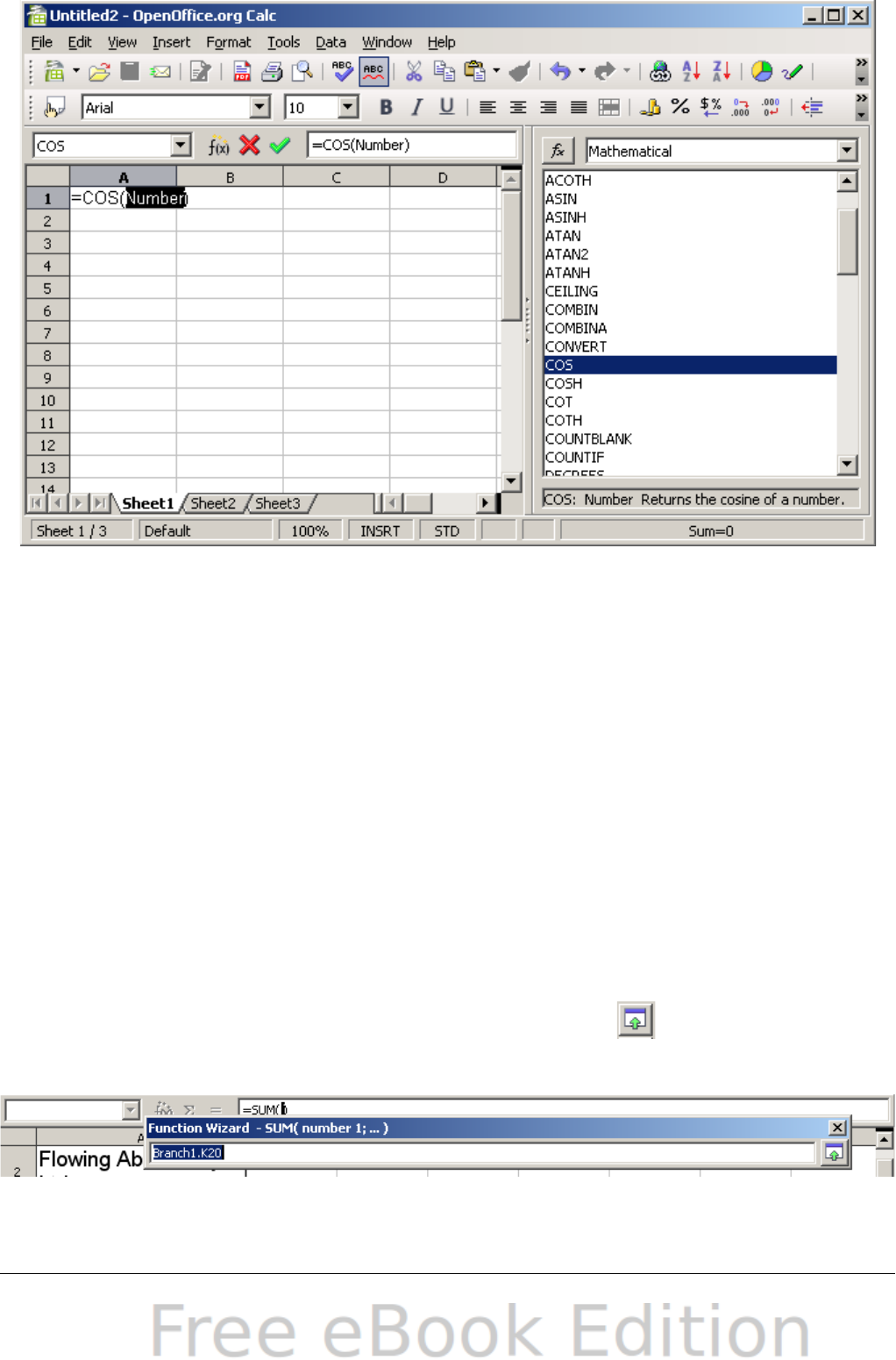
Figure 138: Function List docked to right side of Calc window
Function Wizard
The most commonly used input method is the Function Wizard (Figure
139). To open the Function Wizard, choose Insert > Function, or click
the fx button on the Function tool bar, or press Ctrl+F2. Once open,
the Function Wizard provides the same help features as the Function
List, but adds fields in which you can see the result of a completed
function, as well as the result of any larger formula of which it is part.
Select a category of functions to shorten the list, then scroll down
through the named functions and select the required one. When you
select a function its description appears on the right-hand side of the
dialog. Double-click on the required function.
The Wizard now displays an area to the right where you can enter data
manually in text boxes or click the Shrink button to shrink the
wizard so you can select cells from the worksheet.
Figure 139: Function Wizard after shrinking
200 OpenOffice.org 3.x Calc Guide
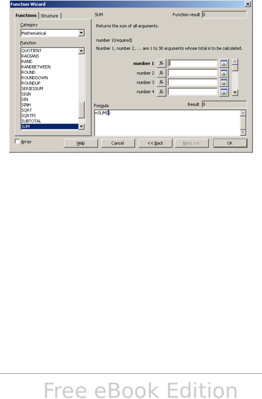
Figure 140: Functions page of Function Wizard.
To select cells, either click directly upon the cell or hold down the left
mouse button and drag to select the required area.
When the area has been selected, click the Shrink button again to
return to the wizard.
If multiple arguments are needed select the next text box below the
first and repeat the selection process for the next cell or range of cells.
Repeat this process as often as required. The Wizard will accept up to
30 ranges or arguments in the SUM function.
Click OK to accept the function and add it to the cell and get the
result.
You can also select the Structure tab (Figure 141) to see a tree view of
the parts of the formula. The main advantage over the Function List is
that each argument is entered in its own field, making it easier to
manage. The price of this reliability is slower input, but this is often a
small price to pay, since precision is generally more important than
speed when creating a spreadsheet.
Chapter 7 Using Formulas and Functions 201
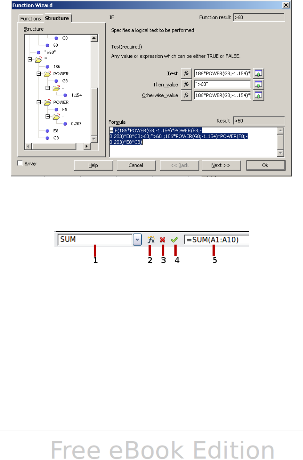
Figure 141: Structure page of Function Wizard
After you enter a function on the Input line, press the Enter key or
click the Accept button on the Function toolbar to add the function to
the cell and get its result.
1Name Box showing list of common functions
2Function Wizard 4Accept
3Cancel 5Input Line
Figure 142: The Function toolbar
If you see the formula in the cell instead of the result, then Formulas
are selected for display in Tools > Options > OpenOffice.org Calc >
View > Display. Deselect Formulas, and the result will display.
However, you can still see the formula in the Input line.
202 OpenOffice.org 3.x Calc Guide
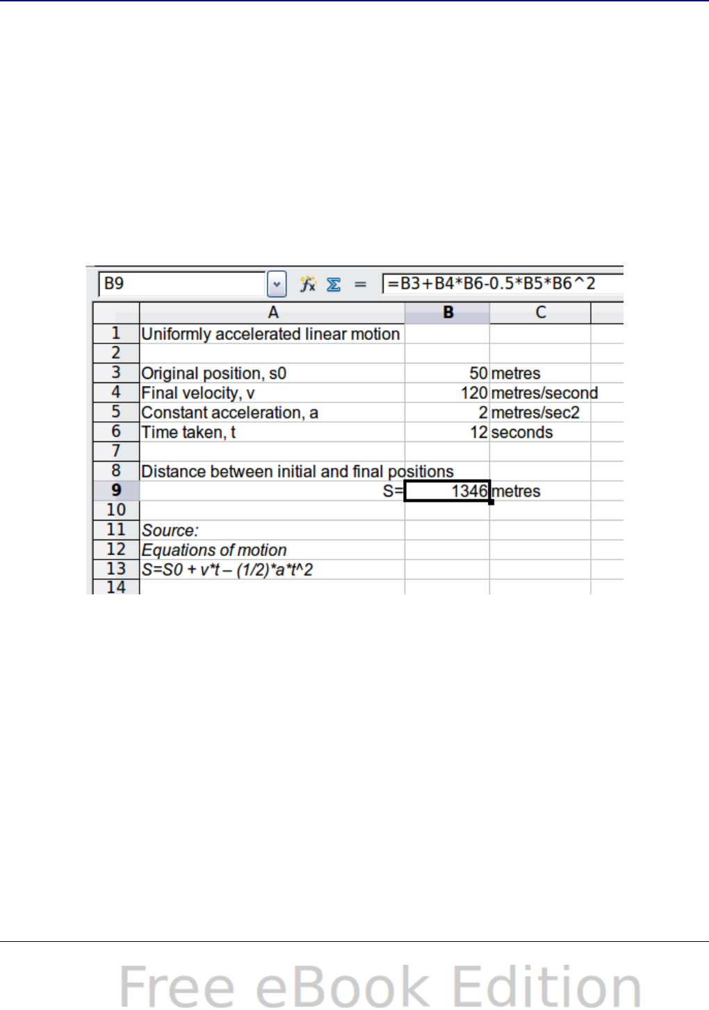
Strategies for creating formulas and
functions
Formulas that do more than a simple calculation or summation of rows
or columns of values usually take a number of arguments. For example,
the classic equation of motion s = s0+ vt - ½at2 calculates the
position of a body knowing its original position, its final velocity, its
acceleration, and the time taken to move from the initial state to the
final state.
For ease of presentation, it is good practice to set up a spreadsheet in
a manner similar to that shown in Figure 143. In this example, the
individual variables are input into cells on the sheet and no editing of
the formula (in cell B9) is required.
Figure 143: Setting up a formula with arguments
You can take several broad approaches when creating a formula. In
deciding which approach to take, consider how many other people will
need to use the worksheets, the life of the worksheets, and the
variations that could be encountered in use of the formula.
If people other than yourself will use the spreadsheet, make sure that
it is easy to see what input is required and where. Explanation of the
purpose of the spreadsheet, basis of calculation, input required and
output(s) generated are often placed on the first worksheet.
A spreadsheet that you build today, with many complicated formulas,
may not be quite so obvious in its function and operation in 6 or 12
Chapter 7 Using Formulas and Functions 203

months time. Use comments and notes liberally to document your
work.
You might be aware that you cannot use negative values or zero values
for a particular argument, but if someone else inputs such a value will
your formula be robust or simply return a standard (and often not too
helpful) Err: message? It is a good idea to trap errors using some form
of logic statements or with conditional formatting.
Place a unique formula in each cell
The most basic strategy is to view whatever formulas are needed as
simple and with a limited useful life. The strategy is then to place a
unique formula in each appropriate cell. This can be recommended
only for very simple or “throw away” (single use) spreadsheets.
Break formulas into parts and combine the parts
The second strategy is similar to the first, but instead you break down
longer formulas into smaller parts and then combine the parts into the
whole. Many examples of this type exist in complex scientific and
engineering calculations where interim results are used in a number of
places in the worksheet. The result of calculating the flow velocity of
water in a pipe may be used in estimating losses due to friction,
whether the pipe is flowing full or partially empty, and in optimizing
the diameter for the given flow regime.
In all cases you should adopt the basic principles of formula creation
described previously.
Use the Basic editor to create functions
A third strategy is to use the Basic editor and create your own
functions and macros. This approach would be used where the result
would greatly simplify the use of the spreadsheet by the end user and
keep the formulas simple with a better chance of avoiding errors. This
approach also can make the maintenance easier by having corrections
or updates kept in one central location. The use of macros is described
in Chapter 12 of this book and is a specialized topic in itself. The
danger of overusing macros and custom functions is that the principles
upon which the spreadsheet is based become much more difficult to
see by a user other than the original author (and sometimes even by
the author!).
204 OpenOffice.org 3.x Calc Guide

Finding and fixing errors
It is common to find situations where errors are displayed. Even with
all the tools available in Calc to help you to enter formulas, making
mistakes is easy. Many people find inputting numbers difficult and
many may make a mistake about the kind of entry that a function's
argument needs. In addition to correcting errors, you may want to find
the cells used in a formula to change their values or to check the
answer.
Calc provides three tools for investigating formulas and the cells that
they reference: error messages, color coding, and the Detective.
Error messages
The most basic tool is error messages. Error messages display in a
formula’s cell or in the Function Wizard instead of the result.
An error message for a formula is usually a three-digit number from
501 to 527, or sometimes an unhelpful piece of text such as NAME?,
REF, or VALUE. The error number appears in the cell, and a brief
explanation of the error on the right side of the status bar.
Most error messages indicate a problem with how the formula was
input, although several indicate that you have run up against a
limitation of either Calc or its current settings.
Error messages are not user-friendly, and may intimidate new users.
However, they are valuable clues to correcting mistakes. You can find
detailed explanations of them in the help, by searching for Error codes
in OpenOffice.org Calc. A few of the most common are:
NAME? (525) No valid reference exists for the argument.
REF (525) The column, row, or sheet for the referenced cell is
missing.
VALUE (519) The value for one of the arguments is not the type that
the argument requires. The value may be entered
incorrectly; for example, double-quotation marks may
be missing around the value. At other times, a cell or
range used may have the wrong format, such as text
instead of numbers.
509 An operator such as an equals sign is missing from the
formula.
510 An argument is missing from the formula.
Chapter 7 Using Formulas and Functions 205
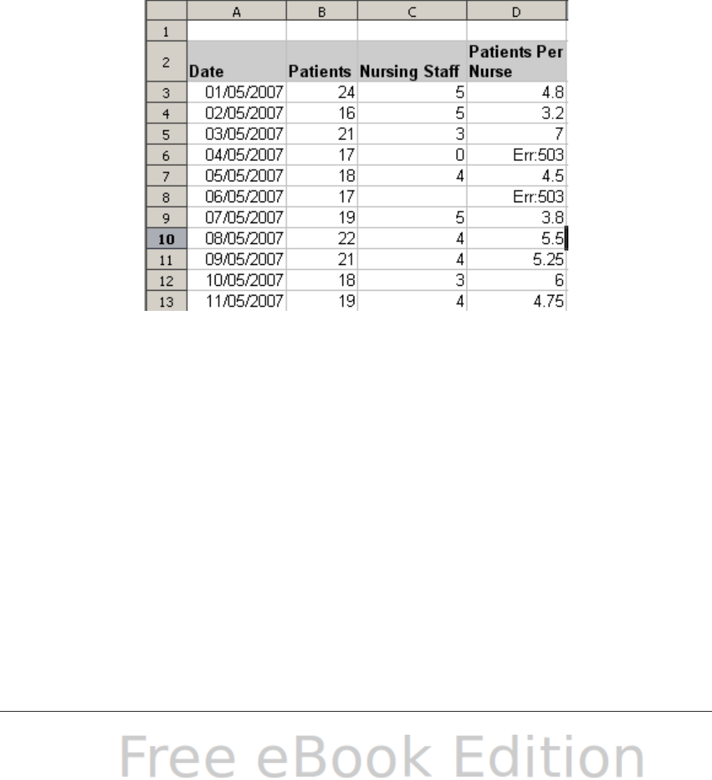
502 The column, row, or sheet for the referenced cell is
missing.
Examples of common errors
Err:503 Division by zero
This error is the result of dividing a number by either the number zero
(0) or a blank cell. There is an easy way to avoid this type of problem.
When you have a zero or blank cell displayed, use a conditional
function. Figure 144 depicts division of column B by column C yielding
2 errors arising from a zero and a blank cell showing in column C.
Figure 144: Examples of Err:503, Division by zero.
It is very common to find an error such as this arising from a situation
where data was not reported or reported incorrectly. When such an
occurrence is possible, an IF function can be used to display the data
correctly. The formula =IF(C3>0, B3/C3, "No Report") can be
entered. The formula is then copied over the remainder of Column D.
The meaning of this formula roughly would be: “If C3 is greater than
0, then compute B3 divided by C3, otherwise enter ‘No Report’”.
It is also possible for the last parameter to use double quotes for a
blank to be entered, or a different formula with a standardized number
being substituted for the lower number. An example of this might be to
use the nursing staff in the unit.
206 OpenOffice.org 3.x Calc Guide
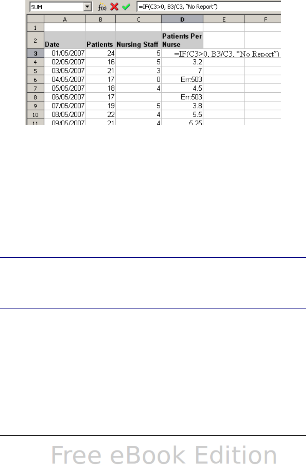
Figure 145: Division by zero solution
#VALUE Non-existent value and #REF! Incorrect references
The non-existent value error is also very common. The most common
appearance of this error arises when a user copies a formula over a
selected area. When copying, it is typical for the program to increment
the represented cells. If you were copying downward from cell B3 the
program would automatically substitute the cell B4 into the next lower
cell and so on until the end of the copying process. If that next cell
contains text or a value that is inappropriate for the formula, then this
error may result. The difficulty usually occurs when one or more of the
parameters in the formula need to be fixed.
Note
To avoid the #VALUE and #REF! errors, give the cell B3 a name
such as TotalExpenses. In that way, the program will carry that
name to each succeeding formula being copied and remove the
need to use the $ to anchor the reference to the TotalExpenses
cell.
Color coding for input
Another useful tool when reviewing a formula is the color coding for
input. When you select a formula that has already been entered, the
cells or ranges used for each argument in the formula are outlined in
color.
Calc uses eight colors for outlining referenced cells, starting with blue
for the first cell, and continuing with red, magenta, green, dark blue,
brown, purple and yellow before cycling through the sequence again.
Chapter 7 Using Formulas and Functions 207
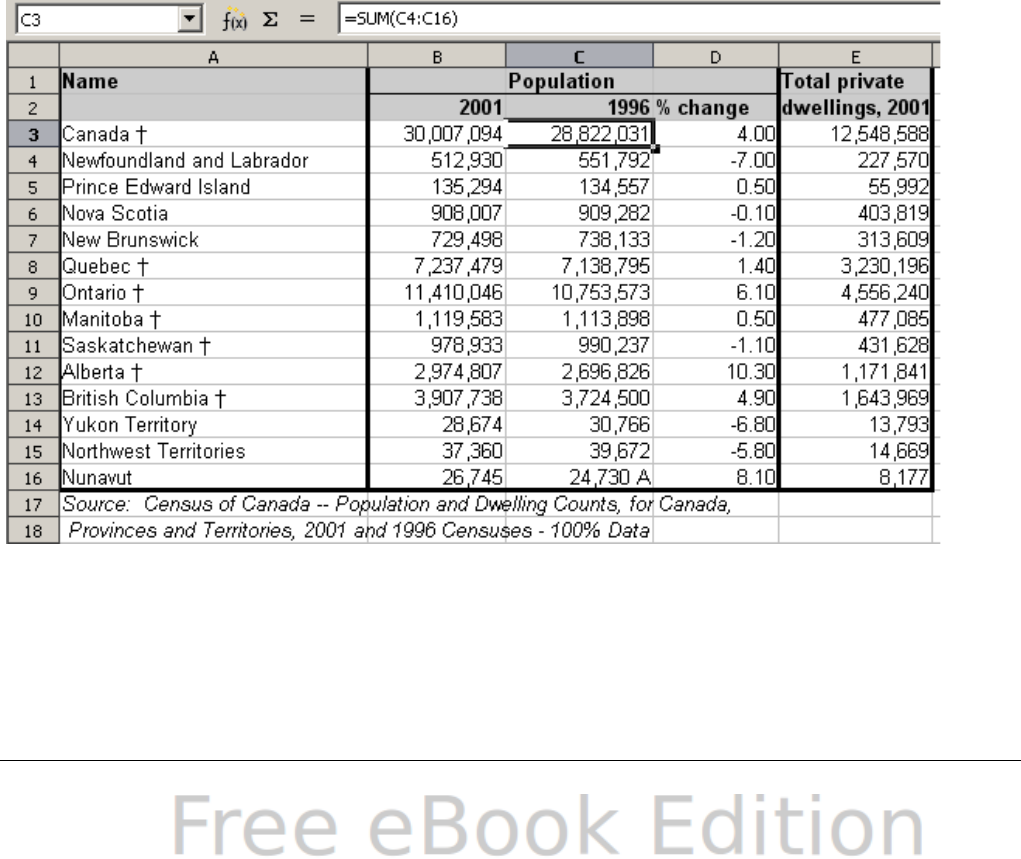
The Detective
In a long or complicated spreadsheet, color coding becomes less
useful. In these cases, consider using the the submenu under Tools >
Detective. The Detective is a tool for checking which cells are used as
arguments by a formula (precedents) and which other formulas it is
nested in (dependents), and tracking errors. It can also be used for
tracing errors, marking invalid data (that is, information in cells that is
not in the proper format for a function’s argument), or even for
removing precedents and dependents.
To use the Detective, select a cell with a formula, then start the
Detective. On the spreadsheet, you will see lines ending in circles to
indicate precedents, and lines ending in arrows for dependents. The
lines show the flow of information.
Use the Detective to assist in following the precedents referred to in a
formula in a cell. By tracing these precedents, you frequently can find
the source of the errors. Place the cursor in the cell in question and
then choose Tools > Detective > Trace Precedents from the menu
bar or press Shift+F7. Figure 146 shows a simple example of tracing
precedents.
Cursor placed in cell
Figure 146: Tracing precedents using the Detective
208 OpenOffice.org 3.x Calc Guide
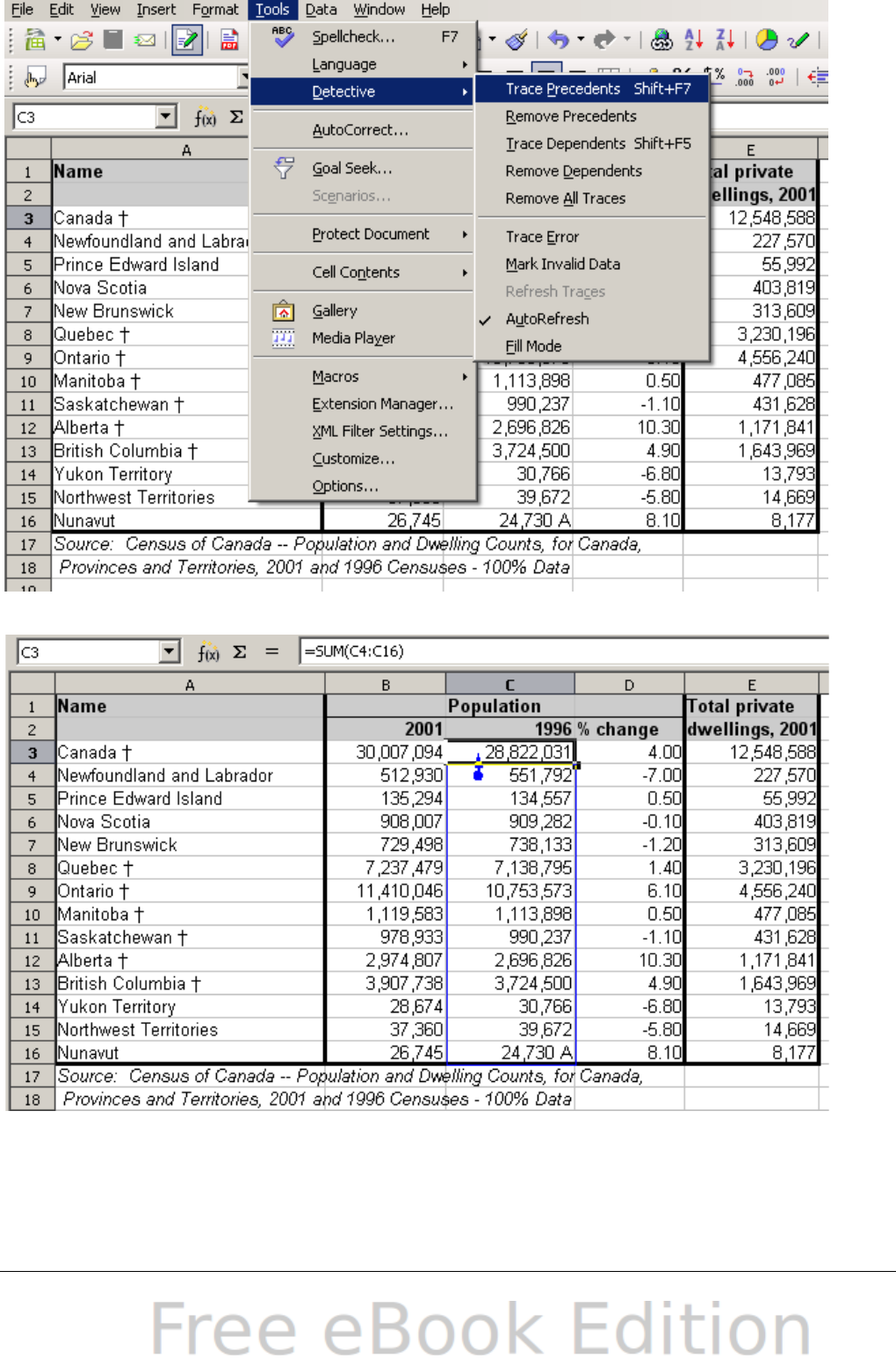
a) Initiate trace by clicking Trace Precedents
b) Source area highlighted in Blue, with arrow pointing to the
calculation cell
(continued): Tracing precedents using the Detective
Chapter 7 Using Formulas and Functions 209

We are concerned that the number shown in Cell C3 is incorrectly
stated. The cause can be seen in the highlighted cells. In this case cell
C16 contains both numeric data as well as letters. Removing the letters
resolves the problem in the calculation.
In other cases we must trace the error. Use the Trace Error function,
found under Tools > Detective > Trace Error, to find the cells that
cause the error.
Examples of functions
For novices, functions are one of the most intimidating features of
OpenOffice.org's Calc. New users quickly learn that functions are an
important feature of spreadsheets, but there are almost four hundred,
and many require input that assumes specialized knowledge.
Fortunately, Calc includes dozens of functions that anyone can use.
Basic arithmetic and statistic functions
The most basic functions create formulas for basic arithmetic or for
evaluating numbers in a range of cells.
Basic arithmetic
The simple arithmetic functions are addition, subtraction,
multiplication, and division.
Except for subtraction, each of these operations has its own function:
•SUM for addition
•PRODUCT for multiplication
•QUOTIENT for division.
Traditionally, subtraction does not have a function.
SUM, PRODUCT and QUOTIENT are useful for entering ranges of cells
in the same way as any other function, with arguments in brackets
after the function name.
However, for basic equations, many users prefer the time-honored
computer symbols for these operations, using the plus sign (+) for
addition, the hyphen (–) for subtraction, the asterisk (*) for
multiplication and the forward slash (/) for division. These symbols are
quick to enter without requiring your hands to stray from the
keyboard.
210 OpenOffice.org 3.x Calc Guide

A similar choice is also available if you want to raise a number by the
power of another. Instead of entering =POWER(A1;2), you can enter
=A1^2.
Moreover, they have the advantage that you enter formulas with them
in an order that more closely approximates human readable format
than the spreadsheet-readable format used by the equivalent function.
For instance, instead of entering =SUM (A1:A2), or possibly =SUM
(A1;A2), you enter =A1+A2. This almost-human readable format is
especially useful for compound operations, where writing
=A1*(A2+A3) is briefer and easier to read than
=PRODUCT(A1;SUM(A2:A3)).
The main disadvantage of using arithmetical operators is that you
cannot directly use a range of cells. In other words, to enter the
equivalent of =SUM (A1:A3), you would need to type =A1+A2+A3.
Otherwise, whether you use a function or an operator is largely up to
you—except, of course, when you are subtracting. However, if you use
spreadsheets regularly in a group setting such as a class or an office,
you might want to standardize on an entry format so that everyone
who handles a spreadsheet becomes accustomed to a standard input.
Simple statistics
Another common use for spreadsheet functions is to pull useful
information out of a list, such as a series of test scores in a class, or a
summary of earnings per quarter for a company.
You can, of course, scan a list of figures if you want basic information
such as the highest or lowest entry or the average. The only trouble is,
the longer the list, the more time you waste and the more likely you
are to miss what you’re looking for. Instead, it is usually quicker and
more efficient to enter a function. Such reasons explain the existence
of a function like COUNT, which does no more than give the total
number of entries in the designated cell range.
Similarly, to find the highest or lowest entry, you can use MIN or MAX.
For each of these formulas, all arguments are either a range of cells, or
a series of cells entered individually.
Each also has a related function, MINA or MAXA, which performs the
same function, but treats a cell formatted for text as having a value of
0 (The same treatment of text occurs in any variation of another
function that adds an "A" to the end). Either function gives the same
result, and could be useful if you used a text notation to indicate, for
example, if any student were absent when a test was written, and you
wanted to check whether you needed to schedule a makeup exam.
Chapter 7 Using Formulas and Functions 211

For more flexibility in similar operations, you could use LARGE or
SMALL, both of which add a specialized argument of rank. If the rank
is 1 used with LARGE, you get the same result as you would with MAX.
However, if the rank is 2, then the result is the second largest result.
Similarly, a rank of 2 used with SMALL gives you the second smallest
number. Both LARGE and SMALL are handy as a permanent control,
since, by changing the rank argument, you can quickly scan multiple
results.
You would need to be an expert to want to find the Poisson Distribution
of a sample, or to find the skew or negative binomial of a distribution
(and, if you are, you will find functions in Calc for such things).
However, for the rest of us, there are simpler statistical functions that
you can quickly learn to use.
In particular, if you need an average, you have a number to choose
from. You can find the arithmetical means—that is, the result when you
add all entries in a list then divided by the number of entries by enter a
range of numbers when using AVERAGE, or AVERAGE A to include text
entries and to give them a value of zero.
In addition, you can get other information about the data set:
•MEDIAN: The entry that is exactly half way between the highest
and lowest number in a list.
•MODE: The most common entry in a list of numbers.
•QUARTILE:The entry at a set position in the array of numbers.
Besides the cell range, you enter the type of Quartile: 0 for the
lowest entry, 1 for the value of 25%, 2 for the value of 50%, 3 for
75%, and 4 for the highest entry. Note that the result for types 1
through 3 may not represent an actual item entered.
•RANK: The position of a given entry in the entire list, measured
either from top to bottom or bottom to top. You need to enter the
cell address for the entry, the range of entries, and the type of
rank (0 for the rank from the highest, or 1 for the rank from the
bottom.
Some of these functions overlap; for example, MIN and MAX are both
covered by QUARTILE. In other cases, a custom sort or filter might
give much the same result. Which you use depends on your
temperament and your needs. Some might prefer to use MIN and MAX
because they are easy to remember, while others might prefer
QUARTILE because it is more versatile.
212 OpenOffice.org 3.x Calc Guide

Using these functions
In some cases, you may be able to get similar results to some of these
functions by setting up a filter or a custom sort. However, in general,
functions are more easily adjusted than filters or sorts, and provide a
wide range of possibilities.
At times, you may just want to enter one or more formulas temporarily
in a convenient blank cell, and delete it once you have finished.
However, if you find yourself using the same functions constantly, you
should consider creating a template and including space for all the
functions you use, with the cell to their left used as a label for them.
Once you have created the template, you can easily update each
formula as entries change, either automatically and on-the-fly or
pressing the F9 key to update all selected cells.
No matter how you use these functions, you will probably find them
simple to use and adaptable for many purposes. By the time you have
mastered this handful, you will be ready to try more complex functions.
Rounding off numbers
For statistical and mathematical purposes, Calc includes a variety of
ways to round off numbers. If you’re a programmer, you may also be
familiar with some of these methods. However, you don’t need to be a
specialist to find some of these methods useful. You may want to round
off for billing purposes, or because decimal places don’t translate well
into the physical world—for instance, if the parts you need come in
packages of 100, then the fact you only need 66 is irrelevant to you;
you need to round up for ordering. By learning the options for
rounding up or down, you can make your spreadsheets more
immediately useful.
When you use a rounding function, you have two choices about how to
set up your formulas. If you choose, you can nest a calculation within
one of the rounding functions. For instance, the formula
=ROUND((SUM(A1;A2)) adds the figures in cells A1 and A2, then
rounds them off to the nearest whole number. However, even though
you don’t need to work with exact figures every day, you may still want
to refer to them occasionally. If that is the case, then you are probably
better off separating the two functions, placing =SUM(A1;A2) in cell
A3, and =ROUND (A3) in A4, and clearly labelling each function.
Rounding methods
The most basic function for rounding numbers in Calc is ROUND. This
function will round off a number according to the usual rules of
Chapter 7 Using Formulas and Functions 213

symmetric arithmetic rounding: a decimal place of .4 or less gets
rounded down, while one of .5 or more gets rounded up. However, at
times, you may not want to follow these rules. For instance, if you are
one of those contractors who bills a full hour for any fraction of an
hour you work, you would want to always round up so you didn’t lose
any money. Conversely, you might choose to round down to give a
slight discount to a long-established customer. In these cases, you
might prefer to use ROUNDUP or ROUNDDOWN, which, as their
names suggest, round a number to the nearest integer above or below
it.
All three of these functions require the single argument of number—
the cell or number to be rounded. Used with only this argument, all
three functions round to the nearest whole number, so that 46.5 would
round to 47 with ROUND or ROUNDUP and 46 with ROUNDDOWN.
However, if you use the optional count argument, you can specify the
number of decimal places to include. For instance, if number was set to
1, then 48.65 would round to 48.7 with ROUND or ROUNDUP and to
48.6 with ROUNDDOWN.
As an alternative to ROUNDDOWN when working with decimals, you
can use TRUNC (short for truncate). It takes exactly the same
arguments as ROUNDDOWN, so which function you use is a matter of
choice. If you aren't working with decimals, you might choose to use
INT (short for integer), which takes only the number argument.
Another option is the ODD and EVEN pair of functions. ODD rounds up
to the nearest odd number if what is entered in the number argument
is a positive number, and rounds down if it is a negative number, while
EVEN does the same for an even number.
Options are the CEILING and FLOOR functions. As you can guess from
the names, CEILING rounds up and FLOOR rounds down. For both
functions, the number that they round to is determined by the closest
multiple of the number that you enter as the significance argument.
For instance, if your business insurance is billed by the work week, the
fact that you were only open three days one week would be irrelevant
to your costs; you would still be charged for an entire week, and
therefore might want to use CEILING in your monthly expenses.
Conversely, if you are building customized computers and completed
4.5 in a day, your client would only be interested in the number ready
to ship, so you might use FLOOR in a report of your progress. If cell E1
contains the value 46.7, =CEILING(E1;7) will return the value 49.
Besides number and significance, both CEILING and FLOOR include
an optional argument called mode, which takes a value of 0 or 1. If
214 OpenOffice.org 3.x Calc Guide

mode is set to 0, and both the number and the significance are
negative numbers, then the result of either function is rounded up; if it
is set to 1, and both the number and the significance are negative
numbers, then the results are rounded down. In other words, if the
number is -11 and the significance is -5, then the result is -10 when the
mode is set to 0, but -15 when set to 1.
However, if you are exchanging spreadsheets between Calc and MS
Excel, remember that the mode argument is not supported by Excel. If
you want the answers to be consistent between the two spreadsheets,
set the mode in Calc to -1.
A function somewhat similar to CEILING and FLOOR is MROUND. Like
CEILING AND FLOOR, MROUND requires two arguments, although,
somewhat confusingly, the second one is called multiple rather than
significance, even though the two are identical. The difference
between MROUND and CEILING and FLOOR is that MROUND rounds
up or down using symmetric arithmetic rounding. For example, if the
number is 77 and the multiple is 5, then MROUND gives a result of 75.
However, if the multiple is changed to 7, then MROUND's result
becomes 77.
Once you become familiar with Calc’s long, undifferentiated list of
functions, you can start to decide which is most useful for your
purposes.
However, one last point is worth mentioning: If you are working with
more than two decimal places, don't be surprised if you don’t see the
same number of decimal places on the spreadsheet as you do on the
function wizard. If you don’t, the reason is that Tools > Options >
OpenOffice.org Calc > Calculate > Decimal Places defaults to 2.
Change the number of decimal places, and, if necessary, uncheck the
Precision as shown box on the same page, and the spreadsheet will
display as expected.
Using regular expressions in functions
A number of functions in Calc allow the use of regular expressions:
SUMIF, COUNTIF, MATCH, SEARCH, LOOKUP, HLOOKUP, VLOOKUP,
DCOUNT, DCOUNTA, DSUM, DPRODUCT, DMAX, DMIN, DAVERAGE,
DSTDEV, DSTDEVP, DVAR, DVARP, DGET.
Whether or not regular expressions are used is selected on the Tools >
Options > OpenOffice.org Calc > Calculate dialog.
Chapter 7 Using Formulas and Functions 215
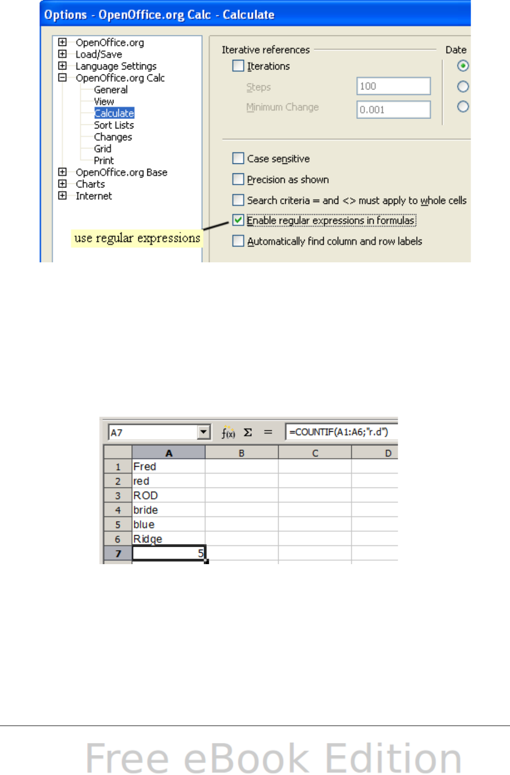
Figure 147: Enabling regular expressions in formulas
For example =COUNTIF(A1:A6;"r.d") with Enable regular
expressions in formulas selected will count cells in A1:A6 which
contain red and ROD.
Additionally if Search criteria = and <> must apply to whole cells
is not selected, then Fred, bride, and Ridge will also be counted. If that
setting is selected, then it can be overcome by wrapping the
expression thus: =COUNTIF(A1:A6;".*r.d.*").
Figure 148: Using the COUNTIF function.
Regular expression searches within functions are always case
insensitive, irrespective of the setting of the Case sensitive checkbox
on the dialog in Figure 147—so red and ROD will always be matched in
the above example. This case-insensitivity also applies to the regular
expression structures ([:lower:]) and ([:upper:]), which match
characters irrespective of case.
216 OpenOffice.org 3.x Calc Guide

Regular expressions will not work in simple comparisons. For example:
A1="r.d" will always return FALSE if A1 contains red, even if regular
expressions are enabled. It will only return TRUE if A1 contains r.d (r
then a dot then d). If you wish to test using regular expressions, try the
COUNTIF function: COUNTIF(A1; "r.d") will return 1 or 0, interpreted
as TRUE or FALSE in formulas like =IF(COUNTIF(A1; "r.d");"hooray";
"boo").
Activating the Enable regular expressions in formulas option
means all the above functions will require any regular expression
special characters (such as parentheses) used in strings within
formulas, to be preceded by a backslash, despite not being part of a
regular expression. These backslashes will need to be removed if the
setting is later deactivated.
Advanced functions
As is common with other spreadsheet programs, OOo Calc can be
enhanced by user-defined functions or add-ins. Setting up user-defined
functions can be done either by using the Basic IDE or by writing
separate add-ins or extensions.
The basics of writing and running macros is covered in Chapter 12,
Calc Macros. Macros can be linked to menus or toolbars for ease of
operation or stored in template modules to make the functions
available in other documents.
Calc Add-ins are specialized office extensions which can extend the
functionality of OpenOffice.org with new built-in Calc functions.
Writing Add-ins requires knowledge of the C++ language, the OOo
SDK, and is for experienced programmers. More information is
available on the OOo wiki page at
http://wiki.services.openoffice.org/wiki/Calc/Add-In/Simple_Calc_Add-
In. A number of extensions for Calc have been written and these can be
found on the extensions site at
http://extensions.services.openoffice.org/. Refer to Chapter 14, Setting
up and Customizing Calc, of the Calc Guide for more details.
Chapter 7 Using Formulas and Functions 217

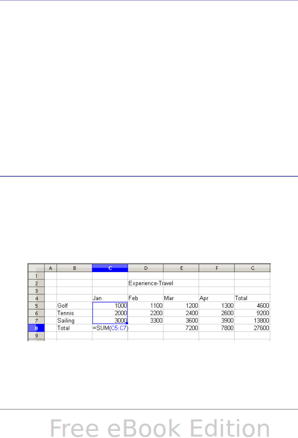
Introduction
Many requests for software support are caused by complicated
formulas and solutions to simple day to day procedures. For more
efficient and effective solutions use the DataPilot, a tool for combining,
comparing, and analyzing large amounts of data easily. By using the
DataPilot, you can view different summaries of the source data, display
the details of areas of interest, and create reports, whether you are a
beginner or an intermediate or advanced user.
This chapter is divided into two sections:
•“Examples with step by step instructions” uses three typical cases
to demonstrate the advantages and applications of the DataPilot.
Follow the examples to learn how easy it is to use the DataPilot.
•“DataPilot functions in detail” starting on page 241 describes the
DataPilot in detail. You can use this part for looking up how a
function is used.
Examples with step by step instructions
This section demonstrates some of the possibilities of the DataPilot in
typical use cases. By following the step by step instructions, you can
recreate the examples and learn about the power of the DataPilot.
Example 1: Sales volume overview
A typical introductory example in courses and books for beginners with
spreadsheets is a simple sales volume overview.
Figure 149: Typical example for beginners
This example demonstrates the user interface and how to insert text
and numbers into cells. Useful aids like AutoFill and drag and drop
have been demonstrated in other chapters. The most important part is
Chapter 8 Using the DataPilot 219

the connection between cells through formulas, for example addition
with the plus operator or the SUM function.
This small exercise might be useful for a first contact with the
program, but it shows only a very small fraction of the tasks in an
office. To create such a sales overview, you also need the original data.
That is, before you can use a spreadsheet for creating the sales
overview, you need to add many single purchases from different lists
and then enter the sums into the relevant cells C5 to F7.
Practical problems and questions
•For displaying additional values for May, June, July, and so on, you
need to add extra columns. This means that you have to change
the structure of the calculation sheet. This is not only somewhat
inefficient from a workflow point of view, it also adds some
practical questions: How do references react, if you add more
columns or rows to the sum formulas?
•The layout, where the timeline is displayed horizontally, might be
less convenient if you add more months. A vertical layout might
be a more efficient use of space. How can the table then be
transposed? Do you have to enter everything again?
•What if the management asks unexpected questions or adds an
additional subdivision for the different sales regions or a
constraint of the sales for a given employee. In these cases you
again have to manually add all the sums and create different
tables in many variations.
•Is it really acceptable and realistic to create such an overview by
adding the different values manually? This is really a lot of work
and extremely error-prone!
Solution
The most important part of your task in the example is the addition of
the Total sales per month cells. This had to be done manually. To do
this automatically with the program, just get the data into Calc. You
can enter the single numbers by hand or you can import a file from
your bookkeeping software. In any case we assume a continuous table
that keeps track of all sales in a somewhat primitive form.
220 OpenOffice.org 3.x Calc Guide
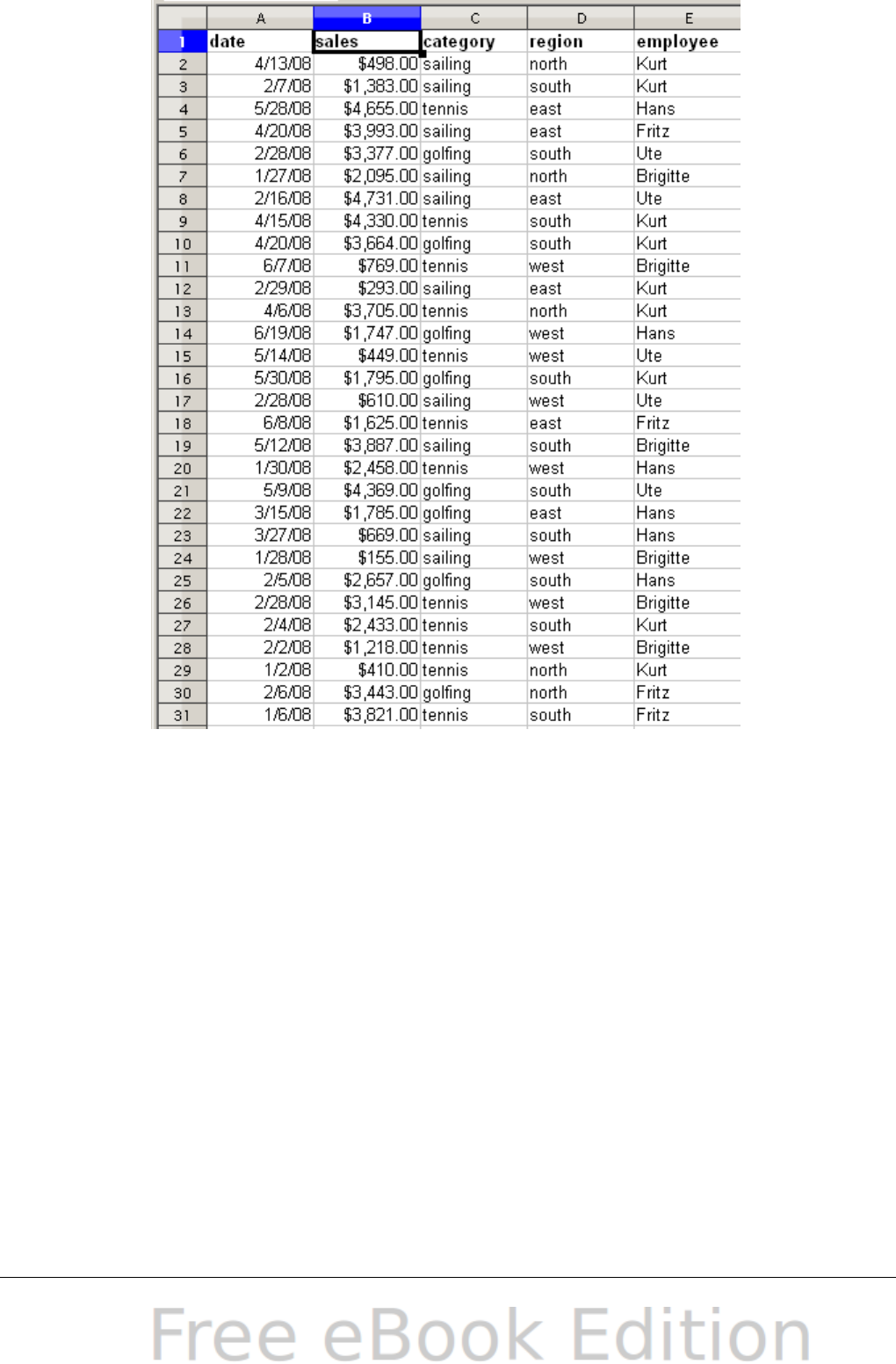
Figure 150: Basic data in Calc
You can create the sales volume overview by following these
instructions:
1) Select the cell A1 (or any other single cell within the list).
2) Select Data > DataPilot > Start. On the Select Source dialog,
select Current selection and click OK.
3) The DataPilot dialog (Figure 151) has four white layout areas and
several fields that look like buttons. These small fields are the
titles of the different columns of your list.
•Move the date field into the Column Fields area.
•Move the sales field into the Data Fields area.
•Move the category field into the Row Fields area.
4) Click More, to see more options in the lower part of the dialog.
5) In the Results to field, select – new sheet – from the drop-down
list.
Chapter 8 Using the DataPilot 221
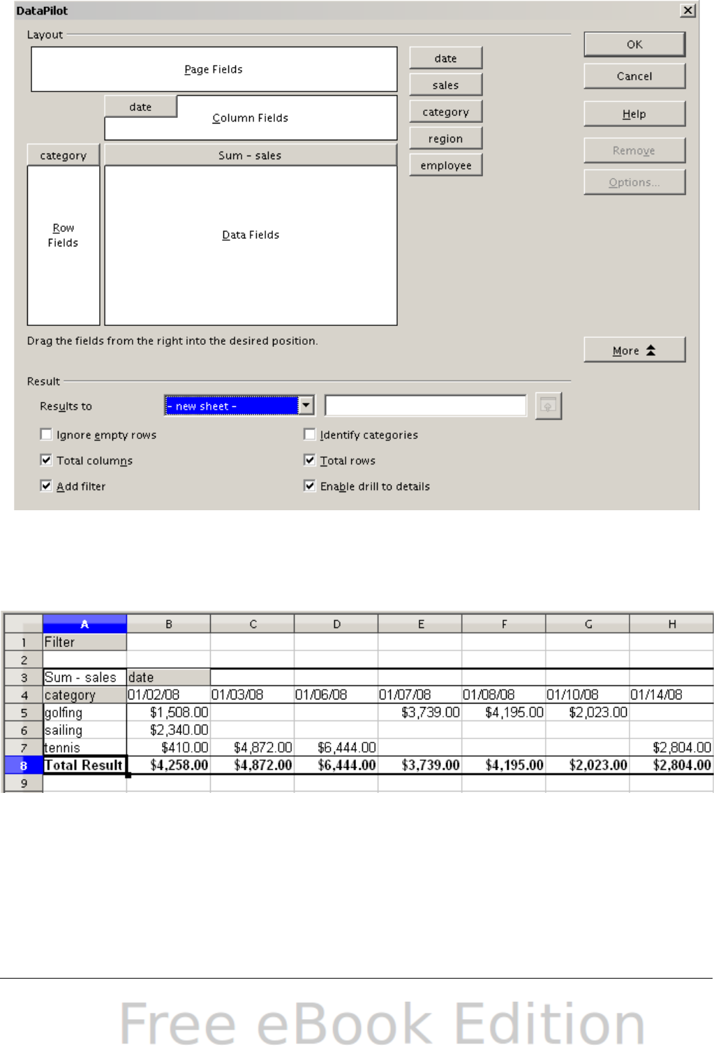
6) Click OK.
Figure 151: DataPilot dialog
7) The result appears on a new sheet. It has the desired structure,
but the columns are not yet grouped into months.
Figure 152: DataPilot result without grouping
8) To group the columns, select cell B4 or any other cell that
contains a date. Then select Data > Group and Outline >
Group. On the Grouping dialog (Figure 153), make sure Intervals
and Months are selected in the Group by section, and click OK.
The result is now grouped for months (Figure 154).
222 OpenOffice.org 3.x Calc Guide
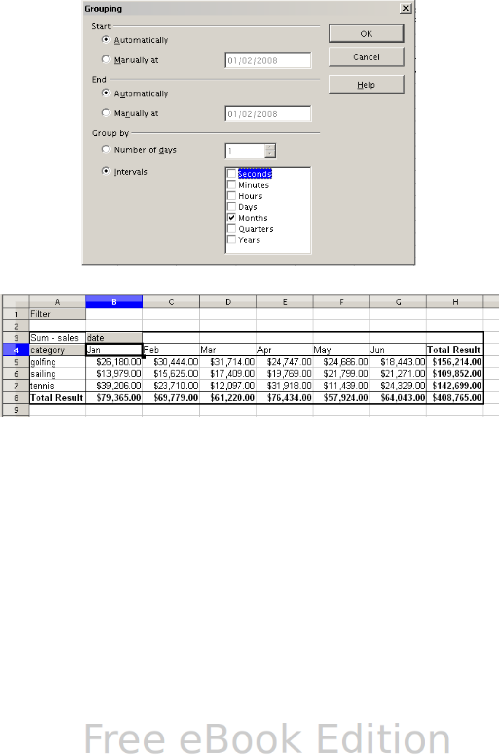
Figure 153: Grouping on months
Figure 154: DataPilot result grouped for months
In this result you will recognize the beginners’ example. It is very easy
to produce, without any further knowledge about the spreadsheet. You
do not have to enter any formulas.
Advantages
1) No manual entering or adding of any values is necessary. There is
less work and fewer errors.
2) The layout is very flexible: months are listed horizontally and
fields vertically or vice versa, in two mouse clicks.
3) Additional differentiating factors are immediately available.
4) Many types of evaluation are possible; for example, number or
average instead of sum, accumulated values, comparisons, and so
on.
Chapter 8 Using the DataPilot 223
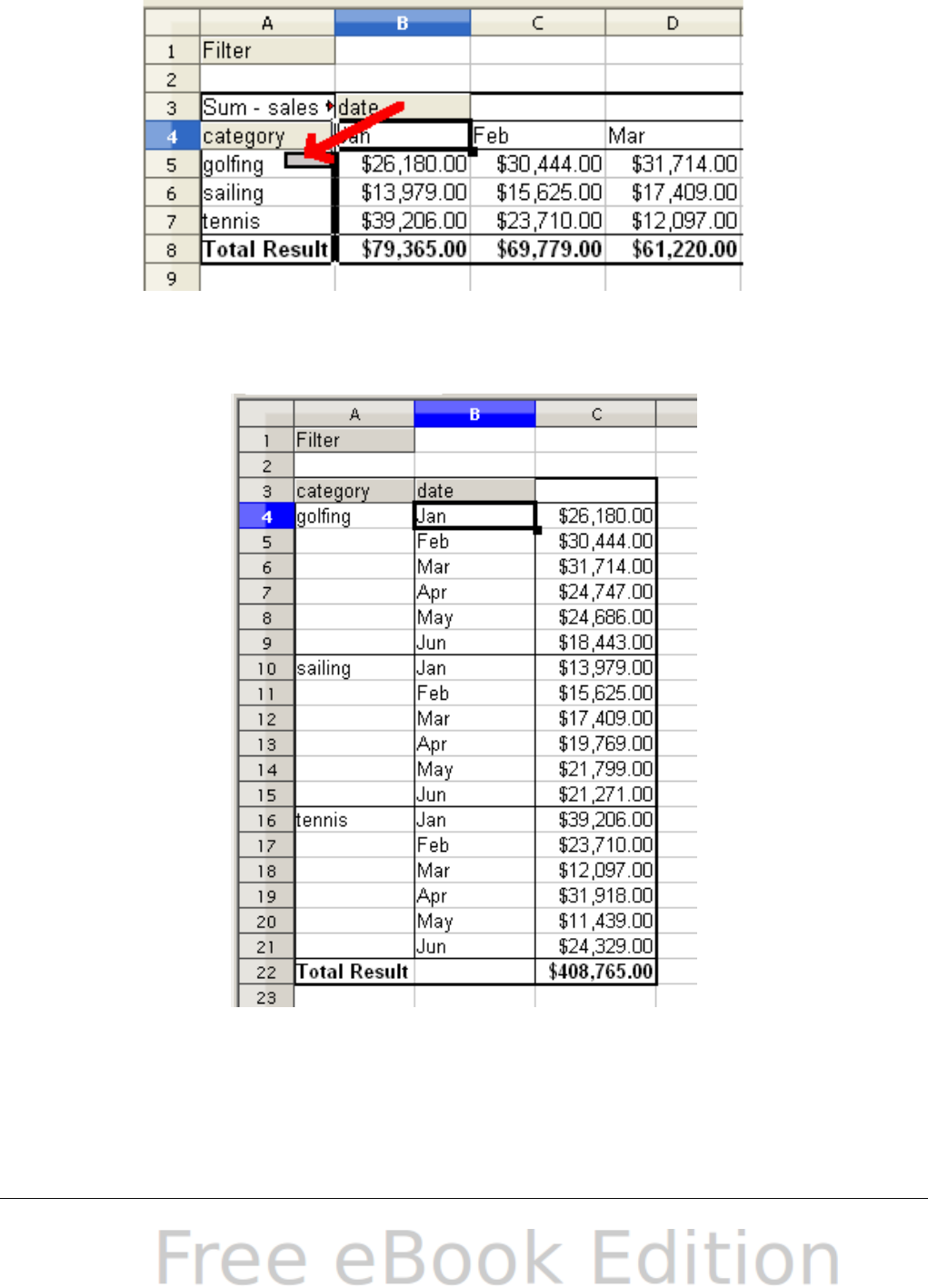
We will now demonstrate some of these advantages.
Starting with the result of Figure 154, drag the Date field under the
Category field, as shown in Figure 155.
Figure 155: Drag Date field under Category field
Now the summary is as shown in Figure 156.
Figure 156: Changed layout
224 OpenOffice.org 3.x Calc Guide
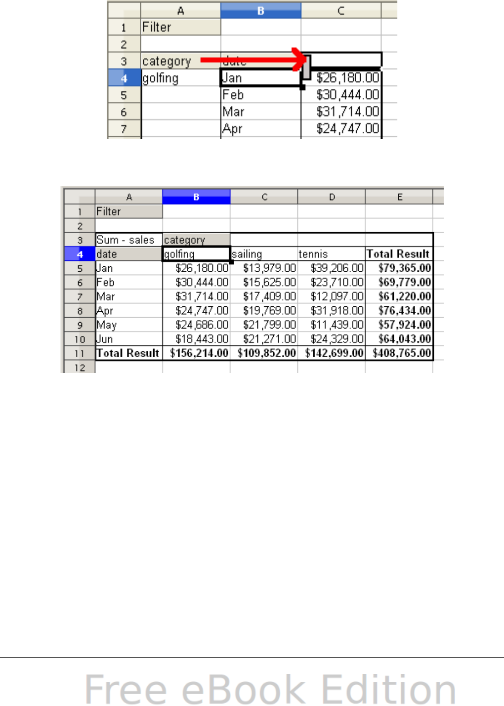
To transpose the table completely, just drag the Category field above
the area of the displayed values, to cell C3 (see Figure 157). The result
of this action is shown in Figure 158.
Figure 157: Drag Category field to right of Data field
Figure 158: Transposed layout of Figure 156
In contrast to the beginners’ example in Figure 149, it is now very
simple to view or add different aspects of the underlying data. For
example, to see the values for different regions, do the following:
1) Select the cell A3 (or any other single cell that is part of the
DataPilot result).
2) Select Data > DataPilot > Start to start the DataPilot again.
Drag the Region field into the Row Fields area. Depending on the
order you choose for the row fields, the result is either regions
with date subdivisions or vice versa.
3) Click OK. The result is shown in Figure 159.
Chapter 8 Using the DataPilot 225
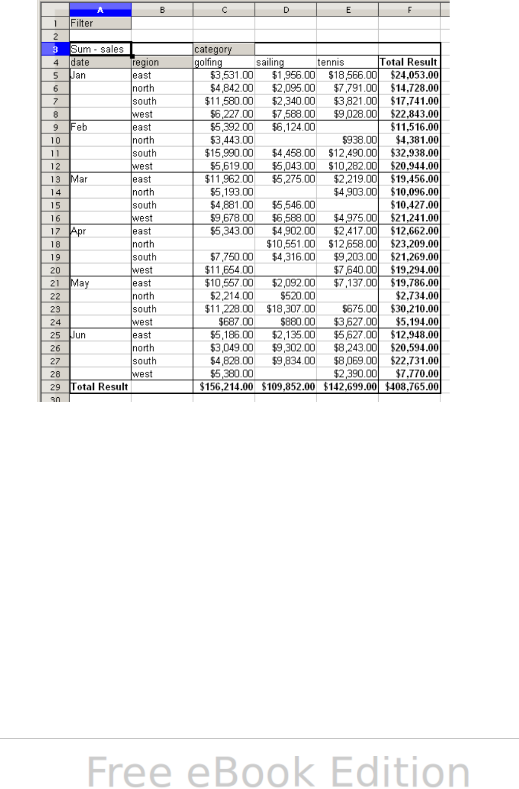
Figure 159: Additional subdivision into regions, added later
In another variation you may want to add the employees.
1) Select the cell A3 (or any other single cell that is part of the
DataPilot result).
2) Select Data > DataPilot > Start, to start the DataPilot again.
•You do not need the Region field in this case. Drag it out of
the layout area.
•Drag the Employee field into the Page Fields area.
3) Click OK. The result is shown in Figure 160.
Fields that you use as page fields are placed in the result above the
summary with the name Filter. You then have a drop-down list that you
can use to show only the sums of a given employee.
Up to now we have not seen the most powerful features of the
DataPilot. The following examples will show you more.
226 OpenOffice.org 3.x Calc Guide
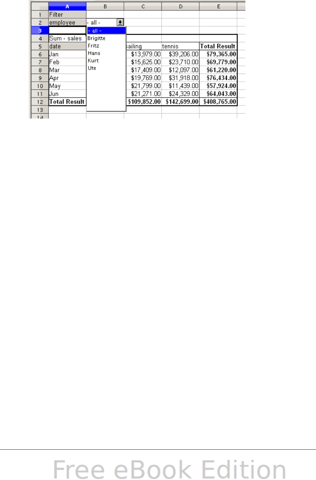
Figure 160: Selection of subtotals for several employees.
Example 2: Timekeeping
This example is often used by consultants and in several variations in
user support. The task is to provide a means for one or more users to
keep track of working hours.
A typical way of doing this is to create a spreadsheet per month and a
sum sheet with all the results of one year. For each employee, there is
one file (see Figures 161 and 162 for examples of two pages from the
file for one employee).
Practical problems and questions
•It is very difficult and time-consuming to create the timekeeping
table: 12 sheets that have to be copied from a raw template and
adjusted for each month, and a sheet with all the yearly sums
with references to all the other sheets. Users often search for a
macro to make the creation easier.
•The file shown contains only the data of one employee. How can
you get all the data for all the employees, so that you can have a
summary of all the work hours from all employees of a
department or the whole company?
•How can you compare employees and/or departments?
•The shown file contains data for one year. How can you compare
it with the data of the previous years?
Chapter 8 Using the DataPilot 227
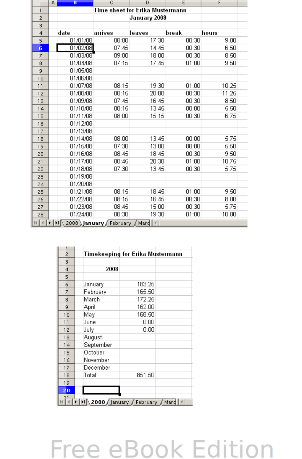
Figure 161: One month of timekeeping for one employee
Figure 162: Yearly sums for one employee
228 OpenOffice.org 3.x Calc Guide
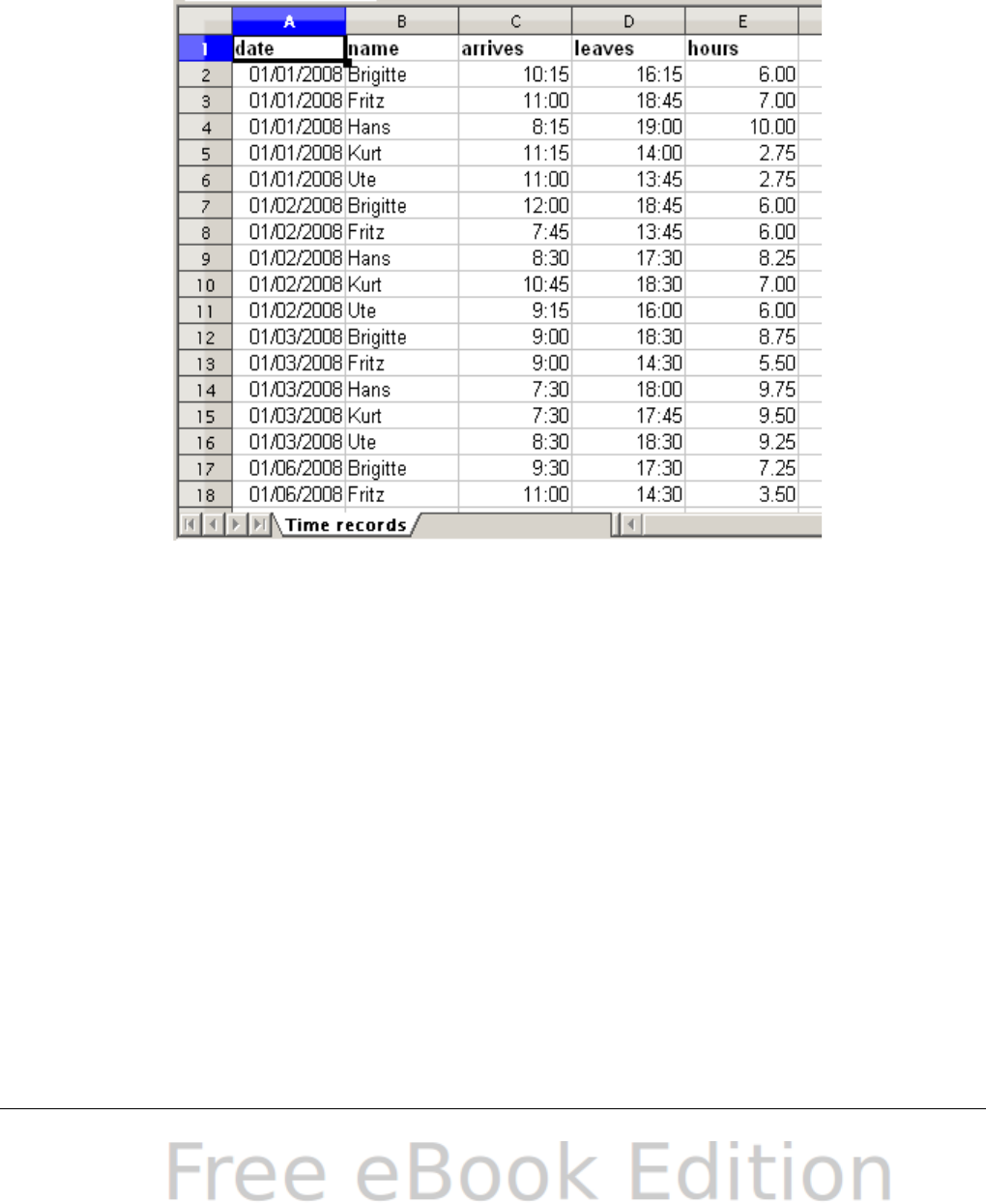
Solution
To use the DataPilot for this task, collect all the data into one single
table. This can be done either manually or by importing a file from an
(electronic) timekeeping machine.
In very simple cases, each employee takes care of their own working
hours. If you need calculations that cover several employees,
departments, or the whole company, just copy everything into one huge
table (Figure 163).
Figure 163: Data basis in Calc
Using the DataPilot requires only 12 mouse clicks and gives you a nice
overview within seconds :
1) Select the cell A1 (or any other single cell within the list).
2) Choose Data > DataPilot > Start and click OK.
3) On the DataPilot dialog (Figure 164):
•Drag date into the Row Fields area.
•Drag hours into the Data Fields area. Notice that it becomes
Sum – hours.
•Drag name into the Column Fields area.
4) Click More to show more options in the lower part of the dialog.
5) In the Results to field, select – new sheet – from the drop-down
list.
6) Click OK.
Chapter 8 Using the DataPilot 229
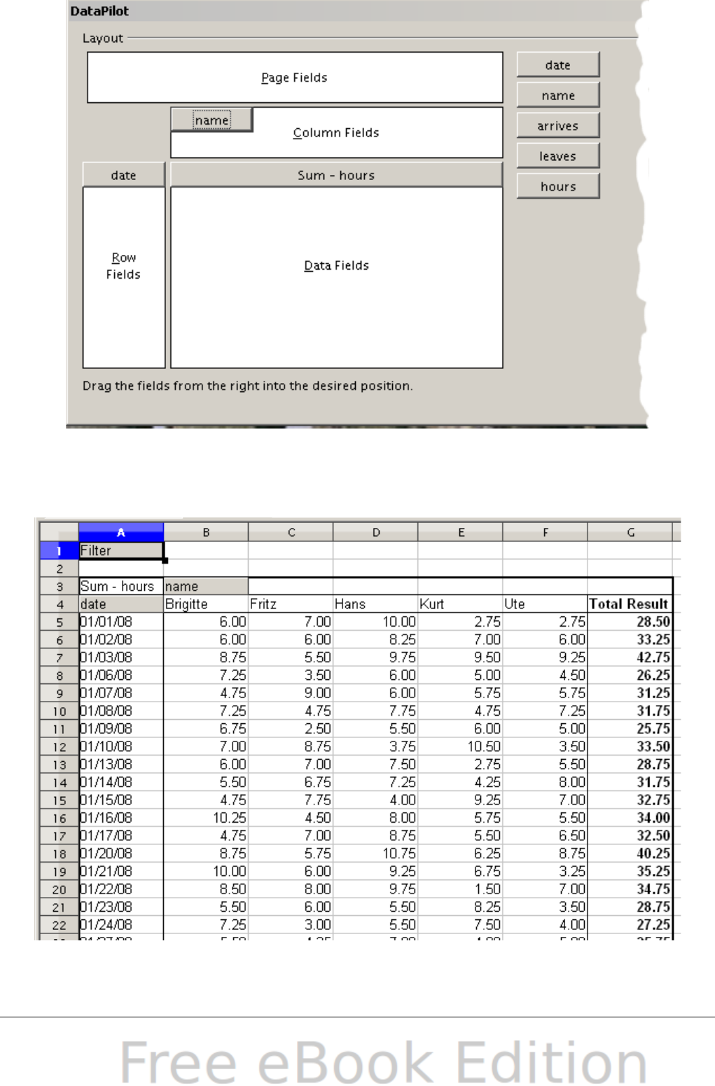
Figure 164: Part of DataPilot dialog
The result appears on a new sheet.
Figure 165: The evaluation, done within seconds with DataPilot
230 OpenOffice.org 3.x Calc Guide
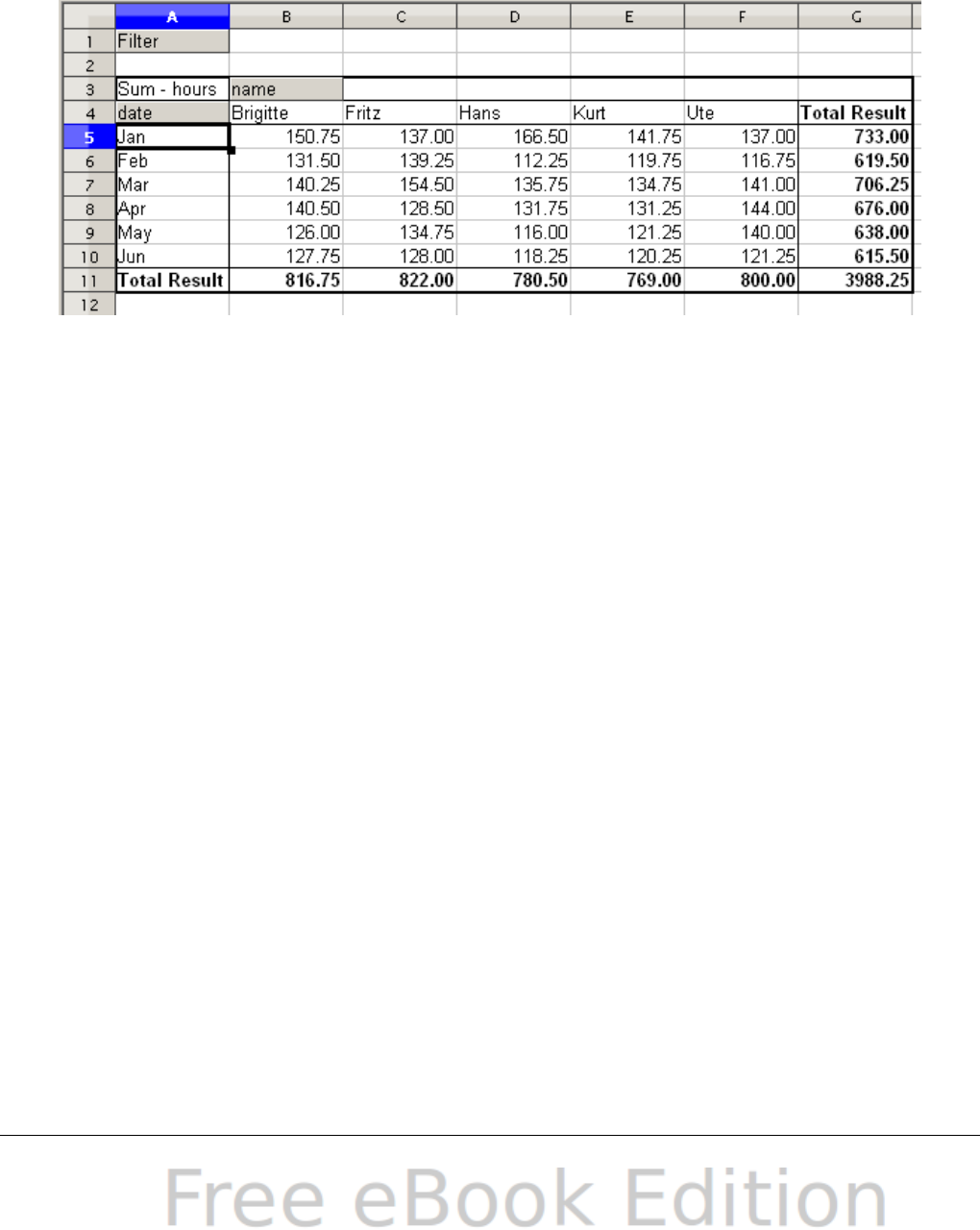
The result is much more powerful than is possible with the classic
formula-based calculation. For example, you can summarize the daily
results to a monthly result very easily:
1) To group together the rows, select the cell A5 (or any other cell
that contains a date).
2) Choose Data > Group and Outline > Group and click OK. The
result is now grouped into months.
Figure 166: Monthly sums
If you need a result with a percentage, start the DataPilot from this
page.
1) Select the cell A3 (or any other single cell that contains a result
of the DataPilot).
2) Choose Data > DataPilot > Start.
3) Double-click on Sum – hours to open the Data Field dialog
(Figure 167).
4) Click on More, to see more options.
5) Switch Displayed value > Type to % of column.
6) Click OK twice.
The result shows percentages as a decimal number. If you prefer to
have a percent format, select the cells and click on the % icon in the
menu bar.
Chapter 8 Using the DataPilot 231
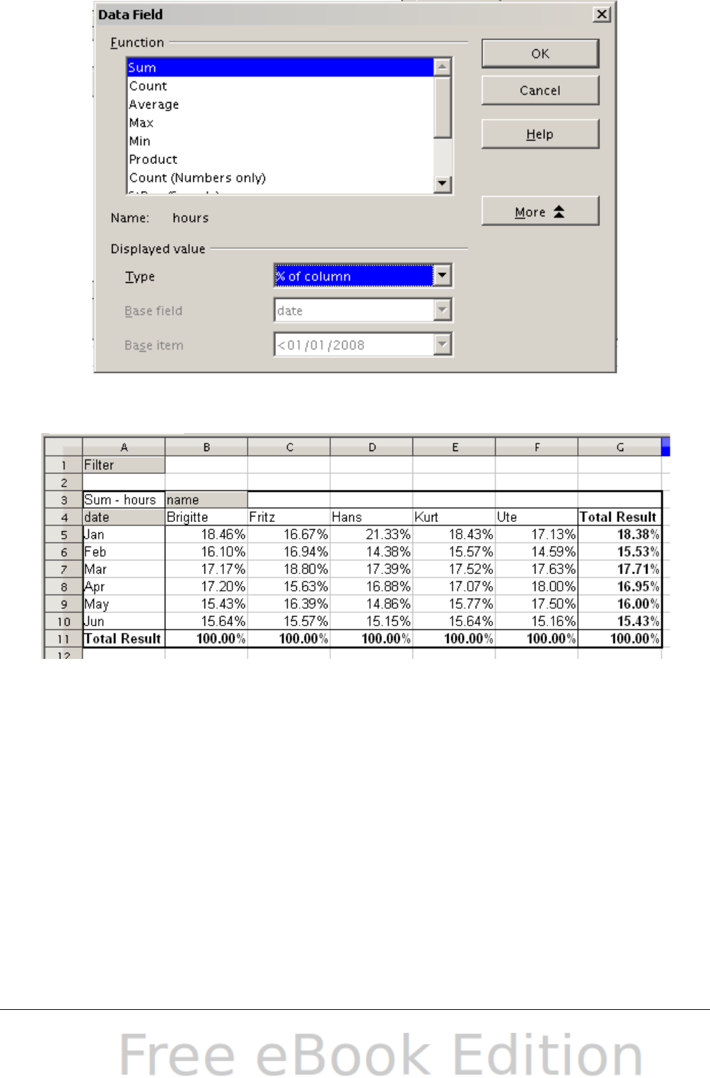
Figure 167: Properties of the data field
Figure 168: Result with percentages
To get a comparison between employees, start the DataPilot again:
1) Select the cell A3 (or any other cell that contains a result of the
DataPilot).
2) Choose Data > DataPilot > Start.
3) Double-click on Sum – hours to open the Data Field dialog.
4) Click More, to see more options.
•Switch the Type of the displayed value to Difference from.
•Switch the Base Field to name.
•Switch the Base Item to Brigitte.
5) Click OK twice.
232 OpenOffice.org 3.x Calc Guide
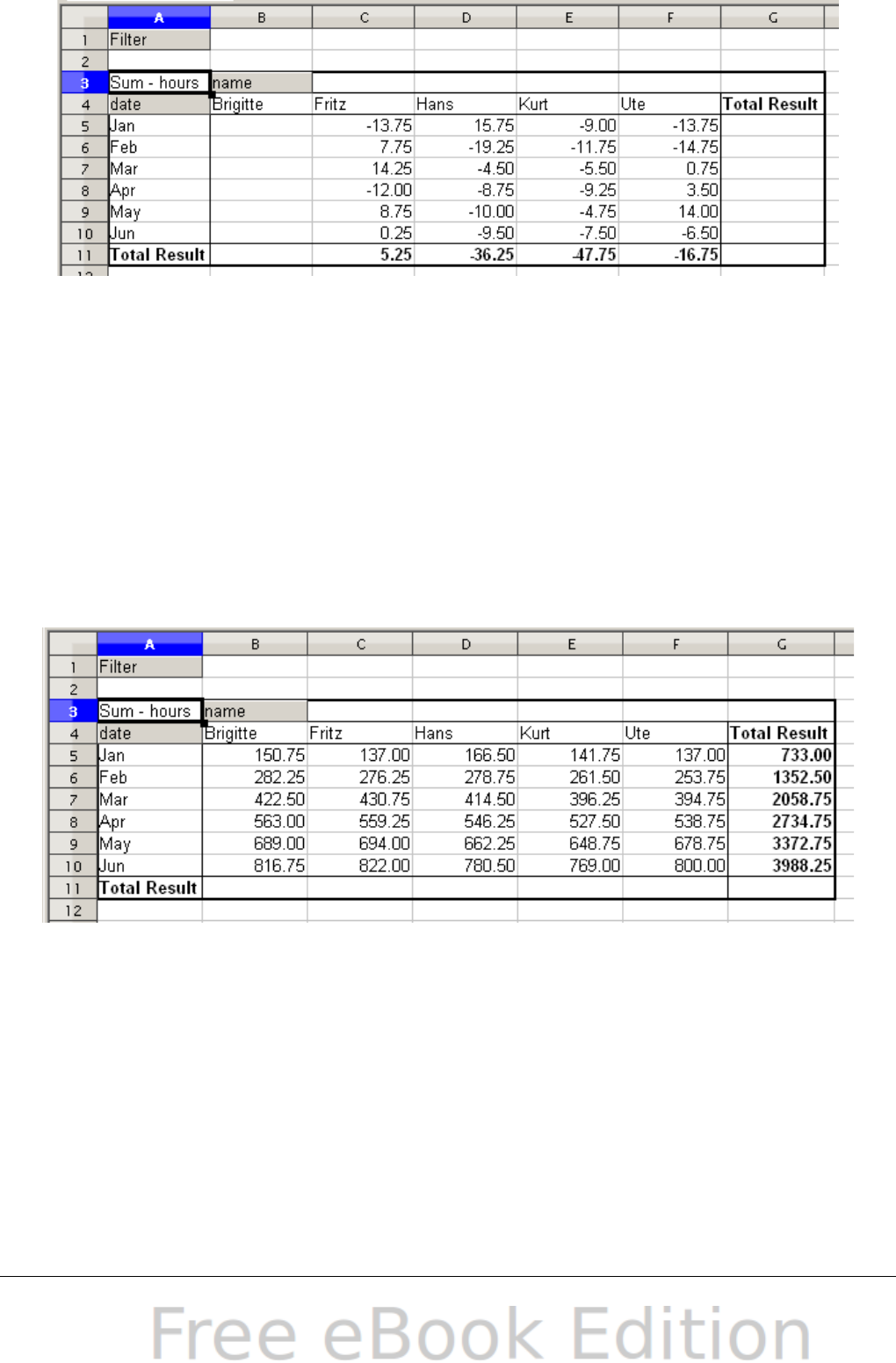
Figure 169: Absolute comparison with Brigitte
As a final example we switch to an accumulated view; that is,
continuing sums of all values:
1) Choose Data > DataPilot > Start.
2) Double-click on Sums – hours to open the Data Field dialog.
3) Click More, to see more options.
•Switch the type of the displayed value to Running total in.
•Switch the Base Field to Date.
4) Click OK twice.
Figure 170: The DataPilot now shows accumulated values
Differences and advantages
These examples show an important aspect of the DataPilot. Normally
you have to collect your data according to the way you want the result
to be represented. This means you have to use a specific structure and
you are stuck with it.
The DataPilot works more like a real database. The source data is
collected in a simple spreadsheet that contains all data. Only when you
want to look at it do you select which part of the data you want to use.
Chapter 8 Using the DataPilot 233
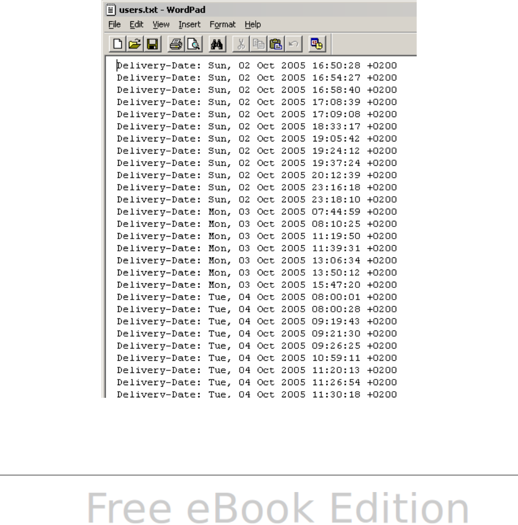
Example 3: Frequency distribution
For showing the frequency of incidents, Calc uses the function
FREQUENCY. This formula has to be used in a so-called matrix
formula. This is an advanced feature. Alternatively you can use the
DataPilot, which requires almost no knowledge of spreadsheets.
In our example we want to investigate the number of emails that go to
the Germanophone support mailing list (users@de.openoffice.org). We
want to know how the activity on the list is distributed during the day.
The starting point for this example is the mailbox file of the
Thunderbird mail client. The command
grep 'Delivery-Date:' Inbox
creates a text file that contains for the timespan of more than 2 years
one line for each message, with date and time (Figure 171).
Figure 171: Raw data for the frequency of
the messages
234 OpenOffice.org 3.x Calc Guide
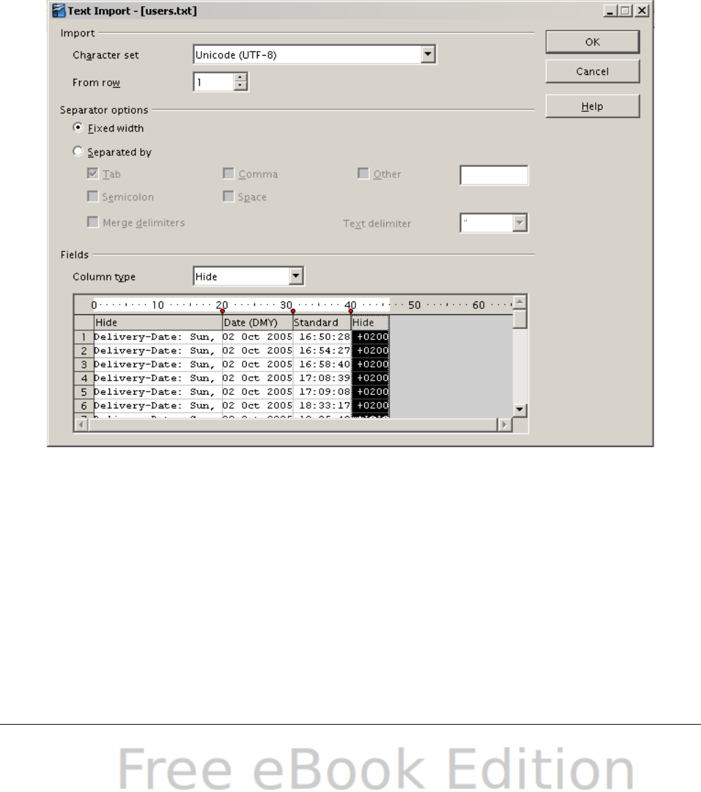
To import the data into a table in Calc, open the text file users.txt
containing the raw data. The Text Import dialog appears. Here you can
choose your import options. Use the following properties:
Separator options: Fixed width
Divide into columns at position 20, 31 and 40
Column types:
Column 1: Hide
Column 2: Date (DMY)
Column 3: Standard
Column 4: Hide
Figure 172: Import settings
Figure 173 shows the imported raw data with a line added at the top
containing titles for each column.
Chapter 8 Using the DataPilot 235
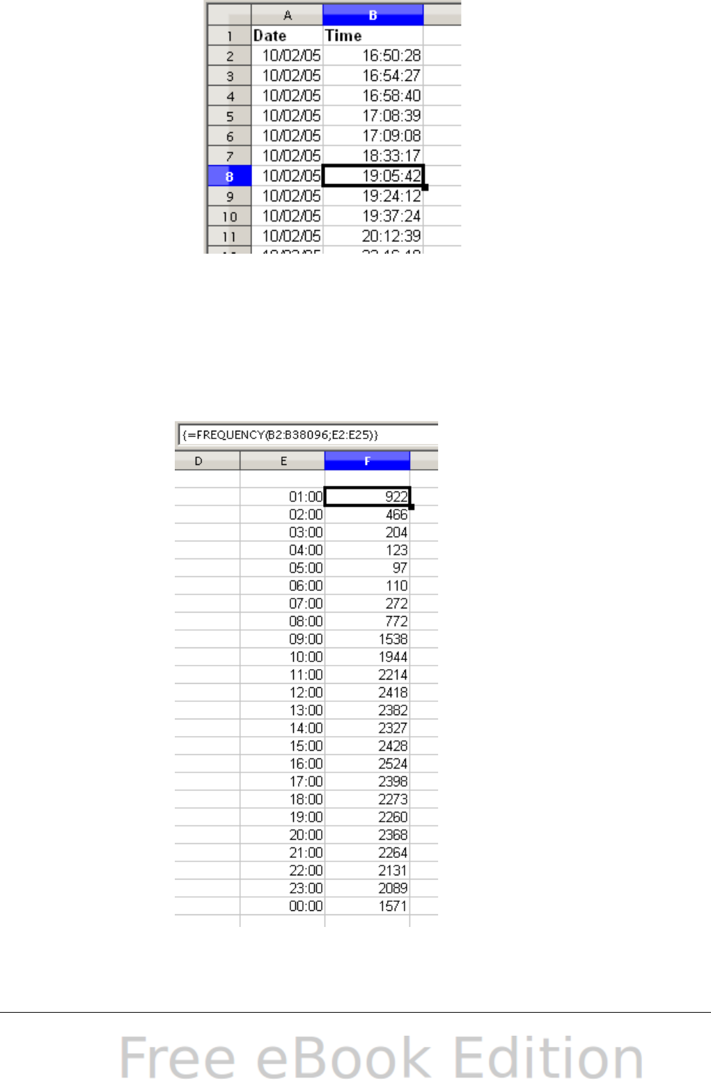
Figure 173: Raw data in Calc
Solution with a matrix formula
To calculate the frequency you have to create 24 classes, one for each
hour. In the next column you enter the number of emails with the
function FREQUENCY.
Figure 174: FREQUENCY function
in a matrix formula
236 OpenOffice.org 3.x Calc Guide
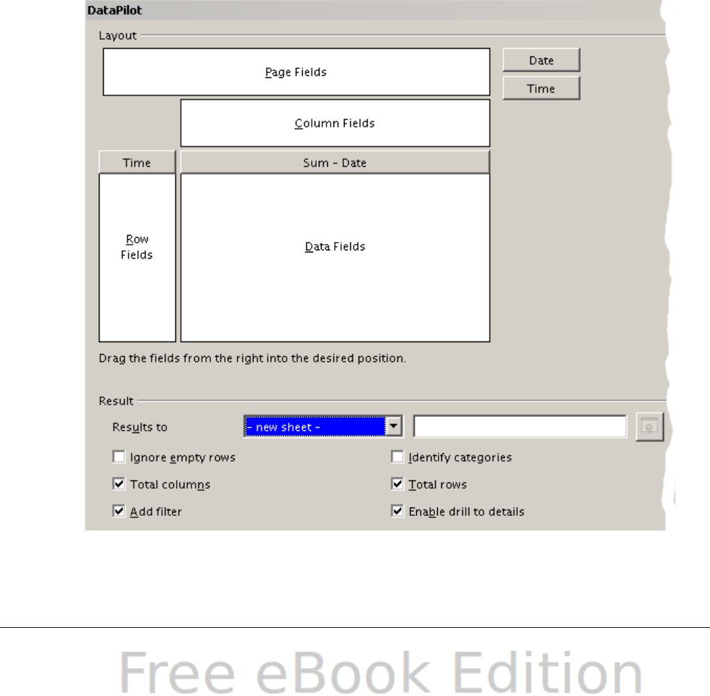
The first argument is the cell area with the times of all approximately
38,000 emails. The second argument is the cell area E2:E25 that
describes the frequency classes. To enter the formula, first select the
cell area F2:F25, then enter the formula. Then finish the formula by
using the key combination Shift+Ctrl+Enter. This indicates to the
program that you want to use a matrix formula. To indicate the matrix
formula, the program uses curly brackets.
This technique is most often known only to advanced users.
Solution with the DataPilot
With the DataPilot you can achieve the same result much easier and
faster. The solution is also possible for less advanced users. Starting
with the raw data (Figure 173), you need only a few mouse clicks.
1) Select the cell A1 (or any other cell within the list).
2) Choose Data > DataPilot > Start and click OK.
Figure 175: Part of DataPilot dialog
Chapter 8 Using the DataPilot 237
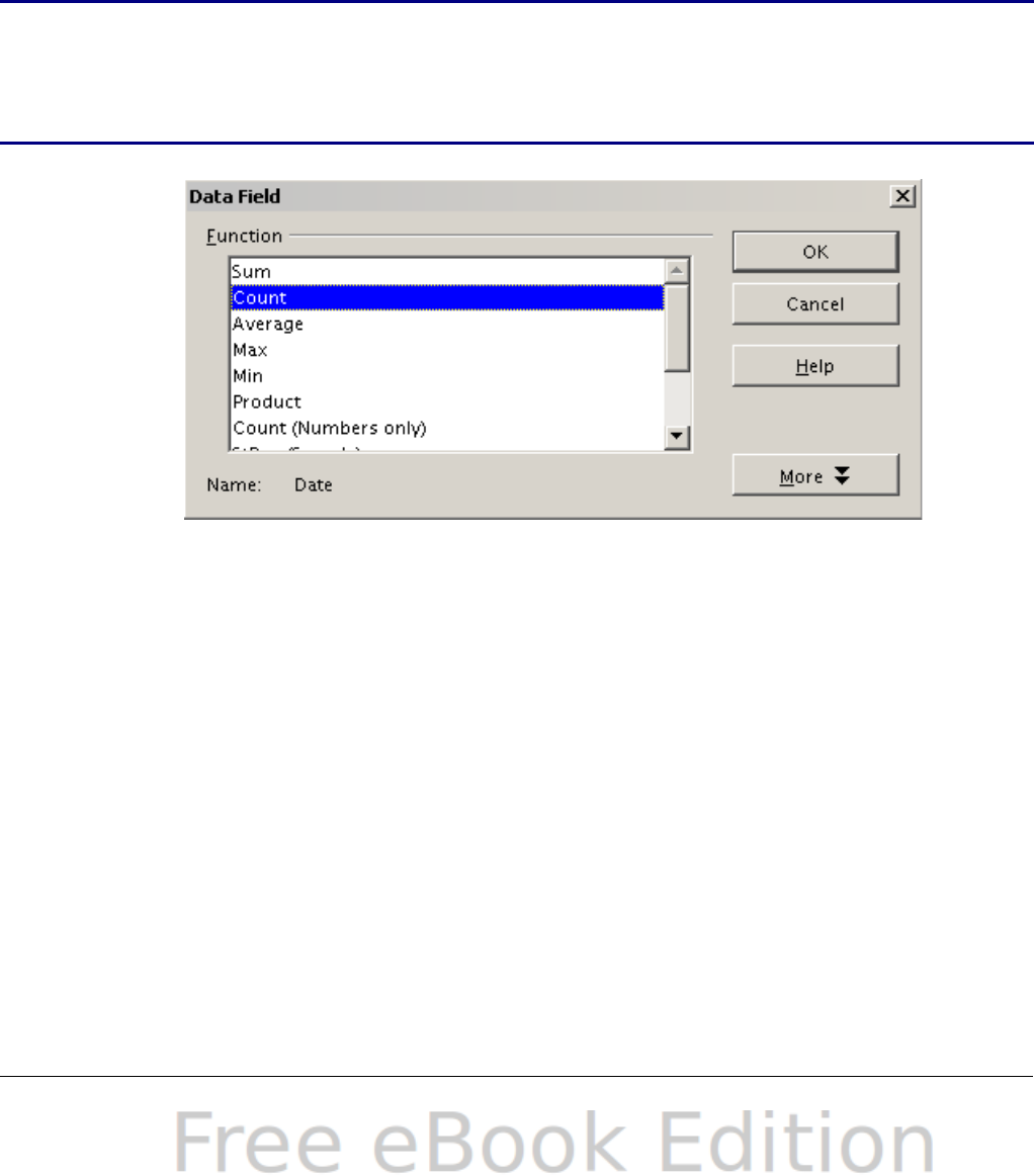
3) In the DataPilot:
•Drag Time into the Row Fields area.
•Drag Date into the Data Fields area.
4) Click More to show more options in the lower part of the dialog.
5) Choose – new sheet – for Results to.
6) In this case we need to count the number of values, not their sum.
Double-click on Sum – Date to open the Data Field dialog and
select the function Count (see Figure 176).
7) Click OK. As an intermediate result, you get a DataPilot table that
has for every time within the raw data a separate line.
Note
This may be a very time-consuming process because of the large
number of items. The time does not depend that much on the
number of lines but rather on the number of rows needed for the
table that contains the results.
Figure 176: Properties of the data field
8) For grouping the rows, select the cell A4 or any other cell that
contains a time.
9) Choose Data > Group and Outline > Group, select for the
interval Hours and click OK. The result is now grouped according
to hours.
238 OpenOffice.org 3.x Calc Guide

Figure 177: properties for grouping according to hours
10) Figure 178 shows the Data Field dialog for the data field Number
– Date. Click More and select as type % of column. The result is
shown in Figure 180. Figure 179 shows the absolute occurrence.
Whether the relative values are shown as a decimal (0.1) or as a
percentage (10%) depends only on the cell formatting itself and
has nothing to do with the DataPilot.
Figure 178: Data Field settings for relative values
Chapter 8 Using the DataPilot 239
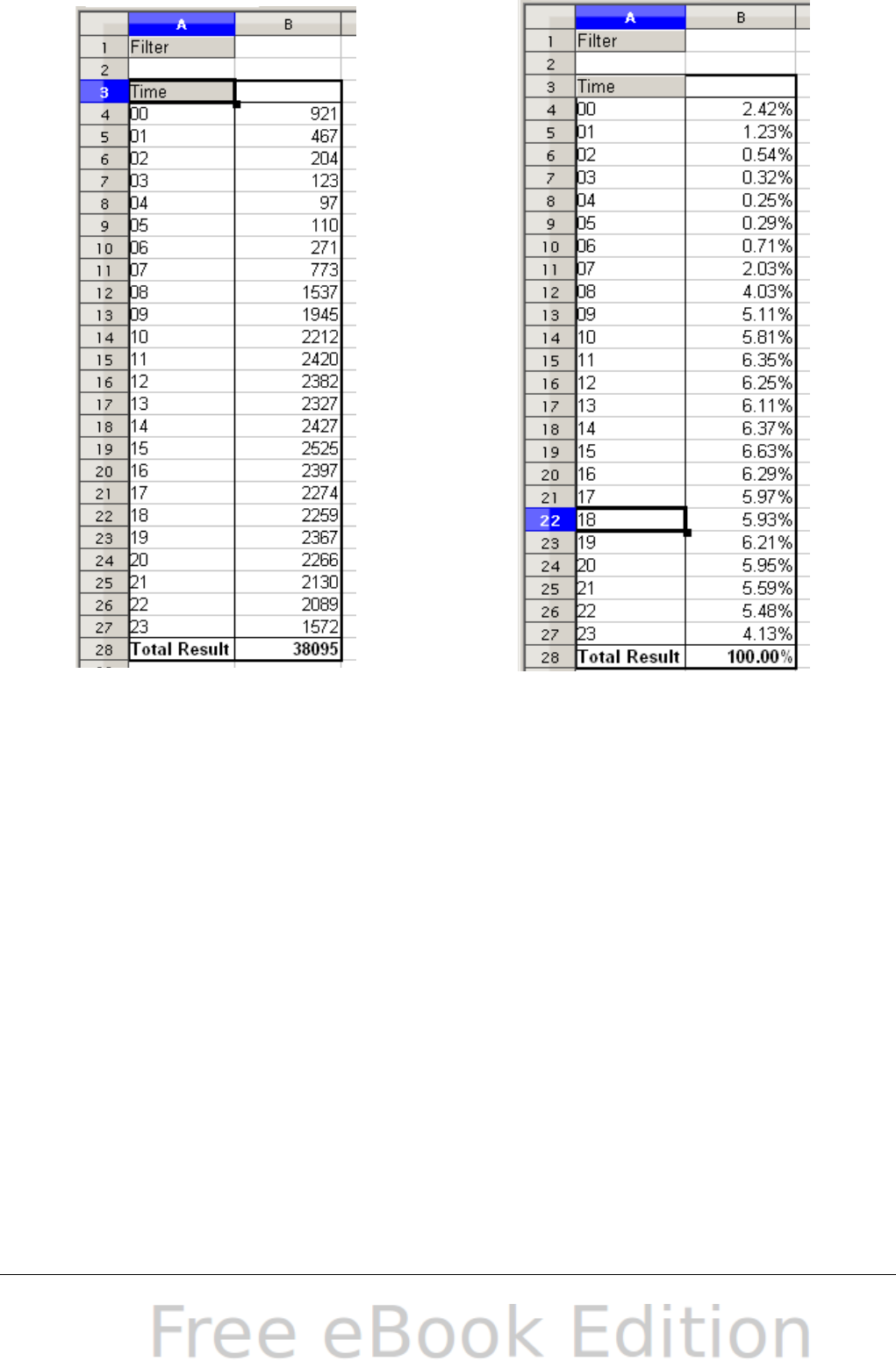
Figure 179: Frequency
distribution with the DataPilot
Figure 180: Relative
occurrence
240 OpenOffice.org 3.x Calc Guide
DataPilot functions in detail
This part describes the use and options of the DataPilot in detail.
The database (preconditions)
The first thing needed to work with the DataPilot is a list of raw data,
similar to a database table, consisting of rows (data sets) and columns
(data fields). The field names are in the first row above the list.
The data source could be an external file or database. For the simplest
case, where data is contained in a Calc spreadsheet, Calc offers sorting
functions that do not require the DataPilot.
For processing data in lists, the program needs to know where in the
spreadsheet the table is. The table can be anywhere in the sheet, in
any position. A spreadsheet can contains several unrelated tables.
Calc recognizes your lists automatically. It uses the following logic:
Starting from the cell you’ve selected (which must be within your list),
Calc checks the surrounding cells in all 4 directions (left, right, above,
below). The border is recognized if the program discovers an empty
row or column, or if it hits the left or upper border of the spreadsheet.
This means that the described functions can only work correctly if
there are no empty rows or columns in your list. Avoid empty lines (for
example for formatting). You can format your list by using cell formats.
Rule No empty rows or empty columns are allowed within lists.
If you select more than one single cell before you start sorting, filtering
or calling the DataPilot, then the automatic list recognition is switched
off. Calc assumes that the list matches exactly the cells you have
selected.
Rule For sorting, filtering, or using the DataPilot, always select only
one cell.
A relatively big source for errors is that you might declare a list by
mistake and you sort your list. If you select multiple cells (for example,
a whole column) then the sorting mixes up the data that should be
together in one row.
In addition to these formal aspects, the logical structure of your table
is very important when using the DataPilot.
Chapter 8 Using the DataPilot 241

Rule Calc lists must have the normal form; that is, they must have a
simple linear structure.
When entering the data, do not add outlines, groups, or summaries.
This becomes clear when we think about what we could have done
wrong in our Sales list example in the section “Examples with step by
step instructions” starting at page 219. Here are some mistakes
commonly made by inexperienced spreadsheet users:
1) You could have made several sheets, for example, a sheet for each
group of articles. Analyses are then possible only within each
group. Analyses for several groups would be a lot of work.
2) In the Sales list, instead of only one column for the amount, you
could have made a column for the amounts for each employee.
The amounts then had to be entered into the appropriate column.
An analysis with the DataPilot would not be possible any more. In
contrast, one result of the DataPilot is that you can get results for
each employee if you have entered everything in one column.
3) You could have entered the amounts in chronological order. At the
end of each month you could have made a sum total. In this case,
sorting the list for different criteria is not possible because the
DataPilot will treat the sum totals the same as any other figure.
Getting monthly results is one of the very fast and easy features
of the DataPilot.
Start
Start the DataPilot with Data > DataPilot > Start. If the list to be
analyzed is in a spreadsheet table, select one cell within this list. Calc
recognizes and selects the list automatically for use with the DataPilot.
242 OpenOffice.org 3.x Calc Guide
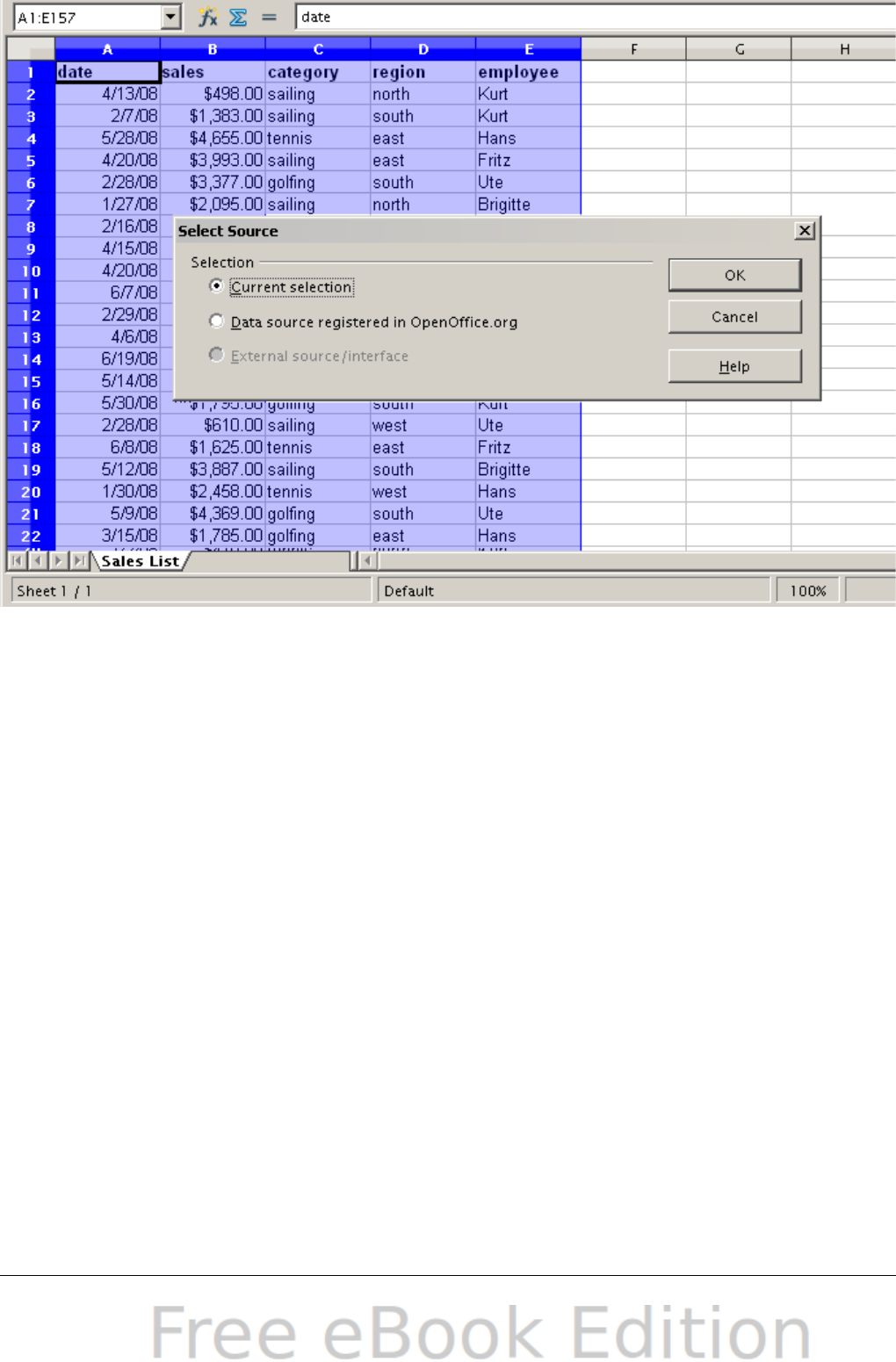
Figure 181: After the start of the DataPilot
Data source
There are usually three possibilities for the DataPilot to have a data
source: a Calc spreadsheet, an external data source that has to be
registered in OpenOffice.org, and access to an OLAP system (not
available at this time).
Calc spreadsheet
The simplest and most often used case is analyzing a list in a Calc
spreadsheet. The list might be updated regularly or the data might be
imported from a different application.
A huge list can, for example, be copied from a different application and
pasted into Calc. The behavior of Calc while inserting the data depends
on the format of the data. If the format is acceptable, the data is copied
directly into Calc. However, if the data is in plain text, a dialog appears
with the text import assistant; see Chapter 1 (Introducing Calc) for
more more information.
Chapter 8 Using the DataPilot 243

Calc can import data from a huge number of foreign data formats, for
example from other spreadsheets (Excel, Lotus 1, 2, 3), from databases
(like dBase), and from simple text files.
The drawback of copying or importing foreign data is that it will not
update automatically if there are changes in the source file. With a
Calc file you are limited to 65535 rows.
Registered data source
A registered data source in OpenOffice.org is a connection to data held
in a database outside Calc. This means that the data to be analyzed will
not be saved in Calc. It always uses the data from the original source.
Calc is able to use many different data sources and also databases that
are created and maintained with OpenOffice.org Base. See Chapter 10
(Linking Calc Data) for more information.
External data (OLAP)
No implementation exists at the moment so this option is not available.
The DataPilot dialog
The function of the DataPilot is managed in two places: first in the
DataPilot dialog and second through manipulations of the result in the
spreadsheet. This section describes the dialog in detail.
Basic layout
In the DataPilot are four white areas that show the layout of the result.
Beside these fields are buttons with the names of the fields in your
data source. To define a layout, drag and drop these field buttons into
the white areas.
The Data Fields area in the middle must contain at least one field.
Advanced users can use more than one field here. For the data field an
aggregate function is used. For example, if you move the sales field
into the Data Fields area, it appears there as Sum – sales.
244 OpenOffice.org 3.x Calc Guide
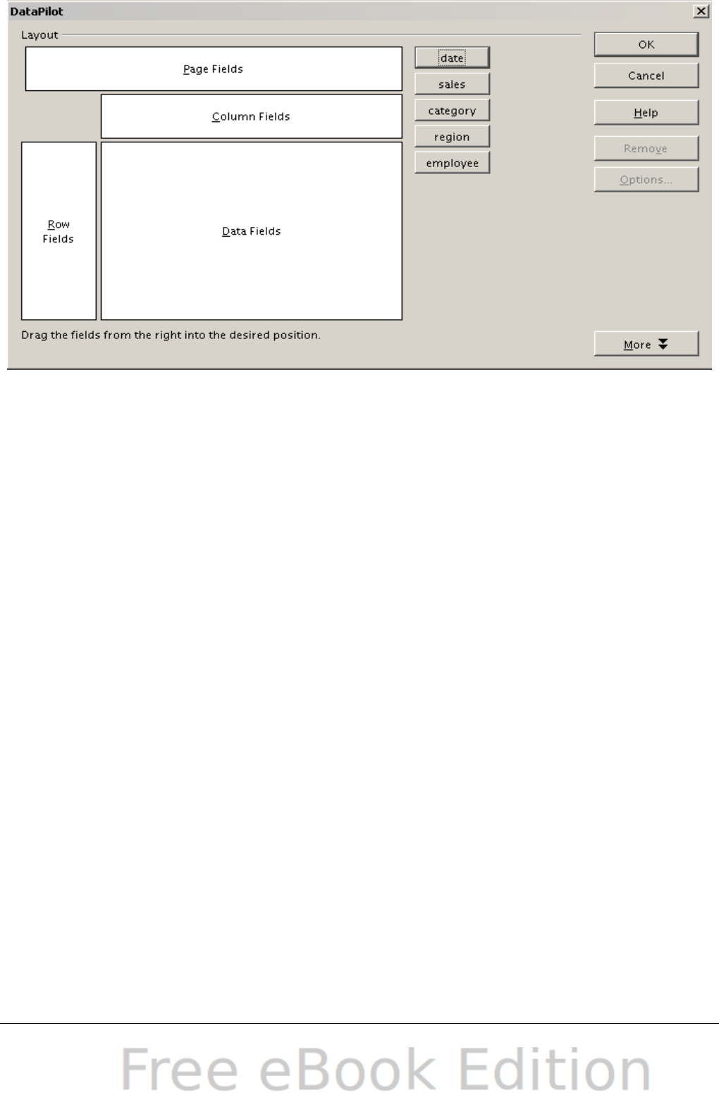
Figure 182: DataPilot dialog
Row Fields and Column Fields indicate in which groups the result will
be sorted in the rows and columns. If there are no entries in one of
these area, then partial sums will not be provided for the
corresponding rows or columns. Often more than one field is used at
the same time get partial sums for rows or columns. The order of the
fields gives the order of the sums from overall to specific.
For example, if you drag region and employee into the Row Fields
area, the sum will be divided into the employees. Within the employees
will be the listing for the different regions.
Fields that are placed into the Page Fields area appear in the result
above as a drop down list. The summary in your result takes only that
part of your base data into account that you’ve selected. For example,
if you use employee as a page field, you can filter the result shown for
each employee.
To remove a field from the white layout area just drag it to the border
and drop it (the cursor will change to a crossed symbol), or click the
Remove button.
More options
To expand the DataPilot and show more options, click More.
Chapter 8 Using the DataPilot 245
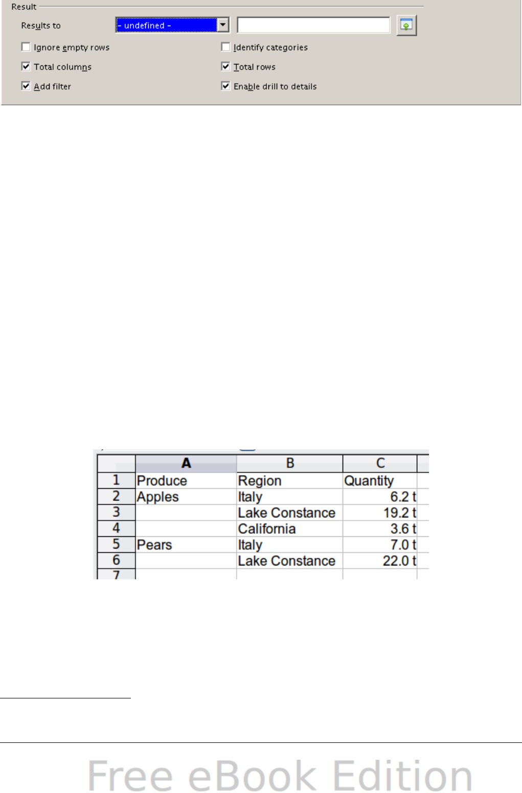
Figure 183: Expanded dialog of the DataPilot
Results to
Results to defines where your result will be shown. If you do not
enter anything, the DataPilot will put your result below the list that
contains your data. This could result in overwriting any data that is
already in that location. To avoid overwriting data, you can leave
Results to as – undefined – and enter a cell reference to tell the
DataPilot where to show the results.1 However, a generally better
approach is to use - new sheet – to add a new sheet to the
spreadsheet file and place the results there.
Ignore empty rows
If the source data is not in the recommended form, this option tells
the DataPilot to ignore empty rows.
Identify categories
If the source data has missing entries in a list and does not meet the
recommended data structure (see Figure 184), the DataPilot adds it
to the listed category above it. If this option is not chosen, then the
DataPilot inserts (empty).
Figure 184: Example of data with missing
entries in Column A
The option Identify categories ensures that in this case rows 3 and 4
are added to the product Apples and row 6 is added to Pears (see
Figure 185).
1 In this case the word - undefined – is misleading because the output position is in fact
defined.
246 OpenOffice.org 3.x Calc Guide
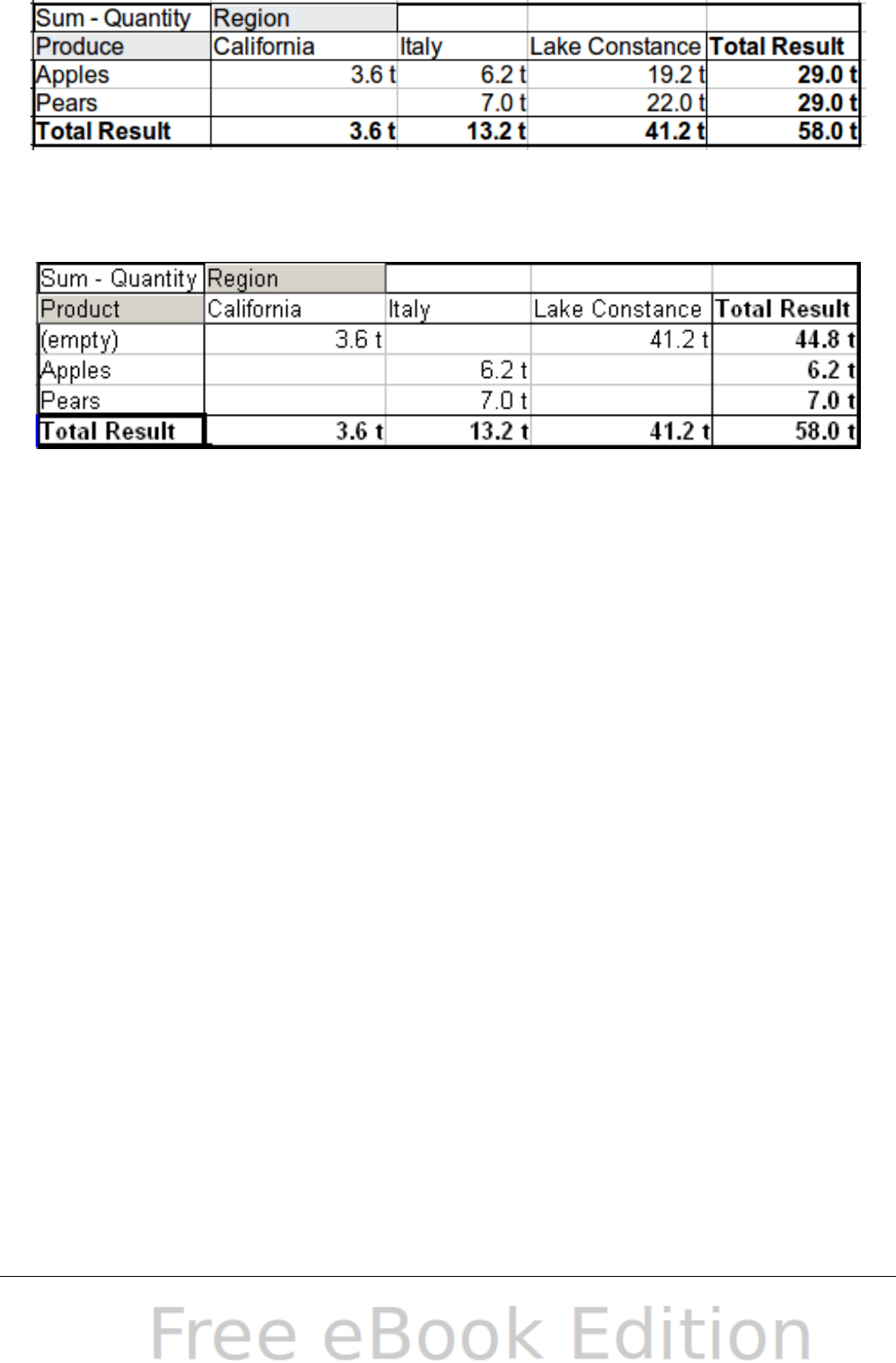
Figure 185: DataPilot result with Identify categories selected
Without category recognition, the DataPilot shows an (empty)
category (Figure 186).
Figure 186: DataPilot result without Identify categories selected
Logically, the behavior without category recognition is better. A list
with the shown missing entries is also less useful, because you
cannot use other functions such as sorting or filtering.
Total columns / total rows
With this option you decide if the DataPilot will show an extra row
with the sums of each column or if it adds on the very right a column
with the sums of each row. In some cases, an added total sum is
useless, for example if your entries are accumulated or in
comparisons.
Add filter
Use this option to add or hide the cell labelled Filter above the
DataPilot results. This cell is a convenient button for additional
filtering options within the DataPilot.
Enable drill to details
If you double-click on a single cell in the DataPilot result, this
function gives a more detailed listing of an individual entry. If this
function is disabled, the double-click will keep its usual edit function
within a spreadsheet.
Chapter 8 Using the DataPilot 247
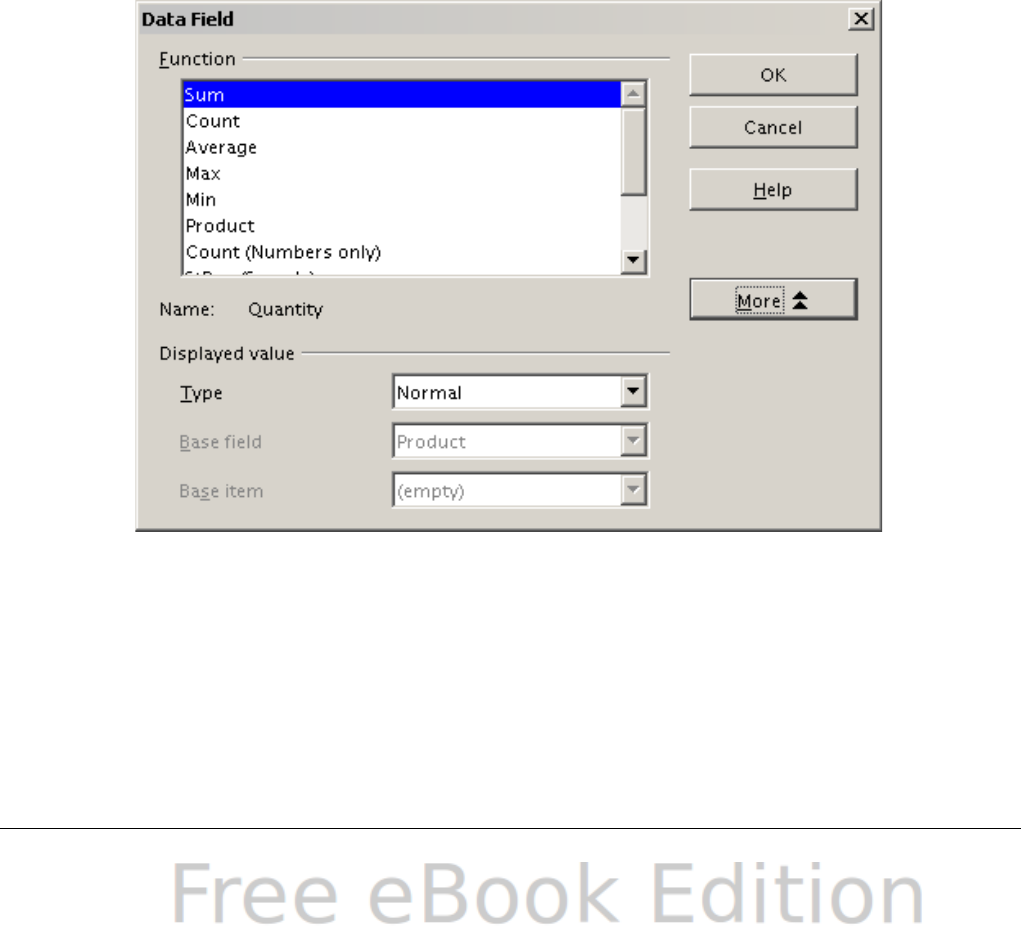
More settings for the fields
The options discussed in the previous section are valid for the
DataPilot in general. Additionally, you can change settings for every
field that you have added to the DataPilot layout. Do this either by
clicking on the Options button in the DataPilot dialog or by double-
clicking on the appropriate field.
There are differences between data fields, row or column fields, and
page fields of the DataPilot.
Data fields
In the preferences dialog of a data field you can select the Sum
function for accumulating the values from your data source. In many
cases you will need the sum function, but other functions (like
standard distribution or a counting function) are also available. For
example, the counting function can be useful for non-numerical data
fields.
On the Data Field dialog, click More to see more options.
Figure 187: Expanded dialog for a data field
In the Displayed value section, you can choose more possibilities for
analysis by using the aggregate function. Depending on the setting for
Type, you have to choose a definition for Base field and Base
element.
248 OpenOffice.org 3.x Calc Guide
Type Base field Base element Analysis
Normal — — Simple use of the
chosen aggregate
function (for
example, sum)
Difference
from
Selection of a
field from the
data source of
the DataPilot
(for example,
employee)
Selection of an
element from the
selected base
field (for
example,
Brigitte)
Result as difference
to the result of the
base element (for
example, Sales
volume of the
employees as
difference of the
sales volume of
Brigitte)
% of Selection of a
field from the
data source of
the DataPilot
(for example,
employee)
Selection of an
element from the
selected base
field (for
example,
Brigitte)
Result as a ratio
based on the result
of the base element
(for example, Sales
result of the
employee relative to
the sales result of
Brigitte)
% difference
from
Selection of a
field from the
data source of
the DataPilot
(for example,
employee)
Selection of an
element from the
selected base
field (for
example.
Brigitte)
Result as relative
difference to the
result of the base
element (for
example, Sales
volume of the
employees as
relative difference of
the sales volume of
Brigitte)
Running
total in
Selection of a
field from the
data source of
the DataPilot
(for example,
date)
— Result as a
continuing sum (for
example, Continuing
sum of the sales
volume for days or
months)
% of row — — Result as relative
part of the result in
the whole row (for
example the row
sum)
Chapter 8 Using the DataPilot 249
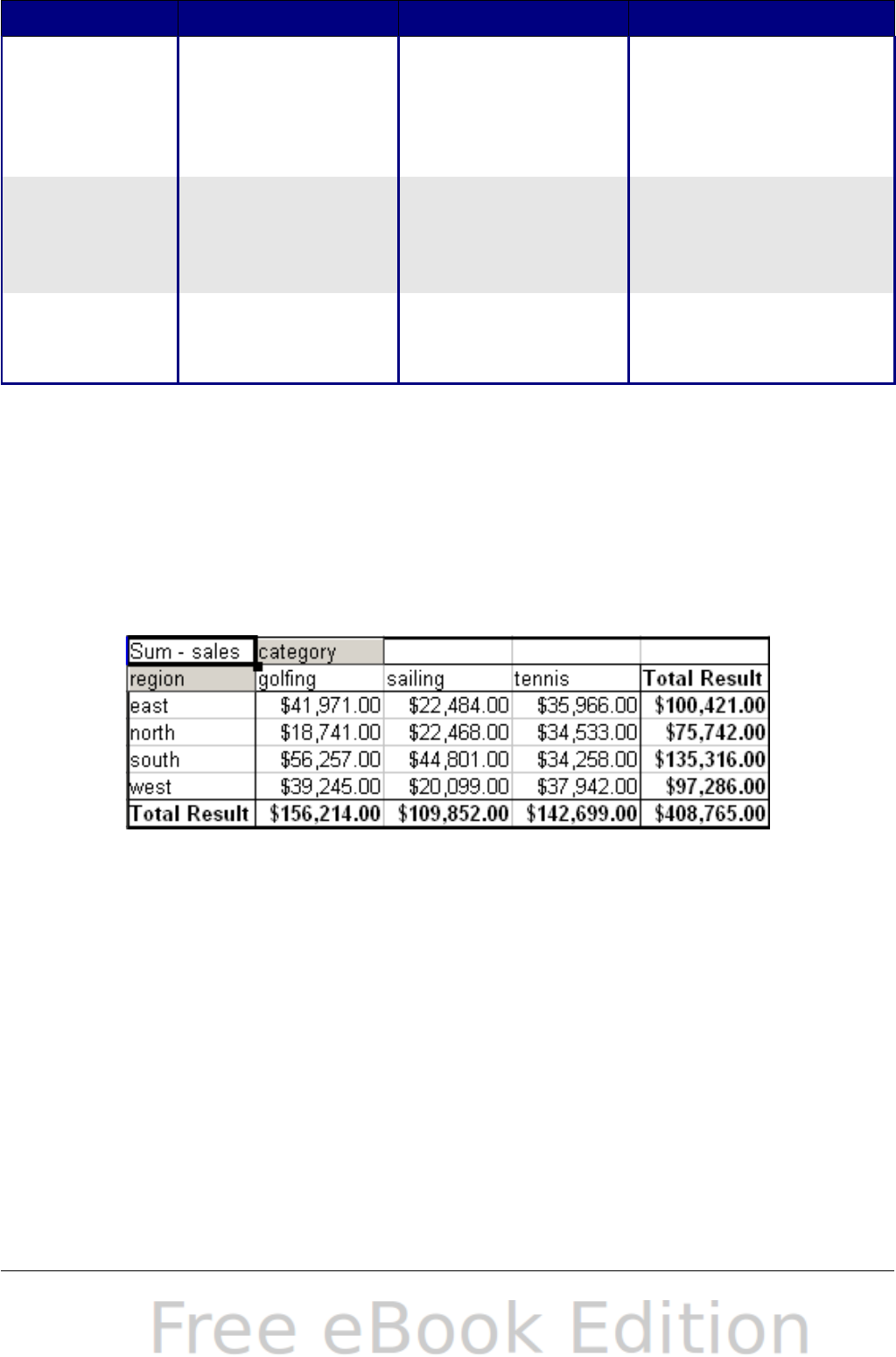
Type Base field Base element Analysis
% of column — — Result as relative
part of the total
column (for
example, the column
sum)
% of total — — Result as relative
part of the overall
result (for example
the total sum)
Index — — Default result x total
result / (row result x
column result)
Row and column fields
In the preferences dialog for the row or column fields, you can display
the partial sums for each category. Partial sums are deactivated by
default. They are only useful if the values in one row or column field
can be divided into partial sums for another (sub)field.
Some examples are shown in the next three figures.
Figure 188: No subdivision with only one row or column field
250 OpenOffice.org 3.x Calc Guide
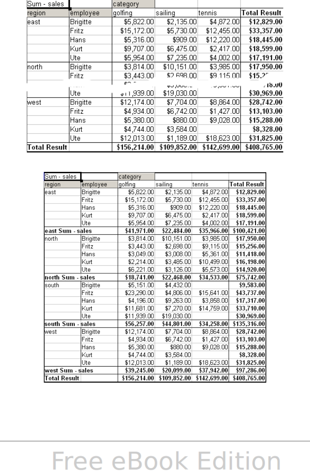
Figure 189: Division of the regions for employees without partial sums
Figure 190: Division of the regions for employees with partial sums
Select the option Automatically to use the aggregate function for the
partial results that can also be used for the data fields (see above). To
Chapter 8 Using the DataPilot 251
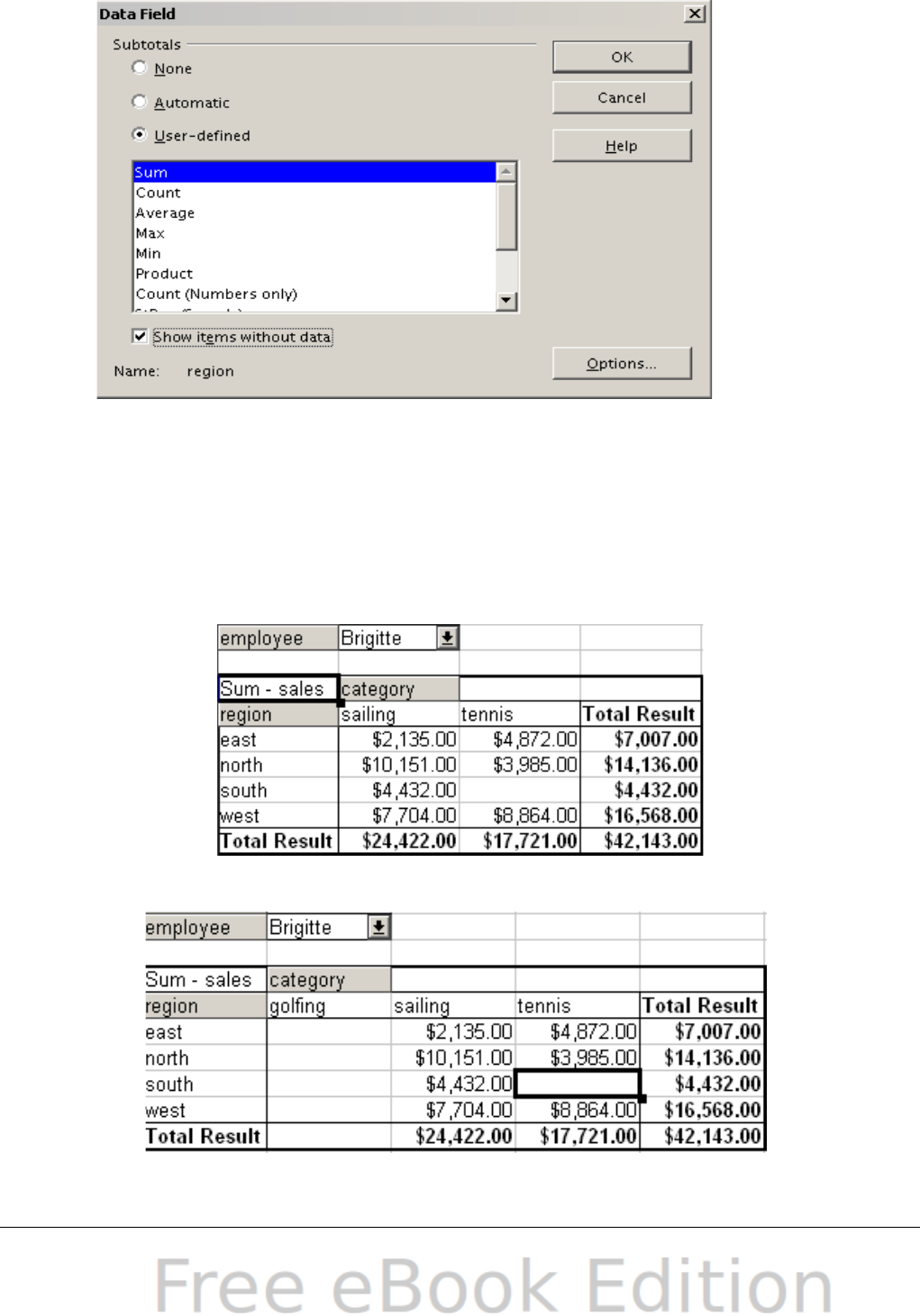
set up the aggregate function for the partial results independently
from the overall settings of the DataPilot, select User-defined.
Figure 191: Preferences dialog of a row or column field
Normally, the DataPilot does not show a row or column for categories
that have no entries in the underlying database. By choosing the Show
items with no data option, you can force this.
For illustration purposes, the data was manipulated in such a way that
the employee Brigitte has no sales values for the golfing category.
Figure 192: Default setting
Figure 193: Setting “Show Items with no data”
252 OpenOffice.org 3.x Calc Guide

Page fields
The preferences dialog for page fields is the same as for row and
column fields, even though it appears to be useless to do the same
settings as described for the row and column fields. With the flexible
use of the DataPilot you can often switch the use of the different fields
for pages, columns or rows. The fields keep the settings that you made
for them. For this, the page field has the same properties as a row or
column field. These settings only take effect when you use the field not
as page field but as row or column field.
Working with the results of the DataPilot
One very important feature is the flexibility of the DataPilot. An
analysis can be changed with only a few mouse clicks. Some functions
of the DataPilot can be used only with the results of an analysis.
Start the dialog
Right-click in the area of the resulting table of the DataPilot and
choose Start toopen the DataPilot dialog with all current settings.
Change layout by using drag and drop
The easiest and fastest method to change the layout of the DataPilot is
drag and drop. Within the result table of the DataPilot, move one of the
page, column, or row fields to a different position (see “Examples with
step by step instructions” starting on page 219).
You can remove a column, row, or page field from the DataPilot by
clicking on and dragging it out of the DataPilot.
Grouping rows or columns
For many analyses or summaries, the categories have to be grouped.
You can merge the results in classes or periods. In the DataPilot you do
a grouping after you have first made an ungrouped DataPilot table.
You can access the grouping with the menu entry Data > Group and
Outline > Group or by pressing F12. It is important that you select
the correct cell area. The grouping function is mainly determined by
the type of values that have to be grouped. You need to distinguish if
you have scalar values, date or time values, or other values, such as
text, that you want grouped.
Chapter 8 Using the DataPilot 253
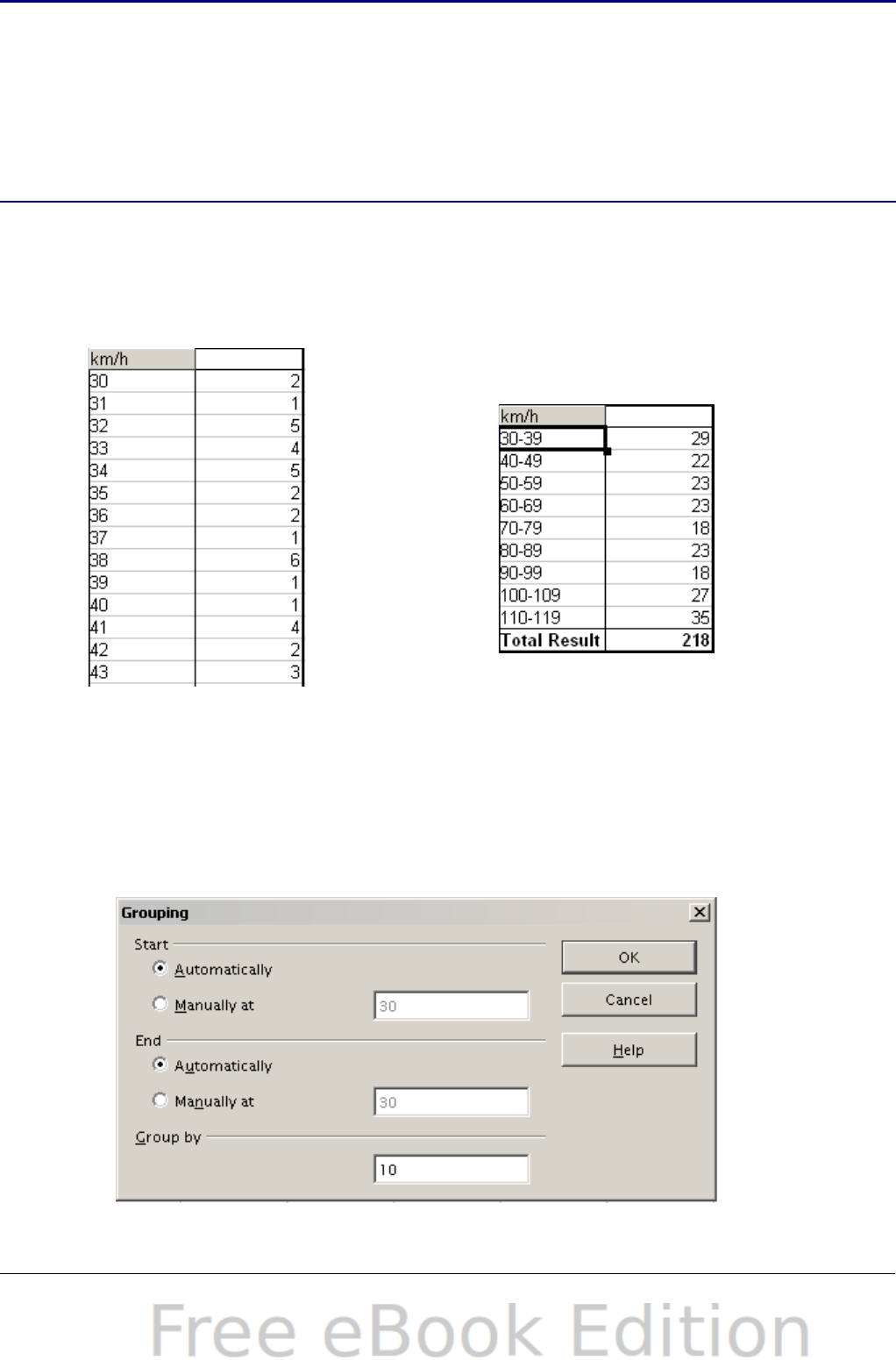
Note
Before you can group, you have to produce a DataPilot with
ungrouped data. The time needed for creating a DataPilot
depends mostly on the number of columns and rows and not on
the size of the basic data. Through grouping you can produce the
DataPilot with a small number of rows and columns. The
DataPilot can contain a lot of categories, depending on your data
source. Computing time may take several minutes.
Grouping of categories with scalar values
For grouping scalar values, select a single cell in the row or column of
the category to be grouped.
Figure 194: DataPilot
without grouping (frequency
of the km/h values of a radar
control)
Figure 195: DataPilot
with grouping (classes
of 10 km/h each)
Choose Data > Group and Outline > Group from the menu bar or
press F12; you get the following dialog.
Figure 196: Grouping dialog with scalar categories
254 OpenOffice.org 3.x Calc Guide
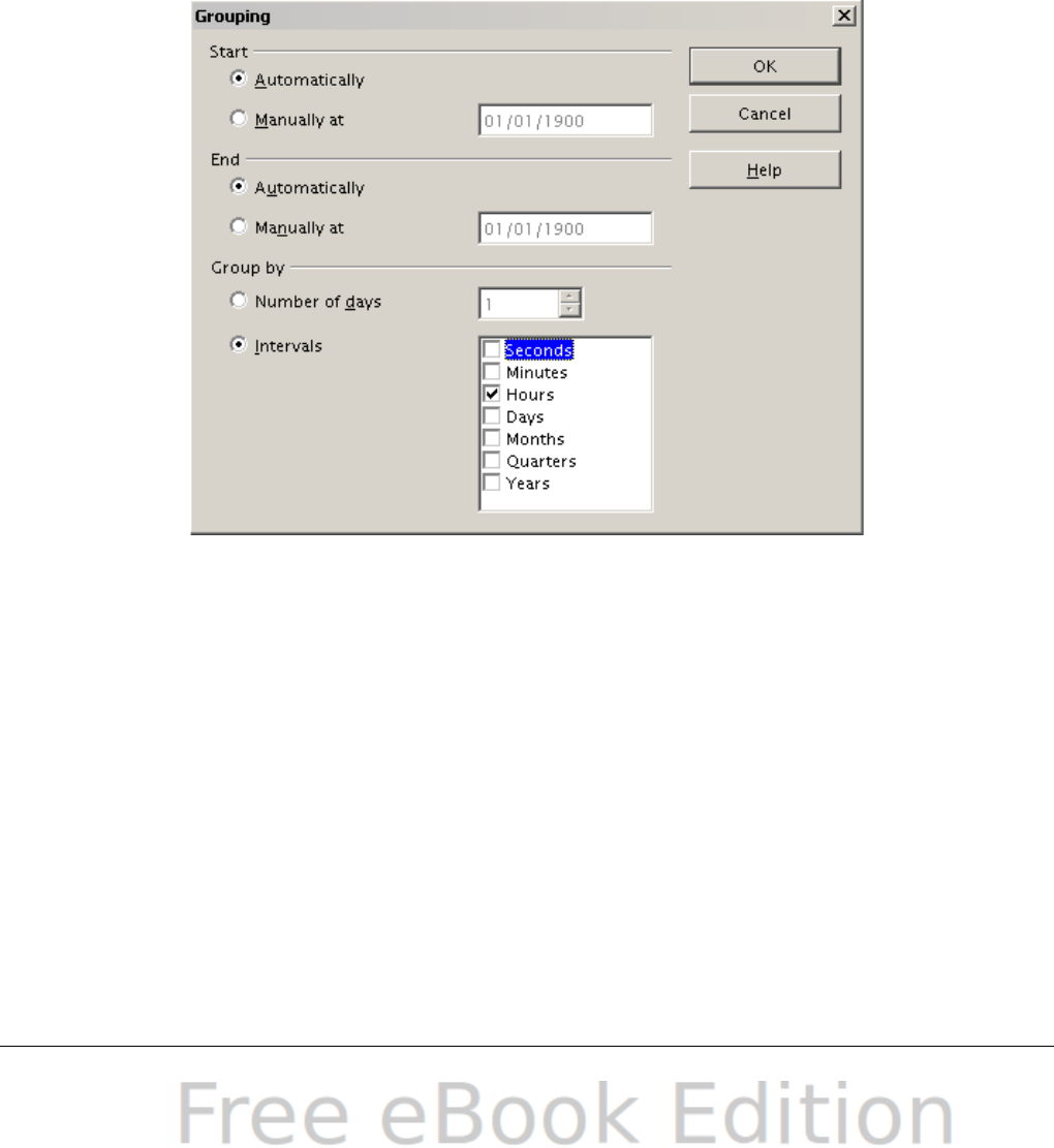
You can define in which value range (start/end) the grouping should
take place. The default setting is the whole range from smallest to
biggest value. In the Grouping after field you can enter the class size,
this means the interval size (in this example groups of 10 km/h each).
Grouping of categories with date or time values
For grouping date or time values select a single cell in the column or
row of the category that should be grouped. This was demonstrated in
all three examples in the section “Examples with step by step
instructions” starting on page 219.
With the menu entry Data > Group and Outline > Group or by
pressing F12, you get the following dialog.
Figure 197: Grouping dialog for categories
with dates or times
You can decide in which date or time area (start/end) the grouping
should take place. The default setting is the whole area from the
earliest to the latest value. In the Group by field you can enter the
class size (the interval size), that should be used for grouping.
Possible intervals are: seconds, minutes, hours, days, months, quarters
and years. These can be combined, for example grouping of years and
within the years according to months.
As alternative you can enter any number of days as grouping interval.
Chapter 8 Using the DataPilot 255

Tip
For grouping the DataPilot in calendar weeks, define the
beginning as a Sunday or Monday and manually enter the
grouping interval of 7 days.
Grouping without the automatic creation of intervals
If the categories contain text fields, then the automatic creation of
intervals isn't possible. You can define for each category of any data
type which categories you want to put together in one group.
Every time you use the menu entry Data > Group and Outline >
Group or you press F12 and you have more than one cell selected,
then all the cells will be selected as one group.
Figure 198: Database with
nonscalar categories (departments)
Figure 199:
DataPilot with
nonscalar
categories
For grouping of non scalar categories, select in the result of the
DataPilot all single categories that you want to put in one group.
Tip
You can select several non-contiguous cells in one step by
pressing and holding the Control key while left-clicking with the
mouse.
Choose the Data > Group and Outline > Group from the Menu bar
or press F12. Repeat this for all groups that you want to create from
the different categories.
256 OpenOffice.org 3.x Calc Guide
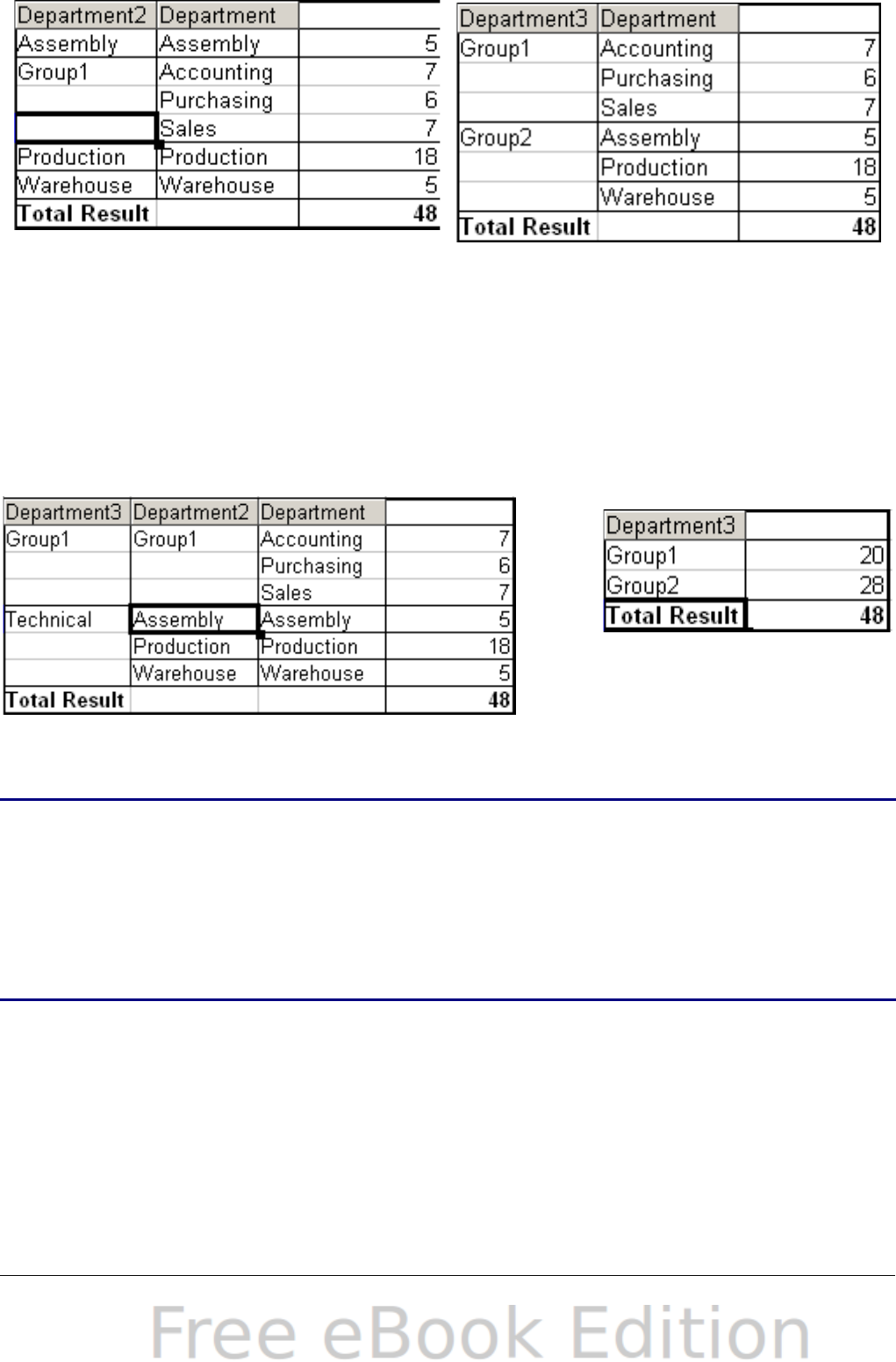
Figure 200: Summary of single
categories in one group Figure 201: Grouping finished
You can change the automatically given names for the groups and the
newly created group field by right-clicking on a name. The DataPilot
will remember these settings, even if you change the layout later on.
For the following pictures, the dialog was called again (with a right-
click) and within the preferences menu the option Automatic was
selected.
Figure 202: Renamed groups and partial
results
Figure 203: Reduced
to the new groups
Note
A well-structured database makes manual sorting within the
DataPilot obsolete. In the example shown, you could add another
column with the name Department, that has the correct entry for
each person based on whether the employee’s department
belongs to either the Office or Technical group. The mapping for
this (1:n relationship) can be done easily with the VLOOKUP
function from Calc.
Sorting the result
The result of any DataPilot is sorted (categories) in columns and rows
in an ascending order. You can change the sorting in two ways:
•Sort manually by using drag and drop.
•Sort automatically by choosing the options in the preferences
dialog of the row or column field.
Chapter 8 Using the DataPilot 257
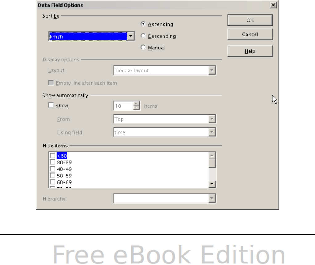
Sort manually by using drag and drop
You can change the order within the categories by moving the cells
with the category values in the result table of the DataPilot.
Please be aware that in Calc a cell must be selected. It is not enough
that this cell contains the cell cursor. The background of a selected cell
is marked with a different color. To achieve this, click in one cell with
no extra key pressed and redo this by pressing also the Shift or Ctrl
key. Another possibility is to keep the mouse button pressed on the cell
you want to select, move the mouse to a neighbor cell and move back
to your original cell before you release the mouse button.
Sort automatically
1) To sort automatically, start the preference options of the row or
column field by right-clicking on the table area with the DataPilot
result.
2) Select Start to open the DataPilot (Figure 151).
3) Within the Layout area of the DataPilot, double-click the field you
want to sort.
4) In the Data Field dialog (Figure 191), click Options to display the
Data Field Options dialog (Figure 204).
Figure 204: Options for a row or column field
258 OpenOffice.org 3.x Calc Guide
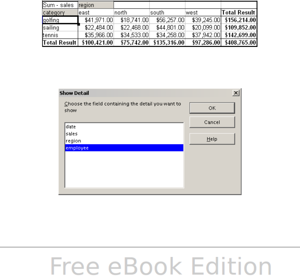
For Sort by select how to display the information, either Ascending or
Descending. On the left side is a drop-down list where you can select
the field this setting should apply to. With this method you can specify
that sorting does not happen according to the categories but according
to the results of the data field.
Drilling (showing details)
Drill allows you to show the related detailed data for a single,
compressed value in the DataPilot result. To activate a drill, double-
click on the cell or choose Data > Group and Outline > Show
Details. You have to distinguish two cases:
1) The active cell is the category of a row or column field.
In this case drill means an additional breakdown into the
categories of another field.
For example, double-click on the cell with the value golfing in the
row field region. In this case the values that are aggregated in
the golfing category are subdivided according to another field.
Figure 205: Before the drill down for the category golfing
Since there are more possibilities for subdivision, a dialog
appears so you can choose your setting.
Figure 206: Selection of the field for the subdivision
Chapter 8 Using the DataPilot 259
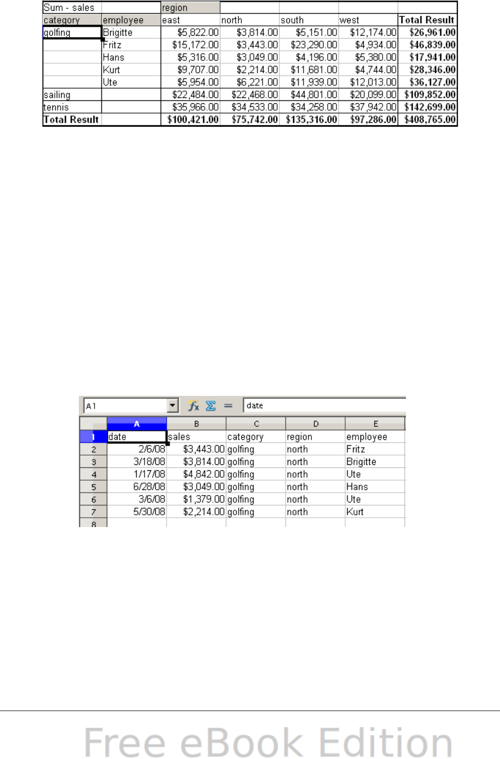
Figure 207: After the drill down
To hide the details again, double-click on the cell containing
golfing or choose Data > Group and Outline > Hide Details.
The DataPilot remembers your selection (in our example the
employee field), so that for the next drill down for a category in
the region field, the dialog does not appear. To remove the
employee selection, open the DataPilot dialog by right-clicking
and choosing Start, then delete the unwanted selection in the
row or column field.
2) The active cell is a value of the data field.
In this case drilldown means a listing of all data entries of the
data source that aggregates to this value.
Double-click on the cell with the value $18,741 from Figure 205.
You now have a new list of all data sets that are included in this
value. This list is shown in a new sheet.
Figure 208: New table sheet after the drilldown
for a value in a data field.
Filtering
To limit the DataPilot analysis to a subset of the information that is
contained in the data basis, you can filter with the DataPilot.
260 OpenOffice.org 3.x Calc Guide
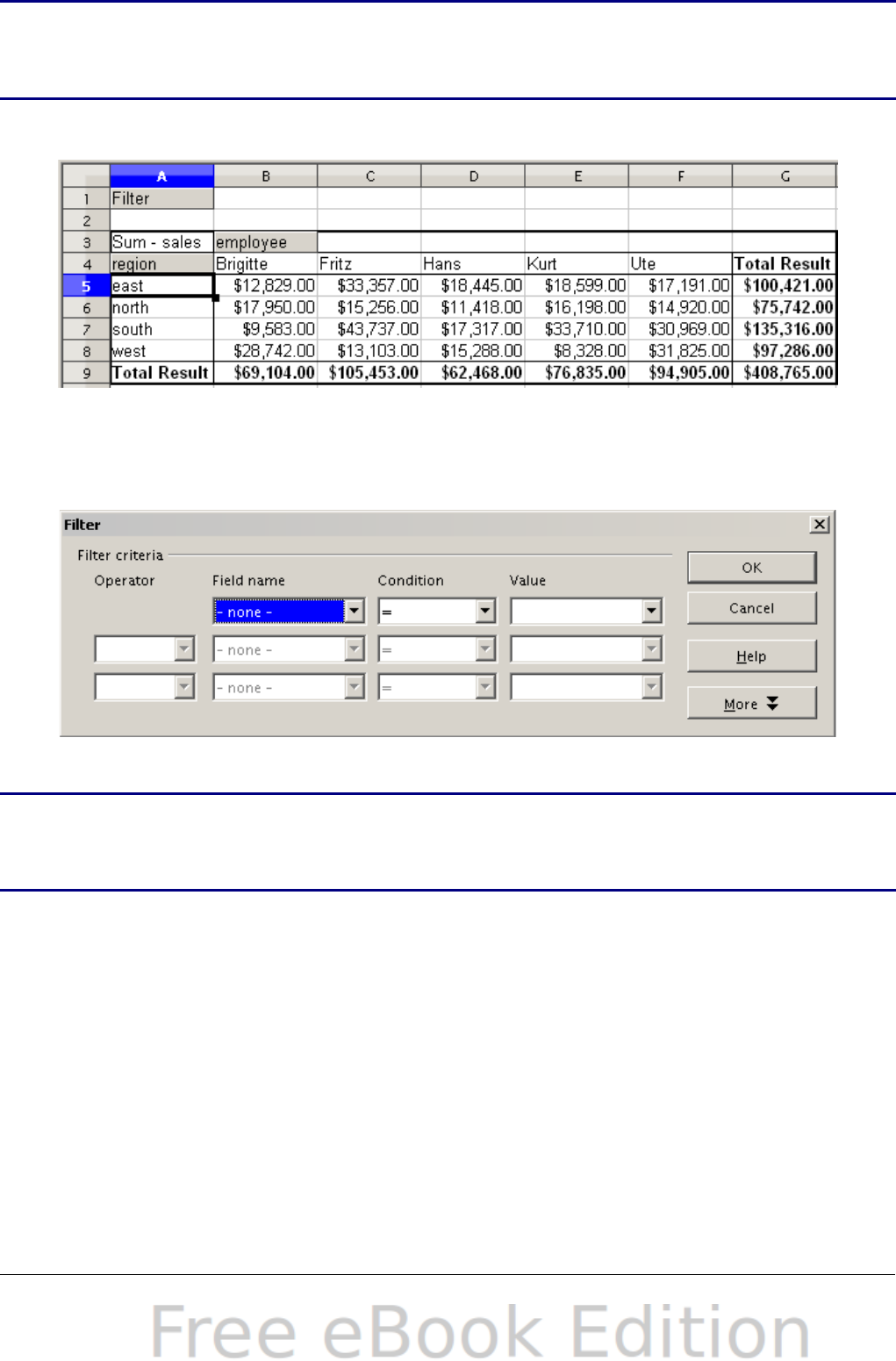
Note
An Autofilter or default filter used on the sheet has no effect for
the analysis of the DataPilot. The DataPilot always uses the
complete list that was selected when it was started.
To do this, click Filter on the top left side above the results.
Figure 209: Filter field in the upper left area of the DataPilot
In the Filter dialog, you can define of up to 3 filter options that are
used in the same way as Calc’s default filter.
Figure 210: Dialog for defining the filter
Note
Even if they are not called a filter, page fields are a practical way
to filter the results. The advantage is that the filtering criteria
used are clearly visible.
Updating (refreshing) changed values
After you have created the DataPilot, changes in the source data do not
cause an automatic update in the resulting table. You have to always
update (refresh) the DataPilot manually.
Changes in the source data could appear in two ways:
1) The content of existing data sets has been changed.
For example, you might have changed a sales value afterward. To
update the DataPilot, right-click in the result area and choose
Refresh (or choose Data > DataPilot > Refresh from the menu
bar).
Chapter 8 Using the DataPilot 261

2) You have added or deleted data sets in the original list.
In this case the change means that the DataPilot has to use a
different area of the spreadsheet for its analysis. A change of the
data reference for an existing DataPilot is not possible. You must
redo the DataPilot.
Cell formatting
The cells in the results area of the DataPilot are automatically
formatted in a simple format by Calc. You can change this formatting
using all the tools in Calc, but please note that if you make any change
in the design of the DataPilot or any updates, the formatting will return
to the that applied automatically by Calc.
For the number format in the data field, Calc uses the number format
that is used in the corresponding cell in the source list. In most cases,
this is useful (for example, if the values are in the currency format,
then the corresponding cell in the result area is also formatted as
currency). However, if the result is a fraction or a percentage, the
DataPilot does not recognize that this might be a problem; such results
must either be without a unit or be displayed as a percentage.
Although you can correct the number format manually, the correction
stays only until the next update.
Multiple data fields
Until now we have assumed that the layout of the DataPilot contains
only one data field. However, it is possible to have several data fields in
the middle of the layout. This makes summaries and analyses of
multiple aspects possible.
You could, for example, list all the sales values per day and additionally
give the number of entries per day. To do this, put both the sales field
and the date field into the Data Fields area. For the date field, select
the Count-date option for the aggregate function (see Figure 172).
Since every entry has a specific date, this field will give you the
number of entries for each date. If you group the values per month,
you get an overview with the sales value and the number of closed
sales for each category and month (see Figure 170).
262 OpenOffice.org 3.x Calc Guide
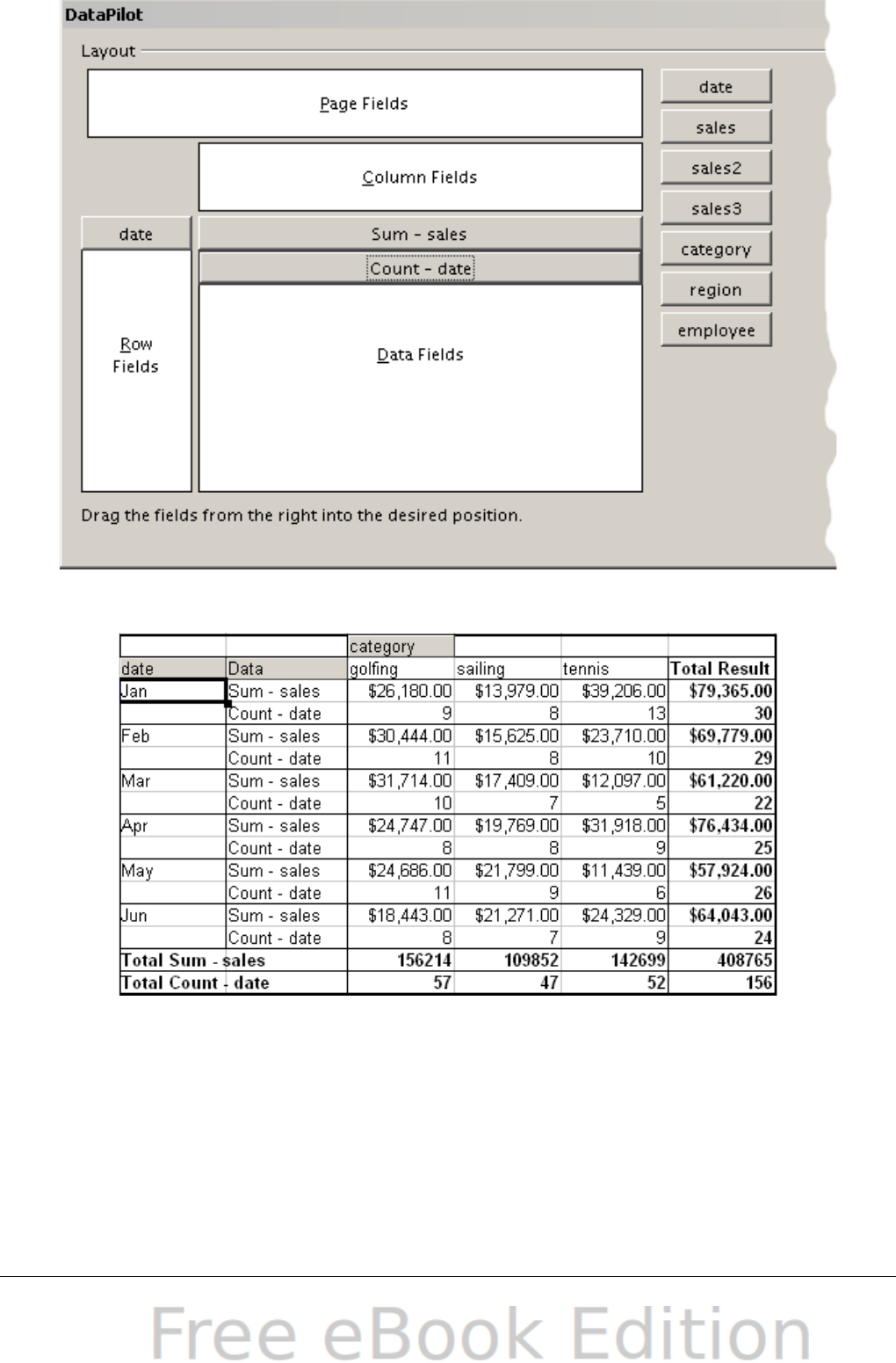
Figure 211: Multiple data fields in the DataPilot
Figure 212: DataPilot shows sales value and number of entries
For manipulating the existing data fields, DataPilot result contains a
field called Data. You can move it just like row or column fields by
using drag and drop. This is an easy way to archive a different
structure for the results (see Figures 213 and 214).
Chapter 8 Using the DataPilot 263
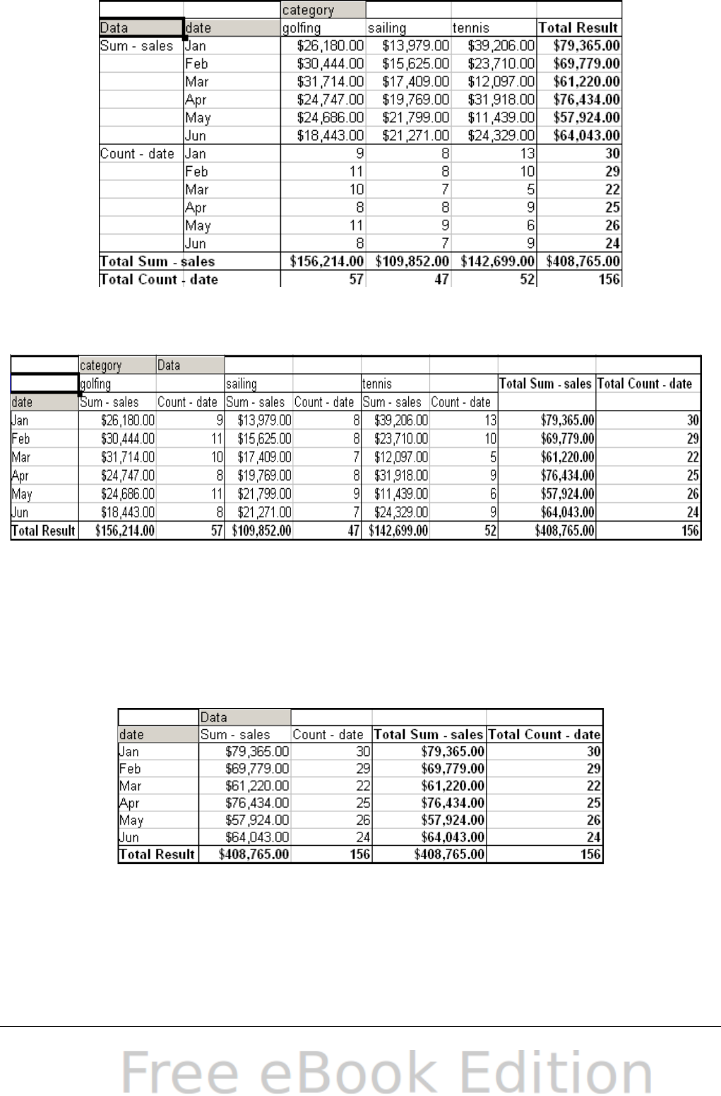
Figure 213: Layout option for presenting the sums
and numbers of the sales values
Figure 214: Another layout option for presenting the sums and
numbers of the sales values
If you want to put the different data fields in different columns and
your DataPilot does not contain another column field or you sort the
different data fields in different rows and don’t have another row field,
then it is useful to disable the view of the row or column sums
Figure 215: Unnecessary columns
264 OpenOffice.org 3.x Calc Guide
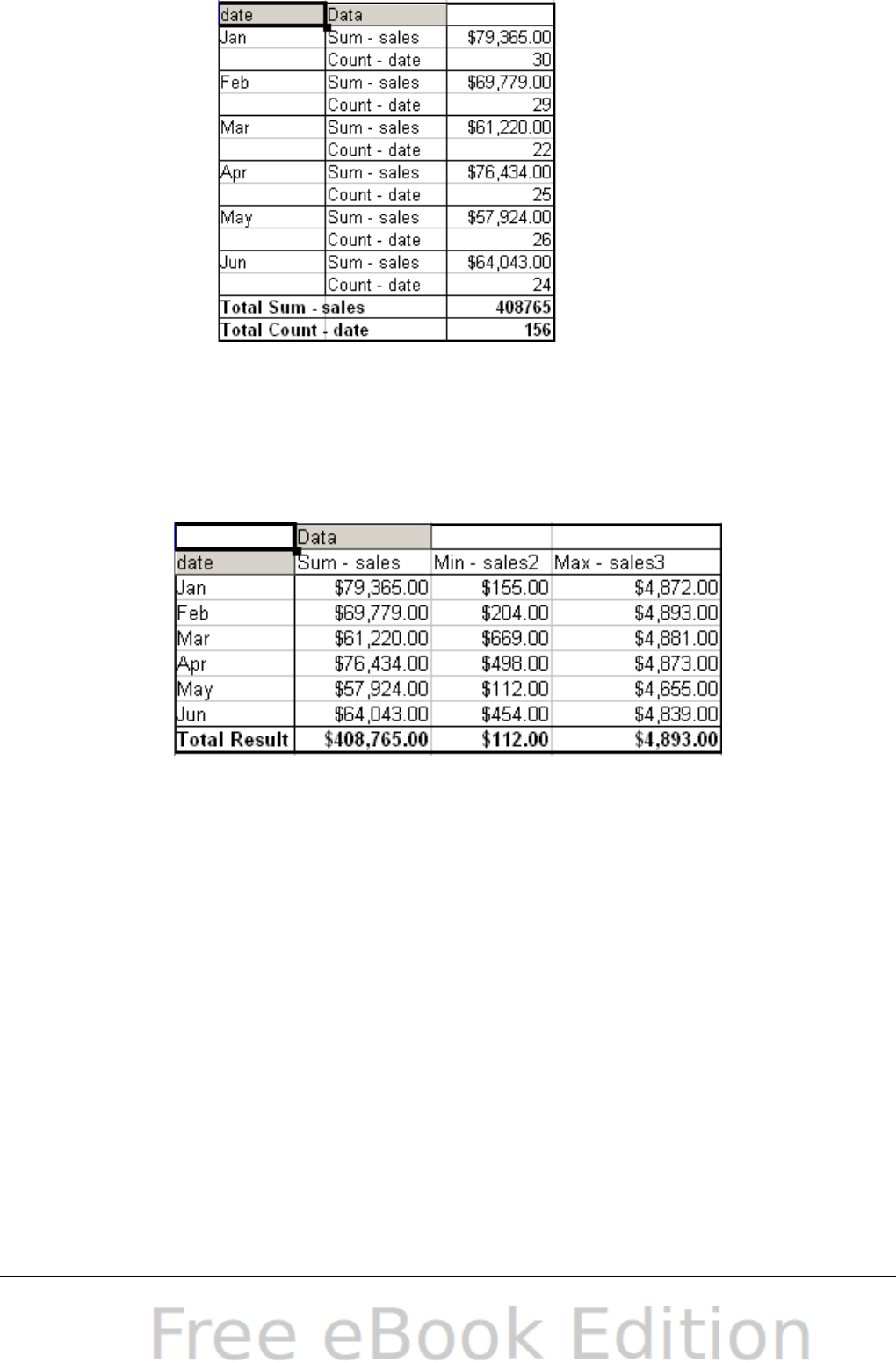
Figure 216: Disabled column sums
A frequent use case for multiple data fields is the aggregation of one
value according to different aggregate functions at the same time. You
can create a DataPilot that shows you the monthly sales values and
shows you additionally the smallest and the largest amounts.
Figure 217: Multiple analyses for the same
data field
Unfortunately, Calc does not allow you to use the same data field
multiple times. For such multiple analyses you have to duplicate the
respective column in the source. This column is then available within
the DataPilot; it just happens to have identical values.
Chapter 8 Using the DataPilot 265
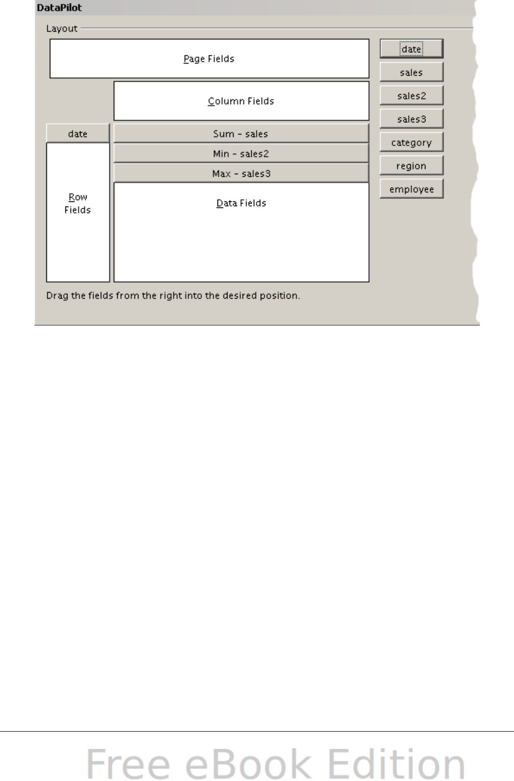
Figure 218: Multiple identical fields for sales value, that have
been created as duplicates within your source.
Shortcuts
If you use the DataPilot very often, you might find the frequent use of
the menu paths (Data > DataPilot > Start and Data > Group and
Outline > Group) inconvenient.
For grouping, a shortcut is already defined: F12. For starting the
DataPilot, you can define your own keyboard shortcut. If you prefer to
have toolbar icons instead of keyboard shortcuts, you can create a
user-defined symbol and add it to either your own custom made toolbar
or the Standard toolbar.
For an explanation how to create keyboard shortcuts or add icons to
toolbars, see Chapter 14 (Setting Up and Customizing Calc).
266 OpenOffice.org 3.x Calc Guide
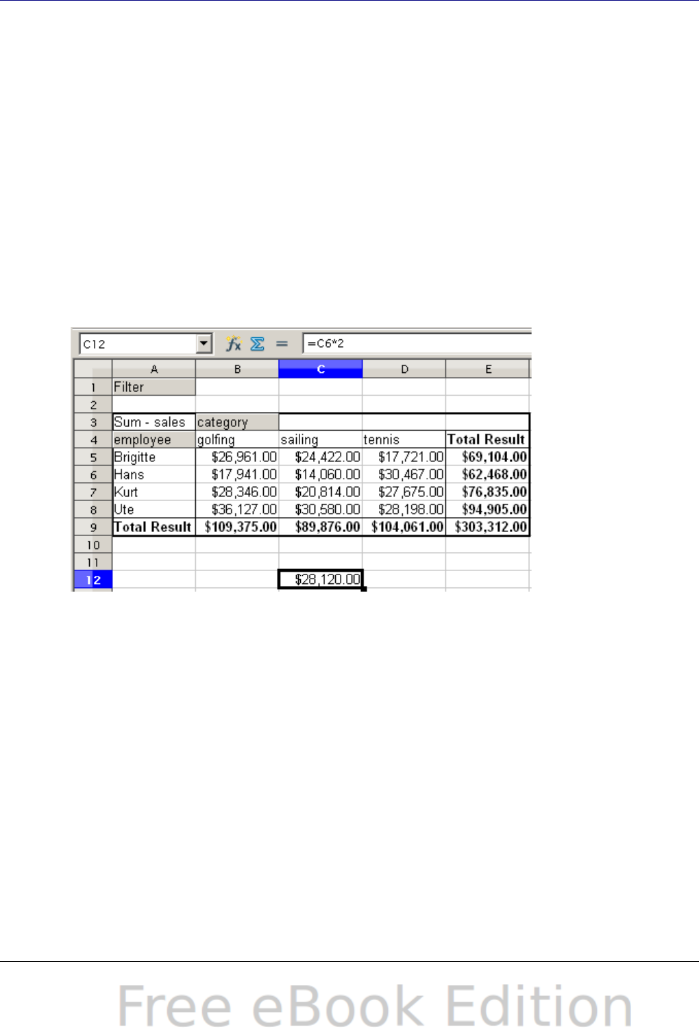
Function GETPIVOTDATA
The function GETPIVOTDATA can be used with formulas in Calc if you
want to reuse the results from the DataPilot elsewhere in your
spreadsheet.
Difficulty
Normally you create a reference to a value by entering the address of
the cell that contains the value. For example, the formula =C6*2
creates a reference to cell C6 and returns the doubled value.
If this cell is located in the results area of the DataPilot, it contains the
result that was calculated by referencing specific categories of the row
and column fields. In Figure 219, the cell C6 contains the sum of the
sales values of the employee Hans in the category Sailing. The formula
in the cell C12 uses this value.
Figure 219: Formula reference to a cell of the DataPilot
If the underlying data or the layout of the DataPilot changes, then you
must take into account that the sales value for Hans might appear in a
different cell. Your formula still references the cell C6 and therefore
uses a wrong value. The correct value is in a different location. For
example, in Figure 220, the location is now C7.
Chapter 8 Using the DataPilot 267
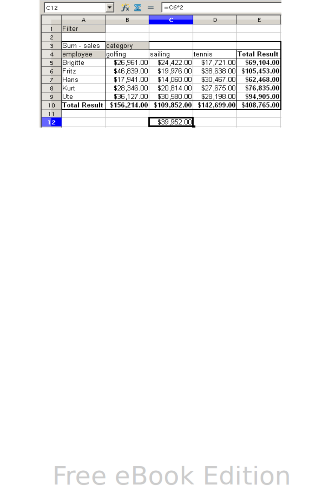
Figure 220: The value that you really want to use can
be found now in a different location.
The function GETPIVOTDATA allows you to have a reference to a value
inside the DataPilot by using the specific identifying categories for this
value.
Syntax
The syntax has two variations:
GETPIVOTDATA(target field, DataPilot; [ Field name / Element; ... ])
GETPIVOTDATA(DataPilot; specification)
First syntax variation
The target field to specify which data field of the DataPilot is used
within the function. If your DataPilot has only one data field, this entry
is ignored, but you must enter it anyway.
If your DataPilot has more than one data field, then you have to enter
the field name from the underlying data source (for example “sales
value”) or the field name of the data field itself (for example “sum –
sales value”).
The argument DataPilot specifies the DataPilot that you want to use.
It is possible that your document contains more than one DataPilot.
Enter here a cell reference that is inside the results area of your
DataPilot. It might be a good idea to always use the upper left corner
cell of your DataPilot, so you can be sure that the cell will always be
within your DataPilot even if the layout changes.
Example: GETPIVOTDATA("sales value";A1)
268 OpenOffice.org 3.x Calc Guide
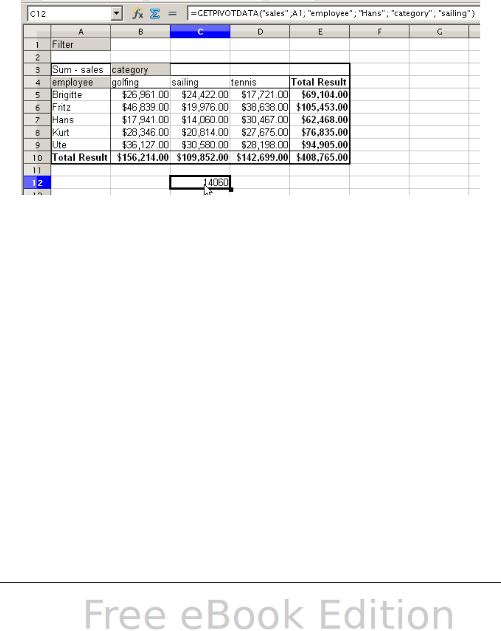
If you enter only the first two arguments, then the function returns the
total result of the DataPilot.
You can add more arguments as pairs with field name and element to
retrieve specific partial sums. In the example in Figure 221, where we
want to get the partial sum of Hans for sailing, the formula in cell C12
would look like this:
=GETPIVOTDATA("sales value";A1;"employee";"Hans";"category";"sailing")
Figure 221: First syntax variation
Second syntax variation
The argument DataPilot has to be given in the same way as for the
other syntax variation.
For the specifications, enter a list separated by spaces to specify the
value you want from the DataPilot. This list must contain the name of
the data field, if there is more than one data field, otherwise it is not
required. To select a specific partial result, add more entries in the
form of Field name[element].
In the example in Figure 222, where we want to get the partial sum of
Hans for Sailing, the formula in cell C12 would look like this:
=GETPIVOTDATA(A1;"sales value employee[Hans] category[sailing]")
Chapter 8 Using the DataPilot 269
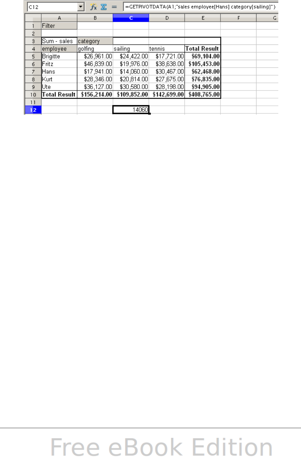
Figure 222: Second syntax variation
270 OpenOffice.org 3.x Calc Guide

Chapter 9
Data Analysis
Using Scenarios, Goal Seek, Solver, others

Introduction
Once you are familiar with functions and formulas, the next step is to
learn how to use Calc's automated processes to quickly perform useful
analysis of your data.
Calc includes several tools to help you manipulate the information in
your spreadsheets, ranging from features for copying and reusing data,
to creating subtotals automatically, to varying information to help you
find the answers you need. These tools are divided between the Tools
and Data menus.
If you are a newcomer to spreadsheets, these tools can be
overwhelming at first. However, they become simpler if you remember
that they all depend on input from either a cell or a range of cells that
contain the data with which you are working.
You can always enter the cells or range manually, but in many cases it
is easier to select the cells with the mouse. Click the Shrink/Maximize
icon beside a field to temporarily reduce the size of the tool’s
window, so you can see the spreadsheet underneath and select the
cells required.
Sometimes, you may have to experiment with which data goes into
which field, but, once you have found out, you then set a selection of
options, many of which can be ignored in any given case. Just keep the
basic purpose of each tool in mind, and you should have little trouble
with Calc’s function tools.
You don’t need to learn them, especially if your spreadsheet use is
simple, but as your manipulation of data becomes more sophisticated,
they can save time in making calculations, especially as you start to
deal with hypothetical situations. Just as importantly, they can allow
you to preserve your work and to share it with other people—or
yourself at a later session.
One function tool not mentioned here are DataPilots (also known as
pivot tables), but they are a topic that is sufficiently complex that it
requires a separate chapter. (See Chapter 8.)
Consolidating data
Data > Consolidate provides a way to combine data from two or more
ranges of cells into a new range while running one of several functions
(such as Sum or Average) on the data. During consolidation, the
contents of cells from several sheets can be combined into one place.
272 OpenOffice.org 3.x Calc Guide
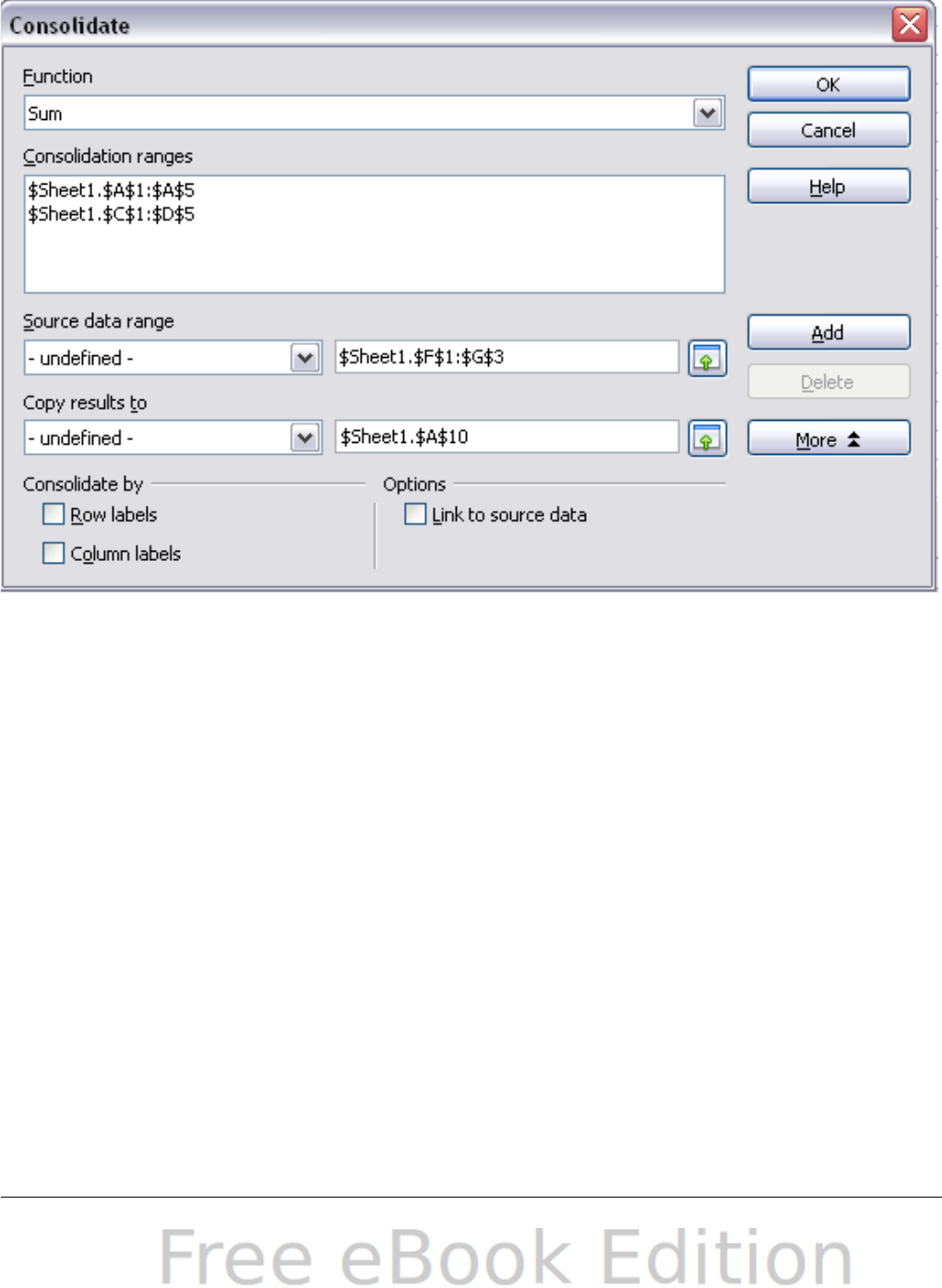
1) Open the document containing the cell ranges to be consolidated.
2) Choose Data > Consolidate to open the Consolidate dialog.
Figure 223 shows this dialog after making the changes described
below.
Figure 223: Defining the data to be consolidated
3) The Source data range list contains any existing named ranges
(created using Data > Define Range) so you can quickly select
one to consolidate with other areas.
If the source range is not named, click in the field to the right of
the drop-down list and either type a reference for the first source
data range or use the mouse to select the range on the sheet. (You
may need to move the Consolidate dialog or click on the Shrink
icon to reach the required cells.)
4) Click Add. The selected range is added to the Consolidation
ranges list.
5) Select additional ranges and click Add after each selection.
6) Specify where you want to display the result by selecting a target
range from the Copy results to drop-down list.
If the target range is not named, click in the field next to Copy
results to and enter the reference of the target range or select
the range using the mouse or position the cursor in the top left
Chapter 9 Data Analysis 273
cell of the target range. Copy results to takes only the first cell of
the target range instead of the entire range as is the case for
Source data range.
7) Select a function from the Function list. This specifies how the
values of the consolidation ranges will be calculated. The default
setting is Sum, which adds the corresponding cell values of the
Source data range and gives the result in the target range.
Most of the available functions are statistical (such as Average,
Min, Max, Stdev), and the tool is most useful when you are
working with the same data over and over.
8) At this point you can click More in the Consolidate dialog to
access the following additional settings:
•Select Link to source data to insert the formulas that
generate the results into the target range, rather than the
actual results. If you link the data, any values modified in the
source range are automatically updated in the target range.
Caution The corresponding cell references in the target range are
inserted in consecutive rows, which are automatically ordered
and then hidden from view. Only the final result, based on the
selected function, is displayed.
•Under Consolidate by, select either Row labels or Column
labels if the cells of the source data range are not to be
consolidated corresponding to the identical position of the cell
in the range, but instead according to a matching row label or
column label. To consolidate by row labels or column labels,
the label must be contained in the selected source ranges. The
text in the labels must be identical, so that rows or columns
can be accurately matched. If the row or column label of one
source data range does not match any that exist in other
source data ranges, it is added to the target range as a new
row or column.
9) Click OK to consolidate the ranges.
10) If you are continually working with the same range, then you
probably want to use Data > Define Range to give it a name.
The consolidation ranges and target range are saved as part of the
document. If you later open a document in which consolidation has
been defined, this data is still available.
274 OpenOffice.org 3.x Calc Guide
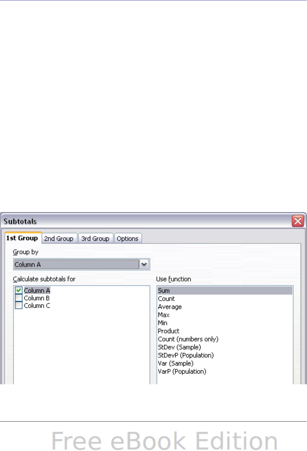
Creating subtotals
SUBTOTAL is a function listed under the Mathematical category when
you use the Function Wizard (Insert > Function). Because of its
usefulness, the function has a graphical interface accessible from Data
> Subtotals.
As the name suggests, SUBTOTAL totals data arranged in an array—
that is, a group of cells with labels for columns. Using the Subtotals
dialog, you can select up to three arrays, then choose a statistical
function to apply to them. When you click OK, Calc adds subtotal and
grand total rows to the selected arrays, using the Result and Result2
cell styles to differentiate those entries. By default, matching items
throughout your array will be gathered together as a single group
above a subtotal.
To insert subtotal values into a sheet:
1) Ensure that the columns have labels.
2) Select the range of cells that you want to calculate subtotals for,
and then choose Data > Subtotals.
3) In the Subtotals dialog, in the Group by list, select the column by
which the subtotals need to be grouped. A subtotal will be
calculated for each distinct value in this column.
Figure 224: Setting up subtotals
Chapter 9 Data Analysis 275
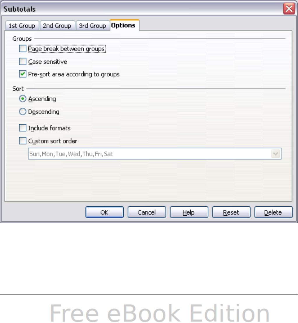
4) In the Calculate subtotals for box, select the columns
containing the values that you want to create subtotals for. If the
contents of the selected columns change later, the subtotals are
automatically recalculated.
5) In the Use function box, select the function that you want to use
to calculate the subtotals.
6) Click OK.
If you use more than one group, then you can also arrange the
subtotals according to choices made on the dialog’s Options page,
including ascending and descending order or using one of the
predefined custom sorts defined in Tools > Options >
OpenOffice.org Calc > Sort Lists.
Figure 225: Choosing options for subtotals
276 OpenOffice.org 3.x Calc Guide

Using “what if” scenarios
Scenarios are a tool to test “what-if” questions. Each scenario is
named, and can be edited and formatted separately. When you print
the spreadsheet, only the contents of the currently active scenario are
printed.
A scenario is essentially a saved set of cell values for your calculations.
You can easily switch between these sets using the Navigator or a
drop-down list which can be shown beside the changing cells. For
example, if you wanted to calculate the effect of different interest rates
on an investment, you could add a scenario for each interest rate, and
quickly view the results. Formulas that rely on the values changed by
your scenario are updated when the scenario is opened. If all your
sources of income used scenarios, you could efficiently build a complex
model of your possible income.
Creating scenarios
Tools > Scenarios opens a dialog with options for creating a scenario.
To create a new scenario:
1) Select the cells that contain the values that will change between
scenarios. To select multiple ranges, hold down the Ctrl key as
you click. You must select at least two cells.
2) Choose Tools > Scenarios.
3) On the Create Scenario dialog (Figure 226), enter a name for the
new scenario. It’s best to use a name that clearly identifies the
scenario, not the default name as shown in the illustration. This
name is displayed in the Navigator and in the title bar of the
border around the scenario on the sheet itself.
4) Optionally add some information to the Comment box. The
example shows the default comment. This information is
displayed in the Navigator when you click the Scenarios icon and
select the desired scenario.
5) Optionally select or deselect the options in the Settings section.
See page 278 for more information about these options.
6) Click OK to close the dialog. The new scenario is automatically
activated.
You can create several scenarios for any given range of cells.
Chapter 9 Data Analysis 277
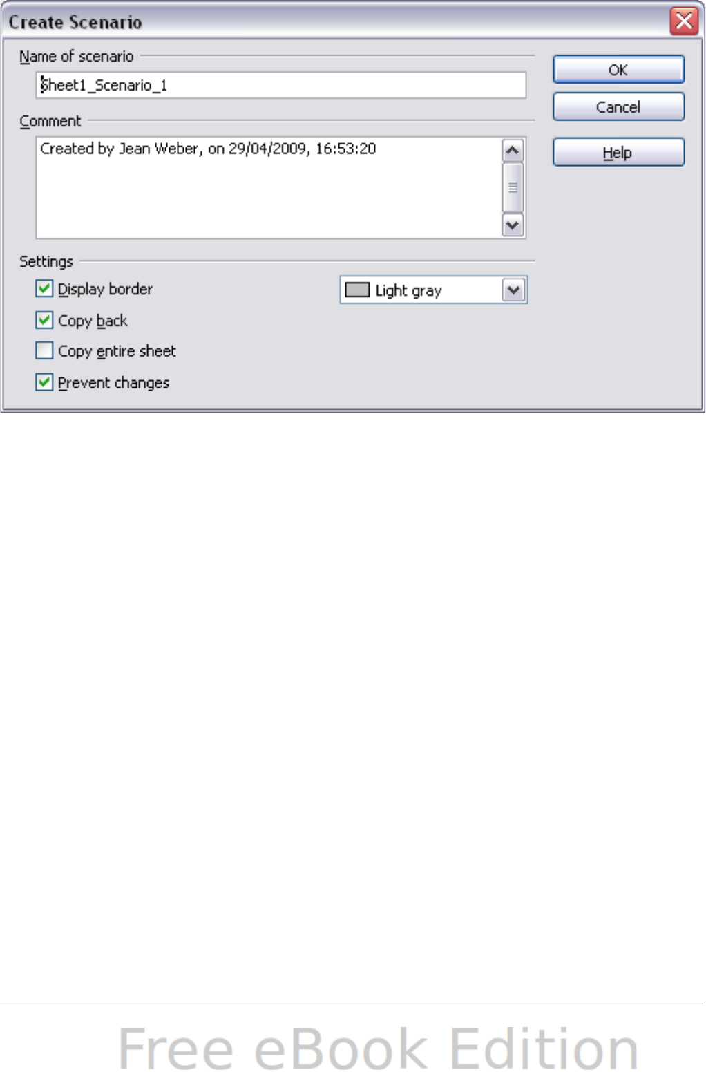
Figure 226: Creating a scenario
Settings
The lower portion of the Create Scenario dialog contains several
options. The default settings (as shown in Figure 226) are likely to be
suitable in most situations.
Display border
Places a border around the range of cells that your scenario alters.
To choose the color of the border, use the field to the right of this
option. The border has a title bar displaying the name of the active
scenario. Click the arrow button to the right of the scenario name to
open a drop-down list of all the scenarios that have been defined for
the cells within the border. You can choose any of the scenarios from
this list at any time.
Copy back
Copies any changes you make to the values of scenario cells back
into the active scenario. If you do not select this option, the saved
scenario values are never changed when you make changes. The
actual behavior of the Copy back setting depends on the cell
protection, the sheet protection, and the Prevent changes setting
(see Table 11 on page 280).
278 OpenOffice.org 3.x Calc Guide

Caution
If you are viewing a scenario which has Copy back enabled and
then create a new scenario by changing the values and selecting
Tools > Scenarios, you also inadvertently overwrite the values
in the first scenario.
This is easily avoided if you leave the current values alone,
create a new scenario with Copy back enabled, and then change
the values only when you are viewing the new scenario.
Copy entire sheet
Adds to your document a sheet that permanently displays the new
scenario in full. This is in addition to creating the scenario and
making it selectable on the original sheet as normal.
Prevent changes
Prevents changes to a Copy back-enabled scenario when the sheet
is protected but the cells are not. Also prevents changes to the
settings described in this section while the sheet is protected. A
fuller explanation of the effect this option has in different situations
is given below.
Changing scenarios
Scenarios have two aspects which can be altered independently:
•Scenario properties (the settings described above)
•Scenario cell values (the entries within the scenario border)
The extent to which either of these aspects can be changed is
dependent upon both the existing properties of the scenario and the
current protection state of the sheet and cells.
Changing scenario properties
If the sheet is protected (Tools > Protect Document > Sheet), and
Prevent changes is selected then scenario properties cannot be
changed.
If the sheet is protected, and Prevent changes is not selected, then all
scenario properties can be changed except Prevent changes and
Copy entire sheet, which are disabled.
If the sheet is not protected, then Prevent changes does not have any
effect, and all scenario properties can be changed.
Chapter 9 Data Analysis 279
Changing scenario cell values
Table 11 summarizes the interaction of various settings in preventing
or allowing changes in scenario cell values.
Table 11: Prevent changes behavior for scenario cell value changes
Settings Change allowed
Sheet protection ON
Scenario cell protection OFF
Prevent changes ON
Copy back ON
Scenario cell values cannot be
changed.
Sheet protection ON
Scenario cell protection OFF
Prevent changes OFF
Copy back ON
Scenario cell values can be changed,
and the scenario is updated.
Sheet protection ON
Scenario cell protection OFF
Prevent changes ON or OFF
Copy back OFF
Scenario cell values can be changed,
but the scenario is not updated due to
the Copy back setting.
Sheet protection ON
Scenario cell protection ON
Prevent changes ANY SETTING
Copy back ANY SETTING
Scenario cell values cannot be
changed.
Sheet protection OFF
Scenario cell protection ANY
SETTING
Prevent changes ANY SETTING
Copy back ANY SETTING
Scenario cell values can be changed
and the scenario is updated or not,
depending on the Copy back setting.
Working with scenarios using the Navigator
After scenarios are added to a spreadsheet, you can jump to a
particular scenario by selecting it from the list in the Navigator.
To find a scenario in the Navigator, click the Scenarios icon in the
Navigator. The defined scenarios are listed, along with the comments
that were entered when the scenarios were created.
To apply a scenario to the current sheet, double-click the scenario
name in the Navigator.
280 OpenOffice.org 3.x Calc Guide
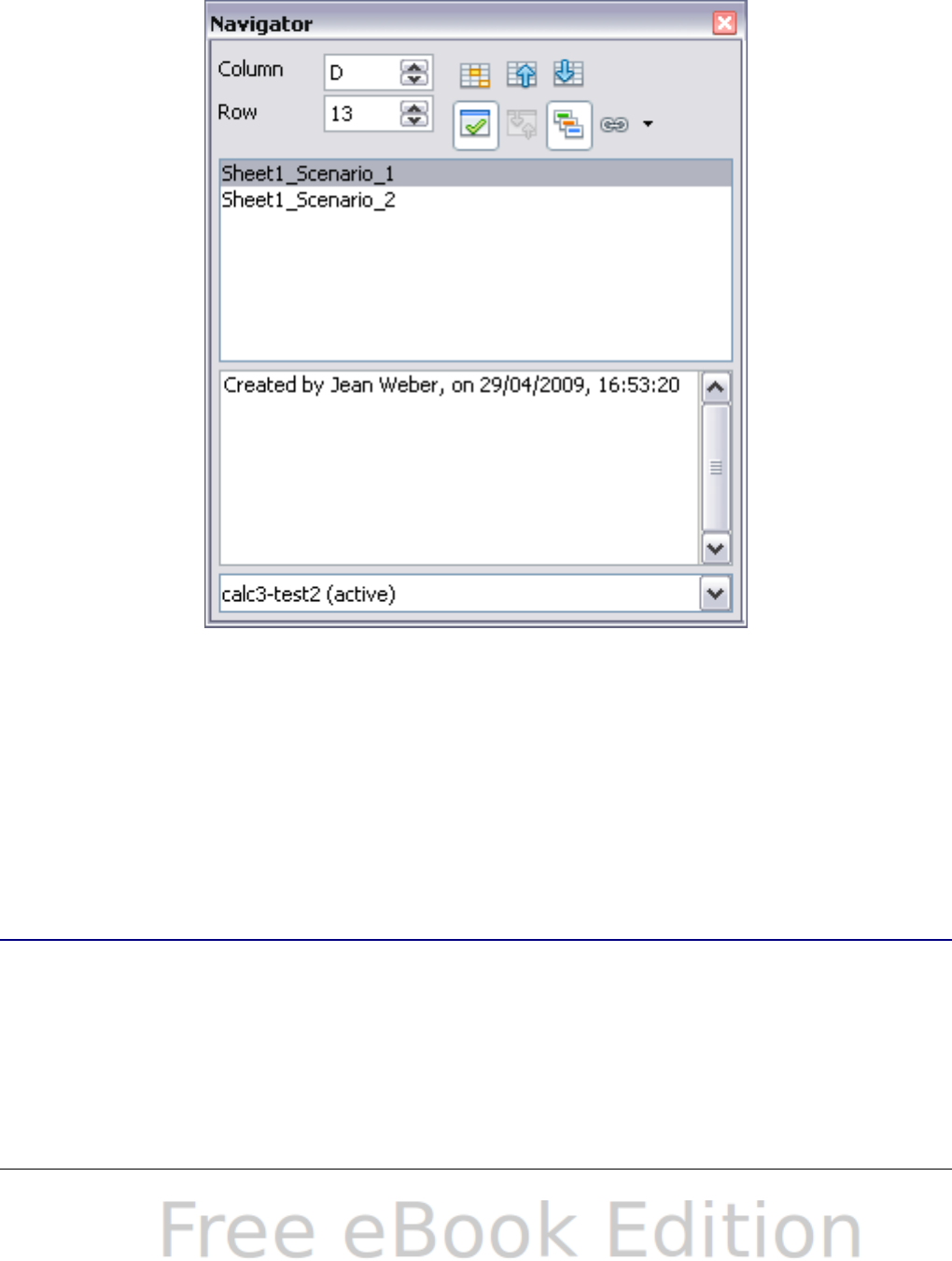
To delete a scenario, right-click the name in the Navigator and choose
Delete.
To edit a scenario, including its name and comments, right-click the
name in the Navigator and choose Properties. The Edit Properties
dialog is the same as the Create Scenario dialog (Figure 226).
Figure 227: Scenarios in the Navigator
Tracking values in scenarios
To learn which values in the scenario affect other values, choose Tools
> Detective > Trace Dependents. Arrows point to the cells that are
directly dependent on the current cell.
Using other “what if” tools
Like scenarios, Data > Multiple Operations is a planning tool for
“what if” questions. Unlike a scenario, the Multiple Operations tool
does not present the alternate versions in the same cells or with a
drop-down list. Instead, the Multiple Operations tool creates a formula
array: a separate set of cells showing the results of applying the
formula to a list of alternative values for the variables used by the
Chapter 9 Data Analysis 281

formula. Although this tool is not listed among the functions, it is really
a function that acts on other functions, allowing you to calculate
different results without having to enter and run them separately.
To use the Multiple Operations tool, you need two arrays of cells. The
first array contains the original or default values and the formulas
applied to them. The formulas must be in a range.
The second array is the formula array. It is created by entering a list of
alternative values for one or two of the original values.
Once the alternative values are created, you use the Multiple
Operations tool to specify which formulas you are using, as well as the
original values used by the formulas. The second array is then filled
with the results of using each alternative value in place of the original
values.
The Multiple Operations tool can use any number of formulas, but only
one or two variables. With one variable, the formula array of
alternative values for the variables will be in a single column or row.
With two variables, you should outline a table of cells such that the
alternative values for one variable are arranged as column headings,
and the alternative values for the other variable act as row headings.
Setting up multiple operations can be confusing at first. For example,
when using two variables, you need to select them carefully, so that
they form a meaningful table. Not every pair of variables is useful to
add to the same formula array. Yet, even when working with a single
variable, a new user can easily make mistakes or forget the
relationships between cells in the original array and cells in the
formula array. In these situations, Tools > Detective can help to
clarify the relations.
You can also make formula arrays easier to work with if you apply
some simple design logic. Place the original and the formula array
close together on the same sheet, and use labels for the rows and
columns in both. These small exercises in organizational design make
working with the formula array much less painful, particularly when
you are correcting mistakes or adjusting results.
Note
If you export a spreadsheet containing multiple operations to
Microsoft Excel, the location of the cells containing the formula
must be fully defined relative to the data range.
282 OpenOffice.org 3.x Calc Guide

Multiple operations in columns or rows
In your spreadsheet, enter a formula to calculate a result from values
that are stored in other cells. Then, set up a cell range containing a list
of alternatives for one of the values used in the formula. The Multiple
Operations command produces a list of results adjacent to your
alternative values by running the formula against each of these
alternatives.
Note
Before you choose the Data > Multiple Operations option, be
sure to select not only your list of alternative values but also the
adjacent cells into which the results should be placed.
In the Formulas field of the Multiple Operations dialog, enter the cell
reference to the formula that you wish to use.
The arrangement of your alternative values dictates how you should
complete the rest of the dialog. If you have listed them in a single
column, you should complete the field for Column input cell. If they are
along a single row, complete the Row input cell field. You may also use
both in more advanced cases. Both single and double-variable versions
are explained below.
The above can be explained best by examples. Cell references
correspond to those in the following figures.
Let’s say you produce toys that you sell for $10 each (cell B1). Each toy
costs $2 to make (cell B2), in addition to which you have fixed costs of
$10,000 per year (cell B3). How much profit will you make in a year if
you sell a particular number of toys?
Calculating with one formula and one variable
1) To calculate the profit, first enter any number as the quantity
(items sold); in this example, 2000 (cell B4). The profit is found
from the formula Profit=Quantity * (Selling price – Direct costs) –
Fixed costs. Enter this formula in B5: =B4*(B1-B2)-B3.
2) In column D enter a variety of alternative annual sales figures,
one below the other; for example, 500 to 5000, in steps of 500.
3) Select the range D2:E11, and thus the values in column D and the
empty cells (which will receive the results of the calculations)
alongside in column E.
4) Choose Data > Multiple Operations.
5) With the cursor in the Formulas field of the Multiple operations
dialog, click cell B5.
Chapter 9 Data Analysis 283
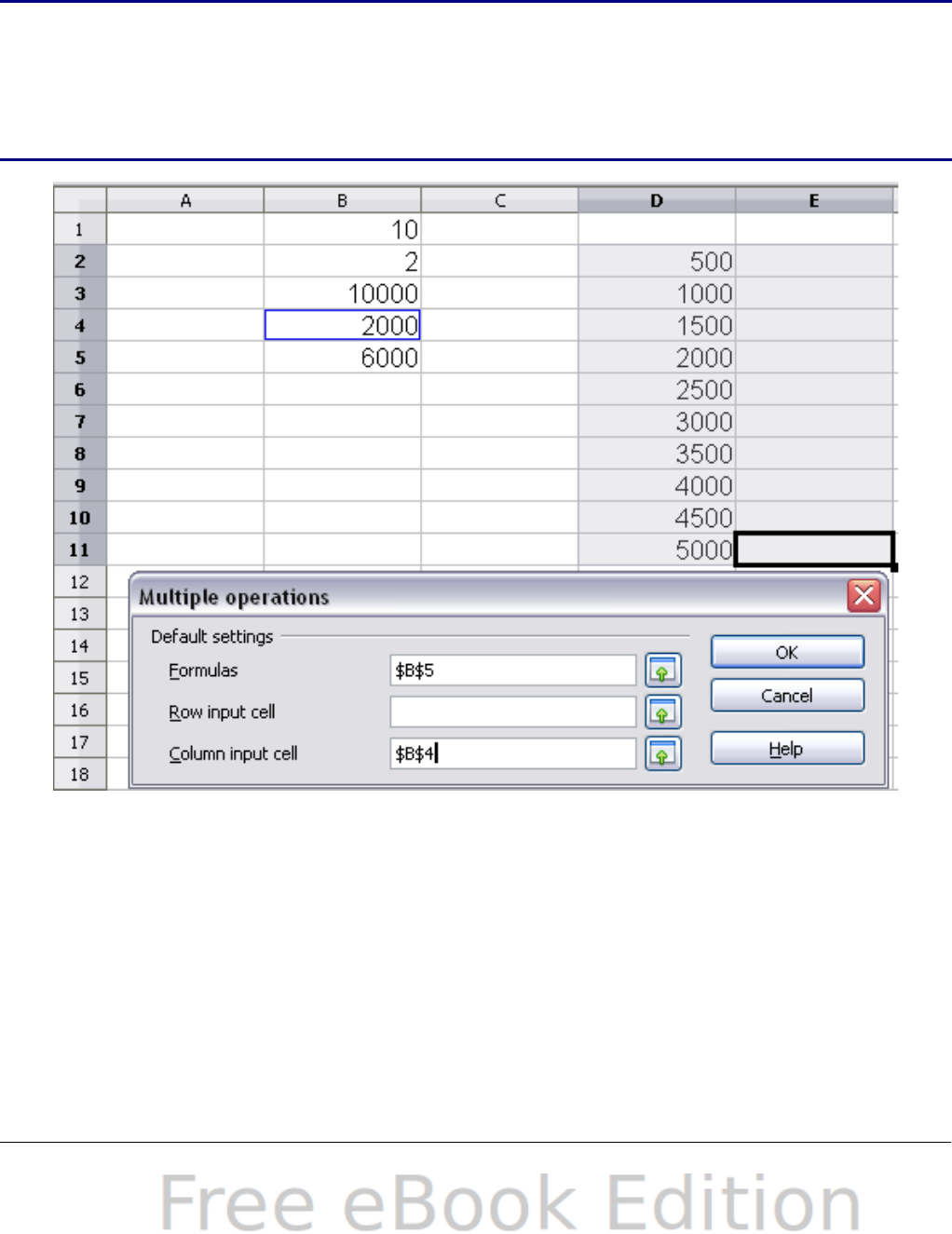
6) Set the cursor in the Column input cell field and click cell B4. This
means that B4, the quantity, is the variable in the formula, which
is to be replaced by the column of alternative values. Figure 228
shows the worksheet and the Multiple operations dialog.
7) Click OK. The profits for the different quantities are now shown
in column E. See Figure 229.
Tip
You may find it easier to mark the required reference in the
sheet if you click the Shrink icon to reduce the Multiple
operations dialog to the size of the input field. The icon then
changes to the Maximize icon; click it to restore the dialog to its
original size.
Figure 228: Sheet and Multiple operations dialog showing input
284 OpenOffice.org 3.x Calc Guide
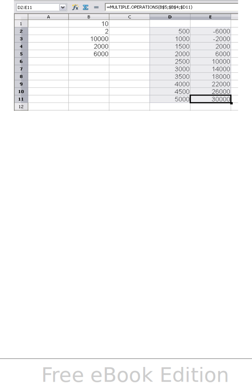
Figure 229: Sheet showing results of multiple operations calculations
Calculating with several formulas simultaneously
1) In the sheet from the previous example, delete the contents of
column E.
2) Enter the following formula in C5: =B5/B4. You are now
calculating the annual profit per item sold.
3) Select the range D2:F11, thus three columns.
4) Choose Data > Multiple Operations.
5) With the cursor in the Formulas field of the Multiple operations
dialog, select cells B5 and C5.
6) Set the cursor in the Column input cell field and click cell B4.
Figure 230 shows the worksheet and the Multiple operations
dialog.
Chapter 9 Data Analysis 285

Figure 230: Sheet and dialog showing input
7) Click OK. Now the profits are listed in column E and the annual
profit per item in column F.
Figure 231: Results of multiple operations calculations
286 OpenOffice.org 3.x Calc Guide

Multiple operations across rows and columns
You can carry out multiple operations simultaneously for both columns
and rows in so-called cross-tables. The formula must use at least two
variables, the alternative values for which should be arranged so that
one set is along a single row and the other set appears in a single
column. These two sets of alternative values will form column and row
headings for the results table produced by the Multiple Operations
procedure.
Select the range defined by both data ranges (thus including all of the
blank cells that are to contain the results) and choose Data >
Multiple operations. Enter the cell reference to the formula in the
Formulas field. The Row input cell and the Column input cell fields are
used to enter the reference to the corresponding cells of the formula.
Caution
Beware of entering the cell reference of a variable into the
wrong field. The Row input cell field should contain not the cell
reference of the variable which changes down the rows of your
results table, but that of the variable whose alternative values
have been entered along a single row.
Calculating with two variables
You now want to vary not just the quantity produced annually, but also
the selling price, and you are interested in the profit in each case.
Expand the table shown in Figure 230 above. D2 thru D11 already
contain the numbers 500, 1000 and so on, up to 5000. In E1 through
H1 enter the numbers 8, 10, 15 and 20.
1) Select the range D1:H11.
2) Choose Data > Multiple Operations.
3) With the cursor in the Formulas field of the Multiple operations
dialog, click cell B5 (profit).
4) Set the cursor in the Row input cell field and click cell B1. This
means that B1, the selling price, is the horizontally entered
variable (with the values 8, 10, 15 and 20).
5) Set the cursor in the Column input cell field and click cell B4. This
means that B4, the quantity, is the vertically entered variable.
Chapter 9 Data Analysis 287
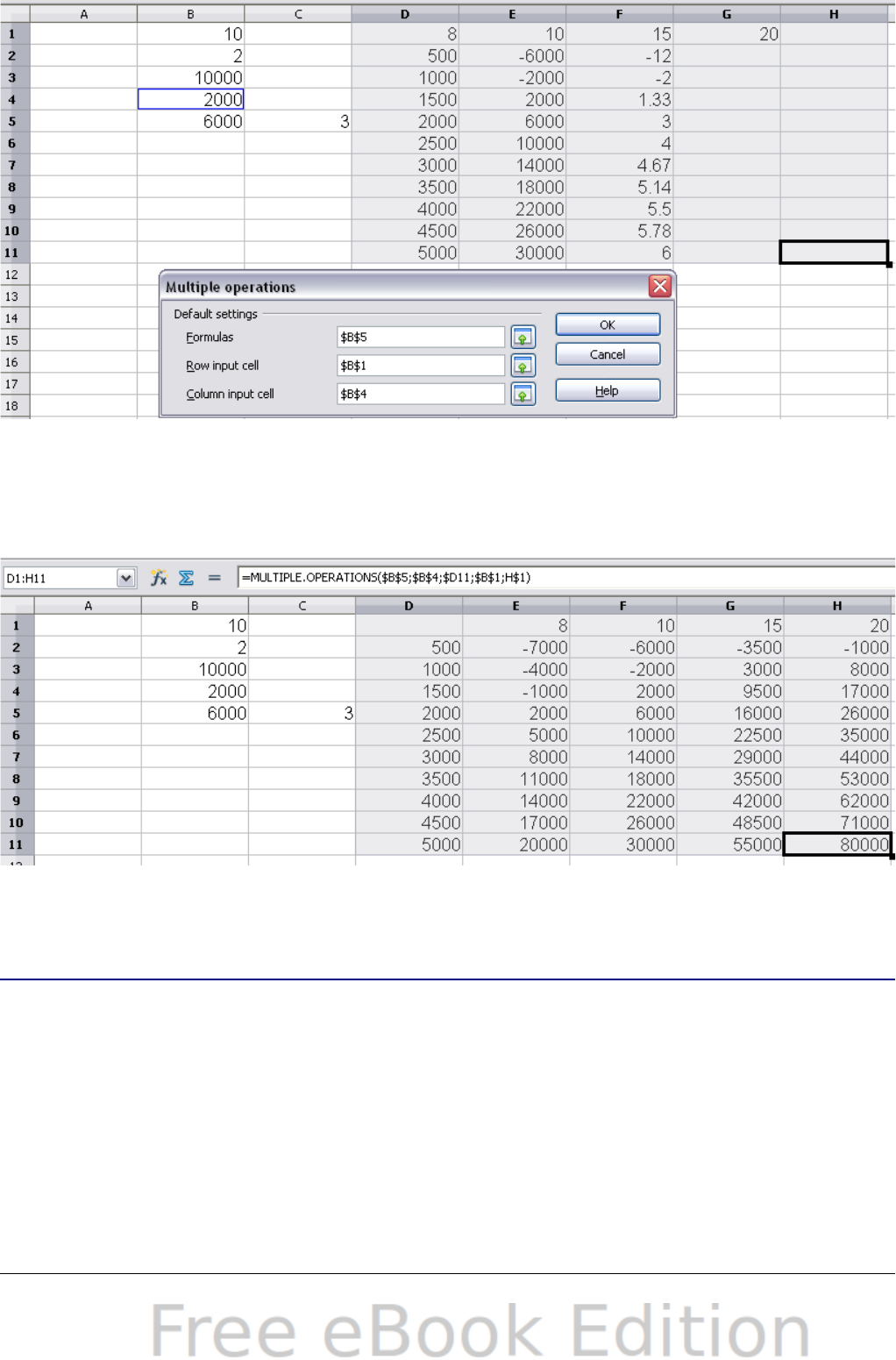
Figure 232: Sheet and dialog showing input
6) Click OK. The profits for the different selling prices are now
shown in the range E2:H11.
Figure 233: Results of multiple operations calculations
Working backwards using Goal Seek
Usually, you create a formula to calculate a result based upon existing
values. By contrast, using Tools > Goal Seek you can discover what
values will produce the result that you want.
To take a simple example, imagine that the Chief Financial Officer of a
company is developing sales projections for each quarter of the
forthcoming year. She knows what the company’s total income must be
for the year to satisfy stockholders. She also has a good idea of the
company’s income in the first three quarters, because of the contracts
288 OpenOffice.org 3.x Calc Guide

that are already signed. For the fourth quarter, however, no definite
income is available. So how much must the company earn in Q4 to
reach its goal? The CFO can enter the projected earnings for each of
the other three quarters along with a formula that totals all four
quarters. Then she runs a goal seek on the empty cell for Q4 sales, and
receives her answer.
Other uses of goal seek may be more complicated, but the method
remains the same. Only one argument can be altered in a single goal
seek.
Goal Seek example
To calculate annual interest (I), create a table with the values for the
capital (C), number of years (n), and interest rate (i). The formula is
I = C*n*i.
Let us assume that the interest rate i of 7.5% and the number of years
n (1) will remain constant. However, you want to know how much the
investment capital C would have to be modified in order to attain a
particular return I. For this example, calculate how much capital C
would be required if you want an annual return of $15,000.
Enter each of the values mentioned above into adjacent cells (for
Capital, C, an arbitrary value like $100,000 or it can be left blank; for
number of years, n, 1; for interest rate, i, 7.5%). Enter the formula to
calculate the interest, I, in another cell. Instead of C, n, and i, use the
reference to the cell with the corresponding value. In our example
(Figure 231), this would be =B1*B2*B3.
1) Place the cursor in the formula cell (B4), and choose Tools >
Goal Seek.
2) In the Goal Seek dialog, the correct cell is already entered in the
Formula cell field.
3) Place the cursor in the Variable cell field. In the sheet, click in the
cell that contains the value to be changed, in this example it is B1.
4) Enter the desired result of the formula in the Target value field. In
this example, the value is 15000. Figure 234 shows the cells and
fields.
Chapter 9 Data Analysis 289
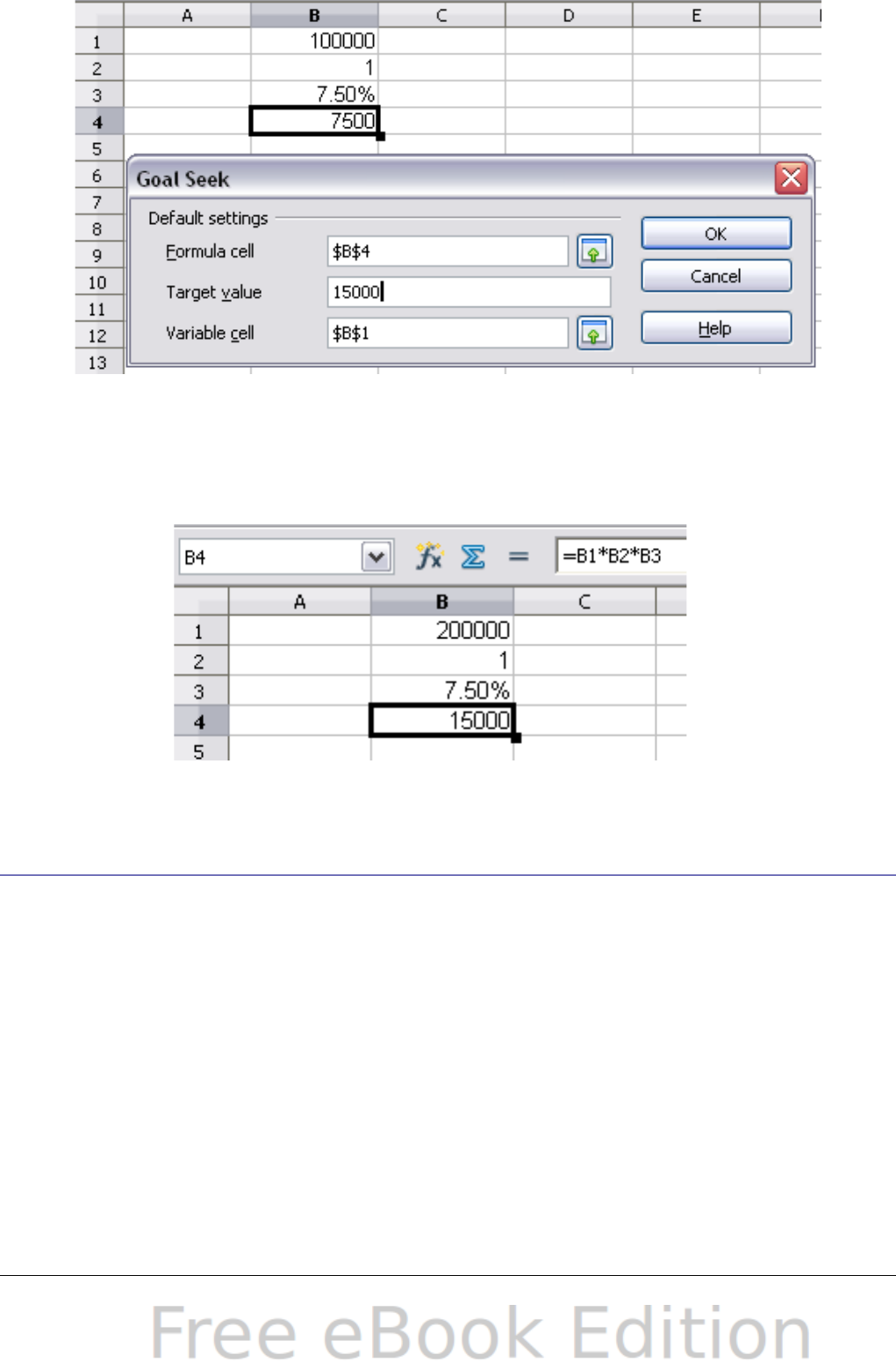
Figure 234: Example setup for goal seek
5) Click OK. A dialog appears informing you that the Goal Seek was
successful. Click Yes to enter the goal value into the variable cell.
The result is shown below.
Figure 235: Result of goal seek operation
Using the Solver
Tools > Solver amounts to a more elaborate form of Goal Seek. The
difference is that the Solver deals with equations with multiple
unknown variables. It is specifically designed to minimize or maximize
the result according to a set of rules that you define.
Each of these rules defines whether an argument in the formula should
be greater than, less than, or equal to the figure you enter. If you want
the argument to remain unchanged, you must enter a rule that
specifically states that the cell should be equal to its current entry. For
arguments that you would like to change, you need to add two rules to
define a range of possible values: the limiting conditions. For example,
you can set the constraint that one of the variables or cells must not be
bigger than another variable, or not bigger than a given value. You can
290 OpenOffice.org 3.x Calc Guide
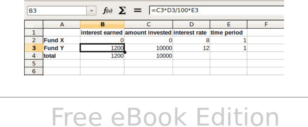
also define the constraint that one or more variables must be integers
(values without decimals), or binary values (where only 0 and 1 are
allowed).
Once you have finished setting up the rules, click the Solve button to
begin the automatic process of adjusting values and calculating
results. Depending on the complexity of the task, this may take some
time.
Solver example
Let’s say you have $10,000 that you want to invest in two mutual funds
for one year. Fund X is a low risk fund with 8% interest rate and Fund
Y is a higher risk fund with 12% interest rate. How much money should
be invested in each fund to earn a total interest of $1000?
To find the answer using Solver:
1) Enter labels and data:
•Row labels: Fund X, Fund Y, and total, in cells A2 thru A4.
•Column labels: interest earned, amount invested, interest
rate, and time period, in cells B1 thru E1.
•Interest rates: 8 and 12, in cells D2 and D3.
•Time period: 1, in cells E2 and E3.
•Total amount invested: 10000, in cell C4.
2) Enter an arbitrary value (0 or leave blank) in cell C2 as amount
invested in Fund X.
3) Enter formulas:
•In cell C3, enter the formula C4–C2 (total amount – amount
invested in Fund X) as the amount invested in Fund Y.
•In cells B2 and B3, enter the formula for calculating the
interest earned (see Figure 236).
•In cell B4, enter the formula B2+B3 as the total interest
earned.
Figure 236: Example setup for Solver
Chapter 9 Data Analysis 291
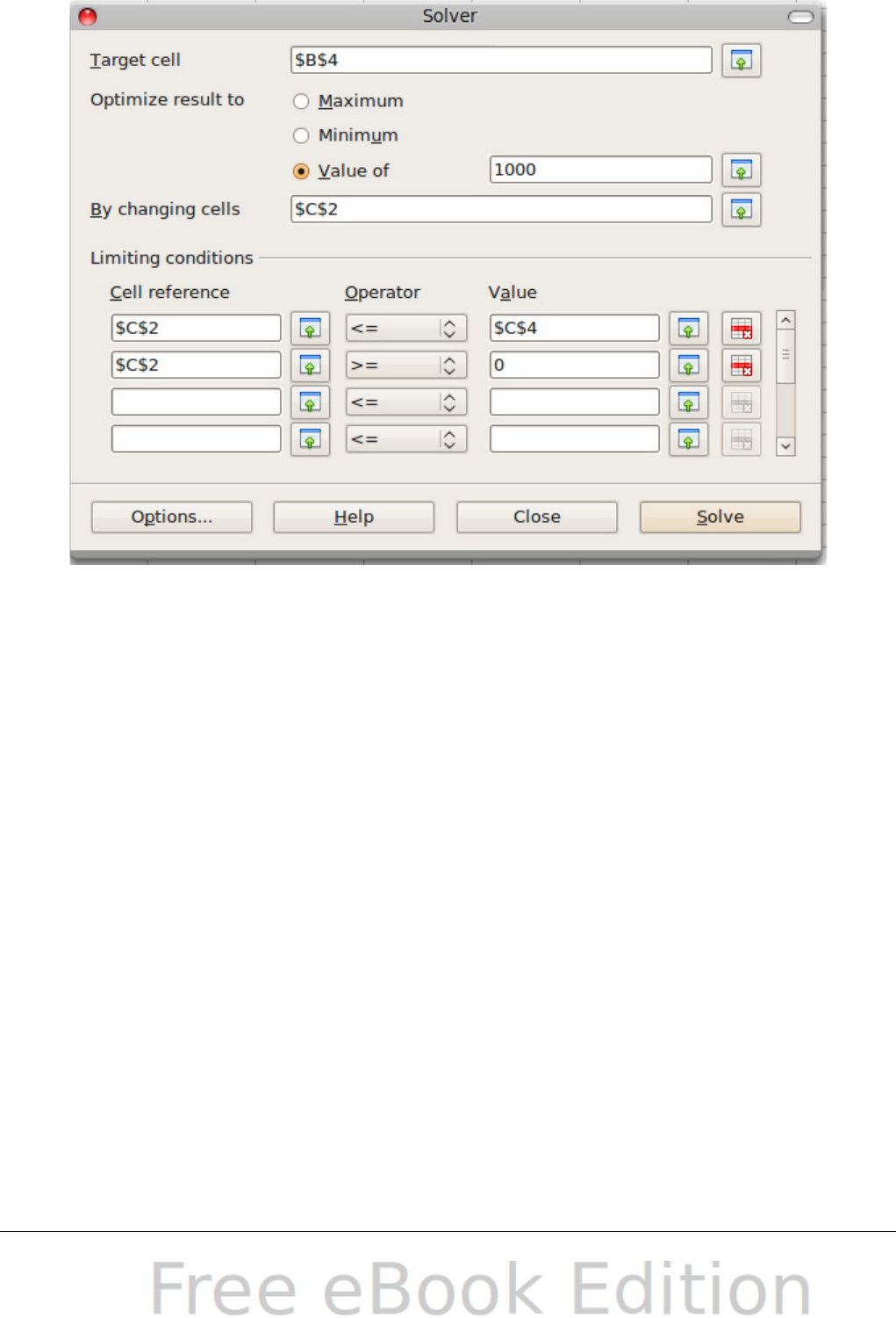
4) Choose Tools > Solver. The Solver dialog opens.
Figure 237: The Solver dialog
5) Click in the Target cell field. In the sheet, click in the cell that
contains the target value. In this example it is cell B4 containing
total interest value.
6) Select Value of and enter 1000 in the field next to it. In this
example, the target cell value is 1000 because your target is a
total interest earned of $1000. Select Maximum or Minimum if
the target cell value needs to be one of those extremes.
7) Click in the By changing cells field and click on cell C2 in the
sheet. In this example, you need to find the amount invested in
Fund X (cell C2).
8) Enter limiting conditions for the variables by selecting the Cell
reference, Operator and Value fields. In this example, the amount
invested in Fund X (cell C2) should not be greater than the total
amount available (cell C4) and should not be less than 0.
9) Click OK. A dialog appears informing you that the Solving
successfully finished. Click Keep Result to enter the result in the
cell with the variable value. The result is shown in Figure 238.
292 OpenOffice.org 3.x Calc Guide
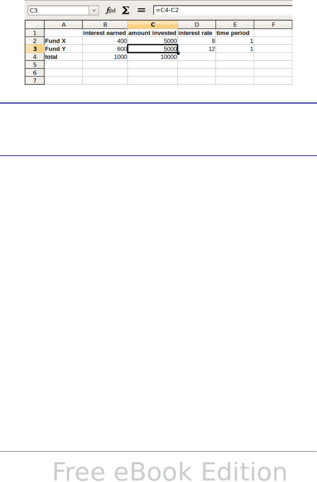
Figure 238: Result of Solver operation
Note
The default solver supports only linear equations. For nonlinear
programming requirements, try the EuroOffice Solver or Sun’s
Solver for Nonlinear Programming [Beta]. Both are available
from the OpenOffice.org extensions repository. (For more about
extensions, see Chapter 14 (Setting up and Customizing Calc.)
Chapter 9 Data Analysis 293

Chapter 10
Linking Calc Data
Sharing data in and out of Calc
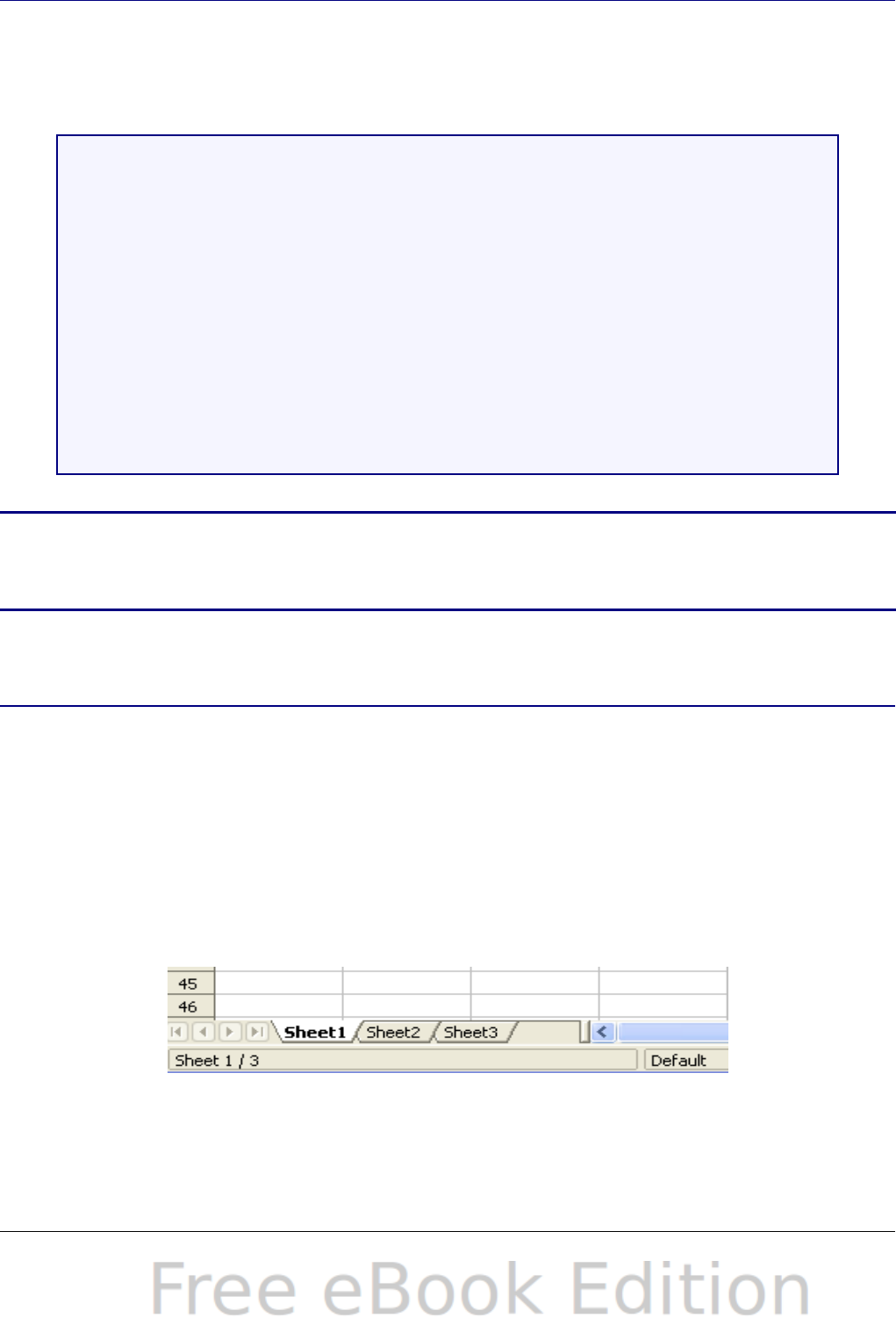
Why use multiple sheets?
Chapter 1 introduced the concept of multiple sheets in a spreadsheet.
Multiple sheets help keep information organized; once you link those
sheets together, you unleash the full power of Calc. Consider this case.
John is having trouble keeping track of his personal
finances. He has several bank accounts and the information
is scattered and disorganized. He can’t get a good grasp on
his finances until he can see everything at once.
To resolve this, John decided to track his finances in OOo
Calc. John knows Calc can do simple mathematical
computations to help him keep a running tab of his
accounts, and he wants to set up a summary sheet so that
he can see all of his account balances at once.
This can be accomplished easily.
Note
For users with experience using Microsoft Excel, a Calc sheet is
called either a sheet or worksheet in Excel. What Excel calls a
workbook, Calc calls a spreadsheet (the whole document).
Setting up multiple sheets
Chapter 1 gives a detailed explanation of how to set up multiple sheets
in a spreadsheet. Here is a quick review.
Identifying sheets
When you open a new spreadsheet it has, by default, three sheets
named Sheet1, Sheet2, and Sheet3. Sheets in Calc are managed using
tabs at the bottom of the spreadsheet, as shown below.
Figure 239: Default sheet tabs
Chapter 10 Linking Calc Data 295
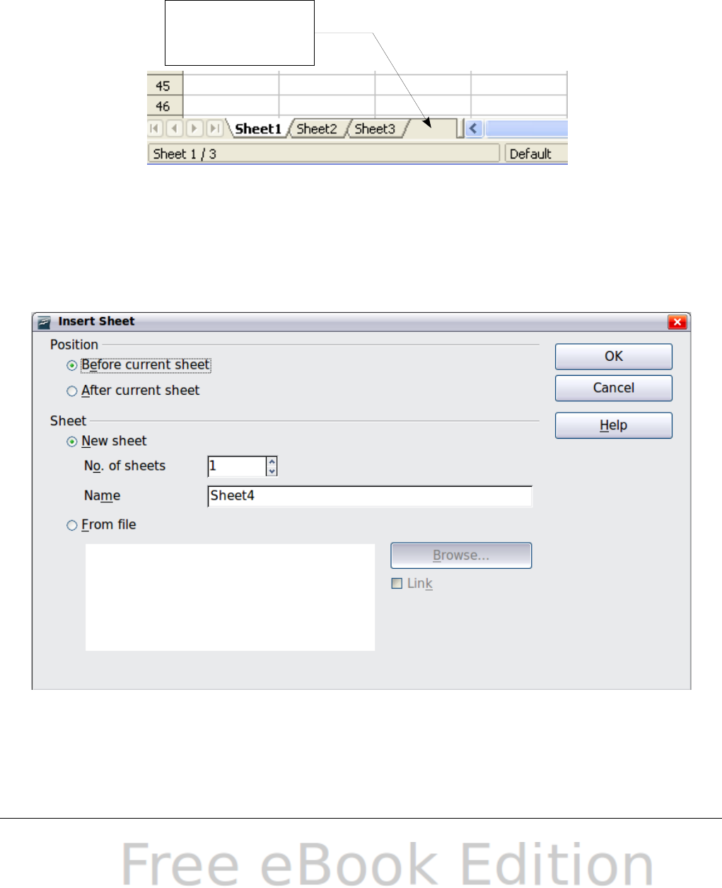
Inserting new sheets
There are several ways to insert a new sheet. The first step, in all
cases, is to select the sheet that will be next to the new sheet. Then do
any of the following:
•Select Insert > Sheet from the menu bar, or
•Right-click on the tab and select Insert Sheet, or
•Click in an empty space at the end of the line of sheet tabs.
Figure 240: Creating a new sheet
Each method opens the Insert Sheet dialog. Here you can choose to
put the new sheet before or after the selected sheet and how many
sheets to insert.
Figure 241. Insert Sheet dialog
296 OpenOffice.org 3.x Calc Guide
Click here to
create a new
sheet

We need 6 sheets, one for each of the 5 accounts and one as a
summary sheet so we will add 3 more. We also want to name each of
these sheets for the account they represent: Summary, Checking
Account, Savings Account, Credit Card 1, Credit Card 2, and Car Loan.
We have two choices: insert 3 new sheets and rename all 6 sheets
afterwards; or rename the existing sheets, then insert the 3 new
sheets one at a time, renaming each new sheet during the insert step.
To insert sheets and rename afterwards:
1) In the Insert Sheet dialog, choose the position for the new sheets
(in this example, we use After current sheet).
2) Choose New sheet and 3 as the No. of sheets. (Three sheets are
already provided by default.) Because you are inserting more than
one sheet, the Name box is not available.
3) Click OK to insert the sheets.
4) For the next steps, go to “Renaming sheets” on page 298.
To insert sheets and name them at the same time:
1) Rename the existing sheets Summary, Checking Account, and
Savings Account, as described in “Renaming sheets” on page 298.
2) In the Insert Sheet dialog, choose the position for the first new
sheet.
3) Choose New sheet and 1 as the No. of sheets. The Name box is
now available.
4) In the Name box, type a name for this new sheet, for example
Credit Card 1.
5) Click OK to insert the sheet.
6) Repeat steps 1–4 for each new sheet, giving them the names
Credit Card 2 and Car Loan.
Inserting sheets from a different spreadsheet
On the Insert Sheet dialog, you can also add a sheet from a different
spreadsheet file (for example, another Calc or Excel spreadsheet), by
choosing the From file option. Click Browse and select the file; a list
of the available sheets appears in the box. Select the sheet to import.
If, after you select the file, no sheets appear you probably selected an
invalid file type (not a spreadsheet, for example).
Chapter 10 Linking Calc Data 297
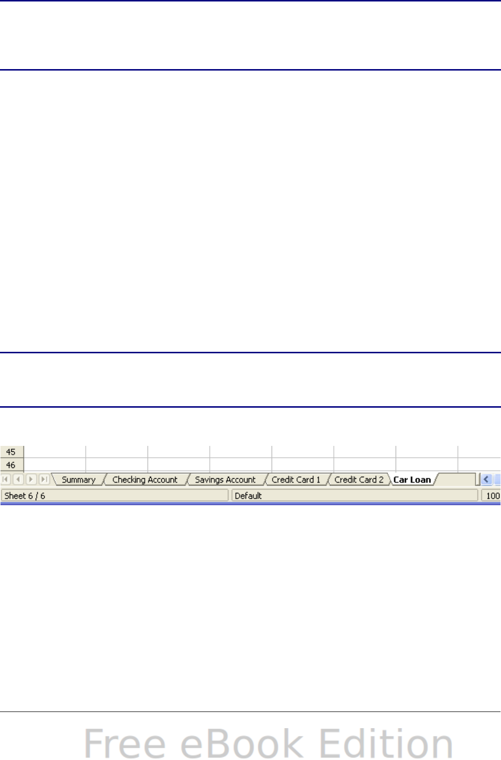
Tip
For a shortcut to inserting a sheet from another file, choose
Insert > Sheet from file from the menu bar. The Insert Sheet
dialog opens with the From file option preselected, and then the
Insert dialog opens on top of it.
If you prefer, select the Link option to insert the external sheet as a
link instead as a copy. This is one of several ways to include “live” data
from another spreadsheet. (See also “Linking to external data” on page
307.) The links can be updated manually to show the current contents
of the external file; or, depending on the options you have selected in
Tools > Options > OpenOffice.org Calc > General > Updating,
whenever the file is opened.
Renaming sheets
Sheets can be renamed at any time. To give a sheet a more meaningful
name:
•Enter the name in the name box when you create the sheet, or
•Double click on the sheet tab, or
•Right-click on a sheet tab, select Rename Sheet from the pop-up
menu and replace the existing name.
Note
If you want to save the spreadsheet to Microsoft Excel format,
the following characters are not allowed in sheet names: \ / ? * [ ]
: and ' as the first or last character of the name.
Your sheet tab area should now look like this.
Figure 242: Six renamed sheets
Now we will set up the account ledgers. This is just a simple summary
that includes the previous balance plus the amount of the current
transaction. For withdrawals, we enter the current transaction as a
negative number so the balance gets smaller. A basic ledger is shown
in Figure 243.
This ledger is set up in the sheet named Checking Account. The total
balance is added up in cell F3. You can see the equation for it in the
formula bar. It is the summary of the opening balance, cell C3, and all
of the subsequent transactions.
298 OpenOffice.org 3.x Calc Guide
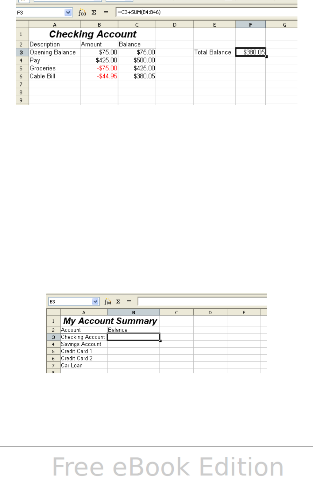
Figure 243: Checking ledger
Referencing other sheets
On the Summary sheet we display the balance from each of the other
sheets. If you copy the example in Figure 243 onto each account, the
current balances will be in cell F3 of each sheet.
There are two ways to reference cells in other sheets: by entering the
formula directly using the keyboard or by using the mouse. We will
look at the mouse method first.
Creating the reference with the mouse
On the Summary sheet, set up a place for all five account balances, so
we know where to put the cell reference. Figure 244 shows a summary
sheet with a blank Balance column. We want to place the reference for
the checking account balance in cell B3.
Figure 244: Blank summary
To make the cell reference in cell B3, select the cell and follow these
steps.
1) Click on the = icon next to the input line. The icons change and
an equals sign appears in the input line as in Figure 245.
Chapter 10 Linking Calc Data 299
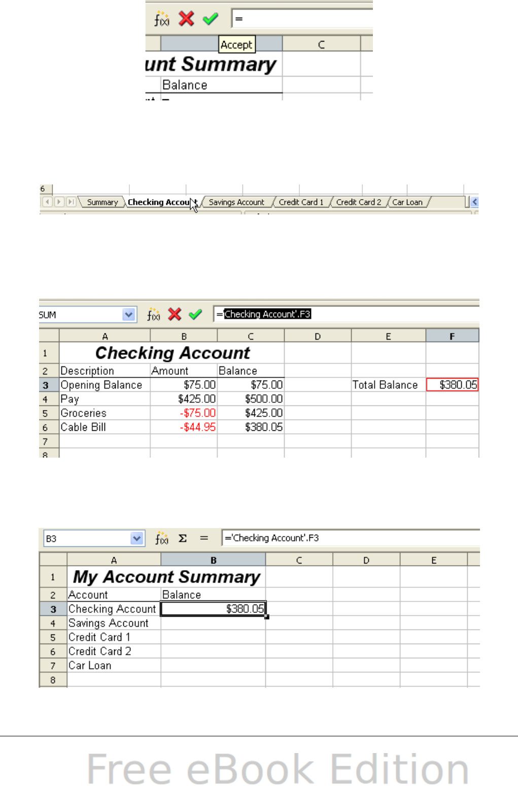
Figure 245: Equal sign in input line
2) Now, click on the sheet tab for the sheet containing the cell to be
referenced. In this case, that is the Checking Account sheet as
shown in Figure 246.
Figure 246: Click on the checking account tab
3) Click on cell F3 (where the balance is) in the Checking Account
sheet. The phrase ‘Checking Account’.F3 should appear in the
input line as in Figure 247.
Figure 247: Cell reference selected
4) Click the green checkmark in the input line to finish.
5) The Summary sheet should now look like Figure 248.
Figure 248: Finished checking account reference
300 OpenOffice.org 3.x Calc Guide
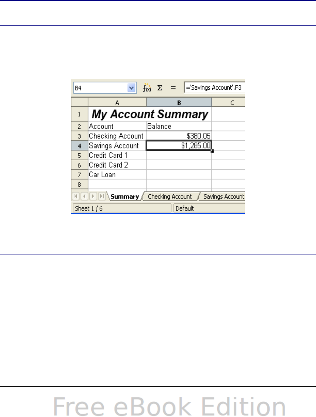
Creating the reference with the keyboard
From Figure 248, you can deduce how the cell reference is
constructed. The reference has two parts: the sheet name (‘Checking
Account’) and the cell reference (F3). Notice that they are separated
by a period.
Note The sheet name is in single quotes because it contains a space,
and the mandatory period (.) always falls outside any quotes.
So, you can fill in the Savings Account cell reference by just typing it
in. Assuming that the balance is in the same cell (F3) in the Savings
Account sheet, the cell reference should be =’Savings Account’.F3 (see
Figure 249).
Figure 249: Savings account reference
Referencing other documents
John decides to keep his family account information in a different
spreadsheet file from his own summary. Fortunately Calc can link
different files together. The process is the same as described for
different sheets in a single spreadsheet, but we add one more step to
indicate which file the sheet is in.
Creating the reference with the mouse
To create the reference with the mouse, both spreadsheets need to be
open. Select the cell in which the formula is going to be entered.
1) Click the = icon next to the input line.
Chapter 10 Linking Calc Data 301
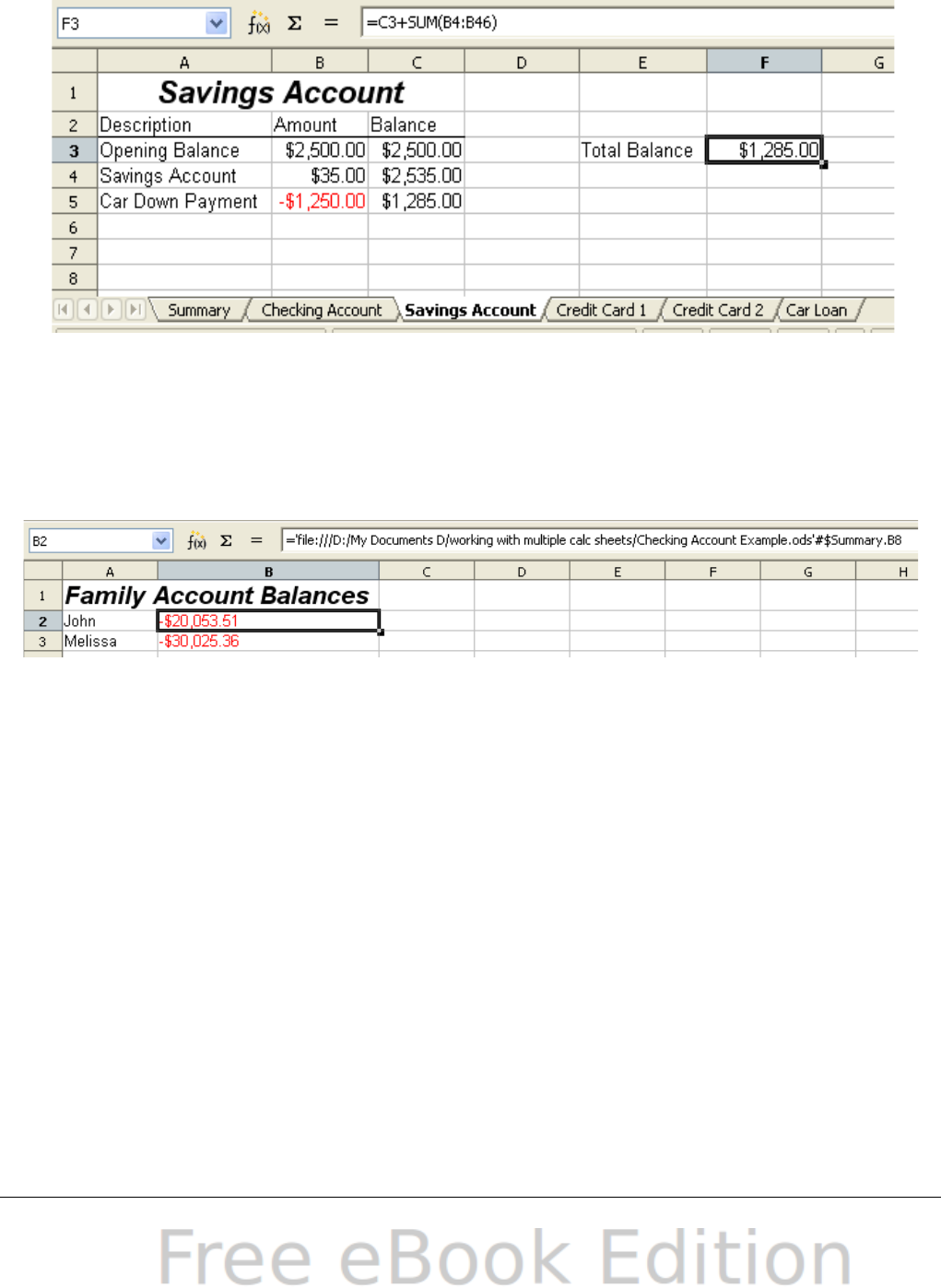
2) Switch to the other spreadsheet (the process to do this will vary
depending on which operating system you are using).
3) Select the sheet (Savings Account) and then the reference cell
(F3).
Figure 250: Selecting the savings account reference cell
4) Switch back to the original spreadsheet.
5) Click on the green check mark on the input line.
Your spreadsheet should now resemble Figure 251.
Figure 251: Linked files
You will get a good feel for the format of the reference if you look
closely at the input line. Based on this line you can create the
reference using the keyboard.
Creating the reference with the keyboard
Typing the reference is simple once you know the format the reference
takes. The reference has three parts to it:
•Path and file name
•Sheet name
•Cell
Looking at Figure 251 you can see the the general format for the
reference is
=’file:///Path & File Name’#$SheetName.CellName
302 OpenOffice.org 3.x Calc Guide

Note The reference for a file has three forward slashes /// and the
reference for a hyperlink has two forward slashes //.
Hyperlinks and URLs
Hyperlinks can be used in Calc to jump to a different location from
within a spreadsheet and can lead to other parts of the current file, to
different files or even to web sites.
Relative and absolute hyperlinks
Hyperlinks can be stored within your file as either relative or absolute.
A relative hyperlink says, Here is how to get there starting from where
you are now (meaning from the folder in which your current document
is saved) while an absolute hyperlink says, Here is how to get there no
matter where you start from.
An absolute link will stop working only if the target is moved. A
relative link will stop working only if the start and target locations
change relative to each other. For instance, if you have two
spreadsheets in the same folder linked to each other and you move the
entire folder to a new location, a relative hyperlink will not break.
To change the way that OOo stores the hyperlinks in your file, select
Tools > Options > Load/Save > General and choose if you want
URLs saved relatively when referencing the File System, or the
Internet, or both.
Calc will always display an absolute hyperlink. Don’t be alarmed when
it does this even when you have saved a relative hyperlink—this
‘absolute’ target address will be updated if you move the file.
Note
Make sure that the folder structure on your computer is the
same as the file structure on your web server if you save your
links as relative to the file system and you are going to upload
pages to the Internet.
Tip
When you rest the mouse pointer on a hyperlink, a help tip
displays the absolute reference, since OOo uses absolute path
names internally. The complete path and address can only be
seen when you view the result of the HTML export (saving the
spreadsheet as an HTML file), by loading the HTML file as Text,
or by opening it with a text editor.
Chapter 10 Linking Calc Data 303
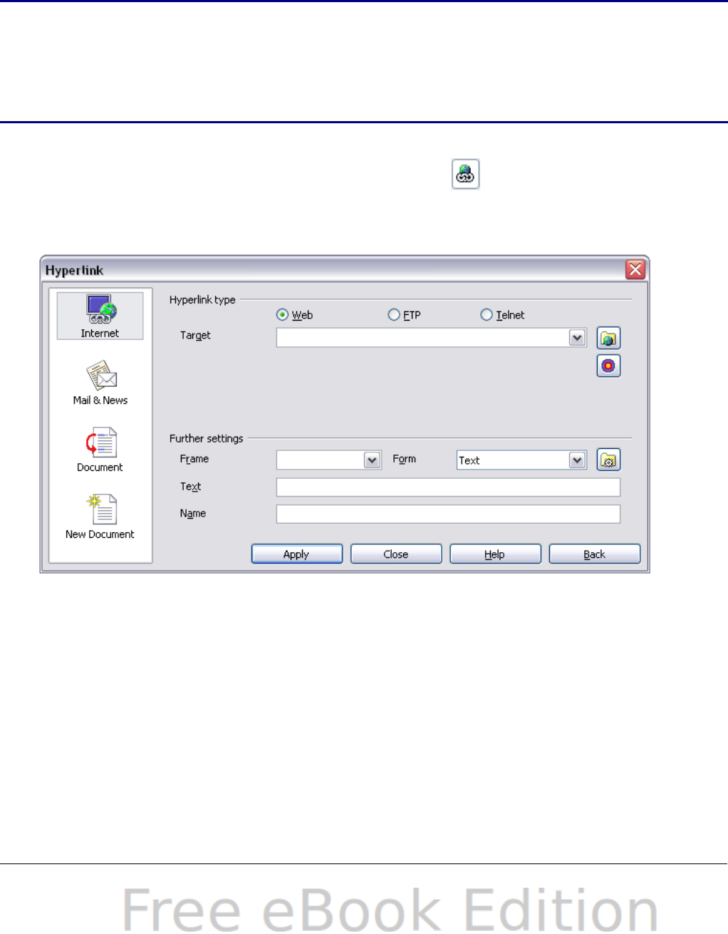
Creating hyperlinks
When you type text that can be used as a hyperlink (such as a website
address or URL), Calc formats it automatically, creating the hyperlink
and applying to the text a color and background shading. If this does
not happen, you can enable this feature using Tools > AutoCorrect
Options > Options and selecting URL Recognition.
Tips
To change the color of hyperlinks, go to Tools > Options >
OpenOffice.org > Appearance, scroll to Unvisited links and/or
Visited links, pick the new colors and click OK. Caution: this will
change the color for all hyperlinks in all components of
OpenOffice.org—this may not be what you want.
You can also insert and modify links using the Hyperlink dialog. To
display the dialog, click the Hyperlink icon on the Standard
toolbar or choose Insert > Hyperlink from the menu bar. To turn
existing text into a link, highlight it before opening the dialog.
Figure 252. Hyperlink dialog showing details for Internet links
On the left side, select one of the four categories of hyperlinks:
•Internet: the hyperlink points to a web address, normally
starting with http://
•Mail & News: the hyperlink opens an email message that the
pre-addressed to a particular recipient
•Document: the hyperlink points to a place in either the current
document or another existing document
•New document: the hyperlink creates a new document.
304 OpenOffice.org 3.x Calc Guide
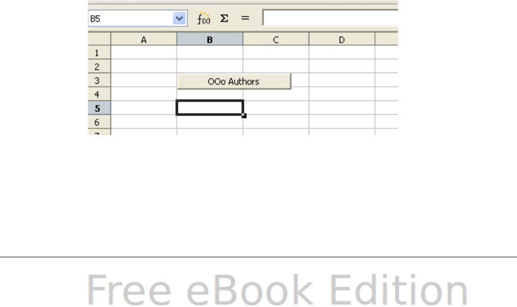
The top right part of the dialog changes according to the choice made
for the hyperlink category from the left panel. A full description of all
the choices, and their interactions, is beyond the scope of this chapter.
Here is a summary of the most common choices used in spreadsheets.
For an Internet hyperlink, choose the type of hyperlink (Web, FTP, or
Telnet), and enter the required web address (URL).
For a Mail and News hyperlink, specify whether it is a mail or news
link, the receiver address and for email, also the subject.
For a Document hyperlink, specify the document path (the Open File
button opens a file browser); leave this blank if you want to link to a
target in the same spreadsheet. Optionally specify the target in the
document (for example a specific sheet). Click on the Target in
document icon to open the Navigator where you can select the target,
or if you know the name of the target, you can type it into the box.
For a New Document hyperlink, specify whether to edit the newly
created document immediately (Edit now) or just create it (Edit
later), and enter the file name and the type of document to create
(text, spreadsheet, etc.). The Select path button opens a directory
picker dialog.
The Further settings section in the bottom right of the dialog is
common to all the hyperlink categories, although some choices are
more relevant to some types of links.
•Set the value of Frame to determine how the hyperlink will open.
This applies to documents that open in a Web browser.
•Form specifies if the link is to be presented as text or as a button.
Figure 253 shows a link formatted as a button.
Figure 253: OOo Authors hyperlink as button
•Text specifies the text that will be visible to the user. If you do not
enter anything here, Calc will use the full URL or path as the link
text. Note that if the link is relative and you move the file, this
text will not change, though the target will.
Chapter 10 Linking Calc Data 305
•Name is applicable to HTML documents. It specifies text that will
be added as a NAME attribute in the HTML code behind the
hyperlink.
•Events button: this button will be activated to allow Calc to react
to events for which the user has written some code (macro). This
function is not covered in this chapter.
Note
A hyperlink button is a type of form control. As with all form
controls, it can be anchored or positioned by right-clicking on the
button in design mode. More information about forms can be
found in Chapter 15 of the Writer Guide.
For the button to work , the spreadsheet must not be in design
mode. To toggle design mode on and off, view the Form Controls
toolbar (View > Toolbars > Form Controls) and click the
Design Mode On/Off button .
Editing hyperlinks
To edit an existing link, place the cursor anywhere in the link and click
the Hyperlink icon on the Standard toolbar or select Insert >
Hyperlink from the menu bar. The Hyperlink dialog (Figure 252)
opens. If the Hyperlink is in button form, the spreadsheet must have
Design Mode on in order to edit the Hyperlink. Make your changes and
click Apply. If you need to edit several hyperlinks, you can leave the
Hyperlink dialog open until you have edited all of them. Be sure to
click Apply after each one. When you are finished, click Close.
Removing hyperlinks
You can remove the clickable link from hyperlink text—leaving just the
text—by right-clicking on the link and selecting Default Formatting.
This option is also available from the Format menu. You may then
need to re-apply some formatting in order for it to match the rest of
your document.
To erase the link text or button from the document completely, select it
and press the Backspace or Delete key.
306 OpenOffice.org 3.x Calc Guide

Linking to external data
You can insert tables from HTML documents, and data located within
named ranges from an OpenOffice.org Calc or Microsoft Excel
spreadsheet, into a Calc spreadsheet. (To use other data sources,
including database files in OOo Base, see “Linking to registered data
sources” on page 312.)
You can do this in two ways: using the External Data dialog or using
the Navigator. If your file has named ranges or named tables, and you
know the name of the range or table you want to link to, using the
External Data dialog method is quick and easy. However, if the file has
several tables, and you want to pick only one of them, you may not be
able to easily determine which is which; in that case, the Navigator
method may be easier.
Using the External Data dialog
1) Open the Calc document where the external data is to be
inserted. This is the target document.
2) Select the cell where the upper left-hand cell of the external data
is to be inserted.
3) Choose Insert > Link to External Data.
4) On the External Data dialog (Figure 254), type the URL of the
source document or click the [...] button to open a file selection
dialog. Press Enter to get Calc to load the list of available tables.
5) In the Available tables/range list, select the named ranges or
tables you want to insert. You can also specify that the ranges or
tables are updated every (number of) seconds.
6) Click OK to close the dialog and insert the linked data.
Notes
1) The Available tables/ranges list remains empty until you
press Enter after typing the URL of the source. If you select
the source document using the […] button, then pressing
Enter is not required.
2) The OK button remains unavailable (grayed out) until you
select one or more tables/ranges in the list. You can hold
down the Ctrl key while clicking on tables/ranges to select
more than one.
3) No images are imported
Chapter 10 Linking Calc Data 307

Figure 254: Selecting a table or range in a source document
from the Web
Using the Navigator
1) Open the OpenOffice.org Calc spreadsheet in which the external
data is to be inserted (target document).
2) Open the document from which the external data is to be taken
(source document). If the source document is a Web page, choose
Web Page Query (OpenOffice.org Calc) as the file type.
Figure 255: Opening a file using the Web Page Query filter
308 OpenOffice.org 3.x Calc Guide
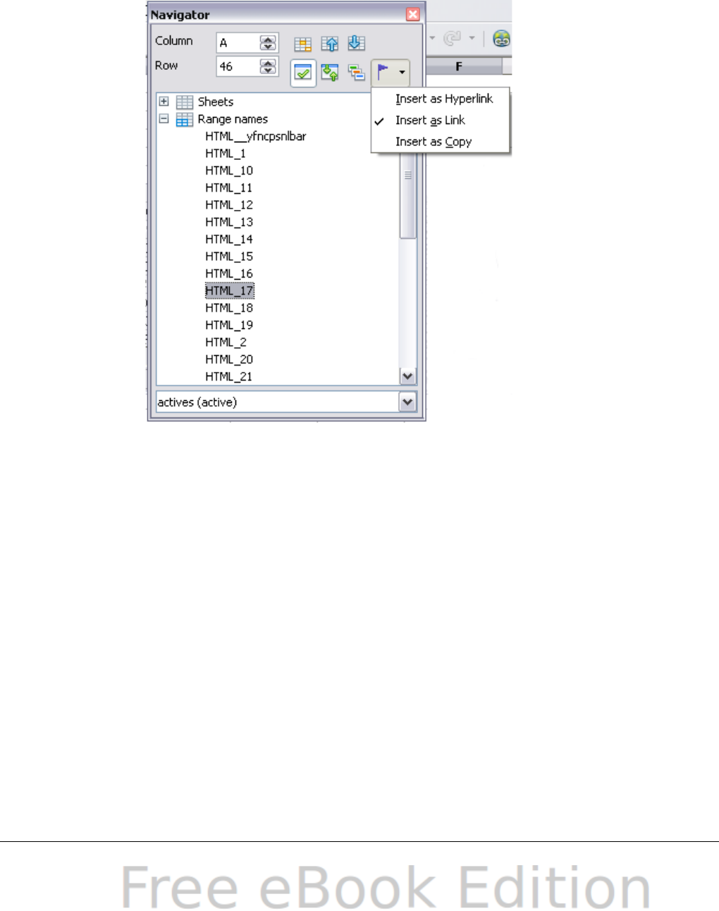
3) In the target document, press F5 to open the Navigator.
4) At the bottom of the Navigator, select the source document. (In
Figure 256, the source is named actives.)
The Navigator now shows the range names or the tables
contained in the source document (the example contains range
names; other documents have a list of tables). Click on the + next
to Range names to display the list.
Figure 256: Selecting a data range in a
source document, to be inserted as a link
5) In the Navigator, select the Insert as Link drag mode, as shown
in Figure 256.
6) Select the required range or table and drag it from the Navigator
into the target document, to the cell where you want the upper
left-hand cell of the data range to be.
7) In the target document, check the Navigator. Instead of a + by
Range names, it shows a + by Linked areas. Click the + to see the
same range name (see Figure 257).
Chapter 10 Linking Calc Data 309
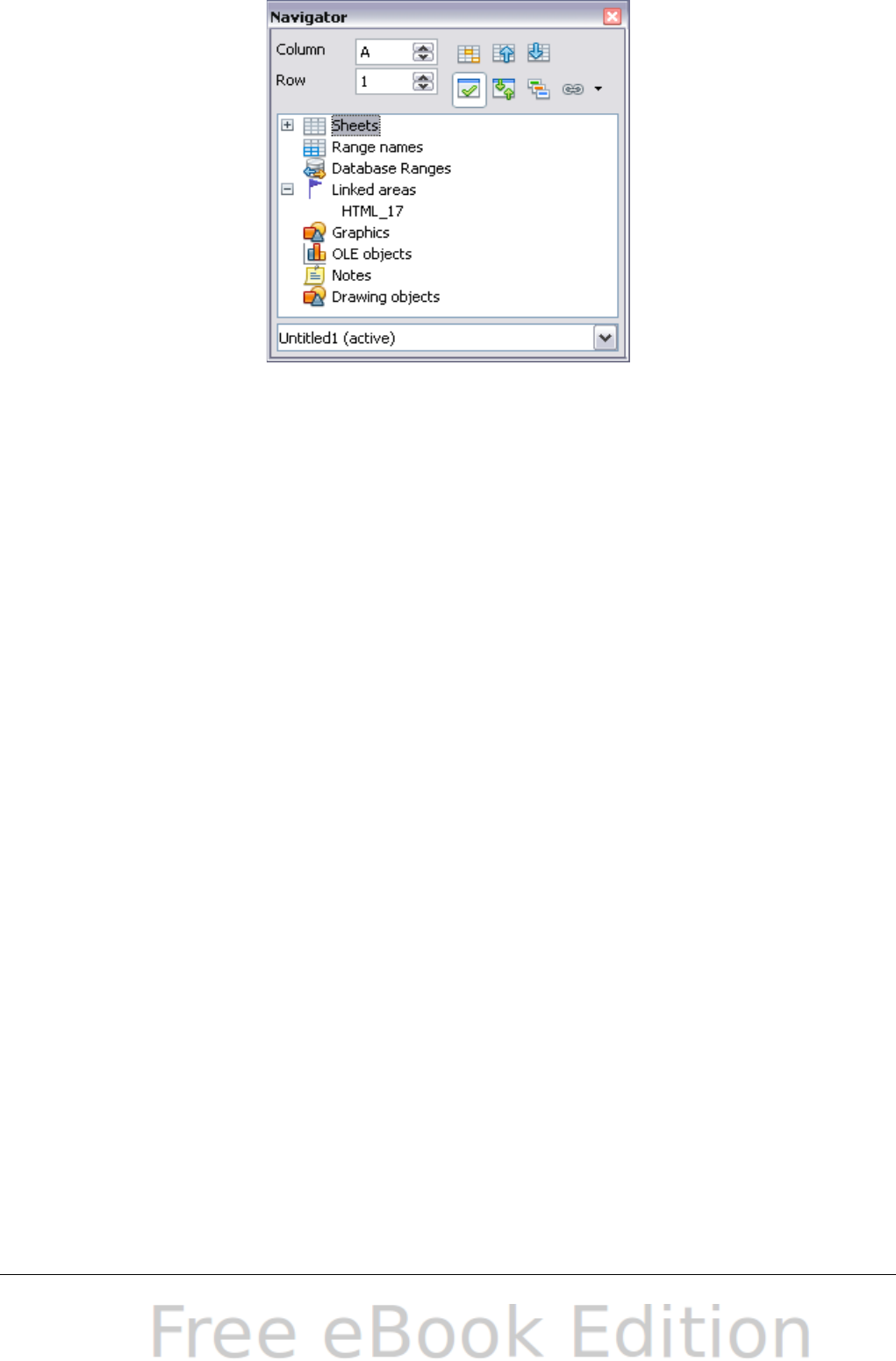
Figure 257: Linked areas in
target spreadsheet
How to find the required data range or table
The examples above show that the import filter gave names to the data
rangers (tables) in the sample web page starting from HTML_1. It also
created two additional range names (not visible in the illustration):
HTML_all – designates the entire document
HTML_tables – designates all HTML tables in the document
If the data tables in the source HTML document have been given
names (using the ID attribute on the TABLE tag), or the external
spreadsheet includes named ranges, those names appear in the list
along with the ranges Calc has sequentially numbered.
If the data range or table you want is not named, how can you tell
which one to select?
Go to the source document, which you opened in Calc. In the
Navigator, double-click on a range name: that range is highlighted on
the sheet (see Figure 258).
If the Formula Bar is visible, the range name is also displayed in the
Name box at the left-hand end (see Figure 259).
310 OpenOffice.org 3.x Calc Guide
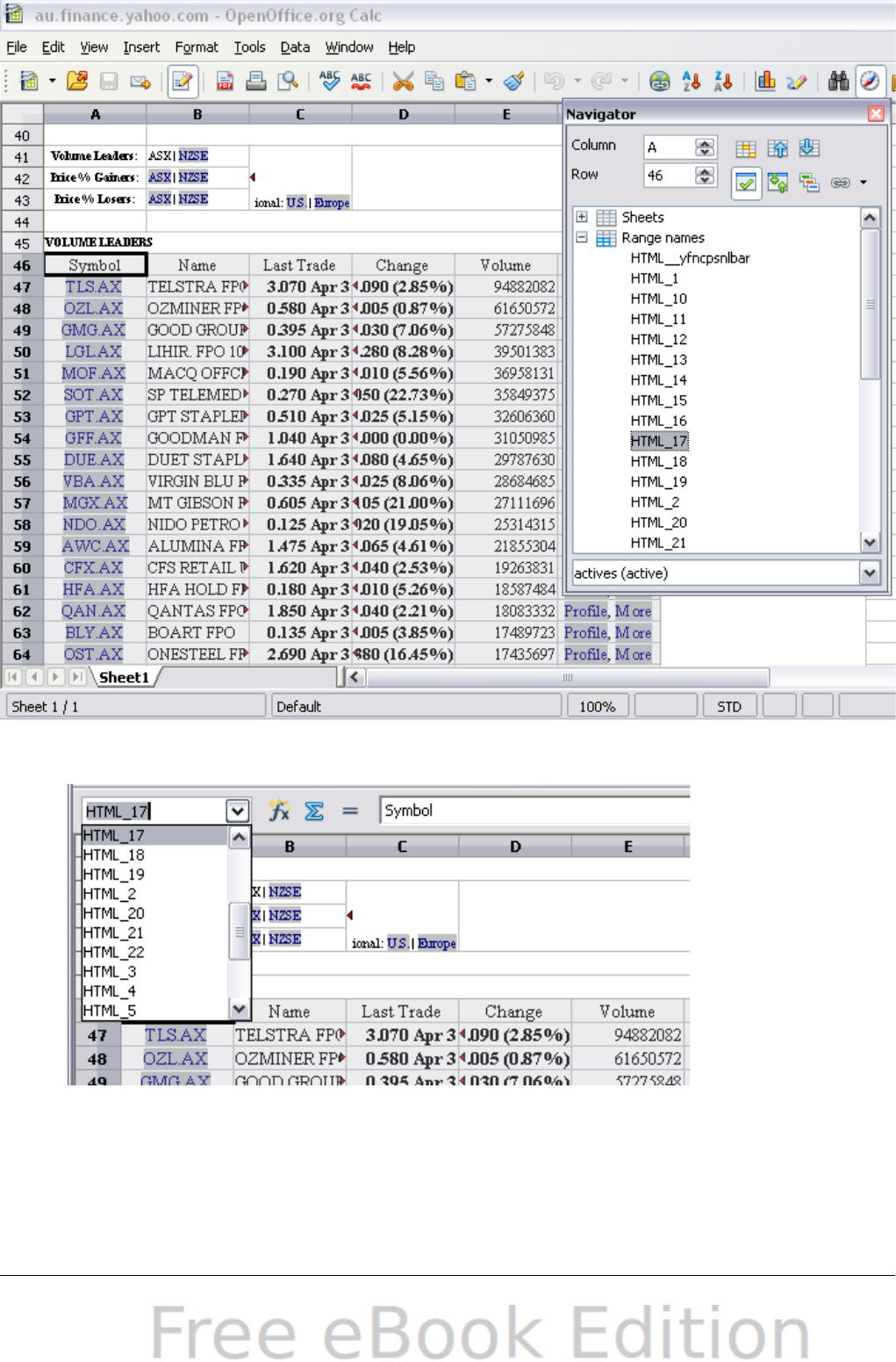
Figure 258: Using the Navigator to find a data range name
Figure 259: Using the Name box to find a data range name
Chapter 10 Linking Calc Data 311
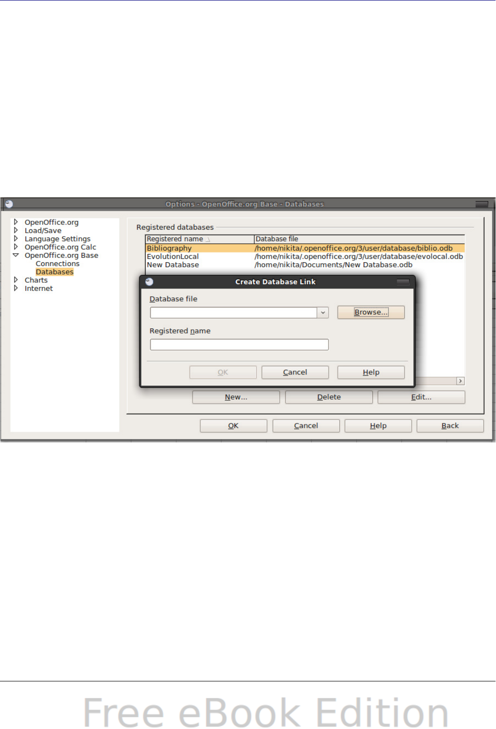
Linking to registered data sources
You can access a variety of databases and other data sources and link
them into Calc documents.
First you need to register the data source with OpenOffice.org. (To
register means to tell OOo what type of data source it is and where the
file is located.) The way to do this depends on whether or not the data
source is a database in *.odb format.
To register a data source that is in *.odb format:
1) Choose Tools > Options > OpenOffice.org Base > Databases.
2) Click the New button (below the list of registered databases) to
open the Create Database Link dialog (Figure 260).
Figure 260: Registering databases
3) Enter the location of the database file, or click Browse to open a
file browser and select the database file.
4) Type a name to use as the registered name for the database and
click OK. The database is added to the list of registered
databases. The OK button is enabled only when both fields are
filled in.
To register a data source that is not in *.odb format:
1) Choose File > New > Database to open the Database Wizard.
2) Select Connect to an existing database. The choices for
database type depend on your operating system. For example,
312 OpenOffice.org 3.x Calc Guide
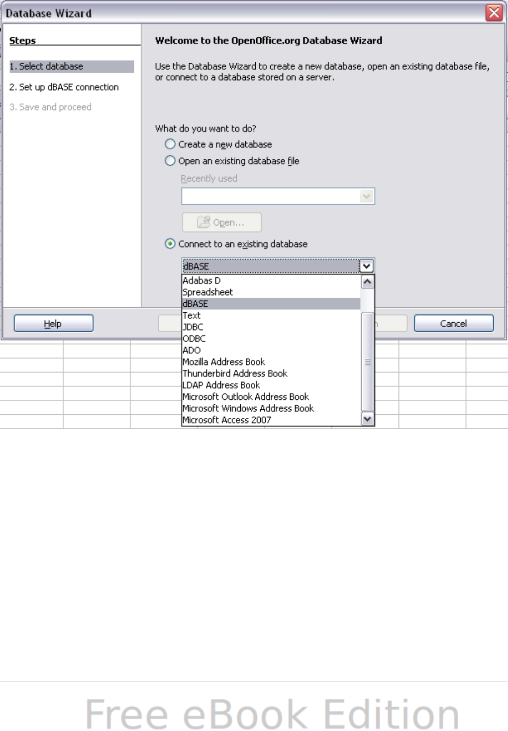
Microsoft Access and other Microsoft products are not among the
choices if you are using Linux. In our example, we chose dBASE.
Figure 261: Registering a database using the Database Wizard
3) Click Next. Type the path to the database file or click Browse
and use the Open dialog to navigate to and select the database
file before clicking Open.
4) Click Next. Select Yes, register the database for me, but clear the
checkbox marked Open the database for editing.
5) Click Finish. Name and save the database in the location of your
choice. Note: changes made to the *.odb do not affect the original
dBASE file.
Once a data source has been registered, it can be used by any OOo
component (for example Calc).
Chapter 10 Linking Calc Data 313
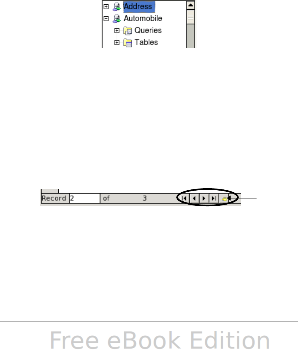
Viewing data sources
Open a document in Calc. To view the data sources available, press F4
or select View > Data Sources from the menu bar. The Data Source
View pane opens above the spreadsheet. A list of registered databases
is in the Data Explorer area on the left. (The built-in Bibliography
database is included in the list.)
To view each database, click on the + to the left of the name of the
database. (This has been done for the Automobile database in Figure
262.) Click on the + next to Tables to view the individual tables.
Figure 262: Databases
Now click on a table to see all the records held in it. The data records
are displayed on the right side of the Data Source View pane. To see
more columns, you can click the Explorer On/Off button to hide the
Data Explorer area.
At the top of the Data Source View pane, below the Calc toolbars, is
the Table Data bar. This toolbar includes buttons for saving records,
editing data, finding records, sorting, filtering, and other functions. For
more details about this toolbar, see the Help for data source browser.
Below the records is the Form Navigation bar, which shows which
record is selected and the total number of records. To the right are five
tiny buttons; the first four move backwards or forwards through the
records, or to the beginning or end.
Figure 263: Data Source View navigation buttons
Editing data sources
Some data sources (such as spreadsheets) cannot be edited in the data
source view.
In editable data sources, records can be edited, added, or deleted. If
you cannot save your edits, you need to open the database in Base and
edit it there; see “Launching Base to work on data sources”. You can
also hide columns and make other changes to the display.
314 OpenOffice.org 3.x Calc Guide

Launching Base to work on data sources
You can launch OOo Base at any time from the Data Source View pane.
Right-click on a database or the Tables or Queries icons and select
Edit Database File. Once in Base, you can edit, add, and delete tables,
queries, forms, and reports.
For more about using Base, see Chapter 8 (Getting Started with Base)
in the Getting Started guide.
Using data sources in Calc spreadsheets
Data from the tables in the data source pane can be placed into Calc
documents in a variety of ways.
You can select a cell or an entire row in the data source pane and drag
and drop the data into the spreadsheet. The data is inserted at the
place where you release the mouse button.
An alternative method uses the Data to Text icon and will include the
column headings above the data you insert:
1) Click the cell of the spreadsheet which you want to be the top left
of your data including the column names.
2) Press F4 to open the database source window and select the table
containing the data you want to use.
3) Select the rows of data you want to add to the spreadsheet:
•Click the gray box to the left of the row you want to select if
only selecting one row. That row is highlighted.
•To select multiple adjacent rows, hold down the Shift key
while clicking the gray box of the rows you need.
•To select multiple separate rows, hold down the Control key
while selecting the rows. The selected rows are highlighted.
•To select all the rows, click the gray box in the upper left
corner. All rows are highlighted.
4) Click the Data to text icon to insert the data into the
spreadsheet cells.
You can also drag the data source column headings (field names) onto
your spreadsheet to create a form for viewing and editing individual
records one at a time. Follow these steps:
1) Click the gray box at the top of the column (containing the field
name you wish to use) to highlight it.
Chapter 10 Linking Calc Data 315
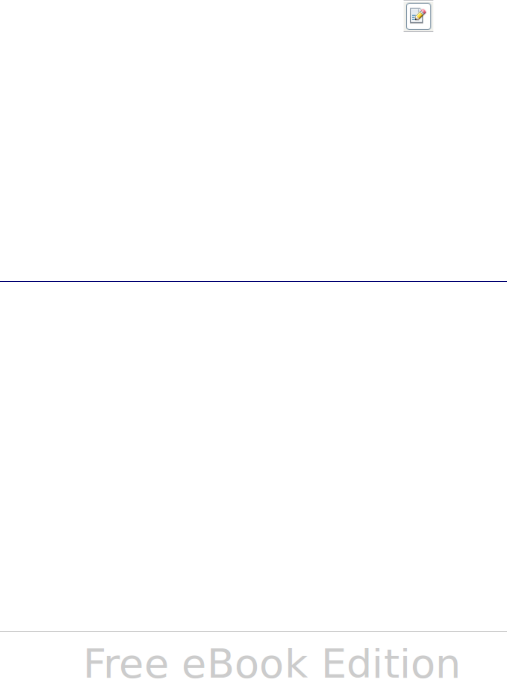
2) Drag and drop the gray box to where you want the record to
appear in the spreadsheet.
3) Repeat until you have moved all of the fields you need to where
you want them.
4) Close the Data Source window: press F4.
5) Save the spreadsheet and click the Edit File button on the
Standard toolbar, to make the spreadsheet read-only. All of the
fields will show the value for the data of the first record you
selected.
6) Add the Form Navigation toolbar: View > Toolbars > Form
Navigation. By default, this toolbar opens at the bottom of the
Calc window, just above the status bar.
7) Click the arrows on the Form Navigation toolbar to view the
different records of the table. The number in the Record box
changes as you move through the records. The data in the fields
changes to correspond to the data for that particular record
number. You can also search for a specific record, sort and filter
records, and do other tasks using this toolbar.
Embedding spreadsheets
Spreadsheets can be embedded in other OOo files. This is often used in
Writer or Impress documents so that Calc data can be used in a text
document. You can embed the spreadsheet as either an OLE or DDE
object. The difference between a DDE object and a Linked OLE object
is that a Linked OLE object can be edited from the document in which
it is added as a link, but a DDE object cannot.
For example, if a Calc spreadsheet is pasted into a Writer document as
a DDE object, then the spreadsheet cannot be edited in the Writer
document. But if the original Calc spreadsheet is updated, the changes
are automatically made in the Writer document. If the spreadsheet is
inserted as a Linked OLE object into the Writer document, then the
spreadsheet can be edited in the Writer as well as in the Calc
document and both documents are in sync with each other.
Object Linking and Embedding (OLE)
The major benefit of an OLE (Object Linking and Embedding) object is
that it is quick and easy to edit the contents just by double-clicking on
316 OpenOffice.org 3.x Calc Guide
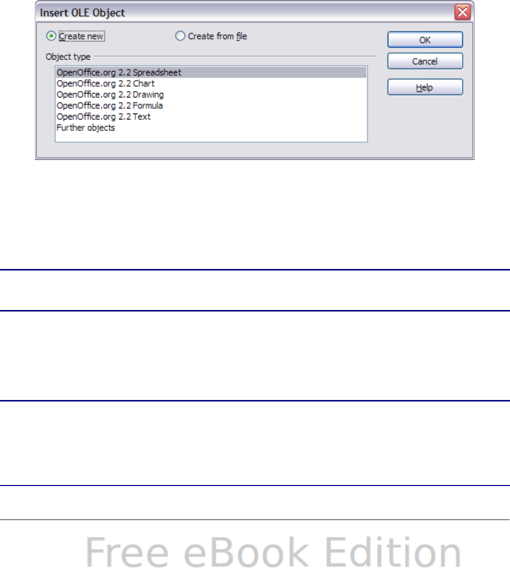
it. You can also insert a link to the object that will appear as an icon
rather than an area showing the contents itself.
OLE objects can be linked to a target document or be embedded in the
target document. Linking inserts information which will be updated
with any subsequent changes to the original file, while embedding
inserts a static copy of the data. If you want to edit the embedded
spreadsheet, double-click on the object.
To embed a spreadsheet as an OLE object in a presentation:
1) Place the cursor in the document and location you want the OLE
object to be.
2) Select Insert > Object > OLE Object. The dialog below opens.
Figure 264: Insert OLE object dialog
3) You can either create a new OLE object or create from a file.
To create a new object:
1) Select Create new and select the object type among the available
options.
Note “Further objects” is only available if you are using the Windows
operating system.
2) Click OK. An empty container is placed in the slide.
3) Double-click on the OLE object to enter the edit mode of the
object. The application devoted to handling that type of file will
open the object.
Note
If the object inserted is handled by OpenOffice.org, then the
transition to the program to manipulate the object will be
seamless; in other cases the object opens in a new window and
an option in the File menu becomes available to update the
object you inserted.
Chapter 10 Linking Calc Data 317
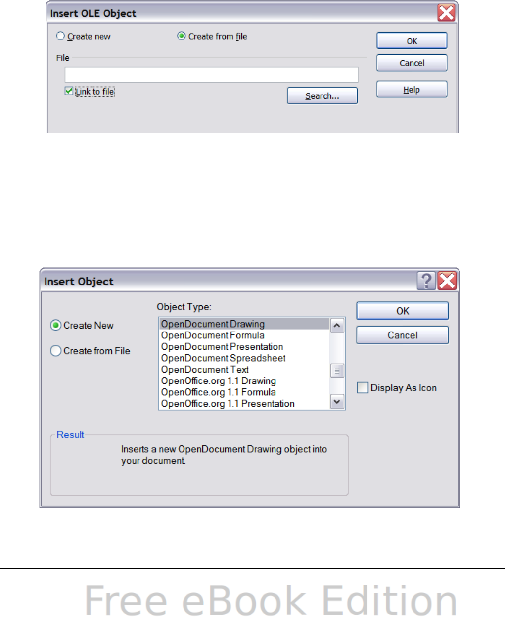
To insert an existing object:
1) To create from a file, select Create from file. The dialog changes
to look like Figure 265.
2) To insert the object as a link, select the Link to file option.
Otherwise, the object will be embedded.
3) Click Search, select the required file in the Open dialog, then
click Open. A section of the inserted file is shown in the
document.
Figure 265: Inserting an object as a link
Other OLE objects
Under Windows, the Insert OLE Object dialog box has an extra entry,
Further objects, as shown in Figure 266.
1) Double-click on the entry Further objects to open the dialog
shown below.
Figure 266: Inserting an OLE object under Windows
318 OpenOffice.org 3.x Calc Guide

2) Select Create New to insert a new object of the type selected in
the Object Type list, or select Create from File to create a new
object from a file.
3) If you choose Create from File, the dialog shown below opens.
Click Browse and choose the file to insert. The inserted file
object is editable by the Windows program that created it.
If instead of inserting an object, you want to insert a link to an
object, select the Display As Icon option.
Figure 267: Insert object from a file
Non-linked OLE object
If the OLE object is not linked, it can be edited in the new document.
For instance, if you insert a spreadsheet into a Writer document, you
can essentially treat it as a Writer table (with a little more power). To
edit it, double-click on it.
Linked OLE object
When the spreadsheet OLE object is linked, if you change it in Writer it
will change in Calc; if you change it in Calc, it will change in Writer.
This can be a very powerful tool if you create reports in Writer using
Calc data, and want to make a quick change without opening Calc.
Note
You can only edit one copy of a spreadsheet at a time. If you
have a linked OLE spreadsheet object in an open Writer
document and then open the same spreadsheet in Calc, the Calc
spreadsheet will be a read-only copy.
Chapter 10 Linking Calc Data 319
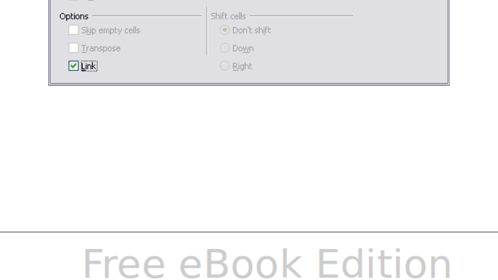
Dynamic Data Exchange (DDE)
DDE is an acronym for Dynamic Data Exchange, a mechanism whereby
selected data in document A can be pasted into document B as a
linked, ‘live’ copy of the original. It would be used, for example, in a
report written in Writer containing time-varying data, such as sales
results sourced from a Calc spreadsheet. The DDE link ensures that, as
the source spreadsheet is updated so is the report, thus reducing the
scope for error and reducing the work involved in keeping the Writer
document up to date.
DDE is a predecessor of OLE. With DDE, objects are linked through file
reference, but not embedded. You can create DDE links either within
Calc cells in a Calc sheet, or in Calc cells in another OOo doc such as
in Writer.
DDE link in Calc
Creating a DDE link in Calc is similar to creating a cell reference. The
process is a little different, but the result is the same.
1) In Calc, select the cells that you want to make the DDE link to.
2) Copy them: Edit > Copy or Ctrl+C.
3) Go to the place in the spreadsheet where you want the link to be.
4) Select Edit > Paste Special.
5) When the Paste Special dialog opens, select the Link option on
the bottom left of the dialog (Figure 268). Click OK.
The cells now reference the copied data, and the formula bar shows a
reference beginning with {=DDE.
If you now edit the original cells, the linked cells will update.
Figure 268: Location of Link option on Paste Special dialog in Calc
320 OpenOffice.org 3.x Calc Guide
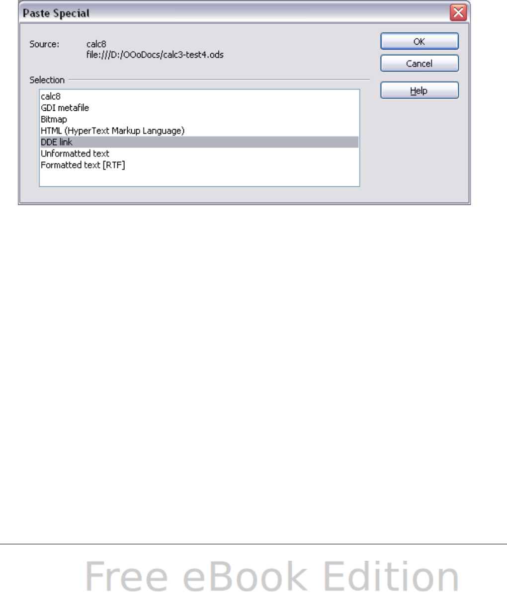
DDE link in Writer
The process for creating a DDE link from Calc to Writer is similar to
creating a link within Calc.
1) In Calc, select the cells to make the DDE link to. Copy them.
2) Go to the place in your Writer document where you want the DDE
link. Select Edit > Paste Special.
3) Select DDE Link (Figure 269). Click OK.
Now the link has been created in Writer. When the Calc spreadsheet is
updated, the table in Writer is automatically updated.
Figure 269: Paste Special dialog in Writer, with DDE link selected
Chapter 10 Linking Calc Data 321

Chapter 11
Sharing and Reviewing
Documents
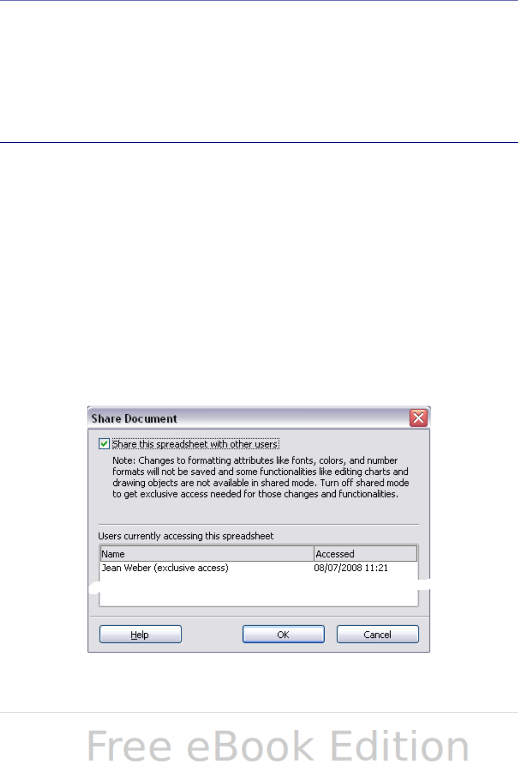
Introduction
This chapter covers methods for editing shared documents: sharing
(collaboration), recording changes, adding comments, reviewing
changes, merging and comparing documents, and saving and using
document versions. Basic editing techniques are discussed in Chapter
2 (Entering, Editing, and Formatting Data).
Sharing documents (collaboration)
In OpenOffice.org Writer, Impress, and Draw, only one user at a time
can open any document for editing. In Calc, many users can open the
same spreadsheet for writing at the same time.
Each user who wants to collaborate should be sure to enter a name on
the Tools > Options > OpenOffice.org > User Data page.
Some menu commands are not available (grayed out) when change
tracking or document sharing is activated.
Setting up a spreadsheet for sharing
At any time, you can set up a spreadsheet for sharing with others. With
the spreadsheet document open, choose Tools > Share Document to
activate the collaboration features for this document. A dialog opens
where you can enable or disable sharing.
Figure 270: Choosing to share a spreadsheet
Chapter 11 Sharing and Reviewing Documents 323

To enable sharing, select the box at the top of the dialog, and then
click OK. A message appears stating that you must save the document
to activate shared mode. Click Yes to continue. The word (shared) is
then shown on the title bar after the document’s title.
The Tools > Share Document command can be used to switch the
mode for a document from unshared to shared. However, if you want to
use a shared document in unshared mode, you need to save the shared
document using another name or path. This creates a copy of the
spreadsheet that is not shared.
Opening a shared spreadsheet
When you open a spreadsheet document that is in shared mode, a
message appears stating that the document is in shared mode and that
some features are not available in this mode. After clicking OK, the
document is opened in shared mode.
The following features are known to be disabled in a shared
spreadsheet document:
Edit > Changes, except for Merge Document
Edit > Compare Document
Edit > Sheet > Move/Copy & Delete
Insert > Cells Shift Cells Down & Shift Cells Right
Insert > Sheet from file
Insert > Names
Insert > Comment
Insert > Picture > From File
Insert > Movie and Sound
Insert > Object
Insert > Chart
Insert > Floating Frame
Format > Sheet > Rename, Tab Color
Format > Merge Cells > Merge and Center, Merge Cells, Split Cells
Format > Print Ranges
Tools > Protect Document
Data > Define Range
Data > Sort
Data > Subtotals
Data > Validity
Data > Multiple Operations
Data > Consolidate
Data > Group and Outline (all)
Data > DataPilot
324 OpenOffice.org 3.x Calc Guide
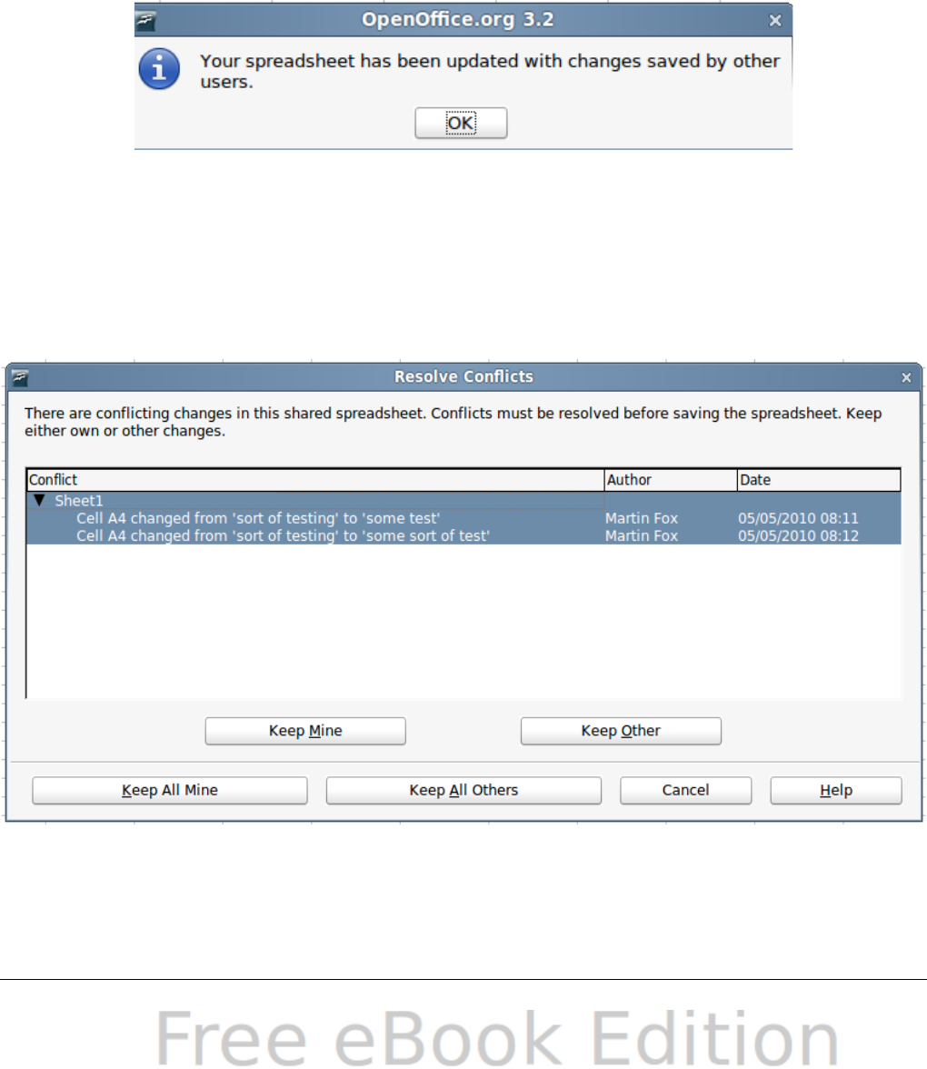
Saving a shared spreadsheet
When you save a shared spreadsheet, one of several situations may
occur:
•If the document was not modified and saved by another user since
you opened it, the document is saved.
•If the document was modified and saved by another user since
you opened it, one of the following events will occur:
–If the changes do not conflict, the document is saved, the
dialog below appears, and any cells modified by the other user
are shown with a red border.
Figure 271: Update message after saving
–If the changes conflict, the Resolve Conflicts dialog is shown.
You must decide for each conflict which version to keep, yours
or the other person’s. When all conflicts are resolved, the
document is saved. While you are resolving the conflicts, no
other user can save the shared document.
Figure 272: Resolve Conflicts dialog
•If another user is trying to save the shared document and resolve
conflicts, you see a message that the shared spreadsheet file is
Chapter 11 Sharing and Reviewing Documents 325

locked due to a merge-in in progress. You can choose to cancel
the Save command for now, or retry saving later.
When you successfully save a shared spreadsheet, the document shows
the latest version of all changes saved by all users.
Recording changes
You can use several methods to record changes that you or others
make to a document.
•You can use change marks to show added material, deleted
material, and changes to formatting. Later, you or another person
can review the document and accept or reject each change.
•If you are not using file sharing, you can make changes to a copy
of the document (stored in a different folder, under a different
name, or both), then use Calc to compare the files and show the
changes. See page 337.
•You can save versions that are stored as part of the original file.
See page 337.
Reviewers can leave comments in the document, either attached to
specific changes or standalone.
Preparing a document for review (optional)
When you send a document to someone else to review or edit, you may
want to protect it first so that the editor or reviewer does not have to
remember to turn on the revision marks. After you have protected the
document, any user must enter the correct password in order to turn
off protection and accept or reject changes.
1) Open the document and make sure that the Edit > Changes >
Record menu item has a check mark next to it, indicating that
change recording is active.
2) (Optional) Click Edit > Changes > Protect Records. On the
Protect Records dialog, type a password (twice) and click OK.
Note
Passwords must contain at least five characters.
It is not necessary to password protect the document while
preparing it for review.
326 OpenOffice.org 3.x Calc Guide
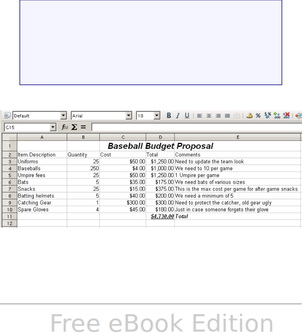
Identifying copies of spreadsheets
When not using the document sharing feature, it is important to keep
track of the different copies of the document. This can be done either
in the file name or in the file title. If you have not provided a file title in
the spreadsheet’s properties, the spreadsheet’s file name is displayed
in the title bar. To set the title of the spreadsheet, select File >
Properties > Description.
Recording changes (tutorial)
For this chapter we will work with a budget proposal for a baseball
team.
You are the sponsor of a youth baseball team. The coach
has submitted a budget to you for the season and you need
to edit the costs and return it to her.
You are concerned that if you just make the changes, then
the coach won't see the changes you made. You decide to
use Calc with the record changes feature turned on, so that
the coach can easily see the change you have made.
Figure 273 shows the budget spreadsheet your coach submitted.
Figure 273: Baseball budget spreadsheet
Looking over the figures, you see a few places where money could be
saved:
•Post-game snacks can be bought by parents.
•New uniforms can wait; only buy 10 to replace damaged ones.
Chapter 11 Sharing and Reviewing Documents 327
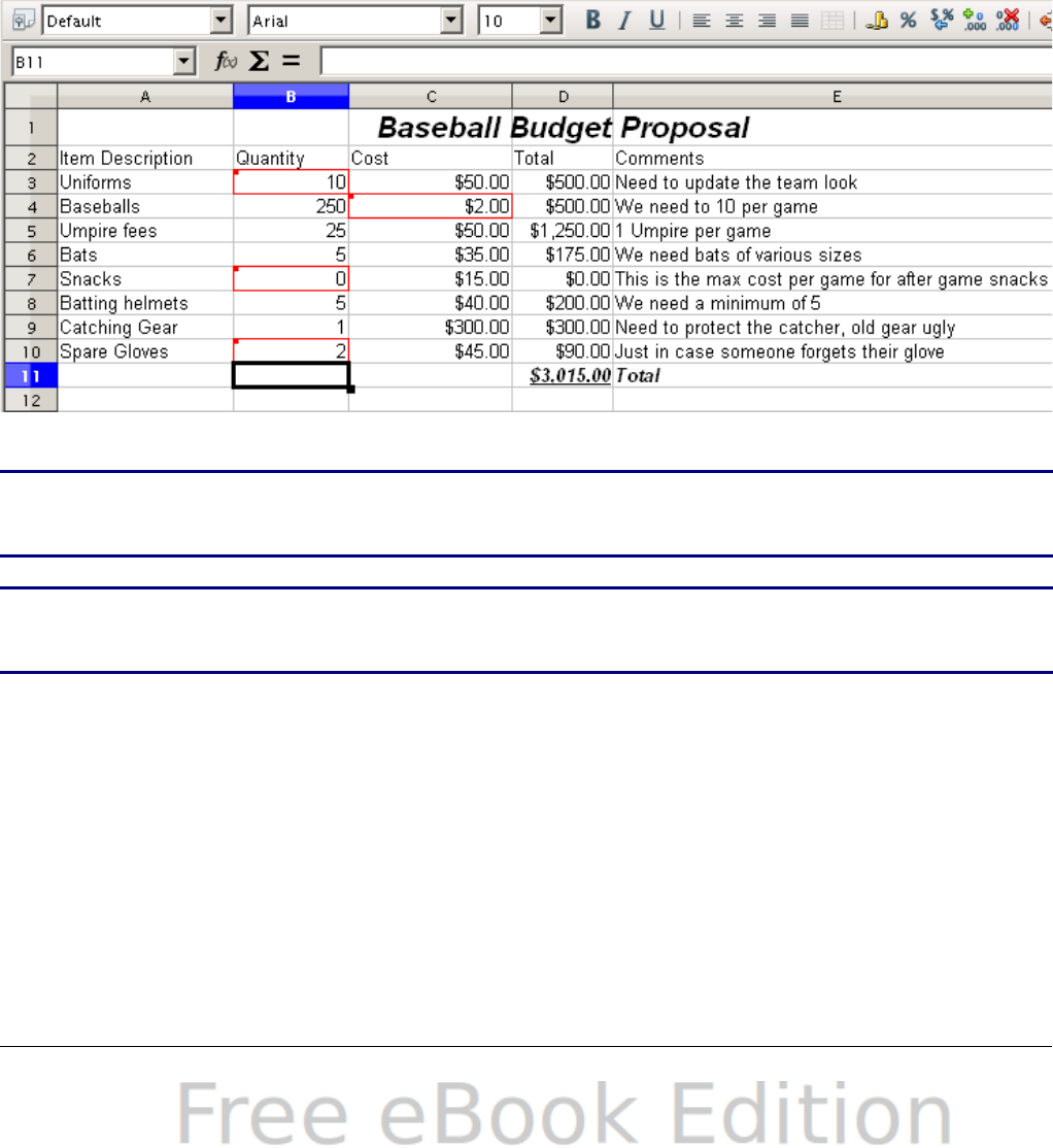
•Buy cheaper baseballs.
•Only buy 2 spare gloves.
To make these changes, use the record changes feature in Calc. To
start recording changes:
1) Open the Budget Spreadsheet.
2) Select Edit > Changes > Record from the menu bar.
3) Begin editing the document.
A colored border, with a dot in the upper left-hand corner, appears
around a cell where changes were made (Figure 274). Other reviewers
then quickly know which cells were edited. A deleted column or row is
marked by a heavy colored bar.
Figure 274: Edited document with red border on changed cells
Tip Some changes, for example cell formatting, are not recorded and
marked.
Tip To change the color that indicates changes, select Tools >
Options > OpenOffice.org Calc > Changes.
When you finish editing the document, you can send it to your coach.
You may want to explain your rationale for the changes. You can share
your insight in two ways: by adding comments to the changes you
made, or by adding general comments to the spreadsheet.
328 OpenOffice.org 3.x Calc Guide
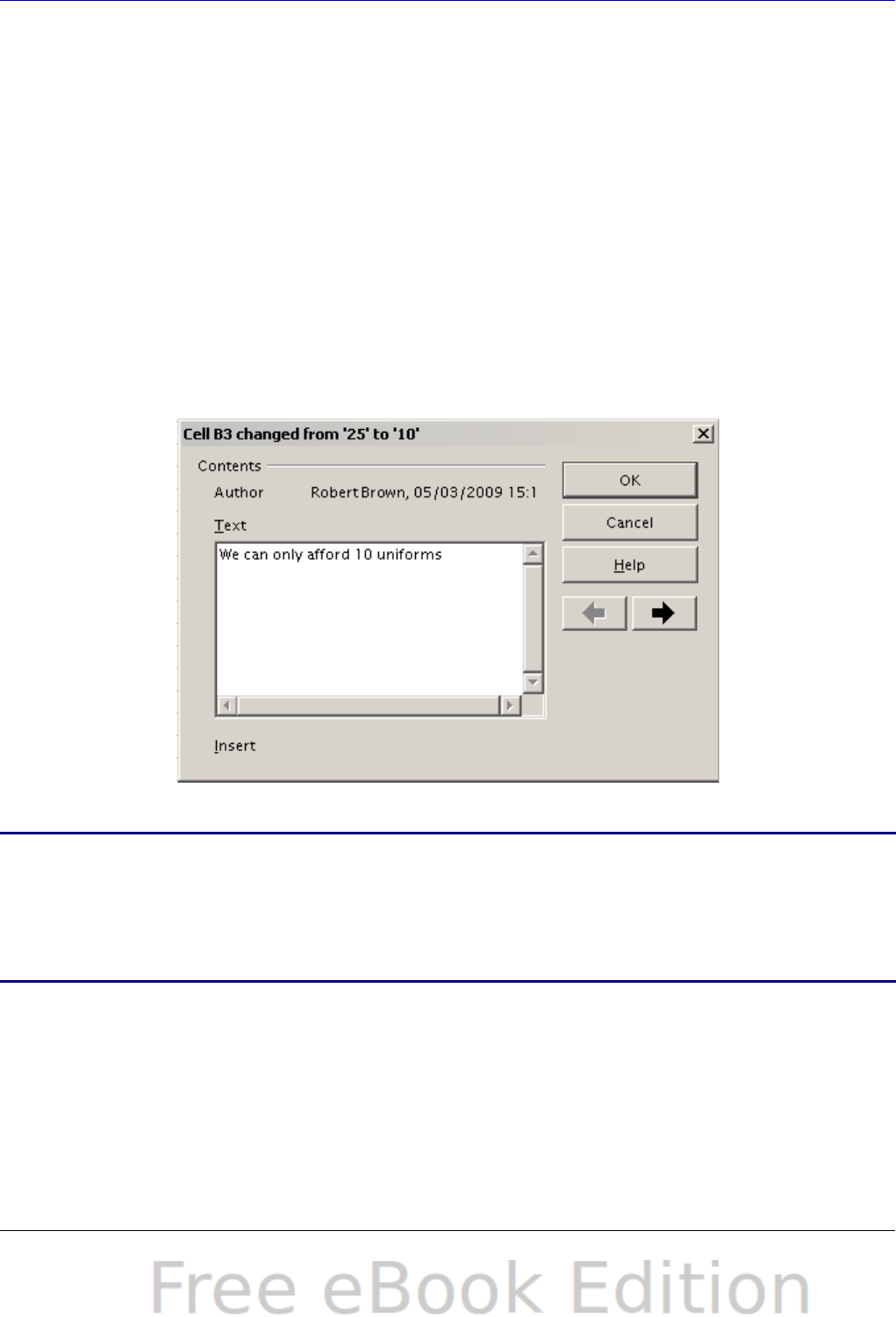
Adding comments to changes
Calc automatically adds to any recorded change a comment that
describes what was changed (for example, Cell B4 changed from ‘9’ to
‘4’). Reviewers and authors can add their own comments to explain
their reasons for the changes.
To add a comment to a change:
1) Make the change to the spreadsheet.
2) Select the cell with the change.
3) Choose Edit > Changes > Comments. The dialog shown in
Figure 275 appears. The automatically-added comment provided
by Calc appears in the title bar of this dialog and cannot be
edited.
4) Type your own comment and click OK.
Figure 275: Comment dialog
Tip
You can step through your changes one at a time using the left
and right arrows on the right hand side of the Comment dialog,
and add comments to each change. The title bar for the
Comment dialog shows the cell and the change you are
commenting on.
After you have added a comment to a changed cell, you can see it by
hovering the mouse pointer over the cell, as shown in Figure 276.
Chapter 11 Sharing and Reviewing Documents 329
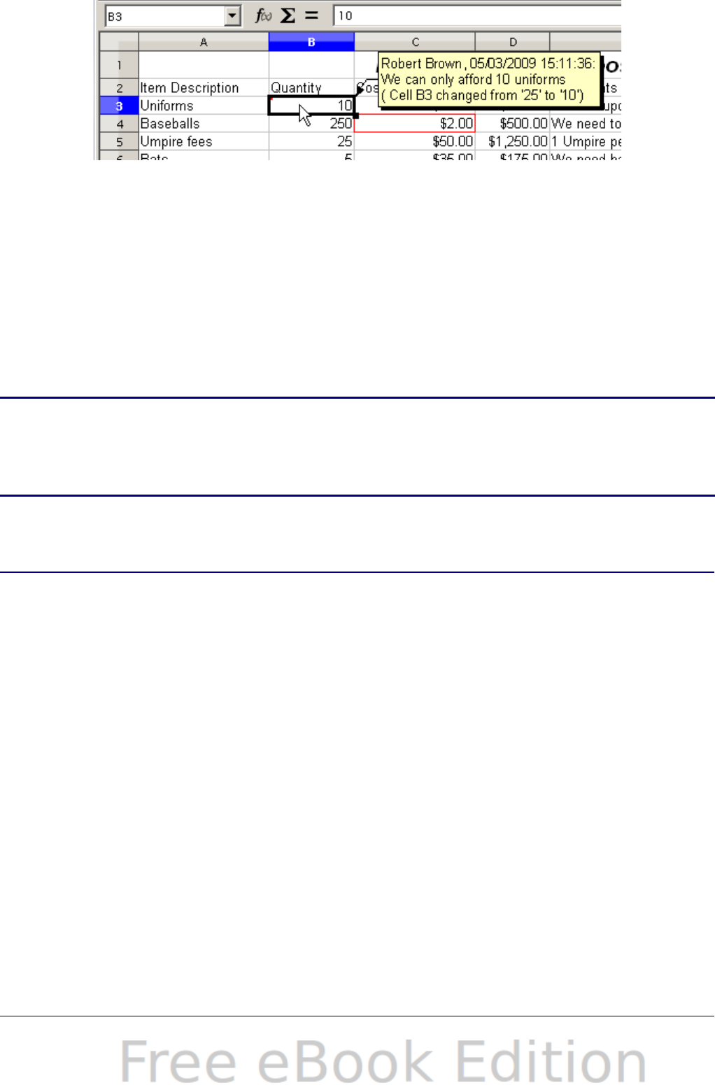
Figure 276: Comment added to cell B3
The comment also appears in the dialog when you are accepting and
rejecting changes, as shown in the first line of Figure 281 on page 335.
Editing change comments
1) Select the cell with the change comment that you want to edit.
2) Select Edit > Changes > Comments.
3) Edit the comment and click OK.
Tip
You can view your comments one at a time using the left and
right arrows located on the right hand side of the Comment
dialog. You do not need to click OK after editing each comment;
you can save them all at once when you’re done editing.
Adding other comments
Calc provides another type of comments (formerly called “notes”),
which authors and reviewers often use to exchange ideas, ask for
suggestions, or brainstorm in the document.
To add a comment:
1) Select the cell that the comment applies to.
2) Select Insert > Comment or right-click and select Insert
Comment. (The latter method does not work if the automatic
spelling checker is active and the cell contains a misspelled
word.) The box shown in Figure 277 appears.
3) Type the text of your comment in the box.
4) Click outside the box to close it.
330 OpenOffice.org 3.x Calc Guide

Figure 277: Inserting a comment
Now the cell to which you added the comment has a colored dot in the
upper right-hand corner, as shown in Figure 278. It does not have a
colored border, unless the cell was also changed.
Figure 278: Colored dot in cell containing a comment
Tip You can change the colors Calc uses for notes by selecting Tools
> Options > OpenOffice.org > Appearance.
To view the comment you just added, hover the mouse pointer over the
cell that has a comment; the comment appears, as shown below.
Figure 279: Viewing a comment
Editing comments
You can edit and format the text of a comment, just as you do for any
other text.
1) Right-click on the cell containing the comment marker, and
choose Show comment from the pop-up menu.
2) Select the comment, then double-click on it. The cursor changes
to the usual blinking text-entry cursor, and the Formatting toolbar
changes to show text attributes.
Chapter 11 Sharing and Reviewing Documents 331

3) When done, click outside the comment to deselect it. To hide the
comment again, right-click on the cell and deselect Show
Comment on the pop-up menu.
Formatting comments
You can change the background color, border style, transparency, and
other attributes of a comment.
1) Right-click on the cell containing the comment marker, and
choose Show comment from the pop-up menu.
2) Click on the comment itself. The Formatting toolbar changes to
show many of the comment formatting options. These are the
same as the options for formatting graphics; see Chapter 5 (Using
Graphics in Calc) for more information.
You can also right-click on the comment to see a menu of choices,
some of which lead to dialogs in which you can fine-tune the
formatting; these dialogs are also discussed in Chapter 5.
3) When done, click outside the comment to deselect it. To hide the
comment again, right-click on the cell and deselect Show
Comment on the pop-up menu.
Finding comments using the Navigator
The small comment markers in the corners of cells can be difficult to
see, so Calc provides another way to find them, by using the Navigator.
If any comments are in the spreadsheet, the Navigator shows a mark
(usually a + or an arrow) next to the word Comments. Click on this
mark to display a list of comments. Double-click on the comment you
want to jump directly to the cell it is associated with.
Reviewing changes
At this point, we are going to change our perspective from the point of
view of the team sponsor to that of the coach, so we can see how to
review and accept or reject the changes to the document the coach
originally wrote.
332 OpenOffice.org 3.x Calc Guide
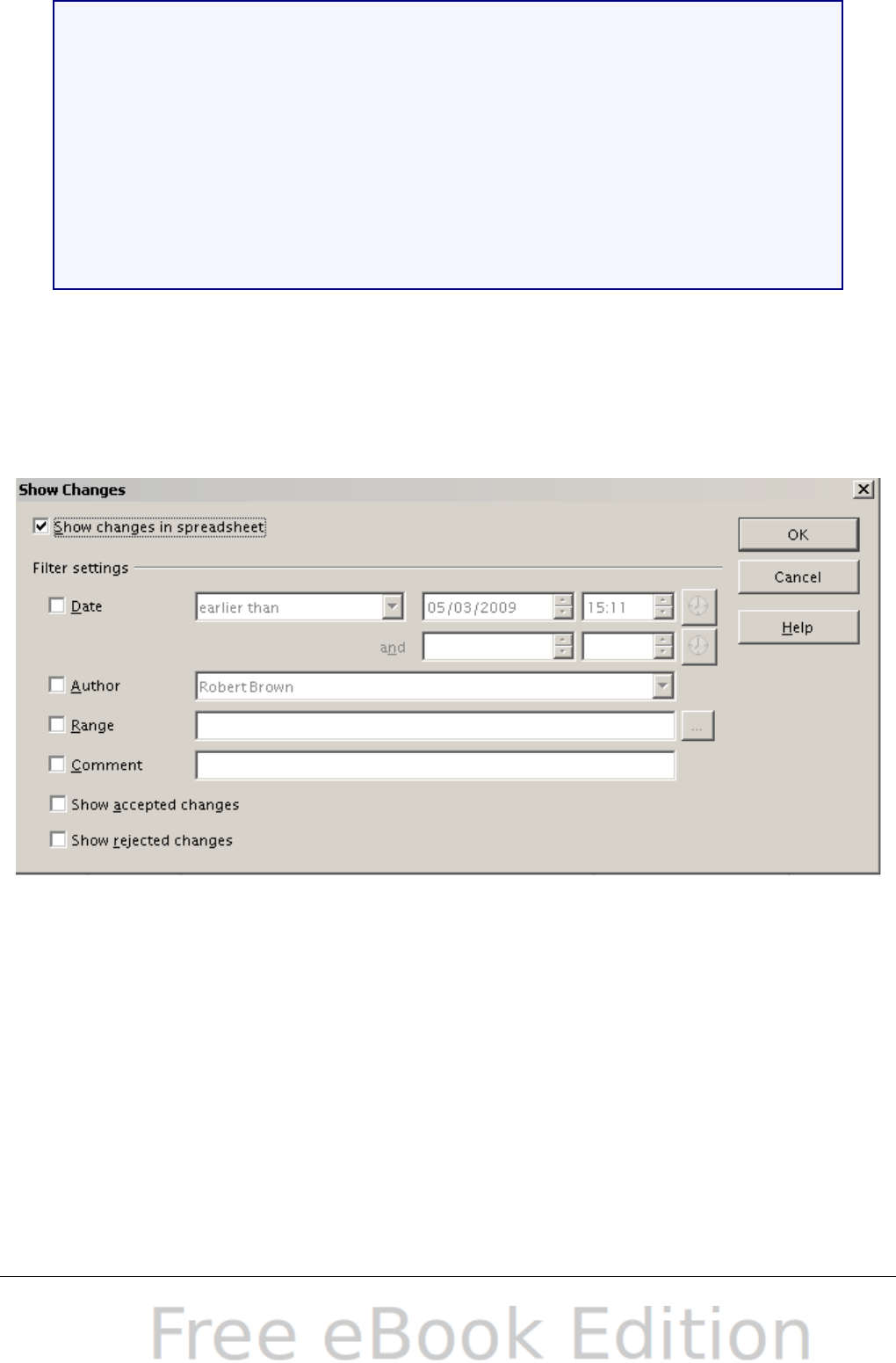
You are the coach of a youth baseball team and you
submitted a potential budget created in Calc to your team
sponsor.
Your sponsor has reviewed the document using the record
changes feature of Calc. Now, you want to review those
changes and accept or reject the counter proposal.
Because the sponsor recorded changes in Calc, you can
easily see what changes were made and decide how to act.
Viewing changes
Calc gives you tremendous control over what changes you see when
reviewing a document. To change the available filters, select Edit >
Changes > Show. The dialog shown in Figure 280 opens.
Figure 280: Show changes dialog
Using the different settings, you can control which changes appear on
screen. You can filter based on:
•Date – Only changes made in a certain time range are displayed.
•Author – Only changes made by a specific author are displayed.
This is especially useful if you have multiple reviewers on the
document.
•Range – Only changes made in a specific range of cells are
displayed. This is especially useful if you have a large spreadsheet
and only want to review a part of it.
Chapter 11 Sharing and Reviewing Documents 333

•Comment – Searches the content of the comments and only
displays changes which have comments that match the search
criteria.
•Show accepted changes – Only changes you accepted are
displayed.
•Show rejected changes – Only changes you rejected are
displayed.
Note
You can also access the filter control in the Accept or Reject
Changes dialog shown in Figure 281. Click the Filter tab to get a
set of options similar to those shown in Figure 280.
Accepting or rejecting changes
When you receive a document back with changes, the beauty of the
recording changes system becomes evident. Now, as the original
author, you can step through each change and decide how to proceed.
To begin this process:
1) Open the edited document.
2) Select Edit > Changes > Accept or Reject. The dialog shown in
Figure 281 appears.
3) Calc steps through the changes one at a time. You can choose to
accept or reject each change as you go through.
The Comment column by default contains an explanation of the change
that was made. If the reviewer added a comment to the change, it is
displayed, followed by the description of the change, as in the first line
of Figure 281.
If more than one person has reviewed the document, one reviewer may
have modified another reviewer’s change. If so, the changes are
hierarchically arranged with a plus sign for opening up the hierarchy.
334 OpenOffice.org 3.x Calc Guide
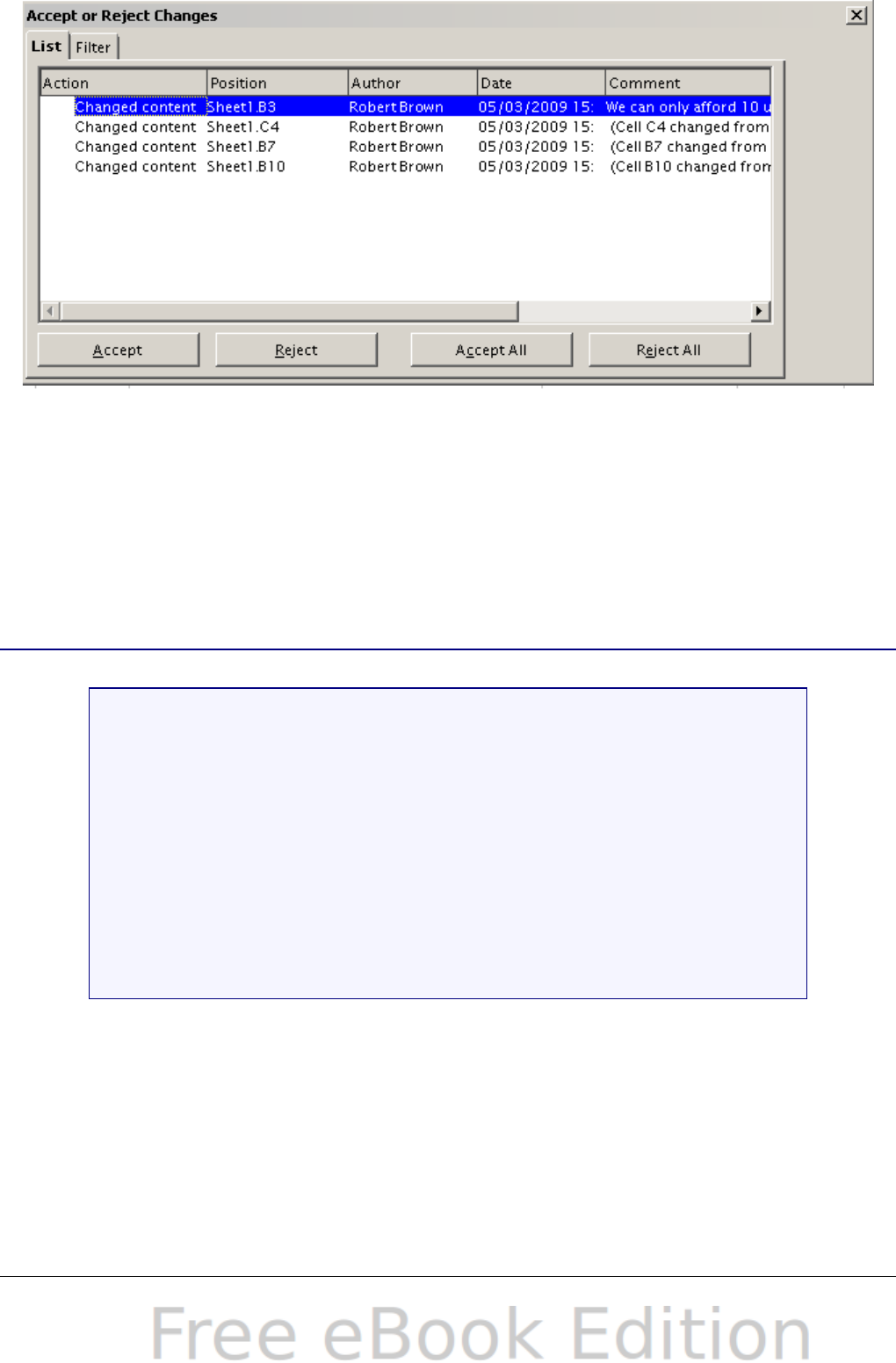
Figure 281: Accept or Reject changes dialog
On the Filter tab of this dialog (not shown here), you can choose how
to filter the list of changes: by date, author, cell range, or comments
containing specific terms. After selecting the filter criteria, switch back
to the List tab to see the results.
Merging documents
You submitted your budget proposal to your sponsor,
but you sent it to one of your assistant coaches as
well. Both of them returned their revised budget to
you at the same time.
You could review each document and the changes
separately, but to save time, you want to see both of
their revisions simultaneously.
To do this, you can use Calc’s merge document
feature.
The processes discussed to this point are effective when you have one
reviewer at a time. Sometimes, however, multiple reviewers all return
edited versions of a document at the same time. In this case, it may be
quicker to review all of these changes at once, rather than one review
at a time. For this purpose, you can merge documents in Calc.
Chapter 11 Sharing and Reviewing Documents 335
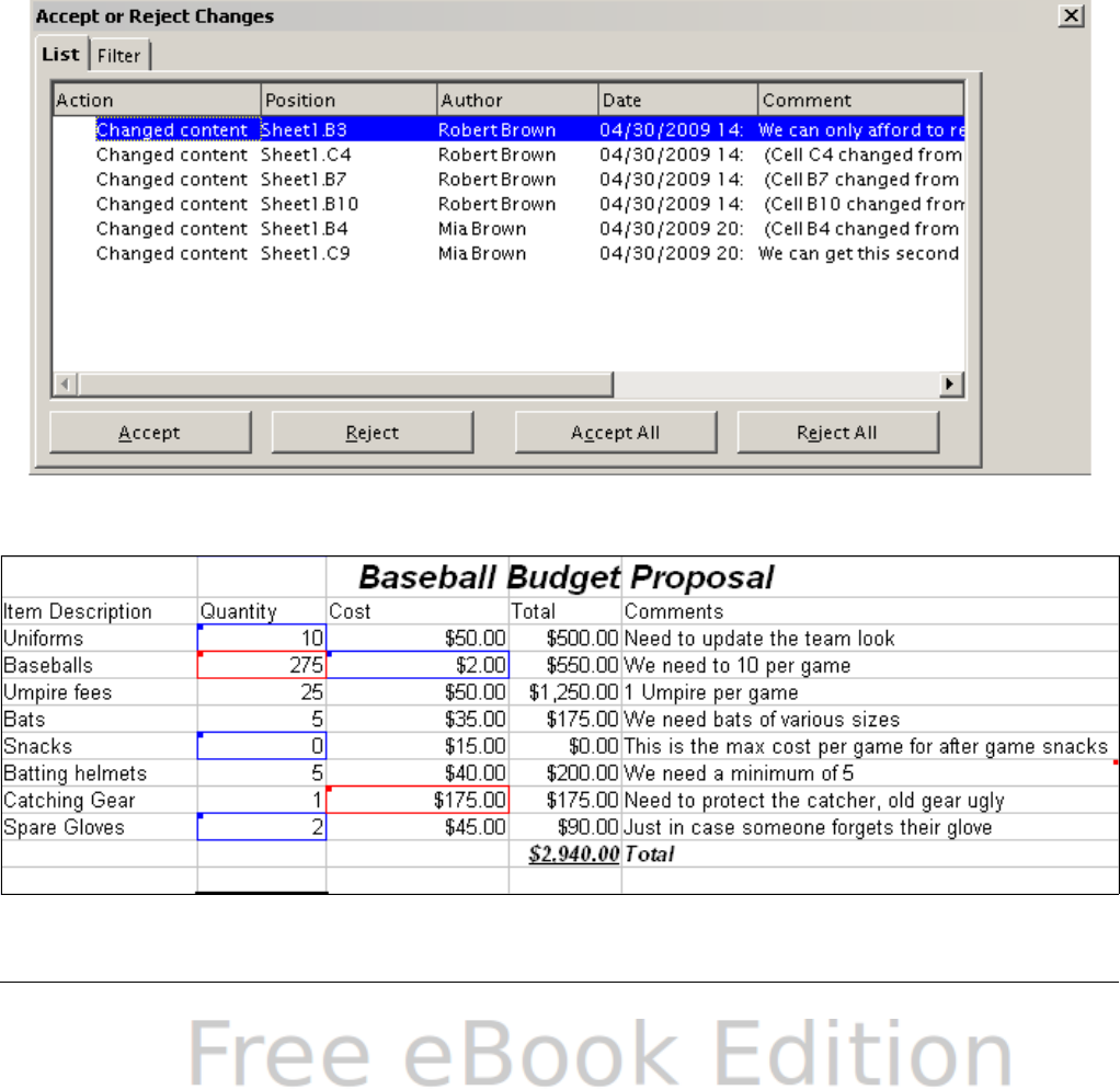
To merge documents, all of the edited documents need to have
recorded changes in them.
1) Open the original document.
2) Select Edit > Changes > Merge Document.
3) A file selection dialog opens. Select a file you want to merge and
click OK.
4) After the documents merge, the Accept or Reject Changes dialog
opens, as in Figure 282, showing changes by more than one
reviewer. If you want to merge more documents, close the dialog
and then repeat steps 2 and 3.
Now all of the changes are combined into one document and you can
accept or reject the changes. Changes from different authors appear in
different colors in the document, as shown in Figure 283. In this
example, all of the changes from Robert are blue and the changes from
Mia are red.
Figure 282: Accept or Reject for merged documents
Figure 283: Merged documents with different author colors
336 OpenOffice.org 3.x Calc Guide
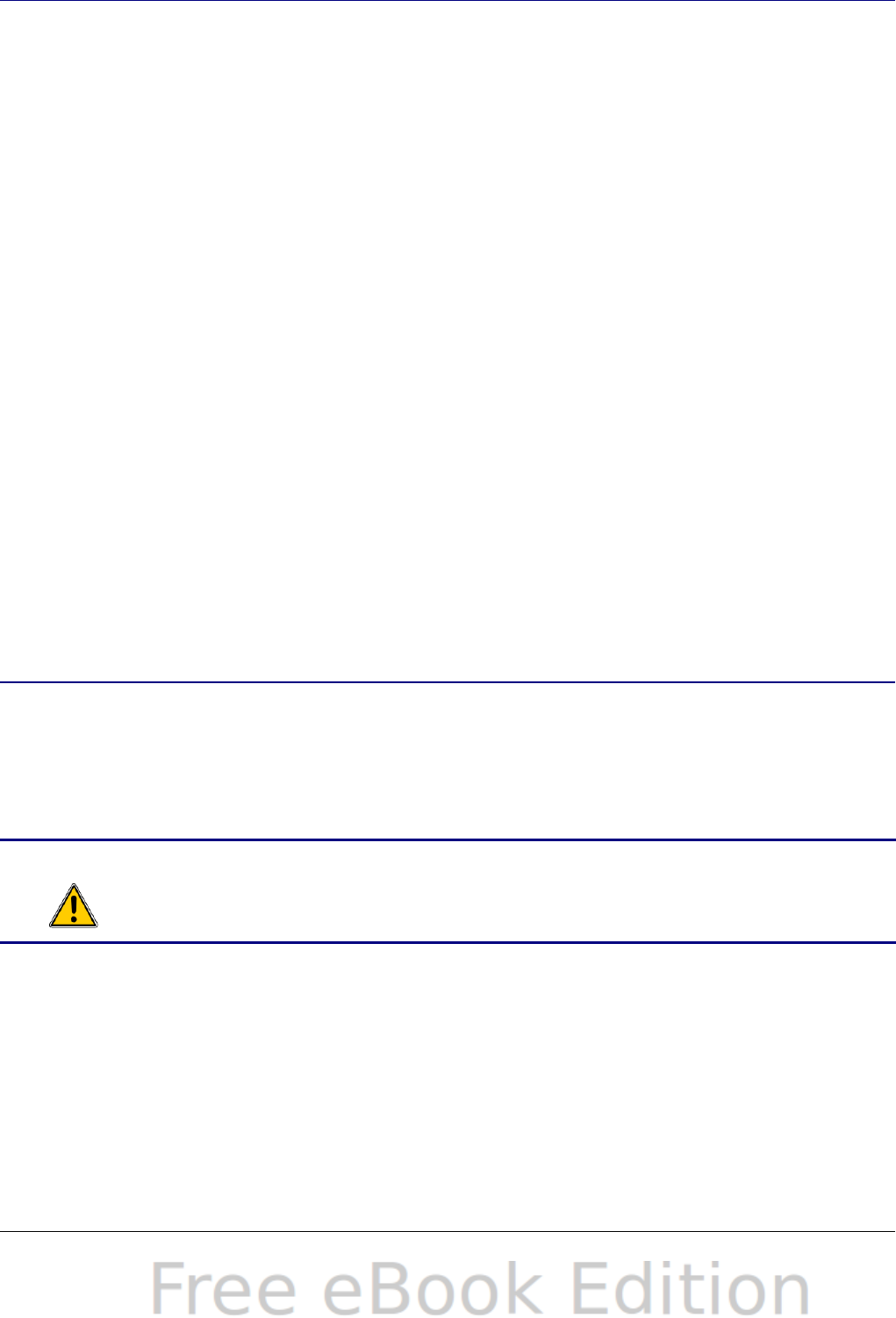
Comparing documents
Sometimes when sharing documents, reviewers may forget to record
the changes they make. This is not a problem with Calc, because Calc
can find the changes by comparing documents.
In order to compare documents you need to have the original
document and the one that is edited. To compare them:
1) Open the edited document that you want to compare with the
original document.
2) Select Edit > Compare Document.
3) An open document dialog appears. Select the original document
and click Insert.
Calc finds and marks the changes as follows:
•All data that occurs in the edited document but not in the original
is identified as inserted.
•All data that is in your original document but is not in the edited
document is identified as deleted.
•All data that is changed, is marked as changed.
From this point you can go through and accept or reject changes as
you could normally.
Saving versions
Most documents go through many drafts. It is often useful to save new
versions of a document. You can do this by saving a copy of the
document (under a different name) after each revision, or you using
Calc’s version feature.
Caution
If you do a Save As... of a document with different versions
stored in it, the old versions are not saved in the new file.
To use version management in Calc:
1) Choose File > Versions. The Versions dialog opens.
Chapter 11 Sharing and Reviewing Documents 337
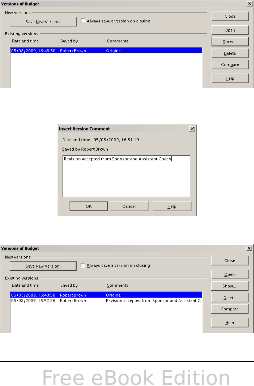
Figure 284: Version management dialog
2) Click the Save New Version button to save a new version.
3) A dialog opens where you can enter comments about this version.
Figure 285: Version comment dialog
4) After you enter your comment and click OK, the new version is
included in the version list.
Figure 286: Updated version list
338 OpenOffice.org 3.x Calc Guide

Now when you save the file, both versions are saved in the same file.
From this point you can:
•Open an old version – Select the version and click the Open
button and a read-only version of a previous version opens.
•Compare all versions – Clicking the Compare button performs an
action similar to merging documents together. An Accept or
Reject Changes dialog opens showing all of the changes through
the different versions.
•Review the comments – Select a version and click the Show
button to display the full comments made by yourself or other
reviewers.
Note The new file is bigger in size, as if two spreadsheets were
saved together.
Chapter 11 Sharing and Reviewing Documents 339

Chapter 12
Calc Macros
Automating repetitive tasks
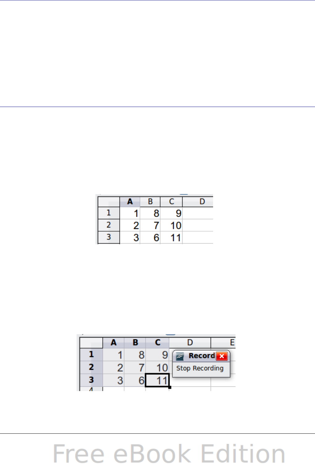
Introduction
A macro is a saved sequence of commands or keystrokes that are
stored for later use. An example of a simple macro is one that “types”
your address. The OpenOffice.org (OOo) macro language is very
flexible, allowing automation of both simple and complex tasks. Macros
are especially useful to repeat a task the same way over and over
again. This chapter briefly discusses common problems related to
macro programming using Calc.
Using the macro recorder
Chapter 13 of the Getting Started guide (Getting Started with Macros)
provides a basis for understanding the general macro capabilities in
OpenOffice.org using the macro recorder. An example is shown here
without the explanations in the Getting Started guide. The following
steps create a macro that performs paste special with multiply.
1) Open a new spreadsheet.
2) Enter numbers into a sheet.
Figure 287: Enter numbers
3) Select cell A3, which contains the number 3, and copy the value
to the clipboard.
4) Select the range A1:C3.
5) Use Tools > Macros > Record Macro to start the macro
recorder. The Record Macro dialog is displayed with a stop
recording button.
Figure 288: Stop recording button
Chapter 12 Calc Macros 341

6) Use Edit > Paste Special to open the Paste Special dialog.
Figure 289: Paste Special dialog
7) Set the operation to Multiply and click OK. The cells are now
multiplied by 3.
Figure 290: Cells multiplied by 3
8) Click Stop Recording to stop the macro recorder. The
OpenOffice.org Basic Macros dialog opens.
9) Select the current document (see Figure 291). For this example,
the current Calc document is Untitled 1. Existing documents show
a library named Standard. This library is not created until the
document is saved or the library is needed, so at this point your
new document does not contain a library. You can create a new
library to contain the macro, but this is not necessary.
342 OpenOffice.org 3.x Calc Guide
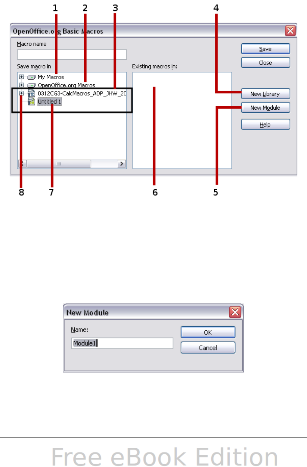
1My Macros 5Create new module in library
2OpenOffice.org Macros 6Macros in selected library
3Open documents 7Current document
4Create new library 8Expand/collapse list
Figure 291: Parts of the OpenOffice.org Basic Macros dialog
10) Click New Module. If no libraries exist, then the Standard library
is automatically created and used. In the New Module dialog, type
a name for the new module or leave the name as Module1.
11) Click OK to create a new module named Module1. Select the
newly created Module1, type PasteMultiply in the Macro name
box at the upper left, and click Save. (See Figure 292.)
Chapter 12 Calc Macros 343
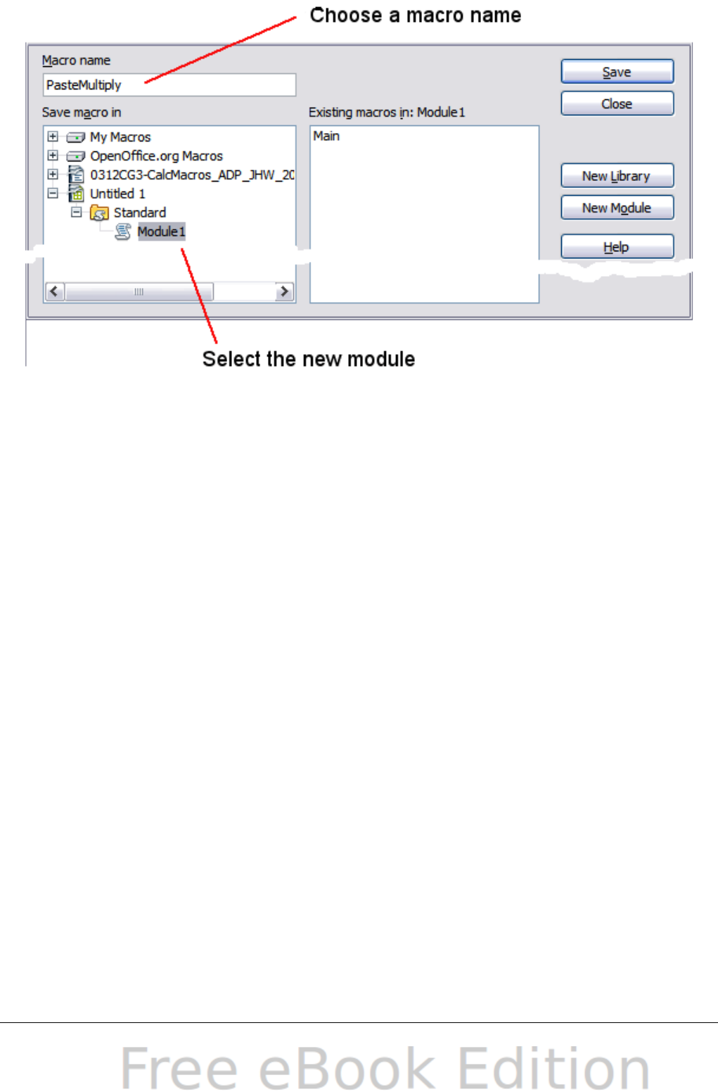
Figure 292: Select the module and name the macro
The created macro is saved in Module1 of the Standard library in the
Untitled 1 document. Listing 1 shows the contents of the macro.
Listing 1. Paste special with multiply.
sub PasteMultiply
rem --------------------------------------------------------------
rem define variables
dim document as object
dim dispatcher as object
rem --------------------------------------------------------------
rem get access to the document
document = ThisComponent.CurrentController.Frame
dispatcher = createUnoService("com.sun.star.frame.DispatchHelper")
rem --------------------------------------------------------------
dim args1(5) as new com.sun.star.beans.PropertyValue
args1(0).Name = "Flags"
args1(0).Value = "A"
args1(1).Name = "FormulaCommand"
args1(1).Value = 3
args1(2).Name = "SkipEmptyCells"
args1(2).Value = false
args1(3).Name = "Transpose"
args1(3).Value = false
args1(4).Name = "AsLink"
args1(4).Value = false
args1(5).Name = "MoveMode"
args1(5).Value = 4
dispatcher.executeDispatch(document, ".uno:InsertContents", "", 0, args1())
end sub
344 OpenOffice.org 3.x Calc Guide
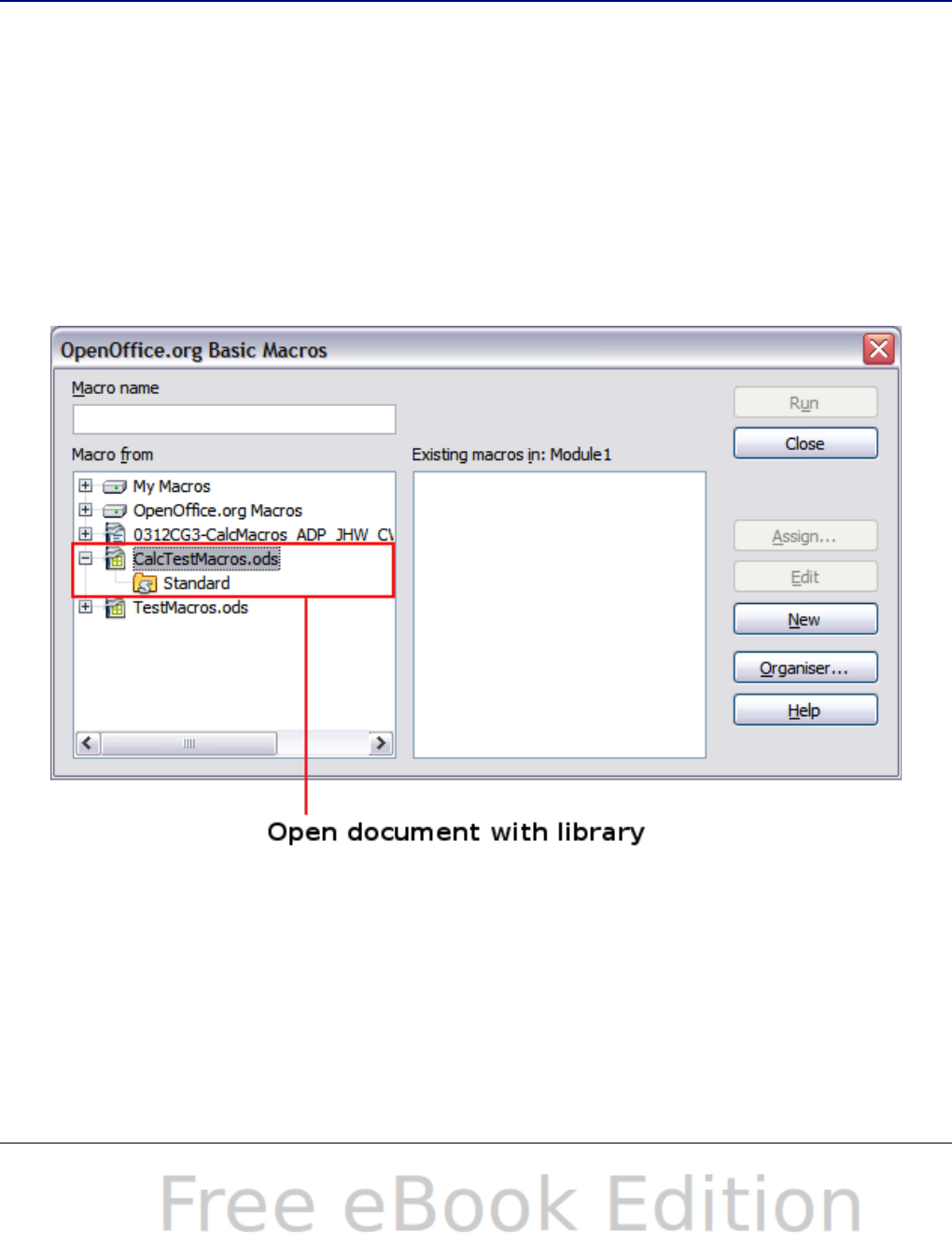
More detail on recording macros is provided in Chapter 13 (Getting
Started with Macros) in the Getting Started guide; we recommend you
read it if you have not already done so. More detail is also provided in
the following sections, but not as related to recording macros.
Write your own functions
Calc can call macros as Calc functions. Use the following steps to
create a simple macro:
1) Create a new Calc document named CalcTestMacros.ods.
2) Use Tools > Macros > Organize Macros > OpenOffice.org
Basic to open the OpenOffice.org Basic Macros dialog. The
Macro from box lists available macro library containers including
currently open OOo documents. My Macros contains macros that
you write or add to OOo. OpenOffice.org Macros contains macros
included with OOo and should not be changed.
Figure 293: OpenOffice.org Basic Macros dialog
3) Click Organizer to open the OpenOffice.org Basic Macro
Organizer dialog. On the Libraries tab, select the document to
contain the macro.
Chapter 12 Calc Macros 345

Figure 294: OpenOffice.org Basic Macro Organizer
4) Click New to open the New Library dialog.
Figure 295: New Library dialog
5) Enter a descriptive library name (such as AuthorsCalcMacros)
and click OK to create the library. The new library name is shown
the library list, but the dialog may show only a portion of the
name.
Figure 296: The library is shown in the organizer
346 OpenOffice.org 3.x Calc Guide
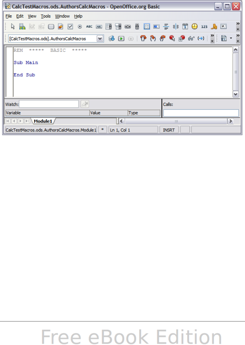
6) Select AuthorsCalcMacros and click Edit to edit the library. Calc
automatically creates a module named Module1 and a macro
named Main.
Figure 297: Basic Integrated Development Environment (IDE)
7) Modify the code so that it is the same as that shown in Listing
2.The important addition is the creation of the NumberFive
function, which returns the number five. The Option Explicit
statement forces all variables to be declared before they are used.
If Option Explicit is omitted, variables are automatically defined
at first use as type Variant.
8) Save the modified Module1.
Listing 2. Function that returns five.
REM ***** BASIC *****
Option Explicit
Sub Main
End Sub
Function NumberFive()
NumberFive = 5
End Function
Chapter 12 Calc Macros 347
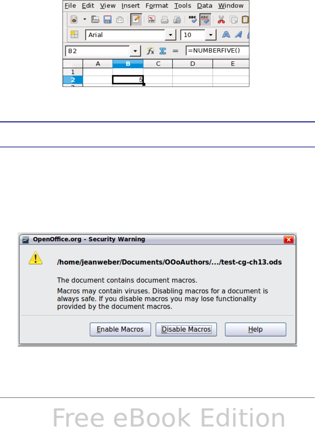
Using a macro as a function
Using the newly created Calc document CalcTestMacros.ods, enter
the formula =NumberFive() (see Figure 298). Calc finds the macro and
calls it.
Figure 298: Use the NumberFive() Macro
as a Calc function
Tip Function names are not case sensitive. In Figure 298, you can
enter =NumberFive() and Calc clearly shows =NUMBERFIVE().
Save the Calc document, close it, and open it again. Depending on your
settings in Tools > Options > OpenOffice.org > Security > Macro
Security, Calc will dislay the warning shown in Figure 299 or the one
shown in Figure 300. You will need to click Enable Macros, or Calc
will not allow any macros to be run inside the document. If you do not
expect a document to contain a macro, it is safer to click Disable
Macros in case the macro is a virus.
Figure 299: OOo warns you that a document contains macros
348 OpenOffice.org 3.x Calc Guide
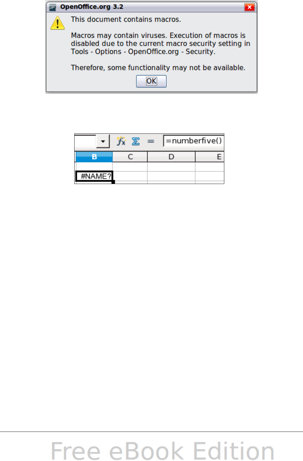
Figure 300: Warning if macros are disabled
If you choose to disable macros, then when the document loads, Calc
can no longer find the function.
Figure 301: The function is gone
When a document is created and saved, it automatically contains a
library named Standard. The Standard library is automatically loaded
when the document is opened. No other library is automatically loaded.
Calc does not contain a function named NumberFive(), so it checks all
opened and visible macro libraries for the function. Libraries in
OpenOffice.org Macros, My Macros, and the Calc document are
checked for an appropriately named function (see Figure 291). The
NumberFive() function is stored in the AuthorsCalcMacros library,
which is not automatically loaded when the document is opened.
Use Tools > Macros > Organize Macros > OpenOffice.org Basic
to open the OpenOffice.org Basic Macros dialog (see Figure 302).
Expand CalcTestMacros and find AuthorsCalcMacros. The icon for a
loaded library is a different color from the icon for a library that is not
loaded.
Click the expansion symbol (usually a plus or a triangle) next to
AuthorsCalcMacros to load the library. The icon changes color to
indicate that the library is now loaded. Click Close to close the dialog.
Unfortunately, the cells containing =NumberFive() are in error. Calc
does not recalculate cells in error unless you edit them or somehow
change them. The usual solution is to store macros used as functions in
the Standard library. If the macro is large or if there are many macros,
Chapter 12 Calc Macros 349
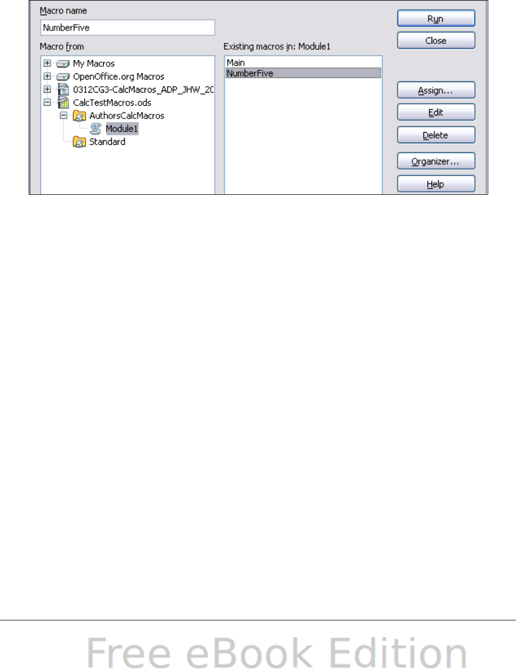
a stub with the desired name is stored in the Standard library. The stub
macro loads the library containing the implementation and then calls
the implementation.
1) Use Tools > Macros > Organize Macros > OpenOffice.org
Basic to open the OpenOffice.org Basic Macros dialog. Select the
NumberFive macro and click Edit to open the macro for editing.
Figure 302: Select a macro and click Edit
2) Change the name of NumberFive to NumberFive_Implementation
(see Listing 3).
Listing 3. Change the name of NumberFive to
NumberFive_Implementation
Function NumberFive_Implementation()
NumberFive_Implementation() = 5
End Function
3) In the Basic IDE (see Figure 297), hover the mouse cursor over
the toolbar buttons to display the tool tips. Click the Select
Macro button to open the OpenOffice.org Basic Macros dialog
(see Figure 302).
4) Select the Standard library in the CalcTestMacros document and
click New to create a new module. Enter a meaningful name such
as CalcFunctions and click OK. OOo automatically creates a
macro named Main and opens the module for editing.
5) Create a macro in the Standard library that calls the
implementation function (see Listing 4). The new macro loads the
AuthorsCalcMacros library if it is not already loaded, and then
calls the implementation function.
350 OpenOffice.org 3.x Calc Guide

6) Save, close, and reopen the Calc document. This time, the
NumberFive() function works.
Listing 4. Change the name of NumberFive to
NumberFive_Implementation.
Function NumberFive()
If NOT BasicLibraries.isLibraryLoaded("AuthorsCalcMacros") Then
BasicLibraries.LoadLibrary("AuthorsCalcMacros")
End If
NumberFive = NumberFive_Implementation()
End Function
Passing arguments to a macro
To illustrate a function that accepts arguments, we will write a macro
that calculates the sum of its arguments that are positive —it will
ignore arguments that are less than zero (see Listing 5).
Listing 5. PositiveSum calculates the sum of the positive arguments.
Function PositiveSum(Optional x)
Dim TheSum As Double
Dim iRow As Integer
Dim iCol As Integer
TheSum = 0.0
If NOT IsMissing(x) Then
If NOT IsArray(x) Then
If x > 0 Then TheSum = x
Else
For iRow = LBound(x, 1) To UBound(x, 1)
For iCol = LBound(x, 2) To UBound(x, 2)
If x(iRow, iCol) > 0 Then TheSum = TheSum + x(iRow, iCol)
Next
Next
End If
End If
PositiveSum = TheSum
End Function
The macro in Listing 5 demonstrates a couple of important techniques:
1) The argument x is optional. If the argument is not optional and it
is called without an argument, OOo prints a warning message
every time the macro is called. If Calc calls the function many
times, then the error is displayed many times.
2) IsMissing checks that an argument was passed before the
argument is used.
Chapter 12 Calc Macros 351

3) IsArray checks to see if the argument is a single value, or an
array. For example, =PositiveSum(7) or =PositiveSum(A4). In
the first case, the number 7 is passed as an argument, and in the
second case, the value of cell A4 is passed to the function.
4) If a range is passed to the function, it is passed as a two-
dimensional array of values; for example, =PositiveSum(A2:B5).
LBound and UBound are used to determine the array bounds that
are used. Although the lower bound is one, it is considered safer
to use LBound in case it changes in the future.
Tip
The macro in Listing 5 is careful and checks to see if the
argument is an array or a single argument. The macro does not
verify that each value is numeric. You may be as careful as you
like. The more things you check, the more robust the macro is,
and the slower it runs.
Passing one argument is as easy as passing two: add another argument
to the function definition (see Listing 6). When calling a function with
two arguments, separate the arguments with a semicolon; for example,
=TestMax(3; -4).
Listing 6. TestMax accepts two arguments and returns the larger of
the two.
Function TestMax(x, y)
If x >= y Then
TestMax = x
Else
TestMax = y
End If
End Function
Arguments are passed as values
Arguments passed to a macro from Calc are always values. It is not
possible to know what cells, if any, are used. For example,
=PositiveSum(A3) passes the value of cell A3, and PositiveSum has no
way of knowing that cell A3 was used. If you must know which cells are
referenced rather than the values in the cells, pass the range as a
string, parse the string, and obtain the values in the referenced cells.
352 OpenOffice.org 3.x Calc Guide

Writing macros that act like built-in functions
Although Calc finds and calls macros as normal functions, they do not
really behave as built-in functions. For example, macros do not appear
in the function lists. It is possible to write functions that behave as
regular functions by writing an Add-In. However, this is an advanced
topic that is not covered here; see
http://wiki.services.openoffice.org/wiki/SimpleCalcAddIn.
Accessing cells directly
You can access the OOo internal objects directly to manipulate a Calc
document. For example, the macro in Listing 7 adds the values in cell
A2 from every sheet in the current document. ThisComponent is set by
StarBasic when the macro starts to reference the current document. A
Calc document contains sheets: ThisComponent.getSheets(). Use
getCellByPosition(col, row) to return a cell at a specific row and
column.
Listing 7. Add cell A2 in every sheet.
Function SumCellsAllSheets()
Dim TheSum As Double
Dim i As integer
Dim oSheets
Dim oSheet
Dim oCell
oSheets = ThisComponent.getSheets()
For i = 0 To oSheets.getCount() - 1
oSheet = oSheets.getByIndex(i)
oCell = oSheet.getCellByPosition(0, 1) ' GetCell A2
TheSum = TheSum + oCell.getValue()
Next
SumCellsAllSheets = TheSum
End Function
Tip
A cell object supports the methods getValue(), getString(),
and getFormula() to get the numerical value, the string value, or
the formula used in a cell. Use the corresponding set functions to
set appropriate values.
Use oSheet.getCellRangeByName("A2") to return a range of cells by
name. If a single cell is referenced, then a cell object is returned. If a
cell range is given, then an entire range of cells is returned (see
Listing 8). Notice that a cell range returns data as an array of arrays,
Chapter 12 Calc Macros 353
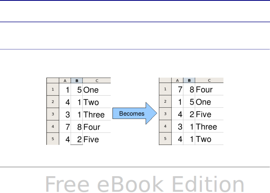
which is more cumbersome than treating it as an array with two
dimensions as is done in Listing 5.
Listing 8. Add cell A2:C5 in every sheet
Function SumCellsAllSheets()
Dim TheSum As Double
Dim iRow As Integer, iCol As Integer, i As Integer
Dim oSheets, oSheet, oCells
Dim oRow(), oRows()
oSheets = ThisComponent.getSheets()
For i = 0 To oSheets.getCount() - 1
oSheet = oSheets.getByIndex(i)
oCells = oSheet.getCellRangeByName("A2:C5")
REM getDataArray() returns the data as variant so strings
REM are also returned.
REM getData() returns data data as type Double, so only
REM numbers are returned.
oRows() = oCells.getData()
For iRow = LBound(oRows()) To UBound(oRows())
oRow() = oRows(iRow)
For iCol = LBound(oRow()) To UBound(oRow())
TheSum = TheSum + oRow(iCol)
Next
Next
Next
SumCellsAllSheets = TheSum
End Function
Tip When a macro is called as a Calc function, the macro cannot
modify any value in the sheet from which the macro was called.
Sorting
Consider sorting the data in Figure 288. First, sort on column B
descending and then column A ascending.
Figure 303: Sort column B descending and column A ascending
354 OpenOffice.org 3.x Calc Guide

The example in Listing 9, however, demonstrates how to sort on two
columns.
Listing 9. Sort cells A1:C5 on Sheet 1.
Sub SortRange
Dim oSheet ' Calc sheet containing data to sort.
Dim oCellRange ' Data range to sort.
REM An array of sort fields determines the columns that are
REM sorted. This is an array with two elements, 0 and 1.
REM To sort on only one column, use:
REM Dim oSortFields(0) As New com.sun.star.util.SortField
Dim oSortFields(1) As New com.sun.star.util.SortField
REM The sort descriptor is an array of properties.
REM The primary property contains the sort fields.
Dim oSortDesc(0) As New com.sun.star.beans.PropertyValue
REM Get the sheet named "Sheet1"
oSheet = ThisComponent.Sheets.getByName("Sheet1")
REM Get the cell range to sort
oCellRange = oSheet.getCellRangeByName("A1:C5")
REM Select the range to sort.
REM The only purpose would be to emphasize the sorted data.
'ThisComponent.getCurrentController.select(oCellRange)
REM The columns are numbered starting with 0, so
REM column A is 0, column B is 1, etc.
REM Sort column B (column 1) descending.
oSortFields(0).Field = 1
oSortFields(0).SortAscending = FALSE
REM If column B has two cells with the same value,
REM then use column A ascending to decide the order.
oSortFields(1).Field = 0
oSortFields(1).SortAscending = True
REM Setup the sort descriptor.
oSortDesc(0).Name = "SortFields"
oSortDesc(0).Value = oSortFields()
REM Sort the range.
oCellRange.Sort(oSortDesc())
End Sub
Chapter 12 Calc Macros 355

Conclusion
This chapter provides a brief overview on how to create libraries and
modules, using the macro recorder, using macros as Calc functions,
and writing your own macros without the macro recorder. Each topic
deserves at least one chapter, and writing your own macros for Calc
could easily fill an entire book. In other words, this is just the
beginning of what you can learn!
356 OpenOffice.org 3.x Calc Guide

Chapter 13
Calc as a Simple Database
A guide for users and macro programmers
Introduction
A Calc document is a very capable database, providing sufficient
functionality to satisfy the needs of many users. This chapter presents
the capabilities of a Calc document that make it suitable as a database
tool. Where applicable, the functionality is explained using both the
GUI (Graphical User Interface) and macros.
Note
Although this document was initially created for macro
programmers, the content should be accessible to all users. If you
do not use macros, then skip those portions that deal with
macros. On the other hand, if you want to learn more about
macros, be certain to check out the book OpenOffice.org Macros
Explained.
In a database, a record is a group of related data items treated as a
single unit of information. Each item in the record is called a field. A
table consists of records. Each record in a table has the same
structure. A table can be visualized as a series of rows and columns.
Each row in the table corresponds to a single record and each column
corresponds to the fields. A spreadsheet in a Calc document is similar
in structure to a database table. Each cell corresponds to a single field
in a database record. For many people, Calc implements sufficient
database functionality that no other database program or functionality
is required.
While teaching, a spreadsheet might be used as a grading program.
Each row represents a single student. The columns represent the
grades received on homework, labs, and tests (see Table 12). The
strong calculation capability provided in a spreadsheet makes this an
excellent choice.
Table 12. Simple grading spreadsheet
A B C D E F G
1Name Test 1 Test 2 Quiz 1 Quiz 2 Average Grade
2Andy 95 93 93 92 93.25
3Betty 87 92 65 73 79.25
4Bob 95 93 93 92 93.25
5Brandy 45 65 92 85 71.75
6Frank 95 93 85 92 91.25
7Fred 87 92 65 73 79.25
358 OpenOffice.org 3.x Calc Guide
A B C D E F G
8Ilsub 70 85 97 79 82.75
9James 45 65 97 85 73
10 Lisa 100 97 100 93 97.5
11 Michelle 100 97 100 65 90.5
12 Ravi 87 92 86 93 89.5
13 Sal 45 65 100 92 75.5
14 Ted 100 97 100 85 95.5
15 Tom 70 85 93 65 78.25
16 Whil 70 85 93 97 86.25
Tip
Although the choice to associate a row to a record rather than a
column is arbitrary, it is almost universal. In other words, you are
not likely to hear someone refer to a column of data as a single
database record.
Associating a range with a name
In a Calc document, a range refers to a contiguous group of cells
containing at least one cell. You can associate a meaningful name to a
range, which allows you to refer to the range using the meaningful
name. You can create either a database range, which has some
database-like functionality, or a named range, which does not. A name
is usually associated with a range for one of three reasons:
1) Associating a range with a name enhances readability by using a
meaningful name.
2) If a range is referenced by name in multiple locations, you can
point the name to another location and all references point to the
new location.
3) Ranges associated to a name are shown in the Navigator, which is
available by pressing the F5 key or clicking on the icon. The
Navigator allows for quick navigation to the associated ranges.
Named range
The most common usage of a named range is, as its name implies, to
associate a range of cells to a meaningful name. For example, I created
Chapter 13 Calc as a Simple Database 359
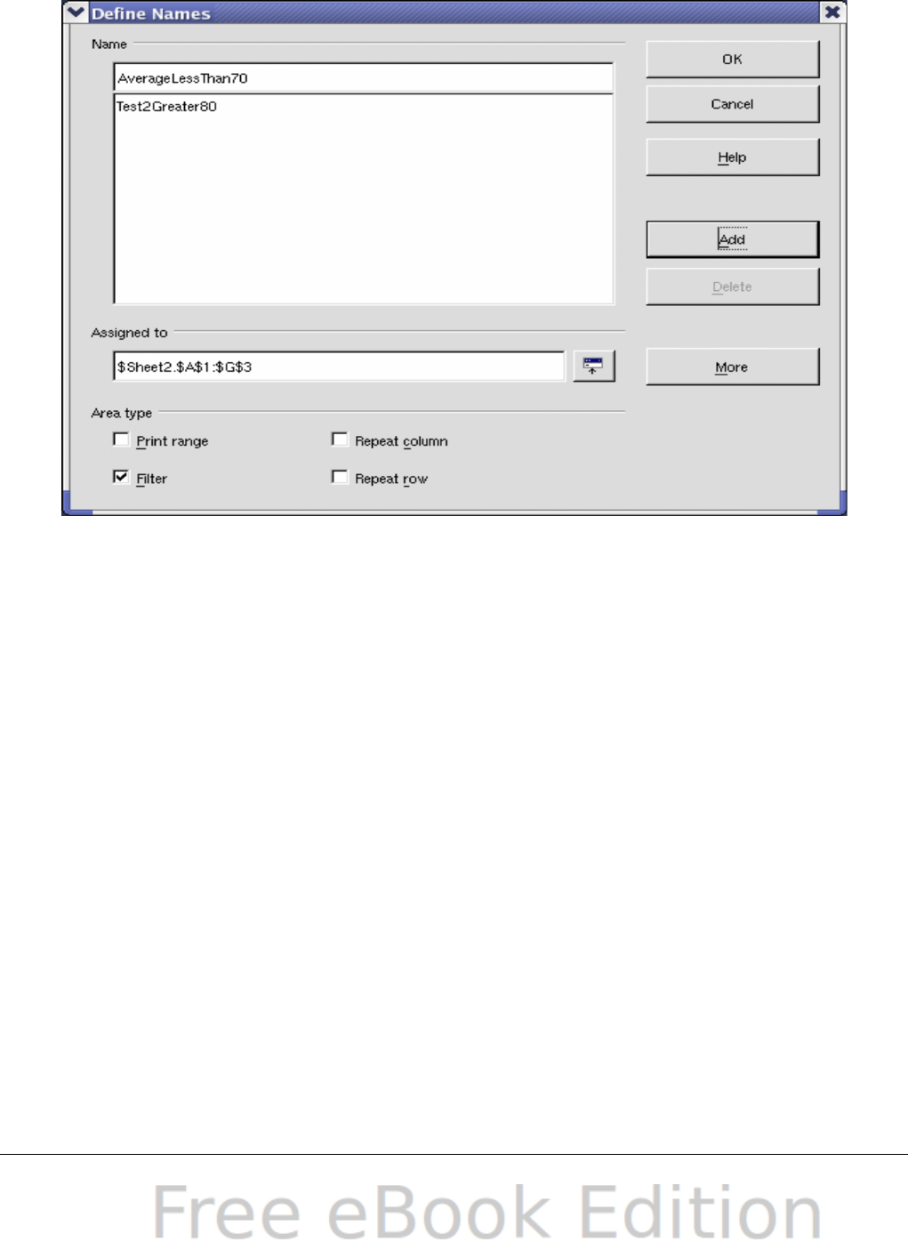
a range named Scores, and then I used the following equation:
=SUM(Scores). To create a named range, select the range to define.
Use Insert > Names > Define to open the Define Names dialog. Use
the Define Names dialog to add and modify one named range at a time.
Figure 304. Define a named range.
In a macro, a named range is accessed, created, and deleted using the
NamedRanges property of a Calc document. Use the methods
hasByName(name) and getByName(name) to verify and retrieve a
named range. The method getElementNames() returns an array
containing the names of all named ranges. The NamedRanges object
supports the method addNewByname, which accepts four arguments;
the name, content, position, and type. The macro in Listing 10 creates
a named range, if it does not exist, that references a range of cells.
Listing 10. Create a named range that references $Sheet1.$B$3:$D$6.
Sub AddNamedRange()
Dim oRange ' The created range.
Dim oRanges ' All named ranges.
Dim sName$ ' Name of the named range to create.
Dim oCell ' Cell object.
Dim s$
sName$ = "MyNRange"
oRanges = ThisComponent.NamedRanges
360 OpenOffice.org 3.x Calc Guide
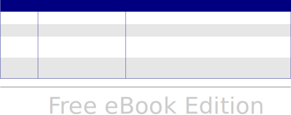
If NOT oRanges.hasByName(sName$) Then
REM I can obtain the cell address by obtaining the cell
REM and then extracting the address from the cell.
Dim oCellAddress As new com.sun.star.table.CellAddress
oCellAddress.Sheet = 0 'The first sheet.
oCellAddress.Column = 1 'Column B.
oCellAddress.Row = 2 'Row 3.
REM The first argument is the range name.
REM The second argument is formula or expression to
REM use. The second argument is usually a string that
REM defines a range.
REM The third argument specifies the base address for
REM relative cell references.
REM The fourth argument is a set of flags that define
REM how the range is used, but most ranges use 0.
REM The fourth argument uses values from the
REM NamedRangeFlag constants (see Table 13).
s$ = "$Sheet1.$B$3:$D$6"
oRanges.addNewByName(sName$, s$, oCellAddress, 0)
End If
REM Get a range using the created named range.
oRange = ThisComponent.NamedRanges.getByName(sName$)
REM Print the string contained in cell $Sheet1.$B$3
oCell = oRange.getReferredCells().getCellByPosition(0,0)
Print oCell.getString()
End Sub
The method addNewByname() accepts four arguments; the name,
content, position, and type. The fourth argument to the method
addNewByName() is a combination of flags that specify how the named
range will be used (see Table 13). The most common value is 0, which
is not a defined constant value.
Table 13. com.sun.star.sheet.NamedRangeFlag constants.
Value Name Description
1 FILTER_CRITERIA The range contains filter criteria.
2 PRINT_AREA The range can be used as a print range.
4 COLUMN_HEADER The range can be used as column headers
for printing.
8 ROW_HEADER The range can be used as row headers for
printing.
Chapter 13 Calc as a Simple Database 361

The third argument, a cell address, acts as the base address for cells
referenced in a relative way. If the cell range is not specified as an
absolute address, the referenced range will be different based on
where in the spreadsheet the range is used. The relative behavior is
illustrated in Listing 11, which also illustrates another usage of a
named range—defining an equation. The macro in Listing 11 creates
the named range AddLeft, which refers to the equation A3+B3 with C3
as the reference cell. The cells A3 and B3 are the two cells directly to
the left of C3, so, the equation =AddLeft() calculates the sum of the
two cells directly to the left of the cell that contains the equation.
Changing the reference cell to C4, which is below A3 and B3, causes
the AddLeft equation to calculate the sum of the two cells that are to
the left on the previous row.
Listing 11. Create the AddLeft named range.
Sub AddNamedFunction()
Dim oSheet 'Sheet that contains the named range.
Dim oCellAddress 'Address for relative references.
Dim oRanges 'The NamedRanges property.
Dim oRange 'Single cell range.
Dim sName As String 'Name of the equation to create.
sName = "AddLeft"
oRanges = ThisComponent.NamedRanges
If NOT oRanges.hasByName(sName) Then
oSheet = ThisComponent.getSheets().getByIndex(0)
oRange = oSheet.getCellRangeByName("C3")
oCellAddress = oRange.getCellAddress()
oRanges.addNewByName(sName, "A3+B3", oCellAddress, 0)
End If
End Sub
Tip
Listing 11 illustrates two capabilities that are not widely known.
A named range can define a function. Also, the third argument
acts as the base address for cells referenced in a relative way.
Select the range containing the headers and the data and then use
Insert > Names > Create to open the Create Names dialog (see
Figure 305), which allows you to simultaneously create multiple named
ranges based on the top row, bottom row, right column or left column.
If you choose to create ranges based on the top row, one named range
is created for each column header—the header is not included in the
named range. Although the header is not included in the range, the
text in the header is used to name the range.
362 OpenOffice.org 3.x Calc Guide
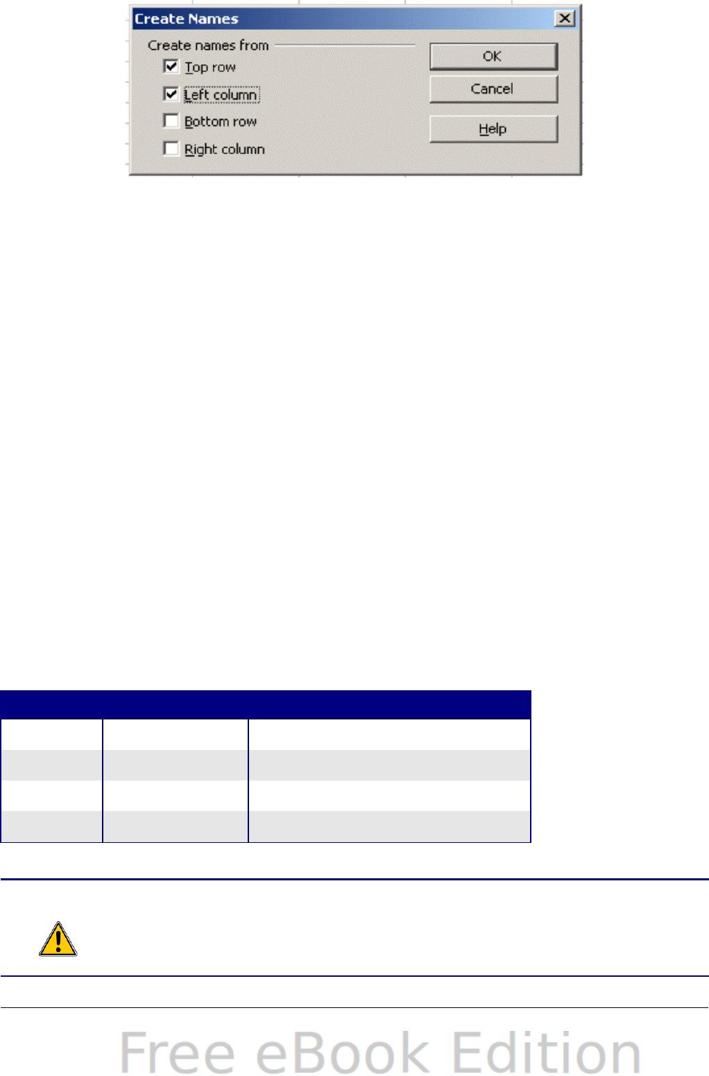
Figure 305. Define a named range.
The macro in Listing 12 creates three named ranges based on the top
row of a named range.
Listing 12. Create many named ranges.
Sub AddManyNamedRanges()
Dim oSheet 'Sheet that contains the named range.
Dim oAddress 'Range address.
Dim oRanges 'The NamedRanges property.
Dim oRange 'Single cell range.
oRanges = ThisComponent.NamedRanges
oSheet = ThisComponent.getSheets().getByIndex(0)
oRange = oSheet.getCellRangeByName("A1:C20")
oAddress = oRange.getRangeAddress()
oRanges.addNewFromTitles(oAddress, _
com.sun.star.sheet.Border.TOP)
End Sub
The constants in Table 14 determine the location of the headers when
multiple ranges are created using the method addNewFromTitles().
Table 14. com.sun.star.sheet.Border constants.
Value Name Description
0 TOP Select the top border.
1 BOTTOM Select the bottom border.
2 RIGHT Select the right border.
3 LEFT Select the left border.
Caution It is possible to create multiple named ranges with the same
name. Creating multiple ranges with a single command
increases the likelihood that multiple ranges will be created
with the same name—avoid this if possible.
Chapter 13 Calc as a Simple Database 363
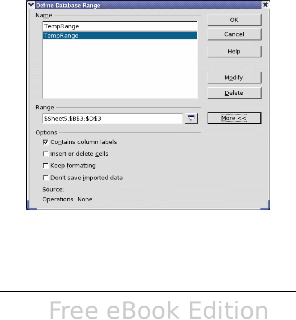
Database range
Although a database range can be used as a regular named range, a
database range also defines a range of cells in a spreadsheet to be
used as a database. Each row in a range corresponds to a record and
each cell corresponds to a field. You can sort, group, search, and
perform calculations on the range as if it were a database.
A database range provides behavior that is useful when performing
database related activities. For example, you can mark the first row as
headings. To create, modify, or delete a database range, use Data >
Define Range to open the Define Data Range dialog (see Figure 306).
When you first define a range, the Modify button shown in the example
is labeled New.
Figure 306. Define a database range.
In a macro, a database range is accessed, created, and deleted from
the DatabaseRanges property. The macro in Listing 13 creates a
database range named MyName and sets the range to be used as an
auto filter.
364 OpenOffice.org 3.x Calc Guide
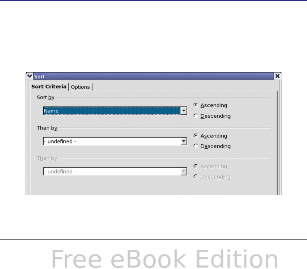
Listing 13. Create a database range and an auto filter.
Sub AddNewDatabaseRange()
Dim oRange 'DatabaseRange object.
Dim oAddr 'Cell address range for the database range.
Dim oSheet 'First sheet, which will contain the range.
Dim oDoc 'Reference ThisComponent with a shorter name.
oDoc = ThisComponent
If NOT oDoc.DatabaseRanges.hasByName("MyName") Then
oSheet = ThisComponent.getSheets().getByIndex(0)
oRange = oSheet.getCellRangeByName("A1:F10")
oAddr = oRange.getRangeAddress()
oDoc.DatabaseRanges.addNewByName("MyName", oAddr)
End If
oRange = oDoc.DatabaseRanges.getByName("MyName")
oRange.AutoFilter = True
End Sub
Sorting
The sorting mechanism in a Calc document rearranges the data in the
sheet. The first step in sorting data is to select the data that you want
to sort. To sort the data in Table 23, select the cells from A1 to G16—if
you include the column headers, indicate this in the sort dialog (see
Figure 308). Use Data > Sort to open the Sort dialog (see Figure 307).
You can sort by up to three columns or rows at a time.
Figure 307. Sort by the Name column.
Chapter 13 Calc as a Simple Database 365
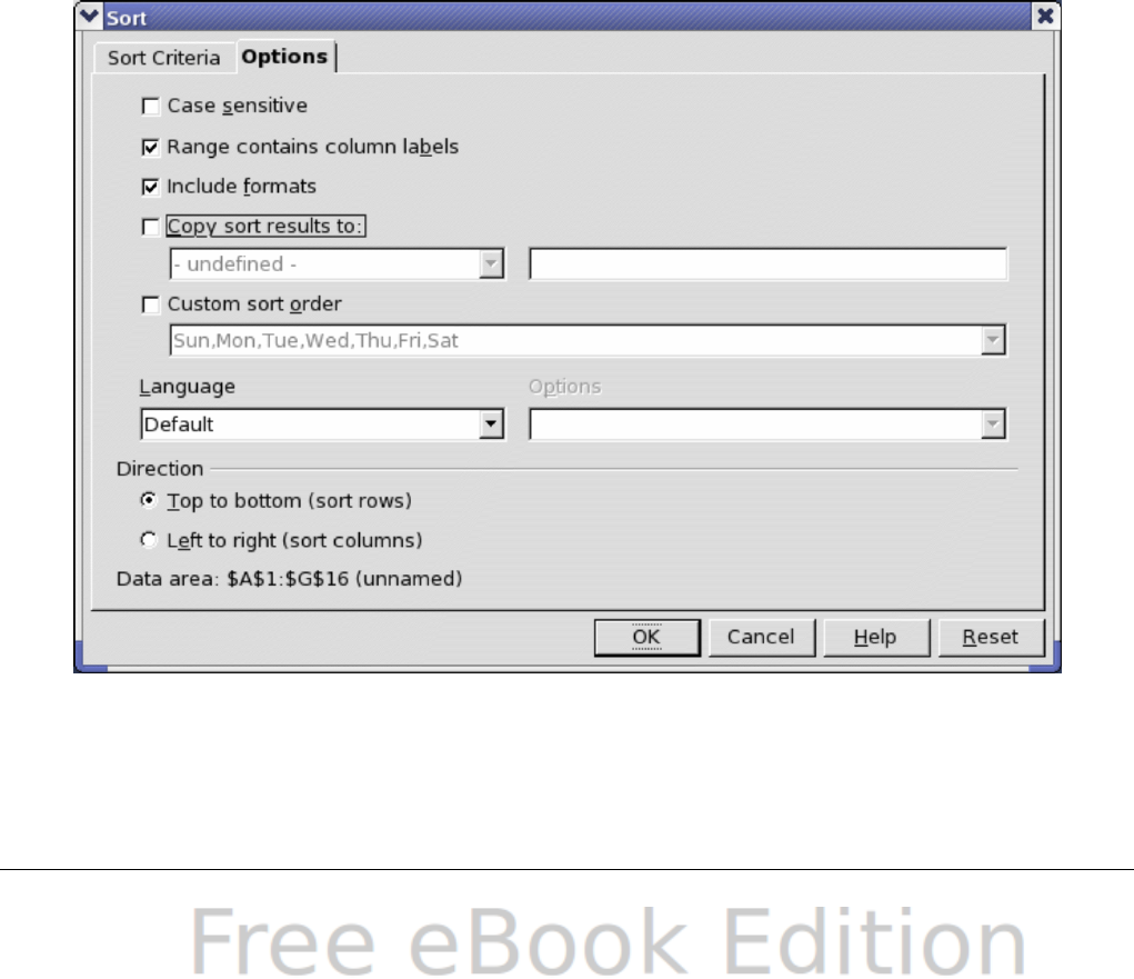
Click on the Options tab (see Figure 308) to set the sort options. Check
the Range contains column labels checkbox to prevent column
headers from being sorted with the rest of the data. The Sort by list
box in Figure 307 displays the columns using the column headers if the
Range contains column labels checkbox in Figure 308 is checked. If
the Range contains column labels checkbox is not checked,
however, then the columns are identified by their column name;
Column A, for example.
Normally, sorting the data causes the existing data to be replaced by
the newly sorted data. The Copy sort results to checkbox, however,
causes the selected data to be left unchanged and a copy of the sorted
data is copied to the specified location. You can either directly enter a
target address (Sheet3.A1, for example) or select a predefined range.
Check the Custom sort order checkbox to sort based on a predefined
list of values. To set your own predefined lists, use Tools > Options >
OpenOffice.org Calc > Sort Lists and then enter your own sort lists.
Predefined sort lists are useful for sorting lists of data that should not
be sorted alphabetically or numerically. For example, sorting days
based on their name.
Figure 308. Set sort options.
366 OpenOffice.org 3.x Calc Guide
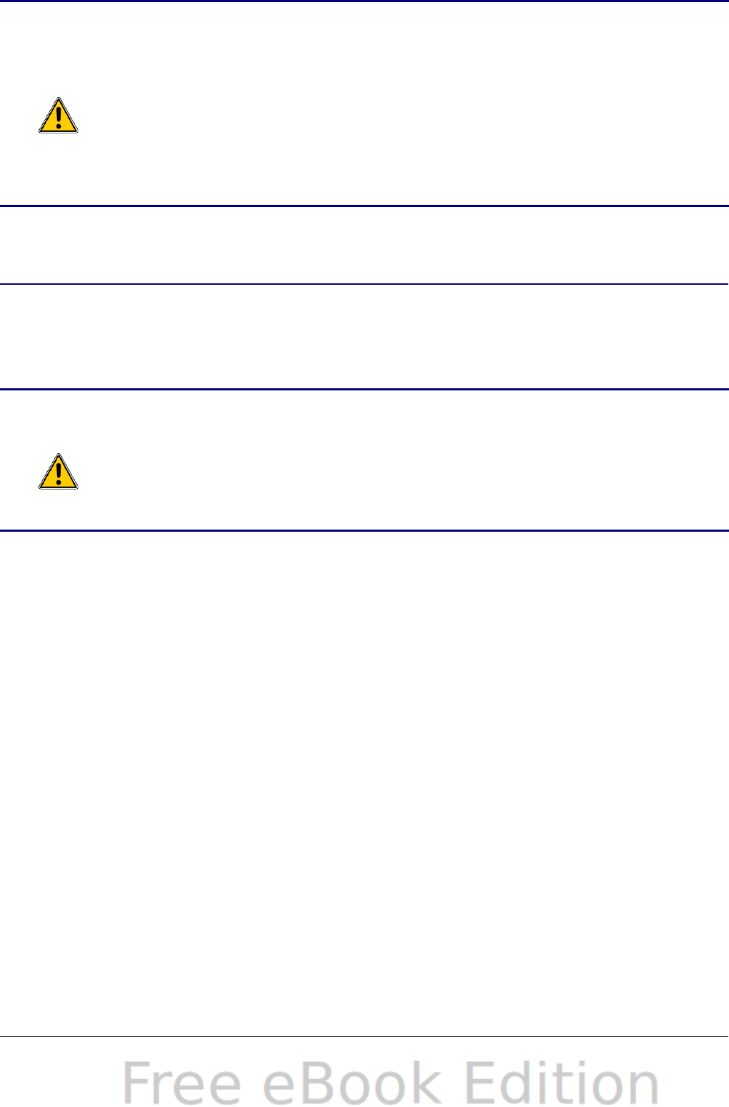
Caution
When a cell is moved during a sort operation, external
references to that cell are not updated. If a cell that contains a
relative reference to another cell is moved, the reference is
relative to the new position when sorting is finished. Know the
behavior of references during sorting and do not be alarmed;
this is almost always what you want—because the reference is
to the right or left in the same row. Also, we have not found a
spreadsheet program that exhibits a different behavior for
references while sorting.
Filters
Use filters to limit the visible rows in a spreadsheet. Generic filters,
common to all sorts of data manipulations, are automatically provided
by the auto filter capability. You can also define your own filters.
Caution
After applying a filter, some rows are visible and some rows are
not. If you select multiple rows in one operation, you will also
select the invisible rows contained between the selected visible
rows. Operations, such as delete, act on all of the selected
rows. To avoid this problem, you must individually select each
of the filtered rows using the control key.
Auto filters
Use auto filters to quickly create easily accessible filters found to be
commonly used in many different types of applications. After creating
an auto filter for a specific column, a combo box is added to the
column. The combo box provides quick access to each of the auto filter
types.
•The All auto filter causes all rows to be visible.
•The Standard auto filter opens the Standard Filter dialog and is
the same as the standard filter.
•The Top 10 auto filter displays the ten rows with the largest value.
If the value 70 is in the top ten values, then all rows containing
the value 70 in the filtered column are displayed. In other words,
more than ten rows may be displayed.
•An auto filter entry is created for each unique entry in the
column.
Chapter 13 Calc as a Simple Database 367
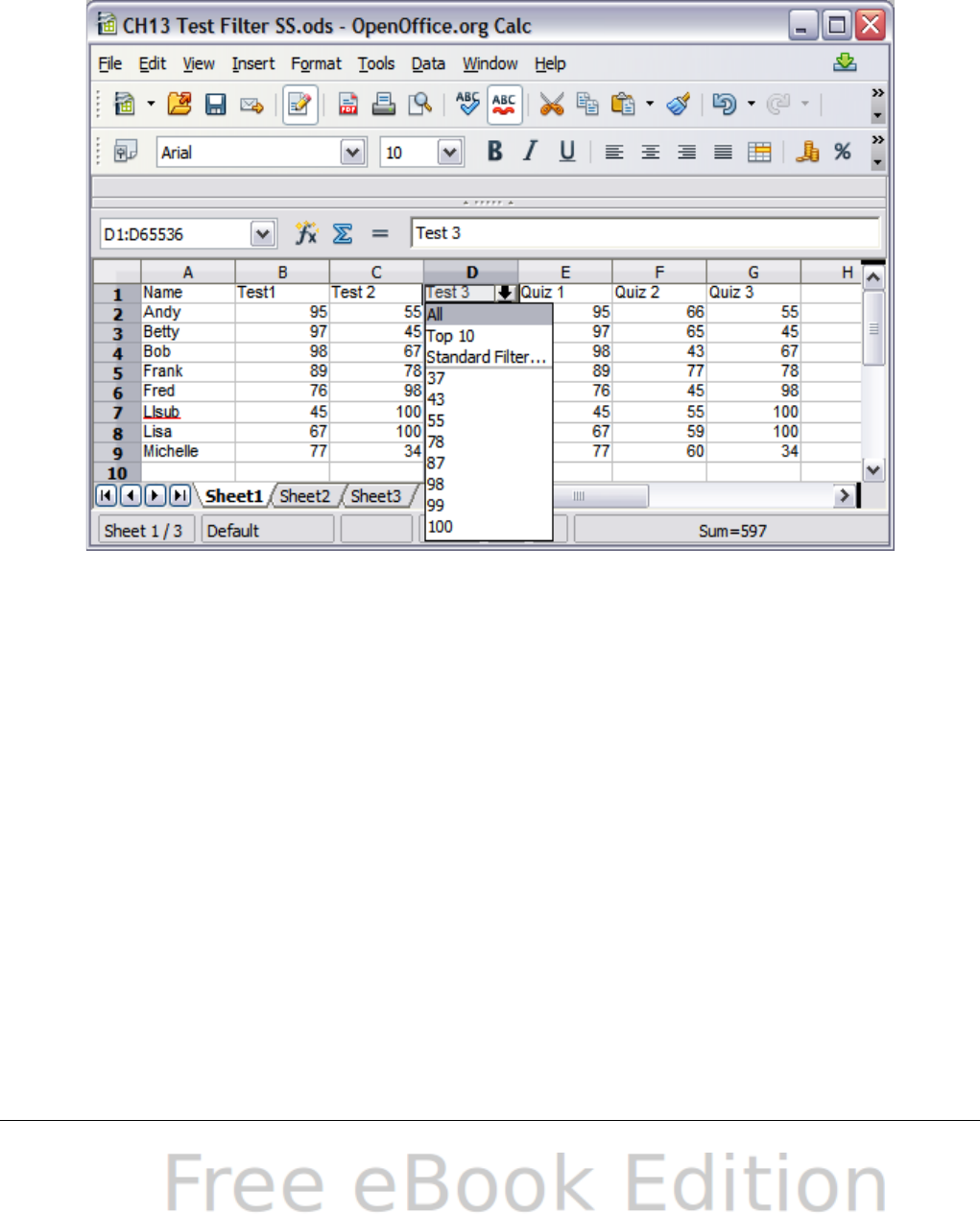
To create an auto filter, first select the columns to filter. For example,
using the data in Table 12, select data in columns B and C. If you do
not select the title rows, Calc asks if the title row or the current row
should be used. Although you can place the auto filter in any row, only
the rows below the auto filter are filtered. Use Data > Filter >
AutoFilter to insert the auto filter combo box in the appropriate cell.
Finally, use the drop-down arrow to choose an appropriate auto filter
(see Figure 309).
Figure 309: Use an auto filter with column C
Remove an auto filter by repeating the steps to create the auto filter—
in other words, the menu option acts as a toggle to turn the auto filter
on and off. When an auto filter is removed, the combo box is removed
from the cell. The macro in Listing 13 demonstrates creating an auto
filter for a range.
Standard filters
Use Data > Filter > Standard Filter to open Standard Filter dialog
(see Figure 310) and limit the view based on 1 to 3 filter conditions.
Use Data > Filter > Remove Filter to turn off the filter.
368 OpenOffice.org 3.x Calc Guide
Figure 310: Use the standard filter
The macro in Listing 14 creates a simple filter for the first sheet.
Listing 14. Create a simple sheet filter.
Sub SimpleSheetFilter()
Dim oSheet ' Sheet that will contain the filter.
Dim oFilterDesc ' Filter descriptor.
Dim oFields(0) As New com.sun.star.sheet.TableFilterField
oSheet = ThisComponent.getSheets().getByIndex(0)
REM If argument is True, creates an empty filter
REM descriptor. If argument is False, create a
REM descriptor with the previous settings.
oFilterDesc = oSheet.createFilterDescriptor(True)
With oFields(0)
REM I could use the Connection property to indicate
REM how to connect to the previous field. This is
REM the first field so this is not required.
'.Connection = com.sun.star.sheet.FilterConnection.AND
'.Connection = com.sun.star.sheet.FilterConnection.OR
REM The Field property is the zero based column
REM number to filter. If you have the cell, you
REM can use .Field = oCell.CellAddress.Column.
Chapter 13 Calc as a Simple Database 369

.Field = 5
REM Compare using a numeric or a string?
.IsNumeric = True
REM The NumericValue property is used
REM because .IsNumeric = True from above.
.NumericValue = 80
REM If IsNumeric was False, then the
REM StringValue property would be used.
REM .StringValue = "what ever"
REM Valid operators include EMPTY, NOT_EMPTY, EQUAL,
REM NOT_EQUAL, GREATER, GREATER_EQUAL, LESS,
REM LESS_EQUAL, TOP_VALUES, TOP_PERCENT,
REM BOTTOM_VALUES, and BOTTOM_PERCENT
.Operator = com.sun.star.sheet.FilterOperator.GREATER_EQUAL
End With
REM The filter descriptor supports the following
REM properties: IsCaseSensitive, SkipDuplicates,
REM UseRegularExpressions,
REM SaveOutputPosition, Orientation, ContainsHeader,
REM CopyOutputData, OutputPosition, and MaxFieldCount.
oFilterDesc.setFilterFields(oFields())
oFilterDesc.ContainsHeader = True
oSheet.filter(oFilterDesc)
End Sub
When a filter is applied to a sheet, it replaces any existing filter for the
sheet. Setting an empty filter in a sheet will therefore remove all filters
for that sheet (see Listing 15).
Listing 15. Remove the current sheet filter.
Sub RemoveSheetFilter()
Dim oSheet ' Sheet to filter.
Dim oFilterDesc ' Filter descriptor.
oSheet = ThisComponent.getSheets().getByIndex(0)
oFilterDesc = oSheet.createFilterDescriptor(True)
oSheet.filter(oFilterDesc)
End Sub
370 OpenOffice.org 3.x Calc Guide

Listing 16 demonstrates a more advanced filter that filters two
columns and uses regular expressions. I noticed some unexpected
behavior while working with Listing 16. Although you can create a
filter descriptor using any sheet cell range, the filter applies to the
entire sheet.
Listing 16. A simple sheet filter using two columns.
Sub SimpleSheetFilter_2()
Dim oSheet ' Sheet to filter.
Dim oRange ' Range to be filtered.
Dim oFilterDesc ' Filter descriptor.
Dim oFields(1) As New com.sun.star.sheet.TableFilterField
oSheet = ThisComponent.getSheets().getByIndex(0)
oRange = oSheet.getCellRangeByName("E12:G19")
REM If argument is True, creates an
REM empty filter descriptor.
oFilterDesc = oRange.createFilterDescriptor(True)
REM Setup a field to view cells with content that
REM start with the letter b.
With oFields(0)
.Field = 0 ' Filter column A.
.IsNumeric = False ' Use a string, not a number.
.StringValue = "b.*" ' Everything starting with b.
.Operator = com.sun.star.sheet.FilterOperator.EQUAL
End With
REM Setup a field that requires both conditions and
REM this new condition requires a value greater or
REM equal to 70.
With oFields(1)
.Connection = com.sun.star.sheet.FilterConnection.AND
.Field = 5 ' Filter column F.
.IsNumeric = True ' Use a number
.NumericValue = 70 ' Values greater than 70
.Operator = com.sun.star.sheet.FilterOperator.GREATER_EQUAL
End With
oFilterDesc.setFilterFields(oFields())
oFilterDesc.ContainsHeader = False
oFilterDesc.UseRegularExpressions = True
oSheet.filter(oFilterDesc)
End Sub
Chapter 13 Calc as a Simple Database 371
Advanced filters
An advanced filter supports up to eight filter conditions, as opposed to
the three supported by the simple filter. The criteria for an advanced
filter is stored in a sheet. The first step in creating an advanced filter is
entering the filter criteria into the spreadsheet.
1) Select an empty space in the Calc document. The empty space
may reside in any sheet in any location in the Calc document.
2) Duplicate the column headings from the area to be filtered into
the area that will contain the filter criteria.
3) Enter the filter criteria underneath the column headings (see
Table 24). The criterion in each column of a row is connected with
AND. The criteria from each row are connected with OR.
Table 15. Example advanced filter criteria
Name Test 1 Test 2 Quiz 1 Quiz 2 Average Grade
="Andy" >80
<80
Tip
Define named ranges to reference your advanced filter criteria
and any destination ranges for filtered data (see Figure 304).
Each appropriately configured named range is available in drop
down list boxes in the Advanced Filter dialog (see Figure 311).
After creating one or more sets of filter criteria, apply an advanced
filter as follows:
1) Select the sheet ranges that contain the data to filter.
2) Use Data > Filter > Advanced Filter to open the Advanced
Filter dialog (see Figure 311).
3) Select the range containing the filter criteria and any other
relevant options.
4) Click OK.
Applying an advanced filter using a macro is simple (see Listing 17).
The cell range containing the filter criteria is used to create a filter
descriptor, which is then used to filter the range containing the data.
372 OpenOffice.org 3.x Calc Guide
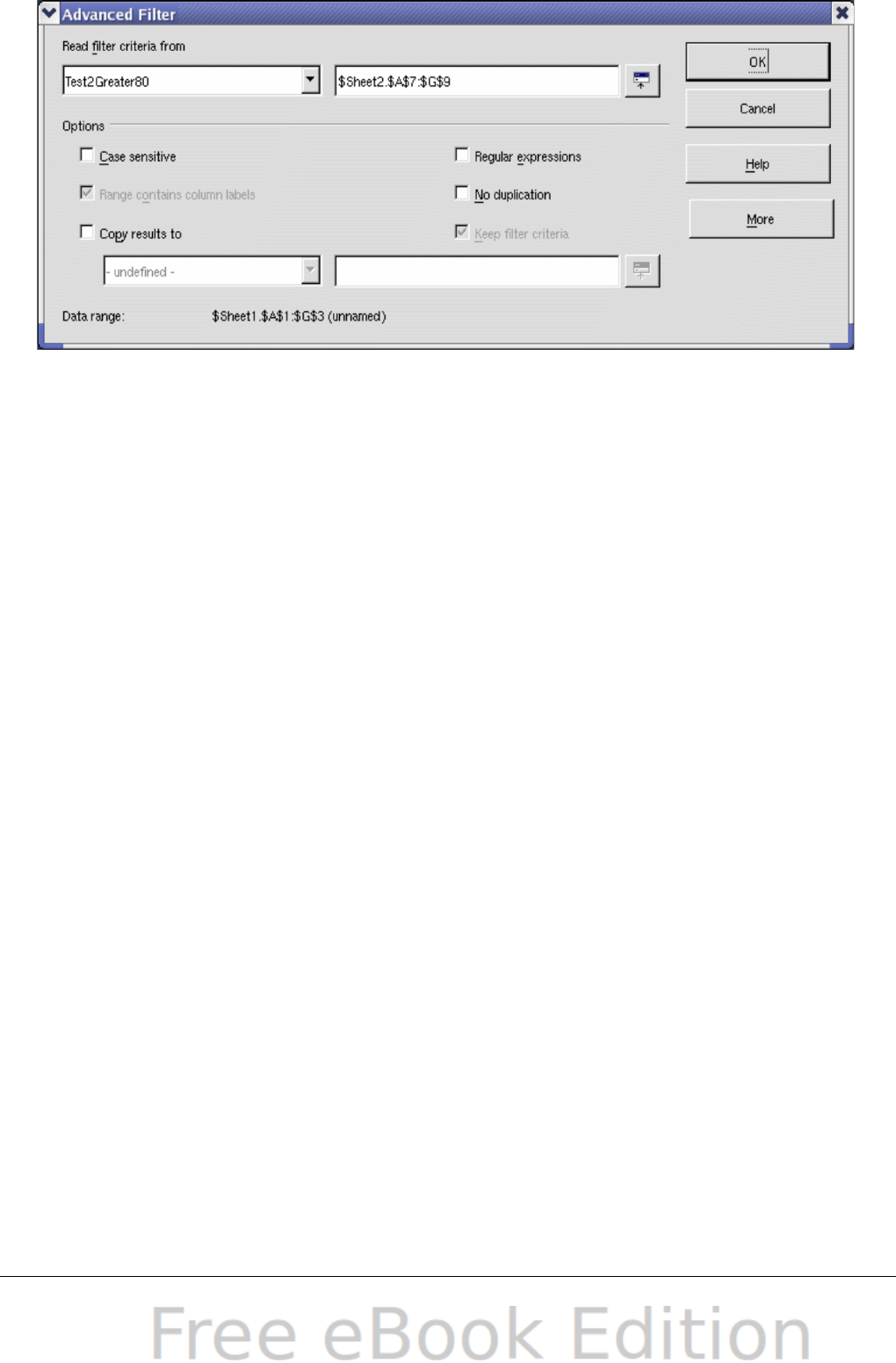
Figure 311. Apply an advanced filter using a previously defined
named range.
Listing 17. Use an advanced filter.
Sub UseAnAdvancedFilter()
Dim oSheet 'A sheet from the Calc document.
Dim oRanges 'The NamedRanges property.
Dim oCritRange 'Range that contains the filter criteria.
Dim oDataRange 'Range that contains the data to filter.
Dim oFiltDesc 'Filter descriptor.
REM Range that contains the filter criteria
oSheet = ThisComponent.getSheets().getByIndex(1)
oCritRange = oSheet.getCellRangeByName("A1:G3")
REM You can also obtain the range containing the
REM filter criteria from a named range.
REM oRanges = ThisComponent.NamedRanges
REM oRange = oRanges.getByName("AverageLess80")
REM oCritRange = oRange.getReferredCells()
REM The data that I want to filter
oSheet = ThisComponent.getSheets().getByIndex(0)
oDataRange = oSheet.getCellRangeByName("A1:G16")
oFiltDesc =
oCritRange.createFilterDescriptorByObject(oDataRange)
oDataRange.filter(oFiltDesc)
End Sub
Change properties on the filter descriptor to change the behavior of
the filter (see Table 16).
Chapter 13 Calc as a Simple Database 373
The filter created in Listing 17 filters the data in place. Modify the
OutputPosition property to specify a different output position (see
Listing 18). The filter descriptor must be modified before the filter is
applied.
Table 16. Advanced filter properties.
Property Comment
ContainsHeader Boolean (true or false) that specifies if the first row
(or column) contains headers which should not be
filtered.
CopyOutputData Boolean that specifies if the filtered data should be
copied to another position in the document.
IsCaseSensitive Boolean that specifies if the case of letters is
important when comparing entries.
Orientation Specifies if columns
(com.sun.star.table.TableOrientation.COLUMNS) or
rows (com.sun.star.table.TableOrientation.ROWS)
are filtered.
OutputPosition If if CopyOutputData is True , specifies the position
where filtered data are to be copied.
SaveOutputPosition Boolean that specifies if the OutputPosition position
is saved for future calls.
SkipDuplicates Boolean that specifies if duplicate entries are left
out of the result.
UseRegularExpressi
ons
Boolean that specifies if the filter strings are
interpreted as regular expressions.
Listing 18. Copy filtered results to a different location.
REM Copy the output data rather than filter in place.
oFiltDesc.CopyOutputData = True
REM Create a CellAddress and set it for Sheet3,
REM Column B, Row 4 (remember, start counting with 0)
Dim x As New com.sun.star.table.CellAddress
x.Sheet = 2
x.Column = 1
x.Row = 3
oFiltDesc.OutputPosition = x
(Advanced material.) The OutputPosition property returns a copy of a
struct. Because a copy is returned, it is not possible to set the
individual values directly. For example, oFiltDesc.OutputPosition.Row
374 OpenOffice.org 3.x Calc Guide

= 2 does not work (because you set the Row on the copy to 2, but do
not change the original).
Manipulating filtered data
Filtered data copied to a new location may be selected, modified, and
deleted at will. Data that is not copied, however, requires special
attention because rows that do not match the filter criteria are simply
hidden. OpenOffice.org behaves differently depending on how the cells
became hidden and what operation is done.
Cells may be hidden using an outline, data filter, or the hide command.
When data is moved by dragging or using cut and paste, all of the cells
are moved—including the hidden cells. When copying data, however,
filtered data includes only the visible cells and data hidden using an
outline or the hide command copies all of the data.
Calc functions similar to database
functions
Although every Calc function can be used for database manipulation,
the functions in Table 17 are more commonly used as such. Some
functions’ names differ only by the letter appended at the end;
AVERAGE and AVERAGEA, for example. Functions that do not end with
the letter A operate only on numeric values and cells that contain text
or are empty are ignored. The corresponding function whose name
ends with the letter A, treats text values as a number with the value of
zero; blank cells are still ignored.
Table 17. Functions frequently used as database functions.
Function Description
AVERAGE Return the average. Ignore empty cells and cells that
contain text.
AVERAGEA Return the average. The value of text is 0 and empty cells
are ignored.
COUNT Count the number of numeric entries; text entries are
ignored.
COUNTA Count the number of non-empty entries.
COUNTBLANK Return the number of empty cells.
COUNTIF Return the number of cells that meet the search criteria.
Chapter 13 Calc as a Simple Database 375
Function Description
HLOOKUP Search for a specific value across the columns in the first
row of an array. Return the value from a different row in
the same column.
INDEX Return the content of a cell, specified by row and column
number or an optional range name.
INDIRECT Return the reference specified by a text string.
LOOKUP Return the contents of a cell either from a one-row or
one-column range or from an array.
MATCH Search an array and return the relative position of the
found item.
MAX Return the maximum numeric value in a list of
arguments.
MAXA Return the maximum numeric value in a list of
arguments. The value of text is 0.
MIN Return the minimum numeric value in a list of arguments.
MINA Return the minimum numeric value in a list of arguments.
The value of text is 0.
MEDIAN Return the median of a set of numbers.
MODE Return the most common value in a data set. If there are
several values with the same frequency, it returns the
smallest value. An error occurs when a value doesn’t
appear twice.
OFFSET Return the value of a cell offset by a certain number of
rows and columns from a given reference point.
PRODUCT Return the product of the cells.
STDEV Estimate the standard deviation based on a sample.
STDEVA Estimate the standard deviation based on a sample. The
value of text is 0.
STDEVP Calculate the standard deviation based on the entire
population.
STDEVPA Calculate the standard deviation based on the entire
population.
SUBTOTAL Calculate a specified function based on a subset created
using AutoFilters.
SUM Return the sum of the cells.
376 OpenOffice.org 3.x Calc Guide

Function Description
SUMIF Calculate the sum for the cells that meet the search
criteria.
VAR Estimate the variance based on a sample.
VARA Estimate the variance based on a sample. The value of
text is 0.
VARP Estimate the variance based on the entire population.
VARPA Estimate the variance based on the entire population. The
value of a text is 0.
VLOOKUP Search for a specific value across the rows in the first
column of an array. Returns the value from a different
column in the same row.
Most of the functions in Table 17 require no explanation, either
because they are well understood (SUM, for example) or because if you
need to use them then you know what they are (STDEV, for example).
Unfortunately, some of the more useful functions are infrequently used
because they are not well understood.
Count and sum cells that match conditions: COUNTIF
and SUMIF
The COUNTIF and SUMIF functions calculate their values based on
search criteria. The search criteria can be a number, expression, text
string, or even a regular expression. The search criteria can be
contained in a referenced cell or it can be included directly in the
function call.
The COUNTIF function counts the number of cells in a range that
match specified criteria. The first argument to COUNTIF specifies the
range to search and second argument is the search criteria. Table 18
illustrates different search criteria using the COUNTIF function
referencing the data shown in Table 12.
The first two arguments for SUMIF serve the same purpose as the
arguments for COUNTIF; the range that contains the cells to search
and the search criteria. The third and final argument for SUMIF
specifies the range to sum. For each cell in the search range that
matches the search criteria, the corresponding cell in the sum range is
added into the sum.
Chapter 13 Calc as a Simple Database 377
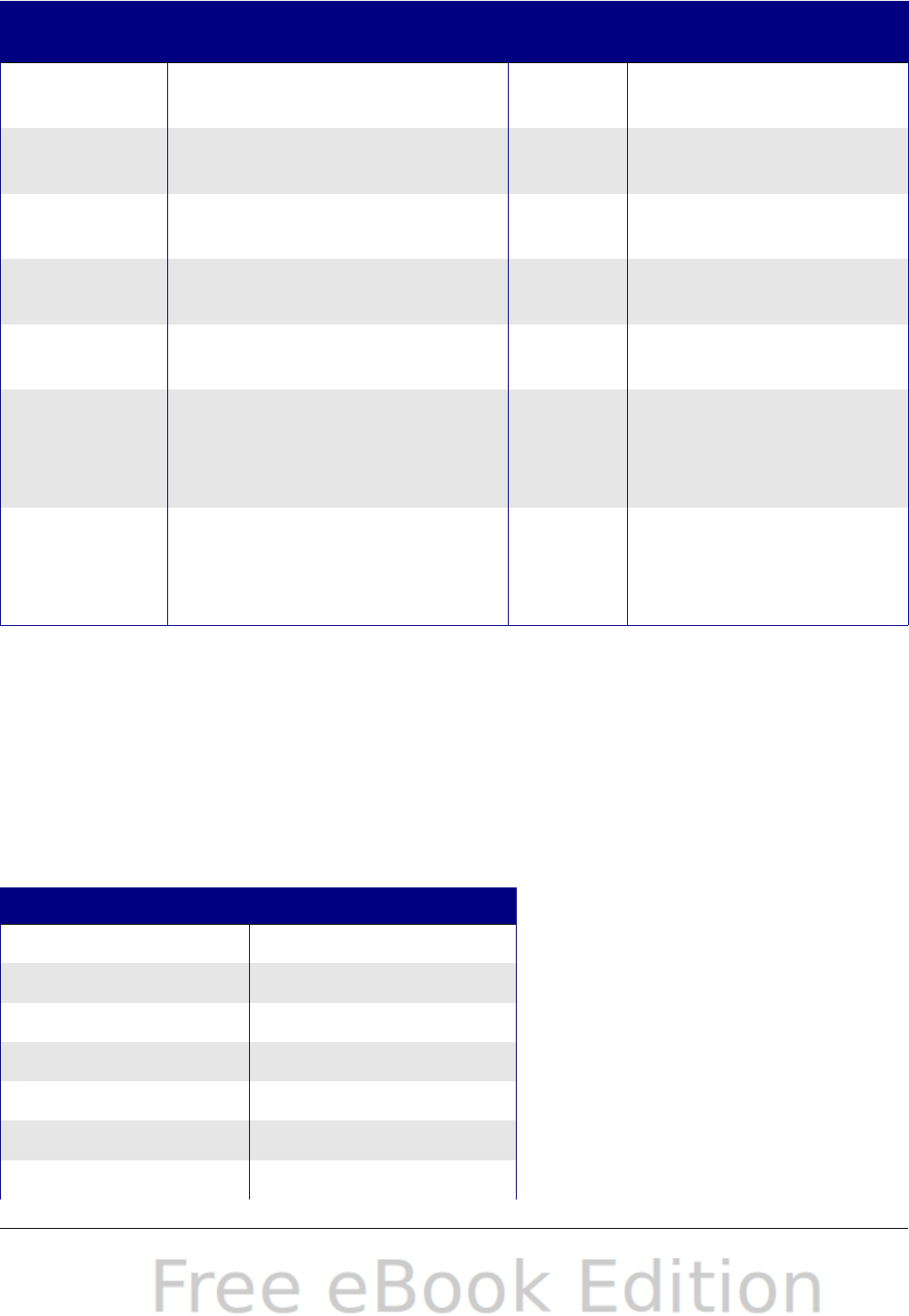
Table 18. Examples of search criteria for the COUNTIF and SUMIF
functions.
Criteria
Type
Function Result Description
Number =COUNTIF(B1:C16; 95) 3 Finds numeric values
of 95.
Text =COUNTIF(B1:C16; "95") 3 Finds numeric or text
values of 95.
Expression =COUNTIF(B1:C16;
">95")
6 Finds numeric values
greater than 95.
Expression =COUNTIF(B1:C16;
2*45+5)
3 Finds only numeric
values of 95.
Regular
expression
=COUNTIF(B1:C16; "9.*") 12 Finds numbers or
text that start with 9.
Reference
a cell
=COUNTIF(B1:C16; B3) 3 Finds a number or
number and text
depending on the
data type in cell B3.
Regular
expression
=SUMIF(A1:A16; "B.*";
B1:B16)
227 Sum Column B for
names in Col. A
starting with the
letter B.
Ignore filtered cells using SUBTOTAL
The SUBTOTAL function applies a function (see Table 19) to a range of
data, but it ignores cells hidden by a filter and cells that already
contain a SUBTOTAL. For example, =SUBTOTAL(2, "B2:B16") counts
the number of cells in B2:B16 that are not hidden by a filter.
Table 19. Function index for the SUBTOTAL function.
Function index Function
1 AVERAGE
2 COUNT
3 COUNTA
4 MAX
5 MIN
6 PRODUCT
7 STDEV
378 OpenOffice.org 3.x Calc Guide

Function index Function
8 STDEVP
9 SUM
10 VAR
11 VARP
Tip
Do not forget that the SUBTOTAL function ignores cells that use
the SUBTOTAL function. Say you have a spreadsheet that tracks
investments. The retirement investments are grouped together
with a subtotal. The same is true of regular investments. You can
use a single subtotal that includes the entire range without
worrying about the subtotal cells.
Using formulas to find data
Calc offers numerous methods to find data in a sheet. For example,
Edit > Find & Replace moves the display cursor based on simple and
advanced searching. Use Data > Filter to limit what is displayed
rather than simply moving the cursor. Calc also offers lookup functions
used in formulas, for example a formula to look up a student’s grade
based on their test score.
Search a block of data using VLOOKUP
Use VLOOKUP to search the first column (columns are vertical) of a
block of data and return the value from another column in the same
row. For example, search the first column for the name “Fred” and
then return the value in the cell two columns to the right. VLOOKUP
supports two forms:
VLOOKUP(search_value; search_range; return_column_index)
VLOOKUP(search_value; search_range; return_column_index;
sort_order)
The first argument, search_value, identifies the value to find. The
search value can be text, a number, or a regular expression. For
example, Fred searches for the text Fred, 4 searches for the number 4,
and F.* is the regular expression for finding something that starts with
the letter F.
The second argument, search_range, identifies the cells to search;
only the first column is searched. For example, B3:G10 searches the
same sheet containing the VLOOKUP formula and Sheet2.B3:G10
searches the range B3:G10 on the sheet named Sheet2.
Chapter 13 Calc as a Simple Database 379

The return_column_index identifies the column to return; a value of 1
returns the first column in the range. The statement =VLOOKUP("Bob";
A1:G9; 1) finds the first row in A1:G9 containing the text Bob, and
returns the value in the first column. The first column is the searched
column, so the text Bob is returned. If the column index is 2, then the
value in the cell to the right of Bob is returned: column B.
The final column, sort_order, is optional. The default value for
sort_order is 1, which specifies that the first column is sorted in
ascending order; a value of 0 specifies that the data is not sorted. A
non-sorted list is searched by sequentially checking every cell in the
first column for an exact match. If an exact match is not found, the text
#N/A is returned.
A more efficient search routine is used if the data is sorted in
ascending order. If one exact match exists, the returned value is the
same as for a non-sorted list; but it is faster. If a match does not exist,
the largest value in the column that is less than or equal to the search
value is returned. For example, searching for 7 in (3, 5, 10) returns 5
because 7 is between 5 and 10. Searching for 27 returns 10, and
searching for 2 returns #N/A because there is no match and no value
less than 2.
Use VLOOKUP when:
•The data is arranged in rows and you want to return data from
the same row. For example, student names with test and quiz
scores to the right of the student’s name.
•Searching the first column of a range of data.
Search a block of data using HLOOKUP
Use HLOOKUP to search the first row (rows are horizontal) of a block
of data and return the value from a row in the same column. HLOOKUP
supports the same form and arguments as VLOOKUP:
HLOOKUP(search_value; search_range; return_row_index)
HLOOKUP(search_value; search_range; return_row_index; sort_order)
Use HLOOKUP when:
•The data is arranged in columns and you want to return data from
the same column. For example, student names with test and quiz
scores underneath the student’s name.
•Searching the first row of a range of data.
380 OpenOffice.org 3.x Calc Guide

Search a row or column using LOOKUP
LOOKUP is similar to HLOOKUP and VLOOKUP. The search range for
the LOOKUP function is a single sorted row or column. LOOKUP has
two forms:
LOOKUP(search_value; search_range)
LOOKUP(search_value; search_range; return_range)
The search value is the same as HLOOKUP and VLOOKUP. The search
range, however, must be a single row or a single column; for example,
A7:A12 (values in column A) or C5:Q5 (values in row 5). If the
return_range is omitted, the matched value is returned. Using
LOOKUP without a return range is the same as using HLOOKUP or
VLOOKUP with a column index of 1.
The return range must be a single row or column containing the same
number of elements as the search range. If the search value is found in
the fourth cell in the search range, then the value in the fourth cell in
the return range is returned. The return range can have a different
orientation than the search range. In other words, the search range
can be a row and the return range may be a column.
Use LOOKUP when:
•The search data is sorted in ascending order.
•The search data is not stored in the same row, column, or
orientation as the return data.
Use MATCH to find the index of a value in a range
Use MATCH to search a single row or column and return the position
that matches the search value. Use MATCH to find the index of a value
in a range. The supported forms for MATCH are as follows:
=MATCH(search_value; search_range)
=MATCH(search_value; search_range; search_type)
The search value and search range are the same as for LOOKUP. The
final argument, search type, controls how the search is performed. A
search type of 1, sorted in ascending order, is the default. A search
type of -1 indicates that the list is sorted in descending order. A search
type of 0 indicates that the list is not sorted. Regular expressions can
only be used on an unsorted list.
Use MATCH when:
•You need an index into the range rather than the value.
Chapter 13 Calc as a Simple Database 381

•The search data is in descending order and the data is large
enough that the data must be searched assuming that it is sorted;
because it is faster to sort a sorted list.
Examples
Consider the data in Table 23. Each student’s information is stored in a
single row. Write a formula to return the average grade for Fred. The
problem can be restated as Search column A in the range A1:G16 for
Fred and return the value in column F (column F is the sixth column).
The obvious solution is =VLOOKUP("Fred"; A2:G16; 6). Equally
obvious is =LOOKUP("Fred"; A2:A16; F2:F16).
It is common for the first row in a range to contain column headers. All
of the search functions check the first row to see if there is a match
and then ignore it if it does not contain a match, in case the first row is
a header.
What if the column heading Average is known, but not the column
containing the average? Find the column containing Average rather
than hard coding the value 6. A slight modification using MATCH to
find the column yields
=VLOOKUP("Fred"; A2:G16; MATCH("Average"; A1:G1; 0)); notice
that the heading is not sorted. As an exercise, use HLOOKUP to find
Average and then MATCH to find the row containing Fred.
As a final example, write a formula to assign grades based on a
student’s average score. Assume that a score less than 51 is an F, less
than 61 is an E, less than 71 is a D, less than 81 is a C, less than 91 is a
B, and 91 to 100 is an A. Assume that the values in Table 20 are in
Sheet2.
Table 20. Associate scores to a grade.
A B
1Score Grade
20 F
351 E
461 D
571 C
681 B
791 A
382 OpenOffice.org 3.x Calc Guide
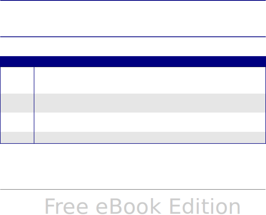
The formula =VLOOKUP(83; $Sheet2.$A$2:$B$7; 2) is an obvious
solution. Dollar signs are used so that the formula can be copied and
pasted to a different location and it will still reference the same values
in Table 20.
ADDRESS returns a string with a cell’s address
Use ADDRESS to return a text representation of a cell address based
on the row, column, and sheet; ADDRESS is frequently used with
MATCH. The supported forms for ADDRESS are as follows:
ADDRESS(row; column)
ADDRESS(row; column; abs)
ADDRESS(row; column; abs; sheet)
The row and column are integer values where ADDRESS(1; 1) returns
$A$1. The abs argument specifies which portion is considered
absolute and which portion is considered relative (see Table 21); an
absolute address is specified using the $ character. The sheet is
included as part of the address only if the sheet argument is used. The
sheet argument is treated as a string. Using
ADDRESS(MATCH("Bob";A1:A5 ; 0); 2) with the data in Table 20
returns $B$2.
Tip
Calc supports numerous powerful functions that are not
discussed here. For example, the ROW, COLUMN, ROWS, and
COLUMNS statements are not discussed; a curious person would
investigate these functions.
Table 21. Values supported by the abs argument to ADDRESS.
Value Description
1 Use absolute addressing. This is the default value if the argument
is missing or an invalid value is used. ADDRESS(2; 5; 1) returns
$E$2.
2 Use an absolute row reference and a relative column reference.
ADDRESS(2; 5; 2; "Blah") returns Blah.E$2.
3
Use a relative row reference and an absolute column reference.
ADDRESS(2; 5; 3) returns $E2.
4 Use relative addressing. ADDRESS(2; 5; 4) returns E2.
Chapter 13 Calc as a Simple Database 383
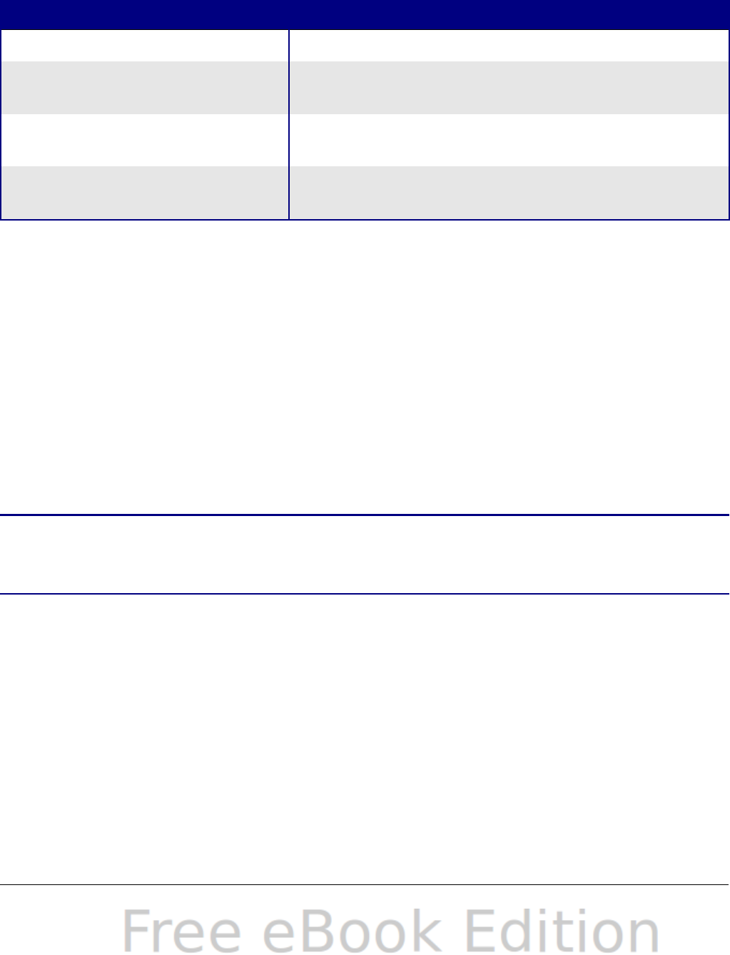
INDIRECT converts a string to a cell or range
Use INDIRECT to convert a string representation of a cell or range
address to a reference to the cell or range. Table 22 contains examples
accessing data as shown in Table 20.
Table 22. Examples using INDIRECT.
Example Comment
INDIRECT("A2") Returns cell A2, which contains Bob.
INDIRECT(G1) If Cell G1 contains the text A2, then this
returns Bob.
SUM(INDIRECT("B1:B5")) Returns the sum of the range B1:B5, which
is 194.
INDIRECT(ADDRESS(2; 1)) Returns the contents of cell $A$2, which is
Bob.
OFFSET returns a cell or range offset from another
Use OFFSET to return a cell or range offset by a specified number of
rows and columns from a given reference point. The first argument,
specifies the reference point. The second and third arguments specify
the number of rows and columns to move from the reference point; in
other words, where the new range starts. The OFFSET function has
the following syntax:
OFFSET(reference; rows; columns)
OFFSET(reference; rows; columns; height)
OFFSET(reference; rows; columns; height; width)
Tip
If the width or height is included, the OFFSET function returns a
range. If both the width and height are missing, a cell reference
is returned.
If the height or width are missing, they default to 1. If the height is
present, then a range reference is returned rather than a cell
reference. Using values from Table 12, Listing 19 uses OFFSET to
obtain the quiz scores for the student named Bob.
Listing 19. Complex example of OFFSET.
=SUM(OFFSET(INDIRECT(ADDRESS(MATCH("Bob";A1:A16; 0); 4)); 0; 0; 1; 2))
In its entirety, Listing 19 is complex and difficult to understand. Table
23 isolates each function in Listing 19, providing an easy to understand
explanation of how the example works.
384 OpenOffice.org 3.x Calc Guide
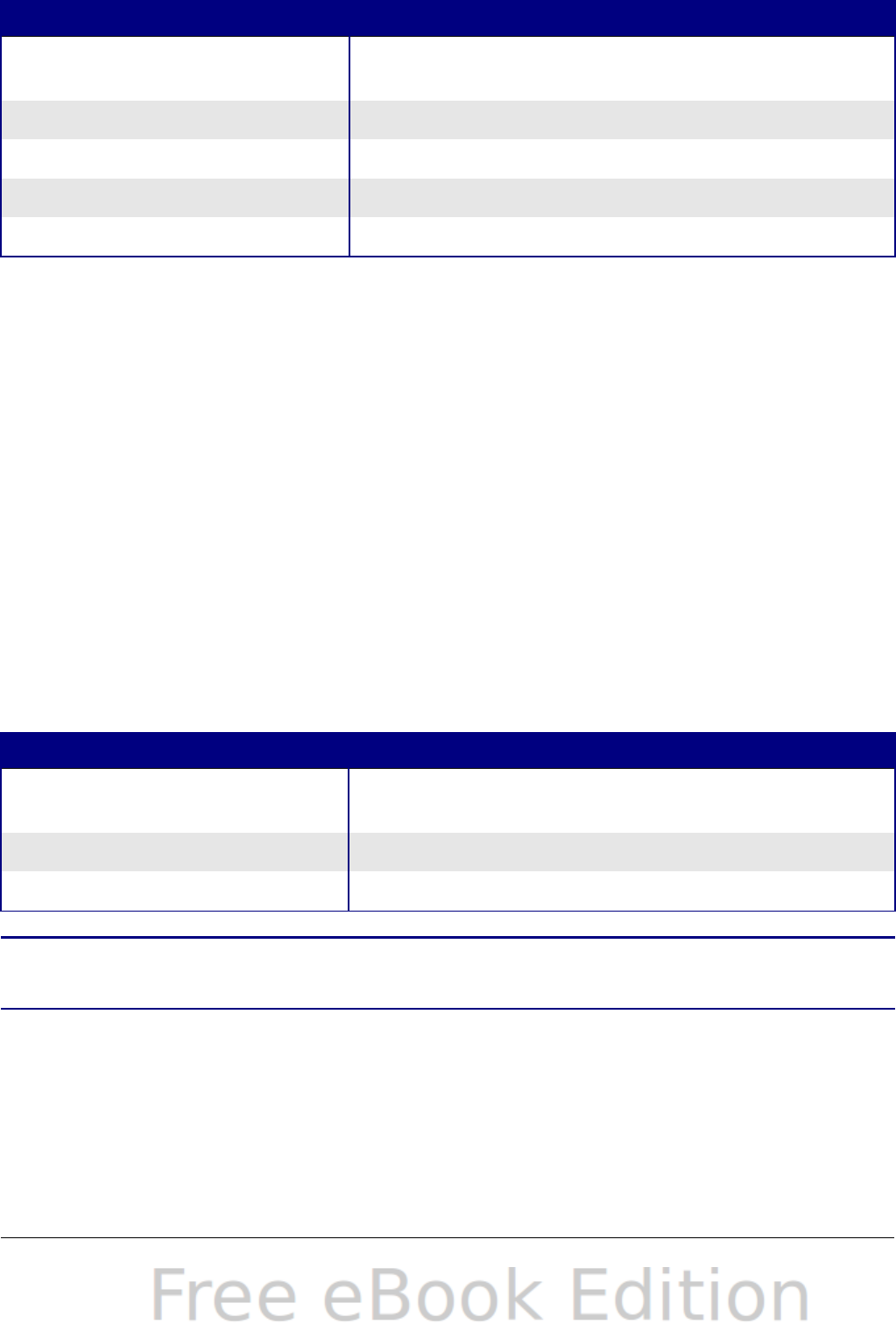
Table 23. Breakdown of Listing 19.
Function Description
MATCH("Bob";A1:A16; 0) Return 4 because Bob is the fourth entry in
column A.
ADDRESS(4; 4) Return $D$4.
INDIRECT("$D$4") Convert $D$4 into a reference to the cell D4.
OFFSET($D$4; 0; 0; 1; 2) Return the range D4:E4.
SUM(D4:E4) Return the sum of Bob’s quiz scores.
Although Listing 19 works as intended, it breaks easily and
unexpectedly. Consider, for example, what happens if the range is
changed to A2:A16. MATCH returns an offset into the provided range,
so MATCH("Bob";A2:A16 ; 0) returns 3 rather than 4. ADDRESS(3; 4)
returns $D$3 rather than $D$4 and Betty’s quiz scores are returned
instead of Bob’s. Listing 20 uses a slightly different method to obtain
Bob’s quiz scores.
Listing 20. Better use of OFFSET.
=SUM(OFFSET(A1; MATCH("Bob"; A1:A16; 0)-1; 3; 1; 2))
Table 24 contains a description of each function used in Listing 20. To
help convince yourself that Listing 20 is better than Listing 19, replace
A1 with A2 in both Listing 20 and Table 24 and notice that you still
obtain Bob’s quiz scores.
Table 24. Breakdown of Listing 20.
Function Description
MATCH("Bob";A1:A16; 0)-1 Return 3 because Bob is the fourth entry in
column A.
OFFSET(A1; 3; 3; 1; 2) Return the range D4:E4.
SUM(D4:E4) Return the sum of Bob’s quiz scores.
Tip The first argument to OFFSET can be a range so you can use a
defined range name.
INDEX returns cells inside a specified range
INDEX returns the cells specified by a row and column number. The
row and column number are relative to the upper left corner of the
specified reference range. For example, using =INDEX(B2:D3; 1; 1)
Chapter 13 Calc as a Simple Database 385
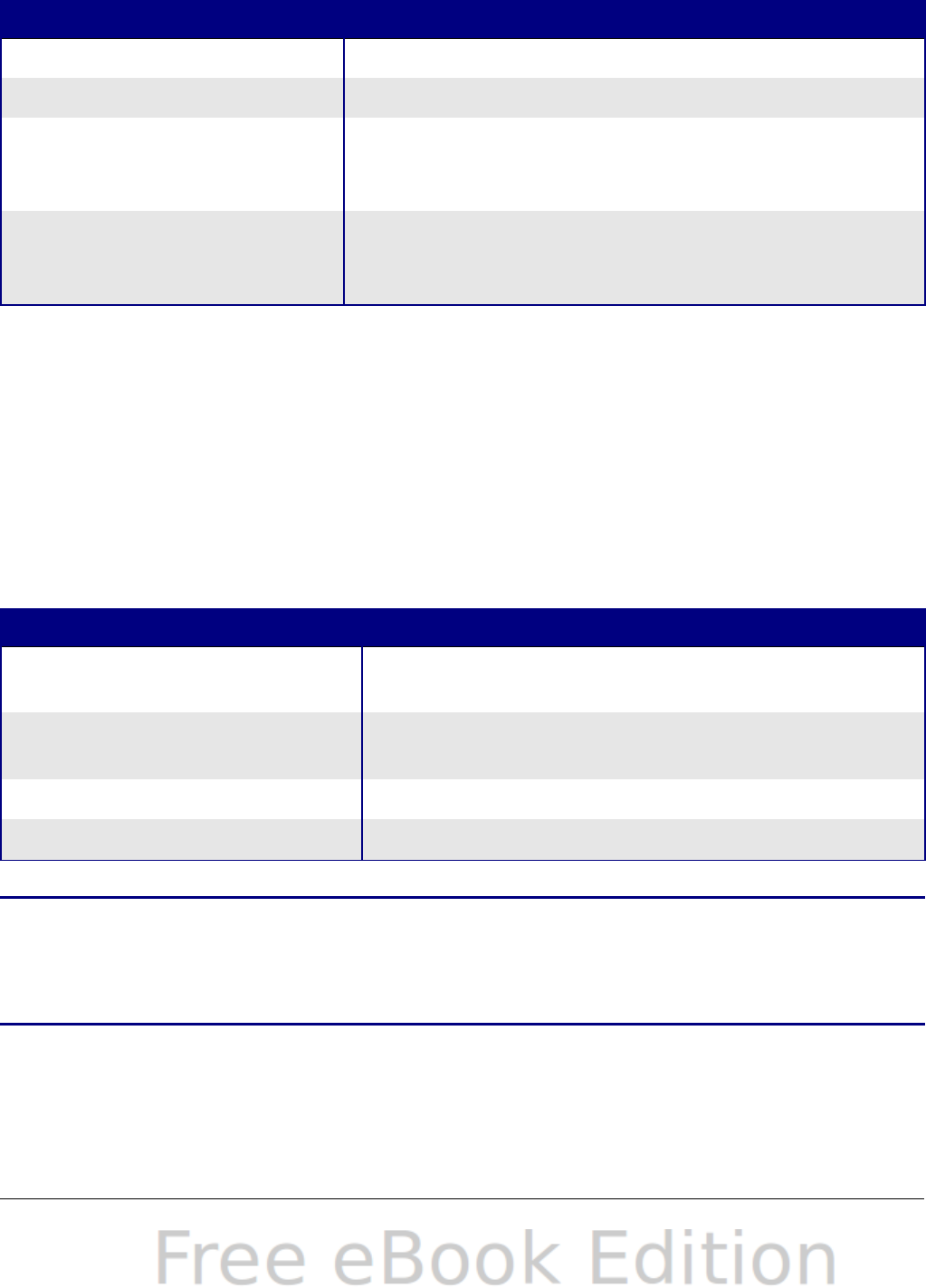
returns the cell B2. Table 25 lists shows the syntax for using the
INDEX function.
Table 25. Syntax for INDEX.
Syntax Description
INDEX(reference) Return the entire range.
INDEX(reference; row) Return the specified row in the range.
INDEX(reference; row;
column)
Return the cell specified by row and column. A
row and column of 1 returns the cell in the
upper left corner of the range.
INDEX(reference; row;
column; range)
A reference range can contain multiple ranges.
The range argument specifies which range to
use.
The INDEX function can return an entire range, a row, or a single
column (see Table 25). The ability to index based on the start of the
reference range provides some interesting uses. Using the values
shown in Table 12, Listing 21 finds and returns Bob’s quiz scores.
Table 26 contains a listing of each function used in Listing 21.
Listing 21. Return Bob’s quiz scores.
=SUM(OFFSET(INDEX(A2:G16; MATCH("Bob"; A2:A16; 0)); 0; 3; 1; 2))
Table 26. Breakdown of Listing 21.
Function Description
MATCH("Bob";A2:A16; 0) Return 3 because Bob is the third entry in
column A2:A16.
INDEX(A2:A16; 3) Return A4:G4—the row containing Bob’s quiz
scores.
OFFSET(A4:G4; 0; 3; 1; 2) Return the range D4:E4.
SUM(D4:E4) Return the sum of Bob’s quiz scores.
Tip
A simple range contains one contiguous rectangular region of
cells. It is possible to define a multi-range that contains multiple
simple ranges. If the reference consists of multiple ranges, you
must enclose the reference or range name in parentheses.
If reference argument to the INDEX function is a multi-range, then the
range argument specifies which simple range to use (see Table 27).
386 OpenOffice.org 3.x Calc Guide
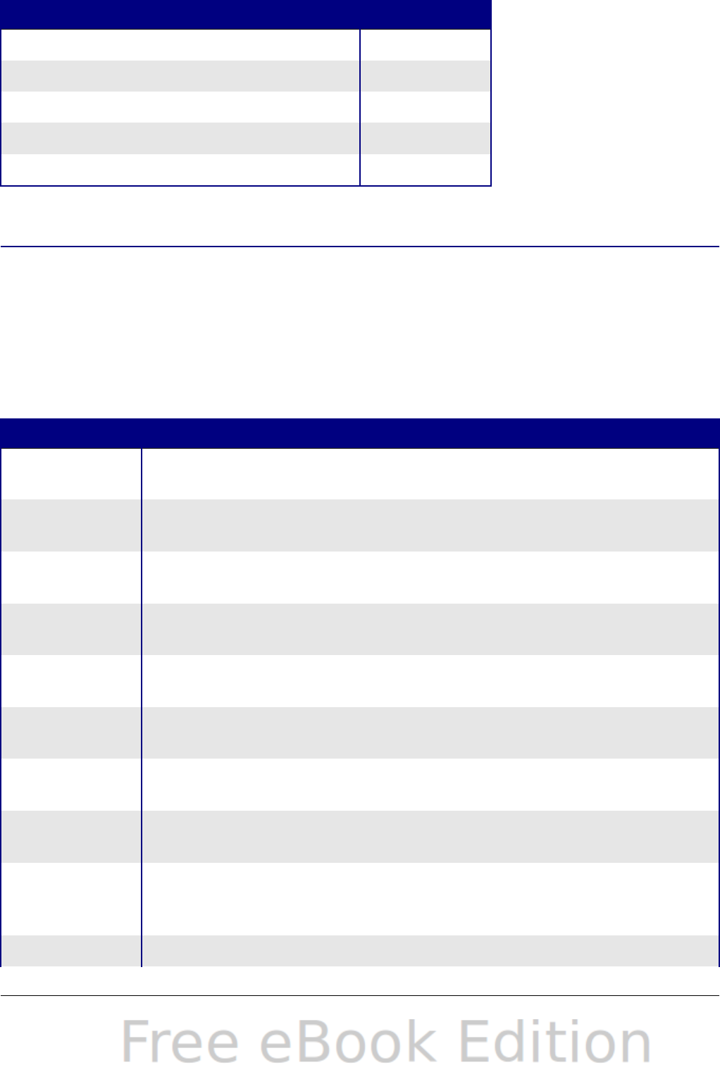
Table 27. Using INDEX with a multi-range.
Function Returns
=INDEX(B2:G2; 1; 2) 93
=INDEX(B5:G5; 1; 2) 65
=INDEX((B2:G2;B5:G5); 1; 2) 93
=INDEX((B2:G2;B5:G5); 1; 2; 1) 93
=INDEX((B2:G2;B5:G5); 1; 2; 2) 65
Database-specific functions
Although every Calc function can be used for database manipulation,
the functions in Table 28 are specifically designed for use as a
database. The descriptions in Table 28 use the following terms
interchangeably: row and record, cell and field, and database and all
rows.
Table 28. Database functions in a Calc document.
Function Description
DAVERAGE Return the average of all fields that matches the search
criteria.
DCOUNT Count the number of records containing numeric data that
match the search criteria.
DCOUNTA Count the number of records containing text data that match
the search criteria.
DGET Return the contents of a field that matches the search
criteria.
DMAX Return the maximum content of a field that matches the
search criteria.
DMIN Return the minimum content of a field that matches the
search criteria.
DPRODUCT Return the product of the fields that matches the search
criteria.
DSTDEV Calculate the standard deviation using the fields that match
the search criteria. The fields are treated as a sample.
DSTDEVP Calculate the standard deviation using the fields that match
the search criteria. The fields are treated as the entire
population.
DSUM Return the sum of all fields that matches the search criteria.
Chapter 13 Calc as a Simple Database 387
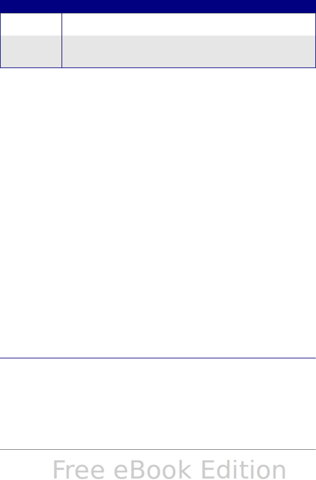
Function Description
DVAR Calculate the variance using the fields that match the search
criteria. The fields are treated as a sample.
DVARP Calculatesthe variance using the fields that match the
search criteria. The fields are treated as the entire
population.
The syntax for the database functions are identical.
DCOUNT(database; database field; search criteria)
The database argument is the cell range that defines the database. The
cell range should contain the column labels (see Listing 22). The
following examples, assume that the data from Table 12 is placed in
Sheet 1 and the filter criteria in Table 15 is placed in Sheet 2.
Listing 22. The database argument includes the headers.
=DCOUNT(A1:G16; "Test 2"; Sheet2.A1:G3)
The database field specifies the column on which the function operates
after the search criteria is applied and the data rows are selected. The
database field can be specified using the column header name or as an
integer. If the column is specified as an integer, 0 specifies the entire
data range, 1 specifies the first column, 2 specifies the second column,
and so on. Listing 23 calculates the average test score for the rows
that match the search criteria.
Listing 23. “Test 2” is column 3.
=DAVERAGE(A1:G16; "Test 2"; Sheet2.A1:G3)
=DAVERAGE(A1:G16; 3; Sheet2.A1:G3)
The search criteria is the cell range containing search criteria. The
search criteria is identical to the advanced filters; criteria in the same
row is connected by AND and criteria in different rows is connected by
OR.
Conclusion
A Calc document provides sufficient database functionality to satisfy
the needs of most people. The infrequently used database functions,
such as OFFSET and INDEX, are worth the time to learn and they can
save yourself time in the long run.
388 OpenOffice.org 3.x Calc Guide

Chapter 14
Setting up and
Customizing Calc

Introduction
This chapter describes some common customizations that you may
wish to do. In addition to selecting options from those provided, you
can customize menus, toolbars, and keyboard shortcuts, add new
menus and toolbars, and assign macros to events. However, you cannot
customize context (right-click) menus.
Other customizations are made easy by extensions that you can install
from the OpenOffice.org website or from other providers.
Note
Customizations to menus and toolbars can be saved in a template.
To do so, first save them in a document and then save the document
as a template as described in Chapter 4 (Using Styles and
Templates in Calc).
Choosing options that affect all of OOo
This section covers some of the settings that apply to all the
components of OpenOffice.org. Other general options are discussed in
Chapter 2 (Setting Up OpenOffice.org) in the Getting Started guide.
5) Click Tools > Options. The list on the left-hand side varies
depending on which component of OOo is open.
6) Click the + sign to the left of OpenOffice.org on the left-hand
side. A list of subsections drops down.
Note
The Back button has the same effect on all pages of the Options
dialog. It resets the options to the values that were in place
when you opened OpenOffice.org.
390 OpenOffice.org 3.x Calc Guide
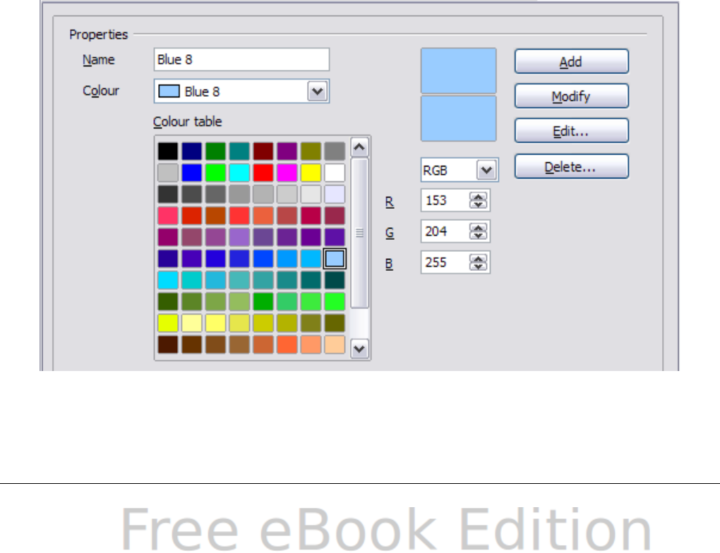
User Data options
Calc uses the first and last name stored in the OpenOffice.org – User
Data page to fill in the Created and Modified fields in the document
properties, and the optional Author field often used in the footer of a
printed spreadsheet. Fill in the form on this page.
Print options
Set the print options to suit your default printer and your most
common printing method. You can change these settings at any time,
either through this dialog or during the printing process (by clicking
the Options button on the Print dialog).
In the Options dialog, click OpenOffice.org > Print.
See Chapter 6 (Printing, Exporting, and E-mailing) for more about the
options on this page.
Color options
On the OpenOffice.org – Colors page, you can specify colors to use in
OOo documents. You can select a color from a color table, edit an
existing color, and define new colors. These colors are stored in your
color palette and are then available in all components of OOo.
Figure 312: Defining colors to use in color palettes in OOo
Chapter 14 Setting up and Customizing Calc 391
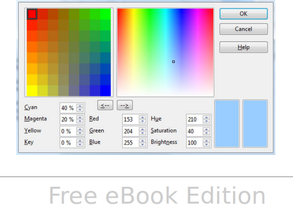
To modify a color:
1) Select the color to modify from the list or the color table.
2) Enter the new values that define the color. If necessary, change
the settings from RGB (Red, Green, Blue) to CMYK (Cyan,
Magenta, Yellow, Black) or vice versa. The changed color appears
in the lower of the two color preview boxes at the top.
3) Modify the Name as required.
4) Click the Modify button. The newly defined color is now listed in
the Color table.
Alternatively, click the Edit button to open the Color dialog, shown in
Figure 313. Here you can select a color from one of the color windows
in the upper area, or you can enter values in the lower area using your
choice of RGB, CMYK, or HSB (Hue, Saturation and Brightness) values.
The upper right color window is linked directly with the color input
fields in the lower area; as you choose a color in the upper window, the
numbers change accordingly. The two color fields at the lower right
show the value of the selected color on the left and the currently set
value from the color value fields on the right.
Modify the color components as required and click OK to exit the
dialog. The newly defined color now appears in the lower of the color
preview boxes shown in Figure 312. Type a name for this color in the
Name box, then click the Add button. A small box showing the new
color is added to the Color table.
Figure 313: Editing colors
392 OpenOffice.org 3.x Calc Guide
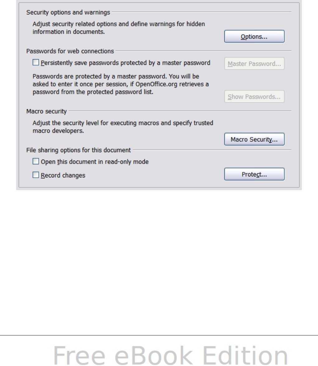
Another way to define or alter colors is through the Colors page of the
Area dialog, where you can also save and load palettes, a feature that
is not possible here. In Calc, draw a temporary draw object and use the
context menu of this object to open the Area dialog. If you load a
palette in one component of OOo, it is only active in that component;
the other components keep their own palettes.
Security options
Use the OpenOffice.org – Security page to choose security options for
saving documents and for opening documents that contain macros.
Figure 314: Choosing security options for opening and saving
documents
Security options and warnings
If you record changes, save multiple versions, or include hidden
information or notes in your documents, and you do not want some
of the recipients to see that information, you can set warnings to
remind you to remove this information, or you can have OOo remove
some information automatically. Note that (unless removed) much of
this information is retained in a file whether the file is in
OpenOffice.org’s default OpenDocument format, or has been saved
to other formats, including PDF.
Chapter 14 Setting up and Customizing Calc 393
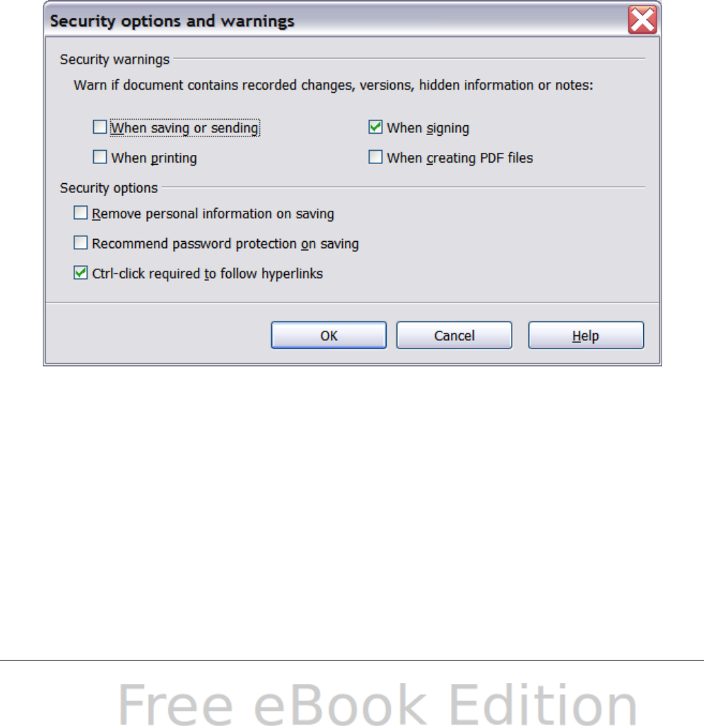
Click the Options button to open a separate dialog with specific
choices (Figure 315).
Remove personal information on saving. Select this option to
always remove user data from the file properties when saving the
file. To manually remove personal information from specific
documents, deselect this option and then use the Delete button
under File > Properties > General.
Ctrl-click required to follow hyperlinks. In older versions of
OOo, clicking on a hyperlink in a document opened the linked
document. Now you can choose whether to keep this behavior (by
unchecking this box). Many people find creation and editing of
documents easier when accidental clicks on links do not activate the
links.
The other options on this dialog should be self-explanatory.
Figure 315: Security options and warnings dialog
Passwords for web connections
You can enter a master password to enable easy access to sites that
require a user name and password.
Persistently save passwords protected by a master password.
If enabled, OOo securely stores all passwords that you use to
access files from web servers. You can retrieve the passwords from
the list after you enter the master password.
394 OpenOffice.org 3.x Calc Guide
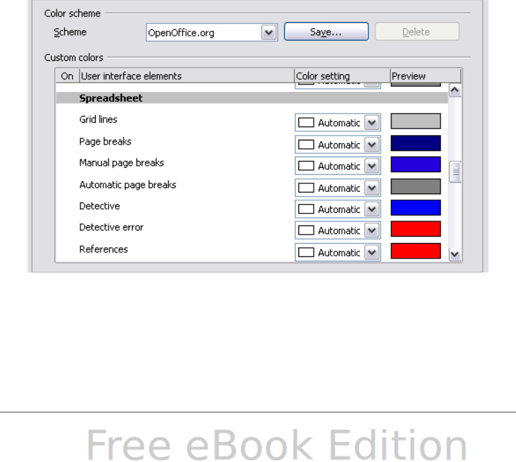
Macro security
Click the Macro Security button to open the Macro Security dialog
(not shown here), where you can adjust the security level for
executing macros and specify trusted sources.
File sharing options for this document
Select the Open this document in read-only mode option to
restrict this document to be opened in read-only mode only. This
option protects the document against accidental changes. It is still
possible to edit a copy of the document and save that copy with the
same name as the original.
Select the Record changes option to enable recording changes.
This is the same as Edit > Changes > Record. To allow other users
of this document to apply changes, but prevent them from disabling
change recording, click the Protect button and enter a password.
Appearance options
On the OpenOffice.org – Appearance page, you can specify which items
are visible and the colors used to display various items.
Figure 316: Changing the color of grid points in Calc
Scroll down in the page until you find Spreadsheet.
To change the default color for grid points, click the down-arrow by the
color and select a new color from the pop-up box.
If you wish to save your color changes as a color scheme, click Save,
type a name in the Scheme box; then click OK.
Chapter 14 Setting up and Customizing Calc 395
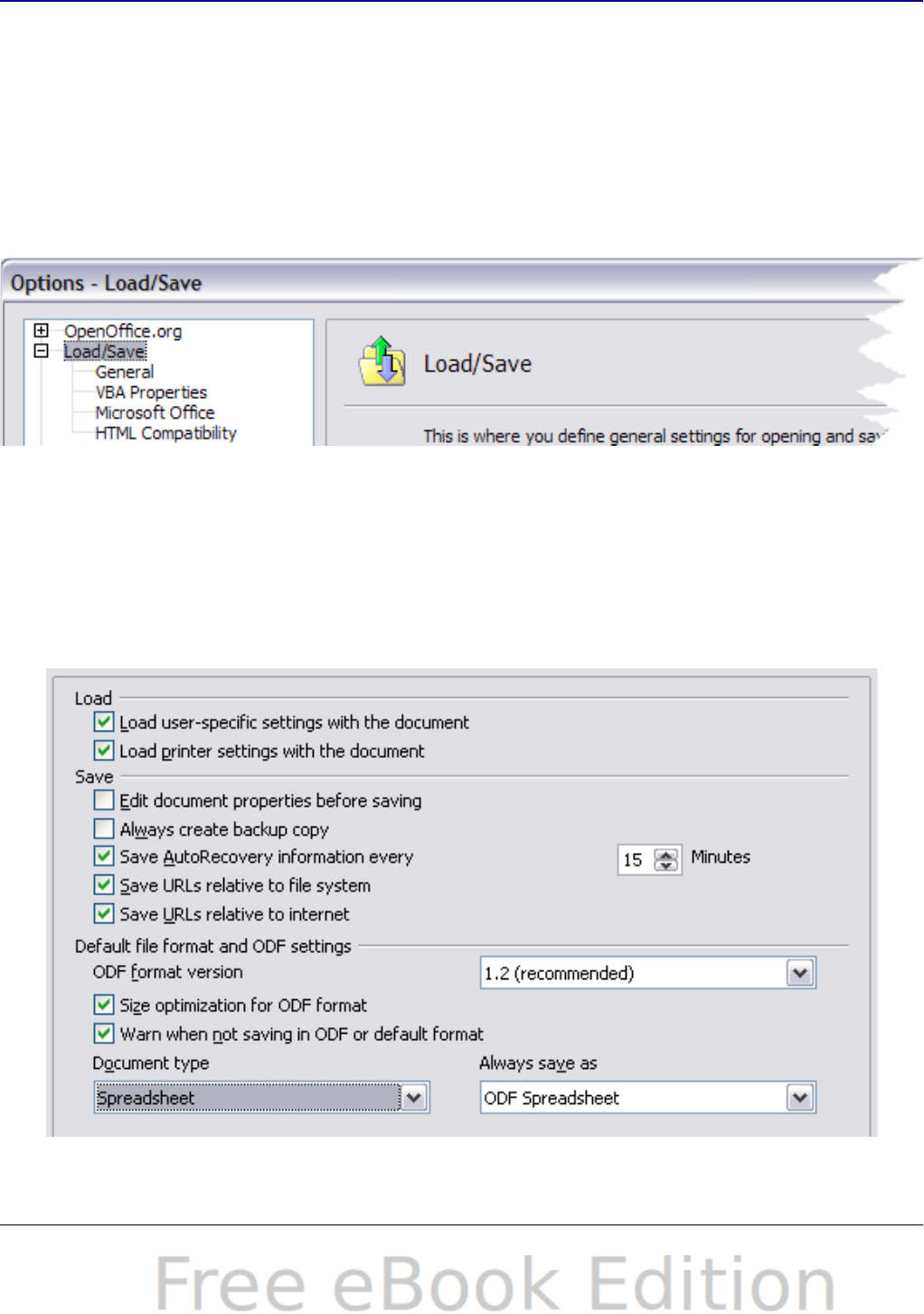
Choosing options for loading and saving
documents
You can set the Load/Save options to suit the way you work. This
chapter describes only a few of the options, those more relevant to
working with Calc. See Chapter 2 (Setting Up OpenOffice.org) in the
Getting Started guide for a description of the other options.
If the Options dialog is not already open, click Tools > Options. Click
the + sign to the left of Load/Save to display the list of load/save
options pages.
Figure 317: Load/Save options
General Load/Save options
Most of the choices on the Load/Save – General page are familiar to
users of other office suites. Those specific to OpenOffice.org are in the
Default file format and ODF settings section.
Figure 318: Choosing Load and Save options
396 OpenOffice.org 3.x Calc Guide

ODF format version
OpenOffice.org by default saves documents in OpenDocument
Format (ODF) version 1.2. While this allows for improved
functionality, there may be backwards compatibility issues. When a
file saved in ODF 1.2 is opened in an earlier version of
OpenOffice.org (using ODF 1.0/1.1), some of the advanced features
may be lost. Two notable examples are the functions ADDRESS and
INDIRECT and the formatting of numbered lists. If you plan to share
documents with people who are still using older versions of
OpenOffice.org, it is recommended that you save the document
using ODF version 1.0/1.1.
Size optimization for ODF format
OpenOffice.org documents are XML files. When you select this
option, OOo writes the XML data without indents and line breaks. If
you want to be able to read the XML files in a text editor in a
structured form, deselect this option.
Document type
If you routinely share documents with users of Microsoft Excel, you
might want to change the Always save as attribute for spreadsheets
to one of the Excel formats.
VBA Properties Load/Save options
On the Load/Save – VBA Properties page, you can choose whether to
keep any macros in Microsoft Office documents that are opened in
OpenOffice.org.
Figure 319: Choosing
Load/Save VBA Properties
Chapter 14 Setting up and Customizing Calc 397
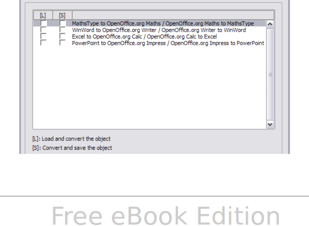
•If you choose Save original Basic code, the macros will not
work in OpenOffice.org but are retained if you save the file into
Microsoft Office format.
•If you choose Load Basic code to edit, the changed code is
saved in an OpenOffice.org document but is not retained if you
save into an Microsoft Office format.
•If you are importing a Microsoft Excel file containing VBA code,
you can select the option Executable code. Whereas normally
the code is preserved but rendered inactive (if you inspect it with
the StarBasic IDE you will notice that it is all commented), with
this option the code is ready to be executed.
Microsoft Office Load/Save options
On the Load/Save – Microsoft Office page, you can choose what to do
when importing and exporting Microsoft Office OLE objects (linked or
embedded objects or documents such as spreadsheets or equations).
Select the [L] options to convert Microsoft OLE objects into the
corresponding OpenOffice.org OLE objects when a Microsoft document
is loaded into OOo (mnemonic: “L” for “load”).
Select the [S] options to convert OpenOffice.org OLE objects into the
corresponding Microsoft OLE objects when a document is saved in a
Microsoft format (mnemonic: “S” for “save”).
Figure 320: Choosing Load/Save Microsoft Office options
398 OpenOffice.org 3.x Calc Guide
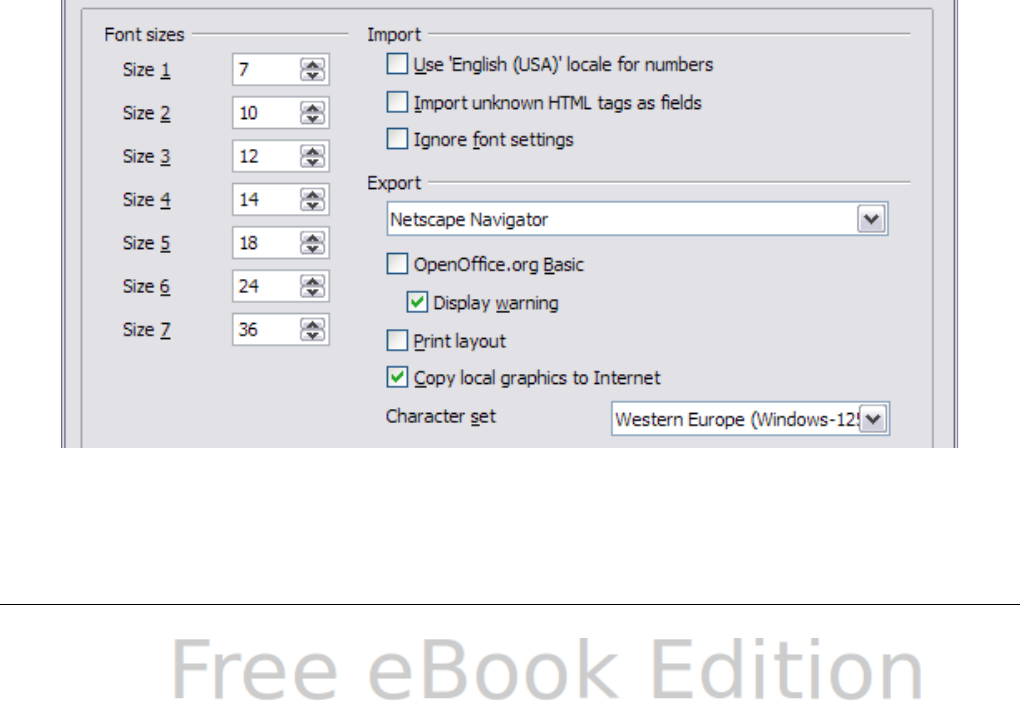
HTML compatibility Load/Save options
Choices made on the Load/Save – HTML Compatibility page
(Figure 321) affect HTML pages imported into OpenOffice.org and
those exported from OOo. See HTML documents; importing/exporting
in the Help for more information.
The main items of interest for Calc users are in the Export section:
OpenOffice.org Basic and Display warning.
Export - OpenOffice.org Basic
Select this option to include OOo Basic macros (scripts) when
exporting to HTML format. You must activate this option before you
create the OpenOffice.org Basic macro; otherwise the script will not
be inserted. OpenOffice.org Basic macros must be located in the
header of the HTML document. Once you have created the macro in
the OpenOffice.org Basic IDE, it appears in the source text of the
HTML document in the header.
If you want the macro to run automatically when the HTML
document is opened, choose Tools > Customize > Events. See
Chapter 12 (Calc Macros) for more information.
Export - Display warning
When the OpenOffice.org Basic option (see above) is not selected,
the Display warning option becomes available. If the Display
warning option is selected, then when exporting to HTML a
warning is shown that OpenOffice.org Basic macros will be lost.
Figure 321: Choosing HTML compatibility options
Chapter 14 Setting up and Customizing Calc 399
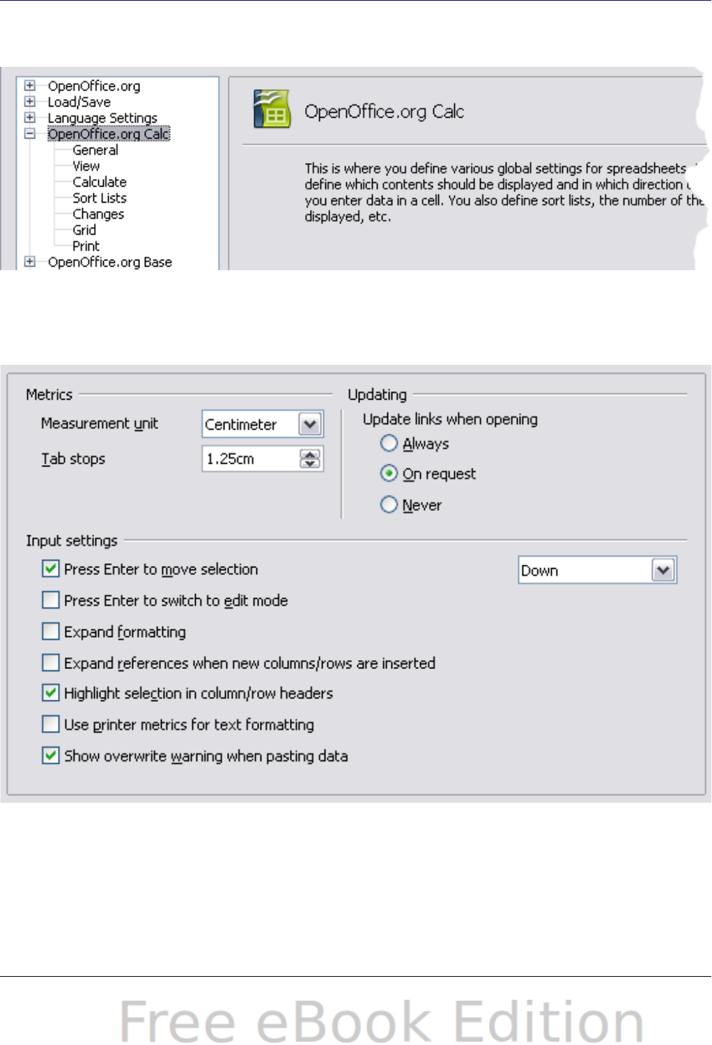
Choosing options for Calc
In the Options dialog, click the + sign to the left of OpenOffice.org
Calc on the left-hand side. A list of subsections drops down.
General options for Calc
In the Options dialog, choose OpenOffice.org Calc > General.
Figure 322: Selecting general options for Calc
Metrics section
Choose the unit of measurement used in spreadsheets and the default
tab stops distance.
400 OpenOffice.org 3.x Calc Guide

Updating section
Choose whether to update links when opening a document always, only
on request, or never. Regardless of this setting, you can manually
update links at any time. You might want to avoid updating links when
opening documents if they often contain many charts or linked
graphics that would slow down loading.
Input settings section
Press Enter to move selection
Specifies that pressing Enter moves the cursor to another cell. If
this option is selected, you can also choose the direction the cursor
moves: up, down, left, or right. If this option is not selected,
pressing Enter completes data entry for a cell but does not move the
cursor.
Press Enter to switch to edit mode
Specifies that pressing Enter puts the selected cell into edit mode.
Expand formatting
Specifies whether to automatically apply the formatting attributes of
an inserted cell to empty adjacent cells. If, for example, an inserted
cell has the bold attribute, this attribute will also apply to empty
adjacent cells. However, cells that already have a special format will
not be modified by this function. To see the affected range, press
Ctrl+* (multiplication sign on the number pad). The format will also
apply to all new values inserted within this range.
Expand references when new columns/rows are inserted
Specifies whether to expand references when inserting columns or
rows adjacent to the reference range. This is only possible if the
reference range, where the column or row is inserted, originally
spanned at least two cells in the desired direction.
Example: If the range A1:B1 is referenced in a formula and you
insert a new column after column B, the reference is expanded to
A1:C1. If the range A1:B1 is referenced and a new row is inserted
under row 1, the reference is not expanded, since there is only a
single cell in the vertical direction.
If you insert rows or columns in the middle of a reference area, the
reference is always expanded.
Highlight selection in column/row headings
Specifies whether to highlight column and row headers in the
selected columns or rows.
Chapter 14 Setting up and Customizing Calc 401
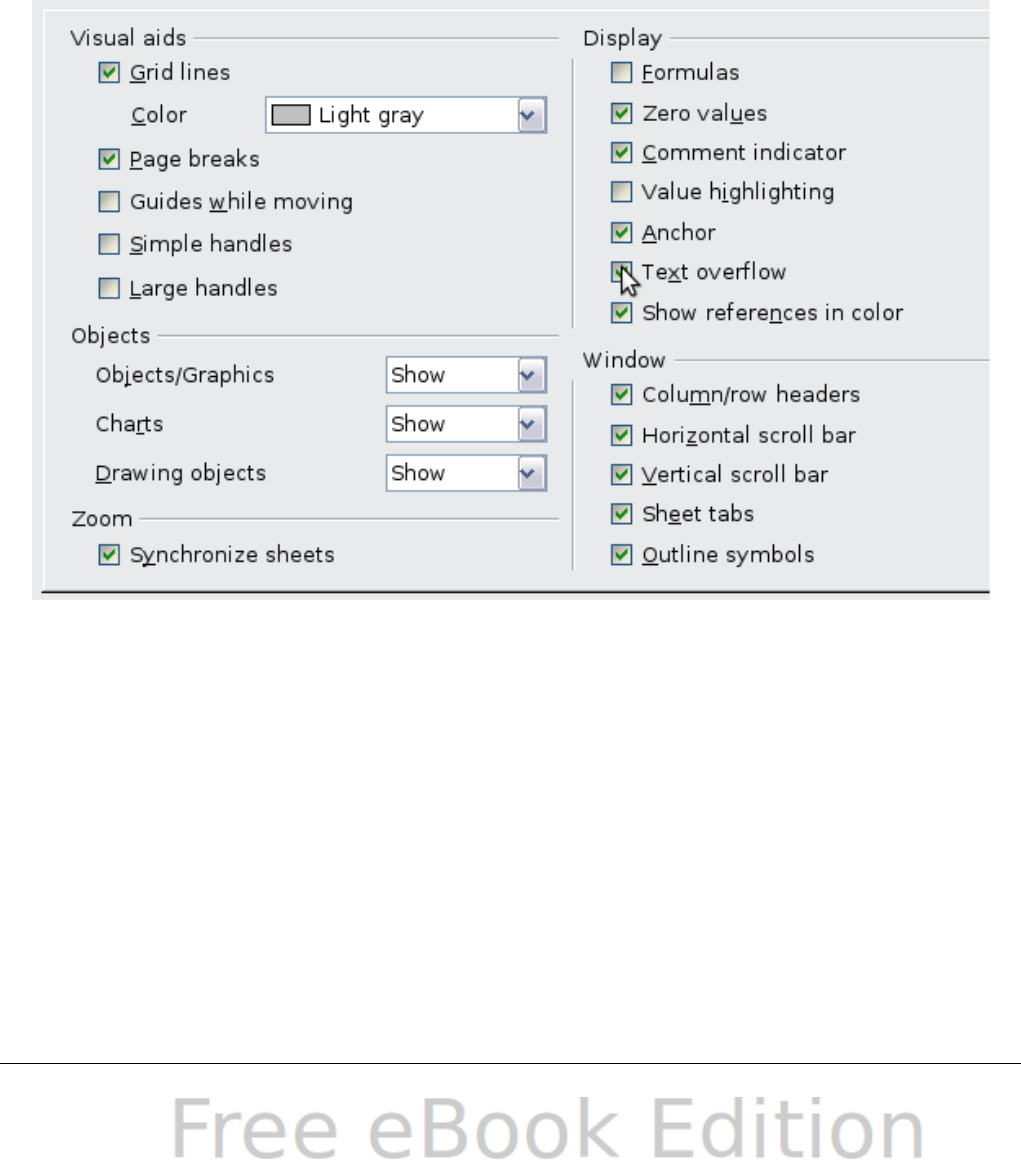
Use printer metrics for text formatting
Specifies that printer metrics are applied for printing and also for
formatting the display on the screen. If this option is not selected, a
printer-independent layout is used for screen display and printing.
Show overwrite warning when pasting data
Specifies that, when you paste cells from the clipboard to a cell
range that is not empty, a warning appears.
View options for Calc
In the Options dialog, choose OpenOffice.org Calc > View.
Figure 323: Selecting view options for Calc
Visual aids section
Specifies which lines are displayed.
Grid lines
Specifies whether to display grid lines between the cells when
viewed onscreen. If this option is selected, you can also specify the
color for the grid lines in the current document. The color choice
overrides the selection made in Tools > Options >
OpenOffice.org > Appearance > Spreadsheet > Grid lines.
402 OpenOffice.org 3.x Calc Guide

For printing, choose Format > Page > Sheet and mark the Grid
option.
Page breaks
Specifies whether to view the page breaks within a defined print
area.
Guides while moving
Specifies whether to view guides when moving drawings, frames,
graphics and other objects. These guides help you align objects.
Simple handles
Specifies whether to display the handles (the eight points on a
selection box) as simple squares without a 3D effect.
Large handles
Specifies that larger than normal handles (the eight points on a
selection box) are displayed.
Display section
Select various options for the screen display.
Formulas
Specifies whether to show formulas instead of results in the cells.
Zero values
Specifies whether to show numbers with the value of 0.
Comment indicator
Specifies that a small rectangle is shown in the top right corner of
the cell when a comment exists for that cell. The text of the
comment is shown when you hover the pointer over the cell, if tips
are enabled under Tools > Options > OpenOffice.org > General.
To display a comment permanently, right-click on the cell and select
Show comment from the pop-up menu.
Value highlighting
Select this option to highlight all values in the sheet. Text is
highlighted in black; numbers in blue; and formulas, logical values,
dates, and so on, in green.
When this command is active, any colors assigned in the document
are not displayed.
Anchor
Specifies whether the anchor icon is displayed when an inserted
object, such as a graphic, is selected.
Chapter 14 Setting up and Customizing Calc 403

Text overflow
If a cell contains text that is wider than the width of the cell, the text
is displayed over empty neighboring cells in the same row. If there is
no empty neighboring cell, a small triangle at the cell border
indicates that the text continues.
Show references in color
Specifies that each reference is highlighted in color in the formula.
The cell range is also enclosed by a colored border as soon as the
cell containing the reference is selected for editing.
Objects section
Specifies whether to display or hide objects in three object groups:
objects and graphics; charts; and drawing objects.
Window section
Specifies whether some elements are visible onscreen: column/row
headers, horizontal scrollbar, vertical scrollbar, sheet tabs, and outline
symbols.
If the Sheet tabs option is not selected, you can only switch between
the sheets by using the Navigator.
Note that there is a slider between the horizontal scrollbar and the
sheet tabs that may be set to one end.
Zoom section
Select the Synchronize sheets option to apply any selected zoom
factor to all sheets in the spreadsheet. If this option is not selected,
separate zoom factors can be applied to individual sheets.
Calculate options
In the Options dialog, choose OpenOffice.org Calc > Calculate.
Use this page to define the calculation settings for spreadsheets.
404 OpenOffice.org 3.x Calc Guide
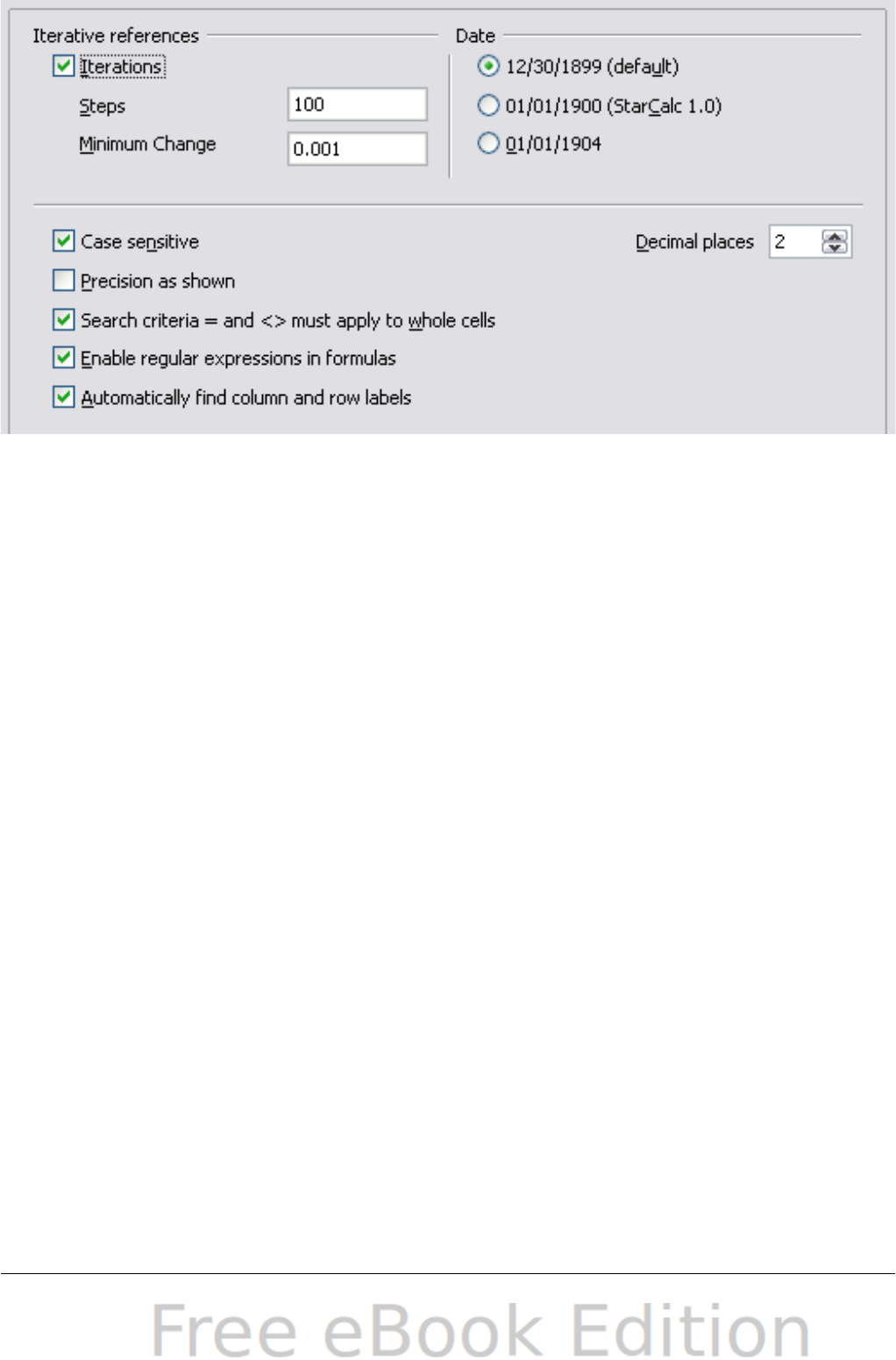
Figure 324: Calc calculation options
Iterative references section
Iterative references are formulas that are continuously repeated until
the problem is solved. In this section you can choose the number of
approximation steps carried out during iterative calculations and the
degree of precision of the answer.
Iterations
Select this option to enable iterations. If this options is not selected,
an iterative reference causes an error message.
Steps
Sets the maximum number of iteration steps.
Minimum Change
Specifies the difference between two consecutive iteration step
results. If the result of the iteration is lower than the minimum
change value, then the iteration will stop.
Date section
Select the start date for the internal conversion from days to numbers.
12/30/1899 (default)
Sets 12/30/1899 as day zero.
01/01/1900 (StarCalc 1.0)
Sets 1/1/1900 as day zero. Use this setting for StarCalc 1.0
spreadsheets containing date entries.
Chapter 14 Setting up and Customizing Calc 405

01/01/1904
Sets 1/1/1904 as day zero. Use this setting for spreadsheets that are
imported in a foreign format.
Other options
Specify a variety of options relevant to spreadsheet calculation.
Case sensitive
Specifies whether to distinguish between upper and lower case in
texts when comparing cell contents. The EXACT text function is
always case-sensitive, independent of the settings in this dialog.
Decimal places
Defines the number of decimals to be displayed for numbers with
the Standard number format. The numbers are displayed as rounded
numbers, but are not saved as rounded numbers.
Precision as shown
Specifies whether to make calculations using the rounded values
displayed in the sheet. Charts will be shown with the displayed
values. If this option is not selected, the displayed numbers are
rounded, but they are calculated internally using the non-rounded
number.
Search criteria = and <> must apply to whole cells
Specifies that the search criteria you set for the Calc database
functions must match the whole cell exactly. When this option is
selected, Calc behaves exactly like MS Excel when searching cells in
the database functions.
This search: Has this result:
win Finds win, but not win95, os2win, or upwind
win.* Finds win and win95, but not os2win or upwind
.*win Finds win and os2win, but not win95 or upwind
.*win.* Finds win, win95, os2win, and upwind
If this option is not selected, the win search pattern acts like .*win.*
—the search pattern can be at any position within the cell when
searching with the Calc database functions.
Enable regular expressions in formulas
Specifies that regular expressions are enabled when searching and
also for character string comparisons. This relates to the database
functions, and to VLOOKUP, HLOOKUP and SEARCH.
406 OpenOffice.org 3.x Calc Guide
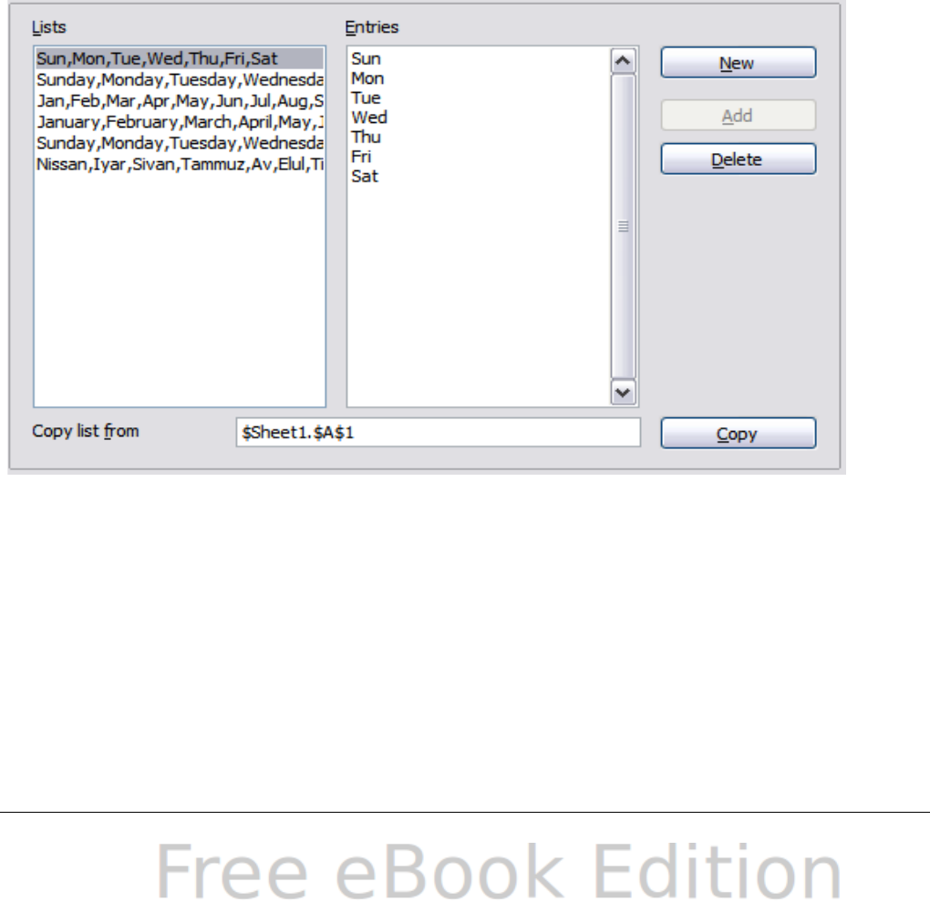
Automatically find column and row labels
Specifies that you can use the text in any cell as a label for the
column below the text or the row to the right of the text. The text
must consist of at least one word and must not contain any
operators.
Example: Cell E5 contains the text Europe. Below, in cell E6, is the
value 100 and in cell E7 the value 200. If the Automatically find
column and row labels option is selected, you can write the
following formula in cell A1: =SUM(Europe).
Sort Lists options
In the Options dialog, choose OpenOffice.org Calc > Sort Lists. Sort
lists are used for more than sorting, for example filling a series of cells
during data entry. In addition to the supplied lists, you can define and
edit your own lists, as described in “Defining a fill series” in Chapter 2
(Entering, Editing, and Formatting Data).
Figure 325: Defining sorting lists in Calc
Chapter 14 Setting up and Customizing Calc 407
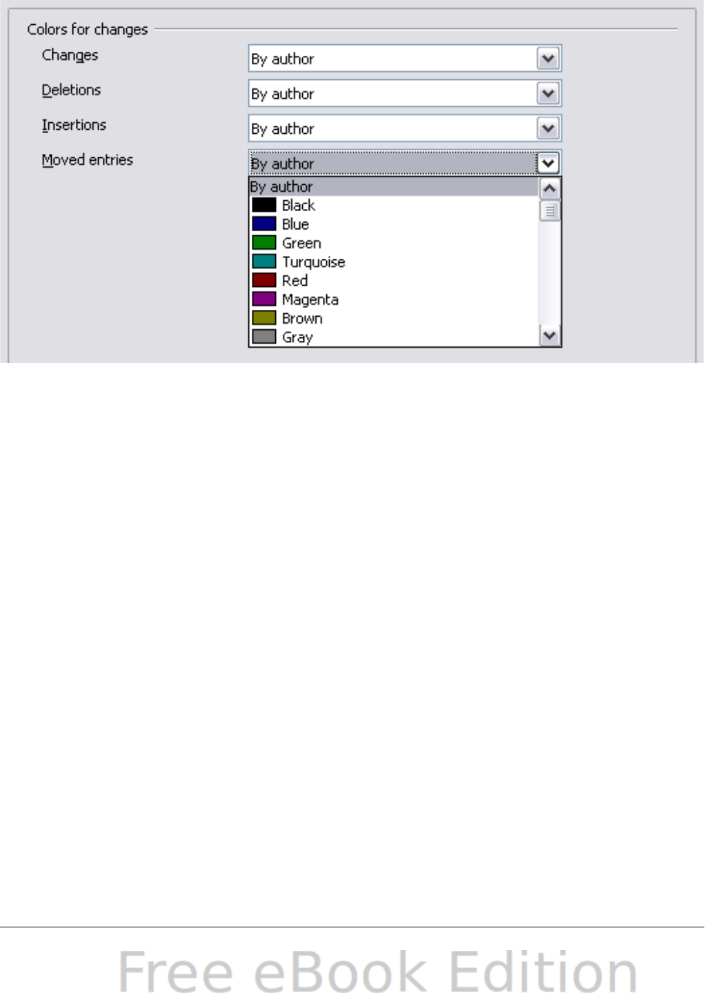
Changes options
In the Options dialog, choose OpenOffice.org Calc > Changes.
Figure 326: Calc options for highlighting changes
On this page you can specify options for highlighting recorded changes
in spreadsheets. You can assign specific colors for insertions, deletions,
and other changes, or you can let Calc assign colors based on the
author of the change; in the latter case, one color will apply to all
changes made by that author.
Grid options
The Grid page defines the grid settings for spreadsheets. Using a grid
helps you determine the exact position of any charts or other objects
you may add to a spreadsheet. You can also set this grid in line with
the snap grid.
If you have activated the snap grid but wish to move or create
individual objects without snap positions, you can press the Ctrl key to
deactivate the snap grid for as long as needed.
In the Options dialog, choose OpenOffice.org Calc > Grid.
408 OpenOffice.org 3.x Calc Guide
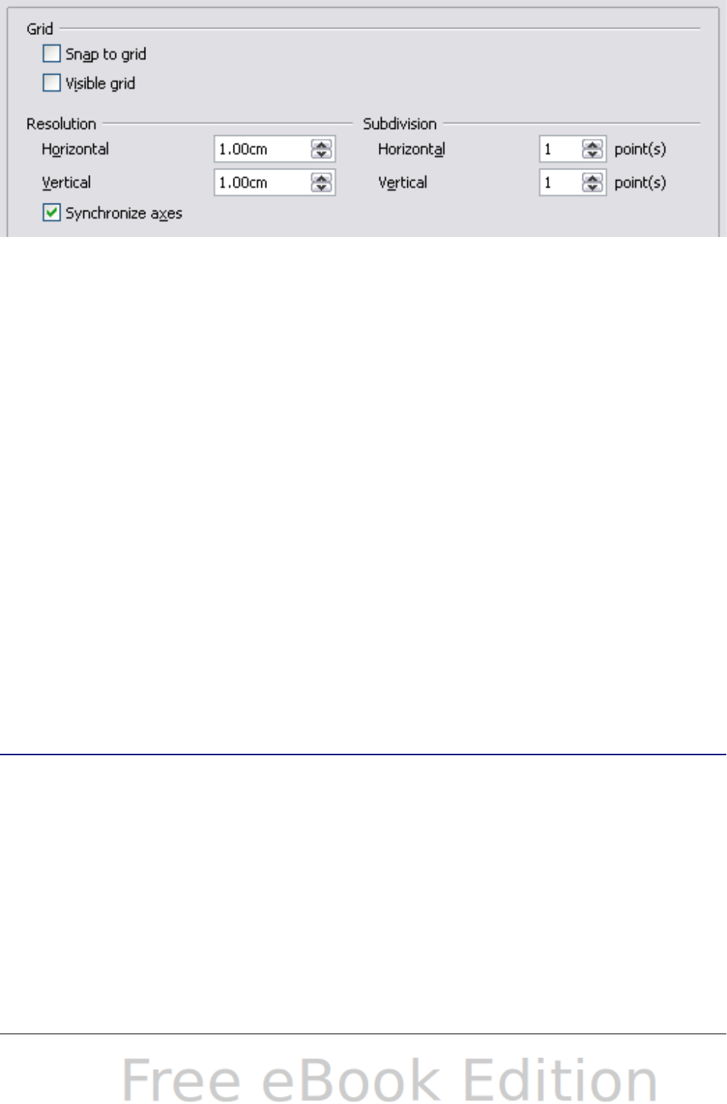
Figure 327: Calc grid options
Grid section
Snap to grid activates the snap function.
Visible grid displays grid points on the screen. These points are not
printed.
Resolution section
Here you can set the unit of distance for the spacing between
horizontal and vertical grid points and subdivisions (intermediate
points) of the grid.
Synchronize axes changes the current grid settings symmetrically.
Print options
In the Options dialog, choose OpenOffice.org Calc > Print. See
Chapter 6 (Printing, Exporting, and E-mailing) for more about the
options on this page.
Controlling Calc’s AutoCorrect functions
Some people find some or all of the items in OOo’s AutoCorrect
function annoying because they change what you type when you do not
want it changed. Many people find some of the AutoCorrect functions
quite helpful; if you do, then select the relevant options. But if you find
unexplained changes appearing in your document, this is a good place
to look to find the cause.
To open the AutoCorrect dialog, click Tools > AutoCorrect Options.
(You need to have a document open for this menu item to appear.)
Chapter 14 Setting up and Customizing Calc 409
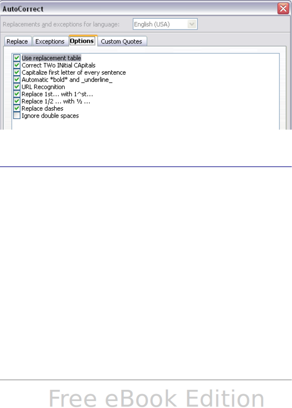
In Calc, this dialog has four tabs, as shown below. Options are
described in the Help; many will be familiar to users of other office
suites.
Figure 328: The AutoCorrect dialog in Calc
Customizing the user interface
Customizing the menu font
If you want to change the menu font from that supplied by OOo to the
system font for your operating system, do this:
1) Choose Tools > Options > OpenOffice.org > View.
2) Check Use system font for user interface and click OK.
Customizing menu content
In addition to changing the menu font, you can add and rearrange
items on the menu bar, add items to menus, and make other changes.
To customize menus:
1) Choose Tools > Customize.
2) On the Customize dialog, pick the Menus page (Figure 329).
3) In the Save In drop-down list, choose whether to save this
changed menu for Calc or for a selected document.
4) In the section OpenOffice.org Calc Menus, select from the
Menu drop-down list the menu that you want to customize. The
list includes all the main menus as well as sub-menus, that is
410 OpenOffice.org 3.x Calc Guide
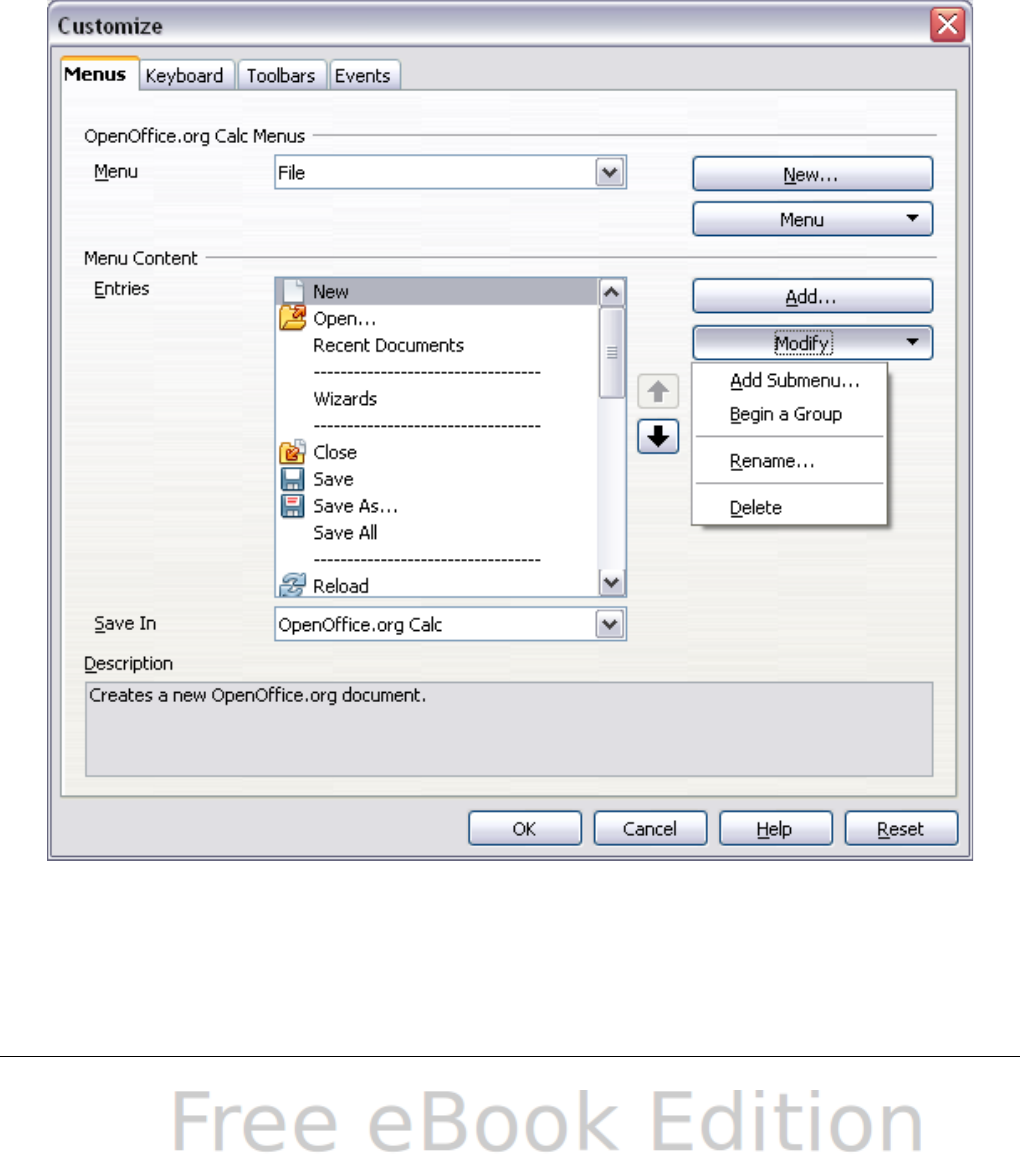
menus that are contained under another menu. For example, in
addition to File, Edit, View, and so on, there is File | Send and
File |Templates. The commands available for the selected menu
are shown in the central part of the dialog.
5) To customize the selected menu, click on the Menu or Modify
buttons. You can also add commands to a menu by clicking on the
Add button. These actions are described in the following sections.
Use the up and down arrows next to the Entries list to move the
selected menu item to a different position.
6) When you have finished making all your changes, click OK to
save them.
Figure 329: The Menus page of the Customize dialog
Chapter 14 Setting up and Customizing Calc 411
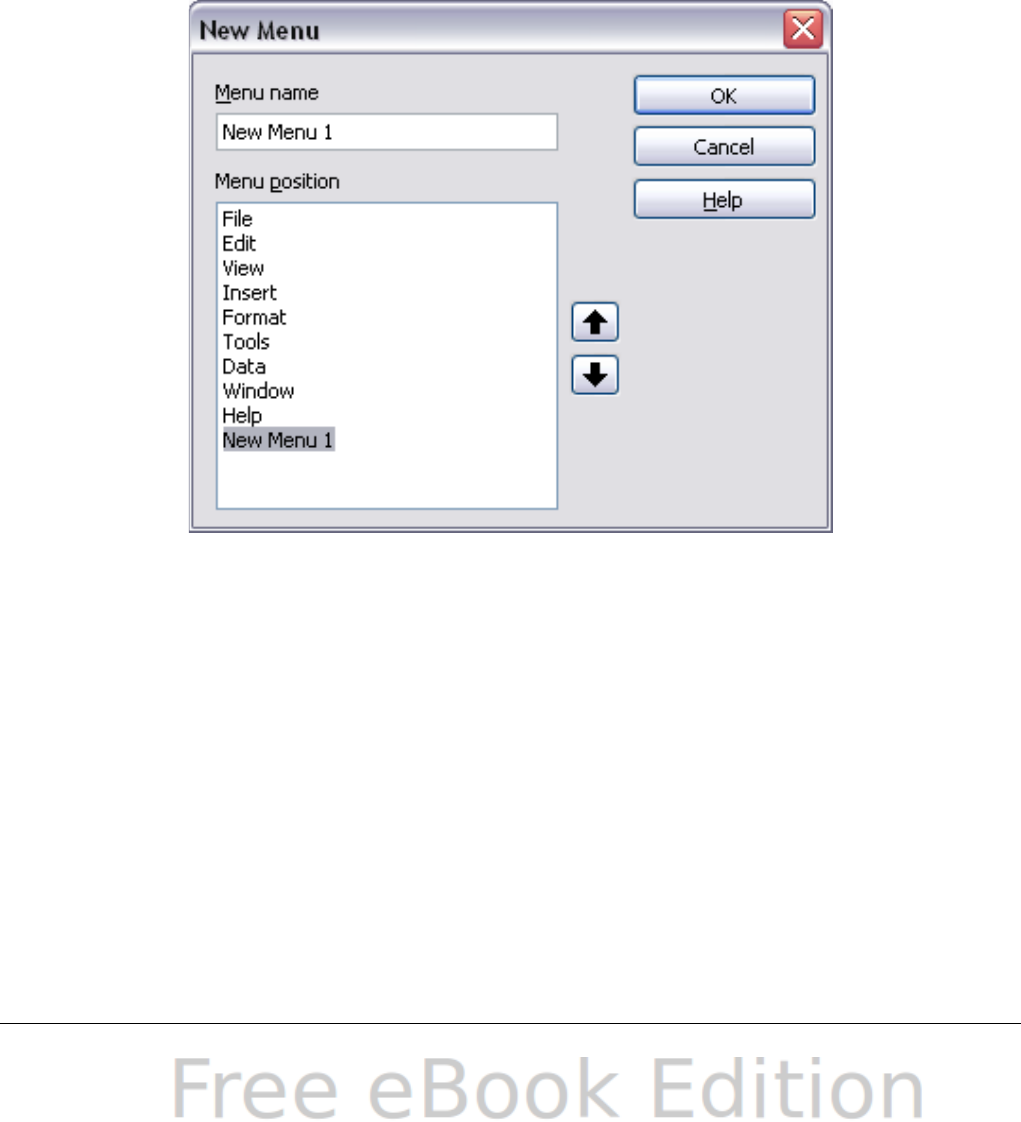
Creating a new menu
In the Customize dialog, click New to display the dialog shown in
Figure 330.
1) Type a name for your new menu in the Menu name box.
2) Use the up and down arrow buttons to move the new menu into
the required position on the menu bar. Click OK to save.
The new menu now appears on the list of menus in the Customize
dialog. (It will appear on the menu bar itself after you save your
customizations.)
After creating a new menu, you need to add some commands to it, as
described in “Adding a command to a menu” on page 413.
Figure 330: Adding a new menu
Modifying existing menus
To modify an existing menu, select it in the Menu list and click the
Menu button to drop down a list of modifications: Move, Rename,
Delete. Not all of these modifications can be applied to all the entries
in the Menu list. For example, Rename and Delete are not available
for the supplied menus.
To move a menu (such as File), choose Menu > Move. A dialog similar
to the one shown in Figure 330 (but without the Menu name box)
opens. Use the up and down arrow buttons to move the menu into the
required position.
412 OpenOffice.org 3.x Calc Guide
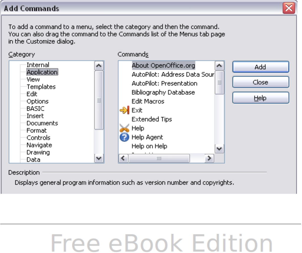
To move submenus (such as File | Send), select the main menu (File) in
the Menu list and then, in the Menu Content section of the dialog,
select the submenu (Send) in the Entries list and use the arrow keys to
move it up or down in the sequence. Submenus are easily identified in
the Entries list by a small black triangle on the right hand side of the
name.
In addition to renaming, you can specify a keyboard shortcut that
allows you to select a menu command when you press Alt+ an
underlined letter in a menu command.
1) Select a menu or menu entry.
2) Click the Menu button and select Rename.
3) Add a tilde (~) in front of the letter that you want to use as an
accelerator. For example, to select the Save All command by
pressing Alt+V, enter Sa~ve All.
Adding a command to a menu
You can add commands to the supplied menus and to menus you have
created. On the Customize dialog, select the menu in the Menu list and
click the Add button in the Menu Content section of the dialog.
Figure 331: Adding a command to a menu
Chapter 14 Setting up and Customizing Calc 413

On the Add Commands dialog, select a category and then the
command, and click Add. The dialog remains open, so you can select
several commands. When you have finished adding commands, click
Close. Back on the Customize dialog, you can use the up and down
arrow buttons to arrange the commands in your preferred sequence.
Modifying menu entries
In addition to changing the sequence of entries on a menu or submenu,
you can add submenus, rename or delete the entries, and add group
separators.
To begin, select the menu or submenu in the Menu list near the top of
the Customize page, then select the entry in the Entries list under
Menu Content. Click the Modify button and choose the required action
from the drop-down list of actions.
Most of the actions should be self-explanatory. Begin a group adds a
separator line after the highlighted entry.
Customizing toolbars
You can customize toolbars in several ways, including choosing which
icons are visible and locking the position of a docked toolbar, as
described in Chapter 1 (Introducing OpenOffice.org) of the Getting
Started guide. This section describes how to create new toolbars and
add other icons (commands) to the list of those available on a toolbar.
To get to the toolbar customization dialog, do any of the following:
•On the toolbar, click the arrow at the end of the toolbar and
choose Customize Toolbar.
•Choose View > Toolbars > Customize from the menu bar.
•Choose Tools > Customize from the menu bar and pick the
Toolbars page (Figure 332).
To customize toolbars:
1) In the Save In drop-down list, choose whether to save this
changed toolbar for Calc or for a selected document.
2) In the section OpenOffice.org Calc Toolbars, select from the
Toolbar drop-down list the toolbar that you want to customize.
3) You can create a new toolbar by clicking on the New button, or
customize existing toolbars by clicking on the Toolbar or Modify
buttons, and add commands to a toolbar by clicking on the Add
button. These actions are described below.
414 OpenOffice.org 3.x Calc Guide
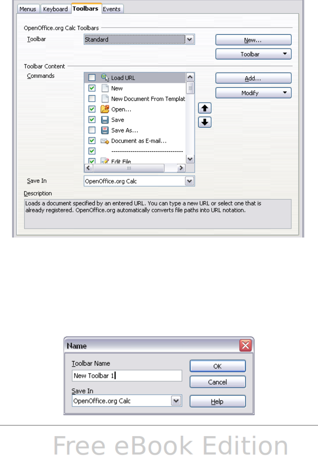
4) When you have finished making all your changes, click OK to
save them.
Figure 332: The Toolbars page of the Customize dialog
Creating a new toolbar
To create a new toolbar:
1) Choose Tools > Customize > Toolbars from the menu bar.
2) Click New. On the Name dialog, type the new toolbar's name and
choose from the Save In drop-down list where to save this
changed menu: for Calc or for a selected document.
Chapter 14 Setting up and Customizing Calc 415

The new toolbar now appears on the list of toolbars in the Customize
dialog. After creating a new toolbar, you need to add some commands
to it, as described below.
Adding a command to a toolbar
If the list of available buttons for a toolbar does not include all the
commands you want on that toolbar, you can add commands. When you
create a new toolbar, you need to add commands to it.
1) On the Toolbars page of the Customize dialog, select the toolbar
in the Toolbar list and click the Add button in the Toolbar Content
section of the dialog.
2) The Add Commands dialog is the same as for adding commands to
menus (Figure 331). Select a category and then the command,
and click Add. The dialog remains open, so you can select several
commands. When you have finished adding commands, click
Close. If you insert an item which does not have an associated
icon, the toolbar will display the full name of the item: the next
section describes how to choose an icon for a toolbar command.
3) Back on the Customize dialog, you can use the up and down
arrow buttons to arrange the commands in your preferred
sequence.
4) When you are done making changes, click OK to save.
Choosing icons for toolbar commands
Toolbar buttons usually have icons, not words, on them, but not all of
the commands have associated icons.
To choose an icon for a command, select the command and click
Modify > Change icon. On the Change Icon dialog (Figure 333),
scroll through the available icons, select one, and click OK to assign it
to the command.
To use a custom icon, create it in a graphics program and import it into
OOo by clicking the Import button on the Change Icon dialog. Custom
icons must be 16 x 16 or 26 x 26 pixels in size and cannot contain more
than 256 colors.
Customizing keyboard shortcuts
In addition to using the built-in keyboard shortcuts (listed in Appendix
A), you can define your own. You can assign shortcuts to standard OOo
functions or your own macros and save them for use with the entire
OpenOffice.org suite or only for Calc.
416 OpenOffice.org 3.x Calc Guide
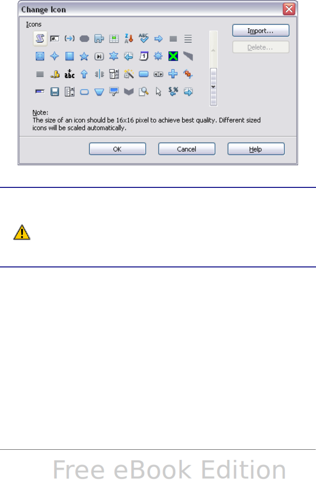
Figure 333: Change Icon dialog
Caution
Be careful when reassigning your operating system’s or OOo’s
predefined shortcut keys. Many key assignments are universally
understood shortcuts, such as F1 for Help, and are always
expected to provide certain results. Although you can easily
reset the shortcut key assignments to the OOo defaults,
changing some common shortcut keys can cause confusion,
frustration and possible data loss or corruption, especially if
other users share your computer.
To adapt shortcut keys to your needs, use the Customize dialog, as
described below.
1) Select Tools > Customize > Keyboard. The Keyboard page of
the Customize dialog opens.
2) To have the shortcut key assignment available only with Calc,
select Calc in the upper right corner of the page; otherwise select
OpenOffice.org to make it available to every component.
3) Next select the required function from the Category and Function
lists.
4) Now select the desired shortcut keys in the Shortcut keys list and
click the Modify button at the upper right.
5) Click OK to accept the change. Now the chosen shortcut keys will
execute the function chosen in step 3 above whenever they are
pressed.
Chapter 14 Setting up and Customizing Calc 417
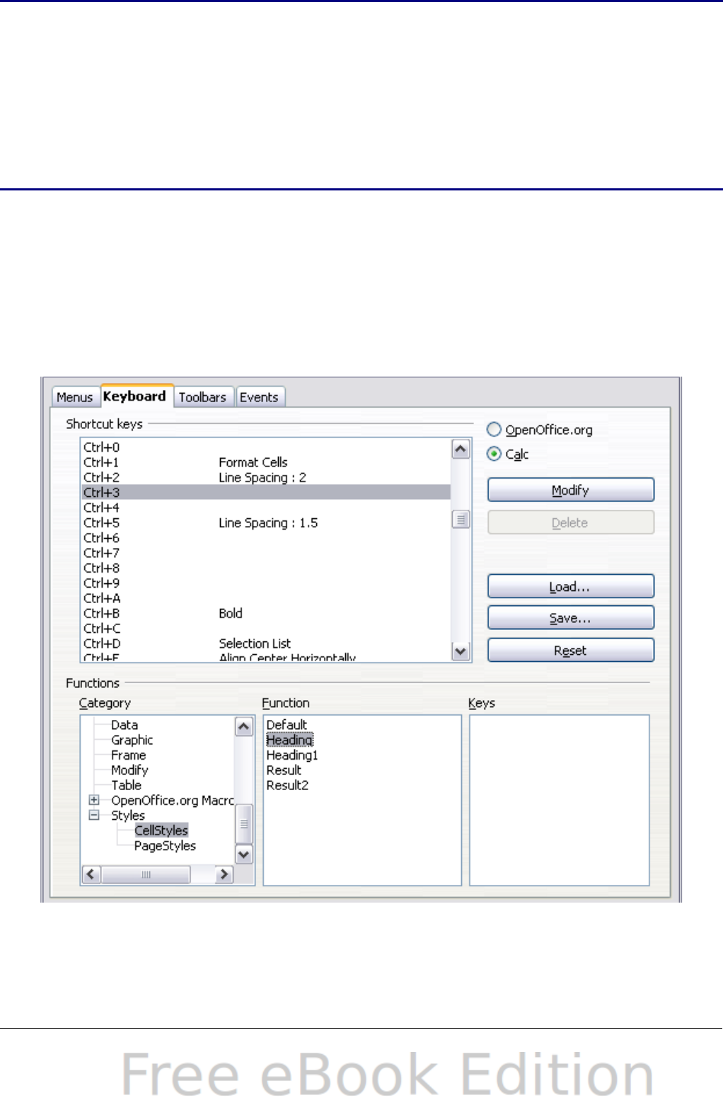
Note
All existing shortcut keys for the currently selected Function are
listed in the Keys selection box. If the Keys list is empty, it
indicates that the chosen key combination is free for use. If it
were not, and you wanted to reassign a shortcut key
combination that is already in use, you must first delete the
existing key.
Shortcut keys that are greyed-out in the listing on the Customize
dialog, such as F1 and F10, are not available for reassignment.
Example: Assigning styles to shortcut keys
You can configure shortcut keys to quickly assign styles in your
document.
1) On the Keyboard page of the Customize dialog, choose the
shortcut keys you want to assign a style to. In this example, we
have chosen Ctrl+3.
Figure 334: Assigning a cell style to a key combination
418 OpenOffice.org 3.x Calc Guide

2) In the Functions section at the bottom of the dialog, scroll down
in the Category list to Styles. Click the + sign to expand the list of
styles.
3) Choose the category of style. (This example uses a cell style, but
you can also choose page styles.) The Function list now displays
the names of the available styles for the selected category. The
example shows OOo’s predefined cell styles.
4) To assign Ctrl+3 to be the shortcut key combination for the
Heading style, select Heading in the Function list, and then click
Modify. Ctrl+3 now appears in the Keys list on the right, and
Heading appears next to Ctrl+3 in the Shortcut keys box at the
top.
5) Make any other required changes, and then click OK to save
these settings and close the dialog.
Saving changes to a file
Changes to the shortcut key assignments can be saved in a keyboard
configuration file for use at a later time, thus permitting you to create
and apply different configurations as the need arises. To save keyboard
shortcuts to a file:
1) After making your keyboard shortcut assignments, click the Save
button on the Customize dialog.
2) In the Save Keyboard Configuration dialog, select All files from
the Save as Type list.
3) Next enter a name for the keyboard configuration file in the
File name box, or select an existing file from the list. If you need
to, browse to find a file from another location.
4) Click Save. A confirmation dialog appears if you are about to
overwrite an existing file, otherwise there will be no feedback and
the file will be saved.
Loading a saved keyboard configuration
To load a saved keyboard configuration file and replace your existing
configuration, click the Load button on the Customize dialog, and then
select the configuration file from the Load Keyboard Configuration
dialog.
Resetting the shortcut keys
To reset all of the keyboard shortcuts to their default values, click the
Reset button near the bottom right of the Customize dialog. Use this
Chapter 14 Setting up and Customizing Calc 419
feature with care as no confirmation dialog will be displayed; the
defaults will be set without any further notice or user input.
Running macros from key combinations
You can also define shortcut key combinations that will run macros.
These shortcut keys are strictly user-defined; none are built in. For
more information on macros, see Chapter 12 (Calc Macros).
Adding functionality with extensions
An extension is a package that can be installed into OpenOffice.org to
add new functionality.
Although individual extensions can be found in different places, the
official OpenOffice.org extension repository is at
http://extensions.services.openoffice.org/. Some extensions are free of
charge; others are available for a fee. Check the descriptions to see
what licenses and fees apply to the ones that interest you.
Installing extensions
To install an extension, follow these steps:
1) Download an extension and save it anywhere on your computer.
2) In OOo, select Tools > Extension Manager from the menu bar.
In the Extension Manager dialog (Figure 335), click Add.
3) A file browser window opens. Find and select the extension you
want to install and click Open. The extension begins installing.
You may be asked to accept a license agreement.
4) When the installation is complete, the extension is listed in the
Extension Manager dialog.
Tip
To get extensions that are listed in the repository, you can open
the Extension Manager and click the Get more extensions
here link. You do not need to download them separately as in
step 1 above.
Note To install a shared extension, you need write access to the
OpenOffice.org installation directory.
420 OpenOffice.org 3.x Calc Guide
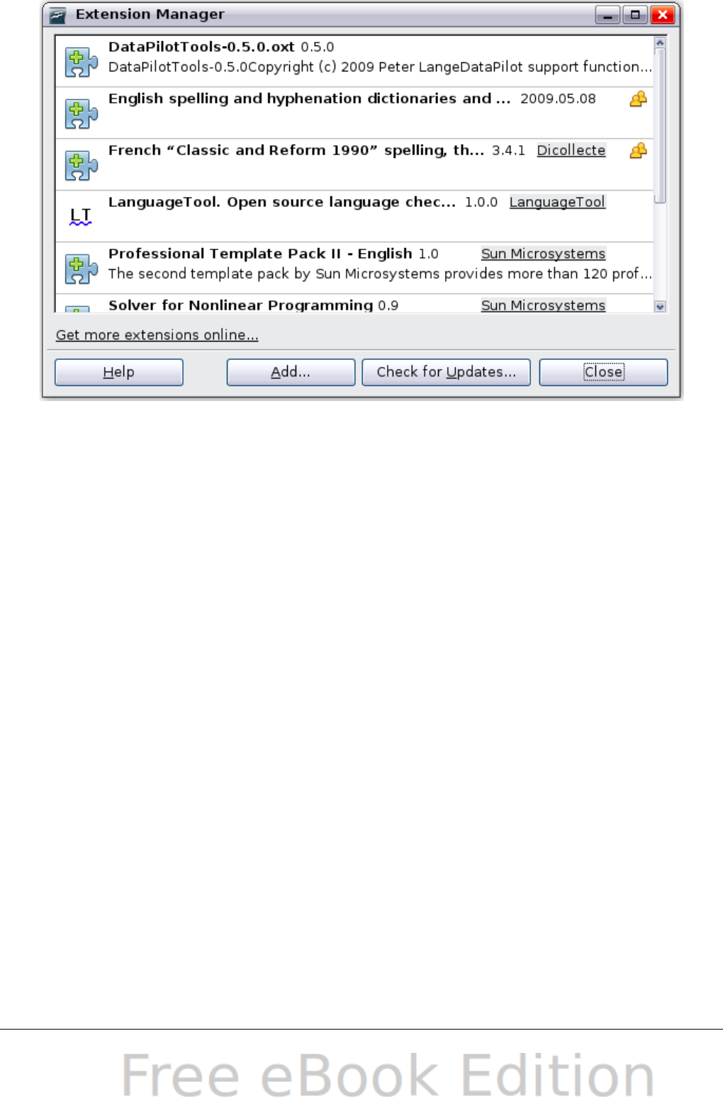
Figure 335: Installing an extension
Using extensions
This section describes a few of the extensions to Calc. In each case,
you need to install the extension as described in the previous section.
rofessional Template Pack II
Provides more than 120 templates for Writer, Calc, and Impress.
Available in several languages. After you have installed this
extension, you will find the templates under File > New >
Templates and Documents.
Solver for Nonlinear Programming
Calc ships with a solver engine for linear programming only. This
extension adds more solvers, which are capable of handling
nonlinear problems as well as linear ones:
•DEPS - Differential Evolution & Particle Swarm Optimization
•SCO - Social Cognitive Optimization
DataPilot Tools for OpenOffice.org Calc
Adds some utility functions that make using the DataPilot easier:
•Display the current source range for a DataPilot
•Change the source range for a DataPilot
•Refresh all DataPilots on the current sheet
Chapter 14 Setting up and Customizing Calc 421

Appendix A
Keyboard Shortcuts
Introduction
You can use Calc without a pointing device such as a mouse or
trackball, by using its built-in keyboard shortcuts.
OOo has a general set of keyboard shortcuts, available in all
components, and a component-specific set directly related to the work
of that component.
For help with OOo’s keyboard shortcuts or using OOo with a keyboard
only, search the OOo online help using the “shortcut” or “accessibility”
keywords.
In addition to using the built-in keyboard shortcuts listed in this
Appendix, you can define your own. See Chapter 14 (Setting Up and
Customizing Calc) for instructions.
Formatting and editing shortcuts are described in Chapter 2 (Entering,
Editing, and Formatting Data).
Navigation and selection shortcuts
Table 29: Spreadsheet navigation shortcuts
Shortcut Keys Effect
Ctrl+Home Moves the cursor to the first cell in the sheet (cell A1).
Ctrl+End Moves the cursor to the last cell on the sheet that
contains data.
Home Moves the cursor to the first cell of the current row.
End Moves the cursor to the last cell of the current row in
a column containing data.
Ctrl+Left Arrow Moves the cursor to the left edge of the current data
range. If the column to the left of the cell that contains
the cursor is empty, the cursor moves to the next
column to the left that contains data.
Ctrl+Right Arrow Moves the cursor to the right edge of the current data
range. If the column to the right of the cell that
contains the cursor is empty, the cursor moves to the
next column to the right that contains data.
Ctrl+Up Arrow Moves the cursor to the top edge of the current data
range. If the row above the cell that contains the
cursor is empty, the cursor moves up to the next row
that contains data.
Appendix A Keyboard Shortcuts 423
Shortcut Keys Effect
Ctrl+Down Arrow Moves the cursor to the bottom edge of the current
data range. If the row below the cell that contains the
cursor is empty, the cursor moves down to the next
row that contains data.
Ctrl+Shift+Arrow Selects all cells containing data from the current cell
to the end of the continuous range of data cells, in the
direction of the arrow pressed. If used to select rows
and columns together, a rectangular cell range is
selected.
Ctrl+Page Up Moves one sheet to the left. In the page preview it
moves to the previous print page.
Ctrl+Page Down Moves one sheet to the right. In the page preview it
moves to the next print page.
Page Up Moves the viewable rows up one screen.
Page Down Moves the viewable rows down one screen.
Alt+Page Up Moves the viewable columns one screen to the left.
Alt+Page Down Moves the viewable columns one screen to the right.
Shift+Ctrl+Page
Up
Adds the previous sheet to the current selection of
sheets. If all the sheets in a spreadsheet are selected,
this combination only selects the previous sheet.
Makes the previous sheet the current sheet.
Shift+Ctrl+Page
Down
Adds the next sheet to the current selection of sheets.
If all the sheets in a spreadsheet are selected, this
combination only selects the next sheet. Makes the
next sheet the current sheet.
Ctrl+* Selects the data range that contains the cursor. A
range is a contiguous cell range that contains data and
is bounded by empty rows and columns. The “*” key is
the multiplication sign on the numeric key pad.
Ctrl+/ Selects the matrix formula range that contains the
cursor. The “/” key is the division sign on the numeric
key pad.
Enter — in a
selected range
By default, moves the cursor down one cell in a
selected range. To specify the direction that the cursor
moves, choose Tools > Options > OpenOffice.org
Calc > General.
424 OpenOffice.org 3.x Calc Guide
Function and arrow key shortcuts
Table 30: Function key shortcuts
Shortcut Keys Effect
F1 Displays the OOo help browser. When the help browser
is already open F1 jumps to the main help page.
Shift+F1 Displays context help.
Ctrl+F1 Displays the note that is attached to the current cell.
F2 Switches to Edit mode and places the cursor at the end
of the contents of the current cell. If the cursor is in an
input box in a dialog that has a minimize button, the
dialog is hidden and the input box remains visible.
Press F2 again to show the whole dialog.
Ctrl+F2 Opens the Function Wizard.
Shift+Ctrl+F2 Moves the cursor to the input line where you can enter
a formula for the current cell.
Ctrl+F3 Opens the Define Names dialog.
F4 Shows or hides the Database Sources menu.
Shift+F4 Rearranges the relative or absolute references (for
example, A1, $A$1, $A1, A$1) in the input field.
F5 Shows or hides the Navigator.
Shift+F5 Traces dependents.
Shift+Ctrl+F5 Moves the cursor to the Name box.
F7 Checks spelling in the current sheet.
Ctrl+F7 Opens the Thesaurus if the current cell contains text.
Shift+F7 Traces precedents.
F8 Turns additional selection mode on or off. In this mode,
you can use the arrow keys to extend the selection. You
can also click in another cell to extend the selection.
Ctrl+F8 Highlights cells containing numeric values (not text).
F9 Recalculates all of the formulas in the sheet.
Ctrl+F9 Updates the selected chart.
F11 Opens the Styles and Formatting window where you
can apply a formatting style to the contents of the cell
or to the current sheet.
Shift+F11 Creates a document template.
Appendix A Keyboard Shortcuts 425
Shortcut Keys Effect
Shift+Ctrl+F11 Updates the templates.
F12 Groups the selected data range.
Ctrl+F12 Ungroups the selected data range.
Table 31. Arrow key shortcuts
Shortcut Keys Effect
Alt+Down Arrow Increases the height of current row.
Alt+Up Arrow Decreases the height of current row.
Alt+Right Arrow Increases the width of the current column.
Alt+Left Arrow Decreases the width of the current column.
Alt+Shift+Arrow
Key
Optimizes the column width or row height based on
the current cell.
Cell formatting shortcuts
Ctrl+1 open the Format Cells dialog.
Note
The shortcuts listed in Table 32 do not work under any Linux
desktop tested. If you would like to have the functionality
described in this table, you must create custom key sequences
as explained in Chapter 14 (Setting Up and Customizing Calc).
Note
The shortcut keys shown in Table 32 do not use the number
keys on the number pad. They use the number keys above the
letter keys on the main keyboard.
Table 32: Formatting shortcut keys
Shortcut Keys Effect
Ctrl+Shift+1 Two decimal places, thousands separator
Ctrl+Shift+2 Standard exponential format
Ctrl+Shift+3 Standard date format
Ctrl+Shift+4 Standard currency format
Ctrl+Shift+5 Standard percentage format (two decimal places)
Ctrl+Shift+6 Standard format
426 OpenOffice.org 3.x Calc Guide
DataPilot shortcuts
Table 33: DataPilot shortcut keys
Shortcut Keys Effect
Tab Changes the focus by moving forward through the
areas and buttons of the dialog.
Shift+Tab Changes the focus by moving backward through the
areas and buttons of the dialog.
Up arrow Moves the focus up one item in the current dialog
area.
Down arrow Moves the focus down one item in the current dialog
area.
Left arrow Moves the focus one item to the left in the current
dialog area.
Right arrow Moves the focus one item to the right in the current
dialog area.
Home Selects the first field in the current layout area.
End Selects the last field in the current layout area.
Alt+R Copies or moves the current field into the “Row” area.
Alt+C Copies or moves the current field into the “Column”
area.
Alt+D Copies or moves the current field into the “Data” area.
Ctrl+Up Arrow Moves the current field up one place.
Ctrl+Down Arrow Moves the current field down one place.
Ctrl+Left Arrow Moves the current field one place to the left.
Ctrl+Right Arrow Moves the current field one place to the right.
Ctrl+Home Moves the current field to the first place.
Ctrl+End Move the current field to the last place.
Alt+O Displays the options for the current field.
Delete Removes the current field from the area.
Appendix A Keyboard Shortcuts 427

Appendix B
Description of Functions

Functions available in Calc
Calc provides all of the commonly used functions found in modern
spreadsheet applications. Since many of Calc’s functions require very
specific and carefully calculated input arguments, the descriptions in
this appendix should not be considered complete references for each
function. Refer to the application Help or the OOo wiki for details and
examples of all functions. On the wiki, start with
http://wiki.services.openoffice.org/wiki/Documentation/How_Tos/Calc:_
Functions_listed_by_category
Over 300 standard functions are available in Calc. More can be added
through extensions to Calc (see Chapter 14). The following tables list
Calc’s functions organized into eleven categories.
Note
Functions whose names end with _ADD are provided for
compatibility with Microsoft Excel functions. They return the
same results as the corresponding functions in Excel (without the
suffix), which though they may be correct, are not based on
international standards.
Terminology: numbers and arguments
Some of the descriptions in this appendix define limitations on the
number of values or arguments that can be passed to the function.
Specifically, functions that refer to the following arguments may lead
to confusion.
•Number_1; number_2;... number_30
•Number 1 to 30
•a list of up to 30 numbers
There is a significant difference between a list of numbers (or integers)
and the number of arguments a function will accept. For, example the
SUM function will only accept a maximum of 30 arguments. This limit
does NOT mean that you can only sum 30 numbers, but that you can
only pass 30 separate arguments to the function.
Arguments are values separated by semi-colons, and can include
ranges which often refer to multiple values. Therefore one argument
can refer to several values, and a function that limits input to 30
arguments may in fact accept more then 30 separate numerical values.
This appendix attempts to clarify this situation by using the term
arguments, rather than any of the other phrases.
Appendix B Description of Functions 429
Mathematical functions
Table 34: Mathematical functions
Syntax Description
ABS(number) Returns the absolute value of the given number.
ACOS(number) Returns the inverse cosine of the given number
in radians.
ACOSH(number) Returns the inverse hyperbolic cosine of the
given number in radians.
ACOT(number) Returns the inverse cotangent of the given
number in radians.
ACOTH(number) Returns the inverse hyperbolic cotangent of the
given number in radians.
ASIN(number) Returns the inverse sine of the given number in
radians.
ASINH(number) Returns the inverse hyperbolic sine of the given
number in radians.
ATAN(number) Returns the inverse tangent of the given
number in radians.
ATAN2(number_x;
number_y)
Returns the inverse tangent of the specified x
and y coordinates. Number_x is the value for the
x coordinate. Number_y is the value for the y
coordinate.
ATANH(number) Returns the inverse hyperbolic tangent of the
given number. (Angle is returned in radians.)
CEILING(number;
significance; mode)
Rounds the given number to the nearest integer
or multiple of significance. Significance is the
value to whose multiple of ten the value is to be
rounded up (.01, .1, 1, 10, etc.). Mode is an
optional value. If it is indicated and non-zero and
if the number and significance are negative,
rounding up is carried out based on that value.
COMBIN(count_1;
count_2)
Returns the number of combinations for a given
number of objects. Count_1 is the total number
of elements. Count_2 is the selected count from
the elements. This is the same as the nCr
function on a calculator.
430 OpenOffice.org 3.x Calc Guide

Syntax Description
COMBINA(count_1;
count_2)
Returns the number of combinations for a given
number of objects (repetition included). Count_1
is the total number of elements. Count_2 is the
selected count from the elements.
CONVERT(value; "text";
"text")
Converts a currency value of a European
currency into Euros. Value is the amount in the
currency to be converted. Text is the official
abbreviation for the currency in question (for
example, "EUR"). The first Text parameter gives
the source value to be converted; the second
Text parameter gives the destination value. Both
text arguments must be within quotes.
COS(number) Returns the cosine of the given number (angle
in radians).
COSH(number) Returns the hyperbolic cosine of the given
number (angle in radians).
COT(number) Returns the cotangent of the given number
(angle in radians).
COTH(number) Returns the hyperbolic cotangent of the given
number (angle in radians).
COUNTBLANK(range) Returns the number of empty cells. Range is the
cell range in which the empty cells are counted.
COUNTIF(range;
criteria)
Returns the number of elements that meet
certain criteria within a cell range. Range is the
range to which the criteria are to be applied.
Criteria indicates the criteria in the form of a
number, a regular expression, or a character
string by which the cells are counted.
DEGREES(number) Converts the given number in radians to
degrees.
EVEN(number) Rounds the given number up to the nearest
even integer.
EXP(number) Returns e raised to the power of the given
number.
FACT(number) Returns the factorial of the given number.
FLOOR(number;
significance; mode)
Rounds the given number down to the nearest
multiple of significance. Significance is the
value to whose multiple of ten the number is to
be rounded down (.01, .1, 1, 10, etc.). Mode is
an optional value. If it is indicated and non-zero
Appendix B Description of Functions 431
Syntax Description
and if the number and significance are negative,
rounding up is carried out based on that value.
GCD(numbers) Returns the greatest common divisor of one or
more integers. Numbers is a list of up to 30
numbers whose greatest common divisor is to be
calculated, separated by semi-colons.
GCD_ADD(numbers) Returns the greatest common divisor of a list of
numbers. Numbers is a list of up to 30 numbers
separated by semi-colons.
INT(number) Rounds the given number down to the nearest
integer.
ISEVEN(value) Returns TRUE if the given value is an even
integer, or FALSE if the value is odd. If the
value is not an integer, the function evaluates
only the integer part of the value.
ISODD(value) Returns TRUE if the given value is an odd
integer, or FALSE if the value is even. If the
value is not an integer, the function evaluates
only the integer part of the value.
LCM(integer_1;
integer_2; ...
integer_30)
Returns the least common multiple of one or
more integers. Integer_1; integer_2;...
integer_30 are integers whose lowest common
multiple is to be calculated.
LCM_ADD(numbers) Numbers is a list of up to 30 numbers separated
by semi-colons. The result is the lowest common
multiple of a list of numbers.
LN(number) Returns the natural logarithm based on the
constant e of the given number.
LOG(number; base) Returns the logarithm of the given number to
the specified base. Base is the base for the
logarithm calculation.
LOG10(number) Returns the base-10 logarithm of the given
number.
MOD(dividend; divisor) Returns the remainder after a number is divided
by a divisor. Dividend is the number which will
be divided by the divisor. Divisor is the number
by which to divide the dividend.
MROUND(number;
multiple)
The result is the nearest integer multiple of the
number.
432 OpenOffice.org 3.x Calc Guide
Syntax Description
MULTINOMIAL
(number(s))
Returns the factorial of the sum of the
arguments divided by the product of the
factorials of the arguments. Number(s) is a list
of up to 30 numbers separated by semi-colons.
ODD(number) Rounds the given number up to the nearest odd
integer.
PI() Returns the value of PI to fourteen decimal
places.
POWER(base; power) Returns the result of a number raised to a power.
Base is the number that is to be raised to the
given power. Power is the exponent by which the
base is to be raised.
PRODUCT(number 1 to
30)
Multiplies all the numbers given as arguments
and returns the product. Number 1 to number
30 are up to 30 arguments whose product is to
be calculated, separated by semi-colons.
QUOTIENT(numerator;
denominator)
Returns the integer result of a division
operation. Numerator is the number that will be
divided. Denominator is the number the
numerator will be divided by.
RADIANS(number) Converts the given number in degrees to
radians.
RAND() Returns a random number between 0 and 1. This
number will recalculate every time data is
entered or F9 is pressed.
RANDBETWEEN
(bottom; top)
Returns an integer random number between
bottom and top (inclusive). This number will
recalculate when the Control+Shift+F9 key
combination is pressed.
ROUND(number; count) Rounds the given number to a certain number
of decimal places according to valid
mathematical criteria. Count (optional) is the
number of the places to which the value is to be
rounded. If the count parameter is negative,
only the whole number portion is rounded. It is
rounded to the place indicated by the count.
ROUNDDOWN(number;
count)
Rounds the given number. Count (optional) is
the number of digits to be rounded down to. If
the count parameter is negative, only the whole
number portion is rounded. It is rounded to the
place indicated by the count.
Appendix B Description of Functions 433

Syntax Description
ROUNDUP(number;
count)
Rounds the given number up. Count (optional)
is the number of digits to which rounding up is
to be done. If the count parameter is negative,
only the whole number portion is rounded. It is
rounded to the place indicated by the count.
SERIESSUM(x; n; m;
coefficients)
Returns a sum of powers of the number x in
accordance with the following formula:
SERIESSUM(x;n;m;coefficients) =
coefficient_1*x^n + coefficient_2*x^(n+m) +
coefficient_3*x^(n+2m) +...+
coefficient_i*x^(n+(i-1)m).
x is the number as an independent variable. n is
the starting power. m is the increment.
Coefficients is a series of coefficients. For each
coefficient the series sum is extended by one
section. You can only enter coefficients using
cell references.
SIGN(number) Returns the sign of the given number. The
function returns the result 1 for a positive sign, –
1 for a negative sign, and 0 for zero.
SIN(number) Returns the sine of the given number (angle in
radians).
SINH(number) Returns the hyperbolic sine of the given number
(angle in radians).
SQRT(number) Returns the positive square root of the given
number. The value of the number must be
positive.
SQRTPI(number) Returns the square root of the product of the
given number and PI.
SUBTOTAL(function;
range)
Calculates subtotals. If a range already contains
subtotals, these are not used for further
calculations. Function is a value that stands for
another function such as Average, Count, Min,
Sum, Var. Range is the range whose cells are
included.
SUM(number_1;
number_2; ...
number_30)
Adds all the numbers in a range of cells.
Number_1; number_2;... number_30 are up to
30 arguments whose sum is to be calculated. You
can also enter a range using cell references.
SUMIF(range; criteria;
sum_range)
Adds the cells specified by a given criteria. The
search supports regular expressions. Range is
434 OpenOffice.org 3.x Calc Guide
Syntax Description
the range to which the criteria are to be applied.
Criteria is the cell in which the search criterion
is shown, or the search criterion itself.
Sum_range is the range from which values are
summed; if it has not been indicated, the values
found in the Range are summed.
SUMSQ(number_1;
number_2; ...
number_30)
Calculates the sum of the squares of numbers
(totaling up of the squares of the arguments)
Number_1; number_2;... number_30 are up to
30 arguments, the sum of whose squares is to be
calculated.
TAN(number) Returns the tangent of the given number (angle
in radians).
TANH(number) Returns the hyperbolic tangent of the given
number (angle in radians).
TRUNC(number; count) Truncates a number to an integer by removing
the fractional part of the number according to
the precision specified in Tools > Options >
OpenOffice.org Calc > Calculate. Number is
the number whose decimal places are to be cut
off. Count is the number of decimal places which
are not cut off.
Financial analysis functions
A note about dates
Date values used as parameters for Calc’s financial functions must be
entered in a specific manner. For example, a date (entered in the US
form) must be surrounded by quotes and with periods separating each
value. To represent August 6, 2004, or 8/6/04, you would enter
“08.06.2004”. If you do not enter the date values as required by the
function, you will not get the correct results. Date formats are locale
specific; check the Help for the acceptable formatting.
A note about interest rates
You can enter interest rates in either of two ways:
•As a decimal. To enter an interest rate as a decimal, divide it by
100 before entering it into a function. For example, to compute a
loan with a 3.25% interest rate, enter .0325 into the function.
Appendix B Description of Functions 435
•As a percentage. To enter an interest rate as a percentage, type in
the interest rate followed by the % key. For example, to compute a
loan with a 3.25% interest rate, enter 3.25% into the function.
If you enter it as 3.25, the function will treat it as a 325% interest rate.
Accounting systems vary in the number of days in a month or a year
used in calculations. The following table gives the integers used for the
basis parameter used in some of the financial analysis functions.
Table 35: Basis calculation types
Basis Calculation
0 or
missing
US method (NASD), 12 months of 30 days each.
1 Exact number of days in months, exact number of days in year.
2 Exact number of days in month, year has 360 days.
3 Exact number of days in month, year has 365 days.
4 European method, 12 months of 30 days each.
Table 36: Financial analysis functions
Syntax Description
ACCRINT(issue;
first_interest; settlement;
rate; par; frequency; basis)
Calculates the accrued interest of a security in
the case of periodic payments. Issue is the
issue date of the security. First_interest is the
first interest date of the security. Settlement
is the maturity date. Rate is the annual
nominal rate of interest (coupon interest rate).
Par is the par value of the security. Frequency
is the number of interest payments per year
(1, 2 or 4). Basis indicates how the year is to
be calculated.
ACCRINTM(issue;
settlement; rate; par;
basis)
Calculates the accrued interest of a security in
the case of one-off payment at the settlement
date. Issue is the issue date of the security.
Settlement is the maturity date. Rate is the
annual nominal rate of interest (coupon
interest rate). Par is the par value of the
security. Basis indicates how the year is to be
calculated.
AMORDEGRC(cost;
date_purchased;
first_period; salvage;
Calculates the amount of depreciation for a
settlement period as degressive amortization.
Unlike AMORLINC, a depreciation coefficient
436 OpenOffice.org 3.x Calc Guide
Syntax Description
period; rate; basis) that is independent of the depreciable life is
used here. Cost is the acquisition cost.
Date_purchased is the date of acquisition.
First_period is the end date of the first
settlement period. Salvage is the salvage
value of the capital asset at the end of the
depreciable life. Period is the settlement
period to be considered. Rate is the rate of
depreciation. Basis indicates how the year is
to be calculated.
AMORLINC(cost;
date_purchased;
first_period; salvage;
period; rate; basis)
Calculates the amount of depreciation for a
settlement period as linear amortization. If the
capital asset is purchased during the
settlement period, the proportional amount of
depreciation is considered. Cost is the
acquisition cost. Date_purchased is the date
of acquisition. First_period is the end date of
the first settlement period. Salvage is the
salvage value of the capital asset at the end of
the depreciable life. Period is the settlement
period to be considered. Rate is the rate of
depreciation. Basis indicates how the year is
to be calculated.
COUPDAYBS(settlement;
maturity; frequency; basis)
Returns the number of days from the first day
of interest payment on a security until the
settlement date. Settlement is the date of
purchase of the security. Maturity is the date
on which the security matures (expires).
Frequency is the number of interest
payments per year (1, 2 or 4). Basis indicates
how the year is to be calculated.
COUPDAYS(settlement;
maturity; frequency; basis)
Returns the number of days in the current
interest period in which the settlement date
falls. Settlement is the date of purchase of
the security. Maturity is the date on which the
security matures (expires). Frequency is the
number of interest payments per year (1, 2 or
4). Basis indicates how the year is to be
calculated.
COUPDAYSNC(settlement;
maturity; frequency; basis)
Returns the number of days from the
settlement date until the next interest date.
Settlement is the date of purchase of the
security. Maturity is the date on which the
security matures (expires). Frequency is the
Appendix B Description of Functions 437
Syntax Description
number of interest payments per year (1, 2 or
4). Basis indicates how the year is to be
calculated.
COUPNCD(settlement;
maturity; frequency; basis)
Returns the date of the first interest date after
the settlement date, and formats the result as
a date. Settlement is the date of purchase of
the security. Maturity is the date on which the
security matures (expires). Frequency is the
number of interest payments per year (1, 2 or
4). Basis indicates how the year is to be
calculated.
COUPNUM(settlement;
maturity; frequency; basis)
Returns the number of coupons (interest
payments) between the settlement date and
the maturity date. Settlement is the date of
purchase of the security. Maturity is the date
on which the security matures (expires).
Frequency is the number of interest
payments per year (1, 2 or 4). Basis indicates
how the year is to be calculated.
COUPPCD(settlement;
maturity; frequency; basis)
Returns the date of the interest date prior to
the settlement date, and formats the result as
a date. Settlement is the date of purchase of
the security. Maturity is the date on which the
security matures (expires). Frequency is the
number of interest payments per year (1, 2 or
4). Basis indicates how the year is to be
calculated.
CUMIPMT(rate; NPER;
PV; S; E; type)
Calculates the cumulative interest payments
(the total interest) for an investment based on
a constant interest rate. Rate is the periodic
interest rate. NPER is the payment period
with the total number of periods. NPER can
also be a non-integer value. The rate and
NPER must refer to the same unit, and thus
both must be calculated annually or monthly.
PV is the current value in the sequence of
payments. S is the first period. E is the last
period. Type is the due date of the payment at
the beginning (1) or end (0) of each period.
CUMIPMT_ADD(rate;
NPER; PV; start_period;
end_period; type)
Calculates the accumulated interest for a
period. Rate is the interest rate for each
period. NPER is the total number of payment
periods. The rate and NPER must refer to the
438 OpenOffice.org 3.x Calc Guide
Syntax Description
same unit, and thus both must be calculated
annually or monthly. PV is the current value.
Start_period the first payment period for the
calculation. End_period the last payment
period for the calculation. Type is the due date
of the payment at the beginning (1) or end (0)
of each period.
CUMPRINC(rate; NPER;
PV; S; E; type)
Returns the cumulative interest paid for an
investment period with a constant interest
rate. Rate is the periodic interest rate. NPER
is the payment period with the total number of
periods. NPER can also be a non-integer value.
The rate and NPER must refer to the same
unit, and thus both must be calculated
annually or monthly. PV is the current value in
the sequence of payments. S is the first period.
E is the last period. Type is the due date of the
payment at the beginning (1) or end (0) of
each period.
CUMPRINC_ADD(rate;
NPER; PV; start_period;
end_period; type)
Calculates the cumulative redemption of a
loan in a period. Rate is the interest rate for
each period. NPER is the total number of
payment periods. The rate and NPER must
refer to the same unit, and thus both must be
calculated annually or monthly. PV is the
current value. Start period is the first
payment period for the calculation. End
period is the last payment period for the
calculation. Type is the due date of the
payment at the beginning (1) or end (0) of
each period.
DB(cost; salvage; life;
period; month)
Returns the depreciation of an asset for a
specified period using the double-declining
balance method. Cost is the initial cost of an
asset. Salvage is the value of an asset at the
end of the depreciation. Life defines the period
over which an asset is depreciated. Period is
the length of each period. The life must be
entered in the same date unit as the
depreciation period. Month (optional) denotes
the number of months for the first year of
depreciation.
DDB(cost; salvage; life;
period; factor)
Returns the depreciation of an asset for a
specified period using the arithmetic-declining
Appendix B Description of Functions 439
Syntax Description
method. Note that the book value will never
reach zero under this calculation type. Cost
fixes the initial cost of an asset. Salvage fixes
the value of an asset at the end of its life. Life
is the number of periods defining how long the
asset is to be used. Period defines the length
of the period. The period must be entered in
the same time unit as the life. Factor
(optional) is the factor by which depreciation
decreases.
DISC(settlement;
maturity; price;
redemption; basis)
Calculates the allowance (discount) of a
security as a percentage. Settlement is the
date of purchase of the security. Maturity is
the date on which the security matures
(expires). Price is the price of the security per
100 currency units of par value. Redemption
is the redemption value of the security per 100
currency units of par value. Basis indicates
how the year is to be calculated.
DOLLARDE(fractional
_dollar; fraction)
Converts a quotation that has been given as a
decimal fraction into a decimal number.
Fractional_dollar is a number given as a
decimal fraction. (In this number, the decimal
value is the numerator of the fraction.)
Fraction is a whole number that is used as
the denominator of the decimal fraction.
DOLLARFR(decimal
_dollar; fraction)
Converts a quotation that has been given as a
decimal number into a mixed decimal fraction.
The decimal of the result is the numerator of
the fraction that would have Fraction as the
denominator. Decimal_dollar is a decimal
number. Fraction is a whole number that is
used as the denominator of the decimal
fraction.
DURATION(rate; PV; FV) Calculates the number of periods required by
an investment to attain the desired value.
Rate (a constant) is the interest rate to be
calculated for the entire duration. Entering
the interest rate divided by the periods per
year, can calculate the interest after each
period. PV is the present value. FV is the
desired future value of the investment.
DURATION_ADD Calculates the duration of a fixed interest
440 OpenOffice.org 3.x Calc Guide
Syntax Description
(settlement; maturity;
coupon; yield; frequency;
basis)
security in years. Settlement is the date of
purchase of the security. Maturity is the date
on which the security matures (expires).
Coupon is the annual coupon interest rate
(nominal rate of interest). Yield is the annual
yield of the security. Frequency is the number
of interest payments per year (1, 2 or 4). Basis
indicates how the year is to be calculated.
EFFECT_ADD(nominal
_rate; Npery)
Calculates the effective annual rate of interest
on the basis of the nominal interest rate and
the number of interest payments per annum.
Nominal interest refers to the amount of
interest due at the end of a calculation period.
Nominal_rate is the annual nominal rate of
interest. Npery is the number of interest
payments per year.
EFFECTIVE(NOM; P) Calculates the effective annual rate of interest
on the basis of the nominal interest rate and
the number of interest payments per annum.
Nominal interest refers to the amount of
interest due at the end of a calculation period.
NOM is the nominal interest. P is the number
of interest payment periods per year.
FV(rate; NPER; PMT; PV;
type)
Returns the future value of an investment
based on periodic, constant payments and a
constant interest rate. Rate is the periodic
interest rate. NPER is the total number of
periods. PMT is the annuity paid regularly per
period. PV (optional) is the present cash value
of an investment. Type (optional) defines
whether the payment is due at the beginning
(1) or the end (0) of a period.
FVSCHEDULE(principal;
schedule)
Calculates the accumulated value of the
starting capital for a series of periodically
varying interest rates. Principal is the
starting capital. Schedule is a series of
interest rates. Schedule has to be entered
with cell references.
INTRATE(settlement;
maturity; investment;
redemption; basis)
Calculates the annual interest rate that results
when a security (or other item) is purchased at
an investment value and sold at a redemption
value with no interest being paid. Settlement
is the date of purchase of the security.
Appendix B Description of Functions 441
Syntax Description
Maturity is the date on which the security is
sold. Investment is the purchase price.
Redemption is the selling price. Basis
indicates how the year is to be calculated.
IPMT(rate; period; NPER;
PV; FV; type)
Calculates the periodic amortization for an
investment with regular payments and a
constant interest rate. Rate is the periodic
interest rate. Period is the period for which
the compound interest is calculated. NPER is
the total number of periods during which
annuity is paid. Period=NPER, if compound
interest for the last period is calculated. PV is
the present cash value in sequence of
payments. FV (optional) is the desired value
(future value) at the end of the periods. Type
(optional) defines whether the payment is due
at the beginning (1) or the end (0) of a period.
IRR(values; guess) Calculates the internal rate of return for an
investment. The values represent cash flow
values at regular intervals; at least one value
must be negative (payments), and at least one
value must be positive (income). Values is an
array containing the values. Guess (optional)
is the estimated value. If you can provide only
a few values, you should provide an initial
guess to enable the iteration.
ISPMT(rate; period;
total_periods; invest)
Calculates the level of interest for unchanged
amortization installments. Rate sets the
periodic interest rate. Period is the number of
installments for calculation of interest.
Total_periods is the total number of
installment periods. Invest is the amount of
the investment.
MDURATION(settlement;
maturity; coupon; yield;
frequency; basis)
Calculates the modified Macauley duration of
a fixed interest security in years. Settlement
is the date of purchase of the security.
Maturity is the date on which the security
matures (expires). Coupon is the annual
nominal rate of interest (coupon interest rate)
Yield is the annual yield of the security.
Frequency is the number of interest
payments per year (1, 2 or 4). Basis indicates
how the year is to be calculated.
442 OpenOffice.org 3.x Calc Guide
Syntax Description
MIRR(values; investment;
reinvest_rate)
Calculates the modified internal rate of return
of a series of investments. Values corresponds
to the array or the cell reference for cells
whose content corresponds to the payments.
Investment is the rate of interest of the
investments (the negative values of the array)
Reinvest_rate is the rate of interest of the
reinvestment (the positive values of the array).
NOMINAL(effective_rate;
Npery)
Calculates the yearly nominal interest rate,
given the effective rate and the number of
compounding periods per year. Effective_rate
is the effective interest rate Npery is the
number of periodic interest payments per
year.
NOMINAL_ADD(effective_
rate; Npery)
Calculates the yearly nominal rate of interest,
given the effective rate and the number of
compounding periods per year. Effective_rate
is the effective annual rate of interest. Npery
is the number of interest payments per year.
NPER(rate; PMT; PV; FV;
type)
Returns the number of periods for an
investment based on periodic, constant
payments and a constant interest rate. Rate is
the periodic interest rate. PMT is the constant
annuity paid in each period. PV is the present
value (cash value) in a sequence of payments.
FV (optional) is the future value, which is
reached at the end of the last period. Type
(optional) defines whether the payment is due
at the beginning (1) or the end (0) of a period.
NPV(Rate; value_1;
value_2; ... value_30)
Returns the net present value of an investment
based on a series of periodic cash flows and a
discount rate. Rate is the discount rate for a
period. Value_1; value_2;... value_30 are
values representing deposits or withdrawals.
ODDFPRICE(settlement;
maturity; issue;
first_coupon; rate; yield;
redemption; frequency;
basis)
Calculates the price per 100 currency units
par value of a security, if the first interest date
falls irregularly. Settlement is the date of
purchase of the security. Maturity is the date
on which the security matures (expires). Issue
is the date of issue of the security.
First_coupon is the first interest date of the
security. Rate is the annual rate of interest.
Yield is the annual yield of the security.
Appendix B Description of Functions 443
Syntax Description
Redemption is the redemption value per 100
currency units of par value. Frequency is the
number of interest payments per year (1, 2 or
4). Basis indicates how the year is to be
calculated.
ODDFYIELD(settlement;
maturity; issue;
first_coupon; rate; price;
redemption; frequency;
basis)
Calculates the yield of a security if the first
interest date falls irregularly. Settlement is
the date of purchase of the security. Maturity
is the date on which the security matures
(expires). Issue is the date of issue of the
security. First_coupon is the first interest
period of the security. Rate is the annual rate
of interest. Price is the price of the security.
Redemption is the redemption value per 100
currency units of par value. Frequency is the
number of interest payments per year (1, 2 or
4). Basis indicates how the year is to be
calculated.
ODDLPRICE(settlement;
maturity; last_interest;
rate; yield; redemption;
frequency; basis)
Calculates the price per 100 currency units
par value of a security, if the last interest date
falls irregularly. Settlement is the date of
purchase of the security. Maturity is the date
on which the security matures (expires).
Last_interest is the last interest date of the
security. Rate is the annual rate of interest.
Yield is the annual yield of the security.
Redemption is the redemption value per 100
currency units of par value. Frequency is the
number of interest payments per year (1, 2 or
4). Basis indicates how the year is to be
calculated.
ODDLYIELD(settlement;
maturity; last_interest;
rate; price; redemption;
frequency; basis)
Calculates the yield of a security if the last
interest date falls irregularly. Settlement is
the date of purchase of the security. Maturity
is the date on which the security matures
(expires). Last_interest is the last interest
date of the security. Rate is the annual rate of
interest. Price is the price of the security.
Redemption is the redemption value per 100
currency units of par value. Frequency is the
number of interest payments per year (1, 2 or
4). Basis indicates how the year is to be
calculated.
PMT(rate; NPER; PV; FV; Returns the periodic payment for an annuity
444 OpenOffice.org 3.x Calc Guide
Syntax Description
type) with constant interest rates. Rate is the
periodic interest rate. NPER is the number of
periods in which annuity is paid. PV is the
present value (cash value) in a sequence of
payments. FV (optional) is the desired value
(future value) to be reached at the end of the
periodic payments. Type (optional) defines
whether the payment is due at the beginning
(1) or the end (0) of a period.
PPMT(rate; period; NPER;
PV; FV; type)
Returns for a given period the payment on the
principal for an investment that is based on
periodic and constant payments and a
constant interest rate. Rate is the periodic
interest rate. Period is the amortization
period. NPER is the total number of periods
during which annuity is paid. PV is the present
value in the sequence of payments. FV
(optional) is the desired (future) value. Type
(optional) defines whether the payment is due
at the beginning (1) or the end (0) of a period.
PRICE(settlement;
maturity; rate; yield;
redemption; frequency;
basis)
Calculates the market value of a fixed interest
security with a par value of 100 currency units
as a function of the forecast yield. Settlement
is the date of purchase of the security.
Maturity is the date on which the security
matures (expires). Rate is the annual nominal
rate of interest (coupon interest rate). Yield is
the annual yield of the security. Redemption
is the redemption value per 100 currency units
of par value. Frequency is the number of
interest payments per year (1, 2 or 4). Basis
indicates how the year is to be calculated.
PRICEDISC(settlement;
maturity; discount;
redemption; basis)
Calculates the price per 100 currency units of
par value of a non-interest-bearing security.
Settlement is the date of purchase of the
security. Maturity is the date on which the
security matures (expires). Discount is the
discount of a security as a percentage.
Redemption is the redemption value per 100
currency units of par value. Basis indicates
how the year is to be calculated.
PRICEMAT(settlement;
maturity; issue; rate;
yield; basis)
Calculates the price per 100 currency units of
par value of a security, that pays interest on
the maturity date. Settlement is the date of
Appendix B Description of Functions 445

Syntax Description
purchase of the security. Maturity is the date
on which the security matures (expires). Issue
is the date of issue of the security. Rate is the
interest rate of the security on the issue date.
Yield is the annual yield of the security. Basis
indicates how the year is to be calculated.
PV(rate; NPER; PMT; FV;
type)
Returns the present value of an investment
resulting from a series of regular payments.
Rate defines the interest rate per period.
NPER is the total number of payment periods.
PMT is the regular payment made per period.
FV (optional) defines the future value
remaining after the final installment has been
made. Type (optional) defines whether the
payment is due at the beginning (1) or the end
(0) of a period.
RATE(NPER; PMT; PV; FV;
type; guess)
Returns the constant interest rate per period
of an annuity. NPER is the total number of
periods, during which payments are made
(payment period). PMT is the constant
payment (annuity) paid during each period. PV
is the cash value in the sequence of payments.
FV (optional) is the future value, which is
reached at the end of the periodic payments.
Type (optional) defines whether the payment
is due at the beginning (1) or the end (0) of a
period. Guess (optional) determines the
estimated value of the interest with iterative
calculation.
RECEIVED(settlement;
maturity; investment;
discount; basis)
Calculates the amount received that is paid for
a fixed-interest security at a given point in
time. Settlement is the date of purchase of
the security. Maturity is the date on which the
security matures. Investment is the purchase
sum. Discount is the percentage discount on
acquisition of the security. Basis indicates how
the year is to be calculated.
RRI(P; PV; FV) Calculates the interest rate resulting from the
profit (return) of an investment. P is the
number of periods needed for calculating the
interest rate. PV is the present value (must be
>0). FV is determines what is desired as the
cash value of the deposit.
446 OpenOffice.org 3.x Calc Guide
Syntax Description
SLN(cost; salvage; life) Returns the straight-line depreciation of an
asset for one period. The amount of the
depreciation is constant during the
depreciation period. Cost is the initial cost of
an asset. Salvage is the value of an asset at
the end of the depreciation. Life is the
depreciation period determining the number
of periods in the depreciation of the asset.
SYD(cost; salvage; life;
period)
Returns the arithmetic-declining depreciation
rate. Use this function to calculate the
depreciation amount for one period of the total
depreciation span of an object. Arithmetic
declining depreciation reduces the
depreciation amount from period to period by
a fixed sum. Cost is the initial cost of an asset.
Salvage is the value of an asset after
depreciation. Life is the period fixing the time
span over which an asset is depreciated.
Period defines the period for which the
depreciation is to be calculated.
TBILLEQ(settlement;
maturity; discount)
Calculates the annual return on a treasury bill.
Settlement is the date of purchase of the
security. Maturity is the date on which the
security matures (expires). (The settlement
and maturity date must be in the same year.)
Discount is the percentage discount on
acquisition of the security.
TBILLPRICE(settlement;
maturity; discount)
Calculates the price of a treasury bill per 100
currency units. Settlement is the date of
purchase of the security. Maturity is the date
on which the security matures (expires).
Discount is the percentage discount upon
acquisition of the security.
TBILLYIELD(settlement;
maturity; price)
Calculates the yield of a treasury bill.
Settlement is the date of purchase of the
security. Maturity is the date on which the
security matures (expires). Price is the price
(purchase price) of the treasury bill per 100
currency units of par value.
VDB(cost; salvage; life;
start; end; factor; type)
Returns the depreciation of an asset for a
specified or partial period using a variable
declining balance method. Cost is the initial
value of an asset. Salvage is the value of an
Appendix B Description of Functions 447
Syntax Description
asset at the end of the depreciation. Life is the
depreciation duration of the asset. Start is the
start of the depreciation entered in the same
date unit as the life. End is the end of the
depreciation. Factor (optional) is the
depreciation factor. FA=2 is double rate
depreciation. Type (optional) defines whether
the payment is due at the beginning (1) or the
end (0) of a period.
XIRR(values; dates; guess) Calculates the internal rate of return for a list
of payments which take place on different
dates. The calculation is based on a 365 days
per year basis, ignoring leap years. If the
payments take place at regular intervals, use
the IRR function. Values and dates are a
series of payments and the series of associated
date values entered as cell references. Guess
(optional) is a guess for the internal rate of
return. The default is 10%.
XNPV(rate; values; dates) Calculates the capital value (net present
value) for a list of payments which take place
on different dates. The calculation is based on
a 365 days per year basis, ignoring leap years.
If the payments take place at regular intervals,
use the NPV function. Rate is the internal rate
of return for the payments. Values and dates
are a series of payments and the series of
associated date values entered as cell
references.
YIELD(settlement;
maturity; rate; price;
redemption; frequency;
basis)
Calculates the yield of a security. Settlement
is the date of purchase of the security.
Maturity is the date on which the security
matures (expires). Rate is the annual rate of
interest. Price is the price (purchase price) of
the security per 100 currency units of par
value. Redemption is the redemption value
per 100 currency units of par value.
Frequency is the number of interest
payments per year (1, 2 or 4). Basis indicates
how the year is to be calculated.
YIELDDISC(settlement;
maturity; price;
redemption; basis)
Calculates the annual yield of a non-interest-
bearing security. Settlement is the date of
purchase of the security. Maturity is the date
on which the security matures (expires). Price
448 OpenOffice.org 3.x Calc Guide
Syntax Description
is the price (purchase price) of the security
per 100 currency units of par value.
Redemption is the redemption value per 100
currency units of par value. Basis indicates
how the year is to be calculated.
YIELDMAT(settlement;
maturity; issue; rate;
price; basis)
Calculates the annual yield of a security, the
interest of which is paid on the date of
maturity. Settlement is the date of purchase
of the security. Maturity is the date on which
the security matures (expires). Issue is the
date of issue of the security. Rate is the
interest rate of the security on the issue date.
Price is the price (purchase price) of the
security per 100 currency units of par value.
Basis indicates how the year is to be
calculated.
Statistical analysis functions
Calc includes over 70 statistical functions which enable the evaluation
of data from simple arithmetic calculations, such as averaging, to
advanced distribution and probability computations. Several other
statistics-based functions are available through the Add-ins which are
noted at the end of this appendix.
Table 37: Statistical analysis functions
Syntax Description
AVEDEV(number1;
number2; ... number_30)
Returns the average of the absolute deviations
of data points from their mean. Displays the
diffusion in a data set. Number_1; number_2;
... number_30 are values or ranges that
represent a sample. Each number can also be
replaced by a reference.
AVERAGE(number_1;
number_2; ... number_30)
Returns the average of the arguments.
Number_1; number_2; ... number_30 are
numerical values or ranges. Text is ignored.
AVERAGEA(value_1;
value_2; ... value_30)
Returns the average of the arguments. The
value of a text is 0. Value_1; value_2; ...
value_30 are values or ranges.
B(trials; SP; T_1; T_2) Returns the probability of a sample with
binomial distribution. Trials is the number of
independent trials. SP is the probability of
Appendix B Description of Functions 449
Syntax Description
success on each trial. T_1 defines the lower
limit for the number of trials. T_2 (optional)
defines the upper limit for the number of trials.
BETADIST(number; alpha;
beta; start; end)
Returns the cumulative beta probability
density function. Number is the value between
Start and End at which to evaluate the
function. Alpha is a parameter to the
distribution. Beta is a parameter to the
distribution. Start (optional) is the lower
bound for number. End (optional) is the upper
bound for number.
BETAINV(number; alpha;
beta; start; end)
Returns the inverse of the cumulative beta
probability density function. Number is the
value between Start and End at which to
evaluate the function. Alpha is a parameter to
the distribution. Beta is a parameter to the
distribution. Start (optional) is the lower
bound for number. End (optional) is the upper
bound for number.
BINOMDIST(X; trials; SP;
C)
Returns the individual term binomial
distribution probability. X is the number of
successes in a set of trials. Trials is the
number of independent trials. SP is the
probability of success on each trial. C = 0
calculates the probability of a single event and
C = 1 calculates the cumulative probability.
CHIDIST(number;
degrees_freedom)
Returns the probability value that a hypothesis
will be confirmed from the indicated chi
square. The probability determined by
CHIDIST can also be determined by CHITEST.
Number is the chi-square value of the random
sample used to determine the error probability.
Degrees_freedom is the degrees of freedom
of the experiment.
CHIINV(number;
degrees_freedom)
Returns the inverse of the one-tailed
probability of the chi-squared distribution.
Number is the value of the error probability.
Degrees_freedom is the degrees of freedom
of the experiment.
CHITEST(data_B; data_E) Returns the chi-square distribution from a
random distribution of two test series based on
the chi-square test for independence. The
probability determined by CHITEST can also
450 OpenOffice.org 3.x Calc Guide

Syntax Description
be determined with CHIDIST, in which case the
chi square of the random sample must then be
passed as a parameter instead of the data row.
Data_B is the array of the observations.
Data_E is the range of the expected values.
CONFIDENCE(alpha;
STDEV; size)
Returns the (1-alpha) confidence interval for a
normal distribution. Alpha is the level of the
confidence interval. STDEV is the standard
deviation for the total population. Size is the
size of the total population.
CORREL(data_1; data_2) Returns the correlation coefficient between
two data sets. Data_1 is the first data set.
Data_2 is the second data set.
COUNT(value_1;
value_2; ... value_30)
Counts how many numbers are in the list of
arguments. Text entries are ignored. Value_1;
value_2; ... value_30 are values or ranges
which are to be counted.
COUNTA(value_1;
value_2; ... value_30)
Counts how many values are in the list of
arguments. Text entries are also counted, even
when they contain an empty string of length 0.
If an argument is an array or reference, empty
cells within the array or reference are ignored.
value_1; value_2; ... value_30 are up to 30
arguments representing the values to be
counted.
COVAR(data_1; data_2) Returns the covariance of the product of
paired deviations. Data_1 is the first data set.
Data_2 is the second data set.
CRITBINOM(trials; SP;
alpha)
Returns the smallest value for which the
cumulative binomial distribution is less than or
equal to a criterion value. Trials is the total
number of trials. SP is the probability of
success for one trial. Alpha is the threshold
probability to be reached or exceeded.
DEVSQ(number_1;
number_2; ... number_30)
Returns the sum of squares of deviations based
on a sample mean. Number_1; number_2; ...
number_30 are numerical values or ranges
representing a sample.
EXPONDIST(number;
lambda; C)
Returns the exponential distribution. Number
is the value of the function. Lambda is the
parameter value. C is a logical value that
determines the form of the function. C = 0
Appendix B Description of Functions 451
Syntax Description
calculates the density function, and C = 1
calculates the distribution.
FDIST(number;
degrees_freedom_1;
degrees_freedom_2)
Calculates the values of an F probability
distribution. Number is the value for which
the F distribution is to be calculated.
Degrees_freedom_1 is the degrees of
freedom in the numerator in the F distribution.
Degrees_freedom_2 is the degrees of
freedom in the denominator in the F
distribution.
FINV(number;
degrees_freedom_1;
degrees_freedom_2)
Returns the inverse of the F probability
distribution. Number is probability value for
which the inverse F distribution is to be
calculated. Degrees_freedom_1 is the number
of degrees of freedom in the numerator of the
F distribution. Degrees_freedom_2 is the
number of degrees of freedom in the
denominator of the F distribution.
FISHER(number) Returns the Fisher transformation for the
given number and creates a function close to
a normal distribution.
FISHERINV(number) Returns the inverse of the Fisher
transformation for the given number and
creates a function close to a normal
distribution.
FORECAST(value; data_Y;
data_X)
Extrapolates future values based on existing x
and y values. Value is the x value, for which
the y value of the linear regression is to be
returned. Data_Y is the array or range of
known y’s. Data_X is the array or range of
known x’s. Does not work for exponential
functions.
FTEST(data_1; data_2) Returns the result of an F test. Data_1 is the
first record array. Data_2 is the second record
array.
GAMMADIST(number;
alpha; beta; C)
Returns the values of a Gamma cumulative
distribution. Number is the value for which
the Gamma distribution is to be calculated.
Alpha is the parameter Alpha of the Gamma
distribution. Beta is the parameter Beta of the
Gamma distribution. C = 0 calculates the
density function, and C = 1 calculates the
452 OpenOffice.org 3.x Calc Guide
Syntax Description
distribution.
GAMMAINV(number;
alpha; beta)
Returns the inverse of the Gamma cumulative
distribution. This function allows you to search
for variables with different distribution.
Number is the probability value for which the
inverse Gamma distribution is to be calculated.
Alpha is the parameter Alpha of the Gamma
distribution. Beta is the parameter Beta of the
Gamma distribution.
GAMMALN(number) Returns the natural logarithm of the Gamma
function, G(x), for the given number.
GAUSS(number) Returns the standard normal cumulative
distribution for the given number.
GEOMEAN(number_1;
number_2; ... number_30)
Returns the geometric mean of a sample.
Number_1; number_2; ... number_30 are
numerical arguments or ranges that represent
a random sample.
HARMEAN(number_1;
number_2; ... number_30)
Returns the harmonic mean of a data set.
Number_1; number_2; ... number_30 are
values or ranges that can be used to calculate
the harmonic mean.
HYPGEOMDIST(X;
n_sample; successes;
n_population)
Returns the hypergeometric distribution. X is
the number of results achieved in the random
sample. N_sample is the size of the random
sample. Successes is the number of possible
results in the total population. N_population
is the size of the total population.
INTERCEPT(data_Y;
data_X)
Calculates the y-value at which a line will
intersect the y-axis by using known x-values
and y-values. Data_Y is the dependent set of
observations or data. Data_X is the
independent set of observations or data.
Names, arrays or references containing
numbers must be used here. Numbers can also
be entered directly.
KURT(number_1;
number_2; ... number_30)
Returns the kurtosis of a data set (at least 4
values required). Number_1; number_2; ...
number_30 are numerical arguments or
ranges representing a random sample of
distribution.
LARGE(data; rank_c) Returns the Rank_c-th largest value in a data
Appendix B Description of Functions 453

Syntax Description
set. Data is the cell range of data. Rank_c is
the ranking of the value (2nd largest, 3rd
largest, etc.) written as an integer.
LOGINV(number; mean;
STDEV)
Returns the inverse of the lognormal
distribution for the given Number, a
probability value. Mean is the arithmetic mean
of the standard logarithmic distribution.
STDEV is the standard deviation of the
standard logarithmic distribution.
LOGNORMDIST(number;
mean; STDEV)
Returns the cumulative lognormal distribution
for the given Number, a probability value.
Mean is the mean value of the standard
logarithmic distribution. STDEV is the
standard deviation of the standard logarithmic
distribution.
MAX(number_1;
number_2; ... number_30)
Returns the maximum value in a list of
arguments. Number_1; number_2; ...
number_30 are numerical values or ranges.
MAXA(value_1; value_2; ...
value_30)
Returns the maximum value in a list of
arguments. Unlike MAX, text can be entered.
The value of the text is 0. Value_1; value_2; ...
value_30 are values or ranges.
MEDIAN(number_1;
number_2; ... number_30)
Returns the median of a set of numbers.
Number_1; number_2; ... number_30 are
values or ranges, which represent a sample.
Each number can also be replaced by a
reference.
MIN(number_1;
number_2; ... number_30)
Returns the minimum value in a list of
arguments. Number_1; number_2; ...
number_30 are numerical values or ranges.
MINA(value_1; value_2; ...
value_30)
Returns the minimum value in a list of
arguments. Here text can also be entered. The
value of the text is 0. Value_1; value_2; ...
value_30 are values or ranges.
MODE(number_1;
number_2; ... number_30)
Returns the most common value in a data set.
Number_1; number_2; ... number_30 are
numerical values or ranges. If several values
have the same frequency, it returns the
smallest value. An error occurs when a value
does not appear twice.
NEGBINOMDIST(X; R; Returns the negative binomial distribution. X is
454 OpenOffice.org 3.x Calc Guide

Syntax Description
SP) the value returned for unsuccessful tests. R is
the value returned for successful tests. SP is
the probability of the success of an attempt.
NORMDIST(number;
mean; STDEV; C)
Returns the normal distribution for the given
Number in the distribution. Mean is the mean
value of the distribution. STDEV is the
standard deviation of the distribution. C = 0
calculates the density function, and C = 1
calculates the distribution.
NORMINV(number;
mean; STDEV)
Returns the inverse of the normal distribution
for the given Number in the distribution.
Mean is the mean value in the normal
distribution. STDEV is the standard deviation
of the normal distribution.
NORMSDIST(number) Returns the standard normal cumulative
distribution for the given Number.
NORMSINV(number) Returns the inverse of the standard normal
distribution for the given Number, a
probability value.
PEARSON(data_1; data_2) Returns the Pearson product moment
correlation coefficient r. Data_1 is the array of
the first data set. Data_2 is the array of the
second data set.
PERCENTILE(data; alpha) Returns the alpha-percentile of data values in
an array. Data is the array of data. Alpha is
the percentage of the scale between 0 and 1.
PERCENTRANK(data;
value)
Returns the percentage rank (percentile) of the
given value in a sample. Data is the array of
data in the sample.
PERMUT(count_1;
count_2)
Returns the number of permutations for a
given number of objects. Count_1 is the total
number of objects. Count_2 is the number of
objects in each permutation.
PERMUTATIONA(count_1;
count_2)
Returns the number of permutations for a
given number of objects (repetition allowed).
Count_1 is the total number of objects.
Count_2 is the number of objects in each
permutation.
PHI(number) Returns the values of the distribution function
for a standard normal distribution for the given
Number.
Appendix B Description of Functions 455

Syntax Description
POISSON(number; mean;
C)
Returns the Poisson distribution for the given
Number. Mean is the middle value of the
Poisson distribution. C = 0 calculates the
density function, and C = 1 calculates the
distribution.
PROB(data; probability:
start; end)
Returns the probability that values in a range
are between two limits. Data is the array or
range of data in the sample. Probability is the
array or range of the corresponding
probabilities. Start is the start value of the
interval whose probabilities are to be summed.
End (optional) is the end value of the interval
whose probabilities are to be summed. If this
parameter is missing, the probability for the
Start value is calculated.
QUARTILE(data; type) Returns the quartile of a data set. Data is the
array of data in the sample. Type is the type of
quartile. (0 = Min, 1 = 25%, 2 = 50%
(Median), 3 = 75% and 4 = Max.)
RANK(value; data; type) Returns the rank of the given Value in a
sample. Data is the array or range of data in
the sample. Type (optional) is the sequence
order, either ascending (0) or descending (1).
RSQ(data_Y; data_X) Returns the square of the Pearson correlation
coefficient based on the given values. Data_Y
is an array or range of data points. Data_X is
an array or range of data points.
SKEW(number_1;
number_2; ... number_30)
Returns the skewness of a distribution.
Number_1; number_2; ... number_30 are
numerical values or ranges.
SLOPE(data_Y; data_X) Returns the slope of the linear regression line.
Data_Y is the array or matrix of Y data.
Data_X is the array or matrix of X data.
SMALL(data; rank_c) Returns the Rank_c-th smallest value in a data
set. Data is the cell range of data. Rank_c is
the rank of the value (2nd smallest, 3rd
smallest, etc.) written as an integer.
STANDARDIZE(number;
mean; STDEV)
Converts a random variable to a normalized
value. Number is the value to be standardized.
Mean is the arithmetic mean of the
distribution. STDEV is the standard deviation
of the distribution.
456 OpenOffice.org 3.x Calc Guide
Syntax Description
STDEV(number_1;
number_2; ... number_30)
Estimates the standard deviation based on a
sample. Number_1; number_2; ...
number_30 are numerical values or ranges
representing a sample based on an entire
population.
STDEVA(value_1; value_2;
... value_30)
Calculates the standard deviation of an
estimation based on a sample. Value_1;
value_2; ... value_30 are values or ranges
representing a sample derived from an entire
population. Text has the value 0.
STDEVP(number_1;
number_2; ... number_30)
Calculates the standard deviation based on the
entire population. Number_1; number_2; ...
number_30 are numerical values or ranges
representing a sample based on an entire
population.
STDEVPA(value_1;
value_2; ... value_30)
Calculates the standard deviation based on the
entire population. Value_1; value_2; ...
value_30 are values or ranges representing a
sample derived from an entire population. Text
has the value 0.
STEYX(data_Y; data_X) Returns the standard error of the predicted y
value for each x in the regression. Data_Y is
the array or matrix of Y data. Data_X is the
array or matrix of X data.
TDIST(number;
degrees_freedom; mode)
Returns the t-distribution for the given
Number. Degrees_freedom is the number of
degrees of freedom for the t-distribution.
Mode = 1 returns the one-tailed test, Mode =
2 returns the two-tailed test.
TINV(number;
degrees_freedom)
Returns the inverse of the t-distribution, for
the given Number associated with the two-
tailed t-distribution. Degrees_freedom is the
number of degrees of freedom for the t-
distribution.
TRIMMEAN(data; alpha) Returns the mean of a data set without the
Alpha proportion of data at the margins. Data
is the array of data in the sample. Alpha is the
proportion of the marginal data that will not be
taken into consideration.
TTEST(data_1; data_2;
mode; type)
Returns the probability associated with a
Student’s t-Test. Data_1 is the dependent array
or range of data for the first record. Data_2 is
Appendix B Description of Functions 457
Syntax Description
the dependent array or range of data for the
second record. Mode = 1 calculates the one-
tailed test, Mode = 2 the two- tailed test. Type
of t-test to perform: paired (1), equal variance
(homoscedastic) (2), or unequal variance
(heteroscedastic) (3).
VAR(number_1;
number_2; ... number_30)
Estimates the variance based on a sample.
Number_1; number_2; ... number_30 are
numerical values or ranges representing a
sample based on an entire population.
VARA(value_1; value_2; ...
value_30)
Estimates a variance based on a sample. The
value of text is 0. Value_1; value_2; ...
value_30 are values or ranges representing a
sample derived from an entire population. Text
has the value 0.
VARP(Number_1;
number_2; ... number_30)
Calculates a variance based on the entire
population. Number_1; number_2; ...
number_30 are numerical values or ranges
representing an entire population.
VARPA(value_1; value_2; ..
.value_30)
Calculates the variance based on the entire
population. The value of text is 0. Value_1;
value_2; ... value_30 are values or ranges
representing an entire population.
WEIBULL(number; alpha;
beta; C)
Returns the values of the Weibull distribution
for the given Number. Alpha is the Alpha
parameter of the Weibull distribution. Beta is
the Beta parameter of the Weibull distribution.
C indicates the type of function: C= 0 the form
of the function is calculated, C=1 the
distribution is calculated.
ZTEST(data; number;
sigma)
Returns the two-tailed P value of a z test with
standard distribution. Data is the array of the
data. Number is the value to be tested. Sigma
(optional) is the standard deviation of the total
population. If this argument is missing, the
standard deviation of the sample is processed.
Date and time functions
Use these functions for inserting, editing, and manipulating dates and
times. OpenOffice.org handles and computes a date/time value as a
number. When you assign the number format “Number” to a date or
458 OpenOffice.org 3.x Calc Guide
time value, it is displayed as a number. For example, 01/01/2000 12:00
PM, converts to 36526.5. This is just a matter of formatting; the actual
value is always stored and manipulated as a number. To see the date or
time displayed in a standard format, change the number format (date
or time) accordingly.
To set the default date format used by Calc. go to Tools > Options >
OpenOffice.org Calc > Calculate.
Caution
When entering dates, slashes or dashes used as date separators
may be interpreted as arithmetic operators. To keep dates from
being interpreted as parts of formulas, and thus returning
erroneous results, always place them in quotation marks, for
example, "12/08/52".
Table 38: Data and time functions
Syntax Description
DATE(year; month; day) Converts a date written as year, month, day to
an internal serial number and displays it in the
cell’s formatting. Year is an integer between
1583 and 9956 or 0 and 99. Month is an
integer between 1 and 12. Day is an integer
between 1 and 31.
DATEVALUE("Text") Returns the internal date number for text in
quotes. Text is a valid date expression and
must be entered with quotation marks.
DAY(number) Returns the day, as an integer, of the given
date value. A negative date/time value can be
entered. Number is a time value.
DAYS(date_2; date_1) Calculates the difference, in days, between
two date values. Date_1 is the start date.
Date_2 is the end date. If Date_2 is an earlier
date than Date_1, the result is a negative
number.
DAYS360(date_1; date_2;
type)
Returns the difference between two dates
based on the 360 day year used in interest
calculations. If Date_2 is earlier than Date_1,
the function will return a negative number.
Type (optional) determines the type of
difference calculation: the US method (0) or
the European method (≠0).
DAYSINMONTH(date) Calculates the number of days in the month of
the given date.
Appendix B Description of Functions 459
Syntax Description
DAYSINYEAR(date) Calculates the number of days in the year of
the given date.
EASTERSUNDAY(integer) Returns the date of Easter Sunday for the
entered year. Year is an integer between 1583
and 9956 or 0 and 99.
EDATE(start_date;
months)
The result is a date a number of Months away
from the given Start_date. Only months are
considered; days are not used for calculation.
Months is the number of months.
EOMONTH(start_date;
months)
Returns the date of the last day of a month
which falls Months away from the given
Start_date. Months is the number of months
before (negative) or after (positive) the start
date.
HOUR(number) Returns the hour, as an integer, for the given
time value. Number is a time value.
ISLEAPYEAR(date) Determines whether a given date falls within a
leap year. Returns either 1 (TRUE) or 0
(FALSE).
MINUTE(number) Returns the minute, as an integer, for the
given time value. Number is a time value.
MONTH(number) Returns the month, as an integer, for the given
date value. Number is a time value.
MONTHS(start_date;
end_date; type)
Calculates the difference, in months, between
two date values. Date_1 is the start (earlier)
date. Date_2 is the end date. Type is one of
two possible values, 0 (interval) or 1 (in
calendar months). If Date_2 is an earlier date
than Date_1, the result is a negative number.
NETWORKDAYS(start
_date; end_date; holidays)
Returns the number of workdays between
start_date and end_date. Holidays can be
deducted. Start_date is the date from which
the calculation is carried out. End_date is the
date up to which the calculation is carried out.
If the start or end date is a workday, the day is
included in the calculation. Holidays
(optional) is a list of holidays. Enter a cell
range in which the holidays are listed
individually.
460 OpenOffice.org 3.x Calc Guide
Syntax Description
NOW() Returns the computer system date and time.
The value is updated when your document
recalculates. NOW is a function without
arguments.
SECOND(number) Returns the second, as an integer, for the
given time value. Number is a time value.
TIME(hour; minute;
second)
Returns the current time value from values for
hours, minutes and seconds. This function can
be used to convert a time based on these three
elements to a decimal time value. Hour,
minute and second must all be integers.
TIMEVALUE(text) Returns the internal time number from a text
enclosed by quotes in a time entry format. The
internal number indicated as a decimal is the
result of the date system used under OOo to
calculate date entries.
TODAY() Returns the current computer system date.
The value is updated when your document
recalculates. TODAY is a function without
arguments.
WEEKDAY(number; type) Returns the day of the week for the given
number (date value). The day is returned as
an integer based on the type. Type determines
the type of calculation: type = 1 (default), the
weekdays are counted starting from Sunday
(Monday = 0); type = 2, the weekdays are
counted starting from Monday (Monday = 1);
type = 3, the weekdays are counted starting
from Monday (Monday = 0).
WEEKNUM(number;
mode)
Calculates the number of the calendar week of
the year for the internal date number. Mode
sets the start of the week and the calculation
type: 1 = Sunday, 2 = Monday.
WEEKNUM_ADD(date;
return_type)
Calculates the calendar week of the year for a
Date. Date is the date within the calendar
week. Return_type sets the start of the week
and the calculation type: 1 = Sunday, 2 =
Monday.
WEEKS(start_date;
end_date; type)
Calculates the difference in weeks between
two dates, start_date and end_date. Type is
one of two possible values, 0 (interval) or 1 (in
numbers of weeks).
Appendix B Description of Functions 461
Syntax Description
WEEKSINYEAR(date) Calculates the number of weeks in a year until
a certain date. A week that spans two years is
added to the year in which most days of that
week occur.
WORKDAY(start_date;
days; holidays)
Returns a date number that can be formatted
as a date. You then see the date of a day that is
a certain number of Workdays away from the
start_date. Holidays (optional) is a list of
holidays. Enter a cell range in which the
holidays are listed individually.
YEAR(number) Returns the year as a number according to the
internal calculation rules. Number shows the
internal date value for which the year is to be
returned.
YEARFRAC(start_date;
end_date; basis)
Returns a number between 0 and 1,
representing the fraction of a year between
start_date and end_date. Start_date and
end_date are two date values. Basis is chosen
from a list of options and indicates how the
year is to be calculated.
YEARS(tart_date;
end_date; type)
Calculates the difference in years between two
dates: the start_date and the end_date. Type
calculates the type of difference.
Logical functions
Use the logical functions to test values and produce results based on
the result of the test. These functions are conditional and provide the
ability to write longer formulas based on input or output.
Table 39: Logical functions
Syntax Description
AND(logical_value_1;
logical_value_2;
...logical_value_30)
Returns TRUE if all arguments are TRUE. If any
element is FALSE, this function returns the FALSE
value. Logical_value_1; logical_value_2;
...logical_value_30 are conditions to be checked.
All conditions can be either TRUE or FALSE. If a
range is entered as a parameter, the function uses
the value from the range that is in the current
column or row. The result is TRUE if the logical
value in all cells within the cell range is TRUE
462 OpenOffice.org 3.x Calc Guide
Syntax Description
FALSE() Set the logical value to FALSE. The FALSE()
function does not require any arguments.
IF(test; then_value;
otherwise_value)
Specifies a logical test to be performed. Test is
any value or expression that can be TRUE or
FALSE. Then_value (optional) is the value that is
returned if the logical test is TRUE.
Otherwise_value (optional) is the value that is
returned if the logical test is FALSE.
NOT(logical_value) Reverses the logical value. Logical_value is any
value to be reversed.
OR(logical_value_1;
logical_value_2;
...logical_value_30)
Returns TRUE if at least one argument is TRUE.
Returns the value FALSE if all the arguments have
the logical value FALSE. Logical_value_1;
logical_value_2; ...logical_value_30 are
conditions to be checked. All conditions can be
either TRUE or FALSE. If a range is entered as a
parameter, the function uses the value from the
range that is in the current column or row.
TRUE() Sets the logical value to TRUE. The TRUE()
function does not require any arguments.
Informational functions
These functions provide information (or feedback) regarding the
results of a test for a specific condition, or a test for the type of data or
content a cell contains.
Table 40: Informational functions
Syntax Description
CELL(info_type;
reference)
Returns information on a cell such as its
address, formatting or contents of a cell based
on the value of the info_type argument.
Info_type specifies the type of information to be
returned and comes from a predefined list of
arguments. Info_type is not case sensitive, but
it must be enclosed within quotes. Reference is
the address of the cell to be examined. If
reference is a range, the cell reference moves
to the top left of the range. If reference is
missing, Calc uses the position of the cell in
which this formula is located.
Appendix B Description of Functions 463
Syntax Description
CURRENT() Calculates the current value of a formula at the
actual position.
FORMULA(reference) Displays the formula of a formula cell at any
position. The formula will be returned as a string
in the Reference position. If no formula cell can
be found, or if the presented argument is not a
reference, returns the error value #N/A.
ISBLANK(value) Returns TRUE if the reference to a cell is blank.
This function is used to determine if the content
of a cell is empty. A cell with a formula inside is
not empty. If an error occurs, the function
returns a logical or numerical value. Value is the
content to be tested.
ISERR(value) Returns TRUE if the value refers to any error
value except #N/A. You can use this function to
control error values in certain cells. If an error
occurs, the function returns a logical or
numerical value. Value is any value or
expression in which a test is performed to
determine whether an error value not equal to
#N/A is present.
ISERROR(value) The ISERROR tests if the cells contain general
error values. ISERROR recognizes the #N/A
error value. If an error occurs, the function
returns a logical or numerical value. Value is
any value where a test is performed to
determine whether it is an error value.
ISEVEN_ADD(number) Tests for even numbers. Returns TRUE (1) if the
number returns a whole number when divided
by 2.
ISFORMULA(reference) Returns TRUE if a cell is a formula cell. If an
error occurs, the function returns a logical or
numerical value. Reference indicates the
reference to a cell in which a test will be
performed to determine if it contains a
reference.
ISLOGICAL(value) Returns TRUE if the cell contains a logical
number format. The function is used in order to
check for both TRUE and FALSE values in
certain cells. If an error occurs, the function
returns a logical or numerical value. Value is the
value to be tested for logical number format.
464 OpenOffice.org 3.x Calc Guide
Syntax Description
ISNA(value) Returns TRUE if a cell contains the #N/A (value
not available) error value. If an error occurs, the
function returns a logical or numerical value.
Value is the value or expression to be tested.
ISNONTEXT(value) Tests if the cell contents are text or numbers,
and returns FALSE if the contents are text. If an
error occurs, the function returns a logical or
numerical value. Value is any value or
expression where a test is performed to
determine whether it is a text or numbers or a
Boolean value.
ISNUMBER(value) Returns TRUE if the value refers to a number. If
an error occurs, the function returns a logical or
numerical value. Value is any expression to be
tested to determine whether it is a number or
text.
ISODD_ADD(number) Returns TRUE (1) if the number does not return
a whole number when divided by 2. Number is
the number to be tested.
ISREF(value) Tests if the content of one or several cells is a
reference. Verifies the type of references in a
cell or a range of cells. If an error occurs, the
function returns a logical or numerical value.
Value is the value to be tested, to determine
whether it is a reference.
ISTEXT(value) Returns TRUE if the cell contents refer to text. If
an error occurs, the function returns a logical or
numerical value. Value is a value, number,
Boolean value, or error value to be tested.
N(value) Returns the number 1, if the parameter is TRUE.
Returns the parameter, if the parameter is a
number. Returns the number 0 for other
parameters. If an error occurs, the function
returns a logical or numerical value. Value is the
parameter to be converted into a number.
NA() Returns the error value #N/A.
TYPE(value) Returns the type of value. If an error occurs, the
function returns a logical or numerical value.
Value is a specific value for which the data type
is determined. Value 1 = number, value 2 = text,
value 4 = Boolean value, value 8 = formula,
value 16 = error value.
Appendix B Description of Functions 465
Database functions
This section deals with functions used with data organized as one row
of data for one record. The Database category should not be confused
with the Base database component in OpenOffice.org. A Calc database
is simple a range of cells that comprises a block of related data where
each row contains a separate record. There is no connection between a
database in OpenOffice.org and the Database category in OOo Calc.
The database functions use the following common arguments:
•Database is a range of cells which define the database.
•Database_field specifies the column where the function operates
on after the search criteria of the first parameter is applied and
the data rows are selected. It is not related to the search criteria
itself. The number 0 specifies the whole data range. To reference
a column by using the column header name, place quotation
marks around the header name.
•Search_criteria is a cell range containing the search criteria..
Empty cells in the search criteria range will be ignored.
Note
All of the search-criteria arguments for the database functions
support regular expressions. For example, “all.*” can be entered
to find the first location of “all” followed by any characters. To
search for text that is also a regular expression, precede every
character with a \ character. You can switch the automatic
evaluation of regular expressions on and off in Tools > Options
> OpenOffice.org Calc > Calculate.
Table 41: Database average
Syntax Description
DAVERAGE(database;
database_field;
search_criteria)
Returns the average of the values of all cells
(fields) in all rows (database records) that match
the specified search_criteria. The search
supports regular expressions.
DCOUNT(database;
database_field;
search_criteria)
Counts the number of rows (records) in a database
that match the specified search_criteria and
contain numerical values. The search supports
regular expressions. For the database_field
parameter, enter a cell address to specify the
column, or enter the number 0 for the entire
database. The parameter cannot be empty.
466 OpenOffice.org 3.x Calc Guide
Syntax Description
DCOUNTA(database;
database_field;
search_criteria)
Counts the number of rows (records) in a database
that match the specified search_criteria and
contain numeric or alphanumeric values. The
search supports regular expressions.
DGET(database;
database_field;
search_criteria)
Returns the contents of the referenced cell in a
database which matches the specified
search_criteria. In case of an error, the function
returns either #VALUE! for no row found, or
Err502 for more than one cell found.
DMAX(database;
database_field;
search_criteria)
Returns the maximum content of a cell (field) in a
database (all records) that matches the specified
search_criteria. The search supports regular
expressions.
DMIN(database;
database_field;
search_criteria)
Returns the minimum content of a cell (field) in a
database that matches the specified
search_criteria. The search supports regular
expressions.
DPRODUCT(database;
database_field;
search_criteria)
Multiplies all cells of a data range where the cell
contents match the search_criteria. The search
supports regular expressions.
DSTDEV(database;
database_field;
search_criteria)
Calculates the standard deviation of a population
based on a sample, using the numbers in a
database column that match the search_criteria.
The records are treated as a sample of data. Note
that a representative result of a large population
can not be obtained from a sample of fewer than
one thousand.
DSTDEVP(database;
database_field;
search_criteria)
Calculates the standard deviation of a population
based on all cells of a data range which match the
search_criteria. The records from the example
are treated as the whole population.
DSUM(database;
database_field;
search_criteria)
Returns the total of all cells in a database field in
all rows (records) that match the specified
search_criteria. The search supports regular
expressions.
DVAR(database;
database_field;
search_criteria)
Returns the variance of all cells of a database field
in all records that match the specified
search_criteria. The records from the example
are treated as a sample of data. A representative
result of a large population cannot be obtained
from a sample population of fewer than one
thousand.
Appendix B Description of Functions 467
Syntax Description
DVARP(database;
database_field;
search_criteria)
Calculates the variance of all cell values in a
database field in all records that match the
specified search_criteria. The records are from
the example are treated as an entire population.
Array functions
Table 42: Array functions
Syntax Description
FREQUENCY(data;
classes)
Calculates the frequency distribution in a one-
column-array. The default value supply and the
number of intervals or classes are used to count
how many values are omitted on the single
intervals. Data is the array of, or reference to, the
set of values to be counted. Classes is the array of
the class set.
GROWTH(data_Y;
data_X; new_data_X;
function_type)
Calculates the points of an exponential trend in an
array. Data_Y is the Y Data array. Data_X
(optional) is the X Data array. New_Data_X
(optional) is the X data array, in which the values
are recalculated. Function_type is optional. If
function_type = 0, functions in the form y = m^x
are calculated. Otherwise, y = b*m^x functions
are calculated.
LINEST(data_Y;
data_X; linear_type;
stats)
Returns the parameters of a linear trend. Data_Y
is the Y Data array. Data_X (optional) is the X Data
array. Linear_Type (optional): If the line goes
through the zero point, then set Linear_Type = 0.
Stats (optional): If Stats=0, only the regression
coefficient is calculated. Otherwise, other
statistics will be seen.
LOGEST(data_Y;
data_X; function_type;
stats)
Calculates the adjustment of the entered data as
an exponential regression curve (y=b*m^x).
Data_Y is the Y Data array. Data_X (optional) is
the X Data array. Function_type (optional): If
function_type = 0, functions in the form y = m^x
are calculated. Otherwise, y = b*m^x functions
are calculated. Stats (optional). If Stats=0, only
the regression coefficient is calculated.
468 OpenOffice.org 3.x Calc Guide
Syntax Description
MDETERM(array) Returns the array determinant of an array. This
function returns a value in the current cell; it is
not necessary to define a range for the results.
Array is a square array in which the determinants
are defined.
MINVERSE(array) Returns the inverse array. Array is a square array
that is to be inverted.
MMULT(array; array) Calculates the array product of two arrays. The
number of columns for array 1 must match the
number of rows for array 2. The square array has
an equal number of rows and columns. Array at
first place is the first array used in the array
product. Array at second place is the second array
with the same number of rows.
MUNIT(dimensions) Returns the unitary square array of a certain size.
The unitary array is a square array where the
main diagonal elements equal 1 and all other
array elements are equal to 0. Dimensions refers
to the size of the array unit.
SUMPRODUCT(array
1; array 2; ...array 30)
Multiplies corresponding elements in the given
arrays, and returns the sum of those products.
Array 1; array 2;...array 30 are arrays whose
corresponding elements are to be multiplied. At
least one array must be part of the argument list.
If only one array is given, all array elements are
summed.
SUMX2MY2(array_X;
array_Y)
Returns the sum of the difference of squares of
corresponding values in two arrays. Array_X is the
first array whose elements are to be squared and
added. Array_Y is the second array whose
elements are to be squared and subtracted.
SUMX2PY2(array_X;
array_Y)
Returns the sum of the sum of squares of
corresponding values in two arrays. Array_X is the
first array whose arguments are to be squared and
added. Array_Y is the second array, whose
elements are to be added and squared.
SUMXMY2(array_X;
array_Y)
Adds the squares of the variance between
corresponding values in two arrays. Array_X is the
first array whose elements are to be subtracted
and squared. Array_Y is the second array, whose
elements are to be subtracted and squared.
Appendix B Description of Functions 469
Syntax Description
TRANSPOSE(array) Transposes the rows and columns of an array.
Array is the array in the spreadsheet that is to be
transposed.
TREND(data_Y;
data_X; new_data_X;
linear_Type)
Returns values along a linear trend. Data_Y is the
Y Data array. Data_X (optional) is the X Data
array. New_data_X (optional) is the array of the X
data, which are used for recalculating values.
Linear_type is optional. If linear_type = 0, then
lines will be calculated through the zero point.
Otherwise, offset lines will also be calculated. The
default is linear_type <> 0.
Spreadsheet functions
Use spreadsheet functions to search and address cell ranges and
provide feedback regarding the contents of a cell or range of cells. You
can use functions such as HYPERLINK() and DDE() to connect to other
documents or data sources.
Table 43: Spreadsheet functions
Syntax Description
ADDRESS(row; column;
abs; sheet)
Returns a cell address (reference) as text,
according to the specified row and column
numbers. Optionally, whether the address is
interpreted as an absolute address (for
example, $A$1) or as a relative address (as
A1) or in a mixed form (A$1 or $A1) can be
determined. The name of the sheet can also
be specified. Row is the row number for the
cell reference. Column is the column number
for the cell reference (the number, not the
letter). Abs determines the type of reference.
Sheet is the name of the sheet.
AREAS(reference) Returns the number of individual ranges that
belong to a multiple range. A range can
consist of contiguous cells or a single cell.
Reference is the reference to a cell or cell
range.
CHOOSE(index; value1; ...
value30)
Uses an index to return a value from a list of
up to 30 values. Index is a reference or
number between 1 and 30 indicating which
value is to be taken from the list. Value1; ...
470 OpenOffice.org 3.x Calc Guide

Syntax Description
value30 is the list of values entered as a
reference to a cell or as individual values.
COLUMN(reference) Returns the column number of a cell
reference. If the reference is a cell, the
column number of the cell is returned; if the
parameter is a cell area, the corresponding
column numbers are returned in a single-row
array if the formula is entered as an array
formula. If the COLUMN function with an
area reference parameter is not used for an
array formula, only the column number of
the first cell within the area is determined.
Reference is the reference to a cell or cell
area whose first column number is to be
found. If no reference is entered, the column
number of the cell in which the formula is
entered is found. Calc automatically sets the
reference to the current cell.
COLUMNS(array) Returns the number of columns in the given
reference. Array is the reference to a cell
range whose total number of columns is to be
found. The argument can also be a single
cell.
DDE(server; file; range;
mode)
Returns the result of a DDE-based link. If the
contents of the linked range or section
changes, the returned value will also change.
The spreadsheet can be reloaded, or Edit >
Links selected, to see the updated links.
Cross-platform links, for example from an
OpenOffice.org installation running on a
Windows machine to a document created on
a Linux machine, are not supported. Server
is the name of a server application.
OpenOffice.org applications have the server
name “Soffice”. File is the complete file
name, including path. Range is the area
containing the data to be evaluated. Mode is
an optional parameter that controls the
method by which the DDE server converts its
data into numbers.
ERRORTYPE(reference) Returns the number corresponding to an
error value occurring in a different cell. With
the aid of this number, an error message text
can be generated. If an error occurs, the
Appendix B Description of Functions 471

Syntax Description
function returns a logical or numerical value.
Reference contains the address of the cell in
which the error occurs.
HLOOKUP(search_criteria;
array; index; sorted)
Searches for a value and reference to the
cells below the selected area. This function
verifies if the first row of an array contains a
certain value. The function returns the value
in a row of the array, named in the index, in
the same column. The search supports
regular expressions.
HYPERLINK(URL) or
HYPERLINK(URL; cell_text)
When a cell that contains the HYPERLINK
function is clicked, the hyperlink opens. URL
specifies the link target. The optional
cell_text argument is the text displayed in
the cell. If the cell_text parameter is not
specified, the URL is displayed.
INDEX(reference; row;
column; range)
Returns the content of a cell, specified by
row and column number or an optional range
name. Reference is a cell reference, entered
either directly or by specifying a range name.
If the reference consists of multiple ranges,
the reference or range name must be
enclosed in parentheses. Row (optional) is
the row number of the reference range, for
which to return a value. Column (optional) is
the column number of the reference range,
for which to return a value. Range (optional)
is the index of the subrange if referring to a
multiple range.
INDIRECT(reference) Returns the reference specified by a text
string. This function can also be used to
return the area of a corresponding string.
Reference is a reference to a cell or an area
(in text form) for which to return the
contents.
LOOKUP(search_criterion;
search_vector;
result_vector)
Returns the contents of a cell either from a
one-row or one-column range or from an
array. Optionally, the assigned value (of the
same index) is returned in a different column
and row. As opposed to VLOOKUP and
HLOOKUP, search and result vectors may be
at different positions; they do not have to be
adjacent. Additionally, the search vector for
the LOOKUP must be sorted, otherwise the
472 OpenOffice.org 3.x Calc Guide

Syntax Description
search will not return any usable results. The
search supports regular expressions.
Search_criterion is the value to be searched
for; entered either directly or as a reference.
Search_vector is the single-row or single-
column area to be searched. Result_vector
is another single-row or single-column range
from which the result of the function is
taken. The result is the cell of the result
vector with the same index as the instance
found in the search vector.
MATCH(search_criterion;
lookup_array; type)
Returns the relative position of an item in an
array that matches a specified value. The
function returns the position of the value
found in the lookup_array as a number.
Search_criterion is the value which is to be
searched for in the single-row or single-
column array. Lookup_array is the reference
searched. A lookup array can be a single row
or column, or part of a single row or column.
Type may take the values 1, 0, or –1. This
corresponds to the same function in
Microsoft Excel. The search supports regular
expressions
OFFSET(reference; rows;
columns; height; width)
Returns the value of a cell offset by a certain
number of rows and columns from a given
reference point. Reference is the cell from
which the function searches for the new
reference. Rows is the number of cells by
which the reference was corrected up
(negative value) or down. Columns is the
number of columns by which the reference
was corrected to the left (negative value) or
to the right. Height is the optional vertical
height for an area that starts at the new
reference position. Width is the optional
horizontal width for an area that starts at the
new reference position.
ROW(reference) Returns the row number of a cell reference.
If the reference is a cell, it returns the row
number of the cell. If the reference is a cell
range, it returns the corresponding row
numbers in a one-column Array if the
formula is entered as an array formula. If the
ROW function with a range reference is not
Appendix B Description of Functions 473
Syntax Description
used in an array formula, only the row
number of the first range cell will be
returned. Reference is a cell, an area, or the
name of an area. If a reference is not
indicated, Calc automatically sets the
reference to the current cell.
ROWS(array) Returns the number of rows in a reference or
array. Array is the reference or named area
whose total number of rows is to be
determined.
SHEET(reference) Returns the sheet number of a reference or a
string representing a sheet name. If no
parameters are entered, the result is the
sheet number of the spreadsheet containing
the formula. Reference (optional) is the
reference to a cell, an area, or a sheet name
string.
SHEETS(reference) Determines the number of sheets in a
reference. If no parameters are entered, the
result is the number of sheets in the current
document. Reference (optional) is the
reference to a sheet or an area.
STYLE(style; time; style2) Applies a style to the cell containing the
formula. After a set amount of time, another
style can be applied. This function always
returns the value 0, allowing it to be added
to another function without changing the
value. Style is the name of a cell style
assigned to the cell. Time is an optional time
range in seconds. Style2 is the optional
name of a cell style assigned to the cell after
a certain amount of time has passed.
VLOOKUP(search_criterion;
array; index; sort_order)
Searches vertically with reference to
adjacent cells to the right. If a specific value
is contained in the first column of an array,
returns the value to the same line of a
specific array column named by index. The
search supports regular expressions.
Search_criterion is the value searched for
in the first column of the array. Array is the
reference, which must include at least two
columns. Index is the number of the column
in the array that contains the value to be
returned. The first column has the number 1.
474 OpenOffice.org 3.x Calc Guide
Syntax Description
Sort_order (optional) indicates whether the
first column in the array is sorted in
ascending order.
Text functions
Use Calc’s text functions to search and manipulate text strings or
character codes.
Table 44: Text functions
Syntax Description
ARABIC(text) Calculates the value of a Roman number. The
value range must be between 0 and 3999. Text
is the text that represents a Roman number.
BASE(number; radix;
[minimum_length])
Converts a positive integer to a specified base
then into text using the characters from the
base's numbering system (decimal, binary,
hexadecimal, etc.). Only the digits 0-9 and the
letters A-Z are used. Number is the positive
integer to be converted. Radix is the base of
the number system. It may be any positive
integer between 2 and 36. Minimum_length
(optional) is the minimum length of the
character sequence that has been created. If
the text is shorter than the indicated minimum
length, zeros are added to the left of the string.
CHAR(number) Converts a number into a character according
to the current code table. The number can be a
two-digit or three-digit integer number.
Number is a number between 1 and 255
representing the code value for the character.
CLEAN(text) Removes all non-printing characters from the
string. Text refers to the text from which to
remove all non-printable characters.
CODE(text) Returns a numeric code for the first character
in a text string. Text is the text for which the
code of the first character is to be found.
CONCATENATE(text_1;
text_2; ...; text_30)
Combines several text strings into one string.
Text_1; text_2; ... text_30 are text passages
that are to be combined into one string.
Appendix B Description of Functions 475
Syntax Description
DECIMAL(text; radix) Converts text with characters from a number
system to a positive integer in the base radix
given. The radix must be in the range 2 to 36.
Spaces and tabs are ignored. The text field is
not case-sensitive. Text is the text to be
converted. To differentiate between a
hexadecimal number, such as A1 and the
reference to cell A1, place the number in
quotation marks; for example, "A1" or "FACE”.
Radix is the base of the number system. It may
be any positive integer between 2 and 36.
DOLLAR(value; decimals) Converts a number to an amount in the
currency format, rounded to a specified
decimal place. Value is the number to be
converted to currency; it can be a number, a
reference to a cell containing a number, or a
formula which returns a number. Decimals
(optional) is the number of decimal places. If no
decimals value is specified, all numbers in
currency format will be displayed with two
decimal places. The currency format is set in
the system settings.
EXACT(text_1; text_2) Compares two text strings and returns TRUE if
they are identical. This function is case-
sensitive. Text_1 is the first text to compare.
Text_2 is the second text to compare.
FIND(find_text; text;
position)
Looks for a string of text within another string.
Where to begin the search can also be defined.
The search term can be a number or any string
of characters. The search is case-sensitive.
Find_text is the text to be found. Text is the
text where the search takes place. Position
(optional) is the position in the text from which
the search starts.
FIXED(number; decimals;
no_thousands_separator)
Specifies that a number be displayed with a
fixed number of decimal places and with or
without a thousands separator. This function
can be used to apply a uniform format to a
column of numbers. Number is the number to
be formatted. Decimals is the number of
decimal places to be displayed.
No_thousands_separator (optional)
determines whether the thousands separator is
used or not. If the parameter is a number not
476 OpenOffice.org 3.x Calc Guide

Syntax Description
equal to 0, the thousands separator is
suppressed. If the parameter is equal to 0 or if
it is missing altogether, the thousands
separators of the current locale setting are
displayed.
LEFT(text; number) Returns the first character or characters in a
text string. Text is the text where the initial
partial words are to be determined. Number
(optional) is the number of characters for the
start text. If this parameter is not defined, one
character is returned.
LEN(text) Returns the length of a string including spaces.
Text is the text whose length is to be
determined.
LOWER(text) Converts all uppercase letters in a text string
to lowercase. Text is the text to be converted.
MID(text; start; number) Returns a text segment of a character string.
The parameters specify the starting position
and the number of characters. Text is the text
containing the characters to extract. Start is
the position of the first character in the text to
extract. Number is the number of characters
in the part of the text.
PROPER(text) Capitalizes the first letter in all words of a text
string. Text is the text to be converted.
REPLACE(text; position;
length; new_text)
Replaces part of a text string with a different
text string. This function can be used to replace
both characters and numbers (which are
automatically converted to text). The result of
the function is always displayed as text. To
perform further calculations with a number
which has been replaced by text, convert it
back to a number using the VALUE function.
Any text containing numbers must be enclosed
in quotation marks so it is not interpreted as a
number and automatically converted to text.
Text is text of which a part will be replaced.
Position is the position within the text where
the replacement will begin. Length is the
number of characters in text to be replaced.
New_text is the text which replaces text..
REPT(text; number) Repeats a character string by the given
number of copies. Text is the text to be
Appendix B Description of Functions 477
Syntax Description
repeated. Number is the number of
repetitions. The result can be a maximum of
255 characters.
RIGHT(text; number) Defines the last character or characters in a
text string. Text is the text of which the right
part is to be determined. Number (optional) is
the number of characters from the right part of
the text.
ROMAN(number; mode) Converts a number into a Roman numeral. The
value range must be between 0 and 3999; the
modes can be integers from 0 to 4. Number is
the number that is to be converted into a
Roman numeral. Mode (optional) indicates the
degree of simplification. The higher the value,
the greater is the simplification of the Roman
numeral.
ROT13(text) Encrypts a character string by moving the
characters 13 positions in the alphabet. After
the letter Z, the alphabet begins again
(Rotation). Applying the encryption function
again to the resulting code, decrypts the text.
Text: Enter the character string to be
encrypted. ROT13(ROT13(Text)) decrypts the
code.
SEARCH(find_text; text;
position)
Returns the position of a text segment within a
character string. The start of the search can be
set as an option. The search text can be a
number or any sequence of characters. The
search is not case-sensitive. The search
supports regular expressions. Find_text is the
text to be searched for. Text is the text where
the search will take place. Position (optional)
is the position in the text where the search is to
start.
SUBSTITUTE(text;
search_text; new text;
occurrence)
Substitutes new text for old text in a string.
Text is the text in which text segments are to
be exchanged. Search_text is the text segment
that is to be replaced (a number of times). New
text is the text that is to replace the text
segment. Occurrence (optional) indicates how
many occurrences of the search text are to be
replaced. If this parameter is missing, the
search text is replaced throughout.
478 OpenOffice.org 3.x Calc Guide
Syntax Description
T(value) Converts a number to a blank text string.
Value is the value to be converted. Also, a
reference can be used as a parameter. If the
referenced cell includes a number or a formula
containing a numerical result, the result will be
an empty string.
TEXT(number; format) Converts a number into text according to a
given format. Number is the numerical value
to be converted. Format is the text which
defines the format. Use decimal and thousands
separators according to the language set in the
cell format.
TRIM(text) Removes spaces that are in front of a string, or
aligns cell contents to the left. Text is the text
in which leading spaces are removed, or the
cell in which the contents will be left-aligned.
UPPER(text) Converts the string specified in the text
parameter to uppercase. Text is the lower case
letters you want to convert to upper case.
VALUE(text) Converts a text string into a number. Text is
the text to be converted to a number.
Add-in functions
Table 45: Add-in functions
Syntax Description
BESSELI(x; n) Calculates the modified Bessel function
In(x). x is the value on which the function
will be calculated. n is the order of the
Bessel function.
BESSELJ(x; n) Calculates the Bessel function Jn(x) (cylinder
function). x is the value on which the
function will be calculated. n is the order of
the Bessel function.
BESSELK(x; n) Calculates the modified Bessel function
Kn(x). x is the value on which the function
will be calculated. n is the order of the
Bessel function.
BESSELY(x; n) Calculates the modified Bessel function
Yn(x), also known as the Weber or Neumann
Appendix B Description of Functions 479

Syntax Description
function. x is the value on which the function
will be calculated. n is the order of the
Bessel function.
BIN2DEC(number) Returns the decimal number for the binary
number entered. Number is the binary
number.
BIN2HEX(number; places) Returns the hexadecimal number for the
binary number entered. Number is the
binary number. Places is the number of
places to be output.
BIN2OCT(number; places) Returns the octal number for the binary
number entered. Number is the binary
number. Places is the number of places to be
output.
COMPLEX(real_num; i_num;
suffix)
Returns a complex number from a real
coefficient and an imaginary coefficient.
Real_num is the real coefficient of the
complex number. I_num is the imaginary
coefficient of the complex number. Suffix is
list of options, "i” or "j”.
CONVERT_ADD(number;
from_unit; to_unit)
Converts a value from one unit of measure to
the corresponding value in another unit of
measure. Number is the number to be
converted. From_unit is the unit from which
conversion is taking place. To_unit is the
unit to which conversion is taking place.
DEC2BIN(number; places) Returns the binary number for the decimal
number entered between –512 and 511.
Number is the decimal number. Places is
the number of places to be output.
DEC2HEX(number; places) Returns the hexadecimal number for the
decimal number entered. Number is the
decimal number. Places is the number of
places to be output.
DEC2OCT(number; places) Returns the octal number for the decimal
number entered. Number is the decimal
number. Places is the number of places to
be output.
DELTA(number_1;
number_2)
Returns TRUE (1) if both numbers are
equal, otherwise returns FALSE (0).
480 OpenOffice.org 3.x Calc Guide
Syntax Description
ERF(lower_limit;
upper_limit)
Returns values of the Gaussian error
integral. Lower_limit is the lower limit of
integral. Upper_limit (optional) is the upper
limit of the integral. If this value is missing,
the calculation takes places between 0 and
the lower limit.
ERFC(lower_limit) Returns complementary values of the
Gaussian error integral between x and
infinity. Lower limit is the lower limit of
integral (x).
FACTDOUBLE(number) Returns the factorial of the number with
increments of 2. If the number is even, the
following factorial is calculated: n*(N-2)*(n-
4)*...*4*2. If the number is uneven, the
following factorial is calculated: n*(N-2)*(n-
4)*...*3*1.
GESTEP(number; step) Returns 1 if number is greater than or equal
to step.
HEX2BIN(number; places) Returns the binary number for the
hexadecimal number entered. Number is
the hexadecimal number. Places is the
number of places to be output.
HEX2DEC(number) Returns the decimal number for the
hexadecimal number entered. Number is
the hexadecimal number.
HEX2OCT(number; places) Returns the octal number for the
hexadecimal number entered. Number is
the hexadecimal number. Places is the
number of places to be output.
IMABS(complex_number) Returns the absolute value (modulus) of a
complex_number. The complex number is
entered in the form "x + yi" or "x + yj"
IMAGINARY(complex
_number)
Returns the imaginary coefficient of a
complex_number. The complex number is
entered in the form "x + yi" or "x + yj"
IMARGUMENT(complex
_number)
Returns the argument (the phi angle) of a
complex_number. The complex number is
entered in the form "x + yi" or "x + yj"
IMCONJUGATE(complex
_number)
Returns the conjugated complex complement
to a complex_number. The complex number
is entered in the form "x + yi" or "x + yj"
Appendix B Description of Functions 481
Syntax Description
IMCOS(complex_number) Returns the cosine of a complex_number.
The complex number is entered in the form
"x + yi" or "x + yj"
IMDIV(numerator;
denominator)
Returns the division of two complex
numbers. Numerator, Denominator are
entered in the form "x + yi" or "x + yj"
IMEXP(complex_number) Returns the power of e (the Eulerian
number) and the complex number. The
complex_number is entered in the form "x
+ yi" or "x + yj"
IMLN(complex_number) Returns the natural logarithm of a
complex_number. The complex_number is
entered in the form "x + yi" or "x + yj”
IMLOG10(complex
_number)
Returns the common logarithm of a
complex_number. The complex number is
entered in the form "x + yi" or "x + yj"
IMLOG2(complex _number) Returns the binary logarithm of a
complex_number. The complex number is
entered in the form "x + yi" or "x + yj"
IMPOWER(complex
_number; number)
Returns the integer power of a
complex_number. The complex number is
entered in the form "x + yi" or "x + yj".
Number is the exponent.
IMPRODUCT(complex
_number;
complex_number_1; ...)
Returns the product of up to 29
complex_numbers. The complex numbers
are entered in the form "x + yi" or "x + yj"
IMREAL(complex _number) Returns the real coefficient of a
complex_number. The complex number is
entered in the form "x + yi" or "x + yj"
IMSIN(complex_number) Returns the sine of a complex_number. The
complex number is entered in the form "x +
yi" or "x + yj"
IMSQRT(complex_number) Returns the square root of a
complex_number. The complex numbers
are entered in the form "x + yi" or "x + yj"
IMSUB(complex_number_1;
complex_number_2)
Returns the subtraction of two
complex_numbers. The complex_numbers
are entered in the form "x + yi" or "x + yj"
IMSUM(complex_number;
complex_number_1; ...)
Returns the sum of up to 29 complex
numbers. The complex_numbers are
482 OpenOffice.org 3.x Calc Guide

Syntax Description
entered in the form "x + yi" or "x + yj"
OCT2BIN(number; places) Returns the binary number for the octal
number entered. Number is the octal
number. Places is the number of places to
be output.
OCT2DEC(number) Returns the decimal number for the octal
number entered. Number is the octal
number.
OCT2HEX(number; places) Returns the hexadecimal number for the
octal number entered. Number is the octal
number. Places is the number of places to
be output.
Appendix B Description of Functions 483

Appendix C
Calc Error Codes
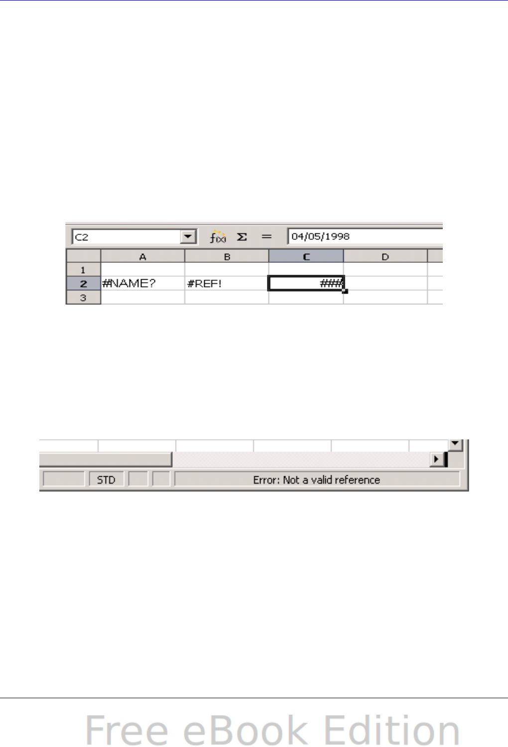
Introduction to Calc error codes
Calc provides feedback for errors of miscalculation, incorrect use of
functions, invalid cell references and values, and other user initiated
mistakes. The feedback may be displayed within the cell that contains
the error (Figure 336) or on the status bar (Figure 337) or in both,
depending on the type of error. Generally speaking, if the error occurs
in the cell that is selected (or contains the cursor), the error message
is displayed on the status bar.
As an example, Figure 336 shows the error code returned when a
column is too narrow to display the entire formatted date. The date
displayed within the input line, 04/05/1998, would fit within the cell
without a problem, but the format used by the cell produces the date
value Sunday, April 05, 1998.
Figure 336: Error codes displayed within cells
When the cell displaying the #REF error code in Figure 336 is
selected, the status bar displays the error message as shown in Figure
337. This message is more descriptive than the message displayed in
the cell, but it still may not provide enough information to correctly
diagnose the problem. For fuller explanations, consult the following
tables and the Help topic, Error Codes in OpenOffice.org Calc.
Figure 337: An error message displayed in the status bar.
This appendix presents error codes in two tables. This first table
explains error messages which are displayed within the cell that
actually contains the error. Except in the case of the ### error, they
all correspond to a Calc error code number. The second table explains
all of the error codes, listed by code number, including those errors
codes in the first table.
Appendix C Calc Error Codes 485
Error codes displayed within cells
Cell error Code Explanation of the error
### N/A The column is too narrow to display the complete
formatted contents of the cell. This is not really an
error value, so there is no corresponding numerical
error code. The solutions to this problem are to
increase the width of the column. or select Format
> Cells > Alignment and click either Wrap text
automatically or Shrink to fit cell size to make the
text match the current column width.
Err502 502 Function argument is not valid, or more than one
matching cell is found by the DGET function.
#NUM! 503 A calculation resulted in an overflow of the defined
value range.
#VALUE 519 The formula within the cell returns a value that
does not correspond to the definition of the formula
or functions used. This error could also mean that
the cell referenced by the formula contains text
instead of a number.
#REF! 524 The formula within the cell uses a reference that
does not exist. Either a column or row description
name could not be resolved, or the column, row, or
sheet that contains a referenced cell is missing.
#NAME? 525 An identifier could not be evaluated: no valid
reference, no valid domain name, no column/row
label, no macro, incorrect decimal divider, add-in
not found. For example, entering in a cell
=sum(bob*5) where there is no cell named “bob” or
containing the text “bob” generates this error.
#DIV/0! 532 Division operator / if the denominator is 0.
Some more functions return this error; see next
table for details.
486 OpenOffice.org 3.x Calc Guide
General error codes
The following table is an overview of the most common error messages
for OOo Calc.
Note
Errors described as Internal errors should not be encountered by
users under normal conditions. Errors listed as Not used are not
currently assigned to any error condition and will not occur.
Code Message Explanation of the error
501 Invalid character Character in a formula is not valid. This error
is the same as the Invalid Name error (525)
except that it occurs within a formula. The cell
containing the error will display the #NAME?
error reference.
502 Invalid argument Function argument is not valid; for example, a
negative number for the root function. This
error also occurs if more than one matching
cell is found by the DGET function.
503 Invalid floating
point operation
(cell displays
#NUM!)
Division by 0, or another calculation that
results in an overflow of the defined value
range (a value too big or too small).
504 Parameter list
error
Function parameter is not valid; for example,
text instead of a number, or a domain
reference instead of a cell reference.
505 Internal syntax
error
Not used.
506 Invalid
semicolon
Not used.
507 Pair missing Not used.
508 Pair missing Missing bracket or parenthesis; for example,
closing brackets but no opening brackets.
509 Missing operator Operator is missing; for example,
"=2(3+4) * ", where the operator between
"2" and "(" is missing.
510 Missing variable Variable is missing; for example, when two
operators are together "=1+*2".
511 Missing variable Function requires more variables than are
provided; for example, AND() and OR().
Appendix C Calc Error Codes 487
Code Message Explanation of the error
512 Formula
overflow
The total number of internal tokens (that is,
operators, variables, brackets) in the formula
exceeds 512, or the total number of matrices
the formula creates exceeds 150. This includes
basic functions that receive too large an array
as a parameter.
513 String overflow An identifier in the formula exceeds 64 KB in
size, or a result of a string operation exceeds
64 KB in size.
514 Internal overflow Sort operation attempted on too much
numerical data (max. 100000) or a calculation
stack overflow.
515 Internal syntax
error
Not used.
516 Internal syntax
error
Matrix is expected on the calculation stack,
but is not available.
517 Internal syntax
error
Unknown error; for example, a document with
a newer function is loaded in an older version
of Calc that does not contain the function.
518 Internal syntax
error
Variable is not available.
519 No result (cell
displays
#VALUE)
Formula yields a value that does not
correspond to the definition, or a cell that is
referenced in the formula contains text instead
of a number.
520 Internal syntax
error
Compiler creates an unknown compiler code.
521 Internal syntax
error
No result.
522 Circular
reference
Formula refers directly or indirectly to itself
and the Iterations option is not selected
under Tools > Options > OpenOffice.org
Calc > Calculate.
523 The calculation
procedure does
not converge
Financial statistics function missed a targeted
value, or iterations of circular references do
not reach the minimum change within the
maximum steps that are set.
524 Invalid
references (cell
displays #REF!)
A column or row description name could not
be resolved, or the column, row, or sheet that
contains a referenced cell is missing.
488 OpenOffice.org 3.x Calc Guide

Code Message Explanation of the error
525 Invalid names
(cell displays
#NAME?)
An identifier could not be evaluated; for
example, no valid reference, no valid domain
name, no column/row label, no macro,
incorrect decimal divider, add-in not found.
526 Internal syntax
error
Obsolete, no longer used, but could come from
old documents if the result is a formula from a
domain.
527 Internal overflow References, such as when a cell references a
cell, are too encapsulated or deeply nested.
This is an internal error and should not be
displayed in OOo version 2.0 or greater.
528–
531
— Not used.
532 Division by zero Division operator / if the denominator is 0.
Some more functions return this error; for
example:
VARP with less than 1 argument
STDEVP with less than 1 argument
VAR with less than 2 arguments
STDEV with less than 2 arguments
STANDARDIZE with stdev=0
NORMDIST with stdev=0
Appendix C Calc Error Codes 489

Index
3
3D chart
appearance 89
area chart 98
bar chart 96
elements 79
formatting 87
illumination 89
line chart 99
moving elements 86
pie chart 96
rotation and perspective 88
rotation, interactive 90
types 75
A
absolute reference 190
advanced functions 217
anchor, visible 403
anchoring of objects 150
appearance of 3D chart 89
appearance options 395
Apply Style list 12, 110
area charts 97
arguments in functions 197, 429
arithmetic operators 182
array functions 468
arrow keys
navigating within spreadsheets 24
assign styles to shortcut keys 111
auto filters 367
AutoCorrect options 409
AutoInput 45
automatic changes, deactivating 44
automatic saving 20
axes labels 76
B
background
cell styles 113
bar charts 95
Base, editing data sources 315
borders
cell styles 113
bubble charts 100
C
Calc options
calculate 404
case sensitive 406
changes 408
dates 405
grid 408
grid lines, viewing 402
guides while moving 403
handles 403
input settings 401
iterative references 405
page breaks, visible 403
screen display 403
sort lists 407
unit of measurement 400
updating links 401
Zoom 404
calculation options 404
calculation order 192
calculations linking sheets 192
case sensitive sorting 66
cell alignment and orientation 57
cell protection 113
cell styles
alignment options 113
applying 109
background 113
border options 113
description 107
Fill Format mode 110
font effects 113
font options 113
linked with 112
numbers 113
cells
description 10, 14
focus 23
hiding and showing 63
information on status bar 15
range 27
selecting 27
validating contents 49
changes
accepting or rejecting 334
adding comments 329
editing comments 330
490 OpenOffice.org 3.x Calc Guide

options 408
recording 327
reviewing 332
viewing 333
chart
appearance of 3D 89
area 79
area background 86
colors 87
creating 73
data labels 80, 92
editing 78
formatting 84
formatting 3D 87
graphic background 87
grids 78
illumination of 3D 89
interactive 3D rotation 90
mean value lines 83
moving elements 86
perspective 88
Position and Size dialog 94
resizing 93
rotation 88
titles 78
trend lines 82
types 95
wall 79
Y error bars 83
chart elements 79
chart type 75, 79
Chart Wizard 74
collaboration 323
color coding for input 207
color options 391
Color toolbar 139
column and line charts 103
column charts 95
columns
deleting 31
freezing 34
hiding and showing 63
inserting 30
selecting 29
comma separated values (CSV) 18, 22
comments
adding 330
editing 331
finding 332
formatting 332
comments on changes
adding 329
editing 330
comparative operators 183
comparing documents 337
concatenation operator 188
consolidating data 272
create document from template 119
creating new spreadsheets 16
cropping 140
CSV files 18, 22
custom sort order 67
customizing
Enter key 26
keyboard shortcuts 416
menus 410
toolbars 414
D
dashes, entering 44
data analysis
consolidating data 272
DataPilot 219
Goal Seek 288
introduction 272
Multiple Operations tool 281
scenarios 277
Solver 290
subtotals 275
data entry
keyboard 42
speeding up 45
data labels on charts 80, 92
data ranges 76
data series 77
data source
data to text 315
editing 314
editing using Base 315
linking 312
registering 312
using in OOo documents 315
viewing 314
data to text 315
database functions 466
database range 364
DataPilot
cell formatting 262
change layout 253
data fields 248
data source 243
Index 491

dialog 244
examples of use 219
filter 260
GETPIVOTDATA 267
group date or time values 255
group rows or columns 253
group scalar values 254
group without intervals 256
multiple data fields 262
page fields 253
preconditions 241
refresh 261
row or column fields 250
shortcuts 266
sort results 257
starting 242
DataPilot Tools 421
date conversion, automatic 45
date functions 458
dates and times, entering 43
DDE link
description 320
in Calc 320
in Writer 321
default template 124
deleting
columns and rows 31
sheets 33
Detective 208
digital rights management (DRM) 172
digital signature 175
digital signature
status bar indicator 15
documents
comparing 337
merging 335
drag and drop 132
drag mode 40
drawing object properties 147
Drawing Object Properties toolbar 147
drawing objects
grouping 148
properties 147
resizing 148
Drawing toolbar 147
drawing tools 145
Dynamic Data Exchange (DDE) 320
E
e-mailing
several recipients 174
Writer document as attachment 174
editing data
changing the contents of cell 52
removing data from a cell 51
replacing cell data 52
en and em dashes, entering 44
Enter key 26
EPS images in PDF 169
Err:503 Division by zero 206
error codes
common messages 487
displayed within cells 486
introduction 485
error messages 205, 210
error-checking formulas 179
errors, finding and fixing 205
EuroOffice Solver 293
export directly as PDF 167
exporting to PDF 167
Extension Manager 123
extensions
DataPilot Tools 421
installing 420
introduction 420
Professional Template Pack 421
Solver for Nonlinear Programming
421
External Data dialog 307
F
FDF 169
features 10
file sharing options 393, 395
Fill Format mode 110
fill series
defining 47
using 46
Fill tool 45
filled net charts 101
filtering 367
filters
advanced 372
auto 367
standard 368
financial analysis functions 435
find and replace
cell styles 69
Find & Replace dialog 68
formulas or values 68
regular expressions 69
text 69
492 OpenOffice.org 3.x Calc Guide

wildcards 69
fixed values 178
focus 23
formatting
chart 84
data labels 92
symbols 92
formatting
autoformatting cells and sheets 59
cell background 59
cell borders 58
conditional 61
themes 60
formatting data
font 56
font effects 56
manual line breaks 54
multiple lines of text 53
numbers 55
shrinking text 54
wrapping 53
Formatting toolbar 12
formula bar 13
formulas
absolute reference 190
breaking into parts 204
calculation examples 180
concatenation operator 188
definition 178
intersection operator 188
operator types 182
operators in 180
range operator 186
relative reference 189
strategies for creating 203
using the Basic editor to create 204
Function List 199
Function Wizard 13, 200
functions
add-in 479
ADDRESS 383
arguments 197, 352, 429
array 468
basic arithmetic 210
CEILING 214
CONCATENATE 184
COUNTIF 216, 377
database 375, 466
date and time 458
date formats 435
definition 178
description 178
entering 180
examples 210
financial analysis 435
FLOOR 214
HLOOKUP 380
INDEX 385
INDIRECT 384
informational 463
logical 462
LOOKUP 381
macros 345
MATCH 381
mathematical 430
MROUND 215
nested 198
OFFSET 384
overview 197
ROUND 213
ROUNDDOWN 214
ROUNDUP 214
simple statistics 211
spreadsheet 470
statistical analysis 449
structure 198
SUBTOTAL 378
SUMIF 377
terminology 429
text 475
VLOOKUP 379
G
Gallery
Hide/Show button 135
opening 134
GETPIVOTDATA 267
Goal Seek 288
graphic filters 138
graphics
adding 130
anchoring 150
arrangement 149
linking 132
positioning 148
resizing 141
transparency 139
graphics mode 138
grid
options 408
grid lines, viewing 402
Index 493

grids in charts 78
guides while moving 403
H
headers and footers 115
Hide/Show button 135
hiding and showing data 63
HTML compatibility 399
hyperlinks
absolute 303
creating 304
Ctrl-click to activate 394
editing 306
relative 303
removing 306
I
illumination of 3D chart 89
image map 151
images
adding 130
context menu 142
cropping 140
embedding 133
inserting from file 130
inserting from the clipboard 134
inserting from the Gallery 134
linking 132
modifying 136
resizing 141
rotating 142
informational functions 463
input settings options 401
insert mode 15
Insert Picture dialog 131
inserting
columns and rows 30
sheets 32
interest rates 435
intersection operator 188
K
keyboard data entry 42
keyboard keys
navigating within spreadsheets 24
keyboard shortcuts
arrow keys 425
assigning 416
cell formatting 426
customizing 417
DataPilot 427
function keys 425
introduction 423
loading from a file 419
navigation 423
resetting to default values 419
saving to a file 419
selection 423
L
layout settings
format 115
page layout 114
table alignment 115
legend of chart 78
line charts 99
linking to external data
External Data dialog 307
find required range 310
Navigator 308
load Basic code to edit 398
load/save options 396
logical functions 462
M
macro recorder 341
macro security options 395
macros 420
macros
accessing cells directly 353
arguments 351
arguments in functions 352
as Calc functions 345
introduction 341
organizing 345
recording 341
sorting data 354
main window, description 11
manual line breaks 54
margins 114
mathematical functions 430
mean value lines 83
menu bar 11
menu font, customizing 410
menus
adding commands 413
creating 412
customizing 410
modifying 412
modifying entries 414
merging documents 335
Microsoft Excel 21
494 OpenOffice.org 3.x Calc Guide

Microsoft Office file conversion 398
moving chart elements 86
moving from sheet to sheet 26
Multiple Operations tool 281
multiple sheets
introduction 295
setting up 295
N
named range 359
navigating within spreadsheets
cell reference 23
focus 23
keyboard 24
methods 23
Navigator 23, 38
scenarios 280
nested functions 198
net charts 101
nonlinear programming solver 293
numbers as text, entering 42
numbers, entering 42
O
Object Linking and Embedding (OLE)
316
ODF plugin (Sun) 20
OLE object
linked 319
non-linked 319
other (Windows) 318
OpenDocument Format 397
opening spreadsheets 17
order of calculation 192
outline group controls 63
overlining 56
OXT extension 123
P
page breaks, visible 403
page style on status bar 15
page styles
applying 111
background 115
borders 115
description 107, 108
options 113
sheet settings 115
paper format 114
password protection 20
password-protect PDF 172
PDF
blank page export 169
digital rights management (DRM) 172
encrypt 172
EPS images 169
export documents to 167
form 169
image compression and resolution 168
initial view selection 169
pages to export 167
password-protect 172
security settings 172
tagged 169
user interface settings 169
PDF Options dialog 167
PDF/A-1 169
perspective of chart 88
picture context menu 142
Picture toolbar 136
pictures
linking 132
resizing 141
transparency 139
pie charts 96
Position and Size dialog for chart 94
Position and Size of graphics 143
precision 406
prepare document for review 326
Print dialog 155
print file directly 155
print options 391
printer metrics 402
printing
choosing what to print 155
printer selection 155
protect a document 326
R
range
database 364
named 359
range operators 186
record changes 326
reference operators 186
references in color 404
referencing
other spreadsheets 301
sheets 299
regular expressions 69
enable in formulas 406
in functions 215
Index 495

relative reference 189
relief options 56
remove personal information on saving
394
removing data from a cell 51
renaming
sheets 33
replacing cell data 52
resolution options 409
rofessional Template Pack 421
rotating images 142
rotation
chart 88
rounding methods 213
rounding off numbers 213
rows
deleting 31
freezing 34
hiding and showing 63
inserting 30
selecting 29
S
save original Basic code 398
saving AutoRecovery info 20
saving spreadsheets
as CSV file 22
as HTML 23
methods 19
to Microsoft Excel format 20
scatter charts 99
scenarios 277
security 20
selecting
cells 27
columns and rows 29
sheets 29
selection list 48
selection mode indicator 15
send document as e-mail 174
shared extension 420
shared spreadsheet
introduction 323
opening 324
saving 325
setting up 323
sheet tabs 14
sheets
deleting 33
description 10
hiding and showing 63
identifying 295
inserting 32, 296
inserting from other spreadsheets 297
navigating 26
referencing 299
renaming 33, 298
searching all 67
selecting 29
sequence number 15
sharing content 48
shrinking text 54
size optimization 397
snap grid 408
Solver 290
Solver for Nonlinear Programming 293,
421
sort lists
options 407
sorting 365
sorting
using macros 354
sorting records
case sensitive 66
sort options 66
sorting data 65
special characters, entering 43
splitting the screen 36
spreadsheet
create from template 119
update from changed template 122
spreadsheet functions 470
spreadsheets
comparing 337
creating new 16
description 10
documentation, internal 179
embedding 316
identifying copies 327
merging 335
opening 17
opening shared spreadsheet 324
saving 19
saving as CSV 22
saving as Microsoft Excel 20
saving shared 325
setting up sharing 323
sharing 323
statistical analysis functions 449
status bar 14
stock charts 102
496 OpenOffice.org 3.x Calc Guide

strikethrough 56
Style dialog 116
style organizer 111
styles
accessing 108
assign to shortcut keys 111
assigning to shortcut keys 418
cell 107
copy 117
create by drag and drop 117
create from selection 116
create using Style dialog 116
delete 119
description 106
linking 116
modifying 111
move 117
organizer 111
page 108, 111
types supported 106
Styles and Formatting window 109
subtotals 275
synchronize axes 409
system font 410
T
template
associate spreadsheet with different
template 125
create spreadsheet from 119
delete 127
delete folder 126
description 106
edit 121
export 128
Extension Manager 123
folder 126
import 127
move 127
organize 126
reset default 125
set custom template as default 124
update document styles from 122
text functions 475
text operators 184
text overflow 404
text, entering 42
time functions 458
title bar 11
titles of charts 78
toolbars
adding commands 416
choosing icons for commands 416
creating 415
description 12
tooltip 12
track changes 326
transparency 139
trend lines 82
typing errors, autocorrect 44
U
underlining 56
unsaved changes indicator 15
URL Recognition 304
user data options 391
user interface, customizing 410
V
validating cell contents 49
value highlighting 403
VBA properties load/save options 397
versions
saving 337
viewing Calc 33
viewing data
filters 64
hiding and showing data 63
outline groups 63
visible grid 409
W
wall of chart 79
wildcards 69
X
XML 397
XY charts 99
Y
Y error bars 83
Z
zoom
dialog 34
slider 16
#
#REF! Incorrect references 207
#VALUE Non-existent value 207
Index 497
