A Beginner's Guide To Structural Equation Ing Beginners 3rd Ed
User Manual: Pdf
Open the PDF directly: View PDF ![]() .
.
Page Count: 510 [warning: Documents this large are best viewed by clicking the View PDF Link!]
- A Beginner’s Guide to Structural Equation Modeling
- Copyright
- Contents
- About the Authors
- Preface
- 1 Introduction
- 2 Data Entry and Data Editing Issues
- 3 Correlation
- 4 SEM Basics
- 5 Model Fit
- 6 Regression Models
- 7 Path Models
- 8 Confirmatory Factor Models
- 9 Developing Structural Equation Models: Part I
- 10 Developing Structural Equation Models: Part II
- 11 Reporting SEM Research: Guidelines and Recommendations
- 12 Model Validation
- 13 Multiple Sample, Multiple Group, and Structured Means Models
- 14 Second-Order, Dynamic, and Multitrait Multimethod Models
- 15 Multiple Indicator–Multiple Indicator Cause, Mixture, and Multilevel Models
- 16 Interaction, Latent Growth, and Monte Carlo Methods
- 17 Matrix Approach to Structural Equation Modeling
- Appendix A: Introduction to Matrix Operations
- Appendix B: Statistical Tables
- Answers to Selected Exercises
- Author Index
- Subject Index

A Beginner’s Guide to
Structural
Equation
Randall E. Schumacker
The University of Alabama
Richard G. Lomax
The Ohio State University
Modeling
Third Edition
Y102005.indb 3 4/3/10 4:25:16 PM

Routledge
Taylor & Francis Group
711 Third Avenue
New York, NY 10017
Routledge
Taylor & Francis Group
27 Church Road
Hove, East Sussex BN3 2FA
© 2010 by Taylor and Francis Group, LLC
Routledge is an imprint of Taylor & Francis Group, an Informa business
International Standard Book Number: 978-1-84169-890-8 (Hardback) 978-1-84169-891-5 (Paperback)
For permission to photocopy or use material electronically from this work, please access www.
copyright.com (http://www.copyright.com/) or contact the Copyright Clearance Center, Inc.
(CCC), 222 Rosewood Drive, Danvers, MA 01923, 978-750-8400. CCC is a not-for-profit organiza-
tion that provides licenses and registration for a variety of users. For organizations that have been
granted a photocopy license by the CCC, a separate system of payment has been arranged.
Trademark Notice: Product or corporate names may be trademarks or registered trademarks, and
are used only for identification and explanation without intent to infringe.
Library of Congress Cataloging-in-Publication Data
Schumacker, Randall E.
A beginner’s guide to structural equation modeling / authors, Randall E.
Schumacker, Richard G. Lomax.-- 3rd ed.
p. cm.
Includes bibliographical references and index.
ISBN 978-1-84169-890-8 (hardcover : alk. paper) -- ISBN 978-1-84169-891-5
(pbk. : alk. paper)
1. Structural equation modeling. 2. Social sciences--Statistical methods. I.
Lomax, Richard G. II. Title.
QA278.S36 2010
519.5’3--dc22 2010009456
Visit the Taylor & Francis Web site at
http://www.taylorandfrancis.com
and the Psychology Press Web site at
http://www.psypress.com
Y102005.indb 4 4/3/10 4:25:16 PM

vii
Contents
About the Authors ...........................................................................................xv
Preface ............................................................................................................. xvii
1 Introduction ................................................................................................1
1.1 What Is Structural Equation Modeling? .......................................2
1.2 History of Structural Equation Modeling .................................... 4
1.3 Why Conduct Structural Equation Modeling? ............................ 6
1.4 Structural Equation Modeling Software Programs ....................8
1.5 Summary ......................................................................................... 10
References .................................................................................................. 11
2 Data Entry and Data Editing Issues ..................................................... 13
2.1 Data Entry ....................................................................................... 14
2.2 Data Editing Issues ........................................................................ 18
2.2.1 Measurement Scale ........................................................... 18
2.2.2 Restriction of Range ......................................................... 19
2.2.3 Missing Data ...................................................................... 20
2.2.4 LISREL–PRELIS Missing Data Example........................ 21
2.2.5 Outliers ............................................................................... 27
2.2.6 Linearity ............................................................................. 27
2.2.7 Nonnormality .................................................................... 28
2.3 Summary ......................................................................................... 29
References .................................................................................................. 31
3 Correlation ................................................................................................33
3.1 Types of Correlation Coefcients .................................................33
3.2 Factors Affecting Correlation Coefcients ................................. 35
3.2.1 Level of Measurement and Range of Values ................. 35
3.2.2 Nonlinearity ...................................................................... 36
3.2.3 Missing Data ......................................................................38
3.2.4 Outliers ............................................................................... 39
3.2.5 Correction for Attenuation .............................................. 39
3.2.6 Nonpositive Denite Matrices ........................................ 40
3.2.7 Sample Size ........................................................................ 41
3.3 Bivariate, Part, and Partial Correlations .....................................42
3.4 Correlation versus Covariance .....................................................46
3.5 Variable Metrics (Standardized versus Unstandardized) ........ 47
3.6 Causation Assumptions and Limitations ...................................48
3.7 Summary ......................................................................................... 49
References .................................................................................................. 51
Y102005.indb 7 4/3/10 4:25:17 PM
viii Contents
4 SEM Basics ................................................................................................ 55
4.1 Model Specication ........................................................................55
4.2 Model Identication ....................................................................... 56
4.3 Model Estimation ........................................................................... 59
4.4 Model Testing ................................................................................. 63
4.5 Model Modication ....................................................................... 64
4.6 Summary ......................................................................................... 67
References .................................................................................................. 69
5 Model Fit .................................................................................................... 73
5.1 Types of Model-Fit Criteria ........................................................... 74
5.1.1 LISREL–SIMPLIS Example ..............................................77
5.1.1.1 Data .....................................................................77
5.1.1.2 Program ..............................................................80
5.1.1.3 Output ................................................................. 81
5.2 Model Fit ..........................................................................................85
5.2.1 Chi-Square (χ2) .................................................................. 85
5.2.2 Goodness-of-Fit Index (GFI) and Adjusted
Goodness-of-Fit Index (AGFI) .........................................86
5.2.3 Root-Mean-Square Residual Index (RMR) .................... 87
5.3 Model Comparison ........................................................................ 88
5.3.1 Tucker–Lewis Index (TLI) ................................................ 88
5.3.2 Normed Fit Index (NFI) and Comparative Fit
Index (CFI) .........................................................................88
5.4 Model Parsimony ........................................................................... 89
5.4.1 Parsimony Normed Fit Index (PNFI) ............................. 90
5.4.2 Akaike Information Criterion (AIC) .............................. 90
5.4.3 Summary ............................................................................ 91
5.5 Parameter Fit ................................................................................... 92
5.6 Power and Sample Size ................................................................. 93
5.6.1 Model Fit ............................................................................ 94
5.6.1.1 Power ................................................................... 94
5.6.1.2 Sample Size ........................................................99
5.6.2 Model Comparison ......................................................... 108
5.6.3 Parameter Signicance ....................................................111
5.6.4 Summary ...........................................................................113
5.7 Two-Step Versus Four-Step Approach to Modeling ................114
5.8 Summary ........................................................................................116
Chapter Footnote .....................................................................................118
Standard Errors ........................................................................................118
Chi-Squares ...............................................................................................118
References ................................................................................................ 120
Y102005.indb 8 4/3/10 4:25:17 PM
Contents ix
6 Regression Models ................................................................................ 125
6.1 Overview ....................................................................................... 126
6.2 An Example ................................................................................... 130
6.3 Model Specication ...................................................................... 130
6.4 Model Identication ..................................................................... 131
6.5 Model Estimation ......................................................................... 131
6.6 Model Testing ............................................................................... 133
6.7 Model Modication ..................................................................... 134
6.8 Summary ....................................................................................... 135
6.8.1 Measurement Error ......................................................... 136
6.8.2 Additive Equation ........................................................... 137
Chapter Footnote .................................................................................... 138
Regression Model with Intercept Term ..................................... 138
LISREL–SIMPLIS Program (Intercept Term) ...................................... 138
References ................................................................................................ 139
7 Path Models ............................................................................................ 143
7.1 An Example ................................................................................... 144
7.2 Model Specication ...................................................................... 147
7.3 Model Identication ..................................................................... 150
7.4 Model Estimation ......................................................................... 151
7.5 Model Testing ............................................................................... 154
7.6 Model Modication ..................................................................... 155
7.7 Summary ....................................................................................... 156
Appendix: LISREL–SIMPLIS Path Model Program ........................... 156
Chapter Footnote .................................................................................... 158
Another Traditional Non-SEM Path Model-Fit Index ............ 158
LISREL–SIMPLIS program ......................................................... 158
References .................................................................................................161
8 Conrmatory Factor Models ............................................................... 163
8.1 An Example ................................................................................... 164
8.2 Model Specication ...................................................................... 166
8.3 Model Identication ......................................................................167
8.4 Model Estimation ......................................................................... 169
8.5 Model Testing ............................................................................... 170
8.6 Model Modication ..................................................................... 173
8.7 Summary ........................................................................................174
Appendix: LISREL–SIMPLIS Conrmatory Factor Model Program ....174
References ................................................................................................ 177
9 Developing Structural Equation Models: Part I.............................. 179
9.1 Observed Variables and Latent Variables ................................. 180
9.2 Measurement Model .................................................................... 184
Y102005.indb 9 4/3/10 4:25:17 PM
x Contents
9.3 Structural Model .......................................................................... 186
9.4 Variances and Covariance Terms .............................................. 189
9.5 Two-Step/Four-Step Approach .................................................. 191
9.6 Summary ....................................................................................... 192
References ................................................................................................ 193
10 Developing Structural Equation Models: Part II ............................ 195
10.1 An Example ................................................................................... 195
10.2 Model Specication ...................................................................... 197
10.3 Model Identication ..................................................................... 200
10.4 Model Estimation ......................................................................... 202
10.5 Model Testing ............................................................................... 203
10.6 Model Modication ..................................................................... 205
10.7 Summary ....................................................................................... 207
Appendix: LISREL–SIMPLIS Structural Equation Model Program .....207
References ................................................................................................ 208
11 Reporting SEM Research: Guidelines and Recommendations ... 209
11.1 Data Preparation .......................................................................... 212
11.2 Model Specication ...................................................................... 213
11.3 Model Identication ..................................................................... 215
11.4 Model Estimation ..........................................................................216
11.5 Model Testing ............................................................................... 217
11.6 Model Modication ..................................................................... 218
11.7 Summary ....................................................................................... 219
References ................................................................................................ 220
12 Model Validation ................................................................................... 223
Key Concepts ........................................................................................... 223
12.1 Multiple Samples .......................................................................... 223
12.1.1 Model A Computer Output ...........................................226
12.1.2 Model B Computer Output ............................................ 227
12.1.3 Model C Computer Output ........................................... 228
12.1.4 Model D Computer Output ...........................................229
12.1.5 Summary .......................................................................... 229
12.2 Cross Validation ........................................................................... 229
12.2.1 ECVI .................................................................................. 230
12.2.2 CVI .................................................................................... 231
12.3 Bootstrap .......................................................................................234
12.3.1 PRELIS Graphical User Interface .................................. 234
12.3.2 LISREL and PRELIS Program Syntax .......................... 237
12.4 Summary ....................................................................................... 241
References ................................................................................................ 243
Y102005.indb 10 4/3/10 4:25:17 PM
Contents xi
13 Multiple Sample, Multiple Group, and Structured
Means Models ........................................................................................ 245
13.1 Multiple Sample Models ............................................................. 245
Sample 1 ........................................................................................ 247
Sample 2 ........................................................................................ 247
13.2 Multiple Group Models ...............................................................250
13.2.1 Separate Group Models .................................................. 251
13.2.2 Similar Group Model .....................................................255
13.2.3 Chi-Square Difference Test ............................................ 258
13.3 Structured Means Models .......................................................... 259
13.3.1 Model Specication and Identication ........................ 259
13.3.2 Model Fit .......................................................................... 261
13.3.3 Model Estimation and Testing ...................................... 261
13.4 Summary ....................................................................................... 263
Suggested Readings ................................................................................ 267
Multiple Samples ......................................................................... 267
Multiple Group Models .............................................................. 267
Structured Means Models ........................................................... 267
Chapter Footnote .................................................................................... 268
SPSS ................................................................................................ 268
References ................................................................................................ 269
14 Second-Order, Dynamic, and Multitrait Multimethod Models .....271
14.1 Second-Order Factor Model ....................................................... 271
14.1.1 Model Specication and Identication ........................ 271
14.1.2 Model Estimation and Testing ...................................... 272
14.2 Dynamic Factor Model .................................................................274
14.3 Multitrait Multimethod Model (MTMM) ................................. 277
14.3.1 Model Specication and Identication ........................ 279
14.3.2 Model Estimation and Testing ...................................... 280
14.3.3 Correlated Uniqueness Model ...................................... 281
14.4 Summary ....................................................................................... 286
Suggested Readings ................................................................................ 290
Second-Order Factor Models ...................................................... 290
Dynamic Factor Models .............................................................. 290
Multitrait Multimethod Models ................................................. 290
Correlated Uniqueness Model ................................................... 291
References ................................................................................................ 291
15 Multiple Indicator–Multiple Indicator Cause, Mixture,
and Multilevel Models ......................................................................... 293
15.1 Multiple Indicator–Multiple Cause (MIMIC) Models ............. 293
15.1.1 Model Specication and Identication ........................ 294
15.1.2 Model Estimation and Model Testing .......................... 294
Y102005.indb 11 4/3/10 4:25:17 PM
xii Contents
15.1.3 Model Modication ........................................................ 297
Goodness-of-Fit Statistics .............................................. 297
Measurement Equations ................................................ 297
Structural Equations ....................................................... 298
15.2 Mixture Models ............................................................................ 298
15.2.1 Model Specication and Identication ........................ 299
15.2.2 Model Estimation and Testing ...................................... 301
15.2.3 Model Modication ........................................................ 302
15.2.4 Robust Statistic ................................................................305
15.3 Multilevel Models ........................................................................ 307
15.3.1 Constant Effects .............................................................. 313
15.3.2 Time Effects ..................................................................... 313
15.3.3 Gender Effects ................................................................. 315
15.3.4 Multilevel Model Interpretation ....................................318
15.3.5 Intraclass Correlation ..................................................... 319
15.3.6 Deviance Statistic ............................................................ 320
15.4 Summary ....................................................................................... 320
Suggested Readings ................................................................................ 324
Multiple Indicator–Multiple Cause Models ............................. 324
Mixture Models ............................................................................ 325
Multilevel Models ........................................................................ 325
References ................................................................................................ 325
16 Interaction, Latent Growth, and Monte Carlo Methods ................ 327
16.1 Interaction Models ....................................................................... 327
16.1.1 Categorical Variable Approach ..................................... 328
16.1.2 Latent Variable Interaction Model ................................ 331
16.1.2.1 Computing Latent Variable Scores ............... 331
16.1.2.2 Computing Latent Interaction Variable ....... 333
16.1.2.3 Interaction Model Output ..............................335
16.1.2.4 Model Modication ......................................... 336
16.1.2.5 Structural Equations—No Latent
Interaction Variable ......................................... 336
16.1.3 Two-Stage Least Squares (TSLS) Approach ................ 337
16.2 Latent Growth Curve Models..................................................... 341
16.2.1 Latent Growth Curve Program ..................................... 343
16.2.2 Model Modication ........................................................344
16.3 Monte Carlo Methods ..................................................................345
16.3.1 PRELIS Simulation of Population Data........................ 346
16.3.2 Population Data from Specied
Covariance Matrix .......................................................... 352
16.3.2.1 SPSS Approach ................................................ 352
16.3.2.2 SAS Approach ..................................................354
16.3.2.3 LISREL Approach ............................................ 355
Y102005.indb 12 4/3/10 4:25:18 PM
Contents xiii
16.3.3 Covariance Matrix from Specied Model ................... 359
16.4 Summary ....................................................................................... 365
Suggested Readings ................................................................................ 368
Interaction Models ....................................................................... 368
Latent Growth-Curve Models .................................................... 368
Monte Carlo Methods .................................................................. 368
References ................................................................................................ 369
17 Matrix Approach to Structural Equation Modeling ....................... 373
17.1 General Overview of Matrix Notation ...................................... 373
17.2 Free, Fixed, and Constrained Parameters ................................. 379
17.3 LISREL Model Example in Matrix Notation ............................ 382
LISREL8 Matrix Program Output (Edited and Condensed)..385
17.4 Other Models in Matrix Notation ..............................................400
17.4.1 Path Model .......................................................................400
17.4.2 Multiple-Sample Model ................................................. 404
17.4.3 Structured Means Model ............................................... 405
17.4.4 Interaction Models .......................................................... 410
PRELIS Computer Output .......................................................... 412
LISREL Interaction Computer Output .......................................416
17.5 Summary ....................................................................................... 421
References ................................................................................................ 423
Appendix A: Introduction to Matrix Operations ...................................425
Appendix B: Statistical Tables ...................................................................439
Answers to Selected Exercises ................................................................... 449
Author Index .................................................................................................. 489
Subject Index ................................................................................................. 495
Y102005.indb 13 4/3/10 4:25:18 PM

xv
About the Authors
RANDALL E. SCHUMACKER received his Ph.D. in educational psychol-
ogy from Southern Illinois University. He is currently professor of educa-
tional research at the University of Alabama, where he teaches courses
in structural equation modeling, multivariate statistics, multiple regres-
sion, and program evaluation. His research interests are varied, including
modeling interaction in SEM, robust statistics (normal scores, centering,
and variance ination factor issues), and SEM specication search issues
as well as measurement model issues related to estimation, mixed-item
formats, and reliability.
He has published in several journals including Academic Medicine,
Educational and Psychological Measurement, Journal of Applied Measurement,
Journal of Educational and Behavioral Statistics, Journal of Research Methodology,
Multiple Linear Regression Viewpoints, and Structural Equation Modeling.
He has served on the editorial boards of numerous journals and is a
member of the American Educational Research Association, American
Psychological Association—Division 5, as well as past-president of the
Southwest Educational Research Association, and emeritus editor of
Structural Equation Modeling journal. He can be contacted at the University
of Alabama College of Education.
RICHARD G. LOMAX received his Ph.D. in educational research meth-
odology from the University of Pittsburgh. He is currently a professor in
the School of Educational Policy and Leadership, Ohio State University,
where he teaches courses in structural equation modeling, statistics, and
quantitative research methodology.
His research primarily focuses on models of literacy acquisition, multi-
variate statistics, and assessment. He has published in such diverse jour-
nals as Parenting: Science and Practice, Understanding Statistics: Statistical
Issues in Psychology, Education, and the Social Sciences, Violence Against
Women, Journal of Early Adolescence, and Journal of Negro Education. He has
served on the editorial boards of numerous journals, and is a member of
the American Educational Research Association, the American Statistical
Association, and the National Reading Conference. He can be contacted at
Ohio State University College of Education and Human Ecology.
Y102005.indb 15 4/3/10 4:25:18 PM

xvii
Preface
Approach
This book presents a basic introduction to structural equation modeling
(SEM). Readers will nd that we have kept to our tradition of keeping
examples rudimentary and easy to follow. The reader is provided with
a review of correlation and covariance, followed by multiple regression,
path, and factor analyses in order to better understand the building blocks
of SEM. The book describes a basic structural equation model followed by
the presentation of several different types of structural equation models.
Our approach in the text is both conceptual and application oriented.
Each chapter covers basic concepts, principles, and practice and then
utilizes SEM software to provide meaningful examples. Each chapter also
features an outline, key concepts, a summary, numerous examples from
a variety of disciplines, tables, and gures, including path diagrams, to
assist with conceptual understanding. Chapters with examples follow the
conceptual sequence of SEM steps known as model specication, identi-
cation, estimation, testing, and modication.
The book now uses LISREL 8.8 student version to make the software and
examples readily available to readers. Please be aware that the student
version, although free, does not contain all of the functional features as a
full licensed version. Given the advances in SEM software over the past
decade, you should expect updates and patches of this software package
and therefore become familiar with any new features as well as explore the
excellent library of examples and help materials. The LISREL 8.8 student
version is an easy-to-use Windows PC based program with pull-down
menus, dialog boxes, and drawing tools. To access the program, and/or
if you’re a Mac user and are interested in learning about Mac availability,
please check with Scientic Software (http://www.ssicentral.com). There
is also a hotlink to the Scientic Software site from the book page for A
Beginner’s Guide to Structural Equation Modeling, 3rd edition on the Textbook
Resources tab at www.psypress.com.
The SEM model examples in the book do not require complicated pro-
gramming skills nor does the reader need an advanced understanding of
statistics and matrix algebra to understand the model applications. We have
provided a chapter on the matrix approach to SEM as well as an appendix
on matrix operations for the interested reader. We encourage the under-
standing of the matrices used in SEM models, especially for some of the
more advanced SEM models you will encounter in the research literature.
Y102005.indb 17 4/3/10 4:25:18 PM

xviii Preface
Goals and Content Coverage
Our main goal in this third edition is for students and researchers to be
able to conduct their own SEM model analyses, as well as be able to under-
stand and critique published SEM research. These goals are supported by
the conceptual and applied examples contained in the book and several
journal article references for each advanced SEM model type. We have
also included a SEM checklist to guide your model analysis according to
the basic steps a researcher takes.
As for content coverage, the book begins with an introduction to SEM
(what it is, some history, why conduct it, and what software is available),
followed by chapters on data entry and editing issues, and correlation.
These early chapters are critical to understanding how missing data, non-
normality, scale of measurement, non-linearity, outliers, and restriction of
range in scores affects SEM analysis. Chapter 4 lays out the basic steps of
model specication, identication, estimation, testing, and modication,
followed by Chapter 5, which covers issues related to model t indices,
power and sample size. Chapters 6 through 10 follow the basic SEM steps
of modeling, with actual examples from different disciplines, using regres-
sion, path, conrmatory factor and structural equation models. Logically
the next chapter presents information about reporting SEM research and
includes a SEM checklist to guide decision-making. Chapter 12 presents
different approaches to model validation, an important nal step after
obtaining an acceptable theoretical model. Chapters 13 through 16 provide
SEM examples that introduce many of the different types of SEM model
applications. The nal chapter describes the matrix approach to structural
equation modeling by using examples from the previous chapters.
Theoretical models are present in every discipline, and therefore can be
formulated and tested. This third edition expands SEM models and appli-
cations to provide the students and researchers in medicine, political sci-
ence, sociology, education, psychology, business, and the biological sciences
the basic concepts, principles, and practice necessary to test their theoreti-
cal models. We hope you become more familiar with structural equation
modeling after reading the book, and use SEM in your own research.
New to the Third Edition
The rst edition of this book was one of the rst books published on SEM,
while the second edition greatly expanded knowledge of advanced SEM
models. Since that time, we have had considerable experience utilizing the
Y102005.indb 18 4/3/10 4:25:18 PM

Preface xix
book in class with our students. As a result of those experiences, the third
edition represents a more useable book for teaching SEM. As such it is an
ideal text for introductory graduate level courses in structural equation
modeling or factor analysis taught in departments of psychology, educa-
tion, business, and other social and healthcare sciences. An understand-
ing of correlation is assumed.
The third edition offers several new surprises, namely:
1. Our instruction and examples are now based on freely available
software: LISREL 8.8 student version.
2. More examples presented from more disciplines, including input,
output, and screenshots.
3. Every chapter has been updated and enhanced with additional
material.
4. A website with raw data sets for the book’s examples and exer-
cises so they can be used with any SEM program, all of the book’s
exercises, hotlinks to related websites, and answers to all of the
exercises for instructors only. To access the website visit the book
page or the Textbook Resource page at www.psypress.com.
5. Expanded coverage of advanced models with more on multiple-
group, multi-level, and mixture modeling (Chs. 13 and 15), second-
order and dynamic factor models (Ch. 14), and Monte Carlo
methods (Ch. 16).
6. Increased coverage of sample size and power (Ch. 5), including
software programs, and reporting research (Ch. 11).
7. New journal article references help readers better understand
published research (Chs. 13–17).
8. Troubleshooting tips on how to address the most frequently
encountered problems are found in Chapters 3 and 11.
9. Chapters 13 to 16 now include additional SEM model examples.
10. 25% new exercises with answers to half in the back of the book
for student review (and answers to all for instructors only on the
book and/or Textbook Resource page at www.psypress.com).
11. Added Matrix examples for several models in Chapter 17.
12. Updated references in all chapters on all key topics.
Overall, we believe this third edition is a more complete book that can
be used to teach a full course in SEM. The past several years have seen an
explosion in SEM coursework, books, websites, and training courses. We
are proud to have been considered a starting point for many beginner’s
to SEM. We hope you nd that this third edition expands on many of the
programming tools, trends and topics in SEM today.
Y102005.indb 19 4/3/10 4:25:18 PM

xx Preface
Acknowledgments
The third edition of this book represents more than thirty years of inter-
acting with our colleagues and students who use structural equation
modeling. As before, we are most grateful to the pioneers in the eld of
structural equation modeling, particularly to Karl Jöreskog, Dag Sörbom,
Peter Bentler, James Arbuckle, and Linda and Bengt Muthèn. These indi-
viduals have developed and shaped the new advances in the SEM eld as
well as the content of this book, plus provided SEM researchers with soft-
ware programs. We are also grateful to Gerhard Mels who answered our
questions and inquiries about SEM programming problems in the chap-
ters. We also wish to thank the reviewers: James Leeper, The University
of Alabama, Philip Smith, Augusta State University, Phil Wood, the
University of Missouri–Columbia, and Ke-Haie Yuan, the University of
Notre Dame.
This book was made possible through the encouragement of Debra
Riegert at Routledge/Taylor & Francis who insisted it was time for a third
edition. We wish to thank her and her editorial assistant, Erin M. Flaherty,
for coordinating all of the activity required to get a book into print. We
also want to thank Suzanne Lassandro at Taylor & Francis Group, LLC
for helping us through the difcult process of revisions, galleys, and nal
book copy.
Randall E. Schumacker
The University of Alabama
Richard G. Lomax
The Ohio State University
Y102005.indb 20 4/3/10 4:25:18 PM

1
1
Introduction
Key Concepts
Latent and observed variables
Independent and dependent variables
Types of models
Regression
Path
Conrmatory factor
Structural equation
History of structural equation modeling
Structural equation modeling software programs
Structural equation modeling can be easily understood if the researcher
has a grounding in basic statistics, correlation, and regression analysis.
The rst three chapters provide a brief introduction to structural equation
modeling (SEM), basic data entry, and editing issues in statistics, and con-
cepts related to the use of correlation coefcients in structural equation
modeling. Chapter 4 covers the essential concepts of SEM: model speci-
cation, identication, estimation, testing, and modication. This basic
understanding provides the framework for understanding the material
presented in chapters 5 through 8 on model-t indices, regression analy-
sis, path analysis, and conrmatory factor analysis models (measurement
models), which form the basis for understanding the structural equation
models (latent variable models) presented in chapters 9 and 10. Chapter 11
provides guidance on reporting structural equation modeling research.
Chapter 12 addresses techniques used to establish model validity and
generalization of ndings. Chapters 13 to 16 present many of the advanced
SEM models currently appearing in journal articles: multiple group, mul-
tiple indicators–multiple causes, mixture, multilevel, structured means,
multitrait–multimethod, second-order factor, dynamic factor, interaction
Y102005.indb 1 3/22/10 3:24:44 PM

2 A Beginner’s Guide to Structural Equation Modeling
models, latent growth curve models, and Monte Carlo studies. Chapter 17
presents matrix notation for one of our SEM applications, covers the differ-
ent matrices used in structural equation modeling, and presents multiple
regression and path analysis solutions using matrix algebra. We include
an introduction to matrix operations in the Appendix for readers who
want a more mathematical understanding of matrix operations. To start
our journey of understanding, we rst ask, What is structural equation
modeling? Then, we give a brief history of SEM, discuss the importance of
SEM, and note the availability of SEM software programs.
1.1 What Is Structural Equation Modeling?
Structural equation modeling (SEM) uses various types of models to
depict relationships among observed variables, with the same basic goal
of providing a quantitative test of a theoretical model hypothesized by
the researcher. More specically, various theoretical models can be tested
in SEM that hypothesize how sets of variables dene constructs and
how these constructs are related to each other. For example, an educa-
tional researcher might hypothesize that a student’s home environment
inuences her later achievement in school. A marketing researcher may
hypothesize that consumer trust in a corporation leads to increased prod-
uct sales for that corporation. A health care professional might believe
that a good diet and regular exercise reduce the risk of a heart attack.
In each example, the researcher believes, based on theory and empirical
research, sets of variables dene the constructs that are hypothesized to be
related in a certain way. The goal of SEM analysis is to determine the extent to
which the theoretical model is supported by sample data. If the sample data
support the theoretical model, then more complex theoretical models can be
hypothesized. If the sample data do not support the theoretical model, then
either the original model can be modied and tested, or other theoretical
models need to be developed and tested. Consequently, SEM tests theoreti-
cal models using the scientic method of hypothesis testing to advance our
understanding of the complex relationships among constructs.
SEM can test various types of theoretical models. Basic models include
regression (chapter 6), path (chapter 7), and conrmatory factor (chap-
ter 8) models. Our reason for covering these basic models is that they
provide a basis for understanding structural equation models (chapters
9 and 10). To better understand these basic models, we need to dene a
few terms. First, there are two major types of variables: latent variables
and observed variables. Latent variables (constructs or factors) are vari-
ables that are not directly observable or measured. Latent variables are
Y102005.indb 2 3/22/10 3:24:44 PM
Introduction 3
indirectly observed or measured, and hence are inferred from a set of
observed variables that we actually measure using tests, surveys, and
so on. For example, intelligence is a latent variable that represents a psy-
chological construct. The condence of consumers in American business
is another latent variable, one representing an economic construct. The
physical condition of adults is a third latent variable, one representing a
health-related construct.
The observed, measured, or indicator variables are a set of variables that
we use to dene or infer the latent variable or construct. For example, the
Wechsler Intelligence Scale for Children—Revised (WISC-R) is an instru-
ment that produces a measured variable (scores), which one uses to infer
the construct of a child’s intelligence. Additional indicator variables, that
is, intelligence tests, could be used to indicate or dene the construct of
intelligence (latent variable). The Dow-Jones index is a standard measure
of the American corporate economy construct. Other measured variables
might include gross national product, retail sales, or export sales. Blood
pressure is one of many health-related variables that could indicate a
latent variable dened as “tness.” Each of these observed or indicator
variables represent one denition of the latent variable. Researchers use
sets of indicator variables to dene a latent variable; thus, other measure-
ment instruments are used to obtain indicator variables, for example, the
Stanford–Binet Intelligence Scale, the NASDAQ index, and an individual’s
cholesterol level, respectively.
Variables, whether they are observed or latent, can also be dened
as either independent variables or dependent variables. An independent
variable is a variable that is not inuenced by any other variable in
the model. A dependent variable is a variable that is inuenced by
another variable in the model. Let us return to the previous examples
and specify the independent and dependent variables. The educational
researcher hypothesizes that a student’s home environment (indepen-
dent latent variable) inuences school achievement (dependent latent
variable). The marketing researcher believes that consumer trust in a
corporation (independent latent variable) leads to increased product
sales (dependent latent variable). The health care professional wants to
determine whether a good diet and regular exercise (two independent
latent variables) inuence the frequency of heart attacks (dependent
latent variable).
The basic SEM models in chapters 6 through 8 illustrate the use of
observed variables and latent variables when dened as independent
or dependent. A regression model consists solely of observed variables
where a single dependent observed variable is predicted or explained by
one or more independent observed variables; for example, a parent’s edu-
cation level (independent observed variable) is used to predict his or her
child’s achievement score (dependent observed variable). A path model is
Y102005.indb 3 3/22/10 3:24:44 PM

4 A Beginner’s Guide to Structural Equation Modeling
also specied entirely with observed variables, but the exibility allows
for multiple independent observed variables and multiple dependent
observed variables—for example, export sales, gross national product,
and NASDAQ index inuence consumer trust and consumer spending
(dependent observed variables). Path models, therefore, test more com-
plex models than regression models. Conrmatory factor models con-
sist of observed variables that are hypothesized to measure one or more
latent variables (independent or dependent); for example, diet, exercise,
and physiology are observed measures of the independent latent variable
“tness.” An understanding of these basic models will help in under-
standing structural equation modeling, which combines path and factor
analytic models. Structural equation models consist of observed variables
and latent variables, whether independent or dependent; for example, an
independent latent variable (home environment) inuences a dependent
latent variable (achievement), where both types of latent variables are
measured, dened, or inferred by multiple observed or measured indica-
tor variables.
1.2 History of Structural Equation Modeling
To discuss the history of structural equation modeling, we explain the fol-
lowing four types of related models and their chronological order of devel-
opment: regression, path, conrmatory factor, and structural equation
models.
The rst model involves linear regression models that use a correlation
coefcient and the least squares criterion to compute regression weights.
Regression models were made possible because Karl Pearson created a
formula for the correlation coefcient in 1896 that provides an index for
the relationship between two variables (Pearson, 1938). The regression
model permits the prediction of dependent observed variable scores
(Y scores), given a linear weighting of a set of independent observed
scores (X scores) that minimizes the sum of squared residual error val-
ues. The mathematical basis for the linear regression model is found in
basic algebra. Regression analysis provides a test of a theoretical model
that may be useful for prediction (e.g., admission to graduate school or
budget projections). In an example study, regression analysis was used
to predict student exam scores in statistics (dependent variable) from a
series of collaborative learning group assignments (independent vari-
ables; Delucchi, 2006). The results provided some support for collabora-
tive learning groups improving statistics exam performance, although
not for all tasks.
Y102005.indb 4 3/22/10 3:24:44 PM
Introduction 5
Some years later, Charles Spearman (1904, 1927) used the correlation
coefcient to determine which items correlated or went together to create
the factor model. His basic idea was that if a set of items correlated or
went together, individual responses to the set of items could be summed
to yield a score that would measure, dene, or infer a construct. Spearman
was the rst to use the term factor analysis in dening a two-factor con-
struct for a theory of intelligence. D.N. Lawley and L.L. Thurstone in 1940
further developed applications of factor models, and proposed instru-
ments (sets of items) that yielded observed scores from which constructs
could be inferred. Most of the aptitude, achievement, and diagnostic
tests, surveys, and inventories in use today were created using factor ana-
lytic techniques. The term conrmatory factor analysis (CFA) is used today
based in part on earlier work by Howe (1955), Anderson and Rubin (1956),
and Lawley (1958). The CFA method was more fully developed by Karl
Jöreskog in the 1960s to test whether a set of items dened a construct.
Jöreskog completed his dissertation in 1963, published the rst article on
CFA in 1969, and subsequently helped develop the rst CFA software pro-
gram. Factor analysis has been used for over 100 years to create measure-
ment instruments in many academic disciplines, while today CFA is used
to test the existence of these theoretical constructs. In an example study,
CFA was used to conrm the “Big Five” model of personality by Goldberg
(1990). The ve-factor model of extraversion, agreeableness, conscientious-
ness, neuroticism, and intellect was conrmed through the use of multiple
indicator variables for each of the ve hypothesized factors.
Sewell Wright (1918, 1921, 1934), a biologist, developed the third type of
model, a path model. Path models use correlation coefcients and regres-
sion analysis to model more complex relationships among observed
variables. The rst applications of path analysis dealt with models of
animal behavior. Unfortunately, path analysis was largely overlooked
until econometricians reconsidered it in the 1950s as a form of simultane-
ous equation modeling (e.g., H. Wold) and sociologists rediscovered it in
the 1960s (e.g., O. D. Duncan and H. M. Blalock). In many respects, path
analysis involves solving a set of simultaneous regression equations that
theoretically establish the relationship among the observed variables in
the path model. In an example path analysis study, Walberg’s theoretical
model of educational productivity was tested for fth- through eighth-
grade students (Parkerson et al., 1984). The relations among the follow-
ing variables were analyzed in a single model: home environment, peer
group, media, ability, social environment, time on task, motivation, and
instructional strategies. All of the hypothesized paths among those vari-
ables were shown to be statistically signicant, providing support for the
educational productivity model.
The nal model type is structural equation modeling (SEM). SEM mod-
els essentially combine path models and conrmatory factor models;
Y102005.indb 5 3/22/10 3:24:44 PM

6 A Beginner’s Guide to Structural Equation Modeling
that is, SEM models incorporate both latent and observed variables. The
early development of SEM models was due to Karl Jöreskog (1969, 1973),
Ward Keesling (1972), and David Wiley (1973); this approach was initially
known as the JKW model, but became known as the linear structural rela-
tions model (LISREL) with the development of the rst software program,
LISREL, in 1973. Since then, many SEM articles have been published; for
example, Shumow and Lomax (2002) tested a theoretical model of paren-
tal efcacy for adolescent students. For the overall sample, neighborhood
quality predicted parental efcacy, which predicted parental involvement
and monitoring, both of which predicted academic and social-emotional
adjustment.
Jöreskog and van Thillo originally developed the LISREL software pro-
gram at the Educational Testing Service (ETS) using a matrix command
language (i.e., involving Greek and matrix notation), which is described
in chapter 17. The rst publicly available version, LISREL III, was released
in 1976. Later in 1993, LISREL8 was released; it introduced the SIMPLIS
(SIMPle LISrel) command language in which equations are written
using variable names. In 1999, the rst interactive version of LISREL was
released. LISREL8 introduced the dialog box interface using pull-down
menus and point-and-click features to develop models, and the path dia-
gram mode, a drawing program to develop models. Karl Jöreskog was rec-
ognized by Cudeck, DuToit, and Sörbom (2001) who edited a Festschrift
in honor of his contributions to the eld of structural equation modeling.
Their volume contains chapters by scholars who address the many top-
ics, concerns, and applications in the eld of structural equation model-
ing today, including milestones in factor analysis; measurement models;
robustness, reliability, and t assessment; repeated measurement designs;
ordinal data; and interaction models. We cover many of these topics in
this book, although not in as great a depth. The eld of structural equa-
tion modeling across all disciplines has expanded since 1994. Hershberger
(2003) found that between 1994 and 2001 the number of journal articles
concerned with SEM increased, the number of journals publishing SEM
research increased, SEM became a popular choice amongst multivariate
methods, and the journal Structural Equation Modeling became the primary
source for technical developments in structural equation modeling.
1.3 Why Conduct Structural Equation Modeling?
Why is structural equation modeling popular? There are at least four
major reasons for the popularity of SEM. The rst reason suggests that
researchers are becoming more aware of the need to use multiple observed
Y102005.indb 6 3/22/10 3:24:45 PM
Introduction 7
variables to better understand their area of scientic inquiry. Basic statis-
tical methods only utilize a limited number of variables, which are not
capable of dealing with the sophisticated theories being developed. The
use of a small number of variables to understand complex phenomena is
limiting. For instance, the use of simple bivariate correlations is not suf-
cient for examining a sophisticated theoretical model. In contrast, struc-
tural equation modeling permits complex phenomena to be statistically
modeled and tested. SEM techniques are therefore becoming the preferred
method for conrming (or disconrming) theoretical models in a quanti-
tative fashion.
A second reason involves the greater recognition given to the valid-
ity and reliability of observed scores from measurement instruments.
Specically, measurement error has become a major issue in many dis-
ciplines, but measurement error and statistical analysis of data have
been treated separately. Structural equation modeling techniques explic-
itly take measurement error into account when statistically analyzing
data. As noted in subsequent chapters, SEM analysis includes latent and
observed variables as well as measurement error terms in certain SEM
models.
A third reason pertains to how structural equation modeling has matured
over the past 30 years, especially the ability to analyze more advanced the-
oretical SEM models. For example, group differences in theoretical models
can be assessed through multiple-group SEM models. In addition, analyz-
ing educational data collected at more than one level—for example, school
districts, schools, and teachers with student data—is now possible using
multilevel SEM modeling. As a nal example, interaction terms can now
be included in an SEM model so that main effects and interaction effects
can be tested. These advanced SEM models and techniques have provided
many researchers with an increased capability to analyze sophisticated
theoretical models of complex phenomena, thus requiring less reliance on
basic statistical methods.
Finally, SEM software programs have become increasingly user-
friendly. For example, until 1993 LISREL users had to input the pro-
gram syntax for their models using Greek and matrix notation. At
that time, many researchers sought help because of the complex pro-
gramming requirement and knowledge of the SEM syntax that was
required. Today, most SEM software programs are Windows-based
and use pull-down menus or drawing programs to generate the pro-
gram syntax internally. Therefore, the SEM software programs are now
easier to use and contain features similar to other Windows-based
software packages. However, such ease of use necessitates statisti-
cal training in SEM modeling and software via courses, workshops,
or textbooks to avoid mistakes and errors in analyzing sophisticated
theoretical models.
Y102005.indb 7 3/22/10 3:24:45 PM

8 A Beginner’s Guide to Structural Equation Modeling
1.4 Structural Equation Modeling Software Programs
Although the LISREL program was the rst SEM software program,
other software programs have subsequently been developed since the
mid-1980s. Some of the other programs include AMOS, EQS, Mx, Mplus,
Ramona, and Sepath, to name a few. These software programs are each
unique in their own way, with some offering specialized features for
conducting different SEM applications. Many of these SEM software
programs provide statistical analysis of raw data (e.g., means, correla-
tions, missing data conventions), provide routines for handling missing
data and detecting outliers, generate the program’s syntax, diagram the
model, and provide for import and export of data and gures of a theo-
retical model. Also, many of the programs come with sets of data and
program examples that are clearly explained in their user guides. Many
of these software programs have been reviewed in the journal Structural
Equation Modeling.
The pricing information for SEM software varies depending on indi-
vidual, group, or site license arrangements; corporate versus educa-
tional settings; and even whether one is a student or faculty member.
Furthermore, newer versions and updates necessitate changes in pric-
ing. Most programs will run in the Windows environment; some run
on MacIntosh personal computers. We are often asked to recommend
a software package to a beginning SEM researcher; however, given the
different individual needs of researchers and the multitude of different
features available in these programs, we are not able to make such a rec-
ommendation. Ultimately the decision depends upon the researcher’s
needs and preferences. Consequently, with so many software packages,
we felt it important to narrow our examples in the book to LISREL–
SIMPLIS programs.
We will therefore be using the LISREL 8.8 student version in the book
to demonstrate the many different SEM applications, including regres-
sion models, path models, conrmatory factor models, and the various
SEM models in chapters 13 through 16. The free student version of the
LISREL software program (Windows, Mac, and Linux editions) can be
downloaded from the website: http://www.ssicentral.com/lisrel/student.
html. (Note: The LISREL 8.8 Student Examples folder is placed in the main
directory C:/ of your computer, not the LISREL folder under C:/Program
Files when installing the software.)
Y102005.indb 8 3/22/10 3:24:45 PM

Introduction 9
Once the LISREL software is downloaded, place an icon on your desk-
top by creating a shortcut to the LISREL icon. The LISREL icon should
look something like this:
LISREL 8.80 Student.lnk
When you click on the icon, an empty dialog box will appear that should
look like this:
NOTE: Nothing appears until you open a program le or data set using
the File or open folder icon; more about this in the next chapter.
We do want to mention the very useful HELP menu. Click on the ques-
tion mark (?), a HELP menu will appear, then enter Output Questions in
the search window to nd answers to key questions you may have when
going over examples in the Third Edition.
Y102005.indb 9 3/22/10 3:25:10 PM

10 A Beginner’s Guide to Structural Equation Modeling
1 . 5 S u m m a r y
In this chapter we introduced structural equation modeling by describ-
ing basic types of variables—that is, latent, observed, independent, and
dependent—and basic types of SEM models—that is, regression, path,
conrmatory factor, and structural equation models. In addition, a brief
history of structural equation modeling was provided, followed by a dis-
cussion of the importance of SEM. This chapter concluded with a brief
listing of the different structural equation modeling software programs
and where to obtain the LISREL 8.8 student version for use with examples
Y102005.indb 10 3/22/10 3:25:11 PM

Introduction 11
in the book, including what the dialog box will rst appear like and a very
useful HELP menu.
In chapter 2 we consider the importance of examining data for issues
related to measurement level (nominal, ordinal, interval, or ratio), restric-
tion of range (fewer than 15 categories), missing data, outliers (extreme
values), linearity or nonlinearity, and normality or nonnormality, all of
which can affect statistical methods, and especially SEM applications.
Exercises
1. Dene the following terms:
a. Latent variable
b. Observed variable
c. Dependent variable
d. Independent variable
2. Explain the difference between a dependent latent variable and
a dependent observed variable.
3. Explain the difference between an independent latent variable
and an independent observed variable.
4. List the reasons why a researcher would conduct structural
equation modeling.
5. Download and activate the student version of LISREL: http://
www.ssicentral.com
6. Open and import SPSS or data le.
References
Anderson, T. W., & Rubin, H. (1956). Statistical inference in factor analysis. In
J. Neyman (Ed.), Proceedings of the third Berkeley symposium on mathemati-
cal statistics and probability, Vol. V (pp. 111–150). Berkeley: University of
California Press.
Cudeck, R., Du Toit, S., & Sörbom, D. (2001) (Eds). Structural equation modeling:
Present and future. A Festschrift in honor of Karl Jöreskog. Lincolnwood, IL:
Scientic Software International.
Delucchi, M. (2006). The efcacy of collaborative learning groups in an under-
graduate statistics course. College Teaching, 54, 244–248.
Goldberg, L. (1990). An alternative “description of personality”: Big Five factor
structure. Journal of Personality and Social Psychology, 59, 1216–1229.
Hershberger, S. L. (2003). The growth of structural equation modeling: 1994–2001.
Structural Equation Modeling, 10(1), 35–46.
Howe, W. G. (1955). Some contributions to factor analysis (Report No. ORNL-1919).
Oak Ridge National Laboratory, Oak Ridge, Tennessee.
Jöreskog, K. G. (1963). Statistical estimation in factor analysis: A new technique and its
foundation. Stockholm: Almqvist & Wiksell.
Y102005.indb 11 3/22/10 3:25:11 PM
12 A Beginner’s Guide to Structural Equation Modeling
Jöreskog, K. G. (1969). A general approach to conrmatory maximum likelihood
factor analysis. Psychometrika, 34, 183–202.
Jöreskog, K. G. (1973). A general method for estimating a linear structural equation
system. In A. S. Goldberger & O. D. Duncan (Eds.), Structural equation models
in the social sciences (pp. 85–112). New York: Seminar.
Keesling, J. W. (1972). Maximum likelihood approaches to causal ow analysis.
Unpublished doctoral dissertation. Chicago: University of Chicago.
Lawley, D. N. (1958). Estimation in factor analysis under various initial assump-
tions. British Journal of Statistical Psychology, 11, 1–12.
Parkerson, J. A., Lomax, R. G., Schiller, D. P., & Walberg, H. J. (1984). Exploring
causal models of educational achievement. Journal of Educational Psychology,
76, 638–646.
Pearson, E. S. (1938). Karl Pearson. An appreciation of some aspects of his life and work.
Cambridge: Cambridge University Press.
Shumow, L., & Lomax, R. G. (2002). Parental efcacy: Predictor of parenting behav-
ior and adolescent outcomes. Parenting: Science and Practice, 2, 127–150.
Spearman, C. (1904). The proof and measurement of association between two
things. American Journal of Psychology, 15, 72–101.
Spearman, C. (1927). The abilities of man. New York: Macmillan.
Wiley, D. E. (1973). The identication problem for structural equation models with
unmeasured variables. In A. S. Goldberger & O. D. Duncan (Eds.), Structural
equation models in the social sciences (pp. 69–83). New York: Seminar.
Wright, S. (1918). On the nature of size factors. Genetics, 3, 367–374.
Wright, S. (1921). Correlation and causation. Journal of Agricultural Research, 20,
557–585.
Wright, S. (1934). The method of path coefcients. Annals of Mathematical Statistics,
5, 161–215.
Y102005.indb 12 3/22/10 3:25:11 PM

13
2
Data Entry and Data Editing Issues
Key Concepts
Importing data le
System le
Measurement scale
Restriction of range
Missing data
Outliers
Linearity
Nonnormality
An important rst step in using LISREL is to be able to enter raw data and/
or import data, such as les from other programs (SPSS, SAS, EXCEL, etc.).
Other important steps involve being able to use LISREL–PRELIS to save
a system le, as well as output and save les that contain the variance–
covariance matrix, the correlation matrix, means, and standard deviations
of variables so they can be input into command syntax programs. The
LISREL–PRELIS program will be briey explained in this chapter to dem-
onstrate how it handles raw data entry, importing of data, and the output
of saved les.
There are several key issues in the eld of statistics that impact our anal-
yses once data have been imported into a software program. These data
issues are commonly referred to as the measurement scale of variables,
restriction in the range of data, missing data values, outliers, linearity, and
nonnormality. Each of these data issues will be discussed because they
not only affect traditional statistics, but present additional problems and
concerns in structural equation modeling.
We use LISREL software throughout the book, so you will need to use
that software and become familiar with their Web site. You should have
downloaded by now the free student version of the LISREL software.
Y102005.indb 13 3/22/10 3:25:11 PM
14 A Beginner’s Guide to Structural Equation Modeling
We use some of the data and model examples available in the free stu-
dent version to illustrate SEM applications. (Note: The LISREL 8.8 Student
Examples folder is placed in the main directory C:/ of your computer.)
The free student version of the software has a user guide, help functions,
and tutorials. The Web site also contains important research, documenta-
tion, and information about structural equation modeling. However, be
aware that the free student version of the software does not contain the
full capabilities available in their full licensed version (e.g., restricted to
15 observed variables in SEM analyses). These limitations are spelled out
on their Web site.
2.1 Data Entry
The LISREL software program interfaces with PRELIS, a preprocessor of
data prior to running LISREL (matrix command language) or SIMPLIS
(easier-to-use variable name syntax) programs. The newer Interactive
LISREL uses a spreadsheet format for data with pull-down menu options.
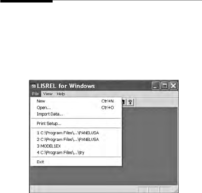
LISREL offers several different options for inputting data and importing
les from numerous other programs. The New, Open, and Import Data
functions provide maximum exibility for inputting data.
The New option permits the creation of a command syntax language
program (PRELIS, LISREL, or SIMPLIS) to read in a PRELIS data le, or
Y102005.indb 14 3/22/10 3:25:12 PM

Data Entry and Data Editing Issues 15
to open SIMPLIS and LISREL saved projects as well as a previously saved
Path Diagram.
The Open option permits you to browse and locate previously saved
PRELIS (.pr2), LISREL (.ls8), or SIMPLIS (.spl) programs; each with their
unique le extension. The student version has distinct folders containing
several program examples, for example LISREL (LS8EX folder), PRELIS
(PR2EX folder), and SIMPLIS (SPLEX folder).
The Import Data option permits inputting raw data les or SPSS
saved les. The raw data le, lsat6.dat, is in the PRELIS folder (PR2EX).
When selecting this le, you will need to know the number of variables
in the le.
Y102005.indb 15 3/22/10 3:25:12 PM
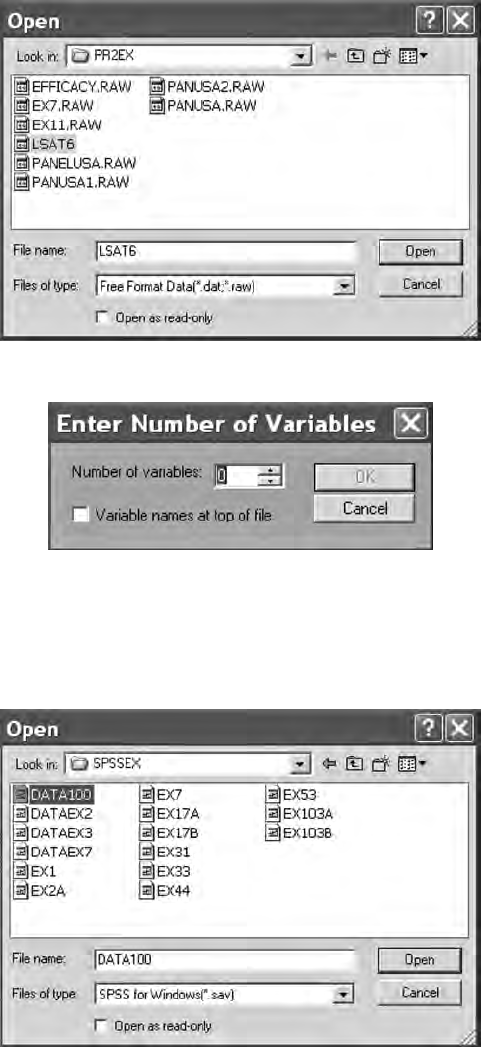
16 A Beginner’s Guide to Structural Equation Modeling
An SPSS saved le, data100.sav, is in the SPSS folder (SPSSEX). Once you
open this le, a PRELIS system le is created.
Y102005.indb 16 3/22/10 3:25:13 PM
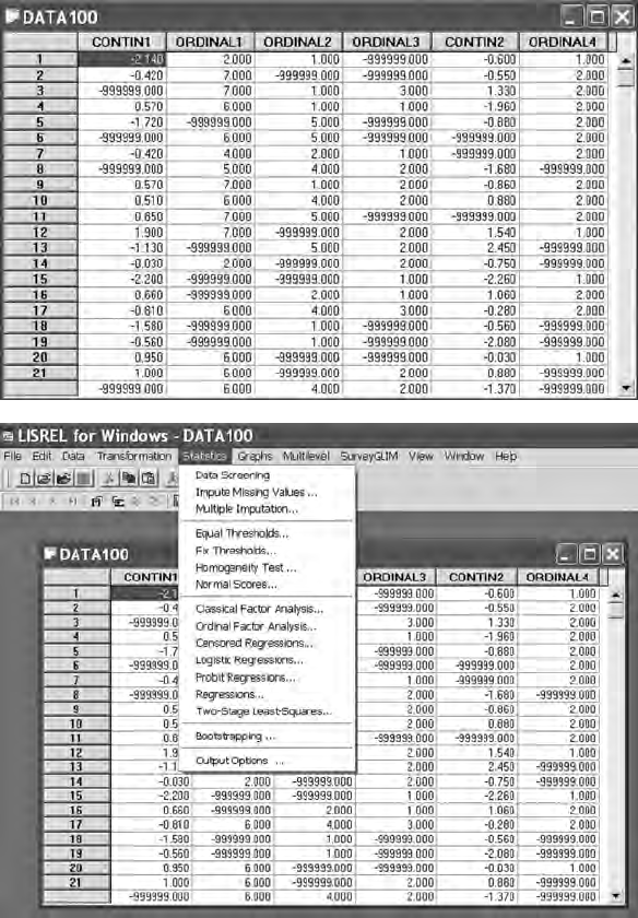
Data Entry and Data Editing Issues 17
Once the PRELIS system le becomes active, then it needs to be saved for
future use. (Note: # symbol may appear if columns are to narrow; simply use
your mouse to expand the columns so that the missing values—999999.00
will appear. Also, if you right-mouse click on the variable names, a menu
appears to dene missing values, etc.). The PRELIS system le (.psf) acti-
vates a pull-down menu that permits data editing features, data transfor-
mations, statistical analysis of data, graphical display of data, multilevel
modeling, and many other related features.
Y102005.indb 17 3/22/10 3:25:16 PM
18 A Beginner’s Guide to Structural Equation Modeling
The statistical analysis of data includes factor analysis, probit regres-
sion, least squares regression, and two-stage least squares methods.
Other important data editing features include imputing missing values,
a homogeneity test, creation of normal scores, bootstrapping, and data
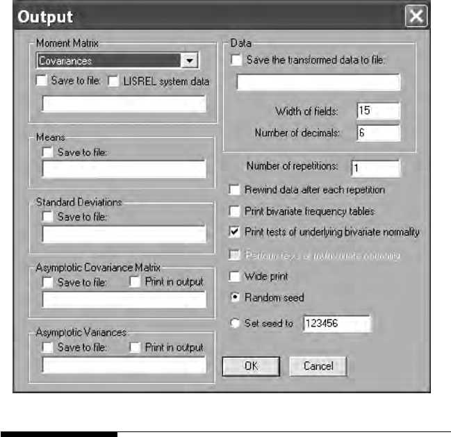
output options. The data output options permit saving different types of
variance–covariance matrices and descriptive statistics in les for use in
LISREL and SIMPLIS command syntax programs. This capability is very
important, especially when advanced SEM models are analyzed in chap-
ters 13 to 16. We will demonstrate the use of this Output Options dialog
box in this chapter and in some of our other chapter examples.
2.2 Data Editing Issues
2.2.1 Measurement Scale
How variables are measured or scaled inuences the type of statistical
analyses we perform (Anderson, 1961; Stevens, 1946). Properties of scale
also guide our understanding of permissible mathematical operations.
Y102005.indb 18 3/22/10 3:25:17 PM
Data Entry and Data Editing Issues 19
For example, a nominal variable implies mutually exclusive groups; a
biological gender has two mutually exclusive groups, male and female.
An individual can only be in one of the groups that dene the levels
of the variable. In addition, it would not be meaningful to calculate a
mean and a standard deviation on the variable gender. Consequently,
the number or percentage of individuals at each level of the gender
variable is the only mathematical property of scale that makes sense.
An ordinal variable, for example, attitude toward school, that is scaled
strongly agree, agree, neutral, disagree, and strongly disagree, implies mutu-
ally exclusive categories that are ordered or ranked. When levels of a
variable have properties of scale that involve mutually exclusive groups
that are ordered, only certain mathematical operations are meaning-
ful, for example, a comparison of ranks between groups. SEM nal
exam scores, an example of an interval variable, possesses the property
of scale, implying equal intervals between the data points, but no true
zero point. This property of scale permits the mathematical operation
of computing a mean and a standard deviation. Similarly, a ratio vari-
able, for example, weight, has the property of scale that implies equal
intervals and a true zero point (weightlessness). Therefore, ratio vari-
ables also permit mathematical operations of computing a mean and
a standard deviation. Our use of different variables requires us to be
aware of their properties of scale and what mathematical operations
are possible and meaningful, especially in SEM, where variance–
covariance (correlation) matrices are used with means and standard
deviations of variables. Different correlations among variables are
therefore possible depending upon the level of measurement, but they
create unique problems in SEM (see chapter 3). PRELIS designates con-
tinuous variables (CO), ordinal variables (OR), and categorical vari-
ables (CL) to make these distinctions.
2.2.2 Restriction of Range
Data values at the interval or ratio level of measurement can be further
dened as being discrete or continuous. For example, SEM nal exam
scores could be reported in whole numbers (discrete). Similarly, the num-
ber of children in a family would be considered a discrete level of mea-
surement—or example, 5 children. In contrast, a continuous variable is
reported using decimal values; for example, a student’s grade point aver-
age would be reported as 3.75 on a 5-point scale.
Karl Jöreskog (1996) provided a criterion in the PRELIS program based
on his research that denes whether a variable is ordinal or interval,
based on the presence of 15 distinct scale points. If a variable has fewer
than 15 categories or scale points, it is referenced in PRELIS as ordi-
nal (OR), whereas a variable with 15 or more categories is referenced as
Y102005.indb 19 3/22/10 3:25:17 PM

20 A Beginner’s Guide to Structural Equation Modeling
continuous (CO). This 15-point criterion allows Pearson correlation coef-
cient values to vary between +/–1.0. Variables with fewer distinct scale
points restrict the value of the Pearson correlation coefcient such that it
may only vary between +/–0.5. Other factors that affect the Pearson cor-
relation coefcient are presented in this chapter and discussed further
in chapter 3.
2.2.3 Missing Data
The statistical analysis of data is affected by missing data values in vari-
ables. That is, not every subject has an actual value for every variable in
the dataset, as some values are missing. It is common practice in statis-
tical packages to have default values for handling missing values. The
researcher has the options of deleting subjects who have missing values,
replacing the missing data values, or using robust statistical procedures
that accommodate for the presence of missing data.
The various SEM software handle missing data differently and have
different options for replacing missing data values. Table 2.1 lists many
of the various options for dealing with missing data. These options can
dramatically affect the number of subjects available for analysis, the
magnitude and direction of the correlation coefcient, or create problems
if means, standard deviations, and correlations are computed based on
different sample sizes. The Listwise deletion of cases and Pairwise dele-
tion of cases are not always recommended options due to the possibil-
ity of losing a large number of subjects, thus dramatically reducing the
sample size. Mean substitution works best when only a small number
of missing values is present in the data, whereas regression imputation
provides a useful approach with a moderate amount of missing data.
In LISREL–PRELIS the expectation maximization (EM), Monte Carlo
Markov Chain (MCMC), and matching response pattern approaches
are recommended when larger amounts of data are missing at random.
TABLE 2.1
Options for Dealing with Missing Data
Listwise Delete subjects with missing data on any variable
Pairwise Delete subjects with missing data on each pair of variables used
Mean substitution Substitute the mean for missing values of a variable
Regression imputation Substitute a predicted value for the missing value of a variable
Expectation
maximization (EM)
Find expected value based on expectation maximization
algorithm
Matching response
pattern
Match cases with incomplete data to cases with complete data
to determine a missing value
Y102005.indb 20 3/22/10 3:25:17 PM

Data Entry and Data Editing Issues 21
More information about missing data is available in resources such as
Enders (2006), McKnight, McKnight, Sidani and Aurelio (2007), and
Peng, Harwell, Liou, and Ehman (2007). Davey and Savla (2010) have
more recently published an excellent book with SAS, SPSS, STATA, and
Mplus source programs to handle missing data in SEM in the context of
power analysis.
2.2.4 LISREL–PRELIS Missing Data Example
Imputation of missing values is possible for a single variable (Impute
Missing Values) or several variables simultaneously (Multiple Imputation)
by selecting Statistics from the tool bar menu. The Impute Missing Values
option uses the matching response pattern approach. The value to be sub-
stituted for the missing value of a single case is obtained from another
case (or cases) having a similar response pattern over a set of matching
variables. In data sets where missing values occur on more than one vari-
able, you can use multiple imputation of missing values with mean sub-
stitution, delete cases, or leave the variables with dened missing values
as options in the dialog box. In addition, the Multiple Imputation option
uses either the expectation maximization algorithm (EM) or Monte Carlo
Markov Chain (MCMC, generating random draws from probability dis-
tributions via Markov chains) approaches to replacing missing values
across multiple variables.
We present an example from LISREL–PRELIS involving the choles-
terol levels for 28 patients treated for heart attacks. We assume the data
to be missing at random (MAR) with an underlying multivariate normal
distribution. Cholesterol levels were measured after 2 days (VAR1), after
4 days (VAR2), and after 14 days (VAR3), but were only complete for 19
of the 28 patients. The data are shown from the PRELIS System File,
chollev.psf. The PRELIS system le was created by selecting File, Import
Data, and selecting the raw data le chollev.raw located in the Tutorial
folder [C:\LISREL 8.8 Student Examples\Tutorial]. We must know the num-
ber of variables in the raw data le. We must also select Data, then Dene
Variables, and then select −9.00 as the missing value for the VAR 3 vari-
able [Optionally, right mouse click on VAR1 in the PRELIS chollev le].
Y102005.indb 21 3/22/10 3:25:18 PM
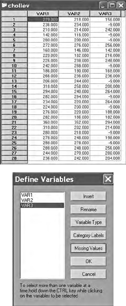
22 A Beginner’s Guide to Structural Equation Modeling
Y102005.indb 22 3/22/10 3:25:18 PM

Data Entry and Data Editing Issues 23
We now click on Statistics on the tool bar menu and select Impute
Missing Values from the pull-down menu.
We next select Output Options and save the transformed data in a new
PRELIS system le cholnew.psf, and output the new correlation matrix,
mean, and standard deviation les.
Y102005.indb 23 3/22/10 3:25:19 PM
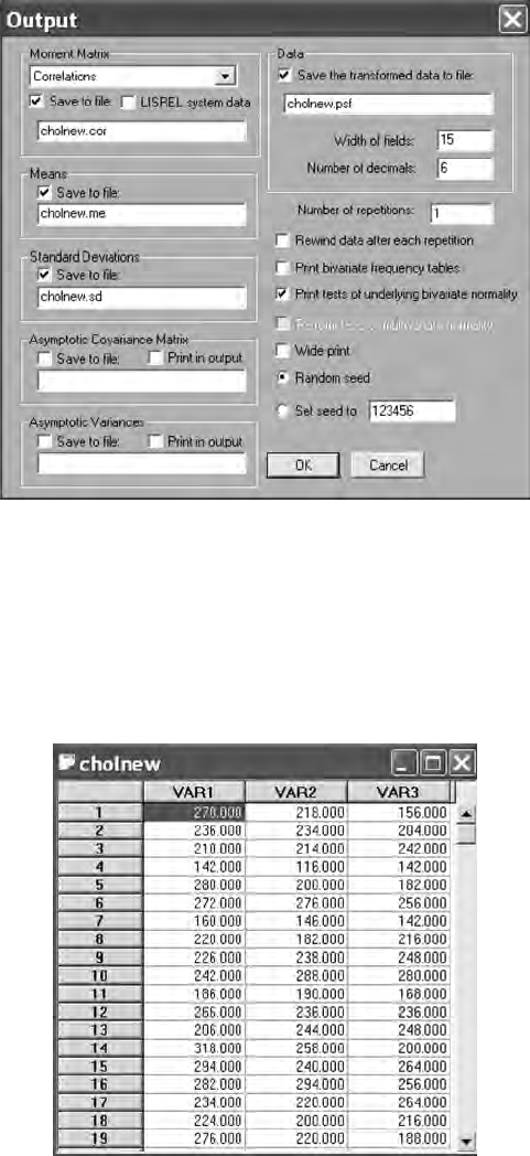
24 A Beginner’s Guide to Structural Equation Modeling
We should examine our data both before (Table 2.2) and after (Table 2.3)
imputation of missing values. Here, we used the matching response pat-
tern method. This comparison provides us with valuable information
about the nature of the missing data.
We can also view our new transformed PRELIS System File, cholnew.psf,
to verify that the missing values were in fact replaced; for example, VAR3
has values replaced for Case 2 = 204, Case 4 = 142, Case 5 = 182, Case 10 =
280, and so on.
Y102005.indb 24 3/22/10 3:25:19 PM

Data Entry and Data Editing Issues 25
TABLE 2.2
Data Before Imputation of Missing Values
Number of Missing Values per Variable
VAR1
-------------- VAR2
------------- VAR3
------------
0 0 9
Distribution of Missing Values
Total Sample Size = 28
Number of Missing Values 0 1
Number of Cases 19 9
Effective Sample Sizes
Univariate (in Diagonal) and Pairwise Bivariate (off
Diagonal) VAR1
-------------- VAR2
------------- VAR3
------------
VAR1 28
VAR2 28 28
VAR3 19 19 19
Percentage of Missing Values
Univariate (in Diagonal) and Pairwise Bivariate (off
Diagonal) VAR1
-------------- VAR2
------------- VAR3
------------
VAR1 0.00
VAR2 0.00 0.00
VAR3 32.14 32.14 32.14
Correlation MatrixVAR1
-------------- VAR2
------------- VAR3
------------
VAR1 1.000
VAR2 0.673 1.000
VAR3 0.395 0.665 1.000
Means VAR1
-------------- VAR2
------------- VAR3
------------
253.929 230.643 221.474
Standard Deviations
VAR1
-------------- VAR2
------------- VAR3
------------
47.710 46.967 43.184
Y102005.indb 25 3/22/10 3:25:20 PM

26 A Beginner’s Guide to Structural Equation Modeling
We have noticed that selecting matching variables with a higher cor-
relation to the variable with missing values provides better imputed
values for the missing data. We highly recommend comparing any anal-
yses before and after the replacement of missing data values to fully
understand the impact missing data values have on the parameter esti-
mates and standard errors. LISREL–PRELIS also permits replacement
TABLE 2.3
Data After Imputation of Missing Values
Number of Missing Values per Variable
VAR1
------------------ VAR2
---------------- VAR3
----------------
0 0 9
Imputations for VAR3
Case 2 imputed with value 204 (Variance Ratio = 0.000), NM= 1
Case 4 imputed with value 142 (Variance Ratio = 0.000), NM= 1
Case 5 imputed with value 182 (Variance Ratio = 0.000), NM= 1
Case 10 imputed with value 280 (Variance Ratio = 0.000), NM= 1
Case 13 imputed with value 248 (Variance Ratio = 0.000), NM= 1
Case 16 imputed with value 256 (Variance Ratio = 0.000), NM= 1
Case 18 imputed with value 216 (Variance Ratio = 0.000), NM= 1
Case 23 imputed with value 188 (Variance Ratio = 0.000), NM= 1
Case 25 imputed with value 256 (Variance Ratio = 0.000), NM= 1
Number of Missing Values per Variable After Imputation
VAR1
------------------ VAR2
---------------- VAR3
----------------
0 0 0
Total Sample Size = 28
Correlation Matrix VAR1
------------------ VAR2
---------------- VAR3
----------------
VAR1 1.000
VAR2 0.673 1.000
VAR3 0.404 0.787 1.000
Means VAR1
------------------ VAR2
---------------- VAR3
----------------
253.929 230.643 220.714
Standard Deviations
VAR1
------------------ VAR2
---------------- VAR3
----------------
47.710 46.967 42.771
Y102005.indb 26 3/22/10 3:25:20 PM

Data Entry and Data Editing Issues 27
of missing values using the EM and MCMC approaches, which may be
practical when matching sets of variables are not possible. A comparison
of EM and MCMC is also warranted in multiple imputations to deter-
mine the effect of using a different algorithm on the replacement of miss-
ing values.
2.2.5 Outliers
Outliers or inuential data points can be dened as data values that are
extreme or atypical on either the independent (X variables) or dependent
(Y variables) variables or both. Outliers can occur as a result of observa-
tion errors, data entry errors, instrument errors based on layout or instruc-
tions, or actual extreme values from self-report data. Because outliers
affect the mean, the standard deviation, and correlation coefcient values,
they must be explained, deleted, or accommodated by using robust sta-
tistics. Sometimes, additional data will need to be collected to ll in the
gap along either the Y or X axes. LISREL–PRELIS has outlier detection
methods available that include the following: box plot display, scatterplot,
histogram, and frequency distributions.
2.2.6 Linearity
Some statistical techniques, such as SEM, assume that the variables are lin-
early related to one another. Thus, a standard practice is to visualize the
coordinate pairs of data points of two continuous variables by plotting the
data in a scatterplot. These bivariate plots depict whether the data are lin-
early increasing or decreasing. The presence of curvilinear data reduces the
magnitude of the Pearson correlation coefcient, even resulting in the pres-
ence of a zero correlation. Recall that the Pearson correlation value indicates
the magnitude and direction of the linear relationships between two vari-
ables. Figure 2.1 shows the importance of visually displaying the bivariate
data scatterplot.
FIGURE 2.1
Left: correlation is linear. Right: correlation is nonlinear.
Y102005.indb 27 3/22/10 3:25:20 PM

28 A Beginner’s Guide to Structural Equation Modeling
2.2.7 Nonnormality
In basic statistics, several transformations are given to handle issues with
nonnormal data. Some of these common transformations are in Table 2.4.
Inferential statistics often rely on the assumption that the data are nor-
mally distributed. Data that are skewed (lack of symmetry) or more fre-
quently occurring along one part of the measurement scale will affect the
variance–covariance among variables. In addition, kurtosis (peakedness)
in data will impact statistics. Leptokurtic data values are more peaked than
the normal distribution, whereas platykurtic data values are atter and
more dispersed along the X axis, but have a consistent low frequency on
the Y axis—that is, the frequency distribution of the data appears more
rectangular in shape.
Nonnormal data can occur because of the scaling of variables (e.g.,
ordinal rather than interval) or the limited sampling of subjects. Possible
solutions for skewness are to resample more participants or to perform a
linear transformation as outlined above. Our experience is that a probit
data transformation works best in correcting skewness. Kurtosis in data
is more difcult to resolve; some possible solutions in LISREL–PRELIS
include additional sampling of subjects, or the use of bootstrap meth-
ods, normalizing scores, or alternative methods of estimation (e.g., WLS
or ADF).
The presence of skewness and kurtosis can be detected in LISREL–
PRELIS using univariate tests, multivariate tests, and measures of skew-
ness and kurtosis that are available in the pull-down menus or output.
One recommended method of handling nonnormal data is to use an
asymptotic covariance matrix as input along with the sample covariance
matrix in the LISREL–PRELIS program, as follows:
TABLE 2.4
Data Transformation Types
y = ln(x) or y = log10(x) or
y = ln(x+0.5)
Useful with clustered data or cases where the standard
deviation increases with the mean
y = sqrt(x) Useful with Poisson counts
y = arcsin((x + 0.375)/(n + 0.75)) Useful with binomial proportions [0.2 < p = x/n < 0.8]
y = 1/x Useful with gamma-distributed x variable
y = logit(x) = ln(x/(1 – x)) Useful with binomial proportions x = p
y = normit(x) Quantile of normal distribution for standardized x
y = probit(x) = 5 + normit(x) Most useful to resolve nonnormality of data
Note: probit(x) is same as normit(x) plus 5 to avoid negative values.
Y102005.indb 28 3/22/10 3:25:21 PM

Data Entry and Data Editing Issues 29
LISREL
CM = boy.cov
AC = boy.acm
SIMPLIS
Covariance matrix from file boy.cov
Asymptotic covariance matrix from file boy.acm
We can use the asymptotic covariance matrix in two different ways: (a) as a
weight matrix when specifying the method of estimation as weighted least
squares (WLS), and (b) as a weight matrix that adjusts the normal-theory
weight matrix to correct for bias in standard errors and t statistics. The
appropriate moment matrix in PRELIS, using OUTPUT OPTIONS, must
be selected before requesting the calculation of the asymptotic covariance
matrix.
PRELIS recognizes data as being continuous (CO), ordinal (OR), or
classes (CL), that is gender (boy, girl). Different correlations are possible
depending upon the level of measurement. A variance–covariance matrix
with continuous variables would use Pearson correlations, while ordinal
variables would use Tetrachoric correlations. If skewed nonnormal data
is present, then consider a linear transformation using Probit. In SEM,
researchers typically output and use an asymptotic variance–covariance
matrix. When using a PRELIS data set, consider the normal score option
in the menu to correct for nonnormal variables.
2 . 3 S u m m a r y
Structural equation modeling is a correlation research method; therefore,
the measurement scale, restriction of range in the data values, missing
data, outliers, nonlinearity, and nonnormality of data affect the variance–
covariance among variables and thus can impact the SEM analysis.
Researchers should use the built-in menu options to examine, graph, and
test for any of these problems in the data prior to conducting any SEM
model analysis. Basically, researchers should know their data character-
istics. Data screening is a very important rst step in structural equation
modeling. The next chapter illustrates in more detail issues related to the
use of correlation and variance–covariance in SEM models. There, we
provide specic examples to illustrate the importance of topics covered
in this chapter. A troubleshooting box summarizing these issues is pro-
vided in Box 2.1.
Y102005.indb 29 3/22/10 3:25:21 PM

30 A Beginner’s Guide to Structural Equation Modeling
BOX 2.1 TROUBLESHOOTING TIPS
Issue Suggestions
Measurement
scale
Need to take the measurement scale of the variables into account
when computing statistics such as means, standard deviations, and
correlations.
Restriction of
range
Need to consider range of values obtained for variables, as
restricted range of one or more variables can reduce the
magnitude of correlations.
Missing data Need to consider missing data on one or more subjects for one or
more variables as this can affect SEM results. Cases are lost with
listwise deletion, pairwise deletion is often problematic (e.g.,
different sample sizes), and thus modern imputation methods are
recommended.
Outliers Need to consider outliers as they can affect statistics such as
means, standard deviations, and correlations. They can either be
explained, deleted, or accommodated (using either robust
statistics or obtaining additional data to ll-in). Can be detected
by methods such as box plots, scatterplots, histograms or
frequency distributions.
Linearity Need to consider whether variables are linearly related, as
nonlinearity can reduce the magnitude of correlations. Can be
detected by scatterplots. Can be dealt with by transformations or
deleting outliers.
Nonnormality Need to consider whether the variables are normally distributed,
as nonnormality can affect resulting SEM statistics. Can be
detected by univariate tests, multivariate tests, and skewness and
kurtosis statistics. Can be dealt with by transformations,
additional sampling, bootstrapping, normalizing scores, or
alternative methods of estimation.
Exercises
1. LISREL uses which command to import data sets?
a. File, then Export Data
b. File, then Open
c. File, then Import Data
d. File, then New
2. Dene the following levels of measurement.
a. Nominal
b. Ordinal
c. Interval
d. Ratio
3. Mark each of the following statements true (T) or false (F).
a. LISREL can deal with missing data.
b. PRELIS can deal with missing data.
Y102005.indb 30 3/22/10 3:25:21 PM

Data Entry and Data Editing Issues 31
c. LISREL can compute descriptive statistics.
d. PRELIS can compute descriptive statistics.
4. Explain how each of the following affects statistics:
a. Restriction of range
b. Missing data
c. Outliers
d. Nonlinearity
e. Nonnormality
References
Anderson, N. H. (1961). Scales and statistics: Parametric and non-parametric.
Psychological Bulletin, 58, 305–316.
Davey, A., & Savla, J. (2009). Statistical power analysis with missing data: A structural
equation modeling approach. Routledge, Taylor & Francis Group: New York.
Enders, C. K. (2006). Analyzing structural equation models with missing data. In
G.R. Hancock & R.O. Mueller (Eds.), Structural equation modeling: A second
course (pp. 313–342). Greenwich, CT: Information Age.
Jöreskog, K. G., & Sörbom, D. (1996). PRELIS2: User’s reference guide. Lincolnwood,
IL: Scientic Software International.
McKnight, P. E., McKnight, K. M., Sidani, S., & Aurelio, J. F. (2007). Missing data: A
gentle introduction. New York: Guilford.
Peng, C.-Y. J., Harwell, M., Liou, S.-M., & Ehman, L. H. (2007). Advances in missing
data methods and implications for educational research. In S.S. Sawilowsky
(Ed.), Real data analysis. Charlotte: Information Age.
Stevens, S. S. (1946). On the theory of scales of measurement. Science, 103,
677–680.
Y102005.indb 31 3/22/10 3:25:21 PM

33
3
Correlation
Key Concepts
Types of correlation coefcients
Factors affecting correlation
Correction for attenuation
Nonpositive denite matrices
Bivariate, part, and partial correlation
Suppressor variable
Covariance and causation
In chapter 2 we considered a number of data preparation issues in struc-
tural equation modeling. In this chapter, we move beyond data prepara-
tion in describing the important role that correlation (covariance) plays
in SEM. We also include a discussion of a number of factors that affect
correlation coefcients as well as the assumptions and limitations of cor-
relation methods in structural equation modeling.
3.1 Types of Correlation Coefficients
Sir Francis Galton conceptualized the correlation and regression proce-
dure for examining covariance in two or more traits, and Karl Pearson
(1896) developed the statistical formula for the correlation coefcient and
regression based on his suggestion (Crocker & Algina, 1986; Ferguson &
Takane, 1989; Tankard, 1984). Shortly thereafter, Charles Spearman (1904)
used the correlation procedure to develop a factor analysis technique.
The correlation, regression, and factor analysis techniques have for many
decades formed the basis for generating tests and dening constructs.
Today, researchers are expanding their understanding of the roles that
correlation, regression, and factor analysis play in theory and construct
Y102005.indb 33 3/22/10 3:25:21 PM

34 A Beginner’s Guide to Structural Equation Modeling
denition to include latent variable, covariance structure, and conrma-
tory factor measurement models.
The relationships and contributions of Galton, Pearson, and Spearman
to the eld of statistics, especially correlation, regression, and factor anal-
ysis, are quite interesting (Tankard, 1984). In fact, the basis of association
between two variables—that is, correlation or covariance—has played a
major role in statistics. The Pearson correlation coefcient provides the
basis for point estimation (test of signicance), explanation (variance
accounted for in a dependent variable by an independent variable), predic-
tion (of a dependent variable from an independent variable through lin-
ear regression), reliability estimates (test–retest, equivalence), and validity
(factorial, predictive, concurrent).
The Pearson correlation coefcient also provides the basis for estab-
lishing and testing models among measured and/or latent variables. The
partial and part correlations further permit the identication of specic
bivariate relationships between variables that allow for the specication
of unique variance shared between two variables while controlling for the
inuence of other variables. Partial and part correlations can be tested for
signicance, similar to the Pearson correlation coefcient, by simply using
the degrees of freedom, n – 2, in the standard correlation table of signi-
cance values (Table A.3) or an F test in multiple regression which tests the
difference in R2 values between full and restricted models (Table A.5).
Although the Pearson correlation coefcient has had a major impact in
the eld of statistics, other correlation coefcients have emerged depend-
ing upon the level of variable measurement. Stevens (1968) provided the
properties of scales of measurement that have become known as nominal,
ordinal, interval, and ratio. The types of correlation coefcients developed
for these various levels of measurement are categorized in Table 3.1.
TABLE 3.1
Types of Correlation Coefcients
Correlation Coefcient Level of Measurement
Pearson product-moment Both variables interval
Spearman rank, Kendall’s tau Both variables ordinal
Phi, contingency Both variables nominal
Point biserial One variable interval, one variable dichotomous
Gamma, rank biserial One variable ordinal, one variable nominal
Biserial One variable interval, one variable articiala
Polyserial One variable interval, one variable ordinal with
underlying continuity
Tetrachoric Both variables dichotomous (nominal articiala)
Polychoric Both variables ordinal with underlying continuities
a Articial refers to recoding variable values into a dichotomy.
Y102005.indb 34 3/22/10 3:25:21 PM

Correlation 35
Many popular computer programs, for example, SAS and SPSS, typi-
cally do not compute all of these correlation types. Therefore, you may
need to check a popular statistics book or look around for a computer pro-
gram that will compute the type of correlation coefcient you need—for
example, the phi and point-biserial coefcient are not readily available. In
SEM analyses, the Pearson coefcient, tetrachoric or polychoric (for several
ordinal variable pairs) coefcient, and biserial or polyserial (for several
continuous and ordinal variable pairs) coefcient are typically used (see
PRELIS for the use of Kendall’s tau-c or tau-b, and canonical correlation).
LISREL permits mixture models, which use variables with both ordinal and
interval-ratio levels of measurement (chapter 15). Although SEM software
programs are now demonstrating how mixture models can be analyzed,
the use of variables with different levels of measurement has traditionally
been a problem in the eld of statistics—for example, multiple regression
and multivariate statistics.
3.2 Factors Affecting Correlation Coefficients
Given the important role that correlation plays in structural equation
modeling, we need to understand the factors that affect establishing rela-
tionships among multivariable data points. The key factors are the level
of measurement, restriction of range in data values (variability, skewness,
kurtosis), missing data, nonlinearity, outliers, correction for attenuation,
and issues related to sampling variation, condence intervals, effect size,
signicance, sample size, and power.
3.2.1 Level of Measurement and Range of Values
Four types or levels of measurement typically dene whether the charac-
teristic or scale interpretation of a variable is nominal, ordinal, interval, or
ratio (Stevens, 1968). In structural equation modeling, each of these types
of scaled variables can be used. However, it is not recommended that they
be included together or mixed in a correlation (covariance) matrix. Instead,
the PRELIS data output option should be used to save an asymptotic cova-
riance matrix for input along with the sample variance-covariance matrix
into a LISREL or SIMPLIS program.
Initially, SEM required variables measured at the interval or ratio level
of measurement, so the Pearson product-moment correlation coefcient
was used in regression, path, factor, and structural equation modeling.
The interval or ratio scaled variable values should also have a sufcient
range of score values to introduce variance (15 or more scale points). If the
Y102005.indb 35 3/22/10 3:25:22 PM
36 A Beginner’s Guide to Structural Equation Modeling
range of scores is restricted, the magnitude of the correlation value is
decreased. Basically, as a group of subjects become more homogeneous,
score variance decreases, reducing the correlation value between the vari-
ables. So, there must be enough variation in scores to allow a correlation
relationship to manifest itself between variables. Variables with fewer
than 15 categories are treated as ordinal variables in LISREL–PRELIS, so
if you are assuming continuous interval-level data, you will need to check
whether the variables meet this condition. Also, the use of the same scale
values for variables can help in the interpretation of results and/or rela-
tive comparison among variables. The meaningfulness of a correlation
relationship will depend on the variables employed; hence, your theoreti-
cal perspective is very important. You may recall from your basic statistics
course that a spurious correlation is possible when two sets of scores cor-
relate signicantly, but their relationship is not meaningful or substantive
in nature.
If the distributions of variables are widely divergent, correlation can
also be affected, and so several data transformations are suggested by
Ferguson and Takane (1989) to provide a closer approximation to a nor-
mal, homogeneous variance for skewed or kurtotic data. Some possible
transformations are the square root transformation (sqrt X), the logarith-
mic transformation (log X), the reciprocal transformation (1/X), and the
arcsine transformation (arcsin X). The probit transformation appears to be
most effective in handling univariate skewed data.
Consequently, the type of scale used and the range of values for the
measured variables can have profound effects on your statistical analysis
(in particular, on the mean, variance, and correlation). The scale and range
of a variable’s numerical values affects statistical methods, and this is no
different in structural equation modeling. The PRELIS program is avail-
able to provide tests of normality, skewness, and kurtosis on variables
and to compute an asymptotic covariance matrix for input into LISREL if
required. The use of normal scores is also an option in PRELIS.
3.2.2 Nonlinearity
The Pearson correlation coefcient indicates the degree of linear relation-
ship between two variables. It is possible that two variables can indicate no
correlation if they have a curvilinear relationship. Thus, the extent to which
the variables deviate from the assumption of a linear relationship will affect
the size of the correlation coefcient. It is therefore important to check for
linearity of the scores; the common method is to graph the coordinate data
points in a scatterplot. The linearity assumption should not be confused
with recent advances in testing interaction in structural equation models
discussed in chapter 16. You should also be familiar with the eta coefcient
as an index of nonlinear relationship between two variables and with the
Y102005.indb 36 3/22/10 3:25:22 PM

Correlation 37
testing of linear, quadratic, or cubic effects. Consult an intermediate statis-
tics text, for example, Lomax (2007) to review these basic concepts.
The heuristic data sets in Table 3.2 will demonstrate the dramatic effect
a lack of linearity has on the Pearson correlation coefcient value. In the
rst data set, the Y values increase from 1 to 10, and the X values increase
from 1 to 5, then decrease from 5 to 1 (nonlinear). The result is a Pearson
correlation coefcient of r = 0; although a nonlinear relationship does exist
in the data, it is not indicated by the Pearson correlation coefcient. The
restriction of range in values can be demonstrated using the fourth heu-
ristic data set in Table 3.2. The Y values only range between 3 and 7, and
the X values only range from 1 to 4. The Pearson correlation coefcient is
also r = 0 for these data. The fth data set indicates how limited sampling
can affect the Pearson coefcient. In these sample data, only three pairs
of scores are sampled, and the Pearson correlation is r = –1.0, or perfectly
negatively correlated.
TABLE 3.2
Heuristic Data Sets
Nonlinear Data Complete Data Missing Data
Y X Y X Y X
1.00 1.00 8.00 6.00 8.00 —
2.00 2.00 7.00 5.00 7.00 5.00
3.00 3.00 8.00 4.00 8.00 —
4.00 4.00 5.00 2.00 5.00 2.00
5.00 5.00 4.00 3.00 4.00 3.00
6.00 5.00 5.00 2.00 5.00 2.00
7.00 4.00 3.00 3.00 3.00 3.00
8.00 3.00 5.00 4.00 5.00 —
9.00 2.00 3.00 1.00 3.00 1.00
10.00 1.00 2.00 2.00 2.00 2.00
Range of Data Sampling Effect
Y X Y X
3.00 1.00 8.00 3.00
3.00 2.00 9.00 2.00
4.00 3.00 10.00 1.00
4.00 4.00
5.00 1.00
5.00 2.00
6.00 3.00
6.00 4.00
7.00 1.00
7.00 2.00
Y102005.indb 37 3/22/10 3:25:22 PM
38 A Beginner’s Guide to Structural Equation Modeling
3.2.3 Missing Data
A complete data set is also given in Table 3.2 where the Pearson correla-
tion coefcient is r = .782, p = .007, for n = 10 pairs of scores. If missing
data were present, the Pearson correlation coefcient would drop to r =
.659, p = .108, for n = 7 pairs of scores. The Pearson correlation coefcient
changes from statistically signicant to not statistically signicant. More
importantly, in a correlation matrix with several variables, the various
correlation coefcients could be computed on different sample sizes. If
we used listwise deletion of cases, then any variable in the data set with
a missing value would cause a subject to be deleted, possibly causing a
substantial reduction in our sample size, whereas pairwise deletion of cases
would result in different sample sizes for our correlation coefcients in
the correlation matrix.
Researchers have examined various aspects of how to handle or treat
missing data beyond our introductory example using a small heuristic
data set. One basic approach is to eliminate any observations where some
of the data are missing, listwise deletion. Listwise deletion is not recom-
mended because of the loss of information on other variables, and statisti-
cal estimates are based on reduced sample size. Pairwise deletion excludes
data only when they are missing on the pairs of variables selected for
analysis. However, this could lead to different sample sizes for the differ-
ent correlations and related statistical estimates. A third approach, data
imputation, replaces missing values with an estimate, for example, the
mean value on a variable for all subjects who did not report any data for
that variable (Beale & Little, 1975; also see chapter 2).
Missing data can arise in different ways (Little & Rubin, 1987, 1990).
Missing completely at random (MCAR) implies that data on variable X are
missing unrelated statistically to the values that have been observed
for other variables as well as X. Missing at random (MAR) implies that
data values on variable X are missing conditional on other variables,
but are unrelated to the values of X. A third situation, nonignorable data,
implies probabilistic information about the values that would have been
observed. For MCAR data, mean substitution yields biased variance and
covariance estimates, whereas listwise and pairwise deletion methods
yield consistent solutions. For MAR data, mean substitution, listwise,
and pairwise deletion methods produce biased results. When missing
data are nonignorable, all approaches yield biased results. It would be
prudent for the researcher to investigate how parameter estimates are
affected by the use or nonuse of a data imputation method. A few ref-
erences are provided to give a more detailed understanding of miss-
ing data (Arbuckle, 1996; Enders, 2006; McKnight, McKnight, Sidani &
Aurelio, 2007; Peng, Harwell, Liou & Ehman, 2007; Wothke, 2000; Davey
& Savla, 2009).
Y102005.indb 38 3/22/10 3:25:22 PM

Correlation 39
3.2.4 Outliers
The Pearson correlation coefcient can be drastically affected by a sin-
gle outlier on X or Y. For example, the two data sets in Table 3.3 indicate
a Y = 27 value (Set A) versus a Y = 2 value (Set B) for the last subject. In
the rst set of data, r = .524, p = .37, whereas in the second set of data,
r = –.994, p = .001. Is the Y = 27 data value an outlier based on limited
sampling or is it a data entry error? A large body of research has been
undertaken to examine how different outliers on X, Y, or both X, and
Y affect correlation relationships, and how to better analyze the data
using robust statistics (Anderson & Schumacker, 2003; Ho & Naugher,
2000; Huber, 1981; Rousseeuw & Leroy, 1987; Staudte & Sheather, 1990).
TABLE 3.3
Outlier Data Sets
Set A Set B
X Y X Y
1 9 1 9
2 7 2 7
3 5 3 5
4 3 4 3
5 27 5 2
3.2.5 Correction for Attenuation
A basic assumption in psychometric theory is that observed data contain mea-
surement error. A test score (observed data) is a function of a true score and
measurement error. A Pearson correlation coefcient will have different val-
ues, depending on whether it was computed with observed scores or the true
scores where measurement error has been removed. The Pearson correlation
coefcient can be corrected for attenuation or unreliable measurement error in
scores, thus yielding a true score correlation; however, the corrected correla-
tion coefcient can become greater than 1.0! Low reliability in the indepen-
dent and/or dependent variables, coupled with a high correlation between
the independent and dependent variable, can result in correlations greater
than 1.0. For example, given a correlation of r = .90 between the observed
scores on X and Y, the Cronbach alpha reliability coefcient of .60 for X scores,
and the Cronbach alpha reliability coefcient of .70 for Y scores, the Pearson
correlation coefcient, corrected for attenuation (r*) , is greater than 1.0:
rr
rr
xy
xy
xx yy
*.
.(.)
.
..== ==
90
60 70
90
648 1 389
Y102005.indb 39 3/22/10 3:25:23 PM

40 A Beginner’s Guide to Structural Equation Modeling
When this happens, a nonpositive denite error message occurs stopping
the SEM program.
3.2.6 Nonpositive Definite Matrices
Correlation coefcients greater than 1.0 in a correlation matrix cause the
correlation matrix to be nonpositive denite. In other words, the solution is
not admissible, indicating that parameter estimates cannot be computed.
Correction for attenuation is not the only situation that causes nonposi-
tive matrices to occur (Wothke, 1993). Sometimes the ratio of covariance
to the product of variable variances yields correlations greater than 1.0.
The following variance–covariance matrix is nonpositive denite because
it contains a correlation coefcient greater than 1.0 between the Relations
and Attribute latent variables (denoted by an asterisk):
Variance–Covariance Matrix
Task 1.043
Relations .994 1.079
Management .892 .905 .924
Attribute 1.065 1.111 .969 1.12
Correlation Matrix
Task 1.000
Relations .937 1.000
Management .908 .906 1.000
Attribute .985 1.010* .951 1.000
Nonpositive denite covariance matrices occur when the determinant of
the matrix is zero or the inverse of the matrix is not possible. This can
be caused by correlations greater than 1.0, linear dependency among the
observed variables, multicollinearity among the observed variables, a
variable that is a linear combination of other variables, a sample size less
than the number of variables, the presence of a negative or zero variance
(Heywood Case), variance–covariance (correlation) values outside the
permissible range, for example, correlation beyond +/−1.0, and bad start
values in the user-specied model. A Heywood case also occurs when the
communality estimate is greater than 1.0. Possible solutions to resolve
this error are to reduce communality or x communality to less than 1.0,
extract a different number of factors (possibly by dropping paths), rescale
observed variables to create a more linear relationship, or eliminate a bad
observed variable that indicates linear dependency or multicollinearity.
Regression, path, factor, and structural equation models mathematically
solve a set of simultaneous equations typically using ordinary least squares
Y102005.indb 40 3/22/10 3:25:23 PM

Correlation 41
(OLS) estimates as initial estimates of coefcients in the model. However,
these initial estimates or coefcients are sometimes distorted or too differ-
ent from the nal admissible solution. When this happens, more reason-
able start values need to be chosen. It is easy to see from the basic regression
coefcient formula that the correlation coefcient value and the standard
deviation values of the two variables affect the initial OLS estimates:
br s
s
xy
y
x
=
.
3.2.7 Sample Size
A common formula used to determine sample size when estimating means
of variables was given by McCall (1982): n = (Z s/e)2, where n is the sample
size needed for the desired level of precision, e is the effect size, Z is the
condence level, and s is the population standard deviation of scores
(s can be estimated from prior research studies, test norms, or the range of
scores divided by 6). For example, given a random sample of ACT scores
from a dened population with a standard deviation of 100, a desired con-
dence level of 1.96 (which corresponds to a .05 level of signicance), and
an effect size of 20 (difference between sampled ACT mean and popula-
tion ACT mean), the sample size needed would be [1.96 (100)/20)]2 = 96.
In structural equation modeling, however, the researcher often requires
a much larger sample size to maintain power and obtain stable parameter
estimates and standard errors. The need for larger sample sizes is also
due in part to the program requirements and the multiple observed vari-
ables used to dene latent variables. Hoelter (1983) proposed the critical
N statistic, which indicates the sample size needed to obtain a chi-square
value that would reject the null hypothesis in a structural equation model.
The required sample size and power estimates that provide a reasonable
indication of whether a researcher’s data ts their theoretical model or to
estimate parameters is discussed in more detail in chapter 5.
SEM software programs estimate coefcients based on the user-specied
theoretical model, or implied model, but also must work with the satu-
rated and independence models. A saturated model is the model with all
parameters indicated, while the independence model is the null model or
model with no parameters estimated. A saturated model with p observed
variables has p (p + 3)/2 free parameters [Note: Number of independent
elements in the symmetric covariance matrix = p(p + 1)/2. Number of
means = p, so total number of independent elements = p (p + 1)/2 + p = p
(p + 3)/2]. For example, with 10 observed variables, 10(10 + 3)/2 = 65 free
parameters. If the sample size is small, then there is not enough informa-
tion to estimate parameters in the saturated model for a large number of
variables. Consequently, the chi-square t statistic and derived statistics
Y102005.indb 41 3/22/10 3:25:23 PM

42 A Beginner’s Guide to Structural Equation Modeling
such as Akaike’s Information Criterion (AIC) and the root-mean-square
error of approximation (RMSEA) cannot be computed. In addition, the t
of the independence model is required to calculate other t indices such
as the Comparative Fit Index (CFI) and the Normed Fit Index (NFI).
Ding, Velicer, and Harlow (1995) located numerous studies (e.g.,
Anderson & Gerbing, 1988) that were in agreement that 100 to 150 subjects
is the minimum satisfactory sample size when conducting structural equa-
tion models. Boomsma (1982, 1983) recommended 400, and Hu, Bentler,
and Kano (1992) indicated that in some cases 5,000 is insufcient! Many
of us may recall rules of thumb in our statistics texts, for example, 10 sub-
jects per variable or 20 subjects per variable. Costello and Osborne (2005)
demonstrated in their Monte Carlo study that 20 subjects per variable is
recommended for best practices in factor analysis. In our examination of
published SEM research, we have found that many articles used from 250
to 500 subjects, although the greater the sample size, the more likely it
is one can validate the model using cross-validation (see chapter 12). For
example, Bentler and Chou (1987) suggested that a ratio as low as ve sub-
jects per variable would be sufcient for normal and elliptical distributions
when the latent variables have multiple indicators and that a ratio of at
least 10 subjects per variable would be sufcient for other distributions.
Determination of sample size is now better understood in SEM model-
ing and further discussed in chapter 5.
3.3 Bivariate, Part, and Partial Correlations
The types of correlations indicated in Table 3.1 are considered bivariate cor-
relations, or associations between two variables. Cohen & Cohen (1983), in
describing correlation research, further presented the correlation between
two variables controlling for the inuence of a third variable. These correla-
tions are referred to as part and partial correlations, depending upon how
variables are controlled or partialled out. Some of the various ways in which
three variables can be depicted are illustrated in Figure 3.1. The diagrams
illustrate different situations among variables where (a) all the variables are
uncorrelated (Case 1), (b) only one pair of variables is correlated (Cases 2
and 3), (c) two pairs of variables are correlated (Cases 4 and 5), and (d) all of
the variables are correlated (Case 6). It is obvious that with more than three
variables the possibilities become overwhelming. It is therefore important to
have a theoretical perspective to suggest why certain variables are correlated
and/or controlled in a study. A theoretical perspective is essential in specify-
ing a model and forms the basis for testing a structural equation model.
The partial correlation coefcient measures the association between two
variables while controlling for a third variable, for example, the association
Y102005.indb 42 3/22/10 3:25:24 PM

Correlation 43
between age and reading comprehension, controlling for reading level.
Controlling for reading level in the correlation between age and compre-
hension partials out the correlation of reading level with age and the cor-
relation of reading level with comprehension. Part correlation, in contrast,
is the correlation between age and comprehension with reading level con-
trolled for, where only the correlation between comprehension and read-
ing level is removed before age is correlated with comprehension.
Whether a part or partial correlation is used depends on the specic
model or research question. Convenient notation helps distinguish these
two types of correlations (1 = age, 2 = comprehension, 3 = reading level):
partial correlation, r12.3, part correlation, r1(2.3) or r2(1.3). Different correla-
tion values are computed depending on which variables are controlled
or partialled out. For example, using the correlations in Table 3.4, we
can compute the partial correlation coefcient r12.3 (correlation between
age and comprehension, controlling for reading level) as follows:
rrrr
rr
12 3 12 13 23
13
223
2
11
45 25 8
.()()
.(.)(.
=−
−−
=−00
125180 43
22
)
[(.)][ (. )] .
−−
=
Y
X Z
CASE 1
Y
XZ
CASE 2
Y
XZXY Z
Z X Y
Y
XZ
CASE 3CASE 4
CASE 5CASE 6
FIGURE 3.1
Possible three-variable relationships.
Y102005.indb 43 3/22/10 3:25:24 PM

44 A Beginner’s Guide to Structural Equation Modeling
Notice that the partial correlation coefcient should be smaller in magni-
tude than the Pearson product-moment correlation between age and com-
prehension, which is r12 = .45. If the partial correlation coefcient is not
smaller than the Pearson product-moment correlation, then a suppressor
variable may be present (Pedhazur, 1997). A suppressor variable correlates
near zero with a dependent variable but correlates signicantly with other
predictor variables. This correlation situation serves to control for variance
shared with predictor variables and not the dependent variable. The partial
correlation coefcient increases in magnitude once this effect is removed
from the correlation between two predictor variables with a criterion.
Partial correlations will be greater in magnitude than part correlations,
except when independent variables are zero correlated with the depen-
dent variable; then, part correlations are equal to partial correlations.
The part correlation coefcient r1(2.3), or correlation between age and
comprehension where reading level is controlled for in comprehension
only, is computed as
r1(2.3) =−
−=−
−
rrr
r
12 13 23
23
2
1
45 25 80
18
.(.)(. )
. 00 42
2=.,
or, in the case of correlating comprehension with age where reading level
is controlled for age only is
r2(1.3) =−
−=−
−
rrr
r
12 13 23
13
2
1
45 25 80
12
.(.)(. )
. 55 26
2=..
The correlation, whether zero-order (bivariate), part, or partial can be
tested for signicance, interpreted as variance accounted for by squaring
each coefcient, and diagrammed using Venn or Ballentine gures to con-
ceptualize their relationships. In our example, the zero-order relationships
among the three variables can be diagrammed as in Figure 3.2. However,
the partial correlation of age with comprehension controlling for reading
level would be r12.3 = .43, or area a divided by the combined area of a and
e [a/(a + e)]; see Figure 3.3. A part correlation of age with comprehension
TABLE 3.4
Correlation Matrix (n = 100)
Variable Age Comprehension Reading Level
1. Age 1.00
2. Comprehension .45 1.00
3. Reading level .25 .80 1.00
Y102005.indb 44 3/22/10 3:25:25 PM

Correlation 45
while controlling for the correlation between reading level and compre-
hension would be r1(2.3) = .42, or just area a; see Figure 3.4.
These examples consider only controlling for one variable when correlat-
ing two other variables (partial), or controlling for the impact of one variable
on another before correlating with a third variable (part). Other higher-
order part correlations and partial correlations are possible (e.g., r12.34, r12(3.4)),
but are beyond the scope of this book. Readers should refer to references for
Age and Comprehension
Age and Reading
Reading and Comprehension
FIGURE 3.2
Bivariate correlations.
e
Age Comprehension
Reading
a
FIGURE 3.3
Partial correlation area.
Y102005.indb 45 3/22/10 3:25:26 PM

46 A Beginner’s Guide to Structural Equation Modeling
a more detailed discussion of part and partial correlation (Cohen & Cohen,
1983; Pedhazur, 1997; Hinkle, Wiersma & Jurs, 2003; Lomax, 2007).
3.4 Correlation versus Covariance
The type of data matrix used for computations in structural equation mod-
eling programs is a variance–covariance matrix. A variance–covariance matrix
is made up of variance terms on the diagonal and covariance terms on the
off-diagonal. If a correlation matrix is used as the input data matrix, most
of the computer programs by default convert it to a variance–covariance
matrix using the standard deviations of the variables, unless specied
otherwise. The researcher has the option to input raw data, a correlation
matrix, or a variance–covariance matrix. The correlation matrix provides
the option of using standardized or unstandardized variables for analysis
purposes. If a correlation matrix is input with a row of variable means
(although optional) and a row of standard deviations, then a variance–
covariance matrix is used with unstandardized output. If only a correla-
tion matrix is input, the means and standard deviations, by default, are
set at 0 and 1, respectively, and standardized output is printed. When raw
data are input, a variance–covariance matrix is computed.
The number of distinct elements in a variance–covariance matrix S is
p(p + 1)/2, where p is the number of observed variables. For example, the
variance–covariance matrix for the following three variables, X, Y, and Z,
is as follows:
X Y Z
X15.80
S = Y10.16 11.02
Z12.43 9.23 15.37
It has 3 (3 + 1)/2 = 6 distinct values: 3 variance and 3 covariance terms.
Age Comprehension
Reading
a
FIGURE 3.4
Part correlation area.
Y102005.indb 46 3/22/10 3:25:27 PM

Correlation 47
Correlation is computed using the variances and covariance among the
bivariate variables, using the following formula:
rs
ss
XY
XY
=2
22
*
Dividing the covariance between two variables (covariance terms are the
off-diagonal values in the matrix) by the square root of the product of the
two variable variances (variances of variables are on the diagonal of the
matrix) yields the following correlations among the three variables:
r
xy = 10.16/(15.80 * 11.02)1/2 = .77
r
xz = 12.43/(15.80 * 15.37)1/2 = .80
r
yz = 9.23/(11.02 * 15.37)1/2 = .71.
Structural equation software uses the variance–covariance matrix rather
than the correlation matrix because Boomsma (1983) found that the analy-
sis of correlation matrices led to imprecise parameter estimates and stan-
dard errors of the parameter estimates in a structural equation model.
In SEM, incorrect estimation of the standard errors for the parameter
estimates could lead to statistically signicant parameter estimates and
an incorrect interpretation of the model—that is, the parameter divided
by the standard error indicates a ratio statistic or T-value, which can be
compared to tabled critical t-values for statistical signicance at different
alpha levels (Table A.2). Browne (1982), Jennrich and Thayer (1973), and
Lawley and Maxwell (1971) have suggested corrections for the standard
errors when correlations or standardized coefcients are used in SEM. In
general, a variance–covariance matrix should be used in structural equa-
tion modeling, although some SEM models require variable means, for
example, structured means models (see chapter 13).
3.5 Variable Metrics (Standardized versus Unstandardized)
Researchers have debated the use of unstandardized or standardized
variables (Lomax, 2007). The standardized coefcients are thought to be
sample specic and not stable across different samples because of changes
in the variance of the variables. The unstandardized coefcients permit
an examination of change across different samples. The standardized
coefcients are useful, however, in determining the relative importance
of each variable to other variables for a given sample. Other reasons for
Y102005.indb 47 3/22/10 3:25:27 PM

48 A Beginner’s Guide to Structural Equation Modeling
using standardized variables are that variables are on the same scale of
measurement, are more easily interpreted, and can easily be converted
back to the raw scale metric. In a SIMPLIS program, adding the command
LISREL OUTPUT SS SC provides a standardized solution (observed vari-
ables) and a completely standardized solution (observed variables and
latent variables).
3.6 Causation Assumptions and Limitations
As previously discussed, the Pearson correlation coefcient is limited by
the range of score values and the assumption of linearity, among other
things. Even if the assumptions and limitations of using the Pearson cor-
relation coefcient are met, a cause-and-effect relationship still has not
been established. The following conditions are necessary for cause and
effect to be inferred between variables X and Y (Tracz, 1992): (a) tempo-
ral order (X precedes Y in time), (b) existence of covariance or correlation
between X and Y, and (c) control for other causes, for example, partial Z
out of X and Y.
These three conditions may not be present in the research design set-
ting, and in such a case, only association rather than causation can be
inferred. However, if manipulative variables are used in the study, then
a researcher could change or manipulate one variable in the study and
examine subsequent effects on other variables, thereby determining
cause-and-effect relationships (Resta & Baker, 1972). In structural equa-
tion modeling, the amount of inuence rather than a cause-and-effect
relationship is assumed and interpreted by direct, indirect, and total
effects among variables, which are explained in chapter 7 where we dis-
cuss path models.
Philosophical differences exist between assuming causal versus infer-
ence relationships among variables, and the resolution of these issues
requires a sound theoretical perspective. Bullock, Harlow, and Mulaik
(1994) provided an in-depth discussion of causation issues related to
structural equation modeling research. We feel that structural equation
models will evolve beyond model t into the domain of model testing
as witnessed by the many new SEM model applications today. Model
testing rather than model t can involve testing signicance of param-
eters, parameter change, or other factors that affect the model outcome
values, and whose effects can be assessed. This approach, we believe, best
depicts a causal assumption. In addition, structural models in longitudi-
nal research can depict changes in latent variables over time (Collins &
Horn, 1992). Pearl (2009) more recently has renewed a discussion about
Y102005.indb 48 3/22/10 3:25:27 PM

Correlation 49
causality and rmly believes it is not mystical or metaphysical, but rather
can be understood in terms of processes (models) that can be expressed in
mathematical expressions ready for computer analysis.
3 . 7 S u m m a r y
In this chapter, we have described some of the basic correlation concepts
underlying structural equation modeling. This discussion included vari-
ous types of bivariate correlation coefcients, part and partial correlation,
variable metrics, factors affecting correlation, the assumptions required in
SEM, and causation versus inference debate in SEM modeling.
Most computer programs do not compute all the types of correlation
coefcients used in statistics, so the reader should refer to a standard sta-
tistics textbook for computational formulas and understanding (Hinkle,
Weirsma, & Jurs, 2003; Lomax, 2007). Structural equation modeling pro-
grams use a variance–covariance matrix, and include features to output
the type of matrices they use. In SEM, categorical and/or ordinal vari-
ables with underlying continuous latent-variable attributes have been
used with tetrachoric or polychoric correlations (Muthén, 1982, 1983, 1984;
Muthén & Kaplan, 1985). PRELIS has been developed to permit a correla-
tion matrix of various types of correlations to be conditioned or converted
into an asymptotic covariance matrix for input into structural equation
modeling programs (Jöreskog & Sörbom, 1993). The use of various corre-
lation coefcients and subsequent conversion into a variance–covariance
matrix will continue to play a major role in structural equation modeling,
especially given mixture models (see chapter 15).
The chapter also presented numerous factors that affect the Pearson
correlation coefcient, for example, restriction of range in the scores,
outliers, skewness, and nonnormality. SEM software also converts cor-
relation matrices with standard deviations into a variance–covariance
matrix, but if attenuated correlations are greater than 1.0, a nonpositive
denite error message will occur because of an inadmissible solution.
Nonpositive denite error messages are all too common among begin-
ners because they do not screen the data, thinking instead that struc-
tural equation modeling will be unaffected. Another major concern is
when OLS initial estimates lead to bad start values for the coefcients
in a model; however, changing the number of default iterations some-
times solves this problem. A troubleshooting box summarizes these
issues (see Box 3.1). In chapter 4, we begin to deal with the basic steps a
researcher takes in conducting SEM, which follows throughout the chap-
ters in the book.
Y102005.indb 49 3/22/10 3:25:27 PM

50 A Beginner’s Guide to Structural Equation Modeling
BOX-3.1 TROUBLESHOOTING TIPS
Issue Suggestions
Measurement
scale
Need to take the measurement scale of the variables into
account when computing correlations.
Restriction of
range
Need to consider range of values obtained for variables, as
restricted range of one or more variables can reduce the
magnitude of correlations. Can consider data transformations
for nonnormal data.
Missing data Need to consider missing data on one or more subjects for one or
more variables as this can affect SEM results. Cases are lost with
listwise deletion, pairwise deletion is often problematic (e.g.,
different sample sizes), and thus modern methods are
recommended.
Outliers Need to consider outliers as they can affect correlations. They
can either be explained, deleted, or accommodated (using
either robust statistics or obtaining additional data to ll-in).
Can be detected by methods such as box plots, scatterplots,
histograms or frequency distributions.
Linearity Need to consider whether variables are linearly related, as
nonlinearity can reduce the magnitude of correlations. Can be
detected by scatterplots and dealt with by transformations or
deleting outliers.
Correction for
attenuation
Less than perfect reliability on observed measures can reduce
the magnitude of correlations and lead to nonpositive denite
error message. Best to use multiple, high quality measures.
Nonpositive
denite
matrices
Can occur in a correlation or covariance matrix due to a
variable that a linear combination of other variables,
collinearity, sample size less than the number of variables,
negative or zero variances, correlations outside of the
permissible range, or bad start values. Solutions include
eliminating the bad variables, rescaling variables, and using
more reasonable starting values.
Sample size Small samples can reduce power and precision of parameter
estimates. At least 100 to 150 cases is necessary for smaller
models with well-behaved data.
Exercises
1. Given the Pearson correlation coefcients r12 = .6, r13 = .7, and
r23 = 4, compute the part and partial correlations r12.3 and r1(2.3).
2. Compare the variance explained in the bivariate, partial, and
part correlations of Exercise 1.
3. Explain causation and describe when a cause-and-effect rela-
tionship might exist.
Y102005.indb 50 3/22/10 3:25:27 PM

Correlation 51
4. Given the following variance-covariance matrix, compute the
Pearson correlation coefcients: rXY
, rXZ, and rYZ:
X Y Z
X 15.80
Y 10.16 11.02
Z 12.43 9.23 15.37
References
Anderson, J. C., & Gerbing, D. W. (1988). Structural equation modeling in practice:
A review and recommended two step approach. Psychological Bulletin, 103,
411–423.
Anderson, C., & Schumacker, R. E. (2003). A comparison of ve robust regression
methods with ordinary least squares regression: Relative efciency, bias, and
test of the null hypothesis. Understanding Statistics, 2, 77–101.
Arbuckle, J. L. (1996). Full information estimation in the presence of incomplete
data. In G. A. Marcoulides and R. E. Schumacker (Eds.). Advanced structural
equation modeling (pp. 243–277). Mahwah, NJ: Lawrence Erlbaum Associates.
Beale, E. M. L., & Little, R. J. (1975). Missing values in multivariate analysis. Journal
of the Royal Statistical Society Series B, 37, 129–145.
Bentler, P. M., & Chou, C. (1987). Practical issues in structural equation modeling.
Sociological Methods and Research, 16, 78–117.
Boomsma, A. (1982). The robustness of LISREL against small sample sizes in
factor analysis models. In K. G. Jöreskog & H. Wold (Eds.), Systems under
indirect observation: Causality, structure, prediction (Part I) (pp. 149–173).
Amsterdam: North-Holland.
Boomsma, A. (1983). On the robustness of LISREL against small sample size and non-
normality. Amsterdam: Sociometric Research Foundation.
Browne, M. W. (1982). Covariance structures. In D. M. Hawkins (Ed.), Topics in applied
multivariate analysis (pp. 72–141). Cambridge: Cambridge University Press.
Bullock, H. E., Harlow, L. L., & Mulaik, S. A. (1994). Causation issues in structural
equation modeling. Structural Equation Modeling: A Multidisciplinary Journal,
1, 253–267.
Cohen, J., & Cohen, P. (1983). Applied multiple regression/correlation analysis for the
behavioral sciences (2nd ed.). Hillsdale, NJ: Lawrence Erlbaum Associates.
Collins, L. M., & Horn, J. L. (Eds.). (1992). Best methods for the analysis of change: Recent
advances, unanswered questions, future directions. Washington, DC: American
Psychological Association.
Costello, A. B., & Osborne, J. (2005). Best practices in exploratory factor analy-
sis: four recommendations for getting the most from your analysis. Practical
Assessment Research & Evaluation, 10(7), 1–9.
Y102005.indb 51 3/22/10 3:25:27 PM
52 A Beginner’s Guide to Structural Equation Modeling
Crocker, L., & Algina, J. (1986). Introduction to classical and modern test theory. New
York: Holt, Rinehart & Winston.
Davey, A., & Savla, J. (2009). Statistical power analysis with missing data: A structural
equation modeling approach. Routledge, Taylor & Francis Group: New York.
Ding, L., Velicer, W. F., & Harlow, L. L. (1995). Effects of estimation methods, num-
ber of indicators per factor, and improper solutions on structural equation
modeling t indices. Structural Equation Modeling: A Multidisciplinary Journal,
2, 119–143.
Enders, C. K. (2006). Analyzing structural equation models with missing data. In
G. R. Hancock & R. O. Mueller (Eds.), Structural equation modeling: A second
course (pp. 313–342). Greenwich, CT: Information Age.
Ferguson, G. A., & Takane, Y. (1989). Statistical analysis in psychology and education
(6th ed.). New York: McGraw-Hill.
Hinkle, D. E., Wiersma, W., & Jurs, S. G. (2003). Applied statistics for the behavioral
sciences (5th ed.). Boston: Houghton Mifin.
Ho, K., & Naugher, J. R. (2000). Outliers lie: An illustrative example of identifying
outliers and applying robust methods. Multiple Linear Regression Viewpoints,
26(2), 2–6.
Hoelter, J. W. (1983). The analysis of covariance structures: Goodness-of-t indices.
Sociological Methods and Research, 11, 325–344.
Hu, L., Bentler, P. M., & Kano, Y. (1992). Can test statistics in covariance structure
analysis be trusted? Psychological Bulletin, 112, 351–362.
Huber, P. J. (1981). Robust statistics. New York: Wiley.
Jennrich, R. I., & Thayer, D. T. (1973). A note on Lawley’s formula for standard
errors in maximum likelihood factor analysis. Psychometrika, 38, 571–580.
Jöreskog, K. G., & Sörbom, D. (1993). PRELIS2 user’s reference guide. Chicago:
Scientic Software International.
Lawley, D. N., & Maxwell, A. E. (1971). Factor analysis as a statistical method.
London: Butterworth.
Little, R. J., & Rubin, D. B. (1987). Statistical analysis with missing data. New
York: Wiley.
Little, R. J., & Rubin, D. B. (1990). The analysis of social science data with missing
values. Sociological Methods and Research, 18, 292–326.
Lomax, R. G. (2007). An introduction to statistical concepts (2nd ed.). Mahwah, NJ:
Lawrence Erlbaum Associates, Inc.
McCall, C. H., Jr. (1982). Sampling statistics handbook for research. Ames: Iowa State
University Press.
McKnight, P. E., McKnight, K. M., Sidani, S., & Aurelio, J. F. (2007). Missing data: A
gentle introduction. New York: Guilford.
Muthén, B. (1982). A structural probit model with latent variables. Journal of the
American Statistical Association, 74, 807–811.
Muthén, B. (1983). Latent variable structural equation modeling with categorical
data. Journal of Econometrics, 22, 43–65.
Muthén, B. (1984). A general structural equation model with dichotomous, ordered
categorical, and continuous latent variable indicators. Psychometrika, 49,
115–132.
Y102005.indb 52 3/22/10 3:25:28 PM
Correlation 53
Muthén, B., & Kaplan, D. (1985). A comparison of some methodologies for the fac-
tor analysis of non-normal Likert variables. British Journal of Mathematical and
Statistical Psychology, 38, 171–189.
Pearl, J. (2009). Causality: Models, reasoning, and inference (2nd edition). Cambridge
University Press: London.
Pearson, K. (1896). Mathematical contributions to the theory of evolution. Part 3.
Regression, heredity and panmixia. Philosophical Transactions, A, 187, 253–318.
Pedhazur, E. J. (1997). Multiple regression in behavioral research: Explanation and pre-
diction (3rd ed.). Fort Worth: Harcourt Brace.
Peng, C.-Y. J., Harwell, M., Liou, S.-M., & Ehman, L. H. (2007). Advances in missing
data methods and implications for educational research. In S. S. Sawilowsky
(Ed.), Real Data Analysis. Charlotte: Information Age.
Resta, P. E., & Baker, R. L. (1972). Selecting variables for educational research.
Inglewood, CA: Southwest Regional Laboratory for Educational Research
and Development.
Rousseeuw, P. J., & Leroy, A. M. (1987). Robust regression and outlier detection. New
York: Wiley.
Spearman, C. (1904). The proof and measurement of association between two
things. American Journal of Psychology, 15, 72–101.
Staudte, R. G., & Sheather, S. J. (1990). Robust estimation and testing. New York: Wiley.
Stevens, S. S. (1968). Measurement, statistics, and the schempiric view. Science, 161,
849–856.
Tankard, J. W., Jr. (1984). The statistical pioneers. Cambridge, MA: Schenkman.
Tracz, S. M. (1992). The interpretation of beta weights in path analysis. Multiple
Linear Regression Viewpoints, 19(1), 7–15.
Wothke, W. (1993). Nonpositive denite matrices in structural equation modeling. In K.
A. Bollen & S. J. Long (Eds.), Testing structural equation models (pp. 256–293).
Newbury Park, CA: Sage.
Wothke, W. (2000). Longitudinal and multi-group modeling with missing data.
In T. D. Little, K. U. Schnabel, & J. Baumert (Eds.), Modeling longitudinal and
multiple group data: Practical issues, applied approaches and specic examples
(pp. 1–24). Mahwah, NJ: Lawrence Erlbaum Associates.
Y102005.indb 53 3/22/10 3:25:28 PM

55
4
SEM Basics
Key Concepts
Model specication and specication error
Fixed, free, and constrained parameters
Under-, just-, and over-identied models
Recursive versus nonrecursive models
Indeterminancy
Different methods of estimation
Specication search
In this chapter we introduce the basic building blocks of SEM analyses,
which follow a logical sequence of ve steps or processes: model specica-
tion, model identication, model estimation, model testing, and model mod-
ication. In subsequent chapters, we further illustrate these ve steps. These
basic building blocks are absolutely essential to conducting SEM models.
4.1 Model Specification
Model specication involves using all of the available relevant theory, research,
and information to develop a theoretical model. Thus, prior to any data col-
lection or analysis, the researcher species a particular model that should be
conrmed using variance–covariance data. In other words, available informa-
tion is used to decide which variables to include in the theoretical model (which
implicitly also involves which variables not to include in the model) and how
these variables are related. Model specication involves determining every rela-
tionship and parameter in the model that is of interest to the researcher. Cooley
(1978) indicated that this was the hardest part of structural equation modeling.
A given model is properly specied when the true population model is
deemed consistent with the implied theoretical model being tested—that is,
Y102005.indb 55 3/22/10 3:25:28 PM

56 A Beginner’s Guide to Structural Equation Modeling
the sample covariance matrix S is sufciently reproduced by the implied theo-
retical model. The goal of the applied researcher is, therefore, to determine the
best possible model that generates the sample covariance matrix. The sample
covariance matrix implies some underlying, yet unknown, theoretical model
or structure (known as covariance structure), and the researcher’s goal is to
nd the model that most closely ts that covariance structure. Take the simple
example of a two-variable situation involving observed variables X and Y. We
know from prior research that X and Y are highly correlated, but why? What
theoretical relationship is responsible for this correlation? Does X inuence Y,
does Y inuence X, or does a third variable Z inuence both X and Y? There
can be many possible reasons why X and Y are related in a particular fashion.
The researcher needs prior research and theories to choose among plausible
explanations and therefore provide the rationale for specifying a model—that
is, testing an implied theoretical model (model specication).
Ultimately, an applied researcher wants to know the extent to which
the true model that generated the data deviates from the implied theoreti-
cal model. If the true model is not consistent with the implied theoretical
model, then the implied theoretical model is misspecied. The difference
between the true model and the implied model may be due to errors of
omission and/or inclusion of any variable or parameter. For example,
an important parameter may have been omitted from the model tested
(model did not indicate that X and Y are related), or an important vari-
able may have been omitted (model did not include an important vari-
able, such as amount of education or training). Likewise, an unimportant
parameter and/or unimportant variable may have been included in the
model, that is, there is an error of inclusion.
The exclusion or inclusion of unimportant variables will produce implied
models that are misspecied. Why should we be concerned about this? The
problem is that a misspecied model may result in biased parameter esti-
mates, in other words, estimates that are systematically different from what
they really are in the true model. This bias is known as specication error. In
the presence of specication error, it is likely that one’s theoretical model
may not t the data and be deemed statistically unacceptable (see model test-
ing in section 4.4). There are a number of procedures available for the detec-
tion of specication error so that a more properly specied model may be
evaluated. The model modication procedures are described in section 4.5.
4.2 Model Identification
In structural equation modeling, it is crucial that the researcher resolve the
identication problem prior to the estimation of parameters. In the identica-
tion problem, we ask the following question: On the basis of the sample
Y102005.indb 56 3/22/10 3:25:28 PM
SEM Basics 57
data contained in the sample covariance matrix S and the theoretical model
implied by the population covariance matrix Σ, can a unique set of param-
eter estimates be found? For example, the theoretical model might suggest
that X + Y = some value, the data might indicate that X + Y = 10, and yet it
may be that no unique solution for X and Y exists. One solution is that X
= 5 and Y = 5, another is that X = 2 and Y = 8, and so on, because there are
an innite number of possible solutions for this problem, that is, there is
an indeterminacy or the possibility that the data ts more than one implied
theoretical model equally well. The problem is that there are not enough
constraints on the model and the data to obtain unique estimates of X and
Y. Therefore, if we wish to solve this problem, we need to impose some con-
straints. One such constraint might be to x the value of X to 1; then Y would
have to be 9. We have solved the identication problem in this instance by
imposing one constraint. However, except for simplistic models, the solu-
tion to the identication problem in structural equation modeling is not so
easy (although algebraically one can typically solve the problem).
Each potential parameter in a model must be specied to be either a free
parameter, a xed parameter, or a constrained parameter. A free param-
eter is a parameter that is unknown and therefore needs to be estimated.
A xed parameter is a parameter that is not free, but is xed to a specied
value, typically either 0 or 1. A constrained parameter is a parameter that is
unknown, but is constrained to equal one or more other parameters.
Model identication depends on the designation of parameters as xed,
free, or constrained. Once the model is specied and the parameter speci-
cations are indicated, the parameters are combined to form one and
only one Σ (model implied variance–covariance matrix). The problem still
exists, however, in that there may be several sets of parameter values that
can form the same Σ. If two or more sets of parameter values generate
the same Σ, then they are equivalent, that is, yield equivalent models (Lee
& Hershberger, 1990; MacCallum, Wegener, Uchino, & Fabrigar, 1993;
Raykov & Penev, 2001). If a parameter has the same value in all equivalent
sets, then the parameter is identied. If all of the parameters of a model
are identied, then the entire model is identied. If one or more of the
parameters are not identied, then the entire model is not identied.
Traditionally, there have been three levels of model identication. They
depend on the amount of information in the sample variance–covariance
matrix S necessary for uniquely estimating the parameters of the model.
The three levels of model identication are as follows:
1. A model is under-identied (or not identied) if one or more
parameters may not be uniquely determined because there is not
enough information in the matrix S.
2. A model is just-identied if all of the parameters are uniquely deter-
mined because there is just enough information in the matrix S.
Y102005.indb 57 3/22/10 3:25:28 PM
58 A Beginner’s Guide to Structural Equation Modeling
3. A model is over-identied when there is more than one way of esti-
mating a parameter (or parameters) because there is more than
enough information in the matrix S.
If a model is either just- or over-identied, then the model is identied.
If a model is under-identied, then the parameter estimates are not to be
trusted, that is, the degrees of freedom for the model is negative. However,
such a model may become identied if additional constraints are imposed,
that is, the degrees of freedom equal 0 or greater than 0 (positive value).
There are several conditions for establishing the identication of a model.
A necessary, but not the only sufcient condition for identication is the
order condition, under which the number of free parameters to be estimated
must be less than or equal to the number of distinct values in the matrix S,
that is, only the diagonal variances and one set of off-diagonal covariance
terms are counted. For example, because s12 = s21 in the off-diagonal of the
matrix, only one of these covariance terms is counted. The number of dis-
tinct values in the matrix S is equal to p(p + 1)/2, where p is the number of
observed variables. The number of free parameters (saturated model—all
paths) with the number of means = p is equal to p(p + 1)/2 + p = p(p + 3)/2
free parameters. For a sample matrix S with 3 observed variables, there are
six distinct values [3(3 + 1)/2 = 6] and 9 free (independent) parameters
[3(3 + 3)/2] that can be estimated. Consequently, the number of free param-
eters estimated in any theoretical implied model must be less than or equal
to the number of distinct values in the S matrix. However, this is only one
necessary condition for model identication; it does not by itself imply that
the model is identied. For example, if the sample size is small (n = 10)
relative to the number of variables (p = 20), then not enough information is
available to estimate parameters in a saturated model. This explanation of
the order condition is referred to as the “t rule” by Bollen (1989).
Whereas the order condition is easy to assess, other sufcient condi-
tions are not—for example, the rank condition. The rank condition requires
an algebraic determination of whether each parameter in the model
can be estimated from the covariance matrix S. Unfortunately, proof of
this rank condition is often problematic in practice, particularly for the
applied researcher. However, there are some procedures that the applied
researcher can use. For a more detailed discussion on the rank condition,
we refer to Bollen (1989) or Jöreskog and Sörbom (1988). The basic concepts
and a set of procedures to handle problems in model identication are
discussed next and in subsequent chapters.
Three different methods for avoiding identication problems are
available. The rst method is in the measurement model, where we
decide which observed variables measure each latent variable. Either
one indicator for each latent variable must have a factor loading xed to
1, or the variance of each latent variable must be xed to 1. The reason
Y102005.indb 58 3/22/10 3:25:29 PM

SEM Basics 59
for imposing these constraints is to set the measurement scale for each
latent variable, primarily because of indeterminacy between the variance
of the latent variable and the loadings of the observed variables on that
latent variable. Utilizing either of these methods will eliminate the scale
indeterminacy problem, but not necessarily the identication problem,
and so additional constraints may be necessary.
The second method comes into play where reciprocal or nonrecursive
structural models are used; such models are sometimes a source of the
identication problem. A structural model is recursive when all of the
structural relationships are unidirectional (two latent variables are not
reciprocally related), that is, no feedback loops exist whereby a latent vari-
able feeds back upon itself. Nonrecursive structural models include a recip-
rocal or bidirectional relationship, so that there is feedback—for example,
models that allow product attitude and product interest to inuence one
another. For a nonrecursive model, ordinary least squares (OLS; see model
estimation in section 4.3) is not an appropriate method of estimation.
The third method is to begin with a parsimonious (simple) model with a
minimum number of parameters. The model should only include variables
(parameters) considered to be absolutely crucial. If this model is identied,
then you can consider including other parameters in subsequent models.
A second set of procedures involves methods for checking on the iden-
tication of a model. One method is Wald’s (1950) rank test. A second,
related method is described by Wiley (1973), Keesling (1972), and Jöreskog
and Sörbom (1988). This test has to do with the inverse of the informa-
tion matrix and is computed in LISREL. Unfortunately, these methods are
not 100% reliable, and there is no general “necessary and sufcient” test
available for the applied researcher to use. Our advice is to use whatever
methods are available for identication. If you still suspect that there is
an identication problem, follow the recommendation of Jöreskog and
Sörbom (1988). The rst step is to analyze the sample covariance matrix
S and save the estimated population matrix Σ. The second step is to ana-
lyze the estimated population matrix Σ. If the model is identied, then the
estimates from both analyses should be identical. Another option, often
recommended, is to use different starting values in separate analyses. If
the model is identied, then the estimates should be identical.
4.3 Model Estimation
In this section we examine different methods for estimating parameters
in a model—that is, estimates of the population parameters in a structural
equation model. We want to obtain estimates for each of the parameters
specied in the model that produce the implied matrix Σ, such that the
Y102005.indb 59 3/22/10 3:25:29 PM
60 A Beginner’s Guide to Structural Equation Modeling
parameter values yield a matrix as close as possible to S, our sample cova-
riance matrix of the observed or indicator variables. When elements in the
matrix S minus the elements in the matrix Σ equal zero (S – Σ = 0), then
χ2 = 0,—that is, one has a perfect model t to the data.
The estimation process involves the use of a particular tting function to
minimize the difference between Σ and S. Several tting functions or esti-
mation procedures are available. Some of the earlier estimation methods
included unweighted or ordinary least squares (ULS or OLS), generalized
least squares (GLS), and maximum likelihood (ML).
The ULS estimates are consistent, have no distributional assumptions
or associated statistical tests, and are scale dependent—that is, changes
in observed variable scale yield different solutions or sets of estimates. In
fact, of all the estimators described here, only the ULS estimation method
is scale dependent. The GLS and ML methods are scale free, which means
that if we transform the scale of one or more of our observed variables,
the untransformed and transformed variables will yield estimates that
are properly related—that is, that differ by the transformation. The GLS
procedure involves a weight matrix W, such as S−1, the inverse of the
sample covariance matrix. Both GLS and ML estimation methods have
desirable asymptotic properties—that is, large sample properties, such as
minimum variance and unbiasedness. Also, both GLS and ML estimation
methods assume multivariate normality of the observed variables (the
sufcient conditions are that the observations are independent and iden-
tically distributed and that kurtosis is zero). The weighted-least squares
(WLS) estimation method generally requires a large sample size and as
a result is considered an asymptotically distribution-free (ADF) estima-
tor, which does not depend on the normality assumption. Raykov and
Widaman (1995) further discussed the use of ADF estimators.
If standardization of the latent variables is desired, one may obtain a
standardized solution (and thereby standardized estimates), where the
variances of the latent variables are xed at 1 by adding the command
line LISREL OUTPUT SS SC to the SIMPLIS program. A separate but
related issue is standardization of the observed variables. When the unit
of measurement for the indicator variables is of no particular interest to
the researcher—that is, arbitrary or irrelevant—then only an analysis of
the correlation matrix is typically of interest. The analysis of correlations
usually gives correct chi-square goodness-of-t values but estimates the
standard errors incorrectly. There are ways to specify a model, analyze a
correlation matrix, and obtain correct standard errors. For example, the
SEPATH structural equation modeling program by Steiger (1995) does
permit correlation matrix input and computes the correct standard errors.
Since the correlation matrix involves a standardized scaling among
the observed variables, the parameters estimated for the measurement
model—for example, the factor loadings—will be of the same order of
Y102005.indb 60 3/22/10 3:25:29 PM
SEM Basics 61
magnitude, that is, on the same scale. When the same indicator variables
are measured either over time (longitudinal analysis), for multiple samples,
or when equality constraints are imposed on two or more parameters, an
analysis of the covariance matrix is appropriate and recommended so as
to capitalize on the metric similarities of the variables (Lomax, 1982).
More recently, other estimation procedures have been developed for
the analysis of covariance structure models. Beginning with LISREL,
automatic starting values have been provided for all of the parameter
estimates. These are referred to as initial estimates and involve a fast, nonit-
erative procedure (unlike other methods such as ML, which is iterative).
The initial estimates involve the instrumental variables and least-squares
methods (ULS and two-stage least-squares method TSLS) developed by
Hagglund (1982). Often, the user may wish to obtain only the initial esti-
mates (for cost efciency) or to use them as starting values in subsequent
analyses. The initial estimates are consistent and rather efcient relative
to the ML estimator, and have been shown, as in the case of the centroid
method, to be considerably faster, especially in large-scale measurement
models (Gerbing & Hamilton, 1994).
If one can assume multivariate normality of the observed variables,
then moments beyond the second—that is, skewness and kurtosis—can
be ignored. When the normality assumption is violated, parameter esti-
mates and standard errors are suspect. One alternative is to use GLS,
which assumes multivariate normality and stipulates that kurtosis be
zero (Browne, 1974). Browne (1982, 1984) later recognized that the weight
matrix of GLS may be modied to yield ADF or WLS estimates, standard
errors, and test statistics. Others (Bentler, 1983; Shapiro, 1983) have devel-
oped more general classes of ADF estimators. All of these methods are
based on the GLS method and specify that the weight matrix be of a cer-
tain form, although none of these methods takes multivariate kurtosis into
account. Research by Browne (1984) suggests that goodness-of-t indices
and standard errors of parameter estimates derived under the assump-
tion of multivariate normality should not be employed if the distribution
of the observed variables has a nonzero value for kurtosis.
An implicit assumption of ML estimators is that information contained
in the rst and second order moments (mean, and variance, respectively)
of the observed variables is sufcient so that information contained in
higher-order moments (skewness and kurtosis) can be ignored. If the
observed variables are interval scaled and multivariate normal, then
the ML estimates, standard errors, and chi-square test are appropriate.
However, if the observed variables are ordinal-scaled and/or extremely
skewed or peaked (nonnormally distributed), then the ML estimates,
standard errors, and chi-square test may not be robust.
The use of binary and ordinal response variables in structural equa-
tion modeling was pioneered by Muthén (1982, 1984). Muthén proposed
Y102005.indb 61 3/22/10 3:25:29 PM
62 A Beginner’s Guide to Structural Equation Modeling
a three-stage limited-information, GLS estimator that provided a large
sample chi-square test of the model and large sample standard errors. The
Muthén categorical variable methodology (CVM) is believed to produce
more suitable coefcients of association than the ordinary Pearson prod-
uct moment correlations and covariance applied to ordered categorical
variables (Muthén, 1983). This is especially the case with markedly skewed
categorical variables, where correlations must be adjusted to assume val-
ues throughout the −1 to +1 range, as is done in the PRELIS program.
The PRELIS computer program handles ordinal variables by comput-
ing a polychoric correlation for two ordinal variables (Olsson, 1979), and
a polyserial correlation for an ordinal and an interval variable (Olsson,
Drasgow, & Dorans, 1982), where the ordinal variables are assumed to have
an underlying bivariate normal distribution, which is not necessary with
the Muthén approach. All correlations (Pearson, polychoric, and polyse-
rial) are then used by PRELIS to create an asymptotic covariance matrix for
input into LISREL. The reader is cautioned to not directly use mixed types
of correlation matrices or covariance matrices in a LISREL–SIMPLIS pro-
gram, but instead use an asymptotic variance–covariance matrix produced
by PRELIS along with the sample variance–covariance matrix as input in
a LISREL–SIMPLIS or LISREL matrix program. The Satorra–Bentler scaled
chi-square would then be reported for the robust model-t measure.
During the past 15 or 20 years, we have seen considerable research on
the behavior of methods of estimation under various conditions. The most
crucial conditions are characterized by a lack of multivariate normality
and interval level variables. When the data are generated from nonnor-
mally distributed populations and/or represent discrete variables, the
normal theory estimators of standard errors and model-t indices dis-
cussed in chapter 5 could be suspect. However, recent simulation research
by Lei and Lomax (2005) indicated that the ML and GLS estimators are
quite comparable in the case of small to moderate nonnormality for inter-
val data (bias is generally quite small and, in fact, ML tends to slightly
outperform GLS). Similar results were obtained by Fan & Wang (1998).
In the case of severe nonnormality for interval data, one of the distribu-
tion free or weighted procedures (ADF, WLS, or GLS) is recommended
(Lomax, 1989). In dealing with noninterval variables, the research indi-
cates that only when categorical data show small to moderate skewness
and kurtosis values (range of −1 to +1, or −1.5 to +1.5) should ML be used.
When these conditions are not met, several options already mentioned are
recommended. These include the use of tetrachoric, polyserial, and poly-
choric correlations rather than Pearson product-moment correlations, or
the use of distribution-free or weighted procedures available in the SEM
software. Considerable research remains to be conducted to determine
what the optimal estimation procedure is for a given set of conditions. In
summary, we recommend the use of ML estimation for slight to moderate
Y102005.indb 62 3/22/10 3:25:29 PM

SEM Basics 63
nonnormal interval and ordinal data, and ADF, WLS, or GLS estimation
for severely nonnormal interval and ordinal data.
4.4 Model Testing
Once the parameter estimates are obtained for a specied SEM model,
the researcher should determine how well the data t the model. In other
words, to what extent is the theoretical model supported by the obtained
sample data? There are two ways to think about model t. The rst is to
consider some global type omnibus test of the t of the entire model. The
second is to examine the t of individual parameters in the model.
We rst consider the global tests in SEM known as model-t criteria.
Unlike many statistical procedures that have a single, most powerful t
index—for example, F test in ANOVA—in SEM there are an increasingly
large number of model-t indices. Many of these measures are based on a
comparison of the model implied covariance matrix Σ to the sample cova-
riance matrix S. If Σ and S are similar in some fashion, then one may say
that the data t the theoretical model. If Σ and S are quite different, then
one may say that the data do not t the theoretical model. We explain
model-t indices in more detail in chapter 5.
Second, we consider the individual parameters of the model. Three
main features of the individual parameters can be considered. One fea-
ture is whether a free parameter is signicantly different from zero. Once
parameter estimates are obtained, standard errors for each estimate are
also computed. A ratio of the parameter estimate to the estimated stan-
dard error can be formed as a critical value, which is assumed to be nor-
mally distributed (unit normal distribution)—that is, the critical value
equals the parameter estimate divided by the standard error of the param-
eter estimate. If the critical value exceeds the expected value at a specied
a level—for example, a = .05, two tailed test, tabled t = 1.96—then that
parameter is signicantly different from zero. The parameter estimate,
standard error, and critical value are routinely provided in the computer
output for a model. A second feature is whether the sign of the parameter
agrees with what is expected from the theoretical model. For example, if
the expectation is that more education will yield a higher income level,
then an estimate with a positive sign would support that expectation.
A third feature is that parameter estimates should make sense—that is,
they should be within an expected range of values. For instance, vari-
ances should not have negative values and correlations should not exceed
1. Thus, all free parameters should be in the expected direction, be statisti-
cally different from zero, and be meaningfully interpreted.
Y102005.indb 63 3/22/10 3:25:29 PM

64 A Beginner’s Guide to Structural Equation Modeling
4.5 Model Modification
If the t of the implied theoretical model is not as strong as one would
like (which is typically the case with an initial model), then the next
step is to modify the model and subsequently evaluate the new modi-
ed model. In order to determine how to modify the model, there are a
number of procedures available for the detection of specication errors
so that more properly specied alternative models may be evaluated dur-
ing respecication process. In general, these procedures are used for per-
forming what is called a specication search (Leamer, 1978). The purpose
of a specication search is to alter the original model in the search for
a model that is better tting in some sense and yields parameters hav-
ing practical signicance and substantive meaning. If a parameter has
no substantive meaning to the applied researcher, then it should never
be included in a model. Substantive interest must be the guiding force
in a specication search; otherwise, the resultant model will not have
practical value or importance. There are procedures designed to detect
and correct for specication errors. Typically, applications of structural
equation modeling include some type of specication search, informal or
formal, although the search process may not always be explicitly stated
in a research report.
An obvious intuitive method is to consider the statistical signicance of
each parameter estimated in the model. One specication strategy would
be to x parameters that are not statistically signicant—that is, have small
critical values, to 0 in a subsequent model. Care should be taken, however,
because statistical signicance is related to power and sample size (see
chapter 5); parameters may not be signicant with small samples but sig-
nicant with larger samples. Also, substantive theoretical interests must
be considered. If a parameter is not signicant, but is of sufcient substan-
tive interest, then the parameter should probably remain in the model.
The guiding rule should be that the parameter estimates make sense to
you. If an estimate makes no sense to you, how are you going to explain it,
how is it going to be of substantive value or meaningful?
Another intuitive method of examining misspecication is to examine
the residual matrix, that is, the differences between the observed cova-
riance matrix S and the model-implied covariance matrix Σ; these are
referred to as tted residuals in the LISREL program output. These values
should be small in magnitude and should not be larger for one variable
than another. Large values overall indicate serious general model misspeci-
cation, whereas large values for a single variable indicate misspecica-
tion for that variable only, probably in the structural model (Bentler, 1989).
Standardized or normalized residuals can also be examined. Theoretically,
these can be treated like standardized z scores, and hence problems can
Y102005.indb 64 3/22/10 3:25:29 PM
SEM Basics 65
be more easily detected from the standardized residual matrix than from
the unstandardized residual matrix. Large standardized residuals (larger
than, say, 1.96 or 2.58) indicate that a particular covariance structure is not
well explained by the model. The model should be examined to determine
ways in which this particular covariance structure could be explained, for
example, by freeing some parameters in the model.
Sörbom (1975) considered misspecication of correlated measurement
error terms in the analysis of longitudinal data. Sörbom proposed consid-
ering the rst order partial derivatives, which have values of zero for free
parameters and nonzero values for xed parameters. The largest value,
in absolute terms, indicates the xed parameter most likely to improve
model t. A second model, with this parameter now free, is then esti-
mated and goodness of t assessed. Sörbom denes an acceptable t as
occurring when the difference between the two model chi-square values
is not signicant. The derivatives of the second model are examined, and
the process continues until an acceptable t is achieved. This procedure,
however, is restricted to the derivatives of the observed variables and pro-
vides indications of misspecication only in terms of correlated measure-
ment error.
More recently, other procedures have been developed to examine model
specication. In the LISREL–SIMPLIS program, modication indices are
reported for all nonfree parameters. These indices were developed by
Sörbom (1986) and represent an improvement over the rst order partial
derivatives already described. A modication index for a particular non-
free parameter indicates that if this parameter were allowed to become
free in a subsequent model, then the chi-square goodness-of-t value
would be predicted to decrease by at least the value of the modication
index. In other words, if the value of the modication index for a nonfree
parameter is 50, then when this parameter is allowed to be free in a sub-
sequent model, the value of chi-square will decrease by at least 50. Thus,
modication indices would suggest ways that the model might be altered
by allowing the corresponding parameters to become free to be estimated
with the researcher arriving at a better tting model. As reported in an
earlier LISREL manual (Jöreskog & Sörbom, 1988), “This procedure seems
to work well in practice” (p. 44).
The LISREL program also provides squared multiple correlations for the
observed variables in the measurement equations. These values indicate
how well the observed variables serve as measures of the latent variables
(reliability measure) and are scaled from 0 to 1. Squared multiple correla-
tions are also given for the variables in the structural equations. These
values serve as an indication of the strength of the structural relationships
(prediction measure) and are also scaled from 0 to 1.
A relatively new index, the expected parameter change, now appears in
the LISREL program computer output. The expected parameter change
Y102005.indb 65 3/22/10 3:25:30 PM
66 A Beginner’s Guide to Structural Equation Modeling
(EPC) statistic in the LISREL program computer output indicates the esti-
mated change in the magnitude and direction of each nonfree parameter
if set free to be estimated (rather than the predicted change in the good-
ness-of-t test as with the modication indices). This could be useful, for
example, if the sign of the potential free parameter is not in the expected
direction (positive instead of negative). This would suggest that such a
parameter should remain xed.
Empirical research suggests that specication searches are most suc-
cessful when the model tested is very similar to the model that generated
the data. More specically, these studies begin with a known true model
from which sample data are generated. The true model is then intention-
ally misspecied. The goal of the specication search is to begin with the
misspecied model and determine whether the true model can be located
as a result of the search. If the misspecied model is more than two or
three parameters different from the true model, then it is difcult to locate
the true model. Unfortunately, in these studies the true model was almost
never located through the specication search, regardless of the search
procedure or combination of procedures that were used (Gallini, 1983;
Gallini & Mandeville, 1984; Saris & Stronkhorst, 1984; MacCallum, 1986;
Baldwin & Lomax, 1990; Tippets, 1992).
What is clear is that there is no single existing procedure sufcient for
nding a properly specied model. As a result, there has been a urry
of research in recent years to determine what combination of procedures
is most likely to yield a properly specied model (Chou & Bentler, 1990;
Herbing & Costner, 1985; Kaplan, 1988, 1989, 1990; MacCallum, 1986;
Saris, Satorra & Sörbom, 1987; Satorra & Saris, 1985; Silvia & MacCallum,
1988). No optimal strategy has been found. A computer program known as
TETRAD was developed by Glymour, Scheines, Spirtes, and Kelly (1987),
and the new version, TETRAD II (Spirtes, Scheines, Meek, & Glymour,
1994), thoughtfully reviewed by Wood (1995), offers new search proce-
dures. A newer specication search procedure, known as Tabu, recently
developed by Marcoulides, Drezner, and Schumacker (1998) can today
readily provide a set of optimum models. If one selected all of the paths in
the model as optional, then all possible models would be listed; for exam-
ple, a multiple regression equation with 17 independent variables and 1
dependent variable would yield 217 or 131,072 regression models, not all of
which would be theoretically meaningful. Selection of the “best” equation
would require the use of some t criteria for comparing models. Applying
Tabu in SEM, for example, χ2 – df, AIC, or BIC would be used for selecting
best models. Current modeling software permits the formulation of all
possible models; however, the outcome of any specication search should
still be guided by theory and practical considerations as well as the time
and cost of acquiring the data.
Y102005.indb 66 3/22/10 3:25:30 PM

SEM Basics 67
Given our lengthy discussion about specication search procedures,
some practical advice is warranted for the researcher. The following is
our suggested eight-step procedure for a specication search:
1. Let substantive theory and prior research guide your model
specication.
2. When you are satised that Rule 1 has been met, test your implied
theoretical model and move to Rule 3.
3. Conduct a specication search, rst on the measurement model,
and then on the structural model.
4. For each model tested, look to see if the parameters are of the
expected magnitude and direction, and examine several appro-
priate goodness-of-t indices.
Steps 5 through 7 can be followed in an iterative fashion. For
example, you might go from Step 5 to Step 6, and successively
on to Steps 7, 6, 5, and so on.
5. Examine the statistical signicance of the nonxed parameters.
Look to see if any nonxed parameters should be xed in a sub-
sequent model.
6. Examine the modication indices, expected parameter change
statistics. Look to see if any xed parameters should be freed in a
subsequent model.
7. Consider examining the standardized residual matrix to see if
anything suspicious is occurring (larger values for a particular
observed variable).
8. Once you determine a nal acceptable model, cross-validate it with
a new sample, or use half of the sample to nd a properly specied
model and use the other half to check it (cross-validation index, or
CVI), or report a single sample cross-validation index (ECVI) for
alternative models (Cudeck & Browne, 1983; Kroonenberg & Lewis,
1982). Cross-validation procedures are discussed in chapter 12.
4 . 6 S u m m a r y
In this chapter we considered the basics of structural equation modeling.
The chapter began with a look at model specication (xed, free, and con-
strained parameters) and then moved on to model identication (under-,
just-, and over-identied models). Next, we discussed the various types of
Y102005.indb 67 3/22/10 3:25:30 PM

68 A Beginner’s Guide to Structural Equation Modeling
estimation procedures. Here we considered each estimation method, its
underlying assumptions, and some general guidelines as to when each
is appropriate. We then moved on to a general discussion of model test-
ing, where the t of a given model is assessed. Finally, we described the
specication search process, where information is used to arrive at a more
properly specied model that is theoretically meaningful. Troubleshooting
tips summarizing these key issues are provided in Box 4.1.
BOX 4.1 TROUBLESHOOTING TIPS
Issue Suggestions
Identication
problem
Solutions include xing parameters (either latent variable
variances or one factor loading for each latent variable),
avoiding nonrecursive models, utilizing parsimonious
models, or determining if a positive degree of freedom exists
when subtracting total number of elements in matrix from
number of free parameters to be estimated in the model.
Estimation
method
For normal and slight to moderate nonnormal interval and
ordinal data, use ML; otherwise consider WLS, ADF, GLS, or
CVM methods.
Specication
search
Examine the statistical signicance of free parameters,
standardized residuals, modication indices, goodness-of-t
indices, squared multiple correlations, as well as expected
parameter change.
In chapter 5, we discuss the numerous goodness-of-t indices in the
LISREL computer output to determine whether a model is parsimoni-
ous, which alternative models are better, and to examine submodels
(nested models). We classify the model-t indices according to whether
a researcher is testing model t, seeking a more parsimonious model
(complex to simple), or comparing nested models. In addition, we discuss
hypothesis testing, parameter signicance, power, and sample size, as
these affect our interpretation of model t and statistical signicance of
parameter estimates.
Exercises
1. Dene model specication.
2. Dene model identication.
3. Dene model estimation.
4. Dene model testing.
Y102005.indb 68 3/22/10 3:25:30 PM

SEM Basics 69
5. Dene model modication.
6. Determine the number of distinct values (variances and covari-
ances) in the following variance–covariance matrix S:
S=
10
25 10
35 45 100
.
..
.. .
7. How many distinct values are in a variance–covariance matrix
for the following variables {hint: [p(p + 1)/2]}:
a. Five variables
b. Ten variables
8. A saturated model with p variables has p(p + 3)/2 free param-
eters. Determine the number of free parameters for the follow-
ing number of variables in a model:
a. Three observed variables
b. Five observed variables
c. Ten observed variables
References
Baldwin, B., & Lomax, R. G. (1990). Measurement model specication error in LISREL
structural equation models. Paper presented at the annual meeting of the
American Educational Research Association, Boston.
Bentler, P. M. (1983). Some contributions to efcient statistics in structural mod-
els: Specication and estimation of moment structures. Psychometrika, 48,
493–517.
Bentler, P. M. (1989). Theory and implementation of EQS: A structural equations pro-
gram. Los Angeles: BMDP Statistical Software.
Bollen, K. A. (1989). Structural equations with latent variables. New York: Wiley.
Browne, M. W. (1974). Generalized least-squares estimators in the analysis of cova-
riance structures. South African Statistical Journal, 8, 1–24.
Browne, M. W. (1982). Covariance structures. In D. M. Hawkins (Ed.), Topics in applied
multivariate analysis (pp. 72–141). Cambridge: Cambridge University Press.
Browne, M. W. (1984). Asymptotically distribution-free methods for the analysis of
covariance structures. British Journal of Mathematical and Statistical Psychology,
37, 62–83.
Y102005.indb 69 3/22/10 3:25:30 PM
70 A Beginner’s Guide to Structural Equation Modeling
Chou, C. -P., & Bentler, P. M. (1990). Power of the likelihood ratio, Lagrange multi-
plier, and Wald tests for model modication in covariance structure analysis. Paper
presented at the annual meeting of the American Educational Research
Association, Boston.
Cooley, W. W. (1978). Explanatory observational studies. Educational Researcher,
7(9), 9–15.
Cudeck, R., & Browne, M. W. (1983). Cross-validation of covariance structures.
Multivariate Behavioral Research, 18, 147–167.
Fan, X., & Wang, L. (1998). Effects of potential confounding factors on t indi-
ces and parameter estimates for true and misspecied models. Structural
Equation Modeling: A Multidisciplinary Journal, 5, 701–735.
Gallini, J. K. (1983). Misspecications that can result in path analysis structures.
Applied Psychological Measurement, 7, 125–137.
Gallini, J. K., & Mandeville, G. K. (1984). An investigation of the effect of sample
size and specication error on the t of structural equation models. Journal of
Experimental Education, 53, 9–19.
Gerbing, D. W., & Hamilton, J. G. (1994). The surprising viability of a simple alter-
nate estimation procedure for construction of large-scale structural equa-
tion measurement models. Structural Equation Modeling: A Multidisciplinary
Journal, 1, 103–115.
Glymour, C. R., Scheines, R., Spirtes, P., & Kelly, K. (1987). Discovering causal struc-
ture. Orlando: Academic.
Hagglund, G. (1982). Factor analysis by instrumental variable methods.
Psychometrika, 47, 209–222.
Herbing, J. R., & Costner, H. L. (1985). Respecication in multiple indicator mod-
els. In H. M. Blalock, Jr. (Ed.), Causal models in the social sciences (2nd ed.,
pp. 321–393). New York: Aldine.
Jöreskog, K. G., & Sörbom, D. (1988). LISREL 7: A guide to the program and applica-
tions. Chicago: SPSS.
Kaplan, D. (1988). The impact of specication error on the estimation, testing, and
improvement of structural equation models. Multivariate Behavioral Research,
23, 69–86.
Kaplan, D. (1989). Model modication in covariance structure analysis: Application
of the parameter change statistic. Multivariate Behavioral Research, 24,
285–305.
Kaplan, D. (1990). Evaluating and modifying covariance structure models: A
review and recommendation. Multivariate Behavioral Research, 25, 137–155.
Keesling, J. W. (1972). Maximum likelihood approaches to causal ow analysis.
Unpublished dissertation. University of Chicago, Department of Education.
Kroonenberg, P. M., & Lewis, C. (1982). Methodological issues in the search for
a factor model: Exploration through conrmation. Journal of Educational
Statistics, 7, 69–89.
Leamer, E. E. (1978). Specication searches. New York: Wiley.
Lee, S., & Hershberger, S. (1990). A simple rule for generating equivalent models in
covariance structure modeling. Multivariate Behavioral Research, 25, 313–334.
Lei, M., & Lomax, R. G. (2005). The effect of varying degrees of nonnormality in
structural equation modeling. Structural Equation Modeling: A Multidisciplinary
Journal, 12, 1–27.
Y102005.indb 70 3/22/10 3:25:30 PM
SEM Basics 71
Lomax, R. G. (1982). A guide to LISREL-type structural equation modeling. Behavior
Research Methods & Instrumentation, 14, 1–8.
Lomax, R. G. (1989). Covariance structure analysis: Extensions and developments.
In B. Thompson (Ed.), Advances in social science methodology (Vol. 1, pp. 171–204).
Greenwich, CT: JAI.
MacCallum, R. C. (1986). Specication searches in covariance structure modeling.
Psychological Bulletin, 100, 107–120.
MacCallum, R. C., Wegener, D. T., Uchino, B. N., & Fabrigar, L. R. (1993). The prob-
lem of equivalent models in applications of covariance structure analysis.
Psychological Bulletin, 114, 185–199.
Marcoulides, G. A., Drezner, Z., & Schumacker, R. E. (1998). Model specica-
tion searches in structural equation modeling using Tabu search. Structural
Equation Modeling: A Multidisciplinary Journal, 5, 365–376.
Muthén, B. (1982). Some categorical response models with continuous latent vari-
ables. In K. G. Jöreskog & H. Wold (Eds.), Systems under indirect observation:
Causality, structure, prediction, Part I (pp. 65–79). Amsterdam: North-Holland.
Muthén, B. (1983). Latent variable structural equation modeling with categorical
data. Journal of Econometrics, 22, 43–65.
Muthén, B. (1984). A general structural equation model with dichotomous, ordered
categorical, and continuous latent variable indicators. Psychometrika, 49,
115–132.
Olsson, U. (1979). Maximum likelihood estimation of the polychoric correlation
coefcient. Psychometrika, 44, 443–460.
Olsson, U., Drasgow, F., & Dorans, N. J. (1982). The polyserial correlation coef-
cient. Psychometrika, 47, 337–347.
Raykov, T., & Penev, S. (2001). The problem of equivalent structural equation
models: An individual residual perspective. In G. A. Marcoulides & R. E.
Schumacker (Eds.), New developments and techniques in structural equation mod-
eling (pp. 297–321). Mahwah, NJ: Lawrence Erlbaum.
Raykov, T., & Widaman, K. F. (1995). Issues in applied structural equation mod-
eling research. Structural Equation Modeling: A Multidisciplinary Journal, 2,
289–318.
Saris, W. E., Satorra, A., & Sörbom, D. (1987). The detection and correction of
specication errors in structural equation models. In C. C. Clogg (Ed.),
Sociological methodology (pp. 105–130). Washington, DC: American Sociological
Association.
Saris, W. E., & Stronkhorst, L. H. (1984). Causal modeling in nonexperimental
research: An introduction to the LISREL approach. Amsterdam: Sociometric
Research Foundation.
Satorra, A., & Saris, W. E. (1985). Power of the likelihood ratio test in covariance
structure analysis. Psychometrika, 50, 83–90.
Shapiro, A. (1983). Asymptotic distribution theory in the analysis of covariance
structures (a unied approach). South African Statistical Journal, 17, 33–81.
Silvia, E. S. M., & MacCallum, R. (1988). Some factors affecting the success of spec-
ication searches in covariance structure modeling. Multivariate Behavioral
Research, 23, 297–326.
Sörbom, D. (1975). Detection of correlated errors in longitudinal data. British
Journal of Mathematical and Statistical Psychology, 27, 229–239.
Y102005.indb 71 3/22/10 3:25:30 PM
72 A Beginner’s Guide to Structural Equation Modeling
Sörbom, D. (1986). Model modication (Research Report 86-3). University of Uppsala,
Department of Statistics, Uppsala, Sweden.
Spirtes, P., Scheines, R., Meek, C., & Glymour, C. (1994). TETRAD II: Tools for causal
modeling. Hillsdale, NJ: Lawrence Erlbaum.
Steiger, J. H. (1995). SEPATH. In STATISTICA 5.0. Tulsa, OK: StatSoft.
Tippets, E. (1992). A comparison of methods for evaluating and modifying covariance
structure models. Paper presented at the annual meeting of the American
Educational Research Association, San Francisco.
Wald, A. (1950). A note on the identication of economic relations. In T. C.
Koopmans (Ed.), Statistical inference in dynamic economic models (pp. 238–244).
New York: Wiley.
Wiley, D. E. (1973). The identication problem for structural equation models with
unmeasured variables. In A. S. Goldberger & O. D. Duncan (Eds.), Structural
equation models in the social sciences (pp. 69–83). New York: Seminar.
Wood, P. K. (1995). Toward a more critical examination of structural equation mod-
els. Structural Equation Modeling: A Multidisciplinary Journal, 2, 277–287.
Y102005.indb 72 3/22/10 3:25:31 PM

73
5
Model Fit
Key Concepts
Conrmatory models, alternative models, model generating
Specication search
Saturated models and independence models
Model t, model comparison, and model parsimony t indices
Measurement model versus structural model interpretation
Model and parameter signicance
Power and sample size determination
In chapter 4, we considered the basic building blocks of SEM, namely,
model specication, model identication, model estimation, model testing,
and model modication. These ve steps fall into three main approaches
for going from theory to a SEM model in which the covariance structure
among variables is analyzed. In the conrmatory approach, a researcher
hypothesizes a specic theoretical model, gathers data, and then tests
whether the data t the model. In this approach, the theoretical model is
either conrmed or disconrmed, based on a chi-square statistical test of
signicance and/or meeting acceptable model-t criteria. In the second
approach using alternative models, the researcher creates a limited num-
ber of theoretically different models to determine which model the data
t best. When these models use the same data set, they are referred to as
nested models. The alternative approach conducts a chi-square difference
test to compare each of the alternative models. The third approach, model
generating, species an initial model (theoretical model), but usually the
data do not t this initial model at an acceptable model-t criterion level, so
modication indices are used to add or delete paths in the model to arrive
at a nal best model. The goal in model generating is to nd a model that
the data t well statistically, but that also has practical and substantive
theoretical meaning. The process of nding the best-tting model is also
referred to as a specication search, implying that if an initially specied
Y102005.indb 73 3/22/10 3:25:31 PM

74 A Beginner’s Guide to Structural Equation Modeling
model does not t the data, then the model is modied in an effort to
improve the t (Marcoulides & Drezner, 2001; 2003). Recent advances in
Tabu search algorithms have permitted the generation of a set of models that
the data t equally well with a nal determination by the researcher of
which model to accept (Marcoulides, Drezner, & Schumacker, 1998).
5.1 Types of Model-Fit Criteria
Finding a statistically signicant theoretical model that also has practical
and substantive meaning is the primary goal of using structural equation
modeling to test theories. A researcher typically uses the following three
criteria in judging the statistical signicance and substantive meaning of
a theoretical model:
1. The rst criterion is the nonstatistical signicance of the chi-square
test and the root-mean-square error of approximation (RMSEA)
values, which are global t measures. A nonstatistically signicant
chi-square value indicates that the sample covariance matrix and
the reproduced model implied covariance matrix are similar. A
RMSEA value less than or equal to .05 is considered acceptable.
2. The second criterion is the statistical signicance of individual
parameter estimates for the paths in the model, which are values
computed by dividing the parameter estimates by their respective
standard errors. This is referred to as a t value, and is typically
compared to a tabled t value of 1.96 at the .05 level of signicance
(two-tailed). [Note: LISREL 8.8 student version now reports the
standard error, z-value, and p-value for each parameter.]
3. The third criterion is the magnitude and direction of the param-
eter estimates, paying particular attention to whether a positive
or negative coefcient makes sense for the parameter estimate.
For example, it would not be theoretically meaningful to have a
negative parameter (coefcient) relating number of hours spent
studying and grade point average.
We now describe the numerous criteria for assessing model t, and offer
suggestions on how and when these criteria might be used. Determining
model t is complicated because several model-t criteria have been
developed to assist in interpreting structural equation models under dif-
ferent model-building assumptions. In addition, the determination of
model t in structural equation modeling is not as straightforward as
it is in other statistical approaches in multivariable procedures, such as
Y102005.indb 74 3/22/10 3:25:31 PM

Model Fit 75
the analysis of variance, multiple regression, discriminant analysis, mul-
tivariate analysis of variance, and canonical correlation analysis. These
multivariable methods use observed variables that are assumed to be
measured without error and have statistical tests with known distribu-
tions. Many SEM model-t indices have no single statistical test of sig-
nicance that identies a correct model, given the sample data, especially
since equivalent models or alternative models can exist that yield exactly the
same data to model t.
Chi-square (c2) is the only statistical test of signicance for testing the
theoretical model (see Table 5.1 for t indices and their interpretation). The
chi-square value ranges from zero for a saturated model with all paths
included to a maximum value for the independence model with no paths
included. The theoretical model chi-square value lies somewhere between
these two extremes. This can be visualized as follows:
Saturated model
(all paths in model)
c2 = 0
Independence model
(no paths in model)
c2 = maximum value
A chi-square value of zero indicates a perfect t or no difference between
values in the sample covariance matrix S and the reproduced implied cova-
riance matrix Σ that was created, based on the specied (implied) theoretical
model. Obviously, a theoretical model in SEM with all paths specied is of
limited interest (saturated model). The goal in structural equation model-
ing is to achieve a parsimonious model with a few substantive meaningful
paths and a nonsignicant chi-square value close to the saturated model
value of zero, thus indicating little difference between the sample covari-
ance matrix and the reproduced implied covariance matrix. The difference
between these two covariance matrices is output in a residual matrix (add
command line Print Residual to SIMPLIS program). When the chi-square
value is nonsignicant (close to zero), residual values in the residual matrix
are close to zero, indicating that the theoretical implied model ts the sam-
ple data, hence there is little difference between the sample covariance
matrix and the model implied (reproduced) covariance matrix.
Many of the model-t criteria are computed-based on knowledge of
the saturated model, independence model, sample size, degrees of free-
dom, and/or the chi-square values to formulate an index of model t
that ranges in value from 0 (no t) to 1 (perfect t). These various model-
t indices, however, are subjectively interpreted when determining an
acceptable model t. Some researchers have suggested that a structural
equation model with a model-t value of .90 or .95 or higher is acceptable
(Baldwin, 1989; Bentler & Bonett, 1980), whereas more recently a noncen-
trality parameter close to zero [NCP = max(0, c2 − df )] has been suggested
Y102005.indb 75 3/22/10 3:25:31 PM

76 A Beginner’s Guide to Structural Equation Modeling
(Browne & Cudeck, 1993; Steiger, 1990). The various structural equation
modeling programs report a variety of model-t criteria, and thus only
those output by LISREL are shown in this chapter. It is recommended that
various model-t criteria be used in combination to assess model t, model
comparison, and model parsimony as global t measures (Hair, Anderson,
Tatham, & Black, 1992).
Some of the t indices are computed given knowledge of the null model c2
(independence model, where the covariance terms are assumed to be zero
in the model), null model df, hypothesized model c2, hypothesized model
df, number of observed variables in the model, number of free parameters
in the model, and sample size. The formula for the goodness-of-t index
(GFI), normed t index (NFI), relative t index (RFI), incremental t index
(IFI), Tucker-Lewis index (TLI), comparative t index (CFI), model AIC,
null AIC, and RMSEA using these values are as follows:
G F I = 1 – [c2model/c2null]
NFI = (c2null − c2model)/c2null
RFI = 1 – [(c2model/dfmodel)/(c2null/dfnull)]
IFI = (c2null − c2model)/(c2null − dfmodel)
T L I = [(c2null/dfnull) − (c2model/dfmodel)]/[(c2null/dfnull) − 1]
CFI = 1 – [(c2model − dfmodel)/(c2null − dfnull)]
TABLE 5.1
Model-Fit Criteria and Acceptable Fit Interpretation
Model-Fit Criterion Acceptable Level Interpretation
Chi-square Tabled c2 value Compares obtained c2 value
with tabled value for given df
Goodness-of-t index
(GFI)
0 (no t) to 1 (perfect t) Value close to .90 or .95 reect
a good t
Adjusted GFI (AGFI) 0 (no t) to 1 (perfect t) Value adjusted for df, with .90
or .95 a good model t
Root-mean square residual
(RMR)
Researcher denes level Indicates the closeness of Σ to
S matrices
Standardized RMR
(SRMR)
< .05 Value less than .05 indicates a
good model t
Root-mean-square error of
approximation (RMSEA)
.05 to .08 Value of .05 to .08 indicate
close t
Tucker–Lewis Index (TLI) 0 (no t) to 1 (perfect t) Value close to .90 or .95 reects
a good model t
Normed t index (NFI) 0 (no t) to 1 (perfect t) Value close to .90 or .95 reects
a good model t
Parsimony t index (PNFI) 0 (no t) to 1 (perfect t) Compares values in alternative
models
Akaike information
criterion (AIC)
0 (perfect t) to positive
value (poor t)
Compares values in
alternative models
Y102005.indb 76 3/22/10 3:25:31 PM
Model Fit 77
Model AIC = c2model + 2q (number of free parameters)
Null AIC = c2 null + 2q (number of free parameters)
RMSEAdfNdf=− −[][( )]
χ
ModelModel Model
/
21
These model-t statistics can also be expressed in terms of the noncen-
trality parameter (NCP), designated by l. The estimate of NCP (l) using
the maximum likelihood chi-square is c2 − df. A simple substitution reex-
presses these model-t statistics using NCP. For example, CFI, TLI, and
RMSEA are as follows:
CFI = 1 – [ lModel/lNull]
TLI = 1 − [(lModel/dfModel)/(lNull/dfNull)]
RMSEANdf=−
λ
ModelModel
/[() ]1
Bollen and Long (1993), as well as Hu and Bentler (1995), have thoroughly
discussed several issues related to model t, and we recommend reading
their assessments of how model-t indices are affected by small sample bias,
estimation methods, violation of normality and independence, and model
complexity, and for an overall discussion of the various model-t indices.
5.1.1 LISREL–SIMPLIS Example
Our purpose in this chapter is to better understand the model-t crite-
ria output by LISREL–SIMPLIS. The theoretical model in Figure 5.1a is
analyzed to aid in the understanding of model-t criteria, signicance
of parameter estimates, and power and sample size determination. The
theoretical basis for this model is discussed in more detail in chapter 8.
The two factor conrmatory model is based on data from Holzinger and
Swineford (1939) using data collected on 26 psychological tests from 301
children in a suburban school district of Chicago. Over the years, different
subsamples of the children and different subsets of the variables in this
dataset have been analyzed and presented in various multivariate statis-
tics textbooks (Gorsuch, 1983; Harmon, 1976), and SEM software program
guide (Jöreskog & Sörbom, 1993, example 5, pp. 2–28). For our analysis, we
used data on the rst six psychological variables for all 301 subjects. The
theoretical model is depicted in Figure 5.1a.
5.1.1.1 Data
The LISREL program can easily import many different le types. To
import the SPSS data le holz.sav, simply click on File, then select Import
Data. Next select SPSS for Windows(*.sav) from the pull-down menu for
Files of type: and then select HOLZ data le. (Note: The data le may be
in a different location, so you may have to search to locate it).
Y102005.indb 77 3/22/10 3:25:32 PM
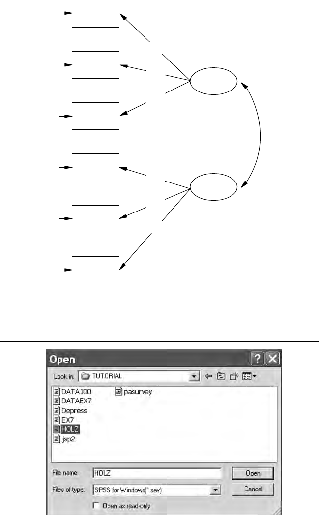
78 A Beginner’s Guide to Structural Equation Modeling
visperc
0.39
cubes
0.81
lozenges
0.68
parcomp
0.27
sencomp
0.27
wordmean
0.30
Spatial
Verbal
0.46
0.84
0.85
0.85
0.57
0.4
0.78
FIGURE 5.1a
Common factor model. (From Holzinger, K. J., & Swineford, F. A. [1939]. A study in factor
analysis: The stability of a bi-factor solution. Supplementary Educational Monographs, No. 48.
Chicago: University of Chicago, Dept. of Education.)
Y102005.indb 78 3/22/10 3:25:33 PM
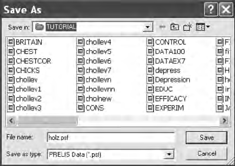
Model Fit 79
After clicking on Open, a Save As dialog box appears to save a PRELIS
System File, so enter holz.psf.
A spreadsheet should appear that contains the variable names and data.
Also, an expanded tool bar menu appears that begins with File, includes
Edit, Data, Transformation, Statistics, Graphs, etc., and ends with the Help
command. The File command also permits the use of an Export LISREL
Data option. The File, then Import Data option should be used to save a
PRELIS System File whenever possible to take advantage of data screen-
ing, imputing missing values, computation of normal scores, output data
options, and many other features in LISREL–PRELIS. For our purposes,
click on Statistics, then select the Output Options. The Output dialog box
will be used to save a correlation matrix le (holz.cor), a means le (holz.
me), and standard deviations le (holz.sd) for the variables we will use to
analyze our theoretical model in Figure 5.1a. The correlation, means, and
standard deviation les must be saved (or moved) to the same directory
as the LISREL–SIMPLIS program le. Click OK and descriptive statistics
appear in the computer output (frequencies, means, standard deviations,
skewness, kurtosis, etc.).
Y102005.indb 79 3/22/10 3:25:33 PM
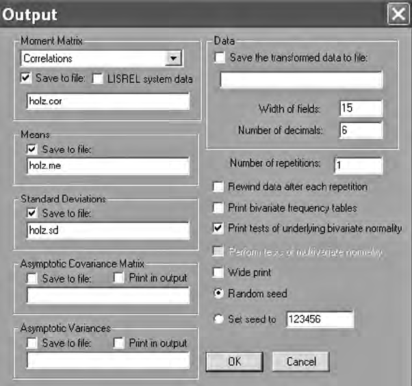
80 A Beginner’s Guide to Structural Equation Modeling
5.1.1.2 Program
The next step is to create the LISREL–SIMPLIS program syntax le that will
specify the model analysis for Figure 5.1a. This is accomplished by select-
ing File on the tool bar, then clicking on New, select Syntax Only, and
then enter the program syntax. If you forget the SIMPLIS program syntax,
refer to the LISREL–SIMPLIS manual or modify an existing program. We
created a LISREL–SIMPLIS program named holz.spl that contains the fol-
lowing program syntax. (Note: The rst three observed variables listed—
gender, ageyear, and birthmon—are contained in the raw data, but are not
analyzed in the SEM model.)
LISREL Figure 5.1a Program
Observed Variables
gender ageyear birthmon visperc cubes lozenges parcomp C
sencomp wordmean
Correlation matrix from file holz.cor
Means from file holz.me
Standard deviations from file holz.sd
Sample Size 301
Y102005.indb 80 3/22/10 3:25:34 PM

Model Fit 81
Latent Variables
Spatial Verbal
Relationships
visperc - lozenges = Spatial
parcomp - wordmean = Verbal
Number of decimals = 5
Path Diagram
End of Problem
Select File, then Save As, to save the le as holz.spl (SIMPLIS le type).
You are now ready to run the analysis using the holz.spl le you just cre-
ated. Click on the running L on the tool bar menu and the ASCII text le
holz.out will appear. The LISREL–SIMPLIS output le will contain several
model-t indices; however, a LISREL–SIMPLIS program (holz.spl) and a
LISREL8 command program (holz.ls8) will report and use different chi-
square t values in the model-t indices—that is, the minimum t func-
tion chi-square (C1), the normal theory weighted least-squares t function
(C2), the Satorra–Bentler scaled chi-square (C3), and the Browne adjusted
chi-square (C4) (see chapter note in Power and Sample Size section for
more detail).
5.1.1.3 Output
5.1.1.3.1 Goodness-of-Fit Statistics—Original Model
Degrees of Freedom = 8
Minimum Fit Function Chi-Square = 24.28099 (P = 0.0020559)
Normal Theory Weighted Least Squares Chi-Square = 24.40679
(P = 0.0019581)
Estimated Noncentrality Parameter (NCP) = 16.40679
90 Percent Condence Interval for NCP = (5.18319 ; 35.23399)
Y102005.indb 81 3/22/10 3:25:34 PM
82 A Beginner’s Guide to Structural Equation Modeling
Minimum Fit Function Value = 0.080937
Population Discrepancy Function Value (F0) = 0.054689
90 Percent Condence Interval for F0 = (0.017277 ; 0.11745)
Root Mean Square Error of Approximation (RMSEA) = 0.082681
90 Percent Condence Interval for RMSEA = (0.046472 ; 0.12116)
P-Value for Test of Close Fit (RMSEA < 0.05) = 0.066396
Expected Cross-Validation Index (ECVI) = 0.16802
90 Percent Condence Interval for ECVI = (0.13061 ; 0.23078)
ECVI for Saturated Model = 0.14000
ECVI for Independence Model = 2.49266
Chi-Square for Independence Model with 15 Degrees of Freedom =
735.79891
Independence AIC = 747.79891
Model AIC = 50.40679
Saturated AIC = 42.00000
Independence CAIC = 776.04157
Model CAIC = 111.59922
Saturated CAIC = 140.84932
Normed Fit Index (NFI) = 0.96700
Nonnormed Fit Index (NNFI) = 0.95765
Parsimony Normed Fit Index (PNFI) = 0.51573
Comparative Fit Index (CFI) = 0.97741
Incremental Fit Index (IFI) = 0.97763
Relative Fit Index (RFI) = 0.93813
Critical N (CN) = 249.24177
Root Mean Square Residual (RMR) = 2.01027
Standardized RMR = 0.047008
Goodness-of-Fit Index (GFI) = 0.97360
Adjusted Goodness-of-Fit Index (AGFI) = 0.93069
Parsimony Goodness-of-Fit Index (PGFI) = 0.37089
The chi-square statistic is signicant, indicating a less-than-adequate model
t to the sample variance–covariance matrix (Minimum Fit Function Chi-
Square = 24.28099, df = 8, p = 0.0020559). Several of the other model-t indi-
ces for the theoretical model in Figure 5.1a indicated a reasonable data
to model t, for example, GFI = .97360, RMSEA = 0.082681, Standardized
RMR = .047008, and NFI = 0.96700. Modication indices in the computer
output, however, offer suggestions on how to further improve the model
to data-t:
Y102005.indb 82 3/22/10 3:25:34 PM
Model Fit 83
The Modification Indices Suggest to Add the
Path to from Decrease in Chi-Square New Estimate
visperc Verbal 10.4 2.62
lozenges Verbal 9.2 -2.32
sencomp Spatial 7.9 -0.79
The Modification Indices Suggest to Add an Error Covariance
Between and Decrease in Chi-Square New Estimate
cubes visperc 9.2 -8.53
lozenges cubes 10.4 8.59
wordmean parcomp 7.9 -5.86
We wanted our theoretical model to keep Verbal and Spatial as separate
constructs (latent variables) with three separate sets of observed variables.
Therefore, we were not interested in adding any paths to either latent vari-
able from the other latent variables observed variables. So, we choose to select
the adding of an error covariance between lozenges and cubes that would
decrease the model-t chi-square value by an estimated 10.4. We, therefore,
added the following command line to our LISREL–SIMPLIS program:
Let the error covariance of lozenges and cubes correlate
Our modied theoretical model is diagrammed in Figure 5.1b. The
resulting computer output indicated a better model t to the data with a
nonsignicant Minimum Fit Function c2 = 13.92604, df = 7, and p =.052513;
RMSEA = .056209; Standardized RMR = 0.032547, and GFI = .98508 . (Note:
We used a strict interpretation of p = .05 for model t, so p = .053 was con-
sidered nonsignicant for model t).
5.1.1.3.2 Goodness-of-Fit Statistics—Modied Model
Degrees of Freedom = 7
Minimum Fit Function Chi-Square = 13.92604 (P = 0.052513)
Normal Theory Weighted Least Squares Chi-Square = 13.63496 (P =
0.058068)
Estimated Noncentrality Parameter (NCP) = 6.63496
90 Percent Condence Interval for NCP = (0.0 ; 21.19420)
Minimum Fit Function Value = 0.046420
Population Discrepancy Function Value (F0) = 0.022117
90 Percent Condence Interval for F0 = (0.0 ; 0.070647)
Root Mean Square Error of Approximation (RMSEA) = 0.056209
90 Percent Condence Interval for RMSEA = (0.0 ; 0.10046)
P-Value for Test of Close Fit (RMSEA < 0.05) = 0.35494
Y102005.indb 83 3/22/10 3:25:35 PM
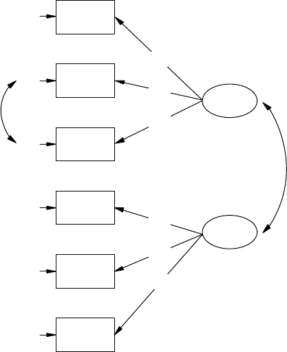
84 A Beginner’s Guide to Structural Equation Modeling
Expected Cross-Validation Index (ECVI) = 0.13878
90 Percent Condence Interval for ECVI = (0.11667 ; 0.18731)
ECVI for Saturated Model = 0.14000
ECVI for Independence Model = 2.49266
Chi-Square for Independence Model with 15 Degrees of Freedom =
735.79891
Independence AIC = 747.79891
Model AIC = 41.63496
Saturated AIC = 42.00000
Independence CAIC = 776.04157
Model CAIC = 107.53450
Saturated CAIC = 140.84932
Normed Fit Index (NFI) = 0.98107
Nonnormed Fit Index (NNFI) = 0.97941
Parsimony Normed Fit Index (PNFI) = 0.45783
visperc
0.09
cubes
0.90
lozenges0.79
parcomp
0.27
sencomp
0.27
wordmean0.30
Spatial
Verbal
0.42
0.20
0.84
0.86
0.85
0.46
0.31
0.96
FIGURE 5.1b
Modied common factor model. (From Holzinger, K. J., & Swineford, F. A. [1939]. A study
in factor analysis: The stability of a bi-factor solution. Supplementary Educational Monographs,
No. 48. Chicago: University of Chicago, Dept. of Education.)
Y102005.indb 84 3/22/10 3:25:35 PM

Model Fit 85
Comparative Fit Index (CFI) = 0.99039
Incremental Fit Index (IFI) = 0.99050
Relative Fit Index (RFI) = 0.95944
Critical N (CN) = 399.01152
Root Mean Square Residual (RMR) = 1.34928
Standardized RMR = 0.032547
Goodness-of-Fit Index (GFI) = 0.98508
Adjusted Goodness-of-Fit Index (AGFI) = 0.95523
Parsimony Goodness-of-Fit Index (PGFI) = 0.32836
Our LISREL–SIMPLIS example will further serve to help our understand-
ing of how the various model-t indices are computed and illustrate how
power and sample size can be determined. Overall, the t indices fall into
the three main categories of model t, model comparison, and model parsi-
mony t indices. Next, we discuss the t indices in these three categories
to understand their development and recommended applications. [Note:
Extensive comparisons and discussions of many of these t indices can
be found in issues of the following journals: Structural Equation Modeling:
A Multidisciplinary Journal, Psychological Bulletin, Psychological Methods, and
Multivariate Behavioral Research.]
5.2 Model Fit
Model t determines the degree to which the sample variance–covariance
data t the structural equation model. Model-t criteria commonly used
are chi-square (c2), the goodness-of-t index (GFI), the adjusted good-
ness-of-t index (AGFI), and the root-mean-square residual index (RMR)
(Jöreskog & Sörbom, 1989). These criteria are based on differences between
the observed (original, S) and model-implied (reproduced, Σ) variance–
covariance matrices.
5.2.1 Chi-Square (c2)
A signicant c2 value relative to the degrees of freedom indicates that
the observed and implied variance–covariance matrices differ. Statistical
signicance indicates the probability that this difference is due to sam-
pling variation. A nonsignicant c2 value indicates that the two matri-
ces are similar, indicating that the implied theoretical model signicantly
reproduces the sample variance–covariance relationships in the matrix.
Y102005.indb 85 3/22/10 3:25:35 PM
86 A Beginner’s Guide to Structural Equation Modeling
The researcher is interested in obtaining a nonsignicant c2 value with
associated degrees of freedom. Thus it may be more appropriate to call the
chi-square test a measure of badness-of-t.
The chi-square test of model t can lead to erroneous conclusions regard-
ing analysis outcomes. The c2 model-t criterion is sensitive to sample
size because as sample size increases (generally above 200), the c2 statistic
has a tendency to indicate a signicant probability level. In contrast, as
sample size decreases (generally below 100), the c2 statistic indicates non-
signicant probability levels. The chi-square statistic is therefore affected
by sample size, as noted by its calculation, c2 = (n − 1) FML, where F is the
maximum likelihood (ML) t function. The c2 statistic is also sensitive to
departures from multivariate normality of the observed variables.
Three estimation methods are commonly used to calculate c2 in latent
variable models (Loehlin, 1987): maximum likelihood (ML), generalized
least squares (GLS), and unweighted least squares (ULS). Each approach
estimates a best-tting solution and evaluates the model t. The ML esti-
mates are consistent, unbiased, efcient, scale invariant, scale free, and
normally distributed if the observed variables meet the multivariate nor-
mality assumption. The GLS estimates have the same properties as the
ML approach under a less stringent multivariate normality assumption
and provide an approximate chi-square test of model t to the data. The
ULS estimates do not depend on a normality distribution assumption;
however, the estimates are not as efcient, nor are they scale invariant or
scale free. The ML c2 statistic is c2 = (n − 1) FML, the GLS c2 statistic is c2 =
(n − 1) FGLS, and the ULS c2 statistic is c2 = (n − 1) FULS. (Note: see Chapter
Footnote.)
In our model analysis, we chose the maximum likelihood chi-square
estimation method (default setting). The ML c2 statistic uses the mini-
mum t function value, which is reported in the computer output. The
minimum t function chi-square for our modied model is calculated as:
c2 = (301 − 1) .046420 = 13.926. (Note: add command line Number of decimals = 5
to SIMPLIS program so Minimum Fit Function Value = 0.046420 will not
differ due to rounding error.)
5.2.2 Goodness-of-Fit Index (GFI) and Adjusted
Goodness-of-Fit Index (AGFI)
The goodness-of-t index (GFI) is based on the ratio of the sum of the
squared differences between the observed and reproduced matrices to
the observed variances, thus allowing for scale. The GFI measures the
amount of variance and covariance in S that is predicted by the repro-
duced matrix Σ. In our original model, GFI = .97, so 97% of the S matrix is
predicted by the reproduced matrix Σ, which improved in the modied
model to 99% where GFI = 0.98508.
Y102005.indb 86 3/22/10 3:25:35 PM
Model Fit 87
The GFI index can be computed for ML, GLS, or ULS estimates (Bollen,
1989). For our modied model the formula expression is:
GFI = 1 – [c2model/c2null]
GFI = 1 – [13.92604/735.79891]
GFI = 1 − .0189264
GFI = .98 ~ .99
(NOTE: The c2null is the Chi-Square for Independence Model with 15
Degrees of Freedom.)
The adjusted goodness-of-t index (AGFI) is adjusted for the degrees of
freedom of a model relative to the number of variables. The AGFI index is
computed as 1 − [(k/df) (1 − GFI)], where k is the number of unique distinct
values in S, which is p(p + 1)/2, and df is the number of degrees of freedom
in the model. The GFI index in our modied model analysis was .985,
therefore the AGFI index is
1 − [(k/df)(1 − GFI)] = 1 – [(15/7)(1 − .985)]
= 1 – [2.14285(.015)]
= 1 − .03
= .97
The GFI and AGFI indices can be used to compare the t of two different
models with the same data or compare the t of a single model using dif-
ferent data, such as separate datasets for males and females, for example,
or examine measurement invariance in group models.
5.2.3 Root-Mean-Square Residual Index (RMR)
The RMR index uses the square root of the mean-squared differences
between matrix elements in S and Σ. Because it has no dened acceptable
level, it is best used to compare the t of two different models with the
same data. The RMR index is computed as
RMR = [(1/k) Σij (sij − σij)2]1/2.
For our example, the original model Root Mean Square Residual
(RMR) = 2.01027 compared to the modied model Root Mean Square
Residual (RMR) = 1.34928. There is also a standardized RMR, known as
Standardized RMR, which has an acceptable level when less than .05.
For our original model, the Standardized RMR = 0.047008, compared
to the modied model with a Standardized RMR = 0.032547, which is
deemed a more acceptable t. (Note: The residual covariance matrix can
Y102005.indb 87 3/22/10 3:25:36 PM

88 A Beginner’s Guide to Structural Equation Modeling
be requested in a LISREL–SIMPLIS program by adding the command
line, Print Residuals.)
5.3 Model Comparison
Given the role chi-square has in the model t of latent variable models,
three other indices have emerged as variants for comparing alternative
models: the Tucker–Lewis index (TLI) or Bentler–Bonett nonnormed
t index (NNFI), the Bentler–Bonett normed t index (NFI) (Bentler &
Bonett, 1980; Loehlin, 1987), and the comparative t index (CFI). These
criteria typically compare a proposed model with a null model (inde-
pendence model). In LISREL the null model is indicated by the indepen-
dence-model chi-square value. The null model could also be any model
that establishes a baseline from which one could expect other alternative
models to be different.
5.3.1 Tucker–Lewis Index (TLI)
Tucker and Lewis (1973) initially developed the TLI for factor analysis
but later extended it to structural equation modeling. The measure can
be used to compare alternative models or to compare a proposed model
against a null model. The TLI is computed using the c2 statistic as
[(c2null /dfnull) − (c2proposed /dfproposed)]/[(c2null /dfnull) − 1]
It is scaled from 0 (no t) to 1 (perfect t). For our modied model analysis,
the NNFI, as it is known in LISREL, was computed as
Nonnormed Fit Index (NNFI)
= [(c2null /dfnull) – (c2proposed /dfproposed)]/[(c2null /dfnull) − 1]
= [(735.79891/15) – (13.92604 /7)]/[(735.7989/15) − 1]
= [(49.05326 – 1.98943)/(49.05326 – 1)]
= [47.06383/48.05326]
= 0.97941
5.3.2 Normed Fit Index (NFI) and Comparative Fit Index (CFI)
The NFI is a measure that rescales chi-square into a 0 (no t) to 1.0 (perfect
t) range (Bentler & Bonett, 1980). It is used to compare a restricted model
Y102005.indb 88 3/22/10 3:25:36 PM

Model Fit 89
with a full model using a baseline null model as follows: (c2null − c2model)/
c2null. In our modied model analysis this was computed as
Normed Fit Index (NFI) = (c2null − c2model)/c2null
= (735.7989 – 13.92604)/735.7989
= .98107
Bentler (1990) subsequently developed a coefcient of comparative t
within the context of specifying a population parameter and distribution,
such as a population comparative t index, to overcome the deciencies
in NFI for nested models. The rationale for assessment of comparative t
in the nested-model approach involves a series of models that range from
least restrictive (Mi) to saturated (Ms). Corresponding to this sequence of
nested models is a sequence of model-t statistics with associated degrees
of freedom. The comparative t index (CFI) measures the improvement in
noncentrality in going from model Mi to Mk (the theoretical model) and
uses the noncentral c2 (dk) distribution with noncentrality parameter lk
to dene comparative t as (li − lk)/li. In our modied model output the
Comparative Fit Index (CFI) = 0.99039.
McDonald and Marsh (1990) further explored the noncentrality and
model-t issue by examining nine t indices as functions of noncentrality
and sample size. They concluded that only the Tucker-Lewis Index and
their relative noncentrality index (RNI) were unbiased in nite samples
and recommended them for testing null or alternative models. For abso-
lute measures of t that do not test null or alternative models, they recom-
mended dk (Steiger & Lind, 1980), because it is a linear function of c2, or
a normed measure of centrality mk (McDonald, 1989), because neither of
these varies systematically with sample size. These model t measures
of centrality are useful when selecting among a few competing models
based upon theoretical considerations.
5.4 Model Parsimony
Parsimony refers to the number of estimated parameters required to
achieve a specic level of model t. Basically, an over-identied model
is compared with a restricted model. The AGFI measure discussed pre-
viously also provides an index of model parsimony. Other indices that
indicate model parsimony are the parsimony normed t index (PNFI),
and the Akaike information criterion (AIC). Parsimony-based t indices
Y102005.indb 89 3/22/10 3:25:36 PM
90 A Beginner’s Guide to Structural Equation Modeling
for multiple indicator models were reviewed by Williams and Holahan
(1994). They found that the AIC performed the best (see their article for
more details on additional indices and related references). The model par-
simony goodness-of-t indices take into account the number of param-
eters required to achieve a given value for chi-square. Lower values for
PNFI and AIC indicate a better model t given a specied number of
parameters in a model.
5.4.1 Parsimony Normed Fit Index (PNFI)
The PNFI measure is a modication of the NFI measure (James, Mulaik, &
Brett, 1982). The PNFI, however, takes into account the number of degrees
of freedom used to obtain a given level of t. Parsimony is achieved with
a high degree of t for fewer degrees of freedom in specifying the coef-
cients to be estimated. The PNFI is used to compare models with different
degrees of freedom and is calculated as PNFI = (dfproposed /dfnull) NFI. In our
modied model analysis the PNFI was:
Parsimony Normed Fit Index (PNFI) = (dfproposed/dfnull) NFI
= (7/15) .98107
= 0.45783
5.4.2 Akaike Information Criterion (AIC)
The AIC measure is used to compare models with differing numbers of
latent variables, much as the PNFI is used (Akaike, 1987). The AIC can be
calculated in two different ways: c2 + 2q, where q = number of free param-
eters in the model, or as c2 – 2df. The rst AIC is positive (as computed
in LISREL), and the second AIC is negative, but either AIC value close to
zero indicates a more parsimonious model. The AIC indicates model t (S
and Σ elements similar) and model parsimony (over-identied model). In
our modied model analysis, the computer output gives several AIC val-
ues for the theoretical model, saturated model, and independence model;
however, we only report two AIC t indices. (Note: AIC uses Normal
theory weighted least squares chi-square not the minimum t function
chi-square.)
Model AIC = Normal Theory c2 + 2q
= 13.63496 + 2 (14)
= 41.63496
Y102005.indb 90 3/22/10 3:25:36 PM
Model Fit 91
Independence AIC = Chi-Square for Independence Model + 2(df -1)
= 735.79891 + 2(6)
= 747.79891
5.4.3 Summary
Mulaik, James, Alstine, Bennett, Lind, and Stilwell (1989) evaluated the
c2, NFI, GFI, AGFI, and AIC goodness-of-t indices. They concluded that
these indices fail to assess parsimony and are insensitive to misspecica-
tion of structural relationships (see their denitive work for additional
information). Their ndings should not be surprising because it has been
suggested that a good t index is one that is independent of sample size,
accurately reects differences in t, imposes a penalty for inclusion of
additional parameters (Marsh, Balla, & McDonald, 1988), and supports the
choice of the true model when it is known (McDonald & Marsh, 1990). No
model-t criteria can actually meet all of these criteria.
We have presented several model-t indices that are used to assess
model t, model comparison, or model parsimony. In addition, we cal-
culated many of these based on the model analyzed in this chapter. The
LISREL program outputs many different model-t criteria because more
than one should be reported. The LISREL user guides also provide an
excellent discussion of the model-t indices in their program. We rec-
ommend that once you feel comfortable using these t indices for your
specic model applications, you check the references cited for additional
information on their usefulness and/or limitations. Following their ini-
tial description, there has been much controversy and discussion on
their subjective interpretation and appropriateness under specic mod-
eling conditions (see Marsh, Balla, & Hau [1996] for further discussion).
Further research and discussion will surely follow; for example, Kenny
& McCoach (2003) indicated that RMSEA improves as more variables are
added to a model, whereas TLI and CFI both decline in correctly specied
models as more variables are added.
When deciding on which model-t indices to report, rst consider
whether the t indices were created for model t, model parsimony, or
model comparison. At the risk of oversimplication, we suggest that c2,
RMSEA, and Standardized RMR be reported for all types of models with
additional t indices reported based on purpose of modeling. For exam-
ple, the CFI should be reported if comparing models. Overall, more than
one model-t index should be reported. If a majority of the t indices on
your list indicate an acceptable model, then your theoretical model is sup-
ported by the data.
Y102005.indb 91 3/22/10 3:25:36 PM

92 A Beginner’s Guide to Structural Equation Modeling
5.5 Parameter Fit
Individual parameter estimates in a model can be meaningless even though
model-t criteria indicate an acceptable measurement or structural model.
Therefore, interpretation of parameter estimates in any model analysis is
essential. The following steps are therefore recommended:
1. Examine the parameter estimates to determine whether they have
the correct sign (either positive or negative).
2. Examine parameter estimates (standardized coefcients) to deter-
mine whether they are out of bounds or exceed an expected range
of values.
3. Examine the parameter estimates for statistical signicance
(T or Z-values = parameter estimate divided by standard error of
parameter estimate).
4. Test for measurement invariance by setting parameter estimates
equal (constraints) in different groups, for example, girls and
boys, then make relative comparisons among the parameter
estimates.
An examination of initial parameter estimates can also help in identi-
fying a faulty or misspecied model. In this instance, initial parame-
ter estimates can serve as start values—for example, initial two-stage
least-squares (TSLS) estimates in LISREL. The researcher then replaces
the TSLS estimate with a user-dened start value. Sometimes param-
eter estimates take on impossible values, as in the case of a correlation
between two variables that exceeds 1.0. Sometimes negative variance is
encountered (known as a Heywood case). Also, if the error variance for
a variable is near zero, the indicator variable implies an almost perfect
measure of the latent variable, which may not be the case. Outliers can
also inuence parameter estimates. Use of sufcient sample size (n > 100
or 150) and several indicators per latent variable (four is recommended
based on the TETRAD approach) has also been recommended to pro-
duce reasonable and stable parameter estimates (Anderson & Gerbing,
1984).
Once these issues have been taken into consideration, the interpreta-
tion of modication indices and expected parameter change can begin
to modify the model, but there is still a need for guidance provided by
the rationale for the theoretical model and the researcher’s expertise.
Researchers should use the model-t indices as potential indicators of
mist when respecifying or modifying a model. Cross-validation or
Y102005.indb 92 3/22/10 3:25:37 PM

Model Fit 93
replication using another independent sample, once an acceptable model
is achieved, is always recommended to ensure stability of parameter
estimates and validity of the model (Cliff, 1983). Bootstrap procedures
also afford a resampling method, given a single sample, to determine
the efciency and precision of sample estimates (Lunneborg, 1987).
These model validation topics are discussed further in chapter 12.
5.6 Power and Sample Size
The determination of power and/or sample size in SEM is complicated
because theoretical models can have several variables or parameter esti-
mates and parameters are typically not independent in a model and have
different standard errors. In SEM we also compare models, oftentimes
nested models with the same data set. Consequently, power and sample
size determination in the situation where a researcher is hypothesis test-
ing (testing a model t to data), comparing alternative models, or desiring
to test a parameter estimate for signicance will be covered with SAS,
SPSS, and G*Power 3 examples using the LISREL–SIMPLIS example in the
chapter. The power for hypothesis testing, or the probability of rejecting Ho
when Ha is true, depends on the true population model, signicance level,
degrees of freedom, and sample size, which involves specifying an effect
size, alpha, and sample size; while sample size determination is achieved
given power, effect size, and alpha level of signicance. Daniel S. Soper
has a user friendly website that provides effect size, power and sample
size determination in statistics (http://www.danielsoper.com/statcalc/).
Hypothesis testing involves conrming that a theoretical model ts the
sample variance–covariance data, comparing t between alternative mod-
els, or testing parameter coefcients for signicance; even whether coef-
cients are equal between groups. These hypothesis testing methods should
involve constrained models with fewer parameters than the initial model.
The initial (full) model represents the null hypothesis (Ho) and the alterna-
tive (constrained) model with fewer parameters is denoted Ha. Each model
generates a c2 goodness-of-t measure, and the difference between the
models for signicance testing is computed as D2 = c2o − c2a, with dfd =
dfo − dfa. The D2 statistic is tested for signicance at a specied alpha level
(probability of Type I error), where Ho is rejected if D2 exceeds the critical
tabled c2 value with dfd degrees of freedom (Table A.4). The chi-square dif-
ference test or likelihood ratio test is used with GLS, ML, and WLS estima-
tion methods.
Y102005.indb 93 3/22/10 3:25:37 PM
94 A Beginner’s Guide to Structural Equation Modeling
The signicance of parameter estimates that do not require two sepa-
rate models to yield separate c2 values includes: (a) generating a two-
sided t or z value for the parameter estimate (T or Z = parameter estimate
divided by standard error of the parameter estimate), and (b) interpret-
ing the modication index directly for the parameter estimate as a c2
test with 1 degree of freedom. The relationship is simply T2 = D2 = MI
(modication index) for large sample sizes. Gonzalez and Grifn (2001),
however, indicated that the standard errors of the parameter estimates
are sensitive to how the model is identied, that is, alternative ways of
identifying a model may yield different standard errors, and hence dif-
ferent T values for the statistical signicance of a parameter estimate.
This lack of invariance due to model identication could result in dif-
ferent conclusions about a parameter’s signicance level from different,
yet equivalent, models on the same data. The authors recommended
that parameter estimates be tested for signicance using the likelihood
ratio (LR) test because it is invariant to model identication, rather than
the T test (or z test).
5.6.1 Model Fit
A traditional approach in SEM is to hypothesize a theoretical model, col-
lect sample data, and test whether the model ts the data. In this chap-
ter we have discussed various t indices to determine if the theoretical
model ts the data. When the theoretical model does not t the data, we
look to modication indices for suggestions on how to modify the model
for an improved t. The power to reject a null hypothesis and sample
size impacts our decision of whether sample data t a theoretical model.
Power and sample size are therefore discussed next.
5.6.1.1 Power
Saris and Satorra (1993) provided an easy to use approach for calculating
power of a theoretical model. Basically, an alternative model is estimated
with sample data to indicate what percent of the time we would correctly
reject the null hypothesis under the assumption that the null hypothesis
(Ho) is false. The minimum t function chi-square value obtained from
tting data to the theoretical model provides an estimate of the noncen-
trality parameter (NCP). NCP is calculated as Normal Theory Weighted
Least Squares c2 – dfmodel. For our modied model the NCP = 13.63496 – 7
= 6.63496, which is provided in the Goodness-of-Fit section of the com-
puter output. This makes computing power using SAS 9.1, SPSS 16.0, or
G*Power 3 straightforward, using their respective command functions.
Y102005.indb 94 3/22/10 3:25:37 PM
Model Fit 95
(Note: c2 = 3.841, df = 1, p = .05 is the critical tabled value for testing
our hypothesis of model t.) Examples for each using NCP are provided
next.
SAS syntax—power
data chapter5;
do obs=1;
ncp = 6.63496;
power = 1 – PROBCHI(3.841, 1, ncp);
output;
end;
proc print;
var ncp power;
run;
SPSS syntax—power
DATA LIST FREE / obs.
BEGIN DATA.
1
END DATA.
compute ncp = 6.63496.
compute power = 1 - NCDF.CHISQ(3.841, 1, ncp).
formats ncp power (f8.5).
List.
In our modied model, NCP = 6.63496, so our power = .73; the output from
the SAS or SPSS syntax was:
obs ncp power
1.00 6.63496 .73105
Power, given your model t, can also be determined using G*power 3 (Faul,
Erdfelder, Lang & Buchner, 2007). The free G*Power 3 software download
is available from the Web site: http://www.psycho.uni-duesseldorf.de/
abteilungen/aap/gpower3/, which is somewhat easier than running the
SAS and SPSS programs. Power and sample size estimates for a priori and
post-hoc statistical applications are available using G*power 3. (Note: We
used G*Power 3, Windows, Release 3.1.0, 2008, but a MAC OS version is
also available). After download and installation, click on the G*Power 3
desktop icon and you should see the following dialog box:
Y102005.indb 95 3/22/10 3:25:37 PM

96 A Beginner’s Guide to Structural Equation Modeling
In the Test family window select “c2 tests”; in the Statistical test window
select “Generic c2 test”; and in the Type of power analysis window, select
“Post-hoc: Compute power – given a, and noncentrality parameter.” Our modi-
ed model had NCP = 6.63496, so we entered this value in the “noncen-
trality parameter l” window along with df = 1 and a = .05. The dialog box
should look like:
Y102005.indb 96 3/22/10 3:25:38 PM
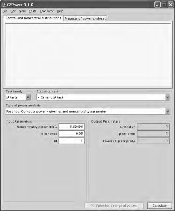
Model Fit 97
Click the Calculate button. The power = .731015 value matches our earlier
calculations. The dialog box should now look like:
Y102005.indb 97 3/22/10 3:25:39 PM
98 A Beginner’s Guide to Structural Equation Modeling
Our modied model has a 73 percent chance of rejecting the null
hypothesis at the .05 level of signicance, which falls short of the .80 level
commonly accepted for power. If we replace the critical chi-square value
in the formula, you can determine power for other alpha levels of signi-
cance. In Table 5.2, we have replaced the critical chi-square value and ran
the SPSS syntax program for alpha values ranging from .10 to .001. If we
test our modied model t at the p = .10 level, then we achieve an accept-
able level of power; other alpha levels from .05 to .001 fall below a .80
power value.
Y102005.indb 98 3/22/10 3:25:40 PM

Model Fit 99
5.6.1.2 Sample Size
An earlier way to determine an appropriate sample size in SEM was given
by Hoelter (1983) as the Critical N (CN) statistic, where CN ≥ 200 was con-
sidered adequate. The Critical N is calculated as:
CN = (c2critical/Fmin) + 1
The critical chi-square (c2critical) is obtained for the model degrees of
freedom at the .05 level of signicance. The CN statistic is output by the
LISREL–SIMPLIS program. In our nal modied model of Figure 5.1b,
CN = 399, Fmin was determined to be .0353432 and c2critical = 14.067 for df =
7 at .05 level of signicance (see Table A.4); so CN = (14.067/.0353432) + 1 =
399. (Note: our modied model computer output indicated Fmin = .04642,
p = .0525, but CN uses Fmin at p = .05). CN gives the sample size at which
the Fmin value leads to a rejection of Ho. Our sample size was N = 301
with a nonsignicant chi-square (minimum t function c2, p = .052; or nor-
mal theory weighted least squares c2, p = .058) and several good model-t
indices, so even if we used Hoelter’s suggestion, we had sufcient sample
size. For a further discussion about CN refer to Bollen and Liang (1988) or
Bollen (1989).
Sample size inuences the calculation of the minimum t function c2.
Recall that the Minimum Fit Function c2 in the modied model was com-
puted as:
Minimum Fit Function c2 = (N – g) × Fmin
= (301 – 1) × (.046420)
= 13.92604
TABLE 5.2
Power for Alpha Levels Given Modied Model NCP
NCP Critical Chi-Square Alpha Power
6.63496 2.706 .10 .82405
6.63496 3.841 .05 .73105
6.63496 5.412 .02 .59850
6.63496 6.635 .01 .50000
6.63496 10.827 .001 .23743
Note: Critical c2 values for df = 1 from Table A.4.
Y102005.indb 99 3/22/10 3:25:40 PM
100 A Beginner’s Guide to Structural Equation Modeling
Sample size also inuences the calculation of the Fmin values as follows:
Fmin = Minimum Fit Function c2/(N – g)
= 13.92604/(301 – 1)
= .046420
The Fmin is computed using the minimum t function c2 in the computer
output, sample size (N), and number of groups (g); while the noncentral-
ity parameter (NCP) is computed using the Normal Theory c2 minus the
degrees of freedom in the model. NCP is therefore computed as:
NCP = Normal Theory Weighted Least Squares c2 – dfmodel
= 13.63496 – 7
= 6.63496
Estimated sample size (N) using these NCP and Fmin values is less than
our actual sample size of N = 301:
N = (NCP/Fmin) + g
= (6.63496/.046420) + 1
= 143.93 ~ 144
You have probably noticed that Fmin is calculated using the Minimum Fit
Function c2, but NCP is calculated using the Normal Theory Weighted
Least Squares c2. LISREL, unlike other SEM software calculates some
measures of t (NCP, RMSEA, and Independence model c2 ) using the
normal theory weighted least squares c2, but uses the minimum t
function c2 for others. Differences between these two can be small if
the multivariate normality assumption holds or very different if not (see
Chapter Footnote for detailed description of standard errors and four
different c2 values: C1 = minimum t function c2; C2 = normal theory
weighted least squares c2; C3 = Satorra–Bentler scaled c2; C4 = c2 cor-
rected for nonnormality).
To determine sample size for given df, alpha, and power for a theoretical
model, the Fmin value would be xed (Fmin value from your nal model; our
modied model had Fmin = .046420), but the NCP value would vary. For
our modied model, the SAS program can be run for differing NCP val-
ues to obtain corresponding sample size and power estimates. (Note: We
Y102005.indb 100 3/22/10 3:25:40 PM

Model Fit 101
are changing values of power in the SAS syntax program, but you can also
x power and change alpha values to obtain different sample sizes for dif-
ferent alpha levels at a specied power level, for example, power = .80).
SAS syntax—sample size
data chapter5;
do obs = 1;
g = 1;
* change values of alpha to obtain sample size for given
power;
alpha = .05;
fmin = .046420;
df = 1;
* change values of power to obtain sample size for given
alpha;
power = .60;
chicrit = quantile(‘chisquare’,1 – alpha, df);
ncp = CINV(power,df,chicrit);
n = (ncp/fmin) + g;
output;
end;
proc print;
var power n alpha ncp fmin g;
run;
The output from this rst run with power = .60 would look like this:
obs power n alpha ncp fmin g chicrit
1 .6 106.535 .05 4.89892 .04642 1 3.84146
We created Table 5.3 by changing the value of power for alpha = .05
for a critical c2 = 3.841, df = 1. (Note: fmin is xed at the value from our
TABLE 5.3
Sample Size for Given Power with Alpha = .05
Power n Alpha ncp fmin g c2 critical
.60 106.535 .05 4.89892 .04642 1 3.84146
.70 133.963 .05 6.17213 .04642 1 3.84146
.73 143.594 .05 6.61923 .04642 1 3.84146
.80 170.084 .05 7.84890 .04642 1 3.84146
.90 227.356 .05 10.5074 .04642 1 3.84146
.95 280.938 .05 12.9947 .04642 1 3.84146
Note: n should be rounded up, for example, 106.535 = 107.
Y102005.indb 101 3/22/10 3:25:40 PM

102 A Beginner’s Guide to Structural Equation Modeling
modied model; alpha is xed at .05, so chicrit will be xed at 3.84146).
A sample size of N = 144 for power = .73 from our modied model was
also correctly computed and indicated in the table. We see in Table 5.3
that sample size requirements increase as power increases, which is
expected.
In our modied model we have N = 301, NCP = 6.63496, and our post-
hoc power = .73 calculated at the .05 level of signicance. A sample size of
N = 170 would have given us power = .80 at the .05 level of signicance.
Are you puzzled? Well, recall that NCP = c2 – dfmodel, so if our model had
resulted in a NCP = 7.84890 with N = 170 at the .05 level of signicance,
then we would have achieved an acceptable level of power = .80. We nd
that the noncentrality parameter (NCP) is affected by the model chi-
square but also the degrees of freedom, which indicates a certain level of
model complexity.
We can also use the SAS syntax—sample size program to examine how
changing the level of signicance affects sample size for a xed power
value. Recall that Fmin is xed at .04642 from our modied model. Table 5.4
contains the output from the SAS program. We see in Table 5.4 that sample
size requirements increase as the level of signicance (alpha) for testing
our model decreases, which is expected.
TABLE 5.4
Sample Size for Given Alpha with Power = .80
Power n Alpha ncp fmin g c2 critical
.8 134.194 .10 6.18288 .04642 1 2.70554
.8 170.084 .05 7.84890 .04642 1 3.84146
.8 217.201 .02 10.0360 .04642 1 5.41189
.8 252.593 .01 11.6790 .04642 1 6.63490
.8 368.830 .001 17.0746 .04642 1 10.8276
Note: c2critical values correspond to alpha values in Table A.4.
We used G*Power 3 to calculate various NCP values given alpha and
power because SPSS 16.0 does not have a command function at this
time to determine the noncentrality parameter (NCP) given power,
df, and critical c2. (Note: SAS, S-Plus, Stata and other statistical soft-
ware have this capability) In the Test family drop-down menu, select
“c2 test”; in the Statistical Test drop-down menu select, “Generic c2 test”;
and in the Type of power analysis, select “Sensitivity: Compute noncentral-
ity parameter – given a, and power.” In the Input Parameters boxes, change
Y102005.indb 102 3/22/10 3:25:40 PM
Model Fit 103
the power value to .80 and the df value to 1. Your dialog box should
now appear as:
Click on the Calculate button; the Output Parameters, “Critical c2” and
“Noncentrality parameter l“ will appear. The G*Power 3.1.0 dialog box will
now display the Critical c2 = 3.84146 (associated with alpha = .05, df = 1)
and corresponding noncentrality parameter for power = .80. Your dialog
box should now look like:
Y102005.indb 103 3/22/10 3:25:41 PM
104 A Beginner’s Guide to Structural Equation Modeling
Table 5.3 reports these same values using the program SAS syntax—
sample size.
You can click on the X-Y plot for a range of values button to enter a range of
power values that can be plotted by corresponding noncentrality param-
eter values. (Note: Check the box for “and displaying the values in the plot”
and change the “in steps of” from .01 to .10 for clarity in the output of the
graph.) The dialog box should look like this:
Y102005.indb 104 3/22/10 3:25:41 PM
Model Fit 105
Click on Draw plot. Your graph will now appear and should look like the
dialog box below:
Y102005.indb 105 3/22/10 3:25:42 PM

106 A Beginner’s Guide to Structural Equation Modeling
(NOTE: A range of power values entered from .6 to .95 indicates the levels
of the noncentrality parameter that one needs to exceed for that level of
power [see Table 5.3].)
In planning a study, we should determine a priori what our sample size
and power values should be. After gathering our data and running our SEM
model (and any modications), we should compute the post-hoc power using
our noncentrality parameter from the LISREL computer output or sample
size (N) using NCP and model Fmin values. This should be easy given that
N = ( NCP/ Fmin) + g. We can a priori specify values or obtain the Fmin value
from our model, calculate NCP using SAS or G*power 3 for a given df, criti-
cal chi-square, power, then use these values to calculate sample size (N).
MacCallum, Browne, and Sugawara (1996) provided a different approach to
testing model-t using the root mean square error of approximation (RMSEA).
Their approach also emphasized condence intervals around RMSEA, rather
than a single point estimate, so they suggested null and alternative values for
RMSEA (exact t: Ho = .00 versus Ha = .05; Close t: Ho = .05 versus Ha = .08;
and Not close t: Ho = .05 versus Ha = .10); researchers can also select their
own. The MacCallum et al. (1996) method tests power, given exact t (Ho;
RMSEA = 0), close t (Ho, RMSEA ≤ .05), or not close t (Ho, RMSEA ≥ .05); and
included SAS programs for calculating power given sample size or sample
size given power using RMSEA. RMSEA is calculated as:
RMSEANCP Ndf=−()//1
For our modied model, NCP = 6.63496; N = 301; and df = 7, so RMSEA =
0.056209:
RMSEA==(. ).6 63496 300 7 056209//
SAS syntax—RMSEA and power
data chapter5;
do obs = 1;
n = 301;
df = 7;
alpha = .05;
* change rmseaHo and rmseaHa values to correspond to exact,
close, and not close values;
rmseaHo = .05;
rmseaHa = .08;
ncpHo = (n-1)*df*rmseaHo*rmseaHo;
ncpHa = (n-1)*df*rmseaHa*rmseaHa;
chicrit = quantile(‘chisquare’,1-alpha,df);
if rmseaHo < rmseaHa then power = 1 –
PROBCHI(chicrit,df,ncpHa);
Y102005.indb 106 3/22/10 3:25:43 PM
Model Fit 107
if rmseaHo > rmseaHa then power = PROBCHI(chicrit,df,ncpHa);
output;
end;
Proc print;
Var n df alpha rmseaHo rmseaHa ncpHo ncpHa chicrit power;
Run;
SPSS syntax—RMSEA and power
DATA LIST FREE / obs.
BEGIN DATA.
1
END DATA.
compute n = 301.
compute df = 7.
compute alpha = .05.
comment change rmseaHo and rmseaHa values to correspond with
exact, close, not close values.
compute rmseaHo = .05.
compute rmseaHa = .08.
compute ncpHo = (n-1)*df*rmseaHo*rmseaHo.
compute ncpHa = (n-1)*df*rmseaHa*rmseaHa.
compute chicrit = IDF.CHISQ(1-alpha,df).
do if (rmseaHo < rmseaHa).
compute power = 1 - NCDF.CHISQ(chicrit, df, ncpHa).
else if (rmseaHo > rmseaHa).
compute power = NCDF.CHISQ(chicrit, df, ncpHa).
end if.
formats chicrit ncpHo ncpHa power (f8.5).
List.
The resulting SAS or SPSS output for close t was given as:
obs n df alpha rmseaHo rmseaHa ncpHo ncpHa chicrit power
1.00 301 7 .05 .05 .08 5.25 13.44 14.0671 .76813
We ran the recommended RMSEA values given by MacCallum et al. (1996)
and listed them in Table 5.5. For exact t, power = .33, for close t, power =
.76, and for not close t, power = .06 ~ .057. A RMSEA model-t value
between .05 and .08 is considered an acceptable model-t index, when
reported with other t indices. Our modied model RMSEA = .056209
and for close t had power = .76813.
Y102005.indb 107 3/22/10 3:25:43 PM

108 A Beginner’s Guide to Structural Equation Modeling
5.6.2 Model Comparison
A likelihood ratio (LR) test is possible between alternative models to
examine the difference in c2 values between the initial model and a modi-
ed model. The LR test with degrees of freedom equal to dfInitial − dfModied
is calculated as:
LR = c2Initial − c2Modied
For our example, the initial model had c2 = 24.28099, df = 8, and the modi-
ed model had c2 = 13.92604, df = 7; therefore, LR = 10.35495 with df = 1,
which is a statistically signicant chi-square value at the .05 level of sig-
nicance (c2 > 3.84, df = 1, a = .05), indicating the models are different.
LRdf = 1 = 24.28099 – 13.92604 = 10.35495
The LR test between models is possible when adding or dropping a single
parameter (path or variable). In LISREL–SIMPLIS, a researcher will most
likely be guided by the modication indices with their associated change
(decrease) in chi-square when respecifying or modifying a model. On the
basis of our LISREL–SIMPLIS modication indices, we chose to add an
error covariance between lozenges and cubes by adding the following com-
mand in our subsequent model analysis because it gave us our largest
decrease in model chi-square (see Figure 5.1b):
Let the error covariance of lozenges and cubes correlate
MacCallum, Browne, and Cai (2006) presented an approach to compare
nested models when the between model degrees of freedom are ≥ 1. They
showed that when testing close t, power results may differ depending
upon the degrees of freedom in each model. Basically, the power to detect
differences will be greater when models being compared have more
degrees of freedom. For any given sample size, power increases as the
model degrees of freedom increases. They dened an effect size (d) in
terms of model RMSEA and degrees of freedom for the two models, so in
TABLE 5.5
MacCallum et al. (1996) Null and Alternative Values for
RMSEA Test of Fit
MacCallum Test Ho Ha Power
Exact .00 .05 .33034
Close .05 .08 .76813
Not Close .05 .01 .05756
Figure 5.1, Modied model (a = .05, df = 7, N = 301).
Y102005.indb 108 3/22/10 3:25:43 PM
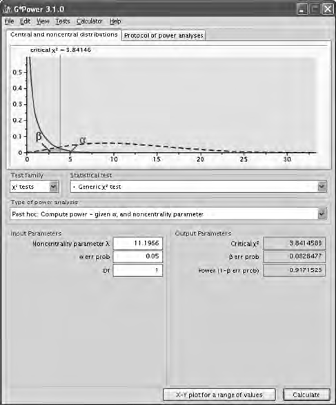
Model Fit 109
our example, the effect size (d) would be computed as:
d = (dfInitial * RMSEA2Initial – dfModied * RMSEA2Modied)
d = ([8 * (.080937)2] – [7 * (.046420)2])
d = (.0524056 − .0150836)
d = .037322
The noncentrality parameter is computed as:
NCP = (N – 1) d
So, for our example:
NCP = (301 – 1) * ( .037322)
NCP = 11.1966
Using G*Power 3, we enter this NCP = 11.1966, .05 level of signicance, and
df = 1 (model degree of freedom difference) and obtained power = .917. The
G*Power 3 dialog box should look like this:
Y102005.indb 109 3/22/10 3:25:44 PM
110 A Beginner’s Guide to Structural Equation Modeling
Power to detect a difference in RMSEA values is therefore possible for
a given sample size with various degrees of freedom. The SAS program
below will also provide an ability to make power comparisons for dif-
ferent model degrees of freedom using RMSEA values from two nested
models.
SAS syntax—effect size, RMSEA, and power
data chapter5;
do obs = 1;
n = 301;
alpha = .05;
dfa = 8;
rmseaA = .080937;
dfb = 7;
rmseaB = .046420;
delta = (dfa*rmseaA*rmseaA) – (dfb*rmseaB*rmseaB);
ncp = (n – 1)*delta;
dfdiff = dfa – dfb;
chicrit = quantile(‘chisquare’,1 – alpha, dfdiff);
power = 1 – PROBCHI(chicrit, dfdiff,ncp);
output;
end;
Proc print;
var n dfa rmseaA dfb rmseaB delta ncp dfdiff chicrit power;
run;
The computer output should look like this:
Obs n dfa rmseaA dfb rmseaB
1 301 8 0.080937 7 0.04642
delta ncp dfdiff chicrit power
.037323 11.1968 1 3.84146 .91716
The power = .91716 indicates a 91% chance of detecting a difference
between the model RMSEA values.
Power is affected by the size of the model degrees of freedom (degrees
of freedom implies a certain degree of model complexity). The G*Power 3
program or the SAS program can be used for models where the difference
in degrees of freedom is greater than one. We therefore ran a comparison
for our model with different levels of degrees of freedom to show how
power is affected. In Table 5.6, power increases dramatically when the
level of degrees of freedom increases from 5 to 14 while maintaining a
model degrees of freedom difference at df = 1. You can also output pro-
gram values for df ≥ 2 to see effect on power.
Y102005.indb 110 3/22/10 3:25:44 PM

Model Fit 111
5.6.3 Parameter Significance
A single parameter can be tested for signicance using nested models.
Nested models involve an initial model being compared to a modied model
in which a single parameter has been xed to zero (dropped) or estimated
(added). In structural equation modeling, the intent is to determine the
signicance of the decrease in the c2 value for the modied model from
the initial model. The LR test was used before to test the difference in the
models for our single parameter that we added (error covariance between
lozenges and cubes).
Power can be computed for testing the signicance of an individual
parameter estimate. For GLS, ML, and WLS estimation methods, this
involves determining the signicance of c2 with one degree of freedom
(c2 > 3.84, df = 1, a = .05) for a single parameter estimate, thus determin-
ing the signicance of the reduction in c2 that should equal or exceed the
modication index value for the parameter estimate xed to zero. Power
values for modication index values can be computed using SAS because
the modication index (MI) is a noncentrality parameter (NCP). The
power of a MI value (NCP) at the .05 level of signicance, df = 1, critical
chi-square value = 3.841 is computed in the following SAS syntax pro-
gram for our MI = 10.4 when adding the error covariance between lozenges
and cubes. Power = .89, so in testing the statistical signicance of MI for our
parameter (error covariance), we have an 89% chance of correctly reject-
ing the null hypothesis and accepting the alternative hypothesis that MI
is different from zero.
SAS syntax—power for parameter MI value
data chapter5;
do obs = 1;
mi = 10.4;
alpha = .05;
TABLE 5.6
MacCallum et al. (2006) Power
at Increasing Model Degrees of
Freedom
dfa dfb Power
5 4 .76756
8 7 .91716*
11 10 .97337
14 13 .99206
(RMSEA approach)
Figure 5.1b Model (a = .05, N = 301).
Y102005.indb 111 3/22/10 3:25:44 PM
112 A Beginner’s Guide to Structural Equation Modeling
df = 1;
chicrit = quantile(‘chisquare’,1 – alpha, df);
power = 1 – PROBCHI(chicrit, df, mi);
output;
end;
Proc print;
var mi power alpha df chicrit;
run;
The SAS output indicated the following:
Obs mi power alpha df chicrit
1 10.4 .89075 .05 1 3.84146
Power values for parameter estimates can also be computed using a
SAS program because a squared T or Z value for a parameter estimate is
asymptotically distributed as a noncentral chi-square, that is, NCP = T2.
Our modied model indicated an error covariance = 8.34 (modication
index indicated a New Estimate at 8.59), with standard error = 2.62, so
T = 8.34/2.62 = 3.19; LISREL program output provided these values for
the added parameter:
Error Covariance for lozenges and cubes = 8.34
(2.62)
3.19
(NOTE: LISREL 8.8 student version lists standared error, Z value, and
p-value in the output)
The power of a squared T value for our parameter estimate is computed in
a SAS program as follows:
SAS syntax—power for parameter T value
data chapter5;
do obs = 1;
T = 3.19;
ncp = T*T;
alpha = .05;
df = 1;
chicrit = quantile(‘chisquare’,1 – alpha, df);
power = 1 – PROBCHI(chicrit, df, ncp);
output;
end;
Proc print;
var ncp power alpha df chicrit;
run;
Y102005.indb 112 3/22/10 3:25:44 PM
Model Fit 113
The SAS output looks like this:
Obs ncp power alpha df chicrit
1 10.1761 .89066 .05 1 3.84146
Power = .89, so in testing the statistical signicance of our parameter esti-
mate, we have an 89% chance of correctly rejecting the null hypothesis and
accepting the alternative hypothesis that T is different from zero. (Note: The
other model-t indices [GFI, AGFI, NFI, IFI, CFI, etc.] do not have a test of
statistical signicance and therefore do not involve power calculations).
5.6.4 Summary
Research suggests that certain model-t indices are more susceptible to
sample size than others, hence, power. We have already learned that c2 is
affected by sample size, that is, c2 = (N − 1) FML , where FML is the maximum
likelihood t function for a model, and therefore c2 increases in direct rela-
tion to N − 1 (Bollen, 1989). Kaplan (1995) also pointed out that power in
SEM is affected by the size of the misspecied parameter, sample size, and
location of the parameter in the model. Specication errors induce bias
in the standard errors and parameter estimates, and thus affect power.
These factors also affect power in other parametric statistical tests (Cohen,
1988). Saris and Satorra (1993) pointed out that the larger the noncentrality
parameter, the greater is the power of the test, that is, an evaluation of the
power of the test is an evaluation of the noncentrality parameter.
Muthén and Muthén (2002) outlined how Monte Carlo methods can be
used to decide on the power for a given specied model using the Mplus
program. Power is indicated as the percentage of signicant coefcients or
the proportion of replications for which the null hypothesis that a param-
eter is equal to zero is rejected at the .05 level of signicance, two-tailed
test, with a critical value of 1.96. The authors suggested that power equal
or exceed the traditional .80 level for determining the probability of reject-
ing the null hypothesis when it is false.
Marsh et al. (1988, 1996) also examined the inuence of sample size on 30
different model-t indices and found that the Tucker–Lewis index (Tucker
& Lewis, 1973) and four new indices based on the Tucker–Lewis index
were the only ones relatively independent of sample size. Bollen (1990)
argued that the claims regarding which model-t indices were affected
by sample size needed further clarication. There are actually two sample
size effects that are confounded: (a) whether sample size enters into the
calculation of the model-t index, and (b) whether the means of the sam-
pling distribution of the model-t index are related to sample size. Sample
size was shown not to affect the calculation of NFI, TLI, GFI, AGFI, and
CN, but the means of the sampling distribution of these model-t indices
Y102005.indb 113 3/22/10 3:25:45 PM

114 A Beginner’s Guide to Structural Equation Modeling
were related to sample size. Bollen (1990) concluded that, given a lack of
consensus on the best measure of t, it is prudent to report multiple mea-
sures rather than to rely on a single choice; we concur.
Muthén and Muthén (2002) also used Mplus to determine appropriate
sample sizes in the presence of model complexity, distribution of vari-
ables, missing data, reliability, and variance–covariance of variables. For
example, given a two-factor CFA model and 10 indicator variables with
normally distributed nonmissing data, a sample size of 150 is indicated
with power = .81. In the presence of missing data, sample size increases to
n = 175. Given nonnormal missing data, sample size increases to n = 315.
Davey & Savla (2009) provide an excellent treatment of statistical power
analysis with missing data via a structural equation modeling approach.
Their examples cover many different types of modeling situations using
SAS, STATA, SPSS, or LISREL syntax programs. This is a must-read book
on the subject of power and sample size, especially in the presence of
missing data.
Finally, one should beware of claims of sample size inuence on t
measures that do not distinguish the type of sample size effect (Satorra &
Bentler, 1994). Cudeck and Henly (1991) also argued that a uniformly neg-
ative view of the effects of sample size in model selection is unwarranted.
They focused instead on the predictive validity of models in the sense of
cross-validation in future samples while acknowledging that sample size
issues are a problem in the eld of statistics in general and unavoidable in
structural equation modeling.
5.7 Two-Step Versus Four-Step Approach to Modeling
Anderson and Gerbing (1988) proposed a two-step model-building
approach that emphasized the analysis of two conceptually distinct mod-
els: a measurement model followed by the structural model (Lomax, 1982).
The measurement model, or factor model, species the relationships among
measured (observed) variables underlying the latent variables. The struc-
tural model species relationships among the latent variables as posited
by theory. The measurement model provides an assessment of convergent
and discriminant validity, and the structural model provides an assess-
ment of nomological validity.
Mulaik et al. (1989) expanded the idea of model t by assessing the rela-
tive t of the structural model among latent variables, independently of
assessing the t of the indicator variables in the measurement model. The
relative normed t index (RNFI) makes the following adjustment to sepa-
rately estimate the effects of the structural model from the measurement
Y102005.indb 114 3/22/10 3:25:45 PM
Model Fit 115
model: RNFIj = (Fu − Fj)/[Fu − Fm − (dfj − dfm)], where Fu = c2 of the full model,
Fj = c2 of the structural model, Fm = c2 of the measurement model, dfj is
the degrees of freedom for the structural model, and dfm is the degrees
of freedom for the measurement model. A corresponding relative parsi-
mony ratio (RP) is given by RPj = (dfj − dfm)/(dfu − dfm), where dfj is the
degrees of freedom for the structural model, dfm is the degrees of freedom
for the measurement model, and dfu is the degrees of freedom for the null
model. In comparing different models for t, Mulaik et al. multiplied RPj
by RNFIj to obtain a relative parsimony t index appropriate for assess-
ing how well and to what degree the models explained both relationships
in the measurement of latent variables and the structural relationships
among the latent variables by themselves. McDonald and Marsh (1990),
however, doubted whether model parsimony and goodness of t could be
captured by this multiplicative form because it is not a monotonic increas-
ing function of model complexity. Obviously, further research will be
needed to clarify these issues.
Mulaik and Millsap (2000) also presented a four-step approach to test-
ing a nested sequence of SEM models:
Step 1 pertains to specifying an unrestricted measurement •
model, namely conducting an exploratory common factor analy-
sis to determine the number of factors (latent variables) that t the
variance–covariance matrix of the observed variables.
Step 2 involves a conrmatory factor analysis model that tests •
hypotheses about certain relations among indicator variables and
latent variables. Basically, certain factor loadings are xed to zero
in an attempt to have only a single nonzero factor loading for each
indicator variable of a latent variable. Sometimes this leads to a
lack of measurement model t because an indicator variable may
have a relation with another latent variable.
Step 3 involves specifying relations among the latent variables in a •
structural model. Certain relations among the latent variables are xed
to zero so that some latent variables are not related to one another.
Step 4 continues if an acceptable t of the structural model is •
achieved, that is, CFI > .95 and RMSEA < .05. In Step 4, a researcher
tests planned hypotheses about free parameters in the model.
Several approaches are possible: (a) perform simultaneous tests
in which free parameters are xed based on theory or estimates
obtained from other research studies; (b) impose xed parameter
values on freed parameters in a nested sequence of models until
a misspecied model is achieved (misspecied parameter); or (c)
perform a sequence of condence-interva l tests around free param-
eters using the standard errors of the estimated parameters.
Y102005.indb 115 3/22/10 3:25:45 PM

116 A Beginner’s Guide to Structural Equation Modeling
We agree with the basic Mulaik and Millsap (2000) approach and recom-
mend that the measurement models for latent variables be established
rst and then structural models establishing relationships among the
latent independent and dependent variables be formed. It is in the formu-
lation of measurement models that most of the model modications occur
to obtain acceptable data to model t. In fact, a researcher could begin
model generation by using exploratory factor analysis (EFA) on a sam-
ple of data to nd the number and type of latent variables in a plausible
model (Costello & Osborne, 2005). Once a plausible model is determined,
another sample of data could be used to conrm or test the factor model,
that is, conrmatory factor analysis (CFA) (Jöreskog, 1969). Exploratory
factor analysis is even recommended as a precursor to conrmatory fac-
tor analysis when the researcher does not have a substantive theoretical
model (Gerbing & Hamilton, 1996).
Measurement invariance is also important to examine, which refers
to considering similar measurement models across different groups; for
example, does the factor (latent variable) imply the same thing to boys
and girls? This usually involves adding between group constraints in the
measurement model. If measurement invariance cannot be established,
then the nding of a between group difference is questionable (Cheung
& Rensvold, 2002). Cheung and Rensvold (2002) also recommend that the
comparative t index (CFI), gamma hat, and McDonald’s noncentrality
index (NCI) be used for testing between group measurement invariance
of CFA models rather than the goodness-of-t index (GFI) or the likeli-
hood ratio test (LR), also known as the chi-square difference test. Byrne
and Watkins (2003) questioned whether measurement invariance could
be established given that individual items on an instrument could exhibit
invariance or group differences. Later, Byrne and Sunita (2006) provided a
step-by-step approach for examining measurement invariance.
5 . 8 S u m m a r y
In this chapter, we began by discussing three approaches a researcher
could take in structural equation modeling: conrmatory models, alter-
native models, and model generation. We then considered categories of
model-t indices—namely, model-t, model comparison, and model
parsimony. In addition, current and new innovative approaches to spec-
ication searches were mentioned for the assessment of model t in struc-
tural equation modeling. We examined in detail the different categories
of model-t criteria because different t indices have been developed
depending on the type of specied model tested. Generally, no single
Y102005.indb 116 3/22/10 3:25:45 PM

Model Fit 117
model-t index is sufcient for testing a hypothesized structural model.
An ideal t index just does not exist. This is not surprising because it has
been suggested that an ideal t index is one that is independent of sample
size, accurately reects differences in t, imposes a penalty for inclusion
of additional parameters (Marsh et al., 1988), and supports the choice of
a true model when it is known (McDonald & Marsh, 1990). The current
model tting practice in LISREL involves the use of modication indices
and/or expected parameter change values, but other advances in speci-
cation search techniques have been investigated (Tabu and optimization
algorithms), with a specication search approach already in AMOS (SPSS,
2009).
A two-factor conrmatory model was analyzed using the LISREL com-
puter program with model-t output to enhance our understanding of
the many different model-t criteria. We concluded in this chapter with
a discussion of a four-step approach to SEM modeling, the signicance
of parameters in a model, power, and sample size. An understanding of
model-t criteria, power, and sample size will help your understanding of
the examples presented in the remaining chapters of the book.
Exercises
1. Dene conrmatory models, alternative models, and model-
generating approaches.
2. Dene model t, model comparison, and model parsimony.
3. Calculate the following t indices for the model output in
Figure 5.1:
GFI = 1 – (c2model/c2null)
NFI = (c2null − c2model)/c2null
RFI = 1 – [(c2model/dfmodel)/(c2null/dfnull)]
IFI = (c2null − c2model)/(c2null − dfmodel)
TLI = [(c2null/dfnull) − (c2model/dfmodel)]/[(c2null/dfnull) − 1]
CFI = 1 – [(c2model − dfmodel)/(c2null − dfnull)]
Model AIC = c2model + 2q (q is the number of free parameters)
Null AIC = c2 null + 2q (q is the number of free parameters)
RMSEAdfNdf=− −[][( )]
χ
ModelModel Model
/
21
or
RMSEANCP Ndf=−()//1
4. How are modication indices in LISREL--SIMPLIS used?
5. What steps should a researcher take in examining parameter
estimates in a model?
6. How should a researcher test for the difference between two
alternative models?
Y102005.indb 117 3/22/10 3:25:46 PM

118 A Beginner’s Guide to Structural Equation Modeling
7. How are structural equation models affected by sample size
and power considerations?
8. Describe the four-step approach for modeling in SEM.
9. What new approaches are available to help a researcher iden-
tify the best model?
10. Use G*Power 3 to calculate power for modied model with
NCP = 6.3496 at p = .05, p = .01, and p = .001 levels of signicance.
What happens to power when alpha increases?
11. Use G*Power 3 to calculate power for modied model with
alpha = .05 and NCP = 6.3496 at df = 1, df = 2, and df = 3 levels
of model complexity. What happens to power when degrees of
freedom increases?
Chapter Footnote
LISREL computes two different sets of standard errors for parameter esti-
mates and up to four different chi-squares for testing overall t of the
model. These new standard errors and chi-squares can be obtained for
single-group problems as well as multiple-group problems using variance–
covariance matrices with or without means.
Which standard errors and which chi-squares will be reported
depends on whether an asymptotic covariance matrix is provided and
which method of estimation is used to t the model (ULS, GLS, ML,
WLS, DWLS). The asymptotic covariance matrix is a consistent esti-
mate of N times the asymptotic covariance matrix of the sample matrix
being analyzed.
Standard Errors
Standard errors are estimated under nonnormality if an asymptotic cova-
riance matrix is used. Standard errors are estimated under multivariate
normality if no asymptotic covariance matrix is used.
Chi-Squares
Four different chi-squares are reported and denoted below as C1, C2, C3,
and C4, where the x indicates that it is reported for any of the ve estima-
tion methods.
Y102005.indb 118 3/22/10 3:25:46 PM
Model Fit 119
Asymptotic covariance matrix not provided:
ULS GLS ML WLS DWLS
C1 — × × — —
C2 ×××— —
C3 — — — — —
C4 — — — — —
Asymptotic covariance matrix provided:
ULS GLS ML WLS DWLS
C1 — ××× —
C2 ×××—×
C3 ×××—×
C4 ×××—×
NOTE: 1. C1 is n − 1 times the minimum value of the t function; C2 is
n − 1 times the minimum of the WLS t function using a weight matrix
estimated under multivariate normality; C3 is the Satorra–Bentler scaled
chi-square statistic or its generalization to mean and covariance struc-
tures and multiple groups (Satorra & Bentler, 1994); C4 is computed from
equations in Browne (1984) or Satorra (1993) using the asymptotic covari-
ance matrix.
The corresponding chi-squares are now given in the output as follows:
C1: Minimum t function chi-square
C2: Normal theory weighted least squares chi-square
C3: Satorra-Bentler scaled chi-square
C4: Chi-square corrected for nonnormality
NOTE 2: Under multivariate normality of the observed variables, C1 and
C2 are asymptotically equivalent and have an asymptotic chi-square
distribution if the model holds exactly and an asymptotic noncentral
chi-square distribution if the model holds approximately. Under nor-
mality and nonnormality, C2 and C4 are correct asymptotic chi-squares,
but may not be the best chi-square in small and moderate samples. Hu,
Bentler, and Kano (1992) and Yuan and Bentler (1997) found that C3 per-
formed better given different types of models, sample size, and degrees
of nonnormality.
Y102005.indb 119 3/22/10 3:25:46 PM

120 A Beginner’s Guide to Structural Equation Modeling
References
Akaike, H. (1987). Factor analysis and AIC. Psychometrika, 52, 317–332.
Anderson, J. C., & Gerbing, D. W. (1984). The effects of sampling error on conver-
gence, improper solutions and goodness-of-t indices for maximum likeli-
hood conrmatory factor analysis. Psychometrika, 49, 155–173.
Anderson, J. C., & Gerbing, D. W. (1988). Structural equation modeling in practice:
A review and recommended two-step approach. Psychological Bulletin, 103,
411–423.
Baldwin, B. (1989). A primer in the use and interpretation of structural equa-
tion models. Measurement and Evaluation in Counseling and Development, 22,
100–112.
Bentler, P. M. (1990). Comparative t indexes in structural models. Psychological
Bulletin, 107, 238–246.
Bentler, P. M., & Bonett, D. G. (1980). Signicance tests and goodness-of-t in the
analysis of covariance structures. Psychological Bulletin, 88, 588–606.
Bollen, K. A. (1989). Structural equations with latent variables. New York: Wiley.
Bollen, K. A. (1990). Overall t in covariance structure models: Two types of sam-
ple size effects. Psychological Bulletin, 107, 256–259.
Bollen, K. A., & Liang, J. (1988). Some properties of Hoelter’s CN. Sociological
Methods and Research, 16, 492–503.
Bollen, K. A., & Long, S. J. (1993). Testing structural equation models. Newbury Park,
CA: Sage.
Browne, M. W. (1984). Asymptotically distribution-free methods for the analysis of
covariance structures. British Journal of Mathematical and Statistical Psychology,
37, 62–83.
Browne, M. W., & Cudeck, R. (1993). Alternative ways of assessing model t. In K.
A. Bollen & J. S. Long (Eds.), Testing structural equation models (pp. 132–162).
Beverly Hills, CA: Sage.
Byrne, B. M., & Watkins, D. (2003). The issue of measurement invariance revisited.
Journal of Cross-Cultural Psychology, 34(2), 155–175.
Byrne, B., & Sunita, M. S. (2006). The MACS approach to testing for multigroup
invariance of a second-order structure-A walk through the process. Structural
Equation Modeling: A Multidisciplinary Journal, 13(2), 287–321.
Cheung, G. W., & Rensvold, R. B. (2002). Evaluating goodness-of-t indexes for
testing measurement invariance. Structural Equation Modeling, 9, 233–255.
Cliff, N. (1983). Some cautions concerning the application of causal modeling
methods. Multivariate Behavioral Research, 18, 115–126.
Cohen, J. (1988). Statistical power analysis for the behavioral sciences (2nd ed.).
Hillsdale, NJ: Lawrence Erlbaum.
Costello, A. B., & Osborne, J. (2005). Best practices in exploratory factor analy-
sis: Four recommendations for getting the most from your analysis. Practical
Assessment Research & Evaluation, 10(7), 1–9.
Cudeck, R., & Henly, S. J. (1991). Model selection in covariance structure analysis
and the “problem” of sample size: A clarication. Psychological Bulletin, 109,
512–519.
Y102005.indb 120 3/22/10 3:25:46 PM
Model Fit 121
Davey, A., & Savla, J. (2010). Statistical Power analysis with missing data: A structural
equation modeling approach. Routledge: Taylor & Francis, New York.
Faul, F., Erdfelder, E., Lang, A.-G., & Buchner, A. (2007). G*Power 3: A exible
statistical power analysis program for the social, behavioral, and biomedical
sciences. Behavior Research Methods, 39, 175–191.
Gerbing, D. W., & Hamilton, J. G. (1996). Viability of exploratory factor analysis
as a precursor to conrmatory factor analysis, Structural Equation Modeling,
3(1), 62–72.
Gonzalez, R., & Grifn, D. (2001). Testing parameters in structural equation mod-
eling: Every “one” matters. Psychological Methods, 6(3), 258–269.
Gorsuch, R. L. (1983). Factor analysis (2nd ed.). Hillsdale, NJ: Lawrence Erlbaum.
Hair, J. F., Jr., Anderson, R. E., Tatham, R. L., & Black, W. C. (1992). Multivariate data
analysis with readings (3rd ed.). New York: Macmillan.
Harmon, H. H. (1976). Modern factor analysis (3rd ed.). Chicago, IL: University of
Chicago Press.
Hoelter, J. W. (1983). The analysis of covariance structures: Goodness-of-t indices.
Sociological Methods and Research, 11, 325–344.
Holzinger, K. J., & Swineford, F. A. (1939). A study in factor analysis: The stability of a
bi-factor solution. Supplementary Educational Monographs, No. 48. Chicago:
University of Chicago, Dept. of Education.
Hu, L., & Bentler, P. M. (1995). Evaluating model t. In R. H. Hoyle (Ed.), Structural
equation modeling: Concepts, issues, and applications (pp. 76–99). Thousand
Oaks, CA: Sage.
Hu, L., Bentler, P. M., & Kano, Y. (1992). Can test statistics in covariance structure
analysis be trusted? Psychological Bulletin, 112, 351–362.
James, L. R., Mulaik, S. A., & Brett, J. M. (1982). Causal analysis: Assumptions, models,
and data. Beverly Hills, CA: Sage.
Jöreskog, K. G. (1969). A general approach to conrmatory maximum likelihood
factor analysis. Psychometrika, 34, 183–202.
Jöreskog, K. G., & Sörbom, D. (1993). LISREL 8: Structural equation modeling with the
SIMPLIS command language. Hillsdale, NJ: Lawrence Erlbaum.
Kaplan, D. (1995). Statistical power in structural equation modeling. In R. H.
Hoyle (Ed.), Structural equation modeling: Concepts, issues, and applications (pp.
100–117). Thousand Oaks, CA: Sage.
Kenny, D. A., & McCoach, D. B. (2003). Effect of the number of variables on mea-
sures of t in structural equation modeling. Structural Equation Modeling, 10,
333–351.
Loehlin, J. C. (1987). Latent variable models: An introduction to factor, path, and struc-
tural analysis. Hillsdale, NJ: Lawrence Erlbaum.
Lomax, R. G. (1982). A guide to LISREL-type structural equation modeling. Behavior
Research Methods and Instrumentation, 14, 1–8.
Lunneborg, C. E. (1987). Bootstrap applications for the behavioral sciences. Vol. 1.
Seattle: University of Washington, Psychology Department.
MacCallum, R. C., Browne, M. W., & Sugawara, H. M. (1996). Power analysis and
determination of sample size for covariance structure modeling. Psychological
Methods, 1, 130–149.
Y102005.indb 121 3/22/10 3:25:46 PM
122 A Beginner’s Guide to Structural Equation Modeling
MacCallum, R. C., Browne, M. W., & Cai, L. (2006). Testing differences between
nested covariance structure models: Power analysis and null hypotheses.
Psychological Methods, 11, 19–35.
Marcoulides, G. A., & Drezner, Z. (2001). Specication searches in structural
equation modeling with a genetic algorithm. In G. A. Marcoulides & R. E.
Schumacker (Eds.), New developments and techniques in structural equation mod-
eling (pp. 247–268). Mahwah, NJ: Lawrence Erlbaum.
Marcoulides, G. A., & Drezner, Z. (2003). Model specication searches using ant
colony optimization algorithms. Structural Equation Modeling, 10, 154–164.
Marcoulides, G. A., Drezner, Z., & Schumacker, R. E. (1998). Model specica-
tion searches in structural equation modeling using Tabu search. Structural
Equation Modeling, 5, 365–376.
Marsh, H. W., Balla, J. R., & Hau, K.-T. (1996). An evaluation of incremental t
indices: A clarication of mathematical and empirical properties. In G. A.
Marcoulides & R. E. Schumacker (Eds.), Advanced structural equation model-
ing: Issues and techniques (pp. 315–353). Mahwah, NJ: Lawrence Erlbaum.
Marsh, H. W., Balla, J. R., & McDonald, R. P. (1988). Goodness-of-t indexes in
conrmatory factor analysis: The effect of sample size. Psychological Bulletin,
103, 391–410.
McDonald, R. P. (1989). An index of goodness-of-t based on noncentrality. Journal
of Classication, 6, 97–103.
McDonald, R. P., & Marsh, H. W. (1990). Choosing a multivariate model:
Noncentrality and goodness of t. Psychological Bulletin, 107, 247–255.
Mulaik, S. A., James, L. R., Alstine, J. V., Bennett, N., Lind, S., & Stilwell, C. D.
(1989). Evaluation of goodness-of-t indices for structural equation models.
Psychological Bulletin, 105, 430–445.
Mulaik, S. A., & Millsap, R. E. (2000). Doing the four-step right. Structural Equation
Modeling, 7, 36–73.
Muthén, B., & Muthén, L. (2002). How to use a Monte Carlo study to decide on
sample size and determine power. Structural Equation Modeling, 9, 599–620.
Saris, W. E., & Satorra, A. (1993). Power evaluation in structural equation mod-
els. In K. Bollen & J. S. Long (Eds.), Testing structural equation models (pp.
181–204). Newbury Park, CA: Sage.
Satorra, A. (1993). Multi-sample analysis of moment structures: Asymptotic
validity of inferences based on second-order moments. In K. Haagen, D. J.
Bartholomew, & M. Deistler (Eds.), Statistical modeling and latent variables (pp.
283–298). Amsterdam: Elsevier.
Satorra, A., & Bentler, P. M. (1994). Corrections for test statistics and standard
errors in covariance structure analysis. In A. Von Eye & C. C. Clogg (Eds.),
Latent variable analysis: Applications for developmental research (pp. 399–419).
Thousand Oaks, CA: Sage.
Soper, D., Statistics Calculators. Retrieved January 2010 from http://www.dan-
ielsoper.com/statcalc/.
SPSS (2009). Statistics 17.0. SPSS, Inc.: Chicago, IL.
Steiger, J. H. (1990). Structural model evaluation and modication: An interval
estimation approach. Multivariate Behavioral Research, 25, 173–180.
Y102005.indb 122 3/22/10 3:25:46 PM
Model Fit 123
Steiger, J. H., & Lind, J. M. (1980, May). Statistically-based tests for the number of com-
mon factors. Paper presented at Psychometric Society Meeting, Iowa City, IA.
Tucker, L. R., & Lewis, C. (1973). The reliability coefcient for maximum likelihood
factor analysis. Psychometrika, 38, 1–10.
Williams, L. J., & Holahan, P. J. (1994). Parsimony-based t indices of multiple indi-
cator models: Do they work? Structural Equation Modeling: A Multidisciplinary
Journal, 1, 161–189.
Yuan, K.-H., & Bentler, P. M. (1997). Mean and covariance structure analysis:
Theoretical and practical improvements. Journal of the American Statistical
Association, 92, 767–774.
Y102005.indb 123 3/22/10 3:25:46 PM

125
6
Regression Models
Key Concepts
Explanation versus prediction
Standardized partial regression coefcients
Coefcient of determination
Squared multiple correlation coefcient
Full versus restricted models
Condence intervals around R2
Measurement error
Additive versus relational model
In this chapter, we consider multiple regression models as a method for
modeling multiple observed variables. Multiple regression, a general lin-
ear modeling approach to the analysis of data, has become increasingly
popular since 1967 (Bashaw & Findley, 1968). In fact, it has become recog-
nized as an approach that bridges the gap between correlation and analysis
of variance in answering research hypotheses (McNeil, Kelly, & McNeil,
1975). Many statistical textbooks elaborate the relationship between mul-
tiple regression and analysis of variance (Draper & Smith, 1966; Edwards,
1979; Hinkle, Wiersma, & Jurs, 2003; Lomax, 2007).
Graduate students who take an advanced statistics course are typically
provided with the multiple linear regression framework for data analysis.
Given knowledge of multiple linear regression techniques (one dependent
variable), understanding can be extended to various multivariable statisti-
cal techniques (Newman, 1988). A basic knowledge of multiple regression
concepts is therefore important in further understanding path analysis as
presented in Chapter 7. This chapter shows how beta weights (standard-
ized partial regression coefcients) are computed in multiple regression
using a structural equation modeling software program. More specically,
we illustrate how the structural equation modeling approach can be used
Y102005.indb 125 3/22/10 3:25:47 PM

126 A Beginner’s Guide to Structural Equation Modeling
to compute parameter estimates in multiple regression and what model-t
criteria are reported. We begin with a brief overview of multiple regression
concepts followed by an example that illustrates model specication, model
identication, model estimation, model testing, and model modication.
6.1 Overview
Multiple regression techniques require a basic understanding of sample
statistics (sample size, mean, and variance), standardized variables, cor-
relation (Pedhazur, 1982), and partial correlation (Cohen & Cohen, 1983;
Houston & Bolding, 1974). In standard score form (z scores), the simple
linear regression equation for predicting the dependent variable Y from a
single independent variable X is
yx
z=z
ˆ,
β
where b is the standardized regression coefcient. The basic rationale for
using the standard-score formula is that variables are converted to the
same scale of measurement, the z scale. Conversion back to the raw-score
scale is easily accomplished by using the raw score, the mean and the stan-
dard deviation.
The relationship connecting the Pearson product-moment correlation
coefcient, the unstandardized regression coefcient b and the standard-
ized regression coefcient b is
β
=zz
z=bs
s=r,
xy
x
2
x
y
xy
∑
∑
where sx and sy are the sample standard deviations for variables X and Y,
respectively. For two independent variables, the multiple linear regression
equation with standard scores is
y1
22
z=z+z
ˆ
ββ
1
and the standardized partial regression coefcients b1 and b2 are com-
puted from
1
yy12
12
22
yy12
12
2
=rrr
1r=rrr
1r
ββ
12 21
−
−
−
−
and.
The correlation between the dependent observed variable Y and the pre-
dicted scores
ˆ
Y
is given the special name multiple correlation coefcient. It is
Y102005.indb 126 3/22/10 3:25:48 PM

Regression Models 127
written as
yy y.12
R=R
ˆ,
where the latter subscripts indicate that the dependent variable Y is being
predicted by two independent variables, X1 and X2. The squared multiple
correlation coefcient is computed as
yy
2y.12
2
1Y2Y
R=R=r r
ˆ.
ββ
++
12
The squared multiple correlation coefcient indicates the amount of vari-
ance explained, predicted, or accounted for in the dependent variable by
the set of independent predictor variables. The R2 value is used as a model-
t criterion in multiple regression analysis.
Kerlinger and Pedhazur (1973) indicated that multiple regression analy-
sis can play an important role in prediction and explanation. Prediction
and explanation reect different research questions, study designs, infer-
ential approaches, analysis strategies, and reported information. In predic-
tion, the main emphasis is on practical application such that independent
variables are chosen by their effectiveness in enhancing prediction of the
dependent variable. In explanation, the main emphasis is on the variabil-
ity in the dependent variable explained by a theoretically meaningful set
of independent variables. Huberty (2003) established a clear distinction
between prediction and explanation when referring to multiple correla-
tion analysis (MCA) and multiple regression analysis (MRA). In MCA, a
parameter of interest is the correlation between the dependent variable Y
and a composite of the independent variables Xp. The adjusted formula
using sample size n and the number of independent predictors p is
RR p
np R
Adj
22 2
11=−
−− −().
In MRA, regression weights are also estimated to achieve a composite for
the independent variables Xp, but the index of t R2 is computed differ-
ently as
RR p
np R
Adj*().
22 2
21=−
−−
When comparing these two formulas, we see that R2
Adj* has a larger adjust-
ment. For example, given R2 = .50, p = 10 predictor variables and n = 100
subjects, these two different t indices are
RR p
np R
Adj
22 2
1150115050 055=−
−− −=−=−()..(. ). .== .45
Y102005.indb 127 3/22/10 3:25:49 PM

128 A Beginner’s Guide to Structural Equation Modeling
RR p
np R
Adj*()..(. ). .
22 2
215022505011=−
−−=−=−=.. .39
Hypothesis testing would involve using the expected value or chance value
of R2 for testing the null hypothesis, which is p/(n − 1), not 0 as typically
indicated. In our example, the expected or chance value for R2 = 10/99 = .10,
so the null hypothesis is H0: r2 = .10. An F test used to test the statistical
signicance of the R2 value is
FRp
Rnp
=−−−
2
2
11
/
/() .
In our example,
FRp
Rnp
=−−−=−=
2
2
11
50 10
15089
05
005
/
/
/
/()
.
(.)
.
. 66 89=.,
which is statistically signicant when compared to the tabled F = 1.93, df =
10,89, p < .05 (Table A.5). In addition to the statistical signicance test, a
researcher should calculate effect sizes and condence intervals to aid under-
standing and interpretation (Soper, 2010).
The effect size (ES) is computed as ES = R2 – [p/(n − 1)]. In our example, ES
R2
Adj = .45 − .10 = .35 and ES R2
Adj* = .39 − .10 = .29. This indicates a moderate
to large effect size according to Cohen (1988), who gave a general reference
for effect sizes (small = .1, medium = .25, and large = .4).
Condence intervals (CIs) around the R2 value can also help our interpre-
tation of multiple regression analysis. Steiger and Fouladi (1992) reported
an R2 CI DOS program that computes condence intervals, power, and
sample size. Steiger and Fouladi (1997) and Cumming and Finch (2001)
both discussed the importance of converting the central F value to an esti-
mate of the noncentral F before computing a condence interval around
R2. Smithson (2001) wrote an R2 SPSS program to compute condence
intervals.
We use the Steiger and Fouladi (1997) R2 CI DOS program with our hypo-
thetical example. After entering the program, Option is selected from the
tool bar menu and then Condence Interval is selected from the drop-
down menu. To obtain R2 CI, the number of subjects (n = 100), the number
of variables (K = 10), the R2 value (R = .35), and the desired condence level
(C = .95) are entered by using the arrow keys (mouse not supported), and
then GO is selected to compute the values. The 95% condence interval
around R2 = .35 is .133 to .449 at the p = .0001 level of signicance for a null
hypothesis that R2 = 0 in the population.
Y102005.indb 128 3/22/10 3:25:50 PM

Regression Models 129
After assessing our initial regression model t, we might want to
determine whether adding or deleting an independent variable would
improve the index of t R2, but we avoid using stepwise regression meth-
ods (Huberty, 1989). We run a second multiple regression equation where
a single independent variable is added or deleted to obtain a second R2
value. We then compute a different F test to determine the statistical sig-
nicance between the two regression models as follows
FRR pp
Rnp
FR
F
=−−
−−−
()()
() ,
2212
21
11
/
/
where R2F is from the multiple regression equation with the full original
set of independent variables p1 and R2
R is from the multiple regression
equation with the reduced set of independent variables p2. In our heuristic
example, we drop a single independent variable and obtain R2
R = .49 with
p2 = 9 predictor variables. The F test is computed as:
FRR pp
Rnp
FR
F
=−−
−−−=−
()()
()
(. .)
2212
21
11
50 49
/
/
//
/
()
(.)
.
...
10 9
150 100 10 1
01
0056 178
−
−−−==
The F value is not signicant at the .05 level, so the variable we dropped
does not statistically add to the prediction of Y, which supports our drop-
ping the single predictor variable; that is, a 1% decrease in R2 is not statisti-
cally signicant. The nine-variable regression model therefore provides a
more parsimonious model.
It is important to understand the basic concepts of multiple regres-
sion and correlation because they provide a better understanding of path
analysis in chapter 7, and structural equation modeling in general. An
example is presented next to further clarify these basic multiple regression
computations.
Y102005.indb 129 3/22/10 3:25:50 PM

130 A Beginner’s Guide to Structural Equation Modeling
6.2 An Example
A multiple linear regression analysis is conducted using data from
Chatterjee and Yilmaz (1992). The data le contains scores from 24 patients
on four variables (Var1 = patient’s age in years, Var2 = severity of illness,
Var3 = level of anxiety, and Var4 = satisfaction level). Given raw data, two
different approaches are possible in LISREL: (a) a system le in LISREL–
PRELIS using regression statistics from the pull-down menu or (b) a cor-
relation or covariance matrix input in the LISREL–SIMPLIS command
syntax le. We choose to compute and input a covariance matrix into a
LISREL–SIMPLIS program.
6.3 Model Specification
Model specication involves nding relevant theory and prior research
to formulate a theoretical regression model. The researcher is interested
in specifying a regression model that should be conrmed with sample
variance–covariance data, thus yielding a high R2 value and statisti-
cally signicant F value. Model specication directly involves deciding
which variables to include or not to include in the theoretical regression
model.
If the researcher does not select the right variables, then the regression
model could be misspecied and lack validity (Tracz, Brown, & Kopriva,
1991). The problem is that a misspecied model may result in biased
parameter estimates or estimates that are systematically different from
what they really are in the true population model. This bias is known as
specication error.
The researcher’s goal is to determine whether the theoretical regression
model ts the sample variance–covariance structure in the data, that is,
whether the sample variance–covariance matrix implies some underlying
theoretical regression model. The multiple regression model of theoretical
interest in our example is to predict the satisfaction level of patients based
on patient’s age, severity of illness, and level of anxiety (independent vari-
ables). This would be characteristic of a MCA model because a particular
set of variables were selected based on theory. The dependent variable
Var4 is therefore predicted by the three independent variables (Var1, Var2,
and Var3). The path diagram of the implied regression model is shown in
Figure 6.1.
Y102005.indb 130 3/22/10 3:25:50 PM
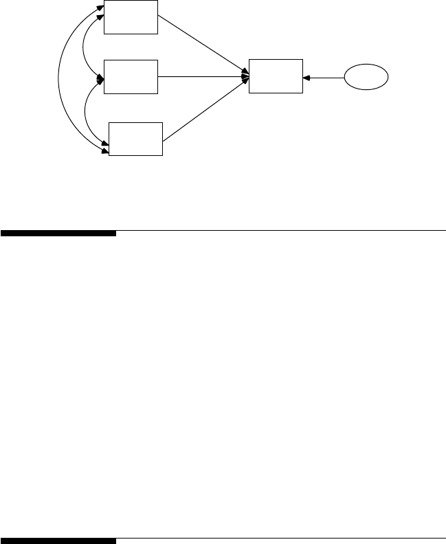
Regression Models 131
6.4 Model Identification
Once a theoretical regression model is specied, the next concern is model
identification. Model identification refers to deciding whether a set of
unique parameter estimates can be computed for the regression equation.
Algebraically, every free parameter in the multiple regression equation can
be estimated from the sample variance–covariance matrix (a free parameter
is an unknown parameter that you want to estimate). The number of dis-
tinct values in the sample variance–covariance matrix equals the number
of parameters to be estimated; thus, multiple regression models are always
considered just-identied (see chapter 4). SEM computer output will there-
fore indicate that regression analyses are saturated models; thus, c2 = 0 and
degrees of freedom = 0. There are 3 variances, 3 covariance terms, 3 regression
weights, and 1 error term so all parameters in the regression equation are
being estimated.
6.5 Model Estimation
Model estimation involves estimating the parameters in the regression model—
that is, computing the sample regression weights for the independent predic-
tor variables. The squared multiple correlation with three predictor variables
(VAR1, VAR2, VAR3) predicting the dependent variable Y (VAR4) is
y.123
2
1y2y3y
R=r+r+r
βββ
123.
var1
var2
var3
var4 error
FIGURE 6.1
Satisfaction regression model.
Y102005.indb 131 3/22/10 3:25:51 PM
132 A Beginner’s Guide to Structural Equation Modeling
The correlation coefcients are multiplied by their respective standard-
ized partial regression weights and summed to yield the squared multiple
regression coefcient R2
y . 1 2 3 .
In LISREL–SIMPLIS, we select File, New, and then Syntax Only in the
dialog box to write the following SIMPLIS program:
Regression Analysis Example (no intercept term)
Observed variables: VAR1 VAR2 VAR3 VAR4
Covariance matrix:
91.384
30.641 27.288
0.584 0.641 0.100
−122.616 −52.576 −2.399 281.210
Sample size: 24
Equation: VAR4 = VAR1 VAR2 VAR3
Number of decimals = 3
Path Diagram
End of Problem
You will be prompted to save the program with a le name (*.spl) before
the program runs.
The critical portion of the LISREL–SIMPLIS regression output without
an intercept term in the regression equation looks like:
VAR4 = − 1.153*VAR1 − 0.267*VAR2 − 15.546*VAR3, Errorvar.= 88.515, R² = 0.685
(0.279) (0.544) (7.232) (27.991)
−4.129 −0.491 −2.150 3.162
Goodness-of-Fit Statistics
Degrees of Freedom = 0
Minimum Fit Function Chi-Square = 0.0 (P = 1.000)
Normal Theory Weighted Least Squares Chi-Square =
0.00 (P = 1.000)
The model is saturated, the fit is perfect!
We notice that the regression weights are identied for each independent
variable (VAR1 – VAR3). Below each regression weight is the standard
error in parenthesis, for example, VAR1 regression weight has a standard
error of .279; with the T or Z value indicated below that, and a p-value
listed below the T or Z value. (Note: LISREL 8.8 Student version lists the
parameter estimate, standerd error, z value, and associated p-value.) Recall
that T = parameter divided by standard error (T = −1.153/.279 = −4.129). If
testing each regression weight at the critical t = 1.96, a = .05 level of sig-
nicance, then VAR1 and VAR3 are statistically signicant, but VAR2 is
not (T = −.491). We also notice that R2 = .685 or 69% of the variability in
Y scores (VAR4) is predicted by knowledge of VAR1, VAR2, and VAR3.
Y102005.indb 132 3/22/10 3:25:51 PM

Regression Models 133
We will later discuss modifying this regression model—that is, dropping
VAR2 (see section 6.7). This example is further explained in Jöreskog and
Sörbom (1993, pp. 1–6).
6.6 Model Testing
Model testing involves determining the t of the theoretical model.
Therefore, we will present how to hand calculate the R2 value from the
correlation matrix output by LISREL, as follows:
CORRELATION MATRIX
VAR1 VAR2 VAR3 VAR4
VAR1 1.0000
VAR2 0.6136 1.0000
VAR3 0.1935 0.3888 1.0000
VAR4 −0.7649 −0.6002 −0.4530 1.0000
The standardized regression coefcients can be obtained from selecting
the standardized solution in the pull down menu of the path diagram win-
dow of the LISREL–SIMPLIS program. We can now verify the R2 value
using the standardized regression formula:
(NOTE: This matches the R2 value in the LISREL–SIMPLIS output as shown
above). The adjusted R2 value for the MCA theoretical regression model
approach is
y.123
2
1y2y3y
R=r+r+r
βββ
123
= −.657(−.7649) + −.083(−.6002)
+ −.294(−.4530) = .685.
RR p
np R
Adj
22 2
11 685 15 315 685=−
−− −= −=−()..(. ). .0047 638=..
The F test for the signicance of the R2 value is
FRp
Rnp
=−−−=−=
2
2
11
685 3
1 685 20
228
0
/
/
/
/()
.
(. )
.
. 1157 14 52=..
The effect size is
R
2 – [p/(n − 1)] = .685 – [3/23] = .685 − .130 = .554.
Y102005.indb 133 3/22/10 3:25:52 PM

134 A Beginner’s Guide to Structural Equation Modeling
This is a large effect size. The 95% condence interval around R2 = .685 using
the R2 CI program is (.33, .83).
The results indicate that a patient’s age, severity of illness, and level of
anxiety make up a statistically signicant set of predictors of a patient’s
satisfaction level. There is a large effect size and the condence interval
reveals the range of R2 values one can expect in conducting a regression
analysis on another sample of data. The negative standardized regression
coefcients indicate that as patient age, severity of illness, and anxiety
increase, patient satisfaction decreases.
6.7 Model Modification
The theoretical regression model included a set of three independent explan-
atory variables, which resulted in a statistically signicant R2 = .685. This
implies that 69% of the patient satisfaction level score variance is explained
by knowledge of a patient’s age, severity of illness, and level of anxiety. The
regression analysis, however, indicated that the regression weight for Var2
was not statistically different from zero (t = −0.491, p > .10). Thus, one might
consider model modication where the theoretical regression model is modi-
ed to produce a two-variable regression equation, thus allowing for the
F test of the difference between the two regression analysis R2 values.
We repeat the steps for the regression analysis, but this time only
including Var1 and Var3 in the analysis. The results for the regression
equation with these two variables, Var1 and Var3 in the LISREL–SIMPLIS
program, are:
VAR4 = − 1.235*VAR1 − 16.780*VAR3, Errorvar. = 89.581, R² = 0.681
(0.220) (6.657) (27.645)
−5.606 −2.521 3.240
The F test for a difference between the two models is
FRR pp
Rnp
FR
F
=−−
−−−=−
()()
()
(. .
2212
21
11
685 68
/
/
1132
1 685 24 31
004
016 25
)( )
(. )
.
...
/
/
−
−−−==
The F test for the difference in the two R2 values was nonsignicant indi-
cating that dropping Var2 does not affect the explanation of a patient’s
satisfaction level (R2 = .685 vs. R2 = .681). We therefore use the more parsi-
monious two-variable regression model (68% of the variance in a patient’s
satisfaction level is explained by knowledge of a patient’s age and level of
anxiety, that is, 68% of 281.210 = 191.22).
Y102005.indb 134 3/22/10 3:25:52 PM

Regression Models 135
Because the R2 value is not 1.0 (perfect explanation or prediction), addi-
tional variables could be added if more recent research indicated that
another variable was relevant to a patient’s satisfaction level, for example,
the number of psychological assessment visits. Obviously, more variables
can be added in the model modication process, but a theoretical basis
should be established by the researcher for the additional variables.
6 . 8 S u m m a r y
This chapter illustrated the important statistics to report when conducting
a regression analysis. We found that the model-t statistics in chapter 5 do
not apply because regression models are saturated just-identied models.
We also showed that the selection of independent variables in the regres-
sion model (model specication) and the subsequent regression model
modication are key issues not easily resolved without a good sound
theoretical justication.
The selection of a set of independent variables and the subsequent
regression model modication are important issues in multiple regression.
How does a researcher determine the best set of independent variables
for explanation or prediction? It is highly recommended that a regression
model be based on some theoretical framework that can be used to guide
the decision of what variables to include. Model specication consists of
determining what variables to include in the model and which variables
are independent or dependent. A systematic determination of the most
important set of variables can then be accomplished by setting the par-
tial regression weight of a single variable to zero, thus testing full and
restricted models for a difference in the R2 values (F test). This approach
and other alternative methods were presented by Darlington (1968).
In multiple regression, the selection of a wrong set of variables can yield
erroneous and inated R2 values. The process of determining which set
of variables yields the best prediction, given time, cost, and stafng, is
often problematic because several methods and criteria are available to
choose from. Recent methodological reviews have indicated that stepwise
methods are not preferred, and that an all-possible-subset approach is rec-
ommended (Huberty, 1989; Thompson, Smith, Miller, & Thomson, 1991).
In addition, the Mallows CP statistic is advocated by some rather than R2
for selecting the best set of predictors (Mallows, 1966; Schumacker, 1994;
Zuccaro, 1992). Overall, which variables are included in a regression equa-
tion will determine the validity of the model and be determined by the
rationale for the model by the researcher (see Chapter Note, for inclusion
of an intercept term).
Y102005.indb 135 3/22/10 3:25:52 PM

136 A Beginner’s Guide to Structural Equation Modeling
Because multiple regression techniques have been shown to be robust
to violations of assumptions (Bohrnstedt & Carter, 1971) and applicable to
contrast coding, dichotomous coding, ordinal coding (Lyons, 1971), and
criterion scaling (Schumacker, 1993), they have been used in a variety of
research designs. In fact, multiple regression equations can be used to
address several different types of research questions. The model speci-
cation issue, however, is paramount in achieving a valid multiple regres-
sion model. Replication, cross-validation, and bootstrapping have all been
applied in multiple regression to determine the validity of a regression
model (see chapter 12 for further discussion of these methods in SEM).
There are other issues related to using the regression method, namely,
variable measurement error and the additive nature of the equation. These
two issues are described next.
6.8.1 Measurement Error
The issue of unreliable variable measurements and their effect on mul-
tiple regression has been previously discussed (Cleary, 1969; Cochran,
1968; Fuller & Hidiroglou, 1978; Subkoviak & Levin, 1977; Sutcliffe, 1958).
A recommended solution was to multiply the dependent variable reliabil-
ity and/or average of the independent variable reliabilities by the R2 value
(Cochran, 1968, 1970). The basic equation using only the reliability of the
dependent variable is
y.123
2y.123
2
yy
R=Rr
ˆ*,
or, including the dependent variable reliability and the average of the
independent variable reliabilities,
y.123
2y.123
2yy xx
R=Rrr
ˆ**.
This is not always possible if reliabilities of the dependent and indepen-
dent variables are unknown. This correction to R2 for measurement error
(unreliability) has intuitive appeal given the denition of classical reli-
ability, namely the proportion of true score variance accounted for given
the observed scores. In our previous example, R2 = .68. If the dependent
variable reliability is .80, then only 54% of the variance in patient’s satis-
faction level is true variance, rather than 68%. Similarly, if the average of
the two independent variable reliabilities was .90, then multiplying .68 by
.80 by .90 yields only 49% variance as true variance. Obviously, unreliable
variables (measurement error) can have a dramatic effect on statistics and
our interpretation of the results. Werts, Rock, Linn, and Jöreskog (1976)
examined correlations, variances, covariances, and regression weights
Y102005.indb 136 3/22/10 3:25:53 PM
Regression Models 137
with and without measurement error and developed a program to correct
the regression weights for attenuation. Our basic concern is that unreli-
able measured variables coupled with a potential misspecied model do
not represent theory well.
The impact of measurement error on statistical analyses is not new,
but is often forgotten by researchers. Fuller (1987) extensively covered
structural equation modeling, and especially extended regression analy-
sis to the case where the variables were measured with error. Cochran
(1968) studied four different aspects of how measurement error affected
statistics: (a) types of mathematical models, (b) standard techniques of
analysis that take measurement error into account, (c) effect of errors of
measurement in producing bias and reduced precision and what remedial
procedures are available, and (d) techniques for studying error of mea-
surement. Cochran (1970) also studied the effects of measurement error
on the squared multiple correlation coefcient.
The validity and reliability issues in measurement have traditionally
been handled by rst examining the validity and reliability of scores on
instruments used in a particular research design. Given an acceptable
level of score validity and reliability, the scores are then used in a sta-
tistical analysis. The traditional statistical analysis of these scores using
multiple regression, however, did not adjust for measurement error,
so it is not surprising that an approach such as SEM was developed
to incorporate measurement error adjustments into statistical analyses
(Loehlin, 1992).
6.8.2 Additive Equation
The multiple regression equation is by denition additive (Y = X1 + X2)
and thus does not permit any other relationships among the variables
to be specied. This limits the potential for variables to have direct,
indirect, and total effects on each other as described in chapter 7 (path
models). In fact, a researcher’s interest should not be with the Pearson
product-moment correlations, but rather with partial or part correla-
tions that reect the unique additive contribution of each variable, that
is, standardized partial regression weights. Even with this emphasis,
the basic problem is that variables are typically added in a regression
model, a process that functions ideally only if all independent vari-
ables are highly correlated with the dependent variable and uncorre-
lated among themselves. Path models, in contrast, provide theoretically
meaningful relationships in a manner not restricted to an additive
model (Schumacker, 1991).
Multiple regression as a general data-analytic technique is widely
accepted and used by educational researchers, behavioral scientists, and
biostatisticians. Multiple regression methods basically determine the overall
Y102005.indb 137 3/22/10 3:25:53 PM

138 A Beginner’s Guide to Structural Equation Modeling
contribution of a set of observed variables to explanation or prediction,
test full and restricted models for the signicant contribution of a variable
in a model, and delineate the best subset of multiple independent predic-
tors. Multiple regression equations also permit the use of nominal, ordinal,
effect, contrast, or polynomial coded variables (Pedhazur, 1982; Pedhazur &
Schmelkin, 1992). The multiple regression approach, however, is not robust
to measurement error and model misspecication (Bohrnstedt & Carter,
1971) and gives an additive model rather than a relational model; hence,
path models play an important role in dening more meaningful theoretical
models to test.
Chapter Footnote
Regression Model with Intercept Term
In the LISREL–SIMPLIS GUIDE (Jöreskog & Sörbom, 1993) we see
our rst use of the CONST command which uses a mean value, thus
includes an intercept term in the model. The SEM modeling type struc-
tured means makes use of this command to test the mean values between
models (see Chapter 13). The following LISREL–SIMPLIS Program
includes the command, CONST, to produce an intercept term in the
regression equation:
LISREL–SIMPLIS Program (Intercept Term)
Regression Analysis
Raw Data from le chatter.psf
Equation: VAR4 = VAR1 VAR2 VAR3 CONST
Path Diagram
End of Problem
The LISREL–SIMPLIS output would look like this:
VA R 4 = 156.62 − 1.15*VAR1 − 0.27*VAR2 − 15.59*VAR3, Errorvar. = 88.46, R² = 0.69
(22.61) (0.28) (0.54) (7.24) (27.97)
6.93 −4.13 −0.49 −2.15 3.16
Y102005.indb 138 3/22/10 3:25:53 PM
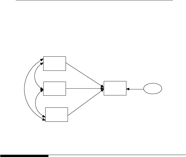
Regression Models 139
In the LISREL 8.8 Student Examples folder, SPLEX, the program EX1A.
SPL computes the regression equation without an intercept term, while
the program EX1B.SPL computes the regression equation with an inter-
cept term. In general, if you include sample means, then an intercept term
is included in the equation. These examples are further explained in the
LISREL8: Structural Equation Modeling with the SIMPLIS Command Language
(Jöreskog & Sörbom, 1993, p. 1–6).
Exercises
1. Analyze the regression model in LISREL–SIMPLIS using the
covariance matrix below with a sample size of 23 as described
in Jöreskog and Sörbom (1993, pp. 3–6). The theoretical regres-
sion model species that the dependent variable, gross national
product (GNP), is predicted by labor, capital, and time (three
independent variables).
Covariance Matrix
GNP 4256.530
Labor 449.016 52.984
Capital 1535.097 139.449 1114.447
Time 537.482 53.291 170.024 73.747
2. Is there an alternative regression model that predicts GNP
better? Report the F, effect size, and condence interval for the
revised model. The regression model is shown in Figure 6.2
Labor
Capitol
Time
GNP error
FIGURE 6.2
GNP regression model.
References
Bashaw, W. L., & Findley, W. G. (1968). Symposium on general linear model approach
to the analysis of experimental data in educational research. (Project No. 7-8096).
Washington, DC: U.S. Department of Health, Education, and Welfare.
Y102005.indb 139 3/22/10 3:25:54 PM
140 A Beginner’s Guide to Structural Equation Modeling
Bohrnstedt, G. W., & Carter, T. M. (1971). Robustness in regression analysis. In
H. L. Costner (Ed.), Sociological methodology (pp. 118–146). San Francisco,
CA: Jossey-Bass.
Chatterjee, S., & Yilmaz, M. (1992). A review of regression diagnostics for behav-
ioral research. Applied Psychological Measurement, 16, 209–227.
Cleary, T. A. (1969). Error of measurement and the power of a statistical test. British
Journal of Mathematical and Statistical Psychology, 22, 49–55.
Cochran, W. G. (1968). Errors of measurement in statistics. Technometrics, 10,
637–666.
Cochran, W. G. (1970). Some effects of errors of measurement on multiple correla-
tion. Journal of the American Statistical Association, 65, 22–34.
Cohen, J. (1988). Statistical power analysis for the behavioral sciences (2nd ed.).
Hillsdale, NJ: Lawrence Erlbaum.
Cohen, J., & Cohen, P. (1983). Applied multiple regression/correlation analysis for the
behavioral sciences (2nd ed.). Hillsdale, NJ: Lawrence Erlbaum.
Cumming, G., & Finch, S. (2001). A primer on the understanding, use and calcula-
tion of condence intervals that are based on central and noncentral distribu-
tions. Educational and Psychological Measurement, 61, 532–574.
Darlington, R. B. (1968). Multiple regression in psychological research and prac-
tice. Psychological Bulletin, 69, 161–182.
Draper, N. R., & Smith, H. (1966). Applied regression analysis. New York: Wiley.
Edwards, A. L. (1979). Multiple regression and the analysis of variance and covariance.
San Francisco, CA: Freeman.
Fuller, W. A. (1987). Measurement error models. New York: Wiley.
Fuller, W. A., & Hidiroglou, M. A. (1978). Regression estimates after correcting for
attenuation. Journal of the American Statistical Association, 73, 99–104.
Hinkle, D. E., Wiersma, W., & Jurs, S.G. (2003). Applied statistics for the behavioral
sciences (5th ed.). Boston, MA: Houghton Mifin.
Houston, S. R., & Bolding, J. T., Jr. (1974). Part, partial, and multiple correlation
in commonality analysis of multiple regression models. Multiple Linear
Regression Viewpoints, 5, 36–40.
Huberty, C. J. (1989). Problems with stepwise methods—Better alternatives. In
B. Thompson (Ed.), Advances in social science methodology (Vol. 1, pp. 43–70).
Greenwich, CT: JAI.
Huberty, C. J. (2003). Multiple correlation versus multiple regression. Educational
and Psychological Measurement, 63, 271–278.
Jöreskog, K. G., & Sörbom, D. (1993). LISREL8: Structural equation modeling with the
SIMPLIS command language. Chicago, IL: Scientic Software International.
Kerlinger, F. N., & Pedhazur, E. J. (1973). Multiple regression in behavioral research.
New York: Holt, Rinehart, & Winston.
Loehlin, J. C. (1992). Latent variable models: An introduction to factor, path, and struc-
tural analysis (2nd ed.). Mahwah, NJ: Lawrence Erlbaum.
Lomax, R. G. (2007). Statistical concepts: A second course (3rd ed.). Mahwah, NJ:
Lawrence Erlbaum.
Lyons, M. (1971). Techniques for using ordinal measures in regression and path
analysis. In H. L. Costner (Ed.), Sociological methodology (pp. 147–171). San
Francisco, CA: Jossey-Bass.
Y102005.indb 140 3/22/10 3:25:54 PM
Regression Models 141
Mallows, C. L. (1966, March). Choosing a subset regression. Paper presented at the
Joint Meetings of the American Statistical Association, Los Angeles.
McNeil, K. A., Kelly, F. J., & McNeil, J. T. (1975). Testing research hypotheses using
multiple linear regression. Carbondale: Southern Illinois University Press.
Newman, I. (1988, October). There is no such thing as multivariate analysis: All analy-
ses are univariate. President’s address at Mid-Western Educational Research
Association, Chicago.
Pedhazur, E. J. (1982). Multiple regression in behavioral research: Explanation and pre-
diction (2nd ed.). New York: Holt, Rinehart, & Winston.
Pedhazur, E. J., & Schmelkin, L. P. (1992). Measurement, design, and analysis: An
integrated approach. Hillsdale, NJ: Lawrence Erlbaum.
Schumacker, R. E. (1991). Relationship between multiple regression, path, factor,
and LISREL analyses. Multiple Linear Regression Viewpoints, 18, 28–46.
Schumacker, R. E. (1993). Teaching ordinal and criterion scaling in multiple regres-
sion. Multiple Linear Regression Viewpoints, 20, 25–31.
Schumacker, R. E. (1994). A comparison of the Mallows Cp and principal compo-
nent regression criteria for best model selection. Multiple Linear Regression
Viewpoints, 21, 12–22.
Smithson, M. (2001). Correct condence intervals for various regression effect
sizes and parameters: The importance of noncentral distributions in comput-
ing intervals. Educational and Psychological Measurement, 61, 605–632.
Soper, D. Statistics Calculators. Retrieved January 2010 from http://www.dan-
ielsoper.com/statcalc/.
Steiger, J. H., & Fouladi, T. (1992). R2: A computer program for interval esti-
mation, power calculation, and hypothesis testing for the squared mul-
tiple correlation. Behavior Research Methods, Instruments, and Computers, 4,
581–582.
Steiger, J. H., & Fouladi, T. (1997). Noncentrality interval estimation and the evaluation
of statistical models. In L. Harlow, S. Mulaik, & J.H. Steiger (Eds.), What if there
were no signicance tests? (pp. 222–257). Mahwah, NJ: Lawrence Erlbaum.
Subkoviak, M. J., & Levin, J. R. (1977). Fallibility of measurement and the power of
a statistical test. Journal of Educational Measurement, 14, 47–52.
Sutcliffe, J. P. (1958). Error of measurement and the sensitivity of a test of signi-
cance. Psychometrika, 23, 9–17.
Thompson, B., Smith, Q. W., Miller, L. M., & Thomson, W. A. (1991, January).
Stepwise methods lead to bad interpretations: Better alternatives. Paper presented
at the annual meeting of the Southwest Educational Research Association,
San Antonio, TX.
Tracz, S. M., Brown, R., & Kopriva, R. (1991). Considerations, issues, and compari-
sons in variable selection and interpretation in multiple regression. Multiple
Linear Regression Viewpoints, 18, 55–66.
Werts, C. E., Rock, D. A., Linn, R. L., & Jöreskog, K. G. (1976). Comparison of
correlations, variances, covariances, and regression weights with or without
measurement error. Psychological Bulletin, 83, 1007–1013.
Zuccaro, C. (1992). Mallows Cp statistic and model selection in multiple linear
regression. Journal of the Market Research Society, 34, 163–172.
Y102005.indb 141 3/22/10 3:25:54 PM

143
7
Path Models
Key Concepts
Path model diagrams
Direct effects, indirect effects, and correlated independent variables
Path (structure) coefcients and standardized partial regression
coefcients
Decomposition of correlations
Original and reproduced correlation coefcients
Full versus limited information function
Residual and standardized residual matrix
In this chapter we consider path models, the logical extension of multiple
regression models. Although path analysis still uses models involving
multiple observed variables, there may be any number of independent
and dependent variables and any number of equations. Thus, as we shall
see, path models require the analysis of several multiple regression equa-
tions using observed variables.
Sewall Wright is credited with the development of path analysis as a
method for studying the direct and indirect effects of variables (Wright,
1921, 1934, 1960). Path analysis is not actually a method for discovering
causes; rather, it tests theoretical relationships, which historically has been
termed causal modeling. A specied path model might actually establish
causal relationships among two variables when:
1. Temporal ordering of variables exists.
2. Covariation or correlation is present among variables.
3. Other causes are controlled for.
4. A variable X is manipulated, which causes a change in Y.
Obviously, a theoretical model that is tested over time (longitudinal research)
and manipulates certain variables to assess the change in other variables
Y102005.indb 143 3/22/10 3:25:54 PM

144 A Beginner’s Guide to Structural Equation Modeling
(experimental research) more closely approaches our idea of causation. In
the social and behavioral sciences, the issue of causation is not as straight-
forward as in the hard sciences, but it has the potential to be modeled.
Pearl (2009) has renewed a discussion of causation in the behavioral
sciences with model examples and rationale for causation as a process
(model) that can be expressed in mathematical expressions ready for com-
puter analysis, which ts into the testing of theoretical path models.
This chapter begins with an example path model, and then proceeds
with sections on model specication, model identication, model estima-
tion, model testing, and model modication.
7.1 An Example
We begin with a path model that will be followed throughout the chapter.
McDonald and Clelland (1984) collected data on the sentiments toward
unions of Southern nonunion textile laborers (n = 173). This example is
presented in the LISREL manual (Jöreskog & Sörbom, 1993, pp. 12–15,
example 3); included in the data les of the LISREL program; and was
utilized by Bollen (1989, pp. 82–83). The model consists of ve observed
variables; the independent variables are the number of years worked in
the textile mill (actually log of years, denoted simply as years) and worker
age (age); the dependent variables are deference to managers (deference),
support for labor activism (support), and sentiment toward unions (sen-
timent). The original variance–covariance matrix, implied model (repro-
duced) variance–covariance matrix, residual matrix, and standardized
residual matrix are given in Table 7.1. The path diagram of the theoretical
proposed model is shown in Figure 7.1.
Path models adhere to certain common drawing conventions that are
utilized in SEM models (Figure 7.2). The observed variables are enclosed by
boxes or rectangles. Lines directed from one observed variable to another
observed variable denote direct effects, in other words, the direct inuence
of one variable on another. For example, it is hypothesized that age has a
direct inuence on support, meaning that the age of the worker may inu-
ence an increase (or decrease) in support. A curved, double-headed line
between two independent observed variables indicates covariance; that is,
they are correlated. In this example, age and years are specied to correlate.
The rationale for such relationships is that there are inuences on both of
these independent variables outside of the path model. Because these inu-
ences are not studied in this path model, it is reasonable to expect that the
same unmeasured variables may inuence both independent variables.
Y102005.indb 144 3/22/10 3:25:55 PM

Path Models 145
Finally, each dependent variable has an error term, denoted by a circle
around the error term pointing toward the proper dependent variable.
Take deference, for example, some variance in deference scores will be pre-
dicted or explained by age and some variance will not. The unexplained
variance will become the error term, which indicates other possible inu-
ences on deference that are not contained in the specied path model.
TABLE 7.1
Original, Reproduced, Residual, and Standardized Residual Covariance
Matrices for the Initial Union Sentiment Model
Original Matrix
Variable Deference Support Sentiment Years Age
Deference 14.610
Support −5.250 11.017
Sentiment −8.057 11.087 31.971
Years −0.482 0.677 1.559 1.021
Age −18.857 17.861 28.250 7.139 215.662
Reproduced Matrix
Variable Deference Support Sentiment Years Age
Deference 14.610
Support −1.562 11.017
Sentiment −5.045 10.210 30.534
Years −0.624 0.591 1.517 1.021
Age −18.857 17.861 25.427 7.139 215.662
Residual Matrix
Variable Deference Support Sentiment Years Age
Deference 0.000
Support −3.688 0.000
Sentiment −3.012 0.877 1.437
Years 0.142 0.086 0.042 0.000
Age 0.000 0.000 2.823 0.000 0.000
Standardized Residual Matrix
Variable Deference Support Sentiment Years Age
Deference 0.000
Support –4.325 0.000
Sentiment –3.991 3.385 3.196
Years 0.581 0.409 0.225 0.000
Age 0.000 0.000 0.715 0.000 0.000
Y102005.indb 145 3/22/10 3:25:55 PM
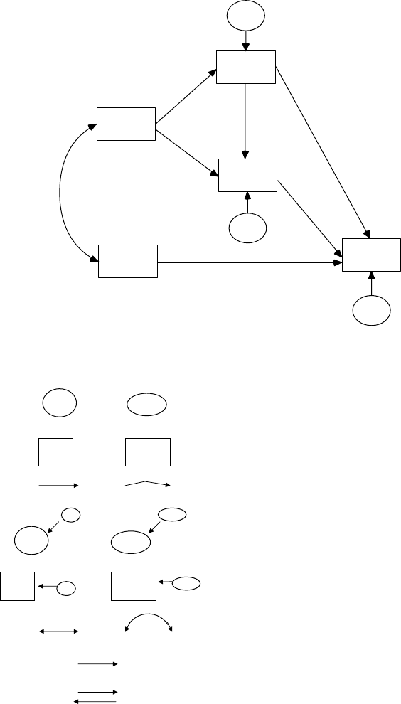
146 A Beginner’s Guide to Structural Equation Modeling
or
or
or
or
or
or
Latent variable
Observed variable
Unidirectional path
Disturbance or error in latent variable
Measurement error in observed variable
Correlation between variables
Recursive (nonreciprocal) relation between variables
Nonrecursive (reciprocal) relation between variables
FIGURE 7.2
Common path diagram symbols.
age
years
deference
support
sentiment
error1
error3
error2
FIGURE 7.1
Union sentiment model.
Y102005.indb 146 3/22/10 3:25:56 PM

Path Models 147
7.2 Model Specification
Model specication is necessary in examining multiple variable relation-
ships in path models, just as in the case of multiple regression. Many dif-
ferent relationships among a set of variables can be hypothesized with
many different parameters being estimated. In a simple three-variable
model, for example, many possible path models can be postulated on the
basis of different hypothesized relationships among the three variables.
For example, in Figure 7.3a–c we see three different path models where
X1 inuences X2. In Model (a), X1 inuences X2, which in turn inuences
Y. Here, X2 serves as a mediator between X1 and Y. In Model (b), an addi-
tional path is drawn from X1 to Y, such that X1 has both a direct and an
indirect effect upon Y. The direct effect is that X1 has a direct inuence on
Y (no variables intervene between X1 and Y), whereas the indirect effect
is that X1 inuences Y through X2, that is, X2 intervenes between X1 and
Y. In Model (c), X1 inuences both X2 and Y; however, X2 and Y are not
related. If we were to switch X1 and X2 around, this would generate three
more plausible path models.
Other path models are also possible. For example, in Figure 7.4(a,b), X1
does not inuence X2. In Model (a), X1 and X2 inuence Y, but are uncor-
related. In Model (b), X1 and X2 inuence Y and are correlated. How can
one determine which model is correct? This is known as model specica-
tion and shows the important role that theory and previous research plays
in justifying a hypothesized model. Path analysis does not provide a way
to specify the model, but rather estimates the effects among the variables
once the model has been specied a priori by the researcher on the basis of
theoretical considerations. For this reason, model specication is a critical
part of SEM modeling.
Path coefcients in path models are usually derived from the values of a
Pearson product moment correlation coefcient (r) and/or a standardized
partial regression coefcient (b) (Wole, 1977). For example, in the path
model of Figure 7.4b, the path coefcients (p) are depicted by arrows from
X1 to Y and X2 to Y, respectively, as:
b
1 = pY1
b
2 = pY2
and the curved arrow between X1 and X2 is denoted as:
r
X1,X2 = p12.
The variable relationships, once specied in standard score form, become
standardized partial regression coefcients. In multiple regression, a
Y102005.indb 147 3/22/10 3:25:56 PM

148 A Beginner’s Guide to Structural Equation Modeling
dependent variable is regressed in a single analysis on all of the indepen-
dent variables. In path analysis, one or more multiple regression analyses
are performed depending on the variable relationships specied in the
path model. Path coefcients are therefore computed only on the basis
of the particular set of independent variables that lead to the dependent
X1 X2 Y
X1
X2
Y
error1 error2
error1
(a)
(b)
(c)
error2
X1
X2
Y
error1
error2
FIGURE 7.3
Possible three-variable models (X1 inuences X2).
Y102005.indb 148 3/22/10 3:25:56 PM
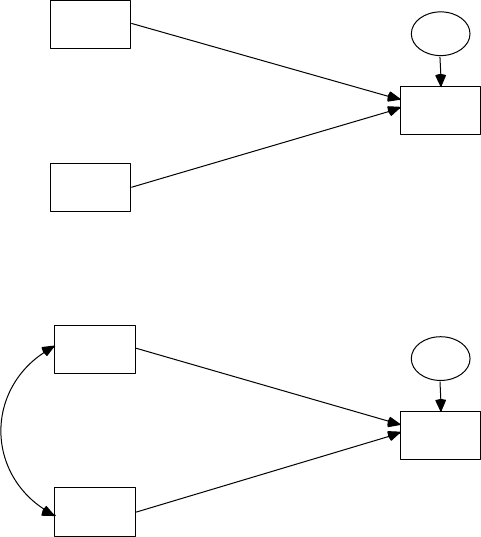
Path Models 149
variable under consideration. In the path model of Figure 7.4b, two stan-
dardized partial regression coefcients (path coefcients) are computed,
pY1 and pY2. The curved arrow represents the covariance or correlation
between the two independent variables p12 in predicting the dependent
variable.
For the union sentiment model, the model specication is as follows.
There are three structural equations in the model, one for each of the three
dependent variables, deference, support, and sentiment. In terms of vari-
able names, the structural equations are as follows.
deference = age + error1
support = age + deference + error2
sentiment = years + support + deference + error3 .
X1
X2
Y
error1
(a)
(b)
X1
X2
Y
error2
FIGURE 7.4
Possible three-variable models (X1 does not inuence X2).
Y102005.indb 149 3/22/10 3:25:57 PM

150 A Beginner’s Guide to Structural Equation Modeling
Substantive information from prior research suggested that those six
paths be included in the specied model; and that other possible paths,
for example from age to sentiment, not be included. This model includes
direct effects, for example from age to support, indirect effects, for exam-
ple from age to support through deference, and correlated independent
variables, for example age and years. Obviously many possible path mod-
els could be specied for this set of observed variables.
7.3 Model Identification
Once a particular path model has been specied, the next concern is
whether the model is identied. In structural equation modeling, it is cru-
cial that the researcher resolve the identication problem prior to the estima-
tion of parameters. The general notion of identication was discussed in
Chapter 4. Here, we consider model identication in the context of path
models, and in particular, for our union sentiment example.
As described in Chapter 4, for the identication problem, we ask the fol-
lowing question: On the basis of the sample data contained in the sample
covariance matrix S and the theoretical model implied by the population
covariance matrix Σ, can a unique set of parameter estimates be found?
For the union sentiment model, for example, we would like to know if the
path between age and deference is identied; an example of one param-
eter to be estimated.
In the union sentiment model, some parameters are xed and others
are free. An example of a xed parameter is that there is no path or direct
relationship between age and sentiment. An example of a free parameter
is that there is a path or direct relationship between age and deference.
In determining identication, rst consider the order condition. Here,
the number of free parameters to be estimated must be less than or equal
to the number of distinct values in the matrix S. In our path model we
specied the following:
6 path coefcients
3 equation error variances
1 correlation among the independent variables
2 independent variable variances
Thus, there are a total of 12 free parameters that we wish to estimate. The
number of distinct values in the matrix S is equal to:
[p (p + 1)]/2 = [5 (5 + 1)]/2 = 15,
Y102005.indb 150 3/22/10 3:25:57 PM

Path Models 151
where p is the number of observed variables in the matrix. Thus, the num-
ber of distinct values in the sample matrix S, 15 is indeed greater than the
number of free parameters, 12. However, this is only a necessary condi-
tion and does not guarantee that the model is identied. According to the
order condition, the model is also overidentied because there are more
values in S than parameters to be estimated.
Although the order condition is easy to assess, other sufcient condi-
tions are not, for example, the rank condition. The sufcient conditions
require us to algebraically determine whether each parameter in the
model can be estimated from the covariance matrix S. According to the
LISREL computer program, which checks on identication, the union sen-
timent model is identied.
7.4 Model Estimation
Once the identication problem has been addressed, the next step is to esti-
mate the parameters of the specied model. In this section, we consider the
following topics: decomposition of the correlation matrix, parameter estima-
tion in general, and parameter estimation of the union sentiment model.
In path analysis, the traditional method of intuitively thinking about
estimation is to decompose the correlation matrix. This harkens back to
the early days of path analysis in the 1960s when sociologists like Arthur S.
Goldberger and Otis D. Duncan were rediscovering and further develop-
ing the procedure. The decomposition idea is that the original correlation
matrix can be completely reproduced if all of the effects are accounted for
in a specied path model. In other words, if all of the possible unidirec-
tional (or recursive) paths are included in a path model, then the observed
correlation matrix can be completely reproduced from the obtained stan-
dardized estimates of the model.
For example, take the model in Figure 7.4b. Here there are two direct
effects, from X1 to Y and from X2 to Y. There are also indirect effects due
to the correlation between X1 and X2. In other words, X1 indirectly inu-
ences Y through X2, and also X2 indirectly affects Y through X1. The cor-
relations among these three variables can be decomposed as follows:
r
12 = p12 (1)
(CO)
r
Y1 = pY1 + p12 pY2 (2)
(DE) (IE)
rY2 = pY2 + p12 pY1, (3)
(DE) (IE)
Y102005.indb 151 3/22/10 3:25:57 PM
152 A Beginner’s Guide to Structural Equation Modeling
where the r values are the actual observed correlations and the p values
are the path coefcients (standardized estimates). Thus, in equation (1),
the correlation between X1 and X2 is simply a function of the path, or
correlation relationship (CO), between X1 and X2. In equation (2), the
correlation between X1 and Y is a function of (a) the direct effect (DE)
of X1 on Y, and (b) the indirect effect (IE) of X1 on Y through X2 [the
product of the path or correlation between X1 and X2 (p12) and the path
or direct effect from X2 to Y (pY2)]. Equation (3) is similar to equation (2)
except that X1 and X2 are reversed; there is both a direct effect and an
indirect effect.
Let us illustrate how this works with an actual set of correlations. The
observed correlations are as follows: r12 = .224, rY1 = .507, and rY2 = .480. The
specied path model and correlation matrix were run in LISREL. The path
coefcients and the complete reproduction of the correlations are:
r12 = p12 = .224 (4)
(CO)
rY1 = pY1 + p12 pY2 = .421 + (.224)(.386) = .507 (5)
(DE) (IE)
rY2 = pY2 + p12 pY1 = .386 + (.224)(.421) = .480. (6)
(DE) (IE)
Here, the original correlations are completely reproduced by the model
because all of the effects are accounted for, direct, indirect, and correlated.
If a path were left out of the model, for example p12, then the correlations
would not be completely reproduced. Thus, the correlation decomposition
approach is a nice conceptual way of thinking about the estimation pro-
cess in path analysis. For further details on the correlation decomposition
approach, we highly recommend reading Duncan (1975).
In chapter 4, we presented the problem of estimation in general.
Parameters can be estimated by different estimation procedures, such
as maximum likelihood (ML), generalized least squares (GLS), and
unweighted least squares (ULS), which are all unstandardized types of
estimates, as well as standardized estimates (the path coefcients previ-
ously described in this chapter were standardized estimates). In addition
to different methods of estimation of the parameter estimates, full versus
limited information estimation functions are invoked based on the soft-
ware chosen for the analysis. Full information estimation computes all of the
parameters simultaneously, whereas limited information estimation com-
putes parameters for each equation separately. The parameters estimated
in structural equation modeling software (LISREL) use full information
estimation and therefore differ from parameter estimates computed in
Y102005.indb 152 3/22/10 3:25:57 PM

Path Models 153
SPSS or SAS, where each equation in the path model is estimated sepa-
rately (limited information estimation). In limited information estimation,
the parameter estimates are determined uniquely in each separate equa-
tion to meet the least squares criterion of minimized residuals.
In the union sentiment example we see the estimation process at work. In
order to utilize the model modication procedures discussed in section 7.6,
we have slightly changed the model specication in Figure 7.1. We remove
the path from deference to support and call this the initial model. We evalu-
ate this initial model, and hope, through the model modication process,
we will obtain the model as originally specied in Figure 7.1. The intention-
ally misspecied model was run using LISREL (Note: The LISREL program
for the correctly specied model is given at the end of the chapter).
The maximum likelihood estimates for the initial model are shown in the
rst column of Table 7.2. All of the parameter estimates are signicantly
TABLE 7.2
Maximum Likelihood Estimatesa and Selected Fit Indices for the Initial
and Final Union Sentiment Models
Paths Initial Model Final Model
Age → deference −.09 −.09
Age → support 0.08 0.06
Deference → support — −.28
Years → sentiment 0.86 0.86
Deference → sentiment −.22 −.22
Support → sentiment 0.85 0.85
Equation error variances
Deference 12.96 12.96
Support 9.54 8.49
Sentiment 19.45 19.45
Independent variables
Variance (age) 215.66 215.66
Variance (years) 1.02 1.02
Covariance (age, years) 7.14 7.14
Selected fit indices
c219.96 1.25
df 4 3
p value .00 .74
RMSEA .15 .00
SRMR .087 .015
GFI .96 1.00
a All estimates signicantly different from zero (p < .05).
Y102005.indb 153 3/22/10 3:25:57 PM

154 A Beginner’s Guide to Structural Equation Modeling
different from zero, p < .05 (the t of the model is discussed next in sec-
tion 7.5). Age has a direct effect on both deference and support; deference
has a direct effect on sentiment; years has a direct effect on sentiment;
and support has a direct effect on sentiment. Numerous indirect effects
are also part of the path model, such as the indirect effect of age on senti-
ment through support. Age and years also have a signicant covariance,
indicating that one or more common unmeasured variables inuence both
age and years.
7.5 Model Testing
An important result of any path analysis is the t of the specied
model. If the t of the path model is good, then the specied model has
been supported by the sample data. If the t of the path model is not so
good, then the specied model has not been supported by the sample
data, and the researcher typically attempts to modify the path model to
achieve a better t (as described in section 7.6). As discussed in chap-
ter 5, LISREL provides modication indices and expected parameter
changes values to guide modifying a model to obtain better model-t
criteria.*
For purposes of the union sentiment example, we include a few model-
t indices at the bottom of Table 7.2. For the initial path model, the c2
statistic, technically a measure of badness of t, is equal to 19.96, with four
degrees of freedom, and p < .01. As the p value is very small and the c2
value is nowhere near the number of degrees of freedom, then according
to this measure of t, the initial path model is poorly specied. The root-
mean-square error of approximation (RMSEA) is equal to .15, somewhat
below the acceptable level for this measure of t (RMSEA < .08 or .05). The
standardized root-mean-square residual (SRMR) is .087, also below the
usual acceptable level of t (SRMR < .08 or .05). Finally, the goodness-of-t
index (GFI) is .96 for the initial model, which is an acceptable level for this
measure of t (GFI > .95). Across this particular set of model-t indices,
the conclusion is that the data to model t is approaching a reasonable
level, but that some model modications might allow us to achieve a bet-
ter model t between the sample variance–covariance matrix S and the
implied model (reproduced) variance–covariance matrix Σ. Model modi-
cation is considered in the next section.
* Another traditional non-SEM path model-t index is described in the Chapter Footnote.
Y102005.indb 154 3/22/10 3:25:58 PM

Path Models 155
7.6 Model Modification
The nal step in structural equation modeling is model modication. In
other words, if the t of the model is less than satisfactory, then the researcher
typically performs a specication search to seek a better tting model. As
described in chapters 4 and 5, several different procedures can be used to
assist in this search. One may eliminate parameters that are not signi-
cantly different from zero and/or include additional parameters to arrive at
a modied model. For the elimination of parameters, the most commonly
used procedure in LISREL is to compare the t statistic for each parameter to
a tabled t value (e.g., t > 1.96) to determine statistical signicance.
For the inclusion of additional parameters, the most commonly used
techniques in LISREL are (a) the modication index (MI) (the expected
value that c2 would decrease if such a parameter were to be included;
large values indicate potentially useful parameters), and (b) the expected
parameter change statistic (EPC) (the approximate value of the new
parameter if added to the model).
In addition, an examination of the residual matrix, or the more useful stan-
dardized residual matrix, often gives clues as to which original covariance or
correlations are not well accounted for by the model. Recall that the residual
matrix is the difference between the observed variance-covariance S and the
model implied (reproduced) variance-covariance matrix Σ. Large residuals
indicate values not well accounted for by the model. Standardized residu-
als are like z scores in that large values (greater than 1.96 or 2.58) indicate
that a particular relationship is not well accounted for by the path model
(Table A.1).
For the initial union sentiment example, the original, model implied
(reproduced), residual, and standardized residual covariance matrices are
given in Table 7.1. Here we see that the largest standardized residual is
between deference and support (−4.325). The t statistics do not suggest
the elimination of any existing parameters from the initial path model
because every parameter is statistically different from zero. With regard
to the possible inclusion of new parameters, the largest modication index
is for the path from deference to support (MI = 18.9). For that potential
path, the estimated value, or expected parameter change (EPC), is −0.28.
Taken together, these statistics indicate that there is something mis-
specied between deference and support that is not captured by the initial
model. Specically, adding a path is recommended from deference to sup-
port. This is precisely the path from the originally specied path model
that we intentionally eliminated from the initial path model. Thus, the
specication search was successful in obtaining the original model. The
ML estimates and selected t indices for the nal model, where this path
is now included, are shown in the second column of Table 7.2. All of the
Y102005.indb 155 3/22/10 3:25:58 PM

156 A Beginner’s Guide to Structural Equation Modeling
parameters included are signicantly different from zero (p < .05), all of the
t indices now indicate an acceptable level of t, and no additional modi-
cation indices are indicated for any further recommended changes. Thus,
we deem this as the nal path model for the union sentiment example.
7 . 7 S u m m a r y
This chapter presented a detailed discussion of path models. We began by
presenting the union sentiment path model and then followed it through-
out the chapter. We moved on to model specication, rst with several
possible three-variable models, and then with the union sentiment model.
The next step was to consider model identication of the union sentiment
model for both the order and rank conditions. Next, we discussed estima-
tion. Here, we introduced the notion of correlation decomposition with
a three-variable model, and the difference between full versus limited
estimation functions, and then considered the full information estimation
results for the union sentiment model. Model testing of the misspecied
union sentiment model was the next step, where the t of the model was
deemed not acceptable. The misspecied model (altered initial model) was
then modied through the addition of one path, thereby arriving at a nal,
best-tting theoretical model, which was the same as our initial model.
We learned that path models permit theoretically meaningful relation-
ships among variables that cannot be specied in a single additive regres-
sion model. However, the issue of measurement error in observed variables
is not treated in either regression or path models (Wole, 1979). The next
chapter helps us to understand how measurement error is addressed in
structural equation modeling via factor models.
Appendix: LISREL–SIMPLIS Path
Model Program (Figure 7.1)
Union Sentiment of Textile Workers
Observed Variables: Deference Support Sentiment Years Age
Covariance matrix:
14.610
−5.250 11.017
−8.057 11.087 31.971
−0.482 0.677 1.559 1.021
−18.857 17.861 28.250 7.139 215.662
Y102005.indb 156 3/22/10 3:25:58 PM
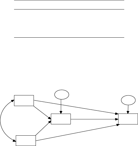
Path Models 157
Sample Size: 173
Relationships
Deference = Age
Support = Age Deference
Sentiment = Years Deference Support
Print Residuals
Options: ND = 3
Path Diagram
End of Problem
Exercise
1. Analyze the following achievement path model (Figure 7.5)
using the LISREL software program. The path model indicates
that income and ability predict aspire, and income, ability, and
aspire predict achieve.
Sample size = 100
Observed variables: quantitative achievement (Ach), family
income (Inc), quantitative ability (Abl), educational aspira-
tion (Asp)
Variance–covariance matrix:
Ach Inc Abl Asp
Ach 25.500
Inc 20.500 38.100
Abl 22.480 24.200 42.750
Asp 16.275 13.600 13.500 17.000
Equations:
Asp = Inc Abl
Ach = Inc Abl Asp
Income
Ability
Achieve
error2
Aspire
error1
FIGURE 7.5
Achievement path model.
Y102005.indb 157 3/22/10 3:25:59 PM

158 A Beginner’s Guide to Structural Equation Modeling
Chapter Footnote
Another Traditional Non-SEM Path Model-Fit Index
The relationship between the original and reproduced correlation matri-
ces is essential for testing the signicance of the path model (Specht, 1975).
The relationship between the two matrices is tested by calculating a chi-
square statistic. A signicant c2 value for a specied level of signicance
(a = .05) indicates that the path model does not t the data. If c2 = 0, then
the original and reproduced correlations in the matrices are identical; in
other words, the correlations are perfectly reproduced by the path model.
Also, if the residuals, for example Pe1 and Pe2, are uncorrelated in a path
model, then the sum of squared residual path coefcients will equal the
chi-square value. A non-signicant chi-square value therefore indicates a
good path model to data t in SEM. Another traditional non-SEM path
model-t index, Q, has been reported in the research literature and there-
fore presented here using a LISREL–SIMPLIS program example with heu-
ristic data.
LISREL–SIMPLIS program
Path analysis of Y
Observed variables Y X1 X2 X3
Sample size 100
Correlation Matrix
1.000
.507 1.000
.480 .224 1.000
.275 .062 .577 1.000
Equation:
Y = X1 X2 X3
X3 = X1 X2
End of Problem
The theoretical path model in Figure 7.6 indicates that two variables,
X1 and X2 predict X3; X1, X2, and X3 predict Y; and X1 and X2 are cor-
related. This original path model is a saturated model because all paths
are included, thus c2 = 0, df = 0, and p = 0. The original path model,
however, has two R-squared values for each regression equation: R2X3.
X1,X2 = .34 and R2Y.X3,X1,X2 = .40. The path model diagram only shows the
1 − R2X3.X1,X2 = .66 and 1 − R2Y.X3,X1,X2 = .60 values. Computer output indi-
cated that the path from X1 to X3 was non-signicant ( p31 = −.071) and
the path from X3 to Y was non-signicant (p3Y = .040). For theoretical
reason, we only dropped path p31 resulting in the modied path model
in Figure 7.7.
Y102005.indb 158 3/22/10 3:25:59 PM
Path Models 159
The modied path model reported a non-signicant c2 = .71, df = 1, and
p = .40 which indicates that the data ts the path model, although the path
coefcient from X3 to Y is still non-signicant, but kept in the model for
theoretical reasons.
The other traditional non-SEM path model-t indices can be accom-
plished by computing the generalized squared multiple correlation
(Pedhazur, 1982) as follows:
R2
m = 1 – (1 – R2
1) (1 − R2
2)…..(1 − R2
p).
The R-squared values are the squared multiple correlation coefcients
from each of the separate regression analyses in the path model. In the
original path model, the two regression analyses yielded R-squared values
of .34 and .40, respectively. The path model-t R2
m would be computed as:
R2
m = 1 – (1 − .34)(1 − .40) = .604
X1
X2
Y
0.60
X3
0.66
0.040
0.423
0.362
–0.071
0.593
0.224
FIGURE 7.6
Original path model.
X1
X2
Y
0.60
X3
0.67
0.04
0.42
0.36
0.58
0.224
FIGURE 7.7
Modied path model.
Y102005.indb 159 3/22/10 3:26:00 PM
160 A Beginner’s Guide to Structural Equation Modeling
An analogous statistic to R2
m, M, and a large sample measure of model
t, Q, are also presented in Pedhazur (1982). Q is oftentimes recommended
because chi-square is affected by sample size. Q varies between zero and one
and is not a function of sample size. The formula for Q is:
Q = (1− R2
m)/(1 – M)
M is calculated in the same manner as R2
m, but with a non-signicant path
deleted. In our example, we dropped the path from X1 to X3 because it
yielded a non-signicant path coefcient and therefore M calculated from
the modied path model would have a different value from R2
m in the orig-
inal path model (M values range between zero and R2
m).
In our example, the path from X1 to X3 in the program was dropped by
changing the rst LISREL–SIMPLIS equation command to read:
Equation: X3 = X2
The M value is computed as:
M = 1 – (1 − .33)(1 − .40) = .598.
Q is now computed as:
Q = [(1 − .604)/( 1 − .598)] = [.396/.402] = .98.
Remember, the closer the value of Q to 1.0, the better the model t. Q can
be tested for signicance using W, which is computed as:
W = − (N – d) loge Q,
where N = sample size, d = number of path coefcients hypothesized to be
zero, loge = natural logarithm (ln). For our example,
W = − (100 − 1) loge (.98) = 2.00.
Since W approximates the c2 distribution with degrees of freedom = d,
the tabled critical chi-square value for d = 1, a = 05, is 3.841 (Table A.4).
W is less than the tabled critical value, therefore nonsignicant, suggest-
ing a good path model t to the data. The W value fell between p = .20
(c2 = 1.642) and p = .10 (c2 = 2.706) in Table A.4.
Prior to SEM, Q and the W path model-t index were reported to test
whether a path model signicantly reproduced the correlation matrix. The
R2
m value was reported to indicate the amount of variation in Y predicted
by the direct and indirect effects of the independent variables. Individual
Y102005.indb 160 3/22/10 3:26:00 PM

Path Models 161
tests of path coefcients were also computed and reported by dividing
the path coefcient by its standard error. We used the path coefcient,
standard error, and associated t-value provided in the computer output to
determine if a path coefcient was nonsignicant, thus dropping it from
the path model.
References
Bollen, K. A. (1989). Structural equations with latent variables. New York: Wiley.
Duncan, O. D. (1975). Introduction to structural equation models. New York: Academic.
Jöreskog, K. G., & Sörbom, D. (1993). LISREL 8: Structural equation modeling with the
SIMPLIS command language. Chicago, IL: Scientic Software International.
McDonald, J. A., & Clelland, D. A. (1984). Textile workers and union sentiment.
Social Forces, 63, 502–521.
Pearl, J. (2009). Causality: Models, reasoning, and inference (2nd ed.). Cambridge
University Press: London.
Pedhazur, E. J. (1982). Multiple regression in behavioral research: Explanation and pre-
diction (2nd ed.). New York: Holt, Rinehart & Winston.
Specht, D. A. (1975). On the evaluation of causal models. Social Science Research,
4, 113–133.
Wole, L. M. (1977). An introduction to path analysis. Multiple Linear Regression
Viewpoints, 8, 36–61.
Wole, L. M. (1979). Unmeasured variables in path analysis. Multiple Linear
Regression Viewpoints, 9, 20–56.
Wright, S. (1921). Correlation and causation. Journal of Agricultural Research, 20,
557–585.
Wright, S. (1934). The method of path coefcients. Annals of Mathematical Statistics,
5, 161–215.
Wright, S. (1960). Path coefcients and path regression: Alternative or complemen-
tary concepts? Biometrics, 16, 189–202.
Y102005.indb 161 3/22/10 3:26:00 PM

163
8
Confirmatory Factor Models
Key Concepts
Conrmatory factor analysis versus exploratory factor analysis
Latent variables (factors) and observed variables
Factor loadings and measurement errors
Correlated factors and correlated measurement errors
In chapter 7 we examined path models as the logical extension of multiple
regression models (chapter 6) to show more meaningful theoretical rela-
tionships among our observed variables. Thus, the two previous chapters
dealt exclusively with models involving observed variables. In this chap-
ter we begin developing models involving factors or latent variables and
continue latent variable modeling throughout the remainder of the book.
As we see in this chapter, a major limitation of models involving only
observed variables is that measurement error is not taken into account.
The use of observed variables in statistics assumes that all of the mea-
sured variables are perfectly valid and reliable, which is unlikely in many
applications. For example, father’s educational level is not a perfect mea-
sure of a socioeconomic status factor and amount of exercise per week is
not a perfect measure of a tness factor.
The validity and reliability issues in measurement have traditionally
been handled by rst examining the validity and reliability of scores on
instruments used in a particular context. Given an acceptable level of score
validity and reliability, the scores are then used in a statistical analysis.
However, the traditional statistical analysis of these scores—for example,
in multiple regression and path analysis—does not adjust for measure-
ment error. The impact of measurement error has been investigated and
found to have serious consequences—for example, biased parameter esti-
mates (Cochran, 1968; Fuller, 1987). Structural equation modeling soft-
ware that accounts for the measurement error of variables was therefore
developed—that is, factor analysis—which creates latent variables used in
structural equation modeling.
Y102005.indb 163 3/22/10 3:26:00 PM

164 A Beginner’s Guide to Structural Equation Modeling
Factor analysis attempts to determine which sets of observed variables
share common variance–covariance characteristics that dene theoreti-
cal constructs or factors (latent variables). Factor analysis presumes that
some factors that are smaller in number than the number of observed
variables are responsible for the shared variance–covariance among the
observed variables. In practice, one collects data on observed variables
and uses factor-analytic techniques to either conrm that a particular
subset of observed variables dene each construct or factor, or explore
which observed variables relate to factors. In exploratory factor model
approaches, we seek to nd a model that ts the data, so we specify differ-
ent alternative models, hoping to ultimately nd a model that ts the data
and has theoretical support. This is the primary rationale for exploratory
factor analysis (EFA). In conrmatory factor model approaches, we seek to
statistically test the signicance of a hypothesized factor model—that is,
whether the sample data conrm that model. Additional samples of data
that t the model further conrm the validity of the hypothesized model.
This is the primary rationale for conrmatory factor analysis (CFA).
In CFA, the researcher species a certain number of factors, which factors
are correlated, and which observed variables measure each factor. In EFA,
the researcher explores how many factors there are, whether the factors are
correlated, and which observed variables appear to best measure each fac-
tor. In CFA, the researcher has an a priori specied theoretical model; in
EFA, the researcher does not have such a model. In this chapter we only
concern ourselves with conrmatory factor models because the focus of the
book is on testing theoretical models; exploratory factor analysis is covered
in depth elsewhere (Comrey & Lee, 1992; Gorsuch, 1983; and Costello &
Osborne, 2005). This chapter begins with a classic example of a conrmatory
factor model and then proceeds with sections on model specication, model
identication, model estimation, model testing, and model modication.
8.1 An Example
We use a classic conrmatory factor model that will be followed through-
out the chapter. Holzinger and Swineford (1939) collected data on 26 psy-
chological tests from seventh- and eighth-grade children in a suburban
school district of Chicago. Over the years, different subsamples of the
children and different subsets of the variables of this dataset have been
analyzed and presented in various multivariate statistics textbooks—for
example, Harmon (1976) and Gorsuch (1983)—and SEM software program
guides—for example, Jöreskog and Sörbom (1993; example 5, pp. 23–28).
The raw data analyzed here are on the rst six psychological variables
for all 301 subjects (see chapter 5); the resulting sample covariance matrix
Y102005.indb 164 3/22/10 3:26:00 PM
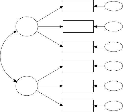
Confirmatory Factor Models 165
S is given in the Appendix. The conrmatory factor model consists of
the following six observed variables: Visual Perception, Cubes, Lozenges,
Paragraph Comprehension, Sentence Completion, and Word Meaning. The
rst three measures were hypothesized to measure a spatial ability fac-
tor and the second three measures to measure a verbal ability factor.
The path diagram of the theoretical proposed model is shown in
Figure 8.1. The drawing conventions utilized in Figure 8.1 were described
in chapter 7. The observed variables are enclosed by boxes or rectangles,
and the factors (latent variables) are enclosed by circles or ellipses—that is,
spatial and verbal. Conceptually, a factor represents the common variation
among a set of observed variables. Thus, for example, the spatial ability
factor represents the common variation among the Visual Perception, Cubes,
and Lozenges tasks. Lines directed from a factor to a particular observed
variable denote the relationship between that factor and that measure.
These relationships are interpreted as factor loadings with the square of
the factor loading called the commonality estimate of the variable.
The measurement errors are enclosed by smaller ellipses and indicate
that some portion of each observed variable is measuring something
other than the hypothesized factor. Conceptually, a measurement error
spatial
visperc
cubes
lozenges
wordmean
paragrap
sentence
err_v
err_c
err_l
err_p
err_s
err_w
verbal
FIGURE 8.1
Conrmatory factor model. (From Holzinger, K. J., & Swineford, F. A. [1939]. A study in factor
analysis: The stability of a bi-factor solution. [Supplementary Educational Monographs, No. 48].
Chicago, IL: University of Chicago, Department of Education.)
Y102005.indb 165 3/22/10 3:26:01 PM

166 A Beginner’s Guide to Structural Equation Modeling
represents the unique variation for a particular observed variable beyond
the variation due to the relevant factor. For example, the Cubes task is
largely a measure of spatial ability, but may also be assessing other char-
acteristics such as a different common factor or unreliability. To assess
measurement error, the variance of each measurement error is estimated
(known as measurement error variance).
A curved, double-headed line between two factors indicates that they
have shared variance or are correlated. In this example, spatial and verbal
ability are specied to covary or correlate. The rationale for this particular
factor correlation is that spatial ability and verbal ability are related to a
more general ability factor and thus should be theoretically related.
A curved, double-headed line between two measurement error vari-
ances indicates that they also have shared variance or are correlated.
Although not shown in this example, two measurement error variances
could be correlated if they shared something in common such as (a) com-
mon method variance where the method of measurement is the same, such
as the same scale of measurement, or they are both part of the same global
instrument, or (b) the same measure is being used at different points in
time, that is, the Cubes task is measured at Time 1 and again at Time 2.
8.2 Model Specification
Model specication is a necessary rst step in analyzing a conrmatory
factor model, just as it was for multiple regression and path models. Many
different relationships among a set of variables can be postulated with
many different parameters being estimated. Thus, many different factor
models can be postulated on the basis of different hypothesized relation-
ships between the observed variables and the factors.
In our example, there are six observed variables with two different
latent variables (factors) being hypothesized. Given this, many dif-
ferent conrmatory factor models are possible. First, each observed
variable can load on either one or both factors. Thus, there could be
anywhere from 6 to 12 total factor loadings. Second, the two factors
may or may not be correlated. Third, there may or may not be corre-
lations or covariance terms among the measurement error variances.
Thus, there could be anywhere from 0 to 15 total correlated measure-
ment error variances.
From the model in Figure 8.1, each observed variable is hypothesized to
measure only a single factor—that is, three observed variables per factor
with six factor loadings; the factors are believed to be correlated (a single fac-
tor correlation); and the measurement error variances are not related (zero
Y102005.indb 166 3/22/10 3:26:01 PM

Confirmatory Factor Models 167
correlated measurement errors. Obviously, we could have hypothesized a
single factor with six observed variables or six factors each with a single
observed variable. When all of this is taken into account, many different
conrmatory factor models are possible with these six observed variables.
How does the researcher determine which factor model is correct? We
already know that model specication is important in this process and indi-
cates the important role that theory and prior research play in justifying
a specied model. Conrmatory factor analysis does not tell us how to
specify the model, but rather estimates the parameters of the model once
the model has been specied a priori by the researcher on the basis of
theoretical and research based knowledge. Once again, model specica-
tion is the hardest part of structural equation modeling.
For our conrmatory factor model, the model specication is dia-
grammed in Figure 8.1 and contains six measurement equations in the
model, one for each of the six observed variables. In terms of the variable
names from Figure 8.1, the measurement equations are as follows:
visperc = function of spatial + err_v
cubes = function of spatial + err_c
lozenges = function of spatial + err_l
paragrap = function of verbal + err_p
sentence = function of verbal + err_s
wordmean = function of verbal + err_w
Substantive theory and prior research suggest that these particular factor
loadings should be included in the specied model (the functions being the
factor loadings), and that other possible factor loadings—for example, vis-
perc loading on verbal, should not be included in the factor model. Our fac-
tor model includes six factor loadings and six measurement error variances,
one for each observed variable, and one correlation between the factors spa-
tial ability and verbal ability with zero correlated measurement errors.
8.3 Model Identification
Once a conrmatory factor model has been specied, the next step is
to determine whether the model is identied. As stated in chapter 4, it
is crucial that the researcher solve the identication problem prior to the
Y102005.indb 167 3/22/10 3:26:01 PM
168 A Beginner’s Guide to Structural Equation Modeling
estimation of parameters. We rst need to revisit model identication in
the context of conrmatory factor models and then specically for our
conrmatory factor model example.
In model identication (see chapter 4), we ask the following question:
On the basis of the sample data contained in the sample variance–
covariance matrix S, and the theoretical model implied by the population
variance–covariance matrix Σ, can a unique set of parameter estimates
be found? For our conrmatory factor model, we would like to know if
the factor loading of Visual Perception on Spatial Ability, Cubes on Spatial
Ability, Lozenges on Spatial Ability, Paragraph Comprehension on Verbal Ability,
Sentence Completion on Verbal Ability, and Word Meaning on Verbal Ability
are identied (can be estimated). In our conrmatory factor model, some
parameters are xed and others are free. An example of a xed parameter
is that Cubes is not allowed to load on Verbal Ability. An example of a free
parameter is that Cubes is allowed to load on Spatial Ability.
In determining identication, we rst assess the order condition. The
number of free parameters to be estimated must be less than or equal to
the number of distinct values in the matrix S. A count of the free param-
eters is as follows:
6 factor loadings
6 measurement error variances
0 measurement error covariance terms or correlations
1 correlation among the latent variables
Thus, there are a total of 13 free parameters that we wish to estimate. The
number of distinct values in the matrix S is equal to
p (p + 1)/2 = 6 (6 + 1)/2 = 21,
where p is the number of observed variables in the sample variance–
covariance matrix. The number of values in S, 21, is greater than the
number of free parameters, 13, with the difference being the degrees of
freedom for the specied model, df = 21 − 13 = 8. However, this is only
a necessary condition and does not guarantee that the model is identi-
ed. According to the order condition, this model is over-identied because
there are more values in S than parameters to be estimated—that is, our
degrees of freedom is positive not zero (just-identied) or negative (under-
identied).
Although the order condition is easy to assess, other sufcient condi-
tions are not, for example, the rank condition. The sufcient conditions
require us to algebraically determine whether each parameter in the
model can be estimated from the covariance matrix S. According to
Y102005.indb 168 3/22/10 3:26:02 PM

Confirmatory Factor Models 169
the LISREL computer program, which checks on identication through
the rank test and information matrix, the conrmatory factor model is
identied.
8.4 Model Estimation
After the identication problem has been addressed, the next step is to
estimate the parameters of the specied factor model. In this section we
consider the following topics: decomposition of the correlation (or variance–
covariance) matrix, parameter estimation in general, and parameter esti-
mation for the conrmatory factor model example.
In factor analysis the traditional method of intuitively thinking about
estimation is to decompose the correlation (or variance–covariance)
matrix. The decomposition notion is that the original correlation (or vari-
ance–covariance) matrix can be completely reproduced if all of the rela-
tions among the observed variables are accounted for by the factors in
a properly specied factor model. If the model is not properly specied,
then the original correlation (or variance–covariance) matrix will not be
completely reproduced. This would occur if (a) the number of factors was
not correct, (b) the wrong factor loadings were specied, (c) the factor cor-
relations were not correctly specied, and/or (d) the measurement error
variances were not specied correctly.
In chapter 4, under model estimation, we considered the statistical
aspects of estimation. We learned, for example, that parameters can be
estimated by different estimation procedures, such as maximum likeli-
hood (ML), generalized least squares (GLS), and unweighted least squares
(ULS), and reported as unstandardized estimates or standardized esti-
mates. We analyzed our conrmatory factor model using maximum like-
lihood estimation with a standardized solution to report our statistical
estimates of the free parameters.
To better understand model modication in section 8.6, we have slightly
changed the conrmatory factor model specied in Figure 8.1. We forced
the observed variable Lozenges to have a factor loading on the latent vari-
able Verbal Ability instead of on the latent variable Spatial Ability. This inten-
tionally misspecied model is shown in Figure 8.2. We therefore use the
conrmatory factor model in Figure 8.2 as our initial model and through
the model modication process in section 8.6 hope to discover the best-
tting model to be the conrmatory factor model originally specied in
Figure 8.1.
The misspecied model (Figure 8.2) was run using LISREL (computer
program in chapter Appendix). The sample variance-covariance matrix S
Y102005.indb 169 3/22/10 3:26:02 PM
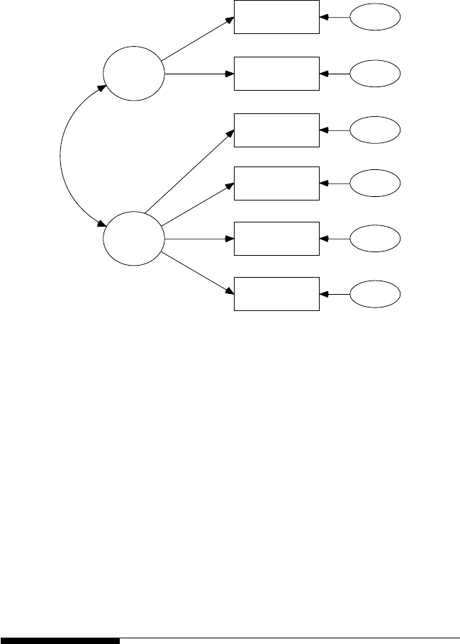
170 A Beginner’s Guide to Structural Equation Modeling
is given at the top of Table 8.1 along with the model implied (reproduced)
matrix, residual matrix, and standardized residual matrix for the mis-
specied model in Figure 8.2.
The rst column in Table 8.2 contains the standardized estimates for
the misspecied model (Figure 8.2), and the second column contains the
standardized estimates for the original model (Figure 8.1). The parameter
estimates are found to be signicantly different from zero (p < .05). The t
of the model is discussed in section 8.5. Of greatest importance is that all
of the factor loadings are statistically signicantly different from zero and
have the expected sign, that is, positive factor loadings.
8.5 Model Testing
An important part of the estimation process in analyzing conrmatory
factor models is to t the sample variance–covariance data to the specied
model. If the t of the model is good, then the specied model is supported
spatial
visperc
cubes
lozenges
wordmean
paragrap
sentence
err_v
err_c
err_l
err_p
err_s
err_w
verbal
FIGURE 8.2
Misspecied conrmatory factor model. (From Holzinger, K. J., & Swineford, F. A. [1939].
A study in factor analysis: The stability of a bi-factor solution. [Supplementary Educational
Monographs, No. 48]. Chicago, IL: University of Chicago, Department of Education.)
Y102005.indb 170 3/22/10 3:26:02 PM

Confirmatory Factor Models 171
by the sample data. If the t of the model is not so good, then the specied
model is not supported by the sample data, and the researcher typically
has to modify the model to achieve a better t (see section 8.6). As previ-
ously discussed in chapter 5, there is a wide variety of model-t indices
available to the SEM researcher.
TABLE 8.1
Original, Reproduced, Residual, and Standardized Residual Covariance
Matrices for the Misspecied Holzinger–Swineford Model
Original Matrix:
Variable Visperc Cubes Lozenges Parcomp Sencomp Wordmean
Visperc 49.064
Cubes 9.810 22.182
Lozenges 27.928 14.482 81.863
Parcomp 9.117 2.515 5.013 12.196
Sencomp 10.610 3.389 3.605 13.217 26.645
Wordmean 19.166 6.954 13.716 18.868 28.502 58.817
Reproduced Matrix:
Variable Visperc Cubes Lozenges Parcomp Sencomp Wordmean
Visperc 49.064
Cubes 9.810 22.182
Lozenges 5.098 1.646 81.863
Parcomp 8.595 2.775 5.266 12.196
Sencomp 12.646 4.083 7.747 13.061 26.645
Wordmean 18.570 5.996 11.376 19.180 28.218 58.817
Residual Matrix:
Variable Visperc Cubes Lozenges Parcomp Sencomp Wordmean
Visperc 0.000
Cubes 0.000 0.000
Lozenges 22.830 12.836 0.000
Parcomp 0.522 −0.260 −0.253 0.000
Sencomp −2.036 −0.694 −4.142 0.155 0.000
Wordmean 0.596 0.958 2.339 −0.312 0.283 0.000
Standardized Residual Matrix:
Variable Visperc Cubes Lozenges Parcomp Sencomp Wordmean
Visperc 0.000
Cubes 0.000 0.000
Lozenges 7.093 5.455 0.000
Parcomp 1.002 −0.668 −0.336 0.000
Sencomp −2.587 −1.182 −3.647 2.310 0.000
Wordmean 0.484 1.046 1.321 −2.861 1.696 0.000
Y102005.indb 171 3/22/10 3:26:02 PM

172 A Beginner’s Guide to Structural Equation Modeling
For our conrmatory factor model example, we report a few t indices at
the bottom of Table 8.2. For the misspecied model, the c2 statistic (techni-
cally a measure of badness of t) is equal to 80.926, with eight degrees of
freedom, and p < .001. The chi-square statistic is signicant, so the speci-
ed conrmatory factor model is not supported by the sample variance–
covariance data. Another interpretation is that because the c2 value is not
close to the number of degrees of freedom, the t of the initial model is poor.
Recall that the noncentrality parameter (NCP) is calculated as c2 – df, has
an expected value of 0 (NCP = 0; perfect t), and is used in computing sev-
eral of the model-t indices. A third criterion is that the root-mean-square
error of approximation (RMSEA) is equal to .174, higher than the acceptable
level of model t (RMSEA < .08 or .05). Finally, the goodness-of-t index
(GFI) is .918 for the misspecied model, which is below the acceptable
TABLE 8.2
Standardized Estimates and Selected Fit Indices for the
Misspecied and Original Holzinger–Swineford Models
Misspecied Model Original Model
Factor loadings:
Visual Perception .79 .78
Cubes .38 .43
Lozenges .20 .57
Paragraph Comprehension .85 .85
Sentence Completion .85 .85
Word Meaning .84 .84
Measurement error variances:
Visual Perception .38 .39
Cubes .86 .81
Lozenges .96 .68
Paragraph Comprehension .27 .27
Sentence Completion .28 .27
Word Meaning .30 .30
Correlation of independent variables:
(Spatial, Verbal) .52 .46
Selected fit Indices:
c280.926 24.407
Df 8 8
p value .001 .002
RMSEA .174 .083
GFI .918 .974
Y102005.indb 172 3/22/10 3:26:03 PM

Confirmatory Factor Models 173
range of model t (GFI > .95). Across this particular set of model-t indices,
the conclusion is that the model t is reasonable, although still not accept-
able, but that some model modication might allow us to achieve a better
sample data (variance–covariance matrix) to conrmatory factor model t.
Determining what change(s) to make to our conrmatory factor model to
achieve a better tting model is considered in the next section.
8.6 Model Modification
A nal step in structural equation modeling is to consider changes to a
specied model that has poor model-t indices—that is, model modica-
tion. This typically occurs when a researcher discovers that the t of the
specied model is less than satisfactory. The researcher typically performs
a specication search to nd a better tting model. As discussed in chap-
ter 4, several different procedures can be used to assist in this specication
search. One may eliminate parameters that are not signicantly different
from zero and/or include additional parameters to arrive at a modied
model. For the elimination of parameters, the most commonly used proce-
dure in LISREL is to compare the t statistic for each parameter to a tabled t
value—for example t = 1.96, at a = .05, two-tailed test; or t = 2.58 at a = .01,
two-tailed test (see Table A.2), to determine statistical signicance.
For the inclusion of additional parameters, the most commonly used
techniques in LISREL are (a) the modication index (MI—the expected
value that c2 would decrease if such a parameter were to be included in
the model; large values indicate potentially useful parameters), and (b) the
expected parameter change statistic (EPC—the approximate value of the
new parameter).
In addition, an examination of the residual matrix, or the more useful
standardized residual matrix, often gives clues as to which original cova-
riance terms or correlations are not well accounted for by the model. The
residual matrix is the difference between the observed covariance or cor-
relation matrix S and the model implied (reproduced) covariance or corre-
lation matrix Σ. Large residuals indicate values not well accounted for by
the model. Standardized residuals are like z scores such that large values
(values greater than 1.96 or 2.58) indicate that a particular relationship is
not well accounted for by the model.
For the misspecied conrmatory factor model in Figure 8.2, the origi-
nal, model-implied (reproduced), residual, and standardized residual
covariance matrices are given in Table 8.1. Here, we see that the two larg-
est residuals are for the Lozenges observed variable (22.830 and 12.836) and
the standardized residuals (7.093 and 5.455) are greater than t = 1.96 or
2.58. The results also indicate that the Lozenges variable should load on the
Y102005.indb 173 3/22/10 3:26:03 PM

174 A Beginner’s Guide to Structural Equation Modeling
Spatial Ability factor to reduce error (MI = 60.11) with an expected param-
eter change (EPC) of 6.30.
The large residuals for Lozenges, the statistically signicant standard-
ized residuals, the modication index, and the expected change value all
indicated that there was something wrong with the Lozenges observed
variable that is not captured by the misspecied model. Specically, the
factor loading for Lozenges should be on the Spatial Ability factor rather
than the Verbal Ability factor. This is precisely the factor loading from the
original specied model in Figure 8.1 that we intentionally eliminated to
illustrate the model modication process. Thus, the use of several modi-
cation criteria in our specication search was successful in obtaining the
original model in Figure 8.1.
The standardized estimates and selected model-t indices for the nal
model (Figure 8.1), where the modication in the Lozenges factor loading
is now included, and are shown in the second column of Table 8.2. All
of the parameters included are statistically signicantly different from
zero (p < .05), and all of the t indices now indicate an acceptable level of
t with no additional model modications indicated. Thus, we consider
this to be the nal best tting conrmatory factor model with our sample
variance-covariance data. The LISREL–SIMPLIS program is provided at
the end of the chapter for this model analysis.
8 . 7 S u m m a r y
This chapter discussed conrmatory factor models using the ve basic build-
ing blocks from model specication through model modication. We began
by analyzing a conrmatory factor model that was misspecied (Figure 8.2)
and interpreted a few model-t criteria where the t of the model was
deemed not acceptable. We then used model modication criteria to modify
the model, which yielded the conrmatory factor model in Figure 8.1. This
conrmatory factor model was deemed to be our nal best tting model.
This nal best tting model can be further validated by testing the same
conrmatory factor model with other samples of data (see chapter 12).
Appendix: LISREL–SIMPLIS Confirmatory
Factor Model Program
Confirmatory Factor Model Figure 8.1
Observed Variables:
VISPERC CUBES LOZENGES PARCOMP SENCOMP WORDMEAN
Y102005.indb 174 3/22/10 3:26:03 PM

Confirmatory Factor Models 175
Covariance Matrix
49.064
9.810 22.182
27.928 14.482 81.863
9.117 2.515 5.013 12.196
10.610 3.389 3.605 13.217 26.645
19.166 6.954 13.716 18.868 28.502 58.817
Sample Size: 301
Latent Variables: Spatial Verbal
Relationships:
VISPERC - LOZENGES = Spatial
PARCOMP - WORDMEAN = Verbal
Print Residuals
Number of Decimals = 3
Path Diagram
End of problem
Exercise
1. Test the following hypothesized conrmatory factor model
(Figure 8.3) using the LISREL computer software program:
Sample Size: 3094
Observed variables:
Academic ability (Academic)
Self-concept (Concept)
Degree aspirations (Aspire)
Degree (Degree)
Occupational prestige (Prestige)
Income (Income)
Correlation matrix:
Academic Concept Aspire Degree Prestige Income
1.000
0.487 1.000
0.236 0.206 1.000
0.242 0.179 0.253 1.000
0.163 0.090 0.125 0.481 1.000
0.064 0.040 0.025 0.106 0.136 1.000
Hypothesized CFA model: The CFA model indicates that the
rst three observed variables measure the latent variable
Academic Motivation (Motivate) and the last three observed
variables measure the latent variable Socioeconomic Status
(SES). Motivate and SES are correlated.
Then modify the model to achieve a better model t as shown in
Figure 8.4.
Y102005.indb 175 3/22/10 3:26:03 PM
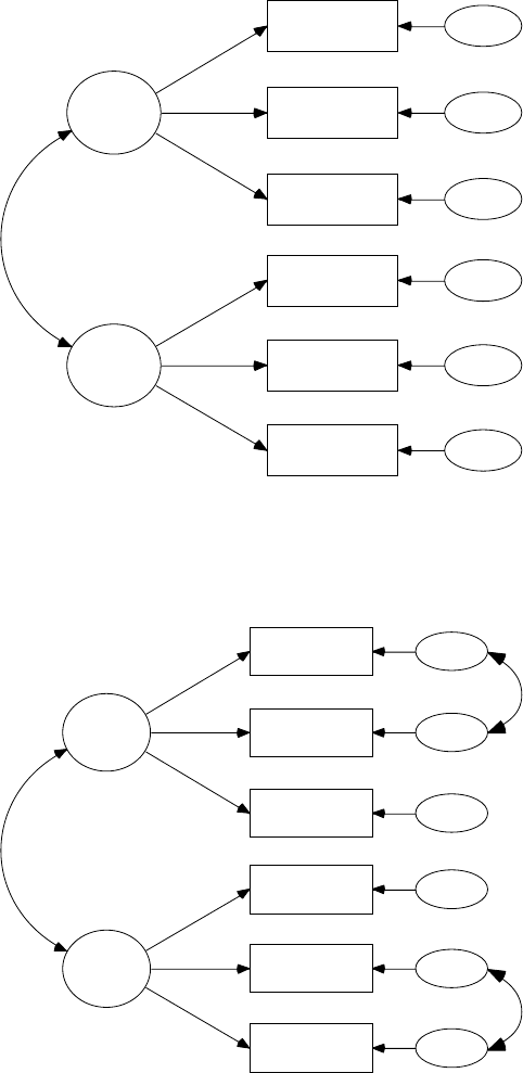
176 A Beginner’s Guide to Structural Equation Modeling
Motivate
Academic
Concept
Aspire
Income
Degree
Prestige
err_ad
err_c
err_l
err_d
err_p
err_i
SES
FIGURE 8.4
Final CFA model for exercise.
Motivate
Academic
Concept
Aspire
Income
Degree
Prestige
err_ad
err_c
err_l
err_d
err_p
err_i
SES
FIGURE 8.3
Hypothesized CFA model for exercise.
Y102005.indb 176 3/22/10 3:26:04 PM

Confirmatory Factor Models 177
References
Cochran, W. G. (1968). Errors of measurement in statistics. Technometrics, 10,
637–666.
Comrey, A. L., & Lee, H. B. (1992). A rst course in factor analysis. Hillsdale, NJ:
Lawrence Erlbaum.
Costello, A. B., & Osborne, J. (2005). Best practices in exploratory factor analy-
sis: four recommendations for getting the most from your analysis. Practical
Assessment Research and Evaluation, 10(7), 1–9.
Fuller, W. A. (1987). Measurement error models. New York: Wiley.
Gorsuch, R. L. (1983). Factor analysis (2nd ed.). Hillsdale, NJ: Lawrence Erlbaum.
Harmon, H. H. (1976). Modern factor analysis (3rd ed., rev.). Chicago: University of
Chicago Press.
Holzinger, K. J., & Swineford, F. A. (1939). A study in factor analysis: The stability
of a bi-factor solution. (Supplementary Educational Monographs, No. 48).
Chicago, IL: University of Chicago, Department of Education.
Jöreskog, K. G., & Sörbom, D. (1993). LISREL 8: Structural equation modeling with the
SIMPLIS command language. Chicago, IL: Scientic Software International.
Y102005.indb 177 3/22/10 3:26:04 PM

179
9
Developing Structural Equation
Models: Part I
Key Concepts
Latent independent and dependent variables
Observed independent and dependent variables
Developing structural models with latent variables
Establishing relationships between latent variables
Covariance terms
The four-step approach to SEM modeling
Structural equation models have been developed in a number of academic
disciplines to substantiate and test theory. Structural equation models
have further helped to establish the relationships between latent variables
or constructs, given a theoretical perspective. The structural equation
modeling approach involves developing measurement models to dene
latent variables and then establishing relationships or structural equation
models with the latent variables. The focus of this chapter is on provid-
ing researchers with a better understanding of how to develop structural
equation models. An attempt is made to minimize matrix and statistical
notation so that the reader can better understand the structural equation
modeling approach.
This chapter begins with a more extensive discussion of observed vari-
ables and latent variables, and then proceeds with sections on the mea-
surement model, the structural model, variances and covariance terms,
and nally the two-step/four-step approaches to structural equation
modeling. Chapter 10 extends the development of SEM models in exam-
ining model specication, model identication, model estimation, model
testing, and model modication.
Y102005.indb 179 3/22/10 3:26:04 PM

180 A Beginner’s Guide to Structural Equation Modeling
9.1 Observed Variables and Latent Variables
In structural equation modeling, as in traditional statistics, we use X and
Y to denote the observed variables. We use X to refer to independent (or
predictor) variables and Y to refer to dependent (or criterion) variables; this
is the same in multiple regression, analysis of variance, and all general lin-
ear models. In structural equation modeling, however, we further dene
latent independent variables using observed variables denoted by X and
latent dependent variables using observed variables denoted by Y. Latent
independent and dependent variables are created with observed variables
using conrmatory factor models discussed in the previous chapter.
There are two major types of variables in structural equation modeling:
observed (indicator) variables and latent (construct) variables. Latent vari-
ables are not directly observable or measured, rather they are observed or
measured indirectly, and hence they are inferred constructs based on what
observed variables we select to dene the latent variable. For example,
intelligence is a latent variable and represents a psychological construct.
Intelligence cannot be directly observed, for example, through visual
inspection of an individual, and thus there is no single agreed upon de-
nition for intelligence. However, intelligence can be indirectly measured
through observed or indicator variables, for example, specic IQ tests.
Observed or indicator variables are variables that are directly observable
or measured. For example, the Wechsler Intelligence Scale for Children–
Revised (WISC-R) is an instrument commonly used to measure children’s
intelligence. The instrument represents one denition or measure of what
we mean by intelligence. Other researchers rely on other denitions or
observed measures, and thus on other instruments, for example, the
Stanford–Binet Intelligence Scale. Latent variables such as intelligence are
not directly observable or measured, but can be indirectly observed or
measured by using several observed (indicator) variables, for example, IQ
tests such as the WISC-R and the Stanford–Binet Intelligence Scale.
Let us further examine the concept of latent variables as they are used
in structural equation models. Consider a basic structural equation model
in which we propose that a latent independent variable predicts a latent
dependent variable. For instance, Intelligence (latent independent variable)
is believed to predict subsequent Scholastic Achievement (latent dependent
variable), which could be depicted as
Intelligence → Achievement
Any latent variable that is predicted by other latent variables in a structural
equation model is known as a latent dependent variable. A latent dependent
variable, therefore, must have at least one arrow pointing to it from another
Y102005.indb 180 3/22/10 3:26:04 PM
Developing Structural Equation Models: Part I 181
latent variable, sometimes referred to as an endogenous latent variable. Any
latent variable that does not have an arrow pointing to it from another latent
variable is known as a latent independent variable, sometimes referred to as an
exogenous latent variable. As shown in the foregoing example, the latent inde-
pendent variable Intelligence does not have any arrows pointing to it from
another latent variable. In our basic structural equation model, Intelligence
is the latent independent variable with no direct lines or arrows pointing to
it, and Achievement is the latent dependent variable because it has an arrow
pointing to it from Intelligence.
Consider adding a third latent variable to our basic structural equa-
tion model, such that Achievement is measured at two points in time. This
model would be depicted as follows:
Intelligence → Achievement1 → Achievement2.
Intelligence is still a latent independent variable. Achievement2 is clearly a
latent dependent variable because there is an arrow pointing to it from
Achievement1. However, there is an arrow pointing to Achievement1 from
Intelligence and another arrow pointing from Achievement1 to Achievement2.
This basic structural equation model indicates that Achievement1 is
predicted by Intelligence, but then Achievement1 predicts Achievement2.
Achievement1 is rst a dependent latent variable and then an independent
latent variable. This type of structural equation model is possible and
illustrates indirect effects using latent variables. Achievement1 in this basic
structural equation model is a mediating latent variable. Our designation
of a latent variable as independent or dependent is therefore determined
by whether or not an arrow is drawn from one latent variable to another
latent variable. If no arrows point to a latent variable from another latent
variable in the structural equation model, then it is a latent independent
variable. If an arrow points to a latent variable from another latent variable
in the structural equation model, then it is a latent dependent variable.
Next, we consider the concept behind the observed or indicator vari-
ables. The latent independent variables are measured by observed inde-
pendent variables via a conrmatory factor analysis measurement model
and traditionally denoted by X. The latent dependent variables are mea-
sured by observed dependent variables via a conrmatory factor analysis
measurement model and traditionally denoted by Y. Following our exam-
ple, we might choose the WISC-R and the Stanford–Binet Intelligence
Scale as observed independent measures of the latent independent vari-
able Intelligence. We can denote these observed variables as X1 and X2. For
each of the achievement latent variables, we might choose the California
Achievement Test and the Metropolitan Achievement Test as our observed
dependent measures. If these measures are observed at two points in time,
then we can denote the observed variables of Achievement1 as Y1 and Y2,
Y102005.indb 181 3/22/10 3:26:05 PM
182 A Beginner’s Guide to Structural Equation Modeling
and those of Achievement2 as Y3 and Y4, respectively. In our SEM model,
each latent variable is measured by two observed variables.
What is the benet of using more than one observed variable to assess a
latent variable? In using a single observed variable to assess a latent vari-
able, we assume that no measurement error is associated with the measure-
ment of that latent variable. In other words, it is assumed that the latent
variable is perfectly measured by the single observed variable, which is
typically not the case. We dene measurement error quite generally here to
include errors due to reliability and validity issues (see chapter 8).
Reliability is concerned with the ability of a measure (score) to be con-
sistent, commonly referred to as internal consistency, consistency over
time, and consistency using similar measures, to denote different types
of measurement error associated with observed variable scores. Would
Jamie’s score on the WISC-R be about the same if measured today as com-
pared with next week? Evidence of score reliability (consistency) could be
shown when a measure is given to the same group of individuals at two
points in time, and the scores are roughly equivalent. If only a single mea-
sure of a latent variable is used and it is not very reliable, then our latent
variable is not dened very well. If the reliability of a single observed
measure of a latent variable is known, then it is prudent to specify or
x the measurement error in the SEM model. This is accomplished, for
example, in LISREL–SIMPLIS by setting the error variance of the single
variable. The error variance of a single variable is determined by the fol-
lowing formula:
Error Variance of X1 = (1 − reliability coefcient) (s2X1).
If the reliability of scores for X1 is .85 with a standard deviation of 5.00,
then the error variance would be computed as:
X1error variance = (1 − .85) (5.00)2 = .15 (25) = 3.75.
In the LISREL–SIMPLIS program, you would then add the following com-
mand line to set the error variance for X1:
Set the error variance of X1 to 3.75
Validity is concerned with the extent to which scores accurately dene
a construct, which is score inference—commonly referred to as content,
factorial, convergent–divergent, and discriminant validity—to denote dif-
ferent types of score inference associated with observed scores. Our inter-
est in validity is how well we can make an inference from the measured
scores to the latent variable; that is, how well do test scores indicate what
they purport to measure. Does Jamie’s score on the WISC-R really measure
Y102005.indb 182 3/22/10 3:26:05 PM
Developing Structural Equation Models: Part I 183
her intelligence or something else, such as her height? Evidence of validity
is shown when two indicators of the same latent variable are substantially
correlated. For example, if WISC-R and height were used as indicators
of the latent variable Intelligence, we would expect them to not be corre-
lated. If only a single measure of a latent variable is used and the score is
not valid (for example, if height is used to measure intelligence), then our
latent variable is not well dened. Establishing the reliability of scores for
our observed variable helps in estimating the validity coefcients (factor
loadings) in our measurement model because score validity is limited by
the reliability of the observed variable scores; that is, the maximum valid-
ity coefcient is less than or equal to the product of the square roots of the
two reliability coefcients,
ρρρ
XY XX YY
≤′′
.
If we selected WISC-R and height as observed indicator variables for
the latent independent variable Intelligence it would certainly not be well
dened and would include measurement error. The selection of only
height as an observed indicator of Intelligence would increase the measure-
ment error and poorly dene the construct. Consequently, in selecting
observed variables to dene a latent variable, we need to select observed
variables that show evidence of both score reliability and score validity
for the intended purpose of our study. Because of the inherent difculty
involved in obtaining reliable and valid measures with a single observed
variable, we strongly encourage you to consider multiple indicator vari-
ables for each latent independent and dependent variable in the structural
equation model.
There are a few obvious exceptions to this recommendation, especially
when research indicates that only one observed variable is available. In this
case, you have no other choice than to dene the latent variable using a
single observed variable or use the observed variable in a Multiple Indicator
Multiple Indicator Cause (MIMIC) model (see chapter 15). Jöreskog and Sörbom
(1993, p. 37, EX7A.SPL) provided the rationale and gave an example for setting
the error variance of a single observed variable (VERBINTM) in dening
the latent variable Verbint. The verbal intelligence test (VERBINTM) was
a fallible (unreliable) measure of the latent variable Verbint, and therefore
it was unreasonable to assume that the error variance was zero (perfectly
reliable). Consequently, the sample reliability coefcient for VERBINTM
was assumed to be rXX’ = .85 rather than 1.00 (perfectly reliable, zero error
variance). The assumed value of the reliability coefcient, hence desig-
nation of the error variance for VERBINTM, will affect parameter esti-
mates as well as standard errors. A reliability coefcient of rXX’ = .85 for
VERBINTM is equivalent to an error variance of 0.15 times the variance of
VERBINTM (3.65)2. The assumed error variance of VERBINTM was com-
puted as .15 (3.65)2 = 1.998.
If we can assume a reasonable reliability coefcient for an observed
variable, then multiplying the observed variable’s variance by 1 minus the
Y102005.indb 183 3/22/10 3:26:05 PM

184 A Beginner’s Guide to Structural Equation Modeling
reliability coefcient provides a reasonable estimate of error variance. In
the LISREL–SIMPLIS program EX7B.SPL, the error variance for the single
observed variable VERBINTM is accomplished by using the SET com-
mand as follows:
SET the error variance of VERBINTM to 1.998
Later in this chapter we show how measurement error is explicitly a part
of any structural equation model. The basic concept, however, is that
multiple observed variables used in dening either a latent indepen-
dent variable or a latent dependent variable permit measurement error
to be estimated through structural equation modeling. This provides the
researcher with additional information about the measurement charac-
teristics of the observed variables. When there is only a single observed
indicator of a latent variable, then measurement error cannot be estimated
through structural equation modeling, but can be xed to a certain value.
Most SEM software programs, such as LISREL, permit the specication
of error variance for single or multiple variables, whether the values are
known or require our best guess. In the next two sections we discuss the
two approaches that make up structural equation modeling: the measure-
ment model and the structural model.
9.2 Measurement Model
As previously mentioned, the researcher species the measurement model
to dene the relationships between the latent variables and the observed
variables. The measurement model in SEM is a conrmatory factor model.
Using our previous example, the latent independent variable Intelligence is
measured by two observed variables, the WISC-R and the Stanford–Binet
Intelligence Scale. Our other latent variables Achievement1 (dependent latent
variable) and Achievement2 (dependent latent variable) are each measured
by the same two observed variables, the California Achievement Test and
the Metropolitan Achievement Test, but at two different times. Both of these
observed variables are composite or scale scores from summing numerous
individual items. In chapter 8, we pointed out that individual items on an
instrument could be used to create a construct (latent variable); hence, con-
rming the unidimensionality of the construct, while taking into account
the observed variable score reliability and t of the measurement model.
The use of many individual items rather than the composite score or item
parcels—that is, collections of individual items as the observed measures
of a latent variable—increases the degrees of freedom in the measurement
model and can cause problems in model t. Measurement characteristics
Y102005.indb 184 3/22/10 3:26:05 PM
Developing Structural Equation Models: Part I 185
at the item level might be more appropriate for exploratory data reduction
methods than they are for SEM measurement models.
The researcher is typically interested in having the following questions
answered about the observed variables: To what extent are the observed
variables actually measuring the hypothesized latent variable; for exam-
ple, how good is the California Achievement Test as a measure of achieve-
ment? Which observed variable is the best measure of a particular latent
variable; for example, is the California Achievement Test a better measure
of achievement than the Metropolitan Achievement Test? To what extent
are the observed variables actually measuring something other than the
hypothesized latent variable? For example, is the California Achievement
Test measuring something other than achievement, such as the quality of
education received? These types of questions need to be addressed when
creating the measurement models that dene the latent variables.
In our measurement model example each latent variable is dened by
two indicator variables. The relationships between the observed vari-
ables and the latent variables are indicated by factor loadings. The factor
loadings provide us with information about the extent to which a given
observed variable is able to measure the latent variable (a squared fac-
tor loading indicates variable communality or amount of variance shared
with the factor). The factor loadings are referred to as validity coefcients
because multiplying the factor loading times the observed variable score
indicates how much of the observed variable score variance is valid (true
score). The observed variable measurement error is dened as that por-
tion of the observed variable score that is measuring something other
than what the latent variable is hypothesized to measure. It serves as a
measure of error variance, and hence assesses the observed variable score
reliability. Measurement error could be the result of (a) an observed vari-
able that is measuring some other latent variable, (b) unreliability, or (c) a
higher second order factor. For example, the California Achievement Test
may be measuring something besides achievement, or it may not yield
very reliable scores. Thus, we would like to know how much measure-
ment error is associated with each observed variable.
In our measurement model there are six measurement equations, one
for each observed variable, which can be illustrated as follows:
California1 = function of Achievement1 + error
Metropolitan1 = function of Achievement1 + error
California2 = function of Achievement2 + error
Metropolitan2 = function of Achievement2 + error
WISC-R = function of Intelligence + error
Stanford–Binet = function of Intelligence + error
Y102005.indb 185 3/22/10 3:26:06 PM

186 A Beginner’s Guide to Structural Equation Modeling
In the LISREL–SIMPLIS program, an explicit denition of the measure-
ment model can be done by specifying measurement equations. One can
expand the variable labels in the measurement model equations using up
to eight characters; the labels are case-sensitive (upper and lower char-
acters are recognized). The measurement model equations are specied,
using either the Relationships: or Paths: command (both methods are equiv-
alent). For the Relationships: command, both the latent variables and the
observed variables can be written using eight-character variable names.
The observed variables are given on the left-hand side of the equation with
spaces between the multiple observed variable names (Cal1, Metro1, Cal2,
Metro2, WISCR, and Stanford) and the latent variables on the right-hand
side of the equation (Achieve1, Achieve2, and Intell). The LISREL–SIMPLIS
measurement equations follow where Achieve1 refers to Achievement1,
Intell refers to Intelligence, Achieve2 refers to Achievement2, Cal1 refers to
California1, Metro1 refers to Metropolitan1, Cal2 refers to California2, Metro2
refers to Metropolitan2, WISCR refers to WISC-R, and Stanford refers to
Stanford–Binet). The command line for Relationships would be written as:
Relationships:
Cal1 Metro1 = Achieve1
Cal2 Metro2 = Achieve2
WISCR Stanford = Intell
For the Paths: command, the latent variables are depicted to the left of the
arrow and the observed variables to the right of the arrow with spaces
between the multiple observed variable names. The command line for
Paths in the following measurement equation would be written as:
Paths:
Achieve1 → Cal1 Metro1
Achieve2 → Cal2 Metro2
Intell → WISCR Stanford
9.3 Structural Model
In chapter 8 we discussed the rationale and process for specifying a
measurement model to indicate whether the latent variables are mea-
sured well, given a set of observed variables. If the latent variables
Y102005.indb 186 3/22/10 3:26:06 PM
Developing Structural Equation Models: Part I 187
(independent and dependent) are measured well, we then specify
a structural model to indicate how these latent variables are related.
The researcher species the structural model to allow for certain rela-
tionships among the latent variables depicted by the direction of the
arrows. In our example we hypothesized that intelligence and achieve-
ment are related in a specic way. We hypothesized that intelligence
predicts later achievement. The hypothesized structural model can now
be specied and tested to determine the extent to which these a priori
hypothesized relationships are supported by our sample variance–
covariance data; that is, Can intelligence predict achievement? Could
there be other latent variables that we need to consider to better predict
achievement? These types of questions are addressed when specifying
the structural model.
At this point we need to provide a more explicit denition of the struc-
tural model and a specic notational system for the latent variables under
consideration. Let us return to our previous example where we indicated
a specic hypothesized relationship for the latent variables:
Intelligence → Achievement1 → Achievement2 .
The hypothesized relationships for the latent variables indicate two latent
dependent variables, so there will be two structural equations. The rst
equation should indicate that Achievement1 is predicted by Intelligence.
The second equation should indicate that Achievement2 is predicted by
Achievement1. These two equations can be illustrated as follows:
Achievement1 = structure coefcient1 * Intelligence + error
Achievement2 = structure coefcient2 *Achievement1 + error
These two equations specify the estimation of two structure coefcients
to indicate the magnitude (strength as well as statistical signicance)
and direction (positive or negative) of the prediction. Each structural
equation also contains a prediction error or disturbance term that indi-
cates the portion of the latent dependent variable that is not explained
or predicted by the other latent variables in that equation. In our exam-
ple there are two structure coefcients, one for Intelligence predicting
Achievement1 and one for Achievement1 predicting Achievement2. Because
there are two structural equations, there are two prediction errors or
disturbances.
The LISREL–SIMPLIS command language permits an easy way to spec-
ify structural equations among the latent variables. The structural model
can be denoted in terms of either the Relationships: or Paths: commands
Y102005.indb 187 3/22/10 3:26:06 PM
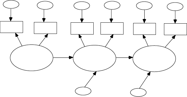
188 A Beginner’s Guide to Structural Equation Modeling
(both methods are equivalent). For the Relationships: command, the latent
variables can be written using eight-character variable names with the
latent dependent variables on the left side of the equation (where Achieve1
refers to Achievement1, Intell refers to Intelligence, and Achieve2 refers to
Achievement2):
Relationships:
Achieve1 = Intell
Achieve2 = Achieve1
For the Paths: command, these latent dependent variables are to the right
of the arrow, as in the following structural equations:
Paths:
Intell → Achieve1
Achieve1 → Achieve2
(NOTE: You do not need to indicate the prediction error in LISREL–
SIMPLIS structural equations for either the Relationships: or Paths: com-
mands because these are known to exist and automatically estimated by
the program.)
The path diagram of the measurement and structural models for our
example is shown in Figure 9.1.
Intell Achieve1 Achieve2
WISCR Stanford Cal1 Metro1 Cal2 Metro2
errorerrorerrorerrorerrorerror
errorerror
FIGURE 9.1
Achievement path model.
Y102005.indb 188 3/22/10 3:26:06 PM

Developing Structural Equation Models: Part I 189
9.4 Variances and Covariance Terms
In structural equation modeling, the term covariance structure analysis or
covariance structure modeling is often used because the estimation of factor
loadings and structure coefcients involves the decomposition of a sample
variance–covariance matrix. In this section we further explore the notion
of variance–covariance as it relates to observed and latent variables. There
are three different variance–covariance terms that we need to dene and
understand. In the structural model there are two variance–covariance
terms to consider. First, there is a variance–covariance matrix of the latent
independent variables. This consists of the variances for each latent inde-
pendent variable, as well as the covariance terms among them. Although
we are interested in the variances (the amount of variance associated with
the latent independent variable intelligence), the covariance terms may or
may not be part of our theoretical model. In our model there is only one
latent independent variable, so there is only one variance term and no
covariance term.
If we specied two latent independent variables in a different struc-
tural equation model, for example, Intelligence and Home Background, we
could include a covariance term for them. We would then be hypothesiz-
ing that Intelligence and Home Background are correlated or covary because
we believe that some common unmeasured latent variable is inuencing
both of them. We could hypothesize that a latent variable not included in
the model, such as Parenting Ability, inuences both Intelligence and Home
Background. In other words, Intelligence and Home Background co-vary, or
are correlated, because of their mutual inuence from Parenting Ability,
which has not explicitly been included in the model (but which perhaps
could be included).
In the LISREL–SIMPLIS program, the variance term would automati-
cally be given or implied in the output for the latent independent variable
Intelligence. A covariance term, if one existed, would also automatically
be given or implied in the output. If one desired the two latent indepen-
dent variables, Intelligence and Home Background, to be uncorrelated or to
have a covariance of zero, then one would specify the following in the
LISREL–SIMPLIS program:
Set the Covariance between Intell and HomeBack to 0
The second set of variance–covariance terms that we need to dene and
understand is in the covariance matrix of the structural equation model for
prediction errors. This consists of the variances for each structural equa-
tion prediction error (the amount of unexplained variance for each struc-
tural equation), as well as covariance terms among them. Although we are
Y102005.indb 189 3/22/10 3:26:07 PM
190 A Beginner’s Guide to Structural Equation Modeling
interested in the variances, the covariance terms may or may not be part of
our model. We could specify that two structural equation prediction errors
are correlated, perhaps because some unmeasured latent variable is lead-
ing to error in both equations. An example of this might be where Parental
Occupational Status (parent income) is not included as a latent variable in
a model where Children’s Education (in years) and Children’s Occupational
Status (income at age 30 years) are latent dependent variables. The struc-
tural equations for Children’s Education and Children’s Occupational Status
would then both contain structural equation prediction error due to the
omission of Parental Occupational Status. Because the same latent variable
was not included in both equations, we expect that the structural equation
prediction errors would be correlated. (Note: Our hypothesized structural
model does not contain any such covariance terms.)
In the LISREL–SIMPLIS program, the variance terms are automatically
included in the output for each structural equation. Because the covari-
ance terms are assumed by the program to be set to zero, one must spec-
ify any covariance terms one wants estimated. A covariance term, if one
existed between Achievement1 and Achievement2, would be specied using
the following command:
Set the Error Covariance between Achieve1 and Achieve2 free
The third set of variance–covariance terms is from the measurement
model. Here, we need to dene and understand the variances and cova-
riance terms of the measurement errors. Although we are interested in
the variances (the amount of measurement error variance associated with
each observed variable), the covariance terms may or may not be part of
our model. We could hypothesize that the measurement errors for two
observed variables are correlated (known as correlated measurement error).
This might be expected in our example model where the indicators of the
latent variables Achievement1 and Achievement2 are the same—for example,
from using the California Achievement Test at two different times. We
might believe that the measurement error associated with the California
Achievement Test at Time 1 is related to the measurement error for the
California Achievement Test at Time 2.
In the LISREL–SIMPLIS program, the variance terms are automatically
specied in the program for each observed variable. Once again, the cova-
riance terms are assumed by the program to be set to zero; so we must
specify any covariance term of interest and allow it to be estimated. A
covariance term, if one existed between the measurement errors for the
California Achievement Test at Times 1 and 2, would be specied using
the following command:
Set the Error Covariance between Cal1 and Cal2 free
Y102005.indb 190 3/22/10 3:26:07 PM

Developing Structural Equation Models: Part I 191
There is one nal variance–covariance term that we need to mention,
and it really represents the ultimate variance–covariance for our com-
bined measurement model and structural model. From the structure
coefcient parameters we estimate in the structural model, the factor
loadings in the measurement model(s), and all of the variance–covariance
terms, we generate an ultimate matrix of variance–covariance terms for
the overall SEM model. This variance–covariance matrix is implied by
the overall model and is denoted by Σ (see chapter 17 for a representa-
tion of all of these matrices). Our goal in structural equation modeling
is to estimate all of the parameters in the overall model and test the
overall t of the model to the sample variance–covariance data. In short,
the parameters in our overall SEM model create an implied variance–
covariance matrix Σ from the sample variance–covariance matrix S,
which contains the sample variances and covariance terms among our
observed variables. We interpret our model-t indices (see chapter 5) to
determine the level of model t between Σ and S (closeness of the val-
ues in the variance–covariance matrix Σ implied by our hypothesized
model, and the sample variance–covariance matrix S given our sample
data). We also examine the magnitude (strength as well as statistical sig-
nicance of parameter estimates) and the direction (positive or negative
coefcients) to provide a meaningful interpretation of our SEM model
results.
9.5 Two-Step/Four-Step Approach
James, Mulaik, and Brett (1982) proposed a two-step modeling approach
that emphasized the analysis of the two conceptually distinct latent vari-
able models: measurement models and structural models. Anderson and
Gerbing (1988) described their approach by stating that the measurement
model provides an assessment of convergent and discriminant validity,
and the structural model provides an assessment of predictive validity.
Mulaik et al. (1989) also expanded the idea of assessing the t of the struc-
tural equation model among latent variables (structural model) indepen-
dently of assessing the t of the observed variables to the latent variables
(measurement model). Their rationale was that even with few latent vari-
ables, most parameter estimates dene the relationships of the observed
variables to the latent variables in the measurement model, rather than
the structural relationships of the latent variables themselves. Mulaik and
Millsap (2000) further elaborated a four-step approach discussed in chap-
ter 5. Jöreskog and Sörbom (1993, p. 113) had earlier summarized many of
their thoughts by stating:
Y102005.indb 191 3/22/10 3:26:07 PM

192 A Beginner’s Guide to Structural Equation Modeling
The testing of the structural model, i.e., the testing of the initially
specied theory, may be meaningless unless it is rst established that
the measurement model holds. If the chosen indicators for a construct
do not measure that construct, the specied theory must be modied
before it can be tested. Therefore, the measurement model should be
tested before the structural relationships are tested.
We have found it prudent to follow their advice. In the establishment of
measurement models, it is best to identify a few good indicators of each
latent variable with three or four indicators being recommended. In our
example, we intentionally used only a few indicators to dene or measure
the latent variables to keep the model simple. We have also found that
when selecting only a few indicator variables, it is easier to check how
well each observed variable denes a latent variable—that is, to examine
the factor loadings, reliability coefcients, and the amount of latent vari-
able variance explained. For example, rather than use individual items
as indicator variables, sum the items to form a total test score or a parcel
score (composite score or scale score). In addition, one can calculate the
reliability of the composite (scale) score and even consider xing the value
of the relevant measurement error variance in the model (as described in
section 9.1), thus reducing the need to estimate one parameter. It is only
after latent variables are adequately dened (measured) that it makes
sense to examine latent variable relationships in a structural model. We
think a researcher with adequately measured latent variables is in a bet-
ter position to establish a substantive, meaningful structural model, thus
supporting theory.
9 . 6 S u m m a r y
This chapter focused on how to develop structural equation models. We
began with a more detailed look at both observed and latent variables.
Next, we discussed the measurement and structural models. We extended
some of the basic concepts found in conrmatory factor models (measure-
ment models) and regression/path models (structural models) to structural
equation modeling. We then described three types of variance–covariance
matrices typically utilized in structural equation models. The chapter con-
cluded with a discussion of the popular two-step/four-step approaches
to structural equation modeling. In chapter 10 we extend our discussion
of the development of structural equation models by considering model
specication, model identication, model estimation, model testing, and
model modication, utilizing a more complex hypothesized theoretical
model.
Y102005.indb 192 3/22/10 3:26:07 PM

Developing Structural Equation Models: Part I 193
Exercises
1. Diagram two indicator variables X1 and X2 of a latent vari-
able LV.
2. Diagram two observed variables X1 and X2 that predict a third
observed variable Y. X1, and X2 are correlated.
3. Diagram a latent independent variable LIV predicting a latent
dependent variable LDV.
4. Would you use a single indicator of a latent variable? Why or
why not?
References
Anderson, J. C., & Gerbing, D. W. (1988). Structural equation modeling in practice:
A review and recommended two-step approach. Psychological Bulletin, 103,
411–423.
James, L. R., Mulaik, S. A., & Brett, J. M. (1982). Causal analysis: Assumptions, models,
and data. Los Angeles, CA: Sage.
Jöreskog, K. G., & Sörbom, D. (1993). LISREL 8: Structural equation modeling with the
SIMPLIS command language. Chicago: Scientic Software International.
Mulaik, S. A., James, L. R., Alstine, J. V., Bennett, N., Lind, S., & Stilwell, C. D.
(1989). Evaluation of goodness-of-t indices for structural equation models.
Psychological Bulletin, 105, 430–445.
Mulaik, S. A., & Millsap, R. E. (2000). Doing the four-step right. Structural Equation
Modeling, 7, 36–73.
Y102005.indb 193 3/22/10 3:26:07 PM

195
10
Developing Structural Equation
Models: Part II
Key Concepts
Factor loadings and measurement errors
Structure coefcients and prediction errors
Variance and covariance terms
Specication search
In chapter 9 we presented the basic framework for the development of
structural equation models. We focused on the measurement model, the
structural model, and the different variance–covariance terms. These
constitute the basic building blocks for analyzing and interpreting a
structural equation model. In this chapter we extend our discussion of the
development of structural equation models. We present a hypothesized
theoretical structural equation model and discuss issues related to model
specication, model identication, model estimation, model testing, and
model modication in the context of that example.
10.1 An Example
We hypothesized a structural equation model based on predicting educa-
tional achievement as a latent dependent variable. The structural model is
diagrammed in Figure 10.1 with four latent variables drawn as ellipses: two
latent independent variables, home background (Home) and Ability, and two
latent dependent variables, aspirations (Aspire) and achievement (Achieve).
Three of the latent variables are dened by using two indicator vari-
ables, and one latent variable, Home, is dened by using three indicator
variables in the measurement model. The indicator variables are depicted
using rectangles as follows: (a) for Home, family income (FamInc), father’s
education (FaEd) and mother’s education (MoEd); (b) for Ability, verbal
Y102005.indb 195 3/22/10 3:26:07 PM
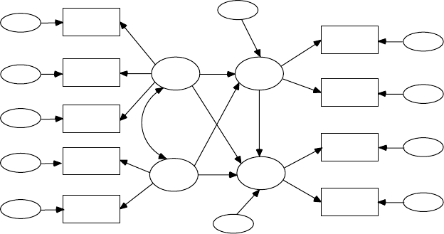
196 A Beginner’s Guide to Structural Equation Modeling
ability (VerbAb) and quantitative ability (QuantAb); (c) for Aspire, educa-
tional aspiration (EdAsp) and occupational aspiration (OcAsp); and (d)
for Achieve, verbal achievement (VerbAch) and quantitative achievement
(QuantAch).
The measurement models for each latent variable identify which observed
variables dene that particular latent variable. An arrow is drawn from the
latent variable to each of its observed indicator variables. For each arrow,
we understand that a factor loading will be computed. For example, the
observed measures of family income, father’s education and mother’s edu-
cation dene the latent variable Home, with each observed variable having a
factor loading estimated. Figure 10.1 has nine arrows going from the latent
variables drawn as ellipses to observed variables drawn as rectangles, thus
nine factor loadings will be estimated.
In Figure 10.1 each observed variable has a unique measurement error.
This is indicated by an arrow pointing to each observed variable and
shows that some portion of each observed variable is measuring some-
thing other than the hypothesized latent variable. For example, mother’s
education (MoEd) is hypothesized to dene Home (home background), but
it may also be assessing other latent variables, a function of other variables
not in the model, random, or systematic error. The unique measurement
error is estimated for each observed variable, so there will be nine unique
measurement errors estimated. Each observed variable has a factor load-
ing and a unique measurement error that forms an equation to compute
the latent variable score; for example,
MoEd = factor loading * Home + measurement error
Home
FamInc
Aspire
AbilityAchieve
FaEd
MoEd
VerbAb
QuantAb
EdAsp
OcAsp
VerbAch
QuantAch
1
11
1
error
error
error
error
error
error
error
error
error
error
error
FIGURE 10.1
Structural equation model of educational achievement.
Y102005.indb 196 3/22/10 3:26:08 PM

Developing Structural Equation Models: Part II 197
Our model diagram does not include any curved arrows for measurement
error, but this issue should be discussed. A curved arrow between two mea-
surement error terms is possible and indicates that the measurement error
terms are correlated. Two measurement error terms could be correlated if
they share something in common, such as common method variance, or if
the same measure is being used at different points in time. For example,
quantitative ability (QuantAb) and quantitative achievement (QuantAch) may
have correlated measurement error terms, for example, because they rep-
resent two measures of quantitative skills. Correlated measurement error
terms may also exist for father’s education (FaEd) and mother’s education
(MoEd), for example, because using the same method of measurement, the
errors for one parent might be reected in the other parent.
A straight arrow leading from a latent variable to a latent dependent vari-
able designates that a structure coefcient is to be estimated. For example,
it was hypothesized that Home (home background) predicts Aspire (aspira-
tions). The structure coefcients we want to estimate in our hypothesized
structural model come from a review of prior research and theory. In our
hypothesized structural model there are ve structure coefcients we want
to estimate. Each latent dependent variable has one or more structure coef-
cients and a unique prediction error that forms an equation; for example,
Aspire = structure coefcient * Home + structure coefcient * Ability
+ prediction error
The prediction error for Aspire indicates that some portion of Aspire (aspi-
ration) is not predicted by the latent independent variables Home and
Ability. There are two equations in our hypothesized structural model, so
we estimate two prediction errors, one for Aspire and one for Achieve:
Aspire = structure coefcient * Home + structure coefcient * Ability
+ prediction error
Achieve = structure coefcient * Home + structure coefcient * Ability
+ structure coefcient * Aspire + prediction error
10.2 Model Specification
Model specication is the rst step in structural equation modeling (also
for regression models, path models, and conrmatory factor models). We
need theory because a set of observed variables can dene a multitude
of different latent variables in a measurement model. In addition, many
Y102005.indb 197 3/22/10 3:26:08 PM
198 A Beginner’s Guide to Structural Equation Modeling
different structural models can be generated on the basis of different
hypothesized relationships among the latent variables.
In our theoretical structural equation model to predict Achieve (educa-
tional achievement) we used nine observed variables and hypothesized
four latent variables. Given this, many different measurement models and
structural models are possible. First, each observed variable can load on one
or more latent variables, so there could be nine or more possible factor load-
ings (up to 36 in our measurement model). Second, the two latent indepen-
dent variables may or may not be correlated. Third, there may or may not be
correlations or covariance terms among the measurement errors, suggesting
there could be anywhere from zero to several possible correlated measure-
ment error terms. Fourth, different structural models could be tested, so we
could have more than ve or less than ve structure coefcients in the dif-
ferent models. Finally, each structural equation has a prediction error—one
for each latent dependent variable—so we could have more or less predic-
tion errors, and the prediction errors could be correlated.
How does a researcher determine which model is correct? We have
already learned that model specication is complicated, and we must
meet certain data conditions with the observed variables (see chapter 2).
Basically, structural equation modeling does not determine which model
to test; rather, it estimates the parameters in a model once that model has
been specied a priori by the researcher based on theoretical knowledge.
Consequently, theory plays a major role in formulating structural equa-
tion models and guides the researcher’s decision on which model(s) to
specify and test. Once again, we are reminded that model specication is
indeed the hardest part of structural equation modeling.
We used theory to formulate our measurement model and structural
model in predicting educational achievement, Achieve (Lomax, 1985). In the
measurement model there are nine equations, one for each observed variable.
From Figure 10.1, we formed the following nine measurement equations:
EdAsp = factor loading * Aspire + measurement error
OcAsp = factor loading * Aspire + measurement error
VerbAch = factor loading * Achieve + measurement error
QuantAch = factor loading * Achieve + measurement error
FamInc = factor loading * Home + measurement error
FaEd = factor loading * Home + measurement error
MoEd = factor loading * Home + measurement error
Y102005.indb 198 3/22/10 3:26:09 PM
Developing Structural Equation Models: Part II 199
VerbAb = factor loading * Ability + measurement error
QuantAb = factor loading * Ability + measurement error
Our latent variables are unobserved and have no denite scale of mea-
surement (origin and unit of measurement are arbitrary). To dene the
measurement model correctly, the origin and unit of measurement for
each latent variable must be dened. The origin of a latent variable is usu-
ally assumed to have a mean of 0. The unit of measurement (variance) of
a latent variable can be set using two different approaches. To compare
our factor loadings (interpret the parameter estimates), we need to dene
a common unit of measurement for the latent variables. This is accom-
plished by setting a single observed variable factor loading to 1 for the
latent variable, for example, EdAsp = 1 * Aspire + measurement error. The
observed variable selected usually represents the best indicator of the
latent variable and is called a reference variable because all other observed
variables for that latent variable are interpreted in relation to its unit of
measurement. Another option is to assume that the latent variables have a
standardized unit of measurement and x the latent variable variance to
1 (see Jöreskog & Sörbom, 1993, p. 173, 174).
In the LISREL–SIMPLIS command language (Jöreskog & Sörbom, 1993),
the measurement model equations are typically written using variable
names. In the Relationships: command, the observed variables are speci-
ed on the left-hand side of the equation with spaces between the multiple
observed variable names and the latent variables on the right-hand side.
The LISREL–SIMPLIS measurement equations are specied using vari-
able names as follows:
Relationships:
EdAsp = 1*Aspire
OcAsp = Aspire
VerbAch = 1*Achieve
QuantAch = Achieve
FamInc = 1*Home
FaEd MoEd = Home
VerbAb = 1*Ability
QuantAb = Ability
(NOTE: The 1* notation in LISREL–SIMPLIS indicates parameters that are
xed to 1.)
Y102005.indb 199 3/22/10 3:26:09 PM

200 A Beginner’s Guide to Structural Equation Modeling
The equations for the structural model are
Aspire = structure coefcient * Home + structure coefcient * Ability
+ prediction error
Achieve = structure coefcient * Home + structure coefcient * Ability
+ structure coefcient * Aspire + prediction error
In LISREL–SIMPLIS, the structural model can be specied using a
Relationships: command. The latent variables can be written as eight-
character variable names with either spaces or plus signs (+) used
between the latent variables. The prediction error terms for the two equa-
tions are assumed, so they are not included. The two structural equations
in LISREL–SIMPLIS are:
Relationships:
Aspire = Home Ability
Achieve = Aspire Home Ability
Finally, we must consider the three different types of variance–covariance
term terms. First, we check for variances and covariance terms among
the latent independent variables. For our model, there are separate vari-
ance terms for Home and Ability and a correlation term for the covariance
between Home and Ability. All of these parameter estimates are auto-
matically specied in the LISREL–SIMPLIS program. Second, we check
for variances and covariance terms among the prediction errors. In our
model there are separate variance terms for each of the two structural
equations—that is, Aspire and Achieve—and no covariance term. These
variance terms are also automatically specied in the LISREL–SIMPLIS
program. Finally, we need to check for variance and covariance terms
among the measurement errors of the observed variables. In our mea-
surement model equations there are nine variance terms for the observed
variables and no covariance terms. These are also automatically specied
in the LISREL–SIMPLIS program. Our careful attention to these details
assists in the specication of our structural equation model.
10.3 Model Identification
Once a structural equation model has been specied, the next step is to
determine whether the model is identied. In chapter 4 we pointed out that
the researcher must solve the identication problem prior to the estimation of
Y102005.indb 200 3/22/10 3:26:09 PM
Developing Structural Equation Models: Part II 201
parameters. For the identication problem, we ask the following question:
On the basis of the sample data contained in the sample variance–covariance
matrix S and the theoretical model implied by the population variance–
covariance matrix Σ, can a unique set of parameter estimates be found? For
the prediction of Achieve (educational achievement) specied in our theo-
retical model, we would like to know whether the factor loadings, measure-
ment errors, structure coefcients, and prediction errors can be estimated
(identied). In our model we xed certain parameters to resolve the origin
and unit of measurement problem (factor loading = 1) while leaving other
parameters free to be estimated. An example of a xed parameter was set-
ting the factor loading for FamInc (family income) on the latent independent
variable Home (home background) to 1. An example of a free parameter was
the factor loading for FaEd (father’s education) on Home (home background)
because it was not xed, but rather free to be estimated.
We determine model identication by rst checking the order condi-
tion. The number of free parameters to be estimated must be less than or
equal to the number of distinct values in the matrix S. A count of the free
parameters is as follows:
5 factor loadings (with 4 other factor loadings xed to 1)
9 measurement error variances
0 measurement error covariance terms
2 latent independent variable variances
1 latent independent variable covariance
5 structure coefcients
2 equation prediction error variances
0 equation prediction error covariance terms
There are a total of 24 free parameters in our structural model that we want
to estimate. The number of distinct values in the matrix S is equal to
p (p + 1)/2 = 9 (9 + 1)/2 = 45,
where p is the number of observed variables in the sample variance–
covariance matrix. The number of values in S, 45, is greater than the num-
ber of free parameters, 24, so the model is probably identied, and we
should be able to estimate the number of free parameters that we speci-
ed. The degrees of freedom for our structural equation model is the dif-
ference between the number of distinct values in the matrix S and the
number of free parameters we want to estimate, df = 45 – 24 = 21. Thus,
according to the order condition, the model is overidentied, as there are
more values in S than parameters to be estimated.
Y102005.indb 201 3/22/10 3:26:09 PM

202 A Beginner’s Guide to Structural Equation Modeling
However, the order condition is only a necessary condition and is no
guarantee that the model is identied. Although the order condition is
easy to assess, other sufcient conditions are not, for example, the rank
condition. These other sufcient conditions require us to algebraically
determine whether each parameter in the model can be estimated from the
sample variance–covariance matrix S. According to the LISREL–SIMPLIS
computer program, which checks on identication through the rank test
and/or information matrix, the hypothesized structural equation model
for predicting Achieve (educational achievement) is identied.
10.4 Model Estimation
Once the identication problem has been resolved, the next step is to
estimate the parameters in the hypothesized structural equation model.
Once again, we can consider the traditional method of intuitively think-
ing about estimation by decomposing the variance–covariance (or cor-
relation) matrix. The decomposition notion is that the original sample
variance–covariance (or correlation) matrix can be completely reproduced
if the relations among the observed variables are totally accounted for by
the theoretical model. If the model is not properly specied, the original
sample variance–covariance matrix will not be completely reproduced.
We now consider the estimation of the parameters for our hypothesized
structural model in Figure 10.1. The sample variance–covariance matrix
S is shown in Table 10.1 and the standardized residual matrix is shown
in Table 10.2. Our initial model was run in LISREL–SIMPLIS (LISREL–
SIMPLIS program in chapter Appendix).
TABLE 10.1
Sample Variance–Covariance Matrix for Example Data
Variable 1 2 3 4 5 6 7 8 9
1 EdAsp 1.024
2 OcAsp .792 1.077
3 VerbAch 1.027 .919 1.844
4 QuantAch .756 .697 1.244 1.286
5 FamInc .567 .537 .876 .632 .852
6 FaEd .445 .424 .677 .526 .518 .670
7 MoEd .434 .389 .635 .498 .475 .545 .716
8 VerbAb .580 .564 .893 .716 .546 .422 .373 .851
9 QuantAb .491 .499 .888 .646 .508 .389 .339 .629 .871
Y102005.indb 202 3/22/10 3:26:09 PM

Developing Structural Equation Models: Part II 203
The maximum likelihood estimates for the initial model are shown in
the rst column of Table 10.3. All of the parameter estimates are within the
expected magnitude and direction based on previous research (Lomax,
1985). All of the parameter estimates are signicantly different from
zero (p < .05), except the structure coefcient of Home predicting Achieve
(achievement) (standardized estimate = .139, t = 1.896, unstandardized esti-
mate = .242). Because this structure coefcient is of substantive theoretical
interest, we will not remove it from the model. Aspire was statistically sig-
nicantly predicted, R2 = .612, and Achieve was statistically signicantly,
predicted R2 = .863, for both structural model equations. Home and Ability
latent variables were highly correlated, r = .728.
10.5 Model Testing
Model testing is the next crucial step in interpreting our results for the
hypothesized structural equation model. When the model-t indices are
acceptable, the hypothesized model has been supported by the sample vari-
ance–covariance data. When the model-t indices are not acceptable, we
usually attempt to modify the model by adding or deleting paths to achieve
a better model to data t (see section 10.6).
For our initial model, we include several model-t indices at the bottom
of Table 10.3 (see chapter 5). For the initial model, the c2 statistic, a mea-
sure of badness of t, is equal to 58.85, 21 degrees of freedom, and p < .001.
Because the c2 value is statistically signicant (p < .001) and is not close in
value to the number of degrees of freedom (recall NCP = 0, based on c2 −
df = 0), this model-t index indicates that the initial model is unacceptable.
The root-mean-square error of approximation (RMSEA) is equal to .095,
TABLE 10.2
Standardized Residual Matrix for Model 1
1 2 3 4 5 6 7 8 9
1. EdAsp .000
2. OcAsp .000 .000
3. VerbAch 1.420 −.797 .000
4. QuantAch −.776 −.363 .000 .000
5. FamInc 3.541 3.106 5.354 2.803 .000
6. FaEd −2.247 −.578 −2.631 −.863 −2.809 .000
7. MoEd −1.031 −1.034 −2.151 −.841 −3.240 6.338 .000
8. VerbAb .877 1.956 −2.276 1.314 4.590 −.903 —2.144.000
9. QuantAb −2.558 .185 1.820 −.574 3.473 —1.293 —2.366.000 .000
Y102005.indb 203 3/22/10 3:26:10 PM

204 A Beginner’s Guide to Structural Equation Modeling
TABLE 10.3
Maximum Likelihood Estimates for Models 1 and 2
Estimates Model 1 Model 2 (modified)
OcAsp factor loading .917 .918
QuantAch factor loading .759 .753
FaEd factor loading 1.007 .782
MoEd factor loading .964 .720
QuantAb factor loading .949 .949
Aspire -> Achieve coefficient .548 .526
Home -> Aspire coefficient .410 .506
Home -> Achieve coefficient .242a.302a
Ability -> Aspire coefficient .590 .447
Ability -> Achieve
coefficient .751 .685
Home variance .532 .662
Ability variance .663 .663
Home, Ability covariance .432 .537
Aspire equation error
variance .335 .319
Achieve equation error
variance .225 .228
EdAsp error variance .160 .161
OcAsp error variance .351 .350
VerbAch error variance .205 .193
QuantAch error variance .342 .349
FamInc error variance .320 .190
FaEd error variance .130 .265
MoEd error variance .222 .373
VerbAb error variance .188 .188
QuantAb error variance .274 .274
FaEd, MoEd error covariance — .173
Goodness-of-fit indices:
c258.85 18.60
df 21 20
p value .000 .548
GFI .938 .980
AGFI .868 .954
RMSR .049 .015
RMSEA .095 .000
a Estimates are not statistically signicantly different from zero (p < .05). The c2 values for
Model 1 and Model 2 can be checked for signicance using Table A.4 in the Appendix.
Y102005.indb 204 3/22/10 3:26:10 PM

Developing Structural Equation Models: Part II 205
which is below the typical acceptable level of model t (criterion RMSEA
< .08 or .05). The goodness-of-t index (GFI) is .938 for the initial model,
which is around our acceptable range of model t (criterion GFI > .95).
Finally, the adjusted goodness-of-t index (AGFI) is .868 for this model,
not an acceptable level of t (criterion AGFI > .95). From this particular set
of model-t indices, we conclude that the hypothesized structural equa-
tion model is reasonable, but that some model modication might allow
us to achieve a more acceptable model to data t. Model modication is
discussed in the next section.
10.6 Model Modification
The nal step in structural equation modeling is to consider model modi-
cation to achieve a better model to data t. If the hypothesized struc-
tural equation model has model-t indices that are less than satisfactory,
a researcher typically performs a specication search to nd a better tting
model to the sample variance–covariance matrix. In chapter 4 we dis-
cussed the different procedures one can use in the specication search
process. For example, the researcher might eliminate parameters that are
not signicantly different from zero and/or include additional parameters.
To eliminate parameters, the most commonly used procedure in LISREL–
SIMPLIS is to compare the t statistic for each parameter to a tabled t value,
for example, t > 1.96, a = .05, two-tailed test, or t > 2.58, a = .01, two-tailed
test (Table A.2) for statistical signicance. To include additional param-
eters, the most commonly used techniques in LISREL–SIMPLIS are to
(a) select the highest modication index (MI; the expected value that c2
would decrease if such a parameter were to be included), and (b) select the
highest expected parameter change statistic (EPC; the approximate value
of the new parameter added to the model).
A researcher could also examine the residual matrix (or the more
useful standardized residual matrix) to obtain clues as to which orig-
inal variances and covariance terms are not well accounted for by the
model (the residual matrix is the difference between the observed
variance–covariance terms in S and the corresponding model implied
(reproduced) variance–covariance terms in Σ). Large standardized resid-
uals—for example, greater than 1.96 or 2.58—indicate that a particular
variable relationship is not well accounted for in the model.
For our hypothesized structural equation model, the original sample vari-
ance–covariance matrix is shown in Table 10.1 and the standardized residual
variance–covariance matrix is given in Table 10.2. The largest standardized
residual is for the relationship between FaEd (father’s education) and MoEd
Y102005.indb 205 3/22/10 3:26:10 PM
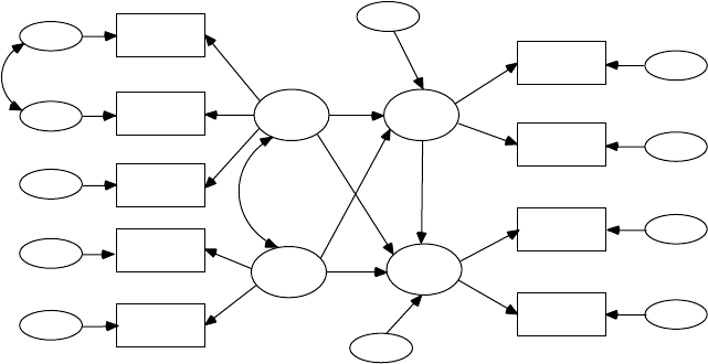
206 A Beginner’s Guide to Structural Equation Modeling
(mother’s education), which is 6.338. (Note: the t statistics do not suggest the
elimination of existing parameters, except one, from the initial model.) When
considering the addition of new parameters in the model, the largest modi-
cation index is for the measurement error covariance between FaEd (father’s
education) and MoEd (mother’s education), which is MI = 40.176. If we were
to estimate that parameter (correlation between FaEd and MoEd measure-
ment errors), the expected parameter change would be EPC = 0.205.
In our specication search, the standardized residual and EPC values
indicated that something was wrong with how we specied the relation-
ship between FaEd (father’s education) and MoEd (mother’s education),
because it was not specied well in the initial model. Consequently, we
decided to specify a measurement error covariance (correlation) between
FaEd (father’s education) and MoEd (mother’s education) because, upon
further reection, there should be common method variance on measures
using the same scale with two different parents.
The ML estimates and selected model-t indices for the modied model,
where the measurement error covariance is now included, are shown in
the second column of Table 10.3 and diagrammed in Figure 10.2. All of the
parameters are statistically signicantly different from zero (p < .05), except
for the path between Home (home background) and Achieve (achievement),
but once again, for substantive theoretical reasons, we chose to leave this
relationship specied in the model. Our selected model-t indices now all
indicate an acceptable level of t, and a second specication search did not
result in any further recommended changes. Thus, we consider our modi-
ed model to be our nal structural equation model for the prediction
Home
FamInc
Aspire
AbilityAchieve
FaEd
MoEd
VerbAb
QuantAb
EdAsp
OcAsp
VerbAch
QuantAch
1
11
1
error
error
error
error
error
error
error
error
error
error
error
FIGURE 10.2
Modied structural equation model of educational achievement.
Y102005.indb 206 3/22/10 3:26:11 PM

Developing Structural Equation Models: Part II 207
of educational achievement. Applying this structural equation model to
other samples of data will, we hope, provide further validation that this is
a theoretically meaningful structural model (see chapter 12).
1 0 . 7 S u m m a r y
This chapter completes the basic discussion of structural equation model-
ing we began in chapter 9. We hypothesized a structural equation model
to predict educational achievement and described it in further detail. We
followed the recommended steps a researcher should take in the struc-
tural equation modeling process, namely model specication, model
identication, model estimation, model testing, and nally model modi-
cation. We did not obtain acceptable model-t indices with our initial
theoretical model, so we conducted a specication search. The speci-
cation search suggested adding a parameter estimate for the correlation
between the measurement error terms of father’s and mother’s education
level. The modied model resulted in acceptable model-t indices, so this
was determined to be our best model to data t. In chapter 11 we provide
suggestions and recommendations for how structural equation modeling
studies should be reported in the literature.
Appendix: LISREL–SIMPLIS Structural
Equation Model Program
Educational Achievement Example—Model 2 Respecified
Observed variables: EdAsp OcAsp VerbAch QuantAch FamInc FaEd
MoEd VerbAb QuantAb
Covariance matrix:
1.024
.792 1.077
1.027 .919 1.844
.756 .697 1.244 1.286
.567 .537 .876 .632 .852
.445 .424 .677 .526 .518 .670
.434 .389 .635 .498 .475 .545 .716
.580 .564 .893 .716 .546 .422 .373 .851
.491 .499 .888 .646 .508 .389 .339 .629 .871
Sample size: 200
Y102005.indb 207 3/22/10 3:26:11 PM

208 A Beginner’s Guide to Structural Equation Modeling
Latent variables: ASPIRE ACHIEVE HOME ABILITY
Relationships:
EdAsp = 1*ASPIRE
OcAsp = ASPIRE
VerbAch = 1*ACHIEVE
QuantAch = ACHIEVE
FamInc = 1*HOME
FaEd MoEd = HOME
VerbAb = 1*ABILITY
QuantAb = ABILITY
ASPIRE = HOME ABILITY
ACHIEVE = ASPIRE HOME ABILITY
Let the error covariances of FaEd and MoEd correlate
Path diagram
End of problem
Exercise
1. Conduct the following structural equation model analysis
using the LISREL–SIMPLIS program:
Sample size = 500
Observed X variables:
ACT score (ACT)
College Grade Point Average (CGPA)
Company entry-level skills test score (ENTRY)
Observed Y variables:
Beginning salary (SALARY)
Current salary due to promotions (PROMO)
Latent dependent variable: Job Success (JOB)
Latent independent variable: Academic Success (ACAD)
Structural model:
ACAD -> JOB
Variance-covariance matrix:
ACT 1.024
CGPA .792 1.077
ENTRY .567 .537 .852
SALARY .445 .424 .518 .670
PROMO .434 .389 .475 .545 .716
References
Jöreskog, K. G., & Sörbom, D. (1993). LISREL 8: Structural equation modeling with the
SIMPLIS command language. Chicago, IL: Scientic Software International.
Lomax, R. G. (1985). A structural model of public and private schools. Journal of
Experimental Education, 53, 216–226.
Y102005.indb 208 3/22/10 3:26:11 PM

209
11
Reporting SEM Research: Guidelines
and Recommendations
Key Concepts
Theoretical models and data preparation
Sample matrix in SPSS or Excel
Model specication and identication
Model estimation and testing
Model modication and specication search
Breckler (1990) reviewed the personality and social psychology research
literature and found several shortcomings of structural equation mod-
eling, namely that model-t indices can be identical for a potentially
large number of models, that assumptions of multivariate normality are
required, that sample size affects results, and that cross-validation of
models was infrequently addressed or mentioned. Many of the studies
only reported a single model-t index. Breckler concluded that there was
cause for concern in the reporting of structural equation modeling results.
Raykov, Tomer, and Nesselroade (1991) proposed guidelines for reporting
SEM results in the journal Psychology and Aging. Maxwell and Cole (1995)
offered some general tips for writing methodological articles, and Hoyle
and Panter (1995) published a chapter on reporting SEM research with an
emphasis on describing the results and what model-t criteria to include.
The Publication Manual of the American Psychological Association (American
Psychological Association, 2001, pp. 161, 164–167, and 185) specically
states that researchers should include the means, standard deviations,
and correlations of the entire set of variables so that others can replicate
and conrm the analysis, as well as provide example tables and gures
for reporting structural equation modeling research. Unfortunately, the
guidelines do not go far enough in outlining the basic information that
should be included to afford an evaluation of the research study and
some fundamental points that should be addressed when conducting
Y102005.indb 209 3/22/10 3:26:11 PM
210 A Beginner’s Guide to Structural Equation Modeling
SEM studies. A few other scholars have previously offered their advice,
as follows.
Boomsma (2000) discussed how to write a research paper when struc-
tural equation models were used in empirical research and how to decide
what information to report. His basic premise was that all information
necessary for someone else to replicate the analysis should be reported.
He provided recommendations along the lines of our basic steps in struc-
tural equation modeling, namely model specication, model identica-
tion, model estimation, model testing, and model modication. Boomsma
found that many studies lacked a theoretical foundation for the theoretical
model, gave a poor description of the model tested, provided no discussion
of the psychometric properties of the variables and level of measurement,
did not include sample data, and had a poor delineation or justication for
the model modication process. He pointed out how difcult it can be to
evaluate or judge the quality of published SEM research.
MacCallum and Austin (2000) provided an excellent survey of problems
in applications of SEM. Thompson (2000) provided guidance for conduct-
ing structural equation modeling by citing key issues and including the
following list of 10 commandments for good structural equation model-
ing behavior: (a) do not conclude that a model is the only model to t the
data, (b) cross-validate any modied model with split-sample data or new
data, (c) test multiple rival models, (d) evaluate measurement models rst,
then structural models, (e) evaluate models by t, theory, and practical
concerns, (f) report multiple model-t indices, (g) meet multivariate nor-
mality assumptions, (h) seek parsimonious models, (i) consider variable
scale of measurement and distribution, and (j) do not use small samples.
McDonald and Ringo Ho (2002) examined 41 of 100 articles in 13 psychologi-
cal journals from 1995 to 1997. They stated that SEM researchers should give a
detailed justication of the SEM model tested along with alternative models,
account for identication, address nonnormality and missing data concerns,
and include a complete set of parameter estimates with standard errors, cor-
relation matrix (and perhaps residuals), and goodness-of-t indices.
We further elaborate several key issues in SEM. First, in structural equa-
tion model analyses several different types of sample data matrices can
be used (e.g., variance-covariance matrix, asymptotic variance-covariance
matrix, Pearson correlation matrix, or polyserial, polychoric, or tetrachoric
matrices). As previously described in chapter 3, the type of matrix used
depends on several factors such as nonnormality and type of variables.
A second issue concerns model identication, that is, the number of
distinct values in the sample variance-covariance matrix should equal or
exceed the number of free parameters estimated in the model (degrees of
freedom should not be negative for the model; the order condition) and
the rank of the matrix should yield a non-zero determinant value (the
rank condition). A researcher must also select from various parameter
Y102005.indb 210 3/22/10 3:26:11 PM
Reporting SEM Research: Guidelines and Recommendations 211
estimation techniques in model estimation, for example, unweighted least
squares, maximum likelihood, or generalized least squares estimation
under the assumption of multivariate normality, or asymptotically distri-
bution-free estimation using ADF or CVM techniques when the multivar-
iate normality assumption is not met. Obviously, many factors discussed
in chapters 2 and 3 affect multivariate normality.
A researcher should also be aware that equivalent models and alterna-
tive models may exist in an over-identied model (more distinct values in
the matrix than free parameters estimated), and rarely are we able to per-
fectly reproduce the sample variance-covariance matrix, given the implied
theoretical model. We use model-t indices and specication searches to
obtain an acceptable model to data t, given alternative models. Model-t
statistics should guide our search for a better tting model. Chapter 5 out-
lined different model-t criteria depending on the focus of the research.
Under some situations, for example, use of large sample sizes, the chi-
square values will be inated leading to statistically signicance, thus
erroneously implying a poor data to model t. A more appropriate use
of the chi-square statistic in this situation would be to compare alterna-
tive models with the same sample data (nested models). The specica-
tion search process involves nding whether a variable should be added
(parameter estimated) or a variable deleted (parameter not estimated). A
researcher, when modifying an initial model, should make one modica-
tion at a time, that is, add or delete one parameter estimate, and give a
theoretical justication for the model change.
Ironically, structural equation modeling requires larger sample sizes
as models become more complex or the researcher desires to conduct
cross-validation with split samples. In traditional multivariate statistics
the rule of thumb is 20 subjects per variable (20:1). The rules of thumb
used in structural equation modeling vary from 100, 200, to 500 or more
subjects per study, depending on model complexity and cross-validation
requirements. Sample size and power are also important considerations
in structural equation modeling (see chapter 5). Finally, a two-step/four-
step approach is important because if measurement models do not t the
observed variables, then relationships among the latent variables in struc-
tural models are not very meaningful.
We nd the following checklist to be valuable when publishing SEM
research and hopefully journal editors will embrace the importance of
this information when published. Our checklist is:
1. Provide a review of literature that supports your theoretical model.
2. Provide the software program used along with the version.
3. Indicate the type of SEM model analysis (multi-level, structured
means, etc.).
Y102005.indb 211 3/22/10 3:26:11 PM

212 A Beginner’s Guide to Structural Equation Modeling
4. Include correlation matrix, sample size, means, and standard
deviations of variables.
5. Include a diagram of your theoretical model.
6. For interpretation of results, describe t indices used and why; include
power and sample size determination; and effect size measure.
Our checklist is important because the SEM software, model, data, and
program will be archived in the journal. The power, sample size, and
effect size will permit future use in meta-analysis studies. Providing this
research in formation w ill also permit fut ure cross-cultural research, multi-
sample or multi-group comparisons, replication, or validation by others in
the research community because the analysis can be further examined.
We have made many of these same suggestions in our previous chap-
ters, so our intentions in this chapter are to succinctly summarize guide-
lines and recommendations for SEM researchers.
11.1 Data Preparation
A researcher should begin a SEM research study with a rationale and pur-
pose for the study, followed by a sound theoretical foundation of the mea-
surement model and the structural model. This includes a discussion of
the latent variables and how they are dened in the measurement model.
The hypothesis should involve the testing of the structural model and/or
a difference between alternative models.
An applied SEM research study typically involves using sample data, in
contrast to a methodological simulation study. The sample matrix should
be described as to the type (augmented, asymptotic, covariance, or cor-
relation), whether multivariate normality assumptions have been met,
the scale of measurement for the observed variables, and be related to
an appropriate estimation technique, for example, maximum likelihood.
Regression analysis, path analysis, factor analysis, and structural equa-
tion modeling all use data as input into a computer program (see SPSS
and Microsoft Excel examples at the end of the chapter). The SEM pro-
gram should include the sample matrix, and for certain models, means
and standard deviations of the observed variables.
To show another way to input data, we can create special data le types
in SPSS by designating special rowtype_ and varname_ elds in the SPSS
Data Editor and entering variable names, an example of which follows
from the Holzinger and Swineford (1939) data previously presented in
chapter 8.
Y102005.indb 212 3/22/10 3:26:11 PM
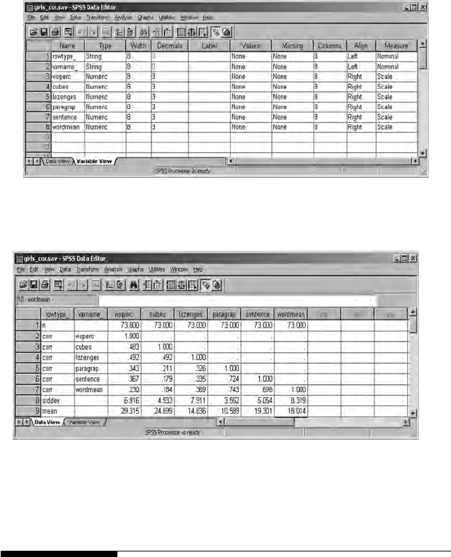
Reporting SEM Research: Guidelines and Recommendations 213
We then enter the individual sample size, correlation coefcients, standard
deviations, and means for the girls’ data. We saved this le as girls_cor.sav.
A set of recommendations for data preparation is given in SEM Checklist
Box 11.1.
11.2 Model Specification
Model specication involves determining every relationship and param-
eter in the model that is of interest to the researcher. Moreover, the goal
of the researcher is to determine, as best possible, the theoretical model
that generates the sample variance–covariance matrix. If the theoretical
model is misspecied, it could yield biased parameter estimates; param-
eter estimates that are different from what they are in the true popula-
tion model, that is, specication error. We do not typically know the true
population model, so bias in parameter estimates is generally attributed
Y102005.indb 213 3/22/10 3:26:12 PM

214 A Beginner’s Guide to Structural Equation Modeling
SEM CHECKLIST BOX 11.1—DATA PREPARATION
1. Have you adequately described the population from which
the random sample data was drawn?
2. Did you report the measurement level and psychometric
properties (i.e., reliability and validity) of your variables?
3. Did you report the descriptive statistics on your variables?
4. Did you create a table with correlations, means and stan-
dard deviations?
5. Did you consider and treat any missing data (e.g., can result
in data analysis issues)? What was the sample size both
before and after treating the missing data?
6. Did you consider and treat any outliers (e.g., can affect sam-
ple statistics)?
7. Did you consider the range of values obtained for variables,
as restricted range of one or more variables can reduce the
magnitude of correlations?
8. Did you consider and treat any nonnormality of the data
(e.g., skewness and kurtosis, data transformations)?
9. Did you consider and treat any multicollinearity among the
variables?
10. Did you consider whether variables are linearly related,
which can reduce the magnitude of correlations?
11. Did you resolve any correlation attenuation (e.g., can result
in reduced magnitude of correlations and error messages)?
12. Did you take the measurement scale of the variables into
account when computing statistics such as means, standard
deviations, and correlations?
13. Did you specify the type of matrix used in the analysis (e.g.,
covariance, correlation (Pearson, polychoric, polyserial),
augmented moment, or asymptotic matrices)?
14. When using the correlation matrix, did you include stan-
dard deviations of the variables in order to obtain correct
estimates of standard errors for the parameter estimates?
15. How can others access your data and SEM program (e.g.,
appendix, Web site, email)?
Y102005.indb 214 3/22/10 3:26:12 PM

Reporting SEM Research: Guidelines and Recommendations 215
to specication error. The model should be developed from the available
theory and research in the substantive area. This should be the main pur-
pose of the literature review.
Recommendations for model modication are provided in SEM
Checklist Box 11.2.
SEM CHECKLIST BOX 11.2—MODEL SPECIFICATION
1. Did you provide a rationale and purpose for your study,
including why SEM rather than another statistical analysis
approach was required?
2. Did you describe your latent variables, thus providing a
substantive background to how they are measured?
3. Did you establish a sound theoretical basis for your mea-
surement models and structural models?
4. Did you theoretically justify alternative models for compari-
son (e.g., nested models)?
5. Did you use a reasonable sample size, thus sufcient power
in testing your hypotheses?
6. Did you clearly state the hypotheses for testing the struc-
tural models?
7. Did you discuss the expected magnitude and direction of
expected parameter estimates?
8. Did you include a gure or diagram of your measurement
and structural models?
9. Have you described every free parameter in the models that
you want to estimate? In contrast, have you considered why
other parameters are not included in the models and/or why
you included constraints or xed certain parameters?
11.3 Model Identification
In structural equation modeling it is crucial that the researcher resolve
the identication problem prior to the estimation of parameters in measure-
ment models and/or structural models. In the identication problem, we
ask the following question: On the basis of the sample data contained in
the sample covariance matrix S, and the theoretical model implied by the
population covariance matrix Σ, can a unique set of parameter estimates
be found?
A set of recommendations for model identication includes the follow-
ing shown in SEM Checklist Box 11.3.
Y102005.indb 215 3/22/10 3:26:12 PM

216 A Beginner’s Guide to Structural Equation Modeling
SEM CHECKLIST BOX 11.3—MODEL IDENTIFICATION
1. Did you specify the number of distinct values in your sam-
ple covariance matrix?
2. Did you indicate the number of free parameters to be
estimated?
3. Did you inform the reader that the order and/or rank condi-
tion was satised?
4. Did you report the number of degrees of freedom and
thereby the level of identication of the model?
5. How did you scale the latent variables (i.e., x either one
factor loading per latent variable or the latent variable vari-
ances to 1.0)?
6. Did you avoid non-recursive models until identication
has been assured?
7. Did you utilize parsimonious models to assist with
identication?
11.4 Model Estimation
In model estimation we need to decide which estimation technique to select
for estimating the parameters in our measurement model and structural
model, that is, our estimates of the population parameters from sample
data. For example, we might choose the maximum likelihood estima-
tion technique because we meet the multivariate normality assumption
(acceptable skewness and kurtosis); there are no missing data; no outli-
ers; and continuous variable data. If the observed variables are interval
scaled and multivariate normal, then the ML estimates, standard errors
and chi-square test are appropriate.
Our experience is that model estimation often does not work because
of messy data. In chapters 2 and 3 we outlined many of the factors that
can affect parameter estimation in general, and structural equation model-
ing specically. Missing data, outliers, multicollinearity, and nonnormal-
ity of data distributions can seriously affect the estimation process and
often result in fatal error messages pertaining to Heywood variables (vari-
ables with negative variance), non-positive denite matrices (determinant
of matrix is zero), or failure to reach convergence (unable to compute a
nal set of parameter estimates). SEM is a correlation research method
and all of the factors that affect correlation coefcients, the general linear
model (regression, path, and factor models), and statistics in general are
Y102005.indb 216 3/22/10 3:26:12 PM

Reporting SEM Research: Guidelines and Recommendations 217
compounded in structural equation modeling. Do not overlook the problems
caused by messy data!
Recommendations for model estimation are given in SEM Checklist
Box 11.4.
SEM CHECKLIST BOX 11.4—MODEL ESTIMATION
1. What is the ratio of chi-square to the degrees of freedom?
2. What is the ratio of sample size to number of parameters?
3. Did you consider tests of parameter estimates?
4. Did you identify the estimation technique based on the type
of data matrix?
5. What estimation technique is appropriate for the distribu-
tion of the sample data (ML and GLS for multivariate nor-
mal data with small to moderate sample sizes; ADF or CVM
for non-normal, asymptotic covariance data, and WLS for
non-normal with large sample sizes)?
6. Did you encounter Heywood cases (negative variance), mul-
ticollinearity, or non-positive denite matrices?
7. Did you encounter and resolve any convergence problems
or inadmissible solution problems by using start values, set-
ting the admissibility check off, using a larger sample size,
or using a different method of estimation?
8. Which SEM program and version did you use?
9. Did you report the R2 values to indicate the t of each sepa-
rate equation?
10. Do parameter estimates have the expected magnitude and
direction?
11.5 Model Testing
Having provided the SEM program and sample data along with our measure-
ment and structural models, anyone can check our results and verify our nd-
ings. In interpreting our measurement model and structural model, we
establish how well the data t the models. In other words, we examine the
extent to which the theoretical model is supported by the sample data. In
model testing we consider model-t indices for the t of the entire model
and examine the specic tests for the statistical signicance of individual
parameters in the model.
A set of recommendations for model testing includes the following as
shown in SEM Checklist Box 11.5.
Y102005.indb 217 3/22/10 3:26:13 PM

218 A Beginner’s Guide to Structural Equation Modeling
SEM CHECKLIST BOX 11.5—MODEL TESTING
1. Did you report several model-t indices (e.g., for a single
model: chi-square, df, GFI, NFI, RMSEA; for a nested model:
LR test, CFI, AIC; for cross-validation indices: CVI, ECVI;
and for parameter estimates, t values and standard errors)?
2. Did you specify separate measurement models and struc-
tural models?
3. Did you check for measurement invariance in the factor
loadings prior to testing between-group parameter esti-
mates in the structural model?
4. Did you provide a table of estimates, standard errors, statisti-
cal signicance (possibly including effect sizes and condence
intervals)?
11.6 Model Modification
If the t of an implied theoretical model is not acceptable, which is typi-
cally the case with an initial model, the next step is model modication and
subsequent evaluation of the new, modied model. Most of model modi-
cations occur in the measurement model rather than the structural model.
Model modication occurs more in the measurement model because that
is where the main source of misspecication occurs and measurement
models are the foundation for the structural model.
After we are satised with our nal best-tting model, future research
should undertake model validation by replicating the study (using multiple
sample analysis, chapter 13), performing cross-validation (randomly split-
ting the sample and running the analysis on both sets of data), or boot-
strapping the parameter estimates to determine the amount of bias. These
model validation topics are covered in chapter 12.
A set of recommendations for model modication is given in SEM
Checklist Box 11.6. Although not fully discussed until chapter 12, a set
SEM CHECKLIST BOX 11.6 —MODEL MODIFICATION
1. Did you compare alternative models or equivalent models?
2. Did you clearly indicate how you modied the initial
model?
Y102005.indb 218 3/22/10 3:26:13 PM

Reporting SEM Research: Guidelines and Recommendations 219
of recommendations for model validation is provided in SEM Checklist
Box 11.7.
1 1 . 7 S u m m a r y
In this chapter we showed that model t is a subjective approach that
requires substantive theory because there is no single best model (other
models may be equally plausible given the sample data and/or equiva-
lent models). In structural equation modeling the researcher follows the
steps of model specication, identication, estimation, testing, and modi-
cation, so we advise the researcher to base measurement and structural
models on sound theory, utilize the two-step/four-step approach, and establish
measurement model t and measurement invariance before model testing
the latent variables in the structural model. We also recommend that theo-
retical models need to be replicated, cross-validated, and/or bootstrapped to
determine the stability of the parameter estimates (see chapter 12). Finally,
we stated that researchers should include their SEM program, data, and
path diagram in any article. This permits a replication of the analysis and
3. Did you provide a theoretical justication for the modied
model?
4. Did you add or delete one parameter at a time? What param-
eters were trimmed?
5. Did you provide parameter estimates and model-t indices
for both the initial model and the modied model?
6. Did you report statistical signicance of free parameters,
modication indices and expected change statistics of xed
parameters, and residual information for all models?
7. How did you evaluate and select the best model?
SEM CHECKLIST BOX 11.7—MODEL VALIDATION
1. Did you replicate your SEM model analysis using another
sample of data (e.g., conduct a multiple sample analysis)?
2. Did you cross-validate your SEM model by splitting your
original sample of data?
3. Did you use bootstrapping to determine the bias in your
parameter estimates?
Y102005.indb 219 3/22/10 3:26:13 PM

220 A Beginner’s Guide to Structural Equation Modeling
verication of the results. We do not advocate using specication searches
to nd the best tting model without having a theoretically justied rea-
son for modifying the initial model. We further advocate using another
sample of data to validate that the modied model is a meaningful and
substantive theoretical structural model. Most importantly, we provide
the researcher with checklists to follow when doing structural equation
modeling. These checklists follow a logical progression from data prepa-
ration through model specication, identication, estimation, testing,
modication, and validation.
Exercise
1. Enter the following data in special matrix format in SPSS and
save as Fels_fem.sav. Use special variable names rowtype_ and
varname_ along with n, corr, stddev, and mean in these special
data sets.
N = 209
Correlation Matrix
Academic 1.00
Athletic .43 1.00
Attract .50 .48 1.00
GPA .49 .22 .32 1.00
Height .10 − .04 −.03 .18 1.00
Weight .04 .02 −.16 −.10 .34 1.00
Rating .09 .14 .43 .15 −.16 −.27 1.00
s.d. .16 .07 .49 3.49 2.91 19.32 1.01
means .12 .05 .42 10.34 .00 94.13 2.65
References
American Psychological Association (2001). Publication manual of the American
Psychological Association (5th ed.). Washington, DC: Author.
Boomsma, A. (2000). Reporting analyses of covariance structure. Structural Equation
Modeling, 7, 461–483.
Breckler, S. J. (1990). Applications of covariance structure modeling in psychology:
Cause for concern? Psychological Bulletin, 107, 260–273.
Holzinger, K. J., & Swineford, F. A. (1939). A study in factor analysis: The stability
of a bi-factor solution. (Supplementary Educational Monographs, No. 48).
Chicago: University of Chicago, Department of Education.
Y102005.indb 220 3/22/10 3:26:13 PM
Reporting SEM Research: Guidelines and Recommendations 221
Hoyle, R. H., & Panter, A. T. (1995). Writing about structural equation models. In R.
H. Hoyle (Ed.), Structural equation modeling: Concepts, issues, and applications
(pp. 158–176). Thousand Oaks, CA: Sage.
MacCallum, R. C., & Austin, J. T. (2000). Applications of structural equation mod-
eling in psychological research. Annual Review of Psychology, 51, 201–226.
Maxwell, S. E., & Cole, D. A. (1995). Tips for writing (and reading) methodological
articles. Psychological Bulletin, 118, 193–198.
McDonald, R. P., & Ringo Ho, M. (2002). Principles and practice in reporting struc-
tural equation analyses. Psychological Methods, 7, 64–82.
Raykov, T., Tomer, A., & Nesselroade, J. R. (1991). Reporting structural equa-
tion modeling results in Psychology and Aging: Some proposed guidelines.
Psychology and Aging, 6, 499–533.
Thompson, B. (2000). Ten commandments of structural equation modeling. In L.
Grimm & P. Yarnold (Eds.), Reading and understanding more multivariate statis-
tics (pp. 261–284). Washington, DC: American Psychological Association.
Y102005.indb 221 3/22/10 3:26:13 PM

223
12
Model Validation
Key Concepts
Replication: multiple samples
Cross validation: randomly split subsamples
Cross validation indexes: ECVI, CVI, and MECVI
Bootstrap via LISREL and PRELIS
Bootstrap via program menu
In previous chapters we learned about the basics of st ruc tural equat ion mod-
eling using the following steps: model specication, identication, estima-
tion, testing, and modication. In this chapter we consider a selection of
topics related to model validation. However, our discussion only scratches
the surface of these approaches in structural equation modeling, so you
should check out the references in this chapter for more information.
We begin by presenting the topic of replication, which uses multiple
samples. In our rst example, the validation of a theoretical conrma-
tory factor model using two samples of data is presented. Cross valida-
tion is presented next, where a larger sample is randomly split into two
subsamples. Then, we present the basics of how to determine the stability
of parameter estimates using the bootstrap method. Ideally, a researcher
should seek model validation with additional samples of data (replication).
The other methods are not as rigorous, but in the absence of replication,
provide evidence of model validity—that is, the viability of the theoretical
framework suggested by the measurement and/or structural models.
12.1 Multiple Samples
A nice feature of structural equation modeling, although not frequently
used, is the possibility of studying a theoretical model and then validating
it using one or more additional samples of data. Theoretical models can
Y102005.indb 223 3/22/10 3:26:14 PM
224 A Beginner’s Guide to Structural Equation Modeling
therefore be examined across samples to determine the degree of invari-
ance in t indices, parameter estimates, and standard errors.
SEM also permits the use of multiple samples in the analysis of quasi-
experimental, experimental, cross-sectional, and/or longitudinal data.
With multiple samples it is possible to estimate separately the parame-
ters for each independent sample, to test whether specied parameters or
parameter matrices are equivalent across the samples (that is, for any of
the parameters in the measurement and/or structural equation models),
or to test whether there are sample mean differences for the indicator vari-
ables and/or for any of the structural equations.
We can obviously estimate parameters in each sample of data sepa-
rately. We would t a theoretical model to the rst sample of data and
then apply the model to the other samples of data. It is possible that a
conrmatory factor model will t all samples of data (multiple samples),
indicating measurement invariance, and yet have different values for
error covariance, factor loadings, or factor correlations. We can also sta-
tistically determine whether certain specied parameters or parameter
matrices are equivalent across samples of data. For instance, one may
be interested in whether factor loadings and factor correlations are sta-
ble across random samples of data applied to a theoretical model. We
could also randomly split a large national sample of data into several
subsamples.
SEM also permits the testing of the equivalence of matrices or param-
eter estimates across several samples taken randomly from a population.
A researcher indicates the specic hypothesis to be tested, for example,
equal factor loadings and factor correlation. For a measurement model,
we could test whether the factor loadings are equal across the samples,
or whether the factor variances and covariance terms are equal across the
samples, or even whether the unique error variances and covariance terms
are equal across samples. For a structural model, we could test whether
the structure coefcients are equal across the samples. For a combined
structural equation model, all parameters in the entire model are tested
for equivalence across the samples. Obviously, in this instance both the
covariance matrix and the coefcients are tested for equality across the
samples, lending itself to a more complex model requiring adequate sam-
ple size and power.
In this chapter, we present four models: Model A with all parameters
invariant; Model B with only error variance and factor correlation invari-
ant; Model C with only factor correlation invariant; and nally Model
D with factor loadings and factor correlation invariant. These examples
should give you a better understanding of how different model attributes
can be tested using multiple samples.
We now demonstrate how to conduct these multiple sample analyses
in LISREL–SIMPLIS using the example in Jöreskog and Sörbom (1996c,
Y102005.indb 224 3/22/10 3:26:14 PM
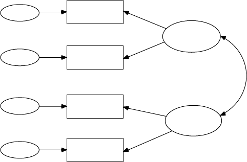
Model Validation 225
example 10, p. 52) that indicated two samples of data on candidates who
took the Scholastic Aptitude Test (SAT) in 1971 (Figure 12.1).
In LISREL–SIMPLIS, measurement and/or structural models can
be specied and tested across samples of data for model validation.
The LISREL–SIMPLIS program stacks separate programs, but does not
require that the observed variables, latent variables, and equations be
repeated in each program when the parameters in the theoretical model
are assumed identical in subsequent individual programs. The second
and subsequent individual programs only need to include their sample
size and variance–covariance matrix. Each individual program, how-
ever, must be designated by use of the special command, Group 1: and
Group 2: etc. (Note: Do not use Sample 1: and Sample 2: etc. to designate
the individual programs).
The computer output indicates results for each individual program
with chi-square contributions to the overall global chi-square value. Each
individual program outputs a chi-square value that sums to the global
chi-square value. A percent contribution to the global chi-square value is
also indicated for each individual program. In a multiple sample analysis,
the global chi-square is a measure of t in all samples to the theoreti-
cal model. (Note: Individual sample parameter values can be obtained by
including the latent variable and equation statements in each subsequent
stacked program.)
LISREL–SIMPLIS generally requires running different multiple sam-
ple program models to determine which parameters are different or
Verbal
Math
VERBAL40
VERBAL50
MATH35
MATH25
err_v40
err_v50
err_m35
err_m25
FIGURE 12.1
Path Diagram for SAT Verbal and Math. (From Jöreskog, K. G., & Sörbom, D., 1993.
Bootstrapping and Monte Carlo experimenting with PRELIS2 and LISREL8. Chicago: Scientic
Software International; example 10, p. 52.)
Y102005.indb 225 3/22/10 3:26:14 PM
226 A Beginner’s Guide to Structural Equation Modeling
similar among factor loadings, error variances, and factor correlations. In
LISREL–SIMPLIS, Model A (EX10A.SPL) tests the equality of all param-
eters across both samples (factor loadings, error variances, and factor
correlation). Model B (EX10B.SPL) allows the factor loadings to be dif-
ferent, but maintains equal error variances and factor correlation. Model
C (EX10C.SPL) allows the factor loadings and error variances to be dif-
ferent, but maintains equal factor correlation across the two samples.
Finally, Model D (EX10D.SPL) species that the factor loadings and the
factor correlation are the same for both samples with the error variances
different.
The LISREL–SIMPLIS Model A program (EX10A.SPL), which tests
equality of all parameters (invariant) across both samples, is:
Group 1: Testing Equality of all model parameters
Model A: Factor Loadings, Correlation, Error Variances Invariant
Observed Variables: VERBAL40 VERBAL50 MATH35 MATH25
Covariance Matrix from File EX10.COV
Sample Size = 865
Latent Variables: Verbal Math
Relationships:
VERBAL40 VERBAL50 = Verbal
MATH35 MATH25 = Math
Group 2: Testing Equality of all model parameters
Covariance Matrix from File EX10.COV
Sample Size = 900
Path diagram
End of problem
12.1.1 Model A Computer Output
Group 1:
Contribution to Chi-Square = 19.16
Percentage Contribution to Chi-Square = 54.92
Group 2:
Contribution to Chi-Square = 15.73
Percentage Contribution to Chi-Square = 45.08
Global Goodness-of-Fit Statistics
Degrees of Freedom = 11
Minimum Fit Function Chi-Square = 34.89 (P = 0.00026)
The global chi-square is signicant, so having all parameters equal (invari-
ant) is not a tenable solution. Some parameters are therefore different in
the two samples.
The LISREL–SIMPLIS Model B program (EX10B.SPL), which tests differ-
ences in factor loadings with equal error variance and factor correlation, is:
Y102005.indb 226 3/22/10 3:26:14 PM
Model Validation 227
Group 1: Testing Equality Of Factor Structures
Model B : Factor Correlation and Error Variances Invariant
Observed Variables: VERBAL40 VERBAL50 MATH35 MATH25
Covariance Matrix from File EX10.COV
Sample Size = 865
Latent Variables: Verbal Math
Relationships:
VERBAL40 VERBAL50 = Verbal
MATH35 MATH25 = Math
Group 2: Testing Equality Of Factor Correlations
Covariance Matrix from File EX10.COV
Sample Size = 900
Relationships:
VERBAL40 VERBAL50 = Verbal
MATH35 MATH25 = Math
Path diagram
End of problem
12.1.2 Model B Computer Output
Group 1:
Contribution to Chi-Square = 15.62
Percentage Contribution to Chi-Square = 52.65
Group 2:
Contribution to Chi-Square = 14.05
Percentage Contribution to Chi-Square = 47.35
Global Goodness-of-Fit Statistics
Degrees of Freedom = 7
Minimum Fit Function Chi-Square = 29.67 (P = 0.00011)
The global chi-square was signicant, which indicates that equal error
variance and equal factor correlation are not tenable results with factor
loadings being different.
The LISREL–SIMPLIS Model C program (EX10C.SPL), which tests differ-
ences in factor loadings and error variance, but equal in factor correlation, is:
Group 1: Testing Equality of Factor Structures
Model C: Factor Correlation Invariant
Observed Variables: VERBAL40 VERBAL50 MATH35 MATH25
Covariance Matrix from File EX10.COV
Sample Size = 865
Latent Variables: Verbal Math
Relationships:
VERBAL40 VERBAL50 = Verbal
MATH35 MATH25 = Math
Group 2: Testing Equality of Factor Correlations
Covariance Matrix from File EX10.COV
Sample Size = 900
Y102005.indb 227 3/22/10 3:26:15 PM
228 A Beginner’s Guide to Structural Equation Modeling
Relationships:
VERBAL40 VERBAL50 = Verbal
MATH35 MATH25 = Math
Set the Error Variances of VERBAL40 - MATH25 free
Path diagram
End of problem
12.1.3 Model C Computer Output
Group 1:
Contribution to Chi-Square = 2.21
Percentage Contribution to Chi-Square = 55.02
Group 2:
Contribution to Chi-Square = 1.81
Percentage Contribution to Chi-Square = 44.98
Global Goodness-of-Fit Statistics
Degrees of Freedom = 3
Minimum Fit Function Chi-Square = 4.03 (P = 0.26)
The factor correlation was r = .76 for both samples. This is tenable, given
the nonsignicant global chi-square statistic (c2 = 4.03, df = 3, p = .26).
The LISREL–SIMPLIS Model D program (EX10D.SPL), which tests factor
loadings and factor correlation the same (invariant), but allows for differ-
ences in error variance is:
Group 1: Testing Equality of Factor Structures
Model D: Factor Loadings and Factor Correlation Invariant
Observed Variables: VERBAL40 VERBAL50 MATH35 MATH25
Covariance Matrix
63.382
70.984 110.237
41.710 52.747 60.584
30.218 37.489 36.392 32.295
Sample Size = 865
Latent Variables: Verbal Math
Relationships:
VERBAL40 VERBAL50 = Verbal
MATH35 MATH25 = Math
Group 2: Testing Equality of Factor Correlations
Covariance Matrix
67.898
72.301 107.330
40.549 55.347 63.203
28.976 38.896 39.261 35.403
Sample Size = 900
Set the Error Variances of VERBAL40 - MATH25 free
Path diagram
End of problem
Y102005.indb 228 3/22/10 3:26:15 PM

Model Validation 229
12.1.4 Model D Computer Output
Group 1:
Contribution to Chi-Square = 5.48
Percentage Contribution to Chi-Square = 50.40
Group 2:
Contribution to Chi-Square = 5.39
Percentage Contribution to Chi-Square = 49.60
Global Goodness-of-Fit Statistics
Degrees of Freedom = 7
Minimum Fit Function Chi-Square = 10.87 (P = 0.14)
The global chi-square indicated a good t of the measurement model
across both samples of data. Therefore, equal factor loadings and factor
correlation with unequal error variances is tenable. Error variances would
typically be different in a measurement model, so assuming equal factor
loadings and factor correlation was theoretically reasonable to test.
12.1.5 Summary
Although the multiple sample programs provide the individual and
global chi-square values, the researcher should consider creating a table
with the parameter values and standard errors. This would provide an
easier comparison of the intended parameter estimates that were modeled
in the different programs.
More complex model comparisons are possible. For example, we could
test the equality of both factor loadings and factor correlations across
three samples of data. Many different measurement and structural models
using the multiple sample approach are possible and have been illustrated
in journal articles, software manuals, and books. The interested reader is
referred to Jöreskog and Sörbom (1993), Muthén (1987) and Bentler and
Wu (2002), as well as books by Hayduk (1987) and Bollen (1989), for more
details on running these various multiple sample models. Other empirical
examples using multiple-sample models are given by Lomax (1983, 1985),
Cole and Maxwell (1985), Faulbaum (1987), and McArdle and Epstein
(1987). A suggested strategy for testing models in the multiple sample case
is also given by Lomax (1983).
12.2 Cross Validation
The replication of a study with a second set of data is often prohibitive
given the time, money, or resources available. An alternative is to ran-
domly split an original sample, given that the sample size is sufcient,
Y102005.indb 229 3/22/10 3:26:15 PM
230 A Beginner’s Guide to Structural Equation Modeling
and run the SEM analysis on one set of data while using the other in a
multiple-sample analysis to compare the results. Cudeck and Browne
(1983) created a split sample cross-validation index (CVI), while Browne
and Cudeck (1989, 1993) developed a single sample cross-validation
(ECVI) and further explained CVI and ECVI in structural equation mod-
eling. Except for a constant scale factor, ECVI is similar to the AIC index
[(1/n)* (AIC)]. Arbuckle and Wothke (1999, p. 406) also report MECVI,
which, except for a scale factor, is similar to BCC [(1/n) * (BCC)]. The
Browne–Cudeck criterion (BCC) imposes a slightly greater penalty for
model complexity than AIC, and is a t index developed specically
for the analysis of moment structures. These t indices are intended for
model comparisons, and thus indicate badness of t; with simple models
that t well receiving low values and poorly tting models receiving
high values.
12.2.1 ECVI
Browne and Cudeck (1989) proposed a single-sample expected cross-
validation index (ECVI) for comparing alternative models using only
one sample of data. The alternative model that results in the smallest
ECVI value should be the most stable in the population. The ECVI is
a function of chi-square and degrees of freedom. It is computed in
LISREL as ECVI = (c/n) + 2(p/n), where c is the chi-square value for
the overall tted model, p is the number of independent parameters
estimated, and n = N − 1 (sample size). Alternatively, ECVI can be
reported as similar to the Akaike Information Criterion, except for a
scale factor—that is, (1/n) * AIC, where n = N – r (N = sample size; r =
number of groups). Browne and Cudeck (1989, 1993) also provided a
condence interval for ECVI. The 90% lower and upper limits(cL ; cU) =
[(dL + d + 2q)/n; (dU + d + 2q)/n], where cL = lower limit, cU = upper limit, dL
= parameter estimate for lower limit, dU = parameter estimate for upper
limit, d = degrees of freedom, and q = the number of parameters. When
sample size is small, it is important to compare the condence intervals
of the ECVI for the alternative competing models. The ECVI is also
not very useful for choosing a parsimonious model when the sample
size is large. In this instance, we recommend one of the parsimonious
model-t indices and/or the comparative t index if comparing alter-
native models (see chapter 5).
Bandalos (1993), in a simulation study, further examined the use of the
one-sample expected cross-validation index and found it to be quite accu-
rate in conrmatory factor models. Other research also indicated that the
one-sample expected cross validation index yielded highly similar results
to those of the two-sample approach (Benson & Bandalos, 1992; Benson &
Y102005.indb 230 3/22/10 3:26:15 PM
Model Validation 231
El-Zahhar, 1994; Benson, Moulin-Julian, Schwarzer, Seipp, & El-Zahhar,
1992).
The ECVI is routinely printed among the t indices reported by LISREL–
SIMPLIS. We used our previous multiple-sample programs in LISREL–
SIMPLIS, but this time ran them separately to obtain the ECVI values. The
ECVI for sample one was close to zero, indicating a measurement model
that would be expected to cross-validate; likewise similar ndings were
reported for the second sample of data. The condence intervals around
ECVI in both programs further supported that ECVI would probably
range between .02 and .03 for this model. (Note: We would not interpret
the ECVI in the multiple-sample model.)
LISREL–SIMPLIS ECVI Output
Sample 1
Expected Cross-Validation Index (ECVI) = 0.021
90 Percent Confidence Interval for ECVI = (0.019 ; 0.028)
ECVI for Saturated Model = 0.011
ECVI for Independence Model = 3.05
Sample 2
Expected Cross-Validation Index (ECVI) = 0.021
90 Percent Confidence Interval for ECVI = (0.021 ; 0.029)
ECVI for Saturated Model = 0.022
ECVI for Independence Model = 3.00
The AIC and BCC values can be computed to show the scale factor rela-
tionship to ECVI. AIC = c2 + 2q = 1.3 + 2(9) = 19.3, that is, reported as 19.255
for the rst sample, where q = number of parameters in the model. AIC =
c2 + 2q = .9 + 2(9) = 18.922 for the second sample. ECVI = [1/(N – r)](AIC) =
[1/(865 – 2)](19.255) = .022 for sample 1 and ECVI = [1/(N – r)] (AIC) = [1/
(900 – 2)](18.922) = .021 for sample 2. N is the sample size in each group and
r is the number of groups. MECVI doesn’t apply in this model analysis,
but is computed as: [1/(N – r)] (BCC) or [1/(865 – 2)] (19.36) and [1/(900 − 2)]
(19.023), respectively.
12.2.2 CVI
Cudeck and Browne (1983) also proposed a cross-validation index (CVI)
for covariance structure analysis that incorporated splitting a sample into
two subsamples. Subsample A is used as a calibration sample, and sub-
sample B is used as the validation sample. The model implied (reproduced)
Y102005.indb 231 3/22/10 3:26:15 PM
232 A Beginner’s Guide to Structural Equation Modeling
covariance matrix, Σa, from the calibration sample is then compared with
the covariance matrix derived from Subsample B, Sb. A CVI value near
zero indicates that the model cross-validates or is the same in the two
subsamples. The cross validation index is denoted as CVI = F(Sb, Σa). The
choice among alternative models can also be based on the model that
yields the smallest CVI value. One could further double-cross-validate by
using Subsample B as the calibration sample and Subsample A as the
validation sample. In this instance, the cross validation index is denoted
as CVI = F(Sa, Σb). If the same model holds regardless of which subsample
is used as the calibration sample, greater condence in the model valid-
ity is achieved. An obvious drawback to splitting a sample into two sub-
samples is that sufcient subsample sizes may not exist to provide stable
parameter estimates. Obviously, this approach requires an initial large
sample that can be randomly split into two subsamples of equal and suf-
cient size.
The CVI can be computed using LISREL–SIMPLIS command language,
but requires two programs with randomly split data and the cross-validate
command. In the following example, two LISREL–SIMPLIS programs are
run to compute the CVI. The rst program reads in the covariance matrix
of the calibration sample (Sa), then generates and saves the model implied
covariance matrix, Σa. The second program uses the covariance matrix of
Subsample B and then outputs the CVI value. The CVI cross validation
example involved randomly splitting an original sample of size 400 and
calculating two separate covariance matrices.
Program One Calibration Sample
Observed Variables: X1 X2 X3
Covariance Matrix
5.86
3.12 3.32
35.28 23.85 622.09
Latent Variables: Factor1
Relationships:
X1-X3 = Factor1
Sample Size: 200
Save Sigma in File MODEL1C
End of problem
Program Two Validation Sample and Compute CVI
Observed Variables: X1 X2 X3
Covariance Matrix
5.74
3.47 4.36
45.65 22.58 611.63
Sample Size: 200
Crossvalidate File MODEL1C
End of problem
Y102005.indb 232 3/22/10 3:26:15 PM
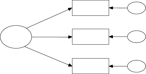
Model Validation 233
A single factor measurement model with three indicator variables is being
tested to see if it cross-validates using a randomly split sample of data
(Figure 12.2).
The low CVI value indicated that the measurement model holds for both
subsamples. The reduced computer output from the CVI cross validation
program is:
PROGRAM ONE CALIBRATION SAMPLE
COVARIANCE MATRIX TO BE ANALYZED
X1 X2 X3
X1 5.86
X2 3.12 3.32
X3 35.28 23.85 622.09
SI was written to file MODEL1C
PROGRAM TWO VALIDATION SAMPLE AND COMPUTE CVI
COVARIANCE MATRIX TO BE ANALYZED
X1 X2 X3
X1 5.74
X2 3.47 4.36
X3 45.65 22.58 611.63
MATRIX SIGMA
X1 X2 X3
X1 5.86
X2 3.12 3.32
X3 35.28 23.85 622.09
CROSS-VALIDATION INDEX (CVI) = 0.38
The ECVI and CVI are most useful after a theoretically implied model has
an acceptable model t, that is, when a specied model yields model-t
Factor
X1
X2
X3
e1
e2
e3
FIGURE 12.2
Single Factor Model (cross validation).
Y102005.indb 233 3/22/10 3:26:16 PM

234 A Beginner’s Guide to Structural Equation Modeling
indices and parameter estimates that are meaningful with sufcient sample
size and power. The number of parameters, model complexity, and sample
size affect these cross validation indices; therefore, you should not routinely
discard other modeling considerations when you select the smaller ECVI of
two competing models, report the CVI from two subsamples, or report the
CVI across samples taken from a population. Currently, LISREL–SIMPLIS
computes ECVI for single sample expected cross validation, however, only
LISREL–SIMPLIS computes CVI for split sample cross validation.
12.3 Bootstrap
The bootstrap method treats a random sample of data as a substitute
for the population (pseudo population) and re-samples from it a speci-
ed number of times, to generate sample bootstrap estimates and stan-
dard errors. These sample bootstrap estimates and standard errors are
averaged and used to obtain a condence interval around the average
of the bootstrap estimates. This average is termed a bootstrap estimator.
The bootstrap estimator and associated condence interval are used to
determine how stable or good the sample statistic is as an estimate of the
population parameter. Obviously, if the random sample initially drawn
from the population is not representative, then the sample statistic and
corresponding bootstrap estimator obtained from re-sampling will yield
misleading results. The bootstrap approach is used in research when rep-
lication with additional sample data and/or cross validation with a split
sample is not possible. Fan (2003) demonstrates how the bootstrap method
is implemented in various software packages and its utility in correla-
tion, regression, analysis of variance, and reliability. We present examples
using PRELIS.
12.3.1 PRELIS Graphical User Interface
Bootstrapping can be accomplished in two different ways using PRELIS
(Jöreskog & Sörbom, 1993; 1996b); LISREL–SIMPLIS program does not
provide bootstrap capabilities. Our rst example will demonstrate the
use of the PRELIS graphical user interface. The second example will use
the PRELIS command language syntax (Jöreskog & Sörbom, 1996b, pp.
185–190). In our rst bootstrap example, we select File, then Import Data
to import the SPSS saved le, dataex7.sav, located in the SPSSEX subfolder
in LISREL 8 Student Examples directory and save the PRELIS SYSTEM
FILE, dataex7.psf.
Y102005.indb 234 3/22/10 3:26:16 PM

Model Validation 235
Y102005.indb 235 3/22/10 3:26:17 PM

236 A Beginner’s Guide to Structural Equation Modeling
We now see the PRELIS SPREADSHEET with the raw data and the
PRELIS tool bar menu with several options from which to choose. We
select Statistics from the toolbar menu, and then Bootstrapping.
Once we select Bootstrapping, a dialog appears that permits us to spec-
ify the number of bootstrap samples, bootstrap fraction, and names for
saving the bootstrap matrix, means and standard deviations. The Syntax
button will create a PRELIS program that you can edit and save. The
Output Options button provides other formats for saving the data.
Y102005.indb 236 3/22/10 3:26:17 PM
Model Validation 237
The output provides us with the PRELIS command language syntax
program and descriptive statistics, as follows.
!PRELIS SYNTAX: Can be edited
SY=’C:\lisrel854\spssex\dataex7.PSF’
OU MA=KM SM=data7.cor ME=data7.me SD=data7.sd XM BS=100 SF=50
BM=data7.cor ME=data7.me SD=data7.sd
Bootstrap Correlation Matrix
NOSAY VOTING COMPLEX NOCARE TOUCH INTEREST
NOSAY 1.000
VOTING 0.292 1.000
COMPLEX 0.259 0.276 1.000
NOCARE 0.462 0.263 0.442 1.000
TOUCH 0.386 0.180 0.294 0.669 1.000
INTEREST 0.408 0.239 0.368 0.710 0.640 1.000
Descriptive Statistics
Variable Mean St. Dev.
NOSAY 0.000 1.000
VOTING 0.000 1.000
COMPLEX 0.000 1.000
NOCARE 0.000 1.000
TOUCH 0.000 1.000
INTEREST 0.000 1.000
12.3.2 LISREL and PRELIS Program Syntax
In our second example, we use LISREL and PRELIS command language
syntax in various programs to further elaborate the bootstrap method. We
rst run a LISREL program using the original sample data. The raw-data
le, efcacy.raw, is provided with LISREL and used in other examples in
the PRELIS2 User’s Reference Guide (Jöreskog & Sörbom, 1996b). A two-
factor model is specied with six factor loadings estimated; three for each
of the factors (see the MO and FR command lines). The LISREL program
is written as:
Estimate factor loadings for model from file efficacy.raw
DA NI=6 NO=297 ME=GLS
RA=efficacy.raw FO;(6F1.0)
CO ALL
MO NX=6 NK=2
FR LX(1,1) LX(2,1) LX(3,1) LX(4,2) LX(5,2) LX(6,2)
OU MA=CM
Y102005.indb 237 3/22/10 3:26:17 PM

238 A Beginner’s Guide to Structural Equation Modeling
The variance-covariance matrix to be analyzed is indicated as:
VAR 1 0.60
VAR 2 0.16 0.59
VAR 3 0.11 0.14 0.59
VAR 4 0.23 0.14 0.21 0.57
VAR 5 0.16 0.08 0.14 0.30 0.49
VAR 6 0.19 0.11 0.17 0.34 0.27 0.53
The six factor loadings for the two factor model specied are estimated as:
Estimate Standard Error
LX(1,1) 0.43 0.05
LX(2,1) 0.30 0.05
LX(3,1) 0.37 0.05
LX(4,2) 0.63 0.04
LX(5,2) 0.48 0.04
LX(6,2) 0.55 0.04
Then, to compute bootstrap estimates of the factor loadings for the two-
factor model with three indicators per factor, the raw data le is read into a
PRELIS program with the number of variables, number of cases, and esti-
mation method specied (DA NI=6 NO=297, ME=GLS). In this example,
the PRELIS program reads in a raw data le containing 6 variables and
297 cases with the generalized least-squares estimation method selected
[RA = efcacy.raw FO;(6F1.0)]. The PRELIS program then generates 10 cova-
riance matrices using the generalized least-squares estimation method.
The number of bootstrap samples to be taken is specied (BS=10), and
these samples are randomly drawn from the raw data le with replace-
ment. A 100% resampling (SF=100) of the raw data le is specied. The
10 covariance matrices are output into a bootstrap save le (BM = efcacy.
cm) for further analysis by another LISREL program. This output le is in
ASCII format and can be examined. The PRELIS program is:
Generate 10 covariance matrices from file efficacy.raw
DA NI=6 NO=297 ME=GLS
RA=efficacy.raw FO;(6F2.0)
OU MA=CM BS=10 SF=100 BM=efficacy.cm
The rst two variance-covariance matrices output into the le efcacy.cm are:
VAR 1 1.00
VAR 2 0.27 1.00
VAR 3 0.26 0.26 1.00
VAR 4 0.46 0.25 0.42 1.00
Y102005.indb 238 3/22/10 3:26:17 PM
Model Validation 239
VAR 5 0.38 0.16 0.27 0.64 1.00
VAR 6 0.43 0.26 0.36 0.72 0.63 1.00
VAR 1 1.00
VAR 2 0.32 1.00
VAR 3 0.11 0.22 1.00
VAR 4 0.40 0.26 0.45 1.00
VAR 5 0.35 0.18 0.36 0.68 1.00
VAR 6 0.34 0.22 0.32 0.72 0.68 1.00
Notice that the diagonal values indicate variances equal to 1.0, whereas
the off-diagonal values indicate the covariance terms. The manipulation
of raw data (recoding variables, selecting cases, transformations) and the
treatment of missing data (imputation method and/or deleting cases list-
wise) should be specied and handled in this program prior to bootstrap
estimation. The researcher can also specify the type of matrix and estima-
tion method desired in the PRELIS program.
The saved le, efcacy.cm, is next read by a LISREL program (CM = ef-
cacy.cm) to estimate 10 sets of six factor loadings for the two-factor model.
The output from this program indicates the 10 different bootstrap sampled
covariance matrices read from the le, as well as parameter estimates, t
indices, and so forth. (Note: The output is no different from running 10
separate stacked programs.)
The LISREL program is written as:
Estimate 10 sets of 6 factor loadings for two factor model
DA NI=6 NO=297 RP=10
CM=efficacy.cm
MO NX=6 NK=2
FR LX(1,1) LX(2,1) LX(3,1) LX(4,2) LX(5,2) LX(6,2)
OU LX=efficacy.lx
The LISREL program indicates that 6 variables and 297 cases were used
to compute the 10 covariance matrices that are read in from the saved le
(CM = efcacy.cm). The program is run 10 times (RP = 10), once for each cova-
riance matrix saved in the le. The model species six variables and two
factors (MO NX=6 NK=2). The parameters (factor loadings) to be estimated
indicate that the rst three variables dene one factor and the last three
variables dene a second factor (see the FR command line, which indicates
elements in the matrix to be free or estimated). The 10 sets of six factor load-
ings are computed and output in a saved le (OU LX=efcacy.lx).
The saved le is then read by the following PRELIS program to generate
the bootstrap estimates and standard errors for the six factor loadings in
the model:
Analyze 10 sets of 6 factor loadings from file efficacy.lx
DA NI=12
Y102005.indb 239 3/22/10 3:26:18 PM
240 A Beginner’s Guide to Structural Equation Modeling
LA
‘LX(1,1)’ ‘LX(1,2)’ ‘LX(2,1)’ ‘LX(2,2)’ ‘LX(3,1)’ ‘LX(3,2)’
‘LX(4,1)’ ‘LX(4,2)’ ‘LX(5,1)’ ‘LX(5,2)’ ‘LX(6,1)’ ‘LX(6,2)’
RA=efficacy.lx
SD ‘LX(1,2)’ ‘LX(2,2)’ ‘LX(3,2)’ ‘LX(4,1)’ ‘LX(5,1)’ ‘LX(6,1)’
CO ALL
OU MA=CM
The PRELIS program analyzes the 10 sets of six factor-loading bootstrap esti-
mates and outputs summary statistics. Notice that we used the SD command
to delete the other six factor loadings that were set to zero in the two-factor
model. For our example, the bootstrap estimator and standard deviation for
the six factor loadings (three-factor loadings for each factor) were:
UNIVARIATE SUMMARY STATISTICS FOR CONTINUOUS VARIABLES
VARIABLE MEAN S. D.
LX(1,1) 0.298 0.322
LX(2,1) 0.447 0.459
LX(3,1) 0.207 0.230
LX(4,2) 0.373 0.384
LX(5,2) 0.251 0.260
LX(6,2) 0.403 0.415
These values can be used to form condence intervals around the origi-
nal sample factor-loading estimates to indicate how stable or good the
estimates are as estimates of population values. Rather than further dis-
cuss the PRELIS and LISREL command language syntax program set-
ups for bootstrapping, we refer you to the manual and excellent help
examples in the software for various straightforward data set examples
and output explanations. These two examples were intended only to
provide a basic presentation of the bootstrap method in structural equa-
tion modeling. Lunneborg (1987) provided additional software to com-
pute bootstrap estimates for means, correlations (bivariate, multivariate,
part, and partial), regression weights, and analysis-of-variance designs,
to name a few. Stine (1990) provided a basic introduction to bootstrap-
ping methods, and Bollen and Stine (1993) gave a more in-depth discus-
sion of bootstrap in structural equation modeling. Mooney and Duval
(1993) also provided an overview of bootstrapping methods, gave a basic
algorithm and program for bootstrapping, and indicated other statis-
tical packages that have bootstrap routines. We therefore refer you to
these references, as well as others presented in this section, for a bet-
ter coverage of the background, rationale, and appropriateness of using
bootstrap techniques.
Y102005.indb 240 3/22/10 3:26:18 PM

Model Validation 241
1 2 . 4 S u m m a r y
In this chapter, our concern was model validation. A theoretical model
requires validation on additional random samples of data. We refer to
this as replication and demonstrated how multiple samples could be tested
against the specied theoretical model. In the absence of replication, cross
validation and bootstrap techniques were discussed as a means of vali-
dating a theoretical model.
The chapter began with a look at replication involving the testing of
the multiple samples of data against the theoretical model, followed by
single sample (ECVI) and split-sample (CVI) cross-validation techniques.
We also introduced the bootstrap method to assess the stability of our
parameter estimates and standard errors, especially given different dis-
tributional assumptions.
We hope that our discussion of these model validation topics in struc-
tural equation modeling has provided you with a basic overview and
introduction to these methods. We encourage you to read the references
provided at the end of the chapter and run some of the program setups
provided in the chapter. We further hope that the basic introduction in
this chapter will permit you to read the research literature and better
understand the topics presented in the chapter. We now turn our atten-
tion to chapters 13 to 16 where we present various advanced SEM appli-
cations to demonstrate the variety of research designs and research
questions that can be addressed using structural equation modeling.
Exercises
1. Test whether the following three variance-covariance matrices
t the theoretical conrmatory factor model in Figure 12.3 using
LISREL–SIMPLIS. The sample size is 80 for each sample. The
variables are entered in order as: SOFED (father’s education),
SOMED (mothers’ education), SOFOC (father’s occupation),
FAFED (father’s education), MOMED (mother’s education), and
FAFOC (father’s occupation).
Sample 1
5.86
3.12 3.32
35.28 23.85 622.09
4.02 2.14 29.42 5.33
2.99 2.55 19.20 3.17 4.64
35.30 26.91 465.62 31.22 23.38 546.01
Sample 2
8.20
3.47 4.36
Y102005.indb 241 3/22/10 3:26:18 PM
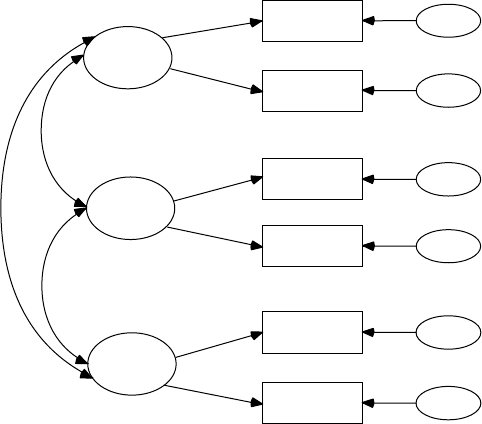
242 A Beginner’s Guide to Structural Equation Modeling
45.65 22.58 611.63
6.39 3.16 44.62 7.32
3.22 3.77 23.47 3.33 4.02
45.58 22.01 548.00 40.99 21.43 585.14
Sample 3
5.74
1.35 2.49
39.24 12.73 535.30
4.94 1.65 37.36 5.39
1.67 2.32 15.71 1.85 3.06
40.11 12.94 496.86 38.09 14.91 538.76
a. Run individual program for sample 1 to determine CFA model
and report CFA parameters.
b. Run individual programs with CFA model on sample 2 and
sample 3 and report CFA parameters.
c. Run multiple-sample program to test factor loadings and factor
correlations invariant (equal) with unequal error variances and
report individual and global chi-square values.
d. Interpret your results.
2. For Exercise #1, Report the single sample expected cross valida-
tion index (ECVI). Given a sample size of 80, would you split the
sample and cross validate the model using CVI?
FED
MED
FOC
SOFED
FAFED
SOMED
MOMED
SOFOC
FAFOC
err_sf
err_ff
err_sm
err_mf
err_sc
err_fc
FIGURE 12.3
Multiple Sample Conrmatory Factor Model.
Y102005.indb 242 3/22/10 3:26:18 PM

Model Validation 243
References
Arbuckle, J. L., & Wothke, W. (1999). AMOS 4.0 User’s Guide. Chicago, IL:
Smallwaters Corporation.
Bandalos, D. (1993). Factors inuencing the cross-validation of conrmatory factor
analysis models. Multivariate Behavioral Research, 28, 351–374.
Benson, J., & Bandalos, D. (1992). Second-order conrmatory factor analysis of the
reactions to tests’ scale with cross-validation. Multivariate Behavioral Research,
27, 459–487.
Benson, J, Moulin-Julian, M., Schwarzer, C., Seipp, B., & El-Zahhar, N. (1992).
Cross-validation of a revised test anxiety scale using multi-national samples.
In K. Hagtvet (Ed.), Advances in test anxiety research: Vol. 7 (pp. 62–83). Lisse,
Netherlands: Swets & Zeitlinger.
Benson, J., & El-Zahhar, N. (1994). Further renement and validation of the revised
test anxiety scale. Structural Equation Modeling: A Multidisciplinary Journal,
1(3), 203–221.
Bentler, P. M., & Wu, E. (2002). EQS for Windows User’s Guide. Encino, CA:
Multivariate Software.
Bollen, K. A. (1989). Structural equations with latent variables. New York: Wiley.
Bollen, K. A., & Stine, R. A. (1993). Bootstrapping goodness-of-t measures in
structural equation models. In K. A. Bollen, & J. S. Long (Eds.), Testing struc-
tural equation models (pp. 66–110). Newbury Park, CA: Sage.
Browne, M., & Cudeck, R. (1989). Single sample cross-validation indices for cova-
riance structures. Multivariate Behavioral Research, 24, 445–455.
Browne, M., & Cudeck, R. (1993). Alternative ways of assessing model t. In K. A. Bollen
& J. S. Long (Eds.), Testing structural equation models. Newbury Park, CA: Sage.
Cole, D. A., & Maxwell, S. E. (1985). Multitrait-multimethod comparisons across
populations: A conrmatory factor analytic approach. Multivariate Behavioral
Research, 20, 389–417.
Cudeck, R., & Browne, M. W. (1983). Cross-validation of covariance structures.
Multivariate Behavioral Research, 18, 147–167.
Fan, X. (2003). Using commonly available software for bootstrapping in both sub-
stantive and measurement analysis. Educational and Psychological Measurement,
63(1), 24–50.
Faulbaum, F. (1987). Intergroup comparisons of latent means across waves.
Sociological Methods and Research, 15, 317–335.
Hayduk, L. A. (1987). Structural equation modeling with LISREL: Essentials and
advances. Baltimore: Johns Hopkins University Press.
Jöreskog, K. G., & Sörbom, D. (1993). Bootstrapping and Monte Carlo experimenting
with PRELIS2 and LISREL8. Chicago: Scientic Software International.
Jöreskog, K. G., & Sörbom, D. (1996a). LISREL8 user’s reference guide. Chicago:
Scientic Software International.
Jöreskog, K. G., & Sörbom, D. (1996b). PRELIS2: User’s reference guide. Chicago:
Scientic Software International.
Jöreskog, K. G., & Sörbom, D. (1996c). LISREL8: Structural equation modeling with
the SIMPLIS command language. Hillsdale, NJ: Lawrence Erlbaum.
Y102005.indb 243 3/22/10 3:26:18 PM
244 A Beginner’s Guide to Structural Equation Modeling
Lomax, R. G. (1983). A guide to multiple sample equation modeling. Behavior
Research Methods and Instrumentation, 15, 580–584.
Lomax, R. G. (1985). A structural model of public and private schools. Journal of
Experimental Education, 53, 216–236.
Lunneborg, C. E. (1987). Bootstrap applications for the behavioral sciences: Vol. 1.
Psychology Department, University of Washington, Seattle.
McArdle, J. J., & Epstein, D. (1987). Latent growth curves within developmental
structural equation models. Child Development, 58, 110–133.
Mooney, C. Z., & Duval, R. D. (1993). Bootstrapping: A nonparametric approach to
statistical inference. Sage University Series on Quantitative Applications in the
Social Sciences, 07-097. Beverly Hills, CA: Sage.
Stine, R. (1990). An introduction to bootstrap methods: Examples and ideas. In J.
Fox. & J. S. Long (Eds.), Modern methods of data analysis (pp. 325–373). Beverly
Hills, CA: SAGE.
Y102005.indb 244 3/22/10 3:26:19 PM

245
13
Multiple Sample, Multiple Group,
and Structured Means Models
Key Concepts
Testing for parameter differences between samples of data
Testing parameter differences between groups
Testing hierarchical intercept and slope differences in nested groups
In previous chapters, we have learned about the basics of structural equa-
tion modeling. In this chapter and subsequent chapters, we will consider
other SEM models that demonstrate the variety of applications suitable
for structural equation modeling. You should be aware, however, that
our discussion will only introduce these SEM models. You are encour-
aged to explore other examples and applications reported in books
(Marcoulides & Schumacker, 1996; Marcoulides & Schumacker, 2001),
LISREL software examples, and the references at the end of this chapter.
Our intention is to provide a basic understanding of the applications in
this chapter to further your interest in the structural equation modeling
approach. We have used LISREL–SIMPLIS program examples to better
illustrate each application.
13.1 Multiple Sample Models
The multiple samples approach was explained in a previous chapter, but
related to testing measurement invariance in a measurement model. We
expand on the multiple sample approach here to include testing a model
for differences in parameter estimates across samples of data. The theo-
retical model is in Figure 13.1a.
The data set we used for our multiple sample approach can be found
in SPSS 16 Sample folder: C:\Program Files\SPSSInc\SPSS16\Samples\
Y102005.indb 245 3/22/10 3:26:19 PM
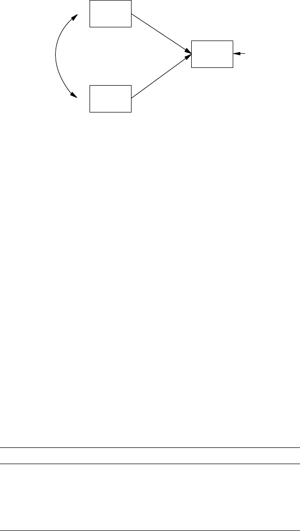
246 A Beginner’s Guide to Structural Equation Modeling
Cars.sav. The Cars.sav data set estimates miles per gallon (mpg) based on
various vehicle characteristics (weight, horsepower, engine displacement,
year of vehicle, etc.). For our purposes we selected mile per gallon as the
dependent variable with vehicle weight and horsepower as independent
predictor variables. The original data set contains N = 406; however, only
N = 392 are useable because of 14 missing cases (8 due to dependent vari-
able missingness and 6 due to independent variable missingness).
The descriptive statistics for the dependent and independent variables
are shown in Table 13.1. The average was 23.45 miles per gallon with an
approximate +/−7.8 miles per gallon standard deviation.
Table 13.2 reports the multiple regression prediction results that yielded
an R2 = .675 (F = 404.583; df = 2, 389; p = .0001). Our interpretation would sug-
gest that two-thirds of the miles per gallon variation can be explained by a
vehicles weight and horsepower. The negative beta coefcients are expected
because as weight and horsepower increase, miles per gallon decrease.
Our interest in multiple samples is to compare the parameter estimates
of each sample to determine whether they differ signicantly. We there-
fore took two random samples without replacement from the Cars.sav
weight
power
mpg
FIGURE 13.1a
Multiple Samples Model.
TABLE 13.1
Complete Sample Descriptive Statistics (N = 392)
Variable Miles Per Gallon Vehicle Weight Horsepower
Miles per gallon 1.0
Vehicle weight –.807 1.0
Horse power –.771 .857 1.0
Mean 23.45 2967.38 104.21
SD 7.805 852.294 38.233
Y102005.indb 246 3/22/10 3:26:19 PM

Multiple Sample, Multiple Group, and Structured Means Models 247
data.* The descriptive statistics for both samples are indicated below in
Table 13.3 and Table 13.4, respectively.
Sample 1
TABLE 13.3
Sample 1 Descriptive Statistics (N = 206)
Variable Miles Per Gallon Vehicle Weight Horsepower
Miles per gallon 1.0
Vehicle weight −.821 1.0
Horse power −.778 .865 1.0
Mean 23.94 2921.67 104.23
SD 8.140 835.421 41.129
Sample 2
TABLE 13.4
Sample 2 Descriptive Statistics (N = 188)
Variable Miles Per Gallon Vehicle Weight Horsepower
Miles per gallon 1.0
Vehicle weight −.823 1.0
Horse power −.760 .855 1.0
Mean 23.59 2952.02 102.72
SD 7.395 805.372 36.234
The SPSS multiple regression analyses are in Table 13.5 and Table 13.6,
respectively, for the two samples of data. We see from the SPSS multiple
* See Chapter Footnote for SPSS details on selecting random samples from Cars.sav.
TABLE 13.2
Multiple Regression Complete Sample
Unstandardized
Coefcients
Standardized
Coefcients
95% Condence
Interval for B
b
Std
Error B t P
Lower
CI
Upper
CI
Constant 44.777 .825 54.307 .0001 43.156 46.398
Vehicle Weight −.005 .001 −.551 −9.818 .0001 −.006 −.004
Horsepower −.061 .011 −.299 −5.335 .0001 −.084 −.039
Y102005.indb 247 3/22/10 3:26:20 PM

248 A Beginner’s Guide to Structural Equation Modeling
regression analysis of the complete data (N = 292) what our sample results
provide in terms of R2 values, F value, and regression coefcients. We also
can visually compare our two individual sample SPSS regression analy-
ses. The results appear to be very similar. Structural equation modeling
software, however, provides the capability of testing whether our results
(parameter estimates) are statistically different.
LISREL provides the ability to compare both samples rather than hav-
ing to run separate multiple regression programs on each sample and
hand calculate a t-test or z-test for differences in the regression weights.
The LISREL multiple sample approach is therefore presented to show how
to stack or include each program with different samples of data.
TABLE 13.6
Sample 2 Multiple Regression Results (N = 188)
Unstandardized
Coefcients
Standardized
Coefcients
95% Condence
Interval for B
b
Std
Error B t p
Lower
CI
Upper
CI
Constant 45.412 1.166 38.957 .0001 43.112 47.712
Vehicle weight −.006 .001 −.642 −8.114 .0001 −.007 −.004
Horsepower −.043 .016 −.212 −2.675 .0001 −.075 −.011
R2 = .689 (F = 204.502; df = 2, 185; p = .001).
Regression model comparing two samples
Group 1: Sample 1
Observed variables: mpg weight power
TABLE 13.5
Sample 1 Multiple Regression Results (N = 206)
Unstandardized
Coefcients
Standardized
Coefcients
95% Condence
Interval for B
b
Std
Error B t p
Lower
CI
Upper
CI
Constant 46.214 1.193 38.723 .0001 43.861 48.568
Vehicle Weight −.006 .001 −.585 −7.550 .0001 −.007 −.004
Horsepower −.054 .015 −.272 −3.509 .0001 −.084 −.024
R2 = .692 (F = 228.206; df = 2, 203; p = .001)
Y102005.indb 248 3/22/10 3:26:20 PM

Multiple Sample, Multiple Group, and Structured Means Models 249
Sample Size: 206
Correlation Matrix
1.0
−.821 1.0
−.778 .865 1.0
Means 23.94 2921.67 104.23
Standard Deviations 8.140 835.421 41.129
Equations:
mpg = weight power
Group 2: Sample 2
Observed variables: mpg weight power
Sample Size: 188
Correlation Matrix
1.0
−.823 1.0
−.760 .855 1.0
Means: 23.59 2952.02 102.72
Standard Deviations: 7.395 805.372 36.234
Path Diagram
End of Problem
The LISREL multisample output in Figure 13.1b reveals that the chi-
square test is nonsignicant (c2 = 2.01, df = 3, p = .57), which indicates that
the two samples do not have statistically different parameter estimates
in the regression model. Another way of thinking about these results is
Chi-Square = 2.01, df =3, p = .57
weight1.03
power1.12
mpg0.31
–0.61
–0.25
0.93
FIGURE 13.1b
Multiple Samples Output.
Y102005.indb 249 3/22/10 3:26:20 PM

250 A Beginner’s Guide to Structural Equation Modeling
that both samples t the theoretical model equally. The regression coef-
cient in common for weight predicting mpg was −.61; the individual
regression weights in SPSS were estimated as −.585 and −.642, respec-
tively. So, it seems reasonable to have a common regression beta weight
of –.61. Looking at the regression weight for power predicting mpg, we
nd a common regression coefcient of −.25. The individual regression
weights in SPSS were estimated as −.272 and −.212, respectively. So, it
seems reasonable to have a common regression beta weight of –.25. Also,
notice that the error of prediction for mpg is .31 (1 – R2), which means that
the common model R2 = .69. We nd that for each individual sample, the
R2 values were .692 and .689, respectively. So, once again, the common R2
value of .69 is reasonable.
The SEM modeling approach is useful for testing whether samples of
data yield similar or different parameter estimates, whether comparing
multiple regression equations, path models, conrmatory factor models,
or structural equation models.
13.2 Multiple Group Models
Multiple group models are set up the same way as multiple sample mod-
els. You are basically applying a single specied model to either one or
more samples of data or in the case of multiple groups, one or more
groups. This type of SEM modeling permits testing for group differences
in the specied model or testing for differences in specic parameter esti-
mates by imposing constraints. For example, Lomax (1985) examined a
model for schooling using the High School and Beyond (HSB) database.
The model included home background, academic orientation, extracur-
ricular activity, achievement, and educational and occupational aspira-
tions as latent variables. The research determined the extent to which
the measurement and structural equation models t both a sample of
public school students and a sample of private school students and also
examined whether model differences existed between the two groups.
The multiple group model analysis should rst establish the acceptance
of the measurement models and measurement invariance for the groups
before hypothesizing any statistically signicant difference in coef-
cients between groups. A LISREL–SIMPLIS multiple group example is
presented based on an example in Arbuckle and Wothke (2003). The mul-
tiple group model is specied to examine the perceived attractiveness
Y102005.indb 250 3/22/10 3:26:21 PM
Multiple Sample, Multiple Group, and Structured Means Models 251
and perceived academic ability differences between a sample of 209 girls
and 207 boys.
The LISREL–SIMPLIS program is constructed to include the GROUP
command to distinguish between the two groups of data. The observed
variables, sample size, means, standard deviations, and correlation
matrix are given for each group. The LISREL–SIMPLIS program pro-
vides a test of a common model when you only include the EQUATIONS
or RELATIONSHIP command in the rst group. The computer output
yields a common model with the parameter estimates. If you wish to
have separate models, hence separate parameter estimates for each group,
you would run each program separately with the same EQUATIONS or
RELATIONSHIP command in both programs.
13.2.1 Separate Group Models
We will begin by rst running a LISREL–SIMPLIS program that provides
separate path analysis estimates for girls and boys. The LISREL–SIMPLIS
program would be run as follows:
Multiple Group Path Model Analysis
Group 1: Girls
Observed Variables academic attract gpa height weight rating
Sample Size = 209
Means .12 .42 10.34 .00 94.13 2.65
Standard Deviation .16 .49 3.49 2.91 19.32 1.01
Correlation Matrix
1.00
.50 1.00
.49 .32 1.00
.10 −.03 .18 1.00
.04 −.16 -.10 .34 1.00
.09 .43 .15 −.16 −.27 1.00
Equation:
academic = gpa attract
attract = academic height weight rating
Let the errors of academic and attract correlate
Group 2: Boys
Observed Variables academic attract gpa height weight rating
Sample Size = 207
Means: .10 .44 8.63 .00 101.91 2.59
Standard Deviations: .16 .49 4.04 3.41 24.32 .97
Correlation Matrix
1.00
Y102005.indb 251 3/22/10 3:26:21 PM
252 A Beginner’s Guide to Structural Equation Modeling
.49 1.00
.58 .30 1.00
−.02 .04 −.11 1.00
−.11 -.19 -.16 .51 1.00
.11 .28 .13 .06 −.18 1.00
Equation:
academic = gpa attract
attract = academic height weight rating
Let the errors of academic and attract correlate
Number of Decimals = 3
Path diagram
End of problem
Computer Output
The annotated computer output for girls and boys multiple-group model
(Figure 13.2a and Figure 13.2b) results are listed below:
GIRLS
Structural Equations
academic = 0.0257* attract + 0.0212*gpa, Errorvar.= 0.0175, R² = 0.296
(0.0427) (0.00329) (0.00213)
0.603 6.440 8.196
attract = 1.688*academic − 0.000248*height – 0.00169*weight + 0.175*rating,
(0.362) (0.0102) (0.00154) (0.0287)
4.666 −0.0244 −1.097 6.085
Errorvar.= 0.155 , R² = 0.386
(0.0110)
14.044
Error Covariance for attract and academic = −0.010
(0.00979)
−0.982
Group Goodness-of-Fit Statistics
Contribution to Chi-Square = 3.773
Percentage Contribution to Chi-Square = 66.580
Root Mean Square Residual (RMR) = 0.105
Standardized RMR = 0.0276
Goodness-of-Fit Index (GFI) = 0.994
Y102005.indb 252 3/22/10 3:26:21 PM
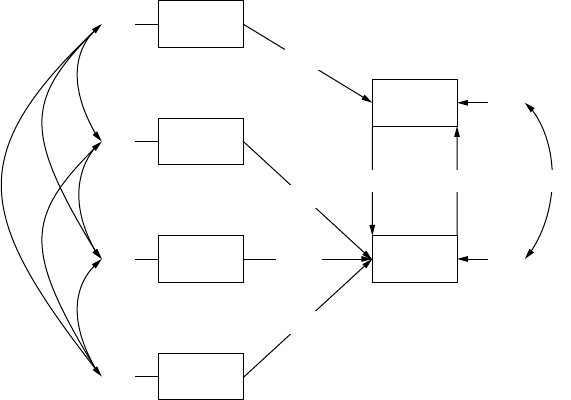
Multiple Sample, Multiple Group, and Structured Means Models 253
BOYS
Structural Equations
academic = 0.00657*attract + 0.0227*gpa, Errorvar.= 0.0175, R² = 0.338
(0.0481) (0.00288) 0.00213)
0.137 7.882 8.196
attract = 1.381*academic + 0.0179*height – 0.00341*weight + 0.0975*rating,
(0.303) (0.00955) (0.00136) (0.0295)
4.560 1.875 −2.504 3.301
Errorvar.= 0.155 , R² = 0.323
(0.0110)
14.044
Error Covariance for attract and academic = −0.001
(0.00989)
−0.095
gpa
height
weight
rating
0.86
0.84
0.77
–0.24
–0.27
–0.15
–0.15
–0.14
1.04
–0.08
0.50
0.55 0.08 –0.12
0.68
0.64
academic
attract
–0.00
–0.08
0.35
FIGURE 13.2a
Multiple Group Model: girls.
Y102005.indb 253 3/22/10 3:26:21 PM

254 A Beginner’s Guide to Structural Equation Modeling
Group Goodness-of-Fit Statistics
Contribution to Chi-Square = 1.894
Percentage Contribution to Chi-Square = 33.420
Root Mean Square Residual (RMR) = 0.0223
Standardized RMR = 0.0183
Goodness-of-Fit Index (GFI) = 0.997
gpa
height
weight
rating
1.15
1.16
1.23
–0.20
0.61
–0.13
0.06
0.14
0.96
–0.19
0.54
0.45 0.02 –0.01
0.68
0.64
academic
attract
0.12
–0.15
0.20
FIGURE 13.2b
Multiple Group Model: boys.
The results indicate different parameter estimates for the girl’s data and
the boy’s data when applied to the model. For example, the reciprocal path
coefcients between academic and attract for the girl’s data were p12 = .55
and p21 = .08, whereas for the boy’s data these same path coefcients were
.45 and .02, respectively. The girl’s data t the path model as indicated by
the nonsignicant chi-square value (c2 = 3.773), and the boy’s data also t
the path model as indicated by their nonsignicant chi-square value (c2 =
1.894). The Global Fit Statistics indicated a chi-square for the hypothesis of
unequal (separate) parameter estimates in the path model (c2 = 5.667, df =
6, p = .461). You will notice that the separate chi-square values for the girls’
and boys’ path model results will add up to this global chi-square value:
c2 = 3.773 (girls) + 1.894 (boys) = 5.667. Our primary interest, however, is in
testing a hypothesis about whether the groups have equal (same) param-
eter estimates in the path model.
Y102005.indb 254 3/22/10 3:26:22 PM
Multiple Sample, Multiple Group, and Structured Means Models 255
13.2.2 Similar Group Model
LISREL–SIMPLIS uses the GROUP command (GROUP must be followed
by a number) and does not use the EQUATION commands in the second
group, when testing whether the two groups share a common path model.
The LISREL–SIMPLIS program would now be as follows:
Multiple Group Path Model Analysis
Group 1: Girls
Observed Variables academic attract gpa height weight rating
Sample Size = 209
Means .12 .42 10.34 .00 94.13 2.65
Standard Deviation .16 .49 3.49 2.91 19.32 1.01
Correlation Matrix
1.00
.50 1.00
.49 .32 1.00
.10 −.03 .18 1.00
.04 −.16 −.10 .34 1.00
.09 .43 .15 −.16 −.27 1.00
Equation:
academic = gpa attract
attract = academic height weight rating
Let the errors of academic and attract correlate
Group 2: Boys
Observed Variables academic attract gpa height weight rating
Sample Size = 207
Means: .10 .44 8.63 .00 101.91 2.59
Standard Deviations: .16 .49 4.04 3.41 24.32 .97
Correlation Matrix
1.00
.49 1.00
.58 .30 1.00
−.02 .04 −.11 1.00
−.11 -.19 −.16 .51 1.00
.11 .28 .13 .06 −.18 1.00
Number of Decimals = 3
Path diagram
End of problem
Computer Output
Structural Equations
academic = 0.0167*attract + 0.0221*gpa, Errorvar. = 0.0174, R² = 0.290
(0.0404) (0.00237) (0.00217)
0.414 9.330 8.039
Y102005.indb 255 3/22/10 3:26:22 PM
256 A Beginner’s Guide to Structural Equation Modeling
attract = 1.439*academic + 0.00863*height – 0.00256*weight + 0.142*rating,
(0.233) (0.00687) (0.00102) (0.0204)
6.189 1.255 −2.499 6.985
Errorvar. = 0.156 , R² = 0.346
(0.0109)
14.309
Error Covariance for attract and academic = −0.003
(0.00796)
−0.429
GIRLS
Group Goodness-of-Fit Statistics
Contribution to Chi-Square = 6.739
Percentage Contribution to Chi-Square = 57.949
Root Mean Square Residual (RMR) = 0.0920
Standardized RMR = 0.0320
Goodness-of-Fit Index (GFI) = 0.989
BOYS
Group Goodness-of-Fit Statistics
Contribution to Chi-Square = 4.890
Percentage Contribution to Chi-Square = 42.051
Root Mean Square Residual (RMR) = 0.0276
Standardized RMR = 0.0249
Goodness-of-Fit Index (GFI) = 0.992
Global Goodness-of-Fit Statistics
Degrees of Freedom = 13
Minimum Fit Function Chi-Square = 11.629 (P = 0.558)
Normal Theory Weighted Least Squares Chi-Square = 11.699
(P = 0.552)
Root Mean Square Error of Approximation (RMSEA) = 0.0
90 Percent Condence Interval for RMSEA = (0.0 ; 0.0633)
P-Value for Test of Close Fit (RMSEA < 0.05) = 0.876
Normed Fit Index (NFI) = 0.975
When the path diagram window is open you will see a window labeled,
Groups: Multiple Group Path Model. The rst path model is for GIRLS. All
of the parameters specied in the EQUATIONS command are set equal
between the two groups. Only the covariance among the observed vari-
ables is free to vary.
Y102005.indb 256 3/22/10 3:26:22 PM
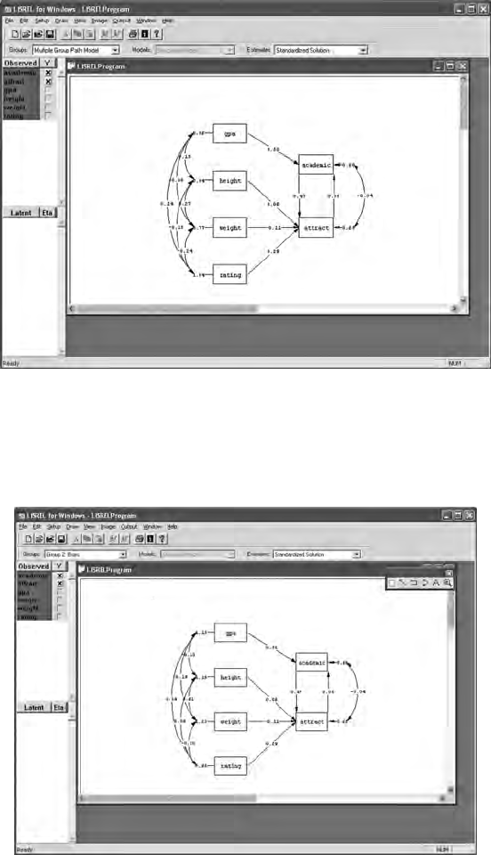
Multiple Sample, Multiple Group, and Structured Means Models 257
When you scroll down to select Group 2: Boys in the Groups window, you
will then see the path diagram for the boys. You will see that the param-
eter estimates are equal for all the paths specied in the EQUATIONS
command. The only parameters free to vary (be different) are the covari-
ance among the observed variables.
You will notice that the parameter estimates are the same in both groups.
For example, p12 = .47 and p21 = .05. The individual chi-square values for each
group also add up to the global chi-square statistic for this common model.
Y102005.indb 257 3/22/10 3:26:23 PM
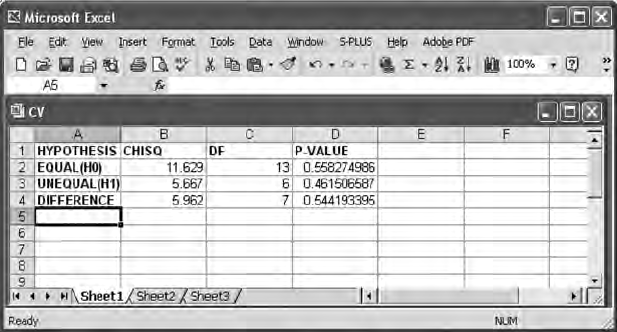
258 A Beginner’s Guide to Structural Equation Modeling
The chi-square for the girls was c2 = 6.739 and the chi-square for the boys
was c2 = 4.890, which yield the global chi-square value of c2 = 11.629, df =
13, p = .558. These results indicated that both sets of data t the path model
based on the hypothesis of similar path coefcients in the path model.
13.2.3 Chi-Square Difference Test
It is possible to compute a chi-square difference test between the two path
model analyses. Recall that the rst LISREL–SIMPLIS program analysis
tested a hypothesis of unequal parameter estimates, while the second
LISREL–SIMPLIS program analysis tested a hypothesis of equal parame-
ter estimates. You can compute a chi-square difference test between these
two models by using an EXCEL spreadsheet program, CV.XLS. You will
nd this EXCEL program by going to the LISREL 8.8 Student Examples
folder on the C:/directory, and then nding the WORKSHOP folder.
Open the CV.XLS program outside the LISREL–SIMPLIS program, oth-
erwise it will crash and cause an error message. All you have to do is enter
the Global Chi-Square value from the analysis of equal parameter estimates
(c2 = 11.629, df = 13) and the Global Chi-Square value from the analysis of
unequal parameter estimates (c2 = 5.667, df = 6). The program calculates
the difference in the chi-square values and associated p-values.
The chi-square difference was c2 = 5.962, df = 7, p = .544, which indicated
no difference between the two model analyses. This implies that the girls’
and boys’ data separately t the path model, as well as both data sets t
a common path model. A different path model analysis might examine
other variables besides gender that produce different results, for example,
Caucasian versus African-American path models.
The dialog box for the chi-square difference test should look like the
one below.
Y102005.indb 258 3/22/10 3:26:23 PM

Multiple Sample, Multiple Group, and Structured Means Models 259
13.3 Structured Means Models
The structured means model is yet another special type of SEM applica-
tion that is used to test group mean differences in observed and/or latent
variables. Mean differences between observed variables in SEM is similar
to analysis of variance and covariance techniques. However, mean differ-
ence in latent variables is unique to SEM.
13.3.1 Model Specification and Identification
The structured means model example (Figure 13.3) is from LISREL–
SIMPLIS and uses the program EX13B.SPL (Jöreskog & Sörbom, 1993,
EX13B.SPL). The structured means model examines the mean difference
between academic and nonacademic boys in 5th and 7th grades on a latent
variable, verbal ability. The structured means model is diagrammed below
where writing and reading scores measure each latent variable at the 5th
grade (Writing5 and Reading5) and 7th grade (Writing7 and Reading7).
Two LISREL–SIMPLIS programs will need to be run to test the mean
difference between the latent variables, Verbal5 and Verbal7. The rst pro-
gram indicates the observed variables and equations that relate to the
structured means model diagram. The coefcient CONST is used to des-
ignate the means in the equations for the observed variables and the latent
variables, respectively. The rst program also includes the sample size,
covariance matrix, and means for the rst group (academic boys). The sec-
ond program includes the sample size, covariance matrix, and means for
the second group (nonacademic boys). In addition, the second program
Verbal7
Verbal5
Writing7
Reading7
Writing5
Reading5
err_w7
err_r7
err_w5
err_r5
FIGURE 13.3
Structured Means Model.
Y102005.indb 259 3/22/10 3:26:24 PM
260 A Beginner’s Guide to Structural Equation Modeling
establishes a test of the mean differences between the latent variables in
the Relationship command:
Relationships:
Verbal5 = CONST
Verbal7 = CONST
The rst and second LISREL–SIMPLIS programs are both stacked into
one complete program, but identied separately using the GROUP com-
mand, as follows:
Group ACADEMIC: Reading and Writing, Grades 5 and 7
Observed Variables: READING5 WRITING5 READING7 WRITING7
Covariance Matrix
281.349
184.219 182.821
216.739 171.699 283.289
198.376 153.201 208.837 246.069
Means 262.236 258.788 275.630 269.075
Sample Size: 373
Latent Variables: Verbal5 Verbal7
Relationships:
READING5 = CONST + 1*Verbal5
WRITING5 = CONST + Verbal5
READING7 = CONST + 1*Verbal7
WRITING7 = CONST + Verbal7
Group NONACADEMIC: Reading and Writing, Grades 5 and 7
Covariance Matrix
174.485
134.468 161.869
129.840 118.836 228.449
102.194 97.767 136.058 180.460
Means 248.675 246.896 258.546 253.349
Sample Size: 249
Relationships:
Verbal5 = CONST
Verbal7 = CONST
Set the Error Variances of READING5 - WRITING7 free
Set the Variances of Verbal5 - Verbal7 free
Set the Covariance between Verbal5 and Verbal7 free
Path diagram
End of problem
(Note: You should rst est abl ish that the data t a t heoret ical model before test-
ing for mean differences in the latent variable. Acceptable model-t indices
for each group, as well as for both groups combined, should be obtained.)
Y102005.indb 260 3/22/10 3:26:24 PM
Multiple Sample, Multiple Group, and Structured Means Models 261
13.3.2 Model Fit
The current example had individual group and combined group model-t
indices that were acceptable.
Academic Boys
Group Goodness-of-Fit Statistics
Contribution to Chi-Square = 4.15
Standardized RMR = 0.025
Goodness-of-Fit Index (GFI) = 0.99
Nonacademic Boys
Group Goodness-of-Fit Statistics
Contribution to Chi-Square = 5.97
Standardized RMR = 0.042
Goodness-of-Fit Index (GFI) = 0.99
Global Goodness-of-Fit Statistics
Degrees of Freedom = 6
Minimum Fit Function Chi-Square = 10.11 (P = 0.12)
Root Mean Square Error of Approximation (RMSEA) = 0.046
90 Percent Condence Interval for RMSEA = (0.0 ; 0.095)
P-Value for Test of Close Fit (RMSEA < 0.05) = 0.27
Comparative Fit Index (CFI) = 1.00
13.3.3 Model Estimation and Testing
The LISREL–SIMPLIS computer output reects the structured mean equa-
tions by replacing the CONST term with the mean value for each group in
the measurement equations.
Measurement Equations: Academic Group
READING5 = 262.37 + 1.00*Verbal5, Errorvar .= 50.15, R² = 0.81
(0.84) (6.02)
312.58 8.34
WRITING5 = 258.67 + 0.84*Verbal5, Errorvar. = 36.48, R² = 0.81
(0.70) (0.024) (4.28)
366.96 34.35 8.52
READING7 = 275.71 + 1.00*Verbal7, Errorvar. = 51.72, R² = 0.82
(0.87) (6.62)
317.77 7.82
Y102005.indb 261 3/22/10 3:26:24 PM

262 A Beginner’s Guide to Structural Equation Modeling
WRITING7 = 268.98 + 0.89*Verbal7, Errorvar. = 57.78, R² = 0.76
(0.80) (0.028) (6.05)
338.00 31.95 9.55
Measurement Equations: Nonacademic Group
READING5 = 262.37 + 1.00*Verbal5, Errorvar.= 23.25, R² = 0.87
(0.84) (6.23)
312.58 3.73
WRITING5 = 258.67 + 0.84*Verbal5, Errorvar. = 42.80, R² = 0.72
(0.70) (0.024) (5.64)
366.96 34.35 7.59
READING7 = 275.71 + 1.00*Verbal7, Errorvar. = 65.67, R² = 0.70
(0.87) (9.87)
317.77 6.65
WRITING7 = 268.98 + 0.89*Verbal7, Errorvar. = 67.36, R² = 0.65
(0.80) (0.028) (8.74)
338.00 31.95 7.71
The structured means model is testing the mean latent variable differ-
ence, which is indicated by the Mean Vector of Independent Variables. Results
are interpreted based on the knowledge that the mean latent value on
Verbal5 and Verbal7 are set to zero (0) in the rst group (academic boys), so
the values reported here are going to indicate that the second group was
either greater than (positive) or less than (negative) the rst group on the
latent variables.
The latent variable mean difference value of −13.80 is indicated for the
rst latent variable, which indicates the mean difference was less than
the rst group, that is, nonacademic boys scored below academic boys on
verbal ability in the 5th grade.
The latent variable mean difference value of –17.31 is indicated for the
second latent variable, which indicates the mean difference was less than
the rst group; that is, nonacademic boys scored below academic boys on
verbal ability in the 7th grade.
Overall, nonacademic boys are scoring below academic boys in the 5th
and 7th grades. The latent variable mean differences are divided by their
standard error to yield a one-sample T value, that is, T = −13.80/1.18 =
−11.71 (within rounding error).
Mean Vector of Independent Variables
Verbal5 Verbal7
−13.80 −17.31
(1.18) (1.24)
−11.71 −13.99
Y102005.indb 262 3/22/10 3:26:24 PM
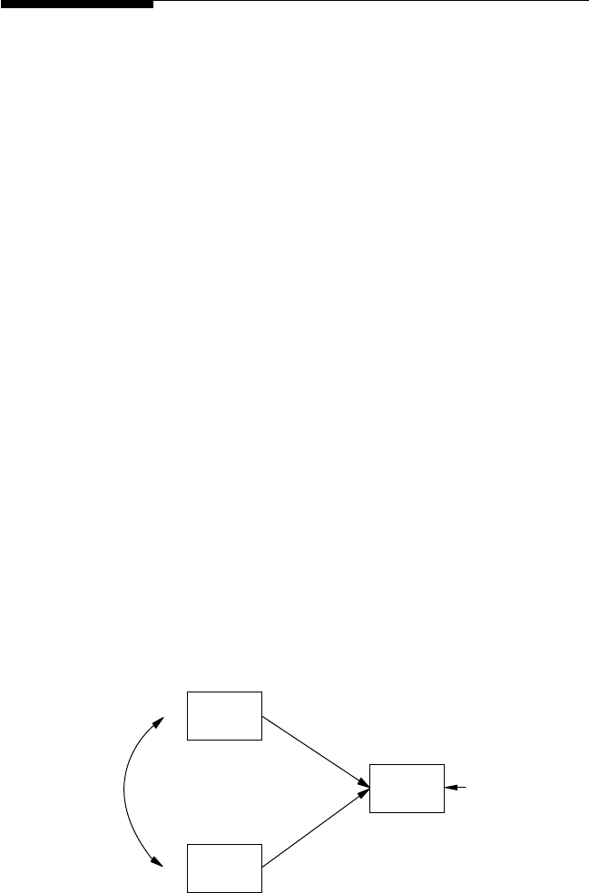
Multiple Sample, Multiple Group, and Structured Means Models 263
1 3 . 4 S u m m a r y
In this chapter we have described multiple samples, multiple group, and
structured means modeling to demonstrate the versatility of structural
equation modeling. The rst application involved comparing structure
coefcients across samples of data. We referred to this as a Multiple Sample
Model. The second application involved testing the difference between
parameter estimates given multiple groups, for example, different grade
levels, different countries, or different schools. We referred to this as a
Multiple Group Model. Our third application demonstrated how to test
for mean differences between groups on latent variables. We referred to
this as a Structured Means Model. This extends the basic analysis of vari-
ance approach where mean differences on observed variables are tested
but, more importantly, mean differences in latent variables can be tested
(Cole, Maxwell, Arvey, & Salas, 1993).
The chapter presented only one example for each of the applications
because a more in depth coverage is beyond the scope of this book.
However, the LISREL software HELP library provides other examples and
can be searched by using keywords to nd other software examples and
explanations. The LISREL User Guide is another excellent reference for
other examples of these applications. We now turn our attention to the
next chapter where other SEM applications are presented and discussed.
Exercises
1. MULTIPLE SAMPLE MODEL
Nursing programs are interested in knowing if their outcomes are
similar from one semester to the next. Two semesters of data were
obtained on how student effort and learning environment predicted
clinical competence in nursing. The regression model is:
effort
learn
comp
FIGURE 13.4
Nursing Multiple Sample Model.
Y102005.indb 263 3/22/10 3:26:25 PM

264 A Beginner’s Guide to Structural Equation Modeling
Create a LISREL–SIMPLIS program to test whether the regression
coefcients in the model are the same or statistically signicantly dif-
ferent for the two semester samples of data. Semester 1 had 250 nurses
and Semester 2 had 205 nurses. (Note: The means and standard devia-
tions were not available, so assume the data is in standardized form
and only use the correlation matrix in your analysis.)
Semester 1 (N = 250)
Clinical Effort Learn
Clinical 1.0
Effort .28 1.0
Learn .23 .25 1.0
Semester 2 (N = 205)
Clinical Effort Learn
Clinical 1.0
Effort .21 1.0
Learn .16 .15 1.0
2. MULTIPLE GROUP MODEL
Create a LISREL–SIMPLIS program that produces output to deter-
mine if path coefcients are statistically signicantly different. You
will need the LISREL–SIMPLIS software and separate data set infor-
mation provided below to perform this task. Also, provide the path
diagrams with interpretation of results using the Excel program.
The path model tests that job satisfaction (satis) is indicated by boss
attitude (boss) and the number of hours worked (hrs). The boss atti-
tude (boss) is in turn indicated by the employee satisfaction (satis).
The boss attitude (boss) is also indicated by the type of work per-
formed (type), level of assistance provided (assist), and evaluation of
the work (eval). The Equation command would therefore be specied
as follows:
Equation:
satis = boss hrs
boss = type assist eval satis
(NOTE: Since a reciprocal relation exists between boss and satis,
the errors would need to be correlated to obtain the correct path
coefcients.)
Y102005.indb 264 3/22/10 3:26:25 PM
Multiple Sample, Multiple Group, and Structured Means Models 265
The data set information to be used to test hypotheses of equal or
unequal parameter estimates in a path model between Germany and
the United States are listed below.
Germany
Path Model Analysis for Germany
Observed Variables satis boss hrs type assist eval
Sample Size = 400
Means 1.12 2.42 10.34 4.00 54.13 12.65
Standard Deviation 1.25 2.50 3.94 2.91 9.32 2.01
Correlation Matrix
1.00
.55 1.00
.49 .42 1.00
.10 .35 .08 1.00
.04 .46 .18 .14 1.00
.01 .43 .05 .19 .17 1.00
United States
Path Model Analysis for United States
Observed Variables satis boss hrs type assist eval
Sample Size = 400
Means: 1.10 2.44 8.65 5.00 61.91 12.59
Standard Deviations: 1.16 2.49 4.04 4.41 4.32 1.97
Correlation Matrix
1.00
.69 1.00
.48 .35 1.00
.02 .24 .11 1.00
.11 .19 .16 .31 1.00
.10 .28 .13 .26 .18 1.00
3. STRUCTURED MEANS MODEL
A researcher is interested in testing whether a low-motivation
group and a high-motivation group in two different cities (Los
Angeles and Chicago) have a production rate mean difference
on the production line. Create and run the two stacked LISREL–
SIMPLIS programs for a test of latent variable mean differences.
Explain results.
The structured means model is diagrammed in Figure 13.5.
Y102005.indb 265 3/22/10 3:26:25 PM
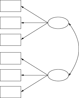
266 A Beginner’s Guide to Structural Equation Modeling
The Low-Motivation data information is:
Group Low Motivation:
Observed Variables: Prod1 Prod2 Prod3 Prod4 Prod5 Prod6
Correlation Matrix
1.00
.64 1.00
.78 .73 1.00
.68 .63 .69 1.00
.43 .55 .50 .59 1.00
.65 .63 .67 .81 .60 1.00
Means 4.27 5.02 4.48 4.69 4.53 4.66
Sample Size: 300
The High-Motivation data information is:
Group High Motivation:
Correlation Matrix
1.00
.72 1.00
.76 .74 1.00
.51 .46 .57 1.00
.32 .33 .39 .40 1.00
.54 .45 .60 .73 .45 1.00
Means 14.35 14.93 14.59 14.86 14.71 14.74
Sample Size: 300
Prod1
Prod2
Prod3
City 1
Prod4
Prod5
Prod6
City 2
FIGURE 13.5
Motivation Structured Means Model.
Y102005.indb 266 3/22/10 3:26:25 PM

Multiple Sample, Multiple Group, and Structured Means Models 267
Suggested Readings
Multiple Samples
Geary, D. C. & Whitworth, R. H. (1988). Dimensional structure of the Wais-R:
A simultaneous multi-sample analysis. Educational and Psychological
Measurement, 48(4), 945–956.
Tschanz, B. T., Morf, C. C., & Turner, C. W. (1998). Gender differences in the struc-
ture of Narcissism: A multi-sample analysis of the narcissistic personality
inventory. Sex Roles: A Journal of Research, 38, 863–868.
Poon, W. Y., & Tang, F. C. (2002). Multisample analysis of multivariate ordinal cat-
egorical variables. Multivariate Behavioral Research, 37, 479–500.
Multiple Group Models
Conner, B. T., Stein, J. A., Longshore, D. (2005). Are cognitive AIDS risk-reduction
model equally applicable among high- and low-risk seekers? Personality &
Individual Differences, 38, 379–393.
Long, B. (1998). Coping with workplace stress: A multiple-group comparison of
female managers and clerical workers. Journal of Counseling Psychology, 45,
65–78.
Unrau, N. & Schlackman, J. (2006, November/December). Motivation and its rela-
tionship with reading achievement in an urban middle school. The Journal of
Educational Research, 100(2), 81–101.
Structured Means Models
Anderson, N., & Lievens, F. (2006). A construct-driven investigation of gender dif-
ferences in a leadership-role assessment center. Journal of Applied Psychology,
91, 555–566.
Hancock, G. (2001). Effect size, power, and sampling size determination for struc-
tured means modeling and mimic approaches to between groups hypoth-
esis testing of means on a testing of means on a single latent construct.
Psychometrika, 66, 3, 373–388.
Hayashi, N., Igarashi, Y., Yamashina, M., & Suda, K. (2002, January/February). Is
there a gender difference in a factorial structure of the positive and negative
syndrome scale? Psychopathology, 35(1), 28–35.
Wei, M. F., Russell, D. W., Mallinckrodt, B., & Zakalik, R. A. (2004). Cultural
equivalence of adult attachment across four ethnic groups: factor structure,
structured means, and associations with negative mood. Journal of Counseling
Psychology, 51, 408–417.
Y102005.indb 267 3/22/10 3:26:26 PM

268 A Beginner’s Guide to Structural Equation Modeling
Chapter Footnote
SPSS
Select Cases: Random Sample
This dialog box allows you to select a random sample based on an
approximate percentage or an exact number of cases. Sampling is per-
formed without replacement; so, the same case cannot be selected more
than once.
Approximately: Generates a random sample of approximately the
specied percentage of cases. Since this routine makes an inde-
pendent pseudo-random decision for each case, the percentage of
cases selected can only approximate the specied percentage. The
more cases there are in the data le, the closer the percentage of
cases selected is to the specied percentage.
Exactly: A user-specied number of cases. You must also specify the
number of cases from which to generate the sample. This second
number should be less than or equal to the total number of cases
in the data le. If the number exceeds the total number of cases in
the data le, the sample will contain proportionally fewer cases
than the requested number.
From the menu choose:
Data
Select Cases
Select Random sample of cases.
Click Sample.
Select the sampling method and enter the percentage or number
of cases.
Y102005.indb 268 3/22/10 3:26:26 PM
Multiple Sample, Multiple Group, and Structured Means Models 269
References
Arbuckle, J. L., & Wothke, W. (2003). Amos 5.0 user’s guide. Chicago, IL:
Smallwaters Corporation.
Cole, D. A., Maxwell, S. E., Arvey, R., & Salas, E. (1993). Multivariate group com-
parisons of variable systems: MANOVA and structural equation modeling.
Psychological Bulletin, 114, 174–184.
Jöreskog, K., & Sörbom, D. (1993). LISREL 8: Structural equation modeling with the
SIMPLIS command language. Chicago, IL: Scientic Software International.
Lomax, R. G. (1985). A structural model of public and private schools. Journal of
Experimental Education, 53, 216–226.
Marcoulides, G., & Schumacker, R. E. (Eds.). (1996). Advanced structural equation
modeling: Issues and techniques. Mahwah, NJ: Lawrence Erlbaum.
Marcoulides, G., & Schumacker, R. E. (Eds.). (2001). New developments and tech-
niques in structural equation modeling: Issues and techniques. Mahwah, NJ:
Lawrence Erlbaum.
Y102005.indb 269 3/22/10 3:26:26 PM

271
14
Second-Order, Dynamic, and
Multitrait Multimethod Models
Key Concepts
Second-order factors
Dynamic models: measuring factors over time
Establishing reliability and validity when measuring multiple traits
and methods
In the previous chapter we learned about comparing samples or groups
using structural equation modeling applications. In this chapter we
present additional applications that expand our understanding of SEM
models, but now related to measurement models. Please be aware that
our discussion will only scratch the surface of the many exciting new
developments in structural equation modeling related to measurement
models. Some of these new applications have been included in chapters
of books (Marcoulides & Schumacker, 1996; Marcoulides & Schumacker,
2001; and Schumacker & Marcoulides, 1998) and journal articles. In
addition, the newest version of LISREL has included these capabilities
with software examples and further explanations. Our intention is to
provide a basic understanding of these topics to further your interest in
the structural equation modeling approach. We have included computer
program examples to better illustrate each type of SEM model.
14.1 Second-Order Factor Model
14.1.1 Model Specification and Identification
A second-order factor model is indicated when rst-order factors are explained
by some higher-order factor structure. Theory plays an important role in justify-
ing a higher-order factor. Visual, verbal, and speed are three psychological factors
Y102005.indb 271 3/22/10 3:26:27 PM
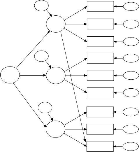
272 A Beginner’s Guide to Structural Equation Modeling
that most likely indicate a second-order factor, namely Ability. A second-order
factor model is therefore hypothesized and diagrammed in Figure 14.1.
14.1.2 Model Estimation and Testing
The data used for testing the second-order factor model is based on an
example in the LISREL 8 Student Examples, SPLEX folder (EX5.spl). The
data are nine psychological variables that identied three common factors
(Visual, Verbal, and Speed). The second-order factor model hypothesizes that
these three common factors indicate a higher-order second factor, Ability.
The LISREL–SIMPLIS program includes the Ability latent variable and
sets the variance of this higher-order second factor to 1.0. (Note: S-C CAPS
loads on both latent variables Visual and Speed, and a single quote is used
when variable names have a space between them.) The LISREL–SIMPLIS
program is therefore written as:
Second-Order Factor Analysis (EX5.SPL)
Observed Variables
‘VIS PERC’ CUBES LOZENGES ‘PAR COMP’ ‘SEN COMP’ WORDMEAN
vispercerr_v
cubeserr_c
lozengeserr_l
paragrap err_p
sentenceerr_s
wordmeanerr_w
addition err_p
countdot err_s
s-c caps
speed
verbalability
visual
D1
D3
D2
err_w
FIGURE 14.1
Second-Order Factor Model.
Y102005.indb 272 3/22/10 3:26:27 PM
Second-Order, Dynamic, and Multitrait Multimethod Models 273
ADDITION COUNTDOT ‘S-C CAPS’
Correlation Matrix
1.000
.318 1.000
.436 .419 1.000
.335 .234 .323 1.000
.304 .157 .283 .722 1.000
.326 .195 .350 .714 .685 1.000
.116 .057 .056 .203 .246 .170 1.000
.314 .145 .229 .095 .181 .113 .585 1.000
.489 .239 .361 .309 .345 .280 .408 .512 1.000
Sample Size 145
Latent Variables: Visual Verbal Speed Ability
Relationships:
‘VIS PERC’ - LOZENGES ‘S-C CAPS’ = Visual
‘PAR COMP’ - WORDMEAN = Verbal
ADDITION - ‘S-C CAPS’ = Speed
Visual = Ability
Verbal = Ability
Speed = Ability
Set variance of Ability = 1.0
Number of Decimals = 3
Wide Print
Print Residuals
Path diagram
End of problem
The selected LISREL–SIMPLIS model-t indices listed below indicated that
the hypothesized second-order factor model has an acceptable t (c2 =
28.744, p = .189, df = 23; RMSEA = .04; GFI = .958).
Goodness-of-Fit Statistics
Degrees of Freedom = 23
Minimum Fit Function Chi-Square = 29.008 (P = 0.180)
Normal Theory Weighted Least Squares Chi-Square = 28.744
(P = 0.189)
Estimated Noncentrality Parameter (NCP) = 5.744
90 Percent Confidence Interval for NCP = (0.0; 23.597)
Root Mean Square Error of Approximation (RMSEA) = 0.0416
90 Percent Confidence Interval for RMSEA = (0.0; 0.0844)
P-Value for Test of Close Fit (RMSEA < 0.05) = 0.580
Root Mean Square Residual (RMR) = 0.0451
Standardized RMR = 0.0451
Expected Cross-Validation Index (ECVI) = 0.505
90 Percent Confidence Interval for ECVI = (0.465; 0.629)
ECVI for Saturated Model = 0.625
ECVI for Independence Model = 4.695
Normed Fit Index (NFI) = 0.956
Goodness-of-Fit Index (GFI) = 0.958
Y102005.indb 273 3/22/10 3:26:27 PM

274 A Beginner’s Guide to Structural Equation Modeling
The structural equations in the computer output indicate the strength of
relationship between the rst-order factors and the second-order factor,
Ability. Visual (.987) is indicated as a stronger measure of Ability, followed
by Verbal (.565) and Speed (.395), with all three being statistically signicant
(t > 1.96). Therefore, student Ability is predominantly a function of visual
perception of geometric congurations with complementary verbal skills
and speed in completing numerical tasks, which enhance a students’
overall ability.
Structural Equations
Visual = 0.987*Ability, Errorvar.= 0.0257, R² = 0.974
(0.229) (0.401)
4.309 0.0640
Verbal = 0.565*Ability, Errorvar.= 0.681 , R² = 0.319
(0.141) (0.170)
4.015 3.997
Speed = 0.395*Ability, Errorvar.= 0.844 , R² = 0.156
(0.132) (0.227)
2.999 3.717
14.2 Dynamic Factor Model
A class of SEM applications that involve stationary and nonstationary latent
variables across time with lagged (correlated) measurement error has been
called dynamic factor analysis (Hershberger, Molenaar, & Corneal, 1996).
A characteristic of the SEM dynamic factor model is that the same mea-
surement instruments are administered to the same subject on two or more
occasions. The purpose of the analysis is to assess change in the latent vari-
able between the ordered occasions due to some event or treatment. When
the same measurement instruments are used over two or more occasions,
there is a tendency for the measurement errors to correlate (autocorrelation);
for example, a specic sequence of correlated error, where error at Time 1
correlates with error at Time 2, and error at Time 2 correlates with error at
Time 3, is called an ARIMA model in econometrics.
Educational research has indicated that anxiety increases the level of
student achievement and performance. Psychological research in contrast
indicates that anxiety has a negative effect upon individuals, thus should
interfere or have a decreasing impact on the level of achievement and per-
formance. Is it possible that both areas of research are correct?
A dynamic factor model was hypothesized to indicate student achieve-
ment and performance measures at three equal time points two weeks
Y102005.indb 274 3/22/10 3:26:27 PM
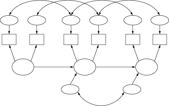
Second-Order, Dynamic, and Multitrait Multimethod Models 275
apart (time 1, time 2, and time 3). The student data indicates achievement
(A1) and performance (P1) at time 1, achievement (A2) and performance
(P2) at time 2, and achievement (A3) and performance (P3) at time 3. The
errors at time 1 were hypothesized to correlate with errors at time 2 and
errors at time 2 were hypothesized to correlate with errors at time 3, indi-
cating an ARIMA model. Time 1 predicts time 2 and time 2 predicts time
3. The dynamic factor model is diagrammed in Figure 14.2a:
error
Time 1
A1
error
P1
error
error
Time 2
A2
error
P2
error
error
Time 3
A3
error
P3
FIGURE 14.2a
Dynamic Factor Model (Wheaton et al., 1977).
The data set contains 600 students who were measured on the same
achievement and performance measures at three different points in time.
The two variables, achievement and performance, dened the factor time.
Thus, the latent variable, time, was represented as time1, time2, and time3,
with two indicator variables at each time point. How well students did
at time 2 was predicted by the time 1 latent variable. Likewise, how well
students did at time 3 was predicted by time 2. Students were given a high
level of anxiety by having to meet deadlines, take frequent quizzes, and
turn in extra assignments. A LISREL–SIMPLIS program was created to
test this dynamic factor model.
Dynamic Factor Model
Observed Variables: A1 P1 A2 P2 A3 P3
Covariance Matrix
11.834
6.947 9.364
6.819 5.091 12.532
Y102005.indb 275 3/22/10 3:26:28 PM
276 A Beginner’s Guide to Structural Equation Modeling
4.783 5.028 7.495 9.986
−3.839 −3.889 −3.841 −3.625 9.610
−2.190 −1.883 −2.175 −1.878 3.552 4.503
Sample Size: 600
Latent Variables: Time1 Time2 Time3
Relationships:
A1 P1 = Time1
A2 P2 = Time2
A3 P3 = Time3
Time2 = Time1
Time3 = Time2
Let the Errors of A1 and A2 correlate
Let the Errors of P1 and P2 correlate
Let the Errors of A2 and A3 correlate
Let the Errors of P2 and P3 correlate
Let the Errors of Time2 and Time3 correlate
Path Diagram
End of Problem
The dynamic factor model results indicated an acceptable model t (c2 =
2.76, df = 2, and p = .25). The structural equations indicate the prediction
across the three time intervals for the latent variable, time. Time 1 was
a statistically signicant predictor of time 2; coefcient was statistically
signicant (T = 12.36) and R2 = .47. Time 2 was a statistically signicant
predictor of time 3; however, the result indicated a negative coefcient
(−.82).
Structural Equations
Time2 = 0.68*Time1, Errorvar. = 0.53 , R² = 0.47
(0.055) (0.071)
12.36 7.50
Time3 = − 0.82*Time2, Errorvar. = 0.80 , R² = 0.20
(0.085) (0.12)
−9.66 6.52
The dynamic factor model would therefore be interpreted as follows: anxi-
ety increased the level of student achievement and performance from time
1 to time 2, but then decreased the level of student achievement and perfor-
mance from time 2 to time 3. Anxiety increased levels of achievement and
performance, but only for a certain amount of time, then it had a negative
effect. So, it appears educational researchers and psychologists are both
correct to some extent. The dynamic factor model claries how anxiety
affects the level of student achievement and performance, given a time
continuum.
The dynamic factor model output with standardized coefcients is
listed in Figure 14.2b with standardized coefcients:
Y102005.indb 276 3/22/10 3:26:28 PM
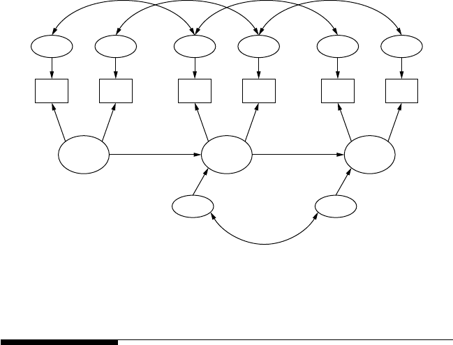
Second-Order, Dynamic, and Multitrait Multimethod Models 277
14.3 Multitrait Multimethod Model (MTMM)
The Multitrait Multimethod model (MTMM) is used to indicate multiple
traits assessed by multiple measures—for example, student achievement
and student motivation (traits) assessed by teacher ratings and student self
ratings (methods). MTMM models, however, are problematic to analyze
as noted by Lomax and Algina (1979) who compared two procedures for
analyzing MTMM matrices. The MTMM matrix does provide a convenient
way to report reliability and construct validity coefcients (Campbell &
Fiske, 1959). Construct validity involves providing psychometric evidence
of convergent validity, discriminant validity, trait, and method effects, even
across populations (Cole & Maxwell, 1985). The Multitrait Multimethod
matrix conveniently displays the convergent validity coefcients, discrimi-
nant validity coefcients, and the reliability coefcients along the diago-
nal. A two-trait/two-method matrix is displayed in Table 14.1.
Reliability coefcients (1) indicate the internal consistency of scores on
the instrument, and therefore should be in the range .85 to .95 or higher.
Convergent validity coefcients (2) are correlations between measures
of the same trait (construct) using different methods (instruments), and
therefore should also be in the range .85 to .95 or higher. Discriminant
validity coefcients (3) are correlations between measures of different
error
Time 1 0.68
1.54 0.41 0.16 0.004
0.29
–0.82
A1
error
P1
error
error
Time 2
A2
error
P2
error
error
Time 3
A3
error
P3
FIGURE 14.2b
Dynamic Factor Model Output.
Y102005.indb 277 3/22/10 3:26:29 PM
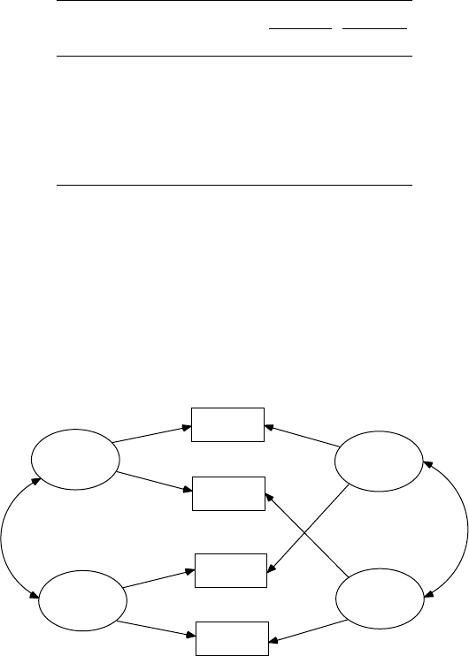
278 A Beginner’s Guide to Structural Equation Modeling
traits (constructs) using the same method (instrument), and should be
much lower than the convergent validity coefcients and/or the instru-
ment reliability coefcients. The basic MTMM model for two traits/two
methods is diagrammed in Figure 14.3a:
Achieve
F1
Motivate
F2
Self
Rating
F3
Teacher
Rating
F4
Rating 1
Rating 2
Rating 3
Rating 4
FIGURE 14.3a
Basic MTMM Model (two traits/two methods).
The correlation of ratings from different methods of the same trait
should be statistically signicant—that is, having convergent validity
(2). The convergent validity coefcients should also be greater than the
correlations of ratings from different traits using the same method—that
is, discriminant validity (3), and the correlations between ratings that
share neither trait nor method (−).
TABLE 14.1
Two-Trait/Two-Method Multitrait Multimethod
Matrix
Method 1 Method 2
Trait A BA B
Method 1. Self Ratings
A. Achievement (1)
B. Motivation (3) (1)
Method 2. Teacher Ratings
A. Achievement (2) — (1)
B. Motivation — (2) (3) (1)
Note: (1) = reliability coefcients; (2) = convergent valid-
ity coefcients; (3) = discriminant validity coef-
cients; and (—) = correlations between ratings that
share neither trait nor method.
Y102005.indb 278 3/22/10 3:26:29 PM
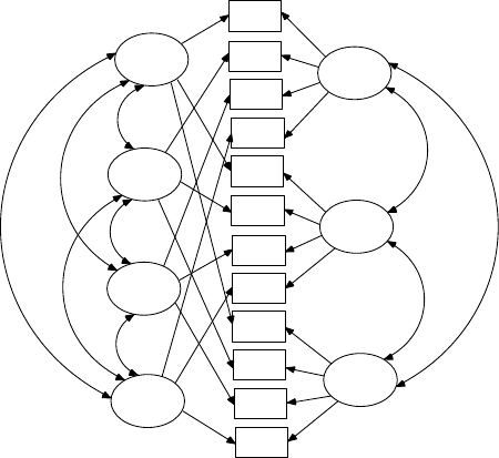
Second-Order, Dynamic, and Multitrait Multimethod Models 279
14.3.1 Model Specification and Identification
The Multitrait Multimethod (MTMM) model example indicates three
methods (self-ratings, peer ratings, and observer ratings) used to assess
four traits of leadership (prominence, achievement, afliation, and leader).
The sample size is N = 240 subjects.
MTMM models are problematic to analyze and typically will require
specifying start values (initial parameter values) and setting AD = OFF
(admissibility check) to obtain convergence—that is, obtain parameter
estimates. (Note: Start values are typically chosen between .1 and .9 so that
the estimation process does not have to start with a zero value for param-
eters in the model; the 2SLS estimates also provide reasonable start val-
ues). The Multitrait Multimethod models are difcult to analyze because
they lack model identication (initially have negative degrees of free-
dom) and can have convergence problems (nonpositive denite matrix).
Consequently, latent variable variances should be set to 1.0, and factor
correlations between traits and methods set to zero, otherwise, the PHI
matrix will be nonpositive denite. Additionally, certain error variances
need to be set equal to prevent negative error variance (Heywood case).
In MTMM models, the different methods are uncorrelated with the differ-
ent traits, so a model diagram helps to visually display the specied model
(Figure 14.3b).
X1
X2
X3
X4
X5
X6
X7
X8
X9
X10
X11
X12
self
peer
obs
prom
ach
affl
lead
FIGURE 14.3b
Multitrait Multimethod Model. (From Bollen, K. A. [1989]. Structural equations with latent
variables. New York: John Wiley & Sons.)
Y102005.indb 279 3/22/10 3:26:30 PM
280 A Beginner’s Guide to Structural Equation Modeling
14.3.2 Model Estimation and Testing
The LISREL–SIMPLIS program to analyze the three sets of ratings on the
four traits as a MTMM model is:
Multitrait-Multimethod Bollen (1989)
!Start Values Added (.5) and Admissibility Check Off (AD=OFF)
Observed Variables: X1 X2 X3 X4 X5 X6 X7 X8 X9 X10 X11 X12
Correlation Matrix
1.0
.50 1.0
.41 .48 1.0
.67 .59 .40 1.0
.45 .33 .26 .55 1.0
.36 .32 .31 .43 .72 1.0
.25 .21 .25 .30 .59 .72 1.0
.46 .36 .28 .51 .85 .80 .69 1.0
.53 .41 .34 .56 .71 .58 .43 .72 1.0
.50 .45 .29 .52 .59 .55 .42 .63 .84 1.0
.36 .30 .28 .37 .53 .51 .43 .57 .62 .57 1.0
.52 .43 .31 .59 .68 .60 .46 .73 .92 .89 .63 1.0
Sample Size: 240
Latent Variables: prom ach affl lead self peer obs
Relationships:
X1 = (.3)*self + (.5)*prom
X2 = (.3)*self + (.5)*ach
X3 = (.3)*self + (.5)*affl
X4 = (.3)*self + (.5)*lead
X5 = (.3)*peer + (.5)*prom
X6 = (.2)*peer + (.5)*ach
X7 = (.2)*peer + (.5)*affl
X8 = (.2)*peer + (.5)*lead
X9 = (.2)*obs + (.5)*prom
X10 = (.3)*obs + (.5)*ach
X11 = (.3)*obs + (.5)*affl
X12 = (.3)*obs + (.5)*lead
Set Variance of prom - obs to 1.0
Set correlation of prom and self to 0
Set correlation of ach and self to 0
Set correlation of affl and self to 0
Set correlation of lead and self to 0
Set correlation of prom and peer to 0
Set correlation of ach and peer to 0
Set correlation of affl and peer to 0
Set correlation of lead and peer to 0
Set correlation of prom and obs to 0
Set correlation of ach and obs to 0
Set correlation of affl and obs to 0
Y102005.indb 280 3/22/10 3:26:30 PM

Second-Order, Dynamic, and Multitrait Multimethod Models 281
Set correlation of lead and obs to 0
Let the error variance of X10 and X12 be equal
OPTIONS: AD = OFF
LISREL OUTPUT
End of Problem
Results from the computer output are summarized in Table 14.2 to dem-
onstrate the interpretation of trait and method effects. The assessment
of Afliation (Af) had the highest error variance when using Self ratings
(error = .67) and Observer ratings (error = .39), thus Afliation was the most
difcult trait to assess using either of these two methods. The self rating
worked best for leadership assessment (factor loading = .61; error variance =
.30). The peer rating method worked best with assessing afliation (factor
loading = .79; error variance = .14). The observer rating method worked best
with assessing achievement (factor loading = .68; error variance = .07).
(NOTE: Most attempts at running MTMM models will result in unidenti-
ed models or lack convergence (unable to estimate parameters). Other
types of MTMM models—for example, correlated uniqueness model or
a composite direct product model—generally work better. A correlated
uniqueness model will therefore be presented next.
14.3.3 Correlated Uniqueness Model
We present an example of a correlated uniqueness model, since it seems
to have less convergence problems with meaningful results, and is
TABLE 14.2
MTMM Estimates of Four Traits Using Three Methods (N = 240)
Traits Methods
Prom Ach Af Lead Self Peer Obs Error
Prom .52 .58 .41
Ach .42 .61 .46
Af .35 .47 .67
Lead .58 .61 .30
Prom .84 .32 .19
Ach .69 .53 .23
Af .48 .79 .14
Lead .84 .43 .09
Prom .80 .53 .09
Ach .69 .68 .07
Af .75 .23 .39
Lead .78 .59 .07
Y102005.indb 281 3/22/10 3:26:30 PM
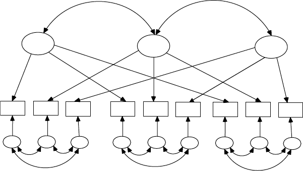
282 A Beginner’s Guide to Structural Equation Modeling
recommended by Marsh and Grayson (1995) and Wothke (1996) as an
alternative to traditional MTMM models. In correlated uniqueness mod-
els, each variable is affected by one trait factor and one error term, and
there are no method factors. The method effects are accounted for by the
correlated error terms of each variable. The correlated error terms only
occur between variables measured by the same method.
Different types of correlated uniqueness models can be analyzed
(Huelsman, Furr, & Nemanick, 2003). For example, one general factor with
correlated uniqueness, two correlated factors with correlated uniqueness,
two correlated factors with uncorrelated uniqueness, or two uncorrelated
factors with correlated uniqueness. Marsh and Grayson (1995) indicated
that a signicant decrease in t between a model with correlated traits,
but no correlated error terms and a model with correlated traits and cor-
related error terms, indicated the presence of method effects. Following
this approach, you can test method effects by analyzing a correlated trait
correlated uniqueness model (CTCU) and a correlated trait (CT) only
model.
Figure 14.3c displays the correlated trait–correlated uniqueness (CTCU)
model with three traits and three methods. The CTCU model represents
the method effects through the correlated error terms of the observed
variables. Figure 14.3d displays the correlated trait (CT) only model with
no correlated error terms. In the CT model, the variables measured by the
same method are grouped under each trait factor.
Trait 1 Trait 2
Var 1 Var 2
e1 e2
Trait 3
Var 3
e3
Var 4 Var 5
e4 e5
Var 6
e6
Var 7 Var 8
e7 e8
Var 9
e9
FIGURE 14.3c
Correlated Trait–Correlated Uniqueness Model.
Y102005.indb 282 3/22/10 3:26:31 PM
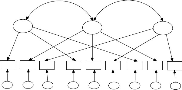
Second-Order, Dynamic, and Multitrait Multimethod Models 283
The data from Bollen (1989) was used again, but this time only three
traits (prom, ach, and af) with three methods (self, peer, and obs) were ana-
lyzed. The LISREL–SIMPLIS program for the CTCU model with corre-
lated traits and correlated error terms is:
Correlated Traits—Correlated Uniqueness Model - Bollen (1989)
Observed Variables: Var1 Var2 Var3 Var4 Var5 Var6 Var7
Var8 Var9
Correlation Matrix
1.0
.50 1.0
.41 .48 1.0
.45 .33 .26 1.0
.36 .32 .31 .72 1.0
.25 .21 .25 .59 .72 1.0
.53 .41 .34 .71 .58 .43 1.0
.50 .45 .29 .59 .55 .42 .84 1.0
.36 .30 .28 .53 .51 .43 .62 .57 1.0
Sample Size: 240
Latent Variables: prom ach affl
Relationships:
Var1 = prom
Var2 = ach
Var3 = affl
Var4 = prom
Var5 = ach
Var6 = affl
Trait 1 Trait 2
Var 1 Var 2
e1 e2
Trait 3
Var 3
e3
Var 4 Var 5
e4 e5
Var 6
e6
Var 7 Var 8
e7 e8
Var 9
e9
FIGURE 14.3d
Correlated Trait Model.
Y102005.indb 283 3/22/10 3:26:31 PM

284 A Beginner’s Guide to Structural Equation Modeling
Var7 = prom
Var8 = ach
Var9 = affl
Set Variance of prom-affl to 1.0
Let Error Covariance of Var1 – Var3 Correlate
Let Error Covariance of Var4 – Var6 Correlate
Let Error Covariance of Var7 – Var9 Correlate
Path Diagram
End of Problem
The results from the computer output are presented in Table 14.3. Findings
indicated that all three traits were statistically signicantly correlated.
More importantly, the observation method was the best for assessing any of
the three traits, as indicated by the higher trait factor loadings and lower
correlated uniqueness error terms. The data also had an acceptable t to
the CTCU model (c2 = 17.38, p = .30, df = 15; RMSEA = .026).
The LISREL program was run again to estimate a correlated trait (CT)-
only model with no correlated error terms. To accomplish this, you simply
delete the following command lines:
Let Error Covariance of Var1 – Var3 Correlate
Let Error Covariance of Var4 – Var6 Correlate
Let Error Covariance of Var7 – Var9 Correlate
TABLE 14.3
Correlated Uniqueness Model with Correlated Traits and Errors
Method Trait
Factor
Loading Uniqueness R2
Correlated Uniqueness
of Error Terms
Self Prom .58 .67 .33 1.0
Ach .48 .77 .23 .24 1.0
Af .40 .85 .16 .20 .30 1.0
Peer Prom .78 .40 .61 1.0
Ach .68 .54 .46 .23 1.0
Af .55 .70 .30 .23 .37 1.0
Observe Prom .92 .16 .84 1.0
Ach .84 .30 .70 .12 1.0
Af .76 .42 .58 .007 −.03 1.0
Trait correlations
Prom 1.0
Ach .93 1.0
Af .88 .93 1.0
Note: c2 = 17.38, p = .30, df = 15; RMSEA = .026; n = 240.
Y102005.indb 284 3/22/10 3:26:31 PM

Second-Order, Dynamic, and Multitrait Multimethod Models 285
The results from the computer output are presented in Table 14.4. The
trait factor loadings, uniqueness, and R2 values are not substantially dif-
ferent from the previous CTCU model; however, the data is not an accept-
able t to the CT model (c2 = 270.63, p = .00001, df = 24; RMSEA = .21).
Comparing the previous CTCU model (c2 = 17.38, p = .30) to this CT model
(c2 = 270.63, p = .00001) indicates a method effect. The method that was
suggested as more effective was the observation method. Some trait cor-
relations in the CT model were greater than 1.0 indicating a nonpositive
denite matrix (1.05 and 1.06—boldfaced). The CT model modication
indices also suggested adding the specic unique error covariance terms
which, if added, would result in the CTCU model.
The Modification Indices Suggest to Add an Error Covariance
Between and Decrease in Chi-Square New Estimate
Var2 Var1 21.4 0.22
Var3 Var1 15.4 0.19
Var3 Var2 27.8 0.28
Var5 Var4 30.4 0.19
Var6 Var4 23.0 0.17
Var6 Var5 76.3 0.35
Var7 Var5 41.0 −0.21
Var7 Var6 27.5 −0.16
TABLE 14.4
Correlated Uniqueness Model with Correlated Traits Only
Method Trait Factor Loading Uniqueness R2
Self Prom .58 .66 .34
Ach .45 .79 .21
Af .41 .83 .17
Peer Prom .79 .37 .63
Ach .72 .48 .52
Af .62 .61 .39
Observe Prom .90 .20 .80
Ach .80 .35 .65
Af .68 .53 .47
Trait Correlationsa
Prom 1.0
Ach 1.05 1.0
Af .95 1.06 1.0
Note: c2 = 270.63, p = .0000, df = 24; RMSEA = .21; n = 240.
a Trait correlation matrix is a nonpositive denite matrix because correlations
are greater than 1.0.
Y102005.indb 285 3/22/10 3:26:32 PM

286 A Beginner’s Guide to Structural Equation Modeling
Var8 Var4 33.7 −0.18
Var8 Var6 10.3 −0.12
Var8 Var7 70.3 0.26
The MTMM model is problematic to analyze, but can be done given
the addition of start values, setting AD = OFF, setting latent variances
to 1.0, setting factor correlations to zero, and setting error variances
equal. The alternative correlated uniqueness model approach in SEM
is easier to obtain convergence (compute parameter estimates), but is
not without controversy over how to interpret the results because more
than one possible explanation may exist for the observed correlated
error terms.
Although Bollen (1989, p. 190–206) and Byrne (1998, p. 228–229) have
demonstrated how to conduct a multitrait multmethod model with a
taxonomy of nested models suggested by Widaman (1985), Marsh and
Grayson (1995) and Wothke (1996) have demonstrated that most attempts
at running MTMM models result in unidentied models or lack con-
vergence, and offer suggestions for other types of MTMM models that
included the correlated uniqueness model or a composite direct product
model. We strongly suggest that you read Marsh and Grayson (1995) or
Wothke (1996) for a discussion of these alternative MTMM models and
problems with analyzing data using a MTMM model.
Saris and Aalberts (2003) questioned the interpretation of the cor-
related uniqueness model approach in SEM. They agreed that one
possible explanation for the observed correlated terms is the similar-
ity of methods for the different traits; however, they provided other
explanations for the correlated error terms. Their alternative models
explained the correlated error terms based on method effects, relative
answers to questions, acquiescence bias, and/or variation in response
patterns when examining characteristics of survey research questions
on a questionnaire. We are, therefore, reminded that error terms do
not necessarily reect a single unknown measure, rather contain sam-
pling error, systematic error, and other potentially unknown measures
(observed variables).
1 4 . 4 S u m m a r y
In this chapter, we have considered second-order factor models, dynamic
factor models, and multitrait multimethod models, including an alterna-
tive correlated uniqueness model. We have learned that the traditional
Y102005.indb 286 3/22/10 3:26:32 PM
Second-Order, Dynamic, and Multitrait Multimethod Models 287
multitrait multimethod model has identication and convergence prob-
lems such that Marsh and Grayson (1995) and Wothke (1996) have recom-
mended alternative approaches, namely correlated uniqueness and direct
product models.
We hope that our discussion of these SEM applications has provided
you with a basic overview and introduction to these methods. We encour-
age you to read the references provided at the end of the chapter and run
some of the program setups provided in the chapter. We further hope
that the basic introduction in this chapter will permit you to read the
research literature and better understand the resulting models presented,
which should support various theoretical perspectives. Attempting a few
basic models will help you better understand the approach; afterwards,
you may wish to attempt one of these SEM applications in your own
research.
Exercises
1. SECOND-ORDER FACTOR ANALYSIS
The psychological research literature tends to suggest that drug use
and depression are leading indicators of suicide among teenagers.
(Note: Set variance of Suicide = 1 for model identication purposes).
Given the following data set information, create and run a LISREL–
SIMPLIS program to conduct a second-order factor analysis.
Observed Variables: drug1 drug2 drug3 drug4 depress1
depress2 depress3 depress4
Sample Size 200
Correlation Matrix
1.000
0.628 1.000
0.623 0.646 1.000
0.542 0.656 0.626 1.000
0.496 0.557 0.579 0.640 1.000
0.374 0.392 0.425 0.451 0.590 1.000
0.406 0.439 0.446 0.444 0.668 .488 1.000
0.489 0.510 0.522 0.467 0.643 .591 .612 1.000
Means 1.879 1.696 1.797 2.198 2.043 1.029 1.947 2.024
Standard Deviations 1.379 1.314 1.288 1.388 1.405 1.269
1.435 1.423
Latent Variables: drugs depress Suicide
The second-order factor model is diagrammed in Figure 14.4:
Y102005.indb 287 3/22/10 3:26:32 PM
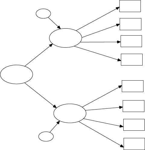
288 A Beginner’s Guide to Structural Equation Modeling
2. DYNAMIC FACTOR MODEL
A sports physician was interested in studying heart rate and muscle
fatigue of female soccer players. She collected data after three soccer
games over a 3-week period. A dynamic factor model was used to
determine if heart rate and muscle fatigue were stable across time for
the 150 female soccer players.
Create a LISREL–SIMPLIS program to analyze and interpret the
dynamic factor model. Include a diagram of the dynamic factor
model. The data set information including observed variables, cova-
riance matrix, sample size, and latent variables are provided below:
Observed Variables: HR1 MF1 HR2 MF2 HR3 MF3
Covariance Matrix
10.75
7.00 9.34
7.00 5.00 11.50
5.03 5.00 7.49 9.96
3.89 4.00 3.84 3.65 9.51
2.90 2.00 2.15 2.88 3.55 5.50
Sample Size: 150
Latent Variables: Time1 Time2 Time3
drug1
drug2
drug3
drug4
depress1
depress2
depress3
depress4
drugs
depress
Suicide
d1
d2
FIGURE 14.4
Siucide Second-Order Factor Model.
Y102005.indb 288 3/22/10 3:26:32 PM
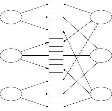
Second-Order, Dynamic, and Multitrait Multimethod Models 289
3. MULTITRAIT MULTIMETHOD (MTMM) MODELS
Students provided ratings of their classroom behavior, motivation
to achieve, and attitude toward learning. Teachers, likewise, pro-
vided ratings of student classroom behavior, perception of students’
motivation to achieve, and attitude toward learning. Finally, other
students or peers provided ratings on these three traits. The three
ratings (student, teacher, and peer) on three traits (behavior, motivate,
attitude) were analyzed in a SEM Multitrait Multimethod model. The
Multitrait Multimethod Model is diagrammed in Figure 14.5:
a. Create and run a LISREL–SIMPLIS program to analyze the
three sets of ratings on the three traits as a MTMM model. The
observed variables, correlation matrix, sample size, and latent
variables are:
Observed Variables: X1 X2 X3 X4 X5 X6 X7 X8 X9
Correlation Matrix
1.0
.40 1.0
.31 .38 1.0
.35 .23 .16 1.0
.26 .22 .21 .62 1.0
.15 .11 .15 .49 .62 1.0
X1
StudentX2
X3
Behavior
X4
Teacher X5
X6
Motivate
X7
Peer X8
X9
Attitude
FIGURE 14.5
Classroom MTMM Model.
Y102005.indb 289 3/22/10 3:26:33 PM

290 A Beginner’s Guide to Structural Equation Modeling
.43 .31 .24 .61 .48 .33 1.0
.40 .35 .19 .49 .45 .32 .74 1.0
.26 .20 .18 .43 .41 .33 .52 .47 1.0
Sample Size: 300
Latent Variables: behavior motivate attitude student
teacher peer
b. Create and run a LISREL–SIMPLIS program to compute a
CTCU and CU model using the data information from above.
Compare the CTCU and CU model results to determine if a
method effect exists. Also, compare the CTCU model with the
MTMM model above, which provides clearer results?
Suggested Readings
Second-Order Factor Models
Chan, D. W. (2006, Fall). Perceived multiple intelligences among male and female
Chinese gifted students in Hong Kong: The structure of the student multiple
intelligences prole. The Gifted Child Quarterly, 50(4), 325–338.
Cheung, D. (2000). Evidence of a single second-order factor in student ratings
of teaching effectiveness. Structural Equation Modeling: A Multidisciplinary
Journal, 7, 442–460.
Rand, D., Conger, R. D., Patterson, G. R., & Ge, X. (1995). It takes two to replicate:
A mediational model for the impact of parents’ stress on adolescent adjust-
ment. Child Development, 66(1), 80–97.
Dynamic Factor Models
Chow, S. M., Nesselroade, J. R., Shifren, K., & McArdle, J. J. (2004). Dynamic struc-
ture of emotions among individuals with Parkinson’s disease. Structural
Equation Modeling, 11(4), 560–582.
Kroonenberg, P. M., van Dam, M., van Uzendoorn, M. H., & Mooijaart, A. (1997,
May). Dynamics of behaviour in the strange situation: A structural equation
approach. British Journal of Psychology, 88, 311–332.
Zuur, A. F., Fryer, R. J., Jolliffe, I. T., Dekker, R., Beukema, J. J. (2003). Estimating
common trends in multivariate time series using dynamic factor analysis.
Environmetrics, 14(7), 665–685.
Multitrait Multimethod Models
Bunting, B. P., Adamson, G., & Mulhall, P. K. (2002). A Monte Carlo examination
of an MTMM model with planned incomplete data structures. Structural
Equation Modeling: A Multidisciplinary Journal, 9, 369–389.
Lim, B., & Ployhart, R. E. (2006, January). Assessing the convergent and discrimi-
nant validity of Goldberg’s international personality item pool. Organizational
Research Methods, 9(1), 29–54.
Y102005.indb 290 3/22/10 3:26:33 PM

Second-Order, Dynamic, and Multitrait Multimethod Models 291
Tildesley, E. A., Hops, H., Ary, D., & Andrews, J. A. (1995). Multitrait-multimethod
model of adolescent deviance, drug use, academic, and sexual behaviors.
Journal of Psychopathology and Behavioral Assessment, 17(2), 185–215.
Correlated Uniqueness Model
Lievens, F., & Van Keer, E. (2001, September). The construct validity of a Belgian
assessment centre: A comparison of different models. Journal of Occupational
and Organizational Psychology, 74, 373–378.
Marsh, H. W., Roche, R. A., Pajares, F., & Miller, M. (1997). Item-specic efcacy
judgments in mathematical problem solving: The downside of standing too
close to trees in a forest. Contemporary Educational Psychology, 22, 363–377.
Quilty, L. C., Oakman, J. M., & Riski, E. (2006). Correlates of the Rosenberg self-
esteem scale method effects. Structural Equation Modeling: A Multidisciplinary
Journal. 13, 99–117.
References
Bollen, K. A. (1989). Structural equations with latent variables. New York: John Wiley
& Sons.
Byrne, B. M. (1998). Structural equation modeling with LISREL, PRELIS, and SIMPLIS:
Basic concepts, applications, and programming. Mahwah, NJ: Lawrence Erlbaum.
Campbell, D. T., & Fiske, D. W. (1959). Convergent and discriminant validation by
the multitrait-multimethod matrix. Psychological Bulletin, 56, 81–105.
Cole, D. A., & Maxwell, S. E. (1985). Multitrait-multimethod comparisons across
populations: A conrmatory factor analytic approach. Multivariate Behavioral
Research, 20, 389–417.
Hershberger, S. L., Molenaar, P. C. M., & Corneal, S. E. (1996). A hierarchy of uni-
variate and multivariate structural times series models (pp. 159–194). In
Marcoulides, G. & Schumacker, R. E. (Eds.), Advanced structural equation mod-
eling: Issues and techniques. Mahwah, NJ: Lawrence Erlbaum.
Huelsman, T. J., Furr, M. R., Nemanick, Jr., R. C. (2003). Measurement of disposi-
tional affect: Construct validity and convergence with a circumplex model of
affect. Educational and Psychological Measurement, 63(4), 655–673.
Lomax, R. G., & Algina, J. (1979). Comparison of two procedures for analyzing
multitrait multimethod matrices. Journal of Educational Measurement, 16, 177–186.
[errata: 1980, 17, 80]
Marcoulides, G., & Schumacker, R. E. (Eds.). (1996). Advanced structural equation
modeling: Issues and techniques. Mahwah, NJ: Lawrence Erlbaum.
Marcoulides, G., & Schumacker, R. E. (Eds.). (2001). New developments and tech-
niques in structural equation modeling. Mahwah, NJ: Lawrence Erlbaum.
Marsh, H. W., & Grayson, D. (1995). Latent variable models of multitrait-
multimethod data. In Hoyle, R. H. (Ed.). Structural equation modeling: Concepts,
issues, and applications. Thousand Oaks, CA: Sage Publications.
Y102005.indb 291 3/22/10 3:26:33 PM
292 A Beginner’s Guide to Structural Equation Modeling
Saris, W. E., & Aalberts, C. (2003). Different explanations for correlated disturbance
terms in MTMM studies. Structural Equation Modeling, 10(2), 193–213.
Schumacker, R. E., & Marcoulides, G. A. (1998). Interaction and nonlinear effects in
structural equation modeling. Mahwah, NJ: Lawrence Erlbaum.
Widaman, K. F. (1985). Hierarchically tested covariance structure models for
multitrait-multimethod data. Applied Psychological Measurement, 9, 1–26.
Wheaton, B., Muthén, B., Alwin, D. F., & Summers, G. F. (1977). Assessing reliabil-
ity and stability in panel models. In D. R. Heise (Ed.), Sociological methodology
(pp 84–136). San Francisco, CA: Jossey-Bass.
Wothke, W. (1996). Models for multitrait-multimethod matrix analysis. In
Marcoulides, G. & Schumacker, R. E. (Eds.), Advanced structural equation mod-
eling: Issues and techniques (pp. 7–56). Mahwah, NJ: Lawrence Erlbaum.
Y102005.indb 292 3/22/10 3:26:33 PM

293
15
Multiple Indicator–Multiple Indicator
Cause, Mixture, and Multilevel Models
Key Concepts
Multiple indicator–multiple cause (MIMIC) models
SEM models with continuous and categorical variables (mixture
models)
Testing multilevel intercept and slope differences in nested groups
(multilevel models).
In this chapter we continue with our presentation and discussion of
SEM model applications. Specically, we present an example where
latent variables are predicted by observed variables (MIMIC model);
an example where continuous and categorical variables are included in
the model (mixture model); and nally an example where nested design
data occur (multilevel model). All three of these SEM applications are
unique and are not possible using traditional statistics (analysis of vari-
ance, etc.).
15.1 Multiple Indicator–Multiple Cause (MIMIC) Models
The term MIMIC refers to multiple indicators and multiple causes and
denes a particular type of SEM model. The MIMIC model involves using
latent variables that are predicted by observed variables. An example by
Jöreskog and Sörbom (1996a, example 5.4, p. 185–187) is illustrated where a
latent variable (social participation) is dened by church attendance, mem-
berships, and friends. The social participation latent variable is predicted by
the observed variables, income, occupation, and education. The MIMIC
model is diagrammed in Figure 15.1a.
Y102005.indb 293 3/22/10 3:26:33 PM
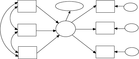
294 A Beginner’s Guide to Structural Equation Modeling
The MIMIC model indicates a latent variable, social, which has arrows
pointing out to the three observed indicator variables (church, member,
friends) with separate measurement error terms for each. This is the mea-
surement part of the MIMIC model that denes the latent variable. In the
MIMIC model, the latent variable, social, also has arrows pointed toward it
from the three observed predictor variables, which have implied correlations
among them (curved arrows). This is the structural part of the MIMIC model
that uses observed variables to predict a latent variable. The MIMIC model
diagram also shows the prediction error for the latent variable, social.
15.1.1 Model Specification and Identification
Model identication pertains to whether the estimates in the MIMIC
model can be calculated, which is quickly gauged by the degrees of free-
dom. Do you recall how the degrees of freedom are determined? There
are a total of 15 free parameters to be estimated in the MIMIC model. The
number of distinct values in the variance-covariance matrix S based on
6 observed variables is: p (p + 1)/2 = 6 (6 + 1)/2 = 21. The degrees of free-
dom are computed by subtracting the number of free parameters from the
number of distinct parameters in the matrix S, which is 21 − 15 = 6.
15.1.2 Model Estimation and Model Testing
The MIMIC model diagram provides the basis for specifying the LISREL–
SIMPLIS program, specically the Latent Variable a nd Relationships command
lines in the LISREL–SIMPLIS program. The LISREL–SIMPLIS program that
species the observed variables, sample size, correlation matrix (standard-
ized variables), and the equations that reect the MIMIC model is:
MIMIC Model
Observed Variables income occup educ church member friends
income
occup
educ
church
member
friends
err_c
err_m
err_f
error
social
FIGURE 15.1a
MIMIC Model.
Y102005.indb 294 3/22/10 3:26:34 PM
Multiple Indicator–Multiple Indicator Cause, Mixture 295
Sample Size 530
Correlation Matrix
1.000
.304 1.000
.305 .344 1.000
.100 .156 .158 1.000
.284 .192 .324 .360 1.000
.176 .136 .226 .210 .265 1.000
Latent Variable social
Relationships
church = social
member = social
friends= social
social = income occup educ
Path Diagram
End of Problem
SEM MIMIC models use goodness-of-t criteria to determine whether a
reasonably good t of the data to the MIMIC model exists. Some basic t
criteria are printed below from the computer output.
Goodness-of-Fit Statistics
Degrees of Freedom = 6
Minimum Fit Function Chi-Square = 12.50 (P = 0.052)
Normal Theory Weighted Least Squares Chi-Square = 12.02
(P = 0.061)
Estimated Noncentrality Parameter (NCP) = 6.02
90 Percent Confidence Interval for NCP = (0.0 ; 20.00)
Root Mean Square Error of Approximation (RMSEA) = 0.044
90 Percent Confidence Interval for RMSEA = (0.0 ; 0.079)
P-Value for Test of Close Fit (RMSEA < 0.05) = 0.56
Expected Cross-Validation Index (ECVI) = 0.079
90 Percent Confidence Interval for ECVI = (0.068 ; 0.11)
Normed Fit Index (NFI) = 0.97
Goodness-of-Fit Index (GFI) = 0.99
The Normal Theory Weighted Least Squares c2 = 12.02, df = 6, and p =
.061 suggests a reasonably good t of the data to the MIMIC model. The
Goodness-of-Fit (GFI) Index suggests that 99% of the variance-covariance
in matrix S is reproduced by the MIMIC model. The LISREL software stan-
dardized solution indicates factor loadings of .47 * church, .74 * member,
and .40 * friends. However, the T-value in the computer output dropped
church as an important indicator variable in dening the latent variable,
social.
Y102005.indb 295 3/22/10 3:26:34 PM
296 A Beginner’s Guide to Structural Equation Modeling
The observed variables, member (T = 6.71) and friends (T = 6.03), were
therefore selected to dene the latent variable social. The measurement
equations from the computer output are listed below.
Measurement Equations
church = 0.47*social, Errorvar. = 0.78 , R² = 0.22
(0.058)
13.61
member = 0.74*social, Errorvar. = 0.46 , R² = 0.54
(0.11) (0.075)
6.71 6.10
friends = 0.40*social, Errorvar. = 0.84 , R² = 0.16
(0.067) (0.058)
6.03 14.51
(NOTE: Because a matrix was used rather than raw data, standard error
and T-value are not output for the reference indicator variable, church. The
HELP menu offers this explanation: LISREL for Windows uses a reference
indicator (indicator with a unit factor loading) to set the scale of each of
the endogenous latent (ETA) variables of the model. If you do not specify
reference indicators for the endogenous latent variables of your model,
LISREL for Windows will select a reference indicator for each endogenous
latent variable of your model. Although LISREL for Windows scales the
factor loadings to obtain the appropriate estimates for the factor loadings
of the reference indicators, it does not use the Delta method to compute
the corresponding standard error estimates).
The observed independent variables (income, occup, and educ) in the
MIMIC model were correlated amongst themselves as identied in the
correlation matrix of the SEM program output:
1.000
.304 1.000
.305 .344 1.000
The structural equation indicated that the latent variable social had 26%
of its variance predicted (R2 = .26), with 74% unexplained error variance
due random or systematic error, and variables not in the MIMIC model.
The T-values for the structural equation coefcients indicated that occup
(occupation) didn’t statistically signicantly predict social (T = parameter
estimate divided by standard error = .097/.056 = 1.73 is less than t = 1.96 at
the .05 level of signicance, two-tailed test), whereas income (T = 3.82) and
educ (T = 4.93) were statistically signicant at the .05 level of signicance.
The structural equation with coefcients, standard errors in parentheses
and associated T values are listed below.
Y102005.indb 296 3/22/10 3:26:34 PM
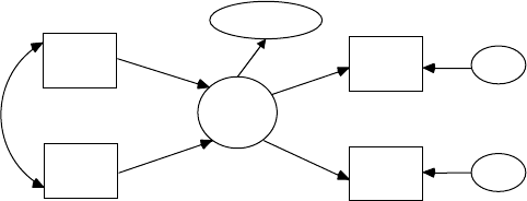
Multiple Indicator–Multiple Indicator Cause, Mixture 297
Structural Equation
Social = 0.23*income + 0.097*occup + 0.33*educ, Errorvar.= 0.74 , R² = 0.26
(0.061) (0.056) (0.068) (0.17)
3.82 1.73 4.93 4.35
15.1.3 Model Modification
The original MIMIC model was therefore modied by dropping church
and occup. The MIMIC model diagram with these modications now
appears in Figure 15.1b.
social
income
educ
member
friends
err_m
err_f
error
FIGURE 15.1b
Modied MIMIC Model.
The model modication t criteria are more acceptable, indicating an
almost perfect t of the data to the MIMIC model, since the Minimum Fit
Function c2 value was close to zero.
Goodness-of-Fit Statistics
Degrees of Freedom = 1
Minimum Fit Function Chi-Square = 0.19 (P = 0.66)
Root Mean Square Error of Approximation (RMSEA) = 0.0
90 Percent Confidence Interval for RMSEA = (0.0 ; 0.088)
P-Value for Test of Close Fit (RMSEA < 0.05) = 0.82
Normed Fit Index (NFI) = 1.00
Goodness-of-Fit Index (GFI) = 1.00
Measurement Equations
member = 0.63*social, Errorvar.= 0.60 , R² = 0.39
(0.08)
7.32
friends = 0.42*social, Errorvar. = 0.82 , R² = 0.17
(0.07) (0.06)
5.54 13.66
Y102005.indb 297 3/22/10 3:26:35 PM

298 A Beginner’s Guide to Structural Equation Modeling
(NOTE: Because a matrix was used rather than raw data, standard errors
are not output for one of the reference indicator variables, member =
0.63*social. The HELP menu offers further explanation as noted above.)
Structural Equations
The structural equation now indicated two statistically signicant predic-
tor variables with R2 = .36. This also implies that 64 percent of the latent
variable variance is left unexplained, mostly due to random or systematic
error or other variables not included in the MIMIC model.
social = 0.31*income + 0.42*educ, Errorvar. = 0.64 , R² = 0.36
(0.063) (0.064) (0.19)
5.01 6.65 3.39
MIMIC models permit the specication of one or more latent variables with
one or more observed variables as predictors of the latent variables. This
type of SEM model demonstrates how observed variables can be incorpo-
rated into theoretical models and tested. We followed the ve basic steps in
SEM: model specication, model identication, model estimation, model
testing, and model modication to obtain our best model to data t.
15.2 Mixture Models
Mixture models in SEM involve the analysis of observed variables that
are categorical and continuous. SEM was originally created using con-
tinuous variables in a sample variance–covariance matrix (Pearson cor-
relation matrix with means and standard deviations); however, today
SEM models with nominal, ordinal, interval, and ratio-level observed
variables can be used in SEM. The use of a mixture of variables, how-
ever, requires using other types of matrices than the Pearson cor-
relation matrix and associated variance–covariance matrix in SEM
programs. In the LISREL software program, PRELIS (Pre-LISREL) is
used to input, edit and handle raw data and produce the type of matrix
needed for the LISREL program (JÖreskog & Sorbom, 1996b). In PRELIS,
a variable is dened as continuous by the CO command (by default
the variable must have a minimum of 15 categories), the OR command
for ordinal variables, or the CL command for class or group variables.
PRELIS can output normal theory variance–covariance matrices (cor-
relation between continuous variables), polychoric matrices (correlation
between ordered categorical variables), polyserial matrices (correlation
Y102005.indb 298 3/22/10 3:26:35 PM

Multiple Indicator–Multiple Indicator Cause, Mixture 299
between continuous and ordered categorical variable), and asymptotic
variance–covariance matrices (continuous and/or ordinal variables
with nonnormality), and augmented moment matrices (matrices with
variable means). Consequently, in LISREL, one would use PRELIS to cre-
ate and save the appropriate variance–covariance matrix, conduct the
analysis as usual, and interpret the t statistic using a robust model-t
measure (Note: The sample variance–covariance matrix and asymptotic
covariance matrix with maximum likelihood estimation is required to
obtain the Satorra–Bentler robust c2 statistic).
15.2.1 Model Specification and Identification
The mixture model example uses variables from the SPSS data set bank-
loan.sav. This is a hypothetical data set that concerns a bank’s efforts to
reduce the rate of loan defaults. The le contains nancial and demo-
graphic information on 850 past and prospective customers. The data set
is located in the SPSS Samples folder, our path location was:
C:\Program Files\SPSSInc\SPSS16\Samples\bankloan.sav
A theoretical model was hypothesized that nancial Ability was a pre-
dictor of Debt. The observed variables age, level of education, years with
current employer, years at current address, and household income in thou-
sands were used as indicators of the latent independent variable, Ability.
The observed variables credit card debt in thousands and other debt in
thousands were used as indicators of the latent dependent variable, Debt.
The SPSS save le (bankloan.sav) was imported and saved as a PRELIS
System File (bankloan.psf). The File, and then Import Data commands,
were used along with the Save As command noted in the following two
dialog boxes.
Y102005.indb 299 3/22/10 3:26:36 PM
300 A Beginner’s Guide to Structural Equation Modeling
We now opened the PRELIS System File, bankloan.psf, and deleted the
variable DEBTINC by clicking on the variable name using the right mouse
button. Next, we deleted the last four variables, Default, preddef1, pred-
def2, and preddef3, leaving seven variables for the theoretical model. We
decided that these ve variables (DEBTINC, Default, preddef1, preddef2,
and preddef3) were not good indicators in our theoretical model. (Note:
The following dialog boxes will appear if you right mouse click on the
variable name).
Y102005.indb 300 3/22/10 3:26:36 PM
Multiple Indicator–Multiple Indicator Cause, Mixture 301
The level of education variable was ordinal (OR), while all other vari-
ables were considered continuous (CO). The mixture model for Ability pre-
dicting Debt is therefore represented in Figure 15.2a.
AGE
ED
EMPLOY
ADDRESS
INCOME
Ability Debt
CREDDEBT
OTHDEBT
FIGURE 15.2a
Mixture Model.
15.2.2 Model Estimation and Testing
In LISREL, we can now write a PRELIS program that will read in the
data and output a polyserial correlation matrix, bankloan.mat. (Note: The
PRELIS program only requires a few lines of code to read in the data
and output 8 different types of matrices [Jöreskog & Sörbom, 1996b,
p. 92–93]). The title of the program is Polyserial correlation matrix. The DA
command species seven input variables (NI = 7) with 850 observations
(NO = 850); missing data is identied by a zero (MI = 0) and treat missing
data listwise (TR = LI). The SY command identies the PRELIS system
le (bankloan.psf). The OU command identies the type of matrix to be
computed—that is, polyserial matrix (MA = PM)—and the name of the
polyserial matrix (PM = bankloan.mat). The PRELIS program was entered
and saved as bankloan.pr2. (Note: We click on the run-P icon to execute
PRELIS programs.)
Y102005.indb 301 3/22/10 3:26:37 PM
302 A Beginner’s Guide to Structural Equation Modeling
Polyserial correlation matrix
DA NI = 7 NO=850 MI = 0 TR = LI
SY FI = bankloan.psf
CO AGE
OR ED
CO EMPLOY
CO ADDRESS
CO INCOME
CO CREDDEBT
CO OTHDEBT
OU MA = PM PM = bankloan.mat
Two variables, EMPLOY and ADDRESS, had missing data leaving an
effective sample size of N = 723. The resulting saved polyserial correlation
matrix, bankloan.mat, is now used in our mixture model program analysis.
The LISREL–SIMPLIS program for the mixture model would be:
Mixture Model using Polyserial Correlation Matrix
Observed Variables: AGE ED EMPLOY ADDRESS INCOME CREDDEBT
OTHDEBT
Sample Size 723
Correlation Matrix
1.000
0.041 1.000
0.524 −0.163 1.000
0.589 0.099 0.335 1.000
0.454 0.251 0.610 0.299 1.000
0.261 0.138 0.380 0.150 0.559 1.000
0.320 0.162 0.411 0.166 0.598 0.647 1.000
Means: 35.903 0.000 9.593 9.216 49.732 1.665 3.271
Standard Deviations: 7.766 1.000 6.588 6.729 40.243 2.227
3.541
Latent Variables Ability Debt
Relationships
AGE ED EMPLOY ADDRESS INCOME = Ability
CREDDEBT OTHDEBT = Debt
Debt = Ability
Number of Decimals = 3
Path Diagram
End of Problem
The theoretical model analysis indicated that the normal theory model t
results were not adequate (c2 = 428.22, df = 13, p = 0.0001, RMSEA = 0.210).
We therefore examined the modication indices to determine any sub-
stantive model modications.
Y102005.indb 302 3/22/10 3:26:38 PM
Multiple Indicator–Multiple Indicator Cause, Mixture 303
15.2.3 Model Modification
The modication indices for Figure 15.2b suggested the following:
The Modification Indices Suggest to Add an Error Covariance
Between and Decrease in Chi-Square New Estimate
AGE CREDDEBT 10.0 −1.30
EMPLOY AGE 34.0 8.11
EMPLOY ED 144.9 −2.28
ADDRESS OTHDEBT 8.9 −1.76
ADDRESS AGE 182.0 20.71
INCOME CREDDEBT 16.3 8.41
INCOME OTHDEBT 14.8 12.86
INCOME AGE 60.3 −72.01
INCOME ED 74.6 9.49
INCOME ADDRESS 38.0 −45.95
We felt that EMPLOY (years with current employer), ED (education level),
ADDRESS (years at current address), and AGE were very much related to
each other. We therefore added the following commands in the LISREL–
SIMPLIS program to correlate their respective error covariance:
Let error covariance of EMPLOY and ED correlate
Let error covariance of ADDRESS and AGE correlate
Let error covariance of EMPLOY and AGE correlate
AGE
ED
EMPLOY
ADDRESS
INCOME
Ability
Chi-Square = 428.22, df = 13, P = 0.0001, RMSEA = 0.210
0.60
0.64
0.97
0.49
0.82
0.27
0.16
0.71 0.76
0.77
0.84
0.41
0.30
0.43
0.85
Debt
CREDDEBT
OTHDEBT
FIGURE 15.2b
Mixture Model output.
Y102005.indb 303 3/22/10 3:26:38 PM
304 A Beginner’s Guide to Structural Equation Modeling
Our results continued to indicate a poor model t (Normal theory c2 =
47.73, df = 10, p = 0.0001, RMSEA = 0.072). We therefore examined addi-
tional modication indices from our second analysis:
The Modification Indices Suggest to Add an Error Covariance
Between and Decrease in Chi-Square New Estimate
ED AGE 12.5 −0.75
ADDRESS ED 14.8 0.73
ADDRESS EMPLOY 30.8 6.53
These modications also seemed reasonable given how years with current
employer; years at current address, age, and education were related. We
therefore added the following additional command lines to the LISREL–
SIMPLIS program:
Let error covariance of EMPLOY and ADDRESS correlate
Let error covariance of ADDRESS and ED correlate
Let error covariance of AGE and ED correlate
The nal theoretical model was therefore modied to include all of these
error covariance correlations with corresponding command lines added
to the LISREL–SIMPLIS program (JÖreskog & Sorbom, 1996c). The nal
LISREL–SIMPLIS program, bankloan.psf, was therefore modied as follows:
Mixture Model Using Polyserial Correlation Matrix
Observed Variables: AGE ED EMPLOY ADDRESS INCOME CREDDEBT
OTHDEBT
Sample Size 723
Correlation Matrix
1.000
0.041 1.000
0.524 −0.163 1.000
0.589 0.099 0.335 1.000
0.454 0.251 0.610 0.299 1.000
0.261 0.138 0.380 0.150 0.559 1.000
0.320 0.162 0.411 0.166 0.598 0.647 1.000
Means: 35.903 0.000 9.593 9.216 49.732 1.665 3.271
Standard Deviations: 7.766 1.000 6.588 6.729 40.243 2.227
3.541
Latent Variables Ability Debt
Relationships
AGE ED EMPLOY ADDRESS INCOME = Ability
CREDDEBT OTHDEBT = Debt
Debt = Ability
Let error covariance of EMPLOY and ED correlate
Let error covariance of ADDRESS and AGE correlate
Let error covariance of EMPLOY and AGE correlate
Y102005.indb 304 3/22/10 3:26:38 PM

Multiple Indicator–Multiple Indicator Cause, Mixture 305
Let error covariance of EMPLOY and ADDRESS correlate
Let error covariance of ADDRESS and ED correlate
Let error covariance of AGE and ED correlate
Number of Decimals = 3
Path Diagram
End of Problem
The theoretical model now had an adequate t to the bank loan data
(Normal Theory c2 = 5.69, df = 7, p = 0.57607, RMSEA = 0.00). However,
we recalled that mixture models should report robust statistics which
will require using an asymptotic covariance matrix in addition to
the sample covariance matrix and maximum likelihood estimation
method. So we next describe how to obtain the Satorra–Bentler scaled
robust statistic.
15.2.4 Robust Statistic
Our SEM analysis required a polyserial correlation matrix because we
had a mixture of variables (ordinal and continuous). We should therefore
be reporting a robust chi-square statistic not a normal theory chi-square
statistic. How do I obtain the Satorra–Bentler Chi-square robust statistic
value? We rst open the PRELIS system le, bankloan.psf, and then save
a covariance matrix (bankloan.cov) and an asymptotic covariance matrix
(bankloan.acm) using the Statistics pull down menu and Output Option as
seen in the dialog box below:
Y102005.indb 305 3/22/10 3:26:39 PM
306 A Beginner’s Guide to Structural Equation Modeling
Our LISREL–SIMPLIS program is now modied to include the Covariance
matrix from le, Asymptotic Covariance Matrix from File, and Method of
Estimation: Maximum Likelihood commands. The computer output under
Goodness-of-Fit statistics will now include the robust Satorra–Bentler
scaled chi-square statistic. The updated LISREL–SIMPLIS program with
these commands would be:
Mixture Model using Polyserial Correlation Matrix
Observed Variables: AGE ED EMPLOY ADDRESS INCOME CREDDEBT
OTHDEBT
Sample Size 723
Covariance matrix from file bankloan.cov
Asymptotic Covariance Matrix from File bankloan.acm
Method of Estimation: Maximum Likelihood
Latent Variables Ability Debt
Relationships
AGE ED EMPLOY ADDRESS INCOME = Ability
CREDDEBT OTHDEBT = Debt
Debt = Ability
Let error covariance of EMPLOY and ED correlate
Let error covariance of ADDRESS and AGE correlate
Let error covariance of EMPLOY and AGE correlate
Let error covariance of EMPLOY and ADDRESS correlate
Let error covariance of ADDRESS and ED correlate
Let error covariance of AGE and ED correlate
Number of Decimals = 3
Path Diagram
End of Problem
The nal theoretical model with the Satorra–Bentler scaled chi-square sta-
tistic reported is shown in Figure 15.2c. The Satorra–Bentler Scaled c2 =
3.419, df = 7, p = 0.844 for the theoretical model compared to the Normal
Theory c2 = 5.69, df = 7, p = 0.57607. We should expect the robust statistic to
indicate a better model t.
The SEM mixture model permits continuous and categorical variables
to be used in a theoretical model. The mixture model however uses a dif-
ferent correlation matrix than the traditional Pearson correlation matrix
with means and standard deviations. Consequently, you will need to use
PRELIS to read in a data set and output a polyserial correlation matrix.
Additionally, you will need to save a covariance matrix and an asymp-
totic covariance matrix in PRELIS and include it in the SIMPLIS pro-
gram along with maximum likelihood estimation method to obtain the
Satorra–Bentler scaled chi-square statistic for appropriate interpretation
of the mixture model.
Y102005.indb 306 3/22/10 3:26:39 PM
Multiple Indicator–Multiple Indicator Cause, Mixture 307
15.3 Multilevel Models
Multilevel models in SEM are so named because of the hierarchical nature
of data in a nested research design. For example, in education a student’s
academic achievement is based in classrooms, so students are nested in
classrooms, teachers are nested within schools, and schools are nested
within districts. The nested research design is in contrast to a crossed
research design where every level is represented. In multilevel models our
interest is in the effects at different levels given the clustered nature of the
data. A simple schematic will illustrate multilevel versus crossed designs.
Multilevel Design: Four teachers are indicated at two schools; however,
teachers 1 and 2 are in School A, while teachers 3 and 4 are in School B.
School A B
Teacher 1 2 3 4
Crossed Design: Four teachers are indicated at two schools with all four
teachers in both schools.
School A B
Teacher 1 2 3 4 1 2 3 4
Several textbooks introduce and present excellent multilevel examples, so
we refer you to those for more information on the analysis of multilevel
models in SEM (Heck & Thomas, 2000; Hox, 2002). We have also provided
a few journal article references that have used the multilevel approach.
AGE
ED
EMPLOY
ADDRESS
INCOME
Ability
Satorra-Bentler Scaled Chi-Square = 3.42, df = 7, P = 0.84377
0.50
0.75
–0.11
0.23
–0.02
0.44 –0.33
0.14
0.94
0.57
0.90
0.08
0.24
0.65 0.75
0.77
0.84
0.41
0.29
0.32
0.96
Debt
CREDDEBT
OTHDEBT
FIGURE 15.2c
Modied Mixture Model (Satorra–Bentler scaled Chi-square).
Y102005.indb 307 3/22/10 3:26:39 PM

308 A Beginner’s Guide to Structural Equation Modeling
LISREL provides an extensive HELP library on multilevel modeling that
includes an overview of multilevel modeling; differences between OLS
and multilevel random coefcient models (MRCM); latent growth curve
models; testing of contrasts; analysis of two-level repeated measures data;
multivariate analysis of educational data; multilevel models for categorical
response variables; and examples using air trafc control data, school, and
survey data. Consequently, you are encouraged to use the HELP library in
LISREL for more information and examples using PRELIS and SIMPLIS
or read about the new statistical features in LISREL by Karl Jöreskog, Dag
Sörbom, Stephen du Toit and Mathilda du Toit (2001).
In LISREL, you will be using the multilevel tool bar menu to demon-
strate variance decomposition, which is a basic multilevel model (equivalent
to a one-way ANOVA with random effects). The multilevel null model is a
preliminary rst step in a multilevel analysis because it provides impor-
tant information about the variability of the dependent variable. You
should always create a null model (intercept only) to serve as a baseline
for comparing additional multilevel models when you add variables to
test whether they signicantly reduce the unexplained variability in the
dependent variable (response or outcome variable).
In LISREL 8.8, student version, nd the directory that is labeled, LISREL
8.8 Student Examples, then select the mlevelex folder, next select the les of type
which indicates PRELIS DATA (*.psf). You will now see PRELIS SYSTEM
FILES (*.psf). Select MOUSE. The dialog box should look like the following:
MOUSE.PSF is a nested data set with nine weight measurements taken
at nine time periods on 82 mice. The data set should contain n = 738 rows
of data (9 × 82), however, the data set only contains n = 698 rows of data
because some weights are missing for the mice, for example, iden2 = 43,
44, 45, etc. The variables in the MOUSE.PSF system le are iden2, iden1,
weight, constant, time, timesq, and gender. The dialog box below displays
the spreadsheet with these variables.
Y102005.indb 308 3/22/10 3:26:40 PM

Multiple Indicator–Multiple Indicator Cause, Mixture 309
The multilevel command now appears on the tool bar menu with linear
and nonlinear model options. Now select Linear Model, and then Title and
Options. You will be specifying variables for each of the options shown
here, but this is accomplished by selecting NEXT after you enter the infor-
mation for Title and Options. You can enter the title Mouse Data: Variance
Decomposition in the dialog box as indicated below, and then click NEXT.
Y102005.indb 309 3/22/10 3:26:40 PM
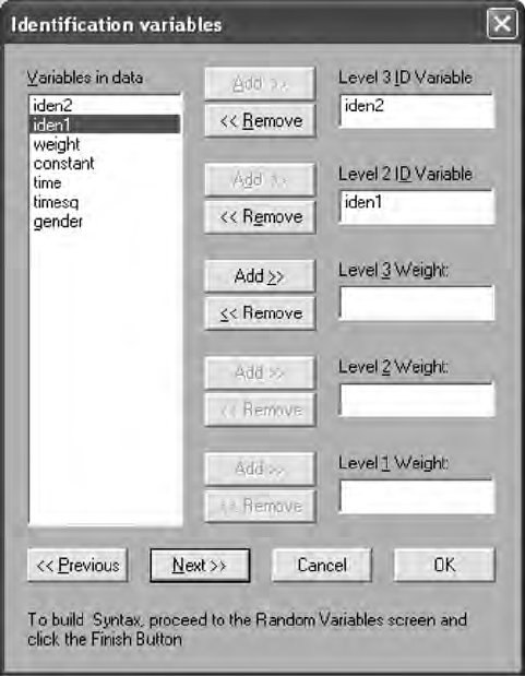
310 A Beginner’s Guide to Structural Equation Modeling
This takes us to the Identication Variables dialog box where you will
add ident2 to level 3 and ident1 to level 2. The variable ident2 ranges from
1 to 82 and identies the unique mouse, while ident1 indicates the 9 time
measurements and ranges from 1 to 9. The dialog box should look like the
one below:
You again click NEXT. This takes us to the Select Response and
Fixed Variables dialog box where you add weight as the select response
(dependent variable and constant as a xed effect to create an intercept only
(null) model). Be sure to unselect the Intercept box in this dialog box as
indicated below:
Y102005.indb 310 3/22/10 3:26:41 PM
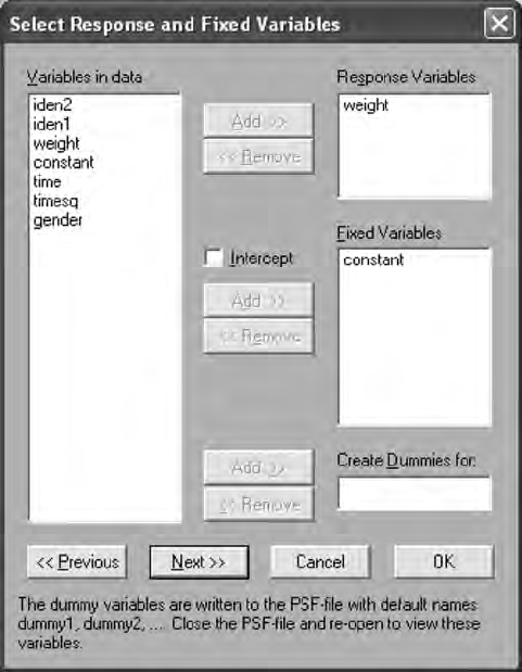
Multiple Indicator–Multiple Indicator Cause, Mixture 311
You again click NEXT. This takes you to the Random Variables dialog
box where you will add constant to both random Level 3 and random Level
2. Constant is the intercept term for the response variable (weight) and
associates an error term for the Level 3 and Level 2 equations. Be sure to
unselect the Intercept boxes in this dialog box for ALL RANDOM LEVELS
as indicated below:
Y102005.indb 311 3/22/10 3:26:41 PM
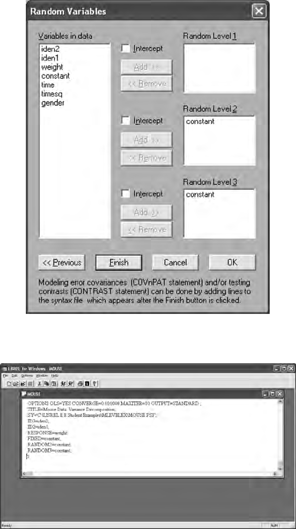
312 A Beginner’s Guide to Structural Equation Modeling
Now click FINISH and a PRELIS program, mouse.pr2 is written.
Y102005.indb 312 3/22/10 3:26:42 PM
Multiple Indicator–Multiple Indicator Cause, Mixture 313
The PRELIS program is executed by clicking the run P (Run PRELIS)
on the tool bar menu. The PRELIS computer output will now indicate the
xed and random results for the baseline model (intercept only). (Note:
Do not use the term constant in your model and also select intercept in the
dialog boxes.)
15.3.1 Constant Effects
The PRELIS computer output for the baseline model (constant) is as follows:
+-------------------------------------+
| FIXED PART OF MODEL |
+-------------------------------------+
------------------------------------------------------------
COEFFICIENTS BETA-HAT STD.ERR. Z-VALUE PR > |Z|
------------------------------------------------------------
constant 28.63410 0.57021 50.21634 0.00000
+--------------------------------+
| -2 LOG-LIKELIHOOD |
+--------------------------------+
DEVIANCE= -2*LOG(LIKELIHOOD) = 5425.490015929897
NUMBER OF FREE PARAMETERS = 3
+---------------------------------------+
| RANDOM PART OF MODEL |
+---------------------------------------+
------------------------------------------------------------
LEVEL 3 TAU-HAT STD.ERR. Z-VALUE PR > |Z|
------------------------------------------------------------
constant/constant 11.32910 4.25185 2.66451 0.00771
------------------------------------------------------------
LEVEL 2 TAU-HAT STD.ERR. Z-VALUE PR > |Z|
------------------------------------------------------------
constant/constant 130.32083 7.42514 17.55130 0.00000
15.3.2 Time Effects
The second multilevel analysis includes adding time to the xed variable
list. To do so, click on Multilevel, Linear Models, and then Select Response
and Fixed Variables in the drop-down menu. Now add time to the xed
variable list as indicated in the dialog box below. You will click NEXT.
Do not change the Random Variables dialog box that appears; simply click
FINISH.
Y102005.indb 313 3/22/10 3:26:42 PM
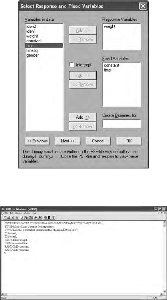
314 A Beginner’s Guide to Structural Equation Modeling
The following PRELIS program will appear in a dialog box with time
added to the FIXED command. To run the updated PRELIS le, mouse.pr2,
click on run P (Run PRELIS).
Y102005.indb 314 3/22/10 3:26:43 PM
Multiple Indicator–Multiple Indicator Cause, Mixture 315
The PRELIS computer output for both constant (baseline) plus time is
as follows:
+-------------------------------------+
| FIXED PART OF MODEL |
+-----------------------------------+
------------------------------------------------------------
COEFFICIENTS BETA-HAT STD.ERR. Z-VALUE PR > |Z|
------------------------------------------------------------
constant 9.09586 0.60387 15.06258 0.00000
time 4.09218 0.06258 65.39108 0.00000
+--------------------------------+
| -2 LOG-LIKELIHOOD |
+--------------------------------+
DEVIANCE= -2*LOG(LIKELIHOOD) = 4137.578760208256
NUMBER OF FREE PARAMETERS = 4
+--------------------------------------+
| RANDOM PART OF MODEL |
+---------------------------------------+
------------------------------------------------------------
LEVEL 3 TAU-HAT STD.ERR. Z-VALUE PR > |Z|
------------------------------------------------------------
constant/constant 20.69397 3.53655 5.85146 0.00000
------------------------------------------------------------
LEVEL 2 TAU-HAT STD.ERR. Z-VALUE PR > |Z|
------------------------------------------------------------
constant/constant 16.46288 0.93806 17.54996 0.00000
15.3.3 Gender Effects
We repeat this process a third time to add gender to the xed variables for a
nal multilevel analysis. To do so, click on Multilevel, Linear Models, and
then Select Response and Fixed Variables in the drop-down menu. Now
add gender to the xed variable list as indicated in the dialog box below.
You will click NEXT. Do not change the Random Variables dialog box that
appears; simply click FINISH. The Select Response and Fixed Variables dia-
log box should look like the following:
Y102005.indb 315 3/22/10 3:26:43 PM
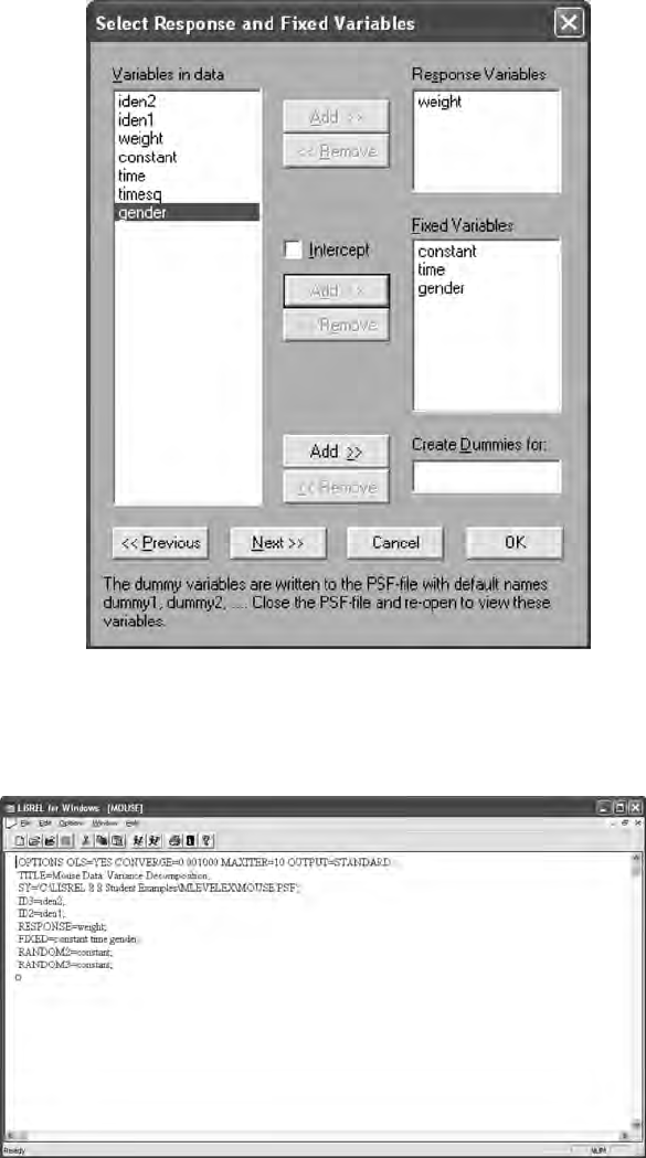
316 A Beginner’s Guide to Structural Equation Modeling
The following PRELIS program will appear in a dialog box with gender
added to the FIXED command. To run the updated PRELIS le, mouse.pr2,
click on run P (Run PRELIS). The following PRELIS program should appear:
Y102005.indb 316 3/22/10 3:26:43 PM
Multiple Indicator–Multiple Indicator Cause, Mixture 317
The PRELIS computer output with constant, time, and gender is as
follows:
+-----------------------------------+
| FIXED PART OF MODEL |
+-----------------------------------+
------------------------------------------------------------
COEFFICIENTS BETA-HAT STD.ERR. Z-VALUE PR >
|Z|
------------------------------------------------------------
constant 9.07800 0.58325 15.56442
0.00000
time 4.08714 0.06261 65.28249 0.00000
gender 1.42015 0.50199 2.82904 0.00467
+--------------------------------+
| -2 LOG-LIKELIHOOD |
+--------------------------------+
DEVIANCE = -2*LOG(LIKELIHOOD) = 4129.941071012016
NUMBER OF FREE PARAMETERS = 5
+---------------------------------------+
| RANDOM PART OF MODEL |
+---------------------------------------+
------------------------------------------------------------
LEVEL 3 TAU-HAT STD.ERR. Z-VALUE PR > |Z|
------------------------------------------------------------
constant/constant 18.68475 3.22290 5.79750 0.00000
------------------------------------------------------------
LEVEL 2 TAU-HAT STD.ERR. Z-VALUE PR > |Z|
------------------------------------------------------------
constant/constant 16.46249 0.93804 17.54996 0.00000
You have now created and run three different PRELIS programs to obtain
the multilevel analysis results for an intercept model (model 1), inter-
cept and time model (model 2), and an intercept, time, and gender model
(model 3). The PRELIS program, mouse.pr2, was updated each time you
changed the number of xed variables. The three PRELIS programs are
listed below where it is easily seen that the FIXED command changed as
you added additional hypothesized variables to obtain a better prediction
of the unexplained variability of the response variable (weight).
Y102005.indb 317 3/22/10 3:26:44 PM
318 A Beginner’s Guide to Structural Equation Modeling
Model 1—Intercept Only
OPTIONS OLS=YES CONVERGE=0.001000 MAXITER=10 OUTPUT=STANDARD ;
TITLE=Mouse Data: Variance Decomposition;
SY=’C:\LISREL 8.8 Student Examples\MLEVELEX\MOUSE.PSF’;
ID3=iden2;
ID2=iden1;
RESPONSE=weight;
FIXED=constant;
RANDOM2=constant;
RANDOM3=constant;
Model 2 – Intercept + Time
OPTIONS OLS=YES CONVERGE=0.001000 MAXITER=10 OUTPUT=STANDARD ;
TITLE=Mouse Data: Variance Decomposition;
SY=’C:\LISREL 8.8 Student Examples\MLEVELEX\MOUSE.PSF’;
ID3=iden2;
ID2=iden1;
RESPONSE=weight;
FIXED=constant time;
RANDOM2=constant;
RANDOM3=constant;
Model 3 – Intercept + Time + Gender
OPTIONS OLS=YES CONVERGE=0.001000 MAXITER=10 OUTPUT=STANDARD ;
TITLE=Mouse Data: Variance Decomposition;
SY=’C:\LISREL 8.8 Student Examples\MLEVELEX\MOUSE.PSF’;
ID3=iden2;
ID2=iden1;
RESPONSE=weight;
FIXED=constant time gender;
RANDOM2=constant;
RANDOM3=constant;
The nal multilevel equation is specied as:
Yij = b1 + b2 Timeij + b2 Genderij + uij + eij.
The PRELIS computer results are summarized in Table 15.1 for com-
parative purposes. (Note: Other multilevel models could include random
effects rather than only xed effects.)
15.3.4 Multilevel Model Interpretation
The computer output for the three PRELIS multilevel programs are sum-
marized in Table 15.1 for the variance decomposition of the response vari-
able, weight. Model 1 provides a baseline model to determine if additional
variables help in reducing the amount of variability in weight. Model 2
with time added, substantially reduced the unexplained variability in
Y102005.indb 318 3/22/10 3:26:44 PM

Multiple Indicator–Multiple Indicator Cause, Mixture 319
weight (c2 = 1287.92, df = 1). Model 3 with gender added also signicantly
reduced the amount of unexplained variability in weight (c2 = 7.63, df = 1).
Therefore, mouse weight variability is statistically signicantly explained
by time and gender xed variables.
15.3.5 Intraclass Correlation
The intraclass correlation coefcient measures the relative homogeneity
within groups in ratio to the total variation. In ANOVA it is computed
as (Between-groups MS − Within-groups MS)/(Between-groups MS +
(n − 1)* Within-Groups MS), where n is the average number of cases in
each category of the independent variable. SPSS has a drop-down menu
option for computing the intraclass correlation coefcient in your data.
If the intraclass correlation coefcient is large and positive, then there
is no variation within the groups, but group means differ. It will be at
its largest negative value when group means are the same but there is
great variation within groups. Its maximum value is 1.0, but its maximum
negative value is (−1/(n − 1)). A negative intraclass correlation coefcient
occurs when between-group variation is less than within-group variation,
indicating a third variable is present with nonrandom effects on the dif-
ferent groups.
The presence of a signicant intraclass correlation coefcient indicates the
need to employ multilevel modeling rather than OLS regression. The main
difference is in the standard errors of the parameters, which have smaller
TABLE 15.1
Summary Results for Multilevel Analysis of Mouse Weight
Multilevel Model
Fixed Factors
Model 1
Constant Only
Model 2
Constant + Time
Model 3 Constant +
Time + Gender
Intercept Only(B0) 28.63 (.57) 9.09 (.60) 9.07 (.58)
Time (B1) 4.09 (.06) 4.08 (.06)
Gender (B2) 1.42 (.50)
Level 2 error variance (eij) 130.32 16.46 16.46
Level 3 error variance (uij) 11.33 20.69 18.68
ICC .079 (8%) .556 (56%) .532 (53%)
Deviance (-2LL) 5425.49 4137.57 4129.94
Df 3 4 5
Chi-square
Difference
(df = 1) 1287.92 7.63
Note: c2 = 3.84, df = 1, p = .05.
Y102005.indb 319 3/22/10 3:26:44 PM

320 A Beginner’s Guide to Structural Equation Modeling
estimates in regression analysis if the intraclass correlation coefcient is
statistically signicant, which can inate (bias) the regression weights. The
intraclass correlation coefcient, using our results, is computed in SEM as:
ICC=+=−−
−−
Φ
ΦΦ
3
32
3
3
TauHat Level
TauHat Level
()
())()
.
..
.
+− −
=+=
TauHat Level 2
11 33
11 33 130 32 079
Therefore, 8% of the variance in weight is explained in the baseline model.
It jumps dramatically when adding time as an explanatory variable to 56%
variance in weight, explained as a function of time. It drops modestly to
53% when adding gender to the equation. The 3% difference is not enough
to infer a nonsignicant effect; therefore time and gender signicantly
explain 53% of the variance in mice weight.
15.3.6 Deviance Statistic
The deviance statistic is computed as −2lnL (likelihood function), which
is used to test for statistical difference in models between Model 1 (con-
stant), Model 2 (constant + time), and Model 3 (constant + time + gender). I
chose the chi-square value of 3.84, df = 1, at the p = .05 level of signicance
to test whether additional variables in the equation explained variance in
mice weight. The baseline deviance value was 5425.49. The chi-square dif-
ference test between this baseline deviance statistic and the second equa-
tion deviance value with time (–2lnL = 4137.57) indicated a difference of
1287.92, which is statistically signicantly different than the tabled critical
chi-square value of 3.84. Consequently, time was a signicant predictor
variable of mice weight. The model with time and gender indicated a devi-
ance statistic of 4129.94 and had a difference from the previous deviance
statistic of 7.63, which was also statistically signicantly different from
the critical tabled chi-square of 3.84. Consequently, time and gender were
statistically signicant predictor variables of mice weight.
1 5 . 4 S u m m a r y
In this chapter, we have described MIMIC, mixture, and multilevel mod-
eling, to further demonstrate the versatility of structural equation mod-
eling. The rst application presented a SEM model that had multiple
indicators of a latent variable where the latent variable was predicted
by multiple observed variables. We refer to this type of SEM model as a
Y102005_C015.indd 320 4/3/10 4:21:44 PM
Multiple Indicator–Multiple Indicator Cause, Mixture 321
Multiple Indicator and Multiple Cause (MIMIC) model. The next appli-
cation involved models that used ordinal and continuous variables.
We refer to this type of SEM model as a Mixture Model. In this appli-
cation, we learned that normal theory t indices apply to continuous
variables that use a Pearson Correlation Matrix with means and stan-
dard deviations of the variables, but that other matrices should be used
when ordinal and continuous variables are present in the SEM model
(for example, polychoric or polyserial matrices). Our nal application
involved analyzing nested data, which has become increasingly popular
in repeated measures, survey, and education data analysis because of
the hierarchical research design. In SEM, we refer to this type of model
as a Multilevel model, but in the research literature this type of model
is referred to by many different names—for example, hierarchical linear,
random-coefcient, variance-component modeling, or HLM.
The chapter presented only one example for each of the applications
because a more in depth coverage is beyond the scope of this book.
However, the LISREL software HELP library and examples can be searched
by using keywords to nd other software examples and explanations. The
LISREL User Guide is also an excellent reference for other examples of
these applications. We now turn our attention to the next chapter where
other SEM applications are presented and discussed.
Exercises
1. MULTIPLE INDICATOR–MULTIPLE CAUSE
(MIMIC) MODEL
Create and run a LISREL–SIMPLIS program given the MIMIC model
below. Please interpret the results including any model modication,
signicance of coefcients, and R2 value. The data set information is:
Observed Variables peer self income shift age
Sample Size 530
Correlation Matrix
1.00
.42 1.00
.24 .35 1.00
.13 .37 .25 1.00
.33 .51 .66 .20 1.00
The following MIMIC Model (next page) includes the latent variable job
satisfaction (satisfac), which is dened in Figure 15.3 by two observed vari-
ables: peer ratings and self ratings. A person’s income level, which shift
they work, and age are observed predictor variables of job satisfaction.
2. MIXTURE MODEL
Given the following Miture Model in Figure 15.4 and data set informa-
tion, write a LISREL program to test the Mixture Model. (Note: Robust
Y102005.indb 321 3/22/10 3:26:45 PM
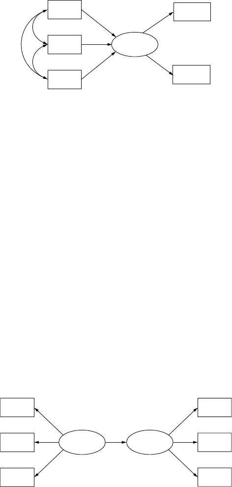
322 A Beginner’s Guide to Structural Equation Modeling
statistics require the raw data le, so no Satorra–Bentler scaled chi-
square possible). The Mixture Model has six observed variables (Age,
Gender, Degree, Region, Hours, and Income) that dene two latent vari-
ables (Person and Earning). A polyserial correlation matrix was created
where CO indicates continuous variable and OR indicates a categori-
cal variable. Age (CO), Gender (OR), and Degree (OR) dene Personal
characteristics, an independent latent variable (Person). Region (OR),
Hours (CO), and Income (CO) dene dependent latent variable Earning
Power (Earning). Personal Characteristics (Person) is hypothesized to
predict Earning Power (Earning).
The data for the Mixture Model is:
Observed Variables: Age Gender Degree Region Hours Income
Correlation Matrix
1.000
0.487 1.000
0.236 0.206 1.000
0.242 0.179 0.253 1.000
0.163 0.090 0.125 0.481 1.000
0.064 0.040 0.025 0.106 0.136 1.000
Means 15.00 10.000 10.000 10.000 7.000 10.000
Standard Deviations 10.615 10.000 8.000 10.000 15.701
10.000
Sample Size 600
The Mixture Model diagram is:
Income
Shift
Age
Peer Rating
Self Rating
Job
Satisfaction
FIGURE 15.3
Job Satisfaction MIMIC model.
Age
Gender
Degree
Region
Hours
Income
Person Earning
FIGURE 15.4
Earning Power Mixture Model.
Y102005.indb 322 3/22/10 3:26:45 PM

Multiple Indicator–Multiple Indicator Cause, Mixture 323
3. MULTILEVEL MODEL
You will need to access the directory, LISREL 8.8 Student Examples. Click
on the mlevelex folder and select the PRELIS system le, income.psf, which
contains the variables region, state, age, gender, marital, etc. There are nine
regions with 51 states nested within the regions. The sample size is n =
6062. It is hypothesized that income varies by state within region.
Open the PRELIS system le, income.psf, and run three PRELIS multi-
level model programs. The rst model will be an intercept only model
with income as the response variable, Level 3 or ID3 = region, and Level
2 or ID2 = state. The second PRELIS program will add gender as a xed
variable. The third PRELIS program will add an additional variable,
marital, as a xed variable. Use the multilevel pull-down menu on the
tool bar to create the programs. (Note: Unselect the Intercept box in
each dialog box).
List Model 1, Model 2, and Model 3 PRELIS programs and sum-
marize the output from the three PRELIS programs in a table. You
will need to hand calculate the intraclass correlation coefcient and
be sure to interpret the comparative results in the table. The MODEL
1 dialog box should look like the following:
Y102005.indb 323 3/22/10 3:26:46 PM
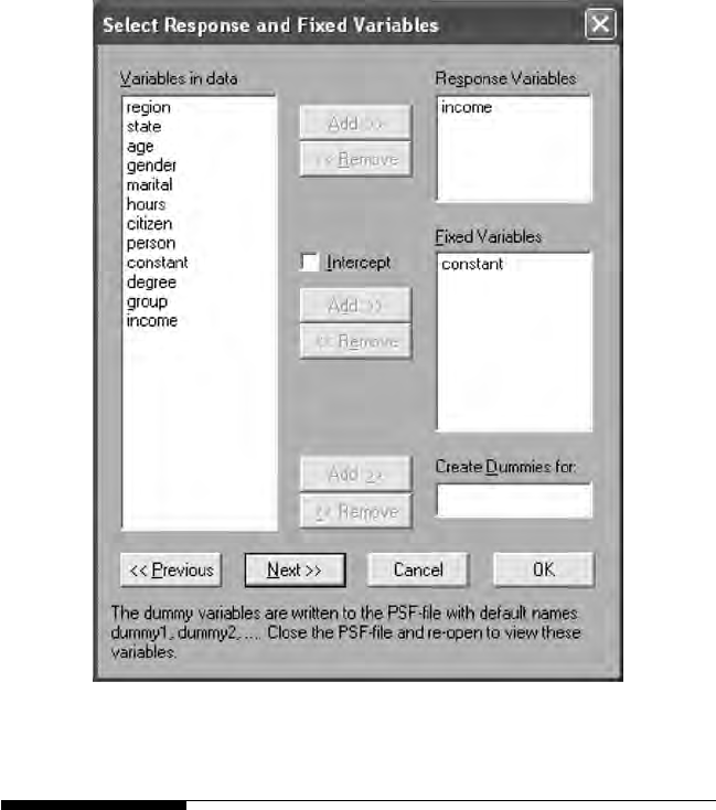
324 A Beginner’s Guide to Structural Equation Modeling
Suggested Readings
Multiple Indicator–Multiple Cause Models
Anderson, K. G., Smith, G. T., & McCarthy, D. M. (2005). Elementary school drink-
ing: The role of temperament and learning. Psychology of Addictive Behaviors,
19(1), 21–27.
Sanchez-Perez, M., & Iniesta-Bonillo, M. A. (2004, Winter). Consumers felt com-
mitment towards retailers: Index development and validation. Journal of
Business and Psychology, 19(2), 141–159.
Shenzad, S. (2006). The determinants of child health in Pakistan: An economic
analysis. Social Indicators Research, 78, 531–556.
Y102005.indb 324 3/22/10 3:26:46 PM

Multiple Indicator–Multiple Indicator Cause, Mixture 325
Mixture Models
Bagley, M. N., & Mokhtarian, P. L. (2002). The impact of residential neighborhood
type on travel behavior: A structural equations modeling approach. The
Annals of Regional Science, 36, 279-297.
Loken, E. (2004). Using latent class analysis to model temperament types.
Multivariate Behavioral Research, 39(4), 625-652.
Lubke, G. H., & Muthen, B. (2005). Investigating population heterogeneity with
factor mixture models. Psychological Methods, 10, 21–39.
Multilevel Models
Bryan, A., Schmiege, S. J., & Broaddus, M. R. (2007). Mediational analysis in HIV/
AIDS research: Estimating multivariate path analytic models in a structural
equation modeling framework. AIDS Behavior, 11, 365–383.
Everson, H. T., & Millsap, R. E. (2004). Beyond individual differences: Exploring
school effects on SAT scores. Educational Psychologist, 39(3), 157–172.
Trautwein, U., Ludtke, O., Schnyder, I., & Niggli, A. (2006). Predicting homework
effect: Support for a domain-specic, multilevel homework model. Journal of
Educational Psychology, 98, 438–456.
References
Heck, R. H., & Thomas, S. L. (2000). An introduction to multilevel modeling techniques.
Mahwah, NJ: Lawrence Erlbaum.
Hox, J. (2002). Multilevel analysis: Techniques and applications. Mahwah, NJ:
Lawrence Erlbaum.
Jöreskog, K., & Sörbom, D. (1996a). LISREL 8: User’s reference guide. Chicago, IL:
Scientic Software International.
Jöreskog, K., & Sörbom, D. (1996b). PRELIS2: User’s reference guide. Chicago, IL:
Scientic Software International.
Jöreskog, K., & Sörbom, D. (1996c). LISREL 8: Structural equation modeling with the
SIMPLIS command language. Chicago, IL: Scientic Software International.
Jöreskog, K., Sörbom, D., du Toit, S., & du Toit, M. (2001). LISREL8: New statistical
features. Chicago, IL: Scientic Software International.
Y102005.indb 325 3/22/10 3:26:46 PM

327
16
Interaction, Latent Growth,
and Monte Carlo Methods
Key Concepts
Main effects and Interaction Effects
Types of Interaction Effects: continuous nonlinear, categorical,
latent variable
Longitudinal data analysis using growth curve models
Monte Carlo methods
16.1 Interaction Models
Most SEM models have assumed that the relations in the models were
linear (i.e., the relations among all variables, observed and latent, are rep-
resented by linear equations). Several studies have been published where
nonlinear and interaction effects are used in multiple regression models;
however, these effects have seldom been tested in path models, and you
will infrequently nd nonlinear factor models. It should not be surprising
to nd that for several decades structural equation modeling has been
based on Linear Structural Relations (LISREL).
SEM models with nonlinear and interaction effects are now possi-
ble and can easily be modeled with recent versions of SEM software.
However, there are several types of nonlinear and interaction effects:
categorical, product indicant, nonlinear, two-stage least squares, and
latent variable using normal scores. For continuous observed variables, a
nonlinear relationship could exist between two observed variables (i.e.,
X1 and X2 are curvilinear); a quadratic (nonlinear) term in the model
(i.e., X2 = X2
1) ; or a product of two observed variables (e.g., X3 = X1X2).
Y102005.indb 327 3/22/10 3:26:47 PM
328 A Beginner’s Guide to Structural Equation Modeling
These three different types of interaction effects all involve continuous
observed variables. For categorical observed variables, interaction effects
are similar to analysis-of-variance and use the multiple-group SEM
model (Schumacker & Rigdon, 1995). These continuous variable and cat-
egorical variable approaches also apply to latent variables (e.g., latent
variable and latent class).
Given that so many different approaches exist, the categorical, latent vari-
able and two-stage least squares examples will be illustrated. Categorical
interaction uses a multigroup (multisample) SEM model. The latent vari-
able interaction uses the product of individual latent variable scores that
are computed and added to the PRELIS system le.
16.1.1 Categorical Variable Approach
In the categorical variable interaction approach, different groups (sam-
ples) are dened by the different levels of the interaction variable. The
basic logic is that if interaction effects are present, then certain parame-
ters should have different values in different groups (samples). Both main
effects and interaction effects can be determined by using different groups
(samples) to test for differences between intercepts and slopes. You accom-
plish this by running two different SEM categorical variable interaction
models: (1) main effects for group differences holding slopes constant, and
(2) interaction effects for group differences with both intercepts and slopes
estimated. These models are sometimes referred to as intercept only and
intercept-slope models.
The following two LISREL–SIMPLIS programs analyze data for two
groups: boys versus girls, where group represents the categorical variable.
Separate covariance matrices and means on the dependent and indepen-
dent variable are input to estimate the prediction of a math score, given a
pretest score. The means are required; otherwise, the intercept values will
be zero. The rst LISREL–SIMPLIS program includes Equation: Math =
CONST Pretest for the girls, but only Equation: Math = CONST for the
boys, which permits different intercept values to be estimated while keep-
ing the slopes equal in the two groups:
Group Girls: Math and Pretest Scores
Observed Variables: Math Pretest
Covariance Matrix:
181.349
84.219 182.821
Means: 82.15 78.35
Sample Size: 373
Equation: Math = CONST Pretest
Group Boys: Math and Pretest Scores
Y102005.indb 328 3/22/10 3:26:47 PM
Interaction, Latent Growth, and Monte Carlo Methods 329
Covariance Matrix:
174.485
34.468 161.869
Means: 48.75 46.98
Sample Size: 249
Equation: Math = CONST
End of Problem
The results indicated that the slopes were equal (slope = .37), and the
intercepts were different (53.26 versus 31.43). The main effect model for
differences in intercepts with equal slopes, however, was not an accept-
able t (c2 = 12.24, p = .002, df = 2).
Girls Group:
Math = 53.26 + 0.37*Pretest, Errorvar. = 155.07, R² = 0.14
(3.04) (0.038) (8.81)
17.53 9.73 17.59
Boys Group:
Math = 31.43 + 0.37*Pretest, Errorvar. = 155.07, R² = 0.12
(1.95) (0.038) (8.81)
16.13 9.73 17.59
The second LISREL–SIMPLIS program uses the Equation: Math =
CONST Pretest in both groups, thus specifying that both intercepts
and slopes are being tested for group differences. Conceptually, this
implies a difference in the means (intercept) and a difference in the rate
of change (slope).
Group Girls: Math and Pretest Scores
Observed Variables: Math Pretest
Covariance Matrix:
181.349
84.219 182.821
Means: 82.15 78.35
Sample Size: 373
Equation: Math = CONST Pretest
Group Boys: Math and Pretest Scores
Covariance Matrix:
174.485
34.468 161.869
Means: 48.75 46.98
Sample Size: 249
Equation: Math = CONST Pretest
End of Problem
Y102005.indb 329 3/22/10 3:26:47 PM
330 A Beginner’s Guide to Structural Equation Modeling
The results indicated that the intercepts (46.06 versus 38.75) and slopes
(.46 versus .21) were different in the two groups. This model with main
and interaction effects present had an acceptable model t (c2 = 1.98, p =.16,
df = 1). The main effect for group differences in math exam scores is given
by the difference in the CONST values: 46.06 − 38.75 = 7.31. The interaction
effect is given by the difference in the slope estimates of pretest values for
the two groups: .46 − .21 = .25.
Girls group:
Math = 46.06 + 0.46*Pretest, Errorvar. = 154.85, R2 = 0.20
(3.80) (0.048) (8.80)
12.13 9.65 17.59
Boys group:
Math = 38.75 + 0.21*Pretest, Errorvar.= 154.85, R2 = 0.045
(3.03) (0.062) (8.80)
12.81 3.43 17.59
A categorical variable interaction model can represent a wide variety of
interaction effects, including higher-order interactions, without requiring
any substantial new methodological developments. This approach can
also be used regardless of whether the interaction intensies or mutes the
effects of the individual variables. Because the interaction effect is repre-
sented in the difference between groups (samples), the researcher is able to
test linear relations of variables within each group (sample), thus avoiding
any potential complications in tting the model. Finally, multiple group
(sample) programs permit parameter constraints across groups thereby
permitting many different hypotheses of group differences.
The categorical interaction approach, however, does have certain weak-
nesses (e.g., smaller subsamples of the total sample size are used). This
could be a serious problem if some groups have low sample sizes that
affect group parameter estimates. This reduction in sample size could
also affect the results of the c2 difference tests. Thus, it is possible that the
categorical-variable approach may yield group samples that are too small,
resulting in a c2 test statistic that misleads the researcher into believing
that an interaction effect exists, whether it does or not. A possible solu-
tion is to minimize the number of distinct parameters being compared in
the model by xing certain parameters to be invariant across the samples
being compared.
The categorical-variable interaction approach is not recommended when
hypothesizing interaction using continuous variables. The basic logic is
that there is a loss of information when reducing a continuous variable
to a categorical variable, for purposes of dening a group (i.e., recode age
Y102005.indb 330 3/22/10 3:26:47 PM
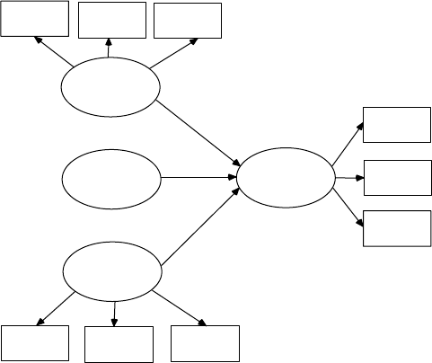
Interaction, Latent Growth, and Monte Carlo Methods 331
into young and old categories). Group misspecication can also occur
when forming groups. Where does one choose the point for dividing a
continuous variable into a categorical variable to form the groups? How
do you justify the arbitrary cut value (i.e., mean, median, or quartile)?
Random-sampling error also ensures that some cases would be misclas-
sied, violating some basic assumptions about subject membership in a
particular group.
16.1.2 Latent Variable Interaction Model
A latent variable interaction model would hypothesize that the indepen-
dent latent variables (ksi1 and ksi2), as well as the product of ksi1 and ksi2
(ksi12), predict a dependent latent variable (eta). The latent variable interac-
tion model is diagrammed in Figure 16.1a.
ETAV2
KSI1
V4
KSI2
V5
V3
V7 V8
V1
V9
V6
KSI12
gamma1
gamma2
gamma3
FIGURE 16.1a
Latent Variable Interaction Model (Schumacker, 2002).
16.1.2.1 Computing Latent Variable Scores
The latent interaction variable approach uses a PRELIS system le and
intermediate steps to create and put latent variable scores into the PRELIS
system le (eta, ksi1, ksi2, and ksi12).
In LISREL, click on File, Open, and then locate the PRELIS SYSTEM
FILE, raw.psf.
Y102005.indb 331 3/22/10 3:26:48 PM

332 A Beginner’s Guide to Structural Equation Modeling
You should see the following PRELIS system le spreadsheet with
the 9 variables (V1 –V9). Also, a tool bar menu will appear across the
top.
You can create a dependent latent variable score and two indepen-
dent latent variable scores, which will automatically be added to the
PRELIS SYSTEM FILE, raw.psf, by using the following LISREL–SIMPLIS
program:
Computing Latent Variable Scores
Observed Variables V1-V9
Raw Data from File raw.psf
Latent Variables : eta ksi1 ksi2
Relationships:
V1 = 1*eta
V2-V3 = eta
V4 = 1*ksi1
V5-V6 = ksi1
V7 = 1*ksi2
V8-V9 = ksi2
PSFfile raw.psf
End of Problem
(NOTE: You will need to close then open the PRELIS system le, raw.psf,
before you will see values for the three latent variables: eta, ksi1, and ksi2.)
Y102005.indb 332 3/22/10 3:26:48 PM
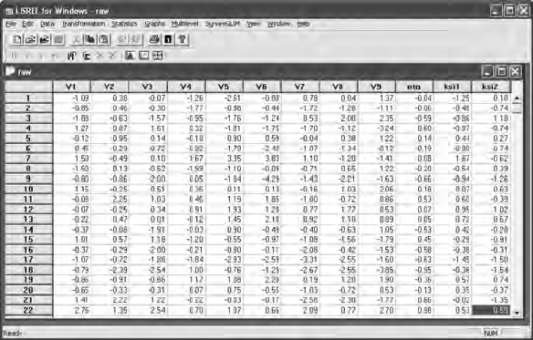
Interaction, Latent Growth, and Monte Carlo Methods 333
The PRELIS system le, raw.psf, is displayed below, and it does contain the
three latent variables computed using the LISREL–SIMPLIS program above.
16.1.2.2 Computing Latent Interaction Variable
You create the latent interaction variable by multiplying the latent variable
scores ksi1 and ksi2. These latent variable scores are unbiased and produce
the same mean and covariance matrix as the latent variables. A PRELIS
program can be used to multiply the two independent latent variables
to create the interaction latent variable, ksi12. The PRELIS NE command
computes the latent interaction variable, which is automatically added to
the PRELIS system le, raw.psf. The CO command will treat the new latent
interaction variable as continuous rather than ordinal level of measure-
ment. The PRELIS program is:
Create Latent Interaction Variable
SY = raw.psf
NE ksi12 = ksi1*ksi2
CO ksi12
OU RA = raw.psf
NOTE: You will need to close then open the PRELIS system le, raw.psf,
before you will see the values for the interaction latent variable: ksi12. The
PRELIS raw.psf le should now contain the latent interaction variable,
ksi12, as shown below:
Y102005.indb 333 3/22/10 3:26:49 PM
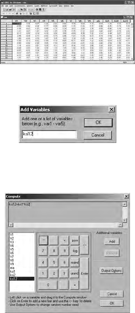
334 A Beginner’s Guide to Structural Equation Modeling
You could alternatively create the latent interaction variable without run-
ning a PRELIS program. Simply, open the PRELIS system le, raw.psf, select
Transformation on the tool bar menu, then click on Compute, and under-
neath Add Variables, click on Add. You should see the Add Variables dialog
box. Now, simply enter the name for the latent interaction variable: ksi12.
Click OK and then the COMPUTE dialog box should appear. Now enter
the equation to create the new latent interaction variable. Follow the
instructions to drag the variable names into an equation in the Compute
dialog box. You can also obtain an equal sign (=) and a product sign (*) by
using the symbols on the calculator. Click on OK, and the latent interac-
tion variable will instantly appear in the PRELIS system le, raw.psf.
Y102005.indb 334 3/22/10 3:26:49 PM
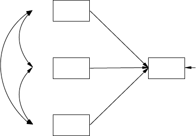
Interaction, Latent Growth, and Monte Carlo Methods 335
(NOTE: If you do not nd the PRELIS System File, raw.psf, you can follow
these same steps with your own continuous variables.)
16.1.2.3 Interaction Model Output
The PRELIS SYSTEM FILE, raw.psf, should now contain the latent inter-
action variable, ksi12. You can run a LISREL–SIMPLIS program to com-
pute the coefcients (gammas) with or without an intercept term in the
structural equation. A LISREL–SIMPLIS program to compute the coef-
cients without an intercept term is:
Latent Interaction Variable Model - No Intercept Term
Observed Variables: V1-V9 eta ksi1 ksi2 ksi12
Raw Data from File raw.psf
Sample Size = 500
Relationships:
eta = ksi1 ksi2 ksi12
Path Diagram
End of Problem
The resultant latent variable interaction model with standardized coef-
cient is diagrammed in Figure 16.1b.
Chi-Square = 0.00, df = 0, P-value = 1.00000, RMSEA = 0.000
ksi1
ksi2
ksi12
eta 0.89
0.11
0.29
–0.04
0.34
0.08
0.04
FIGURE 16.1b
Interaction Model Output.
The structural equation from the LISREL–SIMPLIS computer output
without the intercept term is:
eta = 0.078*ksi1 + 0.16*ksi2 – 0.029*ksi12, Errorvar. = 0.21 , R² = 0.11
0.033) (0.025) (0.033) (0.013)
2.36 6.36 –0.89 15.75
Y102005.indb 335 3/22/10 3:26:50 PM
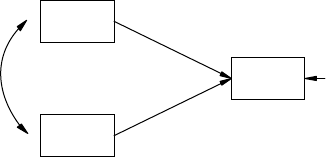
336 A Beginner’s Guide to Structural Equation Modeling
16.1.2.4 Model Modification
The coefcient for the interaction latent variable, ksi12, is not statistically
signicant (T = - 0.89). Therefore, you would drop this latent variable from
the model and use only ksi1 and ksi2.
The modied model output with standardized estimates would appear
as diagrammed in Figure 16.1c.
Chi-Square = 0.00, df = 0, P-value = 1.00000, RMSEA = 0.000
ksi1
ksi2
eta 0.89
0.10
0.29
0.34
FIGURE 16.1c
Interaction Model Modied Output.
The program produces the following output, which yields the same
R-squared value, hence the latent interaction variable did not contribute
to the prediction of eta.
16.1.2.5 Structural Equations—No Latent Interaction Variable
eta = 0.076*ksi1 + 0.16*ksi2, Errorvar.= 0.21 , R² = 0.11
(0.033) (0.025) (0.013)
2.31 6.35 15.76
(NOTE 1: While the PRELIS system le is open, you can use the pull-
down menu to run these models. A latent interaction variable is typically
nonnormal, even when the latent variables are normally distributed. A
solution to this problem is to use the Normal Score option in the pull down
menu for the ksi1, ksi2, and ksi12 latent variables prior to analysis.
(NOTE 2: If eta, ksi1, ksi2, and ksi12 are variables in the PRELIS data
set, another analysis method is available. Select, STATISTICS then use
Regressions to enter the variables into the model equation, that is, RG eta
on ksi1 ksi2 ksi12. Alternatively, the RG command in a PRELIS program
can be used to conduct univariate or multivariate regression, including
ANOVA, ANCOVA, MANOVA, and MANCOVA, as well as other varia-
tions of the general multivariate linear model using a list of Y and X vari-
ables [i.e., RG Y-Varlist ON X-Varlist]).
Y102005.indb 336 3/22/10 3:26:50 PM
Interaction, Latent Growth, and Monte Carlo Methods 337
16.1.3 Two-Stage Least Squares (TSLS) Approach
Recent developments in nonlinear structural equation modeling have
focused on full information methods (e.g., maximum likelihood [ML] or
asymptotically distribution free methods [ADF or WLS]) with a concern
about estimating parameters and standard errors. We recommend boot-
strap estimates of the parameters and standard errors in nonlinear mod-
els, given these estimation methods, because the observed and/or latent
interaction variables don’t meet the multivariate normality assumption.
Other problems or sources of error could exist, which is why start values
are recommended to aid convergence (i.e., the initial TSLS estimates could
be replaced with user dened start values). The two-stage least-squares
(TSLS) estimates and their standard errors are obtained without itera-
tions and therefore provide the researcher with clues to which parameters
exceed their expected values (e.g., correlations with values greater than 1.0
in a nonpositive denite matrix). TSLS estimates therefore provide helpful
information to determine whether the specied model is reasonable.
Bollen (1995, 1996) has indicated that nonlinear SEM models can be esti-
mated using instrumental variables in two stage least squares (TSLS). A
two-stage least squares analysis using instrumental variables is easily run
in LISREL–PRELIS (Jöreskog, Sörbom, du Toit, & du Toit, 2000, pp. 172–174)
using the following RG command (see les KJTSLS1.PR2 and KJTSLS2.PR2):
Estimating Kenny-Judd Model by Bollen’s TSLS
DA NI = 5
LA
Y X1 X2 X3 X4
RA = KJUDD.RAW
CO ALL
NE X1X3 = X1*X3
NE X1X4 = X1*X4
NE X2X3 = X2*X3
NE X2X4 = X2*X4
RG Y ON X1 X3 X1X3 WITH X2 X4 X2X4 RES=U
OU RA = KJRES.RAW
The TSLS results are as follows.
Estimated Equations
Y = 0.936 + 0.340*X1 + 0.399*X3 + 0.965*X1X3 + Error, R² = 0.594
(1.011) (0.115) (0.0883) (0.164)
0.926 2.948 4.516 5.899
The latent variable score approach is also easily run using PRELIS and
SIMPLIS programs (Jöreskog, Sörbom, du Toit, & du Toit, 2000, pp. 173;
see les KJUDD.PR2, KENJUDD.SPL, and KENJUDD.PR2). The following
Y102005.indb 337 3/22/10 3:26:51 PM
338 A Beginner’s Guide to Structural Equation Modeling
PRELIS program KJUDD.PR2, creates the PRELIS SYSTEM FILE, KJUDD.
PSF, the SIMPLIS program KENJUDD.SPL computes the latent variable
scores, and the PRELIS program KENJUDD.PR2 computes the parameter
estimates in the SEM interaction model. The PRELIS program for comput-
ing the PRELIS SYSTEM FILE is:
Computing PSF file from KJUDD.RAW
DA NI = 5
LA; Y X1 X2 X3 X4
RA = KJUDD.RAW
CO ALL
OU MA = CM RA=KJUDD.PSF
The SIMPLIS program for computing the latent variable scores is:
Estimating the Measurement Model in the Kenny–Judd Model
and Latent Variable Scores
System File from File KJUDD.DSF
Latent Variables Ksi1 Ksi2
Relationships
X1 = 1*Ksi1
X2 = Ksi1
X3 = 1*Ksi2
X4 = Ksi2
PSFfile KJUDD.PSF
Path Diagram
End of Problem
The PRELIS program for computing the parameter estimates in the SEM
interaction model is:
Estimating Kenny–Judd Model from Latent Variable Scores
SY = KJUDD.PSF
CO ALL
NE Ksi1Ksi2 = Ksi1*Ksi2
RG Y ON Ksi1 Ksi2 Ksi1Ksi2
OU
Estimated Equations
Y = 1.082 + 0.232*Ksi1 + 0.290*Ksi2 + 0.431*Ksi1Ksi2 + Error, R² = 0.381
(0.0207) (0.0297) (0.0218) (0.0261) Error Variance = 0.393
52.196 7.814 13.281 16.540
Interaction models comprise many different types of models. The use of
continuous variables, categorical variables, nonlinear effects, and latent
variables has intrigued scholars over the years. The current approaches
that appear easy to model are the multigroup categorical approach and
Y102005.indb 338 3/22/10 3:26:51 PM
Interaction, Latent Growth, and Monte Carlo Methods 339
the latent variables score approach, because they are not affected by many
of the problems discussed next.
The testing of interaction effects can present problems in structural equa-
tion modeling. First, you may have the problem of model specication. Linear
models simplify the task of determining relations to investigate and distribu-
tional assumptions to consider, but this may not be the case in latent variable
interaction models. Second, discarding the linearity assumption opens up
the possibility of several product indicant variable and latent variable interac-
tion combinations, but this also serves to magnify the critical role of theory in
focusing the research effort. Third, a researcher who seeks to model categori-
cal interaction effects must also collect data that spans the range of values in
which interaction effects are likely to be evident in the raw data, and must
collect a sample size large enough to permit subsamples. Fourth, we have
noted that the statistical t index and parameter standard errors are based on
linearity and normality assumptions, and we may not have robust results to
recognize the presence of an interaction effect unless it is substantial.
The continuous variable approach does have its good points. It is pos-
sible to check for normality of variables, and to standardize them (Normal
Score option), and the approach does not require creating subsamples
or forming groups where observations could be misclassied, nor does
it require the researcher to categorize a variable and thereby lose infor-
mation. Moreover, the continuous variable approach is parsimonious.
Basically, all but one of the additional parameters involved in the interac-
tion model are exact functions of the main-effects parameters, so the only
new parameters to be estimated are the structure coefcient for the latent
interaction independent variable and the prediction equation error.
The continuous variable approach also has several drawbacks. First,
only a few software programs can perform the necessary nonlinear
constraints, and the programming for testing interaction effects in the
traditional sense is not easy. Second, if you include too many indicator
variables of your latent independent variables, this approach can become
very cumbersome. For example, if one latent independent variable, Factor
1, has n1 measures and the other latent independent variable, Factor 2,
has n2 measures, then the interaction term, Factor 1 x Factor 2, could have
n1 x n2 measures. If each independent latent variable has ve indicator
variables, then the multiplicative latent independent variable interac-
tion would involve 25 indicators. Including the ve measures for each of
the two main-effect latent independent variables and two indicators of a
latent dependent variable, the model would have 37 indicator variables
before any other latent-variable relationships were considered. Third, the
functional form of the interaction needs to be specied. The simple mul-
tiplicative interaction presented here hardly covers other types of interac-
tions, and for these other types of interactions there is little prior research
or available examples to guide the researcher.
Y102005.indb 339 3/22/10 3:26:51 PM
340 A Beginner’s Guide to Structural Equation Modeling
A fourth problem to consider is multicollinearity. It is very likely that
the interaction factor will be highly correlated with the observed variables
used to construct it. This multicollinearity in the measurement model
causes the interaction latent independent variable to be more highly cor-
related with the observed variables of other main effect latent independent
variables than each set of observed variables are with their own respec-
tive main effect latent independent variables. For multiplicative interac-
tions between normally distributed variables, multicollinearity could be
eliminated by centering the observed variables (using scores expressed
as deviations from their means) before computing the product variable.
However, centering the variables alters the form of the interaction relation-
ship. Researchers who want to model other types of interactions may nd
no easy answer to the problem of multicollinearity (Smith & Sasaki, 1979).
A fth concern relates to distributional problems, which are more
serious than those associated with linear modeling techniques using
observed variables only. If the observed variables are nonnormal, then
the variance of the product variable can be very different from the val-
ues implied by the basic measurement model, and the interaction effect
will perform poorly. Of course, permissible transformations may result
in a suitable, normal distribution for the observed variables. The resul-
tant nonnormality, however, in the observed variables violates the distri-
butional assumptions associated with the estimation methods used, for
example, maximum-likelihood. Furthermore, estimation methods that do
not make distributional assumptions may not work for interaction mod-
els. Basically, the asymptotic weight matrix associated with the covariance
matrix for an interaction model may be nonpositive denite because of
dependencies between moments of different observed variables that are
implied by the interaction model. In any case, we would recommend that
you bootstrap the parameter estimates and standard errors to achieve a
more reasonable estimate of these values.
When using the latent variable score approach you should consider
bootstrapping the standard errors because the estimation method used
may give inaccurate estimates of standard errors given violation of
the distributional assumption for the interaction model. Basically, the
asymptotic weight matrix associated with the covariance matrix for an
interaction model may be nonpositive denite because of dependencies
between moments of different observed variables that are implied by the
interaction model. In any case, we would recommend that you bootstrap
the parameter estimates and standard errors to achieve a more reason-
able estimate of these values (Bollen & Stine, 1993; Mooney & Duval,
1993; Lunneborg, 1987; Stine, 1990; Jöreskog & Sörbom, 1993a; and Yang-
Wallentin & Jöreskog, 2001).
In our examples, we have assumed that the relationships in our mod-
els have been linear (i.e., the relationships among all variables, observed
Y102005.indb 340 3/22/10 3:26:51 PM

Interaction, Latent Growth, and Monte Carlo Methods 341
and latent, could be represented by linear equations). Although the use of
nonlinear and interaction effects is popular in regression models (Aiken &
West, 1991), the inclusion of interaction hypotheses in path models have been
minimal (Newman, Marchant, & Ridenour, 1993), and few examples of non-
linear factor models have been provided (McDonald, 1967; Etezadi-Amoli
& McDonald, 1983). SEM models with interaction effects are now possible
and better understood due to several scholars including Kenny and Judd
(1984), Hayduk (1987), Wong and Long (1987), Bollen (1989), Higgins and
Judd (1990), Cole, Maxwell, Arvey, and Salas (1993), Mackenzie and Spreng
(1992), Ping (1993, 1994, 1995), Jöreskog and Yang (1996), Schumacker and
Marcoulides (1998), Algina and Moulder (2001), du Toit and du Toit (2001),
Moulder and Algina (2002), and Schumacker (2002), to name only a few.
Jöreskog and Yang (1996) do provide additional insights into model-
ing interaction effects, given the problems and concerns discussed here.
Jöreskog (2000) discussed many issues related to interaction modeling and
included latent variable scores in LISREL that are easy to compute and
include in interaction modeling. Schumacker (2002) compared the latent
variable score approach to the continuous variable approach using LISREL
matrix command language and found the parameter estimates to be similar
with standard errors reasonably close. Our recommendation would be to
use the latent variable score approach and bootstrap the standard errors. If
unfamiliar with the bootstrap approach, then use the Normal Score option
with interaction variables to avoid nonnormal issues when testing interac-
tion effects.
Structural equation models that include interaction effects are not prev-
alent in the research literature, in part, because of all the concerns men-
tioned here. The categorical variable approach using multiple samples and
constraints has been used most often. The latent variable score approach
using normal scores is a useful way to model interaction with latent vari-
ables. Hopefully, more SEM research will consider interaction hypotheses
given the use of latent variable scores and the use of Normal Score data
conversion for main effect and interaction variables in LISREL–PRELIS.
16.2 Latent Growth Curve Models
Repeated measures analysis of variance has been widely used with
observed variables to statistically test for changes over time. SEM advances
the longitudinal analysis of data to include latent variable growth over
time while modeling both individual and group changes using slopes and
intercepts (McArdle & Epstein, 1987; Stoolmiller, 1995; Byrne & Crombie,
2003). Latent growth curve analysis conceptually involves two different
analyses. The rst analysis is the repeated measures of each individual
Y102005.indb 341 3/22/10 3:26:51 PM

342 A Beginner’s Guide to Structural Equation Modeling
across time that is hypothesized to be linear or nonlinear. The second
analysis involves using the individual’s parameters (slope and intercept
values) to determine the difference in growth from a baseline. The latent
growth curve model (LGM) represents differences over time that takes
into account means (intercepts) and rate of change (slopes), at the indi-
vidual or group level.
LGM permits an analysis of individual parameter differences, which
is critical to any analysis of change. It describes not only an individual’s
growth over time (linear or nonlinear), but also detects differences in
individual parameters over time. LGM using structural equation model-
ing can test the type of individual growth curve, use time varying cova-
riates, establish the type of group curve, and include interaction effects
in latent growth curves (Li, Duncan, T.E., Duncan, S.C., Acock, Yang-
Wallentin, & Hops, 2001). The LGM approach, however, requires large
samples, multivariate normal data, equal time intervals for all subjects,
and change that occurs as a result of the time continuum (Duncan. &
Duncan, 1995).
The latent growth curve model illustrates the use of slope and intercept
as latent variables to model differences over time. The data set contains
168 adolescent responses over a 5-year period (age 11 to age 15) regard-
ing the tolerance toward deviant behaviors, with higher scores indicating
more tolerance of such behavior. The data was transformed (i.e., log X) to
create equal interval linear measures from ordinal data. The latent growth
curve model is diagrammed in Figure 16.2a.
Slope
Intercept
Age11
Age12
Age13
Age14
Age15
E11
E12
0
1
2
3
4
111
1
1
E13
E14
E15
FIGURE 16.2a
Latent Growth Curve Model (Linear).
Y102005.indb 342 3/22/10 3:26:52 PM
Interaction, Latent Growth, and Monte Carlo Methods 343
The slope parameters are coded 0, 1, 2, 3, and 4 to establish a linear
trend with zero used as a common starting point. Other polynomial coef-
cients could be used for quadratic or cubic trend. The intercept param-
eters are coded 1, 1, 1, 1, and 1 to indicate means for the different age
groups. A LISREL–SIMPLIS program was created that shows how these
parameters are stipulated for the two latent variables, slope and intercept.
It also includes a command to correlate slope and intercept (curved arrow
in diagram) and a special term, CONST, to designate means. The LISREL–
SIMPLIS latent growth curve model program is:
16.2.1 Latent Growth Curve Program
Latent Growth Model
Observed Variables: age11 age12 age13 age14 age15
Sample size 168
Correlation matrix
1.000
.161 1.000
.408 .348 1.000
.373 .269 .411 1.000
.254 .143 .276 .705 1.000
Means .201 .226 .326 .417 .446
Standard deviations .178 .199 .269 .293 .296
Latent Variables: slope intercept
Relationships:
age11 = CONST + 0 * slope + 1 * intercept
age12 = CONST + 1 * slope + 1 * intercept
age13 = CONST + 2 * slope + 1 * intercept
age14 = CONST + 3 * slope + 1 * intercept
age15 = CONST + 4 * slope + 1 * intercept
Let slope and intercept correlate
Path Diagram
End of Problem
The initial LISREL–SIMPLIS model results indicated a poor model t
(chi-square = 49.74, df = 7, p = 0.00). The correlation between the intercept
values (group means) and the slope (linear growth) was zero indicating
that level of tolerance at age 11 did not predict growth in tolerance across
the other age groups. However, the group means indicated otherwise, so
model modication was conducted; the means for each age are:
age11 age12 age13 age14 age15
-------- -------- -------- -------- --------
0.20 0.23 0.33 0.42 0.45
Modication indices were indicated that recommended correlating the
error covariance between age 11 and age 12, as well as between age 14
Y102005.indb 343 3/22/10 3:26:52 PM
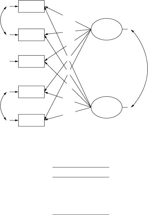
344 A Beginner’s Guide to Structural Equation Modeling
and age 15. These are apparently the two transition periods in the latent
growth curve model were more measurement disturbance was present.
16.2.2 Model Modification
The LISREL–SIMPLIS program was rerun with the following added
commands:
Let error covariance between age11 and age12 correlate
Let error covariance between age14 and age15 correlate
After modication, the latent growth curve model had a more acceptable
model t (chi-square = 11.35, df = 5, and p = .045).
The nal latent growth curve model output with standardized coef-
cients is diagrammed in Figure 16.2b.
Age11
Age12
Age13
Age14
Age15
Slope
0.23
0.35
0.49
0.52
0.51
0.57
0.54
Intercept
–0.53
0.00
FIGURE 16.2b
Latent Growth Model Output.
The individual slopes increased over time:
Group Slope
Age 11 .00
Age 12 .23
Age 13 .35
Age 14 .49
Age 15 .62
Y102005.indb 344 3/22/10 3:26:52 PM

Interaction, Latent Growth, and Monte Carlo Methods 345
The intercepts decreased over time:
Group Intercept
Age 11 .92
Age 12 .80
Age 13 .61
Age 14 .57
Age 15 .54
The negative correlation between the slope and intercept correctly indi-
cates the increase in slope values over time with a corresponding decrease
in intercept values over time (r = –.53).
(NOTE: The LISREL–SIMPLIS computer output does not list the slope and
intercept values, but does display them in the model diagram. They were
copied and listed above for convenience.)
A test of linear rate of growth in the latent growth curve model seemed
appropriate because the means increased from .20 at age 11 to .45 at age
15. The latent growth curve model is appropriately called a Latent Growth
Curve Structured Means Model because group means as well as covari-
ance were specied. There were individual differences in the slopes over
time. The negative correlation between the intercept values (group means),
and the slope values (linear growth) indicated that as age increased the
level of tolerance decreased.
This LGM model indicated a linear rate of growth in adolescent toler-
ance for deviant behavior using the age 11 as the baseline for assessing
linear change over time. You should graph these mean values across the
age levels to graphically display the trend. You should also interpret the
correlation between the intercept and slope because a positive value would
indicate that high initial status at age 11 has a greater rate of change, while
a negative correlation would indicate that high initial status at age 11 has
a lower rate of change. If the average slope value is zero, then no linear
change has occurred. Finally, you can assess how measurement errors
across adjacent years are correlated (e.g., lagged correlation in ARIMA
models). This ability to model measurement error is a unique advantage
of LGM over traditional ANOVA repeated measure designs.
16.3 Monte Carlo Methods
Researchers typically collect a random sample of data and determine if the
sample data t a theoretical model. Model validation (chapter 12) is then
conducted to examine stability of parameter estimates and standard errors.
Generalizations are then usually made to the population parameters.
Y102005.indb 345 3/22/10 3:26:53 PM
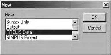
346 A Beginner’s Guide to Structural Equation Modeling
We obviously seldom know the population model, data, or parameters,
so if we wish to investigate how statistics are affected under violations of
assumptions, etc., we need to specify the population model, generate pop-
ulation data (covariance matrix), and now compute model parameters to
examine how parameter estimates, standard errors, and t indices change,
when the model is misspecied. Monte Carlo results are made easier by
writing parameter estimates, standard error estimates, and measures of
t to a le by using PV (PV = <lename>; stores parameter estimates), SV
(SV = <lename>; stores standard errors); and GF (GF = <lename>, stores
goodness-of-t indices) keywords on the LISREL OUTPUT command in
the LISREL–SIMPLIS program. The RP command permits replications,
which is also useful in Monte Carlo studies to examine how these values
change.
The Monte Carlo approach could involve simulating population data,
generating variables from a specied population covariance matrix, or
generating data from a specied model. Monte Carlo methods involve
using a pseudo-random number generator or specifying known popula-
tion values to produce raw data for a population covariance matrix. (Note:
Bang, Schumacker, and Schlieve [1998] found that pseudo-random num-
ber generators do not perform the same way with many yielding non-
random [nonnormal] distributions with sample sizes of less than 10,000).
Our interest in Monte Carlo methods is to determine the robustness of
our sample statistics, which we can only know when our population
model and/or parameters are known. The PRELIS approach to simula-
tion of population data (covariance matrix) is described next for the path
model in Figure 16.3.
16.3.1 PRELIS Simulation of Population Data
PRELIS is considered a preprocessor for LISREL and as such screens data,
creates different types of matrices, and has other useful features for data
creation and data manipulation. PRELIS can easily produce several dif-
ferent types of data distributions—for example, normal and nonnormal.
We will create multivariate normally distributed population data. Simply
click on File, New, and then select PRELIS Data.
Y102005.indb 346 3/22/10 3:26:53 PM

Interaction, Latent Growth, and Monte Carlo Methods 347
An empty PRELIS Data window should appear as indicated below.
We now need to insert the number of variables and the number of cases
that you want to create. We rst create the number of variables, which are
four in Figure 16.3 (V1–V4). We select Data from the tool bar menu, then
Dene Variables. A Dene Variables dialog box appears next and then we
click on Insert.
V2
V3
V1 V4
FIGURE 16.3
Path Model (Monte Carlo).
Y102005.indb 347 3/22/10 3:26:54 PM

348 A Beginner’s Guide to Structural Equation Modeling
An Add Variables dialog box now appears and we enter the names of our
variables, that is, V1-V4., and click OK. These variables will now appear in
the Dene Variables dialog box. Click OK in the Dene Variables dialog box
and they will now appear in the PRELIS Data window.
Next, we select Data from the Tool Bar menu, then Insert Cases. We enter
10000 and click OK.
Y102005.indb 348 3/22/10 3:26:54 PM
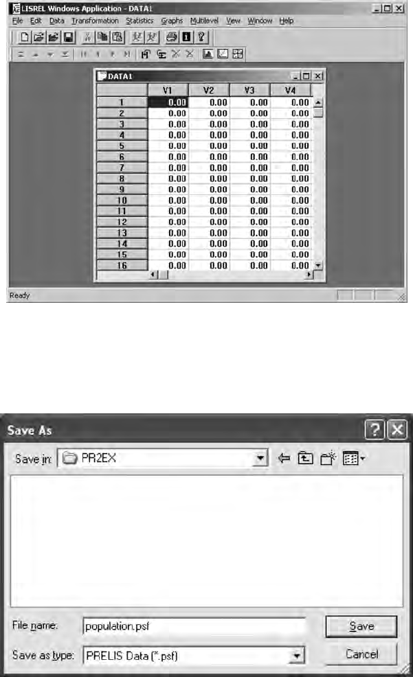
Interaction, Latent Growth, and Monte Carlo Methods 349
The PRELIS Data window now appears with four variables and 10,000
cases, but with zeroes in the cells.
We are now ready to replace the zeroes with numerical values by select-
ing Transformation from the tool bar menu, then Compute; however, we
are rst prompted to save our work as a PRELIS SYSTEM FILE (population.
psf ). (Note: Choose a directory to save the le in that will also contain your
LISREL–SIMPLIS program.)
Y102005.indb 349 3/22/10 3:26:55 PM

350 A Beginner’s Guide to Structural Equation Modeling
We can now carefully follow the directions and use the mouse to
drag and drop variables and click on n(0,1) to enter NRAND into the
equations. The equations were arbitrarily chosen to have a mean and
some correlation with other variables. (Note: Navigating this win-
dow will involve a learning curve; for example, click on Next line
to add the next variable via drag and drop. You also need to use the
mouse to enter numbers and mathematical symbols). When finished,
click OK.
After a few minutes, you will see the computed data values in the
PRELIS system le (population.psf ). Click on the save le icon to save the
data le. You can now use many of the PRELIS tool bar menu features to
calculate statistics or produces graphs of the variables.
Y102005.indb 350 3/22/10 3:26:55 PM

Interaction, Latent Growth, and Monte Carlo Methods 351
Click on Statistics in the tool bar menu, and select Output Options to
save the raw data from the PRELIS system le (population.psf ) into a cova-
riance matrix (population.cov). (Note: A PRELIS program will appear in a
dialog box to show that a program was written to output the covariance
matrix. It will also indicate that variables are treated as continuous [CO],
provide a frequency distribution for each variable, skewness and kurtosis,
and the means and standard deviations of the V1 to V4 variables you cre-
ated as population parameters).
Y102005.indb 351 3/22/10 3:26:56 PM
352 A Beginner’s Guide to Structural Equation Modeling
The covariance matrix (population.cov) can now be input into a LISREL–
SIMPLIS program (population.spl) for the model in Figure 16.3. (Note: We
wanted to treat this covariance matrix as a population matrix to obtain
population parameters, so we generated 10,000 cases.) The LISREL–
SIMPLIS program (population.spl) would be:
PRELIS Data as Population Data for Covariance Matrix
Observed variables V1 V2 V3 V4
Sample size 10000
Covariance matrix from file population.cov
Equations:
V1 = V2 V3
V4 = V1 V2 V3
Path Diagram
LISREL OUTPUT SS SC PV=parameter SV=error GF=fit
End of problem
We can now use the data set or the covariance matrix in a Monte Carlo
study to investigate what parameter estimates and standard errors might
be, given a random sample from the 10,000 cases that constitute the popu-
lation. We can also save the parameter estimates (PV), standard errors
(SV), and model goodness-of-t indices (GF) to separate les using the
LISREL OUTPUT command (Note: SS = standardized solution; SC = com-
pletely standardized solution).
(NOTE: Adding the LISREL OUPUT command RP = 10 would repeat the
analysis 10 times in a Monte Carlo study).
16.3.2 Population Data from Specified Covariance Matrix
There are many different software packages that can be used to generate data
given specication of a population covariance matrix for use in Monte Carlo
studies. We chose SPSS, SAS, and LISREL matrix syntax to illustrate how to
generate population data from specication of a covariance matrix.
16.3.2.1 SPSS Approach
The SPSS MATRIX routine using the Cholesky decomposition can be used to
generate raw data and output an SPSS save le. The SPSS save le can then
be imported into a LISREL program. The following SPSS MATRIX program
only requires the population covariance or correlation matrix (r), sample
size (n), and output le name, Save <lename>. (Note: Save corr/outle = *. ;
it will output data into an SPSS Untitled dialog box which you can then save
as an SPSS save le.) The SPSS MATRIX program requires a symmetrical
matrix as input. To execute the SPSS MATRIX program, open SPSS, select
File, New, and then Syntax. Enter the SPSS Matrix program into the syntax
Y102005.indb 352 3/22/10 3:26:56 PM

Interaction, Latent Growth, and Monte Carlo Methods 353
window, save it, and then click on the run command on the tool bar menu to
execute the program and save the data into an SPSS save le, sample.sav.
MATRIX.
compute popr =
{1, .4, .3, .2;
.4, 1, .6, .7;
.3, .6, 1, .8;
.2, .7, .8, 1}.
Print popr.
compute pi = 3.14159.
compute rown = nrow(popr).
compute n = 10000.
compute corr = sqrt(-2*ln(uniform(n,rown)))&*cos((2*pi)*
uniform(n,rown)).
compute corr=corr*chol(popr).
save corr /outfile = pop.sav.
END MATRIX.
We had the SPSS Matrix program print the popr matrix to verify it was
read correctly. The SPSS output should look like the following:
Run MATRIX procedure:
POPR
1.000000000 .400000000 .300000000 .200000000
.400000000 1.000000000 .600000000 .700000000
.300000000 .600000000 1.000000000 .800000000
.200000000 .700000000 .800000000 1.000000000
------ END MATRIX -----
We can now open the SPSS save le, pop.sav, and compute the bivariate
correlation between the variables, COL1 – COL4, which can be renamed,
if desired.
Y102005.indb 353 3/22/10 3:26:57 PM

354 A Beginner’s Guide to Structural Equation Modeling
The correlation values obtained from SPSS bivariate correlation routine
will approximate the ones specied in the popr matrix. (Note: The correla-
tions should be within .01 of the population correlation/covariance val-
ues. Also, every time you run the SPSS MATRIX program you will get
slightly different values for the correlations, unless using a random seed
number.) The SPSS Correlation Output is in Table 16.1.
TABLE 16.1
SPSS Correlation Output
Correlations
COLUMN 1 COLUMN 2 COLUMN 3 COLUMN 4
COL1 Pearson Correlation 1.000 .404a.304a.201a
Sig. (two-tailed) .000 .000 .000
N 10000.000 10000 10000 10000
COL2 Pearson Correlation .404a1.000 .593a.694a
Sig. (two-tailed) .000 .000 .000
N 10000 10000.000 10000 10000
COL3 Pearson Correlation .304a.593a1.000 .800a
Sig. (two-tailed) .000 .000 .000
N 10000 10000 10000.000 10000
COL4 Pearson Correlation .201a.694a.800a1.000
Sig. (two-tailed) .000 .000 .000
N 10000 10000 10000 10000.000
a Correlation is signicant at the 0.01 level (two-tailed).
16.3.2.2 SAS Approach
A SAS program can also be written to produce data from a population
covariance matrix using a normal distribution function. The SAS program
is written as:
proc iml; /* Generate multivariate normal data in SAS/IML */
cov = {1 .4 .3 .2,
.4 1 .6 .7,
.3 .6 1 .8,
.2 .7 .8 1};
print cov; /* population correlation matrix */
v = nrow(cov); /* calculate number of variables */
n = 10000; /* input number of cases */
seed = 12345; /* random seed number */
l = t(root(cov)); /* calculate cholesky root of cov matrix */
Y102005.indb 354 3/22/10 3:26:57 PM
Interaction, Latent Growth, and Monte Carlo Methods 355
z = normal(j(v,n, seed)); /* generate nvars*samplesize normal distribution */
x = l*z; /* premultiply by cholesky root */
tx = t(x); /* transpose of X */
create cor from tx; /* write out sample data to sas dataset */
append from tx;
quit;
Proc corr data = cor; /* sample covariance matrix */
var col1 col2 col3 col4;
run;
The SAS population matrix and the sample matrix from Proc corr should
be similar, as desired. Changing the seed number, however, will produce
slightly different results each time you run the SAS program. Our SAS 9.1
computer output looked like:
COV
1 0.4 0.3 0.2
0.4 1 0.6 0.7
0.3 0.6 1 0.8
0.2 0.7 0.8 1
The CORR Procedure
4 Variables: COL1 COL2 COL3 COL4
Simple Statistics
Variable N Mean Std Dev Sum Minimum Maximum
COL1 10000 0.00591 1.00676 59.12856 −4.06923 4.13280
COL2 10000 −0.00628 1.00321 −62.81136 −4.47883 3.55955
COL3 10000 0.01407 1.00337 140.74048 −3.50194 3.81102
COL4 10000 0.00662 0.99853 66.17666 −3.45835 3.63828
Pearson Correlation Coefficients, N = 10000
Prob > |r| under H0: Rho=0
COL1 COL2 COL3 COL4
COL1 1.00000 0.41708 0.32340 0.22719
COL2 0.41708 1.00000 0.60942 0.70242
COL3 0.32340 0.60942 1.00000 0.80413
COL4 0.22719 0.70242 0.80413 1.00000
16.3.2.3 LISREL Approach
It is also possible to generate multivariate normal variables with a desired
population covariance matrix using either the Cholesky decomposition or
Y102005.indb 355 3/22/10 3:26:57 PM
356 A Beginner’s Guide to Structural Equation Modeling
factor pattern matrix approach in LISREL. We will rst input four variables
and use the Cholesky decomposed matrix of coefcients to compute four
new variables with the desired covariance structure. Secondly, we will
use a pattern matrix approach to generate the same Cholesky decom-
posed matrix of coefcients that one would use to compute the same new
multivariate normal variables.
16.3.2.3.1 Cholesky Decomposition Approach
Cholesky decomposition of our symmetric population covariance matrix,
S, yields a Lambda Y matrix. The coefcients in the Lambda Y matrix are
then used to compute the new variables. You can save either a covari-
ance matrix (RS option) or raw data (RA option); we saved a covariance
matrix (POP.CM). You will need to run a series of programs to accom-
plish the generation of the multivariate normally distributed data for
your variables.
Program 1 is a LISREL matrix program which inserts a specied popu-
lation covariance matrix (CM) with the number of variables, Y1–Y4 (LE),
indicated for a model (MO) that has the Lambda Y values to be freely esti-
mated (FR). The model must be saturated (c2 = 0) and the residual errors
set to zero (TE = ZE). The resulting Lambda Y matrix provides the coef-
cients to be used to compute the new multivariate normal variables, V1–V4
(LA). (Note: You must specify, all Y variables and associated matrices in
the MO command line; or correspondingly, all X variables and associated
matrices; but not a mix of X and Y variables and associated matrices or the
program will not work.)
Program 1
! Cholesky decomposition matrix approach
DA NI = 4 NO = 10000
LA
V1 V2 V3 V4
CM
1.000
0.41708 1.000
0.32340 0.60942 1.000
0.22719 0.70242 0.80413 1.000
MO NY = 4 NE = 4 LY = FU,FI BE = FU,FI PS = SY,FI TE =ZE
LE
Y1 Y2 Y3 Y4
VA 1.0 PS (1, 1) PS (2, 2) PS (3, 3) PS (4, 4)
FR LY (1, 1) LY (2, 2) LY (3, 3) LY (4, 4)
FR LY (2, 1) LY (3, 1) LY (4, 1)
FR LY (3, 2) LY (4, 2)
FR LY (4, 3)
OU ND = 5 RS
Y102005.indb 356 3/22/10 3:26:57 PM
Interaction, Latent Growth, and Monte Carlo Methods 357
LAMBDA-Y Y1 Y2 Y3 Y4
-------- -------- -------- --------
V1 1.00000 - - - - - -
V2 0.41708 0.90887 - - - -
V3 0.32340 0.52212 0.78918 - -
V4 0.22719 0.66859 0.48351 0.51729
Program 2 uses the Lambda Y values in a PRELIS program to compute
the new variables, V1-V4. The Y1–Y4 variables are rst generated from nor-
mally distributed random data (NRAND function) using a seed value (IX =
12345). Next, new variables are created for V1-V4 using the coefcients from
the Lambda Y matrix and saved in a covariance matrix (CM = POP.CM).
The Y1-Y4 variables are deleted (SD). The RA = <lename> option would
save raw data for the variables instead of a matrix if so desired.
Program 2
! Compute new multivariate normal variables from Lambda Y
matrix
DA NO = 10000
NE Y1 = NRAND
NE Y2 = NRAND
NE Y3 = NRAND
NE Y4 = NRAND
NE V1 = 1 * Y1
NE V2 = .41708 * Y1 + .90887 * Y2
NE V3 = .32340 * Y1 + .52212 * Y2 + .78918 * Y3
NE V4 = .22719 * Y1 + .66859 * Y2 + .48351 * Y3 + .51729* Y4
CO ALL
SD Y1-Y4
OU CM = POP.CM ND = 5 XM IX = 12345
Finally, Program 3 would run a LISREL–SIMPLIS program with the gen-
erated population covariance matrix to produce the specied model in
Figure 16.3.
Program 3
Path model Figure 16.3 with Cholesky decomposed matrix
variables
Observed variables V1 V2 V3 V4
Sample size 10000
!Covariance Matrix from file POP.CM
Covariance Matrix
0.99641
0.42637 1.0185
0.32652 0.62854 1.0379
0.23881 0.72385 0.83883 1.0322
Y102005.indb 357 3/22/10 3:26:57 PM
358 A Beginner’s Guide to Structural Equation Modeling
Equation:
V1 = V2 V3
V4 = V1 V2 V3
Number of Decimals = 5
Path Diagram
End of Problem
(NOTE: We used sample size of 10,000 and 5 decimal places to avoid
rounding error and non-convergence problems.)
16.3.2.3.2 Pattern Matrix Approach
The pattern matrix approach is possible by inputting the pattern matrix
(PA) and corresponding lambda X matrix (MA) with the specied covari-
ance matrix (CM). The results would be the same as before. The Lambda
X coefcients would be the same as before and used in Program 2 above
to compute multivariate normal variables. The LISREL program would be
written as:
! Pattern Matrix approach
DA NI = 4 NO = 10000
LA
V1 V2 V3 V4
CM
1.000
0.41708 1.000
0.32340 0.60942 1.000
0.22719 0.70242 0.80413 1.000
MO NX = 4 NK = 4 PH = ID TD =ZE
PA LX
1 0 0 0
1 1 0 0
1 1 1 0
1 1 1 1
MA LX
1 0 0 0
1 1 0 0
1 1 1 0
1 1 1 1
OU ND = 5 RS
LAMBDA-X
KSI 1 KSI 2 KSI 3 KSI 4
-------- -------- -------- --------
V1 1.00000 - - - - - -
V2 0.41708 0.90887 - - - -
V3 0.32340 0.52212 0.78918 - -
V4 0.22719 0.66859 0.48351 0.51729
Y102005.indb 358 3/22/10 3:26:57 PM
Interaction, Latent Growth, and Monte Carlo Methods 359
(NOTE: It is also straightforward to compute the Cholesky decomposed
matrix using SPSS to check your programming. The SPSS MATRIX pro-
cedure with the original population covariance matrix used (S) and the
resulting Cholesky decomposed matrix [SCHOL] is output as follows.)
MATRIX.
Compute S = {1.00000, .41708, .32340, .22719;
.41708, 1.00000, .60942, .70242;
.32340, .60942, 1.00000, .80413;
.22719, .70242, .80413, 1.00000}.
Print S.
Compute SCHOL = T(CHOL(S)).
Print SCHOL.
END MATRIX.
Run MATRIX procedure:
S
1.000000000 .417080000 .323400000 .227190000
.417080000 1.000000000 .609420000 .702420000
.323400000 .609420000 1.000000000 .804130000
.227190000 .702420000 .804130000 1.000000000
SCHOL
1.000000000 .000000000 .000000000 .000000000
.417080000 .908869778 .000000000 .000000000
.323400000 .522116963 .789180789 .000000000
.227190000 .668592585 .483505465 .517292107
16.3.3 Covariance Matrix from Specified Model
A more appropriate way to generate a population covariance matrix is
from a specied population model. This permits a better way to exam-
ine how model misspecication affects overall model t as well as pre-
dened population parameter values. Unfortunately, the population
model specication and subsequent generation of population model
parameters is not directly possible using LISREL or PRELIS programs.
The reason is that not all matrices, especially covariance and certain error
terms, can be specied in the programs. The solution is to (1) specify a
population model, (2) dene what matrices are indicated in the popula-
tion model, (3) pick values for the population parameters in the matrices,
and then (4) use matrix operations to compute the population covariance
matrix. In a nal step (5), you can verify that the population model with
the population parameters was correctly specied by using the popula-
tion covariance matrix in a LISREL–SIMPLIS program. We will now take
you through these steps to illustrate a better way to conduct Monte Carlo
Y102005.indb 359 3/22/10 3:26:57 PM
360 A Beginner’s Guide to Structural Equation Modeling
studies (rather than simulation of data or generation of data from a speci-
ed correlation/covariance matrix).
Step 1: We begin by specifying a population model in Figure 16.4. The
population model is a conrmatory factor model with two latent inde-
pendent factors, x1 and x2. Each of the latent independent variables is
measured by three indicator (observed) variables. The indicator vari-
ables X1 to X3 dene the rst latent independent variable and indicator
variables X4 to X6 dene the second latent independent variable. Each of
the indicator variables have measurement error, designated as: d1 to d6.
We also have lambda X values or factor loadings for each of the paths
from the latent independent variables to the indicator variables. Finally,
we have to specify the covariance between the two latent independent
variables.
Step 2: We dene what matrices are indicated in this population model.
We described a lambda X matrix (factor loadings), a theta–delta matrix
(measurement error of indicator variables), and a phi matrix (correlation
between the two factors).
Step 3: We specify what we want our population parameters to be in
these matrices. We chose to set factor loadings for X1 to X3 at .6 and factor
loadings for X4 to X6 at .7. We then calculated our measurement errors as
1 − (.6)2 for X1 to X3 and 1 – (.7)2 for X4 to X6; .64 and .51, respectively, in
X1
X2
X3
X4
X5
X6
1
2
FIGURE 16.4
Population Model (Monte Carlo).
Y102005.indb 360 3/22/10 3:26:58 PM
Interaction, Latent Growth, and Monte Carlo Methods 361
the theta–delta matrix. (Note: Failure to have factor loadings and measure-
ment error synchronized—that is, X = T + E—will lead to a nonpositive
denite matrix and error warning.) Finally, we set the factor correlation at
.70. The matrices with our selected population parameters for the conr-
matory factor model would be as follows:
ΛΘ
x=
.
.
.
.
.
.
60
60
60
07
07
07
δ
==
.
.
.
.
.
64 00000
0640 000
00 64 000
000 51 00
0000510
000000 51
10 7
710
.
..
..
=
Φ
Please be aware that these matrices in a LISREL program with a pattern
matrix or MO commands will not create a population covariance matrix
because we cannot specify the measurement errors of the indicator variables
exactly (typically created with random number generator) nor the correlation
between the factors. Also, there are two other implied matrices that would
have zero values: tau matrix of zero mean values for indicator variables (tx )
and alpha matrix for means of our latent independent variables (a), although
these are not used in our calculations of the population covariance matrix
that are implicitly set to zero. These two matrices are indicated as:
τα
x=
=
0
0
0
0
0
0
0
0
Step 4: We now use matrix operations with these matrices to produce the
population covariance matrix (Σ). The covariance matrix equation would
multiply the coefcients in the lambda X matrix (LX) times the phi matrix
(phi) and post multiply times the transpose of the lambda X matrix (LXT),
plus add the measurement error of each indicator variable, which is rep-
resented as:
ΣΛΦΛ Θ= ′+
XX
δ
Y102005.indb 361 3/22/10 3:26:59 PM
362 A Beginner’s Guide to Structural Equation Modeling
We used the SPSS MATRIX procedure to compute the population cova-
riance matrix, which uses full symmetric matrices. The SPSS MATRIX
program is:
Matrix.
compute LX= {.6,.0;
.6,.0;
.6,.0;
.0,.7;
.0,.7;
.0,.7}.
print LX.
compute phi = {1,.7;
.7 ,1}.
print phi.
compute thetad={.64,0,0,0,0,0;
0,.64,0,0,0,0;
0,0,.64,0,0,0;
0,0,0,.51,0,0;
0,0,0,0,.51,0;
0,0,0,0,0,.51}.
print thetad.
compute LXT = T(LX).
print LXT.
compute sigma = LX * phi * LXT + thetad.
print sigma.
end matrix.
The resulting output with a lambda matrix of factor loadings (LX), phi
matrix with factor correlation (PHI), theta–delta matrix with measure-
ment errors for the indicator variables (THETAD), transpose of LX matrix
(LXT) are indicated below, along with the population covariance matrix
(SIGMA):
Run MATRIX procedure:
LX
.6000000000 .0000000000
.6000000000 .0000000000
.6000000000 .0000000000
.0000000000 .7000000000
.0000000000 .7000000000
.0000000000 .7000000000
PHI
1.000000000 .700000000
.700000000 1.000000000
Y102005.indb 362 3/22/10 3:26:59 PM
Interaction, Latent Growth, and Monte Carlo Methods 363
THETAD
.6400000000 .0000000000 .0000000000 .0000000000 .0000000000 0000000000
.0000000000 .6400000000 .0000000000 .0000000000 .0000000000 .0000000000
.0000000000 .0000000000 .6400000000 .0000000000 .0000000000 .0000000000
.0000000000 .0000000000 .0000000000 .5100000000 .0000000000 .0000000000
.0000000000 .0000000000 .0000000000 .0000000000 .5100000000 .0000000000
.0000000000 .0000000000 .0000000000 .0000000000 .0000000000 .5100000000
LXT
.6000000000 .6000000000 .6000000000 .0000000000 .0000000000 .0000000000
.0000000000 .0000000000 .0000000000 .7000000000 .7000000000 .7000000000
SIGMA
1.000000000 .360000000 .360000000 .294000000 .294000000 .294000000
.360000000 1.000000000 .360000000 .294000000 .294000000 .294000000
.360000000 .360000000 1.000000000 .294000000 .294000000 .294000000
.294000000 .294000000 .294000000 1.000000000 .490000000 .490000000
.294000000 .294000000 .294000000 .490000000 1.000000000 .490000000
.294000000 .294000000 .294000000 .490000000 .490000000 1.000000000
------ END MATRIX -----
Step 5: We now include the population covariance matrix (SIGMA) in a
LISREL–SIMPLIS program to produce the population conrmatory factor
model (Figure 16.5) that should indicate the values we picked for the pop-
ulation parameters. We only need to include the lower triangular matrix
in the program. The LISREL–SIMPLIS program with our SIGMA (Σ) cova-
riance matrix is:
Confirmatory Factor Model in Figure 16.5
Observed variables X1 X2 X3 X4 X5 X6
Sample size 1000
Covariance Matrix
1.00000
.360000 1.00000
.360000 .360000 1.00000
.294000 .294000 .294000 1.00000
.294000 .294000 .294000 .490000 1.000000
.294000 .294000 .294000 .490000 .490000 1.00000
Latent variables KSI1 KSI2
Relationships:
X1 - X3 = KSI1
X4 - X6 = KSI2
Number of Decimals = 5
Path Diagram
End of Problem
Figure 16.5 does indeed show the factor loadings, factor correlation,
and measurement error for the indicator variables we specied for our
Y102005.indb 363 3/22/10 3:26:59 PM
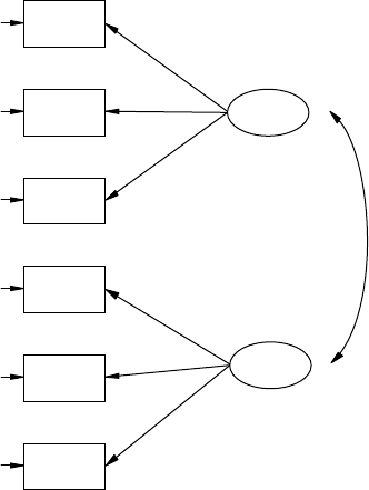
364 A Beginner’s Guide to Structural Equation Modeling
population conrmatory factor model. Please note that the model ts per-
fectly (c2 = 0, p = 1). We could now generate data using this population
covariance matrix in a SAS or SPSS program and introduce various mis-
specied models to determine how our population model is affected—for
example, model-t indices, parameters, and standard errors change.
In SEM, the use of a known population covariance matrix permits a
comparison with alternative models that produce differing implied cova-
riance matrices that can be compared with the population covariance
matrix, as well as an examination of the parameter estimates from the
implied model. The variation in the covariance matrices, parameter esti-
mates, and t indices can be inspected given the new LISREL OUTPUT
optional commands; PV, SV, and GF.
Monte Carlo studies are typically conducted to examine model t,
parameter estimates, and standard errors to determine how much
they uctuate or change under certain conditions, for example, differ-
ent sample sizes, missing data, and/or nonnormal distributions. More
complex programs are possible that use data generated from differ-
ent types of distributions using optional commands other than normal
Chi-Square = 0.00, df = 8, P-value = 1.00000, RMSEA = 0.000
X1
0.64
X20.64
X30.64
X40.51
X50.51
X6
0.51
KSI1
KSI2
0.60
0.60
0.60
0.70
0.70
0.70
0.70
FIGURE 16.5
Conrmatory Factor Model (Monte Carlo).
Y102005.indb 364 3/22/10 3:27:00 PM

Interaction, Latent Growth, and Monte Carlo Methods 365
when generating data. For example, Enders and Bandalos (2001) studied
a three-factor model to compare four methods of missing data estima-
tion. Their experimental condition included different factor loadings,
sample size, percent missingness of data, and type of data missingness
(MCAR or MAR).
Conducting Monte Carlo studies however can be cumbersome. Paxton,
Curran, Bollen, Kirby, and Chen (2001) provided useful steps to fol-
low when conducting a Monte Carlo study. Their basic steps are out-
lined below, but the reader is encouraged to read their complete journal
article.
Step 1: Develop a research question.
Step 2: Create a valid model.
Step 3: Select experimental conditions.
Step 4: Select values of population parameters.
Step 5: Select software package.
Step 6: Conduct simulations.
Step 7: File storage requirements.
Step 8: Troubleshoot and verify results.
Step 9: Summarizing results.
Mooney (1997) provides a basic introduction to Monte Carlo simulation.
Skrondal (2000) and Paxton et al. (2001) also offer advice on Monte Carlo
methods. Fan, Felsovalyi, Sivo, and Keenan (2002) have written an excel-
lent guide for quantitative researchers who wish to conduct Monte Carlo
studies using SAS; a Web site is provided to download a zip le with SAS
Monte Carlo programs. Fan (2005) has also published a “Teachers Corner”
article on using SAS in structural equation modeling. Bandalos (2006) pro-
vides SEM examples generating data from specied models. Long (2008)
additionally provided helpful suggestions associated with managing
data, although using STATA software, the data management suggestions
are helpful. We recommend following their suggestions when conducting
a Monte Carlo study.
1 6 . 4 S u m m a r y
In this chapter we have presented many different types of interaction
models. The use of continuous variables, categorical variables, nonlinear
effects, and latent variables has provided the basis for discussing different
Y102005.indb 365 3/22/10 3:27:00 PM
366 A Beginner’s Guide to Structural Equation Modeling
interaction models. The two current variable interaction approaches that
are easy to model would be the latent variables score approach using
normal scores or two-stage least squares approach. We highly recom-
mend either of these two options. Our discussion of latent growth curve
models introduced SEM applications for longitudinal data analysis of
latent variables. Today, more and more emphasis is being placed on lon-
gitudinal data analysis and models. It is a logical extension to expand
our thinking into the use of latent variables when applying longitudi-
nal models that heretofore had only used observed variables. Finally,
we presented Monte Carlo methods because of the usefulness in creat-
ing population models that then permit examination of how parameter
estimates, standard errors, and t indices are affected by missing data
sample size, nonnormality, distribution assumptions, and other factors
that affect statistical estimation. Specically, we examined four ways to
obtain population data and/or correlation/covariance matrix: (1) simula-
tion of population data, (2) Cholesky decomposition of a specied pop-
ulation matrix to obtain parameter coefcients, (3) pattern matrix of a
specied population matrix, which can also be used to obtain param-
eter coefcients, and nally, (4) obtaining population covariance matrix
from a specied population model. We hope these SEM methods have
enhanced further your understanding of the usefulness of structural
equation modeling.
Exercises
1. INTERACTION MODEL
An organizational psychologist was investigating whether work
tension and collegiality were predictors of job satisfaction. However,
research indicated that work tension and collegiality interact, so a SEM
Interaction Model was hypothesized and tested. The Interaction
Model is diagrammed in Figure 16.6.
Use LISREL to OPEN the PRELIS system le, jobs.psf, then proceed
to follow the necessary steps to create the latent variables (work ten-
sion, collegiality, and job satisfaction, interaction) and add them to
the PRELIS system le. Next, create and run a LISREL–SIMPLIS pro-
gram to test the interaction model. What conclusions can you make
regarding the interaction of the latent variables work tension and
collegiality?
2. LATENT GROWTH CURVE MODEL
News and radio stations in Dallas, Texas, have apparently convinced
the public that a massive crime wave has occurred during the past
4 years, from 2002 to 2005. A criminologist gathered the crime rate
data, but needs your help to run a latent growth curve model to test
Y102005.indb 366 3/22/10 3:27:00 PM
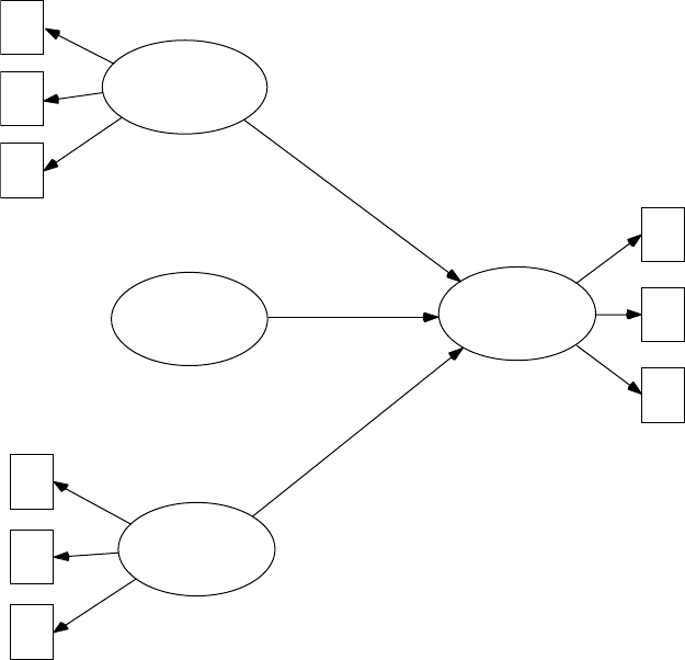
Interaction, Latent Growth, and Monte Carlo Methods 367
whether a linear trend in crime rates exist for the city. The data set
information is:
Observed variables: time1 time2 time3 time4
Sample Size 400
Correlation Matrix
1.000
.799 1.000
.690 .715 1.000
.605 .713 .800 1.000
Means 5.417 5.519 5.715 5.83
Standard Deviations .782 .755 .700 .780
Create a LISREL–SIMPLIS program, diagram the model with stan-
dardized coefcients and interpret your ndings. Have crime rates
increased in Dallas from 2002 to 2005?
V7
V8
V9
V1
V2
V3
Work Tension
×
Collegiality
Collegiality
Work Tension
V4
V5
V6
Job Satisfaction
gamma2
gamma1
gamma3
FIGURE 16.6
Job Satisfaction Exercise.
Y102005.indb 367 3/22/10 3:27:00 PM

368 A Beginner’s Guide to Structural Equation Modeling
3. MONTE CARLO METHOD
Write a program using either SPSS or SAS for the following popula-
tion matrix and generate data (N = 10,000 cases):
1.00
.50 1.00
.30 .70 1.00
.90 .50 .50 1.00
Given the generated data, compute the population correlation matrix.
Does the generated data recover the population correlation values in
the matrix?
Suggested Readings
Interaction Models
Fielding, D., & Torres, S. (2005). A simultaneous equation model of economic devel-
opment and income inequality. Journal of Economic Inequality, 4, 279–301.
Ritchie, M. D., Hahn, L. W., Roodi, N., Bailey, L. R., Dupont, W. D., Parl, F. F., &
Moore, J. H. (2001). Multifactor-dimensionality reduction reveals high-order
interactions among estrogen-metabolism genes in sporadic breast cancer.
American Journal of Human Genetics, 69, 138–147.
Schumacker, R. E. (2002). Latent variable interaction modeling. Structural Equation
Modeling: A Multidisciplinary Journal, 9, 40–54.
Latent Growth-Curve Models
Duncan, S. C., & Duncan, T. E. (1994). Modeling incomplete longitudinal sub-
stance use data using latent variable growth curve methodology. Multivariate
Behavioral Research, 29(4), 313–338.
Ghisletta, P., & McArdle, J. J. (2001). Latent growth curve analyses of the develop-
ment of height. Structural Equation Modeling: A Multidisciplinary Journal, 8,
531–555.
Shevlin, M., & Millar, R. (2006). Career education: An application of latent growth
curve modeling to career information-seeking behavior of school pupils.
British Journal of Educational Psychology, 76, 141–153.
Monte Carlo Methods
Stephenson, M. T., & Holbert, R. L. (2003). A Monte Carlo simulation of observ-
able versus latent variable structural equation modeling techniques.
Communication Research, 30(3), 332–354.
Fan, X. (2005). Using SAS for Monte Carlo simulation research in SEM. Structural
Equation Modeling: A Multidisciplinary Journal, 12(2), 299–33.
Y102005.indb 368 3/22/10 3:27:01 PM

Interaction, Latent Growth, and Monte Carlo Methods 369
Muthèn, L. K., & Muthèn, B. O. (2002). Teacher’s corner: How to use a Monte Carlo
study to decide on sample size and determine power. Structural Equation
Modeling: A Multidisciplinary Journal, 9(4), 599–620.
References
Aiken, L. S., & West, S. G. (1991). Multiple regression: Testing and interpreting interac-
tions. Newbury Park, CA: Sage.
Algina, J., & Moulder, B. C. (2001). A note on estimating the Jöreskog-Yang model
for latent variable interaction using LISREL 8.3. Structural Equation Modeling,
8(1), 40–52.
Bandalos, D. L. (2006). The use of Monte Carlo studies in structural equation mod-
eling. In G. R. Hancock & R. O. Mueller (Eds.), Structural equation modeling: A
second course (pp. 385–426). Greenwich, CT: Information Age.
Bang, J. W., Schumacker, R. E., & Schlieve, P. L. (1998). Random-number generator
validity in simulation studies: An investigation of normality. Educational and
Psychological Measurement, 58(3), 430–450.
Bollen, K. A. (1989). Structural equations with latent variables. New York: John Wiley
& Sons.
Bollen, K. A., & Stine, R. A. (1993). Bootstrapping goodness-of-t measures in
structural equation models. In K. A. Bollen & J. S. Long (Eds.), Testing struc-
tural equation models (pp. 66–110). Newbury Park, CA: Sage.
Bollen, K. A. (1995). Structural equation models that are nonlinear in latent vari-
ables: A least squares estimator. In P. M. Marsden (Ed.), Sociological methodol-
ogy 1995. Cambridge, MA: Blackwell.
Bollen, K. A. (1996). An alternative two stage least squares (2SLS) estimator for
latent variable equations. Psychometrika, 61, 109–121.
Byrne, B. M. & Crombie, G. (2003). Modeling and testing change : an introduction
to the latent growth curve model. Understanding Statistics, 2(3), 177–203.
Cole, D. A., Maxwell, S. E., Arvey, R., & Salas, E. (1993). Multivariate group com-
parisons of variable systems: MANOVA and structural equation modeling.
Psychological Bulletin, 114, 174–184.
Duncan, T. E., & Duncan, S. C. (1995). Modeling the processes of development via
latent variable growth curve methodology. Structural Equation Modeling, 2(3),
187–213.
Du Toit, M., & du Toit, S. (2001). Interactive LISREL: User’s guide. Lincolnwood, IL:
Scientic Software International.
Enders, C. K., & Bandalos, D. L. (2001). The relative performance of full informa-
tion maximum likelihood estimation for missing data in structural equation
models. Structural Equation Modeling, 8, 430–457.
Etezadi-Amoli, J., & McDonald, R. P. (1983). A second generation nonlinear factor
analysis. Psychometrika, 48, 315–342.
Fan, X., Felsovalyi, A., Sivo, S., & Keenan, S. C. (2002). SAS for Monte Carlo Studies:
A Guide for Quantitative Researchers. Sage Publications: CA. [zip le of SAS
Monte Carlo programs available at: http://support.sas.com/publishing/
bbu/57323/57323.zip].
Y102005.indb 369 3/22/10 3:27:01 PM
370 A Beginner’s Guide to Structural Equation Modeling
Fan, X (2005). Using SAS for Monte Carlo simulation research in SEM. Structural
Equation Modeling: A Multidisciplinary Journal, 12(2), 299–33.
Hayduk, L. A. (1987). Structural equation modeling with LISREL. Baltimore, MD:
Johns Hopkins University Press.
Higgins, L. F., & Judd, C. M. (1990). Estimation of non-linear models in the pres-
ence of measurement error. Decision Sciences, 21, 738–751.
Jöreskog, K. G. (2000). Latent variable scores and their uses. Lincolnwood, IL: Scientic
Software International.
Jöreskog, K. G., & Sörbom, D. (1993a). Bootstrapping and Monte Carlo experimenting
with PRELIS2 and LISREL8. Chicago, IL: Scientic Software International.
Jöreskog, K. G., & Sörbom, D. (1993b). LISREL8 user’s reference guide. Chicago, IL:
Scientic Software International, Inc.
Jöreskog, K. G., & Sörbom, D. (1993c). LISREL 8: Structural equation modeling with
the SIMPLIS command language. Chicago: Scientic Software International.
Jöreskog, K. G., & Sörbom, D. (1993d). PRELIS2 user’s reference guide. Chicago, IL:
Scientic Software International.
Jöreskog, K. G., Sörbom, D., Du Toit, S., & Du Toit, M. (2000). LISREL8: New statisti-
cal features. Lincolnwood, IL: Scientic Software International.
Jöreskog, K. G., & Yang, F. (1996). Non-linear structural equation models: The
Kenny-Judd model with interaction effects. In G. A. Marcoulides, & R. E.
Schumacker (Eds.), New developments and techniques in structural equation mod-
eling (pp. 57–88). Mahwah, NJ: Lawrence Erlbaum.
Kenny, D. A., & Judd, C. M. (1984). Estimating the non-linear and interactive effects
of latent variables. Psychological Bulletin, 96, 201–210.
Li, F., Duncan, T. E., Duncan, S. C., Acock, A. C., Yang-Wallentin, F., & Hops, H.
(2001). Interaction models in latent growth curves. In G. A. Marcoulides, &
R. E. Schumacker (Eds.), New developments and techniques in structural equa-
tion modeling (pp. 173–201). Mahwah, NJ: Lawrence Erlbaum.
Long, J. S. (2008). The workow of data analysis using STATA. College Station, TX:
Stata Press.
Lunneborg, C. E. (1987). Bootstrap applications for the behavioral sciences: Vol. 1.
Psychology Department, University of Washington, Seattle.
Mackenzie, S. B., & Spreng, R. A. (1992). How does motivation moderate the
impact of central and peripheral processing on brand attitudes and inten-
tions? Journal of Consumer Research, 18, 519–529.
McArdle, J. J., & Epstein, D. (1987). Latent growth curves within developmental
structural equation models. Child Development, 58, 110–133.
McDonald, R. P. (1967). Nonlinear factor analysis. Psychometric Monograph,
No. 15.
Moulder, B. C., & Algina, J. (2002). Comparison of method for estimating and test-
ing latent variable interactions. Structural Equation Modeling, 9(1), 1–19.
Mooney, C. Z., & Duval, R. D. (1993). Bootstrapping: A nonparametric approach to
statistical inference. Sage University Series on Quantitative Applications in the
Social Sciences, 07-097. Beverly Hills, CA: Sage.
Mooney, C. Z. (1997). Monte Carlo Simulation. Sage Series on Quantitative
Applications in the Social Sciences. Beverly Hills, CA: Sage.
Y102005.indb 370 3/22/10 3:27:01 PM
Interaction, Latent Growth, and Monte Carlo Methods 371
Newman, I., Marchant, G. J., & Ridenour, T. (1993, April). Type VI errors in path
analysis: Testing for interactions. Paper presented at the annual meeting of the
American Educational Research Association, Atlanta.
Paxton, P., Curran, P. J., Bollen, K. A., Kirby, J., & Chen, F. (2001). Monte Carlo experi-
ments: Design and implementation. Structural Equation Modeling, 8, 287–312.
Ping, R. A., Jr. (1993). Latent variable interaction and quadratic effect estimation: A sug-
gested approach. Technical Report. Dayton, OH: Wright State University.
Ping, R. A., Jr. (1994). Does satisfaction moderate the association between alterna-
tive attractiveness and exit intention in a marketing channel? Journal of the
Academy of Marketing Science, 22(4), 364–371.
Ping, R. A., Jr. (1995). A parsimonious estimating technique for interaction and
quadratic latent variables. Journal of Marketing Research, 32(3), 336–347.
Schumacker, R. E., & Marcoulides, G. A. (1998). Interaction and nonlinear effects in
structural equation modeling. Mahwah, NJ: Lawrence Erlbaum.
Schumacker, R. E., & Rigdon, E. (1995, April). Testing interaction effects in structural
equation modeling. Paper presented at the annual meeting of the American
Educational Research Association, San Francisco.
Schumacker, R. E. (2002). Latent variable interaction modeling. Structural Equation
Modeling, 9(1), 40–54.
Skrondal, A. (2001). Design and analysis of Monte Carlo experiments: Attacking
the conventional wisdom. Multivariate Behavioral Research, 35, 137–167.
Smith, K. W., & Sasaki, M. S. (1979). Decreasing multicollinearity: A method for
models with multiplicative functions. Sociological Methods and Research, 8,
35–56.
Stine, R. (1990). An introduction to bootstrap methods: Examples and ideas. In J.
Fox. & J. S. Long (Eds.), Modern methods of data analysis (pp. 325–373). Beverly
Hills, CA: Sage.
Stoolmiller, M. (1995). Using latent growth curves to study developmental pro-
cesses. In J. M. Gottman (Ed.), The analysis of change (pp. 103–138). Mahwah,
NJ: Lawrence Erlbaum.
Wong, S. K., & Long, J. S. (1987). Parameterizing Non-linear Constraints in
Models with Latent Variables. Unpublished manuscript, Indiana University,
Department of Sociology, Bloomington, IN.
Yang-Wallentin, F., & Joreskog, K. G. (2001). Robust standard errors and chi-
squares in interaction models. In G. Marcoulides, & R. E. Schumacker (Eds.),
New developments and techniques in structural equation modeling (pp. 159–171).
Mahwah, NJ: Lawrence Erlbaum.
Y102005.indb 371 3/22/10 3:27:01 PM

373
17
Matrix Approach to Structural
Equation Modeling
Key Concepts
Eight matrices in SEM models
Matrix notation: measurement and structural models
Free, xed, and constrained parameters
Structured means
Mean matrices: tau and kappa
17.1 General Overview of Matrix Notation
We have deliberately delayed presenting the matrix notation used in cal-
culating structural equation models because we wanted to rst present the
basic concepts, principles, and applications of SEM. SEM models are typi-
cally analyzed using the eight different matrices illustrated in Figure 17.1
(Hayduk, 1987); although a few new ones have emerged, for example, tau
and kappa. SEM models may use some combination of these matrices, but
not use all of the matrices in a given analysis, for example, path analysis
or conrmatory factor analysis.
In this chapter we consider the technical matrix notation associated
with the LISREL matrix command language. As described in Jöreskog
and Sörbom (1996), the structural model is written in terms of the follow-
ing matrix equation:
h = Bh + Γx + z (1 7.1)
Y102005.indb 373 3/22/10 3:27:01 PM
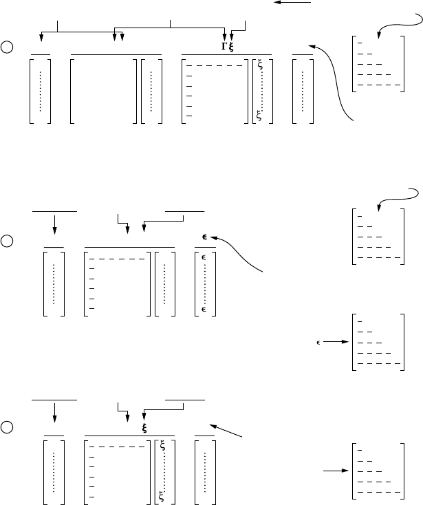
374 A Beginner’s Guide to Structural Equation Modeling
The latent dependent variables are denoted by h (eta) as a vector (m × 1)
of m such variables. The latent independent variables are denoted by x
(ksi) as a vector (n × 1) of n such variables. A matrix Φ (capital phi) con-
tains the variances and covariance terms among these latent independent
variables. The relationships among the latent variables are denoted by B
A vector of
endogenous
concepts
η1
ηm
0000
(m × 1) (m × m) (m × 1) (m × n) (n × 1) (m × 1)
(n × n)
A vector of
“errors” in the
conceptual model.
e covariances
among these errors
constitute Ψ
+ +=
=
00
Matrices of
structural
coefficients
A vector of
exogenous
concepts
e covariances
among those exogenous
concepts constitute Φ
(m × m)
(p × p)
η1
ηm
1
n
η β η
ζ1
ζm
ζ++
A vector of
observed
endogenous
indicators
A matrix of
structural
coefficients
y1
yp
(p × 1) (p × m) (m × 1) (p × 1)
+=
e vector
of endogenous
concepts
η1
ηm
1
p
yΛ
yη+=
A vector of
“errors” in the
measurement model.
e covariances
among these errors
constitute Θ
(q × q)
A vector of
observed
exogenous
indicators
A matrix of
structural
coefficients
x1
xq
(q × 1)(q × n)(n × 1)(q × 1)
+=
e vector
of exogenous
concepts
δ
δ1
δq
xΛx+=
A vector of
“errors” in the
measurement model.
e covariances
among these errors
constitute Θδ
1
2
3
1
n
FIGURE 17.1
Summary of the general structural equation model. (From Hayduk, L. A. (1987). Structural
equation modeling with LISREL: Essentials and advances. Baltimore, MD: Johns Hopkins
University Press.)
Y102005.indb 374 3/22/10 3:27:02 PM
Matrix Approach to Structural Equation Modeling 375
(capital beta) and Γ (capital gamma), the elements of which are denoted by
[b] (lowercase beta) and [g] (lowercase gamma), respectively. The matrix B
is a m × m matrix of structure coefcients that relate the latent dependent
variables to one another. G is a m × n matrix of structure coefcients that
relate the latent independent variables to the latent dependent variables.
The error term z (zeta) in the structural model equation is a vector that
contains the equation prediction errors or disturbance terms. The matrix
Ψ (capital psi) contains the variances and covariance terms among these
latent dependent prediction equation errors.
As described in Jöreskog and Sörbom (1996), the measurement models
are written in the following set of matrix equations:
Y = Λy h + e, (17.2)
for the latent dependent variables, and
X = Λx x + d, (17.3)
for the latent independent variables. The observed variables are denoted
by the vector Y (p × 1) for the measures of the latent dependent variables
h (m × 1), and by the vector X (q × 1) for the measures of the latent inde-
pendent variables x (n × 1). The relationships between the observed vari-
ables and the latent variables (typically referred to as factor loadings) are
denoted by the (p × m) matrix Λy (capital lambda sub y) for the Y’s, the
elements of which are denoted by [λy] (lowercase lambda sub y), and by
the q × n matrix Λx (capital lambda sub x) for the X’s, the elements of which
are denoted by [λx] (lowercase lambda sub x). Finally, the measurement
errors for the Y’s are denoted by the p × 1 vector e (lowercase epsilon)
and for the X’s by the q × 1 vector d (lowercase delta). The theta–epsilon
matrix Θe contains the variances and covariance terms among the errors
for the observed dependent variables. The theta–delta matrix Θd contains
the variances and covariance terms among the errors for the observed
independent variables.
The summary of the general structural equation model in matrix format
depicted by Hayduk (1987) should be studied in great detail. The three
equations diagrammed in matrix format correspond to the structural
model in Equation 17.1, the measurement model for the Y dependent vari-
ables in Equation 17.2, and the measurement model for the X independent
variables in Equation 17.3.
Obviously, not all of the matrices are used in every SEM model. We use our
examples from chapters 9 and 10 to illustrate the matrix notation for a struc-
tural equation model. In our rst example in chapter 9 (see Figure 9.1), there
were two structure coefcients of interest. The rst involved the inuence of
Intelligence on Achievement1. The structure coefcient for this inuence resides
Y102005.indb 375 3/22/10 3:27:02 PM
376 A Beginner’s Guide to Structural Equation Modeling
in the matrix Γ because it represents the relationship between the latent inde-
pendent variable Intelligence and the latent dependent variable Achievement1.
The second structure coefcient involved the inuence of Achievement1 on
Achievement2. This coefcient resides in the matrix B because it represents
the relationship between the latent dependent variable Achievement1 and
the latent dependent variable Achievement2. The nal term in the structural
model of Equation 17.1 is z (zeta), an m × 1 vector of m equation errors or dis-
turbances, which represents that portion of each latent dependent variable
that is not explained or predicted by the model.
In LISREL notation our structural equations are written as
ηγξζ
1111 1
=+,
and
ηβηζ
2211 2
=+,
respectively, or in the complete matrix equation as
η
ηβ
η
η
γ
1
221
1
2
11
00
00
=
+
+
ξζ
ζ
1
1
2
,
where the subscripts on b represent the rows for a latent dependent vari-
able being predicted and columns for a latent dependent variable as the
predictor, respectively. The subscripts for g represent the rows for a latent
dependent variable being predicted and columns for a latent independent
variable as the predictor, respectively.
The values of 0 shown in the matrix equations for B and Γ represent
structure coefcients that we hypothesize to be equal to 0. For example,
because we did not specify that Intelligence inuenced Achievement2, rather
than estimate g21, we set that value to 0. Likewise, we did not specify that
Achievement2 inuenced Achievement1, so we set b12 to 0. Finally, notice that
the diagonal values of B are also 0, that is, b11 and b22. The diagonal val-
ues of B are always set to 0 because they indicate the extent to which a
latent dependent variable inuences itself. These inuences are never of
interest to the SEM researcher. In summary, our matrix equation suggests
that there are potentially four structure coefcients of interest, b12, b21, g11,
and g21; however, our model includes only two of these coefcients. Other
structural models of these same latent variables can be developed that
contain different congurations of structure coefcients.
We now need to provide a more explicit denition of the measurement
models in our example. We have two different measurement models in
Y102005.indb 376 3/22/10 3:27:03 PM
Matrix Approach to Structural Equation Modeling 377
our example, one for the latent dependent variables and one for the latent
independent variables. In LISREL matrix notation these equations are
written for the Ys as
yy111
11
=+
λη ε
yy212
21
=+
λη ε
yy323
32
=+
λη ε
yy424
42
=+
λη ε
and for the Xs as
xx111
11
=+
λξ δ
xx212
21
=+
λξ δ
The factor loadings and error terms also appear in their respective error
variance–covariance matrices. The complete matrix equation for the Ys is
written as
y
y
y
y
y
y
y
y
1
2
3
4
11
21
32
0
0
0
0
=
λ
λ
λ
λ
442
1
2
1
2
3
4
+
η
η
ε
ε
ε
ε
and for the Xs as
x
x
x
x
1
2
11
2
11
21
=
+
λ
λξδ
δ
where the subscripts in λy represent the rows for an observed Y variable
and the columns for a latent dependent variable, and those in λx represent
the rows for an observed X variable and the columns for a latent indepen-
dent variable, respectively.
Y102005.indb 377 3/22/10 3:27:05 PM
378 A Beginner’s Guide to Structural Equation Modeling
The values of 0 shown in the matrix equations for Λy (and theoretically
for Λx, although not for this particular model) represent factor loadings
that we hypothesize to be equal to 0. For example, because we did not
specify that California1 was an indicator of Achievement2, rather than esti-
mate λy12, we set that value to 0. Likewise, we specied that λy22, λy31, and
λy41 were set to 0.
There are several covariance terms that we need to dene. From the
structural model, there are two covariance terms to consider. First, we
dene Φ (capital phi) as an n × n covariance matrix of the n latent indepen-
dent variables, the elements of which are denoted by [f] (lowercase phi).
The diagonal elements of Φ contain the variances of the latent indepen-
dent variables. In our example, model Φ contains only one element, the
variance of Intelligence (denoted by f11).
Second, let us dene Ψ (psi) as an m × m covariance matrix of the m
equation errors z, the elements of which are denoted by [ψ] (lowercase
psi). The diagonal elements of Ψ contain the variances of the equation
errors—that is, the amount of unexplained variance for each equation. In
our example model Ψ contains two diagonal elements, one for each equa-
tion (denoted by ψ11 and ψ22).
From the measurement model there are two additional covariance
terms to be concerned with. First, we dene Θe (capital theta sub epsilon)
as a p × p covariance matrix of the measurement errors for the Ys—that is,
e, the elements of which are denoted by (θe), lowercase theta sub epsilon.
The diagonal elements of Θe contain the variances of the measurement
errors for the Ys. In our example model Θe contains four diagonal ele-
ments, one for each Y. Second, let us dene Θd (capital theta sub delta) as
a q × q covariance matrix of the measurement errors for the Xs—that is, d,
the elements of which are denoted by (θd), lowercase theta sub delta. The
diagonal elements of Θd contain the variances of the measurement errors
for the Xs. In our example model, Θd contains two diagonal elements, one
for each X.
There is one more covariance term that we need to dene, and it rep-
resents the ultimate covariance term. To this point we have dened the
following eight different matrices: B, Γ, Λy, Λx, Φ, Ψ, Θd and Θe. From these
matrices we can generate an ultimate matrix of covariance terms that the
overall model implies, and this matrix is denoted by Σ (sigma). Ofcially,
Σ is a supermatrix composed of four submatrices, as follows:
ΣΣ
ΣΣ
yy yx
xy xx
(17. 4)
This supermatrix certainly looks imposing, but it can be easily under-
stood. First consider the submatrix in the upper left portion of Σ. It deals
Y102005.indb 378 3/22/10 3:27:05 PM

Matrix Approach to Structural Equation Modeling 379
with the covariance terms among the Ys, and in terms of our model can
be written as
ΣΛΙΒ ΓΦΓΨΙΒ ΛΘ
yy yy
=− ′+−
′′
+
−−
[[()()()]],
11
ε
(1 7. 5)
where I is an m × m identity matrix (i.e., a matrix having 1s on the diago-
nal and 0s on the off-diagonal). You can see in Equation 17.5 that all of the
matrices are involved except for those of the measurement model in the
X’s. That is, Equation 17.5 contains the matrices for the structural model
and for the measurement model in the Ys.
Consider next the submatrix in the lower right portion of Σ. It deals
with the covariance terms among the Xs and in terms of our model can
be written as
ΣΛΦΛ Θ
xx xx
=′+[]
δ
(17. 6 )
As shown in Equation 17.6, the only matrices included are those that
involve the X side of the model. This particular portion of the model is the
same as the common factor analysis model, which you may recognize.
Finally, consider the submatrix in the lower left portion of Σ. It deals
with the covariance terms between the X’s and the Y’s and in terms of our
model can be written as
ΣΛΦΓ ΙΛ
xy xy
B=′−′′
−
[()].
1
(1 7.7 )
As shown in Equation 17.7, this portion of the model includes all of our
matrices except for the error terms, that is, Ψ, Θd and Θe. The submatrix in
the upper right portion of Σ is the transposed version of Equation 17.7 (i.e.,
the matrix of Equation 17.7 with rows and columns switched), so we need
not concern ourselves with it.
17.2 Free, Fixed, and Constrained Parameters
Let us return for a moment to our eight structural equation matrices B, Γ,
Λy, Λx, Φ, Ψ, Θd and Θe. In the structural model there are structure coef-
cients in matrices B and Γ. The covariance terms among structural equation
errors are in the matrix Ψ. In the measurement models for latent indepen-
dent and dependent variables, there are factor loadings in the matrices Λx
and Λy, respectively, for their indicator variables. The covariance terms of
measurement errors for the latent independent and dependent variables
are in the matrices Θd and Θe, respectively. The covariance terms among
Y102005.indb 379 3/22/10 3:27:06 PM
380 A Beginner’s Guide to Structural Equation Modeling
the latent independent variables are in the matrix Φ. Each and every ele-
ment in these eight matrices, if used in a particular model, must be speci-
ed to be a free parameter, a xed parameter, or a constrained parameter.
A free parameter is a parameter that is unknown and one that you wish
to estimate. A xed parameter is a parameter that is not free but rather is
xed to a specied value, typically either 0 or 1. A constrained parameter
is a parameter that is unknown, but is constrained to be equal to one or
more other parameters.
For example, consider the following matrix B:
B=
0
0
12
21
β
β
The bs represent values in B that might be parameters of interest and thus
constitute free parameters. The 0s represent values in B that are xed or
constrained to be equal to 0. These diagonal values of B represent the
inuence of a latent dependent variable on itself, and by denition are
always xed to 0. If our hypothesized model included only b21, then b12
would also be xed to 0. For the model specied in Figure 10.2 in chapter
10, B takes the following form:
B=
00
0
21
β
.
For another example, consider the following matrix Λy with the factor
loadings for the latent dependent variable measurement model:
Λy
yy
yy
yy
yy
=
λλ
λλ
λλ
λλ
11 12
21 22
31 32
41 42
Here the λy represent the values in Λy that might be parameters of interest
and would constitute free parameters. This species that we are allow-
ing all of the parameters in Λy to be free so that each of our four indicator
variables (the Y’s) loads on each of our two latent dependent variables (the
h’s). However, in order to solve the identication problem for Λy, some
constraints are usually placed on this matrix whereby some of the param-
eters are xed. We might specify that the rst two indicator variables are
allowed only to load on the rst latent dependent variable (h1) and the
latter two indicators on the second latent dependent variable (h2). Then,
Y102005.indb 380 3/22/10 3:27:07 PM
Matrix Approach to Structural Equation Modeling 381
Λy appears as
Λy
y
y
y
y
=
λ
λ
λ
λ
11
21
32
42
0
0
0
0
Additional constraints in Λy may also be necessary for identication
purposes.
For the structural equation model in chapter 10 (Figure 10.2), the follow-
ing structural equations are specied:
Aspirations = home background + ability + error
Achievement = aspirations + home background + ability + error
The matrix equation would be h = Bh + Γx + z and the elements of the
matrices are
η
ηβ
η
η
γγ
γ
1
221
1
2
11 12
21
00
0
=
+
γγ
ξ
ξ
ζ
ζ
22
1
2
1
2
+
.
The matrix equation for the latent dependent variable measurement model
is Y = Λy h + e, and the elements of the matrices are
y
y
y
y
y
y
1
2
3
4
10
0
01
0
21
42
=
λ
λ
+
η
η
ε
ε
ε
ε
1
2
1
2
3
4
.
The matrix equation for the latent independent variable measurement
model is X = Λx x + d and the elements of the matrices are
x
x
x
x
x
x
x
1
2
3
4
5
10
0
21
3
=
λ
λ
11
52
0
0
0
1
1
2
1
λ
ξ
ξ
δ
x
+
δδ
δ
δ
δ
2
3
4
5
.
Y102005.indb 381 3/22/10 3:27:08 PM

382 A Beginner’s Guide to Structural Equation Modeling
Recall that for each dependent and independent latent variable we xed
one factor loading of an observed variable to 1. This was necessary to
identify the model and to x the scale for the latent variables.
The covariance terms are written next. The covariance matrix for the
latent independent variables is
Φ=
φ
φφ
11
21 22
.
The covariance matrix for the structural equation errors is
Ψ=
ψ
ψψ
11
21 22
.
The covariance matrices for the measurement errors are written as fol-
lows, rst for the indicators of the latent independent variables by
Θ
δ
δ
δ
δδ
δ
δ
θ
θ
θθ
θ
θ
=
11
22
32 33
44
55
0
0
000
0000
and second, for the indicators of the latent dependent variables by
Θ
ε
ε
ε
ε
ε
θ
θ
θ
θ
=
11
22
33
44
0
00
000
NOTE: This matrix output is possible by including the LISREL OUTPUT
command in the LISREL–SIMPLIS program for the model in chapter 10.
17.3 LISREL Model Example in Matrix Notation
The LISREL matrix command language program works directly from
the matrix notation previously discussed and is presented here for the
example in chapter 10. The basic LISREL matrix command language pro-
gram includes TITLE, DATA (DA), INPUT, MODEL (MO), and OUTPUT
Y102005.indb 382 3/22/10 3:27:09 PM
Matrix Approach to Structural Equation Modeling 383
(OU) program statements. The TITLE lines are optional. The user’s guide
provides an excellent overview of the various commands and their pur-
pose (Jöreskog & Sörbom, 1996). The DA statement identies the number
of input variables in the variance–covariance matrix, the NO statement
indicates the number of observations, and MA identies the kind of
matrix to be analyzed, not the kind of matrix to be inputted: MA = CM,
covariance matrix; MA = KM, correlation matrix based on raw scores or
normal scores; MA = MM, matrix of moments (means) about zero; MA =
AM, augmented moment matrix; MA = OM, special correlation matrix of
optimal scores from PRELIS2; and MA = PM, correlation matrix of poly-
choric (ordinal variables) or polyserial (ordinal and continuous variables)
correlations. The SE statement must be used to select and/or reorder vari-
ables used in the analysis of a model (the Y variables must be listed rst).
An external raw score data le can be read using the RA statement with
the FI and FO subcommands, for example, RA FI = raw.dat FO. The FO
subcommand permits the specication of how observations are to be read
(Note: for xed, a FORMAT statement must be enclosed in parentheses;
for free-eld, an asterisk is placed in the rst column, which appears on
the line following the RA command). If FI or UN (logical unit number of
a FORTRAN le) subcommands are not used, then the data must directly
follow the RA command and be included in the program.
In the following LISREL matrix command language program, a lower
diagonal variance–covariance matrix is input, hence, the use of the CM
statement. The SY subcommand, which reads only the lower diagonal ele-
ments of a matrix, has been omitted because it is the default option for
matrix input. The LA statement provides for up to eight characters for
variable labels, with similar subcommand options for input and specica-
tions as with the RA command for data input. (Note: A lower case c per-
mits line continuation for various commands). The LE command permits
variable labels for the latent dependent variables, and the LK command
permits variable labels for the latent independent variables.
The MO command species the model for LISREL analysis. The sub-
commands specify the number of Y variables (ny), number of X variables
(nx), number of latent dependent variables (ne), and number of latent inde-
pendent variables (nk). The form and mode of the eight LISREL param-
eter matrices must be specified and are further explained in the user’s
guide (Jöreskog & Sörbom, 1996). The FU parameter indicates a full
non-symmetric matrix form, and FI indicates a fixed matrix mode,
in contrast to a free mode (FR). The DI statement indicates a diagonal
matrix form, and the SY statement indicates a symmetric matrix form. It is
strongly recommended that any designation of a LISREL model for analy-
sis include the presentation of the eight matrices in matrix form. This will
greatly ease the writing of the MO command and the identication of xed
or free parameters in the matrices on the FR and VA commands. The VA
Y102005.indb 383 3/22/10 3:27:09 PM
384 A Beginner’s Guide to Structural Equation Modeling
command assigns numerical values to the xed parameters. The OU com-
mand permits the selection of various output procedures. One feature of
interest on the OU command is the AM option, which provides for auto-
matic model specication by freeing at each step the xed or constrained
parameters with the largest modication indices, although, as previously
noted, this should not be the sole criterion for model modication.
The LISREL matrix command language program used to analyze the
model in Figure 10.2 of chapter 10, using the default maximum likelihood
estimation method, is as follows:
Modied Model in Figure 10.2, Chapter 10
da ni=9 no=200 ma=cm
cm sy
1.024
.792 1.077
1.027 .919 1.844
.756 .697 1.244 1.286
.567 .537 .876 .632 .852
.445 .424 .677 .526 .518 .670
.434 .389 .635 .498 .475 .545 .716
.580 .564 .893 .716 .546 .422 .373 .851
.491 .499 .888 .646 .508 .389 .339 .629 .871
la
EDASP OCASP VERBACH QUANTACH FAMINC FAED MOED VERBAB
c QUANTAB mo ny=4 nx=5 ne=2 nk=2 be=fu, ga=fu, ph=sy, ps=di,
c ly=fu, lx=fu, td=fu, te=fu,
le
aspire achieve
lk
home ability
fr be(2,1) ga(1,1) ga(1,2) ga(2,1) ga(2,2)
c ly(2,1) ly(4,2) lx(2,1) lx(3,1) lx(5,2)
c te(1,1) te(2,2) te(3,3) te(4,4) td(1,1) td(2,2) td(3,3)
c td(4,4) td(5,5)
c ps(1,1) ps(2,2) ph(1,1) ph(2,2) ph(2,1) td(3,2)
va 1.0 ly(1,1) ly(3,2) lx(1,1) lx(4,2)
ou me=ml all
(NOTE: The c values in the LISREL program denote line continuations in
program statements.)
The LISREL matrix command language requires the user to specically
understand the nature, form, and mode of the eight matrices, and thereby
fully comprehend the model being specied for analysis, even though all
eight matrices may not be used in a particular SEM model. We present the
LISREL output from this program, but do so in an edited and condensed
format. We challenge you to nd the various matrices we have described
in this chapter in the computer output.
Y102005.indb 384 3/22/10 3:27:09 PM
Matrix Approach to Structural Equation Modeling 385
LISREL8 Matrix Program Output (Edited and Condensed)
Modified Model in Figure 10.2, chapter 10
Number of Input Variables 9
Number of Y - Variables 4
Number of X - Variables 5
Number of ETA - Variables 2
Number of KSI - Variables 2
Number of Observations 200
Covariance Matrix
EDASP OCASP VERBACH QUANTACH FAMINC FAED
-------- -------- -------- -------- -------- --------
EDASP 1.02
OCASP 0.79 1.08
VERBACH 1.03 0.92 1.84
QUANTACH 0.76 0.70 1.24 1.29
FAMINC 0.57 0.54 0.88 0.63 0.85
FAED 0.45 0.42 0.68 0.53 0.52 0.67
MOED 0.43 0.39 0.64 0.50 0.47 0.55
VERBAB 0.58 0.56 0.89 0.72 0.55 0.42
QUANTAB 0.49 0.50 0.89 0.65 0.51 0.39
Covariance Matrix
MOED VERBAB QUANTAB
-------- -------- --------
MOED 0.72
VERBAB 0.37 0.85
QUANTAB 0.34 0.63 0.87
LISREL Estimates (Maximum Likelihood)
LAMBDA-Y
aspire achieve
-------- --------
EDASP 1.00 - -
OCASP 0.92 - -
(0.06)
14.34
VERBACH - - 1.00
QUANTACH - - 0.75
(0.04)
18.13
LAMBDA-X home ability
-------- --------
FAMINC 1.00 - -
Y102005.indb 385 3/22/10 3:27:10 PM
386 A Beginner’s Guide to Structural Equation Modeling
FAED 0.78 - -
(0.06)
12.18
MOED 0.72 - -
(0.07)
10.37
VERBAB - - 1.00
QUANTAB - - 0.95
(0.07)
14.10
BETA
aspire achieve
-------- --------
aspire - - - -
achieve 0.53 - -
(0.12)
4.56
GAMMA
home ability
-------- --------
aspire 0.51 0.45
(0.15) (0.15)
3.29 2.96
achieve 0.30 0.69
(0.16) (0.16)
1.87 4.27
Covariance Matrix of ETA and KSI
aspire achieve home ability
-------- -------- -------- --------
aspire 0.86
achieve 1.02 1.65
home 0.57 0.87 0.66
ability 0.57 0.91 0.54 0.66
PHI home ability
-------- --------
home 0.66
(0.09)
7.32
ability 0.54 0.66
(0.07) (0.09)
7.64 7.51
Y102005.indb 386 3/22/10 3:27:10 PM
Matrix Approach to Structural Equation Modeling 387
PSI
Note: This matrix is diagonal.
aspire achieve
-------- --------
0.32 0.23
(0.06) (0.06)
5.61 3.97
Squared Multiple Correlations for Structural Equations
aspire achieve
-------- --------
0.63 0.86
Squared Multiple Correlations for Reduced Form
aspire achieve
-------- --------
0.63 0.81
THETA-EPS
EDASP OCASP VERBACH QUANTACH
-------- -------- -------- --------
0.16 0.35 0.19 0.35
(0.04) (0.05) (0.05) (0.04)
3.88 7.36 3.81 7.95
Squared Multiple Correlations for Y - Variables
EDASP OCASP VERBACH QUANTACH
-------- -------- -------- --------
0.84 0.67 0.90 0.73
THETA-DELTA
FAMINC FAED MOED VERBAB QUANTAB
-------- -------- -------- -------- --------
FAMINC 0.19
(0.04)
4.74
FAED - - 0.27
(0.03)
7.66
MOED - - 0.17 0.37
(0.03) (0.04)
5.28 8.50
VERBAB - - - - - - 0.19
(0.03)
5.41
QUANTAB - - - - - - - - 0.27
(0.04)
7.20
Y102005.indb 387 3/22/10 3:27:10 PM
388 A Beginner’s Guide to Structural Equation Modeling
Squared Multiple Correlations for X - Variables
FAMINC FAED MOED VERBAB QUANTAB
-------- -------- -------- -------- --------
0.78 0.60 0.48 0.78 0.69
Goodness-of-Fit Statistics
Degrees of Freedom = 20
Minimum Fit Function Chi-Square = 19.17 (P = 0.51)
Normal Theory Weighted Least Squares Chi-Square = 18.60
(P = 0.55)
Estimated Non-centrality Parameter (NCP) = 0.0
90 Percent Confidence Interval for NCP = (0.0 ; 12.67)
Minimum Fit Function Value = 0.096
Population Discrepancy Function Value (F0) = 0.0
90 Percent Confidence Interval for F0 = (0.0 ; 0.064)
Root Mean Square Error of Approximation (RMSEA) = 0.0
90 Percent Confidence Interval for RMSEA = (0.0 ; 0.056)
P-Value for Test of Close Fit (RMSEA < 0.05) = 0.91
Expected Cross-Validation Index (ECVI) = 0.35
90 Percent Confidence Interval for ECVI = (0.35 ; 0.42)
ECVI for Saturated Model = 0.45
ECVI for Independence Model = 13.72
Chi-Square for Independence Model with 36 Degrees of
Freedom = 2712.06
Independence AIC = 2730.06
Model AIC = 68.60
Saturated AIC = 90.00
Independence CAIC = 2768.74
Model CAIC = 176.05
Saturated CAIC = 283.42
Normed Fit Index (NFI) = 0.99
Non-Normed Fit Index (NNFI) = 1.00
Parsimony Normed Fit Index (PNFI) = 0.55
Comparative Fit Index (CFI) = 1.00
Incremental Fit Index (IFI) = 1.00
Relative Fit Index (RFI) = 0.99
Critical N (CN) = 391.00
Root Mean Square Residual (RMR) = 0.015
Standardized RMR = 0.015
Goodness-of-Fit Index (GFI) = 0.98
Adjusted Goodness-of-Fit Index (AGFI) = 0.95
Parsimony Goodness-of-Fit Index (PGFI) = 0.44
Y102005.indb 388 3/22/10 3:27:10 PM
Matrix Approach to Structural Equation Modeling 389
Fitted Covariance Matrix
EDASP OCASP VERBACH QUANTACH FAMINC FAED
-------- -------- -------- -------- -------- --------
EDASP 1.02
OCASP 0.79 1.08
VERBACH 1.02 0.93 1.84
QUANTACH 0.77 0.70 1.24 1.29
FAMINC 0.57 0.53 0.87 0.66 0.85
FAED 0.45 0.41 0.68 0.51 0.52 0.67
MOED 0.41 0.38 0.63 0.47 0.48 0.54
VERBAB 0.57 0.52 0.91 0.69 0.54 0.42
QUANTAB 0.54 0.49 0.87 0.65 0.51 0.40
Fitted Covariance Matrix
MOED VERBAB QUANTAB
-------- -------- --------
MOED 0.72
VERBAB 0.39 0.85
QUANTAB 0.37 0.63 0.87
Fitted Residuals
EDASP OCASP VERBACH QUANTACH FAMINC FAED
-------- -------- -------- -------- -------- --------
EDASP 0.00
OCASP 0.00 0.00
VERBACH 0.01 -0.01 0.00
QUANTACH -0.01 -0.01 0.00 0.00
FAMINC -0.01 0.01 0.01 -0.02 0.00
FAED 0.00 0.01 0.00 0.01 0.00 0.00
MOED 0.02 0.01 0.01 0.03 0.00 0.00
VERBAB 0.01 0.04 -0.02 0.03 0.01 0.00
QUANTAB -0.05 0.00 0.02 -0.01 0.00 -0.01
Fitted Residuals
MOED VERBAB QUANTAB
-------- -------- --------
MOED 0.00
VERBAB -0.01 0.00
QUANTAB -0.03 0.00 0.00
Summary Statistics for Fitted Residuals
Smallest Fitted Residual = -0.05
Median Fitted Residual = 0.00
Largest Fitted Residual = 0.04
Y102005.indb 389 3/22/10 3:27:10 PM
390 A Beginner’s Guide to Structural Equation Modeling
Stemleaf Plot
- 4|8
- 3|
- 2|842
- 1|4400
- 0|886542100000000000000
0|2469999
1|1123
2|0067
3|
4|3
Standardized Residuals
EDASP OCASP VERBACH QUANTACH FAMINC FAED
-------- -------- -------- -------- -------- --------
EDASP - -
OCASP - - - -
VERBACH 1.26 -1.01 - -
QUANTACH -0.52 -0.23 - - - -
FAMINC -0.64 0.45 0.55 -1.17 - -
FAED -0.25 0.45 -0.23 0.58 0.15 - -
MOED 0.82 0.30 0.36 0.91 -0.15 - -
VERBAB 0.88 1.93 -2.34 1.50 0.72 0.10
QUANTAB -2.53 0.16 1.59 -0.38 -0.13 -0.50
Standardized Residuals
MOED VERBAB QUANTAB
-------- -------- --------
MOED - -
VERBAB -0.63 - -
QUANTAB -1.10 - - - -
Summary Statistics for Standardized Residuals
Smallest Standardized Residual = -2.53
Median Standardized Residual = 0.00
Largest Standardized Residual = 1.93
Stemleaf Plot
- 2|5
- 2|3
- 1|
- 1|210
- 0|6655
- 0|4322210000000000000
0|122344
0|5567899
1|3
1|569
Y102005.indb 390 3/22/10 3:27:11 PM
Matrix Approach to Structural Equation Modeling 391
Modification Indices and Expected Change
Modification Indices for LAMBDA-Y
aspire achieve
-------- --------
EDASP - - 0.30
OCASP - - 0.30
VERBACH 0.32 - -
QUANTACH 0.32 - -
Expected Change for LAMBDA-Y
aspire achieve
-------- --------
EDASP - - 0.28
OCASP - - -0.26
VERBACH 0.12 - -
QUANTACH -0.09 - -
Standardized Expected Change for LAMBDA-Y
aspire achieve
-------- --------
EDASP - - 0.36
OCASP - - -0.33
VERBACH 0.11 - -
QUANTACH -0.09 - -
Modification Indices for LAMBDA-X
home ability
-------- --------
FAMINC - - 0.40
FAED - - 0.11
MOED - - 0.49
VERBAB 0.63 - -
QUANTAB 0.63 - -
Expected Change for LAMBDA-X
home ability
-------- --------
FAMINC - - 0.18
FAED - - 0.04
MOED - - -0.08
VERBAB 0.16 - -
QUANTAB -0.16 - -
Y102005.indb 391 3/22/10 3:27:11 PM
392 A Beginner’s Guide to Structural Equation Modeling
Standardized Expected Change for LAMBDA-X
home ability
-------- --------
FAMINC - - 0.15
FAED - - 0.03
MOED - - -0.06
VERBAB 0.13 - -
QUANTAB -0.13 - -
No Non-Zero Modification Indices for BETA
No Non-Zero Modification Indices for GAMMA
No Non-Zero Modification Indices for PHI
No Non-Zero Modification Indices for PSI
Modification Indices for THETA-EPS
EDASP OCASP VERBACH QUANTACH
-------- -------- -------- --------
EDASP - -
OCASP - - - -
VERBACH 2.32 1.91 - -
QUANTACH 0.17 0.01 - - - -
Expected Change for THETA-EPS
EDASP OCASP VERBACH QUANTACH
-------- -------- -------- --------
EDASP - -
OCASP - - - -
VERBACH 0.05 -0.05 - -
QUANTACH -0.01 0.00 - - - -
Modification Indices for THETA-DELTA-EPS
EDASP OCASP VERBACH QUANTACH
-------- -------- -------- --------
FAMINC 0.12 0.06 0.86 2.09
FAED 0.62 0.32 0.30 0.15
MOED 1.13 0.40 0.02 0.37
VERBAB 0.51 1.13 8.44 3.03
QUANTAB 4.92 0.30 5.47 0.94
Expected Change for THETA-DELTA-EPS
EDASP OCASP VERBACH QUANTACH
-------- -------- -------- --------
FAMINC -0.01 0.01 0.03 -0.04
FAED -0.01 0.01 -0.01 0.01
MOED 0.02 -0.02 0.00 0.01
Y102005.indb 392 3/22/10 3:27:11 PM
Matrix Approach to Structural Equation Modeling 393
VERBAB 0.02 0.03 -0.09 0.05
QUANTAB -0.06 0.02 0.07 -0.03
Modification Indices for THETA-DELTA
FAMINC FAED MOED VERBAB QUANTAB
-------- -------- -------- -------- --------
FAMINC - -
FAED 0.02 - -
MOED 0.02 - - - -
VERBAB 0.15 0.14 0.36 - -
QUANTAB 0.02 0.05 0.59 - - - -
Expected Change for THETA-DELTA
FAMINC FAED MOED VERBAB QUANTAB
-------- -------- -------- -------- --------
FAMINC - -
FAED 0.00 - -
MOED 0.00 - - - -
VERBAB 0.01 0.01 -0.01 - -
QUANTAB 0.00 0.00 -0.02 - - - -
Maximum Modification Index is 8.44 for Element (4, 3)
of THETA DELTA-EPSILON
Covariances
Y - ETA
EDASP OCASP VERBACH QUANTACH
-------- -------- -------- --------
aspire 0.86 0.79 1.02 0.77
achieve 1.02 0.93 1.65 1.24
Y - KSI
EDASP OCASP VERBACH QUANTACH
-------- -------- -------- --------
home 0.57 0.53 0.87 0.66
ability 0.57 0.52 0.91 0.69
X - ETA
FAMINC FAED MOED VERBAB QUANTAB
-------- -------- -------- -------- --------
aspire 0.57 0.45 0.41 0.57 0.54
achieve 0.87 0.68 0.63 0.91 0.87
Y102005.indb 393 3/22/10 3:27:11 PM
394 A Beginner’s Guide to Structural Equation Modeling
X - KSI
FAMINC FAED MOED VERBAB QUANTAB
-------- -------- -------- -------- --------
home 0.66 0.52 0.48 0.54 0.51
ability 0.54 0.42 0.39 0.66 0.63
First Order Derivatives
LAMBDA-Y
aspire achieve
-------- --------
EDASP 0.00 -0.01
OCASP 0.00 0.01
VERBACH -0.01 0.00
QUANTACH 0.02 0.00
LAMBDA-X
home ability
-------- --------
FAMINC 0.00 -0.01
FAED 0.00 -0.01
MOED 0.00 0.03
VERBAB -0.02 0.00
QUANTAB 0.02 0.00
BETA
aspire achieve
-------- --------
aspire 0.00 0.00
achieve 0.00 0.00
GAMMA
home ability
-------- --------
aspire 0.00 0.00
achieve 0.00 0.00
PHI
home ability
-------- --------
home 0.00
ability 0.00 0.00
Y102005.indb 394 3/22/10 3:27:11 PM
Matrix Approach to Structural Equation Modeling 395
PSI aspire achieve
-------- --------
aspire 0.00
achieve 0.00 0.00
THETA-EPS
EDASP OCASP VERBACH QUANTACH
-------- -------- -------- --------
EDASP 0.00
OCASP 0.00 0.00
VERBACH -0.24 0.21 0.00
QUANTACH 0.07 -0.01 0.00 0.00
THETA-DELTA-EPS
EDASP OCASP VERBACH QUANTACH
-------- -------- -------- --------
FAMINC 0.07 -0.04 -0.15 0.26
FAED 0.21 -0.13 0.13 -0.09
MOED -0.26 0.13 -0.03 -0.13
VERBAB -0.15 -0.20 0.48 -0.32
QUANTAB 0.44 -0.10 -0.38 0.17
THETA-DELTA
FAMINC FAED MOED VERBAB QUANTAB
-------- -------- -------- -------- --------
FAMINC 0.00
FAED -0.03 0.00
MOED 0.03 0.00 0.00
VERBAB -0.08 -0.10 0.15 0.00
QUANTAB -0.03 -0.06 0.18 0.00 0.00
Factor Scores Regressions
ETA
EDASP OCASP VERBACH QUANTACH FAMINC FAED
-------- -------- -------- -------- -------- --------
aspire 0.50 0.21 0.10 0.04 0.04 0.02
achieve 0.12 0.05 0.52 0.22 0.07 0.03
ETA
MOED VERBAB QUANTAB
-------- -------- --------
aspire 0.01 0.02 0.01
achieve 0.01 0.11 0.07
Y102005.indb 395 3/22/10 3:27:12 PM
396 A Beginner’s Guide to Structural Equation Modeling
KSI
EDASP OCASP VERBACH QUANTACH FAMINC FAED
-------- -------- -------- -------- -------- --------
home 0.05 0.02 0.07 0.03 0.41 0.19
ability 0.02 0.01 0.11 0.04 0.07 0.03
KSI
MOED VERBAB QUANTAB
-------- -------- --------
home 0.06 0.07 0.04
ability 0.01 0.37 0.24
Standardized Solution
LAMBDA-Y
aspire achieve
-------- --------
EDASP 0.93 - -
OCASP 0.85 - -
VERBACH - - 1.29
QUANTACH - - 0.97
LAMBDA-X
home ability
-------- --------
FAMINC 0.81 - -
FAED 0.64 - -
MOED 0.59 - -
VERBAB - - 0.81
QUANTAB - - 0.77
BETA
aspire achieve
-------- --------
aspire - - - -
achieve 0.38 - -
GAMMA
home ability
-------- --------
aspire 0.44 0.39
achieve 0.19 0.43
Y102005.indb 396 3/22/10 3:27:12 PM
Matrix Approach to Structural Equation Modeling 397
Correlation Matrix of ETA and KSI
aspire achieve home ability
-------- -------- -------- --------
aspire 1.00
achieve 0.85 1.00
home 0.76 0.83 1.00
ability 0.75 0.87 0.81 1.00
PSI
Note: This matrix is diagonal.
aspire achieve
-------- --------
0.37 0.14
Regression Matrix ETA on KSI (Standardized)
home ability
-------- --------
aspire 0.44 0.39
achieve 0.36 0.58
Total and Indirect Effects
Total Effects of KSI on ETA
home ability
-------- --------
aspire 0.51 0.45
(0.15) (0.15)
3.29 2.96
achieve 0.57 0.92
(0.17) (0.18)
3.26 5.20
Indirect Effects of KSI on ETA
home ability
-------- --------
aspire - - - -
achieve 0.27 0.23
(0.10) (0.09)
2.63 2.62
Y102005.indb 397 3/22/10 3:27:12 PM
398 A Beginner’s Guide to Structural Equation Modeling
Total Effects of ETA on ETA
aspire achieve
-------- --------
aspire - - - -
achieve 0.53 - -
(0.12)
4.56
Largest Eigenvalue of B*B’ (Stability Index) is 0.276
Total Effects of ETA on Y
aspire achieve
-------- --------
EDASP 1.00 - -
OCASP 0.92 - -
(0.06)
14.34
VERBACH 0.53 1.00
(0.12)
4.56
QUANTACH 0.40 0.75
(0.09) (0.04)
4.48 18.13
Indirect Effects of ETA on Y
aspire achieve
-------- --------
EDASP - - - -
OCASP - - - -
VERBACH 0.53 - -
(0.12)
4.56
QUANTACH 0.40 - -
(0.09)
4.48
Total Effects of KSI on Y
home ability
-------- --------
EDASP 0.51 0.45
(0.15) (0.15)
3.29 2.96
OCASP 0.46 0.41
(0.14) (0.14)
3.25 2.93
Y102005.indb 398 3/22/10 3:27:12 PM
Matrix Approach to Structural Equation Modeling 399
VERBACH 0.57 0.92
(0.17) (0.18)
3.26 5.20
QUANTACH 0.43 0.69
(0.13) (0.14)
3.23 5.09
Standardized Total and Indirect Effects
Standardized Total Effects of KSI on ETA
home ability
-------- --------
aspire 0.44 0.39
achieve 0.36 0.58
Standardized Indirect Effects of KSI on ETA
home ability
-------- --------
aspire - - - -
achieve 0.17 0.15
Standardized Total Effects of ETA on ETA
aspire achieve
-------- --------
aspire - - - -
achieve 0.38 - -
Standardized Total Effects of ETA on Y
aspire achieve
-------- --------
EDASP 0.93 - -
OCASP 0.85 - -
VERBACH 0.49 1.29
QUANTACH 0.37 0.97
Standardized Indirect Effects of ETA on Y
aspire achieve
-------- --------
EDASP - - - -
OCASP - - - -
VERBACH 0.49 - -
QUANTACH 0.37 - -
Y102005.indb 399 3/22/10 3:27:13 PM

400 A Beginner’s Guide to Structural Equation Modeling
Standardized Total Effects of KSI on Y
home ability
-------- --------
EDASP 0.41 0.36
OCASP 0.38 0.33
VERBACH 0.46 0.75
QUANTACH 0.35 0.56
At this point, we leave it up to the reader to extract the factor loadings,
error variances, structure coefcients, and disturbance terms from the
various matrices indicated in the standardized solution. It is also help-
ful to determine the direct and indirect effects indicated in the model.
The model-t indices indicated that the data t the modied theoretical
model.
17.4 Other Models in Matrix Notation
This section presents the matrix approach to the path model, the multiple-
sample model, the structured means model and two types of interaction
models in structural equation modeling. The reader is referred to the pre-
vious chapters and references in the book for further detail and explana-
tion of these types of models.
17.4.1 Path Model
The path model in LISREL matrix notation is written as
Y = BY + ΓX + z,
and thus there is no measurement model. Of the eight LISREL matrices,
for the path model we only have the following: B, Γ, Φ, and Ψ.
As an example path model, we again consider the union sentiment
model as previously shown in Figure 7.1 of Chapter 7. The structural equa-
tions in terms of variable names are
Deference (Y1) = Age (X1) + error1
Support (Y2) = Age (X1) + Deference (Y1) + error2
Sentiment (Y3) = Years (X2) + Deference (Y1) + Support (Y2) + error3.
Y102005.indb 400 3/22/10 3:27:13 PM
Matrix Approach to Structural Equation Modeling 401
In terms of matrix equations, this translates into the structural equa-
tion matrices:
Y
Y
Y
Y
1
2
3
21
31 32
000
00
0
=
β
ββ
11
2
3
11
21
32
1
2
0
0
0
Y
Y
X
X
+
γ
γ
γ
+
ζ
ζ
1
2
.
Finally, the relevant LISREL matrices for this model are as follows:
B=
000
00
0
21
31 32
β
ββ
Γ=
γ
γ
γ
11
21
32
0
0
0
Φ=
φ
φφ
11
21 22
Ψ=
ψ
ψ
ψ
11
22
33
0
00
The LISREL path model program would therefore dene these matrices
as follows:
Union Sentiment of Textile Workers
DA NI=5 NO=173 MA=CM
CM SY
14.610
-5.250 11.017
-8.057 11.087 31.971
-0.482 0.677 1.559 1.021
-18.857 17.861 28.250 7.139 215.662
LA
Defer Support Sentim Years Age
SE
1 2 3 5 4
MO NY=3 NX=2 BE=FU,FI GA=FU,FI PH=FU,FR PS=DI
FR BE(2,1) BE(3,1) BE(3,2) GA(1,1) GA(2,1) GA(3,2)
OU ND=2
Y102005.indb 401 3/22/10 3:27:14 PM
402 A Beginner’s Guide to Structural Equation Modeling
Selected computer output from the LISREL path model program would be:
Union Sentiment of Textile Workers
Number of Iterations = 8
LISREL Estimates (Maximum Likelihood)
BETA
Defer Support Sentim
-------- -------- --------
Defer - - - - - -
Support -0.28 - - - -
(0.06)
-4.58
Sentim -0.22 0.85 - -
(0.10) (0.11)
-2.23 7.53
GAMMA
Age Years
-------- --------
Defer -0.09 - -
(0.02)
-4.65
Support 0.06 - -
(0.02)
3.59
Sentim - - 0.86
(0.34)
2.52
PHI Age Years
-------- --------
Age 215.66
(23.39)
9.22
Years 7.14 1.02
(1.26) (0.11)
5.65 9.22
PSI
Note: This matrix is diagonal.
Defer Support Sentim
-------- -------- --------
12.96 8.49 19.45
(1.41) (0.92) (2.11)
9.22 9.22 9.22
Y102005.indb 402 3/22/10 3:27:14 PM
Matrix Approach to Structural Equation Modeling 403
Squared Multiple Correlations for Structural Equations
Defer Support Sentim
-------- -------- --------
0.11 0.23 0.39
Goodness-of-Fit Statistics
Degrees of Freedom = 3
Minimum Fit Function Chi-Square = 1.25 (P = 0.74)
Normal Theory Weighted Least Squares Chi-Square = 1.25
(P = 0.74)
Estimated Non-centrality Parameter (NCP) = 0.0
90 Percent Confidence Interval for NCP = (0.0 ; 4.20)
Minimum Fit Function Value = 0.0073
Population Discrepancy Function Value (F0) = 0.0
90 Percent Confidence Interval for F0 = (0.0 ; 0.025)
Root Mean Square Error of Approximation (RMSEA) = 0.0
90 Percent Confidence Interval for RMSEA = (0.0 ; 0.091)
P-Value for Test of Close Fit (RMSEA < 0.05) = 0.84
Expected Cross-Validation Index (ECVI) = 0.16
90 Percent Confidence Interval for ECVI = (0.16 ; 0.18)
ECVI for Saturated Model = 0.18
ECVI for Independence Model = 1.46
Chi-Square for Independence Model with 10 Degrees of Freedom
= 238.10
Independence AIC = 248.10
Model AIC = 25.25
Saturated AIC = 30.00
Independence CAIC = 268.87
Model CAIC = 75.09
Saturated CAIC = 92.30
Normed Fit Index (NFI) = 0.99
Non-Normed Fit Index (NNFI) = 1.03
Parsimony Normed Fit Index (PNFI) = 0.30
Comparative Fit Index (CFI) = 1.00
Incremental Fit Index (IFI) = 1.01
Relative Fit Index (RFI) = 0.98
Critical N (CN) = 1560.66
Root Mean Square Residual (RMR) = 0.73
Standardized RMR = 0.015
Goodness-of-Fit Index (GFI) = 1.00
Adjusted Goodness-of-Fit Index (AGFI) = 0.99
Parsimony Goodness-of-Fit Index (PGFI) = 0.20
Y102005.indb 403 3/22/10 3:27:14 PM
404 A Beginner’s Guide to Structural Equation Modeling
17.4.2 Multiple-Sample Model
The multiple-sample model in LISREL matrix notation for the measure-
ment model is written as
Y = Λy
(g) h + e
for the latent dependent indicator variables, and
X = Λx
(g) x + d
for the latent independent indicator variables, where g = 1 to G groups
and the other terms are as previously dened. The structural model can be
written as follows:
h = B(g) h + Γ(g) x + z
The four covariance matrices that you are already familiar with are writ-
ten as: Φ(g), Ψ(g), Θd
(g), and Θe
(g). The measurement and structural equations
yield parameter estimates for each of the eight matrices for each group,
B(g), Γ(g), Λy
(g), Λx
(g), Φ(g), Ψ(g), Θd
(g) and Θe
(g).
For instance, with two groups we may be interested in testing whether
the factor loadings are equivalent. These hypotheses for the latent depen-
dent variables are written as
Λy
(1) = Λy
(2)
and for the latent independent variables as
Λx
(1) = Λx
(2)
One might also hypothesize that any of the other matrices are equivalent
so that
Lomax d corr. → Θd
(1) = Θd
(2)
Schumacker d corr. → Θe
(1) = Θe
(2)
B(1) = B(2)
Γ(1) = Γ(2)
Φ(1) = Φ(2)
Ψ(1) = Ψ(2)
Thus, the groups can be evaluated to determine which matrices are equiv-
alent, and which are different.
Y102005.indb 404 3/22/10 3:27:14 PM
Matrix Approach to Structural Equation Modeling 405
17.4.3 Structured Means Model
The structured means model in LISREL matrix notation for the measure-
ment model of the latent dependent indicator variables is written as
Y = ty
(g) + Λy
(g) h + e,
and for the latent independent indicator variables written as
X = tx
(g) + Λx
(g) x + d.
We denote ty and tx as vectors of constant intercept terms (means) for
the indicator variables, and the other terms are as previously dened
(Jöreskog & Sörbom, 1996) denoted these intercept terms as t; other publi-
cations have used u instead]. The structural model is now written as
h = a(g) + B(g) h + Γ(g) x + z,
where a is a vector of constant intercept terms (means) for the structural
equations and the other terms are as previously dened. In most SEM mod-
els the intercept terms are assumed to be zero, so the structured means
model is a special application of SEM used in the analysis of variance as
well as slope and intercept models. In the structured means model, the
intercept term is not zero and therefore estimated (see chapter 6 for inter-
cept terms in regression using CONST term).
In addition to the means of indicator variables being estimated, other
latent variable means can be estimated. The mean of each latent indepen-
dent variable x is given by k; for example, k 1 denotes the mean for x 1. The
mean of each latent dependent variable is given by (I – B)-1 (a + Γk).
In addition to the hypotheses given previously for the simple multiple-
sample model, the structured means model can also examine a, the group
effects for each structural equation, and k, the group effects for each latent
independent variable. We constrain (set equal) the value for one group to
be zero, so we can estimate the difference between that group and a sec-
ond group, which we refer to as a group effect.
In the following LISREL matrix program we hypothesize that academic
and nonacademic boys are different in their reading and writing ability in
fth and seventh grades. The rst structured means program species the
number of groups (NG = 2), the rst group’s (academic boys) sample size
(NO = 373), the number of observed variables (NI = 4), the type of matrix,
that is, a covariance matrix (MA = CM), and the rst group’s covariance
matrix (CM) and means (ME). The second program only has to dene the
second group’s (nonacademic boys) sample size (NO = 249), and the sec-
ond group’s covariance matrix (CM) and means (ME). The means are what
denes a structured means program. Special features of this program are
Y102005.indb 405 3/22/10 3:27:15 PM
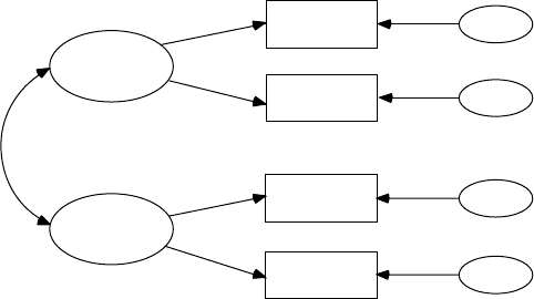
406 A Beginner’s Guide to Structural Equation Modeling
setting TX = FR (t matrix of observed variable means) and KA = FI (k
matrix of latent variable means). This LISREL matrix program parallels the
LISREL–SIMPLIS program in chapter 13 for the structured means model,
that is, adding the LISREL OUTPUT command in the LISREL–SIMPLIS
program yields these same matrices and results (Figure 17.2).
The LISREL matrix structured means program is as follows:
Group: ACADEMIC
DA NI=4 NO=373 MA=CM NG=2
CM SY
281.349
184.219 182.821
216.739 171.699 283.289
198.376 153.201 208.837 246.069
ME
262.236 258.788 275.630 269.075
LA
R5 W5 R7 W7
MO NX=4 NK=2 TX=FR KA=FI
LK
V5 V7
FR LX(2,1) LX(4,2)
VA 1 LX(1,1) LX(3,2)
OU ND=2 AD=OFF
Group: NONACADEMIC
DA NI=4 NO=249 MA=CM
CM SY
174.485
134.468 161.869
129.840 118.836 228.449
Verbal7
Verbal5
Writing7
Reading7
Writing5
Reading5
err_w7
err_r7
err_w5
err_r5
FIGURE 17.2
Structured means model.
Y102005.indb 406 3/22/10 3:27:15 PM
Matrix Approach to Structural Equation Modeling 407
102.194 97.767 136.058 180.460
ME
248.675 246.896 258.546 253.349
MO LX=IN TX=IN KA=FR TD=FR
LA
R5 W5 R7 W7
OU
The model parameters in the rst group for t are set free (FR) and for k are
xed (FI), so that the latent variable intercepts for the rst group are xed to
0. The estimate of the latent variable intercept in the second group (nonaca-
demic boys) is therefore evaluated relative to 0 (academic boys intercept).
The structural model is represented as h2 = a2 + B2 h1 + z2 for both groups
separately for the null hypothesis H0: aacademic boys = anonacademic boys. The edited
and condensed structured means program output is as follows.
Group: ACADEMIC
LISREL Estimates (Maximum Likelihood)
LAMBDA-X EQUALS LAMBDA-X IN THE FOLLOWING GROUP
PHI
V5 V7
-------- --------
V5 220.06
(19.17)
11.48
V7 212.11 233.59
(17.66) (20.50)
12.01 11.40
THETA-DELTA
R5 W5 R7 W7
-------- -------- -------- --------
50.15 36.48 51.72 57.78
(6.02) (4.28) (6.62) (6.05)
8.34 8.52 7.82 9.55
Squared Multiple Correlations for X - Variables
R5 W5 R7 W7
-------- -------- -------- --------
0.81 0.81 0.82 0.76
TAU-X EQUALS TAU-X IN THE FOLLOWING GROUP
Group Goodness-of-Fit Statistics
Contribution to Chi-Square = 4.15
Percentage Contribution to Chi-Square = 41.00
Y102005.indb 407 3/22/10 3:27:15 PM
408 A Beginner’s Guide to Structural Equation Modeling
Root Mean Square Residual (RMR) = 6.07
Standardized RMR = 0.025
Goodness-of-Fit Index (GFI) = 0.99
Group: NONACADEMIC
LISREL Estimates (Maximum Likelihood)
LAMBDA-XKSI 1 KSI 2
-------- --------
R5 1.00 - -
W5 0.84 - -
(0.02)
34.35
R7 - - 1.00
W7 - - 0.89
(0.03)
31.95
PHI
KSI 1 KSI 2
-------- --------
KSI 1 156.34
(16.19)
9.66
KSI 2 126.96 153.73
(14.22) (18.03)
8.93 8.53
THETA-DELTA
R5 W5 R7 W7
-------- -------- -------- --------
23.25 42.80 65.67 67.36
(6.23) (5.64) (9.87) (8.74)
3.73 7.59 6.65 7.71
Squared Multiple Correlations for X-Variables
R5 W5 R7 W7
-------- -------- -------- --------
0.87 0.72 0.70 0.65
TAU-X
R5 W5 R7 W7
-------- -------- -------- --------
262.37 258.67 275.71 268.98
Y102005.indb 408 3/22/10 3:27:15 PM
Matrix Approach to Structural Equation Modeling 409
(0.84) (0.70) (0.87) (0.80)
312.58 366.96 317.77 338.00
KAPPA
KSI 1 KSI 2
-------- --------
-13.80 -17.31
(1.18) (1.24)
-11.71 -13.99
We obtain the latent variable mean differences from the kappa matrix,
where the nonacademic boys were below the academic boys in reading
and writing at both the fth grade (KSI 1) and seventh grade (KSI 2). Our
model-t indices indicate an acceptable theoretical model:
Global Goodness-of-Fit Statistics
Degrees of Freedom = 6
Minimum Fit Function Chi-Square = 10.11 (P = 0.12)
Normal Theory Weighted Least Squares Chi-Square = 9.96
(P = 0.13)
Estimated Noncentrality Parameter (NCP) = 3.96
90 Percent Confidence Interval for NCP = (0.0 ; 16.79)
Minimum Fit Function Value = 0.016
Population Discrepancy Function Value (F0) = 0.0064
90 Percent Confidence Interval for F0 = (0.0 ; 0.027)
Root Mean Square Error of Approximation (RMSEA) = 0.046
90 Percent Confidence Interval for RMSEA = (0.0 ; 0.095)
P-Value for Test of Close Fit (RMSEA < 0.05) = 0.27
Expected Cross-Validation Index (ECVI) = 0.087
90 Percent Confidence Interval for ECVI = (0.068 ; 0.095)
ECVI for Saturated Model = 0.032
ECVI for Independence Model = 3.15
Chi-Square for Independence Model with 12 Degrees of
Freedom = 1947.85
Independence AIC = 1963.85
Model AIC = 53.96
Saturated AIC = 40.00
Independence CAIC = 2007.31
Model CAIC = 173.48
Saturated CAIC = 148.66
Normed Fit Index (NFI) = 0.99
Nonnormed Fit Index (NNFI) = 1.00
Parsimony Normed Fit Index (PNFI) = 0.50
Comparative Fit Index (CFI) = 1.00
Incremental Fit Index (IFI) = 1.00
Relative Fit Index (RFI) = 0.99
Critical N (CN) = 1031.60
Y102005.indb 409 3/22/10 3:27:16 PM

410 A Beginner’s Guide to Structural Equation Modeling
Group Goodness-of-Fit Statistics
Contribution to Chi-Square = 5.97
Percentage Contribution to Chi-Square = 59.00
Root Mean Square Residual (RMR) = 7.69
Standardized RMR = 0.042
Goodness-of-Fit Index (GFI) = 0.99
17.4.4 Interaction Models
I n chapt er 16 we di scus sed fou r di ffer ent t y pes of inte rac t ion mode ls: catego ri-
cal, nonlinear, continuous observed variable, and latent variable (Schumacker
& Marcoulides, 1998). In this chapter we present the LISREL matrix program
using latent variables that parallels the interaction latent variable approach
in Chapter 16 using LISREL–SIMPLIS, except for slight differences in the
standard errors. The matrix approach to latent variable interactions requires
the understanding and use of nonlinear constraints, which has made it dif-
cult for most SEM researchers (Jöreskog & Yang, 1996).
The latent variable interaction approach in LISREL matrix notation for
Figure 17.3 is h1 = g1 x1 + g2 x2 + g3 x3 + z1, where h1 is the latent dependent
variable, x1 and x2 are the main-effect latent independent variables, x3 is
the interaction-effect formed by multiplying x1 and x2, g1 and g2 are the
structure coefcients for the main-effect latent independent variables, g3 is
KS1
KSI1*KSI2
KSI2
ET
gamma3
gamma1
gamma2
V4
V5
V6
V47
V58
V69
V7
V8
V9
V1
V2
V3
FIGURE 17.3
Latent variable interaction (continuous variable approach).
Y102005.indb 410 3/22/10 3:27:16 PM
Matrix Approach to Structural Equation Modeling 411
the structure coefcient for the interaction-effect latent independent vari-
able, and z1 is the error term in the structural equation. Notice that the
relationship between h1 and x3 is itself linear. The structure of the interac-
tion model emerges as a logical extension of the measurement model for
x1 and x2. The basic measurement model is X = Λx + d, where X is a vector
of observed variables, Λ is a matrix of factor loadings, and d is a vector of
measurement error terms. The covariance matrices of these common and
unique factors are Φ and Θd, respectively.
Kenny and Judd (1984) used simple algebraic substitution to develop
their model of multiplicative interaction effects (Hayduk, 1987). Basically,
given two latent independent variables, the models are X1 = λ1 x1 + d1 and
X2 = λ2 x2 + d2. The interaction effect or product is X3 = X1 X2, indicated in
the model as X3 = λ1 λ2 x1 x2 + λ1 x1 d2 + λ2 x2 d1 + d1 d2, or X3 = λ3 x3 + λ1 x4 +
λ2 x5 + d3, where x3 = x1 x2, x4 = x1 d2, x5 = x2 d1, d3 = d1 d2, and λ3 = λ1 λ2. All
of these new latent variables are mutually uncorrelated and uncorrelated
with all other latent variables in the model.
In order to incorporate this interaction effect into the structural equa-
tion model, we need to specify X3 as a function of latent variables whose
variances and covariance terms reect these relationships. This involves
specifying some model parameters as nonlinear functions of other
parameters. In the LISREL program, these types of nonlinear constraints
are indicated by using the VA (value), EQ (equality), and CO (constraint)
commands. For example, the Kenny–Judd interaction model implies that
s2(x3) = s2(x1) s2(x2) + s( x1 x2)2. This relationship using the CO command
line is specied as CO PH(3,3) = PH(1,1) * PH(2,2) + PH(2,1) * * 2. Similarly,
their model implies that s2(x4) = s2(x1) s2(d2), and this relationship is speci-
ed as CO PH(4,4) = PH(1,1) * TD(2,2).
We demonstrate the Kenny and Judd (1984) approach by creating a
simulated data set of nine multivariate normal variables and three
product indicant variables for 500 participants using a PRELIS program
(mvdata1.pr2):
Generate multivariate normal variables – LISREL
DA NO=500
NE X1=NRAND; NE X2=NRAND; NE X3=NRAND
NE X4=NRAND; NE X5=NRAND; NE X6=NRAND
NE X7=NRAND; NE X8=NRAND; NE X9=NRAND
NE V1=X1
NE V2=.378*X1+.925*X2
NE V3=.320*X1+.603*X2+.890*X3
NE V4=.204*X1+.034*X2+.105*X3+.904*X4
NE V5=.076*X1+.113*X2+.203*X3+.890*X4+.925*X5
NE V6=.111*X1+.312*X2+.125*X3+.706*X4+.865*X5+.905*X6
NE V7=.310*X1+.124*X2+.310*X3+.222*X4+.126*X5+.555*X6+.897*X7
NE V8=.222*X1+.111*X2+.412*X3+.312*X4+.212*X5+.312*X6+.789*X7+.899*X8
Y102005.indb 411 3/22/10 3:27:16 PM
412 A Beginner’s Guide to Structural Equation Modeling
NE V9=.321*X1+.214*X2+.124*X3+.122*X4+.234*X5+.212*X6+.690*X7+.789*X8+.907*X9
NE V47=V4*V7
NE V58=V5*V8
NE V69=V6*V9
CO ALL
SD X1-X9
OU MA=CM CM=INTERACT.CM ME=INTERACT.ME RA=INTERACT.PSF XM
IX=784123
Although the nine observed variables were created as multivariate nor-
mal data, the product indicant variables are typically not multivariate nor-
mal. The summary statistics do indicate that the nine observed variables
are univariate normal, but that the three product indicant variables have
skewness and kurtosis, that is, are nonnormal (boldfaced). In LISREL,
maximum likelihood estimation (ML) is the default, and it appears to
work well under mild violations of multivariate normality in the interac-
tion latent variable model. We used the same random number seed as
before so the data could be reproduced (IX = 784123).
PRELIS Computer Output
Univariate Summary Statistics for Continuous Variables
Variable Mean St. Dev. T-Value Skewness Kurtosis
V1 -0.061 0.976 -1.394 0.191 0.048
V2 0.007 1.071 0.142 -0.047 0.280
V3 -0.018 1.105 -0.368 0.175 0.441
V4 -0.015 0.956 -0.359 -0.200 -0.158
V5 -0.013 1.351 -0.209 -0.003 0.168
V6 0.011 1.543 0.163 0.171 0.528
V7 -0.065 1.192 -1.222 -0.081 -0.350
V8 -0.041 1.491 -0.615 0.127 0.092
V9 0.005 1.595 0.075 0.058 0.514
V47 0.325 1.143 6.356 0.958 3.861
V58 0.670 2.179 6.877 1.916 8.938
V69 0.584 2.754 4.745 2.304 15.266
Test of Univariate Normality for Continuous Variables
Skewness Kurtosis Skewness and
Kurtosis
Variable Z-Score P-Value Z-Score P-Value Chi-
Square P-Value
V1 1.749 0.080 0.321 0.748 3.163 0.206
V2 -0.432 0.666 1.256 0.209 1.764 0.414
V3 1.608 0.108 1.811 0.070 5.866 0.053
Y102005.indb 412 3/22/10 3:27:17 PM
Matrix Approach to Structural Equation Modeling 413
V4 -1.833 0.067 -0.695 0.487 3.844 0.146
V5 -0.031 0.975 0.829 0.407 0.688 0.709
V6 1.571 0.116 2.082 0.037 6.802 0.033
V7 -0.746 0.456 -1.865 0.062 4.034 0.133
V8 1.165 0.244 0.513 0.608 1.620 0.445
V9 0.531 0.595 2.039 0.041 4.438 0.109
V47 7.573 0.000 7.085 0.000 107.539 0.000
V58 12.103 0.000 9.622 0.000 239.070 0.000
V69 13.428 0.000 11.101 0.000 303.539 0.000
The PRELIS program saves three les, a covariance matrix (interact.cm),
means (interact.me), and a PRELIS system le (interact.psf). The LISREL
program inputs the les with the covariance matrix and means.
The LISREL program to run the data for the model in Figure 17.3 is:
Fitting Model to Mean Vector and Covariance Matrix
DA NI=12 NO=500
!The three interaction variables are added prior to
program analysis
LA
V1 V2 V3 V4 V5 V6 V7 V8 V9 V47 V58 V69
CM=interact.CM
ME=interact.ME
MO NY=3 NX=9 NE=1 NK=3 TD=SY TY=FR TX=FR KA=FR
FR LY(2) LY(3) GA(1) GA(2) GA(3) LX(2,1) LX(3,1) LX(5,2)
LX(6,2) PH(1,1)-PH(2,2)
FI PH(3,1) PH(3,2)
VA 1 LY(1) LX(1,1) LX(4,2) LX(7,3) !Should be same as
C SIMPLIS program for comparison
FI KA(1) KA(2)
CO LX(7,1)=TX(4)
CO LX(7,2)=TX(1)
CO LX(8,1)=TX(5)*LX(2,1)
CO LX(8,2)=TX(2)*LX(5,2)
CO LX(8,3)=LX(2,1)*LX(5,2)
CO LX(9,1)=TX(6)*LX(3,1)
CO LX(9,2)=TX(3)*LX(6,2)
CO LX(9,3)=LX(3,1)*LX(6,2)
CO PH(3,3)=PH(1,1)*PH(2,2)+PH(2,1)**2
CO TD(7,1)=TX(4)*TD(1,1)
CO TD(7,4)=TX(1)*TD(4,4)
CO TD(7,7)=TX(1)**2*TD(4,4)+TX(4)**2*TD(1,1)+PH(1,1)*TD(4,4)+
C PH(2,2)*TD(1,1)+TD(1,1)*TD(4,4)
CO TD(8,2)=TX(5)*TD(2,2)
CO TD(8,5)=TX(2)*TD(5,5)
CO TD(8,8)=TX(2)**2*TD(5,5)+TX(5)**2*TD(2,2)+LX(2,1)**2*PH(1,
1)*TD(5,5)+
C LX(5,2)**2*PH(2,2)*TD(2,2)+TD(2,2)*TD(5,5)
Y102005.indb 413 3/22/10 3:27:17 PM
414 A Beginner’s Guide to Structural Equation Modeling
CO TD(9,3)=TX(6)*TD(3,3)
CO TD(9,6)=TX(3)*TD(6,6)
CO TD(9,9)=TX(3)**2*TD(4,4)+TX(6)**2*TD(3,3)+LX(3,1)**2*PH(1,
1)*TD(6,6)+
C LX(6,2)**2*PH(2,2)*TD(3,3)+TD(3,3)*TD(6,6)
CO KA(3)=PH(2,1)
CO TX(7)=TX(1)*TX(4)
CO TX(8)=TX(2)*TX(5)
CO TX(9)=TX(3)*TX(6)
OU AD=OFF IT=500 EP=0.001 IM=3 ND=3
The CO command (placing proper constraints in the model) is what
becomes difcult to navigate in creating the matrix programs for latent
variable interaction models. Discussions of different latent variable
interaction models and related issues can be found in Marcoulides and
Schumacker (1996, 2001) and Schumacker and Marcoulides (1998).
Given the LISREL matrix program with a latent variable interaction
term, several matrices need to be specied. The structural equation with
the two main-effect latent variables and the interaction-effect latent vari-
able is as follows:
ηαγξ γξ γξξζ
=+ ++ +
11 22 312
The measurement model with Y observed variables is dened as follows:
YT
yy
=+ +Λ
ηε
The matrices for the Y observed variable measurement model are speci-
ed as:
y
y
y
y
y
y
1
2
3
1
2
3
=
+
τ
τ
τ
()
()
()
11
2
3
1
2
3
λ
λ
η
ε
ε
ε
()
()
,
y
y
+
where the theta–epsilon error matrix specied as follows:
Θ
εεεε
θθθ
=diag(,,)
123
The measurement model for the X observed variables, which includes
both main-effects and the interaction-effect, is dened as follows:
XT
xx
=+ +Λ
ξδ
Y102005.indb 414 3/22/10 3:27:18 PM
Matrix Approach to Structural Equation Modeling 415
The matrices for the X observed variable measurement model are speci-
ed as follows:
x
x
x
x
x
x
xx
xx
xx
1
2
3
4
5
6
14
25
36
=
τ
τ
τ
τ
τ
τ
ττ
ττ
τ
1
2
3
4
5
6
14
25
3
ττ
6
1
+
000
00
00
010
00
00
1
2
3
5
6
41
52 25 25
33
λ
λ
λ
λ
ττ
τλ τλ λλ
τλ ττλ λλ
ξ
ξ
ξ
36 36
1
2
1
ξξ
δ
δ
δ
δ
δ
δ
δ
δ
δ
2
1
2
3
4
5
6
7
8
9
+
with errors in the theta delta matrix Θd denoted as follows:
θ
θ
θ
θ
θ
θ
τθ τθ θ
τ
1
2
3
4
5
6
41 14 7
0
00
000
0000
00000
00 00
0552 25 8
63 36 9
00 00
00 00 00
θτθθ
τθ τθ θ
.
The theta delta values for the observed interaction variables are calculated
as follows:
θτθτθφθφθθθ
θτθτ
74
211
24114 22 114
85
222
2
=++ ++
=+
θθλφθ λφ θθθ
θτθτθλ
52
211 55
222 225
96
233
263
+++
=++22 11 66
222 336
φθ λφ θθθ
++
Y102005.indb 415 3/22/10 3:27:19 PM
416 A Beginner’s Guide to Structural Equation Modeling
The mean vector implied by the interaction of the exogenous latent vari-
ables is dened in the following kappa mean vector matrix:
κ
φ
=
0
0
21
with the variance–covariance of the latent independent variables (ksi1
and ksi2) dened as follows:
Φ=
+
φ
φφ
φφ φ
11
21 22
11 22 21
2
00
We can now look for these matrices and their associated values in the
LISREL computer output.
LISREL Interaction Computer Output
The gamma matrix contains the three structure coefcients of interest for
the two main-effect latent variables [g1 = .077 (.030), t = 2.60 and g2 = .155
(.029), t = 5.378] and the interaction latent variable [g3 = −.029 (.029), t =
–1.004]. The gamma coefcient for the latent variable interaction effect is
nonsignicant (t = −1.004). We should modify our theoretical model and
test main effects only. The edited and condensed LISREL computer output
is as follows:
LISREL Estimates (Maximum Likelihood)
LAMBDA-Y
ETA 1
--------
V1 1.000
V2 2.080
(0.257)
8.097
V3 2.532
(0.325)
7.788
Y102005.indb 416 3/22/10 3:27:19 PM
Matrix Approach to Structural Equation Modeling 417
LAMBDA-X
KSI 1 KSI 2 KSI 3
-------- -------- --------
V4 1.000 - - - -
V5 1.981 - - - -
(0.091)
21.732
V6 1.925 - - - -
(0.090)
21.368
V7 - - 1.000 - -
V8 - - 1.658 - -
(0.072)
22.874
V9 - - 1.493 - -
(0.069)
21.741
V47 -0.070 0.013 1.000
(0.035) (0.028)
-2.027 0.471
V58 -0.094 -0.010 3.285
(0.083) (0.062) (0.173)
-1.142 -0.153 18.960
V69 0.020 -0.049 2.875
(0.090) (0.067) (0.152)
0.226 -0.729 18.940
GAMMA
KSI 1 KSI 2 KSI 3
-------- -------- --------
ETA 1 0.077 0.155 -0.029
(0.030) (0.029) (0.029)
2.602 5.378 -1.004
Covariance Matrix of ETA and KSI
ETA 1 KSI 1 KSI 2 KSI 3
-------- -------- -------- --------
ETA 1 0.150
KSI 1 0.068 0.463
KSI 2 0.137 0.211 0.784
KSI 3 -0.012 - - - - 0.408
Mean Vector of Eta-Variables
ETA 1
--------
-0.006
Y102005.indb 417 3/22/10 3:27:20 PM
418 A Beginner’s Guide to Structural Equation Modeling
PHI
KSI 1 KSI 2 KSI 3
-------- -------- --------
KSI 1 0.463
(0.043)
10.729
KSI 2 0.211 0.784
(0.021) (0.069)
10.236 11.283
KSI 3 - - - - 0.408
(0.041)
9.953
PSI
ETA 1
--------
0.123
(0.029)
4.193
Squared Multiple Correlations for Structural Equations
ETA 1
--------
0.179
THETA-EPS
V1 V2 V3
-------- -------- --------
0.804 0.502 0.267
(0.053) (0.058) (0.074)
15.166 8.618 3.617
Squared Multiple Correlations for Y - Variables
V1 V2 V3
-------- -------- --------
0.157 0.563 0.782
THETA-DELTA
V4 V5 V6 V7 V8 V9
-------- -------- -------- -------- -------- --------
V4 0.458
(0.029)
16.044
V5 - - 0.045
(0.049)
0.931
V6 - - - - 0.796
Y102005.indb 418 3/22/10 3:27:20 PM
Matrix Approach to Structural Equation Modeling 419
(0.065)
12.238
V7 - - - - - - 0.647
(0.043)
15.186
V8 - - - - - - - - 0.105
(0.057)
1.840
V9 - - - - - - - - - - 0.936
(0.070)
13.342
V47 -0.032 - - - - 0.009 - - - -
(0.016) (0.018)
-2.011 0.471
V58 - - -0.002 - - - - -0.001 - -
(0.003) (0.004)
-0.722 -0.152
V69 - - - - 0.008 - - - - -0.031
(0.037) (0.042)
0.226 -0.728
THETA–DELTA
V47 V58 V69
-------- -------- --------
V47 0.957
(0.047)
20.519
V58 - - 0.293
(0.138)
2.129
V69 - - - - 3.745
(0.200)
18.698
Squared Multiple Correlations for X - Variables
V4 V5 V6 V7 V8 V9
-------- -------- -------- -------- -------- --------
0.503 0.976 0.683 0.548 0.954 0.651
Squared Multiple Correlations for X - Variables
V47 V58 V69
-------- -------- --------
0.300 0.938 0.474
Y102005.indb 419 3/22/10 3:27:20 PM
420 A Beginner’s Guide to Structural Equation Modeling
TAU-Y
V1 V2 V3
-------- -------- --------
-0.055 0.019 -0.004
(0.044) (0.048) (0.050)
-1.263 0.386 -0.079
TAU-X
V4 V5 V6 V7 V8 V9
-------- -------- -------- -------- -------- --------
0.013 -0.006 -0.033 -0.070 -0.048 0.011
(0.028) (0.038) (0.045) (0.035) (0.042) (0.047)
0.471 -0.153 -0.729 -2.027 -1.144 0.226
TAU-X
V47 V58 V69
-------- -------- --------
-0.001 0.000 0.000
(0.002) (0.002) (0.002)
-0.456 0.151 -0.215
KAPPA
KSI1 KSI2 KSI3
-------- -------- --------
- - - - 0.211
(0.021)
10.236
Goodness-of-Fit Statistics
Degrees of Freedom = 59
Minimum Fit Function Chi-Square = 403.462 (P = 0.0)
Normal Theory Weighted Least Squares Chi-Square = 365.186
(P = 0.0)
Estimated Non-centrality Parameter (NCP) = 306.186
90 Percent Confidence Interval for NCP = (249.618 ; 370.256)
Minimum Fit Function Value = 0.809
Population Discrepancy Function Value (F0) = 0.614
90 Percent Confidence Interval for F0 = (0.500 ; 0.742)
Root Mean Square Error of Approximation (RMSEA) = 0.102
90 Percent Confidence Interval for RMSEA = (0.0921 ; 0.112)
Y102005.indb 420 3/22/10 3:27:20 PM

Matrix Approach to Structural Equation Modeling 421
P-Value for Test of Close Fit (RMSEA < 0.05) = 0.000
Expected Cross-Validation Index (ECVI) = 0.944
90 Percent Confidence Interval for ECVI = (0.763 ; 1.005)
ECVI for Saturated Model = 0.313
ECVI for Independence Model = 6.300
Chi-Square for Independence Model with 66 Degrees of
Freedom = 3119.580
Independence AIC = 3143.580
Model AIC = 471.186
Saturated AIC = 156.000
Independence CAIC = 3206.156
Model CAIC = 747.560
Saturated CAIC = 562.739
Normed Fit Index (NFI) = 0.871
Nonnormed Fit Index (NNFI) = 0.874
Parsimony Normed Fit Index (PNFI) = 0.778
Comparative Fit Index (CFI) = 0.887
Incremental Fit Index (IFI) = 0.887
Relative Fit Index (RFI) = 0.855
Critical N (CN) = 108.807
Root Mean Square Residual (RMR) = 0.142
Standardized RMR = 0.0636
Goodness-of-Fit Index (GFI) = 0.893
Adjusted Goodness-of-Fit Index (AGFI) = 0.859
Parsimony Goodness-of-Fit Index (PGFI) = 0.676
17.5 Summary
This chapter presented the eight basic matrices used in structural equa-
tion modeling, plus two new matrices, tau and kappa. We also discussed
that for any structural equation model, parameters in these matrices must
be free, xed, or constrained for model identication, model estimation,
and model testing. We presented the matrix notation by providing ve
different SEM models: our theoretical model in chapter 10, a path model,
a multiple-sample model, a structured means model, and an interaction
model. We presented these same models in earlier chapters using LISREL–
SIMPLIS, and displayed them in matrix form in this chapter for compara-
tive purposes. If you wish, simply add the LISREL OUTPUT command
Y102005.indb 421 3/22/10 3:27:20 PM
422 A Beginner’s Guide to Structural Equation Modeling
to these programs to output the matrices presented in this chapter. We
rmly believe that once you master the matrix notation, you will better
understand structural equation modeling.
Exercise
1. The National Science Foundation (NSF) is encouraging students
to seek academic degrees and careers in science, mathematics,
and engineering in the United States. Research has shown a gen-
der difference in science, mathematics, and engineering partici-
pation. A key area of study is to investigate what factors inuence
these gender differences. A latent variable model is hy pothesized
to investigate factors that inuence gender differences because
previous research indicated variables such as characteristics of
students in science, mathematics, and engineering.
A structural equation model with two exogenous latent vari-
ables measured by six observed variables is hypothesized to
predict two endogeneous latent variables measured by ve
observed variables. The rst independent latent variable, x1 =
Family Background, is measured by three variables: X1 = fam-
ily income, X2 = father’s education, and X3 = mother’s education.
The other independent latent variable, x2 = Encouragement, is
measured by three variables: X4 = personal encouragement,
X5 = institutional characteristics, and X6 = admission status.
Students’ characteristics, h1 = Students’ Characteristics, is
measured by three variables: Y1 = cognitive abilities, Y2 = inter-
personal skills, and Y3 = motivation. The other endogenous
variable, h2 = Aspirations, is measured by two variables: Y4 =
occupational aspiration and Y5 = educational aspiration.
The hypothesized structural equation model represents a
two-step approach: measurement (conrmatory factor analysis)
and structural model. The structural model depicts the relation-
ships between four latent variables: x1 = Family Background,
x2 = Encouragement, h1 = Students’ Characteristics, and h2 =
Aspirations. The structural model is
Students’ Characteristics = Family Background + Encouragement
+ Aspirations + error
Aspirations = Family Background + Encouragement + error.
With this information, you should be able to do the following:
1. Diagram the structural equation model.
2. Write the measurement equations using the variable
names.
Y102005.indb 422 3/22/10 3:27:20 PM

Matrix Approach to Structural Equation Modeling 423
3. Write the measurement equations using LISREL matrix
notation.
4. Write the structural equations using the variable names.
5. Write the structural equations using LISREL matrix
notation.
6. Create the matrices for the measurement model.
7. Create the matrices for the structural model.
References
Hayduk, L. A. (1987). Structural equation modeling with LISREL: Essentials and
advances. Baltimore, MD: Johns Hopkins University Press.
Jöreskog, K. G., & Sörbom, D. (1996). LISREL8 user’s reference guide. Chicago, IL:
Scientic Software International.
Jöreskog, K. G., & Yang, F. (1996). Non-linear structural equation models: The
Kenny-Judd model with interaction effects. In G. A. Marcoulides & R. E.
Schumacker (Eds.), Advanced structural equation modeling: Issues and techniques
(pp. 57–88). Mahwah, NJ: Lawrence Erlbaum.
Kenny, D. A., & Judd, C. M. (1984). Estimating the non-linear and interactive effects
of latent variables. Psychological Bulletin, 96, 201–210.
Marcoulides, G., & Schumacker, R. E. (Eds.). (1996). Advanced structural equation
modeling: Issues and techniques. Mahwah, NJ: Lawrence Erlbaum.
Marcoulides, G., & Schumacker, R. E. (Eds.). (2001). New developments and tech-
niques in structural equation modeling. Mahwah, NJ: Lawrence Erlbaum.
Schumacker, R. E., & Marcoulides, G. A. (1998). Interaction and nonlinear effects in
structural equation modeling. Mahwah, NJ: Lawrence Erlbaum.
Y102005.indb 423 3/22/10 3:27:20 PM

425
Appendix A: Introduction
to Matrix Operations
Structural Equation Modeling performs calculations using several differ-
ent matrices. The matrix operations to perform the calculations involve
addition, subtraction, multiplication, and division of elements in the dif-
ferent matrices.* We present these basic matrix operations, followed by a
simple multiple regression example.
Matrix Definition
A matrix is indicated by capital letters (e.g., A, B, or R) and takes the form:
A22
35
56
=
The matrix can be rectangular or square-shaped, and contains an array of
numbers. A correlation matrix would be a square matrix with the value
of 1.0 in the diagonal and variable correlations in the off-diagonal. A cor-
relation matrix is symmetrical because the correlation coefcients in the
lower half of the matrix are the same as the correlation coefcients in the
upper half of the matrix. [Note: we usually only report the diagonal values
and the correlations in the lower half of the matrix.] For example:
R33
10 30 50
30 10 60
50 60 10
=
.. .
...
.. .
,
but we report the following as a correlation matrix:
1.0
.30 1.0
.50 .60 1.0
* Walter L. Sullins (1973). Matrix algebra for statistical applications, Danville, IL: The Interstate
Printers & Publishers, Inc.
Y102005.indb 425 3/22/10 3:27:21 PM

426 Appendix A: Introduction to Matrix Operations
Matrices have a certain number of rows and columns. The A matrix
above has two rows and two columns. The order of a matrix is the size of
the matrix, or number of rows times the number of columns. The order
of the A matrix is 22, and shown as subscripts, where the rst subscript
is the number of rows, and second subscript is the number of columns.
When we refer to elements in the matrix, we use row and column desig-
nations to identify the location of the element in the matrix. The location
of an element has a subscript using the row number rst, followed by the
column number. For example, the correlation r = .30 is in the R21 matrix
location or row 2, column 1.
Matrix Addition and Substraction
Matrix addition adds corresponding elements in two matrices, while
matrix subtraction subtracts corresponding elements in two matrices.
Consequently, the two matrices must have the same order (number of
rows and columns), so we can add A32 + B32 or subtract A32 – B32. In the fol-
lowing example, Matrix A elements are added to Matrix B elements:
352
160
912
135
21 3
07 3
4
+
−
−
=
227
37 3
98 1−
Matrix Multiplication
Matrix multiplication is not as straight forward as matrix addition and
subtraction. For a product of matrices we indicate A •B or AB. If A is an
m × n matrix and B is an n × p matrix, then AB is a m × p matrix of rows
and columns. The number of columns in the rst matrix must match the
number of rows in the second matrix to be compatible and permit multi-
plication of the elements of the matrices. The following example will illus-
trate how the row elements in the rst matrix (A) are multiplied times
the column elements in the second matrix (B) to yield the elements in the
third matrix C.
c11 =1•2+2•1= 2 + 2 = 4
c12 =1•4+2•8= 4 + 16 = 20
c13 =1•6+2•7= 6 + 14 = 20
Y102005.indb 426 3/22/10 3:27:22 PM

Appendix A: Introduction to Matrix Operations 427
c21 =3•2+5•1= 6 + 5 = 11
c22 =3•4+5•8= 12 + 40 = 52
c23 =3•6+5•7= 18 + 35 = 53
AB•=
•
=
12
35
246
187
42020
11 52 53
Matrix C is:
C=
42020
11 52 53
It is important to note that matrix multiplication is noncommutative (i.e.,
AB ≠ BA.) The order of operation in multiplying elements of the matri-
ces is therefore very important. Matrix multiplication, however, is asso-
ciate [i.e., A (BC) = (AB) C] because the order of matrix multiplication is
maintained.
A special matrix multiplication is possible when a single number is mul-
tiplied times the elements in a matrix. The single number is called a scalar.
The scalar is simply multiplied times each of the elements in the matrix.
For example,
D=
=
234
46
68
812
Matrix Division
Matrix division is similar to matrix multiplication with a little twist. In
regular division, we divide the numerator by the denominator. However,
we can also multiply the numerator by the inverse of the denominator. For
example, in regular division, 4 is divided by 2; however, we get the same
results if we multiply 4 by ½. Therefore, matrix division is simply A/B or
A•1/B = AB−1. The special designation of the B−1 matrix is called the inverse
of the B matrix.
Matrix division requires nding the inverse of a matrix, which involves
computing the determinant of a matrix, the matrix of minors, and the matrix
of cofactors. We then create a transposed matrix and an inverse matrix, which
when multiplied yield an identity matrix. We now turn our attention to
nding these values and matrices involved in matrix division.
Y102005.indb 427 3/22/10 3:27:23 PM
428 Appendix A: Introduction to Matrix Operations
Determinant of a Matrix
The determinant of a matrix is a unique number (not a matrix) that uses
all the elements in the matrix for its calculation, and is a generalized vari-
ance for that matrix. For our illustration we will compute the determinant
of a 2 by 2 matrix; leaving higher order matrix determinant computations
for high-speed computers. The determinant is computed by cross multi-
plying the elements of the matrix:
Aab
cd
=
so, the determinant of A = ad − cb.
For example,
A=
25
36
so, the determinant of A =2•6–3•5= −3.
Matrix of Minors
Each element in a matrix has a minor. To nd the minor of each element, simply
draw a vertical and a horizontal line through that element to form a matrix
with one less row and column. We next calculate the determinants of these
minor matrices, and then place them in a matrix of minors. The matrix of minors
would have the same number of rows and columns as the original matrix.
The matrix of minors for the following 3 by 3 matrix would be computed
as follows:
A=
−
−
−
16 3
27 1
314
M71
14 (7)(4)(1)(l)
11 −
=−−29=
M21
34
(2)(4)(1)
12
−
=− −((3)11=−
M27
31
(2)( l) (
13
−
−
=− −−77)(3)19=−
Y102005.indb 428 3/22/10 3:27:24 PM
Appendix A: Introduction to Matrix Operations 429
M63
14
(6)(4) (1)
21
−
−
=−−((3)21−=
M13
34 (1)(4)(3)(
22
−
=−−33) 13=
M16
31
(1)( l) (6)(
23 −
=−−33) 19=−
M63
71(6)(1)(
31
−
=−−33)(7)27=
M13
21
(1)(1)(
32
−
−
=−−33)(2)5−=−
M16
27
(1)(7)(
33 −
=−66)(2)19−=
AMinors =
−−
−
−
29 11 19
21 13 19
27 519
Matrix of Cofactors
A matrix of cofactors is created by multiplying the elements of the matrix of
minors by (−l) for i + j elements, where i = row number of the element and
j = column number of the element. Place these values in a new matrix,
called a matrix of cofactors.
An easy way to remember this multiplication rule is to observe the
matrix below. Start with the rst row and multiply the rst entry by (+),
second entry by (−), third by (+), and so on to the end of the row. For the
second row start multiplying by (−), then (+), then (−), and so on. All odd
rows begin with + sign and all even rows begin with − sign.
+ – +
– + –
+ – +
– + –
Y102005.indb 429 3/22/10 3:27:25 PM
430 Appendix A: Introduction to Matrix Operations
We now proceed by multiplying elements in the matrix of minors by −1 for
the i + j elements.
AMinors =
+−+
−+−
+−+
−−111
111
111
29 11 199
21 13 19
27 519
−
−
to obtain the matrix of cofactors:
CCofactors=
−
−
29 11 19
21 13 19
27 519
Determinant of Matrix Revisited
The matrix of cofactors makes nding the determinant of any size matrix
easy. We multiply elements in any row or column of our original A matrix,
by any one corresponding row or column in the matrix of cofactors to com-
pute the determinant of the matrix. We can compute the determinant
using any row or column, so rows with zeroes makes the calculation of
the determinant easier. The determinant of our original 3 by 3 matrix (A)
using the 3 by 3 matrix of cofactors would be:
detAacacac=++
11 11 12 12 13 13
Recall that matrix A was:
A=
−
−
−
16 3
27 1
314
The matrix of cofactors was:
CCofactors=
−
−
29 11 19
21 13 19
27 519
So, the determinant of matrix A, using the rst row of both matrices is.
det()( )()( )( )( )A=++− −=129611 319 152
Y102005.indb 430 3/22/10 3:27:27 PM
Appendix A: Introduction to Matrix Operations 431
We also could have used the second columns of both matrices and obtained
the same determinant value:
det()( )()( )( )( )A=++− =611713 15 152
Two special matrices, we have already mentioned, also have deter-
minants: diagonal matrix and triangular matrix. A diagonal matrix is a
matrix which contains zero or nonzero elements on its main diagonal,
but zeroes everywhere else. A triangular matrix has zeros only either
above or below the main diagonal. To calculate the determinants of
these matrices, we only need to multiply the elements on the main
diagonal. For example, the following triangular matrix K has a deter-
minant of 96.
K=−
−
2000
4100
15 60
39 28
This is computed by multiplying the diagonal values in the matrix:
det()( )( )( ).K==2168 96
Transpose of a Matrix
The transpose of a matrix is created by taking the rows of an original
matrix C and placing them into corresponding columns of a transpose
matrix, C’. For example:
C=
−
−
29 11 19
21 13 19
27 519
′=
−
−
C
29 21 27
11 13 5
19 19 19
The transposed matrix of the matrix of cofactors is now given the special
term adjoint matrix, designated as Adj(A). The adjoint matrix is important
because we use it to create the inverse of a matrix, our nal step in matrix
division operations.
Y102005.indb 431 3/22/10 3:27:28 PM

432 Appendix A: Introduction to Matrix Operations
Inverse of a Matrix
The general formula for nding an inverse of a matrix is one over the
determinant of the matrix times the adjoint of the matrix:
AAADJA
−=
11[/det] ()
Since we have already found the determinant and adjoint of A, we nd the
inverse of A as follows:
A−=
−
−
11
152
29 21 27
11 13 5
19 19 19
==
−
−
...
...
...
191 138 178
072 086 033
125 125 125
An important property of the inverse of a matrix is that if we multiply
its elements by the elements in our original matrix, we should obtain an
identity matrix. An identity matrix will have 1.0 in the diagonal and zeroes
in the off-diagonal. The identity matrix is computed as:
AA I
−=
1
Because we have the original matrix of A and the inverse of matrix A, we
multiply elements of the matrices to obtain the identity matrix, I:
AA−=
−
−
−
∗
−
1
16 3
27 1
314
191 138 178
0
...
.772 086 033
125 125 125
100
010
00
..
...−
=
11
Matrix Operations in Statistics
We now turn our attention to how the matrix operations are used to com-
pute statistics. We will only cover the calculation of the Pearson correla-
tion and provide the matrix approach in multiple regression, leaving more
complicated analyses to computer software programs.
Pearson Correlation (Variance–Covariance Matrix)
In the book, we illustrated how to compute the Pearson correlation coef-
cient from a variance–covariance matrix. Here, we demonstrate the matrix
Y102005.indb 432 3/22/10 3:27:29 PM

Appendix A: Introduction to Matrix Operations 433
approach. An important matrix in computing correlations is the sums of
squares and cross-products matrix (SSCP). We will use the following pairs
of scores to create the SSCP matrix.
X1 X2
5 1
4 3
6 5
The mean of X1 is 5 and the mean of X2 is 3. We use these mean values
to compute deviation scores from each mean. We rst create a matrix of
deviation scores, D:
D=
−
=
−
−
51
43
65
53
53
53
02
10
122
Next, we create the transpose of matrix D, D’:
′=−
−
D011
202
Finally, we multiply the transpose of matrix D times the matrix of devia-
tion scores to compute the sums of squares and cross-products matrix:
SSCP = D’ * D
SSCP=−
−
∗
−
−
=
011
202
02
10
12
22
28
The sums of squares are along the diagonal of the matrix, and the sum
of squares cross-products are on the off-diagonal. The matrix multiplica-
tions are provided below for the interested reader.
(0)(0) + (−1)(−1) + (1)(1) = 2 [sums of squares = (0² + −1² + 1²)]
(−2)(0) + (0)(−1) + (2)(1) = 2 [sum of squares cross product]
(0)(−2) + (−1)(0) + (1)(2) = 2 [sum of squares cross product]
(−2)(−2) + (0)(0) + (2)(2) = 8 [sums of squares = (−2² + 0² + 2²)]
Y102005.indb 433 3/22/10 3:27:29 PM
434 Appendix A: Introduction to Matrix Operations
Sumofsquares in diagonal of matrix
SSCP=
22
28
Variance–Covariance Matrix
Structural equation modeling uses a sample variance–covariance matrix
in its calculations. The SSCP matrix is used to create the variance–covari-
ance matrix, S:
SSSCP
n
=−1
In matrix notation this becomes ½ times the matrix elements:
Covariance terms in the off-diagonal
of matrix
S=∗
=
1
2
22
28
11
14
Variance of variables in diagonal
of matrix
We can now calculate the Pearson correlation coefcient using the
basic formula of covariance divided by the square root of the product
of the variances.
rXX
VarianceXVarianceX
=∗=∗=
Covariance 12
12
1
14
11
250=.
Multiple Regression
The multiple linear regression equation with two predictor variables is:
y=+ ++
0
ββ β
12
xxe
12i
where y is the dependent variable, x1 and x2 the two predictor variables,
and
β
0is theregression constant or y-interceppt,
andare theregression weights
ββ
12 to be estimated,
andeis theerrorofpreediction.
Y102005.indb 434 3/22/10 3:27:31 PM

Appendix A: Introduction to Matrix Operations 435
Given the data below, we can use matrix algebra to estimate the regres-
sion weights:
yx1x2
3 2 1
2 3 5
4 5 3
5 7 6
8 8 7
We model each subject’s y score as a linear function of the betas:
ye
ye
y
1012
2012
3
31
21
4
== +++
== +++
==
βββ
βββ
21
35
1
2
11
51
81
012
4012
50
βββ
βββ
β
+++
== +++
== +
53
76
3
4
e
ye
y887 5
ββ
12
++e
This series of equations can be expressed as a single matrix equation:
yX e
y
=+
=
β
3
22
4
5
8
1
=
21
135
153
176
187
+
β
β
β
0
1
2
1
2
e
e
e33
4
5
e
e
The rst column of matrix X are 1s, which compute the regression constant.
In matrix form, the multiple linear regression equation is
yX e=+
β
.
Using calculus, we translate this matrix to solve for the regression weights:
ˆ(') '
β
=−
XX Xy
1
Y102005.indb 435 3/22/10 3:27:32 PM

436 Appendix A: Introduction to Matrix Operations
The matrix equation is:
′
X XX
′
ˆ
y
β
=
11111
23578
15367
121
13
5
153
176
187
−1
*
1111 1
23578
15367
3
2
4
5
8
We rst compute X’ X and then compute X’y
′=XX
52522
25 151 130
22 130 120
and
22
131
111
′=
Xy
Next, we create the inverse of X’X, where 1016 is the determinant of X’X.
(')XX−=
−−
−
11
1016
1220 140 72
140 116 100
72 100 130
−
−−
Finally, we solve for the X1 and X2 regression weights:
ˆ
β
1
1016
1220 140 72
140=
−−
−1116 100
72 100 130
−
−−
=
−
22
131
111
.50
1
.25
The multiple regression equation is:
ˆ
yi=+ −.50 1X .25 X
12
We use the multiple regression equation to compute predicted scores and
then compare the predicted values to the original y values to compute the
error of prediction values, e. For example, the rst y score was 3 with X1 = 2
and X2 = 1. We substitute the X1 and X2 values in the regression equation
and compute a predicted y score of 2.25. The error of prediction is com-
puted as y – this predicted y score or 3 – 2.25 = .75. These computations are
Y102005.indb 436 3/22/10 3:27:33 PM
Appendix A: Introduction to Matrix Operations 437
listed below and are repeated for the remaining y values.
ˆ
ˆ
ˆ
y
y
e
1
1
1
=+ −
=
=− =
.50 1( 2) .25 (1)
2.25
3 2.25 .75
ˆ
ˆ
ˆ
y
y
e
2
2
2
=+ −
=
=− =−
.50 1( 3) .25 (5)
2.25
2 2.25 .25
ˆ
ˆ
ˆ
y
y
e
3
3
3
=+ −
=
=− =−
.50 1( 5) .25 (3)
4.75
4 4.75 .75
ˆ
ˆ
ˆ
y
y
e
4
4
4
=+ −
=
=−=−
.50 1( 7) .25 (6)
6.00
56 1.00
ˆ
ˆ
ˆ
y
y
e
5
5
5
=+ −
=
=− =
.50 1( 8) .25 (7)
6.75
8 6.75 1.25
The regression equation is:
ˆ
yi=+ −.50 1.0X .25 X
12
We can now place the Y values, X values, regression weights, and error
terms back into the matrices to yield a complete solution for the Y values.
Notice that the error term vector should sum to zero (0.0). Also notice that
each y value is uniquely composed of an intercept term (.50), a regression
weight (1.0) times an X1 value, a regression weight (−.25) times an X2 value,
and a residual error, e.g., the rst y value of 3 = .5 + 1.0(2) −.25 (1) + .75.
3
2
4
5
8
510
=+..
2
3
55
7
8
.25
1
5
−3
6
7
+
−
−
.
.
.
75
25
75
−−
100
125
.
.
Y102005.indb 437 3/22/10 3:27:34 PM


440 Appendix B: Statistical Tables
TABLE A.1
Areas under the Normal Curve (z-scores)
Second Decimal Place in z
z .00 .01 .02 .03 .04 .05 .06 .07 .08 .09
.0 .0000 .0040 .0080 .0120 .0160 .0199 .0239 .0279 .0319 .0359
.1 .0398 .0438 .0478 .0517 .0557 .0596 .0636 .0675 .0714 .0753
.2 .0793 .0832 .0871 .0910 .0948 .0987 .1026 .1064 .1103 .1141
.3 .1179 .1217 .1255 .1293 .1331 .1368 .1406 .1443 .1480 .1517
.4 .1554 .1591 .1628 .1664 .1700 .1736 .1772 .1808 .1844 .1879
.5 .1915 .1950 .1985 .2019 .2054 .2088 .2123 .2157 .2190 .2224
.6 .2257 .2291 .2324 .2357 .2389 .2422 .2454 .2486 .2517 .2549
.7 .2580 .2611 .2642 .2673 .2704 .2734 .2764 .2794 .2823 .2852
.8 .2881 .2910 .2939 .2967 .2995 .3023 .3051 .3078 .3106 .3133
.9 .3159 .3186 .3212 .3238 .3264 .3289 .3315 .3340 .3365 .3389
1.0 .3413 .3438 .3461 .3485 .3508 .3531 .3554 .3577 .3599 .3621
1.1 .3643 .3665 .3686 .3708 .3729 .3749 .3770 .3790 .3810 .3830
1.2 .3849 .3869 .3888 .3907 .3925 .3944 .3962 .3980 .3997 .4015
1.3 .4032 .4049 .4066 .4082 .4099 .4115 .4131 .4147 .4162 .4177
1.4 .4192 .4207 .4222 .4236 .4251 .4265 .4279 .4292 .4306 .4319
1.5 .4332 .4345 .4357 .4793 .4382 .4394 .4406 .4418 .4429 .4441
1.6 .4452 .4463 .4474 .4484 .4495 .4505 .4515 .4525 .4535 .4545
1.7 .4554 .4564 .4573 .4582 .4591 .4599 .4608 .4616 .4625 .4633
1.8 .4641 .4649 .4656 .4664 .4671 .4678 .4686 .4693 .4699 .4706
1.9 .4713 .4719 .4726 .4732 .4738 .4744 .4750 .4756 .4761 .4767
2.0 .4772 .4778 .4783 .4788 .4793 .4798 .4803 .4808 .4812 .4817
2.1 .4821 .4826 .4830 .4834 .4838 .4842 .4846 .4850 .4854 .4857
2.2 .4861 .4826 .4868 .4871 .4875 .4878 .4881 .4884 .4887 .4890
2.3 .4893 .4896 .4898 .4901 .4904 .4906 .4909 .4911 .4913 .4916
2.4 .4918 .4920 .4922 .4925 .4927 .4929 .4931 .4932 .4934 .4936
2.5 .4938 .4940 .4941 .4943 .4945 .4946 .4948 .4949 .4951 .4952
2.6 .4953 .4955 .4956 .4957 .4959 .4960 .4961 .4962 .4963 .4964
2.7 .4965 .4966 .4967 .4968 .4969 .4970 .4971 .4972 .4973 .4974
2.8 .4974 .4975 .4976 .4977 .4977 .4978 .4979 .4979 .4980 .4981
2.9 .4981 .4982 .4982 .4983 .4984 .4984 .4985 .4985 .4986 .4986
3.0 .4987 .4987 .4987 .4988 .4988 .4989 .4989 .4989 .4990 .4990
3.1 .4990 .4991 .4991 .4991 .4992 .4922 .4992 .4992 .4993 .4993
3.2 .4993 .4993 .4994 .4994 .4994 .4994 .4994 .4995 .4995 .4995
3.3 .4995 .4995 .4995 .4996 .4996 .4996 .4996 .4996 .4996 .4997
3.4 .4997 .4997 .4997 .4997 .4997 .4997 .4997 .4997 .4997 .4998
3.5 .4998
4.0 .49997
4.5 .499997
5.0 .4999997
Y102005.indb 440 3/22/10 3:27:36 PM

Appendix B: Statistical Tables 441
TABLE A.2
Distribution of t for Given Probability Levels
df
Level of Signicance for One-Tailed Test
.10 .05 .025 .01 .005 .0005
Level of Signicance for Two-Tailed Test
.20 .10 .05 .02 .01 .001
1 3.078 6.314 12.706 31.821 63.657 636.619
2 1.886 2.920 4.303 6.965 9.925 31.598
3 1.638 2.353 3.182 4.541 5.841 12.941
4 1.533 2.132 2.776 3.747 4.604 8.610
5 1.476 2.015 2.571 3.365 4.032 6.859
6 1.440 1.943 2.447 3.143 3.707 5.959
7 1.415 1.895 2.365 2.998 3.499 5.405
8 1.397 1.860 2.306 2.896 3.355 5.041
9 1.383 1.833 2.262 2.821 3.250 4.781
10 1.372 1.812 2.228 2.764 3.169 4.587
11 1.363 1.796 2.201 2.718 3.106 4.437
12 1.356 1.782 2.179 2.681 3.055 4.318
13 1.350 1.771 2.160 2.650 3.012 4.221
14 1.345 1.761 2.145 2.624 2.977 4.140
15 1.341 1.753 2.131 2.602 2.947 4.073
16 1.337 1.746 2.120 2.583 2.921 4.015
17 1.333 1.740 2.110 2.567 2.898 3.965
18 1.330 1.734 2.101 2.552 2.878 3.992
19 1.328 1.729 2.093 2.539 2.861 3.883
20 1.325 1.725 2.086 2.528 2.845 3.850
21 1.323 1.721 2.080 2.518 2.831 3.819
22 1.321 1.717 2.074 2.508 2.819 3.792
23 1.319 1.714 2.069 2.500 2.807 3.767
24 1.318 1.711 2.064 2.492 2.797 3.745
25 1.316 1.708 2.060 2.485 2.787 3.725
26 1.315 1.706 2.056 2.479 2.779 3.707
27 1.314 1.703 2.052 2.473 2.771 3.690
28 1.313 1.701 2.048 2.467 2.763 3.674
29 1.311 1.699 2.045 2.462 2.756 3.659
30 1.310 1.697 2.042 2.457 2.750 3.646
40 1.303 1.684 2.021 2.423 2.704 3.551
60 1.296 1.671 2.000 2.390 2.660 3.460
120 1.289 1.658 1.980 2.358 2.617 3.373
∞ 1.282 1.645 1.960 2.326 2.576 3.291
Y102005.indb 441 3/22/10 3:27:36 PM

442 Appendix B: Statistical Tables
TABLE A.3
Distribution of r for Given Probability Levels
Level of Signicance for One-Tailed Test
.05 .025 .01 .005
Level of Signicance for Two-Tailed Test
df .10 .05 .02 .01
1 .988 .997 .9995 .9999
2 .900 .950 .980 .990
3 .805 .878 .934 .959
4 .729 .811 .882 .917
5 .669 .754 .833 .874
6 .622 .707 .789 .834
7 .582 .666 .750 .798
8 .540 .632 .716 .765
9 .521 .602 .685 .735
10 .497 .576 .658 .708
11 .576 .553 .634 .684
12 .458 .532 .612 .661
13 .441 .514 .592 .641
14 .426 .497 .574 .623
15 .412 .482 .558 .606
16 .400 .468 .542 .590
17 .389 .456 .528 .575
18 .378 .444 .516 .561
19 .369 .433 .503 .549
20 .360 .423 .492 .537
21 .352 .413 .482 .526
22 .344 .404 .472 .515
23 .337 .396 .462 .505
24 .330 .388 .453 .496
25 .323 .381 .445 .487
26 .317 .374 .437 .479
27 .311 .367 .430 .471
28 .306 .361 .423 .463
29 .301 .355 .416 .486
30 .296 .349 .409 .449
35 .275 .325 .381 .418
40 .257 .304 .358 .393
45 .243 .288 .338 .372
50 .231 .273 .322 .354
60 .211 .250 .295 .325
70 .195 .232 .274 .303
80 .183 .217 .256 .283
90 .173 .205 .242 .267
100 .164 .195 .230 .254
Y102005.indb 442 3/22/10 3:27:36 PM

Appendix B: Statistical Tables 443
TABLE A.4
Distribution of Chi-Square for Given Probability Levels
Probability
df .99 .98 .95 .90 .80 .70 .50 .30 .20 .10 .05 .02 .01 .001
1 .00016 .00663 .00393 .0158 .0642 .148 .455 1.074 1.642 2.706 3.841 5.412 6.635 10.827
2 .0201 .0404 .103 .211 .446 .713 1.386 2.408 3.219 4.605 5.991 7.824 9.210 13.815
3 .115 .185 .352 .584 1.005 1.424 2.366 3.665 4.642 6.251 7.815 9.837 11.345 16.266
4 .297 .429 .711 1.064 1.649 2.195 3.357 4.878 5.989 7.779 9.488 11.668 13.277 18.467
5 .554 .752 1.145 1.610 2.343 3.000 4.351 6.064 7.289 9.236 11.070 13.388 15.086 20.515
6 .872 1.134 1.635 2.204 3.070 3.828 5.348 7.231 8.558 10.645 12.592 15.033 16.812 22.457
7 1.239 1.564 2.167 2.833 3.822 4.671 6.346 8.383 9.803 12.017 14.067 16.622 18.475 24.322
8 1.646 2.032 2.733 3.490 4.594 5.527 7.344 9.524 11.030 13.362 15.507 18.168 20.090 26.125
9 2.088 2.532 3.325 4.168 5.380 6.393 8.343 10.656 12.242 14.684 16.919 19.679 21.666 27.877
10 2.558 3.059 3.940 4.865 6.179 7.267 9.342 11.781 13.442 15.987 18.307 21.161 23.209 29.588
11 3.053 3.609 4.575 5.578 6.989 8.148 10.341 12.899 14.631 17.275 19.675 22.618 24.725 31.264
12 3.571 4.178 5.226 6.304 7.807 9.034 11.340 14.011 15.812 18.549 21.026 24.054 26.217 32.909
13 4.107 4.765 5.892 7.042 8.634 9.926 12.340 15.119 16.985 19.812 22.362 25.472 27.688 34.528
14 4.660 5.368 6.571 7.790 9.467 10.821 13.339 16.222 18.151 21.064 23.685 26.873 29.141 36.123
15 5.229 5.985 7.261 8.547 10.307 11.721 14.339 17.322 19.311 22.307 24.996 28.259 30.578 37.697
16 5.812 6.614 7.962 9.312 11.152 12.624 15.338 18.418 20.465 23.542 26.296 29.633 32.000 39.252
17 6.408 7.255 8.672 10.085 12.002 13.531 16.338 19.511 21.615 24.769 27.587 30.995 33.409 40.790
18 7.015 7.906 9.390 10.865 12.857 14.440 17.338 20.601 22.760 25.989 28.869 32.346 34.805 42.312
19 7.633 8.567 10.117 11.651 13.716 15.352 18.338 21.689 23.900 27.204 30.144 33.687 36.191 43.820
20 8.260 9.237 10.851 12.443 14.578 16.266 19.337 22.775 25.038 28.412 31.410 35.020 37.566 45.315
21 8.897 9.915 11.591 13.240 15.445 17.182 20.337 23.858 26.171 29.615 32.671 36.343 38.932 46.797
22 9.542 10.600 12.338 14.041 16.314 18.101 21.337 24.939 27.301 30.813 33.924 37.659 40.289 48.268
23 10.196 11.293 13.091 14.848 17.187 19.021 22.337 26.018 28.429 32.007 35.172 38.968 41.638 49.728
24 10.856 11.992 13.848 15.659 18.062 19.943 23.337 27.096 29.553 33.196 36.415 40.270 42.980 51.179
25 11.524 12.697 14.611 16.473 18.940 20.867 24.337 28.172 30.675 34.382 37.652 41.566 44.314 52.620
(continued)
Y102005.indb 443 3/22/10 3:27:36 PM

444 Appendix B: Statistical Tables
TABLE A.4 (CONTINUED)
Distribution of Chi-Square for Given Probability Levels
Probability
df .99 .98 .95 .90 .80 .70 .50 .30 .20 .10 .05 .02 .01 .001
26 12.198 13.409 15.379 17.292 19.820 21.792 25.336 29.246 31.795 35.563 38.885 42.856 45.642 54.052
27 12.879 14.125 16.151 18.114 20.703 22.719 26.336 30.319 32.912 36.741 40.113 44.140 46.963 55.476
28 13.565 14.847 16.928 18.939 21.588 23.647 27.336 31.391 34.027 37.916 41.337 45.419 48.278 56.893
29 14.256 15.574 17.708 19.768 22.475 24.577 28.336 32.461 35.139 39.087 42.557 46.693 49.588 58.302
30 14.953 16.306 18.493 20.599 23.364 25.508 29.336 33.530 36.250 40.256 43.773 47.962 50.892 59.703
32 16.362 17.783 20.072 22.271 25.148 27.373 31.336 35.665 38.466 42.585 46.194 50.487 53.486 62.487
34 17.789 19.275 21.664 23.952 26.938 29.242 33.336 37.795 40.676 44.903 48.602 52.995 56.061 65.247
36 19.233 20.783 23.269 25.643 28.735 31.115 35.336 39.922 42.879 47.212 50.999 55.489 58.619 67.985
38 20.691 22.304 24.884 27.343 30.537 32.992 37.335 42.045 45.076 49.513 53.384 57.969 61.162 70.703
40 22.164 23.838 26.509 29.051 32.345 34.872 39.335 44.165 47.269 51.805 55.759 60.436 63.691 73.402
42 23.650 25.383 28.144 30.765 34.147 36.755 41.335 46.282 49.456 54.090 58.124 62.892 66.206 76.084
44 25.148 26.939 29.787 32.487 35.974 38.641 43.335 48.396 51.639 56.369 60.481 65.337 68.710 78.750
46 26.657 28.504 31.439 34.215 37.795 40.529 45.335 50.507 53.818 58.641 62.830 67.771 71.201 81.400
48 28.177 30.080 33.098 35.949 39.621 42.420 47.335 52.616 55.993 60.907 65.171 70.197 73.683 84.037
50 29.707 31.664 34.764 37.689 41.449 44.313 49.335 54.723 58.164 63.167 67.505 72.613 76.154 86.661
52 31.246 33.256 36.437 39.433 43.281 46.209 51.335 56.827 60.332 65.422 69.832 75.021 78.616 89.272
54 32.793 34.856 38.116 41.183 45.117 48.106 53.335 58.930 62.496 67.673 72.153 77.422 81.069 91.872
56 34.350 36.464 39.801 42.937 46.955 50.005 55.335 61.031 64.658 69.919 74.468 79.815 83.513 94.461
58 35.913 38.078 41.492 44.696 48.797 51.906 57.335 63.129 66.816 72.160 76.778 82.201 85.950 97.039
60 37.485 39.699 43.188 46.459 50.641 53.809 59.335 65.227 68.972 74.397 79.082 84.580 88.379 99.607
62 39.063 41.327 44.889 48.226 52.487 55.714 61.335 67.322 71.125 76.630 81.381 86.953 90.802 102.166
64 40.649 42.960 46.595 49.996 54.336 57.620 63.335 69.416 73.276 78.860 83.675 89.320 93.217 104.716
66 42.240 44.599 48.305 51.770 56.188 59.527 65.335 71.508 75.424 81.085 85.965 91.681 95.626 107.258
68 43.838 46.244 50.020 53.548 58.042 61.436 67.335 73.600 77.571 83.308 88.250 94.037 98.028 109.791
70 45.442 47.893 51.739 55.329 59.898 63.346 69.335 75.689 79.715 85.527 90.531 96.388 100.425 112.317
Note. For larger values of df, the expression √ (X2)2 − √ 2df – 1 may be used as a normal deviate with unit variance, remembering that the probability
for X2 corresponds with that of a single tail of the normal curve.
Y102005.indb 444 3/22/10 3:27:37 PM

Appendix B: Statistical Tables 445
TABLE A.5
The F-Distribution for Given Probability Levels (.05 Level)
df1 df21 2 3 4 5 6 7 8 9 10 12 15 20 24 30 40 60 120 ∞
1 161.4 199.5 215.7 224.6 230.2 234.0 236.8 238.9 240.5 241.9 243.9 245.9 248.0 249.1 250.1 251.1 252.2 253.3 254.3
2 18.51 19.00 19.16 19.25 19.30 19.33 19.35 19.37 19.38 19.49 19.41 19.43 19.45 19.45 19.46 19.47 19.48 19.49 19.50
3 10.13 9.55 9.28 9.12 9.01 8.94 8.89 8.85 8.81 8.79 8.74 8.70 8.66 8.64 8.62 8.59 8.57 8.55 8.53
4 7.71 6.94 6.59 6.39 6.26 6.15 6.09 6.04 6.00 5.96 5.91 5.86 5.80 5.77 5.75 5.72 5.69 5.66 5.63
5 6.61 5.79 5.41 5.19 5.05 4.95 4.88 4.82 4.77 4.74 4.68 4.62 4.56 4.53 4.50 4.46 4.43 4.40 4.36
6 5.99 5.14 4.76 4.53 4.39 4.28 4.21 4.15 4.10 4.06 4.00 3.94 3.87 3.84 3.81 3.77 3.74 3.70 3.67
7 5.59 4.74 4.35 4.12 3.97 3.87 3.79 3.73 3.68 3.64 3.57 3.51 3.44 3.41 3.38 3.34 3.30 3.27 3.23
8 5.32 4.46 4.07 3.84 3.69 3.58 3.50 3.44 3.39 3.35 3.28 3.22 3.15 3.12 3.08 3.04 3.01 2.97 2.93
9 5.12 4.26 3.86 3.63 3.48 3.37 3.29 3.23 3.18 3.14 3.07 3.01 2.94 2.90 2.86 2.83 2.79 2.75 2.71
10 4.96 4.10 3.71 3.48 3.33 3.22 3.14 3.07 3.02 2.98 2.91 2.85 2.77 2.74 2.70 2.66 2.62 2.58 2.54
11 4.84 3.98 3.59 3.36 3.20 3.09 3.01 2.95 2.90 2.85 2.79 2.72 2.65 2.61 2.57 2.53 2.49 2.45 2.40
12 4.75 3.89 3.49 3.26 3.11 3.00 2.91 2.85 2.80 2.75 2.69 2.62 2.54 2.51 2.47 2.43 2.38 2.34 2.30
13 4.67 3.81 3.41 3.18 3.03 2.92 2.83 2.77 2.71 2.67 2.60 2.53 2.46 2.42 2.38 2.34 2.30 2.25 2.21
14 4.60 3.74 3.34 3.11 2.96 2.85 2.76 2.70 2.65 2.60 2.53 2.46 2.39 2.35 2.31 2.27 2.22 2.18 2.13
15 4.54 3.68 3.29 3.06 2.90 2.79 2.71 2.64 2.59 2.54 2.48 2.40 2.33 2.29 2.25 2.20 2.16 2.11 2.07
16 4.49 3.63 3.24 3.01 2.85 2.74 2.66 2.59 2.54 2.49 2.42 2.35 2.28 2.24 2.19 2.1 2.11 2.06 2.01
17 4.45 3.59 3.20 2.96 2.81 2.70 2.61 2.55 2.49 2.45 2.38 2.31 2.23 2.19 2.15 2.10 2.06 2.01 1.96
18 4.41 3.55 3.16 2.93 2.77 2.66 2.58 2.51 2.46 2.41 2.34 2.27 2.19 2.15 2.11 2.06 2.02 1.97 1.92
19 4.38 3.52 3.13 2.90 2.74 2.63 2.54 2.48 2.42 2.38 2.31 2.23 2.16 2.11 2.07 2.03 1.98 1.93 1.88
(continued)
Y102005.indb 445 3/22/10 3:27:37 PM

446 Appendix B: Statistical Tables
TABLE A.5 (CONTINUED)
The F-Distribution for Given Probability Levels (.05 Level)
df1 df21 2 3 4 5 6 7 8 9 10 12 15 20 24 30 40 60 120 ∞
20 4.35 3.49 3.10 2.87 2.71 2.60 2.51 2.45 2.39 2.35 2.28 2.20 2.12 2.08 2.04 1.99 1.95 1.90 1.84
21 4.32 3.47 3.07 2.84 2.68 2.57 2.49 2.42 2.37 2.32 2.25 2.18 2.10 2.05 2.01 1.96 1.92 1.87 1.81
22 4.30 3.44 3.05 2.82 2.66 2.55 2.46 2.40 2.34 2.30 2.23 2.15 2.07 2.03 1.98 1.94 1.89 1.84 1.78
23 4.28 3.42 3.03 2.80 2.64 2.53 2.44 2.37 2.32 2.27 2.20 2.13 2.05 2.01 1.96 1.91 1.86 1.81 1.76
24 4.26 3.40 3.01 2.78 2.62 2.51 2.42 2.36 2.30 2.25 2.18 2.11 2.03 1.98 1.94 1.89 1.84 1.79 1.73
25 4.24 3.39 2.99 2.76 2.60 2.49 2.40 2.34 2.28 2.24 2.16 2.09 2.01 1.96 1.92 1.87 1.82 1.77 1.71
26 4.23 3.37 2.98 2.74 2.59 2.47 2.39 2.32 2.27 2.22 2.15 2.07 1.99 1.95 1.90 1.85 1.80 1.75 1.69
27 4.21 3.35 2.96 2.73 2.57 2.46 2.37 2.31 2.25 2.20 2.13 2.06 1.97 1.93 1.88 1.84 1.79 1.73 1.67
28 4.20 3.34 2.95 2.71 2.56 2.45 2.36 2.29 2.24 2.19 2.12 2.04 1.96 1.91 1.87 1.82 1.77 1.71 1.65
29 4.18 3.33 2.93 2.70 2.55 2.43 2.35 2.28 2.22 2.18 2.10 2.03 1.94 1.90 1.85 1.81 1.75 1.70 1.64
30 4.17 3.32 2.92 2.69 2.53 2.42 2.33 2.27 2.21 2.16 2.09 2.01 1.93 1.89 1.84 1.79 1.74 1.68 1.62
40 4.08 3.23 2.84 2.61 2.45 2.34 2.25 2.18 2.12 2.08 2.00 1.92 1.84 1.79 1.74 1.69 1.64 1.58 1.51
60 4.00 3.15 2.76 2.53 2.37 2.25 2.17 2.10 2.04 1.99 1.92 1.84 1.75 1.70 1.65 1.59 1.53 1.47 1.39
120 3.92 3.07 2.68 2.45 2.29 2.17 2.09 2.02 1.96 1.91 1.83 1.75 1.66 1.61 1.55 1.50 1.43 1.35 1.25
∞ 3.84 3.00 2.60 2.37 2.21 2.10 2.01 1.94 1.88 1.83 1.75 1.67 1.57 1.52 1.46 1.39 1.32 1.22 1.00
Y102005.indb 446 3/22/10 3:27:38 PM

Appendix B: Statistical Tables 447
TABLE A.6
The F Distribution for Given Probability Levels (.01 Level)
df1
df21 2 3 4 5 6 7 8 9 10 12 15 20 24 30 40 60 120 ∞
1 4052 4999.5 5403 5625 5764 5859 5928 5982 6022 6056 6106 6157 6209 6235 6261 6287 6313 6339 6366
2 98.5 99.00 99.17 99.25 99.30 99.33 99.36 99.37 99.39 99.40 99.42 99.43 99.45 99.46 99.47 99.47 99.48 99.49 99.50
3 34.12 30.82 29.46 28.71 28.24 27.91 27.67 27.49 27.25 27.23 27.05 26.87 26.69 26.60 26.50 26.41 26.32 26.22 26.13
4 21.20 18.00 16.69 15.98 5.52 15.21 14.98 14.80 14.66 14.55 14.37 14.20 14.02 13.93 13.84 13.75 13.65 13.56 13.46
5 16.26 13.27 12.06 11.39 10.97 10.67 10.46 10.29 10.16 10.05 9.89 9.72 9.55 9.47 9.38 9.29 9.20 9.11 9.02
6 13.75 10.92 9.78 9.15 8.75 8.47 8.26 8.10 7.98 7.87 7.72 7.56 7.40 7.31 7.23 7.14 7.06 6.97 6.88
7 12.25 9.55 8.45 7.85 7.46 7.19 6.99 6.84 6.72 6.62 6.47 6.31 6.16 6.07 5.99 5.91 5.82 5.74 5.65
8 11.26 8.65 7.59 7.01 6.63 6.37 6.18 6.03 5.91 5.81 5.67 5.52 5.36 5.28 5.20 5.12 5.03 4.95 4.86
9 10.56 8.02 6.99 6.42 6.06 5.80 5.61 5.47 5.35 5.26 5.11 4.96 4.81 4.73 4.65 4.57 4.48 4.40 4.31
10 10.04 7.56 6.55 5.99 5.64 5.39 5.20 5.06 4.94 4.85 4.71 4.56 4.41 4.33 4.25 4.17 4.08 4.00 3.91
11 9.65 7.21 6.22 5.67 5.32 5.07 4.89 4.74 4.63 4.54 4.40 4.25 4.10 4.02 3.94 3.86 3.78 3.69 3.60
12 9.33 6.93 5.95 5.41 5.06 4.82 4.64 4.50 4.39 4.30 4.16 4.01 3.86 3.78 3.70 3.62 3.54 3.45 3.36
13 9.07 6.70 5.74 5.21 4.86 4.62 4.44 4.30 4.19 4.10 3.96 3.82 3.66 3.59 3.51 3.43 3.34 3.25 3.17
14 8.86 6.51 5.56 5.04 4.69 4.46 4.28 4.14 4.03 3.94 3.80 3.66 3.51 3.43 3.35 3.27 3.18 3.09 3.00
15 8.68 6.36 5.42 4.89 4.56 4.32 4.14 4.00 3.89 3.80 3.67 3.52 3.37 3.29 3.21 3.13 3.05 2.96 2.87
16 8.53 6.23 5.29 4.77 4.44 4.20 4.03 3.89 3.78 3.69 3.55 3.41 3.26 3.18 3.10 3.02 2.93 2.84 2.75
17 8.40 6.11 5.18 4.67 4.34 4.10 3.93 3.79 3.68 3.59 3.46 3.31 3.16 3.08 3.00 2.92 2.83 2.75 2.65
18 8.29 6.01 5.09 4.58 4.25 4.01 3.84 3.71 3.60 3.51 3.37 3.23 3.08 3.00 2.92 2.84 2.75 2.66 2.57
19 8.18 5.93 5.01 4.50 4.17 3.94 3.77 3.63 3.52 3.43 3.30 3.15 3.00 2.92 2.84 2.76 2.67 2.58 2.49
(continued)
Y102005.indb 447 3/22/10 3:27:38 PM

448 Appendix B: Statistical Tables
TABLE A.6 (CONTINUED)
The F Distribution for Given Probability Levels (.01 Level)
df1
df21 2 3 4 5 6 7 8 9 10 12 15 20 24 30 40 60 120 ∞
20 8.10 5.85 4.94 4.43 4.10 3.87 3.70 3.56 3.46 3.37 3.23 3.09 2.94 2.86 2.78 2.69 2.61 2.52 2.42
21 8.02 5.78 4.87 4.37 4.04 3.81 3.64 3.51 3.40 3.31 3.17 3.03 2.88 2.80 2.72 2.64 2.55 2.46 2.36
22 7.95 5.72 4.82 4.31 3.9 3.76 3.59 3.45 3.35 3.26 3.12 2.98 2.83 2.75 2.67 2.58 2.50 2.40 2.31
23 7.88 5.66 4.76 4.26 3.94 3.71 3.54 3.41 3.30 3.21 3.07 2.93 2.78 2.70 2.62 2.54 2.45 2.35 2.26
24 7.82 5.61 4.72 4.22 3.90 3.67 3.50 3.36 3.26 3.17 3.03 2.89 2.74 2.66 2.58 2.49 2.40 2.31 2.21
25 7.77 5.57 4.68 4.18 3.85 3.63 3.46 3.32 3.22 3.13 2.99 2.85 2.70 2.62 2.54 2.45 2.36 2.27 2.17
26 7.72 5.53 4.64 4.14 3.82 3.59 3.42 3.29 3.18 3.09 2.96 2.81 2.66 2.58 2.50 2.42 2.33 2.23 2.13
27 7.68 5.49 4.60 4.11 3.78 3.56 3.39 3.26 3.15 3.06 2.93 2.78 2.63 2.55 2.47 2.38 2.29 2.20 2.10
28 7.64 5.45 4.57 4.07 3.75 3.53 3.36 3.23 3.12 3.03 2.90 2.75 2.60 2.52 2.44 2.35 2.26 2.17 2.06
29 7.60 5.42 4.54 4.04 3.73 3.50 3.33 3.20 3.09 3.00 2.87 2.73 2.57 2.49 2.41 2.33 2.23 2.14 2.03
30 7.56 5.39 4.51 4.02 3.70 3.47 3.30 3.17 3.07 2.98 2.84 2.70 2.55 2.47 2.39 2.30 2.21 2.11 2.01
40 7.31 5.18 4.31 3.83 3.51 3.29 3.12 2.99 2.89 2.80 2.66 2.52 2.37 2.29 2.20 2.11 2.02 1.92 1.80
60 7.08 4.98 4.13 36.5 3.34 3.12 2.95 2.82 2.72 2.63 2.50 2.35 2.20 2.12 2.03 1.94 1.84 1.73 1.60
120 6.85 4.79 3.95 3.48 3.17 2.96 2.79 2.66 2.56 2.47 2.34 2.19 2.03 1.95 1.86 1.76 1.66 1.53 1.38
∞ 6.63 4.61 3.78 3.32 3.02 2.80 2.64 2.51 2.41 2.32 2.18 2.04 1.88 1.79 1.70 1.59 1.47 1.32 1.00
Y102005.indb 448 3/22/10 3:27:39 PM

449
Answers to Selected Exercises
Chapter 1
1. Dene the following terms:
a. Latent variable: an unobserved variable that is not directly mea-
sured, but is computed using multiple observed variables.
b. Observed variable: a raw score obtained from a test or mea-
surement instrument on a trait of interest.
c. Dependent variable: a variable that is measured and related to
outcomes, performance, or criterion.
d. Independent variable: a variable that denes mutually exclu-
sive categories (e.g., gender, region, or grade level), or as a con-
tinuous variable, and inuences a dependent variable.
3. List the reasons why a researcher would conduct structural equa-
tion modeling:
a. Researchers are becoming more aware of the need to use mul-
tiple observed variables to better understand their area of sci-
entic inquiry.
b. More recognition is given to the validity and reliability of
observed scores from measurement instruments.
c. Structural equation modeling has improved recently, espe-
cially the ability to analyze more advanced statistical models.
d. SEM software programs have become increasingly user friendly.
Chapter 2
1. LISREL uses which command to import data sets?
c. File, then Import Data
3. Mark each of the following statements true (T) or false (F).
a. LISREL can deal with missing data. F
Y102005.indb 449 3/22/10 3:27:39 PM
450 Answers to Selected Exercises
b. PRELIS can deal with missing data. T
c. LISREL can compute descriptive statistics. T
d. PRELIS can compute descriptive statistics. T
Chapter 3
1. Partial and part correlations:
12 3
674
1714
22
.
.(.)(. )
[(.)][ (. )]
r=−
−−
=.49
123
674
14 35
2
(.)
.(.)(. )
[(.)]..
r=−
−=
3. A meaningful theoretical relationship should be plausible
given that:
a. Variables logically precede each other in time.
b. Variables covary or correlate together as expected.
c. Other inuences or “causes” are controlled.
d. Variables should be measured on at least an interval level.
e. Changes in a preceding variable should affect variables that
follow, either directly or indirectly.
Chapter 4
1. Model specication: developing a theoretical model to test, based
on all of the relevant theory, research, and information available.
3. Model estimation: obtaining estimates for each of the parameters
specied in the model that produced the implied population cova-
riance matrix Σ. The intent is to obtain parameter estimates that
yield a matrix Σ as close as possible to S, our sample covariance
matrix of the observed or indicator variables. When elements in
the matrix S minus the elements in the matrix Σ equal zero (S – Σ
= 0), then c2 = 0 indicating a perfect model t to the data, and all
values in S are equal to values in Σ.
Y102005.indb 450 3/22/10 3:27:40 PM

Answers to Selected Exercises 451
5. Model modication: changing the initial implied model and
retesting the global t and individual parameters in the new
respecied model. To determine how to modify the model,
there are a number of procedures available to guide the adding
or dropping of paths in the model so that alternative models can
be tested.
7. How many distinct values are in a variance–covariance matrix
for the following variables {hint: [p(p+1)/2}?
a. Five variables = 15 distinct values
b. Ten variables = 55 distinct values
Chapter 5
1. Dene conrmatory models, alternative models, and model-
generating approaches.
In conrmatory models, a researcher can hypothesize a specic the-
oretical model, gather data, and then test whether the data t
the model.
In alternative models, a researcher species different models to see
which model ts the sample data the best. A researcher usu-
ally conducts a chi-square difference test.
In model generating, a researcher species an initial model, then
uses modication indices to modify and retest the model to
obtain a better t to the sample data.
3. Calculate the following t indices for the model analysis in
Figure 5.1:
GFI = 1 – [c2model/c2null] = .97
NFI = (c2null − c2model)/c2null = .97
RFI = 1 – [(c2model/dfmodel)/(c2null /dfnull)] = .94
IFI = (c2null − c2model)/(c2null − dfmodel) = .98
TLI = [(c2null/dfnull) − (c2model/dfmodel)]/[(c2null/dfnull) − 1] = .96
CFI = 1 – [(c2model − dfmodel)/(c2null − dfnull)] = .98
Model AIC = c2model + 2q = 50.41
Null AIC = c2 null + 2q = 747.80
RMSEAdfNdf
Model Model Model
=− −=[][( )].
χ
21008/33
Y102005.indb 451 3/22/10 3:27:40 PM
452 Answers to Selected Exercises
5. What steps should a researcher take in examining parameter esti-
mates in a model?
A researcher should examine the sign of the parameter estimate,
whether the value of the parameter estimate is within a reason-
able range of values, and test the parameter for signicance.
7. How are structural equation models affected by sample size and
power considerations?
Several factors affect determining the appropriate sample size
and power, including model complexity, distribution of variables,
missing data, reliability, and variance–covariance of variables. If
variables are normally distributed with no missing data, samples
sizes less than 500 should yield power = .80 and satisfy Hoelter’s
CN criterion. SAS, SPSS, G*Power 3, and other software programs
can be used to determine power and sample size.
9. What new approaches are available to help researchers identify
the best model?
The expected parameter change value has been added to LISREL
output. Tabu and optimization algorithms have been proposed to
identify the best model t with the sample variance–covariance
matrix.
11. Use G*Power 3 to calculate power for modied model with
alpha = .05 and NCP = 6.3496 at df = 1, df = 2, and df = 3 levels
of model complexity. What happens to power when degrees of
freedom increases?
Power decreases as the degrees of freedom increases (power = .73,
df = 1; power = .63, df = 2, and power = .56, df = 3).
Y102005.indb 452 3/22/10 3:27:40 PM

Answers to Selected Exercises 453
0.6
0.4
0.2
002
Critical χ2 = 3.84146
βα
46810 12
14
Y102005.indb 453 3/22/10 3:27:41 PM
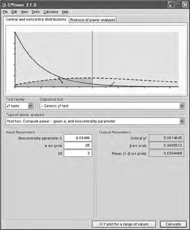
454 Answers to Selected Exercises
0.4
0.5
0.3
0.2
0.1
002
Critical χ2 = 5.99146
β
α
4681012
Y102005.indb 454 3/22/10 3:27:42 PM
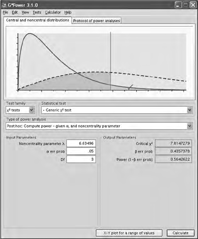
Answers to Selected Exercises 455
0.2
0.15
0.1
0.05
002
Critical χ2 = 7.81473
βα
468101214
Y102005.indb 455 3/22/10 3:27:43 PM

456 Answers to Selected Exercises
Chapter 6
1. The following LISREL–SIMPLIS program is run to analyze the
theoretical regression model for predicting gross national prod-
uct (GNP) from knowledge of labor, capital, and time:
Regression of GNP
Observed variables: GNP LABOR CAPITAL TIME
Covariance matrix:
4256.530
449.016 52.984
1535.097 139.449 1114.447
537.482 53.291 170.024 73.747
Sample size: 23
Equation: GNP = LABOR CAPITAL TIME
Number of decimals = 3
Path diagram
End of problem
Chapter 7
1. LISREL PROGRAM
Achievement path model
Observed variables: Ach Inc Abl Asp
Covariance matrix:
25.500
20.500 38.100
22.480 24.200 42.750
16.275 13.600 13.500 17.000
Sample size: 100
Relationships
Asp = Inc Abl
Ach = Inc Abl Asp
Print residuals
Options: ND = 3
Path diagram
End of problem
Partial LISREL Output
LISREL Estimates (Maximum Likelihood)
Structural Equations
Y102005.indb 456 3/22/10 3:27:43 PM

Answers to Selected Exercises 457
Ach = 0.645*Asp + 0.161*Inc + 0.231*Abl, Errorvar. = 6.507,
R² = 0.745
(0.0771) (0.0557) (0.0514) (0.934)
8.366 2.892 4.497 6.964
Asp = 0.244*Inc + 0.178*Abl, Errorvar. = 11.282, R² = 0.336
(0.0690) (0.0652) (1.620)
3.537 2.724 6.964
Covariance Matrix of Independent Variables
Inc Abl
-------- --------
Inc 38.100
(5.471)
6.964
Abl 24.200 42.750
(4.778) (6.139)
5.065 6.964
Goodness-of-Fit Statistics
Degrees of Freedom = 0
Minimum Fit Function Chi-Square = 0.00 (P = 1.000)
Normal Theory Weighted Least Squares Chi-Square = 0.00 (P =
1.000)
The model is saturated, the fit is perfect!
Chapter 8
1. The following LISREL–SIMPLIS program was written:
Confirmatory Factor Model Exercise Chapter 8
Observed Variables:
Academic Concept Aspire Degree Prestige Income
Correlation Matrix
1.000
0.487 1.000
0.236 0.206 1.000
0.242 0.179 0.253 1.000
0.163 0.090 0.125 0.481 1.000
0.064 0.040 0.025 0.106 0.136 1.000
Sample Size: 3094
Latent Variables: Motivate SES
Y102005.indb 457 3/22/10 3:27:43 PM
458 Answers to Selected Exercises
Relationships:
Academic - Aspire = Motivate
Degree - Income = SES
Print Residuals
Number of Decimals = 3
Path diagram
End of problem
Results overall suggest a less than acceptable t:
Normal Theory Weighted Least Squares Chi-Square = 114.115 (P = 0.0)
Degrees of Freedom = 8
Root Mean Square Error of Approximation (RMSEA) = 0.0655
Standardized RMR = 0.0377
Goodness-of-Fit Index (GFI) = 0.988
Consequently, the model modication indices were examined. The largest
decrease in chi-square results from adding an error covariance between
Concept and Academic (boldfaced), thus allowing us to maintain a
hypothesized two-factor model.
The Modification Indices Suggest to Add the
Path to from Decrease in Chi-Square New Estimate
Concept SES 21.9 −0.14
Aspire SES 78.0 0.21
Degree Motivate 16.1 0.31
Prestige Motivate 18.1 −0.22
The Modification Indices Suggest to Add an Error Covariance
Between and Decrease in Chi-Square New Estimate
Concept Academic 78.0 0.63
Aspire Academic 21.9 −0.12
Degree Aspire 75.3 0.13
Prestige Concept 8.9 −0.04
Income Degree 18.1 −0.10
Income Prestige 16.1 0.07
The following error covariance command line was added.
Let the errors Concept and Academic correlate
The results indicated further model modications. The largest decrease
in chi-square was determined to occur by adding an error covariance
between Income and Prestige (boldfaced in following text), thus main-
taining our hypothesized two-factor conrmatory model.
Y102005.indb 458 3/22/10 3:27:43 PM
Answers to Selected Exercises 459
The Modification Indices Suggest to Add the
Path to from Decrease in Chi-Square New Estimate
Degree Motivate 20.3 0.71
Prestige Motivate 18.4 −0.39
The Modification Indices Suggest to Add an Error Covariance
Between and Decrease in Chi-Square New Estimate
Degree Aspire 10.0 0.09
Prestige Aspire 8.3 –0.05
Income Degree 18.4 –0.10
Income Prestige 20.3 0.08
The following error covariance command line was added.
Let the errors Income and Prestige correlate
The nal results indicated a more acceptable level of t:
Normal Theory Weighted Least Squares Chi-Square = 14.519
(P = 0.0243)
Degrees of Freedom = 6
Root Mean Square Error of Approximation (RMSEA) = 0.0214
Standardized RMR = 0.0123
Goodness-of-Fit Index (GFI) = 0.998
The nal LISREL–SIMPLIS program was:
Modified Confirmatory Factor Model - Exercise Chapter 8
Observed Variables:
Academic Concept Aspire Degree Prestige Income
Correlation Matrix
1.000
0.487 1.000
0.236 0.206 1.000
0.242 0.179 0.253 1.000
0.163 0.090 0.125 0.481 1.000
0.064 0.040 0.025 0.106 0.136 1.000
Sample Size: 3094
Latent Variables: Motivate SES
Relationships:
Academic: Aspire = Motivate
Degree: Income = SES
Let the errors concept and Academic correlate
Let the errors Income and Prestige correlate
Print residuals
Number of decimals = 3
Path diagram
End of problem
Y102005.indb 459 3/22/10 3:27:43 PM
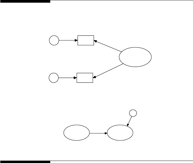
460 Answers to Selected Exercises
Chapter 9
1. Diagram two indicator variables X1 and X2 of a latent variable LV.
e_1
e_2
X1
X2
LV
3. Diagram a latent independent variable LIV predicting a latent
dependent variable LDV.
LDV
LIV
e
Chapter 10
1. The following LISREL–SIMPLIS program was written:
Chapter 10 Exercise
Observed variables: ACT CGPA ENTRY SALARY PROMO
Covariance matrix:
1.024
.792 1.077
.567 .537 .852
.445 .424 .518 .670
.434 .389 .475 .545 .716
Sample size: 500
Latent variables: ACAD JOB
Relationships:
ACT = 1*ACAD
CGPA = ACAD
ENTRY = ACAD
SALARY = 1*JOB
PROMO = JOB
JOB = ACAD
Path diagram
End of problem
Y102005.indb 460 3/22/10 3:27:44 PM
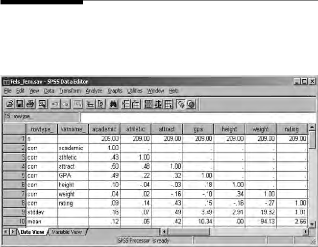
Answers to Selected Exercises 461
The chi-square is statistically signicant (c2 = 116.29, df = 4, p = .000), so the
modication indices are checked and it is suggested to add an error cova-
riance between the measurement error variances of CGPA and ACT.
The Modification Indices Suggest Adding an Error Covariance
Between and Decrease in Chi-Square New Estimate
ACT SALARY 14.0 –0.06
CGPA ACT 113.5 0.43
ENTRY SALARY 40.8 0.10
ENTRY ACT 24.9 –0.15
ENTRY CGPA 23.9 –0.14
The following command line was added:
Let the error covariances between CGPA and ACT correlate
The modied model is acceptable (c2 = 3.04, df = 3, p = .39; RMSEA = .005;
GFI = 1.0). JOB is statistically signicantly predicted, R2 = .70, by the fol-
lowing structural equation:
Structural Equations
JOB = 0.91*ACAD, Errorvar.= 0.18 , R² = 0.70
(0.061) (0.027)
15.01 6.59
Chapter 11
1. SPSS and EXCEL matrix input.
SPSS Matrix Input Example
Y102005.indb 461 3/22/10 3:27:44 PM
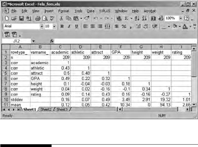
462 Answers to Selected Exercises
Microsoft Excel Matrix Input Example
Chapter 12
1. Multiple Samples
LISREL–SIMPLIS Program (EX11B.SPL)
Sample 1: Parental Socioeconomic Characteristics
Observed Variables: SOFED SOMED SOFOC FAFED MOMED FAFOC
Covariance Matrix
5.86
3.12 3.32
35.28 23.85 622.09
4.02 2.14 29.42 5.33
2.99 2.55 19.20 3.17 4.64
35.30 26.91 465.62 31.22 23.38 546.01
Sample Size: 80
Latent Variables: Fed Med Foc
SOFED = Fed
SOMED = Med
SOFOC = Foc
FAFED = 1*Fed
MOMED = 1*Med
FAFOC = 1*Foc
Set the Error Covariance between SOMED and SOFED free
Y102005.indb 462 3/22/10 3:27:45 PM
Answers to Selected Exercises 463
Sample 2: Parental Socioeconomic Characteristics
Covariance Matrix
8.20
3.47 4.36
45.65 22.58 611.63
6.39 3.16 44.62 7.32
3.22 3.77 23.47 3.33 4.02
45.58 22.01 548.00 40.99 21.43 585.14
SOFED = Fed
SOMED = Med
SOFOC = Foc
Let the Error Variances of SOFED - SOFOC be free
Set the Error Covariance between SOMED and SOFED free
Sample 3: Parental Socioeconomic Characteristics
Covariance Matrix
5.74
1.35 2.49
39.24 12.73 535.30
4.94 1.65 37.36 5.39
1.67 2.32 15.71 1.85 3.06
40.11 12.94 496.86 38.09 14.91 538.76
SOFED = Fed
SOMED = Med
SOFOC = Foc
Let the Error Variances of SOFED - SOFOC be free
Set the Error Covariance between SOMED and SOFED equal to 0
Path diagram
End of problem
Global Goodness-of-Fit Statistics
Degrees of Freedom = 34
Minimum Fit Function Chi-Square = 52.73 (P = 0.021)
Root Mean Square Error of Approximation (RMSEA) = 0.077
90 Percent Confidence Interval for RMSEA = (0.019; 0.12)
P-Value for Test of Close Fit (RMSEA < 0.05) = 0.00038
Normed Fit Index (NFI) = 0.96
Comparative Fit Index (CFI) = 0.99
Critical N (CN) = 252.98
Y102005.indb 463 3/22/10 3:27:45 PM

464 Answers to Selected Exercises
Chapter 13
1. Multiple Sample Model
The two semesters of data did not have means and standard deviations
on the measures for the regression model, so no means and standard
deviations would be included in the multiple sample LISREL–SIMPLIS
program. (Note: Although two samples are used, we still use the GROUP
command.) The LISREL–SIMPLIS program is:
Predicting Clinical Competence in Nursing
Group 1: Semester 1
Observed variables comp effort learn
Sample size: 250
Correlation matrix
1.0
.25 1.0
.28 .23 1.0
Equation
comp = effort learn
Group 2: Semester 2
Observed variables comp effort learn
Sample size: 205
Correlation matrix
1.0
.21 1.0
.16 .15 1.0
Path diagram
End of problem
Computer Output—Multiple Sample Model
The regression model output indicated a nonsignicant chi-square (chi-
square = 1.55, df = 3, p = .67), which implies that the two semesters of sam-
ple data had similar regression coefcients. We nd that the regression
coefcient of effort predicting comp is .20 compared to .25 and .21, respec-
tively, in the two samples. We also nd that the regression coefcient of
learn predicting comp is .19 compared to .28 and .16, respectively, in the
two samples. The correlation between effort and learn is .23 in the com-
mon regression model, compared to .23 and .15, respectively, in the two
samples of data. Finally, we see that the R-squared for the common regres-
sion model is .19 (1-R-squared = .91). The computer output (not shown)
Y102005.indb 464 3/22/10 3:27:45 PM
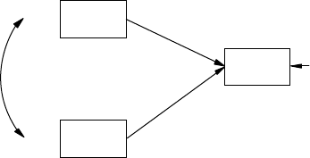
Answers to Selected Exercises 465
indicated R-squared = .09 and .085, respectively, for the two regression
equations from the two samples of data.
effort
learn
comp 0.91
Chi-Square = 1.55, df = 3, P-value = 0.67
0.20
0.19
0.23
3. Structured Means Model
The two stacked LISREL–PRELIS programs are:
Group Low Motivation
Observed Variables: Prod1 Prod2 Prod3 Prod4 Prod5 Prod6
Correlation Matrix
1.00
.64 1.00
.78 .73 1.00
.68 .63 .69 1.00
.43 .55 .50 .59 1.00
.65 .63 .67 .81 .60 1.00
Means 4.27 5.02 4.48 4.69 4.53 4.66
Sample Size: 300
Latent Variables: City1 City2
Relationships:
Prod1 = CONST + 1*City1
Prod2 = CONST + City1
Prod3 = CONST + City1
Prod4 = CONST + 1*City2
Prod5 = CONST + City2
Prod6 = CONST + City2
Group High Motivation:
Correlation Matrix
1.00
.72 1.00
.76 .74 1.00
.51 .46 .57 1.00
.32 .33 .39 .40 1.00
.54 .45 .60 .73 .45 1.00
Means 14.35 14.93 14.59 14.86 14.71 14.74
Y102005.indb 465 3/22/10 3:27:45 PM
466 Answers to Selected Exercises
Sample size: 300
Relationships:
City1 = CONST
City2 = CONST
Path diagram
End of problem
The rst thing you should check is the individual group and combined
group model-t statistics. They were:
Group Goodness-of-Fit Statistics: Low Motivation
Contribution to Chi-Square = 52.92
Root Mean Square Residual (RMR) = 0.11
Goodness-of-Fit Index (GFI) = 0.94
Group Goodness-of-Fit Statistics: High Motivation
Contribution to Chi-Square = 52.06
Root Mean Square Residual (RMR) = 0.13
Goodness-of-Fit Index (GFI) = 0.94
Global Goodness-of-Fit Statistics
Degrees of Freedom = 24
Minimum Fit Function Chi-Square = 104.98 (P = 0.00)
Root Mean Square Error of Approximation (RMSEA) = 0.11
90% Condence Interval for RMSEA = (0.089; 0.13)
P-Value for Test of Close Fit (RMSEA < 0.05) = 0.00
Comparative Fit Index (CFI) = 0.97
These values are adequate, but modication indices were indicated and
are suggested to yield a better model t before proceeding with a test of
latent variable mean differences.
The following command lines should be added to the LISREL–
SIMPLIS program to allow observed variable error variance to be
estimated, estimate latent variable variance, and allow the two latent
variables to correlate:
Set the Error Variances of Prod1 - Prod6 free
Set the Variances of City1 - City2 free
Set the Covariance between City1 and City2 free
Y102005.indb 466 3/22/10 3:27:46 PM
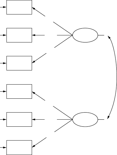
Answers to Selected Exercises 467
The nal Structured Means Model with parameter estimates is:
Prod10.28
Prod20.34
Prod30.20
0.83 City1
0.86
0.89
Prod40.21
Prod50.43
Prod60.23
0.71 City2
0.85
0.90
0.85
The Structured Means Model is testing the mean latent variable dif-
ference, which is indicated by the Mean Vector of Independent Variables.
Results are interpreted based on the knowledge that the mean latent
value on City1 (Los Angeles) and City2 (Chicago) are set to zero (0) in
the rst group (low motivation), so the values reported here are going to
indicate that the second group (high motivation) was either greater than
(positive) or less than (negative) the rst group (low motivation) on the
latent variables.
A latent variable mean difference value of 10.08 is indicated for the rst
latent variable (City1), which indicates a statistically signicant mean dif-
ference (i.e., high motivation group) had mean production rates greater
than the low motivation group in Los Angeles (City1).
A latent variable mean difference value of 10.18 is indicated for the sec-
ond latent variable (City2), which indicates a statistically signicant mean
difference (i.e., high motivation group) had mean production rates greater
than the low motivation group in Chicago (City2).
Overall, the high motivation groups outperformed the low motivation
groups in both cities. City1 and City2 correlated .90, indicating similar
Y102005.indb 467 3/22/10 3:27:46 PM

468 Answers to Selected Exercises
mean difference production rates. The latent variable mean differences
are divided by their standard error to yield a one-sample T value (i.e.,
10.08/.08 = 122.17, within rounding error).
Mean Vector of Independent Variables
City1 City2
-------- --------
10.08 10.18
(0.08) (0.08)
122.17 128.16
Chapter 14
1. Second-Order Factor Analysis
The psychological research literature suggests that drug use and depres-
sion are leading indicators of suicide among teenagers. The following
LISREL–SIMPLIS program was run to test a second-order factor model.
Second Order Factor Analysis Exercise
Observed Variables: drug1 drug2 drug3 drug4 depress1
depress2 depress3 depress4
Sample Size 200
Correlation Matrix
1.000
0.628 1.000
0.623 0.646 1.000
0.542 0.656 0.626 1.000
0.496 0.557 0.579 0.640 1.000
0.374 0.392 0.425 0.451 0.590 1.000
0.406 0.439 0.446 0.444 0.668 .488 1.000
0.489 0.510 0.522 0.467 0.643 .591 .612 1.000
Means 1.879 1.696 1.797 2.198 2.043 1.029 1.947 2.024
Standard Deviations 1.379 1.314 1.288 1.388 1.405 1.269
1.435 1.423
Latent Variables: drugs depress suicide
Relationships
drug1 - drug4 = drugs
depress1 - depress4 = depress
drugs = Suicide
depress = Suicide
Set variance of drugs - Suicide to 1.0
Path diagram
End of problem
Y102005.indb 468 3/22/10 3:27:46 PM
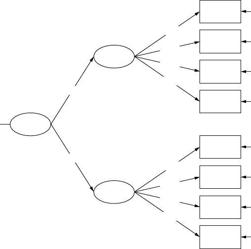
Answers to Selected Exercises 469
The second-order factor model with standardized coefcients had an
acceptable t (Chi-square = 30.85, df = 19, p = .042) and is diagrammed as:
drug1
drug2
drug3
drug4
0.34
0.45
0.35
0.38
drugs
Suicide
depress
0.74
0.82
0.81
0.79
0.98
0.82
1.00
depress1
depress2
depress3
depress4
0.53
0.25
0.44
0.39
0.87
0.69
0.75
0.78
The structure coefcients indicate that the rst factors are strong indi-
cators of the second factor (suicide). Drug use (R-squared = .96) was the
stronger indicator of suicide among teenagers.
Structural Equations
drugs = 0.98*Suicide, Errorvar. = 0.044, R² = 0.96
(0.17)
0.26
depress = 0.82*Suicide, Errorvar. = 0.33, R² = 0.67
(0.12) (0.13)
6.96 2.51
NOTE: Missing t-values and standard errors in SIMPLIS output.
Second-Order Factor Analysis—Suicide example.
Since the ETA variables (drugs and depress) are indicators of the corre-
sponding KSI variable (suicide), LISREL by default xes the loading of the
Y102005.indb 469 3/22/10 3:27:47 PM
470 Answers to Selected Exercises
rst indicator to one. Then, after convergence the value of 1 is rescaled
using the estimated ETA1 variance. Although the corresponding standard
error estimate can be computed using the Delta method, LISREL does not
compute it. As a result, no standard error estimate and t value is written to
the output le. The LISREL 8 syntax program with a raw data le should
produce the standard errors and t-value.
3. MULTITRAIT–MULTIMETHOD MODELS
a. The LISREL–SIMPLIS program to analyze the three methods
(student, teacher, and peer) and three traits (behavior, moti-
vate, and attitude) as a MTMM model using start values and
admissibility check off (increase iterations to achieve conver-
gence) is:
MTMM Model Exercise
Observed Variables: X1 X2 X3 X4 X5 X6 X7 X8 X9
Correlation Matrix
1.0
.40 1.0
.31 .38 1.0
.35 .23 .16 1.0
.26 .22 .21 .62 1.0
.15 .11 .15 .49 .62 1.0
.43 .31 .24 .61 .48 .33 1.0
.40 .35 .19 .49 .45 .32 .74 1.0
.26 .20 .18 .43 .41 .33 .52 .47 1.0
Sample Size: 300
Latent Variables: behavior motivate attitude student
teacher peer
Relationships:
X1 = (.3)*behavior + (.5)*student
X2 = (.3)*motivate + (.5)*student
X3 = (.3)*attitude + (.5)*student
X4 = (.3)*behavior + (.5)*teacher
X5 = (.3)*motivate + (.5)*teacher
X6 = (.3)*attitude + (.5)*teacher
X7 = (.3)*behavior + (.5)*peer
X8 = (.3)*motivate + (.5)*peer
X9 = (.3)*attitude + (.5)*peer
Set variance of behavior - peer to 1.0
Set correlation of student and behavior to 0
Set correlation of student and motivate to 0
Set correlation of student and attitude to 0
Set correlation of teacher and behavior to 0
Set correlation of teacher and motivate to 0
Y102005.indb 470 3/22/10 3:27:47 PM
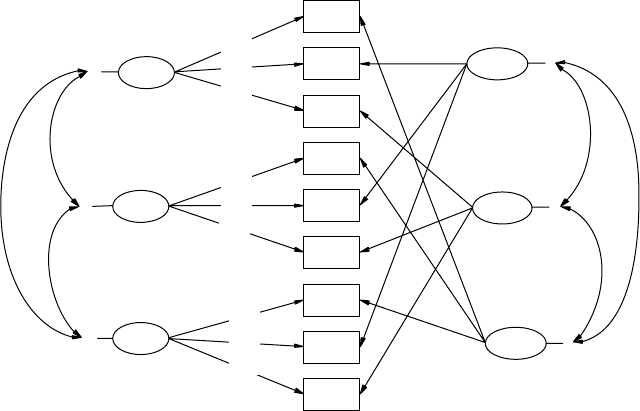
Answers to Selected Exercises 471
Set correlation of teacher and attitude to 0
Set correlation of peer and behavior to 0
Set correlation of peer and motivate to 0
Set correlation of peer and attitude to 0
Options: AD = FF
Path diagram
End of problem
The MTMM model is displayed after dragging the three methods to the
left side of the diagram in the LISREL graph. The MTMM model had
acceptable t indices (Chi-square = 10.85, df = 12, and p = .54).
X1
X2
X3
X4
X5
X6
X7
X8
X9
behavior
motivate
attitude
student
teacher
peer
Chi-Square = 10.85, df = 12, P-value = 0.54203, RMSEA = 0.000
0.51 –0.28
0.60
0.59
0.69
–0.12
0.85
0.74
0.65
0.62
0.60
0.79
1.18
0.80
0.39
0.48
0.74
–0.65
–0.18
–0.42
0.04
–0.65
–0.06
–0.41
The MTMM model results are displayed in Table C.1 to help the inter-
pretation of trait and method effects. The assessment of Attitude regard-
less of which method was used had the higher error variance; Student
ratings (error = .64), Teacher ratings (error = .46), or Peer ratings (error =
.61), thus Attitude was the most difcult trait to assess, based on the three
methods used. The student and teacher rating methods were higher for
motivate (factor loading = .60 and factor loading = .85, respectively). The
peer rating method worked best with behavior, but was fairly similar
across all traits.
Y102005.indb 471 3/22/10 3:27:47 PM

472 Answers to Selected Exercises
b. The LISREL–SIMPLIS program to run a Correlated Traits–
Correlated Uniqueness Model (CTCU) is:
Correlated Traits–Correlated Uniqueness Model Exercise
Observed Variables: X1 X2 X3 X4 X5 X6 X7 X8 X9
Correlation Matrix
1.0
.40 1.0
.31 .38 1.0
.35 .23 .16 1.0
.26 .22 .21 .62 1.0
.15 .11 .15 .49 .62 1.0
.43 .31 .24 .61 .48 .33 1.0
.40 .35 .19 .49 .45 .32 .74 1.0
.26 .20 .18 .43 .41 .33 .52 .47 1.0
Sample Size: 240
Latent Variables: behavior motivate attitude
Relationships:
X1 = behavior
X2 = motivate
X3 = attitude
X4 = behavior
X5 = motivate
X6 = attitude
X7 = behavior
X8 = motivate
X9 = attitude
Set variance of behavior - attitude to 1.0
Let error covariance of X1–X3 correlate
TABLE C.1
MTMM Estimates of Three Methods on Three Traits (N = 300)
Traits Methods
Behavior Motivate Attitude Student Teacher Peer Error
Behavior −.41 .51 .57
Motivate –.28 .60 .56
Attitude –.06 .59 .64
Behavior –.41 .68 .35
Motivate –.12 .85 .27
Attitude .04 .74 .46
Behavior –.65 .65 .15
Motivate –.65 .62 .19
Attitude –.18 .60 .61
Y102005.indb 472 3/22/10 3:27:48 PM
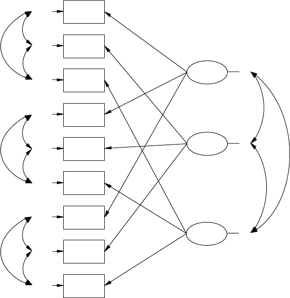
Answers to Selected Exercises 473
Let error covariance of X4–X6 correlate
Let error covariance of X7–X9 correlate
Path diagram
End of problem
The CTCU model is diagrammed as:
X1
0.76
X2
0.85
X3
0.92
X4
0.51
X5
0.65
X6
0.80
X7
0.23
X8
0.37
X9
0.51
behavior
motivate
attitude
0.29
0.60
0.88
0.92
0.85
0.91
0.23
0.19
0.28
0.24
0.23
0.38
0.10
–0.00
–0.04
0.79
0.39
The results are presented in Table C.2. Findings indicated that all three
traits were statistically signicantly correlated. More importantly, the peer
method was the best for assessing any of the three traits, as indicated
by the higher trait factor loadings and lower correlated uniqueness error
terms. Students are probably not rating themselves well and teachers
seemed a little better at rating student behavior and motivation than atti-
tude. The data also had an acceptable t to the CTCU model (c2 = 13.43, p =
.57, df = 15; RMSEA = .000; n = 300).
Y102005.indb 473 3/22/10 3:27:48 PM

474 Answers to Selected Exercises
The LISREL Program was run again to estimate a correlated trait (CT)
only model with no correlated error terms. To accomplish this, you simply
delete the following command lines:
Let Error Covariance of Var1–Var3 Correlate
Let Error Covariance of Var4–Var6 Correlate
Let Error Covariance of Var7–Var9 Correlate
The results yielded a nonpositive denite matrix among the latent vari-
ables (i.e., correlations were greater than 1.0.) Also, the modication indi-
ces suggested adding the very error covariance you deleted. So, the CT
Model is rejected in favor of the CTCU Model.
behavior motivate attitude
behavior 1.00
motivate 1.07 1.00
attitude 0.95 1.10 1.00
W_A_R_N_I_N_G: is not positive definite
TABLE C.2
Correlated Uniqueness Model with Correlated Traits and Errors
Method Trait
Factor
Loading Uniqueness R2
Correlated Uniqueness of
Error Terms
Student Behavior .49 .76 .24 1.0
Motivate .39 .85 .15 .23 1.0
Attitude .29 .92 .08 .19 .28 1.0
Teacher Behavior .70 .51 .49 1.0
Motivate .60 .65 .35 .24 1.0
Attitude .45 .80 .20 .23 .38 1.0
Peer Behavior .88 .23 .77 1.0
Motivate .79 .37 .63 .10 1.0
Attitude .70 .51 .49 .00 –.04 1.0
Trait correlations
Behavior 1.0
Motivate .92 1.0
Attitude .85 .91 1.0
Note: C2 = 13.43, p = .57, df = 15; RMSEA = .000; n = 300.
Y102005.indb 474 3/22/10 3:27:48 PM

Answers to Selected Exercises 475
The Modification Indices Suggest to Add an Error Covariance
Between and Decrease in Chi-Square New Estimate
X2 X1 19.8 0.22
X3 X1 12.6 0.17
X3 X2 25.0 0.26
X5 X4 22.3 0.18
X6 X4 17.3 0.16
X6 X5 64.2 0.34
X7 X5 32.9 –0.22
X7 X6 20.5 –0.16
X8 X4 23.6 –0.18
X8 X6 11.2 –0.14
X8 X7 49.7 0.27
Although the MTMM model achieved an acceptable model t, the nd-
ings were mixed as to which method worked best with the three traits
(behavior, motivate, and attitude). The CTCU model in contrast more
clearly indicated that peers did a better job of rating the traits. Students
tend to know other students more on these traits both in and outside the
classroom, thus providing a theoretical argument for the ndings.
Chapter 15
1. Multiple Indicator and Multiple Cause Model
The following LISREL–SIMPLIS program would be created and run to
determine the parameter estimates and model t.
MIMIC Model of Job Satisfaction
Observed Variables peer self income shift age
Sample Size 530
Correlation Matrix
1.00
.42 1.00
.24 .35 1.00
.13 .37 .25 1.00
.33 .51 .66 .20 1.00
Latent Variable satisfac
Relationships
peer = satisfac
self = satisfac
satisfac = income shift age
Path diagram
End of problem
Y102005.indb 475 3/22/10 3:27:49 PM
476 Answers to Selected Exercises
Initial MIMIC Model Results
The MIMIC model results indicated an adequate t with chi-square = 6.81,
df = 2, and p = .033. The measurement equations indicated that job satis-
faction (satisfac) was adequately dened with self ratings being a better
indicator of job satisfaction than peer ratings.
Measurement Equations
peer = 0.48*satisfac, Errorvar. = 0.77, R² = 0.23
(0.053)
14.49
self = 0.87*satisfac, Errorvar. = 0.25 , R² = 0.75
(0.11) (0.078)
8.10 3.16
The structural equation indicated that 45% of job satisfaction was pre-
dicted by knowledge of income, what shift a person worked, and their
age. However, the coefcient for income was not statistically signicant
(T = −.59). Consequently the model should be modied by dropping this
variable and re-running the analysis.
Structural Equations
satisfac = – 0.032*income + 0.31*shift + 0.56*age, Errorvar.= 0.55, R² = 0.45
(0.054) (0.054) (0.082) (0.11)
–0.59 5.71 6.77 5.14
MIMIC Modification
The MIMIC model modication resulted in little improvement with chi-
square = 6.11, df = 1, and p = .01. The measurement equations were not very
different. Other measures would help to dene the latent variable, job satis-
faction. The structural equation resulted in the same R-squared value, which
indicates that income did not add to the prediction of job satisfaction. A parsi-
monious model was therefore achieved, but the 55% unexplained variance
implies that other variables could be discovered to increase prediction.
Measurement Equations
peer = 0.49*satisfac, Errorvar. = 0.76, R² = 0.24
(0.053)
14.48
self = 0.87*satisfac, Errorvar. = 0.25, R² = 0.75
(0.11) (0.078)
8.12 3.21
Y102005.indb 476 3/22/10 3:27:49 PM
Answers to Selected Exercises 477
Structural Equations
satisfac = 0.31*shift + 0.54*age, Errorvar.= 0.55 , R² = 0.45
(0.053) (0.073) (0.11)
5.72 7.39 5.14
3. Multilevel Model
The multilevel analysis of data in the PRELIS system le, income.psf, was
used with the pull down multilevel menu to create and run 3 different
PRELIS programs. Results are summarized in a table with the intra-class
correlation (hand computed) for comparative purposes.
Model 1 is the baseline model (constant), followed by the added effects
of gender, and the added effects of marital status (marital). The 3 different
PRELIS programs should look as follows:
Model 1 (intercept only)
OPTIONS OLS=YES CONVERGE=0.001000 MAXITER=10 OUTPUT=STANDARD ;
TITLE=income decomposition;
SY=’C:\LISREL 8.8 Student Examples\MLEVELEX\INCOME.PSF’;
ID3=region;
ID2=state;
RESPONSE=income;
FIXED=constant;
RANDOM2=constant;
RANDOM3=constant;
Model 2 (intercept + gender)
OPTIONS OLS=YES CONVERGE=0.001000 MAXITER=10 OUTPUT=STANDARD ;
TITLE=income decomposition;
SY=’C:\LISREL 8.8 Student Examples\MLEVELEX\INCOME.PSF’;
ID3=region;
ID2=state;
RESPONSE=income;
FIXED=constant gender;
RANDOM2=constant;
RANDOM3=constant;
Model 3 (intercept + gender + marital)
OPTIONS OLS=YES CONVERGE=0.001000 MAXITER=10 OUTPUT=STANDARD ;
TITLE=income decomposition;
SY=’C:\LISREL 8.8 Student Examples\MLEVELEX\INCOME.PSF’;
ID3=region;
Y102005.indb 477 3/22/10 3:27:49 PM

478 Answers to Selected Exercises
ID2=state;
RESPONSE=income;
FIXED=constant gender marital;
RANDOM2=constant;
RANDOM3=constant;
The PRELIS program results for the three analyses are summarized in
Table C.1. The baseline model (intercept only) provides the initial break-
down of level 3 and level 2 error variance. The multilevel model for the
added effect of gender is run next. The chi-square difference between Model
1 and Model 2 yields chi-square = 5.40, which is statistically signicant at
the .05 level of signicance. Gender, therefore, does help explain variability
in income. Finally, marital is added to the multilevel model, which yields a
chi-square difference between Model 2 and Model 3 of chi-square = 1.18.
The chi-square difference value is not statistically signicant; therefore,
marital status does not add any additional signicant explanation of vari-
ability in income.
TABLE C.3
Summary Results for Multilevel Analysis of Income
Multilevel Model
Fixed Factors
Model 1
Constant
Model 2 Constant +
Gender
Model 3 Constant +
Gender + Marital
Intercept Only(B0) 10.096 (.099) 10.37 (.15) 10.24 (.19)
Gender (B1) –0.42 (.16) –0.43 (.16)
Marital (B2) .19 (.17)
Level 2 error
variance (eij)
.37 .31 .30
Level 3 error
variance (uij)
.02 .05 .06
ICC .051 (5%) .138 (14%) .166 (17%)
Deviance (–2LL) 11144.29 11138.89 11137.71
Df 3 4 5
χ2 Difference (df = 1) 5.40 1.18
Note: χ2 = 3.84, df = 1, p = .05.
Note: ICC1 =
Φ
ΦΦ
3
32
3
3+=−−
−−+
TauHat Level
TauHat LevelTa
()
()uuHat Level−−
=+=
()
.
.. .
2
02
02 37 051
Y102005.indb 478 3/22/10 3:27:49 PM
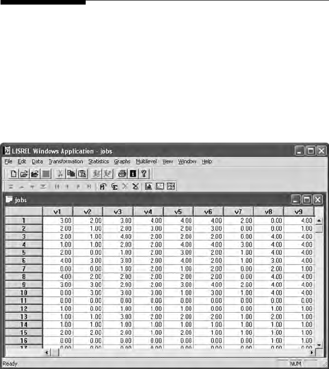
Answers to Selected Exercises 479
Chapter 16
1. Interaction Model
An organizational psychologist was investigating whether work tension
and collegiality were predictors of job satisfaction. However, research indi-
cated that work tension and collegiality interact, so a SEM Interaction Model
was hypothesized and tested. [Note: You need to use a raw data le so that
values for latent variables can be added.]
First open the PRELIS system le, jobs.psf, to view the 9 observed variables.
Second, create the LISREL–SIMPLIS program to create and save the
latent variables in the PRELIS system le, jobs.psf:
Computing Latent Variable Scores
Observed Variables v1-v9
Raw Data from File jobs.psf
Latent Variables : job work colleg
Relationships:
v1=1*job
v2-v3= job
v4=1*work
v5-v6=work
v7=1*colleg
Y102005.indb 479 3/22/10 3:27:50 PM
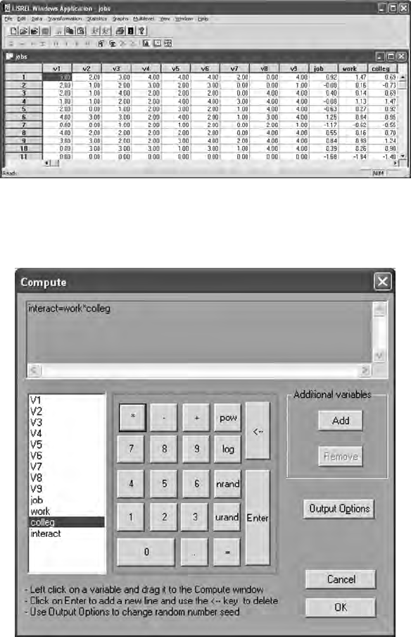
480 Answers to Selected Exercises
v8-v9=colleg
PSFfile jobs.psf
End of problem
NOTE: Remember to close the PRELIS system le, jobs.psf, and then open it
again to see that the latent variables have been added.
Third, create the latent interaction variable by using the
TRANSFORMATION, then COMPUTE on the pull down menu. Select
ADD, enter name for new variable (interact), then drag variable names to
the Compute window (interact=work*colleg).
Y102005.indb 480 3/22/10 3:27:50 PM
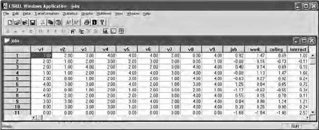
Answers to Selected Exercises 481
Click OK, and the latent interaction variable, interact, will automatically
be added to the PRELIS system le, jobs.psf.
Finally, create and run a LISREL–SIMPLIS program to analyze the
Interaction Model.
Latent Interaction Variable Model - No Intercept Term
Observed Variables: v1-v9 job work colleg interact
Raw Data from File jobs.psf
Sample Size = 200
Relationships:
job = work colleg interact
Path diagram
End of problem
The structural equation indicates that no interaction effect is present
between work tension and collegiality. Rather, work tension and collegiality
are predictors of job satisfaction as direct linear effects.
Structural Equations
job = 0.98*work – 0.18*colleg + 0.036*interact, Errorvar.= 0.22 , R² = 0.80
(0.065) (0.079) (0.038) (0.022)
15.16 –2.29 0.96 9.90
The latent interaction variable should be dropped and the LISREL–SIMPLIS
program run again. The R-squared value does not change indicating that the
interaction effect did not contribute to the prediction of job satisfaction.
Structural Equations
job = 0.97*work – 0.17*colleg, Errorvar. = 0.22 , R² = 0.80
(0.064) (0.078) (0.022)
15.20 –2.17 9.92
Y102005.indb 481 3/22/10 3:27:51 PM
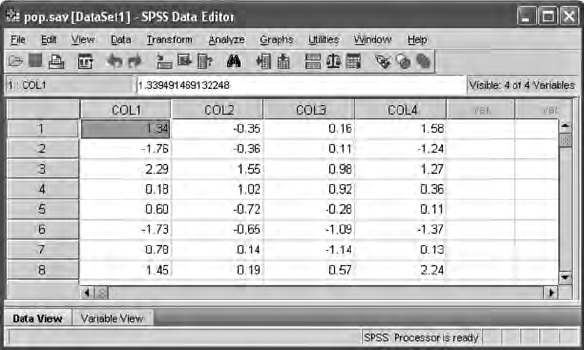
482 Answers to Selected Exercises
3. MONTE CARLO Methods
The SPSS program would input the population matrix values as follows:
MATRIX.
compute popr =
{1, .50, .30, .90;
.50, 1, .70, .50;
.30, .70, 1, .50;
.90, .50, .50, 1}.
Print popr.
compute pi = 3.14159.
compute rown = nrow(popr).
compute n = 10000.
compute corr = sqrt(–2*ln(uniform(n,rown)))&*cos((2*pi)*uniform(n,rown)).
compute corr=corr*chol(popr).
save corr /outle = pop.sav.
END MATRIX.
The SPSS output would look like this:
Run MATRIX procedure:
POPR
1.000000000 .500000000 .300000000 .900000000
.500000000 1.000000000 .700000000 .500000000
.300000000 .700000000 1.000000000 .500000000
.900000000 .500000000 .500000000 1.000000000
------ END MATRIX -----
You would now open the pop.sav le which would look like the following
(Note: Our pop.sav le was in c:\program les\spssinc\spss16 folder).
Y102005.indb 482 3/22/10 3:27:51 PM

Answers to Selected Exercises 483
The SPSS correlation procedure was selected and ran:
The output from the SPSS correlation procedure yielded population corre-
lation values in Table C.4 similar to what we specied in the SPSS MATRIX
program.
TABLE C.4
Correlations
COL1 COL2 COL3 COL4
COL1 Pearson Correlation 1.000 .489** .287** .899**
Sig. (1-tailed) .000 .000 .000
N 10000.000 10000 10000 10000
COL2 Pearson Correlation .489** 1.000 .696** .488**
Sig. (1-tailed) .000 .000 .000
N 10000 10000.000 10000 10000
COL3 Pearson Correlation .287** .696** 1.000 .491**
Sig. (1-tailed) .000 .000 .000
N 10000 10000 10000.000 10000
COL4 Pearson Correlation .899** .488** .491** 1.000
Sig. (1-tailed) .000 .000 .000
N 10000 10000 10000 10000.000
** Correlation is signicant at the 0.01 level (1-tailed).
Y102005.indb 483 3/22/10 3:27:51 PM
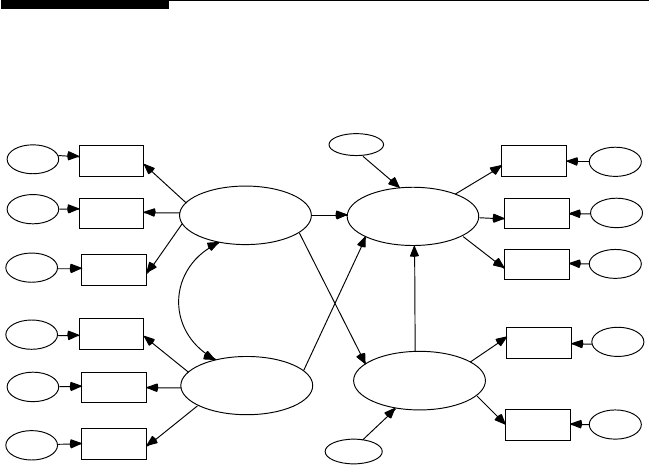
484 Answers to Selected Exercises
Chapter 17
1. The diagrammed structural equation model is shown as
Figure 17.4.
Family
Encourag
Student
Aspire
err_13
err_12
Income
FAED
MOED
Personal
School
Cognate
Self
Motivate
Admit
Occup
Educ
err_7
err_8
err_9
err_10
err_11
err_1
err_2
err_3
err_4
err_5
err_6
FIGURE 17.4
Student characteristic model.
The measurement equations are as follows:
For the X variables using variable names
family income = function of Family Background + error
father’s education = function of Family Background + error
mother’s education = function of Family Background + error
personal encouragement = function of Encouragement + error
institutional characteristics = function of Encouragement + error
admission status = function of Encouragement + error.
The measurement equations for the Xs are
X1 = 1.0 x1 + d1
X2 = lx21 x1 + d2
X3 = lx31 x1 + d3
X4 = 1.0 x2 + d4
Y102005.indb 484 3/22/10 3:27:52 PM
Answers to Selected Exercises 485
X5 = lx52 x2 + d5
X6 = lx62 x2 + d6.
The matrix equations for the Xs are
X
X
X
X
X
X
x
x
1
2
3
4
5
6
21
3
10
0
=
λ
λ
11
52
62
1
1
0
01
0
0
λ
λ
ξ
ξ
x
x
+
δ
δ
δ
δ
δ
δ
1
2
3
4
5
6
For the Y variables using variable names:
cognitive abilities = function of Student Characteristics + error
interpersonal skills = function of Student Characteristics + error
motivation = function of Student Characteristics + error
occupational aspirations = function of Aspiration + error
educational aspirations = function of Aspiration + error.
The measurement equations for the Ys are
Y1 = 1.0 h1 + e1
Y2 = ly21 h1 + e2
Y3 = ly31 h1 + e3
Y4 = 1.0 h2 + e4
Y5 = ly52 h2 + e5.
The matrix equations for the Ys are
Y
Y
Y
Y
Y
Y
y
1
2
3
4
5
6
21
10
0
=
λ
λ
yy
y
y
31
52
62
1
0
01
0
0
λ
λ
η
η
+
11
1
2
3
4
5
6
ε
ε
ε
ε
ε
ε
The structural equations using variable names are
Students’ Characteristics = Family Background + Encouragement + Aspirations + error
Aspirations = Family Background + Encouragement + error.
Y102005.indb 485 3/22/10 3:27:53 PM
486 Answers to Selected Exercises
The structural equations are written as
ηβηγξγξζ
ηγξγξζ
1122 11 1122 1
2211 22 22
=+++
=++.
In matrix form the structural equations are
η
η
βη
η
γγ
γ
1
2
12 1
2
11 12
0
00
=
+
221 22
1
2
1
2
γ
ξ
ξ
ξ
ξ
+
The matrix of the structural coefcients for the endogenous variables is
B=
0
00
12
β
The matrix of the structural coefcients for the exogenous variables is
Γ=
γγ
γγ
11 12
21 22
The matrix of the factor loadings for the endogenous variables is
Λy
y
y
y
=
10
0
0
01
0
21
31
52
λ
λ
λ
The matrix of the factor loadings for the exogenous variables is
Λx
x
x
x
x
=
10
0
0
01
0
0
21
31
52
62
λ
λ
λ
λ
The covariance matrix for the exogenous latent variables is
Φ=
φ
φφ
11
21 22
Y102005.indb 486 3/22/10 3:27:54 PM
Answers to Selected Exercises 487
The covariance matrix for the equation errors is
ψψ
ψ
=
11
22
0
The covariance matrix for the measurement errors of the indicators of the
exogenous latent variables is
Θ
δ
δ
δ
δ
δ
δ
δ
θ
θ
θ
θ
θ
θ
=
11
22
33
44
55
66
0
00
000
0000
00000
The covariance matrix for the measurement errors of the indicators of the
endogenous latent variables is
Θ
ε
ε
ε
ε
ε
ε
θ
θ
θ
θ
θ
=
11
22
33
44
55
0
00
000
0000
The structural equation model can be interpreted from the direct and
indirect effects to yield the total effects for the model. The direct effects
for Aspirations are Family Background (g21) and Encouragement (g22).
The direct effects for Students’ Characteristics are Family Background
(g11), Encouragement (g12), and Aspirations (b12). The indirect effects for
Students’ Characteristics is Family Background through Aspirations (g21 b12).
Thus, the total effects are as follows:
Family Background -> Aspirations = g21
Encouragement -> Aspirations = g22
Family Background -> Students’ Characteristics = g11 + (g21) (b12)
Encouragement -> Students’ Characteristics = g12
Aspirations -> Students’ Characteristics = b12.
Y102005.indb 487 3/22/10 3:27:55 PM

489
Author Index
A
Aalberts, C., 286, 292
Acock, A. C., 342, 370
Adamson, G., 290
Aiken, L. S., 341, 369
Akaike, H., 90, 120
Algina, J., 33, 52, 277, 291, 341, 369, 370
Alstine, J. V., 91, 122, 193
American Psychological Association,
209, 220
Anderson, C., 39, 51
Anderson, J. C., 42, 51, 92, 114, 120,
191, 193
Anderson, K. G., 324
Anderson, N., 267
Anderson, N. H., 18, 31
Anderson, R. E., 76, 121
Anderson, T. W., 5, 11
Andrews, J. A., 291
Arbuckle, J. L., 38, 51, 230, 243, 250, 269
Arvey, R., 263, 269, 341, 369
Ary, D., 291
Aurelio, J. F., 21, 31, 38, 52
Austin, J. T., 210, 221
B
Bagley, M. N., 325
Bailey, L. R., 368
Baker, R. L., 48, 53
Baldwin, B., 66, 69, 75, 120
Balla, J. R., 91, 122
Bandalos, D. L., 230, 243, 365, 369
Bang, J. W., 346, 369
Bashaw, W. L., 125, 139
Beale, E. M. L., 38, 51
Bennett, N., 91, 122, 193
Benson, J., 230, 231, 243
Bentler, P. M., 42, 51, 52, 61, 66, 69, 70,
75, 77, 88, 89, 114, 119, 120, 121,
122, 123, 229, 243
Beukema, J. J., 290
Black, W. C., 76, 121
Blalock, H. M., 5
Bohrnstedt, G. W., 136, 138, 140
Bolding, J. T., Jr., 126, 140
Bollen, K. A., 58, 69, 77, 87, 99, 113, 120,
144, 161, 229, 240, 243, 283,
286, 291, 337, 340, 341, 365,
369, 371
Bonett, D. G., 75, 88, 120
Boomsma, A., 42, 47, 51, 210, 220
Breckler, S. J., 209, 220
Brett, J. M., 90, 121, 191, 193
Broaddus, M. R., 325
Brown, R., 130, 141
Browne, M. W., 47, 51, 61, 67, 69, 70, 76,
106–107, 108, 119, 120, 121,
122, 230, 231, 243
Bryan, A., 325
Buchner, A., 95, 121
Bullock, H. E., 48, 51
Bunting, B. P., 290
Byrne, B. M., 116, 120, 286, 291, 341
C
Cai, L., 108, 122
Campbell, D. T., 277, 291
Carter, T. M., 136, 138, 140
Chan, D. W., 290
Chatterjee, S., 130, 140
Chen, F., 365, 371
Cheung, D., 290
Cheung, G. W., 116, 120
Chou, C., 42, 51, 66, 70
Chow, S. M., 290
Cleary, T. A., 136, 140
Clelland, D. A., 144, 161
Cliff, N., 93, 120
Cochran, W. G., 136, 137, 140, 163, 177
Cohen, J., 42, 46, 51, 113, 120, 126,
128, 140
Cohen, P., 42, 46, 51, 126, 140
Y102005.indb 489 3/22/10 3:27:55 PM
490 Author Index
Cole, D. A., 209, 221, 229, 243, 263, 269,
277, 291, 341, 369
Collins, L. M., 48, 51
Comrey, A. L., 164, 177
Conger, R. D., 290
Conner, B. T., 267
Cooley, W. W., 55, 70
Corneal, S. E., 291
Costello, A. B., 42, 51, 116, 164, 177
Costner, H. L., 66, 70
Crocker, L., 33, 52
Crombie, G., 341, 369
Cudeck, R., 6, 11, 67, 70, 76, 114, 120,
230, 231, 243
Cumming, G., 128, 140
Curran, P. J., 365, 371
D
Darlington, R. B., 135, 140
Davey, A., 21, 31, 38, 52, 114, 121
Dekker, R., 290
Delucchi, M., 4, 11
Ding, L., 42, 52
Dorans, N. J., 62, 71
Draper, N. R., 125, 140
Drasgow, F., 62, 71
Drezner, Z., 66, 71, 74, 122
Duncan, O. D., 5, 151, 152, 161
Duncan, S. C., 342, 368, 369, 370
Duncan, T. E., 342, 368, 369, 370
Dupont, W. D., 368
du Toit, M., 324, 325, 337, 341, 369
du Toit, S., 6, 11, 324, 325, 337,
341, 369
Duval, R. D., 240, 244, 340, 370
E
Edwards, A. L., 125, 140
Ehman, L. H., 21, 31, 38, 53
El-Zahhar, N., 231, 243
Enders, C. K., 21, 31, 38, 52, 365, 369
Epstein, D., 229, 244, 341, 370
Erdfelder, E., 95, 121
Etezadi-Amoli, J., 341, 369
Everson, H. T., 325
F
Fabrigar, L. R., 57, 71
Fan, X., 62, 70, 234, 243, 365, 368, 369, 370
Faul, F., 95, 121
Faulbaum, F., 229, 243
Felsovalyi, A., 365, 369
Ferguson, G. A., 33, 36, 52
Fielding, D., 368
Finch, S., 128, 140
Findley, W. G., 125, 139
Fiske, D. W., 277, 291
Fouladi, T., 128, 141
Fryer, R. J., 290
Fuller, W. A., 136, 137, 140, 163, 177
Furr, M. R., 282, 291
G
Gallini, J. K., 66, 70
Galton, Sir Francis, 33, 34
Ge, X., 290
Geary, D. C., 267
Gerbing, D. W., 42, 51, 61, 70, 92, 114,
116, 120, 121, 191, 193
Ghisletta, P., 368
Glymour, C. R., 66, 70, 72
Goldberg, L., 5, 11
Goldberger, A. S., 151
Gonzalez, R., 94, 121
Gorsuch, R. L., 77, 121, 164, 177
Grayson, D., 282, 286, 287, 291
Grifn, D., 94, 121
H
Hagglund, G., 61, 70
Hahn, L. W., 368
Hair, J. F., Jr., 76, 121
Hamilton, J. G., 61, 70, 116, 121
Hancock, G., 267
Harlow, L. L., 42, 48, 51, 52
Harmon, H. H., 77, 121, 164, 177
Harwell, M., 21, 31, 38, 53
Hau, K.-T., 91, 122
Hayashi, N., 267
Hayduk, L. A., 229, 243, 341, 370, 373,
375, 423
Y102005.indb 490 3/22/10 3:27:55 PM
Author Index 491
Heck, R. H., 307, 325
Henly, S. J., 114, 120
Herbing, J. R., 66, 70
Hershberger, S. L., 6, 11, 57, 70, 291
Hidiroglou, M. A., 136, 140
Higgins, L. F., 341, 370
Hinkle, D. E., 46, 49, 52, 125, 140
Ho, K., 39, 52
Hoelter, J. W., 41, 52, 99, 121
Holahan, P. J., 90, 123
Holbert, R. L., 368
Holzinger, K. J., 77, 121, 164, 177, 212, 220
Hops, H., 291, 342, 370
Horn, J. L., 48, 51
Houston, S. R., 126, 140
Howe, W. G., 5, 11
Hox, J., 307, 325
Hoyle, R. H., 209, 221
Hu, L., 42, 52, 77, 119, 121
Huber, P. J., 39, 52
Huberty, C. J., 127, 129, 135, 140
Huelsman, T. J., 282, 291
I
Igarashi, Y., 267
Iniesta-Bonillo, M. A., 324
J
James, L. R., 90, 91, 121, 122, 191, 193
Jennrich, R. I., 47, 52
Jolliffe, I. T., 290
Jöreskog, K. G., 5, 6, 11, 12, 19, 31, 49, 52,
58, 59, 65, 70, 77, 85, 116, 121,
133, 136, 138, 140, 141, 144, 161,
164, 177, 183, 191, 193, 199, 208,
224, 229, 234, 237, 243, 259,
269, 293, 298, 301, 304, 324,
325, 337, 340, 341, 370, 371,
373, 375, 383, 405, 423
Judd, C. M., 341, 370, 411, 423
Jurs, S. G., 46, 49, 52, 125, 140
K
Kano, Y., 42, 52, 119, 121
Kaplan, D., 49, 53, 66, 70, 113, 121
Keenan, S. C., 365, 369
Keesling, W., 6, 12, 59, 70
Kelly, F. J., 125, 141
Kelly, K., 66, 70
Kenny, D. A., 91, 121, 341, 370, 411, 423
Kerlinger, F. N., 127, 140
Kirby, J., 365, 371
Kopriva, R., 130, 141
Kroonenberg, P. M., 67, 70, 290
L
Lang, A.-G., 95, 121
Lawley, D. N., 5, 12, 47, 52
Leamer, E. E., 64, 70
Lee, H. B., 164, 177
Lee, S., 57, 70
Lei, M., 62, 70
Leroy, A. M., 39, 53
Levin, J. R., 136, 141
Lewis, C., 67, 70, 88, 123
Li, F., 342, 370
Liang, J., 99, 120
Lievens, F., 267, 291
Lim, B., 290
Lind, J. M., 89, 123
Lind, S., 91, 122, 193
Linn, R. L., 136, 141
Liou, S.-M., 21, 31, 38, 53
Little, R. J., 38, 51, 52
Loehlin, J. C., 86, 88, 121, 137, 140
Loken, E., 325
Lomax, R. G., 6, 12, 37, 46, 47, 49, 52, 61,
62, 66, 69, 70, 71, 114, 121, 125,
140, 198, 203, 208, 229, 244,
250, 269, 277, 291
Long, B., 267
Long, J. S., 77, 341, 365, 370, 371
Longshore, D., 267
Lubke, G. H., 325
Ludtke, O., 325
Lunneborg, C. E., 93, 121, 240, 244,
340, 370
Lyons, M., 136, 140
M
MacCallum, R. C., 57, 66, 71, 106–107,
108, 121, 122, 210, 221
Mackenzie, S. B., 341, 370
Y102005.indb 491 3/22/10 3:27:56 PM
492 Author Index
Mallinckrodt, B., 267
Mallows, C. L., 135, 141
Mandeville, G. K., 66, 70
Marchant, G. J., 341, 371
Marcoulides, G. A., 66, 71, 74, 122, 245,
271, 291, 292, 341, 371, 410,
414, 423
Marsh, H. W., 89, 91, 113, 115, 117, 122,
282, 286, 287, 291
Maxwell, A. E., 52
Maxwell, S. E., 47, 209, 221, 229, 243,
263, 269, 277, 291, 341, 369
McArdle, J. J., 229, 244, 290, 341, 368, 370
McCall, C. H., Jr., 41, 52
McCarthy, D. M., 324
McCoach, D. B., 91, 121
McDonald, J. A., 144, 161
McDonald, R. P., 89, 91, 115, 117, 122,
210, 221, 341, 369, 370
McKnight, K. M., 21, 31, 38, 52
McKnight, P. E., 21, 31, 38, 52
McNeil, J. T., 125, 141
McNeil, K. A., 125, 141
Meek, C., 66, 72
Millar, R., 368
Miller, L. M., 135, 141
Miller, M., 291
Millsap, R. E., 115–116, 122, 191,
193, 325
Mokhtarian, P. L., 325
Molenaar, P. C. M., 291
Mooijaart, A., 290
Mooney, C. Z., 240, 244, 340, 365, 370
Moore, J. H., 368
Morf, C. C., 267
Moulder, B. C., 341, 369, 370
Moulin-Julian, M., 231, 243
Mulaik, S. A., 48, 51, 90, 91, 114,
115–116, 121, 122, 191, 193
Mulhall, P. K., 290
Muthén, B., 49, 52, 53, 61–62, 71, 113,
114, 122, 229, 325, 369
Muthén, L., 113, 114, 122, 369
N
Naugher, J. R., 39, 52
Nemanick, R. C., Jr., 282, 291
Nesselroade, J. R., 209, 290
Newman, I., 125, 141, 341, 371
Niggli, A., 325
O
Oakman, J. M., 291
Olsson, U., 62, 71
Osborne, J., 42, 51, 116, 120, 164, 177
P
Pajares, F., 291
Panter, A. T., 209, 221
Parkerson, J. A., 5, 12
Parl, F. F., 368
Patterson, G. R., 290
Paxton, P., 365, 371
Pearl, J., 48, 53, 144, 161
Pearson, E. S., 4, 12
Pearson, K., 4, 33, 34, 53
Pedhazur, E. J., 44, 46, 53, 126, 127, 138,
140, 141, 159, 160, 161
Penev, S., 57, 71
Peng, C.-Y.J., 21, 31, 38, 53
Ping, R. A., Jr., 341, 371
Ployhart, R. E., 290
Poon, W. Y., 267
Q
Quilty, L. C., 291
R
Rand, D., 290
Raykov, T., 57, 60, 71, 209, 221
Rensvold, R. B., 116, 120
Resta, P. E., 48, 53
Ridenour, T., 341, 371
Rigdon, E., 328, 371
Ringo Ho, M., 210, 221
Riski, E., 291
Ritchie, M. D., 368
Roche, R. A., 291
Rock, D. A., 136, 141
Roodi, N., 368
Rousseeuw, P. J., 39, 53
Y102005.indb 492 3/22/10 3:27:56 PM
Author Index 493
Rubin, H., 5, 11, 38, 52
Russell, D. W., 267
S
Salas, E., 263, 269, 341, 369
Sanchez-Perez, M., 324
Saris, W. E., 66, 71, 94, 113, 122,
286, 292
Sasaki, M. S., 340, 371
Satorra, A., 66, 71, 94, 113, 114, 119, 122
Savla, J., 21, 31, 38, 52, 114, 121
Scheines, R., 66, 70
Schiller, D. P., 12
Schlackman, J., 267
Schlieve, P. L., 346, 369
Schmelkin, L. P., 138, 141
Schmiege, S. J., 325
Schnyder, I., 325
Schumacker, R. E., 39, 66, 71, 74, 122,
135, 136, 137, 141, 245, 271,
291, 292, 328, 341, 346, 368,
369, 371, 410, 414, 423
Schwarzer, C., 231, 243
Seipp, B., 231, 243
Shapiro, A., 61, 71
Sheather, R. G., 39, 53
Shenzad, S., 324
Shevlin, M., 368
Shifren, K., 290
Shumow, L., 6, 12
Sidani, S., 21, 31, 38, 52
Silvia, E. S. M., 66, 71
Sivo, S., 365, 369
Skrondal, A., 365, 371
Smith, G. T., 324
Smith, H., 125, 140
Smith, K. W., 340, 371
Smith, Q. W., 135, 141
Smithson, M., 128, 141
Soper, D. S., 93, 122, 128, 141
Sörbom, D., 6, 11, 31, 49, 52, 58, 59, 65,
66, 70, 71, 72, 77, 85, 121, 133,
138, 140, 144, 161, 164, 177, 183,
191, 193, 199, 208, 224, 229, 234,
237, 243, 259, 269, 293, 298, 301,
304, 324, 325, 337, 340, 370, 373,
375, 383, 405, 423
Spearman, C., 5, 33, 34, 53
Specht, D. A., 158, 161
Spirtes, P., 66, 70, 72
Spreng, R. A., 341, 370
Staudte, R. G., 39, 53
Steiger, J. H., 60, 72, 76, 89, 122, 123,
128, 141
Stein, J. A., 267
Stephenson, M. T., 368
Stevens, S. S., 18, 31, 34, 35, 53
Stilwell, C. D., 91, 122, 193
Stine, R., 240, 244, 340, 371
Stoolmiller, M., 341, 371
Stronkhorst, L. H., 66, 71
Subkoviak, M. J., 136, 141
Suda, K., 267
Sugawara, H. M., 106–107, 121
Sullins, W. L., 425
Sunita, M. S., 116, 120
Sutcliffe, J. P., 136, 141
Swineford, F. A., 77, 121, 164, 177,
212, 220
T
Takane, Y., 33, 36, 52
Tang, F. C., 267
Tankard, J. W., Jr., 33, 34, 53
Tatham, R. L., 76, 121
Thayer, D. T., 47, 52
Thomas, S. L., 307, 325
Thompson, B., 135, 141, 210, 221
Thomson, W. A., 135, 141
Thurstone, L. L., 5
Tildesley, E. A., 291
Tippets, E., 66, 72
Tomer, A., 209, 221
Torres, S., 368
Tracz, S. M., 48, 53, 130, 141
Trautwein, U., 325
Tschanz, B. T., 267
Tucker, L. R., 88, 123
Turner, C. W., 267
U
Uchino, B. N., 57, 71
Unrau, N., 267
Y102005.indb 493 3/22/10 3:27:56 PM
494 Author Index
V
van Dam, M., 290
Van Keer, E., 291
van Thillo, M., 6
van Uzendoorn, M. H., 290
Velicer, W. F., 42, 52
W
Walberg, H. J., 5, 12
Wald, A., 59, 72
Wang, L., 62, 70
Watkins, D., 116, 120
Wegener, D. T., 57, 71
Wei, M. F., 267
Werts, C. E., 136, 141
West, S. G., 341, 369
Whitworth, R. H., 267
Widaman, K. F., 60, 71, 286, 292
Wiersma, W., 46, 49, 52, 125, 140
Wiley, D., 6, 12, 59, 72
Williams, L. J., 90, 123
Wold, H., 5
Wole, L. M., 147, 156, 158, 161
Wong, S. K., 341, 371
Wood, P. K., 66, 72
Wothke, W., 38, 40, 53, 230, 243, 250,
269, 282, 286, 287, 292
Wright, S., 5, 12, 143, 158, 161
Wu, E., 229, 243
Y
Yamashina, M., 267
Yang, F., 341, 370, 423
Yang-Wallentin, F., 340, 342, 370, 371
Yilmaz, M., 130, 140
Yuan, K.-H., 123
Z
Zakalik, R. A., 267
Zuccaro, C., 135, 141
Zuur, A. F., 290
Y102005.indb 494 3/22/10 3:27:56 PM

495
Subject Index
A
Addition of matrices, 426
Adjoint matrix, 431
Adjusted goodness-of-t index
(AGFI), 87, 89, 205
Adjusted R2, 127–128, 133–134
Akaike’s Information Criterion
(AIC), 42, 76–77, 89–91,
230
Alternative models, 73, 75, 88, 211
AMOS, 8
ANOVA repeated measure designs,
341–345
Answers to exercises, 449–487
Arcsine transformation, 36
Areas under the Normal Curve
(table), 440
ARIMA, 274
Asymptotic covariance matrix, 28–29,
35, 118
Asymptotic distribution-free (ADF)
estimators, 60, 61, 63
Asymptotic variance-covariance
matrix, 29, 62
B
Badness-of-t statistic, 86, 154,
203, 230
Beta (β) matrix, 374–375, 376, 379,
380
Binary response variables, 61–62
Biserial correlations, 35
Bivariate correlations, 42
Bootstrap, 219, 234–240, 337
latent variable interaction model,
340
PRELIS and LISREL program
syntax, 237–240
PRELIS GUI, 234–237
Bootstrap estimator, 234
Browne-Cudeck criterion (BCC), 230
C
California Achievement Test, 184–185
Categorical variable interaction
model, 328–331, 341
Categorical variable methodology
(CVM), 62
Categorical variables, 19, 29
mixture models, 298–307
Causal assumptions, 48–49
Causal modeling, 143
Cause-effect relationships, 48–49,
143
Chi-square, 85–86
badness-of-t statistic, 86, 154,
203
conrmatory factor models, 172
critical, 99
distribution for given probability
(table), 443–444
estimation methods, 86
LISREL computation, 118–119
LISREL-SIMPLIS multiple sample
analysis, 225
model-t criteria, 74, 75
path model-t index, 158
reporting, 91
residual values and, 75
sample size and, 41, 86, 99–100,
211
Satorra-Bentler scaled robust
statistic, 62, 119, 305–306
Chi-square difference test, 116
categorical-variable interaction
model, 330
multiple group path model
analyses, 258
Cholesky decomposition, 352,
355–358
Class data, 29, 298
Comparative t index (CFI), 42, 76,
89, 116
Condence intervals (CIs), 128
Y102005.indb 495 3/22/10 3:27:56 PM
496 Subject Index
Conrmatory factor analysis (CFA), 5,
163–164
exploratory factor analysis versus,
164
four-step approach and, 115
Conrmatory factor models, 163–164,
184, See also Measurement
models
example, 164–166
LISREL-SIMPLIS program, 174–176
measurement error, 165–166
misspecied model, 169–174
model estimation and, 169–170
model identication and, 167–169
model modication, 173–175
model specication and, 166–167
model testing, 170–173
multiple samples, 224
parameter estimation, 168–170
population model specication,
360, 363–364
variables in, 4
Conrmatory models, 73
Constrained parameters, 57, 380
Construct validity coefcient, 277
Content validity, 182
Continuous variables, 19, 29, 298
interaction models, 330, 339
mixture models, 298–307
nonlinear relations, 327–328
Convergent validity, 114, 182, 191,
277–278
Correction for attenuation, 39, 50, 137
Correlated error covariance, 303–304
Correlated measurement error, 190,
197, 274, 345
Correlated trait-correlated uniqueness
(CTCU) model, 282–286
Correlated uniqueness model,
281–286
LISREL-SIMPLIS program,
283–286
suggested reading, 291
Correlation coefcients, 4–5, 33–35,
42–46, See also Pearson
correlation coefcient
cause-effect relationships, 48–49
correction for attenuation, 39
curvilinear data and, 27
initial OLS estimates, 41
intraclass correlation, 319–320
level of measurement and, 34–36
matrix approach to computing,
432–434
missing data and, 38
model estimation problems, 217
nonlinear data and, 36–37
nonpositive denite matrices,
40–41
outliers and, 39
partial and part, See Partial and
part correlations
regression coefcient and, 126
suppressor variables and, 44
troubleshooting tips, 50
types, 34–35
Correlation computation using
variance and covariance, 47
Correlation matrix, 46–47, 425
conrmatory factor models and
decomposition, 169–170
model estimation and, 60, 202
path models and decomposition of,
151–152
Correlation versus covariance, 46–47
Covariance, path models, 144
Covariance matrix population data
LISREL matrix syntax, 355–359
PRELIS simulation, 346–352
SAS approach, 354–355
from specied model, 359–364
SPSS approach, 352–354
Covariance structure analysis, 189
Covariance structure modeling, 189
Covariance terms, 189–191
matrix notation, 378, 379–380
CP statistic, 135
Critical chi-square, 99
Critical N statistic, 41, 99
Critical value, 63, 64
Crossed research design, 307
Cross-validation, 42, 209, 219, 229–234
LISREL-SIMPLIS output, 231,
232–234
Cross-validation index (CVI), 230,
231–234
Y102005.indb 496 3/22/10 3:27:57 PM
Subject Index 497
Curvilinear data, 27, 36–37, 327, See
also Nonlinear models
troubleshooting tips, 30
D
Data imputation, 38
Data preparation, 212–214
checklist, 214
Data screening, 29
Data transformation, 28, 36, 340
Denite covariance matrices, 40–41, 50
Degrees of freedom
chi-square signicance and, 85–86
expected cross-validation index,
230
MIMIC model, 294
model t and, 75, 87, 89, 172, 184
model identication and, 58,
210, 294
noncentrality parameter and,
100, 102
parsimony NFI and, 90
partial and part correlation
signicance, 34
power and, 93, 108, 110, 452
Dependent variables, 3, 180–181
multiple regression and prediction
and explanation, 127
Determinant, 427, 428, 430–431
Diagonal matrix, 431
Direct effects, path models, 144
Discrete variables, 19
Discriminant validity, 114, 182,
191, 277
Divergent validity, 182
Division of matrices, 427
Dow-Jones Index, 3
Dynamic factor model, 274–277
exercises, 288
LISREL-SIMPLIS program, 275–276
suggested reading, 290
E
Effect size, 108, 128
Endogenous latent variables, 181
EQS, 8
Equivalent models, 75, 211
Error terms, path models, 145
Error term zeta (ζ), 375, 376, 378
Error variance, 182
correlated, 303–304
observed variable measurement
error, 185
reliability coefcient, 183–184
Eta coefcient, 36
EXCEL, 258, 462
Exogenous latent variable, 181
Expectation maximization (EM),
20, 21
Expected cross-validation index
(ECVI), 230–231
Expected parameter change (EPC),
65–66, 155, 173, 205
Explanation and multiple regression,
127
Exploratory factor analysis (EFA),
116, 164
F
Factor analysis, 5, 33–34, 163–164,
See also Conrmatory factor
models
Factorial validity, 182
Factor loadings, 165, 183, See also
Conrmatory factor
analysis
bootstrap estimates, 238–240
matrix notation, 375, 377–378, 379
population model specication,
360
Factor model, 114, See also
Conrmatory factor models;
Measurement models
dynamic factor model, 274–277
second-order factor models,
271–274
Factor pattern matrix approach, 356,
358–359
F-distribution tables, 445–448
Fitted residuals, 64
Fitting functions, 60
Fixed parameters, 57, 150, 168, 201,
380
Y102005.indb 497 3/22/10 3:27:57 PM
498 Subject Index
Four-step approach, 115–116,
191–192
Free parameters, 57, 150, 168,
201, 380
F test, 34, 63, 128–129, 133
Full information estimation, 152
G
G*Power 3 software, 95–96, 102
Gamma (Γ) matrix, 375, 376, 379
Generalized least squares (GLS)
estimation, 60, 63, 86, 152
Goodness-of-t index (GFI), 68, 76,
86–87, 154, 205, See also
Model-t statistics
adjusted GFI (AGFI), 87, 89, 205
conrmatory factor models, 172
MIMIC model, 295, 297
GROUP command, 251, 255
Group mean differences between
observed variables, 259–262
H
Heywood case, 40, 92
Heywood variables, 217
Hierarchical multilevel models, See
Multilevel models
Hypothesis testing, 2, 93, 128
I
Identication problem, 56–57, 150,
200–201, 215
troubleshooting tips, 68
Identity matrix, 427, 432
Implied model, 41
Import data option, 15, 77
Imputation of Missing Values, 21–27
Incremental t index (IFI), 76
Independence model, 41, 75
Independent variables, 3, 180–181
Indeterminacy, 57, 59
Indicator variables, See Observed
variables
Initial estimates, 40, 61, 92, See also
Start values
Intelligence assessment, 3, 180–181
Interaction effects, 327–328
testing in two-stage least-squares
estimate, 339
Interaction models, 7, 327–328
categorical variable approach,
328–331, 341
continuous variable approach,
330, 339
exercises, 366, 479–481
intercept only models, 328
intercept-slope models, 328
latent variable, 331–337, 339–341
LISREL matrix notation, 410–416
LISREL output, 416–421
LISREL program, 413–414
LISREL-SIMPLIS programs,
328–331, 335, 479–481
main effects model holding slopes
constant, 328–329
matrix specication, 414–416
multicollinearity, 340
path analysis and, 341
PRELIS output, 412–413
suggested reading, 368
two-stage least squares approach,
337–341
types of interaction effects, 327–328
Intercept model, 317
Intercept only models, 318–319, 323,
328, 477–478
Intercept-slope models, 328–329, 341–345
Intercept terms, 132, 138–139, 311, 335,
405, 437
Interval variables, 19, 35
Intraclass correlation coefcient,
319–320
Inverse of matrix, 427, 432
J
JKW model, 6
Just-identied model, 57, 131, 134–135
K
Kappa (κ), 405, 409
Kurtosis, 28, 36, 61
Y102005.indb 498 3/22/10 3:27:57 PM
Subject Index 499
L
Lambda X (Λx) matrix, 358, 360, 361,
375, 379
Lambda Y (Λy) matrix, 356–357, 375,
379–381
Latent dependent variables, 180–181
matrix notation, 380–381
Latent growth curve models, 341–345
exercises, 366–367
LISREL-SIMPLIS program, 343
model modication, 344–345
suggested reading, 368
Latent Growth Curve Structured
Means Model, 345
Latent independent variables,
180, 181
matrix notation, 381–382
Latent variable interaction model,
331–337, See also Interaction
models
bootstrap estimates, 340
latent interaction variable
computation, 333–335
latent variable scores, 331–333, 341
LISREL matrix notation, 410–416
LISREL output, 416–421
LISREL program, 413–414
LISREL-SIMPLIS output, 335
matrix specication, 414–416
model modication, 336
PRELIS output, 412–413
problematic issues, 339–341
structural equation, 336
Latent variables, 2–3, 163, 180–181
factor analysis, 163–164, See also
Conrmatory factor
analysis
matrix notation, 374
observed variable selection, 183
origin and unit of measurement,
199
predicted by observed variables
(MIMIC models), 293–298
slope and intercept in latent
growth curve models,
342–345
standardization, 60
testing group mean differences,
259–262
variance-covariance terms, 189–191
Leptokurtic data, 28
Likelihood ratio (LR) test, 108
Limited information estimation, 152
Linearity assumptions, 27, 327
Linear regression models, See
Multiple regression models;
Regression models
LISREL, 6, 8, 13–14, 327, See
also LISREL-PRELIS;
LISREL-SIMPLIS
bootstrapping, 237–240
chi-square computation, 118–119
data entry, 14–18
expected parameter change
statistic, 65–66
historical development of, 6, 7
latent variable interaction model,
413–414, 416–421
multilevel modeling, 308–313
multiple samples program,
248–250
population covariance matrix,
355–359
using LISREL 8.8 student version,
8–10, 14
LISREL matrix notation, 373–379,
382–384
matrix program output example,
384–400
multiple-sample model, 404
path model, 400–403
structured means model,
405–410
see also Matrix approach to SEM
LISREL-PRELIS, 13, See also PRELIS
data entry, 14–18
missing data example, 21–27
mixture models, 301–302
non-normal data handling, 28–29
ordinal variables in, 36
outlier detection, 27
two-stage least squares analysis,
337
variables in, 298–299
LISREL-SIMPLIS, 6
Y102005.indb 499 3/22/10 3:27:57 PM
500 Subject Index
categorical variable interaction
model, 328–331
conrmatory factor model
program, 174–176
correlated traits-correlated
uniqueness model, 283–286
cross-validation index output,
232–234
data entry, 14–18
dynamic factor model, 275–276
expected cross-validation index
output, 231
interaction models, 328–331, 335,
479–481
latent growth curve program, 343
measurement model specication,
186, 199
MIMIC model, 294–298, 475–477
mixture models, 302–306
mixture model using polyserial
correlation matrix, 304–305
model-t criteria program and
output example, 77–85
multiple group path model
analyses, 251–258
multiple regression analysis,
130, 132
multiple sample analysis, 224–229,
462–464
multitrait multimethod model,
280–281, 470–475
path model program, 156–158
population conrmatory factor
model, 363
population data simulation, 352
population model specication,
359
robust Satorra-Bentler scaled
chi-square, 306
second-order factor analysis,
272–274, 468–470
SEM program, 207–208
standardized solutions, 48
structural model specication,
187–188
structured means model, 260–262,
465–468
variance-covariance terms, 189–191
Listwise deletion, 20, 38
Logarithmic transformation, 36
Longitudinal data analysis, 341, 366
M
Main effects model for group
differences, 328–329
Mallow’s CP statistic, 135
Matching response pattern, 20, 21
Matrix approach to SEM
exercises, 422–423, 484–487
free, xed, and constrained
parameters, 380
latent variable interaction models,
410–416
LISREL matrix command
language, 382–384
LISREL program output example,
384–400
matrix notation overview,
373–379
multiple-sample model, 404
path model, 400–403
population model specication,
361
SPSS program, 361
structural model equation,
373–374
Matrix beta (β), 374–375, 376, 379,
380
Matrix equation for structural model,
373–374, 376
Matrix gamma (Γ), 375, 376, 379
Matrix of cofactors, 427, 429–430
Matrix of minors, 427, 428–429
Matrix operations, 425, 432
addition and subtraction, 426
determinant, 427, 428, 430–431
division, 427–432
identity matrix, 432
inverse, 432
matrix denition, 425–426
multiple regression, 434–437
multiplication, 426–427
order of matrix, 426
Pearson correlation coefcient
computation, 432–434
Y102005.indb 500 3/22/10 3:27:57 PM
Subject Index 501
sums of squares and cross-
products, 433–434
transpose, 431
Matrix phi (Φ), 360, 361, 374, 378, 379
Matrix psi (Ψ), 375, 378, 379
Matrix sigma (Σ), See Sigma matrix
Maximum likelihood (ML)
estimation, 60, 61, 86, 152,
153, 204, 217
non-normal data handling, 62–63
Mean differences between observed
variables, 259–262
Mean substitution, 20, 38
Measurement error, 166, 182–184, 196
conrmatory factor model, 165–166
correction for attenuation, 39
correlated, 190, 197, 274, 345
matrix notation, 375, 379, 383
measurement models and, 185
parameter estimates and, 163
population model specication, 361
regression models and, 136–137
SEM and, 7
variance-covariance terms, 190
Measurement invariance, 116
Measurement models, 184–186,
196, 217, 271, See also
Conrmatory factor models
avoiding identication problems,
58–59
dynamic factor model, 274–277
four-step approach, 191–192
LISREL matrix notation, 405
LISREL-SIMPLIS program, 186, 199
matrix notation, 375, 376–377,
379–381
model t, See Model t
model modication and, 218, See
also Model modication
multicollinearity, 340
multiple samples, 224
multitrait multimethod model,
277–290
recommendations, 116
second-order factor models,
271–274
theoretical foundation, 212
two-step approach, 114–115, 191
Measurement scale, 18–19
correlation coefcients, 34–36
troubleshooting tips, 30, 50
Measurement validity issues, 163,
182–183
Mediating latent variables, 181
Meta-analysis, 212
Metropolitan Achievement Test,
184–185
MIMIC model, See Multiple
indicator-multiple cause
(MIMIC) models
Missing data, 20–21
correlation coefcients and, 38
LISREL-PRELIS example, 21–27
missing at random (MAR), 38
missing completely at random
(MCAR), 38
power and, 114
troubleshooting tips, 30, 50
Misspecied models, 56, 64–65,
130, 213, See also Model
specication
biased parameter estimates and,
56, 130, 213
conrmatory factor models,
169–174
model modication, 64–67, See also
Model modication
Mixture models, 35, 49, 298–307
exercises, 321–322
LISREL-PRELIS program,
301–302
LISREL-SIMPLIS programs,
302–306
model estimation and testing,
301–302
model modication, 303–306
model specication and
identication, 299–301
robust statistics, 305–306
suggested reading, 325
Model comparison, 88–89, 108–110
Model estimation, 59–63, 202–203,
210–211, 216–217
checklist, 217
conrmatory factor models,
169–170
Y102005.indb 501 3/22/10 3:27:57 PM
502 Subject Index
messy data problems, 217–218
MIMIC model, 294–298
mixture models, 301–302
multitrait multimethod model,
280–281
path models and, 151–154
regression model, 131–133
second-order factor models,
272–274
structured means model,
261–262
troubleshooting tips, 68
Model t, 73, 85, 94, 217–218, 219
four-step approach, 115–116
ideal t index, 117
model comparison, 88–89,
108–110
Monte Carlo methods, 364
parameter signicance, 111–113
specication search, See
Specication search
structured means model, 261
two-step approach, 114–115
Model-t criteria, 63, 74–77, 85–86,
See also Model-t statistics;
specic indices
global t measures, 75
LISREL-SIMPLIS example, 77–85
MIMIC model, 295, 297
R2, 127–129
Model-t statistics, 63, 68, 76–77, 85,
203–205, 211, 217–218, See also
specic indices
conrmatory factor models, 172
tting functions, 60
model comparison, 88–89
model-t criteria, 74–77
parsimony, 89–91
path models and, 154, 158–161
problems of SEM, 209
reporting, 91
sample size and, 41–42, 113–114
Model generating approach, 73
Model identication, 56–59, 200–202,
215–216
checklist, 216
conrmatory factor models,
167–169
free, xed, and constrained
parameters, 57
methods for avoiding
identication problems,
58–59
MIMIC model, 294
mixture models, 299–301
multitrait multimethod model,
279
order and rank conditions, 58
path models and, 150–151
recommendations, 210–211
regression model, 131
second-order factor models,
271–272
structured means model, 259–260
troubleshooting tips, 68
Model modication, 64–67, 205–207,
211, 218–219
checklist, 218–219
conrmatory factor models,
173–175
latent growth curve model,
344–345
latent variable interaction model,
336
MIMIC model, 297
mixture model example, 303–306
path models and, 155–156
properly specied model, 66
regression analysis, 134–135
Model parsimony, 89–91, 115
Model specication, 55–56, 197–200,
213, 215, See also Misspecied
models; Specication search
checklist, 215
conrmatory factor models,
166–167
MIMIC model, 294
mixture models, 299–301
multitrait multimethod model, 279
path models and, 147–150
population covariance matrix,
359–364
regression model, 130, 135
second-order factor models,
271–272
structured means model, 259–260
Y102005.indb 502 3/22/10 3:27:58 PM
Subject Index 503
Model testing, 63, 203–205, 217–218,
See also Model-t statistics;
Parameter estimates
checklist, 218
conrmatory factor models,
170–173
MIMIC model, 294–298
mixture models, 301–302
multitrait multimethod model,
280–281
path models and, 154
regression model, 133–134
second-order factor models,
272–274
structured means model, 261–262
Model validation, 218, 223, 241, 345,
See also Cross-validation
bootstrapping, 234–240
checklist, 219
cross-validation, 42
multitrait multimethod model,
277
replication using multiple samples,
223–229, 245–250
sample size and, 42
Modication indices, 65, 94, 155, 205
conrmatory factor models, 173
mixture models, 303
model generation approach, 73
power values, 111–113
Monte Carlo Markov Chain (MCMC),
20, 21
Monte Carlo methods, 335, 345–365
basic steps, 365
exercises, 368, 482–483
population covariance matrix from
specied model, 359–364
population data from specied
covariance matrix, 352–359,
482–483
PRELIS population data
simulation, 346–352
pseudo-random number
generation, 346
resources, 365
suggested reading, 368–369
Mplus, 8, 113–114
Multicollinearity, 340
Multilevel models, 7, 307–320
deviance statistic, 320
exercises, 323, 477–478
interpretation, 318–319
intraclass correlation, 319–320
LISREL resources, 308–313
null model, 308
PRELIS program, 313–318, 477–478
suggested reading, 325
variance decomposition, 308
Multiple correlation analysis (MCA),
127
Multiple correlation coefcient,
126–127
Multiple-group models, 7, 250–258
chi-square difference test, 258
exercises, 264–265
interaction effects, 328
LISREL-SIMPLIS path model
analyses, 251–258
separate group models, 251–254
similar group model, 255–258
suggested reading, 267
Multiple indicator-multiple cause
(MIMIC) models, 183,
293–298
exercises, 321, 475–477
goodness-of-t criteria, 295, 297
LISREL-SIMPLIS program,
294–298, 475–477
model estimation and testing,
294–298
model modication, 297
model specication and
identication, 294
structural equations, 298
suggested reading, 324
Multiple linear regression, See
Multiple regression models
Multiple regression models, 125–129,
137–138, See also Regression
models
additive equation, 137–138
all-possible subset approach, 135
exercises, 289
LISREL-SIMPLIS program, 130,
132, 138–139
Mallow’s CP statistic, 135
Y102005.indb 503 3/22/10 3:27:58 PM
504 Subject Index
matrix approach, 434–437
measurement error and, 136–137
model identication and, 131
model modication, 134–135
model specication and, 130, 135
model testing, 133–134
path analysis and, 147–149
path models and, 143
prediction and explanation
applications, 127
R2 index of t, 127–129
robustness, 136, 138
Multiple samples, 223–229, 245–250
exercises, 263–264, 462–465
LISREL matrix notation, 404
LISREL program, 248–250
LISREL-SIMPLIS program,
224–229, 462–464
suggested reading, 267
Multiplication of matrices, 426
Multitrait multimethod model
(MTMM), 277–290
correlated uniqueness model,
281–286
exercises, 289–290, 470–475
LISREL-SIMPLIS programs,
280–281, 470–475
model estimation and testing,
280–281
model specication and
identication, 279
suggested reading, 290
Mx, 8
N
Nested models, 73, 211, 307
comparative t index, 89
model comparison, 108
multilevel models, 307–320, See also
Multilevel models
parameter signicance, 111–113
New option, 14–15
Nominal variables, 19, 35
Nomological validity, 114
Noncentrality index (NCI), 116
Noncentrality parameter (NCP), 75,
77, 94, 100, 102, 172
Nonignorable data, 38
Non-linear data, 27, 30, 36–37
troubleshooting tips, 50
Nonlinear models, 327–328, 341, See
also Interaction models
bootstrap estimates, 337, See also
Bootstrap
continuous variable approach,
330, 339
two-stage least squares approach,
337–341
Non-normality, 28
interaction models and, 340
model estimation and, 62
pseudo-random number
generation, 346
standard error estimation, 118
transformations, 28, 36
troubleshooting tips, 30
Nonpositive denite covariance
matrices, 40–41, 50
Nonrecursive structural models, 59
Normal distribution assumptions, 28,
61, 209, 217, 340
Normed t index (NFI), 42, 76,
88–89
parsimony NFI (PNFI), 89, 90
relative NFI (RNFI), 114–115
O
Observed variables, 3–4, 180
categorical and continuous,
mixture models, 298–307
dening latent variables, 183
latent variable prediction (MIMIC
models), 293–298
measurement error and, 163, 196,
See also Measurement error
reference variables, 199
testing group mean differences,
259
Open option, 15
Order condition, 58, 150, 168, 201
Order of a matrix, 426
Ordinal variables, 19, 29, 35, 61–62
in LISREL-PRELIS, 36, 298
mixture models, 35
Y102005.indb 504 3/22/10 3:27:58 PM
Subject Index 505
Ordinary least squares (OLS)
estimation, 40–41, 59, 60
Origin of latent variable, 199
Outliers, 27, 92
correlation coefcients and, 39
troubleshooting tips, 30, 50
Output Options dialog box, 18
Over-identied model, 58, 211
P
Pairwise deletion, 20, 38
Parameter estimates, 63, 152–153,
217–218, See also Model
estimation
conrmatory factor models,
168–170
detecting specication
errors, 64
estimation methods, 152,
210–211, See also specic
methods
full and limited information,
152–153
initial estimates, 40, 61, 92
measurement error and, 163
misspecied model and bias, 56,
130, 213
model-t criteria, 74
model identication and, 57, 150,
201, 215
Monte Carlo approach, 346,
352, 364
multiple group models, 250–258
multiple samples, 224, 245–250
outliers and, 92
parameter t, 92–93
power values, 112–113
standard error estimation, 118
two-stage least squares approach,
337
Parameter signicance, 92, 94,
111–113
Parsimony, 89–91
relative parsimony t index, 115
Parsimony normed t index (PNFI),
89, 90
Part correlation, 43–44
Partial and part correlations, 34,
42–46
signicance testing, 34
standardized regression weights,
137
Partial regression coefcients, 126
Path coefcients, 147–149
Path diagram, conrmatory factor
model, 165
Path models, 5, 143–144
chi-square difference test, 258
chi-square test, 158
correlation matrix decomposition,
151–152
drawing conventions, 144–146
example, 144–146
interaction hypotheses, 341
LISREL matrix notation, 400–403
LISREL-SIMPLIS multiple group
analyses, 251–258
LISREL-SIMPLIS program, 156–158
model estimation and, 151–154
model-t indices, 158–161
model identication and, 150–151
model modication, 155–156
model specication and, 147–150
model testing, 154
variables in, 3–4
Pattern matrix approach, 356, 358–359
Pearson correlation coefcient,
4–5, 29, 33–34, 35, See also
Correlation coefcients
cause-effect relationships, 48–49
correction for attenuation, 39
matrix approach to computing,
432–434
missing data and, 38
nonlinear data and, 37
outliers and, 39
Pearson product-moment correlation
coefcient, 35, See also
Pearson correlation
coefcient
path coefcients, 147–149
regression coefcient and, 126
Phi matrix (Φ), 360, 361, 374, 378, 379
Platykurtic data, 28
Polychoric correlations, 35, 62
Y102005.indb 505 3/22/10 3:27:58 PM
506 Subject Index
Polyserial correlations, 35, 62, 304–305
Population covariance matrix, 57,
150, 168, 201, 215, 346, 352,
361, See also Sigma matrix;
Variance–covariance matrix
conrmatory factor models, 360,
363–364
LISREL matrix syntax, 355–359
matrix operations, 361
PRELIS simulation, 346–352
SAS approach, 354–355
from specied model, 359–364
SPSS approach, 352–354, 482–483
Power, 93–99
G*Power 3 software, 95–96, 102
missing data and, 114
model comparison, 108–110
parameter estimates, 112–113
RMSEA and, 106–107
RMSEA and effect size, 108–110
SAS syntax, 95, 106, 111–113
SPSS syntax, 95
Prediction and multiple regression,
127
Predictive validity assessment, 191
PRELIS, 49, 346, See also
LISREL-PRELIS
bootstrapping, 234–240
latent variable interaction model,
331–335, 412–413
model estimation and, 62
multilevel modeling, 313–318,
477–478
population data simulation,
346–352
system le, 17
two-stage least squares analysis,
337–338
variables in, 19–20, 29, 62, 298–299
Probit data transformation, 28, 36
Properly specied model, 66
Pseudo-random number generation,
346
Psi matrix (Ψ), 375, 378, 379
Q
Q, 158, 160
R
R2, 127–129, 132–137
correction for measurement error,
136–137
path model-t index, 159
Ramona, 8
Random sample, SPSS, 268
Rank comparison, 19
Rank condition, 58, 202
Ratio variables, 19, 35
Reciprocal transformation, 36
Recursive structural models, 59
Reference variables, 199, 296
Regression, 33–34
Regression imputation, 20
Regression models, 4, 125–129, See also
Multiple regression models
LISREL-SIMPLIS program, 130,
132, 138–139
model estimation and, 131–133
model identication and, 131
model modication, 134–135
model specication and, 130, 135
model testing, 133–134
saturated just-identied models,
131, 134
theoretical framework, 134
variable measurement error,
136–137
variables in, 3
Regression weight correction for
attenuation, 137
Relative t index (RFI), 76
Relative noncentrality index (RNI), 89
Relative normed t index (RNFI),
114–115
Relative parsimony t index, 115
Relative parsimony ratio, 115
Reliability, 163, 182
correction for attenuation, 39, 50
Reliability coefcient, 183–184, 277
multitrait multimethod model, 277
Repeated measures ANOVA, 341–342
latent growth curve model,
341–345
Replication, 219
multiple samples, 223–229, 245–250
Y102005.indb 506 3/22/10 3:27:58 PM
Subject Index 507
Reporting SEM research, 209
checklist, 211–212
data preparation, 212–214
model estimation checklist, 217
model-t indices, 91
model identication checklist,
216
model modication checklist,
218–219
model specication checklist, 215
model testing checklist, 218
model validation checklist, 219
recommendations, 209–210
Residual matrix, 64, 87–88, 155,
173, 205
chi-square value and, 75
Restriction of range, 19–20
troubleshooting tips, 30, 50
Root-mean-square error of
approximation (RMSEA),
76–77, 154, 203
conrmatory factor models, 172
effect size and power, 108–110
model-t criteria, 74
reporting, 91
sample size and, 42
SAS syntax, 106
Root-mean-square residual index
(RMR), 87
S
Sample matrix description, 212
Sample size, 41–42, 93, 114
chi-square and, 41, 86, 99–100,
211
critical N statistic, 41, 99
minimum satisfactory, 42
model-t indices and, 113–114
model validation and, 42
parameter t and, 92
problems of SEM, 209
rule of thumb, 211
SAS syntax, 101–104
troubleshooting tips, 40–41
Sample variance-covariance matrix,
See Variance-covariance
matrix
SAS syntax
effect size, RMSEA, and power,
110
population covariance matrix,
354–355
power, 95
power for parameter modication
indices, 111–113
RMSEA and power, 106
sample size, 101–104
Satorra-Bentler scaled chi-square, 62,
119, 305–306
Saturated model, 41, 75, 131, 134
Scalar matrix multiplication, 427
Scatterplot, 27, 36
Second-order factor models, 271–274
exercises, 287, 468–470
LISREL-SIMPLIS program,
272–274, 468–470
model estimation and testing,
272–274
model specication and
identication, 271–272
suggested reading, 290
Sepath, 8
SEPATH, 60
Sigma matrix (Σ), 57, 59–60, 75,
150, 168, 191, 201, 215,
361, 378–379, See also
Population covariance
matrix; Variance–
covariance matrix
Signicance, See Statistical
signicance
SIMPLIS, 6, See also LISREL-SIMPLIS
Skewness, 28, 36
Slope and intercept parameters, latent
growth model, 341–345
Specication error, 56, 113, 130
detection methods, 64
path models and, 155
recommended procedure, 67
Specication search, 64–67, 73–74,
205–207, 211
conrmatory factor models, 173
troubleshooting tips, 68
Split-sample cross-validation,
229–232
Y102005.indb 507 3/22/10 3:27:58 PM
508 Subject Index
SPSS syntax
MATRIX procedure, 362
population covariance matrix,
352–354, 482–483
power, 95
RMSEA and power, 107
Select Cases: Random Sample,
268
special data le types, 212
Squared multiple correlation
coefcient (R2), 127–129,
132–137, 159
Square root transformation, 36
Standard error
alternative model identication
and, 94
bootstrap estimates, 234
computation, 60, 63, 118
computation, Monte Carlo
methods, 364
Standardization of latent
variables, 60
Standardized partial regression
coefcients, 147
Standardized partial regression
weights, 137
Standardized regression coefcient
(β), 126, 133–134
Standardized residual matrix,
64–65, 155, 173, 202–203,
205
Standardized root-mean-square
residual index, 87, 91, 154
Standardized variables, 47–48
Standardized z scores, 64–65, 126
Stanford-Binet Intelligence Score, 180,
181, 184
Start values, 61, See also Initial
estimates
nonpositive denite matrices, 40
two-stage least squares approach,
337
Statistical signicance, 85, 94
chi-square test, 75, See also
Chi-square
conrmatory factor model
approach, 164
F test, 34, 63, 128–129, 133
hypothesis testing, 93
missing data and, 38
model-t criteria, 74–75, See also
Chi-square; Model t;
Model-t criteria
model modication and, 155,
173, 205
model testing, 48
model testing and, 217
parameter, 92, 94, 111–113
partial and part correlation, 34
path model t, 158
R2, 128
r distribution table, 442
specication search, 64
t distribution table, 441
Structural equation matrices, 373–379,
See also Matrix approach to
SEM
Structural equation model
development, 179, 195,
See also Measurement
models; Structural model
example, 195–197
four-step approach, 191–192
LISREL-SIMPLIS program,
207–208
model estimation, 202–203
model identication, 200–202
model modication, 205–207
model specication, 197–200
model testing, 203–205
two-step approach, 191
variance and covariance terms,
189–191, 200
Structural Equation Modeling
(journal), 6
Structural equation modeling (SEM),
2–4, 179
history of, 4–6
reasons for using, 6–7
reporting, See Reporting SEM
research
sample size requirements, 211,
See also Sample size
shortcomings, 209
Y102005.indb 508 3/22/10 3:27:58 PM
Subject Index 509
“10 commandments”, 210
Structural equation modeling (SEM),
basic components, 55, 73,
See also Model estimation;
Model identication;
Model modication; Model
specication; Model testing
Structural equation modeling (SEM)
software programs, 7–8,
See also LISREL; LISREL-
SIMPLIS; PRELIS
LISREL 8.8 student version, 8
Structural model, 114, 186–188, 200,
212, 217
LISREL-SIMPLIS program, 187–188
matrix equation, 373–374, 376
MIMIC, 298
model modication and, 218
multiple samples, 224
recommendations, 116
Structure coefcients, 187, 197
Structured means models, 259–262
exercises, 265–266, 465–468
LISREL matrix notation, 405–410
LISREL-SIMPLIS programs,
260–262, 465–468
model estimation and testing,
261–262
model t, 261
model specication and
identication, 259–260
suggested reading, 267
Subtraction of matrices, 426
Sums of squares and cross-products
(SSCP) matrix, 433–434
Suppressor variables, 44
T
Tabu, 66, 73–74
Tau (τ), 361, 405
Tetrachoric correlations, 29, 35
TETRAD, 66
Theoretical models, 2, 143, 210, 213
identication problem, 57, 150,
201, 215, See also Model
identication
model t, See Model-t criteria
model specication and, 56, 213,
See also Model specication
regression models and, 134
replication, 219, 223–229
validation, See Cross-validation;
Model validation
Theta-delta (Θδ) matrix, 360–361, 375,
378, 379
Theta-epsilon (Θε) matrix, 375, 378,
379
Transposed matrix, 427, 431
Triangular matrix, 431
Troubleshooting tips, 30, 50, 68
True score correlation, 39
t rule, 58
t statistic, 74, 205
distribution for given probability
(table), 441
Tucker-Lewis index (TLI), 76, 88,
113
Two-stage least-squares (TSLS)
estimates, 92, 337–341
LISREL-PRELIS program, 337
testing interaction effects, 339
Two-step model-building approach,
114–115, 191
U
Under-identied model, 57
Unit of measurement, 199
Unstandardized coefcients,
47–48
Unweighted least squares (ULS)
estimation, 60, 86, 152
V
Validation of model, See Model
validation
Validity issues in measurement,
163, 182–183, 191, See also
Measurement models
Variables, 2–3, See also specic types
standardized and unstandardized,
47–48
Y102005.indb 509 3/22/10 3:27:59 PM
510 Subject Index
Variance-covariance matrix, 46–47,
189, 191, 202, See also
Population covariance
matrix; Sigma matrix
in LISREL-PRELIS, 298–299
matrix approach to correlation
coefcient computation,
434
matrix notation, 374–375
model estimation and, 61, 202,
210–211
nonpositive denite, 40–41
Variance-covariance terms, 189–191,
200
Variance decomposition, 308
W
Wechsler Intelligence Scale for
Children — Revised
(WISC-R), 3, 180, 181, 184
Weighted-least squares (WLS)
estimation, 60, 61, 63, 100
W path model-t index, 160
X
X (independent variable), 180, 181
X and Y cause-effect relationships,
48–49
X scores, 4
Y
Y (dependent variable), 180, 181
Y scores, 4
Z
Zeta error term (ζ), 375, 376, 378
z scores, 64–65, 126
z scores, 155
table, 440
Y102005.indb 510 3/22/10 3:27:59 PM
