AIMA 3ed. Solution Manual
AIMA%203ed.%20-%20Solution%20Manual
AIMA%203ed.%20-%20Solution%20Manual
AIMA%203ed.%20-%20Solution%20Manual
AIMA%203ed.%20-%20Solution%20Manual
AIMA%203ed.%20-%20Solution%20Manual
User Manual: Pdf
Open the PDF directly: View PDF ![]() .
.
Page Count: 237 [warning: Documents this large are best viewed by clicking the View PDF Link!]

Instructor’s Manual:
Exercise Solutions
for
Artificial Intelligence
AModernApproach
Third Edition (International Version)
Stuart J. Russell and Peter Norvig
with contributions from
Ernest Davis, Nicholas J. Hay, and Mehran Sahami
Upper Saddle River Boston Columbus San Francisco New York
Indianapolis London Toronto Sydney Singapore Tokyo Montreal
Dubai Madrid Hong Kong Mexico City Munich Paris Amsterdam Cape Town

Editor-in-Chief: Michael Hirsch
Executive Editor: Tracy Dunkelberger
Assistant Editor: Melinda Haggerty
Editorial Assistant: Allison Michael
Vice President, Production: Vince O’Brien
Senior Managing Editor: Scott Disanno
Production Editor: Jane Bonnell
Interior Designers: Stuart Russell and Peter Norvig
Copyright © 2010, 2003, 1995 by Pearson Education, Inc.,
Upper Saddle River, New Jersey 07458.
All rights reserved. Manufactured in the United States of America. This publication is protected by
Copyright and permissions should be obtained from the publisher prior to any prohibited reproduction,
storage in a retrieval system, or transmission in any form or by any means, electronic, mechanical,
photocopying, recording, or likewise. To obtain permission(s) to use materials from this work, please
submit a written request to Pearson Higher Education, Permissions Department, 1 Lake Street, Upper
Saddle River, NJ 07458.
The author and publisher of this book have used their best efforts in preparing this book. These
efforts include the development, research, and testing of the theories and programs to determine their
effectiveness. The author and publisher make no warranty of any kind, expressed or implied, with
regard to these programs or the documentation contained in this book. The author and publisher shall
not be liable in any event for incidental or consequential damages in connection with, or arising out
of, the furnishing, performance, or use of these programs.
Library of Congress Cataloging-in-Publication Data on File
10987654321
ISBN-13: 978-0-13-606738-2
ISBN-10: 0-13-606738-7
Preface
This Instructor’s Solution Manual provides solutions (or atleastsolutionsketches)for
almost all of the 400 exercises in Artificial Intelligence: A Modern Approach (Third Edition).
We only give actual code for a few of the programming exercise s; writing a lot of code would
not be that helpful, if only because we don’t know what language you prefer.
In many cases, we give ideas for discussion and follow-up questions, and we try to
explain why we designed each exercise.
There is more supplementary material that we want to offer to the instructor, but we
have decided to do it through the medium of the World Wide Web rather than through a CD
or printed Instructor’s Manual. The idea is that this solution manual contains the material that
must be kept secret from students, but the Web site contains material that can be updated and
added to in a more timely fashion. The address for the web site is:
http://aima.cs.berkeley.edu
and the address for the online Instructor’s Guide is:
http://aima.cs.berkeley.edu/instructors.html
There you will find:
•Instructionsonhowtojointheaima-instructors discussion list. We strongly recom-
mend that you join so that you can receive updates, corrections, notification of new
versions of this Solutions Manual, additional exercises andexamquestions,etc.,ina
timely manner.
•Sourcecodeforprogramsfromthetext.WeoffercodeinLisp,Python,andJava,and
point to code developed by others in C++ and Prolog.
•Programmingresourcesandsupplementaltexts.
•Figuresfromthetext,formakingyourownslides.
•Terminologyfromtheindexofthebook.
•OthercoursesusingthebookthathavehomepagesontheWeb.You c an s ee examp le
syllabi and assignments here. Please do not put solution sets for AIMA exercises on
public web pages!
•AIEducationinformationonteachingintroductoryAIcourses.
•OthersitesontheWebwithinformationonAI.Organizedbychapter in the book; check
this for supplemental material.
We welcome suggestions for new exercises, new environments and agents, etc. The
book belongs to you, the instructor, as much as us. We hope thatyouenjoyteachingfromit,
that these supplemental materials help, and that you will share your supplements and experi-
ences with other instructors.
iii

Solutions for Chapter 1
Introduction
1.1
a.Dictionarydefinitionsofintelligence talk about “the capacity to acquire and apply
knowledge” or “the faculty of thought and reason” or “the ability to comprehend and
profit from experience.” These are all reasonable answers, but if we want something
quantifiable we would use something like “the ability to applyknowledgeinorderto
perform better in an environment.”
b.Wedefineartificial intelligence as the study and construction of agent programs that
perform well in a given environment, for a given agent architecture.
c.Wedefineanagent as an entity that takes action in response to percepts from an envi-
ronment.
d.Wedefinerationality as the property of a system which does the “right thing” given
what it knows. See Section 2.2 for a more complete discussion.Bothdescribeperfect
rationality, however; see Section 27.3.
e.Wedefinelogical reasoning as the a process of deriving new sentences from old, such
that the new sentences are necessarily true if the old ones aretrue. (Noticethatdoes
not refer to any specific syntax oor formal language, but it does require a well-defined
notion of truth.)
1.2 See the solution for exercise 26.1 for some discussion of potential objections.
The probability of fooling an interrogator depends on just how unskilled the interroga-
tor is. One entrant in the 2002 Loebner prize competition (which is not quite a real Turing
Test) did fool one judge, although if you look at the transcript, it is hard to imagine what
that judge was thinking. There certainly have been examples of a chatbot or other online
agent fooling humans. For example, see See Lenny Foner’s account of the Julia chatbot
at foner.www.media.mit.edu/people/foner/Julia/. We’d say the chance today is something
like 10%, with the variation depending more on the skill of theinterrogatorratherthanthe
program. In 50 years, we expect that the entertainment industry (movies, video games, com-
mercials) will have made sufficient investments in artificialactorstocreateverycredible
impersonators.
1.3 Yes, they are rational, because slower, deliberative actions would tend to result in more
damage to the hand. If “intelligent” means “applying knowledge” or “using thought and
reasoning” then it does not require intelligence to make a reflex action.
1

2Chapter 1. Introduction
1.4 No. IQ test scores correlate well with certain other measures, such as success in college,
ability to make good decisions in complex, real-world situations, ability to learn new skills
and subjects quickly, and so on, but only if they’re measuring fairly normal humans. The IQ
test doesn’t measure everything. A program that is specialized only for IQ tests (and special-
ized further only for the analogy part) would very likely perform poorly on other measures
of intelligence. Consider the following analogy: if a human runs the 100m in 10 seconds, we
might describe him or her as very athletic and expect competent performance in other areas
such as walking, jumping, hurdling, and perhaps throwing balls; but we would not desscribe
aBoeing747asvery athletic because it can cover 100m in 0.4 seconds, nor would we expect
it to be good at hurdling and throwing balls.
Even for humans, IQ tests are controversial because of their theoretical presuppositions
about innate ability (distinct from training effects) adn the generalizability of results. See
The Mismeasure of Man by Stephen Jay Gould, Norton, 1981 or Multiple intelligences: the
theory in practice by Howard Gardner, Basic Books, 1993 for more on IQ tests, whatthey
measure, and what other aspects there are to “intelligence.”
1.5 In order of magnitude figures, the computational power of the computer is 100 times
larger.
1.6 Just as you are unaware of all the steps that go into making yourheartbeat,youare
also unaware of most of what happens in your thoughts. You do have a conscious awareness
of some of your thought processes, but the majority remains opaque to your consciousness.
The field of psychoanalysis is based on the idea that one needs trained professional help to
analyze one’s own thoughts.
1.7
•Althoughbarcodescanningisinasensecomputervision,these are not AI systems.
The problem of reading a bar code is an extremely limited and artificial form of visual
interpretation, and it has been carefully designed to be as simple as possible, given the
hardware.
•Inmanyrespects.Theproblemofdeterminingtherelevanceof a web page to a query
is a problem in natural language understanding, and the techniques are related to those
we will discuss in Chapters 22 and 23. Search engines like Ask.com, which group
the retrieved pages into categories, use clustering techniques analogous to those we
discuss in Chapter 20. Likewise, other functionalities provided by a search engines use
intelligent techniques; for instance, the spelling corrector uses a form of data mining
based on observing users’ corrections of their own spelling errors. On the other hand,
the problem of indexing billions of web pages in a way that allows retrieval in seconds
is a problem in database design, not in artificial intelligence.
•Toalimitedextent. Suchmenustendstousevocabularieswhich are very limited –
e.g. the digits, “Yes”, and “No” — and within the designers’ control, which greatly
simplifies the problem. On the other hand, the programs must deal with an uncontrolled
space of all kinds of voices and accents.

3
The voice activated directory assistance programs used by telephone companies,
which must deal with a large and changing vocabulary are certainly AI programs.
•Thisisborderline.Thereissomethingtobesaidforviewingtheseasintelligentagents
working in cyberspace. The task is sophisticated, the information available is partial, the
techniques are heuristic (not guaranteed optimal), and the state of the world is dynamic.
All of these are characteristic of intelligent activities. On the other hand, the task is very
far from those normally carried out in human cognition.
1.8 Presumably the brain has evolved so as to carry out this operations on visual images,
but the mechanism is only accessible for one particular purpose in this particular cognitive
task of image processing. Until about two centuries ago therewasnoadvantageinpeople(or
animals) being able to compute the convolution of a Gaussian for any other purpose.
The really interesting question here is what we mean by sayingthatthe“actualperson”
can do something. The person can see, but he cannot compute theconvolutionofaGaussian;
but computing that convolution is part of seeing. This is beyond the scope of this solution
manual.
1.9 Evolution tends to perpetuate organisms (and combinations and mutations of organ-
isms) that are successful enough to reproduce. That is, evolution favors organisms that can
optimize their performance measure to at least survive to theageofsexualmaturity,andthen
be able to win a mate. Rationality just means optimizing performance measure, so this is in
line with evolution.
1.10 This question is intended to be about the essential nature of the AI problem and what is
required to solve it, but could also be interpreted as a sociological question about the current
practice of AI research.
Ascience is a field of study that leads to the acquisition of empirical knowledge by the
scientific method, which involves falsifiable hypotheses about what is. A pure engineering
field can be thought of as taking a fixed base of empirical knowledge and using it to solve
problems of interest to society. Of course, engineers do bitsofscience—e.g.,theymeasurethe
properties of building materials—and scientists do bits of engineering to create new devices
and so on.
As described in Section 1.1, the “human” side of AI is clearly an empirical science—
called cognitive science these days—because it involves psychological experiments designed
out to find out how human cognition actually works. What about the the “rational” side?
If we view it as studying the abstract relationship among an arbitrary task environment, a
computing device, and the program for that computing device that yields the best performance
in the task environment, then the rational side of AI is reallymathematicsandengineering;
it does not require any empirical knowledge about the actual world—and the actual task
environment—that we inhabit; that a given program will do well in a given environment is a
theorem.(Thesameistrueofpuredecisiontheory.)Inpractice,however, we are interested
in task environments that do approximate the actual world, soeventherationalsideofAI
involves finding out what the actual world is like. For example, in studying rational agents
that communicate, we are interested in task environments that contain humans, so we have

4Chapter 1. Introduction
to find out what human language is like. In studying perception, we tend to focus on sensors
such as cameras that extract useful information from the actual world. (In a world without
light, cameras wouldn’t be much use.) Moreover, to design vision algorithms that are good
at extracting information from camera images, we need to understand the actual world that
generates those images. Obtaining the required understanding of scene characteristics, object
types, surface markings, and so on is a quite different kind ofsciencefromordinaryphysics,
chemistry, biology, and so on, but it is still science.
In summary, AI is definitely engineering but it would not be especially useful to us if it
were not also an empirical science concerned with those aspects of the real world that affect
the design of intelligent systems for that world.
1.11 This depends on your definition of “intelligent” and “tell.” In one sense computers only
do what the programmers command them to do, but in another sense what the programmers
consciously tells the computer to do often has very little to do with what the computer actually
does. Anyone who has written a program with an ornery bug knowsthis,asdoesanyone
who has written a successful machine learning program. So in one sense Samuel “told” the
computer “learn to play checkers better than I do, and then play that way,” but in another
sense he told the computer “follow this learning algorithm” and it learned to play. So we’re
left in the situation where you may or may not consider learning to play checkers to be s sign
of intelligence (or you may think that learning to play in the right way requires intelligence,
but not in this way), and you may think the intelligence resides in the programmer or in the
computer.
1.12 The point of this exercise is to notice the parallel with the previous one. Whatever
you decided about whether computers could be intelligent in 1.11, you are committed to
making the same conclusion about animals (including humans), unless your reasons for de-
ciding whether something is intelligent take into account the mechanism (programming via
genes versus programming via a human programmer). Note that Searle makes this appeal to
mechanism in his Chinese Room argument (see Chapter 26).
1.13 Again, the choice you make in 1.11 drives your answer to this question.
1.14
a.(ping-pong)Areasonablelevelofproficiencywasachievedby Andersson’s robot (An-
dersson, 1988).
b.(drivinginCairo)No.Althoughtherehasbeenalotofprogress in automated driving,
all such systems currently rely on certain relatively constant clues: that the road has
shoulders and a center line, that the car ahead will travel a predictable course, that cars
will keep to their side of the road, and so on. Some lane changesandturnscanbemade
on clearly marked roads in light to moderate traffic. Driving in downtown Cairo is too
unpredictable for any of these to work.
c.(drivinginVictorville,California)Yes,tosomeextent,as demonstrated in DARPA’s
Urban Challenge. Some of the vehicles managed to negotiate streets, intersections,
well-behaved traffic, and well-behaved pedestrians in good visual conditions.

5
d.(shoppingatthemarket)No.Norobotcancurrentlyputtogether the tasks of moving in
acrowdedenvironment,usingvisiontoidentifyawidevariety of objects, and grasping
the objects (including squishable vegetables) without damaging them. The component
pieces are nearly able to handle the individual tasks, but it would take a major integra-
tion effort to put it all together.
e.(shoppingontheweb)Yes.Softwarerobotsarecapableofhandling such tasks, par-
ticularly if the design of the web grocery shopping site does not change radically over
time.
f.(bridge)Yes.ProgramssuchasGIBnowplayatasolidlevel.
g.(theoremproving)Yes.Forexample,theproofofRobbinsalgebra described on page
360.
h.(funnystory)No. Whilesomecomputer-generatedproseandpoetry is hysterically
funny, this is invariably unintentional, except in the case of programs that echo back
prose that they have memorized.
i.(legaladvice)Yes,insomecases.AIhasalonghistoryofresearch into applications
of automated legal reasoning. Two outstanding examples are the Prolog-based expert
systems used in the UK to guide members of the public in dealingwiththeintricaciesof
the social security and nationality laws. The social security system is said to have saved
the UK government approximately $150 million in its first yearofoperation. However,
extension into more complex areas such as contract law awaitsasatisfactoryencoding
of the vast web of common-sense knowledge pertaining to commercial transactions and
agreement and business practices.
j.(translation)Yes.Inalimitedway,thisisalreadybeingdone. See Kay, Gawron and
Norvig (1994) and Wahlster (2000) for an overview of the field of speech translation,
and some limitations on the current state of the art.
k.(surgery)Yes.Robotsareincreasinglybeingusedforsurgery, although always under
the command of a doctor. Robotic skills demonstrated at superhuman levels include
drilling holes in bone to insert artificial joints, suturing,andknot-tying. Theyarenot
yet capable of planning and carrying out a complex operation autonomously from start
to finish.
1.15
The progress made in this contests is a matter of fact, but the impact of that progress is
amatterofopinion.
•DARPA Grand Challenge for Robotic Cars In 2004 the Grand Challenge was a 240
km race through the Mojave Desert. It clearly stressed the state of the art of autonomous
driving, and in fact no competitor finished the race. The best team, CMU, completed
only 12 of the 240 km. In 2005 the race featured a 212km course with fewer curves
and wider roads than the 2004 race. Five teams finished, with Stanford finishing first,
edging out two CMU entries. This was hailed as a great achievement for robotics and
for the Challenge format. In 2007 the Urban Challenge put carsinacitysetting,where
they had to obey traffic laws and avoid other cars. This time CMUedgedoutStanford.

6Chapter 1. Introduction
The competition appears to have been a good testing ground to put theory into practice,
something that the failures of 2004 showed was needed. But it is important that the
competition was done at just the right time, when there was theoretical work to con-
solidate, as demonstrated by the earlier work by Dickmanns (whose VaMP car drove
autonomously for 158km in 1995) and by Pomerleau (whose Navlab car drove 5000km
across the USA, also in 1995, with the steering controlled autonomously for 98% of the
trip, although the brakes and accelerator were controlled byahumandriver).
•International Planning Competition In 1998, five planners competed: Blackbox,
HSP, IPP, SGP, and STAN. The result page (ftp://ftp.cs.yale.edu/pub/
mcdermott/aipscomp-results.html)stated“alloftheseplannersperformed
very well, compared to the state of the art a few years ago.” Most plans found were 30 or
40 steps, with some over 100 steps. In 2008, the competition had expanded quite a bit:
there were more tracks (satisficing vs. optimizing; sequential vs. temporal; static vs.
learning). There were about 25 planners, including submissions from the 1998 groups
(or their descendants) and new groups. Solutions found were much longer than in 1998.
In sum, the field has progressed quite a bit in participation, in breadth, and in power of
the planners. In the 1990s it was possible to publish a Planning paper that discussed
only a theoretical approach; now it is necessary to show quantitative evidence of the
efficacy of an approach. The field is stronger and more mature now, and it seems that
the planning competition deserves some of the credit. However, some researchers feel
that too much emphasis is placed on the particular classes of problems that appear in
the competitions, and not enough on real-world applications.
•Robocup Robotics Soccer This competition has proved extremely popular, attracting
407 teams from 43 countries in 2009 (up from 38 teams from 11 countries in 1997).
The robotic platform has advanced to a more capable humanoid form, and the strategy
and tactics have advanced as well. Although the competition has spurred innovations
in distributed control, the winning teams in recent years have relied more on individual
ball-handling skills than on advanced teamwork. The competition has served to increase
interest and participation in robotics, although it is not clear how well they are advancing
towards the goal of defeating a human team by 2050.
•TREC Information Retrieval Conference This is one of the oldest competitions,
started in 1992. The competitions have served to bring together a community of re-
searchers, have led to a large literature of publications, and have seen progress in par-
ticipation and in quality of results over the years. In the early years, TREC served
its purpose as a place to do evaluations of retrieval algorithms on text collections that
were large for the time. However, starting around 2000 TREC became less relevant as
the advent of the World Wide Web created a corpus that was available to anyone and
was much larger than anything TREC had created, and the development of commercial
search engines surpassed academic research.
•NIST Open Machine Translation Evaluation This series of evaluations (explicitly
not labelled a “competition”) has existed since 2001. Since then we have seen great
advances in Machine Translation quality as well as in the number of languages covered.

7
The dominant approach has switched from one based on grammatical rules to one that
relies primarily on statistics. The NIST evaluations seem totrackthesechangeswell,
but don’t appear to be driving the changes.
Overall, we see that whatever you measure is bound to increaseovertime.Formostof
these competitions, the measurement was a useful one, and thestateofthearthasprogressed.
In the case of ICAPS, some planning researchers worry that toomuchattentionhasbeen
lavished on the competition itself. In some cases, progress has left the competition behind,
as in TREC, where the resources available to commercial search engines outpaced those
available to academic researchers. In this case the TREC competition was useful—it helped
train many of the people who ended up in commercial search engines—and in no way drew
energy away from new ideas.

Solutions for Chapter 2
Intelligent Agents
2.1 This question tests the student’s understanding of environments, rational actions, and
performance measures. Any sequential environment in which rewards may take time to arrive
will work, because then we can arrange for the reward to be “over the horizon.” Suppose that
in any state there are two action choices, aand b,andconsidertwocases:theagentisinstate
sat time Tor at time T−1.Instates,actionareaches state s′with reward 0, while action
breaches state sagain with reward 1; in s′either action gains reward 10. At time T−1,
it’s rational to do ain s,withexpectedtotalreward10beforetimeisup;butattimeT,it’s
rational to do bwith total expected reward 1 because the reward of 10 cannot beobtained
before time is up.
Students may also provide common-sense examples from real life: investments whose
payoff occurs after the end of life, exams where it doesn’t make sense to start the high-value
question with too little time left to get the answer, and so on.
The environment state can include a clock, of course; this doesn’t change the gist of
the answer—now the action will depend on the clock as well as onthenon-clockpartofthe
state—but it does mean that the agent can never be in the same state twice.
2.2 Notice that for our simple environmental assumptions we neednotworryaboutquanti-
tative uncertainty.
a.Itsufficestoshowthatforallpossibleactualenvironments(i.e.,alldirtdistributionsand
initial locations), this agent cleans the squares at least asfastasanyotheragent.Thisis
trivially true when there is no dirt. When there is dirt in the initial location and none in
the other location, the world is clean after one step; no agentcandobetter.Whenthere
is no dirt in the initial location but dirt in the other, the world is clean after two steps; no
agent can do better. When there is dirt in both locations, the world is clean after three
steps; no agent can do better. (Note: in general, the condition stated in the first sentence
of this answer is much stricter than necessary for an agent to be rational.)
b.Theagentin(a)keepsmovingbackwardsandforwardsevenafter the world is clean.
It is better to do NoOp once the world is clean (the chapter says this). Now, since
the agent’s percept doesn’t say whether the other square is clean, it would seem that
the agent must have some memory to say whether the other squarehasalreadybeen
cleaned. To make this argument rigorous is more difficult—forexample,couldthe
agent arrange things so that it would only be in a clean left square when the right square
8

9
was already clean? As a general strategy, an agent can use the environment itself as
aformofexternal memory—a common technique for humans who use things like
EXTERNAL MEMORY
appointment calendars and knots in handkerchiefs. In this particular case, however, that
is not possible. Consider the reflex actions for [A, Clean]and [B,Clean].Ifeitherof
these is NoOp,thentheagentwillfailinthecasewherethatistheinitialpercept but
the other square is dirty; hence, neither can be NoOp and therefore the simple reflex
agent is doomed to keep moving. In general, the problem with reflex agents is that they
have to do the same thing in situations that look the same, evenwhenthesituations
are actually quite different. In the vacuum world this is a bigliability,becauseevery
interior square (except home) looks either like a square withdirtorasquarewithout
dirt.
c.Ifweconsiderasymptoticallylonglifetimes,thenitisclear that learning a map (in
some form) confers an advantage because it means that the agent can avoid bumping
into walls. It can also learn where dirt is most likely to accumulate and can devise
an optimal inspection strategy. The precise details of the exploration method needed
to construct a complete map appear in Chapter 4; methods for deriving an optimal
inspection/cleanup strategy are in Chapter 21.
2.3
a.An agent that senses only partial information about the statecannotbeperfectlyra-
tional.
False. Perfect rationality refers to the ability to make gooddecisionsgiventhesensor
information received.
b.There exist task environments in which no pure reflex agent canbehaverationally.
True. A pure reflex agent ignores previous percepts, so cannotobtainanoptimalstate
estimate in a partially observable environment. For example, correspondence chess is
played by sending moves; if the other player’s move is the current percept, a reflex agent
could not keep track of the board state and would have to respond to, say, “a4” in the
same way regardless of the position in which it was played.
c.There exists a task environment in which every agent is rational.
True. For example, in an environment with a single state, suchthatallactionshavethe
same reward, it doesn’t matter which action is taken. More generally, any environment
that is reward-invariant under permutation of the actions will satisfy this property.
d.The input to an agent program is the same as the input to the agent function.
False. The agent function, notionally speaking, takes as input the entire percept se-
quence up to that point, whereas the agent program takes the current percept only.
e.Every agent function is implementable by some program/machine combination.
False. For example, the environment may contain Turing machines and input tapes and
the agent’s job is to solve the halting problem; there is an agent function that specifies
the right answers, but no agent program can implement it. Another example would be
an agent function that requires solving intractable probleminstancesofarbitrarysizein
constant time.

10 Chapter 2. Intelligent Agents
f.Suppose an agent selects its action uniformly at random from the set of possible actions.
There exists a deterministic task environment in which this agent is rational.
True. This is a special case of (c); if it doesn’t matter which action you take, selecting
randomly is rational.
g.It is possible for a given agent to be perfectly rational in twodistincttaskenvironments.
True. For example, we can arbitrarily modify the parts of the environment that are
unreachable by any optimal policy as long as they stay unreachable.
h.Every agent is rational in an unobservable environment.
False. Some actions are stupid—and the agent may know this if it has a model of the
environment—even if one cannot perceive the environment state.
i.Aperfectlyrationalpoker-playingagentneverloses.
False. Unless it draws the perfect hand, the agent can always lose if an opponent has
better cards. This can happen for game after game. The correctstatementisthatthe
agent’s expected winnings are nonnegative.
2.4 Many of these can actually be argued either way, depending on the level of detail and
abstraction.
A. Partially observable, stochastic, sequential, dynamic,continuous,multi-agent.
B. Partially observable, stochastic, sequential, dynamic,continuous,singleagent(unless
there are alien life forms that are usefully modeled as agents).
C. Partially observable, deterministic, sequential, static, discrete, single agent. This can be
multi-agent and dynamic if we buy books via auction, or dynamic if we purchase on a
long enough scale that book offers change.
D. Fully observable, stochastic, episodic (every point is separate), dynamic, continuous,
multi-agent.
E. Fully observable, stochastic, episodic, dynamic, continuous, single agent.
F. Fully observable, stochastic, sequential, static, continuous, single agent.
G. Fully observable, deterministic, sequential, static, continuous, single agent.
H. Fully observable, strategic, sequential, static, discrete, multi-agent.
2.5 The following are just some of the many possible definitions that can be written:
•Agent:anentitythatperceivesandacts;or,onethatcan be viewed as perceiving and
acting. Essentially any object qualifies; the key point is thewaytheobjectimplements
an agent function. (Note: some authors restrict the term to programs that operate on
behalf of ahuman,ortoprogramsthatcancausesomeoralloftheircodeto run on
other machines on a network, as in mobile agents.)
MOBILE AGENT
•Agent function:afunctionthatspecifiestheagent’sactioninresponsetoevery possible
percept sequence.
•Agent program:thatprogramwhich,combinedwithamachinearchitecture,imple-
ments an agent function. In our simple designs, the program takes a new percept on
each invocation and returns an action.

11
•Rationality:apropertyofagentsthatchooseactionsthatmaximizetheirexpectedutil-
ity, given the percepts to date.
•Autonomy:apropertyofagentswhosebehaviorisdeterminedbytheirown experience
rather than solely by their initial programming.
•Reflex agent:anagentwhoseactiondependsonlyonthecurrentpercept.
•Model-based agent:anagentwhoseactionisderiveddirectlyfromaninternalmodel
of the current world state that is updated over time.
•Goal-based agent:anagentthatselectsactionsthatitbelieveswillachieveexplicitly
represented goals.
•Utility-based agent:anagentthatselectsactionsthatitbelieveswillmaximizethe
expected utility of the outcome state.
•Learning agent:anagentwhosebehaviorimprovesovertimebasedonitsexperience.
2.6 Although these questions are very simple, they hint at some very fundamental issues.
Our answers are for the simple agent designs for static environments where nothing happens
while the agent is deliberating; the issues get even more interesting for dynamic environ-
ments.
a.Yes;takeanyagentprogramandinsertnullstatementsthatdo not affect the output.
b.Yes;theagentfunctionmightspecifythattheagentprinttrue when the percept is a
Turing machine program that halts, and false otherwise. (Note: in dynamic environ-
ments, for machines of less than infinite speed, the rational agent function may not be
implementable; e.g., the agent function that always plays a winning move, if any, in a
game of chess.)
c.Yes;theagent’sbehaviorisfixedbythearchitectureandprogram.
d.Thereare2nagent programs, although many of these will not run at all. (Note: Any
given program can devote at most nbits to storage, so its internal state can distinguish
among only 2npast histories. Because the agent function specifies actionsbasedonper-
cept histories, there will be many agent functions that cannot be implemented because
of lack of memory in the machine.)
e.Itdependsontheprogramandtheenvironment.Iftheenvironment is dynamic, speed-
ing up the machine may mean choosing different (perhaps better) actions and/or acting
sooner. If the environment is static and the program pays no attention to the passage of
elapsed time, the agent function is unchanged.
2.7
The design of goal- and utility-based agents depends on the structure of the task en-
vironment. The simplest such agents, for example those in chapters 3 and 10, compute the
agent’s entire future sequence of actions in advance before acting at all. This strategy works
for static and deterministic environments which are either fully-known or unobservable
For fully-observable and fully-known static environments apolicycanbecomputedin
advance which gives the action to by taken in any given state.

12 Chapter 2. Intelligent Agents
function GOAL-BASED-AGENT(percept )returns an action
persistent:state,theagent’scurrentconceptionoftheworldstate
model,adescriptionofhowthenextstatedependsoncurrentstateand action
goal,adescriptionofthedesiredgoalstate
plan,asequenceofactionstotake,initiallyempty
action,themostrecentaction,initiallynone
state ←UPDATE-STATE(state,action ,percept ,model )
if GOAL-ACHIEVED(state,goal)then return anullaction
if plan is empty then
plan ←PLAN(state,goal,model )
action ←FIRST(plan)
plan ←REST(plan)
return action
Figure S2.1 Agoal-basedagent.
For partially-observable environments the agent can compute a conditional plan, which
specifies the sequence of actions to take as a function of the agent’s perception. In the ex-
treme, a conditional plan gives the agent’s response to everycontingency,andsoitisarepre-
sentation of the entire agent function.
In all cases it may be either intractable or too expensive to compute everything out in
advance. Instead of a conditional plan, it may be better to compute a single sequence of
actions which is likely to reach the goal, then monitor the environment to check whether the
plan is succeeding, repairing or replanning if it is not. It may be even better to compute only
the start of this plan before taking the first action, continuing to plan at later time steps.
Pseudocode for simple goal-based agent is given in Figure S2.1. GOAL-ACHIEVED
tests to see whether the current state satisfies the goal or not, doing nothing if it does. PLAN
computes a sequence of actions to take to achieve the goal. This might return only a prefix
of the full plan, the rest will be computed after the prefix is executed. This agent will act to
maintain the goal: if at any point the goal is not satisfied it will (eventually) replan to achieve
the goal again.
At this level of abstraction the utility-based agent is not much different than the goal-
based agent, except that action may be continuously required(thereisnotnecessarilyapoint
where the utility function is “satisfied”). Pseudocode is given in Figure S2.2.
2.8 The file "agents/environments/vacuum.lisp" in the code repository imple-
ments the vacuum-cleaner environment. Students can easily extend it to generate different
shaped rooms, obstacles, and so on.
2.9 Areflexagentprogramimplementingtherationalagentfunction described in the chap-
ter is as follows:
(defun reflex-rational-vacuum-agent (percept)
(destructuring-bind (location status) percept

13
function UTILITY-BASED-AGENT(percept )returns an action
persistent:state,theagent’scurrentconceptionoftheworldstate
model,adescriptionofhowthenextstatedependsoncurrentstateand action
utility −function,adescriptionoftheagent’sutilityfunction
plan,asequenceofactionstotake,initiallyempty
action,themostrecentaction,initiallynone
state ←UPDATE-STATE(state,action ,percept ,model )
if plan is empty then
plan ←PLAN(state,utility −function,model)
action ←FIRST(plan)
plan ←REST(plan)
return action
Figure S2.2 Autility-basedagent.
(cond ((eq status ’Dirty) ’Suck)
((eq location ’A) ’Right)
(t ’Left))))
For states 1, 3, 5, 7 in Figure 4.9, the performance measures are 1996, 1999, 1998, 2000
respectively.
2.10
a.No;seeanswerto2.4(b).
b.Seeanswerto2.4(b).
c.Inthiscase,asimplereflexagentcanbeperfectlyrational.Theagentcanconsistof
atablewitheightentries,indexedbypercept,thatspecifiesanactiontotakeforeach
possible state. After the agent acts, the world is updated andthenextperceptwilltell
the agent what to do next. For larger environments, constructing a table is infeasible.
Instead, the agent could run one of the optimal search algorithms in Chapters 3 and 4
and execute the first step of the solution sequence. Again, no internal state is required,
but it would help to be able to store the solution sequence instead of recomputing it for
each new percept.
2.11
a.Becausetheagentdoesnotknowthegeographyandperceivesonly location and local
dirt, and cannot remember what just happened, it will get stuck forever against a wall
when it tries to move in a direction that is blocked—that is, unless it randomizes.
b.Onepossibledesigncleansupdirtandotherwisemovesrandomly:
(defun randomized-reflex-vacuum-agent (percept)
(destructuring-bind (location status) percept
(cond ((eq status ’Dirty) ’Suck)
(t (random-element ’(Left Right Up Down))))))
14 Chapter 2. Intelligent Agents
Figure S2.3 An environment in which random motion will take a long time to cover all
the squares.
This is fairly close to what the RoombaTM vacuum cleaner does (although the Roomba
has a bump sensor and randomizes only when it hits an obstacle). It works reasonably
well in nice, compact environments. In maze-like environments or environments with
small connecting passages, it can take a very long time to cover all the squares.
c.AnexampleisshowninFigureS2.3.Studentsmayalsowishtomeasure clean-up time
for linear or square environments of different sizes, and compare those to the efficient
online search algorithms described in Chapter 4.
d.Areflexagentwithstatecanbuildamap(seeChapter4fordetails). An online depth-
first exploration will reach every state in time linear in the size of the environment;
therefore, the agent can do much better than the simple reflex agent.
The question of rational behavior in unknown environments isacomplexonebutitis
worth encouraging students to think about it. We need to have some notion of the prior
probability distribution over the class of environments; call this the initial belief state.
Any action yields a new percept that can be used to update this distribution, moving
the agent to a new belief state. Once the environment is completely explored, the belief
state collapses to a single possible environment. Therefore, the problem of optimal
exploration can be viewed as a search for an optimal strategy in the space of possible
belief states. This is a well-defined, if horrendously intractable, problem. Chapter 21
discusses some cases where optimal exploration is possible.Anotherconcreteexample
of exploration is the Minesweeper computer game (see Exercise 7.22). For very small
Minesweeper environments, optimal exploration is feasiblealthoughthebeliefstate

15
update is nontrivial to explain.
2.12 The problem appears at first to be very similar; the main difference is that instead of
using the location percept to build the map, the agent has to “invent” its own locations (which,
after all, are just nodes in a data structure representing thestatespacegraph). Whenabump
is detected, the agent assumes it remains in the same locationandcanaddawalltoitsmap.
For grid environments, the agent can keep track of its (x, y)location and so can tell when it
has returned to an old state. In the general case, however, there is no simple way to tell if a
state is new or old.
2.13
a.Forareflexagent,thispresentsnoadditional challenge, because the agent will continue
to Suck as long as the current location remains dirty. For an agent that constructs a
sequential plan, every Suck action would need to be replaced by “Suck until clean.”
If the dirt sensor can be wrong on each step, then the agent might want to wait for a
few steps to get a more reliable measurement before deciding whether to Suck or move
on to a new square. Obviously, there is a trade-off because waiting too long means
that dirt remains on the floor (incurring a penalty), but acting immediately risks either
dirtying a clean square or ignoring a dirty square (if the sensor is wrong). A rational
agent must also continue touring and checking the squares in case it missed one on a
previous tour (because of bad sensor readings). it is not immediately obvious how the
waiting time at each square should change with each new tour. These issues can be
clarified by experimentation, which may suggest a general trend that can be verified
mathematically. This problem is a partially observable Markov decision process—see
Chapter 17. Such problems are hard in general, but some special cases may yield to
careful analysis.
b.Inthiscase,theagentmustkeeptouringthesquaresindefinitely. The probability that
asquareisdirtyincreasesmonotonicallywiththetimesinceitwaslastcleaned,sothe
rational strategy is, roughly speaking, to repeatedly execute the shortest possible tour of
all squares. (We say “roughly speaking” because there are complications caused by the
fact that the shortest tour may visit some squares twice, depending on the geography.)
This problem is also a partially observable Markov decision process.

Solutions for Chapter 3
Solving Problems by Searching
3.1 In goal formulation, we decide which aspects of the world we are interested in, and
which can be ignored or abstracted away. Then in problem formulation we decide how to
manipulate the important aspects (and ignore the others). Ifwedidproblemformulationfirst
we would not know what to include and what to leave out. That said, it can happen that there
is a cycle of iterations between goal formulation, problem formulation, and problem solving
until one arrives at a sufficiently useful and efficient solution.
3.2
a. We’ll define the coordinate system so that the center of the maze is at (0,0),andthe
maze itself is a square from (−1,−1) to (1,1).
Initial state: robot at coordinate (0,0),facingNorth.
Goal test: either |x|>1or |y|>1where (x, y)is the current location.
Successor function: move forwards any distance d;changedirectionrobotitfacing.
Cost function: total distance moved.
The state space is infinitely large, since the robot’s position is continuous.
b. The state will record the intersection the robot is currently at, along with the direction
it’s facing. At the end of each corridor leaving the maze we will have an exit node.
We’ll assume some node corresponds to the center of the maze.
Initial state: at the center of the maze facing North.
Goal test: at an exit node.
Successor function: move to the next intersection in front ofus,ifthereisone;turnto
face a new direction.
Cost function: total distance moved.
There are 4nstates, where nis the number of intersections.
c. Initial state: at the center of the maze.
Goal test: at an exit node.
Successor function: move to next intersection to the North, South, East, or West.
Cost function: total distance moved.
We no longer need to keep track of the robot’s orientation sin ce it is irrelevant to
16

17
predicting the outcome of our actions, and not part of the goaltest. Themotorsystem
that executes this plan will need to keep track of the robot’s current orientation, to know
when to rotate the robot.
d. State abstractions:
(i) Ignoring the height of the robot off the ground, whether itistiltedoffthevertical.
(ii) The robot can face in only four directions.
(iii) Other parts of the world ignored: possibility of other robots in the maze, the
weather in the Caribbean.
Action abstractions:
(i) We assumed all positions we safely accessible: the robot couldn’t get stuck or
damaged.
(ii) The robot can move as far as it wants, without having to recharge its batteries.
(iii) Simplified movement system: moving forwards a certain distance, rather than con-
trolled each individual motor and watching the sensors to detect collisions.
3.3
a.Statespace:Statesareallpossiblecitypairs(i, j).Themapisnot the state space.
Successor function: The successors of (i, j)are all pairs (x, y)such that Adjacent(x, i)
and Adjacent(y, j).
Goal: Be at (i, i)for some i.
Step cost function: The cost to go from (i, j)to (x, y)is max(d(i, x),d(j, y)).
b.Inthebestcase,thefriendsheadstraightforeachotherinsteps of equal size, reducing
their separation by twice the time cost on each step. Hence (iii) is admissible.
c.Yes:e.g.,amapwithtwonodesconnectedbyonelink. Thetwofriends will swap
places forever. The same will happen on any chain if they startanoddnumberofsteps
apart. (One can see this best on the graph that represents the state space, which has two
disjoint sets of nodes.) The same even holds for a grid of any size or shape, because
every move changes the Manhattan distance between the two friends by 0 or 2.
d.Yes:takeanyoftheunsolvablemapsfrompart(c)andaddaself-loop to any one of
the nodes. If the friends start an odd number of steps apart, a move in which one of the
friends takes the self-loop changes the distance by 1, rendering the problem solvable. If
the self-loop is not taken, the argument from (c) applies and no solution is possible.
3.4 From http://www.cut-the-knot.com/pythagoras/fifteen.shtml, this proof applies to the
fifteen puzzle, but the same argument works for the eight puzzle:
Definition:Thegoalstatehasthenumbersinacertainorder,whichwewill measure as
starting at the upper left corner, then proceeding left to right, and when we reach the end of a
row, going down to the leftmost square in the row below. For anyotherconfigurationbesides
the goal, whenever a tile with a greater number on it precedes atilewithasmallernumber,
the two tiles are said to be inverted.
Proposition:Foragivenpuzzleconfiguration,letNdenote the sum of the total number
of inversions and the row number of the empty square. Then (Nmod2) is invariant under any

18 Chapter 3. Solving Problems by Searching
legal move. In other words, after a legal move an odd Nremains odd whereas an even N
remains even. Therefore the goal state in Figure 3.4, with no inversions and empty square in
the first row, has N=1,andcanonlybereachedfromstartingstateswithoddN,notfrom
starting states with even N.
Proof:Firstofall,slidingatilehorizontallychangesneitherthe total number of in-
versions nor the row number of the empty square. Therefore letusconsiderslidingatile
vertically.
Let’s assume, for example, that the tile Ais located directly over the empty square.
Sliding it down changes the parity of the row number of the empty square. Now consider the
total number of inversions. The move only affects relative positions of tiles A,B,C,andD.
If none of the B,C,Dcaused an inversion relative to A(i.e., all three are larger than A)then
after sliding one gets three (an odd number) of additional inversions. If one of the three is
smaller than A,thenbeforethemoveB,C,andDcontributed a single inversion (relative to
A)whereasafterthemovethey’llbecontributingtwoinversions - a change of 1, also an odd
number. Two additional cases obviously lead to the same result. Thus the change in the sum
Nis always even. This is precisely what we have set out to show.
So before we solve a puzzle, we should compute the Nvalue of the start and goal state
and make sure they have the same parity, otherwise no solutionispossible.
3.5 The formulation puts one queen per column, with a new queen placed only in a square
that is not attacked by any other queen. To simplify matters, we’ll first consider the n–rooks
problem. The first rook can be placed in any square in column 1 (nchoices), the second in
any square in column 2 except the same row that as the rook in column 1 (n−1choices), and
so on. This gives n!elements of the search space.
For nqueens, notice that a queen attacks at most three squares in any given column, so
in column 2 there are at least (n−3) choices, in column at least (n−6) choices, and so on.
Thus the state space size S≥n·(n−3) ·(n−6) ···.Hencewehave
S3≥n·n·n·(n−3) ·(n−3) ·(n−3) ·(n−6) ·(n−6) ·(n−6) ····
≥n·(n−1) ·(n−2) ·(n−3) ·(n−4) ·(n−5) ·(n−6) ·(n−7) ·(n−8) ····
=n!
or S≥3
√n!.
3.6
a.Initialstate:Noregionscolored.
Goal test: All regions colored, and no two adjacent regions have the same color.
Successor function: Assign a color to a region.
Cost function: Number of assignments.
b.Initialstate:Asdescribedinthetext.
Goal test: Monkey has bananas.
Successor function: Hop on crate; Hop off crate; Push crate from one spot to another;
Walk from one spot to another; grab bananas (if standing on crate).
Cost function: Number of actions.

19
c.Initialstate:consideringallinputrecords.
Goal test: considering a single record, and it gives “illegalinput”message.
Successor function: run again on the first half of the records;runagainonthesecond
half of the records.
Cost function: Number of runs.
Note: This is a contingency problem;youneedtoseewhetherarungivesanerror
message or not to decide what to do next.
d.Initialstate:jugshavevalues[0,0,0].
Successor function: given values [x, y, z],generate[12,y,z],[x, 8,z],[x, y, 3] (by fill-
ing); [0,y,z],[x, 0,z],[x, y, 0] (by emptying); or for any two jugs with current values
xand y,pouryinto x;thischangesthejugwithxto the minimum of x+yand the
capacity of the jug, and decrements the jug with yby by the amount gained by the first
jug.
Cost function: Number of actions.
3.7
a.Ifweconsiderall(x, y)points, then there are an infinite number of states, and of paths.
b.(Forthisproblem,weconsiderthestartandgoalpointstobevertices.) Theshortest
distance between two points is a straight line, and if it is notpossibletotravelina
straight line because some obstacle is in the way, then the next shortest distance is a
sequence of line segments, end-to-end, that deviate from thestraightlinebyaslittle
as possible. So the first segment of this sequence must go from the start point to a
tangent point on an obstacle – any path that gave the obstacle awidergirthwouldbe
longer. Because the obstacles are polygonal, the tangent points must be at vertices of
the obstacles, and hence the entire path must go from vertex tovertex.Sonowthestate
space is the set of vertices, of which there are 35 in Figure 3.31.
c.Codenotshown.
d.Implementationsandanalysisnotshown.
3.8
a.Anypath,nomatterhowbaditappears,mightleadtoanarbitrarily large reward (nega-
tive cost). Therefore, one would need to exhaust all possiblepathstobesureoffinding
the best one.
b.Supposethegreatestpossiblerewardisc.Thenifwealsoknowthemaximumdepthof
the state space (e.g. when the state space is a tree), then any path with dlevels remaining
can be improved by at most cd,soanypathsworsethancd less than the best path can be
pruned. For state spaces with loops, this guarantee doesn’t help, because it is possible
to go around a loop any number of times, picking up creward each time.
c.Theagentshouldplantogoaroundthisloopforever(unlessit can find another loop
with even better reward).
d.Thevalueofascenicloopislessenedeachtimeonerevisitsit; a novel scenic sight
is a great reward, but seeing the same one for the tenth time in an hour is tedious, not

20 Chapter 3. Solving Problems by Searching
rewarding. To accommodate this, we would have to expand the state space to include
amemory—astateisnowrepresentednotjustbythecurrentlocation, but by a current
location and a bag of already-visited locations. The reward for visiting a new location
is now a (diminishing) function of the number of times it has been seen before.
e.Realdomainswithloopingbehaviorincludeeatingjunkfoodandgoingtoclass.
3.9
a.Hereisonepossiblerepresentation:Astateisasix-tupleof integers listing the number
of missionaries, cannibals, and boats on the first side, and then the second side of the
river. The goal is a state with 3 missionaries and 3 cannibals on the second side. The
cost function is one per action, and the successors of a state are all the states that move
1or2peopleand1boatfromonesidetoanother.
b.Thesearchspaceissmall,soanyoptimalalgorithmworks. For an example, see the
file "search/domains/cannibals.lisp".Itsufficestoeliminatemovesthat
circle back to the state just visited. From all but the first andlaststates,thereisonly
one other choice.
c.Itisnotobviousthatalmostallmovesareeitherillegalorrevert to the previous state.
There is a feeling of a large branching factor, and no clear waytoproceed.
3.10 Astate is a situation that an agent can find itself in. We distinguish two types of states:
world states (the actual concrete situations in the real world) and representational states (the
abstract descriptions of the real world that are used by the agent in deliberating about what to
do).
Astate space is a graph whose nodes are the set of all states, and whose linksare
actions that transform one state into another.
Asearch tree is a tree (a graph with no undirected loops) in which the root node is the
start state and the set of children for each node consists of the states reachable by taking any
action.
Asearch node is a node in the search tree.
Agoal is a state that the agent is trying to reach.
An action is something that the agent can choose to do.
Asuccessor function described the agent’s options: given a state, it returns a setof
(action, state) pairs, where each state is the state reachable by taking the action.
The branching factor in a search tree is the number of actions available to the agent.
3.11 Aworldstateishowrealityisorcouldbe.Inoneworldstatewe’re in Arad, in another
we’re in Bucharest. The world state also includes which street we’re on, what’s currently on
the radio, and the price of tea in China. A state description isanagent’sinternaldescrip-
tion of a world state. Examples are In(Arad)and In(Bucharest).Thesedescriptionsare
necessarily approximate, recording only some aspect of the state.
We need to distinguish between world states and state descriptions because state de-
scription are lossy abstractions of the world state, becausetheagentcouldbemistakenabout

21
how the world is, because the agent might want to imagine things that aren’t true but it could
make true, and because the agent cares about the world not its internal representation of it.
Search nodes are generated during search, representing a state the search process knows
how to reach. They contain additional information aside fromthestatedescription,suchas
the sequence of actions used to reach this state. This distinction is useful because we may
generate different search nodes which have the same state, and because search nodes contain
more information than a state representation.
3.12 The state space is a tree of depth one, with all states successors of the initial state.
There is no distinction between depth-first search and breadth-first search on such a tree. If
the sequence length is unbounded the root node will have infinitely many successors, so only
algorithms which test for goal nodes as we generate successors can work.
What happens next depends on how the composite actions are sorted. If there is no
particular ordering, then a random but systematic search of potential solutions occurs. If they
are sorted by dictionary order, then this implements depth-first search. If they are sorted by
length first, then dictionary ordering, this implements breadth-first search.
Asignificantdisadvantageofcollapsingthesearchspacelike this is if we discover that
aplanstartingwiththeaction“unplugyourbattery”can’tbeasolution,thereisnoeasyway
to ignore all other composite actions that start with this action. This is a problem in particular
for informed search algorithms.
Discarding sequence structure is not a particularly practical approach to search.
3.13
The graph separation property states that “every path from the initial state to an unex-
plored state has to pass through a state in the frontier.”
At the start of the search, the frontier holds the initial state; hence, trivially, every path
from the initial state to an unexplored state includes a node in the frontier (the initial state
itself).
Now, we assume that the property holds at the beginning of an arbitrary iteration of
the GRAPH-SEARCH algorithm in Figure 3.7. We assume that the iteration completes, i.e.,
the frontier is not empty and the selected leaf node nis not a goal state. At the end of the
iteration, nhas been removed from the frontier and its successors (if not already explored or in
the frontier) placed in the frontier. Consider any path from the initial state to an unexplored
state; by the induction hypothesis such a path (at the beginning of the iteration) includes
at least one frontier node; except when nis the only such node, the separation property
automatically holds. Hence, we focus on paths passing through n(and no other frontier
node). By definition, the next node n′along the path from nmust be a successor of nthat
(by the preceding sentence) is already not in the frontier. Furthermore, n′cannot be in the
explored set, since by assumption there is a path from n′to an unexplored node not passing
through the frontier, which would violate the separation property as every explored node is
connected to the initial state by explored nodes (see lemma below for proof this is always
possible). Hence, n′is not in the explored set, hence it will be added to the frontier; then the
path will include a frontier node and the separation propertyisrestored.
The property is violated by algorithms that move nodes from the frontier into the ex-
22 Chapter 3. Solving Problems by Searching
plored set before all of their successors have been generated, as well as by those that fail to
add some of the successors to the frontier. Note that it is not necessary to generate all suc-
cessors of a node at once before expanding another node, as long as partially expanded nodes
remain in the frontier.
Lemma: Every explored node is connected to the initial state by a path of explored
nodes.
Proof: This is true initially, since the initial state is connected to itself. Since we never
remove nodes from the explored region, we only need to check new nodes we add to the
explored list on an expansion. Let nbe such a new explored node. This is previously on
the frontier, so it is a neighbor of a node n′previously explored (i.e., its parent). n′is, by
hypothesis is connected to the initial state by a path of explored nodes. This path with n
appended is a path of explored nodes connecting n′to the initial state.
3.14
a.False:aluckyDFSmightexpandexactlydnodes to reach the goal. A∗largely domi-
nates any graph-search algorithm that is guaranteed to find optimal solutions.
b.True:h(n)=0is always an admissible heuristic, since costs are nonnegative.
c.True:A*searchisoftenusedinrobotics;thespacecanbediscretized or skeletonized.
d.True:depthofthesolutionmattersforbreadth-firstsearch,notcost.
e.False:arookcanmoveacrosstheboardinmoveone,althoughtheManhattan distance
from start to finish is 8.
3.15
1
2 3
4 5 6 7
8 9 10 1211 13 14 15
Figure S3.1 The state space for the problem defined in Ex. 3.15.
a.SeeFigureS3.1.
b.Breadth-first:1234567891011
Depth-limited: 1 2 4 8 9 5 10 11
Iterative deepening: 1; 1 2 3; 1 2 4 5 3 6 7; 1 2 4 8 9 5 10 11
c.Bidirectionalsearchisveryuseful,becausetheonlysuccessor of nin the reverse direc-
tion is ⌊(n/2)⌋.Thishelpsfocusthesearch.Thebranchingfactoris2intheforward
direction; 1 in the reverse direction.

23
d.Yes;startatthegoal,andapplythesinglereversesuccessor action until you reach 1.
e.Thesolutioncanbereadoffthebinarynumeralforthegoalnumber. Write the goal
number in binary. Since we can only reach positive integers, this binary expansion
beings with a 1. From most- to least- significant bit, skippingtheinitial1,goLeftto
the node 2nif this bit is 0 and go Right to node 2n+1if it is 1. For example, suppose
the goal is 11,whichis1011 in binary. The solution is therefore Left, Right, Right.
3.16
a.Initial state:onearbitrarilyselectedpiece(sayastraightpiece).
Successor function:foranyopenpeg,addanypiecetypefromremainingtypes.(You
can add to open holes as well, but that isn’t necessary as all complete tracks can be
made by adding to pegs.) For a curved piece, add in either orientation;forafork,add
in either orientation and (if there are two holes) connecting at either hole.It’sagood
idea to disallow any overlapping configuration, as this terminates hopeless configura-
tions early. (Note: there is no need to consider open holes, because in any solution these
will be filled by pieces added to open pegs.)
Goal test:allpiecesusedinasingleconnectedtrack,noopenpegsorholes, no over-
lapping tracks.
Step cost:oneperpiece(actually,doesn’treallymatter).
b.Allsolutionsareatthesamedepth,sodepth-firstsearchwould be appropriate. (One
could also use depth-limited search with limit n−1,butstrictlyspeakingit’snotneces-
sary to do the work of checking the limit because states at depth n−1have no succes-
sors.) The space is very large, so uniform-cost and breadth-first would fail, and iterative
deepening simply does unnecessary extra work. There are manyrepeatedstates,soit
might be good to use a closed list.
c.Asolutionhasnoopenpegsorholes,soeverypegisinahole,so there must be equal
numbers of pegs and holes. Removing a fork violates this property. There are two other
“proofs” that are acceptable: 1) a similar argument to the effect that there must be an
even number of “ends”; 2) each fork creates two tracks, and only a fork can rejoin those
tracks into one, so if a fork is missing it won’t work. The argument using pegs and holes
is actually more general, because it also applies to the case of a three-way fork that has
one hole and three pegs or one peg and three holes. The “ends” argument fails here, as
does the fork/rejoin argument (which is a bit handwavy anyway).
d.Themaximumpossiblenumberofopenpegsis3(startsat1,adding a two-peg fork
increases it by one). Pretending each piece is unique, any piece can be added to a peg,
giving at most 12 + (2 ·16) + (2 ·2) + (2 ·2·2) = 56 choices per peg. The total
depth is 32 (there are 32 pieces), so an upper bound is 16832/(12! ·16! ·2! ·2!) where
the factorials deal with permutations of identical pieces. One could do a more refined
analysis to handle the fact that the branching factor shrinksaswegodownthetree,but
it is not pretty.
3.17 a. The algorithm expands nodes in order of increasing path cost;thereforethefirst
goal it encounters will be the goal with the cheapest cost.

24 Chapter 3. Solving Problems by Searching
b. It will be the same as iterative deepening, diterations, in which O(bd)nodes are
generated.
c. d/ϵ
d. Implementation not shown.
3.18 Consider a domain in which every state has a single successor,andthereisasinglegoal
at depth n.Thendepth-firstsearchwillfindthegoalinnsteps, whereas iterative deepening
search will take 1+2+3+···+n=O(n2)steps.
3.19 As an ordinary person (or agent) browsing the web, we can only generate the suc-
cessors of a page by visiting it. We can then do breadth-first search, or perhaps best-search
search where the heuristic is some function of the number of words in common between the
start and goal pages; this may help keep the links on target. Search engines keep the complete
graph of the web, and may provide the user access to all (or at least some) of the pages that
link to a page; this would allow us to do bidirectional search.
3.20 Code not shown, but a good start is in the code repository. Clearly, graph search
must be used—this is a classic grid world with many alternate paths to each state. Students
will quickly find that computing the optimal solution sequence is prohibitively expensive for
moderately large worlds, because the state space for an n×nworld has n2·2nstates. The
completion time of the random agent grows less than exponentially in n,soforanyreasonable
exchange rate between search cost ad path cost the random agent will eventually win.
3.21
a.Whenallstepcostsareequal,g(n)∝depth(n),souniform-costsearchreproduces
breadth-first search.
b.Breadth-firstsearchisbest-firstsearchwithf(n)=depth(n);depth-firstsearchis
best-first search with f(n)=−depth(n);uniform-costsearchisbest-firstsearchwith
f(n)=g(n).
c.Uniform-costsearchisA
∗search with h(n)=0.
3.22 The student should find that on the 8-puzzle, RBFS expands morenodes(because
it does not detect repeated states) but has lower cost per nodebecauseitdoesnotneedto
maintain a queue. The number of RBFS node re-expansions is nottoohighbecausethe
presence of many tied values means that the best path changes seldom. When the heuristic is
slightly perturbed, this advantage disappears and RBFS’s performance is much worse.
For TSP, the state space is a tree, so repeated states are not anissue.Ontheotherhand,
the heuristic is real-valued and there are essentially no tied values, so RBFS incurs a heavy
penalty for frequent re-expansions.
3.23 The sequence of queues is as follows:
L[0+244=244]
M[70+241=311], T[111+329=440]
L[140+244=384], D[145+242=387], T[111+329=440]
D[145+242=387], T[111+329=440], M[210+241=451], T[251+329=580]
25
C[265+160=425], T[111+329=440], M[210+241=451], M[220+241=461], T[251+329=580]
T[111+329=440], M[210+241=451], M[220+241=461], P[403+100=503], T[251+329=580], R[411+193=604],
D[385+242=627]
M[210+241=451], M[220+241=461], L[222+244=466], P[403+100=503], T[251+329=580], A[229+366=595],
R[411+193=604], D[385+242=627]
M[220+241=461], L[222+244=466], P[403+100=503], L[280+244=524], D[285+242=527], T[251+329=580],
A[229+366=595], R[411+193=604], D[385+242=627]
L[222+244=466], P[403+100=503], L[280+244=524], D[285+242=527], L[290+244=534], D[295+242=537],
T[251+329=580], A[229+366=595], R[411+193=604], D[385+242=627]
P[403+100=503], L[280+244=524], D[285+242=527], M[292+241=533], L[290+244=534], D[295+242=537],
T[251+329=580], A[229+366=595], R[411+193=604], D[385+242=627], T[333+329=662]
B[504+0=504], L[280+244=524], D[285+242=527], M[292+241=533], L[290+244=534], D[295+242=537], T[251+329=580],
A[229+366=595], R[411+193=604], D[385+242=627], T[333+329=662], R[500+193=693], C[541+160=701]
S
A
G
B
h=7
h=5
h=1 h=0
21
4
4
Figure S3.2 AgraphwithaninconsistentheuristiconwhichGRAPH-SEARCH fails to
return the optimal solution. The successors of Sare Awith f=5 and Bwith f=7.Ais
expanded first, so the path via Bwill be discarded because Awill already be in the closed
list.
3.24 See Figure S3.2.
3.25 It is complete whenever 0≤w<2.w=0gives f(n)=2g(n).Thisbehavesexactly
like uniform-cost search—the factor of two makes no difference in the ordering of the nodes.
w=1gives A
∗search. w=2gives f(n)=2h(n),i.e.,greedybest-firstsearch. Wealso
have
f(n)=(2−w)[g(n)+ w
2−wh(n)]
which behaves exactly like A
∗search with a heuristic w
2−wh(n).Forw≤1,thisisalways
less than h(n)and hence admissible, provided h(n)is itself admissible.
3.26
a.Thebranchingfactoris4(numberofneighborsofeachlocation).
b.Thestatesatdepthkform a square rotated at 45 degrees to the grid. Obviously there
are a linear number of states along the boundary of the square,sotheansweris4k.

26 Chapter 3. Solving Problems by Searching
c.Withoutrepeatedstatechecking,BFSexpendsexponentially many nodes: counting
precisely, we get ((4x+y+1 −1)/3) −1.
d.Therearequadraticallymanystateswithinthesquarefordepth x+y,sotheansweris
2(x+y)(x+y+1)−1.
e.True;thisistheManhattandistancemetric.
f.False;allnodesintherectangledefinedby(0,0) and (x, y)are candidates for the
optimal path, and there are quadratically many of them, all ofwhichmaybeexpended
in the worst case.
g.True;removinglinksmayinducedetours,whichrequiremoresteps,sohis an under-
estimate.
h.False;nonlocallinkscanreducetheactualpathlengthbelow the Manhattan distance.
3.27
a.n2n.Therearenvehicles in n2locations, so roughly (ignoring the one-per-square
constraint) (n2)n=n2nstates.
b.5n.
c.Manhattandistance,i.e.,|(n−i+1)−xi|+|n−yi|.Thisisexactforalonevehicle.
d.Only(iii)min{h1,...,h
n}.Theexplanationisnontrivialasitrequirestwoobserva-
tions. First, let the work Win a given solution be the total distance moved by all
vehicles over their joint trajectories; that is, for each vehicle, add the lengths of all the
steps taken. We have W≥!ihi≥≥ n·min{h1,...,h
n}.Second,thetotalworkwe
can get done per step is ≤n.(Notethatforeverycarthatjumps2,anothercarhasto
stay put (move 0), so the total work per step is bounded by n.) Hence, completing all
the work requires at least n·min{h1,...,h
n}/n =min{h1,...,h
n}steps.
3.28 The heuristic h=h1+h2(adding misplaced tiles and Manhattan distance) sometimes
overestimates. Now, suppose h(n)≤h∗(n)+c(as given) and let G2be a goal that is
suboptimal by more than c,i.e.,g(G2)>C
∗+c.Nowconsideranynodenon a path to an
optimal goal. We have
f(n)=g(n)+h(n)
≤g(n)+h∗(n)+c
≤C∗+c
≤g(G2)
so G2will never be expanded before an optimal goal is expanded.
3.29 Aheuristicisconsistentiff,foreverynodenand every successor n′of ngenerated by
any action a,
h(n)≤c(n, a, n′)+h(n′)
One simple proof is by induction on the number kof nodes on the shortest path to any goal
from n.Fork=1,letn′be the goal node; then h(n)≤c(n, a, n′).Fortheinductive

27
case, assume n′is on the shortest path ksteps from the goal and that h(n′)is admissible by
hypothesis; then
h(n)≤c(n, a, n′)+h(n′)≤c(n, a, n′)+h∗(n′)=h∗(n)
so h(n)at k+1steps from the goal is also admissible.
3.30 This exercise reiterates a small portion of the classic work of Held and Karp (1970).
a.TheTSPproblemistofindaminimal(totallength)paththrough the cities that forms
aclosedloop. MSTisarelaxedversionofthatbecauseitasksfor a minimal (total
length) graph that need not be a closed loop—it can be any fully-connected graph. As
aheuristic,MSTisadmissible—itisalwaysshorterthanorequal to a closed loop.
b.Thestraight-linedistancebacktothestartcityisaratherweakheuristic—itvastly
underestimates when there are many cities. In the later stageofasearchwhenthereare
only a few cities left it is not so bad. To say that MST dominatesstraight-linedistance
is to say that MST always gives a higher value. This is obviously true because a MST
that includes the goal node and the current node must either bethestraightlinebetween
them, or it must include two or more lines that add up to more. (This all assumes the
triangle inequality.)
c.See"search/domains/tsp.lisp" for a start at this. The file includes a heuristic
based on connecting each unvisited city to its nearest neighbor, a close relative to the
MST approach.
d.See(Cormenet al.,1990,p.505)foranalgorithmthatrunsinO(Elog E)time, where
Eis the number of edges. The code repository currently contains a somewhat less
efficient algorithm.
3.31 The misplaced-tiles heuristic is exact for the problem whereatilecanmovefrom
square A to square B. As this is a relaxation of the condition that a tile can move from
square A to square B if B is blank, Gaschnig’s heuristic cannotbelessthanthemisplaced-
tiles heuristic. As it is also admissible (being exact for a relaxation of the original problem),
Gaschnig’s heuristic is therefore more accurate.
If we permute two adjacent tiles in the goal state, we have a state where misplaced-tiles
and Manhattan both return 2, but Gaschnig’s heuristic returns 3.
To compute Gaschnig’s heuristic, repeat the following untilthegoalstateisreached:
let B be the current location of the blank; if B is occupied by tile X (not the blank) in the
goal state, move X to B; otherwise, move any misplaced tile to B. Students could be asked to
prove that this is the optimal solution to the relaxed problem.
3.32 Students should provide results in the form of graphs and/or tables showing both run-
time and number of nodes generated. (Different heuristics have different computation costs.)
Runtimes may be very small for 8-puzzles, so you may want to assign the 15-puzzle or 24-
puzzle instead. The use of pattern databases is also worth exploring experimentally.

Solutions for Chapter 4
Beyond Classical Search
4.1
a.Localbeamsearchwithk=1is hill-climbing search.
b.Localbeamsearchwithoneinitialstateandnolimitonthenumber of states retained,
resembles breadth-first search in that it adds one complete layer of nodes before adding
the next layer. Starting from one state, the algorithm would be essentially identical to
breadth-first search except that each layer is generated all at once.
c.SimulatedannealingwithT=0at all times: ignoring the fact that the termination step
would be triggered immediately, the search would be identical to first-choice hill climb-
ing because every downward successor would be rejected with probability 1. (Exercise
may be modified in future printings.)
d.SimulatedannealingwithT=∞at all times is a random-walk search: it always
accepts a new state.
e.GeneticalgorithmwithpopulationsizeN=1:ifthepopulationsizeis1,thenthe
two selected parents will be the same individual; crossover yields an exact copy of the
individual; then there is a small chance of mutation. Thus, the algorithm executes a
random walk in the space of individuals.
4.2 Despite its humble origins, this question raises many of the same issues as the scientifi-
cally important problem of protein design. There is a discrete assembly space in which pieces
are chosen to be added to the track and a continuous configuration space determined by the
“joint angles” at every place where two pieces are linked. Thus we can define a state as a set of
oriented, linked pieces and the associated joint angles in the range [−10,10],plusasetofun-
linked pieces. The linkage and joint angles exactly determine the physical layout of the track;
we can allow for (and penalize) layouts in which tracks lie on top of one another, or we can
disallow them. The evaluation function would include terms for how many pieces are used,
how many loose ends there are, and (if allowed) the degree of overlap. We might include a
penalty for the amount of deviation from 0-degree joint angles. (We could also include terms
for “interestingness” and “traversability”—for example, it is nice to be able to drive a train
starting from any track segment to any other, ending up in either direction without having to
lift up the train.) The tricky part is the set of allowed moves.Obviouslywecanunlinkany
piece or link an unlinked piece to an open peg with either orientation at any allowed angle
(possibly excluding moves that create overlap). More problematic are moves to join a peg
28

29
and hole on already-linked pieces and moves to change the angle of a joint. Changing one
angle may force changes in others, and the changes will vary depending on whether the other
pieces are at their joint-angle limit. In general there will be no unique “minimal” solution for
agivenanglechangeintermsoftheconsequentchangestoother angles, and some changes
may be impossible.
4.3 Here is one simple hill-climbing algorithm:
•Connectallthecitiesintoanarbitrarypath.
•Picktwopointsalongthepathatrandom.
•Splitthepathatthosepoints,producingthreepieces.
•Tryallsixpossiblewaystoconnectthethreepieces.
•Keepthebestone,andreconnectthepathaccordingly.
•Iteratethestepsaboveuntilnoimprovementisobservedforawhile.
4.4 Code not shown.
4.5 See Figure S4.1 for the adapted algorithm. For states that OR-SEARCH finds a solution
for it records the solution found. If it later visits that state again it immediately returns that
solution.
When OR-SEARCH fails to find a solution it has to be careful. Whether a state canbe
solved depends on the path taken to that solution, as we do not allow cycles. So on failure
OR-SEARCH records the value of path .Ifastateiswhichhaspreviouslyfailedwhenpath
contained any subset of its present value, OR-SEARCH returns failure.
To avoid repeating sub-solutions we can label all new solutions found, record these
labels, then return the label if these states are visited again. Post-processing can prune off
unused labels. Alternatively, we can output a direct acyclicgraphstructureratherthanatree.
See (Bertoli et al.,2001)forfurtherdetails.
4.6
The question statement describes the required changes in detail, see Figure S4.2 for the
modified algorithm. When OR-SEARCH cycles back to a state on path it returns a token loop
which means to loop back to the most recent time this state was reached along the path to
it. Since path is implicitly stored in the returned plan, there is sufficientinformationforlater
processing, or a modified implementation, to replace these with labels.
The plan representation is implicitly augmented to keep track of whether the plan is
cyclic (i.e., contains a loop)sothatOR-SEARCH can prefer acyclic solutions.
AND-SEARCH returns failure if all branches lead directly to a loop,asinthiscasethe
plan will always loop forever. This is the only case it needs tocheckasifallbranchesina
finite plan loop there must be some And-node whose children allimmediatelyloop.
4.7 Asequenceofactionsisasolutiontoabeliefstateproblemifittakeseveryinitial
physical state to a goal state. We can relax this problem by requiring it take only some initial
physical state to a goal state. To make this well defined, we’llrequirethatitfindsasolution

30 Chapter 4. Beyond Classical Search
function AND-OR-GRAPH-SEARCH(problem)returns aconditionalplan,or failure
OR-SEARCH(problem.INITIAL-STATE,problem ,[])
function OR-SEARCH(state,problem,path )returns aconditionalplan,or failure
if problem.GOAL-TEST(state)then return the empty plan
if state has previously been solved then return RECALL-SUCCESS(state)
if state has previously failed for a subset of path then return failure
if state is on path then
RECORD-FAILURE(state,path )
return failure
for each action in problem.ACTIONS(state)do
plan ←AND-SEARCH(RESULTS(state,action), problem,[state |path ])
if plan ̸=failure then
RECORD-SUCCESS(state,[action |plan])
return [action |plan]
return failure
function AND-SEARCH(states,problem,path )returns aconditionalplan,or failure
for each siin states do
plani←OR-SEARCH(si,problem,path )
if plani=failure then return failure
return [if s1then plan1else if s2then plan2else ...if sn−1then plann−1else plann]
Figure S4.1 AND-ORsearch with repeated state checking.
for the physical state with the most costly solution. If h∗(s)is the optimal cost of solution
starting from the physical state s,then
h(S)=max
s∈Sh∗(s)
is the heuristic estimate given by this relaxed problem. Thisheuristicassumesanysolution
to the most difficult state the agent things possible will solve all states.
On the sensorless vacuum cleaner problem in Figure 4.14, hcorrectly determines the
optimal cost for all states except the central three states (those reached by [suck],[suck, left]
and [suck, right])andtheroot,forwhichhestimates to be 1 unit cheaper than they really
are. This means A∗will expand these three central nodes, before marching towards the
solution.
4.8
a.Anactionsequenceisasolutionforbeliefstatebif performing it starting in any state
s∈breaches a goal state. Since any state in a subset of bis in b,theresultisimmediate.
Any action sequence which is not a solution for belief state bis also not a solution
for any superset; this is the contrapositive of what we’ve just proved. One cannot, in
general, say anything about arbitrary supersets, as the action sequence need not lead to
agoalonthestatesoutsideofb.Onecansay,forexample,thatifanactionsequence

31
function AND-OR-GRAPH-SEARCH(problem)returns aconditionalplan,or failure
OR-SEARCH(problem.INITIAL-STATE,problem ,[])
function OR-SEARCH(state,problem,path )returns aconditionalplan,or failure
if problem.GOAL-TEST(state)then return the empty plan
if state is on path then return loop
cyclic −plan ←None
for each action in problem.ACTIONS(state)do
plan ←AND-SEARCH(RESULTS(state,action), problem,[state |path ])
if plan ̸=failure then
if plan is acyclic then return [action |plan]
cyclic −plan ←[action |plan]
if cyclic −plan ̸=None then return cyclic −plan
return failure
function AND-SEARCH(states,problem,path )returns aconditionalplan,or failure
loopy ←True
for each siin states do
plani←OR-SEARCH(si,problem,path )
if plani=failure then return failure
if plani̸=loop then loopy ←False
if not loopy then
return [if s1then plan1else if s2then plan2else ...if sn−1then plann−1else plann]
return failure
Figure S4.2 AND-ORsearch with repeated state checking.
solves a belief state band a belief state b′then it solves the union belief state b∪b′.
b.Onexpansionofanode,donotaddtothefrontieranychildbelief state which is a
superset of a previously explored belief state.
c.Ifyoukeeparecordofpreviouslysolvedbeliefstates,addachecktothestartofOR-
search to check whether the belief state passed in is a subset of a previously solved
belief state, returning the previous solution in case it is.
4.9
Consider a very simple example: an initial belief state {S1,S
2},actionsaand bboth
leading to goal state Gfrom either initial state, and
c(S1,a,G)=3; c(S2,a,G)=5;
c(S1,b,G)=2; c(S2,b,G)=6.
In this case, the solution [a]costs 3 or 5, the solution [b]costs 2 or 6. Neither is “optimal” in
any obvious sense.
In some cases, there will be an optimal solution. Let us consider just the deterministic
case. For this case, we can think of the cost of a plan as a mapping from each initial phys-
ical state to the actual cost of executing the plan. In the example above, the cost for [a]is

32 Chapter 4. Beyond Classical Search
{S1:3,S
2:5}and the cost for [b]is {S1:2,S
2:6}.Wecansaythatplanp1weakly dominates
p2if, for each initial state, the cost for p1is no higher than the cost for p2.(Moreover,p1
dominates p2if it weakly dominates it and has a lower cost for some state.) If a plan pweakly
dominates all others, it is optimal. Notice that this definition reduces to ordinary optimality in
the observable case where every belief state is a singleton. As the preceding example shows,
however, a problem may have no optimal solution in this sense.Aperhapsacceptableversion
of A
∗would be one that returns any solution that is not dominated byanother.
To understand whether it is possible to apply A∗at all, it helps to understand its depen-
dence on Bellman’s (1957) principle of optimality:An optimal policy has the property that
PRINCIPLE OF
OPTIMALITY
whatever the initial state and initial decision are, the remaining decisions must constitute an
optimal policy with regard to the state resulting from the first decision. It is important to
understand that this is a restriction on performance measures designed to facilitate efficient
algorithms, not a general definition of what it means to be optimal.
In particular, if we define the cost of a plan in belief-state space as the minimum cost
of any physical realization, we violate Bellman’s principle. Modifying and extending the
previous example, suppose that aand breach S3from S1and S4from S2,andthenreachG
from there:
c(S1,a,S
3)=6; c(S2,a,S
4)=2;
c(S1,b,S
3)=6; c(S2,b,S
4)=1.c(S3,a,G)=2; c(S4,a,G)=2;
c(S3,b,G)=1; c(S4,b,G)=9.
In the belief state {S3,S
4},theminimumcostof[a]is min{2,2}=2and the minimum cost
of [b]is min{1,9}=1,sotheoptimalplanis[b].Intheinitialbeliefstate{S1,S
2},thefour
possible plans have the following costs:
[a, a]:min{8,4}=4;[a, b]:min{7,11}=7;[b, a]:min{8,3}=3;[b, b]:min{7,10}=7.
Hence, the optimal plan in {S1,S
2}is [b, a],whichdoesnot choose bin {S3,S
4}even though
that is the optimal plan at that point. This counterintuitivebehaviorisadirectconsequence
of choosing the minimum of the possible path costs as the performance measure.
This example gives just a small taste of what might happen withnonadditiveperfor-
mance measures. Details of how to modify and analyze A
∗for general path-dependent cost
functions are give by Dechter and Pearl (1985). Many aspects of A
∗carry over; for example,
we can still derive lower bounds on the cost of a path through a given node. For a belief state
b,theminimumvalueofg(s)+h(s)for each state sin bis a lower bound on the minimum
cost of a plan that goes through b.
4.10 The belief state space is shown in Figure S4.3. No solution is possible because no path
leads to a belief state all of whose elements satisfy the goal.Iftheproblemisfullyobservable,
the agent reaches a goal state by executing a sequence such that Suck is performed only in a
dirty square. This ensures deterministic behavior and everystateisobviouslysolvable.
4.11
The student needs to make several design choices in answeringthisquestion. First,
how will the vertices of objects be represented? The problem states the percept is a list of
vertex positions, but that is not precise enough. Here is one good choice: The agent has an
33
L
R
L R
S SS
Figure S4.3 The belief state space for the sensorless vacuum world under Murphy’s law.
orientation (a heading in degrees). The visible vertexes arelistedinclockwiseorder,starting
straight ahead of the agent. Each vertex has a relative angle (0 to 360 degrees) and a distance.
We also want to know if a vertex represents the left edge of an obstacle, the right edge, or an
interior point. We can use the symbols L, R, or I to indicate this.
The student will need to do some basic computational geometrycalculations:intersec-
tion of a path and a set of line segments to see if the agent will bump into an obstacle, and
visibility calculations to determine the percept. There areefficientalgorithmsfordoingthis
on a set of line segments, but don’t worry about efficiency; an exhaustive algorithm is ok. If
this seems too much, the instructor can provide an environment simulator and ask the student
only to program the agent.
To answer (c), the student will need some exchange rate for trading off search time with
movement time. It is probably too complex to make the simulation asynchronous real-time;
easier to impose a penalty in points for computation.
For (d), the agent will need to maintain a set of possible positions. Each time the agent
moves, it may be able to eliminate some of the possibilities. The agent may consider moves
that serve to reduce uncertainty rather than just get to the goal.
4.12 This question is slightly ambiguous as to what the percept is—either the percept is just
the location, or it gives exactly the set of unblocked directions (i.e., blocked directions are
illegal actions). We will assume the latter. (Exercise may bemodifiedinfutureprintings.)
There are 12 possible locations for internal walls, so there are 212 =4096 possible environ-
ment configurations. A belief state designates a subset of these as possible configurations;
for example, before seeing any percepts all 4096 configurations are possible—this is a single
belief state.
a.Onlinesearchisequivalenttoofflinesearchinbelief-state space where each action
in a belief-state can have multiple successor belief-states: one for each percept the
agent could observe after the action. A successor belief-state is constructed by taking
the previous belief-state, itself a set of states, replacingeachstateinthisbelief-state
by the successor state under the action, and removing all successor states which are
inconsistent with the percept. This is exactly the construction in Section 4.4.2. AND-OR
search can be used to solve this search problem. The initial belief state has 210=1024
states in it, as we know whether two edges have walls or not (theupperandrightedges
have no walls) but nothing more. There are 2212 possible belief states, one for each set
of environment configurations.
34 Chapter 4. Beyond Classical Search
???
???
?
?
?
?
?
?
???
??
?
?
?
?
?
???
??
?
?
?
?
?
???
??
?
?
?
?
?
???
??
?
?
?
?
?
???
?
?
?
?
?
???
?
?
?
?
?
???
?
?
?
?
?
???
?
?
?
?
?
NoOp
Right
Figure S4.4 The 3×3maze exploration problem: the initial state, first percept, and one
selected action with its perceptual outcomes.
We can view this as a contingency problem in belief state space. After each ac-
tion and percept, the agent learns whether or not an internal wall exists between the
current square and each neighboring square. Hence, each reachable belief state can be
represented exactly by a list of status values (present, absent, unknown) for each wall
separately. That is, the belief state is completely decomposable and there are exactly 312
reachable belief states. The maximum number of possible wall-percepts in each state
is 16 (24), so each belief state has four actions, each with up to 16 nondeterministic
successors.
b.Assumingtheexternalwallsareknown,therearetwointernal walls and hence 22=4
possible percepts.
c.Theinitialnullactionleadstofourpossiblebeliefstates, as shown in Figure S4.4. From
each belief state, the agent chooses a single action which canleadtoupto8beliefstates
(on entering the middle square). Given the possibility of having to retrace its steps at
adeadend,theagentcanexploretheentiremazeinnomorethan18steps,sothe
complete plan (expressed as a tree) has no more than 818 nodes. On the other hand,
there are just 312 reachable belief states, so the plan could be expressed more concisely
as a table of actions indexed by belief state (a policy in the terminology of Chapter 17).
4.13 Hillclimbing is surprisingly effective at finding reasonable if not optimal paths for very
little computational cost, and seldom fails in two dimensions.
35
Current
position
Goal
(a) (b)
Current
position
Goal
Figure S4.5 (a) Getting stuck with a convex obstacle. (b) Getting stuck with a nonconvex
obstacle.
a.Itispossible(seeFigureS4.5(a))butveryunlikely—theobstacle has to have an unusual
shape and be positioned correctly with respect to the goal.
b.Withnonconvexobstacles,gettingstuckismuchmorelikelytobeaproblem(seeFig-
ure S4.5(b)).
c.Noticethatthisisjustdepth-limitedsearch,whereyouchoose a step along the best path
even if it is not a solution.
d.Setkto the maximum number of sides of any polygon and you can alwaysescape.
e.LRTA*alwaysmakesamove,butmaymovebackiftheoldstatelooks better than the
new state. But then the old state is penalized for the cost of the trip, so eventually the
local minimum fills up and the agent escapes.
4.14
Since we can observe successor states, we always know how to backtrack from to a
previous state. This means we can adapt iterative deepening search to solve this problem.
The only difference is backtracking must be explicit, following the action which the agent
can see leads to the previous state.
The algorithm expands the following nodes:
Depth 1: (0,0),(1,0),(0,0),(−1,0),(0,0)
Depth 2: (0,1),(0,0),(0,−1),(0,0),(1,0),(2,0),(1,0),(0,0),(1,0),(1,1),(1,0),(1,−1)

Solutions for Chapter 5
Adversarial Search
5.1 The translation uses the model of the opponent OM(s)to fill in the opponent’s actions,
leaving our actions to be determined by the search algorithm.LetP(s)be the state predicted
to occur after the opponent has made all their moves accordingtoOM.Notethattheop-
ponent may take multiple moves in a row before we get a move, so we need to define this
recursively. We have P(s)=sif PLAYERsis us or TERMINAL-TESTsis true, otherwise
P(s)=P(RESULT(s, OM(s)).
The search problem is then given by:
a.Initialstate:P(S0)where S0is the initial game state. We apply Pas the opponent may
play first
b.Actions:definedasinthegamebyACTIONSs.
c.Successorfunction:RESULT′(s, a)=P(RESULT(s, a))
d.Goaltest:goalsareterminalstates
e.Stepcost:thecostofanactioniszerounlesstheresultingstate s′is terminal, in which
case its cost is M−UTILITY(s′)where M=max
sUTILITY(s).Noticethatallcosts
are non-negative.
Notice that the state space of the search problem consists of game state where we are to
play and terminal states. States where the opponent is to playhavebeencompiledout. One
might alternatively leave those states in but just have a single possible action.
Any of the search algorithms of Chapter 3 can be applied. For example, depth-first
search can be used to solve this problem, if all games eventually end. This is equivalent to
using the minimax algorithm on the original game if OM(s)always returns the minimax
move in s.
5.2
a.Initialstate:twoarbitrary8-puzzlestates.Successorfunction: one move on an unsolved
puzzle. (You could also have actions that change both puzzlesatthesametime;thisis
OK but technically you have to say what happens when one is solved but not the other.)
Goal test: both puzzles in goal state. Path cost: 1 per move.
b.Eachpuzzlehas9!/2reachable states (remember that half the states are unreachable).
The joint state space has (9!)2/4states.
c.Thisislikebackgammon;expectiminimaxworks.
36
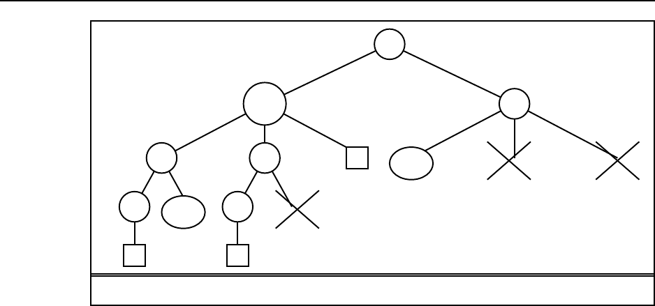
37
bd
cd ad
ce cf cc
de be df bf
ae af ac
dd dd
−4−4
−2
−4−4
<=−6
<=−6<=−6
<=−6
<=−4
−4−4
−4 <=−6
−4
Figure S5.1 Pursuit-evasion solution tree.
d.Actuallythestatementinthequestionisnottrue(itapplies to a previous version of part
(c) in which the opponent is just trying to prevent you from winning—in that case, the
coin tosses will eventually allow you to solve one puzzle without interruptions). For the
game described in (c), consider a state in which the coin has come up heads, say, and
you get to work on a puzzle that is 2 steps from the goal. Should you move one step
closer? If you do, your opponent wins if he tosses heads; or if he tosses tails, you toss
tails, and he tosses heads; or any sequence where both toss tails ntimes and then he
tosses heads. So his probability of winning is at least 1/2+1/8+1/32+···=2/3.So
it seems you’re better off moving away from the goal. (There’s no way to stay the same
distance from the goal.) This problem unintentionally seemstohavethesamekindof
solution as suicide tictactoe with passing.
5.3
a.SeeFigureS5.1;thevaluesarejust(minus)thenumberofsteps along the path from the
root.
b.SeeFigureS5.1;notethatthereisbothanupperboundandalower bound for the left
child of the root.
c.Seefigure.
d.Theshortest-pathlengthbetweenthetwoplayersisalowerbound on the total capture
time (here the players take turns, so no need to divide by two),sothe“?”leaveshavea
capture time greater than or equal to the sum of the cost from the root and the shortest-
path length. Notice that this bound is derived when the Evaderplaysverybadly. The
true value of a node comes from best play by both players, so we can get better bounds
by assuming better play. For example, we can get a better boundfromthecostwhenthe
Evader simply moves backwards and forwards rather than moving towards the Pursuer.
e.Seefigure(wehaveusedthesimplebounds).Noticethatoncethe right child is known

38 Chapter 5. Adversarial Search
to have a value below –6, the remaining successors need not be considered.
f.Thepursueralwayswinsifthetreeisfinite. Toprovethis,let the tree be rooted as
the pursuer’s current node. (I.e., pick up the tree by that node and dangle all the other
branches down.) The evader must either be at the root, in whichcasethepursuerhas
won, or in some subtree. The pursuer takes the branch leading to that subtree. This
process repeats at most dtimes, where dis the maximum depth of the original subtree,
until the pursuer either catches the evader or reaches a leaf node. Since the leaf has no
subtrees, the evader must be at that node.
5.4 The basic physical state of these games is fairly easy to describe. One important thing
to remember for Scrabble and bridge is that the physical stateisnotaccessibletoallplayers
and so cannot be provided directly to each player by the environment simulator. Particularly
in bridge, each player needs to maintain some best guess (or multiple hypotheses) as to the
actual state of the world. We expect to be putting some of the game implementations online
as they become available.
5.5 Code not shown.
5.6 The most obvious change is that the space of actions is now continuous. For example,
in pool, the cueing direction, angle of elevation, speed, andpointofcontactwiththecueball
are all continuous quantities.
The simplest solution is just to discretize the action space and then apply standard meth-
ods. This might work for tennis (modelled crudely as alternating shots with speed and direc-
tion), but for games such as pool and croquet it is likely to fail miserably because small
changes in direction have large effects on action outcome. Instead, one must analyze the
game to identify a discrete set of meaningful local goals, such as “potting the 4-ball” in pool
or “laying up for the next hoop” in croquet. Then, in the current context, a local optimization
routine can work out the best way to achieve each local goal, resulting in a discrete set of pos-
sible choices. Typically, these games are stochastic, so thebackgammonmodelisappropriate
provided that we use sampled outcomes instead of summing overalloutcomes.
Whereas pool and croquet are modelled correctly as turn-taking games, tennis is not.
While one player is moving to the ball, the other player is moving to anticipate the opponent’s
return. This makes tennis more like the simultaneous-actiongamesstudiedinChapter17.In
particular, it may be reasonable to derive randomized strategies so that the opponent cannot
anticipate where the ball will go.
5.7 Consider a MIN node whose children are terminal nodes. If MIN plays suboptimally,
then the value of the node is greater than or equal to the value it would have if MIN played
optimally. Hence, the value of the MAX node that is the MIN node’s parent can only be
increased. This argument can be extended by a simple induction all the way to the root. If
the suboptimal play by MIN is predictable,thenonecandobetterthanaminimaxstrategy.
For example, if MIN always falls for a certain kind of trap and loses, then settingthetrap
guarantees a win even if there is actually a devastating response for MIN.Thisisshownin
Figure S5.2.
5.8
39
MAX
MIN
a1
A
B D
−101000 1000
2
b3
b
1
b2
d
1
d3
d
−5−5−5
a2
Figure S5.2 AsimplegametreeshowingthatsettingatrapforMIN by playing aiis a win
if MIN falls for it, but may also be disastrous. The minimax move is ofcoursea2,withvalue
−5.
(1,4)
(2,4)
(2,3)
(1,3)
(1,2)
(3,2)
(3,4)
(4,3)
(3,1)
(2,4)
(1,4)
+1
−1
?
?
?
−1
−1
−1
+1
+1
+1
Figure S5.3 The game tree for the four-square game in Exercise 5.8. Terminal states are
in single boxes, loop states in double boxes. Each state is annotated with its minimax value
in a circle.
a.(5)Thegametree,completewithannotationsofallminimaxvalues, is shown in Fig-
ure S5.3.
b.(5)The“?”valuesarehandledbyassumingthatanagentwithachoicebetweenwin-
ning the game and entering a “?” state will always choose the win. That is, min(–1,?)
is –1 and max(+1,?) is +1. If all successors are “?”, the backed-up value is “?”.
c.(5)Standardminimaxisdepth-firstandwouldgointoaninfinite loop. It can be fixed

40 Chapter 5. Adversarial Search
by comparing the current state against the stack; and if the state is repeated, then return
a“?” value. Propagationof“?” valuesishandledasabove. Although it works in this
case, it does not always work because it is not clear how to compare “?” with a drawn
position; nor is it clear how to handle the comparison when there are wins of different
degrees (as in backgammon). Finally, in games with chance nodes, it is unclear how to
compute the average of a number and a “?”. Note that it is not correct to treat repeated
states automatically as drawn positions; in this example, both (1,4) and (2,4) repeat in
the tree but they are won positions.
What is really happening is that each state has a well-defined but initially unknown
value. These unknown values are related by the minimax equation at the bottom of
164. If the game tree is acyclic, then the minimax algorithm solves these equations by
propagating from the leaves. If the game tree has cycles, thenadynamicprogramming
method must be used, as explained in Chapter 17. (Exercise 17.7 studies this problem in
particular.) These algorithms can determine whether each node has a well-determined
value (as in this example) or is really an infinite loop in that both players prefer to stay
in the loop (or have no choice). In such a case, the rules of the game will need to define
the value (otherwise the game will never end). In chess, for example, a state that occurs
3times(andhenceisassumedtobedesirableforbothplayers)isadraw.
d.Thisquestionisalittletricky.Oneapproachisaproofbyinduction on the size of the
game. Clearly, the base case n=3 is a loss for A and the base case n=4 is a win for
A. For any n>4,theinitialmovesarethesame:AandBbothmoveonesteptowards
each other. Now, we can see that they are engaged in a subgame ofsizen−2on the
squares [2,...,n−1],except that there is an extra choice of moves on squares 2and
n−1.Ignoringthisforamoment,itisclearthatifthe“n−2”iswonforA,thenA
gets to the square n−1before B gets to square 2(by the definition of winning) and
therefore gets to nbefore B gets to 1,hencethe“n”gameiswonforA.Bythesame
line of reasoning, if “n−2”iswonforBthen“n”iswonforB.Now,thepresenceof
the extra moves complicates the issue, but not too much. First, the player who is slated
to win the subgame [2,...,n−1] never moves back to his home square. If the player
slated to lose the subgame does so, then it is easy to show that he is bound to lose the
game itself—the other player simply moves forward and a subgame of size n−2kis
played one step closer to the loser’s home square.
5.9 For a,thereareatmost9!games.(Thisisthenumberofmovesequences that fill up the
board, but many wins and losses end before the board is full.) For b–e,FigureS5.4showsthe
game tree, with the evaluation function values below the terminal nodes and the backed-up
values to the right of the non-terminal nodes. The values imply that the best starting move for
Xistotakethecenter. Theterminalnodeswithaboldoutlineare the ones that do not need
to be evaluated, assuming the optimal ordering.
5.10
a.AnupperboundonthenumberofterminalnodesisN!,oneforeachorderingof
squares, so an upper bound on the total number of nodes is !N
i=1 i!.Thisisnotmuch
41
x
x
x
xo x
o
xox
o
x
o
x
o
x
o
xo x
o
x
o
x
o
x
o
1
−1 1 −2
1−1 0 0 1 −1−2 0 −1 0
12
Figure S5.4 Part of the game tree for tic-tac-toe, for Exercise 5.9.
bigger than N!itself as the factorial function grows superexponentially.Thisisan
overestimate because some games will end early when a winningpositionisfilled.
This count doesn’t take into account transpositions. An upper bound on the number
of distinct game states is 3N,aseachsquareiseitheremptyorfilledbyoneofthetwo
players. Note that we can determine who is to play just from looking at the board.
b.Inthiscasenogamesterminateearly,andthereareN!different games ending in a draw.
So ignoring repeated states, we have exactly !N
i=1 i!nodes.
At the end of the game the squares are divided between the two players: ⌈N/2⌉to
the first player and ⌊N/2⌋to the second. Thus, a good lower bound on the number of
distinct states is "N
⌈N/2⌉#,thenumberofdistinctterminalstates.
c.Forastates,letX(s)be the number of winning positions containing no O’s and O(s)
the number of winning positions containing no X’s. One evaluation function is then
Eval(s)=X(s)−O(S).Noticethatemptywinningpositionscanceloutintheeval-
uation function.
Alternatively, we might weight potential winning positionsbyhowclosetheyareto
completion.
d.UsingtheupperboundofN!from (a), and observing that it takes 100NN!instructions.
At 2GHz we have 2 billion instructions per second (roughly speaking), so solve for the
largest Nusing at most this many instructions. For one second we get N=9,forone
minute N=11,andforonehourN=12.
5.11 See "search/algorithms/games.lisp"for definitions of games, game-playing
agents, and game-playing environments. "search/algorithms/minimax.lisp"con-
tains the minimax and alpha-beta algorithms. Notice that thegame-playingenvironmentis
essentially a generic environment with the update function defined by the rules of the game.
Turn-taking is achieved by having agents do nothing until it is their turn to move.
See "search/domains/cognac.lisp"for the basic definitions of a simple game
(slightly more challenging than Tic-Tac-Toe). The code for this contains only a trivial eval-
uation function. Students can use minimax and alpha-beta to solve small versions of the
game to termination (probably up to 4×3); they should notice that alpha-beta is far faster

42 Chapter 5. Adversarial Search
than minimax, but still cannot scale up without an evaluationfunctionandtruncatedhorizon.
Providing an evaluation function is an interesting exercise. From the point of view of data
structure design, it is also interesting to look at how to speed up the legal move generator by
precomputing the descriptions of rows, columns, and diagonals.
Very few students w il l have heard o f kalah, s o it is a fa ir a ss i gnment, but the game
is boring—depth 6 lookahead and a purely material-based evaluation function are enough
to beat most humans. Othello is interesting and about the right level of difficulty for most
students. Chess and checkers are sometimes unfair because usually a small subset of the
class will be experts while the rest are beginners.
5.12 The minimax algorithm for non-zero-sum games works exactly as for multiplayer
games, described on p.165–6; that is, the evaluation function is a vector of values, one for
each player, and the backup step selects whichever vector hasthehighestvaluefortheplayer
whose turn it is to move. The example at the end of Section 5.2.2(p.165)showsthatalpha-
beta pruning is not possible in general non-zero-sum games, because an unexamined leaf
node might be optimal for both players.
5.13 This question is not as hard as it looks. The derivation below leads directly to a defini-
tion of αand βvalues. The notation nirefers to (the value of) the node at depth ion the path
from the root to the leaf node nj.Nodesni1...n
ibiare the siblings of node i.
a.Wecanwriten2=max(n3,n
31,...,n
3b3),giving
n1=min(max(n3,n
31,...,n
3b3),n
21,...,n
2b2)
Then n3can be similarly replaced, until we have an expression containing njitself.
b.Intermsoftheland rvalues, we have
n1=min(l2,max(l3,n
3,r
3),r
2)
Again, n3can be expanded out down to nj.Themostdeeplynestedtermwillbe
min(lj,n
j,r
j).
c.Ifnjis a max node, then the lower bound on its value only increases as its successors
are evaluated. Clearly, if it exceeds ljit will have no further effect on n1.Byextension,
if it exceeds min(l2,l
4,...,l
j)it will have no effect. Thus, by keeping track of this
value we can decide when to prune nj.Thisisexactlywhatα-βdoes.
d.Thecorrespondingboundforminnodesnkis max(l3,l
5,...,l
k).
5.14 The result is given in Section 6 of Knuth (1975). The exact statement (Corollary 1 of
Theorem 1) is that the algorithms examines b⌊m/2⌋+b⌈m/2⌉−1nodes at level m.These
are exactly the nodes reached when Min plays only optimal moves and/or Max plays only
optimal moves. The proof is by induction on m.
5.15 With 32 pieces, each needing 6 bits to specify its position on one of 64 squares, we
need 24 bytes (6 32-bit words) to store a position, so we can store roughly 80 million positions
in the table (ignoring pointers for hash table bucket lists).Thisisabout1/22ofthe1800
million positions generated during a three-minute search.
43
0.5 0.5
0.5 0.5
22 221 0 −1 0
210−1
1.5 −0.5
1.5
Figure S5.5 Pruning with chance nodes solution.
Generating the hash key directly from an array-based representation of the position
might be quite expensive. Modern programs (see, e.g., Heinz,2000)carryalongthehash
key and modify it as each new position is generated. Suppose this takes on the order of 20
operations; then on a 2GHz machine where an evaluation takes 2000 operations we can do
roughly 100 lookups per evaluation. Using a rough figure of onemillisecondforadiskseek,
we could do 1000 evaluations per lookup. Clearly, using a disk-resident table is of dubious
value, even if we can get some locality of reference to reduce the number of disk reads.
5.16
a.SeeFigureS5.5.
b.Givennodes1–6,wewouldneedtolookat7and8:iftheywereboth +∞then the
values of the min node and chance node above would also be +∞and the best move
would change. Given nodes 1–7, we do not need to look at 8. Even if it is +∞,themin
node cannot be worth more than −1,sothechancenodeabovecannotbeworthmore
than −0.5,sothebestmovewon’tchange.
c.Theworstcaseisifeitherofthethirdandfourthleavesis−2,inwhichcasethechance
node above is 0. The best case is where they are both 2, then the chance node has value
2. So it must lie between 0 and 2.
d.Seefigure.
5.18 The general strategy is to reduce a general game tree to a one-ply tree by induction on
the depth of the tree. The inductive step must be done for min, max, and chance nodes, and
simply involves showing that the transformation is carried though the node. Suppose that the
values of the descendants of a node are x1...x
n,andthatthetransformationisax +b,where

44 Chapter 5. Adversarial Search
ais positive. We have
min(ax1+b, ax2+b, . . . , axn+b)=amin(x1,x
2,...,x
n)+b
max(ax1+b, ax2+b, . . . , axn+b)=amin(x1,x
2,...,x
n)+b
p1(ax1+b)+p2(ax2+b)+···+pn(axn+b)=a(p1x1+p2x2+···pnxn)+b
Hence the problem reduces to a one-ply tree where the leaves have the values from the original
tree multiplied by the linear transformation. Since x>y⇒ax +b>ay+bif a>0,the
best choice at the root will be the same as the best choice in theoriginaltree.
5.19 This procedure will give incorrect results. Mathematically, the procedure amounts to
assuming that averaging commutes with min and max, which it does not. Intuitively, the
choices made by each player in the deterministic trees are based on full knowledge of future
dice rolls, and bear no necessary relationship to the moves made without such knowledge.
(Notice the connection to the discussion of card games in Section 5.6.2 and to the general
problem of fully and partially observable Markov decision problems in Chapter 17.) In prac-
tice, the method works reasonably well, and it might be a good exercise to have students
compare it to the alternative of using expectiminimax with sampling (rather than summing
over) dice rolls.
5.20
a.Nopruning.Inamaxtree,thevalueoftherootisthevalueofthe best leaf. Any unseen
leaf might be the best, so we have to see them all.
b.Nopruning.Anunseenleafmighthaveavaluearbitrarilyhigher or lower than any other
leaf, which (assuming non-zero outcome probabilities) means that there is no bound on
the value of any incompletely expanded chance or max node.
c.Nopruning.Sameargumentasin(a).
d.Nopruning.Nonnegativevaluesallowlower bounds on the values of chance nodes, but
alowerbounddoesnotallowanypruning.
e.Yes.Ifthefirstsuccessorhasvalue1,theroothasvalue1andallremainingsuccessors
can be pruned.
f.Yes. Supposethefirstactionattheroothasvalue0.6,andthefirstoutcomeofthe
second action has probability 0.5 and value 0; then all other outcomes of the second
action can be pruned.
g.(ii)Highestprobabilityfirst.Thisgivesthestrongestbound on the value of the node,
all other things being equal.
5.21
a.In a fully observable, turn-taking, zero-sum game between two perfectly rational play-
ers, it does not help the first player to know what strategy the second player is using—
that is, what move the second player will make, given the first player’s move.
True. The second player will play optimally, and so is perfectly predictable up to ties.
Knowing which of two equally good moves the opponent will makedoesnotchange
the value of the game to the first player.

45
b.In a partially observable, turn-taking, zero-sum game between two perfectly rational
players, it does not help the first player to know what move the second player will
make, given the first player’s move.
False. In a partially observable game, knowing the second player’s move tells the first
player additional information about the game state that would otherwise be available
only to the second player. For example, in Kriegspiel, knowing the opponent’s future
move tells the first player where one of the opponent’s pieces is; in a card game, it tells
the first player one of the opponent’s cards.
c.Aperfectlyrationalbackgammonagentneverloses.
False. Backgammon is a game of chance, and the opponent may consistently roll much
better dice. The correct statement is that the expected winnings are optimal. It is sus-
pected, but not known, that when playing first the expected winnings are positive even
against an optimal opponent.
5.22 One can think of chance events during a game, such as dice rolls, in the same way
as hidden but preordained information (such as the order of the cards in a deck). The key
distinctions are whether the players can influence what information is revealed and whether
there is any asymmetry in the information available to each player.
a.ExpectiminimaxisappropriateonlyforbackgammonandMonopoly. In bridge and
Scrabble, each player knows the cards/tiles he or she possesses but not the opponents’.
In Scrabble, the benefits of a fully rational, randomized strategy that includes reasoning
about the opponents’ state of knowledge are probably small, but in bridge the questions
of knowledge and information disclosure are central to good play.
b.None,forthereasonsdescribedearlier.
c.Keyissuesincludereasoningabouttheopponent’sbeliefs,theeffectofvariousactions
on those beliefs, and methods for representing them. Since belief states for rational
agents are probability distributions over all possible states (including the belief states of
others), this is nontrivial.

Solutions for Chapter 6
Constraint Satisfaction Problems
6.1 There are 18 solutions for coloring Australia with three colors. Start with SA,which
can have any of three colors. Then moving clockwise, WA can have either of the other two
colors, and everything else is strictly determined; that makes 6 possibilities for the mainland,
times 3 for Tasmania yields 18.
6.2
a.SolutionA:Thereisavariablecorrespondingtoeachofthen2positions on the board.
Solution B: There is a variable corresponding to each knight.
b.SolutionA:Eachvariablecantakeoneoftwovalues,{occupied,vacant}
Solution B: Each variable’s domain is the set of squares.
c.SolutionA:everypairofsquaresseparatedbyaknight’smove is constrained, such that
both cannot be occupied. Furthermore, the entire set of squares is constrained, such that
the total number of occupied squares should be k.
Solution B: every pair of knights is constrained, such that notwoknightscanbeonthe
same square or on squares separated by a knight’s move. Solution B may be preferable
because there is no global constraint, although Solution A has the smaller state space
when kis large.
d.Anysolutionmustdescribeacomplete-state formulation because we are using a local
search algorithm. For simulated annealing, the successor function must completely
connect the space; for random-restart, the goal state must bereachablebyhillclimbing
from some initial state. Two basic classes of solutions are:
Solution C: ensure no attacks at any time. Actions are to remove any knight, add a
knight in any unattacked square, or move a knight to any unattacked square.
Solution D: allow attacks but try to get rid of them. Actions are to remove any knight,
add a knight in any square, or move a knight to any square.
6.3 a. Crossword puzzle construction can be solved many ways. One simple choice is
depth-first search. Each successor fills in a word in the puzzlewithoneofthewordsinthe
dictionary. It is better to go one word at a time, to minimize the number of steps.
b. As a CSP, there are even more choices. You could have a variableforeachboxin
the crossword puzzle; in this case the value of each variable is a letter, and the constraints are
46

47
that the letters must make words. This approach is feasible with a most-constraining value
heuristic. Alternately, we could have each string of consecutive horizontal or vertical boxes
be a single variable, and the domain of the variables be words in the dictionary of the right
length. The constraints would say that two intersecting words must have the same letter in the
intersecting box. Solving a problem in this formulation requires fewer steps, but the domains
are larger (assuming a big dictionary) and there are fewer constraints. Both formulations are
feasible.
6.4 a. For rectilinear floor-planning, one possibility is to have a variable for each of the
small rectangles, with the value of each variable being a 4-tuple consisting of the xand y
coordinates of the upper left and lower right corners of the place where the rectangle will
be located. The domain of each variable is the set of 4-tuples that are the right size for the
corresponding small rectangle and that fit within the large rectangle. Constraints say that no
two rectangles can overlap; for example if the value of variable R1is [0,0,5,8],thennoother
variable can take on a value that overlaps with the 0,0to 5,8rectangle.
b. For class scheduling, one possibility is to have three variables for each class, one with
times for values (e.g. MWF8:00, TuTh8:00, MWF9:00, ...), onewithclassroomsforvalues
(e.g. Wheeler110, Evans330, ...) and one with instructors for values (e.g. Abelson, Bibel,
Canny, ...). Constraints say that only one class can be in the same classroom at the same time,
and an instructor can only teach one class at a time. There may be other constraints as well
(e.g. an instructor should not have two consecutive classes).
c. For Hamiltonian tour, one possibility is to have one variableforeachstoponthetour,
with binary constraints requiring neighboring cities to be connected by roads, and an AllDiff
constraint that all variables have a different value.
6.5 The exact steps depend on certain choices you are free to make;herearetheonesI
made:
a.ChoosetheX3variable. Its domain is {0,1}.
b.Choosethevalue1forX3.(Wecan’tchoose0;itwouldn’tsurviveforwardchecking,
because it would force Fto be 0, and the leading digit of the sum must be non-zero.)
c.ChooseF,becauseithasonlyoneremainingvalue.
d.Choosethevalue1forF.
e.NowX2and X1are tied for minimum remaining values at 2; let’s choose X2.
f.Eithervaluesurvivesforwardchecking,let’schoose0forX2.
g.NowX1has the minimum remaining values.
h.Again,arbitrarilychoose0forthevalueofX1.
i.ThevariableOmust be an even number (because it is the sum of T+Tless than 5
(because O+O=R+10×0). That makes it most constrained.
j.Arbitrarilychoose4asthevalueofO.
k.Rnow has only 1 remaining value.
l.Choosethevalue8forR.
m.Tnow has only 1 remaining value.

48 Chapter 6. Constraint Satisfaction Problems
n.Choosethevalue7forT.
o.Umust be an even number less than 9; choose U.
p.TheonlyvalueforUthat survives forward checking is 6.
q.TheonlyvariableleftisW.
r.TheonlyvalueleftforWis 3.
s.Thisisasolution.
This is a rather easy (under-constrained) puzzle, so it is notsurprisingthatwearriveata
solution with no backtracking (given that we are allowed to use forward checking).
6.6 The problem statement sets out the solution fairly completely. To express the ternary
constraint on A,Band Cthat A+B=C,wefirstintroduceanewvariable,AB.Ifthe
domain of Aand Bis the set of numbers N,thenthedomainofAB is the set of pairs of
numbers from N,i.e. N×N.Nowtherearethreebinaryconstraints,onebetweenAand
AB saying that the value of Amust be equal to the first element of the pair-value of AB;one
between Band AB saying that the value of Bmust equal the second element of the value
of AB;andfinallyonethatsaysthatthesumofthepairofnumbersthat is the value of AB
must equal the value of C.Allotherternaryconstraintscanbehandledsimilarly.
Now that we can reduce a ternary constraint into binary constraints, we can reduce a
4-ary constraint on variables A, B, C, D by first reducing A, B, C to binary constraints as
shown above, then adding back Din a ternary constraint with AB and C,andthenreducing
this ternary constraint to binary by introducing CD.
By induction, we can reduce any n-ary constraint to an (n−1)-ary constraint. We can
stop at binary, because any unary constraint can be dropped, simply by moving the effects of
the constraint into the domain of the variable.
6.7 The “Zebra Puzzle” can be represented as a CSP by introducing avariableforeach
color, pet, drink, country, and cigarette brand (a total of 25variables). Thevalueofeach
variable is a number from 1 to 5 indicating the house number. This is a good representation
because it easy to represent all the constraints given in the problem definition this way. (We
have done so in the Python implementation of the code, and at some point we may reimple-
ment this in the other languages.) Besides ease of expressingaproblem,theotherreasonto
choose a representation is the efficiency of finding a solution. here we have mixed results—
on some runs, min-conflicts local search finds a solution for this problem in seconds, while
on other runs it fails to find a solution after minutes.
Another representation is to have five variables for each house, one with the domain of
colors, one with pets, and so on.
6.8
a.A1=R.
b.H=Rconflicts with A1.
c.H=G.
d.A4=R.
e.F1=R.

49
f.A2=Rconflicts with A1,A2=Gconflicts with H,soA2=B.
g.F2=R.
h.A3=Rconflicts with A4,A3=Gconflicts with H,A3=Bconflicts with A2,so
backtrack. Conflict set is {A2,H,A
4},sojumptoA2.Add{H, A4}to A2’s conflict
set.
i.A2has no more values, so backtrack. Conflict set is {A1,H,A
4}so jump back to A4.
Add {A1,H}to A4’s conflict set.
j.A4=Gconflicts with H,soA4=B.
k.F1=R
l.A2=Rconflicts with A1,A2=Gconflicts with H,soA2=B.
m.F2=R
n.A3=R.
o.T=Rconflicts with F1and F2,T=Gconflicts with G,soT=B.
p.Success.
6.9 The most constrained variable makes sense because it choosesavariablethatis(all
other things being equal) likely to cause a failure, and it is more efficient to fail as early
as possible (thereby pruning large parts of the search space). The least constraining value
heuristic makes sense because it allows the most chances for future assignments to avoid
conflict.
6.11 We’ll trace through each iteration of the while loop in AC-3 (for one possible ordering
of the arcs):
a.RemoveSA −WA,deleteGfrom SA.
b.RemoveSA −V,deleteRfrom SA,leavingonlyB.
c.RemoveNT −WA,deleteGfrom NT.
d.RemoveNT −SA,deleteBfrom NT,leavingonlyR.
e.RemoveNSW −SA,deleteBfrom NSW.
f.RemoveNSW −V,deleteRfrom NSW,leavingonlyG.
g.RemoveQ−NT,deleteRfrom Q.
h.RemoveQ−SA,deleteBfrom Q.
i.removeQ−NSW,deleteGfrom Q,leavingnodomainforQ.
6.12 On a tree-structured graph, no arc will be considered more than once, so the AC-
3algorithmisO(ED),whereEis the number of edges and Dis the size of the largest
domain.
6.13 The basic idea is to preprocess the constraints so that, for each value of Xi,wekeep
track of those variables Xkfor which an arc from Xkto Xiis satisfied by that particular value
of Xi.Thisdatastructurecanbecomputedintimeproportionaltothe size of the problem
representation. Then, when a value of Xiis deleted, we reduce by 1 the count of allowable

50 Chapter 6. Constraint Satisfaction Problems
values for each (Xk,X
i)arc recorded under that value. This is very similar to the forward
chaining algorithm in Chapter 7. See Mohr and Henderson (1986) for detailed proofs.
6.14
We establish arc-consistency from the bottom up because we will then (after establish-
ing consistency) solve the problem from the top down. It will always be possible to find a
solution (if one exists at all) with no backtracking because of the definition of arc consistency:
whatever choice we make for the value of the parent node, therewillbeavalueforthechild.
6.15
It is certainly possible to solve Sudoku problems in this fashion. However, it is not as
effective as the partial-assignment approach, and not as effective as min-conflicts is on the N-
queens problem. Perhaps that is because there are two different types of conflicts: a conflict
with one of the numbers that defines the initial problem is one that must be corrected, but
aconflictbetweentwonumbersthatwereplacedelsewhereinthe rid can be corrected by
replacing either of the two. A version of min-conflicts that recognizes the difference between
these two situations might do better than the naive min-conflicts algorithm.
6.16 Aconstraint is a restriction on the possible values of two or more variables. For
example, a constraint might say that A=ais not allowed in conjunction with B=b.
Backtracking search is a form of depth-first search in which there is a single repre-
sentation of the state that gets updated for each successor, and then must be restored when a
dead end is reached.
AdirectedarcfromvariableAto variable Bin a CSP is arc consistent if, for every
value in the current domain of A,thereissomeconsistentvalueofB.
Backjumping is a way of making backtracking search more efficient, by jumping back
more than one level when a dead end is reached.
Min-conflicts is a heuristic for use with local search on CSP problems. The heuristic
says that, when given a variable to modify, choose the value that conflicts with the fewest
number of other variables.
Acycle cutset is a set of variables which when removed from the constraint graph make
it acyclic (i.e., a tree). When the variables of a cycle cutsetareinstantiatedtheremainderof
the CSP can be solved in linear time.
6.17 Asimplealgorithmforfindingacutsetofnomorethanknodes is to enumerate all
subsets of nodes of size 1,2,...,k,andforeachsubsetcheckwhethertheremainingnodes
form a tree. This algorithm takes time "Pk
i=1 n
nk #,whichisO(nk).
Becker and Geiger (1994; http://citeseer.nj.nec.com/becker94approximation.html) give
an algorithm called MGA (modified greedy algorithm) that findsacutsetthatisnomorethan
twice the size of the minimal cutset, using time O(E+Vlog(V)),whereEis the number of
edges and Vis the number of variables.
Whether the cycle cutset approach is practical depends more on the graph than on the
cutset-finding algorithm. That is because, for a cutset of size c,westillhaveanexponential
(dc)factor before we can solve the CSP. So any graph with a large cutset will be intractable
to solve by this method, even if we could find the cutset with no effort at all.

Solutions for Chapter 7
Logical Agents
7.1 To save space, we’ll show the list of models as a table (Figure S7.1) rather than a
collection of diagrams. There are eight possible combinations of pits in the three squares,
and four possibilities for the wumpus location (including nowhere).
We can see that KB |=α2because every line where KB is true also has α2true.
Similarly for α3.
7.2 As human reasoners, we can see from the first two statements, that if it is mythical, then
it is immortal; otherwise it is a mammal. So it must be either immortal or a mammal, and thus
horned. That means it is also magical. However, we can’t deduce anything about whether it
is mythical. To proide a formal answer, we can enumerate the possible worlds (25=32of
them with 5 proposition symbols), mark those in which all the assertions are true, and see
which conclusions hold in all of those. Or, we can let the machine do the work—in this case,
the Lisp code for propositional reasoning:
> (setf kb (make-prop-kb))
#S(PROP-KB SENTENCE (AND))
> (tell kb "Mythical => Immortal")
T
> (tell kb "˜Mythical => ˜Immortal ˆ Mammal")
T
> (tell kb "Immortal | Mammal => Horned")
T
> (tell kb "Horned => Magical")
T
> (ask kb "Mythical")
NIL
> (ask kb "˜Mythical")
NIL
> (ask kb "Magical")
T
> (ask kb "Horned")
T
7.3
a.SeeFigureS7.2.Weassumethelanguagehasbuilt-inBooleanoperatorsnot,and,or,
iff.
51

52 Chapter 7. Logical Agents
Model KB α2α3
true
P1,3true
P2,2
P3,1true
P1,3,P2,2
P2,2,P3,1
P3,1,P1,3true
P1,3,P3,1,P2,2
W1,3true true
W1,3,P1,3true true
W1,3,P2,2true
W1,3,P3,1true true true
W1,3,P1,3,P2,2true
W1,3,P2,2,P3,1true
W1,3,P3,1,P1,3true true
W1,3,P1,3,P3,1,P2,2true
W3,1,true
W3,1,P1,3true
W3,1,P2,2
W3,1,P3,1true
W3,1,P1,3,P2,2
W3,1,P2,2,P3,1
W3,1,P3,1,P1,3true
W3,1,P1,3,P3,1,P2,2
W2,2true
W2,2,P1,3true
W2,2,P2,2
W2,2,P3,1true
W2,2,P1,3,P2,2
W2,2,P2,2,P3,1
W2,2,P3,1,P1,3true
W2,2,P1,3,P3,1,P2,2
Figure S7.1 AtruthtableconstructedforEx.7.2. Propositionsnotlisted as true on a
given line are assumed false, and only true entries are shown in the table.
b.Thequestionissomewhatambiguous:wecaninterpret“inapartial model” to mean
in all such models or some such models. For the former interpretation, the sentences
False ∧P,True ∨¬P,andP∧¬Pcan all be determined to be true or false in any
partial model. For the latter interpretation, we can in addition have sentences such as
A∧Pwhich is false in the partial model {A=false}.
c.Ageneralalgorithmforpartialmodelsmusthandletheemptypartialmodel,withno
assignments. In that case, the algorithm must determine validity and unsatisfiability,

53
function PL-TRUE?(s,m)returns true or false
if s=True then return true
else if s=False then return false
else if SYMBOL?(s)then return LOOKUP(s,m)
else branch on the operator of s
¬:return not PL-TRUE?(ARG1(s), m)
∨:return PL-TRUE?(ARG1(s), m)or PL-TRUE?(ARG2(s), m)
∧:return PL-TRUE?(ARG1(s), m)and PL-TRUE?(ARG2(s), m)
⇒:(not PL-TRUE?(ARG1(s), m)) or PL-TRUE?(ARG2(s), m)
⇔:PL-TRUE?(ARG1(s), m)iff PL-TRUE?(ARG2(s), m)
Figure S7.2 Pseudocode for evaluating the truth of a sentence wrt a model.
which are co-NP-complete and NP-complete respectively.
d.Ithelpsifand and or evaluate their arguments in sequence, terminating on false or true
arguments, respectively. In that case, the algorithm already has the desired properties:
in the partial model where Pis true and Qis unknown, P∨Qreturns true, and ¬P∧Q
returns false. But the truth values of Q∨¬Q,Q∨True,andQ∧¬Qare not detected.
e.EarlyterminationinBooleanoperatorswillprovideaverysubstantial speedup. In most
languages, the Boolean operators already have the desired property, so you would have
to write special “dumb” versions and observe a slow-down.
7.4 In all cases, the question can be resolved easily by referringtothedefinitionofentail-
ment.
a.False |=True is true because False has no models and hence entails every sentence
AND because True is true in all models and hence is entailed by every sentence.
b.True |=False is false.
c.(A∧B)|=(A⇔B)is true because the left-hand side has exactly one model that is
one of the two models of the right-hand side.
d.A⇔B|=A∨Bis false because one of the models of A⇔Bhas both Aand B
false, which does not satisfy A∨B.
e.A⇔B|=¬A∨Bis true because the RHS is A⇒B,oneoftheconjunctsinthe
definition of A⇔B.
f.(A∧B)⇒C|=(A⇒C)∨(B⇒C)is true because the RHS is false only
when both disjuncts are false, i.e., when Aand Bare true and Cis false, in which case
the LHS is also false. This may seem counterintuitive, and would not hold if ⇒is
interpreted as “causes.”
g.(C∨(¬A∧¬B)) ≡((A⇒C)∧(B⇒C)) is true; proof by truth table enumeration,
or by application of distributivity (Fig 7.11).
h.(A∨B)∧(¬C∨¬D∨E)|=(A∨B)is true; removing a conjunct only allows more
models.

54 Chapter 7. Logical Agents
i.(A∨B)∧(¬C∨¬D∨E)|=(A∨B)∧(¬D∨E)is false; removing a disjunct allows
fewer models.
j.(A∨B)∧¬(A⇒B)is satisfiable; model has Aand ¬B.
k.(A⇔B)∧(¬A∨B)is satisfiable; RHS is entailed by LHS so models are those of
A⇔B.
l.(A⇔B)⇔Cdoes have the same number of models as (A⇔B);halfthe
models of (A⇔B)satisfy (A⇔B)⇔C,asdohalfthenon-models,andthere
are the same numbers of models and non-models.
7.5 Remember, α|=βiff in every model in which αis true, βis also true. Therefore,
a.αis valid if and only if True |=α.
Forward: If alpha is valid it is true in all models, hence it is true in all models of True .
Backward: if True |=αthen αmust be true in all models of True ,i.e.,inallmodels,
hence αmust be valid.
b.Foranyα,False |=α.
Falsedoesn’t hold in any model, so αtrivially holds in every model of False.
c.α|=βif and only if the sentence (α⇒β)is valid.
Both sides are equivalent to the assertion that there is no model in which αis true and
βis false, i.e., no model in which α⇒βis false.
d.α≡βif and only if the sentence (α⇔β)is valid.
Both sides are equivalent to the assertion that αand βhave the same truth value in every
model.
e.α|=βif and only if the sentence (α∧¬β)is unsatisfiable.
As in c,bothsidesareequivalenttotheassertionthatthereisnomodel in which αis
true and βis false.
7.6
a.Ifα|=γor β|=γ(or both) then (α∧β)|=γ.
True. This follows from monotonicity.
b.Ifα|=(β∧γ)then α|=βand α|=γ.
True. If β∧γis true in every model of α,thenβand γare true in every model of α,so
α|=βand α|=γ.
c.Ifα|=(β∨γ)then α|=βor α|=γ(or both).
False. Consider β≡A,γ≡¬A.
7.7 These can be computed by counting the rows in a truth table thatcomeouttrue,but
each has some simple property that allows a short-cut:
a.SentenceisfalseonlyifBand Care false, which occurs in 4 cases for Aand D,leaving
12.
b.SentenceisfalseonlyifA,B,C,andDare false, which occurs in 1 case, leaving 15.
c.Thelastfourconjunctsspecifyamodelinwhichthefirstconjunct is false, so 0.

55
7.8 Abinarylogicalconnectiveisdefinedbyatruthtablewith4rows. Each of the four
rows may be true or false, so there are 24=16possible truth tables, and thus 16 possible
connectives. Six of these are trivial ones that ignore one or both inputs; they correspond to
True,False,P,Q,¬Pand ¬Q.Fourofthemwehavealreadystudied:∧,∨,⇒,⇔.
The remaining six are potentially useful. One of them is reverse implication (⇐instead of
⇒), and the other five are the negations of ∧,∨,⇔,⇒and ⇐.Thefirstthreeofthese
are sometimes called nand,nor,andxor.
7.9 We use the truth table code in Lisp in the directory logic/prop.lisp to show each
sentence is valid. We substitute P, Q, R for α,β,γbecause of the lack of Greek letters in
ASCII. To save space in this manual, we only show the first four truth tables:
> (truth-table "P ˆ Q <=> Q ˆ P")
-----------------------------------------
PQPˆQQˆP(PˆQ)<=>(QˆP)
-----------------------------------------
F F F F \(true\)
TF F F T
FT F F T
TT T T T
-----------------------------------------
NIL
> (truth-table "P | Q <=> Q | P")
-----------------------------------------
PQP|QQ|P(P|Q)<=>(Q|P)
-----------------------------------------
FF F F T
TF T T T
FT T T T
TT T T T
-----------------------------------------
NIL
> (truth-table "P ˆ (Q ˆ R) <=> (P ˆ Q) ˆ R")
-----------------------------------------------------------------------
PQRQˆRPˆ(QˆR)PˆQˆR(Pˆ(QˆR))<=>(PˆQˆR)
-----------------------------------------------------------------------
FFF F F F T
TFF F F F T
FTF F F F T
TTF F F F T
FFT F F F T
TFT F F F T
FTT T F F T
TTT T T T T
-----------------------------------------------------------------------
NIL
> (truth-table "P | (Q | R) <=> (P | Q) | R")
-----------------------------------------------------------------------
PQRQ|RP|(Q|R)P|Q|R(P|(Q|R))<=>(P|Q|R)

56 Chapter 7. Logical Agents
-----------------------------------------------------------------------
FFF F F F T
TFF F T T T
FTF T T T T
TTF T T T T
FFT T T T T
TFT T T T T
FTT T T T T
TTT T T T T
-----------------------------------------------------------------------
NIL
For the remaining sentences, we just show that they are valid according to the validity
function:
> (validity "˜˜P <=> P")
VALID
> (validity "P => Q <=> ˜Q => ˜P")
VALID
> (validity "P => Q <=> ˜P | Q")
VALID
> (validity "(P <=> Q) <=> (P => Q) ˆ (Q => P)")
VALID
> (validity "˜(P ˆ Q) <=> ˜P | ˜Q")
VALID
> (validity "˜(P | Q) <=> ˜P ˆ ˜Q")
VALID
> (validity "P ˆ (Q | R) <=> (P ˆ Q) | (P ˆ R)")
VALID
> (validity "P | (Q ˆ R) <=> (P | Q) ˆ (P | R)")
VALID
7.10
a.Valid.
b.Neither.
c.Neither.
d.Valid.
e.Valid.
f.Valid.
g.Valid.
7.11 Each possible world can be written as a conjunction of literals, e.g. (A∧B∧¬C).
Asserting that a possible world is not the case can be written by negating that, e.g. ¬(A∧B∧
¬C),whichcanberewrittenas(¬A∨¬B∨C).Thisistheformofaclause;aconjunction
of these clauses is a CNF sentence, and can list the negations of all the possible worlds that
would make the sentence false.
7.12 To prove the conjunction, it suffices to prove each literal se parately. To prove ¬B,add
the negated goal S7: B.

57
•ResolveS7withS5,givingS8:F.
•ResolveS7withS6,givingS9:C.
•ResolveS8withS3,givingS10:(¬C∨¬B).
•ResolveS9withS10,givingS11:¬B.
•ResolveS7withS11givingtheemptyclause.
To prove ¬A,addthenegatedgoalS7:A.
•ResolveS7withthefirstclauseofS1,givingS8:(B∨E).
•ResolveS8withS4,givingS9:B.
•Proceedasabovetoderivetheemptyclause.
7.13
a.P⇒Qis equivalent to ¬P∨Qby implication elimination (Figure 7.11), and ¬(P1∧
···∧Pm)is equivalent to (¬P1∨···∨¬Pm)by de Morgan’s rule, so (¬P1∨···∨
¬Pm∨Q)is equivalent to (P1∧···∧Pm)⇒Q.
b.Aclausecanhavepositiveandnegativeliterals;letthenegative literals have the form
¬P1,...,¬Pmand let the positive literals have the form Q1,...,Q
n,wherethePisand
Qjsaresymbols.Thentheclausecanbewrittenas(¬P1∨···∨¬Pm∨Q1∨···∨Qn).
By the previous argument, with Q=Q1∨···∨Qn,itisimmediatethattheclauseis
equivalent to
(P1∧···∧Pm)⇒Q1∨···∨Qn.
c.Foratomspi,q
i,r
i,s
iwhere pj=qk:
p1∧... p
j...∧pn1⇒r1∨...r
n2
s1∧...∧sn3⇒q1∨... q
k...∨qn4
p1∧...pj−1∧pj+1∧pn1∧s1∧...sn3⇒r1∨...rn2∨q1∨... qk−1∨qk+1∨...∨qn4
7.14
a.Correctrepresentationsof“apersonwhoisradicaliselectable if he/she is conservative,
but otherwise is not electable”:
(i) (R∧E)⇐⇒ C
No; this sentence asserts, among other things, that all conservatives are radical,
which is not what was stated.
(ii) R⇒(E⇐⇒ C)
Yes, this says that if a person is a radical then they are elect able if and only if they
are conservative.
(iii) R⇒((C⇒E)∨¬E)
No, this is equivalent to ¬R∨¬C∨E∨¬Ewhich is a tautology, true under any
assignment.
b.Hornform:

58 Chapter 7. Logical Agents
(i) Yes:
(R∧E)⇐⇒ C≡((R∧E)⇒C)∧(C⇒(R∧E))
≡((R∧E)⇒C)∧(C⇒R)∧(C⇒E)
(ii) Yes:
R⇒(E⇐⇒ C)≡R⇒((E⇒C)∧(C⇒E))
≡¬R∨((¬E∨C)∧(¬C∨E))
≡(¬R∨¬E∨C)∧(¬R∨¬C∨E)
(iii) Yes, e.g., True ⇒True.
7.15
a.Thegraphissimplyaconnectedchainof5nodes,onepervariable.
b.n+1solutions. Once any Xiis true, all subsequent Xjsmustbetrue. Hencethe
solutions are ifalses followed by n−itrues, for i=0,...,n.
c.ThecomplexityisO(n2).Thisissomewhattricky.Considerwhatpartofthecomplete
binary tree is explored by the search. The algorithm must follow all solution sequences,
which themselves cover a quadratic-sized portion of the tree. Failing branches are all
those trying a false after the preceding variable is assigned true.Suchconflictsare
detected immediately, so they do not change the quadratic cost.
d.Thesefactsarenotobviouslyconnected.Horn-formlogicalinferenceproblemsneed
not have tree-structured constraint graphs; the linear complexity comes from the nature
of the constraint (implication) not the structure of the problem.
7.16 Aclauseisadisjunctionofliterals,anditsmodelsaretheunion of the sets of models
of each literal; and each literal satisfies half the possible models. (Note that False is un-
satisfiable, but it is really another name for the empty clause.) A 3-SAT clause with three
distinct variables rules out exactly 1/8 of all possible models, so five clauses can rule out
no more than 5/8 of the models. Eight clauses are needed to ruleoutallmodels. Suppose
we have variables A,B,C.Thereareeightmodels,andwewriteoneclausetoruleout
each model. For example, the model {A=false,B=false,C =false}is ruled out by the
clause (¬A∨¬B∨¬C).
7.17
a.Thenegatedgoalis¬G.Resolvewiththelasttwoclausestoproduce¬Cand ¬D.
Resolve with the second and third clauses to produce ¬Aand ¬B.Resolvethesesuc-
cessively against the first clause to produce the empty clause.
b.ThiscanbeansweredwithorwithoutTrue and False symbols; we’ll omit them for
simplicity. First, each 2-CNF clause has two places to put literals. There are 2ndistinct
literals, so there are (2n)2syntactically distinct clauses. Now, many of these clauses are
semantically identical. Let us handle them in groups. There are C(2n, 2) = (2n)(2n−
1)/2=2n2−nclauses with two different literals, if we ignore ordering. All these

59
clauses are semantically distinct except those that are equivalent to True (e.g., (A∨
¬A)), of which there are n,sothatmakes2n2−2n+1clauses with distinct literals.
There are 2nclauses with repeated literals, all distinct. So there are 2n2+1distinct
clauses in all.
c.Resolvingtwo2-CNFclausescannotincreasetheclausesize; therefore, resolution can
generate only O(n2)distinct clauses before it must terminate.
d.First,notethatthenumberof3-CNFclausesisO(n3),sowecannotarguefornonpoly-
nomial complexity on the basis of the number of different clauses! The key observation
is that resolving two 3-CNF clauses can increase the clause size to 4, and so on, so
clause size can grow to O(n),givingO(2n)possible clauses.
7.18
a.Asimpletruthtablehaseightrows,andshowsthatthesentence is true for all models
and hence valid.
b.Fortheleft-handsidewehave:
(Food ⇒Party)∨(Drinks ⇒Party)
(¬Food∨Party)∨(¬Drinks ∨Party)
(¬Food∨Party ∨¬Drinks ∨Party)
(¬Food∨¬Drinks ∨Party)
and for the right-hand side we have
(Food∧Drinks)⇒Party
¬(Food∧Drinks)∨Party
(¬Food∨¬Drinks)∨Party
(¬Food∨¬Drinks ∨Party)
The two sides are identical in CNF, and hence the original sentence is of the form
P⇒P,whichisvalidforanyP.
c.Toprovethatasentenceisvalid,provethatitsnegationisunsatisfiable. I.e., negate
it, convert to CNF, use resolution to prove a contradiction. We can use the above CNF
result for the LHS.
¬[[(Food ⇒Party)∨(Drinks ⇒Party)] ⇒[(Food∧Drinks)⇒Party]]
[(Food ⇒Party)∨(Drinks ⇒Party)] ∧¬[(Food∧Drinks)⇒Party]
(¬Food∨¬Drinks ∨Party)∧Food∧Drinks ∧¬Party
Each of the three unit clauses resolves in turn against the first clause, leaving an empty
clause.
7.19
a.Eachpossibleworldcanbeexpressedastheconjunctionofall the literals that hold in
the model. The sentence is then equivalent to the disjunctionofalltheseconjunctions,
i.e., a DNF expression.

60 Chapter 7. Logical Agents
b.Atrivialconversionalgorithmwouldenumerateallpossible models and include terms
corresponding to those in which the sentence is true; but thisisnecessarilyexponential-
time. We can convert to DNF using the same algorithm as for CNF except that we
distribute ∧over ∨at the end instead of the other way round.
c.ADNFexpressionissatisfiableifitcontainsatleastoneterm that has no contradictory
literals. This can be checked in linear time, or even during the conversion process. Any
completion of that term, filling in missing literals, is a model.
d.Thefirststepsgive
(¬A∨B)∧(¬B∨C)∧(¬C∨¬A).
Converting to DNF means taking one literal from each clause, in all possible ways, to
generate the terms (8 in all). Choosing each literal corresponds to choosing the truth
value of each variable, so the process is very like enumerating all possible models. Here,
the first term is (¬A∧¬B∧¬C),whichisclearlysatisfiable.
e.TheproblemisthatthefinalsteptypicallyresultsinDNFexpressions of exponential
size, so we require both exponential time AND exponential space.
7.20 The CNF representations are as follows:
S1: (¬A∨B∨E)∧(¬B∨A)∧(¬E∨A).
S2: (¬E∨D).
S3: (¬C∨¬F∨¬B).
S4: (¬E∨B).
S5: (¬B∨F).
S6: (¬B∨C).
We omit the DPLL trace, which is easy to obtain from the versioninthecoderepository.
7.21 It is more likely to be solvable: adding literals to disjunctive clauses makes them easier
to satisfy.
7.22
a.Thisisadisjunctionwith28disjuncts,eachonesayingthattwooftheneighborsare
true and the others are false. The first disjunct is
X2,2∧X1,2∧¬X0,2∧¬X0,1∧¬X2,1∧¬X0,0∧¬X1,0∧¬X2,0
The other 27 disjuncts each select two different Xi,j to be true.
b.Therewillbe
"n
k#disjuncts, each saying that kof the nsymbols are true and the others
false.
c.Foreachofthecellsthathavebeenprobed,taketheresulting number nrevealed by the
game and construct a sentence with "n
8#disjuncts. Conjoin all the sentences together.
Then use DPLL to answer the question of whether this sentence entails Xi,j for the
particular i, j pair you are interested in.
d.ToencodetheglobalconstraintthatthereareMmines altogether, we can construct
adisjunctwith"M
N#disjuncts, each of size N.Remember,
"M
N=M!/(M−N)!#.Sofor

61
aMinesweepergamewith100cellsand20mines,thiswillbemorre than 1039,and
thus cannot be represented in any computer. However, we can represent the global
constraint within the DPLL algorithm itself. We add the parameter min and max to
the DPLL function; these indicate the minimum and maximum number of unassigned
symbols that must be true in the model. For an unconstrained problem the values 0 and
Nwill be used for these parameters. For a mineseeper problem the value Mwill be
used for both min and max.WithinDPLL,wefail(returnfalse)immediatelyifmin is
less than the number of remaining symbols, or if max is less than 0. For each recursive
call to DPLL, we update min and max by subtracting one when we assign a true value
to a symbol.
e.NoconclusionsareinvalidatedbyaddingthiscapabilitytoDPLLandencodingthe
global constraint using it.
f.Considerthisstringofalternating1’sandunprobedcells(indicated by a dash):
|-|1|-|1|-|1|-|1|-|1|-|1|-|1|-|
There are two possible models: either there are mines under every even-numbered
dash, or under every odd-numbered dash. Making a probe at either end will determine
whether cells at the far end are empty or contain mines.
7.23 It will take time proportional to the number of pure symbols plus the number of unit
clauses. We assume that KB ⇒αis false, and prove a contradiction. ¬(KB ⇒α)is
equivalent to KB ∧¬α.Fromthissentencethealgorithmwillfirsteliminateallthepure
symbols, then it will work on unit clauses until it chooses either αor ¬α(both of which are
unit clauses); at that point it will immediately recognize that either choice (true or false) for
αleads to failure, which means that the original non-negated assertion αis entailed.
7.24 We omit the DPLL trace, which is easy to obtain from the versioninthecodereposi-
tory. The behavior is very similar: the unit-clause rule in DPLL ensures that all known atoms
are propagated to other clauses.
7.25
Locked t+1 ⇔[Lock t∨(Locked t∧¬Unlock t)] .
7.26 The remaining fluents are the orientation fluents (FacingEast etc.) and WumpusAlive.
The successor-state axioms are as follows:
FacingEast t+1 ⇔(FacingEast t∧¬(TurnLeft t∨TurnRight t))
∨(FacingNorth t∧TurnRight t)
∨(FacingSouth t∧TurnLeft t)
WumpusAlivet+1 ⇔WumpusAlivet∧¬(WumpusAheadt∧HaveArrowt∧Shoot t).
The WumpusAhead fluent does not need a successor-state axiom, since it is definable syn-
chronously in terms of the agent location and orientation fluents and the wumpus location.
The definition is extraordinarily tedious, illustrating theweaknessofpropositionlogic.Note
also that in the second edition we described a successor-state axiom (in the form of a circuit)

62 Chapter 7. Logical Agents
for WumpusAlive that used the Scream observation to infer the wumpus’s death, with no
need for describing the complicated physics of shooting. Such an axiom suffices for state
estimation, but nor for planning.
7.27
The required modifications are to add definitional axioms suchas
P3,1or 2,2⇔P3,1∨P2,2
and to include the new literals on the list of literals whose truth values are to be inferred at
each time step.
One natural way to extend the 1-CNF representation is to add test additional non-literal
sentences. The sentences we choose to test can depend on inferences from the current KB.
This can work if the number of additional sentences we need to test is not too large.
For example, we can query the knowledge base to find out which squares we know
have pits, which we know might have pits, and which states are breezy (we need to do this
to compute the un-augmented 1-CNF belief state). Then, for each breezy square, test the
sentence “one of the neighbours of this square which might have a bit does have a pit.” For
example, this would test P3,1∨P2,2if we had perceived a breeze in square (2,1). Under the
Wumpus physics, this literal will be true iff the breezy square has no known pit around it.

Solutions for Chapter 8
First-Order Logic
8.1 This question will generate a wide variety of possible solutions. The key distinction
between analogical and sentential representations is that the analogical representation au-
tomatically generates consequences that can be “read off” whenever suitable premises are
encoded. When you get into the details, this distinction turns out to be quite hard to pin
down—for example, what does “read off” mean?—but it can be justified by examining the
time complexity of various inferences on the “virtual inference machine” provided by the
representation system.
a.Dependingonthescaleandtypeofthemap,symbolsinthemaplanguage typically
include city and town markers, road symbols (various types),lighthouses,historicmon-
uments, river courses, freeway intersections, etc.
b.Explicitandimplicitsentences:thisdistinctionisalittle tricky, but the basic idea is that
when the map-drawer plunks a symbol down in a particular place, he says one explicit
thing (e.g. that Coit Tower is here), but the analogical structure of the map representa-
tion means that many implicit sentences can now be derived. Explicit sentences: there
is a monument called Coit Tower at this location; Lombard Street runs (approximately)
east-west; San Francisco Bay exists and has this shape. Implicit sentences: Van Ness
is longer than North Willard; Fisherman’s Wharf is north of the Mission District; the
shortest drivable route from Coit Tower to Twin Peaks is the following ....
c.Sentencesunrepresentableinthemaplanguage:TelegraphHill is approximately coni-
cal and about 430 feet high (assuming the map has no topographical notation); in 1890
there was no bridge connecting San Francisco to Marin County (map does not repre-
sent changing information); Interstate 680 runs either eastorwestofWalnutCreek(no
disjunctive information).
d.Sentencesthatareeasiertoexpressinthemaplanguage: anysentencethatcanbe
written easily in English is not going to be a good candidate for this question. Any
linguistic abstraction from the physical structure of San Francisco (e.g. San Francisco
is on the end of a peninsula at the mouth of a bay) can probably beexpressedequally
easily in the predicate calculus, since that’s what it was designed for. Facts such as
the shape of the coastline, or the path taken by a road, are bestexpressedinthemap
language. Even then, one can argue that the coastline drawn onthemapactuallyconsists
of lots of individual sentences, one for each dot of ink, especially if the map is drawn
63

64 Chapter 8. First-Order Logic
using a digital plotter. In this case, the advantage of the mapisreallyintheeaseof
inference combined with suitability for human “visual computing” apparatus.
e.Examplesofotheranalogicalrepresentations:
•Analogaudiotaperecording.Advantages:simplecircuitscan record and repro-
duce sounds. Disadvantages: subject to errors, noise; hard to process in order to
separate sounds or remove noise etc.
•Traditionalclockface.Advantages:easiertoreadquickly, determination of how
much time is available requires no additional computation. Disadvantages: hard to
read precisely, cannot represent small units of time (ms) easily.
•Allkindsofgraphs,barcharts,piecharts.Advantages:enormous data compres-
sion, easy trend analysis, communicate information in a way which we can in-
terpret easily. Disadvantages: imprecise, cannot represent disjunctive or negated
information.
8.2 The knowledge base does not entail ∀xP(x).Toshowthis,wemustgiveamodel
where P(a)and P(b)but ∀xP(x)is false. Consider any model with three domain elements,
where aand brefer to the first two elements and the relation referred to by Pholds only for
those two elements.
8.3 The sentence ∃x, y x =yis valid. A sentence is valid if it is true in every model. An
existentially quantified sentence is true in a model if it holds under any extended interpretation
in which its variables are assigned to domain elements. According to the standard semantics
of FOL as given in the chapter, every model contains at least one domain element, hence,
for any model, there is an extended interpretation in which xand yare assigned to the first
domain element. In such an interpretation, x=yis true.
8.4 ∀x, y x =ystipulates that there is exactly one object. If there are two objects, then
there is an extended interpretation in which xand yare assigned to different objects, so the
sentence would be false. Some students may also notice that any unsatisfiable sentence also
meets the criterion, since there are no worlds in which the sentence is true.
8.5 We will use the simplest counting method, ignoring redundantcombinations. Forthe
constant symbols, there are Dcassignments. Each predicate of arity kis mapped onto a k-ary
relation, i.e., a subset of the Dkpossible k-element tuples; there are 2Dksuch mappings. Each
function symbol of arity kis mapped onto a k-ary function, which specifies a value for each
of the Dkpossible k-element tuples. Including the invisible element, there areD+1choices
for each value, so there are (D+1)
Dkfunctions. The total number of possible combinations
is therefore
Dc·$A
%
k=1
2Dk&·$A
%
k=1
(D+1)
Dk&.
Two things to note: first, the number is finite; second, the maximum arity Ais the most
crucial complexity parameter.
8.6 Validity in firs t- ord er l og ic requires trut h in all possible models:

65
a.(∃xx=x)⇒(∀y∃zy=z).
Val id. T he L H S is valid by i ts el f—in standard FOL , every m ode lhasatleastoneobject;
hence, the whole sentence is valid iff the RHS is valid. (Otherwise, we can find a model
where the LHS is true and the RHS is false.) The RHS is valid because for every value
of yin any given model, there is a z—namely, the value of yitself—that is identical to
y.
b.∀xP(x)∨¬P(x).
Val id. F or any relati on denot ed b y P,everyobjectxis either in the relation or not in it.
c.∀xSmart(x)∨(x=x).
Val id. In every m odel, every object satisfie s x=x,sothedisjunctionissatisfiedregard-
less of whether xis smart.
8.7 This version of FOL, first studied in depth by Mostowski (1951), goes under the title of
free logic (Lambert, 1967). By a natural extension of the truth values for empty conjunctions
(true) and empty disjunctions (false), every universally quantified sentence is true in empty
models and every existentially quantified sentence is false.Thesemanticsalsoneedstobe
adjusted to handle the fact that constant symbols have no referent in an empty model.
Examples of sentences valid in the standard semantics but notinfreelogicinclude
∃xx=xand [∀xP(x)] ⇒[∃xP(x)].Moreimportantly,perhaps,theequivalenceof
φ∨∃xψand ∃xφ∨ψwhen xdoes not occur free in φ,whichisusedforputtingsentences
into CNF, does not hold.
One could argue that ∃xx=x,whichsimplystatesthatthemodelisnonempty,is
not naturally a valid sentence, and that it ought to be possible to contemplate a universe with
no objects. However, experience has shown that free logic seems to require extra work to
rule out the empty model in many commonly occurring cases of logical representation and
reasoning.
8.8 The fact ¬Spouse(George,Laura )does not follow. We need to assert that at most one
person can be the spouse of any given person:
∀x, y, z Spouse(x, z)∧Spouse(y, z)⇒x=y.
With this axiom, a resolution proof of ¬Spouse(George,Laura )is straightforward.
If Spouse is a unary function symbol, then the question is whether ¬Spouse(Laura )=George
follows from Jim ̸=George and Spouse(Laura )=Jim.Theanswerisyes,itdoesfollow.
They could not both be the value of the function applied to the same argument if they were
different objects.
8.9
a.ParisandMarseillesarebothinFrance.
(i) In(Paris ∧Marseilles,France ).
(2) Syntactically invalid. Cannot use conjunction inside a term.
(ii) In(Paris,France )∧In(Marseilles,France ).
(1) Correct.

66 Chapter 8. First-Order Logic
(iii) In(Paris,France )∨In(Marseilles,France ).
(3) Incorrect. Disjunction does not express “both.”
b.ThereisacountrythatbordersbothIraqandPakistan.
(i) ∃cCountry(c)∧Border (c, Iraq )∧Border (c, Pakistan).
(1) Correct.
(ii) ∃cCountry(c)⇒[Border (c, Iraq )∧Border (c, Pakistan)].
(3) Incorrect. Use of implication in existential.
(iii) [∃cCountry(c)] ⇒[Border (c, Iraq)∧Border (c, Pakistan)].
(2) Syntactically invalid. Variable cused outside the scope of its quantifier.
(iv) ∃cBorder (Country(c),Iraq ∧Pakistan).
(2) Syntactically invalid. Cannot use conjunction inside a term.
c.AllcountriesthatborderEcuadorareinSouthAmerica.
(i) ∀cCountry(c)∧Border (c, Ecuador )⇒In(c, SouthAmerica).
(1) Correct.
(ii) ∀cCountry(c)⇒[Border (c, Ecuador )⇒In(c, SouthAmerica)].
(1) Correct. Equivalent to (i).
(iii) ∀c[Country(c)⇒Border (c, Ecuador )] ⇒In(c, SouthAmerica).
(3) Incorrect. The implication in the LHS is effectively an implication in an exis-
tential; in particular, it sanctions the RHS for all non-countries.
(iv) ∀cCountry(c)∧Border (c, Ecuador )∧In(c, SouthAmerica).
(3) Incorrect. Uses conjunction as main connective of a universal quantifier.
d.NoregioninSouthAmericabordersanyregioninEurope.
(i) ¬[∃c, d In(c, SouthAmerica)∧In(d, Europe)∧Borders(c, d)].
(1) Correct.
(ii) ∀c, d [In(c, SouthAmerica)∧In(d, Europe)] ⇒¬Borders(c, d)].
(1) Correct.
(iii) ¬∀cIn(c, SouthAmerica)⇒∃dIn(d, Europe)∧¬Borders(c, d).
(3) Incorrect. This says there is some country in South America that borders every
country in Europe!
(iv) ∀cIn(c, SouthAmerica)⇒∀dIn(d, Europe)⇒¬Borders(c, d).
(1) Correct.
e.Notwoadjacentcountrieshavethesamemapcolor.
(i) ∀x, y ¬Country(x)∨¬Country(y)∨¬Borders(x, y)∨
¬(MapColor (x)=MapColor (y)).
(1) Correct.
(ii) ∀x, y (Country(x)∧Country(y)∧Borders(x, y)∧¬(x=y)) ⇒
¬(MapColor (x)=MapColor (y)).
(1) Correct. The inequality is unnecessary because no country borders itself.
(iii) ∀x, y Country(x)∧Country(y)∧Borders(x, y)∧
¬(MapColor (x)=MapColor (y)).
(3) Incorrect. Uses conjunction as main connective of a universal quantifier.

67
(iv) ∀x, y (Country(x)∧Country(y)∧Borders(x, y)) ⇒MapColor (x̸=y).
(2) Syntactically invalid. Cannot use inequality inside a term.
8.10
a.O(E,S)∨O(E,L).
b.O(J, A)∧∃pp̸=A∧O(J, p).
c.∀pO(p, S)⇒O(p, D).
d.¬∃pC(J, p)∧O(p, L).
e.∃pB(p, E)∧O(p, L).
f.∃pO(p, L)∧∀qC(q, p)⇒O(q, D).
g.∀pO(p, S)⇒∃qO(q, L)∧C(p, q).
8.11
a.Peoplewhospeakthesamelanguageunderstandeachother.
b.Supposethatanextendedinterpretationwithx→Aand y→Bsatisfy
SpeaksLanguage (x, l)∧SpeaksLanguage (y,l)
for some l.ThenfromthesecondsentencewecanconcludeUnderstands(A, B).The
extended interpretation with x→Band y→Aalso must satisfy
SpeaksLanguage (x, l)∧SpeaksLanguage (y,l),
allowing us to conclude Understands(B,A).Hence,wheneverthesecondsentence
holds, the first holds.
c.LetUnderstands(x, y)mean that xunderstands y,andletFriend(x, y)mean that x
is a friend of y.
(i) It is not completely clear if the English sentence is referring to mutual understand-
ing and mutual friendship, but let us assume that is what is intended:
∀x, y Understands(x, y)∧Understands(y, x)⇒(Friend(x, y)∧Friend(y,x)).
(ii) ∀x, y, z F riend(x, y)∧Friend(y,z)⇒Friend(x, z).
8.12 This exercise requires a rewriting similar to the Clark completion of the two Horn
clauses:
∀nNatNum(n)⇔[n=0∨∃mNatNum(m)∧n=S(m)] .
8.13
a.Thetwoimplicationsentencesare
∀sBreezy (s)⇒∃rAdjacent (r, s)∧Pit(r)
∀s¬Breezy(s)⇒¬∃rAdjacent (r, s)∧Pit(r).
The converse of the second sentence is
∀s∃rAdjacent (r, s)∧Pit(r)⇒Breezy(s)
which, combined with the first sentence, immediately gives
∀sBreezy (s)⇔∃rAdjacent (r, s)∧Pit(r).

68 Chapter 8. First-Order Logic
b.Tosaythatapitcausesalladjacentsquarestobebreezy:
∀sPit(s)⇒[∀rAdjacent (r, s)⇒Breezy(r)] .
This axiom allows for breezes to occur spontaneously with no adjacent pits. It would be
incorrect to say that a non-pit causes all adjacent squares tobenon-breezy,sincethere
might be pits in other squares causing one of the adjacent squares to be breezy. But if
all adjacent squares have no pits, a square is non-breezy:
∀s[∀rAdjacent(r, s)⇒¬Pit(r)] ⇒¬Breezy(s).
8.14 Make sure you write definitions with ⇔.Ifyouuse⇒,youareonlyimposingcon-
straints, not writing a real definition. Note that for aunts and uncles, we include the relations
whom the OED says are more strictly defined as aunts-in-law anduncles-in-law,sincethe
latter terms are not in common use.
Grandchild(c, a)⇔∃bChild(c, b)∧Child(b, a)
Greatgrandparent(a, d)⇔∃b, c Child(d, c)∧Child(c, b)∧Child(b, a)
Ancestor(a, x)⇔Child(x, a)∨∃bChild(b, a)∧Ancestor(b, x)
Brother(x, y)⇔Male(x)∧Sibling(x, y)
Sister(x, y)⇔Female(x)∧Sibling(x, y)
Daughter(d, p)⇔Female(d)∧Child(d, p)
Son(s, p)⇔Male(s)∧Child(s, p)
FirstCousin(c, d)⇔∃p1,p
2Child(c, p1)∧Child(d, p2)∧Sibling(p1,p
2)
BrotherInLaw(b, x)⇔∃mSpouse(x, m)∧Brother(b, m)
SisterInLaw(s, x)⇔∃mSpouse(x, m)∧Sister(s, m)
Aunt(a, c)⇔∃pChild(c, p)∧[Sister(a, p)∨SisterInLaw(a, p)]
Uncle(u, c)⇔∃pChild(c, p)∧[Brother(a, p)∨BrotherInLaw(a, p)]
There are several equivalent ways to define an mth cousin ntimes removed. One way is
to look at the distance of each person to the nearest common ancestor. Define Distance(c, a)
as follows:
Distance(c, c)=0
Child(c, b)∧Distance(b, a)=k⇒Distance(c, a)=k+1.
Thus, the distance to one’s grandparent is 2, great-great-grandparent is 4, and so on. Now we
have
MthCousinNTimesRemoved(c, d, m, n)⇔
∃aDistance(c, a)=m+1∧Distance(d, a)=m+n+1.
The facts in the family tree are simple: each arrow representstwoinstancesofChild
(e.g., Child(William,Diana)and Child(William,Charles)), each name represents a
sex proposition (e.g., Male(William)or Female(Diana)), each “bowtie” symbol indi-
cates a Spouse proposition (e.g., Spouse(Charles,Diana)). Making the queries of the
logical reasoning system is just a way of debugging the definitions.
8.15 Although these axioms are sufficient to prove set membership when xis in fact a
member of a given set, they have nothing to say about cases where xis not a member. For

69
example, it is not possible to prove that xis not a member of the empty set. These axioms may
therefore be suitable for a logical system, such as Prolog, that uses negation-as-failure.
8.16 Here we translate List?to mean “proper list” in Lisp terminology, i.e., a cons structure
with Nil as the “rightmost” atom.
List?(Nil)
∀x, l List?(l)⇔List?(Cons(x, l))
∀x, y F irst(Cons(x, y)) = x
∀x, y Rest(Cons(x, y)) = y
∀xAppend(Nil,x)=x
∀v, x, y, z List?(x)⇒(Append(x, y)=z⇔Append(Cons(v, x),y)=Cons(v, z))
∀x¬Find(x, Nil)
∀xList?(z)⇒(Find(x, Cons(y, z)) ⇔(x=y∨Find(x, z))
8.17 There are several problems with the proposed definition. It allows one to prove, say,
Adjacent([1,1],[1,2]) but not Adjacent([1,2],[1,1]);soweneedanadditionalsymmetry
axiom. It does not allow one to prove that Adjacent([1,1],[1,3]) is false, so it needs to be
written as
∀s1,s
2⇔...
Finally, it does not work as the boundaries of the world, so some extra conditions must be
added.
8.18 We need the following sentences:
∀s1Smelly(s1)⇔∃s2Adjacent(s1,s
2)∧In(Wumpus,s
2)
∃s1In(Wumpus,s
1)∧∀s2(s1̸=s2)⇒¬In(Wumpus,s
2).
8.19
a.∃xParent(Joan,x)∧Female(x).
b.∃1xParent(Joan,x)∧Female(x).
c.∃xParent(Joan,x)∧Female(x)∧[∀yParent(Joan,y)⇒y=x].
(This is sometimes abbreviated “Female(ι(x)Parent(Joan,x))”.)
d.∃1cParent(Joan,c)∧Parent(Kevin,c).
e.∃cParent(Joan,c)∧Parent(Kevin,c)∧∀d, p [Parent(Joan,d)∧Parent(p, d)]
⇒[p=Joan ∨p=Kevin]
8.20
a.∀xEven(x)⇔∃yx=y+y.
b.∀xPrime(x)⇔∀y, z x =y×z⇒y=1∨z=1.
c.∀xEven(x)⇒∃y, z Prime(y)∧Prime(z)∧x=y+z.
8.21 If we have WA =red and Q=red then we could deduce WA =Q,whichisundesir-
able to both Western Australians and Queenslanders.

70 Chapter 8. First-Order Logic
8.22
∀kKey(k)⇒[∃t0Before(Now,t0)∧∀tBefore(t0,t)⇒Lost(k, t)]
∀s1,s
2Sock(s1)∧Sock(s2)∧Pair(s1,s
2)⇒
[∃t1Before(Now,t1)∧∀tBefore(t1,t)⇒Lost(s1,t)]∨
[∃t2Before(Now,t2)∧∀tBefore(t2,t)⇒Lost(s2,t)] .
Notice that the disjunction allows for both socks to be lost, as the English sentence im-
plies.
8.23
a.“Notwopeoplehavethesamesocialsecuritynumber.”
¬∃x, y, n Person(x)∧Person(y)⇒[HasSS #(x, n)∧HasSS #(y, n)].
This uses ⇒with ∃.Italsosaysthatnopersonhasasocialsecuritynumberbecause
it doesn’t restrict itself to the cases where xand yare not equal. Correct version:
¬∃x, y, n Person(x)∧Person(y)∧¬(x=y)∧[HasSS #(x, n)∧HasSS #(y,n)]
b.“John’ssocialsecuritynumberisthesameasMary’s.”
∃nHasSS #(John,n)∧HasSS #(Mary,n).
This is OK.
c.“Everyone’ssocialsecuritynumberhasninedigits.”
∀x, n Person(x)⇒[HasSS #(x, n)∧Digits(n, 9)].
This says that everyone has every number. HasSS #(x, n)should be in the premise:
∀x, n Person(x)∧HasSS #(x, n)⇒Digits(n, 9)
d.HereSS #(x)denotes the social security number of x.Usingafunctionenforcesthe
rule that everyone has just one.
¬∃x, y Person(x)∧Person(y)⇒[SS #(x)=SS #(y)]
SS #(John)=SS #(Mary)
∀xPerson(x)⇒Digits(SS #(x),9)
8.24 In this exercise, it is best not to worry about details of tenseandlargerconcernswith
consistent ontologies and so on. The main point is to make surestudentsunderstandcon-
nectives and quantifiers and the use of predicates, functions, constants, and equality. Let the
basic vocabulary be as follows:
Takes(x, c, s):studentxtakes course cin semester s;
Passes(x, c, s):studentxpasses course cin semester s;
Score(x, c, s):thescoreobtainedbystudentxin course cin semester s;
x>y:xis greater than y;
Fand G:specificFrenchandGreekcourses(onecouldalsointerpretthese sentences as re-
ferring to any such course, in which case one could use a predicate Subject(c, f )meaning
that the subject of course cis field f;
Buys(x, y, z):xbuys yfrom z(using a binary predicate with unspecified seller is OK but
manca x≠y

71
less felicitous);
Sells(x, y, z):xsells yto z;
Shaves(x, y):personxshaves person y
Born(x, c):personxis born in country c;
Parent(x, y):xis a parent of y;
Citizen(x, c, r):xis a citizen of country cfor reason r;
Resident(x, c):xis a resident of country c;
Fools(x, y, t):personxfools person yat time t;
Student(x),Person(x),Man(x),Barber(x),Expensive(x),Agent(x),Insured(x),
Smart(x),Politician(x):predicatessatisfiedbymembersofthecorrespondingcategories.
a.SomestudentstookFrenchinspring2001.
∃xStudent(x)∧Takes(x, F, Spring2001).
b.EverystudentwhotakesFrenchpassesit.
∀x, s Student(x)∧Takes(x, F, s)⇒Passes(x, F, s).
c.OnlyonestudenttookGreekinspring2001.
∃xStudent(x)∧Takes(x, G, Spring2001)∧∀yy̸=x⇒¬Takes(y, G, Spring2001).
d.ThebestscoreinGreekisalwayshigherthanthebestscoreinFrench.
∀s∃x∀yScore(x, G, s)>Score(y,F, s).
e.Everypersonwhobuysapolicyissmart.
∀xPerson(x)∧(∃y, z Policy(y)∧Buys(x, y, z)) ⇒Smart(x).
f.Nopersonbuysanexpensivepolicy.
∀x, y, z P erson(x)∧Policy(y)∧Expensive(y)⇒¬Buys(x, y, z).
g.Thereisanagentwhosellspoliciesonlytopeoplewhoarenotinsured.
∃xAgent(x)∧∀y,z Policy(y)∧Sells(x, y, z)⇒(Person(z)∧¬Insured(z)).
h.Thereisabarberwhoshavesallmenintownwhodonotshavethemselves.
∃xBarber(x)∧∀yMan(y)∧¬Shaves(y,y)⇒Shaves(x, y).
i.ApersonbornintheUK,eachofwhoseparentsisaUKcitizenoraUKresident,isa
UK citizen by birth.
∀xPerson(x)∧Born(x, UK)∧(∀yParent(y, x)⇒((∃rCitizen(y,UK,r))∨
Resident(y, UK))) ⇒Citizen(x, UK, Birth).
j.ApersonbornoutsidetheUK,oneofwhoseparentsisaUKcitizen by birth, is a UK
citizen by descent.
∀xPerson(x)∧¬Born(x, UK)∧(∃yParent(y, x)∧Citizen(y, UK,Birth))
⇒Citizen(x, U K, Descent).
k.Politicianscanfoolsomeofthepeopleallofthetime,andthey can fool all of the people
some of the time, but they can’t fool all of the people all of thetime.
∀xPolitician(x)⇒
(∃y∀tPerson(y)∧Fools(x, y, t)) ∧
(∃t∀yPerson(y)⇒Fools(x, y, t)) ∧
¬(∀t∀yPerson(y)⇒Fools(x, y, t))

72 Chapter 8. First-Order Logic
l.AllGreeksspeakthesamelanguage.
∀x, y, l P erson(x)∧[∃rCitizen(x, Greece,r)] ∧Person(y)∧[∃rCitizen(y, Greece,r)]
∧Speaks(x, l)⇒Speaks(y,l)
8.25 This is a very educational exercise but also highly nontrivial. Once students have
learned about resolution, ask them to do the proof too. In mostcases,theywilldiscover
missing axioms. Our basic predicates are Heard(x, e, t)(xheard about event eat time t);
Occurred(e, t)(event eoccurred at time t); Alive(x, t)(xis alive at time t).
∃tHeard(W, DeathOf (N),t)
∀x, e, t Heard(x, e, t)⇒Alive(x, t)
∀x, e, t2Heard(x, e, t2)⇒∃t1Occurred(e, t1)∧t1<t
2
∀t1Occurred(DeathOf(x),t
1)⇒∀t2t1<t
2⇒¬Alive(x, t2)
∀t1,t
2¬(t2<t
1)⇒((t1<t
2)∨(t1=t2))
∀t1,t
2,t
3(t1<t
2)∧((t2<t
3)∨(t2=t3)) ⇒(t1<t
3)
∀t1,t
2,t
3((t1<t
2)∨(t1=t2)) ∧(t2<t
3)⇒(t1<t
3)
8.26 There are three stages to go through. In the first stage, we define the concepts of one-
bit and n-bit addition. Then, we specify one-bit and n-bit adder circuits. Finally, we verify
that the n-bit adder circuit does n-bit addition.
•One-bitadditioniseasy.LetAdd1be a function of three one-bit arguments (the third
is the carry bit). The result of the addition is a list of bits representing a 2-bit binary
number, least significant digit first:
Add1(0,0,0) = [0,0]
Add1(0,0,1) = [0,1]
Add1(0,1,0) = [0,1]
Add1(0,1,1) = [1,0]
Add1(1,0,0) = [0,1]
Add1(1,0,1) = [1,0]
Add1(1,1,0) = [1,0]
Add1(1,1,1) = [1,1]
•n-bit addition builds on one-bit addition. Let Addn(x1,x
2,b)be a function that takes
two lists of binary digits of length n(least significant digit first) and a carry bit (initially
0), and constructs a list of length n+1that represents their sum. (It will always be
exactly n+1bits long, even when the leading bit is 0—the leading bit is theoverflow
bit.)
Addn([],[],b)=[b]
Add1(b1,b
2,b)=[b3,b
4]⇒Addn([b1|x1],[b2|x2],b)=[b3|Addn(x1,x
2,b
4)]
•Thenextstepistodefinethestructureofaone-bitaddercircuit, as given in the text.
Let Add1Circuit(c)be true of any circuit that has the appropriate components and

73
connections:
∀cAdd
1Circuit(c)⇔
∃x1,x
2,a
1,a
2,o
1Type(x1)=Type(x2)=XOR
∧Type(a1)=Type(a2)=AND ∧Type(o1)=OR
∧Connected(Out(1,x
1),In(1,x
2)) ∧Connected(In(1,c),In(1,x
1))
∧Connected(Out(1,x
1),In(2,a
2)) ∧Connected(In(1,c),In(1,a
1))
∧Connected(Out(1,a
2),In(1,o
1)) ∧Connected(In(2,c),In(2,x
1))
∧Connected(Out(1,a
1),In(2,o
1)) ∧Connected(In(2,c),In(2,a
1))
∧Connected(Out(1,x
2),Out(1,c)) ∧Connected(In(3,c),In(2,x
2))
∧Connected(Out(1,o
1),Out(2,c)) ∧Connected(In(3,c),In(1,a
2))
Notice that this allows the circuit to have additional gates and connections, but they
won’t stop it from doing addition.
•Nowwedefinewhatwemeanbyann-bit adder circuit, following the design of Figure
8.6. We will need to be careful, because an n-bit adder is not just an n−1-bit adder
plus a one-bit adder; we have to connect the overflow bit of the n−1-bit adder to the
carry-bit input of the one-bit adder. We begin with the base case, where n=0:
∀cAdd
nCircuit(c, 0) ⇔
Signal(Out(1,c)) = 0
Now, for the recursive case we specify that the first connect the “overflow” output of
the n−1-bit circuit as the carry bit for the last bit:
∀c, n n > 0⇒[AddnCircuit(c, n)⇔
∃c2,d Add
nCircuit(c2,n−1) ∧Add1Circuit(d)
∧∀m(m>0) ∧(m<2n−1) ⇒In(m, c)=In(m, c2)
∧∀m(m>0) ∧(m<n)⇒∧Out(m, c)=Out(m, c2)
∧Connected(Out(n, c2),In(3,d))
∧Connected(In(2n−1,c),In(1,d)) ∧Connected(In(2n, c),In(2,d))
∧Connected(Out(1,d),Out(n, c)) ∧Connected(Out(2,d),Out(n+1,c))
•Now,toverifythataone-bitaddercircuit actually adds correctly, we ask whether, given
any setting of the inputs, the outputs equal the sum of the inputs:
∀cAdd
1Circuit(c)⇒
∀i1,i
2,i
3Signal(In(1,c)) = i1∧Signal(In(2,c)) = i2∧Signal(In(3,c)) = i3
⇒Add1(i1,i
2,i
3)=[Out(1,c),Out(2,c)]
If this sentence is entailed by the KB, then every circuit withtheAdd1Circuit design
is in fact an adder. The query for the n-bit can be written as
∀c, n AddnCircuit(c, n)⇒
∀x1,x
2,y InterleavedInputBits(x1,x
2,c)∧OutputBits(y,c)
⇒Addn(x1,x
2,y)
where InterleavedInputBits and OutputBits are defined appropriately to map bit
sequences to the actual terminals of the circuit. [Note:thislogicalformulationhasnot
been tested in a theorem prover and we hesitate to vouch for itscorrectness.]

74 Chapter 8. First-Order Logic
8.27 The answers here will vary by country. The two key rules for UK passports are given
above.
8.28
a.W(G, T ).
b.¬W(G, E).
c.W(G, T )∨W(M,T).
d.∃sW(J, s).
e.∃xC(x, R)∧O(J, x).
f.∀sS(M,s, R)⇒W(M,s).
g.¬[∃sW(G, s)∧∃pS(p, s, R)].
h.∀sW(G, s)⇒∃p, a S(p, s, a).
i.∃a∀sW(J, s)⇒∃pS(p, s, a).
j.∃d, a, s C(d, a)∧O(J, d)∧S(B,T,a).
k.∀a[∃sS(M,s,a)] ⇒∃dC(d, a)∧O(J, d).
l.∀a[∀s, p S(p, s, a)⇒S(B,s,a)] ⇒∃dC(d, a)∧O(J, d).

Solutions for Chapter 9
Inference in First-Order Logic
9.1 We want to show that any sentence of the form ∀vαentails any universal instantiation
of the sentence. The sentence ∀vαasserts that αis true in all possible extended interpreta-
tions. For any model specifying the referent of ground term g,thetruthofSUBST({v/g},α)
must be identical to the truth value of some extended interpretation in which vis assigned to
an object, and in all such interpretations αis true.
EI states: for any sentence α,variablev,andconstantsymbolkthat does not appear
elsewhere in the knowledge base,
∃vα
SUBST({v/k},α).
If the knowledge base with the original existentially quantified sentence is KB and the result
of EI is KB′,thenweneedtoprovethatKB is satisfiable iff KB′is satisfiable. Forward: if
KB is satisfiable, it has a model Mfor which an extended interpretation assigning vto some
object orenders αtrue. Hence, we can construct a model M′that satisfies KB′by assigning
kto refer to o;sincekdoes not appear elsewhere, the truth values of all other sentences are
unaffected. Backward: if KB′is satisfiable, it has a model M′with an assignment for k
to some object o.Hence,wecanconstructamodelMthat satisfies KB with an extended
interpretation assigning vto o;sincekdoes not appear elsewhere, removing it from the model
leaves the truth values of all other sentences are unaffected.
9.2 For any sentence αcontaining a ground term gand for any variable vnot occuring in
α,wehave
α
∃vSUBST∗({g/v},α)
where SUBST∗is a function that substitutes any or all of the occurrences ofgwith v.Notice
that substituting just one occurrence and applying the rule multiple times is not the same,
because it results in a weaker conclusion. For example, P(a, a)should entail ∃xP(x, x)
rather than the weaker ∃x, y P (x, y).
9.3 Both b and c are sound conclusions; a is unsound because it introduces the previously-
used symbol Everest.Notethatcdoesnotimplythattherearetwomountainsashighas
Everest, because nowhere is it stated that BenNevis is different from Kilimanjaro (or Everest,
for that matter).
9.4 This is an easy exercise to check that the student understandsunification.
75

76 Chapter 9. Inference in First-Order Logic
a.{x/A, y/B, z/B}(or some permutation of this).
b.Nounifier(xcannot bind to both Aand B).
c.{y/John,x/John}.
d.Nounifier(becausetheoccurs-checkpreventsunificationofywith Father(y)).
9.5
a.ForthesentenceEmploys(Mother(John),Father (Richard )),thepageisn’twideenough
to draw the diagram as in Figure 9.2, so we will draw it with indentation denoting chil-
dren nodes:
[1] Employs(x, y)
[2] Employs(x, Father(z))
[3] Employs(x, Father(Richard))
[4] Employs(Mother(w), Father(Richard))
[5] Employs(Mother(John), Father(Richard))
[6] Employs(Mother(w), Father(z))
[4] ...
[7] Employs(Mother(John), Father(z))
[5] ...
[8] Employs(Mother(w), y)
[9] Employs(Mother(John), y)
[10] Employs(Mother(John), Father(z)
[5] ...
[6] ...
b.ForthesentenceEmploys(IBM ,y),thelatticecontainsEmploys(x, y)and Employs(y,y).
c.
9.6 We use a very simple ontology to make the examples easier:
a.Horse(x)⇒Mammal(x)
Cow(x)⇒Mammal(x)
Pig(x)⇒Mammal(x).
b.Offspring(x, y)∧Horse(y)⇒Horse(x).
c.Horse(Bluebeard).
d.Parent(Bluebeard,Charlie).
e.Offspring(x, y)⇒Parent(y, x)
Parent(x, y)⇒Offspring(y, x).
(Note we couldn’t do Offspring(x, y)⇔Parent(y, x)because that is not in the form
expected by Generalized Modus Ponens.)
f.Mammal(x)⇒Parent(G(x),x)(here Gis a Skolem function).
9.7

77
a.LetP(x, y)be the relation “xis less than y”overtheintegers. Then∀x∃yP(x, y)
is true but ∃xP(x, x)is false.
b.ConvertingthepremisetoclausalformgivesP(x, Sk0(x)) and converting the negated
goal to clausal form gives ¬P(q, q).Ifthetwoformulascanbeunified,thenthese
resolve to the null clause.
c.IfthepremiseisrepresentedasP(x, Sk0) and the negated goal has been correctly
converted to the clause ¬P(q, q)then these can be resolved to the null clause under the
substitution {q/Sk0,x/Sk0}.
d.Supposeyouaregiventhepremise∃xCat(x)and you wish to prove Cat(Socrates).
Converting the premise to clausal form gives the clause Cat(Sk1).Ifthisunifieswith
Cat(Socrates)then you can resolve this with the negated goal ¬Cat(Socrates)to
give the null clause.
9.8 Consider a 3-SAT problem of the form
(x1,1∨x2,1∨¬x3,1)∧(¬x1,2∨x2,2∨x3,2)∨...
We want to rewrite this as a single definite clause of the form
A∧B∧C∧... ⇒Z,
along with a few ground clauses. We can do that with the definiteclause
OneOf(x1,1,x
2,1,Not(x3,1)) ∧OneOf(Not(x1,2),x
2,2,x
3,2)∧... ⇒Solved .
The key is that any solution to the definite clause has to assignthesamevaluetoeachoccur-
rence of any given variable, even if the variable is negated insomeoftheSATclausesbutnot
others. We also need to define OneOf.Thiscanbedoneconciselyasfollows:
OneOf(True,x,y)
OneOf(x, T rue, y)
OneOf(x, y, T rue)
OneOf(Not(False),x,y)
OneOf(x, Not(False),y)
OneOf(x, y, Not(False))
9.9 This is quite tricky but students should be able to manage if they check each step care-
fully.
a.(Note:Ateachresolution,werenamethevariablesintherule).
Goal G0: 7≤3+9 Resolve with (8) {x1/7,z1/3+9}.
Goal G1: 7≤y1Resolve with (4) {x2/7,y1/7+0}.Succeeds.
Goal G2: 7+0≤3+9.Resolvewith(8){x3/7+0,z3/3+9}
Goal G3: 7+0≤y3Resolve with (6) {x4/7,y4/0,y3/0+7}Succeeds.
Goal G4: 0+7≤3+9 Resolve with (7) {w5/0,x5/7,y5/3,z5/9}.
Goal G5: 0≤3.Resolvewith(1).Succeeds.
Goal G6: 7≤9.Resolvewith(2).Succeeds.

78 Chapter 9. Inference in First-Order Logic
G4 succeeds
G2 succeeds.
G0 succeeds.
b.From(1),(2),(7){w/0,x/7,y/3,z/9}infer
(9) 0+7≤3+9.
From (9), (6), (8) {x1/0,y1/7,x2/0+7,y2/7+0,z2/3+9}infer
(10) 7+0≤3+9.
(x1,y1are renamed variables in (6). x2,y2,z2are renamed variables in (8).)
From (4), (10), (8) {x3/7,x4/7,y4/7+0,z4/3+9}infer
(11) 7≤3+9.
(x3is a renamed variable in (4). x4,y4,z4are renamed variables in (8).)
9.10 Surprisingly, the hard part to represent is “who is that man.”Wewanttoask“what
relationship does that man have to some known person,” but if we represent relations with
predicates (e.g., Parent(x, y))thenwecannotmaketherelationshipbeavariableinfirst-
order logic. So instead we need to reify relationships. We will use Rel(r, x, y)to say that the
family relationship rholds between people xand y.LetMe denote me and MrX denote
“that man.” We will also need the Skolem constants FM for the father of Me and FX for
the father of MrX.Thefactsofthecase(putintoimplicativenormalform)are:
(1) Rel(Sibling,Me,x)⇒False
(2) Male(MrX)
(3) Rel(Father,FX,MrX)
(4) Rel(Father,FM,Me)
(5) Rel(Son,FX,FM)
We want to be able to show that Me is the only son of my father, and therefore that Me is
father of MrX,whoismale,andthereforethat“thatman”ismyson.Therelevant definitions
from the family domain are:
(6) Rel(Parent,x,y)∧Male(x)⇔Rel(Father,x,y)
(7) Rel(Son,x,y)⇔Rel(Parent,y,x)∧Male(x)
(8) Rel(Sibling,x,y)⇔x̸=y∧∃pRel(Parent,p,x)∧Rel(Parent,p,y)
(9) Rel(Father,x
1,y)∧Rel(Father,x
2,y)⇒x1=x2
and the query we want is:
(Q)Rel(r, M rX, y)
We want to be able to get back the answer {r/Son, y/Me}.Translating1-9andQinto INF

79
(and negating Qand including the definition of ̸=)weget:
(6a)Rel(Parent,x,y)∧Male(x)⇒Rel(Father,x,y)
(6b)Rel(Father,x,y)⇒Male(x)
(6c)Rel(Father,x,y)⇒Rel(Parent,x,y)
(7a)Rel(Son,x,y)⇒Rel(Parent,y,x)
(7b)Rel(Son,x,y)⇒Male(x))
(7c)Rel(Parent,y,x)∧Male(x)⇒Rel(Son,x,y)
(8a)Rel(Sibling,x,y)⇒x̸=y
(8b)Rel(Sibling,x,y)⇒Rel(Parent,P(x, y),x)
(8c)Rel(Sibling,x,y)⇒Rel(Parent,P(x, y),y)
(8d)Rel(Parent,P(x, y),x)∧Rel(Parent,P(x, y),y)∧x̸=y⇒Rel(Sibling,x,y)
(9) Rel(Father,x
1,y)∧Rel(Father,x
2,y)⇒x1=x2
(N)True ⇒x=y∨x̸=y
(N′)x=y∧x̸=y⇒False
(Q′)Rel(r, M rX, y)⇒False
Note that (1) is non-Horn, so we will need resolution to be be sure of getting a solution. It
turns out we also need demodulation to deal with equality. Thefollowingliststhestepsof
the proof, with the resolvents of each step in parentheses:
(10) Rel(Parent,FM,Me)(4,6c)
(11) Rel(Parent,FM,FX)(5,7a)
(12) Rel(Parent,FM,y)∧Me ̸=y⇒Rel(Sibling,Me,y)(10,8d)
(13) Rel(Parent,FM,y)∧Me ̸=y⇒False (12,1)
(14) Me ̸=FX ⇒False (13,11)
(15) Me =FX (14,N)
(16) Rel(Father,Me,MrX)(15,3,demodulation)
(17) Rel(Parent,Me,MrX)(16,6c)
(18) Rel(Son,MrX,Me)(17,2,7c)
(19) False {r/Son, y/Me}(18,Q
′)
9.11 We will give the average-case time complexity for each query /scheme combination
in the following table. (An entry of the form “1; n”meansthatitisO(1) to find the first
solution to the query, but O(n)to find them all.) We make the following assumptions: hash
tables give O(1) access; there are npeople in the data base; there are O(n)people of any
specified age; every person has one mother; there are Hpeople in Houston and Tpeople in
Tiny Town; Tis much less than n;inQ4,thesecondconjunctisevaluatedfirst.
Q1 Q2 Q3 Q4
S1 11; H1; n T ;T
S2 1n;n1; n n;n
S3 n n;n1; n n2;n2
S4 1n;n1; n n;n
S5 11; H1; n T ;T
Anything that is O(1) can be considered “efficient,” as perhaps can anything O(T).Note

80 Chapter 9. Inference in First-Order Logic
that S1 and S5 dominate the other schemes for this set of queries. Also note that indexing on
predicates plays no role in this table (except in combinationwithanargument),becausethere
are only 3 predicates (which is O(1)). It would make a difference in terms of the constant
factor.
9.12 This would work if there were no recursive rules in the knowledge base. But suppose
the knowledge base contains the sentences:
Member(x, [x|r])
Member(x, r)⇒Member(x, [y|r])
Now take the query Member(3,[1,2,3]),withabackwardchainingsystem. Weunifythe
query with the consequent of the implication to get the substitution θ={x/3,y/1,r/[2,3]}.
We then substitute this in to the left-hand side to get Member(3,[2,3]) and try to back
chain on that with the substitution θ.Whenwethentrytoapplytheimplicationagain,we
get a failure because ycannot be both 1and 2.Inotherwords,thefailuretostandardize
apart causes failure in some cases where recursive rules would result in a solution if we did
standardize apart.
9.13 This questions deals with the subject of looping in backward-chaining proofs. A loop
is bound to occur whenever a subgoal arises that is a substitution instance of one of the goals
on the stack. Not all loops can be caught this way, of course, otherwise we would have a way
to solve the halting problem.
a.TheprooftreeisshowninFigureS9.1.ThebranchwithOffspring(Bluebeard, y)and
Parent(y, Bluebeard)repeats indefinitely, so the rest of the proof is never reached.
b.Wegetaninfiniteloopbecauseofruleb,Offspring(x, y)∧Horse(y)⇒Horse(x).
The specific loop appearing in the figure arises because of the ordering of the clauses—
it would be better to order Horse(Bluebeard)before the rule from b.However,aloop
will occur no matter which way the rules are ordered if the theorem-prover is asked for
all solutions.
c.OneshouldbeabletoprovethatbothBluebeardandCharlieare horses.
d.Smithet al. (1986) recommend the following method. Whenever a “looping”goal
occurs (one that is a substitution instance of a supergoal higher up the stack), sus-
pend the attempt to prove that subgoal. Continue with all other branches of the proof
for the supergoal, gathering up the solutions. Then use thosesolutions(suitablyin-
stantiated if necessary) as solutions for the suspended subgoal, continuing that branch
of the proof to find additional solutions if any. In the proof shown in the figure, the
Offspring(Bluebeard,y)is a repeated goal and would be suspended. Since no other
way to prove it exists, that branch will terminate with failure. In this case, Smith’s
method is sufficient to allow the theorem-prover to find both solutions.
9.14 Here is a goal tree:
goals = [Criminal(West)]
goals = [American(West), Weapon(y), Sells(West, y, z), Hostile(z)]
goals = [Weapon(y), Sells(West, y, z), Hostile(z)]
81
Parent(y,Bluebeard)
Horse(h)
Offspring(h,y)
Parent(y,h)
Horse(Bluebeard)
Yes, {y/Bluebeard,
h/Charlie}
Offspring(Bluebeard,y)
Offspring(Bluebeard,y)
Figure S9.1 Partial proof tree for finding horses.
goals = [Missle(y), Sells(West, y, z), Hostile(z)]
goals = [Sells(West, M1, z), Hostile(z)]
goals = [Missle(M1), Owns(Nono, M1), Hostile(Nono)]
goals = [Owns(Nono, M1), Hostile(Nono)]
goals = [Hostile(Nono)]
goals = []
9.15
a.Inthefollowing,anindentedlineisastepdeeperintheproof tree, while two lines at
the same indentation represent two alternative ways to provethegoalthatisunindented
above it. P1 and P2 refer to the first and second clauses of the definition respectively.
We show each goal as it is generated and the result of unifying it with the head of each
clause.
P(A, [2,1,3]) goal
P(2, [2|[1,3]]) unify with head of P1
=> solution, with A = 2
P(A, [2|[1,3]]) unify with head of P2
P(A, [1,3]) subgoal
P(1, [1,3]) unify with head of P1
=> solution, with A = 1
P(A, [1|[3]]) unify with head of P2
P(A, [3]) subgoal
P(3, [3|[]]) unify with head of P1
=> solution, with A = 3
P(A, [3|[]]) unify with head of P2

82 Chapter 9. Inference in First-Order Logic
P(A, []) subgoal (fails)
P(2, [1,A,3]) goal
P(2, [1|[A,3]]) unify with head of P2
P(2, [A,3]) subgoal
P(2, [2,3]) unify with head of P1
=> solution, with A = 2
P(2, [A|[3]]) unify with head of P2
P(2, [3]) subgoal
P(2, [3|[]]) unify with head of P2
P(2, []) subgoal
b.Pcould better be called Member;itsucceedswhenthefirstargumentisanelementof
the list that is the second argument.
9.16 The different versions of sort illustrate the distinction between logical and procedu-
ral semantics in Prolog.
a.sorted([]).
sorted([X]).
sorted([X,Y|L]) :- X<Y, sorted([Y|L]).
b.perm([],[]).
perm([X|L],M) :-
delete(X,M,M1),
perm(L,M1).
delete(X,[X|L],L). %% deleting an X from [X|L] yields L
delete(X,[Y|L],[Y|M]) :- delete(X,L,M).
member(X,[X|L]).
member(X,[_|L]) :- member(X,L).
c.sort(L,M) :- perm(L,M), sorted(M).
This is about as close to an executable formal specification ofsortingasyoucan
get—it says the absolute minimum about what sort means: in order for Mto be a sort of
L,itmusthavethesameelementsasL,andtheymustbeinorder.
d.Unfortunately,thisdoesn’tfareaswellasaprogramasitdoes as a specification. It
is a generate-and-test sort: perm generates candidate permutations one at a time, and
sorted tests them. In the worst case (when there is only one sorted permutation, and
it is the last one generated), this will take O(n!) generations. Since each perm is O(n2)
and each sorted is O(n),thewholesort is O(n!n2)in the worst case.
e.Here’sasimpleinsertionsort,whichisO(n2):
isort([],[]).
isort([X|L],M) :- isort(L,M1), insert(X,M1,M).
insert(X,[],[X]).
insert(X,[Y|L],[X,Y|L]) :- X=<Y.
insert(X,[Y|L],[Y|M]) :- Y<X, insert(X,L,M).
9.17 This exercise illustrates the power of pattern-matching, which is built into Prolog.

83
a.Thecodeforsimplificationlooksstraightforward,butstudents may have trouble finding
the middle way between undersimplifying and looping infinitely.
simplify(X,X) :- primitive(X).
simplify(X,Y) :- evaluable(X), Y is X.
simplify(Op(X)) :- simplify(X,X1), simplify_exp(Op(X1)).
simplify(Op(X,Y)) :- simplify(X,X1), simplify(Y,Y1), simplify_exp(Op(X1,Y1)).
simplify_exp(X,Y) :- rewrite(X,X1), simplify(X1,Y).
simplify_exp(X,X).
primitive(X) :- atom(X).
b.Hereareafewrepresentativerewriterulesdrawnfromtheextensive list in Norvig (1992).
Rewrite(X+0,X).
Rewrite(0+X,X).
Rewrite(X+X,2*X).
Rewrite(X*X,Xˆ2).
Rewrite(Xˆ0,1).
Rewrite(0ˆX,0).
Rewrite(X*N,N*X) :- number(N).
Rewrite(ln(eˆX),X).
Rewrite(XˆY*XˆZ,Xˆ(Y+Z)).
Rewrite(sin(X)ˆ2+cos(X)ˆ2,1).
c.Herearetherulesfordifferentiation,usingd(Y,X) to represent the derivative of ex-
pression Ywith respect to variable X.
Rewrite(d(X,X),1).
Rewrite(d(U,X),0) :- atom(U), U /= X.
Rewrite(d(U+V,X),d(U,X)+d(V,X)).
Rewrite(d(U-V,X),d(U,X)-d(V,X)).
Rewrite(d(U*V,X),V*d(U,X)+U*d(V,X)).
Rewrite(d(U/V,X),(V*d(U,X)-U*d(V,X))/(Vˆ2)).
Rewrite(d(UˆN,X),N*Uˆ(N-1)*d(U,X)) :- number(N).
Rewrite(d(log(U),X),d(U,X)/U).
Rewrite(d(sin(U),X),cos(U)*d(U,X)).
Rewrite(d(cos(U),X),-sin(U)*d(U,X)).
Rewrite(d(eˆU,X),d(U,X)*eˆU).
9.18 Once you understand how Prolog works, the answer is easy:
solve(X,[X]) :- goal(X).
solve(X,[X|P]) :- successor(X,Y), solve(Y,P).
We could render this in English as “Given a start state, if it isagoalstate,thenthepath
consisting of just the start state is a solution. Otherwise, find some successor state such that
there is a path from the successor to the goal; then a solution is the start state followed by that
path.”
Notice that solve can not only be used to find a path Pthat is a solution, it can also be
used to verify that a given path is a solution.
If you want to add heuristics (or even breadth-first search), you need an explicit queue.
The algorithms become quite similar to the versions written in Lisp or Python or Java or in
pseudo-code in the book.

84 Chapter 9. Inference in First-Order Logic
9.19
a.Resultsfromforwardchaining:
(i) Ancestor(Mother(y),John):Yes,{y/John}(immediate).
(ii) Ancestor(Mother(Mother(y)),John):Yes,{y/John}(second iteration).
(iii) Ancestor(Mother(Mother(Mother(y))),Mother(y)):Yes,{} (second itera-
tion).
(iv) Ancestor(Mother(John),Mother(Mother(John))):Doesnotterminate.
b.Althoughresolutioniscomplete,itcannotprovethisbecause it does not follow. Nothing
in the axioms rules out the possibility of everything being the ancestor of everything
else.
c.Sameanswer.
9.20
a.∃p∀qS(p, q)⇔¬S(q, q).
b.Therearetwoclauses,correspondingtothetwodirectionsof the implication.
C1: ¬S(Sk1,q)∨¬S(q, q).
C2: S(Sk1,q)∨S(q, q).
c.ApplyingfactoringtoC1,usingthesubstitutionq/Sk1gives:
C3: ¬S(Sk1,Sk1).
Applying factoring to C2, using the substitution q/Sk1gives:
C4: S(Sk1,Sk1).
Resolving C3 with C4 gives the null clause.
9.21 This question tests both the student’s understanding of resolution and their ability to
think at a high level about relations among sets of sentences.Recallthatresolutionallowsone
to show that KB |=αby proving that KB ∧¬αis inconsistent. Suppose that in general the
resolution system is called using ASK(KB,α).Nowwewanttoshowthatagivensentence,
say βis valid or unsatisfiable.
Asentenceβis valid if it can be shown to be true without additional information. We
check this by calling ASK(KB0,β)where KB0is the empty knowledge base.
Asentenceβthat is unsatisfiable is inconsistent by itself. So if we emptytheknowl-
edge base again and call ASK(KB0,¬β)the resolution system will attempt to derive a con-
tradiction starting from ¬¬β.Ifitcandoso,thenitmustbethat¬¬β,andhenceβ,is
inconsistent.
9.22 There are two ways to do this: one literal in one clause that is complementary to two
different literals in the other, such as
P(x)¬P(a)∨¬P(b)
or two complementary pairs of literals, such as
P(x)∨Q(x)¬P(a)∨¬Q(b).

85
Note that this does not work in propositional logic: in the first case, the two literals in the
second clause would have to be identical; in the second case, the remaining unresolved com-
plementary pair after resolution would render the result a tautology.
9.23 This is a form of inference used to show that Aristotle’s syllogisms could not capture
all sound inferences.
a.∀xHorse(x)⇒Animal(x)
∀x, h Horse(x)∧HeadOf(h, x)⇒∃yAnimal(y)∧HeadOf(h, y)
b.A. ¬Horse(x)∨Animal(x)
B. Horse(G)
C. HeadOf(H, G)
D. ¬Animal(y)∨¬HeadOf(H, y)
(Here A.comesfromthefirstsentenceina. while the others come from the second. H
and Gare Skolem constants.)
c.ResolveDand Cto yield ¬Animal(G).ResolvethiswithAto give ¬Horse(G).
Resolve this with Bto obtain a contradiction.
9.24 This exercise tests the students’ understanding of models and implication.
a.(A)translatesto“Foreverynaturalnumberthereissomeother natural number that is
smaller than or equal to it.” (B) translates to “There is a particular natural number that
is smaller than or equal to any natural number.”
b.Yes,(A)istrueunderthisinterpretation.Youcanalwayspick the number itself for the
“some other” number.
c.Yes,(B)istrueunderthisinterpretation. Youcanpick0forthe“particularnatural
number.”
d.No,(A)doesnotlogicallyentail(B).
e.Yes,(B)logicallyentails(A).
f.Wewanttotrytoproveviaresolutionthat(A)entails(B).Todothis,wesetourknowl-
edge base to consist of (A) and the negation of (B), which we will call (-B), and try to
derive a contradiction. First we have to convert (A) and (-B) to canonical form. For (-B),
this involves moving the ¬in past the two quantifiers. For both sentences, it involves
introducing a Skolem function:
(A) x≥F1(x)
(-B) ¬F2(y)≥y
Now we can try to resolve these two together, but the occurs check rules out the unifica-
tion. It looks like the substitution should be {x/F2(y),y/F
1(x)},butthatisequivalent
to {x/F2(y),y/F
1(F2(y))},whichfailsbecauseyis bound to an expression contain-
ing y.Sotheresolutionfails,therearenootherresolutionstepstotry,andtherefore(B)
does not follow from (A).
g.Toprovethat(B)entails(A),westartwithaknowledgebasecontaining (B) and the
negation of (A), which we will call (-A):
(-A) ¬F1≥y
(B) x≥F2

86 Chapter 9. Inference in First-Order Logic
This time the resolution goes through, with the substitution{x/F1,y/F
2},thereby
yielding False,andprovingthat(B)entails(A).
9.25 One way of seeing this is that resolution allows reasoning by cases, by which we can
prove Cby proving that either Aor Bis true, without knowing which one. If the query
contains a variable, we cannot prove that any particular instantiation gives a fact that is
entailed. With definite clauses, we always have a single chainofinference,forwhichwecan
follow the chain and instantiate variables; the solution is always a single MGU.
9.26 Not exactly. Part of the definition of algorithm is that it mustterminate. Sincethere
can be an infinite number of consequences of a set of sentences,noalgorithmcangenerate
them all. Another way to see that the answer is no is to rememberthatentailmentforFOLis
semidecidable. If there were an algorithm that generates thesetofconsequencesofasetof
sentences S,thenwhengiventhetaskofdecidingifBis entailed by S,onecouldjustcheck
if Bis in the generated set. But we know that this is not possible, therefore generating the set
of sentences is impossible.
If we relax the definition of “algorithm” to allow for programsthatenumerate the con-
sequences, in the same sense that a program can enumerate the natural numbers by printing
them out in order, the answer is yes. For example, we can enumerate them in order of the
deepest allowable nesting of terms in the proof.

Solutions for Chapter 10
Classical Planning
10.1 Both problem solver and planner are concerned with getting from a start state to a
goal using a set of defined operations or actions, typically inadeterministic,discrete,observ-
able environment. In planning, however, we open up the representation of states, goals, and
plans, which allows for a wider variety of algorithms that decompose the search space, search
forwards or backwards, and use automated generation of heuristic functions.
10.2 This is an easy exercise, the point of which is to understand that “applicable” means
satisfying the preconditions, and that a concrete action instance is one with the variables
replaced by constants. The applicable actions are:
Fly(P1,JFK ,SFO)
Fly(P1,JFK ,JFK )
Fly(P2,SFO,JFK )
Fly(P2,SFO,SFO)
Aminorpointofthisisthattheactionofflyingnowhere—fromone airport to itself—is
allowable by the definition of Fly ,andisapplicable(ifnotuseful).
10.3 This exercise is intended as a fairly easy exercise in describing a domain.
a.Theinitialstateis:
At(Monkey,A)∧At(Bananas, B)∧At(Box, C)∧
Height(Monkey,Low)∧Height(Box,Low)∧Height(Bananas,High)∧
Pushable(Box)∧Climbable(Box)
87

88 Chapter 10. Classical Planning
b.Theactionsare:
Action(ACTION:Go(x, y),PRECOND:At(Monkey,x),
EFFECT:At(Monkey,y)∧¬(At(Monkey,x)))
Action(ACTION:Push(b, x, y),PRECOND:At(Monkey,x)∧Pushable(b),
EFFECT:At(b, y)∧At(Monkey,y)∧¬At(b, x)∧¬At(Monkey,x))
Action(ACTION:ClimbUp(b),
PRECOND:At(Monkey,x)∧At(b, x)∧Climbable(b),
EFFECT:On(Monkey,b)∧¬Height(Monkey,High))
Action(ACTION:Grasp(b),
PRECOND:Height(Monkey,h)∧Height(b, h)
∧At(Monkey,x)∧At(b, x),
EFFECT:Have(Monkey,b))
Action(ACTION:ClimbDown(b),
PRECOND:On(Monkey,b)∧Height(Monkey,High),
EFFECT:¬On(Monkey,b)∧¬Height(Monkey,High)
∧Height(Monkey,Low)
Action(ACTION:UnGrasp(b),PRECOND:Have(Monkey,b),
EFFECT:¬Have(Monkey,b))
c.Insituationcalculus,thegoalisastatessuch that:
Have(Monkey,Bananas,s)∧(∃xAt(Box,x, s0)∧At(Box,x,s))
In STRIPS,wecanonlytalkaboutthegoalstate;thereisnowayofrepresenting the fact
that there must be some relation (such as equality of locationofanobject)betweentwo
states within the plan. So there is no way to represent this goal.
d.Actually,wedidincludethePushableprecondition in the solution above.
10.4 The actions are quite similar to the monkey and bananas problem—you should proba-
bly assign only one of these two problems. The actions are:
Action(ACTION:Go(x, y),PRECOND:At(Shakey,x)∧In(x, r)∧In(y, r),
EFFECT:At(Shakey,y)∧¬(At(Shakey,x)))
Action(ACTION:Push(b, x, y),PRECOND:At(Shakey,x)∧Pushable(b),
EFFECT:At(b, y)∧At(Shakey,y)∧¬At(b, x)∧¬At(Shakey,x))
Action(ACTION:ClimbUp(b),PRECOND:At(Shakey,x)∧At(b, x)∧Climbable(b),
EFFECT:On(Shakey,b)∧¬On(Shakey,Floor))
Action(ACTION:ClimbDown(b),PRECOND:On(Shakey,b),
EFFECT:On(Shakey,Floor)∧¬On(Shakey,b))
Action(ACTION:TurnOn(l),PRECOND:On(Shakey,b)∧At(Shakey,x)∧At(l, x),
EFFECT:TurnedOn(l))
Action(ACTION:TurnOff(l),PRECOND:On(Shakey,b)∧At(Shakey,x)∧At(l, x),
EFFECT:¬TurnedOn(l))

89
The initial state is:
In(Switch1,Room
1)∧In(Door1,Room
1)∧In(Door1,Corridor)
In(Switch1,Room
2)∧In(Door2,Room
2)∧In(Door2,Corridor)
In(Switch1,Room
3)∧In(Door3,Room
3)∧In(Door3,Corridor)
In(Switch1,Room
4)∧In(Door4,Room
4)∧In(Door4,Corridor)
In(Shakey,Room3)∧At(Shakey,XS)
In(Box1,Room
1)∧In(Box2,Room
1)∧In(Box3,Room
1)∧In(Box4,Room
1)
Climbable(Box1)∧Climbable(Box2)∧Climbable(Box3)∧Climbable(Box4)
Pushable(Box1)∧Pushable(Box2)∧Pushable(Box3)∧Pushable(Box4)
At(Box1,X
1)∧At(Box2,X
2)∧At(Box3,X
3)∧At(Box4,X
4)
TurnwdOn(Switch1)∧TurnedOn(Switch4)
Aplantoachievethegoalis:
Go(XS,Door
3)
Go(Door3,Door
1)
Go(Door1,X
2)
Push(Box2,X
2,Door
1)
Push(Box2,Door
1,Door
2)
Push(Box2,Door
2,Switch
2)
10.5 One representation is as follows. We have the predicates:
a.HeadAt(c):tapeheadatcelllocationc,trueforexactlyonecell.
b.State(s):machinestateiss,trueforexactlyonecell.
c.ValueOf (c, v):cellc’s value is v.
d.LeftOf (c1,c
2):cellc1is one step left from cell c2.
e.TransitionLeft (s1,v
1,s
2,v
2):themachineinstates1upon reading a cell with value
v1may write value v2to the cell, change state to s2,andtransitiontotheleft.
f.TransitionRight (s1,v
1,s
2,v
2):themachineinstates1upon reading a cell with value
v1may write value v2to the cell, change state to s2,andtransitiontotheright.
The predicates HeadAt,State,andValueOf are fluents, the rest are constant descrip-
tions of the machine and its tape. Two actions are required:
Action (RunLeft (s1,c
1,v
1,,s
2,c
2,v
2),
PRECOND:State(s1)∧HeadAt(c1)∧ValueOf (c1,v
1)
;∧TransitionLeft (s1,v
1,s
2,v
2)∧LeftOf (c2,c
1)
EFFECT:¬State(s1)∧State(s2)∧¬HeadAt(c1)∧HeadAt(c2)
∧¬ValueOf (c1,v
1)∧ValueOf (c1,v
2))
Action (RunRight (s1,c
1,v
1,,s
2,c
2,v
2),
PRECOND:State(s1)∧HeadAt(c1)∧ValueOf (c1,v
1)
;∧TransitionRight (s1,v
1,s
2,v
2)∧LeftOf (c1,c
2)
EFFECT:¬State(s1)∧State(s2)∧¬HeadAt(c1)∧HeadAt(c2)
∧¬ValueOf (c1,v
1)∧ValueOf (c1,v
2))

90 Chapter 10. Classical Planning
The goal will typically be to reach a fixed accept state. A simple example problem is:
Init(HeadAt (C0)∧State(S1)∧ValueOf (C0,1) ∧ValueOf (C1,1)
∧ValueOf (C2,1) ∧ValueOf (C3,0) ∧LeftOf (C0,C
1)∧LeftOf (C1,C
2)
∧LeftOf (C2,C
3)∧TransitionLeft (S1,1,S
1,0) ∧TransitionLeft (S1,0,S
accept,0)
Goal (State(Saccept))
Note that the number of literals in a state is linear in the number of cells, which means a
polynomial space machine require polynomial state to represent.
10.6 Goals and preconditions can only be positive literals. So a negative effect can only
make it harder to achieve a goal (or a precondition to an actionthatachievesthegoal).There-
fore, eliminating all negative effects only makes a problem easier. This would not be true if
negative preconditions and goals were allowed.
10.7 The initial state is:
On(B,Table)∧On(C, A)∧On(A, T able)∧Clear(B)∧Clear(C)
The goal is:
On(A, B)∧On(B,C)
First we’ll explain why it is an anomaly for a noninterleaved planner. There are two subgoals;
suppose we decide to work on On(A, B)first. We can clear Coff of Aand then move A
on to B.ButthenthereisnowaytoachieveOn(B,C)without undoing the work we have
done. Similarly, if we work on the subgoal On(B,C)first we can immediately achieve it in
one step, but then we have to undo it to get Aon B.
Now we’ll show how things work out with an interleaved plannersuchasPOP.Since
On(A, B)isn’t true in the initial state, there is only one way to achieve it: Move(A, x, B),
for some x.Similarly,wealsoneedaMove(B,x′,C)step, for some x′.Nowlet’slook
at the Move(A, x, B)step. We need to achieve its precondition Clear(A).Wecoulddo
that either with Move(b, A, y)or with MoveToTable(b, A).Let’sassumewechoosethe
latter. Now if we bind bto C,thenallofthepreconditionsforthestepMoveToTable(C, A)
are true in the initial state, and we can add causal links to them. We then notice that there
is a threat: the Move(B,x′,C)step threatens the Clear(C)condition that is required by
the MoveToTable step. We can resolve the threat by ordering Move(B,x′,C)after the
MoveToTable step. Finally, notice that all the preconditions for Move(B,x′,C)are true in
the initial state. Thus, we have a complete plan with all the preconditions satisfied. It turns
out there is a well-ordering of the three steps:
MoveToTable(C, A)
Move(B,Table,C)
Move(A, T able, B)
10.8 Briefly, the reason is the same as for forward search: in the absence of function sym-
bols, a PDDL state space is finite. Hence any complete search algorithm will be complete for
PDDL planning, whether forward or backward.
10.9 The drawing is actually rather complex, and doesn’t fit well onthispage. Somekey
things to watch out for: (1) Both Fly and Load actions are possible at level A0;theplanes

91
can still fly when empty. (2) Negative effects appear in S1,andaremutexwiththeirpositive
counterparts.
10.10
a.Literalsarepersistent,soifitdoesnotappearinthefinallevel, it never will and never
did, and thus cannot be achieved.
b.Inaserialplanninggraph,onlyoneactioncanoccurpertimestep. Thelevelcost(the
level at which a literal first appears) thus represents the minimum number of actions in
aplanthatmightpossiblyachievetheliteral.
10.11 The nature of the relaxed problem is described on p.382.
10.12
a.Itisfeasibletousebidirectionalsearch,becauseitispossible to invert the actions.
However, most of those who have tried have concluded that biderectional search is
generally not efficient, because the forward and backward searches tend to miss each
other. This is due to the large state space. A few planners, such as PRODIGY (Fink and
Blythe, 1998) have used bidirectional search.
b.Again,thisisfeasiblebutnotpopular. PRODIGY is in fact (in part) a partial-order
planner: in the forward direction it keeps a total-order plan(equivalenttoastate-based
planner), and in the backward direction it maintains a tree-structured partial-order plan.
c.AnactionAcan be added if all the preconditions of Ahave been achieved by other
steps in the plan. When Ais added, ordering constraints and causal links are also added
to make sure that Aappears after all the actions that enabled it and that a precondition
is not disestablished before Acan be executed. The algorithm does search forward, but
it is not the same as forward state-space search because it canexploreactionsinparallel
when they don’t conflict. For example, if Ahas three preconditions that can be satisfied
by the non-conflicting actions B,C,andD,thenthesolutionplancanberepresented
as a single partial-order plan, while a state-space planner would have to consider all 3!
permutations of B,C,andD.
10.13 Aforwardstate-spaceplannermaintainsapartialplanthatis a strict linear sequence
of actions; the plan refinement operator is to add an applicable action to the end of the se-
quence, updating literals according to the action’s effects.
Abackwardstate-spaceplannermaintainsapartialplanthatisareversedsequenceof
actions; the refinement operator is to add an action to the beginning of the sequence as long
as the action’s effects are compatible with the state at the beginning of the sequence.
10.14
a.Wecanillustratethebasicideausingtheaxiomgiven. Suppose that Shoottis true
but HaveArrowtis false. Then the RHS of the axiom is false, so HaveArrowt+1 is
false, as we would hope. More generally, if an action precondition is violated, then
both ActionCausesF tand ActionCausesNotF tare false, so the generic successor-
state axiom reduces to
Ft+1 ⇔False ∨(Ft∧True ).

92 Chapter 10. Classical Planning
which is the same as saying Ft+1 ⇔Ft,i.e.,nothinghappens.
b.Yes,theplanplustheaxiomswillentailgoalsatisfaction;theaxiomswillcopyevery
fluent across an illegal action and the rest of the plan will still work. Note that goal
entailment is trivially achieved if we add precondition axioms, because then the plan is
logically inconsistent with the axioms and every sentence isentailedbyacontradiction.
Precondition axioms are a way to prevent illegal actions in satisfiability-based planning
methods.
c.No.AswritteninSection10.4.2,thesucessor-stateaxiomsprecludeprovinganything
about the outcome of a plan with illegal actions. When Poss(a, s)is false, the axioms
say nothing about the situation resulting from the action.
10.15 The main point here is that writing each successor-state axiom correctly requires
knowing all the actions that might add or delete a given fluent; writing a STRIPS axiom, on
the other hand, requires knowing all the fluents that a given action might add or delete.
a.Poss(Fly(p, from,to),s)⇔
At(p, from,s)∧Plane(p)∧Airport (from)∧Airport (to).
b.
Poss(a, s)⇒
(At(p, to,Result (a, s)) ⇔
(∃from a=Fly(p, from,to)) ∨
(At(p, to,s)∧¬∃new new ̸=to ∧a=Fly(p, to,new ))) .
c.Wemustaddthepossibilityaxiomforthenewaction:
Poss(Teleport (p, from,to),s)⇔
At(p, from,s)∧¬Warped (p, s)∧Plane(p)∧Airport (from)∧Airport (to).
The successor-state axiom for location must be revised:
Poss(a, s)⇒
(At(p, to,Result (a, s)) ⇔
(∃from a=Fly(p, from,to)) ∨
(∃from a=Teleport (p, from,to)) ∨
(At(p, to,s)∧¬∃new new ̸=to ∧
(a=Fly(p, to,new )∨a=Teleport (p, to,new)))) .
Finally, we must add a successor-state axiom for Warped :
Poss(a, s)⇒
(Warped(p, Result (a, s)) ⇔
(∃from,to a=Teleport (p, from,to)) ∨Warped (p, s)) .
d.Thebasicprocedureisessentiallygiveninthedescriptionofclassicalplanningas
Boolean satisfiability in 10.4.1, except that there is no grounding step, the precondi-
tion axioms become definitions of Poss for each action, and the successor-state axioms
use the structure given in 10.4.2 with existential quantifiers for all free variables in the
actions, as shown in the examples above.
10.16

93
a.Yes,thiswillfindaplanwheneverthenormalSATPLAN finds a plan no longer than
Tmax.
b.ThiswillnotcauseSATPLAN to return an incorrect solution, but it might lead to plans
that, for example, achieve and unachieve the goal several times.
c.ThereisnosimpleandclearwaytoinduceWALKSAT to find short solutions, because
it has no notion of the length of a plan—the fact that the problem is a planning problem
is part of the encoding, not part of WALKSAT. But if we are willing to do some rather
brutal surgery on WALKSAT, we can achieve shorter solutions by identifying the vari-
ables that represent actions and (1) tending to randomly initialize the action variables
(particularly the later ones) to false, and (1) preferring torandomlyflipanearlieraction
variable rather than a later one.

Solutions for Chapter 11
Planning and Acting in the Real
World
11.1 The simplest extension allows for maintenance goals that hold in the initial state and
must remain true throughout the execution of the plan. Safetygoals(donoharm)aretypically
of this form. This extends classical planning problems to allow a maintenance goal. A plan
solves the problem if the final state satisfies the regular goals, and all visited states satisfy the
maintenance goal.
The life-support example cannot, however, be solved by a finite plan. An extension to
infinite plans can capture this, where an infinite plan solves aplanningproblemifthegoalis
eventually satisfied by the plan, i.e., there is a point after which the goal is continuously true.
Infinite solutions can be described finitely with loops.
For the chandelier example we can allow NoOp actions which do nothing except model
the passing of physics. The idea is that a solution will have a finite prefix with an infinite
tail (i.e., a loop) of NoOps. This will allow the problem specification to capture the insta-
bility of a thrown chandelier, as after a certain number of time steps it would no longer be
suspended.
11.2 We first need to specify the primitive actions: for movement w ehaveForward (t),
TurnLeft (t),andTurnRight (t)where tis a truck, and for package delivery we have Load (p, t)
and Unload(p, t)where pis a package and tis a truck. These can be given PDDL descriptions
in the usual way.
The hierarchy can be built in a number of ways, but one is to use the HLA Nagivate(t, [x, y])
to take a truck tto coordinates [x, y],andDeliver(t, p)to deliver package pto its destina-
tion with truck t.WeassumethefluentAt (o, [x, y]) for trucks and packages orecords their
current position [x, y],thepredicateDestination(p, [x′,y′]) gives the package’s destination.
This hierarchy (Figure S11.1) encodes the knowledge that trucks can only carry one
package at a time, that we need only drop packages off at their destinations not intermediate
points, and that we can serialize deliveries (in reality, trucks would move in parallel, but we
have no representation for parallel actions here). From a higher-level, the hierarchy says that
the planner needs only to choose which trucks deliver which packages in what order, and
trucks should navigate given their destinations.
11.3 To simplify the problem, we assume that at most one refinement of a high-level action
will be applicable at a given time (not much of a restriction since there is a unique solution).
The algorithm shown below maintains at each point the net preconditions and effects
94

95
Refinement (Deliver(t, p),
PRECOND:Truck (t)∧Package(p)∧At (p, [x, y]) ∧Destination(p, [x′,y
′])
STEPS:[Navigate(t, [x, y]),Load (p, t),Navigate(t, [x′,y
′]),Unload (p, t)] )
Refinement (Navigate(t, [x, y]),
PRECOND:Truck (t)∧At(t, [x, y])
STEPS:[])
Refinement (Navigate(t, [x, y]),
PRECOND:Truck (t)
STEPS:[Forward (t),Navigate(t, [x, y])] )
Refinement (Navigate(t, [x, y]),
PRECOND:Truck (t)
STEPS:[TurnLeft (t),Navigate(t, [x, y])] )
Refinement (Navigate(t, [x, y]),
PRECOND:Truck (t)
STEPS:[TurnRight (t),Navigate(t, [x, y])] )
Figure S11.1 Truck hierarchy.
of the prefix of hprocessed so far. This includes both preconditions and effects of primitive
actions, and preconditions of refinements. Note that any literal not in effect is untouched by
the prefix currently processed.
net_preconditions <- {}
net_effects <- {}
remaining <- [h]
while remaining not empty:
a <- pop remaining
if a is primitive:
add to net_preconditions any precondition of a not in effects
add to net_effects the effects of action a, first removing any
complementary literals
else:
r <- the unique refinement whose preconditions do not include
literals negated in net_effect or net_preconditions
add to net_preconditions any preconditions of r not in effect
prepend to remaining the sequence of actions in r
11.4 We cannot draw any conclusions. Just knowing that the optimistic reachable set is
asupersetofthegoalisnomorehelpthanknowingonlythatitintersects the goal: the
optimistic reachable set only guarantees that we cannot reach states outside of it, not that we
can reach any of the states inside it. Similarly, the pessimistic reachable set only says we can
definitely reach state inside of it, not that we cannot reach states outside of it.
11.5 To simplify, we don’t model HLA precondition tests. (Comparing the preconditions
to the optimistic and pessimistic descriptions can sometimes determine if preconditions are
definitely or definitely not satisfied, respectively, but may be inconclusive.)

96 Chapter 11. Planning and Acting in the Real World
The operation to propagate 1-CNF descriptions through descriptions is the same for
optimistic and pessimistic descriptions, and is as follows:
state <- initial state
for each HLA h in order:
for each literal in the description of h:
choose case depending on form of literal:
+l: state <- state - {-l} + {l}
-l: state <- state - {l} + {-l}
poss add l: state <- state + {l}
poss del l: state <- state + {-l}
poss add del l: state <- state + {l,-l}
description <- conjunction of all literals which are
not part of a complementary pair in state
11.6 The natural nondeterministic generalization of DURATION,USE,andCONSUME rep-
resents each as an interval of possible values rather than a single value. Algorithms that work
with quantities can all be modified relatively easily to manage intervals over quantities—for
example, by representing them as inequalities for the lower and upper bounds. Thus, if the
agent starts with 10 screws and the first action in a plan consumes 2–4 screws, then a second
action requiring 5 screws is still executable.
When it comes to conditional effects, however, the fields mustbetreateddifferently.
The USE field refers to a constraint holding during the action, rather than after it is done.
Thus, it has to remain a separate field, since it is not treated in the same way as an effect. The
DURATION and CONSUME fields both describe effects (on the clock and on the quantity of a
resource); thus, they can be folded into the conditional effect description for the action.
11.7 We need one action, Assign,whichassignsthevalueinthesourceregister(orvariable
if you prefer, but the term “register” makes it clearer that wearedealingwithaphysical
location) sr to the destination register dr:
Action(ACTION:Assign(dr, sr),
PRECOND:Register(dr)∧Register(sr)∧Value(dr, dv)∧Value(sr, sv),
EFFECT:Value(dr, sv)∧¬Value(dr, dv))
Now suppose we start in an initial state with Register(R1)∧Register(R2)∧Value(R1,V
1)∧
Value(R2,V
2)and we have the goal Value(R1,V
2)∧Value(R2,V
1).Unfortunately,there
is no way to solve this as is. We either need to add an explicit Register(R3)condition to the
initial state, or we need a way to create new registers. That could be done with an action for
allocating a new register:
Action(ACTION:Allocate(r),
EFFECT:Register(r))
Then the following sequence of steps constitues a valid plan:
Allocate(R3)
Assign(R3,R
1)
Assign(R1,R
2)
Assign(R2,R
1)

97
11.8 Flip can be described using conditional effects:
Action (Flip,
EFFECT:when L:¬L∧when ¬L:L).
To see that a 1-CNF belief state representation stays 1-CNF after Flip,observethat
there are three cases. If Lis true in the belief state, then it is false after Flip;converselyifit
is false. Finally, if Lis unknown before, then it is unknown after: either Lor ¬Lcan obtain.
All other components of the belief state remain unchanged, since it is 1-CNF.
11.9 Using the second definition of Clear in the chapter—namely, that there is a clear space
for a block—the only change is that the destination remains clear if it is the table:
Action(Move(b, x, y),
PRECOND:On(b, x)∧Clear(b)∧Clear(y),
EFFECT:On(b, y)∧Clear(x)∧¬On(b, x)∧(when y̸=Table:¬Clear(y)))
11.10 Let CleanH be true iff the robot’s current square is clean and CleanO be true iff the
other square is clean. Then Suck is characterized by
Action(Suck, PRECOND:,EFFECT:CleanH)
Unfortunately, moving affects these new literals! For Left we have
Action(Left, PRECOND:AtR,
EFFECT:AtL ∧¬AtR ∧when CleanH:CleanO ∧when CleanO:CleanH
∧when ¬CleanO:¬CleanH ∧when ¬CleanH:¬CleanO)
with the dual for Right.
11.11 The main thing to notice here is that the vacuum cleaner moves repeatedly over dirty
areas—presumably, until they are clean. Also, each forward move is typically short, followed
by an immediate reversing over the same area. This is explained in terms of a disjunctive
outcome: the area may be fully cleaned or not, the reversing enables the agent to check, and
the repetition ensures completion (unless the dirt is ingrained). Thus, we have a strong cyclic
plan with sensing actions.
11.12 One solution plan is [Test,ifCultureGrowththen[Drink, Medicate]].

Solutions for Chapter 12
Knowledge Representation
12.1 Sortal predicates:
Player(p)
Mark(m)
Square(q)
Constants:
Xp,Op:Players.
X, O, Blank:Marks.
Q11,Q12 ...Q33:Squares.
S0:Situation.
Atemporal:
MarkOf(p):Functionmappingplayerptohis/hermark.
Winning(q1,q2,q3):Predicate.Squaresq1,q2,q3constitute a winning position.
Opponent(p):Functionmappingplayerpto his opponent.
Situation Calculus:
Result(a, s).
Poss(a, s).
State:
TurnAt(s):Functionmappingsituationsto the player whose turn it is.
Marked(q, s):Functionmappingsquareqand situation sto the mark in qat s.
Wins(p, s).Playerphas won in situation s.
Action:
Play(p, q):Functionmappingplayerpand square qto the action of pmarking q.
Atemporal axioms:
A1. MarkOf(Xp)=X.
A2. MarkOf(Op)=O.
A3. Opponent(Xp)=Op.
A4. Opponent(Op)=Xp.
A5. ∀pPlayer(p)⇔p=Xp ∨p=Op.
A6. ∀mMark(m)⇔m=X∨m=O∨m=Blank.
A7. ∀qSquare(q)⇔q=Q11 ∨q=Q12 ∨...∨q=Q33.
A8. ∀q1,q2,q3WinningPosition(q1,q2,q3) ⇔
98

99
[q1=Q11 ∧q2=Q12 ∧q3=Q13]∨
[q1=Q21 ∧q2=Q22 ∧q3=Q23]∨
...(Similarlyfortheother six winning positions ∨
[q1=Q31 ∧q2=Q22 ∧q3=Q13].
Definition of winning:
A9. ∀p, s W ins(p, s)⇔
∃q1,q2,q3WinningPosition(q1,q2,q3)∧
MarkAt(q1,s)=MarkAt(q2,s)=MarkAt(q3,s)=MarkOf(p)
Causal Axioms:
A10. ∀p, q P layer(p)∧Square(q)⇒
MarkAt(q, Result(Play(p, q),s)) = MarkOf(p).
A11. ∀p, a, s T urnAt(p, s)⇒TurnAt(Opponent(p),Result(a, s)).
Precondition Axiom:
A12. Poss(Play(p, q),s)⇒TurnAt(s)=p∧MarkAt(q, s)=Blank.
Frame Axiom: A13. q1̸=q2⇒MarkAt(q1,Result(Play(p, q2),s)) = MarkAt(q1,s).
Unique names:
A14. X̸=O̸=Blank.
(Note: the unique property on players Xp ̸=Op follows from A14, A1, and A2.)
A15-A50. For each i, j, k, m between 1 and 3 such that either i̸=kor j̸=massert
the axiom Qij ̸=Qkm.
Note: In many theories it is useful to posit unique names axioms between entities of
different sorts e.g. ∀p, q P layer(p)∧Square(q)⇒p̸=q.Inthistheorythesearenot
actually necessary; if you want to imagine a circumstance in which player Xp is actually
the same entity as square Q23 or the same as the action Play(Xp,Q23) there is no harm in
it.
12.2 This exercise and the following two are rather complex, perhaps suitable for term
projects. At this point, we want to strongly urge that you do assign some of these exercises
(or ones like them) to give your students a feeling of what it isreallyliketodoknowl-
edge representation. In general, students find classification hierarchies easier than other rep-
resentation tasks. A recent twist is to compare one’s hierarchy with online ones such as
yahoo.com.
12.3 Aplausiblelanguagemightcontainthefollowingprimitives:
Temporal Predicates:
Poss(a, s)–Predicate:Actionais possible in situation s.Asinsection10.3
Result(a, s)–Functionfromactionaand situation sto situation. As in section
10.3.
Arithmetic: x<y,x≤y,x+y,0.
Window State:

100 Chapter 12. Knowledge Representation
Minimized(w, s),Displayed(w, s),Nonexistent(w, s),Active(w, s)–Pred-
icates. In all these wis a window and sis a situation. (“Displayed(w, s)”means
existent and non-minimized; it includes the case where all ofwis actually oc-
cluded by other windows.)
Window Position:
RightEdge(w, s),LeftEdge(w, s),TopEdge(w, s),BottomEdge(w, s):Func-
tions from a window wand situation sto a coordinate.
ScreenWidth,ScreenHeight:Constants.
Window Order:
InFront(w1,w2,s):Predicate.Windoww1is in front of window w2in situa-
tion s.
Actions:
Minimize(w),MakeV isible(w),Destroy(w),BringToFront(w)–Func-
tions from a window wto an action.
Move(w, dx, dy)–Movewindowwby dx to the left and dy upward. (Quan-
tities dx and dy may be negative.)
Resize(w, dxl, dxr, dyb, dyt)–Resizewindowwby dxl on the left, dxr on
the right, dyb on bottom, and dyt on top.
12.4
aLeftEdge(W1,S0) <LeftEdge(W2,S0)∧RightEdge(W2,S0) <RightEdge(W1,S0)∧
TopEdge(W1,S0) ≤TopEdge(W2,S0)∧BottomEdge(W2,S0) ≤BottomEdge(W1,S0)∧
InFront(W2,W1,S0).
b∀w, s Displayed(w, s)⇒BottomEdge(w, s)<TopEdge(w, s).
c∀w, s P oss(Create(w),s)⇒Displayed(w, Result(Create(w),s)).
dDisplayed(w, s)⇒Poss(Minimize(w),s)
12.5 This is the most involved representation problem. It is suitable for a group project of
2or3studentsoverthecourseofatleast2weeks. Solutionsshould include a taxonomy, a
choice of situation calculus, fluent calculus, or event calculus for handling time and change,
and enough background knowledge. If a logic programming system or theorem prover is not
used, students might want to write out the proofs for at least some of the answers.
12.6 Normally one would assign the preceding exercise in one assignment, and then when it
is done, add this exercise (posibly varying the questions). That way, the students see whether
they have made sufficient generalizations in their initial answer, and get experience with
debugging and modifying a knowledge base.
12.7 Remember that we defined substances so that Water is a category whose elements
are all those things of which one might say “it’s water.” One tricky part is that the English
language is ambiguous. One sense of the word “water” includesice(“that’sfrozenwater”),
while another sense excludes it: (“that’s not water—it’s ice”). The sentences here seem to

101
use the first sense, so we will stick with that. It is the sense that is roughly synonymous with
H2O.
The other tricky part is that we are dealing with objects that change (freeze and melt)
over time. Thus, it won’t do to say w∈Liquid,becausew(a mass of water) might be a
liquid at one time and a solid at another. For simplicity, we will use a situation calculus
representation, with sentences such as T(w∈Liquid, s).Therearemanypossiblecorrect
answers to each of these. The key thing is to be consistent in the way that information is
represented. For example, do not use Liquid as a predicate on objects if Water is used as a
substance category.
a.“Waterisaliquidbetween0and100degrees.” Wewilltranslate this as “For any
water and any situation, the water is liquid iff and only if thewater’stemperatureinthe
situation is between 0 and 100 centigrade.”
∀w, s w ∈Water ⇒
(Centigrade(0) <Temperature(w, s)<Centigrade(100)) ⇔
T(w∈Liquid, s)
b.“Waterboilsat100degrees.” Itisagoodideaheretodosometool-building. On
page 243 we used MeltingPoint as a predicate applying to individual instances of
asubstance. Here,wewilldefineSBoilingPoint to denote the boiling point of all
instances of a substance. The basic meaning of boiling is thatinstancesofthesubstance
becomes gaseous above the boiling point:
SBoilingPoint(c, bp)⇔
∀x, s x ∈c⇒
(∀tT(Temperature(x, t),s)∧t>bp ⇒T(x∈Gas, s))
Then we need only say SBoilingPoint(Water,Centigrade(100)).
c.“ThewaterinJohn’swaterbottleisfrozen.”
We will use the constant Nowto represent the situation in which this sentence holds.
Note that it is easy to make mistakes in which one asserts that only some of the water
in the bottle is frozen.
∃b∀ww∈Water∧b∈WaterBottles∧Has(John,b,Now)
∧Inside(w, b, Now)⇒(w∈Solid,Now)
d.“Perrierisakindofwater.”
Perrier ⊂Water
e.“JohnhasPerrierinhiswaterbottle.”
∃b∀ww∈Water∧b∈WaterBottles∧Has(John,b,Now)
∧Inside(w, b, Now)⇒w∈Perrier
f.“Allliquidshaveafreezingpoint.”
Presumably what this means is that all substances that are liquid at room temper-
ature have a freezing point. If we use RT LiquidSubstance to denote this class of
substances, then we have
∀cRTLiquidSubstance(c)⇒∃tSFreezingPoint(c, t)

102 Chapter 12. Knowledge Representation
where SFreezingPoint is defined similarly to SBoilingPoint.Notethatthisstate-
ment is false in the real world: we can invent categories such as “blue liquid” which do
not have a unique freezing point. An interesting exercise would be to define a “pure”
substance as one all of whose instances have the same chemicalcomposition.
g.“Aliterofwaterweighsmorethanaliterofalcohol.”
∀w, a w ∈Water∧a∈Alcohol ∧Volume(w)=Liters(1)
∧Volume(a)=Liters(1) ⇒Mass(w)>Mass(a)
12.8 This is a fairly straightforward exercise that can be done in direct analogy to the cor-
responding definitions for sets.
a.ExhaustivePartDecomposition holds between a set of parts and a whole, saying
that anything that is a part of the whole must be a part of one of the set of parts.
∀s, w ExhaustiveP artDecomposition(s, w)⇔
(∀pPartOf(p, w)⇒∃p2p2∈s∧PartOf(p, p2))
b.PartPartitionholds between a set of parts and a whole when the set is disjointandis
an exhaustive decomposition.
∀s, w P artP artition(s, w)⇔
PartwiseDisjoint(s)∧ExhaustivePartDecomposition(s, w)
c.AsetofpartsisPartwiseDisjointif when you take any two parts from the set, there
is nothing that is a part of both parts.
∀sPartwiseDisjoint(s)⇔
∀p1,p
2p1∈s∧p2∈s∧p1̸=p2⇒¬∃p3PartOf(p3,p
1)∧PartOf(p3,p
2)
It is not the case that PartPartition(s, BunchOf (s)) for any s.Asetsmay consist of
physically overlapping objects, such as a hand and the fingersofthehand. Inthatcase,
BunchOf (s)is equal to the hand, but sis not a partition of it. We need to ensure that the
elements of sare partwise disjoint:
∀sPartwiseDisjoint(s)⇒PartPartition(s, BunchOf (s)) .
12.9 In the scheme in the chapter, a conversion axiom looks like this:
∀xCentimeters(2.54 ×x)=Inches(x).
“50 dollars” is just $(50),thenameofanabstractmonetaryquantity.Foranymeasurefunc-
tion such as $,wecanextendtheuseof>as follows:
∀x, y x > y ⇒$(x)>$(y).
Since the conversion axiom for dollars and cents has
∀xCents(100 ×x)=$(x)
it follows immediately that $(50) >Cents(50).
In the new scheme, we must introduce objects whose lengths areconverted:
∀xCentimeters(Length (x)) = 2.54 ×Inches(Length (x)) .

103
There is no obvious way to refer directly to “50 dollars” or itsrelationto“50cents”.Again,
we must introduce objects whose monetary value is 50 dollars or 50 cents:
∀x, y $(Value(x)) = 50 ∧Cents(Value(y)) = 50 ⇒$(Value(x)) >$(Value(y))
12.10 Plurals can be handled by a Plural relation between strings, e.g.,
Plural(“computer”,“computers”)
plus an assertion that the plural (or singular) of a name is also a name for the same category:
∀c, s1,s
2Name(s1,c)∧(Plural(s1,s
2)∨Plural(s2,s
1)) ⇒Name(s2,c)
Conjunctions can be handled by saying that any conjunction string is a name for a category if
one of the conjuncts is a name for the category:
∀c, s, s2Conjunct(s2,s)∧Name(s2,c)⇒Name(s, c)
where Conjunct is defined appropriately in terms of concatenation. Probablyitwouldbe
better to redefine RelevantCategoryName instead.
12.11 Section 12.3 includes a couple of axioms for the wumpus world:
Initiates(e, HaveArrow(a),t)⇔e=Start
Terminates (e, HaveArrow(a),t)⇔e∈Shootings(a)
Here is an axiom for turning; the others are similar albeit more complex. Let the term
TurnRight (a)denote the event category of the agent turning right. We want to say about
it that if (say) the agent is facing south up to the beginning oftheaction,thenitisfacingwest
after the action ends, and so on.
T(TurnRight (a),i)⇔[∃hMeets(h, i)∧T(FacingSouth (a),h)⇒
Clipped (FacingSouth (a),i)∧Restored (FacingWest (a),i)]
∨...
12.12 Starts(IK,LK).
Finishes(PK,LK).
During(LK, LJ).
Meets(LK, P J).
Overlap(LK, LC).
Before(IK,PK).
During(IK,LJ).
Before(IK,PJ).
Before(IK,LC).
During(PK,LJ).
Meets(PK,PJ).
During(PK,LC).
During(PJ,LJ).

104 Chapter 12. Knowledge Representation
Overlap(LJ, LC).
During(PJ,LC).
12.13 The main difficulty with simultaneous (also called concurrent) events and actions is
how to account correctly for possible interference. A good starting point is the expository pa-
per by Shanahan (1999). Section 5 of that paper shows how to manage concurrent actions by
the introduction of additional generic predicates Cancels and Canceled,describingcircum-
stances in which actions may interfere with each other. We avoid lots of “non-cancellation”
assertions using the same predicate-completion trick as in successor-state axioms, and the
meaning of cancellation is defined once and for all through itsconnectiontoclipping,restor-
ing, etc.
12.14 For quantities such as length and time, the conversion axiomssuchas
Centimeters(2.54 ×d)=Inches(d)
are absolutes that hold (with a few exceptions) for all time. The same is true for conver-
sion axioms within a given currency; for example, US$(1) = US¢(100).Whenitcomesto
conversion between currencies, we make the simplifying assumption that at any given time t
there is a prevailing exchange rate:
T(ExchangeRate(UK£(1),US$(1)) = 1.55,t)
and the rate is reciprocal:
ExchangeRate(UK£(1),US$(1)) = 1/ExchangeRate(US$(1),UK£(1)) .
What we cannot do, however, is write
T(UK£(1) = US$(1.55),t)
thereby equating abstract amounts of money in different currencies. At any given moment,
prevailing exchange rates across the world’s currencies need not be consistent, and using
equality across currencies would therefore introduce a logical inconsistency. Instead, ex-
change rates should be interpreted as indicating a willingness to exchange, perhaps with some
commission; and exchange rate inconsistency is an opportunity for arbitrage. A more sophis-
ticated model would include the entity offering the rate, limits on amounts and forms of
payment, etc.
12.15 Any object xis an event, and Location(x)is the event that for every subinterval of
time, refers to the place where xis. For example, Location(Peter)is the complex event
consisting of his home from midnight to about 9:00 today, thenvariouspartsoftheroad,then
his office from 10:00 to 1:30, and so on. To say that an event is fixed is to say that any two
moments of the event have the same spatial extent:
∀eFixed(e)⇔
(∀a, b a ∈Moments∧b∈Moments∧Subevent(a, e)∧Subevent(b, e)
⇒SpatialExtent(a)=SpatialExtent(b))

105
12.16 Let Trade(b, x, a, y)denote the class of events where person btrades object yto
person afor object x:
T(Trade(b, x, a, y),i)⇔
T(Owns(b, y),Start(i)) ∧T(Owns(a, x),Start(i))∧
T(Owns(b, x),End(i)) ∧T(Owns(a, y),End(i))
Now the only tricky part about defining buying in terms of trading is in distinguishing a price
(a measurement) from an actual collection of money.
T(Buy(b, x, a, p),i)⇔∃mMoney(m)∧Trade(b, x, a, m)∧Value(m)=p
12.17 There are many possible approaches to this exercise. The ideaisforthestudentsto
think about doing knowledge representation for real; to consider a host of complications and
find some way to represent the facts about them. Some of the key points are:
•Ownershipoccursovertime,soweneedeitherasituation-calculus or interval-calculus
approach.
•Therecanbejointownershipandcorporateownership.Thissuggests the owner is a
group of some kind, which in the simple case is a group of one person.
•Ownershipprovidescertainrights:touse,toresell,togive away, etc. Much of this is
outside the definition of ownership per se,butagoodanswerwouldatleastconsider
how much of this to represent.
•Owncanownabstractobligationsaswellasconcreteobjects. This is the idea behind
the futures market, and also behind banks: when you deposit a dollar in a bank, you
are giving up ownership of that particular dollar in exchangeforownershipoftheright
to withdraw another dollar later. (Or it could coincidentally turn out to be the exact
same dollar.) Leases and the like work this way as well. This istrickyintermsof
representation, because it means we have to reify transactions of this kind. That is,
Withdraw(person, money, bank, time)must be an object, not a predicate.
12.18 We refer the reader to Fagin et al. (1995) for several examples of the type of reasoning
needed. Just to get you started: In Game 1, Alice says “I don’t know.” If Carlos had K-K,
and given that Alice can see Bob’s K-K, then she would know thatBobandCarloshadall
four kings between them and she would announce A-A. Therefore, Carlos does not have K-
K. Then Bob says “I don’t know.” If Carlos had A-A, and given that Bob can see Alice’s
A-A, then he would know that Alice and Carlos had all four aces between them and he would
announce A-A. Therefore, Carlos does not have A-A. ThereforeCarlosshouldannounceA-
K.
12.19
A. The logical omniscience assumption is a reasonable idealization. The limiting factor
here is generally the information available to the players, not the difficulty of making
inferences.
B. This kind of reasoning cannot be accommodated in a theory with logical omniscience.
If logical omniscience were true, then every player could always figure out the optimal
move instantaneously.

106 Chapter 12. Knowledge Representation
C. Logical omniscience is a reasonable idealization. The costs of getting the information
are almost always much greater than the costs of reasoning with it.
D. It depends on the kind of reasoning you want to do. If you wanttoreasonaboutthere-
lation of cryptography to particular computational problems, then logical omniscience
cannot be assumed, because the assumption entails that any computational problem
can be solved instantly. On the other hand, if you are willing to idealize the encryp-
tion/decryption as a magical process with no computational basis, then it may be rea-
sonable to apply a theory with logical omniscience to other aspects of the theory.
12.20 This corresponds to the following open formula:
Man(x)∧∃s1,s
2,s
3Son(s1,x)∧Son(s2,x)∧Son(s3,x)
∧s1̸=s2∧s1̸=s3∧s2̸=s3
∧¬∃d1,d
2,d
3Daughter(d1,x)∧Daughter(d2,x)∧Daughter(d3,x)
∧d1̸=d2∧d1̸=d3∧d2̸=d3
∧∀sSon(s, x)⇒Unemployed(s)∧Married(s)∧Doctor(Spouse(s))
∧∀dDaughter(d, x)⇒Professor(d)∧
(Department(d)=Physics∨Department(d)=Math).
12.21 In many AI and Prolog textbooks, you will find it stated plainlythatimplications
suffice for the implementation of inheritance. This is true inthelogicalbutnotthepractical
sense.
a.Herearethreerules,writteninProlog.Weactuallywouldneed many more clauses on
the right hand side to distinguish between different models,differentoptions,etc.
worth(X,575) :- year(X,1973), make(X,dodge), style(X,van).
worth(X,27000) :- year(X,1994), make(X,lexus), style(X,sedan).
worth(X,5000) :- year(X,1987), make(X,toyota), style(X,sedan).
To find the value of JB, given a data base with year(jb,1973),make(jb,dodge)
and style(jb,van)we would call the backward chainer with the goal worth(jb,D),
and read the value for D.
b.ThetimeefficiencyofthisqueryisO(n),wherenin this case is the 11,000 entries in
the Blue Book. A semantic network with inheritance would allow us to follow a link
from JB to 1973-dodge-van,andfromtheretofollowtheworth slot to find the
dollar value in O(1) time.
c.Withforwardchaining,assoonaswearetoldthethreefactsabout JB, we add the new
fact worth(jb,575).Thenwhenwegetthequeryworth(jb,D),itisO(1) to
find the answer, assuming indexing on the predicate and first argument. This makes
logical inference seem just like semantic networks except for two things: the logical
inference does a hash table lookup instead of pointer following, and logical inference
explicitly stores worth statements for each individual car, thus wasting space if there
are a lot of individual cars. (For this kind of application, however, we will probably
want to consider only a few individual cars, as opposed to the 11,000 different models.)

107
d.Ifeachcategoryhasmanyproperties—forexample,thespecifications of all the replace-
ment parts for the vehicle—then forward-chaining on the implications will also be an
impractical way to figure out the price of a vehicle.
e.Ifwehavearuleofthefollowingkind:
worth(X,D) :- year-make-style(X,Yr,Mk,St),
year-make-style(Y,Yr,Mk,St), worth(Y,D).
together with facts in the database about some other specific vehicle of the same type
as JB, then the query worth(jb,D) will be solved in O(1) time with appropriate
indexing, regardless of how many other facts are known about that type of vehicle and
regardless of the number of types of vehicle.
12.22 When categories are reified, they can have properties as individual objects (such as
Cardinality and Supersets)thatdonotapplytotheirelements. Withoutthedistinctionbe-
tween boxed and unboxed links, the sentence Cardinality(SingletonSets,1) might mean
that every singleton set has one element, or that there si onlyonesingletonset.
12.23 Here is an initial sketch of one approach. (Others are possible.) A given object to be
purchased may require some additional parts (e.g., batteries) to be functional, and there may
also be optional extras. We can represent requirements as a relation between an individual
object and a class of objects, qualified by the number of objects required:
∀xx∈Coolpix995DigitalCamera ⇒Requires (x, AABattery,4) .
We also need to know that a particular object is compatible, i.e., fills a given role appropri-
ately. For example,
∀x, y x ∈Coolpix995DigitalCamera ∧y∈DuracellAABattery
⇒Compatible(y, x, AABattery)
Then it is relatively easy to test whether the set of ordered objects contains compatible re-
quired objects for each object.
12.24 Chapter 23 explains how to use logic to parse text strings and extract semantic infor-
mation. The outcome of this process is a definition of what objects are acceptable to the user
for a specific shopping request; this allows the agent to go outandfindoffersmatchingthe
user’s requirements. We omit the full definition of the agent,althoughaskeletonmayappear
on the AIMA project web pages.
12.25 Here is a simple version of the answer; it can be elaborated ad infinitum.Lettheterm
Buy(b, x, s, p)denote the event category of buyer bbuying object xfrom seller sfor price p.
We want to say about it that btransfers the money to s,andstransfers ownership of xto b.
T(Buy(b, x, s, p),i)⇔
T(Owns(s, x),Start(i))∧
∃mMoney(m)∧p=Value(m)∧T(Owns(b, m),Start(i))∧
T(Owns(b, x),End(i)) ∧T(Owns(s, m),End(i))

Solutions for Chapter 13
Quantifying Uncertainty
13.1 The “first principles” needed here are the definition of conditional probability, P(X|Y)=
P(X∧Y)/P (Y),andthedefinitionsofthelogicalconnectives. Itisnotenough to say that
if B∧Ais “given” then Amust be true! From the definition of conditional probability,and
the fact that A∧A⇔Aand that conjunction is commutative and associative, we have
P(A|B∧A)=P(A∧(B∧A))
P(B∧A)=P(B∧A)
P(B∧A)=1
13.2 The main axiom is axiom 3: P(a∨b)=P(a)+P(b)−P(a∧b).Forthediscrete
random variable X,letabe the event that X=x1,andbbe the event that Xhas any other
value. Then we have
P(X=x1∨X=other)=P(X=x1)+P(X=other)+0
where we know that P(X=x1∧X=other)is 0 because a variable cannot take on two
distinct values. If we now break down the case of X=others,weeventuallyget
P(X=x1∨···∨X=xn)=P(X=x1)+···+P(X=xn).
But the left-hand side is equivalent to P(true),whichis1byaxiom2,sothesumofthe
right-hand side must also be 1.
13.3
a.True. BytheproductruleweknowP(b, c)P(a|b, c)=P(a, c)P(b|a, c),whichby
assumption reduces to P(b, c)=P(a, c).DividingthroughbyP(c)gives the result.
b.False.ThestatementP(a|b, c)=P(a)merely states that ais independent of band c,
it makes no claim regarding the dependence of band c.Acounter-example:aand b
record the results of two independent coin flips, and c=b.
c.False.WhilethestatementP(a|b)=P(a)implies that ais independent of b,itdoes
not imply that ais conditionally independent of bgiven c.Acounter-example:aand b
record the results of two independent coin flips, and cequals the xor of aand b.
13.4 Probably the easiest way to keep track of what’s going on is to look at the probabil-
ities of the atomic events. A probability assignment to a set of propositions is consistent
with the axioms of probability if the probabilities are consistent with an assignment to the
atomic events that sums to 1 and has all probabilities between0and1inclusive.Wecallthe
probabilities of the atomic events a,b,c,andd,asfollows:
108

109
B¬B
Aa b
¬Ac d
We then have the following equations:
P(A)=a+b=0.4
P(B)=a+c=0.3
P(A∨B)=a+b+c=0.5
P(True)=a+b+c+d=1
From these, it is straightforward to infer that a=0.2,b=0.2,c=0.1,andd=0.5.
Therefore, P(A∧B)=a=0.2.Thustheprobabilitiesgivenareconsistentwitharational
assignment, and the probability P(A∧B)is exactly determined. (This latter fact can be seen
also from axiom 3 on page 422.)
If P(A∨B)=0.7,thenP(A∧B)=a=0.Thus,eventhoughthebetoutlinedin
Figure 13.3 loses if Aand Bare both true, the agent believes this to be impossible so the bet
is still rational.
13.5
a.Eachatomiceventisaconjunctionofnliterals, one per variable, with each literal either
positive or negative. For the events to be distinct, at least one pair of corresponding
literals must be nonidentical; hence, the conjunction of thetwoeventscontainsthe
literals Xiand ¬Xifor some i,sotheconjunctionreducestoFalse .
b.Proofbyinductiononn.Forn=0,theonlyeventistheemptyconjunctionTrue ,and
the disjunction containing only this event is also True .Inductivestep:assumetheclaim
holds for nvariables. The disjunction for n+1variables consists of pairs of disjuncts
of the form (Tn∧Xn+1)∨(Tn∧¬Xn+1)for all possible atomic event conjunctions Tn.
Each pair logically reduces to Tn,sotheentiredisjunctionreducestothedisjunction
for nvariables, which by hypothesis is equivalent to True .
c.Letαbe the sentence in question and µ1,...,µ
kbe the atomic event sentences that
entail its truth. Let Mibe the model corresponding to µi(its only model). To prove that
µ1∨...∨µk≡α,simplyobservethefollowing:
•Becauseµi|=α,αis true in all the models of µi,soαis true in Mi.
•Themodelsofµ1∨...∨µkare exactly M1,...,M
kbecause any two atomic events
are mutually exclusive, so any given model can satisfy at mostonedisjunct,and
amodelthatsatisfiesadisjunctmustbethemodelcorresponding to that atomic
event.
•IfanymodelMsatisfies α,thenthecorrespondingatomic-eventsentenceµentails
α,sothemodelsofαare exactly M1,...,M
k.
Hence, αand µ1∨...∨µkhave the same models, so are logically equivalent.
13.6 Equation (13.4) states that P(a∨b)=P(a)+P(b)−P(a∧b).Thiscanbeproved
directly from Equation (13.2), using obvious abbreviationsforthepossible-worldprobabili-

110 Chapter 13. Quantifying Uncertainty
ties:
P(a∨b)=pa,b +pa,¬b+p¬a,b
P(a)=pa,b +pa,¬b
P(b)=pa,b +p¬a,b
P(a∧b)=pa,b .
13.7 This is a classic combinatorics question that could appear inabasictextondiscrete
mathematics. The point here is to refer to the relevant axiomsofprobability: principally,
axiom 3 on page 422. The question also helps students to grasp the concept of the joint
probability distribution as the distribution over all possible states of the world.
a.Thereare
"52
5#=(52 ×51 ×50 ×49 ×48)/(1 ×2×3×4×5) =2,598,960possible
five-card hands.
b.Bythefair-dealingassumption,eachoftheseisequallylikely. By axioms 2 and 3, each
hand therefore occurs with probability 1/2,598,960.
c.Therearefourhandsthatareroyalstraightflushes(oneineach suit). By axiom 3, since
the events are mutually exclusive, the probability of a royalstraightflushisjustthesum
of the probabilities of the atomic events, i.e., 4/2,598,960=1/649,740. For“fourof
akind”events,Thereare13possible“kinds”andforeach,thefifthcardcanbeone
of 48 possible other cards. The total probability is therefore (13 ×48)/2,598,960 =
1/4,165.
These questions can easily be augmented by more complicated ones, e.g., what is the proba-
bility of getting a full house given that you already have two pairs? What is the probability of
getting a flush given that you have three cards of the same suit?Oryoucouldassignaproject
of producing a poker-playing agent, and have a tournament among them.
13.8 The main point of this exercise is to understand the various notations of bold versus
non-bold P, and uppercase versus lowercase variable names. The rest is easy, involving a
small matter of addition.
a.ThisasksfortheprobabilitythatToothache is true.
P(toothache )=0.108 + 0.012 + 0.016 + 0.064 = 0.2
b.ThisasksforthevectorofprobabilityvaluesfortherandomvariableCavity.Ithastwo
values, which we list in the order ⟨true,false⟩.Firstaddup0.108 + 0.012 + 0.072 +
0.008 = 0.2.Thenwehave
P(Cavity)=⟨0.2,0.8⟩.
c.ThisasksforthevectorofprobabilityvaluesforToothache,giventhatCavity is true.
P(Toothache |cavity )=⟨(.108 + .012)/0.2,(0.072 + 0.008)/0.2⟩=⟨0.6,0.4⟩

111
d.ThisasksforthevectorofprobabilityvaluesforCavity,giventhateitherToothache or
Catch is true. First compute P(toothache ∨catch )=0.108 + 0.012 + 0.016 + 0.064 +
0.072 + 0.144 = 0.416.Then
P(Cavity|toothache ∨catch )=
⟨(0.108 + 0.012 + 0.072)/0.416,(0.016 + 0.064 + 0.144)/0.416⟩=
⟨0.4615,0.5384⟩
13.9 Let eand obe the initial scores, mbe the score required to win, and pbe the probability
that Ewins each round. One can easily write down a recursive formulafortheprobability
that Ewins from the given initial state:
wE(p, e, o, m)=⎧
⎨
⎩
1if e=m
0if o=m
p·wE(p, e +1,o,m)+(1−p)·wE(p, e, o +1,m)otherwise
This translates directly into code that can be used to computetheanswer,
wE(0.5,4,2,7) = 0.7734375 .
With a bit more work, we can derive a nonrecursive formula:
wE(p, e, o, m)=pm−e
m−o−1
%
i=0 *i+m−e−1
i+(1 −p)i.
Each term in the sum corresponds to the probability of winningbyexactlyaparticularscore;
e.g., starting from 4–2, one can win by 7–2, 7–3, 7–4, 7–5, or 7–6. Each final score requires E
to win exactly m−erounds while the opponent wins exactly irounds, where i=0,1,...,m−
o−1;andthecombinatorialtermcountsthenumberofwaysthiscanhappenwithoutE
winning first by a larger margin. One can check the nonrecursive formula by showing that
it satisfies the recursive formula. (It may be helpful to suggest to students that they start by
building the lattice of states implied by the above recursiveformulaandcalculating(bottom-
up) the symbolic win probabilities in terms of prather than 0.5, so that they can see the
general shape emerging.)
13.10
a. To compute the expected payback for the machine, we determine the probability for
each winning outcome, multiply it by the amount that would be won in that instance,
and sum all possible winning combinations. Since each symbolisequallylikely,the
first four cases have probability (1/4)3=1/64.
However, in the case of computing winning probabilities for cherries, we must only
consider the highest paying case, so we must subtract the probability for dominating
winning cases from each subsequent case (e.g., in the case of two cherries, we subtract
off the probability of getting three cherries):
CHERRY/CHERRY/? 3/64 = (1/4)2−1/64
CHERRY/?/? 12/64 = (1/4)1−3/64 −1/64
The expectation is therefore
20 ·1/64 + 15 ·1/64 + 5 ·1/64 + 3 ·1/64 + 2 ·3/64 + 1 ·12/64 = 61/64.

112 Chapter 13. Quantifying Uncertainty
Thus, the expected payback percentage is 61/64 (which is lessthan1aswewould
expect of a slot machine that was actually generating revenueforitsowner).
b. We can tally up the probabilities we computed in the previous section, to get
1/64 + 1/64 + 1/64 + 1/64 + 3/64 + 12/64 = 19/64.
Alternatively, we can observe that we win if either all symbols are the same (denote
this event S), or if the first symbol is cherry (denote this event C). Then applying the
inclusion-exclusion identity for disjunction:
P(S∨C)=P(S)+P(C)−P(S∧C)=(1/4)2+1/4−1/64 = 19/64.
c. Using a simple Python simulation, we find a mean of about 210,andamedianof21.
This shows the distribution of number of plays is heavy tailed: most of the time you run
out of money relatively quickly, but occasionally you last for thousands of plays.
import random
def trial():
funds = 10
plays = 0
while funds >= 1:
funds -=1
plays += 1
slots = [random.choice(
["bar", "bell", "lemon", "cherry"])
for i in range(3)]
if slots[0] == slots[1]:
if slots[1] == slots[2]:
num_equal = 3
else:
num_equal = 2
else:
num_equal = 1
if slots[0] == "cherry":
funds += num_equal
elif num_equal == 3:
if slots[0] == "bar":
funds += 20
elif slots[0] == "bell":
funds += 15
else:
funds += 5
return plays
def test(trials):
results = [trial() for i in xrange(trials)]
mean = sum(results) / float(trials)
median = sorted(results)[trials/2]
print "%s trials: mean=%s, median=%s" % (trials, mean, median)

113
test(10000)
13.11 The correct message is received if either zero or one of the n+1bits are corrupted.
Since corruption occurs independently with probability ϵ,theprobabilitythatzerobitsare
corrupted is (1 −ϵ)n+1.Therearen+1mutually exclusive ways that exactly one bit can
be corrupted, one for each bit in the message. Each has probability ϵ(1 −ϵ)n,sotheoverall
probability that exactly one bit is corrupted is nϵ(1 −ϵ)n.Thus,theprobabilitythatthe
correct message is received is (1 −ϵ)n+1 +nϵ(1 −ϵ)n.
The maximum feasible value of n,therefore,isthelargestnsatisfying the inequality
(1 −ϵ)n+1 +nϵ(1 −ϵ)n≥1−δ.
Numerically solving this for ϵ=0.001,δ=0.01,wefindn=147.
13.12 Independence is symmetric (that is, aand bare independent iff band aare indepen-
dent) so P(a|b)=P(a)is the same as P(b|a)=P(b).SoweneedonlyprovethatP(a|b)=
P(a)is equivalent to P(a∧b)=P(a)P(b).Theproductrule,P(a∧b)=P(a|b)P(b),can
be used to rewrite P(a∧b)=P(a)P(b)as P(a|b)P(b)=P(a)P(b),whichsimplifiesto
P(a|b)=P(a).
13.13
Let Vbe the statement that the patient has the virus, and Aand Bthe statements that
the medical tests Aand Breturned positive, respectively. The problem statement gives:
P(V)=0.01
P(A|V)=0.95
P(A|¬V)=0.10
P(B|V)=0.90
P(B|¬V)=0.05
The test whose positive result is more indicative of the virusbeingpresentistheonewhose
posterior probability, P(V|A)or P(V|B)is largest. One can compute these probabilities
directly from the information given, finding that P(V|A)=0.0876 and P(V|B)=0.1538,
so Bis more indicative.
Equivalently, the questions is asking which test has the highest posterior odds ratio
P(V|A)/P (¬V|A).FromtheoddformofBayestheorem:
P(V|A)
P(¬V|A)=P(A|V)
P(A|¬V)
P(V)
P(¬V)
we see that the ordering is independent of the probability of V,andthatwejustneedto
compare the likelihood ratios P(A|V)/P (A|¬V)=9.5and P(B|V)/P (V|¬V)=18to
find the answer.
13.14

114 Chapter 13. Quantifying Uncertainty
If the probability xis known, then successive flips of the coin are independent of each
other, since we know that each flip of the coin will land heads with probability x.Formally,
if F1and F2represent the results of two successive flips, we have
P(F1=heads, F 2=heads|x)=x∗x=P(F1=heads|x)P(F2=heads|x)
Thus, the events F1=heads and F2=heads are independent.
If we do not know the value of x,however,theprobabilityofeachsuccessiveflipis
dependent on the result of all previous flips. The reason for this is that each successive
flip gives us information to better estimate the probability x(i.e., determining the posterior
estimate for xgiven our prior probability and the evidence we see in the mostrecentcoin
flip). This new estimate of xwould then be used as our “best guess” of the probability of the
coin coming up heads on the next flip. Since this estimate for xis based on all the previous
flips we have seen, the probability of the next flip coming up heads depends on how many
heads we saw in all previous flips, making them dependent.
For example, if we had a uniform prior over the probability x,thenonecanshowthat
after nflips if mof them come up heads then the probability that the next one comes up heads
is (m+1)/(n+2),showingdependenceonpreviousflips.
13.15 We are given the following information:
P(test|disease)=0.99
P(¬test|¬disease)=0.99
P(disease)=0.0001
and the observation test.WhatthepatientisconcernedaboutisP(disease|test).Roughly
speaking, the reason it is a good thing that the disease is rareisthatP(disease|test)is propor-
tional to P(disease),soalowerpriorfordisease will mean a lower value for P(disease|test).
Roughly speaking, if 10,000 people take the test, we expect 1 to actually have the disease, and
most likely test positive, while the rest do not have the disease, but 1% of them (about 100
people) will test positive anyway, so P(disease|test)will be about 1 in 100. More precisely,
using the normalization equation from page 480:
P(disease|test)
=P(test|disease)P(disease)
P(test|disease)P(disease)+P(test|¬disease)P(¬disease)
=0.99×0.0001
0.99×0.0001+0.01×0.9999
=.009804
The moral is that when the disease is much rarer than the test accuracy, a positive test result
does not mean the disease is likely. A false positive reading remains much more likely.
Here is an alternative exercise along the same lines: A doctorsaysthataninfantwho
predominantly turns the head to the right while lying on the back will be right-handed, and
one who turns to the left will be left-handed. Isabella predominantly turned her head to the
left. Given that 90% of the population is right-handed, what is Isabella’s probability of being
right-handed if the test is 90% accurate? If it is 80% accurate?
The reasoning is the same, and the answer is 50% right-handed if the test is 90% accu-
rate, 69% right-handed if the test is 80% accurate.

115
13.16 The basic axiom to use here is the definition of conditional probability:
a.Wehave
P(A, B|E)=P(A, B, E)
P(E)
and
P(A|B,E)P(B|E)=P(A, B, E)
P(B,E)
P(B,E)
P(E)=P(A, B, E)
P(E)
hence
P(A, B|E)=P(A|B,E)P(B|E)
b.Thederivationhereisthesameasthederivationofthesimple version of Bayes’ Rule
on page 426. First we write down the dual form of the conditionalized product rule,
simply by switching Aand Bin the above derivation:
P(A, B|E)=P(B|A, E)P(A|E)
Therefore the two right-hand sides are equal:
P(B|A, E)P(A|E)=P(A|B,E)P(B|E)
Dividing through by P(B|E)we get
P(A|B,E)=P(B|A, E)P(A|E)
P(B|E)
13.17 The key to this exercise is rigorous and frequent applicationofthedefinitionofcon-
ditional probability, P(X|Y)=P(X, Y )/P(Y).Theoriginalstatementthatwearegiven
is:
P(A, B|C)=P(A|C)P(B|C)
We start by applying the definition of conditional probability to two of the terms in this
statement:
P(A, B|C)=P(A, B, C)
P(C)and P(B|C)=P(B,C)
P(C)
Now we substitute the right hand side of these definitions for the left hand sides in the original
statement to get:
P(A, B, C)
P(C)=P(A|C)P(B,C)
P(C)
Now we need the definition once more:
P(A, B, C)=P(A|B,C)P(B,C)
We substitute this right hand side for P(A, B, C)to get:
P(A|B,C)P(B,C)
P(C)=P(A|C)P(B,C)
P(C)
Finally, we cancel the P(B,C)and P(C)stoget:
P(A|B,C)=P(A|C)

116 Chapter 13. Quantifying Uncertainty
The second part of the exercise follows from by a similar derivation, or by noticing that A
and Bare interchangeable in the original statement (because multiplication is commutative
and A, B means the same as B,A).
In Chapter 14, we will see that in terms of Bayesian networks, the original statement
means that Cis the lone parent of Aand also the lone parent of B.Theconclusionisthat
knowing the values of Band Cis the same as knowing just the value of Cin terms of telling
you something about the value of A.
13.18
a.Atypical“counting”argumentgoeslikethis:Therearenways to pick a coin, and 2
outcomes for each flip (although with the fake coin, the results of the flip are indistin-
guishable), so there are 2ntotal atomic events, each equally likely. Of those, only 2
pick the fake coin, and 2+(n−1) result in heads. So the probability of a fake coin
given heads, P(fake|heads ),is2/(2 + n−1) = 2/(n+1).
Often such counting arguments go astray when the situation gets complex. It may
be better to do it more formally:
P(Fake|heads)=αP(heads|Fake)P(Fake)
=α⟨1.0,0.5⟩⟨1/n, (n−1)/n⟩
=α⟨1/n, (n−1)/2n⟩
=⟨2/(n+1),(n−1)/(n+1)⟩
b.Nowthereare2knatomic events, of which 2kpick the fake coin, and 2k+(n−1) result
in heads. So the probability of a fake coin given a run of kheads, P(fake|heads k),is
2k/(2k+(n−1)).Notethisapproaches1askincreases, as expected. If k=n=12,
for example, than P(fake|heads10)=0.9973.
Doing it the formal way:
P(Fake|headsk)=αP(headsk|Fake)P(Fake)
=α⟨1.0,0.5k⟩⟨1/n, (n−1)/n⟩
=α⟨1/n, (n−1)/2kn⟩
=⟨2k/(2k+n−1),(n−1)/(2k+n−1)⟩
c.Theproceduremakesanerrorifandonlyifafaircoinischosen and turns up heads k
times in a row. The probability of this
P(headsk|¬fake)P(¬fake)=(n−1)/2kn.
13.19 The important point here is that although there are often manypossibleroutesby
which answers can be calculated in such problems, it is usually better to stick to systematic
“standard” routes such as Bayes’ Rule plus normalization. Chapter 14 describes general-
purpose, systematic algorithms that make heavy use of normalization. We could guess that
P(S|¬M)≈0.05,orwecouldcalculateitfromtheinformationalreadygiven(although the
idea here is to assume that P(S)is not known):
P(S|¬M)=P(¬M|S)P(S)
P(¬M)=(1 −P(M|S))P(S)
1−P(¬M)=0.9998 ×0.05
0.99998 =0.049991

117
Normalization proceeds as follows:
P(M|S)∝P(S|M)P(M)=0.5/50,000 = 0.00001
P(¬M|S)∝P(S|¬M)P(¬M)=0.049991 ×0.99998 = 0.04999
P(M|S)= 0.00001
0.00001+0.04999 =0.0002
P(¬M|S)= 0.00001
0.00001+0.04999 =0.9998
13.20 Let the probabilities be as follows:
xyzP(x, y, z)
FFF a
FFT b
FTF c
FTT d
TFF e
TFT f
TTF g
TTT h
Conditional independence asserts that
P(X, Y |Z)=P(X|Z)P(Y|Z)
which we can rewrite in terms of the joint distribution using the definition of conditional
probability and marginals:
P(X, Y, Z)
P(Z)=P(X, Z)
P(Z)·P(Y,Z)
P(Z)
P(X, Y, Z)=P(X, Z)P(Y,Z)
P(Z)=,!yP(X, y, Z)-(!xP(x, Y, Z))
!x,y P(x, y, Z).
Now we instantiate X, Y, Z in all 8 ways to obtain the following 8 equations:
a=(a+c)(a+e)/(a+c+e+g)or ag =ce
b=(b+d)(b+f)/(b+d+f+h)or bh =df
c=(a+c)(c+g)/(a+c+e+g)or ce =ag
d=(b+d)(d+h)/(b+d+f+h)or df =bh
e=(e+g)(a+e)/(a+c+e+g)or ce =ag
f=(f+h)(b+f)/(b+d+f+h)or df =bh
g=(e+g)(c+g)/(a+c+e+g)or ag =ce
h=(f+h)(d+h)/(b+d+f+h)or bh =df .
Thus, there are only 2 nonredundant equations, ag =ce and bh =df .Thisiswhatwewould
expect: the general distribution requires 8−1=7parameters, whereas the Bayes net with Z
as root and Xand Yas conditionally indepednent children requires 1 parameterforZand
2eachforXand Y,or5inall. Hencetheconditionalindependenceassertionremoves two
degrees of freedom.

118 Chapter 13. Quantifying Uncertainty
13.21 The relevant aspect of the world can be described by two randomvariables:Bmeans
the taxi was blue, and LB means the taxi looked blue.Theinformationonthereliabilityof
color identification can be written as
P(LB|B)=0.75 P(¬LB|¬B)=0.75
We need to know the probability that the taxi was blue, given that it looked blue:
P(B|LB)∝P(LB|B)P(B)∝0.75P(B)
P(¬B|LB)∝P(LB|¬B)P(¬B)∝0.25(1 −P(B))
Thus we cannot decide the probability without some information about the prior probability
of blue taxis, P(B).Forexample,ifweknewthatalltaxiswereblue,i.e.,P(B)=1,then
obviously P(B|LB)=1.Ontheotherhand,ifweadoptLaplace’sPrinciple of Indifference,
which states that propositions can be deemed equally likely in the absence of any differenti-
ating information, then we have P(B)=0.5and P(B|LB)=0.75.Usuallywewillhave
some differentiating information, so this principle does not apply.
Given that 9 out of 10 taxis are green, and assuming the taxi in question is drawn
randomly from the taxi population,wehaveP(B)=0.1.Hence
P(B|LB)∝0.75 ×0.1∝0.075
P(¬B|LB)∝0.25 ×0.9∝0.225
P(B|LB)= 0.075
0.075+0.225 =0.25
P(¬B|LB)= 0.225
0.075+0.225 =0.75
13.22 This question is essentially previewing material in Chapter23(page842),butstu-
dents should have little difficulty in figuring out how to estimate a conditional probability
from complete data.
a.ThemodelconsistsofthepriorprobabilityP(Category)and the conditional probabil-
ities P(Word
i|Category).Foreachcategoryc,P(Category =c)is estimated as the
fraction of all documents that are of category c.Similarly,P(Word
i=true|Category =c)
is estimated as the fraction of documents of category cthat contain word i.
b.Seetheanswerfor13.17.Here,everyevidencevariableisobserved, since we can tell
if any given word appears in a given document or not.
c.Theindependenceassumptionisclearlyviolatedinpractice. For example, the word pair
“artificial intelligence” occurs more frequently in any given document category than
would be suggested by multiplying the probabilities of “artificial” and “intelligence”.
13.23 This probability model is also appropriate for Minesweeper (Ex. 7.11). If the total
number of pits is fixed, then the variables Pi,j and Pk,l are no longer independent. In general,
P(Pi,j =true|Pk,l =true)<P(Pi,j =true|Pk,l =false)
because learning that Pk,l =true makes it less likely that there is a mine at [i, j](as there are
now fewer to spread around). The joint distribution places equal probability on all assign-
ments to P1,2...P
4,4that have exactly 3 pits, and zero on all other assignments. Since there
are 15 squares, the probability of each 3-pit assignment is 1/"15
3#=1/455.

119
To calculate the probabilities of pits in [1,3] and [2,2],westartfromFigure13.7. We
have to consider the probabilities of complete assignments,sincetheprobabilityofthe“other”
region assignment does not cancel out. We can count the total number of 3-pit assignments
that are consistent with each partial assignment in 13.7(a) and 13.7(b).
In 13.7(a), there are three partial assignments with P1,3=true:
•Thefirstfixesallthreepits,socorrespondsto1completeassignment.
•Thesecondleaves1pitintheremaining10squares,socorresponds to 10 complete
assignments.
•Thethirdalsocorrespondsto10completeassignments.
Hence, there are 21 complete assignments with P1,3=true.
In 13.7(b), there are two partial assignments with P1,3=false:
•Thefirstleaves1pitintheremaining10squares,socorresponds to 10 complete assign-
ments.
•Thesecondleaves2pitsintheremaining10squares,socorresponds to "10
2#=45com-
plete assignments.
Hence, there are 55 complete assignments with P1,3=false.Normalizing,weobtain
P(P1,3)=α⟨21,55⟩=⟨0.276,0.724⟩.
With P2,2=true,therearefourpartialassignmentswithatotalof"10
2#+2·"10
1#+
"10
0#=66complete assignments. With P2,2=false,thereisonlyonepartialassignmentwith
"10
1#=10complete assignments. Hence
P(P2,2)=α⟨66,10⟩=⟨0.868,0.132⟩.
13.24 First we redo the calculations of P(frontier )for each model in Figure 13.6. The
three models with P1,3=true have probabilities 0.0001, 0.0099, 0.0099; the two models
with P1,3=false have probabilities 0.0001, 0.0099. Then
P(P1,3|known,b)=α′⟨0.01(0.0001 + 0.0099 + 0.0099),0.99(0.0001 + 0.0099)⟩
≈⟨0.1674,0.8326⟩.
The four models with P2,2=true have probabilities 0.0001, 0.0099, 0.0099, 0.9801; the one
model with P2,2=false has probability 0.0001. Then
P(P2,2|known,b)=α′⟨0.01(0.0001 + 0.0099 + 0.0099 + 0.9801),0.99 ×0.0001⟩
≈⟨0.9902,0.0098⟩.
This means that [2,2] is almost certain death; a probabilistic agent can figure this out and
choose [1,3] or [3,1] instead. Its chance of death at this stage will be 0.1674, while a log-
ical agent choosing at random among the three squares will diewithprobability(0.1674 +
0.9902 + 0.1674)/3=0.4416.Thereasonthat[2,2]issomuchmorelikelytobeapitin
this case is that, for it not to be a pit, both of [1,3] and [3,1] must contain pits, which is very
unlikely. Indeed, as the prior probability of pits tends to 0,theposteriorprobabilityof[2,2]
tends to 1.

120 Chapter 13. Quantifying Uncertainty
13.25 The solution for this exercise is omitted. The main modification to the agent in Fig-
ure 7.20 is to calculate, after each move, the safety probability for each square that is not
provably safe or fatal, and choose the safest if there is no unvisited safe square.
Solutions for Chapter 14
Probabilistic Reasoning
14.1
a. With the random variable Cdenoting which coin {a, b, c}we drew, the network has C
at the root and X1,X2,andX3as children.
The CPT for Cis:
C P (C)
a1/3
b1/3
c1/3
The CPT for Xigiven Care the same, and equal to:
C X1P(C)
aheads 0.2
bheads 0.6
cheads 0.8
b. The coin most likely to have been drawn from the bag given this sequence is the value
of Cwith greatest posterior probability P(C|2heads,1tails).Now,
P(C|2heads,1tails)=P(2heads,1tails|C)P(C)/P (2heads,1tails)
∝P(2heads,1tails|C)P(C)
∝P(2heads,1tails|C)
where in the second line we observe that the constant of proportionality 1/P (2heads,1tails)
is independent of C,andinthelastweobservethatP(C)is also independent of the
value of Csince it is, by hypothesis, equal to 1/3.
From the Bayesian network we can see that X1,X2,andX3are conditionally inde-
pendent given C,soforexample
P(X1=tails, X2=heads, X3=heads|C=a)
=P(X1=tails|C=a)P(X2=heads|C=a)P(X3=heads|C=a)
=0.8×0.2×0.2=0.032
Note that since the CPTs for each coin are the same, we would getthesameprobability
above for any ordering of 2 heads and 1 tails. Since there are three such orderings, we
have
P(2heads, 1tails|C=a)=3×0.032 = 0.096.
121

122 Chapter 14. Probabilistic Reasoning
Similar calculations to the above find that
P(2heads, 1tails|C=b)=0.432
P(2heads, 1tails|C=c)=0.384
showing that coin bis most likely to have been drawn.
Alternatively, one could directly compute the value of P(C|2heads,1tails).
14.2 This question is quite tricky and students may require additional guidance, particularly
on the last part. It does, however, help them become comfortable with operating on complex
sum-of-product expressions, which are at the heart of graphical models.
a.ByEquations(13.3)and(13.6),wehave
P(z|y)=P(y,z)
P(y)=!xP(x, y, z)
!x,z′P(x, y, z′).
b.ByEquation(14.1),thiscanbewrittenas
P(z|y)= !xθ(x)θ(y|x)θ(z|y)
!x,z′θ(x)θ(y|x)θ(z′|y).
c.Forstudentswhoarenotfamiliarwithdirectmanipulationof summation expressions,
the expanding-out step makes it a bit easier to see how to simplify the expressions. Ex-
panding out the sums, collecting terms, using the sum-to-1 property of the parameters,
and finally cancelling, we have
P(z|y)= θ(x)θ(y|x)θ(z|y)+θ(¬x)θ(y|¬x)θ(z|y)
θ(x)θ(y|x)θ(z|y)+θ(x)θ(y|x)θ(¬z|y)+θ(¬x)θ(y|¬x)θ(z|y)+θ(¬x)θ(y|¬x)θ(¬z|y)
=θ(z|y)[θ(x)θ(y|x)+θ(¬x)θ(y|¬x)]
[θ(x)θ(y|x)+θ(¬x)θ(y|¬x)] [θ(z|y)+θ(¬z|y)]
=θ(z|y)[θ(x)θ(y|x)+θ(¬x)θ(y|¬x)]
[θ(x)θ(y|x)+θ(¬x)θ(y|¬x)]
=θ(z|y).
If, instead, students are prepared to work on the summations directly, the key step is
moving the sum over z′inwards::
P(z|y)= θ(z|y)!xθ(x)θ(y|x)
!xθ(x)θ(y|x)!z′θ(z′|y)
=θ(z|y)!xθ(x)θ(y|x)
!xθ(x)θ(y|x)
=θ(z|y).
(Note that the first printing has a typo, asking for θ(x|y)instead of θ(z|y).)
d.Thegeneralcaseisabitmoredifficult—thekeytoasimpleproof is figuring out how to
split up all the variables. First, however, we need a little lemma: for any set of variables
V,wehave
%
v.
i
θ(vi|pa(Vi)) = 1 .

123
This generalizes the sum-to-1 rule for a single variable, andiseasilyprovedbyinduc-
tion given any topological ordering for the variables in V.
One of the principal rules for manipulating nested summations is that a particular
summation can be pushed to the right as long as all occurrencesofthatvariableremain
to the right of the summation. For this reason, the descendants of Z,whichwewill
call U,areaveryusefulsubsetofthevariablesinthenetwork.Inparticular, they have
the property that they cannot be parents of any other variableinthenetwork.(Ifthere
was such a variable, it would be a descendant of Zby definition!) We will divide
the variables into Z,Y(the parents of Z), U(the descendants of Z), and X(all other
variables). We know that variables in Xand Yhave no parents in Zand U.Sowehave
P(z|y)= !x,uP(x,y,z,u)
!x,z′,uP(x,y,z′,u)
=!x,u/iθ(xi|pa(Xi)) /jθ(yj|pa(Yj))θ(z|y)/kθ(uk|pa(Uk))
!x,z′,u/iθ(xi|pa(Xi)) /jθ(yj|pa(Yj))θ(z′|y)/kθ(uk|pa(Uk))
=!x/iθ(xi|pa(Xi)) /jθ(yj|pa(Yj))θ(z|y)!u/kθ(uk|pa(Uk))
!x/iθ(xi|pa(Xi)) /jθ(yj|pa(Yj)) !z′θ(z′|y)!u/kθ(uk|pa(Uk))
(moving the sums in as far as possible)
=!x/iθ(xi|pa(Xi)) /jθ(yj|pa(Yj))θ(z|y)
!x/iθ(xi|pa(Xi)) /jθ(yj|pa(Yj)) !z′θ(z′|y)
(using the generalized sum-to-1 rule for u)
=!x/iθ(xi|pa(Xi)) /jθ(yj|pa(Yj))θ(z|y)
!x/iθ(xi|pa(Xi)) /jθ(yj|pa(Yj))
(using the sum-to-1 rule for z′)
=θ(z|y).
14.3
a. Suppose that Xand Yshare lparents. After the reversal Ywill gain m−lnew parents,
the m−loriginal parents of Xthat it does not share with Y,andlosesoneparent: X.
After the reversal Xwill gain n−lnew parents, the n−l−1original parents of Ythat it
does not share with Xand isn’t Xitself, and plus Y.So,afterthereversalYwill have
n+(m−l−1) = m+(n−l−1) parents, and Xwill have m+(n−l)=n+(m−l)
parents.
Observe that m−l≥0,sincethisisthenumberoforiginalparentsofXnot shared
with Y,andthatn−l−1≥0,sincethisisthenumberoforiginalparentsofYnot
shared with Xand not equal to X.Thisshowsthenumberofparameterscanonly
increase: before we had km+kn,afterwehavekm+(n−l−1) +kn+(m−l).
(As a sanity check on our counting above, if are reversing a single arc without any
extra parents, we have l=0,m=0,andn=1;thepreviousformulassaywewill
have m′=0and n′=1afterwards, which is correct.)
b. For the number of parameters to remain constant, assuming that k>1,requiresbyour

124 Chapter 14. Probabilistic Reasoning
previous calculation that m−l=0and n−l−1=0.ThisholdsexactlywhenXand
Yshare all their parents originally (except Yalso has Xas a parent).
c. For clarity, denote by P′(Y|U, V, W )and P′(X|U, V, W, Y )the new CPTs, and note
that the set of variables V∪Wdoes not include X.Itsufficestoshowthat
P′(X, Y |U, V, W )=P(X, Y |U, V, W )
To see this, let Ddenote the variables, outside of {X, Y }∪U∪V∪W,whichhave
either Xor Yas ancestor in the original network, and Dthose which don’t. Since the
arc reversed graph only adds or removes arcs incoming to Xor Y,itcannotchange
which variables lie in Dor D.Wethenhave
P(D, D, X, Y, U, V, W )=P(D, U, V, W )P(X, Y |U, V, W )P(D|X, Y, U, V, W )
=P′(D, U, V, W )P(X, Y |U, V, W )P(D|X, Y, U, V, W )
=P′(D, U, V, W )P(X, Y |U, V, W )P′(D|X, Y, U, V, W )
=P′(D, U, V, W )P′(X, Y |U, V, W )P′(D|X, Y, U, V, W )
=P′(D, D, X, Y, U, V, W )
the second as arc reversal does not change the CPTs of variables in D, U, V, W contains
all its parents, the third as if we condition on X, Y, U, V, W the original and arc-reversed
Bayesian networks are the same, and the fourth by hypothesis.
Then, calculating:
P′(X, Y |U, V, W )
=P′(Y|U, V, W )P′(X|U, V, W, Y )
=$%
x
P(Y|V,W,x)P(x|U, V )&P(Y|X, V, W )P(X|U, V )
=$%
x
P(Y|U, V, W, x)P(x|U, V )/P (Y|U, V, W )&P(Y|X, V, W )P(X|U, V )
=$%
x
P(Y,U,V,W,x)P(x, U, V )P(U, V, W )
P(U, V, W, x)P(U, V )P(Y,U,V,W)&P(Y|X, V, W )P(X|U, V )
=$%
x
P(x|Y,U,V,W)P(x|U, V )/P (x|U, V, W )&P(Y|X, V, W )P(X|U, V )
=$%
x
P(x|Y,U,V,W)&P(Y|X, V, W )P(X|U, V )
=P(Y|X, V, W )P(X|U, V )
where the third step follows as V, W,x is the parent set of Yit’s conditionally inde-
pendent of U,andthesecondtolaststepfollowsasU, V is the parent set of Xit’s
conditionally independent of x.
14.4

125
a. Yes. Numerically one can compute that P(B,E)=P(B)P(E).TopologicallyBand
Eare d-separated by A.
b. We check whether P(B,E|a)=P(B|a)P(E|a).FirstcomputingP(B,E|a)
P(B,E|a)=αP(a|B,E)P(B,E)
=α⎧
⎪
⎪
⎨
⎪
⎪
⎩
.95 ×0.001 ×0.002 if B=band E=e
.94 ×0.001 ×0.998 if B=band E=¬e
.29 ×0.999 ×0.002 if B=¬band E=e
.001 ×0.999 ×0.998 if B=¬band E=¬e
=α⎧
⎪
⎪
⎨
⎪
⎪
⎩
0.0008 if B=band E=e
0.3728 if B=band E=¬e
0.2303 if B=¬band E=e
0.3962 if B=¬band E=¬e
where αis a normalization constant. Checking whether P(b, e|a)=P(b|a)P(e|a)we
find
P(b, e|a)=0.0008 ̸=0.0863 = 0.3736 ×0.2311 = P(b|a)P(e|a)
showing that Band Eare not conditionally independent given A.
14.5 The question is not very specific about what “remove” means. When a node is a leaf
node with no children, removing it and its CPT leaves the rest of the network unchanged.
When a node has children, however, we have to decide what to do about the CPTs of those
children, since one parent has disappeared. The only reasonable interpretation is that removal
has to leave the posterior of all other variables unchanged regardless of what new CPTs are
supplied for Y’s children.
a.LetXbe the set of all variables in the Bayesian Network except for Yand MB(Y).
Since Yis conditionally independent of all other nodes in the network, given MB(Y),
we have P(X|Y,mb(Y)) = P(X|mb(Y)) = αP(X,mb(Y)).Bydefinition,thepar-
ents of Y’s children are a subset of {Y}∪MB(Y),sonotincludeanyvariablesinX.
Hence, if we expand out P(X,mb(Y)) in terms of CPT entries, all the CPT entries for
Y’s children are constants that can be subsumed in α.
b.Wehavearguedthatanyremovaloperationasdescribedaboveleavesposteriorsun-
changed; therefore, both algorithms will still return the correct answers.
14.6
a.(c)matchestheequation. Theequationdescribesabsoluteindependence of the three
genes, which requires no links among them.
b.(a)and(b).Theassertions are the absent links; the extra links in (b) may be unnecessary
but they do not assert an actual dependence. (c) asserts independence of genes which
contradicts the inheritance scenario.
c.(a)isbest.(b)hasspuriouslinksamongtheHvariables, which are not directly causally
connected in the scenario described. (In reality, handedness may also be passed down
by example/training.)

126 Chapter 14. Probabilistic Reasoning
d.Noticethatthel→rand r→lmutations cancel when the parents have different
genes, so we still get 0.5.
Gmother Gfather P(Gchild =l|...)P(Gchild =r|...)
ll 1−mm
lr 0.50.5
rl 0.50.5
rr m1−m
e.Thisisastraightforwardapplicationofconditioning:
P(Gchild =l)= %
gm,gf
P(Gchild =l|gm,g
f)P(gm,g
f)
=%
gm,gf
P(Gchild =l|gm,g
f)P(gm)P(gf)
=(1−m)q2+0.5q(1 −q)+0.5(1 −q)q+m(1 −q)2
=q2−mq2+q−q2+m−2mq +mq2
=q+m−2mq
f.EquilibriummeansthatP(Gchild =l)(the prior, with no parent information) must equal
P(Gmother =l)and P(Gfather =l),i.e.,
q+m−2mq =q, hence q=0.5.
But few humans are left-handed (x≈0.08 in fact), so something is wrong with the
symmetric model of inheritance and/or manifestation. The “high-school” explanation is
that the “right-hand gene is dominant,” i.e., preferentially inherited, but current studies
suggest also that handedness is not the result of a single geneandmayalsoinvolve
cultural factors. An entire journal (Laterality)isdevotedtothistopic.
14.7 These proofs are tricky for those not accustomed to manipulating probability expres-
sions, and students may require some hints.
a.Thereareseveralwaystoprovethis.Probablythesimplestis to work directly from the
global semantics. First, we rewrite the required probability in terms of the full joint:
P(xi|x1,...,x
i−1,x
i+1,...,x
n)= P(x1,...,x
n)
P(x1,...,x
i−1,x
i+1,...,x
n)
=P(x1,...,x
n)
!xiP(x1,...,x
n)
=/n
j=1P(xj|parentsXj)
!xi/n
j=1P(xj|parentsXj)
Now, all terms in the product in the denominator that do not contain xican be moved
outside the summation, and then cancel with the corresponding terms in the numerator.
This just leaves us with the terms that do mention xi,i.e.,thoseinwhichXiis a child

127
or a parent. Hence, P(xi|x1,...,x
i−1,x
i+1,...,x
n)is equal to
P(xi|parentsXi)/Yj∈Children(Xi)P(yj|parents(Yj))
!xiP(xi|parentsXi)/Yj∈Children(Xi)P(yj|parents(Yj))
Now, by reversing the argument in part (b), we obtain the desired result.
b.ThisisarelativelystraightforwardapplicationofBayes’rule.LetY=Y1,...,y
ℓbe the
children of Xiand let Zjbe the parents of Yjother than Xi.Thenwehave
P(Xi|MB(Xi))
=P(Xi|Parents(Xi),Y,Z1,...,Zℓ)
=αP(Xi|Parents(Xi),Z1,...,Zℓ)P(Y|Parents(Xi),X
i,Z1,...,Zℓ)
=αP(Xi|Parents(Xi))P(Y|Xi,Z1,...,Zℓ)
=αP(Xi|Parents(Xi)) .
Yj∈Children(Xi)
P(Yj|Parents(Yj))
where the derivation of the third line from the second relies on the fact that a node is
independent of its nondescendants given its children.
14.8 Adding variables to an existing net can be done in two ways. Formally speaking,
one should insert the variables into the variable ordering and rerun the network construction
process from the point where the first new variable appears. Informally speaking, one never
really builds a network by a strict ordering. Instead, one asks what variables are direct causes
or influences on what other ones, and builds local parent/child graphs that way. It is usually
easy to identify where in such a structure the new variable goes, but one must be very careful
to check for possible induced dependencies downstream.
a.IcyWeather is not caused by any of the car-related variables, so needs no parents.
It directly affects the battery and the starter motor. StarterMotor is an additional
precondition for Starts.ThenewnetworkisshowninFigureS14.1.
b.Reasonableprobabilitiesmayvaryalotdependingonthekind of car and perhaps the
personal experience of the assessor. The following values indicate the general order of
magnitude and relative values that make sense:
•AreasonablepriorforIcyWeathermightbe0.05(perhapsdepending on location
and season).
•P(Battery|IcyWeather)=0.95,P(Battery|¬IcyWeather)=0.997.
•P(StarterMotor|IcyWeather)=0.98,P(Battery|¬IcyWeather)=0.999.
•P(Radio|Battery)=0.9999,P(Radio|¬Battery)=0.05.
•P(Ignition|Battery)=0.998,P(Ignition|¬Battery)=0.01.
•P(Gas)=0.995.
•P(Starts|Ignition,StarterMotor,Gas)=0.9999,otherentries0.0.
•P(Moves|Starts)=0.998.
c.With8Booleanvariables,thejointhas28−1=255independententries.
d.GiventhetopologyshowninFigureS14.1,thetotalnumberofindependentCPTentries
is 1+2+2+2+2+1+8+2= 20.
128 Chapter 14. Probabilistic Reasoning
Radio
Battery
Ignition Gas
Starts
Moves
IcyWeather
1
2
2
2
2
8
1
2
StarterMotor
Figure S14.1 Car network amended to include IcyWeather and
StarterMotorWorking (SMW).
e.TheCPTforStarts describes a set of nearly necessary conditions that are together
almost sufficient. That is, all the entries are nearly zero except for the entry where all
the conditions are true. That entry will be not quite 1 (because there is always some
other possible fault that we didn’t think of), but as we add more conditions it gets closer
to 1. If we add a Leak node as an extra parent, then the probability is exactly 1 when
all parents are true. We can relate noisy-AND to noisy-OR using de Morgan’s rule:
A∧B≡¬(¬A∨¬B).Thatis,noisy-ANDisthesameasnoisy-ORexceptthatthe
polarities of the parent and child variables are reversed. Inthenoisy-ORcase,wehave
P(Y=true|x1,...,x
k)=1−.
{i:xi=true}
qi
where qiis the probability that the presence of the ith parent fails to cause the child to
be true.Inthenoisy-ANDcase,wecanwrite
P(Y=true|x1,...,x
k)= .
{i:xi=false}
ri
where riis the probability that the absence of the ith parent fails to cause the child to
be false (e.g., it is magically bypassed by some other mechanism).
14.9 This exercise is a little tricky and will appeal to more mathematically oriented students.
a.Thebasicideaistomultiplythetwodensities,matchtheresult to the standard form for
amultivariateGaussian,andhenceidentifytheentriesinthe inverse covariance matrix.
Let’s begin by looking at the multivariate Gaussian. From page 982 in Appendix A we

129
have
P(x)= 1
1(2π)n|Σ|e−1
2“(x−µ)⊤Σ−1(x−µ)”,
where µis the mean vector and Σis the covariance matrix. In our case, xis (x1x2)⊤
and let the (as yet) unknown µbe (m1m2)⊤.Supposetheinversecovariancematrixis
Σ−1=*cd
de
+
Then, if we multiply out the exponent, we obtain
−1
2"(x−µ)⊤Σ−1(x−µ)#=
−1
2·c(x1−m1)2+2d(x1−m1)(x2−m2)+f(x2−m2)2
Looking at the distributions themselves, we have
P(x1)= 1
σ1√2πe−(x1−µ1)2/(2σ2
1)
and
P(x2|x1)= 1
σ2√2πe−(x2−(ax1+b))2/(2σ2
2)
hence
P(x1,x
2)= 1
σ1σ2(2π)e−(σ2
2(x2−(ax1+b))2+σ2
1(x2−(ax1+b))2)/(2σ2
1σ2
2)
We can obtain equations for c,d,andeby picking out the coefficients of x2
1,x1x2,and
x2
2:
c=(σ2
2+a2σ2
1)/σ2
1σ2
2
2d=−2a/σ2
2
e=1/σ2
2
We can check these by comparing the normalizing constants.
1
σ1σ2(2π)=1
1(2π)n|Σ|=1
(2π)21/|Σ−1|
=1
(2π)11/(ce −d2)
from which we obtain the constraint
ce −d2=1/σ2
1σ2
2
which is easily confirmed. Similar calculations yield m1and m2,andpluggingthere-
sults back shows that P(x1,x
2)is indeed multivariate Gaussian. The covariance matrix
is
Σ=*cd
de
+−1
=1
ce −d2*e−d
−dc
+=*σ2
1aσ2
1
aσ2
1σ2
2+a2σ2
1+
b.Theinductionisonn,thenumberofvariables. Thebasecaseforn=1 is trivial.
The inductive step asks us to show that if any P(x1,...,x
n)constructed with linear–
Gaussian conditional densities is multivariate Gaussian, then any P(x1,...,x
n,x
n+1)
130 Chapter 14. Probabilistic Reasoning
constructed with linear–Gaussian conditional densities isalsomultivariateGaussian.
Without loss of generality, we can assume that Xn+1 is a leaf variable added to a net-
work defined in the first nvariables. By the product rule we have
P(x1,...,x
n,x
n+1)=P(xn+1|x1,...,x
n)P(x1,...,x
n)
=P(xn+1|parents(Xn+1))P(x1,...,x
n)
which, by the inductive hypothesis, is the product of a linearGaussianwithamultivari-
ate Gaussian. Extending the argument of part (a), this is in turn a multivariate Gaussian
of one higher dimension.
14.10
a.Withmultiplecontinuousparents,wemustfindawaytomaptheparentvaluevectorto
asinglethresholdvalue. Thesimplestwaytodothisistotakealinearcombinationof
the parent values.
b.Fororderedvaluesy1<y
2<··· <y
d,weassumesomeunobservedcontinuous
dependent variable y∗that is normally distributed conditioned on the parent variables,
and define cutpoints cjsuch that Y=yjiff cj−1≤y∗≤cj.Theprobabilityofthis
event is given by subtracting the cumulative distributions at the adjacent cutpoints.
The unordered case is not obviously meaningful if we insist that the relationship
between parents and child be mediated by a single, real-valued, normally distributed
variable.
14.11 This question exercises many aspects of the student’s understanding of Bayesian net-
works and uncertainty.
a.AsuitablenetworkisshowninFigureS14.2.Thekeyaspectsare: the failure nodes are
parents of the sensor nodes, and the temperature node is a parent of both the gauge and
the gauge failure node. It is exactly this kind of correlationthatmakesitdifficultfor
humans to understand what is happening in complex systems with unreliable sensors.
T G A
FGFA
Figure S14.2 ABayesiannetworkforthenuclearalarmproblem.
b.Nomatterwhichwaythestudentdrawsthenetwork,itshouldnot be a polytree because
of the fact that the temperature influences the gauge in two ways.
c.TheCPTforGis shown below. Students should pay careful attention to the semantics
of FG,whichistruewhenthegaugeisfaulty,i.e.,not working.
131
T=Normal T=High
FG¬FGFG¬FG
G=Normal y x 1−y1−x
G=High 1−y1−x y x
d.TheCPTforAis as follows:
G=Normal G=High
FA¬FAFA¬FA
A0 0 0 1
¬A1 1 1 0
e.Thispartactuallyasksthestudenttodosomethingusuallydone by Bayesian network
algorithms. The great thing is that doing the calculation without a Bayesian network
makes it easy to see the nature of the calculations that the algorithms are systematizing.
It illustrates the magnitude of the achievement involved in creating complete and correct
algorithms.
Abbreviating T=High and G=High by Tand G,theprobabilityofinteresthere
is P(T|A, ¬FG,¬FA).Becausethealarm’sbehaviorisdeterministic,wecanreason
that if the alarm is working and sounds, Gmust be High.BecauseFAand Aare
d-separated from T,weneedonlycalculateP(T|¬FG,G).
There are several ways to go about doing this. The “opportunistic” way is to notice
that the CPT entries give us P(G|T,¬FG),whichsuggestsusingthegeneralizedBayes’
Rule to switch Gand Twith ¬FGas background:
P(T|¬FG,G)∝P(G|T,¬FG)P(T|¬FG)
We then use Bayes’ Rule again on the last term:
P(T|¬FG,G)∝P(G|T,¬FG)P(¬FG|T)P(T)
Asimilarrelationshipholdsfor¬T:
P(¬T|¬FG,G)∝P(G|¬T,¬FG)P(¬FG|¬T)P(¬T)
Normalizing, we obtain
P(T|¬FG,G)=
P(G|T,¬FG)P(¬FG|T)P(T)
P(G|T,¬FG)P(¬FG|T)P(T)+P(G|¬T,¬FG)P(¬FG|¬T)P(¬T)
The “systematic” way to do it is to revert to joint entries (noticing that the subgraph
of T,G,andFGis completely connected so no loss of efficiency is entailed).Wehave
P(T|¬FG,G)=P(T,¬FG,G)
P(G, ¬FG)=P(T,¬FG,G)
P(T,G,¬FG)+P(T,G,¬FG)
Now we use the chain rule formula (Equation 15.1 on page 439) torewritethejoint
entries as CPT entries:
P(T|¬FG,G)=
P(T)P(¬FG|T)P(G|T,¬FG)
P(T)P(¬FG|T)P(G|T,¬FG)+P(¬T)P(¬FG|¬T)P(G|¬T,¬FG)
132 Chapter 14. Probabilistic Reasoning
which of course is the same as the expression arrived at above.LettingP(T)=p,
P(FG|T)=g,andP(FG|¬T)=h,weget
P(T|¬FG,G)= p(1 −g)(1 −x)
p(1 −g)(1 −x)+(1−p)(1 −h)x
14.12
a.Although(i)insomesensedepictsthe“flowofinformation”during calculation, it is
clearly incorrect as a network, since it says that given the measurements M1and M2,
the number of stars is independent of the focus. (ii) correctly represents the causal
structure: each measurement is influenced by the actual number of stars and the focus,
and the two telescopes are independent of each other. (iii) shows a correct but more
complicated network—the one obtained by ordering the nodes M1,M2,N,F1,F2.If
you order M2before M1you would get the same network except with the arrow from
M1to M2reversed.
b.(ii)requiresfewerparametersandisthereforebetterthan(iii).
c.TocomputeP(M1|N),wewillneedtoconditiononF1(that is, consider both possible
cases for F1,weightedbytheirprobabilities).
P(M1|N)=P(M1|N,F1)P(F1|N)+P(M1|N,¬F1)P(¬F1|N)
=P(M1|N,F1)P(F1)+P(M1|N,¬F1)P(¬F1)
Let fbe the probability that the telescope is out of focus. The exercise states that this
will cause an “undercount of three or more stars,” but if N=3orlessthecountwill
be 0 if the telescope is out of focus. If it is in focus, then we will assume there is a
probability of eof counting one two few, and eof counting one too many. The rest of
the time (1 −2e),thecountwillbeaccurate.Thenthetableisasfollows:
N=1 N=2 N=3
M1=0 f+e(1-f) f f
M1=1 (1-2e)(1-f) e(1-f) 0.0
M1=2 e(1-f) (1-2e)(1-f) e(1-f)
M1=3 0.0 e(1-f) (1-2e)(1-f)
M1=4 0.0 0.0 e(1-f)
Notice that each column has to add up to 1. Reasonable values for eand fmight be
0.05 and 0.002.
d.Thisquestioncausesasurprisingamountofdifficulty,soitisimportanttomakesure
students understand the reasoning behind an answer. One approach uses the fact that
it is easy to reason in the forward direction, that is, try eachpossiblenumberofstars
Nand see whether measurements M1=1 and M2=3 are possible. (This is a sort of
mental simulation of the physical process.) An alternative approach is to enumerate the
possible focus states and deduce the value of Nfor each. Either way, the solutions are
N=2,4,or≥6.

133
e.Wecannotcalculatethemostlikelynumberofstarswithoutknowing the prior distribu-
tion P(N).Letthepriorsbep2,p4,andp≥6.TheposteriorforN=2is p2e2(1 −f)2;
for N=4 it is at most p4ef (at most, because with N=4 the out-of-focus telescope
could measure 0 instead of 1); for N≥6it is at most p≥6f2.Ifweassumethatthe
priors are roughly comparable, then N=2 is most likely because we are told that fis
much smaller than e.
For follow-up or alternate questions, it is easy to come up with endless variations on the
same theme involving sensors, failure nodes, hidden state. One can also add in complex
mechanisms, as for the Starts variable in exercise 14.1.
14.13 The symbolic expression evaluated by the enumeration algorithm is
P(N|M1=2,M
2=2) = α%
f1,f2
P(f1,f
2,N,M
1=2,M
2=2)
=α%
f1,f2
P(f1)P(f2)P(N)P(M1=2|f1,N)P(M2=2|f2,N).
Because an out-of-focus telescope cannot report 2 stars in the given circumstances, the only
non-zero term in the summation is for F1=F2=false,sotheansweris
P(N|M1=2,M
2=2) = α(1 −f)(1 −f)⟨p1,p
2,p
3⟩⟨e, (1 −2e),e⟩⟨e, (1 −2e),e⟩
=α′⟨p1e2,p
2(1 −2e)2,p
3e2⟩.
14.14
a.Thenetworkasserts(ii)and(iii).(For(iii),considertheMarkovblanketofM.)
b.P(b, i, ¬m, g, j)=P(b)P(¬m)P(i|b, ¬m)P(g|b, i, ¬m)P(j|g)
=.9×.9×.5×.8×.9=.2916
c.SinceB,I,Mare fixed true in the evidence, we can treat Gas having a prior of 0.9 and
just look at the submodel with G,J:
P(J|b, i, m)=α!gP(J, g)=α[P(J, g)+P(J, ¬g)]
=α[⟨P(j, g),P(¬j, g)⟩+⟨P(j, ¬g),P(¬j, ¬g)⟩
=α[⟨.81,.09⟩+⟨0,0.1⟩]=⟨.81,.19⟩
That is, the probability of going to jail is 0.81.
d.Intuitively,apersoncannotbefoundguiltyifnotindicted, regardless of whether they
broke the law and regardless of the prosecutor. This is what the CPT for Gsays; so G
is context-specifically independent of Band Mgiven I=false.
e.Apardonisunnecessaryifthepersonisnotindictedornotfound guilty; so Iand G
are parents of P.OnecouldalsoaddBand Mas parents of P,sinceapardonismore
likely if the person is actually innocent and if the prosecutor is politically motivated.
(There are other causes of Pardon,suchasLargeDonationT oP residentsP arty,
but such variables are not currently in the model.) The pardon(presumably)isaget-
out-of-jail-free card, so Pis a parent of J.

134 Chapter 14. Probabilistic Reasoning
14.15 This question definitely helps students get a solid feel for variable elimination. Stu-
dents may need some help with the last part if they are to do it properly.
a.
P(B|j, m)
=αP(B)%
e
P(e)%
a
P(a|b, e)P(j|a)P(m|a)
=αP(B)%
e
P(e)3.9×.7×*.95 .29
.94 .001 ++.05 ×.01 ×*.05 .71
.06 .999 +4
=αP(B)%
e
P(e)*.598525 .183055
.59223 .0011295 +
=αP(B)3.002 ×*.598525
.183055 ++.998 ×*.59223
.0011295 +4
=α*.001
.999 +×*.59224259
.001493351 +
=α*.00059224259
.0014918576 +
≈⟨.284,.716⟩
b.Includingthenormalizationstep,thereare7additions,16multiplications,and2divi-
sions. The enumeration algorithm has two extra multiplications.
c.TocomputeP(X1|Xn=true)using enumeration, we have to evaluate two complete
binary trees (one for each value of X1), each of depth n−2,sothetotalworkisO(2n).
Using variable elimination, the factors never grow beyond two variables. For example,
the first step is
P(X1|Xn=true)
=αP(X1)... %
xn−2
P(xn−2|xn−3)%
xn−1
P(xn−1|xn−2)P(Xn=true|xn−1)
=αP(X1)... %
xn−2
P(xn−2|xn−3)%
xn−1
fXn−1(xn−1,x
n−2)fXn(xn−1)
=αP(X1)... %
xn−2
P(xn−2|xn−3)fXn−1Xn(xn−2)
The last line is isomorphic to the problem with n−1variables instead of n;thework
done on the first step is a constant independent of n,hence(byinductiononn,ifyou
want to be formal) the total work is O(n).
d.Herewecanperformaninductiononthenumberofnodesinthepolytree. The base
case is trivial. For the inductive hypothesis, assume that any polytree with nnodes can
be evaluated in time proportional to the size of the polytree (i.e., the sum of the CPT
sizes). Now, consider a polytree with n+1nodes. Any node ordering consistent with
the topology will eliminate first some leaf node from this polytree. To eliminate any

135
leaf node, we have to do work proportional to the size of its CPT. Then, because the
network is a polytree,weareleftwithindependent subproblems, one for each parent.
Each subproblem takes total work proportional to the sum of its CPT sizes, so the total
work for n+1nodes is proportional to the sum of CPT sizes.
14.16
a. Consider a 3-CNF formula C1∧...C
nwith nclauses where each clause is a disjunct
Ci=(ℓi1∨ℓi2∨ℓi3)of literals i.e., each ℓij is either Pkor ¬Pkfor some atomic
proposition P1,...,P
m.
Construct a Bayesian network with a (boolean) variable Sfor the whole formula,
Cifor each clause, and Pkfor each atomic proposition. We will define parents and
CPTs such that for any assignment to the atomic propositions,Sis true if and only if
the 3-CNF formula is true.
Atomic propositions have no parents, and are true with probability 0.5. Each clause
Cihas as its parents the atomic propositions corresponding to the literals ℓi1,ℓi2,and
ℓi3).Theclausevariableistrueiffoneofitsliteralsistrue.Note that this is a determin-
istic CPT. Finally, Shas all the clause variables Cias its parents, and if true if any only
if all clause variables are true.
Notice that P(S=True)>0if and only if the formula is satisfiable, and exact
inference will answer this question.
b. Using the same network as in part (a), notice that P(S=True)=s2−mwhere sis
the number of satisfying assignments to the atomic propositions P1,...,P
m.
14.17
a.Tocalculatethecumulativedistributionofadiscretevariable, we start from a vector
representation pof the original distribution and a vector Pof the same dimension.
Then, we loop through i,addingupthepivalues as we go along and setting Pito the
running sum, !i
j=ipj.Tosamplefromthedistribution,wegeneratearandomnumber
runiformly in [0,1],andthenreturnxifor the smallest isuch that Pi≥r.Anaive
way to find this is to loop through istarting at 1 until Pi≥r.ThistakesO(k)time. A
more efficient solution is binary search: start with the full range [1,k],chooseiat the
midpoint of the range. If Pi<r,settherangefromito the upper bound, otherwise set
the range from the lower bound to i.AfterO(log k)iterations, we terminate when the
bounds are identical or differ by 1.
b.IfwearegeneratingN≫ksamples, we can afford to preprocess the cumulative
distribution. The basic insight required is that if the original distribution were uniform,
it would be possible to sample in O(1) time by returning ⌈kr⌉.Thatis,wecanindex
directly into the correct part of the range (analog random access, one might say) instead
of searching for it. Now, suppose we divide the range [0,1] into kequal parts and
construct a k-element vector, each of whose entries is a list of all those ifor which
Piis in the corresponding part of the range. The iwe want is in the list with index
⌈kr⌉.WeretrievethislistinO(1) time and search through it in order (as in the naive

136 Chapter 14. Probabilistic Reasoning
implementation). Let njbe the number of elements in list j.Thentheexpectedruntime
is given by
k
%
j=1
nj·1/k =1/k ·
k
%
j=1
nj=1/k ·O(k)=O(1)
The variance of the runtime can be reduced by further subdividing any part of the range
whose list contains more than some small constant number of elements.
c.OnewaytogenerateasamplefromaunivariateGaussianistocompute the discretized
cumulative distribution (e.g., integrating by Taylor’s rule) and use the algorithm de-
scribed above. We can compute the table once and for all for thestandardGaussian
(mean 0, variance 1) and then scale each sampled value zto σz+µ.Ifwehada
closed-form, invertible expression for the cumulative distribution F(x),wecouldsam-
ple exactly, simply by returning F−1(r).UnfortunatelytheGaussiandensityisnot
exactly integrable. Now, the density αxe−x2/2is exactly integrable, and there are cute
schemes for using two samples and this density to obtain an exact Gaussian sample. We
leave the details to the interested instructor.
d.WhenqueryingacontinuousvariableusingMontecarloinference, an exact closed-form
posterior cannot be obtained. Instead, one typically definesdiscreteranges,returning
ahistogramdistributionsimplybycountingthe(weighted)number of samples in each
range.
14.18
a.TherearetwouninstantiatedBooleanvariables(Cloudy and Rain)andthereforefour
possible states.
b.First,wecomputethesamplingdistributionforeachvariable, conditioned on its Markov
blanket.
P(C|r, s)=αP(C)P(s|C)P(r|C)
=α⟨0.5,0.5⟩⟨0.1,0.5⟩⟨0.8,0.2⟩=α⟨0.04,0.05⟩=⟨4/9,5/9⟩
P(C|¬r, s)=αP(C)P(s|C)P(¬r|C)
=α⟨0.5,0.5⟩⟨0.1,0.5⟩⟨0.2,0.8⟩=α⟨0.01,0.20⟩=⟨1/21,20/21⟩
P(R|c, s, w)=αP(R|c)P(w|s, R)
=α⟨0.8,0.2⟩⟨0.99,0.90⟩=α⟨0.792,0.180⟩=⟨22/27,5/27⟩
P(R|¬c, s, w)=αP(R|¬c)P(w|s, R)
=α⟨0.2,0.8⟩⟨0.99,0.90⟩=α⟨0.198,0.720⟩=⟨11/51,40/51⟩
Strictly speaking, the transition matrix is only well-defined for the variant of MCMC in
which the variable to be sampled is chosen randomly. (In the variant where the variables
are chosen in a fixed order, the transition probabilities depend on where we are in the
ordering.) Now consider the transition matrix.

137
•Entriesonthediagonalcorrespondtoself-loops. Suchtransitions can occur by
sampling either variable. For example,
q((c, r)→(c, r)) = 0.5P(c|r, s)+0.5P(r|c, s, w)=17/27
•Entrieswhereonevariableischangedmustsamplethatvariable. For example,
q((c, r)→(c, ¬r)) = 0.5P(¬r|c, s, w)=5/54
•Entrieswherebothvariableschangecannotoccur.Forexample,
q((c, r)→(¬c, ¬r)) = 0
This gives us the following transition matrix, where the transition is from the state given
by the row label to the state given by the column label:
(c, r)
(c, ¬r)
(¬c, r)
(¬c, ¬r)
(c, r)(c, ¬r)(¬c, r)(¬c, ¬r)
⎛
⎜
⎜
⎝
17/27 5/54 5/18 0
11/27 22/189 0 10/21
2/9059/153 20/51
01/42 11/102 310/357
⎞
⎟
⎟
⎠
c.Q2represents the probability of going from each state to each state in two steps.
d.Qn(as n→∞)representsthelong-termprobabilityofbeingineachstatestartingin
each state; for ergodic Qthese probabilities are independent of the starting state, so
every row of Qis the same and represents the posterior distribution over states given
the evidence.
e.WecanproduceverylargepowersofQwith very few matrix multiplications. For
example, we can get Q2with one multiplication, Q4with two, and Q2kwith k.Unfor-
tunately, in a network with nBoolean variables, the matrix is of size 2n×2n,soeach
multiplication takes O(23n)operations.
14.19
a. Supposing that q1and q2are in detailed balance we have:
π(x)(αq1(x→x′)+(1−α)q2(x→x′))
=απ(x)q1(x→x′)+(1−α)π(x)q2(x→x′)
=απ(x)q1(x′→x)+(1−α)π(x)q2(x′→x)
=π(x)(αq1(x′→x)+(1−α)q2(x′→x))
b. The sequential composition is defined by
(q1◦q2)(x→x′)=%
x′′
q1(x→x′′)q2(x′′ →x′).
If q1and q2both have πas their stationary distribution, then:
%
x
π(x)(q1◦q2)(x→x′)=%
x
π(x)%
x′′
q1(x→x′′)q2(x′′ →x′)
=%
x′′
q2(x′′ →x′)%
x
π(x)q1(x→x′′)

138 Chapter 14. Probabilistic Reasoning
=%
x′′
q2(x′′ →x′)π(x′′)
=π(x′)
14.20
a. Because a Gibbs transition step is in detailed balance withπ,wehavethattheaccep-
tance probability is one:
α(x′|x)=min
*1,π(x′)q(x|x′)
π(x)q(x′|x)+
=1
since by definition of detailed balance we have
π(x′)q(x|x′)=π(x)q(x′|x).
b. Two prove this in two stages. For x̸=x′the transition probability distribution is
q(x′|x)α(x′|x)and we have:
π(x)q(x′|x)α(x′|x)=π(x)q(x′|x)min*1,π(x′)q(x|x′)
π(x)q(x′|x)+
=min
"π(x)q(x′|x),π(x′)q(x|x′)#
=π(x′)q(x|x′)min*π(x)q(x′|x)
π(x′)q(x|x′),1+
π(x′)q(x|x′)α(x|x′)
For x=x′the transition probability is some q′(x|x)which always satisfies the equation
for detailed balance:
π(x)q′(x|x)=π(x)q′(x|x).
14.21
a.TheclassesareTeam,withinstancesA,B,andC,andMatch,withinstancesAB,
BC,andCA.EachteamhasaqualityQand each match has a Team
1and Team
2and
an Outcome.Theteamnamesforeachmatchareofcoursefixedinadvance.The prior
over quality could be uniform and the probability of a win for team 1 should increase
with Q(Team
1)−Q(Team
2).
b.TherandomvariablesareA.Q,B.Q,C.Q,AB.Outcome,BC.Outcome,andCA.Outcome.
The network is shown in Figure S14.3.
c.Theexactresultwilldependontheprobabilitiesusedinthemodel. Withanyprioron
quality that is the same across all teams, we expect that the posterior over BC.Outcome
will show that Cis more likely to win than B.
d.TheinferencecostinsuchamodelwillbeO(2n)because all the team qualities become
coupled.
e.MCMCappearstodowellonthisproblem,providedtheprobabilities are not too
skewed. Our results show scaling behavior that is roughly linear in the number of
teams, although we did not investigate very large n.
139
A.Q B.Q C.Q
AB.Outcome BC.Outcome CA.Outcome
Figure S14.3 Bayes net showing the dependency structure for the team quality and game
outcome variables in the soccer model.

Solutions for Chapter 15
Probabilistic Reasoning over Time
15.1 For each variable Utthat appears as a parent of a variable Xt+2,defineanauxiliary
variable Uold
t+1,suchthatUtis parent of Uold
t+1 and Uold
t+1 is a parent of Xt+2.Thisgivesus
afirst-orderMarkovmodel. Toensurethatthejointdistribution over the original variables
is unchanged, we keep the CPT for Xt+2 is unchanged except for the new parent name, and
we require that P(Uold
t+1|Ut)is an identity mapping, i.e., the child has the same value as the
parent with probability 1. Since the parameters in this modelarefixedandknown,thereisno
effective increase in the number of free parameters in the model.
15.2
a.Forallt,wehavethefilteringformula
P(Rt|u1:t)=αP(ut|Rt)%
Rt−1
P(Rt|Rt−1)P(Rt−1|u1:t−1).
At the fixed point, we additionally expect that P(Rt|u1:t)=P(Rt−1|u1:t−1).Letthe
fixed-point probabilities be ⟨ρ,1−ρ⟩.Thisprovidesuswithasystemofequations:
⟨ρ,1−ρ⟩=α⟨0.9,0.2⟩⟨0.7,0.3⟩ρ+⟨0.3,0.7⟩(1 −ρ)
=α⟨0.9,0.2⟩(⟨0.4ρ,−0.4ρ⟩+⟨0.3,0.7⟩)
=1
0.9(0.4ρ+0.3) + 0.2(−0.4ρ+0.7)⟨0.9,0.2⟩(⟨0.4ρ,−0.4ρ⟩+⟨0.3,0.7⟩)
Solving this system, we find that ρ≈0.8933.
b.Theprobabilityconvergesto⟨0.5,0.5⟩as illustrated in Figure S15.1. This convergence
makes sense if we consider a fixed-point equation for P(R2+k|U1,U
2):
P(R2+k|U1,U
2)=⟨0.7,0.3⟩P(r2+k−1|U1,U
2)+⟨0.3,0.7⟩P(¬r2+k−1|U1,U
2)
P(r2+k|U1,U
2)=0.7P(r2+k−1|U1,U
2)+0.3(1 −P(r2+k−1|U1,U
2))
=0.4P(r2+k−1|U1,U
2)+0.3
That is, P(r2+k|U1,U
2)=0.5.
Notice that the fixed point does not depend on the initial evidence.
15.3 This exercise develops the Island algorithm for smoothing inDBNs(Binderet al.,
1997).
140
141
0 2 4 6 8 10 12 14 16 18 20
0
0.1
0.2
0.3
0.4
0.5
0.6
0.7
0.8
0.9
1
Figure S15.1 Agraphoftheprobabilityofrainasafunctionoftime,forecast into the
future.
a.ThechaptershowsthatP(Xk|e1:t)can be computed as
P(Xk|e1:t)=αP(Xk|e1:k)P(ek+1:t|Xk)=αf1:kbk+1:t
The forward recursion (Equation 15.3) shows that f1:kcan be computed from f1:k−1and
ek,whichcaninturnbecomputedfromf1:k−2and ek−1,andsoondowntof1:0 and
e1.Hence,f1:kcan be computed from f1:0 and e1:k.Thebackwardrecursion(Equation
15.7) shows that bk+1:tcan be computed from bk+2:tand ek+1,whichinturncanbe
computed from bk+3:tand ek+2,andsoonuptobh+1:tand eh.Hence,bk+1:tcan be
computed from bh+1:tand ek+1:h.Combiningthesetwo,wefindthatP(Xk|e1:t)can
be computed from f1:0,bh+1:t,ande1:h.
b.Thereasoningforthesecondhalfisessentiallyidentical:forkbetween hand t,
P(Xk|e1:t)can be computed from f1:h,bt+1:t,andeh+1:t.
c.Thealgorithmtakes3arguments:anevidencesequence,aninitial forward message,
and a final backward message. The forward message is propagated to the halfway point
and the backward message is propagated backward. The algorithm then calls itself
recursively on the two halves of the evidence sequence with the appropriate forward
and backward messages. The base case is a sequence of length 1 or 2.
d.Ateachleveloftherecursionthealgorithmtraversestheentire sequence, doing O(t)
work. There are O(log2t)levels, so the total time is O(tlog2t).Thealgorithmdoes
adepth-firstrecursion,sothetotalspaceisproportionaltothedepthofthestack,
i.e., O(log2t).Withnislands, the recursion depth is O(lognt),sothetotaltimeis
O(tlognt)but the space is O(nlognt).

142 Chapter 15. Probabilistic Reasoning over Time
15.4 This is a very good exercise for deepening intuitions about temporal probabilistic rea-
soning. First, notice that the impossibility of the sequenceofmostlikelystatescannotcome
from an impossible observation because the smoothed probability at each time step includes
the evidence likelihood at that time step as a factor. Hence, the impossibility of a sequence
must arise from an impossible transition. Now consider such atransitionfromXk=ito
Xk+1 =jfor some i,j,k.ForXk+1 =jto be the most likely state at time k+1,eventhough
it cannot be reached from the most likely state at time k,wecansimplyhaveann-state system
where, say, the smoothed probability of Xk=iis (1 + (n−1)ϵ)/n and the remaining states
have probability (1 −ϵ)/n.TheremainingstatesalltransitiondeterministicallytoXk+1 =j.
From here, it is a simple matter to work out a specific model thatbehavesasdesired.
15.5 The propagation of the ℓmessage is identical to that for filtering:
ℓ1:t+1 =αOt+1T⊤ℓ1:t
Since ℓis a column vector, each entry ℓiof which gives P(Xt=i, e1:t),thelikelihoodis
obtained simply by summing the entries:
L1:t=P(e1:t)=%
i
ℓi.
15.6 Let ℓbe the single possible location under deterministic sensing. Certainly, as ϵ→0,
we expect intuitively that P(Xt=ℓ|e1:t)→1.Ifweassumethatallreachablelocations
are equally likely to be reached under the uniform motion model, then the claim that ℓis
the most likely location under noisy sensing follows immediately: any other location must
entail at least one sensor discrepancy—and hence a probability penalty factor of ϵ—on every
path reaching it in t−1steps, otherwise it would be logically possible in the deterministic
setting. The assumption is incorrect, however: if the neighborhood graph has outdegree k,
the probability of reaching any two locations could differ byafactorofO(kt).Ifwesetϵ
smaller than this, the claim still holds. But for any fixed ϵ,thereareneighborhoodgraphsand
observation sequences such that the claim may be false for sufficiently large t.Essentially,
if t−1steps of random movement are much more likely to reach mthan ℓ—e.g., if ℓis at
the end of a long tunnel of length exactly t−1—then that can outweigh the cost of a sensor
error or two. Notice that this argument requires an environment of unbounded size; for any
bounded environment, we can bound the reachability ratio andsetϵaccordingly.
15.7 This exercise is an important one: it makes very clear the difference between the ac-
tual environment and the agent’s model of it. To generate the equired data, the student will
need to run a world simulator (movment and percepts) using thetruemodel(northwestprior,
southeat movement tendency), while running he agent’s stateestimatorusingtheassumed
model (uniform prior, uniformly random movement). The student will also begin to appreci-
ate the inexpressiveness of HMMs after constructing the 64 ×64 transition matrix from the
more natural representation in terms of coordinates.
Perhaps surprisingly, the data for expected localization error (expected Manhattan dis-
tance between true location and the posterior state estimate) show that having an incorrect
model is not too problematic. A “southeast” bias of bwas implemented by multiplying the
probability of any south or east move by band then renormalizing the distribution before
143
0
1
2
3
4
5
6
0 5 10 15 20 25 30 35 40
Localization error
Number of observations
ε = 0.20
ε = 0.10
ε = 0.05
ε = 0.02
ε = 0.00
0
1
2
3
4
5
6
0 5 10 15 20 25 30 35 40
Localization error
Number of observations
ε = 0.20
ε = 0.10
ε = 0.05
ε = 0.02
ε = 0.00
0
1
2
3
4
5
6
0 5 10 15 20 25 30 35 40
Localization error
Number of observations
ε = 0.20
ε = 0.10
ε = 0.05
ε = 0.02
ε = 0.00
0
1
2
3
4
5
6
0 5 10 15 20 25 30 35 40
Localization error
Number of observations
ε = 0.20
ε = 0.10
ε = 0.05
ε = 0.02
ε = 0.00
Figure S15.2 Graphs showiing the expected localization error as a function of time, for
bias values of 1.0 (unbiased), 2.0, 5.0, 10.0.
sampling. Graphs for four different values of the bias are shown in Figure S15.2. The re-
sults suggest that the sensor data sequence overwhelms any error introduced by the incorrect
motion model.
15.8 The code for this exercise is very similar to that for Exercise15.6.Themaindifference
is the state space: instead of 64 locations, the state space has 256 location–heading pairs, and
the transition matrix is 256 ×256—starting to be a little painful when running hundreds of
trials. We also need to add a “bump” bit to the percept vector, and we assume this is perfectly
observed (else the robot could not always decide to pick a new heading). Generally we expect
localization to be more accurate, since the sensor sequence need only disambiguate among a
small number of possible headings rather than an exponentially growing set of random-walk
paths. Also the exact bump sensor will eliminate many possible states completely.
15.9 The code for this exercise is very similar to that for Exercise15.7.Thestateisagaina
location/heading pair with a 256 ×256 transition matrix. The observation model is different:
instead of a 4-bit percept (16 possible percepts), the percept is a location (or null), for n×m+
1possible percepts. Generally speaking, tracking works wellnearthewallsbecauseanybump
(or even the lack thereof) helps to pin down the location. Awayfromthewalls,thelocation
uncertainty will be slightly worse but still generally accurate because the location errors are

144 Chapter 15. Probabilistic Reasoning over Time
independent and unbiased and the policy is fairly predictable. It is reasonable to expect
students to provide snapshots or movies of true location and posterior estimate, particularly
if they are given suitable graphics infrastructure to make this easy.
15.10
a.LookingatthefragmentofthemodelcontainingjustS0,X0,andX1,wehave
P(X1)=
k
%
s0=1
P(s0);x0
P(x0)P(X1|x0,s
0)
From the properties of the Kalman filter, we know that the integral gives a Gaussian
for each different value of s0.Hence,thepredictiondistributionisamixtureofk
Gaussians, each weighted by P(s0).
b.TheupdateequationfortheswitchingKalmanfilteris
P(Xt+1,S
t+1|e1:t+1)
=αP(et+1|Xt+1,S
t+1)
k
%
st=1;xt
P(xt,s
t|e1:t)P(Xt+1,S
t+1|xt,s
t)
=αP(et+1|Xt+1)
k
%
st=1
P(st|e1:t)P(St+1|st);xt
P(xt|e1:t)P(Xt+1|xt,s
t)
We are given that P(xt|e1:t)is a mixture of mGaussians. Each Gaussian is subject to
kdifferent linear–Gaussian projections and then updated by alinear-Gaussianobserva-
tion, so we obtain a sum of km Gaussians. Thus, after tsteps we have ktGaussians.
c.Eachweightrepresentstheprobabilityofoneofthektsequences of values for the
switching variable.
15.11 This is a simple exercise in algebra. We have
P(x1|z1)=αe
−1
2„(z1−x1)2
σ2
z«e−1
2„(x1−µ0)2
σ2
0+σ2
x«
=αe
−1
2„(σ2
0+σ2
x)(z1−x1)2+σ2
z(x1−µ0)2
σ2
z(σ2
0+σ2
x)«
=αe
−1
2„(σ2
0+σ2
x)(z2
1−2z1x1+x2
1)+σ2
z(x2
1−2µ0x1+µ2
0)
σ2
z(σ2
0+σ2
x)«
=αe
−1
2„(σ2
0+σ2
x+σ2
z)x2
1−2((σ2
0+σ2
x)z1+σ2
zµ0)x1+c
σ2
z(σ2
0+σ2
x)«
=α′e
−1
2
0
B
B
@
(x1−(σ2
0+σ2
x)z1+σ2
zµ0
σ2
0+σ2
x+σ2
z
)2
(σ2
0+σ2
x)σ2
z/(σ2
0+σ2
x+σ2
z)
1
C
C
A.
15.12
a.SeeFigureS15.3.
145
0
1
2
3
4
5
6
7
0 2 4 6 8 10 12
Variance of posterior distribution
Number of time steps
sx2=0.1, sz2=0.1
sx2=0.1, sz2=1.0
sx2=0.1, sz2=10.0
sx2=1.0, sz2=0.1
sx2=1.0, sz2=1.0
sx2=1.0, sz2=10.0
sx2=10.0, sz2=0.1
sx2=10.0, sz2=1.0
sx2=10.0, sz2=10.0
Figure S15.3 Graph for Ex. 15.7, showing the posterior variance σ2
tas a function of tfor
various values of σ2
xand σ2
z.
b.Wecanfindafixedpointbysolving
σ2=(σ2+σ2
x)σ2
z
σ2+σ2
x+σ2
z
for σ2.Usingthequadraticformulaandrequiringσ2≥0,weobtain
σ2=−σ2
x+1σ4
x+4σ2
xσ2
z
σ2
z
We omit the proof of convergence, which, presumably, can be done by showing that the
update is a contraction (i.e., after updating, two differentstartingpointsforσtbecome
closer).
c.Asσ2
x→0,weseethatthefixedpointσ2→0also. This is because σ2
x=0implies
adeterministicpathfortheobject. Eachobservationsupplies more information about
this path, until its parameters are known completely.
As σ2
z→0,thevarianceupdategivesσt+1 →0immediately. That is, if we have an
exact observation of the object’s state, then the posterior is a delta function about that
observed value regardless of the transition variance.
15.13 The DBN has three variables: St,whetherthestudentgetsenoughsleep;Rt,whether
they have red eyes in class; Ct,whetherthestudentsleepsinclass.Stis a parent of St+1,Rt,

146 Chapter 15. Probabilistic Reasoning over Time
and Ct.TheCPTsaregivenby
P(s0)=0.7
P(st+1|st)=0.8
P(st+1|¬st)=0.3
P(rt|st)=0.2
P(rt|¬st)=0.7
P(ct|st)=0.1
P(ct|¬st)=0.3
To reformulate as an HMM with a single observation node, simply combine the 2-valued vari-
ables “having red eyes” and “sleeping in class” into a single 4-valued variable, multiplying
together the emission probabilities. (Probability tables omitted.)
15.14
a.Weapplytheforwardalgorithmtocomputetheseprobabilities.
P(S0)=⟨0.7,0.3⟩
P(S1)=%
s0
P(S1|s0)P(s0)
=(⟨0.8,0.2⟩0.7+⟨0.3,0.7⟩0.3)
=⟨0.65,0.35⟩
P(S1|e1)=αP(e1|S1)P(S1)
=α⟨0.8×0.9,0.3×0.7⟩⟨0.65,0.35⟩
=α⟨0.72,0.21⟩⟨0.65,0.35⟩
=⟨0.8643,0.1357⟩
P(S2|e1)=%
s1
P(S2|s1)P(s1|e1)
=⟨0.7321,0.2679⟩
P(S2|e1:2)=αP(e2|S2)P(S2|e1)
=⟨0.5010,0.4990⟩
P(S3|e1:2)=%
s2
P(S3|s2)P(s2|e1:2)
=⟨0.5505,0.4495⟩
P(S3|e1:3)=αP(e3|S3)P(S3|e1:2)
=⟨0.1045,0.8955⟩
Similar to many students during the course of the school term,thestudentobserved
here seems to have a higher likelihood of being sleep deprivedastimegoeson!
b.Firstwecomputethebackwardsmessages:
P(e3|S3)=⟨0.2×0.1,0.7×0.3⟩

147
=⟨0.02,0.21⟩
P(e3|S2)=%
s3
P(e3|s3)P(|s3)P(s3|S2)
=⟨0.02 ×0.8+0.21 ×0.2,0.02 ×0.3+0.21 ×0.7⟩
=⟨0.0588,0.153⟩
P(e2:3|S1)=%
s2
P(e2|s2)P(e3|s2)P(s2|S1)
=⟨0.0233,0.0556⟩
Then we combine these with the forwards messages computed previously and normal-
ize:
P(S1|e1:3)=αP(S1|e1)P(e2:3|S1)
=⟨0.7277,0.2723⟩
P(S2|e1:3)=αP(S2|e1:2)P(e3|S1)
=⟨0.2757,0.7243⟩
P(S3|e1:3)=⟨0.1045,0.8955⟩
c.Thesmoothedanalysisplacesthetimethestudentstartedsleeping poorly one step
earlier than than filtered analysis, integrating future observations indicating lack of sleep
at the last step.
15.15 The probability reaches a fixed point because there is always some chance of spon-
taneously starting to sleep well again, and students who sleep well sometimes have red eyes
and sleep in class. Even if we knew for sure that the student didn’t sleep well on day t,and
that they slept in class with red eyes on day t+1,therewouldstillbeachancethattheyslept
well on day t+1.
Numerically one can repeatedly apply the forward equations to find equilibrium proba-
bilities of ⟨0.0432,0.9568⟩.
Analytically, we are trying to find the vector (p0,p
1)Twhich is the fixed point to the
forward equation, which one can pose in matrix form as
(p0,p
1)T=α*0.016 0.006
0.042 0.147 +(p0,p
1)T
where αis a normalization constant. That is, (p0,p
1)Tis an eigenvector of the given ma-
trix. Computing, we find that the only positive eigenvalue is 0.1487,whichhaseigenvector
(normalized to sum to one) (0.0432,0.9568)T,justaswenumericallycomputed.
15.16
a.ThecurveofinterestistheoneforE(Batteryt|...5555000000 ...).Intheabsence
of any useful sensor information from the battery meter, the posterior distribution for
the battery level is the same as the projection without evidence. The transition model
for the battery includes a small probability for downward transitions in the battery level
at each time step, but zero probability for upward transitions (there are no recharging
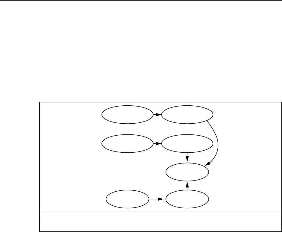
148 Chapter 15. Probabilistic Reasoning over Time
actions in the model). Thus, the stationary distribution towards which the battery level
tends has value 0 with probability 1. The curve for E(Batteryt|...5555000000 ...)
will asymptote to 0.
b.SeeFigureS15.4. TheCPTforBMeter1has a probability of transient failure (i.e.,
reporting 0) that increases with temperature.
c.Theagentcanobviouslycalculatetheposteriordistribution over Temp tby filtering
the observation sequence in the usual way. This posterior canbeinformativeifthe
effect of temperature on transient failure is non-negligible and transient failures occur
more frequently than do major changes in temperature. Essentially, the temperature is
estimated from the frequency of “blips” in the sequence of battery meter readings.
1
Battery
Battery 0
1
BMeter
0
BMBroken 1
BMBroken
0
Temp 1
Temp
Figure S15.4 Modification of Figure 15.13(a) to include the effect of external temperature
on the battery meter.
15.17 The process works exactly as on page 507. We start with the fullexpression:
P(R3|u1,u
2,u
3)=α%
r1%
r2
P(r1)P(u1|r1)P(r2|r1)P(u2|r2)P(R3|r2)P(u3|R3)
Whichever order we push in the summations, the variable elimination process never creates
factors containing more than two variables, which is the samesizeastheCPTsintheoriginal
network. In fact, given an HMM sequence of arbitrary length, we can eliminate the state
variables in any order.

Solutions for Chapter 16
Making Simple Decisions
16.1 It is interesting to create a histogram of accuracy on this task for the students in the
class. It is also interesting to record how many times each student comes within, say, 10% of
the right answer. Then you get a profile of each student: this one is an accurate guesser but
overly cautious about bounds, etc.
16.2
Pat is more likely to have a better car than Chris because she has more information with
which to choose. She is more likely to be disappointed, however, if she takes the expected
utility of the best car at face value. Using the results of exercise 16.11, we can compute the
expected disappointment to be about 1.54 times the standard deviation by numerical integra-
tion.
16.3
a.Theprobabilitythatthefirstheadsappearsonthenth toss is 2−n,so
EMV (L)=
∞
%
n=1
2−n·2n=
∞
%
n=1
1=∞
b.Typicalanswersrangebetween$4and$100.
c.Assumeinitialwealth(afterpayingcto play the game) of $(k−c);then
U(L)=
∞
%
n=1
2−n·(alog2(k−c+2
n)+b)
Assume k−c=$0for simplicity. Then
U(L)=
∞
%
n=1
2−n·(alog2(2n)+b)
=
∞
%
n=1
2−n·an +b
=2a+b
d.Themaximumamountcis given by the solution of
alog2k+b=
∞
%
n=1
2−n·(alog2(k−c+2
n)+b)
149

150 Chapter 16. Making Simple Decisions
For our simple case, we have
alog2c+b=2a+b
or c=$4.
16.4 The program itself is pretty trivial. But note that there are some studies showing you
get better answers if you ask subjects to move a slider to indicate a proportion, rather than
asking for a probability number. So having a graphical user interface is an advantage. The
main point of the exercise is to examine the data, expose inconsistent behavior on the part of
the subjects, and see how people vary in their choices.
16.5
a. Networks (ii) and (iii) can represent this network but not (i).
(ii) is fully connected, so it can represent any joint distribution.
(iii) follows the generative story given in the problem: the flavor is determined (pre-
sumably) by which machine the candy is made by, then the shape is randomly cut, and
the wrapper randomly chosen, the latter choice independently of the former.
(i) cannot represent this, as this network implies that the wrapper color and shape
are marginally independent, which is not so: a round candy is likely to be strawberry,
which is in turn likely to be wrapped in red, whilst converselyasquarecandyislikely
to be anchovy which is likely to be wrapped in brown.
b. Unlike (ii), (iii) has no cycles which we have seen simplifies inference. Its edges also
follow the, so probabilities will be easier to elicit. Indeed, the problem statement has
already given them.
c. Yes, because Wrapper and Shape are d-separated.
d. Once we know the Flavor we know the probability its wrapper will be red or brown. So
we marginalize Flavor out:
P(Wrapper =red)=%
f
P(Wrapper =red, Flavor =f)
=%
f
P(Flavor =f)P(Wrapper =red|Flavor =f)
=0.7×0.8+0.3×0.1
=0.59
e. We apply Bayes theorem, by first computing the joint probabilities
P(Flavor =strawberry, Shape =round, W rapper =red)
=P(Flavor =strawberry)×P(Shape =round|Flavor =strawberry)
×P(Wrapper =red|Flavor =strawberry)
=0.7×0.8×0.8
=0.448
P(Flavor =anchovy, Shape =round, W rapper =red)
=P(Flavor =anchovy)×P(Shape =round|Flavor =anchovy)

151
×P(Wrapper =red|Flavor =anchovy)
=0.3×0.1×0.1
=0.003
Normalizing these probabilities yields that it is strawberry with probability 0.448/(0.448+
0.003) ≈0.9933.
f. Its value is the probability that you have a strawberry uponunwrappingtimesthevalue
of a strawberry, plus the probability that you have a anchovy upon unwrapping times
the value of an anchovy or
0.7s+0.3a.
g. The value is the same, by the axiom of decomposability.
16.6
First observe that C∼[0.25,A;0.75,$0] and D∼[0.25,B;0.75$0].Thisfollows
from the axiom of decomposability. But by substitutability this means that the preference
ordering between the lotteries Aand Bmust be the same as that between Cand D.
16.7
As mentioned in the text, agents whose preferences violate expected utility theory
demonstrate irrational behavior, that is they can be made either to accept a bet that is a guar-
anteed loss for them (the case of violating transitivity is given in the text), or reject a bet that
is a guaranteed win for them. This indicates a problem for the agent.
16.8 The expected monetary value of the lottery Lis
EMV (L)= 1
50 ×$10 + 1
2000000 ×$1000000 = $0.70
Although $0.70 <$1,itisnotnecessarily irrational to buy the ticket. First we will consider
just the utilities of the monetary outcomes, ignoring the utility of actually playing the lottery
game. Using U(Sk+n)to represent the utility to the agent of having ndollars more than the
current state, and assuming that utility is linear for small values of money (i.e., U(Sk+n)≈
n(U(Sk+1)−U(Sk)) for −10 ≤n≤10), the utility of the lottery is:
U(L)= 1
50U(Sk+10)+ 1
2,000,000 U(Sk+1,000,000)
≈1
5U(Sk+1)+ 1
2,000,000 U(Sk+1,000,000)
This is more than U(Sk+1)when U(Sk+1,000,000)>1,600,000U($1).Thus,forapurchase
to be rational (when only money is considered), the agent mustbequiterisk-seeking. This
would be unusual for low-income individuals, for whom the price of a ticket is non-trivial. It
is possible that some buyers do not internalize the magnitudeoftheverylowprobabilityof
winning—to imagine an event is to assign it a “non-trivial” probability, in effect. Apparently,
these buyers are better at internalizing the large magnitudeoftheprize. Suchbuyersare
clearly acting irrationally.

152 Chapter 16. Making Simple Decisions
Some people may feel their current situation is intolerable,thatis,U(Sk)≈U(Sk±1)≈
u⊥.Thereforethesituationofhavingonedollarmoreorlesswould be equally intolerable,
and it would be rational to gamble on a high payoff, even if one that has low probability.
Gamblers also derive pleasure from the excitement of the lottery and the temporary
possession of at least a non-zero chance of wealth. So we should add to the utility of playing
the lottery the term tto represent the thrill of participation. Seen this way, the lottery is just
another form of entertainment, and buying a lottery ticket isnomoreirrationalthanbuying
amovieticket. Eitherway,youpayyourmoney,yougetasmallthrill t,and(mostlikely)
you walk away empty-handed. (Note that it could be argued thatdoingthiskindofdecision-
theoretic computation decreases the value of t.Itisnotclearifthisisagoodthingorabad
thing.)
16.9 This is an interesting exercise to do in class. Choose M1=$100,M2=$100,$1000,
$10000, $1000000. Ask for a show of hands of those preferring the lottery at different values
of p.Studentswillalmostalwaysdisplayriskaversion,butthere may be a wide spread in its
onset. A curve can be plotted for the class by finding the smallest pyielding a majority vote
for the lottery.
16.10 The protocol would be to ask a series of questions of the form “which would you
prefer” involving a monetary gain (or loss) versus an increase (or decrease) in a risk of death.
For example, “would you pay $100 for a helmet that would eliminate completely the one-in-
a-million chance of death from a bicycle accident.”
16.11
First observe that the cumulative distribution function formax{X1,...,X
k}is (F(x))k
since
P(max{X1,...,X
k}≤x)=P(X1≤x,...,Xk≤x)
=P(X1≤x)...P(Xk≤x)
=F(x)k
the second to last step by independence. The result follows astheprobabilitydensityfunction
is the derivative of the cumulative distribution function.
16.12
a. This question originally had a misprint: U(x)=−ex/R instead of U(x)=−e−x/R.
With the former utility function, the agent would be rather unhappy receiving $1000000
dollars.
Getting $400 for sure has expected utility
−e−400/400 =−1/e ≈−0.3679
while the getting $5000 with probability 0.6 and $0 otherwisehasexpectedutility
0.6−e−5000/400 +0.5−e−0/400 =−(0.6e−12.5+0.5) ≈−0.5000
so one would prefer the sure bet.
b. We want to find Rsuch that
e−100/R =0.5e−500/R +0.5
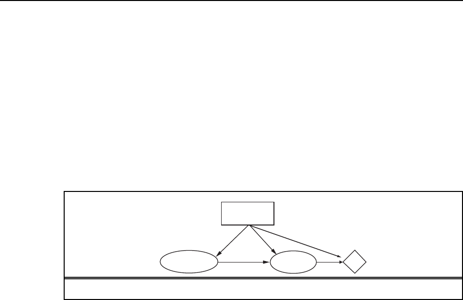
153
Solving this numerically, we find R=152up to 3sf.
16.13 The information associated with the utility node in Figure 16.6 is an action-value
table, and can be constructed simply by averaging out the Deaths,Noise,andCost nodes
in Figure 16.5. As explained in the text , modifications to aircraft noise levels or to the
importance of noise do not result in simple changes to the action-value table. Probably the
easiest way to do it is to go back to the original table in Figure16.5. Theexercisetherefore
illustrates the tradeoffs involved in using compiled representations.
16.14 The answer to this exercise depends on the probability valueschosenbythestu-
dent.
16.15
a. See Figure S16.1.
U
BuyBook
PassMastery
Figure S16.1 Adecisionnetworkforthebook-buyingproblem.
b. For each of B=band B=¬b,wecomputeP(p|B)and thus P(¬p|B)by marginal-
izing out M,thenusethistocomputetheexpectedutility.
P(p|b)=%
m
P(p|b, m)P(m|b)
=0.9×0.9+0.5×0.1
=0.86
P(p|¬b)=%
m
P(p|¬b, m)P(m|¬b)
=0.8×0.7+0.3×0.3
=0.65
The expected utilities are thus:
EU[b]=%
p
P(p|b)U(p, b)
=0.86(2000 −100) + 0.14(−100)
=1620
EU[¬b]=%
p
P(p|¬b)U(p, ¬b)
=0.65 ×2000 + 0.14 ×0
=1300

154 Chapter 16. Making Simple Decisions
c. Buy the book, Sam.
16.16 This exercise can be solved using an influence diagram packagesuchasIDEAL.The
specific values are not especially important. Notice how the tedium of encoding all the entries
in the utility table cries out for a system that allows the additive, multiplicative, and other
forms sanctioned by MAUT.
One of the key aspects of the fully explicit representation inFigure16.5isitsamenabil-
ity to change. By doing this exercise as well as Exercise 16.9,studentswillaugmenttheir
appreciation of the flexibility afforded by declarative representations, which can otherwise
seem tedious.
a.Forthispart,onecouldusesymbolicvalues(high,medium,low) for all the variables
and not worry too much about the exact probability values, or one could use actual
numerical ranges and try to assess the probabilities based onsomeknowledgeofthe
domain. Even with three-valued variables, the cost CPT has 54entries.
b.Thispartalmostcertainlyshouldbedoneusingasoftwarepackage.
c.Ifeachaircraftgenerateshalfasmuchnoise,weneedtoadjust the entries in the Noise
CPT.
d.Ifthenoiseattributebecomesthreetimesmoreimportant,the utility table entries must
all be altered. If an appropriate (e.g., additive) representation is available, then one
would only need to adjust the appropriate constants to reflectthechange.
e.Thispartshouldbedoneusingasoftwarepackage. Somepackages may offer VPI
calculation already. Alternatively, one can invoke the decision-making package repeat-
edly to do all the what-if calculations of best actions and their utilities, as required in
the VPI formula. Finally, one can write general-purpose VPI code as an add-on to a
decision-making package.
16.17 This question is a simple exercise in sequential decision making, and helps in making
the transition to Chapter 17. It also emphasizes the point that the value of information is
computed by examining the conditional plan formed by determining the best action for each
possible outcome of the test. It may be useful to introduce “decision trees” (as the term is
used in the decision analysis literature) to organize the information in this question. (See Pearl
(1988), Chapter 6.) Each part of the question analyzes some aspect of the tree. Incidentally,
the question assumes that utility and monetary value coincide, and ignores the transaction
costs involved in buying and selling.
a.ThedecisionnetworkisshowninFigureS16.2.
b.Theexpectednetgainindollarsis
P(q+)(2000 −1500) + P(q−)(2000 −2200) = 0.7×500 + 0.3×−200 = 290
c.Thequestioncouldprobablyhavebeenstatedbetter:Bayes’theoremisusedtocompute
P(q+|Pass),etc.,whereasconditionalizationissufficienttocomputeP(Pass).
P(Pass)=P(Pass|q+)P(q+)+P(Pass|q−)P(q−)
=0.8×0.7+0.35 ×0.3=0.665
155
Using Bayes’ theorem:
P(q+|Pass)= P(Pass|q+)P(q+)
P(Pass)=0.8×0.7
0.665 ≈0.8421
P(q−|Pass)≈1−0.8421 = 0.1579
P(q+|¬Pass)= P(¬Pass|q+)P(q+)
P(¬Pass)=0.2×0.7
0.335 ≈0.4179
P(q−|¬Pass)≈1−0.4179 = 0.5821
d.Ifthecarpassesthetest,theexpectedvalueofbuyingis
P(q+|Pass)(2000 −1500) + P(q−|Pass)(2000 −2200)
=0.8421 ×500 + 0.1579 ×−200 = 378.92
Thus buying is the best decision given a pass. If the car fails the test, the expected value
of buying is
P(q+|¬Pass)(2000 −1500) + P(q−|¬Pass)(2000 −2200)
=0.4179 ×500 + 0.5821 ×−200 = 92.53
Buying is again the best decision.
e.Sincetheactionisthesameforbothoutcomesofthetest,thetestitselfisworthless(if
it is the only possible test) and the optimal plan is simply to buy the car without the test.
(This is a trivial conditional plan.) For the test to be worthwhile, it would need to be
more discriminating in order to reduce the probability P(q+|¬Pass).Thetestwould
also be worthwhile if the market value of the car were less, or if the cost of repairs were
more.
An interesting additional exercise is to prove the general proposition that if αis the
best action for all the outcomes of a test then it must be the best action in the absence
of the test outcome.
Test
Buy
U
Outcome
Quality
Figure S16.2 Adecisionnetworkforthecar-buyingproblem.

156 Chapter 16. Making Simple Decisions
16.18
a.Intuitively,thevalueofinformationisnonnegativebecause in the worst case one could
simply ignore the information and act as if it was not available. A formal proof therefore
begins by showing that this policy results in the same expected utility. The formula for
the value of information is
VPI
E(Ej)=$%
k
P(Ej=ejk|E)EU(αejk |E,Ej=ejk)&−EU(α|E)
If the agent does αgiven the information Ej,itsexpectedutilityis
%
k
P(Ej=ejk|E)EU(α|E,Ej=ejk)=EU(α|E)
where the equality holds because the LHS is just the conditionalization of the RHS with
respect to Ej.Bydefinition,
EU(αejk |E,Ej=ejk)≥EU(α|E,Ej=ejk)
hence VPI
E(Ej)≥0.
b.Oneexplanationisthatpeopleareawareoftheirownirrationality and may want to
avoid making a decision on the basis of the extra information.Anothermightbethat
the value of information is small compared to the value of surprise—for example, many
people prefer not to know in advance what their birthday present is going to be.
c.Valueofinformationisnotsubmodularingeneral.Supposethat Ais the empty set and
Bis the set Y=1;andsupposethattheoptimaldecisionremainsunchangedunless
both X=1and Y=1are observed.

Solutions for Chapter 17
Making Complex Decisions
17.1 The best way to calculate this is NOT by thinking of all ways to get to any given square
and how likely all those ways are, but to compute the occupancyprobabilitiesateachtime
step. These are as follows:
Up Up Right Right Right
(1,1) 1.1 .02 .026 .0284 .02462
(1,2) .8 .24 .258 .2178 .18054
(1,3) .64 .088 .0346 .02524
(2,1) .1 .09 .034 .0276 .02824
(2,3) .512 .1728 .06224
(3,1) .01 .073 .0346 .02627
(3,2) .001 .0073 .04443
(3,3) .4097 .17994
(4,1) .008 .0656 .08672
(4,2) .0016 .01400
(4,3) .32776
Projection in an HMM involves multiplying the vector of occupancy probabilities by
the transition matrix. Here, the only difference is that there is a different transition matrix for
each action.
17.2 If we pick the policy that goes Right in all the optional states, and construct the cor-
responding transition matrix T,wefindthattheequilibriumdistribution—thesolutionto
Tx =x—has occupancy probabilities of 1/12 for (2,3), (3,1), (3,2), (3,3) and 2/3 for (4,1).
These can be found most simply by computing Tnxfor any initial occupancy vector x,forn
large enough to achieve convergence.
17.3 Stationarity requires the agent to have identical preferences between the sequence pair
[s0,s
1,s
2,...],[s0,s
′
1,s
′
2,...]and between the sequence pair [s1,s
2,...],[s′
1,s
′
2,...].Ifthe
utility of a sequence is its maximum reward, we can easily violate stationarity. For example,
[4,3,0,0,0,...]∼[4,0,0,0,0,...]
but
[3,0,0,0,...]≻[0,0,0,0,...].
157

158 Chapter 17. Making Complex Decisions
We can still define Uπ(s)as the expected maximum reward obtained by executing πstarting
in s.Theagent’spreferencesseempeculiar,nonetheless.Forexample, if the current state
shas reward Rmax,theagentwillbeindifferentamongallactions,butoncetheactionis
executed and the agent is no longer in s,itwillsuddenlystarttocareaboutwhathappens
next.
17.4 This is a deceptively simple exercise that tests the student’s understanding of the for-
mal definition of MDPs. Some students may need a hint or an example to get started.
a.Thekeyhereistogetthemaxandsummationintherightplace.ForR(s, a)we have
U(s)=max
a[R(s, a)+γ%
s′
T(s, a, s′)U(s′)
and for R(s, a, s′)we have
U(s)=max
a%
s′
T(s, a, s′)[R(s, a, s′)+γU(s′)] .
b.Thereareavarietyofsolutionshere. Oneistocreatea“pre-state” pre(s, a, s′)for
every s,a,s′,suchthatexecutingain sleads not to s′but to pre(s, a, s′).Inthisstate
is encoded the fact that the agent came from sand did ato get here. From the pre-state,
there is just one action bthat always leads to s′.LetthenewMDPhavetransitionT′,
reward R′,anddiscountγ′.Then
T′(s, a, pre(s, a, s′)) = T(s, a, s′)
T′(pre(s, a, s′),b,s
′)=1
R′(s, a)=0
R′(pre(s, a, s′),b)=γ−1
2R(s, a, s′)
γ′=γ1
2
c.Inkeepingwiththeideaofpart(b),wecancreatestatespost(s, a)for every s,a,such
that
T′(s, a, post(s, a, s′)) = 1
T′(post(s, a, s′),b,s
′)=T(s, a, s′)
R′(s)=0
R′(post(s, a, s′)) = γ−1
2R(s, a)
γ′=γ1
2
17.5 This can be done fairly simply by:
•Callpolicy-iteration (from "uncertainty/algorithms/dp.lisp")on
the Markov Decision Processes representing the 4x3 grid, with values for the step cost
ranging from, say, 0.0 to 1.0 in increments of 0.02.
•Foranytwoadjacentpoliciesthatdiffer,runbinarysearchonthestepcosttopinpoint
the threshold value.
•Convinceyourselfthatyouhaven’tmissedanypolicies,either by using too coarse an
increment in step size (0.02), or by stopping too soon (1.0).

159
One useful observation in this context is that the expected total reward of any fixed
policy is linear in r,theper-steprewardfortheemptystates. Imaginedrawingthe total reward
of a policy as a function of r—a straight line. Now draw all the straight lines corresponding
to all possible policies. The reward of the optimal policy as a function of ris just the max of
all these straight lines. Therefore it is a piecewise linear,convexfunctionofr.Hencethere
is a very efficient way to find all the optimal policy regions:
•Foranytwoconsecutivevaluesofrthat have different optimal policies, find the optimal
policy for the midpoint. Once two consecutive values of rgive the same policy, then
the interval between the two points must be covered by that policy.
•Repeatthisuntiltwopointsareknownforeachdistinctoptimal policy.
•Suppose(ra1,v
a1)and (ra2,v
a2)are points for policy a,and(rb1,v
b1)and (rb2,v
b2)
are the next two points, for policy b.Clearly,wecandrawstraightlinesthroughthese
pairs of points and find their intersection. This does not mean, however, that there is no
other optimal policy for the intervening region. We can determine this by calculating
the optimal policy for the intersection point. If we get a different policy, we continue
the process.
The policies and boundaries derived from this procedure are shown in Figure S17.1. The
figure shows that there are nine distinct optimal policies! Notice that as rbecomes more
negative, the agent becomes more willing to dive straight into the –1 terminal state rather
than face the cost of the detour to the +1 state.
The somewhat ugly code is as follows. Notice that because the lines for neighboring
policies are very nearly parallel, numerical instability isaseriousproblem.
(defun policy-surface (mdp r1 r2 &aux prev (unchanged nil))
"returns points on the piecewise-linear surface
defined by the value of the optimal policy of mdp as a
function of r"
(setq rvplist
(list (cons r1 (r-policy mdp r1)) (cons r2 (r-policy mdp r2))))
(do ()
(unchanged rvplist)
(setq unchanged t)
(setq prev nil)
(dolist (rvp rvplist)
(let*((rest (cdr (member rvp rvplist :test #’eq)))
(next (first rest))
(next-but-one (second rest)))
(dprint (list (first prev) (first rvp)
’*(first next) (first next-but-one)))
(when next
(unless (or (= (first rvp) (first next))
(policy-equal (third rvp) (third next) mdp))
(dprint "Adding new point(s)")
(setq unchanged nil)
(if (and prev next-but-one
(policy-equal (third prev) (third rvp) mdp)
(policy-equal (third next) (third next-but-one) mdp))

160 Chapter 17. Making Complex Decisions
(let*((intxy (policy-vertex prev rvp next next-but-one))
(int (cons (xy-x intxy) (r-policy mdp (xy-x intxy)))))
(dprint (list "Found intersection" intxy))
(cond ((or (< (first int) (first rvp))
(> (first int) (first next)))
(dprint "Intersection out of range!")
(let ((int-r (/ (+ (first rvp) (first next)) 2)))
(setq int (cons int-r (r-policy mdp int-r))))
(push int (cdr (member rvp rvplist :test #’eq))))
((or (policy-equal (third rvp) (third int) mdp)
(policy-equal (third next) (third int) mdp))
(dprint "Found policy boundary")
(push (list (first int) (second int) (third next))
(cdr (member rvp rvplist :test #’eq)))
(push (list (first int) (second int) (third rvp))
(cdr (member rvp rvplist :test #’eq))))
(t (dprint "Found new policy!")
(push int (cdr (member rvp rvplist :test #’eq))))))
(let*((int-r (/ (+ (first rvp) (first next)) 2))
(int (cons int-r (r-policy mdp int-r))))
(dprint (list "Adding split point" (list int-r (second int))))
(push int (cdr (member rvp rvplist :test #’eq))))))))
(setq prev rvp))))
(defun r-policy (mdp r &aux U)
(set-rewards mdp r)
(setq U (value-iteration mdp
(copy-hash-table (mdp-rewards mdp) #’identity)
:epsilon 0.0000000001))
(list (gethash ’(1 1) U) (optimal-policy U (mdp-model mdp) (mdp-rewards mdp))))
(defun set-rewards (mdp r &aux (rewards (mdp-rewards mdp))
(terminals (mdp-terminal-states mdp)))
(maphash #’(lambda (state reward)
(unless (member state terminals :test #’equal)
(setf (gethash state rewards) r)))
rewards))
(defun policy-equal (p1 p2 mdp &aux (match t)
(terminals (mdp-terminal-states mdp)))
(maphash #’(lambda (state action)
(unless (member state terminals :test #’equal)
(unless (eq (caar (gethash state p1)) (caar (gethash state p2)))
(setq match nil))))
p1)
match)
(defun policy-vertex (rvp1 rvp2 rvp3 rvp4)
(let ((a (make-xy :x (first rvp1) :y (second rvp1)))
(b (make-xy :x (first rvp2) :y (second rvp2)))
(c (make-xy :x (first rvp3) :y (second rvp3)))
(d (make-xy :x (first rvp4) :y (second rvp4))))

161
(intersection-point (make-line :xy1 a :xy2 b)
(make-line :xy1 c :xy2 d))))
(defun intersection-point (l1 l2)
;;; l1 is line ab; l2 is line cd
;;; assume the lines cross at alpha a + (1-alpha) b,
;;; also known as beta c + (1-beta) d
;;; returns the intersection point unless they’re parallel
(let*((a (line-xy1 l1))
(b (line-xy2 l1))
(c (line-xy1 l2))
(d (line-xy2 l2))
(xa (xy-x a)) (ya (xy-y a))
(xb (xy-x b)) (yb (xy-y b))
(xc (xy-x c)) (yc (xy-y c))
(xd (xy-x d)) (yd (xy-y d))
(q (- (*(- xa xb) (- yc yd))
(*(- ya yb) (- xc xd)))))
(unless (zerop q)
(let ((alpha (/ (- (*(- xd xb) (- yc yd))
(*(- yd yb) (- xc xd)))
q)))
(make-xy :x (float (+ (*alpha xa) (*(- 1 alpha) xb)))
:y (float (+ (*alpha ya) (*(- 1 alpha) yb))))))))
17.6
a.Tofindtheproof,itmayhelpfirsttodrawapictureoftwoarbitrary functions fand
gand mark the maxima; then it is easy to find a point where the difference between
the functions is bigger than the difference between the maxima. Assume, w.l.o.g., that
maxaf(a)≥maxag(a),andletfhave its maximum value at a∗.Thenwehave
|max
af(a)−max
ag(a)|=max
af(a)−max
ag(a)(by assumption)
=f(a∗)−max
ag(a)
≤f(a∗)−g(a∗)
≤max
a|f(a)−g(a)|(by definition of max)
b.FromthedefinitionoftheBoperator (Equation (17.6)) we have
|(BU
i−BU′
i)(s)|=|R(s)+γmax
a∈A(s)%
s′
P(s′|s, a)Ui(s′)
−R(s)−γmax
a∈A(s)%
s′
P(s′|s, a)U′
i(s′)|
=γ|max
a∈A(s)%
s′
P(s′|s, a)Ui(s′)−max
a∈A(s)%
s′
P(s′|s, a)U′
i(s′)|
≤γmax
a∈A(s)|%
s′
P(s′|s, a)Ui(s′)−%
s′
P(s′|s, a)U′
i(s′)|
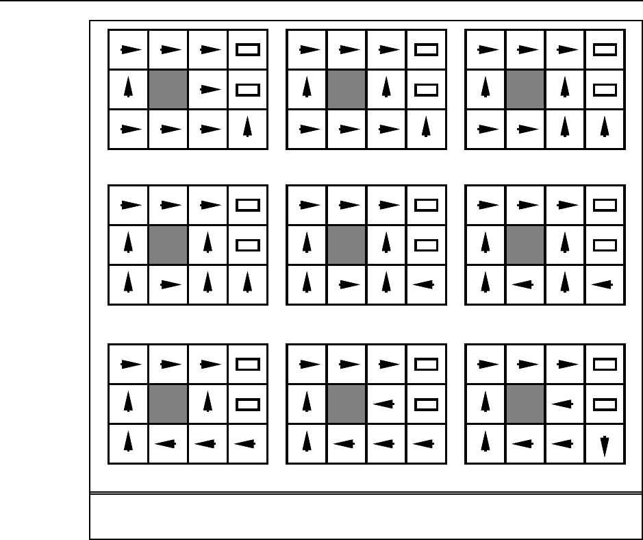
162 Chapter 17. Making Complex Decisions
− 1
+ 1
− 1
+ 1
− 1
+ 1
− 1
+ 1
− 1
+ 1
− 1
+ 1
− 1
+ 1
− 1
+ 1
− 1
+ 1
r = [−1.6284 : −1.3702] r = [−1.3702 : −0.7083]
r = [−0.7083 : −0.4278] r = [−0.4278 : −0.0850] r = [−0.0850 : −0.0480]
r = [−0.0480 : −0.0274] r = [−0.0274 : −0.0218] r = [−0.0218 : 0.0000]
r = [− : −1.6284]
8
Figure S17.1 Optimal policies for different values of the cost of a step in the 4×3envi-
ronment, and the boundaries of the regions with constant optimal policy.
=γ|%
s′
P(s′|s, a∗(s))Ui(s′)−%
s′
P(s′|s, a∗(s))U′
i(s′)|
=γ|%
s′
P(s′|s, a∗(s))(Ui(s′)−U′
i(s′)|
Inserting this into the expression for the max norm, we have
||BU
i−BU′
i)|| =max
s|(BU
i−BU′
i)(s)|
≤γmax
s|%
s′
P(s′|s, a∗(s))(Ui(s′)−U′
i(s′))|
≤γmax
s|Ui(s)−U′
i(s)|=γ||Ui−U′
i||
17.7
163
a.ForUAwe have
UA(s)=R(s)+max
a%
s′
P(s′|a, s)UB(s′)
and for UBwe have
UB(s)=R(s)+min
a%
s′
P(s′|a, s)UA(s′).
b.Todovalueiteration,wesimplyturneachequationfrompart(a)intoaBellmanupdate
and apply them in alternation, applying each to all states simultaneously. The process
terminates when the utility vector for one player is the same as the previous utility
vector for the same player (i.e., two steps earlier). (Note that typically UAand UBare
not the same in equilibrium.)
c.ThestatespaceisshowninFigureS17.2.
d.Wemarktheterminalstatevaluesinboldandinitializeother values to 0. Value iteration
proceeds as follows:
(1,4) (2,4) (3,4) (1,3) (2,3) (4,3) (1,2) (3,2) (4,2) (2,1) (3,1)
UA00000+1 0 0 +1 –1 –1
UB0 0 0 0 –1 +1 0–1 +1 –1 –1
UA000–1 +1 +1 –1 +1 +1 –1 –1
UB–1 +1 +1 –1 –1 +1 –1 –1 +1 –1 –1
UA+1 +1 +1 –1 +1 +1 –1 +1 +1 –1 –1
UB–1 +1 +1 –1 –1 +1 –1 –1 +1 –1 –1
and the optimal policy for each player is as follows:
(1,4) (2,4) (3,4) (1,3) (2,3) (4,3) (1,2) (3,2) (4,2) (2,1) (3,1)
π∗
A(2,4) (3,4) (2,4) (2,3) (4,3) (3,2) (4,2)
π∗
B(1,3) (2,3) (3,2) (1,2) (2,1) (1,3) (3,1)
(1,4)
(1,3)
(1,2)
(2,4)
(2,3)
(2,1)
(3,4)
(3,2)
(3,1)
(4,3)
(4,2)
−1−1
+1
+1
Figure S17.2 State-space graph for the game in Figure 5.17.
17.8
a. r=100.
u l .
u l d
u l l
164 Chapter 17. Making Complex Decisions
See the comments for part d. This should have been r=−100 to illustrate an
alternative behavior:
r r .
d r u
r r u
Here, the agent tries to reach the goal quickly, subject to attempting to avoid the
square (1,3) as much as possible. Note that the agent will choose to move Down in
square (1,2) in order to actively avoid the possibility of “accidentally”movingintothe
square (1,3) if it tried to move Right instead, since the penalty for movingintosquare
(1, 3) is so great.
b. r=−3.
rr.
rru
rru
Here, the agent again tries to reach the goal as fast as possible while attempting to
avoid the square (1,3),butthepenaltyforsquare(1,3) is not so great that the agent
will try to actively avoid it at all costs. Thus, the agent willchoosetomoveRightin
square (1,2) in order to try to get closer to the goal even if it occasionallywillresultin
atransitiontosquare(1,3).
c. r=0.
r r .
u u u
u u u
Here, the agent again tries to reach the goal as fast as possible, but will try to do so
via a path that includes square (1,3) if possible. This results from the fact that square
(1,3) does not incur the reward of −1in all other non-goal states, so it reaching the goal
via a path through that square can potentially have slightly greater reward than another
path of equal length that does not pass through (1,3).
d. r=3.
u l .
u l d
u l l
17.9 The utility of Up is
50γ−
101
%
t=2
γt=50γ−γ21−γ100
1−γ,
while the utility of Down is
−50γ+
101
%
t=2
γt=−50γ+γ21−γ100
1−γ.
Solving numerically we find the indifference point to be γ≈0.9844:largerthanthis
and we want to go Down to avoid the expensive long-term consequences, smaller than this
and we want to go Up to get the immediate benefit.

165
17.10
a.Intuitively,theagentwantstogettostate3assoonaspossible, because it will pay a
cost for each time step it spends in states 1 and 2. However, theonlyactionthatreaches
state 3 (action b)succeedswithlowprobability,sotheagentshouldminimizethecost
it incurs while trying to reach the terminal state. This suggests that the agent should
definitely try action bin state 1; in state 2, it might be better to try action ato get to state
1(whichisthebetterplacetowaitforadmissiontostate3),rather than aiming directly
for state 3. The decision in state 2 involves a numerical tradeoff.
b.Theapplicationofpolicyiterationproceedsinalternating steps of value determination
and policy update.
•Initialization:U←⟨−1,−2,0⟩,P←⟨b, b⟩.
•Val ue d et er mination:
u1=−1+0.1u3+0.9u1
u2=−2+0.1u3+0.9u2
u3=0
That is, u1=−10 and u2=−20.
Policy update:Instate1,
%
j
T(1,a,j)uj=0.8×−20 + 0.2×−10 = −18
while
%
j
T(1,b,j)uj=0.1×0×0.9×−10 = −9
so action bis still preferred for state 1.
In state 2,
%
j
T(1,a,j)uj=0.8×−10 + 0.2×−20 = −12
while
%
j
T(1,b,j)uj=0.1×0×0.9×−20 = −18
so action ais preferred for state 1. We set unchanged?←false and proceed.
•Val ue d et er mination:
u1=−1+0.1u3+0.9u1
u2=−2+0.8u1+0.2u2
u3=0
Once more u1=−10;now,u2=−15.Policy update:Instate1,
%
j
T(1,a,j)uj=0.8×−15 + 0.2×−10 = −14

166 Chapter 17. Making Complex Decisions
while
%
j
T(1,b,j)uj=0.1×0×0.9×−10 = −9
so action bis still preferred for state 1.
In state 2,
%
j
T(1,a,j)uj=0.8×−10 + 0.2×−15 = −11
while
%
j
T(1,b,j)uj=0.1×0×0.9×−15 = −13.5
so action ais still preferred for state 1. unchanged?remains true,andwetermi-
nate.
Note that the resulting policy matches our intuition: when instate2,trytomovetostate
1, and when in state 1, try to move to state 3.
c.Aninitialpolicywithactionain both states leads to an unsolvable problem. The initial
value determination problem has the form
u1=−1+0.2u1+0.8u2
u2=−2+0.8u1+0.2u2
u3=0
and the first two equations are inconsistent. If we were to try to solve them iteratively,
we would find the values tending to −∞.
Discounting leads to well-defined solutions by bounding the penalty (expected dis-
counted cost) an agent can incur at either state. However, thechoiceofdiscountfactor
will affect the policy that results. For γsmall, the cost incurred in the distant future
plays a negligible role in the value computation, because γnis near 0. As a result,
an agent could choose action bin state 2 because the discounted short-term cost of re-
maining in the non-terminal states (states 1 and 2) outweighsthediscountedlong-term
cost of action bfailing repeatedly and leaving the agent in state 2. An additional exer-
cise could ask the student to determine the value of γat which the agent is indifferent
between the two choices.
17.11 The framework for this problem is in "uncertainty/domains/4x3-mdp.lisp".
There is still some synthesis for the student to do for answer b. For c. some experimental de-
sign is necessary.
17.12 (Note: Early printings used “value determination,” a term accidentally left over from
the second edition, instead of “policy evaluation.”) The policy evaluation algorithm calculates
Uπ(s)for a given policy π.ThepolicyforanagentthatthinksUis the true utility and Pis
the true model would be based on Equation (17.4):
π(s)=argmax
a∈A(s)%
s′
P(s′|s, a)U(s′).
167
Given this policy, the policy loss compared to the true optimal policy, starting in state s,is
just Uπ∗(s)−Uπ(s).
17.13 The belief state update is given by Equation (17.11), i.e.,
b′(s′)=αP(e|s′)%
s
P(s′|s, a)b(s).
It may be helpful to compute this in two stages: update for the action, then update for the ob-
servation. The observation probabilities P(e|s′)are all either 0.9 (for squares that actually
have one wall) or 0.1 (for squares with two walls). The following table shows the results.
Note in particular how the probability mass concentrates on (3,2).
Left 1wall Left 1wall
(1,1) .11111 .20000 .06569 .09197 .02090
(1,2) .11111 .11111 .03650 .04234 .00962
(1,3) .11111 .20000 .06569 .09197 .02090
(2,1) .11111 .11111 .03650 .27007 .06136
(2,3) .11111 .11111 .03650 .05985 .01360
(3,1) .11111 .11111 .32847 .06861 .14030
(3,2) .11111 .11111 .32847 .30219 .61791
(3,3) .11111 .02222 .06569 .03942 .08060
(4,1) .11111 .01111 .00365 .00036 .00008
(4,2) 0.01111 .03285 .03321 .06791
(4,3) 0 0 0 0 0
17.14 In a sensorless environment, POMDP value iteration is essentially the same as ordi-
nary state-space search—the branching ocurs only on acton choices, not observations. Hence
the time complexity is O(|A|d).
17.15 Policies for the 2-state MDP all have a threshold belief p,suchthatifb(0) >pthen
the optimal action is Go,otherwiseitisStay.Thequestionis,whatdoesthischangedoto
the threshold? By making sensing more informative in state 0 and less informative in state 1,
the change has made state 0 more desirable, hence the threshold value pincreases.
17.16 This question is simple a matter of examining the definitions.Inadominantstrat-
egy equilibrium [s1,...,s
n],itisthecasethatforeveryplayeri,siis optimal for every
combination t−iby the other players:
∀i∀t−i∀s′
i[si,t
−i]≻
∼[s′
i,t
−i].
In a Nash equilibrium, we simply require that siis optimal for the particular current combi-
nation s−iby the other players:
∀i∀s′
i[si,s
−i]≻
∼[s′
i,s
−i].
Therefore, dominant strategy equilibrium is a special case of Nash equilibrium. The converse
does not hold, as we can show simply by pointing to the CD/DVD game, where neither of the
Nash equilibria is a dominant strategy equilibrium.

168 Chapter 17. Making Complex Decisions
17.17 In the following table, the rows are labelled by A’s move and the columns by B’s
move, and the table entries list the payoffs to A and B respectively.
R P S F W
R0,0 –1,1 1,-1 –1,1 1,-1
P1,-1 0,0 –1,1 –1,1 1,-1
S–1,1 1,-1 0,0 –1,1 1,-1
F1,-1 1,-1 1,-1 0,0 –1,1
W–1,1 –1,1 –1,1 1,-1 0,0
Suppose Achooses a mixed strategy [r:R;p:P;s:S;f:F;w:W],wherer+p+s+
f+w=1.Thepayoffto A of B’s possible pure responses are as follows:
R:+p−s+f−w
P:−r+s+f−w
S:+r−p+f−w
F:−r−p−s+w
W:+r+p+s−f
It is easy to see that no option is dominated over the whole region. Solving for the intersection
of the hyperplanes, we find r=p=s=1/9and f=w=1/3.Bysymmetry,wewillfindthe
same solution when Bchooses a mixed strategy first.
17.18 We apply iterated strict dominance to find the pure strategy. First, Pol: do nothing
dominates Pol: contract,sowedropthePol: contract row. Next, Fed: contract dominates
Fed: do nothing and Fed: expand on the remaining rows, so we drop those columns. Finally,
Pol: expand dominates Pol: do nothing on the one remaining column. Hence the only Nash
equilibrium is a dominant strategy equilibrium with Pol: expand and Fed: contract.Thisis
not Pareto optimal: it is worse for both players than the four strategy profiles in the top right
quadrant.
17.19 This question really has two answers, depending on what assumption is made about
the probability distribution over bidder’s private valuations vifor the item.
In a Dutch auction, just as in a first-price sealed-bid auction, bidders must estimate the
likely private values of the other bidders. When the price is higher than vi,agentiwill not
bid, but as soon as the price reaches vi,hefacesadilemma:bidnowandwintheitemata
higher price than necessary, or wait and risk losing the item to another bidder. In the standard
models of auction theory, each bidder, in addition to a private value vi,hasaprobability
density pi(v1,...,v
n)over the private values of all nbidders for the item. In particular, we
consider independent private values,sothatthedistributionovertheotherbidders’values
INDEPENDENT
PRIVATE VALUES
is independent of vi.Eachbidderwillchooseabid—i.e.,thefirstpriceatwhichthey will bid
if that price is reached—through a bidding function bi(vi).
We are interested in finding a Nash equilibrium (technically aBayes–Nash equilibrium
in which each bidder’s bidding function is optimal given the bidding functions of the other
agents. Under risk-neutrality, optimality of a bid bis determined by the expected payoff, i.e.,
the probability of winning the auction with bid btimes the profit when paying that amount

169
for the item. Now, agent iwins the auction with bid bif all the other bids are less than b;
let the probability of this happening be Wi(b)for whatever fixed bidding functions the other
bidders use. (Wi(b)is thus a cumulative probability distribution and nondecreasing in b;
under independent private values, it does not depend on vi.) Then we can write the expected
payoff for agent ias
Qi(vi,b)=Wi(b)(vi−b)
and the optimality condition in equilibrium is therefore
∀i, b Wi(bi(vi))(vi−bi(vi)) ≥Wi(b)(vi−b).(17.1)
We now prove that the bidding functions bi(vi)must be monotonic,i.e.,nondecreasing in the
private valuation vi.Letvand v′be two different valuations, with b=bi(v)and b′=bi(v′).
Applying Equation (17.1) twice, first to say that (v, b)is better than (v, b′)and then to say
that (v′,b
′)is better than (v′,b),weobtain
Wi(b)(v−b)≥Wi(b′)(v−b′)
Wi(b′)(v′−b′)≥Wi(b)(v′−b)
Rearranging, these become
v(Wi(b)−Wi(b′)) ≥Wi(b)b−Wi(b′)b′
v′(Wi(b′)−Wi(b)) ≥Wi(b′)b′−Wi(b)b
Adding these equations, we have
(v′−v)(Wi(b′)−Wi(b)) ≥0
from which it follows that if v′>v,thenWi(b′)≥Wi(b).Monotonicitydoesnotfollow
immediately, however; we have to handle two cases:
•IfWi(b′)>W
i(b),orifWiis strictly increasing, then b′≥band bi(·)is monotonic.
•Otherwise,Wi(b′)=Wi(b)and Wiis flat between band b′.NowifWiis flat in any
interval [x, y],thenanoptimalbiddingfunctionwillpreferxover any other bid in the
interval since that maximizes the profit on winning without affecting the probability of
winning; hence, we must have b′=band again bi(·)is monotonic.
Intuitively, the proof amounts to the following: if a higher valuation could result in a lower
bid, then by swapping the two bids the agent could increase thesum of the payoffs for the
two bids, which means that at least one of the two original bids is suboptimal.
Returning to the question of efficiency—the property that theitemgoestothebidder
with the highest valuation—we see that it follows immediately from monotonicity in the
case where the bidders’ prior distributions over valuationsaresymmetric or identically dis-
tributed.1
1According to Milgrom (1989), Vickrey (1961) proved that under this assumption, the Dutch auction is efficient.
Vickrey’s argument in Appendix III for the monotonicity of the bidding function is similar to the argument
above but, as written, seems to apply only to the uniform-distribution case he was considering. Indeed, much
of his analysis beginning with Appendix II is based on an inverse bidding function, which implicitly assumes
monotonicity of the bidding function. Many other authors also begin by assuming monotonicity, then derive the
form of the optimal bidding function, and then show it is monotonic. This proves the existence of an equilibrium
with monotonic bidding functions, but not that all equilibria have this property.

170 Chapter 17. Making Complex Decisions
Vickrey (1961) proves that the auction is not efficient in the asymmetric case where one
player’s distribution is uniform over [0,1] and the other’s is uniform over [a, b]for a>0.
Milgrom (1989) provides another, more transparent example of inefficiency: Suppose Alice
has a known, fixed value of $101 for an item, while Bob’s value is$50withprobability0.8
and $75 with probability 0.2. Given that Bob will never bid higher than his valuation, Alice
can see that a bid of $51 will win at least 80% of the time, giving an expected profit of at
least 0.8×($101 −$51) = $40.Ontheotherhand,anybidof$62ormorecannotyieldan
expected profit at most $39, regardless of Bob’s bid, and so is dominated by the bid of $51.
Hence, in any equilibrium, Alice’s bid at most $61. Knowing this, Bob can bid $62 whenever
his valuation is $75 and be sure of winning. Thus, with 20% probability, the item goes to
Bob, whose valuation for it is lower than Alice’s. This violates efficiency.
Besides efficiency in the symmetric case, monotonicity has another important conse-
quence for the analysis of the Dutch (and first-price) auction:itmakesitpossibletoderive
the exact form of the bidding function. As it stands, Equation(17.1)isdifficultorimpossible
to solve because the cumulative distribution of the other bidders’ bids, Wi(b),dependson
their bidding functions, so all the bidding functions are coupled together. (Note the similar-
ity to the Bellman equations for an MDP.) With monotonicity, however, we can define Wi
in terms of the known valuation distributions. Assuming independence and symmetry, and
writing b−1
i(b)for the inverse of the (monotonic) bidding function, we have
Qi(vi,b)=(P(b−1
i(b)))n−1(vi−b)
where P(v)is the probability that an individual valuation is less than v.Atequilibrium,
where bmaximizes Qi,thefirstderivativemustbezero:
∂Q
∂b=0=(n−1)(P(b−1
i(b)))n−2p(b−1
i(b))(vi−b)
b′
i(b−1
i(b)) −(P(b−1
i(b)))n−1
where we have used the fact that df −1(x)/dx =1/f ′(f−1(x)).
For an equilibrium bidding function, of course, b−1
i(b)=vi;substitutingthisandsim-
plifying, we find the following differential equation for bi:
b′
i(vi)=(vi−bi(vi)) ·(n−1)p(vi)/P (vi).
To find concrete solutions we also need to establish a boundarycondition.Supposev0is the
lowest possible valuation for the item; then we must have bi(v0)=v0(Milgrom and Weber,
1982). Then the solution, as shown by McAfee and McMillan (1987), is
bi(vi)=vi−<vi
v0(P(v))n−1dv
(P(vi))n−1.
For example, suppose pis uniform in [0,1];thenP(v)=vand bi(vi)=vi·(n−1)/n,which
is the classical result obtained by Vickrey (1961).
17.20 In such an auction it is rational to continue bidding as long aswinningtheitemwould
yield a profit, i.e., one is willing to bid up to 2vi.Theauctionwillendat2vo+d,sothewinner
will pay vo+d/2,slightlylessthanintheregularversion.

171
17.21 Every game is either a win for one side (and a loss for the other)oratie.With2fora
win, 1 for a tie, and 0 for a loss, 2 points are awarded for every game, so this is a constant-sum
game.
If 1 point is awarded for a loss in overtime, then for some games3pointsareawarded
in all. Therefore, the game is no longer constant-sum.
Suppose we assume that team A has probability rof winning in regular time and team
Bhasprobabilitysof winning in regular time (assuming normal play). Furthermore, assume
team B has a probability qof winning in overtime (which occurs if there is a tie after regular
time). Once overtime is reached (by any means), the expected utilities are as follows:
UO
A=1+p
UO
B=1+q
In normal play, the expected utilities are derived from the probability of winning plus the
probability of tying times the expected utility of overtime play:
UA=2r+(1−r−s)(1 + p)
UB=2s+(1−r−s)(1 + q)
Hence A has an incentive to agree if UO
A>U
A,or
1+p>2r+(1−r−s)(1 + p)or rp −r+sp +s>0or p>r−s
r+s
and B has an incentive to agree if UO
B>U
B,or
1+q>2s+(1−r−s)(1 + q)or sq −s+rq +r>0or q>s−r
r+s
When both of these inequalities hold, there is an incentive totieinregulationplay. Forany
values of rand s,therewillbevaluesofpand qsuch that both inequalities hold.
For an in-depth statistical analysis of the actual effects oftherulechangeandamore
sophisticated treatment of the utility functions, see “Overtime! Rules and Incentives in the
National Hockey League” by Stephen T. Easton and Duane W. Rockerbie, available at
http://people.uleth.ca/˜rockerbie/OVERTIME.PDF.

Solutions for Chapter 18
Learning from Examples
18.1 The aim here is to couch language learning in the framework of the chapter, not to
solve the problem! This is a very interesting topic for class discussion, raising issues of
nature vs. nurture, the indeterminacy of meaning and reference, and so on. Basic references
include Chomsky (1957) and Quine (1960).
The first step is to appreciate the variety of knowledge that goes under the heading
“language.” The infant must learn to recognize and produce speech, learn vocabulary, learn
grammar, learn the semantic and pragmatic interpretation ofaspeechact,andlearnstrategies
for disambiguation, among other things. The performance elements for this (in humans) and
their associated learning mechanisms are obviously very complex and as yet little is known
about them.
Anaivemodelofthelearningenvironmentconsidersjusttheexchange of speech sounds.
In reality, the physical context of each utterance is crucial: a child must see the context in
which “watermelon” is uttered in order to learn to associate “watermelon” with watermel-
ons. Thus, the environment consists not just of other humans but also the physical objects
and events about which discourse takes place. Auditory sensors detect speech sounds, while
other senses (primarily visual) provide information on the physical context. The relevant
effectors are the speech organs and the motor capacities thatallowtheinfanttorespondto
speech or that elicit verbal feedback.
The performance standard could simply be the infant’s general utility function, however
that is realized, so that the infant performs reinforcement learning to perform and respond to
speech acts so as to improve its well-being—for example, by obtaining food and attention.
However, humans’ built-in capacity for mimicry suggests that the production of sounds sim-
ilar to those produced by other humans is a goal in itself. The child (once he or she learns to
differentiate sounds and learn about pointing or other meansofindicatingsalientobjects)is
also exposed to examples of supervised learning: an adult says “shoe” or “belly button” while
indicating the appropriate object. So sentences produced byadultsprovidelabelledpositive
examples, and the response of adults to the infant’s speech acts provides further classification
feedback.
Mostly, it seems that adults do not correct the child’s speech, so there are very few neg-
ative classifications of the child’s attempted sentences. This is significant because early work
on language learning (such as the work of Gold, 1967) concentrated just on identifying the
set of strings that are grammatical, assuming a particular grammatical formalism. If there are
172

173
only positive examples, then there is nothing to rule out the grammar S→Word
∗.Some
theorists (notably Chomsky and Fodor) used what they call the“povertyofthestimulus”argu-
ment to say that the basic universal grammar of languages mustbeinnate,becauseotherwise
(given the lack of negative examples) there would be no way that a child could learn a lan-
guage (under the assumptions of language learning as learning a set of grammatical strings).
Critics have called this the “poverty of the imagination” argument—I can’t think of a learning
mechanism that would work, so it must be innate. Indeed, if we go to probabilistic context
free grammars, then it is possible to learn a language withoutnegativeexamples.
18.2 Learning tennis is much simpler than learning to speak. The requisite skills can be
divided into movement, playing strokes, and strategy. The environment consists of the court,
ball, opponent, and one’s own body. The relevant sensors are the visual system and propri-
oception (the sense of forces on and position of one’s own bodyparts). Theeffectorsare
the muscles involved in moving to the ball and hitting the stroke. The learning process in-
volves both supervised learning and reinforcement learning. Supervised learning occurs in
acquiring the predictive transition models, e.g., where theopponentwillhittheball,where
the ball will land, and what trajectory the ball will have after one’s own stroke (e.g., if I hit
ahalf-volleythis way, it goes into the net, but if I hit it that way, it clears the net). Rein-
forcement learning occurs when points are won and lost—this is particularly important for
strategic aspects of play such as shot placement and positioning (e.g., in 60% of the points
where I hit a lob in response to a cross-court shot, I end up losing the point). In the early
stages, reinforcement also occurs when a shot succeeds in clearing the net and landing in the
opponent’s court. Achieving this small success is itself a sequential process involving many
motor control commands, and there is no teacher available to tell the learner’s motor cortex
which motor control commands to issue.
18.3 The algorithm may not return the “correct” tree, but it will return a tree that is logi-
cally equivalent, assuming that the method for generating examples eventually generates all
possible combinations of input attributes. This is true because any two decision tree defined
on the same set of attributes that agree on all possible examples are, by definition, logically
equivalent. The actually form of the tree may differ because there are many different ways to
represent the same function. (For example, with two attributes Aand Bwe can have one tree
with Aat the root and another with Bat the root.) The root attribute of the original tree may
not in fact be the one that will be chosen by the information gain geuristic when applied to
the training examples.
18.4 This question brings a little bit of mathematics to bear on theanalysisofthelearning
problem, preparing the ground for Chapter 20. Error minimization is a basic technique in
both statistics and neural nets. The main thing is to see that the error on a given training
set can be written as a mathematical expression and viewed as afunctionofthehypothesis
chosen. Here, the hypothesis in question is a single number α∈[0,1] returned at the leaf.
a.Ifαis returned, the absolute error is
E=p(1 −α)+nα=α(n−p)+p=nwhen α=1
=pwhen α=0

174 Chapter 18. Learning from Examples
This is minimized by setting
α=1if p>n
α=0if p<n
That is, αis the majority value.
b.Firstcalculatethesumofsquarederrors,anditsderivative:
E=p(1 −α)2+nα2
dE
dα=2αn−2p(1 −α)=2α(p+n)−2p
The fact that the second derivative, d2E
dα2=2(p+n),isgreaterthanzeromeansthatE
is minimized (not maximized) where dE
dα=0,i.e.,whenα=p
p+n.
18.5 This result emphasizes the fact that any statistical fluctuations caused by the random
sampling process will result in an apparent information gain.
The easy part is showing that the gain is zero when each subset has the same ratio of
positive examples. The gain is defined as
B*p
p+n+−
d
%
k=1
pk+nk
p+nB*pk
pk+nk+
Since p=!pkand n=!nk,ifpk/(pk+nk)is the same for all kwe must have pk/(pk+
nk)=p/(p+n)for all k.Fromthis,weobtain
Gain =B*p
p+n+−B*p
p+n+1
p+n
d
%
k=1
pk+nk
=B*p
p+n+−B*p
p+n+1
p+n(p+n)=0
Note that this holds for all values of pk+nk.Toprovethatthevalueispositiveelsewhere,we
can apply the method of Lagrange multipliers to show that thisistheonlystationarypoint;
the gain is clearly positive at the extreme values, so it is positive everywhere but the stationary
point. In detail, we have constraints !kpk=pand !knk=n,andtheLagrangefunctionis
Λ=B*p
p+n+−%
k
pk+nk
p+nB*pk
pk+nk++λ1$p−%
k
pk&+λ2$n−%
k
nk&.
Setting its derivatives to zero, we obtain, for each k,
∂Λ
∂pk
=−1
p+nB*pk
pk+nk+−pk+nk
p+nlog pk
nk*1
pk+nk−pk
(pk+nk)2+−λ1=0
∂Λ
∂nk
=−1
p+nB*pk
pk+nk+−pk+nk
p+nlog pk
nk*−pk
(pk+nk)2+−λ2=0.
Subtracting these two, we obtain log(pk/nk)=(p+n)(λ2−λ1)for all k,implyingthatat
any stationary point the ratios pk/nkmust be the same for all k.Giventhetwosummation
constraints, the only solution is the one given in the question.
175
18.6 Note that to compute each split, we need to compute Remainder(Ai)for each at-
tribute Ai,andselecttheattributetheprovidestheminimalremaininginformation,sincethe
existing information prior to the split is the same for all attributes we may choose to split on.
Computations for first split: remainders for A1,A2,andA3are
(4/5)(−2/4log(2/4) −2/4log(2/4)) + (1/5)(−0−1/1log(1/1)) = 0.800
(3/5)(−2/3log(2/3) −1/3log(1/3)) + (2/5)(−0−2/2log(2/2)) ≈0.551
(2/5)(−1/2log(1/2) −1/2log(1/2)) + (3/5)(−1/3log(1/3) −2/3log(2/3)) ≈0.951
Choose A2for first split since it minimizes the remaining information needed to classify all
examples. Note that all examples with A2=0,arecorrectlyclassifiedasB=0.Soweonly
need to consider the three remaining examples (x3,x
4,x
5)for which A2=1.
After splitting on A2,wecomputetheremaininginformationfortheothertwoattributes
on the three remaining examples (x3,x
4,x
5)that have A2=1.TheremaindersforA1and
A3are
(2/3)(−2/2log(2/2) −0) + (1/3)(−0−1/1log(1/1)) = 0
(1/3)(−1/1log(1/1) −0) + (2/3)(−1/2log(1/2) −1/2log(1/2)) ≈0.667.
So, we select attribute A1 to split on, which correctly classifies all remaining examples.
18.7 See Figure S18.1, where nodes on successive rows measure attributes A1,A2,andA3.
(Any fixed ordering works.)
0 1
0000111 1
0 1 0 1 0 1 0 1
0 1 0 1
1
00
11
00
11
01
0
(a) (b)
Figure S18.1 XOR function representations: (a) decision tree, and (b) decision graph.
18.8 This is a fairly small, straightforward programming exercise. The only hard part is the
actual χ2computation; you might want to provide your students with a library function to do
this.
18.9 This is another straightforward programming exercise. The follow-up exercise is to
run tests to see if the modified algorithm actually does better.
18.10 Let the prior probabilities of each attribute value be P(v1),...,P(vn).(Theseprob-
abilities are estimated by the empirical fractions among theexamplesatthecurrentnode.)
176 Chapter 18. Learning from Examples
From page 540, the intrinsic information content of the attribute is
I(P(v1),...,P(vn)) =
n
%
i=1 −P(vi)logvi
Given this formula and the empirical estimates of P(vi),themodificationtothecodeis
straightforward.
18.11 If we leave out an example of one class, then the majority of theremainingexamples
are of the other class, so the majority classifier will always predict the wrong answer.
18.12
Test If yes If no
A1=1 1next test
A3=1∧A4=0 0next test
A2=0 0 1
18.13
Proof (sketch): Each path from the root to a leaf in a decision tree represents a logical
conjunction that results in a classification at the leaf node.Wecansimplycreateadecision
list by producing one rule to correspond to each such path through the decision tree where the
rule in the decision list has the test given by the logical conjunction in the path and the output
for the rule is the corresponding classification at the leaf ofthepath. Thusweproduceone
rule for each leaf in the decision tree (since each leaf determines a unique path), constructing
adecisionlistthatcapturesthesamefunctionrepresentedin the decision tree.
Asimpleexampleofafunctionthatcanberepresentedwithstrictly fewer rules in a de-
cision list than the number of leaves in a minimal sized decision tree is the logical conjunction
of two boolean attributes: A1∧A2⇒T.
The decision list has the form: Test If yes If no
A1=T∧A2=TT F
Note: one could consider this either one rule, or at most two rules if we were to represent
it as follows:
Test If yes If no
A1=T∧A2=TTnext test
TF
In either case, the corresponding decision tree has three leaves.
18.14 Note: this is the only exercise to cover the material in section 18.6. Although the
basic ideas of computational learning theory are both important and elegant, it is not easy to
find good exercises that are suitable for an AI class as opposedtoatheoryclass. Ifyouare
teaching a graduate class, or an undergraduate class with a strong emphasis on learning, it
might be a good idea to use some of the exercises from Kearns andVazirani(1994).
a.Ifeachtestisanarbitraryconjunctionofliterals,thenadecision list can represent
an arbitrary DNF (disjunctive normal form) formula directly. The DNF expression
C1∨C2∨···∨Cn,whereCiis a conjunction of literals, can be represented by a

177
decision list in which Ciis the ith test and returns Trueif successful. That is:
C1→True;
C2→True;
...
Cn→True;
True →False
Since any Boolean function can be written as a DNF formula, then any Boolean function
can be represented by a decision list.
b.Adecisiontreeofdepthkcan be translated into a decision list whose tests have at most
kliterals simply by encoding each path as a test. The test returns the corresponding leaf
value if it succeeds. Since the decision tree has depth k,nopathcontainsmorethank
literals.
18.15 The L1loss is minimized by the median, in this case 7, and the L2loss by the mean,
in this case 143/7.
For the first, suppose we have an odd number 2n+1of elements y−n<...<y
0<
...<y
n.Forn=0,ˆy=y0is the median and minimizes the loss. Then, observe that the L1
loss for n+1is
1
2n+3
n+1
%
i=−(n+1) |ˆy−yi|=1
2n+3"|ˆy−yn+1|+|ˆy−y−(n+1)|#+1
2n+3
n
%
i=−n|ˆy−yi|
The first term is equal to |yn+1 −y−(n+1)|whenever yn+1 ≤ˆy≤y−(n+1),e.g.forˆy=y0,
and is strictly larger otherwise. But by inductive hypothesis the second term also is minimized
by ˆy=y0,themedian.
For the second, notice that as the L2loss of ˆygiven data y1,...,y
n
1
n%
i
(ˆy−yi)2
is differentiable we can find critical points:
0= 2
n%
i
(ˆy−yi)
or ˆy=(1/n)!iyi.Takingthesecondderivativeweseethisistheuniquelocalminimum,
and thus the global minimum as the loss is infinite when ˆytends to either infinity.
18.16
a. The circle equation expands into five terms
0=x2
1+x2
2−2ax1−2bx2+(a2+b2−r2)
corresponding to weights w=(2a, 2b, 1,1) and intercept a2+b2−r2.Thisshowsthat
acircularboundaryislinearinthisfeaturespace,allowinglinearseparability.
In fact, the three features x1,x
2,x
2
1+x2
2suffice.
178 Chapter 18. Learning from Examples
b. The (axis-aligned) ellipse equation expands into six terms
0=cx2
1+dx2
2−2acx1−2bdx2+(a2c+b2d−1)
corresponding to weights w=(2ac, 2bd, c, d, 0) and intercept a2+b2−r2.Thisshows
that an elliptical boundary is linear in this feature space, allowing linear separability.
In fact, the four features x1,x
2,x
2
1,x
2
2suffice for any axis-aligned ellipse.
18.17 The examples map from [x1,x
2]to [x1,x
1,x
2]coordinates as follows:
[−1,−1] (negative) maps to [−1,+1]
[−1,+1] (positive) maps to [−1,−1]
[+1,−1] (positive) maps to [+1,−1]
[+1,+1] (negative) maps to [+1,+1]
Thus, the positive examples have x1x2=−1and the negative examples have x1x2=+1.
The maximum margin separator is the line x1x2=0,withamarginof1. Theseparator
corresponds to the x1=0and x2=0axes in the original space—this can be thought of as the
limit of a hyperbolic separator with two branches.
18.18
18.19 XOR (in fact any Boolean function) is easiest to construct using step-function units.
Because XOR is not linearly separable, we will need a hidden layer. It turns out that just one
hidden node suffices. To design the network, we can think of theXORfunctionasORwith
the AND case (both inputs on) ruled out. Thus the hidden layer computes AND, while the
output layer computes OR but weights the output of the hidden node negatively. The network
shown in Figure S18.2 does the trick.
t = 0.5 t = 0.2
W = 0.3
W = 0.3
W = 0.3
W = 0.3
W =− 0.6
Figure S18.2 Anetworkofstep-functionneuronsthatcomputestheXORfunction.
18.20 According to Rojas (1996), the number of linearly separable Boolean functions with
ninputs is
sn=2
n
%
i=0*2n−1
i+
For n≥2we have
sn≤2(n+1)
*2n−1
n+=2(n+1)·(2n−1)!
n!(2n−n−1)! ≤2(n+1)(2
n)n
n!≤2n2
so the fraction of representable functions vanishes as nincreases.

179
18.21 This question introduces some of the concepts that are studied in depth in Chapter 20;
it could be used as an exercise for that chapter too, but is interesting to see at this stage also.
The logistic output is
p=1
1+e−w·x=1
1+e−Pjwjxj.
Taking the log and differentiating, we have
log p=−log "1+e−w·x#
∂log p
∂wi
=−*1
1+e−w·x
∂
∂wi"1+e−w·x#+
=−p·(−xi)·e−w·x=(1−p)xi.
For a negative example, we have
log(1 −p)=−log 1/(1 −p)=−log (1 + ew·x)
∂log p
∂wi
=−*1
1+ew·x
∂
∂wi
(1 + ew·x)+
=−(1 −p)·xi·ew·x=−(1 −p)·xi·p/(1 −p)=−pxi.
The loss function is L=−log pfor a positive example (y=1)andL=−log(1 −p)for a
negative example (y=0). We can write this as a single rule:
L=−log py(1 −p)(1−y)=−ylog p−(1 −y)log(1−p).
Using the above results, we obtain
∂L
∂wi
=−y(1 −p)xi+(1−y)pxi=−xi(y−p)=−xi(y−hw(x))
which has the same form as the linear regression and perceptron learning rules.
18.22 This exercise reinforces the student’s understanding of neural networks as mathemat-
ical functions that can be analyzed at a level of abstraction above their implementation as a
network of computing elements. For simplicity, we will assume that the activation function
is the same linear function at each node: g(x)=cx +d.(Theargumentisthesame(only
messier) if we allow different ciand difor each node.)
a.Theoutputsofthehiddenlayerare
Hj=g$%
k
wk,jIk&=c%
k
wk,jIk+d
The final outputs are
Oi=g⎛
⎝%
j
wj,iHj⎞
⎠=c⎛
⎝%
j
wj,i $c%
k
wk,jIk+d&⎞
⎠+d
Now we just have to see that this is linear in the inputs:
Oi=c2%
k
Ik%
j
wk,jwj,i +d⎛
⎝1+c%
j
wj,i⎞
⎠

180 Chapter 18. Learning from Examples
Thus we can compute the same function as the two-layer networkusingjustaone-layer
perceptron that has weights wk,i =!jwk,jwj,i and an activation function g(x)=
c2x+d,1+c!jwj,i-.
b.Theabovereductioncanbeusedstraightforwardlytoreduceann-layer network to an
(n−1)-layer network. By induction, the n-layer network can be reduced to a single-
layer network. Thus, linear activation function restrict neural networks to represent only
linearly functions.
c.Theoriginalnetworkwithninput and outout nodes and hhidden nodes has 2hn
weights, whereas the “reduced” network has n2weights. When h≪n,theorigi-
nal network has far fewer weights and thus represents the i/o mapping more concisely.
Such networks are known to learn much faster than the reduced network; so the idea of
using linear activation functions is not without merit.
18.23 This question is especially important for students who are not expected to implement
or use a neural network system. Together with 20.15 and 20.17,itgivesthestudentaconcrete
(if slender) grasp of what the network actually does. Many other similar questions can be
devised.
Intuitively, the data suggest that a probabilistic prediction P(Output =1) = 0.8is
appropriate. The network will adjust its weights to minimizetheerrorfunction.Theerroris
E=1
2%
i
(yi−ai)2=1
2[80(1 −a1)2+20(0−a1)2]=50O2
1−80O1+50
The derivative of the error with respect to the single output a1is
∂E
∂a1
=100a1−80
Setting the derivative to zero, we find that indeed a1=0.8.Thestudentshouldspotthe
connection to Ex. 18.8.
18.24 This is just a simple example of the general cross-validationmodel-selectionmethod
described in the chapter. For each possible size of hidden layer up to some reasonable bound,
the k-fold cross-validation score is obtained given the existingtrainingdataandthebest
hidden layer size is chosen. This can be done using the AIMA code or with any of several
public-domain machine learning toolboxes such as WEKA.
18.25 The main purpose of this exercise is to make concrete the notion of the capacity of a
function class (in this case, linear halfspaces). It can be hard to internalize this concept, but
the examples really help.
a.Threepointsingeneralpositiononaplaneformatriangle. Any subset of the points
can be separated from the rest by a line, as can be seen from the two examples in
Figure S18.3(a).
b.FigureS18.3(b)showstwocaseswherethepositiveandnegative examples cannot be
separated by a line.
181
c.Fourpointsingeneralpositiononaplaneformatetrahedron. Any subset of the points
can be separated from the rest by a plane, as can be seen from thetwoexamplesin
Figure S18.3(c).
d.FigureS18.3(d)showsacasewhereanegativepointisinsidethetetrahedronformed
by four positive points; clearly no plane can separate the twosets.
e.Proofomitted.
(a) (b)
(c) (d)
Figure S18.3 Illustrative examples for VC dimensions.

Solutions for Chapter 19
Knowledge in Learning
19.1 In CNF, the premises are as follows:
¬Nationality(x, n)∨¬Nationality(y,n)∨¬Language(x, l)∨Language(y, l)
Nationality(Fernando,Brazil)
Language(Fernando,Portuguese)
We can prove the desired conclusion directly rather than by r efutation. Resolve the first two
premises with {x/F ernando}to obtain
¬Nationality(y, Brazil)∨¬Language(Fernando,l)∨Language(y, l)
Resolve this with Language(Fernando,Portuguese)to obtain
¬Nationality(y, Brazil)∨Language(y,Portuguese)
which is the desired conclusion Nationality(y,Brazil)⇒Language(y,Portuguese).
19.2 This question is tricky in places. It is important to see the distinction between the
shared and unshared variables on the LHS and RHS of the determination. The shared vari-
ables will be instantiated to the objects to be compared in an analogical inference, while the
unshared variables are instantiated with the objects’ observed and inferred properties.
a.Heretheobjectsbeingreasonedaboutarecoins,anddesign,denomination,andmass
are properties of coins. So we have
Coin(c)⇒(Design(c, d)∧Denomination(c, a)≻Mass(c, m))
This is (very nearly exactly) true because coins of a given denomination and design are
stamped from the same original die using the same material; size and shape determine
volume; and volume and material determine mass.
b.Herewehavetobecareful. Theobjectsbeingreasonedaboutare not programs but
runs of a given program.(Thisdeterminationisalsooneoftenforgottenbynovice
programmers.) We can use situation calculus to refer to the runs:
∀pInput(p, i, s)≻Output(p, o, s)
Here the ∀pcaptures the pvariable so that it does not participate in the determination
as one of the shared or unshared variables. The situation is the shared variable. The
determination expands out to the following Horn clause:
Input(p, i, s1)∧Input(p, i, s2)∧Output(p, o, s1)⇒Output(p, o, s2)
182

183
That is, if phas the same input in two different situations it will have thesameoutput
in those situations. This is generally true because computers operate on programs and
inputs deterministically; however, it is important that “input” include the entire state of
the computer’s memory, file system, and so on. Notice that the “naive” choice
Input(p, i)≻Output(p, o)
expands out to
Input(p1,i)∧Input(p2,i)∧Output(p1,o)⇒Output(p2,o)
which says that if any two programs have the same input they produce the same output!
c.Heretheobjectsbeingreasonedarepeopleinspecifictimeintervals. (The intervals
could be the same in each case, or different but of the same kindsuchasdays,weeks,
etc. We will stick to the same interval for simplicity. As above, we need to quantify the
interval to “precapture” the variable.) We will use Climate(x, c, i)to mean that person
xexperiences climate cin interval i,andwewillassumeforthesakeofvarietythata
person’s metabolism is constant.
∀iClimate(x, c, i)∧Diet(x, d, i)∧Exercise(x, e, i)∧Metabolism(x, m)
≻Gain(x, w, i)
While the determinations seems plausible, it leaves out suchfactorsaswaterintake,
clothing, disease, etc. The qualification problem arises with determinations just as with
implications.
d.LetBaldness(x, b)mean that person xhas baldness b(which might be Bald,Partial,
or Hairy,say).Afirststabatthedeterminationmightbe
Mother(m, x)∧Father(g, m)∧Baldness(g, b)≻Baldness(x, b)
but this would only allow an inference when two people have thesamemotherandma-
ternal grandfather because the mand gare the unshared variables on the LHS. Also, the
RHS has no unshared variable. Notice that the determination does not say specifically
that baldness is inherited without modification; it allows, for example, for a hypothet-
ical world in which the maternal grandchildren of a bald man are all hairy, or vice
versa. This might not seem particularly natural, but consider other determinations such
as “Whether or not I file a tax return determines whether or not my spouse must file a
tax return.”
The baldness of the maternal grandfather is the relevant value for prediction, so that
should be the unshared variable on the LHS. The mother and maternal grandfather are
designated by skolem functions:
Mother(M(x),x)∧Father(F(M(x)),M(x)) ∧Baldness(F(M(x)),b
1)
≻Baldness(x, b2)
If we use Fatherand Mother as function symbols, then the meaning becomes clearer:
Baldness(Father(Mother(x)),b
1)≻Baldness(x, b2)
Just to check, this expands into
Baldness(Father(Mother(x)),b
1)∧Baldness(Father(Mother(y)),b
1)
∧Baldness(x, b2)⇒Baldness(y, b2)

184 Chapter 19. Knowledge in Learning
which has the intended meaning.
19.3 Because of the qualification problem, it is not usually possible in most real-world
applications to list on the LHS of a determination all the relevant factors that determine
the RHS. Determinations will usually therefore be true to an extent—that is, if two objects
agree on the LHS there is some probability (preferably greater than the prior) that the two
objects will agree on the RHS. An appropriate definition for probabilistic determinations
simply includes this conditional probability of matching ontheRHSgivenamatchonthe
LHS. For example, we could define Nationality(x, n)≻Language(x, l)(0.90) to mean
that if two people have the same nationality, then there is a 90% chance that they have the
same language.
19.4 This exercise test the student’s understanding of resolution and unification, as well as
stressing the nondeterminism of the inverse resolution process. It should help a lot in making
the inverse resolution operation less mysterious and more amenable to mathematical analysis.
It is helpful first to draw out the resolution “V” when doing these problems, and then to do a
careful case analysis.
a.ThereisnopossiblevalueforC2here. The resolution step would have to resolve away
both the P(x, y)on the LHS of C1and the Q(x, y)on the right, which is not possible.
(Resolution can remove more than one literal from a clause, but only if those literals
are redundant—i.e., one subsumes the other.)
b.Withoutlossofgenerality,letC1contain the negative (LHS) literal to be resolved away.
The LHS of C1therefore contains one literal l,whiletheLHSofC2must be empty.
The RHS of C2must contain l′such that land l′unify with some unifier θ.Nowwe
have a choice: P(A, B)on the RHS of Ccould come from the RHS of C1or of C2.
Thus the two basic solution templates are
C1=l⇒False ;C2=True ⇒l′∨P(A, B)θ−1
C1=l⇒P(A, B)θ−1;C2=True ⇒l′
Within these templates, the choice of lis entirely unconstrained. Suppose lis Q(x, y)
and l′is Q(A, B).ThenP(A, B)θ−1could be P(x, y)(or P(A, y)or P(x, B))and
the solutions are
C1=Q(x, y)⇒False ;C2=True ⇒Q(A, B)∨P(x, y)
C1=Q(x, y)⇒P(x, y);C2=True ⇒Q(A, B)
c.Asbefore,letC1contain the negative (LHS) literal to be resolved away, with l′on the
RHS of C2.Wenowhavefourpossibletemplatesbecauseeachofthetwoliterals in C
could have come from either C1or C2:
C1=l⇒False ;C2=P(x, y)θ−1⇒l′∨P(x, f(y))θ−1
C1=l⇒P(x, f(y))θ−1;C2=P(x, y)θ−1⇒l′
C1=l∧P(x, y)θ−1⇒False ;C2=True ⇒l′∨P(x, f (y))θ−1
C1=l∧P(x, y)θ−1⇒P(x, f(y))θ−1;C2=True ⇒l′

185
Again, we have a fairly free choice for l.However,sinceCcontains xand y,θcannot
bind those variables (else they would not appear in C). Thus, if lis Q(x, y),thenl′
must be Q(x, y)also and θwill be empty.
19.5 We will assume that Prolog is the logic programming language.Itiscertainlytruethat
any solution returned by the call to Resolve will be a correct inverse resolvent. Unfortunately,
it is quite possible that the call will fail to return because of Prolog’s depth-first search. If
the clauses in Resolve and Unify are infelicitously arranged, the proof tree might go down
the branch corresponding to indefinitely nested function symbols in the solution and never
return. This can be alleviated by redesigning the Prolog inference engine so that it works
using breadth-first search or iterative deepening, althoughtheinfinitelydeepbrancheswill
still be a problem. Note that any cuts used in the Prolog program will also be a problem for
the inverse resolution.
19.6 This exercise gives some idea of the rather large branching factor facing top-down ILP
systems.
a.Itisimportanttonotethatpositionissignificant—P(A, B)is very different from
P(B,A)!Thefirstargumentpositioncancontainoneofthefiveexisting variables
or a new variable. For each of these six choices, the second position can contain one of
the five existing variables or a new variable, except that the literal with two new vari-
ables is disallowed. Hence there are 35 choices. With negatedliteralstoo,thetotal
branching factor is 70.
b.Thisseemstobequiteatrickycombinatorialproblem. Theeasiest way to solve it
seems to be to start by including the multiple possibilities that are equivalent under
renaming of the new variables as well as those that contain only new variables. Then
these redundant or illegal choices can be removed later. Now,wecanuseuptor−1
new variables. If we use ≤inew variables, we can write (n+i)rliterals, so using
exactly i>0variables we can write (n+i)r−(n+i−1)rliterals. Each of these
is functionally isomorphic under any renaming of the new variables. With ivariables,
there are are irenamings. Hence the total number of distinct literals (including those
illegal ones with no old variables) is
nr+
r−1
%
i=1
(n+i)r−(n+i−1)r
i!
Now we just subtract off the number of distinct all-new literals. With ≤inew variables,
the number of (not necessarily distinct) all-new literals isir,sothenumberwithexactly
i>0is ir−(i−1)r.Eachofthesehasi!equivalent literals in the set. This gives us
the final total for distinct, legal literals:
nr+
r−1
%
i=1
(n+i)r−(n+i−1)r
i!−
r−1
%
i=1
ir−(i−1)r
i!
which can doubtless be simplified. One can check that for r=2and n=5this gives
35.

186 Chapter 19. Knowledge in Learning
c.Ifaliteralcontainsonlynewvariables,theneitherasubsequent literal in the clause
body connects one or more of those variables to one or more of the “old” variables,
or it doesn’t. If it does, then the same clause will be generated with those two literals
reversed, such that the restriction is not violated. If it doesn’t, then the literal is either
always true (if the predicate is satisfiable) or always false (if it is unsatisfiable), inde-
pendent of the “input” variables in the head. Thus, the literal would either be redundant
or would render the clause body equivalent to False.
19.7 FOIL is available on the web at http://www-2.cs.cmu.edu/afs/cs/project/ai-repository-
/ai/areas/learning/systems/foil/0.html (and possibly other places). It is worthwhile to experi-
ment with it.

Solutions for Chapter 20
Learning Probabilistic Models
20.1 The code for this exercise is a straightforward implementation of Equations 20.1 and
20.2. Figure S20.1 shows the results for data sequences generated from h3and h4.(Plots
for h1and h2are essentially identical to those for h5and h4.) Results obtained by students
may vary because the data sequences are generated randomly from the specified candy dis-
tribution. In (a), the samples very closely reflect the true probabilities and the hypotheses
other than h3are effectively ruled out very quickly. In (c), the early sample proportions are
somewhere between 50/50 and 25/75; furthermore, h3has a higher prior than h4.Asaresult,
h3and h4vie for supremacy. Between 50 and 60 samples, a preponderanceoflimesensures
the defeat of h3and the prediction quickly converges to 0.75.
20.2 This is a nontrivial sequential decision problem, but can be solved using the tools
developed in the book. It leads into general issues of statistical decision theory, stopping
rules, etc. Here, we sketch the “straightforward” solution.
We can think of this problem as a simplified form of POMDP (see Chapter 17). The
“belief states” are defined by the numbers of cherry and lime candies observed so far in the
sampling process. Let these be Cand L,andletU(C, L)be the utility of the corresponding
belief state. In any given state, there are two possible decisions: sell and sample.Thereisa
simple Bellman equation relating Qand Ufor the sampling case:
Q(C, L, sample)=P(cherry|C, L)U(C+1,L)+P(lime|C, L)U(C, L +1)
Let the posterior probability of each hibe P(hi|C, L),thesizeofthebagbeN,andthe
fraction of cherries in a bag of type ibe fi.Thenthevalueobtainedbysellingisgivenby
the value of the sampled candies (which Ann gets to keep) plus the price paid by Bob (which
equals the expected utility of the remaining candies for Bob):
Q(C, L, sell)=CcA+LℓA+%
i
P(hi|C, L)[(fiN−C)cB+((1−fi)N−L)ℓB]
and of course we have
U(C, L)=max{Q(C, L, sell),Q(C, L, sample)}.
Thus we can set up a dynamic program to compute Qgiven the obvious boundary conditions
for the case where C+L=N.Thesolutionofthisdynamicprogramgivestheoptimalpolicy
for Ann. It will have the property that if she should sell at (C, L),thensheshouldalsosell
at (C, L +k)for all positive k.Thus,theproblemistodetermine,foreachC,thethreshold
187
188 Chapter 20. Learning Probabilistic Models
value of Lat or above which she should sell. A minor complication is thattheformulafor
P(hi|C, L)should take into account the non-replacement of candies and the finiteness of N,
otherwise odd things will happen when C+Lis close to N.
20.3 The Bayesian approach would be to take both drugs. The maximumlikelihoodap-
proach would be to take the anti-Bdrug. In the case where there are two versions of B,
the Bayesian still recommends taking both drugs, while the maximum likelihood approach is
now to take the anti-Adrug, since it has a 40% chance of being correct, versus 30% foreach
of the Bcases. This is of course a caricature, and you would be hard-pressed to find a doctor,
even a rabid maximum-likelihood advocate who would prescribe like this. But you can find
ones who do research like this.
20.4 Boosted naive Bayes learning is discussed by Elkan (1997). The application of boost-
ing to naive Bayes is straightforward. The naive Bayes learner uses maximum-likelihood
0
0.2
0.4
0.6
0.8
1
0 20 40 60 80 100
Posterior probability of hypothesis
Number of samples in d
P(h1 | d)
P(h2 | d)
P(h3 | d)
P(h4 | d)
P(h5 | d)
0.4
0.5
0.6
0.7
0.8
0.9
1
0 20 40 60 80 100
Probability that next candy is lime
Number of samples in d
(a) (b)
0
0.2
0.4
0.6
0.8
1
0 20 40 60 80 100
Posterior probability of hypothesis
Number of samples in d
P(h1 | d)
P(h2 | d)
P(h3 | d)
P(h4 | d)
P(h5 | d)
0.4
0.5
0.6
0.7
0.8
0.9
1
0 20 40 60 80 100
Probability that next candy is lime
Number of samples in d
(c) (d)
Figure S20.1 Graphs for Ex. 20.1. (a) Posterior probabilities P(hi|d1,...,d
N)over a
sample sequence of length 100 generated from h3(50% cherry + 50% lime). (b) Bayesian
prediction P(dN+1 =lime|d1,...,d
N)given the data in (a). (c) Posterior probabilities
P(hi|d1,...,d
N)over a sample sequence of length 100 generated from h4(25% cherry
+75%lime).(d)BayesianpredictionP(dN+1 =lime|d1,...,d
N)given the data in (c).

189
parameter estimation based on counts, so using a weighted training set simply means adding
weights rather than counting. Each naive Bayes model is treated as a deterministic classifier
that picks the most likely class for each example.
20.5 We have
L=−m(log σ+log√2π)−%
j
(yj−(θ1xj+θ2))2
2σ2
hence the equations for the derivatives at the optimum are
∂L
∂θ1
=−%
j
xj(yj−(θ1xj+θ2))
σ2=0
∂L
∂θ2
=−%
j
(yj−(θ1xj+θ2))
σ2=0
∂L
∂σ =−m
σ+%
j
(yj−(θ1xj+θ2))2
σ3=0
and the solutions can be computed as
θ1=
m,!jxjyj-−,!jyj-,!jxj-
m,!jx2
j-−,!jxj-2
θ2=1
m%
j
(yj−θ1xj)
σ2=1
m%
j
(yj−(θ1xj+θ2))2
20.6 There are a couple of ways to solve this problem. Here, we show the indicator vari-
able method described on page 743. Assume we have a child variable Ywith parents
X1,...,X
kand let the range of each variable be {0,1}.Letthenoisy-ORparametersbe
qi=P(Y=0|Xi=1,X
−i=0).Thenoisy-ORmodelthenassertsthat
P(Y=1|x1,...,x
k)=1−
k
.
i=1
qxi
i.
Assume we have mcomplete-data samples with values yjfor Yand xij for each Xi.The
conditional log likelihood for P(Y|X1,...,X
k)is given by
L=%
j
log $1−.
i
qxij
i&yj$.
i
qxij
i&1−yj
=%
j
yjlog $1−.
i
qxij
i&+(1−yj)%
i
xij log qi

190 Chapter 20. Learning Probabilistic Models
The gradient with respect to each noisy-OR parameter is
∂L
∂qi
=%
j−yjxij /iqxij
i
qi,1−/iqxij
i-+(1 −yj)xij
qi
=%
j
xij ,1−yj−/iqxij
i-
qi,1−/iqxij
i-
20.7
a.Byintegratingovertherange[0,1],showthatthenormalizationconstantforthedis-
tribution beta[a, b]is given by α=Γ(a+b)/Γ(a)Γ(b)where Γ(x)is the Gamma
function,definedbyΓ(x+1)=x·Γ(x)and Γ(1) = 1.(Forintegerx,Γ(x+1)=x!.)
GAMMA FUNCTION
We will solve this for positive integer aand bby induction over a.Letα(a, b)be
the normalization constant. For the base cases, we have
α(1,b)=1/;1
0
θ0(1 −θ)b−1dθ=−1/[1
b(1 −θ)b]1
0=b
and
Γ(1 + b)
Γ(1)Γ(b)=b·Γ(b)
1·Γ(b)=b.
For the inductive step, we assume for all bthat
α(a−1,b+1)= Γ(a+b)
Γ(a−1)Γ(b+1) =a−1
b·Γ(a+b)
Γ(a)Γ(b)
Now we evaluate α(a, b)using integration by parts. We have
1/α(a, b)=;1
0
θa−1(1 −θ)b−1dθ
=[θa−1·1
b(1 −θ)b]0
1+a−1
b;1
0
θa−2(1 −θ)bdθ
=0+
a−1
b
1
α(a−1,b+1)
Hence
α(a, b)= b
a−1α(a−1,b+1)= b
a−1
a−1
b·Γ(a+b)
Γ(a)Γ(b)=Γ(a+b)
Γ(a)Γ(b)
as required.
b.Themeanisgivenbythefollowingintegral:
µ(a, b)=α(a, b);1
0
θ·θa−1(1 −θ)b−1dθ
=α(a, b);1
0
θa(1 −θ)b−1dθ
=α(a, b)/α(a+1,b)= Γ(a+b)
Γ(a)Γ(b)·Γ(a+1)Γ(b)
Γ(a+b+1)

191
=Γ(a+b)
Γ(a)Γ(b)·aΓ(a)Γ(b)
(a+b)Γ(a+b+1) =a
a+b.
c.Themodeisfoundbysolvingfordbeta[a, b](θ)/dθ=0:
d
dθ(α(a, b)θa−1(1 −θ)b−1)
=α(a, b)[(a−1)θa−2(1 −θ)b−1−(b−1)θa−1(1 −θ)b−2]=0
⇒(a−1)(1 −θ)=(b−1)θ
⇒θ=a−1
a+b−2
d.beta[ϵ,ϵ]=α(ϵ,ϵ)θϵ−1(1 −θ)ϵ−1tends to very large values close to θ=0 and θ=1,
i.e., it expresses the prior belief that the distribution characterized by θis nearly deter-
ministic (either positively or negatively). After updatingwithapositiveexamplewe
obtain the distribution beta[1 + ϵ,ϵ],whichhasnearlyallitsmassnearθ=1(and the
converse for a negative example), i.e., we have learned that the distribution character-
ized by θis deterministic in the positive sense. If we see a “counterexample”, e.g., a
positive and a negative example, we obtain beta[1+ϵ,1+ϵ],whichisclosetouniform,
i.e., the hypothesis of near-determinism is abandoned.
20.8 Consider the maximum-likelihood parameter values for the CPT of node Yin the orig-
inal network, where an extra parent Xk+1 will be added to Y.Ifwesettheparametersfor
P(y|x1,...,x
k,x
k+1)in the new network to be identical to P(y|x1,...,x
k)in the original
netowrk, regardless of the value xk+1,thenthelikelihoodofthedataisunchanged. Maxi-
mizing the likelihood by altering the parameters can then only increase the likelihood.
20.9
a.Theprobabilityofapositiveexampleisπand of a negative example is (1 −π),andthe
data are independent, so the probability of the data is πp(1 −π)n
b.WehaveL=plog π+nlog(1 −π);ifthederivativeiszero,wehave
∂L
∂π =p
π−n
1−π=0
so the ML value is π=p/(p+n),i.e.,theproportionofpositiveexamplesinthedata.
c.Thisisthe“naiveBayes”probabilitymodel.
X1Xk
Y
d.Thelikelihoodofasingleinstanceisaproductofterms. Forapositiveexample,π
times αifor each true attribute and (1 −αi)for each negative attribute; for a negative
example, (1−π)times βifor each true attribute and (1−βi)for each negative attribute.
Over the whole data set, the likelihood is πp(1 −π)n/iαp+
i
i(1 −αi)n+
iβp−
i
i(1 −βi)n−
i.
e.Theloglikelihoodis

192 Chapter 20. Learning Probabilistic Models
L=plog π+nlog(1−π)+!ip+
ilog αi+n+
ilog(1−αi)+p−
ilog βi+n−
ilog(1−βi).
Setting the derivatives w.r.t. αiand βito zero, we have
∂L
∂αi
=p+
i
αi−n+
i
1−αi
=0 and ∂L
∂βi
=p−
i
βi−n−
i
1−βi
=0
giving αi=p+
i/(p+
i+n+
i),i.e.,thefractionofcaseswhereXiis true given Yis true,
and βi=p−
i/(p−
i+n−
i),i.e.,thefractionofcaseswhereXiis true given Yis false.
f.Inthedatasetwehavep=2,n=2,p+
i=1,n+
i=1,p−
i=1,n−
i=1.Fromourfor-
mulæ, we obtain π=α1=α2=β1=β2=0.5.
g.Eachexampleispredictedtobepositivewithprobability0.5.
20.10
a.Considertheidealcaseinwhichthebagswereinfinitelylarge so there is no statistical
fluctuation in the sample. With two attributes (say, Flavor and Wrapper ), we have five
unknowns: θgives the the relative sizes of the bags, θF1and θF2give the proportion
of cherry candies in each bag, and θW1and θW2give the proportion of red wrappers in
each bag. In the data, we observe just the flavor and wrapper foreachcandy;thereare
four combinations, so three independent numbers can be obtained. This is not enough
to recover five unknowns. With three attributes, there are eight combinations and seven
numbers can be obtained, enough to recover the seven parameters.
b.Thecomputationforθ(1) has eight nearly identical expressions and calculations, one of
which is shown. The symbolic expression for θ(1)
F1is shown, but not its evaluation; it
would be reasonable to ask students to write out the expression in terms of the param-
eters, as was done for θ(1),andcalculatethevalue. Thefinalanswersaregiveninthe
chapter.
c.Considerthecontributiontotheupdateforθfrom the 273 red-wrapped cherry candies
with holes:
273
1000 ·θ(0)
F1θ(0)
W1θ(0)
H1θ(0)
θ(0)
F1θ(0)
W1θ(0)
H1θ(0) +θ(0)
F2θ(0)
W2θ(0)
H2(1 −θ(0))
If all of the seven named parameters have value p,thisreducesto
273
1000 ·p4
p4+p3(1 −p)=273p
1000
with similar results for the other candy categories. Thus, the new value for theta(1) just
ends up being 1000p/1000 = p.
We can check the expression for θF1too; for example, the 273 red-wrapped cherry
candies with holes contribute an expected count of
273P(Bag =1|Flavor j=cherry,Wrapper =red ,Holes =1)
=273 θF1θW1θH1θ
θF1θW1θH1θ+θF2θW2θH2(1 −θ)=273p

193
and the 90 green-wrapped cherry candies with no holes contribute an expected count of
90P(Bag =1|Flavor j=cherry,Wrapper =green,Holes =0)
=90 θF1(1 −θW1)(1 −θH1)θ
θF1(1 −θW1)(1 −θH1)θ+θF2(1 −θW2)(1 −θH2)(1 −θ)
=90p2(1 −p)2/p(1 −p)2=90p.
Continuing, we find that the new value for θF1is 560p/1000p=0.56,theproportionof
cherry candies in the entire sample.
For θF2,the273red-wrappedcherrycandieswithholescontributeanexpected
count of
273P(Bag =2|Flavor j=cherry,Wrapper =red ,Holes =1)
=273 θF2θW2θH2(1 −θ)
θF1θW1θH1θ+θF2θW2θH2(1 −θ)=273(1−p)
with similar contributions from the other cherry categories, so the new value is 560(1 −
p)/1000(1−p)=0.56,asforθF1.Similarly,θ(1)
W1=θ(1)
W2=0.545,theproportionofred
wrappers in the sample, and θ(1)
H1=θ(1)
H2=0.550,theproportionofcandieswithholes
in the sample.
Intuitively, this makes sense: because the bag label is invisible, labels 1 and 2 are a
priori indistinguishable; initializing all the conditional parameters to the same value (re-
gardless of the bag) provides no means of breaking the symmetry. Thus, the symmetry
remains.
On the next iteration, we no longer have all the parameters settop,butwedoknow
that, for example,
θF1θW1θH1=θF2θW2θH2
so those terms cancel top and bottom in the expression for the contribution of the 273
candies to θF1,andonceagainthecontributionis273p.
To cut a long story short, all the parameters remain fixed afte rthefirstiteration,
with θat its initial value pand the other parameters at the corresponding empirical
frequencies as indicated above.
d.Thisparttakessometimebutmakestheabstractmathematical expressions in the chap-
ter very concrete! The one concession to abstraction will be the use of symbols for the
empirical counts, e.g.,
Ncr1=N(Flavor =cherry,Wrapper =red ,Holes =1)=273.
with marginal counts Nc,Nr1,etc.Thuswehaveθ(1)
F1=Nc/N =560/1000.
The log likelihood is given by
L(d)=logP(d)=log.
j
P(dj)=%
j
log P(dj)
=Ncr1log P(F=cherry,W =red ,H=1)+
Nlr1log P(F=lime,W =red ,H=1)+

194 Chapter 20. Learning Probabilistic Models
Ncr0log P(F=cherry,W =red ,H=0)+
Nlr0log P(F=lime,W =red ,H=0)+
Ncg1log P(F=cherry,W =green,H=1)+
Nlg1log P(F=lime,W =green,H=1)+
Ncg0log P(F=cherry,W =green,H=0)+
Nlg0log P(F=lime,W =green,H=0)
Each of these probabilities can be expressed in terms of the network parameters, giving
the following expression for L(d):
Ncr1log(θF1θW1θH1θ+θF2θW2θH2(1 −θ)) +
Nlr1log((1 −θF1)θW1θH1θ+(1−θF2)θW2θH2(1 −θ)) +
Ncr0log(θF1θW1(1 −θH1)θ+θF2θW2(1 −θH2)(1 −θ)) +
Nlr0log((1 −θF1)θW1(1 −θH1)θ+(1−θF2)θW2(1 −θH2)(1 −θ)) +
Ncg1log(θF1(1 −θW1)θH1θ+θF2(1 −θW2)θH2(1 −θ)) +
Nlg1log((1 −θF1)(1 −θW1)θH1θ+(1−θF2)(1 −θW2)θH2(1 −θ)) +
Ncg0log(θF1(1 −θW1)(1 −θH1)θ+θF2(1 −θW2)(1 −θH2)(1 −θ)) +
Nlg0log((1 −θF1)(1 −θW1)(1 −θH1)θ+(1−θF2)(1 −θW2)(1 −θH2)(1 −θ))
Hence ∂L/∂θ is given by
Ncr1
θF1θW1θH1−θF2θW2θH2
θF1θW1θH1θ+θF2θW2θH2(1 −θ)
−Nlr1
(1 −θF1)θW1θH1−(1 −θF2)θW2θH2
(1 −θF1)θW1θH1θ+(1−θF2)θW2θH2(1 −θ)
+Ncr0
θF1θW1(1 −θH1)−θF2θW2(1 −θH2)
θF1θW1(1 −θH1)θ+θF2θW2(1 −θH2)(1 −θ)
−Nlr0
(1 −θF1)θW1(1 −θH1)−(1 −θF2)θW2(1 −θH2)
(1 −θF1)θW1(1 −θH1)θ+(1−θF2)θW2(1 −θH2)(1 −θ)
+Ncg1
θF1(1 −θW1)θH1−θF2(1 −θW2)θH2
θF1(1 −θW1)θH1θ+θF2(1 −θW2)θH2(1 −θ)
−Nlg1
(1 −θF1)(1 −θW1)θH1−(1 −θF2)(1 −θW2)θH2
(1 −θF1)(1 −θW1)θH1θ+(1−θF2)(1 −θW2)θH2(1 −θ)
+Ncg0
θF1(1 −θW1)(1 −θH1)−θF2(1 −θW2)(1 −θH2)
θF1(1 −θW1)(1 −θH1)θ+θF2(1 −θW2)(1 −θH2)(1 −θ)
−Nlg0
(1 −θF1)(1 −θW1)(1 −θH1)−(1 −θF2)(1 −θW2)(1 −θH2)
(1 −θF1)(1 −θW1)(1 −θH1)θ+(1−θF2)(1 −θW2)(1 −θH2)(1 −θ)
By inspection, we can see that whenever θF1=θF2,θW1=θW2,andθH1=θH2,the
derivative is identically zero. Moreover, each term in the above expression has the
form k/f(θ)where kdoes not contain θand f′(θ)evaluates to zero under these con-
ditions. Thus the second derivative ∂2L/∂θ2is a collection of terms of the form
−kf′(θ)/(f(θ))2,allofwhichevaluatetozero. Infact,allderivativesevaluate to

195
zero under these conditions, so the likelihood is completelyflatwithrespecttoθin the
subspace defined by θF1=θF2,θW1=θW2,andθH1=θH2.Anotherwaytoseethis
is to note that, in this subspace, the terms within the logs in the expression for L(d)
simplify to terms of the form φFφWφHθ+φFφWφH(1 −θ)=φFφWφH,sothatthe
likelihood is in fact independent of θ!
Arepresentativepartialderivative∂L/∂θF1is given by
Ncr1
θW1θH1θ
θF1θW1θH1θ+θF2θW2θH2(1 −θ)
−Nlr1
θW1θH1θ
(1 −θF1)θW1θH1θ+(1−θF2)θW2θH2(1 −θ)
+Ncr0
θW1(1 −θH1)θ
θF1θW1(1 −θH1)θ+θF2θW2(1 −θH2)(1 −θ)
−Nlr0
θW1(1 −θH1)θ
(1 −θF1)θW1(1 −θH1)θ+(1−θF2)θW2(1 −θH2)(1 −θ)
+Ncg1
(1 −θW1)θH1θ
θF1(1 −θW1)θH1θ+θF2(1 −θW2)θH2(1 −θ)
−Nlg1
(1 −θW1)θH1θ
(1 −θF1)(1 −θW1)θH1θ+(1−θF2)(1 −θW2)θH2(1 −θ)
+Ncg0
(1 −θW1)(1 −θH1)θ
θF1(1 −θW1)(1 −θH1)θ+θF2(1 −θW2)(1 −θH2)(1 −θ)
−Nlg0
(1 −θW1)(1 −θH1)θ
(1 −θF1)(1 −θW1)(1 −θH1)θ+(1−θF2)(1 −θW2)(1 −θH2)(1 −θ)
Unlike the previous case, here the individual terms do not evaluate to zero. Writing
θF1=θF2=Nc/N ,etc.,theexpressionfor∂L/∂θF1becomes
Ncr1
NN
rN1θ
NcNrN1θ+NcNrN1(1 −θ)
−Nlr1
NN
rN1θ
(N−Nc)NrN1θ+(N−Nc)NrN1(1 −θ)
+Ncr0
NN
r(N−N1)θ
NcNr(N−N1)θ+NcNr(N−N1)(1 −θ)
−Nlr0
NN
r(N−N1)θ
(N−Nc)Nr(N−N1)θ+(N−Nc)Nr(N−N1)(1 −θ)
+Ncg1
N(N−Nr)N1θ
Nc(N−Nr)N1θ+Nc(N−Nr)N1(1 −θ)
−Nlg1
N(N−Nr)N1θ
(N−Nc)(N−Nr)N1θ+(N−Nc)(N−Nr)N1(1 −θ)
+Ncg0
N(N−Nr)(N−N1)θ
Nc(N−Nr)(N−N1)θ+Nc(N−Nr)(N−N1)(1 −θ)
−Nlg0
N(N−Nr)(N−N1)θ
(N−Nc)(N−Nr)(N−N1)θ+(N−Nc)(N−Nr)(N−N1)(1 −θ)
196 Chapter 20. Learning Probabilistic Models
This in turn simplifies to
∂L
∂θF1
=(Ncr1+Ncr0+Ncg1+Ncg0)Nθ
Nc−(Nlr1+Nlr0+Nlg1+Nlg0)Nθ
N−Nc
=NcNθ
Nc−(N−Nc)Nθ
N−Nc
=0.
Thus, we have a stationary point as expected.
To identify the nature of the stationary point, we need to examine the second deriva-
tives. We will not do this exhaustively, but will note that
∂2L/∂θ2
F1=−Ncr1
(θW1θH1θ)2
(θF1θW1θH1θ+θF2θW2θH2(1 −θ))2
−Nlr1
(θW1θH1θ)2
((1 −θF1)θW1θH1θ+(1−θF2)θW2θH2(1 −θ))2...
with all terms negative, suggesting (possibly) a local maximum in the likelihood sur-
face. A full analysis requires evaluating the Hessian matrixofsecondderivativesand
calculating its eigenvalues.

Solutions for Chapter 21
Reinforcement Learning
21.1 The code repository shows an example of this, implemented in the passive 4×3envi-
ronment. The agents are found under lisp/learning/agents/passive*.lisp and
the environment is in lisp/learning/domains/4x3-passive-mdp.lisp.(The
MDP is converted to a full-blown environment using the function mdp->environment
which can be found in lisp/uncertainty/environments/mdp.lisp.)
21.2 Consider a world with two states, S0and S1,withtwoactionsineachstate:staystill
or move to the other state. Assume the move action is non-deterministic—it sometimes fails,
leaving the agent in the same state. Furthermore, assume the agent starts in S0and that S1is a
terminal state. If the agent tries several move actions and they all fail, the agent may conclude
that T(S0,Move,S
1)is 0, and thus may choose a policy with π(S0)=Stay,whichisan
improper policy. If we wait until the agent reaches S1before updating, we won’t fall victim
to this problem.
21.3 This question essentially asks for a reimplementation of a general scheme for asyn-
chronous dynamic programming of which the prioritized sweeping algorithm is an exam-
ple (Moore and Atkeson, 1993). For a.,thereiscodeforapriorityqueueinboththeLispand
Python code repositories. So most of the work is the experimentation called for in b.
21.4 This utility estimation function is similar to equation (21.9), but adds a term to repre-
sent Euclidean distance on a grid. Using equation (21.10), the update equations are the same
for θ0through θ2,andthenewparameterθ3can be calculated by taking the derivative with
respect to θ3:
θ0←θ0+α(uj(s)−ˆ
Uθ(s)) ,
θ1←θ1+α(uj(s)−ˆ
Uθ(s))x,
θ2←θ2+α(uj(s)−ˆ
Uθ(s))y,
θ3←θ3+α(uj(s)−ˆ
Uθ(s))2(x−xg)2+(y−yg)2.
21.5 Code not shown. Several reinforcement learning agents are given in the directory
lisp/learning/agents.
21.6 Possible features include:
•Distancetothenearest+1 terminal state.
197

198 Chapter 21. Reinforcement Learning
•Distancetothenearest−1terminal state.
•Numberofadjacent+1 terminal states.
•Numberofadjacent−1terminal states.
•Numberofadjacentobstacles.
•Numberofobstaclesthatintersectwithapathtothenearest+1 terminal state.
21.7 The modification involves combining elements of the environment converter for games
(game->environment in lisp/search/games.lisp)withelementsofthefunction
mdp->environment.Therewardsignalisjusttheutilityofwinning/drawing/losing and
occurs only at the end of the game. The evaluation function used by each agent is the utility
function it learns through the TD process. It is important to keep the TD learning process
(which is entirely independent of the fact that a game is beingplayed)distinctfromthe
game-playing algorithm. Using the evaluation function withadeepsearchisprobablybetter
because it will help the agents to focus on relevant portions of the search space by improving
the quality of play. There is, however, a tradeoff: the deeperthesearch,themorecomputer
time is used in playing each training game.
21.8 This is a relatively time-consuming exercise. Code not showntocomputethree-
dimensional plots. The utility functions are:
a.U(x, y)=1−γ((10 −x)+(10−y)) is the true utility, and is linear.
b.Sameasina,exceptthatU(10,1) = −1.
c.Theexactutilitydependsontheexactplacementoftheobstacles. The best approxima-
tion is the same as in a. The features in exercise 21.9 might improve the approximation.
d.Theoptimalpolicyistoheadstraightforthegoalfromanypoint on the right side of
the wall, and to head for (5, 10) first (and then for the goal) from any point on the left
of the wall. Thus, the exact utility function is:
U(x, y)=1−γ((10 −x)+(10−y)) (if x≥5)
=1−γ((5 −x)+(10−y)) −5γ(if x<5)
Unfortunately, this is not linear in xand y,asstated. Fortunately,wecanrestatethe
optimal policy as “head straight up to row 10 first, then head right until column 10.”
This gives us the same exact utility as in a, and the same linearapproximation.
e.U(x, y)=1−γ(|5−x|+|5−y|)is the true utility. This is also not linear in xand y,
because of the absolute value signs. All can be fixed by introducing the features |5−x|
and |5−y|.
21.9 Code not shown.
21.10 To map evolutionary processes onto the formal model of reinf orcement learning, one
must find evolutionary analogs for the reward signal, learning process, and the learned policy.
Let us start with a simple animal that does not learn during itsownlifetime. Thisanimal’s
genotype, to the extent that it determines animal’s behavioroveritslifetime,canbethought
of as the parameters θof a policy piθ.Mutations,crossover,andrelatedprocessesarethe

199
part of the learning algorithm—like an empirical gradient neighborhood generator in policy
search—that creates new values of θ.Onecanalsoimagineareinforcementlearningprocess
that works on many different copies of πsimultaneously, as evolution does; evolution adds
the complication that each copy of πmodifies the environment for other copies of π,whereas
in RL the environment dynamics are assumed fixed, independentofthepolicychosenby
the agent. The most difficult issue, as the question indicates, is the reward function and
the underlying objective function of the learning process. In RL, the objective function is
to find policies that maximize the expected sum of rewards overtime. Biologistsusually
talk about evolution as maximizing “reproductive fitness,” i.e., the ability of individuals of
agivengenotypetoreproduceandtherebypropagatethegenotype to the next generation.
In this simple view, evolution’s “objective function” is to find the πthat generates the most
copies of itself over infinite time. Thus, the “reward signal”ispositiveforcreationofnew
individuals; death, per se,seemstobeirrelevant.
Of course, the real story is much more complex. Natural selection operates not just at
the genotype level but also at the level of individual genes and groups of genes; the environ-
ment is certainly multiagent rather than single-agent; and,asnotedinthecaseofBaldwinian
evolution in Chapter 4, evolution may result in organisms that have hardwired reward signals
that are related to the fitness reward and may use those signalstolearnduringtheirlifetimes.
As far as we know there has been no careful and philosophicallyvalidattempttomap
evolution onto the formal model of reinforcement learning; any such attempt must be careful
not to assume that such a mapping is possible or to ascribe agoaltoevolution;atbest,one
may be able to interpret what evolution tends to do as if it were the result of some maximizing
process, and ask what it is that is being maximized.

Solutions for Chapter 22
Natural Language Processing
22.1 Code not shown. The distribution of words should fall along a Zipfian distribution: a
straight line on a log-log scale. The generated language should be similar to the examples in
the chapter.
22.2 Using a unigram language model, the probability of a segmentation of a string s1:N
into knonempty words s=w1...w
kis /k
i=1 Plm(wi)where Plm is the unigram language
model. This is not normalized without a distribution over thenumberofwordsk,butlet’s
ignore this for now.
To see that we can find the most probable segmentation of a string by dynamic pro-
gramming, let p(i)be the maximum probability of any segmentation of si:Ninto words.
Then p(N+1)=1and
p(i)= max
j=i,...,N Plm(si:j)p(j+1)
because any segmentation of si:Nstarts with a single word spanning si:jand a segmenta-
tion of the rest of the string sj+1:N.Becauseweareusingaunigrammodel,theoptimal
segmentation of sj+1:Ndoes not depend on the earlier parts of the string.
Using the techniques of this chapter to form a unigram model accessed by the function
prob_word(word),thefollowingPythoncodesolvestheabovedynamicprogramto output
an optimal segmentation:
def segment(text):
length = len(text)
max_prob = [0] *(length+1)
max_prob[length] = 1
split_idx = [-1] *(length+1)
for start in range(length,-1,-1):
for split in range(start+1,length+1):
p = max_prob[split] *prob_word(text[start:split])
if p > max_prob[start]:
max_prob[start] = p
split_idx[start] = split
i=0
words = []
while i < length:
words.append(text[i:split_idx[i]])
i = split_idx[i]
if i == -1:
200

201
return None # for text with zero probability
return words
One caveat is the language model must assign probabilities tounknownwordsbasedontheir
length, otherwise sufficiently long strings will be segmented as single unknown words. One
natural option is to fit an exponential distribution to the words lengths of a corpus. Alter-
natively, one could learn a distribution over the number of words in a string based on its
length, add a P(k)term to the probability of a segmentation, and modify the dynamic pro-
gram to handle this (i.e., to compute p(i, k)the maximum probability of segmenting si:Ninto
kwords).
22.3 Code not shown. The approach suggested here will work in some cases, for authors
with distinct vocabularies. For more similar authors, otherfeaturessuchasbigrams,average
word and sentence length, parts of speech, and punctuation might help. Accuracy will also
depend on how many authors are being distinguished. One interesting way to make the task
easier is to group authors into male and female, and try to distinguish the sex of an author not
previously seen. This was suggested by the work of Shlomo Argamon.
22.4 Code not shown. There are now several open-source projects todoBayesianspam
filtering, so beware if you assign this exercise.
22.5 Doing the evaluation is easy, if a bit tedious (requiring 150 page evaluations for the
complete 10 documents ×3engines×5queries). Explainingthedifferencesismorediffi-
cult. Some things to check are whether the good results in one engine are even in the other
engines at all (by searching for unique phrases on the page); check whether the results are
commercially sponsored, are produced by human editors, or are algorithmically determined
by a search ranking algorithm; check whether each engine doesthefeaturesmentionedinthe
next exercise.
22.6 One good way to do this is to first find a search that yields a single page (or a few pages)
by searching for rare words or phrases on the page. Then make the search more difficult by
adding a variant of one of the words on the page—a word with different case, different suffix,
different spelling, or a synonym for one of the words on the page, and see if the page is still
returned. (Make sure that the search engine requires all terms to match for this technique to
work.)
22.7 Code not shown. The simplest approach is to look for a string ofcapitalizedwords,
followed by “Inc” or “Co.” or “Ltd.” or similar markers. A morecomplexapproachisto
get a list of company names (e.g. from an online stock service), look for those names as
exact matches, and also extract patterns from them. Reporting recall and precision requires a
clearly-defined corpus.
22.8
A. Use the precision on the first 20 documents returned.
B. Use the reciprocal rank of the first relevant document. Or just the rank, considered as a
cost function (large is bad).
C. Use the recall.

202 Chapter 22. Natural Language Processing
D. Score this as 1 if the first 100 documents retrieved contain at least one relevant to the
query and 0 otherwise.
E. Score this as $(A(R+I)+BR −NC)whereRis the number of relevant documents
retrieved, Iis the number of irrelevant documents retrieved, and Cis the number of
relevant documents not retrieved.
F. One model would be a probabilistic one, in which, if the userhasseenRrelevant
documents and Iirrelevant ones, she will continue searching with probability p(R, I)
for some function p,tobespecified.Themeasureofqualityisthentheexpectednumber
of relevant documents examined.

Solutions for Chapter 23
Natural Language for Communication
23.1 No answer required; just read the passage.
23.2 The prior is represented by rules such as
P(N0=A): S→AS
A
where SAmeans “rest of sentence after an A.” Transitions are represented as, for example,
P(Nt+1 =B|Nt=A): SA→BS
B
and the sensor model is just the lexical rules such as
P(Wt=is |Nt=A): A→is .
23.3
a.(i).
b.Thishastwoparses.ThefirstusesVP →VP Adverb,VP →Copula Adjective,
Copula →is,Adjective →well,Adverb →well.Itsprobabilityis
0.2×0.2×0.8×0.5×0.5=0.008 .
The second uses VP →VP Adverbtwice, VP →Verb,Verb→is,andAdverb →
well twice. Its probability is
0.2×0.2×0.1×0.5×0.5×0.5=0.0005 .
The total probability is 0.0085.
c.Itexhibitsbothlexicalandsyntacticambiguity.
d.True.Therecanonlybefinitelymanywaystogeneratethefinitely many strings of 10
words.
23.4 The purpose of this exercise is to get the student thinking about the properties of natural
language. There is a wide variety of acceptable answers. Hereareours:
•Grammar and Syntax Java: formally defined in a reference book. Grammaticality is
crucial; ungrammatical programs are not accepted. English:unknown,neverformally
defined, constantly changing. Most communication is made with “ungrammatical” ut-
terances. There is a notion of graded acceptability: some utterances are judged slightly
ungrammatical or a little odd, while others are clearly rightorwrong.
203

204 Chapter 23. Natural Language for Communication
•Semantics Java: the semantics of a program is formally defined by the language spec-
ification. More pragmatically, one can say that the meaning ofaparticularprogram
is the JVM code emitted by the compiler. English: no formal semantics, meaning is
context dependent.
•Pragmatics and Context-Dependence Java: some small parts of a program are left
undefined in the language specification, and are dependent on the computer on which
the program is run. English: almost everything about an utterance is dependent on the
situation of use.
•Compositionality Java: almost all compositional. The meaning of “A + B” is clearly
derived from the meaning of “A” and the meaning of “B” in isolation. English: some
compositional parts, but many non-compositional dependencies.
•Lexical Ambiguity Java: a symbol such as “Avg” can be locally ambiguous as it might
refer to a variable, a class, or a function. The ambiguity can be resolved simply by
checking the declaration; declarations therefore fulfill inaveryexactwaytherole
played by background knowledge and grammatical context in English. English: much
lexical ambiguity.
•Syntactic Ambiguity Java: the syntax of the language resolves ambiguity. For exam-
ple, in “if (X) if (Y) A; else B;” one might think it is ambiguouswhetherthe“else”
belongs to the first or second “if,” but the language is specified so that it always belongs
to the second. English: much syntactic ambiguity.
•Reference Java: there is a pronoun “this” to refer to the object on which amethodwas
invoked. Other than that, there are no pronouns or other meansofindexicalreference;
no “it,” no “that.” (Compare this to stack-based languages such as Forth, where the
stack pointer operates as a sort of implicit “it.”) There is reference by name, however.
Note that ambiguities are determined by scope—if there are two or more declarations
of the variable “X”, then a use of X refers to the one in the innermost scope surrounding
the use. English: many techniques for reference.
•Background Knowledge Java: none needed to interpret a program, although a local
“context” is built up as declarations are processed. English: much needed to do disam-
biguation.
•Understanding Java: understanding a program means translating it to JVM byte code.
English: understanding an utterance means (among other things) responding to it appro-
priately; participating in a dialog (or choosing not to participate, but having the potential
ability to do so).
As a follow-up question, you might want to compare different languages, for example: En-
glish, Java, Morse code, the SQL database query language, thePostscriptdocumentdescrip-
tion language, mathematics, etc.
23.5 The purpose of this exercise is to get some experience with simple grammars, and to
see how context-sensitive grammars are more complicated than context-free. One approach to
writing grammars is to write down the strings of the language in an orderly fashion, and then
see how a progression from one string to the next could be created by recursive application
of rules. For example:

205
a.Thelanguageanbn:Thestringsareϵ,ab,aabb,...(whereϵindicates the null string).
Each member of this sequence can be derived from the previous by wrapping an aat
the start and a bat the end. Therefore a grammar is:
S→ϵ
S→aSb
b.Thepalindromelanguage:Let’sassumethealphabetisjusta,band c.(Ingeneral,the
size of the grammar will be proportional to the size of the alphabet. There is no way to
write a context-free grammar without specifying the alphabet/lexicon.) The strings of
the language include ϵ,a, b, c, aa, bb, cc, aaa, aba, aca, bab, bbb, bcb, . . . . In general,
astringcanbeformedbybracketinganypreviousstringwithtwo copies of any member
of the alphabet. So a grammar is:
S→ϵ|a|b|c|aSa|bSb|cSc
c.Theduplicatelanguage:Forthemoment,assumethatthealphabet is just ab.(Itis
straightforward to extend to a larger alphabet.) The duplicate language consists of the
strings: ϵ,aa,bb,aaaa,abab,bbbb,baba,...Notethatallstringsareofevenlength.
One strategy for creating strings in this language is this:
•Startwithmarkersforthefrontandmiddleofthestring: wecan use the non-
terminal Ffor the front and Mfor the middle. So at this point we have the string
FM.
•Generateitemsatthefrontofthestring:generateanafollowed by an A,orab
followed by a B.Eventuallyweget,say,FaAaAbBM.Thenwenolongerneed
the Fmarker and can delete it, leaving aAaAbBM.
•Movethenon-terminalsAand Bdown the line until just before the M.Weend
up with aabAABM .
•HoptheAsandBsovertheM,convertingeachtoaterminal(aor b)aswego.
Then we delete the M,andareleftwiththeendresult:aabaab.
Here is a grammar to implement this strategy:
S→FM (starting markers)
F→FaA (introduce symbols)
F→FbB
F→ϵ(delete the Fmarker)
Aa →aA (move non-terminals down to the M)
Ab →bA
Ba →aB
Bb →bB
AM →Ma (hop over Mand convert to terminal)
BM →Mb
M→ϵ(delete the Mmarker)
Here is a trace of the grammar deriving aabaab:
S

206 Chapter 23. Natural Language for Communication
F M
FbBM
FaAbBM
FaAaAbBM
aAaAbBM
aaAAbBM
aaAbABM
aabAABM
aabAAMb
aabAMab
aabMaab
aabaab
23.6 Grammar (A) does not work, because there is no way for the verb “walked” followed
by the adverb “slowly” and the prepositional phrase “to the supermarket” to be parsed as a
verb phrase. A verb phrase in (A) must have either two adverbs or be just a verb. Here is the
parse under grammar (B):
S---NP-+-Pro---Someone
|
|-VP-+-V---walked
|
|-Vmod-+-Adv---slowly
|
|-Vmod---Adv---PP---Prep-+-to
|
|-NP-+-Det---the
|
|-NP---Noun---supermarket
Here is the parse under grammar (C):
S---NP-+-Pro---Someone
|
|-VP-+-V---walked
|
|-Adv-+-Adv---slowly
|
|-Adv---PP---Prep-+-to
|
|-NP-+-Det---the
|
|-NP---Noun---supermarket
23.7 Here is a start of a grammar:
Time => DigitHour ":" DigitMinute
| "midnight" | "noon" | "12 midnight" | "12 noon’’
| ClockHour "o’clock"

207
S→NP VP
|S′Conj S ′
S′→NP VP
|SConj S ′
SConj →S′Conj
NP →me |you |I|it |...
|John |Mary |Boston |...
|stench |breeze |wumpus |pits |...
|Article Noun
|ArticleAdjs Noun
|Digit Digit
|NP PP
|NP RelClause
ArticleAdjs →Article Adjs
VP →is |feel |smells |stinks |...
|VP NP
|VP Adjective
|VP PP
|VP Adverb
Adjs →right |dead |smelly |breezy ...
|Adjective Adjs
PP →Prep NP
RelClause →RelPro VP
Figure S23.1 The final result after turning E0into CNF (omitting probabilities).
| Difference BeforeAfter ExtendedHour
DigitHour => 0 | 1 | ... | 23
DigitMinute => 1 | 2 | ... | 60
HalfDigitMinute => 1 | 2 | ... | 29
ClockHour => ClockDigitHour | ClockWordHour
ClockDigitHour => 1 | 2 | ... | 12
ClockWordHour => "one" | ... | "twelve"
BeforeAfter => "to" | "past" | "before" | "after"
Difference => HalfDigitMinute "minutes" | ShortDifference
ShortDifference => "five" | "ten" | "twenty" | "twenty-five" | "quarter" | "half"
ExtendedHour => ClockHour | "midnight" | "noon"
The grammar is not perfect; for example, it allows “ten beforesix”and“quarterpastnoon,”whicharealittle
odd-sounding, and “half before six,” which is not really OK.

208 Chapter 23. Natural Language for Communication
23.8 The final grammar is shown in Figure S23.1. (Note that in early printings, the question
asked for the rule S′→Sto be added.) In step d,studentsmaybetemptedtodroptherules
(Y→...),whichfailsimmediately.
S→NP(Subjective,number ,person )VP (number ,person )|...
NP(case ,number ,person )→Pronoun(case ,number ,person )
NP(case ,number ,Third )→Name(number )|Noun(number )|...
VP(number ,person )→VP(number ,person )NP(Objective,,)|...
PP →Preposition NP(Objective,,)
Pronoun(Subjective,Singular ,First )→I
Pronoun(Subjective,Singular ,Second )→you
Pronoun(Subjective,Singular ,Third )→he |she |it
Pronoun(Subjective,Plural,First)→we
Pronoun(Subjective,Plural,Second )→you
Pronoun(Subjective,Plural,Third )→they
Pronoun(Objective,Singular ,First)→me
Pronoun(Objective,Singular ,Second )→you
Pronoun(Objective,Singular ,Third )→him |her |it
Pronoun(Objective,Plural ,First )→us
Pronoun(Objective,Plural ,Second )→you
Pronoun(Objective,Plural ,Third )→them
Verb (Singular ,First )→smell
Verb (Singular ,Second )→smell
Verb (Singular ,Third )→smells
Verb (Plural ,)→smell
Figure S23.2 ApartialDCGforE1,modifiedtohandlesubject–verbnumber/person
agreement as in Ex. 22.2.
23.9 See Figure S23.2 for a partial DCG. We include both person and number annotation al-
though English really only differentiates the third person singular for verb agreement (except
for the verb be).
23.10 One parse captures the meaning “I am able to fish” and the other “I put fish in cans.”
Both have the left branch NP →Pronoun →I,whichhasprobability0.16.
•ThefirsthastherightbranchVP →ModalVerb (0.2) with Modal →can (0.3) and
Verb →fish (0.1), so its prior probability is
0.16 ×0.2×0.3×0.1=0.00096 .
•ThesecondhastherightbranchVP →Verb NP (0.8) with Verb →can (0.1) and
NP →Noun →fish (0.6×0.3), so its prior probability is
0.16 ×0.8×0.1×0.6×0.3=0.002304 .

209
As these are the only two parses, and the conditional probability of the string given the parse
is 1, their conditional probabilities given the string are proportional to their priors and sum to
1: 0.294 and 0.706.
23.11 The rule for Ais
A(n′)→aA(n){n′=SUCCESSOR(n)}
A(1) →a
The rules for Band Care similar.
NP(case ,number ,Third )→Name(number )
NP(case ,Plural,Third )→Noun(Plural)
NP(case ,number ,Third )→Article(number )Noun(number )
Article(Singular )→a|an |the
Article(Plural)→the |some |many
Figure S23.3 ApartialDCGforE1,modifiedtohandlearticle–nounagreementasin
Ex. 22.3.
23.12 See Figure S23.3
23.13
a.Webster’sNewCollegiateDictionary(9thedn.) listsmultiple meaning for all these
words except “multibillion” and “curtailing”.
b.Theattachmentofallthepropositionalphrasesisambiguous, e.g. does “from . . . loans”
attach to “struggling” or “recover”? Does “of money” attach to “depriving” or “com-
panies”? The coordination of “and hiring” is also ambiguous;isitcoordinatedwith
“expansion” or with “curtailing” and “depriving” (using British punctuation).
c.Themostclear-cutcaseis“healthycompanies”asanexampleofHEALTHforINA
GOOD FINANCIAL STATE. Other possible metaphors include “Banks . . . recover”
(same metaphor as “healthy”), “banks struggling” (PHYSICALEFFORTforWORK),
and “expansion” (SPATIAL VOLUME for AMOUNT OF ACTIVITY); in these cases,
the line between metaphor and polysemy is vague.
23.14 This is a very difficult exercise—most readers have no idea howtoanswertheques-
tions (except perhaps to remember that “too few” is better than “too many”). This is the
whole point of the exercise, as we will see in exercise 23.14.
23.15 The main point of this exercise is to show that current translation software is far from
perfect. The mistakes made are often amusing for students.
23.16 It’s not true in general. With two phrases of length 1 which areinvertedf2,f
1,we
have d1=0and d2=1−2−1=−2which don’t sum to zero.
23.17

210 Chapter 23. Natural Language for Communication
a.“Ihaveneverseenabetterprogramminglanguage”iseasyformostpeopletosee.
b.“Johnlovesmary”seemstobepreferedto“MarylovesJohn”(on Google, by a margin
of 2240 to 499, and by a similar margin on a small sample of respondents), but both are
of course acceptable.
c.Thisoneisquitedifficult. Thefirstsentenceofthesecondparagraph of Chapter 22
is “Communication is the intentional exchange of information brought about by the
production and perception of signs drawn from a shared systemofconventionalsigns.”
However, this cannot be reliably recovered from the string ofwordsgivenhere. Code
not shown for testing the probabilities of permutations.
d.ThisoneiseasyforstudentsofUShistory,beingthebeginning of the second sentence
of the Declaration of Independence: “We hold these truths to be self-evident, that all
men are created equal ...”
23.18
To solve questions like this more generally one can use the Viterbi algorithm. However,
observe that the first two states must be onset, as onset is the only state which can output
C1and C2.Similarlythelasttwostatemustbeend.Thethirdstateiseither onset or mid,
and the fourth and fifth are either mid or end. Having reduced toeightpossibilities,wecan
exhaustively enumerate to find the most likely sequence and its probability.
First we compute the joint probabilities of the hidden statesandoutputsequence:
P(1234466,OOOMMEE)=0.5×0.2×0.3×0.7×0.7×0.5×0.5
×0.3×0.3.7×0.9×0.1×0.4
=8.335 ×10⁻⁶
P(1234466,OOOMEEE)=5.292 ×10⁻⁷
P(1234466,OOOEMEE)=0
P(1234466,OOOEEEE)=0
P(1234466,OOMMMEE)=1.667 ×10⁻⁵
P(1234466,OOMMEEE)=1.058 ×10⁻⁶
P(1234466,OOMEMEE)=0
P(1234466,OOMEEEE)=6.720 ×10⁻⁸
We find the most likely sequence was O, O, M, M, M, E, E.Normalizing,wefindthis
has probability 0.6253.
23.19 Now we can answer the difficult questions of 22.7:
•Thestepsaresortingtheclothesintopiles(e.g.,whitevs.colored);goingtothewashing
machine (optional); taking the clothes out and sorting into piles (e.g., socks versus
shirts); putting the piles away in the closet or bureau.
•Theactualrunningofthewashingmachineisneverexplicitly mentioned, so that is one
possible answer. One could also say that drying the clothes isamissingstep.
•Thematerialisclothesandperhapsotherwashables.

211
•Puttingtoomanyclothestogethercancausesomecolorstorun onto other clothes.
•Itisbettertodotoofew.
•Sotheywon’trun;sotheygetthoroughlycleaned;sotheydon’t cause the machine to
become unbalanced.

Solutions for Chapter 24
Perception
24.1 The small spaces between leaves act as pinhole cameras. That means that the circular
light spots you see are actually images of the circular sun. You can test this theory next time
there is a solar eclipse: the circular light spots will have a crescent bite taken out of them as
the eclipse progresses. (Eclipse or not, the light spots are easier to see on a sheet of paper
than on the rough forest floor.)
24.2 Consider the set of light rays passing through the center of projection (the pinhole or
the lens center), and tangent to the surface of the sphere. These define a double cone whose
apex is the center of projection. Note that the outline of the sphere on the image plane is just
the cross section corresponding to the intersection of this cone with the image plane of the
camera. We know from geometry that such a conic section will typically be an ellipse. It is
acircleinthespecialcasethatthesphereisdirectlyinfront of the camera (its center lies on
the optical axis).
While on a planar retina, the image of an off-axis sphere wouldindeedbeanellipse,the
human visual system tries to infer what is in the three-dimensional scene, and here the most
likely solution is that one is looking at a sphere.
Some students might note that the eye’s retina is not planar but closer to spherical. On
aperfectlysphericalretinatheimageofaspherewillbecircular. The point of the question
remains valid, however.
24.3 Recall that the image brightness of a Lambertian surface (page 743) is given by I(x, y)=
kn(x, y).s.Herethelightsourcedirectionsis along the x-axis. It is sufficient to consider a
horizontal cross-section (in the x–zplane) of the cylinder as shown in Figure S24.1(a). Then,
the brightness I(x)=kcos θ(x)for all the points on the right half of the cylinder. The left
half is in shadow. As x=rcos θ,wecanrewritethebrightnessfunctionasI(x)=kx
rwhich
reveals that the isobrightness contours in the lit part of thecylindermustbeequallyspaced.
The view from the z-axis is shown in Figure S24.1(b).
24.4 We list the four classes and give two or three examples of each:
a.depth:Betweenthetopofthecomputermonitorandthewallbehindit. Between the
side of the clock tower and the sky behind it. Between the whitesheetsofpaperinthe
foreground and the book and keyboard behind them.
b.surface normal:Atthenearcornerofthepagesofthebookonthedesk.Atthesides of
the keys on the keyboard.
212
213
x
y
x
r
z
illumination
θ
viewer (a) (b)
Figure S24.1 (a) Geometry of the scene as viewed from along the y-axis. (b) The scene
from the z-axis, showing the evenly spaced isobrightness contours.
c.reflectance:Betweenthewhitepaperandtheblacklinesonit.Betweenthe“golden”
bridge in the picture and the blue sky behind it.
d.illumination:Onthewindowsill,theshadowfromthecenterglasspanedivider. On the
paper with Greek text, the shadow along the left from the paperontopofit. Onthe
computer monitor, the edge between the white window and the blue window is caused
by different illumination by the CRT.
24.5 Before answering this exercise, we draw a diagram of the apparatus (top view), shown
in Figure S24.2. Notice that we make the approximation that the focal length is the distance
from the lens to the image plane; this is valid for objects thatarefaraway. Noticethatthis
question asks nothing about the ycoordinates of points; we might as well have a single line
of 512 pixels in each camera.
a.Solvethisbyconstructingsimilartriangles:whosehypotenuse is the dotted line from
object to lens, and whose height is 0.5 meters and width 16 meters. This is similar
to a triangle of width 16cm whose hypotenuse projects onto theimageplane;wecan
compute that its height must be 0.5cm; this is the offset from the center of the image
plane. The other camera will have an offset of 0.5cm in the opposite direction. Thus the
total disparity is 1.0cm, or, at 512 pixels/10cm, a disparityof51.2pixels,or51,since
there are no fractional pixels. Objects that are farther awaywillhavesmallerdisparity.
Writing this as an equation, where dis the disparity in pixels and Zis the distance to
the object, we have:
d=2×512 pixels
10 cm ×16 cm ×0.5m
Z
b.Inotherwords,thisquestionisaskinghowmuchfurtherthan16mcouldanobjectbe,
and still occupy the same pixels in the image plane? Rearranging the formula above by
swapping dand Z,andplugginginvaluesof51and52pixelsford,wegetvaluesof
Zof 16.06 and 15.75 meters, for a difference of 31cm (a little over a foot). This is the
range resolution at 16 meters.
c.Inotherwords,thisquestionisaskinghowfarawaywouldanobject be to generate a
disparity of one pixel? Objects farther than this are in effect out of range; we can’t say
214 Chapter 24. Perception
where they are located. Rearranging the formula above by swapping dand Zwe get
51.2 meters.
512x512
pixels
10cm
10cm
16cm
16m Object
0.5m0.5m
Figure S24.2 Top view of the setup for stereo viewing (Exercise 24.6).
24.6
a.False.Thiscanbequitedifficult,particularlywhensomepoint are occluded from one
eye but not the other.
b.True.Thegridcreatesanapparenttexturewhosedistortiongivesgoodinformationas
to surface orientation.
c.False.
d.False.Adiskviewededge-onappearsasastraightline.
24.7 A, B, C can be viewed in stereo and hence their depths can be measured, allowing
the viewer to determine that B is nearest, A and C are equidistant and slightly further away.
Neither D nor E can be seen by both cameras, so stereo cannot be used. Looking at the
figure, it appears that the bottle occludes DfromYandEfromX,soDandEmustbefurther
away than A, B, C, but their relative depths cannot be determined. There is, however, another
possibility (noticed by Alex Fabrikant). Remember that eachcameraseesthecamera’s-eye
view not the bird’s-eye view. X sees DABC and Y sees ABCE. It is possible that D is very
close to camera X, so close that it falls outside the field of view of camera Y; similarly, E
might be very close to Y and be outside the field of view of X. Hence, unless the cameras
have a 180-degree field of view—probably impossible—there isnowaytodeterminewhether
DandEareinfrontoforbehindthebottle.

Solutions for Chapter 25
Robotics
25.1 To answer this question, consider all possibilities for the initial samples before and
after resampling. This can be done because there are only finitely many states. The following
C++ program calculates the results for finite N.TheresultforN=∞is simply the posterior,
calculated using Bayes rule.
int
main(int argc, char *argv[])
{
// parse command line argument
if (argc != 3){
cerr << "Usage: " << argv[0] << " <number of samples>"
<< " <number of states>" << endl;
exit(0);
}
int numSamples = atoi(argv[1]);
int numStates = atoi(argv[2]);
cerr << "number of samples: " << numSamples << endl
<< "number of states: " << numStates << endl;
assert(numSamples >= 1);
assert(numStates >= 1);
// generate counter
int samples[numSamples];
for (int i = 0; i < numSamples; i++)
samples[i] = 0;
// set up probability tables
assert(numStates == 4); // presently defined for 4 states
double condProbOfZ[4] = {0.8, 0.4, 0.1, 0.1};
double posteriorProb[numStates];
for (int i = 0; i < numStates; i++)
posteriorProb[i] = 0.0;
double eventProb = 1.0 / pow(numStates, numSamples);
//loop through all possibilities
for (int done = 0; !done; ){
// compute importance weights (is probability distribution)
double weight[numSamples], totalWeight = 0.0;
for (int i = 0; i < numSamples; i++)
totalWeight += weight[i] = condProbOfZ[samples[i]];
// normalize them
for (int i = 0; i < numSamples; i++)
weight[i] /= totalWeight;
// calculate contribution to posterior probability
for (int i = 0; i < numSamples; i++)
posteriorProb[samples[i]] += eventProb * weight[i];
// increment counter
for (int i = 0; i < numSamples && i != -1;){
samples[i]++;
if (samples[i] >= numStates)
samples[i++] = 0;
else
i = -1;
if (i == numSamples)
done = 1;
}
}
// print result
cout << "Result: ";
for (int i = 0; i < numStates; i++)
cout << " " << posteriorProb[i];
cout << endl;
// calculate asymptotic expectation
double totalWeight = 0.0;
for (int i = 0; i < numStates; i++)
totalWeight += condProbOfZ[i];
cout << "Unbiased:";
for (int i = 0; i < numStates; i++)
cout << " " << condProbOfZ[i] / totalWeight;
cout << endl;
// calculate KL divergence
double kl = 0.0;
for (int i = 0; i < numStates; i++)
kl += posteriorProb[i] * (log(posteriorProb[i]) -
log(condProbOfZ[i] / totalWeight));
cout << "KL divergence: " << kl << endl;
}
(a) (b)
Figure S25.1 Code to calculate answer to exercise 25.1.
a.Theprogram(correctly)calculatesthefollowingposterior distributions for the four
states, as a function of the number of samples N.NotethatforN=1,themeasurement
is ignored entirely! The correct posterior for N=∞is calculated using Bayes rule.
215
216 Chapter 25. Robotics
N p(sample at s1)p(sample at s2)p(sample at s3)p(sample at s4)
N=1 0.25 0.25 0.25 0.25
N=2 0.368056 0.304167 0.163889 0.163889
N=3 0.430182 0.314463 0.127677 0.127677
N=4 0.466106 0.314147 0.109874 0.109874
N=5 0.488602 0.311471 0.0999636 0.0999636
N=6 0.503652 0.308591 0.0938788 0.0938788
N=7 0.514279 0.306032 0.0898447 0.0898447
N=8 0.522118 0.303872 0.0870047 0.0870047
N=9 0.528112 0.30207 0.0849091 0.0849091
N=10 0.532829 0.300562 0.0833042 0.0833042
N=∞0.571429 0.285714 0.0714286 0.0714286
b.PluggingtheposteriorforN=∞into the definition of the Kullback Liebler Diver-
gence gives us:
NKL(ˆp, p)NKL(ˆp, p)
N=1 0.386329 N=7 0.00804982
N=2 0.129343 N=8 0.00593024
N=3 0.056319 N=9 0.00454205
N=4 0.029475 N=10 0.00358663
N=5 0.0175705 N=∞0
c.TheproofforN=1is trivial, since the re-weighting ignores the measurement proba-
bility entirely. Therefore, the probability for generatingasampleinanyofthelocations
in Sis given by the initial distribution, which is uniform.
For N=2,aproofiseasilyobtainedbyconsideringall24=16ways in which
initial samples are generated:
number samples probability p(z|s)weights probability of resampling
of sample set for each sample for each sample for each location in S
100 1
16
4
5
4
5
1
2
1
2
1
16 00 0
201 1
16
2
5
4
5
3
9
6
9
1
24
1
48 00
302 1
16
1
10
4
5
1
9
8
9
1
18 01
144 0
403 1
16
1
10
4
5
1
9
8
9
1
18 00 1
144
510 1
16
4
5
2
5
6
9
3
9
1
24
1
48 00
611 1
16
2
5
2
5
1
2
1
201
16 00
712 1
16
1
10
2
5
1
5
4
501
20
1
80 0
813 1
16
1
10
2
5
1
5
4
501
20 01
80
920 1
16
4
5
1
10
8
9
1
9
1
18 01
144 0
10 21 1
16
2
5
1
10
4
5
1
501
20
1
80 0
11 22 1
16
1
10
1
10
1
2
1
2001
16 0
12 23 1
16
1
10
1
10
1
2
1
2001
32
1
32
13 30 1
16
4
5
1
10
8
9
1
9
1
18 00 1
144
14 31 1
16
2
5
1
10
4
5
1
501
20 01
80
15 32 1
16
1
10
1
10
1
2
1
2001
32
1
32
16 33 1
16
1
10
1
10
1
2
1
2000 1
16
sum of all probabilities 53
144
73
240
59
360
59
360

217
Aquickcheckshouldconvinceyouthatthesenumbersarethesame as above. Placing
this into the definition of the Kullback Liebler divergence with the correct posterior
distribution, gives us 0.129343.
For N=∞we know that the sampler is unbiased. Hence, the probability of gen-
erating a sample is the same as the posterior distribution calculated by Bayes filters.
Those are given above as well.
d.Herearetwopossiblemodifications.First,iftheinitialrobot location is known with
absolute certainty, the sampler above will always be unbiased. Second, if the sensor
measurement zis equally likely for all states, that is p(z|s1)=p(z|s2)=p(z|s3)=
p(z|s4),itwillalsobeunbiased. Aninvalid answer, which we frequently encountered
in class, pertains to the algorithm (instead of the problem formulation). For example,
replacing particle filters by the exact discrete Bayes filer remedies the problem but is
not a legitimate answer to this question. Neither is the use ofinfinitelymanyparticles.
25.2 Implementing Monte Carlo localization requires a lot of workbutisapremierewayto
gain insights into the basic workings of probabilistic algorithms in robotics, and the intricacies
inherent in real data. We have used this exercise in many courses, and students consistently
expressed having learned a lot. We strongly recommend this exercise!
The implementation is not as straightforward as it may appearatfirstglance.Common
problems include:
•Thesensormodelmodelstoolittlenoise,orthewrongtypeofnoise. Forexample,a
simple Gaussian will not work here.
•Themotionmodelassumestoolittleortoomuchnoise,orthewrong type of noise.
Here a Gaussian will work fine though.
•Theimplementationmayintroduceunnecessarilyhighvariance in the resulting sam-
pling set, by sampling too often, or by sampling in the wrong way. This problem man-
ifests itself by diversity disappearing prematurely, oftenwiththewrongsamplessur-
viving. While the basic MCL algorithm, as stated in the book, suggests that sampling
should occur after each motion update, implementations thatsamplelessfrequently
tend to yield superior results. Further, drawing samples independently of each other
is inferior to so-called low variance samplers. Here is a version of low variance sam-
pling, in which Xdenotes the particles and Wtheir importance weights. The resulting
resampled particles reside in the set S′.
function LOW-VARIANCE-WEIGHTED-SAMPLE-WITH-REPLACEMENT
(
S, W
):
S′={}
b=!N
i=1 W[i]
r=rand(0;b)
for
n=1
to
N
do
i=argmin
j!j
m=1 W[m]≥r
add
S[i]
to
S′
r=(r+rand(0;c))
modulo
b
return
S′
218 Chapter 25. Robotics
x=y=−9
x=y=9
x=y=−1
Feasible region
Excluded region
x=y=1
Figure S25.2 Robot configuration.
The parameter cdetermines the speed at which we cycle through the sample set.While
each sample’s probability remains the same as if it were sampled independently, the re-
sulting samples are dependent, and the variance of the samplesetS′is lower (assuming
c<b). As a pleasant side effect, the low-variance samples is alsoeasilyimplemented
in O(N)time, which is more difficult for the independent sampler.
•Samplesarestartedintheoccupiedorunknownpartsofthemap, or are allowed into
those parts during the forward sampling (motion prediction)stepoftheMCLalgorithm.
•Toofewsamplesareused. Afewthousandshoulddothejob,afew hundred will
probably not.
The algorithm can be sped up by pre-caching all noise-free measurements, for all x-y-θposes
that the robot might assume. For that, it is convenient to define a grid over the space of all
poses, with 10 centimeters spatial and 2 degrees angular resolution. One might then compute
the noise-free measurements for the centers of those grid cells. The sensor model is clearly
just a function of those correct measurements; and computingthosetakesthebulkoftimein
MCL.
25.3 See Figure S25.2.
25.4
A. Hill climbing down the potential moves manipulator B down the rod to the point where
the derivative of the term “square of distance from current position of B to goal position”
is exactly the negative of the derivative of the term “1/square of distance from A to B”.
This is a local minimum of the potential function, because it is a minimum of the sum
of those two terms, with A held fixed, and small movements of A donotchangethe

219
value of the term “1/square of distance from A to B”, and only increase the value of the
term “square of distance from current position of A to goal position”
B. Add a term of the form “1/square of distance between the center of A and the center
of B.” Now the stopping configuration of part A is no longer a local minimum because
moving A to the left decreases this term. (Moving A to the left does also increase the
value of the term “square of distance from current position ofAtogoalposition”,but
that term is at a local minimum, so its derivative is zero, so the gain outweighs the loss,
at least for a while.) For the right combination of linear coefficient, hill climbing will
find its way to a correct solution.
25.5 Let αbe the shoulder and βbe the elbow angle. The coordinates of the end effector are
then given by the following expression. Here zis the height and xthe horizontal displacement
between the end effector and the robot’s base (origin of the coordinate system):
*x
z+=*0cm
60cm ++*sin α
cos α+·40cm +*sin(α+β)
cos(α+β)+·40cm
Notice that this is only one way to define the kinematics. The zero-positions of the angles
αand βcan be anywhere, and the motors may turn clockwise or counterclockwise. Here we
chose define these angles in a way that the arm points straight up at α=β=0;furthermore,
increasing αand βmakes the corresponding joint rotate counterclockwise.
Inverse kinematics is the problem of computing αand βfrom the end effector coordi-
nates xand z.Forthat,weobservethattheelbowangleβis uniquely determined by the
Euclidean distance between the shoulder joint and the end effector. Let us call this distance
d.Theshoulderjointislocated60cm above the origin of the coordinate system; hence, the
distance dis given by d=1x2+(z−60cm)2.Analternativewaytocalculatedis by
recovering it from the elbow angle βand the two connected joints (each of which is 40cm
long): d=2·40cm ·cos β
2.Thereadercaneasilyderivethisfrombasictrigonometry,ex-
ploiting the fact that both the elbow and the shoulder are of equal length. Equating these two
different derivations of dwith each other gives us
1x2+(z−60cm)2=80cm ·cos β
2(25.1)
or
β=±2·arccos 1x2+(z−60cm)2
80cm (25.2)
In most cases, βcan assume two symmetric configurations, one pointing down and one
pointing up. We will discuss exceptions below.
To recover the angle α,wenotethattheanglebetweentheshoulder(thebase)andthe
end effector is given by arctan 2(x, z −60cm).Herearctan 2 is the common generalization
of the arcus tangens to all four quadrants (check it out—it is afunctioninC).Theangleα
is now obtained by adding β
2,againexploitingthattheshoulderandtheelbowareofequal
length:
α=arctan2(x, z −60cm)−β
2(25.3)
Of course, the actual value of αdepends on the actual choice of the value of β.Withthe
exception of singularities, βcan take on exactly two values.

220 Chapter 25. Robotics
The inverse kinematics is unique if βassumes a single value; as a consequence, so does
alpha. For this to be the case, we need that
arccos 1x2+(z−60cm)2
80cm =0 (25.4)
This is the case exactly when the argument of the arccos is 1, that is, when the distance
d=80cm and the arm is fully stretched. The end points x, z then lie on a circle defined by
1x2+(z−60cm)2=80cm.Ifthedistanced>80cm,thereisnosolutiontotheinverse
kinematic problem: the point is simply too far away to be reachable by the robot arm.
Unfortunately, configurations like these are numerically unstable, as the quotient may
be slightly larger than one (due to truncation errors). Such points are commonly called singu-
larities,andtheycancausemajorproblemsforrobotmotionplanningalgorithms. A second
singularity occurs when the robot is “folded up,” that is, β=180
◦.Heretheendeffector’s
position is identical with that of the robot elbow, regardless of the angle α:x=0cm and
z=60cm.Thisisanimportantsingularity,asthereareinfinitely many solutions to the
inverse kinematics. As long as β=180
◦,thevalueofαcan be arbitrary. Thus, this sim-
ple robot arm gives us an example where the inverse kinematicscanyieldzero,one,two,or
infinitely many solutions.
25.6 Code not shown.
25.7
a.TheconfigurationsoftherobotsareshownbytheblackdotsinFigureS25.3.
Figure S25.3 Configuration of the robots.
b.FigureS25.3alsoanswersthesecondpartofthisexercise:it shows the configuration
space of the robot arm constrained by the self-collision constraint and the constraint
imposed by the obstacle.
c.ThethreeworkspaceobstaclesareshowninFigureS25.4.
d.Thisquestionisagreatmindteaserthatillustratesthedifficulty of robot motion plan-
ning! Unfortunately, for an arbitrary robot, a planar obstacle can decompose the workspace
into any number of disconnected subspaces. To see, imagine a 1-DOF rigid robot that
moves on a horizontal rod, and possesses Nupward-pointing fingers, like a giant fork.

221
Asingleplanarobstacleprotrudingverticallyintooneofthe free-spaces between the
fingers could effectively separate the configuration space into N+1disjoint subspaces.
AsecondDOFwillnotchangethis.
More interesting is the robot arm used as an example throughout this book. By
slightly extending the vertical obstacles protruding into the robot’s workspace we can
decompose the configuration space into five disjoint regions.Thefollowingfigures
show the configuration space along with representative configurations for each of the
five regions.
Is five the maximum for any planar object that protrudes into the workspace of this
Figure S25.4 Workspace o bstacles.
Figure S25.5 Configuration space for each of the five regions.

222 Chapter 25. Robotics
particular robot arm? We honestly do not know; but we offer a $1rewardforthefirst
person who presents to us a solution that decomposes the configuration space into six,
seven, eight, nine, or ten disjoint regions. For the reward tobeclaimed,alltheseregions
must be clearly disjoint, and they must be a two-dimensional manifold in the robot’s
configuration space.
For non-planar objects, the configuration space is easily decomposed into any num-
ber of regions. A circular object may force the elbow to be justaboutmaximally
bent; the resulting workspace would then be a very narrow pipethatleavetheshoulder
largely unconstrained, but confines the elbow to a narrow range. This pipe is then easily
chopped into pieces by small dents in the circular object; thenumberofsuchdentscan
be increased without bounds.
25.8
A. x=1·cos(60◦)+2·cos(85◦)=.
y=1·sin(60◦)+2·sin(85◦)=.
φ=90
◦
B. The minimal value of xis 1·cos(70◦)+2·cos(105◦)=−0.176
achieved when the first rotation is actually 70◦and the second is actually 35◦.
The maximal value of xis 1·cos(50◦)+2·cos(65◦)=1.488
achieved when the first rotation is actually 50◦and the second is actually 15◦.
The minimal value of yis 1·sin(50◦)+2·sin(65◦)=2.579
achieved when the first rotation is actually 50◦and the second is actually 15◦.
The maximal value of yis 1·sin(70◦)+2·sin(90◦)=2.94
achieved when the first rotation is actually 70◦and the second is actually 20◦.
The minimal value of φis 65◦achieved when the first rotation is actually 50◦and the
second is actually 15◦.
The maximal value of φis 105◦achieved when the first rotation is actually 70◦and the
second is actually 35◦.
C. The maximal possible y-coordinate (1.0) is achieved when the rotation is executed at
exactly 90◦.Sinceitisthemaximalpossiblevalue,itcannotbethemeanvalue. Since
there is a maximal possible value, the distribution cannot beaGaussian,whichhas
non-zero (though small) probabilities for all values.
25.9 Asimpledeliberatecontrollermightworkasfollows:Initialize the robot’s map with
an empty map, in which all states are assumed to be navigable, or free. Then iterate the
following loop: Find the shortest path from the current position to the goal position in the
map using A*; execute the first step of this path; sense; and modify the map in accordance
with the sensed obstacles. If the robot reaches the goal, declare success. The robot declares
failure when A* fails to find a path to the goal. It is easy to see that this approach is both
complete and correct. The robot always find a path to a goal if one exists. If no such path
exists, the approach detects this through failure of the pathplanner.Whenitdeclaresfailure,
it is indeed correct in that no path exists.

223
Acommonreactivealgorithm,whichhasthesamecorrectnessand completeness prop-
erty as the deliberate approach, is known as the BUG algorithm. The BUG algorithm dis-
tinguishes two modes, the boundary-following and the go-to-goal mode. The robot starts in
go-to-goal mode. In this mode, the robot always advances to the adjacent grid cell closest to
the goal. If this is impossible because the cell is blocked by an obstacle, the robot switches to
the boundary-following mode. In this mode, the robot followstheboundaryoftheobstacle
until it reaches a point on the boundary that is a local minimumtothestraight-linedistance
to the goal. If such a point is reached, the robot returns to thego-to-goalmode. Iftherobot
reaches the goal, it declares success. It declares failure when the same point is reached twice,
which can only occur in the boundary-following mode. It is easy to see that the BUG algo-
rithm is correct and complete. If a path to the goal exists, therobotwillfindit. Whenthe
robot declares failure, no path to the goal may exist. If no such path exists, the robot will
ultimately reach the same location twice and detect its failure.
Both algorithms can cope with continuous state spaces provides that they can accurately
perceive obstacles, plan paths around them (deliberative algorithm) or follow their boundary
(reactive algorithm). Noise in motion can cause failures forbothalgorithms,especiallyifthe
robot has to move through a narrow opening to reach the goal. Similarly, noise in perception
destroys both completeness and correctness: In both cases the robot may erroneously con-
clude a goal cannot be reached, just because its perception was noise. However, a deliberate
algorithm might build a probabilistic map, accommodating the uncertainty that arises from
the noisy sensors. Neither algorithm as stated can cope with unknown goal locations; how-
ever, the deliberate algorithm is easily converted into an exploration algorithm by which the
robot always moves to the nearest unexplored location. Such an algorithm would be complete
and correct (in the noise-free case). In particular, it wouldbeguaranteedtofindandreach
the goal when reachable. The BUG algorithm, however, would not be applicable. A common
reactive technique for finding a goal whose location is unknown is random motion; this algo-
rithm will with probability one find a goal if it is reachable; however, it is unable to determine
when to give up, and it may be highly inefficient. Moving obstacles will cause problems for
both the deliberate and the reactive approach; in fact, it is easy to design an adversarial case
where the obstacle always moves into the robot’s way. For slow-moving obstacles, a common
deliberate technique is to attach a timer to obstacles in the grid, and erase them after a certain
number of time steps. Such an approach often has a good chance of succeeding.
25.10 There are a number of ways to extend the single-leg AFSM in Figure 25.22(b) into
asetofAFSMsforcontrollingahexapod. Astraightforwardextension—though not nec-
essarily the most efficient one—is shown in the following diagram. Here the set of legs is
divided into two, named A and B, and legs are assigned to these sets in alternating sequence.
The top level controller, shown on the left, goes through six stages. Each stage lifts a set
of legs, pushes the ones still on the ground backwards, and then lowers the legs that have
previously been lifted. The same sequence is then repeated for the other set of legs. The
corresponding single-leg controller is essentially the same as in Figure 25.22(b), but with
added wait-steps for synchronization with the coordinatingAFSM.Thelow-levelAFSMis
replicated six times, once for each leg.
224 Chapter 25. Robotics
(a) (b)
Figure S25.6 Controller for a hexapod robot.
For showing that this controller is stable, we show that at least one leg group is on the
ground at all times. If this condition is fulfilled, the robot’s center of gravity will always be
above the imaginary triangle defined by the three legs on the ground. The condition is easily
proven by analyzing the top level AFSM. When one group of legs in s4(or on the way to s4
from s3), the other is either in s2or s1,bothofwhichareontheground.However,thisproof
only establishes that the robot does not fall over when on flat ground; it makes no assertions
about the robot’s performance on non-flat terrain. Our resultisalsorestrictedtostatic stabil-
ity,thatis,itignoresalldynamiceffectssuchasinertia. Forafast-movinghexapod,asking
that its center of gravity be enclosed in the triangle of support may be insufficient.
25.11 We have used this exercise in class to great effect. The students get a clearer picture
of why it is hard to do robotics. The only drawback is that it is alotoffuntoplay,andthus
the students want to spend a lot of time on it, and the ones who are just observing feel like
they are missing out. If you have laboratory or TA sections, you can do the exercise there.
Bear in mind that being the Brain is a very stressful job. It cantakeanhourjusttostack
three boxes. Choose someone who is not likely to panic or be crushed by student derision.
Help the Brain out by suggesting useful strategies such as defining a mutually agreed Hand-
centric coordinate system so that commands are unambiguous.Almostcertainly,theBrain
will start by issuing absolute commands such as “Move the LeftHand12inchespositivey
direction” or “Move the Left Hand to (24,36).” Such actions will never work. The most useful
“invention” that students will suggest is the guarded motiondiscussedinSection25.5—that
is, macro-operators such as “Move the Left Hand in the positive y direction until the eyes say
the red and green boxes are level.” This gets the Brain out of the loop, so to speak, and speeds
things up enormously.
We have also used a related exercise to show why robotics in particular and algorithm
design in general is difficult. The instructor uses as props a doll, a table, a diaper and some
safety pins, and asks the class to come up with an algorithm forputtingthediaperonthe

225
baby. The instructor then follows the algorithm, but interpreting it in the least cooperative
way possible: putting the diaper on the doll’s head unless told otherwise, dropping the doll
on the floor if possible, and so on.

Solutions for Chapter 26
Philosophical Foundations
26.1 We will take the disabilities (see page 949) one at a time. Notethatthisexercisemight
be better as a class discussion rather than written work.
a.be kind:Certainlythereareprogramsthatarepoliteandhelpful,but to be kind requires
an intentional state, so this one is problematic.
b.resourceful:Resourcefulmeans“cleveratfindingwaysofdoingthings.”Many pro-
grams meet this criteria to some degree: a compiler can be clever making an optimiza-
tion that the programmer might not ever have thought of; a database program might
cleverly create an index to make retrievals faster; a checkers or backgammon program
learns to play as well as any human. One could argue whether themachinesare“re-
ally” clever or just seem to be, but most people would agree this requirement has been
achieved.
c.beautiful:ItsnotclearifTuringmeanttobebeautifulortocreatebeauty, nor is it clear
whether he meant physical or inner beauty. Certainly the manyindustrialartifactsin
the New York Museum of Modern Art, for example, are evidence that a machine can
be beautiful. There are also programs that have created art. The best known of these
is chronicled in Aaron’s code: Meta-art, artificial intelligence, and the work of Harold
Cohen (McCorduck, 1991).
d.friendly This appears to fall under the same category as kind.
e.have initiative Interestingly, there is now a serious debate whether software should take
initiative. The whole field of software agents says that it should; critics such as Ben
Schneiderman say that to achieve predictability, software should only be an assistant,
not an autonomous agent. Notice that the debate over whether software should have
initiative presupposes that it has initiative.
f.have a sense of humor We know of no major effort to produce humorous works. How-
ever, this seems to be achievable in principle. All it would take is someone like Harold
Cohen who is willing to spend a long time tuning a humor-producing machine. We note
that humorous text is probably easier to produce than other media.
g.tell right from wrong There is considerable research in applying AI to legal reasoning,
and there are now tools that assist the lawyer in deciding a case and doing research. One
could argue whether following legal precedents is the same astellingrightfromwrong,
and in any case this has a problematic conscious aspect to it.
226

227
h.make mistakes At this stage, every computer user is familiar with software that makes
mistakes! It is interesting to think back to what the world waslikeinTuring’sday,
when some people thought it would be difficult or impossible for a machine to make
mistakes.
i.fall in love This is one of the cases that clearly requires consciousness.Notethatwhile
some people claim that their pets love them, and some claim that pets are not conscious,
Idon’tknowofanybodywhomakesbothclaims.
j.enjoy strawberries and cream There are two parts to this. First, there has been little to
no work on taste perception in AI (although there has been related work in the food and
perfume industries; see http://198.80.36.88/popmech/tech/U045O.html for one such ar-
tificial nose), so we’re nowhere near a breakthrough on this. Second, the “enjoy” part
clearly requires consciousness.
k.make someone fall in love with it This criteria is actually not too hard to achieve; ma-
chines such as dolls and teddy bears have been doing it to children for centuries. Ma-
chines that talk and have more sophisticated behaviors just have a larger advantage in
achieving this.
l.learn from experience Part VI shows that this has been achieved many times in AI.
m.use words properly No program uses words perfectly, but there have been many natural
language programs that use words properly and effectively within a limited domain (see
Chapters 22-23).
n.be the subject of its own thought The problematic word here is “thought.” Many pro-
grams can process themselves, as when a compiler compiles itself. Perhaps closer to
human self-examination is the case where a program has an imperfect representation
of itself. One anecdote of this involves Doug Lenat’s Euriskoprogram. Itusedtorun
for long periods of time, and periodically needed to gather information from outside
sources. It “knew” that if a person were available, it could type out a question at the
console, and wait for a reply. Late one night it saw that no person was logged on, so it
couldn’t ask the question it needed to know. But it knew that Eurisko itself was up and
running, and decided it would modify the representation of Eurisko so that it inherits
from “Person,” and then proceeded to ask itself the question!
o.have as much diversity of behavior as man Clearly, no machine has achieved this, al-
though there is no principled reason why one could not.
p.do something really new This seems to be just an extension of the idea of learning
from experience: if you learn enough, you can do something really new. “Really” is
subjective, and some would say that no machine has achieved this yet. On the other
hand, professional backgammon players seem unanimous in their belief that TDGam-
mon (Tesauro, 1992), an entirely self-taught backgammon program, has revolutionized
the opening theory of the game with its discoveries.
26.2 This exercise depends on what happens to have been published lately. The NEWS
and MAGS databases, available on many online library catalogsystems,canbesearched
for keywords such as Penrose, Searle, Chinese Room, Dreyfus,etc. Wefoundabout90

228 Chapter 26. Philosophical Foundations
reviews of Penrose’s books. Here are some excerpts from a fairly typical one, by Adam
Schulman (1995).
Roger Penrose, the distinguished mathematical physicist, has again entered the lists to rid
the world of a terrible dragon. The name of this dragon is ”strong artificial intelligence.”
Strong Al, as its defenders call it, is both a widely held scientific thesis and an ongoing
technological program. The thesis holds that the human mind is nothing but a fancy calcu-
lating machine-”-a computer made of meat”–and that all thinking is merely computation;
the program is to build faster and more powerful computers that will eventually be able to
do everything the human mind can do and more. Penrose believesthatthethesisisfalse
and the program unrealizable, and he is confident that he can prove these assertions. ...
In Part I of Shadows of the Mind Penrose makes his rigorous casethathumanconscious-
ness cannot be fully understood in computational terms. ...How does Penrose prove that
there is more to consciousness than mere computation? Most people will already find it
inherently implausible that the diverse faculties of human consciousness–self-awareness,
understanding, willing, imagining, feeling–differ only incomplexityfromtheworkings
of, say, an IBM PC.
Students should have no problem finding things in this and other articles with which to dis-
agree. The comp.ai Newsnet group is also a good source of rash opinions.
Dubious claims also emerge from the interaction between journalists’ desire to write
entertaining and controversial articles and academics’ desire to achieve prominence and to be
viewed as ahead of the curve. Here’s one typical result— Is Nature’s Way The Best Way?,
Omni, February 1995, p. 62:
Artificial intelligence has been one of the least successful research areas in computer
science. That’s because in the past, researchers tried to apply conventional computer
programming to abstract human problems, such as recognizingshapesorspeakingin
sentences. But researchers at MIT’s Media Lab and Boston University’s Center for Adap-
tive Systems focus on applying paradigms of intelligence closer to what nature designed
for humans, which include evolution, feedback, and adaptation, are used to produce com-
puter programs that communicate among themselves and in turnlearnfromtheirmistakes.
Profiles In Artificial Intelligence, David Freedman.
This is not an argument that AI is impossible, just that it has been unsuccessful. The full
text of the article is not given, but it is implied that the argument is that evolution worked
for humans, therefore it is a better approach for programs than is “conventional computer
programming.” This is a common argument, but one that ignoresthefactthat(a)thereare
many possible solutions to a problem; one that has worked in the past may not be the best in
the present (b) we don’t have a good theory of evolution, so we may not be able to duplicate
human evolution, (c) natural evolution takes millions of years and for almost all animals
does not result in intelligence; there is no guarantee that artificial evolution will do better (d)
artificial evolution (or genetic algorithms, ALife, neural nets, etc.) is not the only approach
that involves feedback, adaptation and learning. “Conventional” AI does this as well.
26.3 Yes, this is a legitimate objection. R emember, the point of restoring the brain to normal
(page 957) is to be able to ask “What was it like during the operation?” and be sure of

229
getting a “human” answer, not a mechanical one. But the skeptic can point out that it will not
do to replace each electronic device with the corresponding neuron that has been carefully
kept aside, because this neuron will not have been modified to reflect the experiences that
occurred while the electronic device was in the loop. One could fix the argument by saying,
for example, that each neuron has a single activation energy that represents its “memory,” and
that we set this level in the electronic device when we insert it, and then when we remove it,
we read off the new activation energy, and somehow set the energy in the neuron that we put
back in. The details, of course, depend on your theory of what is important in the functional
and conscious functioning of neurons and the brain; a theory that is not well-developed so
far.
26.4 To some extent this question illustrates the slipperiness ofmanyoftheconceptsused
in philosophical discussions of AI. Here is our best guess as to how a philosopher would
answer this question. Remember that “wide content” refers tomeaningascribedbyanoutside
observer with access to both brain and world, while narrow content refers to the brain state
only. So the obvious answer seems to be that under wide contentthestatesoftherunning
program correspond to “having the goal of proving citizenship of the user,” “having the goal
of establishing the country of birth of the user,” “knowing the user was born in the Isle of
Man,” and so on; and under narrow content, the program states are just arbitrary collections of
bits with no obvious semantics in commonsense terms. (After all, the same compiled program
might arise from an isomorphic set of rules about whether mushrooms are poisonous.) Many
philosophers might object, however, that even under wide content the program has no such
semantics because it never had the right kinds of causal connections to experience of the
world that underpins concepts such as birth and citizenship.
26.5 The progress that has been made so far — a limited class of restricted cognitive activi-
ties can be carried out on a computer, some much better than humans, most much worse than
humans — is very little evidence. If all cognitive activitiescanbeexplainedincomputational
terms, then that would at least establish that cognition doesnotrequire the involvement of
anything beyond physical processes. Of course, it would still be possible that something of
the kind is actually involved in human cognition, but this would certainly increase the burden
of proof on those who claim that it is.
26.6 The impact of AI has thus far been extremely small, by comparison. In fact, the social
impact of all technological advances between 1958 and 2008 has been considerably smaller
than the technological advances between 1890 and 1940. The common idea that we live in a
world where technological change advances ever more rapidlyisout-dated.
26.7 This question asks whether our obsession with intelligence merely reflects our view of
ourselves as distinct due to our intelligence. One may respond in two ways. First, note that
we already have ultrafast and ultrastrong machines (for example, aircraft and cranes) but they
have not changed everything—only those aspects of life for which raw speed and strength are
important. Good’s argument is based on the view that intelligence is important in all aspects
of life, since all aspects involve choosing how to act. Second, note that ultraintelligent ma-
chines have the special property that they can easily create ultrafast and ultrastrong machines

230 Chapter 26. Philosophical Foundations
as needed, whereas the converse is not true.
26.8 It is hard to give a definitive answer to this question, but it can provoke some interesting
essays. Many of the threats are actually problems of computertechnologyorindustrialsociety
in general, with some components that can be magnified by AI—examples include loss of
privacy to surveillance, and the concentration of power and wealth in the hands of the most
powerful. As discussed in the text, the prospect of robots taking over the world does not
appear to be a serious threat in the foreseeable future.
26.9 Biological and nuclear technologies provide mush more immediate threats of weapons,
yielded either by states or by small groups. Nanotechnlogy threatens to produce rapidly re-
producing threats, either as weapons or accidently, but the feasibility of this technology is still
quite hypothetical. As discussed in the text and in the previous exercise, computer technology
such as centralized databases, network-attached cameras, and GPS-guided weapons seem to
pose a more serious portfolio of threats than AI technology, at least as of today.
26.10 To decide if AI is impossible, we must first define it. In this book, we’ve chosen a
definition that makes it easy to show it is possible in theory—for a given architecture, we
just enumerate all programs and choose the best. In practice,thismightstillbeinfeasible,
but recent history shows steady progress at a wide variety of tasks. Now if we define AI as
the production of agents that act indistinguishably form (oratleastasintellgientlyas)human
beings on any task, then one would have to say that little progress has been made, and some,
such as Marvin Minsky, bemoan the fact that few attempts are even being made. Others think
it is quite appropriate to address component tasks rather than the “whole agent” problem.
Our feeling is that AI is neither impossible nor a ooming threat. But it would be perfectly
consistent for someone to ffel that AI is most likely doomed tofailure,butstillthattherisks
of possible success are so great that it should not be persued for fear of success.

231
Bibliography

232 Bibliography
Andersson, R. L. (1988). Arobotping-pong
player: Experiment in real-time intelligent con-
trol.MITPress.
Bellman, R. E. (1957). Dynamic Programming.
Princeton University Press.
Bertoli, P., Cimatti, A., Roveri, M., and Traverso,
P. ( 20 01 ). P lann ing in n on de term in ist ic d om ains
under partial observability via symbolic model
checking. In IJCAI-01, pp. 473–478.
Binder, J., Murphy, K., and Russell, S. J. (1997).
Space-efficient inference in dynamic probabilis-
tic networks. In IJCAI-97, pp. 1292–1296.
Chomsky, N. (1957). Syntactic Structures.Mou-
ton.
Cormen, T. H., Leiserson, C. E., and Rivest, R.
(1990). Introduction to Algorithms.MITPress.
Dechter, R. and Pearl, J. (1985). Generalized
best-first search strategies and the optimality of
A*. JACM,32(3), 505–536.
Elkan, C. (1997). Boosting and naive Bayesian
learning. Tech. rep., Department of Computer
Science and Engineering, University of Califor-
nia, San Diego.
Fagin, R., Halpern, J. Y., Moses, Y., and Vardi,
M. Y. (1995). Reasoning about Knowledge.
MIT Press.
Gold, E. M. (1967). Language identification in
the limit. Information and Control,10, 447–474.
Heinz, E. A. (2000). Scalable search in computer
chess.Vieweg.
Held, M. and Karp, R. M. (1970). The traveling
salesman problem and minimum spanning trees.
Operations Research,18, 1138–1162.
Kay, M., Gawron, J. M., and Norvig, P. (1994).
Ver bm ob il: A Tr an sl at io n Sy ste m fo r Fa ce -To -
Face Dialog.CSLIPress.
Kearns, M. and Vazirani, U. (1994). An In-
troduction to Computational Learning Theory.
MIT Press.
Knuth, D. E. (1975). An analysis of alpha–beta
pruning. AIJ,6(4), 293–326.
Lambert, K. (1967). Free logic and the concept of
existence. Notre Dame Journal of Formal Logic,
8(1–2).
McAfee, R. P. and McMillan, J. (1987). Auc-
tions and bidding. Journal of Economic Litera-
ture,25(2), 699–738.
McCorduck, P. (1991). Aaron’s code: Meta-
art, artificial intelligence, and the work of Harold
Cohen.W.H.Freeman.
Milgrom, P. (1989). Auctions and bidding: A
primer. Journal of Economic Perspectives,3(3),
3–22.
Milgrom, P. R. and Weber, R. J. (1982). A theory
of auctions and competitive bidding. Economet-
rica,50(5), 1089–1122.
Mohr, R. and Henderson, T. C. (1986). Arc and
path consistency revisited. AIJ,28(2), 225–233.
Moore, A. W. and Atkeson, C. G. (1993). Pri-
oritized sweeping—Reinforcement learning with
less data and less time. Machine Learning,13,
103–130.
Mostowski, A. (1951). A classification of logical
systems. Studia Philosophica,4, 237–274.
Norvig, P. (1992). Paradigms of Artificial Intel-
ligence Programming: Case Studies in Common
Lisp.MorganKaufmann.
Pearl, J. (1988). Probabilistic Reasoning in Intel-
ligent Systems: Networks of Plausible Inference.
Morgan Kaufmann.
Quine, W. V. (1960). Wo rd an d Obj ec t.
MIT Press.
Rojas, R. (1996). Neural Networks: A Systematic
Introduction.Springer-Verlag.
Schulman, A. (1995). Shadows of the mind: A
search for the missing science of consciousness
(book review). Commentary,99, 66–68.
Shanahan, M. (1999). The event calculus ex-
plained. In Wooldridge, M. J. and Veloso, M.
(Eds.), Artificial Intelligence Today, pp. 409–
430. Springer-Verlag.
Smith, D. E., Genesereth, M. R., and Ginsberg,
M. L. (1986). Controlling recursive inference.
AIJ,30(3), 343–389.

Bibliography 233
Tesauro, G. (1992). Practical issues in temporal
difference learning. Machine Learning,8(3–4),
257–277.
Vickrey, W. (1961). Counterspeculation, auc-
tions, and competitive sealed tenders. Journal
of Finance,16, 8–37.
Wahlster, W. (200 0). Ver bm ob il: Fo u n d a t io ns o f
Speech-to-Speech Translation.SpringerVerlag.
