Bayes Traits V3.Manual

User Manual: Pdf

Open the PDF directly: View PDF .
Page Count: 81

BayesTraits V3

November 2016

Andrew Meade (A.Meade@Reading.ac.uk)

Mark Pagel (M.Pagel@Reading.ac.uk)

Table of Contents 
Disclaimer................................................................................................................................................ 5 
New features / models ........................................................................................................................... 6 
Introduction ............................................................................................................................................ 7 
Methods and Approach .......................................................................................................................... 8 
BayesTraits methods ............................................................................................................................... 8 
Tree Format ............................................................................................................................................ 9 
Data Format ............................................................................................................................................ 9 
Branch lengths ...................................................................................................................................... 10 
Running BayesTraits .............................................................................................................................. 10 
Running BayesTraits with a command file ........................................................................................ 11 
Continuous-time Markov models of trait evolution for discrete traits ................................................ 11 
The Generalised Least Squares model for continuously varying traits ................................................. 13 
Model Testing: Likelihood ratios and Bayes Factors ............................................................................. 13 
Stepping stone sampler .................................................................................................................... 14 
Harmonic mean ................................................................................................................................. 15 
Priors ..................................................................................................................................................... 15 
Burn-in and sampling in MCMC analysis ............................................................................................... 16 
The parameter proposal mechanism and mixing in MCMC analysis .................................................... 17 
Mixing................................................................................................................................................ 17 
Monitoring Acceptance Rates ........................................................................................................... 17 
Over parameterisation .......................................................................................................................... 18 
Parameter restrictions .......................................................................................................................... 18 
Reverse Jump MCMC ............................................................................................................................ 18 
MultiState ML example ......................................................................................................................... 19 
MultiState MCMC example ................................................................................................................... 20 
Parameter restriction example ............................................................................................................. 21 
Tags ....................................................................................................................................................... 23 
Ancestral state reconstruction MultiState / Discrete ........................................................................... 23 
Fixing node values / fossilising .............................................................................................................. 25 
Discrete ................................................................................................................................................. 26 
Discrete independent ........................................................................................................................... 26 
Discrete dependent .............................................................................................................................. 28 
Reverse Jump MCMC and model reduction ......................................................................................... 29 

Covarion model ..................................................................................................................................... 30 
Discrete: Covarion ................................................................................................................................. 31 
Discrete: Heterogeneous ...................................................................................................................... 32 
Local Heterogeneous models of evolution (MultiState and Discrete) ................................................. 32 
Continuous: Random Walk (Model A) ML ............................................................................................ 35 
Continuous: Random Walk (Model A) MCMC ...................................................................................... 35 
Testing trait correlations: continuous ................................................................................................... 35 
Continuous: Directional (Model B) MCMC ........................................................................................... 37 
Continuous: Regression ........................................................................................................................ 37 
Testing trait significance ................................................................................................................... 38 
Continuous: Estimating ancestral sates and tip values ......................................................................... 38 
Estimating unknown values internal nodes .......................................................................................... 38 
Estimating unknown values for tips ...................................................................................................... 39 
Independent contrast ........................................................................................................................... 40 
Independent contrast: Correlation ....................................................................................................... 41 
Independent contrast: regression ........................................................................................................ 42 
Tree transformations, kappa, lambda, delta, OU ................................................................................. 43 
Kappa ................................................................................................................................................ 43 
Delta .................................................................................................................................................. 45 
Lambda .............................................................................................................................................. 46 
Ornstein Uhlenbeck (OU) .................................................................................................................. 48 
Tree transformations table ................................................................................................................... 49 
Tree transformations commands ......................................................................................................... 49 
Variable rates model ............................................................................................................................. 51 
Geo (Geographical) model .................................................................................................................... 52 
Samples of trait data ............................................................................................................................. 53 
Local transformations, kappa, lambda, delta, OU, nodes and branches .............................................. 54 
Reverse Jump local transformations, kappa, lambda, delta, and OU ................................................... 56 
Maximum likelihood search options ..................................................................................................... 58 
MLTries (Maximum Likelihood Tries) ................................................................................................ 58 
MLAlg (Maximum Likelihood Algorithm) .......................................................................................... 58 
MLTol (Maximum Likelihood Tolerance) .......................................................................................... 59 
MLMaxEval (Maximum Likelihood Maximum evaluations) .............................................................. 59 
SetMinMaxRate (Set Minimum Maximum Rate) .............................................................................. 59 

Model options table .............................................................................................................................. 60 
Output files ........................................................................................................................................... 61 
BayesTraits versions .............................................................................................................................. 62 
Quad Precision .................................................................................................................................. 62 
Threaded ........................................................................................................................................... 62 
OpenCL .............................................................................................................................................. 62 
OpenCL graphics hardware ........................................................................................................... 62 
OpenCL driver ............................................................................................................................... 62 
Building BayesTraits from source ......................................................................................................... 63 
Common problem / Frequently Asked Questions ................................................................................ 64 
1) Problems starting the program ................................................................................................. 64 
2) Common tree and data errors .................................................................................................. 64 
3) “Memory allocation error in file …” .......................................................................................... 64 
4) Chain is not mixing between trees. .......................................................................................... 64 
5) Cannot find a valid set of starting parameters. ........................................................................ 64 
6) Too many free parameters to estimate ................................................................................... 65 
7) Run to run variation .................................................................................................................. 65 
Command table ..................................................................................................................................... 66 
Command List ....................................................................................................................................... 68 
References ............................................................................................................................................ 80 
 
   

Disclaimer

Software development is a notoriously error prone activity. While efforts are made to make

the programme as accurate as possible, due to the size and complexity of BayesTraits it will contain

bugs, care must be taken when using the software. If you notice any unusual behaviour including

crashes or inconsistent results please contact the authors with the data, trees and commands used.

New features / models

Version 3 of BayesTraits includes a range of heterogeneous models, removing the assumption that

the model of evolution is constant threw the tree, these can be particularly important for large or

diverse trees.

Automatically detect shifts in rates of evolution (Variable Rates model) for MultiState / discrete data,

as well as continuous.

Kappa, lambda, delta and rate scalars can be applied to nodes within a tree

Allow patterns of evolution to vary within a tree for MultiState / discrete data

Improved parallelism

Integration of a fast / high precision likelihood calculation for multi-state and discrete models

Reverse Jump MCMC (RJ-MCMC) methods to detect changes in evolutionary patterns (kappa,

lambda, and delta)

Improved Maximum Likelihood searching

Geographical models

Distributions of trait data instead of single values

More control over priors

Introduction

BayesTraits is a computer package for performing analyses of trait evolution among groups

of species for which a phylogeny or sample of phylogenies is available. It can be applied to the

analysis of traits that adopt a finite number of discrete states, or to the analysis of continuously

varying traits. The methods can be used to take into account uncertainty about the model of

evolution and the underlying phylogeny. Evolutionary hypotheses can be tested including

Finding rates of evolution

Establishing correlations between traits

Calculating ancestral state values

Building regression models

Predicting unknown values

Testing for modes of evolution

Accelerated / decelerated rates of evolution through time

Magnitude of phylogenetic signal

Variable rate of evolution through time and within the tree

Ornstein-Uhlenbeck processes

If trait change is concentrated at speciation events

Test for covarion evolution

Methods and Approach 
BayesTraits uses Markov chain Monte Carlo (MCMC) methods to derive posterior 
distributions and maximum likelihood (ML) methods to derive point estimates of, log-likelihoods, the 
parameters of statistical models, and the values of traits at ancestral nodes of phylogenies. The user 
can select either MCMC or reversible-jump MCMC. In the latter case the Markov chain searches the 
posterior distribution of different models of evolution as well as the posterior distributions of the 
parameters of these models (see below). 
BayesTraits can be used with a single phylogenetic tree in which case only uncertainty about 
model parameters is explored, or, it can be applied to suitable samples of trees such that models are 
estimated and hypotheses are tested taking phylogenetic uncertainty into account. 
BayesTraits is designed to be as flexible as possible, but users must treat this flexibility with 
care, as it allows models which may not have a valid interpretation, for example you can create 
complex models which cannot be estimated from the given data, such as estimating 100 parameters 
for a 30 taxa tree or build a regression model from unsuitable data. 
BayesTraits methods 
•  MultiState is used to reconstruct how traits that adopt a finite number of discrete states 
evolve on phylogenetic trees. It is useful for reconstructing ancestral states and for testing models 
of trait evolution. It can be applied to traits that adopt two or more discrete states (Pagel, Meade et 
al. 2004) 
•  Discrete is used to analyse correlated evolution between pairs of discrete binary traits. Most 
commonly the two binary states refer to the presence or absence of some feature, but could also 
include “low” and “high”, or any two distinct features. Its uses might include tests of correlation 
among behavioural, morphological, genetic or cultural characters (Pagel 1994, Pagel and Meade 
2006) 
•  Continuous is for the analysis of the evolution of continuously varying traits using a GLS 
framework. It can be used to model the evolution of a single trait, to study correlations among pairs 
of traits, or to study the regression of one trait on two or more other traits (Pagel 1999). 
•  Continuous regression is used to build regression models and use these models to 
reconstruct unknown values (Organ, Shedlock et al. 2007). 
•  Independent contrast methods (Felsenstein 1973, Freckleton 2012) provides a very fast 
alternative to the GLS methods. They are useful for analysing large trees, but some model 
parameters cannot be estimated. 
•  Variable rates is used to detect variations in the rate of evolution threw the tree, accounting 
for changes in rate on a single lineage or for a group of taxa (Venditti, Meade et al. 2011). 
This manual is designed to show how to use the programs that implement these models. 
Detailed information about the methods can be found in the papers listed at the end (some are 
available as pdfs on our website). Syntax and a description of available commands in BayesTraits is 
listed below. 

Model

Data

MultiState

Multistate

Discrete: Independent

Two binary traits

Discrete: Dependent

Two binary traits

Continuous: Random Walk

Continuous traits

Continuous: Directional

Continuous traits

Continuous: Regression

Two or more continuous traits

Independent Contrasts

Continuous traits

Independent Contrasts: Correlation

Two or more continuous traits

Independent Contrasts: Regression

Two or more continuous traits

Discrete: Covarion

Two binary traits

Discrete: Heterogeneous

Two binary traits

Geographical

Two traits longitude and latitude

Tree Format

BayesTraits requires trees to be in Nexus format, trees can include hard polytomies but must

be correctly rooted and include branch lengths. Taxa names must not be included in the description

of the tree but should be linked to a number in the translate section of the tree file, a number of

example trees are included with the program.

Data Format

Data is read from a plain text file (ASCII), with one line for each species or taxon in the tree.

The names must be spelled exactly as in the trees and must not have any spaces within them but do

not need to be in the same order. Following a species name, leave white space (tab or space) and

enter the first column of data, repeat this for additional columns of data (see below). Data for

MultiState analysis should take values such as “0”, “1”, “2” or “A”, “B”, “C” etc. Data for discrete

must be exactly two columns of binary data and must take the values “0” or “1”. Continuous data

should be integers or floating points. If data are missing it should be represented using “-“, for a trait

in MultiState or Discrete the remaining data for the taxa is used, if data are missing for Continuous

models the taxa are removed from the tree. Example data files for MultiState, Discrete and

Continuous data are included with the program.

Example of MultiState data

Taxon01

Taxon02

Taxon03

Taxon04

….

TaxonN

Taxon 3 has missing data for the third site. In Discrete and Multistate missing data are

treated as if the trait could take any of the other states, with equal probability. Alternatively you can

indicate uncertainty about a traits value. For example, the second trait for Taxon 4 is uncertain. The

code BC signifies that it can be in states B or C (with equal probability) but not in state A.

Example of Discrete (binary) data

Taxon01

Taxon02

Taxon03

Taxon04

….

TaxonN

Example of Continuous data

Taxon01

9.0

Taxon02

1.06

Taxon03

5.3

Taxon04

….

TaxonN

1.1

Branch lengths

Model parameters are dependent on branch lengths, as branch lengths can come in differing

units, years, millions of years, expected number of substitutions, it is recommended that the branch

lengths are scaled to have a mean of 0.1 for MultiState and discrete models, this prevents the rates

becoming small, hard to estimate or search for. The command “ScaleTrees” can be used to scale the

branch lengths, if no parameters are supplied the branches are scaled to have a mean of 0.1,

otherwise the branch lengths are scaled by the supplied factor.

Running BayesTraits

BayesTraits is run from the command prompt (Windows) or terminal (OS X and Linux), it is

not run by double clicking on it. The program, tree file and data file should be placed in the same

directory / folder. Start the command prompt / terminal and change to the directory that the

program, tree and data are in and type.

Windows

BayesTraitsV3.exe TreeFile DataFile

Linux / OSX

./BayesTraitsV3 TreeFile DataFile

Where TreeFile is the name of the tree file and DataFile is the name of the data file.

Running BayesTraits with a command file

If you need to run an analysis multiple times or if it is complex it can be more convenient to

place the commands into a command file, instead of typing them in each time. A command file is a

plane ASCII text file, that contains the commands to run.

An example command file is included with the program, “ArtiodactylMLIn.txt”. The file has

three lines.

Run

The first line selects MultiState, the second is for ML analysis and the third is to run the

program. To run BayesTraits using the Artiodacty tree, data and input file use the following

command. The command and their order can be found by running the program normally and noting

your inputs.

Windows

BayesTraitsV3.exe Artiodactyl.trees Artiodactyl.txt < ArtiodactylMLIn.txt

Linux / OS X

./BayesTraitsV3 Artiodactyl.trees Artiodactyl.txt < ArtiodactylMLIn.txt

Continuous-time Markov models of trait evolution for discrete traits

MultiState and Discrete fit continuous-time Markov models to discrete character data. This

model allows the trait to change from the state it is in at any given moment to any other state over

infinitesimally small intervals of time. The rate parameters of the model estimate these transition

rates (see (Pagel 1994) for further discussion). The model traverses the tree estimating transition

rates and the likelihood associated with different states at each node.

The table below shows an example of the model of evolution for a trait that can adopt three

states, 0, 1, and 2. The qij are the transition rates among the three states, and these are what the

method estimates on the tree, based on the distribution of states among the species. If these rates

differ statistically from zero, this indicates that they are a significant component of the model. The

main diagonal elements are constrained to be equal to minus the sum of the other elements in the

row.

Example of the model of evolution for a trait that adopts three states

State

q01

q02

q01

q12

q20

q21

For a trait that adopts four states, the matrix would have twelve entries, for a binary trait

the matrix would have just two.

Discrete tests for correlated evolution in two binary traits by comparing the fit (log-

likelihood) of two of these continuous-time Markov models. One of these is a model in which the

two traits evolve independently on the tree. Each trait is described by a 22 matrix in the same

format as the one above, but in which the trait adopts just two states, “0” and “1”. This creates two

rate coefficients per trait.

The other model, allows the traits to evolve in a correlated fashion such that the rate of

change in one trait depends upon the background state of the other. The dependent model can

adopt four states, one for each combination of the two binary traits (0,0; 0,1; 1,0; 1,1). It is

represented in the program as shown below and the transition rates describe all possible changes in

one state holding the other constant. The main diagonal elements are estimated from the other

values in their row as before. The other diagonal elements are set to zero as the model does not

allow ‘dual’ transitions to occur, the logic being that these are instantaneous transition rates and the

probability of two traits changing at exactly the same instant of time is negligible. Dual transitions

are allowed over longer periods of time, however. See Pagel, 1994 for further discussion of this

model.

State

0,0

0,1

1,0

1,1

0,0

q12

q13

0,1

q21

q24

1,0

q31

q34

1,1

q42

q43

The values of the transition rate parameters will depend upon the units of measurement

used to estimate the branch lengths in the phylogeny. If the branch lengths are increased by a factor

‘c’ the transition rates will be decreased by the same factor ‘c’. This has implications for modelling

the rate parameters in Markov chains (see Branch lengths).

 BayesTraits implements the covarion model for trait evolution (Tuffley and Steel 1998). This 
is a variant of the continuous-time Markov model that allows for traits to vary their rate of evolution 
within and between branches. It is an elegant model that deserves more attention, although users 
may find it of limited value with small trees. 
The Generalised Least Squares model for continuously varying traits 
Phylogenetically structured continuously varying data is analysed using a generalised least 
squares (GLS) approach that assumes a Brownian motion model of evolution (see (Pagel 1997, Pagel 
1999)). In the GLS model, non-independence among the species is accounted for by reference to a 
matrix of the expected covariances among species. This matrix is derived from the phylogenetic 
tree. The model estimates the variance of evolutionary change (the Brownian motion parameter), 
sometimes called the ‘rate’ of change, and the ancestral state of traits at the root of the tree (alpha). 
It can also estimate the covariance of changes between pairs of traits, and this is how it tests for 
correlation. 
The GLS approach as implemented in Continuous makes it possible to transform and scale 
the phylogeny to test the adequacy of the underlying model of evolution, to assess whether 
phylogenetic correction of the data is required, and to test hypotheses about trait evolution itself – 
for example, is trait evolution punctuational or gradual, is there evidence for adaptive radiation, is 
the rate of evolution constant. 
 
Generalised Least Squares (GLS) and independent contrasts 
The generalised least squares (GLS) method requires a number of computationally intensive 
calculations, including matrix inversions, Kronecker products and matrix multiplications. The time it 
takes to calculate a solution for GLS methods increases rapidly with the size of the tree, making 
analysis on large trees computationally intensive. Independent contrast (Felsenstein 1973, 
Freckleton 2012) uses a restricted likelihood method, these methods are computationally efficient at 
the expense of not estimating some parameters, especially when using MCMC, see individual model 
description for information about which parameters are estimated. If speed is an issue, for data sets 
with hundreds or thousands of taxa, independent contrast should be favoured. 
Model Testing: Likelihood ratios and Bayes Factors 
BayesTraits does not test hypotheses for you but prints out the information needed to make 
hypothesis tests. These will be discussed in more detail in conjunction with the examples below, but 
here we outline the two kinds of tests most often used. 
The likelihood ratio (LR) test is often used to compare two maximum likelihoods derived 
from nested models (models that can be expressed such that one is a special or general case of the 
other). The likelihood ratio statistic is calculated as 
LR= 2[log-likelihood(better fitting model) – log-likelihood(worse fitting model)] 

The likelihood ratio statistic is asymptotically distributed as a 2 with degrees of freedom

equal to the difference in the number of parameters between the two models. However, in some

circumstances (Pagel 1994, Pagel 1997) the test may follow a 2 with fewer degrees of freedom.

Variants of the LR test include the Akaike Information Criterion and the Bayesian

Information Criterion. We do not describe these tests here. They are discussed in many works on

phylogenetic inference (see for example, (Felsenstein 2004)).

The LR, Akaike and Bayesian Information Criterion tests presume that the likelihood is at or

near its maximum likelihood value. In a MCMC framework tests of likelihood often rely on Bayes

Factors (BF). The logic is similar to the likelihood ratio test, except here we compare the marginal

likelihoods of two models rather than their maximum likelihoods. The marginal likelihood of a

model is the integral of the model likelihoods over all values of the models parameters and over

possible trees, weighted by their priors. In practice this marginal likelihood is difficult to calculate

and must be estimated.

Stepping stone sampler

The stepping stone sampler (Xie, Lewis et al. 2011) estimates the marginal likelihood by

placing a number of ‘stones’ which link the posterior with the prior, the stones are successively

heated, forcing the chain from the posterior towards the prior, this provides an effective estimate of

the marginal likelihood. The “stones” command, is used to set the sampler, the command takes the

number of stones and the number of iterations to run the chain on each stone. An example of

setting the stones sampler is below, the command sets the sampler to use 100 stones and run each

stone for 10,000 iterations.

Stones 100 10000

The sampler runs after the chain has finished and produces a file with the extension

“Stones.txt”, the log marginal likelihood is recorded on the last line of the file. Other information

such as temperature, the stones likelihood and marginal likelihood of each stone is also included but

this is mainly for diagnostic purposes.

The marginal likelihood from the stepping stone sampler are expressed on a natural log

scale, these values can be converted into Log Bayes Factors using the formula below. Raffety in

(Gilks, Richardson et al. 1996) Pages 163–188, provides an interpretation of these values.

Log Bayes Factors = 2(log marginal likelihood complex model – log marginal likelihood simple model)

Log Bayes Factors

Interpretation

Weak evidence

Positive evidence

5-10

Strong evidence

>10

Very strong evidence

The stepping stone estimate of the marginal likelihood is sensitive to a number of factors,

including, priors, length of the chain, number of estimated parameters and run to run variation. Care

should be taken to ensure estimates are accurate and stable, multiple independent run should be

used, the accuracy of the sampler can be increased by using more stones and/or sampling each

stone for longer. These options should be investigated if there is large run to run variation. Model

testing is a controversial topic with Bayesian analysis, and other options such as BIC, AIK, DIC may be

considered.

The stepping stone sampler places the stones connecting the posterior distribution with the

prior according to a beta distribution, the default uses an α = 0.4, β = 1.0, these parameters seem to

work well but other beta parameters can be specified using the stones command. The stones

command can take the number of stones, the number of iterations per stone, α and β. The

command below uses 250 stones each for 5000 iterations drawn from a beta distribution with an α

of 2.2 and β of 5.7

Stones 250 5000 2.2 5.7

Harmonic mean

Previous versions of BayesTraits produced a running harmonic mean to estimate the

marginal likelihood, this has been removed in version 3, as the stepping stone sampler produces a

more stable estimate and is computationally more efficient. For backwards compatibility a web site

that calculates the log harmonic mean from a sample of likelihoods has been created.

www.evolution.reading.ac.uk/HMeanCalc/

The site take a list of log likelihoods and calculates the log harmonic mean from them. An

example of 10,000 log likelihoods can be found in the file “HarmonicMeanLh.txt”, if the likelihoods

are passed into the text box on the web site, the Log Harmonic mean should be -141.448

Priors

When using the MCMC analysis method, the prior distributions of the parameters of the

model of evolution must be chosen. Uniform or uninformative priors should be used if possible as

these assume all values of the parameters are equally likely a priori and are therefore easily justified.

Uniform priors can be used when the signal in the data is strong. But in a comparative study there

will typically only be one or a few data points (unlike the many hundreds or thousands in a typical

gene-sequence alignment) so a stronger prior than a uniform may be required.

Priors are the soft underbelly of Bayesian analyses. The guiding principle is that if the choice

of prior is critical for a result, you must have a good reason for choosing that prior. It is often useful

to run maximum likelihood analyses on your trees to get a sense of the average values of the

parameters. One option if a uniform with a wide interval does not constrain the parameters is to use

a uniform prior with a narrower range of values, and this might be justified either on biological

grounds or perhaps on the ML results. The ML results will not define the range of the prior but can

give an indication of its midpoint.

NOTE: A rule of thumb when choosing a constrained or informed (non-uniform) prior is that if the

posterior distribution of parameter values seems truncated at either the upper or lower end of the

constrained range, then the limits on the prior must be changed.

The program allows uniform, exponential, gamma, Chi-squared, log normal and normal

distributed priors, specified as “uniform”, “exp”, “gamma”, “chi”, “lognormal”, “normal” and

“sgamma”. The uniform prior requires the user to specify a range, the exponential distribution

always has its mode at zero and then slopes down, whereas the gamma can take a variety of uni-

modal shapes or even mimic the exponential. The exponential prior is useful when the general

feeling is that smaller values of parameters are more likely than larger ones. If the parameters are

thought to take an intermediate value, a gamma prior with an intermediate mean can be used. The

scaled gamma (Venditti, Meade et al. 2011), sgamma, is useful for scalars.

Priors are set using the prior command, the Prior command takes a parameter to set the

prior for, a distribution and the parameters of the distribution. For example,

Prior q01 exp 10

is used to set an exponential prior with a mean of 10 for the rate parameter q01

Prior delta uniform 0 100

sets the prior on delta to a uniform 0 – 100

In many cases you will want to use the same prior on all rate parameters, the PriorAll

command can be used to do this. It is identical to the prior command but does not take a parameter.

For example,

PriorAll exp 10

sets all rate priors to an exponential with a mean of 10

Because it can be difficult to arrive at suitable values for the parameters of the prior

distributions, BayesTraits allows the use of a hyper-prior. A hyper-prior is simply a distribution –

usually a uniform -- from which are drawn values to seed the values of the exponential or gamma

priors. We recommend using hyper-priors as they provide an elegant way to reduce some of the

uncertainty and arbitrariness of choosing priors in MCMC studies. For an example of selecting priors

and using a hyper-prior see (Pagel, Meade et al. 2004)

When using the hyper-prior approach you specify the range of values for the uniform

distribution that is used to seed the prior distribution. Thus, for example

HyperPriorAll exp 0 10

seeds the mean of the exponential prior from a uniform on the interval 0 to 10.

HyperPriorAll gamma 0 10 0 10

seeds the mean and variance of the gamma prior from uniform hyper priors both on the

interval 0 to 10. For a full list of commands see Command List.

Burn-in and sampling in MCMC analysis

The burn-in period of a MCMC run is the early part of the run while the chain is reaching

convergence. It is impossible to give hard and fast rules for how many iterations to give to burn-in.

We often find that a minimum of 10,000 and seldom more than 1,000,000 is sufficient for simple

models. With more complex models (Variable rates model, ect) or larger trees often requiring longer

burn-in periods. The length of burn-in is set with the burnin command. During burn-in nothing is

printed.

Because successive iterations of most Markov chains are autocorrelated, there is frequently

nothing to be gained from printing out each line of output. Instead the chain is sampled or thinned

to ensure that successive output values are roughly independent. This is the job of the sample

command. It instructs the program only to print out every nth sample of the chain. Choose this

value such that the autocorrelation among successive points is low (this can be checked in most

statistics programs or Excel). For many comparative datasets, choosing every 1000th or so iterations

is more than adequate to achieve a low autocorrelation.

The chain is run for 1,010,000 iterations by default, this can be changed with the iterations

command, which takes the number of iterations to run for or -1 for an infinite chain, which can be

stopped by holding Ctrl and pressing C.

The parameter proposal mechanism and mixing in MCMC analysis

Mixing

Mixing, the proportion of proposed changes to a chain that is accepted, is key to a successful

MCMC analysis, MCMC proceeds by proposing changes to parameters. If proposed changes to a

parameter are too large the likelihood will change dramatically, and at convergence many of the

proposed changes will have a poor likelihood. This will cause the chain to have a low acceptance rate

and the chain will mix poorly or even become stuck. The other side of the coin is, if small changes are

proposed the likelihood does not change much, leading to a high acceptance rate, but the chain

typically does not explore the parameter space effectively. An ideal acceptance rate is often

between 20-40% when the chain is at convergence.

Parameter values can vary widely between data sets and trees, as the units data and branch

lengths are in can vary orders of magnitude. This makes it very hard to find a universal proposal

mechanism. An automatic tuning method is used in BayesTraits to adapt the proposal mechanism to

achieve an acceptance rate of 35%.

Monitoring Acceptance Rates

BayesTraits produces a schedule file, which is used to monitor how the chain is mixing, the

file contains the schedule, the percentage of operators tried, followed by a header. The header

shows the number of times an operator was tried and the percentage of times it was accepted, if

auto tune is used the rate deviation values, acceptance rate for that parameter, the average

acceptance for that iteration and the running mean acceptance rate is recorded. The schedule file

should be reviewed to make sure the chain is mixing correctly.

Over parameterisation

Due to the statistical nature of the methods it is possible to create over parameterised

models, were too many parameters are estimated from not enough data. Indications of over

parameterisation include, poorly estimated parameters, parameters trading off against each other,

suboptimal likelihoods, and poor convergence / parameter optimisation. Model complexity can be

reduced by combining parameters with the restrict command, or by using reverse jump MCMC and

ensuring the ratio of parameters to data is not high.

Parameter restrictions

For MultiState and discrete models the number of parameters increases roughly as a square

of the number of states, it is important to have sufficient data to estimate them. MultiState and

discrete models allow parameters to be combined, reducing the number of free parameters. The

restrict command (res) is used to restrict parameters, the command takes two or more parameter

names, restricting all supplied parameters to the first, it can also be used to restrict parameters to a

constant.

The following command restricts alpha2 to alpha1

Res alpha1 alpha2

To restrict all parameters, in an independent model, to alpha1 use

Res alpha1 alpha2 beta1 beta2

ResAll alpha1

Parameters can also be restricted to constants, including zero, in the same way

Res alpha1 1.5

Res alpha1 alpha2 1.5

Model testing (see Model Testing: Likelihood ratios and Bayes Factors) can be used to test if

a parameter is statistically justified, when rates are restricted the number of free parameters is

reduced.

Reverse Jump MCMC

For a complex model the number of possible restrictions is large, and may be impossible to

test. A reverse jump MCMC method (Green 1995) was developed to integrate results over model

parameter and model restrictions, for a detailed description see (Pagel and Meade 2006).

The RevJump (RJ) command is used to select reverse jump MCMC, the command takes a

prior and prior parameters. For example, the command below uses reverse jump with an

exponential prior with a mean of 10. The second command uses reverse jump with a hyper

exponential prior where the mean of the exponential is drawn from a uniform 0 - 100

RevJump exp 10

RJHP exp 0 100

For the general case

RevJump Prior Name Prior parameters

RJHP Prior Name Prior parameters range

Where the prior name is “exp”, “gamma”, “uniform”

Parameter restrictions can be used in combination with Reverse Jump, if you would like to

set parameters to specific values or use a specific set of restrictions.

MultiState ML example

Start the program using the “Artiodactyl.trees” tree file and the “Artiodactyl.txt” file. The

following screen should be presented to you

Please select the model of evolution to use.

1) MultiState

Select 1 for the MultiState model

Please select the analysis method to use.

1) Maximum Likelihood.

2) MCMC

Select 1 for Maximum Likelihood analysis.

The default options will be printed, displaying basic information. This should always be

checked to ensure it is what you expect.

Type

run

to start the analysis

The options for the run will be printed followed by a header row.

Header

Output

Tree No

The tree number, 1-500 for this data

Maximum likelihood value for the tree

qDG

The transition rate from D to G

qGD

The transition rate from G to D

Root P(D)

The probability the root is in state D

Root P(G)

The probability the root is in state G

For each tree in the sample a line of output will be printed. Once all trees have been

analysed the program will terminate.

MultiState MCMC example

Start the program using the “Artiodactyl.trees” tree and “Artiodactyl.txt” data file, the

commands below are used to select MultiState (1) and MCMC (2). The default options will be

printed. The third line sets all priors to an exponential with a mean of 10, and the fourth line starts

the chain with the run command.

PriorAll exp 10

Run

A header will be printed

Header

Output

Iteration

Current iteration of the chain

Current likelihood of the chain

Tree No

Current tree number

qDG

Transition rate from D to G

qGD

Transition rate from G to D

Root P(D)

Probability the root is in state D

Root P(G)

Probability the root is in state G

Followed by some output.

Iteration

Tree No

qDG

qGD

Root

P(D)

Root

P(G)

11000

-7.93307

187

3.702561

2.5446

0.351023

0.648977

12000

-8.98846

495

3.120973

4.914959

0.475628

0.524372

13000

-8.37416

3.799383

4.489798

0.417393

0.582607

14000

-10.2806

17.07613

27.54498

0.499972

0.500028

15000

-10.7122

6.945588

5.865219

0.48436

0.51564

…

1006000

-8.94481

400

8.97661

8.407563

0.473517

0.526483

1007000

-8.53244

147

0.33644

1.477702

0.012116

0.987884

1008000

-8.03562

338

2.454093

3.334973

0.270869

0.729131

1009000

-8.41139

107

2.217407

4.183507

0.365974

0.634026

1010000

-9.72812

7.50541

9.538785

0.484114

0.515886

The output will be saved in a log file, ending “.Log.txt”. Output from the chain is tab

separated and is designed to be used in programs such as Excel and JMP. Run to run output will vary

and is dependent on the random seed used.

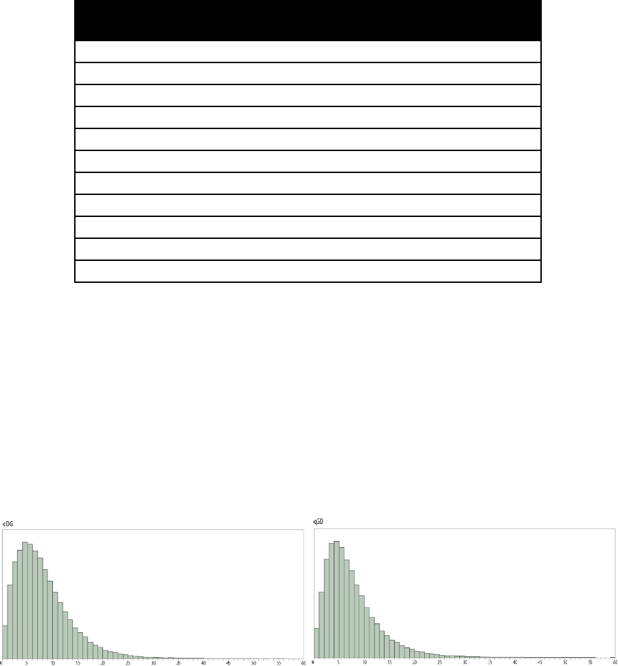
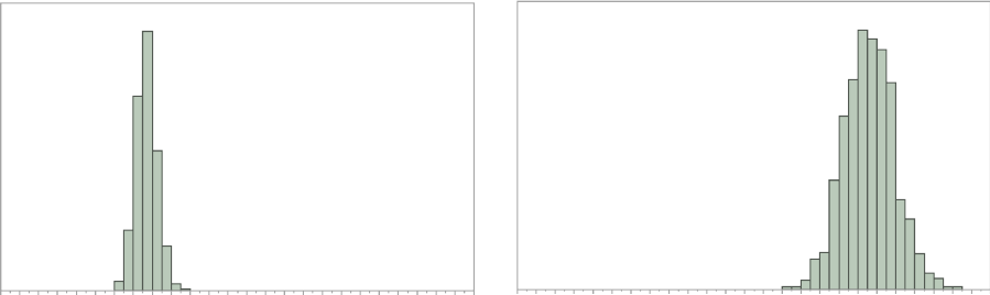
Parameter restriction example

The previous example assumed that the transition rates from state D to G (qDG) and from

state G to D (qGD) were different and both were estimated. The parameter estimates from a longer

run are plotted below, the two distributions show considerable overlap.

To test if the rate D changes to G (qDG) is significantly different from the rate G changes to D

(qGD), re-run the analysis restricting qGD to take the same value as qDG. First calculate the marginal

likelihood of a model which estimates qGD and qDG separately using the commands below. The first

two commands select MultiState (1) and MCMC (2), the third commands uses an exponential prior

with a mean of 10 for both rates, the fourth command uses the stepping stone sampler with 100

stones and 1000 iterations per stone to estimate the marginal likelihood, the fifth command starts

the analysis.

PriorAll exp 10

Stones 100 1000

Run

Once the analysis has finished a file containing the marginal likelihood will be created,

Artiodactyl.txt.Stones.txt, the last line will contain the marginal likelihood, and should be similar to

the line below. There will be run to run variation so the numbers will not be identical, but should be

roughly -8.7

Log marginal likelihood: -8.774642

Rerun the analysis restricting qDG to qGD using the commands below.

PriorAll exp 10

Stones 100 1000

Restrict qDG qGD

Run

The options are the same, except the 5th command sets qGD equal to qDG, the output

should be very similar but the rate parameters (qDG and qGD) will take the same value each

iteration. Once the run has finished, the stepping stone file’s last line should be similar to the one

below.

Log marginal likelihood: -8.296317

Bayes Factors can be used to test if qDG is significantly different from qGD, in this case the

model where qDG = qGD is the simple model as it has one fewer parameters, the model where qDG

≠ qGD is the complex one.

Log Bayes Factor = 2(log marginal likelihood complex model – log marginal likelihood simple model)

Log BF = 2(-8.774642- -8.296317)

Log BF = -0.95665

The log BF is less than two so the simpler model should be favoured (see (Gilks, Richardson

et al. 1996) or the table in Stepping stone sampler)

Values of the marginal likelihood calculated from the stepping stone sampler will vary

between runs, depending on the random seed, values are only for illustrative purposes. These values

are only used to demonstrate basic model testing.

The same restrict command can be used in Maximum Likelihood analysis.

PriorAll exp 10

Restrict qDG qGD

Run

Tags

Tags are used to identify nodes within a sample of trees, they can be used to reconstruct

ancestral states, fix nodes to specific values (fossilise), test if a node has a different rate or mode of

evolution and fit different evolutionary models to subsets of the tree. The AddTag (AT shortcut) is

used to create a tag, it takes a unique name to identify the tag and a list of taxa names that define

the node.

For example, the command below creates a tag called TestTag on a node defined by Sheep

Goat, Cow and Buffalo.

AddTag TestTag Sheep Goat Cow Buffalo Pronghorn

Ancestral state reconstruction MultiState / Discrete

Note: The syntax for reconstructing a node has changed since version 2.0. Tags are now used to

identify nodes within a sample of trees.

The AddMRCA and AddNode commands are used to reconstruct ancestral states in

MultiState and discrete models. The syntax for the two commands is similar.

The commands take a name to identify the reconstructed node in the output, and the name

of a tag (see Tags) that defines the node. BayesTrees

(http://www.evolution.reading.ac.uk/BayesTrees.html) is a graphical tree viewer which can be used

to generate the commands by clicking on the appropriate node.

Start BayesTraits with the Artiodactyl tree and data file (Artiodactyl.trees, Artiodactyl.txt),

use the commands below to reconstruct a node.

AddTag TRecNode Porpoise Dolphin FKWhale Whale

AddNode RecNode TRecNode

Run

The first two commands select the MultiState model and MCMC analysis, the third

command creates a tag called TRecNode defined by four taxa Porpoise, Dolphin, FKWhale and

Whale. The AddNode command is used to reconstruct the tag, it takes a name (RecNode in this

instance), so the node can be identified in the output and the name of the tag to reconstruct.

Two new columns will be added to the output “RecNode P(D)” and “RecNode P(G)”, these

represent the probability of reconstructing a D or a G at RecNode.

BayesTraits uses a sample of trees and some nodes may not be present in all trees, the node

defined by Sheep, Goat, Cow, Buffalo and Pronghorn is only present in 58% of the trees. The

posterior probability of node reconstruction will not be present in some trees, some samples of the

chain will record the ancestral sate as "--" because the node is not present in those trees.

The MRCA command reconstructs the Most Recent Common Ancestor, while a MRCA will be

present in every tree it may not be the same node (see (Pagel, Meade et al. 2004) for more details).

Rerun the analysis using MRCA.

PriorAll exp 10

Res qDG qGD

AddTag TVarNode Sheep Goat Cow Buffalo Pronghorn

AddNode VarNode TVarNode

Run

Any number of nodes can be reconstructed in a single analysis without affecting each other.

Fixing node values / fossilising

Internal nodes can be set to take a fixed value, if external information is available or to test if

the value of one state is significant. The fossil command takes a name, so the node can be identified

in the output, a tag that defines the node and the state or states to fossilise the node in. Fossilised

nodes are found using the most recent common ancestor method.

The command below fossilises a node defined by sheep, goats, cows, buffalo and pronghorn

to state D.

AddTag FNode Sheep Goat Cow Buffalo Pronghorn

Fossil Node01 FNode D

Run

Be aware that fossilising nodes will influence the models, by forcing a node to take a specific

value the model parameters will be affected. The fossil command can be used to fossilise in multiple

states, if the data had three states, A, B and C the fossil command

Fossil Name Tag AC

Fossilises the node in states A and C but not B.

Nodes can be fossilised for continuous models (not currently independent contrast) in the

same way.

AddTag Tag-01 Dorcopsulus_macleayi Dorcopsulus_vanheurni

Fossil Node01 Tag-01 90.95

Run

Fossilising states for discrete models requires a number instead of a state, as there are more

combinations of fossil sates. The table below shows the numbers and their corresponding states. X

denotes the likelihood is left unchanged, - sets the likelihood to zero.

Number

0,0

0,1

1,0

1,1

Discrete

Discrete is used to test if two binary traits are correlated, significance is established by

comparing the likelihoods of two models, one which assumes the traits evolve independently, with

one which assumes the traits evolution is correlated. The examples focus on MCMC but maximum

likelihood can also be used. The examples use a sample of 500 primate trees (“Primates.trees”) and

a data set of two binary traits, estrus advertisement and multi-male mating (“Primates.txt”). Two

binary traits have 4 possible states, written as “0,0”, “0,1”, “1,0” and “1,1”.

Discrete independent

The independent model assumes the two traits evolve independently, e.g. the transition

from 0  1 in the first trait is independent of the state of the second trait. The independent model

has 4 rate parameters, alpha1, beta1, alpah2 and beta2.

Parameter

Symbol

Trait

Transitions

alpha1

1

0  1

beta1

1

1  0

alpha2

2

0  1

beta2

2

1  0

0,0

0,1

1,0

1,1

0,0

2

1

0,1

2

1

1,0

1

2

1,1

1

2

Start BayesTraits with the tree file “Primates.trees” and the data file “Primates.txt”. Using

the commands below to select the independent model (2) and MCMC analysis (2). Set all the priors

to an exponential with a mean of 10 and use the stepping stone sampler with 100 stones and 1000

iterations per stone to estimate the marginal likelihood, the run command is used to start the

analysis. The commands are listed below. The mean for the prior was found by analysing the tree

using Maximum Likelihood and studying the resulting parameter rate estimates.

PriorAll exp 10

Stones 100 1000

Run

The output will be similar to the MultiState analysis, the header will contain.

The stepping stone sampler will produce a file “Primates.txt.Stones.txt”, the marginal

likelihood is recorded in the last line,

Log marginal likelihood: -46.674444

The marginal likelihood will show run to run variation but it should be roughly -46.67.

Header

Output

Iteration

Current iteration of the chain

Current likelihood of the chain

Tree No

Current tree number

alpha1

The alpha1 transition rate

beta1

The beta1 transition rate

alpha2

The alpha2 transition rate

beta2

The beta2 transition rate

Root – P(0,0)

Probability the root is in state 0,0

Root – P(0,1)

Probability the root is in state 0,1

Root – P(1,0)

Probability the root is in state 1,0

Root – P(1,1)

Probability the root is in state 1,1

Discrete dependent

The dependent model assumes that the traits are correlated and the rate of change in one

trait is dependent on the state of the other. The dependent model has 8 parameters, q12, q13, q21,

q24, q31, q34, q42 and q43. Double transitions from state 0,0 to 1,1 or from 0,1 to 1,0 are set to

zero.

Parameter

Dependent on

Trait

Transitions

q12

Trait 1 = 0

0  1

q13

Trait 2 = 0

0  1

q21

Trait 1 = 0

1  0

q24

Trait 2 = 1

0  1

q31

Trait 2 = 0

1  0

q34

Trait 1 = 1

0  1

q42

Trait 2 = 1

1  0

q43

Trait 1 = 1

1  0

0,0

0,1

1,0

1,1

0,0

q1,2

q1,3

0,1

q2,1

q2,4

1,0

q3,1

q3,4

1,1

q4,2

q4,3

Start BayesTraits with the tree file “Primates.trees” and the data file “Primates.txt”, select

the dependent model (3) and MCMC analysis (2). Set all the priors to an exponential with a mean of

10 and use the stepping stone sampler with 100 stones and 1000 iterations per stone to estimate

the marginal likelihood, the final command starts the analysis.

PriorAll exp 10

Stones 100 1000

Run

The output will be very similar to the independent model except that the dependent

parameters are estimated. The marginal likelihood can be found in “Primates.txt.Stones.txt” and

should be roughly -41.62. To test if the traits are correlated calculate a log Bayes Factor (see Model

Testing: Likelihood ratios and Bayes Factors) between the dependent and independent models, in

this case the dependent model is the complex one as it has more parameters. The calculations for

Log Bayes factors is given below.

Log BF = 2(log marginal likelihood complex model – log marginal likelihood simple model)

Log BF = 2(-41.62- -46.67)

Log BF = 10.1

The Log BF of 10.1 suggests there is evidence for correlated evolution. Marginal likelihoods

vary between runs and it is important to get a stable estimate by using multiple independent runs.

Reverse Jump MCMC and model reduction

Given the size of the data and complexity of the models not all parameters may be

statistically distinguishable. The previous parameter restriction example demonstrated how a model

could be simplified by setting parameters equal to each other and how to test if restrictions were

significant. There are 51 possible restrictions for the independent model and over 21,000 for the

dependent model, which would take a long time to test. Reverse jump MCMC (RJ-MCMC) offers an

alternative by integrating results over the model space, weighting naturally by their probabilities,

allowing the users to select viable models and parameters, see (Pagel and Meade 2006) for more

information.

The reverse jump command takes a prior as a parameter, one prior must be applied to all

parameters, the command below uses an RJ MCMC model with an exponential prior with a mean of

RevJump exp 10

RJ MCMC can also be used with a hyper-prior, (RJHP command).

RevJumpHP exp 0 100

Run the primates data and tree, with the dependent model and MCMC analysis, using the

commands below

RevJump exp 10

Stones 100 1000

Run

The output will contain 4 new columns.

Header

Output

No Of Parameters

Number of parameters

No Of Zero

Number of parameters set to zero

Model string

A model string showing parameter restrictions

Dep / InDep

A flag showing if the model is dependent (D)

or independent (I)

Model strings are used to characterise the models restrictions, the string start with ' and is

followed by numbers indicating which parameters are in which groups or a Z if the parameters have

been restricted to zero. For example the model string for a dependent model will have 8

components one for each parameter, the model string “'1 Z 0 0 0 1 1 Z”, has two parameters and

two rates set to zero. The first group consists of the 1st, 6th and 7th parameters (q12, q34 and q42),

the second group is formed of the 3rd, 4th and 5th parameters (q21, q24 and q31), and the 2nd and 8th

parameter is set to zero. This can be checked against the parameter estimates.

To test if a data set is correlated compare the marginal likelihood of an independent model

using RJ MCMC and a dependent model using RJ MCMC.

Covarion model

BayesTraits implements a basic on / off covarion model as described by (Tuffley and Steel

1998) for MultiState and Discrete models, the model requires one additional parameter, the

switching rate between the on / off states. The model allows the rate of evolution to vary through

the tree. The “CV” command is used to activate the covarion model, two additional columns will be

included in the output, “Covar On to Off” and “Covar Off to On”. The switching rate between the on

and off states will be the same.

Below is an example of how to fit a covarion model, using a large bird phylogeny (Jetz,

Thomas et al. 2012) (http://birdtree.org/) and territory data taken from (Tobias, Sheard et al. 2016),

it is used purely as an example and not to make a biological point. First calculate the likelihood and

parameters using a homogenous model. Start BayesTraits with the tree “Bird.trees” and the data file

“BirdTerritory.txt”

ScaleTrees 0.001

Stones 100 1000

Run

The commands select MultiState (1), MCMC (2), the command “ScaleTrees 0.001” is used to

rescale the branch lengths to prevent the rates from becoming very small and the stones command

is used to estimate the marginal likelihood using 100 stones and 1000 iterations per stone, the final

command starts the analysis. This should produce a marginal likelihood of roughly -1942

Then run the data with a covarion model, the commands are the same except the covarion

command turns on the model.

Covarion

ScaleTrees 0.001

Stones 100 1000

Run

This should produce a marginal likelihood of roughly -1781, giving a Bayes Factor of over

300, suggesting it is highly significant.

Discrete: Covarion

The discrete covarion model removes the assumption that a trait is either correlated or not

threw out the tree. It simultaneously fits both an independent and dependent model and uses a

covarion method to switch between them. The model requires 14 parameters, 4 for the

independent model, 8 for the dependent model and 2 that switch between the dependent and

independent models. As this model has a large number of parameters the use of reverse jump is

recommended, in combination with a large tree. If the discrete covarion model is significant this is

not necessarily evidence for correlated evolution, the dependent model may be acting as a second

independent model identifying changes in rates or patterns of evolution, this can be tested for by

comparing models that restrict the dependent parameters to independent ones. The discrete

covarion model supports RJ MCMC, to reduce the large number of parameters required.

Header

Output

Iteration

Current iteration of the chain

Current likelihood of the chain

Tree No

Current tree number

alpha1

The independent alpha1 transition rate

beta1

The independent beta1 transition rate

alpha2

The independent alpha2 transition rate

beta2

The independent beta2 transition rate

q12

The dependent q12 transition rate

q13

The dependent q13 transition rate

q21

The dependent q21 transition rate

q24

The dependent q24 transition rate

q31

The dependent q31 transition rate

q34

The dependent q34 transition rate

q42

The dependent q42 transition rate

q43

The dependent q43 transition rate

qDI

The switching rate between the dependent and independent models

qID

The switching rate between the independent and dependent models

Root - I P(0,0)

Probability the root is in independent state 0,0

Root - I P(0,1)

Probability the root is in independent state 0,1

Root - I P(1,0)

Probability the root is in independent state 1,0

Root - I P(1,1)

Probability the root is in independent state 1,1

Root - D P(0,0)

Probability the root is in dependent state 0,0

Root - D P(0,1)

Probability the root is in dependent state 0,1

Root - D P(1,0)

Probability the root is in dependent state 1,0

Root - D P(1,1)

Probability the root is in dependent state 1,1

Discrete: Heterogeneous

The discrete heterogeneous model is an experimental model which fits both an independent

and a dependent model on a branch by branch bases, each branch is assigned one of the two

models. It can only be used on a single tree with MCMC. The output contains a table “Hetro Model

Key” which links each node in the tree with a number, each iteration of the chain will contain a map

string which indicates which model is assigned to which branch. If the map has a 0 the independent

model is applied to the branch, if the map has a 1 the dependent model is applied. In the same way

a significant result for the discrete covarion model does not necessarily signal correlated evolution

but could be two patterns or rates of evolution, restricting the dependent model to the independent

one can distinguish between these cases. While the model may improve the likelihood the models

assigned to each branch can be highly variable. The discrete covarion model supports RJ MCMC, to

reduce the large number of parameters required.

Local Heterogeneous models of evolution (MultiState and Discrete)

The assumption of a homogenous model of evolution may not be suitable for large

phylogenies, as evolutionary processes may not be constant over long time periods or across a

diverse range of taxa. BayesTraits allows different models of evolution to be fitted to different parts

of the tree. Fitting a different model of evolution allows changes in both rates and patterns of

evolution to be modelled, local transformations can be used to model changes in rates. Fitting a

different model of evolution estimates a separate transition matrix for a subset of the tree, this can

be estimated using MCMC or ML. The command “AddPattern” is used to estimate a separate pattern

of evolution on a node, it takes a name for the pattern and a tag to identify the node on the trees

(see Tags for creating tags).

Below is an example of how to fit a heterogeneous model, using a large bird phylogeny (Jetz,

Thomas et al. 2012) (http://birdtree.org/) and territory data taken from (Tobias, Sheard et al. 2016),

it is used purely as an example and not to make a biological point. First calculate the likelihood and

parameters using a homogenous model, run BayesTraits with the tree file Bird.trees and data file

BirdTerritory.txt, and the following commands

ScaleTrees 0.001

Stones 100 1000

Run

The commands select MultiState (1), MCMC (2), use “ScaleTrees 0.001” to scale the branch

lengths to prevent the rates from becoming small and start the analysis. The stepping stone sampler

is used with 100 stones and 1000 iterations per stone to estimate the marginal likelihood, the

analysis is started with the run command. This should produce a marginal likelihood of roughly -1942

(in BirdTerritory.txt.Stones.txt) and rate parameters (q01 and q10) similar to the ones below.

The commands to run a heterogeneous model, where a different evolutionary model is

fitted to the Passeriformes can be found in the command file “BirdHetCom.txt”, as the tag to define

the Passeriformes has over 3500 taxa and is too large to include.

The commands are

ScaleTrees 0.001

AddTag PasseriformesTag Strigops_habroptila Nestor_notabilis …

AddPattern Passeriformes PasseriformesTag

Stones 100 1000

Run

The run BayesTraits with the trees, data and command file (see Running BayesTraits with a

command file).

0246810 12 14 16 18 20 22 24 0246810 12 14 16 18 20 22 24

q01 q10

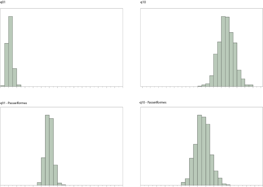
The first three commands select MultiState model, MCMC and scale the tree by a factor of

0.001, the fourth command creates a tag called “PasseriformesTag” defined by the supplied list of

taxa, the fifth command estimates a different pattern of evolution on the node defined by the

PasseriformesTag, the pattern is called “Passeriformes”, the stepping stone sampler is used to

estimate the marginal likelihood. This should produce a marginal likelihood of roughly, -1912.4,

giving a log Bayes Factor of 59.2, suggesting very strong evidence for a heterogeneous pattern of

evolution within the birds. This is born out in the differences in the rate parameters, the parameters

estimated in the Passeriformes are different from the rest of the tree. Interestingly fitting a separate

pattern of evolution alters the estimated ancestral state, from a probability of 0.804 for a

reconstruction of 1 at the root to 0.995.

Different patterns of evolution can be fitted using maximum likelihood or MCMC, they can

be used with MultiState or Independent or Dependent discrete models. Parameters with in a pattern

behave the same as other transition rates, they can be fixed to values, set equal to each other or

modelled using RJ MCMC.

0246 8 10 12 14 16 18 20 22 24 26 28 30

Continuous: Random Walk (Model A) ML

Start BayesTraits with the tree file “Mammal.trees” and data file “MammalBody.txt”, the

tree file is a sample of 50 mammal trees and the data is there corresponding body size, the trees and

data are for illustrative purposes and are not accurate or a good sample. The commands below run a

basic maximum likelihood Brownian motion analysis, 4 selects “Continuous: Random Walk (Model

A)”, 2 selects maximum likelihood and the final command starts the chain.

Run

Basic information will be printed followed by a header

Header

Output

Tree No

The tree number, 1-50 for this data

Maximum likelihood value for the tree

Alpha 1

The phylogenetically corrected mean of the data, also the estimated root value

Sigma^2 1

The phylogenetically corrected variance of the data

Continuous: Random Walk (Model A) MCMC

Start BayesTraits with the tree file “Mammal.trees” and data file “MammalBody.txt”, select

“Continuous: Random Walk (Model A)” (4) and MCMC (2), start the analysis with run

Run

Basic information will be printed followed by a header

Header

Output

Iteration

Current iteration of the chain

Current likelihood of the chain

Tree No

Current tree number

Alpha Trait 1

The phylogenetically corrected mean of the data, also the estimated root value

Sigma^2 1

The phylogenetically corrected variance of the data

Testing trait correlations: continuous

To test if two traits are correlated, the results from two analysis are compared, one in which

a correlation is assumed (the default) and one where the correlation is set to zero. Run an analysis

using the tree file “Mammal.trees” and a data file “MammalBrainBody.txt”, containing brain and

body size data. The commands select “Continuous: Random Walk (Model A)” (4) and MCMC analysis

(2), the stones command is used to estimate the marginal likelihood using 100 stones and 1000

iterations per stone. The final command starts the analysis.

Stones 100 1000

Run

Basic information will be printed followed by a header

Header

Output

Iteration

Current iteration of the chain

Current likelihood of the chain

Tree No

Current tree number

Alpha 1

The phylogenetically corrected mean of the first trait

Alpha 2

The phylogenetically corrected mean of the second trait

Sigma^2 1

The phylogenetically corrected variance of the first trait

Sigma^2 2

The phylogenetically corrected variance of the second trait

R Trait 1 2

R correlation between trait 1 and trait 2

The marginal likelihood is recorded in the last line of the “MammalBrainBody.txt.Stones.txt”

file, it should be roughly -80.93

Rerun the analysis forcing the correlation to be zero using the TestCorrel (TC) command.

TestCorrel

Stones 100 1000

Run

The output should be similar except the “R Trait 1 2” value will be 0, the marginal likelihood

should be roughly -140.64. The significance of the correlation can be tested by computing a Bayes

Factor between the two runs, the model that estimates the correlation will be the complex one.

If the analysis allowing a correlation produced a marginal likelihood of -80.93 and the

analysis with the correlation fixed to zero gave a marginal likelihood of -146.64, this would lead to a

log Bayes Factor of 119.42, suggesting they are highly correlated.

Log BF = 2(log marginal likelihood complex model – log marginal likelihood simple model)

Log BF = 2(-80.93 - -140.64)

Log BF = 119.42

Continuous: Directional (Model B) MCMC

The directional model can be used to test if there is a directional change in a traits evolution,

by testing if a trait is correlated with the root to tip distance of the taxa. Model B cannot be used

with ultrametric trees as there is no root to tip variation between taxa. A fictional data set

“MammalModelB.txt” can be used to test if there is a significant directional trend by performing a

model test between Model A and Model B. If Model B is significant there is signal for a directional

trend in the data. To test if model B is significant, first run an analysis with the tree file

Mammal.trees and the data file MammalModelB.txt, the following commands select model A and

MCMC, the stones command is used to estimate the marginal likelihood using 100 stones and 1000

iterations per stone and the final command starts the analysis.

Stones 100 1000

Run

The marginal likelihood, found in the last line of MammalModelB.txt.Stones.txt should be

roughly 60.5 log units.

The commands below rerun the analysis using Model B, where a directional trend is

estimated in the data.

Stones 100 1000

Run

The marginal likelihood should be roughly 67.28, giving a Log Bayes Factor of roughly 13.56,

suggesting significance.

Log BF = 2(log marginal likelihood complex model – log marginal likelihood simple model)

Log BF = 2(67.28- 60.5)

Log BF = 13.56

Continuous: Regression

The continuous regression model is used to perform regression analysis, test trait

significance and predict unknown values. The regression model takes two or more traits, the first

trait is assumed to be the dependent variable. MammalBrainBodyGt.txt is a data set of mammal

brain, body and gestation time. Run BayesTraits with the “Mammal.trees” tree file and

“MammalBrainBodyGt.txt” data. The commands below select the regression model (6) and MCMC

(2) and the last line runs the analysis.

Run

The header will contain.

Header

Output

Iteration

Current iteration of the chain

Current likelihood of the chain

Tree No

Current tree number

Alpha

Intercept

Beta Trait 2

Regression coefficient for trait 2

Beta Trait 3

Regression coefficient for trait 3

Var

Brownian motion variance

R^2

R2 - Coefficient of determination

SSE

Sum of squared error

SST

Total sum of squared

s.e. Alpha

Standard error Alpha

s.e. Beta-2

Standard error Beta-2

s.e. Beta-3

Standard error Beta-3

Testing trait significance

There are a number of ways to test if a trait is significant in the regression model, the first is

to compare marginal likelihood (MCMC) or likelihood ratios (ML) from runs with and without the

trait. The second is the ratio of the time the regression coefficient crosses the zero point, if a

regression coefficient is well supported it will not switch from positive to negative, or vice versa.

Continuous: Estimating ancestral sates and tip values

Continuous models can be used to estimate unknown values on the tree, either internal

nodes or tips. Estimating unknown values is a two-step process, first a distribution of models is

estimated from available data, secondly the models are used to estimate unknown values. The two-

step process prevents estimated data from affecting the model parameters. Estimating unknown

values can be used with model A, model B and the regression model but only using MCMC.

The “SaveModels” command is used to save models to a specified file, the “LoadModels”

command is used to load the models into BayesTraits. The same model parameters, including tree

transformations, has to be specified when creating a model file and when estimating unknown

values, only very basic error checking is implemented.

Estimating unknown values internal nodes

Start BayesTraits with the “Mammal.trees” file and “MammalBody.txt” data. Select model A

(4) and MCMC analysis (2). Save the models and run the analysis with the commands below, the

models will be saved into a file called “MamBodyModels.bin”

SaveModels MamBodyModels.bin

Run

Once the program has finished a file called “MamBodyModels.bin” will be created.

To estimate data, start BayesTraits with the same tree and data files and use the commands

below to select model A (4) and MCMC (2), the third line loads the models from

MamBodyModels.bin, the fourth and fifth lines define two tags called Tag01 and Tag02 (see Tags)

and the six and seventh lines reconstruct both tags labelling them Node-01 and Node-02 in the

output.

LoadModels MamBodyModels.bin

AddTag Tag01 Whale Hippo Llama Ruminant Pig

AddTag Tag02 Mouse Rat Hystricid Caviomorph

AddMRCA Node-01 Tag01

AddMRCA Node-02 Tag02

Run

The output header will contain

Header

Output

Iteration

Current iteration of the chain

Current likelihood of the chain

Tree No

Current tree number

Model No

Current model number from the model file

Alpha Trait 1

Phylogenetic mean

Sigma^2 1

Brownian motion variance

Est Node-02 - 1

Estimated values for Node-02 trait 1

Est Node-01 - 1

Estimated values for Node-01 trait 1

Estimating unknown values for tips

Data for taxa, as well as internal nodes can be estimated. A data file

“MammalBrainBodyNoTapir.txt” has been created with the data for tapir removed and replaced by

‘-‘. Start BayesTraits with the “Mammal.trees” tree file and “MammalBrainBodyNoTapir.txt” data

file. The commands below select the regression model (6) and MCMC analysis (2), save the models

to a file (MamRegModels.bin) and run the analysis.

SaveModels MamRegModels.bin

Run

A data file “MammalBrainBodyPredTapir.txt” which contains the tapir body size but with the

brain size set to “?”. The use of a question mark in the data is used to indicate the value should be

estimated. Run an analysis using the “Mammal.trees” tree file and

“MammalBrainBodyPredTapir.txt” data file. Select the regression model (6) and MCMC analysis (2).

Use the commands below to load the models and run the analysis

LoadModels MamRegModels.bin

Run

The output will contain a column labelled “Est Tapir – Dep”, with the predicted tapir brain

size, the predicted brain size should be roughly 2.1 ± 0.15, the actual brain size is 2.2.

Independent contrast

BayesTraits implements a range of independent contrast models (Felsenstein 1973,

Freckleton 2012), independent contrast offers a significantly faster alternative to Generalised Least

Squares (GLS) methods for large data sets. Independent contrast models can be run using MCMC or

ML. Start BayesTraits with the tree file “Mammal.trees” and data file “MammalBrainBody.txt”. The

commands below run the independent contrast model (7) using MCMC (2)

Run

The independent contrast model assumes sites are independent, e.g the covariance is set to zero.

The output will contain

Header

Output

Iteration

Current iteration of the chain

Current likelihood of the chain

Tree No

Current tree number

Alpha 1

Phylogenetic mean of the first trait

Alpha 2

Phylogenetic mean of the second trait

Sigma^2 1

Brownian motion variance for the first trait

Sigma^2 2

Brownian motion variance for the second trait

Independent contrast: Correlation

The independent contrasts correlation model allows correlations to be tested between two

traits using the independent contrast framework.

Start BayesTraits with the tree file “Mammal.trees” and data file “MammalBrainBody.txt”.

The commands below are used to select Independent Contrast: Correlation (8) and MCMC (2), the

stones command is used to estimate the marginal likelihood using 100 stones and 1000 iterations

per stone and the final command starts the analysis.

Stones 100 1000

Run

The output will contain

Header

Output

Iteration

Current iteration of the chain

Current likelihood of the chain

Tree No

Current tree number

Alpha 1

Phylogenetic mean of the first trait

Alpha 2

Phylogenetic mean of the second trait

Sigma^2 1

*Brownian motion variance for the first trait

Sigma^2 2

*Brownian motion variance for the second trait

R Trait 1 2

*The covariance between the first and second trait

*Due to the independent contrast framework the variance and covariance parameters are

set to their maximum likelihood values even when using MCMC.

The log marginal likelihood, found in the last line of MammalBrainBody.txt.Stones.txt,

should be roughly -79.3 log units.

To test a correlation between two traits re run the analysis using the “TestCorrel” (TC)

command to set the covariance to zero and calculate a Log Bayes Factor. Start BayesTraits with the

tree file “Mammal.trees” and data file “MammalBrainBody.txt”. The commands below are used to

select Independent Contrast: Correlation (8) and MCMC (2), the TestCorrel command sets the co-

variance to zero, the stones command is used to estimate the marginal likelihood using 100 stones

and 1000 iterations per stone and the final command starts the analysis.

TestCorrel

Stones 100 1000

Run

The log marginal likelihood, found in the last line of MammalBrainBody.txt.Stones.txt,

should be roughly -140.6 log units. The significance can be assessed by calculating Log Bayes Factors,

in this case the complex model assumes the correlation and the simple model sets it to zero.

Log BF = 2(log marginal likelihood complex model – log marginal likelihood simple model)

Log BF = 2(-79.3 - -140.6)

Log BF = 122.6

Independent contrast: regression

The independent contrast models supports simple and multiple regression, using ML and

MCMC. The first trait is assumed to be the dependent variable, subsequent traits are assumed to be

the independent variables. Run an analysis using the tree file “Mammal.trees” and the data file

“MammalBrainBodyGt.txt”. Select “Independent Contrast: Regression”, 9 and MCMC 2, and run the

analysis. The log file will contain

Header

Output

Iteration

Current iteration of the chain

Current likelihood of the chain

Tree No

Current tree number

Alpha

*Analytical value of Intercept

Beta 1

Regression coefficient for trait 2

Beta 2

Regression coefficient for trait 3

* Due to the independent contrast framework the maximum likelihood intercept value is

used, calculated from the regression coefficient, even when using MCMC, it is not an estimated

value.

Tree transformations, kappa, lambda, delta, OU

BayesTraits supports a number of tree transformations including, kappa (κ), lambda (λ),

delta (δ) and Ornstein Uhlenbeck (OU) for both continuous and independent contrast models. These

scaling parameters allow tests of the tempo, mode, and phylogenetic associations of trait evolution.

Kappa, lambda, and delta take the value 1.0 by default, OU takes the value 0. These default values

assume that the phylogeny and its branch lengths accurately describe a constant-variance random

walk model. However, if trait evolution has not followed the topology or the branch lengths, these

values will depart from 1.0. When they do, incorporating them into the analysis of the data (e.g.,

when estimating the correlation between two traits) significantly improves the fit of the data to the

model.

Below is a subset of the primates tree, it will be used to demonstrate tree transforms.

Kappa

The kappa parameter differentially stretches or compresses individual phylogenetic branch

lengths and can be used to test for a punctuational versus gradual mode of trait evolution. Kappa >

1.0 stretches longer branches more than shorter ones, indicating that longer branches contribute

more to trait evolution (as if the rate of evolution accelerates within a long branch). Kappa < 1.0

compresses longer branches more than shorter ones. In the extreme of Kappa = 0.0, trait evolution

is independent of the length of the branch, all branch lengths are set to 1. Kappa = 0.0 is consistent

with a punctuational mode of evolution. Below are examples of the tree transform by a) kappa = 2 b)

kappa = 0.5 and c) kappa = 0

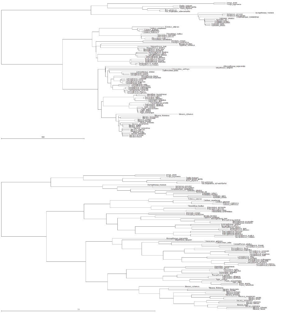
a) Kappa = 2

b) Kappa = 0.5

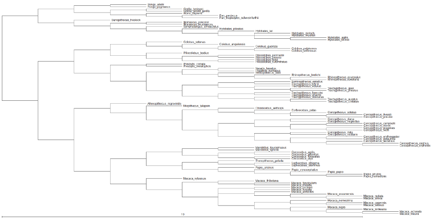
c) Kappa = 0

Delta

The parameter delta scales overall path lengths in the phylogeny - the distance from the

root to the tips, as well as the shared path lengths. It can detect whether the rate of trait evolution

has accelerated or slowed over time as one moves from the root to the tips, and can find evidence

for adaptive radiations. If the estimate of Delta < 1.0, this says that shorter paths (earlier evolution in

the phylogeny) contribute disproportionately to trait evolution - this is the signature of an adaptive

radiation: rapid early evolution followed by slower rates of change among closely related species.

Delta > 1.0 indicates that longer paths contribute more to trait evolution. This is the signature of

accelerating evolution as time progresses. Seen this way, delta is a parameter that detects

differential rates of evolution over time and re-scales the phylogeny to a basis in which the rate of

evolution is constant. Below are examples of the tree transform by a) delta = 0.5 and b) delta = 2

a) Delta 0.5

b) Delta 2

Lambda

The parameter lambda reveals whether the phylogeny correctly predicts the patterns of

covariance among species on a given trait. This important parameter in effect indicates whether one

of the key assumptions underlying the use of comparative methods - that species are not

independent - is true for a given phylogeny and trait. If a trait is in fact evolving among species as if

they were independent, this parameter will take the value 0 and indicate that phylogenetic

correction can be dispensed with. A lambda value of 0 corresponds to the tree being represented as

a star or big-bang phylogeny. If traits are evolving as expected given the tree topology and the

random walk model, lambda takes the value of 1.0. Values of lambda = 1.0 are consistent with the

constant-variance model (sometimes called Brownian motion) being a correct representation of the

data. Intermediate values of lambda arise when the tree topology over-estimates the covariance

among species. Below are examples of the tree transform by a) lambda = 0.75 and b) lambda = 0

a) Lambda = 0.7

b) Lambda = 0

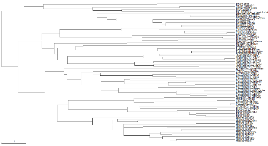
The value of lambda can differ for different traits on the same phylogeny. If the goal is to

estimate the correlation between two traits then lambda should be estimated while simultaneously

estimating the correlation. If, on the other hand, the goal is to characterise traits individually, a

separate lambda can be estimated for each.

Ornstein Uhlenbeck (OU)

The Ornstein Uhlenbeck (OU) transform has traditionally been associated with stabilising

selection, where the OU parameter measures the strength of a return to a theoretical optimum

(Hansen 1997) this may be due to other factors and care should be taken when using and

interpreting OU results. OU parameter values of zero correspond to the default branch lengths,

parameter values >0 are evidence of an OU process. The OU model should only be used with

ultrametric trees for independent contrast models, the correction for non-ultrametric trees (Slater

2014) is implemented for GLM. Below are examples of the tree transform by a) OU = 0.05 and b) OU

= 1, the OU process can produce trees which are very similar to delta transformed trees but the

interpretation is very different. High values of OU can also produce trees which are similar to lambda

trees but again the interpretation is very different.

a) OU = 0.05

b) OU = 1

Tree transformations table

Parameter

Action

lambda

Assess contribution

of phylogeny

Star phylogeny

(species

independent)

phylogenetic

history has

minimal effect

default

phylogeny

not defined

kappa

Scale branch

lengths in tree

punctuational

evolution

stasis in longer

branches

default

gradualism

longer

branches

more change

delta

Scale total path

(root to tip) in tree

not defined

temporally

early change

important

(adaptive

radiation)

default

gradualism

temporally

later change

(species

specific

adaptation)

default

evidence of an

OU process

Four scaling parameters and their interpretation when applied to trait evolution on a

phylogeny

Tree transformations commands

All four parameters can be estimated using ML or MCMC, the syntax for the four parameters

is the same, either the scaling parameter on its own to toggle its estimation (they are not estimated

by default) or the scaling parameter followed by a number to fix the parameter to a given value.

The first command estimates lambda, the second fixes it to 0.5

Lambda

Lambda 0.5

The first command estimates kappa, the second fixes it to 0.5

Kappa

Kappa 0.5

The first command estimates delta, the second fixes it to 0.5

Delta

Delta 0.5

The first command estimates OU, the second fixes it to 0.5

OU 0.5

Model testing, Bayes Factors (MCMC) or Likelihood ratios (ML), can be used to determine if

a transform is significant or if a value of a transform is significant, e.g. is lambda significantly

different from 0.

Variable rates model

The variable rates model allows the rate of change to vary threw time and identifies areas of

the tree where the rate of evolution differs significantly, for an in-depth description see (Venditti,

Meade et al. 2011). The variable rates model can be used with MultiState, Discrete or any of the

independent contrast models. The variable rates model uses RJ MCMC to identify areas of the tree in

which the rate of evolution varies significantly. The model works with a single tree and requires

MCMC analysis. A tree “Marsupials.trees” of roughly 250 marsupials and their body sizes

“Marsupials.txt” is included. Start BayesTraits with the tree and data file, the commands below

select the independent contrast model (7) and MCMC (2), the VarRates command selects the

variable rates option, both burn-in and the number of iterations are increased as reverse jump

models can be harder to converge and have more parameters than the standard Brownian motion

models. Because variable rates models are more complex chains may fail to converge, it is important

to check convergence using multiple chains.

VarRates

Burnin 10000000

Iterations 110000000

Run

The log file will contain

Header

Output

Iteration

Current iteration of the chain

Current likelihood of the chain

Tree No

Current tree number

Alpha 1

Phylogenetic mean of the first trait

Sigma^2 1

Brownian motion variance for the first trait

No RJ Local Branch

Number of branch lengths scaled using variable rates

No RJ Local Node

Number of nodes scaled using variable rates

Two additional data files are created, “Marsupials.txt.Output.trees” contains the trees

scaled by the rate of change, areas which are stretched have an increased rate of change, areas

which are shrunken have a decreased rate. The file “Marsupials.txt.VarRates.txt” contains a detailed

description of the changes, the format of the file is, line 1, number of taxa, followed by a unique

taxa ID and taxa name. The second part is the number of internal nodes, followed by a list of internal

nodes consisting of a unique node ID, branch length (-1 for root), number of taxa which define the

node and the list of taxa ID. The third section details the results of the chain, the columns are

Header

Output

Iteration of the chain

Likelihood of the chain

Lh + Prior

Likelihood + prior

No Pram

Number of rate changes on the tree

Alpha

Estimated phylogenetic mean

Sigma^2

Brownian motion

Alpha Scale

Scale of the prior (unchanging, for diagnostics only)

For each change of rate of the tree (No Param) there is

Header

Output

Node ID

The node ID the change is on

Scale

The value of the scale parameter

Crate It

The iteration the change was created on

Scaler type

The type of the scaler, this can be node,

branch, kappa, lambda or delta

Bayes Factors calculated from marginal likelihoods can be used to test if there is rate

variability by comparing a model with and without variable rates.

A web site that processes the output from a variable rates model is available at

http://www.evolution.reading.ac.uk/VarRatesWebPP/

it can be used to determine how often each node is scaled and by how much.

Geo (Geographical) model

Geographical coordinates (longitude and latitude) cannot be modelled using Brownian

motion due to the spherical nature of the earth. The geo model maps longitude and latitude onto a 3

dimensional Cartesian coordinates system which can be modelled using Brownian motion. The

model requires two sites, longitude and latitude, it can only be used with a single tree, as all

ancestral sates must be simultaneously estimated, the geo model can only be used with MCMC, no

ML option is available.

A phylogenetic tree of 85 Northeast Bantu languages and their geographical coordinates

(longitude and latitude) can be found in NortheastBantu.trees and NortheastBantu.txt. Run

BayesTraits with the tree file and data, the commands below select the Geo model, number 13,

MCMC will automatically be selected, start the model using the run command. The log file will

contain standard MCMC information, iteration, Lh ect and Alpha which will be fixed to two and scale

parameter of roughly 71. The scale parameter is the variance of the normal distribution, with a mean

of 0, that expected changes are drawn from.

Run

The Geo model records the estimated ancestral states in the “.AnsStates.txt” file. The file

assigns a node number to each internal node defined by a list of taxa.

For example

Node-00012 G35_Luguru G36_Kami

Defines Node 12 by two taxa G35_Luguru, G36_Kami.

The second part of the file contains the iteration number, likelihood, parameters and

estimated longitude and latitude for each internal node.

Samples of trait data

Traditionally comparative methods assume trait values are known without error but traits

often show within species variation. BayesTraits allows samples of data to be used, results are

integrated over the sample. There are two types of samples, linked where multiple traits with in a

taxa are taken from the same source, for example if you had brain and body measurements from a

sample and could identify what brains measurements came from what bodies, unlinked data is

where the traits for a taxa are not from the same source.

Samples of data are placed in a text file, the format of the data file is, taxa name, followed

by Linked or UnLinked, then the sample of data separated by comers (,) without spaces or tabs.

Spaces are used if there is more than one trait. The example below defines a sample of data for two

taxa, Taxa1 and Taxa2, the data set has two traits. Taxa1 is linked and the data will be paired, both

the first and second trait must have the same number of data points, and are sampled together.

Taxa2 is unlinked, a sample is not available for the first trait a single value is used, four values are

available for the second trait.

Taxa1 Linked 5.5,6.4,4.9 8.3,9.2,7.7

Taxa2 Unlinked 8 5.5,9.1,6.6,8.3

An example of sample data can be seen in MammalBrainBodySampleData.txt, it has samples

of data for Hippo and Whale, Hippo has 100 linked samples of brain and body size, Whale has 30

unlinked samples of brain and 10 samples of body size. Start BayesTraits with the supplied tree and

data file Mammal.trees and MammalBrainBody.txt, and use the following commands.

DistData MammalBrainBodySampleData.txt

Run

7 selects Independent Contrast and 2 for MCMC, the command “DistData

MammalBrainBodySampleData.txt” is used to read in the sample of data, start the chain with “run”.

The output will have four new columns, Hippo-1 and Hippo-2 that draws from the sample for the

first and second site for Hippo and the same for Whale.

Local transformations, kappa, lambda, delta, OU, nodes and branches

Commonly transformations are applied to the whole tree, assuming a single evolutionary

process, but as trees become large this assumption may not hold. BayesTraits allows local

transforms to be applied to nodes within trees as well as to the root. Local transforms include,

kappa, lambda, delta, OU (see Tree transformations, kappa, lambda, delta, OU), as well as node and

branch scalars. A node transform scales all branches in a node by a value, a branch transform scales

a single branch. A significant scalar, on a branch suggests a change in the trait value which is

inherited by all members of the clade, for example there is a significant branch scaler on the nodes

containing the bats within the mammal tree, as there was a decrease in body size along that branch.

A significant scalar, greater than one, on a node suggests an increase in trait variance for that group.

While the OU model can be fitted to nodes of the tree the implementation does not include the

correction for non-ultrametric trees (Slater 2014).

The syntax to create a local transform (shortcut LT) is

LocalTransform Name TagList Type Value

Where “Name” is an identifier associated with the transform, allowing it to be identified in

the output. Tag List is a list of one or more tags to apply the transform to, BayesTraits can apply the

same transform to one or more nodes on the tree, for example if an ecological factor is associated

with a change in the rate of a traits evolution. “Type” is the transform to apply, this can be Node,

Branch, Kappa, Delta, Lambda or OU. “Value” is optional if you what to set the transform parameter

to a fixed value, if none is supplied the value is estimated using either ML or MCMC.

An example of using local transforms applied to the Marsupials tree and body size

(Marsupials.trees and Marsupials.txt) is given below, this is for illustrative purposes and should not

be viewed as the correct model. First run a model assuming a homogenous evolutionary process

using the commands below, selecting Independent Contrasts and MCMC, the stones command is

used to estimate the marginal likelihood (see Model Testing: Likelihood ratios and Bayes Factors)

using 100 stones and 1000 iterations per stone, the final command starts the analysis.

Stones 100 1000

Run

The estimated marginal log likelihood, found in the last line of the Marsupials.txt.Stones.txt

file, should be roughly -155.5.

Secondly run a model where a local node transform is applied to the clade that includes

Petrogale_brachyotis Petrogale_burbidgei Petrogale_concinna, using the commands below.

AddTag Tag01 Petrogale_brachyotis Petrogale_burbidgei Petrogale_concinna

LocalTransform TransNode Tag01 Node

Stones 100 10000

Run

The first two command select Independent Contrasts and MCMC, the third command

creates a tag called Tag01 that is defined by three taxa, Petrogale_brachyotis Petrogale_burbidgei

Petrogale_concinna. The fourth command applies a local node transform to the defined tag, the

stones command is used to estimate the marginal likelihood. The default prior on the node scalar

called VRNode is a scaled gamma (see (Venditti, Meade et al. 2011)) with an alpha of 1.1 and a beta

of 1, this can be changed (see Priors). Once the chain has run the Marsupials.txt.Stones.txt file

should contain an estimate of the marginal log likelihood, roughly -148

Log BF = 2(log marginal likelihood complex model - log marginal likelihood simple model)

Log BF = 2(-148 - -155.5)

Log BF = 15

The Log Bayes factor suggests “very strong evidence” for a rate shift on node.

The estimated rate scaler is recorded in the output as “TransNode – Node” column of the log

file, below is a plot of the frequency histogram. This shows that the scale is different from 1, the

default, this is borne out by the significant Bayes factor.

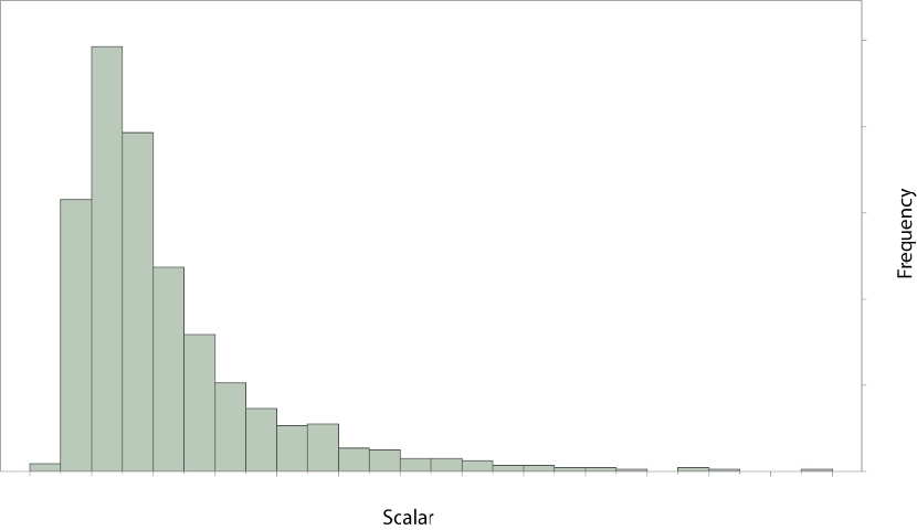
Any number of local transforms can be simultaneously applied to a tree, the transforms can

be mixed, allowing different parts of the tree to be modelled by different processes. Transforms can

be nested within each other, when transforms are nested the nodes deeper in the tree (the nodes

defined by the most taxa) are applied first. This gives the flexibility to create complex models but

they may be hard to interpret or not have a biological foundation. The resulting scaled trees are

logged in an output file ending “.Output.trees” this can be used to visualise the transforms and can

be used for further analysis.

Reverse Jump local transformations, kappa, lambda, delta, and OU

The method for fitting local transformations, described above, requires the number and

location of the transform to be known in advance. This is not often the case, the reverse jump local

transform method can be used to estimate the number and location of transforms with in a tree.

The method is similar to the Variable rates model (see Variable rates model), the variable rates

method estimates the number and location of branch and node scalars, reverse jump local

transform allow the number and location of other evolutionary processes to be modelled, such as

kappa, lambda, and delta. The RJLocalTransform command turns on the use of reverse jump local

transforms, it takes a transform type, kappa, lambda, delta or OU.

For example

RJLocalTransform Delta

Sets reverse jump local transform using delta, more than one reverse jump transform can be

used at the same time but the interpretation can become complex. By default a node must comprise

of at least 10 taxa to be transformed, A minimum number of taxa are used to prevent small nodes

from being transformed, as the transform may fit the data better but may not be interpretable as

the evolutionary process. This limit can be changed with the SetMinTransTaxaNo command.

100

150

200

250

0510 15 20 25 30 35 40 45 50 55 60 65

An example of using reverse jump local transform is given below, using the Marsupials tree

and data set (Marsupials.trees and Marsupials.txt). First run an analysis to establish the marginal

likelihood for the Brownian motion model, using the commands below.

Burnin 1000000

Iterations 10000000

Stones 250 10000

Run

This should produce a marginal likelihood of roughly -155.5. The number of stones, burn-in

and iterations have been increased as reverse jump models can be harder to fit. Run a second

analysis using reverse jump local transform delta, using the commands below.

Burnin 1000000

Iterations 10000000

RJLocalTransform Delta

Stones 250 10000

Run

This should produce a marginal likelihood of roughly -119, a variable rates log file

“Marsupials.txt.VarRates.txt” will be created identifying each node and recording which nodes have

had delta transforms applied and their value, the number of deltas will also be recorded in the log

file. The transformed tree is stored in the nexus tree file “Marsupials.txt.Output.trees”. While the RJ

delta marginal likelihood is significantly higher than the Brownian motion, this may be due to RJ

delta acting as a proxy for variable rates, to test if RJ delta is significant on top of variable rates run

an analysis with both variable rates and RJ delta using the commands below.

VarRates

Burnin 1000000

Iterations 10000000

RJLocalTransform Delta

Stones 250 10000

Run

This should produce a marginal likelihood of roughly -110, suggesting the RJ delta is

significant on top of the variable rates model.

Model

Approximate marginal likelihood

Brownian motion

-155.5

Reverse jump Delta

-119.8

Variable rates

-119.3

Reverse jump Delta + Variable rates

-110.4

Maximum likelihood search options

Under maximum likelihood, estimated parameters which don’t have an analytical solution

have to be searched for, this can be computationally hard if there are a large number of parameters,

they trade off with each other or if the search space is complex to traverse. BayesTraits uses the

NLopt library (Johnson) (http://ab-initio.mit.edu/nlopt). There are a number of options which can be

set to help parameter optimisation. It is important to run the analysis multiple times to ensure that

the results are stable, if each run produces different results the options below can be used to modify

the search algorithm. Limiting the search space using Set Minimum Maximum Rate (SetMinMaxRate)

and increasing the number of maximum likelihood tries (MLTries) can be effective.

MLTries (Maximum Likelihood Tries)

The MLTries command sets the number of times the maximum likelihood algorithm is called,

10 is the default, only the model with the best likelihood is retained. Increasing this number of tries

will produce more stable results at the cost of computational time.

MLAlg (Maximum Likelihood Algorithm)

The MLAlg command is used to set the optimisation algorithm. It takes the name of the

algorithm to use, the default is BOBYQA. The different algorithms have different run times and

behaviours which can vary with data sets and models. For details of the algorithms and references

see (http://ab-initio.mit.edu/wiki/index.php/NLopt_Algorithms)

Name

Reference

BOBYQA

M. J. D. Powell, "The BOBYQA algorithm for bound constrained optimization

without derivatives," Department of Applied Mathematics and Theoretical

Physics, Cambridge England, technical report NA2009/06 (2009).

NEWUOA

M. J. D. Powell, "The NEWUOA software for unconstrained optimization without

derivatives," Proc. 40th Workshop on Large Scale Nonlinear Optimization (Erice,

Italy, 2004).

NELDERMEAD

J. A. Nelder and R. Mead, "A simplex method for function minimization," The

Computer Journal 7, p. 308-313 (1965).

PRAXIS

Richard Brent, Algorithms for Minimization without Derivatives (Prentice-Hall,

1972). (Reprinted by Dover, 2002.)

COBYLA

M. J. D. Powell, "A direct search optimization method that models the objective

and constraint functions by linear interpolation," in Advances in Optimization and

Numerical Analysis, eds. S. Gomez and J.-P. Hennart (Kluwer Academic:

Dordrecht, 1994), p. 51-67.

SBPLX

T. Rowan, "Functional Stability Analysis of Numerical Algorithms", Ph.D. thesis,

Department of Computer Sciences, University of Texas at Austin, 1990.

AUGLAG

Andrew R. Conn, Nicholas I. M. Gould, and Philippe L. Toint, "A globally

convergent augmented Lagrangian algorithm for optimization with general

constraints and simple bounds," SIAM J. Numer. Anal. vol. 28, no. 2, p. 545-572

(1991).

MLTol (Maximum Likelihood Tolerance)

The MLTol command sets the algorithm stopping tolerance, how the stopping tolerance is

used varies between algorithms but it’s commonly used to stop the search. If the likelihood does not

improve by more than a specified tolerance for a given number of tries the algorithm will terminate.

Setting the tolerance lower increases accuracy at the expense of run time, the default is 0.000001

MLMaxEval (Maximum Likelihood Maximum evaluations)

The MLMaxEval command set the maximum number of times the likelihood function is

evaluated, if the number of evaluation exceeds this limit the algorithm terminates, this can stop the

algorithm getting stuck. The default is 20000, using -1 removes any limit.

SetMinMaxRate (Set Minimum Maximum Rate)

The SetMinMaxRate command sets the minimum and maximum boundaries for the

transition rates used by the Multistate and Discrete models. The transition rates are dependent on

the supplied branch lengths (see Branch lengths), if the branch lengths are in millions of years the

transition rates will be very small compared to branch lengths that are in expected number of

substitutions. The default is 1.0e-32 to 100, designed for branch lengths in expected number of

substitutions. If the run to run results are highly variable reducing the search space range can

increase accuracy, if the parameters are bumping up against the range increasing the limit may find

a solution with a better likelihood.

Model options table

1 local transform does not have the same interpretation for MultiState / Discrete data

2 OU transforms assumes the tree is ultrametric (Slater 2014)

MultiState

Discrete: Independent

Discrete: Dependant

Continuous: Random Walk

Continuous: Directional

Continuous: Regression

Independent Contrast

Independent Contrast: Correlation

Independent Contrast: Regression

Discrete: Covarion

Discrete: Heterogeneous

Geo

Fix (Fossilise) internal nodes

✔

Reconstruct Ancestral states

✔

Multiple Patters

✔

Covarion

✔

Variable Rates

✔

Reverse jump model reduction

✔

Gamma Rate Heterogeneity

✔

Kappa

✔

Lambda

✔

Delta

✔

✔2

Local Kappa

✔

Local Lambda

✔1

✔

✔1

Local Delta

✔1

✔

✔1

Local OU

✔1

✔2

✔1

Local Node

✔

Local Branch

✔

Distribution of tip data

✔

Output files

BayesTraits produces several output files, there purpose, format and file extensions are

listed below.

Extension

File

.Log.txt

Log file contains the model options and output

.Schedule.txt

Schedule from the MCMC chain containing information about mixing

.AncStates.txt

Estimated ancestral sates from the Geographical model

.VarRates.txt

Transforms applied to the tree from the variable rates and local transform

models

.Stones.txt

Stepping stone sampler file, the last line will contain the estimated log

marginal likelihood, additional information about the stones is recorded.

.Output.trees

The output trees scaled by variables rates or other transforms, saved in nexus

format, can be turned on using the SaveTrees command

BayesTraits versions

Quad Precision

Quad precision is no longer required as the likelihood is scaled internally to prevent

underflows, this is significantly faster.

Threaded

The threaded version of BayesTraits allows the likelihood calculation, the computationally

intensive part of the program, to be executed over multiple cores, this can speed up the runtime of

the program. The speed increase is data set and model dependent, and for small trees or simple

models the parallel version can run slower than the serial version if the overhead associated with the

threads outstrips the calculation gain. The command “cores” can be used to set how many cores the

program uses.

Note: The threaded version of BayesTraits requires additional library’s to be installed, for

windows the dll file “libiomp5md.dll” must be installed or be in the same directory as the

executable, it is supplied with the program. For OS X “libgomp” and “libgcc_s” must be installed they

are available as part of the homebrew gcc install (https://brew.sh)

OpenCL

OpenCL allows computationally intensive operations to be performed on specialised

hardware, such as graphics cards, which can give large speed increases, especially for big trees,

typically thousands of taxa. To use OpenCL you need three things, graphics hardware that supports

OpenCL, an OpenCL driver installed and the OpenCL version of BayesTraits.

OpenCL graphics hardware

The Khronos group, who oversee the standard, keep a list of OpenCL compatible hardware

(http://www.khronos.org/conformance/adopters/conformant-products/). Typically, any AMD and

NVIDA graphics cards purchased in the last couple of year should support OpenCL but please check.

Each month hundreds of graphics cards are released with different processors, memory and

interfaces. The web site CompuBench (www.compubench.com) provides a comprehensive

comparison of OpenCL performance for different graphics cards.

It is possible to get over a 40 fold speed increase compared to Version 1, the performance

increase is heavily dependent on a number of factors, including tree and data size, model type and

complexity, the underlying hardware both graphics cards and system, and the drivers and operating

system used. As with the OpenMP version of BayesTraits it is possible for the OpenCL version to run

slower.

OpenCL driver

An OpenCL driver is software which provides a level of abstraction between the hardware

and software, allowing a program written using OpenCL to run on a large number of different

hardware platforms. The OpenCL driver is supplied by the hardware manufacture, normally AMD or

NVIDIA, on some systems it comes with the graphics driver and does not need to be installed

separately. If the OpenCL version of BayesTraits fails to start or reports and error before the run

starts, suitable graphics hardware or OpenCL driver may be missing.

Building BayesTraits from source

The source code for BayesTraits is available on the web site and is released under GNU

General Public License V3. The basic build of BayesTraits requires three libraries, NLOpt a nonlinear

optimiser, the GNU Scientific Library (GSL) and Linear Algebra Package (LAPACK) or equivalent (MKL,

ScaLAPACK). The program supports OpenMP and OpenCL if available, the code has been built using

Visual studios (windows), gcc (Linux) and clang (OSX).

The command below will build a basic Linux version,

gcc *.c -O3 -lm -lgsl -lgslcblas -lnlopt -llapack

the command will vary depending on the name of the libraries installed

to build the threaded version,

gcc *.c -O3 -lm -lgsl -lgslcblas -lnlopt -llapack -DOPENMP_THR -fopenmp

a threaded version of lapack library (such as MKL) should be used.

The command below will build a basic OS X version,

clang *.c -O3 -lm -lgsl -lgslcblas -lnlopt -framework Accelerate

clang does not support OpenMP and cannot build the threaded version, the homebrew

(http://brew.sh/) package manager can be used to install gcc.

Common problem / Frequently Asked Questions

1) Problems starting the program

Q) Double clicking on the program does not work.

A) BayesTraits is run from the command line and not by double clicking on it. See

Running BayesTraits section.

2) Common tree and data errors

A) Tree must be in nexus format with a valid translate block. Use the example files as a

template.

B) Tree descriptions must have numbers and not taxa name in them.

C) Trees must be rooted.

D) Trees and data must be encoded using ASCII format not Unicode

E) The error “Could not load data for taxa X”, this error is caused by a taxa being specified

in the tree file but not in the data file. Check spelling and taxa numbers

F) The error “Tree file does not have a valid nexus tag.” Is because a nexus tag is not found

in the tree file. Possible causes are specifying the data file before the tree file.

3) “Memory allocation error in file …”

Error message “Memory allocation error in file …”, is a catch all memory allocation error, the

two main causes of memory allocation errors are running out of memory, this can be due to

too many trees in the tree file or a complex memory intensive model. Try running the

program with a smaller number of trees and simpler models. The second cause of the crash

is due to programming errors, if you believe this is the case, please send along the tree file,

data file and commands used.

4) Chain is not mixing between trees.

This problem can be caused when one tree’s likelihood is significantly better than other

trees in the sample. Trees are sampled in proportion to their likelihood, if one is much better

than the rest it will be sample much often. This can be a particular problem with a large

number of trees when the topology is poorly supported, a chance combination creates a

much better likelihood preventing the chain from mixing. To test if this is the problem run

the sample using ML, this will determine if the tree which the chain gets stuck on has the

best likelihood. Two options are available, the first is to remove the tree from the sample if

you believe it is anomalous for some reason. The second is to use the Equal Tree command

to force the chain to spend an equal amount of time on each tree. The equal tree command

will produce a separate posterior sample of rates, parameters and ancestral states per tree,

instead of a single set integrated over the sample of trees.

5) Cannot find a valid set of starting parameters.

A valid set of parameters to start the chain cannot be found. The model may be invalid, the

combination of restrictions, priors or data may produce an invalid model, for example

setting all the transition rates to zero. Try using simpler models, restricting the number of

model to a single transition rate and slowly building to more complex models.

6) Too many free parameters to estimate

The number of free parameters is limited to 25 or fewer for maximum likelihood. Likelihood

methods allow parameters to be estimated from data, comparative methods data can be

limited, typically consisting of one or more sites for a number of taxa. This limits the number

of parameters which can be accurately estimated from the data. Accurately estimating 25 or

more parameters would require a vast amount of data. So the number of free parameters

under ML is limited, if you believe your data can support more parameters please contact

the authors for this limitation to be removed.

7) Run to run variation

It is important to run the same analysis a number of times, to check for convergence when

using MCMC and to ensure that optimal parameter values have been found when using ML.

Large differences between runs is often a warning sign, commonly this is because of to many

parameters for the data to support or the parameters create a deceptive likelihood surface,

for MCMC this can prevent the chain from converging and / or mixing, for ML different runs

may produce different results. Multiple runs can help identify if this is a problem, for ML

analysis increasing the number of maximum likelihood tries (MLT) per tree can help, the

default of 10 gives a balance between speed and accuracy, increasing this number can help if

there is large run to run variation but also increases the run time. See Maximum likelihood

search options for more information and options about searching.

Command table

The table below lists the commands and gives an overview of them, detailed information is

available in the Command List section below.

Command

Function

A comment, used for annotating input files

AddErr

Adds values to terminal branch lengths to correct for sampling errors

AddMRCA

Reconstruct a node using the most recent common ancestor method

AddNode

Reconstruct a specific node on a tree if present.

AddPattern

Apply a different pattern of evolution to a subset of the tree

AddTag

Create a tag defining a node

AlphaZero

Set the alpha parameter to zero for continuous models

BurnIn

Set the number of iterations to burn-in the MCMC chain

CapRJRates

Cap the maximum number of estimated rates in an RJ MCMC analysis

Cores

Set the number of cores to use in the threaded version of the program

CoVarion

Use a covarion model for MultiState and discrete

CustomSchedule

Sets the MCMC schedule, selecting the frequency of each operator

Delta

Estimate or fixes delta to a specific value

DistData

Use a sample of data instead of single values

EqualTrees

Run the chain on each tree an equal number of iterations

EvenRoot

Split the branch length equally between the in group and outgroup

Exit

Quit the program

Fossil

Fix an internal node at a specific value

Gamma

Use gamma rate heterogeneity for MultiState models with multiple sites

Help

Print a list of options

HyperPrior

Set a hyper prior on a parameter

HyperPriorAll

Set the same hyper prior on all rate parameters

Info

Print the current options

Iterations

Set the number of iterations the chain will run for

Kappa

Estimate or fix kappa to a specific value

Lambda

Estimate or fix lambda to a specific value

LoadModels

Load models from a file

LocalTransform

Transform a node on the tree by scaling a node/branch or using kappa,

lambda, delta or OU

LogFile

Set the name of the log file

MakeUM

Convert the tree to ultrametric using a simple transform

MLAlg

Specify the maximum likelihood algorithm

MLMaxEval

Specify the number of times the maximum likelihood algorithm can

evaluate the likelihood

MLTol

Set the maximum likelihood tolerance

MLTries

Set the number of times to call the maximum likelihood optimiser

NoLh

Turn off the likelihood calculation for MCMC, for testing only

NormaliseQMatrix

Normalise the Q matrix, allowing rates to be compared between data sets

Estimate or fix Ornstein–Uhlenbeck to a specific value

Pis

Set the type of base frequencies to use, none, uniform or empirical

Prior

Set the prior on an estimated parameter

PriorAll

Set all the priors on available parameters

PriorCats

Set the number of categories to discretise the prior distribution into, for

MultiState and discrete rate parameters, default 100

Restrict

Restrict rate parameters, set them equal to each other or a constant

RestrictAll

Restrict all rate parameters to a given parameter or constant

RevJump

Use reverse jump to integrate results over possible models

RevJumpHP

Use reverse jump, with a hyper prior, to integrate results over possible

models

RJLocalTransform

Use reverse jump to apply multiple local transforms (Kappa, Lambda, Delta)

Run

Start the analysis

Sample

Set the sample frequency of the MCMC chain, default 1000

SaveInitialTrees

Save the initial sample of trees

SaveModels

Save the model parameters to a file

SaveTrees

Save the posterior sample of trees, with transforms ect applied

ScaleTrees

Scale the tree by a given value or set the sample to have a mean branch

length of 0.1

Schedule

Toggle the recording of the schedule in an MCMC chain, default is on

Seed

Set the random seed

SetMinMaxRate

Set the minimum and maximum transition rates, ML only

SetMinTransTaxaNo

Set the minimum size node to apply RJ local transform to, default 10

Stones

Use a stepping stone sampler to estimate the marginal likelihood

Symmetrical

Make the transition matrix symmetrical for MultiState models

TestCorrel

Set the correlation between continuous traits to zero

Unrestrict

Remove a restriction

VarRates

Use the variable rates model

Command List

Command: #

Purpose: Add a comment.

Shortcut: //

Parameters: None

Example: # This is a comment.

Command: AddErr

Purpose: Add a specified amount of branch length to terminal nodes to account for

measurement / sampling error

Shortcut: ER

Parameters: A text file containing a list of taxa names and amount of branch length to add for

each taxa

Example: AddErr TaxaErrorFile.txt

Command: AddMRCA

Purpose: To reconstruct an internal node using the most recent common ancestor approach

Shortcut: MRCA

Parameters: A node name and the name of a tag that defines the node.

Example: AddMRCA Node1 Tag1

MRCA Node1 Tag1

Command: AddNode

Purpose: To reconstruct an internal node

Shortcut: AddN

Parameters: A node name and the name of a tag that defines the node.

Example: AddNode Node1 Tag1

AddN Node1 Tag1

Command: AddPattern

Purpose: Estimate a different model of evolution on a subset of the tree

Shortcut: AP

Parameters: A name to identify the pattern and a tag that defines the MRCA

Example: AddPattern Pattern1 Tag1

AP Pattern1 Tag1

Command: AddTag

Purpose: Create a tag that defines a most recent common ancestor across a sample of trees

Shortcut: AT

Parameters: A name to identify the tag and a list of taxa names that define it

Example: AddTag Tag1 Taxa1 Taxa2 Taxa3

AP Primates Macaca Gorilla Pan Hylobates

Command: AlphaZero

Purpose: Sets the intercept (alpha) to zero in a regression model

Shortcut: AZ

Parameters: None

Example: AlphaZero

Command: BurnIn

Purpose: To set the number of iterations to burn the MCMC chain in for, use -1 for an infinite

chain.

Shortcut: BI

Parameters: An integer

Example: BurnIn 50000

BI -1

Command: CapRJRates

Purpose: Cap the maximum number of reverse jump rates to use

Shortcut: Cap

Parameters: An integer, >0

Example: CapRJRates 2

Cap 1

Command: Cores

Purpose: Set the number of cores to use, results will be model / data set dependent, requires

a threaded version of the program.

Shortcut: cor

Parameters: An integer, >1

Example: cores 2

cor 4

Command: CoVarion

Purpose: Turn on/off the convarion model

Shortcut: CV

Parameters: None

Example: CoVarion

Command: CustomSchedule

Purpose: Set a custom schedule for the MCMC chain, the schedule determines how often

each component of the model is perturbed, for example how often delta is changed

relative to alpha. It can be used to turn off changes to a parameter. Setting the

schedule does not have any error checking and should be used with care, for

example scheduling a variable rates operator when the variable rates option has not

been set will cause the program to crash.

Shortcut: CSched

Parameters: An iteration number to start the custom schedule on followed by 26 frequencies

corresponding to the following operators

Position

Operator

Rates

Covarion

Kappa

Delta

Lambda

RJ split / merge

Hyper prior

Estimated data

Solo tree move

Local transform Add / Remove scalar

Local Transform Move

Local Transform Change Scale

Local Transform Hyper Prior

Change Hetero

Tree Move

Gamma

RJ Dummy Code Add / Remove

RJ Dummy Move Node

RJ Dummy Change Beta

Estimate ancestral sates

Change Local Rates

Data distribution

Time Slice - Time

Time Slice - Scale

Global Rate

Example: CustomSchedule 1000000 0 0 0 1 0 0 0 0 0 0 0 0 0 0 0 0 0 0 0 0 0 0 0 0 0 0

CustomSchedule 500000 0.5 0 0 0.1 0 0 0 0 0.4 0 0 0 0 0 0 0 0 0 0 0 0 0 0 0 0 0

Command: Delta

Purpose: Estimate delta or set it to a fixed value

Shortcut: DL

Parameters: None to estimate delta, or a number to fix it to a value

Example: Delta

Delta 0.5

Command: DistData

Purpose: Use a sample of data for taxa instead of a single point.

Shortcut: DD

Parameters: A file containing the sample of data for each taxa, see Samples of trait data for file

format.

Example: DistData SampleDataFile.txt

Command: EqualTrees

Purpose: Force the chain to spend an equal amount of time on each tree in the sample. This

results in a separate posterior distribution per tree.

Shortcut: EQT

Parameters: Number of iterations to burn each tree in for.

Example: EqualTrees 20000

Command: EvenRoot

Purpose: Set midpoint rooting for the sample.

Shortcut: ER

Parameters: None

Example: EvenRoot

Command: Exit

Purpose: Exit BayesTraits without running the analysis

Shortcut: Quit

Parameters: None

Example: Exit

Command: Fossil

Purpose: Fix an internal node to a specific value

Shortcut: FO

Parameters: A name, the name of the tag the defines the node and value to fix the node to, see

Fixing node values / fossilising section above for more information.

Example: Fossil AnsNode Tag1 AB

Fossil AnsNode Tag1 1

Fossil Base Tag1 0.3234

Command: Gamma

Purpose: Estimate or fix gamma rate heterogeneity

Shortcut: GA

Parameters: The number of gamma categories and an optional value to fix the parameter

Example: Gamma 4

Gamma 4 0.5

Command: Help

Purpose: Print a list of commands, not all are valid / working

Shortcut: he

Parameters: none

Example: Help

Command: HyperPrior

Purpose: Set a hyper prior on a parameter

Shortcut: HP

Parameters: A parameter name, a distribution name, and a range to draw each parameter from

Example: HyperPrior q01 exp 0 100

HP q10 gamma 0 100 0 100

Command: HyperPriorAll

Purpose: Set all priors on rate parameters, to a common hyper prior

Shortcut: HPAll

Parameters: A distribution name and range to draw each parameter from

Example: HyperPriorAll Beta 0 100 0 50

HPAll Exp 0 200

Command: Info

Purpose: Print current options

Shortcut: In

Parameters: None

Example: Info

Command: Iterations

Purpose: Set the number of iterations to run the chain for

Shortcut: IT

Parameters: The number of iterations to run the chain for, or -1 for an infinite chain, use Ctrl+C to

terminate the run.

Example: Iterations 1000000

It -1

Command: Kappa

Purpose: Set the kappa scaling parameter

Shortcut: KA

Parameters: None to estimate kappa, or a number to fix it to a specific value

Example: Kappa

KA 0.1

Command: Lambda

Purpose: Set the lambda scaling parameter

Shortcut: LA

Parameters: None to estimate lambda, or a number to fix it to a specific value

Example: Lambda

LA 0.8

Command: LoadModels

Purpose: To load models from a model file, see SaveModels

Shortcut: LM

Parameters: A model file name

Example: LoadModels ModelFile.bin

Command: LocalTransform

Purpose: Apply a local transform to an internal node, this could be a node, branch scalar,

kappa, lambda, delta or OU, See Local transformations, kappa, lambda, delta, OU,

nodes and branches.

Shortcut: LT

Parameters: The name of the transform, one or more tags to apply the transform to, the type of

transform and an optional value to fix the transform to, if emitted the transform

value is estimated.

Example: LocalTransform Trans1 Tag1 Node

LocalTransform Trans1 Tag1 Tag2 Tag3 Branch

LocalTransform Trans1 Tag1 Delta

LocalTransform Trans1 Tag1 Kappa 3.2

Command: LogFile

Purpose: Set the name of the log file and other output files, the default is the name of the

data file.

Shortcut: LF

Parameters: The name of the log file

Example: LogFile Run01

LF ModelALambda

Command: MakeUM

Purpose: Set the branch length to ultrametric using a simple transform

Shortcut: MUM

Parameters: None

Example: MakeUM

MUM

74 
 
 
Command:  MLAlg 
Purpose:  Specify the maximum likelihood algorithm to use, see MLAlg (Maximum Likelihood 
Algorithm) for more information. 
Shortcut:  MLA 
Parameters:  Name of the algorithm, valid options are BOBYQA, NEWUOA, NELDERMEAD, MLAlg, 
COBYLA, SBPLX and AUGLAG 
Example:  MLAlg MLAlg 
    MLA SBPLX 
 
 
Command:  MLMaxEval 
Purpose:  Set the number of times the maximum likelihood algorithm can evaluate the 
likelihood, this can be used to prevent the optimiser getting stuck on local peaks. 
The default is 20000, use -1 to remove this termination criteria. See MLMaxEval 
(Maximum Likelihood Maximum evaluations) for more information 
Shortcut:  MLME 
Parameters:  Number of times to evaluate the likelihood. 
Example:  MLMaxEval 100000 
    MLME -1 
 
Command:  MLTol 
Purpose:  Set the maximum likelihood tolerance, the criteria to stop the optimiser, the default 
is 0.000001 
Shortcut:  MLTO 
Parameters:  The maximum likelihood tolerance. 
Example:  MLTol 0.001 
    MLTO 0.1 
 
Command:  MLTries 
Purpose:  Set the number of times to find the maximum likelihood values, higher values are 
more consistent but take longer to run 
Shortcut:  MLT 
Parameters:  Number of maximum likelihood tries, default 10. See MLTries (Maximum Likelihood 
Tries) for more information.  
Example:  MLTries 35 
    MLT 100 
 
Command:  NormaliseQMatrix 
Purpose:  Normalise the Q matrix, allowing rates to be compared between data sets. A global 
rate is estimated, the rate parameters become relative to each other instead of 
absolute values. 
Shortcut:  NQM 
Parameters:  None 
Example:  NormaliseQMatrix 

NQM

Command: OU

Purpose: Set the Ornstein–Uhlenbeck scaling parameter

Shortcut: OU

Parameters: None to estimate OU, or a number to fix it to a specific value

Example: OU

OU 3.5

Command: Pis

Purpose: Set the state frequencies

Shortcut: Pi

Parameters: Set the state frequencies to empirical values (emp), uniform (uni) or not used

(none). Only valid for MultiState models

Example: Pis emp

Pis uni

Pis none

Command: Prior

Purpose: Set the prior for a parameter

Shortcut: pr

Parameters: A parameter, a distribution type and parameters, distributions include, gamma,

uniform, chi, exp, sgamma, lognormal, normal

Example: Prior alpha1 exp 10

Prior q01 gamma 10 5

Prior q34 Uniform 0 1

Prior OU exp 1

Command: PriorAll

Purpose: Set the prior for all rate parameters

Shortcut: PA

Parameters: A distribution type and parameters, see prior command

Example: PriorAll Exp 10

PriorAll Beta 1 7

Command: PriorCats

Purpose: Specify the number of categories to divide the prior into, default 100, for discrete /

MultiState models.

Shortcut: PCat

Parameters: An integer > 1,

Example: PriorCats 200

PCat 50

Command: Restrict

Purpose: Restrict a rate parameter or parameters to another parameter or a fixed value.

Shortcut: Res

Parameters: A list of parameters to restrict, a parameter or fixed value to restrict to.

Example: Restrict alpha1 beta1

Restrict alpha1 beta1 alpha2 beta2

Restrict beta1 beta2 1.5

Command: RestrictAll

Purpose: Restrict all rate parameters to a parameter or fixed value

Shortcut: ResAll

Parameters: A parameter or fixed value

Example: RestrictAll alpha1

ResAll 0.75

Command: RevJump

Purpose: Set a reverse jump analysis to estimate the discrete or MultiState model of evolution

Shortcut: RJ

Parameters: A prior and prior parameter

Example: RevJump exp 10

RevJump Gamma 4 20

RJ Beta 5.0 2.5

Command: RevJumpHP

Purpose: Set a reverse jump analysis to estimate the discrete or MultiState model of evolution

with a hyper prior

Shortcut: RJHP

Parameters: A hyper prior

Example: RevJumpHP exp 0 100

RevJumpHP gamma 0 100 0 50

Command: RJLocalTransform

Purpose: Use reverse jump to apply multiple local transforms (Kappa, Lambda, Delta)

Shortcut: RJLT

Parameters: Transform type, kappa, lambda or delta

Example: RJLocalTransform delta

RJLT lambda

Command: Run

Purpose: Run the analysis

Shortcut: RU

Parameters: None

Example: Run

Command: Sample

Purpose: Set the sample frequency

Shortcut: SA

Parameters: An integer > 0

Example: Sample 1000

Sample 250

Command: SaveInitialTrees

Purpose: Save the initial sample of trees, excluding deleted taxa and including internal

estimated nodes

Shortcut: SIT

Parameters: A file name to save the trees to

Example: SaveInitialTrees InitTree.trees

SIT InitTree.trees

Command: SaveModels

Purpose: Save the models to a file

Shortcut: SM

Parameters: A file name to save the models to.

Example: SaveModels ModelFile.bin

SM ModelFile.bin

Command: SaveTrees

Purpose: Save the sample of trees during analysis, including transforms

Shortcut: ST

Parameters: A filename to save the trees to

Example: SaveTrees STrees.trees

Command: ScaleTrees

Purpose: Scale the trees by a given value or set the sample to have a mean branch length of

0.1

Shortcut: SCT

Parameters: None to set the tree to have a mean branch length of 0.1 or a scaler

Example: ScaleTrees

ScaleTrees 0.01

SCT 10

Command: Schedule

Purpose: Toggle the recording of the schedule in an MCMC chain, default is on

Shortcut: SH

Parameters: None

Example: Schedule

Command: Seed

Purpose: Set the random seed

Shortcut: Se

Parameters: An integer, > 0, to seed the random number generator from

Example: Seed 39362

Se 483

Command: SetMinMaxRate

Purpose: Set the minimum and maximum transition rates, ML only. Rates cannot be smaller

than 0.00000001, to stop numeric errors. This can help focus maximum likelihood

searching.

Shortcut: SMMR

Parameters: The minimum and maximum transition rates

Example: SetMinMaxRate 0 1

SMMR 5 10

Command: SetMinTransTaxaNo

Purpose: Set the minimum size node to apply RJ local transforms to, default 10

Shortcut: SMTTN

Parameters: The minimum node size to apply an RJ local transform to

Example: SetMinTransTaxaNo 20

SMTTN 5

Command: Stones

Purpose: Initialise the stepping stone sampler

Shortcut: ST

Parameters: The number of stones to use and the number of iterations to use each stone for.

The alpha and beta parameters which specify the beta distribution the stones are

drawn from can also be supplied.

Example: Stones 100 10000

Stone 100 25000 0.6 8.0

Command: Symmetrical

Purpose: Make restrictions to create a symmetrical matrix

Shortcut: SYM

Parameters: None

Example: Symmetrical

SYM

Command: TaxaInfo

Purpose: Show taxa names and numbers

Shortcut: TI

Parameters: None

Example: TaxaInfo

Command: TestCorrel

Purpose: Set the correlation between traits to zero, used for model testing.

Shortcut: TC

Parameters: None

Example: TestCorrel

Command: UnRestrict

Purpose: Remove a parameter restriction

Shortcut: UNRes

Parameters: A parameter to un restrict

Example: UnRestrict q01

Command: UnRestrictAll

Purpose: Remove all restrictions

Shortcut: UnResAll

Parameters: None

Example: None

Command: VarRates

Purpose: Use the variable rates model

Shortcut: VR

Parameters: None

Example: VarRates

References

Felsenstein, J. (1973). "Maximum-likelihood estimation of evolutionary trees from continuous

characters." American journal of human genetics 25(5): 471.

Felsenstein, J. (2004). Inferring phylogenies, Sinauer Associates Sunderland.

Freckleton, R. P. (2012). "Fast likelihood calculations for comparative analyses." Methods in Ecology

and Evolution 3(5): 940-947.

Gilks, W. R., et al. (1996). Introducing markov chain monte carlo. Markov chain Monte Carlo in

practice, Springer.

Green, P. J. (1995). "Reversible jump Markov chain Monte Carlo computation and Bayesian model

determination." Biometrika 82(4): 711-732.

Hansen, T. F. (1997). "Stabilizing selection and the comparative analysis of adaptation." Evolution:

1341-1351.

Jetz, W., et al. (2012). "The global diversity of birds in space and time." Nature 491(7424): 444-448.

Johnson, S. G. "The NLopt nonlinear-optimization package." from http://ab-initio.mit.edu/nlopt.

Organ, C. L., et al. (2007). "Origin of avian genome size and structure in non-avian dinosaurs." Nature

446(7132): 180-184.

Pagel, M. (1994). "Detecting correlated evolution on phylogenies: a general method for the

comparative analysis of discrete characters." Proceedings of the Royal Society of London. Series B:

Biological Sciences 255(1342): 37-45.

Pagel, M. (1997). "Inferring evolutionary processes from phylogenies." Zoologica Scripta 26(4): 331-

348.

Pagel, M. (1999). "Inferring the historical patterns of biological evolution." Nature 401(6756): 877-

884.

Pagel, M. and A. Meade (2006). "Bayesian analysis of correlated evolution of discrete characters by

reversible‐jump Markov chain Monte Carlo." The American Naturalist 167(6): 808-825.

Pagel, M., et al. (2004). "Bayesian estimation of ancestral character states on phylogenies."

Systematic biology 53(5): 673-684.

Slater, G. J. (2014). "Correction to ‘Phylogenetic evidence for a shift in the mode of mammalian body

size evolution at the Cretaceous–Palaeogene boundary’, and a note on fitting macroevolutionary

models to comparative paleontological data sets." Methods in Ecology and Evolution 5(7): 714-718.

Tobias, J. A., et al. (2016). "Territoriality, social bonds, and the evolution of communal signaling in

birds." Frontiers in Ecology and Evolution 4: 74.

Tuffley, C. and M. Steel (1998). "Modeling the covarion hypothesis of nucleotide substitution."

Mathematical biosciences 147(1): 63-91.

Venditti, C., et al. (2011). "Multiple routes to mammalian diversity." Nature 479(7373): 393-396.

Xie, W., et al. (2011). "Improving marginal likelihood estimation for Bayesian phylogenetic model

selection." Systematic biology 60(2): 150-160.

Bayes Traits V3.Manual

Navigation menu

Versions of this User Manual:

Views

Navigation