Big Data Made Easy A Working Guide To The Hadoop Toolset

Frampton

Shelve in

Databases/Data Warehousing

User level:

Beginning–Advanced

www.apress.com

SOURCE CODE ONLINE

BOOKS FOR PROFESSIONALS BY PROFESSIONALS®

Big Data Made Easy

Many corporations are finding that the size of their data sets are outgrowing the capability of their systems to

store and process them. The data is becoming too big to manage and use with traditional tools. The solution:

implementing a big data system.

As Big Data Made Easy: A Working Guide to the Complete Hadoop Toolset shows, Apache Hadoop

offers a scalable, fault-tolerant system for storing and processing data in parallel. It has a very rich toolset

that allows for storage (Hadoop/YARN), configuration (ZooKeeper), collection (Nutch, Solr, Gora, and

HBase), processing (Java Map Reduce and Pig), scheduling (Oozie), moving (Sqoop and Flume), monitoring

(Hue, Nagios, and Ganglia), testing (Bigtop), and analysis (Hive, Impala, and Spark).

The problem is that the Internet offers IT pros wading into big data many versions of the truth and some

outright falsehoods born of ignorance. What is needed is a book just like this one: a wide-ranging but easily

understood set of instructions to explain where to get Hadoop tools, what they can do, how to install them,

how to configure them, how to integrate them, and how to use them successfully. And you need an expert

who has more than a decade of experience—someone just like author and big data expert Mike Frampton.

Big Data Made Easy approaches the problem of managing massive data sets from a systems

perspective, and it explains the roles for each project (like architect and tester, for example) and shows how

the Hadoop toolset can be used at each system stage. It explains, in an easily understood manner and

through numerous examples, how to use each tool. The book also explains the sliding scale of tools available

depending upon data size and when and how to use them. Big Data Made Easy shows developers and

architects, as well as testers and project managers, how to:

• Store big data

• Configure big data

• Process big data

• Schedule processes

• Move data among SQL and NoSQL systems

• Monitor data

• Perform big data analytics

• Report on big data processes and projects

• Test big data systems

Big Data Made Easy also explains the best part, which is that this toolset is free. Anyone can download it

and—with the help of this book—start to use it within a day. With the skills this book will teach you under your

belt, you will add value to your company or client immediately, not to mention your career.

54499

ISBN 978-1-4842-0095-7

For your convenience Apress has placed some of the front

matter material after the index. Please use the Bookmarks

and Contents at a Glance links to access them.

v

Contents at a Glance

About the Author �� xv

About the Technical Reviewer �� xvii

Acknowledgments �� xix

Introduction �� xxi

Chapter 1: The Problem with Data ■ ��1

Chapter 2: Storing and Conﬁguring Data with Hadoop, YARN, and ZooKeeper ■ ��11

Chapter 3: Collecting Data with Nutch and Solr ■ ��57

Chapter 4: Processing Data with Map Reduce ■ ��85

Chapter 5: Scheduling and Workﬂow ■ ��121

Chapter 6: Moving Data ■ ��155

Chapter 7: Monitoring Data ■ ��191

Chapter 8: Cluster Management ■ ��225

Chapter 9: Analytics with Hadoop ■ ��257

Chapter 10: ETL with Hadoop ■ ��291

Chapter 11: Reporting with Hadoop ■ ��325

Index ��361

xxi

Introduction

If you would like to learn about the big data Hadoop-based toolset, then Big Data Made Easy is for you. It provides

a wide overview of Hadoop and the tools you can use with it. I have based the Hadoop examples in this book on

CentOS, the popular and easily accessible Linux version; each of its practical examples takes a step-by-step approach

to installation and execution. Whether you have a pressing need to learn about Hadoop or are just curious, Big Data

Made Easy will provide a starting point and oer a gentle learning curve through the functional layers of Hadoop-

based big data.

Starting with a set of servers and with just CentOS installed, I lead you through the steps of downloading,

installing, using, and error checking. e book covers following topics:

Hadoop installation (V1 and V2)•

Web-based data collection (Nutch, Solr, Gora, HBase)•

Map Reduce programming (Java, Pig, Perl, Hive)•

Scheduling (Fair and Capacity schedulers, Oozie)•

Moving data (Hadoop commands, Sqoop, Flume, Storm)•

Monitoring (Hue, Nagios, Ganglia)•

Hadoop cluster management (Ambari, CDH)•

Analysis with SQL (Impala, Hive, Spark)•

ETL (Pentaho, Talend)•

Reporting (Splunk, Talend)•

As you reach the end of each topic, having completed each example installation, you will be increasing your

depth of knowledge and building a Hadoop-based big data system. No matter what your role in the IT world,

appreciation of the potential in Hadoop-based tools is best gained by working along with these examples.

Having worked in development, support, and testing of systems based in data warehousing, I could see that

many aspects of the data warehouse system translate well to big data systems. I have tried to keep this book practical

and organized according to the topics listed above. It covers more than storage and processing; it also considers

such topics as data collection and movement, scheduling and monitoring, analysis and management, and ETL

and reporting.

is book is for anyone seeking a practical introduction to the world of Linux-based Hadoop big data tools.

It does not assume knowledge of Hadoop, but it does require some knowledge of Linux and SQL. Each command use

is explained at the point it is utilized.

■ IntroduCtIon

xxii

Downloading the Code

e source code for this book is available in ZIP ﬁle format in the Downloads section of the Apress website,

www.apress.com.

Contacting the Author

I hope that you nd this book useful and that you enjoy the Hadoop system as much as I have. I am always interested

in new challenges and understanding how people are using the technologies covered in this book. Tell me about what

you’re doing!

You can nd me on LinkedIn at www.linkedin.com/proﬁle/view?id=73219349.

In addition, you can contact me via my website at www.semtech-solutions.co.nz or by email at

mike_frampton@hotmail.com.

1

Chapter 1

The Problem with Data

The term “big data” refers to data sets so large and complex that traditional tools, like relational databases, are unable

to process them in an acceptable time frame or within a reasonable cost range. Problems occur in sourcing, moving,

searching, storing, and analyzing the data, but with the right tools these problems can be overcome, as you’ll see in

the following chapters. A rich set of big data processing tools (provided by the Apache Software Foundation, Lucene,

and third-party suppliers) is available to assist you in meeting all your big data needs.

In this chapter, I present the concept of big data and describe my step-by-step approach for introducing each

type of tool, from sourcing the software to installing and using it. Along the way, you’ll learn how a big data system can

be built, starting with the distributed file system and moving on to areas like data capture, Map Reduce programming,

moving data, scheduling, and monitoring. In addition, this chapter offers a set of requirements for big data

management that provide a standard by which you can measure the functionality of these tools and similar ones.

A Definition of “Big Data”

The term “big data” usually refers to data sets that exceed the ability of traditional tools to manipulate them—typically,

those in the high terabyte range and beyond. Data volume numbers, however, aren’t the only way to categorize big

data. For example, in his now cornerstone 2001 article “3D Management: Controlling Data Volume, Velocity, and

Variety,” Gartner analyst Doug Laney described big data in terms of what is now known as the 3Vs:

• Volume: The overall size of the data set

• Velocity: The rate at which the data arrives and also how fast it needs to be processed

• Variety: The wide range of data that the data set may contain—that is, web logs, audio, images,

sensor or device data, and unstructured text, among many others types

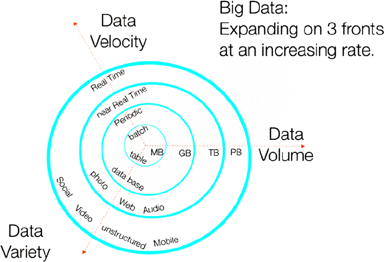
Diya Soubra, a product marketing manager at ARM a company that designs and licenses microprocessors,

visually elaborated on the 3Vs in his 2012 datasciencecentral.com article “The 3Vs that Define Big Data.” He has

kindly allowed me to reproduce his diagram from that article as Figure 1-1. As you can see, big data is expanding in

multiple dimensions over time.

CHAPTER 1 ■ THE PROBLEM WITH DATA

2

You can find real-world examples of current big data projects in a range of industries. In science, for example,

a single genome file might contain 100 GB of data; the “1000 Genomes Project” has amassed 200 TB worth of

information already. Or, consider the data output of the Large Hadron Collider, which produces 15 PB of detector data

per year. Finally, eBay stores 40 PB of semistructured and relational data on its Singularity system.

The Potentials and Difficulties of Big Data

Big data needs to be considered in terms of how the data will be manipulated. The size of the data set will impact

data capture, movement, storage, processing, presentation, analytics, reporting, and latency. Traditional tools quickly

can become overwhelmed by the large volume of big data. Latency—the time it takes to access the data—is as an

important a consideration as volume. Suppose you might need to run an ad hoc query against the large data set or a

predefined report. A large data storage system is not a data warehouse, however, and it may not respond to queries in

a few seconds. It is, rather, the organization-wide repository that stores all of its data and is the system that feeds into

the data warehouses for management reporting.

One solution to the problems presented by very large data sets might be to discard parts of the data so as to

reduce data volume, but this isn’t always practical. Regulations might require that data be stored for a number of

years, or competitive pressure could force you to save everything. Also, who knows what future benefits might be

gleaned from historic business data? If parts of the data are discarded, then the detail is lost and so too is any potential

future competitive advantage.

Instead, a parallel processing approach can do the trick—think divide and conquer. In this ideal solution, the

data is divided into smaller sets and is processed in a parallel fashion. What would you need to implement such

an environment? For a start, you need a robust storage platform that’s able to scale to a very large degree (and

Figure 1-1. Diya Soubra’s multidimensional 3V diagram showing big data’s expansion over time

CHAPTER 1 ■ THE PROBLEM WITH DATA

3

at reasonable cost) as the data grows and one that will allow for system failure. Processing all this data may take

thousands of servers, so the price of these systems must be affortable to keep the cost per unit of storage reasonable.

In licensing terms, the software must also be affordable because it will need to be installed on thousands of servers.

Further, the system must offer redundancy in terms of both data storage and hardware used. It must also operate on

commodity hardware, such as generic, low-cost servers, which helps to keep costs down. It must additionally be able

to scale to a very high degree because the data set will start large and will continue to grow. Finally, a system like this

should take the processing to the data, rather than expect the data to come to the processing. If the latter were to be

the case, networks would quickly run out of bandwidth.

Requirements for a Big Data System

This idea of a big data system requires a tool set that is rich in functionality. For example, it needs a unique kind of

distributed storage platform that is able to move very large data volumes into the system without losing data. The

tools must include some kind of configuration system to keep all of the system servers coordinated, as well as ways

of finding data and streaming it into the system in some type of ETL-based stream. (ETL, or extract, transform, load,

is a data warehouse processing sequence.) Software also needs to monitor the system and to provide downstream

destination systems with data feeds so that management can view trends and issue reports based on the data. While

this big data system may take hours to move an individual record, process it, and store it on a server, it also needs to

monitor trends in real time.

In summary, to manipulate big data, a system requires the following:

A method of collecting and categorizing data•

A method of moving data into the system safely and without data loss•

A storage system that•

Is distributed across many servers•

Is scalable to thousands of servers•

Will offer data redundancy and backup•

Will offer redundancy in case of hardware failure•

Will be cost-effective•

A rich tool set and community support•

A method of distributed system configuration•

Parallel data processing•

System-monitoring tools•

Reporting tools•

ETL-like tools (preferably with a graphic interface) that can be used to build tasks that process •

the data and monitor their progress

Scheduling tools to determine when tasks will run and show task status•

The ability to monitor data trends in real time•

Local processing where the data is stored to reduce network bandwidth usage•

Later in this chapter I explain how this book is organized with these requirements in mind. But let’s now consider

which tools best meet the big data requirements listed above.

CHAPTER 1 ■ THE PROBLEM WITH DATA

4

How Hadoop Tools Can Help

Hadoop tools are a good fit for your big data needs. When I refer to Hadoop tools, I mean the whole Apache

(www.apache.org) tool set related to big data. A community-based, open-source approach to software development,

the Apache Software Foundation (ASF) has had a huge impact on both software development for big data and

the overall approach that has been taken in this field. It also fosters significant cross-pollination of both ideas and

development by the parties involved—for example, Google, Facebook, and LinkedIn. Apache runs an incubator

program in which projects are accepted and matured to ensure that they are robust and production worthy.

Hadoop was developed by Apache as a distributed parallel big data processing system. It was written in

Java and released under an Apache license. It assumes that failures will occur, and so it is designed to offer both

hardware and data redundancy automatically. The Hadoop platform offers a wide tool set for many of the big data

functions that I have mentioned. The original Hadoop development was influenced by Google's MapReduce and

the Google File System.

The following list is a sampling of tools available in the Hadoop ecosystem. Those marked in boldface are

introduced in the chapters that follow:

• Ambari Hadoop management and monitoring

Avro Data serialization system•

Chukwa Data collection and monitoring•

• Hadoop Hadoop distributed storage platform

Hama BSP scientific computing framework•

• HBase Hadoop NoSQL non-relational database

• Hive Hadoop data warehouse

• Hue Hadoop web interface for analyzing data

Mahout Scalable machine learning platform•

• Map/Reduce Algorithm used by the Hadoop MR component

• Nutch Web crawler

• Oozie Workflow scheduler

• Pentaho Open-source analytics tool set

• Pig Data analysis high-level language

• Solr Search platform

• Sqoop Bulk data-transfer tool

• Storm Distributed real-time computation system

• Yarn Map/Reduce in Hadoop Version 2

• ZooKeeper Hadoop centralized configuration system

When grouped together, the ASF, Lucene, and other provider tools, some of which are here, provide a rich

functional set that will allow you to manipulate your data.

CHAPTER 1 ■ THE PROBLEM WITH DATA

5

My Approach

My approach in this book is to build the various tools into one large system. Stage by stage, and starting with the

Hadoop Distributed File System (HDFS), which is the big data file system, I do the following:

Introduce the tool•

Show how to obtain the installation package•

Explain how to install it, with examples•

Employ examples to show how it can be used•

Given that I have a lot of tools and functions to introduce, I take only a brief look at each one. Instead, I show

you how each of these tools can be used as individual parts of a big data system. It is hoped that you will be able to

investigate them further in your own time.

The Hadoop platform tool set is installed on CentOS Linux 6.2. I use Linux because it is free to download and

has a small footprint on my servers. I use Centos rather than another free version of Linux because some of the

Hadoop tools have been released for CentOS only. For instance, at the time of writing this, Ambari is not available

for Ubuntu Linux.

Throughout the book, you will learn how you can build a big data system using low-cost, commodity hardware.

I relate the use of these big data tools to various IT roles and follow a step-by-step approach to show how they

are feasible for most IT professionals. Along the way, I point out some solutions to common problems you might

encounter, as well as describe the benefits you can achieve with Hadoop tools. I use small volumes of data to

demonstrate the systems, tools, and ideas; however, the tools scale to very large volumes of data.

Some level of knowledge of Linux, and to a certain extent Java, is assumed. Don’t be put off by this; instead, think

of it as an opportunity to learn a new area if you aren’t familiar with the subject.

Overview of the Big Data System

While many organizations may not yet have the volumes of data that could be defined as big data, all need to consider

their systems as a whole.A large organization might have a single big data repository. In any event, it is useful to

investigate these technologies as preparation for meeting future needs.

Big Data Flow and Storage

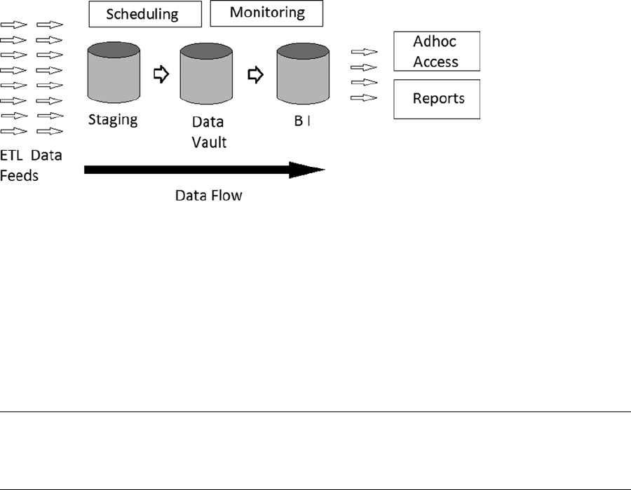
Many of the principles governing business intelligence and data warehousing scale to big data proportions. For

instance, Figure 1-2 depicts a data warehouse system in general terms.

CHAPTER 1 ■ THE PROBLEM WITH DATA

6

As you can see in Figure 1-2, ETL (extraction, transformation, and loading of the data) feeds arrive at the

staging schema of the warehouse and are loaded into their current raw format in staging area tables. The data is

then transformed and moved to the data vault, which contains all the data in the repository. That data might be

filtered, cleaned, enriched, and restructured. Lastly, the data is loaded into the BI, or Business Intelligence, schema

of the warehouse, where the data could be linked to reference tables. It is at this point that the data is available for

the business via reporting tools and adhoc reports. Figure 1-2 also illustrates the scheduling and monitoring tasks.

Scheduling controls when feeds are run and the relationships between them, while monitoring determines whether

the feeds have run and whether errors have occurred. Note also that scheduled feeds can be inputs to the system, as

well as outputs.

Note ■ The data movement flows from extraction from raw sources, to loading, to staging and transformation, and to

the data vault and the BI layer. The acronym for this process is ELT (extract, load, transfer), which better captures what is

happening than the common term ETL.

Many features of this data warehouse system can scale up to and be useful in a big data system. Indeed, the

big data system could feed data to data warehouses and datamarts. Such a big data system would need extraction,

loading, and transform feeds, as well as scheduling, monitoring, and perhaps the data partitioning that a data

warehouse uses, to separate the stages of data processing and access. By adding a big data repository to an IT

architecture, you can extend future possibilities to mine data and produce useful reports. Whereas currently you

might filter and aggregate data to make it fit a datamart, the new architecture allows you to store all of your raw data.

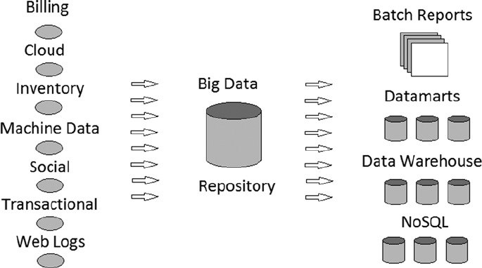
So where would a big data system fit in terms of other systems a large organization might have? Figure 1-3

represents its position in general terms, for there are many variations on this, depending on the type of company and

its data feeds.

Figure 1-2. A general data warehouse system

CHAPTER 1 ■ THE PROBLEM WITH DATA

7

Figure 1-3 does not include all types of feeds. Also, it does not have the feedback loops that probably would exist.

For instance, data warehouse feeds might form inputs, have their data enriched, and feed outputs. Web log data might

be inputs, then enriched with location and/or transaction data, and become enriched outputs. However, the idea here

is that a single, central big data repository can exist to hold an organization's big data.

Benefits of Big Data Systems

Why investigate the use of big data and a parallel processing approach? First, if your data can no longer be processed

by traditional relational database systems (RDBMS), that might mean your organization will have future data

problems. You might have been forced to introduce NoSQL database technology so as to process very large data

volumes in an acceptable time frame. Hadoop might not be the immediate solution to your processing problems,

owing to its high latency, but it could provide a scalable big data storage platform.

Second, big data storage helps to establish a new skills base within the organization. Just as data warehousing

brought with it the need for new skills to build, support, and analyze the warehouse, so big data leads to the same type

of skills building. One of the biggest costs in building a big data system is the specialized staff needed to maintain it

and use the data in it. By starting now, you can build a skills pool within your organization, rather than have to hire

expensive consultants later. (Similarly, as an individual, accessing these technologies can help you launch a new and

lucrative career in big data.)

Third, by adopting a platform that can scale to a massive degree, a company can extend the shelf life of its system

and so save money, as the investment involved can be spread over a longer time. Limited to interim solutions, a

company with a small cluster might reach capacity within a few years and require redevelopment.

Fourth, by getting involved in the big data field now, a company can future-proof itself and reduce risk by

building a vastly scalable distributed platform. By introducing the technologies and ideas in a company now, there

will be no shock felt in later years, when there is a need to adopt the technology.

In developing any big data system, your organization needs to keep its goals in mind. Why are you developing the

system? What do you hope to achieve? How will the system be used? What will you store? You measure the system use

over time against the goals that were established at its inception.

Figure 1-3. A general big data environment

CHAPTER 1 ■ THE PROBLEM WITH DATA

8

What’s in This Book

This book is organized according to the particular features of a big data system, paralleling the general requirements

of a big data system, as listed in the beginning of this chapter. This first chapter describes the features of big data

and names the related tools that are introduced in the chapters that follow. My aim here is to describe as many big

data tools as possible, using practical examples. (Keep in mind, however, that writing deadlines and software update

schedules don’t always mesh, so some tools or functions may have changed by the time you read this.)

All of the tools discussed in this book have been chosen because they are supported by a large user base, which

fulfills big data’s general requirements of a rich tool set and community support. Each Apache Hadoop-based tool has

its own website and often its own help forum. The ETL and reporting tools introduced in Chapters 10 and 11, although

non-Hadoop, are also supported by their own communities.

Storage: Chapter 2

Discussed in Chapter 2, storage represents the greatest number of big data requirements, as listed earlier:

A storage system that•

Is distributed across many servers•

Is scalable to thousands of servers•

Will offer data redundancy and backup•

Will offer redundancy in case of hardware failure•

Will be cost-effective•

A distributed storage system that is highly scalable, Hadoop meets all of these requirements. It offers a high

level of redundancy with data blocks being copied across the cluster. It is fault tolerant, having been designed with

hardware failure in mind. It also offers a low cost per unit of storage. Hadoop versions 1.x and 2.x are installed and

examined in Chapter 2, as well as a method of distributed system configuration. The Apache ZooKeeper system is

used within the Hadoop ecosystem to provide a distributed configuration system for Apache Hadoop tools.

Data Collection: Chapter 3

Automated web crawling to collect data is a much-used technology, so we need a method of collecting and

categorizing data. Chapter 3 describes two architectures using Nutch and Solr to search the web and store data. The

first stores data directly to HDFS, while the second uses Apache HBase. The chapter provides examples of both.

Processing: Chapter 4

The following big data requirements relate to data processing:

Parallel data processing•

Local processing where the data is stored to reduce network bandwidth usage•

Chapter 4 introduces a variety of Map Reduce programming approaches, with examples. Map Reduce programs

are developed in Java, Apache Pig, Perl, and Apache Hive.

CHAPTER 1 ■ THE PROBLEM WITH DATA

9

Scheduling: Chapter 5

The big data requirement for scheduling encompasses the need to share resources and determine when tasks will

run. For sharing Hadoop-based resources, Chapter 5 introduces the Capacity and Fair schedulers for Hadoop. It also

introduces Apache Oozie, showing how simple ETL tasks can be created using Hadoop components like Apache

Sqoop and Apache Pig. Finally, it demonstrates how to schedule Oozie tasks.

Data Movement: Chapter 6

Big data systems require tools to allow safe movement of a variety of data types, safely and without data loss. Chapter 6

introduces the Apache Sqoop tool for moving data into and out of relational databases. It also provides an example of

how Apache Flume can be used to process log-based data. Apache Storm is introduced for data stream processing.

Monitoring: Chapter 7

The requirement for system monitoring tools for a big data system is discussed in Chapter 7. The chapter introduces

the Hue tool as a single location to access a wide range of Apache Hadoop functionality. It also demonstrates the

Ganglia and Nagios resource monitoring and alerting tools.

Cluster Management: Chapter 8

Cluster managers are introduced in Chapter 8 by using the Apache Ambari tool to install Horton Works HDP 2.1 and

Cloudera’s cluster manager to install Cloudera CDH5. A brief overview is then given of their functionality.

Analysis: Chapter 9

Big data requires the ability to monitor data trends in real time. To that end, Chapter 9 introduces the Apache Spark

real-time, in-memory distributed processing system. It also shows how Spark SQL can be used, via an example. It also

includes a practical demonstration of the features of the Apache Hive and Cloudera Impala query languages.

ETL: Chapter 10

Although ETL was briefly introduced in Chapter 5, this chapter discusses the need for graphic tools for ETL chain

building and management. ETL-like tools (preferably with a graphic interface) can be used to build tasks to process

the data and monitor their progress. Thus, Chapter 10 introduces the Pentaho and Talend graphical ETL tools for

big data. This chapter investigates their visual object based approach to big data ETL task creation. It also shows that

these tools offer an easier path into the work of Map Reduce development.

Reports: Chapter 11

Big data systems need reporting tools. In Chapter 11, some reporting tools are discussed and a typical dashboard is

built using the Splunk/Hunk tool. Also, the evaluative data-quality capabilities of Talend are investigated by using the

profiling function.

CHAPTER 1 ■ THE PROBLEM WITH DATA

10

Summary

While introducing the challenges and benefits of big data, this chapter also presents a set of requirements for big data

systems and explains how they can be met by utilizing the tools discussed in the remaining chapters of this book.

The aim of this book has been to explain the building of a big data processing system by using the Hadoop tool

set. Examples are used to explain the functionality provided by each Hadoop tool. Starting with HDFS for storage,

followed by Nutch and Solr for data capture, each chapter covers a new area of functionality, providing a simple

overview of storage, processing, and scheduling. With these examples and the step-by-step approach, you can build

your knowledge of big data possibilities and grow your familiarity with these tools. By the end of Chapter 11, you will

have learned about most of the major functional areas of a big data system.

As you read through this book, you should consider how to use the individual Hadoop components in your own

systems. You will also notice a trend toward easier methods of system management and development. For instance,

Chapter 2 starts with a manual installation of Hadoop, while Chapter 8 uses cluster managers. Chapter 4 shows

handcrafted code for Map Reduce programming, but Chapter 10 introduces visual object based Map Reduce task

development using Talend and Pentaho.

Now it's time to start, and we begin by looking at Hadoop itself. The next chapter introduces the Hadoop

application and its uses, and shows how to configure and use it.

11

Chapter 2

Storing and Configuring Data with

Hadoop, YARN, and ZooKeeper

This chapter introduces Hadoop versions V1 and V2, laying the groundwork for the chapters that follow. Specifically,

you first will source the V1 software, install it, and then configure it. You will test your installation by running a simple

word-count Map Reduce task. As a comparison, you will then do the same for V2, as well as install a ZooKeeper

quorum. You will then learn how to access ZooKeeper via its commands and client to examine the data that it stores.

Lastly, you will learn about the Hadoop command set in terms of shell, user, and administration commands. The

Hadoop installation that you create here will be used for storage and processing in subsequent chapters, when you

will work with Apache tools like Nutch and Pig.

An Overview of Hadoop

Apache Hadoop is available as three download types via the hadoop.apache.org website. The releases are named as

follows:

Hadoop-1.2.1•

Hadoop-0.23.10•

Hadoop-2.3.0•

The first release relates to Hadoop V1, while the second two relate to Hadoop V2. There are two different release

types for V2 because the version that is numbered 0.xx is missing extra components like NN and HA. (NN is “name

node” and HA is “high availability.”) Because they have different architectures and are installed differently, I first

examine both Hadoop V1 and then Hadoop V2 (YARN). In the next section, I will give an overview of each version and

then move on to the interesting stuff, such as how to source and install both.

Because I have only a single small cluster available for the development of this book, I install the different

versions of Hadoop and its tools on the same cluster nodes. If any action is carried out for the sake of demonstration,

which would otherwise be dangerous from a production point of view, I will flag it. This is important because, in

a production system, when you are upgrading, you want to be sure that you retain all of your data. However, for

demonstration purposes, I will be upgrading and downgrading periodically.

So, in general terms, what is Hadoop? Here are some of its characteristics:

It is an open-source system developed by Apache in Java.•

It is designed to handle very large data sets.•

It is designed to scale to very large clusters.•

It is designed to run on commodity hardware.•

CHAPTER 2 ■ STORING AND CONFIGURING DATA WITH HADOOP, YARN, AND ZOOKEEPER

12

It offers resilience via data replication.•

It offers automatic failover in the event of a crash.•

It automatically fragments storage over the cluster.•

It brings processing to the data.•

Its supports large volumes of files—into the millions.•

The third point comes with a caveat: Hadoop V1 has problems with very large scaling. At the time of writing, it is

limited to a cluster size of around 4,000 nodes and 40,000 concurrent tasks. Hadoop V2 was developed in part to offer

better resource usage and much higher scaling.

Using Hadoop V2 as an example, you see that there are four main component parts to Hadoop. Hadoop Common

is a set of utilities that support Hadoop as a whole. Hadoop Map Reduce is the parallel processing system used by

Hadoop. It involves the steps Map, Shuffle, and Reduce. A big volume of data (the text of this book, for example) is

mapped into smaller elements (the individual words), then an operation (say, a word count) is carried out locally

on the small elements of data. These results are then shuffled into a whole, and reduced to a single list of words and

their counts. Hadoop YARN handles scheduling and resource management. Finally, Hadoop Distributed File System

(HDFS) is the distributed file system that works on a master/slave principle whereby a name node manages a cluster

of slave data nodes.

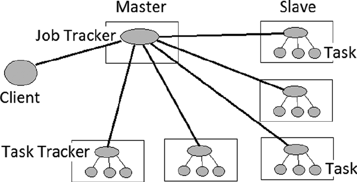
The Hadoop V1 Architecture

In the V1 architecture, a master Job Tracker is used to manage Task Trackers on slave nodes (Figure 2-1). Hadoop’s

data node and Task Trackers co-exist on the same slave nodes.

Figure 2-1. Hadoop V1 architecture

CHAPTER 2 ■ STORING AND CONFIGURING DATA WITH HADOOP, YARN, AND ZOOKEEPER

13

The cluster-level Job Tracker handles client requests via a Map Reduce (MR) API. The clients need only process

via the MR API, as the Map Reduce framework and system handle the scheduling, resources, and failover in the event

of a crash. Job Tracker handles jobs via data node–based Task Trackers that manage the actual tasks or processes. Job

Tracker manages the whole client-requested job, passing subtasks to individual slave nodes and monitoring their

availability and the tasks’ completion.

Hadoop V1 only scales to clusters of around 4,000 to 5,000 nodes, and there are also limitations on the number of

concurrent processes that can run. It has only a single processing type, Map Reduce, which although powerful does

not allow for requirements like graph or real-time processing.

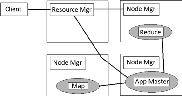
The Differences in Hadoop V2

With YARN, Hadoop V2’s Job Tracker has been split into a master Resource Manager and slave-based Application

Master processes. It separates the major tasks of the Job Tracker: resource management and monitoring/scheduling.

The Job History server now has the function of providing information about completed jobs. The Task Tracker has

been replaced by a slave-based Node Manager, which handles slave node–based resources and manages tasks on

the node. The actual tasks reside within containers launched by the Node Manager. The Map Reduce function is

controlled by the Application Master process, while the tasks themselves may be either Map or Reduce tasks.

Hadoop V2 also offers the ability to use non-Map Reduce processing, like Apache Giraph for graph processing, or

Impala for data query. Resources on YARN can be shared among all three processing systems.

Figure 2-2 shows client task requests being sent to the global Resource Manager and the slave-based Node

Managers launching containers, which have the actual tasks. It also monitors their resource usage. The Application

Master requests containers from the scheduler and receives status updates from the container-based Map Reduce tasks.

Figure 2-2. Hadoop V2 architecture

This architecture enables Hadoop V2 to scale to much larger clusters and provides the ability to have a higher

number of concurrent processes. It also now offers the ability, as mentioned earlier, to run different types of processes

concurrently, not just Map Reduce.

CHAPTER 2 ■ STORING AND CONFIGURING DATA WITH HADOOP, YARN, AND ZOOKEEPER

14

This is an introduction to the Hadoop V1 and V2 architectures. You might have the opportunity to work with both

versions, so I give examples for installation and use of both. The architectures are obviously different, as seen in

Figures 2-1 and 2-2, and so the actual installation/build and usage differ as well. For example, for V1 you will carry out

a manual install of the software while for V2 you will use the Cloudera software stack, which is described next.

The Hadoop Stack

Before we get started with the Hadoop V1 and V2 installations, it is worth discussing the work of companies like

Cloudera and Hortonworks. They have built stacks of Hadoop-related tools that have been tested for interoperability.

Although I describe how to carry out a manual installation of software components for V1, I show how to use one of

the software stacks for the V2 install.

When you’re trying to use multiple Hadoop platform tools together in a single stack, it is important to know what

versions will work together without error. If, for instance, you are using ten tools, then the task of tracking compatible

version numbers quickly becomes complex. Luckily there are a number of Hadoop stacks available. Suppliers can

provide a single tested package that you can download. Two of the major companies in this field are Cloudera and

Hortonworks. Apache Bigtop, a testing suite that I will demonstrate in Chapter 8, is also used as the base for the

Cloudera Hadoop stack.

Table 2-1 shows the current stacks from these companies, listing components and versions of tools that are

compatible at the time of this writing.

Table 2-1. Hadoop Stack Tool Version Details

Cloudera CDH 4.6.0 Hortonworks Data Platform 2.0

Ambari 1.4.4

DataFu 0.0.4

Flume 1.4.0 1.4.0

Hadoop 2.0.0 2.2.0

HCatalog 0.5.0 0.12.0

HBase 0.94 0.96.1

Hive 0.10.0 0.12.0

Hue 2.5.0 2.3.0

Mahout 0.7 0.8.0

Oozie 3.3.2 4.0.0

Parquet 1.2.5

Pig 0.11 0.12.0

Sentry 1.1.0

Sqoop 1.4.3 1.4.4

Sqoop2 1.99.2

Whirr 0.8.2

ZooKeeper 3.4.5 3.4.5

CHAPTER 2 ■ STORING AND CONFIGURING DATA WITH HADOOP, YARN, AND ZOOKEEPER

15

While I use a Hadoop stack in the rest of the book, here I will show the process of downloading, installing,

configuring, and running Hadoop V1 so that you will be able to compare the use of V1 and V2.

Environment Management

Before I move into the Hadoop V1 and V2 installations, I want to point out that I am installing both Hadoop V1 and V2

on the same set of servers. Hadoop V1 is installed under /usr/local while Hadoop V2 is installed as a Cloudera CDH

release and so will have a defined set of directories:

Logging under /var/log; that is, /var/log/hadoop-hdfs/•

Configuration under /etc/hadoop/conf/•

Executables defined as servers under /etc/init.d/; that is, hadoop-hdfs-namenode•

I have also created two sets of .bashrc environment configuration files for the Linux Hadoop user account:

[hadoop@hc1nn ~]$ pwd

/home/hadoop

[hadoop@hc1nn ~]$ ls -l .bashrc*

lrwxrwxrwx. 1 hadoop hadoop 16 Jun 30 17:59 .bashrc -> .bashrc_hadoopv2

-rw-r--r--. 1 hadoop hadoop 1586 Jun 18 17:08 .bashrc_hadoopv1

-rw-r--r--. 1 hadoop hadoop 1588 Jul 27 11:33 .bashrc_hadoopv2

By switching the .bashrc symbolic link between the Hadoop V1 (.bashrc_hadoopv1) and V2 (.bashrc_hadoopv2)

files, I can quickly navigate between the two environments. Each installation has a completely separate set of

resources. This approach enables me to switch between Hadoop versions on my single set of testing servers while

writing this guide. From a production viewpoint, however, you would install only one version of Hadoop at a time.

Hadoop V1 Installation

Before you attempt to install Hadoop, you must ensure that Java 1.6.x is installed and that SSH (secure shell) is

installed and running. The master name node must be able to create an SSH session to reach each of its data nodes

without using a password in order to manage them. On CentOS, you can install SSH via the root account as follows:

yum install openssh-server

This will install the secure shell daemon process. Repeat this installation on all of your servers, then start the

service (as root):

service sshd restart

Now, in order to make the SSH sessions from the name node to the data nodes operate without a password,

you must create an SSH key on the name node and copy the key to each of the data nodes. You create the key with

the keygen command as the hadoop user (I created the hadoop user account during the installation of the CentOS

operating system on each server), as follows:

ssh-keygen

CHAPTER 2 ■ STORING AND CONFIGURING DATA WITH HADOOP, YARN, AND ZOOKEEPER

16

A key is created automatically as $HOME/.ssh/id_rsa.pub. You now need to copy this key to the data nodes. You

run the following command to do that:

ssh-copy-id hadoop@hc1r1m1

This copies the new SSH key to the data node hc1r1m1 as user hadoop; you change the server name to copy the

key to the other data node servers.

The remote passwordless secure shell access can now be tested with this:

ssh hadoop@hc1r1m1

A secure shell session should now be created on the host hc1r1m1 without need to prompt a password.

As Hadoop has been developed using Java, you must also ensure that you have a suitable version of Java installed

on each machine. I will be using four machines in a mini cluster for this test:

hc1nn - A Linux CentOS 6 server for a name node•

hc1r1m1 - A Linux CentOS 6 server for a data node•

hc1r1m2 - A Linux CentOS 6 server for a data node•

hc1r1m3 - A Linux CentOS 6 server for a data node•

Can the name node access all of the data nodes via SSH (secure shell) without being prompted for a password?

And is a suitable Java version installed? I have a user account called hadoop on each of these servers that I use for this

installation. For instance, the following command line shows hadoop@hc1nn, which means that we are logged into the

server hc1nn as the Linux user hadoop:

[hadoop@hc1nn ~]$ java -version

java version "1.6.0_30"

OpenJDK Runtime Environment (IcedTea6 1.13.1) (rhel-3.1.13.1.el6_5-i386)

OpenJDK Client VM (build 23.25-b01, mixed mode)

This command, java -version, shows that we have OpenJDK java version 1.6.0_30 installed. The following

commands create an SSH session on each of the data nodes and checks the Java version on each:

[hadoop@hc1nn ~]$ ssh hadoop@hc1r1m3

Last login: Thu Mar 13 19:41:12 2014 from hc1nn

[hadoop@hc1r1m3 ~]$

[hadoop@hc1r1m3 ~]$ java -version

java version "1.6.0_30"

OpenJDK Runtime Environment (IcedTea6 1.13.1) (rhel-3.1.13.1.el6_5-i386)

OpenJDK Server VM (build 23.25-b01, mixed mode)

[hadoop@hc1r1m3 ~]$ exit

logout

Connection to hc1r1m3 closed.

[hadoop@hc1nn ~]$ ssh hadoop@hc1r1m2

Last login: Thu Mar 13 19:40:45 2014 from hc1nn

[hadoop@hc1r1m2 ~]$ java -version

java version "1.6.0_30"

OpenJDK Runtime Environment (IcedTea6 1.13.1) (rhel-3.1.13.1.el6_5-i386)

OpenJDK Server VM (build 23.25-b01, mixed mode)

CHAPTER 2 ■ STORING AND CONFIGURING DATA WITH HADOOP, YARN, AND ZOOKEEPER

17

[hadoop@hc1r1m2 ~]$ exit

logout

Connection to hc1r1m2 closed.

[hadoop@hc1nn ~]$ ssh hadoop@hc1r1m1

Last login: Thu Mar 13 19:40:22 2014 from hc1r1m3

[hadoop@hc1r1m1 ~]$ java -version

java version "1.6.0_30"

OpenJDK Runtime Environment (IcedTea6 1.13.1) (rhel-3.1.13.1.el6_5-x86_64)

OpenJDK 64-Bit Server VM (build 23.25-b01, mixed mode)

[hadoop@hc1r1m1 ~]$ exit

logout

Connection to hc1r1m1 closed.

These three SSH statements show that a secure shell session can be created from the name node, hc1nn, to each

of the data nodes.

Notice that I am using the Java OpenJDK (http://openjdk.java.net/) here. Generally it’s advised that you use

the Oracle Sun JDK. However, Hadoop has been tested against the OpenJDK, and I am familiar with its use. I don’t

need to register to use OpenJDK, and I can install it on Centos using a simple yum command. Additionally, the Sun

JDK install is more complicated.

Now let’s download and install a version of Hadoop V1. In order to find the release of Apache Hadoop to

download, start here: http://hadoop.apache.org.

Next, choose Download Hadoop, click the release option, then choose Download, followed by Download a

Release Now! This will bring you to this page: http://www.apache.org/dyn/closer.cgi/hadoop/common/. It suggests

a local mirror site that you can use to download the software. It’s a confusing path to follow; I’m sure that this website

could be simplified a little. The suggested link for me is http://apache.insync.za.net/hadoop/common. You may be

offered a different link.

On selecting that site, I’m offered a series of releases. I choose 1.2.1, and then I download the file: Hadoop-

1.2.1.tar.gz. Why choose this particular format over the others? From past experience, I know how to unpack it and use

it; feel free to choose the format with which you’re most comfortable.

Download the file to /home/hadoop/Downloads. (This download and installation must be carried out on each

server.) You are now ready to begin the Hadoop single-node installation for Hadoop 1.2.1.

The approach from this point on will be to install Hadoop onto each server separately as a single-node installation,

configure it, and try to start the servers. This will prove that each node is correctly configured individually. After that,

the nodes will be grouped into a Hadoop master/slave cluster. The next section describes the single-node installation

and test, which should be carried out on all nodes. This will involve unpacking the software, configuring the

environment files, formatting the file system, and starting the servers. This is a manual process; if you have a very large

production cluster, you would need to devise a method of automating the process.

Hadoop 1.2.1 Single-Node Installation

From this point on, you will be carrying out a single-node Hadoop installation (until you format the Hadoop file

system on this node). First, you ftp the file hadoop-1.2.1.tar.gz to all of your nodes and carry out the steps in this

section on all nodes.

So, given that you are logged in as the user hadoop, you see the following file in the $HOME/Downloads

directory:

[hadoop@hc1nn Downloads]$ ls -l

total 62356

-rw-rw-r--. 1 hadoop hadoop 63851630 Mar 15 15:01 hadoop-1.2.1.tar.gz

CHAPTER 2 ■ STORING AND CONFIGURING DATA WITH HADOOP, YARN, AND ZOOKEEPER

18

This is a gzipped tar file containing the Hadoop 1.2.1 software that you are interested in. Use the Linux gunzip

tool to unpack the gzipped archive:

[hadoop@hc1nn Downloads]$ gunzip hadoop-1.2.1.tar.gz

[hadoop@hc1nn Downloads]$ ls -l

total 202992

-rw-rw-r--. 1 hadoop hadoop 207861760 Mar 15 15:01 hadoop-1.2.1.tar

Then, unpack the tar file:

[hadoop@hc1nn Downloads]$ tar xvf hadoop-1.2.1.tar

[hadoop@hc1nn Downloads]$ ls -l

total 202996

drwxr-xr-x. 15 hadoop hadoop 4096 Jul 23 2013 hadoop-1.2.1

-rw-rw-r--. 1 hadoop hadoop 207861760 Mar 15 15:01 hadoop-1.2.1.tar

Now that the software is unpacked to the local directory hadoop-1.2.1, you move it into a better location. To do

this, you will need to be logged in as root:

[hadoop@hc1nn Downloads]$ su -

Password:

[root@hc1nn ~]# cd /home/hadoop/Downloads

[root@hc1nn Downloads]# mv hadoop-1.2.1 /usr/local

[root@hc1nn Downloads]# cd /usr/local

You have now moved the installation to /usr/local, but make sure that the hadoop user owns the installation.

Use the Linux chown command to recursively change the ownership and group membership for files and directories

within the installation:

[root@hc1nn local]# chown -R hadoop:hadoop hadoop-1.2.1

[root@hc1nn local]# ls -l

total 40

drwxr-xr-x. 15 hadoop hadoop 4096 Jul 23 2013 hadoop-1.2.1

You can see from the last line in the output above that the directory is now owned by hadoop and is a member of

the hadoop group.

You also create a symbolic link to refer to your installation so that you can have multiple installations on the same

host for testing purposes:

[root@hc1nn local]# ln -s hadoop-1.2.1 hadoop

[root@hc1nn local]# ls -l

lrwxrwxrwx. 1 root root 12 Mar 15 15:11 hadoop -> hadoop-1.2.1

drwxr-xr-x. 15 hadoop hadoop 4096 Jul 23 2013 hadoop-1.2.1

The last two lines show that there is a symbolic link called hadoop under the directory /usr/local that points to

our hadoop-1.2.1 installation directory at the same level. If you later upgrade and install a new version of the Hadoop

V1 software, you can just change this link to point to it. Your environment and scripts can then remain static and

always use the path /usr/local/hadoop.

Now, you follow these steps to proceed with installation.

CHAPTER 2 ■ STORING AND CONFIGURING DATA WITH HADOOP, YARN, AND ZOOKEEPER

19

1. Set up Bash shell file for hadoop $HOME/.bashrc

When logged in as hadoop, you add the following text to the end of the file $HOME/.bashrc. When you create this

Bash shell, environmental variables like JAVA_HOME and HADOOP_PREFIX are set. The next time a Bash shell is created

by the hadoop user account, these variables will be pre-defined.

#######################################################

# Set Hadoop related env variables

export HADOOP_PREFIX=/usr/local/hadoop

# set JAVA_HOME (we will also set a hadoop specific value later)

export JAVA_HOME=/usr/lib/jvm/jre-1.6.0-openjdk

# some handy aliases and functions

unalias fs 2>/dev/null

alias fs="hadoop fs"

unalias hls 2>/dev/null

alias hls="fs -l"

# add hadoop to the path

export PATH=$PATH:$HADOOP_PREFIX

export PATH=$PATH:$HADOOP_PREFIX/bin

export PATH=$PATH:$HADOOP_PREFIX/sbin

Note that you are not using the $HADOOP_HOME variable, because with this release it has been superseded. If you

use it instead of $HADOOP_PREFIX, you will receive warnings.

2. Set up conf/hadoop-env.sh

You now modify the configuration file hadoop-env.sh to specify the location of the Java installation by setting the

JAVA_HOME variable. In the file conf/hadoop-env.sh, you change:

# export JAVA_HOME=/usr/lib/j2sdk1.5-sun

to

export JAVA_HOME=/usr/lib/jvm/jre-1.6.0-openjdk

Note: When referring to the Hadoop installation configuration directory in this section, and all subsequent

sections for the V1 installation, I mean the /usr/local/hadoop/conf directory.

CHAPTER 2 ■ STORING AND CONFIGURING DATA WITH HADOOP, YARN, AND ZOOKEEPER

20

3. Create Hadoop temporary directory

On the Linux file system, you create a Hadoop temporary directory, as shown below. This will give Hadoop a working

area. Set the ownership to the hadoop user and also set the directory permissions:

[root@hc1nn local]# mkdir -p /app/hadoop/tmp

[root@hc1nn local]# chown -R hadoop:hadoop /app/hadoop

[root@hc1nn local]# chmod 750 /app/hadoop/tmp

4. Set up conf/core-site.xml

You set up the configuration for the Hadoop core component. This file configuration is based on XML; it defines the

Hadoop temporary directory and default file system access. There are many more options that can be specified; see

the Hadoop site (hadoop.apache.org) for details.

Add the following text to the file between the configuration tags:

<name>hadoop.tmp.dir</name>

<value>/app/hadoop/tmp</value>

<description>A base for other temporary directories.</description>

</property>

<name>fs.default.name</name>

<value>hdfs://localhost:54310</value>

<description>The name of the default file system.</description>

</property>

5. Set up conf/mapred-site.xml

Next, you set up the basic configuration for the Map Reduce component, adding the following between the

configuration tags. This defines the host and port name for each Job Tracker server.

<name>mapred.job.tracker</name>

<value>localhost:54311</value>

<description>The host and port for the Map Reduce job tracker

</description>

</property>

<name>mapred.job.tracker.http.address</name>

<value>localhost:50030</value>

</property>

<name>mapred.task.tracker.http.address</name>

<value>localhost:50060</value>

</property>

CHAPTER 2 ■ STORING AND CONFIGURING DATA WITH HADOOP, YARN, AND ZOOKEEPER

21

The example configuration file here is for the server hc1r1m1. When the configuraton is changed to a cluster,

these Job Tracker entries will refer to Name Node machine hc1nn.

6. Set up file conf/hdfs-site.xml

Set up the basic configuration for the HDFS, adding the following between the configuration tags. This defines the

replication level for the HDFS; it shows that a single block will be copied twice. It also specifies the address of the

Name Node web user interface as dfs.http.address:

<name>dfs.replication</name>

<description>The replication level</description>

</property>

<name>dfs.http.address</name>

<value>http://localhost:50070/</value>

</property>

7. Format the file system

Run the following command as the Hadoop user to format the file system:

hadoop namenode -format

Warning ■ Do not execute this command on a running HDFS or you will lose your data!

The output should look like this:

14/03/15 16:08:19 INFO namenode.NameNode: STARTUP_MSG:

/************************************************************

STARTUP_MSG: Starting NameNode

STARTUP_MSG: host = hc1nn/192.168.1.107

STARTUP_MSG: args = [-format]

STARTUP_MSG: version = 1.2.1

STARTUP_MSG: build = https://svn.apache.org/repos/asf/hadoop/common/branches/branch-1.2 -r

1503152; compiled by 'mattf' on Mon Jul 22 15:23:09 PDT 2013

STARTUP_MSG: java = 1.6.0_30

************************************************************/

14/03/15 16:08:20 INFO util.GSet: Computing capacity for map BlocksMap

14/03/15 16:08:20 INFO util.GSet: VM type = 32-bit

14/03/15 16:08:20 INFO util.GSet: 2.0% max memory = 1013645312

14/03/15 16:08:20 INFO util.GSet: capacity = 2^22 = 4194304 entries

14/03/15 16:08:20 INFO util.GSet: recommended=4194304, actual=4194304

14/03/15 16:08:20 INFO namenode.FSNamesystem: fsOwner=hadoop

14/03/15 16:08:20 INFO namenode.FSNamesystem: supergroup=supergroup

14/03/15 16:08:20 INFO namenode.FSNamesystem: isPermissionEnabled=true

14/03/15 16:08:20 INFO namenode.FSNamesystem: dfs.block.invalidate.limit=100

CHAPTER 2 ■ STORING AND CONFIGURING DATA WITH HADOOP, YARN, AND ZOOKEEPER

22

14/03/15 16:08:20 INFO namenode.FSNamesystem: isAccessTokenEnabled=false accessKeyUpdateInterval=0

min(s), accessTokenLifetime=0 min(s)

14/03/15 16:08:20 INFO namenode.FSEditLog: dfs.namenode.edits.toleration.length = 0

14/03/15 16:08:20 INFO namenode.NameNode: Caching file names occuring more than 10 times

14/03/15 16:08:20 INFO common.Storage: Image file /app/hadoop/tmp/dfs/name/current/fsimage of size

112 bytes saved in 0 seconds.

14/03/15 16:08:20 INFO namenode.FSEditLog: closing edit log: position=4, editlog=/app/hadoop/tmp/

dfs/name/current/edits

14/03/15 16:08:20 INFO namenode.FSEditLog: close success: truncate to 4, editlog=/app/hadoop/tmp/

dfs/name/current/edits

14/03/15 16:08:21 INFO common.Storage: Storage directory /app/hadoop/tmp/dfs/name has been

successfully formatted.

14/03/15 16:08:21 INFO namenode.NameNode: SHUTDOWN_MSG:

/************************************************************

SHUTDOWN_MSG: Shutting down NameNode at hc1nn/192.168.1.107

************************************************************/

Now you test that you can start, check, and stop the Hadoop servers on a standalone node without errors. Start

the servers by using:

start-all.sh

You will see this:

starting namenode, logging to

/usr/local/hadoop-1.2.1/libexec/../logs/hadoop-hadoop-namenode-hc1nn.out

localhost: starting datanode, logging to

/usr/local/hadoop-1.2.1/libexec/../logs/hadoop-hadoop-datanode-hc1nn.out

localhost: starting secondarynamenode, logging to

/usr/local/hadoop-1.2.1/libexec/../logs/hadoop-hadoop-secondarynamenode-hc1nn.out

starting jobtracker, logging to

/usr/local/hadoop-1.2.1/libexec/../logs/hadoop-hadoop-jobtracker-hc1nn.out

localhost: starting tasktracker, logging to

/usr/local/hadoop-1.2.1/libexec/../logs/hadoop-hadoop-tasktracker-hc1nn.out

Now, check that the servers are running. Note that you should expect to see the following:

Name node•

Secondary name node•

Job Tracker•

Task Tracker•

Data node•

Running on the master server hc1nn, use the jps command to list the servers that are running:

[hadoop@hc1nn ~]$ jps

2116 SecondaryNameNode

2541 Jps

2331 TaskTracker

2194 JobTracker

CHAPTER 2 ■ STORING AND CONFIGURING DATA WITH HADOOP, YARN, AND ZOOKEEPER

23

1998 DataNode

1878 NameNode

If you find that the jps command is not available, check that it exists as $JAVA_HOME/bin/jps. Ensure that you

installed the Java JDK in the previous step. If that does not work, then try installing the Java OpenJDK development

package as root:

[root@hc1nn ~]$ yum install java-1.6.0-openjdk-devel

Your result shows that the servers are running. If you need to stop them, use the stop-all.sh command, as

follows:

[hadoop@hc1nn ~]$ stop-all.sh

stopping jobtracker

localhost: stopping tasktracker

stopping namenode

localhost: stopping datanode

localhost: stopping secondarynamenode

You have now completed a single-node Hadoop installation. Next, you repeat the steps for the Hadoop V1

installation on all of the nodes that you plan to use in your Hadoop cluster. When that is done, you can move to the

next section, “Setting up the Cluster,” where you’ll combine all of the single-node machines into a Hadoop cluster

that’s run from the Name Node machine.

Setting up the Cluster

Now you are ready to set up the Hadoop cluster. Make sure that all servers are stopped on all nodes by using the

stop-all.sh script.

First, you must tell the name node where all of its slaves are. To do so, you add the following lines to the master

and slaves files. (You only do this on the Name Node server [hc1nn], which is the master. It then knows that it is the

master and can identify its slave data nodes.) You add the following line to the file $HADOOP_PREFIX/conf/masters

to identify it as the master:

hc1nn

Then, you add the following lines to the file $HADOOP_PREFIX/conf/slaves to identify those servers as slaves:

hc1nn

hc1r1m1

hc1r1m2

hc1r1m3

These are all of the machines in my cluster. Your machine names may be different, so you would insert your own

machine names. Note also that I am using the Name Node machine (hc1nn) as a master and a slave. In a production

cluster you would have name nodes and data nodes on separate servers.

On all nodes, you change the value of fs.default.name in the file $HADOOP_PREFIX/conf/core-site.xml to be:

hdfs://hc1nn:54310

This configures all nodes for the core Hadoop component to access the HDFS using the same address.

CHAPTER 2 ■ STORING AND CONFIGURING DATA WITH HADOOP, YARN, AND ZOOKEEPER

24

On all nodes, you change the value of mapred.job.tracker in the file $HADOOP_PREFIX/conf/mapred-site.xml to be:

hc1nn:54311

This defines the host and port names on all servers for the Map Reduce Job Tracker server to point to the Name

Node machine.

On all nodes, check that the value of dfs.replication in the file $HADOOP_PREFIX/conf/hdfs-site.xml is set to 3.

This means that three copies of each block of data will automatically be kept by HDFS.

In the same file, ensure that the line http://localhost:50070/ for the variable dfs.http.address is changed to:

http://hc1nn:50070/

This sets the HDFS web/http address to point to the Name Node master machine hc1nn. With none of the

Hadoop servers running, you format the cluster from the Name Node server—in this instance, hc1nn:

hadoop namenode –format

At this point, a common problem can occur with Hadoop file system versioning between the name node and data

nodes. Within HDFS, there are files named VERSION that contain version numbering information that is regenerated

each time the file system is formatted, such as:

[hadoop@hc1nn dfs]$ pwd

/app/hadoop/tmp/dfs

[hadoop@hc1nn dfs]$ find . -type f -name VERSION -exec grep -H namespaceID {} \;

./data/current/VERSION:namespaceID=1244166645

./name/current/VERSION:namespaceID=1244166645

./name/previous.checkpoint/VERSION:namespaceID=1244166645

./namesecondary/current/VERSION:namespaceID=1244166645

The Linux command shown here is executed as the hadoop user searches for the VERSION files under /app/

hadoop/tmp/dfs and strips the namespace ID information out of them. If this command was executed on the Name

Node server and the Data Node servers, you would expect to see the same value 1244166645. When this versioning

gets out of step on the data nodes, an error occurs, such as follows:

ERROR org.apache.hadoop.hdfs.server.datanode.DataNode: java.io.IOException: Incompatible

namespaceIDs

While this problem seems to have two solutions, only one is viable. Although you could delete the data directory

/app/hadoop/tmp/dfs/data on the offending data node, reformat the file system, and then start the servers, this

approach will cause data loss. The second, more effective method involves editing the VERSION files on the data

nodes so that the namespace ID values match those found on the Name Node machine.

You need to ensure that your firewall will enable port access for Hadoop to communicate. When you attempt to

start the Hadoop servers, check the logs in the log directory (/usr/local/hadoop/logs).

Now, start the cluster from the name node; this time, you will start the HDFS servers using the script start-dfs.sh:

[hadoop@hc1nn logs]$ start-dfs.sh

starting namenode, logging to /usr/local/hadoop-1.2.1/libexec/../logs/hadoop-hadoop-namenode-

hc1nn.out

hc1r1m2: starting datanode, logging to /usr/local/hadoop-1.2.1/libexec/../logs/hadoop-hadoop-

datanode-hc1r1m2.out

CHAPTER 2 ■ STORING AND CONFIGURING DATA WITH HADOOP, YARN, AND ZOOKEEPER

25

hc1r1m1: starting datanode, logging to /usr/local/hadoop-1.2.1/libexec/../logs/hadoop-hadoop-

datanode-hc1r1m1.out

hc1r1m3: starting datanode, logging to /usr/local/hadoop-1.2.1/libexec/../logs/hadoop-hadoop-

datanode-hc1r1m3.out

hc1nn: starting datanode, logging to /usr/local/hadoop-1.2.1/libexec/../logs/hadoop-hadoop-

datanode-hc1nn.out

hc1nn: starting secondarynamenode, logging to /usr/local/hadoop-1.2.1/libexec/../logs/hadoop-

hadoop-secondarynamenode-hc1nn.out

As mentioned, check the logs for errors under $HADOOP_PREFIX/logs on each server. If you get errors like

“No Route to Host,” it is a good indication that your firewall is blocking a port. It will save a great deal of time and

effort if you ensure that the firewall port access is open. (If you are unsure how to do this, then approach your systems

administrator.)

You can now check that the servers are running on the name node by using the jps command:

[hadoop@hc1nn ~]$ jps

2116 SecondaryNameNode

2541 Jps

1998 DataNode

1878 NameNode

If you need to stop the HDFS servers, you can use the stop-dfs.sh script. Don’t do it yet, however, as you will

start the Map Reduce servers next.

With the HDFS servers running, it is now time to start the Map Reduce servers. The HDFS servers should always

be started first and stopped last. Use the start-mapred.sh script to start the Map Reduce servers, as follows:

[hadoop@hc1nn logs]$ start-mapred.sh

starting jobtracker, logging to

/usr/local/hadoop-1.2.1/libexec/../logs/hadoop-hadoop-jobtracker-hc1nn.out

hc1r1m2: starting tasktracker, logging to

/usr/local/hadoop-1.2.1/libexec/../logs/hadoop-hadoop-tasktracker-hc1r1m2.out

hc1r1m3: starting tasktracker, logging to

/usr/local/hadoop-1.2.1/libexec/../logs/hadoop-hadoop-tasktracker-hc1r1m3.out

hc1r1m1: starting tasktracker, logging to

/usr/local/hadoop-1.2.1/libexec/../logs/hadoop-hadoop-tasktracker-hc1r1m1.out

hc1nn: starting tasktracker, logging to

/usr/local/hadoop-1.2.1/libexec/../logs/hadoop-hadoop-tasktracker-hc1nn.out

Note that the Job Tracker has been started on the name node and a Task Tracker on each of the data nodes.

Again, check all of the logs for errors.

Running a Map Reduce Job Check

When your Hadoop V1 system has all servers up and there are no errors in the logs, you’re ready to run a sample Map

Reduce job to check that you can run tasks. For example, try using some data based on works by Edgar Allan Poe. I

have downloaded this data from the Internet and have stored it on the Linux file system under /tmp/edgar. You could

use any text-based data, however, as you just want to run a test to count some words using Map Reduce. It is not the

data that is important but, rather, the correct functioning of Hadoop. To begin, go to the edgar directory, as follows:

cd /tmp/edgar

CHAPTER 2 ■ STORING AND CONFIGURING DATA WITH HADOOP, YARN, AND ZOOKEEPER

26

[hadoop@hc1nn edgar]$ ls -l

total 3868

-rw-rw-r--. 1 hadoop hadoop 632294 Feb 5 2004 10947-8.txt

-rw-r--r--. 1 hadoop hadoop 559342 Feb 23 2005 15143-8.txt

-rw-rw-r--. 1 hadoop hadoop 66409 Oct 27 2010 17192-8.txt

-rw-rw-r--. 1 hadoop hadoop 550284 Mar 16 2013 2147-8.txt

-rw-rw-r--. 1 hadoop hadoop 579834 Dec 31 2012 2148-8.txt

-rw-rw-r--. 1 hadoop hadoop 596745 Feb 17 2011 2149-8.txt

-rw-rw-r--. 1 hadoop hadoop 487087 Mar 27 2013 2150-8.txt

-rw-rw-r--. 1 hadoop hadoop 474746 Jul 1 2013 2151-8.txt

There are eight Linux text files in this directory that contain the test data. First, you copy this data from the Linux

file system into the HDFS directory /user/hadoop/edgar using the Hadoop file system copyFromLocal command:

[hadoop@hc1nn edgar]$ hadoop fs -copyFromLocal /tmp/edgar /user/hadoop/edgar

Now, you check the files that have been loaded to HDFS:

[hadoop@hc1nn edgar]$ hadoop dfs -ls /user/hadoop/edgar

Found 1 items

drwxr-xr-x - hadoop hadoop 0 2014-09-05 20:25 /user/hadoop/edgar/edgar

[hadoop@hc1nn edgar]$ hadoop dfs -ls /user/hadoop/edgar/edgar

Found 8 items

-rw-r--r-- 2 hadoop hadoop 632294 2014-03-16 13:50 /user/hadoop/edgar/edgar/10947-8.txt

-rw-r--r-- 2 hadoop hadoop 559342 2014-03-16 13:50 /user/hadoop/edgar/edgar/15143-8.txt

-rw-r--r-- 2 hadoop hadoop 66409 2014-03-16 13:50 /user/hadoop/edgar/edgar/17192-8.txt

-rw-r--r-- 2 hadoop hadoop 550284 2014-03-16 13:50 /user/hadoop/edgar/edgar/2147-8.txt

-rw-r--r-- 2 hadoop hadoop 579834 2014-03-16 13:50 /user/hadoop/edgar/edgar/2148-8.txt

-rw-r--r-- 2 hadoop hadoop 596745 2014-03-16 13:50 /user/hadoop/edgar/edgar/2149-8.txt

-rw-r--r-- 2 hadoop hadoop 487087 2014-03-16 13:50 /user/hadoop/edgar/edgar/2150-8.txt

-rw-r--r-- 2 hadoop hadoop 474746 2014-03-16 13:50 /user/hadoop/edgar/edgar/2151-8.txt

Next, you run the Map Reduce job, using the Hadoop jar command to pick up the word count from an examples

jar file. This will run a word count on the Edgar Allan Poe data:

[hadoop@hc1nn edgar]$ cd $HADOOP_PREFIX

[hadoop@hc1nn hadoop-1.2.1]$ hadoop jar ./hadoop-examples-1.2.1.jar wordcount

/user/hadoop/edgar /user/hadoop/edgar-results

This job executes the word-count task in the jar file hadoop-examples-1.2.1.jar. It takes data from HDFS under

/user/hadoop/edgar and outputs the results to /user/hadoop/edgar-results. The output of this command is as follows:

14/03/16 14:08:07 INFO input.FileInputFormat: Total input paths to process : 8

14/03/16 14:08:07 INFO util.NativeCodeLoader: Loaded the native-hadoop library

14/03/16 14:08:07 INFO mapred.JobClient: Running job: job_201403161357_0002

14/03/16 14:08:08 INFO mapred.JobClient: map 0% reduce 0%

14/03/16 14:08:18 INFO mapred.JobClient: map 12% reduce 0%

CHAPTER 2 ■ STORING AND CONFIGURING DATA WITH HADOOP, YARN, AND ZOOKEEPER

27

14/03/16 14:08:19 INFO mapred.JobClient: map 50% reduce 0%

14/03/16 14:08:23 INFO mapred.JobClient: map 75% reduce 0%

14/03/16 14:08:26 INFO mapred.JobClient: map 75% reduce 25%

14/03/16 14:08:28 INFO mapred.JobClient: map 87% reduce 25%

14/03/16 14:08:29 INFO mapred.JobClient: map 100% reduce 25%

14/03/16 14:08:33 INFO mapred.JobClient: map 100% reduce 100%

14/03/16 14:08:34 INFO mapred.JobClient: Job complete: job_201403161357_0002

14/03/16 14:08:34 INFO mapred.JobClient: Counters: 29

14/03/16 14:08:34 INFO mapred.JobClient: Job Counters

14/03/16 14:08:34 INFO mapred.JobClient: Launched reduce tasks=1

14/03/16 14:08:34 INFO mapred.JobClient: SLOTS_MILLIS_MAPS=77595

14/03/16 14:08:34 INFO mapred.JobClient: Total time spent by all reduces

waiting after reserving slots (ms)=0

14/03/16 14:08:34 INFO mapred.JobClient: Total time spent by all maps

waiting after reserving slots (ms)=0

14/03/16 14:08:34 INFO mapred.JobClient: Launched map tasks=8

14/03/16 14:08:34 INFO mapred.JobClient: Data-local map tasks=8

14/03/16 14:08:34 INFO mapred.JobClient: SLOTS_MILLIS_REDUCES=15037

14/03/16 14:08:34 INFO mapred.JobClient: File Output Format Counters

14/03/16 14:08:34 INFO mapred.JobClient: Bytes Written=769870

14/03/16 14:08:34 INFO mapred.JobClient: FileSystemCounters

14/03/16 14:08:34 INFO mapred.JobClient: FILE_BYTES_READ=1878599

14/03/16 14:08:34 INFO mapred.JobClient: HDFS_BYTES_READ=3947632

14/03/16 14:08:34 INFO mapred.JobClient: FILE_BYTES_WRITTEN=4251698

14/03/16 14:08:34 INFO mapred.JobClient: HDFS_BYTES_WRITTEN=769870

14/03/16 14:08:34 INFO mapred.JobClient: File Input Format Counters

14/03/16 14:08:34 INFO mapred.JobClient: Bytes Read=3946741

14/03/16 14:08:34 INFO mapred.JobClient: Map-Reduce Framework

14/03/16 14:08:34 INFO mapred.JobClient: Map output materialized

bytes=1878641

14/03/16 14:08:34 INFO mapred.JobClient: Map input records=72369

14/03/16 14:08:34 INFO mapred.JobClient: Reduce shuffle bytes=1878641

14/03/16 14:08:34 INFO mapred.JobClient: Spilled Records=256702

14/03/16 14:08:34 INFO mapred.JobClient: Map output bytes=6493886

14/03/16 14:08:34 INFO mapred.JobClient: CPU time spent (ms)=25930

14/03/16 14:08:34 INFO mapred.JobClient: Total committed heap usage

(bytes)=1277771776

14/03/16 14:08:34 INFO mapred.JobClient: Combine input records=667092

14/03/16 14:08:34 INFO mapred.JobClient: SPLIT_RAW_BYTES=891

14/03/16 14:08:34 INFO mapred.JobClient: Reduce input records=128351

14/03/16 14:08:34 INFO mapred.JobClient: Reduce input groups=67721

14/03/16 14:08:34 INFO mapred.JobClient: Combine output records=128351

14/03/16 14:08:34 INFO mapred.JobClient: Physical memory (bytes)

snapshot=1508696064

14/03/16 14:08:34 INFO mapred.JobClient: Reduce output records=67721

14/03/16 14:08:34 INFO mapred.JobClient: Virtual memory (bytes)

snapshot=4710014976

14/03/16 14:08:34 INFO mapred.JobClient: Map output records=667092

CHAPTER 2 ■ STORING AND CONFIGURING DATA WITH HADOOP, YARN, AND ZOOKEEPER

28

To take a look at the results (found in the HDFS directory /user/hadoop/edgar-results), use the Hadoop file

system ls command:

[hadoop@hc1nn hadoop-1.2.1]$ hadoop fs -ls /user/hadoop/edgar-results

Found 3 items

-rw-r--r-- 1 hadoop supergroup 0 2014-03-16 14:08

/user/hadoop/edgar-results/_SUCCESS

drwxr-xr-x - hadoop supergroup 0 2014-03-16 14:08

/user/hadoop/edgar-results/_logs

-rw-r--r-- 1 hadoop supergroup 769870 2014-03-16 14:08

/user/hadoop/edgar-results/part-r-00000

This shows that the the word-count job has created a file called _SUCCESS to indicate a positive outcome. It has

created a log directory called _logs and a data file called part-r-00000. The last file in the list, the part file, is of the most

interest. You can extract it from HDFS and look at the contents by using the Hadoop file system cat command:

doop@hc1nn hadoop-1.2.1]$ mkdir –p /tmp/hadoop/

doop@hc1nn hadoop-1.2.1]$ hadoop fs -cat

/user/hadoop/edgar-results/part-r-00000 > /tmp/hadoop/part-r-00000

The results reveal that the test job produced a results file containing 67,721 records. You can show this by using

the Linux command wc -l to produce a line count of the results file:

[hadoop@hc1nn hadoop-1.2.1]$ wc -l /tmp/hadoop/part-r-00000

67721 /tmp/hadoop/part-r-00000

By using the Linux head command with a -20 option, you can look at the first 20 lines of the output part file on the

Linux file system:

[hadoop@hc1nn hadoop-1.2.1]$ head -20 /tmp/hadoop/part-r-00000

! 1

" 22

"''T 1

"'-- 1

"'A 1

"'After 1

"'Although 1

"'Among 2

"'And 2

"'Another 1

"'As 2

"'At 1

"'Aussi 1

"'Be 2

"'Being 1

"'But 1

"'But,' 1

"'But--still--monsieur----' 1

"'Catherine, 1

"'Comb 1

CHAPTER 2 ■ STORING AND CONFIGURING DATA WITH HADOOP, YARN, AND ZOOKEEPER

29

Clearly, the Hadoop V1 installation is working and can run a Map Reduce task. (The word-count algorithm does

not seem to strip out characters like quotation marks; this is not an issue for our purposes here, but might be if you

wanted a truly accurate count of the number of times Poe used particular words.)

Hadoop User Interfaces

Up to this point you have installed the release, configured it, and run a simple Map Reduce task to prove that it is

working. But how can you visually examine the Hadoop distributed file system or determine the state of the Hadoop

servers? Well, Hadoop provides a set of built-in user interfaces for this purpose. They are quite basic, but it is

worthwhile knowing about them. (In a large production system, of course, you would use one of the more functional

systems like Ambari for monitoring.)

In this example configuration, you can find the name node UI on port 50070 with a URL of http://hc1nn:50070/

(on the name node hc1nn). This port was defined via the value of the dfs.http.address in the configuration file hdfs-

site.xml. The name node UI shows storage information and node basics, as illustrated in Figure 2-3. It is also possible

to browse the Hadoop file system and logs to determine the state of the nodes. The levels of HDFS storage used and

free can also be determined.

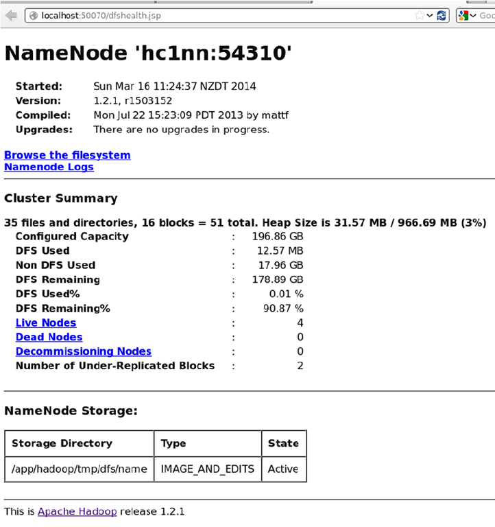
CHAPTER 2 ■ STORING AND CONFIGURING DATA WITH HADOOP, YARN, AND ZOOKEEPER

30

To see the administration information for Map Reduce, go to port 50030 by using the URL http://hc1nn:50030/,

shown in Figure 2-4. This port number refers to the value of the variable mapred.job.tracker.http.address already

defined in the mapred-site.xml configuration file. Figure 2-4 shows the state of the jobs, as well as the capacity per

node in terms of Map and Reduce. It also shows an example word-count job that’s running currently, which that has

completed the Map stage and is 8.33 percent into its Reduce phase.

Figure 2-3. The name node user interface

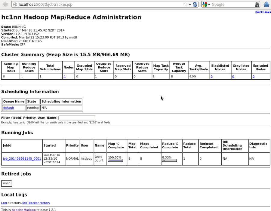
CHAPTER 2 ■ STORING AND CONFIGURING DATA WITH HADOOP, YARN, AND ZOOKEEPER

31

Figure 2-4. Hadoop Job Tracker user interface

The Task Tracker UI is on port 50060; this is the value defined by the variable mapred.task.tracker.http.address in

the configuration file mapred-site.xml. Use the URL http://hc1nn:50060/ (on the name node hc1nn) to access it and

check the status of current tasks. Figure 2-5 shows running and non-running tasks, as well as providing a link to the

log files. It also offers a basic list of task statuses and their progress.

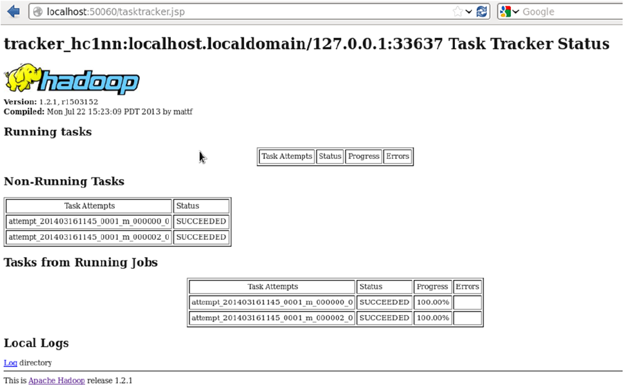
CHAPTER 2 ■ STORING AND CONFIGURING DATA WITH HADOOP, YARN, AND ZOOKEEPER

32

Now that you have tasted the flavor of Hadoop V1, shut it down and get ready to install Hadoop V2.

Hadoop V2 Installation

In moving on to Hadoop V2, you will this time download and use the Cloudera stack. Specifically, you will install CDH

4 because it is available for both 32-bit and 64-bit machines and it supports YARN. I have chosen to install the latest

manual CDH release available at the time of this writing.

In this section, you will not only learn how to obtain and install the Cloudera Hadoop packages; you’ll also

find out how to install, run, and use ZooKeeper, as well as how to configure Hadoop V2. You’ll tour the necessary

directories on the Linux file system and HDFS; lastly, you’ll find out how to control the servers as Linux services.

To begin, you need to add a CDH repository file on all machines as root under /etc/yum.repos.d/. You create a

file named cloudera-cdh4.repo on each server, with the following contents:

root@hc1r1m1 yum.repos.d]# cat cloudera-cdh4.repo

[cloudera-cdh4]

name=Cloudera's Distribution for Hadoop, Version 4

baseurl=http://archive.cloudera.com/cdh4/redhat/6/x86_64/cdh/4/

gpgkey = http://archive.cloudera.com/cdh4/redhat/6/x86_64/cdh/RPM-GPG-KEY-cloudera

gpgcheck = 1

Figure 2-5. The Task Tracker user interface

CHAPTER 2 ■ STORING AND CONFIGURING DATA WITH HADOOP, YARN, AND ZOOKEEPER

33

The Linux cat command shows the contents of the cloudera-cdh4.repo file. The ls –l command shows that it is

owned by the root Linux user:

[root@hc1r1m1 yum.repos.d]# ls -l cloudera-cdh4.repo

-rw-r--r-- 1 root root 229 Sep 6 09:24 cloudera-cdh4.repo

This repository configuration file tells the yum command where to source Cloudera cdh4 software. The above file

is configured for a 64-bit machine (x86_64); a 32-bit machine would have the following lines:

baseurl=http://archive.cloudera.com/cdh4/redhat/6/i386/cdh/4/

gpgkey = http://archive.cloudera.com/cdh4/redhat/6/i386/cdh/RPM-GPG-KEY-cloudera

At this point, Cloudera advises you to install ZooKeeper so that you have a ZooKeeper cluster; you’ll do so in the

next section. Tools like HBase (the distributed database that will be introduced in Chapter 3) rely on it.

ZooKeeper Installation

ZooKeeper is a centralized service for maintaining configuration information in distributed applications. Many of the

tools in the Hadoop ecosystem use it, so it will be helpful to install it now because you will need it later. You install the

ZooKeeper base package as follows:

yum install zookeeper

When you install ZooKeeper, remember that it needs to be installed on an odd number of servers—for example,

three machines. (When voting on an outcome, the odd number of servers makes it possible for ZooKeper to reach a

majority decision.) Next, you install the ZooKeeper server on each node:

yum install zookeeper-server

After installation, the ZooKeeper configuration needs to be altered for your environment. By default, the

configuration file is stored under /etc/zookeeper/conf/zoo.cfg. Its initial contents are the following:

maxClientCnxns=50

# The number of milliseconds of each tick

tickTime=2000

# The number of ticks that the initial

# synchronization phase can take

initLimit=10

# The number of ticks that can pass between

# sending a request and getting an acknowledgement

syncLimit=5

# the directory where the snapshot is stored.

dataDir=/var/lib/zookeeper

# the port at which the clients will connect

clientPort=2181

CHAPTER 2 ■ STORING AND CONFIGURING DATA WITH HADOOP, YARN, AND ZOOKEEPER

34

You need to add to these a section at the bottom of the file to define the port ranges used by ZooKeeper clients

on each of the servers. For instance, on server hc1r1m1, the port range for ZooKeeper server 1 is 60050 to 61050. That

allows for 1,000 client connections per ZooKeeper server.

server.1=hc1r1m1:60050:61050

server.2=hc1r1m2:60050:61050

server.3=hc1r1m3:60050:61050

#server.4=hc1nn:60050:61050

Note also that you have three servers defined and a fourth set up, but commented out to ensure that there will be

an odd number of ZooKeeper instances to form a quorum. Now, you initialize the Hadoop V2 installation:ZooKeeper

installation:

service zookeeper-server init

Edit the files /var/lib/zookeeper/myid on each server, entering integer numbers to match the configuration file.

For instance, for the setup on hc1r1m1, you add a “1” to the file, and so on. This allows each ZooKeeper server to

determine its ID number and so recognize its port range from the configuration file.

You now start ZooKeeper on hc1r1m1, hc1r1m2, and hc1r1m3, using the service command:

service zookeeper-server start

JMX enabled by default

Using config: /etc/zookeeper/conf/zoo.cfg

Starting zookeeper ... STARTED

Under /var/log/zookeeper/, you check the logs to ensure everything is running correctly:

-rw-r--r--. 1 zookeeper zookeeper 21450 Mar 20 18:54 zookeeper.log

-rw-r--r--. 1 zookeeper zookeeper 0 Mar 20 18:50 zookeeper.out

You’ll likely see errors indicating that the servers can’t reach each other, meaning that the firewall is interfering

again. You need to open the ports that ZooKeeper uses and then restart both Iptables and the ZooKeeper server for

the changes to be picked up. If you are unsure how to configure your firewall, approach your systems administrator.

[root@hc1r1m3 conf]# service zookeeper-server restart

Restarting ZooKeeper daemon: JMX enabled by default

Using config: /etc/zookeeper/conf/zoo.cfg

Stopping zookeeper ... STOPPED

JMX enabled by default

Using config: /etc/zookeeper/conf/zoo.cfg

Starting zookeeper ... STARTED

After you restart all of the ZooKeeper servers, they now will run as desired and will contain no errors in their log

files, as shown:

2014-03-20 19:09:34,011 [myid:3] - INFO

[QuorumPeer[myid=3]/0.0.0.0:2181:Environment@100] - Server

environment:os.arch=i386

2014-03-20 19:09:34,012 [myid:3] - INFO

[QuorumPeer[myid=3]/0.0.0.0:2181:Environment@100] - Server

CHAPTER 2 ■ STORING AND CONFIGURING DATA WITH HADOOP, YARN, AND ZOOKEEPER

35

environment:os.version=2.6.32-220.el6.i686

2014-03-20 19:09:34,012 [myid:3] - INFO

[QuorumPeer[myid=3]/0.0.0.0:2181:Environment@100] - Server

environment:user.name=zookeeper

2014-03-20 19:09:34,013 [myid:3] - INFO

[QuorumPeer[myid=3]/0.0.0.0:2181:Environment@100] - Server

environment:user.home=/var/run/zookeeper

2014-03-20 19:09:34,014 [myid:3] - INFO

[QuorumPeer[myid=3]/0.0.0.0:2181:Environment@100] - Server

environment:user.dir=/

2014-03-20 19:09:34,028 [myid:3] - INFO

[QuorumPeer[myid=3]/0.0.0.0:2181:ZooKeeperServer@162] - Created server with

tickTime 2000 minSessionTimeout 4000 maxSessionTimeout 40000 datadir

/var/lib/zookeeper/version-2 snapdir /var/lib/zookeeper/version-2

2014-03-20 19:09:34,030 [myid:3] - INFO

[QuorumPeer[myid=3]/0.0.0.0:2181:Follower@63] - FOLLOWING - LEADER ELECTION

TOOK - 83

2014-03-20 19:09:34,145 [myid:3] - INFO

[QuorumPeer[myid=3]/0.0.0.0:2181:Learner@325] - Getting a snapshot from leader

2014-03-20 19:09:34,154 [myid:3] - INFO

[QuorumPeer[myid=3]/0.0.0.0:2181:FileTxnSnapLog@273] - Snapshotting:

0x100000000 to /var/lib/zookeeper/version-2/snapshot.100000000

Manually Accessing the ZooKeeper Servers

Using the server name, main port number, and some four-letter words, you can manually access the ZooKeeper

servers. Specifically, you can use the nc command to issue additional four-letter commands. This type of access to

ZooKeeper might be useful when you’re investigating problems with the servers or just checking that all is okay.

For this setup, the configuration file lists the main port on each server as 2181. To access the configuration details

for server hc1r1m2, therefore, you use the nc command to issue a conf command. Press Enter after both the nc

command line and the conf command on the following line:

[hadoop@hc1r1m2 ~]$ nc hc1r1m2 2181

conf

clientPort=2181

dataDir=/var/lib/zookeeper/version-2

dataLogDir=/var/lib/zookeeper/version-2

tickTime=2000

maxClientCnxns=50

minSessionTimeout=4000

maxSessionTimeout=40000

serverId=2

initLimit=10

syncLimit=5

electionAlg=3

electionPort=61050

quorumPort=60050

peerType=0

CHAPTER 2 ■ STORING AND CONFIGURING DATA WITH HADOOP, YARN, AND ZOOKEEPER

36

This has outputted the configuration of the ZooKeeper server on hc1r1m2. While it’s on server hc1r1m2, you can

check that the ZooKeeper server on hc1r1m1 is still running by using the ruok (running okay?) command:

[hadoop@hc1r1m2 ~]$ nc hc1r1m1 2181

ruok

imok

The returned value of imok (I’m OK!) tells you the contacted server is running. You can then get the connection

details for server hc1r1m1 by using the cons command:

[hadoop@hc1r1m2 ~]$ nc hc1r1m1 2181

Cons

/192.168.1.106:42731[0](queued=0,recved=1,sent=0)

The response says there is just a single connection to that server. To supplement this with some basic server

details, you use the stat command:

[hadoop@hc1r1m2 ~]$ nc hc1r1m1 2181

stat

Zookeeper version: 3.4.5-cdh4.6.0--1, built on 02/26/2014 09:19 GMT

Clients:

/192.168.1.106:42732[0](queued=0,recved=1,sent=0)

Latency min/avg/max: 0/11/93

Received: 18

Sent: 17

Connections: 1

Outstanding: 0

Zxid: 0x300000006

Mode: follower

Node count: 4

This result provides status information for the ZooKeeper server on hc1r1m1. It has listed information like the

installed version and the volume of messaging. (You can find a full list of ZooKeeper commands on the Cloudera site

at archive.cloudera.com/cdh4/4/zookeeper.)

The ZooKeeper Client

An alternative to the nc command method is to use the built-in ZooKeeper client to access your servers. You can find

it with the type command, as follows:

[hadoop@hc1r1m3 ~]$ type zookeeper-client

zookeeper-client is /usr/bin/zookeeper-client

By default, the client connects to ZooKeeper on the local server:

[hadoop@hc1r1m3 ~]$ zookeeper-client

Connecting to localhost:2181

CHAPTER 2 ■ STORING AND CONFIGURING DATA WITH HADOOP, YARN, AND ZOOKEEPER

37

You can also get a list of possible commands by entering any unrecognized command, such as help:

[zk: localhost:2181(CONNECTED) 1] help

ZooKeeper -server host:port cmd args

connect host:port

get path [watch]

ls path [watch]

set path data [version]

rmr path

delquota [-n|-b] path

quit

printwatches on|off

create [-s] [-e] path data acl

stat path [watch]

close

ls2 path [watch]

history

listquota path

setAcl path acl

getAcl path

sync path

redo cmdno

addauth scheme auth

delete path [version]

setquota -n|-b val path

To connect to one of the other ZooKeeper servers in the quorum, you would use the connect command,

specifying the server and its connection port. If, for example, you’re currently on hc1r1m3, but want to connect to

hc1r1m1 (remember, all servers are connected via port 2181), you use the following:

[zk: localhost:2181(CONNECTED) 0] connect hc1r1m1:2181

[zk: hc1r1m1:2181(CONNECTING) 1] 2014-03-22 13:28:05,898 [myid:] - INFO [main-SendThread(hc1r1m1

:2181):ClientCnxn$SendThread@852] - Socket connection established to hc1r1m1/192.168.1.104:2181,

initiating session

2014-03-22 13:28:05,913 [myid:] - INFO [main-SendThread(hc1r1m1:2181):ClientCnxn$SendThread@1214] -

Session establishment complete on server hc1r1m1/192.168.1.104:2181, sessionid = 0x144e6df88b70004,

negotiated timeout = 30000

[zk: hc1r1m1:2181(CONNECTED) 1]

The result tells you that you are now connected to a ZooKeeper session on client node hc1r1m1 from hc1r1m3.

So far, you have ZooKeeper installed and have learned how to access it manually. In a large cluster, however, a

distributed application would connect to ZooKeeper automatically through one of its language APIs. It would use

the hierarchy of ZNodes to store configuration information. So, at this point you should examine the ZooKeeper

architecture in terms of those ZNodes to understand how they might be used for cluster configuration and

monitoring.

ZooKeeper stores its data in a hierarchy of nodes called ZNodes, each designed to contain a small amount of

data. When you log into the client, you can think of your session as similar to a Unix shell. Just as you can create

directories and files in a shell, so you can create ZNodes and data in the client.

CHAPTER 2 ■ STORING AND CONFIGURING DATA WITH HADOOP, YARN, AND ZOOKEEPER

38

Try creating an empty topmost node named “zk-top,” using this syntax:

[zk: localhost:2181(CONNECTED) 4] create /zk-top ''

Created /zk-top

You can create a subnode, node1, of zk-top as well; you can add the contents cfg1 at the same time:

[zk: localhost:2181(CONNECTED) 5] create /zk-top/node1 'cfg1'

Created /zk-top/node1

To check the contents of the subnode (or any node), you use the get command:

[zk: localhost:2181(CONNECTED) 6] get /zk-top/node1

'cfg1'

The delete command, not surprisingly, deletes a node:

[zk: localhost:2181(CONNECTED) 8] delete /zk-top/node2

The set command changes the context of a node. This command sequence first checks the contents of node1

with get, changes it with set, and then displays the new contents:

[zk: localhost:2181(CONNECTED) 9] get /zk-top/node1

'cfg1'

[zk: localhost:2181(CONNECTED) 10] set /zk-top/node1 'cfg2'

[zk: localhost:2181(CONNECTED) 11] get /zk-top/node1

'cfg2'

The contents of node1 changed from cfg1 to cfg2. Although this is a simple example, it explains the principle.

You can also list the subnodes of a node with the ls command. For example, node1 has no subnodes, but zk-top

contains node1:

[zk: localhost:2181(CONNECTED) 0] ls /zk-top/node1

[]

[zk: localhost:2181(CONNECTED) 1] ls /zk-top

[node1]

You can place watches on the nodes to check whether they change. Watches are one-time events. If the contents

change, then the watch fires and you will need to reset it. To demonstrate, I create a subnode node2 that contains

data2:

[zk: localhost:2181(CONNECTED) 9] create /zk-top/node2 'data2'

[zk: localhost:2181(CONNECTED) 10] get /zk-top/node2

'data2'

CHAPTER 2 ■ STORING AND CONFIGURING DATA WITH HADOOP, YARN, AND ZOOKEEPER

39

Now, I use get to set a watcher on that node. The first command sets a watcher on the node2 data item “data2.”

When I change the data to “data3” with the next set command, the watcher notices the data change and fires, as shown:

[zk: localhost:2181(CONNECTED) 11] get /zk-top/node2 true

'data2'

[zk: localhost:2181(CONNECTED) 12] set /zk-top/node2 'data3'

WATCHER::

WatchedEvent state:SyncConnected type:NodeDataChanged path:/zk-top/node2

In addition to the basic nodes you’ve been working with, you can create sequential and ephemeral nodes with

the create command. Ephemeral nodes exist only for the lifetime of the current session, while sequential nodes have a

sequence number applied to the node name and will persist. To create a sequential node, use the –s option, as shown:

[zk: localhost:2181(CONNECTED) 13] ls /zk-top

[node2, node1]

[zk: localhost:2181(CONNECTED) 14] create -s /zk-top/node3 'data3'

Created /zk-top/node30000000005

[zk: localhost:2181(CONNECTED) 15] ls /zk-top

[node2, node1, node30000000005]

To create an ephemeral node, use the –e option:

[zk: localhost:2181(CONNECTED) 16] create -e /zk-top/node4 'data4'

Created /zk-top/node4

[zk: localhost:2181(CONNECTED) 17] ls /zk-top

[node4, node2, node1, node30000000005]

So, node 4 exists in this session under zk-top. It will disappear when you log out of the session (with quit) and

start a new one. Notice that the ls command at the end of this sequence no longer lists node4:

[zk: localhost:2181(CONNECTED) 18] quit

Quitting...

2014-03-22 14:02:56,572 [myid:] - INFO [main:ZooKeeper@684] - Session: 0x344e6df92ab0005 closed

2014-03-22 14:02:56,572 [myid:] - INFO [main-EventThread:ClientCnxn$EventThread@512] - EventThread

shut down

[hadoop@hc1r1m3 ~]$

[hadoop@hc1r1m3 ~]$ zookeeper-client

[zk: localhost:2181(CONNECTED) 0] ls /zk-top

[node2, node1, node30000000005]

As you can see, node 4 is gone; it only existed for the session in which it was created. Note: you can also make

sequential nodes ephemeral with a command like this:

[zk: localhost:2181(CONNECTED) 16] create -s -e /zk-top/node4 'data4'

CHAPTER 2 ■ STORING AND CONFIGURING DATA WITH HADOOP, YARN, AND ZOOKEEPER

40

ZooKeeper ZNodes and their commands are building blocks for meeting your needs. Ephemeral nodes are

especially useful in a distributed clustered environment, for example. In each session, you could create a node to

see which application nodes were connected. You could also store all your configuration information in a series of

ZooKeeper ZNodes and have the applications use that configuration information on each node. You would then be

able to ensure that the nodes were using the same configuration information.

This has been a basic introduction to ZooKeeper. For further reading, have a look at Cloudera’s site or perhaps have a

go at building your own distributed application.

Hadoop MRv2 and YARN

With ZooKeeper in place, you can continue installing the Cloudera CDH 4 release. The components will be installed

using yum commands as root to install Cloudera packages. I chose to install a Cloudera stack because the installation

has been professionally tested and packaged. The components are guaranteed to work together and with a range

of Hadoop client applications. The instructions that follow describe the installation of the Name Node, Data Node,

Resource Manager, Node Manager, Job History, and Proxy servers.

In comparison to the V1 installation, you do not have to choose the location for your installation; that is done

automatically and the different parts of the installation are placed in meaningful locations. Configuration is placed

under /etc/hadoop, logs are placed under /var/log, and executables are created as Linux servers under /etc/init.d.

Here’s the process:

1. Install the HDFS Name Node component on the master server hc1nn:

[root@hc1nn ~]# yum install hadoop-hdfs-namenode

2. Install the HDFS Data Node component on the slave servers hc1r1m1 through 3:

[root@hc1r1m1 ~]# yum install hadoop-hdfs-datanode

3. Install the Resource Manager component on the Name Node machine hc1nn:

[root@hc1nn ~]# yum install hadoop-yarn-resourcemanager

4. Install the Node Manager and Map Reduce on all of the Data Node slave servers hc1r1m1

through 3:

[root@hc1r1m1 ~]# yum install hadoop-yarn-nodemanager hadoop-mapreduce

5. Install the Job History and Proxy servers on a single node:

yum install hadoop-mapreduce-historyserver hadoop-yarn-proxyserver

That concludes the component package installations.

Now that the software is installed, you need to set up the configuration files that they depend upon. You can find

these configuration files under the directory /etc/hadoop/conf. They all have names like <component>-site.xml,

where <component> is replaced by yarn, hdfs, mapred, or core.

The HDFS term you have come across already; it is the Hadoop distributed file system. YARN stands for “yet

another resource negotiator.” The MAPRED component is short for “Map Reduce,” and CORE is the configuration for

the Hadoop common utilities that support other Hadoop functions.

CHAPTER 2 ■ STORING AND CONFIGURING DATA WITH HADOOP, YARN, AND ZOOKEEPER

41

Use the ls command to view the configuration files that need to be altered:

[root@hc1nn conf]# cd /etc/hadoop/conf

[root@hc1nn conf]# ls -l *-site.xml

-rw-r--r--. 1 root root 904 Feb 26 23:17 core-site.xml

-rw-r--r--. 1 root root 1023 Feb 26 23:17 hdfs-site.xml

-rw-r--r--. 1 root root 904 Feb 26 23:17 mapred-site.xml

-rw-r--r--. 1 root root 2262 Feb 26 23:17 yarn-site.xml

On each node, set up the core-site.xml as follows:

<name>fs.defaultFS</name>

</property>

</configuration>

You need hdfs-site.xml on each node, as well. To set it up, use the form:

<name>dfs.namenode.name.dir</name>

<value>/var/lib/hadoop-hdfs/cache/hdfs/dfs/name</value>

<description> Can be a comma separated list of values </description>

</property>

<name>dfs.permissions.superusergroup</name>

<value>hadoop</value>

</property>

<name>dfs.replication</name>

</property>

</configuration>

Remember, however, to define dfs.namenode.name.dir on the name node and dfs.datanode.data.dir on the data

node. So, the entry for the data nodes would be as follows:

<name>dfs.datanode.name.dir</name>

<value>/var/lib/hadoop-hdfs/cache/hdfs/dfs/name</value>

<description> Can be a comma separated list of values </description>

</property>

CHAPTER 2 ■ STORING AND CONFIGURING DATA WITH HADOOP, YARN, AND ZOOKEEPER

42

On each node, make sure that the directories used in the configuration files exist:

[root@hc1nn conf]# mkdir -p /var/lib/hadoop-hdfs/cache/hdfs/dfs/name

Next, set the ownership of these directories:

[root@hc1nn conf]# chown -R hdfs:hdfs /var/lib/hadoop-hdfs/cache/hdfs/dfs/name

[root@hc1nn conf]# chmod 700 /var/lib/hadoop-hdfs/cache/hdfs/dfs/name

The preceding commands create the name directory, change the ownership to the hdfs user, and set its

permissions. Before starting the name node, though, you have to format the file system (as the hdfs user):

[root@hc1nn conf]# su - hdfs

-bash-4.1$ hdfs namenode –format

Now, you set up the file mapred-site.xml, setting the framework to be yarn:

<name>mapreduce.framework.name</name>

</property>

</configuration>

Next, you set up the file yarn-site.xml. There is a lot of configuration information here, including port addresses,

file system paths, and class path information. (For a full list of available configuration file options, check the Hadoop

site at hadoop.apache.org.)

<name>yarn.nodemanager.aux-services</name>

<value>mapreduce.shuffle</value>

</property>

<name>yarn.nodemanager.aux-services.mapreduce.shuffle.class</name>

<value>org.apache.hadoop.mapred.ShuffleHandler</value>

</property>

<name>yarn.resourcemanager.address</name>

</property>

<name>yarn.resourcemanager.scheduler.address</name>

</property>

CHAPTER 2 ■ STORING AND CONFIGURING DATA WITH HADOOP, YARN, AND ZOOKEEPER

43

<name> yarn.resourcemanager.resource-tracker.address</name>

</property>

<name>yarn.resourcemanager.admin.address</name>

</property>

<name>yarn.resourcemanager.webapp.address</name>

</property>

<name>yarn.log-aggregation-enable</name>

</property>

<description>List of directories to store localized files in.</description>

<name>yarn.nodemanager.local-dirs</name>

<value>/var/lib/hadoop-yarn/cache/${user.name}/nm-local-dir</value>

</property>

<description>Where to store container logs.</description>

<name>yarn.nodemanager.log-dirs</name>

<value>/var/log/hadoop-yarn/containers</value>

</property>

<description>Where to aggregate logs to.</description>

<name>yarn.nodemanager.remote-app-log-dir</name>

<value>/var/log/hadoop-yarn/apps</value>

</property>

<description>Classpath for typical applications.</description>

<name>yarn.application.classpath</name>

<value>

$HADOOP_CONF_DIR,

$HADOOP_COMMON_HOME/*,$HADOOP_COMMON_HOME/lib/*,

$HADOOP_HDFS_HOME/*,$HADOOP_HDFS_HOME/lib/*,

$HADOOP_MAPRED_HOME/*,$HADOOP_MAPRED_HOME/lib/*,

$YARN_HOME/*,$YARN_HOME/lib/*

</value>

</property>

</configuration>

CHAPTER 2 ■ STORING AND CONFIGURING DATA WITH HADOOP, YARN, AND ZOOKEEPER

44

Now, the directories used by YARN, as shown in the configuration above, will need to be created and ownership

and group membership will have to be set to the YARN Linux user and group, as follows:

[root@hc1nn conf]# mkdir -p /var/log/hadoop-yarn/containers

[root@hc1nn conf]# mkdir -p /var/log/hadoop-yarn/apps

[root@hc1nn conf]# chown -R yarn:yarn /var/log/hadoop-yarn/containers

[root@hc1nn conf]# chown -R yarn:yarn /var/log/hadoop-yarn/apps

[root@hc1nn conf]# chmod 755 /var/log/hadoop-yarn/containers

[root@hc1nn conf]# chmod 755 /var/log/hadoop-yarn/apps

You add the following configuration to mapred-site.xml for the Job History server:

<name>mapreduce.jobhistory.address</name>

</property>

<name>mapreduce.jobhistory.webapp.address</name>

</property>

You also need to set up the staging directory in yarn-site.xml. If you don’t specifically create one, YARN will create

a directory under /tmp. To create the directory, add the following xml to yarn-site.xml:

<name>mapreduce.jobhistory.intermediate-done-dir</name>

<value>/var/lib/hadoop-mapreduce/jobhistory/intermediate/donedir</value>

</property>

<name>mapreduce.jobhistory.done-dir</name>

<value>/var/lib/hadoop-mapreduce/jobhistory/donedir</value>

</property>

The directories needed for staging must be created on the file system. You set their ownership and group

membership to yarn, then set the permissions:

[root@hc1nn conf]# mkdir -p /var/lib/hadoop-mapreduce/jobhistory/intermediate/donedir

[root@hc1nn conf]# mkdir -p /var/lib/hadoop-mapreduce/jobhistory/donedir

[root@hc1nn conf]# chown -R yarn:yarn /var/lib/hadoop-mapreduce/jobhistory/intermediate/donedir

[root@hc1nn conf]# chown -R yarn:yarn /var/lib/hadoop-mapreduce/jobhistory/donedir

[root@hc1nn conf]# chmod 1777 /var/lib/hadoop-mapreduce/jobhistory/intermediate/donedir

[root@hc1nn conf]# chmod 750 /var/lib/hadoop-mapreduce/jobhistory/donedir

CHAPTER 2 ■ STORING AND CONFIGURING DATA WITH HADOOP, YARN, AND ZOOKEEPER

45

Now it’s time to start the Hadoop servers. On the Name Node machine (hc1nn), run the following as root to start

the HDFS, YARN, and History servers:

service hadoop-hdfs-namenode start

service hadoop-mapreduce-historyserver start

service hadoop-yarn-resourcemanager start

service hadoop-yarn-proxyserver start

On the Data Node machines (hc1r1m1 to hc1r1m3), run the following as root to start the data node and Node

Manager:

service hadoop-hdfs-datanode start

service hadoop-yarn-nodemanager start

You can make sure that Hadoop is writing to HDFS by executing the Hadoop file system ls command on

the /directory:

[root@hc1nn conf]# su - hdfs

-bash-4.1$ hadoop fs –ls /

Also, ensure that the temporary directory exists on HDFS:

-bash-4.1$ hadoop fs -mkdir /tmp

-bash-4.1$

-bash-4.1$ hadoop fs -chmod -R 1777 /tmp

The permissions “1777” means that any file system user can write to the directory but cannot remove another

user’s files.

You need to create the required directories under HDFS; these directories will be owned and used by YARN for

logging and history data:

[root@hc1nn hadoop-hdfs]# su - hdfs

-bash-4.1$

-bash-4.1$ hadoop fs -mkdir /user/history

-bash-4.1$ hadoop fs -chmod -R 1777 /user/history

-bash-4.1$ hadoop fs -chown yarn /user/history

-bash-4.1$ hadoop fs -mkdir /var/log/hadoop-yarn

-bash-4.1$ hadoop fs -chown yarn:mapred /var/log/hadoop-yarn

At this point, check which top-level directories exist on the Hadoop distributed file system (HDFS). Because

you have executed a long list (ls -l) and have used a recursive switch (-R), you can also see which subdirectories

exist. The following listing shows permissions (drwxrwxrw), plus details like ownership and group membership

(hdfs hadoop):

-bash-4.1$ hadoop fs -ls -R /

drwxrwxrwt - hdfs hadoop 0 2014-03-23 14:58 /tmp

drwxr-xr-x - hdfs hadoop 0 2014-03-23 14:55 /user

drwxrwxrwt - yarn hadoop 0 2014-03-23 14:55 /user/history

drwxr-xr-x - hdfs hadoop 0 2014-03-23 14:56 /var

drwxr-xr-x - hdfs hadoop 0 2014-03-23 14:56 /var/log

drwxr-xr-x - yarn mapred 0 2014-03-23 14:56 /var/log/hadoop-yarn

CHAPTER 2 ■ STORING AND CONFIGURING DATA WITH HADOOP, YARN, AND ZOOKEEPER

46

So, you have the /tmp and /user directories, and the /var/log directory exists with a subdirectory for YARN. Now,

you need to create home directories for the Map Reduce users on HDFS. In this case there is only the hadoop account,

so you change user (su) to the Linux hdfs account, then use the hadoop file system command mkdir to create the

directory and use chown to set its ownership to hadoop:

[root@hc1nn sysconfig]# su - hdfs

-bash-4.1$

-bash-4.1$ hadoop fs -mkdir /user/hadoop

-bash-4.1$ hadoop fs -chown hadoop /user/hadoop

Last step is to set up the Map Reduce user environment in the Bash shell by setting some environmental options

in the Bash configuration file .bashrc. As in the Hadoop V1 installation, this allows you to set environment variables

like JAVA_HOME and HADOOP_MAPRED_HOME in the Bash shell. Each time the Linux account is accessed and a Bash shell is

created, these variables will be pre-defined.

[hadoop@hc1nn ~]$ tail .bashrc

#######################################################

# Set Hadoop related env variables

# set JAVA_HOME (we will also set a hadoop specific value later)

export JAVA_HOME=/usr/lib/jvm/jre-1.6.0-openjdk

export HADOOP_MAPRED_HOME=/usr/lib/hadoop-mapreduce

At this point you have completed the configuration of your installation and you are ready to start the servers.

Remember to monitor the logs under /var/log for server errors; when the servers start, they state the location where

they are logging to.

You start the HDFS servers and monitor the logs for errors:

[root@hc1nn init.d]# cd /etc/init.d

[root@hc1nn init.d]# ls -ld hadoop-hdfs-*

-rwxr-xr-x. 1 root root 4469 Feb 26 23:18 hadoop-hdfs-namenode

[root@hc1nn init.d]# service hadoop-hdfs-namenode start

Starting Hadoop namenode: [ OK ]

starting namenode, logging to /var/log/hadoop-hdfs/hadoop-hdfs-namenode-hc1nn.out

If you start the name node on the master and the data nodes on the slaves, check that the necessary ports

are open in the firewall. For example, I check that port 8020 is open in the firewall configuration. I also show how

the Iptables (Linux kernel firewall) service can be restarted. (I do not provide an in-depth study of the firewall

configuration, as that leads us into the realm of systems administration, which is a separate field.)

[root@hc1nn sysconfig]# cd /etc/sysconfig

[root@hc1nn sysconfig]# grep 8020 iptables

-A INPUT -m state --state NEW -m tcp -p tcp --dport 8020 -j ACCEPT

So, this result tells the firewall to accept tcp-based requests on port 8020.

If the ports are not open, then Iptables needs to be updated with an entry similar to the last line above and the

server restarted, as shown next. (If you are unsure about this, consult your systems administrator.)

CHAPTER 2 ■ STORING AND CONFIGURING DATA WITH HADOOP, YARN, AND ZOOKEEPER

47

[root@hc1nn sysconfig]# service iptables restart

iptables: Setting chains to policy ACCEPT: filter [ OK ]

iptables: Flushing firewall rules: [ OK ]

iptables: Unloading modules: [ OK ]

iptables: Applying firewall rules: [ OK ]

You are now ready to start the YARN servers. First, start the Resource Manager on the master, then start the Node

managers on the data nodes. Finally, check the logs for errors. The sequence of commands you need for doing this is

as follows:

[root@hc1nn init.d]# service hadoop-yarn-resourcemanager start

Starting Hadoop resourcemanager: [ OK ]

starting resourcemanager, logging to /var/log/hadoop-yarn/yarn-yarn-resourcemanager-hc1nn.out

[root@hc1r1m1 init.d]# service hadoop-yarn-nodemanager start

Starting Hadoop nodemanager: [ OK ]

starting nodemanager, logging to /var/log/hadoop-yarn/yarn-yarn-nodemanager-hc1r1m1.out

Running Another Map Reduce Job Test

You have the Hadoop V2 HDFS and YARN servers running; all servers are up on the data nodes and the Node

manager. You have checked the logs and found no errors. So, you are ready to attempt a test of Map Reduce. Try

issuing the word-count job on the Poe data, as was done earlier for Hadoop V1 :

1. Switch user to the Linux hadoop account:

[root@hc1nn ~]$ su – hadoop

2. Next, create the working directory for the data on HDFS:

[hadoop@hc1nn ~]$ hdfs dfs -mkdir -p /user/hadoop/edgar/edgar

3. Now, copy the same edgar test data to the working directory on HDFS:

[hadoop@hc1nn edgar]$ hdfs dfs -copyFromLocal *.txt /user/hadoop/edgar/edgar

4. And finally, run the Map Reduce word-count job:

[hadoop@hc1nn ~]$ hadoop jar /usr/lib/hadoop-mapreduce/hadoop-mapreduce-examples.jar wordcount /

user/hadoop/edgar/edgar /user/hadoop/edgar-results

14/03/23 16:34:46 INFO jvm.JvmMetrics: Initializing JVM Metrics with processName=JobTracker, sessionId=

14/03/23 16:34:48 INFO util.ProcessTree: setsid exited with exit code 0

14/03/23 16:34:48 INFO mapred.Task: Using ResourceCalculatorPlugin : org.apache.hadoop.util.LinuxR

esourceCalculatorPlugin@18b4587

14/03/23 16:34:48 INFO mapred.MapTask: Processing split: hdfs://hc1nn/user/hadoop/edgar/edgar/10947-8.

txt:0+632294

14/03/23 16:34:48 INFO mapred.MapTask: Map output collector class = org.apache.hadoop.mapred.

MapTask$MapOutputBuffer

14/03/23 16:34:48 INFO mapred.MapTask: io.sort.mb = 100

CHAPTER 2 ■ STORING AND CONFIGURING DATA WITH HADOOP, YARN, AND ZOOKEEPER

48

14/03/23 16:34:48 INFO mapred.MapTask: data buffer =

........

14/03/23 16:34:56 INFO mapred.JobClient: Spilled Records=256702

14/03/23 16:34:56 INFO mapred.JobClient: CPU time spent (ms)=0

14/03/23 16:34:56 INFO mapred.JobClient: Physical memory (bytes) snapshot=0

14/03/23 16:34:56 INFO mapred.JobClient: Virtual memory (bytes) snapshot=0

14/03/23 16:34:56 INFO mapred.JobClient: Total committed heap usage (bytes)=1507446784

Notice that the Hadoop jar command is very similar to that used in V1. You have specified an example jar file to

use, from which you will execute the word-count function. An input and output data directory on HDFS has also been

specified. Also, the run time is almost the same.

Okay, the Map Reduce job has finished, so you take a look at the output. In the edgar-results directory, there is a

_SUCCESS file to indicate a positive outcome and a part-r-00000 file that contains the reduced data:

[hadoop@hc1nn ~]$ hadoop fs -ls /user/hadoop/edgar-results

Found 2 items

-rw-r--r-- 2 hadoop hadoop 0 2014-03-23 16:34 /user/hadoop/edgar-results/_SUCCESS

-rw-r--r-- 2 hadoop hadoop 769870 2014-03-23 16:34 /user/hadoop/edgar-results/part-r-00000

The job was successful; you have part data. To examine the part file data, you need to extract it from HDFS. The

Hadoop file system cat command can be used to dump the contents of the part file. This will then be stored in the

Linux file system file /tmp/hadoop/part-r-00000:

[hadoop@hc1nn ~]$ mkdir –p /tmp/hadoop/

[hadoop@hc1nn ~]$ hadoop fs -cat /user/hadoop/edgar-results/part-r-00000 > /tmp/hadoop/part-r-00000

[hadoop@hc1nn ~]$ wc -l /tmp/hadoop/part-r-00000

67721 /tmp/hadoop/part-r-00000

If you use the Linux command wc -l to show the file lines, you’ll see that there are 67,721 lines in the extracted

file. This is the same result as you received from the Map Reduce word-count job in the V1 example. To list the actual

data, you use:

[hadoop@hc1nn ~]$ head -20 /tmp/hadoop/part-r-00000

! 1

" 22

"''T 1

"'-- 1

"'A 1

"'After 1

"'Although 1

"'Among 2

"'And 2

"'Another 1

"'As 2

"'At 1

"'Aussi 1

"'Be 2

"'Being 1

"'But 1

"'But,' 1

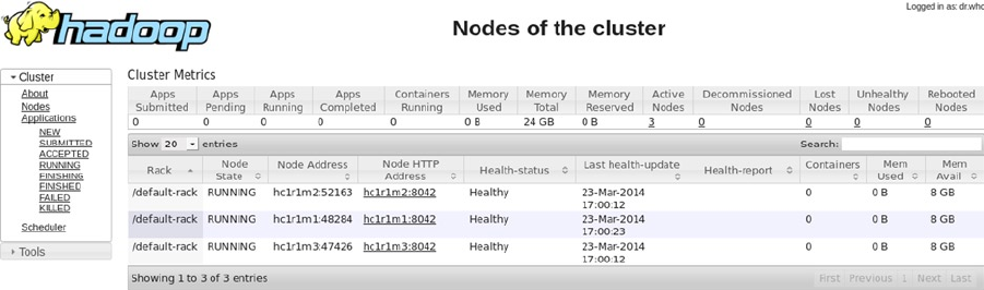
CHAPTER 2 ■ STORING AND CONFIGURING DATA WITH HADOOP, YARN, AND ZOOKEEPER

49

"'But--still--monsieur----' 1

"'Catherine, 1

"'Comb 1

Again, V2 provides a sorted list of words with their counts. The successful test proves that the installed system,

both HDFS and Map Reduce, works. For now, you’re finished with the configuration, although in later chapters of this

book I’ll be introducing more Hadoop components.

Like Hadoop V1, Hadoop V2 offers a web interface for monitoring your cluster’s nodes. Direct your web browser

to http://hc1nn:8088/cluster/nodes, and you can see all of your active data nodes along with information relating

to status and storage. The nodes themselves are actually http links, so you can click on then to drill down further.

Figure 2-6. Hadoop V2 UI cluster nodes

Hadoop Commands

Hadoop offers many additional command-line options. In addition to the shell commands you’ve already used in this

chapter’s examples, I’ll cover some other essential commands here, but only give a brief introduction to get you going.

The following sections will introduce Hadoop shell, user and administration commands. Where possible, I’ve given a

working example for each command. For a complete guide, see the Hadoop site, https://hadoop.apache.org.

Hadoop Shell Commands

The Hadoop shell commands are really user commands; specifically, they are a subset related to the file system.

Each command is invoked using the hadoop keyword, followed by the fs option, which stands for “file system.” Each

subcommand is passed as an argument to the fs option. File paths are specified as uniform resource identifiers, or URIs.

A file on the HDFS can be specified as hdfs:///dir1/dir2/file1, whereas the same file on the Linux file system can

be specified as file:///dir1/dir2/file1. If you neglect to offer a scheme (hdfs or file), then Hadoop assumes you mean

the HDFS.

If you are familiar with Linux or Unix shell commands, then you will find these Hadoop file system commands

similar. You can list files on HDFS using the ls command:

[hadoop@hc1nn ~]$ hadoop fs -ls /user/hadoop/edgar/

Found 1 items

drwxr-xr-x - hadoop hadoop 0 2014-03-23 16:32 /user/hadoop/edgar/edgar

CHAPTER 2 ■ STORING AND CONFIGURING DATA WITH HADOOP, YARN, AND ZOOKEEPER

50

To perform a recursive listing, add the –R option; this means that the ls command will list the topmost directory

and all subdirectories:

[hadoop@hc1nn ~]$ hadoop fs -ls -R /user/hadoop/edgar/

drwxr-xr-x - hadoop hadoop 0 2014-03-23 16:32 /user/hadoop/edgar/edgar

-rw-r--r-- 2 hadoop hadoop 632294 2014-03-23 16:32 /user/hadoop/edgar/edgar/10947-8.txt

-rw-r--r-- 2 hadoop hadoop 559342 2014-03-23 16:32 /user/hadoop/edgar/edgar/15143-8.txt

-rw-r--r-- 2 hadoop hadoop 66409 2014-03-23 16:32 /user/hadoop/edgar/edgar/17192-8.txt

-rw-r--r-- 2 hadoop hadoop 550284 2014-03-23 16:32 /user/hadoop/edgar/edgar/2147-8.txt

-rw-r--r-- 2 hadoop hadoop 579834 2014-03-23 16:32 /user/hadoop/edgar/edgar/2148-8.txt

-rw-r--r-- 2 hadoop hadoop 596745 2014-03-23 16:32 /user/hadoop/edgar/edgar/2149-8.txt

-rw-r--r-- 2 hadoop hadoop 487087 2014-03-23 16:32 /user/hadoop/edgar/edgar/2150-8.txt

-rw-r--r-- 2 hadoop hadoop 474746 2014-03-23 16:32 /user/hadoop/edgar/edgar/2151-8.txt

You can create directories with mkdir; this example will create a directory on HDFS called “test” under the / root

node. Once it has been created, the ls command shows that it exists and is owned by the user hadoop:

[hadoop@hc1nn ~]$ hadoop fs -mkdir /test

[hadoop@hc1nn ~]$ hadoop fs -ls /

Found 5 items

drwxr-xr-x - hadoop hadoop 0 2014-03-24 18:18 /test

The chown and chmod commands change ownership and permissions, respectively. If you know Unix commands,

then these will be familiar. Their syntax is:

[hadoop@hc1nn ~]$ hadoop fs -chown hdfs:hdfs /test

[hadoop@hc1nn ~]$ hadoop fs -chmod 700 /test

[hadoop@hc1nn ~]$ hadoop fs -ls /

Found 5 items

drwx------ - hdfs hdfs 0 2014-03-24 18:18 /test

The chown command has changed the ownership of the HDFS /test directory to user/group hdfs/hdfs. The chmod

command has changed the directory permissions to 700 or rwx --- ---. That is read/write/execute for the owner (hdfs),

and there’s no access for the group or any other user.

You can copy a file to and from the local file system into HDFS by using the copyFromLocal argument:

[hadoop@hc1nn ~]$ hadoop fs -copyFromLocal ./test_file.txt /test/test_file.txt

[hadoop@hc1nn ~]$

[hadoop@hc1nn ~]$ hadoop fs -ls /test

Found 1 items

-rw-r--r-- 2 hadoop hdfs 504 2014-03-24 18:24 /test/test_file.txt

The example above shows that a Linux file system file ./test_file.txt was copied into HDFS to be stored under /test/

test_file.txt. The next example shows how copyToLocal can be used to copy a file from HDFS to the Linux file system:

[hadoop@hc1nn ~]$ hadoop fs -copyToLocal /test/test_file.txt ./test_file2.txt

[hadoop@hc1nn ~]$ ls -l ./test_file*

-rwxr-xr-x. 1 hadoop hadoop 504 Mar 24 18:25 ./test_file2.txt

-rw-rw-r--. 1 hadoop hadoop 504 Mar 24 18:24 ./test_file.txt

CHAPTER 2 ■ STORING AND CONFIGURING DATA WITH HADOOP, YARN, AND ZOOKEEPER

51

In the above example, the HDFS file /test/test_file.txt has been copied to the Linux file system as ./test_file2.txt.

To move a file or directory on HDFS, you use the mv command:

[hadoop@hc1nn ~]$ hadoop fs -mv /test/test_file.txt /test/test_file3.txt

[hadoop@hc1nn ~]$ hadoop fs -ls /test

Found 1 items

-rw-r--r-- 2 hadoop hdfs 504 2014-03-24 18:24 /test/test_file3.txt

The HDFS file /test/test_file.txt has been moved to the HDFS file /test/test_file3.txt. You can recursively delete in

HDFS by using rm -r:

[hadoop@hc1nn ~]$ hadoop fs -rm -r /test

[hadoop@hc1nn ~]$ hadoop fs -ls /

Found 4 items

drwxrwxrwt - hdfs hadoop 0 2014-03-23 14:58 /tmp

drwxr-xr-x - hdfs hadoop 0 2014-03-23 16:06 /user

drwxr-xr-x - hdfs hadoop 0 2014-03-23 14:56 /var

The example above has deleted the HDFS directory /test and all of its contents. To determine the space usage in

HDFS, you use the du (disk usage) command:

[hadoop@hc1nn ~]$ hadoop fs -du -h /

0 /tmp

4.5 M /user

0 /var

The -h option just makes the numbers humanly readable. This last example shows that only the HDFS file system

/user directory is using any space.

Hadoop User Commands

This section introduces some Hadoop user commands that you can use to check the health of the HDFS, determine

the Hadoop version, and carry out large-scale distributed data copies. Hadoop fsck offers the ability to determine

whether the file system is healthy. It displays the total data size plus file and directory volumes. It also offers

information like the replication factor and corrupted blocks. Hadoop distcp provides the functionality to move very

large volumes of data between clusters.

The following example of the fsck command shows that the file system “/” is healthy. No corrupted or under-

replicated blocks are listed. By default, there should be two copies of each block saved (the default replication factor

value was 2). If the HDFS had failed in this area, it would be shown in the report as “Under-replicated blocks” with a

value greater than zero.

CHAPTER 2 ■ STORING AND CONFIGURING DATA WITH HADOOP, YARN, AND ZOOKEEPER

52

[hadoop@hc1nn ~]$ hadoop fsck /

Connecting to namenode via http://hc1nn:50070

FSCK started by hadoop (auth:SIMPLE) from /192.168.1.107 for path / at Mon Mar 24 18:42:09 NZDT 2014

..........Status: HEALTHY

Total size: 4716611 B

Total dirs: 14

Total files:10

Total blocks (validated): 9 (avg. block size 524067 B)

Minimally replicated blocks: 9 (100.0 %)

Over-replicated blocks: 0 (0.0 %)

Under-replicated blocks: 0 (0.0 %)

Mis-replicated blocks: 0 (0.0 %)

Default replication factor: 2

Average block replication: 2.0

Corrupt blocks: 0

Missing replicas: 0 (0.0 %)

Number of data-nodes: 3

Number of racks: 1

FSCK ended at Mon Mar 24 18:42:09 NZDT 2014 in 9 milliseconds

The filesystem under path '/' is HEALTHY

You can use the job command to list jobs, although this example shows no jobs currently running:

[hadoop@hc1nn lib]$ hadoop job -list all

14/03/24 18:53:49 INFO service.AbstractService:

Service:org.apache.hadoop.yarn.client.YarnClientImpl is inited.

14/03/24 18:53:50 INFO service.AbstractService:

Service:org.apache.hadoop.yarn.client.YarnClientImpl is started.

Total jobs:0

JobId State StartTime UserName Queue Priority UsedContainers RsvdContainers UsedMem

RsvdMem NeededMem AM info

To determine which version of Hadoop you are using, as well as the checksum and dates, you use the

version command:

[hadoop@hc1nn lib]$ hadoop version

Hadoop 2.0.0-cdh4.6.0

Subversion git://centos32-6-slave.sf.cloudera.com/data/1/jenkins/workspace/generic-package-

centos32-6/topdir/BUILD/hadoop-2.0.0-cdh4.6.0/src/hadoop-common-project/hadoop-common -r

8e266e052e423af592871e2dfe09d54c03f6a0e8

Compiled by jenkins on Wed Feb 26 01:59:02 PST 2014

From source with checksum a9d36604dfb55479c0648f2653c69095

This command was run using /usr/lib/hadoop/hadoop-common-2.0.0-cdh4.6.0.jar

The version output above shows that you are using Cloudera CDH 4.6, which is actually Hadoop version 2.0.0. It

also shows when the release was built and by whom.

CHAPTER 2 ■ STORING AND CONFIGURING DATA WITH HADOOP, YARN, AND ZOOKEEPER

53

Distcp offers you the ability to copy within a cluster or between clusters. It uses Map Reduce to do this, and it is

designed for large-scale copying. I can provide only a theoretical example here because I have only a small four-node

cluster for writing this book with a single name node. Check the website hadoop.apache.org for more information.

The syntax for distcp is as follows:

[hadoop@hc1nn lib]$ hadoop distcp \

hdfs://hc1nn:8020/test2 \

hdfs://hc2nn:8020/test3

This example shows the contents of cluster one HDFS directory /test2 being copied to cluster two directory /

test3. The URIs used here (hdfs://hc1nn:8020/test2 and hdfs://hc2nn:8020/test3) use a scheme of hdfs, but they also

refer to a hostname and port. These are the hosts and port numbers for the name nodes for the two clusters.

Hadoop Administration Commands

This discussion of Hadoop administration commands will let you sample some of the full set of commands available.

For complete details, check hadoop.apache.org. These commands will enable you to format the HDFS, manage

upgrades, set logging levels, and save configuration information.

You already used one of the administration commands (-format) when you formatted the file system earlier.

Take a second look:

hadoop namenode -format

The format command starts the name node, executes its command, and then shuts the name node down again.

The name node is the centralized place on the HDFS where metadata concerning files in the file system are stored. If

the Hadoop file system is running when this command is executed, then HDFS data is lost.

I won't run the upgrade command here, but you can use it after releasing a new version of Hadoop, as follows:

hadoop namenode -upgrade

This upgrade command will create new working directories on the data nodes for the new Hadoop version. The

previous checkpoint version is kept to allow for a rollback to the previous version of software in case the upgrade

doesn’t work out.

If you need to roll back to the previous version of Hadoop, you can use hadoop namenode -rollback.) This

rollback command will cause Hadoop to revert to the previous version of the working directories.

On the other hand, to finalize the upgrade and remove the old version, you use:

hadoop namenode -finalize

Be sure that the upgrade has worked before you remove the option to roll back.

You can get and set daemon log levels with daemonlog:

[hadoop@hc1nn ~]$ hadoop daemonlog -getlevel hc1nn:8088

CHAPTER 2 ■ STORING AND CONFIGURING DATA WITH HADOOP, YARN, AND ZOOKEEPER

54

org.apache.hadoop.mapred.JobTracker

Connecting to

http://hc1nn:8088/logLevel?log=org.apache.hadoop.mapred.JobTracker

Submitted Log Name: org.apache.hadoop.mapred.JobTracker

Log Class: org.apache.commons.logging.impl.Log4JLogger

Effective level: INFO

By changing getLevel to setLevel, you can set the log levels. Some possible values are all, info, debug, and

error. The level and volume of the information you receive will vary, with all supplying everything and error just

giving an error message.

You can use the dfsadmin report option to get information and administer Hadoop, as follows:

[hadoop@hc1nn ~]$ hadoop dfsadmin -report

Configured Capacity: 158534062080 (147.65 GB)

Present Capacity: 141443452928 (131.73 GB)

DFS Remaining: 141433782272 (131.72 GB)

DFS Used: 9670656 (9.22 MB)

DFS Used%: 0.01%

Under replicated blocks: 0

Blocks with corrupt replicas: 0

Missing blocks: 0

-------------------------------------------------

Datanodes available: 3 (3 total, 0 dead)

Live datanodes:

Name: 192.168.1.106:50010 (hc1r1m2)

Hostname: hc1r1m2

Decommission Status : Normal

Configured Capacity: 52844687360 (49.22 GB)

DFS Used: 4157440 (3.96 MB)

Non DFS Used: 6079811584 (5.66 GB)

DFS Remaining: 46760718336 (43.55 GB)

DFS Used%: 0.01%

DFS Remaining%: 88.49%

Last contact: Wed Mar 26 18:26:18 NZDT 2014

Name: 192.168.1.104:50010 (hc1r1m1)

Hostname: hc1r1m1

Decommission Status : Normal

Configured Capacity: 52844687360 (49.22 GB)

DFS Used: 3698688 (3.53 MB)

Non DFS Used: 3301863424 (3.08 GB)

DFS Remaining: 49539125248 (46.14 GB)

DFS Used%: 0.01%

DFS Remaining%: 93.74%

Last contact: Wed Mar 26 18:26:20 NZDT 2014

CHAPTER 2 ■ STORING AND CONFIGURING DATA WITH HADOOP, YARN, AND ZOOKEEPER

55

Name: 192.168.1.102:50010 (hc1r1m3)

Hostname: hc1r1m3

Decommission Status : Normal

Configured Capacity: 52844687360 (49.22 GB)

DFS Used: 1814528 (1.73 MB)

Non DFS Used: 7708934144 (7.18 GB)

DFS Remaining: 45133938688 (42.03 GB)

DFS Used%: 0.00%

DFS Remaining%: 85.41%

Last contact: Wed Mar 26 18:26:19 NZDT 2014

This report shows the HDFS capacity and usage, as well as the same information on each of the data nodes. It

also shows information like under-replicated blocks, which gives an indication of potential data loss in the event of

server failure.

You can save the name node data structures to file by using the hadoop dfsadmin metasave command:

[hadoop@hc1nn ~]$ hadoop dfsadmin -metasave metaFile1

Created metasave file metaFile1 in the log directory of namenode hdfs://hc1nn

In this example, you could have specified where this file was saved via the attribute hadoop.log.dir. In any

event, having run this command, you can now check the contents of the file via the Linux ls and more commands:

[hadoop@hc1nn hadoop-hdfs]$ ls -l /var/log/hadoop-hdfs/metaFile1

-rw-r--r--. 1 hdfs hdfs 658 Mar 26 18:29 /var/log/hadoop-hdfs/metaFile1

The ls command shows the location of the metadata file that you have created, metaFile1. It also shows that it is

owned by the Linux user hdfs. You can examine the contents of that metadata file by using the Linux more command:

[hadoop@hc1nn hadoop-hdfs]$ more /var/log/hadoop-hdfs/metaFile1

25 files and directories, 9 blocks = 34 total

Live Datanodes: 3

Dead Datanodes: 0

Metasave: Blocks waiting for replication: 0

Mis-replicated blocks that have been postponed:

Metasave: Blocks being replicated: 0

Metasave: Blocks 0 waiting deletion from 0 datanodes.

Metasave: Number of datanodes: 3

192.168.1.106:50010 IN 52844687360(49.22 GB) 4157440(3.96 MB) 0.00%

46760718336(

43.55 GB) Wed Mar 26 18:29:18 NZDT 2014

192.168.1.104:50010 IN 52844687360(49.22 GB) 3698688(3.53 MB) 0.00%

49539125248(

46.14 GB) Wed Mar 26 18:29:20 NZDT 2014

192.168.1.102:50010 IN 52844687360(49.22 GB) 1814528(1.73 MB) 0.00%

45133869056(

42.03 GB) Wed Mar 26 18:29:19 NZDT 2014

The last three lines of this example metadata file relate to data node capacity and data usage. Instead of refering

to the data nodes by their server names, though, their IP addesses have been used. For instance, in my example

cluster, the ip address 192.168.1.102 relates to the datanode hc1r1m3. The file also shows that there are three live data

nodes and none that are dead.

CHAPTER 2 ■ STORING AND CONFIGURING DATA WITH HADOOP, YARN, AND ZOOKEEPER

56

A full explanation of these administration commands is beyond the scope of this chapter, but by using the

dfsadmin command you can manage quotas, control the upgrade, refresh the nodes, and enter safe mode. Check the

Hadoop site hadoop.apache.org for full information.

Summary

In this chapter you have been introduced to both Hadoop V1 and V2 in terms of their installation and use. It is hoped

you can see that, by using the CDH stack release, the installation process and use of Hadoop are much simplified.

In the course of this chapter you have installed Hadoop V1 manually via a download package from the Hadoop

site. You have then installed V2 and YARN via CDH packages and the yum command. Servers for HDFS and YARN are

started as Linux services in V2 rather than as scripts, as in V1. Also, in the CDH release logs, binaries and configuration

functions were separated into their own, specific directories.

You have been shown the same Map Reduce task as run on both versions of Hadoop. Task run times were

comparable between V1 and V2. However, V2 offers the ability to have a larger production cluster than does V1.

(In the following chapters you will look at Map Reduce programming in Java and Pig).

You have also configured Hadoop V2 across a mini cluster with name nodes and data nodes on different servers.

You have installed and used ZooKeeper, setting up a quorum and using the client. (In the next chapter, HBase—the

Hadoop database—will be discussed and that calls upon ZooKeeper).

Lastly, you have looked at the command set for file system and for user and administration commands. True, it

was only a brief look, but further information is available at the Hadoop website.

57

Chapter 3

Collecting Data with Nutch and Solr

Many companies collect vast amounts of data from the web by using web crawlers such as Apache Nutch. Available for

more than ten years, Nutch is an open-source product provided by Apache and has a large community of committed

users. An Apache Lucene open-source search platform, Solr can be used in connection with Nutch to index and

search the data that Nutch collects. When you combine this functionality with Hadoop, you can store the resulting

large data volume directly in a distributed file system.

In this chapter, you will learn a number of methods to connect various releases of Nutch to Hadoop. I will

demonstrate, though architectural examples, what can be accomplished by using the various tools and data.

Specifically, the chapter’s first architectural example uses Nutch 1.8 configured to implicitly use the local Hadoop

installation. If Hadoop is available, Nutch will use it for storage, providing you with the benefits of distributed and

resiliant storage. It does not, however, give you much control over the selection of storage. Nutch will use either

Hadoop, if it is available, or the file system.

In the second architectural example, employing Nutch 2.x, you will be able to specify the storage used via Gora.

By explicitly selecting the storage method in the configuration options, you can gain greater control. This example

uses the HBase database, which still employs Hadoop for distributed storage. You then have the option of choosing a

different storage mechanism at a later date by altering the configuration.

Remember, although these examples are using small amounts of data, the architectures can scale to a high

degree to meet your big data-collection needs.

The Environment

Before we begin, you need to understand a few details about the environment in which we’ll be working. This chapter

demonstrates the use of Nutch with Hadoop V1.2.1 because I could not get Nutch to build against Hadoop V2 at the

time of this writing. (Subsequently, I learned of a version of Nutch developed for YARN, but deadline constraints

prevented me from implementing it here.) Although in Chapter 2 you installed Cloudera CDH4 on the CentOS Linux

server hc1nn, at this point you’ll need to switch back to using Hadoop V1. You’ll manage this via a number of steps

that are explained in the following sections. A shortage of available machines is the only reason I have installed

multiple versions of Hadoop on a single cluster. This kind of multiple Hadoop installation is not appropriate for

project purposes.

Stopping the Servers

The Hadoop Cloudera CDH4 cluster servers may still be running, so they need to be stopped on all nodes in the

Hadoop cluster. Because these servers are Linux services, you need to stop them as the Linux root user. You carry out

the following steps on all servers in the cluster—in this case, hc1nn, hc1r1m1, hc1r1m2, and hc1r1m3.

Chapter 3 ■ ColleCting Data with nutCh anD Solr

58

First, change the user to the root account with the Linux su (switch user) command:

[hadoop@hc1nn ~]$ su –

Next, issue the command sequence:

[root@hc1nn ~]# cd /etc/init.d/

[root@hc1nn init.d]# ls hadoop*mapreduce*

hadoop-0.20-mapreduce-jobtracker hadoop-mapreduce-historyserver

[root@hc1nn init.d]# ls hadoop*yarn*

hadoop-yarn-proxyserver hadoop-yarn-resourcemanager

[root@hc1nn init.d]# ls hadoop*hdfs*

hadoop-hdfs-namenode

The Linux cd (change directory) command moves the current path to /etc/init.d/, and the ls command displays

the Map Reduce, Yarn, and HDFS Hadoop services. (The * character is a wildstar value that matches all text to the end

of the string.) For each of the services displayed, execute the following command:

service <service name> stop

For instance, the stop command stops the proxy server, although it was not running:

[root@hc1nn init.d]# service hadoop-yarn-proxyserver stop

Stopping Hadoop proxyserver: [ OK ]

no proxyserver to stop

Remember to stop the non-HDFS services before the HDFS services and stop Map Reduce and YARN before

HDFS. Once you have done this on all the servers in this small cluster, then Hadoop V2 CDH4 will be stopped. You are

still logged in as root, however, so use the Linux exit command to return control back to the Linux hadoop account

session:

[root@hc1nn init.d]# exit

logout

[hadoop@hc1nn ~]$

Changing the Environment Scripts

In Chapter 2, you worked with two versions of Hadoop with two different environment configurations. The

environment file used to hold these configurations was the Linux hadoop user’s $HOME/.bashrc file. During the

creation of this book, I needed to switch between Hadoop versions frequently, and so I created two separate versions

of the bashrc file on each server in the cluster, as follows:

[hadoop@hc1nn ~]$ pwd

/home/hadoop

Chapter 3 ■ ColleCting Data with nutCh anD Solr

59

[hadoop@hc1nn ~]$ ls -l .bashrc*

lrwxrwxrwx. 1 hadoop hadoop 16 Jun 30 17:59 .bashrc -> .bashrc_hadoopv2

-rw-r--r--. 1 hadoop hadoop 1586 Jun 18 17:08 .bashrc_hadoopv1

-rw-r--r--. 1 hadoop hadoop 1588 Jul 27 11:33 .bashrc_hadoopv2

The Linux pwd command shows that the current location is the Linux hadoop user’s home directory /home/

hadoop/. The Linux ls command produces a long listing that shows a symbolic link called .bashrc, which points

to either a Hadoop V1 or a V2 version of the bashrc configuration file. Currently it is pointing to V2, so you need to

change it back to V1. (I will not explain the contents of the files, as they are listed in Chapter 2).

Delete the symbolic link named .bashrc by using the Linux rm command, then re-create it to point to the V1 file

by using the Linux ln command with a –s (symbolic) switch:

[hadoop@hc1nn ~]$ rm .bashrc

[hadoop@hc1nn ~]$ ln -s .bashrc_hadoopv1 .bashrc

[hadoop@hc1nn ~]$ ls -l .bashrc*

lrwxrwxrwx 1 hadoop hadoop 16 Nov 12 18:32 .bashrc -> .bashrc_hadoopv1

-rw-r--r--. 1 hadoop hadoop 1586 Jun 18 17:08 .bashrc_hadoopv1

-rw-r--r--. 1 hadoop hadoop 1588 Jul 27 11:33 .bashrc_hadoopv2

That creates the correct environment configuration file for the Linux hadopop account, but how does it now take

effect? Either log out using the exit command and log back in, or use the following:

[hadoop@hc1nn ~]$ . ./.bashrc

This means that the .bashrc is executed in the current shell (denoted by the first “ . ” character). The ./ specifies

that the .bashrc file is sourced from the current directory. Now, you are ready to start the Hadoop V1 servers.

Starting the Servers

The Hadoop V1 environment has been configured, and the V2 Hadoop servers have already been stopped. Now, you

change to the proper directory and start the servers:

[hadoop@hc1nn ~]$ cd $HADOOP_PREFIX/bin

[hadoop@hc1nn hadoop]$ pwd

/usr/local/hadoop/bin/

[hadoop@hc1nn bin]$ ./start-dfs.sh

[hadoop@hc1nn bin]$ ./start-mapred.sh

These commands change the directory to the /usr/local/hadoop/bin/ directory using the HADOOP_PREFIX

variable. The HDFS servers are started using the start-dfs.sh script, followed by the Map Reduce servers with start-

mapred.sh. At this point, you can begin the Nutch work, using Hadoop V1 on this cluster.

Architecture 1: Nutch 1.x

This first example illustrates how Nutch, Solr, and Hadoop work together. You will learn how to download, install, and

configure Nutch 1.8 and Solr, as well as how to set up your environment and build Nutch. With the prep work finished,

I’ll walk you through running a sample Nutch crawl using Solr and then storing the data on the Hadoop file system.

Chapter 3 ■ ColleCting Data with nutCh anD Solr

60

In Nutch 1.8, the crawl class has been replaced by the crawl script. The crawl script, which will be described later, runs

the whole Nutch crawl for you, as well as storing data in Hadoop. Then, you will learn how to check that your data has

been processed by Solr.

Nutch Installation

For this first example, you will download and install Nutch 1.8 from the Nutch website (nutch.apache.org). From

the Downloads page, choose the source version of Nutch 1.8. The -src in the file name means that the source files are

included in the software package as well as the binaries. As in the previous chapter, you download a gzipped tar file

(.tar.gz), then unpack it using the gunzip command, followed by the tar xvf command. (In the tar command, x stands

for “extract,” v for “verbose,” and the file name to process is specified after the f option.)

-rw-rw-r--. 1 hadoop hadoop 2757572 Apr 1 18:12 apache-nutch-1.8-src.tar.gz

[hadoop@hc1nn Downloads]$ gunzip apache-nutch-1.8-src.tar.gz

[hadoop@hc1nn Downloads]$ tar xvf apache-nutch-1.8-src.tar

This leaves the raw unpacked Nutch package software extracted under the directory apache-nutch-1.8-src,

as shown here:

[hadoop@hc1nn Downloads]$ ls -ld apache-nutch-1.8-src

drwxrwxr-x. 7 hadoop hadoop 4096 Apr 1 18:13 apache-nutch-1.8-src

Using the mv command, you move this release to a better location and then set the ownership to the Linux

hadoop user with the chown command. Note that I used the -R switch, which recursively changes ownership on

subdirectories and files under the topmost directory, apache-nutch-1.8-src:

[root@hc1nn Downloads]# mv apache-nutch-1.8-src /usr/local

[root@hc1nn Downloads]# cd /usr/local

[root@hc1nn Downloads]# chown -R hadoop:hadoop apache-nutch-1.8-src

[root@hc1nn Downloads]# ln -s apache-nutch-1.8-src nutch

Now the Nutch installation has been moved to /usr/local/ and a symbolic link has been created to point to the

installed software, called “nutch.” That means that the environment can use this alias to point to the installed software

directory. If a new release of Nutch is required in the future, simply change this link to point to it; the environment will

not need to be changed.

[root@hc1nn local]# ls -ld *nutch*

drwxrwxr-x. 7 hadoop hadoop 4096 Apr 1 18:13 apache-nutch-1.8-src

lrwxrwxrwx. 1 root root 20 Apr 1 18:16 nutch -> apache-nutch-1.8-src

Next, you will set up the configuration files. The first step is to create symbolic links to the Hadoop configuration

files in the Nutch build. This avoids the need to copy changes in the Hadoop configuration to the Nutch build each

time such a change occurs. Create the links as follows:

[root@hc1nn Downloads]# cd /usr/local/nutch/conf

[root@hc1nn Downloads]# ln -s /usr/local/hadoop/conf/core-site.xml core-site.xml

[root@hc1nn Downloads]# ln -s /usr/local/hadoop/conf/hdfs-site.xml hdfs-site.xml

[root@hc1nn Downloads]# ln -s /usr/local/hadoop/conf/hadoop-env.sh hadoop-env.sh

[root@hc1nn Downloads]# ln -s /usr/local/hadoop/conf/mapred-site.xml mapred-site.xml

[root@hc1nn Downloads]# ln -s /usr/local/hadoop/conf/masters masters

[root@hc1nn Downloads]# ln -s /usr/local/hadoop/conf/slaves slaves

Chapter 3 ■ ColleCting Data with nutCh anD Solr

61

Then you can check that these links exist by creating a long Linux listing using ls -l:

[hadoop@hc1nn conf]$ ls -l

lrwxrwxrwx. 1 hadoop hadoop 36 Apr 5 14:15 core-site.xml -> /usr/local/hadoop/conf/core-site.xml

lrwxrwxrwx. 1 hadoop hadoop 36 Apr 5 14:16 hadoop-env.sh -> /usr/local/hadoop/conf/hadoop-env.sh

lrwxrwxrwx. 1 hadoop hadoop 36 Apr 5 14:16 hdfs-site.xml -> /usr/local/hadoop/conf/hdfs-site.xml

lrwxrwxrwx. 1 hadoop hadoop 38 Apr 5 14:16 mapred-site.xml -> /usr/local/hadoop/conf/mapred-site.xml

lrwxrwxrwx. 1 hadoop hadoop 38 Apr 5 14:16 masters -> /usr/local/hadoop/conf/masters

lrwxrwxrwx. 1 hadoop hadoop 38 Apr 5 14:16 slaves -> /usr/local/hadoop/conf/slaves

Next, you make some additions to the nutch-site.xml configuration file, as well as to the Hadoop core-site.

xml and mapred-site.xml files. When adding the code snippets, place each new property (identified by the opening

<property> and closing </property> tags) between the configuration tags in the appropriate file. You can find these

files (or links to them) in the Nutch configuration directory /usr/local/nutch/conf.

First, make the nutch-site.xml file changes. These define the name of your Nutch agent and the location of the

plug-ins folders, a source of extra modules:

<name>http.agent.name</name>

<value>NutchHadoopCrawler</value>

</property>

<name>plugin.folders</name>

<value>/usr/local/nutch/build/plugins</value>

</property>

</configuration>

Next, make those changes that are for the Hadoop core component (core-site.xml) in the Nutch configuration

directory /usr/local/nutch/conf/ to enable gzip compression with Hadoop:

<name>io.compression.codecs</name>

<value>org.apache.hadoop.io.compress.GzipCodec,org.apache.hadoop.io.compress.DefaultCodec,org.

apache.hadoop.io.compress.BZip2Codec,org.apache.hadoop.io.compress.SnappyCodec</value>

</property>

Place the changes for the Hadoop Map Reduce component in the mapred-site.xml file in the Nutch configuration

directory /usr/local/nutch/conf/. These specify the memory limitations and the maximum attempt limits for both

Map and Reduce tasks, thereby helping to prevent a runaway task in terms of Map Reduce looping or memory use:

<name>mapred.child.java.opts</name>

</property>

Chapter 3 ■ ColleCting Data with nutCh anD Solr

62

<name>mapreduce.map.maxattempts</name>

</property>

<name>mapreduce.reduce.maxattempts</name>

</property>

<name>mapred.job.map.memory.mb</name>

</property>

<name>mapred.job.reduce.memory.mb</name>

</property>

Each time your Hadoop configuration changes, you need to rebuild your Nutch release with the Apache Ant tool

(which I’ll describe in a moment). The build is carried out from within the build subdirectory of the Nutch release,

and it creates release-specific .jar and .job files, which are used during the Nutch crawl. The .jar file contains the

released Nutch Java components built into a single file. The .job file contains all of the classes and plug-ins needed to

run a Nutch job.

From the Nutch build directory of the existing Nutch 1.8, you can list the .jar and .job files:

[hadoop@hc1nn build]$ pwd

/usr/local/nutch/build

[hadoop@hc1nn build]$ ls -l *.jar *.job

-rw-r--r--. 1 hadoop hadoop 556673 Apr 5 15:35 apache-nutch-1.8.jar

-rw-r--r--. 1 hadoop hadoop 79105966 Apr 5 18:42 apache-nutch-1.8.job

The Nutch Ant build re-creates these files and copies them to their runtime directories, as shown here (the

NUTCH_HOME path variable is defined below):

job file -> $NUTCH_HOME/runtime/deploy

jar file -> $NUTCH_HOME/runtime/local/lib

Note that I am using the Linux hadoop account to define the environment for Nutch. This is convenient because

it is also the user account that owns the Hadoop installation (see Chapter2). However, this user’s shell configuration

file ($HOME/.bashrc) needs to be extended to add environmental variables for Nutch. To do so, add the following text

at the end of the file, then log out of the Linux hadoop account and log back in to pick up the changes:

#######################################################

# Set up Nutch variables

export NUTCH_HOME=/usr/local/nutch

export NUTCH_CONF_DIR=$NUTCH_HOME/conf

Chapter 3 ■ ColleCting Data with nutCh anD Solr

63

export CLASSPATH=.:$NUTCH_HOME/runtime/local/lib

export CLASSPATH=$CLASSPATH:$NUTCH_HOME/conf

export PATH=$PATH:$NUTCH_HOME/bin

You can now build Nutch using Ant. Move to the Nutch installation directory (/usr/local/nutch) using the

NUTCH_HOME variable you just set up. Issue the ant command to start the build. The build output will be copied to the

session window:

[hadoop@hc1nn nutch]# cd $NUTCH_HOME

[hadoop@hc1nn nutch]# ant

Buildfile: build.xml

.....

BUILD SUCCESSFUL

Total time: 11 minutes 15 seconds

It can take quite a while to run the build, depending on the volume of changes and the age of the build; for

instance, this example took me more than 11 minutes. Checking the job file in the Nutch build directory shows (by

date and size) when the Nutch job file has been re-created:

[hadoop@hc1nn home]$ cd $NUTCH_HOME/build

[hadoop@hc1nn build]$ ls -l *.job

-rw-r--r--. 1 hadoop hadoop 79104396 Apr 1 18:34 apache-nutch-1.8.job

With Nutch installed and ready, you can move on to installing Solr, in preparation for using these tools together.

Solr Installation

To begin your installation, download Solr from the Solr website (https://lucene.apache.org/solr). For example,

I selected the zipped file to download and easily unpacked it using the Linux unzip command:

[root@hc1nn Downloads]# ls -l solr-4.7.0.zip

-rw-rw-r--. 1 hadoop hadoop 157644303 Mar 29 13:08 solr-4.7.0.zip

The release unpacks to a directory called solr-4.7.0 in the same location as the .zip file.

[root@hc1nn Downloads]# unzip solr-4.7.0.zip

[root@hc1nn Downloads]# ls -ld solr-4.7.0

drwxr-xr-x. 7 root root 4096 Feb 22 08:39 solr-4.7.0

Move the release to /usr/local/ (the same location as your Nutch and Hadoop software) and change its

ownership and group membership to hadoop. (Remember to use the recursive -R flag with the Linux chown

command.) As with the other software releases, a symbolic link called “solr” is created to point to the installed release.

[root@hc1nn Downloads]# mv solr-4.7.0 /usr/local

[root@hc1nn Downloads]# cd /usr/local

[root@hc1nn local]# chown -R hadoop:hadoop solr-4.7.0

[root@hc1nn local]# ln -s solr-4.7.0 solr

Chapter 3 ■ ColleCting Data with nutCh anD Solr

64

A quick check of the installation under /usr/local/ shows the solr installation directory as owned by Hadoop and

the solr link pointing to it:

[root@hc1nn local]# ls -ld *solr*

lrwxrwxrwx. 1 root root 10 Mar 29 13:11 solr -> solr-4.7.0

drwxr-xr-x. 7 hadoop hadoop 4096 Feb 22 08:39 solr-4.7.0

At this point you have Solr installed in the correct location, and you are ready to configure it. You can set up a

variable in the hadoop user’s Bash shell to point to the Solr installation. Add the following text to the bottom of the

Linux hadoop account configuration file $HOME/.bashrc. This will define the Bash shell environment variable

SOLR_HOME to be /usr/local/solr.

#######################################################

# Set up Solr variables

export SOLR_HOME=/usr/local/solr

Next, configure Solr to integrate it with Nutch. Some of the Nutch configuration files need to be copied to the Solr

configuration directory; copy the files schema.xml and schema-solr4.xml across:

[hadoop@hc1nn ~]$ cd $NUTCH_HOME/conf

[hadoop@hc1nn conf]$ cp schema.xml $SOLR_HOME/example/solr/collection1/conf

[hadoop@hc1nn conf]$ cp schema-solr4.xml $SOLR_HOME/example/solr/collection1/conf

These schema files define the field types and fields that the documents being indexed will contain. Solr uses the

information in the schema files to help it parse and index the data that it processes.

Next, add a few extra fields at the end of the <fields> section of schema.xml:

The filter factory algorithm currently listed in the file is the EnglishPorterFilterFactory, which has been

deprecated. To replace it, you need to specify the SnowballPorterFilterFactory; originally devised by by

Martin Porter, the algorithm is used as a filter to prepare document tokens before they are processed by Solr.

Look for this line:

And replace it with this one:

Now try starting Solr to test that it will work:

[hadoop@hc1nn conf]$ cd $SOLR_HOME/example/

[hadoop@hc1nn example]$ java -jar start.jar &

The & symbol as the end of the line means that the Solr job you are running will run in the background. Look for

any errors in the output that are displayed in the session window.

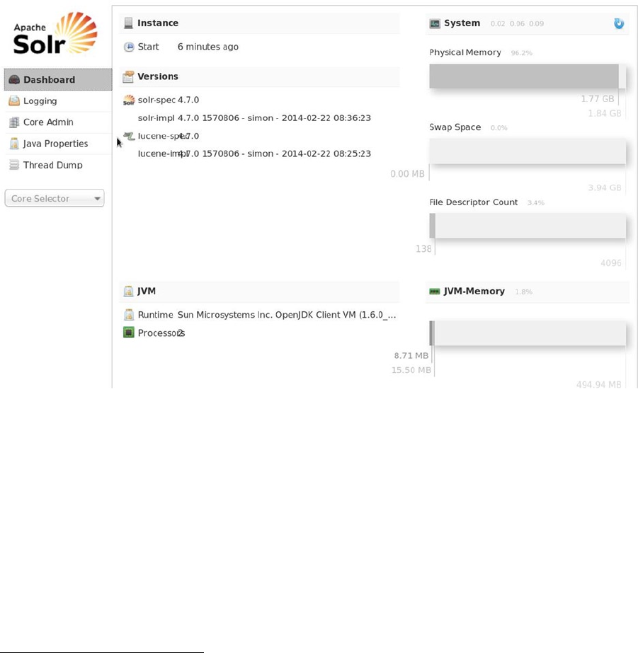
Chapter 3 ■ ColleCting Data with nutCh anD Solr

65

You can also check the log file under $SOLR_HOME/example/logs/. If there are no errors, then try connecting to

the Solr admin client at:

http://localhost:8983/solr/admin/

The Solr admin client (Figure 3-1) contains logging and administrative functions, as well as the core selector that

you will use shortly to examine the results of Solr indexing.

Figure 3-1. The Solr administration user interface

Now that you have Solr running without error and you can connect to its admin client, you are ready to run Nutch

and do a simple web crawl using Hadoop as the storage mechanism.

Running Nutch with Hadoop 1.8

You are ready to run the first crawl using Nutch and Hadoop. For doing this, I have created a seed file on the Linux file

system containing the initial website to crawl. I have also added a single URL to the file, my own website.1

[hadoop@hc1nn nutch]$ ls -l urls

total 4

-rw-rw-r--. 1 hadoop hadoop 19 Apr 5 13:14 seed.txt

1I own the site and it’s contents, so there are no issues with processing the site contents and displaying them here.

Chapter 3 ■ ColleCting Data with nutCh anD Solr

66

This is a small-scale example, so you will start with a single URL to follow. In a real situation, you would populate

the crawl database with a large volume of URLs by using a much larger seed file. You can also download seed file

databases from the Internet. The file at http://rdf.dmoz.org/rdf/content.rdf.u8.gz has around 3 million URLs.

No matter the size of your seed file, you need to copy it (seed.txt, in this case) from the Linux file system to HDFS

(to the nutch/urls directory):

[hadoop@hc1nn nutch]$ hadoop dfs -put urls/seed.txt nutch/urls

[hadoop@hc1nn nutch]$ hadoop dfs -ls nutch/urls

Found 1 items

-rw-r--r-- 1 hadoop supergroup 19 2014-04-05 13:19

/user/hadoop/nutch/urls/seed.txt

Found in $NUTCH_HOME/runtime/deploy/bin, the Nutch crawl command is actually a shell script that

automates the sequence of Nutch operations, as follows:

1. Inject. Inserts a URL into the Nutch crawl database.

2. Generate. Creates a fetch list from the Nutch database for the crawl. This creates a

segment directory within the crawl database for fetch processing.

3. Fetch. Runs the fetcher against the segment created in step 2.

4. Parse. Processes the results of the fetch.

5. Update db. Updates the Nutch crawl database with the results of the parse.

6. Invertlinks. Creates a link map, listing incoming links for this URL.

7. Dedup. Deletes duplicate documents that are in the index.

8. Index. Runs the indexer on the database.

9. Clean. Cleans up after the crawl cycle.

For the actual crawl itself, the syntax of the crawl command is:

crawl <seedDir> <crawlDir> <solrURL> <numberOfRounds>

The seed directory, nutch/urls, will be sourced from HDFS, which is why you copied the URL list to HDFS.

The Solr URL gives Nutch a link to the Solr instance you started in the last section. The number of rounds is actually

the depth that the crawl will process to.

The crawl script runs a couple of steps to decide whether it should use Hadoop for storage. First, it looks for the

job file:

mode=local

if [ -f ../*nutch-*.job ]; then

mode=distributed

fi

Chapter 3 ■ ColleCting Data with nutCh anD Solr

67

Then it checks to determine whether it can access Hadoop:

# check that hadoop can be found on the path

if [ $mode = "distributed" ]; then

if [ $(which hadoop | wc -l ) -eq 0 ]; then

echo "Can't find Hadoop executable. Add HADOOP_HOME/bin to the path or run in local mode."

exit -1;

fi

Given these checks, if Hadoop is available, it will be used for storage; otherwise, the Linux file system will be used.

You can now run the crawl as follows:

cd $NUTCH_HOME/runtime/deploy/bin

./crawl nutch/urls crawl http://hc1nn:8983/solr/ 2

This gives you the Nutch crawl output:

14/04/06 16:56:22 INFO crawl.Injector: Injector: starting at 2014-04-06 16:56:22

14/04/06 16:56:22 INFO crawl.Injector: Injector: crawlDb: /user/hadoop/crawl/crawldb

14/04/06 16:56:22 INFO crawl.Injector: Injector: urlDir: nutch/urls

14/04/06 16:56:22 INFO crawl.Injector: Injector: Converting injected urls to crawl db entries.

14/04/06 16:56:26 INFO util.NativeCodeLoader: Loaded the native-hadoop library

14/04/06 16:56:26 INFO mapred.FileInputFormat: Total input paths to process : 1

14/04/06 16:56:26 INFO mapred.JobClient: Running job: job_201404061342_0056

14/04/06 16:56:27 INFO mapred.JobClient: map 0% reduce 0%

14/04/06 16:56:43 INFO mapred.JobClient: map 50% reduce 0%

14/04/06 16:56:47 INFO mapred.JobClient: map 100% reduce 0%

14/04/06 16:56:51 INFO mapred.JobClient: map 100% reduce 33%

14/04/06 16:56:52 INFO mapred.JobClient: map 100% reduce 100%

14/04/06 16:56:53 INFO mapred.JobClient: Job complete: job_201404061342_0056

............................

14/04/06 17:05:53 INFO mapred.JobClient: Counters: 30

14/04/06 17:05:53 INFO mapred.JobClient: Job Counters

14/04/06 17:05:53 INFO mapred.JobClient: Launched reduce tasks=1

14/04/06 17:05:53 INFO mapred.JobClient: SLOTS_MILLIS_MAPS=10036

14/04/06 17:05:53 INFO mapred.JobClient: Total time spent by all reduces waiting after reserving

slots (ms)=0

14/04/06 17:05:53 INFO mapred.JobClient: Total time spent by all maps waiting after reserving slots (ms)=0

14/04/06 17:05:53 INFO mapred.JobClient: Rack-local map tasks=1

14/04/06 17:05:53 INFO mapred.JobClient: Launched map tasks=2

14/04/06 17:05:53 INFO mapred.JobClient: Data-local map tasks=1

14/04/06 17:05:53 INFO mapred.JobClient: SLOTS_MILLIS_REDUCES=8334

14/04/06 17:05:53 INFO mapred.JobClient: File Input Format Counters

14/04/06 17:05:53 INFO mapred.JobClient: Bytes Read=3746

14/04/06 17:05:53 INFO mapred.JobClient: File Output Format Counters

14/04/06 17:05:53 INFO mapred.JobClient: Bytes Written=0

14/04/06 17:05:53 INFO mapred.JobClient: FileSystemCounters

14/04/06 17:05:53 INFO mapred.JobClient: FILE_BYTES_READ=6

Chapter 3 ■ ColleCting Data with nutCh anD Solr

68

14/04/06 17:05:53 INFO mapred.JobClient: HDFS_BYTES_READ=4096

14/04/06 17:05:53 INFO mapred.JobClient: FILE_BYTES_WRITTEN=246622

14/04/06 17:05:53 INFO mapred.JobClient: Map-Reduce Framework

14/04/06 17:05:53 INFO mapred.JobClient: Map output materialized bytes=12

14/04/06 17:05:53 INFO mapred.JobClient: Map input records=43

14/04/06 17:05:53 INFO mapred.JobClient: Reduce shuffle bytes=12

14/04/06 17:05:53 INFO mapred.JobClient: Spilled Records=0

14/04/06 17:05:53 INFO mapred.JobClient: Map output bytes=0

14/04/06 17:05:53 INFO mapred.JobClient: Total committed heap usage (bytes)=360120320

14/04/06 17:05:53 INFO mapred.JobClient: CPU time spent (ms)=3040

14/04/06 17:05:53 INFO mapred.JobClient: Map input bytes=3431

14/04/06 17:05:53 INFO mapred.JobClient: SPLIT_RAW_BYTES=242

14/04/06 17:05:53 INFO mapred.JobClient: Combine input records=0

14/04/06 17:05:53 INFO mapred.JobClient: Reduce input records=0

14/04/06 17:05:53 INFO mapred.JobClient: Reduce input groups=0

14/04/06 17:05:53 INFO mapred.JobClient: Combine output records=0

14/04/06 17:05:53 INFO mapred.JobClient: Physical memory (bytes) snapshot=408395776

14/04/06 17:05:53 INFO mapred.JobClient: Reduce output records=0

14/04/06 17:05:53 INFO mapred.JobClient: Virtual memory (bytes) snapshot=4121174016

14/04/06 17:05:53 INFO mapred.JobClient: Map output records=0

14/04/06 17:05:53 INFO indexer.CleaningJob: CleaningJob: finished at 2014-04-06 17:05:53, elapsed: 00:00:31

This output has been clipped because it is too long to include all of it here. As long as you get to the CleaningJob

line, you know that the cycle has completed.

Look for any warnings and errors in this output. Common errors relate to undefined or unexpected document

tokens being found while crawling. Updating the schema.xml before starting Solr or attempting the crawl will

minimize these. Also, check the Hadoop logs and the Nutch log under:

$HADOOP_PREFIX/logs/

$NUTCH_HOME/runtime/local/logs/

You can now check the Hadoop file system and see the data being stored there:

[hadoop@hc1nn nutch]$ hadoop fs -ls /user/hadoop

Found 2 items

drwxr-xr-x - hadoop supergroup 0 2014-04-06 14:07

/user/hadoop/crawl

drwxr-xr-x - hadoop supergroup 0 2014-04-06 11:46

/user/hadoop/nutch

The Nutch crawl directory stores the current and old data in subdirectories:

[hadoop@hc1nn nutch]$ hadoop fs -ls /user/hadoop/crawl/crawldb

Found 2 items

drwxr-xr-x - hadoop supergroup 0 2014-04-06 14:16

/user/hadoop/crawl/crawldb/current

drwxr-xr-x - hadoop supergroup 0 2014-04-06 14:07

/user/hadoop/crawl/crawldb/old

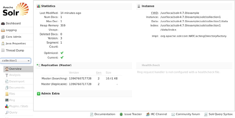
Chapter 3 ■ ColleCting Data with nutCh anD Solr

69

The segments directory has a list of the segments that have been processed:

[hadoop@hc1nn nutch]$ hadoop fs -ls /user/hadoop/crawl/segments

Found 2 items

drwxr-xr-x - hadoop supergroup 0 2014-04-06 14:08

/user/hadoop/crawl/segments/20140406140827

drwxr-xr-x - hadoop supergroup 0 2014-04-06 14:17

/user/hadoop/crawl/segments/20140406141732

You now have data in Solr. To see it, go to the Solr admin web page at http://localhost:8983/solr/ and select

“collection1” in the core selector drop-down menu (halfway down the left side). Figure 3-2 shows that the sample data

has loaded into Solr. Specifically, under the Replication heading on the right, you can see that around 10 KB of data

loaded from the short crawl of the Semtech Solutions web page. Although this is a comparatively small sum of data for

a large-scale distributed system, it serves to prove that the crawl executed and indexed correctly.

Figure 3-2. The Solr sample data after processing

To examine some of the actual data in Solr, you select the Query option (bottom left). An Execute Query option

will appear; select it to see the crawl results. Figure 3-3 shows a sample of the data that Solr has indexed from the

website at the single URL specified in the seed file.

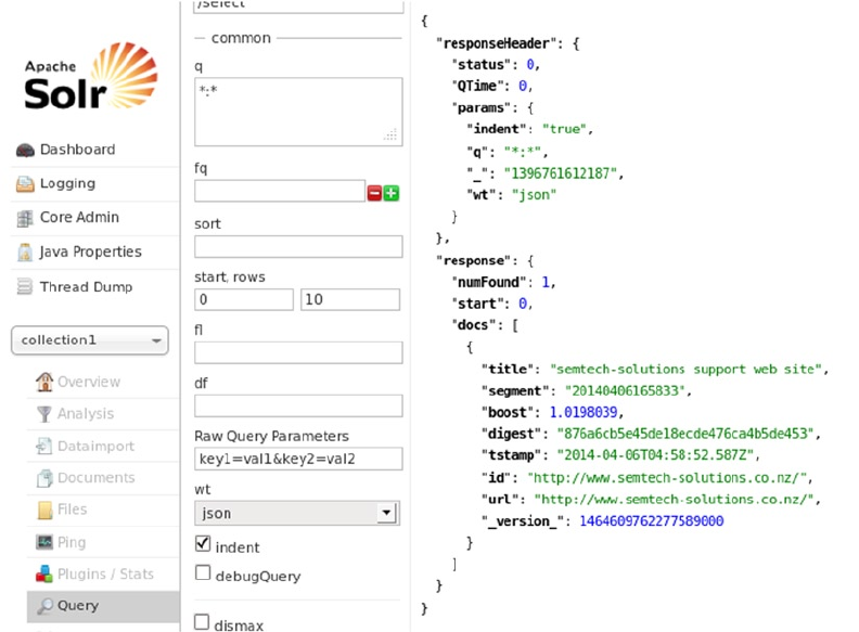
Chapter 3 ■ ColleCting Data with nutCh anD Solr

70

So, that’s it for architecture example 1. You have connected Hadoop 1.2.1 to Nutch 1.8 and indexed the data using

Solr 4.7. Note that during the crawl script, Nutch implicitly checked for Hadoop before using it; otherwise, it would have

used the Linux file system for storage. That is an important point to recognize here because, in the second architectural

example, using Nutch 2.x, you will explicitly configure Nutch to use HBase, and therefore Hadoop as well.

Architecture 2: Nutch 2.x

In the first architecture example, you used Nutch 1.x. When you executed a crawl, Nutch used Hadoop because it

automatically checked whether you were in a distributed environment and it attempted to use Hadoop for storage.

The architecture of this next example enables you to specify the storage you will use for your Nutch crawl. Nutch 2.x

uses Apache Gora (gora.apache.org) to abstract the storage layer. You will also use Apache HBase with Nutch. Using

Hadoop and HDFS for storage, Apache HBase (hbase.apache.org) offers real-time read/write random access to

big data. Should you later need to choose a different storage option, Gora provides the flexibility to do that; you just

change the Gora configuration. For instance, you might decide to use the Apache Accumulo database

(accumulo.apache.org).

Figure 3-3. Solr with crawl results

Chapter 3 ■ ColleCting Data with nutCh anD Solr

71

Nutch and Solr Configuration

You have already learned how to install Nutch and Solr in the first architecture example, so I will be brief here. To

begin, you set up a little configuration in the Linux hadoop account’s $HOME/.bashrc for Solr and Nutch.

The following Bash file defines the Hadoop and Java variables; it also creates some useful aliases for Hadoop

commands, like fs (saves typing). In addition, it sets up the shell search path (PATH) and defines some variables for

Solr and Nutch.

[hadoop@hc1r1m2 ~]$ cd $HOME

[hadoop@hc1r1m2 ~]$ ls -l .bashrc*

-rw-r--r--. 1 hadoop hadoop 1142 Apr 5 15:57 .bashrc

[hadoop@hc1r1m2 ~]$ cat .bashrc

#######################################################

# Set Hadoop related env variables

export HADOOP_PREFIX=/usr/local/hadoop

# set JAVA_HOME (you will also set a hadoop specific value later)

export JAVA_HOME=/usr/lib/jvm/jre-1.6.0-openjdk

# some handy aliases and functions

unalias fs 2>/dev/null

alias fs="hadoop fs"

unalias hls 2>/dev/null

alias hls="fs -l"

unalias cdh 2>/dev/null

alias cdh="cd $HADOOP_PREFIX"

# add hadoop to the path

export PATH=$HADOOP_PREFIX:$PATH

export PATH=$HADOOP_PREFIX/bin:$PATH

export PATH=$HADOOP_PREFIX/sbin:$PATH

#######################################################

# Set up Nutch and Solr variables

export NUTCH_HOME=/usr/local/nutch

export NUTCH_CONF_DIR=$NUTCH_HOME/conf

export SOLR_HOME=/usr/local/solr

export PATH=$PATH:$NUTCH_HOME/bin

You now install Nutch 2.x from Apache on the machine hc1r1m2, because that is where ZooKeeper is already

installed. For example, I download and unpack the appropriate file from the Nutch website

(http://nutch.apache.org/downloads.html):

[hadoop@hc1r1m2 Downloads]$ ls -l apache-nutch-2.2.1-src.tar.gz

-rw-rw-r--. 1 hadoop hadoop 3839858 Apr 7 18:32 apache-nutch-2.2.1-src.tar.gz

Chapter 3 ■ ColleCting Data with nutCh anD Solr

72

As for example 1, you choose the gzipped tar file; using the gunzip and tar xvf Linux commands, it is easily

unpacked. The tar command unpacks the file into the directory named apache-nutch-2.2.1:

[hadoop@hc1r1m2 Downloads]$ gunzip apache-nutch-2.2.1-src.tar.gz

[hadoop@hc1r1m2 Downloads]$ tar xvf apache-nutch-2.2.1-src.tar

Next, you move it to its home location and set up a symbolic link called “nutch” to simplify the path. Also, you use

the Linux chown command with a recursive (-R) switch to change ownership of all files and directories to the Linux

hadoop account.

[root@hc1r1m2 Downloads]# mv apache-nutch-2.2.1 /usr/local

[root@hc1r1m2 Downloads]# cd /usr/local

[root@hc1r1m2 Downloads]# chown –R hadoop:hadoop apache-nutch-2.2.1

[root@hc1r1m2 local]# ln -s apache-nutch-2.2.1 nutch

[root@hc1r1m2 local]# ls -ld *nutch*

drwxrwxr-x. 7 hadoop hadoop 4096 Apr 7 18:33 apache-nutch-2.2.1

lrwxrwxrwx. 1 root root 18 Apr 7 18:35 nutch -> apache-nutch-2.2.1

Okay, so you have a simple environment set up. Next, you set up the Nutch configuration files:

[hadoop@hc1r1m2 ~]$ cd $NUTCH_CONF_DIR ; pwd

/usr/local/nutch/conf

Note that the configuration directory for Nutch is under /usr/local/nutch/conf/, as just shown. Extra Nutch

configuration properties will now be added to these files for Nutch V2. For example, storage.data.store.class indicates

that you are going to use Gora and HBase for storage. (In the Nutch 1.8 architecture, you specified the plug-in folders

and agent name options instead.)

<name>http.agent.name</name>

<value>NutchHadoopCrawler</value>

</property>

<name>storage.data.store.class</name>

<value>org.apache.gora.hbase.store.HBaseStore</value>

</property>

<name>plugin.folders</name>

<value>/usr/local/nutch/build/plugins</value>

</property>

As before, you copy the Nutch configuration files into the Solr configuration directory:

[hadoop@hc1r1m2 ~]$ cd $NUTCH_HOME/conf

[hadoop@hc1r1m2 conf]$ cp schema.xml $SOLR_HOME/example/solr/collection1/conf

[hadoop@hc1r1m2 conf]$ cp schema-solr4.xml $SOLR_HOME/example/solr/collection1/conf

Now, you need to make some changes to the schema file, schema.xml. As before, find the line that specifies the

deprecated EnglishPorterFilterFactory:

Chapter 3 ■ ColleCting Data with nutCh anD Solr

73

Update it to the following to provide filtering functionality for the parsed tokens:

<filter class="solr.SnowballPorterFilterFactory" protected="protwords.txt"

language="English"/>

Add the following lines at the end of the <fields> section to define some extra field types in the documents to be

parsed. (By making these changes you will avoid Nutch document parsing errors):

Build Nutch as you did in the last Nutch release:

[hadoop@hc1r1m2 nutch]$ pwd

/usr/local/nutch

[hadoop@hc1r1m2 nutch]$ ant

Buildfile: build.xml

....

BUILD SUCCESSFUL

Total time: 1 minute 47 seconds

Note: That was a quick build. (As you remember, the last Nutch build took more than 11 minutes). With Nutch

built, you are ready to install Apache HBase, the Hadoop-based database, and test it.

HBase Installation

The pieces are moving into place for this second architecture example. Nutch is installed and built, as well as

configured to use Gora and HBase. The Gora component was included with the Nutch 2.x release, and Apache

ZooKeeper was installed already as part of Chapter2’s installation. Now you need to install Apache HBase.

To demonstrate its use, I show how to install HBase on a single server.

You can download HBase from the HBase website (hbase.apache.org). After clicking the Downloads option on

the left of the page, you may be directed to an alternative mirror site. That’s fine—just follow the link. (I downloaded

the 0.90.4 release). Again, it is a gzipped tar file that needs to be unpacked.

[hadoop@hc1r1m2 Downloads]$ ls -l hbase-0.90.4.tar.gz

-rw-rw-r--. 1 hadoop hadoop 37161251 Apr 8 18:36 hbase-0.90.4.tar.gz

[hadoop@hc1r1m2 Downloads]$ gunzip hbase-0.90.4.tar.gz

[hadoop@hc1r1m2 Downloads]$ tar xvf hbase-0.90.4.tar

Move the unpacked release to /usr/local, and change the ownership to the Linux hadoop user recursively

with chown -R. Then, create a symbolic link called “hbase” under /usr/local/ to simplify both the path and the

environment setup.

root@hc1r1m2 Downloads]# mv hbase-0.90.4 /usr/local

[root@hc1r1m2 Downloads]# cd /usr/local

[root@hc1r1m2 local]# chown -R hadoop:hadoop hbase-0.90.4

[root@hc1r1m2 local]# ln -s hbase-0.90.4 hbase

Chapter 3 ■ ColleCting Data with nutCh anD Solr

74

[root@hc1r1m2 local]# ls -ld *hbase*

lrwxrwxrwx. 1 root root 12 Apr 8 18:38 hbase -> hbase-0.90.4

drwxrwxr-x. 8 hadoop hadoop 4096 Apr 8 18:36 hbase-0.90.4

Next, set up the HBase configuration. You’ll find the configuration files under /usr/local/hbase/conf, as shown:

[hadoop@hc1r1m2 conf]$ pwd

/usr/local/hbase/conf

[hadoop@hc1r1m2 conf]$ ls

hadoop-metrics.properties hbase-site.xml regionservers

hbase-env.sh log4j.properties

You will need to change the contents of the hbase-site.xml file. Specifically, the value of hbase.rootdir needs

to point to the name node on the master server. This allows HBase to store data on HDFS. Also, the distributed flag

(hbase.cluster.distributed) tells HBase that you are using a cluster.

You also need to specify the HBase master address and port number, as well as the value of the region server

port (i/o server) and the fact that it is on a cluster. Other properties to define are the address of the HBase temporary

directory, details for HBase access to ZooKeeper, and limits for ZooKeeper operation.

To start, you add the properties that follow to the hbase-site.xml file between the configuration open

(<configuration>) and configuration closing (</configuration>) XML tags:

<name>hbase.rootdir</name>

<value>hdfs://hc1nn:54310/hbase</value>

</property>

<name>hbase.master</name>

</property>

<name>hbase.master.port</name>

</property>

<name>hbase.regionserver.port</name>

</property>

<name>hbase.cluster.distributed</name>

</property>

Chapter 3 ■ ColleCting Data with nutCh anD Solr

75

<name>hbase.tmp.dir</name>

<value>/var/hbase/</value>

</property>

<name>hbase.zookeeper.quorum</name>

</property>

<name>dfs.replication</name>

</property>

<name>hbase.zookeeper.property.clientPort</name>

</property>

<name>hbase.zookeeper.property.dataDir</name>

<value>/var/lib/zookeeper</value>

</property>

<name>zookeeper.session.timeout</name>

</property>

<name>hbase.client.scanner.caching</name>

</property>

<name>hbase.regionserver.lease.period</name>

</property>

<name>hbase.zookeeper.property.maxClientCnxns</name>

</property>

<name>hbase.zookeeper.property.tickTime</name>

</property>

</configuration>

Chapter 3 ■ ColleCting Data with nutCh anD Solr

76

You also need to tell HBase that it will not be managing the ZooKeeper quorum, because ZooKeeper is already

running. To do so, set up the following variable in the Linux hadoop account environment (I have defined this in my

environment via an entry in $HOME/.bashrc, as follows):

export HBASE_MANAGES_ZK=false

You must make sure that Hadoop and HBase are using the same version of Hadoop core libraries, so issue a pair

of cd and ls commands to check the versions:

[hadoop@hc1r1m2 lib]$ cd /usr/local/hbase/lib

[hadoop@hc1r1m2 lib]$ ls -l hadoop-core-*.jar

-rwxrwxr-x. 1 hadoop hadoop 2707856 Feb 10 2011 hadoop-core-0.20-append-r1056497.jar

[hadoop@hc1r1m2 hadoop]$ cd $HADOOP_PREFIX

[hadoop@hc1r1m2 hadoop]$ ls -l hadoop-core-*.jar

-rw-rw-r--. 1 hadoop hadoop 4203147 Jul 23 2013 hadoop-core-1.2.1.jar

As you can see, the versions don’t match. The HBase Hadoop core file (hadoop-core-0.20-append-r1056497.

jar) is at version 0.20, while the Hadoop jar file (hadoop-core-1.2.1.jar) is at version 1.2.1. Currently, if you tried to run

HBase, it would fail with a connect exception.

You already know from the Hadoop installation you carried out in Chapter 2 that the Hadoop installation is

version 1.2.1. To work with the Hadoop installation, HBase must use the same version of Hadoop libraries. You copy

this library into place, as follows:

[hadoop@hc1r1m2 hadoop]$ cp $HADOOP_PREFIX/hadoop-core-*.jar /usr/local/hbase/lib

[hadoop@hc1r1m2 hadoop]$ cd /usr/local/hbase/lib

[hadoop@hc1r1m2 hadoop]$ mv hadoop-core-0.20-append-r1056497.jar hadoop-core-0.20-append-r1056497.

jar.save

Check the version of the Hadoop commons configuration jar file being used by HBase. This library assists with

the reading of configuration and preference files. If the version is different, then it can be updated by copying the

Hadoop version into place. (This will avoid errors like “NoClassDefFoundError” when you try to run HBase.) Use the

command sequence:

[root@hc1r1m2 lib]# cd /usr/local/hadoop/lib/

[root@hc1r1m2 lib]# ls commons-configuration*

/usr/local/hadoop/lib/commons-configuration-1.6.jar

That shows that the Hadoop version of this file is 1.6. You copy it to the HBase library area:

[root@hc1r1m2 lib]# cd /usr/local/hbase/lib

[root@hc1r1m2 lib]# cp /usr/local/hadoop/lib/commons-configuration* .

Now, you can try starting HBase by using the start script in the HBase bin directory:

[hadoop@hc1r1m2 ~]$ cd /usr/local/hbase

[hadoop@hc1r1m2 hbase]$ ./bin/start-hbase.sh

starting master, logging to

/usr/local/hbase/logs/hbase-hadoop-master-hc1r1m2.out

Chapter 3 ■ ColleCting Data with nutCh anD Solr

77

Note that HBase has given the address of its log file, so you can check the logs for errors. The logs files look like this:

[hadoop@hc1r1m2 hbase]$ ls -l /usr/local/hbase/logs/

total 28

-rw-rw-r--. 1 hadoop hadoop 11099 Apr 9 18:32 hbase-hadoop-master-hc1r1m2.log

-rw-rw-r--. 1 hadoop hadoop 0 Apr 9 18:32 hbase-hadoop-master-hc1r1m2.out

-rw-rw-r--. 1 hadoop hadoop 78 Apr 9 18:30 hbase-hadoop-regionserver-hc1r1m2.log

-rw-rw-r--. 1 hadoop hadoop 250 Apr 9 18:30 hbase-hadoop-regionserver-hc1r1m2.out

A few typical errors reported might be related to ZooKeeper, such as:

2014-04-13 14:53:54,827 WARN org.apache.zookeeper.ClientCnxn: Session 0x14558da65420000 for server

null, unexpected error,

closing socket connection and attempting reconnect

java.net.ConnectException: Connection refused

This indicates that either Zo1oKeeper is down or there are network issues. Make sure that all of your ZooKeeper

servers are up, and check the ZooKeeper logs.

A good way to see that HBase is working is to start a shell and create a table. For example, start the shell as

follows:

[root@hc1r1m2 bin]# pwd

/usr/local/hbase/bin

[root@hc1r1m2 bin]# ./hbase shell

HBase Shell; enter 'help<RETURN>' for list of supported commands.

Type "exit<RETURN>" to leave the HBase Shell

Version 0.90.4, r1150278, Sun Jul 24 15:53:29 PDT 2011

hbase(main):001:0>

Now, create a table named “employer” with a single column named “empname” for the name of the employee

and insert some data:

hbase(main):001:0> create 'employer', 'empname'

0 row(s) in 0.5650 seconds

Insert a single row into the table column created with the employee name "Evans D"; this is row 1:

hbase(main):004:0> put 'employer', 'row1', 'empname', 'Evans D'

0 row(s) in 0.0130 seconds

Check that this data is accessible from the employee table:

hbase(main):005:0> get 'employer', 'row1'

COLUMN CELL

empname: timestamp=1397028137988, value=Evans D

1 row(s) in 0.0330 seconds

hbase(main):006:0> exit

Chapter 3 ■ ColleCting Data with nutCh anD Solr

78

HBase seems to be running okay, but you should check that HBase is storing the data to HDFS. To do so, use the

Hadoop file system ls command. HBase should have created a storage directory on HDFS called “/hbase,” so you can

check that:

[hadoop@hc1nn logs]$ hadoop dfs -ls /hbase

Found 5 items

drwxr-xr-x - hadoop supergroup 0 2014-04-12 19:55 /hbase/-ROOT-

drwxr-xr-x - hadoop supergroup 0 2014-04-12 19:55 /hbase/.META.

drwxr-xr-x - hadoop supergroup 0 2014-04-12 19:57 /hbase/.logs

drwxr-xr-x - hadoop supergroup 0 2014-04-12 19:57 /hbase/.oldlogs

-rw-r--r-- 3 hadoop supergroup 3 2014-04-12 19:55 /hbase/hbase.version

Gora Configuration

Nutch and Solr are ready, HBase and ZooKeeper are ready, and HBase is storing its data to HDFS. Now it is time to

connect Nutch to HBase using the Apache Gora module that was installed with Nutch 2.x. Gora (Gora.apache.org)

provides an in-memory data model for big data and data persistence. It allows you to choose where you will store the

data that Nutch collects, because it supports a variety of data stores. In this section, you will configure Gora to store

Nutch 2.x crawl data to HBase.

You can now set up the Gora connection for Nutch. First, you need to edit the nutch-site.xml file:

[hadoop@hc1r1m2 conf]$ pwd

/usr/local/nutch/conf

[hadoop@hc1r1m2 conf]$ vi nutch-site.xml

Specifically, you add a property called “storage.data.store.class” to specify that HBase will be the default storage

for Nutch Gora. As before, make sure that you add the property to the file so that it sits between the xml open and

close configuration tabs:

<name>storage.data.store.class</name>

<value>org.apache.gora.hbase.store.HBaseStore</value>

<description>Default class for storing data</description>

</property>

Check the Nutch Ivy configuration. Apache Ivy (http://ant.apache.org/ivy/) is a dependency manager that is

integrated with Apache Ant. Intended for Java-based systems, it is mostly used for system build management.

[hadoop@hc1r1m2 ivy]$ pwd

/usr/local/nutch/ivy

[hadoop@hc1r1m2 ivy]$ vi ivy.xml

Make sure that this line is uncommented so that Ivy is configured to use Gora. This is what the line looks like after

the change:

<dependency org="org.apache.gora" name="gora-sql" rev="0.3" conf="*->default" />

Chapter 3 ■ ColleCting Data with nutCh anD Solr

79

Make sure that the gora.properties file is set up correctly, as shown:

[hadoop@hc1r1m2 nutch]$ pwd

/usr/local/nutch

[hadoop@hc1r1m2 nutch]$ vi ./conf/gora.properties

Check that Gora is the default data store. The line here should already exist in the file, but it may be commented

out. Uncomment or add the line. This will set the default Gora data store to be Apache HBase:

gora.datastore.default=org.apache.gora.hbase.store.HBaseStore

Remember that each time you change the Nutch configuration, you need to re-compile Nutch. Do so now, so that

the Gora changes take effect:

[hadoop@hc1r1m2 nutch]$ pwd

/usr/local/nutch

[hadoop@hc1r1m2 nutch]$ ant runtime

Buildfile: build.xml

......

BUILD SUCCESSFUL

Total time: 13 minutes 39 seconds

Running the Nutch Crawl

You have managed to start HBase and you know that HBase is storing its data within Hadoop HDFS. You have a

ZooKeeper quorum running, and HBase is able to connect to it without error. Solr has been started and is running

without error on port 8983. Additionally, Nutch Gora has been configured to use HBase for storage. So now you are

ready to run a Nutch crawl, move to the Nutch home directory as shown by the Linux cd command:

[hadoop@hc1r1m2 nutch]$ cd $NUTCH_HOME

[hadoop@hc1r1m2 nutch]$ pwd

/usr/local/nutch

Now make sure that the seed URL is ready in HDFS. (You know it is ready because you stored it there for the

Nutch 1.x crawl.) Checking the contents of the seed file, you can see that it has a single URL line (my website address).

You could have put a few million lines into this file for a larger crawl, but you can try that later.

[hadoop@hc1r1m2 hadoop]$ hadoop dfs -cat /user/hadoop/nutch/urls/seed.txt

http://www.semtech-solutions.co.nz

You can determine the syntax for the crawl by executing the script name without parameters. The error message

tells you how it should be run:

[hadoop@hc1r1m2 nutch]$ cd runtime/deploy/bin

[hadoop@hc1r1m2 bin]$ ./crawl

Missing seedDir : crawl <seedDir> <crawlID> <solrURL> <numberOfRounds>

The crawl is executed in the same format as for Nutch 1.x, and the output is shown as follows:

[hadoop@hc1nn bin]$ ./crawl urls crawl1 http://hc1r1m2:8983/solr/ 2

Chapter 3 ■ ColleCting Data with nutCh anD Solr

80

14/04/13 17:28:10 INFO crawl.InjectorJob: InjectorJob: starting at 2014-04-13 17:28:10

14/04/13 17:28:10 INFO crawl.InjectorJob: InjectorJob: Injecting urlDir: nutch/urls

14/04/13 17:28:11 INFO zookeeper.ZooKeeper: Client environment:zookeeper.version=3.3.2-1031432,

built on 11/05/2010 05:32 GMT

14/04/13 17:28:11 INFO zookeeper.ZooKeeper: Client environment:host.name=hc1r1m2

14/04/13 17:28:11 INFO zookeeper.ZooKeeper: Client environment:java.version=1.6.0_30

14/04/13 17:28:11 INFO zookeeper.ZooKeeper: Client environment:java.vendor=Sun Microsystems Inc.

14/04/13 17:28:11 INFO zookeeper.ZooKeeper: Client environment:java.home=/usr/lib/jvm/java-1.6.0-

openjdk-1.6.0.0/jre

14/04/13 17:28:11 INFO zookeeper.ZooKeeper: Client

................

14/04/13 17:37:20 INFO mapred.JobClient: Job complete: job_201404131430_0019

14/04/13 17:37:21 INFO mapred.JobClient: Counters: 6

14/04/13 17:37:21 INFO mapred.JobClient: Job Counters

14/04/13 17:37:21 INFO mapred.JobClient: SLOTS_MILLIS_MAPS=54738

14/04/13 17:37:21 INFO mapred.JobClient: Total time spent by all reduces waiting after reserving

slots (ms)=0

14/04/13 17:37:21 INFO mapred.JobClient: Total time spent by all maps waiting after reserving slots (ms)=0

14/04/13 17:37:21 INFO mapred.JobClient: Launched map tasks=8

14/04/13 17:37:21 INFO mapred.JobClient: SLOTS_MILLIS_REDUCES=0

You need to monitor all of your logs; that is, you need to monitor the following:

• ZooKeeper logs, in this case under /var/log/zookeeper. These allow you to ensure that all

servers are up and running as a quorum.

• Hadoop logs, in this case under /usr/local/hadoop/logs. Hadoop and MR must be running

without error so that HBase can use Hadoop.

• HBaselogs, in this case under /usr/local/hbase/logs. You make sure that HBase is running and

able to talk to ZooKeeper.

• Solr output from the Solr session window. It must be running without error so that it can index

the crawl output.

• Nutch output from the crawl session. Any errors will appear in the session window.

Each of the components in this architecture must work for the Nutch crawl to work. If you encounter errors, pay

particular attention to your configuration. For timeout errors in ZooKeeper, try increasing the tickTime and

syncLimit values in your ZooKeeper config files.

Potential Errors

Here are some of the errors that occurred when I tried to use this configuration. They are provided here along with

their reasons and solutions. If you encounter them, go back to the step you missed and correct the error.

Consider the first one:

2014-04-08 19:05:39,334 ERROR

org.apache.hadoop.hbase.master.HMasterCommandLine: Failed to start master

java.io.IOException: Couldnt start ZK at requested address of 2181, instead

got: 2182. Aborting. Why? Because clients (eg shell) wont be able to find this

Chapter 3 ■ ColleCting Data with nutCh anD Solr

81

ZK quorum at

org.apache.hadoop.hbase.master.HMasterCommandLine.startMaster(HMasterCommandLine.java:131)

This problem was caused by one of the ZooKeeper servers (on hc1r1m1) running under the wrong Linux account.

It didn’t have file system access. The solution was to shut it down and start as the correct user.

Another error you may encounter is:

2014-04-09 18:32:53,741 ERROR

org.apache.hadoop.hbase.master.HMasterCommandLine: Failed to start master

java.io.IOException: Unable to create data directory

/var/lib/zookeeper/zookeeper/version-2

Again, this was the same issue as for ZooKeeper in the previous error. The ZooKeeper server (on hc1r1m1) was

running under the wrong Linux account. It didn’t have file system access. The solution was to shut it down and start as

the correct user.

An HBase error that could occur is:

org.apache.hadoop.ipc.RemoteException: Server IPC version 7 cannot communicate

with client version 3

This was an HBase error. IPC version 4 is for Hadoop 1.0, whereas version 7 is for Hadoop 2.0, so HBase expects

Hadoop version 1.x. That is why we are using Hadoop version 1.2.1 with Nutch 2.x.

This error occurred during the Nutch crawl:

14/04/12 20:32:30 ERROR crawl.InjectorJob: InjectorJob:

java.lang.ClassNotFoundException: org.apache.gora.hbase.store.HBaseStore

The Gora configuration was incorrect. Go back, check the setting, and retry the crawl once you’ve fixed it.

These errors occurred during a crawl in the HBase logs:

2014-04-12 20:52:37,955 INFO org.apache.hadoop.hbase.master.ServerManager:

Waiting on regionserver(s) to checkin

org.apache.hadoop.security.AccessControlException:

org.apache.hadoop.security.AccessControlException: Permission denied:

user=root, access=WRITE, inode=".logs":hadoop:supergroup:rwxr-xr-x

They indicate a file system access issue on HDFS for HBase. I had set the HBase directory permissions for the

.logs directory incorrectly.

[hadoop@hc1nn bin]$ hadoop dfs -ls /hbase/ | grep logs

drwxrwxrwx - hadoop supergroup 0 2014-04-13 18:00 /hbase/.logs

Your permissions for HDFS directories should be fine, but if you encounter a permissions access error, you can

use the hadoop dfs -chmod command to set permissions.

This error occurred because I had an error in my /etc/hosts file:

14/04/13 12:00:54 INFO mapred.JobClient: Task Id :

attempt_201404131045_0016_m_000000_0, Status : FAILED

java.lang.RuntimeException: java.io.IOException: java.lang.RuntimeException:

org.apache.hadoop.hbase.ZooKeeperConnectionException: HBase is able to connect

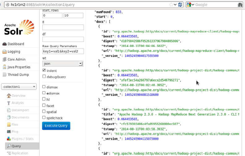
Chapter 3 ■ ColleCting Data with nutCh anD Solr

82

to ZooKeeper but the connection closes immediately. This could be a sign that

the server has too many connections (30 is the default). Consider inspecting

your ZK server logs for that error and then make sure you are reusing

HBaseConfiguration as often as you can. See HTable's javadoc for more

information.

Make sure that your /etc/hosts file entries are defined correctly and that ZooKeeper is working correctly before

you move on to start HBase.

As for architecture example 1, you can check the Solr query page for your results. For this example, because the

seed URL was from my own site, the query found the apache URLs, as shown in Figure 3-4.

Figure 3-4. Solr output showing the crawl data

A Brief Comparison

Of the two architecture examples given in this chapter, the second, using HBase, was the most difficult to use. This

may be the future direction that Nutch is taking, but there are a lot more configuration items to take care of. There

are more components to worry about and check, plus more potential areas of failure. Having said that, the second

architecture example gives you the ability to explicitly choose the storage architecture. If for some reason at a future

date you need to use an alternative system to HBase that Gora supports, you will be able to do that.

You have only used Hadoop V1 in both of these examples. If time had allowed, it would have been useful to use

Hadoop V2 as well. In that case, you would have needed to rebuild both HBase and Nutch using Hadoop V2 libraries.

Nevertheless, it would have been interesting to compare the Nutch processing time using Hadoop V1 and V2.

Chapter 3 ■ ColleCting Data with nutCh anD Solr

83

Summary

In this chapter, you investigated big data collection using Nutch, Solr, Gora, and HBase. You used both Nutch 1.x and

2.x to crawl a seed URL and collect data. Although you crawled only on a small scale, the same process can be used

to gather large volumes of data. You used Solr in both cases to index data passed from Nutch. In the second example,

you used Apache Gora to determine where Nutch would store its data—in this case, it was HBase. You also looked at

two possible approaches for using Nutch and Hadoop. In the first, Nutch implicitly used Hadoop for storage; in the

second, Nutch used Apache Gora to explicitly select HBase for storage.

Where do you go from here? The command sequence and examples given in this chapter should enable you to

apply these approaches to your own system. Take a logical approach, and make sure that HDFS is working before

moving on. Also, make sure that ZooKeeper is working before you attempt HBase. Remember: if you encounter errors,

search the web for solutions, because other people may have encountered similar problems. Also, keep trying to think

of new ways to approach the problem.

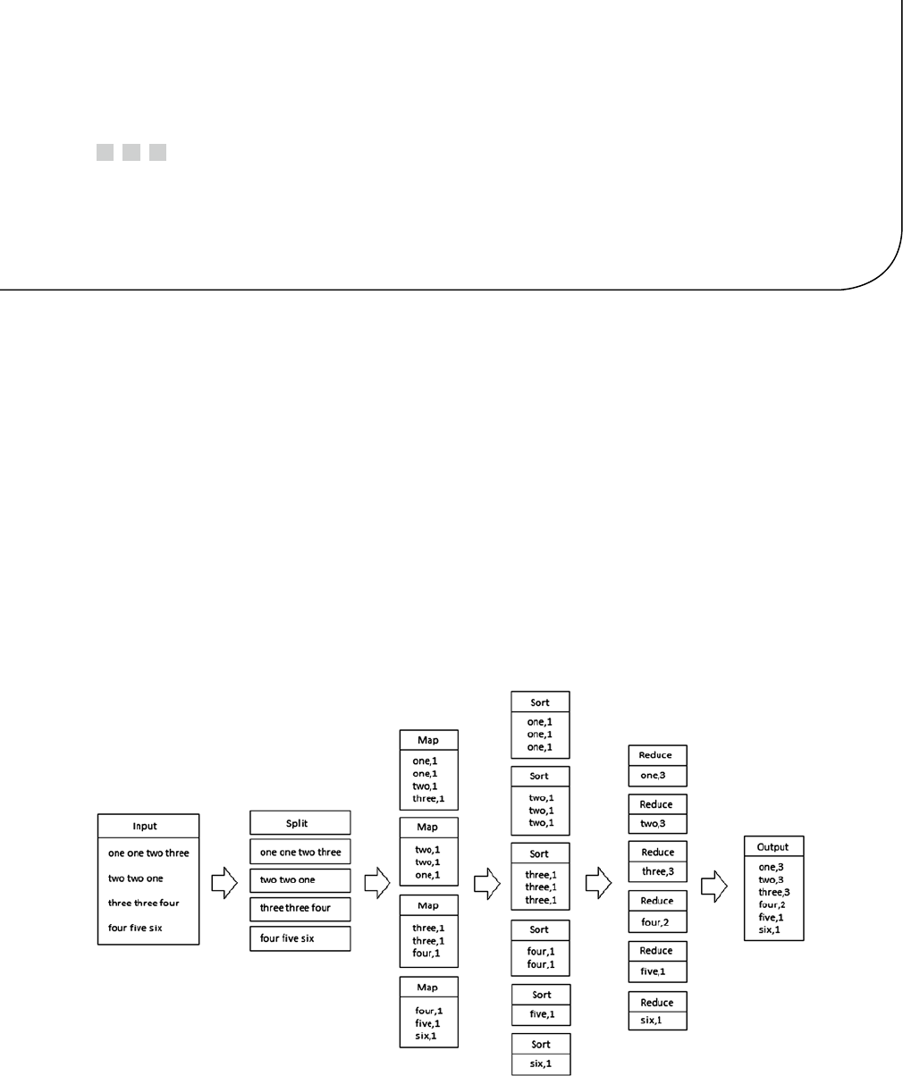
85

Chapter 4

Processing Data with Map Reduce

Hadoop Map Reduce is a system for parallel processing of very large data sets using distributed fault-tolerant storage

over very large clusters. The input data set is broken down into pieces, which are the inputs to the Map functions.

The Map functions then filter and sort these data chunks (whose size is configurable) on the Hadoop cluster data

nodes. The output of the Map processes is delivered to the Reduce processes, which shuffle and summarize the data

to produce the resulting output.

This chapter explores Map Reduce programming through multiple implementations of a simple, but flexible

word-count algorithm. After first coding the word-count algorithm in raw Java using classes provided by Hadoop

libraries, you will then learn to carry out the same word-count function in Pig Latin, Hive, and Perl. Don’t worry about

these terms yet; you will learn to source, install, and work with this software in the coming sections.

An Overview of the Word-Count Algorithm

The best way to understand the Map Reduce system is with an example. A word-count algorithm is not only the

most common and simplest Map Reduce example, but it is also one that contains techniques you can apply to more

complex scenarios. To begin, consider Figure 4-1, which breaks the word-count process into steps.

Figure 4-1. The word-count Map Reduce process

CHAPTER 4 ■ PROCESSING DATA WITH MAP REDUCE

86

The input file on the left of Figure 4-1 is split into chunks of data. The size of these splits is controlled by the

InputSplit method within the FileInputFormat class of the Map Reduce job. The number of splits is influenced by the

HDFS block size, and one mapper job is created for each split data chunk.

Each split data chunk—that is, “one one two three,” is sent to a Mapper process on a Data Node server. In the

word-count example, the Map process creates a series of key-value pairs where the key is the word—for instance,

“one”—and the value is the count of 1. These key-value pairs are then shuffled into lists by key type. The shuffled lists

are input to Reduce tasks, which reduce the list volume by summing the values (in this simple example). The Reduce

output is then a simple list of summed key-value pairs.

The Map Reduce framework takes care of all other tasks, like scheduling and resources.

Map Reduce Native

Now, it’s time to put the word-count algorithm to work, starting with the most basic example: the Map Reduce native

version. The term Map Reduce native means that the Map Reduce code is written in Java using the functionality

provided by the Hadoop core libraries within the Hadoop installation directory. Map Reduce native word-count

algorithms are available from the Apache Software Foundation Hadoop 1.2.1 Map Reduce tutorial on the Hadoop

website (hadoop.apache.org/docs/r1.2.1/). For instance, I sourced two versions of the Hadoop word-count

algorithm and stored them in Java files in a word-count directory, as follows:

[hadoop@hc1nn wordcount]$ pwd

/usr/local/hadoop/wordcount

[hadoop@hc1nn wordcount]$ ls *.java

wc-ex1.java wc-ex2.java

The file wc-ex1.java contains the first simple example, while the second Java file contains a second, more

complex version.

Java Word-Count Example 1

Consider the Java code for the first word-count example. It follows the basic word-count steps shown in Figure 4-1:

01 package org.myorg;

02

03 import java.io.IOException;

04 import java.util.*;

05

06 import org.apache.hadoop.fs.Path;

07 import org.apache.hadoop.conf.*;

08 import org.apache.hadoop.io.*;

09 import org.apache.hadoop.mapred.*;

10 import org.apache.hadoop.util.*;

11

12 public class WordCount

13 {

14

15 public static class Map extends MapReduceBase implements

16 Mapper<LongWritable, Text, Text, IntWritable>

17 {

18 private final static IntWritable one = new IntWritable(1);

19 private Text word = new Text();

20

CHAPTER 4 ■ PROCESSING DATA WITH MAP REDUCE

87

21 public void map(LongWritable key, Text value, OutputCollector<Text,

22 IntWritable output, Reporter reporter) throws IOException

23 {

24 String line = value.toString();

25 StringTokenizer tokenizer = new StringTokenizer(line);

26 while (tokenizer.hasMoreTokens())

27 {

28 word.set(tokenizer.nextToken());

29 output.collect(word, one);

30 }

31 }

32 } /* class Map */

33

34 public static class Reduce extends MapReduceBase implements

35 Reducer<Text, IntWritable, Text, IntWritable>

36 {

37 public void reduce(Text key, Iterator<IntWritable> values,

OutputCollector<Text, IntWritable> output, Reporter reporter)

throws IOException

39 {

40 int sum = 0;

41 while (values.hasNext())

42 {

43 sum += values.next().get();

44 }

45 output.collect(key, new IntWritable(sum));

46 }

47 } /* class Reduce */

48

49 public static void main(String[] args) throws Exception

50 {

51 JobConf conf = new JobConf(WordCount.class);

52 conf.setJobName("wordcount");

53

54 conf.setOutputKeyClass(Text.class);

55 conf.setOutputValueClass(IntWritable.class);

56

57 conf.setMapperClass(Map.class);

58 conf.setCombinerClass(Reduce.class);

59 conf.setReducerClass(Reduce.class);

60

61 conf.setInputFormat(TextInputFormat.class);

62 conf.setOutputFormat(TextOutputFormat.class);

63

64 FileInputFormat.setInputPaths(conf, new Path(args[0]));

65 FileOutputFormat.setOutputPath(conf, new Path(args[1]));

66

67 JobClient.runJob(conf);

68 }

69

70 } /* class WordCount */

CHAPTER 4 ■ PROCESSING DATA WITH MAP REDUCE

88

Describing the Example 1 Code

In this section, we look at the Java code used in the Java-based simple Map Reduce word-count example. We then

proceed to compile it, create a jar file, and run it. This package is called org.myorg, and it is defined at line 1:

01 package org.myorg;

Lines 6 to 10 import Hadoop functionality for Path, configuration, I/O, Map Reduce, and utilities.

06 import org.apache.hadoop.fs.Path;

07 import org.apache.hadoop.conf.*;

08 import org.apache.hadoop.io.*;

09 import org.apache.hadoop.mapred.*;

10 import org.apache.hadoop.util.*;

For the details of these APIs, consult https://hadoop.apache.org/docs/stable/api/org/apache/hadoop/. Just

select the package name—that is, mapred—and then choose package-summary.html. The fs.Path class provides file

system path functionality and the Conf class adds configuration functionality as shown at line 51 in the example. The

IO class adds input/output functionality, while the Util class adds utilities like logging and checksums. The Mapred

class is the Hadoop V1 Map Reduce class API implimentation. The V1 class names are called mapred, while the V2

implementation that you will encounter later in the book uses the term mapreduce.

The Map class is defined at line 15:

15 public static class Map extends MapReduceBase implements

16 Mapper<LongWritable, Text, Text, IntWritable>

Line 25 uses a StringTokenizer to break the input line into words, which are then passed as outputs as key-value

pairs—that is, <word,1>.

25 StringTokenizer tokenizer = new StringTokenizer(line);

26 while (tokenizer.hasMoreTokens())

27 {

28 word.set(tokenizer.nextToken());

29 output.collect(word, one);

30 }

As defined at line 34, the Reduce class accepts shuffled key-value pairs as input:

34 public static class Reduce extends MapReduceBase implements

35 Reducer<Text, IntWritable, Text, IntWritable>

From line 40 on, the code then totals the values for the key-value pairs with the same key and outputs the totaled

key-value pairs; that is, <word,5>:

40 int sum = 0;

41 while (values.hasNext())

42 {

43 sum += values.next().get();

44 }

45 output.collect(key, new IntWritable(sum));

CHAPTER 4 ■ PROCESSING DATA WITH MAP REDUCE

89

The main method at line 49 sets up the Map Reduce configuration by defining the type of input. In this case, the

input is text.

49 public static void main(String[] args) throws Exception

The code then defines the Map, Combine, and Reduce classes, as well as specifying the input/output formats:

51 JobConf conf = new JobConf(WordCount.class);

52 conf.setJobName("wordcount");

53

54 conf.setOutputKeyClass(Text.class);

55 conf.setOutputValueClass(IntWritable.class);

56

57 conf.setMapperClass(Map.class);

58 conf.setCombinerClass(Reduce.class);

59 conf.setReducerClass(Reduce.class);

60

61 conf.setInputFormat(TextInputFormat.class);

62 conf.setOutputFormat(TextOutputFormat.class);

63

64 FileInputFormat.setInputPaths(conf, new Path(args[0]));

65 FileOutputFormat.setOutputPath(conf, new Path(args[1]));

Finally, line 67 runs the job:

67 JobClient.runJob(conf);

Running the Example 1 Code

To compile this code, I used the Java compiler javac, which was installed with the JDK when Java 1.6 was installed. The

compiler expects the Java file name to match the class name, so I renamed the example code as WordCount.Java.

The classes on which this example relies are found in the Hadoop core library that is in the Hadoop release, so

I specified that when compiling the code. Also, I placed the compiled output into a subdirectory called wc_classes,

which can be used when building an example jar file.

[hadoop@hc1nn wordcount]$ cp wc-ex1.java WordCount.java

[hadoop@hc1nn wordcount]$ mkdir wc_classes

[hadoop@hc1nn wordcount]$ javac -classpath $HADOOP_PREFIX/hadoop-core-1.2.1.jar -d wc_classes

WordCount.java

The following recursive listing shows all of the subdirectories and classes from the build of the first example code:

[hadoop@hc1nn wordcount]$ ls -R wc_classes

wc_classes:

org

wc_classes/org:

myorg

wc_classes/org/myorg:

WordCount.class WordCount$Map.class WordCount$Reduce.class

CHAPTER 4 ■ PROCESSING DATA WITH MAP REDUCE

90

Building the code into a jar library using the jar command creates the wordcount1.jar file:

[hadoop@hc1nn wordcount]$ jar -cvf ./wordcount1.jar -C wc_classes .

added manifest

adding: org/(in = 0) (out= 0)(stored 0%)

adding: org/myorg/(in = 0) (out= 0)(stored 0%)

adding: org/myorg/WordCount.class(in = 1546) (out= 750)(deflated 51%)

adding: org/myorg/WordCount$Reduce.class(in = 1611) (out= 648)(deflated 59%)

adding: org/myorg/WordCount$Map.class(in = 1938) (out= 798)(deflated 58%)

[hadoop@hc1nn wordcount]$ ls -l *.jar

-rw-rw-r--. 1 hadoop hadoop 3169 Jun 15 15:05 wordcount1.jar

This file can now be used to run a word-count task on Hadoop. As in previous Map Reduce runs, the input and

output data for the job will be taken from HDFS. To provide the words to count, I copied some data from Edgar Allan

Poe books into a directory on HDFS from the Linux file system. The Linux ls command shows the text files that will

be used:

[hadoop@hc1nn wordcount]$ ls $HOME/edgar

10031.txt 15143.txt 17192.txt 2149.txt 932.txt

Copying these files to the HDFS directory called /user/hadoop/edgar, using the Hadoop file system

copyFromLocal command, sets up the data for the word-count job:

[hadoop@hc1nn wordcount]$ hadoop dfs -copyFromLocal $HOME/edgar/* /user/hadoop/edgar

[hadoop@hc1nn wordcount]$ hadoop dfs -ls /user/hadoop/edgar

Found 5 items

-rw-r--r-- 1 hadoop supergroup 410012 2014-06-15 15:53 /user/hadoop/edgar/10031.txt

-rw-r--r-- 1 hadoop supergroup 559352 2014-06-15 15:53 /user/hadoop/edgar/15143.txt

-rw-r--r-- 1 hadoop supergroup 66401 2014-06-15 15:53 /user/hadoop/edgar/17192.txt

-rw-r--r-- 1 hadoop supergroup 596736 2014-06-15 15:53 /user/hadoop/edgar/2149.txt

-rw-r--r-- 1 hadoop supergroup 63278 2014-06-15 15:53 /user/hadoop/edgar/932.txt

By running the word-count example against the data in the input directory (/user/hadoop/edgar), you create the

results data in the output directory (/user/hadoop/edgar-results). First, though, make sure the processes are all up

before you run the job using jps.

[hadoop@hc1nn wordcount]$ jps

1959 SecondaryNameNode

1839 DataNode

4166 TaskTracker

4272 Jps

1720 NameNode

4044 JobTracker

This shows that the HDFS processes for the data node and name node are running on hc1nn. Also, the Map

Reduce processes for the Task and Job Trackers are running. If you are going to rerun this job, then you will need to

delete the HDFS-based results directory by using the Hadoop file system rmr command:

[hadoop@hc1nn wordcount]$ hadoop dfs -rmr /user/hadoop/edgar-results

CHAPTER 4 ■ PROCESSING DATA WITH MAP REDUCE

91

You can run the job via the Hadoop jar command. The parameters passed to it are the library file you have just

created, the name of the class to run in that library, the input directory on HDFS, and the output directory:

[hadoop@hc1nn wordcount]$ hadoop jar ./wordcount1.jar org.myorg.WordCount /user/hadoop/edgar /user/

hadoop/edgar-results

14/06/15 16:04:50 INFO util.NativeCodeLoader: Loaded the native-hadoop library

14/06/15 16:04:50 INFO mapred.FileInputFormat: Total input paths to process : 5

14/06/15 16:04:51 INFO mapred.JobClient: Running job: job_201406151602_0001

14/06/15 16:04:52 INFO mapred.JobClient: map 0% reduce 0%

14/06/15 16:05:02 INFO mapred.JobClient: map 20% reduce 0%

14/06/15 16:05:03 INFO mapred.JobClient: map 40% reduce 0%

14/06/15 16:05:04 INFO mapred.JobClient: map 60% reduce 0%

........................

14/06/15 16:05:19 INFO mapred.JobClient: Combine input records=284829

14/06/15 16:05:19 INFO mapred.JobClient: Reduce input records=55496

14/06/15 16:05:19 INFO mapred.JobClient: Reduce input groups=36348

14/06/15 16:05:19 INFO mapred.JobClient: Combine output records=55496

14/06/15 16:05:19 INFO mapred.JobClient: Physical memory (bytes) snapshot=912035840

14/06/15 16:05:19 INFO mapred.JobClient: Reduce output records=36348

14/06/15 16:05:19 INFO mapred.JobClient: Virtual memory (bytes) snapshot=7949012992

14/06/15 16:05:19 INFO mapred.JobClient: Map output records=284829

The job has completed (the output shown above has been trimmed), so you can check the output on HDFS

under /user/hadoop/edgar-results/ by using the Hadoop file system ls command:

[hadoop@hc1nn wordcount]$ hadoop dfs -ls /user/hadoop/edgar-results/

Found 3 items

-rw-r--r-- 1 hadoop supergroup 0 2014-06-15 16:05 /user/hadoop/edgar-results/_SUCCESS

drwxr-xr-x - hadoop supergroup 0 2014-06-15 16:04 /user/hadoop/edgar-results/_logs

-rw-r--r-- 1 hadoop supergroup 396500 2014-06-15 16:05 /user/hadoop/edgar-results/part-00000

These results show a _SUCCESS file, so the job was completed without error. As in previous examples, you use

the Hadoop file system cat command to dump the contents of the results file and the Linux head command to limit

the job results to the first 10 rows:

[hadoop@hc1nn wordcount]$ hadoop dfs -cat /user/hadoop/edgar-results/part-00000 | head -10

!) 1

"''T 1

"'And 1

"'As 1

"'Be 2

"'But--still--monsieur----' 1

"'Catherine, 1

"'Comb 1

"'Come 1

"'Eyes,' 1

Well done! You have just compiled and run your own native Map Reduce job from a source file. To create more,

you can simply change the algorithm in Java (or write your own) and follow the same process. One change that might

be useful is to ignore the white-space and symbol characters when counting the words. The example’s output data

contains characters like these (“ or -). The next example adds these refinements.

CHAPTER 4 ■ PROCESSING DATA WITH MAP REDUCE

92

Java Word-Count Example 2

Using the same Map and Reduce classes as the first example, you will find this second example adds pattern filtering

to the code. You can find the file, wc-ex2.java, in the Apache Software Foundation Hadoop 1.2.1 Map Reduce tutorial

at the Hadoop website (hadoop.apache.org/docs/r1.2.1/). Here’s the complete listing:

01 package org.myorg;

02

03 import java.io.*;

04 import java.util.*;

05

06 import org.apache.hadoop.fs.Path;

07 import org.apache.hadoop.filecache.DistributedCache;

08 import org.apache.hadoop.conf.*;

09 import org.apache.hadoop.io.*;

10 import org.apache.hadoop.mapred.*;

11 import org.apache.hadoop.util.*;

12

13 public class WordCount extends Configured implements Tool

14 {

15

16 /*------------------------------------------------------------------*/

17 public static class Map extends MapReduceBase

18 implements Mapper < LongWritable, Text, Text, IntWritable >

19 {

20

21 static enum Counters

22 {

23 INPUT_WORDS

24 }

25

26 private final static IntWritable one = new IntWritable(1);

27 private Text word = new Text();

28

29 private boolean caseSensitive = true;

30 private Set < String > patternsToSkip = new HashSet < String > ();

31

32 private long numRecords = 0;

33 private String inputFile;

34

35 /*---------------------------------------------------------------*/

36 public void configure(JobConf job)

37 {

38 caseSensitive = job.getBoolean("wordcount.case.sensitive", true);

39 inputFile = job.get("map.input.file");

40

41 if (job.getBoolean("wordcount.skip.patterns", false))

42 {

43 Path[] patternsFiles = new Path[0];

44 try

45 {

46 patternsFiles = DistributedCache.getLocalCacheFiles(job);

47 }

CHAPTER 4 ■ PROCESSING DATA WITH MAP REDUCE

93

48 catch (IOException ioe)

49 {

50 System.err.println("Caught exception while getting cached

51 files: " + StringUtils.stringifyException(ioe));

52 }

53 for (Path patternsFile: patternsFiles)

54 {

55 parseSkipFile(patternsFile);

56 }

57 }

58 }

59 /*----------------------------------------------------------------*/

60 private void parseSkipFile(Path patternsFile)

61 {

62 try

63 {

64 BufferedReader fis = new BufferedReader(new

65 FileReader(patternsFile.toString()));

66 String pattern = null;

67 while ((pattern = fis.readLine()) != null)

68 {

69 patternsToSkip.add(pattern);

70 }

71 }

72 catch (IOException ioe)

73 {

74 System.err.println("Caught exception while parsing cached file '"

75 + patternsFile + "' : " + StringUtils.stringifyException(ioe));

76 }

77 }

78 /*----------------------------------------------------------------*/

79 public void map(LongWritable key, Text value, OutputCollector < Text,

80 IntWritable > output, Reporter reporter) throws IOException

81 {

82 String line = (caseSensitive) ? value.toString() :

83 value.toString().toLowerCase();

84

85 for (String pattern: patternsToSkip)

86 {

87 line = line.replaceAll(pattern, "");

88 }

89

90 StringTokenizer tokenizer = new StringTokenizer(line);

91 while (tokenizer.hasMoreTokens())

92 {

93 word.set(tokenizer.nextToken());

94 output.collect(word, one);

95 reporter.incrCounter(Counters.INPUT_WORDS, 1);

96 }

97

CHAPTER 4 ■ PROCESSING DATA WITH MAP REDUCE

94

98 if ((++numRecords % 100) == 0)

99 {

100 reporter.setStatus("Finished processing " + numRecords +

101 " records " + "from the input file: " + inputFile);

102 }

103 }

104

105 } /* class Map */

106

107 /*---------------------------------------------------------------*/

108 public static class Reduce extends MapReduceBase implements Reducer

109 < Text, IntWritable, Text, IntWritable >

110 {

111 public void reduce(Text key, Iterator < IntWritable > values,

112 OutputCollector

113 < Text, IntWritable > output, Reporter reporter) throws

114 IOException

115 {

116 int sum = 0;

117 while (values.hasNext())

118 {

119 sum += values.next().get();

120 }

121 output.collect(key, new IntWritable(sum));

122 }

123 } /* class Reduce */

124 /*------------------------------------------------------------*/

125 public int run(String[] args) throws Exception

126 {

127 JobConf conf = new JobConf(getConf(), WordCount.class);

128 conf.setJobName("wordcount");

129

130 conf.setOutputKeyClass(Text.class);

131 conf.setOutputValueClass(IntWritable.class);

132

133 conf.setMapperClass(Map.class);

134 conf.setCombinerClass(Reduce.class);

135 conf.setReducerClass(Reduce.class);

136

137 conf.setInputFormat(TextInputFormat.class);

138 conf.setOutputFormat(TextOutputFormat.class);

139

140 List < String > other_args = new ArrayList < String > ();

141 for (int i = 0; i < args.length; ++i)

142 {

143 if ("-skip".equals(args[i]))

144 {

145 DistributedCache.addCacheFile(new Path(args[++i]).toUri(), conf);

146 conf.setBoolean("wordcount.skip.patterns", true);

147 }

CHAPTER 4 ■ PROCESSING DATA WITH MAP REDUCE

95

148 else

149 {

150 other_args.add(args[i]);

151 }

152 }

153

154 FileInputFormat.setInputPaths(conf, new Path(other_args.get(0)));

155 FileOutputFormat.setOutputPath(conf, new Path(other_args.get(1)));

156

157 JobClient.runJob(conf);

158 return 0;

159 }

160 /*------------------------------------------------------------------*/

161 public static void main(String[] args) throws Exception

162 {

163 int res = ToolRunner.run(new Configuration(), new WordCount(), args);

164 System.exit(res);

165 }

166

167 } /* class word count*/

Describing the Example 2 Code

Take a closer look at the code for the simpler example, given earlier. Note that line 1 defines the package name as org.

myorg and lines 6 through 11 import the Hadoop functionality for Path, configuration, I/O, Map Reduce, and utilities.

New to this second example is the cache definition, which is used to store the configurations pattern file (which will

be described later):

07 import org.apache.hadoop.filecache.DistributedCache;

Line 13 defines the main WordCount class:

13 public class WordCount extends Configured implements Tool

Meanwhile, the Map class is defined at line 17:

17 public static class Map extends MapReduceBase

18 implements Mapper < LongWritable, Text, Text, IntWritable >

This class now has a configure method defined at line 36, which offers case-sensitivity and pattern-skipping

functionality:

36 public void configure(JobConf job)

The parseSkipFile method at line 60 parses the pattern file for the pattern-skipping functionality just

mentioned. The patternsFile contains a list of patterns that should be removed from the text to be processed when

counting words:

60 private void parseSkipFile(Path patternsFile)

CHAPTER 4 ■ PROCESSING DATA WITH MAP REDUCE

96

The map method is defined at line 79:

79 public void map(LongWritable key, Text value, OutputCollector < Text,

80 IntWritable > output, Reporter reporter) throws IOException

As in the last example, a StringTokenizer (line 90) breaks the line into words, then a while loop outputs the

words as key-value pairs where the key is the word and the value is 1:

90 StringTokenizer tokenizer = new StringTokenizer(line);

91 while (tokenizer.hasMoreTokens())

92 {

93 word.set(tokenizer.nextToken());

94 output.collect(word, one);

95 reporter.incrCounter(Counters.INPUT_WORDS, 1);

96 }

The Reduce class is defined at line 108:

108 public static class Reduce extends MapReduceBase implements Reducer

109 < Text, IntWritable, Text, IntWritable >

The reduce method totals the values for similar words and outputs the key-value pair beginning at line 117:

117 while (values.hasNext())

118 {

119 sum += values.next().get();

120 }

121 output.collect(key, new IntWritable(sum));

There is now a run method (starting at line 125) that contains the functionality from example 1's main method. It

sets the Map Reduce and I/O format classes:

133 conf.setMapperClass(Map.class);

134 conf.setCombinerClass(Reduce.class);

135 conf.setReducerClass(Reduce.class);

136

137 conf.setInputFormat(TextInputFormat.class);

138 conf.setOutputFormat(TextOutputFormat.class);

The new run method parses the skip command line option, saves the pattern file name, and sets the skip

patterns option to True. Processing of the skip file can be seen at line 143 via the –skip command line option:

143 if ("-skip".equals(args[i]))

144 {

145 DistributedCache.addCacheFile(new Path(args[++i]).toUri(), conf);

146 conf.setBoolean("wordcount.skip.patterns", true);

147 }

CHAPTER 4 ■ PROCESSING DATA WITH MAP REDUCE

97

The run method also sets the input and output paths for the job:

154 FileInputFormat.setInputPaths(conf, new Path(other_args.get(0)));

155 FileOutputFormat.setOutputPath(conf, new Path(other_args.get(1)));

Finally, line 157 runs the job:

157 JobClient.runJob(conf);

Running the Example 2 Code

To run this second Java example, you copy its file to the WordCount.java file so that the file name matches the Java class.

[hadoop@hc1nn wordcount]$ cp wc-ex2.java WordCount.java

Then, you remove the contents of the wc_classes directory and re-create it to receive the Java build output. Use

the Linux rm command for the Remove with r for “recursive”and f for “force switches.” Use the Linux mkdir command

to re-create the directory:

[hadoop@hc1nn wordcount]$ rm -rf wc_classes

[hadoop@hc1nn wordcount]$ mkdir wc_classes

You build the WordCount java file by specifying an output directory called wc_classes:

[hadoop@hc1nn wordcount]$ javac -classpath $HADOOP_PREFIX/hadoop-core-1.2.1.jar -d wc_classes

WordCount.java

Then, you list the contents of the wc_classes directory recursively to ensure that the org.myorg directory structure

exists and contains the newly compiled classes:

[hadoop@hc1nn wordcount]$ ls -R wc_classes

wc_classes:

org

wc_classes/org:

myorg

wc_classes/org/myorg:

WordCount.class WordCount$Map.class WordCount$Map$Counters.class WordCount$Reduce.class

You build these classes into a jar library called wordcount1.jar, so that the resulting jar file can be used for a

Hadoop Map Reduce job run. Use the Linux jar command for this (which operates in a similar manner to tar) by

using the options C for “create,” v for “verbose,” and f to specify the file to create:

[hadoop@hc1nn wordcount]$ jar -cvf ./wordcount1.jar -C wc_classes.

added manifest

adding: org/(in = 0) (out= 0)(stored 0%)

adding: org/myorg/(in = 0) (out= 0)(stored 0%)

adding: org/myorg/WordCount.class(in = 2671) (out= 1289)(deflated 51%)

adding: org/myorg/WordCount$Reduce.class(in = 1611) (out= 648)(deflated 59%)

adding: org/myorg/WordCount$Map$Counters.class(in = 983) (out= 504)(deflated 48%)

adding: org/myorg/WordCount$Map.class(in = 4661) (out= 2217)(deflated 52%)

CHAPTER 4 ■ PROCESSING DATA WITH MAP REDUCE

98

[hadoop@hc1nn wordcount]$ ls -l *.jar

-rw-rw-r--. 1 hadoop hadoop 5799 Jun 21 17:19 wordcount1.jar

The test data from the first example is still available on HDFS under the directory /user/hadoop/edgar; this is

shown by using the Hadoop file system ls command:

[hadoop@hc1nn wordcount]$ hadoop dfs -ls /user/hadoop/edgar

Found 5 items

-rw-r--r-- 1 hadoop supergroup 410012 2014-06-19 11:59 /user/hadoop/edgar/10031.txt

-rw-r--r-- 1 hadoop supergroup 559352 2014-06-19 11:59 /user/hadoop/edgar/15143.txt

-rw-r--r-- 1 hadoop supergroup 66401 2014-06-19 11:59 /user/hadoop/edgar/17192.txt

-rw-r--r-- 1 hadoop supergroup 596736 2014-06-19 11:59 /user/hadoop/edgar/2149.txt

-rw-r--r-- 1 hadoop supergroup 63278 2014-06-19 11:59 /user/hadoop/edgar/932.txt

To give this first example a thorough test, I also created a patterns file called patterns.txt that contains a series of

unwanted characters. I have dumped the contents of the file shown here by using the Linux cat command. Note that

some characters have an Escape character (\) at the start of the line to avoid processing errors for characters that Java

might consider to have special meaning. By using an Escape character, you will ensure that these patterns are just

treated as text:

[hadoop@hc1nn wordcount]$ cat patterns.txt

!

"

'

_

;

\(

\)

\#

\$

\&

\.

\,

\*

\-

\/

\{

\}

Copy the patterns.txt onto HDFS into the directory /user/hadoop/java by using the Hadoop file system

copyFromLocal command. Using the Hadoop file system ls command, list the patterns.txt file that is now on HDFS:

[hadoop@hc1nn wordcount]$ hadoop dfs -copyFromLocal ./patterns.txt /user/hadoop/java/patterns.txt

[hadoop@hc1nn wordcount]$ hadoop dfs -ls /user/hadoop/java

Found 1 items

-rw-r--r-- 1 hadoop supergroup 46 2014-06-21 17:29 /user/hadoop/java/patterns.txt

CHAPTER 4 ■ PROCESSING DATA WITH MAP REDUCE

99

Now you are ready to run this extended version of the Java Map Reduce task. The library that was just created is

specified via the Hadoop jar option. This is followed by the Class name to be called within that library. Next, a flag

is set via the -D option to switch the case sensitivity off. After that, the input data file and output directory names on

HDFS are listed. Finally, you specify a skip file to remove any unwanted characters in the data processed:

[hadoop@hc1nn wordcount]$ hadoop jar ./wordcount1.jar org.myorg.WordCount

-Dwordcount.case.sensitive=false /user/hadoop/edgar/10031.txt

/user/hadoop/edgar-results -skip /user/hadoop/java/patterns.txt

The command produces the following Map Reduce task output:

14/06/21 17:40:06 INFO util.NativeCodeLoader: Loaded the native-hadoop library

14/06/21 17:40:06 INFO mapred.FileInputFormat: Total input paths to process : 1

14/06/21 17:40:07 INFO mapred.JobClient: Running job: job_201406211041_0004

14/06/21 17:40:08 INFO mapred.JobClient: map 0% reduce 0%

14/06/21 17:40:15 INFO mapred.JobClient: map 50% reduce 0%

14/06/21 17:40:23 INFO mapred.JobClient: map 100% reduce 16%

14/06/21 17:40:30 INFO mapred.JobClient: map 100% reduce 100%

14/06/21 17:40:31 INFO mapred.JobClient: Job complete: job_201406211041_0004

14/06/21 17:40:31 INFO mapred.JobClient: Counters: 32

14/06/21 17:40:31 INFO mapred.JobClient: Job Counters

14/06/21 17:40:31 INFO mapred.JobClient: Launched reduce tasks=1

14/06/21 17:40:31 INFO mapred.JobClient: SLOTS_MILLIS_MAPS=17198

14/06/21 17:40:31 INFO mapred.JobClient: Total time spent by all reduces waiting after reserving

slots (ms)=0

............................

14/06/21 17:40:31 INFO mapred.JobClient: CPU time spent (ms)=5880

14/06/21 17:40:31 INFO mapred.JobClient: Map input bytes=410012

14/06/21 17:40:31 INFO mapred.JobClient: SPLIT_RAW_BYTES=198

14/06/21 17:40:31 INFO mapred.JobClient: Combine input records=63590

14/06/21 17:40:31 INFO mapred.JobClient: Reduce input records=12581

14/06/21 17:40:31 INFO mapred.JobClient: Reduce input groups=9941

14/06/21 17:40:31 INFO mapred.JobClient: Combine output records=12581

14/06/21 17:40:31 INFO mapred.JobClient: Physical memory (bytes) snapshot=404115456

14/06/21 17:40:31 INFO mapred.JobClient: Reduce output records=9941

14/06/21 17:40:31 INFO mapred.JobClient: Virtual memory (bytes) snapshot=4109373440

14/06/21 17:40:31 INFO mapred.JobClient: Map output records=63590

Check the results directory on HDFS by using the Hadoop file system ls command. The existence of a _SUCCESS

file shows that the job was a success:

[hadoop@hc1nn wordcount]$ hadoop dfs -ls /user/hadoop/edgar-results

Found 3 items

-rw-r--r-- 1 hadoop supergroup 0 2014-06-21 17:40 /user/hadoop/edgar-results/_SUCCESS

drwxr-xr-x - hadoop supergroup 0 2014-06-21 17:40 /user/hadoop/edgar-results/_logs

-rw-r--r-- 1 hadoop supergroup 103300 2014-06-21 17:40 /user/hadoop/edgar-results/part-00000

CHAPTER 4 ■ PROCESSING DATA WITH MAP REDUCE

100

Checking the last 10 lines of the results part file using the Hadoop file system cat command and the Linux tail

command gives a sorted word count with any unwanted characters removed:

[hadoop@hc1nn wordcount]$ hadoop dfs -cat /user/hadoop/edgar-results/part-00000 | tail -10

zanthe 1

zeal 2

zeboin 1

zelo 1

zephyr 1

zimmermann 1

zipped 1

zoar 1

zoilus 3

zone 1

Comparing the Examples

The two Map Reduce native word-count examples (wc-ex1.java and wc-ex2.java) show that raw Java code for Map

Reduce can create complex functionality. They are not, however, the most efficient approaches. Consider the effect

achieved when some simple pattern-filtering options were added. The listing grew from 70 lines in example 1 to 167

lines in example 2. As the code volume increases, so do the cost, complexity, and time to implement. Now, imagine

the effect on a more complex algorithm; the resulting code could quickly become even more unwieldy.

The good news is that alternatives are available. In the next sections, I will introduce some other Map Reduce

coding tools that offer the ability to code these tasks at a higher level and so reduce code volume. Generally, it is more

efficient and cheaper to use less code to achieve your objective. You should write your code at a lower level in Java

only if higher level systems like Pig native (including UDFs), which will be described in the next section, do not offer

the functionality you need.

So, next you will learn to source, install, and use Apache Pig. You will also code the same word-count algorithm

in Pig.

Map Reduce with Pig

As it is able to run in interactive or batch mode, Pig is a higher level programming language for processing large data

sets. You will be able to see that fewer lines of code are needed to carry out the same word-count example. Apache Pig

can be downloaded from pig.apache.org.

As Pig is a higher-level language, you can concentrate more on the logical flow of data processing and less on the

lower-level coding to achieve that processing. Also, Pig integrates well with the visual-object-based ETL and reporting

tools for big data that are introduced in Chapters 10 and 11 of this guide. This means that you have a quicker and

easier path into the world of data processing using Map Reduce. Although this will be explained later, tools like Talend

even help to abstract Map Reduce with its predefined Pig-based functionality.

Installing Pig

For this book’s examples, I chose to download Pig release 0.12.1 from pig.apache.org/releases.html because it is

compatible with the version of Hadoop I have been using up to this point (1.x). The download and installation are

straightforward. From the download page, you select to download Pig 0.8 and later. The Pig website then suggests

a mirror site for from which you can download (in my case, it was www.carfab.com). After clicking that link, you’re

CHAPTER 4 ■ PROCESSING DATA WITH MAP REDUCE

101

offered a series of Pig versions. Choose 0.12.1, and download the version of the release file that is tarred and gzipped.

For example, I used wget to download the release to the server hc1nn, which was convenient because I could

download the package straight to a server directory using the website URL:

[hadoop@hc1nn ~]$ wget http://www.carfab.com/apachesoftware/pig/pig-0.12.1/pig-0.12.1.tar.gz

Next, you unzip the release using the Linux command gunzip, and unpack the tar file using the Linux tar -xvf

command:

[hadoop@hc1nn ~]$ ls -l pig-0.12.1.tar.gz

-rw-rw-r--. 1 hadoop hadoop 59445085 Apr 5 21:44 pig-0.12.1.tar.gz

[hadoop@hc1nn ~]$ gunzip pig-0.12.1.tar.gz

[hadoop@hc1nn ~]$ tar xvf pig-0.12.1.tar

[root@hc1nn hadoop]# ls -ld pig-0.12.1

drwxr-xr-x. 15 hadoop hadoop 4096 Apr 5 21:44 pig-0.12.1

You move the release to a location under /usr/local/ using the Linux mv command, then set up a symbolic link

under /usr/local/ called pig by using the Linux ln command with a –s (symbolic) switch to simplify the path to the

software and the environment. Finally, you use the Linux ls command to create a long listing that displays the link

and the install the Pig directory.

[root@hc1nn hadoop]# mv pig-0.12.1 /usr/local

[root@hc1nn hadoop]# cd /usr/local/

[root@hc1nn hadoop]# ln –s pig-0.12.1 pig

[root@hc1nn local]# ls -ld pig*

lrwxrwxrwx. 1 root root 10 Jun 18 12:02 pig -> pig-0.12.1

drwxr-xr-x. 15 hadoop hadoop 4096 Apr 5 21:44 pig-0.12.1

To simplify access to and use of Pig, you can add some Pig-related variables to the Linux hadoop user's Bash shell

configuration at the bottom of the file $HOME/.bashrc:

#######################################################

# Set up Pig variables

export PIG_HOME=/usr/local/pig

export PATH=$PATH:$PIG_HOME/bin

Once the installation is in place and the environment is set up, you can test that the Pig binary is available and

will run. For example, you can use the Linux type command to check that the Pig Linux command is picked up from

the correct location:

[hadoop@hc1nn ~]$ type pig

pig is hashed (/usr/local/pig/bin/pig)

CHAPTER 4 ■ PROCESSING DATA WITH MAP REDUCE

102

This shows that the path is good—it is the one that was just installed. Issuing the Pig help command is another a

good way to ensure that commands will run without error:

[hadoop@hc1nn ~]$ pig -help

Apache Pig version 0.12.1 (r1585011)

compiled Apr 05 2014, 01:41:34

USAGE: Pig [options] [-] : Run interactively in grunt shell.

Pig [options] -e[xecute] cmd [cmd ...] : Run cmd(s).

Pig [options] [-f[ile]] file : Run cmds found in file.

options include:

..............

-M, -no_multiquery - Turn multiquery optimization off; default is on

-P, -propertyFile - Path to property file

-printCmdDebug - Overrides anything else and prints the actual command used to run Pig, including

any environment variables that are set by the pig command.

The results are good: the pig command is located in /usr/local/pig/bin, and it runs as the help option shows. It is

now time to use it.

Running Pig

Pig lets you choose how you wish to work with it. For example, you can direct where Pig looks for data by specifying

the local mode or the Map Reduce mode (the default). Local mode takes all data from the local server and the file

system, while Map Reduce mode uses Hadoop. In addition, you can run tasks interactively or in batch mode. When

working interactively, you issue Pig commands via the Grunt command prompt. For larger scheduled or background

tasks, you can use batch mode. For the word-count demonstration, you will use Pig interactively in Map Reduce mode.

To prepare to use Pig, you first need to create a Pig working directory on HDFS:

[hadoop@hc1nn edgar]$ hadoop dfs -mkdir /user/hadoop/pig/

Then, you copy a text-based data file of Edgar Allan Poe’s work into that HDFS-based directory from the Linux file

system by using the Hadoop file system command copyFromLocal:

[hadoop@hc1nn edgar]$ cd $HOME/edgar

[hadoop@hc1nn edgar]$ ls

10031.txt 15143.txt 17192.txt 2149.txt 932.txt

[hadoop@hc1nn edgar]$ hadoop dfs -copyFromLocal ./10031.txt /user/hadoop/pig

A quick check on HDFS shows that the file 10031.txt containing the text is now sitting on HDFS in the directory /

user/hadoop/pig:

[hadoop@hc1nn edgar]$ hadoop dfs -ls /user/hadoop/pig

Found 1 items

-rw-r--r-- 1 hadoop supergroup 410012 2014-06-18 12:29 /user/hadoop/pig/10031.txt

CHAPTER 4 ■ PROCESSING DATA WITH MAP REDUCE

103

You can now start Pig in interactive Map Reduce mode. Without any options, the pig command will result in the

interactive Grunt command line after trying to access Hadoop:

[hadoop@hc1nn edgar]$ pig

2014-06-18 12:27:10,055 [main] INFO org.apache.pig.Main - Apache Pig version 0.12.1 (r1585011)

compiled Apr 05 2014, 01:41:34

2014-06-18 12:27:10,056 [main] INFO org.apache.pig.Main - Logging error messages to: /home/hadoop/

edgar/pig_1403051230051.log

2014-06-18 12:27:10,095 [main] INFO org.apache.pig.impl.util.Utils - Default bootup file /home/

hadoop/.pigbootup not found

2014-06-18 12:27:10,386 [main] INFO org.apache.pig.backend.hadoop.executionengine.HExecutionEngine

- Connecting to hadoop file system at: hdfs://hc1nn:54310

2014-06-18 12:27:10,750 [main] INFO org.apache.pig.backend.hadoop.executionengine.HExecutionEngine

- Connecting to map-reduce job tracker at: hc1nn:54311

grunt>

In Pig, the character “--” denotes a comment, meaning text between the -- and the start of the next line is ignored.

The semicolon (;) denotes the end of a Pig native statement. The data file is loaded from HDFS into variable A by using

the load option:

grunt> A = load '/user/hadoop/pig/10031.txt'; -- load the text file

With a single line, you can process each word in the data in variable A into a list of words, place each word from

the list in variable B, then add them to variable C. TOKENIZE splits the data on white-space characters. Here’s the

command you need:

grunt> C = foreach A generate flatten(TOKENIZE((chararray)$0)) as B ; -- get list of words

Next, you can group the identical words into a variable D, and create a list of word counts in variable E by using

the count option:

grunt> D = group C by B ; -- group words

grunt> E = foreach D generate COUNT(C), group; -- create word count

To view the word count, you use the dump command to display the contents of variable E in the session window;

this shows the word-count list. (I’ve listed the last 10 lines here.) As you can see, it’s very basic counting:

grunt> dump E; -- dump result to session

.......

(1,http://pglaf.org/fundraising.)

(1,it!--listen--now--listen!--the)

(1,http://www.gutenberg.net/GUTINDEX.ALL)

(1,http://www.gutenberg.net/1/0/2/3/10234)

(1,http://www.gutenberg.net/2/4/6/8/24689)

(1,http://www.gutenberg.net/1/0/0/3/10031/)

(1,http://www.ibiblio.org/gutenberg/etext06)

(0,)

CHAPTER 4 ■ PROCESSING DATA WITH MAP REDUCE

104

Lastly, you can store the contents of the count, currently in variable E, on HDFS in /user/hadoop/pig/wc_result:

grunt> store E into '/user/hadoop/pig/wc_result' ; -- store the results

grunt> quit ; -- quit interactive session

Having quit the Pig interactive session, you can examine the results of this Pig job on HDFS. The Hadoop file

system ls command shows a success file (_SUCCESS), a part file (part-r-00000) containing the word-count data, and a

logs directory. (I have listed the part file from the word count using the Hadoop file system command cat.) Then, you

can use the Linux tail command to view the last 10 lines of the file. Both options are shown here:

[hadoop@hc1nn edgar]$ hadoop dfs -ls /user/hadoop/pig/wc_result

Found 3 items

-rw-r--r-- 1 hadoop supergroup 0 2014-06-18 13:08 /user/hadoop/pig/wc_result/_SUCCESS

drwxr-xr-x - hadoop supergroup 0 2014-06-18 13:08 /user/hadoop/pig/wc_result/_logs

-rw-r--r-- 1 hadoop supergroup 137870 2014-06-18 13:08 /user/hadoop/pig/wc_result/part-r-00000

[hadoop@hc1nn edgar]$ hadoop dfs -cat /user/hadoop/pig/wc_result/part-r-00000 | tail -10

1 http://gutenberg.net/license

1 Dream'--Prospero--Oberon--and

1 http://pglaf.org/fundraising.

1 it!--listen--now--listen!--the

1 http://www.gutenberg.net/GUTINDEX.ALL

1 http://www.gutenberg.net/1/0/2/3/10234

1 http://www.gutenberg.net/2/4/6/8/24689

1 http://www.gutenberg.net/1/0/0/3/10031/

1 http://www.ibiblio.org/gutenberg/etext06

It is quite impressive that, with five lines of Pig commands (ignoring the dump and quit lines), you can run the

same word-count algorithm as took 70 lines of Java code. Less code means lower development costs and, we all hope,

fewer code-based errors.

While efficient, the interactive Pig example does have a drawback: The commands must be manually typed each

time you want to run a word count. Once you’re finished, they’re lost. The answer to this problem, of course, is to store

the Pig script in a file and run it as a batch Map Reduce job. To demonstrate, I placed the Pig commands from the

previous example into the wordcount.pig file:

[hadoop@hc1nn pig]$ ls -l

total 4

-rw-rw-r--. 1 hadoop hadoop 313 Jun 18 13:24 wordcount.pig

[hadoop@hc1nn pig]$ cat wordcount.pig

01 -- get raw line data from file

02

03 rlines = load '/user/hadoop/pig/10031.txt';

04

05 -- get list of words

06

07 words = foreach rlines generate flatten(TOKENIZE((chararray)$0)) as word;

08

09 -- group the words by word value

10

CHAPTER 4 ■ PROCESSING DATA WITH MAP REDUCE

105

11 gwords = group words by word ;

12

13 -- create a word count

14

15 wcount = foreach gwords generate group, COUNT(words) ;

16

17 -- store the word count

18

19 store wcount into '/user/hadoop/pig/wc_result1' ;

I also added comments, line numbers, and meaningful names for the variables. These modifications can help

when you’re trying to determine what a script is doing. They also help to tie this example to the work in the next

section, on Pig user-defined functions.

Instead of invoking the interactive Grunt command line, you invoke Pig with the name of the file containing

the Pig script. Pig will use Map Reduce mode by default and so access HDFS. The output will be stored in the HDFS

directory /user/hadoop/pig/wc_result1/. So, when the task starts, a Map Reduce job is initiated.

[hadoop@hc1nn pig]$ pig wordcount.pig

...................

Counters:

Total records written : 13219

Total bytes written : 137870

Spillable Memory Manager spill count : 0

Total bags proactively spilled: 0

Total records proactively spilled: 0

Job DAG:

job_201406181226_0003

2014-06-18 13:27:49,446 [main] INFO org.apache.pig.backend.hadoop.executionengine.mapreducelayer.

mapreducelauncher - Success!

As mentioned previously, you can use Hadoop and Linux commands to output the word count:

[hadoop@hc1nn pig]$ hadoop dfs -cat /user/hadoop/pig/wc_result1/part-r-00000 | tail -10

1 http://gutenberg.net/license

1 Dream'--Prospero--Oberon--and

1 http://pglaf.org/fundraising.

1 it!--listen--now--listen!--the

1 http://www.gutenberg.net/GUTINDEX.ALL

1 http://www.gutenberg.net/1/0/2/3/10234

1 http://www.gutenberg.net/2/4/6/8/24689

1 http://www.gutenberg.net/1/0/0/3/10031/

1 http://www.ibiblio.org/gutenberg/etext06

Notice that in both the interactive and batch script versions, the count includes non-alpha-numeric chararacters

like “:”(colon), and that the case of the words has not been standardized. For instance, the word Dream (with a capital D)

is part of the count. In the next section, you will learn how to add greater selectivity to Pig by creating user-defined

functions.

CHAPTER 4 ■ PROCESSING DATA WITH MAP REDUCE

106

Pig User-Defined Functions

Coded in Java, user-defined functions (UDFs) provide custom functionality that you can invoke from a Pig script. For

instance, you might create a UDF if you found that you needed to carry out an operation that the standard Pig Latin

language did not include. This section will provide an example of just such a function. You will examine the UDF Java

code, as well as the method by which it is built into a jar library. You will then use an extended version of the Pig script

from the last section that incorporates this UDF. You will learn how to incorporate both the jar file and its classes into

a Pig script.

As greater functionality was obtained for earlier Map Reduce jobs, such as removing unwanted characters from

the word-count process, the same will be done here. Using Java, you will create a UDF to remove unwanted characters,

so that the final word count is more precise. For instance, I have created a UDF build directory on the Linux file system

under /home/hadoop/pig/wcudfs that contains a number of files:

[hadoop@hc1nn wcudfs]$ pwd

/home/hadoop/pig/wcudfs/

[hadoop@hc1nn wcudfs]$ ls

build_clean_ws.sh build_lower.sh CleanWS.java

The Java files contain the code for UDFs while the shell scripts ( *.sh ) are used to build them. The CleanWS.java

file contains the following code:

01 package wcudfs;

02

03 import java.io.*;

04

05 import org.apache.pig.EvalFunc;

06 import org.apache.pig.data.Tuple;

07 import org.apache.hadoop.util.*;

08

09 public class CleanWS extends EvalFunc<String>

10 {

11 /*--------------------------------------------------------*/

12 @Override

13 public String exec(Tuple input) throws IOException

14 {

15 if (input == null || input.size() == 0)

16 return null;

17 try

18 {

19 String str = (String)input.get(0);

20

21 return str.replaceAll("[^A-Za-z0-9]"," ");

22 }

23 catch(IOException ioe)

24 {

25 System.err.println("Caught exception processing input row : "

26 + StringUtils.stringifyException(ioe) );

27 }

28

CHAPTER 4 ■ PROCESSING DATA WITH MAP REDUCE

107

29 return null;

30 }

31 /*--------------------------------------------------------*/

32

33 } /* class CleanWS */

Line 1 defines the package name to be wcudfs

01 package wcudfs;

Pig and Hadoop functionality for tuples and utilities is imported into the UDF between lines 5 and 7. Line 5

invokes the EvalFunc class and identifies this as an eval type of UDF function:

05 import org.apache.pig.EvalFunc;

06 import org.apache.pig.data.Tuple;

07 import org.apache.hadoop.util.*;

Line 9 specifies the class name as CleanWS, which extends the EvalFunc class and has a String return type.

09 public class CleanWS extends EvalFunc<String>

Line 13 onward defines the exec method that will be called to process every tuple in the data:

13 public String exec(Tuple input) throws IOException

Line 21 changes the return string, removing all characters that are not in the character sets A–Z, a–z, or 0–9 and

replacing them with a space character.

21 return str.replaceAll("[^A-Za-z0-9]"," ");

For example, I built CleanWS as follows:

[hadoop@hc1nn wcudfs]$ cat build_clean_ws.sh

javac -classpath $PIG_HOME/pig-0.12.1.jar -Xlint:deprecation CleanWS.java

The Java compiler is called javac; an option is added via the classpath to include the Pig library in the build. The

lint:deprecation option uses lint to check the code for deprecated API calls. These scripts build the class files:

[hadoop@hc1nn wcudfs]$ ./build_clean_ws.sh

[hadoop@hc1nn wcudfs]$ ls

build_clean_ws.sh CleanWS.class CleanWS.java

The class file is created as part of the build for the Java file. The class file for the UDF is built into a library that can

be used within a Pig script. The library is built using the jar command with the options c (create), v (verbose), and f

(file). The next parameter to be created is the library name, followed by the list of classes to be placed in the library:

[hadoop@hc1nn wcudfs]$ cd ..

[hadoop@hc1nn pig]$ jar cvf wcudfs.jar wcudfs/*.class

added manifest

adding: wcudfs/CleanWS.class(in = 1318) (out= 727)(deflated 44%)

[hadoop@hc1nn pig]$ ls -l wcudfs.jar

-rw-rw-r--. 1 hadoop hadoop 2018 Jun 24 18:57 wcudfs.jar

CHAPTER 4 ■ PROCESSING DATA WITH MAP REDUCE

108

This is the library containing the UDF classes that will be called in the Pig script register line.

Next, take a look at the updated version of the Pig script wordcount2.pig by using the Linux cat command, which

employs the newly created UDF function:

[hadoop@hc1nn pig]$ cat wordcount2.pig

01 REGISTER /home/hadoop/pig/wcudfs.jar ;

02

03 DEFINE CleanWS wcudfs.CleanWS() ;

04

05 -- get raw line data from file

06

07 rlines = load '/user/hadoop/pig/10031.txt' AS (rline:chararray);

08

09 -- filter for empty lines

10

11 clines = FILTER rlines BY SIZE(rline) > 0 ;

12

13 -- get list of words

14

15 words = foreach clines generate

16 flatten(TOKENIZE(CleanWS( (chararray) $0 ))) as word ;

17

18 -- group the words by word value

19

20 gword = group words by word ;

21

22 -- create a word count

23

24 wcount = foreach gword generate group, COUNT(words) ;

25

26 -- store the word count

27

28 store wcount into '/user/hadoop/pig/wc_result1' ;

There are some new terms in this script. At line 1, the REGISTER keyword is used to register the word-count UDF

library wcudfs.jar for use with this Pig script.

01 REGISTER /home/hadoop/pig/wcudfs.jar ;

Line 3 uses the DEFINE keyword to refer to the classes of the package within this library that use a single term.

For instance, the class CleanWS in the package wcudfs, in the library wcudfs.jar, can now be called as just CleanWS in

the code.

03 DEFINE CleanWS wcudfs.CleanWS() ;

Line 11 introduces the FILTER keyword. Using this filter removes any lines that are empty from the data set. The

variable clines is used to contain lines that have more than zero characters. This is accomplished by using a check on

the size of the line (rline) and ensuring that the size is greater than zero.

11 clines = FILTER rlines BY SIZE(rline) > 0 ;

CHAPTER 4 ■ PROCESSING DATA WITH MAP REDUCE

109

Line 16 calls the user-defined function named CleanWS, which removes unwanted characters from the input text.

15 words = foreach clines generate

16 flatten(TOKENIZE(CleanWS( (chararray) $0 ))) as word ;

I have created some Bash shell scripts to assist in running this second Pig job. This is just to provide an example

of how to speed up a manual job. For instance, instead of having to type the Pig job execution command each time,

I can just execute a simple script. Instead of having to manually delete the job results directory for a job rerun, I can

run a clean script. Here is the clean_wc.sh script that was used to delete the job results HDFS directory, employing the

Linux cat command:

[hadoop@hc1nn pig]$ cat clean_wc.sh

01 #!/bin/bash

02

03 # remove the pig script results directory

04

05 hadoop dfs -rmr /user/hadoop/pig/wc_result1

The script does this by calling the Hadoop file system rmr command to remove the directory and its contents.

The next script that is run_wc2.sh, which is used to run the job, calls the clean script (at line 5) each time it is run.

This single script cleans the results directory on HDFS and runs the wordcount2.pig job:

[hadoop@hc1nn pig]$ cat run_wc2.sh

01 #!/bin/bash

02

03 # run the pig wc 2 job

04

05 ./clean_wc.sh

06

07 pig -stop_on_failure wordcount2.pig

This shell script calls the clean_wc.sh script and then invokes the Pig wordcount2.pig script. The pig command

on line 7 is called with a flag (-stop_on_failure), telling it to stop as soon as it encounters an error. The results are

listed via the result_wc.sh script:

[hadoop@hc1nn pig]$ cat result_wc.sh

01 #!/bin/bash

02

03 # remove the pig script results directory

04

05 hadoop dfs -ls /user/hadoop/pig/wc_result1

07

08 hadoop dfs -cat /user/hadoop/pig/wc_result1/part-r-00000 | tail -10

CHAPTER 4 ■ PROCESSING DATA WITH MAP REDUCE

110

This script lists the contents of the Pig job results directory and then dumps the last 10 lines of the part file within

that directory that contains the word-count job data. It does this by using the Hadoop file system cat command and

the Linux tail command. So, to run the job, you just execute the run_wc2.sh Bash script:

[hadoop@hc1nn pig]$ ./run_wc2.sh

Deleted hdfs://hc1nn:54310/user/hadoop/pig/wc_result1

2014-06-24 19:06:44,651 [main] INFO org.apache.pig.Main - Apache Pig version 0.12.1 (r1585011)

compiled Apr 05 2014, 01:41:34

2014-06-24 19:06:44,652 [main] INFO org.apache.pig.Main - Logging error messages to: /home/hadoop/

pig/pig_1403593604648.log

...............................

Input(s):

Successfully read 10377 records (410375 bytes) from: "/user/hadoop/pig/10031.txt"

Output(s):

Successfully stored 9641 records (95799 bytes) in: "/user/hadoop/pig/wc_result1"

Counters:

Total records written : 9641

Total bytes written : 95799

Spillable Memory Manager spill count : 0

Total bags proactively spilled: 0

Total records proactively spilled: 0

Job DAG:

job_201406241807_0002

2014-06-24 19:07:23,252 [main] INFO org.apache.pig.backend.hadoop.executionengine.mapReduceLayer.

MapReduceLauncher - Success!

You then list the results of the job that will output the Pig job results directory and the last 10 lines of the Pig job

data file, as explained in the description of the result_wc_.sh script described above:

[hadoop@hc1nn pig]$ ./result_wc.sh

Found 3 items

-rw-r--r-- 1 hadoop supergroup 0 2014-06-24 19:07 /user/hadoop/pig/wc_result1/_SUCCESS

drwxr-xr-x - hadoop supergroup 0 2014-06-24 19:06 /user/hadoop/pig/wc_result1/_logs

-rw-r--r-- 1 hadoop supergroup 95799 2014-06-24 19:07 /user/hadoop/pig/wc_result1/part-r-00000

unexceptionable 1

constitutionally 1

misunderstanding 1

tintinnabulation 1

unenforceability 1

Anthropomorphites 1

contradistinction 1

preconsiderations 1

undistinguishable 1

transcendentalists 1

CHAPTER 4 ■ PROCESSING DATA WITH MAP REDUCE

111

Notice that all of the unwanted characters have now been removed from the output. Given this simple example,

you will be able to build your own UDF extentions to Pig. You are now able to use Apache Pig to code your Map

Reduce jobs and expand its functionality via UDFs. You can also gain the greater flexibility of reduced code volume by

using your own UDF libraries.

In the next section, you will tackle the same Map Reduce job using Apache Hive, the big-data data warehouse.

A similar word-count algorithm will be presented using Hive QL, Hive’s SQL-like query language. All of these methods

and scripts for creating Map Reduce jobs are presented to give you a sample of each approach. The data that you want

to use and the data architecture that you choose will govern which route you take to create your jobs. The ETL tools

that you choose will also affect your approach—for instance, Talend and Pentaho, to be discussed in Chapter 10, can

integrate well with Pig functionality.

Note ■ For more information on Apache Pig and Pig Latin, see the Apache Software Foundation guide at

http://pig.apache.org/docs/r0.12.1/start.html.

Map Reduce with Hive

This next example involves installing Apache Hive from hive.apache.org. Hive is a data warehouse system that uses

Hadoop for storage. It is possible to interrogate data on HDFS by using an SQL-like language called HiveQL. Hive can

represent HDFS-based data via the use of external tables (described in later chapters) or relational data where there

are relationships between data in different Hive tables.

In this section, I will explain how to source and install Hive, followed by a simple word-count job on the same

data as used previously.

Installing Hive

When downloading and installing Hive, be sure to choose the version compatible with the version of Hadoop you

are using in conjunction with this book. For this section’s examples, I chose version 0.13.1, which is compatible with

Hadoop version 1.2.1 used earlier. As before, I used wget from the Linux command line to download the tarred and

gzipped release from a suggested mirror site:

[hadoop@hc1nn Downloads]$ wget http://apache.mirror.quintex.com/hive/hive-0.13.1/apache-hive-0.13.1-

bin.tar.gz

[hadoop@hc1nn Downloads]$ ls -l apache-hive-0.13.1-bin.tar.gz

-rw-rw-r--. 1 hadoop hadoop 54246778 Jun 3 07:31 apache-hive-0.13.1-bin.tar.gz

As before, you unpack the software using the Linux commands gunzip and tar:

[hadoop@hc1nn Downloads]$ gunzip apache-hive-0.13.1-bin.tar.gz

[hadoop@hc1nn Downloads]$ tar xvf apache-hive-0.13.1-bin.tar

[hadoop@hc1nn Downloads]$ ls -ld apache-hive-0.13.1-bin

drwxrwxr-x. 8 hadoop hadoop 4096 Jun 18 17:03 apache-hive-0.13.1-bin

CHAPTER 4 ■ PROCESSING DATA WITH MAP REDUCE

112

Next, you move the release to /usr/local/ and create a symbolic link to the release to simplify the path and

environment:

[root@hc1nn Downloads]# mv apache-hive-0.13.1-bin /usr/local

[root@hc1nn Downloads]# cd /usr/local

[root@hc1nn local]# ln -s apache-hive-0.13.1-bin hive

[root@hc1nn local]# ls -ld *hive*

drwxrwxr-x. 8 hadoop hadoop 4096 Jun 18 17:03 apache-hive-0.13.1-bin

lrwxrwxrwx. 1 root root 22 Jun 18 17:05 hive -> apache-hive-0.13.1-bin

You update the user environment for the Linux account hadoop via its $HOME/.bashrc. For instance, I added the

following to the end of the file:

#######################################################

# Set up Hive variables

export HIVE_HOME=/usr/local/hive

export PATH=$PATH:$HIVE_HOME/bin

Once installed, Hive needs to use several HDFS-based directories, including a temporary directory and a

warehouse directory. You first check that these exist and are group writeable:

[hadoop@hc1nn bin]$ hadoop fs -mkdir /tmp

[hadoop@hc1nn bin]$ hadoop fs -chmod g+w /tmp

[hadoop@hc1nn bin]$ hadoop fs -mkdir /user/hive/warehouse

[hadoop@hc1nn bin]$ hadoop fs -chmod g+w /user/hive/warehouse

After making one last check for the proper release via the Linux type command, which shows that the hive

command is accessible, you can start Hive by using the hive command, which results in the Hive> prompt:

[hadoop@hc1nn bin]$ type hive

hive is hashed (/usr/local/hive/bin/hive)

[hadoop@hc1nn bin]$ hive

Logging initialized using configuration in jar:file:/usr/local/apache-hive-0.13.1-bin/lib/hive-

common-0.13.1.jar!/hive-log4j.properties

hive>

The hive command starts the Hive command line interface (CLI), readying Hive for some Hive QL.

Hive Word-Count Example

With the Hive CLI running, you’re ready to do a word count on HDFS data using HiveQL. Notice that you must

terminate each command with a semicolon. To create a table to hold the data file lines, use the CREATE TABLE

command. The first parameter is the table’s name—in this case, “rawdata.” Next, you pass the column names and their

type. Here, you specify a single column named“line,”of type STRING:

hive> CREATE TABLE rawdata (line STRING);

CHAPTER 4 ■ PROCESSING DATA WITH MAP REDUCE

113

You load the text files under /user/hadoop/edgar/ on HDFS into the Hive table rawdata by using the LOAD DATA

statement.

hive> LOAD DATA INPATH '/user/hadoop/edgar/' INTO TABLE rawdata ;

The data in the rawdata table is converted to the word-count table via a CREATE TABLE with a sub SELECT. (I have

taken the liberty of adding line numbers to the script that follows to better explain this.) You have created the rawdata

table and populated it with data via a LOAD DATA command. The Hive QL script that will carry out the word count now

is as follows:

hive>

01 > CREATE TABLE wordcount AS

02 > SELECT

03 > word,

04 > count(1) AS count

05 > FROM

06 > (SELECT

07 > EXPLODE(SPLIT(line,' ')) AS word

08 > FROM

09 > rawdata

10 > ) words

11 > GROUP BY word

12 > ORDER BY word ;

Lines 6 to 10 create a derived table called words that takes data from the rawdata table. It does this by splitting the

rawdata.line column into a column called word in the derived table at line 7. The rawdata.line free text is split by

space characters so that the derived table column words.word contains a list of words.

The rest of the Hive QL then groups these words together (line 11), counts the instances of each (line 4), and

orders the list (line 12) that is output.

When you check the word-count table with a SELECT COUNT(*) command, you find there are over 36 thousand

rows:

hive> SELECT COUNT(*) FROM wordcount;

OK

36511

You can narrow your results by using SELECT, as well. Selecting the data from the word count where the count is

greater than 1,500 instances gives a short list of the most frequently occurring words in the data.

hive> SELECT

> word,

> count

> FROM

> wordcount

> WHERE

> count > 1500

> ORDER BY

> count ;

CHAPTER 4 ■ PROCESSING DATA WITH MAP REDUCE

114

he 1585

for 1614

at 1621

his 1795

had 1839

it 1918

my 1921

as 1950

with 2563

that 2726

was 3119

I 4532

in 5149

a 5649

to 6230

and 7826

of 10538

the 18128

This is an SQL-like example that uses HiveQL to run a word count. It is easy to install and use, and Hive

provides a powerful HiveQL interface to the data. Not including the COUNT(*) line, the word-count job took just three

statements. Each of the statements issued to the Hive CLI was passed on to Hadoop as a Map Reduce task.

Whether you employ Hive for Map Reduce will depend on the data you are using, its type, and the relationships

between it and other data streams you might wish to incorporate. You have to view your use of Hive QL in terms of

your ETL chains—that is, the sequence of steps that will transform your data. You might find that Hive QL doesn’t offer

the functionality to process your data; in that case, you would choose either Pig Latin or Java.

Map Reduce with Perl

Additionally, you can use the library-based data streaming functionality provided with Hadoop. The important point

to note is that this approach allows you to process streams of data using Hadoop libraries. With the Hadoop streaming

functionality, you can create Map Reduce jobs from many executable scripts, including Perl, Python, and Bash. It is

best used for textual data, as it allows data streaming between Hadoop and external systems.

In this example, you will run a Perl-based word-count task. (I present this example in Perl simply because I am

familiar with that language.) The streaming library can be found within the Hadoop release as a jar file. This is the

library within Hadoop that provides the functionality for users to write their own scripts and have Hadoop use them

for Map Reduce:

[hadoop@hc1nn hadoop]$ pwd

/usr/local/hadoop

[hadoop@hc1nn hadoop]$ ls -l contrib/streaming/hadoop-*streaming*.jar

-rw-rw-r--. 1 hadoop hadoop 107399 Jul 23 2013 contrib/streaming/hadoop-streaming-1.2.1.jar

First, we need a Perl working directory on HDFS called /user/hadoop/perl which will be used for result data for

the Map Reduce run:

[hadoop@hc1nn python]$ hadoop dfs -mkdir /user/hadoop/perl

CHAPTER 4 ■ PROCESSING DATA WITH MAP REDUCE

115

I have already created a number of scripts in the Linux file system directory /home/hadoop/perl:

[hadoop@hc1nn perl]$ ls

mapper.pl test1.sh wc_clean.sh wordcount.sh

reducer.pl test2.sh wc_output.sh

The file names ending in .pl are Perl scripts, while those ending in .sh are shell scripts used either to test the perl

scripts or to run them. The Map function is in the file mapper.pl and looks like this:

[hadoop@hc1nn perl]$ cat mapper.pl

01 #!/usr/bin/perl

02

03 my $line;

04 my @words = ();

05 my $word;

05

06 # process input line by line

07

08 foreach $line ( <STDIN> )

09 {

10 # strip new line from string

11

12 chomp( $line );

13

14 # strip line into words using space

15

16 @words = split( ' ', $line );

17

18 # now print the name value pairs

19

20 foreach $word (@words)

21 {

22 # convert word to lower case

23

24 $word = lc( $word ) ;

25

26 # remove unwanted characters from string

27

28 $word =~ s/!//g ; # remove ! character from word

29 $word =~ s/"//g ; # remove " character from word

30 $word =~ s/'//g ; # remove ' character from word

31 $word =~ s/_//g ; # remove _ character from word

32 $word =~ s/;//g ; # remove ; character from word

33 $word =~ s/\(//g ; # remove ( character from word

34 $word =~ s/\)//g ; # remove ) character from word

35 $word =~ s/\#//g ; # remove # character from word

36 $word =~ s/\$//g ; # remove $ character from word

37 $word =~ s/\&//g ; # remove & character from word

38 $word =~ s/\.//g ; # remove . character from word

39 $word =~ s/\,//g ; # remove , character from word

40 $word =~ s/\*//g ; # remove * character from word

CHAPTER 4 ■ PROCESSING DATA WITH MAP REDUCE

116

41 $word =~ s/\-//g ; # remove - character from word

42 $word =~ s/\///g ; # remove / character from word

43 $word =~ s/\{//g ; # remove { character from word

44 $word =~ s/\}//g ; # remove } character from word

45 $word =~ s/\}//g ; # remove } character from word

46

47 # only print the key,value pair if the key is not

48 # empty

49

50 if ( $word ne "" )

51 {

52 print "$word,1\n" ;

53 }

54

55 }

56

57 }

This script takes text file lines from STDIN at line 8, the Linux standard input stream; breaks the input down into

lines, then into words at line 16; and strips the words of unwanted characters between lines 28 and 45. It then prints a

series of key-value pairs as word,1 at line 52. Look at the Reduce script in the Perl file reducer.pl:

[hadoop@hc1nn perl]$ cat reducer.pl

01 #!/usr/bin/perl

02

03 my $line;

04 my @lineparams = ();

05 my $oldword,$word,$value,$sumval;

06

07 # the reducer is going to receive a key,value pair from stdin and it

08 # will need to sum up the values. It will need to split the name and

09 # value out of the comma separated string.

10

11 $oldword = "" ;

12

13 foreach $line ( <STDIN> )

14 {

15 # strip new line from string

16

17 chomp( $line );

18

19 # split the line into the word and value

20

21 @lineparams = split( '\,', $line );

22

23 $word = $lineparams[0];

24 $value = $lineparams[1];

25

26 # Hadoop sorts the data by value so just sum similar word values

27

CHAPTER 4 ■ PROCESSING DATA WITH MAP REDUCE

117

28 if ( $word eq $oldword )

29 {

30 $sumval += $value ;

31 }

32 else

33 {

34 if ( $oldword ne "" )

35 {

36 print "$oldword,$sumval\n" ;

37 }

38 $sumval = 1 ;

39 }

40

41 # now print the name value pairs

42

43 $oldword = $word ;

44 }

45

46 # remember to print last word

47

48 print "$oldword,$sumval\n" ;

The reducer.pl Perl script that receives data from the mapper.pl script splits its STDIN (standard input) line into

the key-value pair of word,1 (at line 21). It then groups similar words and increments their count between lines 28 and

39. Lastly, it outputs key-value pairs as word,count at lines 36 and 48.

You already have some basic text files on HDFS under the directory /user/hadoop/edgar on which you can run the

Perl word-count example. Check the data using the Hadoop file system ls command to be sure that it is ready to use:

[hadoop@hc1nn python]$ hadoop dfs -ls /user/hadoop/edgar

Found 5 items

-rw-r--r-- 1 hadoop supergroup 410012 2014-06-15 15:53 /user/hadoop/edgar/10031.txt

-rw-r--r-- 1 hadoop supergroup 559352 2014-06-15 15:53 /user/hadoop/edgar/15143.txt

-rw-r--r-- 1 hadoop supergroup 66401 2014-06-15 15:53 /user/hadoop/edgar/17192.txt

-rw-r--r-- 1 hadoop supergroup 596736 2014-06-15 15:53 /user/hadoop/edgar/2149.txt

-rw-r--r-- 1 hadoop supergroup 63278 2014-06-15 15:53 /user/hadoop/edgar/932.txt

The test1.sh shell script tests the Map function on the Linux command line to ensure that it works, giving a single

word count—that is, a count of 1 for each word in the string:

[hadoop@hc1nn perl]$ cat test1.sh

01 #!/bin/bash

02

03 # test the mapper

04

05 echo "one one one two three" | ./mapper.pl

[hadoop@hc1nn perl]$ ./test1.sh

one,1

two,1

three,1

CHAPTER 4 ■ PROCESSING DATA WITH MAP REDUCE

118

Okay, that works. The input of five words separated by spaces is outputted as five key-value pairs of the words

with a value of 1. Now, you test the Reduce function with test2.sh:

[hadoop@hc1nn perl]$ cat test2.sh

01 #!/bin/bash

02

03 # test the mapper

04

05 echo "one one one two three" | ./mapper.pl | ./reducer.pl

This script pipes the output from the Map function shown above into the Reduce function:

[hadoop@hc1nn perl]$ ./test2.sh

one,3

two,1

three,1

The Reduce function sums the values of the similar words correctly: three instances of the word one followed by

one each of two and three. Now, it is time to run the Hadoop streaming Map Reduce job by using these Perl scripts.

You create three scripts to help with this:

[hadoop@hc1nn perl]$ ls w*

wc_clean.sh wc_output.sh wordcount.sh

The script wc_clean.sh is used to delete the contents of the results directory on HDFS so that the Map Reduce job

can be rerun:

[hadoop@hc1nn perl]$ cat wc_clean.sh

01 #!/bin/bash

02

03 # Clean the hadoop perl run data directory

04

05 hadoop dfs -rmr /user/hadoop/perl/results_wc

This uses the Hadoop file system rmr command to delete the directory and its contents.

The script wc_output.sh is used to display the results of the job:

[hadoop@hc1nn perl]$ cat wc_output.sh

01 #!/bin/bash

02

03 # List the results directory

04

05 hadoop dfs -ls /user/hadoop/perl/results_wc

06

07 # Cat the last ten lines of the part file

08

09 hadoop dfs -cat /user/hadoop/perl/results_wc/part-00000 | tail -10

CHAPTER 4 ■ PROCESSING DATA WITH MAP REDUCE

119

It lists the files in the results directory on HDFS and dumps the last 10 lines of the results part file using the

Hadoop file system cat command and the Lunix tail command.

The script wordcount.sh runs the Map Reduce task by using the Map and Reduce Perl scripts:

[hadoop@hc1nn perl]$ cat wordcount.sh

01 #!/bin/bash

02

03 # Now run the Perl based word count

04

05 cd $HADOOP_PREFIX

06

07 hadoop jar contrib/streaming/hadoop-*streaming*.jar \

08 -file /home/hadoop/perl/mapper.pl \

09 -mapper /home/hadoop/perl/mapper.pl \

10 -file /home/hadoop/perl/reducer.pl \

11 -reducer /home/hadoop/perl/reducer.pl \

12 -input /user/hadoop/edgar/* \

13 -output /user/hadoop/perl/results_wc

The \ characters allow you to make your Hadoop command line more readable by breaking a single command

line over multiple lines. The -file options make a file executable within Hadoop. The -mapper and -reducer options

identify the Map and Reduce functions for the job. The -input option gives the path on HDFS to the input text data.

The -output option specifies where the job output will be placed on HDFS.

The Hadoop jar parameter allows the command line to specify which library file to use—in this case, the

streaming library. Using the last three scripts for cleaning, running, and outputting the results makes the Map Reduce

task quickly repeatable; you do not need to retype the commands! The output is a Map Reduce job, as shown below:

[hadoop@hc1nn perl]$ ./wordcount.sh

packageJobJar: [/home/hadoop/perl/mapper.pl, /home/hadoop/perl/reducer.pl, /app/hadoop/tmp/hadoop-

unjar5199336797215175827/] [] /tmp/streamjob5502063820605104626.jar tmpDir=null

14/06/20 13:35:56 INFO util.NativeCodeLoader: Loaded the native-hadoop library

14/06/20 13:35:56 INFO mapred.FileInputFormat: Total input paths to process : 5

14/06/20 13:35:57 INFO streaming.StreamJob: getLocalDirs(): [/app/hadoop/tmp/mapred/local]

14/06/20 13:35:57 INFO streaming.StreamJob: Running job: job_201406201237_0010

14/06/20 13:35:57 INFO streaming.StreamJob: To kill this job, run:

14/06/20 13:35:57 INFO streaming.StreamJob: /usr/local/hadoop-1.2.1/libexec/../bin/hadoop job

-Dmapred.job.tracker=hc1nn:54311 -kill job_201406201237_0010

14/06/20 13:35:57 INFO streaming.StreamJob: Tracking URL: http://hc1nn:50030/jobdetails.

jsp?jobid=job_201406201237_0010

14/06/20 13:35:58 INFO streaming.StreamJob: map 0% reduce 0%

14/06/20 13:36:06 INFO streaming.StreamJob: map 20% reduce 0%

14/06/20 13:36:08 INFO streaming.StreamJob: map 60% reduce 0%

14/06/20 13:36:13 INFO streaming.StreamJob: map 100% reduce 0%

14/06/20 13:36:15 INFO streaming.StreamJob: map 100% reduce 33%

14/06/20 13:36:19 INFO streaming.StreamJob: map 100% reduce 100%

14/06/20 13:36:22 INFO streaming.StreamJob: Job complete: job_201406201237_0010

14/06/20 13:36:22 INFO streaming.StreamJob: Output: /user/hadoop/perl/results_wc

CHAPTER 4 ■ PROCESSING DATA WITH MAP REDUCE

120

Looking on HDFS, you will find a results_wc directory under /user/hadoop/perl that contains the output of the

word-count task. As in previous examples, it is the part file that contains the result. When you dump the part file to the

session by using the Hadoop file system cat command and the Linux tail command, you limit the results to the last

10 lines, with the following resulting data:

[hadoop@hc1nn perl]$ ./wc_output.sh

Found 3 items

-rw-r--r-- 1 hadoop supergroup 0 2014-06-20 13:36 /user/hadoop/perl/results_wc/_SUCCESS

drwxr-xr-x - hadoop supergroup 0 2014-06-20 13:35 /user/hadoop/perl/results_wc/_logs

-rw-r--r-- 1 hadoop supergroup 249441 2014-06-20 13:36 /user/hadoop/perl/results_wc/part-00000

zephyr,1

zero,1

zigzag,2

zimmermann,5

zipped,1

zoar,1

zoilus,3

zone,1

zones,1

zoophytes,1

The words have been sorted and their values totaled, and many of the unwanted characters have been removed

from the words. This last example shows the wide-ranging possibility of using scripts for Map Reduce jobs with

Hadoop streaming. No Java code was needed and no code was compiled.

Summary

In this chapter you have investigated Map Reduce programming by using one example implemented in several ways.

That is, by using a single algorithm, you can better compare the different approaches.

A Java-based approach, for example, gives a low-level means to Map Reduce development. The downside is that

code volumes are large, and so costs and potential error volume increase. On a positive note, using low-level

Hadoop-based APIs gives a wide range of functionality for your data processing.

In contrast, the Apache Pig examples involved a high-level Pig native code API. This resulted in a lower code

volume and therefore lower costs and quicker times. You can also extend the functionality of Pig by writing user-

defined functions (UDFs) in Java. Pig can be a vehicle for processing HDFS-based data, and although there was no

time to cover it here, it can also load data to Hive by using a product called HCatalog.

A word-count example was then attempted using Hive, the Hadoop data warehouse. A file was imported into a

table and a count of words was created in Hive QL, an SQL-like language. While this is a functional language and quite

easy to use, it may not offer the full range of functions that are available when using Pig and UDFs. Although it was

quick to implement and needed very little code, choosing this technique depends on the complexity of your task.

Lastly, word count was coded in Perl and called via the Hadoop streaming library. This showed that a third-party

language like Python or Perl can be used to create Map Reduce jobs. In this example, unstructured text was employed

for the streaming job, making it possible to create user-defined input and output formats. See the Hadoop streaming

guide at http://hadoop.apache.org/docs/r1.2.1/streaming.html#Hadoop+Streaming.

These different Map Reduce methods offer the ability to create simple ETL building blocks that can be used to

build complex ETL chains. Later chapters will discuss this concept in relation to products like Oozie, Talend, and

Pentaho. Therefore, the reader should consider this chapter in conjunction with Chapter 10, which will present big-

data visual ETL tools such as Talend and Pentaho; these offer a highly functional approach to ETL job creation using

object drag and drop.

121

Chapter 5

Scheduling and Workflow

When you’re working with big data in a distributed, parallel processing environment like Hadoop, job scheduling

and workflow management are vital for efficient operation. Schedulers enable you to share resources at a job level

within Hadoop; in the first half of this chapter, I use practical examples to guide you in installing, configuring, and

using the Fair and Capacity schedulers for Hadoop V1 and V2. Additionally, at a higher level, workflow tools enable

you to manage the relationships between jobs. For instance, a workflow might include jobs that source, clean,

process, and output a data source. Each job runs in sequence, with the output from one forming the input for the

next. So, in the second half of this chapter, I demonstrate how workflow tools like Oozie offer the ability to manage

these relationships.

An Overview of Scheduling

The default Hadoop scheduler was FIFO—first in, first out. It did not support task preemption, which is the ability to

temporarily halt a task and allow another task to access those resources. Apache, though, offers two extra schedulers

for Hadoop—Capacity and Fair—that you can use in place of the default.

Although both schedulers are available in Hadoop V1 and V2, the functions they offer depend on the Hadoop

version you’re using. To decide which scheduler is right for your applications, take a look at the prime features of each,

detailed in the following sections, or consult the Apache Software Foundation website at hadoop.apache.org/docs for

in-depth information.

The Capacity Scheduler

Capacity handles large clusters that are shared among multiple organizations or groups. In this multi-tenancy

environment, a cluster can have many job types and multiple job priorities. Some key features of Capacity are as

follows:

Organization: As it is designed for situations in which clusters need to support multi-tenancy, its resource

sharing is more stringent so as to meet capacity, security, and resource guarantees.

Capacity: Resources are allocated to queues and are shared among the jobs on that queue. It is possible to set

soft and hard limits on queue-based resources.

Security: In a multi-tenancy cluster, security is a major concern. Capacity uses access control lists (ACLs) to

manage queue-based job access. It also permits per-queue administration, so that you can have different settings on

the queues.

Elasticity: Free resources from under-utilized queues can be assigned to queues that have reached their

capacities. When needed elsewhere, these resources can then be reassigned, thereby maximizing utilization.

Multi-tenancy: In a multi-tenancy environment, a single user’s rogue job could possibly soak up multiple

tenants’ resources, which would have a serious impact on job-based service-level agreements (SLAs). The Capacity

scheduler provides a range of limits for these multiple jobs, users, and queues so as to avoid this problem.

Chapter 5 ■ SCheduling and WorkfloW

122

Resource-based Scheduling: Capacity uses an algorithm that supports memory-based resource scheduling for

jobs that are resource intensive.

Hierarchical Queues: When used with Hadoop V2, Capacity supports a hierarchy of queues, so that under-

utilized resources are first shared among subqueues before they are then allocated to other cluster tenant queues.

Job Priorities: In Hadoop V1, the scheduler supports scheduling by job priority.

Operability: Capacity enables you to change the configuration of a queue at runtime via a console that permits

viewing of the queues. In Hadoop V2, you can also stop a queue to let it drain.

The Fair Scheduler

Fair aims to do what its name implies: share resources fairly among all jobs within a cluster that is owned and used by

a single organization. Over time, it aims to share resources evenly to job pools. Some key aspects of Fair are:

Organization: This scheduler organizes jobs into pools, with resources shared among the pools. Attributes, like

priorities, act as weights when the resources are shared.

Resource Sharing: You can specify a minimum level of resources to a pool. If a pool is empty, then Fair shares the

resources of other pools.

Resource Limits: With Fair, you can specify concurrent job limits by user and pool so as to limit the load

on the cluster.

Scheduling in Hadoop V1

Now that you have a sense of each scheduler’s strengths, you’re ready to see them put to work. This section

demonstrates job scheduling in a Hadoop V1 environment. You’ll learn how to configure the Capacity and Fair

schedulers, and you’ll see that the libraries necessary to use them are already supplied with Hadoop V1.2.1, just

waiting for you to plug them in.

V1 Capacity Scheduler

As mentioned, the library used by the Hadoop Capacity scheduler is included in the V1.2.1 release within the lib

directory of the installation, as you can see:

[hadoop@hc1nn lib]$ pwd

/usr/local/hadoop/lib

[hadoop@hc1nn lib]$ ls -l hadoop-capacity-scheduler*

-rw-rw-r--. 1 hadoop hadoop 58461 Jul 23 2013 hadoop-capacity-scheduler-1.2.1.jar

To use the library, you plug it into the configuration by adding the following property to the mapred-site.xml file

in the conf directory of the installation:

<name>mapred.jobtracker.taskScheduler</name>

<value>org.apache.hadoop.mapred.CapacityTaskScheduler</value>

<description>Plugin the Capcity scheduler</description>

</property>

Chapter 5 ■ SCheduling and WorkfloW

123

As described earlier, Capacity is designed for multiple tenancy and is queue-based, with queues shared among

cluster tenants. A configuration file for the queue configuration, called capacity-scheduler.xml, is supplied in the conf

directory as well. The file contains the configuration for the default queue:

[hadoop@hc1nn conf]$ pwd

/usr/local/hadoop/conf

[hadoop@hc1nn conf]$ ls -l capacity-scheduler.xml

-rw-rw-r--. 1 hadoop hadoop 7457 Jul 23 2013 capacity-scheduler.xml

To demonstrate an example of a Hadoop V1 Capacity scheduling queue, I have set up a new queue called

“tqueue” in this file, with the following configuration. The configuration file, which you can copy, shows the attributes

that can be set for the queue. The default queue already exists; the new tqueue queue is added:

<name>mapred.capacity-scheduler.queue.tqueue.capacity</name>

</property>

<name>mapred.capacity-scheduler.queue.tqueue.maximum-capacity</name>

</property>

<name>mapred.capacity-scheduler.queue.tqueue.supports-priority</name>

</property>

<name>mapred.capacity-scheduler.queue.tqueue.minimum-user-limit-percent</name>

</property>

<name>mapred.capacity-scheduler.queue.tqueue.user-limit-factor</name>

</property>

<name>mapred.capacity-scheduler.queue.tqueue.maximum-initialized-active-tasks</name>

</property>

<name>mapred.capacity-scheduler.queue.tqueue.maximum-initialized-active-tasks-per-user</name>

</property>

Chapter 5 ■ SCheduling and WorkfloW

124

<name>mapred.capacity-scheduler.queue.tqueue.init-accept-jobs-factor</name>

</property>

You can specify access controls, such as which users can submit jobs and which can administer queues, in the

conf directory file mapred-queue-acls.xml. For complete details, see the configuration guide supplied by the Apache

Software Foundation, available at hadoop.apache.org/docs/r1.2.1/; click Map Reduce (on the left), and then select

Capacity Scheduler.

Next, in mapred-queue-acls.xml, you need to specify the list of queues via the mapred.queue.names property:

<name>mapred.queue.names</name>

<value>default,tqueue</value>

</property>

Make sure that the sum of the queue capacity values in the configuration file for all the queues is 100. For

instance, both the default and tqueue queues in my configuration file have a capacity value of 50 (see below).

<name>mapred.capacity-scheduler.queue.default.capacity</name>

</property>

<name>mapred.capacity-scheduler.queue.tqueue.capacity</name>

</property>

After you add the configuration for the Capacity scheduler, it will become visible within the system when the Map

Reduce servers are restarted. They can be checked via the Job Tracker user interface. For example, to check the jobs

on the name node hc1nn server, use the URL http://hc1nn:50030/jobtracker.jsp.

Figure 5-1 shows a list of queues, along with their attributes, for the Capacity scheduler on the name node hc1nn

server. Notice the scheduling configuration of the two queues—default and tqueue.

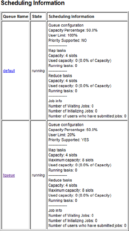
Chapter 5 ■ SCheduling and WorkfloW

125

V1 Fair Scheduler

As was the case for the Capacity scheduler, the library you need to use the Fair scheduler is included with the Hadoop

V1.2.1 installation; it is within the lib directory:

[hadoop@hc1nn lib]$ pwd

/usr/local/hadoop/lib

[hadoop@hc1nn lib]$ ls -l hadoop-fairscheduler*

-rw-rw-r--. 1 hadoop hadoop 70409 Jul 23 2013 hadoop-fairscheduler-1.2.1.jar

Figure 5-1. Capacity scheduler queue list

Chapter 5 ■ SCheduling and WorkfloW

126

However, you need to modify the property mapred.jobtracker.taskScheduler in the file mapred-site.xml within

the conf directory, as follows:

<name>mapred.jobtracker.taskScheduler</name>

<value>org.apache.hadoop.mapred.FairScheduler</value>

<description>Plugin the Fair scheduler</description>

</property>

To give greater control, I add some properties to the mapred-site.xml file to switch off pre-emption by

setting mapred.fairscheduler.preemption to False and I disallow unspecified pool names by setting

mapred.fairscheduler.allow.undeclared.pools to False. Also, I assign pool property names to queue names by

using mapred.fairscheduler.poolnameproperty. Finally, I use the mapred.queue.names property to define a list of

allowed queue names that could be used in the configuration file, all as follows:

<name>mapred.fairscheduler.preemption</name>

<value>false</value>

</property>

<name>mapred.fairscheduler.allow.undeclared.pools</name>

<value>false</value>

</property>

<name>mapred.fairscheduler.poolnameproperty</name>

<value>mapred.job.queue.name</value>

</property>

<name>mapred.queue.names</name>

<value>high_pool,low_pool,default</value>

</property>

To see the full configuration guide, go to the Apache Software Foundation website

(hadoop.apache.org/docs/r1.2.1/), click Map Reduce, and then select Fair Scheduler.

Like the configuration for the Capacity scheduler, you can add access control in the mapred-queue-acls.xml file

for the Fair scheduler to specify user and administration access to each queue. For example, here I grant the hadoop

user access to the high_pool and administration access to that queue, as follows:

<name>mapred.queue.high_pool.acl-submit-job</name>

<value>hadoop</value>

</property>

<name>mapred.queue.low_pool.acl-submit-job</name>

<value>smitha</value>

</property>

Chapter 5 ■ SCheduling and WorkfloW

127

<name>mapred.queue.default.acl-submit-job</name>

<value>jonesb</value>

</property>

<name>mapred.queue.high_pool.acl-administer-jobs</name>

<value>hadoop</value>

</property>

<name>mapred.queue.low_pool.acl-administer-jobs</name>

<value>smitha</value>

</property>

<name>mapred.queue.default.acl-administer-jobs</name>

<value>jonesb</value>

</property>

There is already a configuration file provided for this scheduler in the installation configuration directory:

[hadoop@hc1nn conf]$ pwd

/usr/local/hadoop/conf

[hadoop@hc1nn conf]$ ls -l fair-scheduler.xml

-rw-rw-r--. 1 hadoop hadoop 327 Jul 23 2013 fair-scheduler.xml

I add the following configuration to this file to specify the fair scheduler pools high_pool, low_pool, and default

queues, as well as their attributes, such as the minimum and maximum number of Map and Reduce function

instances, as follows:

</pool>

</pool>

Chapter 5 ■ SCheduling and WorkfloW

128

</pool>

Here, I define three pools (high_pool, low_pool, and default), each with the same configuration for the Map

Reduce minimum and maximum limits. They all have a maximum of 1,000 running jobs, but the high pool has three

times the weighting, so the high_pool will get three times the share of the cluster than the other pools will get.

To show how the Fair scheduler works, I will run a Pig-based job as an example. But before running the job

example, I restart the Map Reduce servers as I did for the Capacity scheduler earlier, so as to pick up the changes to

the configuration. Using the mapred.fairscheduler.pool property, I specify the name of the queue that my Pig Latin

job will be placed on when I issue the command line, using the -D switch, as follows.

[hadoop@hc1nn pig]$ pig -Dmapred.fairscheduler.pool=high_pool wordcount2.pig

Note: If I did not specify the pool to be used by using the –D option, I would encounter an error because, by

default, Fair assumes that the queue name matches the Linux account name. Given that I am running the job using

the Linux hadoop account, Fair would have looked for a queue named “hadoop,” which does not exist. The error

message I would receive is an example of an UndeclaredPoolException error:

Failed Jobs:

JobId Alias Feature Message Outputs

N/A clines,gword,rlines,wcount,words GROUP_BY,COMBINER

Message: org.apache.hadoop.ipc.RemoteException: org.apache.hadoop.mapred.UndeclaredPoolException:

Pool name: 'hadoop' is invalid. Add pool name to the fair scheduler allocation file. Valid pools

are: high_pool, low_pool

However, proceeding with the Fair scheduler example, I can see that the scheduler has started without error from

the Job Server’s log in the install logs directory. I look for the following line:

2014-06-29 13:41:27,882 INFO org.apache.hadoop.mapred.FairScheduler: Successfully configured

FairScheduler

By checking the Job Tracker user interface, I can learn more about the job details. Figure 5-2 shows a compound

image of the Pig Latin job that I submitted to the high_pool pool. For instance, the top table is taken from the list

of running jobs from the Job Tracker user interface. It shows that the hadoop user has submitted the Pig Latin job

wordcount2.pig, which is running.

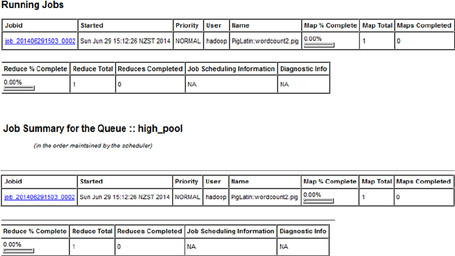
Chapter 5 ■ SCheduling and WorkfloW

129

The second table is taken from the high_pool queue, and it shows that the job was submitted to this queue with

Normal priority, using the command line switch -Dmapred.fairscheduler.pool=high_pool.

Now that you’ve examined the schedulers in Hadoop V1, it’s time to take a look at those same schedulers in

Hadoop V2. You can use the environment section in Chapter 4 to find out how to switch between versions on a single

cluster of servers. You will then see the similarities of the V1 and V2 schedulers, but also note the more advanced

interfaces that V2 offers.

Scheduling in Hadoop V2

In this section, I show how to configure the Capacity and Fair plug-in schedulers for Hadoop V2. You can find full

details at the Apache Software Foundation website (hadoop.apache.org/docs) by selecting your Hadoop version,

then the desired scheduling options from the menu on the left. In comparison to V1, the V2 user interface offers better

functionality and generally looks much more presentable. The configuration is similar, however, and the files that

need to be set up are the same.

Figure 5-2. Fair scheduler job queue

Chapter 5 ■ SCheduling and WorkfloW

130

V2 Capacity Scheduler

You need to set up the Capacity scheduler to work with YARN. You begin by configuring YARN so that its scheduler

class is defined as Capacity, rather than as the default FIFO scheduler. At the end of the yarn-site.xml file, which is

located under /etc/hadoop/conf, you add the following property to define Capacity:

<name>yarn.resourcemanager.scheduler.class</name>

<value>org.apache.hadoop.yarn.server.resourcemanager.scheduler.capacity.CapacityScheduler</value>

</property>

As you remember, Hadoop V2 can support hierarchical queues for each cluster client. This way, free resources

can be shared across a client’s queues before being offered to other queues. To demonstrate how this works, I define

some queues in the Capacity scheduler’s configuration file (capacity-scheduler.xml, found in /etc/hadoop/conf).

Specifically, I define and create three new queues (client1, client2, and client3) and their subqueues, as follows:

<name>yarn.scheduler.capacity.root.queues</name>

<value>client1,client2,client3</value>

</property>

<name>yarn.scheduler.capacity.root.client1.queues</name>

<value>client1a,client1b</value>

</property>

<name>yarn.scheduler.capacity.root.client2.queues</name>

<value>client2a,client2b,client2c</value>

</property>

<name>yarn.scheduler.capacity.root.client3.queues</name>

<value>client3a,client3b</value>

</property>

In addition, for each queue I create, I define its properties in the capacity-scheduler.xml file. The XML that

follows is an example of that needed for one of the queues. Note that this must be repeated for each parent and child

queue; therefore, I must remember to change the name of each attribute to match the queue name—that is, yarn.

scheduler.capacity.root.client1.capacity.

As in the V1 example, the sum of the capacity values for queues in the configuration file must be 100. Also, the

sum of the capacity values for the child queues within a parent queue must be 100. For instance, the children of

client1 are named client1.client1a. This XML sets up the attributes for queue client1 in terms of capacity, state, and

access. In this case, the * values mean “anyone,” so access has been left open:

<name>yarn.scheduler.capacity.root.client1.capacity</name> <value>100</value>

</property>

Chapter 5 ■ SCheduling and WorkfloW

131

<name>yarn.scheduler.capacity.root.client1.user-limit-factor</name> <value>1</value>

</property>

<name>yarn.scheduler.capacity.root.client1.maximum-capacity</name> <value>100</value>

</property>

<name>yarn.scheduler.capacity.root.client1.state</name> <value>RUNNING</value>

</property>

<name>yarn.scheduler.capacity.root.client1.acl_submit_applications</name> <value>*</value>

</property>

<name>yarn.scheduler.capacity.root.client1.acl_administer_queue</name> <value>*</value>

</property>

Now, I get YARN to refresh its queue configuration by using the yarn rmadmin command with a -refreshQueues

option. This causes YARN to reread its configuration files and so pick up the changes that have been made:

[hadoop@hc1nn conf]$ yarn rmadmin –refreshQueues

My reconfigured scheduler is ready, and I now submit a word-count job to show the queues in use. To display

the queue’s functionality, however, I need some test data; therefore, I have created the job’s input data in the HDFS

directory /usr/hadoop/edgar, as the HDFS file system command shows (and I populate it with data):

[hadoop@hc1nn edgar]$ hdfs dfs -ls /usr/hadoop/edgar

Found 5 items

-rw-r--r-- 2 hadoop hadoop 410012 2014-07-01 18:14 /usr/hadoop/edgar/10031.txt

-rw-r--r-- 2 hadoop hadoop 559352 2014-07-01 18:14 /usr/hadoop/edgar/15143.txt

-rw-r--r-- 2 hadoop hadoop 66401 2014-07-01 18:14 /usr/hadoop/edgar/17192.txt

-rw-r--r-- 2 hadoop hadoop 596736 2014-07-01 18:14 /usr/hadoop/edgar/2149.txt

-rw-r--r-- 2 hadoop hadoop 63278 2014-07-01 18:14 /usr/hadoop/edgar/932.txt

The word-count job will read this data, run a word count, and place the output results in the HDFS directory /

usr/hadoop/edgar-results1. The word-count job results look like this:

hdfs \

jar /usr/lib/hadoop-mapreduce/hadoop-mapreduce-examples.jar \

wordcount \

-Dmapred.job.queue.name=client1a \

/usr/hadoop/edgar \

/usr/hadoop/edgar-results1

The backslash characters (\) allow me to spread the command over multiple lines to make it more readable. I’ve

used a -D option to specify the queue in which to place this job (client1a).

Now I examine the scheduler configuration using the Name Node server name hc1nn, with a port value of 8088,

taken from the property yarn.resourcemanager.webapp.address in the configuration file yarn-site.xml:

http://hc1nn:8088/cluster/scheduler. Figure 5-3 illustrates the resulting hierarchy of job queues, with the

currently running word-count Map Reduce job placed in the client1a. child queue.

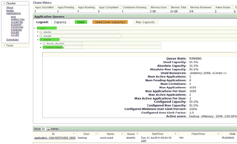
Chapter 5 ■ SCheduling and WorkfloW

132

Note that I have cropped Figure 5-3 so that the used queues are visible. You can see the Map Reduce word-count

job running on the client1.client1a queue. The Capacity scheduler, therefore, is working on Hadoop V2 because it can

accept Hadoop jobs into its queues.

V2 Fair Scheduler

The configuration for the Hadoop V2 Fair scheduler is quite simple and follows the same method as for the V1

configuration. In the yarn-site.xml file within the configuration directory (/etc/hadoop/conf), you define the

yarn.resourcemanager.scheduler.class property.

<name>yarn.resourcemanager.scheduler.class</name>

<value>org.apache.hadoop.yarn.server.resourcemanager.scheduler.fair.FairScheduler</value>

</property>

Then, you set up the default Fair scheduler configuration file fair-scheduler.xml in the same directory.

Figure 5-3. Hadoop V2 Capacity scheduler

Chapter 5 ■ SCheduling and WorkfloW

133

To demonstrate, I have borrowed this file from the V1 configuration:

</pool>

</pool>

</pool>

</allocations>

You now use the yarn rmadmin command to refresh the YARN scheduler queue configuration. This will cause

YARN (as for V2 Capacity) to reread its configuration files and so pick up the changes that you have made:

[hadoop@hc1nn conf]$ yarn rmadmin -refreshQueues

To demonstrate its use, I create a Map Reduce job and specify a queue value of high_queue so that I can ensure

that the submitted job will be processed by the YARN Fair scheduler and will be placed in the right queue.

The job I use specifies the queue name using a -D option:

hadoop \

jar /usr/lib/hadoop-mapreduce/hadoop-mapreduce-examples.jar \

wordcount \

-Dmapred.job.queue.name=high_pool \

/usr/hadoop/edgar \

/usr/hadoop/edgar-results1

Figure 5-4 shows the job status in the scheduler user interface. The queue legend now displays Fair Share, and

the job details appear in the high_pool queue, which is marked in green to indicate it’s being used.

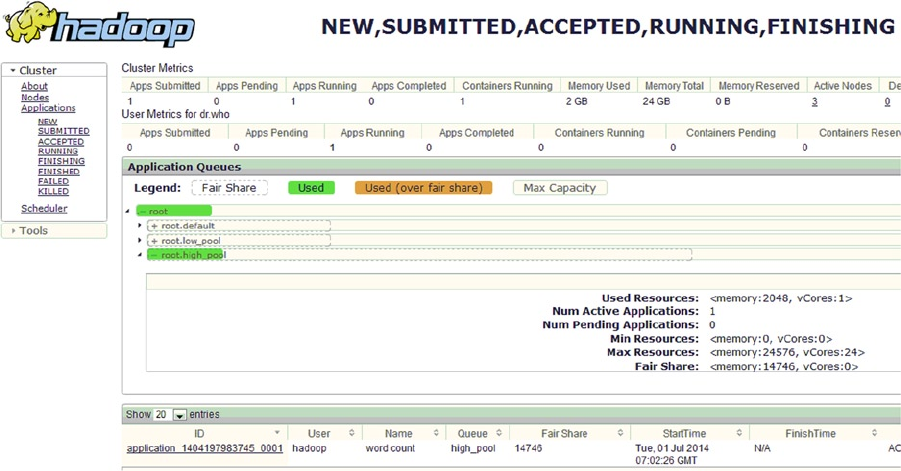
Chapter 5 ■ SCheduling and WorkfloW

134

As shown in Figure 5-4, the V2 fair scheduler is configured and working correctly.

Using Oozie for Workflow

Capacity, Fair, and similar plug-in schedulers deal with resources allocated to individual jobs over a period of time.

However, what about the relationships between jobs and the dependencies between them? That’s where workflow

managers, like Apache’s Oozie, come in. This section examines Hadoop job-based workflows and scheduling, and

demonstrates how tools like Oozie enable you to manage related jobs as workflows.

A workflow scheduler for Hadoop, Oozie is integrated into many of the Hadoop tools, such as Pig, Hive, Map

Reduce, and Streaming. Oozie workflows are defined as directed acyclical graphs (DAGs) and are stored as XML.

In this section, I will demonstrate how to install the Oozie component that is part of the Cloudera installation

that was used in Chapter 2. I show how to check that it is working, and how to create an example workflow. For further

details, check the Apache Software Foundation website at oozie.apache.org.

Installing Oozie

You start by installing the Oozie client and server as root, using Yum, the Linux-based package manager.

You install Oozie on the single CentOS 6 Linux server hc1nn, as follows:

[root@hc1nn conf]# yum install oozie

[root@hc1nn conf]# yum install oozie-client

Figure 5-4. Hadoop V2 Fair scheduler

Chapter 5 ■ SCheduling and WorkfloW

135

Next, you configure Oozie to use YARN by editing the oozie-env.sh file under the directory /etc/oozie/conf:

[root@hc1nn conf]# cd /etc/oozie/conf

[root@hc1nn conf]# ls -l oozie-env.sh

-rw-r--r--. 1 root root 1360 May 29 07:20 oozie-env.sh

You can configure Oozie to use either YARN or Map Reduce V1, but not both at the same time. The

oozie-server-0.20 option is for Map Reduce V1, while setting CATALINA_BASE as oozie-server configures it

to use YARN. (In this demonstration, I have chosen to use YARN because this is Hadoop V2, and it is the default).

Because I’m using YARN, I edit the file as follows:

#export CATALINA_BASE=/usr/lib/oozie/oozie-server-0.20 ## use MRv1

export CATALINA_BASE=/usr/lib/oozie/oozie-server ## use Yarn

Note that I left the MRv1 line in the file but commented it out so that I know how to configure Oozie later if I want

to switch back to use Map Reduce version 1. I have also elected to use the default Derby database that comes with

the Oozie installation. If you need to use an alternative database, such as Oracle or MySql, you can. Check the Oozie

website at oozie.apache.org for details.

To proceed, you set up Oozie and run it as the Linux hadoop user. This is the account where you previously stored

your scripts and set up your Hadoop-based configuration. So, you run the ooziedb.sh script with parameters create

and –run to set up the oozie database:

[hadoop@hc1nn conf]# /usr/lib/oozie/bin/ooziedb.sh create -run

Validate DB Connection

DONE

Check DB schema does not exist

DONE

Check OOZIE_SYS table does not exist

DONE

Create SQL schema

DONE

Create OOZIE_SYS table

DONE

Oozie DB has been created for Oozie version '3.3.2-cdh4.7.0'

The SQL commands have been written to: /tmp/ooziedb-3196886912358277569.sql

This sets up the Oozie Derby database under the directory /var/lib/oozie. In this example, the directory is owned

by the Oozie Linux user. If you plan to use a different account to run Oozie, make sure it has access to this directory

and its contents. (I used the su [switch user] command to switch the user to the Linux root account. I then changed

the directory to /var/lib/oozie and used the Linux chmod command to recursively set permissions to 777. This is

because the Linux hadoop account needs to run Oozie and so access this Derby database instance).

[hadoophc1nn ~]$ su -

[root@hc1nn oozie]$ cd /var/lib/oozie

[root@hc1nn oozie]$ ls –l

drwxr-xr-x. 2 oozie oozie 4096 Jul 9 17:44 oozie-db

[root@hc1nn oozie]$ chmod –R 777 *

[root@hc1nn oozie]$ exit

Chapter 5 ■ SCheduling and WorkfloW

136

To use the Oozie web-based console, it has to be configured. You download and install the file ext-2.2.zip onto

Hadoop. You use wget to download the file:

[hadoop@hc1nn Downloads]$ wget http://extjs.com/deploy/ext-2.2.zip

[hadoop@hc1nn Downloads]$ ls -l ext-2.2.zip

-rw-rw-r--. 1 oozie oozie 6800612 Oct 24 2008 ext-2.2.zip

You unpack the file with the Linux unzip command, and then use the Linux ls command to check the unpacked

directory ext-2.2:

[hadoop@hc1nn Downloads]$ unzip ext-2.2.zip

[hadoop@hc1nn Downloads]$ ls -ld ext-2.2

drwxr-xr-x. 9 oozie oozie 4096 Aug 4 2008 ext-2.2

This unzipped package needs to be moved to the /var/lib/oozie directory, which is the location where Oozie will

look for it when it runs. In this example, I move the installation directory using the root account. The commands that

follow show that the Linux su (switch user) command switches to the root account. The Linux cd (change directory)

command moves it to the Downloads directory. The Linux mv (move) command moves the Oozie web console

package to the /var/lib/oozie/ directory:

[hadoophc1nn ~]$ su -

[root@hc1nn ~]$ cd /home/Hadoop/Downloads

[root@hc1nn Downloads]$ mv ext-2.2 /var/lib/oozie/

[root@hc1nn Downloads]$ cd /var/lib/oozie/

[root@hc1nn Downloads]# ls -l /var/lib/oozie

total 8

drwxrwxr-x. 9 oozie oozie 4096 Aug 4 2008 ext-2.2

drwxr-xr-x. 2 oozie oozie 4096 Jul 9 17:44 oozie-db

[root@hc1nn Downloads]# exit

You unpack the Oozie shared library in a temporary directory under /tmp so that you can install it onto HDFS.

This library provides the functionality for tools like Pig, Hive, and Sqoop when used in workflows. There is a version

for YARN and one for Map Reduce V1. For this example, I use the YARN version because that is what my Hadoop V2

CDH4 cluster is using.

[hadoop@hc1nn ~]$ ls -l /usr/lib/oozie/oozie-sharelib*.gz

-rwxrwxrwx. 1 root root 84338242 May 29 07:02 /usr/lib/oozie/oozie-sharelib-mr1.tar.gz

-rwxrwxrwx. 1 root root 84254668 May 29 07:02 /usr/lib/oozie/oozie-sharelib-yarn.tar.gz

You choose the file that you wish to use; my example needs the YARN version. The Linux mkdir command

creates a directory under /tmp, called “ooziesharelib.” The Linux cd command then moves it to that directory. The tar

command extracts the Oozie tarred and gzipped file oozie-sharelib-yarn.tar.gz; the x option means “extract” while the

z option unzips the tar file:

[hadoop@hc1nn ~]$ mkdir /tmp/ooziesharelib

[hadoop@hc1nn ~]$ cd /tmp/ooziesharelib

[hadoop@hc1nn ooziesharelib]$ tar xzf /usr/lib/oozie/oozie-sharelib-yarn.tar.gz

[hadoop@hc1nn ooziesharelib]$ ls -ld *

drwxr-xr-x. 3 oozie oozie 4096 May 29 06:59 share

Chapter 5 ■ SCheduling and WorkfloW

137

Now, you use the Hadoop file system command put to copy the share directory onto HDFS under /user/Oozie

workflow:

[oozie@hc1nn ooziesharelib]$ hdfs dfs -put share /user/oozie/share

It is quite simple to start the Oozie server by using the Linux service command as the root user. You use the

Linux su command to switch the user to root, then start the Oozie service:

[hadoop@hc1nn ooziesharelib]$ su -

[root@hc1nn ~]$ service oozie start

[root@hc1nn ~]$ exit

Finally, you can use the Oozie client as the Linux hadoop user to access Oozie and check the server’s status:

[hadoop@hc1nn ~]$ oozie admin -oozie http://localhost:11000/oozie -status

System mode: NORMAL

[hadoop@hc1nn ~]$ oozie admin -oozie http://localhost:11000/oozie -version

Oozie server build version: 3.3.2-cdh4.7.0

By setting the OOZIE_URL variable, you can simplify the Oozie client commands. The URL tells the Oozie client the

location in terms of the host name and port of the Oozie server, as follows:

[hadoop@hc1nn ~]$ export OOZIE_URL=http://localhost:11000/oozie

[hadoop@hc1nn ~]$ oozie admin -version

Oozie server build version: 3.3.2-cdh4.7.0

At this point, you can access the Oozie web console via the URL http://localhost:11000/oozie. (I discuss this

in more detail following the discussion of workflows in Oozie).

The Mechanics of the Oozie Workflow

In general, the workflow is a set of chained actions that call HDFS-based scripts like Pig and Hive. All input comes from

HDFS, not from the Linux file system, because Oozie cannot guarantee which cluster nodes will be used to process the

workflow. Created as an XML document, an Oozie workflow script contains a series of linked actions controlled via

pass/fail control nodes that determine where the control flow moves next. The fork option, for example, allows actions

to be run in parallel. You can configure the script to send notifications of the workflow outcome via email or output

message, as well as set action parameters and add tool-specific actions like Pig, Hive, and Java to the workflow.

Oozie Workflow Control Nodes

The workflow control nodes are like traffic cops in a script, directing the flow of work. The start control node defines

the starting point for the workflow. Each workflow script can have only one start node, and it must define an existing

action.

The end control node is also mandatory and indicates the end of the workflow. If the control flow reaches the end

control node, it has finished sucessfully.

Chapter 5 ■ SCheduling and WorkfloW

138

Offering the ability to split the flow of work into a series of parallel streams, the fork and join control nodes are

used as a pair. For instance, you can use these to run several Pig data-processing scripts in parallel. The join control

node will not complete until all of the fork actions have completed.

</fork>

Optional in the workflow, the kill control node stops the workflow. It is useful for error conditions; if any actions

are still running when an error occurs, they will be ended.

<message>Workflow died, error message[${wf:errorMessage(wf:lastErrorNode())}]</message>

</kill>

The decision control node uses a switch statement with a series of cases and a default option to decide which

control flow to use. The first case to be True is used; otherwise, the default case is used. In the pig-decision switch

statement the workflow uses a file system test of file size and will pass control to the end control node if the data

required by the workflow is not greater than 1 GB.

${fs:fileSize("${hdfsRawData}) gt 1 * GB}

</case>

</switch>

</decision>

Oozie Workflow Actions

The best way to understand an Oozie workflow action is to examine an example. I present the following Pig

Latin–based action to define the values of the JobTracker and name node. The prepare section deletes data for the

action. The configuration section then defines the Pig action queue name, and it is followed by a script section

that specifies the script to call. Finally, the OK and error options define which nodes to move to, depending on the

outcome of the Pig script.

<pig>

<job-tracker>${jobTracker}</job-tracker>

<name-node>${nameNode}</name-node>

</prepare>

<name>mapred.job.queue.name</name>

<value>${queueName}</value>

</property>

</configuration>

Chapter 5 ■ SCheduling and WorkfloW

139

</pig>

</action>

Creating an Oozie Workflow

In this example, I examine and run a Pig- and Hive-based Oozie workflow against Oozie. The example uses

a Canadian vehicle fuel-consumption data set that is provided at the website data.gc.ca. You can either

search for “Fuel Consumption Ratings” to find the data set or use the link http://open.canada.ca/data/en/

dataset/98f1a129-f628-4ce4-b24d-6f16bf24dd64.

To begin, I download the English version of each CSV file. For instance, I have downloaded these files using the

Linux hadoop account, downloading them to that account’s Downloads directory, as the Linux ls command shows:

[hadoop@hc1nn Downloads]$ ls

MY1995-1999 Fuel Consumption Ratings.csv MY2007 Fuel Consumption Ratings.csv

MY2000 Fuel Consumption Ratings.csv MY2008 Fuel Consumption Ratings.csv

MY2001 Fuel Consumption Ratings.csv MY2009 Fuel Consumption Ratings.csv

MY2002 Fuel Consumption Ratings.csv MY2010 Fuel Consumption Ratings.csv

MY2003 Fuel Consumption Ratings.csv MY2011 Fuel Consumption Ratings.csv

MY2004 Fuel Consumption Ratings.csv MY2012 Fuel Consumption Ratings.csv

MY2005 Fuel Consumption Ratings.csv MY2013 Fuel Consumption Ratings.csv

MY2006 Fuel Consumption Ratings.csv MY2014 Fuel Consumption Ratings.csv

I then need to copy these files to an HDFS directory so that they can be used by an Oozie workflow job. To do this,

I create some HDFS directories, as follows:

[hadoop@hc1nn Downloads]$ hdfs dfs –mkdir /user/hadoop/oozie_wf

[hadoop@hc1nn Downloads]$ hdfs dfs –mkdir /user/hadoop/oozie_wf/fuel

[hadoop@hc1nn Downloads]$ hdfs dfs –mkdir /user/hadoop/oozie_wf/fuel/rawdata

[hadoop@hc1nn Downloads]$ hdfs dfs –mkdir /user/hadoop/oozie_wf/fuel/pigwf

[hadoop@hc1nn Downloads]$ hdfs dfs –mkdir /user/hadoop/oozie_wf/fuel/entity

[hadoop@hc1nn Downloads]$ hdfs dfs –mkdir /user/hadoop/oozie_wf/fuel/entity/manufacturer

[hadoop@hc1nn Downloads]$ hdfs dfs –mkdir /user/hadoop/oozie_wf/fuel/entity/model

The Hadoop file system ls command produces a long list that shows the three HDFS subdirectories I’ve just

created and that will be used in this example.

[hadoop@hc1nn Downloads]$ hdfs dfs -ls /user/hadoop/oozie_wf/fuel/

Found 3 items

drwxr-xr-x - hadoop hadoop 0 2014-07-12 18:16 /user/hadoop/oozie_wf/fuel/entity

drwxr-xr-x - hadoop hadoop 0 2014-07-12 18:15 /user/hadoop/oozie_wf/fuel/pigwf

drwxr-xr-x - hadoop hadoop 0 2014-07-08 18:16 /user/hadoop/oozie_wf/fuel/rawdata

I employ the rawdata directory under /user/hadoop/oozie_wf/fuel/ on HDFS to contain the CSV data that I

will use. I use the pigwf directory to contain the scripts for the task. I use the entity directory and its subdirectories to

contain the data used by this task.

Chapter 5 ■ SCheduling and WorkfloW

140

So, my next step is to upload the CSV files from the Linux file system Downloads directory to the HDFS directory

rawdata:

[hadoop@hc1nn Downloads]$ hdfs dfs –copyFromLocal *.csv /user/hadoop/oozie_wf/fuel/rawdata

Now, the workflow data are ready, and the scripts and configuration files that the workflow will use need to be

copied into place. For this example, I have created all the necessary files. To begin, I load them to the HDFS pigwf

directory using the Hadoop file system copyFromLocal command:

[hadoop@hc1nn Downloads]$ cd /home/hadoop/oozie/pig/fuel

[hadoop@hc1nn fuel]$ ls

load.job.properties model.pig manufacturer.pig model.sql workflow.xml

manufacturer.sql

[hadoop@hc1nn fuel]$ hdfs dfs –copyFromLocal * /user/hadoop/oozie_wf/fuel/pigwf

Next, using the Hadoop file system ls command, I check the contents of the pigwf directory. The listing shows

the sizes of the files that were just uploaded:

[oozie@hc1nn fuel]$ hdfs dfs -ls /user/oozie/oozie_wf/fuel/pigwf/

Found 6 items

-rw-r--r-- 2 oozie oozie 542 2014-07-06 15:48 /user/oozie/oozie_wf/fuel/pigwf/load.job.properties

-rw-r--r-- 2 oozie oozie 567 2014-07-08 19:13 /user/oozie/oozie_wf/fuel/pigwf/manufacturer.pig

-rw-r--r-- 2 oozie oozie 306 2014-07-12 18:06 /user/oozie/oozie_wf/fuel/pigwf/manufacturer.sql

-rw-r--r-- 2 oozie oozie 546 2014-07-08 19:13 /user/oozie/oozie_wf/fuel/pigwf/model.pig

-rw-r--r-- 2 oozie oozie 283 2014-07-12 18:06 /user/oozie/oozie_wf/fuel/pigwf/model.sql

-rw-r--r-- 2 oozie oozie 2400 2014-07-12 18:15 /user/oozie/oozie_wf/fuel/pigwf/workflow.xml

Note that I actually don’t need to copy the load.job.properties file to HDFS, as it will be located from the local

Linux file system. Having uploaded the files, it is time to explain their contents.

The Workflow Configuration File

The first file is the workflow configuration file, called load.job.properties; this specifies parameters for the workflow.

I have listed its contents using the Hadoop file system cat command and have taken the liberty of adding line numbers

here and elsewhere to use in explaining the steps:

[hadoop@hc1nn fuel]$ hdfs dfs -cat /user/hadoop/oozie_wf/fuel/pigwf/load.job.properties

01 # ----------------------------------------

02 # Workflow job properties

03 # ----------------------------------------

04

05 nameNode=hdfs://hc1nn:8020

06

07 # Yarn resource manager host and port

08 jobTracker=hc1nn:8032

09 queueName=high_pool

10

Chapter 5 ■ SCheduling and WorkfloW

141

11 oozie.libpath=${nameNode}/user/hadoop/share/lib

12 oozie.use.system.libpath=true

13 oozie.wf.rerun.failnodes=true

14

15 hdfsUser=hadoop

16 wfProject=fuel

17 hdfsWfHome=${nameNode}/user/${hdfsUser}/oozie_wf/${wfProject}

18 hdfsRawData=${hdfsWfHome}/rawdata

19 hdfsEntityData=${hdfsWfHome}/entity

20

21 oozie.wf.application.path=${hdfsWfHome}/pigwf

22 oozieWfPath=${hdfsWfHome}/pigwf/

The parameters in this file specify the Hadoop name node by server and port. Because YARN is being employed,

the Resource Manager is defined via its host and port by using the JobTracker variable. Job Tracker is obviously a

Hadoop V1 component name, but this works for YARN. The queue name to be used for this workflow, high_pool, is

also specified.

The library path of the Oozie shared library is defined by oozie.libpath, along with the parameter oozie.use.

system.libpath. The HDFS user for the job is specified, as is a project name. Finally, the paths are defined for the

workflow scripts and entity data that will be produced. The special variable oozie.wf.application.path is used to

define the location of the workflow job file.

The workflow.txt file is the main control file for the workflow job. It controls the flow of actions, via Oozie, and

manages the subtasks. This workflow file runs two parallel streams of processing to process the data in the HDFS

rawdata directory.

The manufacturer.pig script is called to strip manufacturer-based data from the HDFS-based rawdata files. This

data is placed in the HDFS-based entity/manufacturer directory. Then the script manufacturer.sql is called to process

this data to the Hive data warehouse.

In parallel to this (via a fork option in the xml), the model.pig script is called to strip the vehicle model–based

data from the HDFS rawdata files. This data is placed in the HDFS entity/model directory. Then the script model.sql is

called to process this data to the Hive data warehouse.

The workflow.xml workflow file has been built using a combination of the workflow elements described earlier

(see “The Mechanics of the Oozie Workflow”). I have used the Hadoop file system cat command to display its contents:

[hadoop@hc1nn fuel]$ hdfs dfs -cat /user/hadoop/oozie_wf/fuel/pigwf/workflow.xml

01 <workflow-app name="FuelWorkFlow" xmlns="uri:Oozie workflow:workflow:0.1">

02

03 <start to="pig-fork"/>

04

05 <fork name="pig-fork">

06 <path start="pig-manufacturer"/>

07 <path start="pig-model"/>

08 </fork>

09

10 <action name="pig-manufacturer">

11 <pig>

12 <job-tracker>${jobTracker}</job-tracker>

13 <name-node>${nameNode}</name-node>

14 <prepare>

15 <delete path="${hdfsEntityData}/manufacturer"/>

16 </prepare>

Chapter 5 ■ SCheduling and WorkfloW

142

17 <configuration>

18 <property>

19 <name>mapred.job.queue.name</name>

20 <value>${queueName}</value>

21 </property>

22 </configuration>

23 <script>manufacturer.pig</script>

24 </pig>

25 <ok to="pig-join"/>

26 <error to="fail"/>

27 </action>

28

29 <action name="pig-model">

30 <pig>

31 <job-tracker>${jobTracker}</job-tracker>

32 <name-node>${nameNode}</name-node>

33 <prepare>

34 <delete path="${hdfsEntityData}/model"/>

35 </prepare>

36 <configuration>

37 <property>

38 <name>mapred.job.queue.name</name>

39 <value>${queueName}</value>

40 </property>

41 </configuration>

42 <script>model.pig</script>

43 </pig>

44 <ok to="pig-join"/>

45 <error to="fail"/>

46 </action>

47

48 <join name="pig-join" to="hive-fork"/>

49

50 <fork name="hive-fork">

51 <path start="hive-manufacturer"/>

52 <path start="hive-model"/>

53 </fork>

54

55 <action name="hive-manufacturer">

56 <hive xmlns="uri:Oozie workflow:hive-action:0.2">

57 <job-tracker>${jobTracker}</job-tracker>

58 <name-node>${nameNode}</name-node>

59 <configuration>

60 <property>

61 <name>mapred.job.queue.name</name>

62 <value>${queueName}</value>

63 </property>

64 </configuration>

65 <script>model.sql</script>

66 </hive>

67 <ok to="hive-join"/>

Chapter 5 ■ SCheduling and WorkfloW

143

68 <error to="fail"/>

69 </action>

70

71 <action name="hive-model">

72 <hive xmlns="uri:Oozie workflow:hive-action:0.2">

73 <job-tracker>${jobTracker}</job-tracker>

74 <name-node>${nameNode}</name-node>

75 <configuration>

76 <property>

77 <name>mapred.job.queue.name</name>

78 <value>${queueName}</value>

79 </property>

80 </configuration>

81 <script>model.sql</script>

82 </hive>

83 <ok to="hive-join"/>

84 <error to="fail"/>

85 </action>

86

87 <join name="hive-join" to="end"/>

88

89 <kill name="fail">

90 <message>Workflow died, error message[${wf:errorMessage(wf:lastErrorNode())}]</message>

91 </kill>

92

93 <end name="end"/>

94

95 </workflow-app>

The workflow uses a fork control node at line 05 to run the Pig manufacturer and model jobs in parallel. The

join control is issued at line 48 when both Pig jobs have finished. The Pig actions at lines 10 and 29 are exactly the

same as the example earlier (see “Oozie Workflow Actions”). They set up the actions by defining the name node and

the Job Tracker, and then they prepare the job by deleting any previous data. They define the Hadoop-based queue

that the job should be sent to, and finally they define the script to be called.

The Hive jobs use the same fork and join structure as the Pig jobs at lines 50 and 87. The Pig join control node

at line 48 has a to element that passes control to the Hive fork control node at line 50.

48 <join name="pig-join" to="hive-fork"/>

49

50 <fork name="hive-fork">

51 <path start="hive-manufacturer"/>

52 <path start="hive-model"/>

53 </fork>

The workflow definition of the Hive actions are similar to the Pig actions. The only major difference is that the

<Hive> label is used and that there is no prepare section to delete data.

Each of the four actions has a set of error conditions that determine where control will be passed to:

83 <ok to="hive-join"/>

84 <error to="fail"/>

85 </action>

86

Chapter 5 ■ SCheduling and WorkfloW

144

87 <join name="hive-join" to="end"/>

88

89 <kill name="fail">

90 <message>Workflow died, error message[${wf:errorMessage(wf:lastErrorNode())}]</message>

91 </kill>

92

93 <end name="end"/>

An error condition in any of the four main actions passes control to the kill control node, called fail. The OK

condition just passes the control flow to the next success node in the workflow.

Now I will briefly explain the manufacturer and model pig and sql script contents. I have used the Hadoop file

system cat command to display the contents of the manufacturuer.pig file.

[hadoop@hc1nn fuel]$ hdfs dfs -cat /user/hadoop/oozie_wf/fuel/pigwf/manufacturer.pig

01 -- get the raw data from the files from the csv files

02

03 rlines = LOAD '/user/hadoop/oozie_wf/fuel/rawdata/*.csv' USING PigStorage(',') AS

04 ( year:int, manufacturer:chararray, model:chararray, class:chararray, size:float,

cylinders:int,

05 transmission:chararray, fuel:chararray, cons_cityl100:float, cond_hwyl100:float, cons_

citympgs:int,

06 cond_hwympgs:int, lyears:int, co2s:int

07 );

08

09 mlist = FOREACH rlines GENERATE manufacturer;

10

11 dlist = DISTINCT mlist ;

12

13 -- save to a new file

14

15 STORE dlist INTO '/user/hadoop/oozie_wf/fuel/entity/manufacturer/' ;

The pig script is just stripping the manufacturer information from the rawdata CSV files and storing that data

in the HDFS directory under entity/manufacturer. The sql script called manufacturuer.sql then processes that

information and stores it in Hive.

[hadoop@hc1nn fuel]$ hdfs dfs -cat /user/hadoop/oozie_wf/fuel/pigwf/manufacturer.sql

01 drop table if exists rawdata2 ;

02

03 create external table rawdata2 (

04 line string

05 )

06 location '/user/hadoop/oozie_wf/fuel/entity/manufacturer/' ;

07

08 drop table if exists manufacturer ;

09

10 create table manufacturer as

11 select distinct line from rawdata2 where line not like '%=%'

12 and line not like '% % %' ;

Chapter 5 ■ SCheduling and WorkfloW

145

The sql just creates an external Hive table called rawdata2 from the manufacturer HDFS-based files. It then

creates a second table in Hive called “manufacturer” by selecting the contents of the rawdata2 table.

The model.pig and sql files are very similar, pulling vehicle model data from the HDFS-based rawdata files and

moving it to HDFS. I use the Hadoop file system cat command to display the model.pig file:

[hadoop@hc1nn fuel]$ hdfs dfs -cat /user/hadoop/oozie_wf/fuel/pigwf/model.pig

01 -- get the raw data from the files from the csv files

02

03 rlines = LOAD '/user/hadoop/oozie_wf/fuel/rawdata/*.csv' USING PigStorage(',') AS

04 ( year:int, manufacturer:chararray, model:chararray, class:chararray, size:float,

cylinders:int,

05 transmission:chararray, fuel:chararray, cons_cityl100:float, cond_hwyl100:float, cons_

citympgs:int,

06 cond_hwympgs:int, lyears:int, co2s:int

07 );

08

09 mlist = FOREACH rlines GENERATE manufacturer,year,model ;

10

11 dlist = DISTINCT mlist ;

12

13 STORE dlist INTO '/user/hadoop/oozie_wf/fuel/entity/model/' using PigStorage(',');

Again, it strips vehicle model information from the HDFS-based CSV files in the rawdata directory. It then

stores that information in the entity/model HDFS directory. The model.sql script then processes that information to

a Hive table:

[hadoop@hc1nn fuel]$ hdfs dfs -cat /user/hadoop/oozie_wf/fuel/pigwf/model.sql

01 drop table if exists rawdata2 ;

02

03 create external table rawdata2 (

04 line string

05 )

06 location '/user/hadoop/oozie_wf/fuel/entity/model/' ;

07

08 drop table if exists model ;

09

10 create table model as

11 select

12 distinct split(line,',')

13 from rawdata2

14 where

15 line not like '%=%' ;

The Hive QL script creates an external table over the HDFS-based entity/model data, called rawdata2; it then

selects that data into a Hive-based table called “model.”

The intention of this workflow example is to show that complex ETL (“extract, transform, load”) chains of

subtasks can be built using Oozie. The tasks can be run in parallel and control can be added to the workflow to set up

the jobs and define the end conditions. Having described the workflow, it is now time for me to run the job; the next

section explains how the workflow can be run and monitored with the Oozie web-based user interface.

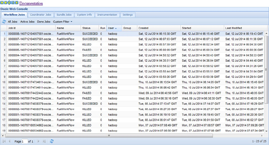
Chapter 5 ■ SCheduling and WorkfloW

146

Running an Oozie Workflow

To make the Oozie task invocation simpler, I define the OOZIE_URL variable. This means that when I want to invoke

an Oozie job, I have simply invoke the oozie command; I do not have to specify the whole Oozie URL. For the Oozie

example, this is as follows:

[hadoop@hc1nn fuel]$ export OOZIE_URL=http://localhost:11000/oozie

The oozie command is then used with a job parameter and the load.job.properties file. The –submit

parameter is used to submit the file, and this returns the Oozie job number 0000000-140706152445409-oozie-oozi-W:

oozie job -config ./load.job.properties -submit

job: 0000000-140706152445409-oozie-oozi-W

The workflow can now be started using this Oozie job number. I issue the oozie command with the parameters

job and –start, followed by the job number:

oozie job -start 0000000-140706152445409-oozie-oozi-W

I can pause and restart the job with the -suspend and -resume oozie command options. The help option passed

to the oozie command gives me a full list of the possible options.

I now access the Oozie console (shown in Figure 5-5) by using the OOZIE_URL value I specified previously.

Figure 5-5. Oozie console job list

Chapter 5 ■ SCheduling and WorkfloW

147

The left column of Figure 5-5 gives a list of job IDs that are issued when each Oozie job is submitted. The next

column to the right shows the workflow name—in this case, FuelWorkFlow. The Status column shows the job's

last status, which could be Prep, Running, Suspended, Succeeded, Failed, or Killed. Table 5-1 lists the meanings of

these statuses.

Table 5-1. Job Statuses and Meanings

Status Meaning

PREP Job just created; it can be moved to Running or Killed.

RUNNING Job is being executed; its state can change to Suspended, Succeeded, Killed, or Failed.

SUSPENDED A running job can be suspended; its state can change to Running or Killed.

SUCCEEDED The job sucessfully reached its end state.

FAILED The job encountered an unexpected error.

KILLED A job action failed or the job was killed by an administrator.

The User and date columns show which Linux user account ran the job and when it was created, started, and

modified. The tabs at the top of the display are for workflows, coordinator jobs, and bundling. Coordinator jobs are

for scheduling, either via time or event, while bundling allows the grouping of coordinator jobs. The other tabs are for

configuration information and metrics.

By selecting an individual workflow job, you can bring up a job-related Oozie window. In Figure 5-6, I have

selected the topmost successful job on the list. As you can see, the Job Info tab shows the job’s attributes and

its actions and status details. The Job Definition tab contains the xml contents of the workflow, while the Job

Configuration tab shows configured attributes for the job. The Job Log tab shows the logged output for this job, as

Figure 5-7 shows.

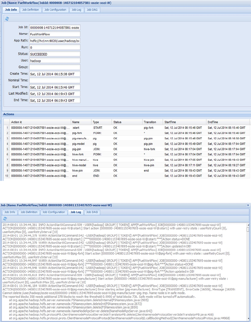
Chapter 5 ■ SCheduling and WorkfloW

148

Figure 5-7. Oozie job log information window

Figure 5-6. Oozie job information window

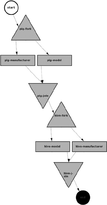
Chapter 5 ■ SCheduling and WorkfloW

149

The Job DAG (directed acyclical graph) tab is interesting because it shows both the structure and the state of the

job's actions. Figures 5-8 and 5-9 provide examples of Oozie DAGs. Figure 5-8 has no state or colors shown on it; it is a

job that has been submitted but not run. However, the DAG contains enough detail so that you can read the labels. It

shows the pig-manufacturer and pig-model tasks running in parallel. The triangular pig-fork and pig-join nodes split

the streams of processing. The Hive-based functionality is organized in the same manner, with the manufacturer and

model Hive tasks running in parallel. The workflow begins with a start node and terminates at an end node.

Figure 5-8. Oozie job DAG with no state information

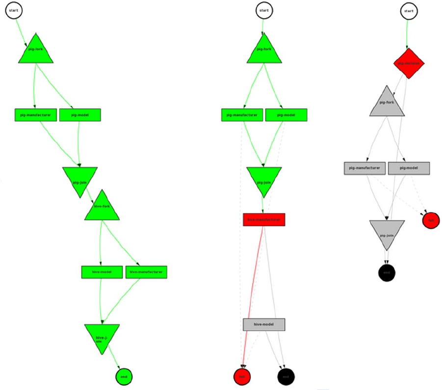
Chapter 5 ■ SCheduling and WorkfloW

150

Figure 5-9 shows three different DAGs. The text is illegible because the figures have been minimized to fit

together on a single page, but you can see the different states that nodes in a DAG can achieve.

For instance, in Figure 5-9 the circles show the start and endpoints, while the triangles show the forks and joins.

The boxes show the actions to be executed, while the actions between a fork and join show that they will be executed

in parallel. The color codes indicate the execution states: gray means that a node has not been executed, green means

that that node has executed sucessfully, red means that an error has occurred, and black is the unreached endpoint.

That is, the DAG on the left completed successfully and the two on the right failed.

Figure 5-9. Oozie job DAG information for three jobs

Chapter 5 ■ SCheduling and WorkfloW

151

Scheduling an Oozie Workflow

How do you schedule a workflow to run at a specific time or run after a given event? For instance, you might want

the workflow to run at 01:00 each Tuesday morning or each time data arrives. Oozie coordinator jobs exist for this

purpose. To continue my example, I updated the workflow properties file to use a coordinator job:

oozieWfPath=${hdfsWfHome}/pigwf

# Job Coordination properties

jobStart=2014-07-10T12:00Z

jobEnd=2014-09-10T12:00Z

# Frequency in minutes

JobFreq=10080

jobNZTimeZone=GMT+1200

oozie.coord.application.path=${hdfsWfHome}/pigwf

The path to the workflow script is now called oozieWfPath, and the path to the coordinator script is called

oozie.coord.application.path, the latter which is the reserved pathname that Oozie expects will be used to identify

a cordinator job. I also specify some time-based parameters to the cordinator job, a start time, an end time, and a job

frequency in minutes. Lastly, I set the time zone for New Zealand.

I create an XML-based coordinator job file called coordinator.xml, which I copy to the workflow directory in

HDFS. The file looks like this:

1 <coordinator-app

2

3 name="FuelWorkFlowCoord"

4 frequency="${JobFreq}"

5 start="${jobStart}"

6 end="${jobEnd}"

7 timezone="${jobNZTimeZone}"

8 xmlns="uri:Oozie workflow:coordinator:0.4">

9

10 <action>

11 <workflow>

12 <app-path>${oozieWfPath}/workflow.xml</app-path>

13 </workflow>

14 </action>

15

16 </coordinator-app>

This is a time-based coordinator job that will run between the start and end dates for a given frequency using

New Zealand time.

I send the coordinator job to Oozie as follows:

oozie job -config ./load.job.properties -submit

job: 0000000-140713100519754-oozie-oozi-C

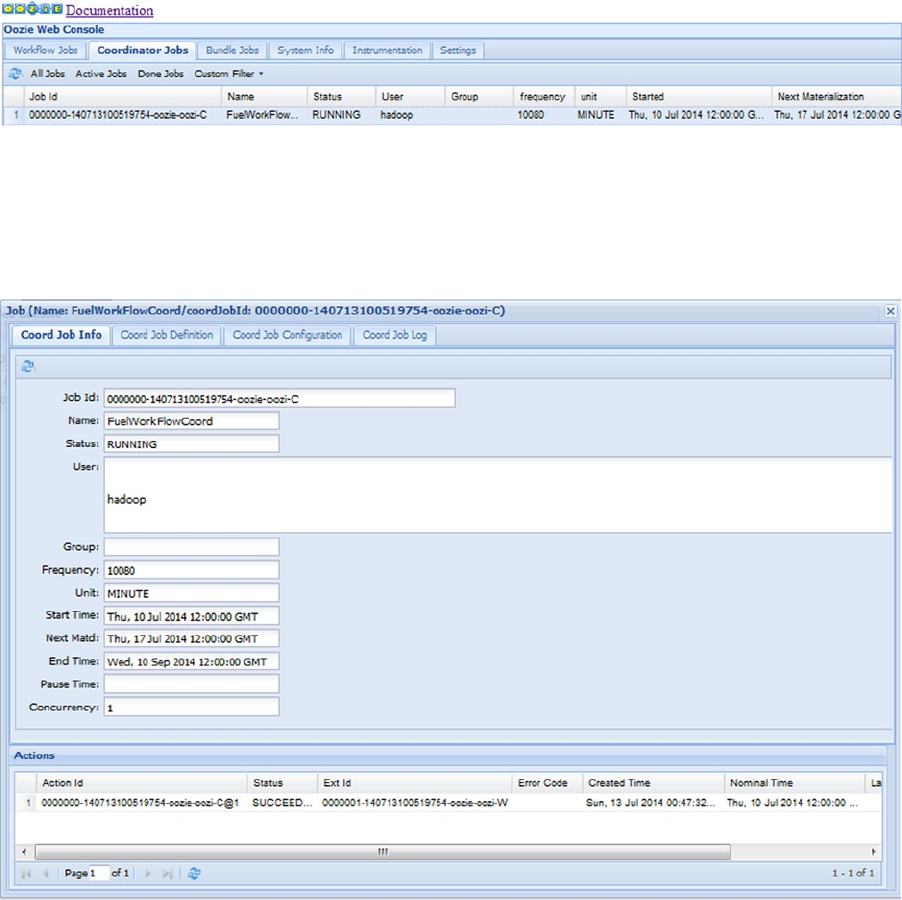
Chapter 5 ■ SCheduling and WorkfloW

152

A coordinator job appears on the Oozie console coordinator tab, as shown in Figure 5-10, indicating that the

coordinator job has started and its frequency is 10,080 minutes (24 hours times 60 minutes times 7 days).

Figure 5-10. Ozzie coordinator job status

So, as set, this job will run weekly at this time until its end date. The last column in Figure 5-10 also shows the

next time that this job will run, which is a week from the start date. Clicking on the job ID provides a window with its

details, as shown in Figure 5-11.

Figure 5-11. Ozzie coordinator job details window

Chapter 5 ■ SCheduling and WorkfloW

153

The Definition tab in the Figure 5-11 window contains the contents of the job’s coordinator.xml file. The

Configuration tab contains all of the job’s parameters in XML from the configuration file. And the Log tab contains the

job’s log entries.

As an extension to this coordinator job, I add a dataset requirement and create a new data set variable, as follows:

DataJobFreq=1440

And the XML now looks like this:

1 <coordinator-app

2

3 name="FuelWorkFlowCoord"

4 frequency="${JobFreq}"

5 start="${jobStart}"

6 end="${jobEnd}"

7 timezone="${jobNZTimeZone}"

8 xmlns="uri:Oozie workflow:coordinator:0.4">

9

10 <datasets>

11 <dataset

12

13 name="vehicle"

14 frequency="${DataJobFreq}"

15 initial-instance="${jobStart}"

16 timezone="${jobNZTimeZone}">

17

18 <uri-template>${hdfsRawData}/${YEAR}_${MONTH}_${DAY}_Fuel_Consumption</uri-template>

19 </dataset>

20 </datasets>

21

22 <action>

23 <workflow>

24 <app-path>${oozieWfPath}/workflow.xml</app-path>

25 </workflow>

26 </action>

27

28 </coordinator-app>

The data set requirement is added between lines 10 and 20, using the hdfsPathRawData variable from

the configuration file and the predefined YEAR, MONTH, and DAY variables. So, if the file for July 13, 2014

(${hdfsRawData}/2014_07_13_Fuel_Consumption) is not available in the rawdata directory, then the job will not run.

This section has provided a brief introduction, via examples, for you to sample Oozie. For a full definition of

workflow specification, you should check the Oozie website at oozie.apache.org. Choose the documentation level

that matches your Oozie installation; there is a detailed specification there for workflow and coordinator jobs. You

could also investigate bundler jobs, which allow you to group coordinator jobs.

Chapter 5 ■ SCheduling and WorkfloW

154

Summary

This chapter presented Hadoop-based schedulers and discussed their use for Hadoop V1 and V2. Remember that

each scheduler type is meant for a different scenario. The Capacity scheduler enables multiple tenants to share a

cluster of resources, while the Fair scheduler enables multiple projects for a single tenant to share a cluster. The

aim overall is to share cluster resources appropriately. Keep checking the Hadoop website (hadoop.apache.org) for

version updates applicable to the scheduling function.

While these schedulers allow the sharing of resources, tools like Oozie offer the ability to schedule jobs that are

organized into workflows by time and event. Using an example, this chapter has shown how to create a workflow and

how to schedule it. Additionally, the Oozie console was used to examine the job output and status.

As a final suggestion, you might consider investigating workflow schedulers like Azkaban and Luigi as well

to give you some idea of comparable functionality. Azkaban uses DAGs like Oozie, and it integrates with Hadoop

components like Pig and Hive. Luigi is a simple workflow engine written in Python; at the time of this writing, it

integrates with Hive but not with Pig.

155

Chapter 6

Moving Data

The tools and methods you use to move big data within the Hadoop sphere depend on the type of data to be

processed. This is a large category with many data sources, such as relational databases, log data, binary data, and

realtime data, among others. This chapter focuses on a few common data types and discusses some of the tools you

can use to process them. For instance, in this chapter you will learn to use Sqoop to process relational database data,

Flume to process log data, and Storm to process stream data.

You will also learn how this software can be sourced, installed, and used. Finally, I will show how a sample data

source can be processed and how all of these tools connect to Hadoop. But I begin with an explanation of the Hadoop

file system commands.

Moving File System Data

You can use Hadoop file system commands to move file-based data into and out of HDFS. In all the examples in this

book that employ Hadoop file system commands, I have used either a simple file name (myfile.txt) or a file name with

a path (/tmp/myfile.txt). However, a file may also be defined as a Uniform Resource Identifier (URI). The URI contains

the file’s path, name, server, and a source identifier. For instance, for the two URIs that follow, the first file is on HDFS

while the second is on the file system. They also show that the files in question are located on the server hc1nn:

hdfs://hc1nn/user/hadoop/oozie_wf/fuel/pigwf/manufacturer.pig

file://hc1nn/tmp/manufacturer.pig

To indicate the data’s source and destination for the move, each command accepts one or more URIs.

The Hadoop file system cat command (below) dumps the contents of the HDFS-based file manufacturer.pig to

STDOUT (the standard out stream on Linux). The URI is the text in the line that starts at the string “hdfs” and ends

with the file type (.pig):

hdfs dfs -cat hdfs://hc1nn/user/hadoop/oozie_wf/fuel/pigwf/manufacturer.pig

On the other hand, the cat command below dumps the Linux file system file flume_exec.sh to STDOUT

(the standard out stream):

hdfs dfs -cat file:///home/hadoop/flume/flume_exec.sh

Although file or hdfs and the server name can be specified in the URI, they are optional. In this chapter I use only

file names and paths.

Now, let’s take a closer look at some of the most useful system commands.

CHAPTER 6 ■ MOVING DATA

156

The Cat Command

The Hadoop file system cat command copies the contents of the URIs presented to it to STDOUT.

hdfs dfs -cat hdfs://hc1nn/user/hadoop/oozie_wf/fuel/pigwf/manufacturer.pig

The cat command is useful if you want to run adhoc Linux-based commands against Hadoop-based data.

For instance, the following:

hdfs dfs -cat hdfs://hc1nn/user/hadoop/oozie_wf/fuel/pigwf/manufacturer.pig | wc -l

would give you a line count of this file using the Linux command wc (word count ), with a -l switch for the number

of lines.

The CopyFromLocal Command

The source for the CopyFromLocal command is the local Linux file system; this command copies files from the local

Linux file system to Hadoop.

[hadoop@hc1nn flume]$ hdfs dfs -copyFromLocal /home/hadoop/flume /tmp/flume

[hadoop@hc1nn flume]$ hdfs dfs -ls /tmp/flume

Found 6 items

-rw-r--r-- 2 hadoop hadoop 1343 2014-07-26 20:09 /tmp/flume/agent1.cfg

-rw-r--r-- 2 hadoop hadoop 1483 2014-07-26 20:09 /tmp/flume/agent1.cfg.nl

-rw-r--r-- 2 hadoop hadoop 45 2014-07-26 20:09 /tmp/flume/flume_clean_hdfs.sh

-rw-r--r-- 2 hadoop hadoop 197 2014-07-26 20:09 /tmp/flume/flume_exec.sh

-rw-r--r-- 2 hadoop hadoop 233 2014-07-26 20:09 /tmp/flume/flume_exec.sh.nl

-rw-r--r-- 2 hadoop hadoop 42 2014-07-26 20:09 /tmp/flume/flume_show_hdfs.sh

In this example, the contents of the Linux file system directory /home/hadoop/flume have been copied to HDFS

under /tmp/flume.

The CopyToLocal Command

For the CopyToLocal command, the destination directory must be the local Linux file system. This command copies

files from HDFS to the Linux file system:

[hadoop@hc1nn flume]$ hdfs dfs -copyToLocal /tmp/flume /tmp/hdfscopy

[hadoop@hc1nn flume]$ ls -l /tmp/hdfscopy

total 24

-rwxr-xr-x. 1 hadoop hadoop 1343 Jul 26 20:13 agent1.cfg

-rwxr-xr-x. 1 hadoop hadoop 1483 Jul 26 20:13 agent1.cfg.nl

-rwxr-xr-x. 1 hadoop hadoop 45 Jul 26 20:13 flume_clean_hdfs.sh

-rwxr-xr-x. 1 hadoop hadoop 197 Jul 26 20:13 flume_exec.sh

-rwxr-xr-x. 1 hadoop hadoop 233 Jul 26 20:13 flume_exec.sh.nl

-rwxr-xr-x. 1 hadoop hadoop 42 Jul 26 20:13 flume_show_hdfs.sh

The contents of the /tmp/hdfscopy directory on HDFS have been copied to the Linux file system directory /tmp/

hdfscopy.

CHAPTER 6 ■ MOVING DATA

157

The Cp Command

The cp command can copy multiple sources to a destination. The sources and destination might be on HDFS or on

the local file system. If multiple sources are specified, the destination must be a directory:

[hadoop@hc1nn flume]$ hdfs dfs -ls /tmp/flume/agent*

Found 1 items

-rw-r--r-- 2 hadoop hadoop 1343 2014-07-26 20:09 /tmp/flume/agent1.cfg

Found 1 items

-rw-r--r-- 2 hadoop hadoop 1483 2014-07-26 20:09 /tmp/flume/agent1.cfg.nl

[hadoop@hc1nn flume]$ hdfs dfs -cp /tmp/flume/agent1.cfg /tmp/flume/agent2.cfg

[hadoop@hc1nn flume]$ hdfs dfs -ls /tmp/flume/agent*

Found 1 items

-rw-r--r-- 2 hadoop hadoop 1343 2014-07-26 20:09 /tmp/flume/agent1.cfg

Found 1 items

-rw-r--r-- 2 hadoop hadoop 1483 2014-07-26 20:09 /tmp/flume/agent1.cfg.nl

Found 1 items

-rw-r--r-- 2 hadoop hadoop 1343 2014-07-26 20:19 /tmp/flume/agent2.cfg

This example shows that an HDFS-based file agent1.cfg is being copied to another HDFS-based file agent2.cfg.

The Get Command

The get command copies HDFS-based files to the local Linux file system. The get command is similar to

copyToLocal, except that copyToLocal must copy to a local Linux file system based file.

[hadoop@hc1nn tmp]$ hdfs dfs -get /tmp/flume/agent2.cfg

[hadoop@hc1nn tmp]$ ls -l ./agent2.cfg

-rwxr-xr-x. 1 hadoop hadoop 1343 Jul 26 20:23 ./agent2.cfg

This example copies the HDFS-based file agent2.cfg to the local Linux directory (“ . ”).

The Put Command

The put command copies a single file or multiple source files and writes them to a destination. This command

can also read from STDIN (the input file stream). The put command is similar to copyFromLocal, except that

copyFromLocal must copy from a local Linux file system based file.

[hadoop@hc1nn tmp]$ ps -ef | hdfs dfs -put - /tmp/ps/list.txt

[hadoop@hc1nn tmp]$ hdfs dfs -cat /tmp/ps/list.txt | head -10

UID PID PPID C STIME TTY TIME CMD

root 1 0 0 13:48 ? 00:00:01 /sbin/init

root 2 0 0 13:48 ? 00:00:00 [kthreadd]

root 3 2 0 13:48 ? 00:00:00 [migration/0]

root 4 2 0 13:48 ? 00:00:03 [ksoftirqd/0]

CHAPTER 6 ■ MOVING DATA

158

root 5 2 0 13:48 ? 00:00:00 [migration/0]

root 6 2 0 13:48 ? 00:00:00 [watchdog/0]

root 7 2 0 13:48 ? 00:00:00 [migration/1]

root 8 2 0 13:48 ? 00:00:00 [migration/1]

root 9 2 0 13:48 ? 00:00:02 [ksoftirqd/1]

This example takes input from STDIN, which is sourced from a full-process listing. The Hadoop file system put

command places the contents in list.txt on HDFS. The Hadoop file system cat command then dumps the contents of

the list.txt file and the Linux head command is used to limit the output to the first 10 lines.

The Mv Command

The mv command allows files to be moved from a source to a destination, but not across a file system:

[hadoop@hc1nn tmp]$ hdfs dfs -ls /tmp/flume/agent*

Found 1 items

-rw-r--r-- 2 hadoop hadoop 1343 2014-07-26 20:09 /tmp/flume/agent1.cfg

Found 1 items

-rw-r--r-- 2 hadoop hadoop 1483 2014-07-26 20:09 /tmp/flume/agent1.cfg.nl

Found 1 items

-rw-r--r-- 2 hadoop hadoop 1343 2014-07-26 20:19 /tmp/flume/agent2.cfg

[hadoop@hc1nn tmp]$ hdfs dfs -mv /tmp/flume/agent2.cfg /tmp/flume/agent3.cfg

[hadoop@hc1nn tmp]$ hdfs dfs -ls /tmp/flume/agent*

Found 1 items

-rw-r--r-- 2 hadoop hadoop 1343 2014-07-26 20:09 /tmp/flume/agent1.cfg

Found 1 items

-rw-r--r-- 2 hadoop hadoop 1483 2014-07-26 20:09 /tmp/flume/agent1.cfg.nl

Found 1 items

-rw-r--r-- 2 hadoop hadoop 1343 2014-07-26 20:19 /tmp/flume/agent3.cfg

This example shows that the HDFS file agent2.cfg has been moved to the file agent3.cfg.

The Tail Command

You can use the Hadoop file system tail command to dump the end of the file to STDOUT. Adding the -f switch

(tail –f) enables you to continuously dump the contents of a file as it changes. The example that follows dumps the

end of the HDFS-based file list.txt.

[hadoop@hc1nn tmp]$ hdfs dfs -tail /tmp/ps/list.txt

0 ? 00:00:00 pam: gdm-password

root 4494 1348 0 14:00 ? 00:00:00 sshd: hadoop [priv]

hadoop 4514 4494 0 14:01 ? 00:00:01 sshd: hadoop@pts/0

hadoop 4515 4514 0 14:01 pts/0 00:00:00 -bash

CHAPTER 6 ■ MOVING DATA

159

root 4539 1348 0 14:01 ? 00:00:00 sshd: hadoop [priv]

hadoop 4543 4539 0 14:01 ? 00:00:01 sshd: hadoop@pts/1

hadoop 4544 4543 0 14:01 pts/1 00:00:00 -bash

postfix 16083 1459 0 20:29 ? 00:00:00 pickup -l -t fifo -u

hadoop 16101 4544 0 20:31 pts/1 00:00:00 ps -ef

hadoop 16102 4544 0 20:31 pts/1 00:00:00 /usr/lib/jvm/java-1.6

As you can see, the system commands enable you to move data to and from Hadoop from the Linux file system,

but what happens if data is in another source such as a database? For that, you’ll need a tool like Sqoop.

Moving Data with Sqoop

You can use the Sqoop tool to move data into and out of relational databases, including Oracle, MySQL, PostgreSQL,

and HSQLDB. Sqoop can place the data onto HDFS and from there move it into Hive, the Hadoop data warehouse.

It provides the ability to incrementally load data and it supports many data formats—for example, CSV and Avro. It is

integrated with such Hadoop-based tools as Hive, HBase, Oozie, Map Reduce, and HDFS. Sqoop is the popular default

Hadoop-based tool of choice for moving this type of data.

In this section I demonstrate how to use Sqoop to import data from a MySQL database. Initially, I load the data

onto HDFS, and then I add the step to load the data directly into a Hive table. But note: Before you start to work with

Sqoop and Hadoop, always make sure that your database (which in my example is MySQL) is configured correctly

on your Hadoop cluster. If it is not, you might get unexpected errors from the Sqoop job and low-level errors in your

database might be masked.

Note ■ For details on the specifics of Sqoop, refer to the Apache Sqoop website at sqoop.apache.org. Make sure you

choose the documentation that matches the version you are using. (The examples in this chapter use version 1.4.3.)

Check the Database

To use Sqoop for this example, I have installed MySQL onto the Linux server hc1nn and MySQL clients onto each of

the data nodes. That means that MySQL will be accessible on all servers in the cluster. Basically, I create a database

called “sqoop” with a user called “sqoop” and a table called “rawdata.” I place some data in the rawdata table, but the

content is not important because whatever is there will be copied. Because I am concentrating on Sqoop, there’s no

need to describe the MySQL configuration or the data any further; there are plenty of sources on the web to describe

the MySQL configuration, if you need more information.

Each data node that will access part of the Map Reduce-based Scoop job may try to access the MySQL database.

So, before running the Sqoop task, I must be sure that MySQL (or whichever database you use) is accessible on each

cluster node and that the test table can be accessed using the test user. To do this, I perform a test on each data node

to ensure the data node can access the remote MySQL database.

For example, I begin the test with the line:

mysql --host=hc1nn --user=sqoop --password=xxxxxxxxxx

CHAPTER 6 ■ MOVING DATA

160

I have obscured the password above, but the command gives MySQL on the local node the username and proper

password, as well as the hostname of the remote server. Once the mysql> prompt is available, I can try to get a row

count from the rawdata table:

mysql> select count(*) from sqoop.rawdata;

+-----------+

| count(*) |

+-----------+

| 20031 |

+-----------+

The results show that the rawdata table exists and is accessible by the sqoop database account, and that the table

contains 20,031 rows of data for the import test. The data is just textual data contained in a table with a single column

called “rawline,” which contains the textual row data. I’m good to go.

Note ■ Any relational database access problems must be fixed before you proceed, given that MySQL is being used in

this example. Further information can be found at the MySQL website at http://dev.mysql.com/doc/.

Install Sqoop

Given that the Cloudera stack was installed in Chapter 2, you can simply install Sqoop as the root user account on the

server hc1nn as follows, using yum:

[root@hc1nn ~]# yum install sqoop

To check that the Sqoop installation was successful, you use the version option:

[hadoop@hc1nn conf]$ sqoop version

Warning: /usr/lib/hcatalog does not exist! HCatalog jobs will fail.

Please set $HCAT_HOME to the root of your HCatalog installation.

Warning: /usr/lib/sqoop/../accumulo does not exist! Accumulo imports will fail.

Please set $ACCUMULO_HOME to the root of your Accumulo installation.

14/07/17 18:41:17 INFO sqoop.Sqoop: Running Sqoop version: 1.4.3-cdh4.7.0

Sqoop 1.4.3-cdh4.7.0

git commit id 8e266e052e423af592871e2dfe09d54c03f6a0e8

Compiled by jenkins on Wed May 28 11:36:29 PDT 2014

Note that this check for my example yielded a couple of warnings: HCatalog and Accumulo (the database) are not

installed. But as they are not used in the example, these warnings can be ignored.

In order to use MySQL, however, you must download and install a connector library for MySQL, as follows:

[root@hc1nn ~]# wget http://dev.mysql.com/get/Downloads/Connector-J/mysql-connector-java-5.1.22.tar.gz

CHAPTER 6 ■ MOVING DATA

161

The wget command downloads the tarred and compressed connector library file from the web address

http://dev.mysql.com/get/Downloads/Connector-J/. As soon as the file is downloaded, you unzip and untar it, and

then move it to the correct location so that it can be used by Sqoop:

[root@hc1nn ~]# ls -l mysql-connector-java-5.1.22.tar.gz

-rw-r--r--. 1 root root 4028047 Sep 6 2012 mysql-connector-java-5.1.22.tar.gz

This command shows the downloaded connector library, while the next commands show the file being unzipped

using the gunzip command and unpacked using the tar command with the expand (x) and file (f) options:

[root@hc1nn ~]# gunzip mysql-connector-java-5.1.22.tar.gz

[root@hc1nn ~]# tar xf mysql-connector-java-5.1.22.tar

[root@hc1nn ~]# ls -lrt

total 9604

drwxr-xr-x. 4 root root 4096 Sep 6 2012 mysql-connector-java-5.1.22

-rw-r--r--. 1 root root 9809920 Sep 6 2012 mysql-connector-java-5.1.22.tar

Now, you copy the connector library to the /usr/lib/sqoop/lib directory so that it is available to Sqoop when it

attempts to connect to a MySQL database:

[root@hc1nn ~]# cp mysql-connector-java-5.1.22/mysql-connector-java-5.1.22-bin.jar /usr/lib/sqoop/lib/

For this example installation, I use the Linux hadoop account. In that user’s $HOME/.bashrc Bash shell

configuration file, I have defined some Hadoop and Map Reduce variables, as follows:

#######################################################

# Set up Sqoop variables

# For each user who will be submitting MapReduce jobs using MapReduce v2 (YARN), or running

# Pig, Hive, or Sqoop in a YARN installation, set the HADOOP_MAPRED_HOME

export HADOOP_CONF_DIR=/etc/hadoop/conf

export HADOOP_COMMON_HOME=/usr/lib/hadoop

export HADOOP_HDFS_HOME=/usr/lib/hadoop-hdfs

export HADOOP_MAPRED_HOME=/usr/lib/hadoop-mapreduce

export YARN_HOME=/usr/lib/hadoop-yarn/

Use Sqoop to Import Data to HDFS

To import data from a database, you use the Sqoop import statement. For my MySQL database example, I use an

options file containing the connection and access information. Because these details are held in a single file, this

method requires less typing each time the task is repeated. The file that will be used to write table data to HDFS

contains nine lines.

The import line tells Sqoop that data will be imported from the database to HDFS. The -- connect option with a

connect string of jdbc:mysql://hc1nn/sqoop tells Sqoop that JDBC will be used to connect to a MySQL database on

server hc1nn called “sqoop.” I use the Linux cat command to show the contents of the Sqoop options file.

CHAPTER 6 ■ MOVING DATA

162

[hadoop@hc1nn sqoop]$ cat import.txt

1 import

2 --connect

3 jdbc:mysql://hc1nn/sqoop

4 --username

5 sqoop

6 --password

7 xxxxxxxxxx

8 --table

9 rawdata

The username and password options in the Sqoop options file provide account access to MySQL, while the table

option shows that the table to be accessed is called “rawdata.” Given that the Sqoop options file describes how to

connect to the relational database that has been set up, the database itself should now be checked.

For MySQL on the server hc1nn to be accessed from all data nodes, the access must be granted within

MySQL—otherwise, you will see errors like this:

14/07/19 20:20:28 ERROR manager.SqlManager: Error executing statement:

com.mysql.jdbc.exceptions.jdbc4.MySQLSyntaxErrorException: Access denied for user

'sqoop'@'localhost' to database 'sqoop.rawdata'

To grant that access, you first log in as the root user. On the MySQL instance on the server hc1nn that contains the

example database “sqoop,” for instance, you log into the database as the root user with the line:

mysql -u root -p

Then you grant access to the database access user (in this case, called “sqoop”) on all servers, as follows:

GRANT ALL PRIVILEGES ON sqoop.rawdata to 'sqoop'@'hc1r1m1';

GRANT ALL PRIVILEGES ON sqoop.rawdata to 'sqoop'@'hc1r1m2';

GRANT ALL PRIVILEGES ON sqoop.rawdata to 'sqoop'@'hc1r1m3';

Also, you set password access for all the remote database users. (The actual passwords here have been crossed

out, but the syntax to use is shown.)

SET PASSWORD FOR 'sqoop'@'hc1nn' = PASSWORD('Xxxxxxxxxxxx');

SET PASSWORD FOR 'sqoop'@'hc1r1m1' = PASSWORD('Xxxxxxxxxxxx');

SET PASSWORD FOR 'sqoop'@'hc1r1m2' = PASSWORD('Xxxxxxxxxxxx');

SET PASSWORD FOR 'sqoop'@'hc1r1m3' = PASSWORD('Xxxxxxxxxxxx');

Finally, you flush the privileges in MySQL in order to make the changes take effect:

FLUSH PRIVILEGES;

Now that the options file has been created, and the MySQL database access has been checked, it is time to

attempt to use Sqoop. The Sqoop command that executes the import by using the options file is as follows:

sqoop --options-file ./import.txt --table sqoop.rawdata -m 1

CHAPTER 6 ■ MOVING DATA

163

Make sure that you specify the -m option (as shown above) to perform a sequential import, or you will encounter

an error like the following. If such an error occurs, just correct your sqoop command and try again.

14/07/19 20:29:46 ERROR tool.ImportTool: Error during import: No primary key could be

found for table rawdata. Please specify one with --split-by or perform a sequential

import with '-m 1'.

Another common error you might see is this one:

14/07/19 20:31:19 INFO mapreduce.Job: Task Id : attempt_1405724116293_0001_m_000000_0,

Status: FAILED

Error: java.lang.RuntimeException: java.lang.RuntimeException: com.mysql.jdbc.exceptions.jdbc4.

CommunicationsException: Communications link failure

This error may mean that MySQL access is not working. Check that you can log in to MySQL on each node and that the

database on the test node (in this case, hc1nn) can be accessed as was tested earlier, in the section “Check the Database.”

By default, the Sqoop import will attempt to install the data in the directory /user/hadoop/rawdata on HDFS.

Before running the import command, though, make sure that the directory does not exist. This is done by using the

HDFS file system -rm option with the -r recursive switch:

[hadoop@hc1nn sqoop]$ hdfs dfs -rm -r /user/hadoop/rawdata

Moved: 'hdfs://hc1nn/user/hadoop/rawdata' to trash at: hdfs://hc1nn/user/hadoop/.Trash/Current

If the directory already exists, you will see an error like this:

14/07/20 11:33:51 ERROR tool.ImportTool: Encountered IOException running import job:

org.apache.hadoop.mapred.FileAlreadyExistsException: Output directory

hdfs://hc1nn/user/hadoop/rawdata already exists

So, to run the Sqoop import job, you use the following command:

[hadoop@hc1nn sqoop]$ sqoop --options-file ./import.txt --table sqoop.rawdata -m 1

The output will then look like this:

Please set $HCAT_HOME to the root of your HCatalog installation.

Please set $ACCUMULO_HOME to the root of your Accumulo installation.

14/07/20 11:35:28 INFO sqoop.Sqoop: Running Sqoop version: 1.4.3-cdh4.7.0

14/07/20 11:35:28 INFO manager.MySQLManager: Preparing to use a MySQL streaming resultset.

14/07/20 11:35:28 INFO tool.CodeGenTool: Beginning code generation

14/07/20 11:35:29 INFO manager.SqlManager: Executing SQL statement: SELECT t.* FROM `rawdata`

AS t LIMIT 1

14/07/20 11:35:29 INFO manager.SqlManager: Executing SQL statement: SELECT t.* FROM `rawdata`

AS t LIMIT 1

14/07/20 11:35:29 INFO orm.CompilationManager: HADOOP_MAPRED_HOME is /usr/lib/hadoop-mapreduce

14/07/20 11:35:31 INFO orm.CompilationManager: Writing jar file: /tmp/sqoop-hadoop/compile/

647e8646a006f6e95b0582fca9ccf4ca/rawdata.jar

14/07/20 11:35:31 WARN manager.MySQLManager: It looks like you are importing from mysql.

14/07/20 11:35:31 WARN manager.MySQLManager: This transfer can be faster! Use the --direct

14/07/20 11:35:31 WARN manager.MySQLManager: option to exercise a MySQL-specific fast path.

14/07/20 11:35:31 INFO manager.MySQLManager: Setting zero DATETIME behavior to convertToNull (mysql)

CHAPTER 6 ■ MOVING DATA

164

14/07/20 11:35:31 INFO mapreduce.ImportJobBase: Beginning import of rawdata

14/07/20 11:35:33 INFO service.AbstractService: Service:org.apache.hadoop.yarn.client.

YarnClientImpl is inited.

14/07/20 11:35:33 INFO service.AbstractService: Service:org.apache.hadoop.yarn.client.

YarnClientImpl is started.

14/07/20 11:35:37 INFO mapreduce.JobSubmitter: number of splits:1

14/07/20 11:35:37 INFO mapreduce.JobSubmitter: Submitting tokens for job: job_1405804878984_0001

14/07/20 11:35:38 INFO client.YarnClientImpl: Submitted application application_1405804878984_0001

to ResourceManager at hc1nn/192.168.1.107:8032

14/07/20 11:35:38 INFO mapreduce.Job: The url to track the job: http://hc1nn:8088/proxy/

application_1405804878984_0001/

14/07/20 11:35:38 INFO mapreduce.Job: Running job: job_1405804878984_0001

14/07/20 11:35:55 INFO mapreduce.Job: Job job_1405804878984_0001 running in uber mode : false

14/07/20 11:35:55 INFO mapreduce.Job: map 0% reduce 0%

14/07/20 11:36:14 INFO mapreduce.Job: map 100% reduce 0%

14/07/20 11:36:14 INFO mapreduce.Job: Job job_1405804878984_0001 completed successfully

14/07/20 11:36:14 INFO mapreduce.Job: Counters: 27

File System Counters

FILE: Number of bytes read=0

FILE: Number of bytes written=92714

FILE: Number of read operations=0

FILE: Number of large read operations=0

FILE: Number of write operations=0

HDFS: Number of bytes read=87

HDFS: Number of bytes written=1427076

HDFS: Number of read operations=4

HDFS: Number of large read operations=0

HDFS: Number of write operations=2

Job Counters

Launched map tasks=1

Other local map tasks=1

Total time spent by all maps in occupied slots (ms)=16797

Total time spent by all reduces in occupied slots (ms)=0

Map-Reduce Framework

Map input records=20031

Map output records=20031

Input split bytes=87

Spilled Records=0

Failed Shuffles=0

Merged Map outputs=0

GC time elapsed (ms)=100

CPU time spent (ms)=3380

Physical memory (bytes) snapshot=104140800

Virtual memory (bytes) snapshot=823398400

Total committed heap usage (bytes)=43712512

File Input Format Counters

Bytes Read=0

File Output Format Counters

Bytes Written=1427076

14/07/20 11:36:14 INFO mapreduce.ImportJobBase: Transferred 1.361 MB in 41.6577 seconds (33.4543 KB/sec)

14/07/20 11:36:14 INFO mapreduce.ImportJobBase: Retrieved 20031 records.

CHAPTER 6 ■ MOVING DATA

165

In this case, the output indicates that the Sqoop import was completed successfully. You check the HDFS data

directory by using the HDFS file system ls command and see the results of the job:

[hadoop@hc1nn sqoop]$ hdfs dfs -ls /user/hadoop/rawdata

Found 2 items

-rw-r--r-- 2 hadoop hadoop 0 2014-07-20 11:36 /user/hadoop/rawdata/_SUCCESS

-rw-r--r-- 2 hadoop hadoop 1427076 2014-07-20 11:36 /user/hadoop/rawdata/part-m-00000

These results show a _SUCCESS file and a part data file. You can dump the contents of the part file by using the

HDFS file system cat command. You can then pipe the contents to the wc (word count) Linux command | wc -l by

using the -l switch to give a file line count:

[hadoop@hc1nn sqoop]$ hdfs dfs -cat /user/hadoop/rawdata/part-m-00000 | wc -l

20031

The output shows that there were 20,031 lines imported from MySQL to HDFS, which matches the data volume

from MySQL. You can double-check the MySQL volume easily:

mysql --host=hc1nn --user=sqoop --password=xxxxxxxxxxxx

mysql> select count(*) from sqoop.rawdata;

+-----------+

| count(*) |

+-----------+

| 20031 |

+-----------+

Good; logging into MySQL as the user sqoop and getting a row count from the database table sqoop.rawdata by

using count (*) gives you a row count of 20,031.

This is a good import and thus a good test of Sqoop. Although this simple example shows an import, you could

also export data to a database. For example, you can easily import data, modify or enrich it and export it to another

database.

Use Sqoop to Import Data to Hive

As you saw, Sqoop can move data to HDFS, but what if you need to move the data into the Hive data warehouse?

Although you could use a Pig Latin or Hive script, Sqoop can directly import to Hive as well.

As for HDFS, you need to remember that Hive must be working on each data node before you attempt the Sqoop

import. Testing before making the import is far better than getting strange errors later. On each node, you run a simple

Hive show tables command, as follows:

[hadoop@hc1nn ~]$ hive

Logging initialized using configuration in file:/etc/hive/conf.dist/hive-log4j.properties

Hive history file=/tmp/hadoop/hive_job_log_ac529ba0-df48-4c65-9440-dbddf48f87b5_42666910.txt

hive>

> show tables;

OK

Time taken: 2.089 seconds

CHAPTER 6 ■ MOVING DATA

166

For the Hive import, you need to add an extra line to the option file: --hive-import (line 10). Once the data is

loaded onto HDFS, the new line will cause it to be loaded into Hive, this time to a table named to match its source:

1 import

2 --connect

3 jdbc:mysql://hc1nn/sqoop

4 --username

5 sqoop

6 --password

7 xxxxxxxxxxxx

8 --table

9 rawdata

10 --hive-import

The Sqoop command to import remains the same—only the contents of the options file change. The data will be

loaded into Hive, and the table in Hive will be named the same as its source table in MySQL, as follows:

sqoop --options-file ./hive-import.txt --table sqoop.rawdata -m 1

Also, before you run the Sqoop command, you should be aware of some potential errors that can occur.

For example, if the Hive Metastore server (the server that manages metadata for Hive) is not running, you will receive

the following error:

14/07/20 11:45:44 INFO hive.HiveImport: org.apache.hadoop.hive.ql.metadata.HiveException:

java.lang.RuntimeException:

Unable to instantiate org.apache.hadoop.hive.metastore.HiveMetaStoreClient

As the Linux root user, you can check the state of the Hive Metastore server by using the following command:

[root@hc1nn conf]# service hive-metastore status

Hive Metastore is dead and pid file exists [FAILED]

Errors also can occur when the server cannot access the Derby database for read/write, as this error from the

/var/log/hive/ hive-metastore.log shows:

2014-07-20 09:20:58,148 ERROR Datastore.Schema (Log4JLogger.java:error(125)) - Failed initialising

database.

Cannot get a connection, pool error Could not create a validated object, cause: A read-only user

or a user in a read-only database is not permitted to disable read-only mode on a connection.

org.datanucleus.exceptions.NucleusDataStoreException: Cannot get a connection, pool error Could

not create a validated object, cause: A read-only user or a user in a read-only database is not

permitted to disable read-only mode on a connection.

If you encounter read/write errors to the Hive Derby database, you can fix them by updating each Hive instance’s

hive-site.xml file under /etc/hive/conf to add the following:

<name>hive.metastore.uris</name>

<value>thrift://hc1nn:9083</value>

IP address (or fully-qualified domain name) and port of the metastore host

</description>

</property>

CHAPTER 6 ■ MOVING DATA

167

These additions tell Hive the server and port of its Metastore server, with the server name matching the physical

host on which it is installed (in this case, hc1nn).

Once all the errors are out of the way, you can import data to Hive. Here is the output of a successful job:

Please set $HCAT_HOME to the root of your HCatalog installation.

Please set $ACCUMULO_HOME to the root of your Accumulo installation.

14/07/21 15:53:07 INFO sqoop.Sqoop: Running Sqoop version: 1.4.3-cdh4.7.0

14/07/21 15:53:07 INFO tool.BaseSqoopTool: Using Hive-specific delimiters for output. You can

override

14/07/21 15:53:07 INFO tool.BaseSqoopTool: delimiters with --fields-terminated-by, etc.

14/07/21 15:53:07 INFO manager.MySQLManager: Preparing to use a MySQL streaming resultset.

14/07/21 15:53:07 INFO tool.CodeGenTool: Beginning code generation

14/07/21 15:53:08 INFO manager.SqlManager: Executing SQL statement: SELECT t.* FROM `rawdata`

AS t LIMIT 1

14/07/21 15:53:08 INFO manager.SqlManager: Executing SQL statement: SELECT t.* FROM `rawdata`

AS t LIMIT 1

14/07/21 15:53:08 INFO orm.CompilationManager: HADOOP_MAPRED_HOME is /usr/lib/hadoop-mapreduce

14/07/21 15:53:11 INFO orm.CompilationManager: Writing jar file: /tmp/sqoop-hadoop/compile/

6cdb761542523f9fe68bb9d0ffca26c3/rawdata.jar

14/07/21 15:53:11 WARN manager.MySQLManager: It looks like you are importing from mysql.

14/07/21 15:53:11 WARN manager.MySQLManager: This transfer can be faster! Use the --direct

14/07/21 15:53:11 WARN manager.MySQLManager: option to exercise a MySQL-specific fast path.

14/07/21 15:53:11 INFO manager.MySQLManager: Setting zero DATETIME behavior to convertToNull (mysql)

14/07/21 15:53:11 INFO mapreduce.ImportJobBase: Beginning import of rawdata

14/07/21 15:53:12 INFO service.AbstractService: Service:org.apache.hadoop.yarn.client.

YarnClientImpl is inited.

14/07/21 15:53:12 INFO service.AbstractService: Service:org.apache.hadoop.yarn.client.

YarnClientImpl is started.

14/07/21 15:53:16 INFO mapreduce.JobSubmitter: number of splits:1

14/07/21 15:53:16 INFO mapreduce.JobSubmitter: Submitting tokens for job: job_1405907667472_0001

14/07/21 15:53:17 INFO client.YarnClientImpl: Submitted application application_1405907667472_0001

to ResourceManager at hc1nn/192.168.1.107:8032

14/07/21 15:53:17 INFO mapreduce.Job: The url to track the job: http://hc1nn:8088/proxy/

application_1405907667472_0001/

14/07/21 15:53:17 INFO mapreduce.Job: Running job: job_1405907667472_0001

14/07/21 15:53:32 INFO mapreduce.Job: Job job_1405907667472_0001 running in uber mode : false

14/07/21 15:53:32 INFO mapreduce.Job: map 0% reduce 0%

14/07/21 15:53:52 INFO mapreduce.Job: map 100% reduce 0%

14/07/21 15:53:52 INFO mapreduce.Job: Job job_1405907667472_0001 completed successfully

14/07/21 15:53:52 INFO mapreduce.Job: Counters: 27

File System Counters

FILE: Number of bytes read=0

FILE: Number of bytes written=92712

FILE: Number of read operations=0

FILE: Number of large read operations=0

FILE: Number of write operations=0

HDFS: Number of bytes read=87

HDFS: Number of bytes written=1427076

HDFS: Number of read operations=4

HDFS: Number of large read operations=0

HDFS: Number of write operations=2

CHAPTER 6 ■ MOVING DATA

168

Job Counters

Launched map tasks=1

Other local map tasks=1

Total time spent by all maps in occupied slots (ms)=17353

Total time spent by all reduces in occupied slots (ms)=0

Map-Reduce Framework

Map input records=20031

Map output records=20031

Input split bytes=87

Spilled Records=0

Failed Shuffles=0

Merged Map outputs=0

GC time elapsed (ms)=97

CPU time spent (ms)=3230

Physical memory (bytes) snapshot=103755776

Virtual memory (bytes) snapshot=823398400

Total committed heap usage (bytes)=43712512

File Input Format Counters

Bytes Read=0

File Output Format Counters

Bytes Written=1427076

14/07/21 15:53:52 INFO mapreduce.ImportJobBase: Transferred 1.361 MB in 39.9986 seconds

(34.8419 KB/sec)

14/07/21 15:53:52 INFO mapreduce.ImportJobBase: Retrieved 20031 records.

14/07/21 15:53:52 INFO manager.SqlManager: Executing SQL statement: SELECT t.* FROM `rawdata`

AS t LIMIT 1

14/07/21 15:53:52 INFO hive.HiveImport: Loading uploaded data into Hive

14/07/21 15:53:56 INFO hive.HiveImport: Logging initialized using configuration in file:/etc/hive/

conf.dist/hive-log4j.properties

14/07/21 15:53:56 INFO hive.HiveImport: Hive history file=/tmp/hadoop/hive_job_log_ca16a3e3-8ece-

4b54-8c5b-e4da6779e121_58562623.txt

14/07/21 15:53:57 INFO hive.HiveImport: OK

14/07/21 15:53:57 INFO hive.HiveImport: Time taken: 0.958 seconds

14/07/21 15:53:59 INFO hive.HiveImport: Loading data to table default.rawdata

14/07/21 15:54:00 INFO hive.HiveImport: Table default.rawdata stats: [num_partitions: 0,

num_files: 2, num_rows: 0, total_size: 1427076, raw_data_size: 0]

14/07/21 15:54:00 INFO hive.HiveImport: OK

14/07/21 15:54:00 INFO hive.HiveImport: Time taken: 2.565 seconds

14/07/21 15:54:00 INFO hive.HiveImport: Hive import complete.

14/07/21 15:54:00 INFO hive.HiveImport: Export directory is empty, removing it.

As you can see, the data was imported to HDFS and then successfully imported to Hive. The warnings in

this output indicate that you could have used a --direct flag in the import that would employ MySQL-specific

functionality for a faster import. (I didn’t use the flag so as to demonstrate a simple data import; I wasn’t worried

about performance.) To check the table’s contents, use the following commands:

hive>

> show tables;

OK

rawdata

Time taken: 1.344 seconds

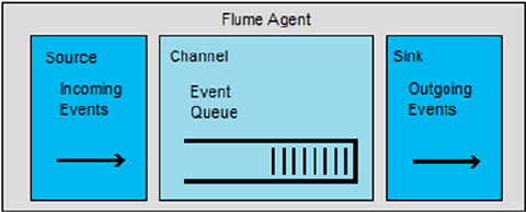
CHAPTER 6 ■ MOVING DATA

169

You can see that the rawdata table was created, but how much data does it contain? To check the row count of

the Hive rawdata table, you use the following:

hive> select count(*) from rawdata;

Total MapReduce jobs = 1

Launching Job 1 out of 1

......

Total MapReduce CPU Time Spent: 2 seconds 700 msec

OK

20031

Time taken: 25.098 seconds

Success is confirmed: the table in Hive contains 20,031 rows, which matches the MySQL table row count.

As you can see from this brief introduction, Sqoop is a powerful relational database data import/export tool for

Hadoop. You can even use Sqoop in an Oozie workflow and schedule complex ETL flows using Sqoop, Pig, and Hive

scripts. Also, you can carry out incremental loads with such Hive options as --incremental and --check-column.

This would be useful if you were receiving periodic data-feed updates from a relational database. Check the sqoop.

apache.org website to learn more.

So with Sqoop, you have seen an example of moving data between a relational database and Hadoop. But what if

the data that you wish to move is in another type of data source? Well, that is where the Apache Flume tool comes into

play. The next section describes it and provides an example of its use.

Moving Data with Flume

Apache Flume (flume.apache.org) is an Apache Software Foundation system for moving large volumes of log-based

data. The Flume data model is defined in terms of agents, where an agent has an event source, a channel, and an event

sink. Agents are defined in Flume configuration files. The source describes the data source. The channel receives event

data from the source and stores it. The sink takes event data from the channel. Figure 6-1 provides a simple example of

a Flume agent; it is the building block of the Flume architecture.

The sink might pass data to the source of another agent or write the data to a store like HDFS, as I’ll demonstrate

in the sections that follow. You can build complex topologies to process log or event data, with multiple agents passing

data to a single agent or to agents processing data in parallel. The following two examples show simple architectures

for Flume. Figure 6-2 shows a hierarchical arrangement, with Flume agents on the left of the diagram passing data on

to subagents that act as collectors for the data and then store the data to HDFS.

Figure 6-1. The Flume agent

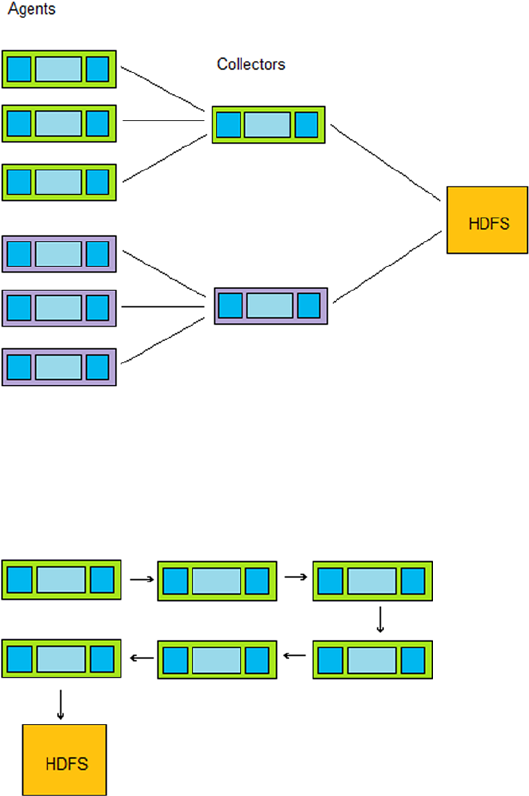
CHAPTER 6 ■ MOVING DATA

170

Figure 6-3 shows a linear arrangement whereby the output from one agent is passed to the next and the next after

that, until it is finally stored on HDFS. No specific architecture is advised here; instead, you should recognize that

Flume is flexible and that you can arrange your Flume architecture to meet your needs.

The Flume user guide shows some example topologies; see http://flume.apache.org/FlumeUserGuide.html.

Install Flume

Before you can move any log data, you must install Flume. Given that I am using the Cloudera CDH4.x stack here,

installation is simple, using the Linux yum commands. You install the Flume server first, as follows:

yum install flume-ng

Figure 6-2. Hierarchical example of Flume architecture

Figure 6-3. Linear example of Flume architecture

CHAPTER 6 ■ MOVING DATA

171

Then you install the component that allows Flume to start up at server boot time:

yum install flume-ng-agent

Finally, you install Flume documentation:

yum install flume-ng-doc

Next, you set up the basic configuration:

[root@hc1nn etc]# cd /etc/flume-ng/conf

[root@hc1nn conf]# ls

flume.conf flume-conf.properties.template flume-env.sh.template log4j.properties

cp flume-conf.properties.template flume.conf

You won’t customize the configuration for the agent now; an agent-based configuration file will be defined shortly.

As with many other Cloudera stack Apache components, you can find the Flume configuration and logs in

the standard places. For instance, logs are located under /var/log/flume-ng, the configuration files are under

/etc/flume-ng/conf, and the flume-ng executable file is /usr/bin/flume-ng.

A Simple Agent

As an example of how Flume works, I build a single Flume agent to asynchronously take data from a Centos

Linux-based message file called /var/log/messages. The message file acts as the data source and is stored in a single

Linux-based channel called channel1. The data sink is on HDFS in a directory called “flume/messages.”

In the Linux hadoop account I have created a number of files to run this example of a Flume job, display the

resulting data, and clean up after the job. These files make the job easier to run; there is minimal typing, and it is

easier to rerun the job because the results have been removed from HDFS. The files will also display the results of the

job that reside on HDFS. You can use scripts like these if you desire.

[hadoop@hc1nn ~]$ cd $HOME/flume

[hadoop@hc1nn flume]$ ls

agent1.cfg flume_clean_hdfs.sh flume_exec_hdfs.sh flume_show_hdfs.sh

The file agent1.cfg is the Flume configuration file for the agent, while the Bash (.sh) files are for running the

agent (flume_exec_hdfs.sh), showing the results on HDFS (flume_show_hdfs.sh), and cleaning up the data on HDFS

(flume_clean_hdfs.sh). Examining each of these files in turn, we see that the show script just executes a Hadoop file

system ls command against the directory /flume/messages, where the agent will write the data.

[hadoop@hc1nn flume]$ cat flume_show_hdfs.sh

#!/bin/bash

hdfs dfs -ls /flume/messages

CHAPTER 6 ■ MOVING DATA

172

The clean script executes a Hadoop file system remove command with a recursive switch:

[hadoop@hc1nn flume]$ cat flume_clean_hdfs.sh

#!/bin/bash

hdfs dfs -rm -r /flume/messages

The execution script, flume_execute_hdfs.sh, runs the Flume agent and needs nine lines:

[hadoop@hc1nn flume]$ cat flume_exec_hdfs.sh

1 #!/bin/bash

2

3 # run the bash agent

4

5 flume-ng agent \

6 --conf /etc/flume-ng/conf \

7 --conf-file agent1.cfg \

8 -Dflume.root.logger=DEBUG,INFO,console \

9 -name agent1

This execution script runs the Flume agent within a Linux Bash shell and is easily repeatable because a single

script has been run, rather than retyping these options each time you want to move log file content. Line 5 actually

runs the agent, while lines 6 and 7 specify the configuration directory and agent configuration file. Line 8 specifies

the log4j log configuration via a -D command line option to show DEBUG, INFO, and console messages. Finally,

line 9 specifies the Flume agent name agent1.

The Flume agent configuration file (agent1.cfg, in this case) must contain the agent’s source, sink, and channel.

Consider the contents of this example file:

[hadoop@hc1nn flume]$ cat agent1.cfg

1 # ----------------------------------------------------------------------

2 # define agent src, channel and sink

3 # ----------------------------------------------------------------------

4

5 agent1.sources = source1

6 agent1.channels = channel1

7 agent1.sinks = sink1

8

9 # ----------------------------------------------------------------------

10 # define agent channel

11 # ----------------------------------------------------------------------

12

13 agent1.channels.channel1.type = FILE

14 agent1.channels.channel1.capacity = 2000000

15 agent1.channels.channel1.checkpointInterval = 60000

16 agent1.channels.channel1.maxFileSize = 10737418240

17

CHAPTER 6 ■ MOVING DATA

173

18 # ----------------------------------------------------------------------

19 # define agent source

20 # ----------------------------------------------------------------------

21

22 agent1.sources.source1.type = exec

23 agent1.sources.source1.command = tail -F /var/log/messages

24 agent1.sources.source1.channels = channel1

25

26 # ----------------------------------------------------------------------

27 # define agent sink

28 # ----------------------------------------------------------------------

29

30 agent1.sinks.sink1.type = hdfs

31 agent1.sinks.sink1.hdfs.path = hdfs://hc1nn/flume/messages

32 agent1.sinks.sink1.hdfs.rollInterval = 0

33 agent1.sinks.sink1.hdfs.rollSize = 1000000

34 agent1.sinks.sink1.hdfs.batchSize = 100

35 agent1.sinks.sink1.channel = channel1

As already defined in the agent execution script, the Flume agent name in this example is agent1. Lines 5 to 7

define the names of the source, channel, and sink.

5 agent1.sources = source1

6 agent1.channels = channel1

7 agent1.sinks = sink1

The channel (channel1) is described between lines 13 and 16. Line 13 specifies that the channel type will be a

file. Line 14 indicates that the maximum capacity of the channel will be 2 million events. Line 15, in milliseconds,

indicates the time between checkpoints. Line 16 specifies the maximum channel file size in bytes.

13 agent1.channels.channel1.type = FILE

14 agent1.channels.channel1.capacity = 2000000

15 agent1.channels.channel1.checkpointInterval = 60000

16 agent1.channels.channel1.maxFileSize = 10737418240

The configuration file lines (22 to 24 ) show how the Flume data source source1 is defined.

22 agent1.sources.source1.type = exec

23 agent1.sources.source1.command = tail -F /var/log/messages

24 agent1.sources.source1.channels = channel1

In this example, I may need to ensure that the Linux account I am using to run this Flume job has access to read the

log file /var/log/messages. Therefore, I grant access using the root account as follows: I use the Linux su (switch user)

command to change the user ID to root. Then I use the Linux chmod command to grant global read privileges while

maintaining current access. The two Linux ls command listings show that extra access has been granted:

su -

ls -l /var/log/messages

-rw------- 1 root root 410520 Nov 22 09:20 /var/log/messages

chmod 644 /var/log/messages

ls -l /var/log/messages

-rw-r--r-- 1 root root 410520 Nov 22 09:25 /var/log/messages

exit

CHAPTER 6 ■ MOVING DATA

174

The source type is defined as “exec” in line 22, but Flume also supports sources of Avro, Thrift, Syslog, jms,

spooldir, twittersource, seq, http, and Netcat. You also could write custom sources to consume your own data types;

see the Flume user guide at flume.apache.org for more information.

The executable command is specified at line 23 as tail -F /var/log/messages. This command causes new

messages in the file to be received by the agent. Line 24 connects the source to the Flume agent channel, channel1.

Finally, lines 30 through 35 define the HDFS data sink:

30 agent1.sinks.sink1.type = hdfs

31 agent1.sinks.sink1.hdfs.path = hdfs://hc1nn/flume/messages

32 agent1.sinks.sink1.hdfs.rollInterval = 0

33 agent1.sinks.sink1.hdfs.rollSize = 1000000

34 agent1.sinks.sink1.hdfs.batchSize = 100

35 agent1.sinks.sink1.channels = channel1

In this example, the sink type is specified at line 30 to be HDFS, but it could also be a value like logger, avro, irc,

hbase, or a custom sink (see the Flume user guide at flume.apache.org for futher alternatives). Line 31 specifies the

HDFS location as a URI, saving the data to /flume/messages.

Line 32 indicates that the logs will not be rolled by time, owing to the value of 0, while the value at line 33

indicates that the sink will be rolled based on size. Line 34 specifies a sink batch size of 100 for writing to HDFS, and

line 35 connects the channel to the sink.

For this example, I encountered the following error owing to a misconfiguration of the channel name:

2014-07-26 14:45:10,177 (conf-file-poller-0) [WARN - org.apache.flume.conf.FlumeConfiguration

$AgentConfiguration.

validateSources(FlumeConfiguration.java:589)] Could not configure source source1 due to: Failed to

configure component!

This error message indicated a configuration error—in this case, it was caused by putting an “s” on the end of the

channels configuration item at line 24. When corrected, the line reads as follows:

24 agent1.sources.source1.channel = channel1

Running the Agent

To run your Flume agent, you simply run your Bash script. In my example, to run the Flume agent agent1, I run the

Centos Linux Bash script flume_exec_hdfs.sh, as follows:

[hadoop@hc1nn flume]$ cd $HOME/flume

[hadoop@hc1nn flume]$ ./flume_execute_hdfs.sh

This writes the voluminous log output to the session window and to the logs under /var/log/flume-ng. For my

example, I don’t provide the full output listing here, but I identify the important parts. Flume validates the agent

configuration and so displays the source, channel, and sink as defined:

2014-07-26 17:50:01,377 (conf-file-poller-0) [DEBUG - org.apache.flume.conf.FlumeConfiguration$Agent

Configuration.isValid(FlumeConfiguration.java:313)] Starting validation of configuration for agent:

agent1, initial-configuration: AgentConfiguration[agent1]

SOURCES: {source1={ parameters:{command=tail -F /var/log/messages, channels=channel1, type=exec} }}

CHAPTER 6 ■ MOVING DATA

175

CHANNELS: {channel1={ parameters:{checkpointInterval=60000, capacity=2000000,

maxFileSize=10737418240, type=FILE} }}

SINKS: {sink1={ parameters:{hdfs.path=hdfs://hc1nn/flume/messages, hdfs.batchSize=100,

hdfs.rollInterval=0, hdfs.rollSize=1000000, type=hdfs, channel=channel1} }}

Flume then sets up the file-based channel:

2014-07-26 17:50:02,858 (lifecycleSupervisor-1-0) [INFO - org.apache.flume.channel.file.FileChannel.

start(FileChannel.java:254)] Starting FileChannel channel1 { dataDirs: [/home/hadoop/.flume/file-

channel/data] }...

The channel on the Linux file system contains checkpoint and log data:

[hadoop@hc1nn flume]$ ls -l $HOME/.flume/file-channel/*

/home/hadoop/.flume/file-channel/checkpoint:

total 15652

-rw-rw-r--. 1 hadoop hadoop 16008232 Jul 26 17:51 checkpoint

-rw-rw-r--. 1 hadoop hadoop 25 Jul 26 17:51 checkpoint.meta

-rw-rw-r--. 1 hadoop hadoop 32 Jul 26 17:51 inflightputs

-rw-rw-r--. 1 hadoop hadoop 32 Jul 26 17:51 inflighttakes

drwxrwxr-x. 2 hadoop hadoop 4096 Jul 26 17:50 queueset

/home/hadoop/.flume/file-channel/data:

total 2060

-rw-rw-r--. 1 hadoop hadoop 0 Jul 26 15:44 log-6

-rw-rw-r--. 1 hadoop hadoop 47 Jul 26 15:44 log-6.meta

-rw-rw-r--. 1 hadoop hadoop 1048576 Jul 26 15:55 log-7

-rw-rw-r--. 1 hadoop hadoop 47 Jul 26 15:56 log-7.meta

-rw-rw-r--. 1 hadoop hadoop 1048576 Jul 26 17:50 log-8

-rw-rw-r--. 1 hadoop hadoop 47 Jul 26 17:51 log-8.meta

The Flume agent sets up the data sink by creating a single empty file on HDFS. The log message indicating this is

as follows:

2014-07-26 17:50:10,532 (SinkRunner-PollingRunner-DefaultSinkProcessor) [INFO - org.apache.

flume.sink.hdfs.BucketWriter.open(BucketWriter.java:220)] Creating hdfs://hc1nn/flume/messages/

FlumeData.1406353810397.tmp

The script flume_show_hdfs.sh can be run as follows, using the Linux hadoop account to show the Flume data

sink file on HDFS:

[hadoop@hc1nn flume]$ ./flume_show_hdfs.sh

Found 1 items

-rw-r--r-- 2 hadoop hadoop 0 2014-07-26 17:50 /flume/messages/FlumeData.1406353810397.tmp

The script reveals that the file is empty, with a zero in the fifth column. When the number of new messages in

the messages file reaches 100 (as defined by batchSize at line 34 of the agent configuration file), the data is written to

HDFS from the channel:

34 agent1.sinks.sink1.hdfs.batchSize = 100

CHAPTER 6 ■ MOVING DATA

176

I can see this behavior by running the Flume show script again:

[hadoop@hc1nn flume]$ ./flume_show_hdfs.sh

Found 11 items

-rw-r--r-- 2 hadoop hadoop 1281 2014-07-26 17:50 /flume/messages/FlumeData.1406353810397

-rw-r--r-- 2 hadoop hadoop 1057 2014-07-26 17:50 /flume/messages/FlumeData.1406353810398

-rw-r--r-- 2 hadoop hadoop 926 2014-07-26 17:50 /flume/messages/FlumeData.1406353810399

-rw-r--r-- 2 hadoop hadoop 1528 2014-07-26 17:50 /flume/messages/FlumeData.1406353810400

-rw-r--r-- 2 hadoop hadoop 1281 2014-07-26 17:50 /flume/messages/FlumeData.1406353810401

-rw-r--r-- 2 hadoop hadoop 1214 2014-07-26 17:50 /flume/messages/FlumeData.1406353810402

-rw-r--r-- 2 hadoop hadoop 1190 2014-07-26 17:50 /flume/messages/FlumeData.1406353810403

-rw-r--r-- 2 hadoop hadoop 1276 2014-07-26 17:50 /flume/messages/FlumeData.1406353810404

-rw-r--r-- 2 hadoop hadoop 1387 2014-07-26 17:50 /flume/messages/FlumeData.1406353810405

-rw-r--r-- 2 hadoop hadoop 1107 2014-07-26 17:50 /flume/messages/FlumeData.1406353810406

-rw-r--r-- 2 hadoop hadoop 1281 2014-07-26 17:51 /flume/messages/FlumeData.1406353810407

As you can see in this example, those 100 messages have been written to HDFS and the data is now available

for further processing in an ETL chain by one of the other processing languages. This has further possibilities. For

instance, you could use Apache Pig native to strip information from these files and employ an Oozie workflow to

organize that processing into an ETL chain.

This simple example uses a simple agent with a single source and sink. You could also organize agents to act

as sources or sinks for later agents in the chain so the feeds can fan in and out. You could build complex agent

processing topologies with many different types, depending upon your needs. Check the Apache Flume website at

flume.apache.org for further configuration examples.

You’ve now seen how to process relational database data with Sqoop and log-based data with Flume, but what

about streamed data? How is it possible to process an endless stream of data from a system like Twitter? The data

would not stop—it would just keep coming. The answer is that systems like Storm allow processing on data streams.

For instance, by using this tool, you can carry out trend analysis continuously on current data in the stream. The next

section examines some uses of Storm.

Moving Data with Storm

Apache Storm (storm.incubator.apache.org) from the Apache Software Foundation is an Apache incubator

project for processing unbounded data streams in real time. (The term “incubator” means that this is a new Apache

project; it is not yet mature. It needs to follow the Apache process before it can “graduate,” and this might mean that

its release process or documentation is not complete.) The best way to understand the significance of Storm is with a

comparison. On Hadoop, a Map Reduce job will start, process its data set, and exit; however, a topology (a Storm job

architecture) will run forever because its data feed is unlimited.

Consider a feed of events from the website Twitter; they just keep coming. When Storm processes a feed from

such a source, it processes the data it receives in real time. So, at any point, what Storm presents is a window on a

stream of data at the current time. Because of this, it also presents current trends in the data. In terms of Twitter, that

might indicate what many people are talking about right now. But also, because the data set is a stream that never

ends, Storm needs to be manually stopped.

A topology is a Storm job architecture. It is described in terms of spouts, steams, and bolts. Streams are streams of

data created from a sequence of data records called tuples.

Figure 6-4 shows a simple Storm data record, or tuple; a sequence or pipe of these data records forms a stream,

which is shown in Figure 6-5.

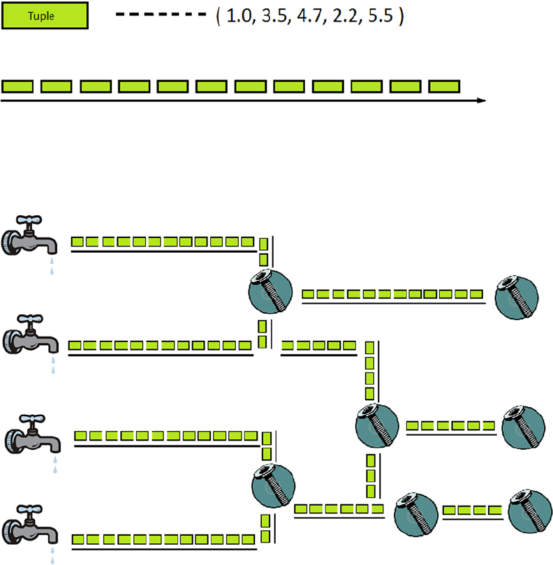
CHAPTER 6 ■ MOVING DATA

177

Data sources in Storm are call spouts, while the joints between the streams are called bolts. The input to a stream

might be a spout or a bolt. Bolts can connect stream outputs to inputs from or to other streams. Figure 6-6 shows a

simple Storm topology. Multiple spouts and bolts have been used to merge stream data.

Storm has a master process called a Nimbus and slave processes called supervisors. Configuration is managed

via ZooKeeper servers. The Nimbus master handles the monitoring and distribution of code and tasks to the slaves.

Hadoop runs potentially long-running batch jobs that will eventually end. Storm provides real-time trend processing

of endless stream-based data that will run until it is manually stopped.

As an incubator project, Storm has not yet matured to the level of a full Apache project. It demands a little more

work than is required of more mature systems to source and build the components. Storm depends on ZeroMQ

(a messaging system) and JZMQ (Java Bindings for ZeroMQ), so you need to install these before you install Storm

itself. In the next sections, I show how to install ZeroMQ, JXMQ, and Storm. Remember, though, that each of the

following installations should be carried out on each server on which Storm will run. You will also need ZooKeeper,

the installation for which was described in Chapter 2. Once you check that everything is operating without error,

you’ll be able to follow my demonstration of the Storm interface and an example of the code samples that Storm

provides on the Storm cluster that I build.

Figure 6-4. A Storm tuple

Figure 6-5. A Storm stream

Figure 6-6. An simple Storm topology

CHAPTER 6 ■ MOVING DATA

178

Install ZeroMQ

Install ZeroMQ on the server hc1nn as the Linux user hadoop into a working directory that you create for the task called

$HOME/storm/zeromq. Download version 2.1.7 of ZeroMQ from the ZeroMQ website as a zipped tar file, as follows:

[hadoop@hc1nn zeromq]$ pwd

/home/hadoop/storm/zeromq

[hadoop@hc1nn zeromq]$ wget http://download.zeromq.org/zeromq-2.1.7.tar.gz

[hadoop@hc1nn zeromq]$ ls -l

total 1836

-rw-rw-r--. 1 hadoop hadoop 1877380 May 12 2011 zeromq-2.1.7.tar.gz

Next, unpack the compressed tar file using tar -xzf. The z option accepts a file with a gzipped file extension and

unzips it. The x option extracts the tar contents, and the f option allows the tar file name to be specified:

[hadoop@hc1nn zeromq]$ tar -xzf zeromq-2.1.7.tar.gz

This shows the contents of the ZeroMQ release:

[hadoop@hc1nn zeromq]$ cd zeromq-2.1.7

[hadoop@hc1nn zeromq-2.1.7]$ ls

acinclude.m4 builds configure.in foreign Makefile.am README zeromq.spec

aclocal.m4 ChangeLog COPYING include Makefile.in src

AUTHORS config COPYING.LESSER INSTALL NEWS tests

autogen.sh configure doc MAINTAINERS perf version.sh

The configure script is used to prepare the release for a build. Note: When I initially used this script, I encountered

this error:

checking for uuid_generate in -luuid... no

configure: error: cannot link with -luuid, install uuid-dev.

The error alerted me that a dependency was missing that ZeroMQ required. To fix this, I installed the following

components as root, using the yum command:

[root@hc1nn ~]# yum install libuuid-devel gcc-c++.x86_64 libtool

Then I set up the build configuration as follows:

[hadoop@hc1nn zeromq]$ ./configure

..............

config.status: creating builds/redhat/zeromq.spec

config.status: creating src/platform.hpp

config.status: executing depfiles commands

config.status: executing libtool commands

CHAPTER 6 ■ MOVING DATA

179

I have truncated the output I received next; if you get these last few lines and see no errors, then you know that

the command has completed successfully.

Now, you run a make command to build ZeroMQ:

[hadoop@hc1nn zeromq-2.1.7]$ make

..............

make[1]: Leaving directory `/home/hadoop/storm/zeromq/zeromq-2.1.7/tests'

make[1]: Entering directory `/home/hadoop/storm/zeromq/zeromq-2.1.7'

make[1]: Nothing to be done for `all-am'.

make[1]: Leaving directory `/home/hadoop/storm/zeromq/zeromq-2.1.7'

Again, the preceding is only a portion of the output to give you the general idea. Having built the release, you are

ready to install it, but you will need to do this as root:

[root@hc1nn zeromq-2.1.7]# make install

make[1]: Entering directory `/home/hadoop/storm/zeromq/zeromq-2.1.7'

make[2]: Entering directory `/home/hadoop/storm/zeromq/zeromq-2.1.7'

make[2]: Nothing to be done for `install-exec-am'.

make[2]: Nothing to be done for `install-data-am'.

make[2]: Leaving directory `/home/hadoop/storm/zeromq/zeromq-2.1.7'

make[1]: Leaving directory `/home/hadoop/storm/zeromq/zeromq-2.1.7'

With ZeroMQ, Storm’s messaging component successfully installed, you can move on to installing JZMQ, the Java

binding component.

Install JZMQ

Create a working directory for this installation at $HOME/storm/jzmq, from which you will carry out the installation.

Use the git command to download a JZMQ release. Use the Linux yum command as root in the first three lines that

follow to install the git command, which enables software downloads:

[hadoop@hc1nn jzmq]$ su -

[root@hc1nn ~]$ yum install git

[root@hc1nn ~]$ exit

[hadoop@hc1nn jzmq]$ git clone https://github.com/nathanmarz/jzmq.git

Initialized empty Git repository in /home/hadoop/storm/jzmq/jzmq/.git/

remote: Counting objects: 611, done.

remote: Compressing objects: 100% (257/257), done.

remote: Total 611 (delta 239), reused 611 (delta 239)

Receiving objects: 100% (611/611), 348.62 KiB | 216 KiB/s, done.

Resolving deltas: 100% (239/239), done.

CHAPTER 6 ■ MOVING DATA

180

Move it into the release directory and list the contents:

[hadoop@hc1nn jzmq]$ cd jzmq

[hadoop@hc1nn jzmq]$ ls

AUTHORS ChangeLog COPYING.LESSER Makefile.am pom.xml src

autogen.sh configure.in debian NEWS README test

builds COPYING jzmq.spec perf README-PERF

Now run the autogen.sh script to prepare this release for a build:

[hadoop@hc1nn jzmq]$ ./autogen.sh

.................

configure.in:14: installing `config/install-sh'

configure.in:14: installing `config/missing'

src/Makefile.am: installing `config/depcomp'

Makefile.am: installing `./INSTALL'

autoreconf: Leaving directory `.'

(Again, the output is cropped.) You use the configure script to set up build Makefiles:

[hadoop@hc1nn jzmq]$ ./configure

...........................

configure: creating ./config.status

config.status: creating Makefile

config.status: creating src/Makefile

config.status: creating perf/Makefile

config.status: creating src/config.hpp

config.status: executing depfiles commands

config.status: executing libtool commands

Now, build the release by executing the make command:

[hadoop@hc1nn jzmq]$ make

.................

echo timestamp > classdist_noinst.stamp

/usr/bin/jar cf zmq-perf.jar *.class

make[2]: Leaving directory `/home/hadoop/storm/jzmq/jzmq/perf'

make[1]: Leaving directory `/home/hadoop/storm/jzmq/jzmq/perf'

make[1]: Entering directory `/home/hadoop/storm/jzmq/jzmq'

make[1]: Nothing to be done for `all-am'.

make[1]: Leaving directory `/home/hadoop/storm/jzmq/jzmq'

Having built the release successfully, you install it as the Linux root account:

[root@hc1nn jzmq]# pwd

/home/hadoop/storm/jzmq/jzmq

[root@hc1nn jzmq]# make install

CHAPTER 6 ■ MOVING DATA

181

..............................

make[1]: Entering directory `/home/hadoop/storm/jzmq/jzmq'

make[2]: Entering directory `/home/hadoop/storm/jzmq/jzmq'

make[2]: Nothing to be done for `install-exec-am'.

make[2]: Nothing to be done for `install-data-am'.

make[2]: Leaving directory `/home/hadoop/storm/jzmq/jzmq'

make[1]: Leaving directory `/home/hadoop/storm/jzmq/jzmq'

That completes the installations for the Storm dependencies; now it’s time to install Storm itself.

Install Storm

Create a working directory $HOME/storm/storm to carry out this installation. Use wget to download version 0.9.2 of

Storm as a gzipped tar file.

[hadoop@hc1nn storm]$ pwd

/home/hadoop/storm/storm

[hadoop@hc1nn storm]$ wget http://supergsego.com/apache/incubator/storm/apache-storm-0.9.2-

incubating/apache-storm-0.9.2-incubating.tar.gz

[hadoop@hc1nn storm]$ ls -l

total 19608

-rw-rw-r--. 1 hadoop hadoop 20077564 Jun 25 02:49 apache-storm-0.9.2-incubating.tar.gz

Using the tar command, unpack the zipped tar file; x means extract, f specifies the archive file, and z decompresses

the file:

[hadoop@hc1nn storm]$ tar -xzf apache-storm-0.9.2-incubating.tar.gz

Using the Linux root account, move the Storm release to the /usr/local directory:

[root@hc1nn ~]# cd /home/hadoop/storm/storm

[root@hc1nn storm]# mv apache-storm-0.9.2-incubating /usr/local

[root@hc1nn storm]# cd /usr/local

Create a symbolic link for the release under /usr/local and name the link “storm.” Using this link to refer to the

release will simplify the environment and make the Storm configuration release version independent:

[root@hc1nn local]# ln -s apache-storm-0.9.2-incubating storm

[root@hc1nn local]# ls -ld *storm*

drwxrwxr-x. 9 hadoop hadoop 4096 Jul 27 11:28 apache-storm-0.9.2-incubating

lrwxrwxrwx. 1 root root 29 Jul 27 11:30 storm -> apache-storm-0.9.2-incubating

Now, create a Storm-related environment variable in the $HOME/.bashrc shell file for the Linux hadoop account:

#######################################################

# Set up Storm variables

export STORM_HOME=/usr/local/storm

export PATH=$PATH:$STORM_HOME/bin

CHAPTER 6 ■ MOVING DATA

182

This action creates a STORM_HOME environment variable that points to the installation. Also, the Storm installation

binary directory has been added to the path so that the Storm executable can be located. Now, you create a Storm

working directory; I place mine under /app/storm:

[root@hc1nn app]# cd /app

[root@hc1nn app]# mkdir storm

[root@hc1nn app]# chown hadoop:hadoop storm

[root@hc1nn app]# ls -l

total 8

drwxr-xr-x. 3 hadoop hadoop 4096 Mar 15 15:38 hadoop

drwxr-xr-x. 2 hadoop hadoop 4096 Jul 27 11:38 storm

I am using my Linux hadoop user account to run Storm, but you might want to use a dedicated Storm account.

You set up the Storm configuration files under $STORM_HOME/conf. Set the following values in the file storm.yaml:

storm.zookeeper.servers:

- "hc1r1m1"

- "hc1r1m2"

- "hc1r1m3"

nimbus.host: "hc1nn"

nimbus.childopts: "-Xmx1024m -Djava.net.preferIPv4Stack=true"

ui.childopts: "-Xmx768m -Djava.net.preferIPv4Stack=true"

supervisor.childopts: "-Djava.net.preferIPv4Stack=true"

worker.childopts: "-Xmx768m -Djava.net.preferIPv4Stack=true"

storm.local.dir: "/app/storm"

These settings specify three ZooKeeper servers (hc1r1m1, hc1r1m2, hc1r1m3 ) to be the nodes on which the slave

Storm processes will run. The master (Nimbus) Storm process is set to run on the server hc1nn. Also, the Storm local

directory is defined as “ /app/storm.”

Now, it is time to check that ZooKeeper is running before you attempt to run Storm.

Start and Check Zookeeper

As the Linux root account, you start the ZooKeeper server on each slave node; root is used because these servers are

Linux-based services:

service zookeeper-server start

The configuration for the ZooKeeper server is stored under /etc/zookeeper/conf/zoo.cfg, while the logs can be

found under /var/log/zookeeper. Check the logs for errors and ensure that each ZooKeeper server is running.

Now, you use a four-letter acronym RUOK (“Are you OK?”) with each server to check that it is running correctly.

The response that you can expect is IMOK (“I am OK”).

CHAPTER 6 ■ MOVING DATA

183

The ZooKeeper installation and use was already described in Chapter. Here are the successful outputs from the

ZooKeeper checks:

nc hc1r1m1 2181

ruok

imok

nc hc1r1m2 2181

ruok

imok

nc hc1r1m3 2181

ruok

imok

Run Storm

With the prep work finished, you’re now ready to run the Storm servers. Start the supervisor processes on the slave

nodes first, and then the Nimbus process on the master server. Also, start the Storm user interface process so that

Storm can be monitored via a web page. On each of the slave nodes (hc1r1m1, hc1r1m2, hc1r1m3 ), you run the Storm

supervisor slave process (via the Linux hadoop account) as a background process ("&"). This will free up the terminal

session if it is required:

storm supervisor &

Run the Storm Nimbus master process on the master server hc1nn, and run the user interface instance on the

same server:

storm nimbus &

storm ui &

The Storm cluster is now running, but you need to check the logs under /usr/local/storm/logs for errors on each

server. Shown in Figure 6-7, the Storm user interface is available at http://hc1nn:8080/.

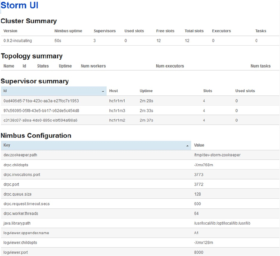
CHAPTER 6 ■ MOVING DATA

184

The Storm user interface shows the supervisor processes running, the Nimbus master, the topologies that are

running, and a cluster summary. In the Figure 6-7 window, no topology can be seen running at the moment (but I

add one in the next section). The Storm release comes with some example topologies in a storm-starter subdirectory.

Next, I build these examples into a jar file and run one of them on the Storm cluster; this will demonstrate the process

and the available tools.

Figure 6-7. The basic Storm user interface

CHAPTER 6 ■ MOVING DATA

185

An Example of Storm Topology

On the master server, I build the storm-starter topology code under $STORM_HOME/examples/storm-starter.

The build creates a jar file that can be run against the cluster under a directory called “target” at this level:

[hadoop@hc1nn ~]$ cd $STORM_HOME/examples/storm-starter

[hadoop@hc1nn storm-starter]$ ls -l

total 2888

drwxr-xr-x. 3 hadoop hadoop 4096 May 6 07:13 multilang

-rw-r--r--. 1 hadoop hadoop 5191 Jun 14 08:35 pom.xml

-rw-r--r--. 1 hadoop hadoop 4825 May 29 04:24 README.markdown

drwxr-xr-x. 4 hadoop hadoop 4096 May 6 07:13 src

-rw-r--r--. 1 hadoop hadoop 2927299 Jun 14 08:57 storm-starter-topologies-0.9.2-incubating.jar

drwxr-xr-x. 3 hadoop hadoop 4096 May 6 07:13 test

I then use Apache Maven version 3.2.1 to build this package:

[hadoop@hc1nn storm-starter]$ mvn package

........................

[INFO] ------------------------------------------------------------------------

[INFO] BUILD SUCCESS

[INFO] ------------------------------------------------------------------------

[INFO] Total time: 04:16 min

[INFO] Finished at: 2014-07-27T13:57:49+12:00

[INFO] Final Memory: 25M/59M

[INFO] ------------------------------------------------------------------------

I have truncated the build output for purposes of this example, but if you get to this success line, then all is good.

So, I check to see that the built library exists:

[hadoop@hc1nn storm-starter]$ ls -lrt target/storm-starter-*-incubating-jar-with-dependencies.jar

-rw-rw-r--. 1 hadoop hadoop 2927301 Jul 27 13:57 target/storm-starter-0.9.2-incubating-jar-with-

dependencies.jar

Note ■ If you want to know which topologies are available for use, you can look at the Java source code under

$STORM_HOME/examples/storm-starter/src/jvm/storm/starter. It might be useful to have a look at this code to familiarize

yourself with how it works. Also, check the Apache Storm website (storm.incubator.apache.org) documentation for

topology coding examples.

[hadoop@hc1nn storm-starter]$ cd $STORM_HOME/examples/storm-starter/src/jvm/storm/starter

[hadoop@hc1nn starter]$ ls *.java

BasicDRPCTopology.java ReachTopology.java TransactionalWords.java

ExclamationTopology.java RollingTopWords.java WordCountTopology.java

ManualDRPC.java SingleJoinExample.java

PrintSampleStream.java TransactionalGlobalCount.java

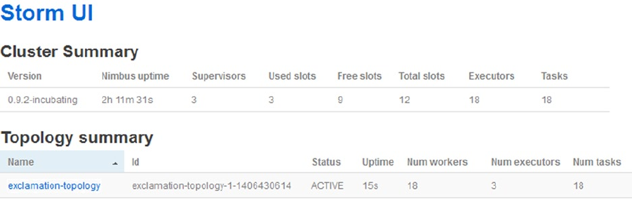
CHAPTER 6 ■ MOVING DATA

186

Now that the storm-start jar file is built, I can run a topology from its contents. Remember that this topology will

run forever, processing a simulated data feed created by the example code. So, I run the exclamation topology, which

just randomly adds exclamation marks to the incoming data. (This may seem like a simple process, but the aim here is

to show how to use and run topologies on Storm. Later, you can investigate building and running your own.) The storm

command line tool launches the topology onto the cluster and has four parameters. The first is the jar parameter,

which is followed by the jar file name that was just built. The third and fourth are the class name and topology name:

storm jar target/storm-starter-*-incubating-jar-with-dependencies.jar \

storm.starter.ExclamationTopology \

exclamation-topology

I now check the status of the topology on the cluster by using the Storm list option. The output that follows

shows that the topology is active, provides timing information, and shows the number of tasks:

[hadoop@hc1nn starter]$ storm list

Topology_name Status Num_tasks Num_workers Uptime_secs

-----------------------------------------------------------------------------------

exclamation-topology ACTIVE 18 3 62

As mentioned, this topology will run forever, providing a series of snapshots of data processed within given data

windows. If I check the Storm user interface (Figure 6-8), I see that there is an active topology called “exclamation-

topology” shown in the Topology Summary section.

Figure 6-8. Storm user interface with running topology

By clicking on the topology name in the user interface, I can drill down into the topology to get more information.

The detailed topology view in Figure 6-9 gives information about the spouts and bolts within the topology, for

example. Remember that spouts provide data sources while bolts process the streams of data. My example includes a

single spout data source, called “word,” whose data is being passed to two bolts, called “exclaim1” and “exclaim2.” The

detailed topology view also lists the volume of data processed and the number of tasks involved.

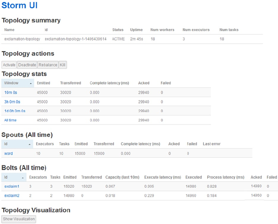
CHAPTER 6 ■ MOVING DATA

187

I also can obtain a visual view of my example’s topology structure by clicking the Show Visualization button.

Figure 6-10 provides an enlarged image of the resulting topology. As you can see, the spout passes data to the bolt

exclaim1, which then passes it on to exclaim2.

Figure 6-9. Detailed view of Storm user interface topology

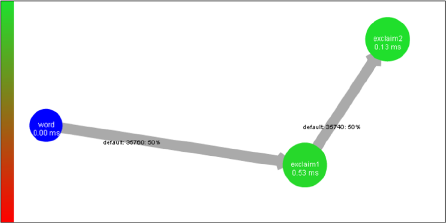
CHAPTER 6 ■ MOVING DATA

188

The green circles in Figure 6-10 are bolts and the blue circle is a spout. The gray arrows are data flows, and the

timing information is shown in each object. This is a simple topology. To do anything meaningful, you would build

a larger structure. If you refresh the user interface (press F5), you will see the statistics update. You will always see a

current window of data showing the current data trend.

The data stream that this topology processes is boundless, meaning that if you want to stop it, you have to manually

kill it. You can do this by using the Storm kill command with the topology name, as I have done for my example:

[hadoop@hc1nn starter]$ storm kill exclamation-topology

2530 [main] INFO backtype.storm.thrift - Connecting to Nimbus at hc1nn:6627

2689 [main] INFO backtype.storm.command.kill-topology - Killed topology: exclamation-topology

Now, when I list the running Storm topologies, I can see that there are none running:

[hadoop@hc1nn starter]$ storm list

3326 [main] INFO backtype.storm.thrift - Connecting to Nimbus at hc1nn:6627

No topologies running.

To shut down Storm, you first stop the supervisor processes on each slave node. To find out which processes are

running, you use the jps command to see a list of processes and their process numbers. In my example, I can see

that the supervisor process on the host hc1r1m2 has a process ID of 17617. I can use this number with the Linux kill

command to kill the process, as follows:

[hadoop@hc1r1m2 logs]$ jps

17617 supervisor

18134 Jps

Figure 6-10. Storm user interface showing topology structure

CHAPTER 6 ■ MOVING DATA

189

[hadoop@hc1r1m2 logs]$ kill -9 17617

[hadoop@hc1r1m2 logs]$

[1]+ Killed storm supervisor

Next, I kill the Nimbus and the user interface processes on the master server hc1nn. Again, I use the jps

command to show the running processes. The Storm user interface shows the name “Core” instead of a meaningful

name. Remember, though, that Storm is an incubator project and so problems like this will be resolved in future

releases. However, when I kill the associated process numbers by using the Linux kill command, I can see that the

Nimbus and UI have stopped:

[hadoop@hc1nn starter]$ jps

24718 core

27661 Jps

24667 nimbus

[hadoop@hc1nn starter]$ kill -9 24718 24667

[hadoop@hc1nn starter]$

[1]- Killed storm nimbus (wd: /usr/local/storm/conf)

(wd now: /usr/local/storm/examples/storm-starter/src/jvm/storm/starter)

[2]+ Killed storm ui (wd: /usr/local/storm/conf)

(wd now: /usr/local/storm/examples/storm-starter/src/jvm/storm/starter)

If this very short introduction to Storm leaves you curious for more information, take a look at the other example

topologies and examine the code. Try running some of these other topologies and see what they do. You can read the

Apache Storm website, but be aware that because Storm is an incubator project, the documentation is a little thin.

Summary

This chapter has highlighted some, but not all, of the many tools and alternatives for moving data. For instance, the

Sqoop2 tool was just recently released. Remember that although most of the examples in this chapter have processed

data in to Hadoop, these same tools can be used to send data out of Hadoop as well. Also, each of the tools examined,

especially Sqoop and Flume, can process multiple types of data. You can also embed your Sqoop data-processing

scripts into Oozie workflows for management and scheduling. This chapter has examined only a small portion of the

functionality that is offered by Sqoop, Flume, and Storm for processing data. You could also examine a tool called

Apache Chukwa (chukwa.apache.org), which has features similar to Flume. Note also that Chapter 10 examines tools

like Pentaho and Talend, with which you can move data using visual building blocks.

The next chapter surveys monitoring systems like Hue to provide a visual view of Hadoop cluster processing. Hue

provides a single, integrated web-based interface by which scripting and monitoring functionality can be accessed.

Examples here and in earlier chapters have used Sqoop, Hive, Pig, and Oozie; next, you’ll be accessing these tools

within Hue.

191

Chapter 7

Monitoring Data

No matter how carefully you set up your big data system, you need to continually monitor HDFS, as well as the

Hadoop jobs and workflows running on it, to ensure the system is running as efficiently as possible. This chapter

examines the Hadoop and third-party tools available for monitoring a big data system, including tools for monitoring

the system-level resources on each node in the cluster and determining how processing is spread across the cluster.

For example, user interface systems such as Hue ease both the use and the monitoring of Hadoop by centralizing

access to Hadoop-based functionality via a single well-designed interface. Systems like Ganglia and Nagios provide

rich open-source, resource-level monitoring and alerting. In the sections that follow, I will provide working examples

for sourcing these systems, installing them, and putting them into use. Because I will use the Cloudera CDH4 stack,

this chapter’s examples will be based upon Hadoop V2.

In the first section I examine the Hadoop Hue browser, sourcing the software, installing and configuring it, and

then I present the user interface in operation.

The Hue Browser

An Apache Software Foundation top-level project released under an Apache 2 license, the Hue browser offers a web-

based user interface on top of Hadoop, including user interfaces for tools like Oozie, Pig, Impala, HBase, and Hive.

It also has a file browser for HDFS and interactive scripting for Pig, Sqoop, Hive, and HBase. There is also a job

browser, a job designer, and an Oozie editor and dashboard.

The Hue browser provides a single location for accessing multiple Hadoop-based tools. For instance, suppose

you were developing an ETL (extract, transform, and load) chain that might pull data from a remote relational

database, run a Pig script on the data in HDFS, and then move the data to Hive. You could develop, test, and run the

ETL components from within Hue. You could even run an Oozie job that would group and schedule the linked ETL

tasks from Hue. For the simple convenience alone, that must be worth considering.

As I use the Cloudera stack version 4, I show how to install and use Hue 2.5.0, the version that comes with

Cloudera CDH4. Later versions are available, but this installation should be a good introduction. Along the way, I also

point out some solutions to common errors that you might encounter while installing and working with Hue. For the

latest news and details on Hue, visit its official website at gethue.com.

Installing Hue

To install Hue, you need to ensure that the components it will integrate with are properly installed. For this example,

that means I have to ensure that the connections to HDFS, YARN, HBase, Oozie, Sqoop, and Sqoop2 are working

correctly before I move on to use Hue itself. It’s advised that you follow each section completely before moving on to

the Hue interface, thereby avoiding unnecessary errors.

Chapter 7 ■ Monitoring Data

192

By example, I install Hue on the CentOS 6 server hc1nn, using the Linux-based yum command as the root user, as

follows:

[root@hc1nn ~]# yum install hue

[root@hc1nn ~]# yum install hue-server

Next, I add some configuration items to Hadoop for Hue. Specifically, under /etc/hadoop/conf, I add the

following entry to the hdfs-site.xml file at the bottom of the configuration section:

<name>dfs.webhdfs.enabled</name>

</property>

This enables a webhdfs Rest API on the name node and data nodes. I repeat this addition on all Hadoop nodes in

my cluster, then add the following changes to the Hadoop core-site.xml file in the same location:

<name>hadoop.proxyuser.hue.hosts</name>

</property>

<name>hadoop.proxyuser.hue.groups</name>

<value>hadoop</value>

</property>

<name>hadoop.proxyuser.hcat.hosts</name>

</property>

<name>hadoop.proxyuser.hcat.groups</name>

<value>hadoop</value>

</property>

<name>fs.trash.interval</name>

</property>

By defining Hue’s Hadoop proxy user settings, these first four entries define the host and group access for hue and

hcat. The final entry specifies the Hue file system trash interval.

Chapter 7 ■ Monitoring Data

193

After making these changes to Hadoop, I restart the Hadoop servers to pick up the changes. Next, I set up the Hue

configuration file under /etc/hue/conf called hue.ini. To begin, I set the secret key to a suitable alpha numeric value

for session hashing. This secret key string should be between 30 and 60 characters long, and it should be random. It is

used for Internet browser cookie session security:

secret_key=kdntwdfjgmxnsprngpwekspfnsmdpwtyiubkdn

I then define the web host and port with the following:

http_host=hc1nn

http_port=8888

I set my web services URL, which I will use later to access Hue:

webhdfs_url=http://hc1nn:50070/webhdfs/v1/

I leave the Hadoop paths as the default values; they are correct for Cloudera Hadoop CDH4:

hadoop_hdfs_home=/usr/lib/hadoop-hdfs

hadoop_bin=/usr/bin/hadoop

hadoop_conf_dir=/etc/hadoop/conf

I now define my YARN configuration as follows:

resourcemanager_host=hc1nn

resourcemanager_port=8032

submit_to=True

resourcemanager_api_url=http://localhost:8088

proxy_api_url=http://localhost:8088

history_server_api_url=http://localhost:19888

node_manager_api_url=http://localhost:8042

My liboozie section to enable the Hue Oozie browser is as follows. (If you remember, this is the Oozie URL that

was used to connect to the Oozie web browser in Chapter 5.) I connect Hue to the Oozie functionality:

oozie_url=http://localhost:11000/oozie

Sqoop2 Server Setup for Hue

Next, I install and set up the Sqoop2 server. Sqoop2 is a server-based version of Sqoop that, at the time of this writing,

does not yet have a full complement of functionals. For instance, right now Sqoop2 cannot transfer data from a

relational database to the Hadoop HBase database. Given that Hue integrates with Sqoop2, I install it so that I can

demonstrate its features via Hue.

It should also be noted at this point that Sqoop2 and Sqoop should not be installed on the same server. I have

installed Sqoop on hc1nn, while Sqoop2 is installed on hc1r1m1. Sqoop2 is installed as the Linux root user, as follows:

[root@hc1r1m1 ~]# yum install sqoop2-server

[root@hc1r1m1 ~]# yum install sqoop2-client

Chapter 7 ■ Monitoring Data

194

The mysql driver library mysql-connector-java-5.1.22-bin.jar in the directory /usr/lib/sqoop/lib that is installed

for Sqoop on hc1nn is copied to the Sqoop2 server hc1r1m1, as follows:

[root@hc1nn lib]# pwd

/usr/lib/sqoop/lib

[root@hc1nn lib]# ls -l mysql-connector-java-5.1.22-bin.jar

-rw-r--r--. 1 root root 832960 Jul 17 18:50 mysql-connector-java-5.1.22-bin.jar

It is copied via ftp to the following directory on hc1r1m1:

/usr/lib/sqoop2/webapps/sqoop/WEB-INF/lib

This MySQL driver gives Sqoop2 the ability to access the MySQL databases from the server hc1r1m1. Having

made these changes, I restart the Sqoop2 server using the Linux server restart command as root:

[root@hc1r1m1 ~]# service sqoop2-server restart

I then update the section in the Hue configuration file hue.ini for Sqoop2 to reflect these changes. The port

number comes from the value of the SQOOP_HTTP_PORT variable in the setenv.sh under /etc/sqoop2/conf on the

sqoop2 install server hc1r1m1:

# Sqoop server URL

server_url=http://hc1r1m1:12000/sqoop

HBase Cluster Setup for Hue

My section for HBase in the hue.ini file has the following entry (which will be used when the HBase cluster is set up).

I determined the HBase port number by looking for the HBase Thrift server port number in the HBase logs. I looked

in the directory /var/log/hbase and searched the log files there for the term “TBoundedThreadPoolServer,” and the

related log message, then provide the port number. The term “Cluster” represents the fact that this is a clustered

version of HBase running on many servers:

hbase_clusters=(Cluster|hc1r1m1:9090)

There are some new HBase servers to introduce in this section, so before I start installing them, let’s review their

purposes. The HBase Region server manages the HBase regions comprising the storages files and blocks. The HBase

Thrift server provides a thrift API for HBase; it means that HBase clients can be developed in multiple languages and can

be used to access HBase. The Hbase Rest server uses an HTTP-based method to access HBase, and access is achieved

and data passed via a web address. The HBase Master process is the main server that manages the other servers.

Before you can use the HBase browser in Hue, you must set up HBase to run as a cluster because Hue attempts

to connect to the HBase Thrift server. For this example, I will install and run HBase on the three nodes where my

ZooKeeper servers are running (hc1r1m1, hc1r1m2, hc1r1m3 ). HBase needs a master node in the cluster, so the first

step for me is to install the HBase Master server (hc1r1m1, for the example):

yum install hbase-master

Next, I install the HBase Thrift server on the HBase master node (hc1r1m1) and I install the Rest and Region

servers on all HBase cluster nodes:

yum install hbase-thrift

yum install hbase-rest

yum install hbase-regionserver

Chapter 7 ■ Monitoring Data

195

Next, I modify the HBase configuration files on all HBase cluster nodes under /etc/hbase/conf. In the

regionservers file used in the Linux Cat command, I insert the name of the HBase master node:

[root@hc1r1m1 conf]# cat regionservers

hc1r1m1

In the HBase environment file hbase-env.sh, I make sure that logging is set up and I ensure that HBase is

configured to not manage ZooKeeper. This is because the ZooKeeper servers are already running and are being used

by multiple Hadoop components. HBase can use them, but does not need to manage them, thereby avoiding any

impact on their availability for other components:

export HBASE_LOG_DIR=/var/log/hbase

export HBASE_MANAGES_ZK=false

I create a link in the HBase configuration directory to the Hadoop core configuration file so that HBase has access

to the Hadoop configuration:

[root@hc1r1m1 conf]# ln -s /etc/hadoop/conf/core-site.xml core-site.xml

[root@hc1r1m1 conf]# ls -l

total 28

lrwxrwxrwx. 1 root root 30 Aug 9 12:07 core-site.xml -> /etc/hadoop/conf/core-site.xml

I next set up the hbase-site.xml file by adding the following property entries between the file’s configuration tags:

<name>hbase.zookeeper.quorum</name>

Comma separated list of Zookeeper servers (match to what is specified

in zoo.cfg but without portnumbers)

</description>

</property>

<name>hbase.cluster.distributed</name>

</property>

<name>hbase.master.wait.on.regionservers.mintostart</name>

</property>

<name>hbase.rootdir</name>

<value>hdfs://hc1nn:8020/hbase</value>

</property>

<name>hbase.rest.port</name>

</property>

Chapter 7 ■ Monitoring Data

196

<name>hbase.master</name>

</property>

The hbase.zookeeper.quorum parameter sets the ZooKeeper quorum servers to be the three listed machines on

which ZooKeeper is installed. Setting the hbase.cluster.distributed parameter to True tells HBase that it is

set up as a cluster. Finally, the HBase parameter hbase.rootdir tells HBase where to access HDFS, while the HBase

hbase.master parameter tells HBase which node is the master node.

With all the pieces in place, I can start the HBase servers. To do so, I use the following script as the Linux root user

on each of the HBase cluster nodes:

for x in `cd /etc/init.d ; ls hbase-*` ; do service $x start ; done

This example installation was intended as a guide for completing your own installation. If all has gone well, you

have installed the components that Hue depends on and you are ready to start using Hue.

Starting Hue

Once the Hue service is started, the Hue error logs can be checked for errors. Some possible errors are described

in the section that follows. Also, you can try to access the Hue interface described in the section “Running Hue.”

Any configuration or operational errors will quickly become apparent. If you encounter a problem, recheck your

configuration steps for a mistake.

You now start the Hue service as the Linux root user using the service command. The Hue service is called “hue”:

[root@hc1nn init.d]# service hue start

Starting hue: [ OK ]

Once the Hue service is running, you can find the Hue logs under the Linux file system directory /var/log/hue.

Look through the logs for any error messages; if you find any, then check the section on errors. If you don’t find a

solution there, check the Hue website at gethue.com:

[hadoop@hc1nn ~]$ cd /var/log/hue

[hadoop@hc1nn hue]$ ls -lrt

total 80

-rw-r--r--. 1 hue hue 0 Jul 17 18:57 access.log

-rw-r--r--. 1 hue hue 0 Jul 17 18:57 shell_output.log

-rw-r--r--. 1 hue hue 0 Jul 17 18:57 shell_input.log

-rw-r--r--. 1 hue hue 15943 Jul 17 19:00 syncdb.log

-rw-r--r--. 1 hue hue 0 Jul 17 19:38 supervisor.out

-rw-r--r--. 1 hue hue 0 Jul 17 19:38 kt_renewer.out

-rw-r--r--. 1 hue hue 526 Jul 17 19:41 error.log

-rw-r--r--. 1 hue hue 310 Jul 19 10:26 kt_renewer.log

-rw-r--r--. 1 hue hue 1784 Jul 19 10:26 beeswax_server.log

-rw-r--r--. 1 hue hue 2753 Jul 19 10:26 supervisor.log

-rw-r--r--. 1 hue hue 278 Jul 19 10:26 runcpserver.out

-rw-r--r--. 1 hue hue 1254 Jul 19 10:26 runcpserver.log

-rw-r--r--. 1 hue hue 40208 Jul 19 10:26 beeswax_server.out

Chapter 7 ■ Monitoring Data

197

Potential Errors

Here are some of the errors that can occur while you are configuring and installing Hue. The details of the errors are

provided along with their causes and solutions. You may encounter errors that are not mentioned here; if so, consult

the Hue website at gethue.com.

For instance, this error occurred in the beeswax_server.out log file:

Booting Derby version The Apache Software Foundation - Apache Derby - 10.4.2.0 - (689064): instance

a816c00e-0147-4341-f063-0000008eef18

on database directory /var/lib/hive/metastore/metastore_db in READ ONLY mode

Database Class Loader started - derby.database.classpath=''

14/07/17 00:38:21 ERROR Datastore.Schema: Failed initialising database.

Cannot get a connection, pool error Could not create a validated object, cause: A read-only user or

a user in a read-only database is not permitted to disable read-only mode on a connection.

The Hue user account needs to be able to access the Hive Metastore server directory /var/lib/hive/metastore/

metastore_db, but this error message indicates that it currently lacks the correct permissions. To rectify this, add a Hue

Linux user account (hue2) that you can use for Hue access to the Linux hadoop group.

If you see this error:

could not create home directory

it implies that there is a configuration error in the file core-site.xml. Check your proxy user settings that were set up

earlier in that file.

If you see an error like the secret key issue shown here:

Secret key should be configured as a random string

it means that the secret key has not been defined in the hue.ini file. See the secret key example configuration

previously used in the “Installing Hue” section.

When attempting to use the Sqoop functionality in Hue, you may see an error like this one:

shell.shelltypes Command '/usr/bin/sqoop2' for entry 'sqoop2' in Shell app configuration

cannot be found on the path.

It means that the Sqoop2 server that Hue depends on has not been installed. See the earlier section “Sqoop2

Server Setup for Hue.”

If a Linux-based account has an associated account in the Hue browser but does not have a home directory, any

of these errors may occur:

Failed to access filesystem root

hadoop.mapred_clusters.default Failed to contact JobTracker plugin at localhost:9290.

Failed to determine superuser of WebHdfs at

Failed to obtain user group information:

User: hue is not allowed to impersonate hue (error 401)

Just as your Linux hadoop account must have a home directory under /home/hadoop, and an associated .bashrc

file, so too must your Hue user account. The account that I use in these examples is Hue2; it has a home directory on

Linux (/home/hue2 ) and a home directory in HDFS (/user/hue2). It also has the same .bashrc contents as the Linux

hadoop user to set up its environment and a Linux user ID number greater than 500. If your account’s user ID is not

greater than 500, you may encounter an error when trying to create scripts.

Chapter 7 ■ Monitoring Data

198

To test webhdfs Hue access, use the Hue LISTSTATUS function. You can test access to the webhdfs Rest interface

using a general URL of the form:

curl -i http://<server>:<port>/webhdfs/v1/tmp?op=LISTSTATUS

This is where the server is the Name Node server name and the port is the port number of the name node. The

command is passed using the curl command, which retrieves information from the URL. The -I option causes

header information to be included in the output. So the full command is:

[hadoop@hc1nn ~]$ curl -i http://hc1nn:50070/webhdfs/v1/tmp?op=LISTSTATUS

And the trimmed output looks like this:

HTTP/1.1 200 OK

Cache-Control: no-cache

Expires: Tue, 05 Aug 2014 07:03:42 GMT

Date: Tue, 05 Aug 2014 07:03:42 GMT

Pragma: no-cache

Expires: Tue, 05 Aug 2014 07:03:42 GMT

Date: Tue, 05 Aug 2014 07:03:42 GMT

Pragma: no-cache

Content-Type: application/json

Content-Length: 1167

Server: Jetty(6.1.26.cloudera.2)

{"FileStatuses":{"FileStatus":[

{"accessTime":0,"blockSize":0,"group":"hadoop","length":0,"modificationTime":1406363236301,"owner":"

hadoop","pathSuffix":"flume","permission":"755","replication":0,"type":"DIRECTORY"},

.................................

The output is the same as an HDFS ls command on the /tmp directory. If you get this type of output, then you

know that your Hue webhdfs Rest interface is working and so Hue should work for you.

Running Hue

It should be possible to connect to the Hue web-based user interface at this point. Any log-based errors encountered

in your installation should have been resolved. Given that, in my example, Hue was installed on the Centos Linux

server hc1nn, I can access the Hue web interface via the URL, http://hc1nn:8888/. For your installation, you simply

substitute your own server name.

On your first login, you will be prompted to create an account and guided through further steps by the Quick Start

wizard. The wizard displays any configuration problems it encounters, as shown in Figure 7-1.

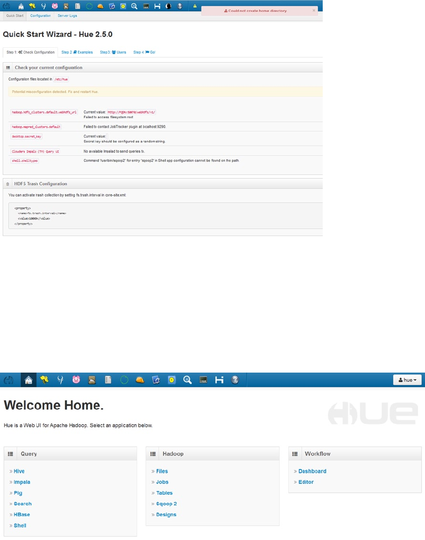
Chapter 7 ■ Monitoring Data

199

Most of the problems listed in Figure 7-1 relate to missing components (such as Impala not having been

installed) or a home directory not existing for the login account on Linux. Make sure that the home directories exist

and that there is a suitable environment shell file, such as .bashrc, set up for the account. Also, as stated earlier, make

sure that the account has a home directory on HDFS under /user. Finally, make sure that the Linux user ID number of

the Linux account is greater than 500 to avoid scripting errors in Hue.

If there are no errors, you will see the Home page for Hue (Figure 7-2), which is divided into three sections of

functions: those for Query, Hadoop, and Workflow. The same functions are displayed with icons across the top of the

Hue screen. In Figure 7-3, for example, the Home icon is highlighted.

Figure 7-1. The Hue Quick Start wizard

Figure 7-2. The Hue home page

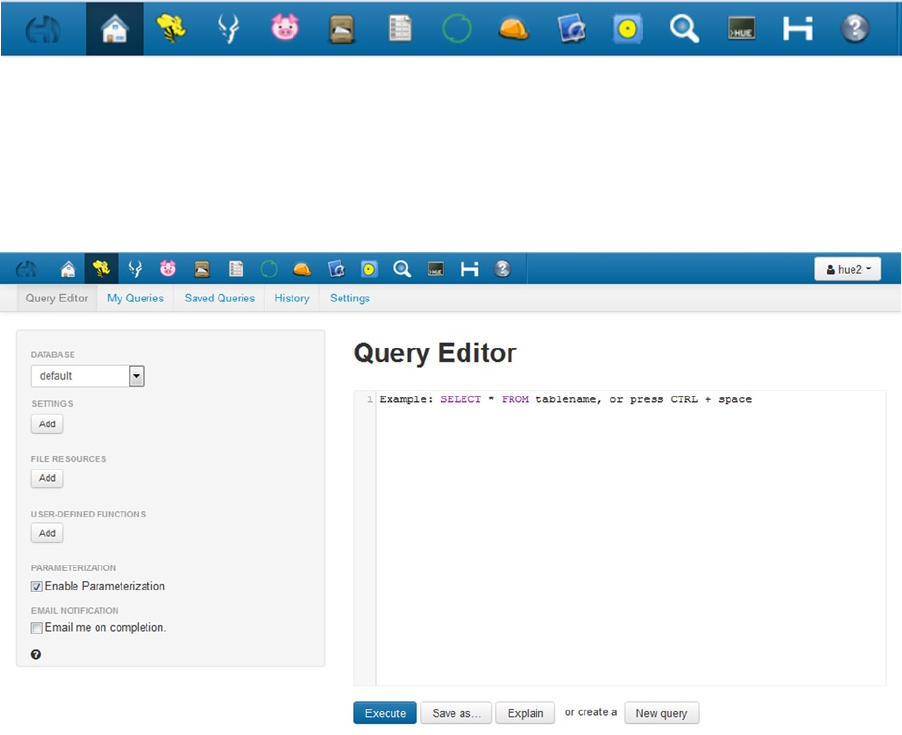
Chapter 7 ■ Monitoring Data

200

Next to the Home icon in Figure 7-3 you’ll see the Bee icon, which provides access to the Hive user interface,

shown in Figure 7-4. This page allows you to load and save Hive queries in Hive QL. It enables you to create queries

and choose which database to run them against. There is also an Explain option, which is similar to an Explain plan in

a relational database system, helping to describe how your query will run.

Figure 7-3. The Hue icons, with Home highlighted

Figure 7-4. The user interface for Hue Hive

The next icon is for access to Impala. (You’ll learn about using Impala via Hue in Chapter 9.) To the right of the

Impala icon is the Pig icon. Click it to see the Pig interface shown in Figure 7-5. In this color-coded Pig file editor you

can load and save Pig scripts, as well as examine logs and run Pig scripts. In addition, it includes a dashboard feature

to examine your running jobs.

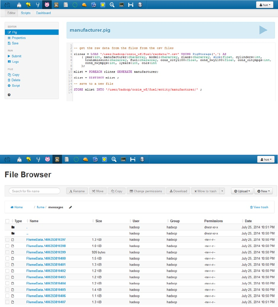
Chapter 7 ■ Monitoring Data

201

The next icon opens the HDSF browser (Figure 7-6). Here, you can upload and download files from the browser,

as well as rename, move, and delete those files. You can also change file permissions and navigate the file system via

clickable directory links. Clicking on a file link allows you to edit that file’s contents, as illustrated in Figure 7-7.

Figure 7-5. The Hue Pig editor

Figure 7-6. The Hue HDFS browser

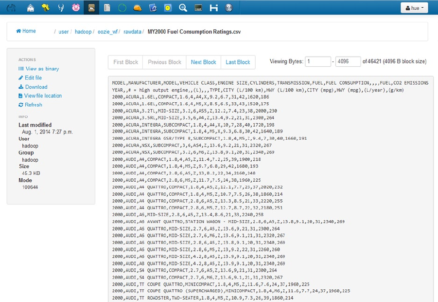
Chapter 7 ■ Monitoring Data

202

You can view file contents block by block, or you can edit the files by clicking the Edit option on the left. The

Actions list at the left also contains options to view the contents as binary and to download the file.

Following the HDFS Browser icon in the bar is the icon for the Metastore manager (Figure 7-8), which enables

you to navigate among your databases. Here, you can manage the databases and tables, as well as import data into

those tables. You can also sample table data to check on the content.

Figure 7-7. The Hue HDFS file editor

Chapter 7 ■ Monitoring Data

203

To the right once more is the icon for the Sqoop user interface (Figure 7-9), with which you can specify and run

Sqoop import and export jobs from Hue.

Figure 7-8. The Hue Metastore manager

Chapter 7 ■ Monitoring Data

204

An import job is specified in terms of its type, followed by where the data is coming from; in the case of Figure 7-9,

it’s mysql), as well as where the data is going to (HDFS, as shown in Figure 7-10).

Figure 7-9. The Hue Sqoop user interface

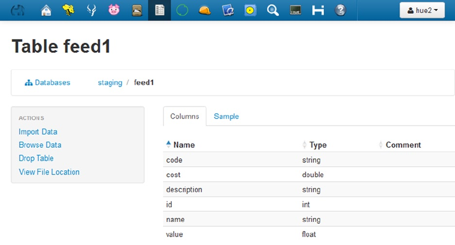
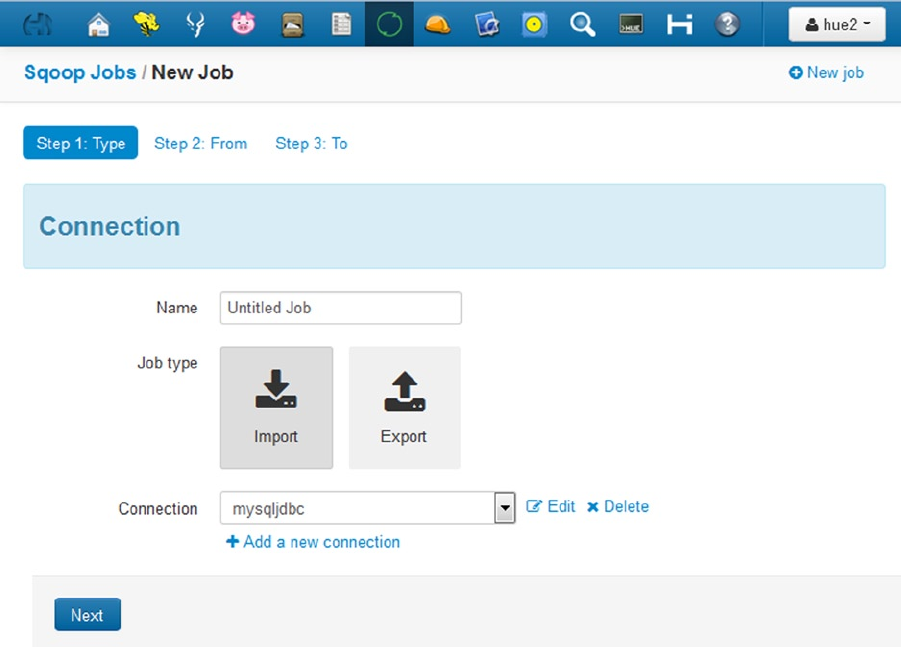
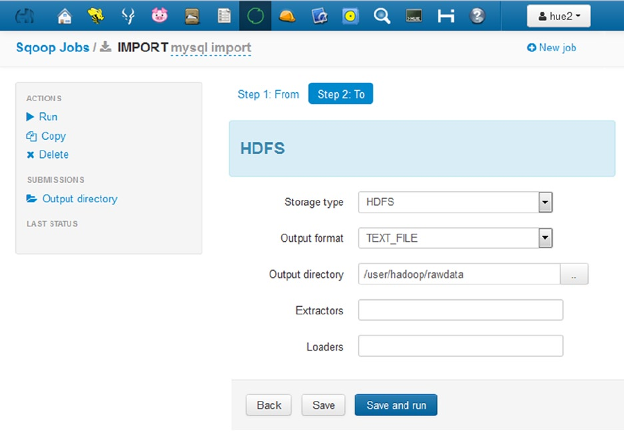
Chapter 7 ■ Monitoring Data

205

The next icon in the top bar, the Job Designer, allows you to create job actions of many different types, including

but not limited to Map Reduce, Pig, Hive, and Sqoop. You can design a job by adding properties and parameters and

then submit that job from the same interface. For example, Figure 7-11 shows a Sqoop action.

Figure 7-10. The Hue Sqoop user interface: output to HDFS

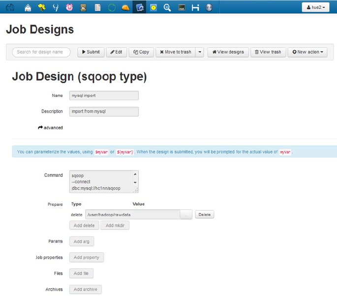
Chapter 7 ■ Monitoring Data

206

Continuing to the right in the top bar, the Oozie icon opens the Oozie workflow interface, which I feel is an

improvement on the default Oozie user interface. From here, you can filter the job list by job type and drill down into

workflows to see further details (Figure 7-12).

Figure 7-11. The Hue job designer: a Sqoop action

Chapter 7 ■ Monitoring Data

207

If you click the next icon, for Hue Shell, you get the option of performing a Pig, Sqoop2, or HBase shell that will

execute an adhoc script (Figure 7-13).

Figure 7-12. The Hue Oozie interface

Figure 7-13. The Hue shell: Pig Grunt

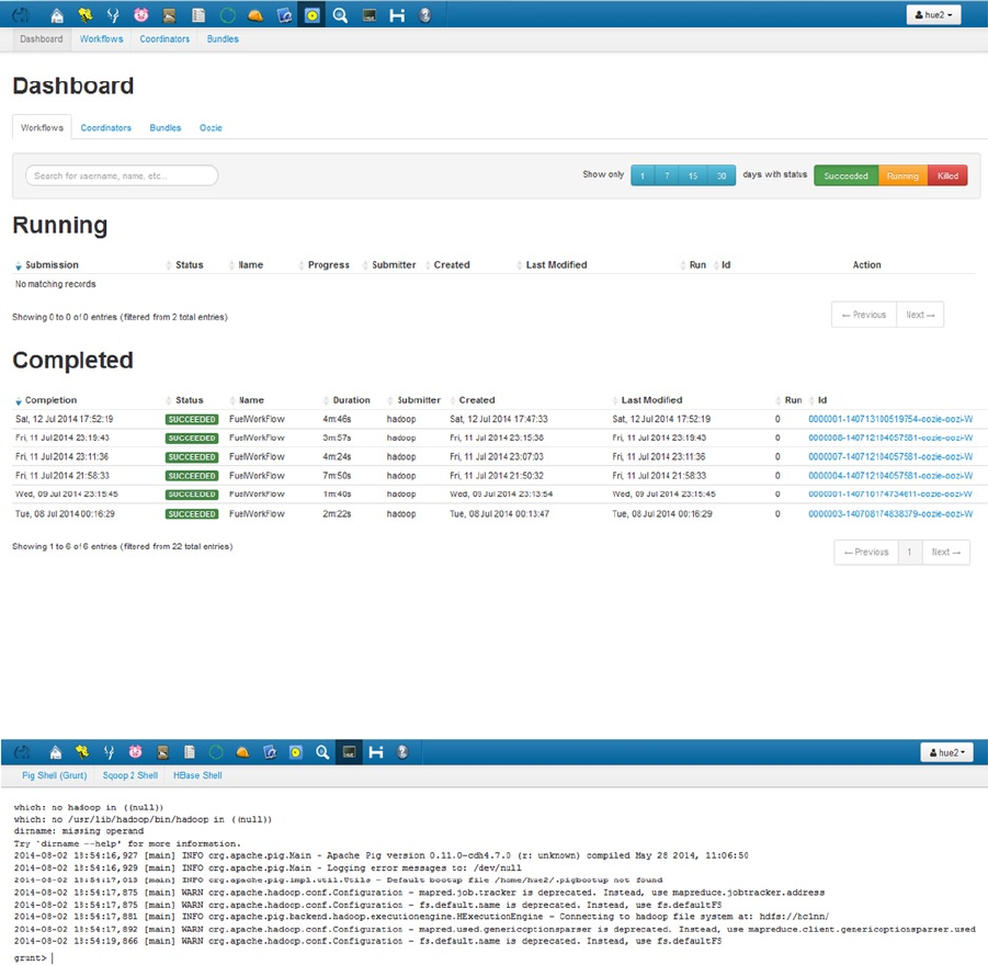
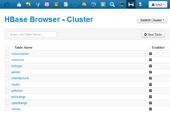
Chapter 7 ■ Monitoring Data

208

The next-to-last icon, which looks like an “H,” is for the HBase browser. Using this browser, you can examine

HBase tables, determine their structure, and manipulate their data. In addition, you can add rows or execute a bulk

upload of data (Figure 7-14).

Figure 7-14. The Hue HBase user interface

The right-most icon (the question mark) is the Hue help option, which is comprehensive. It has a series of sub-

help sections that include helpful topics on all of the Hadoop tools that have been integrated into Hue. If using Hue or

its components becomes unclear at any point, the Hue help pages are a good place to find extra information.

That completes a very quick tour of the Hue browser. It packs a lot of Hadoop functionality into a single user

interface, thereby enabling you to visually create and monitor Hadoop-based jobs and workflows from one interface.

What it doesn’t offer, however, is any low-level monitoring of system-level resources. For that, you need Ganglia and

Nagios. The next sections present these monitoring tools, which can be used with a pre-existing Hadoop cluster.

Ganglia

An open-source monitoring system released under a BSD license, Ganglia is designed for monitoring on distributed

high-performance systems. With Ganglia installed you can monitor a Hadoop-based cluster. The official Ganglia

website is ganglia.sourceforge.net. Ganglia has been integrated into the Ambari Hadoop cluster manager, which

you will examine in Chapter 8.

While Hue provided a single, web-based user interface for accessing Hadoop-based components, Ganglia offers

true monitoring functionality. For example, it is possible to set up graph-based dashboards in Ganglia that show the

state of Hadoop cluster resources. At a glance, it is possible to determine if there is a cluster problem at the present

time or there has been one during the lifetime of each graph. Also, it is possible to add graphs for multiple types of

resources on a single dashboard. (Ganglia will again be discussed in regard to the Ambari Cluster manager, in the next

chapter.)

Here, I first tell how to source and install Ganglia. I also discuss some of the errors that might be encountered.

Then, I discuss its user interface.

Chapter 7 ■ Monitoring Data

209

Installing Ganglia

To install Ganglia on Centos Linux, you first install the Epel repository so that you have a safe location for the Linux

yum command to source the software from. Be sure to execute the Epel repository steps on all Hadoop cluster nodes

to support the Ganglia install. For my example installation, I enable the Epel repository for Centos 6.x (on each node)

working in /tmp/epel:

[root@hc1nn ~]# cd /tmp ; mkdir epel ; cd epel

[root@hc1nn epel]# wget http://dl.fedoraproject.org/pub/epel/6/x86_64/epel-release-6-8.noarch.rpm

[root@hc1nn epel]# wget http://rpms.famillecollet.com/enterprise/remi-release-6.rpm

[root@hc1nn epel]# rpm -Uvh remi-release-6*.rpm epel-release-6*.rpm

When I check the downloaded files in /etc/yum.repos.d/, I see that four files have been sourced:

[root@hc1nn epel]# ls -1 /etc/yum.repos.d/epel* /etc/yum.repos.d/remi.repo

/etc/yum.repos.d/epel-apache-maven.repo

/etc/yum.repos.d/epel.repo

/etc/yum.repos.d/epel-testing.repo

/etc/yum.repos.d/remi.repo

Next, I enable the remi repository by editing the remi.repo file and setting Enabled to 1 in the [remi] section:

[root@hc1nn epel]# vi /etc/yum.repos.d/remi.repo

[remi]

name=Les RPM de remi pour Enterprise Linux 6 - $basearch

#baseurl=http://rpms.famillecollet.com/enterprise/6/remi/$basearch/

mirrorlist=http://rpms.famillecollet.com/enterprise/6/remi/mirror

enabled=1

Now, I am ready to install the Ganglia software on the Hadoop name node (in my example, this is hc1nn) and all

of the data nodes. I install the following packages on the Name Node server hc1nn, using the Linux yum command as

the root user:

yum install ganglia

yum install ganglia-gmetad

yum install ganglia-web

yum install ganglia-gmond

On the data nodes (hc1r1m1, hc1r1m2, hc1r1m3 ), I install the following components:

yum install ganglia

yum install ganglia-gmond

The Ganglia gmond processes will collect data and pass it to the gmetad process on hc1nn. I can then view the

data via the Ganglia web component. I must, however, tell Ganglia the frequency at which to collect the data. On

hc1nn, I specify the Ganglia data-collection frequency in the file gmetad.conf; in my example, I have set it to be two

minutes (120 seconds):

vi /etc/ganglia/gmetad.conf

data_source "my cluster" 120 hc1nn

Chapter 7 ■ Monitoring Data

210

In the same line, I named the cluster “my cluster” for purposes of Ganglia data collection. On the collector server

hc1nn, I set up the gmond.conf file using this name and the other parameters that follow, like this:

[root@hc1nn etc]# vi /etc/ganglia/gmond.conf

cluster {

name = "my cluster"

owner = "unspecified"

latlong = "unspecified"

url = "unspecified"

}

udp_send_channel {

mcast_join = hc1nn

port = 8649

}

udp_recv_channel {

port = 8649

}

tcp_accept_channel {

port = 8649

}

I then restart the collector and node daemons on the collector server hc1nn by using the Linux service

command:

service gmetad restart

service gmond restart

On each data node to be monitored (hc1r1m1, hc1r1m2, hc1r1m3), I set up the configuration of the Ganglia

gmond process by editing the gmond.conf file under /etc/ganglia:

[root@hc1r1m1 etc]# vi /etc/ganglia/gmond.conf

cluster {

name = "my cluster"

owner = "unspecified"

latlong = "unspecified"

url = "unspecified"

}

udp_send_channel {

mcast_join = hc1nn

port = 8649

}

Chapter 7 ■ Monitoring Data

211

Then I restart the Ganglia gmond server by using the Linux service command:

service gmond restart

I make sure that the httpd daemon is running on hc1nn; this supports the Ganglia web interface:

service httpd restart

Also, I make sure that selinux is disabled on all nodes by checking that the SELINUX value is set to the file /etc/

sysconfig/selinux. If this is not the case, then I will need to make the following change and restart my Linux servers:

[root@hc1nn ganglia]# vi /etc/sysconfig/selinux

SELINUX=disabled

Now I wait for the minimum monitoring interval of 120 seconds and attempt to access my Ganglia web interface

by using the URL http://<collector server>/ganglia/. For example, the name of my collector server is hc1nn, with

an IP address of 192.168.1.107, making the URL http://hc1nn/ganglia/.

At this point, I can enable Hadoop metrics collection on all Hadoop servers by editing the hadoop-metrics.

properties file in /etc/hadoop/conf.

[root@hc1r1m1 conf]# cd /etc/hadoop/conf

vi hadoop-metrics.properties

dfs.class=org.apache.hadoop.metrics.ganglia.GangliaContext

dfs.period=10

dfs.servers=localhost:8649

mapred.class=org.apache.hadoop.metrics.ganglia.GangliaContext

mapred.period=10

mapred.servers=localhost:8649

jvm.class=org.apache.hadoop.metrics.ganglia.GangliaContext

jvm.period=10

jvm.servers=localhost:8649

rpc.class=org.apache.hadoop.metrics.ganglia.GangliaContext

rpc.period=10

rpc.servers=localhost:8649

I restart the Hadoop cluster to make the changes take effect.

Chapter 7 ■ Monitoring Data

212

Potential Errors

Potential Ganglia errors can relate to the web server configuration, permissions, access, and Ganglia servers that

might be down. Here are some common error messages and some possible solutions.

For example, if you encounter an error like this on the Ganglia web page:

Not Found

The requested URL /ganglia was not found on this server.

Apache/2.2.15 (CentOS) Server at 192.168.1.107 Port 80

the solution is to edit the Ganglia web configuration file /etc/httpd/conf.d/ganglia.conf and change the Deny line to an

Allow line. The # character comments out a line so that the httpd web server will ignore that line:

#Deny from all

Allow from all

Then you can restart the httpd service on the server hc1nn by using the Linux service command as the Linux

root user:

service httpd restart

Displayed on the Ganglia web user interface, an error like the following implies that the SELINUX option needs to

be disabled on the cluster:

There was an error collecting ganglia data (127.0.0.1:8652): fsockopen error: Permission denied

This means that Ganglia is not compatable with the option enabled. You edit the file /etc/sysconfig/selinux and

set the SELINUX option to the value disabled. You will need to do this as the Linux root user account and restart each

server afterwards. If you’re in doubt, consult a systems administrator; otherwise, use the following command:

[root@hc1nn ganglia]# vi /etc/sysconfig/selinux

SELINUX=disabled

If an error like this occurs in the /var/log/messages file:

Aug 16 17:12:52 hc1nn /usr/sbin/gmetad[4575]: Please make sure that /var/lib/ganglia/rrds is owned

by ganglia

then the directory mentioned, /var/lib/ganglia/rrds, is not owned by the Linux ganglia user account. Check the

ownership of the directory by using the Linux ls long listing and it will show that it is owned by “nobody.” You can

reset ownership recursively using the Linux chmod -R command:

[root@hc1nn log]# ls -ld /var/lib/ganglia/rrds

drwxrwxrwx. 4 nobody root 4096 Aug 16 15:06 /var/lib/ganglia/rrds

[root@hc1nn log]# chown -R ganglia /var/lib/ganglia/rrds

Next, you restart the Ganglia servers on the data collector server hc1nn:

service gmetad restart

service gmond restart

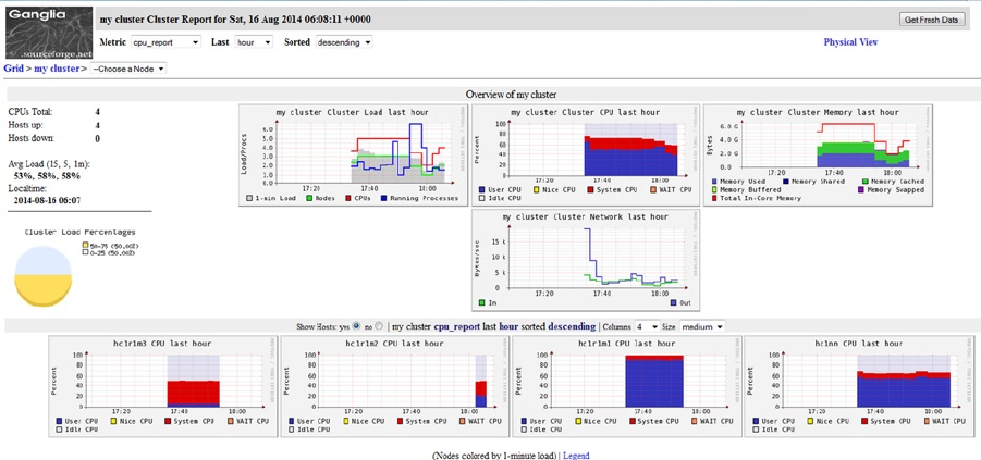
Chapter 7 ■ Monitoring Data

213

If you see an error similar to the following in the /var/log/messages file:

Aug 16 17:28:55 hc1nn /usr/sbin/gmetad[7861]: data_thread() got no answer from any [my cluster]

datasource

check on each server that the Ganglia gmond processes are running. If necessary, restart them using the Linux

service command as the root user:

service gmond restart

The Ganglia Interface

The Ganglia cluster web interface offers an overview of the cluster and a series of clickable icons that represent each

server in the cluster that has been configured to collect data. Figure 7-15 shows the default CPU-based display of the

cluster.

Figure 7-15. Ganglia overview display

In Figure 7-15, notice the Get Fresh Data button (top right) for refreshing your data and the Metric drop-down

menu (top left), from which you can choose to display network, packets, memory, and load information. The visual

display of server states enables you to drill down into those servers that appear to be taking the greatest load. For

example, click on the Name Node display (hc1nn), and you’ll get a detailed display for that server. As you can see in

Figure 7-16, the display provides information about the Ganglia processes, such as when they started and how long they

have been running. It also provides information about the server's memory and CPU configuration. Click the images on

the right of the screen to reveal detailed graphs for the server's load, memory, CPU, network, and packet usage.

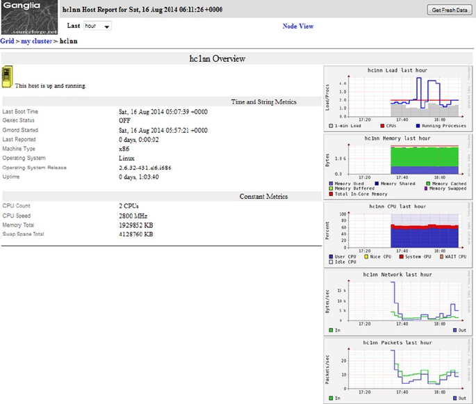
Chapter 7 ■ Monitoring Data

214

The second half of the screen, shown in Figure 7-17, contains a large number of sections and resource graphs.

Because there are so many available, I have selected just a few to display here. However, each is composed of CPU,

disk, load, memory, network, and process graphs. Each category of function being monitored has a number of

aspects: for instance, CPU shows system user and input/output characteristics.

Figure 7-16. Ganglia node display

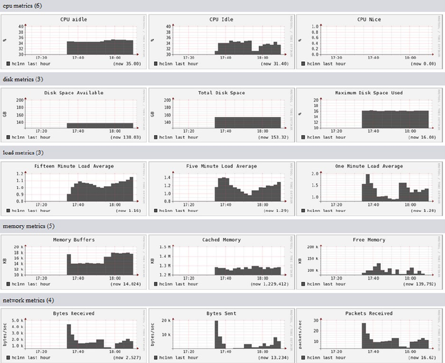
Chapter 7 ■ Monitoring Data

215

While this multitude of resource graphs may be bewildering at first, it does present a wide range of possible

features that Ganglia can be used to monitor. It should be obvious that Ganglia provides suitable functionality to

monitor a Hadoop cluster. Check websites like ganglia.sourceforge.net for further information. Also, try installing

Ganglia yourself and compare the graphs that it produces by default against your own Hadoop cluster.

This chapter also presents the Nagios monitoring system. Nagios extends the possibilities for system monitoring

by providing the ability to create alerts based on the problems that it finds.

Nagios

Nagios is an open-source cluster monitoring system that is available from Nagios Enterprises (www.nagios.org).

While systems like Ganglia offer a wide range of monitoring graph options, the Nagios monitoring system provides

the ability to monitor cluster server attributes and create alerts when problems occur. Nagios has a similar structure to

Ganglia, in that it has a Nagios Master server and client (nrpe) programs. In this section, I show how it can be sourced,

installed, configured, and used to monitor alerts.

Figure 7-17. Ganglia node display

Chapter 7 ■ Monitoring Data

216

It is important to reiterate Nagios’s alerting capability because not only can you determine that there is a problem

but you can also create an automatic alert and raise awareness of the issue. So, the combination of Ganglia and Nagios

for system monitoring is a highly functional duo. Nagios alerts you to a problem while Ganglia provides a color-coded

graph to display the problem. A typical problem might be that Hadoop has run out of memory or disk space. Now, you

can be alerted to the problem and assess the potential solutions.

Installing Nagios

To demonstrate how to install Nagios, I place the Nagios server on the name node, hc1nn, and the Nagios clients on all

of the servers so that the whole cluster will be monitored and the Nagios map (more on this in a moment) will contain

the entire cluster. So, on hc1nn, I install the following servers via the Linux yum command as root:

[root@hc1nn ~]# yum install nagios

[root@hc1nn ~]# yum install nagios-plugins-all

[root@hc1nn ~]# yum install nagios-plugins-nrpe

[root@hc1nn ~]# yum install nrpe

In your installation, you will also need the php and httpd components, which you probably already have

installed. When you execute the following commands, you will receive a “Nothing to do” message if the components

are already installed:

[root@hc1nn ~]# yum install php

[root@hc1nn ~]# yum install httpd

I use the chkconfig command to configure these servers (httpd, nrpe, and Nagios) to start when the server hc1nn

is rebooted. The Nagios server uses the nrpe components on each machine, which in turn use the Nagios plug-ins to

monitor different features, like hosts, devices, and services:

[root@hc1nn ~]# chkconfig httpd on

[root@hc1nn ~]# chkconfig nagios on

[root@hc1nn ~]# chkconfig nrpe on

Now, I install the the following Nagios components on the data nodes (hc1r1m1, hc1r1m2, hc1r1m3) by using the

Linux yum command as root:

[root@hc1nn ~]# yum install nagios

[root@hc1nn ~]# yum install nagios-plugins-all

[root@hc1nn ~]# yum install nrpe

[root@hc1nn ~]# chkconfig nrpe on

On the name node, I set the password for the Nagios administration account, nagiosadmin. I will use this account

and password combination to access the Nagios web browser:

[root@hc1nn ~]# htpasswd -c /etc/nagios/passwd nagiosadmin

Chapter 7 ■ Monitoring Data

217

Thus, I can access the web browser via a URL in this form: http://hc1nn/nagios.

My example uses the name of the name node in my cluster, but it won’t be accesssible until the Nagios server

is started after the configuration has been finalized. Therefore, on the Name Node server hc1nn, I edit the file /etc/

nagios/nagios.cfg, which is the configuration file for the central Nagios server component. I comment out the line that

defines the cfg_file value for localhost (I will later define each of the cluster servers explicitly.)

#cfg_file=/etc/nagios/objects/localhost.cfg

In the same file on hc1nn, I use the cfg_dir attribute to specify the directory location where Nagios will look for

the configuration files:

[root@hc1nn nagios]# grep "^cfg_dir" /etc/nagios/nagios.cfg

cfg_dir=/etc/nagios/conf.d

I go to this location and create empty configuration files for each of the servers in the cluster by using the Linux

touch command:

[root@hc1nn nagios]# cd /etc/nagios/conf.d

[root@hc1nn conf.d]# touch hc1r1m1.cfg

[root@hc1nn conf.d]# touch hc1r1m2.cfg

[root@hc1nn conf.d]# touch hc1r1m3.cfg

[root@hc1nn conf.d]# touch hc1nn.cfg

The contents of each of the server configuration files mirrors the following listing (to which I added line numbers

for easy reference). The important parts of a single server configuration file—in this case, hc1nn.cfg—are described

below. The file sections have been listed along with some text to describe their function. The sum of the numbered

configuration file parts forms a whole that Nagios uses to monitor and alert on a server.

The first entry defines the server details, while the later ones define such services as ping, ssh, and load. For

example, the host definition defines the hostname and its alias, plus its IP address:

1 define host {

2 use linux-server

3 host_name hc1nn

4 alias hc1nn

5 address 192.168.1.107

6 }

Each of the file’s remaining entries define the services available to Nagios on the server. Notice that they take

advantage of the terms “generic-service” and “local-service.” These terms are templates specified in the file /etc/

nagios/objects/templates.cfg, and they provide a way of using pre-defined attributes for the service. For example, the

check_ping service (lines 8 to 13) defines the hostname to ping, hc1nn. In addition, it specifies an average roundtrip

time of 100 milliseconds and a packet loss of 20 percent will produce a warning message. A roundtrip time of 500

milliseconds and a packet loss of 60 percent will trigger a critical error. The commands referred to in the

check_command line (i.e., check_ping) are further defined in the file /etc/nagios/objects/commands.cfg.

8 define service {

9 use generic-service

10 host_name hc1nn

11 service_description PING

12 check_command check_ping!100.0,20%!500.0,60%

13 }

Chapter 7 ■ Monitoring Data

218

The rest of the configuration file contains a list of services defined for the server—in this case, hc1nn.

Although space prevents me from explaining every service definition, you can find details at

http://nagios.sourceforge.net/docs.

15 define service {

16 use generic-service

17 host_name hc1nn

18 service_description SSH

19 check_command check_ssh

20 notifications_enabled 0

21 }

22

23 define service {

24 use generic-service

25 host_name hc1nn

26 service_description Current Load

27 check_command check_local_load!5.0,4.0,3.0!10.0,6.0,4.0

28 }

29

30 ##### extra checks

31

32 define service{

33 use local-service

34 host_name hc1nn

35 service_description Root Partition

36 check_command check_local_disk!20%!10%!/

37 }

38

39 define service{

40 use local-service

41 host_name hc1nn

42 service_description Current Users

43 check_command check_local_users!20!50

44 }

45

46 define service{

47 use local-service

48 host_name hc1nn

49 service_description Total Processes

50 check_command check_local_procs!250!400!RSZDT

51 }

I used the file /etc/nagios/objects/localhost.cfg as a template for each server configuration file, simply by

changing the server name and IP address for each to match the corresponding server. These files give Nagios a map of

servers that it needs to do the monitoring.

With the service configuration files finished, I configure the nrpe.cfg file on each server under /etc/nagios. The

nrpe (Nagios remote plugin executor) process on each host executes the Nagios plug-ins:

vi /etc/nagios/nrpe.cfg

Chapter 7 ■ Monitoring Data

219

In the file, I find the allowed_hosts line and change the server name to indicate which of my servers are allowed

to contact nrpe; for example, I use the following:

allowed_hosts=hc1nn

Also, I add the following command lines to each nrpe.cfg file to define which service commands will be used to

monitor each server—specifically, which check will be carried out on users, loads, disks (/ and /home), and processes:

command[check_users]=/usr/lib/nagios/plugins/check_users -w 5 -c 10

command[check_load]=/usr/lib/nagios/plugins/check_load -w 15,10,5 -c 30,25,20

command[check_root]=/usr/lib64/nagios/plugins/check_disk -w 20% -c 10% -p /

command[check_home]=/usr/lib64/nagios/plugins/check_disk -w 20% -c 10% -p /home

command[check_zombie_procs]=/usr/lib/nagios/plugins/check_procs -w 5 -c 10 -s Z

command[check_total_procs]=/usr/lib/nagios/plugins/check_procs -w 150 -c 200

Now I am ready to start the Nagios servers. On each machine, I start the nrpe server as the Linux root user using

the service command :

[root@hc1nn ~]# service nrpe start

On the name node (hc1nn), I start the httpd and Nagios servers:

[root@hc1nn ~]# service httpd start

[root@hc1nn ~]# service nagios start

Potential Errors

Error messages may be generated while you are installing and trying to run Nagios. For instance, you might see the

following:

error: Starting nagios:CONFIG ERROR! Start aborted. Check your Nagios configuration.

This error may be due to a “hostgroup” entry in the Nagios configuration file. In this case, Nagios won’t start and

there are no log files.

First determine what the error is, then use the Linux which command to determine where the Nagios executable

resides. Run that Nagios executable under /usr/sbin/nagios with a –v parameter and the full path to the Nagios

configuration file. The –v option verifies the configuration file before starting, and so provides extra logged output, as

follows:

which nagios

/usr/sbin/nagios

/usr/sbin/nagios –v /etc/nagios/nagios.cfg

This provides details of a configuration error message, which states that a hostgroup in the configuration file is

incorrect. You comment out this section (with # characters at line position 0) and restart Nagios.

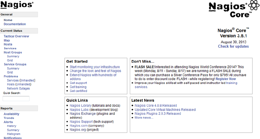
Chapter 7 ■ Monitoring Data

220

The Nagios Interface

With your servers up and running, the Nagios web interface is available at http://hc1nn/nagios/. The home page is

shown in Figure 7-18.

Figure 7-18. Nagios home page

For my example, I can click the Map option on the left of the home page to see the Nagios cluster map showing

the server objects that were created under /etc/nagios/conf.d on hc1nn (bottom right of Figure 7-19). I select a server

icon (such as for hc1nn) in the Nagios map to display the details for that server, as shown on the left of Figure 7-19.

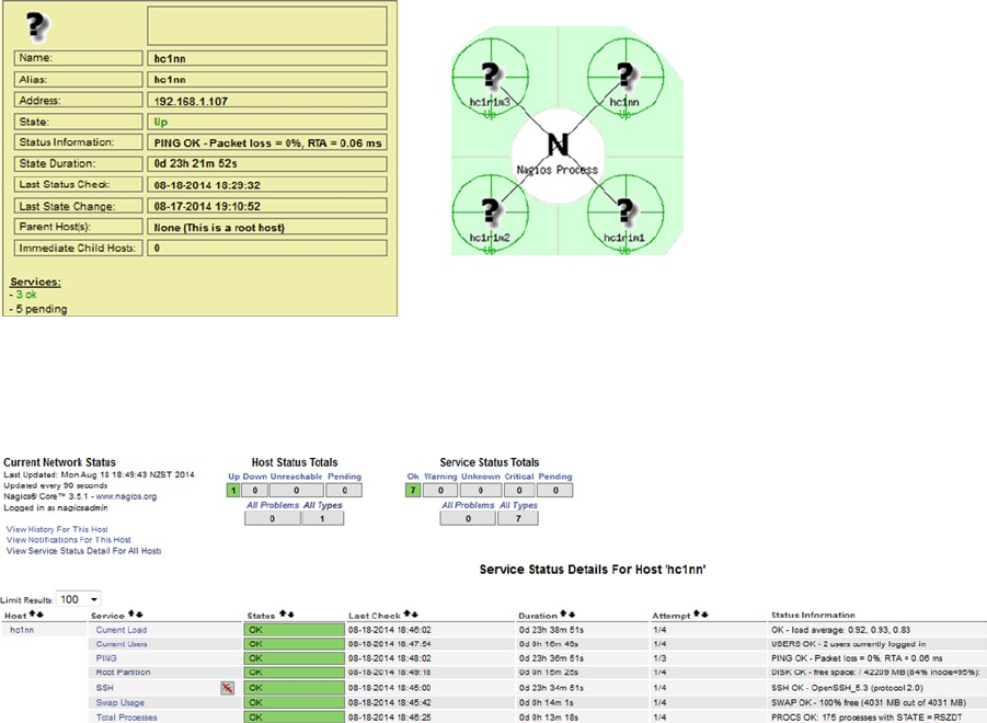
Chapter 7 ■ Monitoring Data

221

Figure 7-19. Nagios map display

If I click one of the servers in the map to drill down to determine server status, I get the results shown in Figure 7-20.

Figure 7-20. Nagios server details

The Nagios display follows a traffic light system: green is good, warnings are yellow, and errors are red. Clicking

the root partition service, as shown in Figure 7-20, allows you to drill down further to determine service details, as

shown in Figure 7-21.

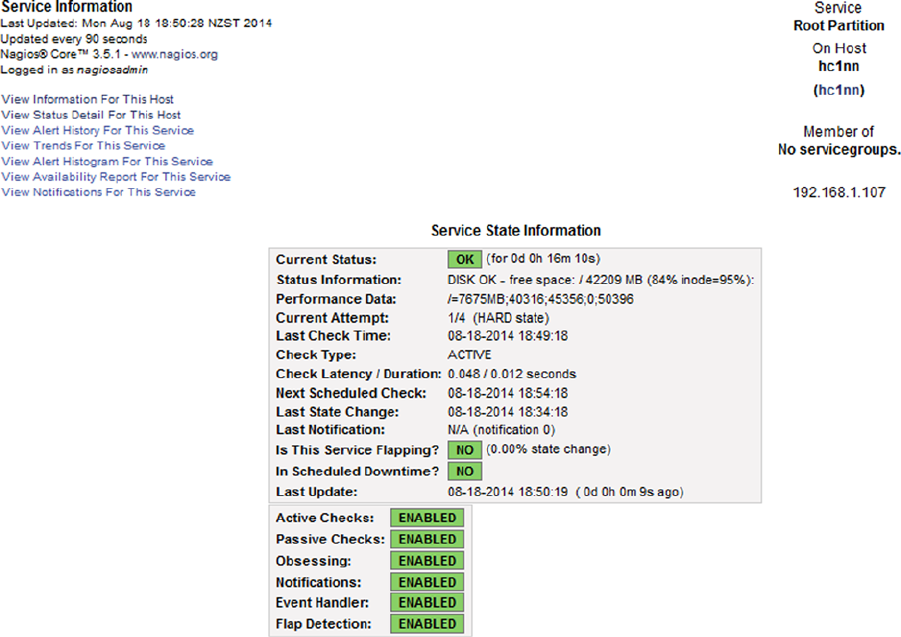
Chapter 7 ■ Monitoring Data

222

To demonstrate what a warning alert looks like, I changed the hc1nn.cfg configuration file on the server hc1nn,

defining the root parition check_command line to provide a warning if free space reaches 90 percent. (A silly measure,

I know, but it will show what a warning alert looks like.)

define service{

use local-service

host_name hc1nn

service_description Root Partition

check_command check_local_disk!90%!10%!/

}

I then saved the configuration file and restarted the Nagios server to pick up the changes:

[root@hc1nn ~]# service nagios restart

Not surprisingly, at the next scheduled check, the alert shown in Figure 7-22 was raised, stating that the root

partition contained less than 90 percent free space.

Figure 7-21. Details of the Nagios root partition

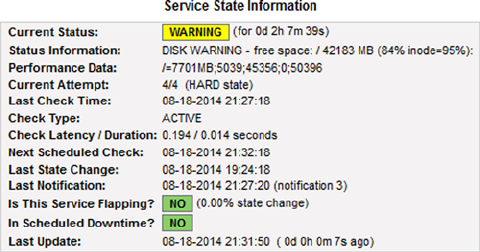
Chapter 7 ■ Monitoring Data

223

Figure 7-22. Nagios root partition alert

This is an example of a monitored alert that could enable critical intervention when your Hadoop cluster

resources become limited. Monitoring and alerting on Hadoop cluster resources should be a mandatory

consideration when you are setting up a cluster yourself.

A combination of Naios and Ganglia could be used on the Hadoop cluster to provide a rich selection of historical

graphs and alerts. Nagios could trigger an alert for Hadoop cluster resources as those resources run low; then Ganglia

could examine the graphs that have recorded the condition of the resources over time.

Summary

This chapter discussed three major enhancements for Hadoop functionality. Hue provides a central location for

scripting and Hadoop-based job monitoring. Through Hue, you can inspect Hive and HBase databases and can

manipulate their data. Hue also offers the ability to visually browse the Hadoop file system HDFS.

Although Hue consolidates Hadoop fuctionality and access into one useful interface, it isn’t a full-scale

monitoring system. (For instance, it doesn’t have the ETL or reporting functionality of Pentaho or Talend, which

are covered in Chapters 10 and 11.) To supplement Hue, Ganglia and Nagios offer cluster monitoring. When used

together, Nagios and Ganglia complement each other: Nagios alerts the user to potential problems, while Ganglia

provides graph-based details to show what has happened, on which server and its type. This combined action will

help in problem investigation before system failure.

225

Chapter 8

Cluster Management

From its inception, Hadoop has been progressing and evolving to help you more easily manage your big data needs.

Compared to version 1, installation of Hadoop V2 via Cloudera's version 4.x stack was an advance; Hadoop tool

binaries were configured as Linux services and Hadoop’s tool-related logging and functionality were moved to logical

places within the Linux file system. The progression continues with the move to cluster managers, which consolidate

all of the tools examined thus far in this book into a single management user interface. Cluster managers automate

much of the difficult task of Hadoop component installation—and their configuration, as well.

This chapter examines Apache Ambari and the Cloudera Cluster Manager, two of several Hadoop cluster

managers that enable you to install the whole Hadoop stack in one go. Management systems like Ambari also use

cluster monitoring tools like Ganglia and Nagios to provide a user interface for management and monitoring within

a single system. In addition, in this chapter you’ll learn about the Apache Bigtop tool, with which you can install the

whole stack, as well as run smoke tests during the installation to test the stack operation.

Although the installation of these components will include the whole Hadoop stack, this chapter primarily

demonstrates the ease of use and overall functionality of the installation systems themselves. (I would need an entire

book to cover each piece of subfunctionality within the Hadoop server stack.) Consider this chapter a snapshot of the

current systems and their functionality. Which system is best for your purposes is a question you can answer only after

matching your needs to their capabilities.

Because systems like Ambari install the whole Hadoop cluster, they are not compatible with pre-existing Hadoop

installs, and therefore they cannot use the same set of servers, as were discussed in earlier chapters (hc1nn for the

name node and hc1r1m1 to hc1r1m3 for the data nodes). For this chapter’s example, I install the cluster on a new set

of 64-bit machines but I preserve the work to date on the old set of machines whose Name Node server was called

hc1nn. The new Name Node server is called hc2nn, and the four data nodes are called hc2r1m1, hc2r1m2, hc2r1m3,

and hc2r1m4. As for the original servers, the “h” in these server names stands for Hadoop, the “c” indicates the cluster

number, the “r” represents the rack number in the cluster, and the “m” represents the machine number within the

Hadoop cluster rack. So, hc2nn is the Name Node server for Hadoop cluster 2. The server hc2r1m4 is the number 4

machine in rack 1 for Hadoop cluster 2. Also, because the systems examined in this chapter are intended for fresh

servers, I reinstall Centos 6 on each machine prior to sourcing each system.

Initially, I install the Ambari Hadoop cluster manager. You will note that I am sourcing Ambari from the

Hortonworks site, so I use it to install the latest Hortonworks Hadoop stack. If you have attempted all of the Hadoop

tool installations up to this point in the book, you will have discovered that Hadoop installations and the necessary

configuration are time-consuming and can be difficult. You may encounter errors that take a lot of time to solve. You

might also find that versions of the components will not work with one another. But at this point, all you really want to

do is use the software.

This is where cluster managers become useful: they automate the installation and configure the Hadoop

cluster and the Hadoop tool set. They provide wizards that advise you when you need to make changes. They have

monitoring tools to automatically check the health of your Hadoop cluster. They also offer a means to continuously

upgrade the Hadoop stack.

CHAPTER 8 ■ CLUSTER MANAGEMENT

226

The Cloudera cluster manager is Cloudera’s own Hadoop cluster manager release, while the Ambari tool is

actually an Apache project. Hortonworks has used Ambari as the mechanism to both release and manage its Hadoop

stack. Given that Cloudera and Hortonworks are two of the best-known Hadoop stack suppliers, it is their cluster

managers that I have chosen to source and install here.

As a last thought before launching into the installation of Ambari, I mention that there are licensing fees

associated with these releases of Hadoop cluster manager. However, the costs are easily offset by the savings in time

and trouble when big problems can be avoided.

The Ambari Cluster Manager

Although Ambari can be used to install many different Hadoop stacks, and is a top-level Apache project in its own

right, I install only the latest HDP stack to demonstrate its functionality. As in prior chapters, I use an example

installation to show how it’s accomplished. I start by sourcing the Ambari code and install the Ambari agents and

server on the new cluster nodes: hc2nn (the Name Node server) and hc2r1m1 through hc2r1m4 (four data nodes).

Note ■ For the latest information on Ambari and up-to-date release documentation, see the official Apache Software

Foundation Ambari website at http://ambari.apache.org/.

Ambari Installation

To install the latest Hortonworks Ambari release, I first install a Hortonworks Centos 6 repository to match the version

of CentOS that is installed, by running the following commands as root:

[root@hc2nn /]# cd /etc/yum.repos.d/

[root@hc2nn yum.repos.d]# wget http://public-repo-1.hortonworks.com/ambari/centos6/1.x/

updates/1.6.1/ambari.repo

The wget command downloads the ambari.repo file to the directory /etc/yum/yum.repos.d. Now, I use the Linux

yum command to install the Ambari server on the Name Node server hc2nn:

[root@hc2nn yum.repos.d]# yum install ambari-server

I run the Ambari server setup command as root to configure the Ambari server component:

[root@hc2nn yum.repos.d]# ambari-server setup

Using python /usr/bin/python2.6

Setup ambari-server

Checking SELinux...

SELinux status is 'enabled'

SELinux mode is 'enforcing'

Temporarily disabling SELinux

WARNING: SELinux is set to 'permissive' mode and temporarily disabled.

OK to continue [y/n] (y)? y

Customize user account for ambari-server daemon [y/n] (n)? y

Enter user account for ambari-server daemon (root):

Adjusting ambari-server permissions and ownership...

CHAPTER 8 ■ CLUSTER MANAGEMENT

227

Checking iptables...

WARNING: iptables is running. Confirm the necessary Ambari ports are accessible. Refer to the Ambari

documentation for more details on ports.

OK to continue [y/n] (y)?

Checking JDK...

[1] - Oracle JDK 1.7

[2] - Oracle JDK 1.6

[3] - Custom JDK

At this point, I choose option 3 for the Java JDK because I have already installed the openJDK on these servers

and I am familiar with its use.

Enter choice (1): 3

WARNING: JDK must be installed on all hosts and JAVA_HOME must be valid on all hosts.

WARNING: JCE Policy files are required for configuring Kerberos security. If you plan to use

Kerberos,please make sure JCE Unlimited Strength Jurisdiction Policy Files are valid on all hosts.

Path to JAVA_HOME: /usr/lib/jvm/java-1.6.0-openjdk-1.6.0.0.x86_64

Validating JDK on Ambari Server...done.

Completing setup...

Configuring database...

Enter advanced database configuration [y/n] (n)?

Default properties detected. Using built-in database.

Checking PostgreSQL...

Running initdb: This may take upto a minute.

Initializing database: [ OK ]

About to start PostgreSQL

Configuring local database...

Connecting to local database...done.

Configuring PostgreSQL...

Restarting PostgreSQL

Ambari Server 'setup' completed successfully.

Whichever JDK option you choose, if the last line of the setup output indicates that the setup is successful, you

can start the Ambari server as root. I do just that, as follows:

ambari-server start

Using python /usr/bin/python2.6

Starting ambari-server

Ambari Server running with 'root' privileges.

Organizing resource files at /var/lib/ambari-server/resources...

Waiting for server start...

Server PID at: /var/run/ambari-server/ambari-server.pid

Server out at: /var/log/ambari-server/ambari-server.out

Server log at: /var/log/ambari-server/ambari-server.log

Ambari Server 'start' completed successfully.

I can now access the Ambari web-based user interface via the Name Node server name and port number 8080:

http://hc2nn:8080

CHAPTER 8 ■ CLUSTER MANAGEMENT

228

The default login account is called “admin” with a password of “admin.” When I log in, the Ambari installation

wizard will start automatically and guide me through the installation.

From the Ambari installation wizard, I set the cluster name and select the installation stack. For my example,

I name the cluster “cluster2” and I select HDP 2.1, the lastest installation stack. Next, I specify the server names on

which to install, making sure to use FQDNs (fully qualified domain names). So, instead of specifying the server short

name of “hc2nn,” I use hc2nn.semtech-solutions.co.nz. When I check the hostnames, Ambari does the equivalent of

the Linux hostname –f command to determine the FQDN; if I hadn’t used FQDNs, this check would fail. My server list

now looks like this:

hc2nn.semtech-solutions.co.nz

hc2r1m1.semtech-solutions.co.nz

hc2r1m2.semtech-solutions.co.nz

hc2r1m3.semtech-solutions.co.nz

hc2r1m4.semtech-solutions.co.nz

If at this point in your own installation you encounter the following permission-based error, you can install

the Ambari agent manually. This error message is probably related to SELinux and the file labeling used by SSH

(secure shell).

Permission denied (publickey,gssapi-keyex,gssapi-with-mic,password).

A manual installation of the Ambari agent on each node is a workaround for this problem. Then, you would just

be manually installing a component that Ambari has not been able to install automatically. Once you have done this

manually, Ambari will complete the cluster installation for you.

If this error is encountered follow these steps; make sure that the Ambari Centos 6 repository is installed on each

machine:

cd /etc/yum.repos.d/

wget http://public-repo-1.hortonworks.com/ambari/centos6/1.x/updates/1.6.1/ambari.repo

Next, I use the Linux yum command as root to install the Ambari agent on each machine, as follows:

yum install ambari-agent

I edit the Ambari configuration file and set the server hostname to be the fully qualified name of the server:

vi /etc/ambari-agent/conf/ambari-agent.ini

hostname=hc2nn.semtech-solutions.co.nz

To register the Ambari machines, I install the Linux time service ntpd on all servers I intend to use. I use the Linux

yum command as root to install the ntp servers and documentation, and I set the server to start at boot time:

yum install ntp ntpdate ntp-doc

chkconfig ntpd on

Next, I initialize and start the ntpd server:

ntpdate pool.ntp.org

service ntpd start

CHAPTER 8 ■ CLUSTER MANAGEMENT

229

Now, I restart the Ambari agent as the root user:

ambari-agent restart

When the agent starts, it registers with the server so that the server has a list of the agent hostnames. I can check

this list by using the curl command and see all the fully qualified server names I have previously specified. For

example, the following curl command accesses the Ambari server URL by using the username and password admin

provided by the -u option. It requests a list of hosts from the server, which is displayed as shown here. For instance, I

ran this command as the Linux root user from the cluster2 Name Node machine hc2nn:

[root@hc2nn ~]# curl -u admin:admin http://hc2nn:8080/api/v1/hosts

{

"href" : "http://192.168.1.103:8080/api/v1/hosts",

"items" : [

{

"href" : "http://192.168.1.103:8080/api/v1/hosts/hc2nn.semtech-solutions.co.nz",

"Hosts" : {

"host_name" : "hc2nn.semtech-solutions.co.nz"

}

},

{

"href" : "http://192.168.1.103:8080/api/v1/hosts/hc2r1m1.semtech-solutions.co.nz",

"Hosts" : {

"host_name" : "hc2r1m1.semtech-solutions.co.nz"

}

},

{

"href" : "http://192.168.1.103:8080/api/v1/hosts/hc2r1m2.semtech-solutions.co.nz",

"Hosts" : {

"host_name" : "hc2r1m2.semtech-solutions.co.nz"

}

},

{

"href" : "http://192.168.1.103:8080/api/v1/hosts/hc2r1m3.semtech-solutions.co.nz",

"Hosts" : {

"host_name" : "hc2r1m3.semtech-solutions.co.nz"

}

},

{

"href" : "http://192.168.1.103:8080/api/v1/hosts/hc2r1m4.semtech-solutions.co.nz",

"Hosts" : {

"host_name" : "hc2r1m4.semtech-solutions.co.nz"

}

]

}

If the full list of server names in this output looks correct, I return to the Ambari user interface and manually

register the agent servers. I can see that all of the servers in cluster2 are listed in the output of the curl command just

given. Figure 8-1 shows notification of a successful registration.

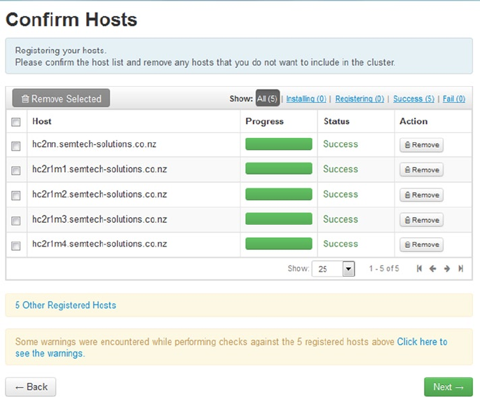
CHAPTER 8 ■ CLUSTER MANAGEMENT

230

I click Next to access the Assign Master window. I keep the default settings here, because the Name Node server

was set as hc2nn and components like Oozie are on a different server, which is hc2r1m1. I click Next again to set up

the slaves and clients. As shown in Figure 8-2, this window defines which servers will be data nodes, node managers,

and region servers, and so on. For my configuration, all of the non-Name Node (hc2nn) machines are set as data

nodes and they all have clients.

Figure 8-1. Ambari server registration

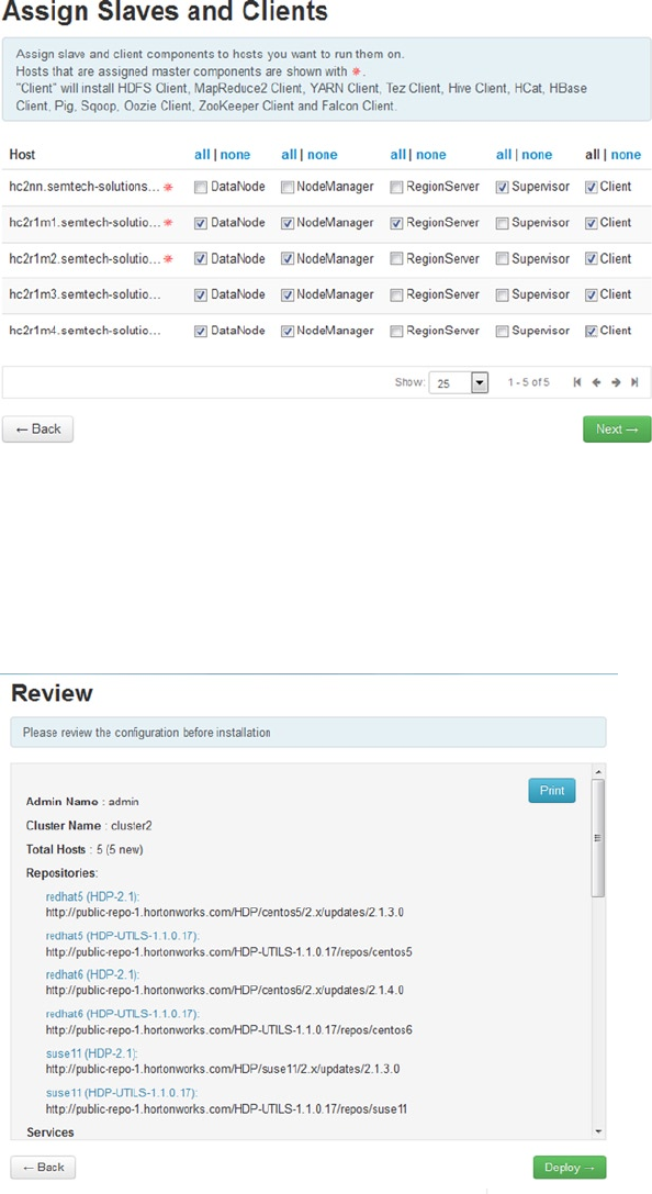
CHAPTER 8 ■ CLUSTER MANAGEMENT

231

Clicking Next once more brings me to the Customize Services window, where I again use the defaults. Here also I

can specify the passwords for the databases and monitoring. I specify passwords for Hive and Oozie, as well as a Nagios

monitoring admin password and email address. I click Next to proceed to the Review Configuration window, as shown

in Figure 8-3. At this stage, I am able to check the configuration that is going to be installed on my Hadoop cluster.

Figure 8-2. List of Ambari slaves and clients

Figure 8-3. Ambari window for reviewing the configuration

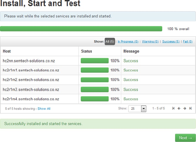
CHAPTER 8 ■ CLUSTER MANAGEMENT

232

I take the time to go through the configuration list to be sure that I am happy both with what is going to be

installed and with the servers on which everything will be installed.

In the Review Configuration window, I click Deploy to move to the next page. The next window gives me a list

of components that will be installed. I select Next to start the installation, which takes around 30 minutes. Figure 8-4

shows the results of the successful installation.

Figure 8-4. Ambari announcement of installation success

From the Install, Start and Test window I click Next to access the Ambari dashboard. The dashboard provides a

visual overview of the Hadoop cluster, showing the services available and the state of resources in the cluster.

Figure 8-5, for example, displays the dashboard’s Metrics tab.

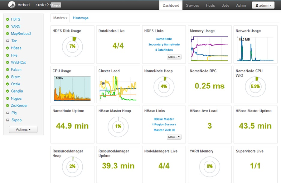
CHAPTER 8 ■ CLUSTER MANAGEMENT

233

The dashboard is the cluster manager home page, and the black menu bar at the top of the page allows me

to select the Dashboard, Services, Hosts, Jobs, or Admin functions. The service list on the left side of the display

allows me to access service-specific details—for example, HDFS. The dashboard display has two tabs—Metrics and

Heatmaps—each of which I will examine shortly. For instance, the Metrics window basically shows the state of the

cluster’s resources.

Clicking one the resource icons provides me with a larger, more detailed display of that cluster resource type. For

instance, I click CPU Usage and get the results shown in Figure 8-6. Specifically, what Figure 8-6 shows is CPU usage

for the last hour. The display is color-coded, with a corresponding key; in this instance, user CPU usage exceeds that

of system usage. It also shows that the cluster resources are being under-utilized, as CPU usage rarely exceeds 50

percent. Also, there is a table of minimum, average, and maximum CPU values for each category. I click OK to close

that display.

Figure 8-5. Ambari dashboard

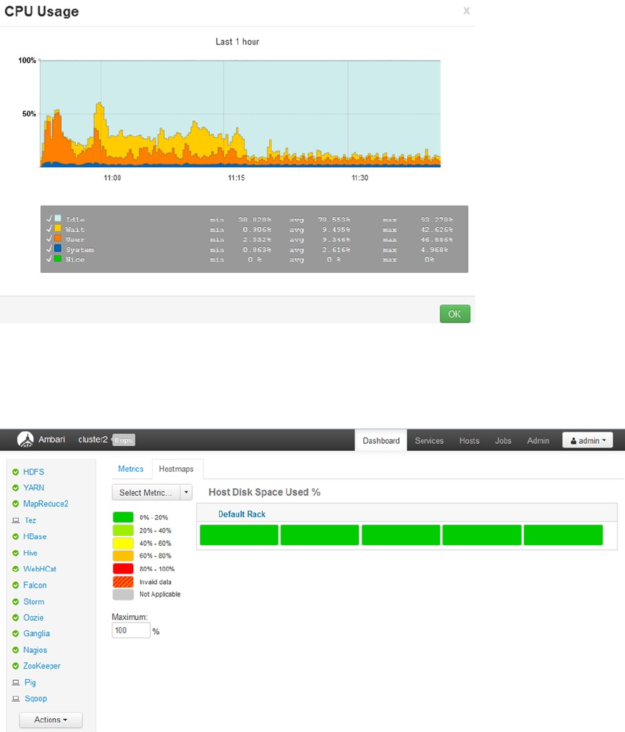
CHAPTER 8 ■ CLUSTER MANAGEMENT

234

Clicking the Heatmaps tab at the top of the dashboard yields a color-coded display for the Hadoop cluster state

for a given metric—in this instance, it is disk usage, as shown in Figure 8-7.

Figure 8-6. Ambari dashboard showing CPU usage

Figure 8-7. Ambari Heatmap display

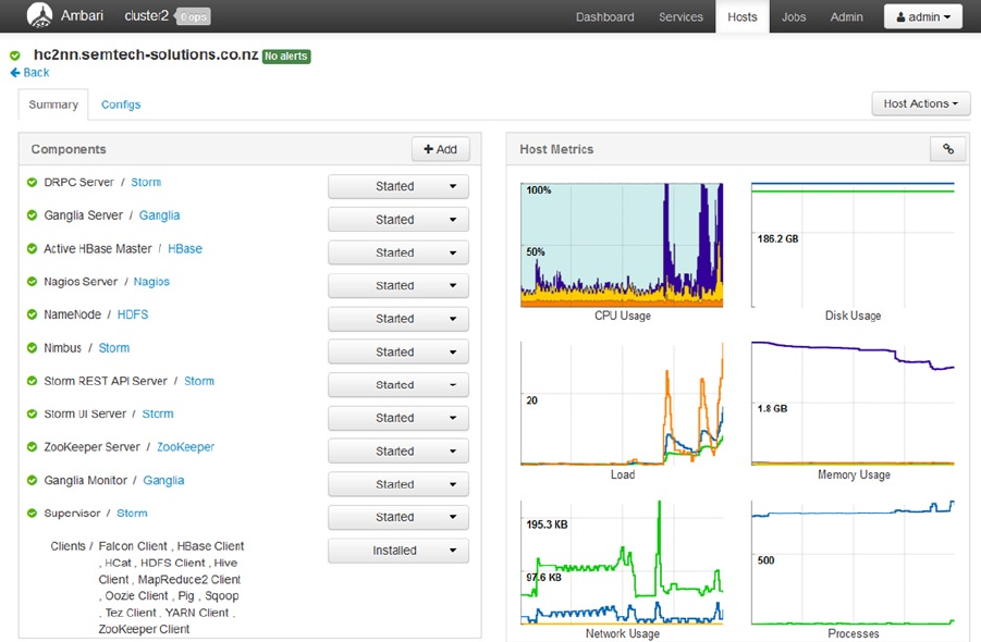
CHAPTER 8 ■ CLUSTER MANAGEMENT

235

The cluster that has been installed has a single server rack called “rack 1.” In Figure 8-7, this is represented by the

five green bars in “Host Disk Space Used %.” Each bar represents a server in the rack. If there were more servers and more

racks, there would be more rows of colored bars. Green represents a good state, while red would represent a problem.

The color-coded key on the left gives the meaning of the color state in the display. In this case, the key presents

disk space usage and it warns when the disk space becomes low on each server.

There is a drop-down menu on the top left of the display so that different Hadoop cluster metrics can be

examined—for instance, memory.

Clicking Services or Hosts in the top bar (next to Dashboard) enables you to see the cluster state from a service or

server point of view. For example, by selecting an individual server, such as the Name Node, in the Hosts interface,

I obtain a detailed view of the state of the Name Node server, as shown in Figure 8-8.

Figure 8-8. State of Ambari server

Figure 8-8 indicates that the system CPU (blue) on the top left graph is spiking to 100 percent. Also, it shows that

memory usage for processes and disk usage seems to be high. I’m not worried about this, though, as I know that my

cluster is a little under-powered, especially where memory is concerned. However, if you see graphs maxing out like

this on your own cluster, you may need to invest in extra resources or examine the cluster loading.

Clicking Admin in the top menu bar will allow you to access the administration functions within Ambari, thus

enabling you to examine users, high availability, the cluster, security, and access.

Finally, from the Dashboard you can also access user interfaces via links for such components as the Name Node,

Resource Manager, HBase, Storm, Oozie, Ganglia, and Nagios by using the menu on the left of the screen. Many of

these interfaces are familiar because I’ve covered them in earlier chapters of this book; it's just that Ambari brings

them all together in one place. For example, Figure 8-9 illustrates how the Resource Manager user interface lists

successful jobs that have completed.

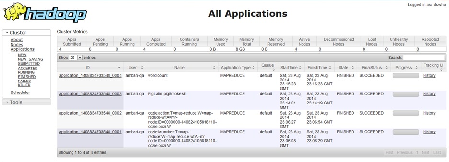
CHAPTER 8 ■ CLUSTER MANAGEMENT

236

That completes this short introduction to Ambari. Given that Ganglia and Nagios monitoring systems were

discusssed in Chapter 7, the Ambari displays should look familiar. That’s because Ambari uses Nagios and Ganglia for

its cluster manager graphs and alerts. In summary, Ambari can help you to install your cluster and provide automatic

monitoring. It can also provide quick access to the web-based user interfaces of the Hadoop components.

Ambari is used for the Hortonworks Hadoop stack, but if you want to use the Cloudera stack, what does that

cluster manager look like? Well, Cloudera has developed its own cluster manager application, which I demonstrate

next. To avoid any conflict between installations, however, I need to reinstall CentOS Linux on all of my cluster2

servers so that they provide a clean base from which to install the next cluster version.

The Cloudera Cluster Manager

In this section I take a look at the Cloudera cluster manager for CDH5. As mentioned in this chapter’s introduction,

both Ambari and the Cloudera cluster managers automate the installation and management of the Hadoop stack.

They also both provide a means for future software updates to be automated. So if you plan to install Hortonworks,

choose Ambari; if you want Cloudera’s releases, choose the Cloudera cluster manager.

Installing Cloudera Cluster Manager

For this example, I use the same 64-bit cluster of machines with 2 GB of memory, but I increase the Name Node

machine’s memory to 4 GB because the Cloudera cluster manager, especially the name node, needs more memory to

avoid swapping. As with the installation of Ambari, I reinstall Centos 6 onto the servers so that the machines are fresh

and free of conflict. Unless otherwise stated, the work is executed as the root user.

You can download the enterprise Cloudera manager binary installer from the Cloudera website at www.cloudera.

com/content/support/en/downloads/cloudera_manager.html. For this example, I store the installer in /tmp on the

Name Node machine hc2nn:

[root@hc2nn tmp]# pwd

/tmp

[root@hc2nn tmp]# ls -l cloudera-manager-installer.bin

-rw-r--r--. 1 root root 510569 Aug 30 19:11 cloudera-manager-installer.bin

Figure 8-9. Ambari Resource Manager user interface

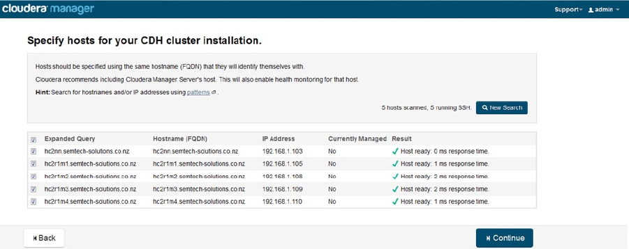
CHAPTER 8 ■ CLUSTER MANAGEMENT

237

I make the binary executable using the Linux chmod command:

[root@hc2nn tmp]# chmod 755 cloudera-manager-installer.bin

[root@hc2nn tmp]# ls -l cloudera-manager-installer.bin

-rwxr-xr-x. 1 root root 510569 Aug 30 19:11 cloudera-manager-installer.bin

Before running the installation, I disable SELinux on each server and reboot the server. I do this as the root user:

vi /etc/selinux/config

I set the SELINUX value to “disabled”:

SELINUX=disabled

[root@hc2nn tmp]# reboot

Then I execute the Cloudera manager binary and follow the prompts until I can access the installation web

browser at http://hc2nn:7180/. I log in as the user admin with a password of “admin” to see a list of the packages

that I can install. I click Continue.

At the next page, I enter the fully qualified domain names (FQDN) hostnames on which I intend to install, in the

form as follows:

192.168.1.103 hc2nn.semtech-solutions.co.nz hc2nn

Then I click the Search button to allow the manager to obtain details about the servers. When the servers are

located, I see “host ready” messages similar to those shown in Figure 8-10.

Figure 8-10. List of Cloudera installation hosts

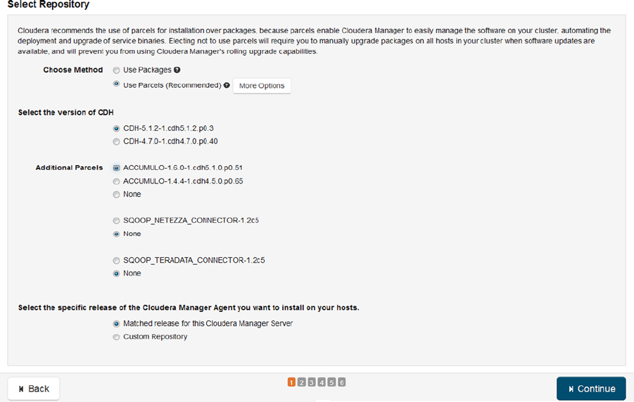
CHAPTER 8 ■ CLUSTER MANAGEMENT

238

I click the Continue button to move to the Select Repository page and choose the installation method,

packages, or parcels (advised). Here, I can also specify the version of CDH to install and any extra parcels, such as

Accumulo. Figure 8-11 shows this repository, with additional parcels like Accumulo and Sqoop to be chosen for

installation, if needed.

Figure 8-11. Cloudera selection repository

I choose to install CDH 5.1.2, as shown in Figure 8-11. I had already installed CDH 4 in Chapter 2, so that

installing CDH5 with the cluster manager is a progression from that previous work.

I click Continue once more, and consider enabling Java encryption. In this example, I leave my installation as the

default option without encryption, simply by clicking Continue to move on.

At the next cluster installation page, which has the title “Provide SSH Login Credentials,” I enter my installation

login credentials. I choose to use the root user and enter the user's password. This time when I click Continue the

actual installation of the Cloudera agent and server modules begins. Banners indicate both the overall progress and

the individual progress per server. Figure 8-12 shows a successful installation. I click Continue again to move on to

installing the selected parcels.

CHAPTER 8 ■ CLUSTER MANAGEMENT

239

After each parcel is downloaded, distributed, and activated, my page looks like that shown in Figure 8-13.

Figure 8-12. Notification of successful Cloudera installation

Figure 8-13. Notice of successful parcel installation

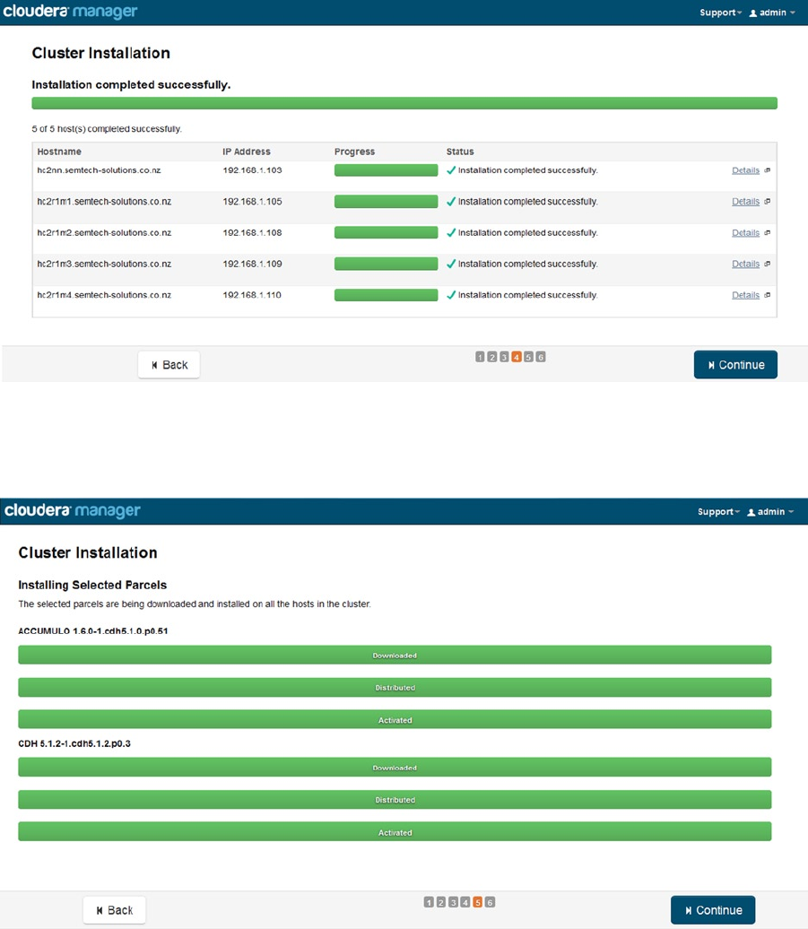
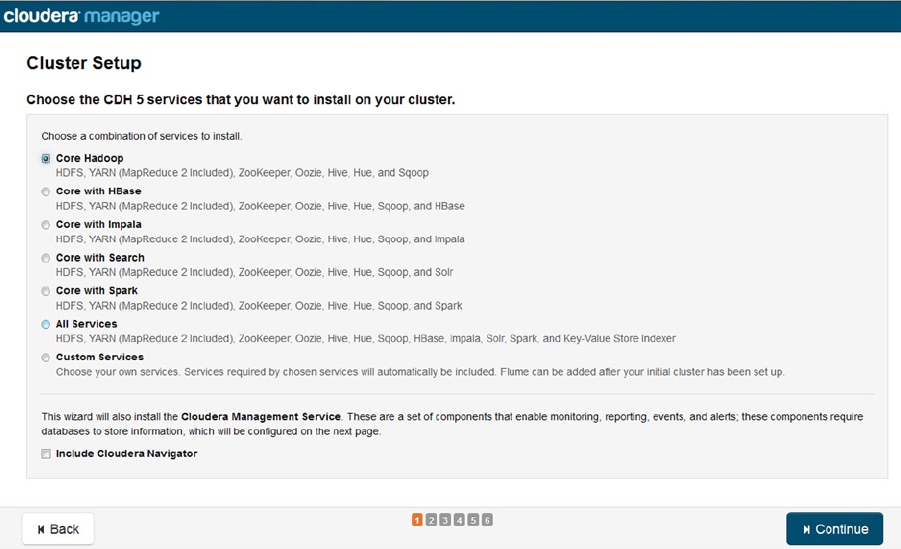
CHAPTER 8 ■ CLUSTER MANAGEMENT

240

After I click Continue, the manager carries out a host inspection to determine whether there are any problems

with the server. If there are none, I click Finish to advance to the first page of the cluster setup, as shown in Figure 8-14,

where I then choose the CDH services to be installed. I choose to install Core Hadoop to reduce the load on my servers,

then click Continue.

Figure 8-14. CDH service installation

Next, I assign the roles that determine where the services will run. For instance, I remember that ZooKeeper

needs a quorum of instances and that it must be an odd number of instances so they can vote successfully. Figure 8-15

shows my assignments. I then click Continue.

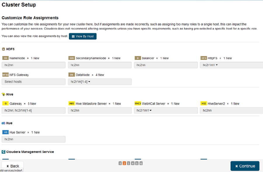
CHAPTER 8 ■ CLUSTER MANAGEMENT

241

On the subsequent Database Setup page (Figure 8-16), I choose whether to use the default embedded database

(my choice) or to specify a custom database. After testing that the connections are successful, by clicking the Test

Connections button, I click Continue.

Figure 8-15. CDH role assignments

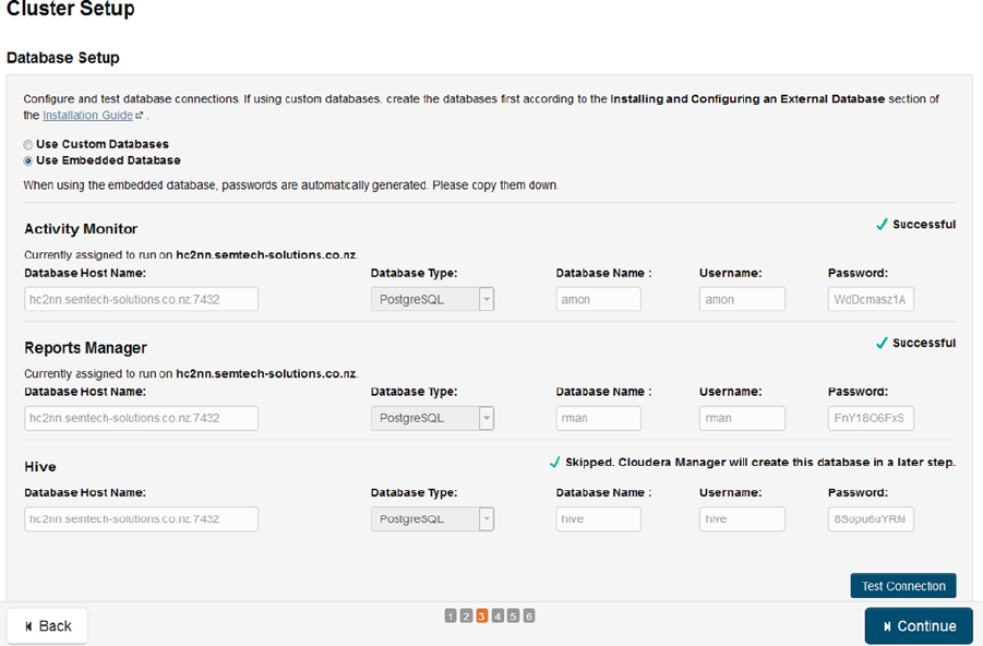
CHAPTER 8 ■ CLUSTER MANAGEMENT

242

At this point I’m given an opportunity to review the changes that will be made. I am happy with them, so I click

Continue to install the cluster services. The Cluster Setup page lets me monitor the progress, as shown in Figure 8-17.

When timeouts occur because there’s a shortage of memory on the name node (as happens to me), I click Retry. Once

the installations are complete, I click Continue.

Figure 8-16. Setting the CDH database connections

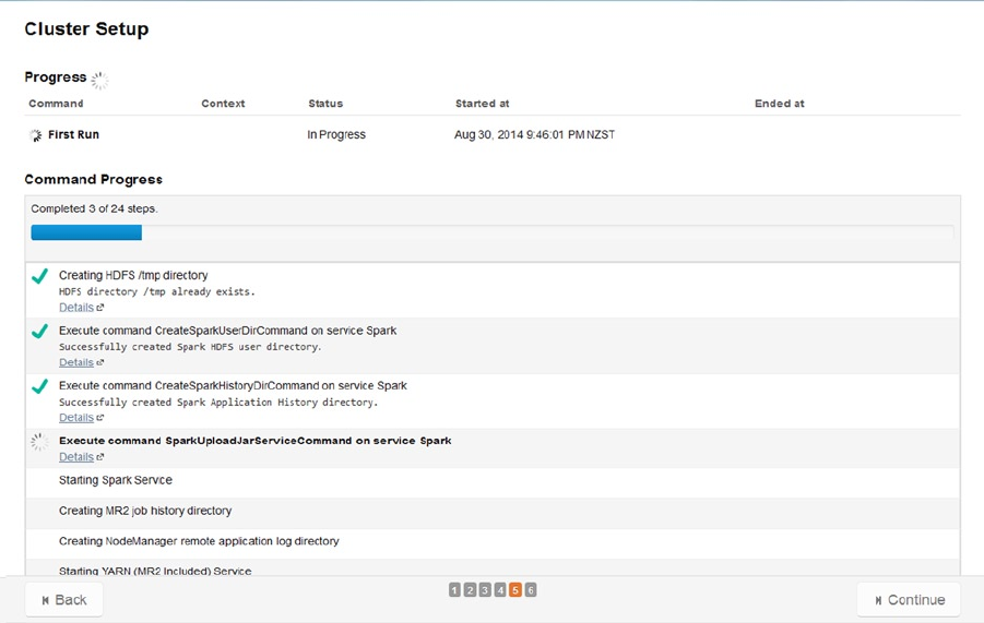
CHAPTER 8 ■ CLUSTER MANAGEMENT

243

Running Cloudera Cluster Manager

When the service installation is completed, I will see the Cluster Manager home screen (Figure 8-18). If I compare

this to the Ambari home dashboard, I can see that the general approach is similar. Each cluster manager has a menu

of services on the left of the display. Each supplier offers a slighty different list of products, though. For instance, the

Ambari service list shows Tez, Falcon, Ganglia, and Nagios; the Cloudera list shows Hue. Both displays offer service

graphs intended to show the state of resources—that is, memory, disk, and CPU.

Figure 8-17. Monitoring the CDH cluster service installation

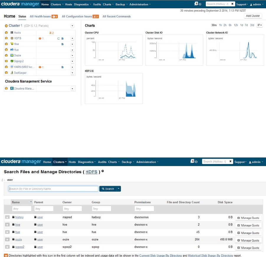
CHAPTER 8 ■ CLUSTER MANAGEMENT

244

I now progress through some of the Cloudera cluster manager screens to demonstrate its functionality.

Like the Hue application, the Cloudera cluster manager has an HDFS browser, shown in Figure 8-19. To access it,

you click the HDFS service on the left of the home page and select the Browse File System option.

Figure 8-18. Cloudera manager’s home page

Figure 8-19. Cloudera manager HDFS Browser

Within the HDFS browser, you can navigate to file system elements by clicking them; the browser then displays a

long list of file system details, including the object name, parent details, owner, group, permissions, an object count,

and storage. Here, you can also specify quotas that allow you to set file or disk space limits for HDFS directories.

Selecting the Clusters drop-down menu from the top bar, then choosing Reports, provides a series of pre-defined

reports. For example, Figure 8-20 reports the current disk usage by user.

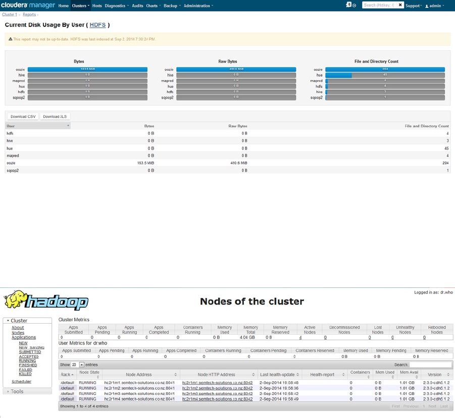
CHAPTER 8 ■ CLUSTER MANAGEMENT

245

Beneath Cluster 1 on the left of Figure 8-18 is a list of options like Hosts, HDFS, and Hive. By selecting one of the

service options from this menu, you can see a cluster manager screen that is dedicated to that service. On the screens

for services like HDFS and Yarn, it is also possible to access a Hadoop web-based user interface for those services.

For instance, by selecting the cluster service YARN, followed by the Resource Manager Web user interface option,

you will see the familiar Resource Manager web user interface, as shown in Figure 8-21.

Figure 8-21. User interface for Cloudera’s Resource Manager

Figure 8-20. Reports of Cloudera cluster manager

Alternatively, by selecting a service option from the Cluster 1 menu, you can determine the state of that service.

For instance, if you select HDFS, you’ll see the resource charts, a status summary, list of health tests, and a health

history, as shown in Figure 8-22.

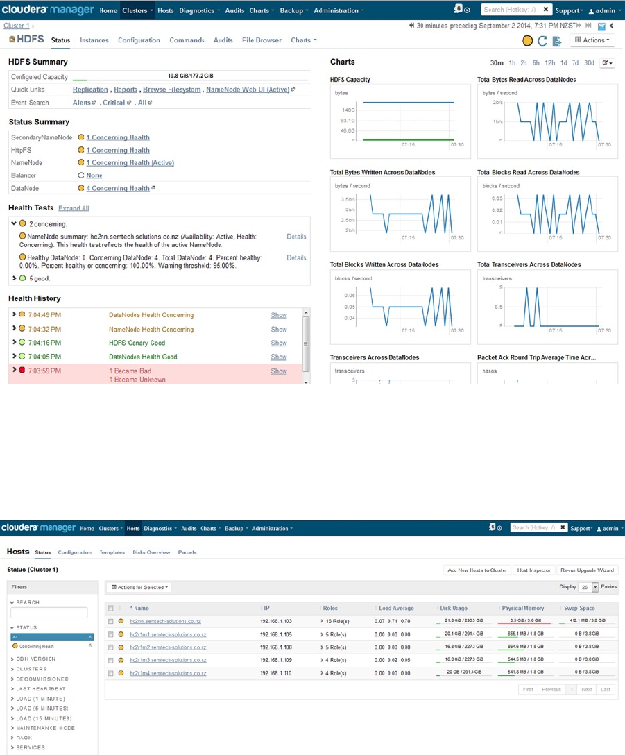
CHAPTER 8 ■ CLUSTER MANAGEMENT

246

Next to Clusters in the top bar is the Hosts option. If you click that, you’ll view a clickable list of cluster hosts, as

shown in Figure 8-23. You can add hosts to the cluster on this page, as well as inspect the hosts, assign them to a rack,

or decommission them. You can also start host roles here. Or, you can Click Disks Overview to obtain a detailed list of

disk statuses, as shown in Figure 8-24.

Figure 8-22. Status of Cloudera services

Figure 8-23. List of Cloudera hosts

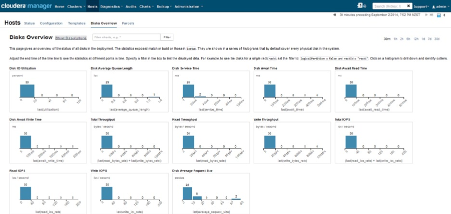
CHAPTER 8 ■ CLUSTER MANAGEMENT

247

Click the Host page’s Parcels option and you’ll see the available parcels that can be installed. Parcels are provided

by Cloudera from CDH4. They provide a mechanism for installing software updates without causing down time for

the Hadoop cluster. They are actually a gzipped tar file bundle of software supplied by Cloudera in its own format,

as are many of the downloaded and unpacked releases mentioned in this book. The difference is that Cloudera adds

metadata to the parcel, which is extra information so that the Cloudera manager knows what to do with the parcel.

The Parcels display as shown in Figure 8-25 checks on the availability of new parcels via a menu option.

The release of new software parcels to your cluster then just becomes a cycle of downloading those new parcels,

distributing them to the cluster, and activating them—all accomplished from this single screen. If you remember the

topics in Chapter 2, and all of the effort that went into installing and configuring CDH4, then you’ll quickly see how

this software release cycle makes the cluster manager worthwhile.

Figure 8-24. Status of Cloudera hosts

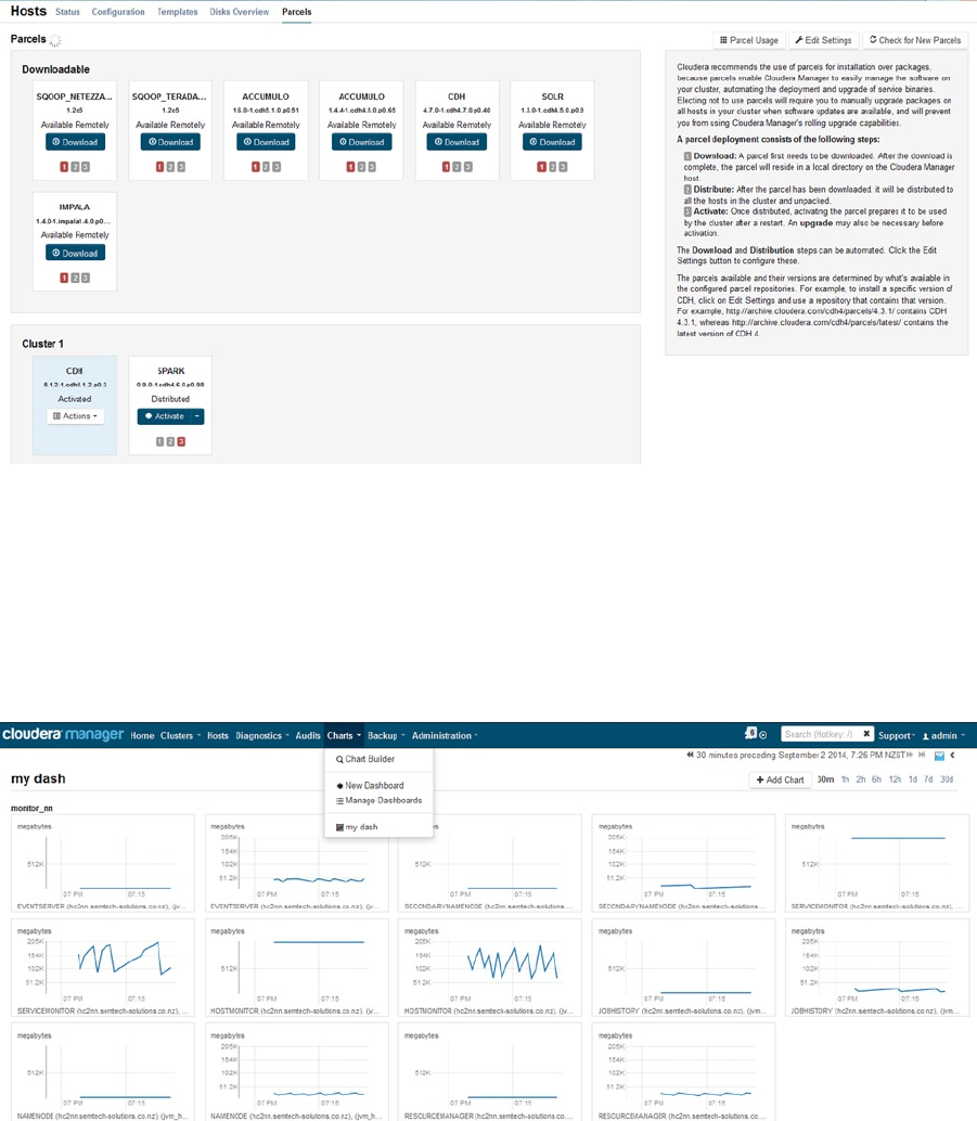
CHAPTER 8 ■ CLUSTER MANAGEMENT

248

In the top bar’s Charts menu, you’ll also find a Chart Builder option that uses an SQL-like language. With it, you

can build your own reporting dashboard. Figure 8-26 shows a simple example of a dashboard that I’ve called “My

Dash,” which I built using the following SQL statement:

select jvm_heap_used_mb/1024, jvm_heap_committed_mb/1024 where category=ROLE and hostname="hc2nn.

semtech-solutions.co.nz"

Figure 8-25. Parcel installation menu

Figure 8-26. Chart builder for Cloudera cluster manager

CHAPTER 8 ■ CLUSTER MANAGEMENT

249

Given a few simple SQL-like statements, you can build a highly functional dashboard using the Cloudera cluster

manager. Figure 8-26 shows the resource usage for the cluster server hc2nn, built using that simple SQL statement.

This type of dashboard generation function certainly proves useful for your cluster monitoring and management.

The Cloudera cluster manager and CDH 5 stack offer a great deal more functionality than can be covered in this

single chapter, but it will give you a sense of the services that the program can provide. Indeed, while developing

this book, Cloudera has been my cluster manager for CDH5. For example, Cloudera enabled me to change the

configuration of my cluster when tuning performance. The early-warning orange icons at the top of Figure 8-18

helped me investigate problems as they arose, and so avoid future entanglements. Also, the software parcels were

especially useful when upgrading existing software and installing extra software. As I mentioned earlier, the costs in

terms of licensing are handily offset by the savings in problem solving.

Apache Bigtop

Although not a cluster manager itself, Apache Bigtop aims to simplify installation and integration in its own way.

Specifically, Bigtop is an attempt by the Apache Software Foundation to provide integration and smoke testing of the

Apache Hadoop tool kit in order to provide an integrated Hadoop tool stack. Through Bigtop, Apache selects multiple

Hadoop tools, each with its own release version, and uses a set of automated smoke tests to ensure that the set of

applications works together as a stack. The result is a well-tested, high-quality, stack-based Hadoop product set.

Cloudera has recognized the value that the Apache Bigtop project is adding by basing its CDH releases on the

Bigtop releases. Although Cloudera does its own testing for its CDH releases, that testing is based on a pre-tested

Bigtop Hadoop stack product.

In this section I show how to source the Bigtop software and install it. Given that the smoke tests are part of

the Apache Bigtop build, there isn’t much to see. But I build Bigtop and extract the results of one smoke test as an

example.

Installing Bigtop

To install Bigtop, I obtain the Linux yum repository file so that Bigtop software can be sourced, I run the following

command on each machine in the cluster:

wget -O /etc/yum.repos.d/bigtop.repo http://archive.apache.org/dist/bigtop/bigtop-0.6.0/repos/

centos6/bigtop.repo

100%[============================================>] 172 --.-K/s in 0s

2014-08-27 18:30:40 (16.7 MB/s) - “/etc/yum.repos.d/bigtop.repo” saved [172/172]

As for installations of the Ambari and Cloudera cluster managers, I make sure the server has CentOS 6 freshly

installed. Next, I use the Linux yum command to install the components necessary for Bigtop on each machine:

yum install -y git cmake git-core git-svn subversion checkinstall build-essential dh-make debhelper

ant ant-optional autoconf automake liblzo2-dev libzip-dev sharutils libfuse-dev reprepro libtool

libssl-dev asciidoc xmlto ssh curl gcc gcc-c++ make fuse protobuf-compiler autoconf automake libtool

shareutils asciidoc xmlto lzo-devel zlib-devel fuse-devel openssl-devel python-devel libxml2-devel

libxslt-devel cyrus-sasl-devel sqlite-devel mysql-devel openldap-devel rpm-build create-repo redhat-

rpm-config wget

CHAPTER 8 ■ CLUSTER MANAGEMENT

250

Now I can install Hadoop. For demonstration purposes, I do only a basic installation to get the name node and

data nodes running. From that point, the installation process is the same as was shown in Chapter 2, but it is sourced

from Bigtop. On the Name Node machine (hc2nn), I install the Name Node and Resource Manager components as the

root user:

yum install hadoop-hdfs-namenode hadoop-yarn-resourcemanager

On the Data Node machines (hc2r1m1 to hc2r1m4), I install the data node and node manager components as the

root user:

yum install hadoop-hdfs-datanode hadoop-yarn-nodemanager

Now, I set up the configuration on each machine in the cluster under /etc/hadoop/conf. I present the necessary

entries and changes briefly here, but you can find full details in Chapter 2.

I add the following to the core-site.xml file:

<name>fs.default.name</name>

</property>

I then modify the hdfs-site.xml file as follows:

<name>dfs.replication</name>

</property>

<name>dfs.permissions.superusergroup</name>

<value>hadoop</value>

</property>

<name>dfs.replication</name>

</property>

Next, I add the following changes to the yarn-site.xml file:

<name>yarn.resourcemanager.address</name>

</property>

<name>yarn.resourcemanager.scheduler.address</name>

</property>

CHAPTER 8 ■ CLUSTER MANAGEMENT

251

<name>yarn.resourcemanager.resource-tracker.address</name>

</property>

<name>yarn.resourcemanager.admin.address</name>

</property>

<name>yarn.resourcemanager.webapp.address</name>

</property>

<name>yarn.resourcemanager.scheduler.class</name>

<value>org.apache.hadoop.yarn.server.resourcemanager.scheduler.fair.FairScheduler</value>

</property>

I place the following entries into the slaves file to indicate where the slave data nodes reside:

hc2r1m1

hc2r1m2

hc2r1m3

hc2r1m4

To ensure that the Hadoop scheduler is correctly configured, I copy the fair-scheduler.xml file that I created in

Chapter 5 and place it in the configuration directory /etc/hadoop/conf. Now I create the Linux and HDFS file system

locations that are needed by the Hadoop server, and I set their ownership and permissions:

[root@hc1nn conf]# mkdir -p /var/lib/hadoop-hdfs/cache/hdfs/dfs/name

[root@hc1nn conf]# chown -R hdfs:hdfs /var/lib/hadoop-hdfs/cache/hdfs/dfs/name

[root@hc1nn conf]# chmod 700 /var/lib/hadoop-hdfs/cache/hdfs/dfs/name

I set the JAVA_HOME variable so that the Hadoop server knows where to find Java:

export JAVA_HOME=/usr/lib/jvm/java-1.6.0-openjdk.x86_64

As the hdfs user, I format the Hadoop file system without the Hadoop servers running:

[root@hc2nn conf]# su - hdfs

-bash-4.1$ hdfs namenode -format

Next, I create the directories used by YARN, setting the ownership and group membership to the YARN Linux

user and group:

[root@hc1nn conf]# mkdir -p /var/log/hadoop-yarn/containers

[root@hc1nn conf]# mkdir -p /var/log/hadoop-yarn/apps

[root@hc1nn conf]# chown -R yarn:yarn /var/log/hadoop-yarn/containers

[root@hc1nn conf]# chown -R yarn:yarn /var/log/hadoop-yarn/apps

[root@hc1nn conf]# chmod 755 /var/log/hadoop-yarn/containers

[root@hc1nn conf]# chmod 755 /var/log/hadoop-yarn/apps

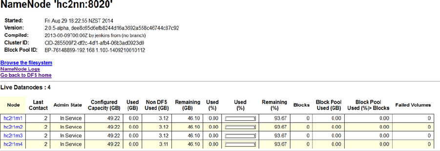
CHAPTER 8 ■ CLUSTER MANAGEMENT

252

Then, I create the file system directories needed for staging. I use chown to set their ownership and group

membership to YARN and the Linux chmod command to set the permissions:

[root@hc1nn conf]# mkdir -p /var/lib/hadoop-mapreduce/jobhistory/intermediate/donedir

[root@hc1nn conf]# mkdir -p /var/lib/hadoop-mapreduce/jobhistory/donedir

[root@hc1nn conf]# chown -R yarn:yarn /var/lib/hadoop-mapreduce/jobhistory/intermediate/donedir

[root@hc1nn conf]# chown -R yarn:yarn /var/lib/hadoop-mapreduce/jobhistory/donedir

[root@hc1nn conf]# chmod 1777 /var/lib/hadoop-mapreduce/jobhistory/intermediate/donedir

[root@hc1nn conf]# chmod 750 /var/lib/hhostnameadoop-mapreduce/jobhistory/donedir

After carrying out these configuration file changes on all cluster nodes, I restart the servers using the root

account. On the name node hc2nn, I enter:

service hadoop-hdfs-namenode start

service hadoop-yarn-resourcemanager start

On the data nodes, I enter:

service hadoop-hdfs-datanode start

service hadoop-yarn-nodemanager start

To confirm that Hadoop is up on the new cluster, I access the web interfaces for the name node and Resource

Manager. I find the name node web interface at http://hc2nn:50070/, then I click Live Datanodes to show the list of

active data nodes; Figure 8-27 shows the results.

Figure 8-27. User interface for Bigtop name nodes

To access the Resource Manager user interface, you go to http://hc2nn:8088/cluster. Click Scheduler in the

left column to view the fair scheduler configuration on the new cluster, as shown in Figure 8-28.

CHAPTER 8 ■ CLUSTER MANAGEMENT

253

Running Bigtop Smoke Tests

You can use Bigtop to quickly install a complete stack of Hadoop software if you don’t want to use a cluster manager

or a stack-based Hadoop release from one of the major suppliers. Even if you never plan to use Bigtop yourself, it is

worth understanding how it works, because major Hadoop vendors like Cloudera use it.

To execute an Apache Bigtop smoke test as my example, I first install Apache Maven, which is used to build and

run the tests.

Note ■ For full details on smoke tests, consult the Apache Bigtop website at http://bigtop.apache.org.

I then download the tar and zipped Maven package to /tmp on the server hc2nn by using a wget call to download:

[root@hc2nn tmp]# cd /tmp

[root@hc2nn tmp]# wget http://supergsego.com/apache/maven/maven-3/3.2.3/binaries/apache-maven-

3.2.3-bin.tar.gz

I unzip the package as the root user and unpack it using the tar command:

[root@hc2nn tmp]# gunzip apache-maven-3.2.3-bin.tar.gz

[root@hc2nn tmp]# tar xvf apache-maven-3.2.3-bin.tar

Now, I move the unpacked Maven directory to /usr/local so that it resides in the correct place and create a

generic symbolic link to point to the release, simplifying the configuration:

[root@hc2nn tmp]# mv apache-maven-3.2.3 /usr/local

[root@hc2nn tmp]# cd /usr/local

[root@hc2nn local]# ln -s apache-maven-3.2.3 apache-maven

[root@hc2nn local]# ls -ld apache-maven*

lrwxrwxrwx. 1 root root 18 Aug 30 08:23 apache-maven -> apache-maven-3.2.3

drwxr-xr-x. 6 root root 4096 Aug 30 08:21 apache-maven-3.2.3

Figure 8-28. User interface for Bigtop Resource Manager

CHAPTER 8 ■ CLUSTER MANAGEMENT

254

I alter the Linux PATH variable so the Maven executable can be found from the command line; the type command

shows that it is located under /usr/local/apache-maven/bin/mvn.

export PATH=/usr/local/apache-maven/bin:$PATH

[root@hc2nn tmp]# type mvn

mvn is /usr/local/apache-maven/bin/mvn

I check the Maven version to ensure that Maven is running without fault:

[root@hc2nn tmp]# mvn -version

Apache Maven 3.2.3 (33f8c3e1027c3ddde99d3cdebad2656a31e8fdf4; 2014-08-12T08:58:10+12:00)

Now, I set up some variables for the tests to define various Hadoop component paths:

export JAVA_HOME=/usr/lib/jvm/java-1.6.0-openjdk.x86_64

export HADOOP_HOME=/usr/lib/hadoop

export HADOOP_CONF_DIR=/etc/hadoop/conf

export ZOOKEEPER_HOME=/usr/lib/zookeeper

export PIG_HOME=/usr/lib/pig

export HADOOP_MAPRED_HOME=/usr/lib/hadoop-mapreduce

I have Hadoop and Pig installed for this example, but if you wanted to determine which other components were

available for installation—say, Sqoop—you could use the yum list function, like this:

[root@hc2nn bigtop-tests]# yum list available | grep sqoop

hue-sqoop.x86_64 2.5.1.5-1.el6 Bigtop

sqoop.noarch 1.99.2.5-1.el6 Bigtop

sqoop-client.noarch 1.99.2.5-1.el6 Bigtop

sqoop-server.noarch 1.99.2.5-1.el6 Bigtop

To run the tests, I first install the test artifacts using the Maven (mvn) install command as root:

cd /home/hadoop/bigtop/bigtop/bigtop-tests/test-artifacts/

mvn -f pom.xml install

I look for the success banner to indicate that there are no errors:

[INFO] ------------------------------------------------------------------------

[INFO] BUILD SUCCESS

[INFO] ------------------------------------------------------------------------

[INFO] Total time: 08:26 min

[INFO] Finished at: 2014-08-30T08:44:38+12:00

[INFO] Final Memory: 20M/129M

[INFO] ------------------------------------------------------------------------

CHAPTER 8 ■ CLUSTER MANAGEMENT

255

Now, I install the configuration components using the same Maven command and look for the same indication of

success:

cd /home/hadoop/bigtop/bigtop/bigtop-tests/test-execution/conf

mvn -f pom.xml install

[INFO] ------------------------------------------------------------------------

[INFO] BUILD SUCCESS

[INFO] ------------------------------------------------------------------------

[INFO] Total time: 22.638 s

[INFO] Finished at: 2014-08-30T09:14:46+12:00

[INFO] Final Memory: 13M/112M

[INFO] ------------------------------------------------------------------------

Finally, I install the common component in the same way:

cd /home/hadoop/bigtop/bigtop/bigtop-tests/test-execution/common

mvn -f pom.xml install

[INFO] ------------------------------------------------------------------------

[INFO] BUILD SUCCESS

[INFO] ------------------------------------------------------------------------

[INFO] Total time: 2.301 s

[INFO] Finished at: 2014-08-30T09:15:30+12:00

[INFO] Final Memory: 9M/78M

[INFO] ------------------------------------------------------------------------

Now I can finally run the smoke test. I move to the desired location under Smokes and run the Maven verify

command. For my test, I will run the Pig test case:

[root@hc2nn pig]# cd /home/hadoop/bigtop/bigtop/bigtop-tests/test-execution/smokes/pig

[root@hc2nn pig]# mvn verify

I won’t reproduce the entire output here, but you can see that it is a series of Hadoop Pig scripts and test results,

like this:

Running org.apache.pig.test.pigunit.pig.TestGruntParser

DUMP output;

A = LOAD 'input.txt' AS (query:CHARARRAY);

STORE output INTO '/path';

Tests run: 5, Failures: 0, Errors: 0, Skipped: 0, Time elapsed: 0.239 sec

This script shows that five test cases within the Pig test were run with no errors, and it demonstrates, briefly, that I

can source a Hadoop stack from the Apache Bigtop project whose element programs have been integration-tested via

a series of smoke tests.

You can download the Bigtop stack yourself and build it. You can also run the smoke tests on your own servers

to prove that the installation will work. By running the smoke tests in your environment, you can prove that the whole

Hadoop stack provided by the Bigtop project works as expected for you. Check the Apache Bigtop website

(bigtop.apache.org) for further information.

CHAPTER 8 ■ CLUSTER MANAGEMENT

256

Summary

Hadoop cluster managers will save you time and effort when you want to both install and upgrade your Hadoop

environments. They automatically create the configuration on each cluster server. They also create a set of

configuration files that are more complete and contain fewer errors than the hand-crafted alternative. Also, cluster

managers offer the ability to globally modify your configuration attributes. The savings in time for that feature alone

are huge if you think about manually changing the configuration files on each server in a cluster of even moderate

size. Although I have examined only the Cloudera and Hortonworks cluster managers in this chapter, others are

available from vendors such as MapR.

In short, the monitoring functionality of the Ambari and Cloudera cluster managers is impressive, and having a

single place to check the state of the Hadoop cluster is very useful.

Although it’s not a cluster manager, I included Apache Bigtop in this chapter for a number of reasons, but mainly

because it is an attempt to integrate and smoke test a complete Hadoop stack. Cloudera uses Apache Bigtop to create

its CDH stacks, for example. Because the work that the Bigtop project is doing is very worthwhile,I think that Hadoop

users should be aware of it.

257

Chapter 9

Analytics with Hadoop

Analytics is the process of finding significance in data, meaning that it can support decision making. Decision

makers turning to Hadoop’s data for their answers will find numerous analytics options. For example, Hadoop-based

databases like Apache Hive and Cloudera Impala offer SQL-like interfaces with HDFS-based data. For in-memory

data processing, Apache Spark is available at a processing rate that is an order faster than Hadoop. For those who have

had experience with relational databases, these SQL-like languages can be a simple path into analytics on Hadoop.

In this chapter, I will explain the building blocks of each Hadoop application’s SQL-like language. The actions

you need to take to transform your data will impact the methods you use to create your complex SQL. Just as in

Chapter 4, when I introduced Pig user-defined functions (UDFs) to extend the functionality of Pig, in this chapter I

will create and use a Hive UDF in an example using Hive QL. I begin with coverage of Cloudera Impala, move on to

Apache Hive, and close the chapter with a discussion of Apache Spark.

Cloudera Impala

Released via an Apache license and provided as an open-source system, Cloudera Impala is a massively parallel

processing (MPP) SQL query engine for Apache Hadoop. Forming part of Cloudera’s data hub concept, Impala is

the company’s Hadoop-based database offering. Chapter 8 introduced the Cloudera cluster manager, which offers

monitoring, security, and a well-defined upgrade process. Impala integrates with this architecture, and given that it

uses HDFS, offers a low-cost, easily expandable, reliable, and robust storage system.

By way of example, I install Impala from the Cloudera CDH 4 stack, then demonstrate how to use it via the Hue

application, as well as how to put Impala’s shell tool and query language to work.

Installation of Impala

The chapter builds on work carried out in previous chapters on Cloudera’s CDH 4 Hadoop stack. So, to follow this

installation, you will need to have completed the installation of the CDH4 Hadoop stack in Chapter 2 and of the Hue

application in Chapter 7. I install Impala manually on server hc1r1m1 and access it via the Hue tool that is already

installed on the server hc1nn. I choose the server hc1r1m1 because I have a limited number of servers and I want to

spread the processing load though my cluster.

So, the first step is to install some components required by Impala, as the Linux root user on the server hc1r1m1,

by issuing the following Linux yum command. (These components may already be installed on your servers; if so, they

will not be reinstalled. This step just ensures that they are available now):

[root@hc1r1m1 ~]# yum install python-devel openssl-devel python-pip

CHAPTER 9 ■ ANALYTICS WITH HADOOP

258

Next, I install a repository file under /etc/yum.repos.d on hc1r1m1 for Impala, so that the Linux yum command

knows where to find the Cloudera Impala software. The repository file is downloaded from Cloudera's site by using

the Linux wget command:

[root@hc1r1m1 ~]# cd /etc/yum.repos.d

[root@hc1r1m1 ~]# wget http://archive.cloudera.com/impala/redhat/6/x86_64/impala/cloudera-impala.repo

I can examine the contents of this downloaded repository file by using the Linux cat command:

[root@hc1r1m1 yum.repos.d]# cat cloudera-impala.repo

[cloudera-impala]

name=Impala

baseurl=http://archive.cloudera.com/impala/redhat/6/x86_64/impala/1/

gpgkey = http://archive.cloudera.com/impala/redhat/6/x86_64/impala/RPM-GPG-KEY-cloudera

gpgcheck = 1

Next, I install the Impala components and the Impala shell by using the yum command as the Linux root user:

[root@hc1r1m1 ~]# yum install impala impala-server impala-state-store impala-catalog impala-shell

These commands install the Impala Catalogue server, the Impala server, the Impala State Store server, and the

Impala scripting shell. The Impala server runs on each node in an Impala cluster; it accepts queries and passes data to

and from the files. The Impala scripting shell acts as a client to receive user commands and passes them to the server.

Key to making an Impala cluster robust, the State Store server monitors the state of an Impala cluster and manages the

workload when something goes wrong. The Catalog server manages metadata—that is, data about data—and passes

details about metadata changes to the rest of the cluster.

As soon as the software is installed, it is time to configure it. I copy the Hive hive-site.xml, the HBase hbase-site.xml,

and the Hadoop files core-site.xml and hdfs-site.xml to the Impala configuration area, which I find under/etc/impala/conf.

The dot character (.) at the end of the cp (copy)command is just Linux shorthand for the current directory:

[root@hc1r1m1 conf]# cd /etc/impala/conf

[root@hc1r1m1 conf]# cp /etc/hive/conf/hive-site.xml .

[root@hc1r1m1 conf]# cp /etc/hadoop/conf/core-site.xml .

[root@hc1r1m1 conf]# cp /etc/hbase/conf/hbase-site.xml .

[root@hc1r1m1 conf]# cp /etc/hadoop/conf/hdfs-site.xml .

To specify the host and port number for the Hive metastore thrift API, as well as to specify a timeout value for

access, I make the following changes to the hive-site.xml file in the Impala configuration area:

<name>hive.metastore.uris</name>

<value>thrift://hc1r1m1:9083</value>

IP address (or fully-qualified domain name) and port of the metastore host

</description>

</property>

CHAPTER 9 ■ ANALYTICS WITH HADOOP

259

<name>hive.metastore.client.socket.timeout</name>

<description>MetaStore Client socket timeout in seconds</description>

</property>

Then, I make the following changes to Impala's copy of the hdfs-site.xml file:

<name>dfs.client.read.shortcircuit</name>

</property>

<name>dfs.domain.socket.path</name>

<value>/var/run/hdfs-sockets/dn</value>

</property>

<name>dfs.client.file-block-storage-locations.timeout</name>

</property>

<name>dfs.datanode.hdfs-blocks-metadata.enabled</name>

</property>

These changes boost performance with HDFS by bypassing (short-circuiting) the data node and accessing the

files directly. They specify a domain socket path and a block storage location timeout. These changes, including the

core-site.xml change that follows, provide a real performance boost to Impala’s operation. So, I make the following

changes to the Impala’s copy of the core-site.xml file:

<name>dfs.client.read.shortcircuit</name>

</property>

If the directory /var/run/hadoop-hdfs/ is group writeable, I make sure that the group is root. To check this, I use

the Linux ls command to get a long listing of the directory:

[root@hc1r1m1 ~]# ls -ld /var/run/hadoop-hdfs/

drwxr-xr-x. 2 hdfs hdfs 4096 Sep 7 09:21 /var/run/hadoop-hdfs/

CHAPTER 9 ■ ANALYTICS WITH HADOOP

260

The permissions string reads d rwx r-x r-x. The d means “directory,” the first three characters are permissions

for the owner, the next set is the group, and the final set is the world (or everybody else). So, the group membership

string has r-x, or read and execute permissions; it is not writeable by the group because the w character is missing.

Also, the string hdfs hdfs indicates that the directory is owned by the user and group hdfs. When I check, I make sure

that the directory is either group writeable by the Linux root user or is not group writeable.

Now, I create the sockets directory and subdirectory under /var/run as the root user:

[root@hc1r1m1 impala]# mkdir -p /var/run/hdfs-sockets/dn

[root@hc1r1m1 impala]# ls -ld /var/run/hdfs-sockets

drwxr-xr-x 3 root root 4096 Sep 7 09:58 /var/run/hdfs-sockets

I start the Impala services (the Impala State Store server, the Catalog server, and the Impala server) as root:

[root@hc1r1m1 ~]# service impala-state-store start

[root@hc1r1m1 ~]# service impala-catalog start

[root@hc1r1m1 ~]# service impala-server start

I check the Impala logs under /var/log/impala for errors. Errors can occur because of incorrect configuration

after installation. For instance, if the sockets directory does not exist, the following error message would appear:

E0907 09:49:42.279753 4815 impala-server.cc:208] ERROR: short-circuit local reads is disabled

because

- Impala cannot read or execute the parent directory of dfs.domain.socket.path

Or, if the configuration value dfs.client.file-block-storage-locations.timeout is either not specified or has too small

a value, the following error message will be issued:

ERROR: block location tracking is not properly enabled because

- dfs.client.file-block-storage-locations.timeout is too low. It should be at least 3000.

E0907 09:49:42.280009 4815 impala-server.cc:210] Aborting Impala Server startup due to improper

configuration

I plan to access Impala via Hue, so on the server hc1nn, I need to change the Hue configuration file hue.ini under

/etc/hue/conf so that Hue knows where to find Impala. To do so, I set the server_host value in the [Impala] section of

the file to the host where Impala is running, hc1r1m1:

server_host=hc1r1m1

After making the change, I restart the Hue server on the host hc1nn as the Linux root user:

[root@hc1nn ~]# service hue restart

The interface is now be ready for use.

Impala User Interfaces

You can access the Impala server user interface via the URL hc1r1m1:25000. Figure 9-1 shows a basic example of this

interface. The Impala State Store server user interface resides at port number 25010, and is reached using the URL

hc1r1m1:25010. The Impala Catalogue server user interface is on port 25020. All three of these interfaces provide

information such as configuration, log content, metrics, and session. Because I concentrate on Impala’s analytics

functionality using SQL, I only examine the Impala server interface and leave you to investigate the other options.

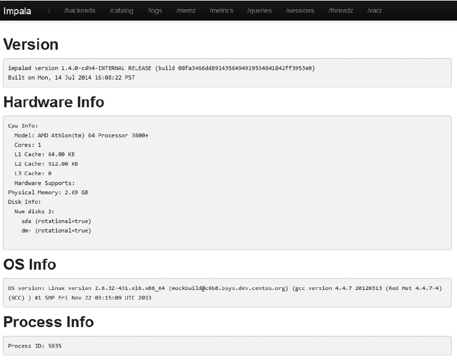
CHAPTER 9 ■ ANALYTICS WITH HADOOP

261

With the Hue server running and configured to access Impala, you can write Impala scripts from the Query Editor

in the Hue interface, as shown in Figure 9-2. To open it, you use the URL hc1nn:8888; and from Hue, you click the

stylized impala head (fourth icon from the left) in the top icon bar.

Figure 9-1. Impala server user interface

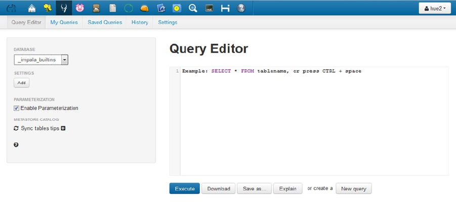
CHAPTER 9 ■ ANALYTICS WITH HADOOP

262

Uses of Impala

The real power of Impala lies not in its interfaces but in its query language and the options that it provides. For

example, it can access HDFS-based data via external tables, and it offers standard SQL-based operations, such as

filters, table joins, subqueries, inserts, and more. These terms are described next, in a step-by-step manner, and then

their corresponding equivalents are examined for Hive. The database itself is highly scalable and robust, as it is built

on top of HDFS.

At this point I need some data to process, so as to demonstrate Impala’s SQL-based functionality. In Chapter 5,

I uploaded a series of fuel consumption CSV data files to HDFS, under the HDFS directory /user/hue2/fuel_

consumption/; the Hadoop file system ls command that follows shows that upload:

[hadoop@hc1r1m1 ~]$ hdfs dfs -ls /user/hue2/fuel_consumption

Found 16 items

-rw-r--r-- 2 hadoop hue2 248956 2014-09-07 18:17 /user/hue2/fuel_consumption/MY1995-1999 Fuel

Consumption Ratings.csv

-rw-r--r-- 2 hadoop hue2 45203 2014-09-07 18:17 /user/hue2/fuel_consumption/MY2000 Fuel

Consumption Ratings.csv

.......................

Consumption Ratings.csv

-rw-r--r-- 2 hadoop hue2 77452 2014-09-07 18:17 /user/hue2/fuel_consumption/MY2013 Fuel

Consumption Ratings.csv

-rw-r--r-- 2 hadoop hue2 77186 2014-09-07 18:17 /user/hue2/fuel_consumption/MY2014 Fuel

Consumption Ratings.csv

Figure 9-2. Impala scripting via Hue user interface

CHAPTER 9 ■ ANALYTICS WITH HADOOP

263

Database Creation

To create a database in Impala, I use the CREATE DATABASE command. I enter the following SQL command in Hue’s

Impala Query Editor to create the fuel database:

CREATE DATABASE fuel ;

After clicking the Execute button to form this text, I find that the database drop-down menu on the Hue’s Impala

user interface has a new option: fuel. To use this database in a SQL script, I can now specify the USE option:

USE fuel ;

Alternatively, I could use the database name before the table name, as shown in this SELECT command:

SELECT * FROM fuel.customer ;

External Table Creation

A Hive external table is a table where you specify the location for data storage rather than using the default value. For

example, by using CREATE EXTERNAL TABLE, I can create an external table against an HDFS directory that contains

comma-separated files (CSV). When the table is dropped the data is not deleted. The following code creates an

external table called “consumption” in the fuel database and that table can then be used to investigate trends in

vehicle fuel consumption:

CREATE EXTERNAL TABLE fuel.consumption

(

myear STRING,

manufacturer STRING,

model STRING,

fclass STRING,

enginesz STRING,

cylinders STRING,

transmission STRING,

fuel STRING,

consumption1 STRING,

consumption2 STRING,

consumption3 STRING,

consumption4 STRING,

avefuel STRING,

co2 STRING

)

ROW FORMAT DELIMITED FIELDS TERMINATED BY ','

LOCATION '/user/hue2/fuel_consumption/';

Because a CSV file uses commas as the column separators, the row following the end parenthesis [)] uses a

DELIMITED option to process the data:

ROW FORMAT DELIMITED FIELDS TERMINATED BY ','

CHAPTER 9 ■ ANALYTICS WITH HADOOP

264

This indicates that the columns are delimited by commas, and so the columns in the table will match the

columns in the CSV file. The final line of the command specifies the location of the data, and the table name is

specified in the form database.table (here, fuel.consumption).

When I want to remove a table, I use the DROP TABLE command. For example, I can remove the “consumption”

table from the fuel database as follows:

DROP TABLE fuel.consumption ;

External tables are useful for data feeds based on files. Rather than load the files into a database table, I could can

create an external table against the files. Then the data can be loaded from the external table as an initial step in an

ETL chain before the data is processed further.

Table Creation

The same information can be used to create an internal table with just a few tweaks of the SQL. I simply remove the

EXTERNAL keyword and leave out the DELIMITED and LOCATION options, as follows:

CREATE TABLE fuel.consumption2

(

myear STRING,

manufacturer STRING,

model STRING,

fclass STRING,

enginesz STRING,

cylinders STRING,

transmission STRING,

fuel STRING,

consumption1 STRING,

consumption2 STRING,

consumption3 STRING,

consumption4 STRING,

avefuel STRING,

co2 STRING

);

For instance, to show which tables exist for the fuel database, I can use the SQL SHOW TABLES command:

SHOW TABLES ;

The result is a single row called “consumption.” To examine the structure of a table, I use the DESCRIBE keyword:

DESCRIBE fuel.consumption;

The result now is a series of output data rows that represent the columns in the table:

0 myear string

1 manufacturer string

2 model string

3 fclass string

4 enginesz string

5 cylinders string

CHAPTER 9 ■ ANALYTICS WITH HADOOP

265

6 transmission string

7 fuel string

8 consumption1 string

9 consumption2 string

10 consumption3 string

11 consumption4 string

12 avefuel string

13 co2 string

The SELECT Statement

The SELECT keyword plucks data from a database table. For example, I can select data from the “consumption” table of

the fuel database. The asterisk (*) indicates that all column data within the table should be selected. (As this example

contains a lot of data, I provide only a couple of rows of the output to give an idea of the results):

SELECT * from fuel.consumption ;

1 1995 ACURA INTEGRA SUBCOMPACT 1.8 4 A4 X 10.2

7 28 1760 202

2 1995 ACURA INTEGRA SUBCOMPACT 1.8 4 M5 X 9.6

7 29 40 1680 193

If I need only a portion of the data, I can replace the asterisk (*) with specific columns names, such as “myear”

and “manufacturer”:

SELECT myear, manufacturer from fuel.consumption ;

1 1995 ACURA

2 1995 ACURA

The WHERE Clause

The WHERE clause is used with SELECT, INSERT, and DELETE statements to filter the results of a request. Here are some

examples of SELECT statements with their WHERE clauses serving as filters for obtaining data by manufacturer or year:

SELECT * from fuel.consumption WHERE manufacturer = 'ACURA' ;

SELECT * from fuel.consumption WHERE myear = '1995' AND manufacturer = 'AUDI' ;

SELECT * from fuel.consumption WHERE myear = '1995' OR manufacturer = 'AUDI' ;

The first statement limits the selected rows to those where “manufacturer” is equal to ACURA. The second limits

the selected rows to where “myear” is 1995 and the “manufacturer” is AUDI. The final example limits the selected

rows to where “myear” is 1995 or the “manufacturer” is AUDI.

CHAPTER 9 ■ ANALYTICS WITH HADOOP

266

The Subquery

SELECT statements can be nested as subqueries. Here are two examples of how that is done. The first is to use a SELECT

statement as a subquery in the FROM clause of an outer SELECT statement, as follows:

SELECT rd.* FROM

(

SELECT

myear,manufacturer,model,enginesz,cylinders

FROM

fuel.consumption

) rd ;

The outer SELECT statement uses a derived table called “rd” and selects all columns from rd using the column

list rd.*. The contents of the parentheses form the derived table named rd, which uses a subquery that selects the

following five columns from the external table fuel.consumption:

myear,manufacturer,model,enginesz,cylinders

This first example uses a subquery as a way to transform table data to form a derived table. For example, you

might want to filter table data or join a group of tables together to form a larger data set.

The second example uses a subquery in the WHERE clause of an SQL statement. In this manner, an outer SELECT

statement selects all column data (fl.*) from the table fuel.consumption, with a subquery in its WHERE clause to filter

on the engine size. The result is a table showing data for which the engine size is greater than average:

SELECT

fl.*

FROM

fuel.consumption fl

WHERE

fl.enginesz > ( SELECT AVG(st.enginesz) FROM fuel.consumption st )

In this second example, the subquery in parentheses selects the average (AVG) engine size value from

the instance of the fuel.consumption table with an alias of “st.” The outer query filters the contents of the fuel.

consumption table with an alias of “fl,” choosing only those rows where the fl.enginesz column is greater than the

average value.

Table Joins

Table joins allow you to join the data in one table to the data in a second table if there are comparable columns in each

table. For instance, the first table could contain a list of people, with each person having a unique identity number.

A second table might contain a list of addresses plus associated personal identity numbers. By joining the two tables

on the identity numbers, you are able to determine a person’s name and address.

The following SQL example selects data from the earlier fuel.consumption table where the columns “myear,”

“manufacturer,” and “model” match another table called fuel.consumption3. Aliases have been used here for the

two tables—rd1 and rd2; this means there’s less typing when you are specifying the table columns and so there’s no

CHAPTER 9 ■ ANALYTICS WITH HADOOP

267

confusion about which table a column belongs to. The SELECT statement will only output a data row if a matching row

is found on the “myear,” “manufacturer,” and “model” columns of both tables:

SELECT

rd1.*

FROM

fuel.consumption rd1,

fuel.consumption3 rd2

WHERE

rd1.myear = rd2.myear AND

rd1. manufacturer = rd2. manufacturer AND

rd1. model = rd2. model

The INSERT Statement

The INSERT statement allows you to insert a single row into an Impala table, or you can combine INSERT with a SELECT

statement to insert multiple rows. These commands are designed to move large data volumes.

In a first example of this command, the INSERT statement inserts a single row into the fuel database table called

consumption2. The number and type of column values specified in parentheses must match the table definition.

Because the data values are strings, they are shown within single quotes:

INSERT INTO fuel.consumption2 VALUES ('1995','ACURA','INTEGRA','SUBCOMPACT','1.8','4','A4',

'X','10.2','7','28','40','1760','202')

Although this single INSERT statement moves a single row of data into the table fuel.consumption2, a second

example offers better performance by using a SELECT statement to populate the table fuel.consumption2 via a bulk

insert:

INSERT INTO TABLE fuel.consumption2 SELECT * FROM fuel.consumption3

This second version is a simple example; no extra filters or table joins have been used. But the size of the subtable

could be large; with a simple statement, you could copy a large volume of data.

Note: When executing an INSERT statement, you may receive an error message similar to the following:

AnalysisException: Unable to INSERT into target table (fuel.consumption2) because Impala does not

have WRITE access to at least one HDFS path: hdfs://hc1nn/user/hive/warehouse/fuel.db/consumption2

This error occurs if the referenced database and/or table name on HDFS is not owned by the HDFS impala user.

To fix this, you change the ownership with a statement like the following:

[hadoop@hc1r1m1 ~]$ hdfs dfs -chown -R impala:supergroup /user/hive/warehouse/fuel.db/

When run as the hadoop user, this statement recursively changes ownership of the HDFS fuel.db directory to the

impala user and changes the group to a supergroup. Then, you drop the table and re-create it to update the Impala

metadata for the table. After these steps, your INSERT statement should work.

This has been a very short introduction to Cloudera Impala SQL. For full details, check the Impala web site at

http://www.cloudera.com/content/cloudera/en/documentation/cloudera-impala. Additionally, try to create your

own SQL statements by joining these simple building blocks. For instance, you can create SELECT statements with

WHERE clauses. And you can add table joins to your SQL statements and consider adding subqueries.

CHAPTER 9 ■ ANALYTICS WITH HADOOP

268

Apache Hive

Like Cloudera Impala, Apache Hive offers an SQL-type language called Hive QL that can be used to manipulate Hive-

based tables. The functionality of Hive QL can be extended by creating user-defined functions (UDF), as you’ll see in

an example shortly.

In this section, I use Hive version 0.10, which was installed in Chapter 7 along with the Hue application. As you

remember, Hue was installed on the server hc1nn and has the URL http://hc1nn:8888/. Though I don’t mention

Hue again in this chapter, I use the Beeswax Hive user interface to enter the scripts at the Hue URL. Here, I walk you,

step by step, through table creation, SELECT statements, joins, and WHERE clauses. To make the examples a bit more

interesting, I have sourced some real UK trade CSV files to use as data.

Note ■ For more information and in-depth documentation on Hive and Hue, see the Apache Hive website at

hive.apache.org.

Database Creation

To begin the example, I create a database to contain this Hive work, using the CREATE DATABASE command. I name the

database and specify to create it only if it does not already exist:

CREATE DATABASE IF NOT EXISTS trade;

I set the current database with the USE command; in this case, I set it to trade:

USE trade;

External Table Creation

External tables are a useful step in an ETL chain because they offer the opportunity to move raw data files from an

HDFS directory into a Hive staging table. From the staging table you can transform the data for its journey to its

final state. Before I demonstrate table creation, though, I need to move the data files that I downloaded from the UK

government data site (data.gov.uk) from the Linux file system on hc1nn to HDFS. (If you want to obtain the same

data set to run these examples, you can source it from http://data.gov.uk/dataset/financial-transactions-

admin-spend-data-ukti.)

To start the move, I create the /data directory on HDFS as the Linux hadoop user:

[hadoop@hc1nn data]$ hdfs dfs -mkdir /data

I then move the data files under the Linux directory /home/hadoop/data/uk_trade to this HDFS directory via a

copyFromLocal HDFS command:

[hadoop@hc1nn uk_trade]$ pwd

/home/hadoop/data/

[hadoop@hc1nn uk_trade]$ ls uk_trade

ukti-admin-spend-apr-2011.csv ukti-admin-spend-jun-2012.csv

ukti-admin-spend-apr-2012.csv ukti-admin-spend-mar-2011.csv

.......

[hadoop@hc1nn data]$ hdfs dfs -copyFromLocal uk_trade /data

CHAPTER 9 ■ ANALYTICS WITH HADOOP

269

[hadoop@hc1nn data]$ hdfs dfs -ls /data/uk_trade

Found 22 items

-rw-r--r-- 2 hadoop hadoop 355466 2014-09-16 18:09 /data/uk_trade/UKTI_FEBRUARY_2013.csv

-rw-r--r-- 2 hadoop hadoop 231177 2014-09-16 18:09 /data/uk_trade/ukti-admin-spend-apr-2011.

csv

.......

The necessary CSV-based data set now resides in HDFS under the directory /data/uk_trade, so I can start using

the data in Hive Query Language (Hive QL) statements. For example, the following CREATE TABLE statement creates

the rawtrans (raw transaction) table in the trade database. (Again, the IF NOT EXISTS clause ensures it is created only

if it does not exist.) The table is linked to the HDFS directory /data/uk_trade/, which contains the UK trade expense

information in CSV format via a LOCATION clause. As the data is in CSV format, the external table specifies that the

fields are delimited by commas, as specified by the ROW FORMAT DELIMITED FIELDS TERMINATED BY clause:

Note ■ As a rule, reserved words appear in uppercase to make the examples clearer, although Hive QL is not

case-sensitive.

CREATE TABLE IF NOT EXISTS

trade.rawtrans

(

dept STRING,

entity STRING,

paydate STRING,

exptype STRING,

exparea STRING,

supplier STRING,

trans STRING,

amount DOUBLE

)

ROW FORMAT DELIMITED FIELDS TERMINATED BY ','

LOCATION '/data/uk_trade';

The columns in the table are separated by commas and are bound by parentheses. The column name is in

lowercase (for instance, dept), followed by the data type in uppercase (such as STRING). The name of the table to be

created is “rawtrans,” and it resides in the trade database. So the name trade.rawtrans refers to the rawtrans table in

the trade database.

The number of columns in the CSV files must match the columns in the SELECT statement. Also, it is good

practice to use meaningful names to represent each column—it avoids confusion later.

I can now access the data in the external table, as a simple COUNT(*) shows. This returns the result that there are

18,976 rows in this external table:

SELECT COUNT(*) FROM trade.rawtrans

CHAPTER 9 ■ ANALYTICS WITH HADOOP

270

Hive UDFs

Hive makes possible the creation of user-defined functions (UDFs), with which you can extend and customize the

functionality of Hive. To demonstrate the process, I create a simple date-conversion function.

Suppose that the date columns in the CSV data that was collected have the wrong format for Hive; specifically,

the dates follow the format dd/MM/yyyy, when they need to have a format of yyyy-MM-dd. Using Java date methods,

I can create a simple Java-based UDF to change the date format. When compiled and loaded into a library, this

function can then be embedded in the Hive QL statements.

To create a Hive UDF, I must install the Scala sbt interactive build tool on the server to compile the Java UDF

package. I create the example UDF on the server hc1nn, so I need to install the sbt program on that server by using the

Linux root account. I download an rpm package for sbt from the scala-sbt.org website to the /tmp directory on hc1nn,

and I install it from there. The following command moves to the /tmp directory and downloads the sbt.rpm package

by using wget:

[root@hc1nn ~]# cd /tmp

[root@hc1nn ~]#wget http://repo.scala-sbt.org/scalasbt/sbt-native-packages/org/scala-sbt/sbt/0.13.1/

sbt.rpm

[root@hc1nn ~]# rpm -ivh sbt.rpm

The final command, rpm, installs the sbt.rpm package with options I for install and v for verify. I also install the

Java OpenJDK 1.6 development package to support this compilation as the root Linux user (because I want access to

tools like jar and jps). I use the openJDK because I can install it via the yum command, and I don’t have to go through a

registration process to get it.

[root@hc2nn ~]# yum install java-1.6.0-openjdk-devel

I compile the new Hive UDF function as the Linux hadoop user, so I use su to change to that account:

[root@hc2nn ~]# su - hadoop

Next, I need to set up a directory structure that will hold the UDF code, so initially I create the directories hive/udf

in the hadoop account home directory to hold my Apache Hive UDF code. Next, I move to that new udf directory:

[hadoop@hc2nn ~]$ mkdir -p hive/udf

[hadoop@hc2nn ~]$ cd hive/udf

At this level, I have created a file called build.sbt that the sbt tool will use to aid in the compilation of the UDF.

It describes details like the function name, the version, the organization that it belongs to, and the version of Scala

installed. Here’s the contents of the file displayed by using the Linux cat command; I have added line numbers to aid

understanding:

[hadoop@hc2nn udf]$ cat build.sbt

01 name := "DateConv"

02

03 version := "0.1"

04

05 organization := "nz.co.semtechsolutions"

06

07 scalaVersion := "2.10.4"

08

CHAPTER 9 ■ ANALYTICS WITH HADOOP

271

09 resolvers += "CDH4" at "https://repository.cloudera.com/artifactory/cloudera-repos/"

10

11 libraryDependencies += "org.apache.hadoop" % "hadoop-core" % "0.20.2" % "provided"

12

13 libraryDependencies += "org.apache.hive" % "hive-exec" % "0.10.0" % "provided"

Each line of this file is separated from the next with a blank line. Notice that the organization name is the reverse

of my company's domain name and the Java package name to which the UDF will belong also uses the same naming

standard. The version of Scala used is defined, as are library dependencies for Hadoop and Hive.

Having created the build sbt file, I now need a directory structure to contain the UDF code. It must match the

structure of the UDF package name, starting with the directories src/main/java. The first line of the Java UDF file

contains a package name:

package nz.co.semtechsolutions.hive.udf;

And so a directory structure must be created to match this, using the mkdir command. Using the -p option causes

all subdirectories in the path to be created at the same time. I then move down to the lowest point in the directory

structure that I have created, the udf directory:

[hadoop@hc2nn udf]$ mkdir -p src/main/java/nz/co/semtechsolutions/hive/udf

[hadoop@hc2nn udf]$ cd src/main/java/nz/co/semtechsolutions/hive/udf

I have created a UDF Java file called DateConv.java that contains the Java code for the UDF function. The

following Linux cat command shows the contents of the Java:

[hadoop@hc2nn udf]$ cat DateConv.java

1 package nz.co.semtechsolutions.hive.udf;

2

3 import org.apache.hadoop.hive.ql.exec.UDF;

4 import org.apache.hadoop.io.Text;

5 import java.text.SimpleDateFormat;

6 import java.util.Date;

7

8 class DateConv extends UDF

9 {

10

11 public Text evaluate(Text s)

12 {

13

14 Text to_value = new Text("");

15

16 if (s != null)

17 {

18 try

19 {

20

21 SimpleDateFormat incommingDateFormat = new SimpleDateFormat

("dd/MM/yyyy");

22 SimpleDateFormat convertedDateFormat = new SimpleDateFormat

("yyyy-MM-dd");

23

CHAPTER 9 ■ ANALYTICS WITH HADOOP

272

24 Date parsedate = incommingDateFormat.parse( s.toString() );

25

26 to_value.set( convertedDateFormat.format(parsedate) );

27

28 }

29 catch (Exception e)

30 {

31 to_value = new Text(s);

32 }

33 }

34 return to_value;

35 }

36 }

The package name is defined at line 1, while import statements to import Hive, Hadoop, and Java functionality

exist between lines 3 and 6.

1 package nz.co.semtech-solutions.hive.udf;

3 import org.apache.hadoop.hive.ql.exec.UDF;

4 import org.apache.hadoop.io.Text;

5 import java.text.SimpleDateFormat;

6 import java.util.Date;

The class DateConv that is the UDF function name is defined at line 8; it extends an existing class UDF.

8 class DateConv extends UDF

At line 11, the public class evaulate is defined, which takes a Text parameter and returns a Text value:

11 public Text evaluate(Text s)

Finally, the main functionality of the UDF occurs between lines 21 and 26 in the try/catch section of the code. The

input date string is converted from the format dd-MM-yyyy to the format yyyy-MM-dd. (This is a somewhat contrived

example that takes only a single date format, but it gives an idea of what can be achieved with Hive UDFs.)

21 SimpleDateFormat incommingDateFormat = new

SimpleDateFormat("dd/MM/yyyy");

22 SimpleDateFormat convertedDateFormat = new

SimpleDateFormat("yyyy-MM-dd");

23

24 Date parsedate = incommingDateFormat.parse( s.toString() );

25

26 to_value.set( convertedDateFormat.format(parsedate) );

Having created the Java file that will form the new UDF function, I move back to the top of the directory structure

by using the Linux cd command and invoke the sbt command to compile the code:

[hadoop@hc2nn udf]$ cd /home/hadoop/hive/udf/

[hadoop@hc2nn udf]$ sbt

[info] Set current project to DateConv (in build file:/home/hadoop/hive/udf/)

CHAPTER 9 ■ ANALYTICS WITH HADOOP

273

I enter the sbt command compile at the sbt> prompt to compile the code, followed by the package command to

package the code into a jar file. Finally, the sbt exit command causes the sbt build session to finish:

> compile

[success] Total time: 3 s, completed Sep 16, 2014 7:50:39 PM

> package

[success] Total time: 1 s, completed Sep 16, 2014 7:50:59 PM

> exit

The jar library containing the new Hive UDF code is contained in the target/scala-{version} directory. It is called

dateconv_2.10-0.1.jar, as the Linux long listing shows:

[hadoop@hc2nn udf]$ ls -l target/scala-2.10/dateconv_2.10-0.1.jar

-rw-rw-r-- 1 hadoop hadoop 1579 Sep 16 19:36 target/scala-2.10/dateconv_2.10-0.1.jar

I can use the Java jar command to show the contents of the library. For example, the following command passes

the options vtf to the jar command and takes the library as a parameter. The v option means verbose, the t option

means show the table of contents, and the f option allows the jar file name to be specified. The output shows the

structure of the jar file and shows that it contains the compiled class file DateConv.class:

[hadoop@hc1nn udf]$ jar vtf target/scala-2.10/dateconv_2.10-0.1.jar

288 Tue Sep 16 19:36:32 NZST 2014 META-INF/MANIFEST.MF

0 Tue Sep 16 19:36:32 NZST 2014 nz/

0 Tue Sep 16 19:36:32 NZST 2014 nz/co/

0 Tue Sep 16 19:36:32 NZST 2014 nz/co/semtechsolutions/

0 Tue Sep 16 19:36:32 NZST 2014 nz/co/semtechsolutions/hive/

0 Tue Sep 16 19:36:32 NZST 2014 nz/co/semtechsolutions/hive/udf/

899 Tue Sep 16 19:36:24 NZST 2014 nz/co/semtechsolutions/hive/udf/DateConv.class

Now that the Hive UDF jar file has been created, I can add it to a Hive shell session so that I can use the new

Hive UDF function in Hive Query language (Hive QL). The following add jar command in my Apache Hive session

registers the jar file with the session:

[hadoop@hc1nn udf]$ hive

hive> add jar /home/hadoop/hive/udf/target/scala-2.10/dateconv_2.10-0.1.jar;

Added /home/hadoop/hive/udf/target/scala-2.10/dateconv_2.10-0.1.jar to class path

Added resource: /home/hadoop/hive/udf/target/scala-2.10/dateconv_2.10-0.1.jar

The full name of the DateConv UDF function is co.nz.semtechsolutions.hive.udf.DateConv. This is a long name

based on the package name. It would be much more convenient and quicker to just refer to the function as DateConv.

That is what the next command does: it registers the temporary function name DateConv based on the long name:

hive> create temporary function DateConv as 'nz.co.semtechsolutions.hive.udf.DateConv';

OK

Time taken: 0.02 seconds

CHAPTER 9 ■ ANALYTICS WITH HADOOP

274

Now, the DateConv Hive UDF function is ready to be used in a Hive QL query by using just its short name,

DateConv. It will take a date with a structure of dd-MM-yyyy and return a date formatted to yyyy-MM-dd for use in a

Hive table. Next, I show how to invoke this function.

Table Creation

Suppose, as the next step in your ETL chain, you want to extract monthly purchase totals by supplier. You could, as

shown earlier, create a table with CREATE TABLE, using the IF NOT EXISTS clause to prevent duplication; for example,

I create the following table:

CREATE TABLE IF NOT EXISTS

trade.suppliertot

(

payyear INT,

paymonth INT,

supplier STRING,

totamount DOUBLE

);

Called “suppliertot” and residing in the trade database, this table would have four columns: one for the year of a

transaction, one for the month, one for the the supplier name, and one for the total amount of the purchases from that

supplier (indicated by the comma-separated list within parentheses). The table would not, however, contain any data

yet, as it has no LOCATION clause to link it to an HDFS directory.

Alternatively, I could create the table via a SELECT statement, which would automatically populate it with data. To

do that, I drop the table first and then run the CREATE statement, as follows:

DROP TABLE trade.suppliertot;

CREATE TABLE IF NOT EXISTS

trade.suppliertot

AS

SELECT

year(DateConv (paydate) ) as payyear,

month(DateConv (paydate) ) as paymonth,

supplier,

SUM(amount) as totamount

FROM

trade.rawtrans

GROUP BY

year(DateConv (paydate) ) ,

month(DateConv (paydate) ) ,

supplier ;

This statement uses the DateConv UDF that was created previously to convert date strings with the format dd/

MM/yyyy to the format yyyy-MM-dd; here, it is used against the “paydate” column. I use the same CREATE TABLE IF

NOT EXISTS option to create the table trade.suppliertot. However, I replace the list of columns in parentheses with an

AS SELECT statement that has four columns that takes data from the table trade.rawtrans via a FROM clause.

I can confirm that this second table now contains the data by issuing the statement SELECT COUNT(*) FROM

trade.suppliertot. This returns the result 391, indicating that the trade.suppliertot table contains 391 rows. The

COUNT(*) is a special aggregation function that returns the number of rows in a table.

CHAPTER 9 ■ ANALYTICS WITH HADOOP

275

The SELECT Statement

The SQL SELECT statement starts with the keyword SELECT, which is followed by a comma-separated list of columns.

The source of the data is identified in the FROM clause, which is followed by the name of the table from which it is

selecting data.

In continuing the second example begun in the previous section, I use the the table with the name trade.

rawtrans. The SELECT statement selects three columns: “paydate,” “supplier,” and “amount.” The “paydate” column,

however, is transformed via the DateConv UDF. The payyear and paymonth values are derived from the “paydate”

column via the year and month functions in Hive. The “amount” column is sum totaled with the aggregating

function SUM.

SELECT

year( DateConv (paydate) ) as payyear,

month(DateConv (paydate) ) as paymonth,

supplier,

SUM(amount) as totamount

FROM

trade.rawtrans

GROUP BY

year( DateConv (paydate) ) ,

month(DateConv (paydate) ) ,

supplier ;

Because the aggregating function SUM is used, a GROUP BY clause is needed to specify which columns are to be

sum totaled. The general rule is that all columns that are not aggregated (i.e. payyear, paymonth, and supplier) must

be in the GROUP BY clause. This example groups data by year, month, and supplier.

The WHERE Clause

When you are running a SELECT statement, you might want to filter the data returned, either because there is too

much data or because you would like to filter on one of the columns. By combining the WHERE clause, column names,

simple operators, and logical expressions like AND and OR, you can build complex filters.

Consider the following example, which adds a filter via the WHERE keyword to the SELECT statement from the

earlier example:

SELECT

year( DateConv (paydate) ) as payyear,

month(DateConv (paydate) ) as paymonth,

supplier,

SUM(amount) as totamount

FROM

trade.rawtrans

WHERE

supplier NOT LIKE 'UK Trade%' AND

supplier NOT LIKE 'Corporate%'

GROUP BY

year( DateConv (paydate) ) ,

month(DateConv (paydate) ) ,

supplier ;

CHAPTER 9 ■ ANALYTICS WITH HADOOP

276

The value of the column supplier is filtered so that it is “not like” UK Trade% and “not like” Corporate%. This

means that the only columns that are selected are those in which the supplier name does not start with the strings UK

Trade and Corporate.

The percent (%) character is a wild card that matches any data in the column; when placed at the end of the string,

it matches everything from that point to the end of the string. Strings are expressed in single quotes and the string is

case sensitive.

I could also use the WHERE clause as follows:

WHERE

supplier = 'ADETIQ LTD' OR

supplier = 'ADS GROUP LTD'

This clause then explicity filters the supplier column on the values that are equal to ADETIQ LTD or ADS GROUP LTD,

and returns the two data rows, as shown:

2013 2 ADETIQ LTD 783.84

2013 2 ADS GROUP LTD 15549.0

The next clause filters the supplier column to equal ADETIQ LTD and not equal (<>) the value ADS GROUP LTD, as

follows:

WHERE

supplier = 'ADETIQ LTD' AND

supplier <> 'ADS GROUP LTD'

And so it returns a single row:

2013 2 ADETIQ LTD 783.84

The Subquery

The SELECT statements can also be used in subqueries. Subqueries are handy when you want to reduce or filter data

from a table before using it. They are coupled for Hive QL in both the FROM clause and the WHERE clause. That is, in the

FROM section of the parent SELECT statement, you simply enclose your subquery in parentheses.

For example, I could select all columns from the trade.rawtrans table, filtering the supplier column to values

containing the string INDIA. This then becomes a derived table with an alias of b, as follows:

SELECT

DateConv (b.paydate) as paydate,

b.supplier,

b.amount

FROM

(

SELECT a.* FROM trade.rawtrans a WHERE a.supplier LIKE '%INDIA%'

) b ;

And this returns the column data:

2013-02-01 THE INDIA SHOP (IMPORTS) LTD 1000.0

2013-02-08 LIVING MEDIA INDIA LTD 4109.3

2013-02-22 UK INDIA BUSINESS COUNCI 4125.0

CHAPTER 9 ■ ANALYTICS WITH HADOOP

277

Notice that the example uses aliases (a, b) in both SELECT statements. The subquery uses an alias (a) for the

table trade.rawtrans, and so its columns are referenced using this alias (a.supplier). The derived table b contains the

table built by the subquery in parentheses. The columns from the derived table are also referenced using an alias

(b.supplier). (This aliasing avoids confusion as to which table, real or derived, a column belongs to.)

You can also use subqueries in the WHERE clause of a SELECT statement (from Hive 0.13), as my example shows

here:

SELECT

DateConv (b.paydate) as paydate,

b.supplier,

b.amount

FROM

trade.rawtrans b

WHERE

b.supplier IN ( SELECT supplier FROM trade.uksupplier );

The data from the trade.rawtrans table with alias b is being filtered against the supplier name. The subquery

in the WHERE clause is checking that the supplier name from trade.rawtrans exists in the UK supplier list table trade.

uksupplier by using the SQL IN clause.

Table Joins

In the real world, you’re seldom pulling data from just one table. What happens if you have data in two tables and you

wish to build a SELECT statement using data from both tables? You can use table joins to merge the data from multiple

tables to form a compound data set. Of course, you will need to know which columns exist in each table and that the

same data exists in each table so that the rows can be joined.

For instance, suppose two derived tables (a and b) each contain a column named “supplier”; that means I can

join them on that column. The SELECT statement that follows uses those two derived tables: the first (aliased a) selects

the “department” and “supplier” columns from the trade.rawtrans table. The second derived table (aliased b) selects

the “supplier” and “amount” columns from the same table. Even though they are taking data from the same table, they

are treated as two different derived tables.

The DISTINCT keyword is used in both subqueries to remove duplicates from the data. The derived tables are

then joined using the JOIN keyword. They are joined on the “supplier” key using the ON keyword. Note: only “equal”

joins are accepted. For instance, you could not say ON ( a.amount > b.amount ).

SELECT

a.dept,

a.supplier,

b.amount

FROM

(

SELECT DISTINCT

c.dept,c.supplier

FROM

trade.rawtrans c

) a

CHAPTER 9 ■ ANALYTICS WITH HADOOP

278

JOIN

(

SELECT DISTINCT

d.supplier,d.amount

FROM

trade.rawtrans d

) b

ON ( a.supplier = b.supplier ) ;

The INSERT Statement

You can use the INSERT statement to add rows to your table. However, it’s a good idea to check the structure of your

table before you consider inserting data. To check the trade.suppliertot table, for example, I would use the DESCRIBE

command:

hive> DESCRIBE trade.suppliertot ;

OK

payyear int

paymonth int

supplier string

totamount double

Time taken: 0.317 seconds

This shows that my table has two integer columns named “payyear” and “paymonth,” followed by a string column

named “supplier” and a double (real) column named “totamount.” So, the table has four columns. I would then check

to see what university suppliers exist in the data by using the following SELECT statement:

SELECT * FROM trade.suppliertot WHERE supplier LIKE 'UNIVERSITY%' ;

2013 2 UNIVERSITY OF EAST LONDON 550.0

2013 2 UNIVERSITY OF THE ARTS LONDON 550.0

So, I have used a SELECT statement to select all (*) columns from the table called “suppliertot” in the database

named “trade.” I added a WHERE clause that searches for suppliers whose name starts with the word “UNIVERSITY”.

This shows me that there are two such rows in the table. Therefore, there are two ways to change the data in this table:

the first is to load data from the HDFS file system, and the second is to insert rows from a SELECT statement.

If I should decide to use the second approach, the following statement inserts rows into the trade.suppliertot

table from the SELECT statement on rows 2 and 3 below. Notice that the WHERE clause is the same as that above, so it

is the two UNIVERSITY rows that will be affected. Notice also that a combination of table rows and hard-coded values

have been selected. The payyear and paymonth values have been selected from the table, while the hard-coded values

‘UNIVERSITY OF SEMTECH’ and 700.0 have been set in column positions 3 and 4 of the SELECT statement:

INSERT INTO TABLE trade.suppliertot

SELECT payyear,paymonth,'UNIVERSITY OF SEMTECH',700.0 FROM

trade.suppliertot WHERE supplier LIKE 'UNIVERSITY%' ;

CHAPTER 9 ■ ANALYTICS WITH HADOOP

279

Running the same SELECT statement to check the university supplier rows in the table now yields four rows. The

year and month were selected from the existing rows, while the supplier and total values were hard-coded:

SELECT * FROM trade.suppliertot WHERE supplier LIKE 'UNIVERSITY%' ;

2013 2 UNIVERSITY OF EAST LONDON 550.0

2013 2 UNIVERSITY OF THE ARTS LONDON 550.0

2013 2 UNIVERSITY OF SEMTECH 700.0

I could also use an OVERWRITE clause in an INSERT statement that will cause existing rows to be overwritten.

Running the INSERT statement again, using the clause INSERT OVERWRITE, causes all four university rows to be

changed:

INSERT OVERWRITE TABLE trade.suppliertot

SELECT payyear,paymonth,'UNIVERSITY OF SEMTECH',950.0 FROM

trade.suppliertot WHERE supplier LIKE 'UNIVERSITY%' ;

SELECT * FROM trade.suppliertot WHERE supplier LIKE 'UNIVERSITY%' ;

2013 2 UNIVERSITY OF SEMTECH 950.0

As this resulting data now shows, all of the rows have the same values. They have all been overwritten by the

INSERT statement.

Organization of Table Data

Simply retrieving data is but one aspect of analytics; organizing the data is another. The following SELECT statement

will produce a list of suppliers and the number of transactions associated with them in the table trade.rawtrans:

SELECT supplier, COUNT(*) FROM trade.rawtrans GROUP BY supplier ;

Although the count of transactions is grouped (GROUP BY) by each supplier so the name and total count for each

supplier is displayed, the statement does not provide any control over the order in which the data is presented. This is

where the ORDER BY clause can be useful. With it, you can order your data in several ways, such as by supplier name,

or present the count values in ascending or descending order. For example, this command will display the supplier

transaction count list in reverse alphabetical order:

SELECT supplier, COUNT(*) FROM trade.rawtrans GROUP BY supplier ORDER BY supplier DESC ;

The DESC clause means “descending”; that is, the supplier names starting with Z will be at the top while those

starting with A will be at the bottom of the list.

CHAPTER 9 ■ ANALYTICS WITH HADOOP

280

That’s fine, but what if you want to find suppliers that meet specific criteria, such as those with more than 1,000

transactions? For this, you must use the HAVING clause:

SELECT

supplier, COUNT(*)

FROM

trade.rawtrans

GROUP BY

supplier

HAVING COUNT(*) > 1000

ORDER BY

supplier DESC ;

Notice that the HAVING clause operates on the COUNT(*) column and uses a greater than (>) operator.

So, with just nine lines of SQL, it is possible to generate the transaction volumes for suppliers by using COUNT(*)

and GROUP BY. The list is sorted in reverse order, with an ORDER BY clause. Finally, the HAVING clause is used to find

the highest volume suppliers. So, by combining these terms in one statement, it is possible to extract some very useful

information from the raw data. The rows with more than 1,000 transactions are shown as follows:

UK Trade & Investment - Trade Development 1158

UK Trade & Investment - Sectors Group 1503

UK Trade & Investment - Regional Directorate 2134

UK Trade & Investment - International Group 1038

UK Trade & Investment - Defence and Security Organisation 2970

UK Trade & Investment - Business Group 1229

When combined with Cloudera Impala and Apache Hive, simple SQL statements become even more powerful.

As you have seen, you can extend the functionality of Apache Hive by using UDFs, while Impala integrates with

Cloudera’s enterprise data hub. For further information on Apache Hive QL, see the Apache language reference at

https://cwiki.apache.org/confluence/display/Hive/LanguageManual.

The power of these SQL-like languages comes partly from their functionality but also from the fact that they

are familiar to people who have had exposure to relational databases. Apache Hive and Impala Cloudera are both

Hadoop HDFS-based databases. In the next section, I briefly demonstrate Apache Spark data processing and use an

SQL statement in Spark to show that SQL can also be used to manipulate Spark-based data. (In Chapter 10, I present

Talend and Pentaho, which are also used to form ETL and manipulate data using a visual object-based approach.)

Apache Spark

Apache Spark is a cluster computing system that offers very fast in-memory distributed processing. You can develop

applications in Java, Python, and Scala or use the built-in scripting shell for ad hoc script development. With the

capability to scale to a very large degree (2000 nodes), Spark is also able to cache data for memory-based analytics.

Spark can run in local mode or use cluster managers, such as Mesos, YARN, or Spark. The cluster manager

manages the executor processes on the worker nodes. The executors run applications on worker nodes and process

application data. Spark uses a resilient distributed data set RDD) data model for data processing.

So while a Hadoop cluster provides a distributed batch processing system for handling very large volumes

of data, Spark works in real time and is much faster. Like Hadoop, it offers a robust distributed processing model;

however, Hadoop uses HDFS, while Spark is a memory-based system. Spark can also integrate with Hadoop, pulling

data from and saving data to HDFS.

CHAPTER 9 ■ ANALYTICS WITH HADOOP

281

Installation of Spark

By way of example, I install Spark onto a 64-bit cluster using the CDH5 name node machine hc2nn and the data nodes

hc2r1m1 to hc2r1m4. Spark works on a master-slave model, so I use the name node machine hc2nn as the master and

the date node machines as the slaves. Unless stated otherwise, I carry out the installation as the Linux root user.

My first step is to set up a suitable repository file under the directory /etc/yum.repos.d on each machine so that

the Linux yum command knows where and how to source the installation packages:

[root@hc2r1m1 ~]# cd /etc/yum.repos.d

[root@hc2r1m1 yum.repos.d]# cat cloudera-cdh5.repo

[cloudera-cdh5]

# Packages for Cloudera's Distribution for Hadoop, Version 5, on RedHat or CentOS 6 x86_64

name=Cloudera's Distribution for Hadoop, Version 5

baseurl=http://archive.cloudera.com/cdh5/redhat/6/x86_64/cdh/5/

gpgkey = http://archive.cloudera.com/cdh5/redhat/6/x86_64/cdh/RPM-GPG-KEY-cloudera

gpgcheck = 1

The repository file (cloudera-cdh5.repo) tells yum to look at the repository URL http://archive.cloudera.com/

cdh5/redhat/6/x86_64/cdh/5/ when installing the software. After setting up the repository file on each machine, I’m

ready to install the Spark services on all machines. This command installs the Spark Master server, History server, and

worker servers, as well as core and Python modules:

[root@hc2r1m1 ~]# yum install spark-core spark-master spark-worker spark-history-server spark-python

I install these components on each node, then set up the configuration under /etc/spark/conf/. I remember to

make these changes on all servers unless instructed otherwise. Initially, I set up the slave files so that Spark knows

where the slaves will run:

[root@hc2r1m1 ~]# cd /etc/spark/conf/

[root@hc2r1m4 conf]# cat slaves

# A Spark Worker will be started on each of the machines listed below.

hc2r1m1

hc2r1m2

hc2r1m3

hc2r1m4

Next, I edit the file spark-env.sh and set the value of the STANDALONE_SPARK_MASTER_HOST variable to be the full

name of the master host:

export STANDALONE_SPARK_MASTER_HOST=hc2nn.semtech-solutions.co.nz

Note ■ If you set this value incorrectly—for instance, using a host short name—you may encounter this error:

14/09/09 18:20:52 ERROR remote.EndpointWriter: dropping message [class akka.actor.SelectChildName]

for non-local recipient [Actor[akka.tcp://sparkMaster@hc2nn:7077/]]

arriving at [akka.tcp://sparkMaster@hc2nn:7077] inbound

addresses are [akka.tcp://sparkMaster@hc2nn.semtech-solutions.co.nz:7077]

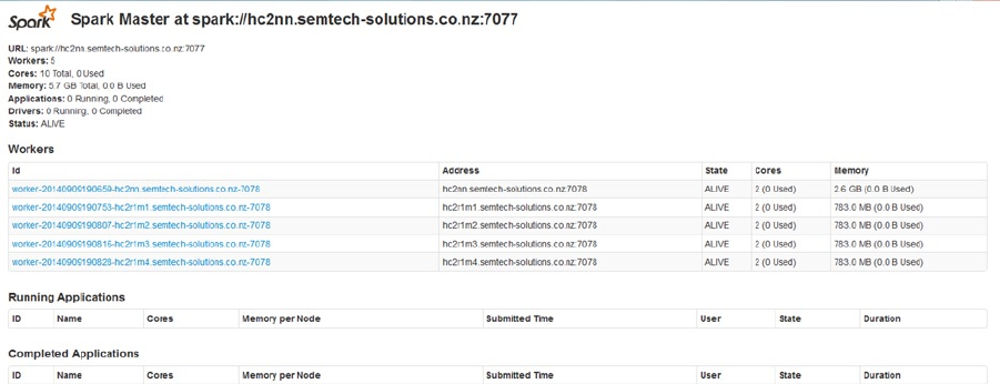
CHAPTER 9 ■ ANALYTICS WITH HADOOP

282

With the correct value for the variable set, I start the Spark Master and History servers on the master node:

[root@hc2nn ~]# service spark-master restart

[root@hc2nn ~]# service spark-history-server restart

Finally, I start the Spark workers on all of the data nodes:

[root@hc2r1m1 ~]# service spark-worker restart

That’s it; I have just started a basic Spark cluster! I now have the choice of user interfaces to monitor the Spark

cluster. In the configuration file spark-env.sh, the following default variables define the master and worker user

interface ports:

export SPARK_MASTER_WEBUI_PORT=18080

export SPARK_WORKER_WEBUI_PORT=18081

The Spark Master user interface can be found at hc2nn:18080; Figure 9-3 shows its appearance before any

applications are run. Notice the Spark Master URL at the top of the page; that’s needed to run applications later.

Figure 9-3. Spark Master server’s user interface

The interface also lists the Spark workers and the machines that they are running on, as well as some information

about the state, cores, and memory available to each worker. (In Figure 9-3, you’ll notice that I have also run a worker

on the name node, just to increase the processing capacity in this example.) The area at the bottom of the screen

in Figure 9-3 provides details on running applications, as well as completed applications. In Figure 9-3, none are

running, so the area is blank.

Uses of Spark

In this section, I use an example to demonstrate the Spark shell, an interactive Spark scripting session, and a Spark

application (provided with the installation) to show you how jobs can be submitted, as well as how they appear in the

Spark user interface. The Spark shell can be used interactively to run ad hoc scripts against Spark cluster-based data.

Running a Spark application, as you will see, allows you to run a job on a Spark cluster by using in-memory processing

in batch mode.

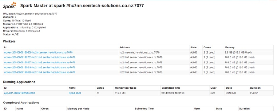
CHAPTER 9 ■ ANALYTICS WITH HADOOP

283

My SQL-based example shows that Spark-based information can be accessed using SQL. Although Spark

processing is not included in Chapter 10’s discussion of Talend and Pentaho, both tools integrate with Spark to offer

visual object-based data manipulation.

The first step in running a Spark script interactively in the Spark shell is to set the master URL displayed on the

Spark Master user interface to be the Spark URL:

[root@hc2nn ~]# spark-shell --master spark://hc2nn.semtech-solutions.co.nz:7077

As shown in Figure 9-4, the Spark shell application is now visible on the Spark Master user interface. The Running

Applications section in Figure 9-4 lists the appplication’s ID and name, as well as the number of cores and the memory

available to the application. I can also check the application’s submission time, state, user, and duration of its run.

Figure 9-4. Spark Master interface with applications listed

If I click one of the worker node IDs listed in the Workers section of the Spark Master interface, I can drill down

for more information, as shown in Figure 9-5. This detailed view shows the cores and memory available on the worker

node plus the executor for the running Spark shell on that node. I click the Back to Master link to return to the Spark

Master interface.

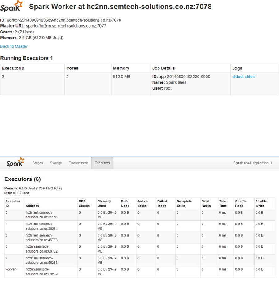
CHAPTER 9 ■ ANALYTICS WITH HADOOP

284

The work of a given application is spread across the cluster over a series of worker executors on each node. To

reach the application user interface, I simply click an application listed on the Spark Master interface that is in the

Running Applications section, as shown in Figure 9-4. The list of executors for this application is is then shown in

Figure 9-6.

Figure 9-5. Spark Worker user interface

Figure 9-6. Spark application interface

Executors are the tasks based on the cluster worker nodes that process and store an application’s data on the

Spark cluster. Figure 9-6 shows that each executor has a unique ID and address. It also shows the state of the executor

in terms of memory and disk, plus the task time.

So, when the interactive Spark shell is running, what can you do with it? To demonstrate a simple script, I read a

Linux-based CSV file from HDFS, run a line count on it in memory, and then do a string search on it. I also confirm the

results by checking the output against Linux commands.

CHAPTER 9 ■ ANALYTICS WITH HADOOP

285

The top few lines of the data from my CSV file using the Linux head command are as follows:

[root@hc2nn fuel_consumption]# head scala.csv

MODEL,MANUFACTURER,MODEL,VEHICLE CLASS,ENGINE SIZE,CYLINDERS,TRANSMISSION,FUEL,FUEL

CONSUMPTION,,,,FUEL,CO2 EMISSIONS

YEAR,,,,(L),,,TYPE,CITY (L/100 km),HWY (L/100 km),CITY (mpg),HWY (mpg),(L/year),(g/km)

2014,ACURA,ILX,COMPACT,2,4,AS5,Z,8.6,5.6,33,50,1440,166

2014,ACURA,ILX,COMPACT,2.4,4,M6,Z,9.8,6.5,29,43,1660,191

2014,ACURA,ILX HYBRID,COMPACT,1.5,4,AV7,Z,5,4.8,56,59,980,113

2014,ACURA,MDX 4WD,SUV - SMALL,3.5,6,AS6,Z,11.2,7.7,25,37,1920,221

I first copy this file to the /tmp directory on HDFS, so that Scala can access it, by using the HDFS file system

copyFromLocal command:

[root@hc2nn fuel_consumption]# hdfs dfs -copyFromLocal scala.csv /tmp/scala.csv

Note that when the Spark shell is used, the special variable sc is created. Called a Spark Context, the variable

describes the connection to the Spark cluster. So, at my Scala shell script prompt (scala >), I use the sc variable in the

following command to read the scala.csv file into memory:

scala> val myFile = sc.textFile("/tmp/scala.csv")

14/09/09 19:55:21 INFO storage.MemoryStore: ensureFreeSpace(74240) called with curMem=155704,

maxMem=309225062

14/09/09 19:55:21 INFO storage.MemoryStore: Block broadcast_1 stored as values to memory (estimated

size 72.5 KB, free 294.7 MB)

myFile: org.apache.spark.rdd.RDD[String] = MappedRDD[3] at textFile at <console>:12

The next command produces a line count on the file, now represented by the variable myFile, in memory:

scala> myFile.count()

14/09/09 19:55:41 INFO spark.SparkContext: Job finished: count at <console>:15, took 3.174464234 s

res1: Long = 1069

The result indicates that there are 1,069 lines in the file. The Spark-based line count can be checked against the

original file on the Linux file system. To do so, I use the Linux wc (word count) command with a -l switch to confirm

the count of 1,069 lines:

[root@hc2nn fuel_consumption]# wc -l scala.csv

1069 scala.csv

The following Spark shell Scala command counts the number of instances of the string “ACURA” in the

in-memory file:

scala> myFile.filter(line => line.contains("ACURA")).count()

14/09/09 19:58:10 INFO spark.SparkContext: Job finished: count at <console>:15, took 2.815524655 s

res0: Long = 12

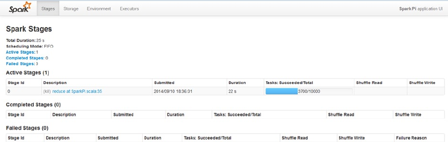
CHAPTER 9 ■ ANALYTICS WITH HADOOP

286

The result is 12 lines; checking that total by using the Linux grep command piped to the same wc command gives

the same result:

[root@hc2nn fuel_consumption]# grep ACURA scala.csv | wc -l

12

Interactively typing the shell commands is useful for short, simple tasks. For larger scripts, you can use the

spark-submit command to submit applications to the Spark cluster. For instance, I use one of the examples in the

spark-examples application library available under /usr/lib/spark/examples/lib/ in the CDH5 release (which is

supplied with the Spark install):

[root@hc2nn ~]# cd /usr/lib/spark/examples/lib/

[root@hc2nn lib]# ls -l spark-examples_2.10-1.0.0-cdh5.1.2.jar

-rw-r--r-- 1 root root 734539 Aug 26 15:07 spark-examples_2.10-1.0.0-cdh5.1.2.jar

I can execute example applications from this library on the cluster and monitor them using the master user

interface. For instance, the following code uses the spark-submit command to run the SparkPi example program

from the examples library. It sets the memory to be used on each worker at 700 MB and the total cores to be used at

10. It uses the same master Spark URL to connect to the cluster and specifies 10,000 tasks/iterations:

[root@hc2nn ~]# spark-submit \

--class org.apache.spark.examples.SparkPi \

--master spark://hc2nn.semtech-solutions.co.nz:7077 \

--executor-memory 700M \

--total-executor-cores 10 \

/usr/lib/spark/examples/lib/spark-examples_2.10-1.0.0-cdh5.1.2.jar \

10000

Checking the Spark Application interface for this application in Figure 9-7 shows the application details and the

progress of the job, such as the duration of the application run. I can also see that the default scheduling mode of FIFO

(first in, first out) is being used. As with YARN, I can set up a fair scheduler for Spark. In the Active Stages section, the

blue bar shows the progress of the application run.

Figure 9-7. Spark Application interface shows details of the job

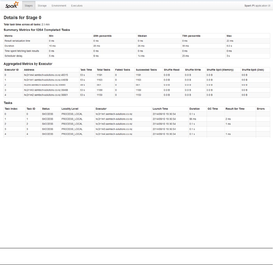
CHAPTER 9 ■ ANALYTICS WITH HADOOP

287

By clicking the Executors tab at the top of the Spark Application interface, I can examine details of the application

task, as shown in Figure 9-8. I can see the spread of tasks across the cluster nodes and the task times by node, as well

as a list of tasks, the nodes they run on, their execution times, and their statuses. The Summary Metrics section also

contains minimum, maximum, and percentile information for details like serialization, duration, and delay.

Figure 9-8. Spark Application interface shows job executors

As you can see from these simple examples, the Spark cluster is easy to install, set up, and use. To investigate

Spark in greater detail, visit the Apache Software Foundation website for Apache Spark at spark.apache.org.

Spark SQL

Rather than using the default Spark context object sc, you can create an SQL context from the default Spark context

and process CSV data using SQL. Spark SQL is an incubator project, however; it is not a mature offering at this

time. For instance, its APIs may yet change, and the version in CDH5 no longer reflects Spark SQL’s latest functions.

Despite that, it does offer some interesting features for memory-based SQL cluster processing. I use a simple example

of CSV file processing using Spark SQL, based on a schema-based RDD example at https://spark.apache.org/

docs/1.0.0/sql-programming-guide.html.

Note ■ For the latest details on Spark SQL, see the Spark website at spark.apache.org.

CHAPTER 9 ■ ANALYTICS WITH HADOOP

288

This example uses the same CSV file as was used in a previous example. The basic steps are to create a SQL

Context object in the Spark shell session to make Spark SQL functionality available, then import the data into a table

and run some SQL against it. Here is the CSV file data in the file /tmp/scala.csv. I have removed its header rows so that

it contains only raw data:

[root@hc2nn fuel_consumption]# head scala.csv

2014,ACURA,ILX,COMPACT,2,4,AS5,Z,8.6,5.6,33,50,1440,166

2014,ACURA,ILX,COMPACT,2.4,4,M6,Z,9.8,6.5,29,43,1660,191

2014,ACURA,ILX HYBRID,COMPACT,1.5,4,AV7,Z,5,4.8,56,59,980,113

2014,ACURA,MDX 4WD,SUV - SMALL,3.5,6,AS6,Z,11.2,7.7,25,37,1920,221

To use SQL in Spark, I enter the following command into my Spark shell:

scala> val sqlContext = new org.apache.spark.sql.SQLContext(sc)

This creates a SqlContext from the default Spark context sc, using the SQLContext class. Next, I import the

sqlContext library functionality so that it is available for the rest of the script:

scala> import sqlContext._

I define the schema using a case class to represent all of the comma-separated fields in the data file line. This

defines the number of fields, their name, order, and type:

scala> case class Vehicle(year: Int,manufacturer: String, model: String, vclass: String, engine:

Double, cylinders: Int, fuel: String, consumption: String, clkm: Double, hlkm: Double, cmpg: Int,

hmpg: Int, co2lyr: Int, co2gkm: Int)

Note ■ The column types are case-sensitive; for instance, “int” will cause an error while “Int” will not.

The data types used here are Int, String, and Double to represent the data vaues in the CSV file. The order is

important, as it should match the data in the CSV file row. Also, reserved words need to be avoided, so I have used the

column name vclass to describe my vehicle class.

Now, I create an RDD from the vehicle record, import the CSV file /tmp/scala.csv, split the file by the comma

character, and convert the data columns by type to match the columns in the schema above:

scala> val vehicle = sc.textFile("/tmp/scala.csv").map(_.split(",")).map(p => Vehicle(

p(0).trim.toInt,

p(1),

p(2),

p(3),

p(4).trim.toDouble,

p(5).trim.toInt,

p(6),

p(7),

CHAPTER 9 ■ ANALYTICS WITH HADOOP

289

p(8).trim.toDouble,

p(9).trim.toDouble,

p(10).trim.toInt,

p(11).trim.toInt,

p(12).trim.toInt,

p(13).trim.toInt

))

That’s quite a complicated statement, but if I break it down, it will seem simpler. The textFile option loads the

CSV file as a text file. The first map option splits the columns in the text file by comma. The next map option maps the

data columns from the previous step into the columns of the vehicle class that was just defined. So, the vehicle RDD

contains the comma-separated data from the file.

I register the vehicle RDD as a table called “vehicle” so that SQL can be executed against the table:

scala> vehicle.registerAsTable("vehicle")

At this point, the data has been imported into the RDD and the RDD has been registered as a table, so I am

ready to execute some SQL against the table. I want to select details of Aston Martin cars from the data. The following

statement creates a schema RDD called “aston” that contains the data from the SELECT statement:

scala> val aston = sql( "SELECT year, manufacturer, model, vclass, engine FROM vehicle WHERE

manufacturer = 'ASTON MARTIN' ")

The SELECT statement takes the year, manufacturer, model, class, and engine size columns from the vehicle table.

It filters the data, selecting only those where the manufacturer’s name is Aston Martin.

When printed, the resulting aston schema RDD appears as a string. One line is printed for each row that is

matched from the table. The five columns from the table that match the columns in the SQL are embedded in the

results string:

scala> aston.map( t => "year: " + t(0) + " manufacturer " + t(1) + " model " + t(2) + " class " +

t(3) + " engine " + t(4) ).collect().foreach(println)

That string prints the following data:

year: 2014 manufacturer ASTON MARTIN model DB9 class MINICOMPACT engine 5.9

year: 2014 manufacturer ASTON MARTIN model RAPIDE class SUBCOMPACT engine 5.9

year: 2014 manufacturer ASTON MARTIN model V8 VANTAGE class TWO-SEATER engine 4.7

year: 2014 manufacturer ASTON MARTIN model V8 VANTAGE S class TWO-SEATER engine 4.7

year: 2014 manufacturer ASTON MARTIN model VANQUISH class MINICOMPACT engine 5.9

Thus, the results show seven matching Aston Martin data rows with their model and class details.

From an analytics point of view, Spark SQL gives analysts SQL-based access to Spark data in memory. In

processing terms, it is much faster than traditional Map Reduce processing. Also, people with a background in

relational databases will be comfortable using SQL to interrogate their data.

CHAPTER 9 ■ ANALYTICS WITH HADOOP

290

Summary

Analysts, whether they be managers, testers, or researchers, need to find meaning in their data. They need to be able

to move, load, extract, and transform all or parts of their data to create meaning. Although the simple examples for

Impala, Hive, and Spark in this chapter may not yield any revelations in your company’s data, they do demonstrate the

available building blocks of analytics and provide an overview of the capabilities of these tools.

In this chapter I have shown that you can represent data on HDFS as a database table and use Hive QL or Impala

SQL to query and transform that data. If you combine the steps in this chapter with tools like Sqoop and Flume

(covered in Chapter 6), you can start to build ETL chains to source, move, and modify your data, step by step.

If you find that you need real-time processing rather than batch processing, you might consider using Apache

Spark. Following the example installation in this chapter, you can start using Spark on your cluster. The Spark SQL

example also shows how to process your Spark cluster based in memory data using SQL.

The next chapter covers the ETL tools Pentaho and Talend, which can be used to visually manipulate Hadoop- and

Spark-based data. They integrate with Map Reduce and Hadoop base tools like Pig, Sqoop, and Hive, and can be used

to create and schedule ETL-based chains using a combination of the Hadoop tools that have been introduced so far.

291

Chapter 10

ETL with Hadoop

Given that Hadoop-based Map Reduce programming is a relatively new skill, there is likely to be a shortage of highly

skilled staff for some time, and those skills will come at a premium price. ETL (extract, transform, and load) tools,

like Pentaho and Talend, offer a visual, component-based method to create Map Reduce jobs, allowing ETL chains

to be created and manipulated as visual objects. Such tools are a simpler and quicker way for staff to approach Map

Reduce programming. I’m not suggesting that they are a replacement for Java or Pig-based code, but as an entry point

they offer a great deal of pre-defined functionality that can be merged so that complex ETL chains can be created and

scheduled. This chapter will examine these two tools from installation to use, and along the way, I will offer some

resolutions for common problems and errors you might encounter.

Pentaho Data Integrator

In this first half of the chapter I explain how to source and install the Pentaho Data Integration (PDI) application.

Offering tools to analyze, visualize, explore, report, and predict in the same platform, PDI can work as a stand-alone

tool or can be downloaded into Pentaho Business Analytics. Pentaho offers enhanced functionality, features, and

professional support for PDI. The open-source version is called Kettle. PDI is downloaded as a generic zipped package

that can be installed on either Windows or Linux. Here’s how to install PDI and use it with Hadoop.

Note ■ For complete details on PDI, see the company’s website at www.pentaho.com/product/data-integration.

Installing Pentaho

You can download the installation package for the Pentaho Data Integrator (PDI) from the following URL:

http://sourceforge.net/projects/pentaho/files/Data%20Integration/5.1/pdi-ce-5.1.0.0-752.zip/

download.

With an installation package that you can use for either Lunix or Windows, the zipped file is 580 MB, so it takes

quite a while to download. By way of example, after I downloaded and extracted the package, I installed the Windows

package on my C: drive, as shown in Figure 10-1. As you can see in Figure 10-1, the software installs into a directory

called “data-integration.” Note the directory structure, the start-up scripts, and the plug-ins directory that have been

marked with red boxes. On Windows, you would start the application using the Spoon.bat script; on Linux, you would

use the Spoon.sh script.

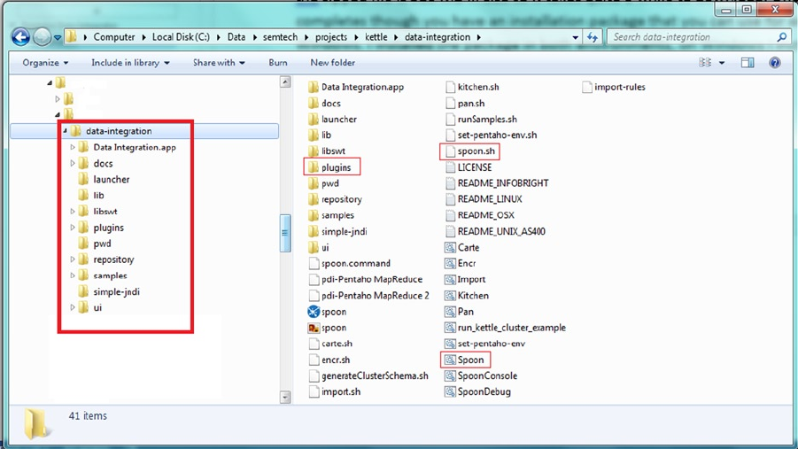
CHAPTER 10 ■ ETL WITH HADOOP

292

Before you start the application, the big data plug-in needs to know what Hadoop configuration you are using.

Figure 10-2 shows the structure of the PDI plugins directory, and specifically, the big data plug-in. It shows that the

pentaho-big-data-plugin resides within the plugins directory. This directory contains a file called plugin.properties

(Figure 10-2), which needs to be altered so that PDI knows which Hadoop version it is connecting to. To determine

which PDI plugin version to use, you check the Pentaho URL http://wiki.pentaho.com/display/BAD/Configuring+

Pentaho+for+your+Hadoop+Distro+and+Version, which provides a mapping of PDI plugin to Hadoop version.

Figure 10-1. Pentaho Data Integrator’s installation structure

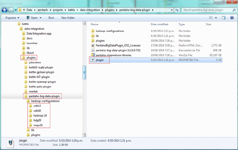
CHAPTER 10 ■ ETL WITH HADOOP

293

The subdirectories shown in the hadoop-configurations directory indicate which Hadoop configuration values

are supported by the pentaho-big-data-plugin. By changing the following line in the file plugin.properties, you set the

configuration:

active.hadoop.configuration=cdh50

For example, the setting shown in Figure 10-2 shows that I have set the pentaho-big-data-plugin for PDI to use

Cloudera’s CDH5 (cdh50). Because I have limited memory available on my CDH5 cluster, I decide to run PDI on a

Windows machine and access Hadoop on Linux remotely.

You also need to copy the Hadoop configuration files to the PDI plug-in hadoop directory. From the Cloudera

CDH5 manager home page, you select the YARN (MR2 Included) option, then select the Actions drop-down menu,

followed by Download Client configuration. The zipped file that is downloaded contains the files core-site.xml,

hadoop-env.sh, hdfs-site.xml, hive-site.xml, mapred-site.xml, and yarn-site.xml. Because I am using the CDH5

(cdh50) configuration, I copy these files to the following PDI directory: data-integration\plugins\pentaho-big-

data-plugin\hadoop-configurations\cdh50.

Pentaho requires Sun/Oracle Java 1.7, which is available at https://java.com/en/download/index.jsp. Be sure

to download and install this on Windows; the cmd.exe Window session output shows my Java installation as follows:

C:\Users\mikejf12>java -version

java version "1.7.0_67"

Java(TM) SE Runtime Environment (build 1.7.0_67-b01)

Java HotSpot(TM) 64-Bit Server VM (build 24.65-b04, mixed mode)

Figure 10-2. Pentaho Data Integrator, showing big data plug-in structure

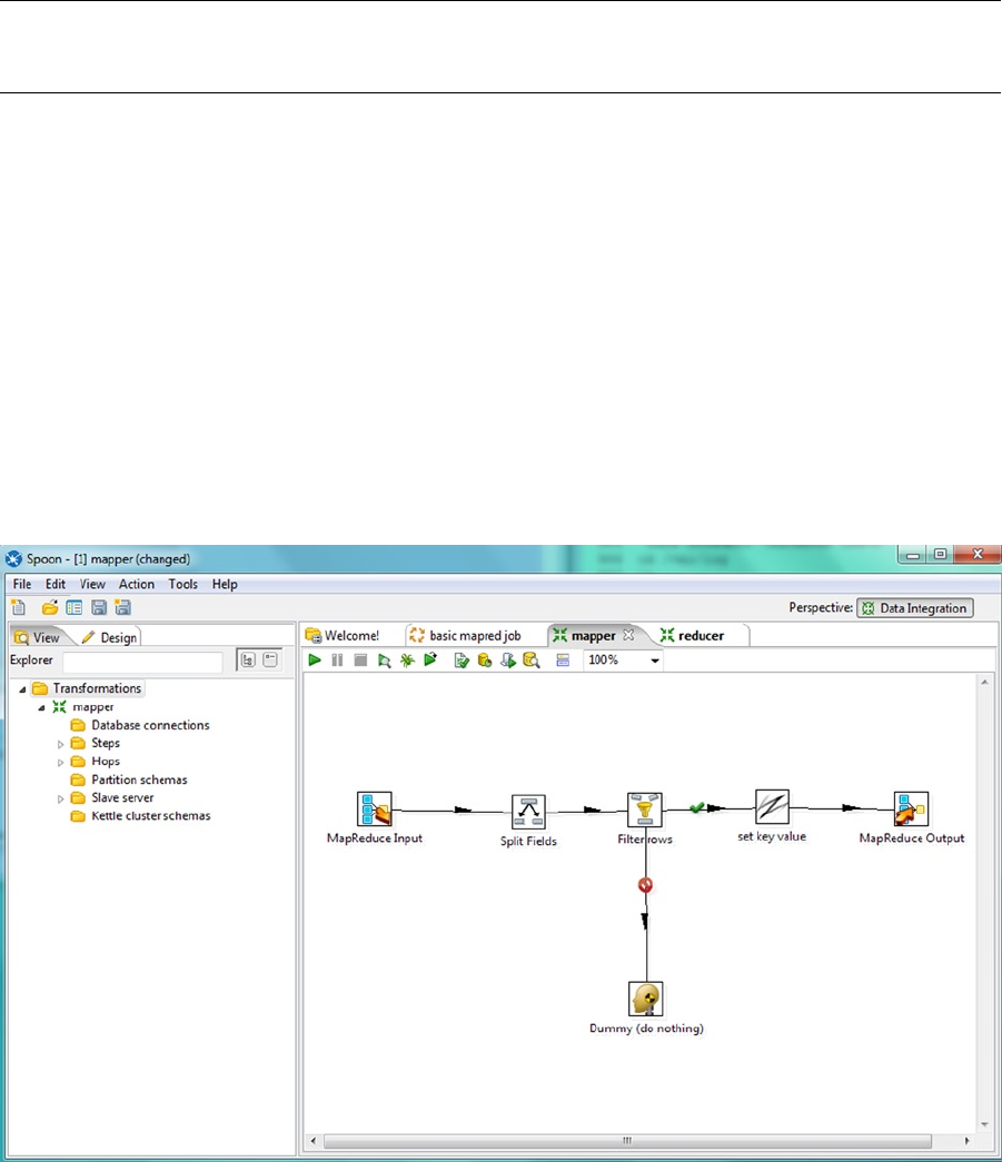
CHAPTER 10 ■ ETL WITH HADOOP

294

Note ■ If you plan to access MySQL with PDI, you also need to install a MySQL jar file from http://dev.mysql.com/

downloads/connector/j/ called mysql-connector-java-5.1.32-bin.jar into the PDI directory data-integration\lib.

I am using CDH5, so I also need to add the following to the copy of yarn-site.xml in the PDI plug-in directory that

was copied from Hadoop. This helps the Pentaho libraries locate the YARN server:

<name>yarn.resourcemanager.hostname</name>

</property>

Running the Data Integrator

You start PDI on Windows by using the Spoon.bat script, which starts the Spoon client application, as shown in

Figure 10-3. This is where you create your Map Reduce jobs.

Figure 10-3. Pentaho’s Spoon main window

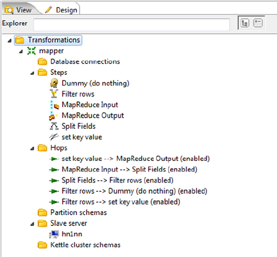
CHAPTER 10 ■ ETL WITH HADOOP

295

To be able to show the functionality of PDI, I have created some tasks, including a Map Reduce job called “basic

mapred job” and the associated Map and Reduce tranformations called “mapper” and “reducer,” respectively. As you

can see, these are already open and displayed in Figure 10-3. Also, note that the Explorer pane functionality on the left

of the figure changes depending on the current job or transformation that is displayed in the right pane.

The Explorer pane on the left of the window has View and Design tabs so that you can either see the content of

the task that you are working on or select functions to add to your job or transformation. The Working pane on the

right currently contains that Map Reduce job I just mentioned, called “basic mapred job” and the two transformations

called “mapper” and “reducer,” which it calls. If you drag the functionality icons from the Explorer pane to the

Working pane on the right, you can then configure and connect the functions to the flow of the task. (There will be

more about those functions later in the chapter.)

The Explorer view of the current mapper transformation, displayed in Figure 10-4, shows that it contains Map

Reduce inputs and outputs, a filter, a field splitter, a set key, and a dummy task. (I’ll explain all of these items in more

detail later.) The view also shows the task workflow hops that will be executed. As Figure 10-4 illustrates, you can

configure a slave server, meaning one instance of PDI uses another as a slave and gets that instance to run a task.

(To learn more about slave servers and how they work, see the Pentaho website at www.pentaho.com.)

Figure 10-4. Pentaho’s Explorer view

Figure 10-5 provides a taste of the functionality that’s available in the Design view. The two columns on the left

list the functions available for transformations (note the expanded big data section), while the two columns on the

right show the functions for jobs, again with an expanded big data view. You can construct transactions in a logical,

step-by-step manner by using these building blocks, then include the transactions in jobs that you schedule

within PDI.

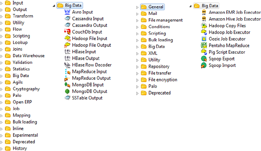
CHAPTER 10 ■ ETL WITH HADOOP

296

Creating ETL

Now that you have a sense of the PDI interface, it’s time to examine an example of a Map Reduce task to see how PDI

functions. I create an ETL example by starting with mapper and reducer transformations, and follow with the Map

Reduce job itself. By following my steps you’ll learn how each module is configured, as well as gain some tips on how

to avoid pitfalls.

To create my PDI Map Reduce example, I first need some data. The HDFS file (rawdata.txt) should look familiar—

parts of it were used in earlier chapters. Here, I use fuel consumption details for various vehicle models over a number

of years. The data file is CSV-based and resides under HDFS at /data/pentaho/rdbms/. I use the Hadoop file system

cat command to dump the file contents and the Linux head command to limit the data output:

[hadoop@hc2nn ~]$ hdfs dfs -cat /data/pentaho/rdbms/rawdata.txt | head -5

1995,ACURA,INTEGRA,SUBCOMPACT,1.8,4,A4,X,10.2,7,28,40,1760,202

1995,ACURA,INTEGRA,SUBCOMPACT,1.8,4,M5,X,9.6,7,29,40,1680,193

1995,ACURA,INTEGRA GS-R,SUBCOMPACT,1.8,4,M5,Z,9.4,7,30,40,1660,191

1995,ACURA,LEGEND,COMPACT,3.2,6,A4,Z,12.6,8.9,22,32,2180,251

1995,ACURA,LEGEND COUPE,COMPACT,3.2,6,A4,Z,13,9.3,22,30,2260,260

Figure 10-5. Pentaho Explorer’s Design view

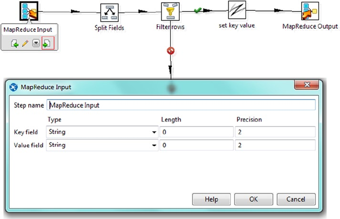
CHAPTER 10 ■ ETL WITH HADOOP

297

Figure 10-6. Input step of mapper transformation

Using Map Reduce, I want to create a count of manufacturer and model groupings from the data. The first step

is to create two transformations: a mapper and a reducer. The mapper receives the file lines and strips those lines

into fields. It filters out any empty lines and creates a key from the fields I am interested in. Finally, it outputs a single

record per line of the compound key and a value of 1. The reducer receives the output from the mapper, sorts data by

the key, then sums the values by key. It then outputs a sorted list of summed values for each key.

Figure 10-6 shows the structure of the mapper transformation.

Each Map Reduce transformation must start with a Map Reduce Input and end with a Map Reduce Output.

To set up the sequence, I simply click the Design tab in the Explorer pane of the main PDI interface, then drag the

components from the Design view to the Working pane on the right. To connect the components into a workflow,

I click a component to open a drop-down menu below it, click the rightmost green arrow icon (bordered in red in

Figure 10-6), and then drag a workflow to the next component to connect them. The workflow arrow indicates the

direction of flow and shows whether the action is unconditional or if it occurs only when the result is True or False. By

double-clicking a component, such as Map Reduce Input, I can open its configuration as shown in Figure 10-6. Here,

I can see that the input component has inputs called “key” and “value,” with fields described as “string” from the

HDFS file data.

Double-clicking the Split Fields icon opens its configuration, as shown in Figure 10-7. This component receives

a file line containing a comma-separated set of file fields that need to be split into separate values in order to be

manipulated. That is what this step does: it splits the string-based value field by using a comma as a separator and it

creates 14 new fields, Field 1 to Field 14.

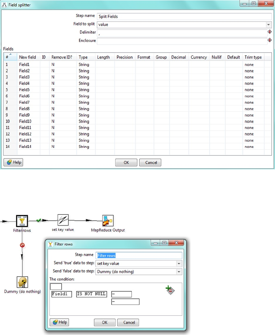
CHAPTER 10 ■ ETL WITH HADOOP

298

The next step in the flow is Filter Rows, a decision point where null rows are discarded based on the value of

Field 1. As you can see in Figure 10-8, the empty rows go to a dummy step whose flow has a False state. Valid rows

move on to the Set Key Value step whose flow has a True state, as indicated by the green tick.

Figure 10-7. Split Fields step of mapper transformation

Figure 10-8. Filter Rows step of mapper transformation

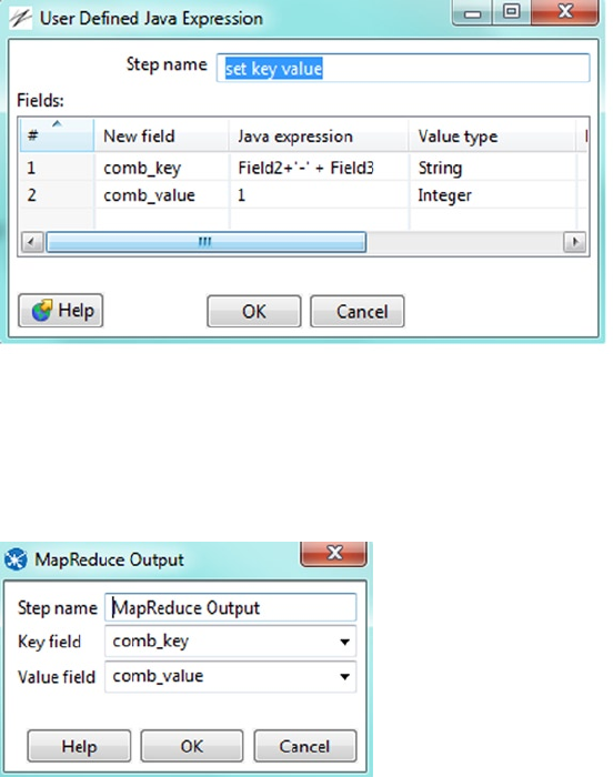
CHAPTER 10 ■ ETL WITH HADOOP

299

After filtering any bad rows out of the data, my next move is to build a compound key from the extracted data

fields via the Set Key Values step. This step creates a combined comb_key key value from Fields 2 and 3, separating

the string values with a dash. (Actually, this is created as a user-defined Java expression. It also creates a comb_value

value field with a value of 1, as shown in Figure 10-9).

Figure 10-9. Java expression for Set Key Values step of mapper transformation

These values are then passed to the MapReduce Output step, which assigns the comb_key and comb_value

variables to the mapper output variables key and value, as shown in Figure 10-10.

Figure 10-10. Output step of mapper transformation

That completes the definition of the mapper transformation that creates a key and value from the incoming data.

As described earlier, the reducer transformation accepts the incoming key / value pair and sorts it, then groups

by key values, sums the value, and finally outputs the results. Figure 10-11 shows the structure of the reducer

transformation. The Input step is the same as for the mapper transformation, but Figure 10-12 provides greater detail

on the Sort Rows step. Here, I define a single field: the sort key field (at the bottom). I also reduce the value in the sort

size field because I didn’t have much data and I wanted to save memory.

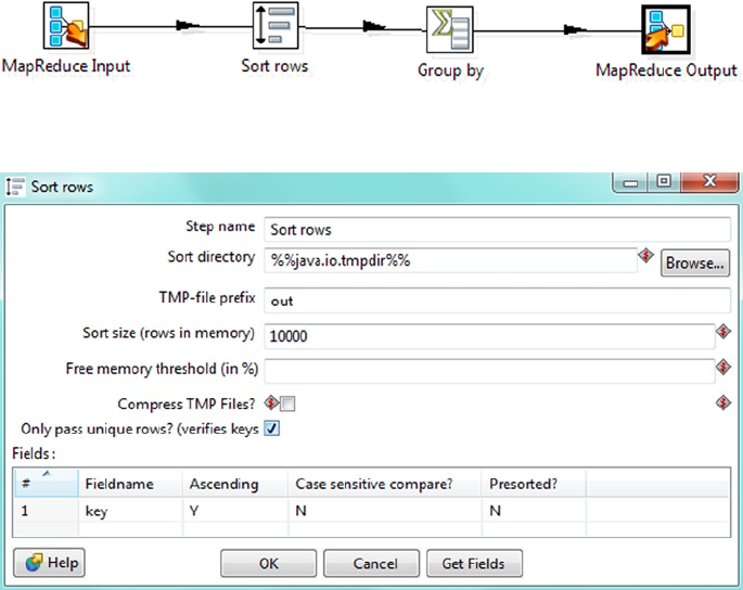
CHAPTER 10 ■ ETL WITH HADOOP

300

Figure 10-13 shows the Group By step, which groups the data by the key value and sums it by the numeric value

to create a new summed value variable called summed_val. The aggregate value is defined as the sum function

working on the value variable.

Figure 10-11. Steps in reducer transformation

Figure 10-12. Sort Rows step of reducer transformation

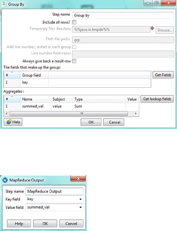
CHAPTER 10 ■ ETL WITH HADOOP

301

Finally, the reducer Output step produces the key/value data pair as the compound key value that was created by

the mapper and the summed value variable summed_val, as shown in Figure 10-14.

Figure 10-13. Group By step of reducer transformation

Figure 10-14. Output step of reducer transformation

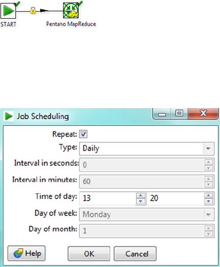
CHAPTER 10 ■ ETL WITH HADOOP

302

With the mapper and reducer transformations now defined, I can create a Map Reduce job, as shown in

Figure 10-15. A job always starts with a Start step, which I have pulled over from the General folder. I also add a Map

Reduce step, which uses the new mapper and reducer transformations.

Figure 10-15. Map Reduce job setup

Figure 10-16. Job scheduling for Map Reduce job

Double-clicking the Start step gives me the option to schedule the job. As you can see in Figure 10-16, this Map

Reduce job is scheduled to run daily at 13:20.

Figure 10-17 shows the Mapper configuration for the Map Reduce job called “pmr1.” The mapper value is defined

as the newly created mapper transformation, while the input and output values are defined as using the mapper

transformation MapReduce Input and Output steps.

CHAPTER 10 ■ ETL WITH HADOOP

303

Clicking the Reducer tab displays the job reducer configuration, as shown in Figure 10-18. The reducer step is

defined as the reducer transformation.

Figure 10-17. Mapper configuration for job

Figure 10-18. Reducer configuration for job

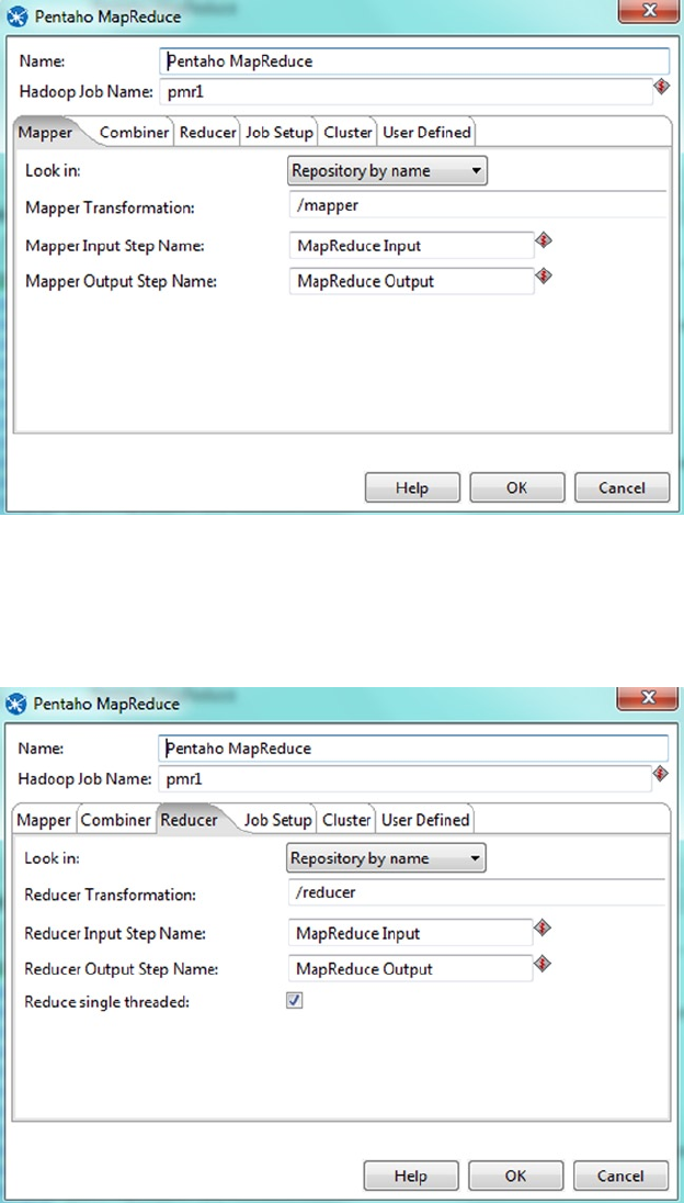
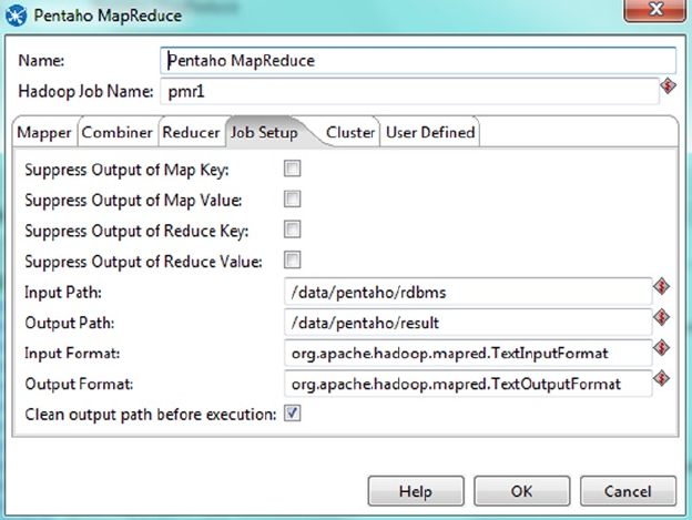
CHAPTER 10 ■ ETL WITH HADOOP

304

Next, I click the Job Setup tab to specify the input and output paths for the job data, a shown in Figure 10-19. The

input data file is stored on HDFS at /data/pentaho/rdbms, as explained earlier.

Figure 10-19. Job Setup tab for job pmr1

The input and output data formats for this job are defined as Hadoop Map Reduce based Java classes, such as

org.apache.hadoop.mapred.TextOutputFormat. The Clean option is selected so that the job can be rerun. That is,

each time the job runs, it will clean out the results directory.

Lastly, I define the connection to the Hadoop cluster using the Cluster tab. As you can see in Figure 10-20, the

only fields that I have changed in this tab are the hostnames and ports, so that Pentaho knows which hosts to connect

to (hc2nn) for HDFS and Map Reduce. I have also specified the ports, 8020 for HDFS and 8032 for the Resource

Manager (which is actually labeled as the Job Tracker, but this is a CDH5 cluster using YARN).

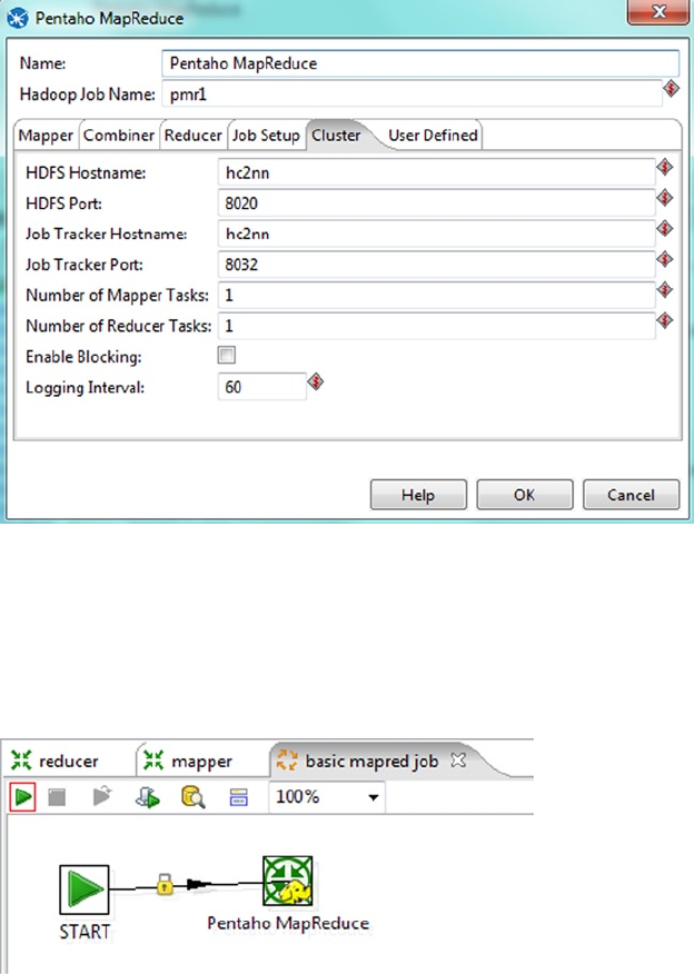
CHAPTER 10 ■ ETL WITH HADOOP

305

Now that the job is fully specified, I can run the Map Reduce job I’ve called “pmr1” against YARN and I can

monitor it via Pentaho PDI and the Resource Manager user interface. When it finishes, I can check the data on HDFS.

Clicking the green run arrow, highlighted with a red box in Figure 10-21, causes the Execute a Job job configuration

window to pop up.

Figure 10-20. Cluster tab for job pmr1

Figure 10-21. Main window for Map Reduce job

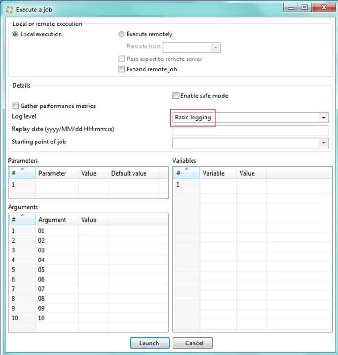
CHAPTER 10 ■ ETL WITH HADOOP

306

Figure 10-22 shows the Execute a Job window, in which I specify the logging levels and metrics so the Pentaho

Map Reduce job can be run. Note that the Logging Level drop-down menu is highlighted and set to Basic Logging in

Figure 10-22. If an error occurs, I can rerun the job and increase the logging level. (There’s more about logging levels

in the main PDI interface as well.)

Figure 10-22. Execute a Job window

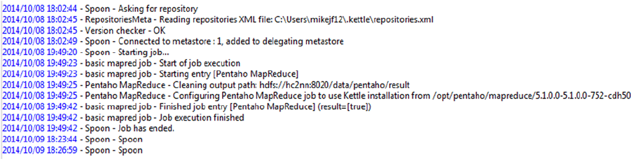
CHAPTER 10 ■ ETL WITH HADOOP

307

Figure 10-23. Results of job run

Clicking the Launch button executes the job and produces the basic-level log output that is shown in Figure 10-23.

I have also monitored this job via my Hadoop Resource Manager interface on the URL http://hc2nn.semtech-

solutions.co.nz:8088/cluster/apps. This URL allows me to watch the job’s progress until it is finished and monitor

log files, if necessary. As I know that the job has finished, there must be an existing part file under the results directory

that contains the results data. To see that output, I run this command from the Linux hadoop account:

[hadoop@hc2nn ~]$ hdfs dfs -cat /data/pentaho/result/part-00000 | head -10

ACURA-1.6 EL 2

ACURA-1.6EL 6

ACURA-1.7EL 12

ACURA-2.2CL 2

ACURA-2.3 CL 2

ACURA-2.3CL 2

ACURA-2.5TL 3

ACURA-3.0 CL 1

ACURA-3.0CL 2

ACURA-3.2 TL 1

I use the Hadoop file system cat command to dump the contents of the HDFS-based results part file, and then

the Linux head command to limit the output to the first 10 rows. What I see, then, is a summed list of vehicle makes

and models.

PDI’s visual interface makes it possible for even inexperienced Hadoop users to create and schedule Map Reduce

jobs. You don’t need to know Map Reduce programming and can work on client development machines. Simply by

selecting graphical functional icons, plugging them together, and configuring them, you can create complex ETL chains.

Potential Errors

Nothing in life goes perfectly, so let’s addresses some errors you may encounter during a job creation.

For instance, while working on the example just given, I discovered that a MySQL connector jar file had not been

installed into the PDI library directory when I tried to connect PDI to MySQL. I received the following error message:

Driver class 'org.gjt.mm.mysql.Driver' could not be found, make sure the 'MySQL' driver (jar file)

is installed.

CHAPTER 10 ■ ETL WITH HADOOP

308

Remember, if you plan to access MySQL with PDI, you also need to install a MySQL jar file called mysql-

connector-java-5.1.32-bin.jar from http://dev.mysql.com/downloads/connector/j/ into the PDI directory

data-integration\lib.

When PDI uses the big data plug-in, it copies libraries and configuration files to a directory called /opt/pentaho

on HDFS. Therefore, you need to make sure the user account you’re using for PDI has the correct permissions. For my

example, I was running PDI from a client Windows machine which employed the user ID from the Windows session

to access HDFS. I received the following error message:

2014/09/30 18:26:20 - Pentaho MapReduce 2 - Installing Kettle to /opt/pentaho/mapreduce/5.1.0.0-

5.1.0.0-752-cdh42

2014/09/30 18:26:28 - Pentaho MapReduce 2 - ERROR (version 5.1.0.0, build 1 from 2014-06-19_19-02-57

by buildguy) : Kettle installation failed

2014/09/30 18:26:28 - Pentaho MapReduce 2 - ERROR (version 5.1.0.0, build 1 from 2014-06-19_19-02-57

by buildguy) : org.apache.hadoop.security.AccessControlException:

Permission denied: user=mikejf12, access=WRITE, inode="/":hdfs:hadoop:drwxr-xr-x

The error was caused because the Windows account (mikejf12) did not have directory access on HDFS. You

can resolve this type of problem by using the HDFS chown and chmod commands to grant access on HDFS as the

commands below show:

[hadoop@hc2nn ~]$ hdfs dfs –chown mikejf12 /opt/pentaho

[hadoop@hc2nn ~]$ hdfs dfs –chmod 777 /opt/pentaho

[hadoop@hc2nn ~]$ hdfs dfs -ls /opt

Found 1 items

drwxrwxrwx - mikejf12 hadoop 0 2014-10-25 16:02 /opt/pentaho

Unfortunately, deadlines prevented me from resolving an error that occurred on my Linux CDH 4.6 cluster when

I tried to run a PDI Map Reduce job. I knew that it was not the fault of PDI, but in fact was a configuration problem

with the cluster, probably YARN. Here’s the error message I received:

2014/10/01 18:08:56 - Pentaho MapReduce 2 - ERROR (version 5.1.0.0, build 1 from 2014-06-19_19-02-57

by buildguy) : Unknown rpc kind RPC_WRITABLE

2014/10/01 18:08:56 - Pentaho MapReduce 2 - ERROR (version 5.1.0.0, build 1 from 2014-06-19_19-

02-57 by buildguy) : org.apache.hadoop.ipc.RemoteException(java.io.IOException): Unknown rpc kind

RPC_WRITABLE

This is a running cluster, but it is not quite configured in the way that PDI needs. If a cluster is configured with

CDH5 manager, then it seems to work, so the difference between the two configurations must hold the clue to the

solution.

The following error occurred when I tried to run the example PDI application on Centos Linux:

# A fatal error has been detected by the Java Runtime Environment:

#

# SIGSEGV (0xb) at pc=0x80a3812b, pid=4480, tid=3078466416

I resolved it by stopping the application from showing the welcome page at startup. To do so, I simply added the

following line to the file $HOME/.kettle/.spoonrc of the user running PDI:

ShowWelcomePageOnStartup=N

CHAPTER 10 ■ ETL WITH HADOOP

309

If the wrong type is specified for a key field, there will be an error message generated similar to the following:

{"type":"TASK_FAILED","event":{"org.apache.hadoop.mapreduce.jobhistory.TaskFailed":{"taskid":"task_1

412385899407_0008_m_000000","taskType":"MAP","finishTime":1412403861583,"error":",

Error: java.io.IOException: org.pentaho.hadoop.mapreduce.converter.TypeConversionException: \n

Error converting to Long: 1995,ACURA,INTEGRA,SUBCOMPACT,1.8,4,A4,X,10.2,7,28,40,1760,202\n

For input string: \"1995,ACURA,INTEGRA,SUBCOMPACT,1.8,4,A4,X,10.2,7,28,40,1760,202\"\n\n

In this case, a string key was incorrectly being treated as a value.

An error in the configuration of the PDI Map Reduce job can cause the following error message:

commons.vfs.FileNotFoundException: Could not read from

"file:///yarn/nm/usercache/mikejf12/appcache/application_1412471201309_0001/

container_1412471201309_0001_01_000013/job.jar"

/yarn/nm/usercache/mikejf12/appcache/application_1412471201309_0001/

container_1412471201309_0001_01_000001

because it is a not a file.

Although it looks like some kind of Hadoop configuration error, it is not. It was again caused by setting the wrong

data type on Map Reduce variable values. Just follow the example installation and configuration in this section and

you will be fine.

Finally, a lack of available memory on the Hadoop Resource Manager host Linux machine produces an error like

the following:

2014-10-07 18:08:57,674 INFO [RMCommunicator Allocator] org.apache.hadoop.mapreduce.v2.app.

rm.RMContainerAllocator:

Reduce slow start threshold not met. completedMapsForReduceSlowstart 1

To resolve a problem like this, try reducing the Resource Manager memory usage in the CDH Manager so that it

does not exceed that available.

Now that you understand how to develop a Map Reduce job using Pentaho, let’s see how to create a similar job

using Talend Open Studio. The illustrative example uses the same Hadoop CDH5 cluster as a data source and for

processing.

Talend Open Studio

Talend offers a popular big data visual ETL tool called Open Studio. Like Pentaho, Talend gives you the ability to create

Map Reduce jobs against existing Hadoop clusters in a logical, step-by-step manner by pulling pre-defined modules

from a palette and linking them in an ETL chain to create a Map Reduce based job. I describe how to source, install,

and use Open Studio, as well as to create a Pig-based Map Reduce job. Along the way, I point out a few common errors

and their solutions.

CHAPTER 10 ■ ETL WITH HADOOP

310

Installing Open Studio for Big Data

You can find Open Studio, as well as a number of other big data offerings, on Talend’s website at www.talend.com,

including a big data sand box and big data Studio and Enterprise editions. For the chapter’s example, I use the free,

30-day trial version downloaded from the Talend website rather than the sandbox version. This is because I plan to

connect Talend to my existing Hadoop cluster and I will tackle any problems as they arise. However, you may find the

sand box version useful because it contains sample code and a fully working Hadoop cluster. Also, I create a Pig-based

Map Reduce job because the full Java-based Map Reduce functionality is available only in the Enterprise product.

When I attempt to install these big data ETL tools, I always try to install them on Windows machines first, as I

hope to use them as clients connecting to my Linux-based Hadoop clusters. A shell-based error prevented me from

doing this at this time, so instead I install the Talend software on the Centos 6 Linux host hc1nn and I configure it to

connect to the CDH5 Hadoop cluster on nc2nn. (See the “Potential Errors” section for details on this error, which calls

for a fix to be added to future Cloudera releases.)

For this installation, I download the Talend Open Studio for Big Data 5.5 from the URL www.talend.com/

download. I select the Big Data tab and download the Open Studio software, as shown in Figure 10-24. (I added red

indicator boxes to the options that I need.) The download took an hour for me; the length of download time depends

on your bandwidth.

Figure 10-24. Software download for Talend

I place the software in a directory called talend in the Linux hadoop user account’s home directory, using the

Linux pwd command:

[hadoop@hc1nn talend]$ pwd

/home/hadoop/talend

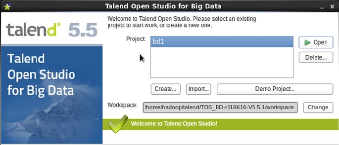
CHAPTER 10 ■ ETL WITH HADOOP

311

The downloaded zip file is 1010 MB and needs to be unzipped before use. The ls -lh command gives a long file

listing with sizes in a more readable form:

[hadoop@hc1nn talend]$ ls -lh TOS_BD-r118616-V5.5.1.zip

-rw-r--r-- 1 hadoop hadoop 1010M Oct 13 18:22 TOS_BD-r118616-V5.5.1.zip

When unpacked with the unzip command, the software resides in a directory called TOS_BD-r118616-V5.5.1:

[hadoop@hc1nn talend]$ unzip TOS_BD-r118616-V5.5.1.zip

[hadoop@hc1nn talend]$ ls

TOS_BD-r118616-V5.5.1 TOS_BD-r118616-V5.5.1.zip

[hadoop@hc1nn talend]$ cd TOS_BD-r118616-V5.5.1

There are a lot of files in this directory, but for this example, all I need to do is run the shell file (.sh). It determines

the architecture of the machine that it resides on and runs the correct binary. For instance, I am running Talend on a

64-bit Centos Linux host.

Running Open Studio for Big Data

To start Talend Open Studio, I issue the following command:

[hadoop@hc1nn TOS_BD-r118616-V5.5.1]$ ./TOS_BD-linux-gtk-x86.sh &

The “and” character (&) means that the job is running in the background so I can enter further commands in the

Linux session, if necessary. The command brings up the Project Chooser window, where I can either create or select a

Talend project, as shown in Figure 10-25. For this example, I select my project called “bd1,” and click Open.

Figure 10-25. Project chooser window for Talend

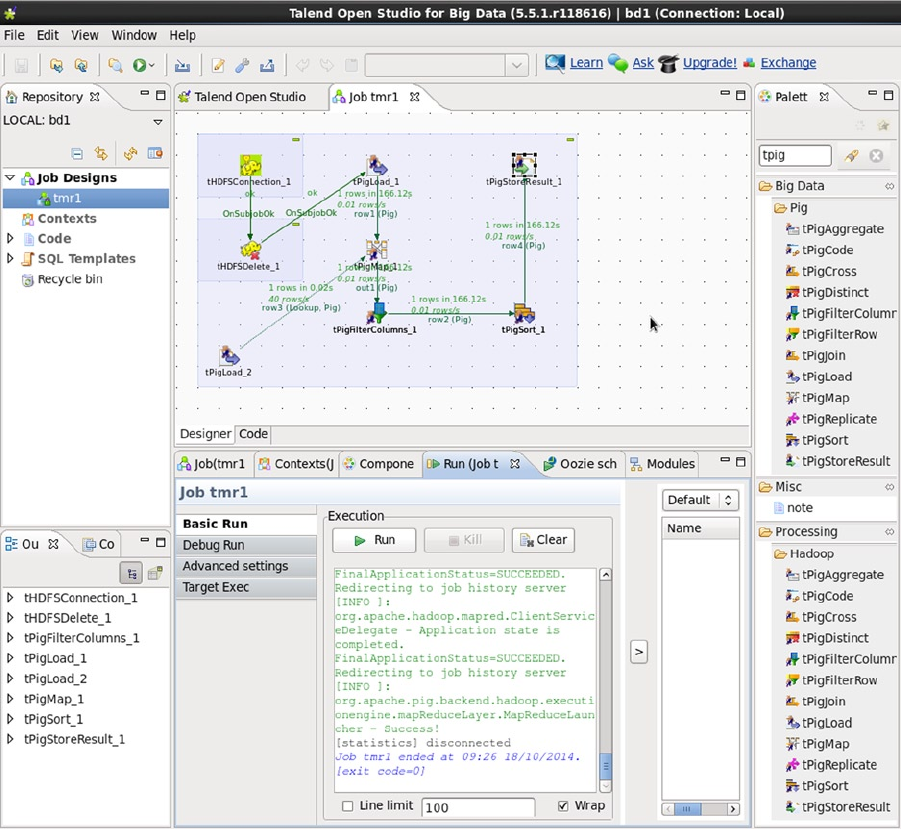
CHAPTER 10 ■ ETL WITH HADOOP

312

To be able to demonstrate the Designer perspective, which is displayed by default, previously I had created the

ETL job called “tmr1.” This allows me to explain the Open Studio interface features. Open Studio for Big Data opens to

the main interface, shown in Figure 10-26. The searchable palette on the right provides a list of dragable modules. For

instance, searching for “thdfs” and “tpig” provides a list of HDFS and Pig modules. The center of the interface contains

the current open jobs as tabs; in this case, tmr1, the Pig-based Map Reduce job I had created previously, is shown. The

arrows indicate data flows or conditions, while the icons represent functional modules, such as tHDFSConnection_1.

Because I have already successfully run tmr1, it shows some extra information about how the fast data rows were

processed (i.e., one row in 166.12 seconds).

Figure 10-26. Main user interface for Open Studio

CHAPTER 10 ■ ETL WITH HADOOP

313

The top-left side of the Figure 10-26 interface shows the local repository for the project bd1; from here, I can

double-click the tmr1 job to open it. At the bottom of the interface is a designer and code section. The Code tab

enables me to examine the Java code that Talend generates from the job file; the Designer tab allows me to both

configure each step of the job by selecting it and to run the job once the configuration is completed.

Before I proceed to use the Open Studio interface, I take a moment to consider the test data that this example

job will use. For instance, I have stored two CSV-based data files in the HDFS directory /data/talend/rdbms/, as the

following Hadoop file system ls command shows:

[hadoop@hc2nn ~]$ hdfs dfs -ls /data/talend/rdbms

Found 2 items

-rw-r--r-- 3 hadoop supergroup 1381638 2014-10-10 16:36 /data/talend/rdbms/rawdata.txt

-rw-r--r-- 3 hadoop supergroup 4389 2014-10-18 08:17 /data/talend/rdbms/rawprices.txt

The first file, called rawdata.txt, contains the vehicle model fuel consumption data that has been used in previous

chapter examples, while the second file, called rawprices.txt, contains the matching model prices. The combined

Hadoop file system cat command and the Linux head commands list the first 10 rows of each file, as follows:

[hadoop@hc2nn ~]$ hdfs dfs -cat /data/talend/rdbms/rawdata.txt | head -10

1995,ACURA,INTEGRA,SUBCOMPACT,1.8,4,A4,X,10.2,7,28,40,1760,202

1995,ACURA,INTEGRA,SUBCOMPACT,1.8,4,M5,X,9.6,7,29,40,1680,193

1995,ACURA,INTEGRA GS-R,SUBCOMPACT,1.8,4,M5,Z,9.4,7,30,40,1660,191

1995,ACURA,LEGEND,COMPACT,3.2,6,A4,Z,12.6,8.9,22,32,2180,251

1995,ACURA,LEGEND COUPE,COMPACT,3.2,6,A4,Z,13,9.3,22,30,2260,260

1995,ACURA,LEGEND COUPE,COMPACT,3.2,6,M6,Z,13.4,8.4,21,34,2240,258

1995,ACURA,NSX,TWO-SEATER,3,6,A4,Z,13.5,9.2,21,31,2320,267

1995,ACURA,NSX,TWO-SEATER,3,6,M5,Z,12.9,9,22,31,2220,255

1995,ALFA ROMEO,164 LS,COMPACT,3,6,A4,Z,15.7,10,18,28,2620,301

1995,ALFA ROMEO,164 LS,COMPACT,3,6,M5,Z,13.8,9,20,31,2320,267

[hadoop@hc2nn ~]$ hdfs dfs -cat /data/talend/rdbms/rawprices.txt | head -10

ACURA,INTEGRA,44284

ACURA,INTEGRA GS-R,44284

ACURA,LEGEND,44284

ACURA,LEGEND COUPE,44284

ACURA,NSX,32835

ACURA,2.5TL,44284

ACURA,3.2TL,44284

For my example, I plan to use only columns 2 and 3 from the first file, which contain the manufacturer and model

details, and the price information from the second file. (Note that these prices are test data, not real prices.)

CHAPTER 10 ■ ETL WITH HADOOP

314

Creating the ETL

Examining a completed job is a good way to understand Open Studio’s modules and workflow. Figure 10-27 shows

job tmr1, the Pig-based Map Reduce job I created for this example. It starts with a connection to HDFS called

tHDFSConnection_1, on the condition that the connection works control is passed to an HDFS delete step called

tHDFSDelete_1, which clears the results directory for the job. If that is okay, then control is passed to a tPigLoad step

called tPigLoad_1, which loads the rawdata.txt file from HDFS. At the same time, another load step called tPigLoad_2

loads the rawprices.txt file from HDFS. The data from these files is then passed to a module called tPigMap_1, which

will combine the data.

Figure 10-27. Work flow for Pig native Map Reduce job

Figure 10-28. Conditional job flow

Figure 10-27 shows that the tPigMap_1 step combines the data from the two files, while the tPigFilterColumns_1

step removes the column data that is not of interest. The tPigSort_1 step sorts the data, then the tPigStoreResult_1 step

saves the sorted data to HDFS.

To create your own jobs, you select modules in the palette and drag them to the center jobs pane. Then, you

right-click the icons to connect the modules via conditional arrows or arrows that represent data flows (as was

done with Pentaho earlier). Figure 10-28 shows the creation of a conditional flow between steps of a job. If the

tHDFSConnection_1 step works, then control will pass to the deletion step. Figure 10-29 illustrates the creation of a

specific data flow between the tPigLoad_1 and tPigMap_1 steps.

CHAPTER 10 ■ ETL WITH HADOOP

315

Now that you have a sense of the job as a whole, take a closer look at how it’s put together. From this point,

I walk slowly through the configuration of each step of the tmr1 example job, as well as point out some common

troublespots. At the end, I run the job and display the results from the HDFS results directory.

As long as the Component tab in the Designer window is clicked, I can select each step in a job and view its

configuration. For the HDFS connection, for example, the Hadoop version is defined as Cloudera and CDH5. The URI

for the Name Node connection is defined via the cluster Name Node host hc2nn, using the port number 8020. The

user name for the connection is defined as the Linux hadoop account; these choices are shown in Figure 10-30.

Figure 10-29. Data flow for Pig Map Reduce job

Figure 10-30. The trm1 job, with HDFS connection

The HDFS delete step shown in Figure 10-31 just deletes the contents of the /data/talend/result/ HDFS directory

so that this Talend job can be rerun. If this succeeds, then control passes to the next step. The ellipses (. . .) button to

the right of the Path field allows me to connect to HDFS and browse for the delete location.

Figure 10-31. HDFS delete step for trm1 job

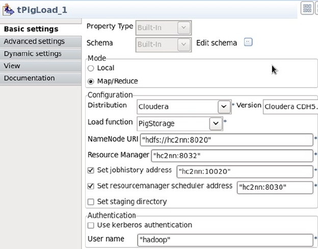
CHAPTER 10 ■ ETL WITH HADOOP

316

Figure 10-32. Loading the HDFS raw data file

At this step I encountered an error message. Initially failing to set the Resource Manager scheduler address

caused the Resource Manager-based job to time out and fail (see the “Potential Errors” section for more detail).

When loading a data file, you must also specify the schema to indicate what columns are in the incoming data,

what they should be called, and what data types they have. For this example, I click the Edit Schema button (shown at

the top of Figure 10-32) to open the Schema window, shown in Figure 10-33.

My next step is to load the rawdata.txt file (tPigLoad_1). Remember that even though the Hadoop cluster may be

fully configured via XML-based site configuration files, the Talend job carries configuration information, as shown

in Figure 10-32. Note also that the Map/Reduce icon has been selected here, telling Talend that this will be a Map

Reduce job. The same CDH5 cluster information has been specified. However, this time the host- and port-based

addresses have been set for the Resource Manager, the Job History server, and the Resource Manager scheduler. The

port values have been suggested by Talend as default values, and they match the default values chosen by the CDH5

Cluster Manager installer. Again, I use the Linux hadoop account for the connection.

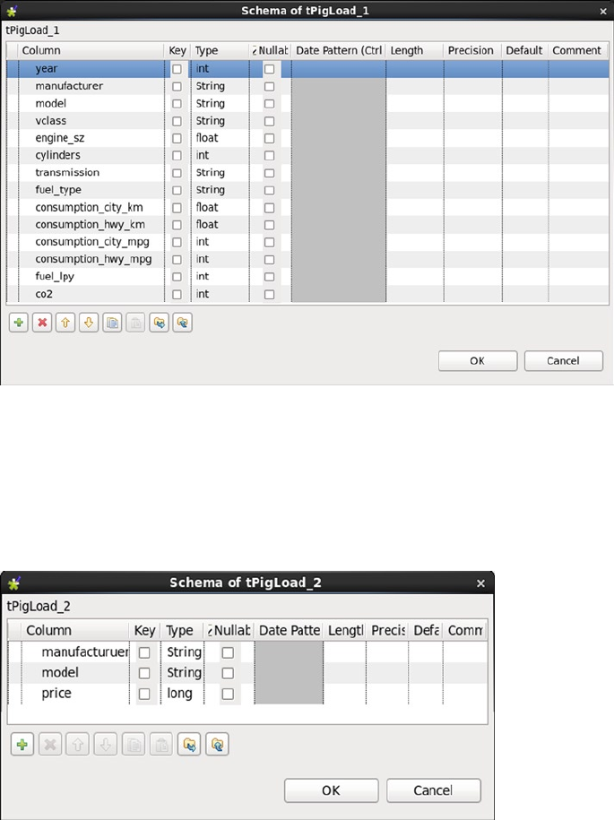
CHAPTER 10 ■ ETL WITH HADOOP

317

I use the green plus icon at the bottom left of the window to manually specify the column names and data types.

I try to make the names meaningful so that they accurately represent the data they contain. I do not add any keys,

and my data does not contain null values, so I leave those fields blank. The schema for the raw prices file from the

tPigLoad_2 step shows just three columns, the last of which is the vehicle price (see Figure 10-34).

Figure 10-33. Schema window for trm1 job

Figure 10-34. Three-column setup for trm1 job

The tPigMap_1 step takes the data from the loaded rawdata.txt and rawprices.txt files and combines them on

the manufacturer and model names. It then outputs the combined schema as a data flow called “out1,” shown in

Figure 10-35. The arrows in Figure 10-35 show the flow of columns between the incoming and outgoing data sources.

The schemas at the bottom of the window show the incoming and outgoing data. Note: the example does not map all

the incoming columns, as in a later step I will filter out the columns that are not needed from the resulting data set.

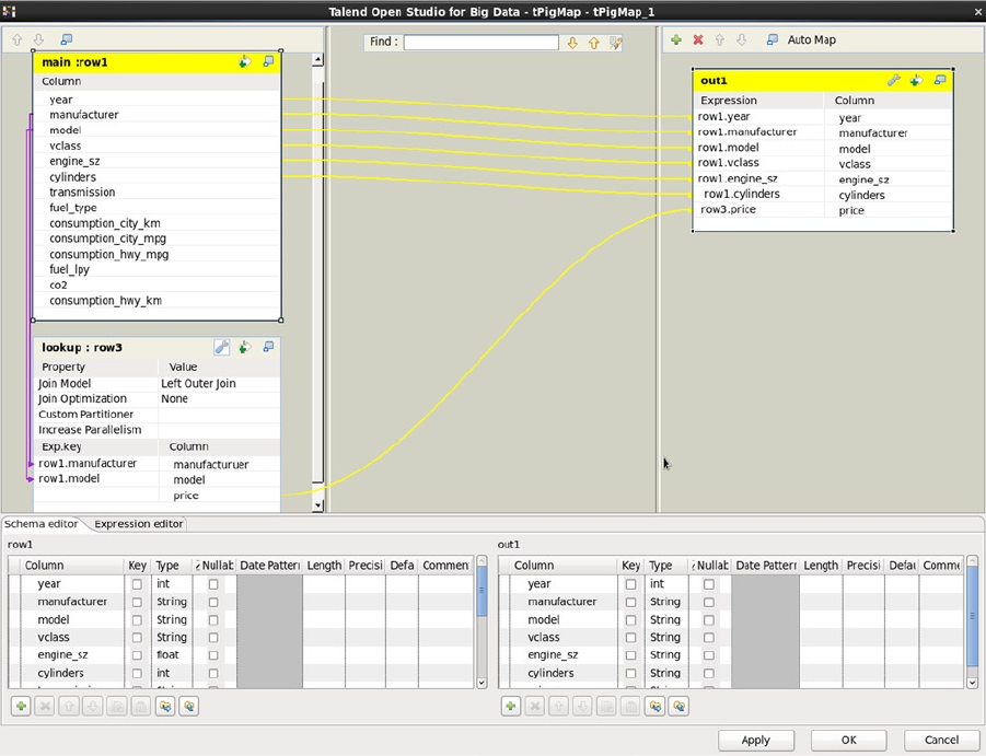
CHAPTER 10 ■ ETL WITH HADOOP

318

The column filtering step separates out the columns in the data source to just those required for the resulting

data set. In this case, the columns have been reduced to the vehicle manufacturer, model, and price information, as

shown Figure 10-36.

Figure 10-35. Incoming and outgoing data flows, with corresponding schemas

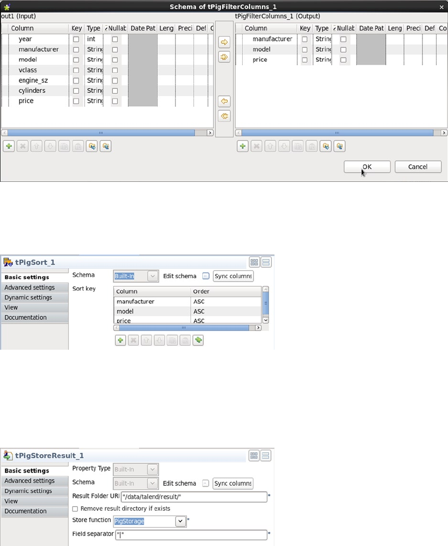
CHAPTER 10 ■ ETL WITH HADOOP

319

The next step is to sort the data and specify the order in which the columns will be sorted; Figure 10-37 shows a

compounded sorting key of manufacturer, model, and price.

Figure 10-36. Filter Columns step to eliminate unneeded columns

Figure 10-37. Sort step to put columns in desired order

Finally, the data is stored via a results step, which specifies where the Map Reduce job will store its data and what

the field separator will be, as shown in Figure 10-38. I use the default storage method of PigStorage and instruct the

data to be stored in the directory /data/talend/result/. Because this is a Map Reduce job, a successful outcome will

create a part file.

Figure 10-38. Results step provides for storage of the data

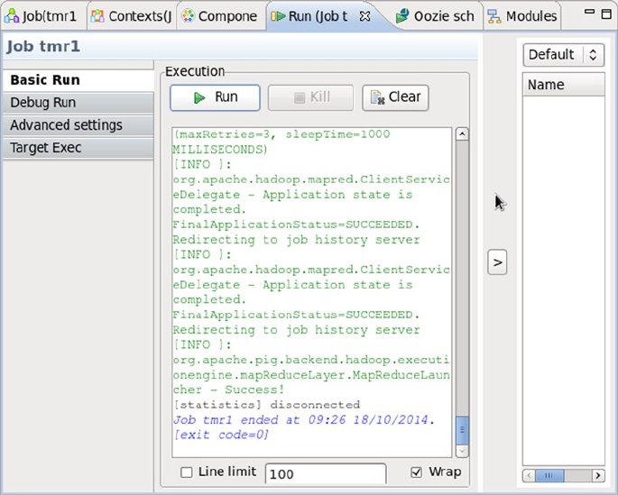
CHAPTER 10 ■ ETL WITH HADOOP

320

Having successfully created the job, I can now run it from the Designer window’s Run tab. I click the Run button

with the green run arrow to start the job. The Basic Run window shows minimal job output, while the Debug Run

option displays a little more output in case of error. The output is color coded; green lines are good and red lines show

an error. See Figure 10-39 for the results of my job example.

Figure 10-39. Job is run and results are shown

Remember that it is possible to track these jobs from the Resource Manager interface, as shown in Figure 10-40.

For my cluster, the Name Node hostname is hc2nn, and the Resource Manager http port number is 8088, so the URL is

hc2nn:8088.

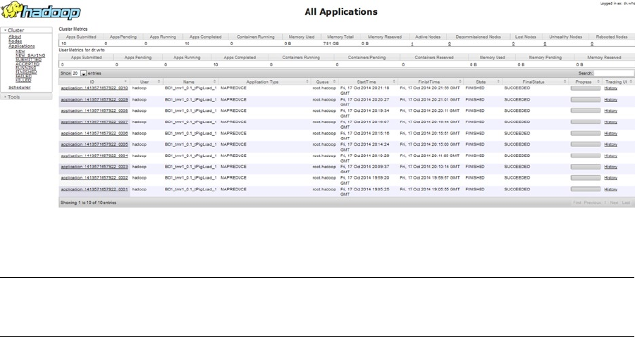
CHAPTER 10 ■ ETL WITH HADOOP

321

Note ■ If a Talend Map Reduce job hangs, the only place you can investigate the details of the job log is by using the

Resource Manager user interface.

Figures 10-39 and 10-40 both show that running this Talend job was a success, meaning I can find its output data

on HDFS in the target directory—/data/talend/result/, in this case. I use the HDFS file system command ls to create a

file listing of that directory showing the resulting data files:

[hadoop@hc2nn ~]$ hdfs dfs -ls /data/talend/result

Found 2 items

-rw-r--r-- 3 hadoop supergroup 0 2014-10-18 09:21 /data/talend/result/_SUCCESS

-rw-r--r-- 3 hadoop supergroup 441159 2014-10-18 09:21 /data/talend/result/part-r-00000

As would be expected, there is a _SUCCESS file and a part file that contains the data. Dumping the contents of the

part file by using the HDFS file system cat command shows me that the vehicle manufacturer, model, and price data

has been sorted and placed in the part file:

[hadoop@hc2nn ~]$ hdfs dfs -cat /data/talend/result/part-r-00000 | head -10

ACURA|1.6 EL|44284

ACURA|1.6EL|44284

Figure 10-40. Resource Manager interface for monitoring the job

CHAPTER 10 ■ ETL WITH HADOOP

322

All of the pricing information is the same because this is a small sample of the pricing test data. The output data

has been formatted with separator vertical (“|”) characters.

This simple example reflects only a small portion of the available Talend functionality, but it shows the potential

for building Map Reduce jobs using a drag-and-drop approach. Remember also that there is still more functionality

in the Talend Enterprise application. With the Enterprise application, you can build traditional Map Reduce jobs by

using a Map Reduce job type and specifying the functionality of the mapper and reducer components of the job.

Potential Errors

Here are some of the errors I encountered when developing this example, as well as their solutions. Check the Talend

forum at www.talendforge.org/forum for past issues encountered and to ask questions if you cannot find a solution

to your problem.

When I installed Talend on a Windows 7 machine, it crashed on startup, with the following error message:

Java was started but returned exit code = 1

C:\Windows\system32\javaw.exe

-Xms154m

-Xmx2536m

-XX:MaxPermSize=3256m

This problem was caused by a Windows patch called kb2977629. My solution was to remove the patch by

following these steps:

1. Select the Start button.

2. Click Control Panel.

3. Click Programs.

4. Under Programs and Features, Click View Installed Updates.

5. Search for kb2977629 and uninstall.

6. Restart Windows.

There was a permissions problem with HDFS when I was running Talend from Linux, which caused the following

error message:

cause:org.apache.hadoop.security.AccessControlException: Permission denied:

user=hadoop, access=WRITE, inode="/tmp/hadoop-yarn":yarn:supergroup:drwxr-xr-x

To fix the problem, I use the Linux su command to change the user to the YARN Linux user, and then used the

HDFS file system chmod command to change the permissions of the directory, as follows:

[root@hc2nn ~]# su - yarn

[yarn@hc2nn ~]$ hdfs dfs -chmod -R 777 /tmp/hadoop-yarn

The following memory-based error occurred because the maximum memory specified for Application Master

component on YARN was less than the level that was needed.

PriviledgedActionException as:hadoop (auth:SIMPLE) cause:java.io.IOException:

org.apache.hadoop.yarn.exceptions.InvalidResourceRequestException:

Invalid resource request, requested memory < 0, or requested memory > max configured,

requestedMemory=1536, maxMemory=1035

CHAPTER 10 ■ ETL WITH HADOOP

323

I solved this problem on YARN by changing the value of the parameter yarn.app.mapreduce.am.resource.mb in

the file yarn-site.xml, under the directory /etc/hadoop/conf. After making the change, I needed to restart the cluster

to pick up the change.

The next error occurred when I tried to run Talend from a Windows 7 host and tried to connect to a Centos 6

Linux-based CDH5 cluster:

83_0004 failed 2 times due to AM Container for appattempt_1413095146783_0004_000002 exited with

exitCode:

1 due to: Exception from container-launch: org.apache.hadoop.util.Shell$ExitCodeException:

/bin/bash: line 0: fg: no job control

org.apache.hadoop.util.Shell$ExitCodeException: /bin/bash: line 0: fg: no job control

This was not a problem with Talend, but a known fix appears in Horton Works HDP 2. I assume that it will soon

be fixed in other cluster stacks like CDH, but at the time of this writing, I used the Talend application only on Linux.

Finally, the following error occurred because I used insufficient configuration settings in the Talend tPigLoad step.

2014-10-14 17:56:13,123 INFO [main] org.apache.hadoop.yarn.client.RMProxy: Connecting to

ResourceManager at /0.0.0.0:8030

2014-10-14 17:56:14,241 INFO [main] org.apache.hadoop.ipc.Client: Retrying connect to server:

0.0.0.0/0.0.0.0:8030. Already tried 0 time(s); retry policy is RetryUpToMaximumCountWithFixedSleep

(maxRetries=10, sleepTime=1000 MILLISECONDS)

2014-10-14 17:56:15,242 INFO [main] org.apache.hadoop.ipc.Client: Retrying connect to server:

0.0.0.0/0.0.0.0:8030. Already tried 1 time(s); retry policy is RetryUpToMaximumCountWithFixedSleep

(maxRetries=10, sleepTime=1000 MILLISECONDS)

Because the Resource Manager scheduler address was not being set on the tPigLoad step, the address on YARN

defaulted to 0.0.0.0:8030, and so the job hung and timed out.

Summary

You can use visual, drag-and-drop Map Reduce enabled ETL tools, such as Pentaho Data Integrator and Talend Open

Studio, for big data processing. These tools offer the ability to tackle the creation of ETL chains for big data by logically

connecting the functional elements that the tools provide. This chapter covered only a fraction of the functionality

that they offer. Both include an abundance of Map Reduce components that you can combine to create more

permutations of functionality than I could possibly examine in these pages.

I created the examples in this chapter using a combination of a Hadoop cluster, which I built using Cloudera’s

CDH5 cluster manager, and the visual ETL big data enabled tools Pentaho and Talend. I think that the errors that I

encountered are either configuration based or will be solved by later cluster stack releases. Remember to check the

company websites for application updates and the supplier forums for problem solutions. If you don’t see a solution

to your ETL problem, don’t be afraid to ask questions; also, consider simplifying your algorithms as a way to zero in on

the cause of a problem.

Just as I believe that cluster managers reduce problems and ongoing costs when creating and managing Hadoop

clusters, so I think tools like Pentaho and Talend will save you money. They provide a quick entry point to the world of

Hadoop-based Map Reduce. I am not suggesting that they can replace low-level Map Reduce programming, because

I’m sure that eventually you will find complex problems that require you to delve down into API code. Rather, these

tools provide a good starting point, an easier path into the complex domain of Map Reduce.

325

Chapter 11

Reporting with Hadoop

Because the potential storage capability of a Hadoop cluster is so very large, you need some means to track both the

data contained on the cluster and the data feeds moving data into and out of it. In addition, you need to consider the

locations where data might reside on the cluster—that is, in HDFS, Hive, HBase, or Impala. Knowing you should track

your data only spawns more questions, however: What type of reporting might be required and in what format? Is a

dashboard needed to post the status of data at any given moment? Are graphs or tables helpful to show the state of a

data source for a given time period, such as the days in a week?

Building on the ETL work carried out in Chapter 10, this chapter will help you sort out the answers to those

questions by demonstrating how to build a range of simple reports using HDFS- and Hive-based data. Although you

may end up using completely different tools, reporting methods, and data content to construct the reports for your

real-world data, the building blocks presented here will provide insight into the tasks on Hadoop that apply to many

other scenarios as well.

This chapter will give you a basic overview of Hunk (the Hadoop version of Splunk) and Talend from a report-

generation point of view. It will show you how to source the software, how to install it, how to use it, and how to create

reports. Some basic errors and their solutions will be presented along with some simple dashboards to monitor the

data. The chapter begins withan introduction to the Hadoop version of Splunk, which is called Hunk.

Note ■ Reports show the state of given data sources in a variety of forms (tables, pie charts, etc.) and might also

aggregate data to show totals or use colors to represent data from different sources. Dashboards provide a single-page

view or overview of a system’s status and might also contain charts with key indicators to show the overall state of

its data.

Hunk

Hunk is the Hadoop version of Splunk (www.splunk.com), and it can be used to create reports and dashboards to

examine the state of the data on a Hadoop cluster. The tool offers search, reporting, alerts, and dashboards from

a web-based user interface. Let’s look at the installation and uses of Hunk, as well as some simple reports and

dashboards.

Installing Hunk

By way of example, I install Hunk onto the Centos 6 Linux host hc2nn and connect it to the Cloudera CDH5 Hadoop

cluster on the same node. Before downloading the Splunk software, though, I must first create an account and register

my details. I source Hunk from www.splunk.com/goto/downloadhunk.

CHAPTER 11 ■ REPORTING WITH HADOOP

326

Version 6 is about 100 MB. I install the software by using the Centos-based Linux hadoop account. Given that

I am logged into the hadoop account, the download file is saved to the Downloads directory, as follows:

[hadoop@hc2nn ~]$ pwd

/home/hadoop/Downloads

[hadoop@hc2nn Downloads]$ ls -l hunk-6.1.3-228780-Linux-x86_64.tar.gz

-rw-r--r-- 1 hadoop hadoop 105332713 Oct 28 18:19 hunk-6.1.3-228780-Linux-x86_64.tar.gz

This is a gzip compressed tar file, so it needs to be unpacked by using the Linux-based gunzip and tar

commands. I use the Linux gunzip command to decompress the .tar.gz file and create a tar archive file. The Linux tar

command then extracts the contents of the tar file to create the Hunk installation directory. In the tar option, x means

extract, v means verbose, and f allows me to specify the tar file to use:

[hadoop@hc2nn Downloads]$ gunzip hunk-6.1.3-228780-Linux-x86_64.tar.gz

[hadoop@hc2nn Downloads]$ tar xvf hunk-6.1.3-228780-Linux-x86_64.tar

[hadoop@hc2nn Downloads]$ ls -ld *hunk*

drwxr-xr-x 9 hadoop hadoop 4096 Nov 1 13:35 hunk

The ls -ld Linux command provides a long list of the Hunk installation directory that has just been created.

The l option provides the list while the d option lists the directory details, rather than its contents.

Having created the installation directory, I now move it to a good location, which will be under /usr/local. I need

to use the root account to do this because the hadoop account will not have the required access:

[hadoop@hc2nn Downloads]# su -

[root@ hc2nn Downloads]# mv hunk /usr/local

[root@ hc2nn Downloads]# cd /usr/local

[root@ hc2nn local]# chown -R hadoop:hadoop hunk

[root@ hc2nn local]# exit

[hadoop@ hc2nn Downloads]$ cd /usr/local/hunk

The Linux su command switches the current user to the root account. The Linux mv command moves the Hunk

directory from the hadoop account Downloads directory to the /usr/local/ directory as root. The cd command then

switches to the /usr/local/ directory, and the chmod command changes the ownership and group membership of

the installation to hadoop. The -R switch just means to change ownership recursively so all underlying files and

directories are affected. The exit command then returns the command to the hadoop login, and the final line

changes the directory to the new installation under /usr/local/hunk.

Now that Hunk is installed and in the correct location, I need to configure it so that it will be able to access the

Hadoop cluster and the data that the cluster contains. This involves creating three files—indexes.conf, props.conf, and

transforms.conf—under the following Hunk installation directory:

[hadoop@hc2nn local]$ cd /usr/local/hunk/etc/system/local

CHAPTER 11 ■ REPORTING WITH HADOOP

327

Of these three files, the indexes.conf file provides Hunk with the means to connect to the Hadoop cluster. For

example, to create a provider entry, I use a sequence similar to the following:

[hadoop@hc2nn local]$ cat indexes.conf

[provider:cdh5]

vix.family = hadoop

vix.command.arg.3 = $SPLUNK_HOME/bin/jars/SplunkMR-s6.0-hy2.0.jar

vix.env.HADOOP_HOME = /usr/lib/hadoop

vix.env.JAVA_HOME = /usr/lib/jvm/jre-1.6.0-openjdk.x86_64

vix.fs.default.name = hdfs://hc2nn:8020

vix.splunk.home.hdfs = /user/hadoop/hunk/workdir

vix.mapreduce.framework.name = yarn

vix.yarn.resourcemanager.address = hc2nn:8032

vix.yarn.resourcemanager.scheduler.address = hc2nn:8030

vix.mapred.job.map.memory.mb = 1024

vix.yarn.app.mapreduce.am.staging-dir = /user

vix.splunk.search.recordreader.csv.regex = \.txt$

This entry creates a provider entry called cdh5, which describes the means by which Hunk can connect to HDFS,

the Resource Manager, and the Scheduler. The entry describes where Hadoop is installed (via HADOOP_HOME) and the

source of Java (via JAVA_HOME). It specifies HDFS access via the local host name and name node port of 8020. Resource

Manager access will be at port 8032, and Scheduler access is at port 8030. The framework is described as YARN, and

the location on HDFS that Hunk can use as a working directory is described via the property vix.splunk.home.hdfs.

The second file, props.conf, describes the location on HDFS of a data source that is stored under /data/hunk/

rdbms/. The first cat command dumps the contents of the file, and the extractcsv value refers to an entry in the file

tranforms.conf that describes the contents of the data file:

[hadoop@hc2nn local]$ cat props.conf

[source::/data/hunk/rdbms/...]

REPORT-csvreport = extractcsv

The third file, transforms.conf, contains an entry called extractcsv, which is referenced in the props.conf

file above. It has two properties: the DELIMS value describes how the data line fields are delimited (in this case, by

commas); and the FIELDS property describes 14 fields of vehicle fuel-consumption data. This is the same fuel-

consumption data that was sourced in Chapter 4, where it was used to create an Oozie workflow.

[hadoop@hc2nn local]$ cat transforms.conf

[extractcsv]

DELIMS="\,"

FIELDS="year","manufacturer","model","class","engine size","cyclinders","transmission","Fuel

Type","fuel_city_l_100km","fuel_hwy_l_100km","fuel_city_mpg","fuel_hwy_mpg","fuel_l_yr","c02_g_km"

CHAPTER 11 ■ REPORTING WITH HADOOP

328

Here’s a sampling of the CSV file contents via an HDFS file system cat command, which dumps the contents of

the file /data/hunk/rdbms/rawdata.txt. The Linux head command limits the output to five lines:

[hadoop@hc2nn local]$ hdfs dfs -cat /data/hunk/rdbms/rawdata.txt | head -5

1995,ACURA,INTEGRA,SUBCOMPACT,1.8,4,A4,X,10.2,7,28,40,1760,202

1995,ACURA,INTEGRA,SUBCOMPACT,1.8,4,M5,X,9.6,7,29,40,1680,193

1995,ACURA,INTEGRA GS-R,SUBCOMPACT,1.8,4,M5,Z,9.4,7,30,40,1660,191

1995,ACURA,LEGEND,COMPACT,3.2,6,A4,Z,12.6,8.9,22,32,2180,251

1995,ACURA,LEGEND COUPE,COMPACT,3.2,6,A4,Z,13,9.3,22,30,2260,260

Now that some basic configuration files are set up, I can start Hunk.

Running Hunk

Hunk is started from the bin directory within the installation as the Linux hadoop account user.

Note ■ When you first start Hunk, you must use the --accept-license option; after that, it may be omitted.

In either case, you start Hunk by using the splunk command:

[hadoop@hc2nn local]$ cd /usr/local/hunk/bin

[hadoop@hc2nn bin]$ ./splunk start --accept-license

When starting, Hunk reads its configuration files, so you need to monitor the output for errors in the

configuration files’ error messages, such as:

Checking conf files for problems...

Invalid key in stanza [source::/data/hunk/rdbms/...] in /usr/local/hunk/etc/system/local/

props.conf, line 3: DELIMS (value: ", ")

If any errors occur, you can fix the configuration files and restart Hunk, as follows:

[hadoop@hc2nn bin]$ ./splunk restart

If all is well, you are presented with a message containing the URL at which to access Hunk’s web-based user

interface:

The Splunk web interface is at http://hc2nn:8000

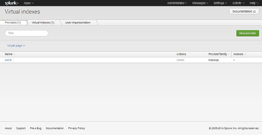
CHAPTER 11 ■ REPORTING WITH HADOOP

329

You can click the cdh5 entry to examine the provider’s details. The entire list of provider properties is too large

to display here, but know that Hunk automatically adds extra entries like vix.splunk.search.recordreader, which

defines how CSV files will be read. To represent most of the details in Figure 11-2, I arranged the list in two columns.

Figure 11-1. Hunk provider cdh5

You will need to login with the account name “admin” and the initial password of “changeme,” which you will

immediately be prompted to change. Once logged in, you will see the Virtual Indexes page, which, as shown in

Figure 11-1, displays the provider cdh5 in the family hadoop that was created in the indexes.conf file. If you don’t see

the Virtual Indexes page, then select Settings and go to Virtual Indexes from the top menu bar.

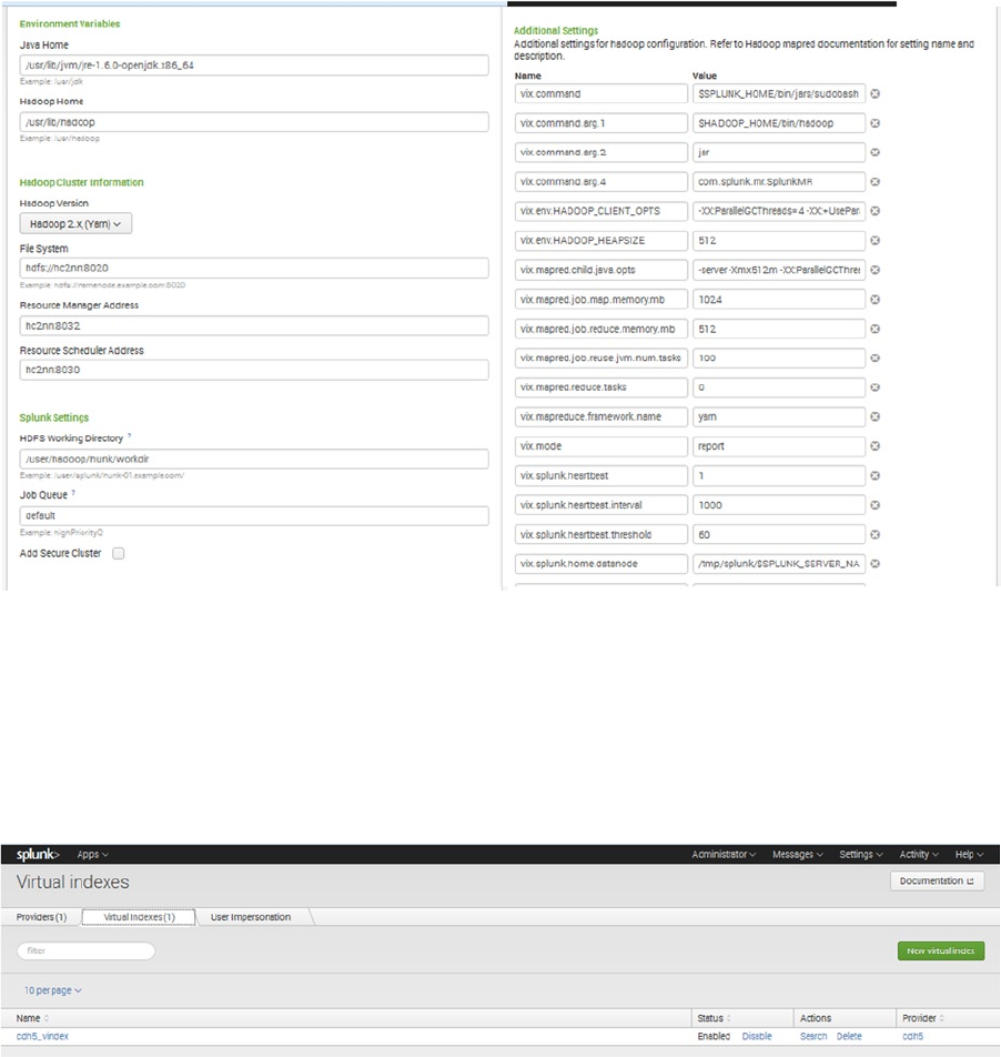
CHAPTER 11 ■ REPORTING WITH HADOOP

330

Figure 11-3. Hunk virtual index cdh5_vindex

Figure 11-2. Properties for Hunk provider cdh5

Note that the Hadoop version in Figure 11-2 is set to YARN to reflect the CDH5 YARN version. It has not been

necessary to specify the Hadoop supplier name.

Now, click Cancel to leave the cdh5 properties view, and click on the Virtual Indexes tab. For the chapter

example, this tab shows that a single virtual index has been created in Hunk called cdh5_vindex, as shown in

Figure 11-3.

Virtual indexes are the means by which hunk accesses the Hadoop cluster-based data. They enable Hunk to use

Map Reduce against the data and present the results within Hunk reports. By selecting the cdh5_vindex entry, you can

examine the attributes of this virtual index (Figure 11-4). Currently, the entry, which was defined in the props.conf file,

doesn’t have much detail.It just defines the directory on HDFS where the CSV data is located. Click the Cancel button

to exit this property details screen.

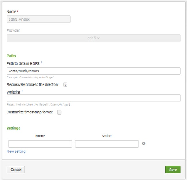
CHAPTER 11 ■ REPORTING WITH HADOOP

331

Creating Reports and Dashboards

Clicking the green menu bar’s Search option opens the Search window, as shown in Figure 11-5. It should be noted

here that report generation is asynchronous. If the report is complex or the data large, then Hunk may take time

to deliver the results. So please be patient, and don’t assume an error has occurred if your results do not return

imediately.

Figure 11-4. Property details of Hunk virtual index cdh5_vindex

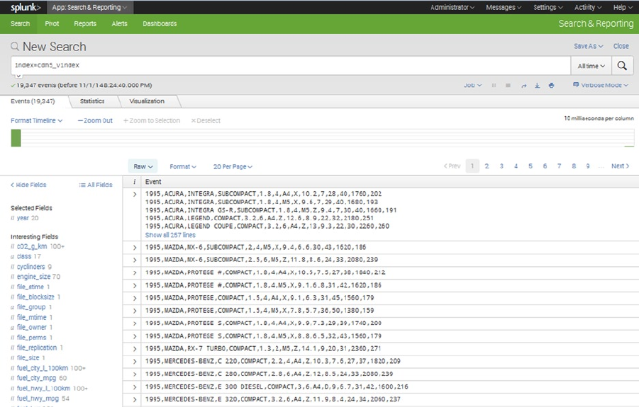
CHAPTER 11 ■ REPORTING WITH HADOOP

332

Figure 11-5 shows the raw-data view of the HDFS-based CSV file data I’ve been working with. I can scroll through

the data by using the Previous and Next options on the top right of the screen. The Raw drop-down menu offers three

choices for the format of the data displayed: raw, list, or table. In my example, I will build reports from this tabular

form of the vehicle data.

The Format drop-down menu’s options depend on the display type and on desired affects like data wrapping,

line number, and drill down. Notice on the left that fields have been split into two categories: selected fields and

interesting fields. The selected fields are those that will be displayed in table mode. The interesting fields are a

combination of those fields defined in the data and those pre-defined by Hunk.

I click any field to view a Hunk Field Summary window, then set the Selected option to Yes to place the field I

have chosen into the set of selected fields, as shown in Figure 11-6. When the mode is changed to Table, that field

appears in the data in the order in which it appears in the selected list. There are a number of pre-defined reports

available, like Top Values, that can be used to create single-column reports. Also, the top 10 values are displayed with

counts and percentages.

Figure 11-5. Hunk Search window

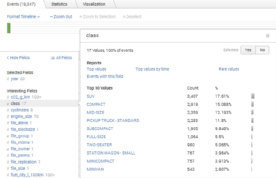
CHAPTER 11 ■ REPORTING WITH HADOOP

333

By selecting the Year field, and then selecting the Top Values report option in the menu that pops up, I can begin

to build a simple report that will show overall volume in my data by year. The report is created under the Visualization

tab. There, I find drop-down menu options for the report’s display, as shown in Figure 11-7. For example, I can switch

the display from a bar chart, to a single line graph, to a pie chart. There is also an option to change the format for each

display type and an option to change the underlying job settings.

Figure 11-6. Hunk Field Summary window

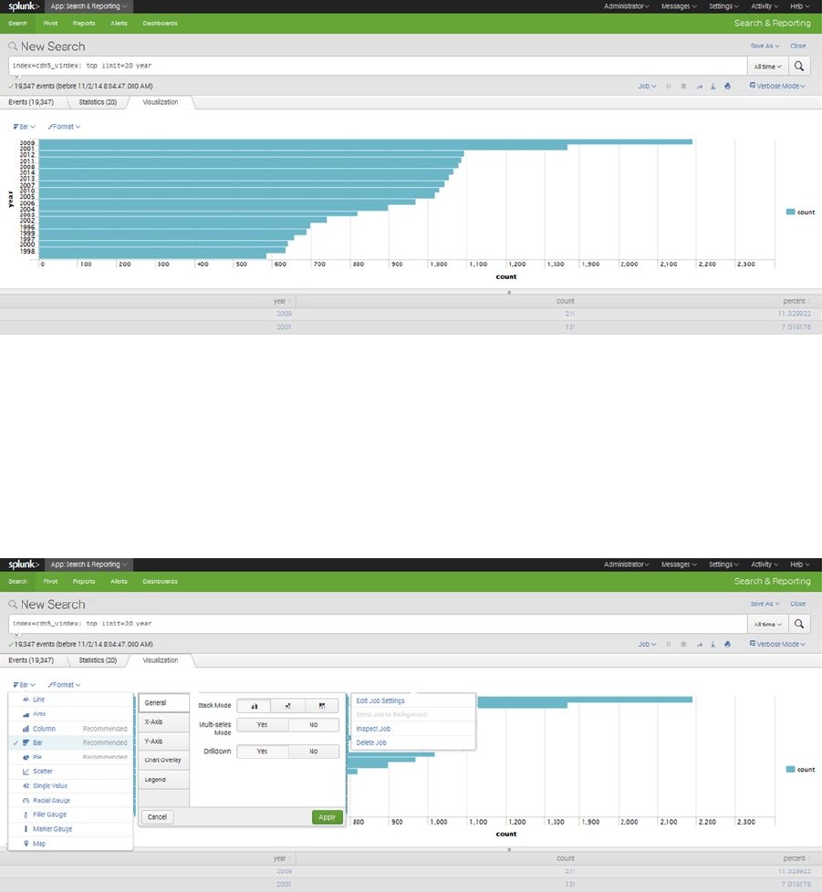
CHAPTER 11 ■ REPORTING WITH HADOOP

334

Figure 11-8. Hunk report menu options

Figure 11-7. Hunk Field bar report

The search command that has created this report is displayed at the top of the page as index=cdh5_vindex | top

limit=20 year. This means that the original search (index=cdh5_vindex) has been piped to the top command, with a

limit of the 20 topmost values for the field year. The report is acting on the year field and displaying a default bar graph

with the year value on the Y axis and the volumes on the X axis.

Figure 11-8 is a concatenated view of the report type, format, and job menus to show the options that are

available by which you can change the appearance and job details of a report.

Figure 11-9 shows all variations on the available options in a single Format menu to change the appearance of

the report. For instance, I could define the attributes of the X and Y axis, general drill down, titles, data intervals, and

position of the legend. I can modify these attributes until I am satisfied with the appearance of my report, then click

the Apply button to put those changes into effect.

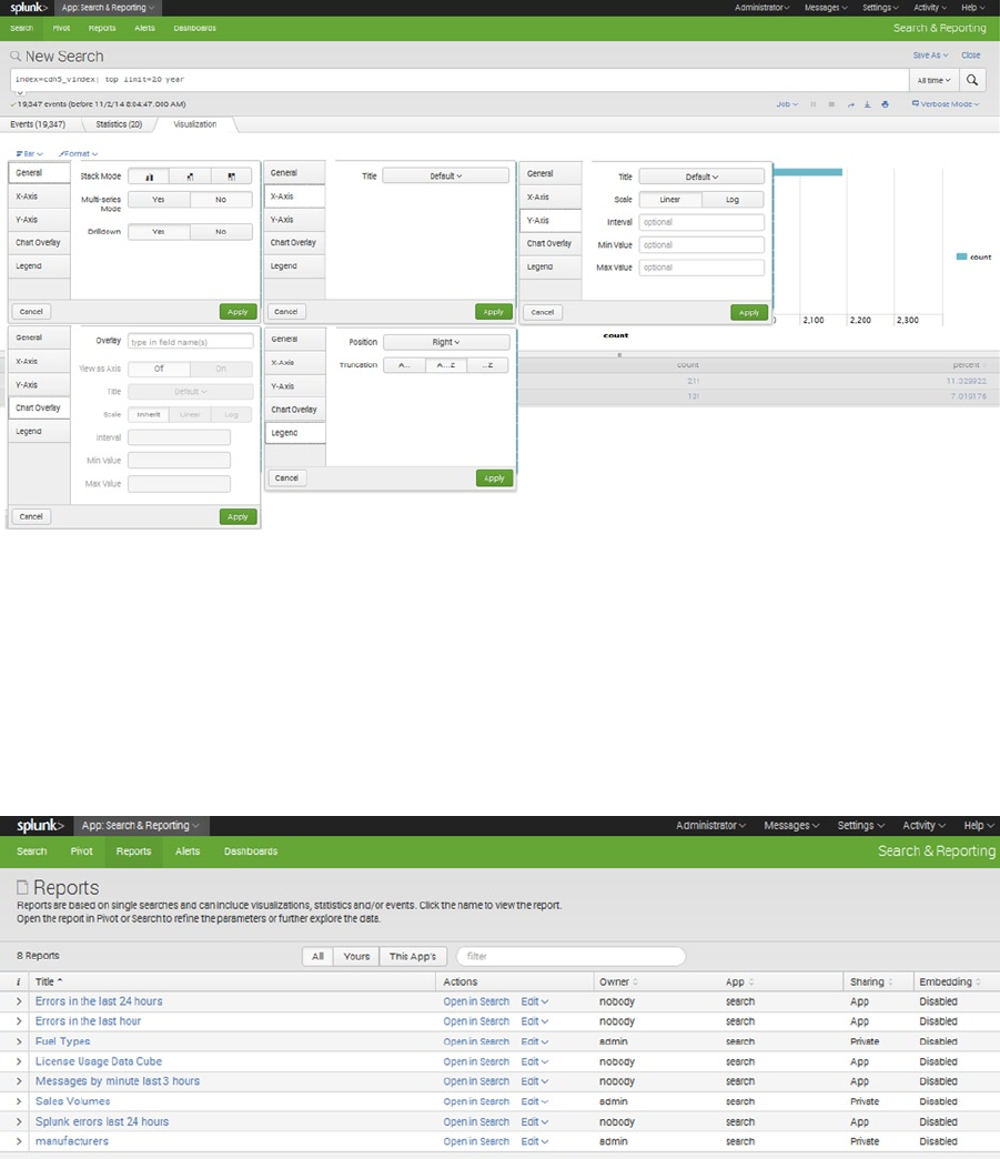
CHAPTER 11 ■ REPORTING WITH HADOOP

335

I click the Save As option to save the report so that it can be used later.

I have saved a number of reports in this manner within Hunk; they are single-column reports that cover areas like

sales volume per year, vehicle manufacturers, and vehicle fuel types. I can view the saved Hunk reports by selecting

the Reports option in the green menu bar. The Reports page, as shown in Figure 11-10, displays details like the report’s

title, ownership, apps, and sharing status. It also shows whether the report has been disabled, and it offers the option

to edit or open the report again.

Figure 11-9. Hunk options for format changes

Figure 11-10. Hunk report status

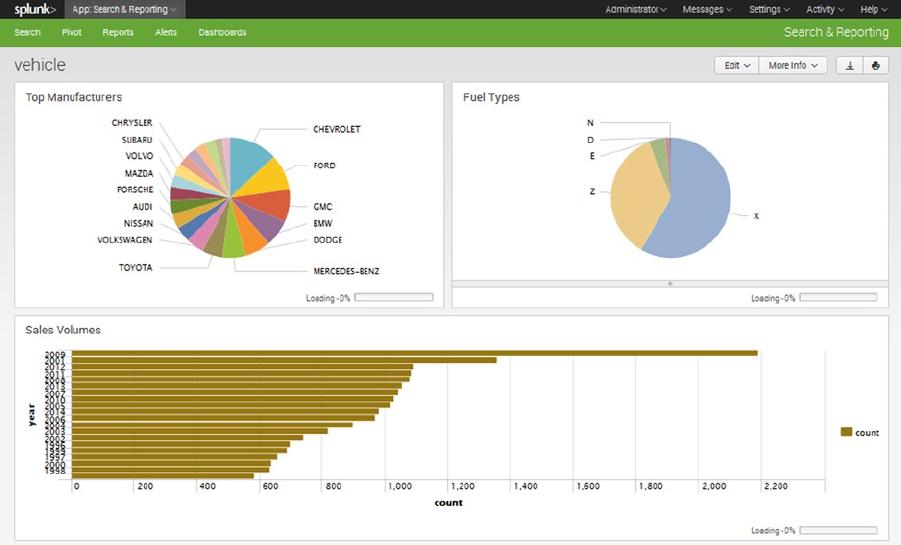
CHAPTER 11 ■ REPORTING WITH HADOOP

336

Many of the reports shown in Figure 11-10 are built into Hunk, but I created the fuel types, sales volumes, and

manufacturers reports. When I save a report, I can choose to add it to a dashboard that I can create at the same time.

For example, in Figure 11-11, I create a dashboard called “Vehicle” to contain the three reports I’ve just mentioned.

Figure 11-11. Hunk dashboard for reports created

To open the dashboard, I choose the Dashboards menu option, then select the Vehicle dashboard. The display

is populated from the current data, giving me, on a single page, an up-to-date view of the state of the data. A simple

example of what can quickly be created to represent HDFS-based data, Figure 11-11 shows two pie charts that display

top manufacturers and fuel types. The bottom bar graph displays sales volume by year. Once the report entries are

on the dashboard, I can edit them to add titles, or drag and drop them into the best positions to give an at-a-glance

impression of the data status.

I can also create complex report expressions to construct multi-column reports. For example, the following

report expression creates a table that contains the minimum CO2 emissions by manufacturer and model and was

supplied by Ledion Bitincka, an architect at Splunk, in response to a question I submitted to the Splunk forum):

index=cdh5_vindex | stats min(c02_g_km) AS minco2 BY manufacturer, model | sort 20 minco2. Thus, the

original search expression index=cdh5_vindex is passed to a stats function that finds the minimum CO2 emissions

value from the column c02_g_km in grams per kilometer and saves it to a new column name called minco2. The results

placed in this column are grouped by manufacturer and model, just as you would group non-aggregated columns in

SQL. Finally, the data is sorted and the top 20 rows are displayed, creating the report shown in Figure 11-12.

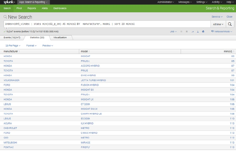
CHAPTER 11 ■ REPORTING WITH HADOOP

337

Note that because a stats function was used to create an aggregated column in the Figure 11-12 table, the

resulting report was displayed in the Statistics tab. Also, the tabs at the top of the page contain a count of records

used in creating the table. The example uses 19,347 records from the raw data for the Events tab and 20 records in the

Statistics tab.

For additional ideas on what can be accomplished with Hunk, take a look at the splunk.com website, particularly

the answers forum. You’ll find ideas about and examples of generating complex reports. Remember that reports can

be created from multiple Hadoop-based sources in Hunk, and that lookup tables can be used to enrich your data.

Potential Errors

I encountered some problems during the Hunk installation and use, probably because of configuration or installation

mistakes. This section shows you what happened and how I fixed the errors.

For instance, I found the following error in a search log when a search failed:

[hadoop@hc2nn hunk]$ pwd

/usr/local/hunk

[hadoop@hc2nn hunk]$ find . -name search.log

./var/run/splunk/dispatch/1414868687.5/search.log

[cdh5] Error while running external process, return_code=255. See search.log for more info

[cdh5] RuntimeException - Failed to create a virtual index filesystem connection: java.net.

UnknownHostException: hc2nn. Advice: Verify that your vix.fs.default.name is correct and available.

Figure 11-12. Hunk multi-column report

CHAPTER 11 ■ REPORTING WITH HADOOP

338

I found the report search logs by running the Linux find command from the Hunk install directory /usr/local/

hunk. I knew that the search log file was named search.log, based on forum answers on splunk.com. The error was

caused by the fact that the user running Hunk did not have access to the Splunk working directory /user/hadoop/

hunk/workdir.

A search log generated this second error, as well:

10-29-2014 19:14:07.385 ERROR ERP.cdh5 - SplunkMR - Failed to create a virtual index filesystem

connection: java.net.UnknownHostException: hc2nn.semtech-solutions.co.nz. Advice: Verify that your

vix.fs.default.name is correct and available.

The error was caused because HDFS was not running. The Hunk report had been run before the Hadoop servers

completed their startup sequence.

This error, again from the search log, seems to be an indication of another underlying problem:

10-30-2014 18:22:55.398 ERROR SearchOperator:stdin - Cannot consume data with unset stream_type

10-30-2014 18:22:55.453 ERROR ExternalResultProvider - Error in 'SearchOperator:stdin': Cannot

consume data with unset stream_type

In this case, I had incorrectly created the configuration for my CSV file processing in the configuration files.

Although from Splunk forum entries I understand that it should not be necessary, adding entries to the files props.

conf and transforms.conf solved this problem.

I initially tried running Hunk from a remote Linux server—remote from the Hadoop cluster that it was trying to

connect to. The following test uses the HDFS file system ls command to examine the / directory on the cluster via the

HDFS-based URI hdfs://hc2nn:8020/:

[hadoop@hc1r1m1 ~]$ hdfs dfs -ls hdfs://hc2nn:8020/

ls: Call From hc1r1m1/192.168.1.104 to hc2nn:8020 failed on connection exception: java.net.

ConnectException: Connection refused; For more details see: http://wiki.apache.org/hadoop/

ConnectionRefused

The access failed, so before attempting to use Hunk, it is important to check that the Hunk Linux user on the

server where it is installed has access to Hadoop.

The following errors were displayed when Hunk was started in the Linux command window:

Checking conf files for problems...

Invalid key in stanza [source::/data/hunk/rdbms/...] in /usr/local/hunk/etc/system/

local/props.conf, line 3: DELIMS

(value: ", ")

Invalid key in stanza [source::/data/hunk/rdbms/...] in /usr/local/hunk/etc/system/

local/props.conf, line 4: FIELDS

(value: f1,f2,f3,f4,f5,f6,f7,f8,f9,f10,f11,f12,f13,f14)

Your indexes and inputs configurations are not internally consistent. For more

information, run 'splunk btool check --

debug' Done

All preliminary checks passed.

CHAPTER 11 ■ REPORTING WITH HADOOP

339

These errors were caused by incorrect configuration file entries while I was learning to use Hunk. I changed the

configuration file entries and restarted Hunk to solve this problem.

If you encounter any of these or additional errors, another good resource to consult is the answers section of the

splunk.com website, including the support menu options. Try to be a good Splunk citizen by adding as much detail

as possible to any questions or answers that you might post on the forum. If you find a solution to your problem, then

post that solution to help future users.

Talend Reports

Expanding on the big data ETL work discussed in Chapter 10, it’s time to examine the reporting capabilities of the

Talend Enterprise big data product—specifically, the profiling functionality. With Talend, you can check the quality of

Hive-based data and build reports from table-based data.

Installing Talend

To download the Talend Enterprise big data application, I go to the URL www.talend.com/download, then select

the Big Data tab and click the Download Free Trial button. I need to enter my details, so I can’t simply execute the

Linux wget command from the Linux command line, as in previous download examples in this book. The package

download is 2 GB, so it will take some time.

The license that was automatically emailed to me does not allow me to access the profiling function. I need

to request a different license from Talend to “unlock” the profiling function on the user interface. (You can contact

Talend via www.talend.com/contact to request similar access.) The Sales Solutions Group Manager at Talend kindly

supplied the license, while others at Talend offered help and documentation so I could develop the example I will

present here.

I install the Talend software on the Centos Linux host hc1nn, using that machine as a client to access the Centos 6

Cloudera CDH5 Hadoop cluster whose name node resides on the server hc2nn. To unpack the software, I use the root

account, accessing it via the Linux su (switch user) command:

[hadoop@hc1nn ~]$ su -

I move to the Linux hadoop account Downloads directory, where the package was downloaded, and I examine

the downloaded file using the Linux ls command to create a long listing:

[root@hc1nn ~]# cd /home/hadoop/Downloads

[root@hc1nn Downloads]$ ls -lh

-rw-r--r-- 1 hadoop hadoop 2.0G Nov 3 18:01 Talend-Tools-Installer-r118616-V5.5.1-installer.zip

The Talend release file is a zipped archive; I unpack it with the Linux unzip command:

[root@hc1nn Downloads]# unzip Talend-Tools-Installer-r118616-V5.5.1-installer.zip

CHAPTER 11 ■ REPORTING WITH HADOOP

340

The following commands display the unpacked directory via a Linux ls command. The Linux cd command then

moves into the unpacked Talend software directory TalendTools-5.5.1-cdrom. After that, the Linux ls command again

provides a long list of the contents of the unpacked software:

[hadoop@hc1nn Downloads]$ ls -ld TalendTools-5.5.1-cdrom

drwxr-xr-x 2 root root 4096 Jun 18 11:25 TalendTools-5.5.1-cdrom

[root@hc1nn Downloads]# cd TalendTools-5.5.1-cdrom

[hadoop@hc1nn TalendTools-5.5.1-cdrom]$ ls -l

total 2081688

-rwxr-xr-x 1 root root 2095344252 Jun 18 11:25 dist

-rwxr-xr-x 1 root root 6171835 Jun 18 11:25 Talend-Tools-Installer-r118616-V5.5.1-linux64-

installer.run

-rwxr-xr-x 1 root root 6003334 Jun 18 11:25 Talend-Tools-Installer-r118616-V5.5.1-linux-

installer.run

-rw-r--r-- 1 root root 18288640 Jun 18 11:25 Talend-Tools-Installer-r118616-V5.5.1-osx-

installer.app.tar

-rwxr-xr-x 1 root root 5829599 Jun 18 11:24 Talend-Tools-Installer-r118616-V5.5.1-windows-

installer.exe

The two files with “linux” in their names are used to install Talend on Linux-based hosts. The other files are used

to install Talend on the Windows and Mac OSX operating systems. The file named “dist” is the largest file in the release

and contains the actual distributed software for the installation. Given that I am installing onto a 32-bit Linux host,

I use the Linux-based file that does not have 64 in its name.

Before I install the Talend software, however, I need to install the Oracle Sun version of the JavaSDK. The Talend

installation will fail if this JavaSDK isn’t available. Because I generally use the Java OpenJDK, I install this Java release

under /usr/local. I download the latest available JavaJDK from the URL http://www.oracle.com/technetwork/java/

javase/downloads/jdk8-downloads-2133151.html to Centos Linux host hc1nn as the Linux hadoop user.

The following commands show the Downloads directory within the Linux hadoop account’s home directory

via the Linux pwd command. They also show a long file listing of the downloaded JavaJDK file using the Linux ls

command:

[hadoop@hc1nn Downloads]$ pwd

/home/hadoop/Downloads

[hadoop@hc1nn Downloads]$ ls -l jdk-8u25-linux*

-rw-rw-r-- 1 hadoop hadoop 162406890 Nov 3 19:23 jdk-8u25-linux-i586.tar.gz

This is a compressed tar archive file (it has a file type of .tar.gz), so I uncompress it using the Linux gunzip

command. This produces a tar archive with a file type of .tar. I then use the Linux tar command to unpack it, using the

option xvf, where x means extract, v means verbose, and f allows the tar file name to be specified. Then, a long file list

shows that the unpacked software resides in a directory called jdk1.8.0_25:

[hadoop@hc1nn Downloads]$ gunzip jdk-8u25-linux-i586.tar.gz

[hadoop@hc1nn Downloads]$ tar xvf jdk-8u25-linux-i586.tar

[hadoop@hc1nn Downloads]$ ls -ld jdk1.8.0_25

drwxr-xr-x 8 hadoop hadoop 4096 Sep 18 11:33 jdk1.8.0_25

CHAPTER 11 ■ REPORTING WITH HADOOP

341

Having extracted the JavaJDK, I use the Linux su (switch user) command to change to the root account and move

the software to /usr/local/. The Linux mv (move) command moves the jdk1.8.0_25 directory. The Linux cd (change

directory) command moves to the /usr/local/ directory. The Linux chown (change owner) command recursively

changes the ownership of the Java release to the Linux hadoop account. Finally, the export command sets the

JAVA_HOME variable to the path of this new Java release:

[hadoop@hc1nn Downloads]$ su -

Password:

[root@hc1nn ~]# cd /home/hadoop/Downloads

[root@hc1nn Downloads]# mv jdk1.8.0_25 /usr/local

[root@hc1nn Downloads]# cd /usr/local

[root@hc1nn local]# chown -R hadoop:hadoop jdk1.8.0_25

[root@hc1nn local]# export JAVA_HOME=/usr/local/jdk1.8.0_25

It is this Oracle Sun JavaJDK that the Talend release requires, so with the JAVA_HOME variable set I can attempt to

install the software. As the root user, I change the directory to the Downloads directory and then change the directory

to the directory containing the unpacked Talend software. After that, I run the non-64 bit linux.run file. The ./

prepended to the name specifies that the installation file will be sourced from the current directory:

[root@hc1nn local]# cd /home/hadoop/Downloads

[root@hc1nn Downloads]# cd TalendTools-5.5.1-cdrom

[root@hc1nn TalendTools-5.5.1-cdrom]#

./Talend-Tools-Installer-r118616-V5.5.1-linux-installer.run

The installation is simple. I just accept all defaults and install only the client application, not the server, as the

server is not required for this example. As mentioned earlier, I also need a platform-enabled license file supplied by

Talend to enable the profiling function. This file is specified during the installation. I install the software to the default

path /opt.

The Talend application also needs an rpm build packaging component; the yum installation command, run as

root, installs the necessary software, as follows:

[root@hc1nn TalendTools-5.5.1-cdrom]# yum install rpm-build

Finally, the Talend client software can be started from the studio subdirectory of the Talend software installation

directory /opt/TalendTools-5.5.1. The 5.5.1 string shows the version of the Talend Enterprise software that has been

installed. The list obtained using the Linux ls command shows that there are numerous Linux .sh and windows .ini

files available for starting Talend. Given that I have installed Talend on a 32-bit Linux host, however, the .sh file has

“linux” in its name but lacks the “64,” which denotes a 64-bit architecture. The ./ in the final command indicates that

the file should be run from the current directory. The “and” character (&) denotes the command should be run in the

background:

[root@hc1nn TalendTools-5.5.1-cdrom]# cd /opt/TalendTools-5.5.1/studio/

[root@hc1nn studio]# ls *.sh *.ini

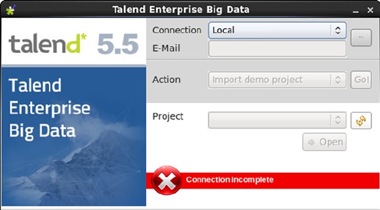
CHAPTER 11 ■ REPORTING WITH HADOOP

342

commandline-linux.sh Talend-Studio-linux-gtk-x86.sh

commandline-linux_x86_64.sh Talend-Studio-solaris-gtk.ini

commandline-mac.sh Talend-Studio-solaris-gtk-x86.ini

Talend-Studio-linux-gtk-ppc.ini Talend-Studio-win32-wpf.ini

Talend-Studio-linux-gtk-x86_64.ini Talend-Studio-win32-x86.ini

Talend-Studio-linux-gtk-x86.ini Talend-Studio-win-x86_64.ini

[root@hc1nn studio]# ./Talend-Studio-linux-gtk-x86.sh &

Some basic connection details need to be specified, then Talend will be available for use. The next section will

take care of these details.

Running Talend

If multiple Talend clients were being installed, it would have made sense to install the Talend server and have the

Talend clients connect to that server. The server would then provide access to a storage repository, which would be

based on SVN. In this way, work created via one client could be shared among multiple users. But because only a single

client was installed and no server, the connection specified is to the local host file system. Figures 11-13 and 11-14

show that the connection details are specified as local and a workspace directory is specified under the studio client

directory under /opt.

Figure 11-13. Talend local connection

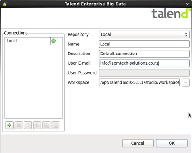
CHAPTER 11 ■ REPORTING WITH HADOOP

343

Although it’s not shown as currently active in Figure 11-13, the Import Demo Project option is enabled when

the connection details are specified. I then click the Go! button to install the big data code I use for this example.

Figure 11-15 shows the installed Talend client running; note that I have opened one of the job examples and have

attempted to connect to Cloudera CDH5. At this point, I am prompted to install any missing Talend or third-party

libraries that are required. Indeed, the yellow banner in Figure 11-15 is prompting a library installation. I install what

is required now to avoid possibility of errors later. (See also the “Potential Errors” section later.) Also, note that I have

placed a red box around the top-right menu option that will be used to change the interface perspective.

Figure 11-14. Details of Talend local connection

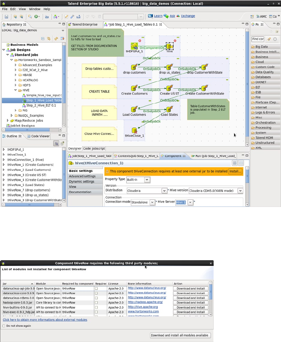
CHAPTER 11 ■ REPORTING WITH HADOOP

344

Figure 11-16 shows an example of the necessary libraries being installed. This process may be slow, but I am

patient until it is 100 percent completed. I won’t describe the integration perspective shown in the Figure 11-16, as it

was described in Chapter 10.

Figure 11-15. Talend Enterprise client

Figure 11-16. Talend libraries installation

CHAPTER 11 ■ REPORTING WITH HADOOP

345

It is important at this point that I check to see that the correct license is installed so that data quality reports can

be generated. From the client user interface, I select the Help option, then select the About License option to bring up

the window that is depicted in Figure 11-17. Notice also that the term “Talend Platform” is displayed in the figure. This

phrase is important, as it denotes that the correct type of license is being used. (To obtain the necessary access and

licenses, contact Talend at www.talend.com/contact.)

Figure 11-17. Details on required Talend license

The profiling perspective can now be accessed by clicking the red-outlined drop-down menu in the top right of

Figure 11-15. I select Other. Next, I choose the “profiling perspective” option, as shown in Figure 11-18.

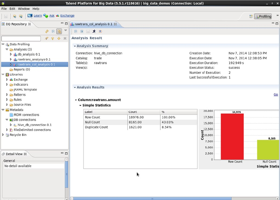
CHAPTER 11 ■ REPORTING WITH HADOOP

346

The Repository pane on the left of the screen shown in Figure 11-18 has a list of previously created analysis

reports and metadata database connections. Earlier, I had created a Hive-based Cloudera CDH5 connection named

hive_db_connection 0.1, as you can see in the list under DB Connections. I also opened the Hive rawtrans table

column analysis report named rawtrans_col_analysis 0.1. The items are expanded in Figure 11-18 to familiarize you

with the display.

To run Talend profiling reports against a CDH5-based Hive data warehouse, I need to know a number of

properties about the Hive installation: which host it is running on, what port number to use to connect to it, the

Linux-based user name of the account to use, the password for that account, and the version of Hive in use. I know

that Hive is installed on my cluster on the server hc2nn, and that the account used will be called hadoop. I also know

Figure 11-18. Talend’s profiling perspective

CHAPTER 11 ■ REPORTING WITH HADOOP

347

the password for that account, plus I know that the Hive version that I am using for Talend is version 2. That means

that the only property I need to determine is the metastore port number. Given that I know all logs will be stored

under /var/log for Cloudera CDH5 servers, I obtain that information as follows:

[hadoop@hc2nn hive]$ pwd

/var/log/hive

[hadoop@hc2nn hive]$ ls -l

total 3828

drwx------ 2 hive hive 4096 Aug 31 12:14 audit

-rw-r--r-- 1 hive hive 2116446 Nov 8 09:58 hadoop-cmf-hive-HIVEMETASTORE-hc2nn.semtech-solutions.

co.nz.log.out

-rw-r--r-- 1 hive hive 1788700 Nov 8 09:58 hadoop-cmf-hive-HIVESERVER2-hc2nn.semtech-solutions.

co.nz.log.out

[hadoop@hc2nn hive]$ grep ThriftCLIService hadoop-cmf-hive-HIVESERVER2-*.log.out | grep listen |

tail -2

2014-11-08 09:49:47,269 INFO org.apache.hive.service.cli.thrift.ThriftCLIService:

ThriftBinaryCLIService listening on 0.0.0.0/0.0.0.0:10000

2014-11-08 09:58:58,608 INFO org.apache.hive.service.cli.thrift.ThriftCLIService:

ThriftBinaryCLIService listening on 0.0.0.0/0.0.0.0:10000

The first command shows, via a Linux pwd (print working directory) command, that I am in the directory /var/

log/hive. (Note: use the cd command to move to that directory, if necessary.) Then, using the Linux ls command

with the -l option to provide a long listing, I check to see which log files exist in this Hive log directory. Finally, I use

the Linux grep command to search the HIVESERVER2-based log file for the string ThriftCLIService. I pipe (|) the

output of this search to another grep command, which searches the ouput further for lines that also contain the text

“listen.” Finally, I limit the output to the last two lines via the Linux tail command with a parameter of -2. The output

contains the port number that I need at the end of the line. Then, 10000 is the default port number that will be used in

the Talend Hive connection for this section.

So, now I am ready to create a Hive database connection. I can do this by right-clicking the DB Connections

option in the Repository pane. Then, I select Create DB Connection to open a form that offers a two-step process for

creating the connection.

The first section requests the name, purpose, description, and status of the connection. Take care to make the

name meaningful. The second step (shown in Figure 11-19) gives the actual connection details. That is, the database

type is set to Hive and the server/port are defined as hc2nn/10000, as previously determined. The Linux account

login for the CentOS host hc2nn is set to hadoop, along with its password. The Hive version is set to Hive2, while

the Hadoop version and instance are set to match the Hadoop cluster being used, Cloudera/CDH5. Finally, the

jdbc string, the Java-based method that Talend will use to connect to Hive, is set to a connection string that uses the

hostname, port, and Hive version.

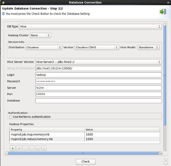
CHAPTER 11 ■ REPORTING WITH HADOOP

348

Figure 11-19. Talend-Hive database connection

Some variables have been added to set the memory used by the Talend Map Reduce jobs in terms of map

and reduce functions. A value of 1000 MB is set for each function via the variables mapred.job.map.memory.mb

and mapred.job.reduce.memory.mb. To check this connection before saving it, I click the Check button. In case of

problems, I first ensure that the cluster is functioning without error, that HDFS is accessible, and that Hive can be

accessed and have Hive QL scripts run against it. (You also might use the Hue interface for this.) The connection

works, so I save it. It subsequently will appear in the Repository pane.

By expanding the objects under the Hive database connection in the Repository pane, I can view a table to the

column level, as shown in Figure 11-20.

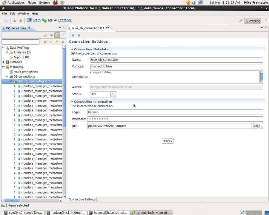
CHAPTER 11 ■ REPORTING WITH HADOOP

349

At this point, I can create a range of reports based on the underlying Hive table data.

Generating Reports

By using the Splunk/Hunk product at the start of this chapter, I was able to quickly create some reports and develop a

dashboard based on HDFS data. When I create Talend reports based on Hive table data, I can start to think about the

quality of the data that’s residing on HDFS and Hive.

As you remember from Chapter 9, you can create Hive external tables to represent HDFS data. In this section,

I create reports that represent the column data in the Hive rawtrans table of the trade information database. The

content of the data in that table is not relevant; it is the functionality of the Talend data-quality reports that I

concentrate on here.

To create the reports that this section will use, I first need to create two rules for data quality under Libraries, then

Rules, then SQL in the Repository pane, and one regular expression pattern by going to Libraries, then Patterns, then

Regex, then Date. The regular expression rule for date is copied from a similar pre-existing rule in the same location,

called date MM DD YYYY. I simply right-click it and select duplicate.

Figure 11-20. Repository view of Talend-Hive database connection

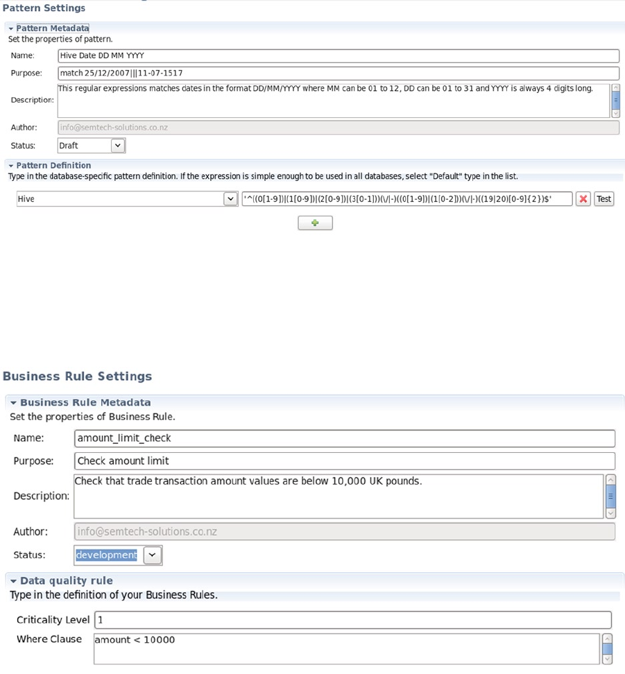
CHAPTER 11 ■ REPORTING WITH HADOOP

350

Shown in Figure 11-21, the new Hive-based rule is now called “Hive Date DD MM YYYY” and will be used to

check Hive table-based dates. Note that the connection type has been set to Hive. The actual regular expression rule,

which appears at the bottom right, basically checks a date column to confirm that it contains a date of the form that’s

either 01/12/2014 or 01-12-2014.

Figure 11-21. Regular expression rule for dates

Figure 11-22. SQL data-quality rule for “amount” column

You can create SQL-based data-quality rules as well. For example, to do so, I right-click the SQL folder under

Libraries, then choose Rules within the Repository pane and select the option New Business Rule. Figures 11-22

and 11-23 show two rules I created to test column values.

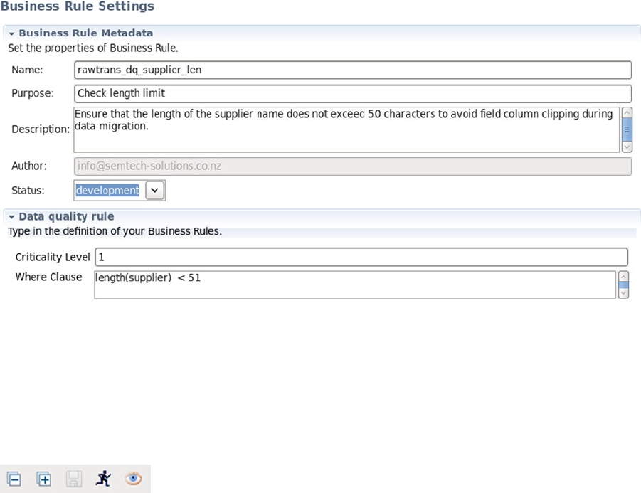
CHAPTER 11 ■ REPORTING WITH HADOOP

351

For instance, Figure 11-22 tests the size of the trade.rawtrans table “amount” column by checking that no

transaction values exceed 10,000 English pounds sterling. The text in the Where clause field is added to the Hive QL

that is generated by Talend and is run against Hive to create the report’s content. In this example, I have not amended

other fields except to add the rule’s name, purpose, and description.

Figure 11-23 is a similar SQL-based data-quality rule, except that in its Where clause field it uses the Hive QL

length function to check the length of the rawtrans table’s Supplier field data in the trade database. Of course, this field

is a string, so this check ensures that a maximum length for the supplier name is adhered to. Checks like this are useful

during data-migration exercises.

Figure 11-23. SQL data-quality rule for “Supplier” column

Now that the rules have been created, it is possible to create some Talend reports on data quality in the trade.

rawtrans Hive table. I concentrate on column-based reports and create single- and multi-column reports, as well as

reports based on SQL and regular expressions. (Note: you can create new reports by right-clicking the Analysis folder

in the Repository pane and selecting the New Analysis option.) Each type of report has the set of control buttons

shown in Figure 11-24.

Figure 11-24. Control buttons for reports

The first two buttons shown in Figure 11-24 contract and expand the report display to either hide or show charts

and/or details. The third button saves any changes, while the fourth is used to run the report. The final “eye” icon

refreshes the report charts.

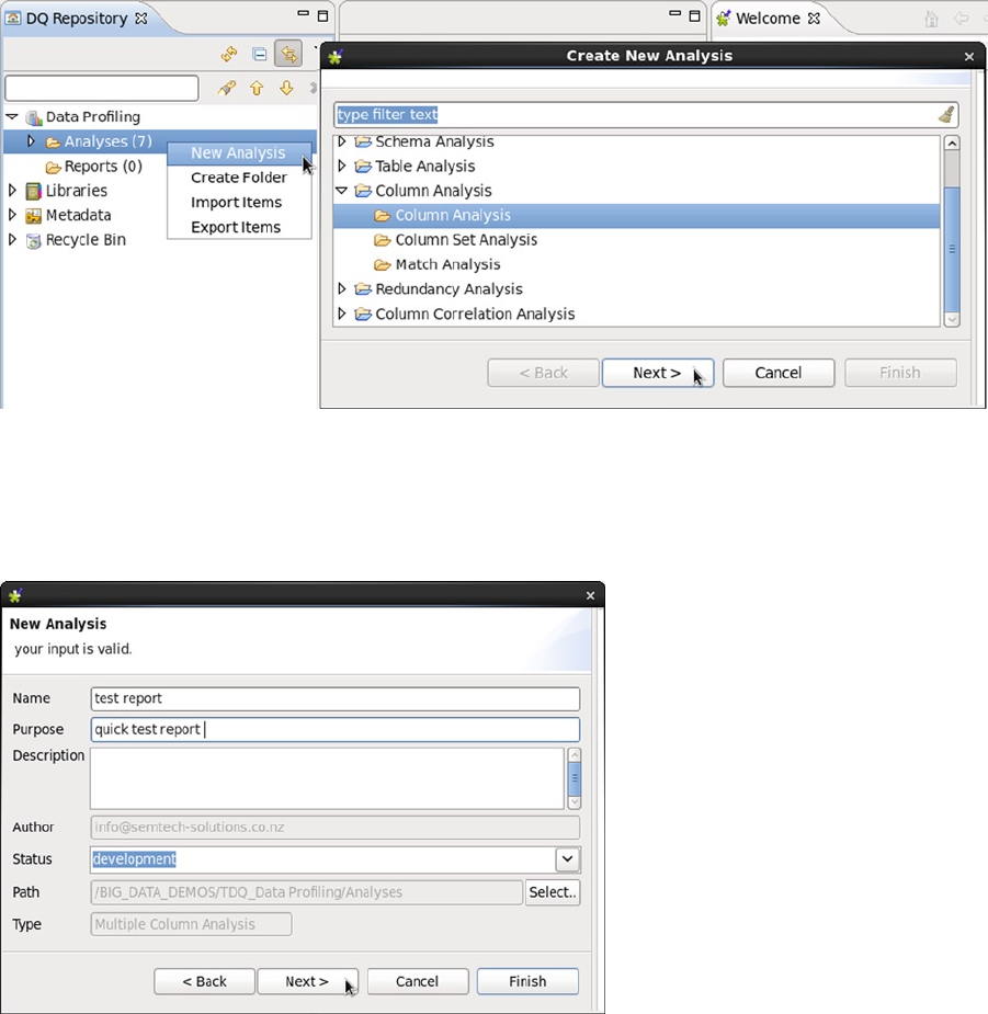
CHAPTER 11 ■ REPORTING WITH HADOOP

352

Single-Column Reports

I create a single-column analysis report by right-clicking the Analysis folder under Data Profiling in the Repository

pane. Next, I choose the report folder and type of column analysis in the pop-up window that is shown in

Figure 11-25.

Figure 11-25. Choosing the type of report to be created

Figure 11-26. Describing and naming the report

I then click Next and enter a report name and a report description, as shown in Figure 11-26.

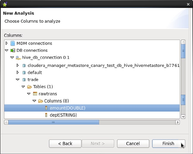
CHAPTER 11 ■ REPORTING WITH HADOOP

353

I click Next again to choose the database table column for the report. I expand the Hive DB connection until the

appropriate database table column can be selected, and then I select Finish, as shown in Figure 11-27.

Figure 11-27. Choosing the database column

Figure 11-28 shows the Analysis Results tab of a single-column report drawn from the rawtrans “amount”

column. It shows both table and bar graph, with the total and null counts for the column. It also shows the spread of

values as the duplicate, distinct, and unique counts for this column.

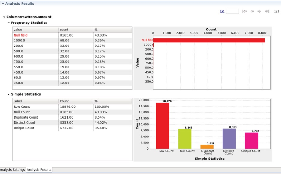
CHAPTER 11 ■ REPORTING WITH HADOOP

354

Multi-Column Reports

In the same way that a single-column report is created, multi-column reports can be generated. When I select the

columns on which the report will be drawn, I press the Control key and select “multiple columns.”

The report shown in Figure 11-29 was created from four columns in the trade.rawtrans table: “amount”,

“department” (dept), “supplier”, and “export area” (exparea). The Data mining Type parameter tells Talend what type

of data it is examining. For the “amount” column, I set it to Interval because that column contains numeric values;

I set it to Unstructured Text for the other columns, as they are strings. The simple statistics displayed in Figure 11-29

include the column row count and counts for distinct, duplicate, and unique values. Clicking the Run icon then runs

the report and produces the bar graph shown on the right.

Figure 11-28. Results for a single-column report

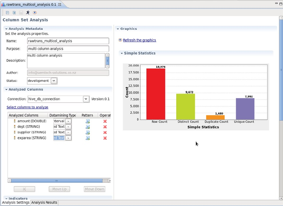
CHAPTER 11 ■ REPORTING WITH HADOOP

355

These reports are fine for a simple check of the table column data, but what about generating and using more

complex rules for data quality that check data values and attributes? Well, that is where SQL and regular expression-

based rules can help.

Reports Based on SQL Rules

Reports on data quality are created when the options Table Analysis and then Business Rule Analysis are chosen when

creating a report. For example, I click Next and enter a report name in the form. I click Next again and expand the

database Hive connection until I can select the appropriate table. I click Next, and I select the SQL-based rule that was

created earlier. Finally, I click Finish to generate the report. The resulting report, shown in Figure 11-30, uses the

SQL-based rule that states amount < 10000 and shows that more that 93 percent of the data values in the “amount”

column fail this data-quality rule.

Figure 11-29. Muliple-column report

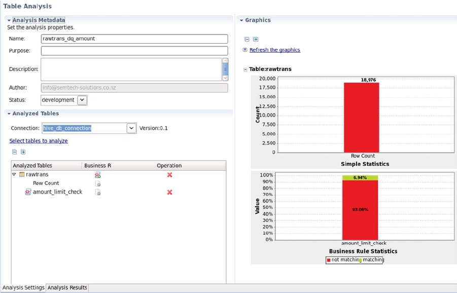
CHAPTER 11 ■ REPORTING WITH HADOOP

356

The SQL-rule statistics in Figure 11-30 show failures in red and passes in green. The report shown in Figure 11-31

checks the length of the supplier string column and displays a failure rate of around 29 percent. Thus, these simple

reports demonstrate that there are improvements needed in the quality of data in this table.

Figure 11-30. SQL-rule results for data-quality report on “amount” column

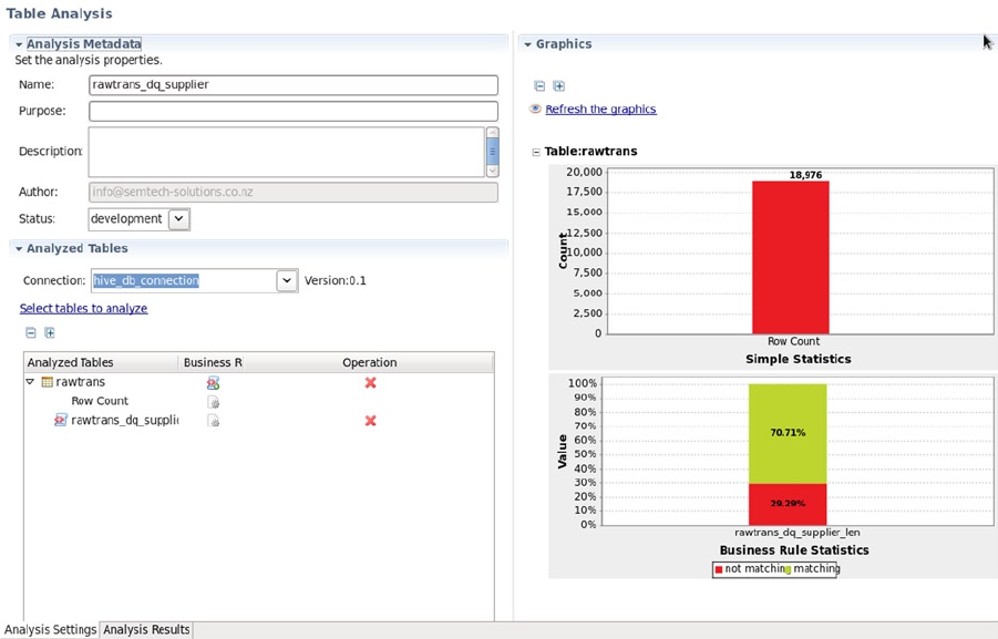
CHAPTER 11 ■ REPORTING WITH HADOOP

357

These reports check the content and data ranges of tabular data, but what about the actual structure or format of

the data? Regular expressions are the tool for this job.

Reports Based on Regular Expressions

This section uses the date-based regular expression rule that was created previously. I begin the example by creating

a new report in the same manner as I did for the single-column report. In the report’s Analyzed Columns section

(Figure 11-32), I click the Pattern icon next to the column to be checked—in this case, it is the “paydate” column,

which is a date-based string column. This invokes the Pattern Selector window. There, I navigate to Regex, then to

date, and to “Hive Date DD MM YYYY”, which is the regular expression-based rule that I created earlier. I select that

rule, and click OK. Now, I click the Run icon to populate the report’s graphs, as shown in Figure 11-32.

Figure 11-31. SQL-rule results for data-quality report on “supplier” column

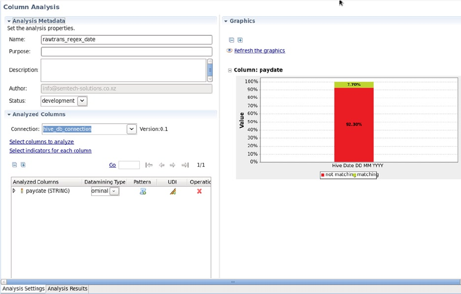
CHAPTER 11 ■ REPORTING WITH HADOOP

358

The Figure 11-32 report shows the output and the fact that over 92 percent of the data in the “paydate” column

has failed the basic date-format test, probably because it is null. The content here is not important, but the usefulness

of these reports is. If you take care when selecting the rules for generating a data-quality report, you can produce a set

of reports like this that have great importance, especially when you are attempting to ensure the quality of HDFS- and

Hive-based data.

Potential Errors

I did encounter a few errors while using Talend’s profiling. Generally these were not problems with Talend itself but,

rather, were configuration issues. By examining my solutions, you will be able to either avoid these errors or use them

to devise your own solutions.

I received the following error, followed by a message stating that I needed to install the library Zql.tar:

zql/ParseException

Figure 11-32. Regular-expression data-quality report on “paydate” column

CHAPTER 11 ■ REPORTING WITH HADOOP

359

This issue was caused by my not installing all third-party libraries when being prompted to do so. The solution is

simple: just click Finish and accept the licensing, then patiently wait for the libraries to install.

Two errors were caused by my setting up the Hive connection incorrectly. Specifically, I received

the following error:Failed to run analysis: rawtrans_analysys

Error message:

Error while processing statement: Failed: Execution Error, return code 1 from

org.apache.hadoop.hive.ql.exec.mr.MapRedTask

and the following error was in the Hive log file /var/log/hive/hadoop-cmf-hive-HIVEMETASTORE-hc2nn.semtech-

solutions.co.nz.log.out:

assuming we are not on mysql: ERROR: syntax error at or near "@@"

The port number should have been set to 10000 for the hiveserver2 address. I used the value 9083, which was

the port value defined in the property hive.metatstore.uris in the file hive-site.xml under the directory /etc/hive/

conf.cloudera.hive.

There was the following error regarding an RPM component:There was an error creating the RPM file:

Could not find valid RPM application:

RPM-building tools are not available on the system

The error occurred because an RPM build component was missing from the Centos Linux host on which Talend

was installed. The solution was to install the component using the yum command install.

Finally, this short error occurred while I was installing the Talend client software and it implied that the Talend

install file called “dist” was corrupted:

Unable to execute validation program

I don’t know how it happened, but I solved the problem by removing the Talend software release directory and

extracting the tar archive a second time.

Summary

Relational database systems encounter data-quality problems, and they use data-quality rules to solve those

problems. Hadoop Hive has the potential to hold an extremely large amount of data—a great deal larger than

traditional relational database systems and at a lower unit cost. As the data volume rises, however, so does the

potential for encountering data-quality issues.

Tools like Talend and the reports that it can produce offer the ability to connect to Hive and, via external tables,

to HDFS-based data. Talend can run user-defined data quality checks against that Hive data. The examples presented

here offer a small taste of the functionality that is available. Likewise, Splunk/Hunk has the potential for generating

reports and creating dashboards to monitor data. After working through the Splunk/Hunk and Talend application

examples provided in this chapter, you might consider investigating the Tableau and Pentaho applications for big data

as well.

You now have the tools to begin creating your own Hadoop-based systems. As you go forward, remember to

check the Apache and tool supplier websites. Consult their forums and ask questions if you encounter problems. As

you find your own solutions, post them as well, so as to help other members of the Hadoop community.

A

Ambari cluster manager

administration functions, 235

color-coded key, 235

conguration le, 228

CPU usage, 233–234

curl command, 229

dashboard’s Metrics tab, 232–233

data nodes, 230

default login account, 228

FQDNs, 228

Heatmaps tab, 233–234

indication, 227

installation, 232

Java JDK, 227

Linux yum command, 226, 228

memory usage, 235

Name Node server, 235

node managers, 230

ntpd server, 228

region servers, 230

registration, 228–230

Resource Manager user interface, 235–236

Review Conguration window, 231

setup command, 226

slaves and clients, 230–231

SSH, 228

time-consuming, 225

-u option, 229

web-based user interface, 227

wget command, 226

Apache Bigtop

installation

core-site.xml le, 250

Data Node machines, 250

fair-scheduler.xml le, 251

le system directories, 252

Hadoop le system, 251

JAVA_HOME variable, 251

Linux yum repository le, 249

Name Node and Resource

Manager components, 250

root account, 252

user interface, 252–253

YARN Linux user and group, 251

yarn-site.xml le, 250

smoke tests

build and run tests, 253

Hadoop component paths, 254

Hadoop Pig scripts and test results, 255

Linux PATH variable, 254

Maven command, 255

Maven (mvn) install command, 254

Maven verify command, 255

tar command, 253

wget, 253

yum list function, 254

Apache Software Foundation (ASF), 4

B

Big data

Apache Sqoop tool, 9

benets, 7

cluster management, 9

data analysis, 9

data collection, 8

data processing, 8

data warehouse system

features, 6

feedback loops, 6–7

scheduling and monitoring tasks, 5–6

denition, 1

distributed storage system, 8

ETL, 9

Index

361

Hadoop tools

ASF, 4

HDFS, 5

multidimensional 3V diagram, 1–2

Oozie tasks, 9

parallel processing approach, 2

reporting tools, 9

requirements, 3

system monitoring tools, 9

C

Capacity scheduler

features, 121

V1 environment

default queue, 123–124

Job Tracker user interface, 124

mapred.queue.names property, 124

queue conguration, 123

queue list, 124–125

tqueue, 123–124

V1.2.1 release, 122

V2 environment

adding property, 130

capacity values, 130

hierarchy of job queues, 131–132

queues and subqueues, 130

word-count job, 131

YARN conguration, 130

yarn rmadmin command, 131

cat command, 156

chmod command, 50

chown command, 50

Cloudera cluster manager

CDH cluster service installation, 242–243

CDH database connections, 241–242

CDH role assignments, 240–241

CDH service installation, 240

chart builder, 248

Cloudera installation, 239

disk status, 246–247

FQDN, 237

HDFS browser, 244

health history, 245

health tests, 245

home screen, 243–244

hosts option, 246

installation, 237–238

Linux chmod command, 237

Parcel installation menu, 239, 247–248

reports, 244–245

resource charts, 245

resource usage, 249

selection repository, 238

SELINUX value, 237

status summary, 245

time saving, 226

user interface, 245

Cluster management

Ambari cluster manager

(see Ambari cluster manager)

Bigtop (see Apache Bigtop)

Cloudera cluster manager

(see Cloudera cluster manager)

CopyFromLocal command, 156

CopyToLocal command, 156

cp command, 157

D, E

Data analytics

Apache Hive

CREATE DATABASE command, 268

CREATE TABLE command, 274

DESC clause, 279

external table creation, 268–269

GROUP BY clause, 279

HAVING clause, 280

INSERT statement, 278–279

ORDER BY clause, 279–280

SELECT statement, 275

subqueries, 276–277

table joins, 277–278

UDFs (see User-dened functions (UDFs)

WHERE clause, 275–276

Apache Spark

copyFromLocal command, 285

executors, 284, 287

head command, 285

installation packages, 281–282

job details, 286

line count, 285

Scala command count, 285

Spark context, 285

Spark shell application, 283

spark-submit command, 286

SQL Context object, 287–289

user interface, 283–284

Cloudera Impala

Catalog server, 258

cat command installation, 258

core-site.xml le, 259

CREATE DATABASE command, 263

DELIMITED and LOCATION option, 264

dot character (.), 258

error messages, 260

external table creation, 263

fuel consumption, 262

hdfs-site.xml le, 259

■ index

362

Big data (cont.)

hive-site.xml le, 258

INSERT statement, 267

permissions string, 260

SELECT statement, 265

socket creation, 260

SQL SHOW TABLES command, 264

subquery, 266

table joins, 266–267

user interface, 260–262

wget command installation, 258

WHERE clause, 265

yum command installation, 257

Data-collection

change directory (cd) command, 58

Gora conguration, 78

Hadoop logs, 80

HBase installation

accessible data, 77

cd and ls commands, 76

conguration le, 74, 76

gzipped tar le, 73

HBase bin directory, 76

hbase-site.xml le, 74

Linux hadoop account environment, 76

logs les, 77

ls command, 78

path and environment setup, 73

typical errors, 77

HBaselogs, 80

Linux cd command, 79

Nutch installation

Bash le, 71

chown command, 72

conguration directory, 61, 72

conguration les, 60, 72

crawl command, 66

crawl output, 67

crawl script, 66

gunzip command, 60, 72

.jar and .job les, 62

Linux le system, 67

Linux hadoop account, 62

Map Reduce looping/memory use, 61

mv command, 60

Nutch crawl directory, 68

NUTCH_HOME variable, 63

nutch-site.xml conguration le, 61

operations, 66

output, 80

segments directory, 69

symbolic links creation, 60

tar xvf Linux commands, 72

potential errors, 80

pwd command, 59

rm command, 59

Solr installation

Bash le, 71

chown command, 72

conguration directory, 72

conguration les, 72

Execute Query option, 69

lter factory algorithm, 64

gunzip and tar xvf Linux commands, 72

hadoop account conguration le, 64

nzip command, 63

output, 80

sample data, 69

Solr administration user interface, 65

user’s Bash shell, 64

start-dfs.sh script, 59

switch user (su) command, 58

ZooKeeper logs, 80

Data monitoring

Ganglia

cluster web interface, 213–215

Epel repository, 209

Ganglia gmond process, 209–210

hadoop-metrics.properties, 211

potential errors, 212–213

remi repository, 209

SELINUX value, 211

yum command, 209

Hue browser

CentOS 6 server hc1nn installation, 192

ETL components, 191

Hadoop core-site.xml le, 192

HBase server, 194–196, 208

hdfs-site.xml le, 192

HDSF browser, 201–202

Hive user interface, 200

Home icon, 199–200

Hue shell, 207

Metastore manager, 202–203

Oozie interface, 206–207

Pig icon, 200–201

potential errors, 197–198

Quick Start wizard, 198–199

secret key string, 193

service command, 196

Sqoop2 server, 193–194

Sqoop user interface, 203–206

YARN conguration, 193

Nagios

account and password combination, 216

cfg_dir attributes, 217

chkcong command, 216

components, 216

generic service, 217–218

host denition, 217

local service, 217–218

■ index

363

nrpe.cfg le, 219

potential errors, 219

structures, 215

touch command installation, 217

web interface, 220–223

yum command installation, 216

dfsadmin metasave command, 55

F

Fair scheduler

key aspects, 122

V1 environment

error, 128

job queue, 129

Job Tracker user interface, 128

pools, 127

properties, 126

V1.2.1 installation, 125

V2 environment

conguration le setup, 132

job status, 133–134

queue name specication, 133

refreshing YARN scheduler

queue conguration, 133

yarn.resourcemanager.

scheduler.class property, 132

Flume

agent conguration le contents, 169, 172

channel, 173

clean script, 172

execution script, 172

ume/messages directory, 171

hierarchical arrangement, 169–170

installation, 170

linear arrangement, 170

Linux ls command, 173

misconguration error, 174

running agent, 174

Fully qualied domain names (FQDNs), 228, 237

G

get command, 157

H

Hadoop Distributed File System (HDFS), 5, 12

Hadoop le system copyFromLocal command, 26

Hadoop scheduler

Capacity (see Capacity scheduler)

Fair scheduler (see Fair scheduler)

FIFO, 121

workow scheduler (see Oozie workow)

Hadoop V1 installation

cluster, 23

Job Tracker user interface, 31

keygen command, 15

Linux user hadoop, 16

map reduce job check, 25

name node user interface, 30

remote passwordless

secure shell access, 16

secure shell daemon process, 15

single-node installation

$HOME/Downloads directory, 17

Bash shell le, 19

conf/core-site.xml le, 20

conf/hadoop-env.sh le, 19

conf/mapred-site.xml le, 20

le conf/hdfs-site.xml le, 21

le system, 21

Linux chown command, 18

temporary directory, 20

SSH statements, 17

Task Tracker user interface, 32

Hadoop V2 installation

Linux cat command, 33

YARN (see Yet another resource negotiator (YARN))

ZooKeeper installation

built-in ZooKeeper client, 36

conguration information, 33

connect command, 37

conf command, 35

cons command, 36

delete command, 38

ephemeral node, 39

nc command line, 35

sequential node, 39

set command, 38

stat command, 36

hbase.zookeeper.quorum parameter, 196

Hunk report

cat command, 327–328

cd command, 326

cdh5 cluster, 327

cdh5_vindex, 330–331

drop-down menu option, 332

exit command, 326

extractcsv value, 327

eld bar report, 333–334

format menu, 334–335

ls-ld command, 326

mv command, 326

potential errors, 337–339

properties, 329–330

report expression, 336–337

report menu options, 334–336

search window, 331–332, 334

■ index

364

Data monitoring (cont.)

splunk command, 328

stats function, 337

su command, 326

summary window, 332–333

tar command, 326

web-based user interface, 328–329

I

InputSplit method, 86

J, K

JZMQ, 179

L

Library path, 141

M, N

manufacturer.pig script, 141

Mapper transformation, PDI

Cluster tab, 305

execution, 306

Filter Rows, 298

input component, 297

Java expression, 299

job conguration, 302

job scheduling, 302

job setup, 302, 304

output, 299, 307

Split Fields, 297

structure, 297

Map Reduce programming

Hive

installation, 111

word-count, 112

Perl

cat and tail command, 119

le mapper.pl le, 115

library-based data streaming functionality, 114

-mapper and-reducer options, 119

Reduce function, 118

reducer.pl Perl script, 116–117

resulting data, 120

script wc_clean.sh, 118

script wc_output.sh, 118

test1.sh shell script tests, 117

working directory, 114

Pig

copyFromLocal command, 102

count option, 103

disadvantages, 104

installation, 100

load option, 103

ls command, 104

UDFs (see User-dened functions (UDFs))

word-count algorithm

cat command, 98

code implementation, 86, 92

congure method, 95

copyFromLocal command, 90, 98

fs.Path class, 88

Hadoop le system rmr command, 90

input and output directory, 91

input/output formats, 89

InputSplit method, 86

jar command, 90

key-value pairs, 88

Linux ls command, 90

Linux mkdir command, 97

ls command, 91

Map class, 88

map method, 96

org.myorg package, 88

output, 99

parseSkipFile method, 95

process, 85

Reduce class, 96

run method, 96

tail command, 100

wc_classes directory, 97

wordcount1.jar, 97

Moving data

moving le system data

cat command, 156

CopyFromLocal command, 156

CopyToLocal command, 156

cp command, 157

get command, 157

mv command, 158

put command, 157

tail command, 158

URI, 155

with Flume

agent conguration le contents, 172

agents, 169

channel, 173

clean script, 172

execution script, 172

ume/messages directory, 171

hierarchical arrangement, 169–170

installation, 170

linear arrangement, 170

Linux ls command, 173

misconguration error, 174

running agent, 174

■ index

365

with Sqoop

importing data to HDFS, 161

importing data to Hive, 165

installation, 160

MySQL conguration, 159

rawdata table, 159–160

rawline column, 160

with Storm

Apache incubator project, 176

installation, 181

JZMQ, 179

Nimbus and slave processes, 177

running, 183

spouts, 177

stream, 176–177

topology, 177, 185

tuple, 176–177

ZeroMQ, 178

ZooKeeper server, 182

mv command, 51, 158

O

Oozie workow

actions, 138

conguration le

displaying contents, cat command, 141

entity/model HDFS directory, 145

error conditions, 143

fork control node, 143

Hive jobs, 143

join control, 143

kill control node, 144

manufacturuer.pig le, 144

model.pig le, 145

parameters, 140–141

rawdata2, 145

sql script, 144

control nodes, 137

creation, 139

Oozie installation, 134

running

help option, 146

job DAG with no state information, 149

job information window, 147–148

job log information window, 147–148

job number, 146

job statuses and meanings, 147

Oozie console, 146

Oozie job DAG information, 150

OOZIE_URL variable, 146

scheduling

coordinator job details window, 152

coordinator job status, 152

coordinator script path, 151

coordinator.xml le, 151

documentation level, 153

job coordination properties, 151

workow script path, 151

XML code, 153

P, Q

parseSkipFile method, 95

Pentaho Data Integration (PDI)

CDH5 conguration, 293

Design view, 295–296

ETL creation

HDFS le, 296

mapper transformation

(see Mapper transformation, PDI)

reducer transformation

(see Reducer transformation, PDI)

Explorer pane, 295

Explorer view, 295

installation package, 291

installation structure, 292

Java installation, 293

Kettle, 291

plugin.properties, 292–293

potential errors, 307–309

Spoon client application, 294

YARN server, 294

put command, 157

R

Reducer transformation, PDI

Cluster tab, 305

execution, 306

job conguration, 303

job scheduling, 302

job setup, 302, 304

output, 301, 307

Sort Rows, 299–300

structure, 299

summed_val variable, 300–301

Relational database

systems (RDBMS), 7

S

Sqoop

importing data to HDFS, 161

importing data to Hive, 165

installation, 160

MySQL conguration, 159

rawdata table, 159–160

rawline column, 160

■ index

366

Moving data (cont.)

Storing and conguring data

Hadoop

administration commands, 53

characteristics, 11

client task requests, 13

cluster-level job tracker handles, 12

environment management, 15

HDFS, 12

Map Reduce, 12

shell commands, 49

stack, 14

user commands, 51

V1 installation (see Hadoop V1 installation)

V2 installation (see Hadoop V2 installation)

YARN handles, 12

Storm stream, 176–177

Storm topology, 177

class name and topology name, 186

coding, 185

exclamation-topology, 186

kill command, 188

Nimbus and UI, 189

running, 186, 188

Storm user interface, 186–187

structure, 187–188

target directory, 185

topology view details, 186–187

Storm tuple, 176–177

Storm user interface, 183–184, 186–187

T

tail command, 158

Talend Open Studio

cat and head command, 313

ETL creation

column ltering, 318–319

conditional ow, 314

data ow, 315

HDFS connection, 315

HDFS delete, 315

incoming and outgoing

data sources, 317–318

output data, 321–322

rawdata.txt le, 316

Resource Manager interface, 320–321

Run tab, 320

Schema window, 316–317

sorting, 319

storage method, 319

three-column setup, 317

tPigLoad, 314

tPigMap_1, 314

work ow, 314

HDFS and Pig modules, 312

installation, 310

ls command, 313

potential errors, 322–323

Project Chooser window, 311

pwd command, 310

sandbox version, 310

software download, 310

unzip command, 311

user interface, 312–313

Talend report

amount column, 351, 356

Centos Linux, 339

client enterprise, 344

control buttons, 352

database connection, 347–349

data-quality rules, 349–351

gunzip command, 340

Hive installation, 347

JAVA_HOME variable, 341

library installation, 344–345

license option, 345

local connection, 342–343

ls command, 339–340

muliple-column report, 355

potential errors, 359

proling perspective, 346

repository pane, 346–347

single-column analysis, 353–354

supplier column, 351, 357

unpacked software, 340

unzip command, 339

yum installation, 341

U, V

Uniform Resource Identier (URI), 155

User-dened functions (UDFs)

cat command, 109, 270–271

CleanWS.java le, 106

creation, 105

date-conversion function, 270

DateConv.java, 271–272

DEFINE keyword, 108

directory structure, 271

exec method, 107

FILTER keyword, 108

functionality, 106–107

jar command, 107

jar library, 273

lint:deprecation option, 107

package name, 272

REGISTER keyword, 108

rpm installation, 270

sbt program, 270

Scala version, 271

tail command, 110

Text value, 272

■ index

367

W, X

workow.txt le, 141

Y

Yet another resource

negotiator (YARN)

component package installation, 40

conguration process, 40

core-site.xml le, 41

Data Node machines, 45

le mapred-site.xml le, 42

le yarn-site.xml le, 42

hdfs-site.xml le, 41

logging and history data, 45

ls command, 41, 45

mapred-site.xml le, 44

recursive switch (-R), 45

yarn-site.xml le, 43–44

yum commands, 40

Z

ZeroMQ, 178

ZooKeeper server, 182

■ index

368

Big Data Made Easy

A Working Guide to the Complete

Hadoop Toolset

Michael Frampton

Big Data Made Easy: A Working Guide to the Complete Hadoop Toolset

is work is subject to copyright. All rights are reserved by the Publisher, whether the whole or part of the material

is concerned, specically the rights of translation, reprinting, reuse of illustrations, recitation, broadcasting,

reproduction on microlms or in any other physical way, and transmission or information storage and retrieval,

electronic adaptation, computer software, or by similar or dissimilar methodology now known or hereafter developed.

Exempted from this legal reservation are brief excerpts in connection with reviews or scholarly analysis or material

supplied specically for the purpose of being entered and executed on a computer system, for exclusive use by the

purchaser of the work. Duplication of this publication or parts thereof is permitted only under the provisions of the

Copyright Law of the Publisher’s location, in its current version, and permission for use must always be obtained from

Springer. Permissions for use may be obtained through RightsLink at the Copyright Clearance Center. Violations are

liable to prosecution under the respective Copyright Law.

ISBN-13 (pbk): 978-1-4842-0095-7

ISBN-13 (electronic): 978-1-4842-0094-0

Trademarked names, logos, and images may appear in this book. Rather than use a trademark symbol with every

occurrence of a trademarked name, logo, or image we use the names, logos, and images only in an editorial fashion

and to the benet of the trademark owner, with no intention of infringement of the trademark.

e use in this publication of trade names, trademarks, service marks, and similar terms, even if they are not identied

as such, is not to be taken as an expression of opinion as to whether or not they are subject to proprietary rights.

While the advice and information in this book are believed to be true and accurate at the date of publication, neither

the authors nor the editors nor the publisher can accept any legal responsibility for any errors or omissions that may

be made. e publisher makes no warranty, express or implied, with respect to the material contained herein.

Managing Director: Welmoed Spahr

Acquisitions Editor: Je Olson

Developmental Editor: Linda Laamme

Technical Reviewer: Andrzej Szymanski

Editorial Board: Steve Anglin, Mark Beckner, Gary Cornell, Louise Corrigan, James DeWolf, Jonathan Gennick,

Robert Hutchinson, Michelle Lowman, James Markham, Matthew Moodie, Je Olson, Jerey Pepper,

Douglas Pundick, Ben Renow-Clarke, Gwenan Spearing, Matt Wade, Steve Weiss

Coordinating Editor: Rita Fernando

Copy Editor: Carole Berglie

Compositor: SPi Global

Indexer: SPi Global

Distributed to the book trade worldwide by Springer Science+Business Media New York, 233 Spring Street, 6th Floor,

New York, NY 10013. Phone 1-800-SPRINGER, fax (201) 348-4505, e-mail orders-ny@springer-sbm.com, or

visit www.springeronline.com. Apress Media, LLC is a California LLC and the sole member (owner) is Springer

Science + Business Media Finance Inc (SSBM Finance Inc). SSBM Finance Inc is a Delaware corporation.

For information on translations, please e-mail rights@apress.com, or visit www.apress.com.

Apress and friends of ED books may be purchased in bulk for academic, corporate, or promotional use. eBook

versions and licenses are also available for most titles. For more information, reference our Special Bulk Sales–eBook

Licensing web page at www.apress.com/bulk-sales.

Any source code or other supplementary materials referenced by the author in this text is available to readers at

www.apress.com. For detailed information about how to locate your book’s source code, go to

www.apress.com/source-code/.

is book is dedicated to my family—to my wife, my son, and my parents.

vii

Contents

About the Author �� xv

About the Technical Reviewer �� xvii

Acknowledgments �� xix

Introduction �� xxi

Chapter 1: The Problem with Data ■ ��1

A Deﬁnition of “Big Data” ��1

The Potentials and Difﬁculties of Big Data ��2

Requirements for a Big Data System �� 3

How Hadoop Tools Can Help ��4

My Approach �� 5

Overview of the Big Data System ��5

Big Data Flow and Storage �� 5

Beneﬁts of Big Data Systems �� 7

What’s in This Book ��8

Storage: Chapter 2 ��8

Data Collection: Chapter 3 �� 8

Processing: Chapter 4 ��8

Scheduling: Chapter 5 �� 9

Data Movement: Chapter 6 ��9

Monitoring: Chapter 7 �� 9

Cluster Management: Chapter 8 �� 9

Analysis: Chapter 9 �� 9

■ Contents

viii

ETL: Chapter 10 ��9

Reports: Chapter 11 �� 9

Summary ��10

Chapter 2: Storing and Conﬁguring Data with Hadoop, YARN, and ZooKeeper ■ ��11

An Overview of Hadoop ��11

The Hadoop V1 Architecture �� 12

The Differences in Hadoop V2 ��13

The Hadoop Stack �� 14

Environment Management �� 15

Hadoop V1 Installation ��15

Hadoop 1�2�1 Single-Node Installation �� 17

Setting up the Cluster �� 23

Running a Map Reduce Job Check �� 25

Hadoop User Interfaces ��29

Hadoop V2 Installation ��32

ZooKeeper Installation �� 33

Hadoop MRv2 and YARN �� 40

Hadoop Commands ��49

Hadoop Shell Commands��49

Hadoop User Commands ��51

Hadoop Administration Commands �� 53

Summary ��56

Chapter 3: Collecting Data with Nutch and Solr ■ ��57

The Environment ��57

Stopping the Servers ��57

Changing the Environment Scripts �� 58

Starting the Servers�� 59

Architecture 1: Nutch 1�x ��59

Nutch Installation �� 60

Solr Installation ��63

Running Nutch with Hadoop 1�8 �� 65

■ Contents

ix

Architecture 2: Nutch 2�x ��70

Nutch and Solr Conﬁguration �� 71

HBase Installation ��73

Gora Conﬁguration �� 78

Running the Nutch Crawl �� 79

Potential Errors �� 80

A Brief Comparison ��82

Summary ��83

Chapter 4: Processing Data with Map Reduce ■ ��85

An Overview of the Word-Count Algorithm ��85

Map Reduce Native ��86

Java Word-Count Example 1 ��86

Java Word-Count Example 2 ��92

Comparing the Examples �� 100

Map Reduce with Pig ��100

Installing Pig �� 100

Running Pig �� 102

Pig User-Deﬁned Functions �� 106

Map Reduce with Hive ��111

Installing Hive �� 111

Hive Word-Count Example ��112

Map Reduce with Perl ��114

Summary ��120

Chapter 5: Scheduling and Workﬂow ■ ��121

An Overview of Scheduling ��121

The Capacity Scheduler �� 121

The Fair Scheduler ��122

Scheduling in Hadoop V1 ��122

V1 Capacity Scheduler �� 122

V1 Fair Scheduler �� 125

■ Contents

x

Scheduling in Hadoop V2 ��129

V2 Capacity Scheduler �� 130

V2 Fair Scheduler �� 132

Using Oozie for Workﬂow ��134

Installing Oozie �� 134

The Mechanics of the Oozie Workﬂow �� 137

Creating an Oozie Workﬂow��139

Running an Oozie Workﬂow �� 146

Scheduling an Oozie Workﬂow ��151

Summary ��154

Chapter 6: Moving Data ■ ��155

Moving File System Data ��155

The Cat Command ��156

The CopyFromLocal Command �� 156

The CopyToLocal Command �� 156

The Cp Command �� 157

The Get Command �� 157

The Put Command ��157

The Mv Command �� 158

The Tail Command �� 158

Moving Data with Sqoop ��159

Check the Database ��159

Install Sqoop �� 160

Use Sqoop to Import Data to HDFS ��161

Use Sqoop to Import Data to Hive �� 165

Moving Data with Flume ��169

Install Flume �� 170

A Simple Agent �� 171

Running the Agent ��174

■ Contents

xi

Moving Data with Storm ��176

Install ZeroMQ ��178

Install JZMQ ��179

Install Storm �� 181

Start and Check Zookeeper �� 182

Run Storm ��183

An Example of Storm Topology �� 185

Summary ��189

Chapter 7: Monitoring Data ■ ��191

The Hue Browser ��191

Installing Hue �� 191

Starting Hue ��196

Potential Errors �� 197

Running Hue �� 198

Ganglia ��208

Installing Ganglia �� 209

Potential Errors �� 212

The Ganglia Interface��213

Nagios ��215

Installing Nagios �� 216

Potential Errors �� 219

The Nagios Interface��220

Summary ��223

Chapter 8: Cluster Management ■ ��225

The Ambari Cluster Manager ��226

Ambari Installation��226

The Cloudera Cluster Manager ��236

Installing Cloudera Cluster Manager �� 236

Running Cloudera Cluster Manager ��243

■ Contents

xii

Apache Bigtop ��249

Installing Bigtop �� 249

Running Bigtop Smoke Tests �� 253

Summary ��256

Chapter 9: Analytics with Hadoop ■ ��257

Cloudera Impala ��257

Installation of Impala ��257

Impala User Interfaces��260

Uses of Impala ��262

Apache Hive ��268

Database Creation ��268

External Table Creation ��268

Hive UDFs �� 270

Table Creation ��274

The SELECT Statement ��275

The WHERE Clause ��275

The Subquery ��276

Table Joins ��277

The INSERT Statement �� 278

Organization of Table Data �� 279

Apache Spark ��280

Installation of Spark��281

Uses of Spark �� 282

Spark SQL �� 287

Summary ��290

Chapter 10: ETL with Hadoop ■ ��291

Pentaho Data Integrator ��291

Installing Pentaho ��291

Running the Data Integrator �� 294

Creating ETL �� 296

Potential Errors �� 307

■ Contents

xiii

Talend Open Studio ��309

Installing Open Studio for Big Data ��310

Running Open Studio for Big Data �� 311

Creating the ETL ��314

Potential Errors �� 322

Summary ��323

Chapter 11: Reporting with Hadoop ■ ��325

Hunk ��325

Installing Hunk �� 325

Running Hunk �� 328

Creating Reports and Dashboards �� 331

Potential Errors �� 337

Talend Reports ��339

Installing Talend �� 339

Running Talend �� 342

Generating Reports ��349

Potential Errors �� 358

Summary ��359

Index ��361

xv

About the Author

Michael Frampton has been in the IT industry since 1990, working in a variety

of roles (tester, developer, support, QA) and many sectors (telecoms, banking,

energy, insurance). He has also worked for major corporations and banks as a

contractor and a permanent member of sta, including Agilent, BT, IBM, HP,

Reuters, and JPMorgan Chase. e owner of Semtech Solutions, an IT/Big Data

consultancy, Mike Frampton currently lives by the beach in Paraparaumu,

New Zealand, with his wife and son. Mike has a keen interest in new IT-based

technologies and the way that technologies integrate. Being married to a ai

national, Mike divides his time between Paraparaumu or Wellington in

New Zealand and their house in Roi Et, ailand.

xvii

About the Technical Reviewer

Andrzej Szymanski started his IT career in 1992, in the data mining, warehousing,

and customer proling industry, the very origins of what is big data today. His main

focus has been data processing and analysis, as well as development, systems, and

database administration across all main platforms, such as IBM Mainframe, Unix,

and Windows, and all leading DBMSs, such as Sybase, Oracle, MS SQL, and MySQL.

Szymanski’s big data and DevOps adventure began in News International, in January

2011, where he was a key player in creating a fully scalable and distributable big data

ecosystem, with an aim of sharing it with subsidiaries of News Corporation. is

involved R&D, solution architecture, creating ETL workows for big data, Continuous

Integration Zero Touch deployment mechanisms, and system administration and knowledge transfer to sister companies,

to name but few of the key areas. Szymanski was born in Poland, where he completed his primary and secondary

education. He studied economics in Moscow, but his key passion has always been computers. He is currently based

in Prague.

xix

Acknowledgments

I would like to thank my wife and son for allowing me the time to write this book. Without your support, Teeruk,

developing this book would not have been possible.

I would also like to thank all those who gladly answered my technical questions about the software covered in

this book. I extend my gratitude to the Apache and Lucene organizations, without whom open-source-based projects

like this one would not be possible. Also, specic thanks go to Deborah Wiltshire (Cloudera); Diya Soubra (ARM);

Mary Starr (Nagios); Michael Armbrust (Spark); Rebecca G. Shomair, Daniel Bechtel, and Michael Mrstik (Pentaho);

and Chris Taylor and Mark Balkenende (Talend).

Lastly, my thanks go to Andrzej Szymanski, who carried out a precise technical check, and to the editorial help

aorded by Rita Fernando, Je Olson, and Linda Laamme.

Big Data Made Easy A Working Guide To The Hadoop Toolset

Big%20Data%20Made%20Easy%20-%20A%20Working%20Guide%20to%20the%20%20Hadoop%20Toolset

Big%20Data%20Made%20Easy%20-%20A%20Working%20Guide%20to%20the%20%20Hadoop%20Toolset

Big%20Data%20Made%20Easy%20-%20A%20Working%20Guide%20to%20the%20%20Hadoop%20Toolset

Big%20Data%20Made%20Easy%20-%20A%20Working%20Guide%20to%20the%20%20Hadoop%20Toolset

Navigation menu

Versions of this User Manual:

Views

Navigation