Big Data SMACK A Guide To Apache Spark, Mesos, Akka, Cassandra, And Kafka
Big%20Data%20SMACK%20A%20Guide%20to%20Apache%20Spark%2C%20Mesos%2C%20Akka%2C%20Cassandra%2C%20and%20Kafka
Big%20Data%20SMACK%20A%20Guide%20to%20Apache%20Spark%2C%20Mesos%2C%20Akka%2C%20Cassandra%2C%20and%20Kafka
Big%20Data%20SMACK%20-%20A%20Guide%20to%20Apache%20Spark%2C%20Mesos%2C%20Akka%2C%20Cassandra%2C%20and%20Kafka
Big%20Data%20SMACK%20A%20Guide%20to%20Apache%20Spark%2C%20Mesos%2C%20Akka%2C%20Cassandra%2C%20and%20Kafka
Big%20Data%20SMACK%20A%20Guide%20to%20Apache%20Spark%2C%20Mesos%2C%20Akka%2C%20Cassandra%2C%20and%20Kafka
User Manual: Pdf
Open the PDF directly: View PDF ![]() .
.
Page Count: 277 [warning: Documents this large are best viewed by clicking the View PDF Link!]
- Contents at a Glance
- Contents
- About the Authors
- About the Technical Reviewer
- Acknowledgments
- Introduction
- Part I: Introduction
- Part II: Playing SMACK
- Chapter 3: The Language: Scala
- Chapter 4: The Model: Akka
- Chapter 5: Storage: Apache Cassandra
- Chapter 6: The Engine: Apache Spark
- Chapter 7: The Manager: Apache Mesos
- Chapter 8: The Broker: Apache Kafka
- Kafka Introduction
- Kafka Installation
- Kafka in Cluster
- Kafka Architecture
- Kafka Producers
- Kafka Consumers
- Kafka Integration
- Kafka Administration
- Summary
- Part III: Improving SMACK
- Chapter 9: Fast Data Patterns
- Fast Data
- ACID vs. CAP
- Integrating Streaming and Transactions
- Streaming Transformations
- Fault Recovery Strategies
- Tag Data Identifiers
- Summary
- Chapter 10: Data Pipelines
- Data Pipeline Strategies and Principles
- Asynchronous Message Passing
- Consensus and Gossip
- Data Locality
- Failure Detection
- Fault Tolerance/No Single Point of Failure
- Isolation
- Location Transparency
- Parallelism
- Partition for Scale
- Replay for Any Point of Failure
- Replicate for Resiliency
- Scalable Infrastructure
- Share Nothing/Masterless
- Dynamo Systems Principles
- Spark and Cassandra
- Akka and Kafka
- Akka and Cassandra
- Akka and Spark
- Kafka and Cassandra
- Summary
- Data Pipeline Strategies and Principles
- Chapter 11: Glossary
- ACID
- agent
- API
- BI
- big data
- CAP
- CEP
- client-server
- cloud
- cluster
- column family
- coordinator
- CQL
- CQLS
- concurrency
- commutative operations
- CRDTs
- dashboard
- data feed
- DBMS
- determinism
- dimension data
- distributed computing.
- driver
- ETL
- exabyte
- exponential backoff
- failover
- fast data
- gossip
- graph database
- HDSF
- HTAP
- IaaS
- idempotence
- IMDG
- IoT
- key-value
- keyspace
- latency
- master-slave
- metadata
- NoSQL
- operational analytics
- RDBMS
- real-time analytics
- replication
- PaaS
- probabilistic data structures
- SaaS
- scalability
- shared nothing
- Spark-Cassandra Connector
- streaming analytics
- synchronization
- unstructured data
- Chapter 9: Fast Data Patterns
- Index

Big Data
SMACK
A Guide to Apache Spark, Mesos,
Akka, Cassandra, and Kaa
—
Raul Estrada
Isaac Ruiz

Big Data SMACK
A Guide to Apache Spark, Mesos, Akka,
Cassandra, and Kafka
Raul Estrada
Isaac Ruiz
Big Data SMACK: A Guide to Apache Spark, Mesos, Akka, Cassandra, and Kafka
Raul Estrada Isaac Ruiz
Mexico City Mexico City
Mexico Mexico
ISBN-13 (pbk): 978-1-4842-2174-7 ISBN-13 (electronic): 978-1-4842-2175-4
DOI 10.1007/978-1-4842-2175-4
Library of Congress Control Number: 2016954634
Copyright © 2016 by Raul Estrada and Isaac Ruiz
This work is subject to copyright. All rights are reserved by the Publisher, whether the whole or part of the
material is concerned, specifically the rights of translation, reprinting, reuse of illustrations, recitation,
broadcasting, reproduction on microfilms or in any other physical way, and transmission or information
storage and retrieval, electronic adaptation, computer software, or by similar or dissimilar methodology now
known or hereafter developed.
Trademarked names, logos, and images may appear in this book. Rather than use a trademark symbol with
every occurrence of a trademarked name, logo, or image we use the names, logos, and images only in an
editorial fashion and to the benefit of the trademark owner, with no intention of infringement of the trademark.
The use in this publication of trade names, trademarks, service marks, and similar terms, even if they are
not identified as such, is not to be taken as an expression of opinion as to whether or not they are subject to
proprietary rights.
While the advice and information in this book are believed to be true and accurate at the date of publication,
neither the authors nor the editors nor the publisher can accept any legal responsibility for any errors or
omissions that may be made. The publisher makes no warranty, express or implied, with respect to the
material contained herein.
Managing Director: Welmoed Spahr
Acquisitions Editor: Susan McDermott
Developmental Editor: Laura Berendson
Technical Reviewer: Rogelio Vizcaino
Editorial Board: Steve Anglin, Pramila Balen, Laura Berendson, Aaron Black, Louise Corrigan,
Jonathan Gennick, Robert Hutchinson, Celestin Suresh John, Nikhil Karkal, James Markham,
Susan McDermott, Matthew Moodie, Natalie Pao, Gwenan Spearing
Coordinating Editor: Rita Fernando
Copy Editor: Kim Burton-Weisman
Compositor: SPi Global
Indexer: SPi Global
Cover Image: Designed by Harryarts - Freepik.com
Distributed to the book trade worldwide by Springer Science+Business Media New York, 233 Spring Street,
6th Floor, New York, NY 10013. Phone 1-800-SPRINGER, fax (201) 348-4505, e-mail
orders-ny@springer-sbm.com ,
or visit
www.springer.com . Apress Media, LLC is a California LLC and the sole member (owner) is Springer
Science + Business Media Finance Inc (SSBM Finance Inc). SSBM Finance Inc is a Delaware corporation.
For information on translations, please e-mail
rights@apress.com , or visit www.apress.com .
Apress and friends of ED books may be purchased in bulk for academic, corporate, or promotional use.
eBook versions and licenses are also available for most titles. For more information, reference our Special
Bulk Sales–eBook Licensing web page at
www.apress.com/bulk-sales .
Any source code or other supplementary materials referenced by the author in this text is available to
readers at
www.apress.com . For detailed information about how to locate your book’s source code, go to
www.apress.com/source-code/ .
Printed on acid-free paper
I dedicate this book to my mom and all the masters out there.
—Raúl Estrada
For all Binnizá people.
—Isaac Ruiz

v
Contents at a Glance
About the Authors ...................................................................................................xix
About the Technical Reviewer ................................................................................xxi
Acknowledgments ................................................................................................xxiii
Introduction ...........................................................................................................xxv
■Part I: Introduction ................................................................................................ 1
■Chapter 1: Big Data, Big Challenges ...................................................................... 3
■Chapter 2: Big Data, Big Solutions ......................................................................... 9
■Part II: Playing SMACK ........................................................................................ 17
■Chapter 3: The Language: Scala .......................................................................... 19
■Chapter 4: The Model: Akka ................................................................................ 41
■Chapter 5: Storage: Apache Cassandra ............................................................... 67
■Chapter 6: The Engine: Apache Spark ................................................................. 97
■Chapter 7: The Manager: Apache Mesos ........................................................... 131
■Chapter 8: The Broker: Apache Kafka ................................................................ 165
■Part III: Improving SMACK ................................................................................. 205
■Chapter 9: Fast Data Patterns ............................................................................ 207
■Chapter 10: Data Pipelines ................................................................................ 225
■Chapter 11: Glossary ......................................................................................... 251
Index ..................................................................................................................... 259

vii
Contents
About the Authors ...................................................................................................xix
About the Technical Reviewer ................................................................................xxi
Acknowledgments ................................................................................................xxiii
Introduction ...........................................................................................................xxv
■Part I: Introduction ................................................................................................ 1
■Chapter 1: Big Data, Big Challenges ...................................................................... 3
Big Data Problems ............................................................................................................ 3
Infrastructure Needs ........................................................................................................ 3
ETL ................................................................................................................................... 4
Lambda Architecture ........................................................................................................ 5
Hadoop ............................................................................................................................. 5
Data Center Operation ...................................................................................................... 5
The Open Source Reign ..........................................................................................................................6
The Data Store Diversifi cation ................................................................................................................6
Is SMACK the Solution? .................................................................................................... 7
■Chapter 2: Big Data, Big Solutions ......................................................................... 9
Traditional vs. Modern (Big) Data ..................................................................................... 9
SMACK in a Nutshell ....................................................................................................... 11
Apache Spark vs. MapReduce ........................................................................................ 12
The Engine......................................................................................................................14
The Model ....................................................................................................................... 15
The Broker ...................................................................................................................... 15
■ CONTENTS
viii
The Storage ....................................................................................................................16
The Container ................................................................................................................. 16
Summary ........................................................................................................................16
■Part II: Playing SMACK ........................................................................................ 17
■Chapter 3: The Language: Scala .......................................................................... 19
Functional Programming ................................................................................................ 19
Predicate ..............................................................................................................................................19
Literal Functions ...................................................................................................................................20
Implicit Loops .......................................................................................................................................20
Collections Hierarchy ..................................................................................................... 21
Sequences ............................................................................................................................................21
Maps .....................................................................................................................................................22
Sets.......................................................................................................................................................23
Choosing Collections ...................................................................................................... 23
Sequences ............................................................................................................................................23
Maps .....................................................................................................................................................24
Sets.......................................................................................................................................................25
Traversing ....................................................................................................................... 25
foreach .................................................................................................................................................25
for .........................................................................................................................................................26
Iterators ................................................................................................................................................27
Mapping ......................................................................................................................... 27
Flattening ....................................................................................................................... 28
Filtering .......................................................................................................................... 29
Extracting ....................................................................................................................... 30
Splitting .......................................................................................................................... 31
Unicity ............................................................................................................................ 32
Merging .......................................................................................................................... 32
Lazy Views ...................................................................................................................... 33
Sorting ............................................................................................................................ 34
■ CONTENTS
ix
Streams .......................................................................................................................... 35
Arrays ............................................................................................................................. 35
ArrayBuffers ...................................................................................................................36
Queues ........................................................................................................................... 37
Stacks ............................................................................................................................ 38
Ranges ........................................................................................................................... 39
Summary ........................................................................................................................40
■Chapter 4: The Model: Akka ................................................................................ 41
The Actor Model ............................................................................................................. 41
Threads and Labyrinths ........................................................................................................................42
Actors 101 ............................................................................................................................................42
Installing Akka ................................................................................................................44
Akka Actors ....................................................................................................................51
Actors ...................................................................................................................................................51
Actor System ........................................................................................................................................53
Actor Reference ....................................................................................................................................53
Actor Communication ...........................................................................................................................54
Actor Lifecycle ......................................................................................................................................56
Starting Actors ......................................................................................................................................58
Stopping Actors ....................................................................................................................................60
Killing Actors .........................................................................................................................................61
Shutting down the Actor System ..........................................................................................................62
Actor Monitoring ...................................................................................................................................62
Looking up Actors .................................................................................................................................63
Actor Code of Conduct ..........................................................................................................................64
Summary ........................................................................................................................66
■Chapter 5: Storage: Apache Cassandra ............................................................... 67
Once Upon a Time... ........................................................................................................ 67
Modern Cassandra................................................................................................................................67
NoSQL Everywhere ......................................................................................................... 67
■ CONTENTS
x
The Memory Value .......................................................................................................... 70
Key-Value and Column .........................................................................................................................70
Why Cassandra? ............................................................................................................. 71
The Data Model .....................................................................................................................................72
Cassandra 101 ............................................................................................................... 73
Installation ............................................................................................................................................73
Beyond the Basics .......................................................................................................... 82
Client-Server ........................................................................................................................................82
Other Clients .........................................................................................................................................83
Apache Spark-Cassandra Connector ....................................................................................................87
Installing the Connector ........................................................................................................................87
Establishing the Connection .................................................................................................................89
More Than One Is Better ................................................................................................. 91
cassandra.yaml ....................................................................................................................................92
Setting the Cluster ................................................................................................................................93
Putting It All Together ..................................................................................................... 95
■Chapter 6: The Engine: Apache Spark ................................................................. 97
Introducing Spark ........................................................................................................... 97
Apache Spark Download ......................................................................................................................98
Let’s Kick the Tires ...............................................................................................................................99
Loading a Data File .............................................................................................................................100
Loading Data from S3 .........................................................................................................................100
Spark Architecture........................................................................................................ 101
SparkContext ......................................................................................................................................102
Creating a SparkContext .....................................................................................................................102
SparkContext Metadata ......................................................................................................................103
SparkContext Methods .......................................................................................................................103
Working with RDDs....................................................................................................... 104
Standalone Apps .................................................................................................................................106
RDD Operations ..................................................................................................................................108
■ CONTENTS
xi
Spark in Cluster Mode .................................................................................................. 112
Runtime Architecture ..........................................................................................................................112
Driver ..................................................................................................................................................113
Executor ..............................................................................................................................................114
Cluster Manager .................................................................................................................................115
Program Execution .............................................................................................................................115
Application Deployment ......................................................................................................................115
Running in Cluster Mode ....................................................................................................................117
Spark Standalone Mode .....................................................................................................................117
Running Spark on EC2 ........................................................................................................................120
Running Spark on Mesos ....................................................................................................................122
Submitting Our Application .................................................................................................................122
Confi guring Resources .......................................................................................................................123
High Availability ..................................................................................................................................123
Spark Streaming .......................................................................................................... 123
Spark Streaming Architecture ............................................................................................................124
Transformations ..................................................................................................................................125
24/7 Spark Streaming ........................................................................................................................129
Checkpointing .....................................................................................................................................129
Spark Streaming Performance ...........................................................................................................129
Summary ...................................................................................................................... 130
■Chapter 7: The Manager: Apache Mesos ........................................................... 131
Divide et Impera (Divide and Rule) ............................................................................... 131
Distributed Systems ..................................................................................................... 134
Why Are They Important? ....................................................................................................................135
It Is Diffi cult to Have a Distributed System ................................................................... 135
Ta-dah!! Apache Mesos ................................................................................................ 137
Mesos Framework ........................................................................................................ 138
Architecture ........................................................................................................................................138
■ CONTENTS
xii
Mesos 101 .................................................................................................................... 140
Installation ..........................................................................................................................................140
Teaming ..............................................................................................................................................146
Let’s Talk About Clusters .............................................................................................. 156
Apache Mesos and Apache Kafka.......................................................................................................157
Mesos and Apache Spark ...................................................................................................................161
The Best Is Yet to Come ......................................................................................................................163
Summary ............................................................................................................................................163
■Chapter 8: The Broker: Apache Kafka ................................................................ 165
Kafka Introduction ........................................................................................................ 165
Born in the Fast Data Era ....................................................................................................................167
Use Cases ...........................................................................................................................................168
Kafka Installation .......................................................................................................... 169
Installing Java .....................................................................................................................................169
Installing Kafka ...................................................................................................................................170
Importing Kafka ..................................................................................................................................170
Kafka in Cluster ............................................................................................................ 171
Single Node–Single Broker Cluster ....................................................................................................171
Single Node–Multiple Broker Cluster .................................................................................................175
Multiple Node–Multiple Broker Cluster ...............................................................................................176
Broker Properties ................................................................................................................................177
Kafka Architecture ........................................................................................................ 178
Log Compaction ..................................................................................................................................180
Kafka Design ......................................................................................................................................180
Message Compression .......................................................................................................................180
Replication ..........................................................................................................................................181
Kafka Producers ........................................................................................................... 182
Producer API .......................................................................................................................................182
Scala Producers ..................................................................................................................................182
Producers with Custom Partitioning ...................................................................................................186
Producer Properties ............................................................................................................................189
■ CONTENTS
xiii
Kafka Consumers ......................................................................................................... 190
Consumer API .....................................................................................................................................190
Simple Scala Consumers ....................................................................................................................191
Multithread Scala Consumers ............................................................................................................194
Consumer Properties ..........................................................................................................................197
Kafka Integration .......................................................................................................... 198
Integration with Apache Spark ...........................................................................................................198
Kafka Administration .................................................................................................... 199
Cluster Tools .......................................................................................................................................199
Adding Servers ...................................................................................................................................200
Summary ...................................................................................................................... 203
■Part III: Improving SMACK ................................................................................. 205
■Chapter 9: Fast Data Patterns ............................................................................ 207
Fast Data ...................................................................................................................... 207
Fast Data at a Glance..........................................................................................................................208
Beyond Big Data .................................................................................................................................209
Fast Data Characteristics ...................................................................................................................209
Fast Data and Hadoop ........................................................................................................................210
Data Enrichment .................................................................................................................................211
Queries ...............................................................................................................................................211
ACID vs. CAP ................................................................................................................. 212
ACID Properties ...................................................................................................................................212
CAP Theorem ......................................................................................................................................213
Consistency ........................................................................................................................................213
CRDT ...................................................................................................................................................214
Integrating Streaming and Transactions ...................................................................... 214
Pattern 1: Reject Requests Beyond a Threshold .................................................................................214
Pattern 2: Alerting on Predicted Trends Variation ...............................................................................215
When Not to Integrate Streaming and Transactions ...........................................................................215
Aggregation Techniques .....................................................................................................................215
■ CONTENTS
xiv
Streaming Transformations .......................................................................................... 216
Pattern 3: Use Streaming Transformations to Avoid ETL.....................................................................216
Pattern 4: Connect Big Data Analytics to Real-Time Stream Processing ............................................217
Pattern 5: Use Loose Coupling to Improve Reliability .........................................................................218
Points to Consider...............................................................................................................................218
Fault Recovery Strategies ............................................................................................ 219
Pattern 6: At-Most-Once Delivery .......................................................................................................219
Pattern 7: At-Least-Once Delivery ......................................................................................................220
Pattern 8: Exactly-Once Delivery ........................................................................................................220
Tag Data Identifi ers ...................................................................................................... 220
Pattern 9: Use Upserts over Inserts ....................................................................................................221
Pattern 10: Tag Data with Unique Identifi ers ......................................................................................221
Pattern 11: Use Kafka Offsets as Unique Identifi ers ...........................................................................222
When to Avoid Idempotency ...............................................................................................................223
Example: Switch Processing...............................................................................................................223
Summary ...................................................................................................................... 224
■Chapter 10: Data Pipelines ................................................................................ 225
Data Pipeline Strategies and Principles ....................................................................... 225
Asynchronous Message Passing ........................................................................................................226
Consensus and Gossip ........................................................................................................................226
Data Locality .......................................................................................................................................226
Failure Detection ................................................................................................................................226
Fault Tolerance/No Single Point of Failure ..........................................................................................226
Isolation ..............................................................................................................................................227
Location Transparency ........................................................................................................................227
Parallelism ..........................................................................................................................................227
Partition for Scale ...............................................................................................................................227
Replay for Any Point of Failure ...........................................................................................................227
Replicate for Resiliency ......................................................................................................................228
■ CONTENTS
xv
Scalable Infrastructure .......................................................................................................................228
Share Nothing/Masterless ..................................................................................................................228
Dynamo Systems Principles ...............................................................................................................228
Spark and Cassandra ................................................................................................... 229
Spark Streaming with Cassandra .......................................................................................................230
Saving Data ........................................................................................................................................232
Saving Datasets to Cassandra ............................................................................................................232
Saving a Collection of Tuples ..............................................................................................................233
Saving a Collection of Objects ............................................................................................................234
Modifying CQL Collections ..................................................................................................................234
Saving Objects of Cassandra User-Defi ned Types ..............................................................................235
Converting Scala Options to Cassandra Options ................................................................................236
Saving RDDs as New Tables ...............................................................................................................237
Akka and Kafka ............................................................................................................ 238
Akka and Cassandra ..................................................................................................... 241
Writing to Cassandra ..........................................................................................................................241
Reading from Cassandra ....................................................................................................................242
Connecting to Cassandra ....................................................................................................................244
Scanning Tweets .................................................................................................................................245
Testing TweetScannerActor ................................................................................................................246
Akka and Spark ............................................................................................................ 248
Kafka and Cassandra ................................................................................................... 249
CQL Types Supported ..........................................................................................................................250
Cassandra Sink ...................................................................................................................................250
Summary ...................................................................................................................... 250
■Chapter 11: Glossary ......................................................................................... 251
ACID .............................................................................................................................. 251
agent ............................................................................................................................ 251
API ................................................................................................................................ 251
BI .................................................................................................................................. 251
■ CONTENTS
xvi
big data ........................................................................................................................ 251
CAP ............................................................................................................................... 251
CEP ............................................................................................................................... 252
client-server ................................................................................................................. 252
cloud............................................................................................................................. 252
cluster .......................................................................................................................... 252
column family ............................................................................................................... 252
coordinator ................................................................................................................... 252
CQL ............................................................................................................................... 252
CQLS ............................................................................................................................. 252
concurrency.................................................................................................................. 253
commutative operations ............................................................................................... 253
CRDTs ........................................................................................................................... 253
dashboard .................................................................................................................... 253
data feed ...................................................................................................................... 253
DBMS............................................................................................................................ 253
determinism ................................................................................................................. 253
dimension data ............................................................................................................. 254
distributed computing. ................................................................................................. 254
driver ............................................................................................................................ 254
ETL ............................................................................................................................... 254
exabyte ......................................................................................................................... 254
exponential backoff ...................................................................................................... 254
failover ......................................................................................................................... 254
fast data ....................................................................................................................... 255
gossip ........................................................................................................................... 255
graph database ............................................................................................................ 255
HDSF............................................................................................................................. 255
■ CONTENTS
xvii
HTAP ............................................................................................................................. 255
IaaS .............................................................................................................................. 255
idempotence ................................................................................................................ 256
IMDG ............................................................................................................................. 256
IoT ................................................................................................................................ 256
key-value ...................................................................................................................... 256
keyspace ...................................................................................................................... 256
latency .......................................................................................................................... 256
master-slave................................................................................................................. 256
metadata ...................................................................................................................... 256
NoSQL ........................................................................................................................... 257
operational analytics .................................................................................................... 257
RDBMS ......................................................................................................................... 257
real-time analytics ....................................................................................................... 257
replication .................................................................................................................... 257
PaaS ............................................................................................................................. 257
probabilistic data structures ........................................................................................ 258
SaaS ............................................................................................................................. 258
scalability ..................................................................................................................... 258
shared nothing ............................................................................................................. 258
Spark-Cassandra Connector ........................................................................................ 258
streaming analytics ...................................................................................................... 258
synchronization ............................................................................................................ 258
unstructured data ......................................................................................................... 258
Index ..................................................................................................................... 259

xix
About the Authors
Raul Estrada has been a programmer since 1996 and a Java developer since the year 2000. He loves
functional languages like Elixir, Scala, Clojure, and Haskell. With more than 12 years of experience in high
availability and enterprise software, he has designed and implemented architectures since 2003. He has
been enterprise architect for BEA Systems and Oracle Inc., but he also enjoys mobile programming and
game development. Now he is focused on open source projects related to data pipelining like Apache Spark,
Apache Kafka, Apache Flink, and Apache Beam.
Isaac Ruiz has been a Java programmer since 2001, and a consultant and an architect since 2003. He has
participated in projects in different areas and varied scopes (education, communications, retail, and others).
He specializes in systems integration, particularly in the financial sector. Ruiz is a supporter of free software
and he likes to experiment with new technologies (frameworks, languages, and methods).

xxi
About the Technical Reviewer
Rogelio Vizcaino has been a programming professionally for ten years, and hacking a little longer than that.
Currently he is a JEE and solutions architect on a consultancy basis for one of the major banking institutions
in his country. Educated as an electronic systems engineer, performance and footprint are more than
“desirable treats” in software to him. Ironically, the once disliked tasks in database maintenance became his
mainstay skills through much effort in the design and development of both relational and non-relational
databases since the start of his professional practice—and the good luck of finding great masters to work
with during the journey. With most of his experience in the enterprise financial sector, Vizcaino’s heart is
with the Web. He keeps track of web-related technologies and standards, where he discovered the delights of
programming back in the late 1990s. Vizcaino considers himself a programmer before an architect, engineer,
or developer; “programming” is an all-encompassing term and should be used with pride. Above all, he likes
to learn, to create new things, and to fix broken ones.

xxiii
Acknowledgments
We want to say thanks to our acquisitions editor, Susan McDermott, who believed in this project from the
beginning; without her help, it would not have started.
We also thank Rita Fernando and Laura Berendson; without their effort and patience, it would not have
been possible to write this book.
We want to thank our technical reviewer, Rogelio Vizcaino; without him, the project would not have
been a success.
We also want to thank all the heroes who contribute open source projects, specifically with Spark,
Mesos, Akka, Cassandra and Kafka, and special recognition to those who develop the open source
connectors between these technologies.
We also thank all the people who have educated us and shown us the way throughout our lives.

xxv
Introduction
During 2014, 2015, and 2016, surveys show that among all software developers, those with higher wages are
the data engineers, the data scientists, and the data architects.
This is because there is a huge demand for technical professionals in data; unfortunately for large
organizations and fortunately for developers, there is a very low offering.
Traditionally, large volumes of information have been handled by specialized scientists and people
with a PhD from the most prestigious universities. And this is due to the popular belief that not all of us have
access to large volumes of corporate data or large enterprise production environments.
Apache Spark is disrupting the data industry for two reasons. The first is because it is an open source
project. In the last century, companies like IBM, Microsoft, SAP, and Oracle were the only ones capable of
handling large volumes of data, and today there is so much competition between them, that disseminating
designs or platform algorithms is strictly forbidden. Thus, the benefits of open source become stronger
because the contributions of so many people make free tools more powerful than the proprietary ones.
The second reason is that you do not need a production environment with large volumes of data or
large laboratories to develop in Apache Spark. Apache Spark can be installed on a laptop easily and the
development made there can be exported easily to enterprise environments with large volumes of data.
Apache Spark also makes the data development free and accessible to startups and little companies.
If you are reading this book, it is for two reasons: either you want to be among the best paid IT
professionals, or you already are and you want to learn how today’s trends will become requirements in the
not too distant future.
In this book, we explain how dominate the SMACK stack, which is also called the Spark++, because it
seems to be the open stack that will most likely succeed in the near future.

PART I
Introduction

3
© Raul Estrada and Isaac Ruiz 2016
R. Estrada and I. Ruiz, Big Data SMACK, DOI 10.1007/978-1-4842-2175-4_1
CHAPTER 1
Big Data, Big Challenges
In this chapter, we expose the modern architecture challenges facing the SMACK stack (Apache Spark,
Mesos, Akka, Cassandra, and Kafka). Also, we present dynamic processing environment problems to see
which conditions are suitable and which are not.
This chapter covers the following:
• Why we need a pipeline architecture for big data
• The Lambda Architecture concept
• ETL and its dark side
Big Data Problems
We live in the information era, where almost everything is data. In modern organizations, there is a suitable
difference between data engineers and data architects. Data engineers are experts who perfectly know the
inner workings and handling of the data engines. The data architect well understands all the data sources—
internal and external. Internal sources are usually owned systems. External sources are systems outside the
organization. The first big data problem is that the number of data sources increases with time.
A few years ago, a big company’s IT department could survive without data architects or data engineers.
Today’s challenge is to find good architects. The main purpose of architecture is always resilience. If the data
architect doesn’t have a data plan, then the data sources and the data size will become unmanageable.
The second problem is obtaining a data sample. When you are a data analyst (the person charged
with the compilation and analysis of numerical information), you need data samples—that is, data from
production environments. If the size of the data and/or the number of data sources increases, then obtaining
data samples becomes a herculean task.
The third big data problem is that the validity of an analysis becomes obsolete as time progresses.
Today, we have all the information. The true value of data is related to time. Within minutes, a
recommendation, an analysis, or a prediction can become useless.
The fourth problem is related to the return on investment of an analysis. The analysis velocity is directly
proportional to the return on investment. If the data analyst can’t get data in a timely way, then analysis costs
increase and the earnings decrease.
Electronic supplementary material The online version of this chapter (doi: 10.1007/978-1-4842-2175-4_1 )
contains supplementary material, which is available to authorized users.
CHAPTER 1 ■ BIG DATA, BIG CHALLENGES
4
Infrastructure Needs
Modern companies require a scalable infrastructure . The costs of your data center are always in accordance
with your business size. There is expensive hardware and costly software. And nowadays, when it comes to
open source software, people’s first thoughts are the high costs of consulting or the developer’s price tag. But
there is good news: today, big data solutions are not exclusive to large budgets.
Technologies must be distributed. Nowadays, when we talk about distributed software , we are no longer
talking about multiple processors; instead, we are talking about multiple data centers. This is the same
system, geographically dispersed.
If your business grows, your data should fit those needs. This is scalability. Most people are afraid of
the term big data , and spend valuable economic resources to tackle a problem that they don’t have. In
a traditional way, your business growth implies your data volumes’ growth. Here, the good news is scale
linearly with cheap hardware and inexpensive software.
Faster processing speed is not related to processor cycles per second, but the speed of all your
enterprise process. The now is everything, opportunities are unique, and few situations are repeatable.
When we talk about complex processing, we are not talking about the “Big O” of an algorithm. This is
related to the number of actors involved in one process.
The data flow is constant. The days when businesses could store everything in warehouses are gone.
The businesses that deliver responses the next day are dying. The now is everything. Data warehouses are
dying because stored data becomes rotten, and data caducity is shorter every day. The costs associated with
a warehouse are not affordable today.
And finally, there is visible and reproducible analysis. As we have mentioned, data analysts need fresh
and live data to satisfy their needs. If data becomes opaque, the business experiences a lack of management.
ETL
ETL stands for extract, transform, load . And it is, even today, a very painful process. The design and
maintenance of an ETL process is risky and difficult. Contrary to what many enterprises believe, they serve
the ETL and the ETL doesn’t serve anyone. It is not a requirement; it is a set of unnecessary steps.
Each step in ETL has its own risk and introduces errors. Sometimes, the time spent debugging the ETL
result is longer than the ETL process itself. ETL always introduces errors. Everyone dedicated to ETL knows
that having no errors is an error. In addition, everyone dedicated to ETL knows that applying ETL onto
sensitive data is playing with the company’s stability.
Everybody knows that when there is a failure in an ETL process, data duplication odds are high.
Expensive debugging processes (human and technological) should be applied after an ETL failure. This
means looking for duplicates and restoring information.
The tools usually cost millions of dollars. Big companies know that ETL is good business for them, but not
for the client. The human race has invested a lot of resources (temporal and economic) in making ETL tools.
The ETL decreases throughput. The performance of the entire company decreases when the ETL
process is running, because the ETL process demands resources: network, database, disk space, processors,
humans, and so forth.
The ETL increases complexity. Few computational processes are as common and as complicated. When
a process requires ETL, the consultants know that the process will be complex, because ETL rarely adds
value to a business’s “line of sight” and requires multiple actors, steps, and conditions.
ETL requires intermediary files writing. Yes, as if computational resources were infinite, costless, and easily
replaceable. In today’s economy, the concept of big intermediary files is an aberration that should be removed.
The ETL involves parsing and reparsing text files. Yes, the lack of appropriate data structures leads to
unnecessary parsing processes. And when they finish, the result must be reparsed to ensure the consistency
and integrity of the generated files.
Finally, the ETL pattern should be duplicated over all our data centers. The number doesn’t matter;
the ETL should be replicated in every data center.
CHAPTER 1 ■ BIG DATA, BIG CHALLENGES
5
The good news is that no ETL pipelines are typically built on the SMACK stack. ETL is the opposite of
high availability, resiliency, and distribution. As rule of thumb, if you write a lot of intermediary files, you
suffer ETL; as if your resources—computational and economic—were infinite.
The first step is to remove the extract phase. Today we have very powerful tools (for example, Scala) that
can work with binary data preserved under strongly typed schemas (instead of using big text dumps parsed
among several heterogeneous systems). Thus, it is an elegant weapon for a more civilized big data age.
The second step is to remove the load phase. Today, your data collection can be done with a modern
distributed messaging system (for example, Kafka) and you can make the distribution to all your clients in
real time. There is no need to batch “load.”
Lambda Architecture
Lambda Architecture is a data processing architecture designed to handle massive quantities of data by
taking advantage of both batch and stream processing methods. As you saw in previous sections, today’s
challenge is to have the batch and streaming at the same time.
One of the best options is Spark. This wonderful framework allows batch and stream data processing in the
same application at the same time. Unlike many Lambda solutions, SMACK satisfies these two requirements: it
can handle a data stream in real time and handle despair data models from multiple data sources.
In SMACK, we persist in Cassandra, the analytics data produced by Spark, so we guarantee the access
to historical data as requested. In case of failure, Cassandra has the resiliency to replay our data before the
error. Spark is not the only tool that allows both behaviors at the same time, but we believe that Apache
Spark is the best.
Hadoop
Apache Hadoop is an open-source software framework written in Java for distributed storage and the
distributed processing of very large data sets on computer clusters built from commodity hardware.
There are two main components associated with Hadoop: Hadoop MapReduce and Hadoop
Distributed File System ( HDFS ). These components were inspired by the Google file system.
We could talk more about Hadoop, but there are lots of books specifically written on this topic. Hadoop was
designed in a context where size, scope, and data completeness are more important than speed of response.
And here you face with a crucial decision: if the issue that you need to solve is more like data
warehousing and batch processing, Apache Hadoop could be your solution. On the other hand, if the issue
is the speed of response and the amount of information is measured in speed units instead of data size units,
Apache Spark is your solution.
Data Center Operation
And we take this space to briefly reflect on how the data center operation has changed.
Yesterday, everything scaled up; today, everything scales out. A few years ago, the term data center
meant proprietary use of specialized and expensive supercomputers. Today’s challenge is to be competitive
using commodity computers connected with a non-expensive network.
The total cost of ownership determines all. Business determines the cost and size of the data center.
Modern startups always rise from a small data center. Buying or renting an expensive data center just to see
if your startup is a good idea has no meaning in the modern economy.
The M in SMACK is a good solution to all your data center needs. With Apache Mesos, you can
“abstract” all the resources from all the interconnected small computers to build a supercomputer with the
linear sum of each machine’s resources: CPU cores, memory, disk, and network.

CHAPTER 1 ■ BIG DATA, BIG CHALLENGES
6
The Open Source Reign
A few years ago, dependency on a vendor was a double-edged sword. On one hand, large companies hired
proprietary software firms to later blame the manufacturer for any failure in their systems. But, on the other
hand, this dependence—all the processes, development, and maintenance—became slow and all the issues
were discussed with a contract in hand.
Many large companies don’t implement open source solutions for fear that no one else can provide the
same support as large manufacturers. But weighing both proposals, the vendor lock-in and the external bug
fixing is typically more expensive than open source solutions.
In the past, the big three-letter monopolies dictated the game rules. Today, the rules are made “by and
for” the developers, the transparency is guaranteed by APIs defined by the same community. Some groups—
like the Apache Software Foundation and the Eclipse Foundation—provide guides, infrastructure, and tools
for sustainable and fair development of these technologies.
Obviously, nothing is free in this life; companies must invest in training their staff on open source
technologies.
The Data Store Diversification
Few people see this, but this is the beginning of the decline of the relational databases era. Since 2010,
and the emergence of NoSQL and NoETL, there has been tough criticism of traditional systems, which is
redefining the leader board.
Due to modern business needs, having everything stored in a relational database will go from being the
standard way to the old-fashioned and obsolete way. Simple daily problems like recording the data, multiple
store synchronization, and expensive store size are promoting NoSQL and NoETL solutions.
When moving data, gravity and location matter. Data gravity is related to the costs associated with
moving a huge amount of data from one point to another. Sometimes, the simple everyday task of restoring a
backup can be a daunting task in terms of time and money.
Data allocation is a modern concept related to moving the computation resources where the data is
located, rather than moving the data to where the computation is. It sounds simple, but due to the hardware
(re)evolution, the ability to perform complex calculations on new and powerful client machines doesn’t
impact customer perception on the performance of the entire system.
DevOps (development operations) is a term coined by Andrew Clay Shafer and Patrick Debois at the
Agile Conference in 2008.
1 Since then, DevOps has become a movement, a culture, and a lifestyle where
software developers and information technology professionals charged with data center operation can live
and work in harmony. How is this achieved? Easy: by dissolving the differences between them.
Today DevOps is one of the most profitable IT specializations. Modern tools like Docker and Spark
simplify the movement between testing and production environments. The developers can have production
data easily and the testing environments are almost mirrored with production environments.
As you will see in Chapter 7 , today’s tendency is containerize the development pipeline from
development to production.
1 http://ieeexplore.ieee.org/xpl/mostRecentIssue.jsp?punumber=4599439
CHAPTER 1 ■ BIG DATA, BIG CHALLENGES
7
Is SMACK the Solution?
Even today, there are very few companies fully using SMACK. That is, many major companies use a flavor
of SMACK—just use one, two, or three letters of the SMACK stack . As previously mentioned, Spark has
many advantages over Hadoop. Spark also solves problems that Hadoop cannot. However, there are some
environments where Hadoop has deep roots and where workflow is completely batch based. In these
instances, Hadoop is usually a better choice.
Several SMACK letters have become a requirement for some companies that are in pilot stages and aim
to capitalize all the investment in big data tools and training. The purpose of this book is to give you options.
The goal is not to make a full pipeline architecture installation of all the five technologies.
However, there are many alternatives to the SMACK stack technologies. For example, Yarn may be an
alternative to Mesos. For batch processing, Apache Flink can be an alternative to Spark. The SMACK stack
axiom is to build an end-to-end pipeline and have the right component in the correct position, so that
integration can be done quickly and naturally, instead of having expensive tools that require a lot of effort to
cohabit among them.

9
© Raul Estrada and Isaac Ruiz 2016
R. Estrada and I. Ruiz, Big Data SMACK, DOI 10.1007/978-1-4842-2175-4_2
CHAPTER 2
Big Data, Big Solutions
In Chapter 1 , we answered the Why? . In this chapter, we will answer the How? . When you understand the
Why, the answer to the How happens in only a matter of time.
This chapter covers the following topics:
• Traditional vs. modern (big) data
• SMACK in a nutshell
• S park, the engine
• M esos, the container
• A kka, the model
• C assandra, the storage
• K afka, the broker
Traditional vs. Modern (Big) Data
Is time quantized? Is there an indivisible amount of time that cannot be divided? Until now, the correct
answer to these questions was “Nobody knows.” The only certain thing is that on a human scale, life doesn’t
happen in batch mode.
Many systems are monitoring a continuous stream of events: weather events, GPS signals, vital signs,
logs, device metrics…. The list is endless. The natural way to collect and analyze this information is as a
stream of data.
Handling data as streams is the correct way to model this behavior, but until recently, this methodology
was very difficult to do well. The previous rates of messages were in the range of thousands of messages per
second—the new technologies discussed in this book can deliver rates of millions of messages per second.
The point is this: streaming data is not a matter for very specialized computer science projects; stream-
based data is becoming the rule for data-driven companies.
Table 2-1 compares the three approaches: traditional data, traditional big data, and modern big data.

CHAPTER 2 ■ BIG DATA, BIG SOLUTIONS
10
Table 2-1. Traditional Data, Traditional Big Data, and Modern Big Data Approaches
CONCEPT TRADITIONAL DATA TRADITIONAL BIG DATA MODERN BIG DATA
Person • IT oriented • IT oriented • Business oriented
Roles • Developer • Data engineer • Business user
• Data architect • Data scientist
Data Sources • Relational • Relational • Relational
• Files • Files • Files
• Message queues • Message queues • Message queues
• Data service • Data service
• NoSQL
Data Processing • Application server • Application server • Application server
• ETL • ETL • ETL
• Hadoop • Hadoop
• Spark
Metadata • Limited by IT • Limited by model • Automatically
generated
• Context enriched
• Business oriented
• Dictionary based
User interface • Self-made • Self-made • Self-made
• Developer skills
required
• Developer skills
required
• Built by business users
• Tools guided
Use Cases • Data migration • Data lakes • Self-service
• Data movement • Data hubs • Internet of Things
• Replication • Data warehouse
offloading
• Data as a Service
Open Source
Technologies
• Fully embraced • Minimal • TCO rules
Tools Maturity • High • Medium • Low
• Enterprise • Enterprise • Evolving
Business Agility • Low • Medium • Extremely high
Automation level • Low • Medium • High
Governance • IT governed • Business governed • End-user governed
Problem Resolution • IT personnel solved • IT personnel solved • Timely or die
Collaboration • Medium • Low • Extremely high
Productivity/Time to
Market
• Slower • Slower • Highly productive
(continued)

CHAPTER 2 ■ BIG DATA, BIG SOLUTIONS
11
Modern technologies and architectures allow you to build systems more easily and efficiently, and
to produce a better model of the way business processes take place. We will explain the real value of a
streaming architecture. The possibilities are vast.
Apache Spark is not a replacement for Hadoop. Spark is a computing engine, whereas Hadoop is a
complete stack for storage, cluster management, and computing tools. Spark runs well over Hadoop.
Hadoop is a ten-year-old technology. Today, we see the rising of many deployments that are not on
Hadoop, including deployments on NoSQL stores (like Cassandra) and deployments directly against cloud
storage (e.g., Amazon S3). In this aspect, Spark is reaching a broader audience than Hadoop.
SMACK in a Nutshell
If you poll several IT people, we agree on a few things, including that we are always searching for a new acronym.
SMACK, as you already know, stands for Spark, Mesos, Akka, Cassandra, and Kafka. They are all open
source technologies and all are Apache software projects, except Akka. The SMACK acronym was coined by
Mesosphere, a company that, in collaboration with Cisco, bundled these technologies together in a product
called Infinity, which was designed to solve some big data challenges where the streaming is fundamental.
1
Big data architecture is required in the daily operation of many companies, but there are a lot of sources
talking about each technology separately.
Let’s discuss the full stack and how to make the integration.
This book is a cookbook on how to integrate each technology in the most successful big data stack. We talk
about the five main concepts of big data architecture and how to integrate/replace/reinforce every technology:
• Spark: The engine
• Mesos: The container
• Akka: The model
• Cassandra: The storage
• Kafka: The message broker
Figure 2-1 represents the reference diagram for the whole book.
Table 2-1. (continued)
CONCEPT TRADITIONAL DATA TRADITIONAL BIG DATA MODERN BIG DATA
• Faster time to market
Integration Analysis • Minimal • Medium • Modeled by analytical
transformations
Real-time • Minimal real time • Minimal real time • In real time or die
Data Access • Primarily batch • Batch • Micro batch
1 https://mesosphere.com/
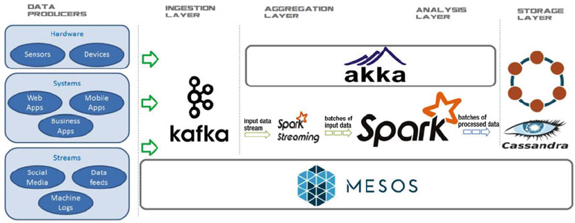
CHAPTER 2 ■ BIG DATA, BIG SOLUTIONS
12
Apache Spark vs. MapReduce
MapReduce is a programming model for processing large data sets with a parallel and distributed algorithm
on a cluster.
As we will see later, in functional programming, there are two basic methods: map() , which is dedicated
filtering and sorting, and reduce() , which is dedicated to doing an operation. As an example, to serve a
group of people at a service window, you must first queue (map) and then attend them (reduce).
The term MapReduce was coined in 1995, when the Message Passing Interface was used to solve
programming issues, as we will discuss later. Obviously, when Google made the implementation, it had only
one use case in mind: web search.
It is important to note that Hadoop born in 2006 and grew up in an environment where MapReduce
reigned. MapReduce was born with two characteristics that mark its life: high latency and batch mode; both
make it incapable to withstand modern challenges.
As you can see in Table
2-2 , Spark is different.
Figure 2-1. SMACK at a glance

CHAPTER 2 ■ BIG DATA, BIG SOLUTIONS
13
Table 2-2. Apache Spark /MapReduce Comparison
CONCEPT Apache Spark MapReduce
Written in Scala/Akka Java
Languages Supported Java, Scala, Python, and R are first-
class citizens.
Everything should be written using Java.
Storage Model Keeps things in memory Keeps things in disk. Takes a long time
to write things to disk and read them
back, making it slow and laborious.
I/O Model Keeps things in memory without I/O.
Operates on the same data quickly.
Requires a lot of I/O activity over disk.
Recovery Runs the same task in seconds or
minutes. Restart is not a problem.
Records everything in disk, allowing
restart after failure
Knowledge The abstraction is high; codification
is intuitive.
Could write MapReduce jobs
intelligently, avoiding overusing
resources, but requires specialized
knowledge of the platform.
Focus Code describes how to process data.
Implementation details are hidden.
Apache Hive programming goes
into code to avoid running too many
MapReduce jobs.
Efficiency Abstracts all the implementation to
run it as efficiently as possible.
Programmers write complex code to
optimize each MapReduce job.
Abstraction Abstracts things like a good high-
level programming language.
It is a powerful and expressive
environment.
Code is hard to maintain over time.
Libraries Adds libraries for machine learning,
streaming, graph manipulation, and
SQL.
Programmers need third-party tools
and libraries, which makes work
complex.
Streaming Real-time stream processing out of
the box.
Frameworks like Apache Storm needed;
increased complexity.
Source Code Size Scala programs have dozens of lines
of code (LOC).
Java programs have hundreds of LOC.
Machine Learning Spark ML If you want to do machine learning, you
have to separately integrate Mahout,
H2O, or Onyx. You have to learn how it
works, and how to build it on.
Graphs Spark GraphX If you want to do graph databases, you
have to select from Giraph, TitanDB,
Neo4J, or some other technologies.
Integration is not seamless.
CHAPTER 2 ■ BIG DATA, BIG SOLUTIONS
14
Apache Spark has these advantages:
• Spark speeds up application development 10 to 100 times faster, making applications
portable and extensible.
• Scala can read Java code. Java code can be rewritten in Scala in a much smaller form
factor that is much easier to read, repurpose, and maintain.
• When the Apache Spark core is improved, all the machine learning and graphs
libraries are improved too.
• Integration is easier: the applications are easier to maintain and costs go down.
If an enterprise bets on one foundation, Spark is the best choice today.
Databricks (a company founded by the Apache Spark creators) lists the following use cases for Spark:
• ETL and data integration
• Business intelligence and interactive analytics
• Advanced analytics and machine learning
• Batch computation for high performance
• Real-time stream processing
Some of the new use cases are just the old use cases done faster; although some use cases are totally
new. There are some scenarios that just can’t be done with acceptable performance on MapReduce.
The Engine
It is important to recall that Spark is better at OLAP (online analytical processing), which are batch jobs
and data mining. Spark is not suitable for OLTP (online transaction processing), such as numerous atomic
transactions; for this type of processing, we strongly recommend Erlang (a beautiful language inspired in the
actor’s model).
Apache Spark has five main components:
• Spark Core
• Spark SQL
• Spark Streaming
• Spark MLib
• Spark GraphX
Each Spark library typically has an entire book dedicated to it. In this book, we try to simply tackle the
Apache Spark essentials to meet the SMACK stack.
The role of Apache Spark on the SMACK stack is to act as the processor and provide real-time data
analysis. It addresses the aggregation and analysis layers.
There are few open source alternatives to Spark. As we’ve mentioned, Apache Hadoop is the classic
approach. The strongest modern adversary is the Apache Flink project, which is good to keep in mind.
CHAPTER 2 ■ BIG DATA, BIG SOLUTIONS
15
The Model
Akka is a model , a toolkit, and a runtime for building distributed, resilient, and highly concurrent
message-driven applications on the Java virtual machine. In 2009, the Akka toolkit was released as open
source. Language bindings exist for both Java and Scala. We need to first analyze Akka in order to understand
the Spark architecture. Akka was designed based on the actor concurrency models:
• Actors are arranged hierarchically
• Asynchronous message (data) passing
• Fault tolerant
• Customizable failure and detection strategies
• Hierarchical supervision
• Adaptive, predictive
• Parallelized
• Load balance
There are many Akka competitors; we make a special mention of Reactor. The actor model is the
foundation of many frameworks and languages. The main languages that are based on the actor model
(called functional languages ) are Lisp, Scheme, Erlang, Haskell, and recently, Scala, Clojure, F#, and Elixir
(a modern implementation of Erlang).
The Broker
Apache Kafka is a publish/subscribe message broker redesigned as a distributed commit log. In SMACK,
Kafka is the data ingestion point, mainly on the application layer. Kafka takes data from applications and
streams and processes them into the stack. Kafka is a distributed messaging system with high throughput. It
handles massive data load and floods. It is the valve that regulates the pressure.
Apache Kafka inspects incoming data volume, which is fundamental for partitioning and distribution
among the cluster nodes. Apache Kafka’s features include the following:
• Automatic broker failover
• Very high performance distributed messaging
• Partitioning and Distribution across the cluster nodes
• Data pipeline decoupling
• A massive number of consumers are supported
• Massive data load handling
Kafka is the champion among a lot of competitors in MOM (message-oriented middleware). In the
MQ family, this includes ActiveMQ, ZeroMQ, IronMQ, and RabbitMQ. The best of all is RabbitMQ, which is
made with Erlang.
The best alternative to Kafka is Apache Storm, which has a lot of integration with Apache Hadoop. Keep
it in mind. Apache Kafka is here to stay.
CHAPTER 2 ■ BIG DATA, BIG SOLUTIONS
16
The Storage
Apache Cassandra is a distributed database. It is the perfect choice when you need to escalate and need
hyper-high availability with no sacrifice in performance. Cassandra was originally used on Facebook in 2008
to handle large amounts of data. It became a top-level Apache project in 2010. Cassandra handles the stack’s
operational data. Cassandra can also be used to expose data to the application layer.
The following are the main features of Apache Cassandra:
• Extremely fast and scalable
• Multi data center, no single point of failure
• Survives when multiple nodes fault
• Easy to operate
• Flexible data modeling
• Automatic and configurable replication
• Ideal for real-time ingestion
• Has a great Apache based community
There are a lot of Cassandra competitors, including DynamoDB (powered by Amazon; it’s contending
in the NoSQL battlefield), Apache HBase (the best-known database implementation of Hadoop), Riak
(made by the Basho samurais; it’s a powerful Erlang database), CouchBase, Apache CouchDB, MongoDB,
Cloudant, and Redis.
The Container
Apache Mesos is a distributed systems kernel that is easy to build and effective to run. Mesos is an
abstraction layer over all computer resources (CPU, memory, storage) on the machines (physical or
virtual), enabling elastic distributed systems and fault tolerance. Mesos was designed with the Linux kernel
principles at a higher abstraction level. It was first presented as Nexus in 2009. In 2011, it was relaunched by
Matei Zaharia under its current name. Mesos is the base of three frameworks:
• Apache Aurora
• Chronos
• Marathon
In SMACK, Mesos orchestrates components and manages resources. It is the secret for horizontal
cluster scalation. Usually, Apache Mesos is combined with Kubernetes (the competitor used by the Google
Cloud Platform) or with Docker (as you will see, more than a competitor, it is a complement to Mesos). The
equivalent in Hadoop is Apache Yarn.
Summary
This chapter, like the previous one, was full of theory. We reviewed the fundamental SMACK diagram as
well as Spark’s advantages over traditional big data technologies such as Hadoop and MapReduce. We also
visited every technology in the SMACK stack, briefly presented each tool’s potential, and most importantly,
we discussed the actual alternatives for each technology. The upcoming chapters go into greater depth
on each of these technologies. We will explore the connectors and the integration practices, and link
techniques, as well as describe alternatives to every situation.

PART II
Playing SMACK

19
© Raul Estrada and Isaac Ruiz 2016
R. Estrada and I. Ruiz, Big Data SMACK, DOI 10.1007/978-1-4842-2175-4_3
CHAPTER 3
The Language: Scala
The main part of the SMACK stack is Spark, but sometimes the S is for Scala. You can develop in Spark in
four languages: Java, Scala, Python, and R. Because Apache Spark is written in Scala, and this book is focused
on streaming architecture, we are going to show examples in only the Scala language.
Other Apache Spark books present their examples in the four languages, but for the SMACK stack ,
simply discussing Scala is enough to develop a robust streaming pipeline. It is important to mention that all
the Java programs run in Scala.
If you came here without previous Scala knowledge, welcome to the crash course. It is always good to
learn a new programming language. We are not going to study Scala as the first programming language,
however. This chapter is organized as a series of exercises in the language. If you already know Scala, try to
follow the exercises to improve your knowledge.
As said by many, programming is just about algorithms and data structures. This chapter covers all the
Scala data structures. The next chapter covers the algorithms—that is, the Akka actor model.
Functional Programming
Our goal in this chapter is not to learn Scala, but to reach the fully functional thinking in all of its pure
expression. It is an open secret that each SMACK technology is independent and autonomous from the
others. However, each could be developed (replaced) in Java or Scala.
The truth is that each and every one of the SMACK technologies can be developed ad hoc. Yes, the sun
shines for everyone in the streaming pipeline world. You can develop from scratch any SMACK technology
or replace one as your project needs.
How to write an entire Apache Akka project is beyond this book’s scope, but you should understand
how it works to make good architectural decisions.
You need to be clear on these rules:
• Scala collections and Java collections are different
• Spark collections and Scala collections are different
There are three fundamentals (among many others) in functional programming :
• Predicates
• Literal functions
• Implicit loops
Predicate
A predicate is a multiple parameter function with just one boolean value as a return.
CHAPTER 3 ■ THE LANGUAGE: SCALA
20
This is an example (with body definition):
def isEven (i: Int) = if (i % 2 == 0) true else false
Here is another example (without body definition):
def isPrime (p: Long)
Note that the function has no parameters, but this is weird. If a function doesn’t receive an input, then
this implies it is obtaining its data from a global variable or a shared context; both are strongly discouraged
(even prohibited) in functional programming. Yes, we know that it could take a random number or take the
system time to make its decisions, but these are special cases.
Literal Functions
In functional programming, functions are first-class citizens. In the 21st century it may sound archaic, but
programming languages that discriminate against functions still exist, usually because they are low-level
languages.
The rule of thumb is to think of it as algebra. In algebra, functions can be composed; you can make
operations with functions and pass functions as other functions parameters. If you have problems with algebra,
then sorry, this book (and programming) is not for you.... Just kidding. In this case, you can think of functions
as traditional object-oriented programming (OOP) objects. So following that idea, you define a higher-order
function in mathematics and computer science as a function that does at least one of the following:
• Takes functions as arguments (as parameters)
• Returns a function as a result
For example, the isEven function could be rewritten as this:
( i: Int) => i % 2 == 0
In this code, the => symbol should be thought of as a transformer .
This is a high-order function because it returns a function. Simple, isn’t it?
Yes, in mathematics, as in life, definitions are difficult but necessary to support and generalize our
theories. With examples, everything is clear.
Implicit Loops
As a final step, the isEven function could be rewritten as this:
_ % 2 == 0
The _ symbol denotes the parameter, or the thing (object, function, entity) to be used as input.
Combined with the filter method, over a list, we find expressions like these:
scala> val oneToTen = List.range(1, 10 )
oneToTen: List[Int] = List(1, 2, 3, 4, 5, 6, 7, 8, 9)
scala> val evens = nums.filter(_ % 2 == 0)
evens: List[Int] = List(2, 4, 6, 8)
The third line contains an implicit loop. Yes, in functional programming we try to avoid loops. If your
code has a lot of for s and while s, it could probably be simplified.
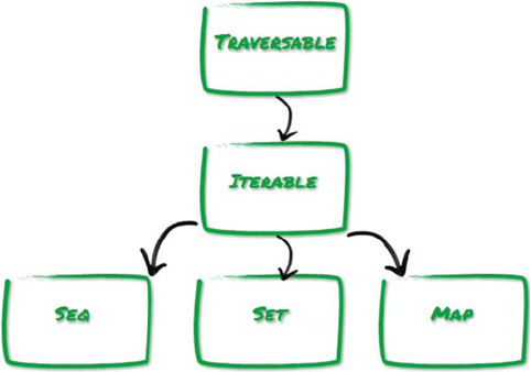
CHAPTER 3 ■ THE LANGUAGE: SCALA
21
Functional is elegant and concise, but of course, there are some memory tricks that can be issued
and solved through structured programming. Throughout history, code readability has proved to be more
effective in economic terms (time and money) than hardware optimization, which has become cheaper.
Collections Hierarchy
At the top of the Scala collections hierarchy there is the Traversable class (as shown in Figure 3-1 ).
All Traversable trait children have the implementation for this method:
def foreach[U](f: Elem => U)
The Iterable trait has implementation in terms of an iterator:
def foreach[U](f: Elem => U): Unit = {
val ite = iterator
while (ite.hasNext) f(ite.next())
}
As you can see, the Iterable trait has three children: Seq , Set , and Map .
Sequences
The Seq trait represents sequences .
As shown in Figure
3-2 , Seq has three children: IndexedSeq , LinearSeq , and Buffer .
Figure 3-1. The Scala collection’s top hierarchy
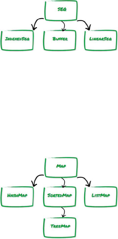
CHAPTER 3 ■ THE LANGUAGE: SCALA
22
A sequence is an iterable that has a length and whose elements start from zero and have fixed index
positions.
LinearSeq and IndexedSeq don’t add any new operations, but each has different performance.
LinearSeq is the list. As you know from functional programming, it has head , tail , and isEmpty
operations. It is very efficient with apply, length, and update operations.
IndexedSeq is the array. As you know from structured programming, it has the index operations. So, if
you have an array of rooms, and you write Room(101) , you access the 101st room.
Buffer is an important mutable sequence. Buffers allow you to update existing elements and to insert,
remove, and add new elements at the end.
M a p s
A map is an iterable consisting of pairs. Each pair consists of a key and a value (also called mappings or
associations ). The Map family is shown in Figure
3-3 .
Scala offers an implicit conversion that lets you write key -> value as an alternate syntax for the (key, value).
For example, Map("uno" -> 1, "dos" -> 2, "tres" -> 3) is the same as Map(("uno", 1), ("dos", 2),
("tres", 3)) , but is easier to read.
Figure 3-2. The Seq children
Figure 3-3. T h e M a p f a m i l y
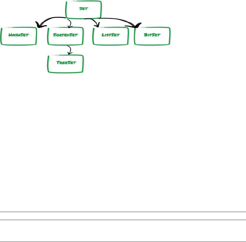
CHAPTER 3 ■ THE LANGUAGE: SCALA
23
Sets
A set is an iterable that contains no duplicate elements. As you can see in Figure 3-4 , the Set hierarchy is
similar to the Map family.
Choosing Collections
Many programmers argue that the Scala type system is difficult and cumbersome. In fact, as you saw, you
have to choose only one of these three types:
• Sequence
• Map
• S e t
The actual decision is to choose between the mutable and immutable versions.
Sequences
There are only two sequences: the LinearSeq (list) and the IndexedSeq (array). The true effort is to learn the
names used, not the hierarchy itself (see Table
3-1 ).
Immutable Sequences
LinearSeq
• List : The list as we know from the functional world.
• Queue : The FIFO data structure of the traditional computer science books.
• Stack : The LIFO data structure of the traditional computer science books.
• Stream : Infinite, lazy and persistent; our everyday flow.
Figure 3-4. T h e S e t f a m i l y
Table 3-1. The Sequence Collections
Immutable Mutable
IndexedSeq Vector ArrayBuffer
LinearSeq List ListBuffer
CHAPTER 3 ■ THE LANGUAGE: SCALA
24
IndexedSeq
• Range : A limited list of integers.
• String : The well-known and limited char sequence.
• Vector : Immutable, indexed, the sedan model of the lists.
Mutable Sequences
LinearSeq
• LinkedList : Those traditionally used as an introduction to the C/C++ pointers.
• DoubleLinkedList : LinkedList with the “previous” method implemented.
• ListBuffer : The List version of the indexed Array.
• MutableList : A list for those non-functional rebels.
• Queue : The FIFO for non-functional guys.
• Stack : The LIFO for non-functional fellas.
IndexedSeq
• Array : A list which length is constant and every element is not.
• ArrayBuffer : An indexed array that always fits memory needs.
• ArrayStack : LIFO implementation when performance matters.
• StringBuilder : Efficient string manipulation for those with a limited memory budget.
M a p s
You have to choose either a mutable map or a sorted map.
Mutable maps
• HashMap : A map whose internal implementation is a hash table.
• LinkedHashMap : Elements are returned as they were inserted.
• ListMap : Elements are returned as the inverse of how they were inserted.
• Map : The map as everybody knows it; key-value pairs.
Immutable maps
• HashMap : A map whose internal implementation is a tree.
• ListMap : Elements are returned as the inverse of how they were inserted.
• Map : The map as everybody knows it; key-value pairs.
• SortedMap : The keys are stored in a sorted order.
• TreeMap : A sorted map; the red-black tree of the traditional computer
science books.
CHAPTER 3 ■ THE LANGUAGE: SCALA
25
Sets
You have to choose either a mutable set or a sorted set.
Mutable sets
• BitSet : Used to save memory, but only integers are allowed.
• HashSet : A set implemented using a hash table.
• LinkedHashSet : The elements are returned as they were inserted.
• TreeSet : The AVL tree of the traditional computer science books.
• Set : The mutable vanilla set.
• SortedSet : The mutable TreeSet, but ordered.
Immutable sets
• BitSet : To save (more) memory, only integers are allowed.
• HashSet : A set implemented using a tree.
• ListSet : A set for the public; a list for those who knows it.
• TreeSet : An immutable set implemented using a tree.
• Set : The immutable vanilla set.
• SortedSet : The immutable TreeSet but ordered.
Traversing
foreach is the standard method for traversing collections in Scala. Its complexity is O(n); that is, the
computation time has a linear relation with the number of elements in the input. We also have the
traditional for and the iterators, as in Java.
f o r e a c h
In Scala, the foreach method takes a function as argument. This function must have only one parameter and
it doesn’t return anything (this is called a procedure ). It operates in every element of the collection, one at a
time. The parameter type of the function must match the type of every element in the collection.
scala> val zahlen = Vector("Eins", "Zwei", "Drei")
zahlen: scala.collection.immutable.Vector[String] = Vector(Eins, Zwei, Drei)
scala> zahlen.foreach(s => print(s))
EinsZweiDrei
This function takes one character and prints it:
scala> def printAChar ( c: Char) { print ( c) }
printAChar: (c: Char)Unit
CHAPTER 3 ■ THE LANGUAGE: SCALA
26
The function is applied to a string (a sequence of chars):
scala> "SMACK".foreach( c => printAChar(c) )
SMACK
The type inference is a useful tool in these modern times:
scala> "SMACK".foreach( printAChar )
SMACK
This is same as the preceding example but with a literal function:
scala> "SMACK".foreach( (c: Char) => print(c) )
SMACK
This is same as the preceding example but uses a type inference and literal functions:
scala> "SMACK".foreach( print )
SMACK
This example uses an implicit loop:
scala> "SMACK: Spark Mesos Akka Cassandra Kafka".split(" ")
Array[String] = Array(SMACK:, Spark, Mesos, Akka, Cassandra, Kafka)
for
As in all modern functional programming languages, we can explore all the elements of a collection with a
for loop .
Remember, foreach and for are not designed to produce new collections. If you want a new collection,
use the for / yield combo.
As we stated earlier, if it’s iterable, then it’s traversable (inheritance 101):
scala> val smack = Traversable("Spark", "Mesos", "Akka", "Cassandra", "Kafka")
smack: Traversable[String] = List(Spark, Mesos, Akka, Cassandra, Kafka)
scala> for (f <- smack) println(f)
Spark
Mesos
Akka
Cassandra
Kafka
scala> for (f <- smack) println( f.toUpperCase )
SPARK
MESOS
AKKA
CASSANDRA
KAFKA
To build a new collection, use the for/yield construct:
CHAPTER 3 ■ THE LANGUAGE: SCALA
27
scala> val smack = Array("Spark", "Mesos", "Akka", "Cassandra", "Kafka")
smack: Array[java.lang.String] = Array(Spark, Mesos, Akka, Cassandra, Kafka)
scala> val upSmack = for (s <- smack) yield s.toUpperCase
upSmack: Array[java.lang.String] = Array(SPARK, MESOS, AKKA, CASSANDRA, KAFKA)
This for/yield construct is called for comprehension .
Now, let’s iterate a map with a for loop:
scala> val smack = Map("S" ->"Spark", "M" -> "Mesos", "A" -> "Akka", "C" ->"Cassandra", "K"
-> "Kafka")
smack: scala.collection.immutable.Map[String,String] = Map(A -> Akka, M -> Mesos, C ->
Cassandra, K -> Kafka, S -> Spark)
scala> for ((k,v) <- smack) println(s"letter: $k, means: $v")
letter: A, means: Akka
letter: M, means: Mesos
letter: C, means: Cassandra
letter: K, means: Kafka
letter: S, means: Spark
I t e r a t o r s
To iterate a collection in Java, you use hasNext() and next() . In Scala, however, they don’t exist, because
there are the map and foreach methods.
You only use iterators in Scala when reading very large streams; a file is the most common example. As
a rule of thumb, you use iterators when it’s not convenient to load all the data structure in memory.
Once it has been used, an iterator remains “exhausted,” as shown in the following:
scala> val iter = Iterator("S","M","A","C","K")
iter: Iterator[String] = non-empty iterator
scala> iter.foreach(println)
S
M
A
C
K
scala> iter.foreach(println)
As you can see, the last line didn’t produce any output, because the iterator is exhausted.
Mapping
Another way to transform collections different from the for/yield is by using the map method call with a
function as argument, as follows:
scala> val smack = Vector("spark", "mesos", "akka", "cassandra", "kafka")
smack: scala.collection.immutable.Vector[String] = Vector(spark, mesos, akka, cassandra, kafka)
CHAPTER 3 ■ THE LANGUAGE: SCALA
28
// the long way
scala> val cap = smack.map(e => e.capitalize)
cap: scala.collection.immutable.Vector[String] = Vector(Spark, Mesos, Akka, Cassandra,
Kafka)
// the short way
scala> val cap = smack.map(_.capitalize)
cap: scala.collection.immutable.Vector[String] = Vector(Spark, Mesos, Akka, Cassandra,
Kafka)
//producing a Vector of Int
scala> val lens = smack.map(_.size)
lens: scala.collection.immutable.Vector[Int] = Vector(5, 5, 4, 9, 5)
//producing a Vector of XML elements
scala> val elem = smack.map(smack => <li>{smack}</li>)
elem: scala.collection.immutable.Vector[scala.xml.Elem] = Vector(<li>spark</li>, <li>mesos</
li>, <li>akka</li>, <li>cassandra</li>, <li>kafka</li>)
Unfortunately, Scala has type inference; that is, there is no a general rule for the collection type returned
after a mapping operation.
You can say that you are a seasoned Scala functional programmer if you can identify the comprehension
to be used: for / yield or map .
scala> val smack = List("spark", "mesos", "akka", "cassandra", "kafka")
smack: List[String] = List(spark, mesos, akka, cassandra, kafka)
// capitalize with map
scala> val m = smack.map(_.capitalize)
m: List[String] = List(Spark, Mesos, Akka, Cassandra, Kafka)
// capitalize with for/yield
scala> val y = for (s <- smack) yield s.capitalize
y: List[String] = List(Spark, Mesos, Akka, Cassandra, Kafka)
Flattening
In functional programming, the flattening process occurs when you convert a list of lists (also called sequence
of sequences or multilist ) into one list. The following is an example:
scala> val allies = List(List("Java","Scala"), List("Javascript","PHP"))
allies: List[List[String]] = List(List(Java, Scala), List(Javascript, PHP))
scala> val languages = allies.flatten
languages: List[String] = List(Java, Scala, Javascript, PHP)
The power of (functional) programming is the expressive power and simplicity. Here we capitalize, flat,
and sort all in one sentence:
scala> val jargon = allies.flatten.map(_.toUpperCase).sorted
jargon: List[String] = List(JAVA, JAVASCRIPT, PHP, SCALA)
CHAPTER 3 ■ THE LANGUAGE: SCALA
29
When you work with connected nodes, flattening helps with the network:
val webFriends = List("Java", "JS")
val javaFriends = List("Scala", "Clojure", "Ceylon")
val jsFriends = List("PHP", "Ceylon")
val friendsOfFriends = List( javaFriends, jsFriends)
scala> val uniqueFriends = friendsOfFriends.flatten.distinct
uniqueFriends: List[String] = List(Scala, Clojure, Ceylon, PHP)
As you may guess, flattening a string produces a list of its chars:
scala> val stuff = List("SMACK", "Scala")
stuff: List[String] = List(SMACK, Scala)
scala> stuff.flatten
List[Char] = List(S, M, A, C, K, s, c, a, l, a)
If a collection contains elements of type None , flattening removes them.
If a collection contains elements of type Some , flattening strips them:
scala> val boxes = Vector(Some("Something"), None, Some(3.14), None)
boxes: scala.collection.immutable.Vector[Option[Any]] = Vector(Some(Something), None,
Some(3.14), None)
scala> boxes.flatten
res1: scala.collection.immutable.Vector[Any] = Vector(Something, 3.14)
Filtering
In functional programming, filtering traverses a collection and builds a new collection with elements that
match specific criteria. This criteria must be a predicate. You apply the predicate to each collection element,
for example:
scala> val dozen = List.range(1, 13)
dozen: List[Int] = List(1, 2, 3, 4, 5, 6, 7, 8, 9, 10, 11, 12)
scala> val multiplesOf3 = dozen.filter(_ % 3 == 0)
multiplesOf3: List[Int] = List(3, 6, 9, 12)
scala> val languages = Set("Java", "Scala", "Clojure", "Ceylon")
languages: scala.collection.immutable.Set[String] = Set(Java, Scala, Clojure, Ceylon)
scala> val c = languages.filter(_.startsWith("C"))
c: scala.collection.immutable.Set[String] = Set(Clojure, Ceylon)
scala> val s = languages.filter(_.length < 6)
s: scala.collection.immutable.Set[String] = Set(Java, Scala)
CHAPTER 3 ■ THE LANGUAGE: SCALA
30
Filtering has the following two rules:
1 . The filter doesn’t modify the collection. You must keep the result in a new one.
2 . Only the elements whose predicate returns true are kept.
Extracting
In this section, we are going to examine the methods to extract subsequences. The following are examples.
// We declare an array of Int from 1 to 9
scala> val magic = (0 to 9).toArray
magic: Array[Int] = Array(0, 1, 2, 3, 4, 5, 6, 7, 8, 9)
// Without the first N elements
scala> val d = magic.drop(3)
d: Array[Int] = Array(3, 4, 5, 6, 7, 8, 9)
// Without the elements matching a predicate
scala> val dw = magic.dropWhile(_ < 4)
dw: Array[Int] = Array(4, 5, 6, 7, 8, 9)
// Without the last N elements
scala> val dr = magic.dropRight(4)
dr: Array[Int] = Array(0, 1, 2, 3, 4, 5)
// Just the first N elements
scala> val t = magic.take(5)
t: Array[Int] = Array(0, 1, 2, 3, 4)
// Just the first elements matching a predicate (from the left)
scala> val tw = magic.takeWhile(_ < 4)
tw: Array[Int] = Array(0, 1, 2, 3)
// Just the last N elements
scala> val tr = magic.takeRight(3)
tr: Array[Int] = Array(7, 8, 9)
// the subsequence between the index A and B
scala> val sl = magic.slice(1,7)
sl: Array[Int] = Array(1, 2, 3, 4, 5, 6)
T h e List methods are used to achieve functional purity.
// head, the first element
scala> val h = magic.head
h: Int = 0
// the head boxed (to prevent errors)
scala> val hb = magic.headOption
hb: Option[Int] = Some(0)
CHAPTER 3 ■ THE LANGUAGE: SCALA
31
// the list without the last element
scala> val in = magic.init
in: Array[Int] = Array(0, 1, 2, 3, 4, 5, 6, 7, 8)
// the last element
scala> val ta = magic.last
ta: Int = 9
// the last boxed (to prevent errors)
scala> val lo = magic.lastOption
lo: Option[Int] = Some(9)
// all the list without the first element (known as tail)
scala> val t = magic.tail
t: Array[Int] = Array(1, 2, 3, 4, 5, 6, 7, 8, 9)
Splitting
For those fans of the database perspective, there are methods to discriminate lists. We split samples into two
groups, as follows.
// Here, a sample list
scala> val sample = List(-12, -9, -3, 12, 18, 15)
sample: List[Int] = List(-12, -9, -3, 12, 18, 15)
// lets separate our sample in two groups
scala> val teens = sample.groupBy(_ > 10)
teens: scala.collection.immutable.Map[Boolean,List[Int]] = Map(false -> List(-12, -9, -3),
true -> List(12, 18, 15))
// to access the generated groups
scala> val t = teens(true)
t: List[Int] = List(12, 18, 15)
scala> val f = teens(false)
f: List[Int] = List(-12, -9, -3)
// partition does the same as groupBy but it returns a List with two Lists
scala> val teens = sample.partition(_ > 10)
teens: (List[Int], List[Int]) = (List(12, 18, 15),List(-12, -9, -3))
// span the list, in one list with the longest index who meets the predicate
scala> val negs = sample.span(_ < 0)
negs: (List[Int], List[Int]) = (List(-12, -9, -3),List(12, 18, 15))
// splitAt generates two lists, one before the index at N, and the rest
scala> val splitted = sample.splitAt(2)
splitted: (List[Int], List[Int]) = (List(-12, -9),List(-3, 12, 18, 15))
// partition can assign the result to a Tuple
scala> val (foo, bar) = sample.partition(_ > 10)
foo: List[Int] = List(12, 18, 15)
bar: List[Int] = List(-12, -9, -3)
CHAPTER 3 ■ THE LANGUAGE: SCALA
32
Unicity
If you want to remove duplicates in a collection, only use unique elements. The following are some
examples.
scala> val duplicated = List("A", "Y", "Y", "X", "X", "Z")
duplicated: List[String] = List(A, Y, Y, X, X, Z)
// The first option is using distinct
scala> val u = duplicated.distinct
u: List[String] = List(A, Y, X, Z)
// the second is is converting the Collection to a Set, duplicates not allowed
scala> val s = duplicated.toSet
s: scala.collection.immutable.Set[String] = Set(A, Y, X, Z)
Merging
For merging and subtracting collections , use ++ and -- . The following show some of examples.
// The ++= method could be used in any mutable collection
scala> val nega = collection.mutable.ListBuffer(-30, -20, -10)
nega: scala.collection.mutable.ListBuffer[Int] = ListBuffer(-30, -20, -10)
// The result is assigned to the original collection, and it is mutable
scala> nega ++= Seq(10, 20, 30)
res0: nega.type = ListBuffer(-30, -20, -10, 10, 20, 30)
scala> val tech1 = Array("Scala", "Spark", "Mesos")
tech1: Array[String] = Array(Scala, Spark, Mesos)
scala> val tech2 = Array("Akka", "Cassandra", "Kafka")
tech2: Array[String] = Array(Akka, Cassandra, Kafka)
// The ++ method merge two collections and return a new variable
scala> val smack = tech1 ++ tech2
smack: Array[String] = Array(Scala, Spark, Mesos, Akka, Cassandra, Kafka)
We have the classic Set operations from Set Theory.
scala> val lang1 = Array("Java", "Scala", "Ceylon")
lang1: Array[String] = Array(Java, Scala, Ceylon)
scala> val lang2 = Array("Java", "JavaScript", "PHP")
lang2: Array[String] = Array(Java, JavaScript, PHP)
// intersection, the elements in both collections
scala> val inter = lang1.intersect(lang2)
inter: Array[String] = Array(Java)
// union, the elements in both collections
CHAPTER 3 ■ THE LANGUAGE: SCALA
33
scala> val addition = lang1.union(lang2)
addition: Array[String] = Array(Java, Scala, Ceylon, Java, JavaScript, PHP)
// to discriminate duplicates we use distinct
scala> val substraction = lang1.union(lang2).distinct
substraction: Array[String] = Array(Java, Scala, Ceylon, JavaScript, PHP)
T h e diff method results depend on which sequence it’s called on (in set theory, A-B is different from B-A):
// difference, the elements in one set that are not in the other
scala> val dif1 = lang1 diff lang2
dif1: Array[String] = Array(Scala, Ceylon)
scala> val dif2 = lang2 diff lang1
dif2: Array[String] = Array(JavaScript, PHP)
Lazy Views
In functional programming, we call something “lazy” when it doesn’t appear until it is needed. A lazy view is
a version of a collection computed and returned when it is actually needed.
By contrast, in Java, all the memory is allocated immediately when the collection is created.
The difference between these two lines could save a lot of memory:
scala> 0 to 25
res0: scala.collection.immutable.Range.Inclusive = Range(0, 1, 2, 3, 4, 5, 6, 7, 8, 9, 10,
11, 12, 13, 14, 15, 16, 17, 18, 19, 20, 21, 22, 23, 24, 25)
scala> (0 to 25).view
res1: scala.collection.SeqView[Int,scala.collection.immutable.IndexedSeq[Int]] = SeqView(...)
To force the memory allocation of a view, use the force instruction:
scala> val v = (0 to 25).view
v: scala.collection.SeqView[Int,scala.collection.immutable.IndexedSeq[Int]] = SeqView(...)
scala> val f = v.force
f: scala.collection.immutable.IndexedSeq[Int] = Vector(0, 1, 2, 3, 4, 5, 6, 7, 8, 9, 10, 11,
12, 13, 14, 15, 16, 17, 18, 19, 20, 21, 22, 23, 24, 25)
Mixing views with the map method significantly improves the performance of your programs. In the
following example, increasing the bounds causes your CPU to struggle.
scala> (0 to 100).map { _ * 3 }
res0: scala.collection.immutable.IndexedSeq[Int] = Vector(0, 3, 6, 9, 12, 15, 18, 21, 24,
27, 30, 33, 36, 39, 42, 45, 48, 51, 54, 57, 60, 63, 66, 69, 72...
scala> (0 to 100).view.map { _ * 3 }
res1: scala.collection.SeqView[Int,Seq[_]] = SeqViewM(...)
CHAPTER 3 ■ THE LANGUAGE: SCALA
34
Good programmers (functional or SQL) know well the views benefits:
• Performance (the reason that you’re reading this book)
• The data structure is similar to database views
Database views were created to allow modifications on big result sets and tables without compromising
the performance.
// lets create an array
scala> val bigData = Array("B", "I", "G", "-", "D", "A", "T", "A")
bigData: Array[String] = Array(B, I, G, -, D, A, T, A)
// and a view over the first elements
scala> val view = bigData.view.slice(0, 4)
view: scala.collection.mutable.IndexedSeqView[String,Array[String]] = SeqViewS(...)
// we modify the VIEW
scala> view(0) = "F"
scala> view(1) = "A"
scala> view(2) = "S"
scala> view(3) = "T"
// voilá, our original array was modified
scala> bigData
res0: Array[String] = Array(F, A, S, T, D, A, T, A)
Sorting
To sort, you use the sorted method with the < , <= , > , and >= operators. The following are some examples.
// sorting Strings
scala> val foo = List("San Francisco", "London", "New York", "Tokio").sorted
foo: List[String] = List(London, New York, San Francisco, Tokio)
// sorting numbers
scala> val bar = List(10, 1, 8, 3.14, 5).sorted
bar: List[Double] = List(1.0, 3.14, 5.0, 8.0, 10.0)
// ascending
scala> List(10, 1, 8, 3.14, 5).sortWith(_ < _)
res0: List[Double] = List(1.0, 3.14, 5.0, 8.0, 10.0)
// descending
scala> List(10, 1, 8, 3.14, 5).sortWith(_ > _)
res0: List[Double] = List(10.0, 8.0, 5.0, 3.14, 1.0)
// ascending alphabetically
scala> List("San Francisco", "London", "New York", "Tokio").sortWith(_ < _)
res0: List[String] = List(London, New York, San Francisco, Tokio)
CHAPTER 3 ■ THE LANGUAGE: SCALA
35
// descending alphabetically
scala> List("San Francisco", "London", "New York", "Tokio").sortWith(_ > _)
res0: List[String] = List(Tokio, San Francisco, New York, London)
// ascending by length
scala> List("San Francisco", "London", "New York", "Tokio").sortWith(_.length < _.length)
res0: List[String] = List(Tokio, London, New York, San Francisco)
// descending by length
scala> List("San Francisco", "London", "New York", "Tokio").sortWith(_.length > _.length)
res0: List[String] = List(San Francisco, New York, London, Tokio)
Streams
Just as views are the lazy version of collections, streams are the lazy version of lists. Here we taste some
stream power:
scala> val torrent = (0 to 900000000).toStream
torrent: scala.collection.immutable.Stream[Int] = Stream(0, ?)
scala> torrent.head
res0: Int = 0
scala> torrent.tail
res1: scala.collection.immutable.Stream[Int] = Stream(1, ?)
scala> torrent.take(3)
res2: scala.collection.immutable.Stream[Int] = Stream(0, ?)
scala> torrent.filter(_ < 100)
res3: scala.collection.immutable.Stream[Int] = Stream(0, ?)
scala> torrent.filter(_ > 100)
res4: scala.collection.immutable.Stream[Int] = Stream(101, ?)
scala> torrent.map{_ * 2}
res5: scala.collection.immutable.Stream[Int] = Stream(0, ?)
scala> torrent(5)
res6: Int = 5
Arrays
Scala is a strong typed language. It determines the array type if it’s not specified.
// in numeric, the biggest data type determines the Collection type
scala> Array(6.67e-11, 3.1415, 333F, 666L)
res0: Array[Double] = Array(6.67E-11, 3.1415, 333.0, 666.0)
CHAPTER 3 ■ THE LANGUAGE: SCALA
36
// we can force manually the type
scala> Array[Number] (6.67e-11, 3.1415, 333F, 666L)
res0: Array[Number] = Array(6.67E-11, 3.1415, 333.0, 666)
There are several ways to create and initialize arrays:
// from Range
scala> val r = Array.range(0, 16)
r: Array[Int] = Array(0, 1, 2, 3, 4, 5, 6, 7, 8, 9, 10, 11, 12, 13, 14, 15)
// from Range with step
scala> val rs = Array.range(-16, 16, 3)
rs: Array[Int] = Array(-16, -13, -10, -7, -4, -1, 2, 5, 8, 11, 14)
// with fill
scala> val f = Array.fill(3)("ha")
f: Array[String] = Array(ha, ha, ha)
// with tabulate
scala> val t = Array.tabulate(9)(n => n * n)
t: Array[Int] = Array(0, 1, 4, 9, 16, 25, 36, 49, 64)
// from List
scala> val a = List("Spark", "Mesos", "Akka", "Cassandra", "Kafka").toArray
a: Array[String] = Array(Spark, Mesos, Akka, Cassandra, Kafka)
// from String
scala> val s = "ELONGATION".toArray
s: Array[Char] = Array(E, L, O, N, G, A, T, I, O, N)
// Scala Arrays corresponds to Java Arrays
scala> val bigData = Array("B", "I", "G", "-", "D", "A", "T", "A")
bigData: Array[String] = Array(B, I, G, -, D, A, T, A)
scala> bigData(0) = "F"
scala> bigData(1) = "A"
scala> bigData(2) = "S"
scala> bigData(3) = "T"
scala> bigData
bigData: Array[String] = Array(F, A, S, T, D, A, T, A)
ArrayBuffers
An ArrayBuffer is an array with dynamic size. The following are some examples.
// initialization with some elements
val cities = collection.mutable.ArrayBuffer("San Francisco", "New York")
// += to add one element
cities += "London"
CHAPTER 3 ■ THE LANGUAGE: SCALA
37
// += to add multiple elements
cities += ("Tokio", "Beijing")
// ++= to add another collection
cities ++= Seq("Paris", "Berlin")
// append, to add multiple elements
cities.append("Sao Paulo", "Mexico")
Queues
The queue follows the first-in, first-out (FIFO) data structure. The following are some examples.
// to use it we need to import it from collection mutable
scala> import scala.collection.mutable.Queue
import scala.collection.mutable.Queue
// here we create a Queue of Strings
scala> var smack = new Queue[String]
smack: scala.collection.mutable.Queue[String] = Queue()
// += operator, to add an element
scala> smack += "Spark"
res0: scala.collection.mutable.Queue[String] = Queue(Spark)
// += operator, to add multiple elements
scala> smack += ("Mesos", "Akka")
res1: scala.collection.mutable.Queue[String] = Queue(Spark, Mesos, Akka)
// ++= operator, to add a Collection
scala> smack ++= List("Cassandra", "Kafka")
res2: scala.collection.mutable.Queue[String] = Queue(Spark, Mesos, Akka, Cassandra, Kafka)
// the Queue power: enqueue
scala> smack.enqueue("Scala")
scala> smack
res3: scala.collection.mutable.Queue[String] =
Queue(Spark, Mesos, Akka, Cassandra, Kafka, Scala)
// its counterpart, dequeue
scala> smack.dequeue
res4: String = Spark
// dequeue remove the first element of the queue
scala> smack
res5: scala.collection.mutable.Queue[String] = Queue(Mesos, Akka, Cassandra, Kafka, Scala)
// dequeue, will take the next element
scala> val next = smack.dequeue
next: String = Mesos
CHAPTER 3 ■ THE LANGUAGE: SCALA
38
// we verify that everything run as the book says
scala> smack
res6: scala.collection.mutable.Queue[String] = Queue(Akka, Cassandra, Kafka, Scala)
T h e dequeueFirst and dequeueAll methods dequeue the elements matching the predicate.
scala> val smack = Queue("Spark", "Mesos", "Akka", "Cassandra", "Kafka")
smack: scala.collection.mutable.Queue[String] = Queue(Spark, Mesos, Akka, Cassandra, Kafka)
// remove the first element containing a k
scala> smack.dequeueFirst(_.contains("k"))
res0: Option[String] = Some(Spark)
scala> smack
res1: scala.collection.mutable.Queue[String] = Queue(Mesos, Akka, Cassandra, Kafka)
// remove all the elements beginning with A
scala> smack.dequeueAll(_.startsWith("A"))
res2: scala.collection.mutable.Seq[String] = ArrayBuffer(Akka)
scala> smack
res3: scala.collection.mutable.Queue[String] = Queue(Mesos, Cassandra, Kafka)
Stacks
The stack follows the last-in, first-out (LIFO) data structure. The following are some examples.
// to use it we need to import it from collection mutable
scala> import scala.collection.mutable.Stack
import scala.collection.mutable.Stack
// here we create a Stack of Strings
scala> var smack = Stack[String]()
smack: scala.collection.mutable.Stack[String] = Stack()
// push, to add elements at the top
scala> smack.push("Spark")
res0: scala.collection.mutable.Stack[String] = Stack(Spark)
scala> smack.push("Mesos")
res1: scala.collection.mutable.Stack[String] = Stack(Mesos, Spark)
// push, to add multiple elements
scala> smack.push("Akka", "Cassandra", "Kafka")
res2: scala.collection.mutable.Stack[String] = Stack(Kafka, Cassandra, Akka, Mesos, Spark)
// pop, to take the last element inserted
scala> val top = smack.pop
top: String = Kafka
scala> smack
res3: scala.collection.mutable.Stack[String] = Stack(Cassandra, Akka, Mesos, Spark)
CHAPTER 3 ■ THE LANGUAGE: SCALA
39
// top, to access the last element without extract it
scala> smack.top
res4: String = Cassandra
// "Cassandra" is still on the top
scala> smack
res5: scala.collection.mutable.Stack[String] = Stack(Cassandra, Akka, Mesos, Spark)
// size, the Seq method to know the number of elements
scala> smack.size
res6: Int = 4
// isEmpty, another Seq method
scala> smack.isEmpty
res7: Boolean = false
// clear, to empty all the stack suddenly
scala> smack.clear
scala> smack
res9: scala.collection.mutable.Stack[String] = Stack()
Ranges
Ranges are most commonly used with loops, as shown in the following examples.
// to, to make a range from a to b (upper limit is included)
scala> 0 to 6
res0: scala.collection.immutable.Range.Inclusive = Range(0, 1, 2, 3, 4, 5, 6)
// until, to make a range from 0 to 7 (upper limit not included)
scala> 0 until 6
res1: scala.collection.immutable.Range.Inclusive = Range(0, 1, 2, 3, 4, 5)
// by, to specify a step (in this case, every 3)
scala> 0 to 21 by 3
res2 scala.collection.immutable.Range = Range(0, 3, 6, 9, 12, 15, 18, 21)
// to, also function with chars
scala> 'a' to 'k'
res3: scala.collection.immutable.NumericRange.Inclusive[Char] = NumericRange(a, b, c, d, e,
f, g, h, i, j, k)
// a Range toList
scala> val l = (0 to 16).toList
l: List[Int] = List(0, 1, 2, 3, 4, 5, 6, 7, 8, 9, 10, 11, 12, 13, 14, 15, 16)
// a Range toArray
scala> val a = (0 to 16).toArray
a: Array[Int] = Array(0, 1, 2, 3, 4, 5, 6, 7, 8, 9, 10, 11, 12, 13, 14, 15, 16)
CHAPTER 3 ■ THE LANGUAGE: SCALA
40
// a Range toSet
scala> val s = (0 to 10).toSet
s: scala.collection.immutable.Set[Int] = Set(0, 5, 10, 1, 6, 9, 2, 7, 3, 8, 4)
// Array has a range method (upper limit excluded)
scala> val a = Array.range(0, 17)
a: Array[Int] = Array(0, 1, 2, 3, 4, 5, 6, 7, 8, 9, 10, 11, 12, 13, 14, 15, 16)
// Vector has a range method (upper limit excluded)
scala> val v = Vector.range(0, 10)
v: collection.immutable.Vector[Int] = Vector(0, 1, 2, 3, 4, 5, 6, 7, 8, 9)
// List has a range method (upper limit excluded)
scala> val l = List.range(0, 17)
l: List[Int] = List(0, 1, 2, 3, 4, 5, 6, 7, 8, 9, 10, 11, 12, 13, 14, 15, 16)
// A list with numbers in a range with a step of 5
scala> val l = List.range(0, 50, 5)
l: List[Int] = List(0, 5, 10, 15, 20, 25, 30, 35, 40, 45)
// An ArrayBuffer with characters in a range
scala> val ab = collection.mutable.ArrayBuffer.range('a', 'f')
ab: scala.collection.mutable.ArrayBuffer[Char] = ArrayBuffer(a, b, c, d, e)
// An old fashioned for loop using a range
scala> for (i <- 1 to 5) println(i)
1
2
3
4
5
Summary
Since all the examples in this book are in Scala, we need to reinforce it before beginning our study. This
chapter provided a review of Scala. We studied the fundamental parts of the language. Programming is about
data structures and algorithms. In this chapter, we discussed the Scala type system (the data structures) and
the principal concepts of functional programming.
The use of object-oriented programming (OOP) in past decades was an era of reusable software
components. Things no longer work that way. Now components interoperate by exchanging immutable data
structures (lists, maps, and sets), which is more like functional programming.
In the next chapter, we review an actor model implementation called Akka. To fully understand the
examples, you need to know the Scala programming language.

41
© Raul Estrada and Isaac Ruiz 2016
R. Estrada and I. Ruiz, Big Data SMACK, DOI 10.1007/978-1-4842-2175-4_4
CHAPTER 4
The Model: Akka
Welcome to the chapter on the SMACK stack model . The A stands for Akka. If the previous chapter’s
objective was to develop functional thinking, this chapter’s objective is to develop actor model thinking.
The chapter on Scala was focused on moving your mind from a structured programming paradigm to
functional programming thinking. This chapter shifts from the object-oriented paradigm to actors-based
programming.
This chapter has three parts:
• Actor model
• Actor communication
• Actor lifecycle
The actor model is fundamental to understanding the SMACK operation. So, by the end of this chapter,
we hope that you can model in terms of actors.
The Actor Model
The Sámi people were the first to inhabit northern Scandinavia. Until the Middle Age, its culture and way of
life (fishing, hunting, and trading) dominated the north of Sweden, Norway, Finland, and the Kola Peninsula
in Russia. In Sámi mythology, the goddess Akka represented beauty and goodness in the world. According
to Sámi people, Akka’s representation on Earth is a beautiful mountain in Laponia, located in northern
Sweden.
In the platform’s context, the letters A and K stand for actor kernel . It is for this reason that the platform
is called Akka and its symbol is the Akka mountain (see Figure
4-1 ).
Figure 4-1. The original and modern Akka logos, representing the Akka mountain

CHAPTER 4 ■ THE MODEL: AKKA
42
The actor model is a mathematical model developed by Carl Hewitt, Peter Bishop, and Richard Steiger at
MIT in 1973 and presented in a paper called “A Universal Modular Actor Formalism for Artificial Intelligence”.
1
So, you may argue that if the actor model is more than 40 years old, why have we been dealing with
another paradigm all of this time? The answer is not simple. When the actor model was developed, hardware
(and memory) was very expensive. Today, it’s just the opposite: hardware is dirt cheap and programmers
are expensive.
To land this idea, consider computer science history. If hardware is very expensive, then to program,
you have to optimize and deal with low-level concepts and implementations related to the hardware. So you
have to think in terms of interruptions, assembly language, and pointers to (physical) memory locations.
As programming language has a higher level, we can ignore the details related to hardware and start talking
in terms that have nothing to do with implementation but with abstraction. Think in concepts as a recursive call,
or function composition, which is hard to do if you have to deal with low-level hardware implementations.
Threads and Labyrinths
Between 1980 and 2003, we experienced the rise and dominance of object-oriented languages. These years
were the dark ages of functional programming. Functional languages were spoken only in academic and
scientific environments, barely related to industry.
An interesting problem arose with object-oriented programming: the implementation of concurrency
and parallelism. These two concepts are the Achilles’ heel of structured and object-oriented programming.
Imagine an implementation of threads in C ++ or Java; complexity is vast and proneness to error is very large.
Concurrency is not easy; making more than one thing with a program is related to dealing with race
conditions, semaphores, mutexes, locks, shared data, and all the stuff related to multithreading. This
includes basic issues to determine precisely what a program with several threads is doing, or when a variable
is being accessed from multiple threads, or what its value is at a given point in time, or how to know if there
are two threads in standby, and if this condition is going to release them (and when) or if it is a deadlock.
Unfortunately, thread-based concurrency gives more challenges than solutions.
Today there is a lot of technical debt in the proprietary thread implementations of concurrency issues.
No one wants to touch huge systems because the code is complex and the chances of a change breaking
everything are very high.
In this context, functional programming experienced rebirth. With the release of Scala in 2003, F#
in 2005, Clojure in 2007, and Elixir in 2012, the actor model approach was declared the winner in solving
concurrency issues.
Actors 101
Actors are objects. An actor is an object that sends and receives messages. According to the actor
specification, the order of the received messages is not relevant; but in Akka, there is an implementation
called a mailbox , which is a stack where messages are consumed.
What the actor does with a received message depends on how you solve a specific problem. The actor
could handle the message internally, it could send a message to another actor, it could create another actor,
or it could take an action with the message. An Akka actor is a high-level abstraction.
The following are the main comparison points between OOP and actors:
• Unit . In OOP, the smallest processing unit is the object; in the actor model, it is the
actor. We already know that in Akka, the actors are objects but an actor is a more
bounded representation of reality than an object.
1 Carl Hewitt, Peter Bishop, and Richard Steiger, A Universal Modular Actor Formalism for Artificial Intelligence
(
http://dl.acm.org/citation.cfm?id=1624804 ,1973).
CHAPTER 4 ■ THE MODEL: AKKA
43
• Encapsulation . In both models, the smallest processing unit encapsulates state and
behavior. In OOP, the state is determined by the value of the attributes in a given
time, and behavior is ruled by the class methods. In the actor model, the state is
determined by the messages; if there are no messages in the mailbox, the actor will
wait indefinitely for messages.
• Access . In OOP, executing object methods from outside of the object is allowed
(but not recommended), as well as access and modify object fields from outside
of the object. In the actor model, access to the actor's methods or fields is strictly
prohibited; all the communication must be done through messages.
• Globals . In OOP, for example, there is the Singleton pattern, which is a class with a
single instance. Global variables and class variables exist, but they are discouraged. In
the actor model, global variables don’t exist. A shared global state doesn’t exist either.
• Messages . In OOP, the messages between Objects could be mutable. In the actor
model, the messages between actors are strictly immutable.
• Exceptions . In OOP exists the traditional and well-known try-catch approach,
which is the most complex way to handle exceptions because you have to manage
all the possible values of the variables involved. In the actor model, the “let it crash”
approach exists; if something fails, let it fail. The exception scenario could affect only
the actor involved, not the complete environment.
• Concurrency and parallelism . In OPP, the most used approach is the thread model,
which is a complex solution to the problem. In the actor model, you don’t have to
worry about concurrency and parallelism, because if everything follows the actor
convention, there is no problem with parallelism.
The following are the Lightbend recommendations for the actor model:
• Think of actors as employees. Think of each actor model as a company.
• Think of the actor’s siblings as people in the same hierarchical level.
• Think of the actor’s children as the employee's subordinates.
• An actor has one (and only one) supervisor—the actor who created it.
• Actor model success is the delegation to subordinates.
The Akka implementation of the actor model has these peculiarities:
• When you create an actor, Akka provides an ActorRef.
• Actors run in real Java threads. Some actors could share the same thread.
• There are three mailbox types: Unbounded, Bounded, and Priority.
• Actors can scan their mailboxes to look for specific messages.
• There is a “dead letter” mailbox with all the actors’ terminated messages.
The Lightbend Reactive Platform (
www.lightbend.com ) is a family of five members, described as follows:
• Scala : The programming language. The Reactive Platform fully supports both Java
and Scala, so you can choose what is best for you.
• Akka : Message-driven runtime. At the center of the Reactive Platform is Akka, a
message-driven middleware or runtime with Scala and Java APIs.
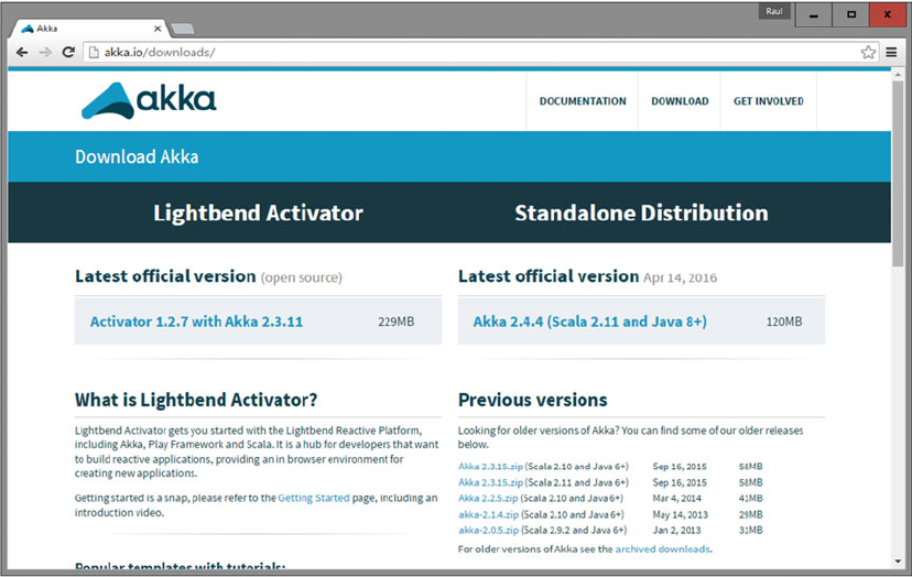
CHAPTER 4 ■ THE MODEL: AKKA
44
• Spark : Apache Spark, which is written in Scala and Akka, is a fast data engine to fuel
Reactive applications.
• Lagom : Reactive microservices framework. An opinionated framework for building
web microservices.
• Play : Just-hit-reload web framework. The Play Framework is the just-hit-reload web
development framework with Scala and Java APIs.
We have always said that Apache Spark is the Scala “killer app.”
In this book, we only cover Scala, Akka, and Spark, but if you are an enthusiastic web service developer
or web developer, don’t pass on the opportunity to explore Lagom and Play, respectively, more deeply.
Installing Akka
Well, enough theory , let's get our feet wet.
The first thing you have to do is go to
http://akka.io/downloads/ , as shown in Figure 4-2 .
Figure 4-2. The Akka download page
Then download the Lightbend Activator according to your platform and operating system. Lightbend is
the company behind Akka; it builds and maintains the Akka message-driven runtime. Follow the installation
instructions from the web page.
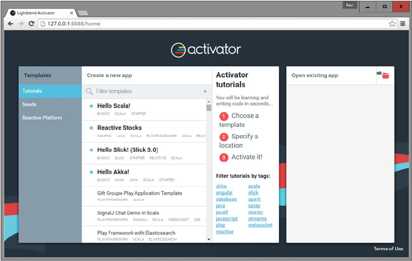
CHAPTER 4 ■ THE MODEL: AKKA
45
After downloading and extracting the package, go to the directory (in this example, we use version 1.3.10):
%> cd activator-dist-1.3.10/bin
Then, execute the activator shell:
%> activator ui
Now go to http://127.0.0.1:8888 . You'll see a web page like the one shown in Figure 4-3 .
Figure 4-3. Lightbend Activator main page
Now select the Hello Akka! application and click the “Create app” button, as shown in Figure 4-4 .
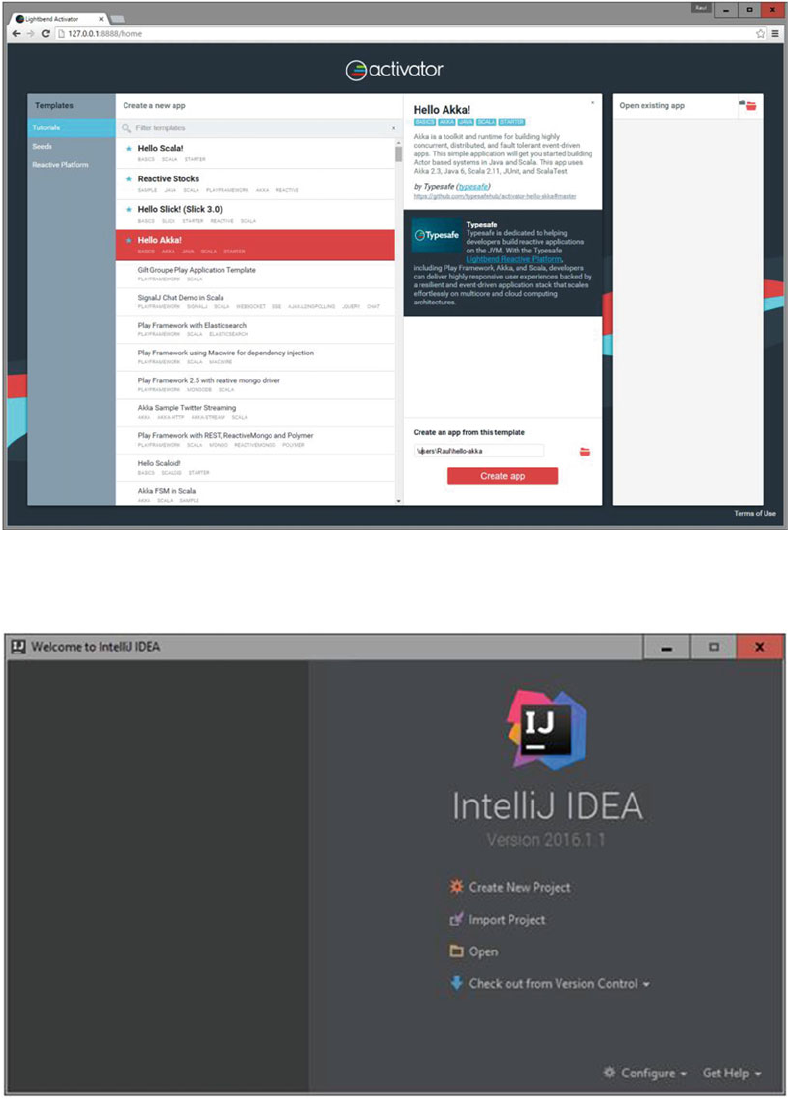
CHAPTER 4 ■ THE MODEL: AKKA
46
Figure 4-4. Creating an Akka application from a template
Figure 4-5. IntelliJ IDEA Community Edition
Now open your IDE. In this case, we used the IntelliJ IDEA Community Edition, as shown in Figure 4-5 .
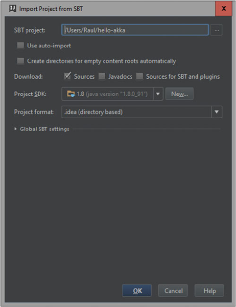
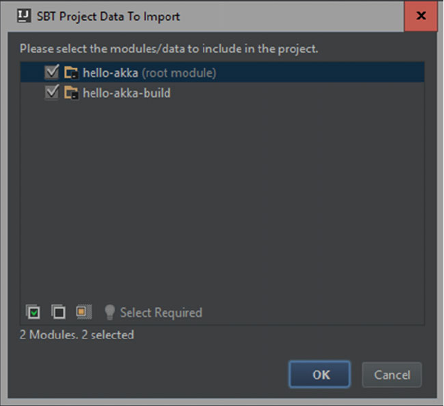
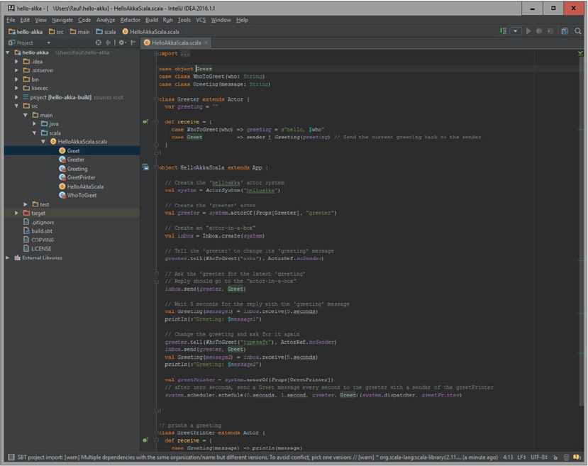
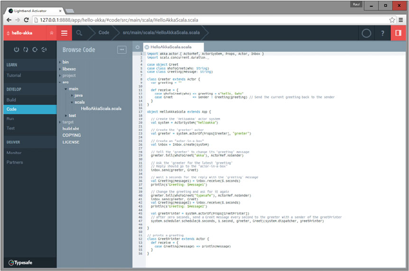
CHAPTER 4 ■ THE MODEL: AKKA
50
Figure 4-9. Lightbend Activator, the Typesafe web IDE
You can build, code, run, and test your Akka applications from your browser.
As you can see in Figure
4-10 , there are a lot of project templates to play with. The Akka world is vast,
and it’s beyond the scope of this book to cover the entire Reactive universe.
As you can see in Figure
4-9 , the Lightbend Activator is a full web IDE.
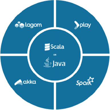
CHAPTER 4 ■ THE MODEL: AKKA
51
Akka Actors
It is essential to recall that before Scala version 2.10, there was a scala.actors package. The Scala actors
library was deprecated in March 2013 and replaced by Akka. Scala actor models prior to version 2.10 should
no longer be used.
A c t o r s
For our first example, we use a multilanguage greeter; that is, we enter a particular language and the
program responds by replying “Good day,” in the language specified.
import akka.actor.Actor
import akka.actor.ActorSystem
import akka.actor.Props
class GreeterActor extends Actor {
def receive = {
case "en" => println("Good day")
case "es" => println("Buen dia")
case "fr" => println("Bonjour")
case "de" => println("Guten Tag")
case "pt" => println("Bom dia")
case _ => println(":(")
}
}
Figure 4-10. Lightbend Reactive Platform
CHAPTER 4 ■ THE MODEL: AKKA
52
object Main extends App {
// build the ActorSystem
val actorSystem = ActorSystem("MultilangSystem")
// instantiate the actor
val greeter = actorSystem.actorOf(Props[GreeterActor], name = "GreeterActor")
// send the actor some messages
greeter ! "en"
greeter ! "es"
greeter ! "fr"
greeter ! "de"
greeter ! "pt"
greeter ! "zh-CN"
// shut down the actor system
actorSystem.shutdown
}
When we run this program, the output is as follows:
$ sbt run
[info] Running Main
Good day
Buen dia
Bonjour
Guten Tag
Bom dia
:(
Process finished with exit code 0
Here is the step-by-step explanation:
• When using Akka actors, you need to import the akka.actor._ package. You at least
need these classes: Actor , ActorSystem , and Props .
• You must define a class of type Actor . In this case, we called it GreeterActor . You can
use any name that you want.
• The actor main performance must be defined under the actor receive() method.
• The structure of the receive() method is typical in functional programming; it is
called a match expression . The lines should always go from the most specific case to
the most general case. The most specific case is at the top and the more general case
is at the bottom.
• The last line in the match expression should be (as good practice; not required) the
default case; it says what to do if the pattern didn’t find a match.
• Recall that the underscore operator ( _ ) in Scala means whatever. If the message
doesn’t find a match, an UnhandledMessage exception is thrown, which represents
poor programming practices.
CHAPTER 4 ■ THE MODEL: AKKA
53
• You create a Main object that extends a Scala app to give your actor a scenario that
displays their histrionic abilities.
• You first need an actor system. Any name with alphanumeric characters is good;
hyphens are allowed but not as the first character.
• To liven up your actor, invoke the actorOf method in the actor system. The actor will
start asynchronously.
• If you want to interact, send messages with the ! operator.
• To finish the play, you must call the shutdown method in the actor system.
Actor System
Imagine the actor system as a theater company, an actors union, or a circus:
• There is a hierarchy; each actor always has a supervisor and an actor can have
siblings and children.
• Actors belonging to the same system of actors share dispatchers, deployments, and
addresses.
• The actor system is the meeting point where the actors are created and searched.
• Internally, the actor system is a thread controller; the actor system decides when to
create threads for an application.
• If the system does not turn off the actors (with the shutdown method), the application
will not end. As long as the actor system is running, the application will continue
running.
Actor Reference
Imagine the actor reference as the actor agent; that is, someone who represents them and receives letters
from his fans:
• The actor system’s actorOf method has two main tasks: start the actor
asynchronously and return the ActorRef requested.
• The ActorRef is a handler, so you cannot directly access the actor and break the actor
system encapsulation rules.
• The ActorRef follows the facade pattern over the actor; that is, it serves as a way to
communicate with the actor without directly accessing the actor. Thus, you never
access actor variables and methods directly, as dictated by the encapsulation
principles.
• The ActorRef is immutable; you cannot change it because it is only a reference.
• An actor has one (and only one) ActorRef. An ActorRef refers to one (and only one)
actor. It is a one-to-one relationship.
• To comply with the Akka actor model, the ActorRef is serializable and server
independent, so you can distribute, copy, and pass references (to the actors’ fans)
across the network.
CHAPTER 4 ■ THE MODEL: AKKA
54
Actor Communication
Actor communication is always more easily explained by example. Just remember that to send a message to
an actor, you use the ! operator.
The ! operator always works with ActorRefs; never between Actor class instances.
In Akka, when you send a message to an actor with the ! operator, the actor that receives the message
also receives a reference to the actor that sent the message; this reference is accessed by the sender variable.
And it helps to send the actor invoker response messages. Recall that sender is a reserved word; use it wisely.
import akka.actor._
case object SendANewCat
case object LiveALife
case object BackToHeaven
case object LifeSpended {
var remaining = 0// a default value
}
class God(indulged: ActorRef) extends Actor {
def receive = {
case SendANewCat =>
println("GOD: Go!, you have seven lives")
indulged ! LiveALife
case LifeSpended =>
if ( LifeSpended.remaining == 0){
println("GOD: Time to Return!")
indulged ! BackToHeaven
context.stop(self)
}
else {
println("GOD: one live spent, " + LifeSpended.remaining + " remaining.")
indulged ! LiveALife
}
case _ => println("GOD: Sorry, I don't understand")
}
}
class Cat extends Actor {
var lives = 7 // All the cats born with 7 lives
def receive = {
case LiveALife =>
println("CAT: Thanks God, I still have " + lives + " lives")
lives -= 1
LifeSpended.remaining = lives
sender ! LifeSpended
case BackToHeaven =>
println("CAT: No more lives, going to Heaven")
context.stop(self)
case _ => println("CAT: Sorry, I don't understand")
}
}
CHAPTER 4 ■ THE MODEL: AKKA
55
object CatLife extends App {
val system = ActorSystem("CatLifeSystem")
val sylvester = system.actorOf(Props[Cat], name = "Sylvester")
val catsGod = system.actorOf(Props(new God(sylvester)), name = "CatsGod")
// God sends a Cat
catsGod ! SendANewCat
system.terminate()
}
Running our example, we get this output:
GOD: Go!, you have seven lives
CAT: Thanks God, I still have 7 lives
GOD: one live spent, 6 remaining.
CAT: Thanks God, I still have 6 lives
GOD: one live spent, 5 remaining.
CAT: Thanks God, I still have 5 lives
GOD: one live spent, 4 remaining.
CAT: Thanks God, I still have 4 lives
GOD: one live spent, 3 remaining.
CAT: Thanks God, I still have 3 lives
GOD: one live spent, 2 remaining.
CAT: Thanks God, I still have 2 lives
GOD: one live spent, 1 remaining.
CAT: Thanks God, I still have 1 lives
GOD: Time to Return!
CAT: No more lives, going to Heaven
Process finished with exit code 0
Here is an actor communication example analysis:
• It is always advisable to model messages as classes within your application; in our
example, we have four objects that we use as a message:
• SendANewCat case object
• LiveALife case object
• BackToHeaven case object
• LifeSpended case object
• CatLife is the application in which we have the main application. The first line
creates the actor system and calls it CatLifeSystem.
• On the next line, we create an ActorRef for the Cat class. An ActorRef to a cat actor is
loaded in the sylvester variable.
• We then create the god actor. Note that the constructor receives a reference to his
indulged cat. This was used to show the relationship between the actors; we could
have declared a constructor with no arguments, but this was only for demonstration
purposes.

CHAPTER 4 ■ THE MODEL: AKKA
56
• Then, we send a message to god requesting a new cat.
• When the god actor receives the message, it starts the cat’s life, until we reach the life
limit, then we stop this actor context.
• The context object is available to all actors in the actor system. It is used to stop the
actors together.
• It is important to recall that cat, god, and indulged are ActorRefs and are not
Actor class instances. An actor should never be accessed directly; always
through messages.
• If we access the actors directly, the environment becomes unreliable in making high
concurrency and parallelism. The message system and encapsulation always ensure
that we are doing a parallelizable and concurrent environment because there are no
shared variables or locks. All transactions are ACID.
Actor Lifecycle
In addition to the constructor, an actor has the following lifecycle methods, which are all described in
Table
4-1 :
• receive
• preStart
• postStop
• preRestart
• postRestart
Table 4-1. Actor Lifecycle Methods
Method Description
constructor Called when a class is instantiated, as in Java.
preStart Called immediately after the actor started.
postStop Called immediately after the actor stopped. Typically for cleaning work.
preRestart Called immediately after the actor restarted. Usually, a restart causes an exception.
The preRestart receives Throwable and the message as parameters; the old object
receives these parameters.
postRestart Called immediately after the actor restarted. Usually, a restart causes an exception.
The postRestart receives a Throwable as parameter; the new object receives this
parameter.
CHAPTER 4 ■ THE MODEL: AKKA
57
In the following example code, The Hulk (the green superhero) is used to show the lifecycle methods:
import akka.actor._
case object GetAngry
class Hulk extends Actor {
println("in the Hulk constructor")
override def preStart {
println("in the Hulk preStart")
}
override def postStop {
println("in the Hulk postStop")
}
override def preRestart(reason: Throwable, message: Option[Any]) {
println("in the Hulk preRestart")
println(s" preRestart message: ${message.getOrElse("")}")
println(s" preRestart reason: ${reason.getMessage}")
super.preRestart(reason, message)
}
override def postRestart(reason: Throwable) {
println("in the Hulk postRestart")
println(s" postRestart reason: ${reason.getMessage}")
super.postRestart(reason)
}
def receive = {
case GetAngry => throw new Exception("ROAR!")
case _ => println("Hulk received a message...")
}
}
object LifecycleTest extends App {
val system = ActorSystem("LifeCycleSystem")
val hulk = system.actorOf(Props[Hulk], name = "TheHulk")
println("sending Hulk a message")
hulk ! "hello Hulk"
Thread.sleep(5000)
println("making Hulk get angry")
hulk ! GetAngry
Thread.sleep(5000)
println("stopping Hulk")
system.stop(hulk)
println("shutting down Hulk system")
system. terminate()
}
CHAPTER 4 ■ THE MODEL: AKKA
58
The following is the output when the program is run:
[info] Running LifecycleTest
sending Hulk a message
in the Hulk constructor
in the Hulk preStart
Hulk received a message...
making Hulk get angry
in the Hulk preRestart
[ERROR] [01/01/2015 01:01:01.964] [LifeCycleSystem-akka.actor.default-dispatcher-6]
[akka://LifeCycleSystem/user/TheHulk] ROAR!
java.lang.Exception: ROAR!
at Hulk$$anonfun$receive$1.applyOrElse(chapter04_03.scala:31)
at akka.actor.Actor$class.aroundReceive(Actor.scala:480)
at Hulk.aroundReceive(chapter04_03.scala:6)
at akka.actor.ActorCell.receiveMessage(ActorCell.scala:525)
at akka.actor.ActorCell.invoke(ActorCell.scala:494)
at akka.dispatch.Mailbox.processMailbox(Mailbox.scala:257)
at akka.dispatch.Mailbox.run(Mailbox.scala:224)
at akka.dispatch.Mailbox.exec(Mailbox.scala:234)
preRestart message: GetAngry
preRestart reason: ROAR!
in the Hulk postStop
in the Hulk constructor
in the Hulk postRestart
postRestart reason: ROAR!
in the Hulk preStart
As an exercise, make the trace source code vs. the program output.
Starting Actors
You have already seen how to create actors from the actor system . To create actors from another actor, you
must use the following context:
class GodWanabe extends Actor {
val = context.actorOf creature (Props [Creature] name = "Creature")
// Add the code for its creation ...
}
Let’s look at the actor lifecycle control between actors with an example based on characters from The
Simpsons . Mr. Burns is the boss and has a nuclear power plant. He hires two employees, Homer Simpson
and Frank Grimes, but then only fires Frank Grimes.
import akka.actor._
case class Hire(name: String)
case class Name(name: String)
class Boss extends Actor {
def receive = {
CHAPTER 4 ■ THE MODEL: AKKA
59
case Hire(name) =>
// here the boss hire personnel
println(s"$name is about to be hired")
val employee = context.actorOf(Props[Employee], name = s"$name")
employee ! Name(name)
case _ => println(s"The Boss can't handle this message.")
}
}
class Employee extends Actor {
var name = "Employee name"
override def postStop {
println(s"I'm ($name) and Mr. Burns fired me: ${self.path}")
}
def receive = {
case Name(name) => this.name = name
case _ => println(s"The Employee $name can't handle this message.")
}
}
object StartingActorsDemo extends App {
val actorSystem = ActorSystem("StartingActorsSystem")
val mrBurns = actorSystem.actorOf(Props[Boss], name = "MrBurns")
// here the boss hires people
mrBurns ! Hire("HomerSimpson")
mrBurns ! Hire("FrankGrimes")
// we wait some office cycles
Thread.sleep(4000)
// we look for Frank and we fire him
println("Firing Frank Grimes ...")
val grimes = actorSystem.actorSelection("../user/MrBurns/FrankGrimes")
// PoisonPill, an Akka special message
grimes ! PoisonPill
println("now Frank Grimes is fired")
}
The following is the output when we run this program:
[info] Running StartingActorsDemo
HommerSimpson is about to be hired
FrankGrimes is about to be hired
Firing Frank Grimes ...
now Frank Grimes is fired
I'm (FrankGrimes) and Mr. Burns fired me: akka://StartingActorsSystem/user/MrBurns/FrankGrimes
Process finished with exit code -1

CHAPTER 4 ■ THE MODEL: AKKA
60
Let’s analyze the starting actors example code:
1 . Create and use the Name and Hire utility classes to send messages between
actors.
2 . When the employee actor receives the Name message, assigns it to the name
variable.
3 . When the boss receives a Hire message, it uses the context.actorOf method to
hire new employees.
4 . As usual, the main program creates the actor system.
5 . The main program then creates the boss actor using the actor system reference.
6 . The main program sends the boss two Hire messages, with HomerSimpson and
FrankGrimes as names.
7 . After a pause (4 seconds), look for Frank Grimes in the actor system, then send
him the PoisonPill message, which is an Akka actor system special message that
asynchronously sends the stop signal to an actor. Use the postStop method to
print a message after PoisonPill.
Stopping Actors
As you saw previously, there are four ways to stop an actor:
• Calling system.stop(ActorRef) from the ActorSystem level
• Calling context.stop(ActorRef) from inside an actor
• Sending an actor the PoisonPill message
• Programming a gracefulStop
Table 4-2 summarizes the ways to stop an actor.
Table 4-2. Ways to Stop an Actor
Message Characteristics
stop When the stop method is received, the actor processes only the current message (if any).
All the messages are discarded: the queued messages in the actor’s mailbox and the
newly arriving.
PoisonPill Once the PoisonPill message is received, it is queued in the actor’s mailbox as any
normal message. Once the PoisonPill message is processed, the actor stops.
gracefulStop This method allows actors to end gracefully, waiting for the timeout signal. If you need
a specific set of instructions before stopping the actor, this is the right way
CHAPTER 4 ■ THE MODEL: AKKA
61
Some aspects to consider when stopping actors:
• The stop message is asynchronous. The stop method could return before the actor is
actually stopped; use it wisely.
• The shutdown process has two subprocesses. First, it suspends the actor’s mailbox.
Second, it sends the stop message to all the actor children; the father actor has to
wait for all its children to stop.
• When you can’t process any more messages, these messages are sent to the dead
letters mailbox. You can access them with the deadLetters method in the actor
system.
• When an actor is stopped, the postStop lifecycle method is invoked. Normally it is
used to clean up resources.
Here is an example of code using system.stop :
import akka.actor._
class Scapegoat extends Actor {
def receive = {
case s:String => println("Message received: " + s)
case _ => println("What?")
}
}
object StopExample extends App {
val system = ActorSystem("StopExample")
val sg = system.actorOf(Props[Scapegoat], name = "ScapeGoat")
sg ! "ready?"
// stop our crash dummy
system.stop(sg)
system.terminate()
}
Killing Actors
The following code shows how to kill actors . It is a very violent way; discretion is advised. Normally, if you
want to stop an actor gracefully, you use the methods described earlier.
import akka.actor._
class ScapeGoat extends Actor {
def receive = {
case s:String => println("Message received: " + s)
case _ => println("Uh?")
}
override def preStart {
println("In preStart method")
}
CHAPTER 4 ■ THE MODEL: AKKA
62
override def postStop {
println("In postStop method")
}
override def preRestart(reason: Throwable, message: Option[Any]) {
println("In preRestart method")
}
override def postRestart(reason: Throwable) {
println("In postRestart method")
}
}
object Abbatoir extends App {
val system = ActorSystem("Abbatoir")
val sg = system.actorOf(Props[ScapeGoat], name = "ScapeGoat")
sg ! "say goodbye"
// finish him!
sg ! Kill
system. terminate()
}
This is the code output:
In preStart method
Message received: say goodbye
In postStop method
Process finished with exit code 0
Shutting down the Actor System
As you have already seen in the examples, this is the method to shut down the actor system:
system.terminate()
Because of its importance, we dedicated this section to this method. Remember, if you don’t call the
shutdown method in your application, the program will run indefinitely.
Actor Monitoring
This code shows how an actor asks to be notified when a child actor dies:
import akka.actor._
class Child extends Actor {
def receive = {
case _ => println("Child received a message")
}
}
CHAPTER 4 ■ THE MODEL: AKKA
63
class Dad extends Actor {
// Dad actor create a child actor
val child = context.actorOf(Props[Child], name = "Son")
context.watch(child)
def receive = {
case Terminated(child) => println("This will not end here -_-")
case _ => println("Dad received a message")
}
}
object ChildMonitoring extends App {
val system = ActorSystem("ChildMonitoring")
// we create a Dad (and it will create the Child)
val dad = system.actorOf(Props[Dad], name = "Dad")
// look for child, then we kill it
val child = system.actorSelection("/user/Dad/Son")
child ! PoisonPill
Thread.sleep(3000)
println("Revenge!")
system. terminate()
}
Running this code produces the following result:
This will not end here
Revenge!
Process finished with exit code 0
Through the watch() method, an actor knows when a subordinate stops. This is very useful because it
lets the supervisor handle the situation.
Note that when an exception occurs within an actor, the actor does not kill himself. In Akka, an
exception makes an actor restart automatically.
Looking up Actors
In the previous example, you saw how to find a specific actor:
val child = system.actorSelection("/user/Dad/Son")
The actorSelection method is available under the actor system and within each actor instance
through the context variable.
You can also look for actors with a relative path; for example, from siblings:
// From an actor brother
val bro = context.actorSelection("../myBrother")
CHAPTER 4 ■ THE MODEL: AKKA
64
The actorSelection method in the actor system can be used to find actors:
val child = system.actorSelection("akka://MonitoringTest/user/Dad/Son")
val child = system.actorSelection(Sec("user", "Dad", "Son"))
With the actorSelection method, you can also look for a sibling:
val child = system.actorSelection(Sec("..." "Son"))
Actor Code of Conduct
At this point, you have seen everything that you need to write actors. To achieve concurrent programming,
it is important to maintain a performance style; that is, a code of ethics among actors. If you keep this code of
ethics, the source code will be easy to debug and won’t have typical multithreaded programming problems,
such as deadlocks and race conditions. In this section, we present the fundamental principles for a good
performance.
Actors Do Not Block Each Other
A written good actor does not block others while processing a message. When an actor blocks another actor,
the first actor cannot attend to a request. If the actor is locked while working on the first request, you cannot
attend to the second request. The worst case scenario is when actors block each other; this is known as
deadlock : the first actor is waiting for the second one to do something and the second one is waiting for the
first one to do something.
Rather than block messages, the code of an actor must prioritize messages as they arrive so that a lock is
never generated. Normally, when you do not know how to handle a lock, good practices indicate that it is the
right time to delegate. You always have to delegate; an actor should not block a message on itself.
Another good practice is to never use Thread.sleep , and to try to avoid the Thread class in your
programs. The actor programming replaces any thread operation. If you need an actor to wait to perform a
task, ideally the actor should be delegated to another lighter actor the time handling. The use of the Thread
class causes more problems than it remedies.
When you need an actor to perform an answer waiting operation, the original actor, let's call it Actor A,
must attend requests—that is its primary function. So if it requires a standby condition, you must generate
an Actor B to standby for the answer and do nothing more. This way, Actor A is free to meet requests, which
is its primary function.
Communication is only via Messages
The key to understanding how the actor model addresses the difficulties of the shared data and lock model is to
provide a space where operations are safe. This sequential space is within each option in the receive method.
In other words, the actors allow you to program multithreaded programs through single-threaded programs
that communicate with each other through asynchronous messages. This multithread abstraction model works
as long as the only form of communication among the stakeholders is through sending messages.
For example, let’s say that there are two actors: GoodPerformer and BadPerformer . Suppose that
GoodPerformer sends a good and nice message to BadPerformer, and as a courtesy, GoodPerformer sends
a reference to himself in the message. Well, suppose that BadPerformer misuses this reference and invokes
methods on GoodPerformer instead of sending messages to GoodPerformer through the ! operator. This
is where the drama begins, because the invoked methods may read an instance of GoodPerformer being
used by another thread. Or worse, the method invoked can modify GoodPerformer’s own variables and
decompose its state.

CHAPTER 4 ■ THE MODEL: AKKA
65
If you continued this lack of privacy, BadPerformer would write synchronization methods on
GoodPerformer’s variables, which would become “shared data,” not only between them, but among all who
could invoke them. This shared data and locks models have brought ruin to many systems.
On the other hand, if for practical purposes you need to share state—for example, maintain code
clarity with other non-functional programmers, you can achieve this state in Scala. The difference between
Erlang and Scala is that Erlang never lets you communicate in a way different from sending messages
between actors. Scala designers did this to preserve the hybrid state language. We can pass endless hours in
discussion on whether this is correct or not.
■ Note We are not saying that you, the reader, should be involved in one of these discussions (of course
not, programmers never enter these discussions). Although now you may be vowing to never share status
or provoke lock conditions. But, we share this example in case you are involved in an argument with purist
programmers.
Imagine that you would need the shared mutable map data structure. That is, it is mutable because you
need to insert a pair (key, value) on the map to obtain the value of a given key, get a key set having specific
value, and so forth—common operations on a mutable map. The actor model states that you must build a
wrapper on the map; that is, an actor contains the map and manages all requests. Only the actor can access
the map, no one else, and that actor only receives and responds to messages, nothing more.
Everything is going well so far, but practical programmers will tell you that for this type of challenge,
there is the ConcurrentHashMap class on Java Concurrency utilities. One of its benefits is that it allows you
to send status change messages to multiple actors (a broadcast), which greatly simplifies life and makes
the code more understandable; however, it does not meet the actor model. Another difference is that the
responses of actors are an asynchronous model; the ConcurrentHashMap response model is synchronous,
simple, and immediate as most understand them.
Messages must be Immutable
Because the Akka actor model provides a single-threaded model, you never need to worry about whether
the objects used in the implementation of these methods are thread-safe . In the actor model, this is called
the share nothing model ; data is confined in a thread instead of being shared by many threads.
But there is one exception to “share nothing,” which is when the message that you send is shared data
among several actors; as a result, you have to worry whether messages are thread-safe. In general, they
should always be thread-safe.
In all good practices you want to avoid unnecessary complexity. The best and simplest way to ensure
that objects in messages are thread-safe is to ensure the use of immutable objects within messages.
Instances of any class having only val fields, which themselves only refer to immutable objects, are
immutable. Besides val, you can use all the immutable classes offered by Scala, such as tuples, strings, lists,
immutable sets, immutable maps, and so on.
Suppose an actor sends a mutable and unsynchronized object as a message (at this point, you could
say that it’s like cussing). And after that, this object is never read nor written again. It might work, but you
are invoking misfortune, because in the future, some code maintainer could debug and see that this object
is shared, and may try to improve scalability, or worse, try to reuse and modify the values for reuse, which
could lead to a bug, which can lead to concurrency disaster.
In general, the best way to arrange your data is to keep all unsynchronized, mutable objects fully
contained within the actors, and therefore accessed only by the owner actor. Whenever objects are
transferred between actors (not messages), you must 100% guarantee what those objects are doing at any
point in time and anywhere in the system.
CHAPTER 4 ■ THE MODEL: AKKA
66
In the actor model, whenever you want to modify a variable that is not your own, you must at least
send a message to the variable owner to warn that you are making changes. Moreover, you must wait for
confirmation that the values can be modified.
If you still want to continue sending objects between actors but without messages, a good alternative
is to send a copy of the object. This at least guarantees that the original object will not be modified by a
foreign entity. A very good example is when you have arrays indiscriminately sent among objects; two
array methods are really good: arr.clone (to send a copy) and arr.toList (to send a copy as a list, which
is also immutable).
Messages must be Self-Contained
When you return the value of a method, the caller has the advantage of knowing what it was doing before
invoking this method, and can take the return value and continue what it was doing.
With actors, things are not so simple. When an actor makes a request, the answer may not be
immediate; it may take a long time. So as conditions are non-blocking, the actor can continue doing other
work while it waits for the response. The problem is that when the answer arrives, how do you know what
was the actor doing when it made the invocation?
One commonly used method to simplify the logic of the actors in a program includes sending
redundant information in messages. If the request is an immutable object, you can cheaply include a
reference to the request in the response. This makes the message larger, but simplifies the actor logic.
Another way to increase redundancy in messages is by building a case class for each type of message.
While such a wrapper is not strictly necessary in many cases, it makes actor programs easier to understand.
Code with case classes are always easier to understand than code using tuples, for example.
Summary
You learned how to build scalable, robust, concurrent programs using the Akka actor model, avoiding the
problems of traditional approaches based on synchronized access and shared and mutable states.
You reviewed Akka’s main concepts:
• Actor model
• Actor communication
• Actor lifecycle
You also explored the actor Code of Conduct.
In the following chapters, you will need Scala/Akka power to code SMACK pipeline applications.

67
© Raul Estrada and Isaac Ruiz 2016
R. Estrada and I. Ruiz, Big Data SMACK, DOI 10.1007/978-1-4842-2175-4_5
CHAPTER 5
Storage: Apache Cassandra
Congratulations! You are almost halfway through this journey. You are at the point where it is necessary to
meet the component responsible for information persistence; the sometimes neglected “data layer” will
take on a new dimension when you have finished this chapter. It’s time to meet Apache Cassandra, a NoSQL
database that provides high availability and scalability without compromising performance.
■ Note We suggest that you have your favorite terminal ready to follow the exercises. This will help you
become familiar with the tools faster.
Once Upon a Time...
Before you start, let’s do a little time traveling to ancient Greece to meet the other Cassandra. In Greek
mythology, there was a priestess who was chastised for her treason to the god Apollo. She asked for the
gift of prophecy in exchange for a carnal encounter; however, she failed to fulfill her part of the deal. For
this, she received this punishment: she would have the gift of prophecy, but no one would ever believe her
prophecies. A real tragedy . This priestess’s name was Cassandra.
Perhaps the modern Cassandra, the Apache project, has come to claim the ancient Cassandra. With
modern Cassandra, it is probably best to believe what she tells you and do not be afraid to ask.
Modern Cassandra
Modern Cassandra represents the persistence layer in our reference implementation.
First, let’s have a short overview of NoSQL, and then continue to the installation and learn how to
integrate Cassandra on the map.
NoSQL Everywhere
Fifteen years ago, nobody imagined the amount of information that a modern application would have
to manage; the Web was only beginning to take its shape today. Computer systems were becoming more
powerful, defying the Moore’s law,
1 not only in large data centers but also in desktop computers, warning us
that the free lunch is over. 2
1 https://en.wikipedia.org/wiki/Moore%27s_law .
2 http://www.gotw.ca/publications/concurrency-ddj.htm .
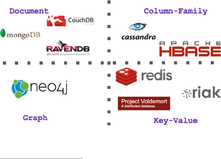
CHAPTER 5 ■ STORAGE: APACHE CASSANDRA
68
In this scenario, those who drove the change had to be innovative in the way that they looked for
alternatives to a relational database management system (RDBMS). Google, Facebook, and Twitter had to
experiment with creating their own data models—each with different architectures—gradually building
what is known today as NoSQL.
The diversity of NoSQL tools is so broad that it is difficult to make a classification. But there was one
audacious guy who did, and he proposed that a NoSQL tool must meet the following characteristics :
• Non-relational
• Open source
• Cluster-friendly
• Twenty-first-century web
• Schemaless
That guy was Martin Fowler and he exposes this in his book with Pramod J. Sadalage, NoSQL Distilled
(Addison-Wesley Professional, 2012).
3
At the GOTO conference in 2013,
4 Fowler presented the “Introduction to NoSQL,” a very educational
presentation well worth checking out.
But how is that NoSQL improves data access performance over traditional RDBMS? It has much to do
with the way NoSQL handles and abstracts data; that is, how it has defined the data model.
Following Martin Fowler’s comments, if you use this criterion, you can classify NoSQL (as shown in
Figure
5-1 ) with distinct types according to this data model: document, column-family, graph, key-value.
Figure 5-1. NoSQL classification according to the data model used
3 http://martinfowler.com/books/nosql.html
4 https://www.youtube.com/watch?v=qI_g07C_Q5I
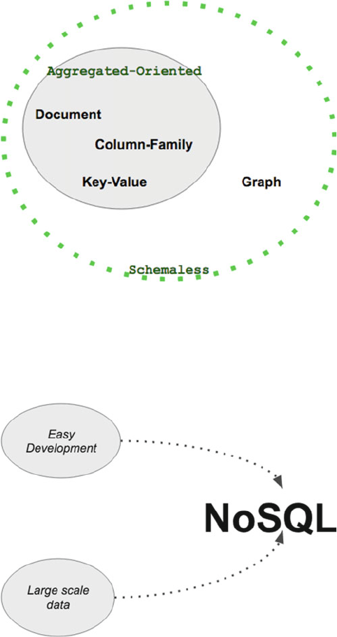
CHAPTER 5 ■ STORAGE: APACHE CASSANDRA
69
Another NoSQL-specific feature is that the data model does not require a data schema, which allows a
greater degree of freedom and faster data access.
As seen in Figure
5-2 , the data models can be grouped as aggregated-oriented and schemaless.
Figure 5-2. Another data model classification
Figure 5-3. A simple way to determine when to use NoSQL
The amount of data to be handled and the need of a mechanism to ease the development are indicators
of when to use NoSQL. Martin Fowler recommends that you use these two major criteria for when to start
using NoSQL, as shown in Figure
5-3 .
Finally, you must remember that there is no silver bullet, and although the rise of SQL is not large, you
must be cautious in choosing when to use it.
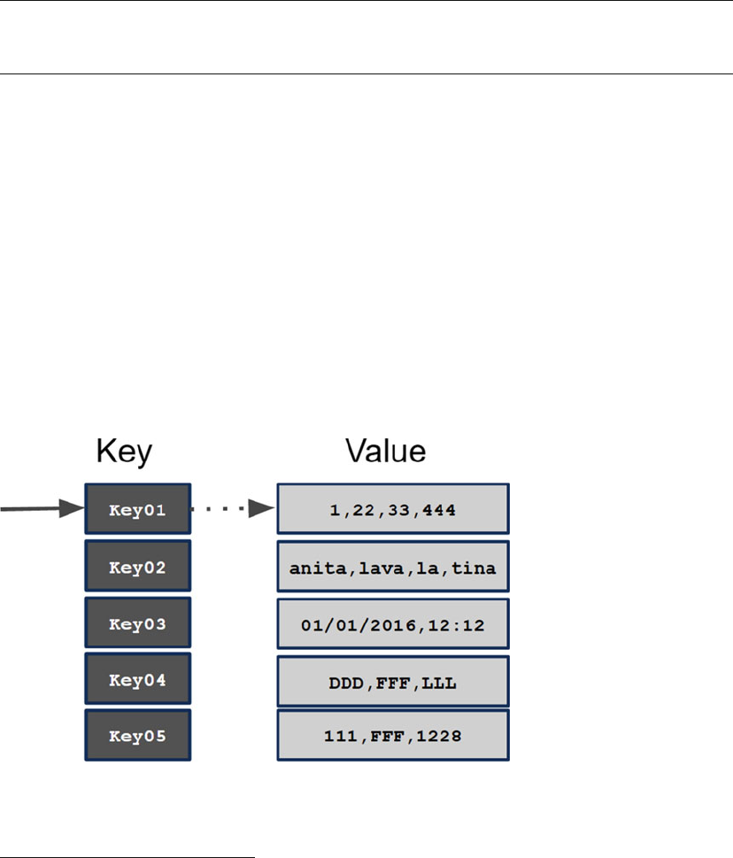
CHAPTER 5 ■ STORAGE: APACHE CASSANDRA
70
The Memory Value
Many of the advantages of NoSQL are based on the fact that a lot of data management is performed in
memory, which gives excellent performance to data access.
■ Note The processing performance of main memory is 800 times faster than HDD, 40 times faster than a
common SSD, and seven times faster than the fastest SSD.
5
Surely, you already know that the memory access is greater than disk access, but with this speed, you
want to do everything in memory. Fortunately, all of these advantages are abstracted by Cassandra and you
just have to worry about what and how to store.
Key-Value and Column
There are two particular data models that to discuss: key-value and column-family. It is common practice
that NoSQL use several data models to increase its performance. Cassandra makes use of key-value and
column-family data models.
Key-Value
The simplest data model is key-value . You have probably already used this paradigm within a programming
language. In a nutshell, it is a hash table.
Given a key, you can access the content (value), as demonstrated in Figure
5-4 .
Figure 5-4. You can imagine this data model as a big hash. The key allows access to certain <content>. This
<content> can be different types of data, which makes it a much more flexible structure.
5 Ki Sun Song, “Introduction to In-Memory Data Grid; Main Features.” http://www.cubrid.org/blog/dev-platform/
introduction-to-in-memory-data-grid-main-features/
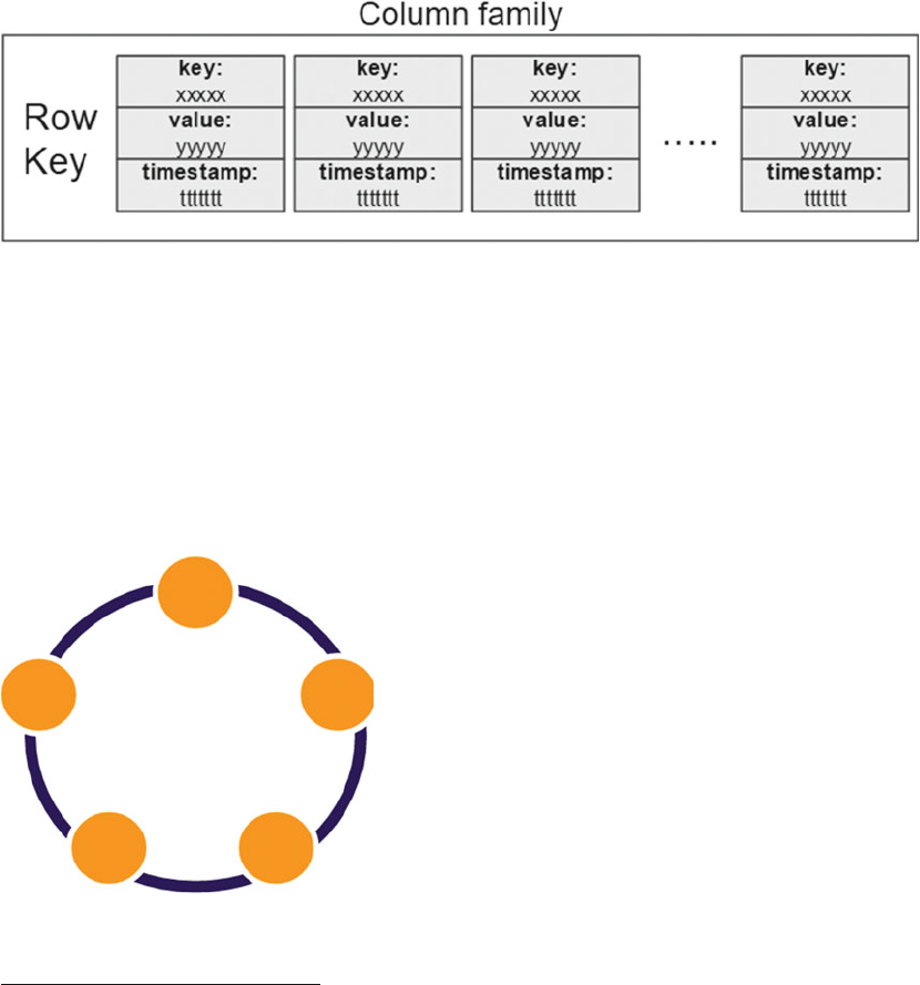
CHAPTER 5 ■ STORAGE: APACHE CASSANDRA
71
Column-Family
An important part of this data model is that the storage and fetch processes are made from columns and not
from rows. Also, a lot of the data model is done in memory, and you already know how important that is.
What’s a column? It is a tuple containing key-value pairs. In the case of several NoSQL, this tuple is
formed by three pairs: name/key, value, and one timestamp.
In this model, several columns (the family) are grouped by a key called a row-key . Figure 5-5 shows this
relationship.
Figure 5-5. A key (row-key) can access the column family. This group exemplifies the data model column-family
Figure 5-6. When all nodes have the same role, having data redundancy is much easier to maintain a
replication, which always help maintain the availability of data.
The main advantage of this model is that it substantially improves write operations, which improves
their performance in distributed environments.
6
Why Cassandra?
Cassandra implements “no single points of failure,” which is achieved with redundant nodes and data.
Unlike legacy systems based on master-slave architectures, Cassandra implements a masterless “ring”
architecture (see Figure
5-6 ).
6 Comparative study of NoSQL document, column store databases, and evaluation of Cassandra. http://airccse.org/
journal/ijdms/papers/6414ijdms02.pdf
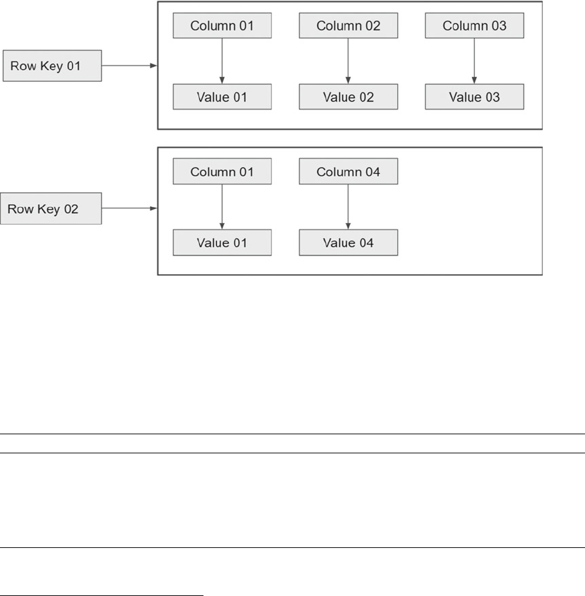
CHAPTER 5 ■ STORAGE: APACHE CASSANDRA
72
With this architecture, all nodes have an identical role: there is no master node. All nodes communicate
with each other using a scalable and distributed protocol called gossip.
7
This architecture, together with the protocol, collectively cannot have a single point of failure. It offers
true continuous availability.
The Data Model
At this point, you can say that the Cassandra data model is based primarily on managing columns. As
mentioned earlier, some NoSQL combine multiple data models, as is the case with Cassandra (see Figure
5-7 ).
Figure 5-7. Cassandra uses a model of combined data; key-value uses this to store and retrieve the columns
Table 5-1. Cassandra Data Model and RDBMS Equivalences
Definition RDBMS Equivalent
Schema/Keyspace A collection of column families. Schema/database
Table/Column-Family A set of rows. Table
Row An ordered set of columns. Row
Column A key/value pair and timestamp. Column (name, value)
Cassandra has some similarity to an RDBMS; these similarities facilitate use and adoption, although
you must remember that they do not work the same way.
Table 5-1 provides some comparisons that help us better understand Cassandra’s concepts.
7 https://docs.datastax.com/en/cassandra/2.1/cassandra/architecture/architectureGossipAbout_c.html
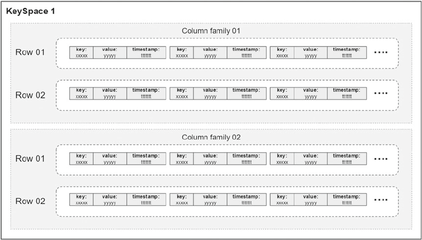
CHAPTER 5 ■ STORAGE: APACHE CASSANDRA
73
Figure 5-8 illustrates the relationships among these concepts.
Figure 5-8. Relationships among column, row, column-family, and keyspace
Cassandra 101
Installation
This section explains how to install Apache Cassandra on a local machine. The following steps were
performed on a Linux machine. At the time of this writing, the stable version is 3.4, released on March 8, 2016.
Prerequisites
Apache Cassandra requires Java version 7 or 8, preferably the Oracle/Sun distribution. The documentation
indicates that it is also compatible with OpenJDK, Zing, and IBM distributions.
File Download
The first step is to download the .zip file distribution downloaded from http://cassandra.apache.org/
download/ .
On the Apache Cassandra project home page (see Figure
5-9 and http://cassandra.apache.org ), the
project logo reminds us of the seeing ability of the mythological character.
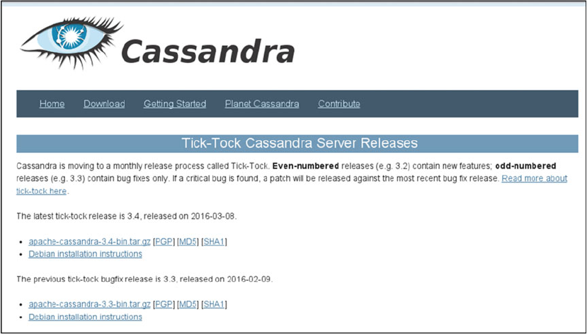
CHAPTER 5 ■ STORAGE: APACHE CASSANDRA
74
Locate the following file:
apache-cassandra-3.4-bin.tar.gz
It’s important to validate file integrity. You do not want it to fail while it’s running. This particular file has
the following values to validate its integrity:
[MD5] e9f490211812b7db782fed09f20c5bb0
[SHA1]7d010b8cc92d5354f384b646b302407ab90be1f0
It’s easy to make this validation. Any flavor of Linux gives the md5 and sha1sum commands, as shown in
the following:
%> md5sum apache-cassandra-3.4-bin.tar.gz
e9f490211812b7db782fed09f20c5bb0 apache-cassandra-3.4-bin.tar.gz
%> sha1sum apache-cassandra-3.4-bin.tar.gz
7d010b8cc92d5354f384b646b302407ab90be1f0 apache-cassandra-3.4-bin.tar.gz
%> ls -lrt apache-cassandra-3.4-bin.tar.gz
-rw-r--r--. 1 rugi rugi 34083682 Mar 7 22:06 apache-cassandra-3.4-bin.tar.gz
Once you have validated the file’s integrity, you can unzip it and continue.
Figure 5-9. Cassandra project home page
CHAPTER 5 ■ STORAGE: APACHE CASSANDRA
75
Start
Starting Apache Cassandra is easy; you only execute the following:
./cassandra -f
INFO 18:06:58 Starting listening for CQL clients on localhost/127.0.0.1:9042 (unencrypted)...
INFO 18:06:58 Not starting RPC server as requested. Use JMX (StorageService->startRPCServer())
or nodetool (enablethrift) to start it
INFO 18:07:07 Scheduling approximate time-check task with a precision of 10 milliseconds
INFO 18:07:07 Created default superuser role 'cassandra'
With this command, your server Apache Cassandra is ready to receive requests. You must always keep
in mind that Apache Cassandra runs with a client-server approach. You have launched the server; the server
is responsible for receiving requests from clients and then giving them answers. So now you need to validate
that clients can send requests.
The next step is to use the CLI validation tool, an Apache Cassandra client.
Validation
Now, let’s execute the CLI tool.
%> ./cqlsh
Connected to Test Cluster at 127.0.0.1:9042.
[cqlsh 5.0.1 | Cassandra 3.4 | CQL spec 3.4.0 | Native protocol v4]
Use HELP for help.
cqlsh>
The first step is to create a keyspace, an analogy with relational databases in which you define the
database, per se.
%>CREATE KEYSPACE mykeyspace WITH REPLICATION = { 'class' : 'SimpleStrategy', 'replication_factor' : 1 };
Once the keyspace is defined, indicate that you will use it.
USE mykeyspace;
This is a familiar sentence, isn’t?
Apache Cassandra, like other NoSQL frameworks, tries to use analogies with the SQL statements that
you already know.
And if you have already defined the database, do you remember what is next? Now you create a test table.
%> CREATE TABLE users ( user_id int PRIMARY KEY, fname text, lname text);
And, having the table, inserting records is simple, as you can see in the following:
%>INSERT INTO users (user_id, fname, lname) VALUES (1745, 'john', 'smith');
%>INSERT INTO users (user_id, fname, lname) VALUES (1744, 'john', 'doe');
%>INSERT INTO users (user_id, fname, lname) VALUES (1746, 'john', 'smith');
CHAPTER 5 ■ STORAGE: APACHE CASSANDRA
76
You make a simple query, like this:
%>SELECT * FROM users;
And, you should have the following results (or similar, if you already modified the data with the inserts):
user_id | fname | lname
---------+-------+-------
1745 | john | smith
1744 | john | doe
1746 | john | smith
With Apache Cassandra, you can create indexes on the fly:
CREATE INDEX ON users (lname);
To facilitate searches on specific fields, do this:
SELECT * FROM users WHERE lname = 'smith';
This is the result:
user_id | fname | lname
---------+-------+-------
1745 | john | smith
1746 | john | smith
And that’s it. This is enough to validate that communication between your CLI and your Cassandra
server is working properly.
Here is the complete output from the previous commands:
{16-03-21 14:05}localhost:~/ opt/apache/cassandra/apache-cassandra-3.4/bin rugi% cd /home/
rugi/opt/apache/cassandra/apache-cassandra-3.4/bin
{16-03-21 14:05}localhost:~/opt/apache/cassandra/apache-cassandra-3.4/bin rugi% ./cqlsh
Connected to Test Cluster at 127.0.0.1:9042.
[cqlsh 5.0.1 | Cassandra 3.4 | CQL spec 3.4.0 | Native protocol v4]
Use HELP for help.
cqlsh> CREATE KEYSPACE mykeyspace WITH REPLICATION = { 'class' : 'SimpleStrategy',
'replication_factor' : 1 };
cqlsh> USE mykeyspace;
cqlsh:mykeyspace> CREATE TABLE users ( user_id int PRIMARY KEY, fname text, lname text);
cqlsh:mykeyspace> INSERT INTO users (user_id, fname, lname) VALUES (1745, 'john', 'smith');
cqlsh:mykeyspace> INSERT INTO users (user_id, fname, lname) VALUES (1744, 'john', 'doe');
cqlsh:mykeyspace> INSERT INTO users (user_id, fname, lname) VALUES (1746, 'john', 'smith');
cqlsh:mykeyspace> SELECT * FROM users;
user_id | fname | lname
---------+-------+-------
1745 | john | smith
1744 | john | doe
1746 | john | smith
(3 rows)
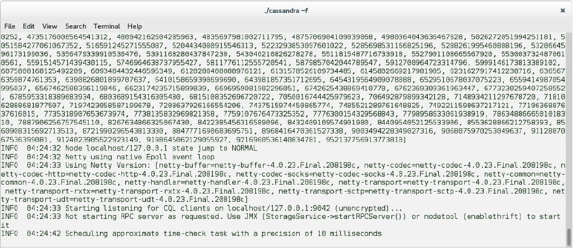
CHAPTER 5 ■ STORAGE: APACHE CASSANDRA
77
cqlsh:mykeyspace> CREATE INDEX ON users (lname);
cqlsh:mykeyspace> SELECT * FROM users WHERE lname = 'smith';
user_id | fname | lname
---------+-------+-------
1745 | john | smith
1746 | john | smith
(2 rows)
cqlsh:mykeyspace> exit
{16-03-21 15:24}localhost:~/opt/apache/cassandra/apache-cassandra-3.4/bin rugi%
You should have two terminals open: one with the server running and the other one with CLI
running. If you check the first one, you will see how CLI is processing the requests. Figure
5-10 shows the
server running.
Figure 5-10. Cassandra server running
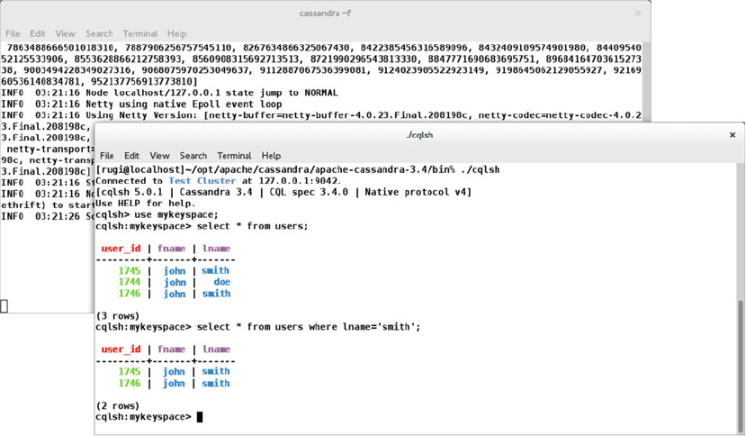
CHAPTER 5 ■ STORAGE: APACHE CASSANDRA
78
CQL
CQL (Cassandra Query Language) is a language similar to SQL. The queries on a keyspace are
made in CQL.
CQL Shell
There are several ways to interact with a keyspace ; in the previous section, you saw how to do it using a shell
called CQL shell (CQLs) . Later you will see other ways to interact with the keyspace.
CQL shell is the primary way to interact with Cassandra; Table
5-2 lists the main commands.
Figure 5-11. CQL running on CQLs
Figure 5-11 is a screenshot of running the test commands described earlier.

CHAPTER 5 ■ STORAGE: APACHE CASSANDRA
79
Table 5-2. Shell Command Summary
Command Description
cqlsh Starts the CQL interactive terminal.
CAPTURE Captures the command output and appends it to a file.
CONSISTENCY Shows the current consistency level; or given a level, sets it.
COPY Imports and exports CSV (comma-separated values) data to and from Cassandra.
DESCRIBE Provides information about the connected Cassandra cluster or about the data
objects stored in the cluster.
EXPAND Formats the output of a query vertically.
EXIT Terminates cqlsh.
PAGING Enables or disables query paging.
SHOW Shows the Cassandra version, host, or tracing information for the current cqlsh
client session.
SOURCE Executes a file containing CQL statements.
TRACING Enables or disables request tracing.
For more detailed information on shell commands, you should visit the following web page:
http://docs.datastax.com/en/cql/3.1/cql/cql_reference/cqlshCommandsTOC.html
Let’s try some of these commands. First, activate the shell, as follows;
{16-04-15 23:54}localhost:~/opt/apache/cassandra/apache-cassandra-3.4/bin rugi% ./cqlsh
Connected to Test Cluster at 127.0.0.1:9042.
[cqlsh 5.0.1 | Cassandra 3.4 | CQL spec 3.4.0 | Native protocol v4]
Use HELP for help.
The describe command can work in specific tables, in all the keyspaces, or in one specific keyspace:
cqlsh> describe keyspaces
system_schema system system_distributed
system_auth mykeyspace system_traces
cqlsh> describe mykeyspace
CREATE KEYSPACE mykeyspace WITH replication = {'class': 'SimpleStrategy', 'replication_
factor': '1'} AND durable_writes = true;
CREATE TABLE mykeyspace.users (
user_id int PRIMARY KEY,
fname text,
lname text
CHAPTER 5 ■ STORAGE: APACHE CASSANDRA
80
) WITH bloom_filter_fp_chance = 0.01
AND caching = {'keys': 'ALL', 'rows_per_partition': 'NONE'}
AND comment = ''
AND compaction = {'class': 'org.apache.cassandra.db.compaction.SizeTieredCompactionStrategy',
'max_threshold': '32', 'min_threshold': '4'}
AND compression = {'chunk_length_in_kb': '64',
'class': 'org.apache.cassandra.io.compress. LZ4Compressor'}
AND crc_check_chance = 1.0
AND dclocal_read_repair_chance = 0.1
AND default_time_to_live = 0
AND gc_grace_seconds = 864000
AND max_index_interval = 2048
AND memtable_flush_period_in_ms = 0
AND min_index_interval = 128
AND read_repair_chance = 0.0
AND speculative_retry = '99PERCENTILE';
CREATE INDEX users_lname_idx ON mykeyspace.users (lname);
T h e show command is also simple to test to see the version number:
cqlsh> show version
[cqlsh 5.0.1 | Cassandra 3.4 | CQL spec 3.4.0 | Native protocol v4]
cqlsh>
As you can see, these commands are very easy to use.
CQL Commands
CQL is very similar to SQL, as you have already seen in the first part of this chapter. You have created a
keyspace, made inserts, and created a filter.
CQL, like SQL, is based on sentences/statements. These sentences are for data manipulation and work
with their logical container, the keyspace. As in SQL statements, they must end with a semicolon (;).
Table 5-3 lists all the language commands.

CHAPTER 5 ■ STORAGE: APACHE CASSANDRA
81
Table 5-3. CQL Command Summary
Command Description
ALTER KEYSPACE Changes the property values of a keyspace.
ALTER TABLE Modifies the column metadata of a table.
ALTER TYPE Modifies a user-defined type. Cassandra 2.1 and later.
ALTER USER Alters existing user options.
BATCH Writes multiple DML statements.
CREATE INDEX Defines a new index on a single column of a table.
CREATE KEYSPACE Defines a new keyspace and its replica placement strategy.
CREATE TABLE Defines a new table.
CREATE TRIGGER Registers a trigger on a table.
CREATE TYPE Creates a user-defined type. Cassandra 2.1 and later.
CREATE USER Creates a new user.
DELETE Removes entire rows or one or more columns from one or more rows.
DESCRIBE Provides information about the connected Cassandra cluster or about the data
objects stored in the cluster.
DROP INDEX Drops the named index.
DROP KEYSPACE Removes the keyspace.
DROP TABLE Removes the named table.
DROP TRIGGER Removes registration of a trigger.
DROP TYPE Drops a user-defined type. Cassandra 2.1 and later.
DROP USER Removes a user.
GRANT Provides access to database objects.
INSERT Adds or updates columns.
LIST PERMISSIONS Lists permissions granted to a user.
LIST USERS Lists existing users and their superuser status.
REVOKE Revokes user permissions.
SELECT Retrieves data from a Cassandra table.
TRUNCATE Removes all data from a table.
UPDATE Updates columns in a row.
USE Connects the client session to a keyspace.
For more detailed information of CQL commands, you can visit the following web page:
http://docs.datastax.com/en/cql/3.1/cql/cql_reference/cqlCommandsTOC.html
Let’s play with some of these commands.
{16-04-16 6:19}localhost:~/opt/apache/cassandra/apache-cassandra-3.4/bin rugi% ./cqlsh
Connected to Test Cluster at 127.0.0.1:9042.
CHAPTER 5 ■ STORAGE: APACHE CASSANDRA
82
[cqlsh 5.0.1 | Cassandra 3.4 | CQL spec 3.4.0 | Native protocol v4]
Use HELP for help.
Use the keyspace created at beginning, as follows:
cqlsh> use mykeyspace;
The DESCRIBE command can be applied to almost any object to discover the keyspace tables.
cqlsh:mykeyspace> describe tables users
Or in a specific table.
cqlsh:mykeyspace> describe users
CREATE TABLE mykeyspace.users (
user_id int PRIMARY KEY,
fname text,
lname text
) WITH bloom_filter_fp_chance = 0.01
AND caching = {'keys': 'ALL', 'rows_per_partition': 'NONE'}
AND comment = ''
AND compaction = {'class': 'org.apache.cassandra.db.compaction.SizeTieredCompactionStrategy',
'max_threshold': '32', 'min_threshold': '4'}
AND compression = { 'chunk_length_in_kb': '64',
'class': 'org.apache.cassandra.io.compress.LZ4Compressor'}
AND crc_check_chance = 1.0
AND dclocal_read_repair_chance = 0.1
AND default_time_to_live = 0
AND gc_grace_seconds = 864000
AND max_index_interval = 2048
AND memtable_flush_period_in_ms = 0
AND min_index_interval = 128
AND read_repair_chance = 0.0
AND speculative_retry = '99PERCENTILE';
CREATE INDEX users_lname_idx ON mykeyspace.users (lname);
cqlsh:mykeyspace> exit
Beyond the Basics
You already know that Apache Cassandra runs on a client-server architecture . The client-server architecture
is used by nearly everyone every day; it is the base of what you know as the Internet.
Client-Server
By definition, the client-server architecture allows distributed applications, since the tasks are divided into
two main parts:
• The service providers: the servers
• The service petitioners : the clients
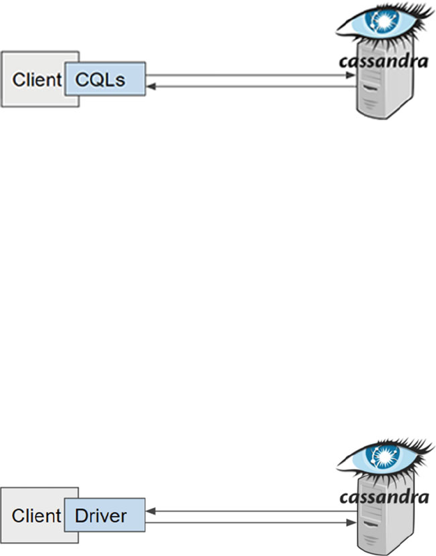
CHAPTER 5 ■ STORAGE: APACHE CASSANDRA
83
In this architecture, several clients are allowed to access the server. The server is responsible for
meeting requests and it handles each one according its own rules. So far, you have only used one client,
managed from the same machine—that is, from the same data network.
Figure 5-12 shows our current client-server architecture in Cassandra.
Figure 5-12. The native way to connect to a Cassandra server is via CQLs.
Figure 5-13. To access a Cassandra server, a driver is required
CQL shell allows you to connect to Cassandra, access a keyspace, and send CQL statements to the
Cassandra server. This is the most immediate method, but in daily practice, it is common to access the
keyspaces from different execution contexts (other systems and other programming languages).
Other Clients
You require other clients, different from CQLs, to do it in the Apache Cassandra context. You require
connection drivers .
Drivers
A driver is a software component that allows access to a keyspace to run CQL statements.
Figure 5-13 illustrates accessing clients through the use of a driver. A driver can access a keyspace and
also allows the execution of CQL sentences.
Fortunately, there are a lot of these drivers for Cassandra in almost any modern programming language.
You can see an extensive list at
http://wiki.apache.org/cassandra/ClientOptions .
Currently, there are different drivers to access a keyspace in almost all modern programming
languages. Typically, in a client-server architecture, there are clients accessing the server from different
clients, which are distributed in different networks, therefore, Figure
5-13 may now look like what’s shown
in Figure
5-14 .
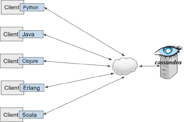
CHAPTER 5 ■ STORAGE: APACHE CASSANDRA
84
The Figure 5-14 illustrates that given the distributed characteristics that modern systems require, the
clients actually are in different points and access the Cassandra server through public and private networks.
Your implementation needs will dictate the required clients.
All languages offer a similar API through the driver. Consider the following code snippets in Java, Ruby,
and Node.
J a v a
The following snippet was tested with JDK 1.8.x.
Get Dependence
With java, it is easiest is to use Maven. You can get the driver using the following Maven artifact:
<dependency>
<groupId>com.datastax.cassandra</groupId>
<artifactId>cassandra-driver-core</artifactId>
<version>3.0.2</version>
</dependency>
Figure 5-14. Different clients connecting to a Cassandra server through the cloud
CHAPTER 5 ■ STORAGE: APACHE CASSANDRA
85
Snippet
The following is the Java snippet:
import com.datastax.driver.core.Cluster;
import com.datastax.driver.core.ResultSet;
import com.datastax.driver.core.Row;
import com.datastax.driver.core.Session;
import java.util.Iterator;
...
public static void main(String[] args) {
Cluster cluster = Cluster.builder().addContactPoint("127.0.0.1").build();
Session session = cluster.connect("mykeyspace");
ResultSet results = session.execute("SELECT * FROM users");
StringBuilder line = new StringBuilder();
for (Iterator<Row> iterator = results.iterator(); iterator.hasNext();) {
Row row = iterator.next();
line.delete(0, line.length());
line.append("FirstName = ").
append(row.getString("fname")).
append(",").append(" ").
append("LastName = ").
append(row.getString("lname"));
System.out.println(line.toString());
}
}
R u b y
The snippet was tested with Ruby 2.0.x.
Get Dependence
In Ruby, obtaining the driver is as simple as installing a gem.
%>gem install cassandra-driver
Snippet
The following is the Ruby snippet:
require 'cassandra'
node = '127.0.0.1'
cluster = Cassandra.cluster(hosts: node)
keyspace = 'mykeyspace'
session = cluster.connect(keyspace)
session.execute("SELECT fname, lname FROM users").each do |row|
p "FirstName = #{row['fname']}, LastName = #{row['lname']}"
end
CHAPTER 5 ■ STORAGE: APACHE CASSANDRA
86
N o d e
The snippet was tested with Node v5.0.0.
Get Dependence
With Node, it could not be otherwise; the driver is obtained with npm.
%>npm install cassandra-driver
%>npm install async
Snippet
The following is the Node snippet:
var cassandra = require('cassandra-driver');
var async = require('async');
var client = new cassandra.Client({contactPoints: ['127.0.0.1'], keyspace: 'mykeyspace'});
client.stream('SELECT fname, lname FROM users', [])
.on('readable', function () {
var row;
while (row = this.read()) {
console.log('FirstName = %s , LastName= %s', row.fname,
row.lname);
}
})
.on('end', function () {
//todo
})
.on('error', function (err) {
// todo
});
</code>
These three snippets did the same thing: made a connection to the Cassandra server, got a reference
to the keyspace, made a single query, and displayed the results. In conclusion, the three snippets generated
the same result:
"FirstName = john, LastName = smith"
"FirstName = john, LastName = doe"
"FirstName = john, LastName = smith"
You can see more examples that use other languages on the following web page:
http://www.planetcassandra.org/apache-cassandra-client-drivers/
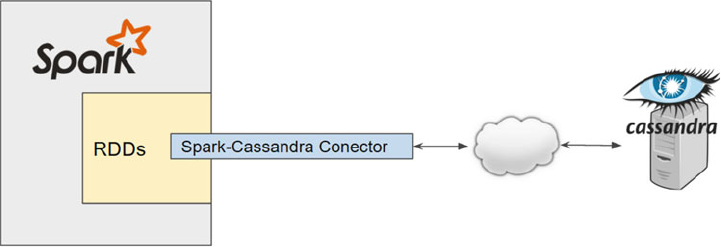
CHAPTER 5 ■ STORAGE: APACHE CASSANDRA
87
Figure 5-15. The Spark-Cassandra Connector is a special type of client that allows access to keyspaces from a
S p a r k c o n t e x t
Apache Spark-Cassandra Connector
Now that you have a clear understanding on how connecting to a Cassandra server is done, let’s talk about
a very special client. Everything that you have seen previously has been done to get to this point. You can
now see what Spark can do since you know Cassandra and you know that you can use it as a storage layer to
improve the Spark performance.
What do you need to achieve this connection? A client. This client is special because it is designed
specifically for Spark, not for a specific language. This special client is called the Spark-Cassandra Connector
(see Figure
5-15 ).
Installing the Connector
The Spark-Cassandra connector has its own GitHub repository. The latest stable version is the master, but
you can access a special version through a particular branch .
Figure 5-16 shows the Spark-Cassandra Connector project home page, which is located at
https://github.com/datastax/spark-cassandra-connector .
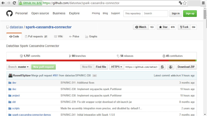
CHAPTER 5 ■ STORAGE: APACHE CASSANDRA
88
At the time of this writing, the most stable connector version is 1.6.0. The connector is basically a . jar
file loaded when Spark starts. If you prefer to directly access the .jar file and avoid the build process,
you can do it by downloading the official maven repository. A widely used repository is located at
http://mvnrepository.com/artifact/com.datastax.spark/spark-cassandra-connector_ .10/1.6.0-M2 .
Generating the .jar file directly from the Git repository has one main advantage: all the necessary
dependencies of the connector are generated. If you choose to download the jar from the official repository,
you must also download all of these dependencies.
Fortunately, there is a third way to run the connector, which is by telling the spark-shell that you require
certain packages for the session to start. This is done by adding the following flag:
./spark-shell --packages datastax:spark-cassandra-connector:1.6.0-M2-s_2.10
The nomenclature of the package is the same used with Gradle, Buildr, or SBT:
GroupID: datastax
ArtifactID: spark-cassandra-connector
Version: 1.6.0-M2-s_2.10
In the preceding lines of code, you are telling the shell that you require that artifact, and the shell will
handle all the units. Now let’s see how it works.
Figure 5-16. The Spark-Cassandra Connector on GitHub
CHAPTER 5 ■ STORAGE: APACHE CASSANDRA
89
Establishing the Connection
The connector version used in this section is 1.6.0 because it is the latest stable version of Apache Spark as of
this writing.
First, validate that the versions are compatible. Access the Spark shell to see if you have the correct
version.
{16-04-18 1:10}localhost:~/opt/apache/spark/spark-1.6.0-bin-hadoop2.6/bin rugi% ./spark-shell
log4j:WARN No appenders could be found for logger (org.apache.hadoop.metrics2.lib.
MutableMetricsFactory).
log4j:WARN Please initialize the log4j system properly.
log4j:WARN See http://logging.apache.org/log4j/1.2/faq.html#noconfig for more info.
Using Spark’s repl log4j profile: org/apache/spark/log4j-defaults-repl.properties
To adjust logging level use sc.setLogLevel(“INFO”)
Welcome to
____ __
/ __/__ ___ _____/ /__
_\ \/ _ \/ _ `/ __/ ‘_/
/___/ .__/\_,_/_/ /_/\_\ version 1.6.0
/_/
Using Scala version 2.10.5 (Java HotSpot(TM) 64-Bit Server VM, Java 1.8.0_60)
Type in expressions to have them evaluated.
Type :help for more information.
....
scala>
Next, try a simple task:
scala> sc.parallelize( 1 to 50 ).sum()
res0: Double = 1275.0
scala>
Stop the shell ( exit command). Now at start time, indicate the package that you require (the
connector). The first time, the shell makes downloading dependencies:
{16-06-08 23:18}localhost:~/opt/apache/spark/spark-1.6.0-bin-hadoop2.6/bin rugi% >./spark-
shell --packages datastax:spark-cassandra-connector:1.6.0-M2-s_2.10
Ivy Default Cache set to: /home/rugi/.ivy2/cache
The jars for the packages stored in: /home/rugi/.ivy2/jars
:: loading settings :: url = jar:file:/home/rugi/opt/apache/spark/spark-1.6.0-bin-hadoop2.6/
lib/spark-assembly-1.6.0-hadoop2.6.0.jar!/org/apache/ivy/core/settings/ivysettings.xml
datastax#spark-cassandra-connector added as a dependency
:: resolving dependencies :: org.apache.spark#spark-submit-parent;1.0
confs: [default]
found datastax#spark-cassandra-connector;1.6.0-M2-s_2.10 in spark-packages
found joda-time#joda-time;2.3 in local-m2-cache
found com.twitter#jsr166e;1.1.0 in central
found org.scala-lang#scala-reflect;2.10.5 in central
CHAPTER 5 ■ STORAGE: APACHE CASSANDRA
90
---------------------------------------------------------------------
| | modules || artifacts |
| conf | number| search|dwnlded|evicted|| number|dwnlded|
---------------------------------------------------------------------
| default | 16 | 2 | 2 | 0 || 16 | 2 |
---------------------------------------------------------------------
:: retrieving :: org.apache.spark#spark-submit-parent
confs: [default]
2 artifacts copied, 14 already retrieved (5621kB/32ms)
log4j:WARN No appenders could be found for logger (org.apache.hadoop.metrics2.lib.
MutableMetricsFactory).
log4j:WARN Please initialize the log4j system properly.
log4j:WARN See http://logging.apache.org/log4j/1.2/faq.html#noconfig for more info.
Using Spark’s repl log4j profile: org/apache/spark/log4j-defaults-repl.properties
To adjust logging level use sc.setLogLevel(“INFO”)
Welcome to
____ __
/ __/__ ___ _____/ /__
_\ \/ _ \/ _ `/ __/ ‘_/
/___/ .__/\_,_/_/ /_/\_\ version 1.6.0
/_/
Using Scala version 2.10.5 (Java HotSpot(TM) 64-Bit Server VM, Java 1.8.0_60)
Type in expressions to have them evaluated.
Type :help for more information.
16/06/08 23:18:59 WARN Utils: Your hostname, localhost.localdomain resolves to a loopback
address: 127.0.0.1; using 192.168.1.6 instead (on interface wlp7s0)
16/06/08 23:18:59 WARN Utils: Set SPARK_LOCAL_IP if you need to bind to another address
Spark context available as sc.
16/06/08 23:19:07 WARN ObjectStore: Version information not found in metastore. hive.
metastore.schema.verification is not enabled so recording the schema version 1.2.0
16/06/08 23:19:07 WARN ObjectStore: Failed to get database default, returning
NoSuchObjectException
SQL context available as sqlContext.
scala>
The connector is loaded and ready for use.
First, stop the Scala executor from the shell:
sc.stop
Next, import the required classes for communication:
import com.datastax.spark.connector._, org.apache.spark.SparkContext, org.apache.spark.
SparkContext._, org.apache.spark.SparkConf
Then, set a variable with the required configuration to connect:
val conf = new SparkConf(true).set(“spark.cassandra.connection.host”, “localhost”)
CHAPTER 5 ■ STORAGE: APACHE CASSANDRA
91
Finally, connect to the well-known keyspace and table that were created at the beginning of this chapter:
val sc = new SparkContext(conf)
val test_spark_rdd = sc.cassandraTable("mykeyspace", "users")
Given the context and keyspace, it is possible to consult the values with the following statement:
test_spark_rdd.foreach(println)
Here is the complete sequence of the five lines of code:
scala> sc.stop
scala> import com.datastax.spark.connector._, org.apache.spark.SparkContext, org.apache.
spark.SparkContext._, org.apache.spark.SparkConf
import com.datastax.spark.connector._
import org.apache.spark.SparkContext
import org.apache.spark.SparkContext._
import org.apache.spark.SparkConf
scala> val conf = new SparkConf(true).set("spark.cassandra.connection.host", "localhost")
conf: org.apache.spark.SparkConf = org.apache.spark.SparkConf@68b5a37d
scala> val sc = new SparkContext(conf)
sc: org.apache.spark.SparkContext = org.apache.spark.SparkContext@3d872a12
scala> val test_spark_rdd = sc.cassandraTable("mykeyspace", "users")
The connection is established and is already accessible through test_spark_rdd to make operations in
our table within our keyspace; for example, to show values.
scala> test_spark_rdd.foreach(println)
CassandraRow{user_id: 1745, fname: john, lname: smith}
CassandraRow{user_id: 1744, fname: john, lname: doe}
CassandraRow{user_id: 1746, fname: john, lname: smith}
More Than One Is Better
Up to this moment, unknowingly, you have been working with a cluster of Cassandra. A cluster with a single
node, but a cluster. Let’s check it. ;)
To check, use the nodetool utility, which is administered as a cluster of the Cassandra nodetool via CLI.
You can run the following to see the full list of commands:
CASSANDRA_HOME/bin>./nodetool
Among the list, you see the status command.
status Print cluster information (state, load, IDs, ...)

CHAPTER 5 ■ STORAGE: APACHE CASSANDRA
92
8 http://docs.datastax.com/en/cassandra/3.0/cassandra/configuration/configCassandra_yaml.html
You can run nodetool with the status command.
CASSANDRA_HOME/bin>./nodetool status
Datacenter: datacenter1
=======================
Status=Up/Down
|/ State=Normal/Leaving/Joining/Moving
-- Address Load Tokens Owns (effective) Host
ID Rack
UN 127.0.0.1 122.62 KiB 256 100.0% 3e7ccbd4-8ffb-4b77-bd06-110d27536cb2 rack1
You can see that you run a cluster with a single node.
cassandra.yaml
When you have a cluster of more than one node, you modify the cassandra.yaml file. In this file, the
necessary settings of each node within a cluster are made. When you have only one node, there’s nothing to
change. The file is located in the CASSANDRA HOME/conf folder.
The file has several options; you can see each option in detail in the documentation.
8 For a basic
configuration, however, there are few options that are required.
Table 5-4 describes the fields to create our cluster. The descriptions were taken from the afore
mentioned documentation.
Table 5-4. Minimum Configuration Options for Each Node in the Cluster
Option Description
cluster_name The name of the cluster.
seed_provider The addresses of the hosts deemed as contact points. Cassandra
nodes use the -seeds list to find each provider and learn the
topology of the ring.
seed_provider - class_name The class within Cassandra that handles the seed logic. It can be
customized, but this is typically not required.
seed_provider- parameters - seeds A comma-delimited list of IP addresses used by gossip for
bootstrapping new nodes joining a cluster.
listen_address The IP address or hostname that Cassandra binds to in order to
connect to other Cassandra nodes.
rpc_address The listen address for client connections (Thrift RPC service and
native transport).
broadcast_rpc_address The RPC address to broadcast to drivers and other Cassandra nodes.
endpoint_snitch Set to a class that implements the IEndpointSnitch interface.

CHAPTER 5 ■ STORAGE: APACHE CASSANDRA
93
9 http://docs.datastax.com/en/cassandra/3.0/cassandra/configuration/secureFireWall.html
Setting the Cluster
In this example , assume that Cassandra is installed on the following machines:
107.170.38.238 (seed)
107.170.112.81
107.170.115.161
The documentation recommends having more than one seed, but because you have only three nodes in
this exercise, leave only a single seed. All machines have Ubuntu 14.04 and JDK 1.8 (HotSpot) ready.
The following steps assume that you are starting a clean installation in each machine, so, if a machine is
running Cassandra, you must stop and delete all data. We recommend that you start with clean installations.
If there is a firewall between the machines, it is important to open specific ports.
9
Machine01
Our first machine has the address 107.170.38.238 and it is the seed. It starts first when you finish setting up
the three machines.
Locate the CASSANDRA HOME/conf/cassandra.yaml file and make the following modifications. All nodes
in the cluster must have the same cluster_name .
cluster_name: 'BedxheCluster'
num_tokens: 256
seed_provider:
- class_name: org.apache.cassandra.locator.SimpleSeedProvider
parameters:
- seeds: “107.170.38.238”
listen_address: 107.170.38.238
rpc_address: 0.0.0.0
broadcast_rpc_address: 1.2.3.4
endpoint_snitch: RackInferringSnitch
Machine02
Our second machine has the address 107.170.112.81. Its setting only changes the value of listen_address .
cluster_name: 'BedxheCluster'
num_tokens: 256
seed_provider:
- class_name: org.apache.cassandra.locator.SimpleSeedProvider
parameters:
- seeds: "107.170.38.238"
listen_address: 107.170.112.81
rpc_address: 0.0.0.0
broadcast_rpc_address: 1.2.3.4
endpoint_snitch: RackInferringSnitch

CHAPTER 5 ■ STORAGE: APACHE CASSANDRA
94
Machine03
Our third machine has the address 107.170.115.161. Its setting also only changes the value of listen_address .
cluster_name: 'BedxheCluster'
num_tokens: 256
seed_provider:
- class_name: org.apache.cassandra.locator.SimpleSeedProvider
parameters:
- seeds: "107.170.38.238"
listen_address: 107.170.115.161
rpc_address: 0.0.0.0
broadcast_rpc_address: 1.2.3.4
endpoint_snitch: RackInferringSnitch
You have now finished the configuration of the nodes.
■ Note This configuration was simple. It was used for illustrative purposes. Configuring a cluster to a
production environment requires studyng several factors and experimenting a lot. Therefore, we recommend
using this setting because it is a simple exercise to begin learning the options.
Booting the Cluster
You first started Cassandra in the seed node (removing the -f flag, Cassandra starts the process and passes
the background).
MACHINE01/CASSANDRA_HOME/bin%>./cassandra
After you started cassandra in the other two nodes.
MACHINE02/CASSANDRA_HOME/bin%>./cassandra
MACHINE03/CASSANDRA_HOME/bin%>./cassandra
Now, if you execute nodetool in any of the machines, you see something like the following.
CASSANDRA_HOME/bin>./nodetool status
Datacenter: 170
===============
Status=Up/Down
|/ State=Normal/Leaving/Joining/Moving
-- Address Load Tokens Owns Host ID Rack
(effective)
UN 107.170.38.238 107.95 KiB 256 68.4% 23e16126-8c7f-4eb8-9ea0-40ae488127e8 38
UN 107.170.115.161 15.3 KiB 256 63.7% b3a9970a-ff77-43b2-ad4e-594deb04e7f7 115
UN 107.170.112.81 102.49 KiB 256 67.9% ece8b83f-d51d-43ce-b9f2-89b79a0a2097 112
Now, if you repeat the creation of the keyspace example in the seed node, you will see how the keyspace
is available in the other nodes. And conversely, if you apply a change to the keyspace in any node, it is
immediately reflected in the others.

CHAPTER 5 ■ STORAGE: APACHE CASSANDRA
95
10 How SoundCloud Uses Cassandra. https://www.infoq.com/presentations/soundcloud-cassandra
11 Spotify: How to Use Apache Cassandra. https://www.youtube.com/watch?v=JWaECFyhvxI
12 Netflix: A State of Xen Chaos Monkey & Cassandra. https://www.youtube.com/watch?v=Mu01DmxQjWA
Execute the following in machine01 (the seed machine):
MACHINE01_CASSANDRA_HOME/bin%> ./cqlsh
cqlsh>CREATE KEYSPACE mykeyspace WITH REPLICATION = { ‘class’ : ‘SimpleStrategy’,
‘replication_factor’ : 1 };
cqlsh>USE mykeyspace;
cqlsh>CREATE TABLE users (user_id int PRIMARY KEY, fname text, lname text);
cqlsh>INSERT INTO users (user_id, fname, lname) VALUES (1745, ‘john’, ‘smith’);
cqlsh>INSERT INTO users (user_id, fname, lname) VALUES (1744, ‘john’, ‘doe’);
cqlsh>INSERT INTO users (user_id, fname, lname) VALUES (1746, ‘john’, ‘smith’);
Execute the following in machine02 or machine03:
CASSANDRA_HOME/bin%>./cqlsh
cqlsh> use mykeyspace;
cqlsh:mykeyspace> select * from users;
user_id | fname | lname
---------+-------+-------
1745 | john | smith
1744 | john | doe
1746 | john | smith
(3 rows)
That’s it. You have a cluster of three nodes working properly.
Putting It All Together
The best way to assimilate all of these concepts is through examples, so in later chapters, we show concrete
examples of the use of this architecture.
As you can see, beginning to use Cassandra is very simple; the similarity to SQL in making queries helps
to manipulate data from the start. Perhaps now that you know the advantages of Cassandra, you want to
know who is using it. There are three companies in particular that have helped increase the popularity of
Cassandra: SoundCloud,
10 Spotify, 11 and Netflix.
12
A lot of the stuff that exists online about Cassandra makes references to these companies, but they are
not the only ones. The following two web pages offer more extensive lists of companies that are committed
to Cassandra, and using some part of their data management in interesting use cases.
• http://www.planetcassandra.org/companies/
• http://www.planetcassandra.org/apache-cassandra-use-cases/
Beyond the advantages Cassandra, as the ring model and distributed data management within
the cluster, its main advantage is the level of integration with Spark, and in general, with the rest of the
technologies in this book.
Surely, you’ll use Cassandra in an upcoming project.

97
© Raul Estrada and Isaac Ruiz 2016
R. Estrada and I. Ruiz, Big Data SMACK, DOI 10.1007/978-1-4842-2175-4_6
CHAPTER 6
The Engine: Apache Spark
If our stack were a vehicle, now we have reached the engine. As an engine, we will disarm it, analyze it,
master it, improve it, and run it to the limit.
In this chapter, we walk hand in hand with you. First, we look at the Spark download and installation,
and then we test it in Standalone mode. Next, we discuss the theory around Apache Spark to understand
the fundamental concepts. Then, we go over selected topics, such as running in high availability (cluster).
Finally, we discuss Spark Streaming as the entrance to the data science pipeline.
This chapter is written for people who have never touched Apache Spark before. But as you can
imagine, due to space, we will not delve into many specific issues.
The following topics are covered in this chapter:
• Introducing Spark
• Spark concepts
• Working with RDD
• Running in cluster
• Spark Streaming
Introducing Spark
Perhaps Apache Spark is the most important technology in the stack. It is divided into five modules: Core ,
SQL , MLIB , Streaming , and GraphX . Simply put, each module deserves a book the same size of the book that
you are now reading. Spark has captured the imagination of developers and analysts, simply because it takes
data manipulation from large laboratories to laptops, from large interdisciplinary teams to lone enthusiasts
who want to make data analysis, and from large corporate clusters to a cheap infrastructure accessible to all.
Spark is both infrastructure software and data science laboratory. Spark as an infrastructure engine can
be attached to powerful tools like Apache Kafka to produce data science pipelines . Simultaneously, it is a data
science laboratory because it represents an engine for machine learning in both a laptop and a productive
cluster, from a few data kilobytes up to what the hardware capacity allows. Likewise, you can build models
based on sample data and then apply them in larger datasets.
In times not so distant, installing the infrastructure for data analysis was an interdisciplinary task among
database specialists, operating system and network analysts, and application engineers and architects.
What makes Apache Spark so attractive is its ability to download and run it on a small and inexpensive
laptop.
Apache Spark (like all the technologies covered in this book) is an open source tool. It only requires Java
version 6 or higher. All the Scala and Akka dependencies are packaged within the distribution.
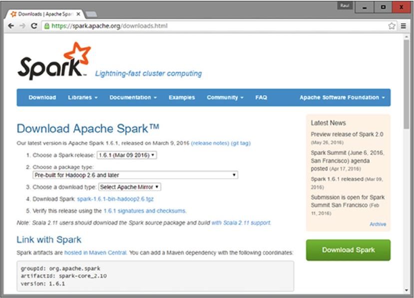
CHAPTER 6 ■ THE ENGINE: APACHE SPARK
98
Apache Spark Download
Regardless of whether you use the development or production version, you must download the latest build
from
https://spark.apache.org/downloads.html (version 1.6.1 as of this writing).
As shown in Figure
6-1 , select Pre-built for Hadoop and later .
Figure 6-1. Apache Spark download page
Spark has a new release every 90 days. For hard-core coders who like to work with the latest builds, try
to clone the repository at
https://github.com/apache/spark . The instructions for generating the build are
available at
https://spark.apache.org/docs/latest/building-spark.html . Both the source code and the
binary prebuilds are available at this link.
To compile the Spark sources, we need the appropriate versions of Scala and the corresponding SDK.
Spark source tar includes the Scala components required.
The Spark development group has done a good job keeping the dependencies. On
https://spark.
apache.org/docs/latest/building-spark.html , you can see the latest information about it. According to
the site, to build Spark with Maven, Java version 6 or higher and Maven 3.0.4 are required.
To uncompress the package, execute the following command:
tar xvf spark-1.6.1-bin-hadoop2.4.tgz
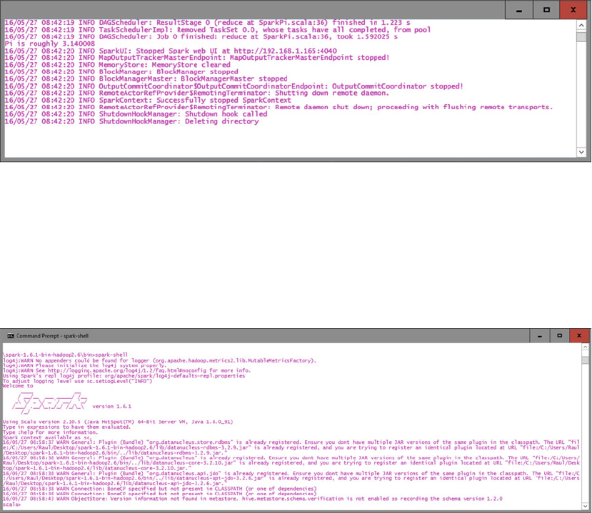
CHAPTER 6 ■ THE ENGINE: APACHE SPARK
99
Let’s Kick the Tires
To test the installation, run the following command:
/opt/spark-1.6.1-bin-hadoop2.6/bin/run-example SparkPi 10
You should see an output like the one shown in Figure
6-2 , with the line Pi is roughly .
Figure 6-2. T e s t i n g A p a c h e S p a r k
To open a Spark interactive shell, go to the bin directory and run the spark-shell:
$> /bin/spark-shell
You should see output similar to Figure 6-3 (which shows Windows 64-bit so that no one feels left out of
this party):
Figure 6-3. The Apache Spark shell
Like all modern shells , the Spark shell includes history. You can access it with the up and down arrows.
There are also autocomplete options that you can access by pressing the Tab key.
As you can see, Spark runs in Scala; the Spark shell is a Scala terminal with more features. This chapter’s
Scala examples run without problems. You can test, as follows:
scala> val num = 1 to 400000
num: scala.collection.immutable.Range.Inclusive = Range (...
CHAPTER 6 ■ THE ENGINE: APACHE SPARK
100
To convert our Range to a RDD (now we see it is that), do the following:
scala> val myRDD = sc.parallelize(num)
myRDD: org.apache.spark.rdd.RDD [Int] = ParallelCollectionRDD [0] at parallelize at <console>
In this case, there is a numeric RDD. Then, as you may guess, you can do all the math operations with
Scala data types. Let’s use only the odd numbers:
scala> myRDD.filter (_% 2 != 0) .collect ()
res1: Array [Int] = Array (1, 3, 5, 7, 9 ...)
Spark returns an int array with odd numbers from 1 to 400,000. With this array, you can make all the
math operations used with Scala int arrays.
Now, you are inside Spark, where things can be achieved in a big corporate cluster.
Basically, Spark is a framework for processing large volumes of data— in gigabytes, terabytes, or even
petabytes. When you work with small data volumes, however, there are many solutions that are more
appropriate than Spark.
The two main concepts are the calculations and scale. The effectiveness of the Spark solution lies in
making complex calculations over large amounts of data, in an expeditious manner.
Loading a Data File
Upload a text file in Spark within the Spark shell:
scala> val bigfile = sc.textFile ("./big/tooBigFile.txt")
This magically loads the tooBigFile.txt file to Spark, with each line a different entry of the RDD
(explained shortly). The RDDs are very versatile in terms of scaling.
If you connect to the Spark master node, you may try to load the file in any of the different machines
in the cluster, so you have to ensure that it can be accessed from all worker nodes in the cluster. In general,
you always put your files in file systems like HDFS or S3. In local mode, you can add the file directly (e.g., sc.
textFile ([path_to_file) ). You can use the addFile() SparkContext function to make a file available to all
machines in this way:
scala> import org.apache.spark.SparkFiles
scala> val myFile = sc.addFile( "/opt/big/data/path/bigFile.dat" )
scala> val txtFile = sc.textFile (SparkFiles.get("bigFile.txt"))
For example, if you load a (big) input file where each line has a lot of numbers, the first RDD file whose
elements are strings (text lines) is not very helpful. To transform the string elements to an array of doubles,
use your knowledge of the Scala language:
scala> val myArrays = textFile.map (line => line.split('').map(_. toDouble))
To verify that this is what you wanted, you can use the first() operator on both txtFile and myArrays
to see that the first element in the txtFile is a string and in myArrays is an Array[Double].
Loading Data from S3
As part of Amazon support, you have access to a file system called Amazon S3 . To access it, you need the
AWS_ACCESS_KEY_ID and AWS_SECRET_ACCESS_KEY variables (to configure them, see the “Running
Spark on EC2” section in this chapter).
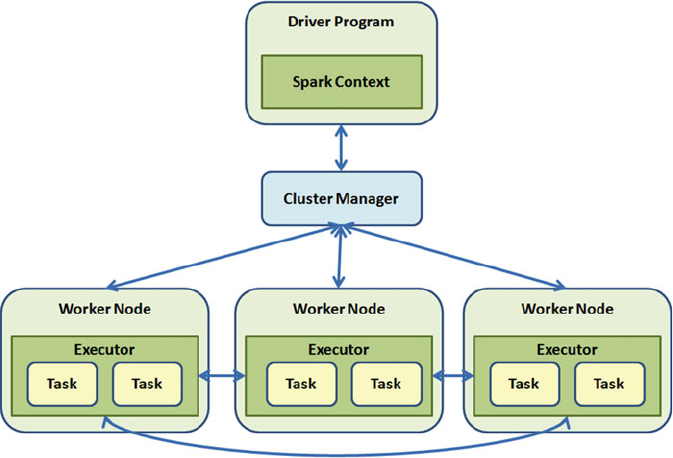
CHAPTER 6 ■ THE ENGINE: APACHE SPARK
101
For instance, you can use the Amazon examples on a data file from Wikipedia:
scala> val myWiki = sc.textFile ("S3N://bigdatademo/sample/wiki/")
We don’t need to set our AWS credentials as parameters for the Spark shell; this is the general path form
for access the S3 file system:
S3N://<AWS ACCESS ID>:<AWS SECRET>@bucket/path
As another example, you can get Wikipedia’s traffic statistics from over the last 16 months at
https://
aws.amazon.com/datasets/wikipedia-traffic-statistics-v2/ .
Spark Architecture
Now is a good time to discuss the Spark mechanism. Let’s first talk about the architecture and then about the
programming.
Parallelism is computational term used when we talk about performing operations in parallel;
that is, if we have a process that works on a portion of data, we can “make copies” of that process to act
simultaneously on the same portion of data. Not all processes are parallelizable. Spark’s power is in its ability
to do parallel computing in a simple way; this is just one of its main advantages.
When you program on your machines or laptops, the Spark shell is run locally. The work is performed in
a single node. When you are working on a cluster, all you have to do is connect the same shell to the cluster
to run it in parallel. Figure
6-4 explains how Spark runs on a cluster.
Figure 6-4. Spark cluster with three executor nodes
CHAPTER 6 ■ THE ENGINE: APACHE SPARK
102
The two main concepts of Spark are the resilient distributed dataset (RDD) and the cluster manager. In a
nutshell, the RDD is a parallelized computational abstraction of a collection. The cluster manager distributes
the code and manages the data represented in the RDDs. The cluster manager has three responsibilities:
controls the distribution and interaction with RDDs, distributes code, and manages the fault-tolerant
execution.
Spark can work over several types of cluster managers; in this chapter, we talk about the standalone
manager, and in a subsequent chapter, we talk about Apache Mesos. Hadoop Yarn is not covered in this book
because we focus only on pipeline architectures, not Hadoop.
If you have Hadoop 2.0 installed, we recommend that you install Spark on Hadoop Yarn. If you have
Hadoop 1.0 installed, we recommend that you use Spark Standalone. It is not suitable to install Apache
Mesos and Hadoop Yarn at the same time.
The Spark driver program distributes the program classes in the cluster. The cluster manager starts the
executors, one on each node, and assigns them a tasks set. When you run a program, all of this enginery
runs transparently in your machines. For example, when you run on a cluster, the entire administration is
transparent to you. That is Spark’s power.
S p a r k C o n t e x t
Now that you have Spark running on your laptop, let’s start programming in more detail. The driver
programs access the Spark core through the SparkContext object, which represents the connection between
the cluster and the nodes. In the shell, Spark is always accessed through the sc variable; if you want to learn
more about the sc variable, type this:
scala> sc
res0: org.apache.spark.SparkContext = org.apache.spark.SparkContext@4152bd0f
Creating a SparkContext
In a program, you can create a SparkContext object with the following code:
val sparkContext = new SparkContext( masterPath, "applicationName", ["SparkPath
(optional)"],["JarsList (optional)"])
It is always possible to hard-code the value of the parameters; however, it is best read from the
environment with suitable defaults. This allows you to run the code when you change the host
without recompiling it. Using local as the default for the master makes it easy to launch the application
in a local testing environment. You must be careful when selecting the defaults. Here’s an example
snippet:
import spark.sparkContext._
import scala.util.Properties
val masterPath = Properties.envOrElse("MASTER","local")
val sparkHome = Properties.get("SPARK_HOME")
val jarFiles = Seq(System.get("JARS"))
val sparkContext = new SparkContext(masterPath, "MyAppName", sparkHome, jarFiles)

CHAPTER 6 ■ THE ENGINE: APACHE SPARK
103
SparkContext Metadata
The SparkContext object has useful metadata (see Table 6-1 ); for example, the version number, the
application name, and the available memory. If you recall, information about the version is displayed when
you start the Spark shell.
Table 6-1. Some Useful SparkContext Metadata
Value Type Use
appName String The application name. If you followed the convention, this
value is useful at runtime.
getConf SparkConf Return a copy of this SparkContext’s configuration.
getExecutorMemoryStatus Map[String,
(Long, Long)]
Return a map from the slave to the maximum memory
available for caching and the remaining memory available
for caching. As it is distributed, it does not prevent OOM
exceptions.
isLocal Boolean Are we running in local?
isStopped Boolean Are we running?
master String Master node name.
sparkUser String Spark OS username.
startTime Long Node start time.
version String Useful when testing several Spark versions.
Here are some examples of SparkContext metadata to print the Spark version, the application name, the
master node’s name and the memory:
$ bin/spark-shell
scala> sc.version
res0: String = 1.6.1
scala> sc.appName
res1: String = Spark shell
scala> sc.master
res2: String = local[*]
scala> sc.getExecutorMemoryStatus
res3: scala.collection.Map[String,(Long, Long)] = Map(localhost:52962 ->
(535953408,535953408))
SparkContext Methods
The SparkContext object is the main entry point for your application and your cluster. It is also used for
loading and saving data. You can use it to launch additional Spark jobs and remove dependencies.
Table
6-2 shows some SparkContext methods, but you can see all the SparkContext attributes and methods
at
https://spark.apache.org/docs/latest/api/scala/#org.apache.spark.SparkContext $ .

CHAPTER 6 ■ THE ENGINE: APACHE SPARK
104
Working with RDDs
The resilient distributed dataset is Apache Spark’s core concept. Spark has four design goals :
• In-memory data storage . This is where Apache Hadoop is defeated, because
Hadoop is primarily disk storage.
• Fault tolerant . Achieved with two features: cluster operations and the application of
linear operations on small data chucks.
• Efficiency . Achieved with operation parallelization between cluster parts.
• Fast . Achieved by minimizing data replication between cluster members.
The main idea is that with RDD, you only can perform two types of operations:
• Transformations . When a transformation is applied on an RDD, a new RDD is
created. For example, the set operations (union, intersection, and join) or as you
learned in Chapter
3 , mapping, filtering, sort, and coalesce.
• Actions . When we apply an action over an RDD, the original RDD does not change.
For example: count, collect, and first.
Computer science has a solid foundation in mathematics; all computer models have a solid
mathematical model behind them. In functional programming, functions are first-class citizens; that is,
functions are not modeled as objects, but are simply functions. When you apply a function to another
function, the result is another function. In algebra this is known as function composition . If function f is
applied to the function g , the operation is denoted as f o g , which is equivalent to f(g()) .
In linear algebra, there are operations between vectors. There are vector operations whose input is
various vectors and the result is a new vector (for example, vector addition). In Spark, vectors would be
RDDs and operations whose return value is an RDD are equivalent to transformations.
Table 6-2. Some Useful SparkContext Methods
Method Parameter Return Use
addJar() path:String Unit Adds jar files for all tasks to be executed
on the SparkContext in the future.
addFile() path:String Unit Distribute a file to all nodes on a cluster.
accumulator() value: T
name: String
Accumulator Creates an accumulator (a distributed
variable among the cluster).
cancelAllJobs() --- Unit Cancel all jobs (scheduled and
running).
clearJobGroup() --- Unit Clear the current thread’s job.
killExecutor() id:String Boolean Request to cluster manager to kill the
specified executors.
setJobDescription() value:String Unit Set a human-readable description of
the current job.
textFile() path:String
minPartitions: int
String Read a text file and return it as an RDD
of strings.
stop() --- Unit Shut down the SparkContext.
CHAPTER 6 ■ THE ENGINE: APACHE SPARK
105
On the other hand, there are functions whose input is several vectors and the output is a scalar value;
for example, the inner product. In Spark, actions are the equivalent of these operations.
As with functional programming, there are also rules for RDDs:
• Immutability . In both actions and transformations, the original RDD is not
modified. Yes, the concept of a “variable” value in functional programming is an
aberration: it does not exist; all the things (functions, values, objects) must be
immutable.
• Resilient . In Spark, the chain of transformations from the first RDD to the last RDD
is always logged; that is, if a failure occurs (the power goes out or someone trips over
the power cord), the process can be reproduced again from the beginning or from
the point of failure.
• Lazy evaluation . Since we live in a functional context, the transformations on
RDDs are always lazy. They are not executed until (and only until) the end result is
required. As you saw in Chapter
3 , this exists to improve performance, because it
avoids unnecessary data processing and the waste of resources (usually caused by
the developer).
• Process aware . As you saw in Chapter
4 , lazy evaluation prevents deadlocks and
bottlenecks, because it prevents the indefinite process of waiting for other processes’
output. Recall that the lazy evaluation emulates all the operations already made and
uses a “result avatar” to estimate the final result.
• Memory storage . By default, RDDs are born, and live and die in memory. The
RDDs are stored on disk only if explicitly requested. This increases the performance
terrifically, because you don’t fetch them from the file system or database.
In addition, we now have the DataFrames API (since 2015). This API offers the following:
• Scalability . You can test kilobyte-sized data samples on your laptop, and then run
the same programs on a production cluster with several terabytes of data.
• Optimization . The powerful Spark SQL Catalyst optimizer offers two advantages:
SQL beautification and SQL optimization. It also provides source code generation
from actual SQL.
• Integration . Smooth integration with the other members of the Spark family (Core,
SQL, Streaming, MLlib, GraphX).
• Multiformat . Supports several data formats and storage systems.
Before continuing, we must take the time to learn about what RDDs are and what they are not.
It is crucial to understand that when an RDD is defined, it actually contains no data. You only create
a container for it. RDDs follow the lazy evaluation principle; an expression is not evaluated until it is
necessary (i.e., when an action is requested). This means that when you try to access the data in an RDD,
you could fail. The data operation to create an RDD is only performed when the data is referenced to store
or catch the RDD.
This also means that when you concatenate a large number of operations, you don’t have to worry
about the excessive operations locking a thread. It is important to keep this in mind during application
development—when you write and compile code, and even when you run the job.
CHAPTER 6 ■ THE ENGINE: APACHE SPARK
106
Standalone Apps
You can run Spark applications in two ways: from the pretty Spark shell or from a program written in Java,
Scala, Python, or R. The difference between the two modes is that when you run standalone applications ,
you must initialize the SparkContext, as you saw in previous sections.
To run a program in Scala or Java, it is best to use Maven (or Gradle or SBT, whichever you want). You
must import the dependency to your project. At the time of this writing, the Spark version is 1.6.1 (version 2
exists, but it’s very new).
The following are the Maven coordinates for version 1.6.1:
groupId = org.apache.spark
artifactId = spark-core_2.10
version = 1.6.1
Initializing the SparkContext
Once you have Spark dependencies installed in your project, the first thing that you have to do is create a
SparkContext.
As you saw earlier, you must first create an object of type SparkConf to configure your application, and
then build a SparkContext object from it.
// All the necessary imports
import org.apache.spark.SparkConf
import org.apache.spark.SparkContext
import org.apache.spark.SparkContext._
// Create the SparkConf object
val conf = new SparkConf().setMaster("local").setAppName("mySparkApp")
// Create the SparkContext from SparkConf
val sc = new SparkContext(conf)
The SparkConf constructor receives two parameters:
• Cluster URL . This is "local" when you want to run the program on one thread on
the local machine, (i.e., without a cluster).
• Application name . This name is used to identify your application in the cluster
manager UI (running in cluster mode). Here we called it mySparkApp.
Standalone Programs
We already have the necessary imports: the SparkConf object and the SparkContext object. Now let’s give
our program a body. It is important to note that all the stuff that runs on the Spark shell should run on Spark
Standalone programs.
In all the “big data” books there is a word-count example; this book could not be the exception. Our
program input is a file (yes, we already know how to load files) of the Franz Kafka novel The Process , in
English.
The exercise objective is to see the number of times a word occurs and to see the most repeated words.
// We create a RDD with the the-process.txt file contents
val myfile = sc.textFile("the-process.txt")
CHAPTER 6 ■ THE ENGINE: APACHE SPARK
107
// Then, we convert the each line text to lowercase
val lowerCase = myFile.map( line => line.toLowerCase)
// We split every line in words (strings separated by spaces)
// As we already know, the split command flattens arrays
val words = lowerCase.flatMap(line => line.split("\\s+"))
// Create the tuple (word, frequency), initial frequency is 1
val counts = words.map(word => (word, 1))
// Let’s group the sum of frequencies by word, (easy isn’t?)
val frequency = counts.reduceByKey(_ + _)
// Reverse the tuple to (frequency, word)
val invFrequency = frequency.map(_.swap)
// Take the 20 more frequent and prints it
invFrequency.top(20).foreach(println)
It is fundamental to note that everything doesn’t run until the last println invocation. Yes, all the
previous words are transformations, and the last line is the action. We will clear this up later.
Hold on, the most frequent types of words (in all human languages) are conjunctions and prepositions,
so before separating each sentence into words in the third step, we filter the “stop words” in English
(obviously there are better lists on Internet, this is just an example).
val tinytStopWords = Set("what", "of", "and", "the", "to", "it", "in", "or", "no", "that",
"is", "with", "by", "those", "which", "its", "his", "her", "me", "him", "on", "an", "if",
"more", "I", "you", "my", "your", "for" )
val words = lowerCase
.flatMap(line => line.split("\\s+"))
.filter(! tinyStopWords.contains(_))
Run the Program
When your program is complete, use the script located on /bin/spark-submit to run it. Modern Java/Scala
IDEs have embedded the Spark integration to run it smoothly.
But this book is mostly read by command-line fellas and old-school soldiers. Here we show how to run
it from a command line with SBT and with Maven:
// To run it with sbt
sbt clean package
$SPARK_HOME/bin/spark-submit \
--class com.apress.smack.WordFreq \
./target/...(as above) \
./README.md ./wordfreq
// To run it with Maven
mvn clean && mvn compile && mvn package
$SPARK_HOME/bin/spark-submit \
--class com.apress.smack.WordFreq \
./target/WordFreq-0.0.1.jar \
./README.md ./wordfreq
If nothing works, you can always refer to the official Spark guide at
http://spark.apache.org/docs/
latest/quick-start.html .

CHAPTER 6 ■ THE ENGINE: APACHE SPARK
108
RDD Operations
RDDs have two types of operations: transformations and actions . Transformations are operations that
receive one or more RDD as input and return a new RDD. Actions return a result to the driver program and/
or store it, and/or trigger a new operation.
If you still get confused and don’t know how to distinguish them, this is the rule: transformations return
RDDs; actions don’t .
Transformations
Transformations are operations with these characteristics:
• Lazy evaluation . Transformations are lazy operations; they aren’t calculated until
you perform an action or explicitly invoke the collect method. This behavior is
inherited from the actor model and functional programming.
• Element-wise . Transformations work on each individual element of a collection;
one at a time.
• Immutable . RDDs are immutable, thus transformations are immutable too (i.e., they can’t
modify the value of the RDD received as a parameter. There are no global variables).
• Lineage graph . Let’s suppose you have a transformations sequence. We have RDDs as
result of transformations in other RDDs. Spark keeps a track of each operation and of
the dependencies among all the RDDs. This record, known as a lineage graph , is kept
to recover the system from a failure. Spark always builds a lineage graph when running
distributed applications on a cluster.
Table 6-3 enumerates the main transformations.
Table 6-3. Spark Main Transformations
Transformation Purpose Example
filter( function) Builds a new RDD by
selecting the elements
on which the function
returns true.
> val rdd = sc.parallelize(List(“Spark”, “Mesos”,
“Akka”, “Cassandra”, “Kafka”))
> val k = rdd.filter(_.contains(“k”))
> k.collect()
Result:
Array[String] = Array(Spark, Akka, Kafka)
map( function) Builds a new RDD by
applying the function on
each element.
> val rdd = sc.parallelize(List(1, 2, 3, 4))
> val t = rdd.map(_*5)
> t.collect()
Result:
Array[Int] = Array(5, 10, 15, 20)
flatMap( function ) The same as map() but
it returns a sequence
instead of a value.
> val rdd = sc.parallelize(List(“Big Data are
Buzzwords”, “Make Fast Data”))
> val fm = rdd.flatMap( s => s.split(“ ”) )
> fm.collect()
Result:
Array[String] = Array(Big, Data, are, Buzzwords,
Make, Fast, Data)
(continued)

CHAPTER 6 ■ THE ENGINE: APACHE SPARK
109
Table 6-4 lists the main transformations on sets.
Transformation Purpose Example
reduceByKey( function,
[number] )
Aggregates the values of a
key using the function.
> val words = fm.map( w => (w, 1) )
> val wordCount = words.reduceByKey( _+_ )
> wordCount.collect()
Result:
Array[(String, Int)] = Array((are,1), (Big,1), (Fast,1),
(Make,1), (Buzzwords,1), (Data,2))
groupByKey([numTasks]) Converts (K, V) to (K,
Iterable<V>).
> val wc = wordCount.map{case(w,c) => (c,w)}
> wc.groupByKey().collect()
Result:
Array[(Int, Iterable[String])] =
Array((1,CompactBuffer(are, Big, Fast, Make,
Buzzwords)), (2,CompactBuffer(Data)))
distinct([numTasks]) Eliminates duplicates. > fm.distinct().collect()
Result:
Array[String] = Array(are, Big, Fast, Make,
Buzzwords, Data)
Table 6-3. (continued)
Table 6-4. Main Transformations on Sets
Transformation Purpose Example
union() Builds a new RDD containing all
elements from the source and the
argument.
> val foo = sc.parallelize(List(“Big”, “Data”))
> val bar = sc.parallelize(List(“Fast”, “Data”))
> foo.union(bar).collect()
Result:
Array[String] = Array(Big, Data, Fast, Data)
intersection() Builds a new RDD containing only
common elements between the
source and argument.
> foo.intersection(bar).collect()
Result:
Array[String] = Array(Data)
cartesian() Builds an RDD with cross product
of all elements from the source and
the argument.
> foo.cartesian(bar).collect()
Result:
Array[(String, String)] = Array((Big,Fast),
(Big,Data), (Data,Fast), (Data,Data))
subtract() Builds a new RDD by removing
common data elements between
source and argument.
> foo.subtract(bar).collect()
Result:
Array[String] = Array(Big)
(continued)

CHAPTER 6 ■ THE ENGINE: APACHE SPARK
110
Actions
Although actions return scalar (simple) values, you must never underestimate them, since the internal
process can become really complex. Actions return the result to the driver program and/or write in and store
the result.
Pipeline of operations are advanced sequentially, operation by operation; however, remember that
everything is lazy evaluation. Flow can advance, and when it finds an action, everything is evaluated to that
point. Actions trigger the evaluation of all previous transformations.
Actions always trigger an evaluation because they must always return a value; if they don’t return a
value or store something, they can’t continue. Table
6-5 enumerates the main Spark actions.
Table 6-5. Main Spark Actions
Action Purpose Example
count() Obtains the number of
RDD elements.
> val smack = sc.parallelize( List(‘s', 'M', 'A', 'C', 'K') )
> smack.count()
Result:
long = 5
collect() Returns all the RDD
elements as an array.
> val smack = sc.parallelize( List(“S”, “M”, “A”, “C”,
“K”) )
> smack.collect()
Result:
Array[String] = Array(S, M, A, C, K)
reduce( function) Aggregates the RDD
elements using the
function.
> val smack = sc.parallelize( List(1, 5, 2, 4, 3) )
> smack.reduce(_+_) // the sum of all
Result:
Int = 15
Transformation Purpose Example
join( RDD,
[number] )
When invoked on (K,V) and (K,W),
creates a new RDD with (K, (V,W))
> val foo = sc.parallelize( Seq((1, “S”), (2, “M”),
(3, “A”), (1, “C”), (4, “K”)))
> val bar = sc.parallelize( Seq((1, “W”), (2, “X”),
(3, “Y”), (2, “Z”)))
> foo.join( bar ).collect()
Result:
Array[(Int, (String, String))] = Array((1,(S,W)),
(1,(C,W)), (2,(M,X)), (2,(M,Z)), (3,(A,Y)))
cogroup( RDD,
[number] )
Converts (K, V) to (K, Iterable<V>). > foo.cogroup(bar).collect()
Result:
Array[(Int, (Iterable[String], Iterable[String]))] =
Array((4,(CompactBuffer(K),CompactBuffer())),
(1,(CompactBuffer(S, C),CompactBuffer(W))),
(2,(CompactBuffer(M),CompactBuffer(X, Z))),
(3,(CompactBuffer(A),CompactBuffer(Y))))
Table 6-4. (continued)
(continued)

CHAPTER 6 ■ THE ENGINE: APACHE SPARK
111
RDD Persistence (Caching)
Now you know that RDDs support lazy evaluation. But what if you want to use the same RDD several
times? If you don’t do this work conscientiously, by default, Spark will recalculate the RDD and all of its
dependencies each time that you apply an action on it. If not done carefully, this can be very expensive.
You can tell Spark to persist the RDD to avoid recalculating them all the time. When you persist an RDD,
the nodes working with it store the RDD partitions assigned to them. If a node fails, Spark recalculates lost
partitions as needed (yes, it’s powerful).
You can also replicate your RDD among several nodes if you want to handle a node failure without
performance implications. As shown in Table
6-6 , Spark offers several levels of persistence to suit all of our
scenarios and needs. Note that when writing data to disk the data is always serialized.
Action Purpose Example
take( n ) Fetches the first n
elements of the RDD.
> val smack = sc.parallelize( List(‘s', 'M', 'A', 'C', 'K') )
> smack.take(4)
Result:
Array[Char] = Array(S, M, A, C)
foreach( function) Executes the function in
each RDD element.
> val s = sc.parallelize(List(1, 4, 2, 3))
> s.foreach(n =>
print( “%s*7=%s ”.format(n, n*7) ))
Result:
1*7=7 4*7=28 2*7=14 3*7=21
first() Fetches the RDD first
element, the same as
take(1).
> val rdd = sc.parallelize(List(4, 3, 2, 1))
> rdd.first()
Result:
Int = 4
saveAsTextFile(path) Writes the RDD content
to the text file on local file
system/HDFS.
> val myLogs = sc.textFile(“/users/smack/
evidence.log”)
> myLogs.filter(_.contains(“Fatal”)).
myLogs.saveAsTextFile(“/users/smack/fact.txt”)
Result:
smack@localhost~/smack$ ls _SUCCESS part-
00000 part-00001
Table 6-5. (continued)
Table 6-6. RDD Persistence Levels
Persistence Level CPU Used Space Used On Disk In Memory
MEMORY_ONLY Low High No Yes
MEMORY_AND_DISK(*) Medium High Some Some
MEMORY_ONLY_SER High Low No Yes
MEMORY_AND_DISK_SER(*) High Low Some Some
DISK_ONLY High Low Yes No
OFF_HEAP (experimental) Low Low Some Some
*Write to disk if there is much data stored in memory. (Note that SER means serializable)
CHAPTER 6 ■ THE ENGINE: APACHE SPARK
112
An important caching scheme is off-heap, a mixed scheme. It was previously called Tachyon, but now
it’s called Alluxio (
http://alluxio.org/ ). Note that the off-heap catching doesn’t guarantee recovery after
failure.
This is a code example:
import org.apache.spark.storage.StorageLevel
val rdd = input.map( foo )
rdd.persist( StorageLevel.DISK_ONLY )
rdd.reduce( bar )
rdd.collect()
Here are some points to consider:
• You must call the persist() method in the code before the first action.
• The persist() function doesn’t force the evaluation.
• Spark automatically evicts old partitions using an LRU (least recently used) cache
policy.
• The persist() method counterpart is the unpersist() method to manually remove
RDDs from the cache.
Spark in Cluster Mode
In this chapter, we have focused on running Spark in local mode. As we mentioned, horizontal scaling is
what makes Spark so powerful. To run Apache Spark on a cluster, you do not need specialized software-
hardware integration engineers. To escalate, you don’t need to make great efforts and stop the entire
production to add more machines to your cluster.
The good news is that the same scripts that you are building on your laptop with examples that are only
a few kilobytes can run on business clusters running terabytes of data. There is no need to change your code,
nor invoke another API. All you have to do is test your model several times to know if it runs correctly, and
then you can deploy it.
In this section, you analyze the runtime architecture of a distributed Spark application. Then you see
the options to run Spark on a cluster.
Apache Spark has its own built-in standalone cluster manager. But you can run it on multiple cluster
managers, including Hadoop YARN, Amazon EC2, and Apache Mesos. This topic is so large that it has its
own chapter in this book.
Runtime Architecture
Before running Spark on a cluster, it’s important to understand the distributed Spark architecture.
As shown in Figure
6-5 , Spark uses a master/slave architecture. The master is called the driver and the
slaves are called executors . When running on a single machine, there is a distributed architecture: a driver
with several executors. The driver runs in its own Java process, and each executor runs in a separate Java
process. This architecture is made on the actor model.
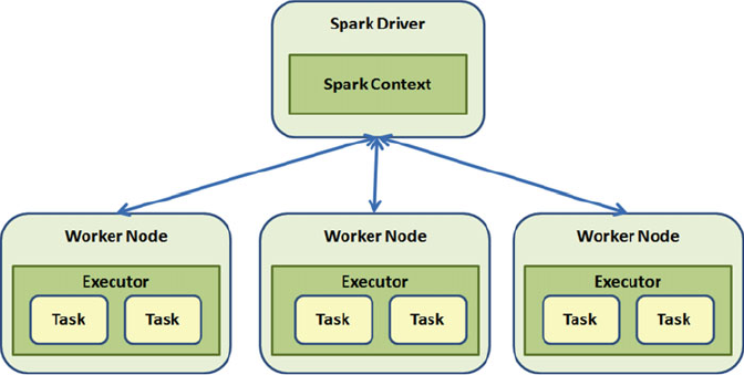
CHAPTER 6 ■ THE ENGINE: APACHE SPARK
113
The driver and executors set is known as a Spark application. If you have more than one machine, the
Spark application must be launched using the cluster manager service. The Spark application architecture is
always the same; it does not matter if it’s clustered or not.
In a typical Spark clustered application architecture, each physical machine has its own executor. You
will see several strategies to know when an executor dies or goes offline.
Driver
The driver is the process where the SparkContext runs. It is in charge of creating and executing
transformations and actions on RDDs. When you run the Spark shell command on your laptop, you are
actually creating a driver program. Its first task is to create the SparkContext, called sc. When the driver
program dies, the entire application dies.
The following sections explain the two responsibilities in the life of a driver program: dividing a
program into tasks and scheduling tasks on executors.
Divide a Program into Tasks
The Spark driver is responsible for splitting the user program , which could be programmed in an inefficient
way in execution units called tasks .
A user program basically applies transformations and actions into one or more RDDs to generate new
RDDs and calculate and/or store data.
Another task of the Spark driver is to generate an operation’s directed acyclic graph (DAG) . With this
graph, the driver knows which tasks are assigned to which node; so if you lost a node, the driver knows at
which point it was at and how to assign the lost node’s tasks to the remaining nodes.
The driver also does pipeline optimizations; it splits the DAG into stages. Each stage has multiple tasks.
In Spark, the task is the smallest work unit; a normal program can launch thousands of tasks.
Figure 6-5. Distributed Spark application
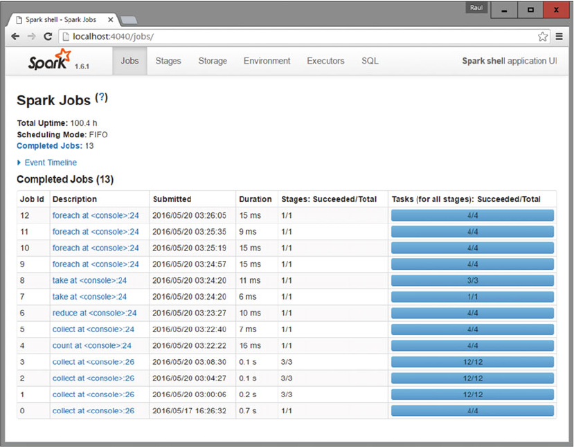
CHAPTER 6 ■ THE ENGINE: APACHE SPARK
114
Scheduling Tasks on Executors
Given a physical execution plan, the Spark driver coordinates which tasks are performed by each executor
node . When an executor starts operating, it registers itself in the driver, so the driver always has an entire
view of all the executor nodes. Each executor is a standalone Java process that can run tasks and store RDDs.
When a program runs, the driver subdivides the program into tasks, sees all the available executor
nodes, and tries to balance the workload among them. The driver also knows which part of the data that
each node has, in order to rebuild everything at the end.
The driver displays its information on the Web, so that the user can always see what is happening; by
default, it runs on port 4040. When you run locally, it can be accessed at http://localhost:4040 , as you can
see in Figure
6-6 (let’s run the Spark shell and browse it).
Figure 6-6. Spark shell application web UI
E x e c u t o r
Executors are responsible for running the individual tasks of a given Spark job. Executors are launched when
you start the Spark application; they live while the Spark application lives.
CHAPTER 6 ■ THE ENGINE: APACHE SPARK
115
Executors have two roles:
• Run the assigned tasks and deliver results to the driver.
• Provide in-memory storage for RDDs. A program called Block Manager runs on each
executor and manages memory and RDDs.
When running Spark in local mode, the driver and executors run in the same process. This is for
development purposes; it is not recommended in a production environment.
Cluster Manager
Spark depends on a cluster manager to coordinate and launch the executors. The cluster manager that
ships with the Spark distribution is called the standalone manager , but it is a pluggable component. You can
change it and use a custom cluster manager like Hadoop Yarn, Amazon EC2, or Apache Mesos.
It is important to note that the terms driver and executor are used when talking about the Spark
application. When we talk about the cluster manager, we use the terms master and worker . It is important
not confuse the terms or to exchange them, because they are different concepts.
Regardless of the cluster manager that you use, Spark provides a single script, called spark-submit, to
launch the program. The spark-submit script can connect to different managers through various options and
manage the cluster resources that the application needs.
Program Execution
When you run a Spark application on a cluster, these are the steps followed by the program:
1 . The user runs the spark-submit shell.
2 . The spark-submit shell launches the driver program, and calls the user program’s
main() method.
3 . The driver program establishes the connection to the cluster manager, which has
the slave machines list. Then, the necessary resources are requested to launch
the executors.
4 . The cluster manager launches executors in each slave node.
5 . The driver program analyzes, divides, and distributes the user application,
sending each executor its tasks.
6 . The tasks run in the executors, calculating and storing the results.
7 . The user program ends when the exit() method in the main() method is
invoked, or when the SparkContext stop() method is called.
8 . The driver program ends the executors and frees the cluster manager’s resources.
Application Deployment
Spark uses the spark-submit tool to send jobs to the cluster manager.
When you run a program in local mode, you only invoke spark-submit passing your script name or jar
file as a parameter.
When you run a program in cluster mode, you have to pass additional parameters—for example, the
size of each executor process.

CHAPTER 6 ■ THE ENGINE: APACHE SPARK
116
The --master flag specifies the cluster URL to which you want to connect. In this case, spark:// means
that we are using Spark in stand-alone mode.
For example:
bin/spark-submit --master spark://skynet:7077 --executor-memory 10g Terminator.jar
Here we indicate that we will run our Terminator program in stand-alone cluster mode in the master
node called SkyNet and each executor node will have 10 gigabytes of memory.
In addition to the cluster URL, spark-submit has several options to specify how you want to run your
application. These options are in of two categories:
• Scheduling data . The amount of resources that each job will have.
• Dependencies . The files and libraries available in the slaves.
Table 6-7 lists and describes some of the spark-submit flags.
Table 6-7. s p a r k - s u b m i t F l a g s
Flag Purpose
--master The cluster manager to connect to (sample values explained in Table 6-8 ).
--deploy-mode Indicates if the program is launched in local mode (client) or cluster mode. In
local mode, the driver is launched where spark-submit is launched. The default
value is client mode.
--class The main application class is Java/Scala.
--name Human-readable name for your application, as displayed in Spark web UI.
--jars List of jar files to upload on application classpath.
--files List of files uploaded on the application’s working directory on each node.
--executor-memory Memory for executors: k for kilobytes, m for megabytes, g for gigabytes.
--driver-memory Memory for the driver process: k for kilobytes, m for megabytes, g for gigabytes.
--conf prop=value A single configuration property value in key-value form.
--properties-file A configuration file with properties in key-value form.
Table 6-8. Master Flag Sample Values
Value Meaning
spark://host:port Connect to a cluster in stand-alone mode at specified host and port. 7077 is the
default port for a stand-alone master.
mesos://host:port Connect to a Mesos cluster at the specified host and port. 5050 is the default port for
the Mesos master.
local Local mode master with a single core.
local[N] Local mode master with N cores.
local[*] Local mode master using as many cores as the machine has.
Table 6-8 lists a few example values that the --master flag could have.
CHAPTER 6 ■ THE ENGINE: APACHE SPARK
117
Now you are able to read this:
$ ./bin/spark-submit \
--master spark://skynet:7077 \
--deploy-mode cluster \
--class com.cyberdyne.Terminator \
--name "T1000 model" \
--jars neuralNetwork.jar,geneticAlgorithm.jar \
--total-executor-cores 300 \
--executor-memory 10g \
terminator.jar
Here we indicate that we will run our terminator.jar program:
• In stand-alone cluster mode in the SkyNet master node on port 7077
• The driver program is launched in cluster mode
• The main class is com.cyberdyne.Terminator
• The application display name is T1000 model
• The neuralNetwork.jar and geneticAlgorithm.jar files are used
• Each executor node uses 300 cores and has 10 gigabytes of memory
Running in Cluster Mode
This section discusses some of the most common methods to install Spark in cluster mode . On a single
laptop, Spark is excellent for developing and testing; but in practice, it is necessary to know how to install
Spark with built-in scripts on a dedicated cluster via SSH (Secure Shell). This section covers how to deploy
on a cluster in Spark Standalone and with Mesos. This section also covers how to deploy Spark in the cloud
with Amazon EC2.
Spark Standalone Mode
When you run bin/start-master.sh , you start an individual master. When you run sbin/start-slaves.sh ,
you start a worker. The default port of the Spark master is always 8080. Because no one wants to go to each
machine and run scripts by hand in each, there is a set of useful scripts in the /bin directory that can help
you run your servers.
A prerequisite to use any of the scripts is to have passwordless SSH access from the master to all worker
machines. It is always advisable to create a special user to run Spark on all machines. In this book, the
examples use the name sparkuser . From the master, you can run the ssh-keygen command to generate the
SSH keys. When an RSA key is generated, by default, it is stored in ~/.ssh/id_rsa.pub . You have to add it to
each host in ~/.ssh/authorized_keys .
The Spark administration scripts require that user names match. If this is not the case, you can
configure alternative user names in ~/.ssh/config .
Now that you have SSH access to the machines, it’s time to configure Spark. There is a template in the
conf/spark-env.sh.template directory, which should be copied to conf/spark-env.sh . Table 6-9 lists
some of the environment variables.

CHAPTER 6 ■ THE ENGINE: APACHE SPARK
118
Table 6-9. Spark Environment Variables
Name Purpose Default value
MESOS_NATIVE_LIBRARY Points to Mesos installation directory. ---
S CALA_HOME Points to Scala installation directory. ---
SPARK_MASTER_IP The IP address where the Spark master
listens and where the workers connect
to; for example, a public one.
hostname command
output
SPARK_MASTER_PORT The port number where the Spark master
listens.
7077
SPARK_MASTER_WEBUI_PORT The port number for the master web user
interface.
8080
SPARK_MASTER_OPTS Configuration properties that apply only
to the master in the form of "-Dx=y ".
---
SPARK_WORKER_CORES Number of cores to be used by the
worker.
Total number of cores
SPARK_WORKER_MEMORY Amount of memory to be used by the
worker.
Total system memory
minus 1GB; if you have
less than 1GB, it’s 512MB.
SPARK_WORKER_PORT The port number on which the worker
runs on.
Random
SPARK_WORKER_WEBUI_PORT The port number of the worker web user
interface.
8081
SPARK_WORKER_DIR Directory on which files from the worker
are stored.
SPARK_HOME/work
SPARK_WORKER_OPTS Configuration properties that apply only
to the worker in the form of "-Dx=y" .
---
SPARK_DAEMON_MEMORY Memory to allocate to the Spark master
and worker daemons.
1GB
SPARK_DAEMON_JAVA_OPTS JVM options for the Spark master and
worker daemons in the form of "-Dx=y" .
---
Once the configuration is made, you must start the cluster. We highly recommend that you install the
pssh tool, which is a set of tools that includes pscp SSH. The pscp command makes it easy to secure copying
between hosts (although it takes a little while); for example:
pscp -v -r -h conf/slaves -l sparkuser ../spark-1.6.1 ~/
When you have finished changing the settings, you need to distribute the configuration to workers, as
shown here:
pscp -v -r -h conf/slaves -l sparkuser conf/spark-env.sh ~/spark-1.6.1/conf/spark-env.sh
After you have copied the files, you are ready to start the cluster. Use these scripts: sbin/start-all.sh ,
sbin/start-master.sh , and sbin/start-slaves.sh .
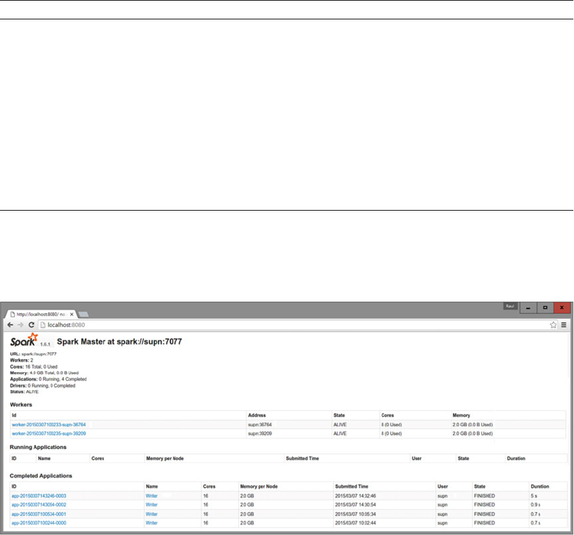
CHAPTER 6 ■ THE ENGINE: APACHE SPARK
119
It is important to note that start-all.sh and start-master.sh are assumed to be running on the
master node in the cluster. All scripts start demonizing, so there is no problem running them on the screen:
ssh master bin/start-all.sh
In the event that you get a java.lang.NoClassDefFoundError: scala/ScalaObject error, check that you
have Scala installed on the host and that the SCALA_HOME environment variable is set properly.
Spark scripts assume that the master has Spark installed in the same directory as your workers. If this is
not the case, you must edit bin/spark-config.sh to point to the correct directories.
Table 6-10 shows the commands provided by Spark to manage the cluster. If you want more
information, go to
http://spark.apache.org/docs/latest/spark-standalone.html#cluster-launch-
scripts .
Table 6-10. Spark Cluster Administration Commands
Command Purpose
bin/slaves.sh <command> Runs the provided command on all of the worker hosts. For example, to
show how long each hosts worker has been up: bin/slave.sh uptime
bin/start-all.sh Starts the master and all the worker hosts. Must be run on the master.
bin/start-master.sh Starts the master host. Must be run on the master.
bin/start-slaves.sh Starts all the worker hosts.
bin/start-slave.sh Starts a specific worker host.
bin/stop-all.sh Stops all master and workers hosts.
bin/stop-master.sh Stops the master host.
bin/stop-slaves.sh Stops all the worker hosts.
Now the Spark cluster is running. As shown in Figure
6-7 , there is a useful web UI running in the master
on port 8080, and in workers running on port 8081. The web UI contains important information about the
workers’ current and past jobs.
Figure 6-7. Spark Master UI
CHAPTER 6 ■ THE ENGINE: APACHE SPARK
120
Now that you have a cluster up and running, you can do several things with it. As with single host
examples, you have the same scripts to run Spark examples on a cluster.
All the example programs are in the examples/src/main/scala/spark/examples/ directory and take
the master parameter, which points them to the master IP host. If you are running on the master host, you
can run the example:
./run spark.examples.GroupByTest spark://'hostname':7077
If you get a java.lang.UnsupportedClassVersionError error, it is because you need to update the JDK. Always
use the supported versions. To check which version compiled your Spark distribution, use the command:
java -verbose -classpath ./core/target/scala-2.11.8/classes/ spark.SparkFiles | head -n 20
Version 49 is JDK 1.5, version 50 is JDK 1.6, and version 60 is JDK 1.7
If you cannot connect to the host, make sure that you have configured your master to listen to all IP
addresses.
Running Spark on EC2
The ec2 directory contains the scripts to run a Spark cluster in Amazon EC 2 . These scripts can be used to run
Spark in single or cluster mode. Spark can also run on Elastic MapReduce, which is the Amazon solution for
MapReduce cluster management.
The final configuration to run Spark in EC2 is at
http://spark.apache.org/docs/latest/ec2-
scripts.html .
To begin, you must have EC2 enabled in your Amazon account. It should generate a key pair for the
Spark cluster. This can be done at
https://portal.aws.amazon.com/gp/aws/securityCredentials .
Remember that the key pairs are generated by region. You must make sure to generate them in the same
region where you run your hosts. You can also choose to upload a SSH public key instead of generating
a new one. They are sensible, so you have to be sure to keep them in a safe place. In our environments,
we need two environment variables, AWS_ACCESS_KEY_ID and AWS_SECRET_ACCESS_KEY, which are
available from our EC2 scripts:
export AWS_ACCESS_KEY_ID = {our} AWS access key
export AWS_SECRET_ACCESS_KEY = {our} AWS secret key
There are some scripts provided by Amazon at
http://aws.amazon.com/developertools/Amazon-EC2 .
To check that everything is running correctly, type this command:
$ Ec2-describe-regions
That should result in the following output:
REGION ap-northeast-1 ec2.ap-northeast-1.amazonaws.com
REGION ap-southeast-1 ec2.ap-southeast-1.amazonaws.com
REGION ap-southeast-2 ec2.ap-southeast-2.amazonaws.com
REGION eu-central-1 ec2.eu-central-1.amazonaws.com
REGION eu-west-1 ec2.eu-west-1.amazonaws.com
REGION us-east-1 ec2.us-east-1.amazonaws.com
REGION us-west-1 ec2.us-west-1.amazonaws.com
REGION us-west-2 ec2.us-west-2.amazonaws.com
REGION sa-east-1 ec2.sa-east-1.amazonaws.com
CHAPTER 6 ■ THE ENGINE: APACHE SPARK
121
The Spark EC2 script automatically generates a group of different security and firewall rules to run the
Spark cluster. By default, our Spark cluster is accessible on port 8080. For security, we strongly recommend
changing the 0.0.0.0/0 address in the spark_ec2.py script with our public IP address.
To start the cluster, use this command:
./ec2/spark-ec2 -k spark-keypair -i pk-{....}.pem -s 1 launch lePetitCluster
Where {....}.pem indicates the path to our private key.
If you get a “not being reliable to SSH to the master” error, it is because the key can be accessed by
others users. Try changing the access permissions to the key so that only one user can read it. If more users
can read it, the SSH will refuse it.
If you get the “cannot yet SSH script to the master” error, it is because we are having a race condition;
the hosts are reporting them as alive. Try changing the -w in setup_cluster by using a sleep of 120 seconds.
If you get a “transient error while launching a cluster” error, try to run the script with the --resume
option.
This makes the scaffolding to make a cluster with a master and a worker node with all default values.
The next task is to verify that the firewall rules work. Access the master on port 8080.
The JPS command gives the following information about our cluster:
root @ ip-172-31-45-56 ~] $ jps
1904 NameNode
2856 Jps
2426 MasterNameNode
2078 SecondaryNodeName
This information is about the name of Spark master, the Hadoop node, and slave nodes.
You can take the example of Pi that you ran on your machine at the beginning of this chapter:
cd spark
bin/run-example SparkPi 10
To terminate the instances, use this command:
ec2/spark-ec2 destroy <cluster name>
To learn all the options that the spark-ec2 command has, run this:
ec2/spark-ec2 -help
There are many types of EC2 instances available; the type has an important impact on the cluster
performance. The type can be specified with --instance-type = [typeName]. If you need a lot of memory, you
can specify it here.
By default, the same instance type is used for masters and workers. To specify a different type of master
you use --master-instance-type = [typeName].
EC2 has also instances of the type GPU, which are very powerful if you run on Envidia graphic cards
because they usually have hundreds of GPUs at a very low cost. The GPU instance type is useful when you
run a worker, if the master is not used. It is important to note that EC2 performance on the GPU may be
lower than when testing locally, because you have more I/O imposed by the hypervisor.
EC2 scripts use the Amazon Machine Images (AMI) provided by the Spark development team; they are
enough for most applications.
CHAPTER 6 ■ THE ENGINE: APACHE SPARK
122
Running Spark on Mesos
This book devotes an entire chapter on Mesos (Chapter 7 ), but we must include a special mention in this
Spark chapter.
Mesos is a cluster management platform to run multiple distributed applications (or frameworks) on a
cluster. Mesos intelligently manages and runs clusters of Spark, Hadoop, Cassandra, Akka, and Kafka. Mesos
can run Spark as separate Mesos tasks or run all in a single Mesos task. Mesos quickly scales horizontally to
manage clusters beyond the size that individual Python scripts allow.
Mesos has a large number of configuration scripts that you can use. For Ubuntu installations, use
configure.ubuntu-lucid-64. In addition to the Spark requirements, you need to ensure that you have the
Python C header files installed. Since Mesos must be installed on all of your machines, you can use Mesos to
configure other machines:
./configure --prefix=/home/sparkuser/mesos && make && make check && make install
As with the Spark Standalone mode configuration, you must ensure that Mesos nodes can find each
other.
Let’s begin by adding the master hostname to mesossprefix/var/mesos/deploy/masters and all the
worker hostnames to mesossprefix/var/mesos/deploy/slaves . Then point the workers to the master in
mesossprefix/var/mesos/conf/mesos.conf .
Once Mesos is configured on your machines, you need to configure Spark to run on Mesos. This is as
simple as copying the conf/spark-env.sh.template file to conf/spark-env.sh and updating the MESOS_
NATIVE_LIBRARY variable to point to the path where Mesos is installed.
Then copy the build to all machines using this secure shell copy command:
pscp -v -r -h -l sparkuser ./mesos /home/sparkuser/mesos
To start Mesos clusters, use mesosprefix/sbin/mesos-start-cluster.sh . Use mesos://[host]:5050
as the master.
Well, that’s roughly what you have to do to run an Apache Spark cluster on Apache Mesos.
Submitting Our Application
To submit our application to a standalone cluster manager, type this:
spark-submit --master spark://masterNodeHost:masterNodePort appName
Previously, you saw the spark-submit command syntax. Now just change the master node address, and
that’s it.
The cluster URL is also displayed in the cluster administrator web UI at http://[masternode]:8080 .
The host name and port should exactly match the URL present in the web UI. As administrators, we can
configure ports other than 7077.
The standalone cluster manager has a -- deploy-mode option :
• Client mode (local, default). The driver runs in the same process as spark-submit. If
you shut down the spark-submit, your cluster goes down.
• Cluster mode . The driver is launched as a different process on a worker node. You
can shut down the machine on which spark-submit is running and everything will
continue running.
CHAPTER 6 ■ THE ENGINE: APACHE SPARK
123
For each executor node, the --total-executor-cores and --executor-memory parameters specify
the number of cores and the available memory. A common error is to ask for more resources than can be
assigned. In this case, the cluster manager can’t start the executor nodes. Always check that your cluster has
the resources that you state in the parameters.
Configuring Resources
In the standalone cluster manager, the resources are controlled by two variables :
• --executor-memory argument of the spark-submit command
• The total memory on each executor. By default, this value is set to 1GB;
unfortunately, in production environments, one gigabyte of memory assigned to
each executor won’t be enough.
• --total-executor-cores argument of the spark-submit command
• The total number of cores used on each executor. The default value is unlimited (i.e.,
the application starts an executor on each available node in the cluster).
To check your current parameters, you can browse the standalone cluster manager’s web UI at
http://[masterNode]:8080 .
By default, the standalone cluster manager disperses the executors onto the largest number of
machines available. For example, suppose you have an eight-node cluster and each machine has four cores.
You launch the application with -- total-executor-cores 6 . Spark will raise only six executors, and tends to
use the largest number of machines possible (i.e., an executor on each machine, leaves two nodes without
an executor).
If you want to use the fewest number of nodes possible, change the spark.deploy.spreadOut
configuration property to false in the conf/spark-defaults.conf configuration file. If we turn off this flag in
our example, we will use only two machines: one with four executors and the other with two executors. The
other six machines won’t run executors.
These settings affect all the applications on the cluster, so use it with caution.
High Availability
You saw how to specify the cluster mode in the Standalone cluster manager deploy mode, so if the spark-
submit process dies, the manager doesn’t also die. This is because the driver runs on one member of the
cluster.
You want to keep your manager running while the last node is still standing. To increase manager life,
there is a top-notch tool called Apache ZooKeeper, which is discussed in Chapter
7 .
Spark Streaming
Life is a continuous process, it is not discrete. Life is a continuous flow.
As we mentioned in earlier chapters, the benefits of the data are greater when the information is fresher.
Many machine learning computations should be calculated in real time from streaming data.
Spark Streaming is the Apache Spark module for managing data flows. Most of Spark is built over the
RDD concept. Spark Streaming introduces a new concept: discretized streams, known as DStreams. A
DStream is an information sequence related to time. Note that a DStream is internally a sequence of RDDs,
thus the name discretized .
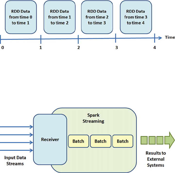
CHAPTER 6 ■ THE ENGINE: APACHE SPARK
124
Just as RDDs has two operations, DStreams also have two types of operations: transformations (results
in another DStream) and output operations , which are designed to store information on external systems.
DStreams have many of same the operations available to RDDs, plus time-related operations, such as sliding
windows.
Unlike batch operations, Spark Streaming applications require additional configurations to provide
24/7 services. Let’s talk about resetting applications in the event of a failure and discuss how to configure
automatic restarts.
Spark Streaming Architecture
Spark Streaming uses the microbatch architecture , in which streaming is considered a continuous series
of small batches of data (see Figure
6-8 ). The magic of Spark Streaming is receiving a continuous flow and
splitting it into small data chunks.
Figure 6-8. A DStream is an RDD sequence
Figure 6-9. Spark Streaming operation
Batches are generated at regular time intervals; if two data chunks come in the same time window, they
are included in the same data batch. The batch size is determined by the parameter batch interval , which
usually has a value between 500 milliseconds and several seconds. The developer specifies this value.
As you can see in Figure
6-9 , the primary Spark Streaming task is to receive a data stream from multiple
sources, and then build a DStream, which is a sequence of RDDs. Each RDD corresponds to a time slice of
the original flow.
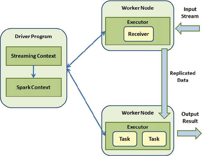
CHAPTER 6 ■ THE ENGINE: APACHE SPARK
125
We can create DStreams from input sources or through applying transformations to other DStreams.
The DStreams support most of the operations that RDDs support. Additionally, DStreams have “stateful”
operations to aggregate data across time.
In addition to transformations, DStreams support output operations, which are similar to actions in the
aspect that RDDs write to external systems; but Spark Streaming batches run periodically, producing the
output batch.
For each input source, Spark launches streaming receivers, which are tasks that run on executors, gather
data from information sources, and store it in RDDs. The receivers are also responsible for replicating data
among other executors to support fault tolerance. This data is stored in the memory of executors in the same
way as the RDDs. As shown in Figure
6-10 , the StreamingContext in the driver program periodically runs
Spark jobs to process this data and combine them with the new RDDs.
Figure 6-10. Spark Streaming execution with Spark components
The same fault tolerance properties offered by RDDs are also offered with DStreams. In the event of a
failure, Spark can recalculate the DStreams at any point in time. However, the recalculation can take time,
especially if the rebuild goes back to the beginning of the execution.
Spark Streaming provides a mechanism called checkpointing that periodically saves the state to a
reliable file system. Typically, a checkpoint occurs every five to ten data batches. When a failure occurs,
Spark restores from the last checkpoint.
Transformations
Transformations on DStreams can be grouped into stateless or stateful.
• Stateless . The data of each processing batch doesn’t depend on the data from
previous batches. These include the RDD transformations such as map() , reduce() ,
and filter() .

CHAPTER 6 ■ THE ENGINE: APACHE SPARK
126
• Stateful. The data or intermediate results from previous batches are used to
calculate the current batch’s results. These include transformations based on sliding
windows and tracking status over time.
Stateless Transformations
Stateless transformations are common RDD transformations applied to each RDD on the DStream. Table 6-11
enumerates the main stateless transformations:
Table 6-11. Main Stateless Transformations
Transformation Purpose Example
map(function) Applies a function to each RDD in the
DStream, returning one DStream as a result.
ds.map(_*3)
flatMap(function) Applies a function to each RDD in the
DStream, returning one DStream with the
content of the returned iterators.
ds.flatMap( str => str.
split(“ ”) )
filter(function) Builds a DStream with only the RDDs
evaluated with true on the function.
ds.filter(_.contains(“k”))
repartition(number) Changes the number of DStream partitions. ds.repartition(9)
reduceByKey(function,
[number] )
Combines the values with the same key in
each batch.
ds.reduceByKey(_+_)
groupByKey() Groups the values with the same key in each
batch.
ds.groupByKey()
Bullet points about stateless transformations:
• Individual. Although it seems as if the transformation is applied to the whole
DStream, it is not. Actually, it is applied individually to each batch element (RDD)
of the DStream. For example, with reduceByKey() , the function is applied on each
individual RDD, not on the whole DStream.
• Join. Stateless transformations can also combine data from multiple DStreams.
For example, DStreams have the same join transformations than RDDs, these are
cogroup() , join() , and leftOuterJoin() . You can use these operations to perform
a join in each DStream batch.
• Merge. You can merge the contents of two different DStreams by using the union()
operation, or by using StreamingContext.union() to merge several DStreams.
• Reuse. DStreams provide the powerful operator called transform() and can operate
directly on the RDDs within a DStream. This operation is called on each element of
the DStream, producing a new DStream. If you have written code for some RDDs and
you want to reuse in Spark Streaming, the transform() method is a good option.
• Transform . In addition to StreamingContext.transform(), you can combine several
DStreams using DStream.transformWith (anotherDStream, function).
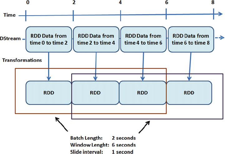
CHAPTER 6 ■ THE ENGINE: APACHE SPARK
127
Stateful Transformations
Stateful transformations are DStream operations that track data across time; data from old batches are used
to generate new batches.
There are two types of stateful transformations:
• Windowed transformations : Operates on data over a window duration.
• Update state by key : Tracks the status between the same key events; for example, a
user session.
Stateful transformations require checkpointing to enable fault tolerance.
Windowed Operations
Windowed operations calculate results in a period longer than the StreamingContext batch interval time,
which allows it to combine the results of several batches.
Windowed operations require two parameters: the window duration and the slide duration. Both must
be multiples of the StreamingContext batch interval.
• The window duration states the number of previous batches that will be considered;
this is the formula:
• Batches considered = Window duration/Batch interval
• Using Figure 6-11 as an example, a DStream with an interval of 2 seconds and a
window duration of 6 seconds considers only the last six batches.
Figure 6-11. Windowed operations example
CHAPTER 6 ■ THE ENGINE: APACHE SPARK
128
• The slide duration indicates how often you want to calculate the results; the default
value is the duration of batch interval.
• For example, if you have a batch interval of 10 seconds and you calculate our window
every 2 seconds, you must change your slide duration to 20 seconds.
The simplest operation that can be performed on a DStream is window() ; it returns information about
the current window to the DStream.
window(windowLength, slideInterval)
Purpose: Returns a new DStream computed from windowed batches of the source DStream.
Example:
val wind = lines.window(Seconds(30),Seconds(10));
wind.foreachRDD( rdd => { rdd.foreach( x => println(x+ " ")) })
Output:
10 10 20 20 10 30 20 30 40 // drops 10
Spark Streaming provides other windowed operations to improve efficiency. For example,
reduceByWindow() and reduceByKeyAndWindow() allow you to make reductions to each window in a very
efficient way. They have a special form that calculates the reduction incrementally and considers only the
input and output data.
Finally, to count data, DStream offers the following:
• countByWindow() returns a DStream with the number of elements in each window.
• countByValueAndWindow() returns a DStream with the counts of each value.
countByWindow( windowLength, slideInterval )
Purpose: Returns a new sliding window count of the elements in a stream.
Example:
lines.countByWindow( Seconds(30), Seconds(10) ).print()
Output:
1 2 3 3
U p d a t e S t a t e b y K e y
Sometimes you need to maintain a state between batches in a DStream.
The updateStateByKey() method provides access to DStream state variables by taking a function that
specifies how to update each key status given new events.
Using the updateStateByKey() method with an update function(event, oldState) takes the past event
(with some key) and its previous state, and returns a new state to make the update.
The following are the parameters of this function:
• events . Lists events in the current batch (can be empty)
• newState . (Optional) If you want to delete the previous state.
The result of updateStateByKey() is a new DStream with RDD in pairs (key, state) at each time frame.
CHAPTER 6 ■ THE ENGINE: APACHE SPARK
129
Output Operations
Output operations specify what to do with the data transformed into a stream. It could be printed on the
screen or stored in a database, for example.
As with the RDD lazy operations, if there is no output operation applied to a DStream or any of its
dependents, the DStream won’t be evaluated. In the same way, if there is no output operations on a
StreamingContext, it won’t start.
Usually, an output operation used for debugging is a simple print() method. Printing the results on
screen counts as an output operation. When going into production, it is vital to consider this. If you remove
all the print() , you may be leaving your program without output operations, and it won’t run.
Once our program is debugged, we can use output operations to store our results. Spark Streaming has
the RDD save() operation for DStreams. Like the RDD operation, it takes the directory on the file system
where you want to store results. Each batch’s results are stored in subdirectories of the specified directory,
with the time and the specified suffix as the file name.
Finally, foreachRDD() is a generic output operation used to make computations on each RDD of the
DStream. It is similar to transform() . It gives also the time of each batch, which saves each time period in a
different location.
24/7 Spark Streaming
Spark Streaming provides a mechanism to ensure fault tolerance. If the input data is stored reliably, Spark
Streaming always calculates the result from it, providing the correct semantics (i.e., as if the data had been
processed without failing nodes).
Spark Streaming applications that run 24/7 need special installation. The first step is to enable
checkpointing on a reliable storage system: HDFS or Amazon S3. Also, note that you must deal with the
driver program fault tolerance, changing some portion of the code.
Checkpointing
Checkpointing is the primary mechanism to enable fault tolerance in Spark Streaming. Spark Streaming
allows you to periodically save the application data in a reliable file system, such as HDFS, or Amazon S3.
Checkpointing has two purposes:
• Limits the state to be recomputed when a fault occurs. Spark Streaming recalculates
the state using a lineage graph of transformations; checkpointing tells you how far
back you should go.
• Driver program fault tolerance. If the driver program of a streaming application
crashes, you can start it again and recover from the last checkpoint. Spark Streaming
reads how much had processed and will resume from that point.
For these reasons checkpointing is important when you run production Spark Streaming applications.
Note that when running in local mode, Spark Streaming won’t run a stateful operation if you don’t
have checkpointing enabled. In this case, you can use a local file system. In a production environment, you
should use a replicated file system, such as HDFS, Amazon S3, or NFS.
Spark Streaming Performance
Spark Streaming has specific considerations in addition to Spark performance considerations.
CHAPTER 6 ■ THE ENGINE: APACHE SPARK
130
Parallelism Techniques
A common way to reduce batch processing time is by increasing the parallelism. There are three ways to
increase it.
• Increasing parallelism . For operations such as reduceByKey() , you can specify
parallelism as an operation parameter.
• Adding receptors . Receptors can be a bottleneck if there are many records to
read and distribute for a single machine. You can add more recipients by creating
multiple input DStreams, which creates multiple receivers, and then apply a union()
operation to merge into a single stream.
• Repartitioning data . If you can’t increase the receivers number, you can redistribute
the input data by explicitly repartitioning it using the repartition() method.
Window Size and Batch Size
A perfect batch size is a common quest. For most applications, 500 milliseconds is a good number for
the minimum batch size . The best method is to start the minimum size batch at a large number, about 10
seconds, and decrease it until reaching the optimal size. If the processing times remain consistent, you can
continue decreasing the batch size, but if the time increases, you have found your number.
Similarly, with windowed operations, the interval to calculate a result has great performance impact.
If it’s a bottleneck, consider increasing this interval for expensive calculations.
Garbage Collector
Garbage collection is problem associated with JVM. You can minimize garbage collection pauses by
enabling the concurrent Mark-and-Sweep garbage collector. Generally, this consumes more resources but
has fewer pauses.
If you do not know how to enable it, use -XX: +UseConcMarkSweepGC in spark.executor.
extraJavaOptions when launching spark-submit. To use the garbage collector less, you can decrease the GC
pressure; for example, by caching RDDs in serialized form.
Summary
This chapter took a very quick look at the engine. You learned how to download, install, and test Apache
Spark. You learned about Spark’s main concepts: RDD, run applications, and the RDD operations:
transformations and actions. You also saw how to run Apache Spark in cluster mode, how to run the driver
program, and how to achieve high availability. Finally, you took a look at Spark Streaming, stateless and
stateful transformations, output operations, how to enable 24/7, and how to improve Spark Streaming
performance.
In the following chapters, you will see how Apache Spark is the engine of the stack. All the other SMACK
technologies are related to Spark.

131
© Raul Estrada and Isaac Ruiz 2016
R. Estrada and I. Ruiz, Big Data SMACK, DOI 10.1007/978-1-4842-2175-4_7
CHAPTER 7
The Manager: Apache Mesos
We are reaching the end of this trip. In this chapter, you will learn how to create your own cluster in a simple way.
The M in SMACK gives us the guidelines to reuse physical or virtual resources, so that you have nothing
to envy to a big data center.
Divide et Impera (Divide and Rule)
While writing this chapter, we participated in several meetups related to topics discussed here, to don’t miss
anything current.
These topics have generated much expectation and interest and it is becoming common to reach
newbies more than those who already know about the subject.
During these talks, several participants asked about distributed systems and distributed processes . These
dynamics
1 were a quick way to understand distributed computing . The group activity seemed simple: Find
the rock-paper-scissors champion among the nearly 40 attendees.
The initial rule: choose someone near, play one match, and the winner finds another winning
contender. The losers serve as “spokespersons” repeating the name of winner; if a new champion beats your
leader, the entire group becomes followers of the new champion.
Simple, right? Well, not so much.
As the time passed and the first winners emerged, the shouting and disorder increased, because it was
not easy to locate new challengers. The dynamics took a few minutes until finally emerged the “furious”
champion (there was a lot of testosterone in the event).
In Figure 7-1 , the circles represent each person and the diamond symbolizes a match. The line coming
out of each diamond represents the winner of the match, and so on, until it reaches the winner.
1 https://twitter.com/isragaytan/status/736376936562233344
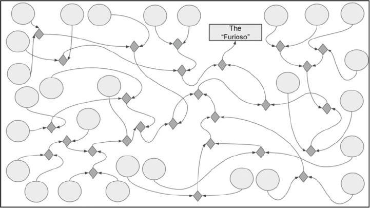
CHAPTER 7 ■ THE MANAGER: APACHE MESOS
132
After the activity, the question was if it is possible to find the champion in less time. It was definitely
possible, but the question was designed to define a strategy. The discussed proposal to remove noise and
disorder concluded that there should be people whose function was locate and “match” winners, which
should expedite the activity.
To give order, these people should also be organized between them to perform their task more
efficiently. These people could also be called coordinators .
Each match requires two participants and generates a winner. You can see that to reach the final match,
the finalists had to win more games than others.
In Figure 7-2 , you can see the first variant to the solution to make our championship more agile. You
might call this dynamic a process .
Figure 7-1. Sequence to find the rock-paper-scissors champion
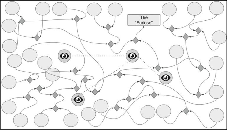
CHAPTER 7 ■ THE MANAGER: APACHE MESOS
133
Our process has something different in this first variant: it uses coordinators.
Now, what happens if you want to more strictly validate each match?
While the coordinators are in communication, the participants may not properly perform a match,
so you must rely on coordinators not for only gain speed but also to ensure that the process is successfully
completed.
A second approach is to generate two large groups (with few coordinators), and in each of these groups,
the coordinator is responsible for validating each match. The winner is sent to a pool of partial winners (that
have won at least one time, but they are not still champions). Two participants are taken from this pool and
the match is made (with supervision of a third coordinator), the winner returns to the pool and the loser is
eliminated from the game.
This pool coordinator is in constant communication with the other two to speed up (or pause) the
participants’ flow. At the end, there is only one winner.
Figure 7-3 shows the implementation of the second variant.
Figure 7-2. Sequence to find the rock-paper-scissors champion using just one main coordinator
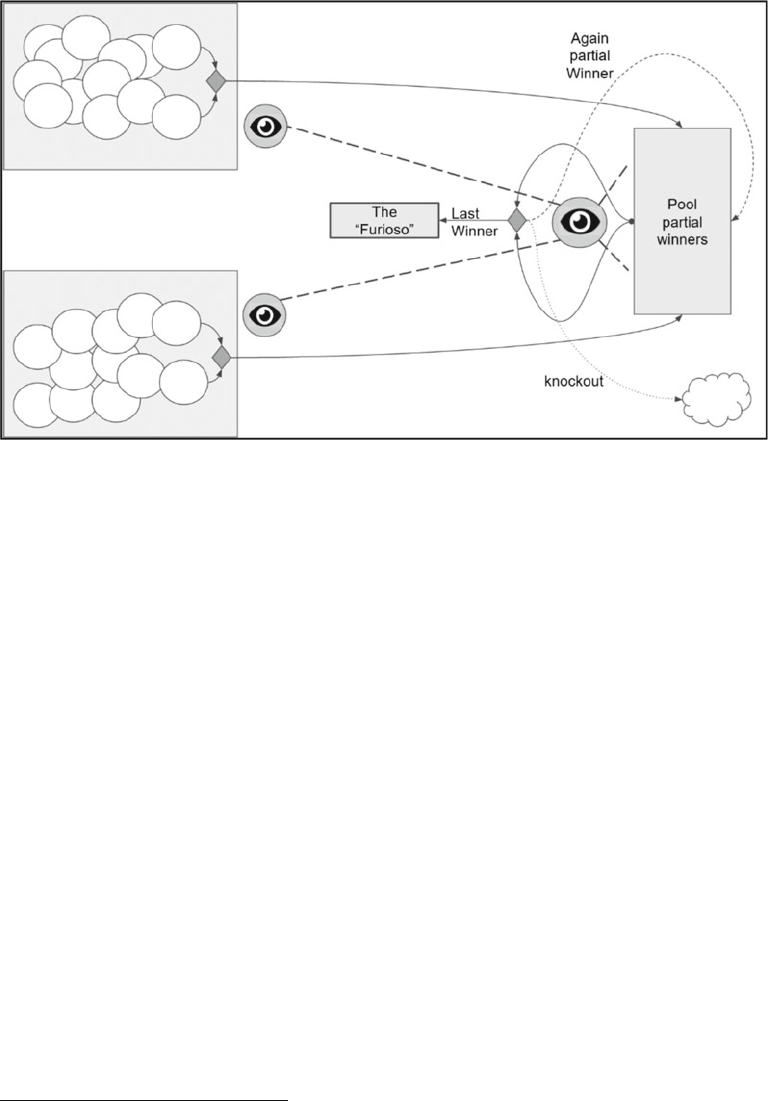
CHAPTER 7 ■ THE MANAGER: APACHE MESOS
134
Figure 7-3. Sequence to find the rock-paper-scissors champion using a main coordinator and ordering the
execution
At this point, you are probably already considering a better strategy to achieve the successful
completion of these tasks. And if theory is correct, the solution should have something to help coordinate
and something to help distribute, so distributes et impera is the modern “divide and conquer.”
Surely, you’re thinking that this exercise is used to illustrate only the concurrency, and that is true. It
is also true that distributed systems make use of concurrency to achieve their goals. If you are particularly
interested in the concurrency topics, you can see another example that clearly and in a fun way shows the
importance of having a coordinator agent in problem resolution.
In the presentation “Concurrency Is Not Parallelism,”
2 Rob Pike, the GO language creator, shows an
interesting example where communication works as “coordinator.” In any case, we decided to tackle the
example from the audience perspective, as we experienced on the meetup.
With this little anecdote, you begin to see what the distribution task involves.
Distributed Systems
To talk about distributed systems today is to talk about how the Internet works.
The Internet is a huge system that shares hardware and software for different purposes; one of them is
to enjoy the Web (http). Today, saying that a system shares hardware and software seems very simple, but it
is still complex.
Distributed systems are not new; they have emerged as computing capacity has increased and data
manipulation has grown. Over the years, research focused on how to share resources in order to optimize tasks.
These resources could be a data repository, RAM, or a printer if you are looking at sharing both physical
and logical resources. But what happens if two people try to access the same resource at the same time?
2 https://blog.golang.org/concurrency-is-not-parallelism
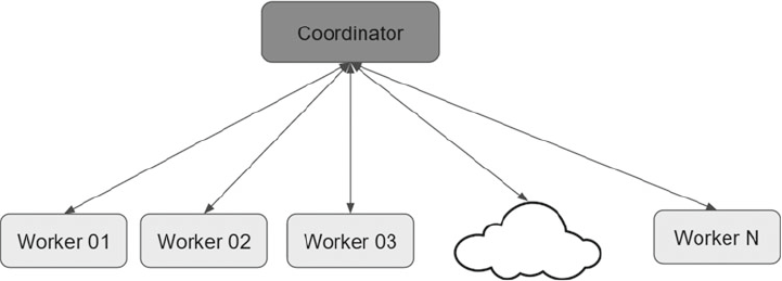
CHAPTER 7 ■ THE MANAGER: APACHE MESOS
135
In earlier days, new requirements encouraged the creation of models that allowed concurrency. Once
concurrency and resource sharing were satisfied, new needs appeared. How to add a new resource to the
system? How to make the entire system scalable?
In these past few paragraphs, we touched on the key points that evolved so that we could have today’s
distributed systems.
It is still difficult to implement a distributed system and thus new tools emerge; one of them is Apache
Mesos, which is what this chapter is about.
Figure 7-4 shows the importance of a distributed systems coordinator.
Figure 7-4. Distributed system anatomy
Why Are They Important?
Reliability and availability (also called high availability ) are the two basic characteristics in today’s systems.
Having information always available and having access to a vital process in economic, healthcare, and
government scopes are requirements that we assume already done. If you also add the growth of users to
a critical system (or a popular system, in the case of the Internet) is almost geometric in some cases, which
requires these systems to be scalable and flexible.
All of these features were achieved years ago, but now they can be achieved at low cost. With few
resources carrying the ease-of-use to other systems, we can take the distributed systems benefits available at
new levels.
It Is Difficult to Have a Distributed System
There are several tasks that must be inherently performed when having a distributed system. This includes
not only monitoring what is happening, but also making a deployment in a whole cluster. It is a task that
must not jeopardize the current version but must reach all the nodes. Each deploy implies a process to
ensure that all nodes are ready to accept it.
And finally, we need to know which resources are available within the entire cluster, which are down
(a node could go down for any reason), and which were recently added (when a new node is added to the
cluster).
All of this results in high-cost data centers, where every hour of wasted time can lead to unnecessary but
costly businesses expenses.
In summary, it’s not easy to implement and maintain a distributed system. Figure
7-5 shows some of the
main problems of working with distributed environments when increasing the number of nodes.
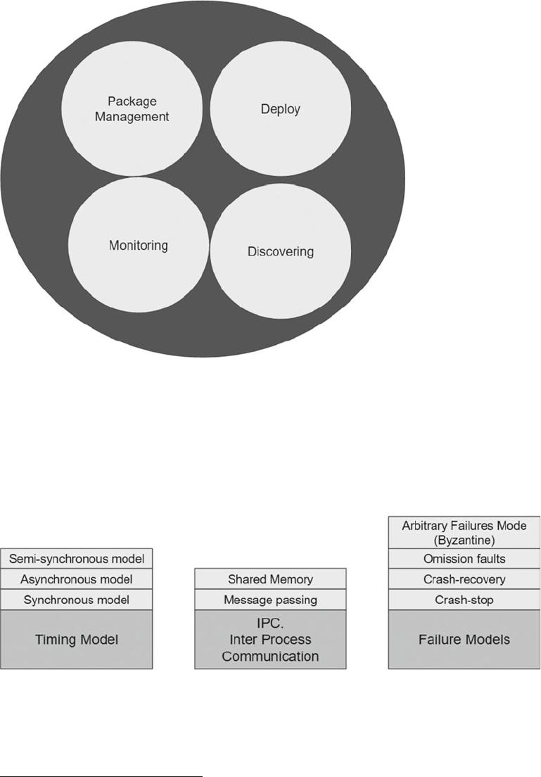
CHAPTER 7 ■ THE MANAGER: APACHE MESOS
136
Part of the complexity of a distributed system is due to its foundation and the way it is implemented,
In the presentation “What You Talk About When You Talk About Distributed Systems,”
3 is discussed
the importance of the fundamentals of distributed systems and reminds us of some of the models that are
currently used to implement them.
Figure 7-6 summarizes some of these models .
Figure 7-5. Typical distributed system tasks that increase the complexity regardless the number of nodes
Figure 7-6. The main distributed models and their implementations
3 https://www.infoq.com/presentations/topics-distributed-systems
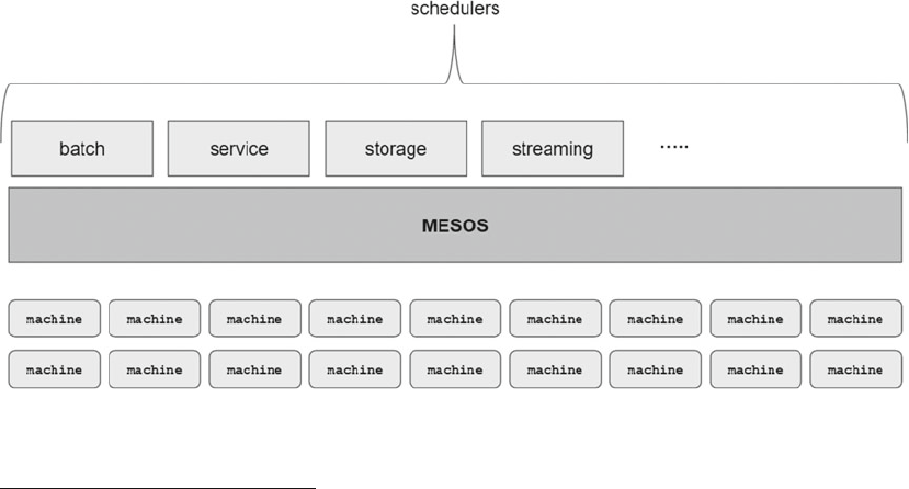
CHAPTER 7 ■ THE MANAGER: APACHE MESOS
137
4 http://videlalvaro.github.io/2015/12/learning-about-distributed-systems.html
5 “Mesos: A Platform for Fine-Grained Resource Sharing in the Data Center” by Benjamin Hindman, Andy Konwinski,
Matei Zaharia, Ali Ghodsi, Anthony D. Joseph, Randy Katz, Scott Shenker, Ion Stoica,
http://people.csail.mit.
edu/matei/papers/2011/nsdi_mesos.pdf
Each of these models has its own implications, so it is possible that a feasible model for one scenario
is not feasible for another scenario. Delving into the world of distributed systems requires a lot of theory.
There is so much material on the subject that there is a post to complement this presentation. If you find this
particular topic interesting, you can find more about it here.
4
In short, it is not easy to implement and maintain a distributed system.
Ta-dah!! Apache Mesos
And it is in this context that Apache Mesos appeared on the scene in 2010.
5 Discussion of distributed systems
a few years ago was about data centers. Having different machines (physical or virtual) connected together,
and making them “seen” as a single large machine is something that data centers already do well, or at least
somewhat good. The objective is to abstract Mesos as many layers that make up a distributed system; in this
case, a data center system.
A Mesos goal is to program and deploy an application in a data center in the same way that it is done on a
PC or a mobile device. Achieving this goal and having it supported on different frameworks is discussed later.
Although tools such as Ansible or Puppet can handle a certain number of nodes, performing the
packaging and deployment tasks usually generate some interesting challenges. The use of resources of a
large machine represents another challenge for data centers, it is common to run into some scenarios where
once added more nodes to the cluster, the CPU usage is uneven, thus wasting much of that large machine
computation power. Usually, this large machine is actually a cluster with several nodes.
The tricky part comes when we have several clusters.
And it is here that Mesos comes in. Mesos is essentially a “general purpose cluster manager,” or a
mechanism to administer several large machines used to drive a data center. This “general purpose”
administration means that Mesos not only manages and schedules batch processes but also other processes.
Figure 7-7 shows the different types of processes that can be scheduled in Apache Mesos.
Figure 7-7. Mesos is a general-purpose cluster manager, not only focused on batch scheduling
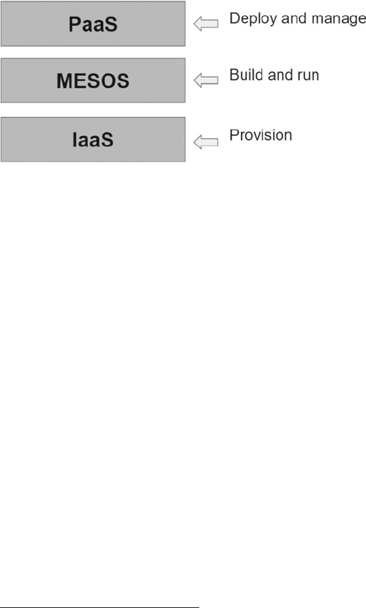
CHAPTER 7 ■ THE MANAGER: APACHE MESOS
138
Apache Mesos tries to solve problems inherent to distributed systems. It tries not only to be a manager
but a whole cluster execution platform powered by the (Mesos) frameworks.
Mesos Framework
One way to better understand the Mesos architecture is with Figure 7-8 . Mesos requires a layer on which
provisioning functions, and then a top layer to expose applications.
Figure 7-8. Level of abstraction in Mesos
In each of these layers, Mesos requires components that allow the service deployment, service finding,
and keep running those services. The frameworks we discuss in this chapter cover some of these tasks.
ZooKeeper discovers services. Chronos is responsible for scheduling the services. Marathon and Aurora
are responsible for executing the services. These are not the only frameworks to perform the tasks, but they
are the most commonly used.
A r c h i t e c t u r e
The Apache Mesos official documentation begins with a chart that shows its powerful architecture .
6
Mesos consists of master servers, which can handle as many slaves as they receive (up to 10,000
according to the documentation). These slaves manage software components called Mesos frameworks,
which are responsible for task execution.
With this scheme, we can see the importance of the frameworks.
Every framework has two parts: a scheduler that records the services offered by the master and slave
nodes or servers that process the tasks to be executed.
You can read more about architecture in an MIT paper “Mesos: A Platform for Fine-Grained Resource
Sharing in the Data Center” by Benjamin Hindman, Andy Konwinski, Matei Zaharia, Ali Ghodsi, Anthony D.
Joseph, Randy Katz, Scott Shenker, and Ion Stoica.
7
Figures 7-9 and 7-10 are adapted from the official Mesos web site at http://mesos.apache.org . They
show an overview of the Mesos architecture and the major frameworks with which it interacts.
6 http://mesos.apache.org/documentation/latest/architecture/
7 http://people.csail.mit.edu/matei/papers/2011/nsdi_mesos.pdf
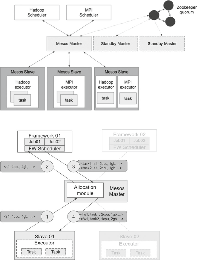
CHAPTER 7 ■ THE MANAGER: APACHE MESOS
139
Figure 7-9. Mesos architecture: master servers (only one at a time) interact with various slave servers
Figure 7-10. A framework obtains a scheduler and performs a task

CHAPTER 7 ■ THE MANAGER: APACHE MESOS
140
8 Developing Frameworks for Apache Mesos. https://www.youtube.com/watch?v=ZYoXodSlycA
In the first figure we can see that the center of all is the Mesos master, basically a daemon process that
coordinates certain number of agents (Mesos prefers to call them agents rather than servers that are part of
the cluster). These agents live in each node in a cluster. You also see an important component in the Mesos
ecosystem: ZooKeeper. Later you will learn about the importance of this component.
The second figure describes the two components that all the frameworks need to run a task: a scheduler
and an executor. While there are already a lot of Mesos frameworks ready to run, knowing the parts of
a framework is attractive not only to better understand their execution, but also to know what involves
creating your own framework.
8
Mesos 101
Now that you have an overview of the Mesos ecosystem, let’s look at Apache Mesos in action.
The Mesos ecosystem tries to work as an operating system in the data centers world; therefore, most
documentation mentions that Mesos is the kernel of the operating system. In the following pages, you will
learn the steps to install this kernel. Then you will learn how to install ZooKeeper, which is the responsible for
maintaining information synchronized across all nodes. We continue with Chronos, who keeps running all the
defined services. Finally, Marathon and Aurora are responsible for maintaining the services running, each one in
their own way.
Here we go.
Installation
You are now ready to install Mesos. The installation has three steps: get the binary, get the dependencies,
and start Mesos. Something very important to keep in mind is that there is no installer to perform all the
steps. Mesos takes advantage of the capabilities of each operating system and therefore must make a
compilation of components to leverage the capabilities of the native environment.
Generating native libraries by platform optimizes the performance.
If you’re not going to compile with the make command, do not worry, the script is very complete and
does almost all the work for you. As you shall see, the installation only requires to meet the dependencies to
compile correctly.
Get the Installer
When this book was written, the stable version of Apache Mesos was 0.28.1.
For a step-by-step installation , follow the guide provided at this web page:
http://mesos.apache.org/gettingstarted/
This guide recommends downloading the latest stable distributable, as follows:
wget http://www.apache.org/dist/mesos/0.28.1/mesos-0.28.1.tar.gz
The following is the downloaded file size:
-rw-r--r--. 1 rugi rugi 29108023 Apr 13 15:07 mesos-0.28.1.tar.gz
Unpack it with this:
%>tar -zxf mesos-0.28.1.tar.gz
CHAPTER 7 ■ THE MANAGER: APACHE MESOS
141
A folder called mesos-0.28-1 should be created with this content:
-rw-r--r-- 1 isaacruiz staff 414 Apr 5 20:25 mesos.pc.in
-rw-r--r-- 1 isaacruiz staff 60424 Apr 5 20:25 configure.ac
-rwxr-xr-x 1 isaacruiz staff 3647 Apr 5 20:25 bootstrap
-rw-r--r-- 1 isaacruiz staff 1111 Apr 5 20:25 README.md
-rw-r--r-- 1 isaacruiz staff 162 Apr 5 20:25 NOTICE
-rw-r--r-- 1 isaacruiz staff 3612 Apr 5 20:25 Makefile.am
-rw-r--r-- 1 isaacruiz staff 28129 Apr 5 20:25 LICENSE
-rw-r--r-- 1 isaacruiz staff 324089 Apr 5 20:25 ltmain.sh
-rw-r--r-- 1 isaacruiz staff 46230 Apr 5 20:25 aclocal.m4
-rwxr-xr-x 1 isaacruiz staff 860600 Apr 5 20:25 configure
-rwxr-xr-x 1 isaacruiz staff 6872 Apr 5 20:25 missing
-rwxr-xr-x 1 isaacruiz staff 14675 Apr 5 20:25 install-sh
-rwxr-xr-x 1 isaacruiz staff 23566 Apr 5 20:25 depcomp
-rwxr-xr-x 1 isaacruiz staff 35987 Apr 5 20:25 config.sub
-rwxr-xr-x 1 isaacruiz staff 42938 Apr 5 20:25 config.guess
-rwxr-xr-x 1 isaacruiz staff 7333 Apr 5 20:25 compile
-rwxr-xr-x 1 isaacruiz staff 5826 Apr 5 20:25 ar-lib
-rw-r--r-- 1 isaacruiz staff 45159 Apr 5 20:25 Makefile.in
drwxr-xr-x 4 isaacruiz staff 136 Apr 5 20:28 support
drwxr-xr-x 5 isaacruiz staff 170 Apr 5 20:28 mpi
drwxr-xr-x 3 isaacruiz staff 102 Apr 5 20:28 include
drwxr-xr-x 23 isaacruiz staff 782 Apr 5 20:28 bin
drwxr-xr-x 13 isaacruiz staff 442 Apr 5 20:28 3rdparty
drwxr-xr-x 43 isaacruiz staff 1462 Apr 5 20:28 src
drwxr-xr-x 15 isaacruiz staff 510 May 8 18:40 m4
Once unzipped, go to the mesos-0.28-1 directory, as follows:
%>cd mesos-0.28-1
Make a directory called build and then go to this directory:
%>mkdir build
%>cd build
Inside this folder, start generating the binaries for your machine:
%>../configure
%>make
The make operation can take a lot of time because in addition to dependency compilation, your
machine configuration may be responsible for downloading and configuring the scripts to run Mesos.
If you have a modern computer, you probably have more than one processor. You can speed up the
process by using the make command to indicate the number of processors that you have and by suppressing
the console outputs (without verbose mode), as shown in the following:
%>make -j 2 V=0
This command indicates that you have a machine with two processors and you don’t want verbosity.
In Unix/Linux operating systems, we can see the status with the %>nproc or %>lscpu commands.

CHAPTER 7 ■ THE MANAGER: APACHE MESOS
142
Missing Dependencies
The installation process is still in improvement, particularly because the compilation relies heavily on the
computer characteristics in which we want to install Apache Mesos.
The compilation process assumes that we have all the required libraries for compiling; therefore, at
http://mesos.apache.org/gettingstarted/ are listed the required libraries for the following operating
systems:
• Ubuntu 14.04
• Mac OS: Yosemite and El Capitan
• CentOS 6.6
• CentOS 7.2
We strongly suggest to investigate before making an installation; also, install the following libraries on
your computer according to your operating system and version:
libcurl
libapr-1
These are typically two missing dependencies .
If you use yum or apt-get , lean on the search options offered by each tool. If you are trying to install on
a Mac, before anything, run the following command to ensure that you have the developer tools updated in
the command line.
xcode-select --install
■ Note Ensure the libraries’ compatibility. The make command execution is a task that could exceed the 20
minutes. Be patient; it is always difficult to use something earlier than version 1.0.
Start Mesos
Once past the dependencies and make construction stages, starting Mesos is very simple, just need to run
two lines.
Master Server
The first line starts the master server . Since the working directory points to a system directory, be sure to run
the command as a privileged user:
%>cd build
%>./bin/mesos-master.sh --ip=127.0.0.1 --work_dir=/var/lib/mesos
CHAPTER 7 ■ THE MANAGER: APACHE MESOS
143
This is the typical console output:
%>./bin/mesos-master.sh --ip=127.0.0.1 --work_dir=/var/lib/mesos
I0508 16:48:54.315554 2016645120 main.cpp:237] Build: 2016-05-08 16:20:08 by isaacruiz
I0508 16:48:54.315907 2016645120 main.cpp:239] Version: 0.28.1
I0508 16:48:54.315989 2016645120 main.cpp:260] Using 'HierarchicalDRF' allocator
I0508 16:48:54.320935 2016645120 leveldb.cpp:174] Opened db in 4589us
I0508 16:48:54.323814 2016645120 leveldb.cpp:181] Compacted db in 2845us
I0508 16:48:54.323899 2016645120 leveldb.cpp:196] Created db iterator in 32us
I0508 16:48:54.323932 2016645120 leveldb.cpp:202] Seeked to beginning of db in 18us
I0508 16:48:54.323961 2016645120 leveldb.cpp:271] Iterated through 0 keys in the db in 20us
I0508 16:48:54.325166 2016645120 replica.cpp:779] Replica recovered with log positions 0 ->
0 with 1 holes and 0 unlearned
I0508 16:48:54.336277 528384 recover.cpp:447] Starting replica recovery
I0508 16:48:54.338512 2016645120 main.cpp:471] Starting Mesos master
I0508 16:48:54.357270 528384 recover.cpp:473] Replica is in EMPTY status
I0508 16:48:54.368338 2016645120 master.cpp:375] Master 7f7d9b4b-c5e4-48be-bbb7-78e6fac701ea
(localhost) started on 127.0.0.1:5050
I0508 16:48:54.368404 2016645120 master.cpp:377] Flags at startup: --allocation_
interval="1secs" --allocator="HierarchicalDRF" --authenticate="false" --authenticate_
http="false" --authenticate_slaves="false" --authenticators="crammd5" --authorizers="local"
--framework_sorter="drf" --help="false" --hostname_lookup="true" --http_
authenticators="basic" --initialize_driver_logging="true" --ip="127.0.0.1" --log_auto_
initialize="true" --logbufsecs="0" --logging_level="INFO" --max_completed_frameworks="50"
--max_completed_tasks_per_framework="1000" --max_slave_ping_timeouts="5" --port="5050"
--quiet="false" --recovery_slave_removal_limit="100%" --registry="replicated_log"
--registry_fetch_timeout="1mins" --registry_store_timeout="20secs" --registry_strict="false"
--root_submissions="true" --slave_ping_timeout="15secs" --slave_reregister_timeout="10mins"
--user_sorter="drf" --version="false" --webui_dir="/Users/isaacruiz/Downloads/mesos/
mesos-0.28.1/build/../src/webui" --work_dir="/var/lib/mesos" --zk_session_timeout="10secs"
W0508 16:48:54.378363 2016645120 master.cpp:380]
**************************************************
Master bound to loopback interface! Cannot communicate with remote schedulers or slaves. You
might want to set '--ip' flag to a routable IP address.
**************************************************
S l a v e S e r v e r
The second line is responsible for starting the first Mesos slave server :
%>cd build
%> ./bin/mesos-slave.sh --master=127.0.0.1:5050
This is the typical console output:
%>./bin/mesos-slave.sh --master=127.0.0.1:5050
I0508 16:49:09.586303 2016645120 main.cpp:223] Build: 2016-05-08 16:20:08 by isaacruiz
I0508 16:49:09.587652 2016645120 main.cpp:225] Version: 0.28.1
I0508 16:49:09.588884 2016645120 containerizer.cpp:149] Using isolation: posix/cpu,posix/
mem,filesystem/posix
CHAPTER 7 ■ THE MANAGER: APACHE MESOS
144
I0508 16:49:09.627917 2016645120 main.cpp:328] Starting Mesos slave
I0508 16:49:09.630908 3747840 slave.cpp:193] Slave started on 1)@192.168.1.5:5051
I0508 16:49:09.630956 3747840 slave.cpp:194] Flags at startup: --appc_simple_discovery_
uri_prefix="http://" --appc_store_dir="/tmp/mesos/store/appc" --authenticatee="crammd5"
--container_disk_watch_interval="15secs" --containerizers="mesos" --default_role="*"
--disk_watch_interval="1mins" --docker="docker" --docker_kill_orphans="true" --docker_
registry="https://registry-1.docker.io" --docker_remove_delay="6hrs" --docker_socket="/
var/run/docker.sock" --docker_stop_timeout="0ns" --docker_store_dir="/tmp/mesos/store/
docker" --enforce_container_disk_quota="false" --executor_registration_timeout="1mins"
--executor_shutdown_grace_period="5secs" --fetcher_cache_dir="/tmp/mesos/fetch" --fetcher_
cache_size="2GB" --frameworks_home="" --gc_delay="1weeks" --gc_disk_headroom="0.1"
--hadoop_home="" --help="false" --hostname_lookup="true" --image_provisioner_backend="copy"
--initialize_driver_logging="true" --isolation="posix/cpu,posix/mem" --launcher_dir="/Users/
isaacruiz/Downloads/mesos/mesos-0.28.1/build/src" --logbufsecs="0" --logging_level="INFO"
--master="127.0.0.1:5050" --oversubscribed_resources_interval="15secs" --port="5051"
--qos_correction_interval_min="0ns" --quiet="false" --recover="reconnect" --recovery_
timeout="15mins" --registration_backoff_factor="1secs" --sandbox_directory="/mnt/mesos/
sandbox" --strict="true" --switch_user="true" --version="false" --work_dir="/tmp/mesos"
I0508 16:49:39.704506 3747840 slave.cpp:464] Slave resources: cpus(*):2; mem(*):7168;
disk(*):482446; ports(*):[31000-32000]
I0508 16:49:39.704661 3747840 slave.cpp:472] Slave attributes: [ ]
I0508 16:49:39.704684 3747840 slave.cpp:477] Slave hostname: 192.168.1.5
I0508 16:49:39.719388 1064960 state.cpp:58] Recovering state from '/tmp/mesos/meta'
I0508 16:49:39.720755 4284416 status_update_manager.cpp:200] Recovering status update
manager
I0508 16:49:39.721927 4284416 containerizer.cpp:407] Recovering containerizer
I0508 16:49:39.728039 2674688 provisioner.cpp:245] Provisioner recovery complete
I0508 16:49:39.728682 3211264 slave.cpp:4565] Finished recovery
I0508 16:49:39.732142 2138112 status_update_manager.cpp:174] Pausing sending status updates
I0508 16:49:39.732161 3211264 slave.cpp:796] New master detected at master@127.0.0.1:5050
I0508 16:49:39.733449 3211264 slave.cpp:821] No credentials provided. Attempting to register
without authentication
I0508 16:49:39.733577 3211264 slave.cpp:832] Detecting new master
I0508 16:49:40.588644 2138112 slave.cpp:971] Registered with master master@127.0.0.1:5050;
given slave ID 7f7d9b4b-c5e4-48be-bbb7-78e6fac701ea-S0
I0508 16:49:40.589226 528384 status_update_manager.cpp:181] Resuming sending status updates
I0508 16:49:40.589984 2138112 slave.cpp:1030] Forwarding total oversubscribed resources
Like the other frameworks covered in this book, keep running the both commands to run successfully;
first the master server and then the slave server.
In Figure 7-11 , we can see the both windows running simultaneously.
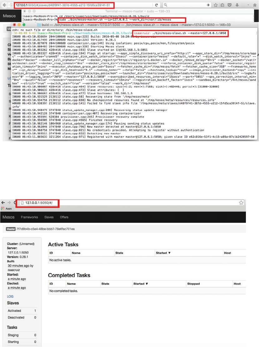
CHAPTER 7 ■ THE MANAGER: APACHE MESOS
145
Figure 7-11. Two consoles showing the execution, in front the master server, and in back a slave server
At this point, with the master and slave started, it’s already possible to access the Mesos web console.
The console listens on port 5050. Thus, open your favorite browser and go to
http://127.0.0.1:5050 . See
the Apache Mesos main screen running with one slave server. In Figure
7-12 , you see the main screen of the
Mesos console.
Figure 7-12. Mesos server main screen running
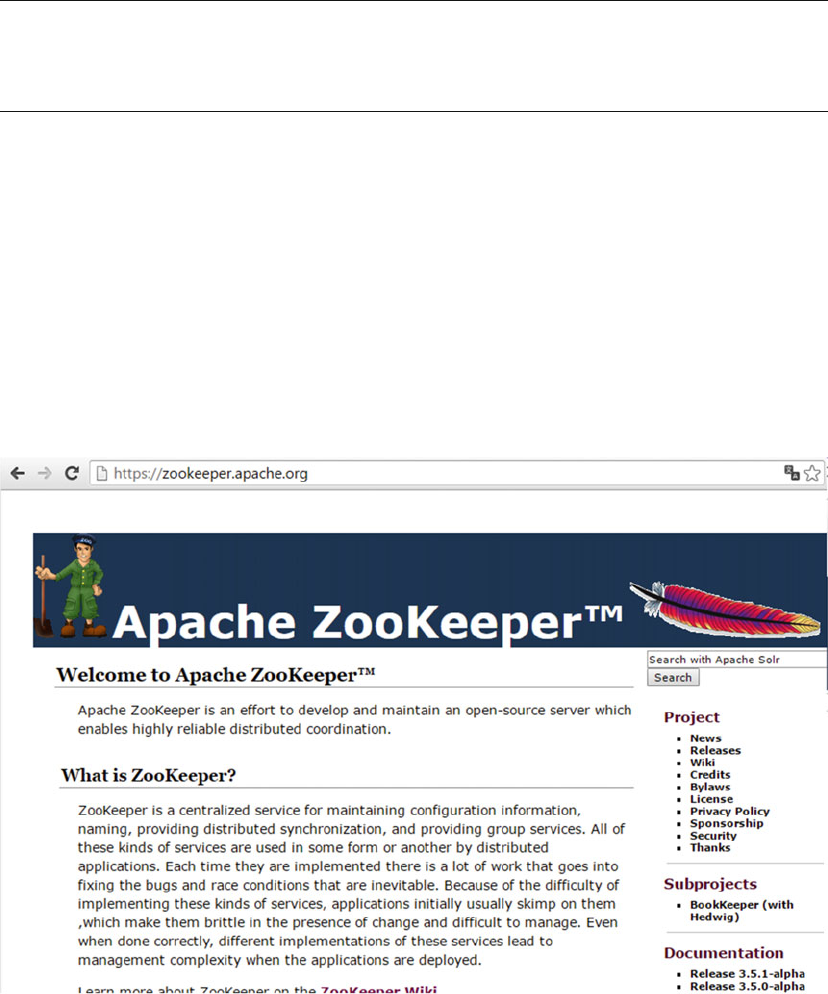
CHAPTER 7 ■ THE MANAGER: APACHE MESOS
146
Figure 7-13. The Apache ZooKeeper home page
■ Note Before continuing, have at hand the location of the libmesos.so file (or the libmesos.dylib file if
compiling on a Mac with OS X). This file is required to integrate with frameworks, as discussed next. Use the
find -name * libmesos.. command to locate it.
Teaming
Although Mesos has still not reached version 1.0, there are already several frameworks that contribute to a
robust ecosystem and perfectly complement the Mesos objectives. In particular, there are four frameworks
to know: ZooKeeper, Chronos, Marathon, and Aurora.
ZooKeeper
The official site of the ZooKeeper framework tells us that it is a centralized naming service, which
simultaneously allows to maintain configuration information in a distributed way.
Figure 7-13 shows the Apache ZooKeeper home page .
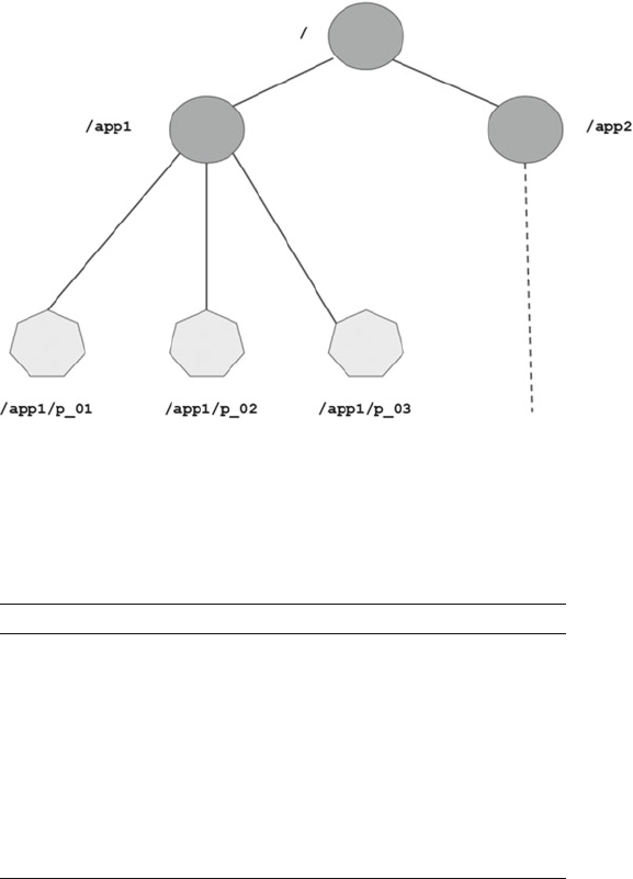
CHAPTER 7 ■ THE MANAGER: APACHE MESOS
147
Do you remember the diagram showing the Mesos architecture? ZooKeeper’s strength is to keep
distributed processes through service replication; customers connect to multiple servers (there is one main
server) and from there, they get the information they need.
To manage the information, ZooKeeper creates a distributed namespace (see Figure
7-14 ) across all
nodes; this namespace is similar to a standard file system.
Figure 7-14. ZooKeeper namespace
ZooKeeper was designed to be simple to use. The API only has seven messages, as shown in Table
7-1 .
Table 7-1. Messages in the ZooKeeper API
Message Definition
create Creates a node at a location in the three.
delete Deletes a node.
exist Tests if a node exists at a location.
get data Reads the data from the node.
set data Writes data to a node.
get children Retrieves a list of a node’s children.
sync Waits for data to be propagated.
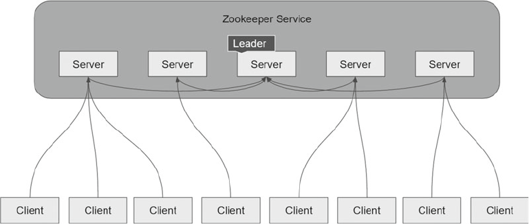
CHAPTER 7 ■ THE MANAGER: APACHE MESOS
148
Figure 7-15 shows how ZooKeeper maintains high availability with the services scheduled. There is
a main server (leader). All servers know each other and they all keep their status in memory. While more
servers are active, the availability of services is assured.
Figure 7-15. ZooKeeper service
Clients, meanwhile, connect to a single server. A TCP connection maintains communication with this
server (sending heartbeats). If something happens to the server, the client only connects to another server.
Installation
At the time of this writing, the stable version of ZooKeeper was 3.4.6. The installation process is simple.
Download the binary file of the latest stable version from this web page:
http://zookeeper.apache.org/releases.html
The tar.gz file for this version has the following size:
Mode LastWriteTime Length Name
---- ------------- ------ ----
-a---- 15/05/2016 08:17 a. m. 17699306 zookeeper-3.4.6.tar.gz
Once unzipped, the first is to create a configuration file; the configuration file must be named zoo.cfg
and it must be located in the conf/ directory.
By default, the conf/ directory has as an example file where the parameters to set are described in detail.
In short, a zoo.cfg file must have at least the following values:
/opt/apache/zookeeper/zookeeper-3.4.6/conf%> vi zoo.cfg
tickTime=2000
initLimit=10
syncLimit=5
dataDir=/tmp/zookeeper
clientPort=2181
CHAPTER 7 ■ THE MANAGER: APACHE MESOS
149
The same directory has a sample file; we can copy its contents to our zoo.cfg file.
Once the zoo.cfg file is configured, to check the status to validate the ZooKeeper configuration file
location and execution mode run this command.
~/opt/apache/zookeeper/zookeeper-3.4.6/bin%>./zkServer.sh status
JMX enabled by default
Using config: /Users/isaacruiz/opt/apache/zookeeper/zookeeper-3.4.6/bin/../conf/zoo.cfg
Mode: standalone
If we run only the zKServer.sh file, we can see the list of tasks that can be used with the ZooKeeper
binary (be sure to execute instructions with a user that has enough privileges):
~/opt/apache/zookeeper/zookeeper-3.4.6/bin%>./zkServer.sh
Password:
JMX enabled by default
Using config: /users/isaacruiz/opt/apache/zookeeper/zookeeper-3.4.6/bin/../conf/zoo.cfg
Usage: ./zkServer.sh {start|start-foreground|stop|restart|status|upgrade|print-cmd}
{16-05-10 21:24}:~/opt/apache/zookeeper/zookeeper-3.4.6/bin isaacruiz%
As you can see, we have the following tasks:
start, start-foreground, stop, restart, status, upgrade, print-cmd
Now, to start ZooKeeper.
~/opt/apache/zookeeper/zookeeper-3.4.6/bin%>./zkServer.sh start
JMX enabled by default
Using config: /users/isaacruiz/opt/apache/zookeeper/zookeeper-3.4.6/bin/../conf/zoo.cfg
Starting zookeeper ... STARTED
{16-05-10 21:24} opt/apache/zookeeper/zookeeper-3.4.6/bin isaacruiz%
Chronos
The second component is Chronos , the substitute for the cron sentence in the Mesos context. The home
page of this project is at
https://mesos.github.io/chronos/ .
If you’ve used a Unix-based operating system, have probably performed the repetitive execution of
a process using this operating system utility. Chronos does the same; it is a task scheduler. Only in the
Chronos context, it is a distributed task scheduler, and in addition to isolating tasks, it can orchestrate them.
Another advantage of Chronos is to schedule tasks using the ISO 8601 8; the notation offered by this
standard is much friendlier in specifying the time intervals to execute tasks. Chronos runs directly on Mesos.
It is the first line of interaction with the outside world. Its integration is in both the master and the slave
servers, and through this communication manages the records of the jobs to be done.
The Chronos architecture is shown in Figure
7-16 .
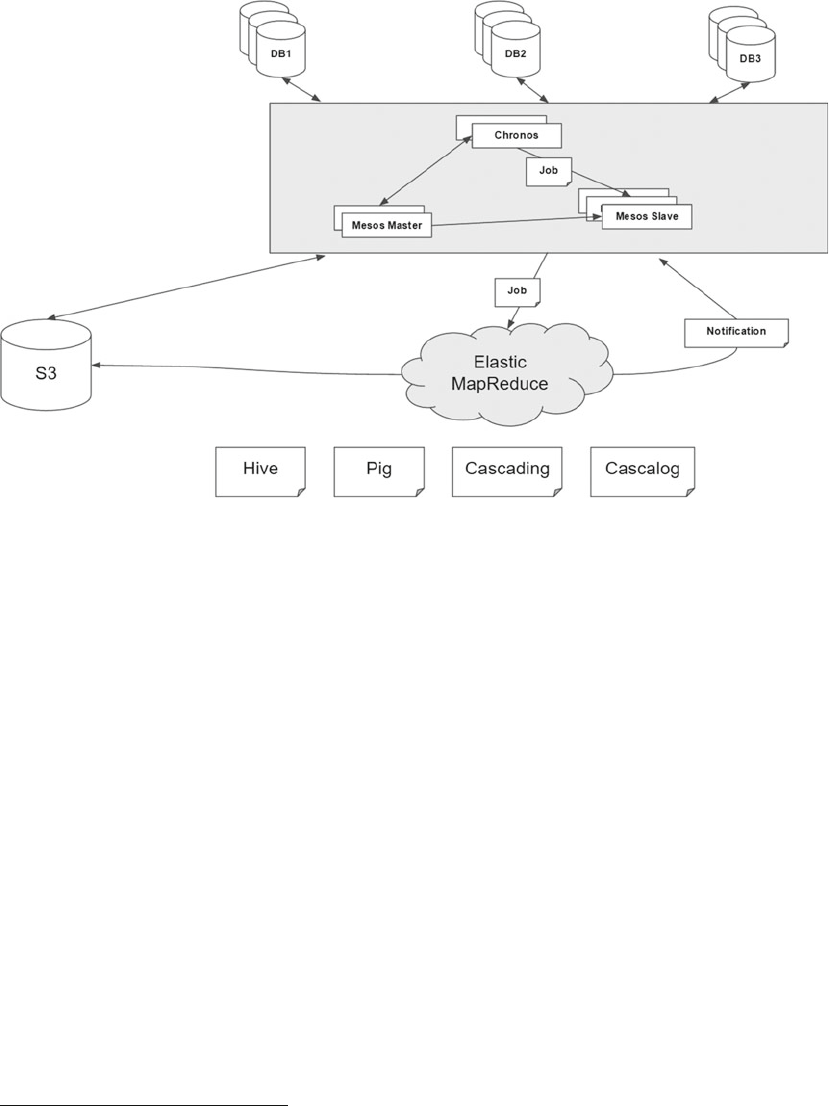
CHAPTER 7 ■ THE MANAGER: APACHE MESOS
150
Installation
At the time of this writing, the stable Chronos version was 2.4.0. Having a mature version, the installation
process is simple, but it is a little slow for the binary generation of the platform where it is used.
The installation process assumes that you have already installed a version of Mesos (0.20.x) and
ZooKeeper. And have also installed Apache Maven 3.x and JDK 1.6 or higher.
The installation process begins by downloading the binary from the home page:
9
curl -0 https://github.com/mesos/chronos/archive/2.3.4.tar.gz
tar xvf 2.3.4.tar.gz
Once the file is decompressed, note that the main folder contains the POM files required by Maven to
perform their tasks.
The directory contents should be similar to the following:
~/opt/apache/chronos/chronos-2.4.0%> ls -lrt
total 104
drwxr-xr-x@ 4 isaacruiz staff 136 Aug 28 2015 src
-rw-r--r--@ 1 isaacruiz staff 17191 Aug 28 2015 pom.xml
drwxr-xr-x@ 14 isaacruiz staff 476 Aug 28 2015 docs
-rw-r--r--@ 1 isaacruiz staff 2521 Aug 28 2015 changelog.md
Figure 7-16. Chronos architecture
9 https://mesos.github.io/chronos/docs/
CHAPTER 7 ■ THE MANAGER: APACHE MESOS
151
-rw-r--r--@ 1 isaacruiz staff 1165 Aug 28 2015 build.xml
drwxr-xr-x@ 13 isaacruiz staff 442 Aug 28 2015 bin
-rw-r--r--@ 1 isaacruiz staff 3087 Aug 28 2015 README.md
-rw-r--r--@ 1 isaacruiz staff 837 Aug 28 2015 NOTICE
-rw-r--r--@ 1 isaacruiz staff 11003 Aug 28 2015 LICENSE
-rw-r--r--@ 1 isaacruiz staff 470 Aug 28 2015 Dockerfile
The only thing remaining is to run the mvn package to generate the .jar file used to start Chronos.
~/opt/apache/chronos/chronos-2.4.0%> mvn package
[INFO] Scanning for projects...
[INFO]
[INFO] ------------------------------------------------------------------------
[INFO] Building chronos 2.4.0
[INFO] ------------------------------------------------------------------------
Downloading: https://repo1.maven.org/maven2/org/apache/maven/plugins/maven-antrun-
plugin/1.7/maven-antrun-plugin-1.7.pom
Downloaded: https://repo1.maven.org/maven2/org/apache/maven/plugins/maven-antrun-plugin/1.7/
maven-antrun-plugin-1.7.pom (5 KB at 0.5 KB/sec)
Downloading: https://repo1.maven.org/maven2/org/apache/maven/plugins/maven-antrun-
plugin/1.7/maven
...
...
...
Downloaded: https://repo.maven.apache.org/maven2/org/slf4j/slf4j-api/1.6.1/slf4j-api-
1.6.1.jar (25 KB at 5.9 KB/sec)
[INFO] Dependency-reduced POM written at: /Users/isaacruiz/opt/apache/chronos/chronos-2.4.0/
dependency-reduced-pom.xml
[INFO] Dependency-reduced POM written at: /Users/isaacruiz/opt/apache/chronos/chronos-2.4.0/
dependency-reduced-pom.xml
[INFO] ------------------------------------------------------------------------
[INFO] BUILD SUCCESS
[INFO] ------------------------------------------------------------------------
[INFO] Total time: 03:55 min
[INFO] Finished at: 2016-05-19T01:45:13-05:00
[INFO] Final Memory: 68M/668M
[INFO] ------------------------------------------------------------------------
This step can take time, depending on your Internet connection and your machine’s characteristics.
R u n
Having the .jar file (found in the target directory), it is possible start Chronos with the following line:
~/opt/apache/chronos/chronos-2.4.0%> java -cp target/chronos*.jar org.apache.mesos.chronos.
scheduler.Main --master zk://localhost:2181/mesos --zk_hosts localhost:2181
[2016-05-19 01:45:56,621] INFO --------------------- ( org.apache.mesos.chronos.scheduler.
Main$:26)
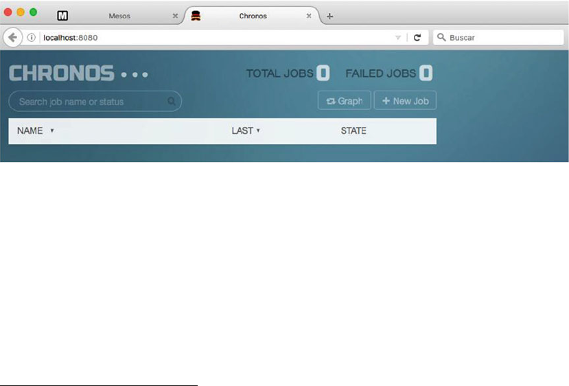
CHAPTER 7 ■ THE MANAGER: APACHE MESOS
152
[2016-05-19 01:45:56,624] INFO Initializing chronos. (org.apache.mesos.chronos.scheduler.Main$:27)
[2016-05-19 01:45:56,627] INFO --------------------- (org.apache.mesos.chronos.scheduler.Main$:28)
[2016-05-19 01:45:59,109] INFO Wiring up the application (org.apache.mesos.chronos.
scheduler.config.MainModule:39)
...
...
2016-05-19 01:46:01,446:3328(0x700002495000):ZOO_INFO@check_events@1703: initiated
connection to server [::1:2181]
2016-05-19 01:46:01,449:3328(0x700002495000):ZOO_INFO@check_events@1750: session
establishment complete on server [::1:2181], sessionId=0x154c75bb0940008, negotiated
timeout=10000
I0519 01:46:01.451170 16019456 group.cpp:349] Group process (group(1)@192.168.1.5:53043)
connected to ZooKeeper
I0519 01:46:01.452013 16019456 group.cpp:831] Syncing group operations: queue size (joins,
cancels, datas) = (0, 0, 0)
Now Apache Chronos is running.
One Chronos advantage is that is already in an advanced version; it has a web interface that allows to
manage scheduled jobs. This web interface is available in the following port:
http://localhost:8080/
F i g u r e 7-17 shows this screen.
Figure 7-17. Chronos web interface
Part of the Chronos power lies in its API,
10 from which you can better interact from other integration
points. You can easily try curl , as follows:
~/opt/apache/chronos/chronos-2.4.0%> curl -L -X GET http://localhost:8080/scheduler/jobs
[]%
Right now, there are no scheduled jobs, so both the web interface and the API report the same thing: no
scheduled tasks.
10 https://mesos.github.io/chronos/docs/api.html

CHAPTER 7 ■ THE MANAGER: APACHE MESOS
153
Marathon
Marathon is another tool that fits very well with Mesos; although it can be used independently, with Mesos it
is even more powerful, and given the integration, it is a lot easier to use.
The Marathon home page is at
https://mesosphere.github.io/marathon/ . From this page we can
download the latest stable version; at the time of this writing, the version was 1.1.1.
Figure 7-18 shows the Marathon home page .
Figure 7-18. Marathon home page
A quick way to understand Marathon is with this phrase: “A self-serve interface to your cluster.
Distributed init for long-running services.”
11
Probably you have used the init command on any Unix-based operating system that helps us to start
tasks and/or processes already defined and configured on the operating system’s host.
Marathon has a particular way to manage the tasks execution.
12 Marathon intends to help keep each
task executed by Mesos 100% available.
11 Simplifying with Mesos and Marathon. h ttps://www.youtube.com/watch?v=OgVaQPYEsVo
12 https://mesosphere.github.io/marathon/docs/
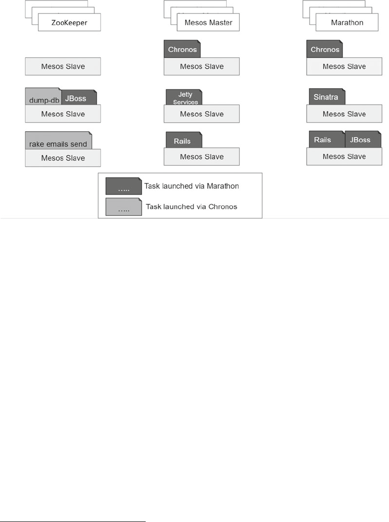
CHAPTER 7 ■ THE MANAGER: APACHE MESOS
154
Figure 7-19 shows the Marathon architecture. It is based on official documentation at
https://mesosphere.github.io/marathon/ .
Figure 7-19. Marathon architecture
13 https://github.com/mesos/chronos
In our chart, we can add the Chronos framework.
13
When Marathon starts, it launches two Chronos instances: one operates Marathon and the other exists
because Chronos is a framework that can work with Mesos. This also ensures that there will always be two
Chronos instances running and ready to receive tasks.
Installation
The main binary is downloaded directly from the Marathon home page. Once the file is decompressed, we
can start it (Marathon assumes that Mesos and ZooKeeper are already running).
Before running it, be sure to export the MESOS_NATIVE_JAVA_LIBRARY variable pointing to the route
already detected (the Marathon start file will look in /usr/lib ). When running it, check if the current os user
has read permission on system directories.
opt/apache/marathon/marathon-1.1.1/bin%>./start --master local
MESOS_NATIVE_JAVA_LIBRARY is not set. Searching in /usr/lib /usr/local/lib.
MESOS_NATIVE_LIBRARY, MESOS_NATIVE_JAVA_LIBRARY set to '/usr/local/lib/libmesos.dylib'
[2016-05-15 15:23:22,391] INFO Starting Marathon 1.1.1 with --master local
(mesosphere.marathon.Main$:main)
[2016-05-15 15:23:26,322] INFO Connecting to ZooKeeper... (mesosphere.marathon.Main$:main)
[2016-05-15 15:23:26,346] INFO Client environment:zookeeper.version=3.4.6-1569965, built on
02/20/2014 09:09 GMT (org.apache.zookeeper.ZooKeeper:main)
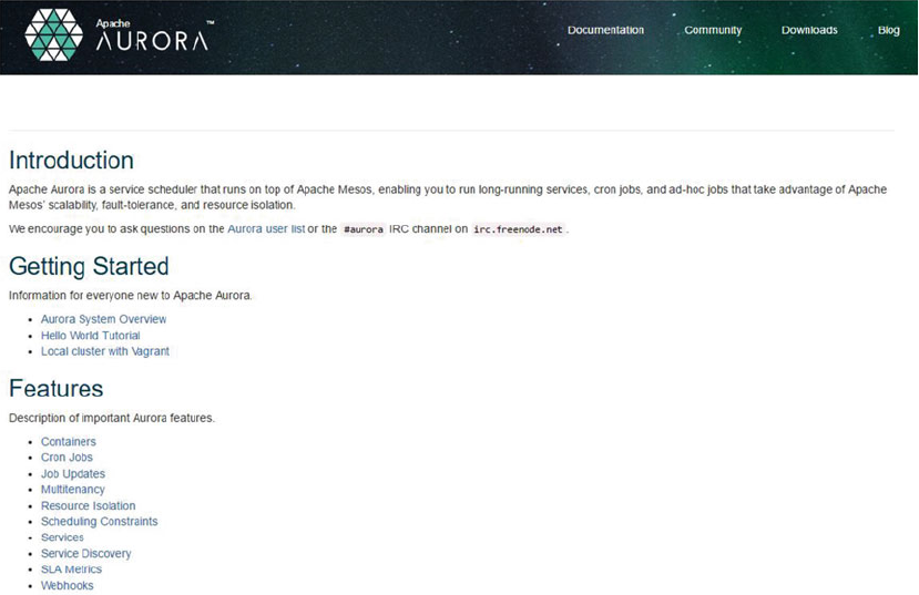
CHAPTER 7 ■ THE MANAGER: APACHE MESOS
155
[2016-05-15 15:23:26,347] INFO Client environment:host.name=192.168.1.5
(org.apache.zookeeper.ZooKeeper:main)
[2016-05-15 15:23:26,348] INFO Client environment:java.version=1.8.0_51
(org.apache.zookeeper.ZooKeeper:main)
[2016-05-15 15:23:26,349] INFO Client environment:java.vendor=Oracle Corporation
(org.apache.zookeeper.ZooKeeper:main)
[2016-05-15 15:23:26,349] INFO Client environment:java.home=/Library/Java/
JavaVirtualMachines/jdk1.8.0_51.jdk/Contents/Home/jre (org.apache.zookeeper.ZooKeeper:main)
Aurora
Aurora is one of the Mesos frameworks. (Do you remember the diagram?) Mesos requires frameworks to
retrieve a scheduler and run a task from it.
Aurora allows to run applications and services through a set of machines. Its primary responsibility is to
maintain this state of execution as long as possible; the ideal is “always.”
Figure 7-20 shows the Aurora project home page .
Figure 7-20. Aurora home page http://aurora.apache.org/
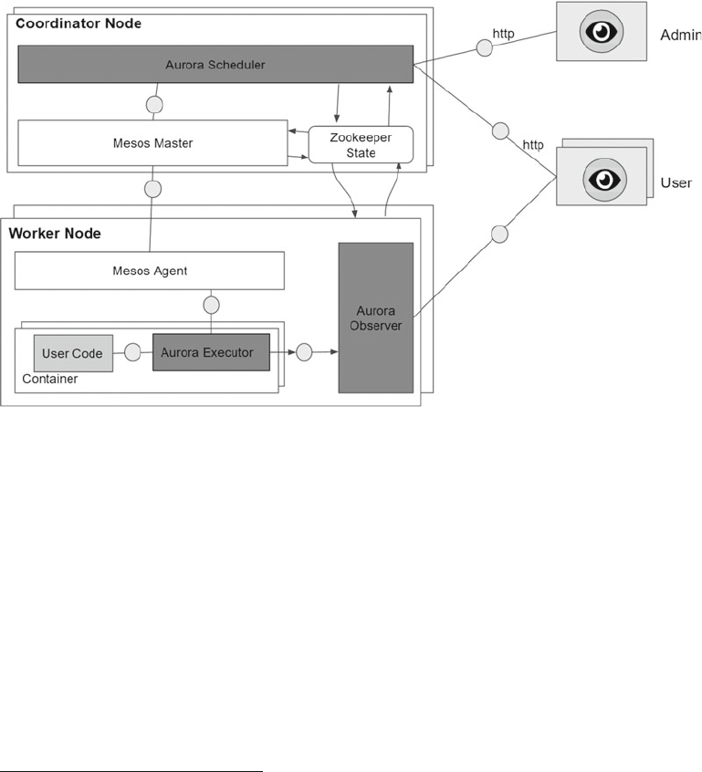
CHAPTER 7 ■ THE MANAGER: APACHE MESOS
156
If a machine fails, Aurora is responsible for rescheduling the execution of a task in service if one of the
remaining machines is available.
The use of Aurora
14 on Twitter is the most widespread use case. It is used as a reference on the Aurora
main page; the introduction
15 is provided by the Twitter senior staff engineer.
Overview
Figure 7-21 shows the components of Aurora; this is based on the official documentation ( http://aurora.
apache.org/ ).
Figure 7-21. Aurora components
Aurora is currently at version 0.30.0.
Let’s Talk About Clusters
Apache Mesos was designed to work in clusters. These Mesos clusters require a main server named MASTER
and several secondary servers called SLAVES . Original, isn’t it?
Figure 7-22 shows the relationship between the coordinator and master-slave servers. It is based on
official Mesos documentation.
14 Introduction to Apache Aurora. https://www.youtube.com/watch?v=asd_h6VzaJc
15 Operating Aurora and Mesos at Twitter. https://www.youtube.com/watch?v=E4lxX6epM_U
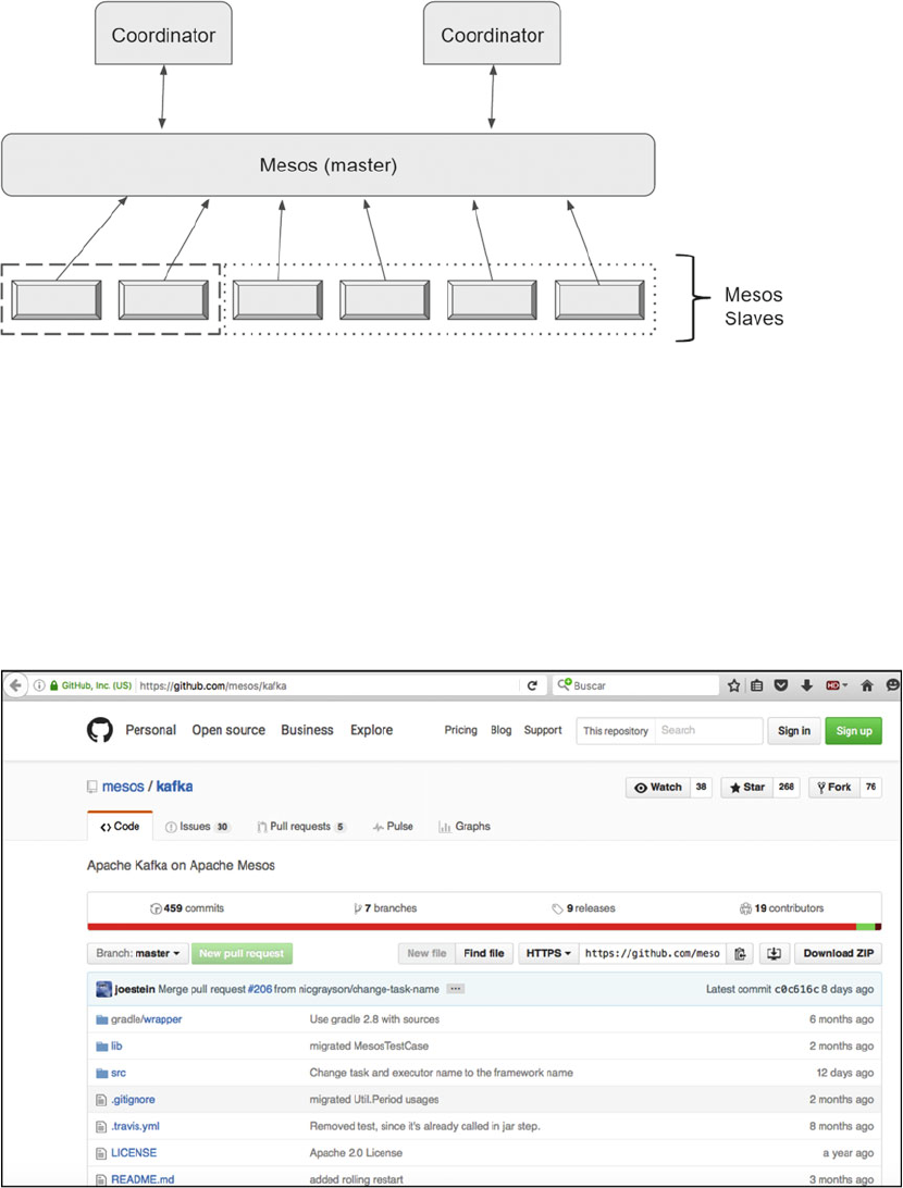
CHAPTER 7 ■ THE MANAGER: APACHE MESOS
157
Figure 7-22. Master and slaves server distribution
There are already several frameworks available for use by Mesos. The true potential is the ability to
create special Mesos frameworks using any of the supported languages: Java, Scala, Python, and C ++.
One of these ready-to-use frameworks is the Apache Kafka framework.
Apache Mesos and Apache Kafka
Apache Kafka is one of the frameworks ready to be used with Mesos. There is a GitHub repository in charge
of this project. Figure
7-23 shows the main screen of the project on GitHub .
Figure 7-23. Mesos/Kafka GitHub project
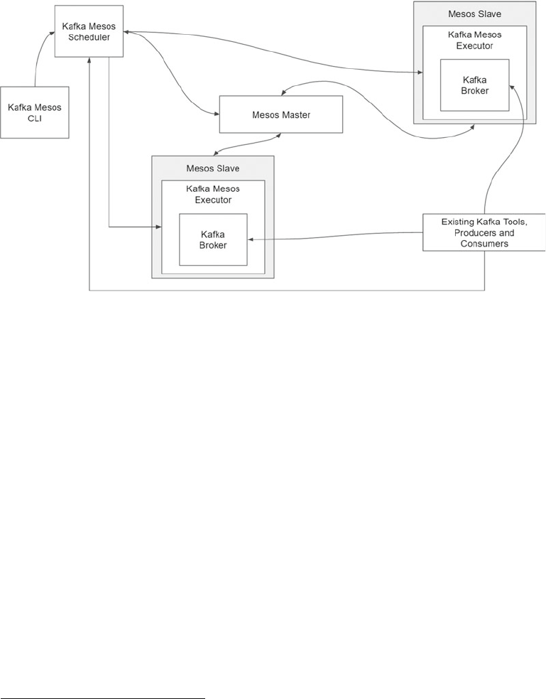
CHAPTER 7 ■ THE MANAGER: APACHE MESOS
158
Like any Mesos framework, Kafka requires schedulers to run tasks. In Figure 7-24 , we can see the
relationship between the scheduler and executor , the basic components of any framework in Mesos. The
figure shows an already known scheme but particularly applied to Apache Kafka; it is based on official
documentation.
16
Figure 7-24. The Apache Kafka framework and its interaction with Apache Mesos
Before building the binaries, check if you have already installed Java and Gradle (the automated
building tool for Java projects).
JDK Validation
JDK validation is easy; you just need to ask for the active version.
/opt/apache/kafka> java -version
java version "1.8.0_51"
Java(TM) SE Runtime Environment (build 1.8.0_51-b16)
Java HotSpot(TM) 64-Bit Server VM (build 25.51-b03, mixed mode)
Gradle Validation
Gradle validation is easy. In this example is installed the Gradle version 2.9:
~/opt/apache/kafka%> gradle -version
------------------------------------------------------------
Gradle 2.9
------------------------------------------------------------
16 https://mesosphere.com/blog/2015/07/16/making-apache-kafka-elastic-with-apache-mesos/
CHAPTER 7 ■ THE MANAGER: APACHE MESOS
159
Build time: 2015-11-17 07:02:17 UTC
Build number: none
Revision: b463d7980c40d44c4657dc80025275b84a29e31f
Groovy: 2.4.4
Ant: Apache Ant(TM) version 1.9.3 compiled on December 23 2013
JVM: 1.8.0_51 (Oracle Corporation 25.51-b03)
{16-05-10 17:55}Isaacs-MacBook-Pro-2:~/opt/apache/kafka isaacruiz%
Export libmesos Location
Follow the instructions provided in the guide. When compiling Mesos, several native libraries are
generated. Find the file called libmesos .so (or libmesos.dylib if you’re on a Mac with OS X) and export
it or declare it in the file: kafka-mesos.sh
# export MESOS_NATIVE_JAVA_LIBRARY=/usr/local/lib/libmesos.so
Now start cloning the repository. The console output will be similar to this:
~/opt/apache/kafka%> git clone https://github.com/mesos/kafka
Cloning into 'kafka'...
remote: Counting objects: 4343, done.
remote: Total 4343 (delta 0), reused 0 (delta 0), pack-reused 4343
Receiving objects: 100% (4343/4343), 959.33 KiB | 44.00 KiB/s, done.
Resolving deltas: 100% (1881/1881), done.
Checking connectivity... done.
Once the repository is cloned, proceed to build the Kafka-Mesos binaries with the command:
gradle jar
Gradle is characterized by place the artifacts required for compilation in the directories according to the
invocation structure, this task may take a while depending on the script dependencies.
~/opt/apache/kafka/kafka@master%> ./gradlew jar
Downloading https://services.gradle.org/distributions/gradle-2.8-all.zip
........................................................................
Unzipping /Users/isaacruiz/.gradle/wrapper/dists/gradle-2.8-all/ah86jmo43de9lfa8xg9ux3c4h/
gradle-2.8-all.zip to /Users/isaacruiz/.gradle/wrapper/dists/gradle-2.8-all/
ah86jmo43de9lfa8xg9ux3c4h
Set executable permissions for: /Users/isaacruiz/.gradle/wrapper/dists/gradle-2.8-all/
ah86jmo43de9lfa8xg9ux3c4h/gradle-2.8/bin/gradle
:compileJava UP-TO-DATE
:compileScala
Download https://repo1.maven.org/maven2/org/scala-lang/scala-library/2.10.6/scala-library-
2.10.6.pom
Download https://repo1.maven.org/maven2/org/apache/mesos/mesos/0.25.0/mesos-0.25.0.pom
...
CHAPTER 7 ■ THE MANAGER: APACHE MESOS
160
Download https://repo1.maven.org/maven2/org/scala-lang/scala-reflect/2.10.6/
scala-reflect-2.10.6.jar
:processResources UP-TO-DATE
:classes
:compileTestJava UP-TO-DATE
:compileTestScala
[ant:scalac] Element '/Users/isaacruiz/opt/apache/kafka/kafka/out/gradle/resources/main'
does not exist.
:processTestResources UP-TO-DATE
:testClasses
:test
:jar
BUILD SUCCESSFUL
Total time: 29 mins 54.98 secs
This build could be faster, please consider using the Gradle Daemon: https://docs.gradle.
org/2.8/userguide/gradle_daemon.html
{16-05-10 18:33}Isaacs-MacBook-Pro-2:~/opt/apache/kafka/kafka@master isaacruiz%
After the Gradle compilation , you should have a structure similar to the following:
~/opt/apache/kafka/kafka@master%> ls -lrt
total 34360
drwxr-xr-x 6 isaacruiz staff 204 May 10 18:02 src
-rwxr-xr-x 1 isaacruiz staff 1634 May 10 18:02 quickstart.sh
drwxr-xr-x 3 isaacruiz staff 102 May 10 18:02 lib
-rwxr-xr-x 1 isaacruiz staff 307 May 10 18:02 kafka-mesos.sh
-rw-r--r-- 1 isaacruiz staff 422 May 10 18:02 kafka-mesos.properties
-rwxr-xr-x 1 isaacruiz staff 4971 May 10 18:02 gradlew
drwxr-xr-x 3 isaacruiz staff 102 May 10 18:02 gradle
-rw-r--r-- 1 isaacruiz staff 1769 May 10 18:02 build.gradle
-rw-r--r-- 1 isaacruiz staff 29334 May 10 18:02 README.md
-rw-r--r-- 1 isaacruiz staff 11325 May 10 18:02 LICENSE
drwxr-xr-x 3 isaacruiz staff 102 May 10 18:25 out
-rw-r--r-- 1 isaacruiz staff 17522191 May 10 18:33 kafka-mesos-0.9.5.0.jar
Now you can use the main shell, use the help command to learn about valid sentences.
{16-05-10 19:05}Isaacs-MacBook-Pro-2:~/opt/apache/kafka/kafka> ./kafka-mesos.sh help
Usage: <command>
Commands:
help [cmd [cmd]] - print general or command-specific help
scheduler - start scheduler
broker - broker management commands
topic - topic management commands
Run `help <command>` to see details of specific command
{16-05-10 21:25}Isaacs-MacBook-Pro-2:~/opt/apache/kafka/kafka%>
CHAPTER 7 ■ THE MANAGER: APACHE MESOS
161
Or you can start the scheduler directly:
{16-05-10 21:25}Isaacs-MacBook-Pro-2:~/opt/apache/kafka/kafka%> ./kafka-mesos.sh scheduler
Loading config defaults from kafka-mesos.properties
2016-05-10 21:25:33,573 [main] INFO ly.stealth.mesos.kafka.Scheduler$ - Starting
Scheduler$:
debug: true, storage: zk:/mesos-kafka-scheduler
mesos: master=master:5050, user=vagrant, principal=<none>, secret=<none>
framework: name=kafka, role=*, timeout=30d
api: http://192.168.3.5:7000, bind-address: <all>, zk: master:2181, jre: <none>
Mesos and Apache Spark
Since its earliest releases, Spark was ready for Mesos. The web page that explains how to perform the
integration is
http://spark.apache.org/docs/latest/running-on-mesos.html .
It’s easy to start Spark to work with Mesos. Just be careful when establishing the libmesos file location
(the native library compiled earlier).
First, validate that Mesos is running by opening a browser and validating that your host is active as
follows:
http://MESOS_HOST:5050/
The next step is to locate the file called libmesos.so (or libmesos.dylib if you’re on a Mac with OS X)
and make it available as an environment variable:
export MESOS_NATIVE_JAVA_LIBRARY=<path to libmesos.so>
Once this is done, try running this line:
~/opt/apache/spark/spark-1.6.1-bin-hadoop2.6/bin%> ./spark-shell --master mesos://MESOS_
HOST:5050
If you receive this error:
Failed to load native library from Mesos
Failed to load native Mesos library from
/Users/your_user/Library/Java/Extensions:
/Users/your_user/Library/Java/Extensions/Library/Java/Extensions:
/Network/Library/Java/Extensions:
/System/Library/Java/Extensions:
/usr/lib/java:.
Copy the libmesos.so file to any of these routes, preferably one within your user directory to avoid
conflicts with another version after you compile. If the path does not exist, you must create it.
The following is the successful output. The prompt appears available, and more importantly, Mesos
recognizes an active framework.
16-05-15 12:47}Isaacs-MacBook-Pro-2:~/opt/apache/spark/spark-1.6.1-bin-hadoop2.6/bin
isaacruiz% ./spark-shell --master mesos://localhost:5050
log4j:WARN No appenders could be found for logger (org.apache.hadoop.metrics2.lib.
MutableMetricsFactory).
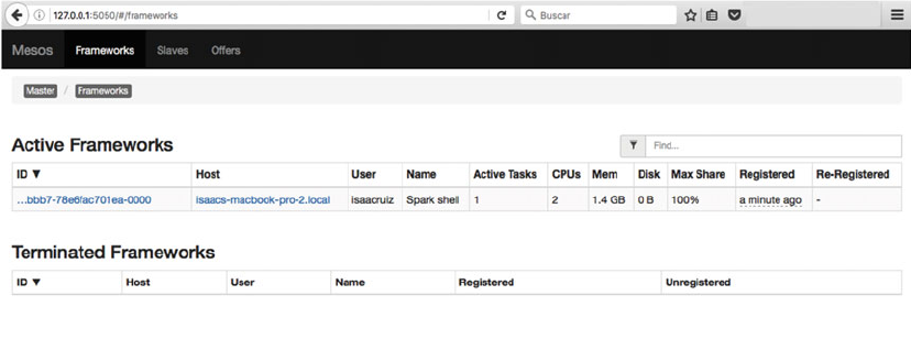
CHAPTER 7 ■ THE MANAGER: APACHE MESOS
162
log4j:WARN Please initialize the log4j system properly.
log4j:WARN See http://logging.apache.org/log4j/1.2/faq.html#noconfig for more info.
Using Spark's repl log4j profile: org/apache/spark/log4j-defaults-repl.properties
To adjust logging level use sc.setLogLevel("INFO")
Welcome to
____ __
/ __/__ ___ _____/ /__
_\ \/ _ \/ _ `/ __/ ’_/
/___/ .__/\_,_/_/ /_/\_\ version 1.6.1
/_/
Using Scala version 2.10.5 (Java HotSpot(TM) 64-Bit Server VM, Java 1.8.0_51)
Type in expressions to have them evaluated.
Type :help for more information.
I0515 12:48:34.810873 62210048 sched.cpp:222] Version: 0.28.1
I0515 12:48:34.842321 57393152 sched.cpp:326] New master detected at master@127.0.0.1:5050
I0515 12:48:34.843389 57393152 sched.cpp:336] No credentials provided. Attempting to
register without authentication
I0515 12:48:34.876587 60612608 sched.cpp:703] Framework registered with 7f7d9b4b-c5e4-48be-
bbb7-78e6fac701ea-0000
Spark context available as sc.
SQL context available as sqlContext.
scala>
From the web console, we can see the running frameworks as shown in Figure
7-25 .
Figure 7-25. Apache Spark already appears in the list of active frameworks
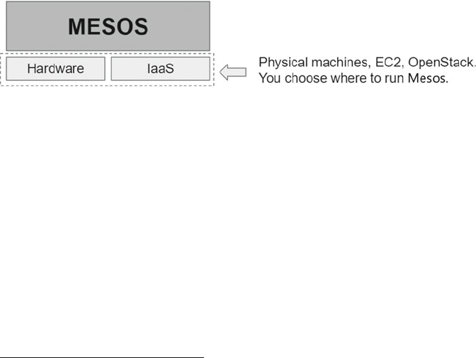
CHAPTER 7 ■ THE MANAGER: APACHE MESOS
163
The Best Is Yet to Come
At the beginning of this chapter, we mentioned that Mesos is still in pre-1.0 versions. All of Mesos’s versatility
and usefulness work and can be achieved in version 0.28.0. (Imagine when we get to version 1.0!) The
expectation level is high, and no wonder: on April 2016, Wired magazine published an article titled “You
want to build an empire like Google’s? This is your OS.”
17 Among other things, the article mentions that
Google runs on architectures similar to Apache Mesos. It also mentions Mesos’s history and its creator, Ben
Hindman; part of the original design includes creating data centers in the same way that software runs on a
mobile device or a laptop.
Through Mesosphere, 18 the company launched by Hindman, any company (and any of us) can build an
infrastructure similar to Google’s.
If anything is missing to give new impetus to startups, Mesos probably covers it.
At MesosConf-Europe in 2015, Hindman presented the “State of Apache Mesos”
19 and a brief summary
with three main indicators of the growing Mesos community:
• New users: Cisco, Apple, Yelp, Ericsson
• New frameworks: Elastic, Kibana, MySQL, rial, CRATE, and Logstash
• New books: This book is among the proof.
Every month and a half, a smaller version (now in 0.28) is released; by the end of 2016, it will likely be at
version 0.40 or 0.50. Mesos surely has many surprises ahead—as we say, the best is yet to come.
And if that is not enough, as shown in Figure
7-26 , Mesos is designed to run in the cloud as physical
machines , so the hardware layer is transparent.
In 2016, presentations at #MesosConf North America
20 highlighted growing interest in Mesos.
Summary
In this chapter, you learned a little more about distributed systems. Now you know how difficult it is to try
to build one. You learned that Mesos is a general-purpose cluster manager. You know its architecture and
part of its ecosystem. Within this ecosystem, you know about the main frameworks that Mesos interacts
with to increase its potential. The chapter also overviewed why Mesos is considered a SDK for distributed
environments.
17 http://www.wired.com/2016/04/want-build-empire-like-googles-os/
18 https://mesosphere.com/
19 https://www.youtube.com/watch?v=K-x7yOy8Ymk&list=PLGeM09tlguZS6MhlSZDbf-gANWdKgje0I
20 https://www.linux.com/news/mesoscon-north-america-2016-video-sessions
Figure 7-26. Mesos can run both physical machines and cloud

165
© Raul Estrada and Isaac Ruiz 2016
R. Estrada and I. Ruiz, Big Data SMACK, DOI 10.1007/978-1-4842-2175-4_8
CHAPTER 8
The Broker: Apache Kafka
The goal of this chapter is to get you familiar with Apache Kafka and show you how to solve the consumption
of millions of messages in a pipeline architecture. Here we show some Scala examples to give you a solid
foundation for the different types of implementations and integrations for Kafka producers and consumers.
In addition to the explanation of the Apache Kafka architecture and principles, we explore Kafka
integration with the rest of the SMACK stack, specifically with Spark and Mesos. At the end of the chapter, we
show how to administer Apache Kafka.
This chapter covers the following topics:
• Kafka introduction
• Kafka installation
• Kafka in cluster
• Kafka architecture
• Kafka producers
• Kafka consumers
• Kafka integration
• Kafka administration
Kafka Introduction
The Apache Kafka author, Jay Kreps, who took a lot of literature courses in the college, if the project is mainly
optimized for writing (in this book when we say “optimized” we mean 2 million writes per second on three
commodity machines) when he open sourced it, he thought it should have a cool name: Kafka, in honor of
Franz Kafka, who was a very prolific author despite dying at 40 age.
Nowadays, real-time information is continuously generated. This data needs easy ways to be delivered
to multiple types of receivers. Most of the time the information generators and the information consumers
are inaccessible to each other; this is when integration tools enter the scene.
In the 1980s, 1990s and 2000s, the large software vendors whose names have three letters (IBM, SAP,
BEA, etc.) and more (Oracle, Microsoft, Google) have found a very well-paid market in the integration layer,
the layer where live: enterprise service bus, SOA architectures, integrators, and other panaceas that cost
several millions of dollars.
Now, all traditional applications tend to have a point of integration between them, therefore, creating
the need for a mechanism for seamless integration between data consumers and data producers to avoid
any kind of application rewriting at either end.
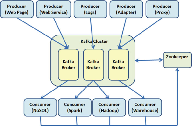
CHAPTER 8 ■ THE BROKER: APACHE KAFKA
166
As we mentioned in earlier chapters, in the big data era, the first challenge was the data collection and
the second challenge was to analyze that huge amount of data.
Message publishing is the mechanism for connecting heterogeneous applications through sending
messages among them. The message router is known as message broker. Apache Kafka is a software solution
to quickly route real-time information to consumers.
The message broker provides seamless integration, but there are two collateral objectives: the first is to
not block the producers and the second is to not let the producers know who the final consumers are.
Apache Kafka is a real-time publish-subscribe solution messaging system: open source,
distributed, partitioned, replicated, commit-log based with a publish-subscribe schema. Its main
characteristics are as follows:
• Distributed . Cluster-centric design that supports the distribution of the messages
over the cluster members, maintaining the semantics. So you can grow the cluster
horizontally without downtime.
• Multiclient . Easy integration with different clients from different platforms: Java,
.NET, PHP, Ruby, Python, etc.
• Persistent . You cannot afford any data lost. Kafka is designed with efficient O(1), so
data structures provide constant time performance no matter the data size.
• Real time . The messages produced are immediately seen by consumer threads;
these are the basis of the systems called complex event processing (CEP) .
• Very high throughput . As we mentioned, all the technologies in the stack are
designed to work in commodity hardware. Kafka can handle hundreds of read and
write operations per second from a large number of clients.
Figure 8-1 shows an Apache Kafka messaging system typical scenario.
Figure 8-1. Apache Kafka typical scenario
CHAPTER 8 ■ THE BROKER: APACHE KAFKA
167
On the producers’ side, you can find several types of actors , for example:
• Adapters . Generate transformation information; for example, a database listener or
a file system listener.
• Logs . The log files of application servers and other systems, for example.
• Proxies . Generate web analytics information.
• Web pages . Front-end applications generating information.
• Web services . The service layer; generate invocation traces.
You could group the clients on the customer side as three types:
• Offline . The information is stored for posterior analysis; for example, Hadoop and
data warehouses.
• Near real time . The information is stored but it is not requested at the same time; for
example, Apache Cassandra, and NoSQL databases.
• Real time . The information is analyzed as it is generated; for example, an engine like
Apache Spark or Apache Storm (used to make analysis over HDFS).
Born in the Fast Data Era
As we have mentioned, data is the new ingredient of Internet-based systems. Simply, a web page needs to
know user activity, logins, page visits, clicks, scrolls, comments, heat zone analysis, shares, and so forth.
Traditionally, the data was handled and stored with traditional aggregation solutions. Due to the high
throughput, the analysis could not be done until the next day. Today, yesterday’s information often useless.
Offline analysis such as Hadoop is being left out of the new economy.
There are several examples of Apache Kafka use cases:
• Web searches based on relevance
• Application security: login analysis, brute force attack detection, systemic denial of
service attack detection
• Recommendations based on popularity, correlation
• Sentiment analysis, tendencies, segmentation
• Collecting data from device sensors or sophisticated sensors like surveillance
cameras to GPS cell phone sensors; passing through sensors: light, temperature,
pressure, humidity
• Real-time merchandising to a huge population
• Collecting logs from business systems such as application server logs, CRM, ERP, and
so forth.
In all of these cases, the analysis is done in real time or it is never done, without middle points.
Apache Kafka usually is compared to traditional messaging systems such as ActiveMQ or RabitMQ.
The difference is the data volume that Kafka can handle in real time.

CHAPTER 8 ■ THE BROKER: APACHE KAFKA
168
U s e C a s e s
Well, you have seen some business scenarios that are solved with Apache Kafka. In which layer in the
architecture should you put Kafka? Here are some popular (real examples with real enterprises) use cases:
• Commit logs . What happens when your system does not have a log system? In these
cases, you can use Kafka. Many times systems do not have logs, simply because (so
far) it’s not possible to handle such a large data volume. The stories of application
servers falling simply because they could not write their logs correctly with the
verbosity needed by the business are more common than it seems. Kafka can also
help to start and restart fallen log servers.
• Log aggregation . Contrary to what people believe, much of the work of the
onsite support team is on log analysis. Kafka not only provides a system for log
management, but it can also handle heterogeneous aggregation of several logs. Kafka
can physically collect the logs and remove cumbersome details such as file location
or format. In addition, it provides low latency and supports multiple data sources
while making distributed consumption.
• Messaging . Systems are often heterogeneous, and instead of rewriting them, you
have to translate between them. Often the manufacturer’s adapters are unaffordable
to a company; for such cases, Kafka is the solution because it is open source and can
handle more volume than many traditional commercial brokers.
• Stream processing . We could write an entire book on this topic. In some business
cases, the process of collecting information consists of several stages. A clear
example is when a broker is used not only to gather information but also to
transform it. This is the real meaning and success of the Enterprise Service Bus (ESB)
architectures. With Kafka, the information can be collected and further enriched;
this (very well paid) enrichment process is known as stream processing .
• Record user activity . Many marketing and advertising companies are interested in
recording all the customer activity on a web page. This seems a luxury, but until recently,
it was very difficult to keep track of the clicks that a user makes on a site. For those tasks
where the data volume is huge, you can use Kafka for real-time process and monitoring.
All of this seems good, but who is using Kafka today? Here are some examples:
• LinkedIn . 1 Used for activity stream and operational metrics. We cannot imagine the
today’s LinkedIn newsfeed without Kafka.
• Uber . 2 Relied on Kafka data feeds to bulk-load log data into Amazon S3 to stream
change-data logs from the local data centers .
• Twitter . 3 Handling five billion sessions a day in real time requires Kafka to handle
their stream processing infrastructure.
• Netflix . 4 Kafka is the backbone of Netflix’s data pipeline for real-time monitoring and
event processing.
1 https://engineering.linkedin.com/blog/2016/04/kafka-ecosystem-at-linkedin
2 http://www.datanami.com/2015/10/05/how-uber-uses-spark-and-hadoop
3 https://blog.twitter.com/2015/handling-five-billion-sessions-a-day-in-real-time
4 http://techblog.netflix.com/2013/12/announcing-suro-backbone-of-netflixs.html
CHAPTER 8 ■ THE BROKER: APACHE KAFKA
169
• Spotify . 5 Kafka is used as part of their log delivery system.
• Yahoo . Used by the media analytics team as a real-time analytics pipeline. Their
cluster handles 20Gbps of compressed data.
Kafka Installation
Go to the Apache Kafka home page at http://kafka.apache.org/downloads , as shown in Figure 8-2 .
Figure 8-2. Apache Kafka download page
The Apache Kafka current version available as a stable release is 0.10.0.0. The major limitation with Kafka
since 0.8.x is that it is not backward-compatible. So, you cannot replace this version for one prior to 0.8.
Once you download the available release, let’s proceed with the installation.
Installing Java
You need to install Java 1.7 or later. Download the latest JDK from Oracle’s web site at http://www.oracle.
com/technetwork/java/javase/downloads/index.html .
For example, to install in Linux:
1 . Change the file mode:
[restrada@localhost opt]# chmod +x jdk-8u91-linux-x64.rpm
5 http://www.meetup.com/stockholm-hug/events/121628932/
CHAPTER 8 ■ THE BROKER: APACHE KAFKA
170
2 . Change the directory in which you want to perform the installation:
[restrada@localhost opt]# cd <directory path name>
3 . To install the software in the /usr/java/ directory, type the following command:
[restrada@localhost opt]# cd /usr/java
4 . Run the installer using this command:
[restrada@localhost java]# rpm -ivh jdk-8u91-linux-x64.rpm
5 . Finally, add the JAVA_HOME environment variable. This command will write the
JAVA_HOME environment variable to the /etc/profile file:
[restrada@localhost opt]# echo "export JAVA_HOME=/usr/java/jdk1.8.0_91" >>
/etc/profile
Installing Kafka
To install in Linux , take the following steps.
1 . Extract the downloaded kafka_2.10-0.10.0.0.tgz file:
[restrada@localhost opt]# tar xzf kafka_2.10-0.10.0.0.tgz
2 . Add the Kafka bin directory to PATH as follows:
[restrada@localhost opt]# export KAFKA_HOME=/opt/kafka_2.10-0.10.0.0
[restrada@localhost opt]# export PATH=$PATH:$KAFKA_HOME/bin
I m p o r t i n g K a f k a
To include Kafka in our programming projects, we include the dependencies.
With SBT:
// https://mvnrepository.com/artifact/org.apache.kafka/kafka_2.10
libraryDependencies += "org.apache.kafka" % "kafka_2.10" % "0.10.0.0"
With Maven:
<!-- https://mvnrepository.com/artifact/org.apache.kafka/kafka_2.10 -->
<dependency>
<groupId>org.apache.kafka</groupId>
<artifactId>kafka_2.10</artifactId>
<version>0.10.0.0</version>
</dependency>
With Gradle:
// https://mvnrepository.com/artifact/org.apache.kafka/kafka_2.10
compile group: 'org.apache.kafka', name: 'kafka_2.10', version: '0.10.0.0'
CHAPTER 8 ■ THE BROKER: APACHE KAFKA
171
Kafka in Cluster
We are ready to program with the Apache Kafka publisher-subscriber messaging system. In Kafka, there are
three types of clusters:
• Single node–single broker
• Single node–multiple broker
• Multiple node–multiple broker
A Kafka cluster has five main components:
• Topic . A category or feed name in which messages are published by the message
producers. Topics are partitioned; each partition is represented by an ordered
immutable messages sequence. The cluster has a partitioned log for each topic. Each
message in the partition has a unique sequential id called an offset.
• Broker . A Kafka cluster has one or more physical servers in which each one may
have one or more server processes running. Each server process is called a broker .
The topics live in the broker processes.
• Producer . Publishes data to topics by choosing the appropriate partition in the
topic. For load balancing, the messages allocation to the topic partition can be done
in a round-robin mode or by defining a custom function.
• Consumer . Applications or processes subscribed to topics and process the feed of
published messages.
• ZooKeeper . ZooKeeper is the coordinator between the broker and the consumers.
ZooKeeper coordinates the distributed processes through a shared hierarchical
name space of data registers; these registers are called znodes .
There are two differences between ZooKeeper and a file system:
• Every znode has data associated and is designed to store coordination data.
• Znodes are limited on the amount of data that they can have.
Single Node–Single Broker Cluster
An example diagram of a single node– single broker cluster is shown in Figure 8-3 .
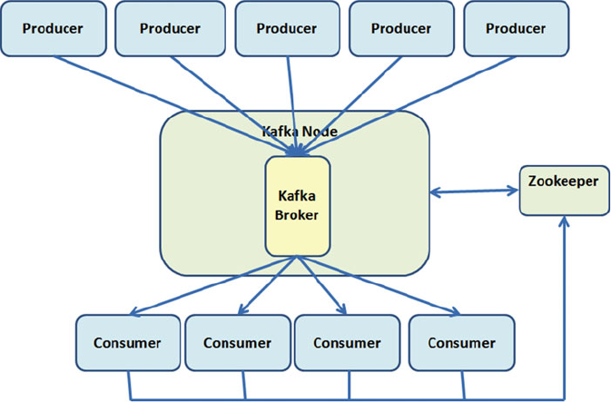
CHAPTER 8 ■ THE BROKER: APACHE KAFKA
172
First, start the ZooKeeper server. Kafka provides a simple ZooKeeper configuration file to launch a
single ZooKeeper instance. To install the ZooKeeper instance, use the following command:
[restrada@localhost kafka_2.10.0-0.0.0.0]# bin/zookeeper-server-start.sh config/zookeeper.
properties
The following are the main properties defined in zookeeper.properties:
• dataDir . The data directory where ZooKeeper is stored:
dataDir=/tmp/zookeeper
• clientPort . The listening port for client requests. By default, ZooKeeper listens in the
2181 TCP port:
clientPort=2181
• maxClientCnxns . The limit per IP for the number of connections (0 = unbounded):
maxClientCnxns=0
For more information about Apache ZooKeeper, visit the project page at
http://zookeeper.apache.org/ .
Starting the Broker
After start ZooKeeper , start the Kafka broker with the following command:
[restrada@localhost kafka_2.10.0-0.0.0.0]# bin/kafka-server-start.sh config/server.
properties
Figure 8-3. Single node–single broker Kafka cluster example
CHAPTER 8 ■ THE BROKER: APACHE KAFKA
173
The following are the main properties defined in server.properties:
• Broker id . The unique positive integer id for each broker.
Broker.id=0
• Port . The port where the socket server listens on:
port=9092
• Log dir . The directory to store log files:
log.dir=/tmp/kafka10-logs
• Num partitions . The number of log partitions per topic:
num.partitions=2
• ZooKeeper connect . The ZooKeeper connection URL:
zookeeper.connect=localhost:2181
Creating a Topic
Kafka has a command to create topics. Let’s create a topic called amazingTopic with one partition and one replica:
[restrada@localhost kafka_2.10.0-0.0.0.0]#bin/kafka-topics.sh --create --zookeeper
localhost:2181 --replication-factor 1 --partitions 1 --topic amazingTopic
Obtain the output, as follows:
Created topic "amazingTopic".
These are the parameters:
• --replication-factor 1 indicates one replica
• --partition 1 indicates one partition
• --zookeeper localhost:2181 indicates the ZooKeeper URL
To obtain the list of topics on any Kafka server, use the following command:
[restrada@localhost kafka_2.10.0-0.0.0.0]# bin/kafka-topics.sh --list
--zookeeper localhost:2181
Obtain the output:
amazingTopic
Starting a Producer
Kafka has a command line to start producers . It accepts input from the command line and publishes them as
messages. By default, each new line is considered a message.
[restrada@localhost kafka_2.10.0-0.0.0.']# bin/kafka-console-producer.sh --broker-list
localhost:9092 --topic amazingTopic
CHAPTER 8 ■ THE BROKER: APACHE KAFKA
174
Two parameters are required:
• broker-list . The URL of the brokers to be connected.
• topic . The name of the topic used to send a message to its subscribers.
Now type the following:
Valar morghulis [Enter]
Valar dohaeris [Enter]
You get this output:
Valar morghulis
Valar dohaeris
The following are the main properties defined in producer.properties :
• Metadata broker list . A list of brokers used for bootstrapping knowledge about the
rest of the cluster.
Format: host1:port1, host2:port2
metadata.broker.list=localhost:9092
• Compression codec . The compression codec for data generated.
Example: none, gzip, snappy
compression.codec=none
Later on this chapter, you see how to write producers.
Starting a Consumer
Kafka has a command line to start a message consumer client . It shows the output at the command line as
soon as it subscribes to the topic in the broker:
[restrada@localhost kafka_2.10.0-0.0.0.0]# bin/kafka-console-consumer.sh --zookeeper
localhost:2181 --topic amazingTopic --from-beginning
As you request from-beginning, you see the following output:
Valar morghulis
Valar dohaeris
The following is the main property defined in consumer.properties:
• Group id . A string that identifies a set of consumers in the same group:
group.id=test-consumer-group
Later on this chapter, you will learn how to write consumers.
Now let’s play with the new toy architecture. Open each technology in a different console: ZooKeeper, broker,
producer, and consumer. Type the commands in the producer and watch them displayed in the consumer.
If you don’t recall how to run producers or consumers, running the command with no arguments will
show the possible parameters.
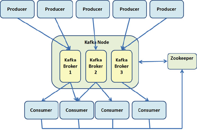
CHAPTER 8 ■ THE BROKER: APACHE KAFKA
175
Single Node–Multiple Broker Cluster
An example diagram of a single node– multiple broker cluster is shown in Figure 8-4 .
Figure 8-4. Single node–multiple broker Kafka cluster example
As usual, start the ZooKeeper server:
[restrada@localhost kafka_2.10.0-0.0.0.0]# bin/zookeeper-server-start.sh config/zookeeper.
properties
You need a different server.properties file for every broker. Let’s call them: server-1.properties, server-2.
properties, server-3.properties, and so forth.
In server-1.properties, specify the following:
• broker.id=1
• port=9093
• log.dir=/tmp/kafka-logs-1
Similarly, on server-2.properties, specify the following:
• broker.id=2
• port=9094
• log.dir=/tmp/kafka-logs-2
Follow the same procedure for server-3.properties:
• broker.id=3
• port=9095
• log.dir=/tmp/kafka-logs-3
CHAPTER 8 ■ THE BROKER: APACHE KAFKA
176
Starting the Brokers
With ZooKeeper running , start the Kafka brokers with the following commands:
[restrada@localhost kafka_2.10.0-0.0.0.0]# bin/kafka-server-start.sh config/server-1.
properties
[restrada@localhost kafka_2.10.0-0.0.0.0]# bin/kafka-server-start.sh config/server-2.
properties
[restrada@localhost kafka_2.10.0-0.0.0.0]# bin/kafka-server-start.sh config/server-3.
properties
Creating a Topic
Using the command to create topics, create a topic called reAmazingTopic ( re stands for replicated ). It has
two partitions and two replicas:
[restrada@localhost kafka_2.10.0-0.0.0.0]#bin/kafka-topics.sh --create --zookeeper
localhost:2181 --replication-factor 2 --partitions 2 --topic reAmazingTopic
Obtain the output, as follows:
Created topic "reAmazingTopic".
Starting a Producer
Now that you know the command to start producers , indicating more brokers in the broker-list is a trivial
task:
[restrada@localhost kafka_2.10.0-0.0.0.0]# bin/kafka-console-producer.sh --broker-list
localhost:9093, localhost:9094, localhost:9095 --topic reAmazingTopic
Yes, our architects always have weird requirements; if we need to run multiple producers connecting to
different broker combinations, we need to specify a different broker-list for each producer.
Starting a Consumer
To start a consumer , use the same Kafka command that you already know:
[restrada@localhost kafka_2.10.0-0.0.0.0]# bin/kafka-console-consumer.sh --zookeeper
localhost:2181 --from-beginning --topic reAmazingTopic
Multiple Node–Multiple Broker Cluster
An example of a multiple node–multiple broker cluster is shown in Figure 8-5 .
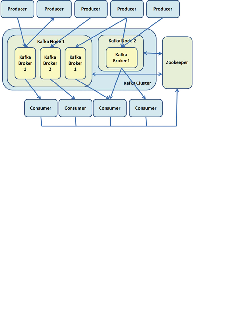
CHAPTER 8 ■ THE BROKER: APACHE KAFKA
177
Here you are in front of the real power of the cluster. Kafka should be installed in every machine in
the cluster. Every physical server could have one or many Kafka brokers. All the nodes on the same cluster
should connect to the same ZooKeeper.
But don’t worry, all the previous commands remain equal. The commands for ZooKeeper, broker,
producer, and consumer don’t change.
Broker Properties
To recapitulate the section, Table 8-1 lists the most popular broker properties.
6
Figure 8-5. Multiple node–multiple broker Kafka cluster
Table 8-1. Kafka Broker Most Important Properties
Name Default value Description
broker.id 0 Each broker is identified with a positive integer id. This id
is the broker’s name and allows the broker to be moved to a
different host or port without losing consumers.
log.dirs /tmp/kafka-logs The directory where the log data is stored. Each new partition
created will be placed in the directory with the fewest partitions.
zookeper.connect localhost:2181 The ZooKeeper’s connection string in the hostname:port/
chroot form. Here, chroot is the base directory for the path
operations (namespace for sharing with other applications on
the same ZooKeeper cluster).
(continued)
6 The complete list is in http://kafka.apache.org/documentation.html#brokerconfigs

CHAPTER 8 ■ THE BROKER: APACHE KAFKA
178
Kafka Architecture
In its beginning, LinkedIn used Java Message Service (JMS) . But when more power was needed (i.e., a
scalable architecture), the LinkedIn development team decided to build the project that we know today
as Kafka. In 2011, Kafka was an open source Apache project. In this chapter, section we give you some
reflections on why things are designed in the way they are.
The following are Kafka’s project goals:
• An API . Supports custom implementation of producers and consumers.
• Low overhead . Low network latency and low storage overhead with message
persistence on disk.
• High throughput . Publishes and subscribes millions of messages; supports data
feeds and real time.
• Distributed . Highly scalable architecture to handle low-latency delivery.
• High availability . Autobalances consumers in case of failure.
• Fault tolerant . Guarantees data integrity in case of failure.
Kafka is more than a queuing platform; the messages are received and enqueued to be delivered to a
consumer pool.
Kafka is more than a published-subscriber platform; the messages are not published to all customers.
The following describes Kafka’s operation in a nutshell:
• Messages are published to a Kafka topic, which is a message queue or a message
category.
• The Kafka topic runs in the Kafka broker, which is a server. Kafka brokers do not just
run the topics, but also store the messages when required.
• The consumers use the ZooKeeper service to get the information to track the
messages (the data about a message state).
Figure 8-6 shows a topic with three partitions. You can see the five Kafka components: ZooKeeper,
broker, topic, producer, and consumer.
Name Default value Description
host.name null The broker’s hostname. If this is set, it will only bind to this
address. If this is not set, it will bind to all interfaces and
publish one to ZooKeeper.
num.partitions 1 The number of partitions per topic if a partition count isn’t
given at topic creation.
auto.create.topics.
enable
true Enables the autocreation of the topic on the server. If this is
set to true, the attempts to produce, consume, or fetch data
for a non-existent topic will automatically create a new one
with the default replication factor and the default number of
partitions.
default.replication.
factor
1 The default replication factor for automatically created topics.
Table 8-1. (continued)
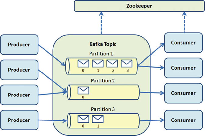
CHAPTER 8 ■ THE BROKER: APACHE KAFKA
179
The following describes parts of the partition.
• Segment files . Internally, every partition is a logical log file, represented as a set of
segment files with the same size. The partition is a sequence of ordered messages.
When a message is published, the broker appends the message to the last segment of
the file. When a certain number of messages is reached, the segment file is flushed to
the disk. Once the file is flushed, the messages are available for consumption by the
consumers.
• Offset . The partitions are assigned to a unique sequential number called an offset .
The offset is used to identify messages inside the partition. The partitions are
replicated between the servers for fault tolerance.
• Leaders . Inside Kafka, each partition has one Kafka server as it leader . The other
servers are followers . The leader of a partition coordinates the read and write
requests for that partition. The followers asynchronously replicate the data from the
leader. If the leader fails, another server becomes the new leader. In a cluster, every
server has two roles: the leader on some partitions and a follower on other partitions.
• Groups . The consumers are organized into groups. Each consumer is represented as
a process; one process belongs to only one group.
In Kafka, there are three ways to deliver messages (as a reflection exercise, think about why there are
only three):
• Messages are never redelivered but may be lost.
• Messages may be redelivered but never lost.
• Messages are delivered once and only once.
Figure 8-6. A topic with three partitions
CHAPTER 8 ■ THE BROKER: APACHE KAFKA
180
Log Compaction
There are two types of retention: finer-grained (per message) and coarser-grained (time based). Log
compaction is the process to pass from time-based to per-message retention.
In Kafka, the retention policy can be set to per-topic (time based), size-based, and log compaction–
based. Log compaction ensures the following:
• Reads begin at offset 0; if the consumer begins at the start of the log, the messages
are in the order that they were written.
• Messages have sequential offsets that never change.
• Message order is always preserved.
• A group of background threads recopy log segment files; the records whose keys
appear in the log head are removed.
As another reflection exercise, can you deduce why the log compaction ensures these four points?
K a f k a D e s i g n
The following are Kafka design bullet points:
• Storage . The purpose of Kafka is to provide message processing. The main functions
are caching and storing messages on a file system. The caching and flushing to disk
are configurable.
• Retention . If a message is consumed, the message is not wasted; it is retained,
allowing message reconsumption.
• Metadata . In many messaging systems, the message metadata is kept at the server
level. In Kafka, the message state is maintained at the consumer level. This prevents
the following:
• Multiple deliveries of the same message
• Losing messages due to failures
• OLTP . Consumers store the state in ZooKeeper, but Kafka also allows the storage in
OLTP external systems (online transaction processing).
• Push and pull . Producers push the message to the broker and consumers pull the
message from the broker.
• Masterless . Like Apache Cassandra, Apache Kafka is masterless; you can remove any
broker at any time. The metadata is maintained by ZooKeeper and shared with the
customers.
• Synchronous . Producers have the option to be asynchronous or synchronous when
sending messages to the broker.
Message Compression
There are cases where the network bandwidth is the bottleneck. This usually does not happen, but it could.
In Kafka, there is a mechanism to compress groups of messages. Note that without being compression
experts, we can deduce that it is better to compress a group of messages than compress every message
individually.
CHAPTER 8 ■ THE BROKER: APACHE KAFKA
181
When a group of messages is compressed, the network overhead is reduced. Before Kafka 0.8.0,
groups of messages were compressed and presented to the consumer as a single message; the consumer
decompressed it later. But there were issues with decompression that made overhead.
Since Kafka 0.8.0, some changes were introduced to the broker to handle offsets; so the problem was
moved to the broker, but the overall performance improved. The lead broker is responsible for compressing
messages, which lowers the network overhead but could also increase the load in the broker’s CPU.
As you saw, Kafka handles Gzip and Snappy compression protocols. You need to specify this
configuration in the producer to use compression.
• compression.codec . This parameter indicates the codec for all data generated on
the producer. The default value is none. The valid values are none, gzip, and snappy.
• compressed.topics . This parameter turns on the compression on particular
topics. Note that if the list of compressed topics is empty, then you are enabling the
compression for all the topics. If the compression codec is none, the compression is
disabled for all the topics.
If there is a mission in your work that does not let you sleep, and it is related to mirror data across
data centers, consider using Kafka. Kafka is a good option when you have to transfer huge amounts
of data between active and passive data centers in a compressed format with low network bandwidth
overhead.
Replication
When you have message partitioning in Kafka, the partitioning strategy decision is made on the broker
side. The decision on how the message is partitioned is made at the producer end. The broker stores the
messages as they arrive. If you recall, the number of partitions configured for each topic is done in the
Kafka broker.
Replication is one of the best features introduced in Kafka 0.8.0. Replication ensures that messages
will be published and consumed in the event of broker failure. Both producers and consumers are
replication-aware.
In replication, each partition has n replicas of a message (to handle n –1 failures). One replica acts as
the leader. ZooKeeper knows who the replica leader is. The lead replica has a list of its follower replicas. The
replicas store their part of the message in local logs.
Kafka has two replication modes : the synchronous replication process and the asynchronous
replication process .
This is the synchronous replication process:
1 . The producer identifies the lead replica from ZooKeeper.
2 . The producer publishes the message.
3 . When the message is published, it is written to the lead replica’s log.
4 . The followers pull the message.
5 . The leader waits for all the followers to acknowledge that the replica was written.
6 . Once replications are complete, the leader sends the acknowledgment to the
producer.
This is the asynchronous replication process:
1 . The producer identifies the lead replica from ZooKeeper.
2 . The producer publishes the message.
CHAPTER 8 ■ THE BROKER: APACHE KAFKA
182
3 . When the message is published, it is written to the lead replica’s log.
4 . The followers pull the message.
5 . Once the message is written on the lead replica, the leader sends the
acknowledgment to the consumer.
As you can see, asynchronous mode is faster, but it is not fault tolerant.
Replication ensures strong durability and high availability. It guarantees that any successfully published
message will not be lost and will be consumed, even in the event of broker failures.
Kafka Producers
As you saw, producers are applications that create messages and publish them to the broker. Normally,
producers are front-end applications, web pages, web services, back-end services, proxies, and adapters to
legacy systems. You can write Kafka producers in Java, Scala, C, and Python.
The process begins when the producer connects to any live node and requests metadata about the
partitions’ leaders on a topic so as to put the message directly to the partition’s lead broker.
Producer API
First, you need to understand the required classes to write a producer:
• Producer . The class is KafkaProducer <K, V> in org.apache.kafka.clients.producer.
KafkaProducer
KafkaProducer is a type of Java generic written in Scala. K specifies the partition key
type and V specifies the message value.
• ProducerRecord . The class is ProducerRecord <K, V> in org.apache.kafka.clients.
producer.ProducerRecord
This class encapsulates the data required for establishing the connection with the
brokers (broker list, partition, message serializer, and partition key).
ProducerRecord is a type of Java generic written in Scala. K specifies the partition key
type and V specifies the message value.
The Producer API encapsulates all the low-level producer implementations. The default mode is
asynchronous, but you can specify in producer.type in the producer configuration.
Scala Producers
Now let’s write a simple Scala Kafka producer to send messages to the broker. The SimpleProducer class
is used to create a message for a specific topic and to send it using message partitioning. This chapter’s
examples were tested with Scala version 2.10.
Step 1. Import Classes
Import two classes:
import org.apache.kafka.clients.producer.{KafkaProducer, ProducerRecord}
CHAPTER 8 ■ THE BROKER: APACHE KAFKA
183
Step 2. Define Properties
Define the following properties :
val props = new Properties()
props.put("metadata.broker.list",
"192.168.146.132:9093, 192.168.146.132:9094, 192.168.146.132:9095")
props.put("serializer.class", "kafka.serializer.StringEncoder")
props.put("request.required.acks", "1")
producer = new KafkaProducer(props)
As you can see, the properties are as follows:
• metadata.broker.list
Specifies the list of brokers that connect to the producer in the format [node:port,
node:port] . As you know, Kafka determines the lead broker of the topic.
• serializer.class
Specifies the serializer used while preparing the message for transmission from the
producer to the broker.
In this example, we use the string encoder provided by Kafka. By default, the
serializer for the key and message is the same, but you can also implement the
custom serializer class by extending kafka.serializer.Encoder.
• request.required.acks
Indicates to the broker to send an acknowledgment to the producer when a message
is received.
1 means that the producer receives an acknowledgment once the lead replica has
received the message. The default mode is “fire and forget,” so that it is not informed
in the event of message loss.
Step 3. Build and Send the Message
The following code should be self-explanatory:
val runtime = new Date().toString
val msg = "Message Publishing Time - " + runtime
val data = new ProducerRecord[String, String](topic, msg)
producer.send(data)
Listing 8-1 shows the complete SimpleProducer.
CHAPTER 8 ■ THE BROKER: APACHE KAFKA
184
Listing 8-1. SimpleProducer.scala
package apress.ch08
import java.util.{Date, Properties}
import apress.ch08.SimpleProducer._
import org.apache.kafka.clients.producer.{KafkaProducer, ProducerRecord}
object SimpleProducer {
private var producer: KafkaProducer[String, String] = _
def main(args: Array[String]) {
val argsCount = args.length
if (argsCount == 0 || argsCount == 1)
throw new IllegalArgumentException(
"Provide topic name and Message count as arguments")
// Topic name and the message count to be published is passed from the
// command line
val topic = args(0)
val count = args(1)
val messageCount = java.lang.Integer.parseInt(count)
println("Topic Name - " + topic)
println("Message Count - " + messageCount)
val simpleProducer = new SimpleProducer()
simpleProducer.publishMessage(topic, messageCount)
}
}
class SimpleProducer {
val props = new Properties()
// Set the broker list for requesting metadata to find the lead broker
props.put("bootstrap.servers",
"192.168.146.132:9093, 192.168.146.132:9094, 192.168 146.132:9095")
//This specifies the serializer class for keys
props.put("key.serializer", "org.apache.kafka.common.serialization.StringSerializer")
props.put("value.serializer", "org.apache.kafka.common.serialization.StringSerializer")
// 1 means the producer receives an acknowledgment once the lead replica
// has received the data. This option provides better durability as the
// client waits until the server acknowledges the request as successful.
props.put("request.required.acks", "1")
producer = new KafkaProducer(props)
CHAPTER 8 ■ THE BROKER: APACHE KAFKA
185
private def publishMessage(topic: String, messageCount: Int) {
for (mCount <- 0 until messageCount) {
val runtime = new Date().toString
val msg = "Message Publishing Time - " + runtime
println(msg)
// Create a message
val data = new ProducerRecord[String, String](topic, msg)
// Publish the message
producer.send(data)
}
// Close producer connection with broker.
producer.close()
}
}
Step 4. Create the Topic
Before running the program, you must create the topic . You can create it using the API (amazing, isn’t it?) or
from the command line:
[restrada@localhost kafka_2.10.0-0.0.0.0]#bin/kafka-topics.sh --create --zookeeper
localhost:2181 --replication-factor 1 --partitions 3 --topic amazingTopic
Step 5. Compile the Producer
Compile the program with this command:
[restrada@localhost kafka_2.10.0-0.0.0.0]# scalac . apress/ch08/SimpleProducer.scala
Step 6. Run the Producer
Run the SimpleProducer with the following command:
[restrada@localhost kafka_2.10.0-0.0.0.0]# scala apress.ch08.SimpleProducer amazingTopic 10
This program takes two arguments: the topic name and the number of messages to publish.
Step 7. Run a Consumer
As you already saw, you can run the consumer program with the following command:
[restrada@localhost kafka_2.10.0-0.0.0.0]# bin/kafka-console-consumer.sh --zookeeper
localhost:2181 --from-beginning --topic amazingTopic
CHAPTER 8 ■ THE BROKER: APACHE KAFKA
186
Producers with Custom Partitioning
Let’s jump to the next level by writing another program that implements customized message partitioning .
The example consists of recollecting the IPs visiting a web site, which are recorded and published. The
message has three parts: timestamp, web site name, and IP address.
Step 1. Import Classes
Import these classes:
import java.util.Date
import java.util.Properties
import java.util.Random
import org.apache.kafka.clients.producer.KafkaProducer
import org.apache.kafka.clients.producer.ProducerRecord
Step 2. Define Properties
Define the following properties :
val props = new Properties()
props.put("metadata.broker.list",
"192.168.146.132:9092, 192.168.146.132:9093, 192.168.146.132:9094")
props.put("serializer.class", "kafka.serializer.StringEncoder")
// Defines the class to be used for determining the partition
// in the topic where the message needs to be sent.
props.put("partitioner.class", "apress.ch08.SimplePartitioner")
props.put("request.required.acks", "1")
producer = new KafkaProducer(props)
Step 3. Implement the Partitioner class
Write the SimplePartitioner class that extends the Partitioner abstract class. The class takes the key, in this
case the IP address, and makes a modulo operation with the number of partitions. Listing
8-2 shows the
SimplePartitioner code.
Listing 8-2. SimplePartitioner.scala
package apress.ch08
import java.util
import kafka.utils.VerifiableProperties
import org.apache.kafka.clients.producer.KafkaProducer
import org.apache.kafka.clients.producer.Partitioner
CHAPTER 8 ■ THE BROKER: APACHE KAFKA
187
import org.apache.kafka.common.Cluster
object SimplePartitioner {
private var producer: KafkaProducer[String, String] = _
}
class SimplePartitioner extends Partitioner {
def partition(key: AnyRef, a_numPartitions: Int): Int = {
var partition = 0
val partitionKey = key.asInstanceOf[String]
val offset = partitionKey.lastIndexOf('.')
if (offset > 0) {
partition = java.lang.Integer.parseInt(partitionKey.substring(offset + 1)) %
a_numPartitions
}
Partition
}
override def partition(topic: String,
key: AnyRef,
keyBytes: Array[Byte],
value: AnyRef,
valueBytes: Array[Byte],
cluster: Cluster): Int = partition(key, 10)
override def close() {
}
override def configure(configs: util.Map[String, _]) {
}
}
Step 4. Build and Send the Message
Listing 8-3 presents the complete CustomPartitionProducer.scala.
Listing 8-3. CustomPartitionProducer.scala
package apress.ch08
import java.util.Date
import java.util.Properties
import java.util.Random
import org.apache.kafka.clients.producer.KafkaProducer
import org.apache.kafka.clients.producer.ProducerRecord
import CustomPartitionProducer._
object CustomPartitionProducer {
var producer: KafkaProducer[String, String] = _
CHAPTER 8 ■ THE BROKER: APACHE KAFKA
188
def main(args: Array[String]) {
val argsCount = args.length
if (argsCount == 0 || argsCount == 1)
throw new IllegalArgumentException(
"Please provide topic name and Message count as arguments")
// Topic name and the message count to be published is passed from the
// command line
val topic = args(0)
val count = args(1)
val messageCount = java.lang.Integer.parseInt(count)
println("Topic Name - " + topic)
println("Message Count - " + messageCount)
val simpleProducer = new CustomPartitionProducer()
simpleProducer.publishMessage(topic, messageCount)
}
}
class CustomPartitionProducer {
val props = new Properties()
// Set the broker list for requesting metadata to find the lead broker
props.put("metadata.broker.list",
"192.168.146.132:9092, 192.168.146.132:9093, 192.168.146.132:9094")
// This specifies the serializer class for keys
props.put("serializer.class", "kafka.serializer.StringEncoder")
// Defines the class to be used for determining the partition
// in the topic where the message needs to be sent.
props.put("partitioner.class", "apress.ch08.SimplePartitioner")
// 1 means the producer receives an acknowledgment once the lead replica
// has received the data. This option provides better durability as the
// client waits until the server acknowledges the request as successful.
props.put("request.required.acks", "1")
producer = new KafkaProducer(props)
private def publishMessage(topic: String, messageCount: Int) {
val random = new Random()
for (mCount <- 0 until messageCount) {
val clientIP = "192.168.14." + random.nextInt(255)
val accessTime = new Date().toString
val msg = accessTime + ",kafka.apache.org," + clientIP
println(msg)
// Create a ProducerRecord instance
val data = new ProducerRecord[String, String](topic, clientIP, msg)

CHAPTER 8 ■ THE BROKER: APACHE KAFKA
189
// Publish the message
producer.send(data)
}
producer.close()
}
}
Step 5. Create the Topic
Before running the program, you must create the pageHits topic from the command line:
[restrada@localhost kafka_2.10.0-0.0.0.0]#bin/kafka-topics.sh --create --zookeeper
localhost:2181 --replication-factor 3 --partitions 5 --topic pageHits
Step 6. Compile the Programs
Compile the programs with the following commands:
[restrada@localhost kafka_2.10.0-0.0.0.0]# scalac . apress/ch08/SimplePartitioner.scala
[restrada@localhost kafka_2.10.0-0.0.0.0]# scalac . apress/ch08/CustomPartitionProducer.
scala
Step 7. Run the Producer
Run CustomPartitionProducer with the following command:
[restrada@localhost kafka_2.10.0-0.0.0.0]# scala apress.ch08.CustomPartitionProducer
pageHits 100
The program takes two arguments: the topic name and the number of messages to publish.
Step 8. Run a Consumer
As you already saw, you can run the consumer program with the following command:
[restrada@localhost kafka_2.10.0-0.0.0.0]# bin/kafka-console-consumer.sh --zookeeper
localhost:2181 --from-beginning --topic pageHits
Producer Properties
To recapitulate the section, Table 8-2 lists the most popular producer properties.
7
7 The complete list is in http://kafka.apache.org/documentation.html#producerconfigs

CHAPTER 8 ■ THE BROKER: APACHE KAFKA
190
Table 8-2. Kafka Producer Most Important Properties
Name Type Default Description
bootstrap.servers list The producer uses this property to get metadata
about topics, partitions, and replicas. The format is
host1:port1,host2:port2.
key.serializer class Specifies the serializer class for the messages. The default
encoder accepts and returns the same byte.
value.serializer class Specifies the serializer value for the messages.
acks string 1 Controls when the producer request is considered
complete and when the producer receives an
acknowledgment from the broker:
0 = producer will never wait for an acknowledgment from
the broker; lowest latency, but with weakest durability.
1 = producer receives an acknowledgment once the lead
replica has received the data; better durability as the client
waits until the server acknowledges a successful request.
–1 = producer will receive an acknowledgment once
all the in-sync replicas have received the data; the best
durability.
buffer.memory long 33554432 The total bytes of memory that the producer can use to
buffer records waiting to be sent to the server.
compression.type string none Specifies the compression codec for all data generated
by this producer. The values accepted are none, gzip, and
snappy.
retries int 0 Setting a value greater than zero will cause the client to
resend any record whose send fails with a potentially
transient error.
Kafka Consumers
As you saw, consumers are applications that consume the messages published by the broker. Normally,
producers are real-time analysis applications, near real-time analysis applications, NoSQL solutions, data
warehouses, back-end services, and subscriber-based solutions. You can write Kafka producers in Java,
Scala, C, and Python.
The consumer subscribes for the message consumption on a specific topic on the Kafka broker. The
consumer then makes a fetch request to the lead broker to consume the message partition by specifying
the message offset. The consumer works in the pull model and always pulls all available messages after its
current position.
Consumer API
In the Kafka 0.8.0 version, there were two API types for consumers: the high-level API and the low-level API.
In version 0.10.0, they are unified.
CHAPTER 8 ■ THE BROKER: APACHE KAFKA
191
To use the consumer API with Maven, you should import the following dependency:
<dependency>
<groupId>org.apache.kafka</groupId>
<artifactId>kafka-clients</artifactId>
<version>0.10.0.0</version>
</dependency>
The consumer API classes with SBT are imported, as follows:
// https://mvnrepository.com/artifact/org.apache.kafka/kafka-clients
libraryDependencies += "org.apache.kafka" % "kafka-clients" % "0.10.0.0"
The consumer API classes with Gradle are imported:
// https://mvnrepository.com/artifact/org.apache.kafka/kafka-clients
compile group: 'org.apache.kafka', name: 'kafka-clients', version: '0.10.0.0'
Simple Scala Consumers
Let’s write a single threaded Scala consumer using the Consumer API for consuming the messages from
a topic. This SimpleConsumer is used to fetch messages from a topic and consume them. We assume that
there is a single partition in the topic.
Step 1. Import Classes
Import these classes:
import java.util
import java.util.Properties
import kafka.consumer.ConsumerConfig
Step 2. Define Properties
Define the following properties :
val props = new Properties()
props.put("zookeeper.connect", zookeeper)
props.put("group.id", groupId)
props.put("zookeeper.session.timeout.ms", "500")
props.put("zookeeper.sync.time.ms", "250")
props.put("auto.commit.interval.ms", "1000")
new ConsumerConfig(props)
Now let’s go over the major properties mentioned in the code:
• zookeeper.connect. Specifies the ZooKeeper <node:port> connection used to find
the ZooKeeper running instance in the cluster. ZooKeeper is used to store offsets of
messages consumed for a specific topic and partition by this consumer group.
CHAPTER 8 ■ THE BROKER: APACHE KAFKA
192
• group.id . Specifies the consumer group name (shared by all the consumers in the
group). This is the process name used by ZooKeeper to store offsets.
• zookeeper.session.timeout.ms . Specifies the ZooKeeper session timeout in
milliseconds. Represents the amount of time Kafka will wait for a ZooKeeper
response to a request before giving up and continuing with consuming messages.
• zookeeper.sync.time.ms . Specifies the ZooKeeper sync time (in milliseconds)
between the leader and the followers.
• auto.commit.interval.ms . Defines the frequency (in milliseconds) at which
consumer offsets get committed.
Step 3. Code the SimpleConsumer
Write the SimpleConsumer class , as shown in Listing 8-4 .
Listing 8-4. SimpleConsumer.scala
package apress.ch08
import java.util
import java.util.Properties
import kafka.consumer.ConsumerConfig
import SimpleConsumer._
import scala.collection.JavaConversions._
object SimpleConsumer {
private def createConsumerConfig(zookeeper: String, groupId: String): ConsumerConfig = {
val props = new Properties()
props.put("zookeeper.connect", zookeeper)
props.put("group.id", groupId)
props.put("zookeeper.session.timeout.ms", "500")
props.put("zookeeper.sync.time.ms", "250")
props.put("auto.commit.interval.ms", "1000")
new ConsumerConfig(props)
}
def main(args: Array[String]) {
val zooKeeper = args(0)
val groupId = args(1)
val topic = args(2)
val simpleHLConsumer = new SimpleConsumer(zooKeeper, groupId, topic)
simpleHLConsumer.testConsumer()
}
}
CHAPTER 8 ■ THE BROKER: APACHE KAFKA
193
class SimpleConsumer(zookeeper: String, groupId: String, private val topic: String) {
private val consumer =
kafka.consumer.Consumer.createJavaConsumerConnector(createConsumerConfig(zookeeper,
groupId))
def testConsumer() {
val topicMap = new util.HashMap[String, Integer]()
topicMap.put(topic, 1)
val consumerStreamsMap = consumer.createMessageStreams(topicMap)
val streamList = consumerStreamsMap.get(topic)
for (stream <- streamList; aStream <- stream)
println("Message from Single Topic :: " + new String(aStream.message()))
if (consumer != null) {
consumer.shutdown()
}
}
}
Step 4. Create the Topic
Before running the program, you must create the amazingTopic topic from the command line:
[restrada@localhost kafka_2.10.0-0.0.0.0]#bin/kafka-topics.sh --create --zookeeper
localhost:2181 --replication-factor 1 --partitions 3 --topic amazingTopic
Step 5. Compile the Program
Compile the program with the following command:
[restrada@localhost kafka_2.10.0-0.0.0.0]# scalac . apress/ch08/SimpleConsumer.scala
Step 6. Run the Producer
Run the SimpleProducer with the following command:
[restrada@localhost kafka_2.10.0-0.0.0.0]# scala apress.ch08.SimpleProducer amazingTopic 100
Step 7. Run the Consumer
Run SimpleConsumer with the following command:
[restrada@localhost kafka_2.10.0-0.0.0.0]# scala apress.ch08.SimpleConsumer localhost:2181
testGroup amazingTopic
The SimpleConsumer class takes three arguments: the ZooKeeper connection string in <host:port>
form, the unique group id, and the Kafka topic name.
CHAPTER 8 ■ THE BROKER: APACHE KAFKA
194
Multithread Scala Consumers
A multithreaded consumer API design is based on the number of partitions in the topic and has a one-to-
one mapping approach between the thread and the partitions in the topic.
If you don’t have the one-to-one relation, conflicts may occur, such as a thread that never receives a
message or a thread that receives messages from multiple partitions. Let’s program MultiThreadConsumer.
Step 1. Import Classes
Import these classes:
import java.util
import java.util.Properties
import java.util.concurrent.ExecutorService
import java.util.concurrent.Executors
import kafka.consumer.ConsumerConfig
Step 2. Define Properties
Define the following properties :
val props = new Properties()
props.put("zookeeper.connect", zookeeper)
props.put("group.id", groupId)
props.put("zookeeper.session.timeout.ms", "500")
props.put("zookeeper.sync.time.ms", "250")
props.put("auto.commit.interval.ms", "1000")
new ConsumerConfig(props)
Step 3. Code the MultiThreadConsumer
Write the MultiThreadConsumer class , as shown in Listing 8-5 .
Listing 8-5. MultiThreadConsumer.scala
package apress.ch08
import java.util
import java.util.Properties
import java.util.concurrent.ExecutorService
import java.util.concurrent.Executors
import kafka.consumer.ConsumerConfig
import MultiThreadConsumer._
import scala.collection.JavaConversions._
object MultiThreadConsumer {
CHAPTER 8 ■ THE BROKER: APACHE KAFKA
195
private def createConsumerConfig(zookeeper: String, groupId: String): ConsumerConfig = {
val props = new Properties()
props.put("zookeeper.connect", zookeeper)
props.put("group.id", groupId)
props.put("zookeeper.session.timeout.ms", "500")
props.put("zookeeper.sync.time.ms", "250")
props.put("auto.commit.interval.ms", "1000")
new ConsumerConfig(props)
}
def main(args: Array[String]) {
val zooKeeper = args(0)
val groupId = args(1)
val topic = args(2)
val threadCount = java.lang.Integer.parseInt(args(3))
val multiThreadHLConsumer = new MultiThreadConsumer(zooKeeper, groupId, topic)
multiThreadHLConsumer.testMultiThreadConsumer(threadCount)
try {
Thread.sleep(10000)
} catch {
case ie: InterruptedException =>
}
multiThreadHLConsumer.shutdown()
}
}
class MultiThreadConsumer(zookeeper: String, groupId: String, topic: String) {
private var executor: ExecutorService = _
private val consumer = kafka.consumer.Consumer.createJavaConsumerConnector(createConsumer
Config(zookeeper,
groupId))
def shutdown() {
if (consumer != null) consumer.shutdown()
if (executor != null) executor.shutdown()
}
def testMultiThreadConsumer(threadCount: Int) {
val topicMap = new util.HashMap[String, Integer]()
// Define thread count for each topic
topicMap.put(topic, threadCount)
// Here we have used a single topic but we can also add
// multiple topics to topicCount MAP
val consumerStreamsMap = consumer.createMessageStreams(topicMap)
val streamList = consumerStreamsMap.get(topic)
CHAPTER 8 ■ THE BROKER: APACHE KAFKA
196
// Launching the thread pool
executor = Executors.newFixedThreadPool(threadCount)
// Creating an object messages consumption
var count = 0
for (stream <- streamList) {
val threadNumber = count
executor.submit(new Runnable() {
def run() {
val consumerIte = stream.iterator()
while (consumerIte.hasNext)
println("Thread Number " + threadNumber + ": " + new String(consumerIte.next().
message()))
println("Shutting down Thread Number: " + threadNumber)
}
})
count += 1
}
if (consumer != null) consumer.shutdown()
if (executor != null) executor.shutdown()
}
}
Step 4. Create the Topic
Before running the program, you must create the amazingTopic topic from the command line:
[restrada@localhost kafka_2.10.0-0.0.0.0]#bin/kafka-topics.sh --create --zookeeper
localhost:2181 --replication-factor 2 --partitions 4 --topic amazingTopic
Step 5. Compile the Program
Compile the program with the following command:
[restrada@localhost kafka_2.10.0-0.0.0.0]# scalac . apress/ch08/MultiThreadConsumer.scala
Step 6. Run the Producer
Run SimpleProducer with the following command:
[restrada@localhost kafka_2.10.0-0.0.0.0]# scala apress.ch08.SimpleProducer amazingTopic 100
Step 7. Run the Consumer
Run MultiThreadConsumer with the following command:
[restrada@localhost kafka_2.10.0-0.0.0.0]# scala apress.ch08.MultiThreadConsumer
localhost:2181 testGroup amazingTopic 4

CHAPTER 8 ■ THE BROKER: APACHE KAFKA
197
MultiThreadConsumer takes four arguments:
• ZooKeeper connection string in <host:port> form
• An unique group id
• Kafka topic name
• Thread count
This program prints all partitions of messages associated with each thread.
Consumer Properties
To recapitulate the section, Table 8-3 lists the most popular consumer properties.
8
Table 8-3. Kafka Consumer Most Important Properties
Name Default Type Description
bootstrap.servers list A list of pairs host/port to establishing the initial
connection to the cluster. Should be in the form
host1:port1,host2:port2, and so forth.
fetch.min.bytes 1 int The minimum amount of data the server should return
for a fetch request. Setting this to something greater
than 1 causes the server to wait to accumulate larger
data amounts, which improves server throughput a bit
at the cost of additional latency.
group.id “” string A unique string that identifies the consumer group that
this consumer belongs to.
heartbeat.interval.ms 3000 int The expected time between heartbeats to the
consumer coordinator when using Kafka’s group
management facilities.
key.deserializer class A deserializer class for key that implements the
Deserializer interface.
max.partition.fetch.bytes 1048576 int The maximum amount of data per partition that the
server will return. The maximum total memory used
for a request is #partitions * max.partition.fetch.bytes.
session.timeout.ms 30000 int Timeout used to detect failures when using Kafka’s
group management facilities. When a consumer’s
heartbeat is not received within the session timeout,
the broker will mark the consumer as failed and
rebalance the group.
value.deserializer class Deserializer class for value that implements the
Deserializer interface.
8 The complete list is in http://kafka.apache.org/documentation.html#consumerconfigs
CHAPTER 8 ■ THE BROKER: APACHE KAFKA
198
Kafka Integration
When processing small amounts of data in real time, it is not a challenge when using Java Messaging Service
(JMS); but learning from LinkedIn’s experience, you see that this processing system has serious performance
limitations when dealing with large data volumes. Moreover, this system is a nightmare when trying to scale
horizontally, because it can’t.
Integration with Apache Spark
In the next example, you need a Kafka cluster up and running. Also, you need Spark installed on your
machine, ready to be deployed.
Apache Spark has a utility class to create the data stream to be read from Kafka. But, as with any Spark
project, you first need to create SparkConf and the Spark StreamingContext.
val sparkConf = new SparkConf().setAppName("SparkKafkaTest")
val jssc = new JavaStreamingContext(sparkConf, Durations.seconds(10))
Create the hash set for the topic and Kafka consumer parameters:
val topicsSet = new HashSet[String]()
topicsSet.add("mytesttopic")
val kafkaParams = new HashMap[String, String]()
kafkaParams.put("metadata.broker.list", "localhost:9092")
You can create a direct Kafka stream with brokers and topics:
val messages = KafkaUtils.createDirectStream(
jssc,
classOf[String],
classOf[String],
classOf[StringDecoder],
classOf[StringDecoder],
kafkaParams,
topicsSet)
With this stream, you can run the regular data processing algorithms .
1 . Create a Spark StreamingContext that sets up the entry point for all stream
functionality. Then set up the stream processing batch interval at 10 seconds.
2 . Create the hash set for the topics to read from.
3 . Set the parameters for the Kafka producer using a hash map. This map must have
a value for metadata.broker.list, which is the comma-separated list of host and
port numbers.
4 . Create the input DStream using the KafkaUtils class.
Once you have the DStream ready, you can apply your algorithms to it. Explaining how to do that is
beyond the scope of this book.
Spark Streaming is explained in detail in Chapter
6 .
CHAPTER 8 ■ THE BROKER: APACHE KAFKA
199
Kafka Administration
There are numerous tools provided by Kafka to administrate features such as cluster management, topic
tools, and cluster mirroring. Let’s look at these tools in detail.
Cluster Tools
As you already know, when replicating multiple partitions, you can have replicated data. Among replicas,
one acts as leader and the rest as followers. When there is no leader, a follower takes leadership.
When the broker has to be shut down for maintenance activities, the new leader is elected
sequentially. This means significant I/O operations on ZooKeeper. With a big cluster, this means a delay in
availability.
To reach high availability, Kafka provides tools for shutting down brokers. This tool transfers the
leadership among the replicas or to another broker. If you don’t have an in-sync replica available, the tool
fails to shut down the broker to ensure data integrity.
This tool is used through the following command:
[restrada@localhost kafka_2.10.0-0.0.0.0]# bin/kafka-run-class.sh kafka.admin.
ShutdownBroker --zookeeper <zookeeper_host:port/namespace> --broker <brokerID> --num.retries
3 --retry.interval.ms 100
The ZooKeeper URL and the broker id are mandatory parameters. There are other optional parameters;
for example, num.retries (the default value is 0) and retry.interval.ms (the default value is 1000).
When the server is stopped gracefully, it syncs all of its logs to disk to avoid any log recovery when it
is restarted again, because log recovery is a time-consuming task. Before shutdown, it migrates the leader
partitions to other replicas; so it ensures low downtime for each partition.
Controlled shutdown is enabled in this way:
controlled.shutdown.enable=true
When there is a big cluster, Kafka ensures that the lead replicas are equally distributed among the
broker. If a broker fails in shutdown, this distribution cannot be balanced.
To maintain a balanced distribution, Kafka has a tool to distribute lead replicas across the brokers in the
cluster. This tool’s syntax is as follows:
[restrada@localhost kafka_2.10.0-0.0.0.0]# bin/kafka-preferred-replica-election.sh
--zookeeper <zookeeper_host:port/namespace>
This tool updates the ZooKeeper path with a list of topic partitions whose lead replica needs to be
moved. If the controller finds that the preferred replica is not the leader, it sends a request to the broker to
make the preferred replica the partition leader. If the preferred replica is not in the ISR list, the controller fails
the operation to avoid data loss.
You can specify a JSON list for this tool in this format:
[restrada@localhost kafka_2.10.0-0.0.0.0]# bin/kafka-preferred-replicaelection.
sh --zookeeper <zookeeper_host:port/namespace> --path-to-jsonfile
topicPartitionList.json
CHAPTER 8 ■ THE BROKER: APACHE KAFKA
200
The following is the topicPartitionList.json file format:
{"partitions":
[
{"topic": "AmazingTopic", "partition": "0"},
{"topic": "AmazingTopic", "partition": "1"},
{"topic": "AmazingTopic", "partition": "2"},
{"topic": "reAmazingTopic", "partition": "0"},
{"topic": "reAmazingTopic", "partition": "1"},
{"topic": "reAmazingTopic", "partition": "2"},
]
}
Adding Servers
When you add servers to the cluster, a unique broker id needs to be assigned to the new server. This way,
adding a server doesn’t assign data partitions. So, a new server won’t perform any work until new partitions
are migrated to it or new topics are created.
Let’s discuss moving partitions between brokers. There is a tool that reassigns partitions in bin/kafka-
reassign-partitions.sh. This tool takes care of everything. When migrating, Kafka makes the new server a
follower of the migrating partition. This enables the new server to fully replicate the existing data in the
partition.
The reassign-partition tool runs in three different modes:
• --generate . Moves the partitions based on the topics and the brokers list shared with
the tool.
• --execute . Moves the partitions based on the user plan specified in --reassignment-
json-file.
• --verify . Moves the partitions based on the status (successful/failed/in progress) of
the last --execute.
The partition reassignment tool could be used to move selected topics form current brokers to new
brokers. The administrator provides a list of topics and a target list of new broker ids. This tool distributes the
partitions of a given topic among the new brokers. For example:
[restrada@localhost kafka_2.10.0-0.0.0.0]# cat topics-for-new-server.json
{"partitions":
[{"topic": "amazingTopic",
{"topic": "reAmazingTopic"}],
"version":1
}
[restrada@localhost kafka_2.10.0-0.0.0.0]# bin/kafka-reassign-partitions.sh --zookeeper
localhost:2181 --topics-to-move-json-file topics-for-new-server.json --broker-list
"4,5" -–generate new-topic-reassignment.json
This command generates the assignment (new-topic-reassignment.json) plan to move all partitions
for topics amazingTopic and reAmazingTopic to the new set of brokers having ids 4 and 5. At the end of this
move, all partitions will only exist on brokers 5 and 6. To initiate the assignment with the kafka-reassign-
partitions.sh tool, use this:
CHAPTER 8 ■ THE BROKER: APACHE KAFKA
201
[restrada@localhost kafka_2.10.0-0.0.0.0]# bin/kafka-reassign-partitions. sh --zookeeper
localhost:2181 --reassignment-json-file new-topic-reassignment.json --execute
You could use this tool to selectively move the partitions from the existing broker to the new broker:
[restrada@localhost kafka_2.10.0-0.0.0.0]# cat partitions-reassignment.json
{"partitions":
[{"topic": "amazingTopic",
"partition": 1,
"replicas": [1,2,4] }],
}],
"version":1
}
[restrada@localhost kafka_2.10.0-0.0.0.0]# bin/kafka-reassign-partitions.sh --zookeeper
localhost:2181 --reassignment-json-file partitions-reassignment.json --execute
This command moves some replicas for certain partitions to the new server. Once the reassignment is
done, the operation can be verified:
[restrada@localhost kafka_2.10.0-0.0.0.0]# bin/kafka-reassign-partitions. sh --zookeeper
localhost:2181 --reassignment-json-file new-topic-reassignment.json --verify
Status of partition reassignment:
Reassignment of partition [amazingTopic,0] completed successfully
Reassignment of partition [amazingTopic,1] is in progress
Reassignment of partition [amazingTopic,2] completed successfully
Reassignment of partition [reAmazingTopic,0] completed successfully
Reassignment of partition [reAmazingTopic,1] completed successfully
Reassignment of partition [reAmazingTopic,2] is in progress
To separate a server from the Kafka cluster, you have to move the replica for all partitions hosted on the
server to be detached from the remaining brokers. You can also use the kafka-reassign-partitions.sh tool to
increase the partition’s replication factor, as follows:
[restrada@localhost kafka_2.10.0-0.0.0.0]# cat increase-replication-factor.json {"partitions
":[{"topic":"amazingTopic","partition":0,"replicas":[2,3]}],
"version":1 }
[restrada@localhost kafka_2.10.0-0.0.0.0]# bin/kafka-reassign-partitions.sh --zookeeper
localhost:2181 --reassignment-json-file increase-replication-factor.json --execute
This command assumes that partition 0 of the amazingTopic has a replication factor of 1 (the replica
is on broker 2); and now it increases the replication factor to 2 and also creates the new replica on the next
server, which is broker 3.
Kafka Topic Tools
When Kafka creates topics, it uses the default number of partitions (1) and the default replication factor (1).
In real life, you need to specify these parameters.
CHAPTER 8 ■ THE BROKER: APACHE KAFKA
202
[restrada@localhost kafka_2.10.0-0.0.0.0]# bin/kafka-topics.sh --create --zookeeper
localhost:2181/chroot --replication-factor 3 --partitions 10 --topic amazingTopic
You can interpret this command as follows: replication factor 3 means that up to two servers can fail
before data access is lost. Ten partitions are defined for a topic, which means that the full data set will be
handled by no more than ten brokers, excluding replicas.
To alter existent Kafka topics , use this command:
[restrada@localhost kafka_2.10.0-0.0.0.0] # bin/kafka-topics.sh --alter --zookeeper
localhost:2181/chroot --partitions 20 --topic amazingTopic
With this command, we are adding ten more partitions to the topic created in the previous example.
To delete a topic, use the following command:
[restrada@localhost kafka_2.10.0-0.0.0.0]# bin/kafka-topics.sh --delete --zookeeper
localhost:2181/chroot --topic amazingTopic
Using the kafka-topics.sh utility, the configuration can also be added to the Kafka topic, as follows:
[restrada@localhost kafka_2.10.0-0.0.0.0]# bin/kafka-topics.sh --alter --zookeeper
localhost:2181/chroot --topic amazingTopic --config <key>=<value>
To remove a configuration from the topic, use the following command:
[restrada@localhost kafka_2.10.0-0.0.0.0]# bin/kafka-topics.sh --alter --zookeeper
localhost:2181/chroot --topic amazingTopic --deleteconfig <key>=<value>
There is a utility to search for the list of topics on the server. The list tool provides a listing of topics and
information about partitions, replicas, and leaders by querying ZooKeeper.
The following command obtains a list of topics:
[restrada@localhost kafka_2.10.0-0.0.0.0]# bin/kafka-topics.sh --list --zookeeper
localhost:2181
The table obtained with this command has the following headers :
• leader : A randomly selected node for a specific portion of the partitions; responsible
for the reads and writes on this partition.
• replicas : The list of nodes that holds the log for a specified partition.
• isr : The subset of the in-sync list of replicas that is currently alive and in-sync with
the leader.
Cluster Mirroring
Mirroring is used to create a replication of an existing cluster; for example, replicating an active data center
into a passive data center. The mirror-maker tool mirrors the source cluster into a target cluster.
To mirror the source cluster, bring up the target cluster and start the mirror-maker processes, as follows:
[restrada@localhost kafka_2.10.0-0.0.0.0]# bin/kafka-run-class.sh kafka.tools. MirrorMaker
--consumer.config sourceClusterConsumer.config --num.streams 2 --producer.config
targetClusterProducer.config --whitelist=".*"
CHAPTER 8 ■ THE BROKER: APACHE KAFKA
203
There are also tools to check the position of the consumer while mirroring or in general. The tool shows
the position of all the consumers in a consumer group and how far they are to the log’s end; it also indicates
how well cluster mirroring is performing. This tool is used as follows:
[restrada@localhost kafka_2.10.0-0.0.0.0]#bin/kafka-run-class.sh kafka.tools.
ConsumerOffsetChecker --group MirrorGroup --zkconnect localhost:2181 --topic kafkatopic
Summary
During this complete journey through Apache Kafka, we touched upon many important facts. You learned
how to install Kafka, how to set up a Kafka cluster with single and multiple brokers on a single node, how
to run command-line producers and consumers, and how to exchange some messages. You discovered
important Kafka broker settings. You also learned the reason why Kafka was developed, its installation
procedures, and its support for different types of clusters.
We explored the Kafka’s design approach and wrote a few basic producers and consumers. Finally,
we discussed Kafka’s integration with technologies, such as Spark. In the next chapter, we review all the
enterprise integration patterns.

PART III
Improving SMACK

207
© Raul Estrada and Isaac Ruiz 2016
R. Estrada and I. Ruiz, Big Data SMACK, DOI 10.1007/978-1-4842-2175-4_9
CHAPTER 9
Fast Data Patterns
In this chapter, we examine well-known patterns in developing fast data applications. As you know, there
are two approaches: (1) the batch, on disk, traditional approach and (2) the streaming, on memory, modern
approach. The patterns in this chapter apply to both approaches.
The chapter has three main sections. In the first, we discuss the concept of fast data to differentiate
it from big data. In the second section, we discuss the differences between ACID and CAP in order to
understand the capabilities and limitations of both in fast data. The third section features recipes with
design patterns to write certain types of streaming applications.
The chapter’s goal is to make a cookbook with a recipe collection for fast data application development.
Of course, there are many more recipes and patterns than revealed here, but recall that the fast data
approach is relatively new.
This chapter covers the following:
• Fast data
• ACID vs. CAP
• Integrating streaming and transactions
• Streaming transformations
• Fault recovery strategies
• Tag data identifiers
Fast Data
Lately, some marketing and IT companies have abused some important terms to create great illusions,
which only resulted in frustration when it was discovered that these buzzwords were not the panacea that
everyone expected; two of these terms were big data and the cloud .
If you are perceptive, you may have noticed that in this book we try to avoid the term “big data” because
although many organizations require data analysis, they do not have large volumes of data. Businesses do
not really want big data, they need fast data.
At this moment, we are living in the fast data explosion, driven by mobile-devices proliferation, the
Internet of Things (IoT), and machine-to-machine (M2M) communication. In regards to business needs, it
is due to close interaction with customers, personalized offers, and reaction recording.
One characteristic of fast data applications is the ingestion of vast amounts of data streams. Note the big
difference between ingestion and storage. Businesses require real-time analysis and the need to combine
transactions on live data with real-time analytics.
CHAPTER 9 ■ FAST DATA PATTERNS
208
Fast data applications solve three challenges:
• Data streams analysis
• Data pipelines
• Real-time user interaction
We are too close to this change, so we cannot accurately distinguish the border between big data and
fast data. Nor can we precisely identify which one has the greater value for business. All we know so far is
that each one brings different values.
Another distinguishing phenomenon is that we have reached the boundaries of traditional models. For
example, we consider the model of relational databases a pillar of all modern technological knowledge. We
have reached the level where questioning relational model transitions is no longer a far-fetched proposal but
a viable recurring option.
NoSQL solutions offer speed and scale in exchange for a lack on transactionality and query capabilities.
Today, developers do not use a single technology; they have to use several (a clear example is the SMACK
stack) because one technology is no longer enough. The problem with this approach is that it has a steep
learning curve, often adds unnecessary complexity, causes duplication of effort, and often sacrifices
performance to increase speed.
The question to answer in this chapter (and in the book) is this: How do we combine real-time data
stream analysis with a reliable, scalable, and simple architecture?
Many companies have opted for the traditional batch approach, but history has shown that it requires
too much infrastructure and both human and computational efforts. Or we can opt for a modern approach,
which often involves the challenge of traditional paradigms, such as Batch, SQL, and ACID processing.
Although there are many skeptics, this approach simplifies development and increases the performance by
reducing infrastructure costs.
Fast Data at a Glance
Today’s world is interactive. Information delivery should go to the right person at the right device in the right
place at the right moment; or using the correct terms—personalized, ubiquitous, geolocalized, and in real
time. That is what you call fast data.
However, building fast data applications requires a tremendous skill set. This chapter is a
compendium of some patterns to handle analysis of data streams with operational workloads. A pattern
is a recipe; this chapter is a cookbook to overcome the well-known challenges with new and more
predictable applications.
Fast data applications must scale across multiple machines and multiple coordinate systems, and above
all, reduce the complexity of the issue. Recall that an application must be simple, reliable, and extensible.
In order to quickly implement data, you need to understand the structure, the data flow, and the implicit
requirements of data management.
Right now fast data styles are being created for developers who are having problems with current
development scalability. Many fast data issues far exceed the capabilities of traditional tools and techniques,
creating new challenges still unresolved by systems that are slow and don’t scale.
Modern problems cannot be solved by traditional approaches. The new tools must be created
from thinking differently and using approaches that challenge traditional paradigms. That’s how
LinkedIn generated Kafka, Facebook generated Cassandra, and the AMPLab generated Spark and
Mesos. And in turn, this generated new companies, such as Confluent, DataStax, Databricks, and
Mesosphere.
If anything is certain it is that when each technology in the SMACK stack was coded, the thinking and
skills of the people involved were vastly different from what they gained from past experiences.
CHAPTER 9 ■ FAST DATA PATTERNS
209
Beyond Big Data
In a world with abundant and mundane discussions on big data, where marketing makes more noise than
technology, fast data was born in a work context, midnight calls, and aggressive and excessive competition
between companies looking to provide the best service at the lowest cost. Fast data is the agent of change;
the engine that defines a new economy.
In a nutshell, you can say that fast data is data on the move. It is the streaming of hundreds of millions
of endpoints to applications and servers. Imagine if you can mobile devices, sensors, financial transactions,
logs, retail systems, telecommunication routers, authorization systems, and so forth. Everything changes
for developers; you can only say that the increase in data is constant. There is Moore’s law, which states
that each year the amount of data is doubled. As mentioned in earlier chapters, the world was a quiet and
peaceful place when data was stored for eternal rest; that’s what you call big data , which is stored in Hadoop,
in data warehouses, and in data lakes .
Fast data, on the other hand, is data arising from turmoil, data in motion, data streaming. An intrinsic
feature of fast data is that data streams have to be treated in real time. The big data era is based on the
analysis of structured and non-structured data stored in Hadoop and data warehouses through batch
processes.
The SMACK stack emerges across verticals to help developers build applications to process fast data
streams (note that here you also use the term fast data stream instead of big data stream ). The sole purpose
of the SMACK stack is processing data in real time and outputting data analysis in the shortest possible
time, which is usually in milliseconds. For example, bank authorizations on credit cards can’t delay too long
before the client application times out. Although, some applications tolerate responses on minutes, the
scenario where the big data analysis is delivered tomorrow is no longer viable.
Fast Data Characteristics
Fast data applications meet several characteristics. As we will discuss later, they influence architecture
decisions. There are three main characteristics:
• Fast ingestion
• Analysis streaming
• Per event transactions
Fast Ingestion
The first stage in the data streaming process is data ingestion. The purpose of ingestion is to have a direct
interface with data sources in order to make changes and the normalization of input data. Ingestion presents
the challenge of extracting value from data and labeling it by assigning key-value pairs.
There are two types of ingestion:
• Direct ingestion . Here a system module hooks directly with the API generation.
System speed depends on the speed of the API and the network. The analysis
engines have a direct adapter. One advantage is that it can be very simple; a
disadvantage is that it is not flexible—making changes that don’t affect the
performance can be a complex process.
• Message queue . When you do not have access to the data generation API, you can
use a broker such as Apache Kafka. In this case, the data is managed in the form of
queues. The advantage, as you know, is that you can partition, replicate, sort, and
manage the pipeline in proportion to the pressure over the slower component.
CHAPTER 9 ■ FAST DATA PATTERNS
210
Analysis Streaming
As the data is created, it reaches the analysis engine. Data can come in multiple types and formats. Often
the data is enriched with metadata about the transformation process. This information may come through
messages or events. Examples include sensor data of all types, user interaction with a web site, transaction
data, and so forth.
The increase in the amount of fast data has made analysis move from the backend layer to the
streaming layer. Every day there is less analysis in data warehouses. The ability to analyze data streams and
make decisions with live transaction is most wanted today.
Per Event Transactions
As analysis platforms have to produce real-time analysis over incoming data, analysis speed far exceeds
human speed. Hence, machine learning tools on streaming data are recent trending.
To generate value on streaming data, you must take action in real time. This has two reasons. The first
is a technical reason related to the fact that real-time data chunks are “stored” in memory, and you cannot
store them on a disk or another storage medium, because you quickly flood large amounts of space and
because you likely don’t have the money and hardware of Facebook or Twitter to indefinitely store the
data. The second is a business reason that has to do with decision making in real time; for example, online
authorization charges, real-time user interaction with web site recording, real-time multiplayer game
engines, and so forth.
The ability to extract information as it arrives and to combine it with business logic in real time makes
possible modern fraud detection systems, trading shares on the stock market, or the Uber operation.
On the data management layer, all the actions must be able to read and write many pieces of data,
storing only results, inferences, and recommendations. It is worth noting that online input data is not stored,
because there is no space or budget to store this amount of data.
All of this can be summarized as the interaction of the event when it arrives. The streams of high-speed
data required to have high-availability schemas are discussed later in a section on the at-least-one schema
on event delivery.
The modern challenge for data engineers is the extraction and capture of the value on per-event
transactions .
Fast Data and Hadoop
And what if you already have our big data model mounted on Apache Hadoop? Well, the important thing
here is to build a front end. The front end of a big data system must have every one of the following functions:
filter, de-dupe, aggregate, enrich, and denormalize.
If you already have a model like Hadoop , it is important to change the whole paradigm. You can
continue using Hadoop, but instead of storing all the information in Hadoop as it arrives, you use an engine
like Spark to move all Lambda Architecture to a streaming architecture, and from a batch processing model
to an online pipeline processing model.
The associated costs and the time to do common operations, as filter, de-dupe, aggregate, and so forth,
in a model such as the Spark is drastically reduced compared if you made it over Apache Hadoop with a
next-day batch model. Moreover, a batch model usually has no redundancy and high availability schemas,
and if so, they are very expensive.
The batch processing schemas always require the process of cleaning data before storing it. In a
pipelined architecture, the cleaning process is part of the ingestion process.
Another modern alternative is to dump the Hadoop Distributed File System (HDFS). An advantage of the
pipeline model is that very old and obsolete data can be eliminated as new data arrives. In the pipeline model,
no garbage is stored because the data stored is not input data, but those produced by the same engine.
CHAPTER 9 ■ FAST DATA PATTERNS
211
A Hadoop developer’s recurring complaint is the difficulty of analysis to scale. With a pipeline model,
counting and aggregation reduces the problem by several orders of magnitude. By reducing the size of stored
data, you reduce the time to analyze it.
Hadoop developers also complain when they have to send aggregates to HDFS; with a fast data front
end, this doesn’t happen because the aggregates are sent as they arrive—no batch process and everything is
microbatching in Spark.
Data Enrichment
Data enrichment is another advantage of fast data over traditional models. The data always has to be filtered,
correlated, and enriched before being stored in the database. Performing the enrichment process at the
streaming stage provides the following advantages :
• NoETL process. As you saw, unnecessary latency created by ETL processes is avoided
in a streaming model.
• Unnecessary disk I/O is removed. As you saw, as Hadoop solutions are based on
disk, everything in fast data is based on memory. Everything is in real time because
there is no time for batch processes.
• The use of hardware is reduced. Because you don’t have to store everything and
you don’t have to do very complex analysis over data lakes, the cost of hardware is
dramatically reduced; resources (processor, memory, network, and disk) are used
more efficiently.
Since fast data entry feeds are information streams, maintaining the semantics between streams is
simpler because it creates a consistent and clean system. This can only be achieved if you act in each event
individually; here there are no big data windows or handling large data chunks susceptible to errors.
These per event transactions need three capacities :
• Stream connection oriented . You need clusters of Kafka, Cassandra, Spark, and
Hadoop/HDFS.
• Fast searches . To enrich each event with metadata.
• Contextual filtering . Reassembles discrete input events in logical events that add
more meaning to the business.
In short, transactions per event require the entire system to be stateful; that is, everything is in memory
and has to store the minimum in disk.
Queries
Take the example of advertising based on user clicks on a given web page. How do you know which ad
the user clicked? How do you know that it wasn’t a robot? How do you know the amount to charge the
advertising agency at the end of month?
Another example is when you have a security system attack. How do you know when you are being
attacked by a denial of service? How do you know that an operation is fraudulent? To find out if another
machine is attacking, should you consider only the information from the last hour?
Today all contracts are based on a service-level agreement (SLA). In order to verify at the end of the
month that you meet those contracts, you need to make queries , sometimes very sophisticated, of the data
within your system.
Not meeting an SLA could lead to multimillion-dollar sanctions. Knowing that you met the SLA requires
the ability to make queries in your system. This fast data feature allows the user to query at any time and over
any time frame.

CHAPTER 9 ■ FAST DATA PATTERNS
212
ACID vs. CAP
Fast data is a transformation process. There are two key concepts in modern data management: the ACID
properties and CAP theorem. In both acronyms, the C stands for consistency , but it means something
different to each. We will discuss the differences between the Cs later.
Let’s now delve into transactions. The core concepts of a transaction are semantics and guarantees. The
more data a computer handles, more important its function, but also more complex and prone to errors.
At the beginning of the computer age, when two computers had to write the same data at the same time,
the academia noted that the process should be regulated to ensure that data was not corrupted or written
incorrectly. When computers were exposed to human interaction, the risk of human error in the middle of a
calculation became a major concern.
The rules were defined by Jim Gray
1 and published by the Association for Computing Machinery
(ACM) in 1976. In the 1980s, IBM and other companies were responsible for popularizing ACID.
It was like everything in computer science: on paper things worked perfectly, but in practice
strong performance discussions are untied. Today, ACID transactions are a mainstay in any
database course.
A transaction consists of one or more operations in a linear sequence on the database state. All modern
database engines should start, stop, and cancel (or roll back) a set of operations (reads and writes) as a
metadata operation.
Transactional semantics alone do not make the transaction. You have to add ACID properties to prevent
developers from being lost when they have concurrent access on the same record.
ACID Properties
ACID means Atomic, Consistent, Isolated, and Durable.
• Atomic . All the transaction parts should be treated as a single action. This is the
mantra: All parts are completed or none is completed. In a nutshell, if part of the
transaction fails, the state of the database remains unchanged.
• Consistent . Transactions must follow the rules and restrictions defined by the
database (e.g. constraints, cascades, triggers). All data that is written to the database
must be valid. No transaction must invalidate the database state. (Note that this is
different from the C in the CAP theorem.)
• Isolated . To achieve concurrency control, transactions isolation must be the same
as if you were running the transactions in serial, sequentially. No transaction should
affect another transaction. In turn, any incomplete transaction should not affect
another transaction.
• Durable . Once the transaction is committed, the change must be persisted and
should not change anymore. Likewise, it should not cause conflicts with other
operations. Note that this has nothing to do with writing to disk and recent
controversies, because many modern databases live on memory or are distributed
on the users’ mobile devices.
1 http://dl.acm.org/citation.cfm?doid=360363.360369

CHAPTER 9 ■ FAST DATA PATTERNS
213
CAP Theorem
The CAP theorem is a tool to explain the problems of a distributed system. It was presented by Eric Brewer
at the 2000 Symposium on Principles of Distributed Computing, and formalized and demonstrated (as good
theorem) by Gilbert and Lynch
2 in 2002.
CAP means Consistent, Available, and Partition Tolerant.
• Consistent . All replicas of the same data must have the same value across the
distributed system.
• Available . Each living node in a distributed system must be able to process
transactions and respond to queries.
• Partition Tolerant . The system will continue to operate even if it has network
partitioning.
These are the original sad words of the CAP theorem: “In the face of network partitions, you can’t have
both perfect consistency and 100% availability. Plan accordingly.”
It is a very sad theorem because it does not mention what is possible, but the impossibility of
something. The CAP theorem is known as the “You-Pick-Two” theorem; however, you should avoid this
conception, because choosing AP does not mean that you will not be consistent, and choosing CP does not
mean that you will not be available. In fact, most systems are not any of the three. It means that designing a
system is to give preference to two of the three characteristics.
Furthermore, it is not possible to choose CA. There cannot be a distributed system in which the
partitions are ignored. By definition, a non-partitioned network means not having a distributed system. And
if you don’t have a distributed system, the CAP theorem is irrelevant. Thus, you can never exclude the P.
Consistency
The ACID consistency was formulated in terms of databases. Consistency in the CAP theorem is formulated
in terms of distributed systems.
In ACID, if a scheme states that a value must be unique, then a consistent system reinforces the
uniqueness of that value across all operations. A clear example is when you want to delete a primary key
when you have references to other tables using constraints; the database engine will indicate that there are
children records and you cannot erase the key.
The CAP consistency indicates that each replica of the original value—spread across the nodes of a
distributed system—will always have the same value. Note that this warranty is logical, not physical. Due
to network latency (even running over optic fiber at the speed of light), it is physically impossible for a
replication of all nodes to take zero seconds. However, the cluster can present a logical view to customers to
ensure that everyone sees the same value.
The two concepts reach their splendor when systems offer more than a simple key-value store. When
systems offer all ACID properties across the cluster, the CAP theorem makes its appearance, restricting the
CAP consistency.
On the other hand, when you have CAP consistency, through repeated readings and full transactions,
the ACID consistency should be offered in every node. Thus, the systems that prefer CAP availability over
CAP consistency rarely ensure ACID consistency.
2 http://dl.acm.org/citation.cfm?id=564601 :

CHAPTER 9 ■ FAST DATA PATTERNS
214
C R D T
To explain eventual consistency , consider the example of a cluster with two machines. When the cluster
works, the writings are spread equally to both machines and everything works fine. Now suppose that
communication between the two machines fails but the service is still active. At the end of the day, you will
have two machines with different information.
To rectify this fault, traditional approaches offer very complex rectification processes to examine both
servers and try to resynchronize the state.
Eventual consistency (EC) is a process that facilitates the data administrator’s life. The original white
paper on Dynamo (the Amazon database)
3 formally defined eventual consistency as the method by which
several replicas may become temporarily different, but eventually converge to the same value. Dynamo
guarantees that the fix process is not complex.
It is worth noting that eventual consistency is not immediate; so two queries may yield different results until
synchronization is complete. The problem is that EC does not guarantee that the data converges to the latest
information, but to the more correct value. This is where the correctness definition becomes complicated.
Many techniques have been developed to offer an easier solution under these conditions. It’s important to
mention conflict-free replicated data types (CRDTs) . The problem with these methods is that in practice, they offer
fewer guarantees on the final status of the system than those offered by the CAP theorem. The benefit of CRDT is
that under certain partitioning conditions, the high availability offer leaves nodes operating.
The EC Dynamo-style is very different from the log-based rectification methods offered by the bank
industry to move money between bank accounts. Both systems can diverge for a period of time, but banks
usually take longer and reach a more precise agreement.
Integrating Streaming and Transactions
Imagine the operation of these high- speed transactional applications: real-time payments, real-time
authorization, anti-fraud systems, and intelligent alerting. These applications would not be conceived today
if there weren’t a mix of real-time analysis and transaction processing.
Transactions in these applications require real-time analysis as input. Since it is impossible in real time
to redo the analysis based on data derived from a traditional data store, to scale, you must keep streaming
aggregation within the transaction. Unlike regular batch operations, aggregation streams maintain the
consistency, up-to-dateness, and accuracy of the analysis, which is necessary for the transaction.
In this pattern, you sacrifice the ability to make ad-hoc analyses in exchange for high-speed access to
the analysis, which is necessary for the application.
Pattern 1: Reject Requests Beyond a Threshold
Consider a high-volume-requests web page that implements sophisticated usage metrics for groups and
individual users as a function of each operation.
The metrics are used for two main purposes:
• Billing charges based on use
• To force the same contracted service quality level (expressed as the number of
requests per second, per user, and per group).
In this case, the platform implementation of the policy verification should have counters for every
user and group of users. These counters must be accurate (because they are inputs for billing and
implementation of service quality policies), and they must be accessible in real time to evaluate and
authorize (or deny) new accesses.
3 http://www.allthingsdistributed.com/files/amazon-dynamo-sosp2007.pdf
CHAPTER 9 ■ FAST DATA PATTERNS
215
It is necessary to maintain a balance in real time for each user. To accurately maintain a balance, you
need an ACID OLTP system. The same system requires the ability to maintain high-speed aggregations.
The scalability of the solution is achieved by combining aggregation transactions with real-time high-
speed transmission. Examples of these systems include new credits granting systems and used credit
deductions).
Pattern 2: Alerting on Predicted Trends Variation
Imagine an operational monitoring platform where you need to issue warnings or alarms when a threshold
predicate is exceeded at a statistically significant level. This system combines two capabilities:
• It keeps the analysis on real time (counters, streaming add-ons, and status summary
of current use)
• It compares the analysis with the predicted trend. If the trend is exceeded, the system
should raise an alert.
The system records this alarm to suppress other alerts (limiting the intermittency of an alarm for
a single event). This is another system that requires the combination of analytical and transactional
capabilities.
Analyzed separately, this system needs three independent systems working simultaneously:
• An analysis system that is microdosing real-time analysis
• An application reading these analyses and the trend line predicted to generate alerts
on the application
• A transactional system that stores the generated alerts data and that implements
suppression logic
The execution of three tightly coupled systems like this (our solution requires the three systems
running) reduces the reliability and complicates the operation.
To achieve real time analysis you need to combine the request-response system with event processing
streaming applications.
When Not to Integrate Streaming and Transactions
OLAP (online analytical processing) systems offer the benefit of rapid analytical queries without pre-
aggregation. These systems can execute complex queries over huge data, but within the threshold, they work
in batch, reporting to human analysts in the data workflow. These systems are not compatible with high-
speed transactional workloads because they are optimized to batch reporting, not OLTP (online transaction
processing) applications.
Aggregation Techniques
Pre-aggregation is a technique with many algorithms and features developed. The following are common
techniques for implementing real-time aggregation:
• Windowed events . Used to express moving averages or a timeframe summary of a
continuous event. These techniques are found in CEP (complex event processing) or
microbatching systems like Apache Spark.
CHAPTER 9 ■ FAST DATA PATTERNS
216
• Probabilistic data structures . Data is added within a certain margin of error
bounded by probability. These algorithms typically exchange precision for space,
allowing estimation in a smaller storage space. Examples of probabilistic data
structures and algorithms include Bloom filters, as in Apache Cassandra.
• Materialized views . A view could define aggregation, partition, filter, or join.
Materialized views group the base data and keep a physical copy of the resulting
data. Materialized views allow declarative aggregations, which eliminate coding and
offer easy, concise, and accurate aggregation. You find examples of this in Oracle DB,
Postgres, SQL Server, and MySQL.
Streaming Transformations
Effectively processing big data often requires multiple database engines, each with a special purpose.
Usually, systems good at online CEP (complex event processing ) are not good at batch processing against
large data volumes. Some systems are good for high-velocity problems; others are good for large volume
problems. In most cases, you need to integrate these systems to run meaningful applications.
Usually, the data arrives at high-velocity ingest-oriented systems and is processed into the volume-
oriented systems. In more advanced cases, predictive models, analysis, and reports are generated on
the volume-oriented systems and sent as feedback to the velocity-oriented systems to support real-time
applications. The real-time analysis from the fast systems is integrated into downstream applications and
operational dashboards that process real-time alerts, alarms, insights, and trends.
In a nutshell, many fast data applications run on top of a set of tools. Usually, the platform components
include the following:
• At least one large shared storage pool (e.g., HDFS, Apache Cassandra)
• A high performance BI analytics query tool (e.g., a columnar SQL system, Apache
Spark)
• A batch processing system (e.g., Map Reduce, Apache Spark)
• A streaming system (e.g. Apache Kafka)
The input data and processing output move across these systems. The key to solve many big data
challenges is the design of this dataflow as a processing pipeline that coordinates these different systems.
Pattern 3: Use Streaming Transformations to Avoid ETL
The new events captured into a long-term repository often require transformation, filtering, or processing
before being available for exploitation. For example, an application that captures user sessions consisting of
several discrete events, enriching those events with static data to avoid expensive repeated joins in the batch
layer, and/or filtering redundant events storing only unique values.
There are (at least) two approaches to run this process:
1 . The data can be stored in a long-term repository and then ETLed (extracted,
transformed, and loaded) to its final form. This approach trades I/O, storage, and
time (results are delayed until the entire ETL process is completed) for a slightly
simpler architecture (e.g., move data directly from a queue to HDFS).
2 . This approach is referred as schema on read . It reduces the choice of back-end
systems to those of schema-free systems, removing the non-optimal, depending
on your specific reporting requirements.
CHAPTER 9 ■ FAST DATA PATTERNS
217
3 . Execute the transformations in a streaming way before the data arrives at the
long-term repository. This approach adds a streaming component (Apache
Spark) between the source queue (Apache Kafka) and the final repository
(Apache Cassandra), creating a continuous processing pipeline.
4 . Moving the entire process to a real-time processing pipeline has several
advantages. Writing I/O to the back-end system is drastically reduced (in the first
model, raw data input is written, and then the ETLed data is written; with this
approach only ETLed data is written).
5 . You have this comparison between the two approaches:
• The second model leaves more I/O available for the primary purpose of the
back-end repository: data analysis and reporting activities.
• In the second approach, the operational errors are noticeable nearly in real time.
When using ETL, the raw data is not inspected until the entire ETL process runs.
This delays operational notifications of corrupt inputs or missing data.
• In the second model, the time to insight is reduced. For example, when
managing data of sessions, a session can participate in batch reporting before
being closed. With ETL, you must wait approximately half of the ETL period
before the data is available for processing.
Pattern 4: Connect Big Data Analytics to Real-Time Stream Processing
The incoming events from real-time processing applications require back-end systems analysis. The
following are some examples:
• On an alerting system that notifies when an interval exceeds historical patterns, the
data describing the historical pattern needs to be available.
• Applications managing real-time customer experiences or personalization often use
customer segmentation reports generated by statistical analysis running on a batch
analytics system.
• Hosting OLAP outputs in a fast, scalable query cache to support operators and
applications that need high-speed and highly concurrent access to data.
In all of these cases, the reports, analysis, and models from big data analytics need to be made available
to real-time applications. In this case, information flows from the big data–oriented system (batch) to the
high velocity system (streaming).
This brings important requirements:
• The fast data, speed-oriented application requires a data management system
capable of holding the state generated by the batch system.
• This state needs to be regularly updated or fully replaced. There are a few common ways
to manage the refresh cycle. The best trade-off depends on the specific application.
Some applications (e.g., applications based on user segmentation) require per record consistency but
can tolerate eventual consistency across records. In these cases, updating state in the velocity-oriented
database on a per-record base is sufficient.
CHAPTER 9 ■ FAST DATA PATTERNS
218
Updates will need to do the following:
• Communicate new records (in our example, new customers)
• Update existing records (customers that have been recategorized)
• Delete outdated records (ex-customers)
The records in the velocity system should be timestamped for operational monitoring and alerts
generated if stale records persist beyond an expected refresh cycle.
Other applications require the analysis to be strictly consistent. If it is not sufficient for each record to be
internally consistent, the records set as a whole requires guaranteed consistency. These cases are often seen
in analytic query caches. Often these caches are queried for additional levels of aggregation; aggregations
that span multiple records. Producing a correct result therefore requires that the full data set be consistent.
A reasonable approach to transferring this report data from the batch analytics system to the real-
time system is to write the data into a shadow table. Once the shadow table is completely written, it can be
atomically swapped, with the main table addressed by the application. The application will either see only
data from the previous version of the report or only data from the new version of the report, but it will never
see a mix of data from both reports in a single query.
Pattern 5: Use Loose Coupling to Improve Reliability
When connecting multiple systems, it is imperative that all systems have an independent administration.
Any part of the pipeline could fail, although the other systems remain available and functional. If the (batch)
back end is offline, the (high velocity) front end should still operate, and vice versa.
This requires thinking through several design constraints:
• The location of data that cannot be pushed (or pulled) through the pipeline. The
components responsible for the durability of stalled data.
• The failure and availability model of each component in the pipeline.
• The system recovery process. The list of the components that have record meaning
or can have recovery sources for lost data or interrupted processing.
• When a component fails, the list of the components become unavailable. The time
upstream components maintain functionality.
These constraints form the recovery time objective (RTO) .
In every pipeline, there is a slowest component, the bottleneck . When designing a system, you must
explicitly choose a component that will be the bottleneck. Having many systems, each with identical
performance, a minor degradation on any system will create an overall bottleneck. Operationally, this is a
pain. It is better to choose the most reliable component as the bottleneck or the most expensive resource as
the bottleneck so that you can achieve a more predictable reliability level.
Points to Consider
Connecting multiple systems is always a complex task. This complexity is not linear with the number of
systems. Generally, complexity increases in the function of connections (in the worst-case scenario, you
have N*N connections between N systems).
This problem cannot be solved with a single stand-alone monolithic system. However, high velocity
and large volume data management scenarios typically require a combination of specialized systems. When
combining these systems, you must carefully design dataflow and connections between them.
Make a couple of designs, so each system operates independently of the failure of the others. Use
multiple systems to simplify; for example, replace batch ETL processes with continuous processes.
CHAPTER 9 ■ FAST DATA PATTERNS
219
Fault Recovery Strategies
Most streaming applications move data across multiple processing stages.
Often, the events land in a queue and are then read by downstream components. Those components
might write new data back to a queue as they process, or might directly stream data to their downstream
components. Building a reliable data pipeline always implies designing fault recovery strategies.
When multiple processing components are connected, statistically, one component will fail, or become
unreachable or unavailable. When this occurs, the other components should continue receiving data. When
the failed component comes back online, it must recover its previous state and then continue processing
new events. Here we discuss how to resume processing.
Idempotency is a specific technique to achieve exactly-once semantics.
Additionally, when processing horizontally scaled pipelines, each stage has multiple servers or
processes running in parallel. A subset of servers within the cluster can always fail. In this case, the failed
servers need to be recovered and their work needs to be reassigned.
There are a few factors that complicate these situations and lead to different trade-offs:
• Usually, it is uncertain to determine what the last processed event was. Typically,
it is not feasible to two-phase commit the event processing across all pipeline
components.
• Event streams are often partitioned across several processors. Processors and
upstream sources can fail in arbitrary combinations. Picturing everything as a single,
unified event flow is not recommendable.
Here we discuss three options for resuming processing distinguished by how events near the failure
time are handled. The approaches to solving the problem are explained as follows.
Pattern 6: At-Most-Once Delivery
At-most-once delivery allows dropping some events. In this case, the events not processed by an interruption
are simply dropped and they don’t become part of the input of the downstream system. Note that, this
pattern is only accepted when the data itself is low value or loses value if it is not immediately processed.
The following are points to evaluate an at-most-once delivery:
• The historical analytics should show which data is unavailable.
• If the event stream will be eventually stored into an OLAP or data lake, you need
reports and data algorithms that detect and manage the missing values.
• It should be clear which data is lost.
Lost data generally is not aligned exactly with session boundaries, time windows, or even data sources.
It is also probable that only partial data was dropped during the outage period, so some values are present.
Additional points to be considered include the maximum outage period and the size of largest dropped gap.
If your pipeline is designed to ignore events during outages, you should determine each pipeline
component mean recovery time to understand the data volume that will be lost during a typical failure. The
maximum allowable data loss is a fundamental consideration when designing an at-most-once delivery
pipeline.
Most of the pipelines are shared infrastructure. The pipeline is a platform supporting many
applications. You should consider whether all current and expected future applications can detect and
support data loss due to at-most-once delivery.
You should not assume that during an outage data is always discarded by upstream systems. When
recovering from a failure, many systems (especially queues and checkpoint subscribers) read points and
resume event transmission from that checkpoint; this is at-least-once delivery.
CHAPTER 9 ■ FAST DATA PATTERNS
220
It is not correct to assume that at-most-once delivery is the default strategy if another is not explicitly
chosen. Designing at-most-once delivery requires explicit choices and implementation.
Pattern 7: At-Least-Once Delivery
At-least-once delivery replays recent events starting from an acknowledged (known processed) event.
This approach presents some data more than once to the processing pipeline. The typical implementation
returns at-least-once delivery checkpoints to a safe point (so you know that they have been processed).
After a failure, the processing is resumed from the checkpoint. As it is possible that events were
successfully processed after the checkpoint, these events will be replayed during recovery. This replay
means that downstream components will see each event at least once.
There are a number of considerations when using at-least-once delivery:
• This delivery can lead to an unordered event delivery. Note that regardless of
the failure model chosen, you should assume that some events will arrive late,
unordered, or not arrive.
• Data sources are not well coordinated and rarely are events from sources delivered
end to end over a single TCP/IP connection or some other order guaranteeing
protocol.
• If the processing operations are not idempotent, replaying events could corrupt and
change the output. When designing at-least-once delivery, you must identify and
classify processes as idempotent or not.
• If processing operations are not deterministic, replaying events will produce different
outputs. Common examples of nondeterministic operations include querying the
current clock time or invoking a remote service that could be unavailable.
• This delivery requires a durability contract with upstream components. In the case
of failure, some upstream component must have a durable record of the event
from which to replay. You should clearly identify durability responsibility through
the pipeline, and manage and monitor durable components appropriately. Test
operational behavior when the disks fail or are full.
Pattern 8: Exactly-Once Delivery
This type of processing is the ideal because each event is processed exactly once. It avoids the difficult side
effects and considerations raised by the other two deliveries. You have exposed the strategies to achieve
exactly-once semantics using idempotency in combination with at-least-once delivery.
The following are the fundamental aspects of designing distributed recovery schemas:
• Input streams are usually partitioned across multiple processors
• Inputs can fail on a per partition basis
• Events can be recovered using different strategies
Tag Data Identifiers
When dealing with data streams facing a possible failure, processing each datum exactly once is extremely
difficult. If the processing system fails, it may not be easy to determine which data was successfully
processed and which was not.
CHAPTER 9 ■ FAST DATA PATTERNS
221
The traditional approaches to this problem are complex, because they require strongly consistent processing
systems and smart clients to determine thorough introspection of which data was processed and which was not.
The strongly consistent systems have become scarcer and throughput needs have skyrocketed. This
approach has become hard and impractical. Many have failed on precise answers and opted for answers that
are as correct as possible under certain circumstances.
As you saw, the Lambda Architecture proposes doing all calculations twice, in two different ways, to
provide cross-checks. CRDTs have been proposed as a way to add data structures that can be reasoned when
using eventually consistent data stores.
These are not the best options, but idempotency offers another path.
By definition, an idempotent operation is an operation that has the same effect no matter how many
times it is applied. The simplest example is setting a value. If you set x = 3.1416, and then you set x = 3.1416
again, the second action doesn’t have any effect.
The relation with exactly-once processing is as follows: for idempotent operations, there is no effective
difference between at-least-once processing and exactly-once processing. And you know that at-least-once
processing is easier to achieve.
One of the core tools used to build robust applications on these platforms is leveraging the idempotent
setting of values in eventually consistent systems. Setting individual values is a weaker tool than the twentieth-
century ACID transactional model. CRDTs offer more, but come with rigid constraints and restrictions. It is
very dangerous to build something without a deep understanding of the offer and how it works.
The advent of consistent systems that truly scale gives a broader set of supported idempotent processing,
which can improve and simplify past approaches dramatically. ACID transactions can be built to read and
write multiple values based on business logic, while offering the same effects if repeatedly executed.
Pattern 9: Use Upserts over Inserts
An upsert is shorthand for describing a conditional insert. In a nutshell, if the row exists, don’t insert it. If the
row doesn’t exist, insert it.
Some SQL systems have specific syntax for upserts, an ON CONFLICT clause, a MERGE statement, or
even a straightforward UPSERT statement. Some NoSQL systems have ways to express the same thing. For
key-value stores, the default PUT behavior is an upsert.
When dealing with rows that can be uniquely identified, through a unique key or a unique value, upsert
is an idempotent operation.
When the status of an upsert is unclear, often due to the client server or network failure, you can see that
it’s safe to send it repeatedly until its success can be verified. Note that this type of retry often takes a lot of
time to reverse.
Pattern 10: Tag Data with Unique Identifiers
The idempotent operations are difficult when data is not uniquely identifiable. For example, imagine a
digital ad application that tracks clicks on a web page. Let’s say that an event arrives as a three-value tuple
that says user U clicked on spot S at time T with a resolution in seconds. The upsert pattern simply can’t be
used because it would be possible to record multiple clicks by the same user in the same spot in the same
second. This leads to the first subpattern.
Subpattern: Fine-Grained Timestamps
One solution to this click problem is to increase the timestamp resolution to a point at which clicks are
unique. If the timestamp allows milliseconds, it is reasonable to assume that the user couldn’t click faster
than once per millisecond. This enables upsert and idempotency.
CHAPTER 9 ■ FAST DATA PATTERNS
222
It is always critical to verify on the client side that generated events are in fact unique. Trusting a
computer’s time API to reflect real-world time is a common dangerous mistake. There is a lot of hardware
and software that offer milliseconds values, but just on 100ms resolutions. Moreover, the NTP (network
time protocol) is able to move clocks backward in many default configurations. Virtualization software is a
common example for messing with guest operating system clocks.
To implement it well, you must always check the client side to make sure that the last event and new
event have different timestamps before sending them to the server.
Subpattern: Unique IDs at the Event Source
If you can generate a unique id at the client, send that value with the event to ensure that it is unique. If
events are generated in one place, it is possible that a simple incrementing counter can uniquely identify
events. The trick with a counter is to ensure that you do not use values again after restarting some service.
The following are unique ids approaches :
• Use a central server distributing block of unique ids. A database with strong
consistency (e.g., Apache Cassandra) or an agreement system such as ZooKeeper (as
you saw on Apache Kafka) can be used to assign blocks. If the event producer fails,
then some ids are wasted; 64 bits are enough ids to cover any loss.
• Combine timestamps with ids for uniqueness. If you use millisecond timestamps
but want to ensure uniqueness, you start an every-millisecond counter. If two events
share a millisecond, give one counter the value 0 and another counter the value 1.
This ensures uniqueness.
• Combine timestamps and counters in a 64-bit number. Some databases generate
unique ids, dividing 64-bit integers into sections, using 41 bits to identify a
millisecond timestamp, 10 bits as a millisecond counter, and 10 bits as an event
source id. This leaves one bit for the sign, avoiding issues mixing signed and
unsigned integers. Note that 41 bits of milliseconds is about 70 years. Obviously, you
can play with the bit sizes for each field, but be careful to anticipate the case where
time moves backward.
In case you need something simpler than getting incrementing ids correct, try a universally unique
identifier (UUID) library to generate universally unique ids. These work in different ways, but often combine
machine information, such as a MAC address, with random values and timestamp values, similar to what
was described earlier. The upside is that you can safely assume that UUIDs are unique; the downside is that
they often require 16 or more bytes to store.
Pattern 11: Use Kafka Offsets as Unique Identifiers
As you already saw, Apache Kafka has built-in unique identifiers. Combining the topic id with the offset in
the log can uniquely identify the event. This sounds like a panacea, but there are reasons to be careful:
• Inserting items into Kafka has the same problems as any other distributed system.
Managing exactly-once insertion into Apache Kafka is not easy and it doesn’t offer
the right tools (at the time of this writing) to manage idempotency when writing to a
topic.
• If the Kafka cluster is restarted, topic offsets may no longer be unique. It may be
possible to use a third value (e.g., a Kafka cluster id) to make the event unique.
CHAPTER 9 ■ FAST DATA PATTERNS
223
When to Avoid Idempotency
Idempotency can add storage overhead as it stores extra ids for uniqueness. It can add complexity,
depending on many factors, such as whether your event processor has certain features or whether your app
requires complex operations to be idempotent.
You must evaluate the effort to build an idempotent application against the cost of having imperfect
data once in a while. Keep in mind that some data has less value than other data, and spending developer
time ensuring that it is perfectly processed may be poor project management.
Another reason to avoid idempotent operations is that the event processor or data store makes it very
hard to achieve.
Example: Switch Processing
Consider a phone switch support calls with two events:
1 . A request is put on hold (or starts a request).
2 . A request is attended.
The system must ingest these events and compute the average hold time.
Case 1: Ordered Requests
In this case, events for a given customer always arrive in the order in which they are generated. Event
processing in this example is idempotent, so a request may arrive multiple times, but you can always assume
that events arrive in the order they happened.
State schema contains a single tuple containing the total hold time and the total number of hold
occurrences. It also contains a set of ongoing holds.
When a request is put on hold (or a request is started), upsert a record into the set of ongoing holds. You
use one of the methods described earlier to assign a unique id. Using an upsert instead of an insert makes
this operation idempotent.
When a request is attended, you look up the corresponding ongoing hold in the state table. If the
ongoing hold is found, you remove it, calculate the duration based on the two correlated events, and update
the global hold time and global hold counts accordingly. If this message is seen repeatedly, the ongoing hold
record will not be found; the second time it will be processed and can be ignored at that point.
This works quite well, is simple to understand, and is efficient. Guaranteeing order is certainly possible,
but it is backstage work. Often it’s easier to break the assumption on the processing end, where you may have
an ACID consistent processor that makes dealing with complexity easier.
Case 2: Unordered Requests
In this case, requests may arrive in any order. The problem with unordered requests is that you cannot delete
from the outstanding holds table when you get a match. What you can do, in a strongly consistent system, is
keep one row per hold and mark it as matched when its duration is added to the global duration sum. The
row must be kept around to catch repeated messages.
You must hold the events until you are sure that another event for a particular hold could not arrive.
This may be minutes, hours, or days, depending on the situation.
This approach is also simple, but requires an additional state. The cost of maintaining an additional
state should be weighed against the value of perfectly correct data. It is also possible to drop event records
early and allow data to be slightly wrong, but only when events are delayed abnormally. This is a decent
compromise between space and correctness in some scenarios.
CHAPTER 9 ■ FAST DATA PATTERNS
224
Summary
In this chapter …
• You read a fast data cookbook.
• You reviewed the fast data concept and compared it with big data and traditional
data models.
• You also saw the differences between ACID properties and the CAP theorem. You
saw the differences in the term consistency in both concepts.
• You reviewed how to integrate modern streaming analytics techniques with
transactions.
• You saw how to make streaming transformations to achieve data pipelines
processing.
• You learned about fault recovery strategies: at-most-once, at-least-once and
exactly-once.
• You learned how to use tag data identifiers.
In the next chapter, you apply these concepts to data pipeline patterns.

225
© Raul Estrada and Isaac Ruiz 2016
R. Estrada and I. Ruiz, Big Data SMACK, DOI 10.1007/978-1-4842-2175-4_10
CHAPTER 10
Data Pipelines
Well, we have reached the chapter where we have to connect everything, especially theory and practice. This
chapter has two parts: the first part is an enumeration of the data pipeline strategies and the second part is
how to connect the technologies:
• Spark and Cassandra
• Akka and Kafka
• Akka and Cassandra
• Akka and Spark
• Kafka and Cassandra
Data Pipeline Strategies and Principles
The following are data pipeline strategies and principles:
• Asynchronous message passing
• Consensus and gossip
• Data locality
• Failure detection
• Fault tolerance / no single point of failure
• Isolation
• Location transparency
• Parallelism
• Partition for scale
• Replay for any point of failure
• Replicate for resiliency
• Scalable infrastructure
• Share nothing
• Dynamo systems principles
CHAPTER 10 ■ DATA PIPELINES
226
It is important to mention that not all technologies implement SMACK stack strategies; this is because
some technologies are not designed to take this strategy into consideration or the strategy is doesn’t fit its
design. In this section, we try to define concepts and explain how technologies meet. Note that we don’t
cover Apache Mesos, because it is more implicit to the infrastructure than the pipeline architecture.
Asynchronous Message Passing
Technologies: Akka, Kafka, Spark
An actor sends a message to a process (another actor) and relies on the process and the supporting
system to select and invoke the actual code to run. Asynchronous message passing is implemented, so
all the complexities that naturally occur when trying to synchronize actors and data are handled by an
intermediary level of software, called middleware . The most common middleware to support asynchronous
message passing is called message-oriented middleware (MOM).
Consensus and Gossip
Technologies: Akka, Cassandra
The Paxos protocol is a family of protocols for solving consensus . In Paxos, followers send commands to a
leader. During normal operation, the leader receives a client’s command, assigns it a new command number ( n ),
and then begins the n th instance of the consensus algorithm by sending messages to a set of acceptor processes.
A gossip protocol occurs when one node transmits information about the new instances to only some
of their known colleagues, and if one of them already knows from other sources about the new node, the first
node’s propagation is stopped. Thus, the information about the node is propagated in an efficient and rapid
way through the network.
Data Locality
Technologies: Cassandra, Kafka
Related storage locations are frequently accessed, depending on the memory access pattern. There
are two types of locality: temporal and spatial. Temporal locality refers to the reuse of specific data and/
or resources within a short duration of time. Spatial locality refers to the use of data within relatively close
storage locations. In practice,
latency and throughput are affected by the efficiency of the cache , which is
improved by increasing the locality of reference.
Failure Detection
Technologies: Cassandra, Spark, Akka, Kafka
In Kafka, upon successfully registering a consumer, the coordinator adds the consumer to the ping
request scheduler’s queue, which then tries to keep track of whether the consumer is still alive.
In Cassandra, failure detection is a method for locally determining (from the gossip state and the
history) if another node in the system is up or down. Cassandra uses this information to avoid routing client
requests to unreachable nodes whenever possible.
In Akka and Spark, you use three Spark properties related to network variables: spark.akka.heartbeat.
pauses, spark.akka.failure-detector.threshold, and spark.akka.heartbeat.interval.
Fault Tolerance/No Single Point of Failure
Technologies: Spark, Cassandra, Kafka
A single point of failure (SPOF) is the part of a system that, if it fails, stops the entire system from
working. SPOFs are not desirable in any system using high availability or reliability.
CHAPTER 10 ■ DATA PIPELINES
227
Isolation
Technologies: Spark, Cassandra, Kafka
Cassandra is at the opposite end of the ACID properties used in most relational databases, because it
uses BASE (Basically Available Soft-state Eventual consistency). Cassandra’s weak consistency comes in the
form of eventual consistency , which means that the database eventually reaches a consistent state. As the
data is replicated, the latest version is sitting on a particular node, but older versions are still out there on
other nodes; yet eventually all nodes will see the latest version.
In Spark, each application gets its own executor processes, which stays up for the duration of the entire
application and runs tasks in multiple threads. This has the benefit of isolating applications from each other.
Location Transparency
Technologies: Akka, Spark, Cassandra, Kafka
In Spark, Cassandra, and Kafka, location transparency allows reading and writing to any node in a
cluster, and the system replicates the information to the entire cluster.
One of Akka’s key contributions to the actor model is the concept of location transparency . An actor’s
mailing address can actually be a remote location but the location is “transparent” to the developer. Akka
abstracts away the transmission of the message over the network; the actor’s mailing address is always
accessed the same way.
Parallelism
Technologies: Spark, Cassandra, Kafka, Akka
In Kafka, there is parallelism of the partition within the topic. Kafka is able to provide ordering, which
guarantees load balancing over a pool of consumer processes.
In Cassandra and Spark, there is data parallelism , a form of distributing data across multiple
processors
in
a cluster environment and different parallel computing nodes. It contrasts task parallelism , another form
of parallelism.
In Spark and Akka, task parallelism focuses on distributing
tasks (performed by individual processes or
threads ) across different processors.
Partition for Scale
Technologies: Cassandra, Spark, Kafka, Akka
A network partition refers to the failure of a network device that causes a network to split. If you recall
the
CAP theorem , the partition tolerance in this context means a data processing system’s ability to continue
processing data even if a network partition causes communication errors between subsystems. All the
SMACK technologies are network topology aware .
Replay for Any Point of Failure
Technologies: Spark, Cassandra, Kafka, Akka
In Spark there is checkpointing , the computation to recover, the streaming computation (i.e., the
DStreams set up with the streaming context) periodically checkpoints to another set of files in the same
fault-tolerant file system.
For Kafka and Cassandra, there is the ZooKeeper operation (see Chapters
5 and 8 , respectively).
For Akka, there is the Akka persistence (see Chapter
4 ).
CHAPTER 10 ■ DATA PIPELINES
228
Replicate for Resiliency
Technologies: Spark, Cassandra, Kafka
Kafka replicates the log for each topic’s partitions across a configurable number of servers. This allows
automatic failover to these replicas when a server in the cluster fails, so messages remain available in the
presence of failures.
Cassandra stores replicas on multiple nodes to ensure reliability and fault tolerance. A replication
strategy determines the nodes where replicas are placed. The total number of replicas across the cluster is
referred to as the replication factor . All replicas are equally important; there is no primary or master replica.
If you recall, Spark does not implement replication. Spark uses HDFS implementations , which
implement replication. Spark can recompute chunks of data as a function of input data in HDFS, so if a node
crashes, the results for those input shards are computed again in the cluster. Spark can checkpoint computed
data back to HDFS, so it saves the results of expensive computations. Spark also makes checkpoints on
streams (DStream instances).
Scalable Infrastructure
Technologies: Spark, Cassandra, and Kafka
For Spark, recall that you can use either the
stand-alone deploy mode , which only needs Java installed
on each node, or the Mesos and Yarn cluster managers.
In Kafka, adding servers to a cluster is done simply by assigning them unique broker ids and then
starting Kafka on the new servers. However, these new servers are not automatically assigned any data
partitions, so unless partitions are moved to them, they won’t do any work until new topics are created.
Usually when you add machines to your cluster, you need to move some existing data to these machines.
Cassandra allows you to add capacity to a cluster by introducing new nodes to the cluster in stages or by
adding an entire data center.
Share Nothing/Masterless
Technologies: Cassandra, Akka
In shared nothing architecture , each node is independent and self-sufficient, and there is no single
point of contention across the system. More specifically, none of the nodes shares memory or disk storage.
The architecture of Cassandra is masterless , meaning all nodes are the same. Cassandra provides
automatic data distribution across all nodes that participate in a ring or database cluster. Since Cassandra
is masterless, a client can connect with any node in a cluster. Clients can interface with a Cassandra node
using CQL on any node.
Dynamo Systems Principles
Dynamo is a set of techniques that when applied together make a highly available key-value distributed data
store or structured storage system. Its principles are as follows:
• Incremental scalability : Dynamo should be able to scale out one storage host
(referred to as a node ) with minimal impact on both the system’s operators and the
system itself.
• Symmetry : Every node in Dynamo has the same set of responsibilities as its
peers; there is no distinguished node that takes a special role or an extra set of
responsibilities.
CHAPTER 10 ■ DATA PIPELINES
229
• Decentralization : The Dynamo design favors decentralized peer-to-peer techniques
over centralized control.
• Heterogeneity : The Dynamo system is able to exploit heterogeneity in the
infrastructure it runs on. For example, the work distribution must be proportional to
each individual server’s capabilities. This is fundamental and powerful when adding
new nodes with higher capacity and it doesn’t have to upgrade all hosts at once.
Spark and Cassandra
To work with Apache Spark and Apache Cassandra together, you need to work with the Spark-Cassandra
connector . If you recall the history, Cassandra was created on Facebook, but as it became a bigger project,
it needed one enterprise to support it. Although Apache Cassandra is an open source project, the company
responsible for making decisions with Cassandra is DataStax.
DataStax developed the Spark-Cassandra connector, which is a wonderful library that lets you do three
fundamental but powerful tasks:
• Expose Cassandra tables as Spark RDDs
• Write Spark RDDs to Cassandra
• Execute CQL queries in your Spark applications
The following are some Apache-Cassandra connector features:
• Compatible with Apache Cassandra version 2.0 or higher
• Compatible with Apache Spark versions 1.0 through 1.5
• Compatible with Scala versions 2.10 and 2.11
• Exposes Cassandra tables as Spark RDDs
• Maps table rows to CassandraRow objects or tuples
• Maps rows to objects of user-defined classes
• Saves RDDs back to Cassandra by an implicit saveToCassandra call (nice, with one
instruction)
• Makes joins with a Cassandra data subset using joinWithCassandraTable call
• Allows RDDs partition according to Cassandra replication using
repartitionByCassandraReplica call
• Converts data types between Cassandra and Scala
• Supports all the Cassandra data types, including collections
• Filters rows on server side via the CQL WHERE clause
• Allows the for execution on arbitrary CQL statements
• Plays with Cassandra virtual nodes
• Works with PySpark DataFrames
It is very important to emphasize that the development of the connector is performed after versions of
Apache Spark, Apache Cassandra, and Scala are released; typically, the most current versions are not supported.
Connector version compatibility is shown in Table 10-1 .

CHAPTER 10 ■ DATA PIPELINES
230
Table 10-1. Spark Cassandra Connector Version Compatibility
Connector Spark Cassandra Cassandra Java Driver
1.6 1.6 2.1.5, 2.2, 3.0 3.0
1.5 1.5, 1.6 2.1.5, 2.2, 3.0 3.0
1.4 1.4 2.1.5 2.1
1.3 1.3 2.1.5 2.1
1.2 1.2 2.1, 2.0 2.1
1.1 1.1, 1.0 2.1, 2.0 2.1
1.0 1.0, 0.9 2.0 2.0
Spark Streaming with Cassandra
As you know, Spark Streaming extends the core API to allow high throughput and fault-tolerant processing
of live data streams. Data can be ingested from many sources, such as Akka, Apache Kafka, Apache Flume,
ZeroMQ, TCP sockets, and so forth. The results are stored in Cassandra.
If you didn’t know, there is support for Akka within Spark streaming. Chapter
8 has an example of how
to use Apache Kafka with Spark Streaming, for which we also show an embedded Kafka and ZooKeeper
server for quick user prototyping.
Setting up Spark Streaming
Let’s revisit the classic example of word count with Spark Streaming, which writes to the console with
wordCounts.print() .
1 . Create a StreamingContext with a SparkConf configuration.
val ssc = new StreamingContext(sparkConf, Seconds(1))
2 . Create a DStream that connects to the server at IP and port.
val lines = ssc.socketTextStream(serverIP, serverPort)
3 . Count each word in each batch.
val words = lines.flatMap(_.split(" "))
val pairs = words.map( word => (word, 1) )
val wordCounts = pairs.reduceByKey(_ + _)
4 . Print a few of the counts to the console (don’t forget the start() method).
wordCounts.print()
ssc.start()
Setting up Cassandra
Let’s add the Cassandra-specific functions on the StreamingContext and RDD into scope. To do this, you
simply replace the print to console with pipe the output to Cassandra (the Spark-Cassandra connector does
all the magic):
import com.datastax.spark.connector.streaming._
wordCounts.saveToCassandra("streaming_test", "words")
CHAPTER 10 ■ DATA PIPELINES
231
Setting up SparkContext
The following explains how to set up the SparkContext .
1 . As usual, start by importing Spark:
import org.apache.spark._
2 . Before creating the SparkContext, set the spark.cassandra.connection.host
property to the address of one of the Cassandra nodes:
val conf = new SparkConf(true).set("spark.cassandra.connection.host",
"127.0.0.1")
3 . Create a SparkContext. Substitute 127.0.0.1 with the actual address of your Spark
master (or use "local" to run in local mode):
val sc = new SparkContext("spark://127.0.0.1:7077", "test", conf)
4 . Enable Cassandra-specific functions on the SparkContext, RDD, and DataFrame:
import com.datastax.spark.connector._
Create a Streaming Context
The second parameter in the streaming context is the batchDuration , which sets the interval that
streaming data will be divided into batches. Note that the Spark API supports milliseconds, seconds,
and minutes, all accepted as duration. Try not to confuse this duration with scala.concurrent.
duration.Duration .
val ssc = new StreamingContext(conf, Seconds(n))
Creating a Stream
We can create a stream with any stream type available or with a custom Spark stream. The Spark-Cassandra
connector supports Akka actor streams, subsequently it will support many more stream types. We can also
extend the types already provided.
import com.datastax.spark.connector.streaming.TypedStreamingActor
K a f k a S t r e a m
The Kafka stream creates an input stream that pulls messages from a Kafka broker:
val stream = KafkaUtils.createStream[String, String, StringDecoder, StringDecoder]( ssc,
kafka.kafkaParams, Map(topic -> 1), StorageLevel.MEMORY_ONLY)
A c t o r S t r e a m
The following is an actor stream:
val stream = ssc.actorStream[String](Props[TypedStreamingActor[String]], "stream",
StorageLevel.MEMORY_AND_DISK)
CHAPTER 10 ■ DATA PIPELINES
232
Enable Spark Streaming with Cassandra
Do the following to enable Cassandra-specific functions on the StreamingContext, DStream, and RDD:
import com.datastax.spark.connector.streaming._
In our example, streaming_test is the keyspace name and words is the table name.
Saving Data
This shows how to save data:
val wc = stream.flatMap(_.split("\\s+"))
.map(x => (x, 1))
.reduceByKey(_ + _)
.saveToCassandra("streaming_test", "words", SomeColumns("word", "count"))
This starts the computation:
sc.start()
Reading the StreamingContext from Cassandra
To read the StreamingContext from Cassandra, we use something like this:
val rdd = ssc.cassandraTable("streaming_test", "key_value")
.select("key", "value").where("foo = ?", 3)
Loading and Analyzing Data from Cassandra
Use the sc.cassandraTable method to view this table as a Spark RDD:
val rdd = sc.cassandraTable("test", "kv")
println(rdd.count)
println(rdd.first)
println(rdd.map(_.getInt("value")).sum)
Saving data from a RDD to Cassandra
The following shows how to add two more rows to the table:
val collection = sc.parallelize(Seq(("key3", 3), ("key4", 4)))
collection.saveToCassandra("test", "kv", SomeColumns("key", "value"))
Saving Datasets to Cassandra
It’s possible to save any RDD to Cassandra , not just a CassandraRDD. The requisite is that the object class of
RDD is a tuple and has property names corresponding to Cassandra column names.
CHAPTER 10 ■ DATA PIPELINES
233
It’s also possible to save an RDD to an existing Cassandra table, as well as to let the connector create the
appropriate table automatically, based on the definition of the RDD item class.
To save an RDD to an existing table, you need to import com.datastax.spark.connector._ and
call the saveToCassandra method with the keyspace name, the table name, and the list of columns. It is
important to include at least all the primary key columns. To save an RDD into a new table, instead of calling
saveToCassandra , you have to call saveAsCassandraTable or saveAsCassandraTableEx with the name of the
table you want to create.
Saving a Collection of Tuples
Assume the following table definition:
CREATE TABLE ks.words (word text PRIMARY KEY, count int);
save( "bar", 20);
save("foo",10);
You have the following Spark code:
val collection = sc.parallelize(Seq(("cat", 30), ("dog", 40)))
collection.saveToCassandra("ks", "words", SomeColumns("word", "count"))
cqlsh:test> select * from words;
word | count
------+-------
bar | 20
foo | 10
cat | 30
dog | 40
(4 rows)
With tuples, the use of a custom mapper is also supported, as shown here:
val collection = sc.parallelize(Seq((30, "cat"), (40, "dog")))
collection.saveToCassandra("ks", "words", SomeColumns("word" as "_2", "count" as "_1"))
cqlsh:test> select * from words;
word | count
------+-------
bar | 20
foo | 10
cat | 30
dog | 40
(4 rows)
CHAPTER 10 ■ DATA PIPELINES
234
Saving a Collection of Objects
When saving a collection of objects of a class defined by the user, the items to be saved must provide
appropriately named public property accessors to get every column to be saved. This example provides
more information on property column naming conventions.
case class WordCount(word: String, count: Long)
val collection = sc.parallelize(Seq(WordCount("fox", 50), WordCount("cow", 60)))
collection.saveToCassandra("ks", "words", SomeColumns("word", "count"))
cqlsh:test> select * from words;
word | count
------+-------
bar | 20
foo | 10
cat | 30
dog | 40
fox | 50
cow | 60
You can specify custom columns to property mapping with SomeColumns . If the property names in the
objects to be saved don’t correspond to the column names in the destination table, use the “as” keyword on
the column names that you want to override. The parameter order uses the table column name first, and
then the object property name.
For example, let’s say that you want to save WordCount objects to a table that has word (TEXT) and num
(INT) columns. This is the table definition in Cassandra:
CREATE TABLE ks.words (word text PRIMARY KEY, count int);
This is the Spark code:
case class WordCount(word: String, count: Long)
val collection = sc.parallelize(Seq(WordCount("fox", 50), WordCount("cow", 60)))
collection.saveToCassandra("ks", "words2", SomeColumns("word", "num" as "count"))
Modifying CQL Collections
The default behavior of the Spark-Cassandra connector is to overwrite collections when inserted into a
Cassandra table. To override this behavior, you can specify a custom mapper with instructions on how to
treat the collection.
The following are the operations supported:
• append/add (lists, sets, maps)
• prepend (lists)
• remove (lists, sets) not supported for maps
• overwrite (lists, sets, maps): default
CHAPTER 10 ■ DATA PIPELINES
235
Let’s take the elements from rddSetField and remove them from the corresponding "a_set" C*
column, and then take elements from rddMapField and add them to the "a_map" C* column, where the key
== key C* column is in the RDD elements.
("key", "a_set" as "rddSetField" remove , "a_map" as "rddMapField" append)
The following is an example schema:
CREATE TABLE ks.collections_mod (
key int PRIMARY KEY,
list_col list<text>,
map_col map<text, text>,
set_col set<text>
)
The following are appending and prepending lists:
val listElements = sc.parallelize(Seq(
(1,Vector("One")),
(1,Vector("Two")),
(1,Vector("Three"))))
val preElements = sc.parallelize(Seq(
(1,Vector("PreOne")),
(1,Vector("PreTwo")),
(1,Vector("PreThree"))))
listElements.saveToCassandra("ks", "collections_mod", SomeColumns("key", "list_col" append))
preElements.saveToCassandra("ks", "collections_mod", SomeColumns("key", "list_col" prepend))
cqlsh> select * from ks.collections_mod where key = 1;
key | list_col |map_col | set_col
------+-----------------------------------------+--------+----------
1 | ['PreThree', 'PreTwo', 'PreOne', 'One', | null | null
'Two', 'Three']
(1 rows)
Saving Objects of Cassandra User-Defined Types
To save structures consisting of many fields, use a case class or a com.datastax.spark.connector.UDTValue
class. An instance of this class can be easily obtained from a Scala map by calling the fromMap method.
Take the following table definition as an example:
CREATE TYPE ks.address (city text, street text, number int);
CREATE TABLE ks.companies (name text PRIMARY KEY, address FROZEN<address>);
CREATE TABLE ks.udts (key text PRIMARY KEY, name text, addr FROZEN<address>);
CHAPTER 10 ■ DATA PIPELINES
236
You can use a case class to insert into the UDT:
case class Address(street: String, city: String, zip: Int)
val address = Address(city = "San Jose", zip = 95126, street = "Santa Clara")
val col = Seq((1, "Raul", address))
sc.parallelize(col).saveToCassandra(ks, "udts", SomeColumns("key", "name", "addr"))
Or use the fromMap of UDTValue to create the UDT:
import com.datastax.spark.connector.UDTValue
case class Company(name: String, address: UDTValue)
val address = UDTValue.fromMap(Map("city" -> "Palo Alto", "street" -> "Infinite Loop",
"number" -> 1))
val company = Company("Apple", address)
sc.parallelize(Seq(company)).saveToCassandra("ks", "companies")
Converting Scala Options to Cassandra Options
To convert Cassandra options to Scala options, you use an implemented implicit. This means that Cassandra
options can be dealt with as if they were normal Scala options. For the reverse transformation (from a Scala
option into a Cassandra option), you need to define the None behavior. This is done via CassandraOption.
deleteIfNone and CassandraOption.unsetIfNone .
import com.datastax.spark.connector.types.CassandraOption
//Setup original data (1, 1, 1) ... (6, 6, 6)
sc.parallelize(1 to 6).map(x => (x,x,x)).saveToCassandra(ks, "tab1")
//Setup options Rdd (1, None, None) (2, None, None) ... (6, None, None)
val optRdd = sc.parallelize(1 to 6).map(x => (x, None, None))
//Deleting second column, but ignore the third column
optRdd.map{ case (x: Int, y: Option[Int], z: Option[Int]) =>
(x, CassandraOption.deleteIfNone(y), CassandraOption.unsetIfNone(z))
}.saveToCassandra(ks, "tab1")
val results = sc.cassandraTable[(Int, Option[Int], Option[Int])](ks, "tab1").collect
The following shows the results:
(1, None, Some(1)),
(2, None, Some(2)),
(3, None, Some(3)),
(4, None, Some(4)),
(5, None, Some(5)),
(6, None, Some(6))
CHAPTER 10 ■ DATA PIPELINES
237
Saving RDDs as New Tables
As mentioned, you use the saveAsCassandraTable method to automatically create a new table with the
given name and save the RDD into it. The keyspace that you are saving to must exist. The following code
creates a new words_new table in the test keyspace with word and count columns, where word becomes a
primary key:
case class WordCount(word: String, count: Long)
val collection = sc.parallelize(Seq(WordCount("dog", 50), WordCount("cow", 60)))
collection.saveAsCassandraTable("test", "words_new", SomeColumns("word", "count"))
To customize the table definition, call saveAsCassandraTableEx . The following code demonstrates how
to add another column of int type to the table definition, creating a new words_new_2 table:
import com.datastax.spark.connector.cql.{ColumnDef, RegularColumn, TableDef}
import com.datastax.spark.connector.types.IntType
case class WordCount(word: String, count: Long)
val table1 = TableDef.fromType[WordCount]("test", "words_new")
val table2 = TableDef("test", "words_new_2", table1.partitionKey, table1.clusteringColumns,
table1.regularColumns :+ ColumnDef("additional_column", RegularColumn, IntType))
val collection = sc.parallelize(Seq(WordCount("dog", 50), WordCount("cow", 60)))
collection.saveAsCassandraTableEx(table2, SomeColumns("word", "count"))
The following is example code to create a table with a custom definition. It defines which columns are
partition and clustering column keys:
import com.datastax.spark.connector.cql.{ColumnDef, RegularColumn, TableDef,
ClusteringColumn, PartitionKeyColumn}
import com.datastax.spark.connector.types._
// 1. Define the RDD structure
case class outData(col1:UUID, col2:UUID, col3: Double, col4:Int)
// 2. Define columns
val p1Col = new ColumnDef("col1",PartitionKeyColumn,UUIDType)
val c1Col = new ColumnDef("col2",ClusteringColumn(0),UUIDType)
val c2Col = new ColumnDef("col3",ClusteringColumn(1),DoubleType)
val rCol = new ColumnDef("col4",RegularColumn,IntType)
// 3. Create table definition
val table = TableDef("test","words",Seq(p1Col),Seq(c1Col, c2Col),Seq(rCol))
// 4. Map RDD into custom data structure and create the table
val rddOut = rdd.map(s => outData(s._1, s._2(0), s._2(1), s._3))
rddOut.saveAsCassandraTableEx(table, SomeColumns("col1", "col2", "col3", "col4"))
CHAPTER 10 ■ DATA PIPELINES
238
Akka and Kafka
A connector is available for Scala 2.11 at Maven Central in the following coordinates:
libraryDependencies += "com.typesafe.akka" %% "akka-stream-kafka" % "0.11-M4"
This is a producer settings example:
import akka.kafka._
import akka.kafka.scaladsl._
import org.apache.kafka.common.serialization.StringSerializer
import org.apache.kafka.common.serialization.ByteArraySerializer
val producerSettings = ProducerSettings(system, new ByteArraySerializer, new
StringSerializer).withBootstrapServers("localhost:9092")
The following is a produce messages example:
Source(1 to 10000)
.map(_.toString)
.map(elem => new ProducerRecord[Array[Byte], String]("topic1", elem))
.to(Producer.plainSink(producerSettings))
This is an example of produce messages in a flow:
Source(1 to 10000).map(elem => ProducerMessage.Message(new ProducerRecord[Array[Byte],
String]("topic1", elem.toString), elem))
.via(Producer.flow(producerSettings))
.map { result =>
val record = result.message.record
println(s"${record.topic}/${record.partition} ${result.offset}: ${record.value}
(${result.message.passThrough}")
result
}
This is a consumer settings example:
import akka.kafka._
import akka.kafka.scaladsl._
import org.apache.kafka.common.serialization.StringDeserializer
import org.apache.kafka.common.serialization.ByteArrayDeserializer
import org.apache.kafka.clients.consumer.ConsumerConfig
val consumerSettings = ConsumerSettings(system, new ByteArrayDeserializer, new
StringDeserializer)
.withBootstrapServers("localhost:9092")
.withGroupId("group1")
.withProperty(ConsumerConfig.AUTO_OFFSET_RESET_CONFIG, "earliest")
CHAPTER 10 ■ DATA PIPELINES
239
The following database example shows consumer messages and stores a representation, including offset:
db.loadOffset().foreach { fromOffset =>
val subscription = Subscriptions.assignmentWithOffset(new TopicPartition("topic1", 1)
-> fromOffset)
Consumer.plainSource(consumerSettings, subscription)
.mapAsync(1)(db.save)}
This is a consume messages at-most-once example:
Consumer.atMostOnceSource(consumerSettings.withClientId("client1"), Subscriptions.
topics("topic1"))
.mapAsync(1) { record =>
rocket.launch(record.value)
}
This is a consume messages at-least-once example:
Consumer.committableSource(consumerSettings.withClientId("client1"), Subscriptions.
topics("topic1"))
.mapAsync(1) { msg =>
db.update(msg.value).flatMap(_ => msg.committableOffset.commitScaladsl())
}
This is a connect a consumer to a producer example:
Consumer.committableSource(consumerSettings.withClientId("client1"))
.map(msg =>
ProducerMessage.Message(new ProducerRecord[Array[Byte], String]("topic2", msg.value),
msg.committableOffset))
.to(Producer.commitableSink(producerSettings))
This is a consume messages at-least-once and commit in batches example:
Consumer.committableSource(consumerSettings.withClientId("client1"), Subscriptions.
topics("topic1"))
.mapAsync(1) { msg =>
db.update(msg.value).map(_ => msg.committableOffset)
}
.batch(max = 10, first => CommittableOffsetBatch.empty.updated(first)) { (batch, elem)
=>
batch.updated(elem)
}
.mapAsync(1)(_.commitScaladsl())
Here is a reusable Kafka consumer example:
//Consumer is represented by actor
//Create new consumer
val consumer: ActorRef = system.actorOf(KafkaConsumerActor.props(consumerSettings))
CHAPTER 10 ■ DATA PIPELINES
240
//Manually assign topic partition to it
val stream1 = Consumer
.plainExternalSource[Array[Byte], String](consumer, Subscriptions.assignment(new
TopicPartition("topic1", 1)))
.via(business)
.to(Sink.ignore)
//Manually assign another topic partition
val stream2 = Consumer
.plainExternalSource[Array[Byte], String](consumer, Subscriptions.assignment(new
TopicPartition("topic1", 2)))
.via(business)
.to(Sink.ignore)
This is a consumer group example:
//Consumer group represented as Source[(TopicPartition, Source[Messages])]
val consumerGroup = Consumer.committablePartitionedSource(consumerSettings.
withClientId("client1"), Subscriptions.topics("topic1"))
//Process each assigned partition separately
consumerGroup.map {
case (topicPartition, source) =>
source
.via(business)
.toMat(Sink.ignore)(Keep.both)
.run()
}.mapAsyncUnordered(maxPartitions)(_._2)
Here is a use case:
import akka.actor.ActorSystem
import akka.stream.ActorMaterializer
import akka.stream.scaladsl.{Sink, Source}
import com.softwaremill.react.kafka.KafkaMessages._
import org.apache.kafka.common.serialization.{StringSerializer, StringDeserializer}
import com.softwaremill.react.kafka.{ProducerMessage, ConsumerProperties,
ProducerProperties, ReactiveKafka}
import org.reactivestreams.{ Publisher, Subscriber }
implicit val actorSystem = ActorSystem("ReactiveKafka")
implicit val materializer = ActorMaterializer()
val kafka = new ReactiveKafka()
val publisher: Publisher[StringConsumerRecord] = kafka.consume(ConsumerProperties(
bootstrapServers = "localhost:9092",
topic = "lowercaseStrings",
groupId = "groupName",
valueDeserializer = new StringDeserializer()
))
val subscriber: Subscriber[StringProducerMessage] = kafka.publish(ProducerProperties(
bootstrapServers = "localhost:9092",
CHAPTER 10 ■ DATA PIPELINES
241
topic = "uppercaseStrings",
valueSerializer = new StringSerializer()
))
Source.fromPublisher(publisher).map(m => ProducerMessage(m.value().toUpperCase))
.to(Sink.fromSubscriber(subscriber)).run()
Akka and Cassandra
Let’s use the DataStacks Cassandra driver and Akka to build an application that downloads tweets and
then stores their id, text, name, and date in a Cassandra table. This shows you how to build a simple Akka
application with just a few actors, how to use Akka I/O to make HTTP requests, and how to store the data in
Cassandra.
Let’s begin by constructing the core of our system. It contains three actors: two that interact with the
database and one that downloads the tweets. TwitterReadActor reads from the cluster, TweetWriteActor
writes into the cluster, and TweetScanActor downloads the tweets and passes them to TweetWriteActor to be
written.
class TweetReadActor(cluster: Cluster) extends Actor { ... }
class TweetWriterActor(cluster: Cluster) extends Actor { ... }
class TweetScanActor(tweetWrite: ActorRef, queryUrl: String => String) extends Actor { ... }
The constructor parameter of the read and write actors is Cassandra’s Cluster instance. The scan actor takes
an ActorRef of the write actor and a function that, given a String query, can construct the query URL to download
the tweets. To construct our application, we have to instantiate the actors in the right sequence, as follows:
val system = ActorSystem()
def queryUrl(query: String): String = ???
val cluster: Cluster = ???
val reader = system.actorOf(Props(new TweetReaderActor(cluster)))
val writer = system.actorOf(Props(new TweetWriterActor(cluster)))
val scanner = system.actorOf(Props(new TweetScannerActor(writer, queryUrl)))
Writing to Cassandra
Now that we have the structure, we can take a look at TwitterWriterActor. It receives instances of Tweet and
writes to the tweets keyspace in Cassandra.
class TweetWriterActor(cluster: Cluster) extends Actor {
val session = cluster.connect(Keyspaces.akkaCassandra)
val preparedStatement = session.prepare("INSERT INTO tweets(key, user_user, text,
createdat) VALUES (?, ?, ?, ?);")
def receive: Receive = {
case tweets: List[Tweet] =>
case tweet: Tweet =>
}
}
CHAPTER 10 ■ DATA PIPELINES
242
To store the tweets, we need to connect to the correct keyspace, which gives us the Cassandra session.
Trying to be as efficient as possible, we will take advantage of Cassandra’s PreparedStatements and
BoundStatements. The PreparedStatement is a pre-chewed CQL statement, a BoundStatement is a prepared
statement whose parameter values are set.
class TweetWriterActor(cluster: Cluster) extends Actor {
val session = cluster.connect(Keyspaces.akkaCassandra)
val preparedStatement = session.prepare("INSERT INTO tweets(key, user_user, text,
createdat) VALUES (?, ?, ?, ?);")
def saveTweet(tweet: Tweet): Unit =
session.executeAsync(preparedStatement.bind(tweet.id.id, tweet.user.user, tweet.text.
text, tweet.createdAt))
def receive: Receive = {
case tweets: List[Tweet] =>
case tweet: Tweet =>
}
}
The only thing that remains to be done is to use it in the receive function.
class TweetWriterActor(cluster: Cluster) extends Actor {
val session = cluster.connect(Keyspaces.akkaCassandra)
val preparedStatement = session.prepare("INSERT INTO tweets(key, user_user, text,
createdat) VALUES (?, ?, ?, ?);")
def saveTweet(tweet: Tweet): Unit =
session.executeAsync(preparedStatement.bind(tweet.id.id, tweet.user.user, tweet.text.
text, tweet.createdAt))
def receive: Receive = {
case tweets: List[Tweet] => tweets foreach saveTweet
case tweet: Tweet => saveTweet(tweet)
}
}
We now have the code that saves instances of Tweet to the keyspace in our Cassandra cluster.
Reading from Cassandra
Reading the data is ever so slightly more complex. We need to be able to construct Cassandra queries; then,
given a Cassandra row, we need to be able to turn it into our Tweet object. We want to take advantage of the
asynchronous nature of the Cassandra driver.
object TweetReaderActor {
case class FindAll(maximum: Int = 100)
case object CountAll
}
CHAPTER 10 ■ DATA PIPELINES
243
class TweetReaderActor(cluster: Cluster) extends Actor {
val session = cluster.connect(Keyspaces.akkaCassandra)
val countAll = new BoundStatement(session.prepare("select count(*) from tweets;"))
def receive: Receive = {
case FindAll(maximum) =>
// reply with List[Tweet]
case CountAll =>
// reply with Long
}
}
We have defined the FindAll and CountAll messages that our actor will react to. We have also left in the
code that gives us the session and then used the session to construct a BoundStatement that counts all rows.
Next up, we need to be able to construct an instance of Tweet given a row.
class TweetReaderActor(cluster: Cluster) extends Actor {
...
def buildTweet(r: Row): Tweet = {
val id = r.getString("key")
val user = r.getString("user_user")
val text = r.getString("text")
val createdAt = r.getDate("createdat")
Tweet(id, user, text, createdAt)
}
...
}
We simply pick the values of the columns in the row and use them to make an instance of Tweet. We
would like to asynchronously execute some query, map the rows returned from that query execution to turn
them into the tweets, and then pipe the result to the sender.
class TweetReaderActor(cluster: Cluster) extends Actor {
val session = cluster.connect(Keyspaces.akkaCassandra)
val countAll = new BoundStatement(session.prepare("select count(*) from tweets;"))
import scala.collection.JavaConversions._
import cassandra.resultset._
import context.dispatcher
import akka.pattern.pipe
def buildTweet(r: Row): Tweet = {...}
def receive: Receive = {
case FindAll(maximum) =>
val query = QueryBuilder.select().all().from(Keyspaces.akkaCassandra, "tweets").
limit(maximum)
session.executeAsync(query) map(_.all().map(buildTweet).toList) pipeTo sender
case CountAll =>
session.executeAsync(countAll) map(_.one.getLong(0)) pipeTo sender
}
}
CHAPTER 10 ■ DATA PIPELINES
244
We construct the query using Cassandra’s QueryBuilder. We call the executeAsync method on the
session, which returns ResultSetFuture. Using implicit conversion in cassandra.resultset._ , we turn the
ResultSetFuture into Scala’s Future[ResultSet]. This allows us to use the Future.map method to turn the
ResultSet into List[Tweet].
Calling the session.executeAsync(query) map expects as its parameter a function from ResultSet to
some type B. In our case, B is List[Tweet]. The ResultSet contains the all() method, which returns java.util.
List[Row]. To be able to map over java.util.List[Row], we need to turn it into the Scala List[Row]. To do so, we
bring in the implicit conversions in scala.collection.JavaConversions . And now, we can complete the
parameter of the Future.map function.
session.executeAsync gives us Future[List[Tweet]], which is tantalizingly close to what we need. We
do not want to block for the result, and we don’t use the onSuccess function, because all that it would do is
pass on the result to the sender. So, instead, we pipe the success of the future to the sender. That completes
the picture, explaining the entire session.executeAsync(query) map(_.all().map(buildTweet).toList)
pipeTo sender line.
Connecting to Cassandra
We need to explain where the cluster value comes from. Thinking about the system you are writing, you
may need to have different values of cluster for tests and for the main system. Moreover, the test cluster will
most likely need some special setup. You simply define that there is a CassandraCluster trait that returns
the cluster and to give implementations that do the right thing: one that loads the configuration from the
ActorSystem’s configuration and one that is hard-coded to be used in tests.
trait CassandraCluster {
def cluster: Cluster
}
The configuration-based implementation and the test configuration differ only in the values they use to
make the Cluster instance.
// in src/scala/main
trait ConfigCassandraCluster extends CassandraCluster {
def system: ActorSystem
private def config = system.settings.config
import scala.collection.JavaConversions._
private val cassandraConfig = config.getConfig("akka-cassandra.main.db.cassandra")
private val port = cassandraConfig.getInt("port")
private val hosts = cassandraConfig.getStringList("hosts").toList
lazy val cluster: Cluster =
Cluster.builder().
addContactPoints(hosts: _*).
withCompression(ProtocolOptions.Compression.SNAPPY).
withPort(port).
build()
}
// in src/scala/test
trait TestCassandraCluster extends CassandraCluster {
def system: ActorSystem
CHAPTER 10 ■ DATA PIPELINES
245
private def config = system.settings.config
import scala.collection.JavaConversions._
private val cassandraConfig = config.getConfig("akka-cassandra.test.db.cassandra")
private val port = cassandraConfig.getInt("port")
private val hosts = cassandraConfig.getStringList("hosts").toList
lazy val cluster: Cluster =
Cluster.builder().
addContactPoints(hosts: _*).
withPort(port).
withCompression(ProtocolOptions.Compression.SNAPPY).
build()
}
This allows you to mix in the appropriate trait and get the properly configured cluster. You want to have
the cluster in a well-known state, so you create the CleanCassandra trait that resets the cluster given by a
CassandraCluster.cluster.
trait CleanCassandra extends SpecificationStructure {
this: CassandraCluster =>
private def runClq(session: Session, file: File): Unit = {
val query = Source.fromFile(file).mkString
query.split(";").foreach(session.execute)
}
private def runAllClqs(): Unit = {
val session = cluster.connect(Keyspaces.akkaCassandra)
val uri = getClass.getResource("/").toURI
new File(uri).listFiles().foreach { file =>
if (file.getName.endsWith(".cql")) runClq(session, file)
}
session.shutdown()
}
override def map(fs: => Fragments) = super.map(fs) insert Step(runAllClqs())
}
When you mix in this trait into your test, it registers the runAllClqs() steps to be executed before all
other steps in the test.
Scanning Tweets
Now that you know that you can safely store and retrieve the tweets from Cassandra, you need to write the
component that is going to download them. In our system, this is the TweetScannerActor that receives a
message of type String, and it performs the HTTP request to download the tweets.
CHAPTER 10 ■ DATA PIPELINES
246
class TweetScannerActor(tweetWrite: ActorRef, queryUrl: String => String)
extends Actor with TweetMarshaller {
import context.dispatcher
import akka.pattern.pipe
private val pipeline = sendReceive ~> unmarshal[List[Tweet]]
def receive: Receive = {
case query: String => pipeline(Get(queryUrl(query))) pipeTo tweetWrite
}
}
trait TweetMarshaller {
type Tweets = List[Tweet]
implicit object TweetUnmarshaller extends Unmarshaller[Tweets] {
val dateFormat = new SimpleDateFormat("EEE MMM d HH:mm:ss Z yyyy")
def mkTweet(status: JsValue): Deserialized[Tweet] = {
val json = status.asJsObject
...
}
def apply(entity: HttpEntity): Deserialized[Tweets] = {
val json = JsonParser(entity.asString).asJsObject
...
}
}
}
The typeclass instance is the TweetUnmarshaller singleton, which extends Unmarshaller[Tweets].
Notice that we have also defined a type alias, Tweets = List[Tweet], by extending Unmarshaller[Tweets]. We
must implement the apply method, which is applied to HttpEntity. It should return deserialized tweets or
indicate an error.
Testing TweetScannerActor
To test the scanner fully, we would like to use a well-known service. But where do we get it? We can’t really
use the live service, because the tweets keep changing. It seems that the only way is to implement a mock
service and use it in our tests.
class TweetScanActorSpec extends TestKit(ActorSystem())
with SpecificationLike with ImplicitSender {
sequential
val port = 12345
def testQueryUrl(query: String) = s"http://localhost:$port/q=$query"
val tweetScan = TestActorRef(new TweetScannerActor(testActor, testQueryUrl))
CHAPTER 10 ■ DATA PIPELINES
247
"Getting all ‘typesafe’ tweets" >> {
"should return more than 10 last entries" in {
val twitterApi = TwitterApi(port)
tweetScan ! "typesafe"
Thread.sleep(1000)
val tweets = expectMsgType[List[Tweet]]
tweets.size mustEqual 4
twitterApi.stop()
success
}
}
}
When constructing TweetScannerActor, we give it the testActor and a function that returns URLs on
localhost on some port. In the body of the example, we start the mock TwitterApi on the given port, and use
TweetScannerActor to make the HTTP request. Because we gave the testActor the writer ActorRef, we should
now be able to see the List[Tweet] that would have been sent to TweetWriterActor.
Because our mock tweet set contains four tweets, we can make the assertion that the list indeed
contains four tweets.
Since the components in the system work as expected, we can therefore assemble the App object, which
brings everything together in a command-line interface.
object Main extends App with ConfigCassandraCluster {
import Commands._
import akka.actor.ActorDSL._
def twitterSearchProxy(query: String) = s"http://twitter-search-proxy.herokuapp.com/
search/tweets?q=$query"
implicit lazy val system = ActorSystem()
val write = system.actorOf(Props(new TweetWriterActor(cluster)))
val read = system.actorOf(Props(new TweetReaderActor(cluster)))
val scan = system.actorOf(Props(new TweetScannerActor(write, twitterSearchProxy)))
// we don't want to bother with the ``ask`` pattern, so
// we set up sender that only prints out the responses to
// be implicitly available for ``tell`` to pick up.
implicit val _ = actor(new Act {
become {
case x => println(">>> " + x)
}
})
@tailrec
private def commandLoop(): Unit = {
Console.readLine() match {
case QuitCommand => return
case ScanCommand(query) => scan ! query.toString
CHAPTER 10 ■ DATA PIPELINES
248
case ListCommand(count) => read ! FindAll(count.toInt)
case CountCommand => read ! CountAll
case _ => return
}
commandLoop()
}
// start processing the commands
commandLoop()
// when done, stop the ActorSystem
system.shutdown()
}
We have the main commandLoop() function, which reads the line from standard input, matches it
against the commands, and sends the appropriate messages to the right actors. It also mixes in the “real”
source of the Cassandra cluster values and specifies the live function that constructs the URL to retrieve
the tweets.
Akka and Spark
We start developing Spark Streaming application by creating a SparkConf that’s followed by a
StreamingContext.
val conf = new SparkConf(false) // skip loading external settings
.setMaster("local[*]") // run locally with enough threads
.setAppName("Spark Streaming with Scala and Akka") // name in Spark web UI
.set("spark.logConf", "true")
.set("spark.driver.port", s"$driverPort")
.set("spark.driver.host", s"$driverHost")
.set("spark.akka.logLifecycleEvents", "true")
val ssc = new StreamingContext(conf, Seconds(1))
This gives a context to access the actor system that is of type ReceiverInputDStream .
val actorName = "helloer"
val actorStream: ReceiverInputDStream[String] = ssc.actorStream[String](Props[Helloer],
actorName)
DStream lets you define a high-level processing pipeline in Spark Streaming.
actorStream.print()
In the preceding case, the print() method is going to print the first ten elements of each RDD
generated in this DStream. Nothing happens until start() is executed.
ssc.start()
CHAPTER 10 ■ DATA PIPELINES
249
With the context up and running, the code connects to an Akka remote actor system in Spark Streaming
that hosts the helloer actor and sends messages that, as the preceding code shows, display them all to
standard output.
import scala.concurrent.duration._
val actorSystem = SparkEnv.get.actorSystem
val url = s"akka.tcp://spark@$driverHost:$driverPort/user/Supervisor0/$actorName"
val timeout = 100 seconds
val helloer = Await.result(actorSystem.actorSelection(url).resolveOne(timeout), timeout)
helloer ! "Hello"
helloer ! "from"
helloer ! "Apache Spark (Streaming)"
helloer ! "and"
helloer ! "Akka"
helloer ! "and"
helloer ! "Scala"
Kafka and Cassandra
We need to use kafka-connect-cassandra , which is published by Tuplejump on Maven Central. It is defined
as a dependency in the build file. Let’s looking at the following example, with SBT:
libraryDependencies += "com.tuplejump" %% "kafka-connect-cassandra" % "0.0.7"
This code polls Cassandra with a specific query. Using this, data can be fetched from Cassandra in
two modes:
• bulk
• timestamp based
The modes change automatically based on the query, for example:
SELECT * FROM userlog ; //bulk
SELECT * FROM userlog WHERE ts > previousTime() ; //timestamp based
SELECT * FROM userlog WHERE ts = currentTime() ; //timestamp based
SELECT * FROM userlog WHERE ts >= previousTime() AND ts <= currentTime() ; //timestamp
based
H e r e , previousTime() and currentTime() are replaced before fetching the data.

CHAPTER 10 ■ DATA PIPELINES
250
CQL Types Supported
CQL Type Schema Type
ASCII STRING
VARCHAR STRING
TEXT STRING
BIGINT INT64
COUNTER INT64
BOOLEAN BOOLEAN
DECIMAL FLOAT64
DOUBLE FLOAT64
FLOAT FLOAT32
TIMESTAMP TIMESTAMP
The following types are not currently supported: BLOB, INET, UUID, TIMEUUID, LIST, SET, MAP,
CUSTOM, UDT, TUPLE, SMALLINT, TINYINT, DATE, and TIME.
Cassandra Sink
Cassandra Sink stores Kafka SinkRecord in Cassandra tables. Currently, only the STRUCT type is supported
in the SinkRecord. The STRUCT can have multiple fields with primitive field types. We assume one-to-one
mapping between the column names in the Cassandra sink table and the field names.
The SinkRecords has this STRUCT value:
{
'id': 1,
'username': 'user1',
'text': 'This is my first tweet'
}
The library doesn’t create the Cassandra tables; users are expected to create them before starting the sink.
Summary
This chapter reviewed the connectors among all the SMACK stack technologies. The Spark and Kafka
connection was explained in the Chapter
8 . Apache Mesos integration was explained in Chapter 7 . We end
this book with a brief fast data glossary for you to consult if you need the definition of a specific term.

251
© Raul Estrada and Isaac Ruiz 2016
R. Estrada and I. Ruiz, Big Data SMACK, DOI 10.1007/978-1-4842-2175-4_11
CHAPTER 11
Glossary
This glossary of terms and concepts aids in understanding the SMACK stack.
ACID
The acronym for Atomic, Consistent, Isolated, and Durable. (See Chapter 9 .)
agent
A software component that resides within another, much larger, software component. An agent can access
the context of the component and execute tasks. It works automatically and is typically used to execute tasks
remotely. It is an extension of a software program customized to perform tasks.
API
The acronym for application programming interface . A set of instructions, statements, or commands that
allow certain software components to interact or integrate with one another.
B I
The acronym for business intelligence . In general, the set of techniques that allow software components to
group, filter, debug, and transform large amounts of data with the aim of improving a business processes.
big data
The volume and variety of information collected. Big data is an evolving term that describes any large amount
of structured, semi-structured, and unstructured data that has the potential to be mined for information.
Although big data doesn’t refer to any specific quantity, the term is often used when speaking about petabytes
and exabytes of data. Big data sy stems facilitate the exploration and analysis of large data sets.
CAP
The acronym for Consistent, Available, and Partition Tolerant . (See Chapter 9 .)
CHAPTER 11 ■ GLOSSARY
252
CEP
The acronym for complex event processing . A technique used to analyze data streams steadily. Each flow of
information is analyzed and generates events; in turn, these events are used to initiate other processes at
higher levels of abstraction within a workflow/service.
client-server
An application execution paradigm formed by two components that allows distributed environments.
This consists of a component called the server , which is responsible for first receiving the requests of the
clients (the second component). After receiving requests, they are processed by the server. For each request
received, the server is committed to returning an answer.
cloud
Systems that are accessed remotely; mainly hosted on the Internet. They are generally administrated by third
parties.
cluster
A set of computers working together through a software component. Computers that are part of the
cluster are referred to as nodes . Clusters are a fundamental part of a distributed system; they maintain the
availability of data.
column family
In the NoSQL world, this is a paradigm for managing data using tuples—a key is linked to a value and a
timestamp. It handles larger units of information than a key-value paradigm.
coordinator
In scenarios where there is competition, the coordinator is a cornerstone. The coordinator is tasked with the
distribution of operations to be performed and to ensure the execution thereof. It also manages any errors
that may exist in the process.
CQL
The acronym for Cassandra Query Language . A statements-based language very similar to SQL in that it uses
SELECT, INSERT, UPDATE, and DELETE statements. This similarity allows quick adoption of the language
and increases productivity.
CQLS
A Cassandra-owned CLI tool to run CQL statements.
CHAPTER 11 ■ GLOSSARY
253
concurrency
In general, the ability to run multiple tasks. In the world of computer science, it refers to the ability to
decompose a task into smaller units so that you can run them separately while waiting for the union of these
isolated tasks that represent the execution the total task.
commutative operations
A set of operations are said to be commutative if they can be applied in any order without affecting the
ending state. For example, a list of account credits and debits is considered commutative because any
ordering leads to the same account balance. If there is an operation in the set that checks for a negative
balance and charges a fee, however, then the order in which the operations are applied does matter, so it is
not commutative.
CRDTs
The acronym for conflict-free replicated data types . A collection data structures designed to run on
systems with weak CAP consistency, often across multiple data centers. They leverage commutativity and
monotonicity to achieve strong eventual guarantees in a replicated state. Compared to strongly consistent
structures, CRDTs offer weaker guarantees, additional complexity, and can require additional space.
However, they remain available for writes during network partitions that would cause strongly consistent
systems to stop processing.
dashboard
A graphical way for indicators to report certain processes or services. Mainly used for monitoring critical
activities.
data feed
An automated mechanism used to retrieve updates from a source of information. The data source must be
structured to read data in a generic way.
DBMS
The acronym for database management system . A software system used to create and manage databases. It
provides mechanisms to create, modify, retrieve, and manage databases.
determinism
In data management, a deterministic operation always has the same result given a particular input and state.
Determinism is important in replication. A deterministic operation can be applied to two replicas, assuming
the results will match. Determinism is also useful in log replay. Performing the same set of deterministic
operations a second time will give the same result.
CHAPTER 11 ■ GLOSSARY
254
dimension data
Infrequently changing data that expands upon data in fact tables or event records. For example, dimension
data may include products for sale, current customers, and current salespeople. The record of a particular
order might reference rows from these tables so as not to duplicate data. Dimension data not only saves
space, but it also allows a product to be renamed and have that new name instantly reflected in all
open orders. Dimensional schemas also allow the easy filtering, grouping, and labeling of data. In data
warehousing, a single fact table, a table storing a record of facts or events, combined with many dimension
tables full of dimension data, is referred to as a star schema .
distributed computing .
A physical and logical model that allows communication between computers distributed across a network.
Its goal is to keep the computers together as a single computer, thus achieving resource utilization.
This is a complex issue in the world of computer science.
driver
In a general sense, a driver is a connection between two heterogeneous pieces of hardware or software.
A driver connects the software of two separate systems and provides an interface that allows
interaction between them.
ETL
An acronym for extract , transform , load . The traditional sequence by which data is loaded into a database.
Fast data pipelines may either compress this sequence, or perform analysis on or in response to
incoming data before it is loaded into the long-term data store.
exabyte
(EB) Equivalent to 1024^6 bytes.
exponential backoff
A way to manage contention during failure. During failure, many clients try to reconnect at the same time,
overloading the recovering system. Exponential backoff is a strategy of exponentially increasing the timeouts
between retries on failure. If an operation fails, wait one second to retry. If that retry fails, wait two seconds,
then four seconds, and so forth. This allows simple one-off failures to recover quickly, but for more complex
failures, there will eventually be a load low enough to successfully recover. Often the growing timeouts are
capped at some large number to bound recovery times, such as 16 seconds or 32 seconds.
failover
Also known as fault tolerance , this is the mechanism by which a system is still operating despite failure.

CHAPTER 11 ■ GLOSSARY
255
fast data
The processing of streaming data at real-time velocity, enabling instant analysis, awareness, and action.
Fast data is data in motion, streaming into applications and computing environments from hundreds of
thousands to millions of endpoints—mobile devices, sensor networks, financial transactions, stock tick
feeds, logs, retail systems, telco call routing and authorization systems, and more. Systems and applications
designed to take advantage of fast data enable companies to make real-time, per-event decisions that have
direct, real-time impact on business interactions and observations. Fast data operationalizes the knowledge
and insights derived from “big data” and enables developers to design fast data applications that make real-
time, per-event decisions. These decisions may have direct impact on business results through streaming
analysis of interactions and observations, which enables in-transaction decisions to be made.
gossip
(Protocol) The protocol that Cassandra uses to maintain communication between nodes that form a cluster.
Gossip is designed to quickly spread information between nodes and thereby quickly overcome the failures
that occur, thus achieving the reliability of the data.
graph database
In the NoSQL world, a type of data storage based on graph theory to manage it. This basically means that
nodes maintain their relationships through edges; each node has properties and the relationship between
properties that can work with them.
HDSF
The acronym for Hadoop Distributed File System. A distributed file system that is scalable and portable.
Designed to handle large files and used in conjunction TCP/IP and RPC protocols. Originally designed for
the Hadoop framework, today it is used by a variety of frameworks.
H T A P
The acronym for Hybrid Transaction Analytical Processing architectures. Enables applications to analyze
live data as it is created and updated by transaction processing functions. According to the Gartner 2014
Magic Quadrant, HTAP is described as follows: “…they must use the data from transactions, observations,
and interactions in real time for decision processing as part of, not separately from, the transactions.”
1
IaaS
The acronym for Infrastructure as a Service . Provides the infrastructure of a data center on demand. This
includes (but not limited to) computing, storage, networking services, etc. The IaaS user is responsible for
maintaining all software installed.
1 Gartner, Inc., “Hybrid Transaction/Analytical Processing Will Foster Opportunities for Dramatic Business Innovation,”
January 2014,
https://www.gartner.com/doc/2657815/hybrid-transactionanalytical-processing-foster-
opportunities .
CHAPTER 11 ■ GLOSSARY
256
idempotence
An idempotent operation is an operation that has the same effect no matter how many times it is applied.
See Chapter
9 for a detailed discussion on idempotence, including an example of idempotent processing.
IMDG
The acronym for in-memory data grid . A data structure that resides entirely in RAM and is distributed across
multiple servers. It is designed to store large amounts of data.
IoT
The acronym for the Internet of Things . The ability to connect everyday objects with the Internet. These
objects generally get real-world information through sensors, which take the information to the Internet
domain.
key-value
In the NoSQL world, a paradigm for managing data using associative arrays; certain data related to a key.
The key is the medium of access to the value to update or delete it.
keyspace
In Apache Cassandra, a keyspace is a logical grouping of column families. Given the similarities between
Cassandra and an RDBMS, think of a keyspace as a database.
latency
(Net) The time interval that occurs between the source (send) and the destination (receive). Communication
networks require physical devices, which generate the physical reasons for this “delay.”
master-slave
A communication model that allows multiple nodes (slaves) to maintain the data dependency or processes
of a master node (master). Usually, this communication requires that slaves have a driver installed to
communicate with the master.
metadata
Data that describes other data. Metadata summarizes basic information about data, which make finding and
working with particular instances of data easier.
CHAPTER 11 ■ GLOSSARY
257
NoSQL
Data management systems that (unlike RDBMS systems) do not use scheme, have non-relational data, and
are "cluster friendly," and therefore are not as strict when managing data. This allows better performance.
operational analytics
(Another term for operational BI). The process of developing optimal or realistic recommendations for
real-time, operational decisions based on insights derived through the application of statistical models and
analysis against existing and/or simulated future data, and applying these recommendations to real-time
interactions. Operational database management systems (also referred to as OLTP, or online transaction
processing databases) are used to manage dynamic data in real time. These types of databases allow you to
do more than simply view archived data; they allow you to modify that data (add, change, or delete) in real
time.
RDBMS
The acronym for relational database management system . A particular type of DBMS that is based on the
relational model. It is currently the most widely used model in production environments.
real-time analytics
An overloaded term. Depending on context, “real time” means different things. For example, in many
OLAP use cases, “real time” can mean minutes or hours; in fast data use cases, it may mean milliseconds.
In one sense, “real time” implies that analytics can be computed while a human waits. That is, answers
can be computed while a human waits for a web dashboard or a report to compute and redraw. “Real
time” also may imply that analytics can be done in time to take some immediate action. For example,
when someone uses too much of their mobile data plan allowance, a real-time analytics system notices
this and triggers a text message to be sent to that user. Finally, “real time” may imply that analytics can
be computed in time for a machine to take action. This kind of real time is popular in fraud detection
or policy enforcement. The analysis is done between the time a credit or debit card is swiped and the
transaction is approved.
replication
(Data) The mechanism for sharing information with the aim of creating redundancy between different
components. In a cluster, data replication is used to maintain consistent information.
PaaS
The acronym for Platform as a Service . Offers integration with other systems or development platforms,
which provides a reduction in development time.
CHAPTER 11 ■ GLOSSARY
258
probabilistic data structures
Probabilistic data structures are data structures that have a probabilistic component. In other words, there is
a statistically bounded probability for correctness (as in Bloom filters). In many probabilistic data structures,
the access time or storage can be an order of magnitude smaller than an equivalent non-probabilistic data
structure. The price for this savings is the chance that a given value may be incorrect, or it may be impossible
to determine the exact shape or size of a given data structure. However, in many cases, these inconsistencies
are either allowable or can trigger a broader, slower search on a complete data structure. This hybrid
approach allows many of the benefits of using probability, and also can ensure correctness of values.
SaaS
The acronym for Software as a Service. Allows the use of hosted cloud applications. These applications
are typically accessed through a web browser. Its main advantages are to reduce initial cost and to reduce
maintenance costs. It allows a company to focus on their business and not on hardware and software issues.
scalability
A system property to stably adapt to continued growth; that is, without interfering with the availability and
quality of the services or tasks offered.
shared nothing
A distributed computing architecture in which each node is independent and self-sufficient. There is no single
point of contention across the system. More specifically, none of the nodes share memory or disk storage.
Spark-Cassandra Connector
A connector that allows an execution context Spark and to access an existing keyspace on a Cassandra
server.
streaming analytics
Streaming analytics platforms can filter, aggregate, enrich, and analyze high-throughput data from multiple
disparate live data sources and in any data format to identify simple and complex patterns to visualize
business in real time, detect urgent situations, and automate immediate actions. Streaming operators
include Filter, Aggregate, Geo, Time windows, temporal patterns, and Enrich.
synchronization
Data synchronization. In a cluster that consists of multiple nodes, you must keep data synchronized to
achieve availability and reliability.
unstructured data
Any information that is not generated from a model or scheme or is not organized in a predefined manner.

259
© Raul Estrada and Isaac Ruiz 2016
R. Estrada and I. Ruiz, Big Data SMACK, DOI 10.1007/978-1-4842-2175-4
A
ACID , 251
Actor model
Akka installation , 44
Akka logos , 41
OOP vs . actors , 42–43
thread-based concurrency , 42
Agents server , 140, 251
Aggregation techniques
materialized views , 216
probabilistic data structures , 216
windowed events , 215
Akka Actors
actor communication , 54–56
actor lifecycle methods , 56–58
actor monitoring , 62–63
actor reference , 53
actorSelection () method , 63
actor system , 53, 58
BadPerformer , 64
deadlock , 64
GoodPerformer , 64
GreeterActor , 52
import akka.actor.Actor , 51–52
installation , 44
kill Actors , 61–62
match expression , 52
receive() method , 52
shut down () method , 62
starting actors , 58–60
stopping actors , 60–61
read.sleep , 64–65
Apache Cassandra
cassandra.yaml , 92
client-server architecture , 82
driver , 83–85
service petitioners , 82
service providers , 82
via CQLs , 83
cluster booting , 94–95
cluster setting , 93–94
connection establishment , 89–91
data model , 72
GitHub , 88
gossip , 72
installation
CQL commands , 80–81
CQL shell , 78–80
DESCRIBE command , 82
execution , 75
le download , 73–74
requirements , 73
validation , 75–78
memory access
column-family , 71
key-value , 70
NoSQL
characteristics , 68
data model , 68–69
Apache Kafka
add servers
amazingTopic , 200
cluster mirroring , 202
headers , 202
Kafka topics , 202
reAmazingTopic , 200
reassign-partition
tool , 200
remove con guration , 202
replication factor , 201
architecture
design , 180
goals , 178
groups , 179
leaders , 179
log compaction , 180
message compression , 180
o set , 179
replication modes , 181
segment les , 179
cluster
broker property , 177
components , 171
Index
■ INDEX
260
multiplebroker (see Multiple broker )
singlebroker (see Single broker )
consumer
consumer API , 190
multithreadedconsumer (see Multithreaded
consume )
properties , 197
Scalaconsumer (see Scala consumer )
GitHub project , 157
Gradle compilation , 158, 160
installation
importing , 170
install Java 1.7 , 169
Linux , 170
integration
Apache Spark , 198
consumer parameters , 198
data processing algorithms , 198
JDK validation , 158
libmesos , 159
message broker
CEP , 166
distributed , 166
multiclient , 166
persistent , 166
scenario , 166
types of, actors , 167
uses , 168–169
producers
custompartitioning (see Custom
partitioning )
Producer API , 182
Properties , 190
Scala Kafkaproducer (see Scala
Kafka producer )
tools , 199–200
Apache Mesos
clusters
ApacheKafka (see Apache Kafka )
Apache Spark , 161–162
indicators , 163
MASTER , 156
SLAVES , 156
concurrency , 134
coordinators , 132
distributed systems , 134
characteristics , 135
complexity , 136
models , 136
types of, processes , 137
dynamic process , 132
Framework
abstraction levels , 138
architecture , 138
implementation , 133
Mesos 101
Aurora framework , 155–156
Chronosframework (see Chronos
framework )
installation (see Mesos installation )
Marathon framework , 153–154
ZooKeeper framework , 146–148
rule , 131
Apache Spark
Amazon S3 , 100
architecture
metadata , 103
methods , 104
object creation , 102
sparkcontext , 102
cluster manager
administration
commands , 119
Amazon EC2 , 120
architecture , 112
cluster mode , 117
deploy-mode option , 122
driver , 113–115, 254
environment variables , 118
execution , 115
master ag , 116
Mesos , 122
scheduling data , 116
Spark Master UI , 119
spark-submit ags , 116
spark-submit script , 115
variables , 123
core module , 97
download page , 98
GraphX module , 97
MLIB module , 97
modern shells , 99
Parallelism , 101
RDDs
dataframes API , 105
goals , 104
operations (see RDD operations )
rules , 105
standalone applications , 106–107
types , 104
SQL module , 97
Streaming
24/7 spark streaming , 129
architecture , 124
batch size , 130
checkpointing , 125, 129
garbage collector , 130
module , 97
operation , 124
Apache Kafka (cont.)
■ INDEX
261
parallelism techniques , 130
Transformations (see Transformations )
testing , 99
Upload text le , 100
Application programming interface (API) , 251
B
Big Data , 251
Akka model , 15
Apache Cassandra , 16
Apache Hadoop , 5
Apache Kafka , 15
Apache Mesos , 16
data center operation , 5
DevOps , 6
open source technology , 6
data engineers , 3
ETL , 4–5
infrastructure needs , 3
lambda architecture , 5
OLAP , 14
prediction , 3
SMACK stack , 7, 12
vs . Modern Big Data , 10
vs . Traditional Big Data , 10
vs . Traditional Data , 10
Business intelligence (BI) , 251
C
Cassandra Query Language (CQL) , 78, 252
cassandra.yaml , 92
Chronos framework
architecture , 150
installation process , 150
.jar le , 151
web interface , 152
Client-server , 252
Cloud , 252
Cluster , 252
Commutative operations , 253
Complex event processing (CEP) , 166, 216, 252
Concurrency , 253
Con ict-free replicated data types (CRDTs) , 214, 253
Consistent, Available, and Partition
Tolerant (CAP) , 251
Coordinator , 252
Cqlsh , 75, 79
Custom Partitioning
compile , 189
consumer program , 189
create topic , 189
CustomPartitionProducer.scala , 187
import , 186
properties , 186
RUN command , 189
SimplePartitioner class , 186
D
Dashboard , 253
Data allocation , 6
Data analyst , 3
Data architects , 3
Data feed , 253
Data gravity , 6
Data pipelines
Akka and Cassandra
CassandraCluster , 244
Con gCassandraCluster App , 247
TestActorRef class , 246
TweetScanActor downloads , 241, 245
TweetWriteActor writes , 241
TwitterReadActor reads , 241–242
Akka and Kafka , 238–241
Akka and Spark
ReceiverInputDStream , 248
remote actor system , 249
ssc.start() method , 248
StreamingContext , 248
asynchronous message passing , 226
checkpointing , 227
consensus , 226
data locality , 226
data parallelism , 227
Dynamo system , 228
failure detection , 226
gossip protocol , 226
HDFS implementations , 228
isolation , 227
kafka-connect-cassandra , 249
bulk mode , 249
CQL types , 249
SinkRecords , 250
timestamp based mode , 249
location transparency , 227
masterless , 228
network partition , 227
replication , 228
scalable infrastructure , 228
shared nothing architecture , 228
Spark-Cassandra connector , 229–230
Cassandra function , 230
CassandraOption.deleteIfNone , 236
CassandraOption.unsetIfNone , 236
collection of, Objects , 234
collection of, Tuples , 233
Enable Spark Streaming , 232
modify CQL collections , 234
■ INDEX
262
save RDD , 237
saving data , 232
setting up Spark Streaming , 230
Stream creation , 231
user-de ned types , 235
SPOF , 226
Data recovery , 219
DBMS , 253
Determinism , 253
Development operations (DevOps) , 6
Dimension data , 254
Directed acyclic graph (DAG) , 113
Distributed computing , 254
E
Eventual consistency (EC) , 214
Exponential backo , 254
Extract, Transformtransform,
and Loadload (ETL) , 4–5, 254
F
Failover , 254
Fast data , 255
ACID vs . CAP
consistency , 213
CRDT , 214
properties , 212
theorem , 213
Apache Hadoop , 210
applications , 208
big data , 209
characteristics
analysis streaming , 210
direct ingestion , 209
message queue , 209
per-event transactions , 210
data enrichment , 211
advantages , 211
capacity , 211
data pipelines , 208
data recovery , 219
data streams analysis , 208
queries , 211
real-time user interaction , 208
Streaming Transformations , 214, 216
Tag data identi ers
avoid idempotency , 223
idempotent operation , 221
ordered requests , 223
timestamp resolution , 221
unique id , 221–222
unordered requests , 223
use o set , 222
use upsert , 221
G
gossip , 255
Graph database , 255
H
Hadoop Distributed File System (HDSF) , 5, 255
Hybrid Transaction Analytical Processing (HTAP) , 255
I
Infrastructure as a Service (IaaS) , 255
In-memory data grid (IMDG) , 256
Internet of ings (IoT) , 256
J
Java Message Service (JMS) , 178
K
Keyspace , 78, 256
Key-value , 256
L
Lambda architecture , 5
Latency , 256
Lazy evaluation , 33
Literal functions , 20
M
Map() method , 12
Maps
immutable maps , 24
mutable maps , 24
master-slave , 256
Mesos installation
libraries , 142
master server , 142
missing dependency , 142
slave server , 143–145
stepby-step installation , 140
Metadata , 256
Multiple broker
consumer client , 176
reAmazingTopic , 176
server.properties , 175
Data pipelines (cont.)
■ INDEX
263
start producers , 176
ZooKeeper running , 176
Multithreaded consumer
amazingTopic , 196
Compile , 196
import , 194
Multi readConsumer class , 194
properties , 194
Run Multi readConsumer , 196
Run SimpleProducer , 196
N
NoSQL , 257
O
Online analytical analytical processing (OLAP) , 14
Online transaction processing (OLTP) , 14
Operational analytics , 257
P, Q
Platform as a Service (PaaS) , 257
Probabilistic data structures , 258
R
Relational database management
system (RDBMS) , 257
RDD operations
main spark actions , 110
persistence levels , 111
Transformations , 108–109
Real-time analytics , 257
Recovery time objective (RTO) , 218
reduce() method , 12
Replication , 257
modes
asynchronous replication process , 181
synchronous replication process , 181
Resilient distributed dataset (RDDs) , 104
S
Software as a Service (SaaS) , 258
Scala
Array
creation , 36
type , 35
ArrayBu er , 36–37
extract subsequences , 30–31
ltering , 29–30
attening , 28–29
functional programming , 19
implicit loops , 20–21
literal functions , 20
predicate , 19–20
hierarchy collections , 21
map , 22
sequences , 21–22
set , 23
Lazy evaluation , 33–34
mapping , 27–28
merging and
subtracting , 32–33
queues , 37–38
ranges , 39–40
sort method , 34–35
split method , 31
stacks , 38–39
streams , 35
traversing collections
for loop , 26–27
foreach method , 25–26
iterators , 27
unicity , 32
Scalability , 258
Scala consumer
amazingTopic , 193
Compile , 193
Import , 191
properties , 191
Run command , 193
Run SimpleConsumer , 193
SimpleConsumer class , 192
Scala Kafka producer
compile command , 185
consumer program , 185
create topic , 185
de ne properties , 183
import , 182
metadata.broker.list , 183
request.required.acks , 183
Run command , 185
serializer.class , 183
SimpleProducer.scala code , 184
Sequence collections
immutable sequences , 23
mutable sequences , 24
Sets
immutable sets , 25
mutable sets , 25
Shared nothing , 258

■ INDEX
264
Single broker
amazingTopic , 173
consumer client , 174
producer.properties , 174
start producers , 173
start ZooKeeper , 172
Single point of failure (SPOF) , 226
SMACK stack model , 19, 41
Spark-Cassandra Connector , 87–88, 258
Streaming analytics , 258
Streaming Transformations , 214, 216
Synchronization , 258
T
Transformations
output operations , 129
stateful transformations
updateStateByKey()method , 128
Windowed operations , 127
stateless transformations , 126
U, V, W, X, Y, Z
Unstructured data , 258
