Carpenter's Guide To Innovative SAS Techniques Carpenter‘s 2012
User Manual: Pdf
Open the PDF directly: View PDF ![]() .
.
Page Count: 571 [warning: Documents this large are best viewed by clicking the View PDF Link!]
- Contents
- Part 1 Data Preparation
- Chapter 1 Moving, Copying, Importing, and Exporting Data
- Chapter 1 Working with Your Data
- Chapter 3 Just In the DATA Step
- 3.1 Working across Observations
- 3.2 Calculating a Person’s Age
- 3.2.1 Simple Formula
- 3.3 Using DATA Step Component Objects
- 3.4 Doing More with the INTNX and INTCK Functions
- 3.5 Variable Conversions
- 3.6 DATA Step Functions
- 3.7 Joins and Merges
- 3.8 More on the SET Statement
- 3.9 Doing More with DO Loops
- 3.10 More on Arrays
- Chapter 4 Sorting the Data
- Chapter 5 Working with Data Sets
- Chapter 6 Table Lookup Techniques
- Part 2 Data Summary, Analysis, and Reporting
- Chapter 7 MEANS and SUMMARY Procedures
- 7.1 Using Multiple CLASS Statements and CLASS
- Statement Options
- 7.2 Letting SAS Name the Output Variables
- 7.3 Statistic Specification on the OUTPUT Statement
- 7.4 Identifying the Extremes
- 7.5 Understanding the _TYPE_ Variable
- 7.6 Using the CHARTYPE Option
- 7.7 Controlling Summary Subsets Using the WAYS
- Statement
- 7.8 Controlling Summary Subsets Using the TYPES
- Statement
- 7.9 Controlling Subsets Using the CLASSDATA= and
- EXCLUSIVE Options
- 7.10 Using the COMPLETETYPES Option
- 7.11 Identifying Summary Subsets Using the LEVELS
- and WAYS Options
- 7.12 CLASS Statement vs. BY Statement
- Chapter 8 Other Reporting and Analysis Procedures
- Chapter 9 SAS/GRAPH Elements You Should Know-Even if You Don't Use SAS/GRAPH
- Chapter 10 Presentation Graphics-More than Just SAS/GRAPH
- Chapter 11 Output Delivery System
- Chapter 7 MEANS and SUMMARY Procedures
- Part 3 Techniques, Tools, and Interfaces
- C h a p t e r
- 12.1 Using Preloaded Formats to Modify Report
- Contents
- 12.2 Doing More with Picture Formats
- 12.3 Multilabel (MLF) Formats
- 12.4 Controlling Order Using the NOTSORTED Option
- 12.5 Extending the Use of Format Translations
- 12.6 ANYDATE Informats
- 12.7 Building Formats from Data Sets
- 12.8 Using the PVALUE Format
- 12.9 Format Libraries
- Chapter 13 Interfacing with the Macro Language
- 13.1 Avoiding Macro Variable Collisions—Make Your
- 13.2 Using the SYMPUTX Routine
- 13.3 Generalized Programs—Variations on a Theme
- 13.4 Utilizing Macro Libraries
- 13.5 Metadata-Driven Programs
- 13.6 Hard Coding—Just Don’t Do It
- 13.7 Writing Macro Functions
- 13.8 Macro Information Sources
- 13.9 Macro Security and Protection
- 13.10 Using the Macro Language IN Operator
- 13.11 Making Use of the MFILE System Option
- 13.12 A Bit on Macro Quoting
- Chapter 14
- Chapter 15 Miscellaneous Topics
- Appendix A Topical Index
- Appendix B Usage Index
- C h a p t e r
- References
- Index

Carpenter’s Guide to
Innovative
SAS® Techniques
Art Carpenter

support.sas.com/publishing
Carpenter’s Guide to
Innovative SAS® Techniques
Art Carpenter
&DUSHQWHU$UW&DUSHQWHU¶V*XLGHWR,QQRYDWLYH6$67HFKQLTXHV&RS\ULJKW6$6,QVWLWXWH,QF&DU\1RUWK&DUROLQD86$
$
//5,*+765(6(59(')RUDGGLWLRQDO6$6UHVRXUFHVYLVLWVXSSRUWVDVFRPSXEOLVKLQJ
The correct bibliographic citation for this manual is as follows: Carpenter, Art. 2012. Carpenter’s Guide to Innovative
SAS® Techniques. Cary, NC: SAS Institute Inc.
Carpenter’s Guide to Innovative SAS® Techniques
Copyright © 2012, SAS Institute Inc., Cary, NC, USA
ISBN 978-1-61290-202-9 (electronic book)
ISBN 978-1-60764-991-5
All rights reserved. Produced in the United States of America.
For a hard-copy book: No part of this publication may be reproduced, stored in a retrieval system, or transmitted, in
any form or by any means, electronic, mechanical, photocopying, or otherwise, without the prior written permission
of the publisher, SAS Institute Inc.
For a Web download or e-book: Your use of this publication shall be governed by the terms established by the
vendor at the time you acquire this publication.
The scanning, uploading, and distribution of this book via the Internet or any other means without the permission of
the publisher is illegal and punishable by law. Please purchase only authorized electronic editions and do not
participate in or encourage electronic piracy of copyrighted materials. Your support of others’ rights is appreciated.
U.S. Government Restricted Rights Notice: Use, duplication, or disclosure of this software and related
documentation by the U.S. government is subject to the Agreement with SAS Institute and the restrictions set forth in
FAR 52.227-19, Commercial Computer Software-Restricted Rights (June 1987).
SAS Institute Inc., SAS Campus Drive, Cary, North Carolina 27513-2414
1st printing, March 2012
SAS® Publishing provides a complete selection of books and electronic products to help customers use SAS software
to its fullest potential. For more information about our e-books, e-learning products, CDs, and hard-copy books, visit
the SAS Publishing Web site at support.sas.com/publishing or call 1-800-727-3228.
SAS® and all other SAS Institute Inc. product or service names are registered trademarks or trademarks of SAS
Institute Inc. in the USA and other countries. ® indicates USA registration.
Other brand and product names are registered trademarks or trademarks of their respective companies.
&DUSHQWHU$UW&DUSHQWHU¶V*XLGHWR,QQRYDWLYH6$67HFKQLTXHV&RS\ULJKW6$6,QVWLWXWH,QF&DU\1RUWK&DUROLQD86$
$
//5,*+765(6(59(')RUDGGLWLRQDO6$6UHVRXUFHVYLVLWVXSSRUWVDVFRPSXEOLVKLQJ
For the ancient history buffs - as the Mamas and Papas used to say, “This is dedicated to the one I
love.” That would be my wife Marilyn who supported me (sometimes quite literally) during “one
more book project,” and who suggested the word ‘Innovative’ for the title.
&DUSHQWHU$UW&DUSHQWHU¶V*XLGHWR,QQRYDWLYH6$67HFKQLTXHV&RS\ULJKW6$6,QVWLWXWH,QF&DU\1RUWK&DUROLQD86$
$
//5,*+765(6(59(')RUDGGLWLRQDO6$6UHVRXUFHVYLVLWVXSSRUWVDVFRPSXEOLVKLQJ
iv
&DUSHQWHU$UW&DUSHQWHU¶V*XLGHWR,QQRYDWLYH6$67HFKQLTXHV&RS\ULJKW6$6,QVWLWXWH,QF&DU\1RUWK&DUROLQD86$
$
//5,*+765(6(59(')RUDGGLWLRQDO6$6UHVRXUFHVYLVLWVXSSRUWVDVFRPSXEOLVKLQJ

Contents
About This Book xvii
Acknowledgments xxv
About the Author xxvii
Part 1 Data Preparation 1
Chapter 1 Moving, Copying, Importing, and Exporting
Data 3
1.1 LIBNAME Statement Engines 4
1.1.1 Using Data Access Engines to Read and Write Data 5
1.1.2 Using the Engine to View the Data 6
1.1.3 Options Associated with the Engine 6
1.1.4 Replacing EXCEL Sheets 7
1.1.5 Recovering the Names of EXCEL Sheets 8
1.2 PROC IMPORT and EXPORT 9
1.2.1 Using the Wizard to Build Sample Code 9
1.2.2 Control through the Use of Options 9
1.2.3 PROC IMPORT Data Source Statements 10
1.2.4 Importing and Exporting CSV Files 12
1.2.5 Preventing the Export of Blank Sheets 15
1.2.6 Working with Named Ranges 16
1.3 DATA Step INPUT Statement 17
1.3.1 Format Modifiers for Errors 18
1.3.2 Format Modifiers for the INPUT Statement 18
1.3.3 Controlling Delimited Input 20
1.3.4 Reading Variable-Length Records 24
1.4 Writing Delimited Files 28
1.4.1 Using the DATA Step with the DLM= Option 28
1.4.2 PROC EXPORT 29
1.4.3 Using the %DS2CSV Macro 30
1.4.4 Using ODS and the CSV Destination 31
1.4.5 Inserting the Separator Manually 31
1.5 SQL Pass-Through 32
1.5.1 Adding a Pass-Through to Your SQL Step 32
1.5.2 Pass-Through Efficiencies 33
1.6 Reading and Writing to XML 33
1.6.1 Using ODS 34
1.6.2 Using the XML Engine 34
&DUSHQWHU$UW&DUSHQWHU¶V*XLGHWR,QQRYDWLYH6$67HFKQLTXHV&RS\ULJKW6$6,QVWLWXWH,QF&DU\1RUWK&DUROLQD86$
$
//5,*+765(6(59(')RUDGGLWLRQDO6$6UHVRXUFHVYLVLWVXSSRUWVDVFRPSXEOLVKLQJ
vi Contents
Chapter 2 Working with Your Data 37
2.1 Data Set Options 38
2.1.1 REPLACE and REPEMPTY 40
2.1.2 Password Protection 41
2.1.3 KEEP, DROP, and RENAME Options 42
2.1.4 Observation Control Using FIRSTOBS and OBS Data Set
Options 43
2.2 Evaluating Expressions 45
2.2.1 Operator Hierarchy 45
2.2.2 Using the Colon as a Comparison Modifier 46
2.2.3 Logical and Comparison Operators in Assignment
Statements 47
2.2.4 Compound Inequalities 49
2.2.5 The MIN and MAX Operators 50
2.2.6 Numeric Expressions and Boolean Transformations 51
2.3 Data Validation and Exception Reporting 52
2.3.1 Date Validation 52
2.3.2 Writing to an Error Data Set 55
2.3.3 Controlling Exception Reporting with Macros 58
2.4 Normalizing - Transposing the Data 60
2.4.1 Using PROC TRANSPOSE 61
2.4.2 Transposing in the DATA Step 63
2.5 Filling Sparse Data 65
2.5.1 Known Template of Rows 65
2.5.2 Double Transpose 67
2.5.3 Using COMPLETYPES with PROC MEANS or PROC
SUMMARY 70
2.5.4 Using CLASSDATA 70
2.5.5 Using Preloaded Formats 72
2.5.6 Using the SPARSE Option with PROC FREQ 73
2.6 Some General Concepts 73
2.6.1 Shorthand Variable Naming 73
2.6.2 Understanding the ORDER= Option 77
2.6.3 Quotes within Quotes within Quotes 79
2.6.4 Setting the Length of Numeric Variables 81
2.7 WHERE Specifics 82
2.7.1 Operators Just for the WHERE 83
2.7.2 Interaction with the BY Statement 86
2.8 Appending Data Sets 88
2.8.1 Appending Data Sets Using the DATA Step and SQL
UNION 88
2.8.2 Using the DATASETS Procedure’s APPEND Statement 90
&DUSHQWHU$UW&DUSHQWHU¶V*XLGHWR,QQRYDWLYH6$67HFKQLTXHV&RS\ULJKW6$6,QVWLWXWH,QF&DU\1RUWK&DUROLQD86$
$
//5,*+765(6(59(')RUDGGLWLRQDO6$6UHVRXUFHVYLVLWVXSSRUWVDVFRPSXEOLVKLQJ

Contents vii
2.9 Finding and Eliminating Duplicates 90
2.9.1 Using PROC SORT 91
2.9.2 Using FIRST. and LAST. BY-Group Processing 92
2.9.3 Using PROC SQL 93
2.9.4 Using PROC FREQ 93
2.9.5 Using the Data Component Hash Object 94
2.10 Working with Missing Values 97
2.10.1 Special Missing Values 97
2.10.2 MISSING System Option 98
2.10.3 Using the CMISS, NMISS, and MISSING Functions 99
2.10.4 Using the CALL MISSING Routine 100
2.10.5 When Classification Variables are Missing 100
2.10.6 Missing Values and Macro Variables 101
2.10.7 Imputing Missing Values 101
Chapter 3 Just In the DATA Step 103
3.1 Working across Observations 105
3.1.1 BY-Group Processing—Using FIRST. and LAST.
Processing 105
3.1.2 Transposing to ARRAYs 107
3.1.3 Using the LAG Function 108
3.1.4 Look-Ahead Using a MERGE Statement 110
3.1.5 Look-Ahead Using a Double SET Statement 111
3.1.6 Look-Back Using a Double SET Statement 111
3.1.7 Building a FIFO Stack 113
3.1.8 A Bit on the SUM Statement 114
3.2 Calculating a Person’s Age 114
3.2.1 Simple Formula 115
3.2.2 Using Functions 116
3.2.3 The Way Society Measures Age 117
3.3 Using DATA Step Component Objects 117
3.3.1 Declaring (Instantiating) the Object 119
3.3.2 Using Methods with an Object 119
3.3.3 Simple Sort Using the HASH Object 120
3.3.4 Stepping through a Hash Table 121
3.3.5 Breaking Up a Data Set into Multiple Data Sets 126
3.3.6 Hash Tables That Reference Hash Tables 128
3.3.7 Using a Hash Table to Update a Master Data Set 130
3.4 Doing More with the INTNX and INTCK Functions 132
3.4.1 Interval Multipliers 132
3.4.2 Shift Operators 133
3.4.3 Alignment Options 134
3.4.4 Automatic Dates 136
&DUSHQWHU$UW&DUSHQWHU¶V*XLGHWR,QQRYDWLYH6$67HFKQLTXHV&RS\ULJKW6$6,QVWLWXWH,QF&DU\1RUWK&DUROLQD86$
$
//5,*+765(6(59(')RUDGGLWLRQDO6$6UHVRXUFHVYLVLWVXSSRUWVDVFRPSXEOLVKLQJ
viii Contents
3.5 Variable Conversions 138
3.5.1 Using the PUT and INPUT Functions 138
3.5.2 Decimal, Hexadecimal, and Binary Number Conversions 143
3.6 DATA Step Functions 143
3.6.1 The ANY and NOT Families of Functions 144
3.6.2 Comparison Functions 145
3.6.3 Concatenation Functions 147
3.6.4 Finding Maximum and Minimum Values 147
3.6.5 Variable Information Functions 148
3.6.6 New Alternatives and Functions That Do More 154
3.6.7 Functions That Put the Squeeze on Values 163
3.7 Joins and Merges 165
3.7.1 BY Variable Attribute Consistency 166
3.7.2 Variables in Common That Are Not in the BY List 169
3.7.3 Repeating BY Variables 170
3.7.4 Merging without a Clear Key (Fuzzy Merge) 171
3.8 More on the SET Statement 172
3.8.1 Using the NOBS= and POINT= Options 172
3.8.2 Using the INDSNAME= Option 174
3.8.3 A Comment on the END= Option 175
3.8.4 DATA Steps with Two SET Statements 175
3.9 Doing More with DO Loops 176
3.9.1 Using the DOW Loop 176
3.9.2 Compound Loop Specifications 178
3.9.3 Special Forms of Loop Specifications 178
3.10 More on Arrays 180
3.10.1 Array Syntax 180
3.10.2 Temporary Arrays 181
3.10.3 Functions Used with Arrays 182
3.10.4 Implicit Arrays 183
Chapter 4 Sorting the Data 185
4.1 PROC SORT Options 186
4.1.1 The NODUPREC Option 186
4.1.2 The DUPOUT= Option 187
4.1.3 The TAGSORT Option 188
4.1.4 Using the SORTSEQ Option 188
4.1.5 The FORCE Option 190
4.1.6 The EQUALS or NOEQUALS Options 190
4.2 Using Data Set Options with PROC SORT 190
4.3 Taking Advantage of Known or Knowable Sort Order 191
&DUSHQWHU$UW&DUSHQWHU¶V*XLGHWR,QQRYDWLYH6$67HFKQLTXHV&RS\ULJKW6$6,QVWLWXWH,QF&DU\1RUWK&DUROLQD86$
$
//5,*+765(6(59(')RUDGGLWLRQDO6$6UHVRXUFHVYLVLWVXSSRUWVDVFRPSXEOLVKLQJ
Contents ix
4.4 Metadata Sort Information 193
4.5 Using Threads 194
Chapter 5 Working with Data Sets 197
5.1 Automating the COMPARE Process 198
5.2 Reordering Variables on the PDV 200
5.3 Building and Maintaining Indexes 202
5.3.1 Introduction to Indexing 203
5.3.2 Creating Simple Indexes 204
5.3.3 Creating Composite Indexes 206
5.3.4 Using the IDXWHERE and IDXNAME Options 206
5.3.5 Index Caveats and Considerations 207
5.4 Protecting Passwords 208
5.4.1 Using PROC PWENCODE 208
5.4.2 Protecting Database Passwords 209
5.5 Deleting Data Sets 211
5.6 Renaming Data Sets 211
5.6.1 Using the RENAME Function 212
5.6.2 Using PROC DATASETS 212
Chapter 6 Table Lookup Techniques 213
6.1 A Series of IF Statements—The Logical Lookup 215
6.2 IF -THEN/ELSE Lookup Statements 215
6.3 DATA Step Merges and SQL Joins 216
6.4 Merge Using Double SET Statements 218
6.5 Using Formats 219
6.6 Using Indexes 221
6.6.1 Using the BY Statement 222
6.6.2 Using the KEY= Option 222
6.7 Key Indexing (Direct Addressing)—Using Arrays to Form a Simple
Hash 223
6.7.1 Building a List of Unique Values 223
6.7.2 Performing a Key Index Lookup 224
6.7.3 Using a Non-Numeric Index 226
6.8 Using the HASH Object 227
&DUSHQWHU$UW&DUSHQWHU¶V*XLGHWR,QQRYDWLYH6$67HFKQLTXHV&RS\ULJKW6$6,QVWLWXWH,QF&DU\1RUWK&DUROLQD86$
$
//5,*+765(6(59(')RUDGGLWLRQDO6$6UHVRXUFHVYLVLWVXSSRUWVDVFRPSXEOLVKLQJ
x Contents
Part 2 Data Summary, Analysis, and
Reporting 231
Chapter 7 MEANS and SUMMARY Procedures 233
7.1 Using Multiple CLASS Statements and CLASS Statement
Options 234
7.1.1 MISSING and DESCENDING Options 236
7.1.2 GROUPINTERNAL Option 237
7.1.3 Order= Option 238
7.2 Letting SAS Name the Output Variables 238
7.3 Statistic Specification on the OUTPUT Statement 240
7.4 Identifying the Extremes 241
7.4.1 Using the MAXID and MINID Options 241
7.4.2 Using the IDGROUP Option 243
7.4.3 Using Percentiles to Create Subsets 245
7.5 Understanding the _TYPE_ Variable 246
7.6 Using the CHARTYPE Option 248
7.7 Controlling Summary Subsets Using the WAYS Statement 249
7.8 Controlling Summary Subsets Using the TYPES Statement 250
7.9 Controlling Subsets Using the CLASSDATA= and EXCLUSIVE
Options 251
7.10 Using the COMPLETETYPES Option 253
7.11 Identifying Summary Subsets Using the LEVELS and WAYS
Options 254
7.12 CLASS Statement vs. BY Statement 255
Chapter 8 Other Reporting and Analysis
Procedures 257
8.1 Expanding PROC TABULATE 258
8.1.1 What You Need to Know to Get Started 258
8.1.2 Calculating Percentages Using PROC TABULATE 262
8.1.3 Using the STYLE= Option with PROC TABULATE 265
8.1.4 Controlling Table Content with the CLASSDATA Option 267
8.1.5 Ordering Classification Level Headings 269
8.2 Expanding PROC UNIVARIATE 270
8.2.1 Generating Presentation-Quality Plots 270
8.2.2 Using the CLASS Statement 273
8.2.3 Probability and Quantile Plots 275
8.2.4 Using the OUTPUT Statement to Calculate Percentages 276
8.3 Doing More with PROC FREQ 277
8.3.1 OUTPUT Statement in PROC FREQ 277
8.3.2 Using the NLEVELS Option 279
&DUSHQWHU$UW&DUSHQWHU¶V*XLGHWR,QQRYDWLYH6$67HFKQLTXHV&RS\ULJKW6$6,QVWLWXWH,QF&DU\1RUWK&DUROLQD86$
$
//5,*+765(6(59(')RUDGGLWLRQDO6$6UHVRXUFHVYLVLWVXSSRUWVDVFRPSXEOLVKLQJ
Contents xi
8.4 Using PROC REPORT to Better Advantage 280
8.4.1 PROC REPORT vs. PROC TABULATE 280
8.4.2 Naming Report Items (Variables) in the Compute Block 280
8.4.3 Understanding Compute Block Execution 281
8.4.4 Using a Dummy Column to Consolidate Compute Blocks 283
8.4.5 Consolidating Columns 284
8.4.6 Using the STYLE= Option with LINES 285
8.4.7 Setting Style Attributes with the CALL DEFINE Routine 287
8.4.8 Dates within Dates 288
8.4.9 Aligning Decimal Points 289
8.4.10 Conditionally Executing the LINE Statement 290
8.5 Using PROC PRINT 291
8.5.1 Using the ID and BY Statements Together 291
8.5.2 Using the STYLE= Option with PROC PRINT 292
8.5.3 Using PROC PRINT to Generate a Table of Contents 295
Chapter 9 SAS/GRAPH Elements You Should Know—Even if
You Don’t Use SAS/GRAPH 297
9.1 Using Title Options with ODS 298
9.2 Setting and Clearing Graphics Options and Settings 300
9.3 Using SAS/GRAPH Statements with Procedures That Are Not
SAS/GRAPH Procedures 303
9.3.1 Changing Plot Symbols with the SYMBOL Statement 303
9.3.2 Controlling Axes and Legends 306
9.4 Using ANNOTATE to Augment Graphs 309
Chapter 10 Presentation Graphics—More than Just
SAS/GRAPH 313
10.1 Generating Box Plots 314
10.1.1 Using PROC BOXPLOT 314
10.1.2 Using PROC GPLOT and the SYMBOL Statement 315
10.1.3 Using PROC SHEWHART 316
10.2 SAS/GRAPH Specialty Techniques and Procedures 317
10.2.1 Building Your Own Graphics Font 317
10.2.2 Splitting a Text Line Using JUSTIFY= 319
10.2.3 Using Windows Fonts 319
10.2.4 Using PROC GKPI 320
10.3 PROC FREQ Graphics 323
&DUSHQWHU$UW&DUSHQWHU¶V*XLGHWR,QQRYDWLYH6$67HFKQLTXHV&RS\ULJKW6$6,QVWLWXWH,QF&DU\1RUWK&DUROLQD86$
$
//5,*+765(6(59(')RUDGGLWLRQDO6$6UHVRXUFHVYLVLWVXSSRUWVDVFRPSXEOLVKLQJ
xii Contents
Chapter 11 Output Delivery System 325
11.1 Using the OUTPUT Destination 326
11.1.1 Determining Object Names 326
11.1.2 Creating a Data Set 327
11.1.3 Using the MATCH_ALL Option 330
11.1.4 Using the PERSIST= Option 330
11.1.5 Using MATCH_ALL= with the PERSIST= Option 331
11.2 Writing Reports to Excel 332
11.2.1 EXCELXP Tagset Documentation and Options 333
11.2.2 Generating Multisheet Workbooks 334
11.2.3 Checking Out the Styles 335
11.3 Inline Formatting Using Escape Character Sequences 337
11.3.1 Page X of Y 338
11.3.2 Superscripts, Subscripts, and a Dagger 340
11.3.3 Changing Attributes 341
11.3.4 Using Sequence Codes to Control Indentations, Spacing, and
Line Breaks 342
11.3.5 Issuing Raw RTF Specific Commands 344
11.4 Creating Hyperlinks 345
11.4.1 Using Style Overrides to Create Links 345
11.4.2 Using the LINK= TITLE Statement Option 347
11.4.3 Linking Graphics Elements 348
11.4.4 Creating Internal Links 350
11.5 Traffic Lighting 352
11.5.1 User-Defined Format 352
11.5.2 PROC TABULATE 353
11.5.3 PROC REPORT 354
11.5.4 Traffic Lighting with PROC PRINT 355
11.6 The ODS LAYOUT Statement 356
11.7 A Few Other Useful ODS Tidbits 358
11.7.1 Using the ASIS Style Attribute 358
11.7.2 ODS RESULTS Statement 358
Part 3 Techniques, Tools, and
Interfaces 361
Chapter 12 Taking Advantage of Formats 363
12.1 Using Preloaded Formats to Modify Report Contents 364
12.1.1 Using Preloaded Formats with PROC REPORT 365
12.1.2 Using Preloaded Formats with PROC TABULATE 367
12.1.3 Using Preloaded Formats with the MEANS and SUMMARY
Procedures 369
&DUSHQWHU$UW&DUSHQWHU¶V*XLGHWR,QQRYDWLYH6$67HFKQLTXHV&RS\ULJKW6$6,QVWLWXWH,QF&DU\1RUWK&DUROLQD86$
$
//5,*+765(6(59(')RUDGGLWLRQDO6$6UHVRXUFHVYLVLWVXSSRUWVDVFRPSXEOLVKLQJ
Contents xiii
12.2 Doing More with Picture Formats 370
12.2.1 Date Directives and the DATATYPE Option 371
12.2.2 Working with Fractional Values 373
12.2.3 Using the MULT and PREFIX Options 374
12.2.4 Display Granularity Based on Value Ranges – Limiting
Significant Digits 376
12.3 Multilabel (MLF) Formats 377
12.3.1 A Simple MLF 377
12.3.2 Calculating Rolling Averages 378
12.4 Controlling Order Using the NOTSORTED Option 381
12.5 Extending the Use of Format Translations 382
12.5.1 Filtering Missing Values 382
12.5.2 Mapping Overlapping Ranges 383
12.5.3 Handling Text within Numeric Values 383
12.5.4 Using Perl Regular Expressions within Format Definitions 384
12.5.5 Passing Values to a Function as a Format Label 384
12.6 ANYDATE Informats 388
12.6.1 Reading in Mixed Dates 389
12.6.2 Converting Mixed DATETIME Values 389
12.7 Building Formats from Data Sets 390
12.8 Using the PVALUE Format 392
12.9 Format Libraries 393
12.9.1 Saving Formats Permanently 393
12.9.2 Searching for Formats 394
12.9.3 Concatenating Format Catalogs and Libraries 394
Chapter 13 Interfacing with the Macro Language 397
13.1 Avoiding Macro Variable Collisions—Make Your Macro Variables
%Local 398
13.2 Using the SYMPUTX Routine 400
13.2.1 Compared to CALL SYMPUT 401
13.2.2 Using SYMPUTX to Save Values of Options 402
13.2.3 Using SYMPUTX to Build a List of Macro Variables 402
13.3 Generalized Programs—Variations on a Theme 403
13.3.1 Steps to the Generalization of a Program 403
13.3.2 Levels of Generalization and Levels of Macro Language
Understanding 405
13.4 Utilizing Macro Libraries 406
13.4.1 Establishing an Autocall Library 406
13.4.2 Tracing Autocall Macro Locations 408
13.4.3 Using Stored Compiled Macro Libraries 408
13.4.4 Macro Library Search Order 409
&DUSHQWHU$UW&DUSHQWHU¶V*XLGHWR,QQRYDWLYH6$67HFKQLTXHV&RS\ULJKW6$6,QVWLWXWH,QF&DU\1RUWK&DUROLQD86$
$
//5,*+765(6(59(')RUDGGLWLRQDO6$6UHVRXUFHVYLVLWVXSSRUWVDVFRPSXEOLVKLQJ

xiv Contents
13.5 Metadata-Driven Programs 409
13.5.1 Processing across Data Sets 409
13.5.2 Controlling Data Validations 410
13.6 Hard Coding—Just Don’t Do It 415
13.7 Writing Macro Functions 417
13.8 Macro Information Sources 420
13.8.1 Using SASHELP and Dictionary tables 420
13.8.2 Retrieving System Options and Settings 422
13.8.3 Accessing the Metadata of a SAS Data Set 424
13.9 Macro Security and Protection 426
13.9.1 Hiding Macro Code 426
13.9.2 Executing a Specific Macro Version 427
13.10 Using the Macro Language IN Operator 430
13.10.1 What Can Go Wrong 430
13.10.2 Using the MINOPERATOR Option 431
13.10.3 Using the MINDELIMITER= Option 432
13.10.4 Compilation vs. Execution for these Options 432
13.11 Making Use of the MFILE System Option 433
13.12 A Bit on Macro Quoting 434
Chapter 14 Operating System Interface and Environmental
Control 437
14.1 System Options 438
14.1.1 Initialization Options 438
14.1.2 Data Processing Options 441
14.1.3 Saving SAS System Options 444
14.2 Using an AUTOEXEC Program 446
14.3 Using the Configuration File 446
14.3.1 Changing the SASAUTOS Location 447
14.3.2 Controlling DM Initialization 449
14.4 In the Display Manager 449
14.4.1 Showing Column Names in ViewTable 450
14.4.2 Using the DM Statement 451
14.4.3 Enhanced Editor Options and Shortcuts 452
14.4.4 Macro Abbreviations for the Enhanced Editor 456
14.4.5 Adding Tools to the Application Tool Bar 461
14.4.6 Adding Tools to Pull-Down and Pop-up Menus 463
14.4.7 Adding Tools to the KEYS List 466
14.5 Using SAS to Write and Send E-mails 467
&DUSHQWHU$UW&DUSHQWHU¶V*XLGHWR,QQRYDWLYH6$67HFKQLTXHV&RS\ULJKW6$6,QVWLWXWH,QF&DU\1RUWK&DUROLQD86$
$
//5,*+765(6(59(')RUDGGLWLRQDO6$6UHVRXUFHVYLVLWVXSSRUWVDVFRPSXEOLVKLQJ
Contents xv
14.6 Recovering Physical Location Information 468
14.6.1 Using the PATHNAME Function 468
14.6.2 SASHELP VIEWS and DICTIONARY Tables 468
14.6.3 Determining the Executing Program Name and Path 469
14.6.4 Retrieving the UNC (Universal Naming Convention) Path 470
Chapter 15 Miscellaneous Topics 473
15.1 A Few Miscellaneous Tips 474
15.1.1 Customizing Your NOTEs, WARNINGs, and ERRORs 474
15.1.2 Enhancing Titles and Footnotes with the #BYVAL and
#BYVAR Options 475
15.1.3 Executing OS Commands 477
15.2 Creating User-defined Functions Using PROC FCMP 479
15.2.1 Building Your Own Functions 479
15.2.2 Storing and Accessing Your Functions 481
15.2.3 Interaction with the Macro Language 482
15.2.4 Viewing Function Definitions 483
15.2.5 Removing Functions 484
15.3 Reading RTF as Data 485
15.3.1 RTF Diagram Completion 486
15.3.2 Template Preparation 486
15.3.3 RTF as Data 487
Appendix A Topical Index 489
Appendix B Usage Index 491
Global Statements and Options 492
Statements, Global 492
Macro Language 493
GOPTIONS, Graphics 493
Options, System 493
Options, Data Set 495
Procedures: Steps, Statements, and Options 495
Procedures 495
DATA Step: Statements and Options 500
Statements, DATA Step 500
Format Modifiers 501
Functions 501
Hash Object 504
&DUSHQWHU$UW&DUSHQWHU¶V*XLGHWR,QQRYDWLYH6$67HFKQLTXHV&RS\ULJKW6$6,QVWLWXWH,QF&DU\1RUWK&DUROLQD86$
$
//5,*+765(6(59(')RUDGGLWLRQDO6$6UHVRXUFHVYLVLWVXSSRUWVDVFRPSXEOLVKLQJ
xvi Contents
Output Delivery System, ODS 504
ODS Destinations and Tagsets 504
ODS Attributes 505
ODS Options 505
ODS Statements 506
SAS Display Manager 506
Display Manager Commands 506
References 507
User Publications 507
Generally Good Reading—Lots More to Learn 518
SAS Documentation 518
SAS Usage Notes 518
Discussion Forums 518
Newsletters, Corporate and Private Sites 519
User Communities 519
Publications 519
Learning SAS 520
Index 521
&DUSHQWHU$UW&DUSHQWHU¶V*XLGHWR,QQRYDWLYH6$67HFKQLTXHV&RS\ULJKW6$6,QVWLWXWH,QF&DU\1RUWK&DUROLQD86$
$
//5,*+765(6(59(')RUDGGLWLRQDO6$6UHVRXUFHVYLVLWVXSSRUWVDVFRPSXEOLVKLQJ

About This Book
The Intent of this Book
The goal of this book is to broaden the usage of a number of SAS programming tools and
techniques. This is a very eclectic collection of ideas and tips that have been advanced over the
years by any number of users. Some are quite advanced; however, most require only an
intermediate understanding of the general concepts surrounding the tip. For instance if the
technique involves the use of a double SET statement, you should have a decent understanding of
the DATA step and how it is compiled and executed. Many of the techniques are even simple and
are essentially suggestions along the lines of “Did you know that you can . . . .?”
What this Book is NOT
As is the case with any book that deals with a very broad range of topics, no single topic can be
covered with all possible detail. For example SAS Formats are discussed in this book in several
places; however, if you want more information on SAS formats, a full book has been written on
that subject alone (Bilenas, 2005), consequently the content of that book will not be repeated in
this one.
Except for a few of the especially advanced topics (I get to decide which ones), for most topics,
this book makes no attempt to explain the basics. There are several very good “getting started”
books on various aspects of SAS, this book is NOT one of them. If you want the basic how-to for
a procedure or technique consult one of these other books. Of course, the reality is that some of
the readers of this book will have more, or less, experience than others. I have made some attempt
at offering brief explanations on most topics. Hopefully the depth of this book will be enough to
get you started in the right direction for any given topic, even if it does not cover that topic
thoroughly.
By its very nature this book is not designed to be read linearly, front to back, instead I anticipate
that the reader will use it either as a reference for a specific technique, an exploration tool for
learning random new ‘tidbits’, or perhaps most effectively as a sleeping aid. The MORE
INFORMATION and SEE ALSO sections, as well as, the topical index in Appendix A, and the
usage index in Appendix B should help you find and navigate to related topics.
What this Book is . . .
There are literally hundreds of techniques used on a daily basis by the users of SAS software as
they perform analyses and generate reports. Although sometimes obscure, most of these
techniques are relatively easy to learn and generally do not require any specialized training before
they can be implemented. Unfortunately a majority of these techniques are used by only a very
small minority of the analysts and programmers. They are not used more frequently, simply
because a majority of SAS users have not been exposed to them. Left to ourselves it is often very
difficult to ‘discover’ the intricacies of these techniques and then to sift through them for the
nuggets that have immediate value. Certainly this is true for myself as I almost daily continue to
learn new techniques. I regret that the nugget that I learn tomorrow will not make it into this book.
This book introduces and demystifies a series of those nuggets. It covers a very broad range of
mostly Base SAS topics that have proven to be useful to the intermediate or advanced SAS
programmer who is involved with the analysis and reporting of data. The intended audience is
expected to have a firm grounding in Base SAS. For most of the covered topics, the book will
introduce useful techniques and options, but will not ‘teach the procedure’.
&DUSHQWHU$UW&DUSHQWHU¶V*XLGHWR,QQRYDWLYH6$67HFKQLTXHV&RS\ULJKW6$6,QVWLWXWH,QF&DU\1RUWK&DUROLQD86$
$
//5,*+765(6(59(')RUDGGLWLRQDO6$6UHVRXUFHVYLVLWVXSSRUWVDVFRPSXEOLVKLQJ

xviii About This Book
I have purposefully avoided detailed treatment of advanced topics that are covered in other books.
These include, but are not limited to: statistical graphics (Friendly, 1991), advanced ODS topics
(Haworth et al, 2009), the macro language (Carpenter, 2004), PROC REPORT (Carpenter,
2007a), PROC TABULATE (Haworth, 1999), SAS/GRAPH (Carpenter and Shipp, 1995), and the
annotate facility (Carpenter, 1999).
The more advanced users may find that they are already using some of these techniques, and I
hope that this is the case for you. However I believe that the range of topics is broad enough that
there will be something for everyone. It may only take a single nugget to ‘pay for the book’.
Intended Audience
This book is intended to be used by intermediate and advanced SAS programmers and SAS users
who are faced with large or complex reporting and analysis tasks. It is especially for those that
have a desire to learn more about the sometimes obscure options and techniques used when
writing code for the advanced analysis and reporting of data. SAS is complex enough that it can
be very difficult, even for an advanced user, to have a knowledge base that is diverse enough to
cover all the necessary topics. Covering, at least at a survey level, as many of these diverse topics
as possible is the goal of this book.
This book has not been written for the user who is new to SAS. While this book contains a great
deal that the new user will find valuable, unlike an introductory book that goes into great detail,
most of the topics in this book are fairly brief and are intended more to spark the reader’s interest
rather than to provide a complete reference. The assumption is that most readers of this book will
have sufficient background to ‘dig deeper’ for the details of the topics that most interest them.
Overview of Chapters
Part 1 Data Preparation
Most tasks involving the use of SAS revolve around the data. The analyst is often responsible for
bringing the data into the SAS world, manipulating it so that it can be analyzed, and for the
analysis preparation itself. Although not all phases of data preparation are necessary for every
project or task, the analyst must be prepared for a wide variety of variations on the theme.
Chapter 1: Moving, Copying, Importing and Exporting Data
The issues surrounding the movement of data into and out of the SAS environment are as diverse
as the types and sources of data.
Chapter 2: Working with Your Data
Once the data is available to SAS there are a number of ways that it can be manipulated and
prepped for analysis. In addition to the DATA step, SAS contains a number of tools to assist in
the process of data preparation.
Chapter 3: Just in the DATA Step
There are a number of tools and techniques that apply only to the DATA step.
Chapter 4: Sorting the Data
The order of the rows in a data table can affect not only how the data are analyzed, but also how it
is presented.
&DUSHQWHU$UW&DUSHQWHU¶V*XLGHWR,QQRYDWLYH6$67HFKQLTXHV&RS\ULJKW6$6,QVWLWXWH,QF&DU\1RUWK&DUROLQD86$
$
//5,*+765(6(59(')RUDGGLWLRQDO6$6UHVRXUFHVYLVLWVXSSRUWVDVFRPSXEOLVKLQJ
About This Book xix
Chapter 5: Working with Data Sets
Very often there are things that we can do to the data tables that will assist with the analysis and
reporting process.
Chapter 6: Table Lookup Techniques
The determination of a value for a variable based on another variable’s value requires a lookup for
the desired value. As our tables become complex lookup techniques can become quite specialized.
Part 2 Data Summary, Analysis, and Reporting
The use of SAS for the summarization and analysis of data is at the heart of what SAS does best.
And of course, since there is so much that you can do, it is very hard to know of all the techniques
that are available. This part of the book covers some of the more useful techniques, as well as a
few that are underutilized, either because they are relatively new, or because they are somewhat
obscure.
Several of these techniques apply to a number of different procedures. And the discussion
associated with them can be found in various locations within this book. In all cases these are
techniques of which I believe the SAS power user should be aware.
Chapter 7: MEANS and SUMMARY Procedures
Although almost all SAS programs make use of these procedures, there are a number of options
and techniques that are often overlooked.
Chapter 8: Other Reporting and Analysis Procedures
Several commonly used procedures have new and/or underutilized options, which when used, can
greatly improve the programmer’s efficiency.
Chapter 9: SAS/GRAPH Elements You Should Know – Even If You Don’t Use
SAS/GRAPH
A number of statements, options, and techniques that were developed for use with SAS/GRAPH
can also be taken advantage of outside of SAS/GRAPH.
Chapter 10: Presentation Graphics – More than Just SAS/GRAPH
A number of Base SAS procedures as well as procedures from products other than SAS/GRAPH
produce presentation-quality graphics. Some of the highlights and capabilities of those procedures
are discussed in this chapter.
Chapter 11: Output Delivery System
Most reporting takes advantage of the Output Delivery System. A great deal has been written
about ODS; in this chapter a few specialized techniques are discussed.
Part 3 Techniques, Tools, and Interfaces
In addition to the coding nuts and bolts of SAS, there are a number of tools and techniques, many
of which transcend SAS that can be especially helpful to the developer. This part of the book is
less about DATA and PROC steps and more about how they work together and how they
interface with the operating environment.
Chapter 12: Taking Advantage of Formats
There is a great deal more that you can do with formats in addition to the control of the display of
values.
&DUSHQWHU$UW&DUSHQWHU¶V*XLGHWR,QQRYDWLYH6$67HFKQLTXHV&RS\ULJKW6$6,QVWLWXWH,QF&DU\1RUWK&DUROLQD86$
$
//5,*+765(6(59(')RUDGGLWLRQDO6$6UHVRXUFHVYLVLWVXSSRUWVDVFRPSXEOLVKLQJ
xx About This Book
Chapter 13: Interfacing with the Macro Language
When building advanced macro language applications there are a number of things of which the
developer should be aware.
Chapter 14: Operating System Interface and Environmental Control
While not necessarily traditional SAS, application programmers must be able to interface with the
operating system, and there is a great deal more than one would anticipate at first glance.
Chapter 15: Miscellaneous Topics
There are a number of isolated topics that, while they do not fit into the other chapters, do indeed
still have value.
Software Used to Develop the Book's Content
This book is based on SAS 9.3. Although every effort has been made to include the latest
information available at the time of printing, new features will be made available in later releases.
Be sure to check out the SAS Web site for current updates and check the SAS OnlineDoc for
enhancements and changes in new releases of SAS.
Using this Book
Initial publication of this book will be the traditional hard copy paper. As time and technology
permits, it is hoped that the book will also be made available in various forms electronically.
Display of SAS Code and Output
The type face for the bulk of the text is Times New Roman.
The majority of the code will appear in a shaded box and will
appear in the Courier New font.
Text written to the
SAS LOG will appear in a box with a dotted border, and
like the code box the text will be in the Courier New
font.
The Output Delivery System, ODS, has been used to present the output generated by SAS
procedures. Throughout the book it is common to show only portions of the output from a given
procedure. Output written to the LISTING destination will
appear in an un-shaded solid bordered box using the
Courier New font. The output written to other ODS
destinations will be presented as screen shot graphics
appropriate to that destination. Although color is included in most ODS styles, color will not be
presented in this book. If you want to see the color output, you are encouraged to execute the
sample code associated with the appropriate section so that you can see the full output.
Occasionally raw data will also be presented in an unshaded box with a solid border.
SAS terms, keywords, options and such are capitalized, as are data set and variable names. Terms
that are to be emphasized are written in italics, as are nonstandard English words (such as fileref)
that are common in the SAS vernacular.
SAS Code appears in a
shaded box.
LOG Window in a box with a
dotted border.
SAS OUTPUT Window in an
unshaded box.
&DUSHQWHU$UW&DUSHQWHU¶V*XLGHWR,QQRYDWLYH6$67HFKQLTXHV&RS\ULJKW6$6,QVWLWXWH,QF&DU\1RUWK&DUROLQD86$
$
//5,*+765(6(59(')RUDGGLWLRQDO6$6UHVRXUFHVYLVLWVXSSRUWVDVFRPSXEOLVKLQJ

About This Book xxi
References and Links
Throughout the book references are included so that the reader can find more detail on various
topics. Most, but not all, of these references are shown in the MORE INFORMATION and SEE
ALSO sections.
MORE INFORMATION Sections
Related topics that are discussed further within this book are pointed out in the MORE
INFORMATION section that follows most sections of the book. Locations are identified by
section number.
SEE ALSO Sections
References to sources outside of this book are made in the SEE ALSO section. Citations refer to a
variety of sources. Usually the citation will include the author’s name and the year of publication.
Additional detail for each citation, including a live link, can be found in the References section.
There are also a number of references to SAS Institute’s support site (support.sas.com).
Unfortunately internal addressing on this site is changing constantly, and while every effort has
been made to make all links as current as possible, any links to this site should be considered to be
suspect until verified.
Locating References
If you are reading this book using an electronic device, you will notice that most of the links cited
in the SEE ALSO sections are live. Each of the papers or books listed also has a live link in the
References section of this book. Every attempt has been made to ensure that these links are
current; however, it is the very nature of the Web that links change, and this will be especially
true throughout the life of this book.
Whether you are reading this book using the traditional paper format or if you are using an
electronic device all of the links in this book, including the links to all the cited papers in the
References section, as well as the links embedded within the text of the book, have been made
available to you as live links on sasCommunity.org under a category named using the title of this
book. As I discover that links have gone stale or have changed they will be updated at this
location whenever possible. Please let me know if you discover a stale or bad link.
Navigating the Book
In addition to the standard word index at the back of the book two appendixes have been provided
that will help you navigate the book and to find related topics:
Appendix A – Topical Index Find related items by technique or topic
Appendix B – Usage Index Find statements, options, and keywords as they are used in
examples.
The MORE INFORMATION sections will also guide you to related topics elsewhere within the
book.
Using the Sample Programs and Sample Data
A series of sample programs and data sets from this book are available for your use. These are
available in a downloadable ZIP file, either from the author page for this book at
support.sas.com/authors or from sasCommunity.org. The sample programs are organized by
chapter, and named according to the section in which they are described. They can be used ‘out of
the box’; however, you may need to establish some macro variables and libraries. This is done
&DUSHQWHU$UW&DUSHQWHU¶V*XLGHWR,QQRYDWLYH6$67HFKQLTXHV&RS\ULJKW6$6,QVWLWXWH,QF&DU\1RUWK&DUROLQD86$
$
//5,*+765(6(59(')RUDGGLWLRQDO6$6UHVRXUFHVYLVLWVXSSRUWVDVFRPSXEOLVKLQJ
xxii About This Book
automatically for you if you use the suggested AUTOEXEC.SAS program and the assumed folder
structure.
The ZIP file will contain the primary folder \InnovativeTechniques and the three subfolders
\SASCode, \Results, and \Data. To use the SAS programs you will want to first set up a SAS
environment as described in Chapter 14, “Operating System Interface and Environmental
Control.” The \SASCode directory contains an AUTOEXEC.SAS program that you will want to
take advantage of by following the instructions in Section 14.2 and 14.1.1. As it is currently
written the autoexec program expects that the SAS session initialization will include an
&SYSPARM definition (see Section 14.1.1).
The following SAS catalogs and data tables are used by the sample programs, and are made
available through the use of the ADVRPT libref, which is automatically established by the
AUTOEXEC.SAS program.
The clinical trial study data has been fabricated for this book and does not reflect any real or
actual study. Although the names of drugs and symptoms are nominally factual, data values do
not necessarily reflect real-world situations. Careful inspection of the data tables will surface a
number of data issues that are, in part, discussed throughout the book. Although I have introduced
some data errors for use in this book, the bulk of the ADVRPT.DEMOG data set was created by
Kirk Lafler, Software Intelligence Corporation, and has been used with his permission.
The manufacturing data is nominally actual data, but it has been highly edited for use in this book.
I would suggest that you do not adjust any process controls based on this data.
Data Group Data Group Member Name Description
Clinical Trial Study Data AE Adverse events
CLINICNAMES Clinic names and locations
CONMED Concomitant Medications
DEMOG Demographic Information
LAB_CHEMISTRY Laboratory Chemistry
results
Study Metadata DATAEXCEPTIONS Data exclusion criteria
DSNCONTROL Data set level metadata
FLDCHK Automated data field check
metadata (see Section
13.5.2)
Manufacturing Manufacturing Data MFGDATA Manufacturing process test
data
Miscellaneous Function Definitions FUNCTIONS User-defined functions
using PROC FCMP (see
Section 15.2)
Password Control PASSTAB See Section 5.4.2
PWORD This is a simplified version
of the PASSTAB data set
(See Section 2.1.2)
&DUSHQWHU$UW&DUSHQWHU¶V*XLGHWR,QQRYDWLYH6$67HFKQLTXHV&RS\ULJKW6$6,QVWLWXWH,QF&DU\1RUWK&DUROLQD86$
$
//5,*+765(6(59(')RUDGGLWLRQDO6$6UHVRXUFHVYLVLWVXSSRUWVDVFRPSXEOLVKLQJ
About This Book xxiii
Catalog Name Member Type Description
FONTS Fonts, graphical User-defined SAS/GRAPH
font
PROJFMT Formats User-defined format library
SASMACR Stored Compiled
Macros
Stored compiled macro
library (see Section 13.9)
Corrections, Typos, and Errors
Although every effort has been made by numerous reviewers and editors to catch my typos and
technical errors, it is conceivable – however unlikely – that one still remains in the book. Any
errata that are discovered after publication will be collected and published on sasCommunity.org.
Please visit the category dedicated to this book on sasCommunity.org. There you can get the latest
updates and corrections, and you can let me know of anything that you discover. Will you be the
first to report something?
Author Page
You can access the author page for this book at http://support.sas.com/authors. This page includes
several features that relate to this specific book, including more information about the book and
author, book reviews, and book updates; book extras such as example code and data; and contact
information for the author and SAS Press.
Additional Resources
SAS offers a rich variety of resources to help build your SAS skills and explore and apply the full
power of SAS software. Whether you are in a professional or academic setting, we have learning
products that can help you maximize your investment in SAS.
Bookstore http://support.sas.com/publishing/
Training http://support.sas.com/training/
Certification http://support.sas.com/certify/
Higher Education Resources http://support.sas.com/learn/
SAS OnDemand for Academics http://support.sas.com/ondemand/
Knowledge Base http://support.sas.com/resources/
Support http://support.sas.com/techsup/
Learning Center http://support.sas.com/learn/
Community http://support.sas.com/community/
SAS Forums http://communities.sas.com/index.jspa
User community wiki http://www.sascommunity.org/wiki/Main_Page
&DUSHQWHU$UW&DUSHQWHU¶V*XLGHWR,QQRYDWLYH6$67HFKQLTXHV&RS\ULJKW6$6,QVWLWXWH,QF&DU\1RUWK&DUROLQD86$
$
//5,*+765(6(59(')RUDGGLWLRQDO6$6UHVRXUFHVYLVLWVXSSRUWVDVFRPSXEOLVKLQJ

xxiv About This Book
Comments or Questions?
If you have comments or questions about this book, you can contact the author through SAS as
follows:
Mail: SAS Institute Inc.
SAS Press
Attn: Art Carpenter
SAS Campus Drive
Cary, NC 27513
Email: saspress@sas.com
Fax: (919) 677-4444
Please include the title of this book in your correspondence.
SAS Publishing News
Receive up-to-date information about all new SAS publications via e-mail by subscribing to the
SAS Publishing News monthly eNewsletter. Visit support.sas.com/subscribe.
.
&DUSHQWHU$UW&DUSHQWHU¶V*XLGHWR,QQRYDWLYH6$67HFKQLTXHV&RS\ULJKW6$6,QVWLWXWH,QF&DU\1RUWK&DUROLQD86$
$
//5,*+765(6(59(')RUDGGLWLRQDO6$6UHVRXUFHVYLVLWVXSSRUWVDVFRPSXEOLVKLQJ
Acknowledgments
Writing this book has been a fun adventure, and it has provided me the opportunity to work with a
number of talented and helpful folks. From small conversations to extended dialogs I would like
to thank all of those who helped to make this book possible. I would especially like to thank the
following members of the SAS community who gave so freely to this endeavor.
Bob Virgle and Peter Eberhardt both contributed several suggestions for the title of this book.
Because their suggestions were judged by others to be too humorous, their ideas were ultimately
not used; however, I liked them nonetheless and wish they could have been incorporated.
During the writing of this book it was my privilege to learn from the contributions and help of
several of the world-class SAS programming legends, including, but not limited to, Peter
Crawford, Paul Dorfman, John King, Art Trabachneck, and Ian Whitlock.
I’d like to thank the following technical reviewers at SAS who contributed substantially to the
overall quality of the book’s content: Amber Elam, Kim Wilson, Scott McElroy, Kathryn
McLawhorn, Ginny Piechota, Russ Tyndall, Grace Whiteis, Chevell Parker, Jan Squillace, Ted
Durie, Jim Simon, Kent Reeve, and Kevin Russell. In addition to the SAS reviewers, helpful
comments and suggestions were received from William Benjamin Jr. and Peter Crawford. Rick
Langston at SAS contributed a number of his examples and explanations to the sections on
formats and functions. The reviewers and editors were thorough; therefore, any mistakes or
omissions that remain are mine alone and in no way reflect a lack of effort on the part of the
reviewers to guide me. To paraphrase Merle Haggard, “they tried to guide me better, but their
pleadings I denied, I have only me to blame, because they tried.”
&DUSHQWHU$UW&DUSHQWHU¶V*XLGHWR,QQRYDWLYH6$67HFKQLTXHV&RS\ULJKW6$6,QVWLWXWH,QF&DU\1RUWK&DUROLQD86$
$
//5,*+765(6(59(')RUDGGLWLRQDO6$6UHVRXUFHVYLVLWVXSSRUWVDVFRPSXEOLVKLQJ
xxvi
&DUSHQWHU$UW&DUSHQWHU¶V*XLGHWR,QQRYDWLYH6$67HFKQLTXHV&RS\ULJKW6$6,QVWLWXWH,QF&DU\1RUWK&DUROLQD86$
$
//5,*+765(6(59(')RUDGGLWLRQDO6$6UHVRXUFHVYLVLWVXSSRUWVDVFRPSXEOLVKLQJ
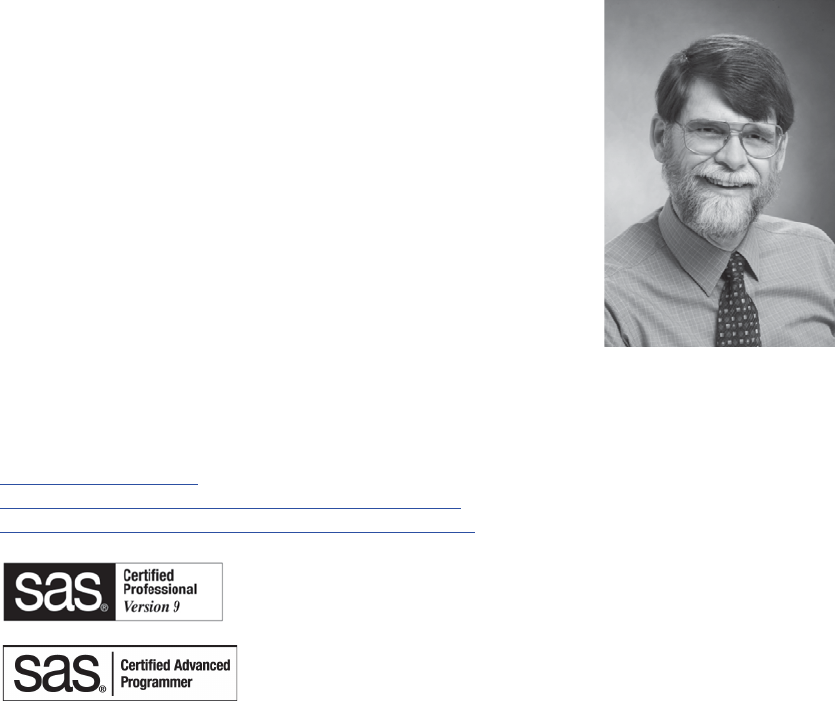
About the Author
This is Art Carpenter’s fifth book and his publications list includes
numerous papers and posters presented at SAS Global Forum, SUGI,
and other user group conferences. Art is a SAS Silver Circle member
and has been using SAS® since the mid 1970’s, and he has served in
various leadership positions in local, regional, national, and
international user groups. He is a SAS Certified Base Programmer
for SAS 9, SAS Certified Clinical Trials Programmer Using SAS 9
and a SAS Certified Advanced Programmer for SAS 9. Through
California Occidental Consultants he teaches SAS courses and
provides contract SAS programming support nationwide.
Author Contact
Arthur L. Carpenter
California Occidental Consultants
10606 Ketch Circle
Anchorage, AK 99515
(907) 865-9167
art@caloxy.com
http://www.caloxy.com
http://www.sascommunity.org/wiki/User:ArtCarpenter
http://support.sas.com/publishing/authors/carpenter.html
&DUSHQWHU$UW&DUSHQWHU¶V*XLGHWR,QQRYDWLYH6$67HFKQLTXHV&RS\ULJKW6$6,QVWLWXWH,QF&DU\1RUWK&DUROLQD86$
$
//5,*+765(6(59(')RUDGGLWLRQDO6$6UHVRXUFHVYLVLWVXSSRUWVDVFRPSXEOLVKLQJ
xxviii
&DUSHQWHU$UW&DUSHQWHU¶V*XLGHWR,QQRYDWLYH6$67HFKQLTXHV&RS\ULJKW6$6,QVWLWXWH,QF&DU\1RUWK&DUROLQD86$
$
//5,*+765(6(59(')RUDGGLWLRQDO6$6UHVRXUFHVYLVLWVXSSRUWVDVFRPSXEOLVKLQJ

Part 1
Data Preparation
Chapter 1 Moving, Copying, Importing, and Exporting Data 3
Chapter 2 Working with Your Data 37
Chapter 3 Just in the DATA Step 103
Chapter 4 Sorting the Data 185
Chapter 5 Working with Data Sets 197
Chapter 6 Table Lookup Techniques 213
&DUSHQWHU$UW&DUSHQWHU¶V*XLGHWR,QQRYDWLYH6$67HFKQLTXHV&RS\ULJKW6$6,QVWLWXWH,QF&DU\1RUWK&DUROLQD86$
$
//5,*+765(6(59(')RUDGGLWLRQDO6$6UHVRXUFHVYLVLWVXSSRUWVDVFRPSXEOLVKLQJ
2
&DUSHQWHU$UW&DUSHQWHU¶V*XLGHWR,QQRYDWLYH6$67HFKQLTXHV&RS\ULJKW6$6,QVWLWXWH,QF&DU\1RUWK&DUROLQD86$
$
//5,*+765(6(59(')RUDGGLWLRQDO6$6UHVRXUFHVYLVLWVXSSRUWVDVFRPSXEOLVKLQJ

Chapter 1
Moving, Copying, Importing, and Exporting Data
1.1 LIBNAME Statement Engines 4
1.1.1 Using Data Access Engines to Read and Write Data 5
1.1.2 Using the Engine to View the Data 6
1.1.3 Options Associated with the Engine 6
1.1.4 Replacing EXCEL Sheets 7
1.1.5 Recovering the Names of EXCEL Sheets 8
1.2 PROC IMPORT and EXPORT 9
1.2.1 Using the Wizard to Build Sample Code 9
1.2.2 Control through the Use of Options 9
1.2.3 PROC IMPORT Data Source Statements 10
1.2.4 Importing and Exporting CSV Files 12
1.2.5 Preventing the Export of Blank Sheets 15
1.2.6 Working with Named Ranges 16
1.3 DATA Step INPUT Statement 17
1.3.1 Format Modifiers for Errors 18
1.3.2 Format Modifiers for the INPUT Statement 18
1.3.3 Controlling Delimited Input 20
1.3.4 Reading Variable-Length Records 24
1.4 Writing Delimited Files 28
1.4.1 Using the DATA Step with the DLM= Option 28
1.4.2 PROC EXPORT 29
1.4.3 Using the %DS2CSV Macro 30
1.4.4 Using ODS and the CSV Destination 31
1.4.5 Inserting the Separator Manually 31
&DUSHQWHU$UW&DUSHQWHU¶V*XLGHWR,QQRYDWLYH6$67HFKQLTXHV&RS\ULJKW6$6,QVWLWXWH,QF&DU\1RUWK&DUROLQD86$
$
//5,*+765(6(59(')RUDGGLWLRQDO6$6UHVRXUFHVYLVLWVXSSRUWVDVFRPSXEOLVKLQJ
4Carpenter’s Guide to Innovative SAS Techniques
1.5 SQL Pass-Through 32
1.5.1 Adding a Pass-Through to Your SQL Step 32
1.5.2 Pass-Through Efficiencies 33
1.6 Reading and Writing to XML 33
1.6.1 Using ODS 34
1.6.2 Using the XML Engine 34
A great deal of the process of the preparation of the data is focused on the movement of data from
one table to another. This transfer of data may be entirely within the control of SAS or it may be
between disparate data storage systems. Although most of the emphasis in this book is on the use
of SAS, not all data are either originally stored in SAS or even ultimately presented in SAS. This
chapter discusses some of the aspects associated with moving data between tables as well as into
and out of SAS.
When moving data into and out of SAS, Base SAS allows you only limited access to other
database storage forms. The ability to directly access additional databases can be obtained by
licensing one or more of the various SAS/ACCESS products. These products give you the ability
to utilize the SAS/ACCESS engines described in Section 1.1 as well as an expanded list of
databases that can be used with the IMPORT and EXPORT procedures (Section 1.2).
SEE ALSO
Andrews (2006) and Frey (2004) both present details of a variety of techniques that can be used to
move data to and from EXCEL.
1.1 LIBNAME Statement Engines
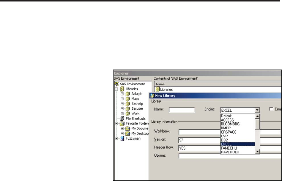
In SAS®9 a number of engines are available for the LIBNAME statement. These engines allow
you to read and write data to and from sources other than SAS. These engines can reduce the need
to use the IMPORT and EXPORT procedures.
The number of available engines depends on which products your company has licensed from
SAS. One of the most popular is SAS/ACCESS® Interface to PC Files.
You can quickly determine
which engines are available
to you. An easy way to build
this list is through the NEW
LIBRARY window.
From the SAS Explorer right
click on LIBRARIES and
select NEW. Available
engines appear in the
ENGINE pull-down list.
Pulling down the engine list
box on the ‘New Library’
dialog box shown to the
right, indicates the engines,
&DUSHQWHU$UW&DUSHQWHU¶V*XLGHWR,QQRYDWLYH6$67HFKQLTXHV&RS\ULJKW6$6,QVWLWXWH,QF&DU\1RUWK&DUROLQD86$
$
//5,*+765(6(59(')RUDGGLWLRQDO6$6UHVRXUFHVYLVLWVXSSRUWVDVFRPSXEOLVKLQJ

Chapter 1: Moving, Copying, Importing, and Exporting Data 5
libname toxls excel "&path\data\newwb.xls"; n
proc sort data=advrpt.demog
out=toxls.demog; o
by clinnum;
run;
data getdemog;
set toxls.demog; p
run;
libname toxls clear; q
including the EXCEL engine, among others, which are available to this user.
PROC SETINIT can also be used to determine which products have been licensed.
The examples in this section show various aspects of the EXCEL engine; however, most of what
is demonstrated can be applied to other engines as well.
SEE ALSO
Choate and Martell (2006) discuss the EXCEL engine on the LIBNAME statement in more detail.
Levin (2004) used engines to write to ORACLE tables.
1.1.1 Using Data Access Engines to Read and Write Data
In the following example, the EXCEL engine is used to create an EXCEL workbook, store a SAS
data set as a sheet in that workbook, and then read the data back from the workbook into SAS.
n The use of the
EXCEL engine
establishes the TOXLS
libref so that it can be
used to convert to and
from the Microsoft Excel
workbook NEWWB.XLS.
If it does not already
exist, the workbook will
be created upon execution
of the LIBNAME
statement. For many of
the examples in this book, the macro variable &PATH is assumed to have been defined. It
contains the upper portion of the path appropriate for the installation of the examples on your
system. See the book’s introduction and the AUTOEXEC.SAS in the root directory of the
example code, which you may download from support.sas.com/authors.
o Data sets that are written to the TOXLS libref will be added to the workbook as named sheets.
This OUT= option adds a sheet with the name of DEMOG to the NEWWB.XLS workbook.
p A sheet can be read from the workbook, and brought into the SAS world, simply by naming the
sheet.
q As should be the case with any libref, when you no longer need the association, the libref
should be cleared. This can be especially important when using data engines, since as long as the
libref exists, access to the data by applications other than SAS is blocked. Until the libref is
cleared, we are not able to view or work with any sheets in the workbook using Excel.
MORE INFORMATION
LIBNAME statement engines are also discussed in Sections 1.1.2 and 1.2.6. The XML engine is
discussed in Section 1.6.2.
&DUSHQWHU$UW&DUSHQWHU¶V*XLGHWR,QQRYDWLYH6$67HFKQLTXHV&RS\ULJKW6$6,QVWLWXWH,QF&DU\1RUWK&DUROLQD86$
$
//5,*+765(6(59(')RUDGGLWLRQDO6$6UHVRXUFHVYLVLWVXSSRUWVDVFRPSXEOLVKLQJ
6 Carpenter’s Guide to Innovative SAS Techniques
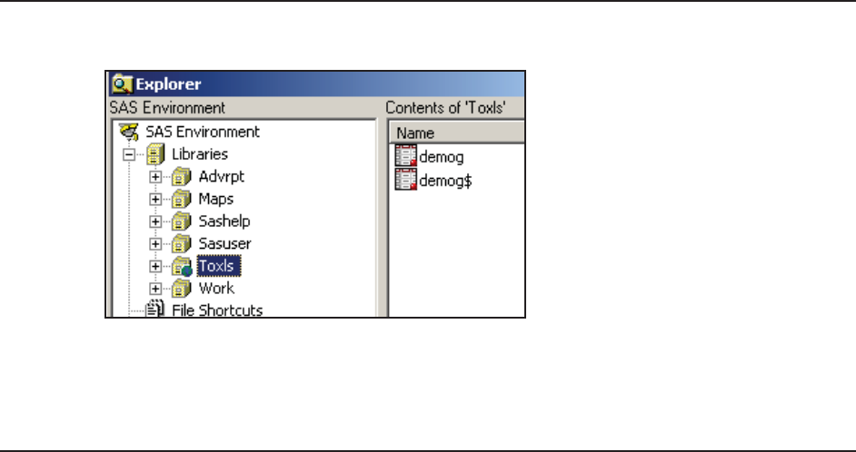
1.1.2 Using the Engine to View the Data
Once an access engine has been established by a libref, we are able to do almost all of the things
that we typically do with SAS data sets
that are held in a SAS library.
The SAS Explorer shows the contents
of the workbook with each sheet
appearing as a data table.
When viewing an EXCEL workbook
through a SAS/ACCESS engine, each
sheet appears as a data set. Indeed you
can use the VIEWTABLE or View
Columns tools against what are actually
sheets. Notice in this image of the SAS
Explorer, that the DEMOG sheet shows up twice. Sheet names followed by a $ are actually
named ranges, which under EXCEL can actually be a portion of the entire sheet. Any given sheet
can have more than one named range, so this becomes another way to filter or subset what
information from a given sheet will be brought into SAS through the SAS/ACCESS engine.
1.1.3 Options Associated with the Engine
The SAS/ACCESS engine is acting like a translator between two methods of storing information,
and sometimes we need to be able to control the interface. This can often be accomplished
through the use of options that modify the translation process. Many of these same options appear
in the PROC IMPORT/EXPORT steps as statements or options.
It is important to remember that not all databases store information in the same relationship as
does SAS. SAS, for instance, is column based - an entire column (variable) will be either numeric
or character. EXCEL, on the other hand, is cell based – a given cell can be considered numeric,
while the cell above it in the same column stores text. When translating from EXCEL to SAS we
can use options to establish guidelines for the resolution of ambiguous situations such as this.
Connection Options
For database systems that require user identification and passwords these can be supplied as
options on the LIBNAME statement.
USER User identification
PASSWORD User password
others Other connection options vary according to the database to which
you are connecting
LIBNAME Statement Options
These options control how information that is passed through the interface is to be processed.
Most of these options are database specific and are documented in the sections dealing with your
database.
&DUSHQWHU$UW&DUSHQWHU¶V*XLGHWR,QQRYDWLYH6$67HFKQLTXHV&RS\ULJKW6$6,QVWLWXWH,QF&DU\1RUWK&DUROLQD86$
$
//5,*+765(6(59(')RUDGGLWLRQDO6$6UHVRXUFHVYLVLWVXSSRUWVDVFRPSXEOLVKLQJ

Chapter 1: Moving, Copying, Importing, and Exporting Data 7
When working with EXCEL typical LIBNAME options might include:
HEADER Determines if a header row exists or should be added to the table.
MIXED Some columns contain both numeric and character information.
VER Controls which type (version) of EXCEL is to be written.
Data Source Options
Some of the same options associated with PROC IMPORT (see Section 1.2.3) can also be used on
the LIBNAME statement. These include:
GETNAMES Incoming variable names are available in the first row of the
incoming data.
SCANTEXT A length is assigned to a character variable by scanning the
incoming column and determining the maximum length.
1.1.4 Replacing EXCEL Sheets
While the EXCEL engine allows you to establish, view, and use a sheet in an Excel workbook as
a SAS data set, you cannot update, delete or replace the sheet from within SAS. It is possible to
replace the contents of a sheet, however, with the help of PROC DATASETS and the
SCAN_TEXT=NO option on the LIBNAME statement. The following example shows how to
replace the contents of an EXCEL sheet.
In the first DATA step the programmer has ‘accidently’ used a WHERE clause n that writes the
incorrect data, in this case 0
observations, to the EXCEL
sheet. Simply correcting and
rerunning the DATA step o
will not work because the sheet
already exists.
We could step out of SAS and
use EXCEL to manually
remove the bad sheet; however,
we would rather do it from
within SAS. First we must
reestablish the
libref using the
SCAN_TEXT=NO
option p. PROC
DATASETS can
then be used to
delete the sheet. In
actuality the sheet
has not truly been deleted, but merely cleared of all contents. Since the sheet is now truly empty
and the SCAN_TEXT option is set to NO, we can now replace the empty sheet with the desired
contents.
libname toxls excel "&path\data\newwb.xls";
data toxls.ClinicNames;
set advrpt.clinicnames;
where clinname>'X';n
run;
* Running the DATA step a second time
* results in an error;
data toxls.ClinicNames; o
set advrpt.clinicnames;
run;
libname toxls excel
"&path\data\newwb.xls"
scan_text=no p;
proc datasets library=toxls nolist;
delete ClinicNames;
quit;
&DUSHQWHU$UW&DUSHQWHU¶V*XLGHWR,QQRYDWLYH6$67HFKQLTXHV&RS\ULJKW6$6,QVWLWXWH,QF&DU\1RUWK&DUROLQD86$
$
//5,*+765(6(59(')RUDGGLWLRQDO6$6UHVRXUFHVYLVLWVXSSRUWVDVFRPSXEOLVKLQJ

8Carpenter’s Guide to Innovative SAS Techniques
The DATA step can now be rerun q, and the
sheet contents will now be correct. When SAS
has completed its work with the workbook, and
before you can use the workbook using EXCEL
you will need to clear the libref. This can be done
using the CLEAR option on the LIBNAME
statement r.
MORE INFORMATION
See Section 1.2 for more information on options and statements in PROC IMPORT and PROC
EXPORT. In addition to PROC DATASETS, Section 5.4 discusses other techniques that can be
used to delete tables. Section 14.4.5 also has an example of deleting data sets using PROC
DATASETS.
SEE ALSO
Choate and Martell (2006) discuss this and numerous other techniques that can be used with
EXCEL.
1.1.5 Recovering the Names of EXCEL Sheets
Especially when writing automated systems you may need to determine the names of workbook
sheets. There are a couple of ways to do this.
If you know the libref(s) of interest, the automatic view SASHELP.VTABLE can be used in a
DATA step to see the sheet names. This view
contains one observation for every SAS data set in
every SAS library in current use, and for the
TOXLS libref the sheet names will be shown as
data set names.
When there are a number of active
libraries, the process of building this
table can be lengthy. As a general rule
using the DICTIONARY.MEMBERS
table in a PROC SQL step has a couple
of advantages. It is usually quicker
than the SASHELP.VTABLE view, and it also has an ENGINE column which allows you to
search without knowing the specific libref.
The KEEP statement or the preferred KEEP= data set option could have been used in these
examples to reduce the number of variables (see Section 2.1.3).
MORE INFORMATION
SASHELP views and DICTIONARY tables are discussed further in Section 13.8.1.
SEE ALSO
A thread in the SAS Forums includes similar examples.
http://communities.sas.com/thread/10348?tstart=0
data toxls.ClinicNames; q
set advrpt.clinicnames;
run;
libname toxls clear; r
data sheetnames;
set sashelp.vtable;
where libname = 'TOXLS';
run;
proc sql;
create table sheetnames as
select * from dictionary.members
where engine= 'EXCEL' ;
quit ;
&DUSHQWHU$UW&DUSHQWHU¶V*XLGHWR,QQRYDWLYH6$67HFKQLTXHV&RS\ULJKW6$6,QVWLWXWH,QF&DU\1RUWK&DUROLQD86$
$
//5,*+765(6(59(')RUDGGLWLRQDO6$6UHVRXUFHVYLVLWVXSSRUWVDVFRPSXEOLVKLQJ

Chapter 1: Moving, Copying, Importing, and Exporting Data 9
1.2 PROC IMPORT and EXPORT
Like the SAS/ACCESS engines discussed in Section 1.1, the IMPORT and EXPORT procedures
are used to translate data into and out of SAS from a variety of data sources. The SAS/ACCESS
product, which is usually licensed separately through SAS (but may be bundled with Base SAS),
controls which databases you will be able to move data to and from. Even without SAS/ACCESS
you can still use these two procedures to read and write text files such as comma separated
variables (CSV), as well as files using the TAB and other delimiters to separate the variables.
1.2.1 Using the Wizard to Build Sample Code
The import/export wizard gives you a step-by-step guide to the process of importing or exporting
data. The wizard is easy enough to use, but like all wizards does not lend itself to automated or
batch processing. Fortunately the wizard is actually building a PROC IMPORT/EXPORT step in
the background, and you can capture the completed code. For both the import and export process
the last screen prompts you to ‘Create SAS Statements.’
The following PROC EXPORT step
was built using the EXPORT
wizard. A simple inspection of the
code indicates what needs to be
changed for a future application of
the EXPORT procedure. Usually
this means that the wizard itself
needs to be run infrequently.
n The DATA= option identifies the data set that is to be converted.
o In this case, since we are writing to EXCEL p the OUTFILE= identifies the workbook.
q If the sheet already exists, it will be replaced.
r The sheet name can also be provided.
Converting the previous generic step to one that creates a CSV file is very straightforward.
SEE ALSO
Raithel (2009) discusses the use of the EXPORT wizard to generate code in a sasCommunity.org
tip.
1.2.2 Control through the Use of Options
There are only a few options that need to be specified. Of these most of the interesting ones are
used when the data are being imported (clearly SAS already knows all about the data when it is
being exported).
PROC EXPORT DATA= sashelp.class
OUTFILE= "&path\data\class.csv"
DBMS=csv
REPLACE;
RUN;
PROC EXPORT DATA= WORK.A n
OUTFILE= "C:\temp\junk.xls"o
DBMS=EXCELp
REPLACEq;
SHEET="junk";r
RUN;
&DUSHQWHU$UW&DUSHQWHU¶V*XLGHWR,QQRYDWLYH6$67HFKQLTXHV&RS\ULJKW6$6,QVWLWXWH,QF&DU\1RUWK&DUROLQD86$
$
//5,*+765(6(59(')RUDGGLWLRQDO6$6UHVRXUFHVYLVLWVXSSRUWVDVFRPSXEOLVKLQJ

10 Carpenter’s Guide to Innovative SAS Techniques
DBMS= Identifies the incoming database structure (including .CSV and .TXT).
Since database structures change with versions of the software, you should
know the database version. Specific engines exist at the version level for
some databases (especially Microsoft’s EXCEL and ACCESS). The
documentation discusses which engine is optimized for each software
version.
REPLACE Determines whether or not the destination target (data set, sheet, table) is
replaced if it already exists.
1.2.3 PROC IMPORT Data Source Statements
These statements give you additional control over how the incoming data are to be read and
interpreted. Availability of any given source statement depends on the type (DBMS=) of the
incoming data.
DATAROW First incoming row that contains data.
GETNAMES The names of the incoming columns are available
in the first row of the incoming data. Default
column names when none are available on the
incoming table are VAR1, VAR2, etc.
GUESSINGROWS Number of rows SAS will scan before determining
if an incoming column is numeric or character.
This is especially important for mixed columns
and early rows are all numeric. In earlier versions
of SAS modifications to the SAS Registry were
needed to change the number of rows used to
determine the variable’s type, which is fortunately no
longer necessary.
RANGE and SHEET For spreadsheets a specific sheet name, named
range, or range within a sheet can be specified.
SCANTEXT and TEXTSIZE PROC IMPORT assigns a length to a character variable
by scanning the incoming column and determining
the maximum.
When using GETNAMES to read column names from the source data, keep in mind that most
databases use different naming conventions than SAS and may have column names that will cause
problems when imported. By default illegal characters are replaced with an underscore (_) by
PROC IMPORT. When you need the original column name, the system option
VALIDVARNAME=ANY (see Section 14.1.2) allows a broader range of acceptable column
names.
&DUSHQWHU$UW&DUSHQWHU¶V*XLGHWR,QQRYDWLYH6$67HFKQLTXHV&RS\ULJKW6$6,QVWLWXWH,QF&DU\1RUWK&DUROLQD86$
$
//5,*+765(6(59(')RUDGGLWLRQDO6$6UHVRXUFHVYLVLWVXSSRUWVDVFRPSXEOLVKLQJ
Chapter 1: Moving, Copying, Importing, and Exporting Data 11
In the contrived data for the following example we have an EXCEL file containing a subject
number and a response variable (SCALE). The import wizard can be used to generate a PROC
IMPORT step that will read the XLS file (MAKESCALE.XLS) and
create the data set WORK.SCALEDATA. This PROC IMPORT
step creates two numeric variables.
Notice that the form of the
supporting statements is different than form most procedures. They look more like options
(option=value;) than like statements. The GETNAMES= statement n is used to determine the
variable names from the first column.
When importing data SAS must determine if a given column is to be numeric or character. A
number of clues are utilized to make this determination. SAS will scan a number of rows for each
column to try to determine if all the values are numeric. If a non-numeric value is found, the
column will be read as a character variable; however, only some of the rows are scanned and
consequently an incorrect determination is possible. o The MIXED= statement is used to specify
that the values in a given column are always of a single type (numeric or character). When set to
YES, the IMPORT procedure will tend to create character variables in order to accommodate
mixed types.
In this contrived example it turns out that starting with subject 271 the variable SCALE starts
taking on non-numeric values. Using the previous PROC IMPORT
step does not detect this change, and creates SCALE as a numeric
variable. This, of course, means that data will be lost as SCALE will
be missing for the observations starting from row 712.
For PROC IMPORT to correctly read the information in SCALE it
needs to be a character variable. We can encourage IMPORT to
create a character variable by using the MIXED and
G
U
E
GUESSINGROWS
statements.
PROC IMPORT OUT= WORK.scaledata
DATAFILE= "C:\Temp\makescale.xls"
DBMS=EXCEL REPLACE;
RANGE="MAKESCALE";
GETNAMES=YES; n
MIXED=NO; o
SCANTEXT=YES;
USEDATE=YES;
SCANTIME=YES;
RUN;
PROC IMPORT OUT= WORK.scaledata
DATAFILE= "C:\Temp\makescale.xls"
DBMS=excel REPLACE;
GETNAMES=YES;
MIXED=YES; p
RUN;
&DUSHQWHU$UW&DUSHQWHU¶V*XLGHWR,QQRYDWLYH6$67HFKQLTXHV&RS\ULJKW6$6,QVWLWXWH,QF&DU\1RUWK&DUROLQD86$
$
//5,*+765(6(59(')RUDGGLWLRQDO6$6UHVRXUFHVYLVLWVXSSRUWVDVFRPSXEOLVKLQJ

12 Carpenter’s Guide to Innovative SAS Techniques
PROC IMPORT OUT= WORK.scaledata
DATAFILE= "C:\Temp\makescale.xls"
DBMS=xls REPLACE; q
GETNAMES=YES; r
GUESSINGROWS=800; s
RUN;
Changing the MIXED= value to YES p is not necessarily sufficient to cause SCALE to be a
character value; however, if the value of the DBMS option is changed from EXCEL to XLS q,
the MIXED=YES statement r is honored and SCALE is written as a character variable in the
data set SCALEDATA.
When MIXED=YES is not
practical the
GUESSINGROWS=
statement can sometimes
be used to successfully
determine the type for a
variable.
GUESSINGROWS cannot be used when DBMS=EXCEL, however it can be used when
DBMS=XLS. Since GUESSINGROWS s changes the number of rows that are scanned prior to
determining if the column should be numeric or character, its use can increase the time and
resources required to read the data.
SEE ALSO
The SAS Forum thread http://communities.sas.com/thread/12743?tstart=0 has a PROC IMPORT
using NAMEROW= and STARTROW= data source statements. The thread
http://communities.sas.com/thread/30405?tstart=0 discusses named ranges, and it and the thread
http://communities.sas.com/thread/12293?tstart=0 show the use of several data source statements.
1.2.4 Importing and Exporting CSV Files
Comma Separated Variable, CSV, files have been a standard file type for moving data between
systems for many years. Fortunately we now have a number of superior tools available to us so
that we do not need to resort to CSV files as often. Still they are commonly used and we need to
understand how to work with them.
Both the IMPORT and EXPORT procedures can work with CSV files (this capability is a part of
the Base SAS product and a SAS/ACCESS product is not required). Both do the conversion by
first building a DATA step, which is then executed.
Building a DATA Step
When you use the import/export wizard to save the PROC step (see Section 1.2.1), the resulting
DATA step is not saved. Fortunately you can still get to the generated DATA step by recalling the
last submitted code.
1. Execute the IMPORT/EXPORT procedure.
2. While in the Display Manager, go to RUNĺRecall Last Submit.
Once the code generated by the procedure is loaded into the editor, you can modify it for other
purposes or simply learn from it. For the simple PROC EXPORT step in Section 1.2.1, the
following code is generated:
&DUSHQWHU$UW&DUSHQWHU¶V*XLGHWR,QQRYDWLYH6$67HFKQLTXHV&RS\ULJKW6$6,QVWLWXWH,QF&DU\1RUWK&DUROLQD86$
$
//5,*+765(6(59(')RUDGGLWLRQDO6$6UHVRXUFHVYLVLWVXSSRUWVDVFRPSXEOLVKLQJ

Chapter 1: Moving, Copying, Importing, and Exporting Data 13
Headers are Not on Row 1
The ability to create column names based on information contained in the data is very beneficial.
This is especially important when building a large SAS table from a CSV file with lots of
columns. Unfortunately we do not always have a CSV file with the column headers in row 1.
Since GETNAMES=YES assumes that the headers are in row 1 we cannot use
GETNAMES=YES. Fortunately this is SAS, so there are alternatives.
The CSV file created in the PROC EXPORT step in Section 1.2.1 has been modified so that the
column names are on row 3. The first few lines of the file are:
/**********************************************************************
* PRODUCT: SAS
* VERSION: 9.1
* CREATOR: External File Interface
* DATE: 11APR09
* DESC: Generated SAS Datastep Code
* TEMPLATE SOURCE: (None Specified.)
***********************************************************************/
data _null_;
set SASHELP.CLASS end=EFIEOD;
%let _EFIERR_ = 0; /* set the ERROR detection macro variable */
%let _EFIREC_ = 0; /* clear export record count macro variable */
file 'C:\InnovativeTechniques\data\class.csv' delimiter=','
DSD DROPOVER lrecl=32767;
format Name $8. ;
format Sex $1. ;
format Age best12. ;
format Height best12. ;
format Weight best12. ;
if _n_ = 1 then /* write column names */
do;
put
'Name'
','
'Sex'
','
'Age'
','
'Height'
','
'Weight'
;
end;
do;
EFIOUT + 1;
put Name $ @;
put Sex $ @;
put Age @;
put Height @;
put Weight ;
;
end;
if _ERROR_ then call symputx('_EFIERR_',1); /*set ERROR detection
macro variable*/
if EFIEOD then call symputx('_EFIREC_',EFIOUT);
run;
&DUSHQWHU$UW&DUSHQWHU¶V*XLGHWR,QQRYDWLYH6$67HFKQLTXHV&RS\ULJKW6$6,QVWLWXWH,QF&DU\1RUWK&DUROLQD86$
$
//5,*+765(6(59(')RUDGGLWLRQDO6$6UHVRXUFHVYLVLWVXSSRUWVDVFRPSXEOLVKLQJ

14 Carpenter’s Guide to Innovative SAS Techniques
The DATA step generated by PROC IMPORT (E1_2_3c_ImportWO.SAS), simplified somewhat
for this example, looks something like:
Clearly SAS has
substituted VAR1,
VAR2, and so on for
the unknown variable
names. If we knew the
variable names, all we
would have to do to fix
the problem would be
to rename the variables.
The following macro
reads the header row
from the appropriate
row in the CSV file,
and uses that
information to rename
the columns in
WORK.CLASSWO.
Class Data from SASHELP,,,,
Comma Separated rows; starting in row 3,,,,
Name,Sex,Age,Height,Weight
Alfred,M,14,69,112.5
Alice,F,13,56.5,84
Barbara,F,13,65.3,98
Carol,F,14,62.8,102.5
. . . . data not shown . . . .
data WORK.CLASSWO ;
infile "&path\Data\classwo.csv" delimiter = ','
MISSOVER DSD lrecl=32767 firstobs=4 ;
informat VAR1 $8. ;
informat VAR2 $1. ;
informat VAR3 best32. ;
informat VAR4 best32. ;
informat VAR5 best32. ;
format VAR1 $8. ;
format VAR2 $1. ;
format VAR3 best12. ;
format VAR4 best12. ;
format VAR5 best12. ;
input
VAR1 $
VAR2 $
VAR3
VAR4
VAR5
;
run;
&DUSHQWHU$UW&DUSHQWHU¶V*XLGHWR,QQRYDWLYH6$67HFKQLTXHV&RS\ULJKW6$6,QVWLWXWH,QF&DU\1RUWK&DUROLQD86$
$
//5,*+765(6(59(')RUDGGLWLRQDO6$6UHVRXUFHVYLVLWVXSSRUWVDVFRPSXEOLVKLQJ

Chapter 1: Moving, Copying, Importing, and Exporting Data 15
SEE ALSO
McGuown (2005) also discusses the code generated by PROC IMPORT when reading a CSV file.
King (2011) uses arrays and hash tables to read CSV files with unknown or varying variable lists.
These flexible and efficient techniques could be adapted to the type of problem described in this
section.
1.2.5 Preventing the Export of Blank Sheets
PROC EXPORT does not protect us from writing a blank sheet when our exclusion criteria
excludes all possible rows from a given sheet n. In the following example we have inadvertently
asked to list all students
with SEX=’q’. There are
none of course, and the
resulting sheet is blank,
except for the column
headers.
%macro rename(headrow=3, rawcsv=, dsn=);
%local lib ds i;
data _null_ ;
infile "&path\Data\&rawcsv"
scanover lrecl=32767 firstobs=&headrow;
length temp $ 32767;
input temp $;
i=1;
do while(scan(temp,i,',') ne ' ');
call symputx('var'||left(put(i,4.)),scan(temp,i,','),'l');
i+1;
end;
call symputx('varcnt',i-1,'l');
stop;
run;
%* Determine the library and dataset name;
%if %scan(&dsn,2,.) = %then %do;
%let lib=work;
%let ds = %scan(&dsn,1,.);
%end;
%else %do;
%let lib= %scan(&dsn,1,.);
%let ds = %scan(&dsn,2,.);
%end;
proc datasets lib=&lib nolist;
modify &ds;
rename
%do i = 1 %to &varcnt;
var&i = &&var&i
%end;
;
quit;
%mend rename;
%rename(headrow=3, rawcsv=classwo.csv, dsn=work.classwo)
proc export data=sashelp.class(where=(sex='q'n))
outfile='c:\temp\classmates.xls'
dbms=excel2000
replace;
SHEET='sex: Q';
run;
&DUSHQWHU$UW&DUSHQWHU¶V*XLGHWR,QQRYDWLYH6$67HFKQLTXHV&RS\ULJKW6$6,QVWLWXWH,QF&DU\1RUWK&DUROLQD86$
$
//5,*+765(6(59(')RUDGGLWLRQDO6$6UHVRXUFHVYLVLWVXSSRUWVDVFRPSXEOLVKLQJ

16 Carpenter’s Guide to Innovative SAS Techniques
We can prevent this from occurring by first identifying those levels of SEX that have one or more
rows. There are a number of ways to generate a list of values of a variable; however, an SQL step
is ideally suited to place those values into a macro variable for further processing.
The name of the data set that is to be exported, as well as the classification variable, are passed to
the macro %MAKEXLS as named parameters.
o An SQL step is
used to build a list of
distinct values of the
classification variable.
p These values are
saved in the macro
variable
&VALUELIST.
q A %DO loop is
used to process across
the individual values,
which are extracted r
from the list using the
%SCAN function.
s The PROC
EXPORT step then
creates a sheet for the
selected value. t
SEE ALSO
A similar example which breaks a data set into separate sheets can be found in the article
“Automatically_Separating_Data_into_Excel_Sheets” on sasCommunity.org.
http://www.sascommunity.org/wiki/Automatically_Separating_Data_into_Excel_Sheets
1.2.6 Working with Named Ranges
By default PROC IMPORT and the LIBNAME statement’s EXCEL engine expect EXCEL data
to be arranged in a certain way (column headers, if present, on row one column A; and data
starting on row two). It is not unusual, however, for the data to be delivered as part of a report or
as a subset of a larger table. One solution is to manually cut and paste the data onto a blank sheet
so that it conforms to the default layout. It can often be much easier to create a named range.
%macro makexls(dsn=,class=);
%local valuelist listnum i value;
proc sql noprint;
select distinct &class o
into :valuelist separated by ' ' p
from &dsn;
%let listnum = &sqlobs;
quit;
%* One export for each sheet;
%do i = 1 %to &listnum; q
%let value = %scan(&valuelist,&i,%str( )); r
proc export data=&dsn(where=(&class="&value")) s
outfile="c:\temp\&dsn..xls"
dbms=excel2000
replace;
SHEET="&class:&value";
run;
%end;
%mend makexls;
%makexls(dsn=sashelp.class,class=sex)
&DUSHQWHU$UW&DUSHQWHU¶V*XLGHWR,QQRYDWLYH6$67HFKQLTXHV&RS\ULJKW6$6,QVWLWXWH,QF&DU\1RUWK&DUROLQD86$
$
//5,*+765(6(59(')RUDGGLWLRQDO6$6UHVRXUFHVYLVLWVXSSRUWVDVFRPSXEOLVKLQJ
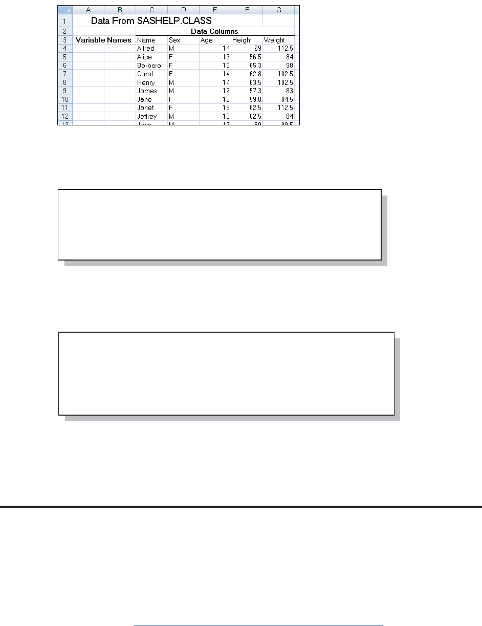
Chapter 1: Moving, Copying, Importing, and Exporting Data 17
The EXCEL spreadsheet shown here
contains the SASHELP.CLASS data
set (only part of which is shown here);
however, titles and columns have been
added. Using the defaults PROC
IMPORT will not be able to
successfully read this sheet.
To facilitate the use of this spreadsheet,
a named range was created for the
rectangle defined by C3-G22 . This
range was given the name ‘CLASSDATA’. This named range can now be used when reading the
data from this sheet.
When reading a named range using the EXCEL engine on the LIBNAME statement, the named
range
(CLASSDATA) is
used just as you
would the sheet
name n.
o When using an
engine on the LIBNAME statement be sure to clear the libref so that you can use the spreadsheet
outside of SAS.
When using PROC IMPORT to read a named range, the RANGE= statement p is used to
designate the
named range of
interest. Since
the name of the
named range is
unique to the
workbook, a
sheet name is
not required.
MORE INFORMATION
The EXCEL LIBNAME engine is introduced in Section 1.1.
1.3 DATA Step INPUT Statement
The INPUT statement is loaded with options that make it extremely flexible. Since there has been
a great deal written about the basic INPUT statement, only a few of the options that seem to be
under used have been collected here.
SEE ALSO
An overview about reading raw data with the INPUT statement can be found in the SAS
documentation at http://support.sas.com/publishing/pubcat/chaps/58369.pdf. Schreier (2001)
gives a short overview of the automatic _INFILE_ variable along with other information
regarding the reading of raw data.
libname seexls excel "&path\data\E1_2_6classmates.xls";
data class;
set seexls.classdata; n
run;
libname seexls clear; o
proc import out=work.classdata
datafile= "&path\data\E1_2_6classmates.xls"
dbms=xls replace;
getnames=yes;
range='classdata'; p
run;
&DUSHQWHU$UW&DUSHQWHU¶V*XLGHWR,QQRYDWLYH6$67HFKQLTXHV&RS\ULJKW6$6,QVWLWXWH,QF&DU\1RUWK&DUROLQD86$
$
//5,*+765(6(59(')RUDGGLWLRQDO6$6UHVRXUFHVYLVLWVXSSRUWVDVFRPSXEOLVKLQJ

18 Carpenter’s Guide to Innovative SAS Techniques
1.3.1 Format Modifiers for Errors
Inappropriate data within an input field can cause input errors that prevent the completion of the
data set. As the data are read, a great many messages can also be generated and written to the
LOG. The (?) and (??) format modifiers control error handling. Both the ? and the ?? suppress
error messages in the LOG; however, the ?? also resets the automatic error variable (_ERROR_)
to 0. This means that while both of these operators control what is written to the LOG only the ??
will necessarily prevent the step from terminating when the maximum error count is reached.
In the following step, the third data row contains an invalid value for AGE. AGE is assigned a
missing value, and because of the ?? operator no
‘invalid data’ message is written to the LOG.
MORE INFORMATION
The ?? modifier is used with the INPUT function in
Sections 2.3.1 and 3.6.1.
SEE ALSO
The SAS Forum thread found at http://communities.sas.com/message/48729 has an example that
uses the ?? format modifier.
1.3.2 Format Modifiers for the INPUT Statement
Some of the most difficult input coding occurs when combining the use of informats with LIST
style input. This style is generally required when columns are not equally spaced so informats
can’t be easily used, and the fields are delimited with blanks. LIST is also the least flexible input
style. Informat modifiers include:
& allows embedded blanks in character variables
: allows the use of informats for non-aligned columns
~ allows the use of quotation marks within data fields
Because of the inherent disadvantages of LIST input (space delimited fields), when it is possible,
consider requesting a specific unique delimiter. Most recently generated files of this type utilize a
non-blank delimiter, which allows you to take advantage of some of the options discussed in
Section 1.3.3. Unfortunately many legacy files are space delimited, and we generally do not have
the luxury of either requesting a specific delimiter or editing the existing file to replace the spaces
with delimiters.
There are two problems in the data being read in the following code. The three potential INPUT
statements (two of the three are commented) highlight how the ampersand and colon can be used
to help read the data. Notice that DOB does not start in a consistent column and the second last
name has an embedded blank.
data base;
input age ?? name $;
datalines;
15 Fred
14 Sally
x John
run;
&DUSHQWHU$UW&DUSHQWHU¶V*XLGHWR,QQRYDWLYH6$67HFKQLTXHV&RS\ULJKW6$6,QVWLWXWH,QF&DU\1RUWK&DUROLQD86$
$
//5,*+765(6(59(')RUDGGLWLRQDO6$6UHVRXUFHVYLVLWVXSSRUWVDVFRPSXEOLVKLQJ

Chapter 1: Moving, Copying, Importing, and Exporting Data 19
Using the first INPUT statement without informat modifiers n shows, that for the second data
line, both the date and the last name have been read incorrectly.
Assuming the second INPUT statement o was commented and used, the colon modifier is placed
in front of the date informat. The colon allows the format to essentially float to the appropriate
starting point by using LIST input and then applying the informat once the value is found.
The birthdays are now being read
correctly; however, Susan’s last
name is being split because the
embedded blank is being
interpreted as a field delimiter.
The ampersand p can be used to
allow embedded spaces within a
field.
By placing an ampersand after the variable name (LNAME) p, the blank space becomes part of
the variable rather than
a delimiter. We are
now reading both the
date of birth and the
last name correctly.
While the ampersand
is also used as a macro
language trigger, this
will not be a problem
when it is used as an INPUT statement modifier as long as it is not immediately followed by text
that could be interpreted as a macro variable name (letter or underscore). In this example the
ampersand is followed by the semicolon so there will be no confusion with the macro language.
1.3.2a List Input Modifiers
Obs lname fname dob
1 Johnson Sam 12/15/1945
2 83 Susan 10/10/2019
title '1.3.2a List Input Modifiers';
data base;
length lname $15;
input fname $ dob mmddyy10. lname $ ; n
*input fname $ dob :mmddyy10. lname $ ; o
*input fname $ dob :mmddyy10. lname $ &; p
datalines;
Sam 12/15/1945 Johnson
Susan 10/10/1983 Mc Callister
run;
1.3.2a List Input Modifiers
Obs lname fname dob
1 Johnson Sam 12/15/1945
2 Mc Susan 10/10/1983
input fname $ dob :mmddyy10. lname $ &; p
1.3.2a List Input Modifiers
Obs lname fname dob
1 Johnson Sam 12/15/1945
2 Mc Callister Susan 10/10/1983
&DUSHQWHU$UW&DUSHQWHU¶V*XLGHWR,QQRYDWLYH6$67HFKQLTXHV&RS\ULJKW6$6,QVWLWXWH,QF&DU\1RUWK&DUROLQD86$
$
//5,*+765(6(59(')RUDGGLWLRQDO6$6UHVRXUFHVYLVLWVXSSRUWVDVFRPSXEOLVKLQJ

20 Carpenter’s Guide to Innovative SAS Techniques
While the trailing ampersand can be helpful it can also introduce problems as well. If the data had
been slightly more complex, even this solution might not have worked. The following data also
contains a city name. Even though the city is not being read, the trailing & used with the last name
(LNAME) causes the city
name to be confused with
the last name.
Because of the trailing &
and the length of LNAME
($15) a portion of the city
(New York) has been read
into the LNAME for the
second observation. On the
first observation the last
name is correct because
more than one space
separates Johnson and
Seattle. Even with the
trailing &, more than one
space is still successfully
seen as a field delimiter.
On the second observation the city would not have been confused with the last name had there
been two or more spaces between the two fields.
q Placing the FORMAT statement within the DATA step causes the format to be associated with
the variable DOB in subsequent steps. The INFORMAT statement is only used when reading the
data.
r The DATALINES statement causes subsequent records to be read as data up to, but not
including, the first line that contains a semicolon. In the previous examples the RUN statement
doubles as the end of data marker. Many programmers use a separate semicolon to perform this
task. Both styles are generally considered acceptable (as long as you are using the RUN statement
to end your step).
With only a single space between the last name and the city, the trailing & alone is not sufficient
to help the INPUT statement distinguish between these two fields. Additional variations of this
example can be found in Section 1.3.3.
MORE INFORMATION
LIST input is a form of delimited input and as such these options also apply to the examples
discussed in Section 1.3.3. When the date form is not consistent one of the any date informats
may be helpful. See Section 12.6 for more information on the use of these specialized informats.
SEE ALSO
The SAS Forum thread http://communities.sas.com/message/42690 discusses the use of list input
modifiers.
1.3.3 Controlling Delimited Input
Technically LIST input is a form of delimited input, with the default delimiter being a space. This
means that the modifiers shown in Section 1.3.2 apply to other forms of delimited input, including
comma separated variable, CSV, files.
title '1.3.2b List Input Modifiers';
data base;
length lname $15;
input fname $ dob :mmddyy10. lname $ &;
format dob mmddyy10.; q
datalines;
Sam 12/15/1945 Johnson Seattle
Susan 10/10/1983 Mc Callister New York
; r
run;
1.3.2b List Input Modifiers
Obs lname fname dob
1 Johnson Sam 12/15/1945
2 Mc Callister Ne Susan 10/10/1983
&DUSHQWHU$UW&DUSHQWHU¶V*XLGHWR,QQRYDWLYH6$67HFKQLTXHV&RS\ULJKW6$6,QVWLWXWH,QF&DU\1RUWK&DUROLQD86$
$
//5,*+765(6(59(')RUDGGLWLRQDO6$6UHVRXUFHVYLVLWVXSSRUWVDVFRPSXEOLVKLQJ

Chapter 1: Moving, Copying, Importing, and Exporting Data 21
INFILE Statement Options
Options on the INFILE statement are used to control how the delimiters are to be interpreted.
DELIMITER Specifies the character that delimits fields (other than the default - a
space). This option is often abbreviated as DLM=.
DLMSTR Specifies a single multiple character string as a delimiter.
DLMOPT Specifies parsing options for the DLMSTR option.
DSD Allows character fields that are surrounded by quotes (by setting the
comma as the delimiter). Two successive delimiters are interpreted as
individual delimiters, which allow missing values to be assigned
appropriately. DSD also removes quotation marks from character
values surrounded by quotes. If the comma is not the delimiter you will
need to use the DLM= option along with the DSD option.
Some applications, such as Excel, build delimiter separated variable files with quotes surrounding
the fields. This can be critical if a field’s value can contain the field separator. For default list
input, where a space is a delimiter, it can be very difficult to successfully read a field with an
embedded blank (see Section 1.3.2 which discusses the use of trailing & to read embedded
spaces). The DSD option alerts SAS to the potential of quoted character fields. The following
example demonstrates simple comma-separated data.
n Although the INFILE statement is
often not needed when using the
DATALINES, CARDS, or CARDS4
statements, it can be very useful
when the options associated with the
INFILE statement are needed. The
fileref can be DATALINES or
CARDS.
The DLM= option is used to specify
the delimiter. In this
example the field
delimiter is specified as
a comma o.
The fields containing character data have been quoted. Since we do not actually want the quote
marks to be a part of the data fields, the DSD option p alerts the parser to this possibility and the
quotes themselves become a part of the field delimiting process.
Using the DSD option results in data
fields without the quotes.
1.3.3a Delimited List Input Modifiers
Obs lname fname dob
1 Johnson Sam 12/15/1945
2 Mc Callister Susan 10/10/1983
data base;
length lname $15;
infile datalines n dlm=','; o
*infile datalines dlm=',' dsd; p
input fname $ lname $ dob :mmddyy10.;
datalines;
'Sam','Johnson',12/15/1945
'Susan','Mc Callister',10/10/1983
run;
1.3.3a Delimited List Input Modifiers
Obs lname fname dob
1 'Johnson' 'Sam' 12/15/1945
2 'Mc Callister' 'Susan' 10/10/1983
infile datalines dlm=',' dsd; p
&DUSHQWHU$UW&DUSHQWHU¶V*XLGHWR,QQRYDWLYH6$67HFKQLTXHV&RS\ULJKW6$6,QVWLWXWH,QF&DU\1RUWK&DUROLQD86$
$
//5,*+765(6(59(')RUDGGLWLRQDO6$6UHVRXUFHVYLVLWVXSSRUWVDVFRPSXEOLVKLQJ

22 Carpenter’s Guide to Innovative SAS Techniques
On the INPUT Statement
The tilde (~) qcan be used to modify a format, much the same way as a colon (:); however, the
two modifiers are not exactly the same.
The tilde format modifier correctly reads the BIRTHLOC field; however, it preserves the quote
marks that surround the field. Like the colon, the tilde can either precede or follow the $ for
character variables. As an aside notice that for this example quote marks surround the numeric
date value for the first row. The field is still processed correctly as a numeric SAS date value.
Replacing the tilde q with a colon (:) would cause the BIRTHLOC value to be saved without the
quote marks. If instead we supply a length for BIRTHLOC r, neither a format nor the tilde will
be needed.
1.3.3c Delimited List Input Modifiers
BIRTHLOC without a Format Modifier
BIRTHLOC Length Specified
Obs lname birthloc fname dob
1 Johnson Fresno, CA Sam 12/15/1945
2 Mc Callister Seattle, WA Susan 10/10/1983
title '1.3.3c Delimited List Input Modifiers';
title2 'BIRTHLOC without a Format Modifier';
title3 'BIRTHLOC Length Specified';
data base;
length lname birthloc $15; r
infile datalines dlm=',' dsd;
input fname $ lname $ birthloc $ dob :mmddyy10. ;
datalines;
'Sam','Johnson', 'Fresno, CA',12/15/1945
'Susan','Mc Callister','Seattle, WA',10/10/1983
run;
1.3.3b Delimited List Input Modifiers
Using the ~ Format Modifier
Obs lname fname birthloc dob
1 Johnson Sam 'Fresno, CA' 12/15/1945
2 Mc Callister Susan 'Seattle, WA' 10/10/1983
title '1.3.3b Delimited List Input Modifiers';
title2 'Using the ~ Format Modifier';
data base;
length lname $15;
infile datalines dlm=',' dsd;
input fname $ lname $ birthloc $~q15. dob :mmddyy10. ;
datalines;
'Sam','Johnson', 'Fresno, CA','12/15/1945'
'Susan','Mc Callister','Seattle, WA',10/10/1983
run;
&DUSHQWHU$UW&DUSHQWHU¶V*XLGHWR,QQRYDWLYH6$67HFKQLTXHV&RS\ULJKW6$6,QVWLWXWH,QF&DU\1RUWK&DUROLQD86$
$
//5,*+765(6(59(')RUDGGLWLRQDO6$6UHVRXUFHVYLVLWVXSSRUWVDVFRPSXEOLVKLQJ

Chapter 1: Moving, Copying, Importing, and Exporting Data 23
data imports;
infile cards dlm='/,';
input id importcode $ value;
cards;
14,1,13
25/Q9,15
6,D/20
run;
Obs id importcode value
1 14 1 13
2 25 Q9 15
3 6 D 20
data imports;
retain dlmvar '/,'; s
infile cards dlm=dlmvar;
input id importcode $ value;
cards;
14,1,13
25/Q9,15
6,D/20
run;
data imports;
infile cards dlmstr=',,/';
input id importcode $ value;
cards;
14,,/1/,,/13
25,,/Q9,,,/15
6,,/,D,,/20
run;
Multiple Delimiters
It is possible to read delimited input streams that contain more than one delimiter. In the following
small example two delimiters, a comma and a
slash are both used to delimit the data values.
Notice that the DLM option causes either the
comma or the slash to be used as field
delimiters, but not the slash comma together as a
single delimiter (see the DLMSTR option below
to create a single multiple character delimiter).
s Because the INFILE statement is executed for
each observation, the value assigned to the DLM
option does not necessarily need to be a
constant. It can also be a variable or can be
changed using IF-THEN/ELSE logic. In the
simplest form this variable could be assigned in
a retain statement.
t This simple example demonstrates a delimiter
that varies by observation. Here the first
character of each line is the delimiter that is to
be used in that line. The delimiter is read, stored,
and then used on the INFILE statement. Here we
are taking advantage of the executable
nature of the INFILE statement.
Using DLMSTR
Unlike the DLM option, which designates one or more delimiters, the DLMSTR option declares a
specific list of characters to use as a delimiter. Here
the delimiter is the sequence of characters comma-
comma-slash (,,/). Notice in the LISTING of the
IMPORT data set, that extra commas and slashes
are read as data.
data imports;
infile cards;
input dlmvar $1. @;
infile cards dlm=dlmvar; t
input @2 id importcode $ value;
cards;
,14,1,13
/25/Q9/15
~6~D~20
run;
1.3.3g Use a delimiter string
Obs id importcode value
1 14 1/ 13
2 25 Q9, 15
3 6 ,D 20
&DUSHQWHU$UW&DUSHQWHU¶V*XLGHWR,QQRYDWLYH6$67HFKQLTXHV&RS\ULJKW6$6,QVWLWXWH,QF&DU\1RUWK&DUROLQD86$
$
//5,*+765(6(59(')RUDGGLWLRQDO6$6UHVRXUFHVYLVLWVXSSRUWVDVFRPSXEOLVKLQJ

24 Carpenter’s Guide to Innovative SAS Techniques
SEE ALSO
The following SAS Forum thread discussed the use of the DLM and DLMSTR options
http://communities.sas.com/message/46192. The use of the tilde when writing data was discussed
on the following forum thread: http://communities.sas.com/message/57848. The INFILE and
FILE statements are discussed in more detail by First (2008).
1.3.4 Reading Variable-Length Records
For most raw data files, including the small ones shown in most of the preceding examples, the
number of characters on each row has not been consistent. Inconsistent record length can cause
problems with lost data and incomplete fields. This is especially true when using the formatted
style of input. Fortunately there are several approaches to reading this kind of data successfully.
The Problem Is
Consider the following data file containing a list of patients. Unless it has been built and defined
as a fixed-length file, which is very unlikely on most operating systems including Windows, each
record has a different length. The individual records physically stop after the last non-blank
character. When we try to read the last name on the third row (Rachel’s last name is unknown),
we will be attempting to read past the end of the physical record and there will almost certainly be
an error.
The following code attempts to read the above data. However, we have a couple of problems.
The LOG shows two notes; there is a LOST CARD and the INPUT statement reached past the
end of the line.
filename patlist "&path\data\patientlist.txt";
data patients;
infile patlist;
input @2 sex $1.
@8 fname $10.
@18 lname $15.;
run;
title '1.3.4a Varying Length Records';
proc print data=patients;
run;
F Linda Maxwell
M Ronald Mercy
F Rachel
M Mat Most
M David Nabers
F Terrie Nolan
F June Olsen
M Merv Panda
M Mathew Perez
M Robert Pope
M Arthur Reilly
M Adam Robertson
&DUSHQWHU$UW&DUSHQWHU¶V*XLGHWR,QQRYDWLYH6$67HFKQLTXHV&RS\ULJKW6$6,QVWLWXWH,QF&DU\1RUWK&DUROLQD86$
$
//5,*+765(6(59(')RUDGGLWLRQDO6$6UHVRXUFHVYLVLWVXSSRUWVDVFRPSXEOLVKLQJ

Chapter 1: Moving, Copying, Importing, and Exporting Data 25
The resulting data set has a number of data problems. Even a quick inspection of the data shows
that the data fields have become confused.
Our INPUT statement requests SAS to
read 15 spaces starting in column 18;
however, there are never 15 columns
available (the longest record is the last
– Robertson – with a last name of 9
characters. To fill our request, it skips
to column 1 of the next physical record
to read the last name. When this
happens the notes mentioned in the
LOG are generated.
INFILE Statement Options (TRUNCOVER, MISSOVER)
Two INFILE statement options can be especially useful in controlling how SAS handles short
records.
MISSOVER Assigns missing values to variables beyond the end of the physical
record. Partial variables are set to missing.
TRUNCOVER Assigns missing values to variables beyond the end of the physical
record. Partial variables are truncated, but not necessarily set to
missing.
FLOWOVER SAS finishes the logical record using the next physical record.
This is the default.
The TRUNCOVER option is specified
and as much information as possible is
gathered from each record; however,
SAS does not go to the next physical
record to complete the observation.
NOTE: LOST CARD.
sex=M fname=Adam lname= _ERROR_=1 _N_=6
NOTE: 12 records were read from the infile PATLIST.
The minimum record length was 13.
The maximum record length was 26.
NOTE: SAS went to a new line when INPUT statement reached past the end of a line.
1.3.4a Varying Length Records
Obs sex fname lname
1 F Linda M Ronald
2 F M Mat M David
3 F Terrie F June
4 M Merv M Mathew
5 M Robert M Arthur
title '1.3.4b Varying Length Records';
title2 'Using TRUNCOVER';
data patients(keep=sex fname lname);
infile patlist truncover;
input @2 sex $1.
@8 fname $10.
@18 lname $15.;
run;
&DUSHQWHU$UW&DUSHQWHU¶V*XLGHWR,QQRYDWLYH6$67HFKQLTXHV&RS\ULJKW6$6,QVWLWXWH,QF&DU\1RUWK&DUROLQD86$
$
//5,*+765(6(59(')RUDGGLWLRQDO6$6UHVRXUFHVYLVLWVXSSRUWVDVFRPSXEOLVKLQJ

26 Carpenter’s Guide to Innovative SAS Techniques
Generally the TRUNCOVER option is easier to
apply than the $VARYING informat, and there
is no penalty for including a TRUNCOVER
option on the INFILE statement even when you
think that you will not need it.
By including the TRUNCOVER option on the
INFILE statement, we have now correctly read
the data without skipping a record, while
correctly assigning a missing value to Rachel’s
last name.
Using the $VARYING Informat
The $VARYING informat was created to be used with variable-length records. This informat
allows us to determine the record length and then use that length for calculating how many
columns to read. As a general rule, you should first attempt to use the more flexible and easier to
apply TRUNCOVER option on the INFILE statement, before attempting to use the $VARYING
informat.
Unlike other informats $VARYING utilizes a secondary value to determine how many bytes to
read. Very often this value depends on the overall length of the record. The record length can be
retrieved with the LENGTH= option n and a portion of the overall record length is used to read
the field with a varying width.
The classic use of the $VARYING informat is shown in the following example, where the last
field on the record has an inconsistent width from record to record. This is also the type of data
read for which the
TRUNCOVER option was
designed.
n The LENGTH= option on the
INFILE statement specifies a
temporary variable (LEN) which
holds the length of the current
record.
o An INPUT statement with just a
trailing @ is used to load the record into
the input buffer. Here the length is
determined and loaded into the variable
LEN. The trailing @ holds the record so
that it can be read again.
p The width of the last name is
calculated (total length less the number of
characters to the left of the name). The
variable NAMEWIDTH holds this value
for use by the $VARYING informat.
title2 'Using the $VARYING Informat';
data patients(keep=sex fname lname);
infile patlist length=len n;
input @; o
namewidth = len-17; p
input @2 sex $1.
@8 fname $10.
@18 lname $varying15. namewidth q;
run;
1.3.4c Varying Length Records
Using the $VARYING Informat
Obs sex fname lname
1 F Linda Maxwell
2 M Ronald Mercy
3 F M Mat r
4 M David Nabers
5 F Terrie Nolan
6 F June Olsen
7 M Merv Panda
8 M Mathew Perez
9 M Robert Pope
10 M Arthur Reilly
11 M Adam Robertson
1.3.4b Varying Length Records
Using TRUNCOVER
Obs sex fname lname
1 F Linda Maxwell
2 M Ronald Mercy
3 F Rachel
4 M Mat Most
5 M David Nabers
6 F Terrie Nolan
7 F June Olsen
8 M Merv Panda
9 M Mathew Perez
10 M Robert Pope
11 M Arthur Reilly
12 M Adam Robertson
&DUSHQWHU$UW&DUSHQWHU¶V*XLGHWR,QQRYDWLYH6$67HFKQLTXHV&RS\ULJKW6$6,QVWLWXWH,QF&DU\1RUWK&DUROLQD86$
$
//5,*+765(6(59(')RUDGGLWLRQDO6$6UHVRXUFHVYLVLWVXSSRUWVDVFRPSXEOLVKLQJ

Chapter 1: Moving, Copying, Importing, and Exporting Data 27
q The width of the last name field for this particular record follows the $VARYING15. informat.
Here the width used with the $VARYING informat is the widest possible value for LNAME and
also establishes the variable’s length.
Inspection of the resulting data shows that we are now reading the correct last name; however, we
still have a data issue r for the third and fourth input lines. Since the third data line has no last
name, the $VARYING informat jumps to the next data record. The TRUNCOVER option on the
INFILE statement discussed above addresses this issue successfully.
In fact for the third record the variable FNAME, which uses a $10 informat, reaches beyond the
end of the record and causes the data to be misread.
s Using a LENGTH
statement to declare the
variable lengths avoids the
need to add a width to the
informats.
t Neither a first or last
name is included. This code
assumes that a gender (SEX)
is always present.
u The record is too short to
have a last name, but must
contain a first name of at
least one letter.
v The last name must have
at least one letter.
w The variable
NAMEWIDTH will contain the width of the rightmost variable. The value of this variable is
generally of no interest, but it is kept here so that you can see its values change for each
observation.
It is easy to see that the $VARYING informat is more difficult to use than either the
TRUNCOVER or the MISSOVER options. However, the $VARYING informat can still be
helpful. In the following simplified example suggested by John King there is no delimiter and yet
the columns are not of constant width. To make things more interesting the variable with the
inconsistent width is not on the end of the input string.
The first field (WIDTH) contains the
number of characters in the second field
(DATANAME). This value is used with the
$VARYING informat to correctly read the
data set name while not reading past the
name and into the next field (DATACODE).
data patients(keep=sex fname lname namewidth w);
length sex $1 fname $10 lname $15; s
infile patlist length=len;
input @;
if len lt 8 then do; t
input @2 sex $;
end;
else if len le 17 then do; u
namewidth = len-7;
input @2 sex $
@8 fname $varying. namewidth;
end;
else do; v
namewidth = len-17;
input @2 sex $
@8 fname $
@18 lname $varying. namewidth; w
end;
run;
data datacodes;
length dataname $15;
input @1 width 2.
dataname $varying. width
datacode :2.;
datalines;
5 Demog43
2 AE65
13lab_chemistry32
run;
&DUSHQWHU$UW&DUSHQWHU¶V*XLGHWR,QQRYDWLYH6$67HFKQLTXHV&RS\ULJKW6$6,QVWLWXWH,QF&DU\1RUWK&DUROLQD86$
$
//5,*+765(6(59(')RUDGGLWLRQDO6$6UHVRXUFHVYLVLWVXSSRUWVDVFRPSXEOLVKLQJ

28 Carpenter’s Guide to Innovative SAS Techniques
SEE ALSO
Cates (2001) discusses the differences between MISSOVER and TRUNCOVER. A good
comparison of these options can also be found in the SAS documentation
http://support.sas.com/documentation/cdl/en/basess/58133/HTML/default/viewer.htm#a00264581
2.htm .
SAS Technical Support example #37763 uses the $VARYING. informat to write a zero-length
string in a REPORT example http://support.sas.com/kb/37/763.html.
1.4 Writing Delimited Files
Most modern database systems utilize metadata to make the data itself more useful. When
transferring data to and from Excel, for instance, SAS can take advantage of this metadata. Flat
files do not have the advantage of metadata and consequently more information must be
transferred through the program itself. For this reason delimited data files should not be our first
choice for transferring information from one database system to another. That said we do not
always have that choice. We saw in Section 1.3 a number of techniques for reading delimited
data.
Since SAS already knows all about a given SAS data set (it has access to the metadata), it is much
more straightforward to write delimited files.
MORE INFORMATION
Much of the discussion on reading delimited data also applies when writing delimited data (see
Section 1.3).
1.4.1 Using the DATA Step with the DLM= Option
When reading delimited data using the DATA step, the INFILE statement is used to specify a
number of controlling options. Writing the delimited file is similar; however, the FILE statement
is used. Many of the same options that appear on the INFILE statement can also be used on the
FILE statement. These include:
DLM=
DLMSTR=
DSD
While the DSD option by default implies a comma as the delimiter, there are differences between
the uses of these two options. The DSD option will cause values which contain an embedded
delimiter character to be double quoted. The DSD option also causes missing values to appear as
two consecutive delimiters, while the DLM= alone writes the missing as either a period or a
blank.
&DUSHQWHU$UW&DUSHQWHU¶V*XLGHWR,QQRYDWLYH6$67HFKQLTXHV&RS\ULJKW6$6,QVWLWXWH,QF&DU\1RUWK&DUROLQD86$
$
//5,*+765(6(59(')RUDGGLWLRQDO6$6UHVRXUFHVYLVLWVXSSRUWVDVFRPSXEOLVKLQJ

Chapter 1: Moving, Copying, Importing, and Exporting Data 29
In the following example three columns from the ADVRPT.DEMOG data set are to be written to
the comma separated variable (CSV) file. The FILE statement is used to specify the delimiter
using the
DLM= n
option. Just in
case one of the
fields contains
the delimiter (a
comma in this
example), the
Delimiter
Sensitive Data
option, DSD o, is also included. Using the DSD option is a good general practice.
When you also want the first row to contain the column names, a conditional PUT p statement
can be used to write them. The data itself is also written using a PUT statement q.
MORE INFORMATION
The example in Section 1.4.4 shows how to insert the header row without explicitly naming the
variables.
All the variables on the PDV can be written by using the statement PUT (_ALL_)(:); (see
Section 1.4.5).
1.4.2 PROC EXPORT
Although a bit less flexible than the DATA step, the EXPORT procedure is probably easier to use
for simple cases. However, it has some characteristics that make it ‘not so easy’ when the data are
slightly less straightforward.
The EXPORT step shown here is intended to mimic the output file generated by the DATA step
in Section 1.4.1; however, it is not successful and we need to understand why.
nThree variables
have been selected
from
ADVRPT.DEMOG
and EXPORT is
used to create a
CSV file.
o The OUTFILE= option points to the fileref associated with the file to be created. Notice that
the extension of the file’s name matches the selected database type p.
p The DBMS= option is used to declare the type for the generated file. In this case a CSV file.
Other choices include TAB and DLM (and others if one of the SAS/ACCESS products has been
licensed).
q The DELIMITER= option is used to designate the delimiter. It is not necessary in this example
as the default delimiter for a CSV file is a comma. This option is most commonly used when
DBMS is set to DLM and something other than a space, the default delimiter for DBMS=DLM, is
desired as the delimiter.
filename outspot "&path\data\E1_4_1demog.csv";
data _null_;
set advrpt.demog(keep=fname lname dob);
file outspot dlm=',' n
dsd; o
if _n_=1 then put 'FName,LName,DOB'; p
put fname lname dob mmddyy10.; q
run;
filename outspot "&path\data\E1_4_2demog.csv";
proc export data=advrpt.demog(keep=fname lname dob) n
outfile=outspot o
dbms=csv p replace;
delimiter=','; q
run;
&DUSHQWHU$UW&DUSHQWHU¶V*XLGHWR,QQRYDWLYH6$67HFKQLTXHV&RS\ULJKW6$6,QVWLWXWH,QF&DU\1RUWK&DUROLQD86$
$
//5,*+765(6(59(')RUDGGLWLRQDO6$6UHVRXUFHVYLVLWVXSSRUWVDVFRPSXEOLVKLQJ

30 Carpenter’s Guide to Innovative SAS Techniques
A quick inspection of the file generated by the PROC EXPORT step shows that all the variables
from the ADVRPT.DEMOG data set have been included in the file; however, only those variables
in the KEEP= data set option have values. Data set options n cannot be used with the incoming
data set when EXPORT creates delimited data. Either you will need to write all the variables or
the appropriate variables need to be selected in a previous step (see Section 1.4.3). This behavior
is an artifact of the way that PROC EXPORT writes the delimited file. PROC EXPORT writes a
DATA step and builds the variable list from the metadata, ignoring the data set options. When the
data are actually read into the constructed DATA step; however, the KEEP= data set option is
applied, thus resulting in the missing values.
1.4.3 Using the %DS2CSV Macro
The DS2CSV.SAS file is a macro that ships with Base SAS, and is accessed through the SAS
autocall facility. Its original authorship predates many of the current capabilities discussed
elsewhere in Section 1.4. The macro call is fairly straightforward; however, the macro code itself
utilizes SCL functions and lists and is outside the scope of this book.
The macro is controlled through the use of a series of named or keyword parameters. Only a small
subset of this list of
parameters is shown here.
n As was the case with
PROC EXPORT in Section
1.4.2, if you need to
eliminate observations or
columns a separate step is
required.
o The data set to be processed is passed to the macro.
p The macro can be executed on a server by using RUNMODE=Y.
q By default the variable labels are used in the column header. Generally you will want the
column names to be passed to the CSV file. This is done using the LABELS= parameter.
r The CSVFILE= parameter is used to name the CSV file. This parameter does not accept a
fileref.
SEE ALSO
A search of SAS documentation for the macro name, DS2CSV, will surface the documentation
for this macro.
subject,clinnum,lname,fname,ssn,sex,dob,death,race,edu,wt,ht,symp,death2
,,Adams,Mary,,,12AUG51,,,,,,,
,,Adamson,Joan,,,,,,,,,,
,,Alexander,Mark,,,15JAN30,,,,,,,
,,Antler,Peter,,,15JAN34,,,,,,,
,,Atwood,Teddy,,,14FEB50,,,,,,,
. . . . data not shown . . . .
data part;
set advrpt.demog(keep=fname lname dob); n
run;
%ds2csv(data=part, o
runmode=b, p
labels=n, q
csvfile=&path\data\E1_4_3demog.csv) r
&DUSHQWHU$UW&DUSHQWHU¶V*XLGHWR,QQRYDWLYH6$67HFKQLTXHV&RS\ULJKW6$6,QVWLWXWH,QF&DU\1RUWK&DUROLQD86$
$
//5,*+765(6(59(')RUDGGLWLRQDO6$6UHVRXUFHVYLVLWVXSSRUWVDVFRPSXEOLVKLQJ

Chapter 1: Moving, Copying, Importing, and Exporting Data 31
1.4.4 Using ODS and the CSV Destination
The Output Delivery System, ODS, and the CVS tagset can be used to generate CSV files. When
you want to create a CSV file of the data, complete with column headers, the CSV destination can
be used in conjunction with
PROC PRINT.
n The new delimited file is
specified using the FILE=
option.
o TAGSET options are
specified in the OPTIONS list.
A list of available options can
be seen using the DOC=’HELP’ option.
p The delimiter can be changed from a
comma with the DELIMITER= option.
q The OBS column is removed using the
NOOBS option.
r Select variables and variable order using the
VAR statement in the PROC PRINT step.
s As always be sure to close the destination.
MORE INFORMATION
Chapter 11 discusses a number of aspects of the Output Delivery System.
SEE ALSO
There have been several SAS forum postings on the CSV destination.
http://communities.sas.com/message/29026#29026
http://communities.sas.com/message/19459
1.4.5 Inserting the Separator Manually
When using the DATA step to create the delimited file, the techniques shown in Section 1.4.1 will
generally be sufficient. However you may occasionally require more control, or you may want to
take control of the delimiter more directly.
One suggestion that has been seen in the literature uses the PUT statement to insert the delimiter.
Here the _ALL_ variable list
shortcut has been used to specify
that all variables are to be written.
This shortcut list requires a
corresponding text, format, or
other modifier for each of the
variables. In this case we have
specified a comma, e.g., (',') n.
This approach will work to some extent, but it is not perfect in that a comma precedes each line of
data.
ods csv file="&path\data\E1_4_4demog.csv)" n
options(doc='Help' o
delimiter=";");p
proc print data=advrpt.demog
noobs;q
var fname lname dob; r
run;
ods csv close; s
"fname";"lname";"dob"
"Mary";"Adams";"12AUG51"
"Joan";"Adamson";"."
"Mark";"Alexander";"15JAN30"
"Peter";"Antler";"15JAN34"
"Teddy";"Atwood";"14FEB50"
. . . . data not shown . . . .
data _null_;
set advrpt.demog(keep=fname lname dob);
file csv_a;
if _n_=1 then put 'FName,LName,DOB';
put (_all_)(','); n
run;
&DUSHQWHU$UW&DUSHQWHU¶V*XLGHWR,QQRYDWLYH6$67HFKQLTXHV&RS\ULJKW6$6,QVWLWXWH,QF&DU\1RUWK&DUROLQD86$
$
//5,*+765(6(59(')RUDGGLWLRQDO6$6UHVRXUFHVYLVLWVXSSRUWVDVFRPSXEOLVKLQJ

32 Carpenter’s Guide to Innovative SAS Techniques
The DSD option on the FILE statement o implies a comma as the delimiter, although the DLM=
option can be used to specify a
different option (see Section 1.4.1).
The _ALL_ list abbreviation can
still be used; however, a neutral
modifier must also be selected.
Either the colon (:) or the question
mark (?) p, will serve the purpose.
Because the DSD option has been used, an approach such as this one will also work when one or
more of the variables contain an embedded delimiter.
1.5 SQL Pass-Through
SQL pass through allows the user to literally pass instructions through a SAS SQL step to the
server of another database. Passing code or SQL instructions out of the SQL step to the server can
have a number of advantages, most notably significant efficiency gains.
1.5.1 Adding a Pass-Through to Your SQL Step
The pass-through requires three elements to be successful:
A connection must be formed to the server/database. n
Code must be passed to the server/database. o
The connection must be closed. p
These three elements will be formulated as statements (n CONNECT and p DISCONNECT) or
as a clause within the FROM CONNECTION phrase o.
The connection that is established using the CONNECT statement n and is then referred to in the
FROM CONNECTION TO phrase.
Notice that the SQL code that is being passed to the database, not a SAS database, o is within the
parentheses. This code must be appropriate for the receiving database. In this case the pass
through is to a DB2 table via an ODBC connection.
There are a number of types of connections and while ODBC connections, such as the one
established in this example, are almost universally available in the Microsoft/Windows world,
they are typically slower than SAS/ACCESS connections.
proc sql noprint;
connect to odbc (dsn=clindat uid=Susie pwd=pigtails); n
create table stuff as select * from connection to odbc (
select * from q.org o
for fetch only
);
disconnect from odbc; p
quit;
data _null_;
set advrpt.demog(keep=fname lname dob);
file csv_b dsd;o
if _n_=1 then put 'FName,LName,DOB';
put (_all_)(?) p;
run;
&DUSHQWHU$UW&DUSHQWHU¶V*XLGHWR,QQRYDWLYH6$67HFKQLTXHV&RS\ULJKW6$6,QVWLWXWH,QF&DU\1RUWK&DUROLQD86$
$
//5,*+765(6(59(')RUDGGLWLRQDO6$6UHVRXUFHVYLVLWVXSSRUWVDVFRPSXEOLVKLQJ

Chapter 1: Moving, Copying, Importing, and Exporting Data 33
1.5.2 Pass-Through Efficiencies
When using PROC SQL to create and pass database-specific code to a database other than SAS,
such as Oracle or DB2, it is important that you be careful with how you program the particular
problem. Depending on how it is coded SQL can be very efficient or very inefficient, and this can
be an even more important issue when you use pass-through techniques to create a data subset.
Passing information back from the server is usually slower than processing on the server. Design
the pass-through to minimize the amount of returned information. Generally the primary database
will be stored at a location with the maximum processing power. Take advantage of that power.
At the very least minimizing the amount of information that has to be transferred back to you will
help preserve your bandwidth.
In SQL, data sets are processed in memory. This means that large data set joins should be
performed where available memory is maximized. When a join becomes memory bound
subsetting the data before the join can be helpful. Know and understand your database and OS,
some WHERE statements form clauses that are applied to the result of the join rather than to the
incoming data set.
Even when you do not intend to write to the primary database that is being accessed using an SQL
pass-through, extra process checking may be involved against that data table. These checks,
which can be costly, can potentially be eliminated by designating the incoming data table as read-
only. This can be accomplished in a number of ways. In DB2 using the clause for fetch only
in the code that is being passed to the database eliminates write checks against the incoming table.
In the DB2 pass-through example in Section 1.5.1 we only want to extract or fetch data. We speed
up the process by letting the database know that we will not be writing any data – only fetching it.
MORE INFORMATION
An SQL step using pass-through code can be found in Section 5.4.2.
1.6 Reading and Writing to XML
Extensible Markup Language, XML, has a hierarchical structure while SAS data sets are record or
observation based. Because XML is fast becoming a universal data exchange format, it is
incumbent for the SAS programmer to have a working knowledge of how to move information
from SAS to XML and from XML to SAS.
The XML engine (Section 1.6.2) was first introduced in Version 8 of SAS. Later the ODS XML
destination was added; however, currently the functionality of the XML destination has been built
into the ODS MARKUP destination (see Section 1.6.1).
Because XML is text based and each row contains its own metadata, the files themselves can be
quite large.
SEE ALSO
A very nice overview of XML and its relationship to SAS can be found in (Pratter, 2008). Other
introductory discussions on the relationship of XML to SAS include: Chapal (2003), Palmer
(2003 and 2004), and in the SAS documentation on “XML Engine with DATA Step or PROC
COPY”.
&DUSHQWHU$UW&DUSHQWHU¶V*XLGHWR,QQRYDWLYH6$67HFKQLTXHV&RS\ULJKW6$6,QVWLWXWH,QF&DU\1RUWK&DUROLQD86$
$
//5,*+765(6(59(')RUDGGLWLRQDO6$6UHVRXUFHVYLVLWVXSSRUWVDVFRPSXEOLVKLQJ

34 Carpenter’s Guide to Innovative SAS Techniques
1.6.1 Using ODS
You can create an XML file using the ODS MARKUP destination. The file can contain procedure
output in XML form, and this XML file can then be passed to another application that utilizes /
reads XML. By default the
MARKUP destination
creates a XML file.
n The FILE= option is used
to designate the name of the
file to be created. Notice the
use of the XML extension.
o The procedure must be
within the ODS ‘sandwich.’
p The destination must be closed before the file n can be used outside of SAS.
MORE INFORMATION
If the application that you are planning to use with the XML file is Excel, the EXCELXP tagset is
a superior choice (see Section 11.2).
SEE ALSO
The LinkedIn thread
http://www.linkedin.com/groupItem?view=&srchtype=discussedNews&gid=70702&item=74453
221&type=member&trk=eml-anet_dig-b_pd-ttl-cn&ut=34c4-P0gjofkY1
follows a discussion of the generation of XML using ODS.
1.6.2 Using the XML Engine
The use of the XML engine is a process similar to the one shown in Section 1.6.1, and can be used
to write to the XML format. XML is a markup language and XML code is stored in a text file that
can be both read and written
by SAS. As in the example
above, an engine is used on
the LIBNAME statement to
establish the link with SAS
that performs the conversion.
A fileref is established and it
is used in the LIBNAME
statement.
n On the LIBNAME
statement that has the XML
engine, the XMLFILEREF=
option is used to point to the
fileref either containing the XML file or, as is the case in this example, the file that is to be
written.
filename xmllst "&path\data\E1_6_2list.xml";
libname toxml xml xmlfileref=xmllst; n
* create a xml file (E1_6_2list.xml);
data toxml.patlist; o
set advrpt.demog(keep=lname fname sex dob);
run;
* convert xml to sas;
data fromxml;
set toxml.patlist; o
run;
title1 '1.6.1 Using ODS MARKUP';
ods markup file="&path\data\E1_6_1Names.xml"; n
* create a xml file of the report; o
proc print data=advrpt.demog;
var lname fname sex dob;
run;
ods markup close; p
&DUSHQWHU$UW&DUSHQWHU¶V*XLGHWR,QQRYDWLYH6$67HFKQLTXHV&RS\ULJKW6$6,QVWLWXWH,QF&DU\1RUWK&DUROLQD86$
$
//5,*+765(6(59(')RUDGGLWLRQDO6$6UHVRXUFHVYLVLWVXSSRUWVDVFRPSXEOLVKLQJ

Chapter 1: Moving, Copying, Importing, and Exporting Data 35
o The libref TOXML can
be used to both read and
write the XML file. The
name of the data set
(PATLIST) is recorded as a
part of the XML file p. This
means that multiple SAS
data sets can be written to
the same XML file.
The selected variables are
written to the XML file.
Notice that the variables are
named on each line and that
the date has been re-coded
into a YYYY-MM-DD
form, and that the missing
DOB for ‘Joan Adamson’
has been written using the missing= notation.
SEE ALSO
Hemedinger and Slaughter (2011) briefly describe the use of XML and the XML Mapper.
<?xml version="1.0" encoding="windows-1252" ?>
- <TABLE>
- <PATLIST> p
<lname>Adams</lname>
<fname>Mary</fname>
<sex>F</sex>
<dob>1951-08-12</dob>
</PATLIST>
- <PATLIST>
<lname>Adamson</lname>
<fname>Joan</fname>
<sex>F</sex>
<dob missing="." />
</PATLIST>
. . . . the remaining observations are not shown . . . .
&DUSHQWHU$UW&DUSHQWHU¶V*XLGHWR,QQRYDWLYH6$67HFKQLTXHV&RS\ULJKW6$6,QVWLWXWH,QF&DU\1RUWK&DUROLQD86$
$
//5,*+765(6(59(')RUDGGLWLRQDO6$6UHVRXUFHVYLVLWVXSSRUWVDVFRPSXEOLVKLQJ
36
&DUSHQWHU$UW&DUSHQWHU¶V*XLGHWR,QQRYDWLYH6$67HFKQLTXHV&RS\ULJKW6$6,QVWLWXWH,QF&DU\1RUWK&DUROLQD86$
$
//5,*+765(6(59(')RUDGGLWLRQDO6$6UHVRXUFHVYLVLWVXSSRUWVDVFRPSXEOLVKLQJ

Chapter 2
Working with Your Data
2.1 Data Set Options 38
2.1.1 REPLACE and REPEMPTY 40
2.1.2 Password Protection 41
2.1.3 KEEP, DROP, and RENAME Options 42
2.1.4 Observation Control Using FIRSTOBS and OBS Data Set Options 43
2.2 Evaluating Expressions 45
2.2.1 Operator Hierarchy 45
2.2.2 Using the Colon as a Comparison Modifier 46
2.2.3 Logical and Comparison Operators in Assignment Statements 47
2.2.4 Compound Inequalities 49
2.2.5 The MIN and MAX Operators 50
2.2.6 Numeric Expressions and Boolean Transformations 51
2.3 Data Validation and Exception Reporting 52
2.3.1 Date Validation 52
2.3.2 Writing to an Error Data Set 55
2.3.3 Controlling Exception Reporting with Macros 58
2.4 Normalizing - Transposing the Data 60
2.4.1 Using PROC TRANSPOSE 61
2.4.2 Transposing in the DATA Step 63
2.5 Filling Sparse Data 65
2.5.1 Known Template of Rows 65
2.5.2 Double Transpose 67
2.5.3 Using COMPLETYPES with PROC MEANS or PROC SUMMARY 70
2.5.4 Using CLASSDATA 70
&DUSHQWHU$UW&DUSHQWHU¶V*XLGHWR,QQRYDWLYH6$67HFKQLTXHV&RS\ULJKW6$6,QVWLWXWH,QF&DU\1RUWK&DUROLQD86$
$
//5,*+765(6(59(')RUDGGLWLRQDO6$6UHVRXUFHVYLVLWVXSSRUWVDVFRPSXEOLVKLQJ

38 Carpenter’s Guide to Innovative SAS Techniques
2.5.5 Using Preloaded Formats 72
2.5.6 Using the SPARSE Option with PROC FREQ 73
2.6 Some General Concepts 73
2.6.1 Shorthand Variable Naming 73
2.6.2 Understanding the ORDER= Option 77
2.6.3 Quotes within Quotes within Quotes 79
2.6.4 Setting the Length of Numeric Variables 81
2.7 WHERE Specifics 82
2.7.1 Operators Just for the WHERE 83
2.7.2 Interaction with the BY Statement 86
2.8 Appending Data Sets 88
2.8.1 Appending Data Sets Using the DATA Step and SQL UNION 88
2.8.2 Using the DATASETS Procedure’s APPEND Statement 90
2.9 Finding and Eliminating Duplicates 90
2.9.1 Using PROC SORT 91
2.9.2 Using FIRST. and LAST. BY-Group Processing 92
2.9.3 Using PROC SQL 93
2.9.4 Using PROC FREQ 93
2.9.5 Using the Data Component Hash Object 94
2.10 Working with Missing Values 97
2.10.1 Special Missing Values 97
2.10.2 MISSING System Option 98
2.10.3 Using the CMISS, NMISS, and MISSING Functions 99
2.10.4 Using the CALL MISSING Routine 100
2.10.5 When Classification Variables Are Missing 100
2.10.6 Missing Values and Macro Variables 101
2.10.7 Imputing Missing Values 101
In SAS the data set is central to most of our analyses and reporting. This means that it is crucial
that we have the power to know all sorts of things about our data. The power that we need comes
from a multitude of SAS tools and techniques. This chapter is a fairly random collection of these
tools and techniques that can help us accomplish our goals of working with our data sets.
2.1 Data Set Options
Data set options can be used to modify how a data set is either read or written. There are over
three dozen of these options, and while you will generally only make use of a hand full of them,
you should have a good idea of their scope.
&DUSHQWHU$UW&DUSHQWHU¶V*XLGHWR,QQRYDWLYH6$67HFKQLTXHV&RS\ULJKW6$6,QVWLWXWH,QF&DU\1RUWK&DUROLQD86$
$
//5,*+765(6(59(')RUDGGLWLRQDO6$6UHVRXUFHVYLVLWVXSSRUWVDVFRPSXEOLVKLQJ

Chapter 2: Working with Your Data 39
To use these option(s) place them in parentheses immediately following the name of the data set
to which they are to be applied. While data set options can be used virtually anytime the data set
is named, some of the options are situation dependent, which means that you will have to
understand what an option does before applying it. For instance, options that control how a data
set is to be read would not be used on a DATA statement.
In the following example the KEEP data set option is applied to the data set being used by PROC
SORT.
Regardless of how many variables are in ADVRPT.DEMOG the SORT procedure will only have
to deal with the three variables named in the KEEP= option. For a SORT procedure this can
substantially speed up the processing.
Data set options apply only to the data set to which they are associated. Here all the variables
from YEAR2006 will be included.
Only the variables from
YEAR2007 will be limited by the
KEEP= data set option.
This is not the case when a data set
list abbreviation is used. Only
these three variables will be read
from the incoming data sets
(WORK.YEARxxxxxx). The
variable list applies to each incoming data set; consequently, an error is generated if a variable is
not present on one or more of the incoming data sets.
For a number of the data set options, similar functionality can be obtained through the use of
DATA step statements or through the use of system options. System options are the most general
(they would apply to all data sets); DATA step statements will only apply to data sets within that
DATA step, and data set options are the most specific as they apply only to a specific data set.
MORE INFORMATION
Additional information on the use of data set options with PROC SORT can be found in Section
4.2. The INDSNAME= option, along with the IN= data set options, are discussed in Section 3.8.2.
proc sort data=advrpt.demog(keep= lname fname ssn)
out=namesonly;
by lname fname;
run;
data yr6_7;
set year2006
year2007(keep=subject visit labdt);
run;
data yr6_7;
set year:(keep=subject visit labdt);
run;
&DUSHQWHU$UW&DUSHQWHU¶V*XLGHWR,QQRYDWLYH6$67HFKQLTXHV&RS\ULJKW6$6,QVWLWXWH,QF&DU\1RUWK&DUROLQD86$
$
//5,*+765(6(59(')RUDGGLWLRQDO6$6UHVRXUFHVYLVLWVXSSRUWVDVFRPSXEOLVKLQJ

40 Carpenter’s Guide to Innovative SAS Techniques
2.1.1 REPLACE and REPEMPTY
Since it is possible to create an empty (zero observation) data set, we may want to control whether
or not the new table will replace an existing table of the
same name. For this example, assume that the data set
ADVRPT.CLASS already exists. Because there are no
ages > 25 in the SASHELP.CLASS data set, the WHERE
clause in this DATA step will always be false, no
observations will be written, and the data set
ADVRPT.CLASS will be replaced with an empty data set.
The REPLACE and REPEMPTY data set options allow us to control the conditions under which
the data set is replaced.
REPLACE REPLACE=NO prevents the replacement of a permanent data set.
This data set option overrides the system option of the same name.
REPLACE=YES is the default.
REPEMPTY Determines whether or not an empty data set can overwrite an
existing data set.
For full protection these two options are usually used together. Normally we want to be able to
replace permanent data sets, unless the new version is empty. In the following DATA step there
are no observations where AGE is greater than 25, so zero observations will be returned.
However, since
REPEMPTY=NO, the data set
ADVRPT.CLASS will not be
replaced.
Traditionally the issue of overwriting a data set which has observations with an empty one has
been especially problematic when the semicolon has been left off of the DATA statement. In the
following DATA step, because of the missing semicolon n the SET statement is masked and
three empty data sets are created (ADVRPT.VERYIMPORTANT, WORK.SET, and
SASHELP.CLASS).
n The missing semicolon causes SAS to see the
SET statement as part of the DATA statements.
The result is that there is no incoming data set;
consequently, the created data sets will have no
variables or observations.
oThe DATASTMTCHK system option protects us from this very problem by not allowing data
sets to be created with names, such as SET and MERGE. Setting DATASTMTCHK to NONE
removes this protection.
pThe REPEMPTY=NO option will protect our very important data set, but unfortunately not the
SASHELP.CLASS data set.
data advrpt.class;
set sashelp.class;
where age > 25;
run;
options DATASTMTCHK=NONE; o
data advrpt.VeryImportant n
set sashelp.class;
run;
data advrpt.class(replace=yes repempty=no);
set sashelp.class;
where age > 25;
run;
options DATASTMTCHK=NONE; o
data advrpt.VeryImportant(replace=yes repempty=no) p
set sashelp.class;
run;
&DUSHQWHU$UW&DUSHQWHU¶V*XLGHWR,QQRYDWLYH6$67HFKQLTXHV&RS\ULJKW6$6,QVWLWXWH,QF&DU\1RUWK&DUROLQD86$
$
//5,*+765(6(59(')RUDGGLWLRQDO6$6UHVRXUFHVYLVLWVXSSRUWVDVFRPSXEOLVKLQJ
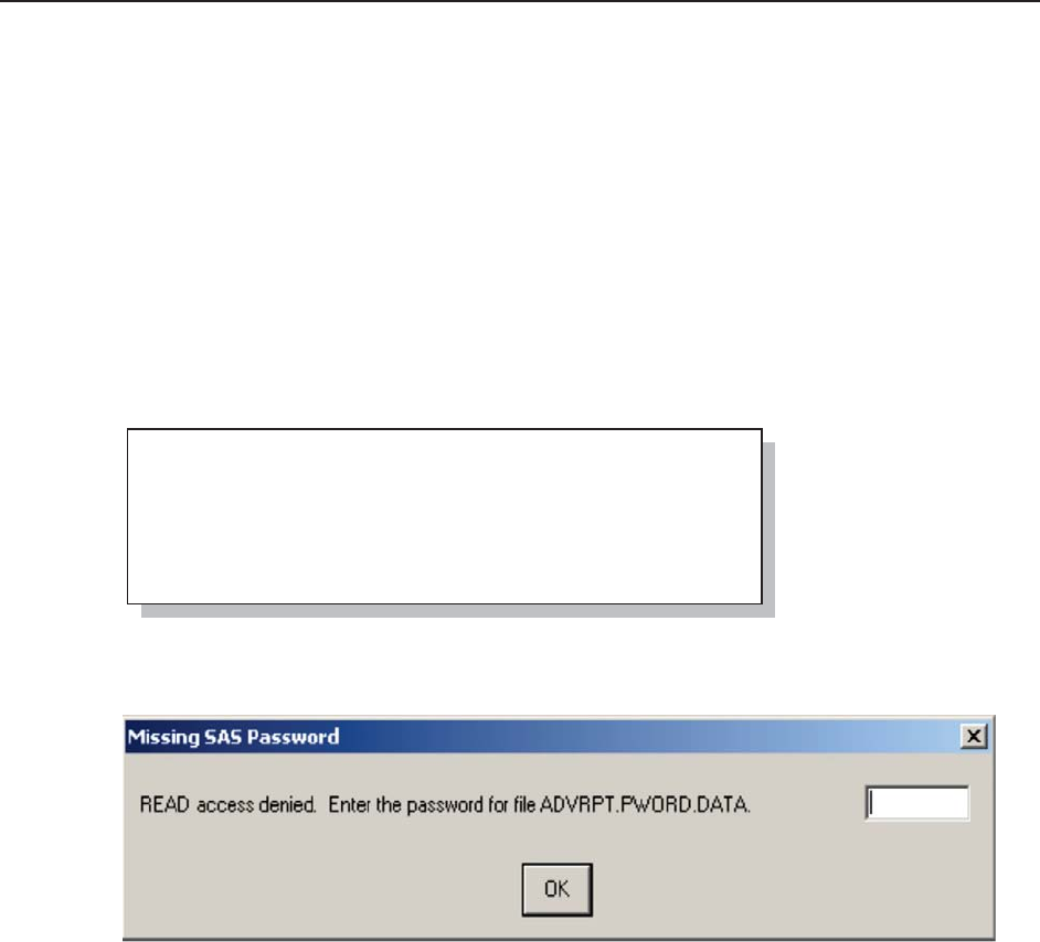
Chapter 2: Working with Your Data 41
Without a compelling reason to do so, it is my opinion that the value of DATASTMTCHK should
not be set to NONE. If you must change the option, use the REPLACE and REPEMPTY data set
options p to provide some protection.
2.1.2 Password Protection
Data sets can be both encrypted and password protected. Password and encryption data set options
include:
ALTER Password to alter the data set
ENCRYPT Encrypt the data set
PW Specify the password
PWREQ Password request window
READ Password to read the data set
WRITE Password to write to the data set
The following DATA step creates a data set that is not only encrypted, but requires different
passwords for both reading and writing.
Before PROC PRINT can display the protected data set, the following dialogue box will appear
requesting the READ password.
While these password protections can be useful within SAS, the protected files are still vulnerable
to deletion or manipulation using tools outside of SAS. Including the ENCRYPT option adds
another layer of protection from tools other than SAS.
MORE INFORMATION
More about password protection including the use of a data set containing passwords, such as the
one used in this section, is used in Section 5.4.2.
data advrpt.pword(encrypt=yes pwreq=yes
read=readpwd write=writepwd);
DB='DEApp'; UID='MaryJ'; pwd='12z3'; output;
DB='p127'; UID='Mary'; pwd='z123'; output;
run;
proc print data=advrpt.pword;
run;
&DUSHQWHU$UW&DUSHQWHU¶V*XLGHWR,QQRYDWLYH6$67HFKQLTXHV&RS\ULJKW6$6,QVWLWXWH,QF&DU\1RUWK&DUROLQD86$
$
//5,*+765(6(59(')RUDGGLWLRQDO6$6UHVRXUFHVYLVLWVXSSRUWVDVFRPSXEOLVKLQJ
42 Carpenter’s Guide to Innovative SAS Techniques
2.1.3 KEEP, DROP, and RENAME Options
When using the KEEP, DROP, or RENAME in a DATA step, you can choose between using data
set options or DATA step statements. When multiple data sets are either created or read, DATA
step statements apply to all created data sets, while data set options can be applied to specific data
sets. As a general rule, when you have a choice, data set options are preferred over statements, as
the data set options give you more control and the code is generally clearer.
The KEEP statement is the functional opposite of the DROP statement. The following discussion
for the KEEP statement and the KEEP= data set option could just as easily been applied to the
DROP statement and DROP= data set option. Here I am showing the KEEP statement and
KEEP= data set option because I have an admitted bias against the DROP statement and DROP=
data set option. The DROP statement and DROP= data set option work fine, both do exactly what
they are supposed to do, and both can save the programmer typing when the list of variables to
keep is long, and the list of variables to drop is short. However, the KEEP conveys more
information to the programmer by documenting which variables the programmer does need to
continue to think about.
The following examples highlight the differences between the KEEP statement and the KEEP=
data set option. The KEEP statement below n is only applied to the new data set (WORK.LABS)
and in no way affects the Program Data Vector or what variables will be read from the incoming
data set (ADVRPT.LAB_CHEMISTRY).
n The KEEP statement variable list is applied
to the new outgoing data set.
oThe IF statement is executed after the entire
observation is read and loaded into the PDV.
Using the KEEP statement n is exactly the
same as specifying the KEEP= option on the data set in the DATA statement p. The KEEP=
option on the SET statement q, however, is applied before the PDV is built. Only those variables
listed will be read from the incoming data set and included on the PDV.
p The KEEP= data set option only impacts which variables will be written to the new data set.
q On the SET statement the KEEP= data set option is applied to the incoming data set; therefore,
this variable list affects which variables will appear on the PDV. Because SODIUM is used in the
WHERE= clause r in this example, the KEEP= data set option must also include SODIUM, even
though it is not written to the new data set.
r The WHERE= filter is specified as a data set option and is applied before observations are
read.
The RENAME option allows you to change the name of a variable either as it is read or as it is
written. Like the RENAME statement, the syntax is of the form oldname=newname. Placing the
RENAME= option on the SET statement s causes the name to be changed before it is written to
the PDV.
data labs(keep=subject visit labdt); p
set advrpt.lab_chemistry(keep=subject visit labdt sodium q
where=(sodium>'142')); r
run;
data labs;
set advrpt.lab_chemistry;
keep subject visit labdt; n
if sodium>'142'; o
run;
&DUSHQWHU$UW&DUSHQWHU¶V*XLGHWR,QQRYDWLYH6$67HFKQLTXHV&RS\ULJKW6$6,QVWLWXWH,QF&DU\1RUWK&DUROLQD86$
$
//5,*+765(6(59(')RUDGGLWLRQDO6$6UHVRXUFHVYLVLWVXSSRUWVDVFRPSXEOLVKLQJ

Chapter 2: Working with Your Data 43
s The original name (LABDT) is changed to the new name (LABDATE).
t The new name would be used in any programming statements and it also appears on the
KEEP= variable list.
When the RENAME= and KEEP= options are both used on the same data set, it is important to
understand which is applied first. In the following DATA step the incoming data set has both a
RENAME= and KEEP= option.
u Since the KEEP= option is applied before the RENAME= option, the original variable name is
used on the incoming KEEP= variable list.
MORE INFORMATION
When combined with PROC SORT these data set options can have a huge impact on processing
efficiencies, see Section 4.2.
2.1.4 Observation Control Using FIRSTOBS and OBS Data Set Options
The data set options FIRSTOBS and OBS can be used separately or in conjunction with one
another to limit which observations are read and/or written. Their operation is similar to the
system options with corresponding names; however, as data set options their application can be
more refined.
FIRSTOBS specifies the number of the first observation to be read
OBS specifies the last observation that is to be read (when FIRSTOBS is
not also used, this corresponds to the number of observations that
will be read).
In the following PROC PRINT step we have requested that only the first 6 observations be
printed n.
proc print data=sashelp.class(obs=6); n
run;
data labs(keep=subject visit labdate)t;
set advrpt.lab_chemistry(rename=(labdt=labdate)s
keep=subject visit labdtu sodium
);
if sodium>'142';
run;
data labs(keep=subject visit labdate)t;
set advrpt.lab_chemistry(rename=(labdt=labdate))s;
if sodium>'142';
run;
&DUSHQWHU$UW&DUSHQWHU¶V*XLGHWR,QQRYDWLYH6$67HFKQLTXHV&RS\ULJKW6$6,QVWLWXWH,QF&DU\1RUWK&DUROLQD86$
$
//5,*+765(6(59(')RUDGGLWLRQDO6$6UHVRXUFHVYLVLWVXSSRUWVDVFRPSXEOLVKLQJ

44 Carpenter’s Guide to Innovative SAS Techniques
The FIRSTOBS= option o identifies the first observation that is to be printed.
When these two options are used together p they work independently of each other. It is
important to remember that the OBS= option counts from observation 1 regardless of the value of
FIRSTOBS. This is demonstrated in the following example.
Only the first 6 observations are available to be printed (OBS=6); however, the first to be printed
is the fourth observation (FIRSTOBS=4). As a result only three observations are actually printed.
2.1.4c firstobs=4 obs=6
Obs Name Sex Age Height Weight
4 Carol F 14 62.8 102.5
5 Henry M 14 63.5 102.5
6 James M 12 57.3 83.0
title1 '2.1.4c firstobs=4 obs=6';
proc print data=sashelp.class(firstobs=4 obs=6); p
run;
2.1.4b firstobs=4
Obs Name Sex Age Height Weight
4 Carol F 14 62.8 102.5
5 Henry M 14 63.5 102.5
6 James M 12 57.3 83.0
7 Jane F 12 59.8 84.5
8 Janet F 15 62.5 112.5
9 Jeffrey M 13 62.5 84.0
10 John M 12 59.0 99.5
11 Joyce F 11 51.3 50.5
12 Judy F 14 64.3 90.0
13 Louise F 12 56.3 77.0
14 Mary F 15 66.5 112.0
15 Philip M 16 72.0 150.0
16 Robert M 12 64.8 128.0
17 Ronald M 15 67.0 133.0
18 Thomas M 11 57.5 85.0
19 William M 15 66.5 112.0
title1 '2.1.4b firstobs=4';
proc print data=sashelp.class(firstobs=4); o
run;
2.1.4a obs=6
Obs Name Sex Age Height Weight
1 Alfred M 14 69.0 112.5
2 Alice F 13 56.5 84.0
3 Barbara F 13 65.3 98.0
4 Carol F 14 62.8 102.5
5 Henry M 14 63.5 102.5
6 James M 12 57.3 83.0
&DUSHQWHU$UW&DUSHQWHU¶V*XLGHWR,QQRYDWLYH6$67HFKQLTXHV&RS\ULJKW6$6,QVWLWXWH,QF&DU\1RUWK&DUROLQD86$
$
//5,*+765(6(59(')RUDGGLWLRQDO6$6UHVRXUFHVYLVLWVXSSRUWVDVFRPSXEOLVKLQJ

Chapter 2: Working with Your Data 45
Adding a WHERE clause q changes the counting process. The WHERE clause is applied first;
consequently, the counts and the selection of the observations is based on the subset of
observations.
The resulting LISTING shows that only the fourth, fifth, and sixth male patients have been
displayed.
2.2 Evaluating Expressions
A SAS expression contains a combination of operators, constants, functions, and variables.
Expressions are used in a number of ways, both within the DATA step and in the PROC step.
Very often when we encounter the term ‘expression’, we most commonly think of comparison
expressions; however, they are actually much more general and can also appear in other
statements such as assignment statements. It is important to remember that, regardless of their use,
the evaluation of an expression will follow a series of steps or rules. Understanding these rules
can lead us to a more expansive use of expressions.
2.2.1 Operator Hierarchy
Operators are like verbs in the expression. They tell SAS what to do with things like constants and
variables. In order to avoid confusion and ambiguity, operators are assigned a hierarchy or order
in which they are applied. The hierarchy is formed by seven groups of operators, and within a
group, operators of equal rank are applied from left to right (except Group 1 which is applied right
to left).
At a simple level, we need to understand why the expression (5+6*2) is equal to 17 and not 22.
But as we encounter expressions in non-standard form, such as some of those in Sections 2.2.2
and 2.2.3, we need to have a solid understanding of this hierarchy, if we are to understand why the
expressions evaluate the way that they do.
2.1.4d firstobs=4 obs=6 where (sex=m)
Obs Name Sex Age Height Weight
9 Jeffrey M 13 62.5 84.0
10 John M 12 59.0 99.5
15 Philip M 16 72.0 150.0
title1 '2.1.4d firstobs=4 obs=6 where (sex=m)';
proc print data=sashelp.class(firstobs=4 obs=6
where=(sex='M')); q
run;
&DUSHQWHU$UW&DUSHQWHU¶V*XLGHWR,QQRYDWLYH6$67HFKQLTXHV&RS\ULJKW6$6,QVWLWXWH,QF&DU\1RUWK&DUROLQD86$
$
//5,*+765(6(59(')RUDGGLWLRQDO6$6UHVRXUFHVYLVLWVXSSRUWVDVFRPSXEOLVKLQJ

46 Carpenter’s Guide to Innovative SAS Techniques
Group Operators
Parentheses Operations within parentheses are performed first
Group 1
(performed right
to left)
Exponentiation (**)
Prefix operators, such as, positive (+), negative (-), and negation
Minimum (MIN,><) and maximum (MAX, <>)
Group 2 Multiplication (*) and division (/)
Group 3 Addition (+) and subtraction (-)
Group 4 Concatenation (||)
Group 5 Comparisons such as equal (=) and less than (<)
Group 6 AND - Boolean comparison (&)
Group 7 OR - Boolean comparison (|)
Since any of these operators can appear in any expression, whether in an assignment statement or
an IF statement, we need to expand our perception of what an expression should contain. The
assignment statement shown
here creates the variable
SEASON which can contain one
of the numeric values 0 thru 4
depending on the month of the
date of birth. The ‘less-than-or-
equal-to’ comparison operators (Group 5) return a zero or one which is multiplied against the
constants. The comparison operators are just another form of expression operators and are
perfectly suited to assignment statements as well as to logical expressions.
Although it is important to understand the logic of the previous assignment statement, it could
have been more simply written using the CEIL
function. However the two statements are not
equivalent. When DOB is missing, the first
assignment statement returns a zero, while this one returns a missing value.
MORE INFORMATION
There are some additional comparison operators that are unique to the WHERE statement (see
Section 2.7.1). The MIN and MAX operators are further discussed in Section 2.2.5.
2.2.2 Using the Colon as a Comparison Modifier
The colon ( : ) can be used as an operator modifier when character values are being compared.
The colon permits the comparison
of two strings of unequal length,
and the colon follows the
comparison operator of choice. In
the example to the left, the
subsetting IF statement will select
all observations which have a LNAME starting with ‘Mar’. Since it does not matter whether the
value with the smaller length is on the left or right side of the equal sign, a last name of ‘Ma’
would also be selected. The lengths of the values on both sides are determined and the smaller
season = 1*(1 le month(dob) le 3)
+ 2*(4 le month(dob) le 6)
+ 3*(7 le month(dob) le 9)
+ 4*(10 le month(dob) le 12);
data Mar;
set advrpt.demog (keep=lname fname);
if lname =: 'Mar';
run;
season= ceil(month(dob)/3);
&DUSHQWHU$UW&DUSHQWHU¶V*XLGHWR,QQRYDWLYH6$67HFKQLTXHV&RS\ULJKW6$6,QVWLWXWH,QF&DU\1RUWK&DUROLQD86$
$
//5,*+765(6(59(')RUDGGLWLRQDO6$6UHVRXUFHVYLVLWVXSSRUWVDVFRPSXEOLVKLQJ

Chapter 2: Working with Your Data 47
length is selected and applied to both sides. An IF statement with the two values reversed would
produce the same result.
The colon comparison operator modifier can also be used with the IN operator. In this example
the WHERE statement will select a
variety of last names that start with
the indicated strings. Notice that the
target strings are not all of the same length. The number of compared characters in LNAME will
be appropriate for each of the individual values.
Trailing blanks are counted and are used to determine matches. The following WHERE statement
will return both ‘Adams’ and ‘Adamson’; however,
if the TRIM function had not been used only
‘Adamson’ would have been found.
Similar functionality can be achieved in an SQL step; however, the syntax can vary. The colon
operator can be used in a WHERE= data set option whenever you are importing a SAS data set
(see Section 2.1).
n The =: can be used
within the WHERE=
data set option even
when it is used within
the SQL step.
o Although it worked
in the WHERE= data set
option, the =: will not
work in an SQL
WHERE clause. This
SELECT statement will
fail.
p In SQL the EQT
operator is similar to the =:, and because it is an SQL operator it can be used in the SQL WHERE clause.
In addition to the EQT operator, SQL also supports the LET (<=:) and GET (>=:) operators.
SEE ALSO
The colon comparison modifier is not available in the macro language; however, macros have
been written to provide similar functionality. See Carpenter (2004, Section 7.6.3 pg. 196).
2.2.3 Logical and Comparison Operators in Assignment Statements
In Section 2.2.1 the following assignment statement is briefly introduced. This is an example of a
value look-up where the value of month determines the value of SEASON (Chapter 6 goes into
detail on a variety of table look-up
coding strategies). In this case the
process could have been simplified by
the use of a format. More importantly,
however, it demonstrates the use of a
comparison operator (LE) in an
assignment statement.
if 'Mar' =: lname;
where lname in:('Me', 'Mar', 'Adams');
where 'Adamso'=: trim(lname);
season = 1*(1 le month(dob) le 3)
+ 2*(4 le month(dob) le 6)
+ 3*(7 le month(dob) le 9)
+ 4*(10 le month(dob) le 12);
proc sql;
title2 'Used in SQL data set WHERE=';
select lname, fname, dob
from advrpt.demog(where=(lname=:'Adams')); n
title2 'Used in SQL WHERE Clause';
select lname, fname, dob
from advrpt.demog
where lname=:'Adams'; o
proc sql;
title2 'Using the EQT operator';
select lname, fname, dob
from advrpt.demog
where lname eqt 'Adams'; p
quit;
&DUSHQWHU$UW&DUSHQWHU¶V*XLGHWR,QQRYDWLYH6$67HFKQLTXHV&RS\ULJKW6$6,QVWLWXWH,QF&DU\1RUWK&DUROLQD86$
$
//5,*+765(6(59(')RUDGGLWLRQDO6$6UHVRXUFHVYLVLWVXSSRUWVDVFRPSXEOLVKLQJ

48 Carpenter’s Guide to Innovative SAS Techniques
In fact, as was mentioned in Section 2.2.1 there is no reason why any of the logical and
comparison operators cannot appear in an assignment statement. The key to their use is to
remember that logical expressions will yield either TRUE or
FALSE, which is represented by 1 or 0 respectively. For a date
of birth in May the previous equation is evaluated as is shown
on the left. The expression results in a value of 2 for SEASON.
When you are generating a numeric value based on a logical
determination, such as this one, you should be able to write the assignment statement in a form
similar to the one above. However, it is not unusual to see this type of assignment made through a
series of less efficient IF-THEN/ELSE statements.
Although the previous example could have also been made using a user-defined format and a PUT
function (see Section 6.5), the assignment of a value to GROUP using the series of IF-
THEN/ELSE statements, such as the one shown here, does not so easily lend itself to a solution
involving a
format. The value
can, however, be
determined with
an assignment
statement containing the same
logic as was used in these IF-
THEN/ELSE statements.
Since assignment statements
tend to be processed faster
than IF-THEN/ELSE
statements, it is likely that the use of assignment statements can decrease processing time. This
type of assignment statement will also generally out perform a PUT function.
Since True/False determinations always result in either a 0 or a 1, this same approach can be
especially useful if assigning a numeric 0,1 value to a variable. In the following DATA step we
would like to create a flag that indicates whether or not the date of birth is before 1950. Three
equivalent flags have been created to demonstrate three different methods.
n Very often IF-THEN/ELSE statements are used. These statements tend to process slower than
assignment statements.
o The logical expression appears on the right of the equal sign.
p The IFN function can be used to assign the result. This function has added value when a result
other than just 0 or 1 is to be returned.
season = 1*(0)
+ 2*(1)
+ 3*(0)
+ 4*(0);
if sex = 'M' and year(dob) > 1949 then group=1;
else if sex = 'M' and year(dob) le 1949 then group=2;
else if sex = 'F' and year(dob) > 1949 then group=3;
else if sex = 'F' and year(dob) le 1949 then group=4;
group = 1*(sex = 'M' and year(dob) > 1949)
+ 2*(sex = 'M' and year(dob) le 1949)
+ 3*(sex = 'F' and year(dob) > 1949)
+ 4*(sex = 'F' and year(dob) le 1949);
data flags;
set advrpt.demog (keep=lname fname dob sex);
if year(dob) > 1949 then boomer=1; n
else boomer=0;
boomer2 = year(dob) > 1949; o
boomer3 = ifn(year(dob) > 1949, 1, 0); p
run;
&DUSHQWHU$UW&DUSHQWHU¶V*XLGHWR,QQRYDWLYH6$67HFKQLTXHV&RS\ULJKW6$6,QVWLWXWH,QF&DU\1RUWK&DUROLQD86$
$
//5,*+765(6(59(')RUDGGLWLRQDO6$6UHVRXUFHVYLVLWVXSSRUWVDVFRPSXEOLVKLQJ

Chapter 2: Working with Your Data 49
A similar coding structure is used when you need to create a flag that depends on whether or not
an item is in a list of values. Here we need to determine if the number 3 is contained in one or
more of the variables X1 through X4.
q FLAG1 is created by determining if the
value 3 is in the array A. If it is, a 1 is
stored.
r The WHICHN function returns an item
number if the value in the first argument is
found (otherwise a 0 is returned). This
value is then converted to a 0 or a 1 by use
of a double negation (see Section 2.2.6 for
more on the use of the double negation).
MORE INFORMATION
The assignment statements discussed in this section are simple table lookups. Chapter 6 discusses
a variety of different table lookup techniques in more detail. The IFN and IFC functions are
discussed more in Section 3.6.6.
SEE ALSO
The sasCommunity.org tip
http://www.sascommunity.org/wiki/Tips:Creating_a_flag_avoiding_the_If_..._Then_Structure
discusses the use of this type of expression in an assignment statement. The discussion tab
includes alternative forms that can be used in an SQL step. The example of flags used to indicate
presence of a value in a list was suggested by Chang Chung and Mike Rhoads. Their examples
can be found at:
http://www.sascommunity.org/wiki/Tips:Double_negatives_to_normalize_a_boolean_value and
http://www.listserv.uga.edu/cgi-bin/wa?A2=ind1101c&L=sas-l&D=1&O=D&P=9693,
respectively.
2.2.4 Compound Inequalities
When a compound inequality is used in an expression it is important to understand how the
expression is evaluated. An expression with a compound inequality very often contains a variable
between two values, which form the upper and lower
limits of a range. This compound expression is
effectively interpreted as two distinct inequalities which
are joined with an AND. The value of
EDU must meet both conditions for the
overall expression to evaluate as true.
Misplacing the parentheses totally changes the way that the expression is evaluated. Notice the
placement of the parentheses in this WHERE
statement. The inequality inside the parentheses is
evaluated to True or False (0 or 1), and the result
compared to 16. This expression will be true for all values of EDU (both 0 and 1 are less than 16).
You may be thinking ‘OK, so what, I will be careful with parentheses. Why should I care?’ Of
course I think that the way that SAS evaluates these expressions is both interesting and important,
but there are also practical benefits.
if 13 le edu le 16;
if (13 le edu) and (edu le 16);
where (13 le edu) le 16 ;
data _null_;
input x1-x4;
array a {*} x1-x4;
flag1 = (3 in a); q
flag2 = ^^whichn(3,of x:); r
put flag1= flag2=;
datalines;
1 2 3 4
5 6 7 8
run;
&DUSHQWHU$UW&DUSHQWHU¶V*XLGHWR,QQRYDWLYH6$67HFKQLTXHV&RS\ULJKW6$6,QVWLWXWH,QF&DU\1RUWK&DUROLQD86$
$
//5,*+765(6(59(')RUDGGLWLRQDO6$6UHVRXUFHVYLVLWVXSSRUWVDVFRPSXEOLVKLQJ

50 Carpenter’s Guide to Innovative SAS Techniques
%let x = 5;
%let y = 4;
%let z = 3;
%if &x lt &y lt &z %then
%put &x < &y < &z;
In the macro language compound inequalities are not evaluated the same way as we might think
based on our knowledge of DATA step expressions. The
resolved macro variables in the expression in this %IF-
%THEN statement show that the expression should be
evaluated as false; however, it evaluates as TRUE and
the %PUT executes.
This happens because the compound
expression in the
macro language is
not broken up into
two distinct inequalities like it would be in the DATA step. Instead it is evaluated as if there were
parentheses around the first portion of the comparison. The expression is evaluated left to right,
and (&x lt &y) will be either TRUE or FALSE (1 or 0). Either way as long as &Z is > 1, the
overall expression will be TRUE.
In actual applications compound inequalities such as the ones shown above are quite common. It
is much less likely that you will use other forms of compound expressions; however, as was
shown in the example with the %IF statement, it is important to understand how the expression is
evaluated.
2.2.5 The MIN and MAX Operators
CAVEAT
It is my opinion that these two operators, and their mnemonics (see Section 2.2.1), should never
be used. They are included in this section primarily so that this warning can be given. When you
want to return either the minimum or maximum, always use either the MIN or MAX function.
These functions have none of the problems associated with these the two operators.
The MIN and MAX operators return the minimum or maximum of two values respectively.
In this WHERE statement the smaller value of the variables Y
and Z will be compared to the value of the variable X. The
MIN and MAX operators allow the comparison of exactly two
variables, while the preferred MIN and MAX functions can
work with any number of variables.
These two operators do not behave the same in WHERE statement expressions as they do in an IF
statement expression, and the differences are important. Actually they are only important if you
intend to ignore the caveat and go ahead and use these operators. Assuming that you like living on
the edge, read on.
Potential Problem #1 - Mnemonics
In the IF statement these two operators can be replaced with their mnemonics; however, these
mnemonics do not work in the same way in the WHERE statement.
where x = (y min z);
where x = min(y, z);
%if 5 lt 4 lt 3 %then %put 5 < 4 < 3;
%if (&x lt &y) lt &z %then %put &x < &y < &z;
&DUSHQWHU$UW&DUSHQWHU¶V*XLGHWR,QQRYDWLYH6$67HFKQLTXHV&RS\ULJKW6$6,QVWLWXWH,QF&DU\1RUWK&DUROLQD86$
$
//5,*+765(6(59(')RUDGGLWLRQDO6$6UHVRXUFHVYLVLWVXSSRUWVDVFRPSXEOLVKLQJ
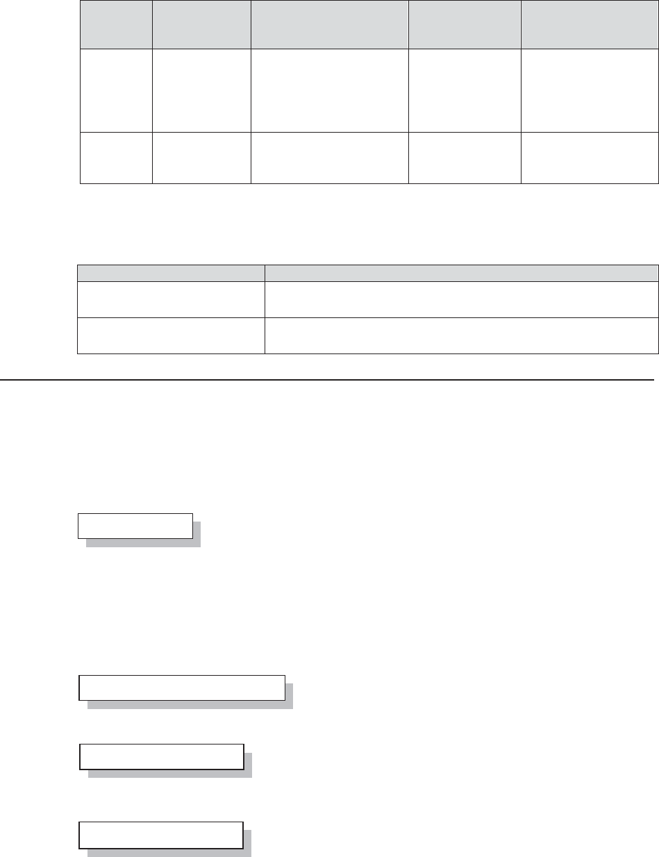
Chapter 2: Working with Your Data 51
Operator
IF Statement
Mnemonic
WHERE Statement
Caveat for the
Mnemonic
IF and WHERE
Clause
Results
MIN >< Mnemonic is not
supported in WHERE,
although MIN is
converted to >< in the
LOG
where x=(y><z);
if x=(y><z);
WHERE ĺ error
IF works as expected
MAX <> Mnemonic is interpreted
as not equal in the
WHERE
where x=(y<>z); True when X=1 and
Y not equal to Z or
when X=0 and Y=Z
Potential Problem #2 – Negative Values
When the negative sign is used with the first value associated with these operators, the
expressions are not interpreted the same in the WHERE and IF statements.
Expression Result
if -2 = (-5 min 2); True – the minus sign is applied after the MIN operator, essentially
the same as: if -2 = -(5 min 2);
where -2 = (-5 min 2); False – the minus sign is applied before the MIN operator,
comparison is the same as: where -2 = -5;
2.2.6 Numeric Expressions and Boolean Transformations
It is sometimes necessary to transform numeric values to Boolean (0 or 1) values. There is no one
function that does this, and indeed the exact transformation may be too situational for a specific
function.
True / False
Partly because of the way that SAS handles TRUE/FALSE, i.e., false is 0 or missing and all else
is true, the missing values must also map to 0. The double negation (NOT)
is used to perform the transformation. Since negation is a Boolean
operator, it converts the original value to either a zero or a one.
MORE INFORMATION
Double negation is used to convert a number to a binary 0/1 operator in an example in Section
12.6.2.
Replace Missing with 0
For reporting purposes missing values can be replaced by a 0 using a simple assignment
statement. The COALESCE function returns the first non-
missing value. In this example if DOB is missing a 0 is
returned. Prior to the inclusion of the COALESCE
function, this same operation was sometimes accomplished using the SUM function. Be careful
when working with dates as was done here. Remember that,
although both are false, a date of missing and a date of 0 have
different meanings.
These two expressions do not result in a Boolean value. If you want to convert all missing values
to 0 and all other values to 1 (including 0) you can use the
negation of the MISSING function. In this expression MVAL will
be 1 for all numbers except missing.
x = ^^dob;
z = coalesce(dob,0);
y = sum(dob,0);
mval=^missing(val);
&DUSHQWHU$UW&DUSHQWHU¶V*XLGHWR,QQRYDWLYH6$67HFKQLTXHV&RS\ULJKW6$6,QVWLWXWH,QF&DU\1RUWK&DUROLQD86$
$
//5,*+765(6(59(')RUDGGLWLRQDO6$6UHVRXUFHVYLVLWVXSSRUWVDVFRPSXEOLVKLQJ

52 Carpenter’s Guide to Innovative SAS Techniques
data posneg;
do v=.,-2 to 2;
*if positive;
pos = sign(v)=1;
* Not positive;
notpos = (sign(v) in(-1,0));
* Negative;
neg = ^sign(v)=-1;
* Not negative;
notneg = sign(v) in (0,1);
output posneg;
end;
run;
Determine Positive or Negative Values
Because of missing values and the 0 value, we have four distinct possibilities when separating
positive and negative values. The groups of
positive and non-negative values are not
necessarily the same. Fortunately we can
build the Boolean flag for each of these four
possibilities, with the use of the SIGN
function, which returns -1 for values < 0, 0
for values=0, 1 for values > 0, and missing
for missing values.
SEE ALSO
Several of the code examples in this section
have been suggested by Howard Schreier in
the sasCommunity.org article:
http://www.sascommunity.org/wiki/Numeric
_transformations .
2.3 Data Validation and Exception Reporting
Although we sometimes have the opportunity to work with data that has already been scrubbed
clean, often a major portion of our work is the preparation and cleaning of the data. This is
especially true for data that has been hand entered or for data that comes from a source without
your high standards of excellence. In the biotech/pharmaceutical industries a great deal of time
and careful attention to detail is spent on the validation of the data.
For large or complex data sets the manual/visual process of finding data errors is just not
practical. We need some tools that will allow us to automate the validation process.
When reporting on errors in your data, you will need to be able to communicate the specific
problem and precisely where it occurs. Generally this means that you will have to identify the
specific row and column (observation and variable). To identify a particular row you need to
know the values of all the variables that form the data set’s primary key (the BY variables that
identify the data down to the row level).
SEE ALSO
Wright (2006), and the related papers by Nelson (2004a, 2004b), discusses an approach to the
validation of SAS programs. Bahler (2001) provides a summary of a variety of data cleaning
techniques. Ron Cody (2008b) has written an entire book on data cleaning techniques.
2.3.1 Date Validation
Since we will work with dates, we need to know how to detect and work with incomplete or
inappropriate date values. There are several issues that we need to understand.
2.2.6 Boolean Conversions
Positive or Negative?
Obs v pos notpos neg notneg
1 . 0 0 0 0
2 -2 0 1 0 0
3 -1 0 1 0 0
4 0 0 1 0 1
5 1 1 0 0 1
6 2 1 0 0 1
&DUSHQWHU$UW&DUSHQWHU¶V*XLGHWR,QQRYDWLYH6$67HFKQLTXHV&RS\ULJKW6$6,QVWLWXWH,QF&DU\1RUWK&DUROLQD86$
$
//5,*+765(6(59(')RUDGGLWLRQDO6$6UHVRXUFHVYLVLWVXSSRUWVDVFRPSXEOLVKLQJ

Chapter 2: Working with Your Data 53
Using Formats to Check Date Strings
Formats, whether they are user defined or provided by SAS, can be powerful tools when
searching the data for values that are inappropriate, incomplete, missing, or out of range.
Dates can be particularly problematic for some types of data, such as survey response data. Often
the dates are collected as character strings and then checked before conversion to a SAS date.
Collecting them as character
strings is important so that we can
record partial dates. In the second
observation shown to the left, the
date might be from the response:
“My second visit was in June of
2004. I do not remember the exact
day.”
The INPUT function in the
WHERE statement attempts to
convert the character string into a
date. Invalid values will result in a
missing value, which is selected
by the WHERE.
When the
INPUT function
is used with the
format
MMDDY. for
an incorrectly
structured
value, as it is in the second observation, an error is issued in the LOG. This error message can be
suppressed by using either the ?? format modifier (see Section 1.3.1) or the NOFMTERR system
option.
The ?? format modifier suppresses format error messages and can be used with the INFORMAT
in the INPUT function, and is more specific than the NOFMTERR system option as it can be
applied to a specific informat. The
subsetting IF statement in this step
replaces the WHERE statement in the
previous example, as the ?? informat
modifier cannot be used in the
WHERE statement.
Because we can suppress the error messages, we have more latitude in the use of formats to
rebuild dates with missing components. As before, let’s assume that our incoming dates are
received as character strings with either the day or month potentially coded as ‘XX’. This
example shows the subject’s response to the question: “When did you stop smoking?” Very
typically the patient is unable to remember the date let alone the day of the month. In this example
we have decided to replace missing days with the 15th and if the month is missing with the year
midpoint July 1. This code assumes that at least the year is present.
data visitdates;
visit=1; v_date_ = '05/25/2004'; output;
visit=2; v_date_ = '06/XX/2004'; output;
run;
proc print data=visitdates;
where input(v_date_,mmddyy10.) = .;
run;
2.3.1 Date Validation Using Formats
Date Errors
Obs visit v_date_
2 2 06/XX/2004
9 proc print data=visitdates;
10 where input(v_date_,mmddyy10.) eq .;
11 run;
ERROR: INPUT function reported 'ERROR: Invalid date value'
while processing WHERE clause.
data dateerrors;
set visitdates;
if input(v_date_,?? mmddyy10.) eq .;
run;
proc print data=dateerrors;
run;
&DUSHQWHU$UW&DUSHQWHU¶V*XLGHWR,QQRYDWLYH6$67HFKQLTXHV&RS\ULJKW6$6,QVWLWXWH,QF&DU\1RUWK&DUROLQD86$
$
//5,*+765(6(59(')RUDGGLWLRQDO6$6UHVRXUFHVYLVLWVXSSRUWVDVFRPSXEOLVKLQJ

54 Carpenter’s Guide to Innovative SAS Techniques
n The first attempt is made to build the SAS date (Q_DATE) using the INPUT function.
o If the SAS date is missing, one or more elements are probably coded as XX. First we check the
day of the month.
p When the day of the month is coded as XX, the value of 15 is substituted. Notice the use of the
SUBSTR function on the left side of the = sign to perform the substitution (see Section 3.6.6 for
more on the use of the SUBSTR function to substitute characters into the string).
q The date is again checked now for a potentially missing month value.
r A month coded as XX is detected, and the month and day are substituted.
s The corrected date string is converted to a SAS date.
Checking for Missing Date Values
In the ADVRPT.DEMOG data set the variable DEATH records the date of death for those
patients that died while under the care of a clinic (remember this is made up data and no patients
were harmed for the writing of this book). We would like to filter the patients for those with a
date of death. We need to remember that a SAS date contains the number of elapsed days since
January, 1, 1960 (day 0). Dates before this date are negative numbers.
The WHERE statement can be used and a couple alternative forms of the expression could be
suggested. We need to keep in mind that we are filtering for valid dates.
One possible expression might be to filter for values that are greater
than zero; however, this clearly excludes any dates before January 2,
1960, and is NOT sufficient.
Since we want to exclude missing dates, and missing values are false, another possible expression
would be to simply check to see if DEATH is false. This nearly works, but
it has a subtle flaw. Here we will exclude the valid date of death January
where death>0;
where death;
data quit_dates;
subject=201; q_date_ = '05/25/1975'; output;
subject=205; q_date_ = '10/XX/2001'; output;
subject=208; q_date_ = 'XX/XX/1966'; output;
run;
data Qdates(keep=subject q_date_ q_date);
set quit_dates;
format q_date date9.;
q_date = input(q_date_,??mmddyy10.); n
if missing(q_date) then do; o
* Substitute missing day of month with 15;
if substr(q_date_,4,2)='XX' then substr(q_date_,4,2)='15'; p
q_date = input(q_date_,??mmddyy10.);
end;
if missing(q_date) then do; q
* Substitute missing month with 07;
if substr(q_date_,1,2)='XX' then do; r
substr(q_date_,1,2)='07';
* reset day of month also;
substr(q_date_,4,2)='01';
end;
q_date = input(q_date_,??mmddyy10.); s
end;
run;
&DUSHQWHU$UW&DUSHQWHU¶V*XLGHWR,QQRYDWLYH6$67HFKQLTXHV&RS\ULJKW6$6,QVWLWXWH,QF&DU\1RUWK&DUROLQD86$
$
//5,*+765(6(59(')RUDGGLWLRQDO6$6UHVRXUFHVYLVLWVXSSRUWVDVFRPSXEOLVKLQJ

Chapter 2: Working with Your Data 55
1, 1960, which is day zero and will be interpreted as false.
What we really need to do is eliminate only the missing values and we should focus on this. Two
expressions can be used. We can explicitly exclude the missing value and allow all others or we
can accept any value that is larger than
missing (all numbers positive or
negative are larger than missing).
Sometimes you will be working with data that utilizes more than one type of missing value. Since
numeric variables can take on up to 28 types of missing values (., .a, .b, …. , .z, and ._), you may
need to account for these when testing for missing. Of the 28 types of numeric missing values the
smallest is ._, the next smallest is ., and the largest is .z. Therefore,
to effectively test for all these missing value types, we need to code
for the largest (.z). All missing values would also be
detected by using the MISSING function.
MORE INFORMATION
The WHERE= data set option is used in examples in Sections 2.1.3, 2.1.4d, and 2.2.2.
SEE ALSO
Hunt (2010) shows alternate methodologies for the completion of dates. Alternate solutions for
the completion of partial dates can be found on the SAS Forums, see the following thread:
http://communities.sas.com/message/40648#40648.
2.3.2 Writing to an Error Data Set
When attempting to identify the observations that contain data errors, it is often helpful to build a
secondary data set containing just those observations with errors. Error reporting through a data
set is as simple as adding conditional logic and another OUTPUT statement.
n The variable list in the error data set should contain all the variables that form the primary key,
as well as those being tested.
o In this example we are converting the text date to a SAS date. The use of the ?? format
modifier to suppress error messages in the LOG is discussed in Section 2.3.1.
p Incomplete dates, those that cannot be converted to valid SAS dates, result in a missing value.
q In this example the data set MEDSTARTDATES will contain all observations, including those
with errors. To remove observations with errors from this data set, simply start the OUTPUT
statement with an ELSE statement. The statement becomes: else output medstartdates;
data medstartdates(keep=subject mednumber drug
medstdt_ medstartdate)
medstarterr(keep=subject mednumber drug medstdt_); n
set advrpt.conmed(keep=subject mednumber drug medstdt_);
medstartdate = input(medstdt_,?? mmddyy10.); o
if medstartdate = . then output medstarterr; p
output medstartdates; q
run;
where death ne .; where death > .;
where death > .z;
where ^missing(death);
&DUSHQWHU$UW&DUSHQWHU¶V*XLGHWR,QQRYDWLYH6$67HFKQLTXHV&RS\ULJKW6$6,QVWLWXWH,QF&DU\1RUWK&DUROLQD86$
$
//5,*+765(6(59(')RUDGGLWLRQDO6$6UHVRXUFHVYLVLWVXSSRUWVDVFRPSXEOLVKLQJ

56 Carpenter’s Guide to Innovative SAS Techniques
The resulting data table (WORK.MEDSTARTERR) will contain one observation for each
MEDSTDT_ value that cannot be converted to a valid SAS date.
When testing more than one variable or different variables in different data sets, this form for the
error reporting data set is not flexible enough. This is often the case when we build an automated
system for validating our data. In an automated system, the exception data set needs to contain
sufficient information for the data manager to get back to the value in question. A minimum
amount of information would include:
DSN data set name
List of Variables key variables and their values
ERRVAR variable containing the exception
ERRVAL flagged value
ERRTEXT reason that the value was flagged (exception criteria)
ERRRATING exception rating (may be needed to identify critical
variables)
This form of the error data set has one observation per error. It allows the reporting of more than
one variable per observation and even errors from multiple data sets. In order to maximize
flexibility, consider making the flagged value a character variable. This will require the
conversion of numeric values to character, but adds flexibility. Also, since the list of key variables
will likely change between data sets, many of the various key variables will be missing for
observations that come from data sets for which they are not part of the key. As long as you are
careful when designing your original data sets so that variables that appear in multiple data sets
always have the same attributes, this will not be a problem.
2.3.2a Collecting Date Errors
Obs SUBJECT mednumber drug MEDSTDT_
51 206 2 LUPRON XX/XX/1999
52 206 3 CALCIUM CITRATE --/--/----
53 206 4 MVI --/--/----
54 207 1 METOPROLOL --/--/----
55 207 1 CLONIDINE --/--/----
56 207 1 LUPRON XX/XX/1996
57 207 2 DYAZIDE --/--/----
58 207 2 COUMADIN XX/XX/1996
. . . . portions of the table are not shown . . . .
&DUSHQWHU$UW&DUSHQWHU¶V*XLGHWR,QQRYDWLYH6$67HFKQLTXHV&RS\ULJKW6$6,QVWLWXWH,QF&DU\1RUWK&DUROLQD86$
$
//5,*+765(6(59(')RUDGGLWLRQDO6$6UHVRXUFHVYLVLWVXSSRUWVDVFRPSXEOLVKLQJ

Chapter 2: Working with Your Data 57
n The list of variables in the error reporting data table includes the variables which form the
primary key for this data table (SUBJECT VISIT LABDT).
o Read the data set to be checked.
p Enter the DO block when this specific data exception has been detected.
q Save the name of the data table being checked.
r Save the name of the variable being tested.
s Capture the data value for further inspection. When character values have been converted for
the check, save the raw or character value. This allows you to see any text that might contribute to
character to numeric conversion issues.
t The error test should describe the problem detected in the data.
u If required, assign an error severity code.
v Write this observation out to the error report data set (ERRRPT).
w The second exception criterion is tested in a DO block that is essentially the same as the first
DO block p.
The resulting error report data set contains all the information necessary to locate, evaluate, and
start the correction process.
title1 '2.3.2b Hardcoded Exception Reporting';
data errrpt(keep=dsn errvar errval errtxt errrating
subject visit labdt); n
length dsn $25
errvar $15
errval $25
errtxt $20
errrating 8;
set advrpt.lab_chemistry; o
if potassium lt 3.1 then do; p
dsn = 'advrpt.lab_chemistry'; q
errvar = 'potassium'; r
errval = potassium; s
errtxt = 'Low value(<3.1)'; t
errrating= 1; u
output errrpt; v
end;
if potassium gt 6.7 then do; w
dsn = 'advrpt.lab_chemistry';
errvar = 'potassium';
errval = potassium;
errtxt = 'High value(>6.7)';
errrating=2;
output errrpt;
end;
run;
&DUSHQWHU$UW&DUSHQWHU¶V*XLGHWR,QQRYDWLYH6$67HFKQLTXHV&RS\ULJKW6$6,QVWLWXWH,QF&DU\1RUWK&DUROLQD86$
$
//5,*+765(6(59(')RUDGGLWLRQDO6$6UHVRXUFHVYLVLWVXSSRUWVDVFRPSXEOLVKLQJ

58 Carpenter’s Guide to Innovative SAS Techniques
From a coding standpoint, the beauty of this approach is that you can have as many checks as are
needed, and each one is simply implemented by the addition of another DO block. The
disadvantage becomes apparent for large studies and for complex data tables. While not terribly
complex, the program(s) can become large. More importantly, since each individual check is
implemented in the program, new or changed criteria require that the program itself be
revalidated. These problems can be addressed by storing the test criteria outside of the program.
One very convenient way to do this is to store the exception criteria in a data table (see Section
2.3.3).
MORE INFORMATION
Non-numeric values are detected and written to an error data set in Section 3.6.1.
2.3.3 Controlling Exception Reporting with Macros
In the DATA step shown in Example 2.3.2b, a DO block is constructed for each data check. Since
each one of these DO blocks is very similar, they are prime candidates for being written for us by
the macro language. The following macro, %ERRRPT, will build this DO block.
When the
%ERRRPT macro
is called from
within the DATA
step, the IF
THEN/DO
statements
become:
Although we have simplified the code somewhat, there has still not been a huge savings in our
coding effort. Of course we could have the macro language do even more of the lifting for us. If
we could tell the macro language what and how many checks were needed, then each of the
individual macro calls, including the IF THEN/DO, could be generated by a single macro call.
if potassium lt 3.1 then do;
%errrpt(dsn = advrpt.lab_chemistry,
errvar = potassium,
errval = potassium,
errtxt = %str(Low value%(<3.1%)),
errrating= 1)
if potassium gt 6.7 then do;
%errrpt(dsn = advrpt.lab_chemistry,
errvar = potassium,
errval = potassium,
errtxt = %str(High value%(>6.7%)),
errrating= 2)
run;
2.3.2b Hardcoded Exception Reporting
Obs dsn errvar errval errtxt errrating SUBJECT VISIT LABDT
1 advrpt.lab_chemistry potassium 6.8 High value(>6.7) 2 203 4 09/29/2006
2 advrpt.lab_chemistry potassium 3 Low value(<3.1) 1 208 10 03/09/2007
%macro errrpt(dsn=,errvar=,errval=,errtxt=,errrating=);
dsn = "&dsn";
errvar = "&errvar";
errval = &errval;
errtxt = "&errtxt";
errrating= &errrating;
output errrpt;
end;
%mend errrpt;
&DUSHQWHU$UW&DUSHQWHU¶V*XLGHWR,QQRYDWLYH6$67HFKQLTXHV&RS\ULJKW6$6,QVWLWXWH,QF&DU\1RUWK&DUROLQD86$
$
//5,*+765(6(59(')RUDGGLWLRQDO6$6UHVRXUFHVYLVLWVXSSRUWVDVFRPSXEOLVKLQJ

Chapter 2: Working with Your Data 59
An easy way to store and pass along the needed information is through the use of a SAS data set.
We can create a data set that contains the constraints for each data exception check. Each
observation can then be used to build data exception and error trapping reports. For the previous
example the data set might contain the following.
This data set is then used by a macro to build a series of macro variable lists. These lists are then
processed (each observation in the data set becomes a test or DO block). The %ERRPT macro
shown below builds these lists using an SQL step and then uses the lists to create a series of DO
blocks using the macro variables in the list to ‘fill in the blanks’.
n The macro %ERRRPT is used to control the error reporting process. Macro %DO loops must
appear inside of a macro definition.
%macro errrpt(dsn=, bylst=subject); n
%local i chkcnt;
proc sql noprint;
select errtst, errvar, errval, errtxt, errrating
into :errtst1-:errtst99, o
:errvar1-:errvar99,
:errval1-:errval99,
:errtxt1-:errtxt99,
:errrating1-:errrating99
from vallab; p
%let chkcnt = &sqlobs; q
quit;
data errrpt(keep=dsn errvar errval errtxt errrating
&bylst); r
length dsn $25
errvar $15
errval $25
errtxt $15
errrating 8;
set &dsn s ;
%do i = 1 %to &chkcnt; t
%* Write as many error checks as are needed;
if &&errvar&i &&errtst&i u then do;
dsn = "&dsn";
errvar = "&&errvar&i"; v
errval = &&errval&i;
errtxt = "&&errtxt&i";
errrating= &&errrating&i;
output errrpt;
end;
%end;
run;
%mend errrpt;
%errrpt(dsn=advrpt.lab_chemistry,
bylst=subject visit labdt) w
2.3.3b Data Set with Exception Criteria
Obs errtst errvar errval errtxt errrating
1 lt 3.1 potassium potassium Low value(<3.1) 1
2 gt 6.7 potassium potassium High value(>6.7) 2
&DUSHQWHU$UW&DUSHQWHU¶V*XLGHWR,QQRYDWLYH6$67HFKQLTXHV&RS\ULJKW6$6,QVWLWXWH,QF&DU\1RUWK&DUROLQD86$
$
//5,*+765(6(59(')RUDGGLWLRQDO6$6UHVRXUFHVYLVLWVXSSRUWVDVFRPSXEOLVKLQJ

60 Carpenter’s Guide to Innovative SAS Techniques
o The values that are being read from the control data set p are stored in a series of macro
variables. These take the form of &ERRVAL1, &ERRVAL2, etc. This code would allow up to,
but no more than, 99 tests. There is no penalty for making this number too big (I like to over shoot
by at least an order of magnitude); however, there is no hint in the LOG or elsewhere if the
number is too small (values will just not get saved).
q The number of observations that are read from the control data set are saved in the macro
variable &CHKCNT. This will be the total number of checks for this data set.
r The variables that form the primary key are included in the KEEP= list.
s The data set to be checked is specified on the SET statement.
t The macro %DO loop will iterate the number of times of the number contained in the macro
variable &CHKCNT, which is once for each observation in the control data set. Each of the
iterations will result in a DO block, with one DO block for each test to be performed.
u For the second %DO loop iteration the IF statement becomes:
if potassium gt 6.7 then do;
v The individual macro variables are addressed using the &&VAR&I macro variable form. For
the second pass of the macro %DO loop (&i=2), the macro variable reference &&ERRVAR&I
resolves to &ERRVAR2, which in turn resolves to potassium.
w The macro call contains the name of the data set to be checked and its list of BY variables.
MORE INFORMATION
The use of data sets to drive macros is discussed further in Section 13.5.
2.4 Normalizing - Transposing the Data
Most, but not all, SAS procedures prefer to operate against normalized data, which tends to be tall
and narrow, and often contains classification variables that are used to identify individual rows. In
the following presentation of the data, there is one value of SODIUM per observation and the
classification variables are SUBJECT and VISIT.
2.4 Normalizing Data
Normal Form
Obs SUBJECT VISIT sodium
1 208 1 13.7
2 208 2 14.1
3 208 4 14.1
4 208 5 14.1
5 208 6 13.9
6 208 7 13.9
7 208 8 14.0
8 208 9 14.0
9 208 10 14.0
10 209 1 14.0
. . . . portions of the table are not shown . . . .
&DUSHQWHU$UW&DUSHQWHU¶V*XLGHWR,QQRYDWLYH6$67HFKQLTXHV&RS\ULJKW6$6,QVWLWXWH,QF&DU\1RUWK&DUROLQD86$
$
//5,*+765(6(59(')RUDGGLWLRQDO6$6UHVRXUFHVYLVLWVXSSRUWVDVFRPSXEOLVKLQJ

Chapter 2: Working with Your Data 61
The same data could also be presented in a non-normal form, which tends to have one column for
each level of one of the classification variables. In the following example, there is one observation
per patient, with a column for each visit’s sodium value.
Since we often do not have control over the form of the data when we receive it, we need to be
able to both convert the data from the normal to non-normal form and from non-normal to normal
form. This process is known as transposing the data and the operations are commonly performed
either by PROC TRANSPOSE or in the DATA step.
PROC TRANSPOSE is an efficient, powerful procedure for performing a transpose operation.
The DATA step can be more flexible; however, PROC TRANSPOSE has the advantage of not
requiring knowledge of how many transformed variables there will be prior to the transformation.
SEE ALSO
Toby Dunn (2010) discusses the differences between the normal and non-normal data forms and
suggests programming motivations for using one form over the other. When summarizing at the
same time as transposing, the MEANS and SUMMARY procedures can be very useful. King and
Zdeb (2010) use the IDGROUP option on the OUTPUT statement to control the transpose
process.
2.4.1 Using PROC TRANSPOSE
PROC TRANSPOSE tends to be less than intuitive for most users. The coding is not particularly
difficult; however, for most users it is often hard to visualize what the resulting data set will look
like. There is also a trap in this procedure that, when sprung, can cause the corruption of the data.
The following step, which creates a non-normal version of the lab chemistry data, demonstrates a
simple PROC TRANSPOSE and will also be used to demonstrate the PROC TRANSPOSE trap.
n DATA= identifies the incoming data set.
o The transposed data set is named with the OUT= option. Notice the use of the colon to select
all variable names that start with the letters VISIT (see Section 2.6.1 for more on variable naming
shortcuts).
p The PREFIX= option identifies text that will be used to form the new column names.
proc transpose data=lab_chemistry(keep=subject visit sodium) n
out=lab_nonnormal(keep=subject visit:) o
prefix=Visit; p
by subject; q
var sodium; r
run;
2.4 Normalizing Data
Non-normal Form
S V V V V V V V
U V V V V V V V V i i i i i i i
B i i i i i i i i s s s s s s s
J s s s s s s s s i i i i i i i
O E i i i i i i i i t t t t t t t
b C t t t t t t t t 1 1 1 1 1 1 1
s T 1 2 4 5 6 7 8 9 0 1 2 3 4 5 6
1 208 13.7 14.1 14.1 14.1 13.9 13.9 14 14 14.0 . . . . . .
2 209 14.0 14.0 13.9 14.2 14.5 13.8 14 . 13.8 14 14.1 14.2 14 .1 14 14.1
&DUSHQWHU$UW&DUSHQWHU¶V*XLGHWR,QQRYDWLYH6$67HFKQLTXHV&RS\ULJKW6$6,QVWLWXWH,QF&DU\1RUWK&DUROLQD86$
$
//5,*+765(6(59(')RUDGGLWLRQDO6$6UHVRXUFHVYLVLWVXSSRUWVDVFRPSXEOLVKLQJ

62 Carpenter’s Guide to Innovative SAS Techniques
q The transposition process takes place within the group of variable(s) in the BY statement. In
this example each distinct SUBJECT will form one row.
r The column SODIUM is transposed to rows.
Notice the value of SODIUM for patient 208 on visit #3 and #9. Compare this result to that shown
in Section 2.4. Although it is not immediately obvious without careful inspection of the data, the
TRANSPOSE trap has been sprung and the transposed data has been corrupted. The values of
SODIUM have in some cases become associated with the wrong visit!
When using PROC TRANSPOSE there are two ways to identify the row, or rows, within which
the transpose is to take place. In the previous example the BY statement is used. However, since
there are multiple visits for each subject, there are multiple rows within each SUBJECT and these
become the new columns (VISIT1, VISIT2, VISIT3, and so on). The problem is that there is
nothing in our code that ties the VISIT variable to the new column, which in this case will be one
of the variables VISIT1 through VISIT14. Patient 208 missed visits 3 and 9, consequently their
ninth visit should have been classified as VISIT11. However, since it was the ninth observation
for patient 208, PROC TRANSPOSE incorrectly classified the data to VISIT9. Notice that both
patients 208 and 209 are showing data for VISIT3, although both actually missed visit #3.
The ID statement, which was not included in the previous example, can also be used to help
identify rows. This statement names a variable that will be used to create the variable names for
the new columns. More importantly it also ties a value in a specific row to a specified new
column.
This type of problem is easily solved by the following rule: the combination of variables on the
BY and ID statements must identify down to the row level.
In the following PROC TRANSPOSE step, an ID statement has been added. The BY variable,
SUBJECT s, and the ID variable, VISIT t, form a unique key for this data set (any given
combination of these two variables will identify at most one observation).
title2 '2.4.1b BY and ID Form a Unique Key';
proc transpose data=lab_chemistry(keep=subject visit sodium)
out=lab_nonnormal(keep=subject visit:)
prefix=Visit;
by subject; s
id visit; t
var sodium;
run;
Using PROC TRANSPOSE
2.4.1a Incompletely Specified Observations
S V V V V V
U V V V V V V V V V i i i i i
B i i i i i i i i i s s s s s
J s s s s s s s s s i i i i i
O E i i i i i i i i i t t t t t
b C t t t t t t t t t 1 1 1 1 1
s T 1 2 3 4 5 6 7 8 9 0 1 2 3 4
1 208 13.7 14.1 14.1 14.1 13.9 13.9 14 14.0 14 . . . . .
2 209 14.0 14.0 13.9 14.2 14.5 13.8 14 13.8 14 14.1 14.2 14.1 14 14.1
&DUSHQWHU$UW&DUSHQWHU¶V*XLGHWR,QQRYDWLYH6$67HFKQLTXHV&RS\ULJKW6$6,QVWLWXWH,QF&DU\1RUWK&DUROLQD86$
$
//5,*+765(6(59(')RUDGGLWLRQDO6$6UHVRXUFHVYLVLWVXSSRUWVDVFRPSXEOLVKLQJ
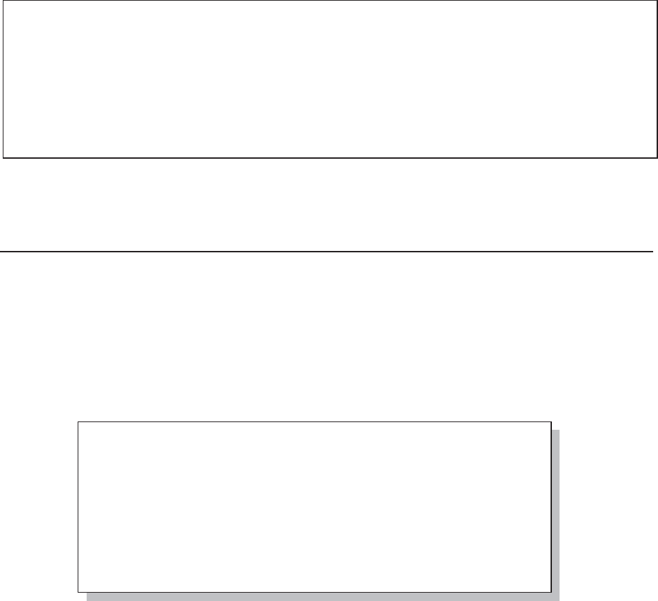
Chapter 2: Working with Your Data 63
Notice that there is no variable for VISIT3, because neither of these two patients had a visit
number 3, so their third physical visit was visit number 4.
SEE ALSO
The IDGROUP option in PROC MEANS and in PROC SUMMARY is used to transpose data in
King and Zdeb (2010).
2.4.2 Transposing in the DATA Step
The DATA step offers a great deal of flexibility to the process of transposing data. Commonly the
process of transposing will involve the use of an array and an iterative DO loop.
Rows to Columns
In order to transpose observations into columns, a series of observations must be processed for
each new observation. The array statement is used to hold the values from the individual
observations. Once all of the individual observations have been consolidated, the values in the
array are written out to the new observation in the new data set.
n The array values are retained so that we can accumulate sodium values across visits.
o We know that there can be no more than 16 patient visits, so this becomes the dimension of the array.
p Since visit values are retained, the array containing the visit values are cleared at the start of
each subject.
q The array is indexed using the visit number. This guarantees that the value of sodium will be
assigned to the correct array variable.
r The new observation is written after all the incoming observations for each subject have been
processed.
data lab_nonnormal(keep=subject visit1-visit16);
set lab_chemistry(keep=subject visit sodium);
by subject;
retain visit1-visit16 ; n
array visits {16} visit1-visit16; o
if first.subject then do i = 1 to 16; p
visits{i} = .;
end;
visits{visit} = sodium; q
if last.subject then output lab_nonnormal; r
run;
Using PROC TRANSPOSE
2.4.1b BY and ID Form a Unique Key
S V V V V V V V
U V V V V V V V V i i i i i i i
B i i i i i i i i s s s s s s s
J s s s s s s s s i i i i i i i
O E i i i i i i i i t t t t t t t
b C t t t t t t t t 1 1 1 1 1 1 1
s T 1 2 4 5 6 7 8 9 0 1 2 3 4 5 6
1 208 13.7 14.1 14.1 14.1 13.9 13.9 14 14 14.0 . . . . . .
2 209 14.0 14.0 13.9 14.2 14.5 13.8 14 . 13.8 14 14.1 14.2 14.1 14 14.1
&DUSHQWHU$UW&DUSHQWHU¶V*XLGHWR,QQRYDWLYH6$67HFKQLTXHV&RS\ULJKW6$6,QVWLWXWH,QF&DU\1RUWK&DUROLQD86$
$
//5,*+765(6(59(')RUDGGLWLRQDO6$6UHVRXUFHVYLVLWVXSSRUWVDVFRPSXEOLVKLQJ

64 Carpenter’s Guide to Innovative SAS Techniques
Unlike the data set generated by PROC TRANSPOSE, notice that, even though VISIT3 does not
appear in the untransposed data, this data set includes a variable for VISIT3. This is a result of the
implicit use of VISIT3 in the ARRAY statement n.
Columns to Rows
You can also use the DATA step to normalize a data set. In the previous example we converted
some lab data for two patients from a normal form to a non-normal form. We will now use a
similar DATA step to convert it back to its original form.
s The variables necessary for
the conversion are kept on the
incoming data set.
t The VISITS array is declared
with each of the visits as an
element.
u The DO loop index is VISIT
which increments for each visit.
The index variable, VISIT, is
added to the Program Data Vector and will be
written to the new data set.
v The variable SODIUM is created from the array
element identified with VISIT as the index.
w Since the OUTPUT statement is inside the
DO loop, it will write an observation for each of
the iterations of the DO loop.
The resulting data set will have an observation for
each patient X visit combination. This now
includes combinations that did not originally exist.
In this example SUBJECT 208 now has
observations for VISIT 3 and VISIT 11-
VISIT16, and the value for SODIUM is
appropriately missing for each of these visits.
Observations with missing SODIUM values
could easily be removed by adding an IF
criterion to the OUTPUT statement w.
Transposing in the DATA step
2.4.2a Rows to Columns
S v v v v v v v
U v v v v v v v v v i i i i i i i
B i i i i i i i i i s s s s s s s
J s s s s s s s s s i i i i i i i
O E i i i i i i i i i t t t t t t t
b C t t t t t t t t t 1 1 1 1 1 1 1
s T 1 2 3 4 5 6 7 8 9 0 1 2 3 4 5 6
1 208 13.7 14.1 . 14.1 14.1 13.9 13.9 14 14 14.0 . . . . . .
2 209 14.0 14.0 . 13.9 14.2 14.5 13.8 14 . 13.8 14 14.1 14.2 14.1 14 14.1
title2 '2.4.2b Columns to Rows';
data lab_normal(keep=subject visit sodium);
set lab_nonnormal(keep=subject visit:); s
by subject;
array visits {16} visit1-visit16; t
do visit = 1 to 16; u
sodium = visits{visit}; v
output lab_normal; w
end;
run;
Transposing in the DATA step
2.4.2b Columns to Rows
Obs SUBJECT visit sodium
1 208 1 13.7
2 208 2 14.1
3 208 3 .
4 208 4 14.1
5 208 5 14.1
6 208 6 13.9
7 208 7 13.9
8 208 8 14.0
9 208 9 14.0
10 208 10 14.0
11 208 11 .
12 208 12 .
13 208 13 .
14 208 14 .
15 208 15 .
16 208 16 .
17 209 1 14.0
18 209 2 14.0
19 209 3 .
portions of the table not shown If sodium gt .z then output lab_normal;
&DUSHQWHU$UW&DUSHQWHU¶V*XLGHWR,QQRYDWLYH6$67HFKQLTXHV&RS\ULJKW6$6,QVWLWXWH,QF&DU\1RUWK&DUROLQD86$
$
//5,*+765(6(59(')RUDGGLWLRQDO6$6UHVRXUFHVYLVLWVXSSRUWVDVFRPSXEOLVKLQJ

Chapter 2: Working with Your Data 65
2.5 Filling Sparse Data
Sometimes when data are entered observations are created only when there is a specific value.
Observations, which reflect only missing values or for count data counts of 0, are not created.
This creates denser data as there will be fewer missing values. Depending on which observations
are included entire classification levels or combinations of classification levels could be missing
from the data. This means that the data itself does not reflect the true sampling scheme.
Sometimes we need to show all possible levels - not just those with non-missing values.
Creating observations, with the appropriate missing values, is sometimes known as creating
sparse (less dense) data.
The examples shown in this section work with the LAB_CHEMISTRY data, which has one row
per patient per visit. Missed visits are not represented in the data and will not be represented in
tables and reports.
Each patient (SUBJECT) in the LAB_CHEMISTRY data should have an observation for each of
the first 10 visits and may or may not have subsequent follow-up for visits 11 through 16. We
need to make sure that each patient has an observation for the first 10 visits.
2.5.1 Known Template of Rows
When we know the full list of values that the classification variable(s) should take on, a template
can be built and merged back onto the original data. The process of merging the template
containing all possible combinations of the classification variables will add the appropriate
observations to the data set. For the following example we want each SUBJECT to have at least
the first 10 visits.
proc sort data=advrpt.lab_chemistry n
out=lab_chemistry;
by subject visit;
run;
proc sort data=advrpt.lab_chemistry
out=sublist(keep=subject) o
nodupkey; p
by subject;
run;
data subvislist;
set sublist;
do visit = 1 to 10; q
output subvislist;
end;
run;
data sparsed;
merge subvislist r
lab_chemistry;
by subject visit; s
run;
&DUSHQWHU$UW&DUSHQWHU¶V*XLGHWR,QQRYDWLYH6$67HFKQLTXHV&RS\ULJKW6$6,QVWLWXWH,QF&DU\1RUWK&DUROLQD86$
$
//5,*+765(6(59(')RUDGGLWLRQDO6$6UHVRXUFHVYLVLWVXSSRUWVDVFRPSXEOLVKLQJ

66 Carpenter’s Guide to Innovative SAS Techniques
n The data set to be filled (sparsed) is sorted by the classification variables that will be used to
fill the data.
o A data set is created that contains only the classification variable(s) that do not need to be
filled. In this example it is SUBJECT number.
p NODUPKEY is used to eliminate all duplicate subjects. This list of distinct subject numbers
could have also been created in a simple SQL step.
q The list of unique subjects is read and a DO loop is used to output an observation for each
SUBJECT - VISIT combination. When multiple classification variables need to be filled, nested
DO loops are needed.
r The template data set (SUBVISLIST) is merged back onto the original data set. Any extra rows
in the template data, rows that did not appear in the original data, will now also appear in the
sparsed data set.
s The BY list will contain all the classification variables.
The LISTING for SUBJECT 210 shows that an observation has been added for visits 3 and 9.
Even if they had not already been in the data for SUBJECT 210, visits 11-16 would not have been
added.
This process can also be done in a PROC SQL step, either way the concept is the same.
2.5.1 Creating a Sparse Table
Every Patient should have the first 10 visits
Some patients have up to 16 visits
Obs SUBJECT visit LABDT potassium sodium chloride
114 210 1 02/19/2007 5.0 14.0 103
115 210 2 02/28/2007 4.0 14.2 103
116 210 3 . . . .
117 210 4 03/14/2007 3.9 14.1 101
118 210 5 03/09/2007 4.7 14.4 105
119 210 6 03/16/2007 4.7 14.5 104
120 210 7 03/26/2007 4.7 14.3 103
121 210 8 03/28/2007 4.4 14.1 102
122 210 9 . . . .
123 210 10 07/10/2007 4.3 14.2 106
124 210 11 04/06/2007 4.1 14.2 104
125 210 12 04/17/2007 4.0 13.9 103
126 210 13 04/19/2007 4.4 14.2 104
127 210 14 04/26/2007 4.1 14.1 99
128 210 15 05/22/2007 3.8 13.8 99
129 210 16 06/27/2007 5.2 14.3 104
. . . . Results for only SUBJECT 210 are shown . . . .
&DUSHQWHU$UW&DUSHQWHU¶V*XLGHWR,QQRYDWLYH6$67HFKQLTXHV&RS\ULJKW6$6,QVWLWXWH,QF&DU\1RUWK&DUROLQD86$
$
//5,*+765(6(59(')RUDGGLWLRQDO6$6UHVRXUFHVYLVLWVXSSRUWVDVFRPSXEOLVKLQJ

Chapter 2: Working with Your Data 67
2.5.2 Double Transpose
When all possible levels of a classification variable are not known, or not easily specified in a DO
loop, it is often possible to create a sparsed data set by performing two PROC TRANSPOSE
steps. Rather than building a template data set as was done in Section 2.5.1, we will let the data
itself determine the classification levels. It should be noted that the results of this technique and
those obtained in Section 2.5.1 are not necessarily the same.
The first PROC TRANSPOSE step creates one column for each value of the variable to be
sparsed (VISIT). Assuming that a given visit exists somewhere in the data, it will be represented
as a column after the first PROC TRANSPOSE step.
The second PROC TRANSPOSE step reconverts the columns (one for each possible visit) into
rows. The data now has the original form (as before the first PROC TRANSPOSE); however,
every visit column is now represented as a row for every subject.
n The incoming data set must be sorted at least to the level of the BY statement q.
o PROC TRANSPOSE is used to convert the rows that are to be filled into columns.
p The PREFIX= option specifies the text used to form the root portion of the new variable
names.
q The BY statement lists the classification variables that do not need to be filled.
r The variable VISIT will be used to identify which columns were formed from which rows. In
this case, the numeric variable VISIT will be combined with the prefix text p to form the new
column name.
proc sort data=advrpt.lab_chemistry n
out=lab_chemistry
nodupkey;
by subject visit;
run;
proc transpose data=lab_chemistry o
out=labtran
prefix=Visit; p
by subject; q
id visit; r
var sodium potassium chloride;
run;
proc transpose data=labtran s
out=sparsed(rename=(_name_=Visit)); t
by subject; u
id _name_; v
var visit:; w
run;
&DUSHQWHU$UW&DUSHQWHU¶V*XLGHWR,QQRYDWLYH6$67HFKQLTXHV&RS\ULJKW6$6,QVWLWXWH,QF&DU\1RUWK&DUROLQD86$
$
//5,*+765(6(59(')RUDGGLWLRQDO6$6UHVRXUFHVYLVLWVXSSRUWVDVFRPSXEOLVKLQJ

68 Carpenter’s Guide to Innovative SAS Techniques
s The data set LABTRAN will be transposed back to the original set of rows and columns.
t By default rows in the new data set (SPARSED) will be identified with the variable _NAME_.
This variable is renamed to VISIT.
u The incoming data set (LABTRAN) has one observation per SUBJECT _NAME_
combination.
v The ID statement identifies the variable (_NAME_) that contains the names of the new
columns.
w Each of the variables starting with VISIT is included in the transpose (see Section 2.6.1 for
more on variable list abbreviations).
Prior to the first transpose, inspection of the data for SUBJECT=210 shows that this subject has
missed both visits 3 and 9.
After the first PROC TRANSPOSE o the data (WORK.LABTRAN) looks like the following (for
SUBJECT=210). There is now a VISIT9 column for this subject, even though this subject did not
have a VISIT9 in the data; however, there is still no column for visit 3. This is because no subject
in the entire data set had a VISIT3.
2.5.2 Creating a Sparse Table
Using a Double Transpose
Prior to First Transpose
Obs SUBJECT VISIT LABDT potassium sodium chloride
95 210 1 02/19/2007 5.0 14.0 103
96 210 2 02/28/2007 4.0 14.2 103
97 210 4 03/14/2007 3.9 14.1 101
98 210 5 03/09/2007 4.7 14.4 105
99 210 6 03/16/2007 4.7 14.5 104
100 210 7 03/26/2007 4.7 14.3 103
101 210 8 03/28/2007 4.4 14.1 102
102 210 10 07/10/2007 4.3 14.2 106
103 210 11 04/06/2007 4.1 14.2 104
104 210 12 04/17/2007 4.0 13.9 103
105 210 13 04/19/2007 4.4 14.2 104
106 210 14 04/26/2007 4.1 14.1 99
107 210 15 05/22/2007 3.8 13.8 99
108 210 16 06/27/2007 5.2 14.3 104
&DUSHQWHU$UW&DUSHQWHU¶V*XLGHWR,QQRYDWLYH6$67HFKQLTXHV&RS\ULJKW6$6,QVWLWXWH,QF&DU\1RUWK&DUROLQD86$
$
//5,*+765(6(59(')RUDGGLWLRQDO6$6UHVRXUFHVYLVLWVXSSRUWVDVFRPSXEOLVKLQJ

Chapter 2: Working with Your Data 69
The second PROC TRANSPOSE s uses this data as input and since all visits are included on the
VAR statement w, each visit becomes a row in the new table.
This subject now has a data row for VISIT9 (with missing values) even though VISIT9 was not in
the original data for this subject. This implies that at least one subject had a VISIT9. Since
VISIT3 still does not appear, we can infer that no subject in our study had a VISIT3. This
technique requires that the row that is to be sparsed (visits 3 and 9) appear in the data set
somewhere at least once.
Remember when using PROC TRANSPOSE that it is very important that some combination of
the BY and ID variables identify down to the row level (see Section 2.4.1).
MORE INFORMATION
The TRANSPOSE procedure and some of its pitfalls (gotcha’s) can be found in Section 2.4.1.
2.5.2 Creating a Sparse Table
Using a Double Transpose
First Transpose
Obs SUBJECT _NAME_ Visit1 Visit2 Visit4 Visit5 Visit6 Visit7 Visit8
31 210 sodium 14 14.2 14.1 14.4 14.5 14.3 14.1
32 210 potassium 5 4.0 3.9 4.7 4.7 4.7 4.4
33 210 chloride 103 103.0 101.0 105.0 104.0 103.0 102.0
Obs Visit9 Visit10 Visit11 Visit12 Visit13 Visit14 Visit15 Visit16
31 . 14.2 14.2 13.9 14.2 14.1 13.8 14.3
32 . 4.3 4.1 4.0 4.4 4.1 3.8 5.2
33 . 106.0 104.0 103.0 104.0 99.0 99.0 104.0
2.5.2 Creating a Sparse Table
Using a Double Transpose
Second Transpose
Obs SUBJECT Visit sodium potassium chloride
151 210 Visit1 14.0 5.0 103
152 210 Visit2 14.2 4.0 103
153 210 Visit4 14.1 3.9 101
154 210 Visit5 14.4 4.7 105
155 210 Visit6 14.5 4.7 104
156 210 Visit7 14.3 4.7 103
157 210 Visit8 14.1 4.4 102
158 210 Visit9 . . .
159 210 Visit10 14.2 4.3 106
160 210 Visit11 14.2 4.1 104
161 210 Visit12 13.9 4.0 103
162 210 Visit13 14.2 4.4 104
163 210 Visit14 14.1 4.1 99
164 210 Visit15 13.8 3.8 99
165 210 Visit16 14.3 5.2 104
&DUSHQWHU$UW&DUSHQWHU¶V*XLGHWR,QQRYDWLYH6$67HFKQLTXHV&RS\ULJKW6$6,QVWLWXWH,QF&DU\1RUWK&DUROLQD86$
$
//5,*+765(6(59(')RUDGGLWLRQDO6$6UHVRXUFHVYLVLWVXSSRUWVDVFRPSXEOLVKLQJ

70 Carpenter’s Guide to Innovative SAS Techniques
2.5.3 Using COMPLETYPES with PROC MEANS or PROC SUMMARY
The COMPLETETYPES option can be used on the PROC MEANS or PROC SUMMARY
statement to force the
procedure to generate
statistics for all
combinations of the
classification variables.
In Section 2.5.2 a double
PROC TRANSPOSE is
used to determine all of the
combinations of
SUBJECT and VISIT.
This can also be
accomplished using the
COMPLETETYPES
option on the PROC
MEANS or PROC
SUMMARY statement.
There are no VISIT 9
observations for
SUBJECT 210; however,
since at least one subject
somewhere in the
LAB_CHEMISTRY data
table had a VISIT 9, the
report generated from the
PROC MEANS results
will show a VISIT 9 for all
subjects n.
Behind the scenes PROC MEANS and PROC SUMMARY are really the same procedure, so this
technique works with either procedure.
MORE INFORMATION
The COMPLETETYPES option is also discussed in Section 7.10. The COMPLETETYPES
option also has implications when using preloaded formats; see Section 12.1.3.
2.5.4 Using CLASSDATA
The CLASSDATA option is used with the TABULATE, MEANS, and SUMMARY procedures
to specify a data set that contains levels of one or more classification variables. If the data set
contains levels that are not found in the data, those levels will be included in the resulting
summary.
proc means data=advrpt.lab_chemistry
completetypes noprint nway;
class subject visit;
var sodium potassium chloride;
output out=allvisits sum=;
run;
2.5.3 Creating a Sparse Table
Using COMPLETETYPES
Obs SUBJECT VISIT sodium potassium chloride
151 210 1 14.0 5.0 103
152 210 2 14.2 4.0 103
153 210 4 14.1 3.9 101
154 210 5 14.4 4.7 105
155 210 6 14.5 4.7 104
156 210 7 14.3 4.7 103
157 210 8 14.1 4.4 102
158 210 9 . . . n
159 210 10 14.2 4.3 106
160 210 11 14.2 4.1 104
161 210 12 13.9 4.0 103
162 210 13 14.2 4.4 104
163 210 14 14.1 4.1 99
164 210 15 13.8 3.8 99
165 210 16 14.3 5.2 104
&DUSHQWHU$UW&DUSHQWHU¶V*XLGHWR,QQRYDWLYH6$67HFKQLTXHV&RS\ULJKW6$6,QVWLWXWH,QF&DU\1RUWK&DUROLQD86$
$
//5,*+765(6(59(')RUDGGLWLRQDO6$6UHVRXUFHVYLVLWVXSSRUWVDVFRPSXEOLVKLQJ

Chapter 2: Working with Your Data 71
The data set WORK.VISITS is
constructed to have one
observation for each of the
potential 16 visits n. This data
set is then used with the
CLASSDATA= option o and
the EXCLUSIVE option in the
PROC MEANS step.
Although in the
LAB_CHEMISTRY data set
there are no subjects that have a
visit 3 and SUBJECT 210 does
not have a visit 9, in the
summary data set
(WORK.ALLMEANS) p
which was created by PROC
MEANS, each subject will have
a summary row for all
sixteen visits. Subject 210,
which is shown here, now
has both a visit 3 q, and a
visit 9 r.
ASIDE: The CLASSDATA
data set must contain each
of the CLASS variables.
MORE INFORMATION
The CLASSDATA option is also discussed in Sections 7.9 (PROC MEANS and PROC
SUMMARY) and 8.1.4 (PROC TABULATE).
proc sort data=advrpt.demog(keep=subject)
out=subjects nodupkey;
by subject;
run;
data Visits;
set subjects;
do visit = 1 to 16; n
output visits;
end;
run;
proc means data=advrpt.lab_chemistry
classdata=visits o
noprint nway exclusive;
class subject visit;
var sodium potassium chloride;
output out=allvisits p sum=;
run;
2.5.4 Using CLASSDATA
MEANS / SUMMARY
Obs SUBJECT VISIT sodium potassium chloride
161 210 1 14.0 5.0 103
162 210 2 14.2 4.0 103
163 210 3 . . . q
164 210 4 14.1 3.9 101
165 210 5 14.4 4.7 105
166 210 6 14.5 4.7 104
167 210 7 14.3 4.7 103
168 210 8 14.1 4.4 102
169 210 9 . . . r
170 210 10 14.2 4.3 106
171 210 11 14.2 4.1 104
172 210 12 13.9 4.0 103
173 210 13 14.2 4.4 104
174 210 14 14.1 4.1 99
175 210 15 13.8 3.8 99
176 210 16 14.3 5.2 104
&DUSHQWHU$UW&DUSHQWHU¶V*XLGHWR,QQRYDWLYH6$67HFKQLTXHV&RS\ULJKW6$6,QVWLWXWH,QF&DU\1RUWK&DUROLQD86$
$
//5,*+765(6(59(')RUDGGLWLRQDO6$6UHVRXUFHVYLVLWVXSSRUWVDVFRPSXEOLVKLQJ
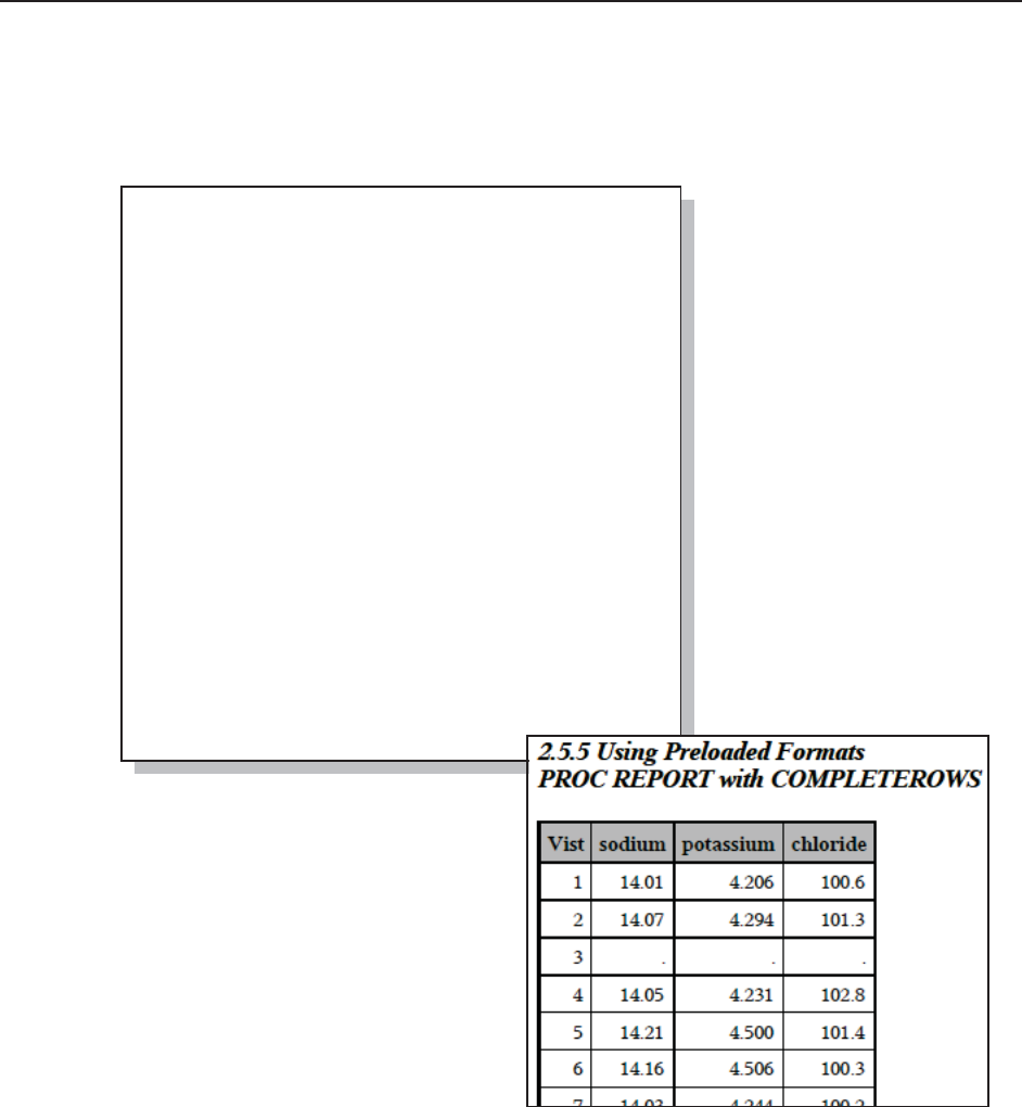
72 Carpenter’s Guide to Innovative SAS Techniques
2.5.5 Using Preloaded Formats
For the TABULATE, MEANS, SUMMARY, and REPORT procedures, preloaded formats can be
used to add rows to output tables. Like the CLASSDATA option shown in Section 2.5.4, this
method adds the sparsed rows to the table, not the data set. Thus, we are not required to either
modify the original data or to even make a copy.
Let’s assume that we need to
generate a report of mean lab
chemistry values for lab visits.
The report must contain the first
10 visits regardless of whether or
not they appear in the data.
n A format is created which
contains each of the first 10
visits.
o The COMPLETEROWS
option, which is unique to PROC
REPORT, is used to ensure that
every row in the preloaded
format will appear in the report.
p The PRELOADFMT option
will always be present when
using preloaded formats. Here
the PRELOADFMT option is
associated with the format to be preloaded
by placing both on the DEFINE
statement. A portion of the resultant
report is shown to the right.
MORE INFORMATION
Preloaded formats can also be used to
exclude observations, and are introduced
and discussed in more detail in Section
12.1.
proc format; n
value visits
1='1'
2='2'
3='3'
4='4'
5='5'
6='6'
7='7'
8='8'
9='9'
10='10';
run;
ods pdf file="&path\results\E2_5_5.pdf";
proc report data=advrpt.lab_chemistry nowd
completerows;o
column visit sodium potassium chloride;
define visit / group
f=visits. preloadfmt p
'Visit' order=data;
define sodium /analysis mean f=5.2;
define potassium /analysis mean f=5.3;
define chloride/analysis mean f=5.1;
run;
ods pdf close;
&DUSHQWHU$UW&DUSHQWHU¶V*XLGHWR,QQRYDWLYH6$67HFKQLTXHV&RS\ULJKW6$6,QVWLWXWH,QF&DU\1RUWK&DUROLQD86$
$
//5,*+765(6(59(')RUDGGLWLRQDO6$6UHVRXUFHVYLVLWVXSSRUWVDVFRPSXEOLVKLQJ
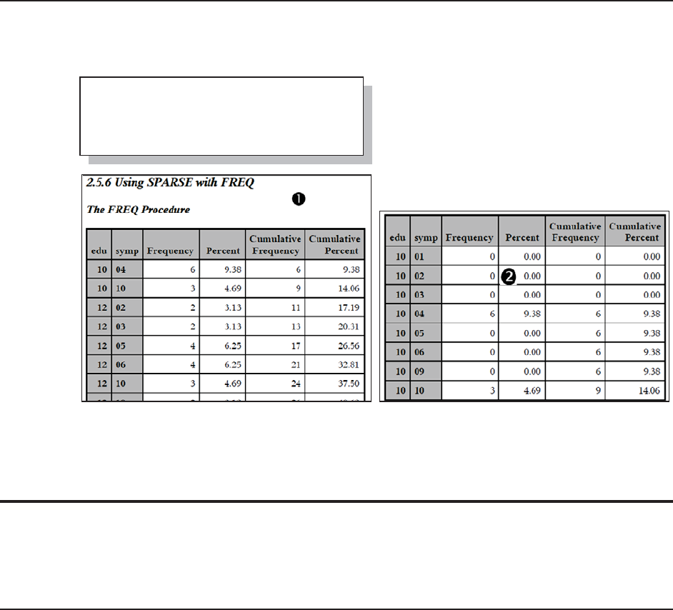
Chapter 2: Working with Your Data 73
2.5.6 Using the SPARSE Option with PROC FREQ
By default the table generated by PROC FREQ will contain only those levels that actually exist in
the data. In the first TABLE statement n, only the combinations of the two classification
variables (EDU and SYMP) will exist in the
table. The SPARSE option on the second
TABLE statement o will have all
combinations of any value of EDU and SYMP.
Notice that on the first table EDU=10 has only
two levels of SYMP (04 and 10); however, on
the second table o each level of SYMP that
exists somewhere in the data set is associated
with EDU=10. Notice that, since no subject has a SYMP of either ‘07’ or ‘08’, those levels are not
included in the SPARSED reports.
2.6 Some General Concepts
There are a number of general techniques, shortcuts, and did you know that you cans, of which
you should be aware.
2.6.1 Shorthand Variable Naming
When creating a long list of variable names it is sometimes helpful to not actually write each
name individually. Fortunately there are several ways to create lists of variables that require less
coding.
These shorthand variable lists can be used wherever a list of variables is expected. This includes
the VAR, KEEP, DROP, and ARRAY statements.
Common Prefix Variable Lists (Numbered Range)
Variables with a common prefix and a numeric suffix can be listed as:
visit1 - visit10
proc freq data=advrpt.demog;
table edu*symp/ list; n
table edu*symp/ list sparse; o
run;
&DUSHQWHU$UW&DUSHQWHU¶V*XLGHWR,QQRYDWLYH6$67HFKQLTXHV&RS\ULJKW6$6,QVWLWXWH,QF&DU\1RUWK&DUROLQD86$
$
//5,*+765(6(59(')RUDGGLWLRQDO6$6UHVRXUFHVYLVLWVXSSRUWVDVFRPSXEOLVKLQJ

74 Carpenter’s Guide to Innovative SAS Techniques
This list will include all the variables between VISIT1 and VISIT10 inclusively. As a general rule,
it does not matter if all the variables are already present on the PDV, and their order on the PDV
is not important. However, as with any list of variables, the usage itself can have unintended
consequences.
In the following ARRAY statement only the first 10 visits will be included in the array; however,
if one of these variables is not already on the PDV, it will be added.
array vis {10} visit1 - visit10;
The KEEP statement does not establish variables, so unlike the previous ARRAY statement,
variables in the list that are not already on the PDV will cause an error. If there is no VISIT3
variable on the PDV, the following KEEP statement will produce a warning.
keep visit1 - visit10;
This type of list can be used wherever a variable list is expected. This includes statements and
options such as: KEEP, DROP, VAR, RETAIN. Functions that accept a list of values, e.g., MIN,
MAX, MEAN, require the use of the OF operator to prevent confusion with a subtraction.
m = max(of visit1 - visit10);
PDV Order Dependent Lists (Named Range)
When the order of the variables on the PDV is known, you can use the double dash to specify the
list. Unlike the common prefix variable list shown above, the order of the variables on the PDV is
very important and this form of variable list cannot be used to create variables. The following
PROC CONTENTS step shows the variables in ADVRPT.DEMOG and their relative position on
the PDV (through the use of the VARNUM option – the VARNUM option replaces the now
outdated POSITION option).
The resulting listing shows the names of the variables, their attributes, and their order.
title1 '2.6.1 Variable Shorthand Lists';
title2 'List of variables and their positions';
proc contents data=advrpt.demog varnum;
run;
&DUSHQWHU$UW&DUSHQWHU¶V*XLGHWR,QQRYDWLYH6$67HFKQLTXHV&RS\ULJKW6$6,QVWLWXWH,QF&DU\1RUWK&DUROLQD86$
$
//5,*+765(6(59(')RUDGGLWLRQDO6$6UHVRXUFHVYLVLWVXSSRUWVDVFRPSXEOLVKLQJ

Chapter 2: Working with Your Data 75
The variable list LNAME--SYMP includes all variables (numeric and character) in the data set
ADVRPT.DEMOG except SUBJECT, CLINNUM, and DEATH2.
Inclusion of the list modifiers NUMERIC and CHARACTER can be used to restrict the list to just
numeric or just character. Again the list is order dependent and includes the endpoints, assuming
they are the correct type. The list DOB-numeric-HT excludes RACE, while the list SEX-
character-SYMP, contains only three variables (SEX, RACE, and SYMP).
Inclusion of an incorrect type does not cause an error. The designation death-character-symp
will correctly contain the two variables RACE and SYMP.
Unlike the list abbreviation with a single dash (common prefix numbered list), this list form
cannot be used to create variables or add variables to the PDV. It can, however, be otherwise used
where you need a list of variables.
CAVEAT
Since the order of the variables on the PDV is generally of secondary importance to most SAS
programmers be very careful when using these forms of lists. If the variable order changes for
some reason, the list may no longer be what you intend.
Using the Colon Operator (Name Prefix)
Variables named with a common prefix (with or without a numeric suffix) can be listed by
following the prefix with a colon.
For the data set STATS generated by the following PROC SUMMARY, you could select all the
statistics associated with HT by using the list HT_: p.
2.6.1 Variable Shorthand Lists
List of variables and their positions
The CONTENTS Procedure
Variables in Creation Order
# Variable Type Len Format Label
1 subject Num 8
2 CLINNUM Char 6 clinic number
3 LNAME Char 10 last name
4 FNAME Char 6 first name
5 SSN Char 9 social security number
6 SEX Char 1 patient sex
7 DOB Num 8 DATE7. date of birth
8 DEATH Num 8 DATE7. date of death
9 RACE Char 1 race
10 EDU Num 8 years of education
11 WT Num 8 weight in pounds
12 HT Num 8 height in inches
13 SYMP Char 2 symptom code
14 death2 Num 8 DATE9.
&DUSHQWHU$UW&DUSHQWHU¶V*XLGHWR,QQRYDWLYH6$67HFKQLTXHV&RS\ULJKW6$6,QVWLWXWH,QF&DU\1RUWK&DUROLQD86$
$
//5,*+765(6(59(')RUDGGLWLRQDO6$6UHVRXUFHVYLVLWVXSSRUWVDVFRPSXEOLVKLQJ

76 Carpenter’s Guide to Innovative SAS Techniques
n The analysis variables HT and WT are used to generate a series of statistics. The names of
these statistics are automatically generated o, and are of the form of analsysisvariable_statistic
(see Section 7.2 more details on the AUTONAME option).
p The list of all statistics generated for the HT variable will be printed using the name prefix list
in the VAR statement.
MORE INFORMATION
This list abbreviation is used in a PROC TRANSPOSE example in Section 2.5.2.
Special Name Lists
Three name lists exist that allow you to address variables by their type. These include:
_CHARACTER_ All character variables
_NUMERIC_ All numeric variables
_ALL_ All variables on the PDV
Since each of these lists pertains to the current list of variables, they will not create variables. In
each case the resulting list of variables will be in the same order as they are on the Program Data
Vector.
The _ALL_ list abbreviation is used in the following DATASETS step to remove the label and
format attributes from a data set. This example
was suggested by SAS Sample #25052.
The MODIFY statement opens the
WORK.DEMOG data set and the ATTRIB
statement is applied to all the data set’s variables
by listing the variables using the _ALL_ list
abbreviation.
SEE ALSO
This example with further explanation can be found in the SAS Sample library at
http://support.sas.com/kb/25/052.html.
proc summary data=advrpt.demog;
class race edu;
var ht wt; n
output out=stats
mean=
stderr=
min=/autoname; o
run;
proc print data=stats;
id race edu;
var ht_: p;
run;
proc datasets lib=work nolist;
modify demog;
attrib _all_ label=' '
format=;
contents;
quit;
&DUSHQWHU$UW&DUSHQWHU¶V*XLGHWR,QQRYDWLYH6$67HFKQLTXHV&RS\ULJKW6$6,QVWLWXWH,QF&DU\1RUWK&DUROLQD86$
$
//5,*+765(6(59(')RUDGGLWLRQDO6$6UHVRXUFHVYLVLWVXSSRUWVDVFRPSXEOLVKLQJ
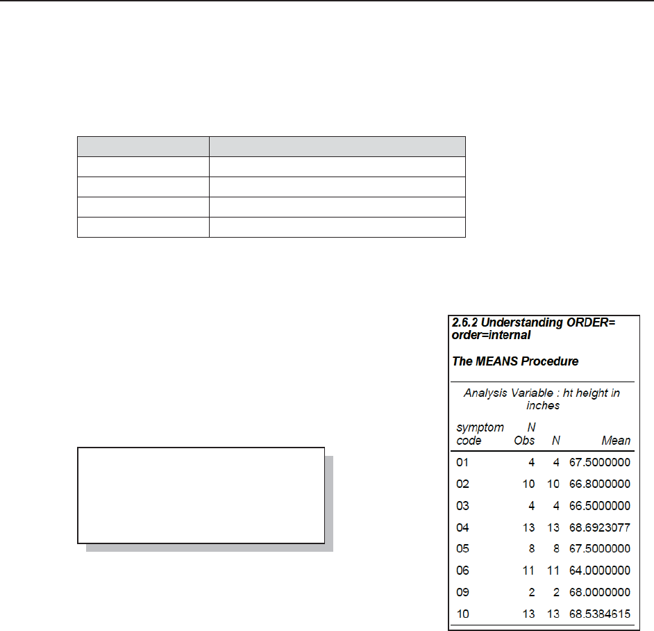
Chapter 2: Working with Your Data 77
2.6.2 Understanding the ORDER= Option
The ORDER= option can be used with most procedures that classify or summarize data. It allows
us to control both the analysis and display order of information without physically sorting the
data. Depending on the procedure the option may be applied on the PROC statement or on one or
more of the supporting statements, such as the CLASS statement.
The option can take on the values of:
Option Value: Order is based on:
INTERNAL the unformatted values (like PROC SORT)
FORMATTED the formatted value
FREQ the descending frequency
DATA the order of the data values
For most procedures the default value for ORDER= is INTERNAL.
In each of the following examples, a simple PROC MEANS with a single classification variable
(SYMP) is used to demonstrate the effect of the ORDER=
option.
ORDER=INTERNAL
This is typically the order of the variable if it had been sorted
with PROC SORT, and is usually the procedure’s default. Its
alias is UNFORMATTED.
The ORDER=
option is not
specified and
the PROC
MEANS
default order
for all
classification
variables is ORDER=INTERNAL. As a result the symptoms
appear in alphabetical order (SYMP is character).
ORDER=FORMATTED
When the ORDER=FORMATTED option is used the values are first formatted and then ordered.
title2 'order=internal';
proc means data=advrpt.demog
n mean;
class symp;
var ht;
run;
&DUSHQWHU$UW&DUSHQWHU¶V*XLGHWR,QQRYDWLYH6$67HFKQLTXHV&RS\ULJKW6$6,QVWLWXWH,QF&DU\1RUWK&DUROLQD86$
$
//5,*+765(6(59(')RUDGGLWLRQDO6$6UHVRXUFHVYLVLWVXSSRUWVDVFRPSXEOLVKLQJ
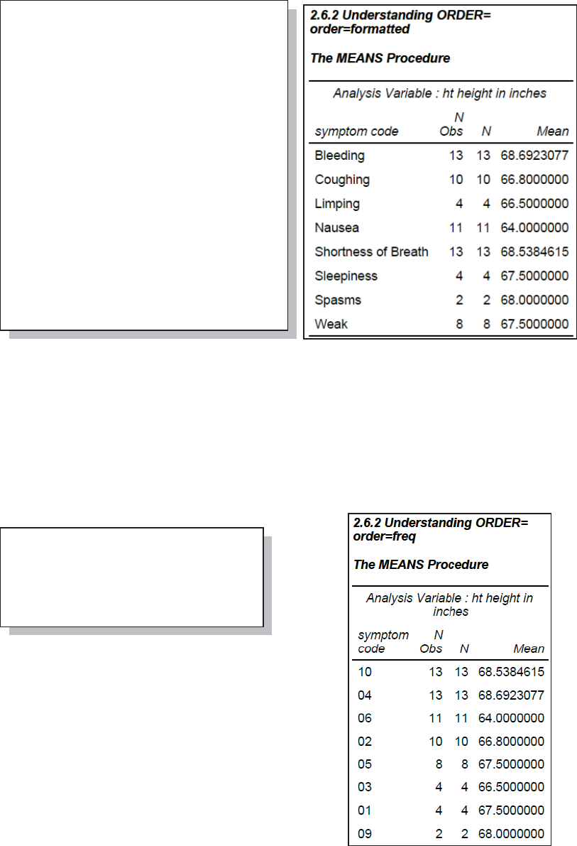
78 Carpenter’s Guide to Innovative SAS Techniques
n The ORDER=FORMATTED option on the PROC statement is applied to all classification
variables.
o The user-defined format $SMPTOM. is applied to the classification variable SYMP.
The formatted values now determine the order of the rows for the classification variable.
ORDER=FREQ
The frequency of the levels of the classification variable is used to determine the order when
ORDER=FREQ is used.
p Placing the ORDER= option on the CLASS
statement instead of on the PROC statement, allows the
selective application of the option to only specific
classification variables (see Section 7.1.3 for more on
the use of options on the CLASS statement).
The symptoms are now listed in order of decreasing
frequency. The CLASS statement also supports the
ASCENDING option which can be used with the
ORDER=FREQ option to list the levels in ascending
order.
proc format;
value $SYMPTOM
'01'='Sleepiness'
'02'='Coughing'
'03'='Limping'
'04'='Bleeding'
'05'='Weak'
'06'='Nausea'
'07'='Headache'
'08'='Cramps'
'09'='Spasms'
'10'='Shortness of Breath';
run;
title2 'order=formatted';
proc means data=advrpt.demog
n mean
order=formatted; n
class symp;
var ht;
format symp $symptom.; o
run;
title2 'order=freq';
proc means data=advrpt.demog
n mean;
class symp / order=freq; p
var ht;
run;
&DUSHQWHU$UW&DUSHQWHU¶V*XLGHWR,QQRYDWLYH6$67HFKQLTXHV&RS\ULJKW6$6,QVWLWXWH,QF&DU\1RUWK&DUROLQD86$
$
//5,*+765(6(59(')RUDGGLWLRQDO6$6UHVRXUFHVYLVLWVXSSRUWVDVFRPSXEOLVKLQJ
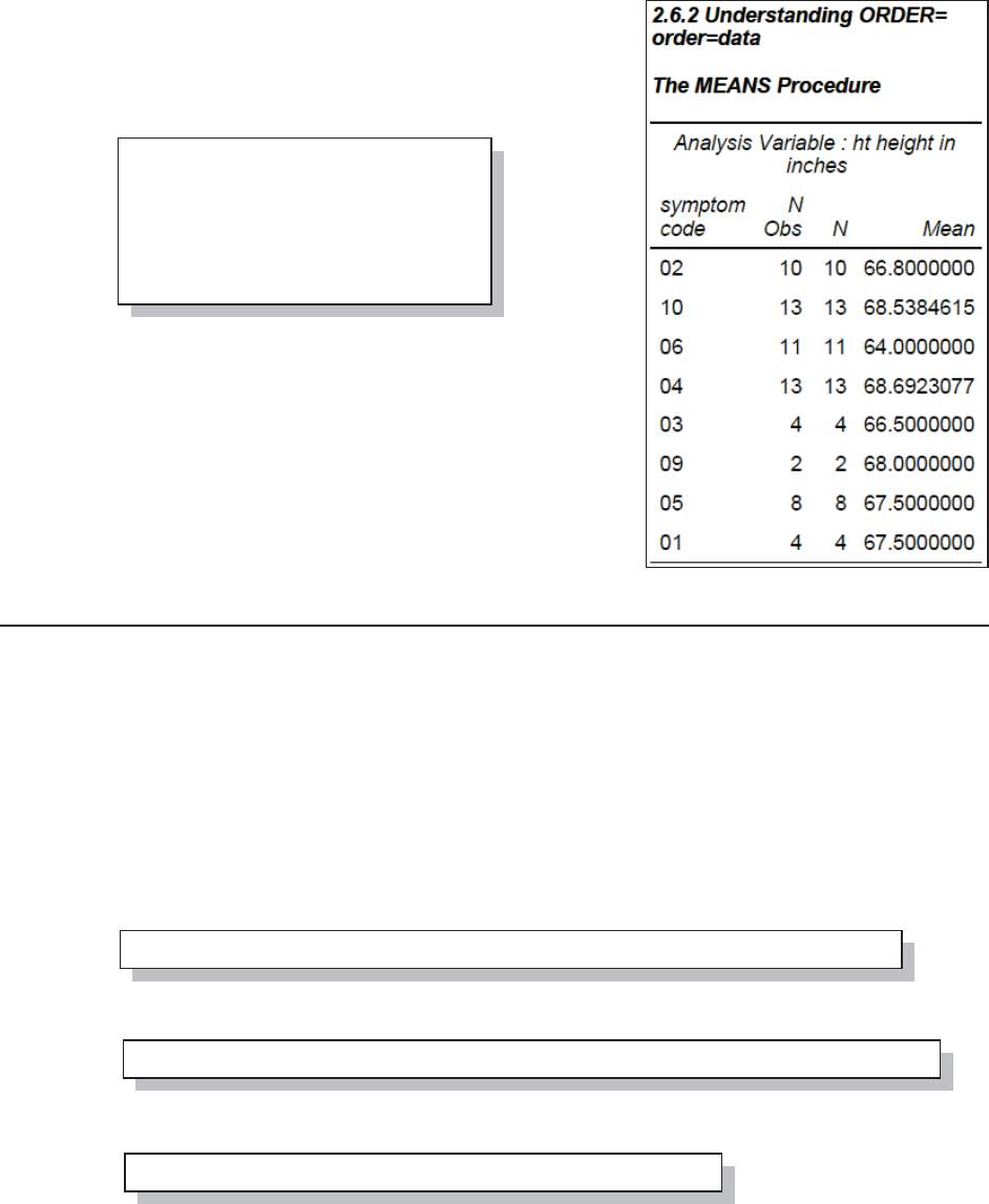
Chapter 2: Working with Your Data 79
ORDER=DATA
The order of the classification variables will reflect their
order in the data itself. The first level detected will be
written first. The data do not have to be in any particular
order.
Symptom 02 (coughing) is the first symptom in the data,
followed by 10 and 06.
MORE INFORMATION
Missing values of classification variables are not
normally included in the table, see Section 7.1.1 to
change this behavior. The ORDER= option is discussed
in terms of the TABULATE procedure in Section 8.1.5.
2.6.3 Quotes within Quotes within Quotes
The quote mark is used to identify constant text to the parser. Sometimes that quoted string of
constant text will itself contain quotes. Fortunately SAS comes with both single and double quotes
and either can be used within the other. But what happens if you need to call a macro variable
within the interior string? Regardless of which type is used on the inside, the macro variable will
be within single quotes and, therefore, will probably not be resolved.
Each of the following three statements has a quoted string within a quoted string. And each
executes successfully.
A DEFINE routine in a REPORT step compute block:
An X statement executing a Windows DIR command:
A DM statement being used to reroute the LOG file (see Section 14.4.2):
title2 'order=data';
proc means data=advrpt.demog
n mean
order=data;
class symp;
var ht;
run;
x 'dir "c:\myloc\*.sas" /o:n /b > c:\myloc\pgmlist.txt';
dm 'log; file "c:\myloc\logdump1.log"';
call define(_col_,'style', 'style={flyover="myloc"}');
&DUSHQWHU$UW&DUSHQWHU¶V*XLGHWR,QQRYDWLYH6$67HFKQLTXHV&RS\ULJKW6$6,QVWLWXWH,QF&DU\1RUWK&DUROLQD86$
$
//5,*+765(6(59(')RUDGGLWLRQDO6$6UHVRXUFHVYLVLWVXSSRUWVDVFRPSXEOLVKLQJ

80 Carpenter’s Guide to Innovative SAS Techniques
Now assume that we need to embed a macro variable in the above examples. Since macro
variables tend not to be resolved when they are used inside of single quotes, we need to
understand not only how the statements are parsed and executed, but how we can recode them.
Simply substituting the macro variable into the statement does not always work. Interestingly it
does not necessarily fail either.
n While it is generally true that macro variables will not be resolved when they occur within
single quotes, this is not strictly true. The CALL DEFINE routine is only called from within a
PROC REPORT compute block (not shown), and because of the way that these blocks are
executed the macro variable will be resolved even though it is inside of single quotes. Nothing
special needs to be done.
o The X statement will not work as it is currently coded; the macro variable will not resolve.
When we pass a path to the OS under Windows, the path should be enclosed in double quotes.
Under the current versions of SAS the X statement generally no longer requires the use of the
quotes that
surround the
command that
is to be passed to the OS. This simplifies the statement and eliminates the problem. When this
does not work, consider one of the solutions used for the DM statement.
p In the DM statement the string following the keyword DM must be quoted, and the macro
variable will not be resolved. The macro quoting functions can be helpful by temporarily masking
the single quotes until after the macro variable has been resolved. Since the single quote has been
masked, the semicolon used to separate the two DM commands must also be temporarily masked.
Prior to execution the macro quoting is removed using the %UNQUOTE function. An approach
similar to this may be needed in the FILENAME statement as well. Here we are using the pipe
engine to route the results of the DOS command to a virtual (piped) file.
In fact, since we are delaying recognition of the quote marks, we do not even need to use both
types of quote marks. In the X statement shown here, the %STR function is used to delay
recognition of the inner pair of double quotes
until after the outer ones have been utilized.
Within SAS it is not too unusual to be able to delay the parser’s recognition of a character by
doubling it. This technique was common before double quotes were introduced into the language.
To show an apostrophe in a title statement two
single quotes were used. This works because the
parser sees the two single quotes and in a second
%let temp = myloc;
call define(_col_,'style', 'style={flyover="&temp"}'); n
x 'dir "c:\&temp\*.sas" /o:n /b > c:\&temp\pgmlist.txt'; o
dm 'log; file "c:\&temp\logdump1.log"'; p
x dir "c:\&temp\*.sas" /o:n /b > c:\&temp\pgmlist.txt;
dm %unquote(%bquote(')log%bquote(;)file "c:\&temp\logdump1.log" %bquote('));
title1 'Tom''s Truck';
x "%str(md %"&temp\output%"; )";
filename list pipe %unquote(%bquote(')dir "&temp\*.rtf" /o:n /b %bquote('));
&DUSHQWHU$UW&DUSHQWHU¶V*XLGHWR,QQRYDWLYH6$67HFKQLTXHV&RS\ULJKW6$6,QVWLWXWH,QF&DU\1RUWK&DUROLQD86$
$
//5,*+765(6(59(')RUDGGLWLRQDO6$6UHVRXUFHVYLVLWVXSSRUWVDVFRPSXEOLVKLQJ

Chapter 2: Working with Your Data 81
pass of the string, converts them to a single quote mark (an apostrophe). This technique still
works and we can use it to our advantage in the DM statement that we have been working with.
Here only double quote marks are used. Notice a single double quote at the start, a double double
quote in the middle of the string,
and a triple double quote at the end.
This will require three passes for the
parser to resolve all the strings. In the meantime the macro variable will have been resolved.
This works because the quote marks are being used by the parser to 'mark' the strings in such a
way as to tell the parser how to handle the string. Double double quote marks are resolved to a
just one ‘mark’ in a second pass of the parser, and by then the macro variable has been resolved.
Rewriting the DM statement using single quotes would only partially be successful. The parser
would handle the resolution process for the quotes the same; however, since the first pair of single
quotes still resolves to a single quote, that quote would prevent the resolution of the macro
variable.
More rarely you may need a third level of quoting. For this problem what we really want is a third
type of quote mark. We only have two, however, so again we can take advantage of the parsing
process, and consequently expand the previous technique to additional levels. Surround the whole
string with single quotes, as you have already done. Then change each interior single quote to two
single quotes (not a double quote). This forces the parser to take a second pass.
2.6.4 Setting the Length of Numeric Variables
While we regularly reduce or control the length of character variables, we more rarely do so for
numeric variables. In both cases reduction of variable length can be a successful strategy to
reduce data set storage requirements. However, there are specific issues associated with reduction
of the length of numeric variables – reducing the length of a numeric variable, especially non-
integers, can drastically reduce the precision of the variable. The documentation associated with
your version of SAS and your OS will cover topics such as the loss of precision and the size of
integers that can be stored with a given length.
So how can you minimize storage costs by controlling length? With character variables it is easy;
use the minimum length that avoids truncation. For numeric variables it is less straightforward.
One of the first considerations is the value itself. If a numeric code is just a code, such as clinic
number, and will not be used in calculations, it should generally be stored as a character variable.
An exception would be social security numbers (SSN) and Employer Identification Numbers
(EIN), which can be stored in 8 bytes as a numeric variable, but require at least 9 bytes as
character variables.
While SAS dates, which are always integer values, can be safely stored in four bytes, most users
and some companies (as company policy) never reduce (or never allow the reduction of) the
length of numeric variables – “just in case.” Given that storage is generally cheap and access is
generally fast, my rule of thumb is that codes (regardless of content) are text. Only numbers are
stored as numeric values. And I only rarely reduce the length of a numeric value.
While the readers of this book are probably an exception, most users are not sophisticated enough
to understand the subtle implications of reducing length for numeric variables. If they do
understand AND/OR they know that they are only dealing with integers, then some reduction of
storage requirements can be achieved by reducing the length of numeric variables.
dm "log; file ""c:\&temp\logdump1.log""";
dm 'log; file ''c:\&temp\logdump1.log''';
&DUSHQWHU$UW&DUSHQWHU¶V*XLGHWR,QQRYDWLYH6$67HFKQLTXHV&RS\ULJKW6$6,QVWLWXWH,QF&DU\1RUWK&DUROLQD86$
$
//5,*+765(6(59(')RUDGGLWLRQDO6$6UHVRXUFHVYLVLWVXSSRUWVDVFRPSXEOLVKLQJ

82 Carpenter’s Guide to Innovative SAS Techniques
2.7 WHERE Specifics
The WHERE statement (DATA and PROC steps), WHERE= data set option, and PROC SQL
WHERE clause provide subsetting capabilities that are not otherwise available. While the
subsetting IF in the DATA step can have similar syntax and often similar results, the filter
generated by a WHERE can be substantially different in efficiency, usage, syntax, and result. The
differences are important.
When importing or exporting data, it is often necessary to filter portions of data that are to be
transferred. There are several ways to provide this filtering, and building a WHERE clause, which
can be used in a variety of data import and export situations, is a core methodology. It can be used
in both procedure and DATA steps, and can be generated using statements, options, and clauses.
Having a firm understanding of the capability of the WHERE can have a major impact when
transferring large amounts of data.
The WHERE is a primary tool for the creation of subsets of data. It can be used as a statement,
data set option, and as an SQL clause. Not only is it flexible in how it can be used, it has a number
of inherently beneficial properties. The following are a few comments about the WHERE that
mostly fall into the category of “Did you know that….”.
When creating a data subset in a DATA step the WHERE generally tends to be more efficient
than the subsetting IF statement. The selection criteria associated with the IF statement is applied
to the values in the PDV, which means that every observation is read, and then potentially
discarded. The WHERE clause on the other hand is applied before the observation is read, which
can save resources by minimizing the I/O. The WHERE does have some additional overhead and
the efficiency gains are first noticed and become more pronounced (compared to the subsetting IF
statement) as the fraction of discarded data becomes larger.
Clearly the WHERE clause must evaluate observations; however, sometimes complete blocks of
observations can be eliminated depending on what SAS knows about the data. When the WHERE
clause is applied to an indexed data set, the WHERE clause will take advantage of the indexes to
optimize the selection process.
In the DATA step and in procedures, a WHERE clause can be established either through the use
of the WHERE statement n or as a WHERE= data set option o on the incoming data set. As a
general rule best practices suggest that the WHERE statement should be used only when the
WHERE= data set option is not available, as the use of the data set option tends to make the code
easier to understand. The following two steps yield the same subset of the observations in the data
set ADVRPT.DEMOG.
title1 'E1.4b WHERE Data Set Option';
proc print data=advrpt.demog(where=(year(dob)>1960))o;
var lname fname sex dob;
run;
title1 'E1.4a WHERE Statement';
proc print data=advrpt.demog;
var lname fname sex dob;
where year(dob)>1960;n
run;
&DUSHQWHU$UW&DUSHQWHU¶V*XLGHWR,QQRYDWLYH6$67HFKQLTXHV&RS\ULJKW6$6,QVWLWXWH,QF&DU\1RUWK&DUROLQD86$
$
//5,*+765(6(59(')RUDGGLWLRQDO6$6UHVRXUFHVYLVLWVXSSRUWVDVFRPSXEOLVKLQJ
Chapter 2: Working with Your Data 83
In PROC SQL there are three ways of using the WHERE clause:
WHERE clause in a pass-through
WHERE clause in the SAS SQL
WHERE= data set option
Obviously if we are writing code that will be passed through SQL to a database system other than
SAS, Oracle for instance, the WHERE= data set option cannot be used. The WHERE clause in
SQL pass-through code has to be appropriate to the receiving database, and SAS data set options
can only be applied to SAS data sets. More on the efficiency issues of an SQL pass-through is
discussed in Section 1.4.
In a SAS SQL step there can be performance differences between the WHERE clause and the
WHERE= data set option. As was mentioned above, the WHERE= data set option is generally
optimized for use with indexes. Depending on the type of JOIN the WHERE clause will
sometimes be applied after the read.
2.7.1 Operators Just for the WHERE
While the basic syntax of the WHERE statement is similar to that of the subsetting IF statement,
there are several operators that can be used only with the WHERE (statement, data set option, or
SQL clause). These include:
BETWEEN Builds an inclusive range
CONTAINS String search
IS MISSING Check for missing values
LIKE Pattern matching
SAME WHERE clause concatenation
=* Sounds like
The examples below all use the WHERE statement, but these operators apply to the WHERE=
data set option and the SQL WHERE clause as well.
BETWEEN
The BETWEEN operator allows us to establish an inclusive range.
n The acceptable range for EDU is between
15 and 17 inclusively.
o The same list could have been established
using this compound expression, which can
also be used in an IF statement.
The negation of this range is requested by using the NOT operator with the BETWEEN operator.
The following two WHERE statements are equivalent to each other and are the exact opposites of
those in the previous PROC PRINT step.
where edu not between 15 and 17;
where edu lt 15 or edu gt 17;
title2 'BETWEEN';
proc print data=advrpt.demog;
var lname fname edu;
where edu between 15 and 17; n
/* where 15 le edu le 17;*/ o
run;
&DUSHQWHU$UW&DUSHQWHU¶V*XLGHWR,QQRYDWLYH6$67HFKQLTXHV&RS\ULJKW6$6,QVWLWXWH,QF&DU\1RUWK&DUROLQD86$
$
//5,*+765(6(59(')RUDGGLWLRQDO6$6UHVRXUFHVYLVLWVXSSRUWVDVFRPSXEOLVKLQJ

84 Carpenter’s Guide to Innovative SAS Techniques
CONTAINS
The CONTAINS operator works much like the INDEX function to determine if a text string can
be found within another string. The word CONTAINS can be replaced with its mnemonic, the
question mark (?).
p All last names that contain the letters
‘son’ will be printed. Like all string
comparisons the search is case sensitive.
q The question mark could be used to
replace the CONTAINS operator.
r The INDEX function could also be used.
CONTAINS is negated by preceding the operator with a NOT or other negation mnemonic.
IS MISSING
The IS MISSING operator can be used to check for missing values. One advantage is that it can
be used to check for either a numeric or a character missing value. Either the IS MISSING or the
IS NULL operator can be used.
s The syntax is the same for
numeric variables (EDU) and
character variables (SYMP).
t IS NULL can be used
instead of IS MISSING.
u When checking for missing
values using the ‘traditional’ approach the programmer must be aware of the variable’s type.
Negation is formed using NOT (or other negation operator). The NOT may appear either before
the IS or between the IS and MISSING.
LIKE
The LIKE operator allows for simple pattern matching. When appropriate, more complex pattern
matching can be accomplished using regular expressions in the RX() family of functions. This
operator uses the percent sign (%) and the underscore (_) as wildcards. The % will stand for any
number of characters and the _ is a place holder for exactly one character.
The following table shows some examples using the LIKE operator and alternate equivalent
expressions.
Using the LIKE
Operator
Without the LIKE Operator What It Does
lname like 'S%' lname =: 'S'
substr(lname,1,1) = 'S'
Find all last names beginning
with a capital S.
lname like '%ly%' index(lname,'ly') > 0
lname contains 'ly'
Find all last names containing
an 'ly'.
lname like 'Ch__' substr(lname,1,2) = 'Ch' and
length(lname)<5
Any two, three, or four letter
last names starting with Ch.
where edu is not missing or symp not is missing;
title2 'CONTAINS';
proc print data=advrpt.demog;
var lname fname edu;
where lname contains 'son'; p
/* where lname ? 'son';*/ q
/* where index(lname,'son');*/ r
run;
title2 'IS MISSING';
proc print data=advrpt.demog;
var lname fname edu symp;
where edu is missing or symp is missing; s
/* where edu is null or symp is null;*/ t
/* where edu = . or symp = ' ';*/ u
run;
&DUSHQWHU$UW&DUSHQWHU¶V*XLGHWR,QQRYDWLYH6$67HFKQLTXHV&RS\ULJKW6$6,QVWLWXWH,QF&DU\1RUWK&DUROLQD86$
$
//5,*+765(6(59(')RUDGGLWLRQDO6$6UHVRXUFHVYLVLWVXSSRUWVDVFRPSXEOLVKLQJ

Chapter 2: Working with Your Data 85
When using the % and _ with the LIKE operator, you need to be careful, as it is possible to return
unanticipated values.
A trailing _ will not select anything if the _ is past the length of the variable.
Whenever the % is followed by other search characters, be sure to enclose the string in
single quotes to prevent the macro parser from interpreting the % as a macro trigger.
When the searched string contains either a _ or a % there can be confusion between the
wildcards and the actual characters. Be sure that you specify what you really mean. Since
the CONTAINS operator does not utilize wildcards, it can be used when your target
string contains an underscore or percent sign.
Negation of the LIKE operator is achieved using the standard negation operators.
SAME
The SAME operator allows you to specify a composite clause through the use of separate
WHERE statements. Primarily used in interactive or run-group processing, it has little use in other
programming situations, since the clause cannot be maintained across step boundaries.
The first clause is specified as usual, and the second is appended with the SAME operator. If the
SAME operator had not been included on the second
WHERE statement, the second clause would have
replaced the first. When joining two WHERE clauses
with the SAME operator, the two clauses are
effectively joined with an AND (both clauses have to
be true for the overall result to be true).
It is common to explicitly specify the AND on the
subsequent WHERE clauses. This can reduce
ambiguity.
In both cases the resulting WHERE statement could have been written as:
Sounds like
The sounds like operator, which is coded using the mnemonic = *, uses the same algorithm as the
SOUNDEX function:
The first letter is preserved
Vowels are eliminated
Double letters are compressed
The remaining letters are converted to numbers using a scheme that nominally groups
letters that sound similarly in English
proc print data=advrpt.demog;
var lname fname edu symp;
where lname like 'S%';
where same edu le 15;
run;
where lname like 'S%';
where same and edu le 15;
where lname like 'S%' and edu le 15;
&DUSHQWHU$UW&DUSHQWHU¶V*XLGHWR,QQRYDWLYH6$67HFKQLTXHV&RS\ULJKW6$6,QVWLWXWH,QF&DU\1RUWK&DUROLQD86$
$
//5,*+765(6(59(')RUDGGLWLRQDO6$6UHVRXUFHVYLVLWVXSSRUWVDVFRPSXEOLVKLQJ

86 Carpenter’s Guide to Innovative SAS Techniques
In theory two words with similar pronunciation will yield the same code.
In this example we are searching for all patients
with last names that sound something like ‘che’.
The resulting listing shows two names that
match the requested text string. Since vowels
are dropped, as is the silent ‘h’, the portion that
is actually used to form the comparison is the
‘C’.
MORE INFORMATION
There can be serious and sometimes
unanticipated consequences for using the MIN and MAX operators. These operators are available
to expressions in both the WHERE and IF statements, but they behave differently depending on
how they are used. Please review Section 2.2.5 before using either of these two operators or their
mnemonics.
2.7.2 Interaction with the BY Statement
When a WHERE clause is created and a BY statement is also present, the groups of observations
formed using the BY variables are created after the application of the WHERE clause. This means
that any FIRST. or LAST. processing will be applied only to those observations that meet the
WHERE criteria. The result can be quite different from using a subsetting IF statement to form
the groups, as the BY groups are formed before the IF statement is applied.
The following DATA step correctly counts the number of distinct symptoms within each clinic
(CLINNUM). Since we do not want to
count observations without symptoms
(SYMP=’ ‘), a WHERE statement n is
used to exclude those observations, and the
variable WSYMPCNT is used to
accumulate the symptom count within each
clinic (CLINNUM).
o The first observation for a given clinic
is used to initialize the counter,
WSYMCNT.
p Each distinct value of SYMP is counted. We could count either FIRST or LAST here.
q When we have processed all the rows for this clinic we know that we have the total count and
we can output the result.
proc print data=advrpt.demog;
var lname fname dob;
where lname =* 'che';
run;
2.7.1 Operators Just for the WHERE
Sounds like
Obs LNAME FNAME DOB
14 Chou John 15MAY58
15 Chu David 18JUN51
data WHEREcnt(keep=clinnum Wsympcnt);
set demog(keep=clinnum symp);
by clinnum symp;
where symp ne ' '; n
if first.clinnum then do; o
Wsympcnt=0;
end;
if first.symp then Wsympcnt+1; p
if last.clinnum then output; q
run;
&DUSHQWHU$UW&DUSHQWHU¶V*XLGHWR,QQRYDWLYH6$67HFKQLTXHV&RS\ULJKW6$6,QVWLWXWH,QF&DU\1RUWK&DUROLQD86$
$
//5,*+765(6(59(')RUDGGLWLRQDO6$6UHVRXUFHVYLVLWVXSSRUWVDVFRPSXEOLVKLQJ

Chapter 2: Working with Your Data 87
Using the subsetting IF statement r instead of
the WHERE
statement n
changes the
way that the
BY groups are formed. If the DATA step that
uses the IF statement r does not take this
formation process into account, the results will
be incorrect.
The table above shows the counts for these two
methods for a few of the clinics. Clearly we can
see that there is disagreement for two of these
clinics, and the reason for this difference is at
the heart of the problem.
Examination of the data used to form the counts shows that the variable SYMP has at least one
missing value for each of the clinics that have an incorrect count.
When the subsetting IF statement r executes, it eliminates these rows, but more importantly
these rows are also the rows for which FIRST.CLINNUM is true. Since the row is eliminated, the
counter cannot be reset o. This does not happen when the WHERE statement n is used because
the BY groups are formed after the elimination of rows. As a result FIRST.CLINNUM will be
available for testing and will not be eliminated inappropriately.
You are not constrained to using the WHERE with BY-group processing, but you must be careful.
If we remove the subsetting IF statement from the DATA step and add the same logic to the line
that counts the symptoms, the counting problem is corrected.
Interestingly a comparison of the WHERE statement and the corrected logic using the IF
statement highlight another difference between the two approaches.
Notice that a clinic number
(038362), which was not in the
previous report, now appears. All
observations for this clinic have
SYMP=’ ‘; consequently, it was
completely removed from
consideration by both the
WHERE and the subsetting IF
statements nr. Since the revised
DATA step does not eliminate
if first.symp & symp ne ' ' then IFsympcnt+1;
if symp ne ' '; r
2.7.2 WHERE and BY Group Processing
Obs CLINNUM SYMP subject
1 031234 01 127
2 031234 01 168
3 031234 04 110
4 031234 04 156
5 033476 148
6 033476 161
7 033476 09 116
8 033476 09 157
9 036321 02 128
10 036321 02 147
11 036321 06 135
12 036321 06 169
13 038362 145
14 038362 175
15 043320 132
16 043320 134
17 043320 02 124
18 043320 02 152
19 046789 10 107
20 046789 10 121
21 049060 02 101
22 049060 02 108
23 049060 02 164
24 049060 02 165
2.7.2 WHERE and BY Group Processing
Showing Counts
Obs CLINNUM IFsympcnt Wsympcnt
1 031234 2 2
2 033476 3 1
3 036321 2 2
4 043320 3 1
5 046789 1 1
6 049060 1 1
2.7.2 WHERE and BY Group Processing
Showing Counts Using the Corrected IF
Obs CLINNUM IFsympcnt Wsympcnt
1 031234 2 2
2 033476 1 1
3 036321 2 2
4 038362 0 .
5 043320 1 1
6 046789 1 1
7 049060 1 1
&DUSHQWHU$UW&DUSHQWHU¶V*XLGHWR,QQRYDWLYH6$67HFKQLTXHV&RS\ULJKW6$6,QVWLWXWH,QF&DU\1RUWK&DUROLQD86$
$
//5,*+765(6(59(')RUDGGLWLRQDO6$6UHVRXUFHVYLVLWVXSSRUWVDVFRPSXEOLVKLQJ

88 Carpenter’s Guide to Innovative SAS Techniques
rows, and instead chooses which rows should be counted, this clinic now shows up with a count
of 0. Of course you have to decide whether or not this clinic is appropriate for your report.
2.8 Appending Data Sets
There are several approaches that can be taken when appending two (or more) data sets. Each of
these approaches has its own costs and capabilities. It is important for the programmer to
understand the differences, similarities, and efficiencies of these techniques.
The examples in this
section use the data
sets BIG and SMALL
to build the data set
BIGGER. The BIG
data set, which is
really only pretending
to be big, is simply a
portion of the familiar
SASHELP.CLASS
data set and SMALL
is a single
observation data set
with nominally the
same variables.
Notice, however, that the SMALL data set has the variable WT instead of WEIGHT, and the
order of WT and HEIGHT on the PDV has been reversed.
2.8.1 Appending Data Sets Using the DATA Step and SQL UNION
One of the simplest, if not the most simple, approach for appending two data sets is through the
use of the SET statement.
In this simplified example, a small transaction data set (SMALL)
is appended onto a larger data set. The variable list in the new data
set will be a union of the two data sets. Although this approach is
sometimes necessary, it is unfortunately more commonly used by a
programmer who does not understand the operations conducted by
SAS in order to
carry out the
instructions. This
DATA step will
read and write
each of the
observations one
at a time from the
BIG data set
before reading
any of the
observations
from the SMALL
data set. Since we are not doing anything with these observations (only reading and then writing),
data bigger;
set big small;
run;
title '2.8 Appending Data Sets';
* Create a not so big data set;
data big;
set sashelp.class
(keep=name sex age height weight);
where name > 'L';
output big;
* create a duplicate for Mary;
if name=:'M' then output big;
run;
data small;
* The variable WEIGHT has been misspelled as WT;
* The variables WT and HEIGHT are out of order;
name='fred'; sex='m'; age=5; wt=45; height=30;
run;
2.8 Appending Data Sets
Using the SET Statement
Obs Name Sex Age Height Weight wt
1 Louise F 12 56.3 77 .
2 Mary F 15 66.5 112 .
3 Mary F 15 66.5 112 . o
4 Philip M 16 72.0 150 .
5 Robert M 12 64.8 128 .
6 Ronald M 15 67.0 133 .
7 Thomas M 11 57.5 85 .
8 William M 15 66.5 112 .
9 fred m 5 30.0 . 45 n
&DUSHQWHU$UW&DUSHQWHU¶V*XLGHWR,QQRYDWLYH6$67HFKQLTXHV&RS\ULJKW6$6,QVWLWXWH,QF&DU\1RUWK&DUROLQD86$
$
//5,*+765(6(59(')RUDGGLWLRQDO6$6UHVRXUFHVYLVLWVXSSRUWVDVFRPSXEOLVKLQJ

Chapter 2: Working with Your Data 89
this is not very efficient. However it can be used to concatenate a very large number of data sets
with a minimal amount of coding.
Variable attributes are determined from those in the left-most data set in which the variable
appears, in this case the data set BIG. Variables unique to the SMALL data set will be added to
the PDV on the right and subsequently to data set BIGGER. The order of the variables in data set
SMALL is not important. n Notice that the single observation contributed by data set SMALL is
the last one in the listing, and the variable WT has been added last to the PDV for data set
BIGGER. o The duplicate observation for Mary correctly appears twice in data set BIGGER.
A simple RENAME= data set option for the
data set SMALL corrects this naming issue
and the data sets are appended correctly.
The use of the SQL UNION clause is similar to the previous DATA step, in that all observations
from both data sets must be read (in the case of SQL, they are read into memory first) and then
written. This SQL step is more sensitive than the DATA step
to variable order and type. In fact it is the order of the
variables in the second table, and not the variable name,
that determines which column from data set SMALL is
matched to which column in data set BIG. This can have
disastrous consequences.
This SQL UNION produces almost the same data set as the
SET in the previous example; however, the differences are
very important. In data set
SMALL the variable HEIGHT
has a value of 30 and WT is 45.
The SQL UNION has ignored
the names of the variables in
data set SMALL and has
appended their values onto the
BIGGER data set using position
alone. p
Notice also that the duplicate
observation for MARY has been
eliminated o. If the keyword ALL had been used with the SQL UNION operator (UNION ALL),
the duplicate observation would not have been removed. The CORR keyword can also be used
with SQL UNION. This keyword would both eliminate duplicate records and any variables that
are not in common to both tables (UNION CORR).
In an SQL step we can duplicate the results of the DATA step’s SET statement by naming the
incoming variables, while also renaming WT. q
Variable order is determined on the SELECT
clause (Height has been listed before Weight to
match the order in data set BIGGER), and r
WT is renamed to WEIGHT. s Notice that to
prevent the elimination of duplicate
observations, the ALL keyword has been added
to the UNION statement.
proc sql noprint;
create table bigger as
select *
from big
union
select *
from small;
quit;
2.8 Appending Data Sets
Using SQL UNION
Obs Name Sex Age Height Weight
1 Louise F 12 56.3 77
2 Mary F 15 66.5 112 o
3 Philip M 16 72.0 150
4 Robert M 12 64.8 128
5 Ronald M 15 67.0 133
6 Thomas M 11 57.5 85
7 William M 15 66.5 112
8 fred m 5 45.0 30 p
data bigger;
set big
small(rename=(wt=weight));
run;
proc sql noprint;
create table bigger as
select *
from big
union all s
select Name,Sex,Age,Height q,
wt as Weight r
from small;
quit;
&DUSHQWHU$UW&DUSHQWHU¶V*XLGHWR,QQRYDWLYH6$67HFKQLTXHV&RS\ULJKW6$6,QVWLWXWH,QF&DU\1RUWK&DUROLQD86$
$
//5,*+765(6(59(')RUDGGLWLRQDO6$6UHVRXUFHVYLVLWVXSSRUWVDVFRPSXEOLVKLQJ

90 Carpenter’s Guide to Innovative SAS Techniques
proc datasets library=work nolist;
append base=big
data=small
force p;
quit;
2.8.2 Using the DATASETS Procedure’s APPEND Statement
The APPEND statement in PROC DATASETS is designed to efficiently append two data tables.
The primary advantage of using PROC DATASETS’ APPEND statement is that it does not read
any of the observations from the data set
named with the BASE= option n. The second
data set (DATA= option o) is read and
appended to the first. Rather than create a new
data set, the BIG data set is to be replaced
with the appended version.
APPEND assumes that both data tables have the same suite of variables and that those variables
have the same attributes. The APPEND statement above fails because of the inconsistencies in the
two PDVs:
NAME is $8 in BIG and $4 in SMALL
WT exists in SMALL, but is not found in BIG
Variables in the BASE= data set that are not in the DATA= data set do not create a problem.
Adding the FORCE option p to the APPEND statement permits the process to take place despite
the inconsistencies. The new version of the data
set BIG will retain the same variables and
variable attributes as were found on the first
version of data set BIG. A
listing of the new version of
data set BIG shows that the
single observation from data
set SMALL has been added;
however, its value for WT has
been lost. A warning is issued
to the LOG for each of the
inconsistencies.
The functionality of the APPEND procedure, which is no longer documented, has been
incorporated into the DATASETS procedure’s APPEND statement.
2.9 Finding and Eliminating Duplicates
When talking about duplicates, we need to be careful about our terminology. Duplicate
observations are equivalent in all regards – the values of all the variables are the same.
Observations with duplicate key variables (BY variables) may or may not be duplicate
observations. Checks for duplicate key variables, such as the NODUPKEY option in PROC
SORT, ignore all the variables that are not on the BY statement, and only compare values
associated with the key variables.
proc datasets library=work nolist;
append base=big n
data=small o;
quit;
2.8 Appending Data Sets
Using the APPEND Statement
Obs Name Sex Age Height Weight
1 Louise F 12 56.3 77
2 Mary F 15 66.5 112
3 Philip M 16 72.0 150
4 Robert M 12 64.8 128
5 Ronald M 15 67.0 133
6 Thomas M 11 57.5 85
7 William M 15 66.5 112
8 fred m 5 30.0 .
&DUSHQWHU$UW&DUSHQWHU¶V*XLGHWR,QQRYDWLYH6$67HFKQLTXHV&RS\ULJKW6$6,QVWLWXWH,QF&DU\1RUWK&DUROLQD86$
$
//5,*+765(6(59(')RUDGGLWLRQDO6$6UHVRXUFHVYLVLWVXSSRUWVDVFRPSXEOLVKLQJ
Chapter 2: Working with Your Data 91
The detection and elimination of duplicate observations can be very important, especially when
dealing with data sets that should have no duplicates. There are several techniques for dealing
with duplicate observations; however, they are not equally effective. It is also important to note
that very often program authors are not as careful as they should be when distinguishing between
duplicate observations and duplicate key values.
This table shows the first few lines of the lab chemistry data. The variables SUBJECT and VISIT
should form a unique key (they don’t) and there should be no duplicate observations (there are –
see observations 1 and 3 above). This table will be used in the examples below.
SEE ALSO
Kohli (2006) reviews some of the techniques shown in this section, as well as discussing some
others.
2.9.1 Using PROC SORT
The NODUPLICATES option (a.k.a. NODUPREC and NODUPS) on the PROC SORT statement
is often used in the mistaken belief that it removes duplicate observations. Actually it will
eliminate duplicate observations, but only up to a point. This option only eliminates duplicate
observations if they fall next to each other after sorting. This means that if your key (BY)
variables are insufficient to bring two duplicate observations next to each other, the duplicate will
not be eliminated.
To be absolutely certain that all duplicates are eliminated, the BY statement must contain either a
sufficient key or all the variables in the data set (_ALL_). This is generally not very practical and
certainly not very efficient. I have found that if your data set contains a derived variable such as a
statistic, for instance a mean or variance, including that variable on the BY statement is likely to
create a sufficient key so that the NODUPLICATES option will indeed eliminate all duplicate
observations.
The data set used in the examples in this section, ADVRPT.LAB_CHEMISTRY, has 166
observations. These include three pairs of duplicate observations and two more pairs of
observations with duplicate key variable values (SUBJECT VISIT).
After using the NODUPLICATES option with an insufficient key, the LOG shows that only 5
duplicate observations were eliminated.
Re-running the SORT step using all the variables in the data set shows, however, that 6 duplicate
observations were eliminated.
Obs SUBJECT VISIT LABDT potassium sodium chloride
1 200 1 07/06/2006 3.7 14.0 103
2 200 2 07/13/2006 4.9 14.4 106
3 200 1 07/06/2006 3.7 14.0 103
4 200 4 07/13/2006 4.1 14.0 103
proc sort data=advrpt.lab_chemistry
out=none noduprec
;
by subject;
run;
NOTE: There were 169 observations read from
the data set ADVRPT.LAB_CHEMISTRY.
NOTE: 5 duplicate observations were deleted
proc sort data=advrpt.lab_chemistry
out=none nodup;
by _all_;
run; NOTE: There were 169 observations read from
the data set ADVRPT.LAB_CHEMISTRY.
NOTE: 6 duplicate observations were deleted.
&DUSHQWHU$UW&DUSHQWHU¶V*XLGHWR,QQRYDWLYH6$67HFKQLTXHV&RS\ULJKW6$6,QVWLWXWH,QF&DU\1RUWK&DUROLQD86$
$
//5,*+765(6(59(')RUDGGLWLRQDO6$6UHVRXUFHVYLVLWVXSSRUWVDVFRPSXEOLVKLQJ

92 Carpenter’s Guide to Innovative SAS Techniques
The NODUPKEY option will successfully return a list of unique combinations of the BY
variables, and does not suffer from any of the limitations of the NODUPLICATES option.
MORE INFORMATION
Section 4.1.1 discusses in more detail the NODUPREC option and its associated inability to
remove duplicate observations. This section also presents the NODUPKEY and DUPOUT=
options.
2.9.2 Using FIRST. and LAST. BY-Group Processing
In the DATA step checks for duplicate key fields can be implemented using the BY-group
processing techniques known as FIRST. and LAST. processing. Because FIRST. and LAST.
processing can only be used with variables listed in a BY statement, these checks are necessarily
restricted to duplicates in the key fields.
The data are sorted and
the same BY statement is
used in both the SORT
and DATA steps n.
Inclusion of the BY
statement automatically
makes the FIRST. and
LAST. temporary
variables available for
each variable on the BY
statement. An
observation with a
unique set of key fields
will necessarily be both the FIRST. and the LAST. observation for that combination of key
variables. An observation that is not both FIRST. and LAST. o will necessarily be non-unique.
The listing of the duplicates shows those
observations that do not have unique
values of their key variables. Since we
have only shown three variables, we do
not know if the entire observation is
duplicated or not. Certainly for
SUBJECT 200 p the lab date (LABDT)
indicates that while the key fields are not
unique, the observations are not
necessarily duplicates.
Clearly this technique allows us to distinguish between
unique and non-unique combinations of key variables,
but does not create a data set with an exhaustive list of
all possible unique combinations. However, to build a
data set of all possible unique combinations of the key
variables requires only minor changes to the DATA
step. By changing the IF statement to a subsetting IF
statement, which checks only for the first or last occurrence of the BY variable combination, we
guarantee that each combination of the two BY variables will be unique.
title1 '2.9.2 Using FIRST. and LAST. Processing';
proc sort data=advrpt.lab_chemistry
(keep = subject visit labdt)
out=labs;
by subject visit; n
run;
data dups;
set labs;
by subject visit; n
if not (first.visit and last.visit); o
run;
proc print data=dups;
run;
Obs SUBJECT VISIT LABDT
1 200 1 07/06/2006
2 200 1 07/06/2006
3 200 4 07/13/2006
4 200 4 07/13/2006
5 200 7 08/04/2006
6 200 7 08/04/2006
7 200 9 09/12/2006 p
8 200 9 09/13/2006 p
9 200 9 09/13/2006
portions of the table not shown
data unique;
set labs(keep=subject visit);
by subject visit;
if first.visit;
run;
&DUSHQWHU$UW&DUSHQWHU¶V*XLGHWR,QQRYDWLYH6$67HFKQLTXHV&RS\ULJKW6$6,QVWLWXWH,QF&DU\1RUWK&DUROLQD86$
$
//5,*+765(6(59(')RUDGGLWLRQDO6$6UHVRXUFHVYLVLWVXSSRUWVDVFRPSXEOLVKLQJ

Chapter 2: Working with Your Data 93
MORE INFORMATION
The use of FIRST. and LAST. processing is described in more detail in Section 3.1.1.
SEE ALSO
The following SAS Forum thread contains examples of NODUPKEY, the DUPOUT option and
the use of FIRST. and LAST. processing http://communities.sas.com/message/41965#41965.
2.9.3 Using PROC SQL
We can remove duplicate observations using an SQL step and the DISTINCT function. The
asterisk in the DISTINCT * function is used to
indicate that all the variables are to be considered
when looking for duplicates. Since SQL holds
the entire data set in memory, all observations –
not just adjacent ones – are compared. The
resulting data set will not contain any duplicate
observations. Adding an ORDER BY clause will
cause the new data set to be sorted.
If you only want to create a list of unique key values, adding a KEEP= option to the incoming
data set in the FROM clause will restrict the variables that are checked by the DISTINCT
function. The SQL SET operators EXCEPT, INTERSECT, and UNION can also be used to return
unique rows.
2.9.4 Using PROC FREQ
PROC FREQ can be used to build a data set of key variable combinations that are either already
unique or already non-unique. It can also be used to create unique combinations of key variables.
The following code does not eliminate duplicates, but like the first example in Section 3.9.2
(FIRST. and LAST.
processing), it only
selects combinations
that are already
unique. PROC FREQ
creates a data set with one row for each combination of SUBJECT and VISIT. The variable
COUNT indicates how often that combination appears in the data. Using COUNT in a WHERE
clause allows us to select for duplicated (COUNT>1) or unique (COUNT=1) combinations of the
key variables (SUBJECT and VISIT).
The default data set that is created by the TABLE statement contains a list of unique combinations
of the key
variables. Using
the KEEP= option
is a simple way to
save this list of
unique
combinations and the result is sorted!
proc SQL noprint;
create table nodups as
select distinct *
from advrpt.lab_chemistry
order by subject,visit;
quit;
proc freq data=advrpt.lab_chemistry;
table subject*visit / noprint
out=unique(where=(count=1));
run;
proc freq data=advrpt.lab_chemistry;
table subject*visit / noprint
out=unique(keep=subject visit);
run;
&DUSHQWHU$UW&DUSHQWHU¶V*XLGHWR,QQRYDWLYH6$67HFKQLTXHV&RS\ULJKW6$6,QVWLWXWH,QF&DU\1RUWK&DUROLQD86$
$
//5,*+765(6(59(')RUDGGLWLRQDO6$6UHVRXUFHVYLVLWVXSSRUWVDVFRPSXEOLVKLQJ

94 Carpenter’s Guide to Innovative SAS Techniques
2.9.5 Using the Data Component Hash Object
The data component hash object can be used to eliminate both duplicate observations and
duplicate key values. Because the hash object is loaded into memory it can be a fast alternative
that does not require the incoming data set to be sorted.
An incoming data set can be loaded directly into the hash object or it can be loaded one
observation at a time using one or more methods that have been designed to work with the data
component objects.
Determining a Unique Key
In the following example the hash object is loaded from a SAS data set one observation at a time.
Each observation is written to the object using the key variables and successive observations
overwrite previous
observations with the
same combination of
key values.
n The hash table must
be defined before it
can be used. This DO
block will only be
executed once. It is at
this time that the hash
object is instantiated
and its structure is
defined. This IF statement and its associated overhead could be eliminated if the SET statement s
was placed within a special type of DO loop known as a DOW loop (introduced in Section 3.9.1
and used later in this section).
o The CHEM hash table is established. The ORDERED: ‘Y’ option causes the table to be written in
ascending order based on the values of the variables that have been named as key variables p.
p The key variables for the CHEM hash table are defined using the DEFINEKEY method. These
variables are used to determine how an observation is to be written to the hash table when the
REPLACE method t is executed. Notice the use of the dot notation to form the association with
the specific hash table and its key variables.
q The data variables that are to be transferred from the PDV to the hash table are specified. In
this example we are interested in building a list of unique key variables, so LABDT is not needed.
It has been included here to make it easier to see how the REPLACE method works (see t).
r The definition of the CHEM hash table is complete.
s Observations from the incoming data set are read sequentially using the SET statement.
t The REPLACE method is used to write
the contents of the Program Data Vector
to the CHEM hash object. If the current
combination of key variable values
already exists in the hash table, they will
be replaced – not added. Subject 200 has
three observations for VISIT 9 (lab dates
were 9/12 and 9/13 – see table in Section
2.9.2). Because of the use of the
data _null_;
if _n_=1 then do; n
declare hash chem (ordered:'Y') ; o
chem.definekey ('subject', 'visit'); p
chem.definedata ('subject','visit','labdt'); q
chem.definedone (); r
end;
set advrpt.lab_chemistry end=eof; s
rc = chem.replace(); t
if eof then chem.output(dataset:'nokeydups'); u
run;
2.9.5 Using the Hash Object
Eliminating Duplicate KEY Values
Obs SUBJECT VISIT LABDT
7 200 8 08/11/2006
8 200 9 09/13/2006
9 200 10 10/13/2006
portions of the table not shown
&DUSHQWHU$UW&DUSHQWHU¶V*XLGHWR,QQRYDWLYH6$67HFKQLTXHV&RS\ULJKW6$6,QVWLWXWH,QF&DU\1RUWK&DUROLQD86$
$
//5,*+765(6(59(')RUDGGLWLRQDO6$6UHVRXUFHVYLVLWVXSSRUWVDVFRPSXEOLVKLQJ

Chapter 2: Working with Your Data 95
REPLACE method, the observation with a lab date of 9/13 overwrote the one for 9/12
u After the last observation has been read, the contents of the CHEM hash table are written to the
data set WORK.NOKEYDUPS.
Eliminating Duplicate Observations
With only a slight modification, the previous example can be used to eliminate duplicate
observations rather than duplicate key values. The difference is in the definition of the key
variables v.
v The list of key variables has been expanded to include all the variables. Much like using the
_ALL_ in the BY statement of PROC SORT (see Section 2.9.1), this forces the hash object to
recognize and replace duplicate observations.
While the previous code does what we want it to do, it could be more efficient. There are two IF
statements (n and u) that are executed for every observation on the incoming data set, but each
is true only once. We can eliminate both IF statements by using what is commonly referred to as a
DOW loop (DO-Whitlock). Named for Ian Whitlock, who popularized the approach by
demonstrating its advantages, this loop places the SET statement inside of a DO UNTIL loop.
Because all of the incoming observations are read inside of the DO UNTIL loop, there is only one
pass of the DATA step during execution. Here the STOP statement is not necessary since we have
read the last observation from the incoming data set. As a general rule the STOP provides
insurance against infinite loops when processing using this approach.
If you want to eliminate duplicate observations you can take better advantage of the properties of
the hash object. In the following DATA step the incoming data are loaded into the hash object
directly using the DATASET: constructor on the DECLARE statement, and then written to the
data set WORK.NODUPS using the OUTPUT method.
data _null_;
if _n_=1 then do;
declare hash chem (ordered:'Y') ;
chem.definekey ('subject', 'visit','labdt', 'sodium', 'potassium', 'chloride'); v
chem.definedata('subject', 'visit','labdt', 'sodium', 'potassium', 'chloride') ;
chem.definedone () ;
end;
set advrpt.lab_chemistry end=eof;
rc = chem.replace();
if eof then chem.output(dataset:'nodups');
run;
data _null_;
declare hash chem (ordered:'Y') ;
chem.definekey ('subject', 'visit','labdt', 'sodium', 'potassium', 'chloride');
chem.definedata('subject', 'visit','labdt', 'sodium', 'potassium', 'chloride') ;
chem.definedone () ;
do until(eof);
set advrpt.lab_chemistry end=eof;
rc = chem.replace();
end;
chem.output(dataset:'nodups');
stop;
run;
&DUSHQWHU$UW&DUSHQWHU¶V*XLGHWR,QQRYDWLYH6$67HFKQLTXHV&RS\ULJKW6$6,QVWLWXWH,QF&DU\1RUWK&DUROLQD86$
$
//5,*+765(6(59(')RUDGGLWLRQDO6$6UHVRXUFHVYLVLWVXSSRUWVDVFRPSXEOLVKLQJ

96 Carpenter’s Guide to Innovative SAS Techniques
w Since there is no SET statement, the attributes of variables in the data set created by the
OUTPUT method must be established. In this example the attributes are defined using the
LENGTH statement. The CALL MISSING routine initializes the variables and assigns them
missing values.
Using the LENGTH statement to set the variable attributes requires a certain level of knowledge
about the incoming data set. We can avoid the LENGTH statement and the use of the MISSING
method by taking advantage of the information that SAS already knows.
In the following DATA step the SET statement will never be executed (the expression in the IF
statement is false), so no observations are read; however, during DATA step compilation the
attributes of the variables are loaded into the PDV. Since the last observation is not read from the
incoming data set, the STOP statement is needed to close the implied loop created by the SET
statement.
MORE INFORMATION
DATA step component objects are discussed in more detail in Section 3.3.
SEE ALSO
Kohli (2006) includes a brief example of the use of the hash object to remove duplicate
observations. Secosky and Bloom (2007) provide a nice introduction to DATA step component
(HASH) objects.
data _null_;
length subject $3 w
visit 8
labdt 8
sodium potassium chloride $12;
declare hash chem (dataset:'advrpt.lab_chemistry', ordered:'Y') ;
chem.definekey ('subject','visit','labdt','sodium','potassium','chloride');
chem.definedata('subject','visit','labdt','sodium','potassium','chloride');
chem.definedone () ;
call missing(subject,visit,labdt, sodium, potassium,chloride);
chem.output(dataset:'nodups');
run;
data _null_;
if 0 then set advrpt.lab_chemistry(keep= subject visit labdt
sodium potassium chloride);
declare hash chem (dataset:'advrpt.lab_chemistry', ordered:'Y') ;
chem.definekey ('subject', 'visit','labdt', 'sodium', 'potassium', 'chloride');
chem.definedata('subject', 'visit','labdt', 'sodium', 'potassium', 'chloride') ;
chem.definedone () ;
chem.output(dataset:'nodups');
stop;
run;
&DUSHQWHU$UW&DUSHQWHU¶V*XLGHWR,QQRYDWLYH6$67HFKQLTXHV&RS\ULJKW6$6,QVWLWXWH,QF&DU\1RUWK&DUROLQD86$
$
//5,*+765(6(59(')RUDGGLWLRQDO6$6UHVRXUFHVYLVLWVXSSRUWVDVFRPSXEOLVKLQJ

Chapter 2: Working with Your Data 97
2.10 Working with Missing Values
While even the most novice of SAS programmers is familiar with the general concept of working
with missing values, most do not realize that there is a great deal more to the topic. To many
programmers this seems like a simple topic; however, the ability to fully take advantage of
missing values, both character and numeric, is essential when processing data within SAS.
MORE INFORMATION
The replacement of missing values in PROC TABULATE is discussed separately in
Section 8.1.1.
SEE ALSO
Humphreys (2006) includes a number of nice examples and explanations on the use of missing
values.
2.10.1 Special Missing Values
Although we usually think of a period (.) as the symbol for a numeric missing value, there are
actually 28 different numeric missing values. In addition to the period, which is most commonly
used, numeric missing values can also be designated by preceding each of the 26 letters of the
alphabet (a through z) and the underscore with a period. These different values can be used to
distinguish between kinds of missing values, such as a dropped sample as opposed to a sample
that was not taken.
When using these special missing values we need to know how to read them, how to use them,
and how they will be displayed. In the following step two different missing values are read from a
flat file. These are then processed as a
part of an expression. Notice that the
missing values are designated by
following the period with the
designation letter.
Interestingly, when this data set is printed, the special missing value is displayed capitalized and
without the period.
When the data are coded without
the dot in front of the letter, the
MISSING statement can be used
to declare specific letters as
special missing values. The dot is
still used when designating the
missing value in code.
data ages;
input name $ age;
if age=.y then note='Too Young';
else if age=.f then note='Refused';
datalines;
Fred 15
Sally .f
Joe .y
run;
2.10.1 Missing Numerics
Obs name age note
1 Fred 15
2 Sally F Refused
3 Joe Y Too Young
data ages;
missing f y;
input name $ age;
if age=.y then note='Too Young';
else if age=.f then note='Refused';
datalines;
Fred 15
Sally f
Joe y
run;
&DUSHQWHU$UW&DUSHQWHU¶V*XLGHWR,QQRYDWLYH6$67HFKQLTXHV&RS\ULJKW6$6,QVWLWXWH,QF&DU\1RUWK&DUROLQD86$
$
//5,*+765(6(59(')RUDGGLWLRQDO6$6UHVRXUFHVYLVLWVXSSRUWVDVFRPSXEOLVKLQJ

98 Carpenter’s Guide to Innovative SAS Techniques
There is a hierarchy associated with the 28 numeric missing values, and understanding this
hierarchy can become critical when comparisons between them are made. In terms of size (sort
order) the traditional missing value (.) is neither the smallest nor the largest of the 28 types of
numeric missing values. The ._ is smallest, and is the only missing value smaller than (.). The
largest numeric missing value is .z.
Suppose we want to subset for all valid dates in a data set. The WHERE clause or subsetting IF
statement might be written as where date > .; . However, this expression would only eliminate
two of the 28 potential types of numeric missing values. In order to guarantee that all numeric
missing values are eliminated, the expression should be written as where date > .z; .
Conversely, if you are searching for the smallest numeric value, (._) is smaller than the traditional
missing (.).
MORE INFORMATION
The .z missing value is used in a subsetting example in Section 2.3.1. A user-defined informat is
created to import special codes that need to be mapped to special numeric missing values in
Section 12.5.3.
2.10.2 MISSING System Option
The MISSING system option allows you to specify a character to display other than the period (.).
Like all system option settings, once specified the replacement value remains in effect, persists,
until the end of the SAS session, job, or until reset.
The data set SHOWMISS has three observations and two missing values, the special missing
value .f (see Section 2.10.1) and a standard missing value. The MISSING option will not change
how a missing value is read or how it is used in an
expression; however, it does change how the missing
value is displayed. n Here the MISSING system
option is given the value of ‘X’ (the use of the quotes
is optional on the OPTIONS statement.
Examination of the PROC PRINT results shows that
special missing values (.f) are not replaced; however,
the missing value for Joe’s age o has been replaced
with an X.
Because you are limited to a single
character when using the MISSING
system option, it is often far more
flexible to write and use a user-
defined format to recode missing
values (see Section 12.5.3).
SEE ALSO
The SAS Forum thread found at http://communities.sas.com/message/57619#57619 discusses the
use of the MISSING system option.
data showmiss;
input name $ age;
datalines;
Fred 15
Sally .f
Joe .
run;
options missing=X; n
title2 'MISSING Text is: X';
proc print data=showmiss;
run;
2.10.2 Using the MISSING System Option
MISSING Text is: X
Obs name age
1 Fred 15
2 Sally F
3 Joe X o
&DUSHQWHU$UW&DUSHQWHU¶V*XLGHWR,QQRYDWLYH6$67HFKQLTXHV&RS\ULJKW6$6,QVWLWXWH,QF&DU\1RUWK&DUROLQD86$
$
//5,*+765(6(59(')RUDGGLWLRQDO6$6UHVRXUFHVYLVLWVXSSRUWVDVFRPSXEOLVKLQJ

Chapter 2: Working with Your Data 99
2.10.3 Using the CMISS, NMISS, and MISSING Functions
The CMISS and NMISS functions have been designed to count the number of arguments
(character and numeric arguments respectively) with missing values, while the MISSING function
detects whether or not its argument (numeric or character) is missing.
This example uses the NMISS and CMISS functions
to count the number of numeric and character
missing values within each observation. The
expression used as the argument for the MISSING
function will return a 1 if any one of the values of X,
Y, or Z are missing.
When you do not know the variable names or you just do not want to list them, the NMISS and
CMISS functions can still be used. A variant of the following expression was suggested on a SAS
Forum thread to perform this count.
n The _NUMERIC_ and _CHARACTER_ variable list abbreviations (see Section 2.6.1) are used
instead of explicit variable lists.
o A non-missing numeric constant has been added as an argument just in case there are no
numeric variables.
p A non-missing character constant has been added as an argument to prevent an error if there
are no character variables.
q The variable TOT_MISSING will always be missing at this point (unless its value is retained),
therefore it will be counted by NMISS. Consequently we want to decrease the count by one.
MORE INFORMATION
The MISSING function is used in Section 2.2.6 to convert missing values to 0.
data cntmiss;
infile cards missover;
input (a b c) ($1.) x y z;
nmisscnt = nmiss(x,y,z);
cmisscnt = cmiss(a,b,c);
missval = missing(x+y+z);
datalines;
abc 1 2 3
de 3 4 .
. . .
1 2 .a
ghi
run;
2.10.3 Using the NMISS, CMISS and MISSING Functions
Noticing Missing Values
Obs a b c x y z nmisscnt cmisscnt missval
1 a b c 1 2 3 0 0 0
2 . . . 3 3 1
3 d e 3 4 . 1 1 1
4 . . . 3 3 1
5 1 2 A 1 3 1
6 g h i . . . 3 0 1
n o n p q
tot_missing = nmiss( of _numeric_,1 ) + cmiss( of _character_, 'a' ) -1;
&DUSHQWHU$UW&DUSHQWHU¶V*XLGHWR,QQRYDWLYH6$67HFKQLTXHV&RS\ULJKW6$6,QVWLWXWH,QF&DU\1RUWK&DUROLQD86$
$
//5,*+765(6(59(')RUDGGLWLRQDO6$6UHVRXUFHVYLVLWVXSSRUWVDVFRPSXEOLVKLQJ

100 Carpenter’s Guide to Innovative SAS Techniques
SEE ALSO
These two SAS Forum threads discuss missing value functions:
http://communities.sas.com/message/57614
http://communities.sas.com/message/57624.
2.10.4 Using the CALL MISSING Routine
Unlike the MISSING function which detects missing values, the CALL MISSING routine assigns
missing values. The arguments to the MISSING routine can be numeric, character, or both. The
arguments to this routine can also be variable lists, list abbreviations, and even calls to arrays.
In the example shown here
the CALL MISSING
routine is used to clear the
values of an array
(ANNUAL) by setting
them all to missing. Rather
than using a DO loop to
step through the array one
element at a time to assign
the missing values, the
MISSING routine allows
us to access the array
values much more efficiently.
SEE ALSO
This example is used in a sasCommunity.org tip:
http://www.sascommunity.org/wiki/Tips:Use_CALL_MISSING_to_Set_a_List_of_Variables_to_
Missing.
The CALL MISSING routine is used to avoid uninitialized variable notes in the SAS Forum
thread:
http://communities.sas.com/message/56784.
2.10.5 When Classification Variables Are Missing
Throughout SAS, when classification variables are missing, their associated observation is
excluded from the analysis. This is true for procedures with explicit CLASS statements, such as
PROC MEANS and PROC GLM, as well as for those with implicit classification variables, such
as PROC FREQ and PROC REPORT. Sometimes this is the behavior that you want; however,
often it is important that these observations not be removed. The MISSING option allows missing
values to be valid levels of the classification variable.
The MISSING option can be used with most procedures that have either implicit or explicit
classification variables. This option can be used on a CLASS statement or on the PROC
statement. When used on the PROC statement the option applies to all the classification variables;
however, when it is used on the CLASS statement it is only applied to those specific classification
variables. In PROC FREQ the MISSING option can also be used as an option on the TABLES
statement, and in PROC REPORT it can appear on the DEFINE statement.
MORE INFORMATION
The MISSING option on a CLASS statement is discussed in Section 7.1.1.
data annual(keep=year q: totsales);
set sashelp.retail(keep=sales date year);
by year;
retain q1-q4 .;
array annual {4} q1-q4;
if first.year then call missing(of annual{*});
annual{qtr(date)}=sales;
if last.year then do;
totsales=sum(of q:);
output annual;
end;
run;
&DUSHQWHU$UW&DUSHQWHU¶V*XLGHWR,QQRYDWLYH6$67HFKQLTXHV&RS\ULJKW6$6,QVWLWXWH,QF&DU\1RUWK&DUROLQD86$
$
//5,*+765(6(59(')RUDGGLWLRQDO6$6UHVRXUFHVYLVLWVXSSRUWVDVFRPSXEOLVKLQJ

Chapter 2: Working with Your Data 101
2.10.6 Missing Values and Macro Variables
The macro language does not support the concept of a missing value. While a macro variable can
take on the value of a blank or a period, these values are not treated as missing values by the
macro language. A macro variable can take on a null value; that is, the macro variable can store
nothing. This is not possible for variables on a data set.
When working with null macro variables the syntax may at first look odd to the DATA step
programmer.
This %IF statement is considered to be standard syntax for
comparing a macro variable (&CITY) to a null value. Since
DATA step comparisons must have something on the right of
the comparison operator, this form makes some macro programmers uneasy. Other methods for
comparing against a null value include the use of a
quoting function such as %STR. Since the macro variable
can contain nothing the %LENGTH function can return a
zero, and this can also be used to detect a null value
in a macro variable.
2.10.7 Imputing Missing Values
There are a number of techniques that have been proposed for imputing missing values in a data
set. These include various schemes using spline fitting techniques, which can be found in the
SAS/GRAPH procedure G3GRID. The SAS/ETS procedure EXPAND and the SAS/STAT
procedure STDIZE can also estimate missing values. Of these, however, only PROC MI (Multiple
Imputation) has the primary objective of imputing missing values and is by far the most
sophisticated.
This procedure works well; however, there is a caveat of which the user should be aware. Since
the procedure calculates values based on the values of related variables it can be sensitive to
changes in the order of the data. The PROC MI results may change, although usually not by a lot,
just by changing the sort order of the data. And mere changes in the order of the variables in the
VAR statement can also result in minor changes to the imputed values even with a fixed SEED
value.
Neither of these situations is alarming, unless you encounter them and are not expecting them.
%if &city = %then %do;
% if &city = %str() %then %do;
% if %length(&city) = 0 %then %do;
&DUSHQWHU$UW&DUSHQWHU¶V*XLGHWR,QQRYDWLYH6$67HFKQLTXHV&RS\ULJKW6$6,QVWLWXWH,QF&DU\1RUWK&DUROLQD86$
$
//5,*+765(6(59(')RUDGGLWLRQDO6$6UHVRXUFHVYLVLWVXSSRUWVDVFRPSXEOLVKLQJ
102
&DUSHQWHU$UW&DUSHQWHU¶V*XLGHWR,QQRYDWLYH6$67HFKQLTXHV&RS\ULJKW6$6,QVWLWXWH,QF&DU\1RUWK&DUROLQD86$
$
//5,*+765(6(59(')RUDGGLWLRQDO6$6UHVRXUFHVYLVLWVXSSRUWVDVFRPSXEOLVKLQJ

Chapter 3
Just In the DATA Step
3.1 Working across Observations 105
3.1.1 BY-Group Processing—Using FIRST. and LAST. Processing 105
3.1.2 Transposing to ARRAYs 107
3.1.3 Using the LAG Function 108
3.1.4 Look-Ahead Using a MERGE Statement 110
3.1.5 Look-Ahead Using a Double SET Statement 111
3.1.6 Look-Back Using a Double SET Statement 111
3.1.7 Building a FIFO Stack 113
3.1.8 A Bit on the SUM Statement 114
3.2 Calculating a Person’s Age 114
3.2.1 Simple Formula 115
3.2.2 Using Functions 116
3.2.3 The Way Society Measures Age 117
3.3 Using DATA Step Component Objects 117
3.3.1 Declaring (Instantiating) the Object 119
3.3.2 Using Methods with an Object 119
3.3.3 Simple Sort Using the HASH Object 120
3.3.4 Stepping through a Hash Table 121
3.3.5 Breaking Up a Data Set into Multiple Data Sets 126
3.3.6 Hash Tables That Reference Hash Tables 128
3.3.7 Using a Hash Table to Update a Master Data Set 130
3.4 Doing More with the INTNX and INTCK Functions 132
3.4.1 Interval Multipliers 132
3.4.2 Shift Operators 133
&DUSHQWHU$UW&DUSHQWHU¶V*XLGHWR,QQRYDWLYH6$67HFKQLTXHV&RS\ULJKW6$6,QVWLWXWH,QF&DU\1RUWK&DUROLQD86$
$
//5,*+765(6(59(')RUDGGLWLRQDO6$6UHVRXUFHVYLVLWVXSSRUWVDVFRPSXEOLVKLQJ
104 Carpenter’s Guide to Innovative SAS Techniques
3.4.3 Alignment Options 134
3.4.4 Automatic Dates 136
3.5 Variable Conversions 138
3.5.1 Using the PUT and INPUT Functions 138
3.5.2 Decimal, Hexadecimal, and Binary Number Conversions 143
3.6 DATA Step Functions 143
3.6.1 The ANY and NOT Families of Functions 144
3.6.2 Comparison Functions 145
3.6.3 Concatenation Functions 147
3.6.4 Finding Maximum and Minimum Values 147
3.6.5 Variable Information Functions 148
3.6.6 New Alternatives and Functions That Do More 154
3.6.7 Functions That Put the Squeeze on Values 163
3.7 Joins and Merges 165
3.7.1 BY Variable Attribute Consistency 166
3.7.2 Variables in Common That Are Not in the BY List 169
3.7.3 Repeating BY Variables 170
3.7.4 Merging without a Clear Key (Fuzzy Merge) 171
3.8 More on the SET Statement 172
3.8.1 Using the NOBS= and POINT= Options 172
3.8.2 Using the INDSNAME= Option 174
3.8.3 A Comment on the END= Option 175
3.8.4 DATA Steps with Two SET Statements 175
3.9 Doing More with DO Loops 176
3.9.1 Using the DOW Loop 176
3.9.2 Compound Loop Specifications 178
3.9.3 Special Forms of Loop Specifications 178
3.10 More on Arrays 180
3.10.1 Array Syntax 180
3.10.2 Temporary Arrays 181
3.10.3 Functions Used with Arrays 182
3.10.4 Implicit Arrays 183
The DATA step is the heart of the data preparation and analytic process. It is here that the true
power of SAS resides. It is complex and rich in capability. A good SAS programmer must be
strong in the DATA step. This chapter explores some of those things that are unique to the DATA
step.
SEE ALSO
Whitlock (2008) provides a nice introduction to the process of debugging one’s program.
&DUSHQWHU$UW&DUSHQWHU¶V*XLGHWR,QQRYDWLYH6$67HFKQLTXHV&RS\ULJKW6$6,QVWLWXWH,QF&DU\1RUWK&DUROLQD86$
$
//5,*+765(6(59(')RUDGGLWLRQDO6$6UHVRXUFHVYLVLWVXSSRUWVDVFRPSXEOLVKLQJ

Chapter 3: Just In the DATA Step 105
3.1 Working across Observations
Because SAS reads one observation at a time into the PDV, it is difficult to remember the values
from an earlier observation (look-back) or to anticipate the values of a future observation (look-
ahead). Without doing something extra, only the current observation is available for use. This is
of course not a problem when using PROC SQL or even Excel, because the entire table is loaded
into memory. In the DATA step even the values of temporary or derived variables must be
retained if they are to be available for future observations.
The problems inherent with single observation processing are especially apparent when we need
to work with our data in groups. The BY statement can be used to define groups, but the detection
and handling of group boundaries is still an issue. Fortunately there is more than one approach to
this type of processing.
SEE ALSO
The sasCommunity.org article “Four methods of performing a look-ahead read” discusses a
number of different methods that can be used to process across observations
http://www.sascommunity.org/wiki/Four_methods_of_performing_a_look-ahead_read.
Another sasCommunity.org article “Look-Ahead and Look-Back” also presents methods for
performing look-back reads. http://www.sascommunity.org/wiki/Look-Ahead_and_Look-Back.
Howard Schreier has written a number of papers and sasCommunity.org articles on look-ahead
and look-back techniques, including one of the classics on the subject (Schreier, 2003). Dunn and
Chung (2005) discuss additional techniques, such as interleaving, which is not covered in this
book.
3.1.1 BY-Group Processing—Using FIRST. and LAST. Processing
FIRST. and LAST. processing refers to the temporary variables that are automatically available
when a BY statement is used in a DATA step. For each variable in the BY statement, two
temporary numeric variables will be created with the naming convention of FIRST.varname and
LAST.varname. The values of these Boolean variables will either be 1 for true or 0 for false. On
the first observation of the BY group FIRST.varname=1 and on the last observation of the BY
group LAST.varname=1.
The data set REGIONS contains observations on subjects within clinics. The clinics are scattered
across the country, which for administration
purposes has been grouped into regions. The BY
statement causes the FIRST. and LAST.
temporary variables (temporary variables are not
written to the new data set) to be created. Before
the BY statement can be used, the data must be
either sorted or indexed. Sorting REGIONS and
clinic numbers, as is done in this example, using
the BY statement by region clinnum; allows
us to use the same BY statement in the DATA
step.
proc sort data=regions;
by region clinnum;
run;
data showfirstlast;
set regions;
by region clinnum;
FirstRegion = first.region;
LastRegion = last.region;
FirstClin = first.clinnum;
LastClin = last.clinnum;
run;
&DUSHQWHU$UW&DUSHQWHU¶V*XLGHWR,QQRYDWLYH6$67HFKQLTXHV&RS\ULJKW6$6,QVWLWXWH,QF&DU\1RUWK&DUROLQD86$
$
//5,*+765(6(59(')RUDGGLWLRQDO6$6UHVRXUFHVYLVLWVXSSRUWVDVFRPSXEOLVKLQJ

106 Carpenter’s Guide to Innovative SAS Techniques
The following table demonstrates the values taken on by these temporary variables.
FIRST.REGION=1 on the first observation for each value of REGION (obs.=1, 5, 11), while
FIRST.CLINNUM=1 each time CLINNUM changes within REGION (obs=1, 3, 5, 7, 11).
LAST.REGION and LAST.CLINNUM are set in a similar manner for the last values in a group.
These temporary variables can be used to detect changes of groups (group boundaries) within a
data set. This is especially helpful when we want to count items within groups, which is exactly
what we do in the following example. Our study was conducted in clinics across the country and
the country is divided into regions. We need to determine how many subjects and how many
clinics there are within each region.
The DATA step must contain a BY
statement n with the variables that
form the groups of interest (regions
and clinics).
The count accumulator variables
(CLINCNT and PATCNT) must be
initialized each time a new region is
encountered. This group boundary
is detected using FIRST.REGION
o.
Using FIRST.CLINNUM as is done here p or alternatively LAST.CLINNUM ensures that we
count each clinic only once within each region.
In this incoming data set each observation represents a unique patient; consequently, each
observation contributes to the patient count q.
After all observations within a region have been processed (counted) LAST.REGION=1, and the
final counts are written to the new data set, COUNTER. r
First Last First Last
Obs REGION CLINNUM SSN Region Region Clin Clin
1 1 011234 345751123 1 0 1 0
2 1 011234 479451123 0 0 0 1
3 1 014321 075312468 0 0 1 0
4 1 014321 190473627 0 1 0 1
5 10 107211 315674321 1 0 1 0
6 10 107211 471094671 0 0 0 1
7 10 108531 366781237 0 0 1 0
8 10 108531 476587764 0 0 0 0
9 10 108531 563457897 0 0 0 0
10 10 108531 743787764 0 1 0 1
11 2 023910 066425632 1 0 1 0
12 2 023910 075345932 0 0 0 0
13 2 023910 091550932 0 0 0 1
.. . . . Portions of the output table not shown . . . .
data counter(keep=region clincnt patcnt);
set regions(keep=region clinnum);
by region clinnum; n
if first.region then do; o
clincnt=0;
patcnt=0;
end;
if first.clinnum then clincnt + 1; p
patcnt+1; q
if last.region then output; r
run;
&DUSHQWHU$UW&DUSHQWHU¶V*XLGHWR,QQRYDWLYH6$67HFKQLTXHV&RS\ULJKW6$6,QVWLWXWH,QF&DU\1RUWK&DUROLQD86$
$
//5,*+765(6(59(')RUDGGLWLRQDO6$6UHVRXUFHVYLVLWVXSSRUWVDVFRPSXEOLVKLQJ

Chapter 3: Just In the DATA Step 107
Whenever you write a DATA step such as this one to count items within a group, watch to make
sure that it contains the three primary elements shown in this example:
Counter initialization o
Counting of the elements of interest pq
Saving / writing the counters r
In this particular example, the statement at p can be simplified and made more efficient at the
same time by replacing the IF-THEN with a slightly
modified SUM statement. The temporary variable
FIRST.CLINNUM is always 1 or 0.
A change in a higher order variable on the BY statement (FIRST. or LAST. is true) necessitates a
change on any lower order variable (any variable to the right in the BY statement). This is
stressed by the example
shown here, where PART
and UNIT are ordered using
the BY statement BY PART
UNIT;. Notice that
whenever FIRST.UNIT=1
necessarily FIRST.PART=1.
This is the case even when
the same value of PART
was in the previous
observation (observation 3
is the first occurrence of UNIT=‘B’, and FIRST.PART=1 although PART=‘x’ is on observation 2
as well).
3.1.2 Transposing to ARRAYs
Performing counts within groups, as was done in Section 3.1.1, is a fairly straightforward process
because each observation is handled only one time. When more complex statistics are required, or
when we need to be able to examine two or more observations at a time, temporary arrays can be
used to hold the data of interest.
Moving items into temporary arrays allows us to process across observations. Moving averages,
interval analysis, and other statistics are easily generated once the array has been filled.
Essentially we are temporarily transposing the data using arrays in the DATA step (see Section
2.4.2 for more on transposing data in the DATA step).
In the following example an array of lab visit dates n is used to determine the average number of
days between scheduled lab visits. The dimension of the array VDATE is the upper bound of the
number of possible visits. Since we are not interested in the dates themselves, the keyword
_TEMPORARY_ is used to create a list of temporary variables.
clincnt + first.clinnum; p
show lower level changes
First Last First Last
Obs unit part Unit Unit Part Part
1 A w 1 0 1 1
2 A x 0 1 1 1
3 B x 1 0 1 0
4 B x 0 1 0 1
5 C x 1 1 1 1
&DUSHQWHU$UW&DUSHQWHU¶V*XLGHWR,QQRYDWLYH6$67HFKQLTXHV&RS\ULJKW6$6,QVWLWXWH,QF&DU\1RUWK&DUROLQD86$
$
//5,*+765(6(59(')RUDGGLWLRQDO6$6UHVRXUFHVYLVLWVXSSRUWVDVFRPSXEOLVKLQJ

108 Carpenter’s Guide to Innovative SAS Techniques
We want to calculate the mean number of days for each subject, and FIRST.SUBJECT is used to
detect the initial
observation for each
subject o. This allows us
to initialize the array and
other variables used to
generate the statistics of
interest.
p The visit number
provides the index to the
array and the date itself
(LABDT) is loaded into
the array.
Once all the visits for this
subject have been loaded
into the array
(LAST.SUBJECT=1) q,
we can process across the
array in whatever ways
we need to solve the
problem at hand. In this
case we are interested in
determining the number of
days between any two
nominal visit dates. This
difference is calculated r and summed s so that the mean number of days between visits can be
determined t.
This solution only considers intervals between nominal visits and not between actual visits. If a
subject missed visit three, the intervals between visit two and visit four would not be calculated
(both are missing and do not contribute to the number of intervals because visit 3 was missed).
The change to the program to use all intervals based on actual dates is simple because all the visit
dates are already in the array. Although not shown here, the alternate DATA step is included in
the sample code for this section.
The beauty of this solution is that arrays are expandable and process very quickly. Arrays of
thousands of values are both common and reasonable.
When processing arrays, as was done here, it is often necessary to clear the array when crossing
boundary conditions o. In this example a loop was used to set each
value to missing and an
alternate technique would
be to avoid the DO loop by
taking advantage of the CALL MISSING routine.
3.1.3 Using the LAG Function
The LAG function can be used to track values of a variable from previous observations. This is
known as a look-back read. Effectively the LAG function retains values from one observation to
the next. The function itself is executable and values are loaded into memory when the function is
executed. This has caused users some confusion. In the following example the statement
lagvisit= lag(visit);o loads the current value of VISIT into memory where it is held,
along with the value from the previous observation. Whenever the variable LAGVISIT is used in
data labvisits(keep=subject count meanlength);
set advrpt.lab_chemistry;
by subject;
array Vdate {16} _temporary_; n
retain totaldays count 0;
if first.subject then do; o
totaldays=0;
count = 0;
do i = 1 to 16;
vdate{i}=.;
end;
end;
vdate{visit} = labdt; p
if last.subject then do; q
do i = 1 to 15;
between = vdate{i+1}-vdate{i}; r
if between ne . then do;
totaldays = totaldays+between; s
count = count+1;
end;
end;
meanlength = totaldays/count; t
output;
end;
run;
do i = 1 to 16;
vdate{i}=.;
end;
call missing(of vdate{*});
&DUSHQWHU$UW&DUSHQWHU¶V*XLGHWR,QQRYDWLYH6$67HFKQLTXHV&RS\ULJKW6$6,QVWLWXWH,QF&DU\1RUWK&DUROLQD86$
$
//5,*+765(6(59(')RUDGGLWLRQDO6$6UHVRXUFHVYLVLWVXSSRUWVDVFRPSXEOLVKLQJ

Chapter 3: Just In the DATA Step 109
an expression, the value of VISIT from the previous observation is returned. Because the current
value must be loaded for each observation, the LAG function must be executed for each
observation. When the LAG function is conditionally executed with an IF statement or inside of a
conditionally executed DO block, the LAG function may not return what you expect.
The following example uses the LAG function to determine the number of days since the previous
visit. The data are sorted and the
BY statement is used n to
establish the FIRST.SUBJECT
temporary variable. The LAG
function is used to save the value
of the VISIT and LABDT o
variables. The first observation for
each subject is used to establish a
base visit date and the remaining
observations p are used to
calculate interval length from the
previous visit q. For the first
observation of each subject
LAGVISIT and LAGDATE will
contain the last values from the previous subject. These meaningless values are not used because
they are excluded by the IF statement p.
This PROC PRINT listing of the resultant data table shows the relationship between the current
and lagged values.
The DIF function is designed to calculate the difference between a value and its lag value, as we
have done here. In the previous example the INTERVAL could
have been calculated using the DIF function.
The full code for this solution is shown in example program E3_1_3b.sas.
SEE ALSO
Schreier (2007) discusses in detail the issues associated with conditionally executing the LAG
function and shows how to do it appropriately.
3.1.3 Using the LAG Function
SUBJECT lagvisit VISIT lagdate LABDT interval
200 1 2 07/06/2006 07/13/2006 7
2 5 07/13/2006 07/21/2006 8
5 6 07/21/2006 07/29/2006 8
6 7 07/29/2006 08/04/2006 6
7 8 08/04/2006 08/11/2006 7
8 9 08/11/2006 09/12/2006 32
9 9 09/12/2006 09/13/2006 1
9 10 09/13/2006 10/13/2006 30
201 1 2 07/07/2006 07/14/2006 7
2 5 07/14/2006 07/21/2006 7
5 4 07/21/2006 07/26/2006 5
. . . .Portions of the table are not shown . . . .
data labvisits(keep=subject visit lagvisit
interval lagdate labdt);
set labdates;
by subject; n
lagvisit= lag(visit); o
lagdate = lag(labdt); o
if not first.subject then do; p
interval = labdt - lagdate; q
if interval ne . then output;
end;
format lagdate mmddyy10.;
run;
interval= dif(labdt);
&DUSHQWHU$UW&DUSHQWHU¶V*XLGHWR,QQRYDWLYH6$67HFKQLTXHV&RS\ULJKW6$6,QVWLWXWH,QF&DU\1RUWK&DUROLQD86$
$
//5,*+765(6(59(')RUDGGLWLRQDO6$6UHVRXUFHVYLVLWVXSSRUWVDVFRPSXEOLVKLQJ

110 Carpenter’s Guide to Innovative SAS Techniques
3.1.4 Look-Ahead Using a MERGE Statement
While the LAG function can be used to remember or look-back to previous observations, it is
more problematic to anticipate information on an observation that has not yet been read. The
MERGE statement can be used to read two observations at once, the one of current interest and a
portion of the next one.
In this example we need to calculate the number of days until the next laboratory date (LABDT),
which will be on the next observation. The visits have been sorted by date within SUBJECT.
n Since the MERGE statement is purposefully being used without a BY statement, the warning is
turned off by using the SAS system option MERGENOBY= set to the value of NOWARN.
o The current observation is being read and only the variables of interest are kept.
p The FIRSTOBS= data set option causes this read of the LABDATES to be one observation
ahead of the current observation o. The value of this option could be adjusted to allow a look-
ahead of any number of observations.
q Only those variables specifically needed for the look-ahead are read.
r The look-ahead variables are renamed so that they can coexist on the Program Data Vector.
s The look-ahead calculations are performed. Here the number of days until the patient’s next
visit is calculated.
When the last observation is read from the primary o data set, there will be no corresponding
observation in the look-ahead data set p and its associated variables will be missing.
For large data sets this technique has the disadvantage or requiring two passes of the data. It does
not, however, require sorting but it does assume that the data are correctly arranged in the look-
ahead order.
MORE INFORMATION
The complete code for this example shows the use of the GETOPTION function to collect the
current setting of the MERGENOBY option and then reset it after the program’s execution. The
MERGENOBY option is discussed in Section 14.1.2.
SEE ALSO
Mike Rhodes was one of the first SAS programmers to propose a look-ahead technique similar to
the one described in this section during a SAS-L conversation. It is likely that this “look-ahead” or
“simulating a LEAD function” was first published in the original “Combining and Modifying SAS
Data Sets: Examples, Version 6, First Edition,” in example 5.6.
options mergenoby=nowarn ; n
data nextvisit(keep=subject visit labdt days2nextvisit);
merge labdates(keep=subject visit labdt) o
labdates(firstobs=2 p
keep=subject labdt q
rename=(subject=nextsubj labdt=nextdt)); r
Days2NextVisit = ifn(subject=nextsubj,nextdt-labdt, ., .); s
run;
&DUSHQWHU$UW&DUSHQWHU¶V*XLGHWR,QQRYDWLYH6$67HFKQLTXHV&RS\ULJKW6$6,QVWLWXWH,QF&DU\1RUWK&DUROLQD86$
$
//5,*+765(6(59(')RUDGGLWLRQDO6$6UHVRXUFHVYLVLWVXSSRUWVDVFRPSXEOLVKLQJ

Chapter 3: Just In the DATA Step 111
3.1.5 Look-Ahead Using a Double SET Statement
Using two SET statements within the same DATA step can have a similar effect as the MERGE
statement. While this technique can offer you some additional control, there may also be some
additional overhead in terms of processing.
Like in the example in Section 3.1.4, the following example calculates the number of days to the
next visit. An observation is read n and then the look-ahead observation is conditionally read
using a second SET statement q.
n The primary or current observation is read with the first SET statement.
o The END= option on the SET statement creates the temporary variable LASTLAB that will
take on the value of 1 only when the last observation is being read.
p When the current observation is not the last, there will be at least one more look-ahead
observation. Prepare to read that look-ahead observation. This is a minor additional overhead that
the example in Section 3.1.4 does not have.
q The look-ahead observation is read by using the FIRSTOBS= data set option to provide an
initial off-set from the current observation. This value could be changed to look-ahead more than
one observation.
r The look-ahead calculations are performed.
A solution similar to the one shown here has been proposed by Jack Hamilton.
MORE INFORMATION
A double SET statement is used with the POINT= option to look both forward and backward in
the second example in Section 3.8.1.
3.1.6 Look-Back Using a Double SET Statement
A look-back for an unknown number of observations is not easily accomplished using the LAG
function. Arrays can be used (see Section 3.1.2), but coding can be tricky. Two SET statements
can be applied to the problem without resorting to loading and manipulating an array.
data nextvisit(keep=subject visit labdt days2nextvisit);
set labdates(keep=subject visit labdt) n
end=lastlab; o
if not lastlab then do; p
set labdates(firstobs=2 q
keep=subject labdt
rename=(subject=nextsubj labdt=nextdt));
Days2NextVisit = ifn(subject=nextsubj,nextdt-labdt, ., .); r
end;
run;
&DUSHQWHU$UW&DUSHQWHU¶V*XLGHWR,QQRYDWLYH6$67HFKQLTXHV&RS\ULJKW6$6,QVWLWXWH,QF&DU\1RUWK&DUROLQD86$
$
//5,*+765(6(59(')RUDGGLWLRQDO6$6UHVRXUFHVYLVLWVXSSRUWVDVFRPSXEOLVKLQJ

112 Carpenter’s Guide to Innovative SAS Techniques
In this example we would like to find all lab visits that fall between the first and second
POTASSIUM reading that meets or exceeds 4.2 inclusively. Patients with fewer than two such
readings are not to be included, nor are any readings that are not between these two (first and
second) peaks. Clearly we are going to have to find the second occurrence for a patient, if it
exists, and then look-back and collect all the observations between the two observations of
interest. This can be done using two SET statements. The first SET statement steps through the
observations and notes the locations of the peak values. When it is needed the second SET
statement is used to read the observations between the peaks.
n The variables that are used to remember information across observations are retained.
o The observation is counted. In this case _N_ could have been used instead of OBSCNT;
however, since _N_ counts passes of the DATA step, it is not as robust when data are read from
within a DO loop, such as is done here.
p The retained variables must be initialized for each subject.
q Initialize the flag variable FOUND. This variable notes whether or not a second peak value has
been found.
r When true, either the first or second peak (value of POTASSIUM >= 4.2) has been found.
s This must be the first peak and the current observation number is stored. If a second peak is
found, this will become the starting point for reading the data between peaks.
t The flag variable FOUND notes that the second peak has been found and that we no longer
need to search for additional observations for this subject.
u The DO loop index variable POINT cycles through the observation numbers between the two
peaks.
v The POINT= option is used to indicate the temporary variable (POINT) that holds the
observation number that is to be read.
data BetweenPeaks(keep=subject visit labdt potassium);
set labdates(keep=subject labdt potassium);
by subject labdt;
retain firstloc . n
found ' ';
obscnt+1; o
if first.subject then do; p
found=' '; q
firstloc=.;
end;
if found=' ' and potassium ge 4.2 then do; r
if firstloc=. then firstloc=obscnt; s
else do;
* This is the second find, write list;
found='x'; t
do point=firstloc to obscnt; u
set labdates(keep= subject visit labdt potassium)
point=point; v
output betweenpeaks; w
end;
end;
end;
run;
&DUSHQWHU$UW&DUSHQWHU¶V*XLGHWR,QQRYDWLYH6$67HFKQLTXHV&RS\ULJKW6$6,QVWLWXWH,QF&DU\1RUWK&DUROLQD86$
$
//5,*+765(6(59(')RUDGGLWLRQDO6$6UHVRXUFHVYLVLWVXSSRUWVDVFRPSXEOLVKLQJ

Chapter 3: Just In the DATA Step 113
w The observation is written to the new data set.
The program only collects the observations between the first two peaks. It could be modified to
collect information between additional peaks by reinitializing the flag FOUND and by resetting
FIRSTLOC to OBSCNT. This step also continues to process a subject even if a second peak has
been found.
MORE INFORMATION
A double SET statement is used with the POINT= option to look both forward and backward in
the second example in Section 3.8.1. A look-back is performed using an array in Section 3.10.2.
SEE ALSO
SAS Forum discussions of similar problems include both DATA step and SQL step solutions
http://communities.sas.com/message/46165#46165.
3.1.7 Building a FIFO Stack
When processing across a series of observations for the calculation of statistics, such as running
averages, a stack can be helpful. A stack is a collection of values that have automatic entrance and
exit rules. Within the DATA step, implementation of stack techniques is through the use of arrays.
In Section 3.1.2 an array was used to process across a series of values; however, the values
themselves were not rotated through the array as they are in a stack.
Stacks come in two basic flavors: First-In-First-Out (FIFO) and Last-In-First-Out (LIFO). For
moving averages the FIFO stack is most useful. In a FIFO stack the oldest value in the stack is
removed to make room for the newest value.
In the following example a three-day moving average of potassium levels is to be calculated for
each subject. The stack is implemented through the use of an array with the same dimension as
the number of elements in the moving average.
n The array elements are retained.
o The visits within subject are to be
counted.
p The array has the same dimension as
the number of elements to be used in
the moving average. Notice that the
array is indexed to start at 0, because
the index is calculated with the MOD
function t.
q For each subject it is necessary to
clear the stack (array) and the counter
(VISITCNT).
r The loop index steps through the
elements of the array so that the
individual values can be cleared. This
DO loop could have been replaced with
a call missing(of stack{*});
(see example program E3_1_7b.sas).
s The visit within subject is counted.
data Average(keep=subject visit labdt
potassium Avg3day);
set labdates;
by subject;
* dimension of array is number of
* items to be averaged;
retain temp0-temp2 n
visitcnt .; o
array stack {0:2} temp0-temp2; p
if first.subject then do; q
do i = 0 to 2 by 1; r
stack{i}=.;
end;
visitcnt=0;
end;
visitcnt+1; s
index = mod(visitcnt,3); t
stack{index} = potassium; u
avg3day = mean(of temp:); v
run;
&DUSHQWHU$UW&DUSHQWHU¶V*XLGHWR,QQRYDWLYH6$67HFKQLTXHV&RS\ULJKW6$6,QVWLWXWH,QF&DU\1RUWK&DUROLQD86$
$
//5,*+765(6(59(')RUDGGLWLRQDO6$6UHVRXUFHVYLVLWVXSSRUWVDVFRPSXEOLVKLQJ

114 Carpenter’s Guide to Innovative SAS Techniques
t The array index is calculated using the MOD function. This function is the key to rotating the
values in and out of the stack. The newest value will always replace, and therefore remove, the
oldest element in the stack. This is what makes this a FIFO stack.
u The value of POTASSIUM is loaded into the correct element in the stack.
v The average of the array elements (the values in the stack) is calculated.
Some coding alternatives can be found in example program E3_1_7b.sas.
MORE INFORMATION
A multi-label format is used to calculate moving averages without building a stack in Section
12.3.2.
3.1.8 A Bit on the SUM Statement
As we have seen in the other subsections of Section 3.1, in the DATA step it is necessary to take
deliberate steps if we intend to work across observations. In this DATA step we want to keep an
accumulator on AGE. nThe variable must first be
retained and initialized to 0. o Then for each
observation the AGE is added to the total (TOTAGE).
The coding can be simplified by using the SUM
statement. Since the SUM statement has an implied
RETAIN statement and automatically initializes to 0,
the RETAIN statement is not needed.
Some programmers assume that these two methods of
accumulation are equivalent; however, that is not the
case, and the difference is non-trivial. Effectively
the SUM statement calls the SUM function, which
ignores missing values. If AGE is missing, the
accumulated total value for either p or q will not
be affected; however, the total at o will be set to
missing and will be unable to do further
accumulations.
MORE INFORMATION
The sasCommunity tip
http://www.sascommunity.org/wiki/Tips:SUM_Statement_and_the_Implied_SUM_Function
mentions the use of the implied SUM function.
3.2 Calculating a Person’s Age
The calculation of an individual’s age can be problematic. Dates are generally measured in terms
of days (or seconds if a datetime value is used), so we have to convert the days to years. To some
extent, how we calculate age will depend on how we intend to use the value. The society’s
concept of age is different than the mathematical concept. Age in years is further complicated by
the very definition of a year as one rotation of the earth around the sun. This period does not
convert to an integer number of days, and it is therefore further complicated by leap years. Since
data totalage;
set sashelp.class;
retain totage 0; n
totage = totage+age; o
run;
data totalage;
set sashelp.class;
totage+age; p
run;
data totalage;
set sashelp.class;
retain totage 0;
totage = sum(totage,age); q
run;
&DUSHQWHU$UW&DUSHQWHU¶V*XLGHWR,QQRYDWLYH6$67HFKQLTXHV&RS\ULJKW6$6,QVWLWXWH,QF&DU\1RUWK&DUROLQD86$
$
//5,*+765(6(59(')RUDGGLWLRQDO6$6UHVRXUFHVYLVLWVXSSRUWVDVFRPSXEOLVKLQJ

Chapter 3: Just In the DATA Step 115
approximately every fourth year contains an extra day, society’s concept of a year as a unit does
not have a constant length.
In our society we get credit for a year of life on our birthday. Age, therefore, is always an integer
that is incremented only on our birthday (this creates what is essentially a step function). When
we want to use age as a continuous variable, say as a covariate in a statistical analysis, we would
lose potentially valuable information using society’s definition. Instead we want a value that has
at least a couple of decimal places of accuracy, and that takes on the characteristics of a
continuous variable rather than those of a step function.
The following examples calculate a patient’s age, at the date of their death (this is all made up
data—no one was actually harmed in the writing of this book), using seven different formulas.
As an aside, if you are going to use the age in years as a continuous variable in an analysis such as
a regression or analysis of covariance, there is no real advantage (other than a change in units) in
converting from days to years. Consider using age in days to avoid the issues associated with the
conversion to years.
SEE ALSO
A well-written explanation of the calculation of age and the issues associated with those
calculations can be found in Sample Tip 24808 by William Kreuter (2004). Cassidy (2005) also
discusses a number of integer age calculations.
3.2.1 Simple Formula
When you need to determine age in years and you want a fractional age (continuous values), a
fairly well accepted industry standard approximates leap years with a quarter day each year.
Depending on how leap years fall relative to the date of death and birth, the approximation could
be off by as much as what is essentially two days over the interval. Over a person’s lifetime, or
even over a period of just a few years, two days will cause an error in at most the third decimal
place.
There are several other, somewhat less accurate, variations on this formula for age in years.
age1 = (death - dob) / 365.25;
3.2 Calculating Age
DOB DEATH age1 age2 age3 age4 age5 age6 age6a age7
21NOV31 13APR86 54.3929 54.4301 55 54 55 54.3918 54.3918 54
03JAN37 13APR88 51.2745 51.3096 51 51 51 51.2759 51.2740 51
19JUN42 03AUG85 43.1239 43.1534 43 43 43 43.1233 43.1233 43
19JAN42 03AUG85 43.5373 43.5671 43 43 43 43.5370 43.5370 43
23JAN37 13JUN88 51.3867 51.4219 51 51 51 51.3878 51.3863 51
18OCT33 21JUL87 53.7550 53.7918 54 53 54 53.7562 53.7562 53
17MAY42 03SEP87 45.2977 45.3288 45 45 45 45.2986 45.2986 45
07APR42 03AUG87 45.3224 45.3534 45 45 45 45.3233 45.3233 45
01NOV31 13APR86 54.4476 54.4849 55 54 55 54.4466 54.4466 54
18APR33 21MAY87 54.0890 54.1260 54 54 54 54.0904 54.0904 54
18APR43 21MAY87 44.0903 44.1205 44 44 44 44.0904 44.0904 44
&DUSHQWHU$UW&DUSHQWHU¶V*XLGHWR,QQRYDWLYH6$67HFKQLTXHV&RS\ULJKW6$6,QVWLWXWH,QF&DU\1RUWK&DUROLQD86$
$
//5,*+765(6(59(')RUDGGLWLRQDO6$6UHVRXUFHVYLVLWVXSSRUWVDVFRPSXEOLVKLQJ
116 Carpenter’s Guide to Innovative SAS Techniques
data year;
test2000 = yrdif('07JAN2000'd,'07JAN2001'd,"ACTual");
test2001 = yrdif('07JAN2001'd,'07JAN2002'd,"ACTual");
put test2000=;
put test2001=;
run;
Group Operators
age2 = (death - dob) / 365; Ignores leap years. Error is approximately 1 day in four
years.
age3 = year(death) - year(dob); Treats all days within the year of birth and the year of
death as equal.
age4 = year(death-dob) - 1960; Similar inaccuracy as AGE3. If this formula makes
intuitive sense, then you probably have deeper issues
and you may need to deal with them professionally.
3.2.2 Using Functions
The INTCK function counts the number of intervals between two dates (see Section 3.4.3 for
more on the INTCK function). When the selected interval is 'year', it returns an integer number
of years. Since by default this function always measures from the start of the interval, the
resulting calculation would be the same as if the two dates were both first shifted to January 1.
This means that the result will ignore dates of birth and death and could be incorrect by as much
as a full year. AGE3 and AGE5 give the
same result, as they both ignore date within
year.
Unlike the INTCK function the YRDIF function does not automatically shift to the start of the
interval and it partially accounts for leap years. This function was designed for the securities
industry to calculate interest for fixed
income securities based on industry rules,
and returns a fractional age. Note the use
of the third argument (basis), since there is more than one possible entry that starts with the letters
‘act’, ‘act’ is not an acceptable abbreviation for ‘actual’.
With a basis of ACTUAL the YRDIF function does not handle leap days in the way that we
would hope for when
calculating age. Year
2000 was a leap year
and year 2001 was
not. In terms of a
calculated value for
age, we would
expect both
TEST2000 and
TEST2001 to have a
value of 1.0. Like
the formula for
AGE1 shown above, the leap day is being averaged across four years. If we were to examine a
full four-year period (with exactly one leap day), the YRDIF function returns the correct age in
years (age=4.0).
When dealing with longer periods, such as the lifetime of an individual, the averaging of leap
days would introduce an error of at most ¾ of a day over the period. As such this function is very
comparable to the simple formula (AGE1 in Section 3.2.1), which could only be off by at most 2
days over the same period. Both of these formulas tend to vary only in the third or fourth decimal
place.
test2004 = yrdif('07JAN2000'd,'07JAN2004'd,"ACTual");
put test2004=;
age5 = intck('year',dob,death);
age6 = yrdif(dob,death,'actual');
test2000=1.0000449135
test2001=1
&DUSHQWHU$UW&DUSHQWHU¶V*XLGHWR,QQRYDWLYH6$67HFKQLTXHV&RS\ULJKW6$6,QVWLWXWH,QF&DU\1RUWK&DUROLQD86$
$
//5,*+765(6(59(')RUDGGLWLRQDO6$6UHVRXUFHVYLVLWVXSSRUWVDVFRPSXEOLVKLQJ

Chapter 3: Just In the DATA Step 117
Caveat for YRDIF with a Basis of ACTUAL
As is generally appropriate, the YRDIF function does not include the last day of the interval (the
date of the second argument) when counting the total number of days. SAS Institute strongly
recommends that YRDIF, with a basis of ACTUAL, not be used to calculate age.
http://support.sas.com/kb/3/036.html and http://support.sas.com/kb/36/977.html .
Starting with SAS 9.3
The YRDIF function supports a basis of AGE. This is now the most accurate method for
calculating a continuous age in years, as it
appropriately handles leap years.
SEE ALSO
If you need even more accuracy consult Adams (2009) for more precise continuous formulas.
3.2.3 The Way Society Measures Age
Society thinks of age as whole years, with credit withheld until the date of the anniversary of the
birth. The following equation measures age in whole years. It counts the months between the two
dates, subtracts one month if the day boundary has not been crossed for the last month, and then
converts months to years.
CAVEAT
This formula, and indeed how we measure age in general, has issues with birthdays that fall on
February 29.
MORE INFORMATION
This formula is used in a macro function in Section 13.7.
SEE ALSO
Chung and Whitlock (2006) discuss this formula as well as a version written as a macro function.
Sample code #36788 applies this formula using the FCMP procedure
http://support.sas.com/kb/36/788.html.
And Sample Code # 24567 applies it in a DATA step http://support.sas.com/kb/24/567.html.
3.3 Using DATA Step Component Objects
DATA step component objects are unlike anything else in the DATA step. They are a part of the
DATA Step Component Interface, DSCI, which was added to the DATA step in SAS®9. The
objects are compiled within the DATA step and task-specific methods are applied to the object.
Because of their performance advantages, knowing how to work with DATA step component
objects is especially important to programmers working with large data sets. Aside from the
performance advantages, these objects can accomplish some tasks that are otherwise difficult if
not impossible.
age7 = floor(( intck( 'month', dob, death)
- ( day(death) < day(dob)))/ 12);
age6a = yrdif(dob,death,'age');
&DUSHQWHU$UW&DUSHQWHU¶V*XLGHWR,QQRYDWLYH6$67HFKQLTXHV&RS\ULJKW6$6,QVWLWXWH,QF&DU\1RUWK&DUROLQD86$
$
//5,*+765(6(59(')RUDGGLWLRQDO6$6UHVRXUFHVYLVLWVXSSRUWVDVFRPSXEOLVKLQJ

118 Carpenter’s Guide to Innovative SAS Techniques
The two primary objects (there were only two in SAS 9.1) are HASH and HITER. Both are used
to form memory resident hash tables, which can be used to provide efficient storage and retrieval
of data using keys. The term hash has been broadly applied to techniques used to perform direct
addressing of data using the values of key variables.
The hash object allows us to store a data table in memory in such a way as to allow very efficient
read and write access based on the values of key variables. The processing time benefits can be
huge especially when working with large data sets. These benefits are realized not only because
all the processing is done in memory, but also because of the way that the key variables are used
to access the data. The hash iterator object, HITER, works with the HASH object to step through
rows of the object one at a time.
Additional objects have been added in SAS 9.2 and the list of available objects is expected to
continue to grow. Others objects include:
Java object
Logger and Appender objects
Once you have started to understand how DATA step component objects are used, the benefits
become abundantly clear. The examples that follow are included to give you some idea of the
breadth of possibilities.
MORE INFORMATION
In other sections of this book, DATA step component objects are also used to:
eliminate duplicate observations in Section 2.9.5
conduct many-to-many merges in Section 3.7.6
perform table look-ups in Section 6.8
SEE ALSO
An index of information sources on the overall topic of hashing can be found at
http://www.sascommunity.org/wiki/Hash_object_resources.
Getting started with hashing text can be found at
http://support.sas.com/rnd/base/datastep/dot/hash-getting-started.pdf.
Detailed introductions to the topic of hashing can be found in Dorfman and Snell (2002 and
2003); Dorfman and Vyverman (2004b); and Ray and Secosky (2008). Additionally, Jack
Hamilton (2007), Eberhardt (2010), as well as Secosky and Bloom (2007) each also provide a
good introduction to DATA step objects. Richard DeVenezia has posted a number of hash
examples on his Web site
http://www.devenezia.com/downloads/sas/samples/ .
One of the more prolific authors on hashing in general and the HASH object is Paul Dorfman. His
very understandable papers on the subject should be considered required reading. Start with
Dorfman and Vyverman (2005) or the slightly less recent Dorfman and Shajenko (2004a), both
papers contain a number of examples and references for additional reading.
SAS 9.2 documentation can be found at http://support.sas.com/kb/34/757.html, and with a
description of DATA step component objects at
http://support.sas.com/documentation/cdl/en/lrcon/61722/HTML/default/a002586295.htm.
&DUSHQWHU$UW&DUSHQWHU¶V*XLGHWR,QQRYDWLYH6$67HFKQLTXHV&RS\ULJKW6$6,QVWLWXWH,QF&DU\1RUWK&DUROLQD86$
$
//5,*+765(6(59(')RUDGGLWLRQDO6$6UHVRXUFHVYLVLWVXSSRUWVDVFRPSXEOLVKLQJ
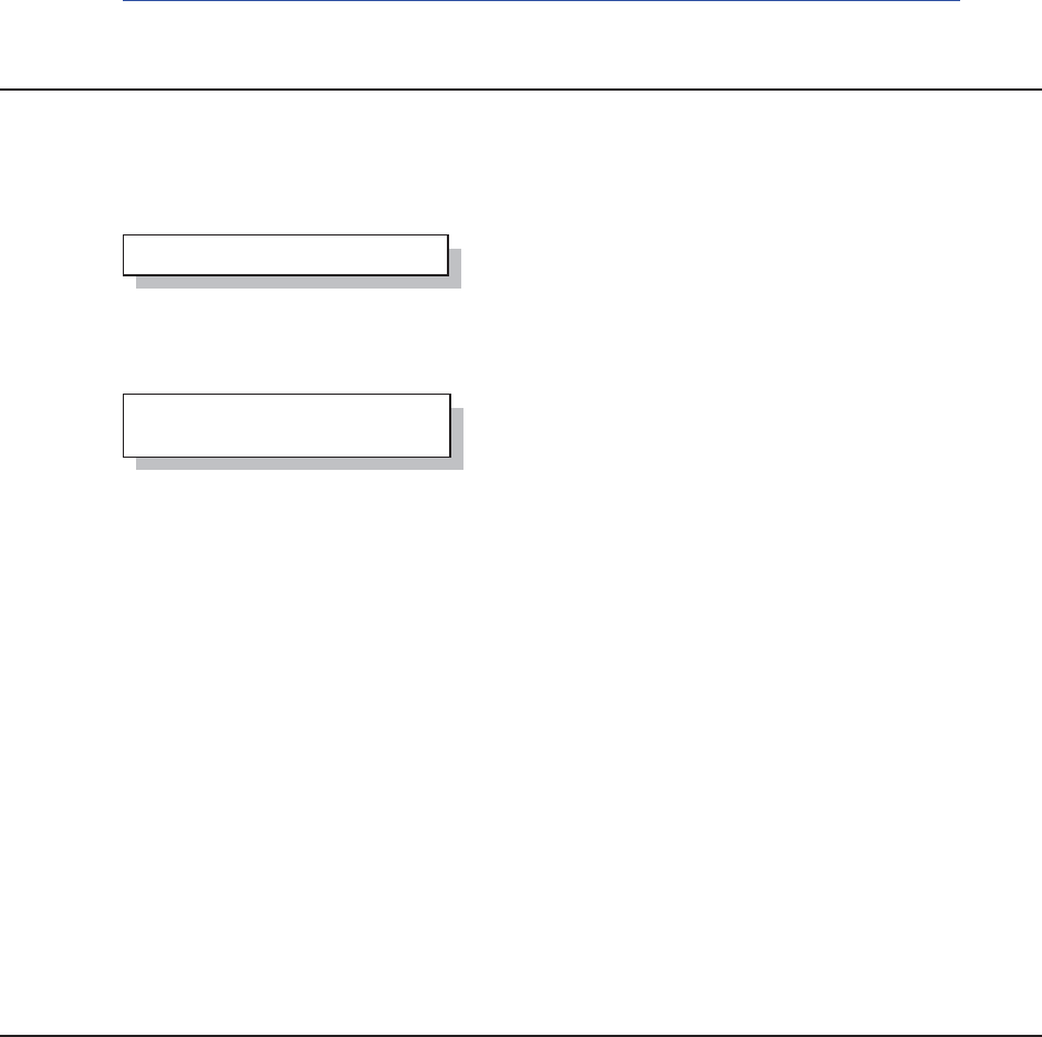
Chapter 3: Just In the DATA Step 119
A brief summary of syntax and a couple of simple examples can be found in the SAS®9 HASH
OBJECT Tip Sheet at
http://support.sas.com/documentation/cdl/en/lrcon/61722/HTML/default/a002586295.htm.
The construction of stacks and other methods are discussed by Edney (2009).
3.3.1 Declaring (Instantiating) the Object
The component object is established, instantiated, by the DECLARE statement in the DATA step.
Each object is named and this name is also established on the DECLARE statement, which can be
abbreviated as DCL.
The name of the object is followed by parentheses which
may or may not contain constructor methods. The name of
the object, in this example HASHNAME, is actually a
variable on the DATA step’s PDV. The variable contains the hash object and as such it cannot be
used as a variable in the traditional ways.
You can also instantiate the object in two statements. Here
it is more apparent that the name of the object is actually a
special kind of DATA step variable. Although not a
variable in the traditional sense, it can contain information
about the object that can on occasion be used to our advantage.
When the object is created (declared), you will often want to control some of its attributes. This is
done through the use of arguments known as constructors. These appear in the parentheses, are
followed by a colon, and include the following:
DATASET: name of the SAS data set to load into the hash object
HASHEXP: exponent that determines the number of key locations (slots)
ORDERED: determines how the key variables are to be ordered in the hash table
The HASH object is used to create a hash table, which is accessed using the values of the key
variables. When the table needs to be accessed sequentially, the HITER object is used in
conjunction with the hash table to allow sequential reads of the hash table in either direction
The determination of an efficient value for HASHEXP: is not straightforward. This is an exponent
so a value of 4 yields 24 = 16 locations or slots. Each slot can hold an infinite number of items;
however, to maximize efficiency, there needs to be a balance between the number of items in a
slot and the number of slots. The default size is 8 (28=256 slots). The documentation suggests that
for a million items 512 to 1024 slots (HASHEXP = 9 or 10) should offer good performance.
3.3.2 Using Methods with an Object
The DECLARE statement is used to create and name the object. Although a few attributes of the
object can be specified using constructor arguments when the object is created, additional
methods are available not only to help refine the definition of the object, but how it is used as
well. There are quite a few of these methods, several of which will be discussed in the examples
that follow.
Methods are similar to functions in how they are called. The method name is followed by
parentheses that may or may not contain arguments. When called, each method returns a value
indicating success or failure of its operation. For each method success is 0. Like with DATA step
routines, you might choose to utilize or ignore this return code value.
declare hash hashname();
dcl hash hashname;
hashname = _new_ hash();
&DUSHQWHU$UW&DUSHQWHU¶V*XLGHWR,QQRYDWLYH6$67HFKQLTXHV&RS\ULJKW6$6,QVWLWXWH,QF&DU\1RUWK&DUROLQD86$
$
//5,*+765(6(59(')RUDGGLWLRQDO6$6UHVRXUFHVYLVLWVXSSRUWVDVFRPSXEOLVKLQJ

120 Carpenter’s Guide to Innovative SAS Techniques
Since there may be more than one object defined within the DATA step, it is necessary to tie a
given method call to the appropriate object. This is accomplished using a dot notation. The
method name is preceded with the name of the object to which it is to be associated, and the two
names are separated with a
dot.
Methods are used both to
refine the definition of the
object, as well as to operate against it. Methods that are used to define the object follow the
DECLARE statement and include:
DEFINEKEY list of variables forming the primary key
DEFINEDATA list of data set variables
DEFINEDONE closes the object definition portion of the code
During the execution of the DATA step, methods are also used to read and write to the object. A
few of these methods include:
ADD adds the specified data on the PDV to the object
FIND retrieves information from the object based on the values of the key
variables
MISSING initializes a list of variables on the PDV to missing
OUTPUT writes the object’s contents to a SAS data set
REPLACE writes data from the PDV to an object; matching key variables are replaced
3.3.3 Simple Sort Using the HASH Object
Because the hash object can be ordered by keys, it can be used to sort a table. In the following
example we would like to order the data set ADVRPT.DEMOG by subject within clinic number.
This sort can be easily accomplished using PROC SORT; however, as a demonstration a hash
object can also be used.
A DATA _NULL_ step is used to define and load the hash object. After the data have been loaded
into the hash table, it is written out to the new sorted data set. Only one pass of the DATA step is
made during the execution phase and no data are read using the SET statement.
hashname.definekey('subject', 'visit');
hashname.definedata('subject','visit','labdt') ;
hashname.definedone() ;
proc sort data=advrpt.demog(keep=clinnum subject lname fname dob)
out=list nodupkey;
by clinnum subject;
run;
data _null_; n
if 0 then set advrpt.demog(keep=clinnum subject lname fname dob); o
declare hash clin (dataset:'advrpt.demog', ordered:'Y'); p
clin.definekey ('clinnum','subject'); q
clin.definedata ('clinnum','subject','lname','fname','dob'); r
clin.definedone (); s
clin.output(dataset:'clinlist'); t
stop; u
run;
&DUSHQWHU$UW&DUSHQWHU¶V*XLGHWR,QQRYDWLYH6$67HFKQLTXHV&RS\ULJKW6$6,QVWLWXWH,QF&DU\1RUWK&DUROLQD86$
$
//5,*+765(6(59(')RUDGGLWLRQDO6$6UHVRXUFHVYLVLWVXSSRUWVDVFRPSXEOLVKLQJ

Chapter 3: Just In the DATA Step 121
n A DATA _NULL_ step is used to build and take advantage of the hash object.
o The SET statement is used only during the DATA step’s compilation phase to add the
variables, their attributes, and initial value (missing) to the PDV. The IF statement can never be
true; consequently, no observations can be read during the execution of the DATA step.
p The hash object is instantiated with the name CLIN. The object is further defined to contain the
data set ADVRPT.DEMOG and will be ordered using the key variables in ascending order. The
use of the DATASET: constructor method is sufficient to cause the entire data set to be loaded
into the hash object, which is held in memory. The ORDERED: constructor can be used to specify
either an ascending (‘a’, ‘ascending’, ‘yes’, or ‘y’) or descending (‘descending’, ‘d’, ‘n’, or ‘no’)
ordering.
q The sort key variables are included in the same order as they would be in the BY statement of
PROC SORT. The resulting data set will necessarily contain no duplicate key values (the
NODUPKEY option on the PROC SORT statement).
r List the variables that will be on the data set that is being created. Key variables listed on the
DEFINEKEY method q are not automatically included in this list.
s The hash object has been defined. Close the definition section initiated by the DECLARE
statement p.
t The contents of the CLIN hash object are written to the data set WORK.CLINLIST using the
OUTPUT method and the DATASET: constructor.
u The STOP statement closes the implied loop created by the SET statement o.
When a method is called as was the OUTPUT method above t, a return code is generated. If you
want to write more robust steps, you should capture and potentially query this return code. The
statement at t becomes: rc=clin.output(dataset:'clinlist'); Although not a problem in
this step, when a method is not successful and is unable to pass back a return code value, as would
be the case shown in the example t, an error is generated which results in an abnormal end to the
DATA step. While this seems to be less of an issue for the methods used in the declaration of the
object, it definitely is an issue for those methods that read and write to and from the hash object,
e.g., FIND, OUTPUT, ADD. It has been my experience that you should always capture the return
code from one of these methods, even if you are not going to test or otherwise use the return code.
CAVEAT
Although the HASH object can be used to sort a data table, as was shown above, using the HASH
object will not necessarily be more efficient than using PROC SORT. Remember that the DATA
step itself has a fair amount of overhead, and that the entire table must be placed into memory
before the hash keys can be constructed. While the TAGSORT option can be used with PROC
SORT for very large data sets, it may not even be possible to fit a very large data set into memory.
As with most tools within SAS you must select the one appropriate for the task at hand.
3.3.4 Stepping through a Hash Table
Unlike in the previous example where the data set was loaded and then immediately dumped from
the hash table, very often we will need to process the contents of the hash table item by item. The
advantage of the hash table is the ability to access its items using an order based on the values of
the key variables.
There are a couple of different approaches to stepping through the items of a hash table. When
you know the values of the key variables they can be used to find and retrieve the item of interest.
This is a form of a table look-up, and additional examples of table look-ups using a hash object
&DUSHQWHU$UW&DUSHQWHU¶V*XLGHWR,QQRYDWLYH6$67HFKQLTXHV&RS\ULJKW6$6,QVWLWXWH,QF&DU\1RUWK&DUROLQD86$
$
//5,*+765(6(59(')RUDGGLWLRQDO6$6UHVRXUFHVYLVLWVXSSRUWVDVFRPSXEOLVKLQJ

122 Carpenter’s Guide to Innovative SAS Techniques
can be found in Section 6.8. A second approach takes advantage of the hash iterator object,
HITER, which is designed to work with a series of methods that read successive items (forwards
or backwards) from the hash table.
The examples used in this section perform what is essentially a many-to-many fuzzy merge. Some
of the patients (SUBJECT) in our study have experienced various adverse events which have been
recorded in ADVRPT.AE. We want to know what if any drugs the patient started taking within
the 5 days prior to the event. Since a given drug can be associated with multiple events and a
given event can be associated with multiple drugs, we need to create a data set containing all the
combinations for each patient that matches the date criteria.
Using the FIND Method with Successive Key Values
The FIND method uses the values of the key variables in the PDV to search for and retrieve a
record from the hash table. When we know all possible values of the keys, we can use this method
to find all the associated items in the hash table.
data drugEvents(keep=subject medstdt drug aestdt aedesc sev);
declare hash meds(ordered:'Y') ; n
meds.definekey ('subject', 'counter');
meds.definedata('subject', 'medstdt','drug') ;
meds.definedone () ;
* Load the medication data into the hash object;
do until(allmed); o
set advrpt.conmed(keep=subject medstdt drug) end=allmed;
by subject; p
if first.subject then counter=0;q
counter+1; r
rc=meds.add();
end;
do until(allae); s
set advrpt.ae(keep=subject aedesc aestdt sev) end=allae;
counter=1; t
rc=meds.find(); u
do while(rc=0);
* Was this drug started within 5 days of the AE?;
if (0 le aestdt - medstdt lt 5) then output drugevents; v
counter+1; w
rc=meds.find();u
end;
end;
stop;
run;
&DUSHQWHU$UW&DUSHQWHU¶V*XLGHWR,QQRYDWLYH6$67HFKQLTXHV&RS\ULJKW6$6,QVWLWXWH,QF&DU\1RUWK&DUROLQD86$
$
//5,*+765(6(59(')RUDGGLWLRQDO6$6UHVRXUFHVYLVLWVXSSRUWVDVFRPSXEOLVKLQJ
Chapter 3: Just In the DATA Step 123
n The MEDS hash table is declared and its keys and data variables are defined.
o A DO UNTIL loop is used to read the medication observations into the MEDS hash table. We
have not used the DATASET: constructor as was done in Section 3.3.3, because we are
performing IF-THEN processing and creating an additional variable (COUNTER) within this
loop.
p Because we are using FIRST.SUBJECT to initialize the counter variable, the BY statement is
needed. This adds a restriction to the incoming data set—it must be in sorted order. The next
example shows a way around this restriction.
q A unique numeric variable, COUNTER, is established as a key variable. Not only will this
variable guarantee that each observation from ADVRPT.CONMED is stored in the hash table
(each row has a unique key), but we will be able to use this counter to step through the rows of the
table u. For a given patient the item (row) counter is initialized to 0.
r The row counter is incremented for each incoming row for this patient and the observation is
then written to the MEDS object using the ADD method.
s Establish a loop to read each observation from the ADVRPT.AE data set. For each of these
observations, which gives us the SUBJECT number and the event date (AESTDT), we want to
find and check all the entries for this subject that reside in the hash table.
t Initialize the COUNTER so that we will start retrieving the first item for this specific patient.
uThe FIND method will be used to retrieve the item that matches the current values of the key
variables (SUBJECT and COUNTER). Since COUNTER=1 this will be the first item for this
subject. This and each successive item for this subject is checked against the 5-day criteria inside
the DO WHILE loop.
v If the onset of the adverse event (AESTDT) is within 5 days of the medication start date
(MEDSTDT), the observation is saved to WORK.DRUGEVENTS.
w The key value is incremented and the next item is retrieved using the FIND method. The DO
WHILE executes until the FIND method is no longer able to retrieve anymore items for this
subject and the return code for FIND (RC) is no longer 0.
In the previous example we loaded the MEDS hash table using a unique counter for each
medication used by each subject. This counter became the second key variable. In that example
the process of initializing and incrementing the counter depended on the data having already been
grouped by patient. For very large data sets, it may not be practical to either sort or group the data.
If we had not used FIRST. processing, we would not have needed the BY statement, and as a
result we would not have needed the data to be grouped by patient. We can eliminate these
requirements by storing the subject number and the count in a separate hash table. Since we really
only need to store one value for each patient—the number of medications encountered so far, we
could do this as an array of values. In the following example this is what we do by creating a hash
table that matches patient number with the number of medications encountered for that patient.
&DUSHQWHU$UW&DUSHQWHU¶V*XLGHWR,QQRYDWLYH6$67HFKQLTXHV&RS\ULJKW6$6,QVWLWXWH,QF&DU\1RUWK&DUROLQD86$
$
//5,*+765(6(59(')RUDGGLWLRQDO6$6UHVRXUFHVYLVLWVXSSRUWVDVFRPSXEOLVKLQJ

124 Carpenter’s Guide to Innovative SAS Techniques
The hash table SUBJCNT contains the number of medications that have been read for each patient
at any given time. As additional medications are encountered, the COUNTER variable is
incremented.
n A hash table to hold the counter for each patient (SUBJECT) is declared. The key variable is
SUBJECT and the only data variable is COUNTER.
o An observation is read from the medications data set. This loads a value of SUBJECT into the
PDV.
p The COUNTER is initialized to 1 when this value of SUBJECT has not yet been loaded into
the SUBJCNT hash table. Remember that a successful FIND will return a 0 value. This means
that the expression SUBJCNT.FIND() will be true when the current value of SUBJECT is the first
time that subject has been encountered. When SUBJCNT.FIND() successfully returns a value
(this is not the first time this SUBJECT has been read from the medications data set), the
expression evaluates to false and the COUNTER is incremented q. Either way the
SUBJCNT.FIND() has been executed.
q When this value of SUBJECT is found in the hash table, the COUNTER is returned and loaded
into the PDV. This SUM statement then causes COUNTER to be incremented.
r The updated COUNTER value is written to the hash table. The REPLACE method causes this
value of COUNTER to overwrite a previous value.
s The medication information along with the updated value of COUNTER is saved.
data drugEvents(keep=subject medstdt drug aestdt aedesc sev);
* define a hash table to hold the subject counter;
declare hash subjcnt(ordered:'y'); n
subjcnt.definekey('subject');
subjcnt.definedata('counter');
subjcnt.definedone();
declare hash meds(ordered:'Y') ;
meds.definekey ('subject', 'counter');
meds.definedata('subject', 'medstdt','drug','counter') ;
meds.definedone () ;
* Load the medication data into the hash object;
do until(allmed);
set advrpt.conmed(keep=subject medstdt drug) end=allmed; o
* Check subject counter: initialize if not found,
otherwise increment;
if subjcnt.find() then counter=1; p
else counter+1; q
* update the subject counter hash table;
rc=subjcnt.replace(); r
* Use the counter to add this row to the meds hash table;
rc=meds.add(); s
end;
do until(allae);
. . . . . the remainder of the DATA step is unchanged from the previous example . . . . .
&DUSHQWHU$UW&DUSHQWHU¶V*XLGHWR,QQRYDWLYH6$67HFKQLTXHV&RS\ULJKW6$6,QVWLWXWH,QF&DU\1RUWK&DUROLQD86$
$
//5,*+765(6(59(')RUDGGLWLRQDO6$6UHVRXUFHVYLVLWVXSSRUWVDVFRPSXEOLVKLQJ

Chapter 3: Just In the DATA Step 125
Essentially we have used the SUBJCNT hash table to create a dynamic single dimension array
with SUBJECT as the index and the value of COUNTER as the value stored. For any given
subject we can dynamically determine the number of medications that have been encountered so
far and use that value when writing to the MEDS hash table.
Using the Hash Iterator Object
In the previous examples we stepped through a hash object by controlling the values of its key
variables. You can also use the hash iterator object and its associated methods to step through a
hash object.
Like the previous examples in this section we again use a unique key variable (COUNTER) to
form the key for each patient medication combination. The solution shown here again assumes
that the medication data are grouped by subject, but we have already seen how we can overcome
this limitation. The difference in the solution presented below is the use of the hash iterator object,
HITER. Declaring this object allows us to call a number of methods that will only work with this
object.
n The hash iterator object is declared and named MEDSITER. Notice that its one argument is the
name of the hash object (MEDS) with which it is to be associated.
o The MEDS hash object is loaded as it was in the previous examples.
p The FIRST method returns the very first item in the MEDSITER hash object. Notice that the
name of the method is preceded by the name of the iterator object, MEDSITER. Since FIRST
does not take the values of the key variables into consideration, except for the first patient, we are
data drugEvents(keep=subject medstdt drug aestdt aedesc sev);
declare hash meds(ordered:'Y') ;
declare hiter medsiter('meds'); n
meds.definekey ('subj', 'counter');
meds.definedata('subj', 'medstdt','drug','counter') ;
meds.definedone () ;
* Load the medication data into the hash object;
do until(allmed); o
set advrpt.conmed(keep=subject medstdt drug) end=allmed;
by subject;
if first.subject then do;
counter=0;
subj=subject;
end;
counter+1;
rc=meds.add();
end;
do until(allae);
set advrpt.ae(keep=subject aedesc aestdt sev) end=allae;
rc = medsiter.first(); p
do until(rc); q
* Was this drug started within 5 days of the AE?;
if subj=subjectr & 0<=aestdt-medstdt<5s then output drugevents;
if subj gt subject then leave; t
rc=medsiter.next(); u
end;
end;
stop;
run;
&DUSHQWHU$UW&DUSHQWHU¶V*XLGHWR,QQRYDWLYH6$67HFKQLTXHV&RS\ULJKW6$6,QVWLWXWH,QF&DU\1RUWK&DUROLQD86$
$
//5,*+765(6(59(')RUDGGLWLRQDO6$6UHVRXUFHVYLVLWVXSSRUWVDVFRPSXEOLVKLQJ

126 Carpenter’s Guide to Innovative SAS Techniques
forced to cycle through earlier patients until we get to the patient of interest. Because the
MEDSITER object is linked to the MEDS object we are actually retrieving from the MEDS object
via the MEDSITER object.
q The DO UNTIL reads successive items from the hash object until the NEXT method u is
unable to return another item or until all the items for the current subject have been exhausted t.
Remember that the return code (RC) for methods is 0 for success and non-zero for failure.
r We are only interested in those medications that are associated with the current patient
(SUBJECT), s and that meet the date criterion.
t The DO UNTIL loop started at q steps through all the medications stored in the hash object.
Since they are ordered by subject, once we have finished with the current patient (SUBJECT) we
can leave the loop.
u The NEXT method is used to read the next item from the hash object. The next item is
determined by the key variables and the way the hash object was ordered. MEDS was specified to
be in ascending order by the ORDERED: constructor method. Although not used in this example
there is also a PREV method to retrieve the previous item.
The order of the observations in the ADVRPT.AE data set in the preceding examples does not
matter. If the data were in known SUBJECT order we could have saved on memory usage by
loading the MEDS hash table one subject (BY group) at a time. To remove the values for the
previous SUBJECT the CLEAR method could be used to clear the hash table values and would be
executed for each FIRST.SUBJECT. The example in Section 3.3.5 has a hash object that stores
data for only a single clinic at a time; however, in that example the object is deleted and re-
instantiated for each clinic.
3.3.5 Breaking Up a Data Set into Multiple Data Sets
We have been given a data set that is to be broken up into a series of subsets, each subset being
based on some aspect of the data. In the example that follows we want to create a data set for each
clinic. That means a data set for each unique value of the variable CLINNUM. The brute force
approach would
require knowing,
and then hard
coding, the
individual clinic
codes, using a
DATA step such as
the one to the left.
Actually there are many more clinic codes than shown here, but I find hard coding to be very
tiring so I only did enough to show the intent of the step. Clearly this is neither a practical, nor a
smart, solution.
There have been any number of papers offering macro language solutions to this type of problem
(Fehd and Carpenter, 2007); however, all of those solutions require two passes of the data. One
pass of the data to determine the list of values, and a second pass to utilize that list. By using a
hash table we can accomplish the task in a single pass of the data.
A DATA _NULL_ step is used to create the data sets. Since we are not specifying the names of
the data sets that are to be created, they will have to be declared using the OUTPUT hash method.
data clin011234 clin014321 clin023910 clin024477;
set advrpt.demog;
if clinnum= '011234' then output clin011234;
else if clinnum= '014321' then output clin014321;
else if clinnum= '023910' then output clin023910;
else if clinnum= '024477' then output clin024477;
run;
&DUSHQWHU$UW&DUSHQWHU¶V*XLGHWR,QQRYDWLYH6$67HFKQLTXHV&RS\ULJKW6$6,QVWLWXWH,QF&DU\1RUWK&DUROLQD86$
$
//5,*+765(6(59(')RUDGGLWLRQDO6$6UHVRXUFHVYLVLWVXSSRUWVDVFRPSXEOLVKLQJ

Chapter 3: Just In the DATA Step 127
n During the compilation phase of the DATA step, the SET statement is used to establish the
attributes for the variables on the PDV. These attributes will be used to build the data sets that are
written by the OUTPUT method u.
o Declare the CLIN hash object, which will hold the data for one clinic at a time.
p Instantiate the hash object, CLIN, which was declared earlier o. This object will hold the data
for each individual clinic. Each clinic will be loaded into the CLIN object one at a time r.
q Using the iterator object for the ALL object, HALL, retrieve the very first item (set of values)
from the hash object. Save this clinic number in the LASTCLIN variable for comparison with
later values. This value is used to detect when we cross clinic boundaries t.
r The current values on the PDV are written to the CLIN object. For the very first item retrieved
from the HALL object these values were read by the FIRST method q; otherwise, the values
were read by the NEXT method s in the previous pass of this DO UNTIL (DONE) loop.
data _null_;
if 0 then set advrpt.demog(keep=clinnum subject lname fname dob); n
* Hash ALL object to hold all the data;
declare hash all (dataset: 'advrpt.demog', ordered:'Y');
all.definekey ('clinnum','subject');
all.definedata ('clinnum','subject','lname','fname','dob');
all.definedone ();
declare hiter hall('all');
* CLIN object holds one clinic at a time;
declare hash clin; o
* define the hash for the first clinic; p
clin = _new_ hash(ordered:'Y');
clin.definekey('clinnum','subject');
clin.definedata('clinnum','subject','lname','fname','dob');
clin.definedone();
* Read the first item from the full list;
done=hall.first(); q
lastclin = clinnum;
do until(done); *loop across all clinics;
clin.add(); r
done = hall.next(); s
if clinnum ne lastclin or done then do; t
* This is the first obs for this clinic or the very last obs;
* write out the data for the previous clinic;
clin.output(dataset:'clin'||lastclin); u
* Delete the CLIN hash object;
clin.delete();v
clin = _new_ hash(ordered:'Y');
clin.definekey('clinnum','subject');
clin.definedata('clinnum','subject','lname','fname','dob');
clin.definedone();
lastclin=clinnum; w
end;
end;
stop;
run;
&DUSHQWHU$UW&DUSHQWHU¶V*XLGHWR,QQRYDWLYH6$67HFKQLTXHV&RS\ULJKW6$6,QVWLWXWH,QF&DU\1RUWK&DUROLQD86$
$
//5,*+765(6(59(')RUDGGLWLRQDO6$6UHVRXUFHVYLVLWVXSSRUWVDVFRPSXEOLVKLQJ

128 Carpenter’s Guide to Innovative SAS Techniques
s Unlike the END= option on the SET statement, which is assigned a true value when processing
the last observation, the NEXT method returns a 0 until it attempts to read past the last item. This
means that DONE is not true on the last observation that will be read out of the HALL object.
One more pass of this loop will be required. We take advantage of this behavior to write out the
contents of CLIN for the last clinic number.
t When the clinic number that was just retrieved is different from the previous one (or when we
are done reading items), we know that it is time to write out the contents of the CLIN object to a
data set. The values in the PDV which were just loaded by the NEXT method contain items from
a different clinic, but they have yet to be loaded into the CLIN object.
u The OUTPUT method is used to write the contents of the CLIN object, which contains the
rows for only one clinic, to the named SAS data set. The data set name contains the value of the
clinic number that is stored in the data set, and the name of the data set is determined during the
execution of the statement.
v We have written out the contents of the clinic specific hash object (CLIN) u so we are finished
using it. In this example we will delete CLIN and then reestablish it for the next clinic. Since we
have already declared CLIN o, it can be re-created using the _NEW_ keyword on the assignment
statement. Rather than deleting and then reestablishing the CLIN object, we could have cleared it
by using the CLEAR method. rc=clin.clear(); (see the sample programs associated with this
section for the full DATA step).
w The current clinic number is saved for comparison t against the next retrieved item s. If this
is the very last item (DONE=1), this is unnecessary, but costs us little.
MORE INFORMATION
The example in Section 3.3.6 also creates multiple data subsets using nested hash objects.
SEE ALSO
Hamilton (2007) discusses this topic in very nice detail, including background and alternate
approaches.
3.3.6 Hash Tables That Reference Hash Tables
The value of the variable that names a hash table holds information that is unique to that table.
The assignment statement shown to the left,
instantiates the hash table HASHNUM, and
when it is executed a unique value associated
with this object is stored in the variable HASHNUM. While this variable exists on the PDV, it is
not a variable in the traditional DATA step numeric/character sense—in a real sense the value
held by this variable is the whole hash object. This implies that we can instantiate multiple hash
tables using the same name as long as the value of the hash table variable changes.
The example in Section 3.3.5 used two independent hash tables to break up one data set into
multiple data-dependent data tables—one table for each clinic. That solution loads the data for a
specific clinic into a hash table from a master hash table. Once loaded the data subset is written to
a data set and the associated hash table is deleted or cleared. This process requires that each
observation has three I/O passes.
1. It is read from the incoming data set and loaded into the master hash table.
2. The data for a given clinic is read from the master and loaded into a hash table containing data
only for that clinic.
3. The data are written to the new clinic-specific data set using the OUTPUT method.
hashnum = _new_ hash(ordered:'Y');
&DUSHQWHU$UW&DUSHQWHU¶V*XLGHWR,QQRYDWLYH6$67HFKQLTXHV&RS\ULJKW6$6,QVWLWXWH,QF&DU\1RUWK&DUROLQD86$
$
//5,*+765(6(59(')RUDGGLWLRQDO6$6UHVRXUFHVYLVLWVXSSRUWVDVFRPSXEOLVKLQJ

Chapter 3: Just In the DATA Step 129
In the following example the data for individual clinics are loaded directly into the hash object
designated for that hash object. Although a hash object is used to organize and track the hash
objects used for the individual clinics, a master hash object containing all the data is not required.
n The EACHCLIN hash object and its associated iterator, HEACH, are declared and instantiated.
EACHCLIN is ordered by its key variable CLINNUM, and although it is a key variable, it is also
included as a data element. The other data variable is HASHNUM, which will contain a value that
will allow us to access the information associated with the hash table that holds the clinic-specific
information. CLINNUM is only needed for the process that follows because it is used in the name
of the data table that is created using the OUTPUT method w.
o The hash object HASHNUM is declared but not instantiated until r. This object will be used
to hold the data for the individual clinics. The DECLARE statement creates the variable
HASHNUM that will contain a distinct identifying value for each of the individual hash objects.
p An observation is read from the incoming data set and the values of the variables that will be
added to the hash objects are stored in the PDV.
data _null_;
* Hash object to hold just the HASHNUM pointers;
declare hash eachclin(ordered:'Y'; n
eachclin.definekey('clinnum');
eachclin.definedata('clinnum','hashnum');
eachclin.definedone ();
declare hiter heach('eachclin');
* Declare the HASHNUM object;
declare hash hashnum; o
do until(done);
set advrpt.demog(keep=clinnum subject lname fname dob) end=done; p
* Determine if this clinic number has been seen before;
if eachclin.check() then do; q
* This is the first instance of this clinic number;
* create a hash table for this clinic number;
hashnum = _new_ hash(ordered:'Y'); r
hashnum.definekey ('clinnum','subject');
hashnum.definedata ('clinnum','subject','lname','fname','dob');
hashnum.definedone ();
* Add to the overall list;
rc=eachclin.replace(); s
end;
* Retrieve this clinic number and its hash number;
rc=eachclin.find(); t
* Add this observation to the hash table for this clinic.;
rc=hashnum.replace(); u
end;
* Write the individual data sets;
* There will be one data set for each clinic;
do while(heach.next()=0); v
* Write the observations associated with this clinic;
rc=hashnum.output(dataset:'clinic'||clinnum); w
end;
stop;
run;
&DUSHQWHU$UW&DUSHQWHU¶V*XLGHWR,QQRYDWLYH6$67HFKQLTXHV&RS\ULJKW6$6,QVWLWXWH,QF&DU\1RUWK&DUROLQD86$
$
//5,*+765(6(59(')RUDGGLWLRQDO6$6UHVRXUFHVYLVLWVXSSRUWVDVFRPSXEOLVKLQJ

130 Carpenter’s Guide to Innovative SAS Techniques
q The CHECK method is used to ascertain whether or not this is the first occurrence of this
current clinic number, CLINNUM. This method returns a 0 if it has already been encountered and
the DO block is not executed.
r When a hash object is Instantiated for this clinic number, a value is assigned to the variable
HASHNUM for this hash object. HASHNUM is also a data variable in the EACHCLIN object.
s Since this is the first time that this clinic number has been encountered, it is added to the
EACHCLIN hash object. EACHCLIN is ordered by CLINNUM, but also stores the associated
value of HASHNUM, which is the variable holding the value of the hash object for the current
clinic.
t The FIND method is used to retrieve the HASHNUM value associated with the clinic number
(CLINNUM) that was added to the PDV by the SET statement p.
u This observation is added to the hash object that is associated with this clinic. The value of the
variable HASHNUM has been retrieved from the hash object EACHCLIN t that contains the list
of clinicspecific hash objects.
v The NEXT method is used to successively retrieve the HASHNUM values from the HEACH
iterator object, which contains one item for each clinic number.
w The data stored in the hash object that are identified by the variable HASHNUM are written to
the data set using the OUTPUT method. Notice that the name of the data set is constructed during
the execution of the DO loop. The value stored in the variable HASHNUM was retrieved from the
HEACH iterator object using the NEXT method v, and this value, when used with the OUTPUT
object, identifies which of the clinic-specific hash tables is to be written. The NEXT method also
returns a value of CLINNUM which is used in the construction of the name of the data set.
SEE ALSO
An early paper by Dorfman and Vyerman (2005) contains a number of examples including one
that is very similar to this one. Some of the earliest published examples of hash objects that point
to hash objects were presented by Richard DeVenzia on SAS-L (DeVenezia, 2004).
3.3.7 Using a Hash Table to Update a Master Data Set
When you want to update a SAS data set using a transaction data set, the UPDATE and MODIFY
statements can be used. UPDATE requires sorted data sets, while the MODIFY statement’s
efficiency can be greatly improved with sorting or indexes. A similar result can be achieved using
a hash table.
&DUSHQWHU$UW&DUSHQWHU¶V*XLGHWR,QQRYDWLYH6$67HFKQLTXHV&RS\ULJKW6$6,QVWLWXWH,QF&DU\1RUWK&DUROLQD86$
$
//5,*+765(6(59(')RUDGGLWLRQDO6$6UHVRXUFHVYLVLWVXSSRUWVDVFRPSXEOLVKLQJ

Chapter 3: Just In the DATA Step 131
In this example a transaction data set (TRANS) has been created using FNAME and LNAME as
the key variables, and the
value of SEX is to be
updated. To illustrate what
happens when values of the
key variables are incorrect,
the last name of Peter
Antler has been misspelled
(this name will not exist in
the master).
n The key variables are
defined as LNAME and
FNAME.
o The variable that we
want to update is added to
the hash table.
p Each of the transaction
observations are added to
the UPD hash table.
q An observation is read
from the master data set.
This loads the values of the key variables into the PDV.
r Using the key values for this master record, a transaction record is recovered from the UPD
hash table. If there is no update record, the PDV is not altered and the observation is unchanged.
s The updated record from the master file is
written. More typically the master data set
would be replaced; here a temporary copy
(WORK.NEWDEMOG) is created.
t Because all the processing takes place within
loops, the STOP statement is needed to
terminate the DATA step.
u The misspelled transaction (Antla) is NOT added to the master data set, nor is the value of SEX
changed for Peter Antler.
SEE ALSO
A similar solution was suggested by user @KSharp in a SAS Forum discussion on HASH objects
http://communities.sas.com/message/53968.
* Build a transaction file;
data trans;
length lname $10 fname $6 sex $1;
fname='Mary'; lname='Adams'; sex='N'; output;
fname='Joan'; lname='Adamson';sex='x'; output;
* The last name is misspelled;
fname='Peter';lname='Anla'; sex='A'; output;
run;
data newdemog(drop=rc);
declare hash upd(hashexp:10);
upd.definekey('lname', 'fname'); n
upd.definedata('sex'); o
upd.definedone();
do until(lasttrans);
set trans end=lasttrans;
rc=upd.add(); p
end;
do until(lastdemog);
set advrpt.demog end=lastdemog; q
rc=upd.find(); r
output newdemog; s
end;
stop; t
run;
3.3.7 Update a Master
Obs fname lname sex
1 Mary Adams N
2 Joan Adamson x
3 Mark Alexander M
4 Peter Antler M u
&DUSHQWHU$UW&DUSHQWHU¶V*XLGHWR,QQRYDWLYH6$67HFKQLTXHV&RS\ULJKW6$6,QVWLWXWH,QF&DU\1RUWK&DUROLQD86$
$
//5,*+765(6(59(')RUDGGLWLRQDO6$6UHVRXUFHVYLVLWVXSSRUWVDVFRPSXEOLVKLQJ

132 Carpenter’s Guide to Innovative SAS Techniques
3.4 Doing More with the INTNX and INTCK Functions
The INTNX and INTCK functions are used to work with date, time, and datetime intervals. Both
can work with a fairly extensive list of interval types; however, you can add even more flexibility
to these two functions by using interval multipliers, shift operators, and alignment options.
Using these two functions is not always straightforward; however, you need to be aware of how
they make their interval determinations. Of primary importance is that by default they both make
their calculations based on the start of the current interval. For instance when using a YEAR
interval type for any date in 2009, the current interval will start on January 1, 2009. As a result of
the interval start, the two
function calls shown here
will both return an
interval length of one
year.
SEE ALSO
Interval multipliers and shift operators are complex topics. Fortunately the documentation for the
INTNX and INTCK functions is well written and should be consulted for additional important
details.
These two functions are carefully described by Cody (2010), and this is a good source for further
information on the topics in this section.
3.4.1 Interval Multipliers
Interval multipliers allow you to alter the definition of the interval length. Interval multipliers are
simply implemented as integers that are appended to the standard interval. The interval ‘WEEK’
has a length of 7 days while the same interval with a multiplier of 2 (WEEK2) will have an
interval length of 14 days.
In the following rather silly example we would like to schedule a follow-up exam in two weeks
(14 days). EXAMDT_2 is calculated to be one two-week interval in the future using an interval
multiplier of two n.
EXAMDTX2, on the other hand,
is determined by requesting two
one-week intervals o. Nominally
we would expect that the two
future dates would be the same;
however, because the two INTNX
functions measure intervals from
the start of their respective
interval, the resulting dates are not always the same. The point of this example is to understand
why.
data ExamSchedule;
do visdt = '25may2009'd to '14jun2009'd;
examdt_2 = intnx('week2'n,visdt,1);
examdtx2 = intnx('week',visdt,2 o);
output;
end;
format visdt examdt_2 examdtx2 date9.;
run;
twoday = intck('year','31dec2008'd,'01jan2009'd);
twoyr = intck('year','01jan2008'd,'31dec2009'd);
&DUSHQWHU$UW&DUSHQWHU¶V*XLGHWR,QQRYDWLYH6$67HFKQLTXHV&RS\ULJKW6$6,QVWLWXWH,QF&DU\1RUWK&DUROLQD86$
$
//5,*+765(6(59(')RUDGGLWLRQDO6$6UHVRXUFHVYLVLWVXSSRUWVDVFRPSXEOLVKLQJ

Chapter 3: Just In the DATA Step 133
June 7, 2009 was a Sunday and since a week interval starts on a Sunday, each of these uses of the
INTNX function advances the date
to a Sunday. Clearly interval
multipliers change the way that the
function views the start of the
interval.
When an interval is expanded the
new interval start date will relate
back to the beginning of time
(January 1, 1960). May 24th was a
Sunday and it started both the
WEEK and WEEK2 interval. May
25, therefore, was advanced to
June 7 for both interval types. May
31st (also a Sunday), however, did
NOT start a WEEK2 interval, but
it did start a WEEK interval.
Consequently these two INTNX
functions give different results
when based on dates in the range
of May 31 to June 6, 2009 (Obs=7-
13).
If we use an interval multiplier to create a three-year interval (YEAR3), the interval start date
would be determined based on the first three-year interval, which would start on January 1, 1960.
MORE INFORMATION
Alignment options are available for the INTNX function that can be helpful when the start of the
interval that you are measuring from is not what you want. See Section 3.4.3.
3.4.2 Shift Operators
Both the INTNX and INTCK functions by default measure from the start of the base interval.
Weeks start on Sunday; years start on January 1st, and so on. Shift operators can be used to change
the way that the function determines the start of the interval. A week could start on Monday, or a
fiscal year could start on July 1st.
The shift operator is designated by a number following a decimal point at the end of the interval
name. The units of the shift depend on how the interval is defined. Weeks contain seven days and
start on Sunday, which has the value of 1. The interval WEEK.2, therefore, would indicate a
seven day week that starts on a Monday. The following example shows a series of shifts on a
week interval (June 7, 2009 was a Sunday).
3.4.1 Interval Multipliers
Obs visdt examdt_2 examdtx2
1 25MAY2009 07JUN2009 07JUN2009
2 26MAY2009 07JUN2009 07JUN2009
3 27MAY2009 07JUN2009 07JUN2009
4 28MAY2009 07JUN2009 07JUN2009
5 29MAY2009 07JUN2009 07JUN2009
6 30MAY2009 07JUN2009 07JUN2009
7 31MAY2009 07JUN2009 14JUN2009
8 01JUN2009 07JUN2009 14JUN2009
9 02JUN2009 07JUN2009 14JUN2009
10 03JUN2009 07JUN2009 14JUN2009
11 04JUN2009 07JUN2009 14JUN2009
12 05JUN2009 07JUN2009 14JUN2009
13 06JUN2009 07JUN2009 14JUN2009
14 07JUN2009 21JUN2009 21JUN2009
15 08JUN2009 21JUN2009 21JUN2009
16 09JUN2009 21JUN2009 21JUN2009
17 10JUN2009 21JUN2009 21JUN2009
18 11JUN2009 21JUN2009 21JUN2009
19 12JUN2009 21JUN2009 21JUN2009
20 13JUN2009 21JUN2009 21JUN2009
21 14JUN2009 21JUN2009 28JUN2009
&DUSHQWHU$UW&DUSHQWHU¶V*XLGHWR,QQRYDWLYH6$67HFKQLTXHV&RS\ULJKW6$6,QVWLWXWH,QF&DU\1RUWK&DUROLQD86$
$
//5,*+765(6(59(')RUDGGLWLRQDO6$6UHVRXUFHVYLVLWVXSSRUWVDVFRPSXEOLVKLQJ

134 Carpenter’s Guide to Innovative SAS Techniques
The WEEK interval starts on a
Sunday and WEEK.1 does not
change the interval start. WEEK.2,
however, will change the start to a
Monday.
Using a PROC PRINT on the
resulting data set shows how the
dates progress. More importantly, it
shows us that the date is reset to the
start of the adjusted interval first
and then advanced 7 days. n In the
LISTING output below, notice the
values based on the VISDT of
Wednesday, June 3, 2009. DAY4 is advanced to June 10th (DAY4 was defined using WEEK.4,
which is an interval starting on a Wednesday), so advancing 7 days yields June 10th. For DAY5
(WEEK.5 defines a week starting on Thursday), on the other hand, Wednesday is at the end of the
interval and the measurement is taken from the previous Thursday (May 29).
A typical use of a shift operator is to create a fiscal year with the interval start on July 1. Since
years are made up of months, the interval ‘YEAR.7’ would shift the start of the year by seven
months. Interval multipliers and shift operators can be used together. A five-year interval starting
on July 1st could be specified as YEAR5.7.
3.4.3 Alignment Options
Although alignment options are now available for both INTNX and INTCK, they are not the same
for the two functions.
Alignment with the INTNX Function
Since it is not always convenient to advance values based on the start of the interval, as was done
in Sections 3.4.1 and 3.4.2, the INTNX function has the ability to change this behavior through
alignment options. These options may be specified as an optional fourth argument, which can
change how the function offsets from the interval start point. Without using the alignment options
all displacements are
measured from the
start of the interval;
consequently, if we advance a date by one year from June 3, 2000 the resulting date is January 1,
2001. Alignment options allow us to measure the displacement other than from the start of the
interval.
data ExamSchedule;
do visdt = '01jun2009'd to '15jun2009'd;
day = intnx('week',visdt,1);
day1 = intnx('week.1',visdt,1);
day2 = intnx('week.2',visdt,1);
day3 = intnx('week.3',visdt,1);
day4 = intnx('week.4',visdt,1);
day5 = intnx('week.5',visdt,1);
day6 = intnx('week.6',visdt,1);
day7 = intnx('week.7',visdt,1);
output;
end;
format visdt day: date7.;
run;
3.4.2 Shift Operators
visdt day day1 day2 day3 day4 day5 day6 day7
01JUN09 07JUN09 07JUN09 08JUN09 02JUN09 03JUN09 04JUN09 05JUN09 06JUN09
02JUN09 07JUN09 07JUN09 08JUN09 09JUN09 03JUN09 04JUN09 05JUN09 06JUN09
03JUN09 07JUN09 07JUN09 08JUN09 09JUN09 10JUN09 04JUN09 05JUN09 06JUN09 n
04JUN09 07JUN09 07JUN09 08JUN09 09JUN09 10JUN09 11JUN09 05JUN09 06JUN09
05JUN09 07JUN09 07JUN09 08JUN09 09JUN09 10JUN09 11JUN09 12JUN09 06JUN09
06JUN09 07JUN09 07JUN09 08JUN09 09JUN09 10JUN09 11JUN09 12JUN09 13JUN09
. . . . portions of the listing are not shown . . . .
new = intnx('year','03jun2000'd,1);
&DUSHQWHU$UW&DUSHQWHU¶V*XLGHWR,QQRYDWLYH6$67HFKQLTXHV&RS\ULJKW6$6,QVWLWXWH,QF&DU\1RUWK&DUROLQD86$
$
//5,*+765(6(59(')RUDGGLWLRQDO6$6UHVRXUFHVYLVLWVXSSRUWVDVFRPSXEOLVKLQJ

Chapter 3: Just In the DATA Step 135
The alignment option positions the result of the function relative to the original interval. It can
take on the values of:
beginning b interval start (default)
middle m interval center
end e interval end
same s same relative position as the initial interval
Each of these options is demonstrated in the DATA step that follows. A date in June is advanced
one month into the future (July) using each of the alignment options. The result is predicable and,
as we might anticipate,
the ‘END’ alignment
option correctly
advances to July 31st
even though June has
30 days. For months
with 31 days the
‘MIDDLE’ option will
give a different result
than it will for months
with fewer days.
If you ask the INTNX function to advance a date to an illegal value, you will not receive an error
message. Each of these two statements use the ‘SAMEDAY’ alignment option to advance a date
to a value that does
not exist. The LOG
shows that the
INTNX function
returns a reasonable alternative, in this
case the actual last day of the month.
Alignment with the INTCK Function
By default the INTCK function counts intervals by counting the number of interval starts. Thus if
your start and end dates span a single Sunday they are considered to be one week apart. As was
demonstrated in the example in Section 3.4, this can result in the counting of partial intervals
equally with full intervals.
data ExamSchedule;
do visdt = '01jun2007'd to '10jun2007'd;
next_d = intnx('month',visdt,1);
next_b = intnx('month',visdt,1,'beginning');
next_m = intnx('month',visdt,1,'middle');
next_e = intnx('month',visdt,1,'end');
next_s = intnx('month',visdt,1,'same');
output;
end;
format visdt next: date7.;
run;
3.4.3 Alignment Options
Obs visdt next_d next_b next_m next_e next_s
1 01JUN07 01JUL07 01JUL07 16JUL07 31JUL07 01JUL07
2 02JUN07 01JUL07 01JUL07 16JUL07 31JUL07 02JUL07
3 03JUN07 01JUL07 01JUL07 16JUL07 31JUL07 03JUL07
4 04JUN07 01JUL07 01JUL07 16JUL07 31JUL07 04JUL07
5 05JUN07 01JUL07 01JUL07 16JUL07 31JUL07 05JUL07
6 06JUN07 01JUL07 01JUL07 16JUL07 31JUL07 06JUL07
7 07JUN07 01JUL07 01JUL07 16JUL07 31JUL07 07JUL07
8 08JUN07 01JUL07 01JUL07 16JUL07 31JUL07 08JUL07
9 09JUN07 01JUL07 01JUL07 16JUL07 31JUL07 09JUL07
10 10JUN07 01JUL07 01JUL07 16JUL07 31JUL07 10JUL07
leap = intnx('year', '29feb2008'd, 1, 's');
short= intnx('month','31may2008'd, 1, 's');
leap=28FEB2009 short=30JUN2008
&DUSHQWHU$UW&DUSHQWHU¶V*XLGHWR,QQRYDWLYH6$67HFKQLTXHV&RS\ULJKW6$6,QVWLWXWH,QF&DU\1RUWK&DUROLQD86$
$
//5,*+765(6(59(')RUDGGLWLRQDO6$6UHVRXUFHVYLVLWVXSSRUWVDVFRPSXEOLVKLQJ

136 Carpenter’s Guide to Innovative SAS Techniques
The alignment option on the INTCK function has two settings:
C continuous
D discrete (this is the default)
The difference between these two option values can be demonstrated by counting the intervals
between two dates. In this example the number of intervals (weeks) between the base date
(START), which is
fixed at Wednesday,
September 14, 2011,
and END which is a
date that advances up
to a month beyond
START.
The resulting data set
contains the number
of elapsed weeks as
calculated by the INTCK function using the alignment option.
The variables WEEKS and WEEKSD are both incremented each time the interval boundary is
crossed (Sunday – 18
and 25 September).
However, the
continuous alignment
option causes WEEKSC
to be incremented only
when a full interval has
elapsed—the interval
boundary has
effectively been
adjusted to start at the
date that starts the
interval.
3.4.4 Automatic Dates
Although the INTNX function is designed to advance a date or time value, it can used in a number
of other situations where its immediate application is not as obvious.
Collapsing Dates
The INTNX function can be used to collapse a series of dates into a single date, thus allowing the
new date to be used as a classification variable. When a format is available, most procedures can
use the formatted value to form groups (ORDER=FORMATTED; see Section 2.6.2). However,
when a format is not available the INTNX function can be used as an alternative.
To collapse dates we take advantage of the characteristic of the function that adjusts dates to the
start of the interval (or the middle or end using the alignment option). If we then advance each
date by 0 intervals the dates are collapsed
into a single date. In the manufacturing data
(ADVRPT.MFGDATA) items are being
built continuously with the manufacturing
hourgrp = intnx('hour',datetime,0);
twohr = intnx('hour2',datetime,0);
data check;
start = '14sep2011'd; * the 14th was a Wednesday;
do end = start to intnx('month',start,1,'s');
weeks = intck('weeks',start,end);
weeksc= intck('weeks',start,end,'c');
weeksd= intck('weeks',start,end,'d');
output check;
end;
format start end date9.;
run;
Obs start end weeks weeksc weeksd
1 14SEP2011 14SEP2011 0 0 0
2 14SEP2011 15SEP2011 0 0 0
3 14SEP2011 16SEP2011 0 0 0
4 14SEP2011 17SEP2011 0 0 0
5 14SEP2011 18SEP2011 1 0 1
6 14SEP2011 19SEP2011 1 0 1
7 14SEP2011 20SEP2011 1 0 1
8 14SEP2011 21SEP2011 1 1 1
9 14SEP2011 22SEP2011 1 1 1
10 14SEP2011 23SEP2011 1 1 1
11 14SEP2011 24SEP2011 1 1 1
12 14SEP2011 25SEP2011 2 1 2
. . . . portions of the listing are not shown . . . .
&DUSHQWHU$UW&DUSHQWHU¶V*XLGHWR,QQRYDWLYH6$67HFKQLTXHV&RS\ULJKW6$6,QVWLWXWH,QF&DU\1RUWK&DUROLQD86$
$
//5,*+765(6(59(')RUDGGLWLRQDO6$6UHVRXUFHVYLVLWVXSSRUWVDVFRPSXEOLVKLQJ

Chapter 3: Just In the DATA Step 137
time stored as a datetime value. We would like to group the items into a one-hour periods. Using
the first INTNX function call shown here, all items manufactured within the same hour will have
the same value of HOURGRP. For instance this will group all times between 06:00 and 06:59 into
the same group (06:00). If we had needed to create two-hour interval groups we could have used
an interval multiplier (TWOHR).
Expanding Dates
The INTNX function can also be used to expand a single date or datetime value into a series of
equally spaced values. The expansion is as simple as a DO loop. This DATA step creates 12
observations with DATE taking on
the value of the first day of each
month in 2007.
This usage of the INTNX function
is written specifically so that the
resulting dates always fall on the
first of the month. Sometimes we
need the date to be centered on the
interval. This is problematic for
months, because they do not have
equal length. The midpoint
alignment option for the INTNX
function (shown here to generate MIDMON) only works to a point. The resulting dates will fall
on the 14th, 15th, or 16th depending on the length of the month. Consistency is usually more
important than technical accuracy (relative to the midpoint which does not really even exist for
most months). The variable MON15 will always contain a date that falls on the 15th of each
month. This consistency is achieved by adding 14 days to the beginning of the month so variable
MON15 will always contain a date that falls on the 15th of each month.
Date Intervals or Ranges
In the following example the macro variable &DATE contains a date (in DATE9. form), and we
need to subset the data for all dates that fall in the same month. The goal is to specify the start and
end points of the correct interval, in this case the correct month of the correct year.
nAdvancing to the start of
an interval is the default.
Here the date is advanced 0
months—effectively the
start of the current month.
oThe last day of the month
is obtained by specifying
the ‘end’ alignment option. Another common way to
find the last day of the month is to find the first day of
the following month and subtract one day.
Previous Month by Name
The INTNX and INTCK functions can also be utilized by the macro language. We will be given
a three-letter month abbreviation and our task is to return the abbreviation of the previous month.
To do this we need to use the INTNX function to advance the month one month into the past. The
macro function %SYSFUNC will be used to allow us to access the INTNX function outside of the
DATA step.
data monthly(drop=i);
do i = 0 to 11;
date = intnx('month','01jan2007'd,i);
output monthly;
end;
format date date9.;
run;
midmon = intnx('month','01jan2007'd,i,'m');
mon15 = intnx('month','01jan2007'd,i) + 14;
%let date=12jun2007;
data june07;
set advrpt.lab_chemistry;
if intnx('month',labdt,0) n
le "&date"d
le intnx('month',labdt,0,'end'); o
run;
(intnx('month',labdt,1)-1)
&DUSHQWHU$UW&DUSHQWHU¶V*XLGHWR,QQRYDWLYH6$67HFKQLTXHV&RS\ULJKW6$6,QVWLWXWH,QF&DU\1RUWK&DUROLQD86$
$
//5,*+765(6(59(')RUDGGLWLRQDO6$6UHVRXUFHVYLVLWVXSSRUWVDVFRPSXEOLVKLQJ

138 Carpenter’s Guide to Innovative SAS Techniques
n A three-letter month abbreviation is created. One month prior to ‘Mar’ is ‘Feb’.
o The INPUTN function converts the three-letter month abbreviation into a SAS date. The year
number used here is unimportant. Although the PUT and INPUT functions cannot be used with
%SYSFUNC, their execution time analogues can be used with %SYSFUNC. These analogues are
type-specific. Here the INPUTN function, which writes a numeric value p (a SAS date in this
case), is used instead of the INPUT function.
q The date contained in &DTVAL is advanced one month into the past. Notice that the interval
name is constant text and is not quoted when using the INTNX function within a %SYSFUNC.
r The PUTN function converts the numeric SAS date contained in &LAST to a three-letter
month abbreviation. &MOLAST correctly now contains ‘Feb’.
The intermediate macro variables
are not really needed, but for
illustration purposes they do
simplify the code. The more
complex statement without these macro variables is shown in the sample code for this section.
MORE INFORMATION
A SAS date is created from a macro variable using the PUTN function in Section 3.5.1. A related
example to the one shown here is also shown in Section 3.5.2.
SEE ALSO
A more complex version of this code example was used in a SAS Forum thread
http://communities.sas.com/message/47615.
3.5 Variable Conversions
When we use the term variable conversions, we most often are referring to the conversion of the
variable’s type from numeric to character or character to numeric. We could also be referring to
the conversion of the units associated with the values of the variable.
3.5.1 Using the PUT and INPUT Functions
When a numeric variable is used in a character expression or when a character variable is used in
a numeric expression, the variable’s type has to be converted before the expression can be
evaluated. By default these conversions are handled automatically by SAS. However, whenever a
variable’s type is converted, SAS writes a note in the LOG. Although this note is fairly innocuous,
in some situations or even industries the note itself is sufficient to cast doubt on your program.
%let mo=Mar; n
%* Create a date for this month (01mar2010);
%let dtvalp = %sysfunc(inputn(&mo.2010,monyy7.)); o
%* Previous month;
%let last = %sysfunc(intnx(month,&dtval,-1)); q
%* Determine the abbreviation of the previous month;
%let molast = %sysfunc(putn(&last,monname3.)); r
%put mo=&mo dtval=&dtval molast=&molast;
140 %put mo=&mo dtval=&dtval molast=&molast;
mo=Mar dtval=18322 molast=Feb
&DUSHQWHU$UW&DUSHQWHU¶V*XLGHWR,QQRYDWLYH6$67HFKQLTXHV&RS\ULJKW6$6,QVWLWXWH,QF&DU\1RUWK&DUROLQD86$
$
//5,*+765(6(59(')RUDGGLWLRQDO6$6UHVRXUFHVYLVLWVXSSRUWVDVFRPSXEOLVKLQJ

Chapter 3: Just In the DATA Step 139
In the DATA step shown here, the variable SUBJECT is character, and we need to create a
numeric analog. Since subject number is just an identification string, one could argue that it is
more appropriately character. However, for this example I would like to convert the character
value to numeric.
n The variable SUBJECT is added
to the Program Data Vector, PDV,
as a numeric variable.
o The conversion takes place
when the character value of SUBJC is forced into the numeric variable SUBJECT. The LOG
shows:
There is nothing wrong with allowing SAS to perform these automatic conversions. In fact there
is evidence (Virgle, 1998) to suggest that these are the most efficient conversions. However, since
as was mentioned above, there are some programming situations where even this rather benign
note in the LOG is unacceptable, we need alternatives that do not produce this note. The PUT and
INPUT families of functions provide this alternative.
When SAS performs an automatic conversion of a numeric value to a character, the result is right
justified (behind the scenes a PUT function is used with a BEST. format). Usually you will want
the character value to be left justified and this is most easily accomplished using the LEFT
function, which operates on character strings. When converting from character to numeric, as was
done above, this is not an issue.
The PUT and INPUT functions can be used directly to convert from numeric to character and
character to numeric. Added power is provided through the use of a format. The PUT function is
used to convert from numeric to character and the INPUT function is used to convert from
character to numeric.
PUT always results in a character string. The format matches the type of the
incoming variable.
INPUT results in a variable with the same type as the informat.
MORE INFORMATION
The PUTN and INPUTN functions are used with %SYSFUNC in a macro language example in
Section 3.4.4.
Character to Numeric
In the AE data the subject is coded as character and we would like to have it converted to a
numeric variable. Converting the value by forcing the character variable into numeric variable, as
was done above, will get the job done; however, the conversion message will appear in the LOG.
data ae(drop=subjc);
set advrpt.ae(rename=(subject=subjc));
length subject 8; n
subject=subjc; o
run;
NOTE: Character values have been converted to numeric values at the
places given by:
(Line):(Column).
114:15
&DUSHQWHU$UW&DUSHQWHU¶V*XLGHWR,QQRYDWLYH6$67HFKQLTXHV&RS\ULJKW6$6,QVWLWXWH,QF&DU\1RUWK&DUROLQD86$
$
//5,*+765(6(59(')RUDGGLWLRQDO6$6UHVRXUFHVYLVLWVXSSRUWVDVFRPSXEOLVKLQJ

140 Carpenter’s Guide to Innovative SAS Techniques
When the INPUT function is used
with a numeric informat, the
incoming value (SUBJC) is
converted to numeric without the
note appearing in the LOG.
Character dates are converted to SAS
dates in the same manner. Again the
key is that a numeric infomat causes
the INPUT function to return a
numeric value. The selection of the
informat depends on the form of the character date.
SEE ALSO
The SAS Forum thread http://communities.sas.com/message/29331 discusses character to
numeric conversion when special characters are involved.
Numeric to Character
The PUT function is generally used to convert a numeric value to a character string. Because a
numeric format is used, the resulting string is right justified. Very often a LEFT function is then
applied to left justify the string. The LEFT function can be avoided by using the format
justification modifier. Here
WORDDT1 will be a right justified
string. WORDDT2 and WORDDT3
will be left justified. When
WORDDT3 is formed the -L causes
the format to left justify the string without using the LEFT function.
Using User-Defined INFORMATS
In a SAS Forum thread the following question (and I paraphrase) was posted. “How can I convert
the name of a color to a numeric code?” One of the suggested solutions highlights a common
misunderstanding of the relationship of formats and informats.
The data set COLORS has the variable COLOR
which takes on the values of ‘yellow’, ‘blue’,
and so on.
p We define a format ($ctonum.) that converts
the colors to numbers. The format attempts to
make the resultant value numeric by not quoting
the values on the right side of the assignments in
the VALUE statement.
qThe format $CTONUM cannot be used with
the INPUT function, so the PUT is used to
generate the numeric value as a character
variable.
r The character variable X is then converted to
the numeric code (Z) through the use of the
INPUT function.
data conmed;
set advrpt.conmed;
startdt = input(medstdt_,mmddyy10.);
run;
data ae(drop=subjc);
set advrpt.ae(rename=(subject=subjc));
subject = input(subjc,3.);
run;
proc format;
value $ctonum p
'yellow' = 1
'blue' = 2
'red' = 3;
run;
data colors;
color='yellow'; output colors;
color='blue'; output colors;
color='red'; output colors;
run;
data codes;
set colors;
x = put(color,$ctonum.); q
z = input(x,3.); r
run;
worddt1 = put(medstdt,worddate18.);
worddt2 = left(put(medstdt,worddate18.));
worddt3 = put(medstdt,worddate18.-l);
&DUSHQWHU$UW&DUSHQWHU¶V*XLGHWR,QQRYDWLYH6$67HFKQLTXHV&RS\ULJKW6$6,QVWLWXWH,QF&DU\1RUWK&DUROLQD86$
$
//5,*+765(6(59(')RUDGGLWLRQDO6$6UHVRXUFHVYLVLWVXSSRUWVDVFRPSXEOLVKLQJ

Chapter 3: Just In the DATA Step 141
The reason that this format will not work with the PUT function is actually simple. There is a
distinct difference between formats and informats. The INPUT function expects an informat. The
previous example can be simplified by creating CTONUM. as a numeric informat using the
INVALUE statement.
When the INPUT function is used with a numeric informat the result will be a numeric value.
Consequently, we need to create a numeric informat that will convert color to a numeric code.
s Since we want to create a numeric informat,
the format name CTONUM. is not preceded by
a $.
t Notice that the value to be assigned (the right
side of the equal sign) is not quoted. It was not
quoted in the previous example p; however,
there we were creating a character format (as
evidenced by the $ in the name), and the quotes
were assumed.
u The numeric informat CTONUM. is used to
convert the color string to a numeric code. The
variable X will be numeric.
Execution or Run-Time Versions
Generally when we use the PUT or INPUT functions we know what format is to be used, and we
can specify it like in the previous examples. When specified this way, these formats are applied
when the statement is compiled. Sometimes the format that is to be applied is unknown until the
DATA step actually executes. Usually this means that the format itself is not constant for all the
observations and is either supplied on the data itself or it is dependent on the data.
The PUT and INPUT functions each come with an execution time analogue for both numeric and
character values (PUTN, PUTC, INPUTN, and INPUTC). For each of these four functions, the
format/informat used by the function is determined during the execution of the function.
In the following example, the incoming dates are supplied in a variety of forms and each has a
format that is to be used in its conversion to a SAS date. The date is read as a character value, as
is the format that will be used in the conversion. The variable FMT, which contains the informat
that is to be applied in the
conversion, becomes the second
argument of the INPUTN
function.
data dates;
input @4 cdate $10. @15 fmt $9.;
ndate = inputn(cdate,fmt);
format ndate date9.;
datalines;
01/13/2003 mmddyy10.
13/01/2003 ddmmyy10.
13jan2003 date9.
13jan03 date7.
13/01/03 ddmmyy8.
01/02/03 mmddyy8.
03/02/01 yymmdd8.
run;
3.5.1 PUT and INPUT Functions
Using INPUTN
Obs cdate fmt ndate
1 01/13/2003 mmddyy10. 13JAN2003
2 13/01/2003 ddmmyy10. 13JAN2003
3 13jan2003 date9. 13JAN2003
4 13jan03 date7. 13JAN2003
5 13/01/03 ddmmyy8. 13JAN2003
6 01/02/03 mmddyy8. 02JAN2003
7 03/02/01 yymmdd8. 01FEB2003
proc format;
invalue ctonum s
'yellow' = 1 t
'blue' = 2
'red' = 3;
run;
data colors;
color='yellow'; output colors;
color='blue'; output colors;
color='red'; output colors;
run;
data codes;
set colors;
x = input(color,ctonum.); u
run;
&DUSHQWHU$UW&DUSHQWHU¶V*XLGHWR,QQRYDWLYH6$67HFKQLTXHV&RS\ULJKW6$6,QVWLWXWH,QF&DU\1RUWK&DUROLQD86$
$
//5,*+765(6(59(')RUDGGLWLRQDO6$6UHVRXUFHVYLVLWVXSSRUWVDVFRPSXEOLVKLQJ

142 Carpenter’s Guide to Innovative SAS Techniques
Examination of the LISTING output of the data set WORK.DATES shows that the incoming
character strings have been correctly translated into SAS dates using the informats supplied in the
data.
MORE INFORMATION
In many cases when dealing with inconsistent date forms, one of the “anydate” informats can also
be successfully applied (see Section 12.6).
SEE ALSO
The INPUTN function was a solution to a question posed in the SAS Forums
http://communities.sas.com/thread/30362?tstart=0.
Using the PUTN Function with the %SYSFUNC Macro Function
As was done in the last example of Section 3.4.4, when you need to perform a numeric/character
conversion using the INPUT or PUT functions in the macro language you will need to use one of
the execution time versions. The function itself is accessed using the %SYSFUNC macro
function.
The following example writes the date value stored in the automatic macro variable
&SYSDATE9 to the LOG
using the WORDDATE18.
format. Without the PUTN
function, the date constant would not be recognized as such by the macro language, and the macro
variable &SYSDATE9 would not be converted to a SAS date value.
The PUTN function can be applied to other date formats. The following macro function will
return the name of the previous month and its year. The PUTN function converts a date value to
the name of the
month by using
the
MONNAME.
format.
n All macro
variables are
forced onto the
local symbol
table.
o The INTNX function is used to advance the date one month into the past. &PREVDT is now a
SAS date value representing the first day of the previous month.
p The PUTN function is used to write the name of the month of the date held in &PREVDT.
q The four-digit year associated with the previous month is retrieved using the YEAR function.
r The macro %LASTMY is called from within the TITLE2 statement. When the macro executes
the macro call is replaced by the month name and its associated year. The TITLE shown here
would result if the macro
was called for any date in
October 2011.
%put %sysfunc(putn("&sysdate9."d,worddate18.));
%macro lastmy;
%local prevdt tmon tyr; n
%let prevdt =
%sysfunc(intnx(month,%sysfunc(today()),-1)); o
%let tmon = %sysfunc(putn(&prevdt,monname9.)); p
%let tyr = %sysfunc(year(&prevdt)); q
&tmon/&tyr
%mend lastmy;
* Write last month's month and year into a title;
TITLE2 "Counts for the Previous Month/Year (%lastmy)"; r
3.5.1 PUT and INPUT Functions
Counts for the Previous Month/Year (September/2011)
&DUSHQWHU$UW&DUSHQWHU¶V*XLGHWR,QQRYDWLYH6$67HFKQLTXHV&RS\ULJKW6$6,QVWLWXWH,QF&DU\1RUWK&DUROLQD86$
$
//5,*+765(6(59(')RUDGGLWLRQDO6$6UHVRXUFHVYLVLWVXSSRUWVDVFRPSXEOLVKLQJ

Chapter 3: Just In the DATA Step 143
3.5.2 Decimal, Hexadecimal, and Binary Number Conversions
The conversion of decimal values to hex, octal, and binary is often accomplished through the use
of formats and informats in conjunction with the PUT and INPUT functions.
When converting from a decimal number to binary, hex, or octal, you can use the PUT function
along with the respective formats (BINARY., HEX.,
or OCTAL.). In this example the decimal number 456
is being converted. The PUT statement writes these
values to the LOG, which shows that the conversion
was successful. Because these are integer
conversions, decimal fractions are lost (through
truncation).
When you need to convert from one of these number
systems to decimal, the INPUT function is used.
Informats of the same name as the formats that were
used in the PUT function are used in this conversion
as well. In this example the PUT function is again
used to confirm the conversion by writing the values
to the LOG.
The LOG shows that the original
decimal number of 456 has been
converted to other number systems
and back to decimal.
In SAS/GRAPH both the RGB color scale and the gray scale use hex numbers to specify specific
color values. The 256 (162) possible shades of gray are coded in a hex number. The codes for a
gray scale number will range from GRAY00 to GRAYFF. For RGB colors there are 256 shades
of each of the three primary colors of red, green, blue. Some color wheels use decimal values
rather than hex values and a specific color value might require conversion. As was shown above,
the HEX. format would be used with the PUT function to provide the converted value. A macro
(%PATTERN) that performs a series of these conversions for a gray scale example can be found
in Carpenter (2004, Section 7.4.2).
The functions ANYXDIGIT and NOTXDIGIT can be used to parse a character string for hex
numbers (see Section 3.6.1). ANYXDIGIT returns the position of the first number or any of the
letters A through F. The NOTXDIGIT returns the functional opposite and returns the position of
the first character that cannot be a part of a hex number.
3.6 DATA Step Functions
It is simply not possible to enumerate all of the useful and important DATA step functions in a
single section of a book such as this one. In fact the topic fills a complete book (Cody, 2010),
which should be required reading for every SAS programmer. This section only covers a few of
the functions that seem to be underutilized, either because they are newer to the language, have
newer functionality, or because they just have trouble making friends.
It should be noted that many of the newer functions, as well as some of the old standbys have
additional modifiers that greatly expand the utility and flexibility of the functions. A classic
example would be the COMPRESS function, which has been available for a very long time.
While its default behavior remains unchanged, it can now do much more. It is important for even
advanced SAS programmers to reread and refamiliarize themselves with these functions.
data convert;
length bin $20;
* Converting from Decimal;
dec = 456;
bin = put(dec,binary9.);
oct = put(dec,octal.);
hex = put(dec,hex.);
put dec= bin= oct= hex=;
* Converting to Decimal;
bdec = input(bin,binary9.);
odec = input(oct,octal.);
hdec = input(hex,hex.);
put bdec= odec= hdec=;
run;
dec=456 bin=111001000 oct=710 hex=000001C8
bdec=456 odec=456 hdec=456
&DUSHQWHU$UW&DUSHQWHU¶V*XLGHWR,QQRYDWLYH6$67HFKQLTXHV&RS\ULJKW6$6,QVWLWXWH,QF&DU\1RUWK&DUROLQD86$
$
//5,*+765(6(59(')RUDGGLWLRQDO6$6UHVRXUFHVYLVLWVXSSRUWVDVFRPSXEOLVKLQJ

144 Carpenter’s Guide to Innovative SAS Techniques
SEE ALSO
Cody (2010) is an excellent source of information on the syntax and use of functions.
3.6.1 The ANY and NOT Families of Functions
The ANY family of functions is group of character search functions with names that start with
ANY, and like the INDEX function they search for the first occurrence of the stated target and
return the position.
ANYALNUM first alpha or numeric value
ANYALPHA first alpha character
ANYDIGIT first digit (number)
ANYPUNCT first punctuation (special character—not alpha numeric)
ANYSPACE first space (although the definition of a space is broader than just a
blank)
ANYUPPER first uppercase letter
ANYXDIGIT first character that could be a part of a hexadecimal number
In the example below the variables SODIUM, POTASSIUM, and CLORIDE are to be converted
from character to numeric. Before the conversion takes place we would like to verify that the
conversion will be successful; that is, that there are no non-numeric values. Using the INPUT
function directly will perform the conversion and will correctly produce missing values; however,
values that cannot be converted (because they contain non-numeric characters) will also produce
errors in the log. These errors can be eliminated by first checking the value with the ANYALPHA
function.
data lab_chem_n(keep=subject visit labdt
sodium_n potassium_n chloride_n)
valcheck(keep=subject visit variable value note); n
set lab_chem;
length variable $15 value $5 note $25;
array val {3} $6 sodium potassium chloride;
array nval {3} sodium_n potassium_n chloride_n;
do i = 1 to 3;
if anyalpha(left(val{i})) then do; o
variable = vname(val{i});
value=val{i};
note = 'Value is non-numeric';
output valcheck; n
end;
else do;
* Convert value;
nval{i} = input(val{i},best.); p
end;
end;
output lab_chem_n; q
run;
&DUSHQWHU$UW&DUSHQWHU¶V*XLGHWR,QQRYDWLYH6$67HFKQLTXHV&RS\ULJKW6$6,QVWLWXWH,QF&DU\1RUWK&DUROLQD86$
$
//5,*+765(6(59(')RUDGGLWLRQDO6$6UHVRXUFHVYLVLWVXSSRUWVDVFRPSXEOLVKLQJ

Chapter 3: Just In the DATA Step 145
n The values which will not properly convert are saved in a data set.
o The ANYALPHA function is used to determine if the conversion will be successful, and any
values that will cause a problem are written out to the data set VALCHECK for further
evaluation.
p The remaining values are converted using the BEST. informat. The ?? format modifier could
also be used to suppress the error messages
in the LOG; however, in this example we
want notification of the invalid values.
q The observation with the converted values is written to the new data set.
This solution will not work for character values containing scientific notation. While the BEST.
informat will successfully convert values containing scientific notation, the ANYALPHA function
will also flag the ‘E’. Additional logic such as used in the autocall macro function %DATATYP
would be required.
The NOT family of functions, which also contains over a dozen functions, are nominally the
functional opposite of the ANY functions. These functions are used to detect text that is not
present. For instance the NOTALPHA function returns the position of the first non-alpha
character. The NOTDIGIT is very similar to the ANYALPHA function; however, NOTDIGIT
could not be substituted for ANYALPHA at o above. NOTDIGIT detects trailing blanks, plus
signs, minus signs, and decimal points even though they could be part of a number. A nearly
equivalent use of NOTDIGIT to the ANYALPHA shown above could be coded as:
All of the functions in these two families have an optional second argument, which adds a great
deal of flexibility to what these functions can
accomplish. This argument, which is the start
position, can be either a positive or negative
integer. When negative, the search is right to left
rather than left to right as it is when positive. In either case the value returned is the position
counting left to right. In the example shown here, the ANYALPHA will find the letter ‘x’ and will
return a 5.
MORE INFORMATION
The ANYDIGIT function is used in one of the examples in Section 3.6.5 and one of the examples
in Section 3.6.6 uses the ANYALPHA function. The ?? format modifier is introduced in Section
1.3.1 and used with the INPUT function in Section 2.3.1.
3.6.2 Comparison Functions
Performing inexact comparisons has always been, well, inexact, not to mention tedious and
difficult. Traditional comparison functions have included SOUNDEX and SPEDIST. This family
of comparison functions has been expanded and now provides several ways to look at the
similarities or differences between two strings. These additional functions include:
COMPARE compares two strings
COMPLEV computes a distance between two strings based on similarities
COMPGED computes a generalized distance between two strings
COMPCOST this routine adjusts the comparison criteria for COMPGED
text = '1234x6yz9';
pos = anyalpha(text,-6);
if notdigit(trim(left(compress(val{i},'+-.')))) then do; o
nval{i} = input(val{i},?? best.); p
&DUSHQWHU$UW&DUSHQWHU¶V*XLGHWR,QQRYDWLYH6$67HFKQLTXHV&RS\ULJKW6$6,QVWLWXWH,QF&DU\1RUWK&DUROLQD86$
$
//5,*+765(6(59(')RUDGGLWLRQDO6$6UHVRXUFHVYLVLWVXSSRUWVDVFRPSXEOLVKLQJ

146 Carpenter’s Guide to Innovative SAS Techniques
Each of these functions supports a number of arguments that allow a variety of types of
comparisons.
In the following example the data contains names of various metals that have possibly been
misspelled. We need
to determine the
correct spelling.
Similar problems
arise when trying to
match names or
drugs which also
often include
abbreviations. For
this example we
have a data set that
contains all the
correctly spelled
metals
(WORK.METALS).
In an attempt to
simplify the code a
bit for this example,
the number of
metals (10) and the
maximum length of
the metal’s name
($9) have been
hardcoded.
n The observations
with perfect
matches are saved in WORK.PERFECT, while the best guess for the mismatched values is saved
in WORK.POTENTIAL o.
p A temporary array is defined to hold the known good spellings.
q The table that contains the correct spellings is loaded into the array p.
r The data (with the potentially misspelled metal names in the variable DATNAME) is read.
s The loop, which steps through the list of correctly spelled metal names, is entered.
t The current potentially misspelled name is compared to one of the correctly spelled names and
a measure of their similarity is stored in COST. The more similar they are the lower the cost.
Exact matches will have a cost of 0. The third argument of the COMPGED function is used to
specify one or more comparison modifiers. These include:
I (the letter i) ignore case
L (the letter L) remove leading blanks
u When there is a perfect match, the COMPGED function returns a 0. This observation is saved
in WORK.PERFECT and there is no need to check any other spellings.
v The non-zero cost is checked against those already found for this observation. If it is less than
the lowest found so far, we have a better match and its NAME and COST are saved.
data perfect (keep=datname value) n
potential(keep=datname name value mincost); o
array metals {10} $9 _temporary_ ; p
do until(done); q
set metals end=done;
cnt+1;
metals{cnt} = name;
end;
do until(datdone);
set namelist(keep=datname value)
end=datdone;r
mincost=9999999;
do i = 1 to 10; s
cost = compged(datname,metals{i},'il'); t
if cost=0 then do; u
output perfect;
goto gotit;
end;
else if cost lt mincost then do; v
mincost=cost;
name = metals{i};
end;
end;
output potential; w
gotit:
end;
stop;
run;
&DUSHQWHU$UW&DUSHQWHU¶V*XLGHWR,QQRYDWLYH6$67HFKQLTXHV&RS\ULJKW6$6,QVWLWXWH,QF&DU\1RUWK&DUROLQD86$
$
//5,*+765(6(59(')RUDGGLWLRQDO6$6UHVRXUFHVYLVLWVXSSRUWVDVFRPSXEOLVKLQJ

Chapter 3: Just In the DATA Step 147
w After checking all 10 possibilities, the closest match is written to WORK.POTENTIAL. This
data set can be further examined in the process of building a mapping dictionary.
The benefits of using the comparison functions over direct comparison include the ability to make
the comparison case insensitive, ignore leading blanks, compare strings of unequal length, and to
remove quotes from the comparison.
Although the functions COMPBL, COMPRESS, and COMPOUND also start with the letters
COMP, they are not a part of this family of comparison functions.
MORE INFORMATION
A further discussion of DATA steps with two SET statements can be found in Section 3.8.3 and
the use of the DOW loop in Section 3.9.1.
3.6.3 Concatenation Functions
Functions are now available that allow us to perform concatenation operations without resorting
to the concatenation operator ( ||). These include:
CAT same as ||, it preserves leading and trailing blanks
CATQ adds a delimiter and quotes individual items
CATS removes leading and trailing blanks
CATT removes only trailing blanks
CATX removes leading and trailing blanks, but also adds a separator between
strings (you get to choose the separator)
The following statement, which was used in a PROC REPORT compute block, places a text string
containing both the
mean and standard
deviation in a single
report item. The resulting value might appear as something like: 15.23 (4.567).
As a general rule the CAT functions are considered to be preferred to the concatenation operator.
SEE ALSO
The CATS function is used in a CALL EXECUTE example in Fehd and Carpenter (2007).
3.6.4 Finding Maximum and Minimum Values
When finding the maximum or minimum values from within a list of variables and/or values, the
MAX and MIN functions are no longer the only functions from which to choose. Functions that
can return the maximum and minimum values include:
LARGEST Returns the nth largest value from a list of values
MAX Returns the largest value from a list of values
SMALLEST Returns the nth smallest value from a list of values (ignores missing
values)
MIN Returns the smallest value from a list of values (ignores missing
values)
ORDINAL Returns the nth smallest value from a list of values (includes missing
values)
_c5_ = cats(put(_c3_,6.2),' (',put(_c4_,7.3),')');
&DUSHQWHU$UW&DUSHQWHU¶V*XLGHWR,QQRYDWLYH6$67HFKQLTXHV&RS\ULJKW6$6,QVWLWXWH,QF&DU\1RUWK&DUROLQD86$
$
//5,*+765(6(59(')RUDGGLWLRQDO6$6UHVRXUFHVYLVLWVXSSRUWVDVFRPSXEOLVKLQJ

148 Carpenter’s Guide to Innovative SAS Techniques
The MAX and MIN functions can only return the single largest or smallest value. When you use
the LARGEST and SMALLEST functions; however, you can choose something other than that
single extreme. In addition the ORDINAL function allows the consideration of missing values as
a minimum value.
In this example we would like to determine the dates of the first two and last two visits for each
subject. Since we need more than just the maximum and minimum date for each subject, the
MAX and MIN functions cannot be used. In this data set we cannot depend on the visit number as
subjects sometimes
complete visits out
of order.
n Create an array to
contain the (up to
16) visit dates.
o The CALL
MISSING routine is
used to clear the
array for each new
subject.
p Load the dates
into the array using
the visit number as
the array index.
q The SMALLEST
and LARGEST functions are applied to the array of values.
r The first argument of the SMALLEST (and LARGEST) function determines which extreme
value is to be selected. When this argument is a 1, these functions mimic the MIN and MAX
functions. In this function call, the two (2) selects the next to smallest value.
MORE INFORMATION
A comparison of the MAX and MIN functions to the MAX and MIN operators (and why the
operators should never be used), can be found in Section 2.2.5.
3.6.5 Variable Information Functions
Variable information functions can be used to provide information about the characteristics of the
variables in a data set during DATA step execution. Usually you already know these
characteristics while you are programming; however, this is not always the case. Generalized
macro applications often are designed to work against data sets whose characteristics are
unknown during macro development. Much of this information can be retrieved using these
functions.
There are over two dozen functions in the Variable Information category. The following list is
adapted from the SAS documentation.
data Visitdates(keep=subject firstdate seconddate
lastdate next2last);
set advrpt.lab_chemistry;
by subject;
array dates {16} _temporary_; n
if first.subject then call missing(of dates{*}); o
* Save dates;
dates{visit} = labdt; p
if last.subject then do; q
firstdate = smallest(1,of dates{*});
seconddate = smallest(2,of dates{*}); r
next2last = largest(2,of dates{*});
lastdate = largest(1,of dates{*});
output visitdates;
end;
format firstdate seconddate
lastdate next2last date9.;
run;
&DUSHQWHU$UW&DUSHQWHU¶V*XLGHWR,QQRYDWLYH6$67HFKQLTXHV&RS\ULJKW6$6,QVWLWXWH,QF&DU\1RUWK&DUROLQD86$
$
//5,*+765(6(59(')RUDGGLWLRQDO6$6UHVRXUFHVYLVLWVXSSRUWVDVFRPSXEOLVKLQJ
Chapter 3: Just In the DATA Step 149
VNEXT Returns the name, type, and length of a variable that is used in a
DATA step.
VARRAY Returns a value that indicates whether the specified name is an
array.
VARRAYX Returns a value that indicates whether the value of the specified
argument is an array.
VFORMAT Returns the format that is associated with the specified variable.
VFORMATD Returns the decimal value of the format that is associated with the
specified variable.
VFORMATDX Returns the decimal value of the format that is associated with the
value of the specified argument.
VFORMATN Returns the format name that is associated with the specified
variable.
VFORMATNX Returns the format name that is associated with the value of the
specified argument.
VFORMATW Returns the format width that is associated with the specified
variable.
VFORMATWX Returns the format width that is associated with the value of the
specified argument.
VFORMATX Returns the format that is associated with the value of the specified
argument.
VINARRAY Returns a value that indicates whether the specified variable is a
member of an array.
VINARRAYX Returns a value that indicates whether the value of the specified
argument is a member of an array.
VINFORMAT Returns the informat that is associated with the specified variable.
VINFORMATD Returns the decimal value of the informat that is associated with the
specified variable.
VINFORMATDX Returns the decimal value of the informat that is associated with the
value of the specified variable.
VINFORMATN Returns the informat name that is associated with the specified
variable.
VINFORMATNX Returns the informat name that is associated with the value of the
specified argument.
VINFORMATW Returns the informat width that is associated with the specified
variable.
VINFORMATWX Returns the informat width that is associated with the value of the
specified argument.
VINFORMATX Returns the informat that is associated with the value of the
specified argument.
VLABEL Returns the label that is associated with the specified variable.
VLABELX Returns the label that is associated with the value of the specified
argument.
VLENGTH Returns the compile-time (allocated) size of the specified variable.
&DUSHQWHU$UW&DUSHQWHU¶V*XLGHWR,QQRYDWLYH6$67HFKQLTXHV&RS\ULJKW6$6,QVWLWXWH,QF&DU\1RUWK&DUROLQD86$
$
//5,*+765(6(59(')RUDGGLWLRQDO6$6UHVRXUFHVYLVLWVXSSRUWVDVFRPSXEOLVKLQJ

150 Carpenter’s Guide to Innovative SAS Techniques
VLENGTHX Returns the compile-time (allocated) size for the variable that has a
name that is the same as the value of the argument.
VNAME Returns the name of the specified variable.
VNAMEX Validates the value of the specified argument as a variable name.
VTYPE Returns the type (character or numeric) of the specified variable.
VTYPEX Returns the type (character or numeric) for the value of the
specified argument.
VVALUE Returns the formatted value that is associated with the variable that
you specify.
VVALUEX Returns the formatted value that is associated with the argument
that you specify.
You may not see an immediate need for many of these functions and routines, but when you start
building programs that need to dynamically gather information about a data set, they can be
indispensible. I believe that you should at least understand them well enough to know to look
them up when you do need to use them.
The VNEXT routine can be especially helpful as it can return not only the variable’s name, but its
type (numeric/character) and length as well. In addition it can be used to step through, one-at-a-
time, all the variables (including temporary variables) in a data set.
n P_TYPE will be used to store the type of the variable POTASSIUM (N or C). The variable
P_LEN will hold the length of the selected variable.
o These values will be constant for the entire data set (the attributes of the variable POTASSIUM
can’t change), so we only need to call the VNEXT routine once.
p Notice that the arguments are variable names—not character strings.
data labdat;
set advrpt.lab_chemistry;
retain p_type ' ' p_len .; n
if _n_=1 then do; o
call vnext(potassium,p_type,p_len); p
end;
run;
3.6.5 Using Variable Information Functions
VNEXT and a Specific Variable
Obs SUBJECT VISIT LABDT potassium sodium chloride p_type p_len
1 200 1 07/06/2006 3.7 14.0 103 C 3
2 200 2 07/13/2006 4.9 14.4 106 C 3
3 200 1 07/06/2006 3.7 14.0 103 C 3
4 200 4 07/13/2006 4.1 14.0 103 C 3
. . . . portions of the table are not shown . . . .
&DUSHQWHU$UW&DUSHQWHU¶V*XLGHWR,QQRYDWLYH6$67HFKQLTXHV&RS\ULJKW6$6,QVWLWXWH,QF&DU\1RUWK&DUROLQD86$
$
//5,*+765(6(59(')RUDGGLWLRQDO6$6UHVRXUFHVYLVLWVXSSRUWVDVFRPSXEOLVKLQJ

Chapter 3: Just In the DATA Step 151
Although this same information can also be gathered a number of ways (e.g., PROC CONTENTS,
SASHELP.VCOLUMNS, DICTIONARY.COLUMNS), a practical use of the VNEXT routine is
to build elements of a data dictionary. The following example is a first attempt at using VNEXT
to cycle through all the variables of a data set.
q The variable NAME will be used to
hold the name of the variable to be
retrieved by VNEXT. Since this
variable is blank, the VNEXT routine
will retrieve the name, type, and
length of the next variable on the Data
Set Data Vector.
r Loop through all the variables on
the data set. VNEXT will return a
blank when it is unable to retrieve
another variable name. Although the
variable NAME is initialized to blank
q, the DO UNTIL loop will still
execute at least once as it is evaluated at the bottom of the loop.
s The name, type, and length of each variable are written to the data set LISTALLVAR.
t Since we are only interested in the variable attributes (metadata), we do not actually need to
read any data, so the
step is stopped.
u The variables used
by the VNEXT
routine are a part of
the Program Data
Vector and
consequently they are
processed by VNEXT
as well.
v On the last
iteration, the VNEXT
routine fails to return
a value (name=’ ‘);
however, the
OUTPUT statement s is not conditionally executed so the observation is written to the data set.
Notice that all variables on the PDV, including temporary variables such as _ERROR_ and _N_
are also retrieved by VNEXT. If a BY statement had been present, FIRST. and LAST. variables
would have also appeared in the list.
You can limit the variable list to
only those on the incoming data
set by a simple modification to
the loop logic r. In this code we
search until we find the first
variable that we have defined for
use with VNEXT, the variable
NAME w. Since the OUTPUT
statement is conditionally
executed, the observation with
name=‘name’ is not written to
the data set.
%let dsn = advrpt.lab_chemistry;
data listallvar(keep=dsn name type len);
if 0 then set &dsn;
length name $15;
retain dsn "&dsn" type ' ' len .;
name= ' '; q
do until (name=' '); r
call vnext(name,type,len);
output listallvar; s
end;
stop; t
run;
Obs name dsn type len
1 SUBJECT advrpt.lab_chemistry C 3
2 VISIT advrpt.lab_chemistry N 8
3 LABDT advrpt.lab_chemistry N 8
4 potassium advrpt.lab_chemistry N 8
5 sodium advrpt.lab_chemistry N 8
6 chloride advrpt.lab_chemistry N 8
7 name advrpt.lab_chemistry C 15 u
8 dsn advrpt.lab_chemistry C 20
9 type advrpt.lab_chemistry C 1
10 len advrpt.lab_chemistry N 8
11 _ERROR_ advrpt.lab_chemistry N 8
12 _N_ advrpt.lab_chemistry N 8
13 advrpt.lab_chemistry 0 v
%let dsn = advrpt.lab_chemistry;
data listvar(keep=dsn name type len);
if 0 then set &dsn;
length name $15;
retain dsn "&dsn" type ' ' len .;
name= ' ';
do until (name='name'); w
call vnext(name,type,len);
if name ne 'name' then output listvar;
end;
stop;
run;
&DUSHQWHU$UW&DUSHQWHU¶V*XLGHWR,QQRYDWLYH6$67HFKQLTXHV&RS\ULJKW6$6,QVWLWXWH,QF&DU\1RUWK&DUROLQD86$
$
//5,*+765(6(59(')RUDGGLWLRQDO6$6UHVRXUFHVYLVLWVXSSRUWVDVFRPSXEOLVKLQJ

152 Carpenter’s Guide to Innovative SAS Techniques
Since the VNEXT routine can be used to retrieve variable attributes, these attributes can then be
used during DATA step execution to retrieve the data itself. In the following example, character
variables have been stored as codes and their associated formats have been added to the data set’s
metadata. We need to create a new data set with the same variable names, but we want the values
to be formatted rather than stored as codes. In the motivating problem we do not know how many
variables are to be converted or even their names. A similar problem was resolved using a macro
language solution by Rosenbloom (2011a).
The variables SEX, SYMP, and RACE in the demographics data set (ADVRPT.DEMOG) are to
be recoded using their associated
formats, which are defined and
added to the metadata in the
sample program partially shown
here. In the program shown
below, we are simulating that we
do not know the names of the
coded variables (SEX, SYMP,
and RACE).
Each of these variables has a format assigned to it using the following FORMAT statement.
Notice that the name of the
format is not necessarily the
same as its variable.
Remember that for the purposes of this example we are assuming that we do not know either the
names of the
variables or the
names of their
formats.
n The data are
sorted using the key
variables whose
names we do know.
The sort order
becomes important
when we transpose
the data back into its
original form (see w
below).
o Only the key
variables and the
two derived
variables are to be
written to the new
data set. This data
set will have one
observation for each
of the unknown
variables for each of the original observations.
p The length of VARVALUE must be large enough to store the longest possible formatted value.
proc sort data=advrpt.demog
(keep=lname fname sex symp race)
out=codedat;
by lname fname; n
format sex $gender. symp $symptom. race $race.;
run;
data namelist(keep=lname fname varname varvalue); o
set codedat;
length varname name type $15 varvalue $30; p
array vlist{25} $15 _temporary_; q
if _n_=1 then do until (name=' '); r
call vnext(name,type); s
if upcase(name) not in:('LNAME' 'FNAME' t
'NAME' 'TYPE'
'VARNAME' 'VARVALUE')
and type='C' then do;
cnt+1;
vlist{cnt}=vnamex(name); u
end;
end;
do i = 1 to cnt;
varname = vlist{i}; v
varvalue = vvaluex(varname);
output namelist;
end;
run;
3.6.5 Using Variable Information Functions
Retrieving and Using Formats
Obs lname fname sex symp race
1 Adams Mary F 02 2
2 Adamson Joan F 10 2
3 Alexander Mark M 1
4 Antler Peter M 10 2
. . . . portions of the listing are not shown . . . .
format sex $gender. symp $symptom. race $race.;
&DUSHQWHU$UW&DUSHQWHU¶V*XLGHWR,QQRYDWLYH6$67HFKQLTXHV&RS\ULJKW6$6,QVWLWXWH,QF&DU\1RUWK&DUROLQD86$
$
//5,*+765(6(59(')RUDGGLWLRQDO6$6UHVRXUFHVYLVLWVXSSRUWVDVFRPSXEOLVKLQJ
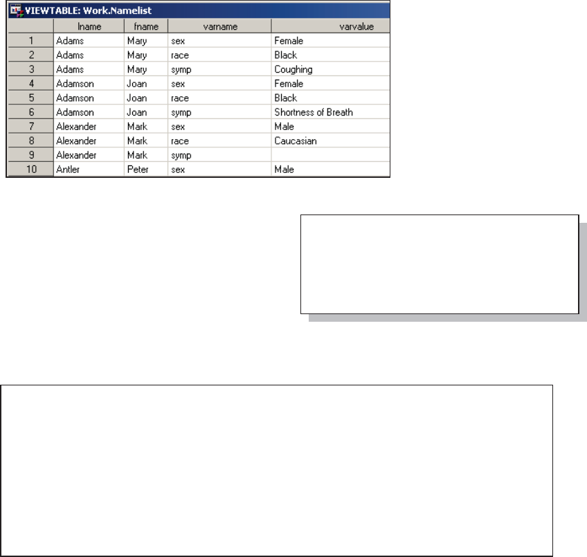
Chapter 3: Just In the DATA Step 153
q The temporary array holds the names of the variables of interest. The dimension has to be
sufficiently large. In this example a dimension of three would have been sufficient.
r A DO UNTIL loop is used to step through the unknown number of variables and to store their
names in the array. Since we are dealing with the metadata at this point we only need to process
this information one time.
s The VNEXT routine retrieves successive variable names and stores the name and type in the
variables NAME and TYPE.
t All character variables (TYPE=‘C’), excluding those used in the DATA step, are selected for
loading into the array of variable names.
u The VNAMEX function is used to store the value contained in the variable NAME in the name
list array. This function allows the resolved value of NAME to be recovered. The VNAME
function would have stored the unresolved value (NAME).
v The variable name is recovered from the array and stored in VARNAME. VARNAME now
contains the name of the variable whose code we also need to recover. The VVALUEX function
not only retrieves the value
of that variable, but also the
formatted value of that
variable. Since we want the
formatted value, this is
perfect.
The NAMELIST data set
will have one observation for
each of the unknown
variables. VARNAME
contains the original variable
name and VARVALUE contains its formatted value.
The general form of the original data is
reconstructed by transforming these rows into
columns using PROC TRANSPOSE.
w The variable holding the name of the variable
of interest is used as the ID variable in the
PROC TRANSPOSE step.
After the transpose step the data reflects the original form of the data; however, the coded values
have been converted to the formatted values.
3.6.5 Using Variable Information Functions
Retrieving and Using Formats
Obs lname fname sex race symp
1 Adams Mary Female Black Coughing
2 Adamson Joan Female Black Shortness of Breath
3 Alexander Mark Male Caucasian
4 Antler Peter Male Black Shortness of Breath
5 Atwood Teddy Male Nausea
. . . . portions of the listing are not shown . . . .
proc transpose data=namelist
out=original(drop=_name_);
by lname fname;
id varname; w
var varvalue;
run;
&DUSHQWHU$UW&DUSHQWHU¶V*XLGHWR,QQRYDWLYH6$67HFKQLTXHV&RS\ULJKW6$6,QVWLWXWH,QF&DU\1RUWK&DUROLQD86$
$
//5,*+765(6(59(')RUDGGLWLRQDO6$6UHVRXUFHVYLVLWVXSSRUWVDVFRPSXEOLVKLQJ

154 Carpenter’s Guide to Innovative SAS Techniques
Rather than use the original variable name we may want to use the format name as the name of
the new variable. Even this is only a slight alteration of the previous code. Here the VFORMATX
function recovers
the format name
from which we
grab just the
name portion
using the
SUBSTR
function
(excluding the leading $ sign and the trailing numbers).
MORE INFORMATION
The VTYPE function is used to retrieve a variable’s type in the second example in Section 11.2.2.
Metadata information can be retrieved through a variety of techniques. Additional approaches are
discussed in Section 13.8.
SEE ALSO
The VNEXT routine documentation contains a simplified version of the first example and can be
found in the SAS documentation
http://support.sas.com/documentation/cdl/en/lrdict/64316/HTML/default/viewer.htm#a002295699
.htm.
3.6.6 New Alternatives and Functions That Do More
While most DATA step functions are fairly straightforward, some have uses that one might not at
first anticipate. Others have seldom used optional arguments that give the function added utility.
As a general rule using and understanding these functions is not the difficulty—knowing that they
exist and remembering to use them is the issue.
To make matters even more interesting, a number of new functions were introduced with SAS®9.
Many of these have similar utility to existing functions, but have been augmented so as to provide
more flexibility and power.
The ARCOS Function
When you need a value to approximate the constant pi, avoid
hard coding a less accurate value. The ARCOS(-1) returns the
value of pi to as many significant digits as should be needed
for most applications. The value of pi is also one of the
constant values that can be returned by the CONSTANT function
The COALESCE Function
The COALESCE function is used to find the first non-missing value in a list of values (variables).
This function does not have any modifiers that allow it to search other than from left to right.
However, it is possible to control the order of the values/variables listed in the call to the function.
This allows one to return either the first, or by reversing the order, the last non-missing value.
SEE ALSO
Mike Zdeb provided a tip on sasCommunity.org that uses the COALESCE function to take the
difference between the first and last non-missing values in a list of values
http://www.sascommunity.org/wiki/Tips:Find_the_LAST_Non-
Missing_Value_in_a_List_of_Variables.
pi1 = arcos(-1);
pi2 = constant('pi');
do i = 1 to cnt;
varvalue = vvaluex(vlist{i});
varname = substr(vformatx(vlist{i}),
2,
(anydigit(vformatx(vlist{i}))-2));
output namelistc;
end;
&DUSHQWHU$UW&DUSHQWHU¶V*XLGHWR,QQRYDWLYH6$67HFKQLTXHV&RS\ULJKW6$6,QVWLWXWH,QF&DU\1RUWK&DUROLQD86$
$
//5,*+765(6(59(')RUDGGLWLRQDO6$6UHVRXUFHVYLVLWVXSSRUWVDVFRPSXEOLVKLQJ

Chapter 3: Just In the DATA Step 155
proc sql noprint;
select lname
into :namelist separated by '/'
from advrpt.demog(where=(lname=:'S'));
quit;
%put &namelist;
%put the number of names is %sysfunc(countw(&namelist,/));
The Counting Functions
The functions in the COUNT family return the number of items in a string. These can be strings
of characters or words. Each function supports three arguments. The first is always the string that
is to be searched. The usage of the second argument varies for each of these functions, and the
real power and flexibility of these functions is achieved through the use of the third argument,
which can take on a number of different values.
COUNT counts appearances of a specific string of characters
COUNTC counts the characters that either do or do not appear in a string of
characters
COUNTW counts the number of words in a string
The COUNTC and COUNTW functions both support well over a dozen modifiers for the third
argument. These modifiers allow you to add characters or digits to the list, count from the left or
right, and add a number of different types of special characters.
These functions can also be used in the macro language. Here the COUNTW function is used with
%SYSFUNC
to count the
number of
names in a list.
SEE ALSO
The COUNTW function was used in the SAS Forum thread
http://communities.sas.com/thread/14720.
The DIM Function
The DIM function was designed to return the dimension of an array. This implies that it counts
variables and in the
past, prior to the
advent of the
COUNTW function
– shown above, it
has been used to
count the number
of words in a list.
Here we fool the
DIM function by
using a list of words as variable names. The DIM function then counts these words. This approach
for counting is more restrictive than the COUNTW function shown above because the words must
conform to SAS variable naming conventions: the list must be space separated, the &COUNT
macro variable is placed on the global symbol table, and the DATA step is required.
%macro wcount(list);
%* Count the number of words in &LIST;
%global count;
data _null_;
array nlist{*} &list;
call symputx('count', dim(nlist));
run;
%mend wcount;
%wcount(&namelist)
%put The total number of words in &namelist is: &count;
28 %put &namelist;
Saunders/Simpson/Smith/Stubs
29 %put the number of names is %sysfunc(countw(&namelist,/));
the number of names is 4
&DUSHQWHU$UW&DUSHQWHU¶V*XLGHWR,QQRYDWLYH6$67HFKQLTXHV&RS\ULJKW6$6,QVWLWXWH,QF&DU\1RUWK&DUROLQD86$
$
//5,*+765(6(59(')RUDGGLWLRQDO6$6UHVRXUFHVYLVLWVXSSRUWVDVFRPSXEOLVKLQJ

156 Carpenter’s Guide to Innovative SAS Techniques
SEE ALSO
This example was adapted from one shown by Cheng (2011). The technique itself was first
proposed by Michael Friendly (1991).
The GEOMEAN Function
There are several different types of means. Usually when we refer to a mean we are actually
referring to the arithmetic average. Another type of
mean is the Geometric mean, which is calculated
by the GEOMEAN function. An artifact of the
geometric mean’s formula is that it can also be
used to calculate the nth root of a number.
The 5th root of X would be coded as
GEOMEAN(X,1,1,1,1) the value and a series of
ones (1 less than the root).
The IFC and IFN Functions
The IFC and IFN functions give us the ability to consolidate a set of certain types of IF-
THEN/ELSE statements with a single function call. Generally these functions are used for a
single comparison that results in TRUE/FALSE/MISSING, which in turn is used to determine a
variable assignment.
The IFN function is used to return a numeric result, while the IFC function returns a character
string. For both functions the arguments are:
1st expression
2nd result returned when the expression is true
3rd result returned when the expression is false
4th result returned when the expression is missing (optional)
In the following example the patients are being divided into GENERATION according to birth
year.
data generation;
set advrpt.demog(keep=lname fname dob);
length generation $10;
if year(dob) = . then generation='Unknown';
else if year(dob) lt 1945 then generation= 'Greatest';
else if year(dob) ge 1945 then generation = 'Boomer';
run;
title2 'GEOMEAN';
data roots;
do x = 0 to 30 by 5;
*Square root;
root2 = sqrt(x);
nth2 = x**(1/2);
g2 = geomean(x,1);
*Cube root;
nth3 = x**(1/3);
g3 = geomean(x,1,1);
*4th root;
nth4 = x**(1/4);
g4 = geomean(x,1,1,1);
output;
end;
run;
&DUSHQWHU$UW&DUSHQWHU¶V*XLGHWR,QQRYDWLYH6$67HFKQLTXHV&RS\ULJKW6$6,QVWLWXWH,QF&DU\1RUWK&DUROLQD86$
$
//5,*+765(6(59(')RUDGGLWLRQDO6$6UHVRXUFHVYLVLWVXSSRUWVDVFRPSXEOLVKLQJ

Chapter 3: Just In the DATA Step 157
The three IF/ELSE/IF statements can be replaced by a single assignment statement that takes
advantage of the IFC function.
The two solutions are not identical. The IFC function shown above will never return a missing
value. The expression can only resolve to 0 or 1. A missing DOB will result in a missing year
which will necessarily be less than a constant. When using IFC or IFN with the intent that it can
select the 4th (missing) argument you must make sure that it is possible that the expression can
indeed resolve to a missing value. That is not the case here.
The solution is simple; as programmers the issue is for us to remember to be careful. One solution
is to multiply the stated expression by the variable that could be missing. Here the expression is
multiplied by the year of the DOB. The sense of the expression is not changed, but it can now take
on a missing value.
MORE INFORMATION
A similar IFC function is discussed in terms of the FINDC function in the next subsection.
SEE ALSO
When used with the %SYSFUNC macro function, Fehd (2009) shows how the IFN and IFC
functions can be used to conditionally execute global statements.
The INDEX and FIND Families
While the three functions in the INDEX family (INDEX, INDEXC, and INDEXW) remain
unchanged, the newer FIND functions (FIND, FINDC, and FINDW) provide the same basic
functionality with a great deal of additional flexibility. The FIND functions support both the
ability to state a start position, as well as, modifiers that can be used to fine tune the search.
In the following example a string of comma separated words (LIST) is to be subsetted by
removing the last word in the list (unless it is the only word). The FINDC function is used to find
the location of the last word delimiter, in this case a comma. Like the INDEX function FINDC
returns the position of the first occurrence of the second argument n.
data generation2;
set advrpt.demog(keep=lname fname dob);
length generation $10;
generation =ifc(year(dob) ge 1945,'Boomer','Greatest','Unknown');
run;
ifc(year(dob)*(year(dob) ge 1945),'Boomer','Greatest','Unknown');
&DUSHQWHU$UW&DUSHQWHU¶V*XLGHWR,QQRYDWLYH6$67HFKQLTXHV&RS\ULJKW6$6,QVWLWXWH,QF&DU\1RUWK&DUROLQD86$
$
//5,*+765(6(59(')RUDGGLWLRQDO6$6UHVRXUFHVYLVLWVXSSRUWVDVFRPSXEOLVKLQJ

158 Carpenter’s Guide to Innovative SAS Techniques
data lists;
input list $;
datalines;
A
A,B
A,B,C
A,B,C,D
A,B,C,D,
run;
data shorter;
set lists; n o p
commaloc=findc(list, ',','b',-length(list));
if commaloc=0 then newlist=list; q
else newlist=substr(list,1,commaloc-1); r
run;
3.6.6 Using Other Functions
FINDC
Obs list commaloc newlist
1 A 0 A
2 A,B 2 A
3 A,B,C 4 A,B
4 A,B,C,D 6 A,B,C
5 A,B,C,D, 8 A,B,C,D
The third o and fourth p
arguments can be in either
order (one must be a
character code and the other
an integer. In this example
the third argument o is a
‘b’. This instructs SAS to
search from right to left,
rather than the usual left to
right. A right to left search
can also be requested by
using a negative 4th
argument. In this example
the 4th argument p requests
that the search be right to left and that
it should start at the last position in
the string. When the 4th argument is
negative the ‘b’ modifier should not
be needed. However in my
experience, a positive integer in the
4th argument will not necessarily
search right to left in the presence of
the ‘b’ modifier.
q If a comma is not found there is only one word and nothing is eliminated.
r When a comma is found COMMALOC will contain the position of the rightmost comma.
SUBSTR is used to keep everything to the left of that comma.
NEWLIST could have been assigned without the IF-THEN/ELSE through the use of the IFC
function. This function would yield the same values, but it could cause an error to be written to
the LOG. When
there is only one
word in the list
(there are no
commas), the value of COMMALOC will be 0. When COMMALOC=0 (FALSE) the value of
LIST is assigned, although the second argument (TRUE) will not be executed it is still evaluated.
The result of the expression COMMALOC-1 will be minus 1 (-1), and that is an illegal argument
for the SUBSTR function, hence the ERROR in the LOG—even though the SUBSTR function is
not executed.
SEE ALSO
A variation of this problem was posed on a SAS Forum post and this solution was proposed by
@Patrick http://communities.sas.com/message/100071.
newlist = ifc(commaloc,substr(list,1,commaloc-1),list);
&DUSHQWHU$UW&DUSHQWHU¶V*XLGHWR,QQRYDWLYH6$67HFKQLTXHV&RS\ULJKW6$6,QVWLWXWH,QF&DU\1RUWK&DUROLQD86$
$
//5,*+765(6(59(')RUDGGLWLRQDO6$6UHVRXUFHVYLVLWVXSSRUWVDVFRPSXEOLVKLQJ

Chapter 3: Just In the DATA Step 159
Another common problem is to find or detect all locations of a character within a larger string.
The INDEX function will only detect the first location. Unlike the INDEX function, the FINDC
function has the ability to start the search in a position other than the leftmost position.
In this example we want to enumerate the location of each delimiter in a string.
s The delimiter is
declared.
t A counter is added
just to count the
occurrences of the
delimiter. When
POSITION=0 nothing is
added to the counter,
otherwise 1 is added.
u The position is
initialized to zero. This
allows us to increment
by 1 in the third
argument of the FINDC
function w.
v A DO UNTIL loop is used
to step through the string. The
loop will terminate when
FINDC fails to find another
occurrence of the delimiter.
Since the DO UNTIL always
executes at least once, it is ok
that position was initialized to
zero.
w The FINDC function
returns the next location of the
delimiter starting at POSITION+1. If none is found a zero is returned.
SEE ALSO
Variations on this solution were posted by @ArtT and @Ksharp in response to a question on a
SAS Forums thread http://communities.sas.com/thread/30629?tstart=0.
The ROUND Function
The ROUND function is most typically used to round a number to the nearest integer; however, it
also has a less commonly used second argument that
allows us to round to any value. Here the weights of the
individuals in our study (the weights are measured to
the nearest pound) are being grouped by rounding to
the nearest 50 pounds.
data wtgroup;
set advrpt.demog;
wtgroup = round(wt,50);
run;
data listloc (keep=id cnt position);
informat id $30.;
input id;
delimiter='!'; s
cnt=0; t
position=0; u
do until(position=0); v
position=findc(id,delimiter,position+1); w
cnt+ ^^position;t
if cnt=0 or position ne 0 then output listloc;
end;
cards;
1!2!3445!!!
!!!
123
run;
3.6.6 Using Other Functions
FINDC
Obs id cnt position
1 1!2!3445!!! 1 2
2 1!2!3445!!! 2 4
3 1!2!3445!!! 3 9
4 1!2!3445!!! 4 10
5 1!2!3445!!! 5 11
6 !!! 1 1
7 !!! 2 2
8 !!! 3 3
9 123 0 0
&DUSHQWHU$UW&DUSHQWHU¶V*XLGHWR,QQRYDWLYH6$67HFKQLTXHV&RS\ULJKW6$6,QVWLWXWH,QF&DU\1RUWK&DUROLQD86$
$
//5,*+765(6(59(')RUDGGLWLRQDO6$6UHVRXUFHVYLVLWVXSSRUWVDVFRPSXEOLVKLQJ

160 Carpenter’s Guide to Innovative SAS Techniques
The midpoints of the intervals are
centered on the even 50 pound
increments. This technique is
often used to form consolidated
age intervals such as decades
(round to the nearest 10 years).
The SCAN Function
The SCAN function is used to retrieve a word from a string. The word extracted by this function
is determined by the numeric second argument of the scan function. When the word number is
positive the words are counted from the left end of the string and when it is negative the words are
counted from the right.
In SAS 9.2 the SCAN function has a number of enhancements. Like a number of the newer
SAS®9 functions, SCAN now supports an optional fourth argument which can be used to modify
the way that the SCAN function operates. There are over 20 modifiers available for the function,
and they add a great deal
of flexibility to the word
selection process.
In this example the
character variable
AUTOLOC contains the
three locations used for
the autocall macro
library. Two are quoted
physical paths and one of these contains an embedded blank (the word delimiter).
n Using the SCAN function without a modifier does not separate the words correctly because of
the embedded blank (see the value in the variable WOQ).
o Adding the ‘Q’ modifier as the fourth argument to the function causes the SCAN function to
ignore word delimiters within quoted strings, and correctly separates the three words (WQ).
p Including the ‘R’
modifier along with
the ‘Q’ modifier
correctly separates the
words and removes
the quotes from the
two quoted words.
MORE INFORMATION
A macro that uses the SCAN function to separate the autocall macro locations can be found in
Section 13.8.2.
data locations;
autoloc = " 'c:\my documents' 'c:\temp' sasautos";
do i = 1 to 3;
woq = scan(autoloc,i,' '); n
wq = scan(autoloc,i,' ','q'); o
wqr = scan(autoloc,i,' ','qr'); p
output ;
end;
run;
i woq n wq owqr p
1 'c:\my 'c:\my documents' c:\my documents
2 documents' 'c:\temp' c:\temp
3 'c:\temp' sasautos sasautos
3.6.6 Using Other Functions
ROUND
Obs lname fname wt wtgroup
1 Adams Mary 155 150
2 Adamson Joan 158 150
3 Alexander Mark 175 200
4 Antler Peter 240 250
5 Atwood Teddy 105 100
6 Banner John 175 200
. . . . portions of the report not shown . . . .
&DUSHQWHU$UW&DUSHQWHU¶V*XLGHWR,QQRYDWLYH6$67HFKQLTXHV&RS\ULJKW6$6,QVWLWXWH,QF&DU\1RUWK&DUROLQD86$
$
//5,*+765(6(59(')RUDGGLWLRQDO6$6UHVRXUFHVYLVLWVXSSRUWVDVFRPSXEOLVKLQJ

Chapter 3: Just In the DATA Step 161
The SUBSTR Function
The SUBSTR function has the capability of not only extracting one or more characters from a
string, it can also be used to insert characters into an existing string. This is accomplished by
placing the SUBSTR function on the left side of the equal sign. In the following example the
variable MEDSTDT_ is a character date in the form of mm/dd/yyyy. Unknown values, such as
month, have been recorded using XX. The IF statement checks the values of the fourth and fifth
characters (day of month), and it replaces any values of ‘XX’ with ‘15’.
The real power of this substitution can be seen when it is coupled with the use of a format. The
text date MEDSTDT_ may contain a month code in the first two positions. We would like to
substitute a month number for the code, but we of course would rather not write a series of IF-
THEN/ELSE statements.
q A user defined format, $MOCONV., is created with the codes to map to month number.
r The ANYALPHA function is used to detect a non-numeric value in the month field.
s The SUBSTR function on the left indicates that the value of the PUT will be inserted into the
first two columns.
t The SUBSTR function is also used to obtain the code that is to be applied to the format. The
code allows us to substitute the beginning, middle, or final month depending on the coded value.
MORE INFORMATION
An example in Section 2.3.1 also substitutes date values using the SUBSTR on the left side of the
= sign. That example also takes advantage of the ?? format modifier.
The TRANWRD Function
The TRANWRD function is used to replace words within a text string with other text. The
function is straightforward in how it is used; however, there is a potential problem. By default,
unless otherwise
specified, the length of
the returned string is
$200. This means that
you should be sure to
specify a length for the
variable that is
receiving the
translated text.
u The variable
if substr(medstdt_,4,2)='XX' then substr(medstdt_,4,2)='15';
proc format ; q
value $moconv
'XX', 'xx' = '06'
'LL', 'll' = '01'
'ZZ', 'zz' = '12';
run;
data conmed204(keep=subject medstdt_);
set advrpt.conmed(where=(subject='204'));
if r anyalpha(substr(medstdt_,1,2)) then
substr(medstdt_,1,2)=put(substr(medstdt_,1,2),$moconv2.);
run; s t
data _null_;
length newstatement1 $34;
statement = "I enjoy going to SUGI conferences.";
newstatement1 = tranwrd(statement,"SUGI", "SGF");u
newstatement2 = tranwrd(statement,"SUGI", "SGF");v
length_newstatement1 = lengthc(newstatement1);
length_newstatement2 = lengthc(newstatement2);
put length_newstatement1 = ;
put length_newstatement2 = ;
run;
&DUSHQWHU$UW&DUSHQWHU¶V*XLGHWR,QQRYDWLYH6$67HFKQLTXHV&RS\ULJKW6$6,QVWLWXWH,QF&DU\1RUWK&DUROLQD86$
$
//5,*+765(6(59(')RUDGGLWLRQDO6$6UHVRXUFHVYLVLWVXSSRUWVDVFRPSXEOLVKLQJ

162 Carpenter’s Guide to Innovative SAS Techniques
data Visitdates(keep=subject date visit note);
set advrpt.lab_chemistry;
by subject;
array dates {16} _temporary_; n
array maxvis {3} _temporary_; o
if first.subject then call missing(of dates{*});
* Save dates;
dates{visit} = labdt; p
if last.subject then do i = 1 to 3;
date = largest(i,of dates{*}); q
visit = whichn(date,of dates{*}); r
if i=1 then do;
call missing(of maxvis{*});
note=' '; s
end;
else if visit>=min(of maxvis{*}) then note='*'; t
else note=' ';
output visitdates;
maxvis{i}=visit; u
end;
format date date9.;
run;
3.5.1 PUT and INPUT Functions
Using WHICHN to check Visit Order
Obs SUBJECT VISIT date note
. . . . portions of the table are not shown . . . .
19 206 7 07FEB2007
20 206 7 07FEB2007 *
21 206 8 05JAN2007 *
22 207 10 09MAR2007
23 207 9 31JAN2007
24 207 8 03JAN2007
25 208 7 30MAR2007
26 208 7 30MAR2007 *
27 208 10 09MAR2007 *
28 209 16 27JUN2007
29 209 13 07JUN2007
30 209 15 23MAY2007 *
. . . . portions of the table not shown . . . .
NEWSTATEMENT1 will have a length of $34, because its length was set using a LENGTH
statement.
v NEWSTATEMENT2, on the other hand, will have a length of $200, because its length was not
otherwise specified.
SEE ALSO
A further discussion of the hidden gotcha of the TRANWRD function can be found in the
sasCommunity.org article titled “Caution with the TRANWRD Function!”
http://www.sascommunity.org/wiki/Caution_with_the_TRANWRD_Function!
The WHICHN Function
The WHICHN function searches a list of values for a specific value and returns the position of the
result. In this example the last three visits (by latest date) are selected and the visit numbers are
checked to see if
the visits have
been taken in
order.
n Define the array
to hold the visit
dates.
o We are
interested in only
the last three visits.
p Load the visit
dates into the
DATES array
using the visit
number as the array index. There are at most
16 visits.
q Determine the three latest dates. These
should be the largest visit numbers.
r The WHICHN function is used to detect
the visit number associated with this date.
For ties the first value detected is returned,
consequently for subjects 206 and 208 the
incorrect visit number is returned for the
second of the tied dates.
s The last (largest date) visit cannot be out of order.
t If this visit number is larger than any of the previous visits then at least one visit was taken out
of order, and this visit should be flagged. Notice that the current visit has not yet been added to
MAXVIS array.
u Place this visit number in the list of visits associated with the three latest (largest) dates.
&DUSHQWHU$UW&DUSHQWHU¶V*XLGHWR,QQRYDWLYH6$67HFKQLTXHV&RS\ULJKW6$6,QVWLWXWH,QF&DU\1RUWK&DUROLQD86$
$
//5,*+765(6(59(')RUDGGLWLRQDO6$6UHVRXUFHVYLVLWVXSSRUWVDVFRPSXEOLVKLQJ

Chapter 3: Just In the DATA Step 163
SEE ALSO
A related SAS Forum thread uses the WHICHN and VNAME functions to retrieve variable
names associated with the largest values http://communities.sas.com/thread/30487?tstart=0.
3.6.7 Functions That Put the Squeeze on Values
A number of character functions are available that can be used to remove characters from a text
string. These include, but are not limited to:
COMPRESS Removes characters from a text string.
COMPBL Removes multiple blanks by translating them into single blanks.
%COMPRES Like COMPBL this macro function removes multiple blanks.
DEQUOTE Removes matching quotes from a string that starts with a quote.
STRIP Removes leading and trailing blanks.
TRANSLATE Replaces characters in a text string at the character level.
TRANSWRD Replaces character groups.
TRANSTRN Replaces character groups.
Functions that trim and left justify a list of characters also remove blanks. These include: LEFT,
%LEFT, %QLEFT, TRIM, TRIMN, %TRIM, and %QTRIM. The CATS, CATT, and CATX
functions can also be used to remove leading and/or trailing blanks.
The COMPRESS Function
The COMPRESS function can remove much more than just blanks from a string. The first
argument of this function is the string that is to be compressed and the second argument can be
used to specify one or more characters that are to either be removed or not to be removed. The
third argument can specify a modifier, and there are over a dozen that can be used to specify
groups or classes of characters to either remove or retain. Taken together the second and third
arguments provide an extremely flexible tool.
In this example, the second argument
usually specifies the characters to
remove; however, because the third
argument is specified as ‘k’ they are instead the characters
that are kept.
The following example uses the COMPRESS function to count the number of lines of code in a
SAS program by counting the semicolons. The ‘k’ is used to remove every character except
semicolons in the COMPRESS function. The LENGTH function is then used to count the
semicolons for that physical line.
Since some physical lines of a
program may not have a
semicolon the INDEX function is
used to determine if a semicolon
is present. The count is then
written to a macro variable. To
speed up the processing no IF-
THEN/ELSE statements are used
(executing the SYMPUTX on
every incoming row can sometimes be more efficient than executing an IF statement to check for
the last observation).
string1 = 'ABCDEABCDE';
string2 = compress(string1,'CAE','k');
string1=ABCDEABCDE
string2=ACEACE
filename code "c:\sascode\ABC.sas";
data _null_;
infile code truncover;
input ;
justsemi = compress(_infile_,';','k');
cnt+index(justsemi,';')*length(justsemi);
call symputx('cnt',cnt);
run;
%put line count is: &cnt;
&DUSHQWHU$UW&DUSHQWHU¶V*XLGHWR,QQRYDWLYH6$67HFKQLTXHV&RS\ULJKW6$6,QVWLWXWH,QF&DU\1RUWK&DUROLQD86$
$
//5,*+765(6(59(')RUDGGLWLRQDO6$6UHVRXUFHVYLVLWVXSSRUWVDVFRPSXEOLVKLQJ

164 Carpenter’s Guide to Innovative SAS Techniques
MORE INFORMATION
The COMPRESS function is used with the NOTDIGIT function in an example in Section 3.6.1.
SEE ALSO
A number of examples that expound on the use of the COMPRESS function’s third argument can
be found in Murphy and Proskin (2006).
The STRIP Function
The STRIP function removes both leading and trailing blanks from a character string. Unlike the
TRIM and TRIMN functions, the STRIP function can result in a string with a length of zero. The
STRIP function was originally intended to work with the concatenation operator. The statement
shown here detects all values of PRODUCT that are exactly ‘0’ after removing any leading and
trailing spaces.
This example is taken from an
answer provided by @ArtT in
the SAS Forum thread http://communities.sas.com/thread/30382?tstart=0.
The TRANSLATE Function
The TRANSLATE function is designed to replace characters and the replacement character
cannot have a null length, consequently
this function generally does not result in
a shorter string. There are a couple of
situations, however, where this is not
true. By default the new variable created
by TRANSLATE will have the same
length as the original variable (STRING1
in this example). When the first letter in
the string is replaced with a blank, the
blank is not preserved (STRING2), but
the length is not changed so we have
effectively moved the blank to the end
(the string has essentially been left
justified). Converting the last character to a blank, STRING3, is more complex. As is shown by
STRING4 the trailing blank is preserved on the PDV. However the trailing blank is truncated and
the variable’s length is adjusted when the variable is written to the new data set.
For this function remember that the order of the to/from arguments
is different than from the other functions in the translation family.
data test;
string1 = 'ABCDE';
string2 = translate(string1,' ','A');
string3 = translate(string1,' ','E');
string4 = string3||'x';
put string1=;
put string2=;
put string3=;
put string4=;
len2 = length(string2);
len3 = length(string3);
put len2= len3=;
run;
string1=ABCDE
string2=BCDE
string3=ABCD
string4=ABCD x
len2=5 len3=4
if strip(product) eq "0" then output dontwant;
&DUSHQWHU$UW&DUSHQWHU¶V*XLGHWR,QQRYDWLYH6$67HFKQLTXHV&RS\ULJKW6$6,QVWLWXWH,QF&DU\1RUWK&DUROLQD86$
$
//5,*+765(6(59(')RUDGGLWLRQDO6$6UHVRXUFHVYLVLWVXSSRUWVDVFRPSXEOLVKLQJ

Chapter 3: Just In the DATA Step 165
Removing Quotes—The DEQUOTE, COMPRESS, and TRANSTRN Functions
It is occasionally helpful to be able to remove quotes from a string. The DEQUOTE,
COMPRESS, and TRANSTRN functions can each be used to remove quotes, but they do not
necessary yield the same result. DEQUOTE only removes pairs of quotes, but it will also truncate
the remainder of the string. COMPRESS and TRANSTRN can replace all occurrences without
looking for quote pairs.
n STRING1 contains both
single and double quote
pairs.
o STRING2 contains an
unmatched single quote
(apostrophe).
p DEQUOTE removes
the quotes from CA and
truncates the remainder of
the string.
q The apostrophe is
unmatched and therefore
untouched by DEQUOTE.
r s COMPRESS can be
given a list of characters,
here both single and
double quotes. All are
removed.
t The ‘p’3rd argument modifier on the
COMPRESS function (replace punctuation) also
removes single and double quotes.
u The TRANSTRN function can replace a
character with a null string (specified here with
the TRIMN function), but it cannot replace a
series of individual characters as can the
COMPRESS function. Only double quotes have
been removed.
v The single quote (apostrophe) is replaced with a null string.
3.7 Joins and Merges
Although merges and joins are both commonly used and generally used successfully, you should
be aware that there are some caveats, as well as things to keep in mind when doing this type of
processing.
data quoteless;
string1 = "'CA', ""OR"", 'WA'"; n
string2 = "Tom's Truck"; o
dq1 = dequote(string1); p
dq2 = dequote(string2); q
cprs1=compress(string1,"%bquote('")"); r
cprs2=compress(string2,"%bquote('")"); s
cprs3=compress(string2,,'p'); t
trns1=transtrn(string1,"%bquote(")",trimn('')); u
trns2=transtrn(string2,"'",trimn('')); v
put string1=;n
put string2=;o
put dq1=; p
put dq2=; q
put cprs1=; r
put cprs2=; s
put cprs3=; t
put trns1=; u
put trns2=; v
run;
string1='CA', "OR", 'WA' n
string2=Tom's Truck o
dq1=CA p
dq2=Tom's Truckq
cprs1=CA, OR, WAr
cprs2=Toms Trucks
cprs3=Toms Truckt
trns1='CA', OR, 'WA'u
trns2=Toms Truckv
&DUSHQWHU$UW&DUSHQWHU¶V*XLGHWR,QQRYDWLYH6$67HFKQLTXHV&RS\ULJKW6$6,QVWLWXWH,QF&DU\1RUWK&DUROLQD86$
$
//5,*+765(6(59(')RUDGGLWLRQDO6$6UHVRXUFHVYLVLWVXSSRUWVDVFRPSXEOLVKLQJ

166 Carpenter’s Guide to Innovative SAS Techniques
3.7.1 BY Variable Attribute Consistency
Merges and joins are very susceptible to inconsistencies in the joining criteria. The variable(s) that
are used in the BY statement must have the same attributes or unfortunate things can happen.
Inconsistent BY Variable Type
In the following example we would like to add the patient’s first and last names to the lab data.
The common variable is the SUBJECT number, and we use SUBJECT as a BY variable in a data
set MERGE. The incoming data sets have been sorted, but the step fails to execute.
Fortunately the error message
in the LOG is very helpful.
Typically when we misuse a variable’s type, such as when we use a character variable in an
arithmetic statement, SAS will attempt to convert the variable’s type. When the variable is in the
BY statement, a conversion is not possible and the step fails.
Converted Type
In the previous example we were unable to perform the merge because the BY variable SUBJECT
was character in one data set and numeric in the other. In the DATA step below, the numeric
SUBJECT (which has three digits) in DEMOG is converted to character prior to its use as a BY
variable.
Unfortunately only part of the problem has been solved. Looking at the resulting data set we see
that we were unable to retrieve any names.
data demog_c;
set advrpt.demog(keep=subject lname fname
rename=(subject=ptid));
subject = put(ptid,4.);
run;
data labnames;
merge demog_c(keep=subject lname fname)
advrpt.lab_chemistry(keep=subject visit labdt
in=inlab);
by subject;
if inlab;
run;
data labnames;
merge advrpt.demog(keep=subject lname fname)
advrpt.lab_chemistry(keep=subject visit labdt
in=inlab);
by subject;
if inlab;
run;
ERROR: Variable subject has been defined as
both character and numeric.
&DUSHQWHU$UW&DUSHQWHU¶V*XLGHWR,QQRYDWLYH6$67HFKQLTXHV&RS\ULJKW6$6,QVWLWXWH,QF&DU\1RUWK&DUROLQD86$
$
//5,*+765(6(59(')RUDGGLWLRQDO6$6UHVRXUFHVYLVLWVXSSRUWVDVFRPSXEOLVKLQJ
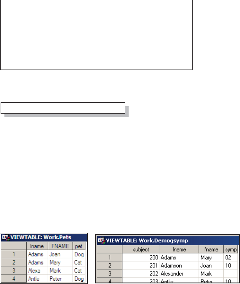
Chapter 3: Just In the DATA Step 167
The problem is in the way that we have used the PUT function. When we converted the numeric
value to character, we used the numeric format 4. Numeric formats create right justified character
strings, consequently the resulting value starts with a blank. Adding a LEFT function would have
solved this problem, but would have
introduced a more subtle one.
In the data set ADVRPT.LAB_CHEMISTRY, the variable SUBJECT has a length of $3;
however, in the previous statement the resulting variable will have a length of $4. In this
particular example the inconsistent length will not cause a problem, but as is shown next, it can
under some circumstances cause a problem that can be harder to detect.
Inconsistent Length
Remember that a variable and its attributes are added to the PDV when the variable is first
encountered as the DATA step is processed during the compilation phase. Once the attributes are
established they will not be changed even if additional or contradictory information is found while
compiling the remainder of the DATA step. The following rather silly example illustrates the
problem.
I would like to use the data set WORK.PETS to add the family pet to the demographic
information in ADVRPT.DEMOG.
The pet information contains the owner’s first and last name.
Inconsistent Joining Criteria
3.7.1b Converted Type
Obs lname fname subject VISIT LABDT
1 200 1 07/06/2006
2 200 2 07/13/2006
3 200 1 07/06/2006
4 200 4 07/13/2006
5 200 4 07/13/2006
. . . . portions of the table not shown . . . .
subject = left(put(ptid,4.));
&DUSHQWHU$UW&DUSHQWHU¶V*XLGHWR,QQRYDWLYH6$67HFKQLTXHV&RS\ULJKW6$6,QVWLWXWH,QF&DU\1RUWK&DUROLQD86$
$
//5,*+765(6(59(')RUDGGLWLRQDO6$6UHVRXUFHVYLVLWVXSSRUWVDVFRPSXEOLVKLQJ

168 Carpenter’s Guide to Innovative SAS Techniques
Before performing the merge both data sets are sorted; however, the DATA step fails and the
errors include a “not properly sorted” message.
In this example the truncation occurs because the length of the variable LNAME in the data set
PETS ($5) determines the length for LNAME on the PDV. The result is truncation when values
from DEMOGSYMP are
read. In fact, because of
the truncation of LNAME
in the data set
DEMOGSYMP, Joan
Adamson becomes Joan
Adams, and since Joan Adams now follows Mary Adams the rows are no longer physically
sorted. It could have been worse. If Joan Adamson had a first name alphabetically after Mary, say
Tricia, Tricia Adams would have followed Mary alphabetically and no sort error would have been
reported.
The truncation problem could have been avoided with the use of a LENGTH statement prior to
the MERGE statement (the length of LNAME on DEMOGSYMP is $10). This problem would
have also been solved by simply reordering the two data sets on the MERGE statement.
WARNING: Multiple lengths were specified for the BY variable lname by
input data sets. This may cause unexpected results.
ERROR: BY variables are not properly sorted on data set WORK.DEMOGSYMP.
lname=Adams FNAME=Mary pet=Cat subject=101 SYMP=02 FIRST.lname=1
LAST.lname=0 FIRST.FNAME=1
LAST.FNAME=1 _ERROR_=1 _N_=2
NOTE: The SAS System stopped processing this step because of errors.
proc sort data=pets;
by lname fname;
run;
proc sort data=advrpt.demog(keep=subject lname fname symp)
out=demogsymp;
by lname fname;
run;
data petsymptoms;
merge pets(keep=lname fname pet)
demogsymp(keep=subject lname fname symp);
by lname fname;
run;
data petsymptoms;
length lname $10;
merge pets(keep=lname fname pet)
demogsymp(keep=subject lname fname symp);
. . . . code not shown . . . .
&DUSHQWHU$UW&DUSHQWHU¶V*XLGHWR,QQRYDWLYH6$67HFKQLTXHV&RS\ULJKW6$6,QVWLWXWH,QF&DU\1RUWK&DUROLQD86$
$
//5,*+765(6(59(')RUDGGLWLRQDO6$6UHVRXUFHVYLVLWVXSSRUWVDVFRPSXEOLVKLQJ
Chapter 3: Just In the DATA Step 169
Numeric BY Variables
Extreme care must be taken if you ever need to use numeric BY variables, especially variables
with non-integer values. Because of the way that numbers are stored within the computer, even
numbers that appear to be integers may not actually be
integers. This can be simply demonstrated by creating
a value that is slightly different from 1.
Examining the LOG shows that even the BEST32.
format displays
this value (Y=) as
1. The HEX16.
format does show
these two numbers
differently, but really how often would you use the HEX format to double-check the integers?
Worse if we were to use this variable as a BY variable as is done
next, the difference is sufficient to sabotage the merge. The LOG
shows that the data set BOTH has two observations—one for each
value of Y, where there would only have been one observation if
the values were seen as equal.
At some point the fuzz rules come into play and the difference is so small that SAS considers
them to be equal. In this example adding one more zero to the number of decimal places in the
first definition of Y would have been sufficient for the merge to have been successful.
The take-away point is, be very careful when using numeric BY variables in a merge.
SEE ALSO
Ron Cody wrote Sample Note 33-407 on issues associated with variable attribute inconsistencies,
and suggests an automated solution http://support.sas.com/kb/33/407.html .
3.7.2 Variables in Common That Are Not in the BY List
After a merge or join, variables common to more than one data set will appear only once in the
new data set. This means that there can be variables that overwrite each other.
In the following example we merge two data sets by SUBJECT. Each also contains the variable
DATE; however, DATE is not included on the BY statement. In order to make the example a bit
easier to follow the SORT steps have used the NODUPKEY option so that each SUBJECT
appears only once.
data similar;
x = 1;
y = 3.000000000000001/3;
if x=y then put 'the same';
put x= best32.;
put y= best32.;
put x= hex16.;
put y= hex16.;
run;
x=1
y=1
x=3FF0000000000000
y=3FF0000000000001
data other;
y=1; a='a';
run;
data both;
merge similar
other;
by y;
run; NOTE: There were 1 observations read from the data set
WORK.SIMILAR.
NOTE: There were 1 observations read from the data set WORK.OTHER.
NOTE: The data set WORK.BOTH has 2 observations and 3 variables.
&DUSHQWHU$UW&DUSHQWHU¶V*XLGHWR,QQRYDWLYH6$67HFKQLTXHV&RS\ULJKW6$6,QVWLWXWH,QF&DU\1RUWK&DUROLQD86$
$
//5,*+765(6(59(')RUDGGLWLRQDO6$6UHVRXUFHVYLVLWVXSSRUWVDVFRPSXEOLVKLQJ

170 Carpenter’s Guide to Innovative SAS Techniques
n For this example the date variables
have both been renamed to DATE, and
then sorted by subject using the o
NODUPKEY option.
p A WHERE clause restricting the
DATE has been placed on the
LABCHEM data; however, the clause
does not change the resultant table.
Inspection of the data set AELAB shows
that although we have restricted lab dates to those before '01sep2006'd, we seem to have dates that
do not meet the criteria. In fact these are actually the AE start dates that have overwritten the dates
from the LABCHEM data set. q SUBJECT 202 in the LABCHEM data set has a date of
'07jul2006'd, but that value has been replaced by the one in AE, which is missing.
Because the PDV is constructed from left to right, the LABCHEM date label is used in the new
data set. It is also because the data are read from the rightmost data set last that the AE date
overwrites the LABCHEM date.
3.7.3 Repeating BY Variables
When merging, the BY variables should identify down to the row level in all, but at most one of
the data sets named on the MERGE statement. This means that at most only one of the incoming
data sets will not have a sufficient key (BY variables do not identify down to the row level).
When the BY variables do not form a primary key (identify down to the row level) for more than
one data set, a NOTE is
issued to the LOG, and more
importantly, within the BY
group the merge takes place as a one-to-one merge and this is rarely desirable.
proc sort data=advrpt.lab_chemistry(keep=subject labdt
rename=(labdt=date)) n
out=labchem nodupkey; o
by subject;
run;
proc sort data=advrpt.ae(keep=subject aestdt
rename=(aestdt=date)) n
out=ae nodupkey; o
by subject;
run;
data aelab;
merge labchem(where=(date<'01sep2006'd)) p
ae;
by subject;
run;
3.7.2 Variables in Common
Obs SUBJECT date
1 200 07/28/2006
2 201 07/06/2006
3 202 . q
4 203 09/13/2006
5 204 09/27/2006
. . . . portions of the table not shown . . . .
NOTE: MERGE statement has more than one data set
with repeats of BY values.
&DUSHQWHU$UW&DUSHQWHU¶V*XLGHWR,QQRYDWLYH6$67HFKQLTXHV&RS\ULJKW6$6,QVWLWXWH,QF&DU\1RUWK&DUROLQD86$
$
//5,*+765(6(59(')RUDGGLWLRQDO6$6UHVRXUFHVYLVLWVXSSRUWVDVFRPSXEOLVKLQJ

Chapter 3: Just In the DATA Step 171
Here the LABCHEM and AE data sets are merged BY SUBJECT. For SUBJECT 200 there
are 14 LABCHEM observations, but only 4 AE observations. The
fourth AE observation is repeated for the remaining LABCHEM
observations. Clearly this will be unacceptable in virtually all
situations. It is
essential that you
understand the data
and whether or not
the BY variables
form a sufficient
key.
3.7.4 Merging without a Clear Key (Fuzzy Merge)
When a clear set of BY variables are not available (as was the case in the example in Section
3.7.3) logic will be needed to create the appropriate assignments. For this reason these types of
merges are collectively known as fuzzy merges.
As a general rule these types of merges are best handled with an SQL step rather than the DATA
step. The SQL join holds all combinations of the rows from both tables in memory (Cartesian
product). This allows the programmer to apply logic to select the appropriate rows.
In this example we would like to identify all the adverse events for each patient that occurred
within 5 days of a
laboratory visit date. The
subject numbers are
equated in the WHERE
clause as is the logic
needed to evaluate the
proximity of the two dates.
The DATA step can also be used to perform a fuzzy merge. In Section 6.4 a DATA step with two
SET statements performs a merge. A similar technique can be applied to a fuzzy merge through
logic; however, the coding can become quite tricky.
SEE ALSO
Heaton (2008) discusses the use of hash objects to perform many-to-many merges, and has a good
set of references to other papers having to do with the use of hash objects.
proc sql noprint;
create table aelab as
select a.subject,labdt, visit, aestdt, aedesc
from labchem as L, ae as a
where (l.subject=a.subject)
& (labdt le aestdt le labdt+5)
;
quit;
Obs SUBJECT VISIT LABDT AEDESC
1 200 1 07/06/2006 DIARRHEA (X1)
2 200 2 07/13/2006 PAIN-NECK
3 200 1 07/06/2006 PAIN-MUSCULAR CHEST
4 200 4 07/13/2006 INCREASED EOS (6)
5 200 4 07/13/2006 INCREASED EOS (6)
6 200 5 07/21/2006 INCREASED EOS (6)
7 200 6 07/29/2006 INCREASED EOS (6)
. . . . portions of the table are not shown . . . .
data aelab;
merge labchem
ae;
by subject;
run;
&DUSHQWHU$UW&DUSHQWHU¶V*XLGHWR,QQRYDWLYH6$67HFKQLTXHV&RS\ULJKW6$6,QVWLWXWH,QF&DU\1RUWK&DUROLQD86$
$
//5,*+765(6(59(')RUDGGLWLRQDO6$6UHVRXUFHVYLVLWVXSSRUWVDVFRPSXEOLVKLQJ

172 Carpenter’s Guide to Innovative SAS Techniques
3.8 More on the SET Statement
Although a majority of DATA steps use the SET statement, few programmers take advantage of
its full potential. The SET statement has options that can be used to control how the data are to be
read.
END= used to detect the last observation from the incoming data set(s)
(see Section 3.9.1).
KEY= specifies an index to be used when reading (see Section 6.6.2).
INDSNAME= used to identify the current data source (see Section 3.8.2).
NOBS= number of observations (see Section 3.8.1).
OPEN= determines when to open a data set.
POINT= designates the next observation to read (see Section 3.8.1).
UNIQUE used with KEY= to read from the top of the index
(see Section 6.6.2).
MORE INFORMATION
Several of these options are also used in the examples in Section 3.9.
3.8.1 Using the NOBS= and POINT= Options
The SET statement by default performs a sequential read; that is, one observation after another;
first observation to last. It is also possible to perform a non-sequential read using the POINT=
option to tell the SET statement which observation to read next. Very often the POINT= option is
used in conjunction with the NOBS= option, which returns the number of observations in the data
set at DATA step compilation.
The POINT= option identifies a temporary variable that indicates the number of the next
observation to read. The NOBS= option also identifies a temporary variable, which after DATA
step compilation, will hold the number of observations on the incoming data set.
This short example reads the last 10 observations from the incoming data set. The temporary
variable OBS (defined by the NOBS= option) will hold the number of observations available to
read. A DO loop with PT
(defined by the POINT=
option) as the index
variable is then used to
cycle through the last few
observations.
Note the use of the STOP
statement to terminate the
DATA step after reading
the 10 observations. Normally, when the last observation is read from the incoming data set, the
DATA step is automatically terminated. The use of the POINT= option disables the DATA step’s
ability to detect that it has finished reading from the incoming data set.
The POINT= option allows us to read observations in a non-sequential manner (in any order).
When the value of the next observation to read is determined randomly, it is possible to draw a
random subsample.
data lastfew;
if obs ge 10 then do pt =obs-9 to obs by 1;
set sashelp.class point=pt nobs=obs;
output lastfew;
end;
else put 'NOTE: Only ' obs ' observations.';
stop;
run;
&DUSHQWHU$UW&DUSHQWHU¶V*XLGHWR,QQRYDWLYH6$67HFKQLTXHV&RS\ULJKW6$6,QVWLWXWH,QF&DU\1RUWK&DUROLQD86$
$
//5,*+765(6(59(')RUDGGLWLRQDO6$6UHVRXUFHVYLVLWVXSSRUWVDVFRPSXEOLVKLQJ

Chapter 3: Just In the DATA Step 173
The %RAND_WO
macro shown here
uses these two options
to randomly read
(without replacement)
a subset of the
observations from the
incoming data set.
Because the user only
specifies the fraction
of the total number of
observations, the
macro must know the
total number of
available observations
so that the subset size
can be calculated.
This value is stored in
the temporary
variable OBSCNT, which is defined on the SET statement r through the use of the NOBS=
option.
n The total number of observations to be selected is calculated as a fraction of the total number
of observations (OBSCNT). Although it may seem that the OBSCNT variable is being used
before it is defined r, in fact OBSCNT is established and assigned a value during DATA step
compilation.
o An array is used to track whether or not a given observation has already been selected. The
array dimension must exceed the number of observations on the incoming data set. This version
of the macro will accommodate up to 10,000 observations; however, arrays can easily handle
much larger dimensions.
p The variable POINT is randomly generated with an integer value that ranges from 1 to the
number of observations in the data set (OBSCNT). This variable will be used to determine the
next observation to be read.
q A check is made against the flag in the array to determine if the selected observation has
already been read. If it has not already been selected, it is then read. Using an array to store the
flag is the fastest form of a look-up (see Chapter 6).
r The SET statement uses the POINT= and NOBS= options to name the temporary variables.
Tradition, although certainly not a necessity, often uses the variable names to be the same as the
options (POINT=POINT and NOBS=NOBS).
s When an observation has been selected, a flag is set in the array. This prevents the observation
from being read again. Here the flag is a numeric 1 which takes 8 bytes of storage. If a character
$1 flag had been used the array could have been defined as a character array and 70,000 bytes of
memory could have been saved.
t Whenever you use a SET statement inside of a loop, especially when using the POINT=
option, the automatic detection of the last observation is disabled. Be sure to include a STOP to
prevent an infinite loop.
%macro rand_wo(dsn=,pcnt=0);
* Randomly select observations from &DSN;
data rand_wo(drop=cnt totl);
* Calculate the number of obs to read;
totl = ceil(&pcnt*obscnt); n
array obsno {10000} _temporary_; o
do until(cnt = totl);
point = ceil(ranuni(0)*obscnt); p
if obsno{point} ne 1 then do; q
* This obs has not been selected before;
set &dsn point=point nobs=obscnt; r
output;
obsno{point}=1; s
cnt+1;
end;
end;
stop; t
run;
%mend rand_wo;
%rand_wo(dsn=advrpt.demog,pcnt=.3)
&DUSHQWHU$UW&DUSHQWHU¶V*XLGHWR,QQRYDWLYH6$67HFKQLTXHV&RS\ULJKW6$6,QVWLWXWH,QF&DU\1RUWK&DUROLQD86$
$
//5,*+765(6(59(')RUDGGLWLRQDO6$6UHVRXUFHVYLVLWVXSSRUWVDVFRPSXEOLVKLQJ

174 Carpenter’s Guide to Innovative SAS Techniques
The POINT= and NOBS= options can also be helpful when performing look-ahead or look-back
reads of the data. In the following example we need to detect observations with certain thresholds
and then determine if the value is aberrant by reporting the previous observation and the following
two observations as well as the extreme value. Each observation is counted and the counter is
used to establish the value used by POINT.
u The observation is counted. CNT will determine the range of values (observation numbers)
taken on by the temporary variable POINT.
v If a given observation has a sodium value of 14.4 or greater we need to print the previous
observation and the next two observations (up to 4 observations—within a subject).
w The temporary variables POINT and NOBS are associated with the SET statement options of
the same name.
This solution does not take into consideration whether or not a given observation has already been
written to the data set. An array can be used to flag an observation once it has been used without
adding much additional overhead. The sample program E3_8_1b.SAS contains a program that
utilizes an array to allow a given observation to be printed only once.
SEE ALSO
Hamilton (2001) includes limitations and alternatives to the NOBS= option. A more sophisticated
version of the %RAND_WO macro can be found in Carpenter (2004, Section 11.2.3).
3.8.2 Using the INDSNAME= Option
The INDSNAME= option was added to the SET statement in SAS 9.2. This option stores the
name of the data set from which the current observation was read. Prior to its introduction, the
IN= data set option was used to make this determination.
In this example we want to concatenate the two data sets (BOOMER and OTHERS) and we want
to create a variable (GROUP) to identify the data source. Two solutions, one using IN= and the
other using INDSNAME= are shown and contrasted.
n The IN= data set option (see Section 2.1 for more on data set options) names a temporary
numeric variable that takes on the values of
0 or 1 depending on whether or not a given
observation is from this data set.
data grouped1;
set boomer(in=inboom) n
others(in=inoth);
if inboom then group='BOOMER'; o
else if inoth then group='OTHERS';
run;
data surrounded(keep=subject visit sodium);
set advrpt.lab_chemistry(keep=subject sodium
rename=(subject=sub1));
cnt+1; u
if sodium ge 14.4 then do point=(cnt-1) to (cnt+2); v
if 1 le point le nobs then do;
set advrpt.lab_chemistry point=point nobs=nobs; w
if sub1=subject then output surrounded;
end;
end;
run;
&DUSHQWHU$UW&DUSHQWHU¶V*XLGHWR,QQRYDWLYH6$67HFKQLTXHV&RS\ULJKW6$6,QVWLWXWH,QF&DU\1RUWK&DUROLQD86$
$
//5,*+765(6(59(')RUDGGLWLRQDO6$6UHVRXUFHVYLVLWVXSSRUWVDVFRPSXEOLVKLQJ

Chapter 3: Just In the DATA Step 175
o IF-THEN/ELSE processing is used to determine the data source and to assign a value to the
variable GROUP.
For large data sets the IF-THEN/ELSE can be time consuming and can be avoided altogether by
using the INDSNAME= SET statement
option.
p The INDSNAME= option identifies a
temporary character variable (DSN) that
holds the name of the data set from which
the current observation has been read.
q Since the variable DSN will contain a
two-level name (‘WORK.BOOMER’), the libref portion is removed using the SCAN function,
and the name portion (the second word) is stored in the variable GROUP.
r The length of the GROUP variable is declared; otherwise, the SCAN function would return a
length of $200.
INDSNAME= has a default length of $41. This may not be long enough if you are using a
physical path (which is generally not recommended by this author).
3.8.3 A Comment on the END= Option
The END= option can be used to create a numeric (0/1) temporary variable that indicates that the
last record has been read. In the following example the EOF variable o, which has been defined
using the END=option, is used to control when a
PUT statement is to be executed.
The IF statement n is true only once, and its
action (the PUT statement) is executed only on
the last pass of the DATA step.
However notice that the IF statement o is before the
SET statement. This reminds us that by default the
DATA step is not fully terminated until the attempt
is made to execute the SET statement after the last
observation has been read.
3.8.4 DATA Steps with Two SET Statements
As can be seen in numerous examples throughout this chapter, the DATA step may contain
multiple SET statements. Multiple SET statements can give you a great deal of power and
flexibility over the process of reading the data. However, as you take control of the read process,
exercise caution and be sure that you understand what you are requesting the DATA step to
execute.
This simplest case of a double SET statement is essentially a one-to-one
merge with restrictions. And the restrictions (conditions if you will) are
very important.
Without other controls (usually supplied by the programmer), the number
of observations in the new data set is determined by the number of
observations in the smallest original data set. As soon as SAS reads the last observation from
data grouped2;
set boomer
others indsname=dsn; p
length group $6; r
group=scan(dsn,2,'.'); q
run;
data new;
set a;
set b;
run;
data a;
if eof then put total=; n
set sashelp.class end=eof; o
end=eof;
total+age;
put 'last ' age= total= eof=;
run;
last Age=12 total=212 eof=0
last Age=15 total=227 eof=0
last Age=11 total=238 eof=0
last Age=15 total=253 eof=1
total=253
&DUSHQWHU$UW&DUSHQWHU¶V*XLGHWR,QQRYDWLYH6$67HFKQLTXHV&RS\ULJKW6$6,QVWLWXWH,QF&DU\1RUWK&DUROLQD86$
$
//5,*+765(6(59(')RUDGGLWLRQDO6$6UHVRXUFHVYLVLWVXSSRUWVDVFRPSXEOLVKLQJ

176 Carpenter’s Guide to Innovative SAS Techniques
either data set the full DATA step is not fully executed again. You will notice that in all of the
other examples with two SET statements, that there are some restrictions or controls on how the
SET statements are executed. Generally we want the step to terminate on our conditions, and not
necessarily just because a last observation is read from one of the data sets.
Like in a MERGE, if there are variables in common, the values that are read in from the last data
set replace those read in from earlier ones. Also like in a MERGE the PDV will contain all
variables from either of the incoming data sets and each variable will be assigned attributes based
on its first encounter during the compilation of the DATA step. As always any variable that is
read from an incoming data set is automatically retained.
As was seen in Sections 3.1.5, 3.1.6, and 3.8.1, it is possible and sometimes even very
advantageous to be able to use multiple SET statements. Just be sure that you understand what is
happening when you do so, and be sure that you exercise caution as you take control of the read
process.
MORE INFORMATION
Two SET statements are used in the second example of Section 3.8.1. The example in Section
3.6.2 uses DOW loops to read two data sets using two SET statements.
SEE ALSO
A solution to a SAS Forum question utilized a DATA step with two SET statements
http://communities.sas.com/message/42266.
3.9 Doing More with DO Loops
The four principle forms of the DO statement are well known and commonly applied to great
advantage. However, there is so much more that we can do with this statement and sometimes in
surprising ways. This section discusses a few of these techniques.
SEE ALSO
Paul Dorfman (2002) gives a very nice overview of the DO loop and demonstrates many of its
behaviors. Fehd (2007) discusses the differences between the DO UNTIL and DO WHILE loops.
An extensive list of references and links can be found on sasCommunity.org at
http://www.sascommunity.org/wiki/Do_until_last.var.
3.9.1 Using the DOW Loop
While it may have been first proposed by Don Henderson, the DOW loop, which is also known as
the DO-W loop, was named for Ian Whitlock who popularized the technique and was one of the
first to demonstrate its efficiencies. The DOW loop can often be used to improve DATA step
performance, and in its simplest form the DOW loop takes control of the DATA step’s implied
loop.
Consider the DATA step’s implied loop. During the execution phase each executable statement in
the DATA step will execute once for each observation in the incoming data set (WORK.BIG).
This includes a fair amount of behind the scenes processing.
When the DATA statement n is executed, values of derived
variables are cleared and the value of the temporary variable _N_
is incremented. For the step shown here, we do not care about
these things. By using the DOW loop to circumvent the implied
data implied; n
set big;
output implied;
run;
&DUSHQWHU$UW&DUSHQWHU¶V*XLGHWR,QQRYDWLYH6$67HFKQLTXHV&RS\ULJKW6$6,QVWLWXWH,QF&DU\1RUWK&DUROLQD86$
$
//5,*+765(6(59(')RUDGGLWLRQDO6$6UHVRXUFHVYLVLWVXSSRUWVDVFRPSXEOLVKLQJ

Chapter 3: Just In the DATA Step 177
loop, these operations, and others, do not take place.
To create a DOW loop place the SET statement within
the control of a DO loop o. Then take control of the
reading process. Here the END= option p is used to
detect the end of file; this is used to terminate the DO
UNTIL loop. When the loop terminates, we have read all
the data and we are ready to terminate the DATA step.
The STOP q statement prevents the execution of another
iteration of the implied loop n.
Another typical use of a DOW loop is seen when using multiple SET statements to merge data
sets. Here the mean weight of the individuals in the study is calculated and then used to determine
the percent difference from the mean. Since the mean weight is calculated in a separate step, the
means must be merged back onto the original data.
A common solution is to use an IF statement to conditionally execute the first SET statement r.
Since _n_=1 will only be true once, the single observation from WORK.MEANS will only be
read once. The implied loop of the
DATA step will then be used to
read all the observations from the
analysis data set s . This solution
requires that the IF statement r
be checked for every incoming
observation of the analysis data
set s. This is unnecessary and
could be very time consuming. A
DOW loop can be employed to
remove the IF statement and to improve the processing efficiency of the step.
Since only one pass is made through the DATA step, the IF, which was used to control the read of
the summary data set, is not
needed t.
u A DOW loop, which will
execute for each observation on
the analysis data set, is initiated
using a DO UNTIL loop.
v The END= SET statement
option is used to create an end of
file flag that will terminate the
DO UNTIL loop u.
w The STOP statement terminates the DATA step with only one pass of the implied loop.
MORE INFORMATION
A DOW loop is used in Section 2.9.5 to load a hash object.
SEE ALSO
Dorfman (2009) details the DOW loop and its history.
data dowloop;
do until(eof); o
set big end=eof; p
output dowloop;
end;
stop; q
run;
proc summary data=advrpt.demog;
var wt;
output out=means mean=/autoname;
run;
data Diff1;
if _n_=1 then set means(keep=wt_mean); r
set advrpt.demog(keep=lname fname wt); s
diff = (wt-wt_mean)/wt_mean;
run;
data Diff2;
set means(keep=wt_mean); t
do until(eof);u
set advrpt.demog(keep=lname fname wt)
end=eof;v
diff = (wt-wt_mean)/wt_mean;
output diff2;
end;
stop; w
run;
&DUSHQWHU$UW&DUSHQWHU¶V*XLGHWR,QQRYDWLYH6$67HFKQLTXHV&RS\ULJKW6$6,QVWLWXWH,QF&DU\1RUWK&DUROLQD86$
$
//5,*+765(6(59(')RUDGGLWLRQDO6$6UHVRXUFHVYLVLWVXSSRUWVDVFRPSXEOLVKLQJ

178 Carpenter’s Guide to Innovative SAS Techniques
3.9.2 Compound Loop Specifications
The iterative DO loop is commonly used to step through a list of values. What is less commonly
known is that we are not restricted to a single list. Here the variable COUNT takes on the values
of 1, 2, 3, 5, 10, 15, 20, 26, and 33. This
DO statement actually has four distinct
loop specifications. The first (1 to 3) has
an implied BY and the last two consist of a single value. In fact the TO and the BY are not
required as is demonstrated by the last two specifications. The numbers themselves do not need to
be numeric constants, but can also be stated as expressions that resolve to a number.
To illustrate the use of expressions this example includes an expression; however, the iterative
DO is limited to a single index variable. In the DO statement shown here, the writer would like to
iterate across COUNT (1, 2, 3) and
then across CNT (4, 6, 8). However
this is not what happens.
The CNT=4 is interpreted as a logical expression which will resolve to 0 or 1. If CNT is not equal
to 4 the second loop specification will cause COUNT to take on the values of 0, 2, 4, 6, 8;
otherwise, the specification results in the
values 1, 3, 5, 7. Effectively the DO
statement is coded as if parentheses
surrounded the expression.
Since the individual values are expressions,
you may also use expressions that resolve to
character values.
3.9.3 Special Forms of Loop Specifications
Iterative DO loops are evaluated at the bottom of the loop. After each pass, at the END statement,
the loop counter is incremented and then evaluated. This is shown in the following simple loop.
The LOG shows that the variable has been
incremented to 4
before it exits the
loop.
Usually this behavior is acceptable; however, we may want to control whether or not the counter
will be incremented the final time. We can add an UNTIL to the DO statement to provide
additional control over how the loop is exited. The LOG shows that the UNTIL clause is executed
before the counter (COUNT) is incremented.
do count=1 to 3, 5 to 20 by 5, 26, 33;
do count=1 to 3, cnt=4 to 8 by 2;
do count=1 to 3, (cnt=4) to 8 by 2;
do month = 'Jan', 'Feb', 'Mar';
data _null_;
do count=1 to 3;
put 'In loop ' count=;
end;
put 'Out of loop ' count=;
run;
In loop count=1
In loop count=2
In loop count=3
Out of loop count=4
data _null_;
do count=1 to 3 until(count=3);
put 'In loop ' count=;
end;
put 'Out of loop ' count=;
run;
In loop count=1
In loop count=2
In loop count=3
Out of loop count=3
&DUSHQWHU$UW&DUSHQWHU¶V*XLGHWR,QQRYDWLYH6$67HFKQLTXHV&RS\ULJKW6$6,QVWLWXWH,QF&DU\1RUWK&DUROLQD86$
$
//5,*+765(6(59(')RUDGGLWLRQDO6$6UHVRXUFHVYLVLWVXSSRUWVDVFRPSXEOLVKLQJ

Chapter 3: Just In the DATA Step 179
A variation on the use of the UNTIL can also be seen in the following example which counts the
number of visits within clinics (CLINNUM). PROC FREQ could also have been used and would
have probably been more efficient, but that is quite beside the point.
A common approach to this type of
counting problem is to use FIRST. and
LAST. processing to detect the group
(clinic number) boundaries. This solution
requires us to track and maintain the
counter (CNT) and to control the process
with two IF statements. We can simplify
the code and increase efficiencies by taking
advantage of DO loops.
The DO loop surrounds the SET statement (see more about DOW loops in Section 3.9.1), and the
UNTIL is used to terminate the loop. Since we do not know the upper bound of the loop, notice
that the iterative portion of the loop
specification (cnt=1 by 1) does not
contain a TO keyword, which
effectively creates an infinite loop. The
loop is terminated with the UNTIL. A
side benefit of this approach is that the
counter variable, CNT, is automatically
taken care of for us. By using the DOW loop and by eliminating the IF statements, this DATA
step will execute more quickly than the first approach.
SEE ALSO
The SAS Forums thread
http://communities.sas.com/message/57412
has a similar counting example with alternate
solutions.
In this example we need to assign a value (of the variable I) from the last observation in the data
set to a macro variable using
SYMPUTX, what is the best approach?
Two typical solutions are shown here.
Which will be more efficient—the step
that executes SYMPUTX for each
observation, or the one that executes the
IF for each observation, but the
SYMPUTX only once?
It turns out that the SYMPUTX has
more overhead than even the IF, so the second approach is faster. However, while discussing this
issue with John King, he suggested the following even more efficient approach. It is presented
here mostly as an aid in understanding DATA step execution.
data frq;
do cnt = 1 by 1 until(last.clinnum);
set demog;
by clinnum;
end;
run;
data frq;
set demog;
by clinnum;
if first.clinnum then cnt=0;
cnt+1;
if last.clinnum then output frq;
run;
data _null_;
set big;
call symputx('bigx',i);
run;
data _null_;
set big end=eof;
if eof then call symputx('bigx',i);
run;
3.9.3 Special Loop Specifications
Obs cnt clinnum
1 2 011234
2 2 014321
3 3 023910
4 4 024477
5 2 026789
6 4 031234
. . . . portions of the table are not shown . . . .
&DUSHQWHU$UW&DUSHQWHU¶V*XLGHWR,QQRYDWLYH6$67HFKQLTXHV&RS\ULJKW6$6,QVWLWXWH,QF&DU\1RUWK&DUROLQD86$
$
//5,*+765(6(59(')RUDGGLWLRQDO6$6UHVRXUFHVYLVLWVXSSRUWVDVFRPSXEOLVKLQJ

180 Carpenter’s Guide to Innovative SAS Techniques
n This will be true only
for zero observation
data sets. The EOF
variable is created using
the END= option at t.
o The loop reads from
the last observation first.
This is the key that
makes this approach the
faster of the three shown
here. The UNTIL forces the exit of the loop after a single pass.
p The _ERROR_ flag is set to 0. This flag will be reset if there is a problem when the SET
statement attempts to read the next observation.
q The POINT= and NOBS= options are specified. The END= option cannot be declared here as
this SET statement will not be executed for zero observation data sets.
r The assignment of the variable I is made using SYMPUTX.
s Once the value has been determined the DATA step is stopped. This prevents the execution of
the second SET statement t.
t A second SET statement protects us from data sets with zero observations. The END= option is
declared here. Because of the DROP= option this step will fail if the incoming data set has no
variables.
3.10 More on Arrays
Arrays have been included in examples in a number of sections in this book. While their use
generally seems fairly straightforward, there are a number of aspects of their definition and
application that are not as generally well known.
SEE ALSO
Stroupe (2007) discusses array basics as does Waller (2010) who also includes the use of implicit
arrays.
3.10.1 Array Syntax
The ARRAY statement gives us a way to address a list of values using a numeric index. The most
common array syntax uses a list of
variables. However, there are a
number of alternative forms, some
of which can have surprising consequences.
data _null_;
if eof then stop; n
do _n_ = nobs to 1 by -1 until(_error_ eq 0); o
_error_ = 0; p
set BIG point=_n_ nobs=nobs; q
end;
if _error_ eq 0 then call symputx('bigx',i); r
stop; s
set BIG(drop=_all_) end=eof; t
run;
array chem {3} potassium sodium chloride;
&DUSHQWHU$UW&DUSHQWHU¶V*XLGHWR,QQRYDWLYH6$67HFKQLTXHV&RS\ULJKW6$6,QVWLWXWH,QF&DU\1RUWK&DUROLQD86$
$
//5,*+765(6(59(')RUDGGLWLRQDO6$6UHVRXUFHVYLVLWVXSSRUWVDVFRPSXEOLVKLQJ

Chapter 3: Just In the DATA Step 181
ARRAY Statement Syntax Comments About This Syntax
array list {3} aa bb cc; Array dimension of 3, indexed from 1 to 3, LIST{2} addresses
BB
array list {1:3} aa bb cc; Array dimension of 3, indexed from 1 to 3, LIST{2} addresses
BB
array list {0:2} aa bb cc; Array dimension of 3, indexed from 0 to 2, LIST{1} addresses
BB (see Section 3.1.7)
array vis {16} visit1-visit16; Undefined variables within the list will be added to the PDV
array vis {*} visit1-visit16; SAS determines the dimension of the array by counting the
elements. Variables are created as needed before the array
dimension is determined.
array visit {16} ; Will create variables VISIT1-VISIT16
array nvar {*} _numeric_; Array includes all numeric variables in PDV order
array nvar {*} _character_; Array includes all character variables in PDV order
array clist {3} $2 aa bb cc; Array elements are character with a length of 2
array clist {3} $1 (‘a’, ‘b’,’c’);
array clist {4:6} $1 (‘a’, ‘b’,’c’);
The variables CLIST1-CLIST3 will be created and loaded with
the values of ‘a’, ‘b’, ‘c’ respectively
SEE ALSO
Additional syntax options and examples for the ARRAY statement can be found at
http://www.cpc.unc.edu/research/tools/data_analysis/sastopics/arrays.
3.10.2 Temporary Arrays
Each of the examples of ARRAY statements in Section 3.10.1 worked with a list of variables. If
the variables did not already exist the ARRAY statement would create them. Sometimes,
however, you want to be able to have access to the power of an array without creating variables.
Temporary arrays create unnamed, temporary, but addressable, variables that will be retained
during the processing of the DATA step. Because these variables are temporary they will not be
written to the new data set.
Temporary arrays are defined using the keyword _TEMPORARY_ instead of the list of variables.
When using _TEMPORARY_ you must provide the array dimension.
ARRAY Statement Syntax Comments About This Syntax
array visdate {16} _temporary_; Values are initialized to numeric missing
array list {5} _temporary_ (11,12,13,14,15); LIST{3} is initialized to 13
array list {5} _temporary_ (11:15); LIST{3} is initialized to 13
array list {6} _temporary_ (6*3); All array values are initialized to 3
array list {6} _temporary_ (2*1:3); LIST{3} is initialized to 3, LIST{4} is initialized to 1
MORE INFORMATION
A temporary array is used in Section 3.1.2.
SEE ALSO
Keelan (2002) has examples of several forms of temporary arrays.
&DUSHQWHU$UW&DUSHQWHU¶V*XLGHWR,QQRYDWLYH6$67HFKQLTXHV&RS\ULJKW6$6,QVWLWXWH,QF&DU\1RUWK&DUROLQD86$
$
//5,*+765(6(59(')RUDGGLWLRQDO6$6UHVRXUFHVYLVLWVXSSRUWVDVFRPSXEOLVKLQJ

182 Carpenter’s Guide to Innovative SAS Techniques
3.10.3 Functions Used with Arrays
Most functions will accept array values as arguments; however, some functions are designed to
work with arrays, and others have particular use with arrays. Some of these functions have been
shown in other sections of the book as well as here.
The DIM Function
The DIM function (introduced in Section 3.6.6) returns the dimension of an array. It is especially
useful when the programmer does not know the dimension of the array when writing the program.
In this example we want to divide each of the
chemistry values by 100. nWe select all numeric
variables by using the _NUMERIC_ shortcut, but
we do not necessarily know how many numeric
variables there are in the list.
o The upper bound of the iterative DO loop is
specified using the DIM function. The dimension
is established during the compilation of the DATA
step and is available to the DIM function during
DATA step execution.
The LBOUND and HBOUND Functions
The LBOUND and HBOUND functions can be especially helpful when you want to step through
the elements of an array whose index does not start at one. This type of indexing is often done
when the index value itself has meaning or is stored as a part of the data.
In this example we would like to find for any given subject all the other subjects that are within
one inch of having the same height. This particular solution uses two passes of the data and DOW
loops.
p The array is
specified using the
lowest and highest
subject numbers.
q The height for this
subject is loaded into
the array. Parentheses
are used here;
however, I suggest that
curly braces should
always be used for
array calls.
r The iterative DO
loop steps through the
subject numbers based
on the range definition in the ARRAY statement p.
s The height for the other subject (HSUBJ) is recovered from the array.
t The two height values are compared for proximity.
u The STOP is not really needed here, but is included as a visual reminder to the programmer
that we are controlling the data read using DOW loops.
data newchem(drop=i);
set advrpt.lab_chemistry
(drop=visit labdt);
array chem {*} _numeric_; n
do i=1 to dim(chem); o
chem{i} = chem{i}/100;
end;
run;
data CloseHT;
array heights {200:276} _temporary_; p
do until(done);
set advrpt.demog(keep=subject ht) end=done;
heights(subject)=ht; q
end;
done=0;
do until(done);
set advrpt.demog(keep=subject ht) end=done;
do Hsubj = lbound(heights) to hbound(heights); r
closeHT = heights{hsubj}; s
if (ht-1 le closeht le ht+1) t
& (subject ne hsubj) then output closeHT;
end;
end;
stop; u
run;
&DUSHQWHU$UW&DUSHQWHU¶V*XLGHWR,QQRYDWLYH6$67HFKQLTXHV&RS\ULJKW6$6,QVWLWXWH,QF&DU\1RUWK&DUROLQD86$
$
//5,*+765(6(59(')RUDGGLWLRQDO6$6UHVRXUFHVYLVLWVXSSRUWVDVFRPSXEOLVKLQJ

Chapter 3: Just In the DATA Step 183
Normally a code such as SUBJECT would be stored as a character field; however, storing it as a
numeric field, as is done in ADVRPT.DEMOG, allows for its use as an array index.
Other Handy Functions
A number of functions that were not necessarily designed to be used with arrays also have utility
when processing across arrays. The WHICHN (see Section 3.6.6) and VNAME (see Section
3.6.5) functions, and the CALL MISSING (see Sections 2.9.5 and 2.10.4) routine are particularly
helpful.
These three functions are used together in this example, which compares a given visit date with all
the previous visit dates with the aim of detecting duplicate visit dates. The name of the duplicate
visit is returned.
n The array to hold the
visit dates is established.
A temporary array could
have been used, except we
want to retrieve the
variable name through the
use of the VNAME
function r.
o The values of the array
variables are retained.
Since this is not a
temporary array the values
are not automatically
retained across observations.
p The array is cleared (all values set to missing) through the use of the CALL MISSING routine.
q WHICHN returns the number of the first duplicate date stored in the array (the date of the
current visit has not yet been added to the array).
r The name of the DUPth array element is returned. In this example the array index starts at one;
consequently, the visit number and the index number are the same. VNAME would be especially
needed when this was not the case.
s The current visit date is added to the array.
SEE ALSO
The WHICHN and DIM functions are used in the SAS Forum thread
http://communities.sas.com/thread/30377?tstart=0.
3.10.4 Implicit Arrays
Implicit arrays (sometimes incorrectly referred to as non-indexed arrays) have been in the SAS
language longer than the more recent explicitly indexed arrays. The implicit arrays utilize an
implicit index – one that is not generally specified by the user. Array calls do not include an
index, and consequently, the array calls can be easily confused with variable names. Most SAS
programmers, including this author, try to avoid the use of implicit arrays.
This type of array was only documented through SAS 6, and then only for backward
compatibility. They were completely deprecated starting with SAS 7 and are no longer supported.
data dupdates(keep=subject visit labdt dupvisit);
array vdates {16} visit1-visit16; n
set advrpt.lab_chemistry;
by subject;
retain visit1-visit16 .; o
length dupvisit $7;
if first.subject then
call missing(of vdates{*}); p
dup = whichn(labdt, of vdates{*}); q
if dup then do;
dupvisit = vname(vdates{dup}); r
if dup ne visit then output dupdates;
end;
vdates{visit}=labdt; s
run;
&DUSHQWHU$UW&DUSHQWHU¶V*XLGHWR,QQRYDWLYH6$67HFKQLTXHV&RS\ULJKW6$6,QVWLWXWH,QF&DU\1RUWK&DUROLQD86$
$
//5,*+765(6(59(')RUDGGLWLRQDO6$6UHVRXUFHVYLVLWVXSSRUWVDVFRPSXEOLVKLQJ

184 Carpenter’s Guide to Innovative SAS Techniques
SEE ALSO
SAS Usage Note #1780 (http://support.sas.com/kb/1/780.html) discusses the removal of implicit
arrays. The use of implicit arrays is discussed by Waller (2010).
&DUSHQWHU$UW&DUSHQWHU¶V*XLGHWR,QQRYDWLYH6$67HFKQLTXHV&RS\ULJKW6$6,QVWLWXWH,QF&DU\1RUWK&DUROLQD86$
$
//5,*+765(6(59(')RUDGGLWLRQDO6$6UHVRXUFHVYLVLWVXSSRUWVDVFRPSXEOLVKLQJ

Chapter 4
Sorting the Data
4.1 PROC SORT Options 186
4.1.1 The NODUPREC Option 186
4.1.2 The DUPOUT= Option 187
4.1.3 The TAGSORT Option 188
4.1.4 Using the SORTSEQ Option 188
4.1.5 The FORCE Option 190
4.1.6 The EQUALS or NOEQUALS Options 190
4.2 Using Data Set Options with PROC SORT 190
4.3 Taking Advantage of Known or Knowable Sort Order 191
4.4 Metadata Sort Information 193
4.5 Using Threads 194
Sorting data is always a resource-intensive operation; therefore, using PROC SORT wisely can
save you both time and computing effort. Fortunately, there are both options and strategies to
assist you in selecting more efficient, if not optimal methodologies.
MORE INFORMATION
Indexes can be an alternative to sorting the data. Section 5.3 discusses the creation and
maintenance of indexes.
&DUSHQWHU$UW&DUSHQWHU¶V*XLGHWR,QQRYDWLYH6$67HFKQLTXHV&RS\ULJKW6$6,QVWLWXWH,QF&DU\1RUWK&DUROLQD86$
$
//5,*+765(6(59(')RUDGGLWLRQDO6$6UHVRXUFHVYLVLWVXSSRUWVDVFRPSXEOLVKLQJ

186 Carpenter’s Guide to Innovative SAS Techniques
4.1 PROC SORT Options
There are a number of options associated with PROC SORT that can be used not only to control
performance and capabilities of the procedure, but also the resulting data set. One of the options,
NODUPREC, is of special interest as its misuse can result in unanticipated results.
4.1.1 The NODUPREC Option
It is my opinion that the NODUPREC option (as well as its aliases NODUPLICATES and
NODUP) is used far too often. While it performs just as is specified in the documentation, it does
not do what many users think it does. Consequently, when I see it used in someone else’s code, it
always raises a red flag that begs me to look closer at the data. Most users of this option think that
it will remove all duplicate observations, and although this is what it nominally is supposed to do,
it does not necessarily cause PROC SORT to remove all duplicate observations. In fact it only
removes duplicate observations that are adjacent after sorting. When the sorting process results in
a data set in which duplicate observations are not next to each other (they do not come one after
the other sequentially), they will not be detected and the duplicate observation(s) will not be
removed.
The following PROC SORT uses the NODUPREC option with the intent that it will remove any
duplicate observations.
In a listing of the resulting data set
(lab_chem) we can see that
observations 1 and 3 are duplicates
that have not been detected by
PROC SORT.
When key fields in the BY statement are sufficient to form a primary key, the observations will
necessarily be reordered sufficiently to cause the NODUPREC option to work as we would hope
that it would. In the previous example if the BY statement had included VISIT and LABDT as
well as SUBJECT, the duplicate record would have been removed.
In fact the
LOG shows
that
although
three
observations
were indeed removed in this example (4.1.1a), the two rows that are checked (obs 1 and 3) are
also duplicates and neither was removed.
title1 '4.1.1a NODUPLICATES in PROC SORT';
proc sort data=advrpt.lab_chemistry
out=lab_chem
noduprec;
by subject;
run;
4.1.1a NODUPLICATES in PROC SORT
Obs SUBJECT VISIT LABDT SODIUM POTASSIUM CHLORIDE
1 200 1 07/06/2006 140 3.6 103
9
2 200 2 07/13/2006 144 4.81 106
3 200 1 07/06/2006 140 3.6 103
9
4 200 4 07/13/2006 140 4.02 103
5 200 4 07/13/2006 140 4 103
6 200 5 07/21/2006 142 4.57 104
. . . portions of the listing are not shown . . . .
NOTE: There were 169 observations read from the data set
ADVRPT.LAB_CHEMISTRY.
NOTE: 3 duplicate observations were deleted.
NOTE: The data set WORK.LAB_CHEM has 166 observations and 6
variables
&DUSHQWHU$UW&DUSHQWHU¶V*XLGHWR,QQRYDWLYH6$67HFKQLTXHV&RS\ULJKW6$6,QVWLWXWH,QF&DU\1RUWK&DUROLQD86$
$
//5,*+765(6(59(')RUDGGLWLRQDO6$6UHVRXUFHVYLVLWVXSSRUWVDVFRPSXEOLVKLQJ

Chapter 4: Sorting the Data 187
When you do not have a primary key, or if you do not know which variables will form a primary
key, the only way to guarantee that duplicate observations are removed is
to list all the data set’s variables in the BY statement. The list of all
variables could be abbreviated by using the _ALL_ list abbreviation.
In practice this tends to be a very inefficient solution to the problem of duplicate observations.
Although inefficient, if your data set size is such that the extra sorting resources do not impact
you to a very great degree, then using _ALL_ at least works and does what we need it to do when
using NODUPREC. Generally, although not foolproof, the inclusion of a derived variable (such
as a variance or standard deviation) along with the probable primary key variables is often
sufficient to successfully reorder the observations so that duplicates will be in adjacent rows.
The NODUPKEY option does not have this problem as only the key fields are evaluated during
the check for duplicate values.
MORE INFORMATION
The Hash object is used to eliminate duplicate observations in Section 2.9.5. The NODUPREC
option is also discussed in the context of the NOEQUALS option in Section 4.1.6.
4.1.2 The DUPOUT= Option
When the NODUPREC or the NODUPKEY options are used, the LOG will note when
observations are removed; however, which observations were removed is not apparent. If you
want to be able to see these observations, the DUPOUT= option can be used to save the
eliminated observations into a separate data table.
In the example that follows, the BY statement now includes a sufficient key to reorder the
problem observations noted in the previous section. The removed observations are written to a
separate data set (WORK.REMOVEDOBS).
Because we are using a sufficient key to reorder the problem observations noted in the previous
section, that duplicate is now also being deleted. n
Although we have detected these duplicate observations, without using what we know to be a
sufficient key, we cannot guarantee that these are all of the duplicate observations.
4.1.2 NODUPLICATES and DUPOUT= in PROC SORT
Obs SUBJECT VISIT LABDT SODIUM POTASSIUM CHLORIDE
1 200 1 07/06/2006 140 3.6 103 n
2 200 9 09/13/2006 139 4.06 103
3 201 2 07/14/2006 140 4.15 101
4 202 6 07/29/2006 139 5.68 96
title1 '4.1.2 NODUPLICATES and DUPOUT= in PROC SORT';
proc sort data=advrpt.lab_chemistry
out=lab_chem
dupout=RemovedObs
noduprec;
by subject visit labdt;
run;
proc print data=removedobs(obs=10);
run;
by _all_;
&DUSHQWHU$UW&DUSHQWHU¶V*XLGHWR,QQRYDWLYH6$67HFKQLTXHV&RS\ULJKW6$6,QVWLWXWH,QF&DU\1RUWK&DUROLQD86$
$
//5,*+765(6(59(')RUDGGLWLRQDO6$6UHVRXUFHVYLVLWVXSSRUWVDVFRPSXEOLVKLQJ

188 Carpenter’s Guide to Innovative SAS Techniques
Removal of duplicate observations can also be accomplished using Hash objects (see Sections
2.9.5 and 3.3); however, costs can be similar to those experienced when sorting with _ALL_.
4.1.3 The TAGSORT Option
As the data set to be sorted increases in size (number of rows, number of key variables, or number
of variables in the table), more and more resources are required to complete the sorting process.
The process itself can result in a number of temporary copies of all or part of the data set that is
being sorted, and if the data set is large enough, these temporary tables can exceed the amount of
available storage in the WORK directory.
When successful sorting is hampered by a lack of intermediate storage, the TAGSORT option can
be used. This option causes PROC SORT to separate the key fields from the rest of the data. The
key fields are then sorted, and after the sorting is complete, the data set is reconstructed using the
new sort order.
While the TAGSORT option decreases storage requirements during the sort process, the overall
time to complete the sort will usually increase.
4.1.4 Using the SORTSEQ Option
PROC SORT uses what is known as the ‘collating sequence’ to determine the sorted order of
values. Traditionally there have been two collating sequences, EBCDIC (for mainframe
computers) and ASCII (for most other machines running Operating Systems like Windows and
UNIX). You have long been able to select one or the other of these two different collating
sequences by specifying the EBCDIC or ASCII options on the PROC SORT statement.
With the introduction of National Language Support, NLS, additional collating sequences have
been made available to support languages other than English. Like ASCII and EBCDIC these
other collating sequences are also selected through options, which include: DANISH, POLISH,
SWEDISH, and NATIONAL. The NATIONAL sequence is selected when your site has specified
a customized sequence.
The SORTSEQ option allows you to further refine the way the selected collating sequence is
used. This includes subsets or locals within a national collating sequence. Even without changing
the base collating sequence the SORTSEQ option can be beneficial.
Reordering Numeric Strings
When character strings that contain numbers are sorted the values are sorted alphabetically. This
can be visually unappealing in that the values seem out of order, e.g., ‘10’ < ‘2’. This is shown
when we sort on REGION, a $2 character string containing numeric values that range from ‘1’ to
‘10’. The result has
region ‘10’ sorted
between regions ‘1’
and ‘2’.
The SORTSEQ option
can be used to change
this default behavior. When the SORTSEQ option is assigned the
keyword LINGUISTIC n, a number of additional keyword qualifiers can
also be specified. Turning on the NUMERIC_COLLATION o causes the
regions to be ordered as if they were numeric. Region ‘10’ will now be
sorted last.
proc sort data=advrpt.clinicnames
(keep=region)
out= regions1 nodupkey;
by region;
run;
Obs region
1 1
2 10
3 2
4 3
5 4
6 5
7 6
8 7
9 8
10 9
&DUSHQWHU$UW&DUSHQWHU¶V*XLGHWR,QQRYDWLYH6$67HFKQLTXHV&RS\ULJKW6$6,QVWLWXWH,QF&DU\1RUWK&DUROLQD86$
$
//5,*+765(6(59(')RUDGGLWLRQDO6$6UHVRXUFHVYLVLWVXSSRUWVDVFRPSXEOLVKLQJ

Chapter 4: Sorting the Data 189
Case-Sensitive Reordering
Depending on the collating sequence the lowercase letters will all sort either before or after the
uppercase letters. The examples in this section have taken the first five names from the
ADVRPT.DEMOG data set and copied them into all uppercase and all lowercase, as well as the
original mixed case.
The side-by-side comparison shows
the difference between these two
primary collating sequences (the code
for generating the ASCII sequence is
in the sample programs).
We can further refine the sequencing by using keyword qualifiers.
The CASE_FIRST=UPPER p qualifier causes uppercase to take
priority over lowercase. Notice, however, that the order is still not the
same as ASCII which also gives priority to uppercase letters. Here the
sensitivity is within the word not across the list of words. The
CASE_FIRST keyword qualifier can also take on the value of
LOWER.
proc sort data=advrpt.clinicnames(keep=region)
out= regions2
sortseq=linguistic n (numeric_collation=on)o
nodupkey;
by region;
run;
proc sort data=anames
out=anamesE
sortseq=ebcdic;
by lname;
run;
title3 'EBCDIC Sequence';
proc print data=anamesE;
run;
ASCII Sequence
Obs lname
1 ADAMS
2 ADAMSON
3 ALEXANDER
4 ANTLER
5 ATWOOD
6 Adams
7 Adamson
8 Alexander
9 Antler
10 Atwood
11 adams
12 adamson
13 alexander
14 antler
15 atwood
EBCDIC Sequence
Obs lname
1 adams
2 adamson
3 alexander
4 antler
5 atwood
6 Adams
7 Adamson
8 Alexander
9 Antler
10 Atwood
11 ADAMS
12 ADAMSON
13 ALEXANDER
14 ANTLER
15 ATWOOD
proc sort data=anames
out=anamesc
sortseq=linguistic (case_first=upper); p
by lname;
run;
Case_First=Upper
Obs lname
1 ADAMS
2 Adams
3 adams
4 ADAMSON
5 Adamson
6 adamson
7 ALEXANDER
8 Alexander
9 alexander
10 ANTLER
11 Antler
12 antler
13 ATWOOD
14 Atwood
15 atwood
&DUSHQWHU$UW&DUSHQWHU¶V*XLGHWR,QQRYDWLYH6$67HFKQLTXHV&RS\ULJKW6$6,QVWLWXWH,QF&DU\1RUWK&DUROLQD86$
$
//5,*+765(6(59(')RUDGGLWLRQDO6$6UHVRXUFHVYLVLWVXSSRUWVDVFRPSXEOLVKLQJ

190 Carpenter’s Guide to Innovative SAS Techniques
4.1.5 The FORCE Option
When the OUT= option is not used on the PROC SORT statement, the incoming data set is
replaced with its sorted analogue. When the data set is indexed or if the metadata sort indicators
(such as is created by the SORTEDBY= data set option – see Section 4.4) indicate that the data
set is already sorted, the sorting does not take place. For indexed data sets this protects the index,
and for data sets that are already sorted this conserves resources. When this default behavior is not
what you want, the FORCE option can be used.
4.1.6 The EQUALS or NOEQUALS Options
Typically when PROC SORT reorders observations based on the levels of the BY variables, the
block of observations within a given level or BY group do not change their order. Generally we
do not care about the order of the rows within a BY group; if we did we would add another
variable to the BY list. While this default behavior can be controlled at the operating system
option level using the SORTEQUALS or the NOSORTEQUALS option, it can also be controlled
at the PROC SORT step level using the EQUALS or NOEQUALS options.
Under earlier versions of SAS this order preservation made sense from an operational point of
view. Fewer resources were expended by handling the rows as a block. Under the current versions
of SAS this default behavior may no longer be our best choice. With multi-threading available to
the SORT procedure, portions of these blocks may be divided up across processors. When the
rows are returned from the different threads, additional resources may actually be expended just to
preserve the order within a block, an order that we probably do not care about.
The NOEQUALS option can be used on the PROC SORT statement to allow SAS to not worry
about maintaining the original order within groups. Allowing the within block order to change (by
not forcing it to be preserved) through the use of the NOEQUALS option can save resources;
however, it can also have other impacts. The order returned, especially when multiple processors
are involved, can change from one sort to the next. Since the NODUPREC option (see Section
4.1.1) relies on observation order, its results may also vary from one run to the next when the
NOEQUALS option is used.
MORE INFORMATION
Caveats associated with the use of the NODUPREC option are discussed in Section 4.1.1.
4.2 Using Data Set Options with PROC SORT
One of the primary efficiency techniques used to speed up our programs is to eliminate variables
and/or observations as soon as possible in the data handling process. Just as we will seldom carry
a parka in our luggage when visiting Miami, we should not carry the extra baggage of variables or
observations that are not needed. Trimming up the data can have a major impact in the time
needed to complete a PROC SORT.
Fortunately for us the process of culling unneeded variables and observations can be handled
within the PROC SORT step itself through the use of data set options.
&DUSHQWHU$UW&DUSHQWHU¶V*XLGHWR,QQRYDWLYH6$67HFKQLTXHV&RS\ULJKW6$6,QVWLWXWH,QF&DU\1RUWK&DUROLQD86$
$
//5,*+765(6(59(')RUDGGLWLRQDO6$6UHVRXUFHVYLVLWVXSSRUWVDVFRPSXEOLVKLQJ

Chapter 4: Sorting the Data 191
If you associate the KEEP= or WHERE= data set options with the data set that is being generated
(on the OUT= data set), variables and
observations are removed after the sort
has been completed. Although this will
help with efficiency in subsequent
steps, it will do little to help with the
current PROC SORT.
When data set options are associated with the incoming data set, they are applied before the
PROC SORT is executed. This can
substantially reduce the processing
requirements of the PROC SORT.
Additional efficiency gains can be
achieved by eliminating observations.
Like in the previous example, which eliminated columns, eliminating observations before they are
read (on the DATA= data set) as opposed to as they are being written to the final data set (on the
OUT= data set), can make a substantial difference.
SEE ALSO
The use of the WHERE= data set option on the incoming data set is discussed by Benjamin
(2007).
4.3 Taking Advantage of Known or Knowable Sort
Order
While there can be a negative impact associated with the use of PROC SORT, we obviously still
need to be able to use it to reorder the data. Or do we? Often thinking about your program, its
flow, and how it is organized, can help you make sure that you only use PROC SORT when it is
actually needed. Some strategies to help minimize the number of SORT steps could include the
following:
Plan Your Sorts
Since sorts can be costly, plan your program and data flow around your sorts rather than
programming sorts as they are needed in your program. If several different steps use a specific
sort order, sort the data once for all the steps rather than placing the steps so that the data must be
sorted, resorted, and then sorted back to the first order a second time.
Use CLASS Statements
Unless you are going to explicitly use a BY statement, most procedures do not require the data in
a specific order. Obviously there are exceptions; however, the point is that you often do not
necessarily need to sort your data. This is especially true of procedures that use implicit or explicit
classification variables. CLASS statements do NOT require sorted or even ordered data.
When using the MEANS or SUMMARY procedures for instance, the procedure will probably
execute faster when a BY statement is used instead of a CLASS statement (of course the results
may not contain exactly the same information). However, the BY statement requires sorted data
and the sorting itself may increase the overall processing time such that using the CLASS
statement would have ultimately been more efficient. The CLASS statement will avoid sorting,
but will generally require more memory.
proc sort data=realbig
out=onoutgoing(keep=sodium2);
by sodium2;
run;
proc sort data=realbig(keep=sodium2)
out=onincoming;
by sodium2;
run;
&DUSHQWHU$UW&DUSHQWHU¶V*XLGHWR,QQRYDWLYH6$67HFKQLTXHV&RS\ULJKW6$6,QVWLWXWH,QF&DU\1RUWK&DUROLQD86$
$
//5,*+765(6(59(')RUDGGLWLRQDO6$6UHVRXUFHVYLVLWVXSSRUWVDVFRPSXEOLVKLQJ

192 Carpenter’s Guide to Innovative SAS Techniques
4.3 Predicting Sort Order
mean
Obs race edu symp _TYPE_ _FREQ_ HT
1 . 0 8 66.25
2 . 01 1 2 64.00
3 . 02 1 4 66.50
4 . 03 1 2 68.00
5 12 2 4 67.50
6 14 2 2 64.00
7 15 2 2 66.00
8 12 02 3 2 67.00
9 12 03 3 2 68.00
10 14 01 3 2 64.00
11 15 02 3 2 66.00
12 1 . 4 6 67.00
13 4 . 4 2 64.00
14 1 . 02 5 4 66.50
15 1 . 03 5 2 68.00
16 4 . 01 5 2 64.00
17 1 12 6 4 67.50
18 1 15 6 2 66.00
19 4 14 6 2 64.00
20 1 12 02 7 2 67.00
21 1 12 03 7 2 68.00
22 1 15 02 7 2 66.00
23 4 14 01 7 2 64.00 by _type_;
by race edu symp;
by _type_ race edu symp;
class race edu symp /
order=internal;
MORE INFORMATION
The use of threads to improve efficiency is discussed in Section 4.5. Differences between the BY
and CLASS statements for the MEANS or SUMMARY procedures are discussed in Section 7.12.
Anticipate Procedure Output Order
For procedures that create output data sets, the order of the data is generally known or at least
knowable, and knowing the order of the generated data, or planning the procedure so that it
generates data in the desired order can eliminate the necessity of a subsequent PROC SORT. To
control the possible orderings of the output data set, be sure to take advantage of the ORDER=
option. Generally speaking, the order of the classification variables on the incoming data does not
affect the output order unless the ORDER= option is set to DATA (see Section 2.6.2).
Even procedures that do not support the CLASS statement may have implied classification
variables (e.g., PROC FREQ), and the values of these variables, along with the ORDER= option,
help to determine the order of any generated data sets.
The following table is a listing of a data set that was created by a PROC SUMMARY step. By
inspection you can see the sort
order and you could even infer
the CLASS statement. You can
also infer the ORDER= option
associated with each variable on
the CLASS statement.
Assuming that the classification
variables are not formatted,
inspection of this table suggests
the following CLASS statement
(for this procedure INTERNAL is
the default value for the
ORDER= option).
If this data set was to be used in a
subsequent step, each of these
BY statements could be used
without first using a PROC
SORT.
&DUSHQWHU$UW&DUSHQWHU¶V*XLGHWR,QQRYDWLYH6$67HFKQLTXHV&RS\ULJKW6$6,QVWLWXWH,QF&DU\1RUWK&DUROLQD86$
$
//5,*+765(6(59(')RUDGGLWLRQDO6$6UHVRXUFHVYLVLWVXSSRUWVDVFRPSXEOLVKLQJ

Chapter 4: Sorting the Data 193
Avoid Sorting by Using Indexes
Indexes provide you with a way to establish one or more virtual sort orders against a data set.
While an index must be created and maintained, for stable data sets this cost may be minimal
relative to the cost of sorting and then re-sorting the data.
When an index is created it is stored in a separate file from the data set itself. Whenever the data
set is modified, even if the modification does not alter the order of the rows, the index must be
recreated. The index file itself will take storage space. The amount of required space will depend
on several factors, including the number of rows in the table, the number of indexes that have
been established, and the number of variables that make up each index. Additional benefits of
indexes include optimized searches with WHERE clauses and the ability to perform double SET
statement merges and table look-ups without sorting (see Sections 6.4 and 6.6).
MORE INFORMATION
Indexes are discussed in more detail in Section 5.3.
Using PROC SQL to Avoid Sorts
When PROC SQL operates on a data table, the entire table is loaded into memory. While this
means that PROC SQL can be limited in what it can do with larger tables (limited by available
memory), it also means that the sort order of incoming data is rarely an issue within the SQL step.
A match merge in the DATA step requires a BY statement; however, this is not the case with the
equivalent JOIN in an SQL step. Also, the GROUP clause, which is analogous to the CLASS
statement, is also available in the SQL step. Before sorting the data, consider whether or not the
use of an SQL step might yield the same result, while avoiding a SORT, as well as, an additional
pass of the data.
If a data set is too large to sort, especially if you have tried the TAGSORT option, then it is likely
to be too large to be effectively handled by an SQL step.
4.4 Metadata Sort Information
When data are sorted or indexed, information about the sort is stored as a part of the table’s
metadata. In this example a simple
PROC SORT is executed, and the data
set’s metadata is then displayed using
PROC CONTENTS.
Among other things, information about
how the data is sorted is contained in
two different sections of the PROC
CONTENTS output.
The upper-most section shows the internal sorted flag n, which takes on the values of either YES
or NO.
title1 '4.4a Showing SORT Meta-data';
proc sort data=advrpt.lab_chemistry
out=lab_chem
noduplicates; ⎪
by subject visit labdt; ⎨
run;
proc contents data=lab_chem;
run;
&DUSHQWHU$UW&DUSHQWHU¶V*XLGHWR,QQRYDWLYH6$67HFKQLTXHV&RS\ULJKW6$6,QVWLWXWH,QF&DU\1RUWK&DUROLQD86$
$
//5,*+765(6(59(')RUDGGLWLRQDO6$6UHVRXUFHVYLVLWVXSSRUWVDVFRPSXEOLVKLQJ

194 Carpenter’s Guide to Innovative SAS Techniques
When the SORTED flag n contains YES, indicating that the data are sorted, an additional section
is added to the PROC CONTENTS output. This
section lets us know more about the conditions
of the sort, and these include the BY variables
o and sort options q.
p When SAS does the sorting the
VALIDATED flag is set to YES.
The SORTEDBY Data Set Option
When the data are already sorted, but not by SAS, the SORTED metadata flag will not be changed
to YES, and we can miss out on performance enhancements that take advantage of known sort
order. We can let SAS know that the data are actually sorted by setting the SORTED flag set to
YES. You can set the SORTED metadata indicator flag directly by using the SORTEDBY data
set option.
Not only is the SORTED flag set to YES, but the sort information section is also completed.
Notice, however, that the VALIDATED indicator is still set to NO r. We are trusted, but only
trusted so far.
4.5 Using Threads
Some operations within a computer are computationally intensive. This is especially true for
sorting operations and also for the calculation of large numbers of summary statistics. When
multiple CPUs are available, some procedures will follow the principle of ‘divide and conquer,’
and they can split up computationally challenging tasks by spreading the work out among the
available CPUs. This distributed work load can offer substantial improvements in the elapsed time
to complete tasks.
4.4a Showing SORT Metadata
The CONTENTS Procedure
Data Set Name WORK.LAB_CHEM Observations 165
Member Type DATA Variables 6
Engine V9 Indexes 0
Created Thu, Nov 05, 2009 02:26:48 PM Observation Length 56
Last Modified Thu, Nov 05, 2009 02:26:48 PM Deleted Observations 0
Protection Compressed NO
Data Set Type Sorted YES n
Sort Information
Sortedby SUBJECT VISIT LABDT o
Validated YES p
Character Set ANSI
Sort Option NODUPREC q
title1 '4.4b Using the SORTEDBY Option';
data lab2(sortedby=subject visit);
set lab_chem;
run;
proc contents data=lab2;
run;
Sort Information
Sortedby SUBJECT VISIT
Validated NO r
Character Set ANSI
&DUSHQWHU$UW&DUSHQWHU¶V*XLGHWR,QQRYDWLYH6$67HFKQLTXHV&RS\ULJKW6$6,QVWLWXWH,QF&DU\1RUWK&DUROLQD86$
$
//5,*+765(6(59(')RUDGGLWLRQDO6$6UHVRXUFHVYLVLWVXSSRUWVDVFRPSXEOLVKLQJ

Chapter 4: Sorting the Data 195
The system option THREADS is used to allow SAS to take advantage of multiple CPUs.
Although some of the documentation refers to the option in the singular, it needs to be
THREADS. When multi-threads are used, a note is added to the LOG.
A number of Base SAS procedures, as well as several in SAS/STAT®, support multi-threaded
operations. Additionally, support can also be found in some SAS Enterprise Miner® procedures
and in some SAS/ACCESS® engines. Base procedures which have multi-threaded capabilities
include: SORT, MEANS, SUMMARY, SQL, TABULATE, and REPORT.
Although the use of multiple threads will generally improve processing thru-put, this does not
necessarily have to be the case. Since resources are used not only to create and maintain the
threads, but also to coordinate the information flow between threads, it is possible that the use of
these resources can outweigh the advantage of the multiple threads. It is important for you to test
your environment with and without threads to determine which has the better performance. You
should test with both THREADS and NOTHREADS and, depending on your data and code,
determine which is more efficient.
When more than two CPUs are present on the system, you may not want all of them to be
available for use by SAS. The system option, CPUCOUNT, is used to control how many of the
available CPUs can be used by SAS.
SEE ALSO
Additional information on multi-threading can be found on the SAS R&D site
http://support.sas.com/rnd/scalability/procs/index.html.
&DUSHQWHU$UW&DUSHQWHU¶V*XLGHWR,QQRYDWLYH6$67HFKQLTXHV&RS\ULJKW6$6,QVWLWXWH,QF&DU\1RUWK&DUROLQD86$
$
//5,*+765(6(59(')RUDGGLWLRQDO6$6UHVRXUFHVYLVLWVXSSRUWVDVFRPSXEOLVKLQJ
196
&DUSHQWHU$UW&DUSHQWHU¶V*XLGHWR,QQRYDWLYH6$67HFKQLTXHV&RS\ULJKW6$6,QVWLWXWH,QF&DU\1RUWK&DUROLQD86$
$
//5,*+765(6(59(')RUDGGLWLRQDO6$6UHVRXUFHVYLVLWVXSSRUWVDVFRPSXEOLVKLQJ

Chapter 5
Working with Data Sets
5.1 Automating the COMPARE Process 198
5.2 Reordering Variables on the PDV 200
5.3 Building and Maintaining Indexes 202
5.3.1 Introduction to Indexing 203
5.3.2 Creating Simple Indexes 204
5.3.3 Creating Composite Indexes 206
5.3.4 Using the IDXWHERE and IDXNAME Options 206
5.3.5 Index Caveats and Considerations 207
5.4 Protecting Passwords 208
5.4.1 Using PROC PWENCODE 208
5.4.2 Protecting Database Passwords 209
5.5 Deleting Data Sets 211
5.6 Renaming Data Sets 211
5.6.1 Using the RENAME Function 212
5.6.2 Using PROC DATASETS 212
While we are usually most interested in the data values and the analysis results that they generate,
there are a number of operations that take place at the data table level. Sometimes we need to be
able to work with the entire table and not just at the observation level. Fortunately SAS provides
us with a number of tools for this type of processing.
&DUSHQWHU$UW&DUSHQWHU¶V*XLGHWR,QQRYDWLYH6$67HFKQLTXHV&RS\ULJKW6$6,QVWLWXWH,QF&DU\1RUWK&DUROLQD86$
$
//5,*+765(6(59(')RUDGGLWLRQDO6$6UHVRXUFHVYLVLWVXSSRUWVDVFRPSXEOLVKLQJ

198 Carpenter’s Guide to Innovative SAS Techniques
5.1 Automated Comparisons
Obs with differences
Obs _TYPE_ _OBS_ SUBJECT VISIT LABDT SODIUM POTASSIUM CHLORIDE
1 BASE 2 200 2 07/13/2006 144 4.9 106
2 COMPARE 2 200 2 07/13/2006 1A4 4.9 106
3 BASE 20 202 1 07/07/2006 139 4.8 96
4 COMPARE 20 202 1 07/07/2006 1A9 4.8 96
5.1 Automating the COMPARE Process
While PROC COMPARE does a good job of comparing data sets, visual inspection of the output
is tedious. Fortunately the COMPARE procedure has sufficient options so that its output can be
utilized in an automated process.
The primary PROC COMPARE options that you will need to use include:
DATA the base data set
COMPARE the comparison data set
OUT the new data set with the differences
OUTBASE include the base data set observation
OUTCOMP include the compare data set observation
OUTNOEQUAL only write differences
It is of primary importance that the combination of the BY and ID statements include sufficient
variables to form a unique key. If a unique key is not formed the COMPARE procedure will be
unable to keep the two data sets synchronized. This implies that you may need to do a pre-
analysis to check for duplicates in the key variables.
The first step in the automated comparison process is to create a data set containing only those rows
that have differences. These rows are written to a data set using the OUTNOEQUAL option r.
n The DATA= and COMPARE= options determine
which two data sets are to be compared.
o A data set is created using the OUT= option, which
will contain the observations with the differences.
p The data set of the differences should contain the
original observations from both of the data sets that are
being compared.
q Since the process is being automated, there is no need to create any printed output.
r Only those observations that contain differences need to be written to the data set.
For this example changes have been artificially inserted in the values of SODIUM for two
observations in the data set LAB_CHEM2 (see the sample code for the full program).
Because the OUTNOEQUAL r option has been specified, when a difference is detected, the
OUTBASE OUTCOMP p options cause the entire observation from each of the two incoming
data sets to be written to the data set named in the OUT= option. This data set has the additional
variables _TYPE_ and _OBS_ to help identify the original observations.
proc compare
data=lab_chem n
compare=lab_chem2 n
out=cmpr o
outbase outcomp p
noprint q
outnoequal r;
id subject visit labdt;
run;
&DUSHQWHU$UW&DUSHQWHU¶V*XLGHWR,QQRYDWLYH6$67HFKQLTXHV&RS\ULJKW6$6,QVWLWXWH,QF&DU\1RUWK&DUROLQD86$
$
//5,*+765(6(59(')RUDGGLWLRQDO6$6UHVRXUFHVYLVLWVXSSRUWVDVFRPSXEOLVKLQJ

Chapter 5: Working with Data Sets 199
_TYPE_ refers to the two data sets being compared: n
BASE the data set identified with the DATA= option
COMPARE the data set identified in the COMPARE= option
Each pair of rows in the data set WORK.CMPR o has at least one difference; however, searching
these pairs of rows for the differences is only incrementally easier than searching the original
output. We need to further isolate the individual values that are different. Since we know that
there is at least one difference within each BASE/COMPARE pair of observations, we need to
examine each pair of values for each variable individually within this observation pair. This can
be more easily accomplished if we first transpose the data so that each value pair can be isolated.
PROC TRANSPOSE is used to create a data set with one observation per pair of variables within
each of the two observations. Again the BY and ID statements are used to isolate the key
variables. The variable _OBS_, which reflects the original observation number, is added to the
BY statement to help make the identification process easier.
s The BY statement
is used to identify
down to the two rows
with differences. The
ID statement u
further identifies
down to the specific
row.
t In the VAR
statement we need to
list all the variables
that need to be compared. Since we do not necessarily know the names of the variables we can
use variable list abbreviations (see Section 2.6.1). _ALL_ could also have been used here. When
the variables to be compared are known (as is technically the case in this example) they can be
named explicitly.
u The ID variable _TYPE_, which contains ‘BASE’ and ‘COMPARE’, is used to name the two
new columns formed in the transformation process. These will be character variables when the
variables in the VAR statement are either all character or a mixture of numeric and character.
When there is a mixture of variable types, as is the case in this example, a conversion note is
written to the LOG.
The data set TDIFF will now have one row for each original variable, and the values from the two
original data sets are stored in the variables BASE and COMPARE. By selecting for unequal
BASE and COMPARE values, we can determine the differences that have been detected in the
comparison process.
vThe variables BASE
and COMPARE now
contain the original
values of the variable
named VARIABLE,
which was renamed from _NAME_.
proc sort data=cmpr; o
by subject visit labdt _obs_;
run;
proc transpose data=cmpr
out=tdiff(drop=_label_
rename=(_name_=variable));
by subject visit labdt _obs_; s
var _numeric_ _character_; t
id _type_; u
run;
title3 'After Transpose';
proc print data=tdiff(where=(variable ne '_TYPE_'
& base ne comparev));
run;
&DUSHQWHU$UW&DUSHQWHU¶V*XLGHWR,QQRYDWLYH6$67HFKQLTXHV&RS\ULJKW6$6,QVWLWXWH,QF&DU\1RUWK&DUROLQD86$
$
//5,*+765(6(59(')RUDGGLWLRQDO6$6UHVRXUFHVYLVLWVXSSRUWVDVFRPSXEOLVKLQJ

200 Carpenter’s Guide to Innovative SAS Techniques
In this example the differences are only printed; however, they could have been easily stored in a
data set for further processing.
MORE INFORMATION
A macro that further generalizes the comparison process can be found in program E5_1b.sas,
which is located in the sample programs accompanying this book.
5.2 Reordering Variables on the PDV
The order of the variables on the Program Data Vector, PDV, is generally of no concern to the
SAS programmer. Indeed there are no tools in the language that are specifically designed to help
us to change the order once it has been established. Although they come up fairly infrequently,
there are legitimate occasions that force us to either know or change the order of the variables on
the PDV.
Sometimes when we create an EXCEL spreadsheet, the resulting columns need to be in a specific
order. PROC EXPORT (see Section 1.2) will use the PDV order of the variables to determine the
order of the EXCEL columns. To change this order we need to change the order of the variables
going into PROC EXPORT.
The current order of the variables can be seen in a number of ways. Some of the most
straightforward of these include:
When PROC PRINT is used without an ID, BY, or VAR statement, the variables are
printed in the order of their position.
VIEWTABLE in the Display Manager displays the variables in position order.
PROC CONTENTS displays the position of each variable, and with the VARNUM
option (formerly the POSITION option) it will also list the variables in position order.
The COLUMNS window in the Display Manager displays the columns in position order
by default.
Within a DATA step the order of the variables on the PDV is determined as the step is compiled.
If the step reads a data set, as with a SET statement, the incoming data set is examined and its
variables are added to the PDV using the same order. Once the order is determined on the PDV it
is fixed and cannot be altered. If we want to control the order we must do so before it is fixed.
Using the VARNUM option in a PROC CONTENTS step reveals, among other attributes, the
order of the variables in ADVRPT.DEMOG. The left-most column is the variable or position
number.
5.1 Automated Comparisons
Obs with differences
After Transpose
Obs SUBJECT VISIT LABDT _OBS_ variable BASE COMPARE
6 200 2 07/13/2006 2 SODIUM 144 1A4
14 202 1 07/07/2006 20 SODIUM 139 1A9
&DUSHQWHU$UW&DUSHQWHU¶V*XLGHWR,QQRYDWLYH6$67HFKQLTXHV&RS\ULJKW6$6,QVWLWXWH,QF&DU\1RUWK&DUROLQD86$
$
//5,*+765(6(59(')RUDGGLWLRQDO6$6UHVRXUFHVYLVLWVXSSRUWVDVFRPSXEOLVKLQJ

Chapter 5: Working with Data Sets 201
In the example that follows, only a few of the variables from ADVRPT.DEMOG flow through to
the new data set, and the order of these variables is changed by the use of the LENGTH statement.
n The KEEP and DROP statements/options do not change or affect the order of variables on the
PDV.
o The LENGTH statement is used not only to assign the length attribute to these four variables,
but it also adds them to the PDV. Since the LENGTH statement appears before the SET statement
these variables and their associated attributes are added to the PDV before any variables or
attributes are contributed by the SET statement. Attributes for these variables that have not been
specified, for example formats or labels, will be picked up from the metadata of the incoming data
set named on the SET statement.
p Although the variables DEATH and EDU are not to be included on the new data set, they must
be available on the PDV for use by the WHERE statement.
Notice that while the order has changed for the variables in the LENGTH statement, the order for
the remaining variables is the same as it was on the incoming data.
5.2 Reordering Variables on the PDV
The CONTENTS Procedure
Variables in Creation Order
# Variable Type Len Format Label
1 subject Num 8
2 clinnum Char 6 clinic number
3 lname Char 10 last name
4 fname Char 6 first name
5 ssn Char 9 social security number
6 sex Char 1 patient sex
7 dob Num 8 DATE7. date of birth
8 death Num 8 DATE7. date of death
9 race Char 1 race
10 edu Num 8 years of education
11 wt Num 8 weight in pounds
12 ht Num 8 height in inches
13 symp Char 2 symptom code
14 death2 Num 8 DATE9.
data demog2(keep=subject lname fname sex ht wt dob symp); n
length lname $10 fname $6 sex $1 symp $2; o
set advrpt.demog(keep=subject lname fname sex edu n
death ht wt dob symp);
where death and edu>15; p
run;
5.2 Reordering Variables on the PDV
Obs lname fname sex symp subject dob wt ht
1 James Debra F 05 232 19JUN42 163 63
2 Manley Debra F 05 241 19JAN42 163 63
&DUSHQWHU$UW&DUSHQWHU¶V*XLGHWR,QQRYDWLYH6$67HFKQLTXHV&RS\ULJKW6$6,QVWLWXWH,QF&DU\1RUWK&DUROLQD86$
$
//5,*+765(6(59(')RUDGGLWLRQDO6$6UHVRXUFHVYLVLWVXSSRUWVDVFRPSXEOLVKLQJ

202 Carpenter’s Guide to Innovative SAS Techniques
The ARRAY, FORMAT, INFORMAT, RETAIN, and ATTRIB statements can also be used in a
similar manner to reorder variables on the PDV. The KEEP, DROP, and RENAME statements
cannot be used to change variable order. Generally the recommended choice of statements for
reordering the variables is the RETAIN statement as it does not require any other attributes and
does not otherwise change behavior of variables that are being brought into the DATA step via
the SET or MERGE statements.
In the previous example the LENGTH statement o could have been replaced with a RETAIN
statement, which does not require additional
knowledge of the attributes of the variables that are
to be reordered.
It is also possible to reorder variables using an SQL step. Here the SELECT statement q is used
to specify the new variable order. Notice that unlike the DATA step a full list of variables must be
specified unless
you use the
asterisk (*) r to
specify all
variables, in
which case you
will see them in
PDV order.
When you read more than one data set in a step, the order of variables is determined to some
extent by the order that the data sets are read in. Variables are added to the PDV in the order that
they are encountered by the compiler. The order of the variables taken from the first data set seen
by the compiler will be written to the PDV first. Variables not already on the PDV will be added
to the PDV in the order that they are encountered on subsequent data sets. This means that you
may have some control of variable order by controlling the order in which your incoming data
sets are first seen.
MORE INFORMATION
Although I do not necessarily recommend their use, some of the variable list abbreviations require
you to have specific knowledge of the order of the variables (see Section 2.6.1).
SEE ALSO
SAS Usage Note 8395 discusses the reordering of variables at
http://support.sas.com/kb/8/395.html.
5.3 Building and Maintaining Indexes
It is a bit surprising how few programmers actually take advantage of indexing. True the topic can
be a bit complex; after all, a book has been written on the subject (Raithel, 2006). Complex or not
you do not need a lot of knowledge to take advantage of them.
Indexes give us the ability to virtually sort a data table without physically sorting it. More than
one index can be created for any give data table and with multiple indexes it is possible to
effectively sort the data set multiple ways at the same time. Once created the index allows the use
of the BY statement and other processing techniques as if the data had been sorted using PROC
SORT. The index can also be very helpful in subsetting and merging situations.
proc sql ;
create table demog4 as
q select lname, fname, sex, symp, subject, dob, wt, ht
from advrpt.demog(keep=subject lname fname sex
edu death ht wt dob symp)
where death and edu>15;
select * r
from demog4;
quit;
retain lname fname sex symp;
&DUSHQWHU$UW&DUSHQWHU¶V*XLGHWR,QQRYDWLYH6$67HFKQLTXHV&RS\ULJKW6$6,QVWLWXWH,QF&DU\1RUWK&DUROLQD86$
$
//5,*+765(6(59(')RUDGGLWLRQDO6$6UHVRXUFHVYLVLWVXSSRUWVDVFRPSXEOLVKLQJ

Chapter 5: Working with Data Sets 203
MORE INFORMATION
Indexes are used with the KEY= option in a table lookup example in Section 6.6, and discussed
relative to the use of the WHERE statement in Section 2.7.
SEE ALSO
The SAS Press book written by Michael Raithel (2006) is the definitive work on SAS indexes. A
shorter introduction to the practical aspects of indexes can be found in Raithel (2004). Clifford
(2005) addresses a number of frequently asked questions about indexes. Andrews and Kress (year
unknown) compare the DATASETS and SQL procedures for the building of indexes.
5.3.1 Introduction to Indexing
Indexes provide a search tool that allows the detection and extraction of a data subset. Well-
defined indexes can be especially useful in increasing the efficiency of the subsetting process. The
highest efficiency gains can be had as the data subset becomes smaller relative to the size of the
overall data set. An index that segments the data into subsets that are no more than 10 or 15% of
the total data set will tend to provide the most efficiency benefits.
Data set variables are used to define indexes. The selected variables should be chosen so that they
maximize the ability to discriminate or break up the data into smaller subsets. Variables that take
on only a few levels, such as GENDER or RACE, would probably make poor candidates, while
variables such as SUBJECTID or NAME, which take on many more levels relative to the size of
the overall data set, would tend to make better index variables. You can also use two or more
variables in combination in order to increase the ability of the index to discriminate among data
subsets. When the data are also sorted, the variables used to sort the data are also good index
variable candidates.
Indexes can be simple (a single variable) or composite (two or more variables), and they can be
created in a DATA step, an SQL step, or through PROC DATASETS. Once created, the user can
take advantage of indexes in several different ways. Sometimes SAS will even take advantage of
available indexes without the user’s knowledge. The system option MSGLEVEL=I will cause
index usage notes to be written to the LOG.
There are options available in some statements that will specifically invoke indexes (see Section
6.6). While the user can use indexes simply by including the appropriate BY statement, this is not
necessarily the best use of indexes. BY-group processing with the index can be inefficient,
especially when the full data set is being processed.
Indexes are named and for a simple index, which consists of a single variable, the name is the
same as that variable. For composite indexes, which use two or more variables, a name must be
provided (the name must be different from any variables on the data set). The index name is used
to identify the index file, but is not used by the user to retrieve the index. Indexes are used by
specifying the names of the variables that make up the index (simple or composite).
The metadata shown by the CONTENTS
procedure shows that the INDEXES flag n is
now set and shows the number of indexes
associated with this table.
proc contents data=advrpt.demog;
run;
&DUSHQWHU$UW&DUSHQWHU¶V*XLGHWR,QQRYDWLYH6$67HFKQLTXHV&RS\ULJKW6$6,QVWLWXWH,QF&DU\1RUWK&DUROLQD86$
$
//5,*+765(6(59(')RUDGGLWLRQDO6$6UHVRXUFHVYLVLWVXSSRUWVDVFRPSXEOLVKLQJ

204 Carpenter’s Guide to Innovative SAS Techniques
The index definitions are also
included in the data set’s metadata as
can be seen by looking at the listing
generated by PROC CONTENTS.
The name of each index is shown
under the column labeled Index o.
For composite indexes the variable
list is also shown under the column
labeled Variables p.
When an index has been selected, its use will be mentioned in the LOG.
The indexes are not actually stored in the data set itself. Instead they reside in a separate file.
Under Windows the index file has the same name as the data set with which it is associated;
however, the extension is different.
5.3.2 Creating Simple Indexes
Indexes can be created using a DATASETS step, an SQL step, or a DATA step. Each of the next
three steps creates a simple index. Later in this section these indexes are used in several PROC
PRINT steps.
n The data set receiving the index is
named. The data set may be either
permanent or temporary.
o The index to be created is named. For
simple indexes the name is the same as the
single variable used to form the index.
p The variable used to define the index is
named (separately in the SQL step).
The three methods for creating the index will
tend to have different efficiencies based on your
particular data. Each method of creating the
index will read and handle the data differently.
66 proc print data=advrpt.demog;
67 by sex race edu;
NOTE: An index was selected to execute the BY statement.
The observations will be returned in index order rather than
in physical order. The selected index is for the variable(s):
sex
race
edu
5.3.1 Metadata for an Indexed Table
The CONTENTS Procedure
Data Set Name ADVRPT.DEMOG Observations 77
Member Type DATA Variables 14
Engine V9 Indexes 3 n
Created Tue, Sep 22, 2009 10:57:37 AM Observation Length 96
Alphabetic List of Indexes and Attributes
# of
Unique
# Index Values Variables
o p
1 group 23 sex race edu
2 ssn 76
3 subject 77
proc datasets lib=advrpt;
modify demog; n
index create clinnum; o p
quit;
proc sql noprint;
create index clinnum o
on advrpt.demog n (clinnum)p;
quit;
data demog2n(index=(clinnum op));
set advrpt.demog;
run;
&DUSHQWHU$UW&DUSHQWHU¶V*XLGHWR,QQRYDWLYH6$67HFKQLTXHV&RS\ULJKW6$6,QVWLWXWH,QF&DU\1RUWK&DUROLQD86$
$
//5,*+765(6(59(')RUDGGLWLRQDO6$6UHVRXUFHVYLVLWVXSSRUWVDVFRPSXEOLVKLQJ

Chapter 5: Working with Data Sets 205
* Create index on ssn;
proc sql noprint;
create index ssn
on advrpt.demog (ssn);
quit;
options msglevel=i; q
* Use the ssn index;
proc print data=advrpt.demog;
var lname fname;
where ssn < '3';
id ssn;
run;
Of these three methods of creating indexes, the DATA step is the only one that reads the entire
data set. PROC SQL and PROC DATASETS don’t read the data in the same way; primarily they
just add the index file. This means that the generation of the index can be more costly when done
with a DATA step, and its cost will grow as the volume of data grows.
When the MSGLEVEL system option is set to I q, a note will be written to the LOG when an
index is utilized. In this PROC PRINT step the data
are subsetted using the SSN variable. The LOG
shows that the index for SSN was selected for use
with the WHERE clause.
Once the indexes have been created, a BY
statement using the indexed variable(s) will
cause the index to be used. In the two PROC
PRINT steps, two different BY r statements
are used with the same incoming data set.
Since both are indexes, that data may not be
sorted by either of the two BY variables;
however, both steps will execute successfully.
An index can be removed from a data set through the
use of PROC DATASETS. The index to be removed is
identified by its name (simple or composite) on the
INDEX statement along with the DELETE option. In
this step the simple index CLINNUM is being removed
from the ADVRPT.DEMOG data set.
proc print data=advrpt.demog;
by clinnum; r
id clinnum;
run;
proc print data=advrpt.demog;
by ssn; r
id ssn;
run;
139 proc print data=advrpt.demog;
140 var lname fname;
141 where ssn < '3';
INFO: Index ssn selected for WHERE
clause optimization. q
proc datasets lib=advrpt;
modify demog;
index delete clinnum;
quit;
&DUSHQWHU$UW&DUSHQWHU¶V*XLGHWR,QQRYDWLYH6$67HFKQLTXHV&RS\ULJKW6$6,QVWLWXWH,QF&DU\1RUWK&DUROLQD86$
$
//5,*+765(6(59(')RUDGGLWLRQDO6$6UHVRXUFHVYLVLWVXSSRUWVDVFRPSXEOLVKLQJ

206 Carpenter’s Guide to Innovative SAS Techniques
5.3.3 Creating Composite Indexes
Since composite indexes are made up of two or more variables, the index name must necessarily
be different from the individual variables and different from any other variable on the data set. In
the first three steps below, composite indexes are created using three different methods. The
PROC PRINT steps that follow then make use of two of these indexes.
n The data set receiving the
index is named. A given data set
may contain multiple indexes at
any given time.
o The index to be created is
named and the name must be
different from other variables in
the data set.
p The list of variables
making up the index is
written inside the
parentheses.
The name of a composite index is not used in the BY statement; however, the variables used to
define the index can be used in the BY statement. When using a composite index you can specify
any inclusive subset of
the variables starting from
the left.q Consequently
just as a data set that is
sorted by DRUG
MEDSTDT, must
necessarily also be sorted DRUG, this sorted hierarchy will be true for indexes as well.
5.3.4 Using the IDXWHERE and IDXNAME Options
In the absence of an index SAS will satisfy the conditions of a WHERE expression by reading the
data sequentially. When an index is present, SAS determines whether or not the utilization of the
index will be optimal. Without the index the data is read sequentially; however, the use of the
index can produce a non-sequential processing of the data. You can force the use of the index
through the use of the IDXWHERE data set option. The IDXNAME data set option can also be
used to specify a specific index when more than one exists.
Both of the examples below print portions of the same data set. The composite index
DRGSTART was established for this data set in Section 5.3.3. Without the IDXWHERE option,
the DRGSTART index has not been applied. And, as is shown by the consecutive numbers in the
OBS column, a sequential read of the data took place. In the second PROC PRINT (to the right)
the use of the index is requested and a non-sequential read takes place.
proc datasets lib=advrpt;
modify conmed; n
index create drgstart o=(drug medstdt); p
quit;
proc sql noprint;
create index drgstart o
on advrpt.conmed n (drug medstdt)p;
quit;
proc means data=advrpt.conmed noprint;
by drug; q
var mednumber;
output out=sumry max= n=/autoname;
run;
data cmed2n(index=(drgstarto=(drug medstdt)p));
set advrpt.conmed;
run;
&DUSHQWHU$UW&DUSHQWHU¶V*XLGHWR,QQRYDWLYH6$67HFKQLTXHV&RS\ULJKW6$6,QVWLWXWH,QF&DU\1RUWK&DUROLQD86$
$
//5,*+765(6(59(')RUDGGLWLRQDO6$6UHVRXUFHVYLVLWVXSSRUWVDVFRPSXEOLVKLQJ

Chapter 5: Working with Data Sets 207
SEE ALSO
During SQL joins SAS will determine whether or not it is optimal to utilize an index. The
_METHOD option can be used to determine when an index has been utilized (Lavery, 2005).
5.3.5 Index Caveats and Considerations
While the use of indexes can provide a number of efficiency gains, their use is not without a price.
The user should have sufficient information to make an informed decision as to when to build and
use indexes.
Remember that the indexes are stored in a separate file from the data set. The indexes must
therefore be deliberately maintained. If you update a data set without updating its indexes, the
indexing will be lost. If you copy a data set, the index file must also be copied. PROC
DATASETS and PROC COPY know to look for and copy index files, but data set copies made at
the OS level require that the index file be explicitly copied.
The index file will take up space. How much space depends on a number of factors, but the
volume can be non-trivial. Indexes also take time to build and are therefore most appropriate for
fairly stable data sets. Here stability is measured against the cost and effort of building and
maintaining the index.
5.3.4 Using IDXWHERE
Without IDXWHERE
Obs drug medspdt
21 B1-VIT 01/01/2010
22 ACCUPRIL/HCT2 01/01/2010
44 B1-VIT 01/01/2010
45 ACCUPRIL/HCT2 09/09/2006
67 B1-VIT 10/24/2006
68 ACCUPRIL/HCT2 12/10/2006
90 B1-VIT 01/01/2010
91 ACCUPRIL/HCT2 01/01/2010
113 B1-VIT 01/01/2010
114 ACCUPRIL/HCT2 01/01/2010
136 B1-VIT 05/13/2007
137 ACCUPRIL/HCT2 03/05/2007
159 B1-VIT .
160 ACCUPRIL/HCT2 04/30/2007
182 B1-VIT 08/25/2007
183 ACCUPRIL/HCT2 09/24/2007
5.3.4 Using IDXWHERE
With IDXWHERE
Obs drug medspdt
114 ACCUPRIL/HCT2 01/01/2010
22 ACCUPRIL/HCT2 01/01/2010
45 ACCUPRIL/HCT2 09/09/2006
68 ACCUPRIL/HCT2 12/10/2006
91 ACCUPRIL/HCT2 01/01/2010
137 ACCUPRIL/HCT2 03/05/2007
160 ACCUPRIL/HCT2 04/30/2007
183 ACCUPRIL/HCT2 09/24/2007
113 B1-VIT 01/01/2010
136 B1-VIT 05/13/2007
21 B1-VIT 01/01/2010
44 B1-VIT 01/01/2010
67 B1-VIT 10/24/2006
90 B1-VIT 01/01/2010
159 B1-VIT .
182 B1-VIT 08/25/2007
title2 'Without IDXWHERE';
proc print data=advrpt.conmed;
where drug < 'C';
var drug medspdt;
run;
title2 'With IDXWHERE';
proc print
data=advrpt.conmed
(idxwhere=yes
idxname=drgstart);
where drug < 'C';
var drug medspdt;
run;
&DUSHQWHU$UW&DUSHQWHU¶V*XLGHWR,QQRYDWLYH6$67HFKQLTXHV&RS\ULJKW6$6,QVWLWXWH,QF&DU\1RUWK&DUROLQD86$
$
//5,*+765(6(59(')RUDGGLWLRQDO6$6UHVRXUFHVYLVLWVXSSRUWVDVFRPSXEOLVKLQJ
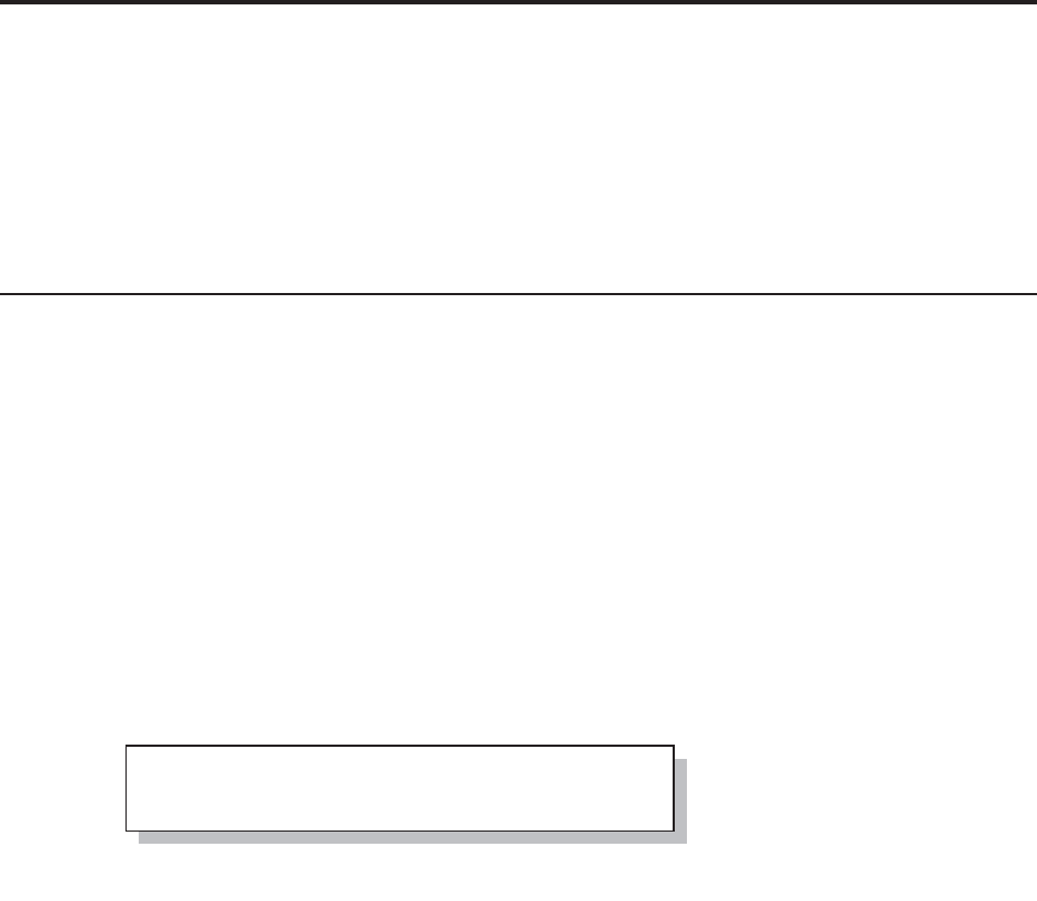
208 Carpenter’s Guide to Innovative SAS Techniques
5.4 Protecting Passwords
When using SQL pass-through statements to access remote databases we often have to pass user
identification and password information to the remote database. If we use those passwords in our
program, our user ID and password will be surfaced for all to see. Very often we need to protect
our passwords and to a lesser extent our user ID. The level of protection will vary from industry to
industry, but the basics are the same.
Fortunately there are a number of ways to protect our passwords.
5.4.1 Using PROC PWENCODE
The PWENCODE procedure can be used to encode or encrypt passwords. Encoding is a text
substitution technique that disguises your password through a series of text substitutions.
Encryption, which is a more secure method than encoding (available starting in SAS 9.2), uses
mathematical operations in the transformation of the text.
I have had very limited success at using this procedure to protect passwords. First, encoding is not
a very strong protection, but more importantly the encoded or encrypted text can often be used
instead of the password. It does not particularly matter if the bad guys cannot ‘see’ the actual
password if the encoded text string, which they can see, will work in its place.
Encoding or encrypting your password through PROC PWENCODE creates and then allows you
to use a text string instead of the actual password. It protects your password from being viewed
directly, since only the encoded/encrypted string is visible. However, remember that the visible
string, while not the password, can still be used as the password. This means that we will also
need to protect this encoded/encrypted string.
In this PWENCODE step our
password ‘pharmer’ is to be
encrypted (under SAS 9.1 the
default was encoding). As the
procedure executes, the encrypted value of ‘pharmer’ is written to the text file (PWFILE.TXT) as:
{sas002}81F6943F251507393B969C0753B2D73B and is not otherwise surfaced
for viewing.
Once the value has been stored in the text file, it can be recovered and used at some point in the
future. The SAS documentation for PROC PWENCODE shows how this value can be stored in a
macro variable or written to the LOG. Both approaches are not practical, because if the user (or
someone else) can see the encoded/encrypted value, they can then use it instead of the real
password. They may not know your real password, but that does not matter; they still have access
to your data.
We need to be able to use the password without ever surfacing its value, either in a macro variable
or to the LOG. In the following DATA step the LIBNAME function is used to create a libref
which establishes an ODBC connection to an SQL server. The password is recovered from the
text file and the value is inserted into the PASSWORD= option.
filename pwfile "&path\results\pwfile.txt";
proc pwencode in='pharmer' out=pwfile;
run;
&DUSHQWHU$UW&DUSHQWHU¶V*XLGHWR,QQRYDWLYH6$67HFKQLTXHV&RS\ULJKW6$6,QVWLWXWH,QF&DU\1RUWK&DUROLQD86$
$
//5,*+765(6(59(')RUDGGLWLRQDO6$6UHVRXUFHVYLVLWVXSSRUWVDVFRPSXEOLVKLQJ

Chapter 5: Working with Data Sets 209
The encoded/encrypted password cannot be utilized in all coding situations that require the use of
a password. For example, the RENAME function (see Section 5.6.1) allows the use of passwords,
but restricts them to 8 characters (this limitation should be fixed in a future release of SAS).
MORE INFORMATION
The discussion in Section 5.4.2 takes an alternate approach to the protection of passwords.
SEE ALSO
Although slightly dated by subsequent releases of SAS, Steven (2007) describes the use of the
PWENCODE procedure.
5.4.2 Protecting Database Passwords
The following method places the sensitive information, such as passwords and user identification
codes, in a protected data set. And then we write our program (the macro %SECRETSQL) to
extract the password without surfacing it.
The data set ADVRPT.PASSTAB includes the user ID and password for several different
databases. The data set itself is encrypted and password protected using data set options.
Notice that the macro variable &SYSLAST has been cleared to remove the name of this data set
from the global symbol table.
The macro %SECRETSQL retrieves the passwords from the password data set and then uses the
information in the SQL pass-through in such a way that the password is never surfaced to the
LOG.
data advrpt.passtab(encrypt=yes pwreq=yes
read=readpwd write=writepwd
alter=chngpwd );
format dsn uid pwd $8.;
dsn='dbprod'; uid='mary'; pwd='wish2pharm'; output;
dsn='dbprod'; uid='john'; pwd='data4you'; output;
dsn='dbdev'; uid='mary'; pwd='hope2pharm'; output;
run;
%let syslast=;
data _null_;
length tmp $1024 opt $1200;
infile pwfile truncover;
input tmp;
opt='dsn=SQLServer user=myid password="'||left(trim(tmp))||'"';
rc=libname('sqlsrv',,'odbc', opt);
txt=sysmsg();
put rc= txt=;
run;
&DUSHQWHU$UW&DUSHQWHU¶V*XLGHWR,QQRYDWLYH6$67HFKQLTXHV&RS\ULJKW6$6,QVWLWXWH,QF&DU\1RUWK&DUROLQD86$
$
//5,*+765(6(59(')RUDGGLWLRQDO6$6UHVRXUFHVYLVLWVXSSRUWVDVFRPSXEOLVKLQJ

210 Carpenter’s Guide to Innovative SAS Techniques
n The macro variables that will contain the sensitive information are placed in the temporary
local symbol table.
o We will read the password from the secret password data set. Notice that the user of this macro
does not even need to know of the existence of the password data set.
p Macro variables are retrieved by using the SYMGET function rather than the more common
macro variable reference with an ampersand (&UU or &DBNAME). This is done because the
SYMGET function does not write macro variable values in the LOG, even when macro
debugging options, such as SYMBOLGEN, are turned on.
q The SYMGET function does not always execute in the CONNECT statement. The macro
quoting function %SUPERQ will also resolve the macro variable without surfacing its value to
the LOG.
r The user creates a macro called %PASSTHRU that contains only those SQL statements that
are to be processed by the remote database. The user does not need to see anything inside the
%SECRETSQL macro.
s The macro call only contains information that is not sensitive.
When the %SECRETSQL macro is kept in a stored compiled macro library, the source statements
will not be available to the person using it (see Section 13.9 and Sun and Carpenter (2011) for
information on protecting the macro code itself).
MORE INFORMATION
Data set options that provide data set protections are described in more detail in Section 2.1.2.
SQL pass-through is introduced in Section 1.5. The PWENCODE procedure can potentially also
be used to provide password security (see Section 5.4.1). Issues dealing with macro source code
security are also discussed in Section 13.9.
SEE ALSO
The %SECRETSQL macro and a number of related techniques are described in more detail by
Sherman and Carpenter (2007).
%macro secretsql(dbname, username);
%local dd uu pp; n
Proc SQL noprint nofeedback;
(
SELECT dsn, uid, pwd into :dd, :uu, :pp
FROM advrpt.passtab(read=readpwd) o
WHERE dsn=trim(symget('dbname')) p
AND uid=trim(symget('username'))
);
connect to odbc(dsn=%superq(dd) uid=%superq(uu) pwd=%superq(pp)); q
create table mylib.mytable as select * from connection to odbc(
%passthru r /* contains your pass-thru SQL statement(s) */
);
disconnect from odbc;
quit;
%mend secretsql;
%secretsql(dbname=dbprod, username=John)s
&DUSHQWHU$UW&DUSHQWHU¶V*XLGHWR,QQRYDWLYH6$67HFKQLTXHV&RS\ULJKW6$6,QVWLWXWH,QF&DU\1RUWK&DUROLQD86$
$
//5,*+765(6(59(')RUDGGLWLRQDO6$6UHVRXUFHVYLVLWVXSSRUWVDVFRPSXEOLVKLQJ

Chapter 5: Working with Data Sets 211
5.5 Deleting Data Sets
There are a number of ways of deleting data sets, both from within SAS and from the operating
system. Although generally we do not need to delete our data sets during the execution of a
program, sometimes when processing especially large data sets, it can be necessary to clear data
sets from the WORK library in order to free up disk space.
PROC DATASETS is the tool most often used from within a SAS program. When using PROC
DATASETS, there are two basic ways of carrying out the deletions.
n The library from which the items are to be deleted is specified.
o Select the type of item to be deleted. Data sets have the MEMTYPE=DATA. When deleting
catalogs the CATALOG procedure can also be used.
p The NOLIST option suppresses the list of members prior to the deletion from being written to
the LOG.
q The KILL option deletes all items of the specified type o to be deleted.
r The DELETE statement lists one or more items to delete from the specified library n.
Although no longer documented, the DELETE procedure is still available. This procedure s is
one of the very few, if not only, procedures
to allow more than one data set name to be
associated with the DATA= option.
Data sets can also be deleted from within an SQL step by using the DROP TABLE statement t.
Notice that more than one table can be listed on
the DROP TABLE statement by separating the
names with a comma.
SEE ALSO
Rosenbloom and Lafler (2011d) discuss the use of PROC DATASETS to delete data sets.
5.6 Renaming Data Sets
Data sets can be renamed using a variety of methods including a number of ways through the use
of the OS tools. Renaming data sets from within a program is also possible, and for some
situations even preferable as the process can be automated using the macro language.
proc datasets library=work n
memtype=data o
nolist p
kill q;
quit;
proc datasets library=work n
memtype=data o
nolist p;
delete male female; r
quit;
proc delete data=male allgender s;
run;
proc sql;
drop table allgender, male; t
quit;
&DUSHQWHU$UW&DUSHQWHU¶V*XLGHWR,QQRYDWLYH6$67HFKQLTXHV&RS\ULJKW6$6,QVWLWXWH,QF&DU\1RUWK&DUROLQD86$
$
//5,*+765(6(59(')RUDGGLWLRQDO6$6UHVRXUFHVYLVLWVXSSRUWVDVFRPSXEOLVKLQJ

212 Carpenter’s Guide to Innovative SAS Techniques
data male
female;
set sashelp.class;
if sex='M' then output male;
else output female;
run;
%let rc=%sysfunc(rename(work.male,Males,data));
%put &RC;
5.6.1 Using the RENAME Function
The DATA step function RENAME can be used to rename data sets, catalogs, and even
directories. Like most DATA step functions it can also be utilized by the macro language. Here
the data set WORK.MALE is being renamed to WORK.MALES.
Notice that the libref for the
new name (second
argument) is implied and is
not explicitly included. The
function returns a 0 for a
successful rename
operation.
5.6.2 Using PROC DATASETS
Within the DATASETS procedure there are two primary methods for renaming data sets and
catalogs:
CHANGE changes or renames a data set
AGE renames a group of data sets to form a series of previous versions
The CHANGE statement is designed to
rename one or more data sets. The data sets
are listed on the CHANGE statement in
OLDNAME=NEWNAME pairs. In this
example the data set WORK.CURRENT is
renamed to WORK.NOW. Because the data
sets are being renamed, not copied (which
uses the COPY statement), the library for the
old and new name will always be the same. If
a data set with the NEW name already exists the rename will not take place.
When you need to retain one or more snapshots (backup) copies of a data set, the AGE statement
can be used to perform the operation. The oldest data set is deleted and then in order of age the
data sets are renamed one at a time. In this example CURRENTV7 would be deleted,
CURRENTV6 is renamed to CURRENTV7, and so on until the most recent version of
CURRENT is renamed to CURRENTV1.
If this AGE statement was executed
every morning, there would be a backup
or ‘aged’ copy of CURRENT for each
day of the week.
data current;
created = datetime();
format created datetime18.;
run;
proc datasets library=work nolist;
change current=now;
quit;
proc datasets library=mydata nolist;
age current currentV1 - currentV7;
quit;
&DUSHQWHU$UW&DUSHQWHU¶V*XLGHWR,QQRYDWLYH6$67HFKQLTXHV&RS\ULJKW6$6,QVWLWXWH,QF&DU\1RUWK&DUROLQD86$
$
//5,*+765(6(59(')RUDGGLWLRQDO6$6UHVRXUFHVYLVLWVXSSRUWVDVFRPSXEOLVKLQJ

Chapter 6
Table Lookup Techniques
6.1 A Series of IF Statements—The Logical Lookup 215
6.2 IF -THEN/ELSE Lookup Statements 215
6.3 DATA Step Merges and SQL Joins 216
6.4 Merge Using Double SET Statements 218
6.5 Using Formats 219
6.6 Using Indexes 221
6.6.1 Using the BY Statement 222
6.6.2 Using the KEY= Option 222
6.7 Key Indexing (Direct Addressing)—Using Arrays to Form a Simple Hash 223
6.7.1 Building a List of Unique Values 223
6.7.2 Performing a Key Index Lookup 224
6.7.3 Using a Non-Numeric Index 226
6.8 Using the HASH Object 227
A table lookup is performed when you use the value of a variable (e.g., a clinic number) to
determine the value of another variable (e.g., clinic name). Often this second piece of information
must be ‘looked up’ in some other secondary table or location. The process of finding the
appropriate piece of information is generally fast; however, as the number of items and/or
observations increases, the efficiency of the process becomes increasingly important. Fortunately
there are a number of techniques for performing these table lookups.
These techniques can be radically different both in terms of programming complexity and in
performance. As the programmer, you will be faced with not only a variety of techniques, but also
performance issues. Which technique will perform best, or even adequately, will vary from
situation to situation. This means that there is no easy answer to the question, ‘Which technique
should I use?’ It is possible, however, to give you some general guidelines.
&DUSHQWHU$UW&DUSHQWHU¶V*XLGHWR,QQRYDWLYH6$67HFKQLTXHV&RS\ULJKW6$6,QVWLWXWH,QF&DU\1RUWK&DUROLQD86$
$
//5,*+765(6(59(')RUDGGLWLRQDO6$6UHVRXUFHVYLVLWVXSSRUWVDVFRPSXEOLVKLQJ
214 Carpenter’s Guide to Innovative SAS Techniques
In this chapter data set size is often used as a decision point for determining which of these
techniques to use. But what exactly is a large data set? This answer too will be situational. It will
depend a lot on your OS and your hardware (including available memory and processing
capabilities). You will know a data set is large when you have to be careful with the techniques
used to process it. For table lookups this chapter will give you alternatives. Each is a compromise
between processing efficiency and coding complexity. Each section should give you sufficient
information to help you make an informed decision. In all cases you will probably want to test
your candidate techniques using your data and your hardware.
6.1 and 6.2 IF – THEN/ELSE
This is the slowest and least sophisticated of the techniques discussed in this chapter; however,
these techniques may be adequate for small data sets and simple lookups.
6.3 Merges and Joins
These techniques tend to be slower than the use of formats (6.5); however, they do allow the
retrieval of multiple items.
6.4 Double SET Statement DATA Steps
Replacing the MERGE statement with a double SET statement generally provides a performance
boost, but the technique is more programming intensive.
6.5 Format-Driven Lookup
These techniques tend to be substantially faster than the use of merges and joins. These
techniques are probably the best first choice for most situations with small to somewhat large data
sets.
6.6 Using Indexes
Indexes can improve the performance of merge and join techniques, especially when the indexes
have already been created. Depending on the situation these techniques might outperform the use
of formats.
6.7 Key Indexing (Array Processing)
The use of DATA step arrays and memory eliminates the need for sorting. Although there are
potential memory constraints, key indexing typically out performs merges and joins, and for
larger data sets out performs the use of formats. When it is possible to use them, array (direct
addressing) techniques, such as these, will also generally outperform hash table techniques.
6.8 Hash Tables
Hash tables (hashing) is more flexible than array processing techniques, and except for array
processing techniques, these techniques are typically the fastest of the lookup techniques. Coding
requires an understanding of the DATA step component hash objects and methods. For very large
data sets, the use of hash tables may be the only viable choice.
In each of the examples in this chapter we will be using lookup techniques to determine the clinic
name based on the clinic number.
SEE ALSO
An overview of lookup techniques, which includes several nice examples with explanations, can
be found in Liu (2008). Aker (2002) and Carpenter (2001b) each discuss differences and
programming techniques for lookups including those for match merging, format lookups, and the
use of arrays. An overview of lookup techniques with emphasis on hash tables and hash objects
can be found in Dorfman and Vyverman (2004b). Comparison papers on the efficiency of table
lookup techniques include Stroupe and Jolley (2008) as well as Jolley and Stroupe (2007).
&DUSHQWHU$UW&DUSHQWHU¶V*XLGHWR,QQRYDWLYH6$67HFKQLTXHV&RS\ULJKW6$6,QVWLWXWH,QF&DU\1RUWK&DUROLQD86$
$
//5,*+765(6(59(')RUDGGLWLRQDO6$6UHVRXUFHVYLVLWVXSSRUWVDVFRPSXEOLVKLQJ

Chapter 6: Table Lookup Techniques 215
6.1 A Series of IF Statements—The Logical Lookup
The simplest form of a table lookup makes use of the IF-THEN statement. Although easy to code,
this is one of the slowest table lookup methods. Essentially this technique creates the new variable
with its associated value through the use of IF-THEN processing. Effectively we are ‘hard coding’
the clinic name within the program. This technique is demonstrated in the following DATA step.
The problem with this approach is that it is not practical if there are more than a very few codes to
lookup; besides this is VERY inefficient. SAS must execute each IF statement even if an earlier
IF statement was found to be true. To make matters worse, IF statements require a fair bit of
processing time.
This is an example of a 100% lookup. It is a sequential search and one where every code is
checked regardless of whether or not the answer has already been found.
6.2 IF -THEN/ELSE Lookup Statements
A substantially faster method than the IF-THEN, is to use the IF-THEN / ELSE statement
combination. The following DATA step executes more quickly than the previous one because as
soon as one IF statement is found to be true, its associated ELSE is not executed. Consequently as
soon as an expression is found to be true, none of the remaining IF-THEN / ELSE statements are
executed. This technique can be made somewhat faster if the more likely outcomes are placed
earlier in the list.
In terms of performance efficiency this technique is similar to that of the DATA step’s SELECT
statement and the CASE statement in SQL.
data demognames;
set advrpt.demog(keep=clinnum lname fname);
length clinname $35;
if clinnum='011234' then clinname = 'Boston National Medical';
if clinnum='014321' then clinname = 'Vermont Treatment Center';
if clinnum='107211' then clinname = 'Portland General';
if clinnum='108531' then clinname = 'Seattle Medical Complex';
if clinnum='023910' then clinname = 'New York Metro Medical Ctr';
if clinnum='024477' then clinname = 'New York General Hospital';
run;
data demognames;
set advrpt.demog(keep=clinnum lname fname);
length clinname $35;
if clinnum='011234' then clinname = 'Boston National Medical';
else if clinnum='014321' then clinname = 'Vermont Treatment Center';
else if clinnum='107211' then clinname = 'Portland General';
else if clinnum='108531' then clinname = 'Seattle Medical Complex';
else if clinnum='023910' then clinname = 'New York Metro Medical Ctr';
else if clinnum='024477' then clinname = 'New York General Hospital';
run;
&DUSHQWHU$UW&DUSHQWHU¶V*XLGHWR,QQRYDWLYH6$67HFKQLTXHV&RS\ULJKW6$6,QVWLWXWH,QF&DU\1RUWK&DUROLQD86$
$
//5,*+765(6(59(')RUDGGLWLRQDO6$6UHVRXUFHVYLVLWVXSSRUWVDVFRPSXEOLVKLQJ

216 Carpenter’s Guide to Innovative SAS Techniques
The SELECT statement is on par with the IF-THEN / ELSE combination when performing table
lookups. It can even be a bit faster (Virgle, 1998). Again processing time is minimized when the
most likely match is located early in the list.
Interestingly Virgle (1998) found that the efficiency of the SELECT statement can sometimes be
enhanced by placing the entire expression on the WHEN statement.
There are two overriding issues with these techniques. The primary problem is that the search is
sequential. When the list is long the average number of comparisons goes up quickly, even when
you carefully order the list. The second, but no less important, issue is that these techniques hard
code the values in the program. This is just not smart programming.
Fortunately, the other lookup techniques in this chapter not only avoid hard coding altogether, but
also minimize the need for sequential searches.
6.3 DATA Step Merges and SQL Joins
The use of joins in an SQL step and the MERGE in the DATA step is another very common way
to perform table lookups by matching values between two data sets. The MERGE statement
(when used with the BY statement as it usually is) requires sorted or indexed data sets, while the
SQL step does not. There are advantages and disadvantages to both processes.
MERGE Statement
The MERGE statement is used to combine two or more data sets. For the purpose of this
discussion, one of these data sets will contain the information that is to be looked up. The BY
statement is used to make sure that the observations are correctly aligned. The BY statement
data demognames;
set advrpt.demog(keep=clinnum lname fname);
select(clinnum);
when( '011234') clinname='Boston National Medical';
when( '014321') clinname='Vermont Treatment Center';
when( '107211') clinname='Portland General';
when( '108531') clinname='Seattle Medical Complex';
when( '023910') clinname='New York Metro Medical Ctr';
when( '024477') clinname='New York General Hospital';
otherwise;
end;
run;
data demognames;
set advrpt.demog(keep=clinnum lname fname);
select;
when(clinnum='011234') clinname='Boston National Medical';
when(clinnum='014321') clinname='Vermont Treatment Center';
when(clinnum='107211') clinname='Portland General';
when(clinnum='108531') clinname='Seattle Medical Complex';
when(clinnum='023910') clinname='New York Metro Medical Ctr';
when(clinnum='024477') clinname='New York General Hospital';
otherwise;
end;
run;
&DUSHQWHU$UW&DUSHQWHU¶V*XLGHWR,QQRYDWLYH6$67HFKQLTXHV&RS\ULJKW6$6,QVWLWXWH,QF&DU\1RUWK&DUROLQD86$
$
//5,*+765(6(59(')RUDGGLWLRQDO6$6UHVRXUFHVYLVLWVXSSRUWVDVFRPSXEOLVKLQJ

Chapter 6: Table Lookup Techniques 217
should include sufficient variables to form a unique key in all but at most one of the data sets. For
the example below ADVRPT.CLINICNAMES has exactly one observation for each value of
CLINNUM.
Because the BY statement is used, the data must be sorted. Sorting can be time consuming, or
even on occasion impossible for very large data sets or for data sets on tape. In the following steps
PROC SORT is used to reorder the data into temporary (WORK) data sets. These are then merged
using the MERGE statement.
For a successful lookup using the
MERGE statement, both of the incoming
data sets must be indexed or in sorted
order and as was discussed in Chapter 4
sorting can be operationally expensive.
The following PROC PRINT listing of
the first 10 observations of the merged
data shows that the CLINICNAME has
been successfully acquired.
As anticipated the observations are
sorted by CLINNUM. Notice also that
the variable CLINNAME, which came
from the right-most data set in the
MERGE statement, is last on the PDV.
The IF statement n has been used to eliminate any clinic numbers in CLINICNAMES that do not
appear in DEMOG. This logic will not eliminate cases where there is a clinic number in DEMOG
that does not appear in CLINICNAMES (the clinic name will be missing). If we want to restrict
the lookup to only those clinic numbers with matches in CLINICNAMES, the IF statement n
could be replaced with if indemog and innames;. This result is achieved directly in the
SQL join discussed next o.
proc sort data=advrpt.demog
out=demog;
by clinnum;
run;
proc sort data=advrpt.clinicnames
out=clinicnames;
by clinnum;
run;
data demognames(keep=clinnum clinname
lname fname);
merge demog(in=indemog)
clinicnames(in=innames);
by clinnum;
if indemog; n
run;
6.3 Lookup By Joining or Merging Two Tables
10 Observations of the merged data
Obs clinnum lname fname clinname
1 011234 Nabers David Boston National Medical
2 011234 Taber Lee Boston National Medical
3 014321 Lawless Henry Vermont Treatment Center
4 014321 Mercy Ronald Vermont Treatment Center
5 023910 Atwood Teddy New York Metro Medical Ctr
6 023910 Harbor Samuel New York Metro Medical Ctr
7 023910 Leader Zac New York Metro Medical Ctr
8 024477 Haddock Linda New York General Hospital
9 024477 Little Sandra New York General Hospital
10 024477 Maxwell Linda New York General Hospital
. . . . portions of the table are not shown . . . .
&DUSHQWHU$UW&DUSHQWHU¶V*XLGHWR,QQRYDWLYH6$67HFKQLTXHV&RS\ULJKW6$6,QVWLWXWH,QF&DU\1RUWK&DUROLQD86$
$
//5,*+765(6(59(')RUDGGLWLRQDO6$6UHVRXUFHVYLVLWVXSSRUWVDVFRPSXEOLVKLQJ

218 Carpenter’s Guide to Innovative SAS Techniques
SQL Join
When using SQL, the merging process is called a join. The SQL join operations do not require
sorting and can be more efficient than the DATA step MERGE, unless the tables are so large that
they do not fit well into memory.
Just because an SQL join does not require the incoming data to be sorted, does not mean that no
resources are going to be expended in preparation for the join (lookup). Hidden from view, but
within the processing of the SQL step, lookup techniques are being applied. These behind the
scenes operations are very similar to the hash techniques that we can explicitly apply and control
in the DATA step (see Sections 6.7 and 6.8).
There are a number of different types of joins within SQL, and one that closely matches the
previous step is shown below.
In this example we have added the requirement (through the use of a WHERE clause o) that the
clinic number be in both data
tables. The WHERE clause is
used to select rows that have
matching values of
CLINNUM on both incoming
tables. This is a more stringent
criteria than was used in the
DATA step shown above n.
SQL does not require either of the two data sets to be sorted prior to the join, and unless we
specifically request that the resulting data table be sorted (ORDER BY clause) it will reflect the
order of the incoming data. This can be seen in the order of the clinic number in the PROC
PRINT results shown below.
6.4 Merge Using Double SET Statements
There are a number of schemes that have been published that utilize two SET statements in the
same DATA step. These SET statements replace the single MERGE statement and the
programmer takes charge of the joining process (keeping the two data sets in sync). These
techniques can be faster but more complicated than a MERGE. However they do still require that
both incoming data sets be sorted.
6.3 Lookup By Joining or Merging Two Tables
10 Observations of the Joined data
Obs clinnum clinname lname fname
1 049060 Atlanta General Hospital Adams Mary
2 082287 Denver Security Hospital Adamson Joan
3 066789 Austin Medical Hospital Alexander Mark
4 063742 Houston General Antler Peter
5 023910 New York Metro Medical Ctr Atwood Teddy
6 066789 Austin Medical Hospital Banner John
7 046789 Tampa Treatment Complex Baron Roger
8 049060 Atlanta General Hospital Batell Mary
9 095277 San Francisco Bay General Block Will
10 031234 Bethesda Pioneer Hospital Candle Sid
. . . . portions of the table are not shown . . . .
proc sql noprint;
create table demognames2 as
select a.clinnum, b.clinname, lname, fname
from advrpt.demog a, advrpt.clinicnames b
where a.clinnum=b.clinnum; o
quit;
&DUSHQWHU$UW&DUSHQWHU¶V*XLGHWR,QQRYDWLYH6$67HFKQLTXHV&RS\ULJKW6$6,QVWLWXWH,QF&DU\1RUWK&DUROLQD86$
$
//5,*+765(6(59(')RUDGGLWLRQDO6$6UHVRXUFHVYLVLWVXSSRUWVDVFRPSXEOLVKLQJ

Chapter 6: Table Lookup Techniques 219
In this example, the two incoming data sets have already been sorted (by CLINNUM). The
primary data set
contains the
observations for
which we need the
clinic name. The
secondary data set
(CLINICNAMES)
contains just the
names that are to be
retrieved. It is both
possible and even
likely that the lookup
data set will contain
values that have no match in the first or primary data set. This is fine as long as we plan for the
possibility p.
n An observation is read from the primary data set. Because DEMOG and CLINICNAMES both
use the variable CLINNUM to hold the clinic number, when it is read from the DEMOG data set
it is renamed CODE. This allows us to access and compare the clinic numbers from both data sets
at the same time opr.
o The value of CODE (clinic number from DEMOG) is compared to the value of CLINNUM,
which comes from the second data set (CLINICNAMES). On the very first pass, no observation
will have been read from CLINICNAMES, and CLINNUM will be missing. Codes that do not
have matching names will not be written out r.
p The DO WHILE is used to read successive rows from the second data set.
q It is possible that there are codes and names in the CLINICNAMES data set that are not in the
primary data set (DEMOG). These observations will necessarily have a CLINNUM that is less
than CODE. This loop p cycles through any extra names until the second data set ‘catches up’ to
the first (CODE=CLINNUM).
r This code matches the current value of CLINNUM and the observation is written out.
As in the MERGE example shown earlier, the data still have to be sorted before the above DATA
step can be used. Although the sorting restrictions are the same as when you use the MERGE
statement, the advantage of the double SET can be a substantial reduction in processing time.
MORE INFORMATION
The use of two SET statements in one DATA step is introduced in Section 3.8.4 and used in
examples in Sections 3.1.5 and 3.1.6.
6.5 Using Formats
The use of FORMATS allows us to step away from the logical processing of assignment
statements, and to take advantage of the search techniques that are an inherent part of the use of
FORMATS. When a value is retrieved from a format, a binary search is used and this means that
we can search 2N items in N or fewer tries. With 10 guesses we can search over 1000 items. Since
binary searches operate by iteratively splitting a list in half until the target is found, these searches
tend to be faster than sequential searches—especially as the number of items increases.
data withnames(keep=subject clinnum clinname);
set demog(rename=(clinnum=code)); n
* The following expression is true only when
* the current CODE is a duplicate.;
if code=clinnum then output; o
do while(code>clinnum); p
* lookup the clinic name using the code (clinnum)
* from the primary data set;
set clinicnames(keep=clinnum clinname); q
if code=clinnum then output; r
end;
run;
&DUSHQWHU$UW&DUSHQWHU¶V*XLGHWR,QQRYDWLYH6$67HFKQLTXHV&RS\ULJKW6$6,QVWLWXWH,QF&DU\1RUWK&DUROLQD86$
$
//5,*+765(6(59(')RUDGGLWLRQDO6$6UHVRXUFHVYLVLWVXSSRUWVDVFRPSXEOLVKLQJ

220 Carpenter’s Guide to Innovative SAS Techniques
For many users, especially those with smaller data sets and lookup tables, the efficiency gains
realized here may be sufficient for most if not all tasks. Formats with several thousands of items
have been used successfully as lookup tables.
Formats can be built and added to a library (permanent or temporary) through the use of PROC
FORMAT (see Chapter 12). The process of creating a format is both fast and straightforward. The
following format ($CNAME.) contains an association between the clinic code and its name.
Of course typing in a few values is
not a ‘big deal’; however, as the
number of entries increases the
process tends to become tedious and
error prone. Fortunately it is possible
to build a format directly from a SAS
data set. The CNTLIN= option
identifies a data set that contains
specific variables. These variables
store the information needed to build
the format, and as a minimum must include the name of the format (FMTNAME), the incoming
value (START), and the value that the incoming value will be translated to (LABEL). The
following DATA step builds the data set CONTROL, which is used by PROC FORMAT. Notice
the use of the RENAME= option and the RETAIN statement. One advantage of this technique is
that the control data set does not need to be sorted.
Since we already have a data set with the matched value pairs (ADVRPT.CLINICNAMES), it is a
perfect candidate for
building a format
automatically.
n The control data
set containing the
variables
(FMTNAME,
START, and
LABEL) is created
based on the data set ADVRPT.CLINICNAMES.
o The START variable (left side of the = sign in the value statement) is created by renaming
CLINNUM.
p The LABEL variable (right side of the = sign in the value statement) is created by renaming
CLINNAME.
q The format name is a constant and is created using the RETAIN statement.
r The format is created by PROC FORMAT through the use of the CNTLIN= option which
points to the control data set.
proc format;
value $cname
'011234'='Boston National Medical'
'014321'='Vermont Treatment Center'
'107211'='Portland General'
'108531'='Seattle Medical Complex'
'023910'='New York Metro Medical Ctr'
. . . . some code not shown . . . .
'024477'='New York General Hospital';
run;
data control; n
set advrpt.clinicnames(keep=clinname clinnum
rename=(clinnum=start o
clinname=label)); p
retain fmtname '$cname'; q
run;
proc format cntlin=control; r
run;
&DUSHQWHU$UW&DUSHQWHU¶V*XLGHWR,QQRYDWLYH6$67HFKQLTXHV&RS\ULJKW6$6,QVWLWXWH,QF&DU\1RUWK&DUROLQD86$
$
//5,*+765(6(59(')RUDGGLWLRQDO6$6UHVRXUFHVYLVLWVXSSRUWVDVFRPSXEOLVKLQJ

Chapter 6: Table Lookup Techniques 221
Once the format has been defined, the PUT function s can be used to assign a value to the
variable CLINICNAME
by using the $CNAME.
format.
Remember the PUT
function always returns a
character string; when a numeric value is required, the INPUT function can be used. The length of
the new variable is determined by the format used in the PUT function. If no length is specified,
as in this example, the variable’s length will be based on the longest value in the format ($27. in
this example). A shorter format width, say $CNAME20., would cause the variable to have the
shorter length (truncation would be a possibility). Values longer than the longest formatted value
will not increase the variable’s length past the longest formatted value.
The previous DATA step will be substantially faster than the IF-THEN/ELSE or SELECT
processing steps shown above. The difference becomes even more dramatic as the number of
items in the lookup list increases. The lookup itself will use the format $CNAME., and hence will
employ a binary search. As a rule of thumb, format searches should be very efficient up until the
number of items to look up exceeds 20,000 or so items.
MORE INFORMATION
An assignment statement technique that outperforms a PUT function lookup when creating a
numeric result is discussed in Section 2.2.3. Data are used to create user-defined formats in
Section 12.7.
6.6 Using Indexes
Indexes are a way to logically sort your data without physically sorting it. If you find that you are
sorting and then re-sorting data to accomplish your various merges, you may find that indexes
will be helpful.
Indexes must be created, stored, and maintained. They are usually created through either PROC
DATASETS (shown below) or through PROC SQL; however, they can also be created in a
DATA step. The index stores the order of the data as if it had been physically sorted. Once an
index exists, SAS will be able to access it, and you will be able to use the data set with the
appropriate BY statement even though the data has never been physically sorted.
Resources are required to create an index, and these resources should be taken into consideration.
Indexes are stored in a separate file, and the size of this file can be substantial especially as the
number of indexes, observations, and variables used to form the indexes increases.
Indexes can substantially speed up processes. They can also SLOW things down (Virgle, 1998).
Not all data sets are good candidates to be indexed and not all variables will form good indexes.
Be sure to read about indexes (see Section 5.3 for more on indexes), and then experiment
carefully before investing a lot in the use of indexes.
data fmtnames(keep=subject clinnum clinname dob);
set demog(keep = subject dob clinnum);
clinname = left(put(clinnum,$cname.)); s
run;
&DUSHQWHU$UW&DUSHQWHU¶V*XLGHWR,QQRYDWLYH6$67HFKQLTXHV&RS\ULJKW6$6,QVWLWXWH,QF&DU\1RUWK&DUROLQD86$
$
//5,*+765(6(59(')RUDGGLWLRQDO6$6UHVRXUFHVYLVLWVXSSRUWVDVFRPSXEOLVKLQJ

222 Carpenter’s Guide to Innovative SAS Techniques
The following example shows the creation of indexes for the two data sets of interest. The library
containing the data sets, ADVRPT, is identified n. The NOLIST option prevents PROC
DATASETS from writing a list of all
the objects in this library to the LOG.
o The MODIFY statement is then
used to name the data sets that are to
receive the indexes. And the INDEX
statement p defines the index for each
data set.
q The unique option forces unique values for CLINNUM.
MORE INFORMATION
The building, maintenance, and use of indexes are discussed further in Section 5.3.
6.6.1 Using the BY Statement
Making use of an index can be as simple as using a BY statement. When the BY variable is an
index, the index is automatically
used, and the data does not need
to be sorted. However relying on
an index to perform a merge is
not necessarily as fast as a merge
on sorted data. The advantage is
that we do not have to sort the
data prior to the merge, and the time required to perform the sort should be taken into
consideration. Assuming the indexes have already been created, one of the following techniques
should generally give you better performance over an indexed merge.
6.6.2 Using the KEY= Option
You can also look up a value when an index exists on only the data set that contains the values to
be looked up. The KEY= option on the SET statement identifies an index that is to be used.
r An observation is read
from the primary,
potentially unsorted data
set. This loads a value for
the index variable
(CLINNUM) into the PDV.
s An observation is read
from the lookup data set. Because the KEY= option has been specified, the observation
corresponding to the current value of CLINNUM is returned. Since this is an indexed read, the
observations read from ADVRPT.DEMOG can be in any order, and values of CLINNUM can be
repeated.
t The temporary variable _IORC_ will be 0 when an indexed value is successfully read. If the
value of CLINNUM is not found, _IORC_ will not be equal to 0 and we will need to supply a
missing value for the clinic name. Otherwise the value of CLINNAME will have been retained
from the previous observation.
proc datasets library=advrpt nolist;n
modify clinicnames; o
index create clinnum p/ unique; q
modify demog; o
index create clinnum; p
quit;
data mrgnames;
merge demog(keep=subject clinnum edu)
clinicnames(keep=clinnum clinname);
by clinnum;
run;
data keynames;
set advrpt.demog
(keep=subject clinnum lname fname); r
set advrpt.clinicnames key=clinnum/unique; s
if _iorc_ne 0 then clinname=' '; t
run;
&DUSHQWHU$UW&DUSHQWHU¶V*XLGHWR,QQRYDWLYH6$67HFKQLTXHV&RS\ULJKW6$6,QVWLWXWH,QF&DU\1RUWK&DUROLQD86$
$
//5,*+765(6(59(')RUDGGLWLRQDO6$6UHVRXUFHVYLVLWVXSSRUWVDVFRPSXEOLVKLQJ

Chapter 6: Table Lookup Techniques 223
The values returned to _IORC_ may change in future releases of SAS. Rather than depend
directly on the value of _IORC_, the SAS supplied autocall library macro %SYSRC can be used
to ‘decode’ the
values contained
in _IORC_. The
following example
is the same as the
previous one, but
it takes advantage
of two of the over
two dozen values
accepted by
%SYSRC. u The
SELECT
statement is used
to compare the
returned _IORC_
value with codes
of interest.
_IORC_ will be an
integer: 0 for success and >0 for various types of failure.
v For a given error mnemonic, the %SYSRC macro returns the number associated with the
associated error. _SOK is the mnemonic for success and %SYSRC returns a 0, which matches the
value of _IORC_.
w When a specific value of CLINNUM is not on the index, the error mnemonic is _DSENOM.
SEE ALSO
Additional examples and discussion on the use of the KEY= option can be found in Aker (2000).
6.7 Key Indexing (Direct Addressing)—Using Arrays to
Form a Simple Hash
Sometimes when sorting is not an option or when you just want to speed up a search, the use of
arrays can be just what you need. Also known as direct addressing, variations on this form of
lookup tend to be the fastest of the lookup techniques discussed in this chapter; however, there are
some restrictions on their use that can limit their flexibility. These techniques require you to
create arrays, sometimes very large arrays. Fortunately under current versions of SAS you can
build arrays that can contain millions of values (Dorfman, 2000a, 2000b).
6.7.1 Building a List of Unique Values
To introduce this topic consider the problem of creating a list of unique values from a data set. In
terms of the data sets being used in this set of examples, we would like to establish a list of unique
clinic numbers within the data set
ADVRPT.DEMOGS. One of several ways that you
could use to solve this problem is shown to the left.
Here PROC SORT uses a NODUPKEY option to
build a data set with unique values of CLINNUM.
data rckeylookup;
set advrpt.demog(keep=subject clinnum lname fname);
set advrpt.clinicnames key=clinnum/unique;
select (_iorc_); u
when (%sysrc(_sok)) do; v
* lookup was successful;
output;
end;
when (%sysrc(_dsenom)) do; w
* No matching clinic number found;
clinname='Unknown';
output;
end;
otherwise do;
put 'Problem with lookup ' clinnum=;
stop;
end;
end;
run;
proc sort data=advrpt.demog
out=uniquenums
nodupkey;
by clinnum;
run;
&DUSHQWHU$UW&DUSHQWHU¶V*XLGHWR,QQRYDWLYH6$67HFKQLTXHV&RS\ULJKW6$6,QVWLWXWH,QF&DU\1RUWK&DUROLQD86$
$
//5,*+765(6(59(')RUDGGLWLRQDO6$6UHVRXUFHVYLVLWVXSSRUWVDVFRPSXEOLVKLQJ

224 Carpenter’s Guide to Innovative SAS Techniques
This works, assuming that the data set can be sorted and that the cost of the resources expended in
the sorting process is reasonable. An alternate method appropriate for data sets of all sizes makes
use of DATA step arrays.
To avoid sorting, we somehow have to “remember” which clinic codes we have already seen. The
way to do this is to use the ARRAY statement. The beauty of this technique is that the search is
very quick because it has to check only one item. We accomplish this by using the clinic code
itself as the index to the array.
n Establish an array with
sufficient dimension to handle all
the clinic numbers.
o Read a clinic number.
p When the array element is
missing, this is the first
occurrence of this clinic number.
Write it out and then mark it r
so it will not be written again.
q Write out this clinic number.
r Mark this number as having been seen.
As an observation is read from the incoming data set, the character clinic code is converted to a
number using the INPUT function and then is used as the index for the ARRAY CHECK. If the
array value is missing, this is the first (unique) occurrence of this clinic number. It is then marked
as found (the value is set to 1). Notice that this step will allow a range of clinic codes from 1 to
999,999. Larger ranges, into the 10s of millions, are easily accommodated.
The array used in the previous example is numeric; however, we could have stored a single byte
character flag and reduced the memory requirements by a factor of 8.
s The array is declared to be
a character array of $1
elements.
t The check is made for a
missing (blank) array value.
u A non-blank character is
stored to indicate that this
clinic number has been found.
6.7.2 Performing a Key Index Lookup
In the previous example an array was used to look up whether or not an item had been found
before. This process of looking up a value is exactly what we do when we merge two data sets. In
the following DATA step the list of codes are read sequentially, once, into an array that stores the
clinic name (instead of just the number 1) again using the clinic code as the array subscript. The
second DO UNTIL then reads the data set of interest. In this loop the clinic name is recovered
from the array and assigned to the variable CLINNAME.
In addition to its speed of execution, a major advantage of this technique is that neither of the
incoming data sets needs to be sorted.
data uniquekey;
array check {999999} _temporary_; n
set advrpt.demog; o
if check{input(clinnum,6.)}=. then do; p
output; q
check{input(clinnum,6.)}=1; r
end;
run;
data uniquekey;
array check {999999} $1 _temporary_; s
set advrpt.demog;
if check{input(clinnum,6.)}=' ' t then do;
output;
check{input(clinnum,6.)}='x';u
end;
run;
&DUSHQWHU$UW&DUSHQWHU¶V*XLGHWR,QQRYDWLYH6$67HFKQLTXHV&RS\ULJKW6$6,QVWLWXWH,QF&DU\1RUWK&DUROLQD86$
$
//5,*+765(6(59(')RUDGGLWLRQDO6$6UHVRXUFHVYLVLWVXSSRUWVDVFRPSXEOLVKLQJ

Chapter 6: Table Lookup Techniques 225
This technique is known as key indexing because the index of the array is the value of the variable
that we want to use as the lookup value.
The array itself may be numeric or character depending on whether a numeric or character value
is to be retrieved. The index, however, must be numeric (or convertible to numeric as in this
example). Large arrays are common. In this example there are almost a million array elements,
when the example needs a mere 27. Memory is fast, cheap, and generally available on most
modern machines, thus making this overkill a small price.
n A character array of temporary values is established. This array will hold the values to be
retrieved (clinic names), and will be indexed by the clinic number (CLINNUM). The length of the
array elements must be sufficient to hold each value being inserted into the array.
o A loop is used to read all of the observations from the data set that contains the values to be
looked up. Because the temporary variable ALLNAMES is defined using the END= option on the
SET statement, it will be 0 for all observations except the last one, and then it will be assigned the
value of 1 (true).
p The value of the clinic name, CLINNAME, is stored in the array element identified by the
clinic number. The INPUT function is used to convert the character variable CLINNUM into an
integer.
q An observation is read from the primary data set. This loads the value of the clinic number into
the Program Data Vector, PDV, where it can be used to retrieve the clinic name from the
CHKNAME array.
r The clinic name is retrieved from the CHKNAME array using the value of the clinic number
just retrieved from the primary data set.
s Because we have placed the SET statements inside of DO loops, it is necessary to terminate the
DATA step directly.
data clinnames(keep=subject lname fname clinnum clinname);
array chkname {999999} $35 _temporary_; n
do until(allnames); o
set advrpt.clinicnames end=allnames;
chkname{input(clinnum,6.)}=clinname; p
end;
do until(alldemog);
set advrpt.demog(keep=subject lname fname clinnum) q
end=alldemog;
clinname = chkname{input(clinnum,6.)}; r
output clinnames;
end;
stop; s
run;
&DUSHQWHU$UW&DUSHQWHU¶V*XLGHWR,QQRYDWLYH6$67HFKQLTXHV&RS\ULJKW6$6,QVWLWXWH,QF&DU\1RUWK&DUROLQD86$
$
//5,*+765(6(59(')RUDGGLWLRQDO6$6UHVRXUFHVYLVLWVXSSRUWVDVFRPSXEOLVKLQJ

226 Carpenter’s Guide to Innovative SAS Techniques
Because we are working with arrays this technique is not limited to the retrieval of a single value.
In this example we want to retrieve both the clinic name and the region associated with the clinic
number. t The only real difference is the addition of another array.
As was noted above memory is fast and usually readily available. We should still be at least
conscious of our memory usage. In this example the maximum length of a clinic name is 27
characters. Since the ARRAY definition will not affect the length of the new variable (array
elements were defined as $35 and 35>27), this array statement has wasted almost 8 megabytes
(999,999 * 8 bytes) of memory. Although not a lot of memory for a small array such as this one,
you should at least be aware of the overall cost of your array. This technique will not work in all
situations. As the number of array elements increases, the amount of memory used also increases.
Paul Dorfman (2000a) discusses memory limitations. Certainly most modern computers should
accommodate arrays with the number of elements in the millions.
For situations where this technique requires unreasonable amounts of memory, other techniques
such as bitmapping and hashing are available. Again Paul Dorfman is the acknowledged expert in
this area and his cited papers should be consulted for more details.
MORE INFORMATION
In the sample programs associated with this section there is a key indexing example that stores
and retrieves multiple values of multiple variables.
6.7.3 Using a Non-Numeric Index
One of the limitations of the key indexing techniques is that the index to the array must be
numeric. This limitation is overcome completely by the use of hash objects (see Section 6.8). In
the examples in Section 6.7.2 the index is a character string that contains a number; therefore, the
INPUT function can be used to create the numeric index value. What if the character string does
not readily convert to a number?
When the number of items to be looked up is fairly small, for example fewer than 20 or 30
thousand, a format can be used to convert the character key to a number. In this example let’s
assume that CLINNUM could not be converted directly to a number. Instead we create a numeric
informat to create a unique artificial index number.
data crnames(keep=subject lname fname clinnum clinname region);
array chkname {999999} $35 _temporary_;
array chkregn {999999} $2 _temporary_;
do until(allnames);
set advrpt.clinicnames end=allnames;
chkname{input(clinnum,6.)}=clinname;
chkregn{input(clinnum,6.)}=region; t
end;
do until(alldemog);
set advrpt.demog(keep=subject lname fname clinnum)
end=alldemog;
clinname = chkname{input(clinnum,6.)};
region = chkregn{input(clinnum,6.)}; t
output crnames;
end;
stop;
run;
&DUSHQWHU$UW&DUSHQWHU¶V*XLGHWR,QQRYDWLYH6$67HFKQLTXHV&RS\ULJKW6$6,QVWLWXWH,QF&DU\1RUWK&DUROLQD86$
$
//5,*+765(6(59(')RUDGGLWLRQDO6$6UHVRXUFHVYLVLWVXSSRUWVDVFRPSXEOLVKLQJ

Chapter 6: Table Lookup Techniques 227
n A control file is
created that will be used
to build the conversion
format NAM2NUM. (see
Section 12.7).
o The TYPE variable
declares this to be a
numeric informat.
p The label is the
numeric counter.
q Since we are reading
the whole data set (one
observation per unique
clinic number), we can
save the number of
possible values. This
value can be used to
provide a dimension to
the array.
r The CONTROL data
set is used by PROC
FORMAT to create the
NAM2NUM. format.
s The format is used to convert the character value into a usable array index.
6.8 Using the HASH Object
Users with very large data sets are often limited by constraints that are put on them by memory or
processor speed. Often, for instance, it is not practical or perhaps even possible to sort a very large
data set. Unsorted data sets cannot be merged using a BY statement unless the data set is indexed,
and this type of merge is generally not feasible (see Section 6.6.1). Joins in SQL may be possible
by using the BUFFERSIZE option, but this still may not be a useful solution. Fortunately there
are a number of techniques for handling these situations as well.
In Section 6.7.2 an array was used to hold and retrieve values. This is a form of a simple hash
table. In SAS®9 the DATA step has a HASH object that will hold and access the array portion of
this hash array. This hash object is a DATA step component object (DATA step component
objects are introduced and discussed in Section 3.3).
While key indexing is fast and works well, it does have limitations that the hash object can overcome.
Key indexing requires a numeric value as the array index. While techniques have been
developed to work around this limitation, hash objects are designed to work with
character or numeric keys.
Unless using a multi-dimensional array, key indexing can use only a single key while
hash objects can use composite keys.
Multiple fields can be returned with a hash object.
data control(keep=fmtname start label type); n
set advrpt.clinicnames(keep=clinnum
rename=(clinnum=start))
end=eof;
retain fmtname 'nam2num' type 'I'; o
label=_n_; p
output control;
if eof then call symputx('levels',_n_); q
run;
proc format cntlin=control; r
run;
data clinnames(keep=subject lname fname
clinnum clinname);
array chkname {&levelsq} $35 _temporary_;
do until(allnames);
set advrpt.clinicnames end=allnames;
chkname{input(clinnum,nam2num.s)}=clinname;
end;
do until(alldemog);
set advrpt.demog(keep=subject lname fname
clinnum)
end=alldemog;
clinname = chkname{input(clinnum,nam2num.s)};
output clinnames;
end;
stop;
run;
&DUSHQWHU$UW&DUSHQWHU¶V*XLGHWR,QQRYDWLYH6$67HFKQLTXHV&RS\ULJKW6$6,QVWLWXWH,QF&DU\1RUWK&DUROLQD86$
$
//5,*+765(6(59(')RUDGGLWLRQDO6$6UHVRXUFHVYLVLWVXSSRUWVDVFRPSXEOLVKLQJ

228 Carpenter’s Guide to Innovative SAS Techniques
Essentially the hash object defines an array in memory, initializes its values with data from a
table, and sets up an indexing variable or variables that can be either numeric or character.
n The attributes for the variables that are to be retrieved from the hash object need to be
established on the PDV. This SET statement is used only during DATA step compilation to
determine variable attributes.
o The HASH object itself is defined, named, and loaded using the DECLARE statement. The
attributes of the object are then defined using the DEFINEKEY, DEFINEDATA, and
DEFINEDONE methods. This hash object has been named LOOKUP, and has been loaded with
the data that contains the values (CLINNAME) that we want to be able to look up.
p The number of bins (28=256) used by the hash table is specified.
q The DEFINEKEY method is used to list one or more key variables whose values are used to
index the LOOKUP hash table.
r The DEFINEDATA method lists those variables to be added to the LOOKUP hash table. The
values of these variables can be retrieved using the FIND method. Although not needed here, you
may want to include the key variables here as well if they are also to be retrieved.
s A DO UNTIL loop is used to cycle through the observations in the primary data set.
t An observation is read and its value for CLINNUM is loaded into the PDV. Since CLINNUM
is a key variable for the hash object q, its value will automatically be used by the FIND
method v when retrieving the value of the clinic name.
u The temporary variable DONE will be set to 1 when the last observation is read from
ADVRPT.DEMOG.
data hashnames(keep=subject clinnum clinname lname fname);
* Define the attributes for variables on lookup table;
if 0 then set advrpt.clinicnames; n
* Create and load the hash object;
declare hash lookup(dataset: 'advrpt.clinicnames', o
hashexp: 8); p
lookup.defineKey('clinnum'); q
lookup.defineData('clinname'); r
lookup.defineDone();
* Read the primary data;
do until(done); s
set advrpt.demog(keep=subject clinnum lname fname) t
end=done; u
if lookup.find() = 0 then output hashnames; v
end;
stop; w
run;
&DUSHQWHU$UW&DUSHQWHU¶V*XLGHWR,QQRYDWLYH6$67HFKQLTXHV&RS\ULJKW6$6,QVWLWXWH,QF&DU\1RUWK&DUROLQD86$
$
//5,*+765(6(59(')RUDGGLWLRQDO6$6UHVRXUFHVYLVLWVXSSRUWVDVFRPSXEOLVKLQJ

Chapter 6: Table Lookup Techniques 229
v The clinic name, which is being held in the hash table, is retrieved through the use of the FIND
method. This method returns its success (0) or failure. When the retrieval is successful, we write
out the resulting observation (with the clinic name defined).
w Since the SET statement is inside a loop, we should always stop the implied DATA step loop
manually.
The DATA step shown above is commonly coded using something similar to the following
simpler step that is shown here. The definition and loading of the hash object is done inside a DO
block that is executed only once, and the SET statement that reads the ADVRPT.DEMOG data set
t is not within a DO UNTIL loop (thus eliminating the need to include a STOP statement w).
From a performance perspective, it is valuable to understand the difference between these two
DATA steps. While the code used in the former step is more complex, it will probably process
faster than the code shown here. This performance advantage will be more apparent as the size of
the data set ADVRPT.DEMOG increases.
data hashnames(keep=subject clinnum clinname lname fname);
if _n_= 1 then do;
* Define the attributes for variables on lookup table;
if 0 then set advrpt.clinicnames; n
* Create and load the hash object;
declare hash lookup(dataset: 'advrpt.clinicnames', o
hashexp: 8); p
lookup.defineKey('clinnum'); q
lookup.defineData('clinname'); r
lookup.defineDone();
end;
* Read the primary data;
set advrpt.demog(keep=subject clinnum lname fname); t
if lookup.find() = 0 then output hashnames; v
run;
&DUSHQWHU$UW&DUSHQWHU¶V*XLGHWR,QQRYDWLYH6$67HFKQLTXHV&RS\ULJKW6$6,QVWLWXWH,QF&DU\1RUWK&DUROLQD86$
$
//5,*+765(6(59(')RUDGGLWLRQDO6$6UHVRXUFHVYLVLWVXSSRUWVDVFRPSXEOLVKLQJ
230
&DUSHQWHU$UW&DUSHQWHU¶V*XLGHWR,QQRYDWLYH6$67HFKQLTXHV&RS\ULJKW6$6,QVWLWXWH,QF&DU\1RUWK&DUROLQD86$
$
//5,*+765(6(59(')RUDGGLWLRQDO6$6UHVRXUFHVYLVLWVXSSRUWVDVFRPSXEOLVKLQJ

Part 2
Data Summary, Analysis, and Reporting
Chapter 7 MEANS and SUMMARY Procedures 233
Chapter 8 Other Reporting and Analysis Procedures 257
Chapter 9 SAS/GRAPH Elements You Should Know—Even if You Don’t
Use SAS/GRAPH 297
Chapter 10 Presentation Graphics—More than Just SAS/GRAPH 313
Chapter 11 Output Delivery System 325
&DUSHQWHU$UW&DUSHQWHU¶V*XLGHWR,QQRYDWLYH6$67HFKQLTXHV&RS\ULJKW6$6,QVWLWXWH,QF&DU\1RUWK&DUROLQD86$
$
//5,*+765(6(59(')RUDGGLWLRQDO6$6UHVRXUFHVYLVLWVXSSRUWVDVFRPSXEOLVKLQJ
232
&DUSHQWHU$UW&DUSHQWHU¶V*XLGHWR,QQRYDWLYH6$67HFKQLTXHV&RS\ULJKW6$6,QVWLWXWH,QF&DU\1RUWK&DUROLQD86$
$
//5,*+765(6(59(')RUDGGLWLRQDO6$6UHVRXUFHVYLVLWVXSSRUWVDVFRPSXEOLVKLQJ

Chapter 7
MEANS and SUMMARY Procedures
7.1 Using Multiple CLASS Statements and CLASS Statement Options 234
7.1.1 MISSING and DESCENDING Options 236
7.1.2 GROUPINTERNAL Option 237
7.1.3 Order= Option 238
7.2 Letting SAS Name the Output Variables 238
7.3 Statistic Specification on the OUTPUT Statement 240
7.4 Identifying the Extremes 241
7.4.1 Using the MAXID and MINID Options 241
7.4.2 Using the IDGROUP Option 243
7.4.3 Using Percentiles to Create Subsets 245
7.5 Understanding the _TYPE_ Variable 246
7.6 Using the CHARTYPE Option 248
7.7 Controlling Summary Subsets Using the WAYS Statement 249
7.8 Controlling Summary Subsets Using the TYPES Statement 250
7.9 Controlling Subsets Using the CLASSDATA= and EXCLUSIVE Options 251
7.10 Using the COMPLETETYPES Option 253
7.11 Identifying Summary Subsets Using the LEVELS and WAYS Options 254
7.12 CLASS Statement vs. BY Statement 255
While the MEANS and SUMMARY procedures have been a part of Base SAS for a long time
(MEANS is an original procedure), and while these procedures are used extensively, many users
of these procedures actually take advantage of only a fraction of their capabilities. Primarily this
is true because a great deal can be accomplished with fairly simple procedure steps.
&DUSHQWHU$UW&DUSHQWHU¶V*XLGHWR,QQRYDWLYH6$67HFKQLTXHV&RS\ULJKW6$6,QVWLWXWH,QF&DU\1RUWK&DUROLQD86$
$
//5,*+765(6(59(')RUDGGLWLRQDO6$6UHVRXUFHVYLVLWVXSSRUWVDVFRPSXEOLVKLQJ

234 Carpenter’s Guide to Innovative SAS Techniques
class race sex edu;
With recent enhancements (especially in SAS 8 and SAS®9), a number of additional capabilities
have been added to the MEANS and SUMMARY procedures, and even the ‘seasoned’
programmer may not have been exposed to them. This chapter covers some of the more useful of
these capabilities. Because these two procedures have the same capabilities and have very few
differences, most of the examples and text in this chapter will highlight only one of them. In each
case either of the two procedures could be used.
Prior to SAS 6, MEANS and SUMMARY were distinct procedures with overlapping capabilities.
Currently the same software is used behind the scenes regardless of which procedure the user
calls; therefore, their capabilities are now the same. The only real differences between these
procedures are seen in their defaults, and then primarily in the way each procedure creates printed
tables. By default MEANS always creates a table to be printed. If you do not want a printed table
you must explicitly turn it off (NOPRINT option). On the other hand, the SUMMARY procedure
never creates a printed table unless it is specifically requested (PRINT option).
SEE ALSO
Carpenter (2008) discusses these two procedures in more detail, including an introduction as well
as additional options not covered in this book.
7.1 Using Multiple CLASS Statements and CLASS
Statement Options
Although the following discussion concerning the use of multiple CLASS statements and CLASS
statement options is within the context of the MEANS and SUMMARY procedures, it can be
generalized to most procedures that use the CLASS statement.
The CLASS statement can be specified as a single statement or
it can be broken up into a series of CLASS statements. The
order of the CLASS statements determines the overall order of
the classification variables.
The CLASS statement now accepts options and for most
procedures that accept the CLASS statement, a single class
statement can be replaced by a series of CLASS statements.
This allows us to control the application of CLASS statement
options to specific classification variables. One or more options
are specified on a CLASS statement by preceding the option with a slash. While it is not
necessary to have multiple CLASS statements just to apply CLASS statement options, multiple
CLASS statements allow you to apply these options differentially. For instance when you use the
MISSING option on the PROC statement, it is applied to all of the classification variables. By
using multiple CLASS statements along with the MISSING option on the CLASS statement, you
can choose which classification variables are to utilize the MISSING option.
CLASS statement options include:
ASCENDING/DESCENDING (Section 7.1.1)
Analogous to the DESCENDING option in PROC SORT and other procedures, these options
allow you to reverse the order of the displayed values.
class race sex;
class edu;
class race sex;
class edu / missing;
&DUSHQWHU$UW&DUSHQWHU¶V*XLGHWR,QQRYDWLYH6$67HFKQLTXHV&RS\ULJKW6$6,QVWLWXWH,QF&DU\1RUWK&DUROLQD86$
$
//5,*+765(6(59(')RUDGGLWLRQDO6$6UHVRXUFHVYLVLWVXSSRUWVDVFRPSXEOLVKLQJ

Chapter 7: MEANS and SUMMARY Procedures 235
GROUPINTERNAL and EXCLUSIVE (Section 7.1.2)
You can use these two options to control how formats associated with CLASS variables are to be
used when forming groups (see Section 12.1 for the related topic on preloaded formats).
MISSING (Section 7.1.1)
Observations with missing levels of the classification variables are normally excluded from the
analysis. This option allows missing values to represent valid levels of the classification variable.
MLF (Section 12.3)
Multilevel formats allow overlapping formatted levels.
ORDER= (Section 7.1.3)
This option allows you to control the order of the classification variables levels. The ORDER=
option is discussed in more detail in Section 2.6.1.
PRELOADFMT and EXCLUSIVE (Section 12.1.3)
When formats are preloaded they can be used to establish data filters when forming groups.
The following example performs a simple SUMMARY step and generates the data set STATS. In
this step the two classification variables
(RACE and EDU) are used to summarize
the data for the two analysis variables
(HT and WT).
Examination of the partial listing below
shows that only 75 (of the potential 77)
observations were used in the calculation
of the summary statistics. At this point it
is not clear why two of the observations
were excluded from the analysis.
In the examples that follow, this analysis will be repeated using various CLASS statement
options.
MORE INFORMATION
The CLASS statement is not the only statement that can be split. Both the VAR statement and the
CLASS statement are commonly split to allow the assignment of options in PROC TABULATE,
and there is a PROC PRINT example in Section 8.5.2 with multiple VAR statements.
7.1 Single Class Statement
Obs race edu _TYPE_ _FREQ_ htmean wtmean htse wtse
1 . 0 75 67.6000 161.200 0.40670 3.9272
2 10 1 11 71.3636 194.091 0.96552 5.7532
3 12 1 19 67.0526 168.105 0.65102 6.3628
4 13 1 4 70.0000 197.000 1.15470 10.3923
5 14 1 10 64.2000 108.400 0.13333 1.4236
6 15 1 7 65.2857 155.571 0.86504 11.1160
7 16 1 10 70.4000 165.200 0.54160 6.1946
8 17 1 10 65.2000 145.200 0.74237 7.9342
9 18 1 4 69.0000 174.000 2.30940 15.5885
10 1 . 2 42 68.4762 176.143 0.58756 4.0053
11 2 . 2 17 67.6471 162.000 0.76668 8.1633
. . . . portions of the output are not shown . . . .
title1 '7.1 Single Class Statement';
proc summary data=advrpt.demog;
class race edu;
var ht wt;
output out=stats
mean= htmean wtmean
stderr=htse wtse
;
run;
proc print data=stats;
run;
&DUSHQWHU$UW&DUSHQWHU¶V*XLGHWR,QQRYDWLYH6$67HFKQLTXHV&RS\ULJKW6$6,QVWLWXWH,QF&DU\1RUWK&DUROLQD86$
$
//5,*+765(6(59(')RUDGGLWLRQDO6$6UHVRXUFHVYLVLWVXSSRUWVDVFRPSXEOLVKLQJ

236 Carpenter’s Guide to Innovative SAS Techniques
7.1.1 MISSING and DESCENDING Options
It is very important to understand that all SAS procedures eliminate an entire observation from the
analysis if any one of the classification variables has a missing value. This is true for both
explicitly declared classification variables (through the use of the CLASS statement), or implicitly
declared classification variables such as those on the TABLES statement in PROC FREQ (which
does not use a CLASS statement). Since the entire observation is eliminated, this can affect data
summaries that do not even include the offending classification variable. This is a problem that
can result in incorrect analyses.
The data table ADVRPT.DEMOG has 77 rows; however, because of missing values in one or
both of the classification variables, only 75 observations have been used in the previous summary
(Section 7.1). From the LISTING above, or even by inspection of the LOG, it is unclear which
classification variable has the missing values.
In the next example, the DESCENDING option is applied to RACE and the MISSING option is
applied to the classification variable EDU.
n The groups formed by RACE are now shown
in decreasing (DESCENDING) order.
o A missing value for the variable EDU will
now be considered to be a valid level and will be
included in the report. Any observation with a
missing value for RACE will still be excluded.
The overall number of observations is now 76, and we can see that there is one observation with a
missing value of EDU (OBS=2 in the listing). Since there are 77 observations in the data set, there
must be an observation with a missing value for RACE as well.
7.1.1 Multiple Class Statements
MISSING and DESCENDING Options
Obs race edu _TYPE_ _FREQ_ htmean wtmean htse wtse
1 . 0 76 67.6053 162.237 0.40135 4.0115
2 . o 1 1 68.0000 240.000 . .
3 10 1 11 71.3636 194.091 0.96552 5.7532
4 12 1 19 67.0526 168.105 0.65102 6.3628
5 13 1 4 70.0000 197.000 1.15470 10.3923
6 14 1 10 64.2000 108.400 0.13333 1.4236
7 15 1 7 65.2857 155.571 0.86504 11.1160
8 16 1 10 70.4000 165.200 0.54160 6.1946
9 17 1 10 65.2000 145.200 0.74237 7.9342
10 n 18 1 4 69.0000 174.000 2.30940 15.5885
11 5 . 2 4 66.5000 147.000 0.86603 0.0000
12 4 . 2 4 64.5000 113.500 0.28868 0.8660
13 3 . 2 8 65.0000 112.000 0.65465 4.5826
14 2 . 2 18 67.6667 166.333 0.72310 8.8325
15 1 . 2 42 68.4762 176.143 0.58756 4.0053
. . . . portions of the table are not shown . . . .
proc summary data=advrpt.demog;
class race/descending; n
class edu/missing; o
var ht wt;
output out=stats
mean= htmean wtmean
stderr=htse wtse
;
run;
&DUSHQWHU$UW&DUSHQWHU¶V*XLGHWR,QQRYDWLYH6$67HFKQLTXHV&RS\ULJKW6$6,QVWLWXWH,QF&DU\1RUWK&DUROLQD86$
$
//5,*+765(6(59(')RUDGGLWLRQDO6$6UHVRXUFHVYLVLWVXSSRUWVDVFRPSXEOLVKLQJ

Chapter 7: MEANS and SUMMARY Procedures 237
7.1.2 GROUPINTERNAL Option
When a classification variable is associated with a format, that format is used in the formation of
the groups. In the next example, the EDULEVEL. format maps the years of education into levels
of education.
n The EDULEVEL. format maps
years of education into three ranges.
o In the SUMMARY step the
FORMAT statement has been used to
create the association between EDU
and the EDULEVEL. format.
p The MISSING option has not been
applied; consequently missing values
of EDU will not be included in the
summary.
A PROC PRINT LISTING of the
resulting data table shows that the
SUMMARY procedure has used the
format to collapse the individual levels
of EDU into the three levels of the
formatted classification variable.
To use the original data values (internal values) to form the groups, rather than the formatted
values, the GROUPINTERNAL option is added to the
CLASS statement.
Notice that
although the
original values of
EDU are used to
form the groups,
the formatted
values are still
displayed. In this
example we could
have achieved
similar results by
using the
ORDER=INTERNAL option shown in Section 7.1.3.
title1 '7.1.2 CLASS Statement Options';
proc format;
value edulevel n
0-12 = 'High School'
13-16= 'College'
17-high='Post Graduate';
run;
title2 'GROUPINTERNAL not used';
proc summary data=advrpt.demog;
class edu; p
var ht wt;
output out=stats
mean= MeanHT MeanWT
;
format edu edulevel.; o
run;
proc print data=stats;
run;
class edu/groupinternal;
7.1.2 CLASS Statement Options
Using GROUPINTERNAL
Obs edu _TYPE_ _FREQ_ MeanHT MeanWT
1 . 0 76 67.5526 160.461
2 High School 1 11 71.3636 194.091
3 High School 1 19 67.0526 168.105
4 College 1 4 70.0000 197.000
5 College 1 11 64.1818 108.091
6 College 1 7 65.2857 155.571
7 College 1 10 70.4000 165.200
8 Post Graduate 1 10 65.2000 145.200
9 Post Graduate 1 4 69.0000 174.000
7.1.2 CLASS Statement Options
GROUPINTERNAL not used
Obs edu _TYPE_ _FREQ_ MeanHT MeanWT
1 . 0 76 67.5526 160.461
2 High School 1 30 68.6333 177.633
3 College 1 32 67.0938 147.438
4 Post Graduate 1 14 66.2857 153.429
&DUSHQWHU$UW&DUSHQWHU¶V*XLGHWR,QQRYDWLYH6$67HFKQLTXHV&RS\ULJKW6$6,QVWLWXWH,QF&DU\1RUWK&DUROLQD86$
$
//5,*+765(6(59(')RUDGGLWLRQDO6$6UHVRXUFHVYLVLWVXSSRUWVDVFRPSXEOLVKLQJ

238 Carpenter’s Guide to Innovative SAS Techniques
7.1.3 Order= Option
When procedures create ordered output, often based on the classification variables, there are
several different criteria that can be used to determine the order. The ORDER= option is used to
establish the scheme, which establishes the ordering criteria. The ORDER= option can generally
appear on the PROC statement where it applies to all the classification variables (implicit or
explicit), or as an option on the CLASS statement where it can be applied to selected
classification variables.
These schemes include:
DATA order is based on the order of the incoming data
FORMATTED values are formatted first and then ordered
FREQ the order is based on the frequency of the class level
INTERNAL same as UNFORMATTED or GROUPINTERNAL
The default ordering is always INTERNAL (whether or not the variable is formatted) except for
PROC REPORT. In PROC REPORT, formatted variables have a default order of FORMATTED.
Using the ORDER=FREQ option on the CLASS statement causes the table to be ordered
according to the most common levels of education.
In this table EDU has been left unformatted. Notice that the order of the rows for EDU is based on
the value of _FREQ_.
7.2 Letting SAS Name the Output Variables
In each of the examples in Section 7.1, the statistics that are to be calculated and written to the
output data set are explicitly specified. However, you do not necessarily have to specify the
statistics or provide names for the variables that are to hold the calculated values.
OUTPUT Statement without Specified Statistics
When no statistics are specified on the OUTPUT statement, the resulting data set will contain a
specific set of statistics and will be in a different form. Rather than one column per statistic, the
statistics will be in a transposed form—one row per statistic. The type of statistic is named in the
_STAT_ column.
7.1.3 CLASS Statement Options
Using ORDER=FREQ
Obs edu _TYPE_ _FREQ_ MeanHT MeanWT
1 . 0 76 67.5526 160.461
2 12 1 19 67.0526 168.105
3 14 1 11 64.1818 108.091
4 10 1 11 71.3636 194.091
5 17 1 10 65.2000 145.200
6 16 1 10 70.4000 165.200
7 15 1 7 65.2857 155.571
8 18 1 4 69.0000 174.000
9 13 1 4 70.0000 197.000
class edu/order=freq;
&DUSHQWHU$UW&DUSHQWHU¶V*XLGHWR,QQRYDWLYH6$67HFKQLTXHV&RS\ULJKW6$6,QVWLWXWH,QF&DU\1RUWK&DUROLQD86$
$
//5,*+765(6(59(')RUDGGLWLRQDO6$6UHVRXUFHVYLVLWVXSSRUWVDVFRPSXEOLVKLQJ

Chapter 7: MEANS and SUMMARY Procedures 239
This SUMMARY step uses the OUTPUT statement with only the OUT= option. No statistics
have been requested; consequently, a
standard suite of statistics (the same list
for the default printed statistics) are
calculated and included in the data set.
One column (named after the analysis
variable) holds the value for each of the
statistics noted under the variable
_STAT_.
While this form
of data set can
have its uses,
you need to be
careful when
using it, as the
variable HT
contains
different types of
information for
each row.
AUTONAME and AUTOLABEL Options
The OUTPUT statement has always used options to name the summary data set (OUT=), and
usually the summary statistics of interest (e.g., MEAN=, N=, MAX=). A second type of option
can be placed on the OUTPUT statement. These options follow a slash (/) on the OUTPUT
statement and include:
AUTONAME allows MEANS and SUMMARY to determine names for the
generated variables
AUTOLABEL allows MEANS and SUMMARY to supply a label for each
generated variable
LEVELS adds the _LEVELS_ column to the summary data set (see Section
7.11)
WAYS adds the _WAYS_ column to the summary data set (see Section
7.11)
When a statistic is requested on the OUTPUT statement, the variable that it generates has the
default name of the corresponding analysis variable in the VAR statement. Since only one statistic
can be generated using the default name, there will be a naming conflict if default naming is used
when two or more statistics are requested. For this reason the following PROC SUMMARY will
fail because of naming conflicts in the new data set STATS. Actually it only partially fails, which
is probably worse. An error is produced in the LOG, but a partial table is still produced.
title1 '7.2 No Statistics Specified';
proc summary data=advrpt.demog;
class race;
var ht;
output out=stats;
run;
7.2 No Statistics Specified
Obs race _TYPE_ _FREQ_ _STAT_ ht
1 0 76 N 76.0000
2 0 76 MIN 62.0000
3 0 76 MAX 74.0000
4 0 76 MEAN 67.6053
5 0 76 STD 3.4989
6 1 1 42 N 42.0000
7 1 1 42 MIN 62.0000
8 1 1 42 MAX 74.0000
9 1 1 42 MEAN 68.4762
10 1 1 42 STD 3.8078
. . . . portions of the table are not shown . . . .
&DUSHQWHU$UW&DUSHQWHU¶V*XLGHWR,QQRYDWLYH6$67HFKQLTXHV&RS\ULJKW6$6,QVWLWXWH,QF&DU\1RUWK&DUROLQD86$
$
//5,*+765(6(59(')RUDGGLWLRQDO6$6UHVRXUFHVYLVLWVXSSRUWVDVFRPSXEOLVKLQJ

240 Carpenter’s Guide to Innovative SAS Techniques
The AUTONAME option allows you to select multiple
statistics without picking a name for the resulting variables in
the OUTPUT table. The generated names are unique and
therefore naming conflicts are eliminated. Similarly the
AUTOLABEL option
creates a label, which is
based on the analysis
variable’s existing label,
for variables added to the
OUT= data set.
Conveniently the names of the generated variables are both reasonable and predictable, and are in
the form of variable_statistic.
7.3 Statistic Specification on the OUTPUT Statement
When creating variables based on statistics specified on the OUTPUT statement, there are several
ways to name the variables and to associate the resultant variable with the original analysis
variable.
The most traditional way of specifying the statistics and naming the generated variables is shown
to the left. The option specifying the statistic (N=
and MEAN= are shown here) is followed by a
variable list. This form requires the programmer to
make sure that the list of analysis variables and the
list of new variables that hold the values of the
selected statistics are in the same position and order.
The disadvantages of this form include:
The order of the statistics is tied to the order of the analysis variables.
A statistic must be generated for each of the analysis variables; that is, in order to
calculate a mean for WT you must also calculate a mean for HT (since HT is first on the
VAR statement).
This is not the only, or even
necessarily the most practical, way of
specifying the statistics and their
associated variables. A list of
analysis variables can be included in
parentheses as a part of the statistic
7.2 Using AUTONAME
ht_Std
Obs race _TYPE_ _FREQ_ ht_N ht_Mean Err
1 0 76 76 67.6053 0.40135
2 1 1 42 42 68.4762 0.58756
3 2 1 18 18 67.6667 0.72310
4 3 1 8 8 65.0000 0.65465
5 4 1 4 4 64.5000 0.28868
6 5 1 4 4 66.5000 0.86603
proc summary
data=advrpt.demog;
class race;
var ht;
output out=stats
n=
mean=
stderr=
;
run;
output out=stats
n=
mean=
stderr=/autoname
;
var ht wt;
output out=stats
n = n_ht n_wt
mean= mean_HT Mean_WT
;
var ht wt;
output out=stats
n(wt) = n_wt n
mean(wt ht) = mean_WT Mean_HT o
;
&DUSHQWHU$UW&DUSHQWHU¶V*XLGHWR,QQRYDWLYH6$67HFKQLTXHV&RS\ULJKW6$6,QVWLWXWH,QF&DU\1RUWK&DUROLQD86$
$
//5,*+765(6(59(')RUDGGLWLRQDO6$6UHVRXUFHVYLVLWVXSSRUWVDVFRPSXEOLVKLQJ

Chapter 7: MEANS and SUMMARY Procedures 241
option. This allows you to specify a subset of the analysis variables n, as was done here with the
N statistic. You can also use this technique to control the order of the usage of the analysis
variables o.
It is also possible to split up the specification of the statistics of interest. A given statistic can be
specified multiple times, each with a different analysis variable. This form of option specification
gives you quite a bit of flexibility, not only over which statistics will be calculated for which
analysis variables, but also over the order of the
generated variables on the resultant data set.
A PROC PRINT of the data set WORK.STATS
generated by the OUTPUT statement to the left shows the
variable order. You might also notice that SAS
remembers the case of the name of the variable as it is
first defined: Mean_HT as opposed to mean_WT.
It is also possible to specify more than one OUTPUT statement within a given PROC step. Each
OUTPUT statement could have a different combination of statistics.
7.4 Identifying the Extremes
When working with data, it is not at all unusual to want to be able to identify the observations that
contain the highest or lowest values of the analysis variables. These extreme values are
automatically displayed in PROC UNIVARIATE output, but must be requested in the MEANS
and SUMMARY procedures.
While the MIN and MAX statistics show the extreme value, they do not identify the observation
that contains the extreme. Fortunately there are a couple of ways to identify the observation that
contains the MAX or MIN.
7.4.1 Using the MAXID and MINID Options
The MAXID and MINID options in the OUTPUT statement can be used to identify the
observations with the maximum and minimum values (the examples in this section are for
MAXID; however, MINID has the same syntax). The general form of the option is:
var ht wt;
output out=stats
n(wt) = n_wt
mean(wt) = mean_WT
n(ht) = n_ht
mean(ht) = Mean_HT
;
7.3 Splitting the Stat(varlist)=
Obs race _TYPE_ _FREQ_ n_wt mean_WT n_ht Mean_HT
1 0 76 76 162.237 76 67.6053
2 1 1 42 42 176.143 42 68.4762
3 2 1 18 18 166.333 18 67.6667
4 3 1 8 8 112.000 8 65.0000
5 4 1 4 4 113.500 4 64.5000
6 5 1 4 4 147.000 4 66.5000
MAXID(analysis_var_list(ID_var_list))=new_var_list
&DUSHQWHU$UW&DUSHQWHU¶V*XLGHWR,QQRYDWLYH6$67HFKQLTXHV&RS\ULJKW6$6,QVWLWXWH,QF&DU\1RUWK&DUROLQD86$
$
//5,*+765(6(59(')RUDGGLWLRQDO6$6UHVRXUFHVYLVLWVXSSRUWVDVFRPSXEOLVKLQJ

242 Carpenter’s Guide to Innovative SAS Techniques
The MAXID option is used in the following example to identify which subjects had the
maximums for each value of any classification variables. This option allows us to add a new
variable to the OUTPUT data set, which takes on the value of the ID variable for the maximum
observation.
The maximum for the analysis
variable HT is requested n for
each RACE. We would also like
to know which SUBJECT had the
maximum HT o (the subject
number is to be stored in the
variable MAXHTSUBJECT).
Using the same generalized
option syntax as was discussed in
the previous section, there are
several variations of the syntax
for the MAXID option shown in
this example. In this
case there is a single
analysis variable and
a single ID variable.
When there is more
than one analysis
variable, the MAXID
statement can be
expanded following
the same syntax rules
as were discussed in
Section 7.3.
In this example the subject number of the tallest and of the heaviest subjects in the study are to be
displayed.
var ht wt;
output out=stats
mean= meanHT MeanWT
max=maxHt maxWT
maxid(ht(subject) wt(subject))=maxHtSubject MaxWtSubject
;
title1 '7.4.1a Using MAXID';
title2 'One Analysis Variable';
proc summary data=advrpt.demog;
class race;
var ht;
output out=stats
mean= meanHT
max=maxHt n
maxid(ht(subject))=maxHtSubject o
;
run;
proc print data=stats;
run;
7.4.1a Using MAXID
One Analysis Variable
max maxHt
Obs race _TYPE_ _FREQ_ meanHT Ht Subject
n o
1 0 76 67.6053 74 209
2 1 1 42 68.4762 74 209
3 2 1 18 67.6667 72 201
4 3 1 8 65.0000 68 215
5 4 1 4 64.5000 65 244
6 5 1 4 66.5000 68 212
7.4.1b Using MAXID
Two Analysis Variables
max max maxHt MaxWt
Obs race _TYPE_ _FREQ_ meanHT MeanWT Ht WT Subject Subject
1 0 76 67.6053 162.237 74 240 209 203
2 1 1 42 68.4762 176.143 74 215 209 208
3 2 1 18 67.6667 166.333 72 240 201 203
4 3 1 8 65.0000 112.000 68 133 215 215
5 4 1 4 64.5000 113.500 65 115 244 230
6 5 1 4 66.5000 147.000 68 147 212 211
&DUSHQWHU$UW&DUSHQWHU¶V*XLGHWR,QQRYDWLYH6$67HFKQLTXHV&RS\ULJKW6$6,QVWLWXWH,QF&DU\1RUWK&DUROLQD86$
$
//5,*+765(6(59(')RUDGGLWLRQDO6$6UHVRXUFHVYLVLWVXSSRUWVDVFRPSXEOLVKLQJ

Chapter 7: MEANS and SUMMARY Procedures 243
Because of the flexibility for structuring options in the OUTPUT statement, the previous MAXID
option could also have been written as:
When more than one variable is needed to identify the observation with the extreme value, the
MAXID supports a list. As before when specifying lists, there is a one-to-one correspondence
between the two lists (the list of ID variables and the list of generated variables). In this OUTPUT
statement both the SUBJECT and SSN are used in the list of identification variables.
Consequently a new variable is created for each in the summary data set.
7.4.2 Using the IDGROUP Option
The MAXID and MINID options allow you to capture only a single extreme. It is also possible to
display a group of the extreme values using the IDGROUP option.
Like the MAXID and MINID options, this option allows you to capture the maximum or
minimum value and associated ID variable(s). More importantly, however, you may select more
than just the single extreme value.
In this example the
maximum WT has
been requested using
the MAX statistic n.
In addition the
IDGROUP option
has been requested to
identify the two p
individuals
(identified by using
SUBJECT and SEX q) with the largest values of WT o.
r The prefix for the variable name that will hold SUBJECT number with the maximum weight is
MAXSUBJ. Since there is no corresponding prefix for SEX, the original variable will be used as
the prefix. Because we have only one analysis variable, there will not be a naming conflict;
however, not specifying the new variable’s name is generally to be avoided. Even with the
/AUTONAME option in force there can be naming conflicts with only moderately complex
IDGROUP options that do not name the new variables.
var ht wt;
output out=stats
mean= meanHT MeanWT
max=maxHt maxWT
maxid(ht(subject))=maxHtSubject
maxid(wt(subject))=maxWtSubject
;
var ht wt;
output out=stats
mean= meanHT MeanWT
max=maxHt maxWT
maxid(ht(subject ssn))= MaxHtSubject MaxHtSSN
maxid(wt(subject ssn))= MaxWtSubject MaxWtSSN
;
proc summary data=advrpt.demog;
class race;
var wt;
output out=stats
mean= MeanWT
max(wt)=maxWT n
idgroup (max(wt)out[2](subject sex)=maxsubj)
; o p q r
run;
&DUSHQWHU$UW&DUSHQWHU¶V*XLGHWR,QQRYDWLYH6$67HFKQLTXHV&RS\ULJKW6$6,QVWLWXWH,QF&DU\1RUWK&DUROLQD86$
$
//5,*+765(6(59(')RUDGGLWLRQDO6$6UHVRXUFHVYLVLWVXSSRUWVDVFRPSXEOLVKLQJ

244 Carpenter’s Guide to Innovative SAS Techniques
Since we have requested the top two p values, the values are written to MAXSUBJ_1,
MAXSUBJ_2, SEX_1, and SEX_2. Notice that a number indicating the relative position is
appended to the variable name. In this example we can see that the second heaviest subject in the
study had a subject number of 236 and a SEX of M.
The request for the MAX in IDGROUP is actually independent of the MAX= request issued at n.
In the previous example we are able to see who the second heaviest subject was, but because we
used the MAX option, which shows only one value—the heaviest, we cannot see the weight of the
second heaviest individual. This problem disappears with a slight modification of the IDGROUP
option.
In the following example we want to identify the two oldest individuals within each group
(minimum value of
DOB). Since we
want to see the date
of birth for each of
the oldest two
individuals, DOB s
has been included in
the list of ID
variables. Notice that
the MIN statistic, which would show only one DOB, is not being used at all.
SEE ALSO
The IDGROUP option is used to transpose data in King and Zdeb (2010). It is also used in a
subsetting question in the SAS Forum thread
http://communities.sas.com/message/102002102002.
7.4.2a Using IDGROUP
max
Obs race _TYPE_ _FREQ_ MeanWT WT maxsubj_1 maxsubj_2 sex_1 sex_2
1 0 76 162.237 240 203 236 M M
2 1 1 42 176.143 215 208 216 M M
3 2 1 18 166.333 240 203 236 M M
4 3 1 8 112.000 133 215 256 M M
5 4 1 4 113.500 115 230 240 F F
6 5 1 4 147.000 147 211 212 M M
7.4.2b Using IDGROUP with the Analysis Variable
MinDOB_ MinDOB_ Oldest Oldest Oldest Oldest
Obs race _TYPE_ _FREQ_ 1 2 Subj_1 Subj_2 Gender_1 Gender_2
1 0 76 03NOV21 05NOV24 252 269 M M
2 1 1 42 03NOV21 05NOV24 252 269 M M
3 2 1 18 15JAN34 15AUG34 203 236 M M
4 3 1 8 02JUL46 11JUN47 234 268 F M
5 4 1 4 13FEB48 28FEB49 230 240 F F
6 5 1 4 18FEB51 18JUN51 212 214 M M
proc summary data=advrpt.demog;
class race;
var dob;
output out = stats
idgroup (min(dob)out[2](dob s subject sex)=
MinDOB OldestSubj OldestGender)
;
run;
&DUSHQWHU$UW&DUSHQWHU¶V*XLGHWR,QQRYDWLYH6$67HFKQLTXHV&RS\ULJKW6$6,QVWLWXWH,QF&DU\1RUWK&DUROLQD86$
$
//5,*+765(6(59(')RUDGGLWLRQDO6$6UHVRXUFHVYLVLWVXSSRUWVDVFRPSXEOLVKLQJ

Chapter 7: MEANS and SUMMARY Procedures 245
7.4.3 Using Percentiles to Create Subsets
The percentile statistics can be used to create search bounds for potential outlier boundaries.
Several percentile statistics are available including the 1% and 5% bounds. In this example we
would like to know if any observations fall outside of the 1% percentiles.
n The 1st and 99th
percentiles are
calculated and saved
in the data set
STATS.
o The single
observation of
WORK.STATS is
added to the
Program Data Vector
(PDV).
p The analysis data
are read one row at a
time in a DO UNTIL
loop. The END=
option on the SET
statement creates the
numeric 0/1 variable
DONE, which is
used to end the loop.
q Check to see if
the current POTASSIUM reading is above or below the 1st and 99th percentiles.
r A STOP statement has not been used. Although the SET statement is inside the DO UNTIL
loop, the STOP is not necessary because all observations have been read from the STATS data
set.
s The NOBYLINE system option removes the BY variable values from the table created by
PRINT.
t A BY statement is used so that the values can be loaded into the #BYVAL options on the
TITLE statement.
u Since the bounds are constants, the #BYVAL option is used to place them in the title.
Generally TITLE statements are placed outside of the PROC step; however, for better clarity,
when I use the #BYVAR and #BYVAL options I like to move the TITLE statement so that it
follows the BY statement.
MORE INFORMATION
The TITLE statement option #BYVAL is introduced in Section 15.1.2.
title1 '7.4.3 Using Percentiles';
proc summary data=advrpt.lab_chemistry;
var potassium;
output out=stats
p1= n
p99= /autoname;
run;
data chkoutlier;
set stats(keep=potassium_p1 potassium_p99); o
do until (done);
set advrpt.lab_chemistry o
(keep=subject visit potassium)
end=done; p
if potassium_p1 ge potassium
or potassium ge potassium_p99 q
then output chkoutlier;
end; r
run;
options nobyline; s
proc print data=chkoutlier;
by potassium_p1 potassium_p99; t
title2 'Potassium 1% Bounds are #byval1, #byval2'; u
run;
&DUSHQWHU$UW&DUSHQWHU¶V*XLGHWR,QQRYDWLYH6$67HFKQLTXHV&RS\ULJKW6$6,QVWLWXWH,QF&DU\1RUWK&DUROLQD86$
$
//5,*+765(6(59(')RUDGGLWLRQDO6$6UHVRXUFHVYLVLWVXSSRUWVDVFRPSXEOLVKLQJ

246 Carpenter’s Guide to Innovative SAS Techniques
7.5 Understanding the _TYPE_ Variable
One of the variables automatically included in the summary data set is _TYPE_. By default this is
a numeric variable, which can be used to help us track the level of summarization, and to
distinguish the groups of statistics. It is not, however, intuitively obvious how to predict its value.
In this SUMMARY step there are
three variables in the CLASS
statement (RACE, EDU, and
SYMP).
Examination of a listing of the
data set STATS shows that
_TYPE_ varies from 0 to 7 (8
distinct values). With the
_TYPE_=0 associated with the
single row that summarizes across
the entire data set (all three
classification
variables are
ignored), and with
_TYPE_=7
summarizing the
interaction of all
three classification
variables (all three
classification
variables are used).
The remaining
values of _TYPE_
represent other
combinations of
classification
variables and vary
according to which
are used and which
are ignored.
proc summary
data=advrpt.demog
(where=(race in('1','4')
& 12 le edu le 15
& symp in('01','02','03')))
;
class race edu symp;
var ht;
output out=stats
mean= meanHT
;
run;
7.5 Understanding _TYPE_
mean
Obs race edu symp _TYPE_ _FREQ_ HT
1 . 0 8 66.25
2 . 01 1 2 64.00
3 . 02 1 4 66.50
4 . 03 1 2 68.00
5 12 2 4 67.50
6 14 2 2 64.00
7 15 2 2 66.00
8 12 02 3 2 67.00
9 12 03 3 2 68.00
10 14 01 3 2 64.00
11 15 02 3 2 66.00
12 1 . 4 6 67.00
13 4 . 4 2 64.00
14 1 . 02 5 4 66.50
15 1 . 03 5 2 68.00
16 4 . 01 5 2 64.00
17 1 12 6 4 67.50
18 1 15 6 2 66.00
19 4 14 6 2 64.00
20 1 12 02 7 2 67.00
21 1 12 03 7 2 68.00
22 1 15 02 7 2 66.00
23 4 14 01 7 2 64.00
&DUSHQWHU$UW&DUSHQWHU¶V*XLGHWR,QQRYDWLYH6$67HFKQLTXHV&RS\ULJKW6$6,QVWLWXWH,QF&DU\1RUWK&DUROLQD86$
$
//5,*+765(6(59(')RUDGGLWLRQDO6$6UHVRXUFHVYLVLWVXSSRUWVDVFRPSXEOLVKLQJ

Chapter 7: MEANS and SUMMARY Procedures 247
The following table summarizes the eight possible combinations of these three classification
variables for the LISTING shown above. Under the classification variables, a 0 indicates that
levels of the classification variable are being ignored when calculating the summary statistics,
while a 1 indicates that the classification variables is being used. When considered together, these
three zeros and ones (representing each classification variable) form a 3-digit binary number (one
digit for each of the three classification variables. When this binary value is converted to decimal,
the result yields _TYPE_.
CLASS VARIABLES
Observation
Number
RACE EDU SYMP Binary
Value
_TYPE_
1 0 0 0 000 0
2 - 4 0 0 1 001 1
5 - 7 0 1 0 010 2
8 - 11 0 1 1 011 3
12 - 13 1 0 0 100 4
14 - 16 1 0 1 101 5
17 - 19 1 1 0 110 6
20 - 23 1 1 1 111 7
22=4 21=2 20=1
The conversion of a binary number to decimal involves the use of powers of 2. A binary value of
110 = 1*22 + 1*21 + 0*20 = 1*4 + 1*2 + 0*1 = 6 = _TYPE_.
The NWAY option limits the output data set to the highest order interaction and consequently
only the highest value of _TYPE_ would be displayed.
MORE INFORMATION
Interestingly enough, some SAS programmers find converting a binary number to a decimal
number to be inconvenient. The CHARTYPE option (see Section 7.6) makes that conversion
unnecessary.
&DUSHQWHU$UW&DUSHQWHU¶V*XLGHWR,QQRYDWLYH6$67HFKQLTXHV&RS\ULJKW6$6,QVWLWXWH,QF&DU\1RUWK&DUROLQD86$
$
//5,*+765(6(59(')RUDGGLWLRQDO6$6UHVRXUFHVYLVLWVXSSRUWVDVFRPSXEOLVKLQJ

248 Carpenter’s Guide to Innovative SAS Techniques
7.6 Using the CHARTYPE Option
The CHARTYPE option displays _TYPE_ as a character binary value rather than the decimal
value. The following example repeats the example shown in Section 7.5, while adding the
CHARTYPE option on the PROC statement.
Instead of being numeric,
_TYPE_ is now created as a
character variable with a length
corresponding to the number of
classification variables.
proc summary
data=advrpt.demog
(where=(race in('1','4')
& 12 le edu le 15
& symp in('01','02','03')))
chartype;
class race edu symp;
var ht;
output out=stats
mean= meanHT
;
run;
7.6 Using the CHARTYPE Option
mean
Obs race edu symp _TYPE_ _FREQ_ HT
1 . 000 8 66.25
2 . 01 001 2 64.00
3 . 02 001 4 66.50
4 . 03 001 2 68.00
5 12 010 4 67.50
6 14 010 2 64.00
7 15 010 2 66.00
8 12 02 011 2 67.00
9 12 03 011 2 68.00
10 14 01 011 2 64.00
11 15 02 011 2 66.00
12 1 . 100 6 67.00
13 4 . 100 2 64.00
14 1 . 02 101 4 66.50
15 1 . 03 101 2 68.00
16 4 . 01 101 2 64.00
17 1 12 110 4 67.50
18 1 15 110 2 66.00
19 4 14 110 2 64.00
20 1 12 02 111 2 67.00
21 1 12 03 111 2 68.00
22 1 15 02 111 2 66.00
23 4 14 01 111 2 64.00
&DUSHQWHU$UW&DUSHQWHU¶V*XLGHWR,QQRYDWLYH6$67HFKQLTXHV&RS\ULJKW6$6,QVWLWXWH,QF&DU\1RUWK&DUROLQD86$
$
//5,*+765(6(59(')RUDGGLWLRQDO6$6UHVRXUFHVYLVLWVXSSRUWVDVFRPSXEOLVKLQJ

Chapter 7: MEANS and SUMMARY Procedures 249
7.7 Controlling Summary Subsets Using the WAYS
Statement
When you do not need to calculate all possible combinations of the classification variables, you
can save not only the resources used in calculating the unneeded values, but the effort of
eliminating them later as well. There are several ways that you can specify which combinations
are of interest. The WAYS statement can be used to specify the number of classification variables
to utilize.
Combinations of the WAYS statement for three classification variables include the following
summarizations:
ways 0; across all classification variables
ways 1; each classification variable individually (no cross products)
ways 2; each two-way combination of the classification variables (two-way
interactions)
ways 3; three-way interaction. For three classification variables, this is the same
as using the NWAY option
ways 0,3; lists of numbers are acceptable
When the number of classification variables becomes large the WAYS statement can utilize an
incremental list much like an iterative DO.
ways 0 to 9 by 3;
In the following example main effect summaries and the three-way interaction are eliminated; as a
matter of fact, they are not even calculated.
The WAYS statement has been
used to request calculation of
only the overall summary and the
two-way interactions.
Notice in the listing shown below
that _TYPE_ does not take on the
values of 1 or 2. These would be
the main effect summaries for
SYMP and EDU, respectively. A
full examination of the table
shows that _TYPE_
appropriately only takes on the values of 0, 3, 5, and 6.
proc summary data=advrpt.demog
(where=(race in('1','4')
& 12 le edu le 15
& symp in('01','02','03')));
class race edu symp;
var ht;
ways 0,2;
output out=stats
mean= meanHT
;
run;
&DUSHQWHU$UW&DUSHQWHU¶V*XLGHWR,QQRYDWLYH6$67HFKQLTXHV&RS\ULJKW6$6,QVWLWXWH,QF&DU\1RUWK&DUROLQD86$
$
//5,*+765(6(59(')RUDGGLWLRQDO6$6UHVRXUFHVYLVLWVXSSRUWVDVFRPSXEOLVKLQJ

250 Carpenter’s Guide to Innovative SAS Techniques
7.8 Controlling Summary Subsets Using the TYPES
Statement
Like the WAYS statement, the TYPES statement can be used to select and limit the data roll-up
summaries. As an added bonus, the TYPES statement eliminates much of the need to understand
and to be able to use the _TYPE_ automatic variable. While the WAYS statement (see Section
7.7) lists which levels of summarization are desired, TYPES designates specific summarization
levels (effects and interactions).
The TYPES statement used here
explicitly requests that statistics
be calculated only for the main
effect for EDU, and the
interaction between RACE and
SYMP. None of the other effects
or summarizations will even be
calculated.
7.7 Using the WAYS Statement
mean
Obs race edu symp _TYPE_ _FREQ_ HT
1 . 0 8 66.25
2 12 02 3 2 67.00
3 12 03 3 2 68.00
4 14 01 3 2 64.00
5 15 02 3 2 66.00
6 1 . 02 5 4 66.50
7 1 . 03 5 2 68.00
8 4 . 01 5 2 64.00
9 1 12 6 4 67.50
10 1 15 6 2 66.00
11 4 14 6 2 64.00
7.8 Using the TYPES Statement
mean
Obs race edu symp _TYPE_ _FREQ_ HT
1 12 2 4 67.5
2 14 2 2 64.0
3 15 2 2 66.0
4 1 . 02 5 4 66.5
5 1 . 03 5 2 68.0
6 4 . 01 5 2 64.0
proc summary data=advrpt.demog
(where=(race in('1','4')
& 12 le edu le 15
& symp in('01','02','03')));
class race edu symp;
var ht;
types edu race*symp;
output out=stats
mean= meanHT
;
run;
&DUSHQWHU$UW&DUSHQWHU¶V*XLGHWR,QQRYDWLYH6$67HFKQLTXHV&RS\ULJKW6$6,QVWLWXWH,QF&DU\1RUWK&DUROLQD86$
$
//5,*+765(6(59(')RUDGGLWLRQDO6$6UHVRXUFHVYLVLWVXSSRUWVDVFRPSXEOLVKLQJ

Chapter 7: MEANS and SUMMARY Procedures 251
For the following CLASS statement:
class race edu symp;
Variations of the TYPES statement could also include:
types (); overall summary
types race*edu edu*symp; two two-way interactions
types race*(edu symp); two two-way interactions
types race*edu*symp; three-way interaction—same as NWAY
7.9 Controlling Subsets Using the CLASSDATA= and
EXCLUSIVE Options
While the WAYS and TYPES statements control the combinations of classification variables that
are to be summarized, you can also specify which levels of the classification variables are to
appear in the report or output data set by creating a data set that contains the combinations and
levels of interest. The data set can even include levels of classification variables that do not exist
in the data itself, but that nonetheless are to appear in the data set or report.
This DATA step builds a data set
that will be used with the
CLASSDATA= option. As an
illustration, it also adds a level for
each classification variable that
does not exist in the data.
The data set specified with the CLASSDATA
option becomes a sophisticated filter for the data
entering into the analysis.
The CLASSDATA option can be paired with the EXCLUSIVE option to radically change the
observations that are available to the procedure. When the EXCLUSIVE option is not used, all
levels of the classification variables
that exist either in the analysis data
or in the CLASSDATA= data set
are included in the summary data
set. Since we specifically included a
level for each of the classification
variables that are not in the data, we
should expect to see them
summarized in the summary data set.
data selectlevels(keep=race edu symp);
set advrpt.demog
(where=(race in('1','4')
& 12 le edu le 15
& symp in('01','02','03')));
output;
* For fun add some nonexistent levels;
if _n_=1 then do;
edu=0;
race='0';
symp='00';
output;
end;
run;
Show the SELECTLEVELS Data
Obs race edu symp
1 0 0 00
2 1 12 02
3 1 12 03
4 1 15 02
5 4 14 01
proc summary data=advrpt.demog
classdata=selectlevels;
class race edu symp;
var ht;
output out=stats mean= meanHT;
run;
&DUSHQWHU$UW&DUSHQWHU¶V*XLGHWR,QQRYDWLYH6$67HFKQLTXHV&RS\ULJKW6$6,QVWLWXWH,QF&DU\1RUWK&DUROLQD86$
$
//5,*+765(6(59(')RUDGGLWLRQDO6$6UHVRXUFHVYLVLWVXSSRUWVDVFRPSXEOLVKLQJ

252 Carpenter’s Guide to Innovative SAS Techniques
In the data that is
being summarized the
variable SYMP never
takes on the value of
‘00’, but since it is a
value of SYMP in the
CLASSDATA= data
set it appears in the
summary data.
When the EXCLUSIVE option is paired with the CLASSDATA= option the makeup of the
summary data set can be altered
dramatically. The EXCLUSIVE option
forces only those levels that are in the
CLASSDATA= data set to appear in the
summary report. This includes the levels
of the classification variables that do not
appear in the data set.
The summary
lines for
observations 2 and
6 represent levels
of the
classification
variables that do
not appear in the
data. They were
generated through
a combination of
the
CLASSDATA=
data set and the
EXCLUSIVE
option.
Through the use of these two options we have the capability of creating a sophisticated filter for
the classification variables. This combination not only gives us the ability to remove levels, but to
add them as well.
The ability to add levels at run time without altering the analysis data set has some potentially
huge advantages. First, we can modify the filter by changing the CLASSDATA= data set without
changing the program that utilizes the data set. Second, we do not need to ‘sparse’ the data (see
Section 2.5 for other sparsing techniques) prior to the analysis, thus increasing the program’s
efficiency.
MORE INFORMATION
The CLASSDATA= and EXCLUSIVE options are also available in the TABULATE procedure
(see Section 8.1.4).
proc summary data=advrpt.demog
classdata=selectlevels
exclusive;
class race edu symp;
var ht;
output out=stats mean= meanHT;
run;
7.9 Using the CLASSDATA and EXCLUSIVE Options
mean
Obs race edu symp _TYPE_ _FREQ_ HT
1 . 0 8 66.25
2 . 00 1 0 .
3 . 01 1 2 64.00
4 . 02 1 4 66.50
5 . 03 1 2 68.00
6 0 2 0 .
7 12 2 4 67.50
8 14 2 2 64.00
9 15 2 2 66.00
. . . . portions of the table are not shown . . . .
CLASSDATA without EXCLUSIVE
Obs race edu symp _TYPE_ _FREQ_ meanHT
1 . 0 63 67.2381
2 . 00 1 0 .
3 . 01 1 4 67.5000
4 . 02 1 10 66.8000
. . . . portions of the table are not shown . . . .
&DUSHQWHU$UW&DUSHQWHU¶V*XLGHWR,QQRYDWLYH6$67HFKQLTXHV&RS\ULJKW6$6,QVWLWXWH,QF&DU\1RUWK&DUROLQD86$
$
//5,*+765(6(59(')RUDGGLWLRQDO6$6UHVRXUFHVYLVLWVXSSRUWVDVFRPSXEOLVKLQJ

Chapter 7: MEANS and SUMMARY Procedures 253
7.10 Using the COMPLETETYPES Option
All combinations of the classification variables may not exist in the data and therefore those
combinations will not appear in the summary table. If all possible combinations are desired,
regardless as to whether
or not they exist in the
data, you can use the
COMPLETETYPES
option on the PROC
statement.
In the data
(ADVRPT.DEMOG)
there are no
observations with both EDU=12 and SYMP=‘01’; however, since both levels exist somewhere in
the data (individually or in combination with another classification variable), the
COMPLETETYPES option causes the combination to appear in the summary data set (obs=8).
MORE INFORMATION
COMPLETETYPES is also used to create sparsed data in Section 2.5.3.
The procedures REPORT and TABULATE also have the ability to display non-existent
combinations. See Section 8.1.4 for a TABULATE example. Preloaded formats can also be used
to similar advantage, see Section 12.1 for examples with the MEANS, SUMMARY,
TABULATE, and REPORT procedures.
7.10 Using the COMPLETETYPES Option
mean
Obs race edu symp _TYPE_ _FREQ_ HT
1 . 0 8 66.25
2 . 01 1 2 64.00
3 . 02 1 4 66.50
4 . 03 1 2 68.00
5 12 2 4 67.50
6 14 2 2 64.00
7 15 2 2 66.00
8 12 01 3 0 .
9 12 02 3 2 67.00
10 12 03 3 2 68.00
11 14 01 3 2 64.00
12 14 02 3 0 .
13 14 03 3 0 .
14 15 01 3 0 .
15 15 02 3 2 66.00
. . . . portions of the table are not shown . . . .
proc summary data=advrpt.demog
(where=(race in('1','4')
& 12 le edu le 15
& symp in('01','02','03')))
completetypes;
class race edu symp;
var ht;
output out=stats mean= meanHT;
run;
&DUSHQWHU$UW&DUSHQWHU¶V*XLGHWR,QQRYDWLYH6$67HFKQLTXHV&RS\ULJKW6$6,QVWLWXWH,QF&DU\1RUWK&DUROLQD86$
$
//5,*+765(6(59(')RUDGGLWLRQDO6$6UHVRXUFHVYLVLWVXSSRUWVDVFRPSXEOLVKLQJ

254 Carpenter’s Guide to Innovative SAS Techniques
7.11 Identifying Summary Subsets Using the LEVELS
and WAYS Options
LEVELS and WAYS are options that can be used on the OUTPUT statement. They add the
variables _LEVEL_ and _WAY_, respectively to
the generated data table. Together or individually
these variables can be used to help navigate the
summary data set.
The LEVELS option n adds the variable
_LEVEL_ to the OUT= data table. This numeric
variable contains a sequential counter of rows
within a given value of _TYPE_. This can be
useful when working with rows within _TYPE_. Not only does the combination of _TYPE_ and
_LEVEL_ form a unique sorted key for the new data set but, for further subsetting and subsequent
summarization, when FIRST._TYPE_ is true, _LEVEL_ will necessarily equal 1.
The WAYS option o adds the variable _WAY_ to the OUT= data table. This numeric variable
equals the number of classification variables that were used to calculate each observation. A two-
way interaction between two classification variables will have _WAY_=2.
proc summary data=advrpt.demog;
class race edu;
var ht;
output out=stats
mean= meanHT /levels n
ways; o
run;
7.11 Using the LEVELS and WAYS Options
Obs race edu _WAY_ _TYPE_ _LEVEL_ _FREQ_ meanHT
o n
1 . 0 0 1 75 67.6000
2 10 1 1 1 11 71.3636
3 12 1 1 2 19 67.0526
4 13 1 1 3 4 70.0000
5 14 1 1 4 10 64.2000
6 15 1 1 5 7 65.2857
7 16 1 1 6 10 70.4000
8 17 1 1 7 10 65.2000
9 18 1 1 8 4 69.0000
10 1 . 1 2 1 42 68.4762
11 2 . 1 2 2 17 67.6471
12 3 . 1 2 3 8 65.0000
13 4 . 1 2 4 4 64.5000
14 5 . 1 2 5 4 66.5000
15 1 10 2 3 1 11 71.3636
16 1 12 2 3 2 16 67.2500
17 1 13 2 3 3 4 70.0000
18 1 15 2 3 4 5 64.2000
19 1 16 2 3 5 2 71.0000
20 1 17 2 3 6 2 63.0000
. . . . portions of the table are not shown . . . .
&DUSHQWHU$UW&DUSHQWHU¶V*XLGHWR,QQRYDWLYH6$67HFKQLTXHV&RS\ULJKW6$6,QVWLWXWH,QF&DU\1RUWK&DUROLQD86$
$
//5,*+765(6(59(')RUDGGLWLRQDO6$6UHVRXUFHVYLVLWVXSSRUWVDVFRPSXEOLVKLQJ

Chapter 7: MEANS and SUMMARY Procedures 255
7.12 CLASS Statement vs. BY Statement
Although the CLASS and BY statements will often produce similar results, the user should be
aware of the differences, not only in performance, but in function as well, for these two
statements.
In terms of general operation the BY statement requires the incoming data to be sorted. Given that
the data is sorted, the data is processed in BY groups—one group at a time. This requires less
memory and processing resources than when the CLASS statement is used. However, when the
data is not already sorted, the sorting of the data itself will generally outweigh the performance
advantages of the BY statement.
When the CLASS statement is used, it is possible to calculate any of the possible interactions
among the classification variables. This is not possible when using BY group processing. We can
examine statistics within each unique combination of BY variables, but not across BY variables.
When a classification variable takes on a missing value, the entire observation is removed from
the analysis (see Section 7.1.1 for the use of the MISSING option to change this behavior).
Missing levels of the BY variables are considered valid levels and are not eliminated.
Since the MEANS and SUMMARY procedures allow for multi-threaded processing, if you
execute SAS on a server or a machine with multiple CPUs you may see a performance difference
in the use of BY vs. CLASS statements. The procedure will take advantage of multi-threading for
both types of summarizations; however, the internals are not necessarily the same. You may want
to experiment a bit on your system.
&DUSHQWHU$UW&DUSHQWHU¶V*XLGHWR,QQRYDWLYH6$67HFKQLTXHV&RS\ULJKW6$6,QVWLWXWH,QF&DU\1RUWK&DUROLQD86$
$
//5,*+765(6(59(')RUDGGLWLRQDO6$6UHVRXUFHVYLVLWVXSSRUWVDVFRPSXEOLVKLQJ
256
&DUSHQWHU$UW&DUSHQWHU¶V*XLGHWR,QQRYDWLYH6$67HFKQLTXHV&RS\ULJKW6$6,QVWLWXWH,QF&DU\1RUWK&DUROLQD86$
$
//5,*+765(6(59(')RUDGGLWLRQDO6$6UHVRXUFHVYLVLWVXSSRUWVDVFRPSXEOLVKLQJ

Chapter 8
Other Reporting and Analysis Procedures
8.1 Expanding PROC TABULATE 258
8.1.1 What You Need to Know to Get Started 258
8.1.2 Calculating Percentages Using PROC TABULATE 262
8.1.3 Using the STYLE= Option with PROC TABULATE 265
8.1.4 Controlling Table Content with the CLASSDATA Option 267
8.1.5 Ordering Classification Level Headings 269
8.2 Expanding PROC UNIVARIATE 270
8.2.1 Generating Presentation-Quality Plots 270
8.2.2 Using the CLASS Statement 273
8.2.3 Probability and Quantile Plots 275
8.2.4 Using the OUTPUT Statement to Calculate Percentages 276
8.3 Doing More with PROC FREQ 277
8.3.1 OUTPUT Statement in PROC FREQ 277
8.3.2 Using the NLEVELS Option 279
8.4 Using PROC REPORT to Better Advantage 280
8.4.1 PROC REPORT vs. PROC TABULATE 280
8.4.2 Naming Report Items (Variables) in the Compute Block 280
8.4.3 Understanding Compute Block Execution 281
8.4.4 Using a Dummy Column to Consolidate Compute Blocks 283
8.4.5 Consolidating Columns 284
8.4.6 Using the STYLE= Option with LINES 285
8.4.7 Setting Style Attributes with the CALL DEFINE Routine 287
8.4.8 Dates within Dates 288
8.4.9 Aligning Decimal Points 289
&DUSHQWHU$UW&DUSHQWHU¶V*XLGHWR,QQRYDWLYH6$67HFKQLTXHV&RS\ULJKW6$6,QVWLWXWH,QF&DU\1RUWK&DUROLQD86$
$
//5,*+765(6(59(')RUDGGLWLRQDO6$6UHVRXUFHVYLVLWVXSSRUWVDVFRPSXEOLVKLQJ

258 Carpenter’s Guide to Innovative SAS Techniques
8.4.10 Conditionally Executing the LINE Statement 290
8.5 Using PROC PRINT 291
8.5.1 Using the ID and BY Statements Together 291
8.5.2 Using the STYLE= Option with PROC PRINT 292
8.5.3 Using PROC PRINT to Generate a Table of Contents 295
A number of Base SAS procedures provide a variety of analysis and summarization techniques.
Although some have similar capabilities, each also has some unique features. Some of these
features rely on newer options or less commonly used statements. Some of these options and
statements are discussed in this chapter.
MORE INFORMATION
The MEANS and SUMMARY procedures are discussed in Chapter 7.
SEE ALSO
Cynthia Zender (2008) discusses a number of techniques for the generation of complex reports.
8.1 Expanding PROC TABULATE
PROC TABULATE has been confounding new users of the procedure for a number of years.
Actually it is not just new users, but any user who is new to TABULATE. For the most part, this
is because the TABLE statement, which is the procedure’s primary statement, is constructed
differently than any other procedure statement. Understanding the structure of the TABLE
statement is the key to successfully writing a TABULATE step. Fortunately the building blocks
that form the primary syntax structure of the TABLE statement are not that difficult to master.
Once the fundamentals are understood, the more complex topics can be tackled more successfully.
SEE ALSO
The definitive go-to reference for this procedure is Lauren Haworth’s 1999 book PROC
TABULATE by Example. Also Dianne Rhodes (2005) provides a very crisp explanation of the
origins of TABULATE and the relationships among the various elements of the TABLE
statement. Carpenter (2010a) introduces not only the beginning elements of TABULATE, but also
discusses a number of advanced techniques that are not covered in this book.
8.1.1 What You Need to Know to Get Started
Like most procedures, PROC TABULATE has a number of statements that define how the
procedure is to summarize the data. Of these statements, virtually every TABULATE step will
have the following three:
CLASS variables used to form groups within either rows or columns
VAR numeric variables that are to be summarized
TABLE table definition
&DUSHQWHU$UW&DUSHQWHU¶V*XLGHWR,QQRYDWLYH6$67HFKQLTXHV&RS\ULJKW6$6,QVWLWXWH,QF&DU\1RUWK&DUROLQD86$
$
//5,*+765(6(59(')RUDGGLWLRQDO6$6UHVRXUFHVYLVLWVXSSRUWVDVFRPSXEOLVKLQJ
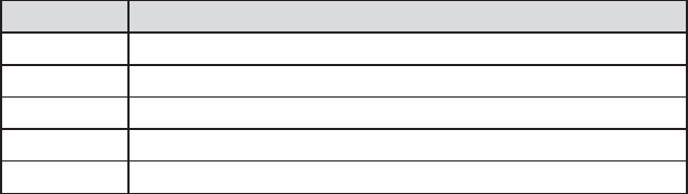
Chapter 8: Other Reporting and Analysis Procedures 259
The TABLE statement is the heart of the TABULATE step. It is the complexity of the TABLE
statement that tends to thwart the user who is new to the procedure. The key to its use is to
remember that it has parts (dimensions) and definitions within those parts. Break it down a piece
at a time and it should make more sense.
The first and primary building blocks of the TABLE statement are the table dimensions. The
table(s) generated by TABULATE can have up to three comma-separated dimensions to their
definition: page, row, and column. These dimensions always appear in page, row, column order:
page defines how the individual pages are formed (used less often)
row defines the rows of the table within each page (almost always present)
column defines the columns within rows and pages (always present)
You will always have at least a column dimension and you cannot have a page dimension without
also having both row and column dimensions. The general makeup of the TABLE statement
therefore looks something like the following. It is very important to notice that the three
dimensions are comma separated. This is the only time that commas are used in the TABLE
statement; the commas separate these three dimensions (definition parts).
table page, row, column;
Generally you will want your entire table on one page; it’s easier to read, so there will not be a
page dimension and your TABLE statement looks like:
table row, column;
To build the individual page, row, and column dimensions, you will use a combination of option
and element phrasing. The three types of phrases are:
singular used when a single element is needed
concatenated multiple elements are joined using a space
nested one element is nested within another using an asterisk
There are several symbols or operators that are commonly used to work with these various
elements. These include the following:
Operator What It Does
space Forms concatenations
* Nests elements—forms hierarchies
( ) Forms groups of elements
‘text’ Adds text
F= Assigns a format
Singular Elements
A singular element has, as the name implies, a single variable. In the following table statement
there is a single classification variable (RACE) in the row dimension and a single analysis
variable (WT) in the column dimension.
&DUSHQWHU$UW&DUSHQWHU¶V*XLGHWR,QQRYDWLYH6$67HFKQLTXHV&RS\ULJKW6$6,QVWLWXWH,QF&DU\1RUWK&DUROLQD86$
$
//5,*+765(6(59(')RUDGGLWLRQDO6$6UHVRXUFHVYLVLWVXSSRUWVDVFRPSXEOLVKLQJ
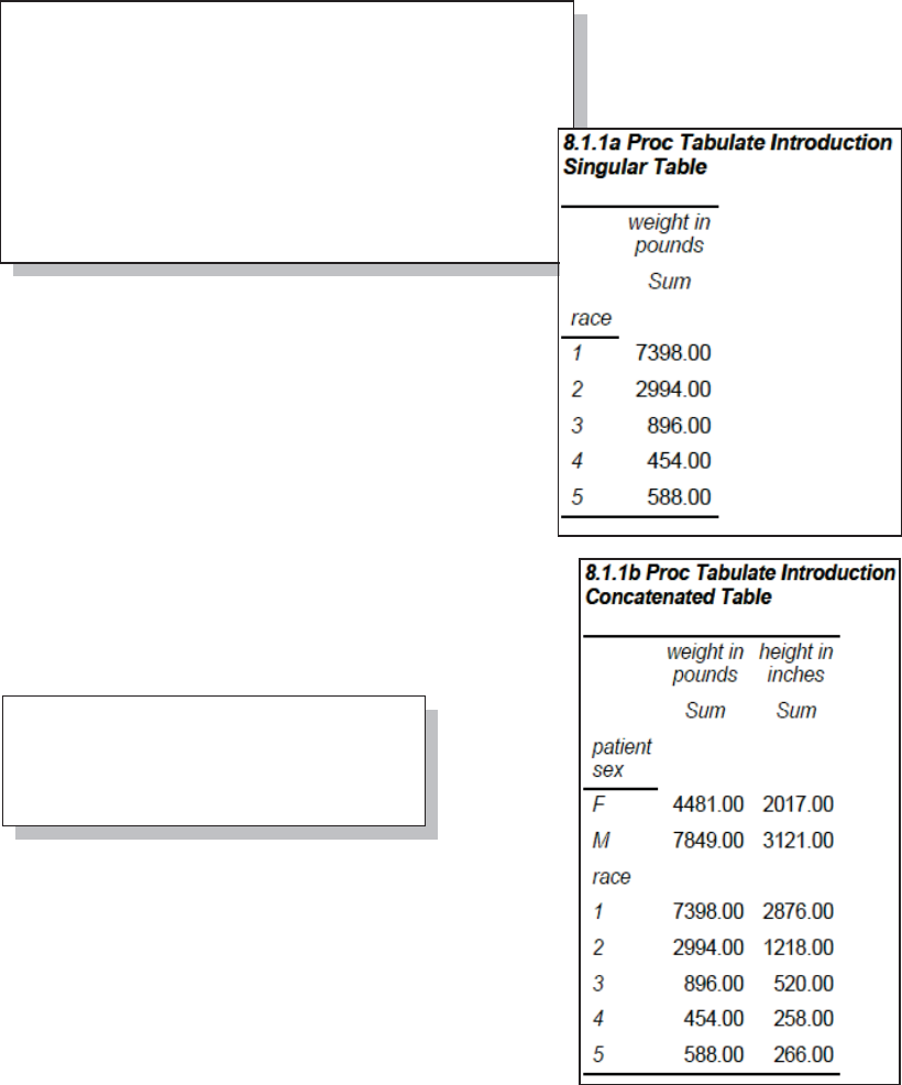
260 Carpenter’s Guide to Innovative SAS Techniques
Since RACE is a classification
variable, the resulting table will
have a single row for each
unique value of RACE.
The analysis variable, WT, is specified in the VAR
statement, and a single column, with a heading showing
the variable’s label, will be generated for the statistic
based on WT.
Since no statistic was specifically requested, the default
statistic (SUM) is displayed.
Concatenated Elements
Concatenated tables allow us to easily combine multiple
elements within columns and/or rows. A concatenated
definition is formed when two or more space separated
elements are included in the same dimension.
This
example
augments
the table
from the
previous
example (8.1.1a) by adding a second classification variable
and a second analysis variable. The label associated with
each analysis variable is by default used in the column
header.
The analysis and classification variables can be used in
page, row, or column dimensions.
Nested Elements
Nested definitions allow us to create tables within tables.
The nested elements can be classification variables, analysis variables, statistics, options, and
modifiers; and are designated as nested elements through the use of the asterisk.
ods pdf file="&path\results\E8_1_1a.pdf"
style=journal;
title1 '8.1.1a Proc Tabulate Introduction';
title2 'Singular Table';
proc tabulate data=advrpt.demog;
class race;
var wt;
table race,wt;
run;
ods pdf close;
proc tabulate data=advrpt.demog;
class race sex;
var ht wt;
table sex race,wt ht;
run;
&DUSHQWHU$UW&DUSHQWHU¶V*XLGHWR,QQRYDWLYH6$67HFKQLTXHV&RS\ULJKW6$6,QVWLWXWH,QF&DU\1RUWK&DUROLQD86$
$
//5,*+765(6(59(')RUDGGLWLRQDO6$6UHVRXUFHVYLVLWVXSSRUWVDVFRPSXEOLVKLQJ
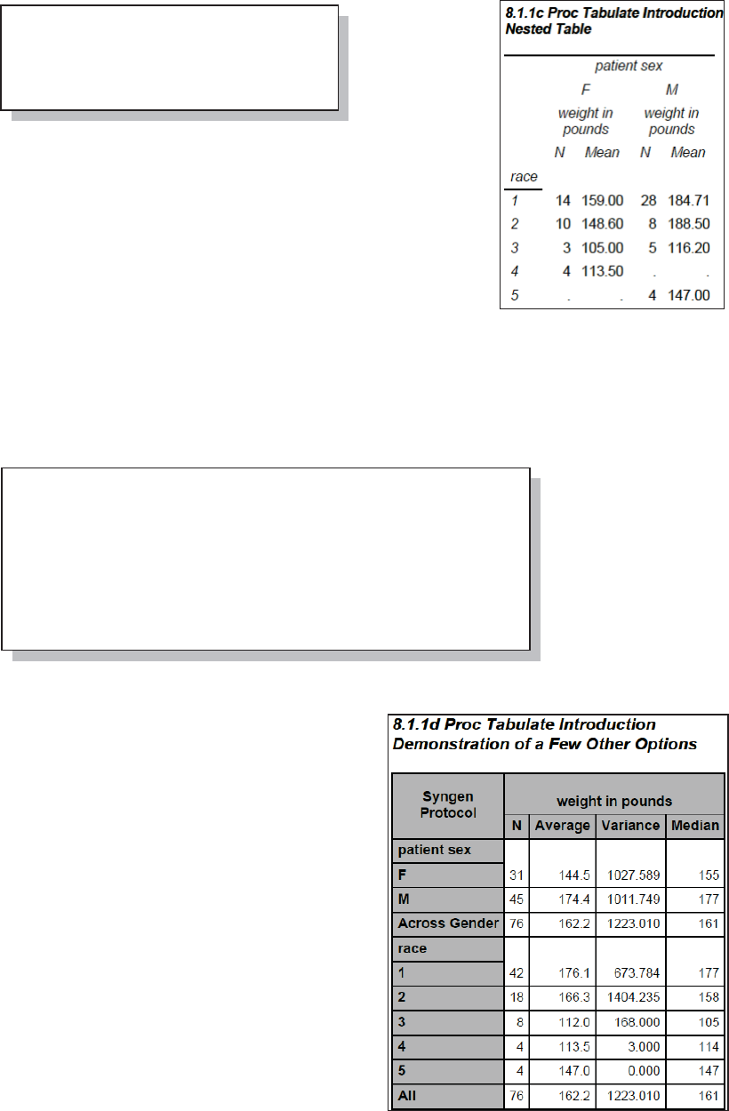
Chapter 8: Other Reporting and Analysis Procedures 261
In this TABLE statement, the row dimension is singular (RACE), while the column dimension
has the analysis
variable (WT)
nested within a
classification
variable (SEX).
Notice also that two space-separated statistics are concatenated
into a group with parentheses, and then the group is nested
under the analysis variable WT, which, as was mentioned, is
nested within SEX.
Combinations of Elements
In most practical uses of TABULATE, the TABLE statement
will contain a combination of nested and concatenated elements.
These will include not only variables and statistics, but options
as well. The TABULATE procedure is rich in options, and once you have started to build simple
tables such as those shown above, you would be well advised to seek out more complete
references to the procedure.
The following example contains additional options, and demonstrates a few of the more complex
techniques that are commonly used with many of the tables generated by TABULATE.
n An overall format is
designated for the
analysis cells in the
table. This default
format can be
overwritten by
associating individual
formats with each
statistic p. Because the
other statistics have
specific formats, this default format is applied only to the VARIANCE in this table.
o The table definition has two concatenated
elements in the row dimension. The ALL
keyword summarizes across the associated
element. Here it creates a row that summarizes
across all values of SEX. A text label can be
assigned to an element by using the equal sign.
Without the text label the word ‘All’ appears in
the table (as it does for RACE).
p Formats can be associated with specific
variables and statistics by nesting the F= option
under the desired element.
q There are a number of options that can be
applied on the TABLE statement (following the
/) for the table as a whole. The BOX= option
adds text in the upper left corner of the table.
proc tabulate data=advrpt.demog;
class race sex;
var wt;
table race,sex*wt*(n mean);
run;
proc tabulate data=advrpt.demog format=8.3 ; n
class race sex ;
var wt;
table sex o all='Across Gender' race all,
wt*(n*f=2.0 mean*f=7.1 var median*f=6.0) p
/ box='Syngen Protocol'; q
keylabel mean = 'Average' r
var = 'Variance';
run;
&DUSHQWHU$UW&DUSHQWHU¶V*XLGHWR,QQRYDWLYH6$67HFKQLTXHV&RS\ULJKW6$6,QVWLWXWH,QF&DU\1RUWK&DUROLQD86$
$
//5,*+765(6(59(')RUDGGLWLRQDO6$6UHVRXUFHVYLVLWVXSSRUWVDVFRPSXEOLVKLQJ
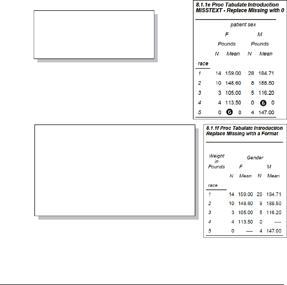
262 Carpenter’s Guide to Innovative SAS Techniques
r The KEYLABEL statement allows you to assign a text label to statistics and to the keyword
ALL.
In example 8.1.1c there were no males for RACE 4 nor were there any females for RACE 5. This
is reflected in missing values for the N and MEAN. Missing values can be replaced with the
MISSTEXT= option s.
Notice
that each
of the
missing
values
has been
replaced
by a zero
(we could have selected other text, such as an asterisk). In
this example a zero for the N is appropriate; however, the
mean really is not zero. We need a way to indicate that it is
not a calculable value.
Fortunately a user-defined format can be used to provide the
reader with the necessary cues.
t The MZERO. format will translate a missing value into four
dashes.
u The MZERO. format is associated with the mean.
v Since the format is applied before the MISSTEXT option, we can still use MISSTEXT=0 to
replace the missing value for N.
8.1.2 Calculating Percentages Using PROC TABULATE
Because of the need to determine the denominator, the calculation of percentages in the
TABULATE procedure can be problematic. Although there are situations where the
determination of the denominator has to be done outside of the TABULATE step, the procedure
does offer a number of tools that make this necessity less common.
proc tabulate data=advrpt.demog;
class race sex;
var wt;
table race,
sex*wt='Pounds'*(n mean)
/ misstext='0' s;
run;
proc format;
value mzero
.='----' t
other=[6.2];
run;
proc tabulate data=advrpt.demog;
class race sex;
var wt;
table race, u
sex='Gender'*wt=' '*(n mean*f=mzero.)
/box='Weight in Pounds'
misstext='0'; v
run;
&DUSHQWHU$UW&DUSHQWHU¶V*XLGHWR,QQRYDWLYH6$67HFKQLTXHV&RS\ULJKW6$6,QVWLWXWH,QF&DU\1RUWK&DUROLQD86$
$
//5,*+765(6(59(')RUDGGLWLRQDO6$6UHVRXUFHVYLVLWVXSSRUWVDVFRPSXEOLVKLQJ
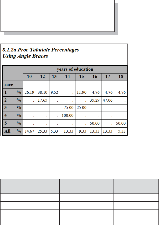
Chapter 8: Other Reporting and Analysis Procedures 263
PCTN and PCTSUM Options
The PCTN and PCTSUM options request the calculation of percentages based on the denominator
specified using angle brackets. PCTN bases the percentages on counts (N), while PCTSUM bases
the percentages on the total of an analysis variable.
The following example requests percentages based on counts. An analysis variable (VAR
statement) is not needed in this step since the percentages are based on counts and no other
statistics are requested.
n Within each value of RACE, calculate
the percentage of observations for each
value of EDU. Since PCTN is nested
within RACE, the denominator <EDU> is
the total count for that value of RACE.
o The column dimension is based on
the classification variable EDU. There
is no analysis variable; therefore, the
count is converted to a percent.
Although the determination of the
denominator is straightforward in this
example, it is often more complex.
The procedure’s documentation and
Haworth (1999) show more complex
examples.
Percentage Generation Statistics
Sometimes it can be difficult to obtain the correct denominator by using the angle brackets.
Fortunately there are also several percentage generation statistics. For each of these statistics, the
denominator (which can be based on the report, the page, the row, or the column) is
predetermined.
Percentage applies to:
Percent Frequency
(N)
Percent Total
(SUM)
Report reppctn reppctsum
Page pagepctn pagepctsum
Column colpctn colpctsum
Row rowpctn rowpctsum
proc tabulate data=advrpt.demog;
class race edu;
table (race all)*pctn<edu>='%' n,
edu; o
run;
&DUSHQWHU$UW&DUSHQWHU¶V*XLGHWR,QQRYDWLYH6$67HFKQLTXHV&RS\ULJKW6$6,QVWLWXWH,QF&DU\1RUWK&DUROLQD86$
$
//5,*+765(6(59(')RUDGGLWLRQDO6$6UHVRXUFHVYLVLWVXSSRUWVDVFRPSXEOLVKLQJ
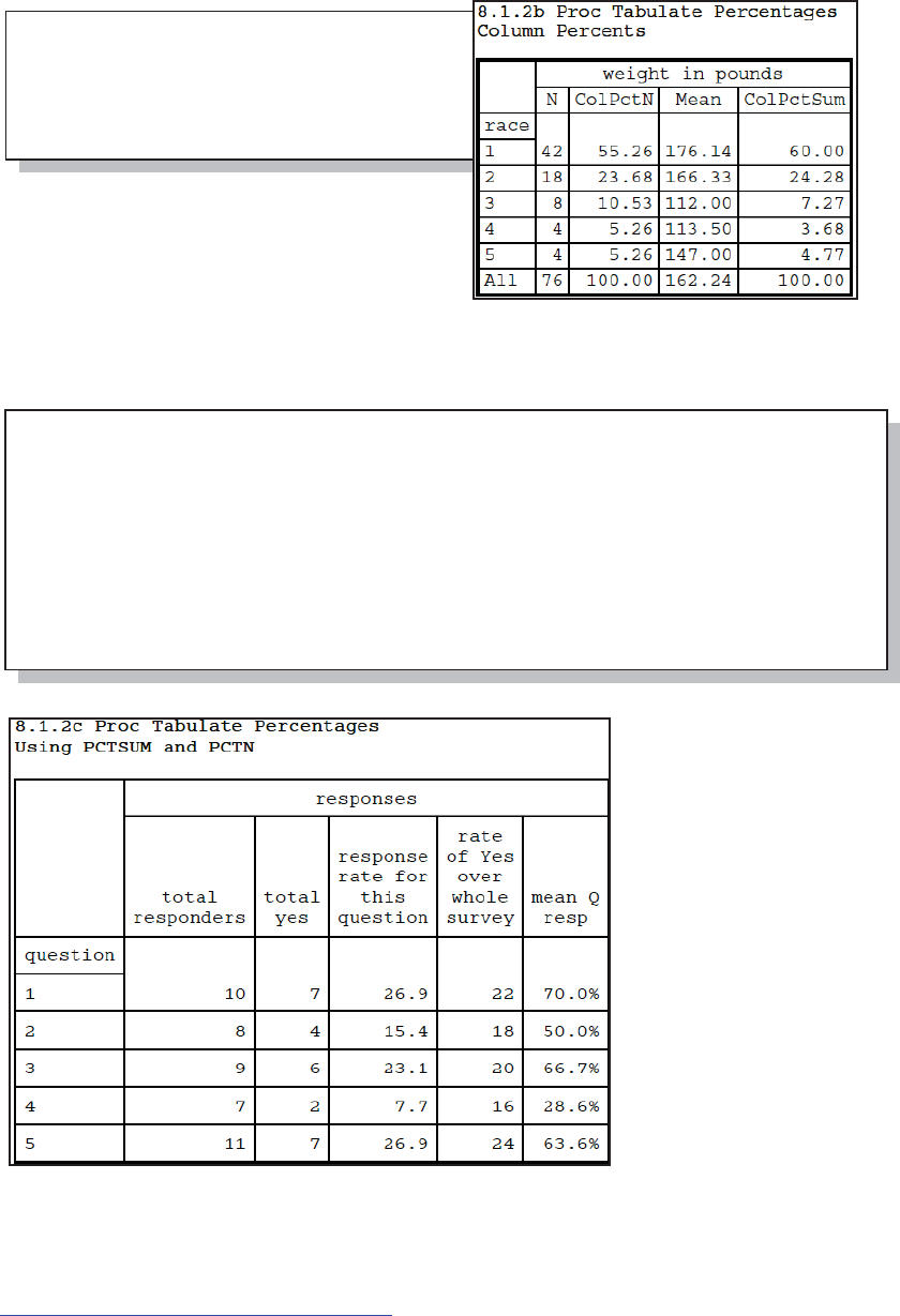
264 Carpenter’s Guide to Innovative SAS Techniques
In the following example the percentages are for the columns rather than rows. The displayed
percentages are calculated using both the N
(COLPCTN) and the total WT (COLPCTSUM).
The following example summarizes survey data. Here the response variable (RESP) takes on the
values of 0 or 1 (no or yes).
Notice that unlike the first
example the denominator
for PCTSUM and PCTN
has not been specified. In
this TABULATE step, the
assumed denominator will
be across the whole report.
p The COMMA7. format
has been applied to these
two statistics. For the
LISTING destination, the
width of the format will be
taken into consideration
when forming the width of
the column. For other
destinations, such as PDF
(style=minimal) which is
shown here, the format
width is used only in the display of the number itself and will have no affect on the column width.
SEE ALSO
The survey example is discussed with alternative coding structures in the SAS Forum thread at
http://communities.sas.com/message/42094.
proc tabulate data=advrpt.demog;
class race;
var wt;
table race all,
wt*(n colpctn mean colpctsum);
run;
proc tabulate data=survey;
class question;
var resp;
table question,
resp='responses'*(n='total responders' *f= comma7. p
sum='total yes' *f= comma7. p
pctsum='response rate for this question'*f=5.1
pctn='rate of Yes over whole survey' *f= 5.
mean='mean Q resp' * f=percent7.1
) /rts=40;
run;
&DUSHQWHU$UW&DUSHQWHU¶V*XLGHWR,QQRYDWLYH6$67HFKQLTXHV&RS\ULJKW6$6,QVWLWXWH,QF&DU\1RUWK&DUROLQD86$
$
//5,*+765(6(59(')RUDGGLWLRQDO6$6UHVRXUFHVYLVLWVXSSRUWVDVFRPSXEOLVKLQJ
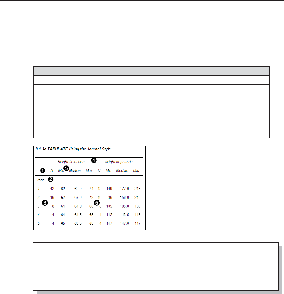
Chapter 8: Other Reporting and Analysis Procedures 265
8.1.3 Using the STYLE= Option with PROC TABULATE
The TABULATE procedure is one of three procedures that accept the STYLE override option. Its
use in TABULATE is similar, but not the same as its use in the PRINT (see Section 8.5.2) and
REPORT (see Section 8.4.6) procedures. This option allows the user to control how various
aspects of the table are to appear by overriding the ODS style attributes.
Styles can be applied to a number of areas within the table from general overall attributes, down
to the attributes of a specific cell. These areas include:
Table Area STYLE= Used on
n Box Cell BOX= option
o Class Heading CLASS statement
pClass Levels CLASSLEV statement
q Analysis Variable Headings VAR statement
r Statistics Headings (keywords) KEYWORD statement
s Value Cells PROC and TABLE statements
s Individual Cells PROC and TABLE statements
To the left is a fairly typical TABULATE table.
The callout numbers on the table correspond to the
callout descriptions above.
The following code was used to generate this
example table. Notice that the RTS= option applies
only to the LISTING destination. The ODS
statements are not shown here, but are included in
the sample code for this book. See
http://support.sas.com/authors.
proc tabulate data=advrpt.demog;
class race;
var ht wt;
table race,
(ht wt)*(n*f=2. min*f=4. median*f=7.1 max*f=4.)
/rts=6;
run;
&DUSHQWHU$UW&DUSHQWHU¶V*XLGHWR,QQRYDWLYH6$67HFKQLTXHV&RS\ULJKW6$6,QVWLWXWH,QF&DU\1RUWK&DUROLQD86$
$
//5,*+765(6(59(')RUDGGLWLRQDO6$6UHVRXUFHVYLVLWVXSSRUWVDVFRPSXEOLVKLQJ
266 Carpenter’s Guide to Innovative SAS Techniques
The STYLE= option can be used to control virtually all of the same attributes that can be set by
the ODS style. Some of these attributes can be dependent on the ODS destination, OS, or printer;
however, the most commonly used attributes are generally available. Some of these common
attributes include:
Controls Attribute Possible Values
Font font_face= times, courier, other fonts supported by the OS
Text size font_size= 6, 8, 10 (sizes appropriate to the font)
Text style font_style= italic, roman
Text density font_weight= bold, medium
Text width font_width= narrow, wide
Foreground
color
foreground= color (color printers or displays)
Background
color
background= color (color printers or displays)
The STYLE= option uses either curly braces or square brackets to contain the list of attributes and
their values. This step demonstrates the use of the STYLE override in a variety of statements. The
callout numbers refer back to the previous table, as well as to the code that follows.
n The background color and a label of the RTS box are changed. Notice that the label has been
removed from RACE in the TABLE statement and placed in the box using the LABEL= option.
o The heading for RACE is to be written without italic (the default). For the JOURNAL style,
which is used in this example, italic is the default for the heading; consequently, this option has no
effect. For other styles, such as PRINTER, italic is not the default and this style override would
make a difference.
p The labels of the individual levels of RACE are centered. The STYLE= option on the
CLASSLEV statement applies to the individual levels.
proc tabulate data=advrpt.demog;
class race / style={font_style=roman}; o
classlev race / style={just=center}; p
var ht wt / style={font_weight=bold q
font_size=4};
table race='(encoded)',
(ht wt)*(n*f=2.*{style={font_weight=bold s
font_face='times new roman'}}
min*f=4. median*f=7.1 max*f=4.)
/rts=6
box={label='Race' n
style={background=grayee}};
keyword n / style={font_weight=bold}; r
run;
&DUSHQWHU$UW&DUSHQWHU¶V*XLGHWR,QQRYDWLYH6$67HFKQLTXHV&RS\ULJKW6$6,QVWLWXWH,QF&DU\1RUWK&DUROLQD86$
$
//5,*+765(6(59(')RUDGGLWLRQDO6$6UHVRXUFHVYLVLWVXSSRUWVDVFRPSXEOLVKLQJ
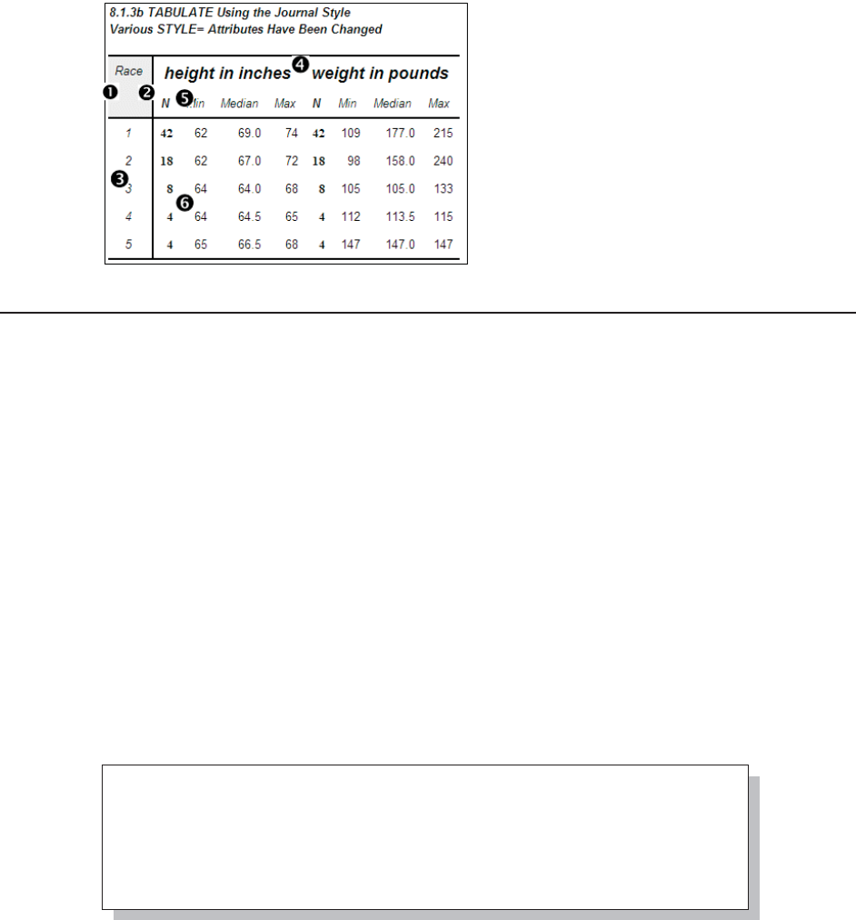
Chapter 8: Other Reporting and Analysis Procedures 267
q On the VAR statement the STYLE= option
changes the attributes associated with the
variable headings.
r Adjust the label for the N statistic by bolding
it. Notice that the headings for the other
statistics remain unchanged.
s Cell attributes associated only with the N
statistic are bolded.
8.1.4 Controlling Table Content with the CLASSDATA Option
The content of the table formed by the TABULATE procedure is influenced a great deal by the
levels of classification variables in the data. Through the use of the CLASSDATA option we can
identify a secondary data set to further influence the table appearance.
For the examples in this section the data set SYMPLEVELS contains only the variable SYMP,
which takes on only the values ‘00’, ‘01’, and ‘02’. It should be noted, however, that in the data to
be analyzed (ADVRPT.DEMOG) the variable SYMP never takes on the value ‘00’, but otherwise
ranges from ‘01’ to ‘10’.
Using CLASSDATA with the EXCLUSIVE Option
The behavior and application of the CLASSDATA= option and the EXCLUSIVE option is very
similar in the TABULATE step as it is in the MEANS and SUMMARY procedures (see Section
7.9). The CLASSDATA= option specifies a data set containing levels of the classification
variables. These levels may or may not exist in the analysis data and can be used to either force
levels into the table or to exclude levels from the table.
When the CLASSDATA= option is used with the EXCLUSIVE option, as in the following
example, only those levels in the CLASSDATA= data set (including any levels not in the analysis
data set) are displayed.
proc tabulate data=advrpt.demog
classdata=symplevels exclusive;
class symp;
var ht wt;
table symp,
(ht wt)*(n*f=2. min*f=4. median*f=7.1 max*f=4.);
run;
&DUSHQWHU$UW&DUSHQWHU¶V*XLGHWR,QQRYDWLYH6$67HFKQLTXHV&RS\ULJKW6$6,QVWLWXWH,QF&DU\1RUWK&DUROLQD86$
$
//5,*+765(6(59(')RUDGGLWLRQDO6$6UHVRXUFHVYLVLWVXSSRUWVDVFRPSXEOLVKLQJ
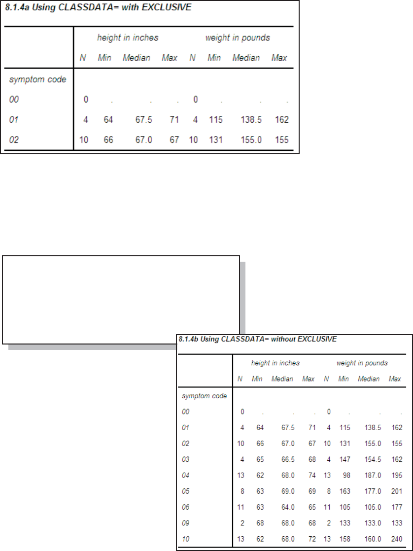
268 Carpenter’s Guide to Innovative SAS Techniques
proc tabulate data=advrpt.demog
classdata=symplevels;
class symp;
var ht wt;
table symp,
(ht wt)*(n*f=2. min*f=4.
median*f=7.1 max*f=4.);
run;
The symptom code
‘00’ does not exist in
the analysis data, but is
included in the table.
Symptom codes ‘03’
through ‘10’ are
excluded from the table
as they do not appear in
the data set
SYMPLEVELS.
When the
CLASSDATA= option
is used without the
EXCLUSIVE option, all levels of the classification variable from either the CLASSDATA= data
set or the analysis data are included in the table.
The EXCLUSIVE option can also appear on the CLASS statement; however, it will work with the
CLASSDATA= option only when it is used on the PROC statement.
Using CLASSDATA without the EXCLUSIVE Option
When the EXCLUSIVE option is not used, the levels of the CLASSDATA data set can still be
used to add rows to the resulting
table. Here the EXCLUSIVE option
has been removed from the previous
example.
In this example the SYMP= ‘00’ level
has been added to the table; however,
no rows have been excluded.
MORE INFORMATION
Section 12.1.2 discusses the use of pre-
loaded formats with PROC
TABULATE to accomplish similar
results.
&DUSHQWHU$UW&DUSHQWHU¶V*XLGHWR,QQRYDWLYH6$67HFKQLTXHV&RS\ULJKW6$6,QVWLWXWH,QF&DU\1RUWK&DUROLQD86$
$
//5,*+765(6(59(')RUDGGLWLRQDO6$6UHVRXUFHVYLVLWVXSSRUWVDVFRPSXEOLVKLQJ
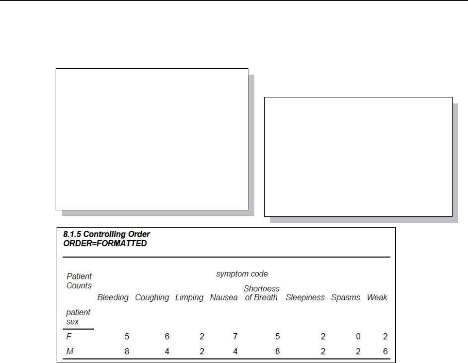
Chapter 8: Other Reporting and Analysis Procedures 269
proc format;
value $SYMPTOM
'01'='Sleepiness'
'02'='Coughing'
'03'='Limping'
'04'='Bleeding'
'05'='Weak'
'06'='Nausea'
'07'='Headache'
'08'='Cramps'
'09'='Spasms'
'10'='Shortness of Breath';
run;
8.1.5 Ordering Classification Level Headings
Like many procedures that use classification variables, the default order for the level headings is
ORDER=INTERNAL. Unlike the REPORT procedure the default order does not change for
formatted variables.
The format $SYMPTOM., which is shown here,
is used with the variable SYMP. Whether or not
the format is
applied, the
heading
values reflect
the
INTERNAL
order of the
values of
SYMP. Only
if the format is
assigned and
the
ORDER=FORMATTED is specified will the headings be placed in formatted order.
proc tabulate data=advrpt.demog
order=formatted;
class symp sex;
var wt;
table sex*wt=' '*n=' '
,symp
/box='Patient Counts'
row=float
misstext='0';
format symp $symptom.;
run;
&DUSHQWHU$UW&DUSHQWHU¶V*XLGHWR,QQRYDWLYH6$67HFKQLTXHV&RS\ULJKW6$6,QVWLWXWH,QF&DU\1RUWK&DUROLQD86$
$
//5,*+765(6(59(')RUDGGLWLRQDO6$6UHVRXUFHVYLVLWVXSSRUWVDVFRPSXEOLVKLQJ
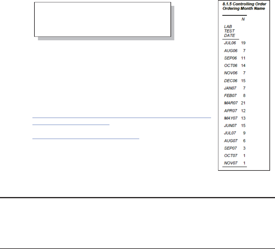
270 Carpenter’s Guide to Innovative SAS Techniques
When dealing with date values the internal order or the order of the date values is often preferred
over the formatted order. In the following example the visit dates are counted within months;
however, we want to view the monthly totals in chronological (INTERNAL) order. In this
example if we had used either the MONNAME. or MONTH. formats, the months for the two
years would
have been
confounded.
MORE INFORMATION
The ORDER= option is discussed in detail in Section 2.6.2. The VALUE
statement in PROC FORMAT has the option NOTSORTED, which
allows you to both format a variable and control the value order, is
described in Section 12.4.
SEE ALSO
Formatting a TABULATE prior to copying it to Excel is discussed in a
sasCommunity.org article at
http://www.sascommunity.org/wiki/Proc_Tabulate:_Making_the_result_
table_easier_to_copy_to_Excel. Indenting row headers is discussed in a
SAS Forum thread, which contains links to other papers as well, at
http://communities.sas.com/message/45339.
8.2 Expanding PROC UNIVARIATE
The capabilities of this procedure have been expanded in each of the last several releases of SAS
and it is not unusual for even seasoned programmers to be only partially aware of all that it can
now do. This section is a survey of some of those newer or less commonly known capabilities.
8.2.1 Generating Presentation-Quality Plots
A number of presentation-quality graphics, such as those produced by SAS/GRAPH, can also be
produced by PROC UNIVARIATE. Some of the plotting capabilities require the presence of
SAS/GRAPH even though a SAS/GRAPH procedure is not being called. Graphics are
implemented through a series of statements which include:
HISTOGRAM builds histograms
INSET adds legends and text to the graph
PROBPLOT creates probability plots
QQPLOT creates quantile-quantile plots
proc tabulate data=advrpt.lab_chemistry;
class labdt /order=internal;
table labdt,n*f=2.;
format labdt monyy.;
run;
&DUSHQWHU$UW&DUSHQWHU¶V*XLGHWR,QQRYDWLYH6$67HFKQLTXHV&RS\ULJKW6$6,QVWLWXWH,QF&DU\1RUWK&DUROLQD86$
$
//5,*+765(6(59(')RUDGGLWLRQDO6$6UHVRXUFHVYLVLWVXSSRUWVDVFRPSXEOLVKLQJ

Chapter 8: Other Reporting and Analysis Procedures 271
The following example shows some of the flexibility of these statements by building three
histograms that are overlaid by the normal distribution. In this example the plot generated by
UNIVARIATE will be written to a file.
n The plot is to be saved as an EMF file. EMF and the older CGM files are generally considered
best if the plot is to be imported into a word processing document as it has been here. The EMF
file type has the further advantage of the capability of modifying and editing the graph in the
Microsoft Image Editor.
o The DEVICE graphics option specifies the type of file to be created.
p The GSFNAME graphics option identifies the fileref that points to the file that is to be
generated.
q The classification variables RACE and SEX form 10 combinations based on 5 values of RACE
and 2 for SEX. These form the rows and columns for the plot.
r In a color representation of the histogram, the vertical bars are cyan.
s The scale of the vertical axis will be based on the patient counts. Other choices for the scale
could include: PERCENT and PROPORTION.
t A label is specified for the vertical axis of each of the five histograms.
u The INSET statement inserts text, including various statistics, into the graph. Here the MEAN
of HT is written in the upper right (NorthEast) corner of each graph using the 5.2 format and
SWISSB, a SAS/GRAPH font. Notice that the default font for the title and the selected font for
the INSET (SWISSB) are not particularly good choices. Under Windows most Windows fonts are
available for use in graphics such as this. Alternatively the font could have been specified as
font='Arial Narrow /b' . ARIAL is used in the next example.
filename out821a "&path\results\g821a.emf"; n
goptions device=emf o
gsfname=out821a p
noprompt;
title1 '8.2.1a Plots by PROC UNIVARIATE';
proc univariate data=advrpt.demog;
class race sex;
var ht;
histogram /nrows=5 ncols=2 q
intertile=1 cfill=cyan r vscale=count s
vaxislabel='Count'; t
inset u mean='Mean Height: ' (5.2) / noframe position=ne
height=2 font=swissxb;
run;
quit;
&DUSHQWHU$UW&DUSHQWHU¶V*XLGHWR,QQRYDWLYH6$67HFKQLTXHV&RS\ULJKW6$6,QVWLWXWH,QF&DU\1RUWK&DUROLQD86$
$
//5,*+765(6(59(')RUDGGLWLRQDO6$6UHVRXUFHVYLVLWVXSSRUWVDVFRPSXEOLVKLQJ
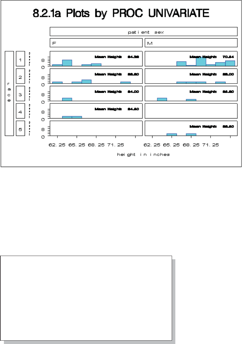
272 Carpenter’s Guide to Innovative SAS Techniques
The histograms that are generated by the HISTOGRAM statement can be overlaid with one of
several different statistical distributions. These distributions include:
normal
lognormal
gamma
Weibull
In this example a normal distribution is overlaid on a histogram of the data.
vThe MIDPOINTS
option is used to specify
both the range of the
values to be plotted and
the widths of the
individual bins represented
by the histogram bars.
This MIDPOINTS option
is the same as is used in
PROC GCHART and the
syntax is similar to an
iterative DO loop.
title1 f=arial
'8.2.1b Normal Plots by PROC UNIVARIATE';
proc univariate data=advrpt.demog;
var wt;
histogram /midpoints=100 to 250 by 15 v
cfill=cyan vscale=count
vaxislabel='Count'
normal (l=2 color=red); w
inset mean='Mean: ' (6.2)/position=nw
height=4 font=arial;
run;
quit;
&DUSHQWHU$UW&DUSHQWHU¶V*XLGHWR,QQRYDWLYH6$67HFKQLTXHV&RS\ULJKW6$6,QVWLWXWH,QF&DU\1RUWK&DUROLQD86$
$
//5,*+765(6(59(')RUDGGLWLRQDO6$6UHVRXUFHVYLVLWVXSSRUWVDVFRPSXEOLVKLQJ
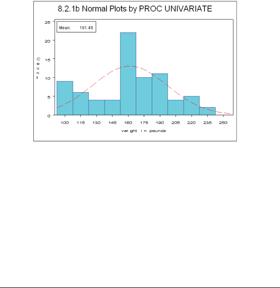
Chapter 8: Other Reporting and Analysis Procedures 273
wThe normal
distribution
(based on the
mean and
variance of
the data) is to
be overlaid on
the histogram.
The line type
is to be dashed
(L=2) and the
line color is
set to RED.
The INSET
statement is
used to write
the mean in
the upper left
(NorthWest)
corner.
Notice the quality of the title font. The TITLE statement has specified the ARIAL font, which
renders better than SWISSB in an EMF file (see Section 9.1 for more on adding options to TITLE
statements).
Although not shown in this example, you can collect the actual and predicted percentage of
observations for each midpoint by using the OUTHISTOGRAM= option. This option names a
data set that will contain the predicted percentage for each distribution.
Although UNIVARIATE is not a SAS/GRAPH procedure, the graphics that it produces can take
advantage of some of the other SAS/GRAPH capabilities. It will recognize several SAS/GRAPH
statements, including AXIS and SYMBOL statements. Additionally it respects the ANNO=
option so that it can utilize the ANNOTATE facility of SAS/GRAPH.
MORE INFORMATION
Section 9.2 discusses other SAS/GRAPH options and statements that can be used outside of
SAS/GRAPH. Under some conditions the default font selection for portions of the graph results in
virtually unreadable text. Portions of the text in the plot in Section 8.2.1a are very hard to read.
This can be mitigated by using the FTEXT option, which is also discussed in Section 9.2.
8.2.2 Using the CLASS Statement
As is the case with a number of other summary and analysis procedures, multiple CLASS
statements and CLASS statement options are supported (see Section 7.1). However, unlike other
summary procedures, you can only specify up to two classification variables.
&DUSHQWHU$UW&DUSHQWHU¶V*XLGHWR,QQRYDWLYH6$67HFKQLTXHV&RS\ULJKW6$6,QVWLWXWH,QF&DU\1RUWK&DUROLQD86$
$
//5,*+765(6(59(')RUDGGLWLRQDO6$6UHVRXUFHVYLVLWVXSSRUWVDVFRPSXEOLVKLQJ
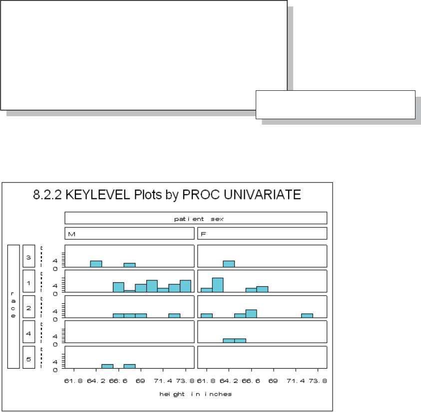
274 Carpenter’s Guide to Innovative SAS Techniques
One of the CLASS statement options used specifically with UNIVARIATE is the KEYLEVEL=
option. This option can be used to control plot order by specifying a primary or key value for the
classification variable.
The selected level will be
displayed first.
The single CLASS
statement used here could
have been rewritten as
two statements, one for
each classification variable.
When using a CLASS statement, the printed output is also broken up into each combination of
classification variables.
In the plot,
notice that
RACE level ‘3’
and SEX level
‘M’ are
positioned
first—they have
been designated
as the
KEYLEVELs.
Some of the
other text in this
graphic is very
hard to read,
and not only
because of the
size of the
graph on this
page. When
fonts are not explicitly declared, default hardware fonts are sometimes selected that do not render
well for all devices. The FTEXT= option, which is discussed in Section 9.2, can be used to
explicitly specify default fonts.
title1 f=arial
'8.2.2 KEYLEVEL Plots by PROC UNIVARIATE';
proc univariate data=advrpt.demog;
class race sex/keylevel=('3' 'M');
var ht;
histogram /nrows=5 ncols=2
intertile=1 cfill=cyan vscale=count
vaxislabel='Count';
run;
quit;
class race / keylevel='3';
class sex / keylevel='M';
&DUSHQWHU$UW&DUSHQWHU¶V*XLGHWR,QQRYDWLYH6$67HFKQLTXHV&RS\ULJKW6$6,QVWLWXWH,QF&DU\1RUWK&DUROLQD86$
$
//5,*+765(6(59(')RUDGGLWLRQDO6$6UHVRXUFHVYLVLWVXSSRUWVDVFRPSXEOLVKLQJ
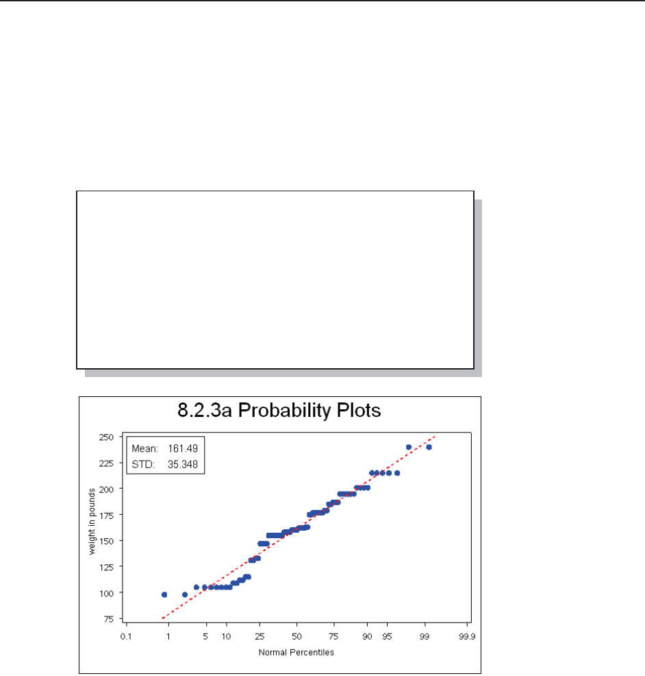
Chapter 8: Other Reporting and Analysis Procedures 275
8.2.3 Probability and Quantile Plots
In addition to histograms, UNIVARIATE has the capability of generating probability and
quantile-quantile plots. The syntax and resulting graphics are similar for each of these types of
plots. Typically these plots are used to compare the data to a known or hypothetical distribution.
Probability plots are most suited as a graphical estimation of percentiles, while the quantile-
quantile plots (also known as QQplots) are better suited for the graphical estimation of
distribution parameters.
Probability Plots
Probability plots can be generated by use of the PROBPLOT statement.
n The SYMBOL
statement can be used to
control the plot symbols
for the percentiles. Here
the requested plot
symbol is a blue dot.
o The probability plot is
to be compared to a
normal distribution. The
mean and standard
deviation can be
specified (MU and
SIGMA), or they can be
estimated from the data,
as was done here.
p The estimated
distribution is to be
depicted with a dashed
(L=2) red line with a
thickness of 2.
As the distribution of the
data approaches the
theoretical distribution,
the data percentile points
should fall on the dashed
line.
title1 f=arial '8.2.3a Probability Plots';
symbol1 v=dot c=blue; n
proc univariate data=advrpt.demog;
var wt;
probplot /normal(mu=est sigma=est o
color=red l=2 w=2); p
inset mean='Mean: ' (6.2)
std ='STD: ' (6.3) / position=nw
height=4 font=arial;
run;
&DUSHQWHU$UW&DUSHQWHU¶V*XLGHWR,QQRYDWLYH6$67HFKQLTXHV&RS\ULJKW6$6,QVWLWXWH,QF&DU\1RUWK&DUROLQD86$
$
//5,*+765(6(59(')RUDGGLWLRQDO6$6UHVRXUFHVYLVLWVXSSRUWVDVFRPSXEOLVKLQJ
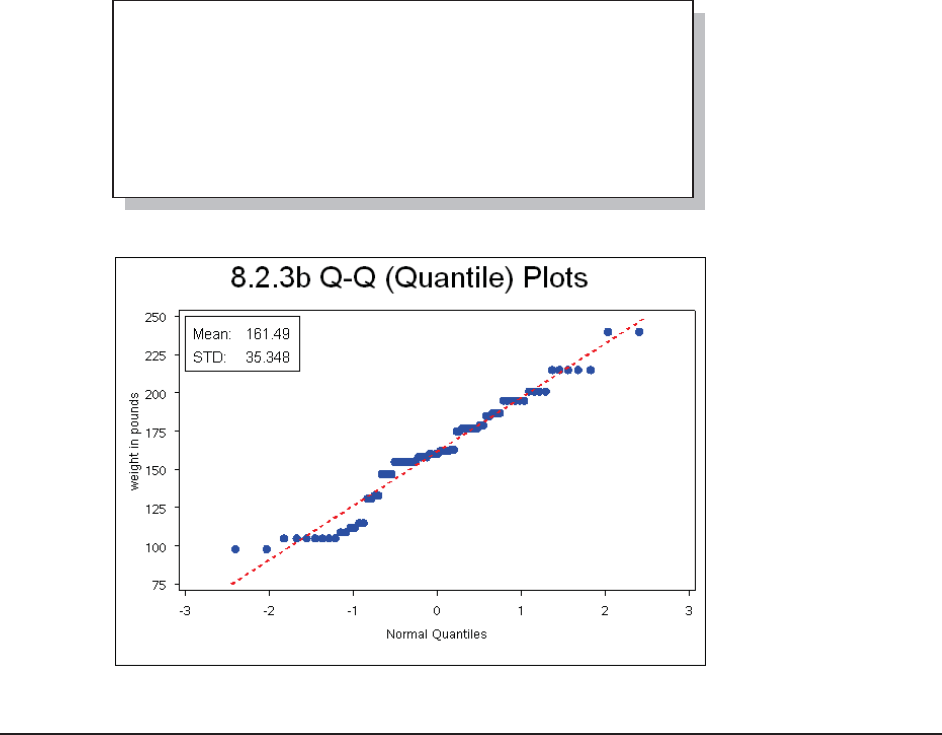
276 Carpenter’s Guide to Innovative SAS Techniques
QQ Plots
Rather than using the percentiles as the horizontal axis, the quantile plots break the horizontal axis
into quantile ranges.
This QQPLOT statement
uses the same options as
were used in the
percentile probability
plots.
The resulting plots are
generally very similar.
8.2.4 Using the OUTPUT Statement to Calculate Percentages
UNIVARIATE now supports the use of the OUTPUT statement. The syntax is essentially the
same as is used in the MEANS and SUMMARY procedures; however, there are a number of
statistics that are only available in the UNIVARIATE procedure. These statistics include several
test statistics that are not included in the printed output. It is also possible to generate a wider
range of percentiles. When used in conjunction with a CLASS statement, the output data set
contains one observation per combination of classification levels. There are no rollup levels; the
results are essentially what you would expect when using the NWAYS option with the MEANS
or SUMMARY procedures.
The example shown here uses the OUTPUT statement to create a data set containing a series of
percentiles that cannot be easily obtained in the MEANS or SUMMARY procedures.
proc univariate data=advrpt.demog;
var wt;
qqplot /normal(mu=est sigma=est
color=red l=2 w=2);
inset mean='Mean: ' (6.2)
std ='STD: ' (6.3) / position=nw
height=4 font=arial;
run;
&DUSHQWHU$UW&DUSHQWHU¶V*XLGHWR,QQRYDWLYH6$67HFKQLTXHV&RS\ULJKW6$6,QVWLWXWH,QF&DU\1RUWK&DUROLQD86$
$
//5,*+765(6(59(')RUDGGLWLRQDO6$6UHVRXUFHVYLVLWVXSSRUWVDVFRPSXEOLVKLQJ

Chapter 8: Other Reporting and Analysis Procedures 277
n The output data set will contain one
observation for each level of the
classification variable.
o The data set UNISTATS will be created
by the OUTPUT statement.
p The PCTLPRE= option provides a prefix
for the names of the variables containing the
percentiles which are requested by the
PCTLPTS option.
q The percentile request uses syntax similar to an iterative DO, which can include a compound
list as is shown here.
8.3 Doing More with PROC FREQ
Although PROC FREQ has been a part of SAS from its inception, it has changed very little.
There are, however, a few newer and underutilized options that are now available.
8.3.1 OUTPUT Statement in PROC FREQ
In addition to the ODS OUTPUT destination, the OUTPUT statement can be used in a PROC
FREQ step to write statistics generated by the procedure to a data set. The list of available
statistics, as is shown in the documentation, is fairly extensive and corresponds to the statistics
that can be generated by the TABLES statement.
The desired statistics must be requested on the TABLES statement if they are to be available in
the OUTPUT statement.
proc univariate data=advrpt.demog
noprint;
class sex; n
var wt;
output out=unistats o
mean = wt_mean
pctlpre=wt_ p
pctlpts=0 to 10 by 2.5, q
50,
90 to 100 by 2.5;
run;
8.2.4 Using the OUTPUT Statement in UNIVARIATE
Obs sex wt_mean wt_0 wt_2_5 wt_5 wt_7_5 wt_10
1 F 144.548 98 98 98 105 105
2M172.913 105 105 105 105 133
Obs wt_50 wt_90 wt_92_5 wt_95 wt_97_5 wt_100
1 155 187 187 187 215 215
2 177 215 215 215 240 240
&DUSHQWHU$UW&DUSHQWHU¶V*XLGHWR,QQRYDWLYH6$67HFKQLTXHV&RS\ULJKW6$6,QVWLWXWH,QF&DU\1RUWK&DUROLQD86$
$
//5,*+765(6(59(')RUDGGLWLRQDO6$6UHVRXUFHVYLVLWVXSSRUWVDVFRPSXEOLVKLQJ
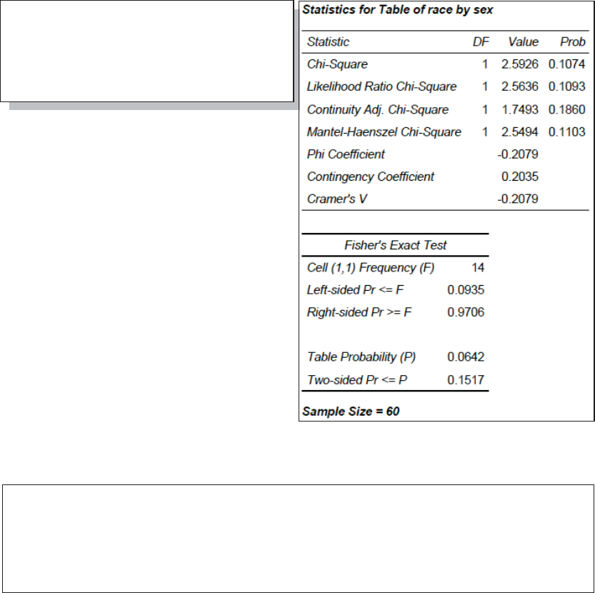
278 Carpenter’s Guide to Innovative SAS Techniques
n The CHISQ option requests a series of
contingency table statistics for the table
defined by RACE and SEX.
o The data set WORK.FREQSTATS will be
created.
p Rather than select specific statistics by
name, all the statistics generated by the
CHISQ option on the TABLE statement are to
be included in the data set. This option
generates a warning as the ALL keyword
requests statistics that are not included in the
CHISQ option. The warning would not have
been issued had either the ALL been replaced
with CHISQ or if the additional statistics
requested by the ALL had been included in the
TABLES statement (MEASURES, CMH, N).
The portion of the table generated by the CHISQ option is shown here.
Many of these same values can be found in the data set, which has been printed below.
8.3.1 Using the OUTPUT Statement in FREQ
Obs N _PCHI_ DF_PCHI P_PCHI _LRCHI_ DF_LRCHI P_LRCHI _AJCHI_ DF_AJCHI P_AJCHI _MHCHI_
1 60 2.59259 1 0.10736 2.56359 1 0.10935 1.74934 1 0.18596 2.54938
Obs DF_MHCHI P_MHCHI XPL_FISH XPR_FISH XP2_FISH _PHI_ _CONTGY_ _CRAMV_
1 1 0.11034 0.093531 0.97063 0.15174 -0.20787 0.20352 -0.20787
proc freq data=advrpt.demog
(where=(race in('1','2')));
table race*sex/chisq; n
output out=FreqStats o
all; p
run;
&DUSHQWHU$UW&DUSHQWHU¶V*XLGHWR,QQRYDWLYH6$67HFKQLTXHV&RS\ULJKW6$6,QVWLWXWH,QF&DU\1RUWK&DUROLQD86$
$
//5,*+765(6(59(')RUDGGLWLRQDO6$6UHVRXUFHVYLVLWVXSSRUWVDVFRPSXEOLVKLQJ
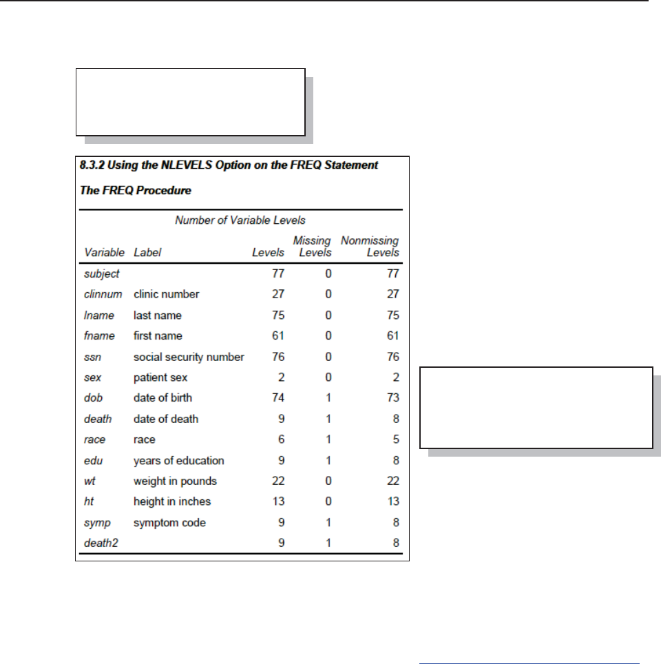
Chapter 8: Other Reporting and Analysis Procedures 279
8.3.2 Using the NLEVELS Option
The NLEVELS option on the PROC FREQ statement generates a summary table that shows the
number of levels, including missing, for each of the classification variables included in the
TABLES statement. In this example the TABLE
statement requests a count of levels for all variables in
the data set. The NOPRINT option prevents the
printing of all tables, except the one generated by the
NLEVELS option.
The resulting table shows all the
variables in ADVRPT.DEMOG and
the number of distinct values of each.
Knowing the number of distinct levels
of a variable can be helpful when
writing automated programs. The data
contained in the NLEVELS table can
be written to a data set using the ODS
OUTPUT destination, and once there
it can be harvested as metadata for use
by the macro language.
MORE INFORMATION
The ODS OUTPUT destination is discussed in more detail in Section 11.1.
SEE ALSO
SAS Tip number 30867 discusses the NLEVELS option at http://support.sas.com/kb/30/867.html.
proc freq data=advrpt.demog
nlevels;
table _all_/noprint;
run;
ods output nlevels=varcnts;
proc freq data=advrpt.demog
nlevels;
table _all_/noprint;
run;
&DUSHQWHU$UW&DUSHQWHU¶V*XLGHWR,QQRYDWLYH6$67HFKQLTXHV&RS\ULJKW6$6,QVWLWXWH,QF&DU\1RUWK&DUROLQD86$
$
//5,*+765(6(59(')RUDGGLWLRQDO6$6UHVRXUFHVYLVLWVXSSRUWVDVFRPSXEOLVKLQJ

280 Carpenter’s Guide to Innovative SAS Techniques
8.4 Using PROC REPORT to Better Advantage
Like PROC TABULATE, the REPORT procedure is underutilized by many analysts. The details
of its usage can be found in Carpenter’s Complete Guide to the SAS REPORT Procedure
(Carpenter, 2007a). This section will not provide an introduction to the procedure, but will instead
cover a few topics that have been known to be problematic.
Much of the confusion is centered on the use of the compute block, which is unique to PROC
REPORT. Consequently, most of the examples in this section involve the use of the compute
block. Carpenter (2007a) has a number of more detailed examples on the syntax, use, and
operating sequencing of the compute block. This book also includes a Microsoft PowerPoint copy
of Russ Lavery’s “Animated Guide to the REPORT Procedure’s Compute Block.”
MORE INFORMATION
The use of pre-loaded formats with PROC REPORT to create report subsets can be found in
Section 12.1.1.
8.4.1 PROC REPORT vs. PROC TABULATE
Both the REPORT and TABULATE procedures can create summary reports and each has
basically the same access to the standard suite of summary statistics.
Unlike TABULATE, the REPORT procedure can provide detail reporting as well as summary
reporting capabilities. REPORT has the added flexibility to calculate and display columns of
information based on other columns in the report.
Because of the unique way that the TABULATE procedure structures the report table it has a
great deal more flexibility to present the groups, sub-groups, and statistics as either rows or
columns. This is especially true for vertically concatenated reports, which are very
straightforward in TABULATE and difficult in REPORT (see Carpenter, 2007a, Section 10.1 for
details on creating a vertically concatenated report using PROC REPORT).
8.4.2 Naming Report Items (Variables) in the Compute Block
Compute blocks are unique to the REPORT procedure. While they have a number of similarities
to the DATA step, there are sufficient differences, not only in syntax, but more importantly in
how they are executed, which is why they warrant a discussion in this book.
In the DATA step you name the items (variables) on the Program Data Vector , PDV, explicitly
by name. Although the term variable is often used to address values in the compute block, they
are more accurately known as report items. In the compute block the rules for naming report items
are not nearly as straightforward as in the DATA step. In the compute block there is no PDV, and
the compute block can be used to address report items that are not actually variables.
There are four different situations that determine how a report item is to be named in the compute
block. These result in three distinct report item naming conventions.
SEE ALSO
The topic of naming report items in compute blocks is specifically addressed in Carpenter (2006a
and 2007a).
&DUSHQWHU$UW&DUSHQWHU¶V*XLGHWR,QQRYDWLYH6$67HFKQLTXHV&RS\ULJKW6$6,QVWLWXWH,QF&DU\1RUWK&DUROLQD86$
$
//5,*+765(6(59(')RUDGGLWLRQDO6$6UHVRXUFHVYLVLWVXSSRUWVDVFRPSXEOLVKLQJ

Chapter 8: Other Reporting and Analysis Procedures 281
Explicitly by Name
In the DATA step variable names are used explicitly. While this same naming convention will
sometimes work in the compute block, you need to understand when it will and will not work. The
name is used explicitly when the variable or report item:
has a define usage of GROUP, ORDER, COMPUTED, or DISPLAY
is a temporary variable, which is created and used only in a compute block
is the automatic temporary variable named _BREAK_
is a report item alias (see below)
Using a Compound Name
Compound variable names are needed when a report item has a define usage of ANALYSIS,
which means that is has been used to calculate a statistic (SUM is the default). The compound
name is a combination of the variable name and the
statistic that it has been used to calculate. The general
form is variablename.statistic, and in the compute block
you might address the mean of the variable WT as shown
to the left.
Directly When Using an Alias
Creating an alias of a report item allows you to use that report item in multiple ways. The
following COLUMN statement generates a series
of aliases for the HT analysis variable. Each of
these aliases will be used to calculate a different
statistic.
When an alias is used in a compute
block, it is named explicitly. Here
the HTMIN alias of HT is used in a
LINE statement.
Indirectly When Using the Absolute Column Number
The define type of ACROSS creates a series of columns. These columns, and indeed any column
in the report, can be referenced by using the column number as an indirect column reference.
This pseudo variable name is always of the form, _Cxx_, where the xx is the column number as
read from left to right on the report. The column count even includes any columns that will
ultimately not be printed, e.g., those columns defined with NOPRINT or NOZERO.
When one or more report items have a define usage of ACROSS, it is not possible to address the
transposed columns by name. To address these columns it is necessary to use absolute column
numbers.
MORE INFORMATION
Absolute column references are used in the example in Section 8.4.3.
8.4.3 Understanding Compute Block Execution
In the following example a compute block is used to convert the mean weight from pounds to
kilograms. Since WT is nested under SEX, which has a define usage of ACROSS, there will be
two columns associated with WT. As a consequence, absolute column numbers must be used in
the compute block that performs the conversion o.
compute wt;
wt.mean = wt.mean/2.2;
endcomp;
column region ht
ht=htmin ht=htmax
ht=htmean ht=htmedian;
compute after;
line @3 'Minimum height is ' htmin 6.1;
endcomp;
&DUSHQWHU$UW&DUSHQWHU¶V*XLGHWR,QQRYDWLYH6$67HFKQLTXHV&RS\ULJKW6$6,QVWLWXWH,QF&DU\1RUWK&DUROLQD86$
$
//5,*+765(6(59(')RUDGGLWLRQDO6$6UHVRXUFHVYLVLWVXSSRUWVDVFRPSXEOLVKLQJ

282 Carpenter’s Guide to Innovative SAS Techniques
Although this step executes without any syntax errors, it contains a huge logic error. In order
to understand the error and what causes it we need to first understand the execution of the
compute blocks.
n Patient weight is nested
within SEX, which has a define
usage of ACROSS. An alias for
WT, ALLWTMEAN, is also
declared.
o In the compute block for WT,
the values for each of the two
genders are converted from
pounds to kilograms.
p _C2_ holds the mean weight
of female patients and is the
second column in the report
(counting from left to right).
q ALLWTMEAN (mean weight ignoring SEX) is a computed report item and is named directly.
In this example there are two compute
blocks, one associated with WT and one for
the alias ALLWTMEAN. Since there are
two columns associated with WT within
SEX (one for each of the two genders), the
compute block for WT will execute twice
for each row in the report. As a matter of
fact, counting the one for ALLWTMEAN,
three compute block executions take place
for each report row.
Since the compute block for WT will
execute twice for each report row, this
causes a very nasty error. Notice that in the
mean weights for females, the values have
been divided by 2.2 twice. The problem
goes away if the calculations for _C2_ and _C3_ are placed in the compute block for
ALLWTMEAN, which is executed only once for each row.
r The compute block for ALLWTMEAN will execute only once. Any given compute block can
reference any report item to its left on the COLUMN statement, so there is no issue with placing
references to all three columns in this single compute block.
proc report data=advrpt.demog nowd;
column edu sex,wt n wt=allwtmean;
define edu / group 'Years/Ed.';
define sex / across order=formatted;
define wt / mean 'Mean' format=5.1;
define allwtmean / mean 'Mean' format=5.1;
compute wt; o
_c2_ = _c2_/2.2; p
_c3_ = _c3_/2.2;
endcomp;
compute allwtmean; q
allwtmean = allwtmean/2.2;
endcomp;
run;
8.4.3a Showing ACROSS With
Compute Blocks
Convert LB to KG
patient sex
Years F M
Ed. Mean Mean Mean
10 . 88.2 88.2
12 31.4 81.7 76.4
13 44.4 86.8 89.5
14 22.7 47.7 49.1
15 34.0 60.5 70.7
16 32.6 75.9 75.1
17 29.5 70.5 66.0
18 . 79.1 79.1
&DUSHQWHU$UW&DUSHQWHU¶V*XLGHWR,QQRYDWLYH6$67HFKQLTXHV&RS\ULJKW6$6,QVWLWXWH,QF&DU\1RUWK&DUROLQD86$
$
//5,*+765(6(59(')RUDGGLWLRQDO6$6UHVRXUFHVYLVLWVXSSRUWVDVFRPSXEOLVKLQJ

Chapter 8: Other Reporting and Analysis Procedures 283
The resulting report now shows
that the mean weight for the
females has been successfully
converted to kilograms.
8.4.4 Using a Dummy Column to Consolidate Compute Blocks
In the previous section we were able to solve a nasty problem by taking advantage of a compute
block associated with a report item that lay to the right of the columns with the problem. When
there is no compute block ‘to the right’, a compute block that is based on a dummy column can be
used to calculate all three mean values. In this example, ALLWTMEAN is to the left of the other
columns. Consequently, its compute block could not be used in calculations of report items to its
right in the COLUMN statement.
proc report data=advrpt.demog nowd;
column edu sex,wt wt=allwtmean;
define edu / group 'Years/Ed.';
define sex / across order=formatted;
define wt / mean 'Mean' format=5.1;
define allwtmean / mean 'Mean' format=5.1;
compute allwtmean; r
_c2_ = _c2_/2.2;
_c3_ = _c3_/2.2;
allwtmean = allwtmean/2.2;
endcomp;
run;
8.4.3b Showing ACROSS With Compute Blocks
Convert LB to KG
patient sex
Years F M
Ed. Mean Mean Mean
10 . 88.2 88.2
12 69.1 81.7 76.4
13 97.7 86.8 89.5
14 49.9 47.7 49.1
15 74.8 60.5 70.7
16 71.8 75.9 75.1
17 64.9 70.5 66.0
18 . 79.1 79.1
&DUSHQWHU$UW&DUSHQWHU¶V*XLGHWR,QQRYDWLYH6$67HFKQLTXHV&RS\ULJKW6$6,QVWLWXWH,QF&DU\1RUWK&DUROLQD86$
$
//5,*+765(6(59(')RUDGGLWLRQDO6$6UHVRXUFHVYLVLWVXSSRUWVDVFRPSXEOLVKLQJ
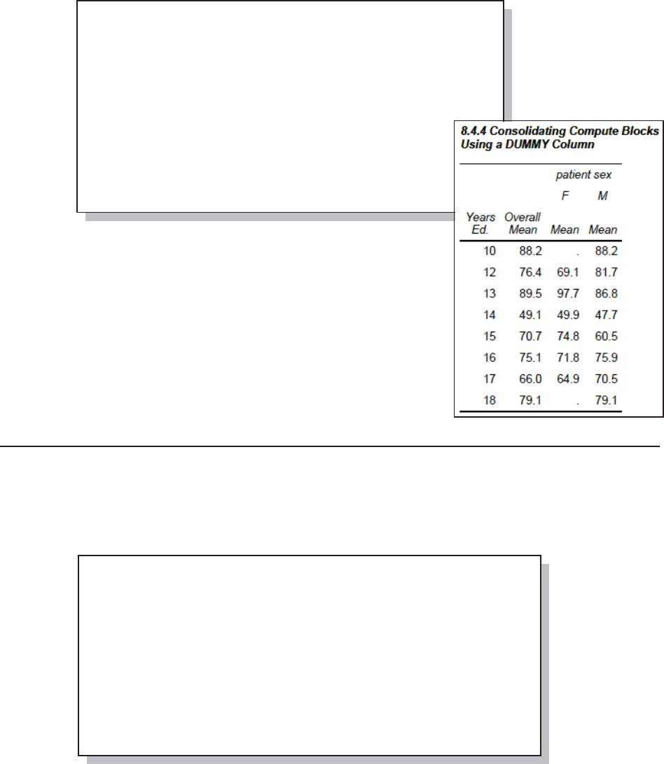
284 Carpenter’s Guide to Innovative SAS Techniques
n The DUMMY
column must be the
furthest to the right on
the COLUMN
statement. Or at least
it must be to the right
of any columns used
in the compute block.
o The NOPRINT option appears on the DEFINE statement
for DUMMY as we are not interested in having this column
displayed.
p The column numbers for the male and female values have
now changed (_C3_ is now the mean weight of the females).
Since these three conversions are independent of each other,
they can be performed in any order.
8.4.5 Consolidating Columns
Sometimes we want to show the information contained in multiple report items within a single
column. Doing so provides us with additional control over the appearance of the report items. In
the following example we want to display the mean along with its standard error, and we want the
values to be displayed as mean (se).
n WT, its alias
WTSE, and the
computed
report item
MEANSE, are
all nested under
SEX o, which
has a define
usage of
ACROSS.
p The values
for WT and
WTSE are not to be printed. They are used only to form the concatenated value (MEANSE).
q The computed report item MEANSE is defined.
r The computed variable MEANSE is defined as character with length of 15.
s The mean (_C2_) and the SE (_C3_) for females are concatenated into a single value (_C4_).
proc report data=advrpt.demog nowd;
column edu wt=allwtmean sex,wt dummy n;
define edu / group 'Years/Ed.';
define allwtmean / mean 'Overall Mean' format=7.1;
define sex / across order=formatted;
define wt / mean 'Mean' format=5.1;
define dummy / computed noprint o;
compute dummy;
_c4_ = _c4_/2.2; p
_c3_ = _c3_/2.2;
allwtmean = allwtmean/2.2;
endcomp;
run;
proc report data=advrpt.demog nowd;
column edu sex,(wt wt=wtse meanse n);
define edu / group 'Years/Ed.';
define sex / across order=formatted; o
define wt / mean noprint; p
define wtse / stderr noprint;
define meanse / computed 'Mean (SE)' format=$15.; q
compute meanse/char length=15; r
_c4_ = cat(put(_c2_,5.2),' (',put(_c3_,5.2),')'); s
_c7_ = cat(put(_c5_,5.2),' (',put(_c6_,5.2),')');
endcomp;
run;
&DUSHQWHU$UW&DUSHQWHU¶V*XLGHWR,QQRYDWLYH6$67HFKQLTXHV&RS\ULJKW6$6,QVWLWXWH,QF&DU\1RUWK&DUROLQD86$
$
//5,*+765(6(59(')RUDGGLWLRQDO6$6UHVRXUFHVYLVLWVXSSRUWVDVFRPSXEOLVKLQJ

Chapter 8: Other Reporting and Analysis Procedures 285
The computed
report item
MEANSE is
constructed in the
compute block by
concatenating the
MEAN and SE,
neither of which is
printed individually.
This also allows us
to add the
parentheses.
Because SEX has
the define usage of ACROSS, absolute column references must be used in the compute block.
8.4.6 Using the STYLE= Option with LINES
When writing to destinations such as PDF, RTF, and HTML, the STYLE= option can be used to
override values in the ODS style without using PROC TEMPLATE to redefine the style itself.
This option is available for use with the REPORT, TABULATE, and PRINT procedures. In
REPORT, it can be used with the LINE statement in the compute block.
Here the style override
option is used to
change the
justification, font, font
style, and font size of
the text written by the
LINE statements.
In the LINE statement,
the @10 and @15
control the left most
starting position for the
text. These values are
ignored for
destinations other than
LISTING, and the
STYLE option is
ignored in the
LISTING destination.
8.4.5 Consolidating Columns within an ACROSS Variable
Weight Within Gender
patient sex
Years F M
Ed. Mean (SE) Mean (SE)
10 . ( . ) 194.1 ( 5.75)
12 152.0 ( 9.71) 179.8 ( 6.73)
13 215.0 ( . ) 191.0 (12.00)
14 109.9 ( 1.78) 105.0 ( 0.00)
15 164.6 (13.72) 133.0 ( 0.00)
16 158.0 ( 0.00) 167.0 ( 7.70)
17 142.8 ( 9.84) 155.0 ( 0.00)
18 . ( . ) 174.0 (15.59)
proc report data=advrpt.demog nowd;
column edu sex,(wt wt=wtse) wt=n wt=allwt;
define edu / group 'Years/Ed.';
define sex / across order=formatted;
define wt / mean 'Mean' F=5.1;
define wtse / stderr 'StdErr' f=5.2;
define n / n noprint;
define allwt / mean 'Overall/Mean' f=5.1;
compute after/style(lines)={just=center
font_face=Arial
font_style=italic
font_size=10pt};
line ' ';
line @10 'Overall Statistics:';
line @15 n 3. ' Subjects had a mean weight of
'
allwt 5.1 ' pounds';
endcomp;
run;
&DUSHQWHU$UW&DUSHQWHU¶V*XLGHWR,QQRYDWLYH6$67HFKQLTXHV&RS\ULJKW6$6,QVWLWXWH,QF&DU\1RUWK&DUROLQD86$
$
//5,*+765(6(59(')RUDGGLWLRQDO6$6UHVRXUFHVYLVLWVXSSRUWVDVFRPSXEOLVKLQJ
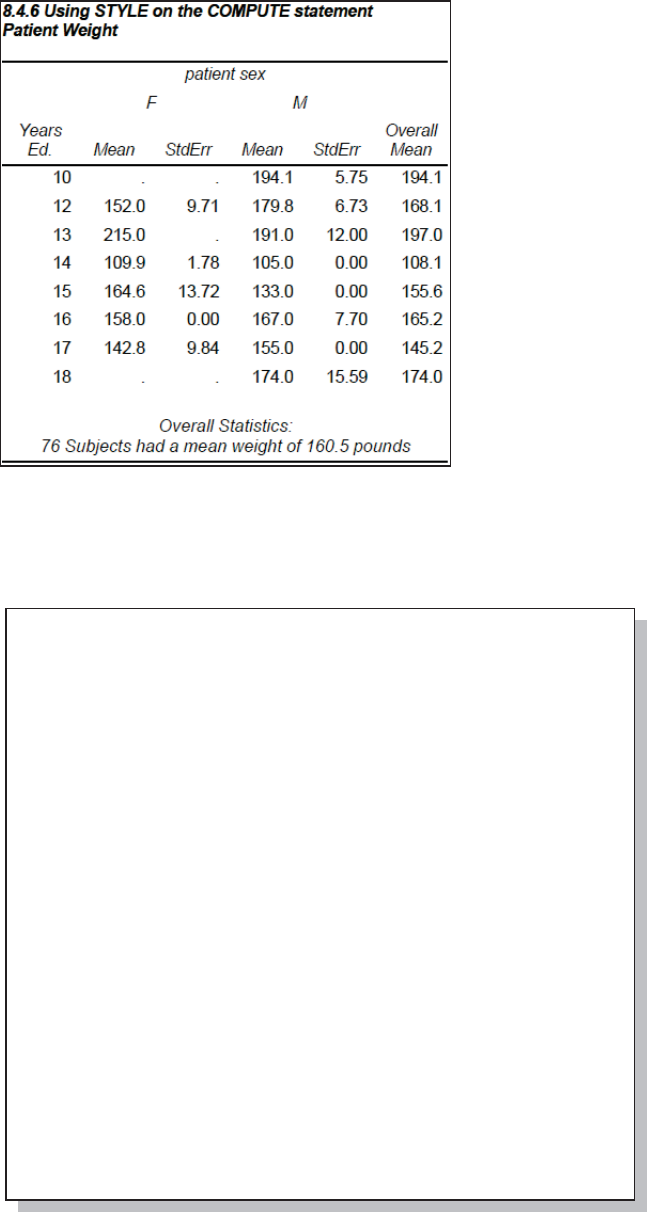
286 Carpenter’s Guide to Innovative SAS Techniques
Inline formatting can also be used in the
compute block with the LINE statement;
however, there are a couple of things that
you should be aware of as the formatting
becomes more complicated. Since LINE
statements are consolidated before
execution, you may not be able to change
style attributes at the LINE statement level
within a compute block. In this example
the STYLE option will be applied to each
of the LINE statements.
If you do need to change attributes on
individual lines, the inline formatting will
probably have to be done in a separate
compute block. This can pose a problem if
you are working with the COMPUTE
AFTER (end of report) compute block.
In the following example an artificial variable PAGEFLAG is introduced. Since it is a constant,
the COMPUTE AFTER PAGEFLAG block and the COMPUTE AFTER block will both take
place at the end of the report. This will allow LINE statements with two different styles to be
used.
n An escape
character is
specified for use
with the inline
formatting
sequences.
o Inline
formatting is used
to right justify the
title.
p A constant
variable is created
that will allow us
to have a second
compute block at
the end of the
report.
q This report item
is not printed, but
since it has a define
usage of GROUP,
a compute block
can be associated
with it.
* Show the use of the inline formatting;
ods rtf file="&path\results\E8_4_6b.rtf";
ods escapechar='~'; n
title1 '8.4.6b Using Inline Formatting';
title2 '~S={just=r} Patient Weight'; o
data demog;
set advrpt.demog;
pageflag=1; p
run;
proc report data=demog(where=(sex='F')) nowd;
column pageflag edu sex,(wt wt=wtse) wt=n wt=allwt;
define pageflag / group noprint; q
. . . . define statements not shown . . . .
compute after pageflag; r
line "~S={just=l background=pink } Females Only";
endcomp;
compute after/style(lines)={just=center s
font_face=Arial
font_style=italic
font_size=10pt};
line ' ';
line @10 'Overall Statistics:';
line @15 n 3. ' Subjects had a mean weight of '
allwt 5.1 ' pounds';
endcomp;
run;
ods rtf close;
&DUSHQWHU$UW&DUSHQWHU¶V*XLGHWR,QQRYDWLYH6$67HFKQLTXHV&RS\ULJKW6$6,QVWLWXWH,QF&DU\1RUWK&DUROLQD86$
$
//5,*+765(6(59(')RUDGGLWLRQDO6$6UHVRXUFHVYLVLWVXSSRUWVDVFRPSXEOLVKLQJ
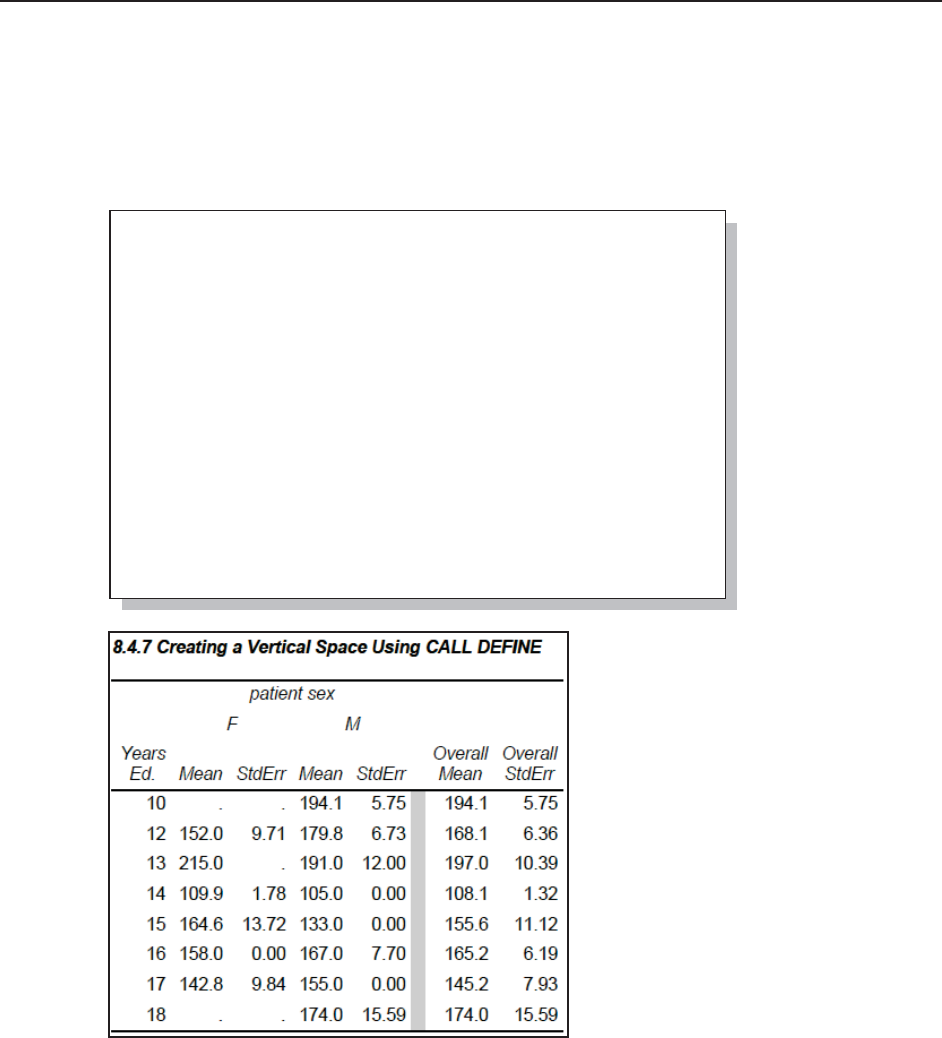
Chapter 8: Other Reporting and Analysis Procedures 287
r A COMPUTE AFTER block is defined for the constant report item.
s Effectively there are now two compute blocks that will be executed at the end of the report.
SEE ALSO
More detail on the use of the style override option (see Sections 11.4.1 and 11.5 for more
examples) and inline formatting (see Section 8.6) can be found in Carpenter’s Complete Guide to
the SAS REPORT Procedure (Carpenter 2007a).
8.4.7 Setting Style Attributes with the CALL DEFINE Routine
Unique to PROC REPORT, the CALL DEFINE routine can be used in the compute block to set
various attributes. Unlike the STYLE= option shown in Section 8.4.6, as a routine CALL
DEFINE can be conditionally executed. This highly flexible routine can be used to set or reset a
number of attributes including formats, links, and styles.
In the following example the DEFINE routine is used to form a visual boundary by changing the
background color for a dummy column. The PDF destination is used to create the report, and a
gray vertical band is
generated through the
use of a computed
variable, DUMMY,
and the CALL
DEFINE routine.
n A computed
column is created to
hold the visual
separator.
o The label for the
computed column is
set to blank.
p _COL_ indicates
that the result of the
routine is to be applied to the entire
column. The second argument, STYLE,
indicates that this is to be a style
override. The third argument is the style
attribute that will be overridden.
q The background color is set to a light
shade of gray.
r Although the cell width is set to 1mm,
you will probably need to experiment to
obtain the desired width as this is only a
nominal value.
s The computed variable is assigned a
missing value.
proc report data=advrpt.demog nowd;
column edu sex,(wt wt=wtse) dummy n
wt=allwt wt=allwtse;
define edu / group 'Years/Ed.';
define sex / across order=formatted;
define wt / mean 'Mean' F=5.1;
define wtse / stderr 'StdErr' f=5.2;
define dummy / computed ' ' ; o
define allwt / mean 'Overall/Mean' f=5.1;
define allwtse / stderr 'Overall/StdErr' f=5.2;
compute dummy/char length=1;
call define(_col_,'style', p
'style={background=cxd3d3d3 q
cellwidth=1mm}'); r
dummy = ' '; s
endcomp;
run;
&DUSHQWHU$UW&DUSHQWHU¶V*XLGHWR,QQRYDWLYH6$67HFKQLTXHV&RS\ULJKW6$6,QVWLWXWH,QF&DU\1RUWK&DUROLQD86$
$
//5,*+765(6(59(')RUDGGLWLRQDO6$6UHVRXUFHVYLVLWVXSSRUWVDVFRPSXEOLVKLQJ
288 Carpenter’s Guide to Innovative SAS Techniques
SEE ALSO
Section 7.5 of Carpenter’s Complete Guide to the SAS REPORT Procedure (Carpenter 2007a)
discusses the CALL DEFINE routine in detail.
8.4.8 Dates within Dates
When a report item is nested within itself, the resulting table is generally less than satisfactory
unless you take some precautions.
Processing dates can be especially problematic as they can fall into several ranges at the same
time. A given date is specific to a year, to a quarter, and to a month. When you want to create
summarizations for more than one date level at
the same time, you could create dummy
variables for each level and then summarize
using these levels as classification variables.
This requires an extra step, such as the one
shown to the left, which we can avoid when
using PROC REPORT.
In the previous DATA step, the variable LABDT is used to create two different summary levels.
The date is being used two different ways at the same time. You can conduct the same type of
summarizations in a REPORT step by creating an alias; however, whenever you nest a variable
under itself, you should be aware of some of the pitfalls of the technique.
The following report counts the number of patients that were seen for each visit type within
quarter and year. The same variable, LABDT, is used for both the quarter and year summary.
n Spanning text is defined for the report.
o The lab date is nested under an alias of lab date (YEAR). The N statistic is nested under
SODIUM, which is in turn nested under date.
p The dates will be consolidated into each represented year. The order will be determined by the
formatted value.
q The quarters are nested within year, and every quarter—regardless of year—will appear under
each year. This means that ‘2007Q1’ will appear without any values under year 2006. We can
eliminate these empty columns through the use of the NOZERO option.
r Any column that is always empty is completely eliminated by the NOZERO option.
proc report data=advrpt.lab_chemistry nowd;
column visit ('Patient Counts Within Quarter' n
labdt=year, labdt,sodium,n); o
define visit / group'Visit';
define year / across format=year. order=formatted ' ' p;
define labdt / across format=yyq6. order=internal ' '; q
define sodium / display ' ';
define n / ' ' format=2. nozero r
style={just=center}; s
run;
data visits;
set advrpt.lab_chemistry
(keep=visit labdt sodium);
year=year(labdt);
qtr = qtr(labdt);
run;
&DUSHQWHU$UW&DUSHQWHU¶V*XLGHWR,QQRYDWLYH6$67HFKQLTXHV&RS\ULJKW6$6,QVWLWXWH,QF&DU\1RUWK&DUROLQD86$
$
//5,*+765(6(59(')RUDGGLWLRQDO6$6UHVRXUFHVYLVLWVXSSRUWVDVFRPSXEOLVKLQJ
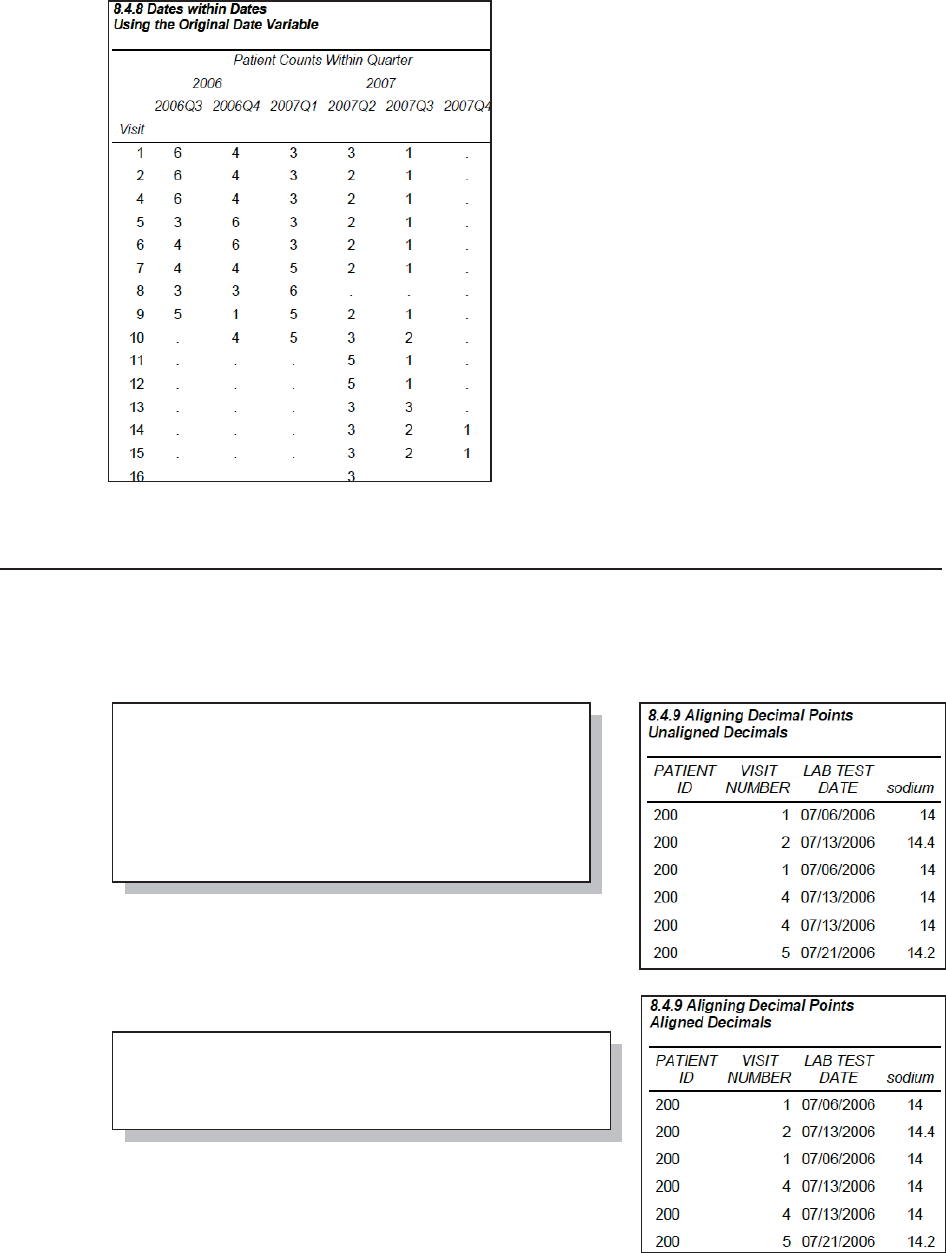
Chapter 8: Other Reporting and Analysis Procedures 289
ods pdf file="&path\results\e8_4_9a.pdf"
style=journal;
title2 'Unaligned Decimals';
proc report data=advrpt.Lab_chemistry
nowd;
column subject visit labdt sodium;
run;
ods pdf close;
s The STYLE= option is used to center the
counts within each quarter.
The use of the NOZERO option is a key technique
when nesting variables such as a date within itself.
Without the use of the NOZERO option there
would necessarily be a number of empty columns.
This example counts the number of patients with
non-missing values of SODIUM. While the N
statistic can be used for the lab date, the NOZERO
option will not work on a grouping variable.
Consequently, an intermediate analysis variable,
SODIUM, is needed. SODIUM is a variable that
in this case we are not particularly interested in,
but it allows us to use the N statistic.
In this example the quarters are ordered
appropriately and the ORDER=INTERNAL
option q is not necessary. If, instead of using
quarters the dates had been grouped using month
name, this option could have been used to place the columns in date order rather than alphabetical
order.
8.4.9 Aligning Decimal Points
Unlike PROC PRINT the REPORT procedure does not by default align decimal points within a
column of the output. This can be seen in the following example, which prints the values of
SODIUM in the LAB_CHEMISTRY data set.
There are a couple of easy ways to align the decimal points
in the SODIUM column. When you are writing to the RTF
or PDF destination, as we are here, the JUST= style attribute
can be used on the DEFINE statement.
While the columns are aligned, the decimal point is not
always shown. When the use of a format is an option, and
it generally is, the format will not only cause the decimal
points to be aligned, but the decimal point will be
displayed.
proc report data=advrpt.Lab_chemistry nowd;
column subject visit labdt sodium;
define sodium / style(column)={just=d};
run;
&DUSHQWHU$UW&DUSHQWHU¶V*XLGHWR,QQRYDWLYH6$67HFKQLTXHV&RS\ULJKW6$6,QVWLWXWH,QF&DU\1RUWK&DUROLQD86$
$
//5,*+765(6(59(')RUDGGLWLRQDO6$6UHVRXUFHVYLVLWVXSSRUWVDVFRPSXEOLVKLQJ
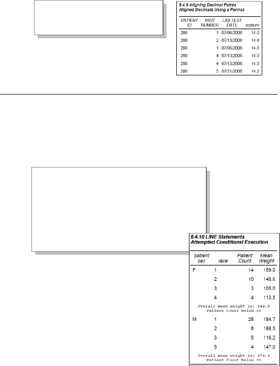
290 Carpenter’s Guide to Innovative SAS Techniques
proc report data=advrpt.demog nowd;
column sex race wt wt=meanwt;
define sex / group;
define race / group;
define wt / analysis n 'Patient Count';
define meanwt/ analysis mean 'Mean Weight' f=5.1;
compute after sex; n
if wt.n ge 35 then do; o
line 'Overall mean weight is: ' meanwt 5.1; p
end;
else line 'Patient Count Below 35'; q
endcomp;
run;
Here a format is used to align the decimal points instead of the style override.
8.4.10 Conditionally Executing the LINE Statement
Unlike in the DATA step where we can conditionally execute the PUT statement, the analogous
LINE statement in a PROC REPORT compute block cannot be conditionally executed. However,
we can conditionally assign values to write with the LINE statement. The first attempt, which is
shown below, demonstrates this problem.
In this example we would like to write a message following each level of SEX. If the count is 35
or more, we want to display the mean weight; however, for counts under 35, we just want a note
stating the low count.
n The text will be
written after each
grouping of the report
item SEX.
o If the total N is
greater than 34, we want
to write the mean p
using a LINE statement.
q For small numbers, we just want this constant text to be
written.
Clearly the LINE statements have not been executed
conditionally. In fact both statements have been executed for
each level of the report item SEX! This is obviously not
what we intended, but what actually happened?
proc report data=advrpt.Lab_chemistry
nowd;
column subject visit labdt sodium;
define sodium / f=4.1;
run;
&DUSHQWHU$UW&DUSHQWHU¶V*XLGHWR,QQRYDWLYH6$67HFKQLTXHV&RS\ULJKW6$6,QVWLWXWH,QF&DU\1RUWK&DUROLQD86$
$
//5,*+765(6(59(')RUDGGLWLRQDO6$6UHVRXUFHVYLVLWVXSSRUWVDVFRPSXEOLVKLQJ
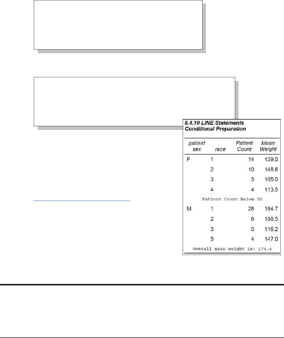
Chapter 8: Other Reporting and Analysis Procedures 291
During the process that evaluates the statements in a compute block, the LINE statements are
effectively moved to the
end of the step. The
compute block from above
essentially becomes the one
shown here. This behavior
is very different from
anything that we see in the
DATA step.
Consequently we cannot conditionally execute the LINE statement; we can, however,
conditionally build what will be displayed by the LINE statement.
r Here we create a temporary variable (TEXT) that will
take on the desired value to be displayed.
s The LINE statement is then executed.
SEE ALSO
The conditional execution of the LINE statement in
PROC REPORT is discussed in SAS Sample #37763 at
http://support.sas.com/kb/37/763.html.
8.5 Using PROC PRINT
PROC PRINT is one of those procedures that everyone uses on a regular basis. It is designed to
dump the data and is generally not used to generate pretty output. However, there are some things
that you can do with PRINT that can make even this standard procedure more useful.
8.5.1 Using the ID and BY Statements Together
Although the PRINT procedure does not have a CLASS statement you can offset groups with a
combination of the BY and ID statements. Variables that are common to these two statements will
cause two changes to the standard report generated by PROC PRINT.
compute after sex;
if wt.n ge 35 then do;
text= 'Overall mean weight is: '||put(meanwt,5.1); r
end;
else text = 'Patient Count Below 35'; r
line text $31.; s
endcomp;
compute after sex; n
if wt.n ge 35 then do; o
end;
else;
line 'Overall mean weight is: ' meanwt 5.1; p
line 'Patient Count Below 35'; q
endcomp;
&DUSHQWHU$UW&DUSHQWHU¶V*XLGHWR,QQRYDWLYH6$67HFKQLTXHV&RS\ULJKW6$6,QVWLWXWH,QF&DU\1RUWK&DUROLQD86$
$
//5,*+765(6(59(')RUDGGLWLRQDO6$6UHVRXUFHVYLVLWVXSSRUWVDVFRPSXEOLVKLQJ

292 Carpenter’s Guide to Innovative SAS Techniques
8.5.1 PRINT with BY and ID Statements
region clinnum clinname
1 011234 Boston National Medical
014321 Vermont Treatment Center
10 107211 Portland General
108531 Seattle Medical Complex
2 023910 New York Metro Medical Ctr
024477 New York General Hospital
026789 Geneva Memorial Hospital
. . . . portions of this table are not shown . . . .
In the PRINT step to the left,
both the BY and ID
statements use the variable
REGION. When used
together this way, the value
for REGION is written only
once for each region (this is
the default behavior for
PROC REPORT for GROUP
and ORDER variables). Also
a blank line has been inserted
after each REGION.
This specialized layout for
PROC PRINT is generated
when all of the variables in
the BY statement also appear
in the same order at the start
of the ID statement.
8.5.2 Using the STYLE= Option with PROC PRINT
The STYLE= option, which is discussed in Sections 8.1.3 and 8.4.6, can also be used with PROC
PRINT. This is a style override option and it is used to change the attributes generated by the
selected ODS style.
In the general syntax shown here, notice that the attributes are surrounded by curly brackets.
style<(location)>={attribute=attribute_value}
In the current releases of SAS you are able to use the square bracket instead of the curly braces.
Specification of the location is optional, since there is a default assignment when it is left off.
However, you generally will want to specify the location as it is used to control where the
attribute assignment is to be applied. Supported locations include:
DATA cells (also COLUMNS or COL)
TOTAL sub-total (used on the SUM statement)
GRANDTOTAL overall total (used on the SUM statement)
HEADER column header (also HEAD and HDR)
N used when the N option is specified
OBS cells in the OBS column
OBSHEADER header for the OBS column
TABLE controls table structure such as cell width
The STYLE= option can be applied on the PROC PRINT statement as well as on other procedure
step statements. A combination of the specified location and the statement containing the option
will determine what portion of the table is modified by the option.
title1 '8.5.1 PRINT with BY and ID Statements';
proc print data=advrpt.clinicnames;
by region;
id region;
var clinnum clinname;
run;
&DUSHQWHU$UW&DUSHQWHU¶V*XLGHWR,QQRYDWLYH6$67HFKQLTXHV&RS\ULJKW6$6,QVWLWXWH,QF&DU\1RUWK&DUROLQD86$
$
//5,*+765(6(59(')RUDGGLWLRQDO6$6UHVRXUFHVYLVLWVXSSRUWVDVFRPSXEOLVKLQJ
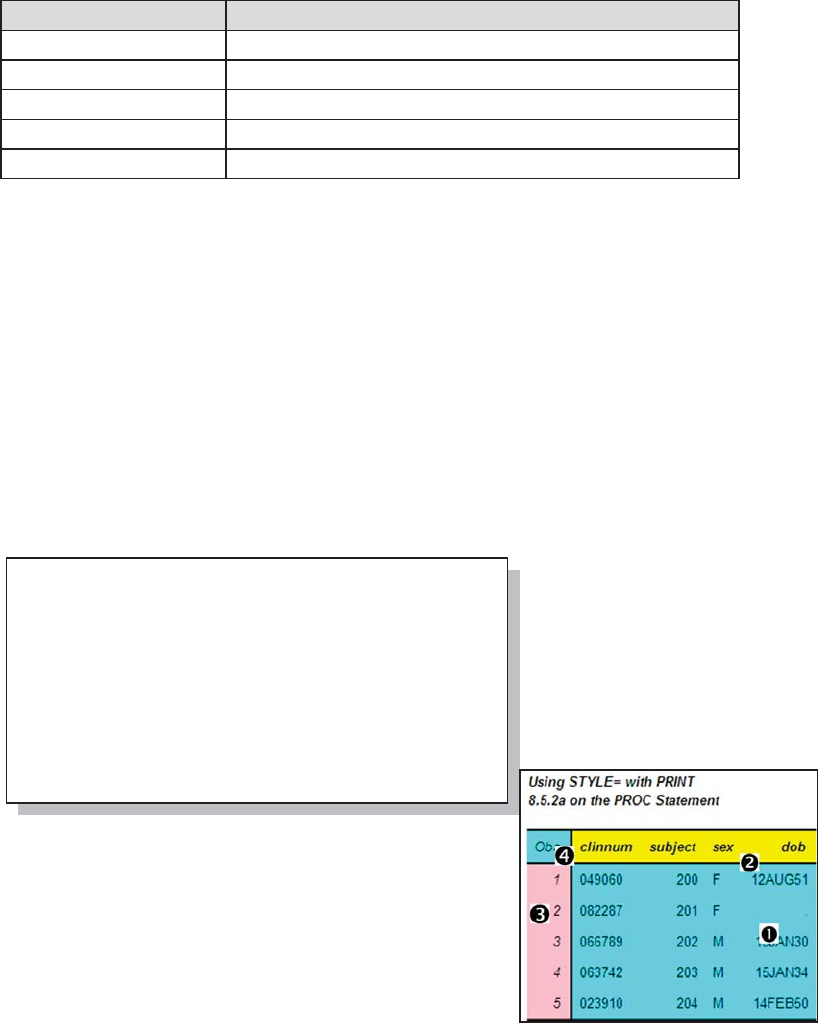
Chapter 8: Other Reporting and Analysis Procedures 293
title1 'Using STYLE= with PRINT';
title2 '8.5.2a on the PROC Statement';
proc print data=advrpt.demog(obs=5)
style(col)= [background=cyan] n
style(header)= [background=yellow o
font_weight=bold]
style(obs)= [background=pink] p
style(obsheader)= [background=cyan] q
;
var clinnum subject sex dob;
run;
Not all style option locations are appropriate for all PRINT statements. The following table shows
the available locations and the statements to which they can be applied.
PROC Statements Supported Style Locations
PROC PRINT data header, n, obs, obsheader, table
BY none
ID header, data
VAR header, data
SUM header, data, total, grandtotal
Some of the style attributes that can be modified include:
BACKGROUND
BORDERCOLOR
BORDERCOLORDARK
BORDERCOLORLIGHT
FONT_FACE
FONT_WEIGHT
FOREGROUND
In the PROC Statement
When the STYLE= option is used on the PROC statement, the attributes tend to control the
overall appearance of this
particularly attractive table.
n The background color is reset
for all the data values in each
column.
o Two attributes for the column
headers are reset.
p The background color for the OBS column is set to
pink.
q The background color for the OBS column header is
changed to CYAN.
&DUSHQWHU$UW&DUSHQWHU¶V*XLGHWR,QQRYDWLYH6$67HFKQLTXHV&RS\ULJKW6$6,QVWLWXWH,QF&DU\1RUWK&DUROLQD86$
$
//5,*+765(6(59(')RUDGGLWLRQDO6$6UHVRXUFHVYLVLWVXSSRUWVDVFRPSXEOLVKLQJ
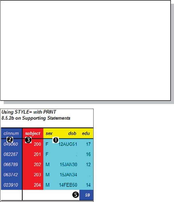
294 Carpenter’s Guide to Innovative SAS Techniques
Supporting Statements
Although style attributes used with the PROC statement generally apply to the table as a whole,
STYLE= options that are applied on supporting statements give you more specific control.
Additionally these attributes tend to override those set on the PROC statement.
Like the CLASS statement (see Section 7.1), which can be split into multiple statements, several
of the PRINT statements that allow lists of variables can also be split into multiple statements.
This allows you to
specify different options
for different variables.
We can take advantage
of this ability when
applying the STYLE=
option pq.
n The STYLE=
options on the PROC
statement override the
defaults associated with
the ODS style,
JOURNAL.
o Two locations are specified for the ID variable. Notice
that the HEADER location has been abbreviated as
HDR.
p Two STYLE= options, each with its own location, are
specified. Since both have the same attributes, they could
have been combined as in o.
q The VAR statement has been split into two
statements. These variables do not have a style override
and will utilize the attributes specified in the PROC
statement n.
r The column total receives three attribute overrides.
MORE INFORMATION
The style override option is used to produce traffic lighting effects is discussed in Section 11.5.4.
proc print data=advrpt.demog(obs=5)
style(col)= [background=cyan] n
style(header)= [background=yellow
font_weight=bold]
;
id clinnum / style(hdr data o)={background=blue
foreground=white};
var subject / style(header)={background=red p
foreground=white}
style(column)={background=red
foreground=white};
var sex dob edu; q
sum edu / style(grandtotal)={font_weight=bold r
background=blue
foreground=white};
run;
&DUSHQWHU$UW&DUSHQWHU¶V*XLGHWR,QQRYDWLYH6$67HFKQLTXHV&RS\ULJKW6$6,QVWLWXWH,QF&DU\1RUWK&DUROLQD86$
$
//5,*+765(6(59(')RUDGGLWLRQDO6$6UHVRXUFHVYLVLWVXSSRUWVDVFRPSXEOLVKLQJ
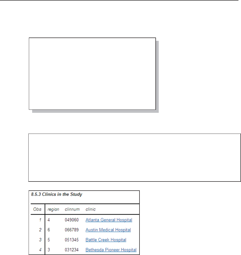
Chapter 8: Other Reporting and Analysis Procedures 295
8.5.3 Using PROC PRINT to Generate a Table of Contents
The PRINT procedure is designed to work with lists of information. When the list of values
contains links to other files, PRINT can create a table of contents to a report.
In this example HTML anchor tags are formed as data values. When they are displayed by ODS
in the HTML destination these
values become links to other files.
The character variable CLINIC is
used to hold the HTML anchor
tag. The CATT function n is used
to concatenate the pieces of the
anchor tag statement. The clinic
number o is used in the name of
the file to which the tag will link.
The name of the clinic p will be
displayed. In the PROC PRINT
step q all that is required is to
display the data. The LISTING
destination does not know what to do with an HTML anchor tag and will therefore show the data
as it is stored r.
When the table is displayed using the
HTML destination, the value is interpreted
as an anchor tag and is displayed as a
linkable item. Here the first four items in
the PROC PRINT are shown.
MORE INFORMATION
The creation of links is discussed in more detail in Section 11.4.
SEE ALSO
The REPORT procedure is even more flexible for creating this type of display. See Carpenter
(2007b) for more on creating links in your table.
8.5.3 Clinics in the Study
Obs region clinnum clinic
1 4 049060 <a href='cn049060.html'>Atlanta General Hospital</a> r
2 6 066789 <a href='cn066789.html'>Austin Medical Hospital</a>
3 5 051345 <a href='cn051345.html'>Battle Creek Hospital</a>
4 3 031234 <a href='cn031234.html'>Bethesda Pioneer Hospital</a>
. . . . portions of the table are not shown . . . .
data clinlinks(keep=region clinnum clinic);
set clinicnames;
length clinic $70;
clinic = catt("<a href='cn", n
clinnum, o
".html'>",
clinname, p
"</a>");
run;
proc print data=clinlinks;
var region clinnum clinic; q
run;
&DUSHQWHU$UW&DUSHQWHU¶V*XLGHWR,QQRYDWLYH6$67HFKQLTXHV&RS\ULJKW6$6,QVWLWXWH,QF&DU\1RUWK&DUROLQD86$
$
//5,*+765(6(59(')RUDGGLWLRQDO6$6UHVRXUFHVYLVLWVXSSRUWVDVFRPSXEOLVKLQJ
296
&DUSHQWHU$UW&DUSHQWHU¶V*XLGHWR,QQRYDWLYH6$67HFKQLTXHV&RS\ULJKW6$6,QVWLWXWH,QF&DU\1RUWK&DUROLQD86$
$
//5,*+765(6(59(')RUDGGLWLRQDO6$6UHVRXUFHVYLVLWVXSSRUWVDVFRPSXEOLVKLQJ

Chapter 9
SAS/GRAPH Elements You Should Know—Even if
You Don’t Use SAS/GRAPH
9.1 Using Title Options with ODS 298
9.2 Setting and Clearing Graphics Options and Settings 300
9.3 Using SAS/GRAPH Statements with Procedures That Are Not SAS/GRAPH
Procedures 303
9.3.1 Changing Plot Symbols with the SYMBOL Statement 303
9.3.2 Controlling Axes and Legends 306
9.4 Using ANNOTATE to Augment Graphs 309
The Output Delivery System, ODS, gives us a great deal of the kind of control that we must have
in order to produce the kinds of reports and tables that are expected of us. Although we will often
include graphical elements in our tables, it turns out that a number of options, statements, and
techniques that are associated with SAS/GRAPH can be utilized to our benefit even when we are
NOT creating graphs. In this chapter you will learn how to take advantage of these graphical
elements even when you are not using SAS/GRAPH.
Some of the options and statements described in this chapter are not available if your site has not
licensed SAS/GRAPH. If SAS/GRAPH is not available to you, try to get your site to license it;
otherwise, experiment. A lot of the things shown in this chapter will work anyway, but not
everything!
SEE ALSO
Carpenter (2010b) contains a number of other related examples.
&DUSHQWHU$UW&DUSHQWHU¶V*XLGHWR,QQRYDWLYH6$67HFKQLTXHV&RS\ULJKW6$6,QVWLWXWH,QF&DU\1RUWK&DUROLQD86$
$
//5,*+765(6(59(')RUDGGLWLRQDO6$6UHVRXUFHVYLVLWVXSSRUWVDVFRPSXEOLVKLQJ

298 Carpenter’s Guide to Innovative SAS Techniques
9.1 Using Title Options with ODS
For destinations that support font and color attributes, the Output Delivery System, ODS, honors
many of the SAS/GRAPH title and footnote options.
A few of the traditional TITLE/FOOTNOTE statement options include:
Color= color designation
BColor= background color specification
Height= height of the text (usually specified in points)
Justify= text justification (left, center, right)
Font= font designation (can include hardware and software fonts)
Most of these options can be abbreviated. For the options shown above, you can use the uppercase
letters in the option name as an abbreviation.
There are also a few font modification options. These include:
BOLD boldface the text
ITALIC italicize the text
UNDERLINE underline the text
Colors can include most standard color names as well as any of the RGB or gray-scale colors that
are appropriate for the output destination.
These options are listed in the Base SAS TITLE statement documentation, as well as in the
SAS/GRAPH documentation; however, a number of the SAS/GRAPH TITLE statement options
are not supported outside of the graphics environment. The following example demonstrates some
of these TITLE statement options using titles associated with an RTF report.
n You may use any font
available to your system. Fonts
consisting of more than one
word must be enclosed in
quotation marks.
o The font size is set to 15
points. This can be a fairly
nominal size, as actual size can
depend on the destination and
how it is displayed.
p The background color is set
to yellow.
q JUSTIFY=LEFT has been abbreviated.
r The font is boldfaced.
title1 f='times new roman' n
h=15pt c=blue o
bc=yellow p
'9.1a Using TITLE Options';
ods rtf file="&path\results\E9_1a.rtf"
style=rtf;
title2 f='Arial' h=13pt c=red
j=l q
bold r
'English Units';
proc report data=advrpt.demog nowd split='*';
. . . portions of the REPORT step are not shown . . . .
&DUSHQWHU$UW&DUSHQWHU¶V*XLGHWR,QQRYDWLYH6$67HFKQLTXHV&RS\ULJKW6$6,QVWLWXWH,QF&DU\1RUWK&DUROLQD86$
$
//5,*+765(6(59(')RUDGGLWLRQDO6$6UHVRXUFHVYLVLWVXSSRUWVDVFRPSXEOLVKLQJ
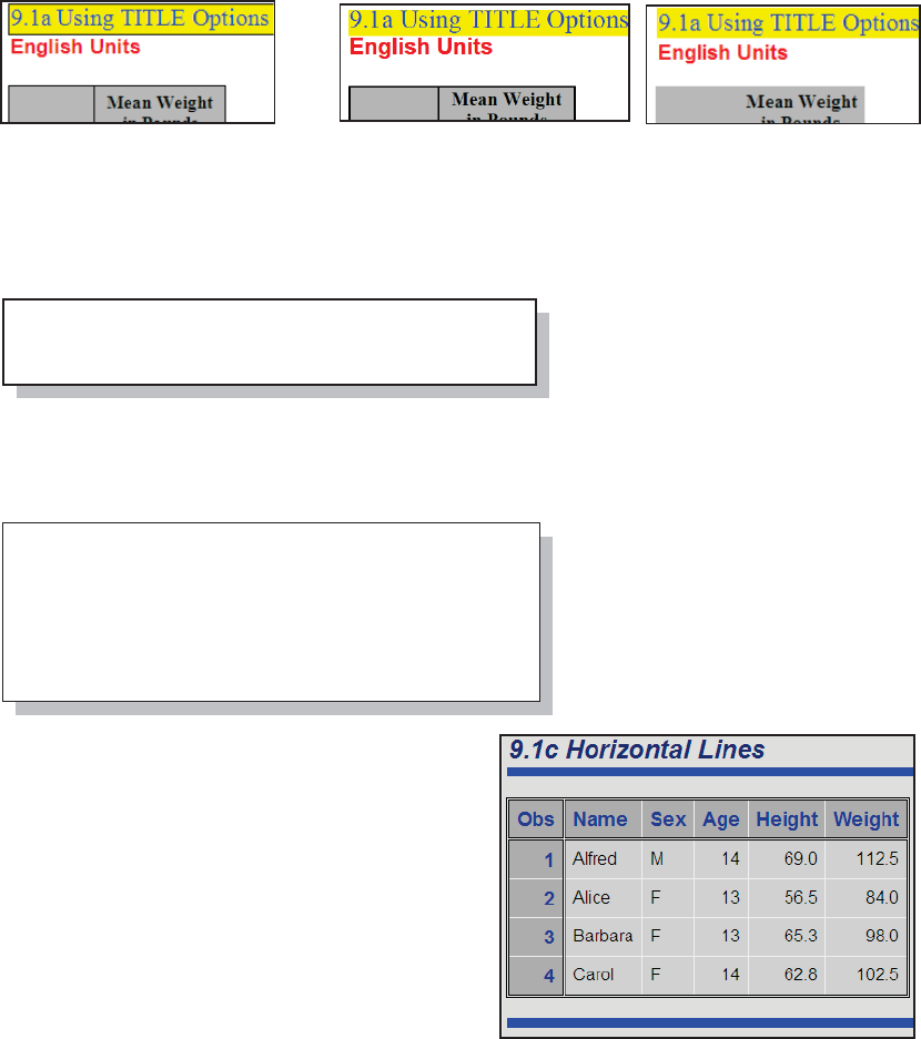
Chapter 9: SAS/GRAPH Elements You Should Know— Even If You Don’t Use SAS/GRAPH 299
RTF PDF HTML
When using the RTF style in the RTF destination, changing the background color (BC=) adds a
box around the title.
In RTF, by default, the titles and footnotes are added to the HEADER and FOOTERS of the
document when the table is imported. Footers are at the bottom of the physical page, and not
necessarily at the bottom of the table.
The titles/footnotes can be made a
part of the table itself through the use
of the BODYTITLE option. For
shorter tables this can move the
footnote to the base of the table.
Through the use of the background color option (BCOLOR) you can change the color behind the
title’s text. This option can also be used to create colorful horizontal lines. s The BCOLOR
option specifies the background
color. t Some text, if only a blank
space, must be specified.
There are quite a few other SAS/GRAPH TITLE
statement options. Most of these options are
ignored outside of SAS/GRAPH. Depending on
the destination and style, some SAS/GRAPH
TITLE statement options are occasionally not
ignored (when you think that they should be). In
these cases they tend to yield unanticipated results.
ods rtf file="&path\results\E9_1b.rtf"
style=rtf
bodytitle;
title1 '9.1c Horizontal Lines';
title2 h=5pt bcolor=blue ' '; s
footnote h=5pt bcolor=blue ' '; t
ods html file="&path\results\E9_1c.html";
proc print data=sashelp.class(obs=4);
run;
ods html close;
&DUSHQWHU$UW&DUSHQWHU¶V*XLGHWR,QQRYDWLYH6$67HFKQLTXHV&RS\ULJKW6$6,QVWLWXWH,QF&DU\1RUWK&DUROLQD86$
$
//5,*+765(6(59(')RUDGGLWLRQDO6$6UHVRXUFHVYLVLWVXSSRUWVDVFRPSXEOLVKLQJ
300 Carpenter’s Guide to Innovative SAS Techniques
SEE ALSO
The horizontal lines example originated from a tip supplied by Don Henderson on
sasCommunity.org at http://www.sascommunity.org/wiki/Tip_of_the_Day:April_26.
TITLE / FOOTNOTE options are also documented at
http://support.sas.com/documentation/cdl/en/lrdict/64316/HTML/default/viewer.htm#a000220968
.htm (see Example 3 for specific usages of these options).
9.2 Setting and Clearing Graphics Options and Settings
Most procedures that have graphics capabilities can also take advantage of many graphics options
and settings. Not all of the graphics options will be utilized outside of the SAS/GRAPH
environment, so you may need to do some experimenting to determine which graphics options are
used for your OS, version of SAS, ODS destination, and the procedure of interest.
Graphics options are set through the use of the GOPTIONS statement. Like the OPTIONS
statement, this global statement is used to set one or more graphics options. Because there are a
great many aspects to the preparation and presentation of a high-resolution graphic, there are
necessarily a large number of graphics options.
A few of the more commonly used options are shown here.
Option
Example
Value
What It Does
htext= 2.5 sets the size for text
ftext= Arial sets a default font for text characters
border noborder
border
determines if a border is to be placed around the graphic
device= emf identifies the instruction set for the rendering of the graphic
gsfname= fileref the graphic is written to the file at this location
Because these options and settings have a scope for the entire session, if you are in an interactive
session and execute two or more programs that use or change some of these options, it is not
uncommon to have the options from one program interfere
with the options of the next program. You can mitigate this
interference by setting or resetting the options to their default
values at the start of each program by using the RESET= option.
goptions reset=symbol;
&DUSHQWHU$UW&DUSHQWHU¶V*XLGHWR,QQRYDWLYH6$67HFKQLTXHV&RS\ULJKW6$6,QVWLWXWH,QF&DU\1RUWK&DUROLQD86$
$
//5,*+765(6(59(')RUDGGLWLRQDO6$6UHVRXUFHVYLVLWVXSSRUWVDVFRPSXEOLVKLQJ
Chapter 9: SAS/GRAPH Elements You Should Know— Even If You Don’t Use SAS/GRAPH 301
FILENAME fileref "&path\results\FinalReport.emf";
goptions reset=all border n
ftext=simplex; o
GOPTIONS GSFNAME=fileref GSFMODE=replace p
DEVICE=emf; q
*goptions device=win r
targetdevice=emf; s
The RESET= graphics option can be used to reset a number of different groups of graphic
settings. The following table shows some of these groups.
RESET= What It Does
all resets all graphics options and settings. Resets values from some other
statements as well (see below).
goptions resets only graphics options to their default values
symbol clears all symbol statement definitions
legend clears all legend statement definitions
title clears all title definitions; same as title1;
footnote clears all footnote definitions; same as footnote1;
The following is a rather typical set of GOPTION statements.
n The RESET=all option
clears all graphics options
and sets them to their
default values. Borders
around the graphs are then
turned on.
o The FTEXT= option is
used to set the default font
for graphics text. SIMPLEX is similar to ARIAL; however, this SAS/GRAPH font may not be
available if your site does not license SAS/GRAPH.
p Graphics Stream File options, GSF, are used to route the graph to a file.
GSFNAME= points to the destination of the graphic (in this case a fileref named
FILEREF).
GSFMODE= if the graphic file already exists, REPLACE indicates that the graphic is to
be replaced.
q The DEVICE= option is used to structure the graph for the appropriate physical or virtual
destination. EMF is a good device when the graphic is to be included in a word processing
document.
r During program development you will want to see the graph displayed on the monitor
(DEVICE=WIN); however, you may want to view it as it will ultimately be displayed on the final
destination. The TARGETDEVICE= option s attempts to show you the graph on the display
device (DEVICE=) using the constraints of the eventual final device (TARGETDEVICE=). In
this production example this development statement has been commented out.
&DUSHQWHU$UW&DUSHQWHU¶V*XLGHWR,QQRYDWLYH6$67HFKQLTXHV&RS\ULJKW6$6,QVWLWXWH,QF&DU\1RUWK&DUROLQD86$
$
//5,*+765(6(59(')RUDGGLWLRQDO6$6UHVRXUFHVYLVLWVXSSRUWVDVFRPSXEOLVKLQJ
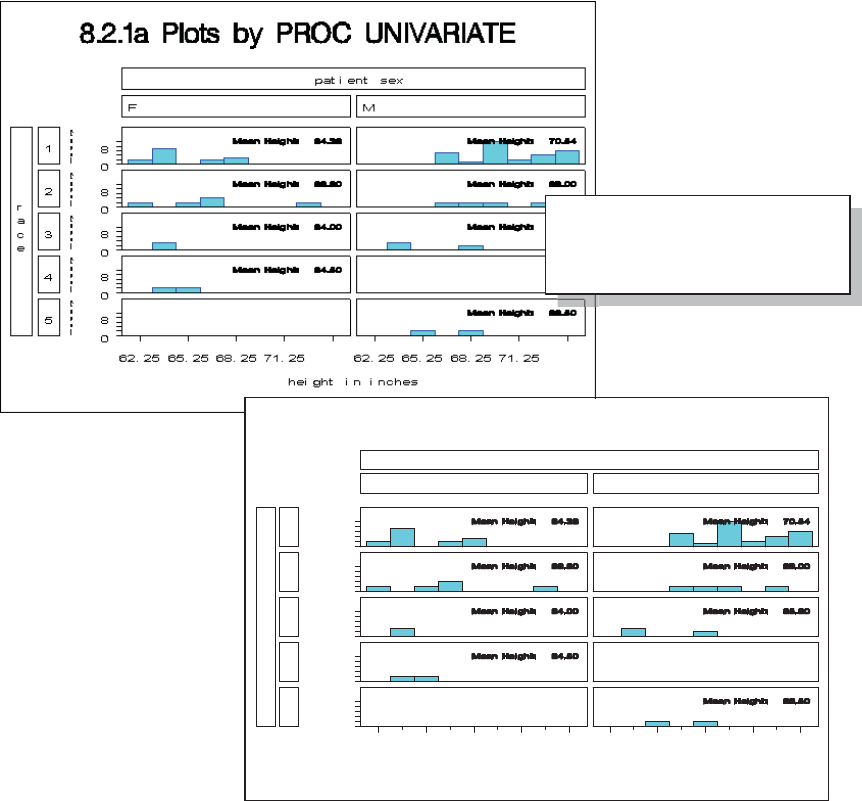
302 Carpenter’s Guide to Innovative SAS Techniques
FTEXT= can be especially important when generating graphics using procedures such as PROC
UNIVARIATE. In the example plot appearing in Section 8.2.1a, and shown here as well, some of
the text is virtually
unreadable. This can be
a result of the automatic
default selection of
hardware fonts that do
not scale appropriately.
The FTEXT= option t
can be used to specify
the default font. The
only coding changes
between these two
versions of this graphic is
the use of the FTEXT=
option. Notice that there
are several changes
including text orientation
as well as readability.
Note that the font used on
the interior graphics was
not changed.
When these options are
being used with ODS you
may want to control
whether or not they should
override the selected style.
Starting in SAS 9.2 the
application of some of
these options can be restricted with the use of the ODS USEGOPT statement. When USEGOPT is
in effect, the settings for the following graphics options will take precedence over the ODS style
and will affect all of your ODS output, including tables as well as graphics GOPTIONS. Affected
graphics options include:
FTEXT=, CTEXT=, HTEXT=, FTITLE=, CTITLE=, HTITLE=.
When ODS NOUSEGOPT is in effect, the settings for these graphics options will not override the
value in the style definition in your ODS output.
MORE INFORMATION
Although not generally shown in the code included in the text of this book, graphics options are
used in examples throughout Chapters 9 and 10. Examine the sample code for more examples of
the use of graphics options.
goptions device=emf
ftext=arial t
gsfname=out821a
noprompt;
DB$5,$/3ORWVE\352&81,9$5,$7(
)
&RXQW
0
&RXQW
&RXQW
&RXQW
&RXQW
KHLJKWLQLQFKHV
UDFH
SDWLHQWVH[
&DUSHQWHU$UW&DUSHQWHU¶V*XLGHWR,QQRYDWLYH6$67HFKQLTXHV&RS\ULJKW6$6,QVWLWXWH,QF&DU\1RUWK&DUROLQD86$
$
//5,*+765(6(59(')RUDGGLWLRQDO6$6UHVRXUFHVYLVLWVXSSRUWVDVFRPSXEOLVKLQJ

Chapter 9: SAS/GRAPH Elements You Should Know— Even If You Don’t Use SAS/GRAPH 303
9.3 Using SAS/GRAPH Statements with Procedures
That Are Not SAS/GRAPH Procedures
There are a number of other procedures that although not part of SAS/GRAPH are none-the-less
able to take advantage of SAS/GRAPH statements when generating high-resolution graphs.
A few of the more common procedures that I have found to be useful that also have high-
resolution graphics capabilities include:
Base
PROC UNIVARIATE (see Section 8.2)
SAS/QC
PROC CAPABILITY
PROC SHEWART (see Section 10.1.3)
SAS/STAT
PROC BOXPLOT (see Section 10.1.1)
PROC PROBIT
PROC REG
The remainder of this section is a very brief introduction to some of the statements that can be
used outside of SAS/GRAPH. Better and more complete introductions to SAS/GRAPH can be
found in numerous papers, as well as in several books.
CAVEAT
If you do not have access to SAS/GRAPH and depending on your release of SAS, some of the
techniques and capabilities described in this section may not be available to you. This is true even
if you are not using a SAS/GRAPH procedure.
MORE INFORMATION
The probability and QQ plots generated by PROC UNIVARIATE in Section 8.2.3 can take
advantage of the SYMBOL statement (see Section 9.3.1).
Section 9.1 demonstrates the use of SAS/GRAPH options in TITLE and FOOTNOTE statements
as they can be applied to output generated by the Output Delivery System.
SEE ALSO
Books that specifically provide introductions to SAS/GRAPH include Carpenter and Shipp
(1995), Carpenter (1999), and Miron (1995).
9.3.1 Changing Plot Symbols with the SYMBOL Statement
The SYMBOL statement is used to control the appearance of items within the graphics area. As
you would suspect this includes plot symbols, but it also controls the appearance of lines, and how
points are joined with these lines. All plot symbols and lines have attributes, e.g., color, size,
shape, thickness. These attributes are all controlled with the SYMBOL statement.
&DUSHQWHU$UW&DUSHQWHU¶V*XLGHWR,QQRYDWLYH6$67HFKQLTXHV&RS\ULJKW6$6,QVWLWXWH,QF&DU\1RUWK&DUROLQD86$
$
//5,*+765(6(59(')RUDGGLWLRQDO6$6UHVRXUFHVYLVLWVXSSRUWVDVFRPSXEOLVKLQJ
304 Carpenter’s Guide to Innovative SAS Techniques
There can be up to 99 numbered SYMBOL statements. Attributes to be controlled are specified
through the use of options. Options are
specified through the use of their names and,
in most cases, the names can be abbreviated.
This SYMBOL statement requests that the plot symbols (a dot) be blue, with a size (height) of .8
units.
Fortunately, since the SYMBOL statement is heavily used, it is usually fairly straightforward to
apply. A quick study of the documentation will usually serve as a first pass instruction. Like so
many things in SAS however, there are a few traps that you should be aware of when applying the
SYMBOL statement in more complex situations.
A few of the numerous SYMBOL statement options are shown in the following table.
Option
Option
Abbreviation
Example
Value
What It Does
color= c= blue sets the color of the symbol or line
height= h= 1.5 specifies the size of the symbol
value= v= star identifies the symbol to be used in the plot
interpol= i= join indicates how plot symbols are to be connected
line= l= 1 assigns line numbers; 1, 2 , and 33 are the most
useful
width= w= 2.1 identifies line width; the default is usually 1
SYMBOL Definitions Are Cumulative
Although SYMBOL statements, like TITLE and FOOTNOTE statements, are numbered, that is
about the only similarity with regard to the way that the definitions are established. When a
TITLE3 statement is specified, the definition for TITLE3 is completely replaced. Not only is a
given TITLE statement the complete definition for that title, but that same TITLE3 statement
automatically clears titles 4 through 10. SYMBOL statement definitions, on the other hand, are
cumulative, and each numbered statement is independent of statements with other numbers.
The two SYMBOL statements on the left could be rewritten as a series of statements.
The graphics option RESET can be used in the GOPTIONS statement to clear SYMBOL
statement definitions.
SYMBOL Definition Selection Is NOT User Directed
When symbols or lines are to be used in a graph, the procedure first checks to see if there are any
user defined symbol definitions (of course, there are defaults for everything when SYMBOL
statements have not been used). The procedure then selects the next available symbol definition.
This means that if SYMBOL2 was just used, the procedure will look for a SYMBOL3 definition.
symbol1 color = blue h = .8 v=dot;
symbol1 color = blue v=none
i=box10 bwidth=3;
symbol2 color = red v=dot
i=join line=2 h=1.2;
symbol2 v=dot i=join;
symbol1 color = blue;
symbol2 color = red;
symbol1 v=none i=box10 bwidth=3;
symbol2 line=2 h=1.2;
goptions reset=symbol;
&DUSHQWHU$UW&DUSHQWHU¶V*XLGHWR,QQRYDWLYH6$67HFKQLTXHV&RS\ULJKW6$6,QVWLWXWH,QF&DU\1RUWK&DUROLQD86$
$
//5,*+765(6(59(')RUDGGLWLRQDO6$6UHVRXUFHVYLVLWVXSSRUWVDVFRPSXEOLVKLQJ
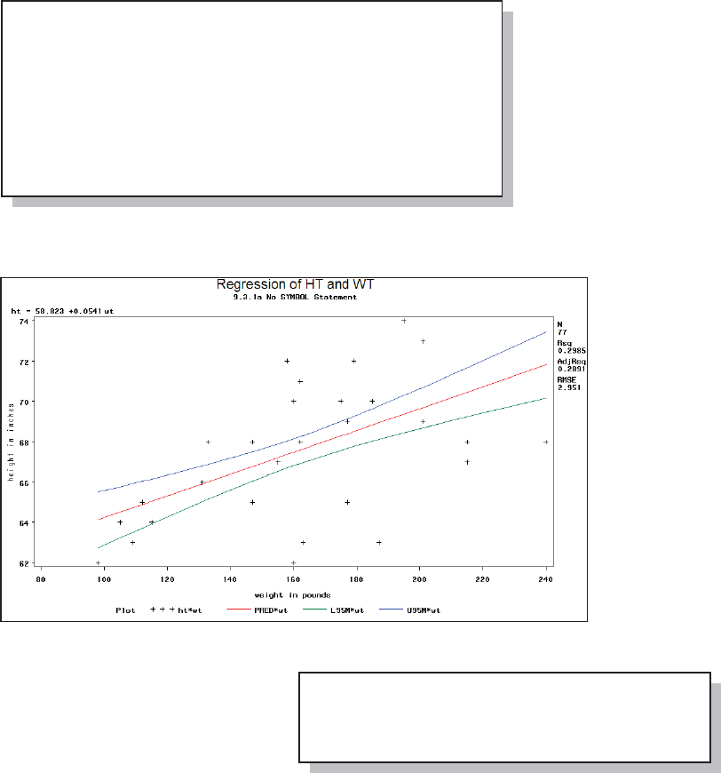
Chapter 9: SAS/GRAPH Elements You Should Know— Even If You Don’t Use SAS/GRAPH 305
Unfortunately it is not generally possible to directly tie a given symbol statement to a given line or
symbol. This means that you will need to have at least a basic understanding of symbol definition
selection for the procedure that you are planning on using.
The following example uses PROC REG to perform a regression analysis on HT and WT in the
DEMOG data set. The PLOT statement can be used to create a plot of the results of the analysis.
n All graphics options are
set to their defaults.
o TITLE statement
options are used to select
boldface ARIAL as the
font for the first title.
p HT is used as the
dependent variable.
q The CONF option is used to request the plotting of the confidence intervals and predicted
values.
Although the
procedure selects
colors and line
types for the
predicted value
line and for the
confidence
intervals, the
data is plotted
using the plus
‘+’ symbol.
We can use the
SYMBOL
statement to gain
control of the
plot symbol.
r For the data points, the
SYMBOL1 statement is used to
select the plot symbol attributes. In
this case the color and the symbol
(V=).
s The color for the estimated line is specified. You will need to experiment to determine which
SYMBOL statement will be used by which aspect of the graph.
goptions reset=all; n
title1 f=arial bold 'Regression of HT and WT'; o
title2 '9.3.1a No SYMBOL Statement';
proc reg data=advrpt.demog;
model ht = wt; p
plot ht*wt/conf; q
run;
quit;
title2 '9.3.1b With SYMBOL Statements';
symbol1 c=blue v=dot; r
symbol2 c=red; s
symbol3 c=green r=2; t
&DUSHQWHU$UW&DUSHQWHU¶V*XLGHWR,QQRYDWLYH6$67HFKQLTXHV&RS\ULJKW6$6,QVWLWXWH,QF&DU\1RUWK&DUROLQD86$
$
//5,*+765(6(59(')RUDGGLWLRQDO6$6UHVRXUFHVYLVLWVXSSRUWVDVFRPSXEOLVKLQJ
306 Carpenter’s Guide to Innovative SAS Techniques
t The
confidence lines
are colored
green. The R=
option causes
this symbol
definition to be
reused a second
time. Otherwise,
we could have
specified the
SYMBOL4
definition to be
the same as the
SYMBOL3
definition.
The colors and plot symbols are shown in the legend at the bottom of the graph. You can take
control of the legend though the use of the LEGEND statement (see Section 9.3.2). Although not
supported by PROC REG, for some procedures you can eliminate the legend altogether using the
NOLEGEND option.
9.3.2 Controlling Axes and Legends
Control of any and all aspects of the horizontal and vertical axes can be obtained through the use
of the AXIS statement. This global statement can be one of the most complex statements in
SAS/GRAPH, if not within SAS itself, and it is clearly outside of the scope of this book to do
much more than just partially describe this statement. Closely related to the AXIS statement in
syntax is the LEGEND statement, which is used to control the appearance of the graph’s legend.
The following is a brief introduction to these two statements.
Like the SYMBOL statement, you can have up to 99 numbered AXIS and LEGEND statements.
Also like the SYMBOL statement, the axis and legend
definitions are cumulative. Both axis and legend definitions
can be cleared with the RESET= option.
AXIS Statement
The AXIS statement can be used to control the axis lines, tick marks, tick mark text, and axis
labels. You can specify fonts and color for all text. For any of the lines you can control the styles
(type of line), thickness, color, and length.
The axis definition is built through a series of options. Some of these options will themselves have
options, and the layers of options with options can often be three deep. To make things even more
interesting, some options will appear in multiple ways and their effect will depend on position and
usage. Clearly just knowing how to apply the options and how to nest them can be complicated.
Most of the options that can appear in several different aspects of the statement are text
appearance options. Most options are similar to those used as TITLE and FOOTNOTE statement
options (see Section 9.1), and there is also some overlap with those options used in the SYMBOL
statement. Some of the more common text appearance options include:
goptions reset=axis;
goptions reset=legend;
&DUSHQWHU$UW&DUSHQWHU¶V*XLGHWR,QQRYDWLYH6$67HFKQLTXHV&RS\ULJKW6$6,QVWLWXWH,QF&DU\1RUWK&DUROLQD86$
$
//5,*+765(6(59(')RUDGGLWLRQDO6$6UHVRXUFHVYLVLWVXSSRUWVDVFRPSXEOLVKLQJ
Chapter 9: SAS/GRAPH Elements You Should Know— Even If You Don’t Use SAS/GRAPH 307
Option
Option
Abbreviation
Example
Value
What It Does
height= h= 10pct sets size to 10 percent
color= c= cxdedede sets color to a shade of gray
font= f= Arial sets the font to ARIAL
‘text string’ ‘Units are mg’ assigns a text string to the option
The first layer of options control major aspects of the axis. These include such things as:
ORDER= range of values to be included
LABEL= axis label
VALUE= tick mark control
MAJOR= major tick marks (the ones with text)
MINOR= minor tick marks
When building an AXIS statement, parentheses are used to form groups of sub-options, and
indenting to each level of option can be helpful in keeping track of which options go with what.
This is a fairly typical AXIS statement.
Notice that the values of options are in
parentheses. This allows you to specify
the sub-options.
n ORDER= Restricts the axis range;
data can be excluded. Here the range of
the axis is limited to values between 3
and 6 with major tick marks at the
integers. The VALUE= option (shown
in the LEGEND example) specifies the
attributes of the major tick marks.
o H= sets the height of the
label’s text to 2 units (the default
units are cells).
p FONT= specifies the font.
Fonts with multiple words
should be quoted.
q ‘text’ specifies the text for the
label, which overrides the
variable’s label.
r MINOR= specifies the
number of minor tick marks. The
keyword NONE can be used to
turn off minor tick marks.
s ANGLE= rotates the entire label 90 degrees (from horizontal to vertical). Angle=0 is
horizontal.
axis2 order =(3 to 6 by 1) n
label =(h=2 o
font='Times New Roman' p
"Potassium Levels")q
minor =(n=1) r
angle=90 s
rotate=0 t ;
axis1 minor=(n=4) r
color=black
label=( "BMI")
order=(15 to 40 by 5);
Potassium Levels
3
4
5
6
BMI
15 20 25 30 35 40
9.3.2a Initial Visit BMI and Potassium
Using an AXIS Statement
&DUSHQWHU$UW&DUSHQWHU¶V*XLGHWR,QQRYDWLYH6$67HFKQLTXHV&RS\ULJKW6$6,QVWLWXWH,QF&DU\1RUWK&DUROLQD86$
$
//5,*+765(6(59(')RUDGGLWLRQDO6$6UHVRXUFHVYLVLWVXSSRUWVDVFRPSXEOLVKLQJ
308 Carpenter’s Guide to Innovative SAS Techniques
t ROTATE= rotates the letters within the
line of text individually.
u The individual AXIS definitions are
assigned to an axis on the plot or graphic
through options on the PLOT statement.
LEGEND Statement
The general syntax, statement structure, and even many of the options of the AXIS statement are
shared with the LEGEND statement. In the regression plots in Section 9.3.1, the legend appears at
the bottom of the graph. We can change its location as well as its appearance.
n The legend can be INSIDE or
OUTSIDE of the graphics area. It
can also be moved vertically and
horizontally.
o The VALUE= option controls the
text associated with the four
individual items in the legend.
p The LABEL=NONE option turns
off the legend’s label.
q The FRAME option adds a box
around the legend. Other options
allow you to change the width, color,
and shadowing of the frame.
r The ACROSS=2 option
allows at most 2 items for
each row in the legend.
s The LEGEND= option
identifies the appropriate
legend statement.
For this graph, especially
when displayed in black and
white, the legend is fairly
superfluous. Many
procedures have an option
(NOLEGEND) that can be
used to prevent the display
of the option. PROC REG
does not support the
NOLEGEND option. Consequently, there is no way to prevent the legend from appearing when
any of the PLOT statement options that cause multiple items to be displayed (such as CONF) are
used. The following example uses a LEGEND statement to minimize the impact of the legend.
legend1 position=(top left inside) n
value=(f='arial' t=1 'Height' o
t=2 'Predicted'
t=3 'Upper 95'
t=4 'Lower 95')
label=none p
frame q
across=2; r
proc reg data=advrpt.demog;
model ht = wt;
plot ht*wt/conf
legend=legend1; s
run;
proc gplot data=bmi;
plot potassium*bmi/haxis=axis1 u
vaxis=axis2;
run;
ht = 58.823 +0.0541wt
N
77
Rsq
0.2985
AdjRsq
0.2891
RMSE
2.951
Regression of HT and WT
9.3.2b Using a LEGEND Statement
height in inches
62
64
66
68
70
72
74
weight in pounds
80 100 120 140 160 180 200 220 240
Height Predicted
Upper 95 Lower 95
&DUSHQWHU$UW&DUSHQWHU¶V*XLGHWR,QQRYDWLYH6$67HFKQLTXHV&RS\ULJKW6$6,QVWLWXWH,QF&DU\1RUWK&DUROLQD86$
$
//5,*+765(6(59(')RUDGGLWLRQDO6$6UHVRXUFHVYLVLWVXSSRUWVDVFRPSXEOLVKLQJ
Chapter 9: SAS/GRAPH Elements You Should Know— Even If You Don’t Use SAS/GRAPH 309
t The text for the individual values is turned off.
u The label is turned off.
v The individual symbol
elements cannot be turned
off (SHAPE does not
support NONE); therefore,
the values are made very
small.
w The LEGEND2
definition is selected for
use.
MORE INFORMATION
The AXIS statement is used in an example in Section 10.1.1.
9.4 Using ANNOTATE to Augment Graphs
The annotate facility gives us the ability to customize the output generated by the procedure. The
huge advantage is that the customization can be data dependent, without recoding. The key to the
process is the annotate data set. This data set contains the instructions that are to be passed to the
annotate facility. Each observation in the data set is one instruction, and very often the instruction
is fairly primitive, e.g., pick up a pen.
The instructions in the data set are passed to the procedure that is generating the graphic through
the use of the ANNOTATE= option. You can tell if a procedure can take advantage of the
annotate facility when it supports this option or its abbreviation, which is ANNO=.
Since the annotate facility interprets each observation of the annotate data set as an instruction, it
uses the values of specific variables to form the intent of the instruction. You do not get to choose
the names of the variables, but you have a great deal to do with the values that the variables take
on. In order for the instruction to provide a valid instruction to annotate, the variables and their
values have to provide answers to three primary questions.
legend2 value= none t
label=none u
shape=symbol(.001,.001); v
proc reg data=advrpt.demog;
model ht = wt;
plot ht*wt/conf
legend=legend2; w
run;
ht = 58.823 +0.0541wt
N
77
Rsq
0.2985
AdjRsq
0.2891
RMSE
2.951
Regression of HT and WT
9.3.2c Eliminating the Legend
height in inches
62
64
66
68
70
72
74
weight in pounds
80 100 120 140 160 180 200 220 240
&DUSHQWHU$UW&DUSHQWHU¶V*XLGHWR,QQRYDWLYH6$67HFKQLTXHV&RS\ULJKW6$6,QVWLWXWH,QF&DU\1RUWK&DUROLQD86$
$
//5,*+765(6(59(')RUDGGLWLRQDO6$6UHVRXUFHVYLVLWVXSSRUWVDVFRPSXEOLVKLQJ

310 Carpenter’s Guide to Innovative SAS Techniques
Questions to Be Asked Possible Variables Used to Answer the Questions
WHAT is to be done? FUNCTION (this variable will always be present)
WHERE is it to be done? X, Y, XSYS, YSYS
HOW is it to be done? COLOR, SIZE, STYLE, POSITION
The value of the variable FUNCTION is always specified, and this value determines what other
variables will be used by annotate when the instruction is executed. FUNCTION should be a
character variable with a length of 8. There are over two dozen possible values for FUNCTION;
three of the commonly used values are shown here.
Value of
FUNCTION
What It Does
label adds a text label to the graphic
move moves the pointer to another position on the graphic without drawing
anything
draw draws a line from the current position to a new position on the graphic
Other commonly used annotate functions include tools for:
generating polygons, bars, and pie slices
drawing symbols, arrows, and lines
including text and images
For annotate operations that are associated with a location on a graphic, variables are used to
specify the location. In order to identify a location, you will need to specify the coordinate system
(e.g., XSYS, YSYS) and a location within that coordinate system (e.g., X, Y).
In this example the Body Mass
Index, BMI, is calculated and
then added using the annotate
facility to the regression plot
generated by PROC REG (see
Section 9.3).
n The annotate data set is
named (WORK.BMILABEL),
and the variables that it will
contain are specified.
o The annotate variables
FUNCTION and COLOR are
assigned a length in order to
avoid truncation. This is
always a good idea.
p The annotate variables that
are constant for all the
instructions (observations) are
assigned values with the
RETAIN.
data bmilabel(keep=function n
xsys ysys x y
text color style
position size);
set advrpt.demog;
* Define annotate variable attributes;
length color function $8; o
retain function 'label' p
xsys ysys '2'
color 'red'
style 'arial'
position '2'
size .8;
* Calculate the BMI. Note those outside of
* the range of 18 - 26;
bmi = wt / (ht*ht) * 703;
if bmi lt 18 or bmi gt 26 then do; q
* Create a label;
text = put(bmi,4.1); r
x=wt;
y=ht;
output bmilabel; s
end;
run;
&DUSHQWHU$UW&DUSHQWHU¶V*XLGHWR,QQRYDWLYH6$67HFKQLTXHV&RS\ULJKW6$6,QVWLWXWH,QF&DU\1RUWK&DUROLQD86$
$
//5,*+765(6(59(')RUDGGLWLRQDO6$6UHVRXUFHVYLVLWVXSSRUWVDVFRPSXEOLVKLQJ
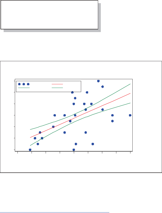
Chapter 9: SAS/GRAPH Elements You Should Know— Even If You Don’t Use SAS/GRAPH 311
q Create an annotate instruction (a label) only for those observations with a BMI outside of the
stated range.
r The variables X and Y contain the coordinates of this data point on the graph. TEXT, the
annotate label, contains the value of the variable BMI.
s Write this annotate instruction to the annotate data set.
t The ANNO= option is used to name the data set n that contains the annotate instructions.
The BMI values that are outside of the selected range are added to the plot as annotate labels. The
location of the label is based on the data values that are also used to generate the plot and the
regression.
SEE ALSO
An introduction to the annotate facility can be found in Carpenter (1999).
Values can also be added to points using the SYMBOL statement option POINTLABEL. See
http://communities.sas.com/message/100627#100627.
proc reg data=advrpt.demog;
model ht = wt;
plot ht*wt/conf legend=legend1
anno=bmilabel; t
run;
36.5
33.7
17.9
32.7
29.3
26.5
29.726.126.1
26.5
28.9
26.5
17.9
36.5
28.9
33.733.7
29.3
33.1
26.126.1 29.7
32.7
33.1
29.5
33.1
26.5
29.5
ht = 58.823 +0.0541 wt
N
77
Rsq
0.2985
AdjRsq
0.2891
RMSE
2.951
9.4 Annotated BMI Labels
height in inches
62
64
66
68
70
72
74
weight in pounds
80 100 120 140 160 180 200 220 240
Height Predicted
Upper 95 Lower 95
&DUSHQWHU$UW&DUSHQWHU¶V*XLGHWR,QQRYDWLYH6$67HFKQLTXHV&RS\ULJKW6$6,QVWLWXWH,QF&DU\1RUWK&DUROLQD86$
$
//5,*+765(6(59(')RUDGGLWLRQDO6$6UHVRXUFHVYLVLWVXSSRUWVDVFRPSXEOLVKLQJ
312
&DUSHQWHU$UW&DUSHQWHU¶V*XLGHWR,QQRYDWLYH6$67HFKQLTXHV&RS\ULJKW6$6,QVWLWXWH,QF&DU\1RUWK&DUROLQD86$
$
//5,*+765(6(59(')RUDGGLWLRQDO6$6UHVRXUFHVYLVLWVXSSRUWVDVFRPSXEOLVKLQJ

Chapter 10
Presentation Graphics—More than Just SAS/GRAPH
10.1 Generating Box Plots 314
10.1.1 Using PROC BOXPLOT 314
10.1.2 Using PROC GPLOT and the SYMBOL Statement 315
10.1.3 Using PROC SHEWHART 316
10.2 SAS/GRAPH Specialty Techniques and Procedures 317
10.2.1 Building Your Own Graphics Font 317
10.2.2 Splitting a Text Line Using JUSTIFY= 319
10.2.3 Using Windows Fonts 319
10.2.4 Using PROC GKPI 320
10.3 PROC FREQ Graphics 323
SAS/GRAPH software has had the ability to create presentation-quality graphs since its
introduction. Currently within SAS there are several graphing systems, with some of the newest
innovations associated with ODS Statistical Graphics. Outside of these two graphics systems there
are a number of procedures that have plotting and graphing capabilities that are comparable to
SAS/GRAPH. A well-rounded programmer will be aware of each of these systems and will be
able to take advantage of the strengths of each. This chapter briefly discusses the plotting
capabilities of some procedures that are not part of SAS/GRAPH.
MORE INFORMATION
The plotting capability of PROC UNIVARIATE (see Sections 8.2.1 through 8.2.3) and PROC
REG (see Sections 9.3 and 9.4) are demonstrated in other sections of the book.
A review of the SYMBOL, AXIS, and LEGEND statements, which are used throughout this
chapter, can be found in Chapter 9.
&DUSHQWHU$UW&DUSHQWHU¶V*XLGHWR,QQRYDWLYH6$67HFKQLTXHV&RS\ULJKW6$6,QVWLWXWH,QF&DU\1RUWK&DUROLQD86$
$
//5,*+765(6(59(')RUDGGLWLRQDO6$6UHVRXUFHVYLVLWVXSSRUWVDVFRPSXEOLVKLQJ

314 Carpenter’s Guide to Innovative SAS Techniques
SEE ALSO
Carpenter (2010b) demonstrates a number of these procedures along with a variety of capabilities.
SAS has extensive graphing capabilities that are not covered in this book. Introductions to
SAS/GRAPH can be found in Carpenter and Shipp (1995) and Miron (1995). The annotate
facility is introduced in Carpenter (1999). ODS Graphics and Statistical Graphics are described in
the books by Kuhfeld (2010), as well as Matange and Heath (2011).
10.1 Generating Box Plots
A box plot is a type of graph that has been used to display more than two dimensions worth of
information on a single graph. Unlike some other graphics techniques that also attempt to display
more than two dimensions, the box plot can do so without creating visual distortions that
otherwise can mislead the reader (Carpenter 1994 and Carpenter 1995, Section 5.7). Although
used heavily in some disciplines, they are unfortunately ignored in others.
Traditionally, the number of ways to generate a box plot within SAS was fairly limited. User-
written programs were common with some of the more sophisticated published examples
presented by Michael Friendly (Friendly, 1991). The SYMBOL statement within SAS/GRAPH
can also be used to generate box plots; however, even with the addition of recent options this is
still a limited technique. More recent additions to SAS provide procedures that can be used to
generate box plots. Of these, the only procedure dedicated to the generation of box plots is PROC
BOXPLOT (see Section 10.1.1), which is part of SAS/STAT software. Other procedures that
generate variations of this type of data display include:
PROC GPLOT SAS/GRAPH (using the SYMBOL statement, see Section 10.1.2)
PROC MIXED SAS/STAT
PROC SHEWART SAS/QC (see Section 10.1.3)
SEE ALSO
The programs and macros found in Michael Friendly’s book (Friendly, 1991) are well written and
well explained. The techniques described provide a flexibility that is hard to beat even in the
newer procedures.
10.1.1 Using PROC BOXPLOT
PROC BOXPLOT, a fairly recent addition to SAS/STAT software, is used to create a variety of
types of box plots. The PLOT statement is used to provide primary control, and PLOT statement
options in addition to those shown in the example below include:
BOXSTYLE indicates the type of box to be displayed
BOXWIDTH used to control the box width
BOXWIDTHSCALE allows box width to vary according to a function of the
group size
NOTCHES draws the boxes with notches
SYMBOLLEGEND attaches a legend statement (see Section 9.3.2)
&DUSHQWHU$UW&DUSHQWHU¶V*XLGHWR,QQRYDWLYH6$67HFKQLTXHV&RS\ULJKW6$6,QVWLWXWH,QF&DU\1RUWK&DUROLQD86$
$
//5,*+765(6(59(')RUDGGLWLRQDO6$6UHVRXUFHVYLVLWVXSSRUWVDVFRPSXEOLVKLQJ
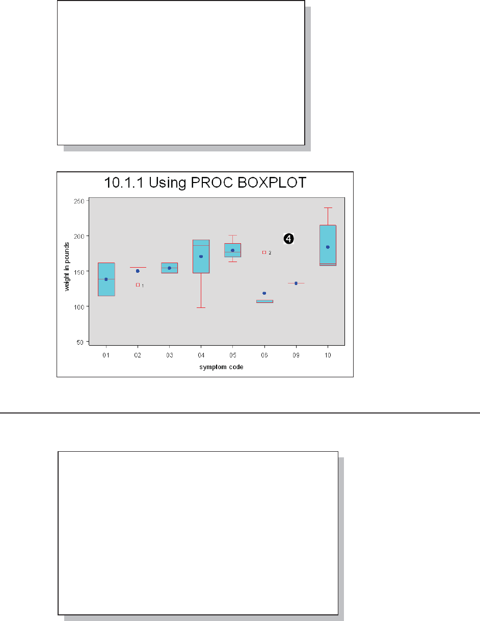
Chapter 10: Presentation Graphics—More than Just SAS/GRAPH 315
Although this is a SAS/STAT procedure, it has the capability of utilizing statements that are
normally associated with SAS/GRAPH. These include the SYMBOL, AXIS, and LEGEND
statements (see Section 9.3).
n The background color inside of
the frame is set to gray using the
color CXdedede.
o There are several styles of boxes.
SCHEMATICID causes points
outside of the whiskers to be labeled
using the ID variable, which is
RACE q, in this graph.
p The AXIS statement is used to control various aspects of the vertical axis. AXIS statements can
be applied to either the
horizontal axis, HAXIS=,
or the vertical axis,
VAXIS= (see Section
9.3).
q The ID statement
names the variable(s) used
to identify the outlying
points.
In this example the
SYMBOL statement has
been used to control the
color and symbol
designating the mean (a
blue dot). The median is
designated with a
horizontal line and the upper and lower limits of the box are the 25th and 75th percentiles.
10.1.2 Using PROC GPLOT and the SYMBOL Statement
The SYMBOL statement (see Section 9.3.1) can be used to generate box plots directly in the
GPLOT procedure. The
control is through the use of
the INTERPOL= option,
which is usually abbreviated
as I=. When I= takes on the
value of BOX, data are
condensed into a box plot for
constant values of the
horizontal variable (SYMP).
symbol1 color = blue h = .8 v=dot;
axis1 minor=none color=black
label=(angle=90 rotate=0);
proc boxplot data=demog;
plot wt*symp/ cframe = cxdedede n
boxstyle = schematicid o
cboxes = red
cboxfill = cyan
vaxis = axis1 p
;
id race; q
run;
symbol1 color = blue v=none i=box10 bwidth=3; n
symbol2 color = red v=dot i=none h=1.2;
axis1 minor=none color=black
order=(50 to 250 by 50)
label=(angle=90 rotate=0);
axis2 order = ('00' '01' '02' '03' '04' '05' o
'06' '07' '08' '09' '10' '11')
value = (t=1 ' ' t=12 ' '); p
proc gplot data=demog;
plot wt*symp/ haxis = axis2
vaxis = axis1
;
run;
&DUSHQWHU$UW&DUSHQWHU¶V*XLGHWR,QQRYDWLYH6$67HFKQLTXHV&RS\ULJKW6$6,QVWLWXWH,QF&DU\1RUWK&DUROLQD86$
$
//5,*+765(6(59(')RUDGGLWLRQDO6$6UHVRXUFHVYLVLWVXSSRUWVDVFRPSXEOLVKLQJ
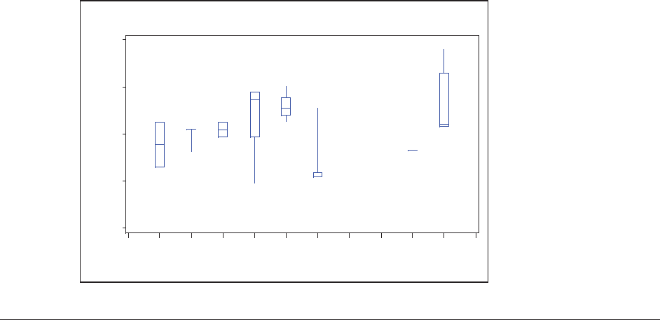
316 Carpenter’s Guide to Innovative SAS Techniques
n The boxes that form the box plot are defined using this SYMBOL statement. The options form
the characteristics of the boxes:
Color= identifies the outline color
Value= indicates that plot symbols are not needed
Interpol= requests box plots with the BOX option BOX10 whiskers are at the 10th and
90th percentiles
bwidth= specifies the width of the boxes
o The major tick marks
for the horizontal axis are
declared. ‘00’ and ‘11’ do
not appear in the data and
their labels are set to
blank using the VALUE
option p. They provide
horizontal spacing
control.
10.1.3 Using PROC SHEWHART
PROC SHEWHART, which is available in SAS/QC software, can be used to generate a number
of process control charts, and box plots are one of the supported chart forms.
The following code can be used to create box plots using PROC SHEWHART. Note that the
horizontal plot variable must be character.
weight in pounds
50
100
150
200
250
symptom code
01 02 03 04 05 06 07 08 09 10
10.1.2 Box Plots using the I= Option
&DUSHQWHU$UW&DUSHQWHU¶V*XLGHWR,QQRYDWLYH6$67HFKQLTXHV&RS\ULJKW6$6,QVWLWXWH,QF&DU\1RUWK&DUROLQD86$
$
//5,*+765(6(59(')RUDGGLWLRQDO6$6UHVRXUFHVYLVLWVXSSRUWVDVFRPSXEOLVKLQJ
Chapter 10: Presentation Graphics—More than Just SAS/GRAPH 317
symbol1 color = blue v=dot i=box10 bwidth=3;
symbol2 color = red v=dot i=none h=1.2;
axis1 minor=none color=black
order=(50 to 250 by 50)
label=(angle=90 rotate=0);
axis2 order = ('00' '01' '02' '03' '04' '05'
'06' '07' '08' '09' '10' '11')
value = (t=1 ' ' t=12 ' ');
proc shewhart data=demog;
boxchart wt*symp/
haxis = axis2
vaxis = axis1
stddeviations nolimits
;
run;
symbol1 color = blue v=dot h=2;
10.1.3 Box Plots using PROC SHEWHART
Z=158.5
UCL
LCL
01 02 03 04 05 06 07 08 09 10
50
100
150
200
250
weight in pounds
symptom code
3s Lim its:
Subgroup Sizes: Min n = 2 Max n = 13
The AXIS statements are used
to augment the axes. Although
SHEWHART and
CAPABILITY are not
SAS/GRAPH procedures, they
support AXIS, SYMBOL, and
PATTERN statements.
You can also use the ANNOTATE
facility with these procedures.
10.2 SAS/GRAPH Specialty Techniques and Procedures
SAS/GRAPH software has been a product of SAS software for quite a long time. During that time
not only has its capabilities continued to expand, but so have the technologies to which it is
delivering. As a result there are a great many graphics problems that have been solved over the
years. Here are a few of the more interesting.
10.2.1 Building Your Own Graphics Font
Although the plot symbols available through SAS/GRAPH software are generally adequate for
our graphing needs, occasionally you may want to tailor plot symbols for specific needs. The
GFONT procedure can be used to create plot symbols. The procedure is used to draw the symbol
shape in much the same way as the annotate facility is used to draw, that is by drawing from one
coordinate to the next.
In this example we are not satisfied with the ‘lumpy’ appearance of the dot symbol, and would
like to create a smoother symbol. This portion of a
graph was generated using the standard DOT
symbol.
We can smooth out the circle by generating our
own symbol using PROC GFONT.
&DUSHQWHU$UW&DUSHQWHU¶V*XLGHWR,QQRYDWLYH6$67HFKQLTXHV&RS\ULJKW6$6,QVWLWXWH,QF&DU\1RUWK&DUROLQD86$
$
//5,*+765(6(59(')RUDGGLWLRQDO6$6UHVRXUFHVYLVLWVXSSRUWVDVFRPSXEOLVKLQJ
318 Carpenter’s Guide to Innovative SAS Techniques
A control data set that draws the font characters (in this case just a circle) is first generated in a
DATA step. Like annotate data sets, specific variables are used to pass information to the GFONT
procedure. Here we are drawing the outline of a circle using 721 short line segments. This control
data set is then passed to GFONT.
n The variable CHAR is used to
hold the keyboard character ‘c’
used to designate this symbol
within the MYDOT font u.
o Symbol segments allow you to
create symbols with disconnected
parts (segments). This symbol
has only one segment so this
value is a constant.
p This is to be a polygon figure.
q Width of the character
(PTYPE=’w’). The symbol will
have a width of 100 units. Allow
about 10% extra for character
spacing.
r This is the first coordinate of the plot symbol ( PTYPE=’v’).
s The segment is written to the control data set.
t Generated fonts are stored in a catalog named FONTs. SAS/GRAPH software searches for this
catalog in numbered librefs whose names start with GFONT.
u Name the font.
v We want the shape to be filled.
w Increase the font resolution. You may notice
little or no difference between a value of 1 and 3.
The resulting dots are a bit smoother. In this screen
capture some pixelation has taken place when the
image was copied into this document.
SEE ALSO
Carpenter (1995) uses PROC GFONT to create a logo and sunflower symbols that self adjust
according to the plotted value. Plot symbol resolution was further discussed with alternate
solutions in the SAS Forum thread at
http://support.sas.com/forums/thread.jspa?threadID=12547&start=0&tstart=0.
data fontdata(keep=char seg x y lp ptype);
retain char 'c' n
seg 1 o
lp 'p';p
ptype='w'; x=-10; y=110; output fontdata;q
ptype='v'; x=100; y=50; output fontdata;r
do deg = 0 to 360 by .5;
rad = deg*arcos(-1)/180;
x=50*cos(rad)+50;
y=50*sin(rad)+50;
output fontdata; s
end;
run;
libname gfont0 "&path\data"; t
proc gfont data=fontdata
name=mydot u
filled v
resolution=3; w
run;
symbol1 f=mydot u c=blue v='c' n h=1;
&DUSHQWHU$UW&DUSHQWHU¶V*XLGHWR,QQRYDWLYH6$67HFKQLTXHV&RS\ULJKW6$6,QVWLWXWH,QF&DU\1RUWK&DUROLQD86$
$
//5,*+765(6(59(')RUDGGLWLRQDO6$6UHVRXUFHVYLVLWVXSSRUWVDVFRPSXEOLVKLQJ
Chapter 10: Presentation Graphics—More than Just SAS/GRAPH 319
10.2.2 Splitting a Text Line Using JUSTIFY=
Within SAS/GRAPH software you can use the text justification option to split lines of text. Very
often this technique can
be used where you
otherwise would be
unable to split the text
line. All that you need
to do is to repeat the
justification option. The
second occurrence will
cause a line split.
n The justification
option can be written as
either JUSTIFY or
abbreviated as a J. The
position (Left, Center,
or Right) can also be
abbreviated. Here the
repeated justification
option causes a split in
the text of the title.
o The reference label
on the vertical reference
line has been split into
three text lines.
p The horizontal axis
label has been split into
two lines.
10.2.3 Using Windows Fonts
SAS/GRAPH software has a number of built-in fonts. In addition if you are executing in the
Windows environment, you may also use Windows TrueType fonts.
The GOPTIONS statement (see Section 9.2) is used to specify graphics options, and one of these
options, the FTEXT= option, can be used to specify fonts. On titles the FONT= option (see
Section 9.1) can also be used to specify fonts.
n Arial has been selected as the default
font for all graphics text. As a general
rule, fonts that are not SAS/GRAPH
fonts should be quoted when they are
named as a graphics option. The name
must be quoted when it has more than
one word.
title1 f=arial h=1.2 justify=c '10.2.2'
j=center 'Splitting Text'; n
symbol1 c=blue v=dot h=1.5;
symbol2 c=red v=dot h=1.5;
axis1 reflabel = (h=1.5
t=1 c=red j=left 'Overweight' o
j=l ' '
j=l c=blue 'Normal');
axis2 order=(1920 to 1970 by 10)
label=(j=c 'Birthyear'j=c 'All Subjects'); p
goptions reset=all noborder
device=emf
gsfname=image gsfmode=replace
ftext='Arial'; n
title1 f=arial 'This is a Title'; o
&DUSHQWHU$UW&DUSHQWHU¶V*XLGHWR,QQRYDWLYH6$67HFKQLTXHV&RS\ULJKW6$6,QVWLWXWH,QF&DU\1RUWK&DUROLQD86$
$
//5,*+765(6(59(')RUDGGLWLRQDO6$6UHVRXUFHVYLVLWVXSSRUWVDVFRPSXEOLVKLQJ
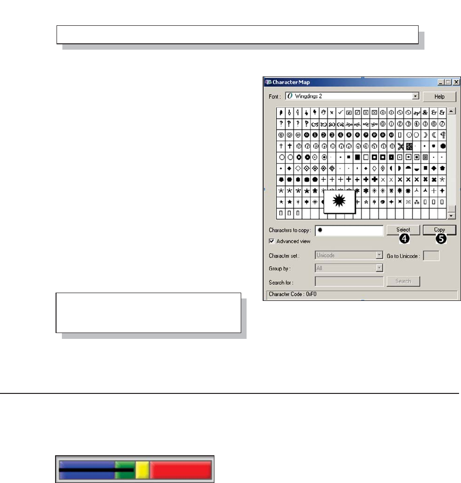
320 Carpenter’s Guide to Innovative SAS Techniques
o The font for a title can also be specified (see Section 9.1 for more on TITLE statement
options). It is not necessary to quote the font name in the TITLE statement, unless the font name
has more than one word, e.g., ‘Times New Roman’.
You can see a list of available fonts, and their alternate designations, by selecting the FONTS
entry in the Windows control panel. Select Start ĺ Control Panel ĺ Fonts.
Some fonts have named variations that include bold and italics (‘Arial Bold’). You may also want
to specify font modifiers. Of the three available font modifiers, bold (/bold or /bo p) and italic
(/italics or /it), are the most commonly used.
There are a number of symbol sets that are included with SAS/GRAPH software. For symbol sets
other than the default symbol set, the name of
the symbol set is specified with the FONT= (or
F=) option on the SYMBOL statement. For
special characters that are not SAS/GRAPH
special characters (characters that do not have a
value mapped to the keyboard), the character
can often be inserted from the character map
(shown to the right). Select Start ĺ Programs
ĺ Accessories ĺ System Tools ĺ Character
Map. q Select the character of interest; as
shown on the right, a starburst design from the
Wingdings 2 font has been selected. r Press the
copy button to place the code in the paste buffer.
s Paste the value into the appropriate location
(the V= option on the SYMBOL statement is
shown here). Notice that the symbol is likely to
appear differently in the SAS program than it
will in the graph.
CAVEAT: If you choose a non-standard font that is only available on your local machine, your
SAS program becomes less transportable.
10.2.4 Using PROC GKPI
The GKPI (Key Performance Indicator) procedure is fairly new to SAS/GRAPH. This procedure
allows you to quickly build indicator bars or dials that show the relative status of a value within a
range that you have specified. There are several types of performance indicators available through
this procedure. The horizontal slider (HBULLET) is
shown here. You can specify the range of values, colors
to separate ranges, and the current value.
symbol1 c=blue
f='wingdings 2' v='ð' s
i=box10 bwidth=3;
axis1 label=(f='arial/bo p' angle=90 rotate=0 'Patient Weight');
&DUSHQWHU$UW&DUSHQWHU¶V*XLGHWR,QQRYDWLYH6$67HFKQLTXHV&RS\ULJKW6$6,QVWLWXWH,QF&DU\1RUWK&DUROLQD86$
$
//5,*+765(6(59(')RUDGGLWLRQDO6$6UHVRXUFHVYLVLWVXSSRUWVDVFRPSXEOLVKLQJ

Chapter 10: Presentation Graphics—More than Just SAS/GRAPH 321
The JAVAIMG device n is required for the
construction of the indicator. Here the
GOPTION statement also sets the horizontal
(XPIXELS) and vertical (YPIXELS) size in
pixels.
Each execution of the procedure generates a single indicator graphic; therefore, for practical
applications the GKPI procedure step will need to be called within a macro loop of some kind.
o The indicator value,
which determines the
length of the horizontal
line, is passed into the
macro and is treated as a
constant in the GKPI
procedure.
p The value range
endpoints are specified.
These will set the zones for the colors q as well as the placement of the ACTUAL= and
TARGET= values.
q The colors of the individual segments are specified. In this example these are constants, but
they too could be declared using macro parameters.
r The NAME= option names the file that will contain the individual indicators.
We would like to report on each subject’s body mass index, BMI, value. In that report we need to
show the indicator calculated for each specific subject. This means that we need to run the GKPI
procedure once for each subject in the data set after first calculating the BMI value. The CALL
EXECUTE routine allows us to create a series of macro calls; one for each observation in the
DATA step.
s It is necessary to have an ODS destination open. We will not use this GIF file, but it will also
contain the individual indicators.
t The BMI value is calculated.
u The subject number will become a part of the name of the file that contains the indicator that
will be imported by PROC REPORT.
%macro slider(gname,bmi);
proc gkpi mode=raised;
hbullet actual=&bmi o bounds=(0 18.5 25 30 50)p /
noavalue nobvalue
target=. colors=(blue,green,yellow,red) q
name="c:\temp\&gname" r;
run;
quit;
%mend slider;
goptions reset=all noborder
device=javaimg n
xpixels=130 ypixels=50
ftext='Arial';
title;
ods html file="c:\temp\slider.gif"; s
data bmi(keep=subject ht wt gname bmi);
set advrpt.demog(obs=8);
length gname $4;
bmi = wt / (ht*ht) * 703; t
gname=cats('G',subject); u
call execute('%slider('||gname||','||put(bmi,4.1)||')'); v
run;
ods html close;
&DUSHQWHU$UW&DUSHQWHU¶V*XLGHWR,QQRYDWLYH6$67HFKQLTXHV&RS\ULJKW6$6,QVWLWXWH,QF&DU\1RUWK&DUROLQD86$
$
//5,*+765(6(59(')RUDGGLWLRQDO6$6UHVRXUFHVYLVLWVXSSRUWVDVFRPSXEOLVKLQJ
322 Carpenter’s Guide to Innovative SAS Techniques
v The CALL EXECUTE routine is used to build a series of macro
calls—one for each incoming observation. The macro %SLIDER is
passed the parameters needed for each specific subject (the subject
number and the associated BMI value). This is sufficient
information for PROC GKPI to generate the subject specific
indicator.
After all the calls to the macro %SLIDER have been executed, a
series of PNG files will have been generated r. These files have
been named v so that they can be imported by PROC REPORT w in the correct order.
w The REPORT step creates a computed
report item (SLIDER) that will hold the
indicator image. The temporary variable
IMGFILE contains the pointer to the PNG
file r that contains the image. For subject
200, IMGFILE contains:
style={postimage='c:\temp
\G200.png'}.
A portion of the resultant PDF file is shown
here.
%slider(G200,24.3)
%slider(G201,21.4)
%slider(G202,25.1)
%slider(G203,36.5)
%slider(G204,18.0)
%slider(G205,25.1)
%slider(G206,23.0)
%slider(G207,24.3)
ods pdf file="&path\results\E10_2_4.pdf" style=default;
title font=arial '10.2.4 Using GKPI';
proc report data=bmi nowd;
column subject gname ht wt bmi slider;
. . . . code not shown . . . .
define slider / computed ' ';
compute slider/char length=62;
slider=' ';
imgfile = "style={postimage='c:\temp\"||trim(left(gname))||".png'}";
call define ('slider','style',imgfile); w
endcomp;
run;
ods pdf close;
&DUSHQWHU$UW&DUSHQWHU¶V*XLGHWR,QQRYDWLYH6$67HFKQLTXHV&RS\ULJKW6$6,QVWLWXWH,QF&DU\1RUWK&DUROLQD86$
$
//5,*+765(6(59(')RUDGGLWLRQDO6$6UHVRXUFHVYLVLWVXSSRUWVDVFRPSXEOLVKLQJ
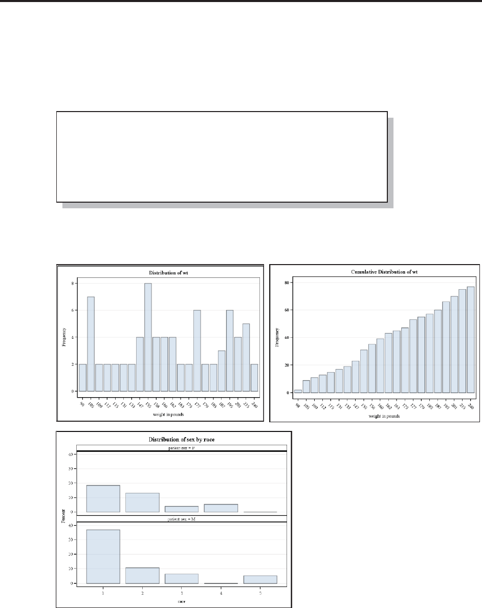
Chapter 10: Presentation Graphics—More than Just SAS/GRAPH 323
10.3 PROC FREQ Graphics
The FREQ procedure has now been included in the list of base procedures that can produce
graphics through the ODS Statistical Graphics routines. The TABLE statement supports the
PLOT= option, which can be used to generate a number of graphs.
A number of different types of plots are available, especially if you are calculating test statistics,
such as those generated with the CHISQ option. The PLOTS= option is used to make the plot
requests. You
may specify
specific types of
plots, as is done
below, or you
may request all
plots
(plots=all).
n The CUMFREQPLOT can be used to generate frequency and cumulative frequency
histograms. There are a number of modifier options that further refine the plot requests. Here we
specifically request that the vertical axis be frequencies.
o For two-way tables we often need to
see the relationship between the
frequencies of the combinations of
values. In this plot request we ask for a
frequency plot of the relationship
between the RACE and SEX. The plot
request has been modified to have the
vertical axes show percentages.
ods graphics on;
ods pdf file="&path\results\E10_3.pdf";
proc freq data=advrpt.demog;
table wt / plots=cumfreqplot(scale=freq); n
table sex*race/plots=freqplot(scale=percent); o
run;
ods pdf close;
&DUSHQWHU$UW&DUSHQWHU¶V*XLGHWR,QQRYDWLYH6$67HFKQLTXHV&RS\ULJKW6$6,QVWLWXWH,QF&DU\1RUWK&DUROLQD86$
$
//5,*+765(6(59(')RUDGGLWLRQDO6$6UHVRXUFHVYLVLWVXSSRUWVDVFRPSXEOLVKLQJ
324
&DUSHQWHU$UW&DUSHQWHU¶V*XLGHWR,QQRYDWLYH6$67HFKQLTXHV&RS\ULJKW6$6,QVWLWXWH,QF&DU\1RUWK&DUROLQD86$
$
//5,*+765(6(59(')RUDGGLWLRQDO6$6UHVRXUFHVYLVLWVXSSRUWVDVFRPSXEOLVKLQJ

Chapter 11
Output Delivery System
11.1 Using the OUTPUT Destination 326
11.1.1 Determining Object Names 326
11.1.2 Creating a Data Set 327
11.1.3 Using the MATCH_ALL Option 330
11.1.4 Using the PERSIST= Option 330
11.1.5 Using MATCH_ALL= with the PERSIST= Option 331
11.2 Writing Reports to Excel 332
11.2.1 EXCELXP Tagset Documentation and Options 333
11.2.2 Generating Multisheet Workbooks 334
11.2.3 Checking Out the Styles 335
11.3 Inline Formatting Using Escape Character Sequences 337
11.3.1 Page X of Y 338
11.3.2 Superscripts, Subscripts, and a Dagger 340
11.3.3 Changing Attributes 341
11.3.4 Using Sequence Codes to Control Indentations, Spacing, and
Line Breaks 342
11.3.5 Issuing Raw RTF Specific Commands 344
11.4 Creating Hyperlinks 345
11.4.1 Using Style Overrides to Create Links 345
11.4.2 Using the LINK= TITLE Statement Option 347
11.4.3 Linking Graphics Elements 348
11.4.4 Creating Internal Links 350
11.5 Traffic Lighting 352
11.5.1 User-Defined Format 352
&DUSHQWHU$UW&DUSHQWHU¶V*XLGHWR,QQRYDWLYH6$67HFKQLTXHV&RS\ULJKW6$6,QVWLWXWH,QF&DU\1RUWK&DUROLQD86$
$
//5,*+765(6(59(')RUDGGLWLRQDO6$6UHVRXUFHVYLVLWVXSSRUWVDVFRPSXEOLVKLQJ
326 Carpenter’s Guide to Innovative SAS Techniques
11.5.2 PROC TABULATE 353
11.5.3 PROC REPORT 354
11.5.4 Traffic Lighting with PROC PRINT 355
11.6 The ODS LAYOUT Statement 356
11.7 A Few Other Useful ODS Tidbits 358
11.7.1 Using the ASIS Style Attribute 358
11.7.2 ODS RESULTS Statement 358
The Output Delivery System, ODS, has so many intricacies that only a very few can be mentioned
here. Indeed, more than one book has been written where ODS is either the primary topic or an
important secondary topic. This chapter is aimed at highlighting a few useful topics.
SEE ALSO
The classic go-to document for ODS is Output Delivery System: The Basics and Beyond by
Haworth, Zender and Burlew (2009). Find tip sheets for ODS at
http://support.sas.com/rnd/base/ods/scratch/ods-tips.pdf
Lund (2006) covers a great many of the topics found in this chapter and has a very nice summary
of ODS attributes and the destinations to which they apply.
11.1 Using the OUTPUT Destination
While most procedures have one or more options that can be used to route procedural results to
data sets, not all values can be captured this way. The OUTPUT destination allows us to capture
procedure results as data. This destination is especially useful when there is no option available to
write a specific statistic to a data set, or when a procedure does not have the capability of
generating output data sets.
The output from each procedure is organized into one or more objects. These objects have a series
of properties including a name and a label. This name (or the label) can be used on the ODS
OUTPUT statement as an option to create an output data set.
The examples in this section use PROC UNIVARIATE; however, most of the discussion applies
to most other procedures as well.
11.1.1 Determining Object Names
In its simplest, the UNIVARIATE procedure creates five output objects, and we will need at least
the object name to make use of the OUTPUT
destination.
The labels of the five basic objects produced
by PROC UNIVARIATE for each of the
analysis variables can be seen in the
RESULTS window. If you right click on the
label you can examine the objects attributes, including the name.
ods trace on; n
proc univariate data=advrpt.demog;
var ht wt;
run;
ods trace off; o
&DUSHQWHU$UW&DUSHQWHU¶V*XLGHWR,QQRYDWLYH6$67HFKQLTXHV&RS\ULJKW6$6,QVWLWXWH,QF&DU\1RUWK&DUROLQD86$
$
//5,*+765(6(59(')RUDGGLWLRQDO6$6UHVRXUFHVYLVLWVXSSRUWVDVFRPSXEOLVKLQJ
Chapter 11: Output Delivery System 327
Since the ODS TRACE statement with the ON option n was used, these attributes will also be
displayed in the LOG. The portion of the LOG shown to the right shows the attributes of two of
the five objects. The TRACE statement is turned off with the OFF option o.
11.1.2 Creating a Data Set
The name of the output object (or its label) is used as an option on the ODS OUTPUT statement
to name the data set that is to be created. In this example we want to collect information on the
observations with the extreme values. By default PROC UNIVARIATE identifies the five
observations containing the maximums and minimums of the analysis variables.
n In this case we only want
PROC UNIVARIATE to create a
data set (no printed output), so
all destinations other than
OUTPUT are closed. We could
not just use the NOPRINT
option, because it also blocks the
ability of the OUTPUT
destination to create a data set.
o The name of one or more
output objects (EXTREMEOBS)
is used as an option on the ODS OUTPUT statement to name the data set that is to be created
(WORK.MAXMIN).
p The ID statement names one or more variables useful in identifying the selected observations.
q Two analysis variables are specified.
r The LISTING destination has been turned back on and PROC PRINT is used to show the data
set built by the OUTPUT destination.
The LISTING output of the resulting data set (WORK.MAXMIN) shows the observation number
and identification variables for the five maximum and minimum values for each analysis variable.
portions of the LOG not shown.
Output Added:
-------------
Name: Quantiles
Label: Quantiles
Template: base.univariate.Quantiles
Path: Univariate.wt.Quantiles
-------------
Output Added:
-------------
Name: ExtremeObs
Label: Extreme Observations
Template: base.univariate.ExtObs
Path: Univariate.wt.ExtremeObs
ods listing close; n
title1 '11.1.2a Naming the OUTPUT Data Set';
ods output extremeobs=maxmin; o
proc univariate data=advrpt.demog;
id lname fname; p
var ht wt; q
run;
ods listing; r
proc print data=maxmin;
run;
&DUSHQWHU$UW&DUSHQWHU¶V*XLGHWR,QQRYDWLYH6$67HFKQLTXHV&RS\ULJKW6$6,QVWLWXWH,QF&DU\1RUWK&DUROLQD86$
$
//5,*+765(6(59(')RUDGGLWLRQDO6$6UHVRXUFHVYLVLWVXSSRUWVDVFRPSXEOLVKLQJ

328 Carpenter’s Guide to Innovative SAS Techniques
Using CLASS and BY Variables
When CLASS or BY variables are added to the PROC step, the resulting data set is expanded to
include them.
s Data set options (see Section 2.1) can be included when naming the new data set.
t When one or more classification variables are used, they are added to the new data set for each
combination of levels. The BY statement yields a similar result; however, the order of both the
observations and the variables will be different.
Using the Object’s Label
The object’s label can be used instead of the object name on the ODS OUTPUT statement. Here
the example from 11.1.2a is
repeated using the quoted label
(extreme observations) u instead
of the object name.
11.1.2a Naming the OUTPUT Data Set
Var lname_ fname_ lname_ fname_ High
Obs Name Low Low Low LowObs High High High Obs
1 ht 62 Moon Rachel 51 74 Lawless Henry 38
2 ht 62 Karson Shawn 36 74 Mercy Ronald 50
3 ht 62 Cranston Rhonda 18 74 Nabers David 53
4 ht 62 Carlile Patsy 11 74 Panda Merv 56
5 ht 63 Temple Linda 72 74 Taber Lee 70
6 wt 98 Karson Shawn 36 215 Mann Steven 43
7 wt 98 Carlile Patsy 11 215 Marks Gerald 44
8 wt 105 Stubs Mark 69 215 Rose Mary 63
9 wt 105 Maxwell Linda 49 240 Antler Peter 4
10 wt 105 Leader Zac 39 240 Kin
g
Dou
g
37
title1 '11.1.2b CLASS Variable Present';
ods output extremeobs=maxclass(keep=sex varname high s
lname_high fname_high);
ods listing close;
proc univariate data=advrpt.demog;
class sex; t
id lname fname;
var ht wt;
run;
11.1.2b CLASS Variable Present
Var lname_ fname_
Obs Name sex High High High
t
1 ht F 68 East Jody
2 ht F 68 Rose Mary
3 ht F 68 Wills Norma
4 ht F 72 Adamson Joan
5 ht F 72 Olsen June
6 ht M 74 Lawless Henry
7 ht M 74 Mercy Ronald
. . . . portions of this listing are not shown . . . .
ods output u'extreme observations'=extobs;
&DUSHQWHU$UW&DUSHQWHU¶V*XLGHWR,QQRYDWLYH6$67HFKQLTXHV&RS\ULJKW6$6,QVWLWXWH,QF&DU\1RUWK&DUROLQD86$
$
//5,*+765(6(59(')RUDGGLWLRQDO6$6UHVRXUFHVYLVLWVXSSRUWVDVFRPSXEOLVKLQJ

Chapter 11: Output Delivery System 329
Driving an Automated Process
Any data set or even any information arranged in rows and columns can be used as the driving
information for automating a process. The SAS macro language is especially powerful when it
comes to creating applications and programs that rely on external information to make decisions.
In this example that external information will be a data set created through the use of ODS and the
OUTPUT destination. The example process shown here, one that we would like to execute many
times, is a simple PROC PRINT, but in reality it could be any number of DATA and PROC steps.
In this case we want to execute the %PROCESS macro
once for every level of a classification variable (in this
example the classification variable must be character).
The control will be accomplished using a WHERE
clause n that will be constructed in the controlling
macro (%DOPROCESS) q.
The controlling macro, %DOPROCESS, uses PROC FREQ with the OUTPUT destination o to
form a data set containing one level for each distinct value of the classification variable
(&CVAR).
o ODS OUTPUT and a PROC
FREQ are used to create a data set
(WORK.LEVELS) that will contain
one row for each unique value of the
classification variable (&CVAR).
p The data set created by the
OUTPUT destination is read as input
for the DATA _NULL_ step.
q The WHERE criteria is
constructed and placed in the variable
WHR, which will be added as text to
the macro call r.
r CALL EXECUTE is used to build a series of calls to the macro %PROCESS; one for each
level of the classification variable.
s The %DOPROCESS macro is called with the data set and classification variable of interest.
MORE INFORMATION
In this example an SQL step could have also been used to create the data set WORK.LEVELS,
but this is not always the case. PROC SQL is used to create a distinct list of values in the second
example in Section 11.2.2.
%macro process(dsn=,whr=);
proc print data=&dsn;
where &whr; n
run;
%mend process;
%macro doprocess(dsn=, cvar=);
ods output onewayfreqs=levels; o
proc freq data=&dsn;
table &cvar;
run;
data _null_;
set levels; p
whr = cats("&cvar='",&cvar,"'"); q
call execute('%nrstr(%process(dsn='
||"&dsn"||',whr='
||whr||'))'); r
run;
%mend doprocess;
%doprocess(dsn=advrpt.demog, cvar=sex) s
&DUSHQWHU$UW&DUSHQWHU¶V*XLGHWR,QQRYDWLYH6$67HFKQLTXHV&RS\ULJKW6$6,QVWLWXWH,QF&DU\1RUWK&DUROLQD86$
$
//5,*+765(6(59(')RUDGGLWLRQDO6$6UHVRXUFHVYLVLWVXSSRUWVDVFRPSXEOLVKLQJ
330 Carpenter’s Guide to Innovative SAS Techniques
11.1.3 Using the MATCH_ALL Option
Obviously once the data set has been created, a variety of subsetting techniques can be used to
break it up into distinct slices. If you know that the data set is to be broken up using BY/CLASS
values, you can save the
subsetting step(s) by using the
MATCH_ALL option n.
Notice the placement of the
option, within parentheses
following the object name.
In this step there are four
combinations of SEX (M/F) and
the analysis variables (HT/WT),
and the MATCH_ALL option
generates four data sets - one for
each combination. The first is named WORK.MATCHED, the second WORK.MATCHED1, and
so on. The listing for the first combination (WORK.MATCHED) is shown below. Notice that in
this example a BY statement was used, rather than a CLASS statement as in the example in
Section 11.1.2b. This allows you to observe the differences in the order of the variables and
observations. Here the first of the data sets (WORK.MATCHED) is printed.
11.1.4 Using the PERSIST= Option
The PERSIST option is typically used to modify selection lists, and what we have essentially
done in the ODS OUTPUT statement (Section 11.1.3) is specify a list of selected objects. The
PERSIST= option determines how long the specified object should remain on the selection list.
For the OUTPUT destination the list of selected objects is by default cleared (EXCLUDE ALL) at
the step boundary.
ods output extremeobs(match_all n )=matched;
proc sort data=advrpt.demog
out=bysex;
by sex;
run;
proc univariate data=bysex;
by sex;
id lname fname;
var ht wt;
run;
11.1.3 Using MATCH_ALL
matched
Var lname_ fname_ lname_ fname_ High
Obs sex Name Low Low Low LowObs High High High Obs
1 F ht 62 Moon Rachel 19 68 East Jody 6
2 F ht 62 Karson Shawn 12 68 Rose Mary 22
3 F ht 62 Cranston Rhonda 5 68 Wills Norma 30
4 F ht 62 Carlile Patsy 4 72 Adamson Joan 2
5 F ht 63 Temple Linda 28 72 Olsen June 21
&DUSHQWHU$UW&DUSHQWHU¶V*XLGHWR,QQRYDWLYH6$67HFKQLTXHV&RS\ULJKW6$6,QVWLWXWH,QF&DU\1RUWK&DUROLQD86$
$
//5,*+765(6(59(')RUDGGLWLRQDO6$6UHVRXUFHVYLVLWVXSSRUWVDVFRPSXEOLVKLQJ

Chapter 11: Output Delivery System 331
ods output extremeobs(match_all=series n
persist=proc o)=HT_WT p;
ods listing close;
proc univariate data=advrpt.demog;
class sex;
id lname fname;
var ht wt;
run;
proc univariate data=advrpt.demog;
class edu;
id lname fname;
var ht wt;
run;
ods output close;
Although the OUTPUT destination will by default generate data sets from a single PROC step,
you may want to create a data set based on the results of two or more steps (generally of the same
procedure). Rather than first creating the data sets individually and then later combining them in
a secondary DATA step,
they can be combined
directly using the PERSIST=
option n.
n Using PERSIST=PROC
maintains the selection list
past the step boundary. The
data set remains open until
the destination is closed o or
the list is otherwise cleared.
This allows ODS to write the
results of more than one
procedure to the same data set
(WORK.PMATCHED).
o This ODS destination is closed. When the PERSIST= option is used it is important to close this
destination. In this example you could have also used CLEAR instead of CLOSE; however,
CLEAR merely resets the SELECT/EXCLUDE list to EXCLUDE=ALL.
The list of variables generated by the two PROC UNIVARIATE steps is almost the same. Since
the classification variable differs, each step will contribute its classification variable as a column
in the new data set (WORK.PMATCH). Effectively the data sets created by the two procedure
steps individually have been concatenated. Adding the MATCH_ALL option would have resulted
in separate data sets (see Section 11.1.5).
SEE ALSO
The PERSIST= option is discussed by Bryant, Muller, and Pass (2003).
11.1.5 Using MATCH_ALL= with the PERSIST= Option
When the MATCH_ALL= option and the PERSIST= option are used together, a series of related
data sets with similar Program Data Vectors can be generated.
In this example the
MATCH_ALL= results in a
series of data sets in the
form of p
WORK.HT_WT,
WORK.HT_WT1,
WORK.HT_WT2, etc.
Since we are using multiple
procedures o along with
classification variables, the
number of data sets may
not be easily known. n The
list of the names of the data
sets generated by the use of
the MATCH_ALL=option
can be stored in a macro variable (&SERIES) n.
title1 '11.1.4 Using the Persist Option';
ods output extremeobs(persist=proc n)=pmatched;
ods listing close;
proc univariate data=advrpt.demog;
class sex;
id lname fname;
var ht wt;
run;
proc univariate data=advrpt.demog;
class edu;
id lname fname;
var ht wt;
run;
ods output close; o
&DUSHQWHU$UW&DUSHQWHU¶V*XLGHWR,QQRYDWLYH6$67HFKQLTXHV&RS\ULJKW6$6,QVWLWXWH,QF&DU\1RUWK&DUROLQD86$
$
//5,*+765(6(59(')RUDGGLWLRQDO6$6UHVRXUFHVYLVLWVXSSRUWVDVFRPSXEOLVKLQJ
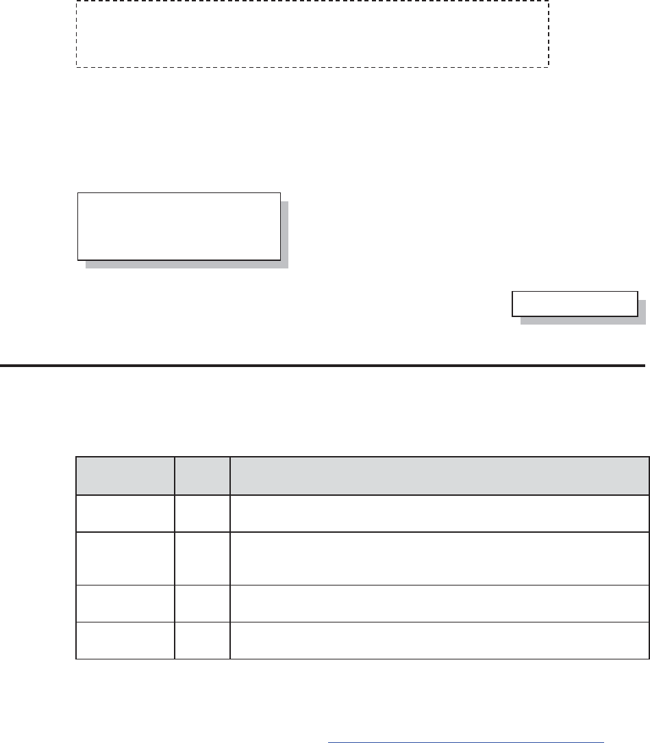
332 Carpenter’s Guide to Innovative SAS Techniques
64 %put &series;
HT_WT HT_WT1 HT_WT2 HT_WT3 HT_WT4 HT_WT5 HT_WT6 HT_WT7 HT_WT8
HT_WT9 HT_WT10 HT_WT11 HT_WT12 HT_WT13 HT_WT14 HT_WT15
HT_WT16 HT_WT17 HT_WT18 HT_WT19
For this
example we
could write
this macro
variable’s
value to the LOG using the %PUT statement.
In earlier versions of SAS this list was often used with a SET statement to concatenate the data
sets. This gives us some additional control. In the DATA step that concatenates these data sets an
IF statement q has been used to subset the data. A WHERE statement could not be used because
the variable EDU is present only in those data sets generated by the second PROC UNIVARIATE
step. The SET statement could also have been written without the macro variable by using a data
set list abbreviation.
When using the current versions of SAS, the
MATCH_ALL= option is no longer necessary to produce a
concatenated data set. In this example including the
PERSIST= o without the MATCH_ALL= n (see Section
11.1.4), would result in a single data set (WORK.HT_WT) that included
the output from both PROC UNIVARIATE steps.
11.2 Writing Reports to Excel
There are several ways to write reports and procedure output directly to EXCEL tables. The
results vary and method selection should depend on the desired result.
Destination
File
Type
File Characteristics
HTML HTML
Uses the HTML4 tagset to generate an HTML 4.0 file. Not all style
attributes are transferred to EXCEL.
HTML3 HTML
HTML 3.2 standard file. Was the only HTML destination under SAS
8. Attribute handling is different than the HTML destination under
SAS®9.
MSOFFICE2k HTML (tagset) Supports importation of SAS/GRAPH images. Optimized for
MSOffice 2k environment.
EXCELXP XML
(tagset) Emphasis is on the data not the text. Supports writing to
EXCEL Workbooks and multiple worksheets.
By far the most flexible approach and the only one that supports the XML standard is through the
use of the EXCELXP tagset. This tagset is under constant development with new features being
added on a regular basis. The latest version of this tagset along with a number of supporting
papers and examples can be downloaded at http://support.sas.com/rnd/base/ods/odsmarkup/.
data HT_WT_all;
set &series;
if edu < '13'; q
run;
set ht_wt:;
&DUSHQWHU$UW&DUSHQWHU¶V*XLGHWR,QQRYDWLYH6$67HFKQLTXHV&RS\ULJKW6$6,QVWLWXWH,QF&DU\1RUWK&DUROLQD86$
$
//5,*+765(6(59(')RUDGGLWLRQDO6$6UHVRXUFHVYLVLWVXSSRUWVDVFRPSXEOLVKLQJ
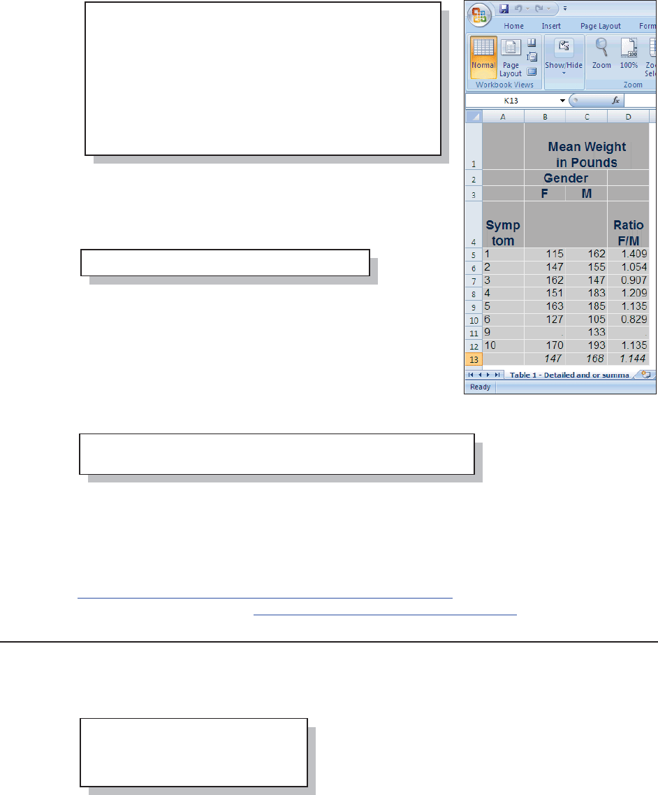
Chapter 11: Output Delivery System 333
n EXCELXP is a tagset within the MARKUP destination.
You may also address the tagset as an option on the ODS
MARKUP statement o .
The emphasis for this tagset is on the data and not necessarily
on the text. Notice that, using the defaults, the two titles do not
even appear in the Excel spreadsheet. Of course the titles can
be included through the use of the embedded _titles='yes'
option. This is just one of the many available options. To see
the current list of available options use the DOC=’help’ option
p, which writes a list of options to the LOG.
SEE ALSO
The EXCELXP tagset is further discussed in (Andrews, 2008). Eric Gebhart (Gebhart, 2010) has
written a number of papers on this tagset. Vince DelGobbo has written over a dozen papers on the
EXCELXP tagset. An overall index to Vince’s papers can be found at
http://www.sas.com/events/cm/867226/ExcelXPPaperIndex.pdf with a full list of his and other
SAS author’s papers found at http://support.sas.com/rnd/papers/index.html.
11.2.1 EXCELXP Tagset Documentation and Options
The operation of the EXCELXP tagset is controlled through the use of options. These are
implemented using the OPTIONS option with the options themselves enclosed in parentheses
which follow the OPTIONS keyword. Here the DOC=
option is used to write the tagset’s full documentation
to the LOG. If you want to learn about recent changes
to the tagset, the CHANGELOG option
options(doc="changelog") will show you the
timing of changes and summary of new features.
ods tagsets.excelxp n
style=default
path="&path\results"
body="E11_2.xls";
title1 '11.2 Using the EXCELXP Tagset';
title2 "Using the ExcelXP Tagset";
proc report data=advrpt.demog
nowd split='*';
portions of the PROC REPORT step not shown
oods markup tagset=excelxp . . .
ODS tagsets.excelxp file="&path\results\test.xml"
p options(doc="help");
ODS tagsets.excelxp
path="&path\results"
body="E11_2_1.xls"
options(doc="help");
&DUSHQWHU$UW&DUSHQWHU¶V*XLGHWR,QQRYDWLYH6$67HFKQLTXHV&RS\ULJKW6$6,QVWLWXWH,QF&DU\1RUWK&DUROLQD86$
$
//5,*+765(6(59(')RUDGGLWLRQDO6$6UHVRXUFHVYLVLWVXSSRUWVDVFRPSXEOLVKLQJ

334 Carpenter’s Guide to Innovative SAS Techniques
SEE ALSO
The EXCELXP tagset is constantly being updated and refined. If you are using the version of the
EXCELXP tagset that was shipped with SAS it is unlikely to be current. You can learn how to
download and install the latest version of the EXCELXP tagset by reading SAS Note #32394 at
http://support.sas.com/kb/32/394.html.
11.2.2 Generating Multisheet Workbooks
When writing a report or data set to Excel, it is not uncommon to need to break it up into portions
that are written to individual sheets in the workbook. This can be accomplished in a couple of
different ways. The primary difference between the two techniques shown here is whether you are
sending a report or just the data to the spreadsheet.
When writing a report to Excel the EXCELXP tagset is the most flexible choice. This is
demonstrated in this example with a PROC PRINT. This technique utilizes BY-group processing
to break up the report.
n The EXCELXP tagset is
selected for use.
o Let the tagset determine the
sheet name.
p The SHEET_INTERVAL
option determines how to break
up the sheets.
q Titles will not be included
on the report. This is the
default.
r The BY line must be
specified when using the
SHEET_INTERVAL of
‘BYGROUP’ p.
For this macro call one sheet will be created for each level of RACE, including any missing
values of RACE.
%macro multisheet(dsn=,bylist=);
ods tagsets.excelxp n
style=default
path="&path\results"
body="E11_2_2a.xls"
options(sheet_name='none' o
sheet_interval='bygroup' p
embedded_titles='no'); q
proc sort data=&dsn out=sorted;
by &bylist;
proc print data=sorted;
by &bylist; r
run;
ods tagsets.excelxp close;
%mend multisheet;
%multisheet(dsn=advrpt.demog,bylist=race)
&DUSHQWHU$UW&DUSHQWHU¶V*XLGHWR,QQRYDWLYH6$67HFKQLTXHV&RS\ULJKW6$6,QVWLWXWH,QF&DU\1RUWK&DUROLQD86$
$
//5,*+765(6(59(')RUDGGLWLRQDO6$6UHVRXUFHVYLVLWVXSSRUWVDVFRPSXEOLVKLQJ

Chapter 11: Output Delivery System 335
When breaking up a data set to multiple sheets we do not need to invoke the power of the
EXCELXP tagset. Instead we can use PROC EXPORT. Here the EXPORT step is inside of a
%DO loop that will execute once for each level of the selected classification variable.
s PROC SQL is used to
create a series of macro
variables to hold the distinct
levels of the classification
variable (&CVAR).
t A DATA _NULL_ step is
used to determine if the
classification variable is
numeric or character.
u The WHERE criteria is
established differentially for
numeric and character
variables.
v The data set is subsetted
using the WHERE criteria
established at u.
w The sheet is named using
a combination of the
variable’s name and its
value.
SEE ALSO
The must-read paper on this topic is by Vince DelGobbo (2007). The PROC EXPORT example
shown here was adapted to a sasCommunity.org article which shows a less generalized program
to break up a data set into separate EXCEL sheets
http://www.sascommunity.org/wiki/Automatically_Separating_Data_into_Excel_Sheets.
11.2.3 Checking Out the Styles
In addition to customized styles that you or your company may have created, SAS ships with over
40 predefined styles. With so many styles to choose from and since not all style attributes are
carried over to the Excel spreadsheet when reports are written to Excel using the EXCELXP
tagset, it becomes important to be able to visualize your report for each of the currently defined
styles.
%macro multisheet(dsn=,cvar=);
%local varcnt type string i;
proc sql noprint; s
select distinct &cvar
into :idvar1 - :idvar&sysmaxlong
from &dsn;
%let varcnt = &sqlobs;
quit;
data _null_; t
if 0 then set &dsn;
call symputx('type',vtype(&cvar),'l');
stop;
run;
%do i = 1 %to &varcnt;
%if &type=N %then %let string=&&idvar&i; u
%else %let string="&&idvar&i";
proc export
data=&dsn(where=(&cvar=&string)) v
outfile="&path\results\E11_2_2b.xls"
dbms= excel
replace;
sheet = "&cvar._&&idvar&i"; w
run;
%end;
%mend multisheet;
%multisheet(dsn=advrpt.demog,cvar=race)
&DUSHQWHU$UW&DUSHQWHU¶V*XLGHWR,QQRYDWLYH6$67HFKQLTXHV&RS\ULJKW6$6,QVWLWXWH,QF&DU\1RUWK&DUROLQD86$
$
//5,*+765(6(59(')RUDGGLWLRQDO6$6UHVRXUFHVYLVLWVXSSRUWVDVFRPSXEOLVKLQJ

336 Carpenter’s Guide to Innovative SAS Techniques
The %SHOWSTYLES macro uses the macro language to write a report to Excel once for each
available style.
n An SQL step is
used to create a
macro variable for
each of the unique
style names.
o The number of
styles found is saved
in &STYLECNT.
p Inside the %DO
loop the style name
will be contained in
the macro variable
reference
&&STYLE&I. The
filename, therefore,
contains the style
name.
q The style of
interest is specified
on the STYLE=
option.
r The sheet name
will be the name of
the style.
s The report code
will be exactly the
same for each of the
styles.
t The %SHOWSTYLES macro is called.
title1 '11.2.3 Showing Style in Excel';
%macro showstyles;
%local i stylecnt;
proc sql noprint;
select scan(style,2,'.') n
into: style1-:style&sysmaxlong
from sashelp.vstyle;
%let stylecnt = &sqlobs; o
quit;
%do i = 1 %to &stylecnt;
ods markup tagset=excelxp
path="&path\results"
file="&&style&i...xml" p
style=&&style&I q
options(sheet_name="&&style&i" r
embedded_titles='yes');
title2 "Using the &&style&i Style";
proc report data=sashelp.class nowd; s
column name sex age height weight;
define age / analysis mean f=4.1;
define height / analysis mean f=4.1;
define weight / analysis mean f=5.1;
rbreak after /summarize;
run;
ods markup close;
%end;
%mend showstyles;
ods listing close;
%showstyles t
&DUSHQWHU$UW&DUSHQWHU¶V*XLGHWR,QQRYDWLYH6$67HFKQLTXHV&RS\ULJKW6$6,QVWLWXWH,QF&DU\1RUWK&DUROLQD86$
$
//5,*+765(6(59(')RUDGGLWLRQDO6$6UHVRXUFHVYLVLWVXSSRUWVDVFRPSXEOLVKLQJ
Chapter 11: Output Delivery System 337
11.3 Inline Formatting Using Escape Character
Sequences
There are some types of formatting that is difficult or impossible to implement directly using ODS
styles and options. However, through the use of an escape character it is possible to pass
destination-specific commands directly to the destination that builds the output. The escape
character alerts ODS that the associated formatting sequence of characters are not to be used
directly by ODS, but rather are to be passed to the receiving destination.
The escape character should be one that you do not otherwise use in your SAS programs. Since I
tend to not use the tilde as a negation mnemonic, it makes a
good escape character. The escape character is designated using
the ODS ESCAPECHAR option.
The escape character is used to note an escape sequence that may contain one or more destination
commands or functions. The syntax varies by the kind of command.
Type General Form Used to Section
Formatting
Functions
~{function text} Control pagination,
superscripts, subscripts.
11.3.1
11.3.2
Style
Modification
~S={attribute characteristics}
~{style elements and attributes}
Assign style attributes. 11.3.3
Sequence Codes ~code Manipulate line breaks,
wrapping, and indentations.
11.3.4
Raw Text
Insertion
~R/destination “rawtext”
~R “rawtext”
Insert destination-specific
codes.
11.3.5
SEE ALSO
Carpenter (2007a, Section 8.6) discusses inline formatting in the context of PROC REPORT
steps.
Haworth, Zender, and Burlew (2009) discuss the use of the escape character and inline formatting
sequences in a variety of usages.
Zender (2007) covers all the basics in this easy-to-read SAS Global Forum paper on inline
formatting. If you want to know more, this should be the first paper that you read on this topic.
ods escapechar=’~’;
&DUSHQWHU$UW&DUSHQWHU¶V*XLGHWR,QQRYDWLYH6$67HFKQLTXHV&RS\ULJKW6$6,QVWLWXWH,QF&DU\1RUWK&DUROLQD86$
$
//5,*+765(6(59(')RUDGGLWLRQDO6$6UHVRXUFHVYLVLWVXSSRUWVDVFRPSXEOLVKLQJ
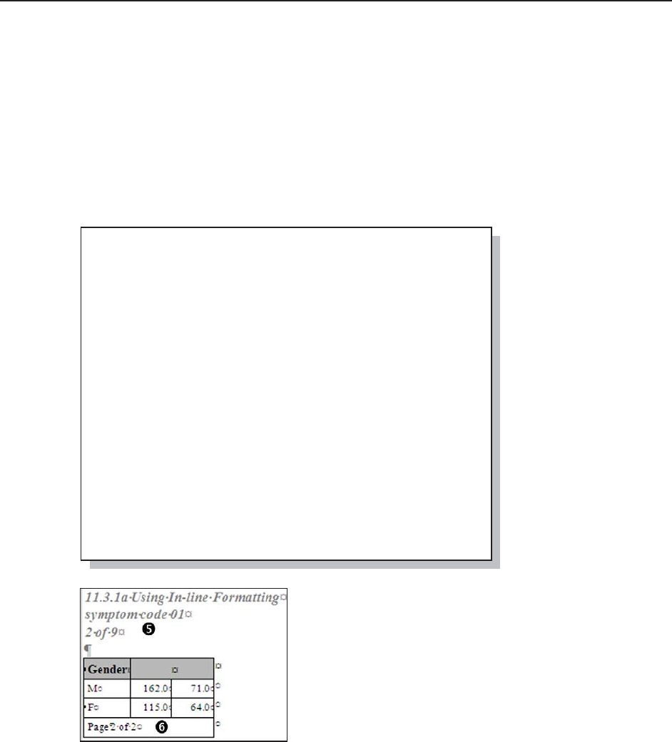
338 Carpenter’s Guide to Innovative SAS Techniques
11.3.1 Page X of Y
A common requirement for multipage reports is to indicate the current page as well as the total
number of pages, something like page 2 of 6. This can be accomplished in several ways, and
the appropriate methodology depends on the destination, the placement of the text, and how the
text is to be written out.
The RTF Destination - Using PAGEOF
When writing to the RTF destination, the pageof sequence can potentially be used to add page
numbering. Designed to be used in a title or footnote, this formatting sequence can have
unintended consequences when used elsewhere or if the BODYTITLE option is also used.
In this example a PROC REPORT step is executed with a BY statement causing a new page to be
generated for each value
of the BY variable.
n The tilde is designated
as the escape character.
o Because the value of
the BY variable has been
placed in the title using
the #BYVAL and
#BYVAR options, the
BYLINE is turned off.
These options may not
fully work if the TITLE
statement containing the
options is outside the
PROC step.
p The pageof formatting
sequence is designated in
the title. Notice that the
sequence is enclosed in
braces that follow the escape character. The page numbering
appears correctly in the title line r.
q For demonstration purposes the page numbering has also
been requested through the LINE statement, which will write
at the bottom of the report. Here the numbering is calculated
incorrectly s. Remember that the pageof formatting
sequence is designed to be used in the TITLE or
FOOTNOTE statements and not in a LINE statement.
When using RTF with MSWORD, the page numbers are
sometimes not shown until the document is either printed or viewed in the print preview window.
ods escapechar='~'; n
options nobyline;
ods rtf file="&path\results\E11_3_1a.rtf"
style=rtf;
proc sort data=advrpt.demog
out=demog;
by symp;
run;
proc report data=demog nowd split='*';
title2 '#byvar1 #byval1'; o
title3 '~{pageof}'; p
by symp;
column sex wt ht;
define sex / group 'Gender' order=data;
define wt / analysis mean format=6.1 ' ';
define ht / analysis mean format=6.1 ' ';
compute after;
line @3 'Page ~{pageof}'; q
endcomp;
run;
ods _all_ close;
&DUSHQWHU$UW&DUSHQWHU¶V*XLGHWR,QQRYDWLYH6$67HFKQLTXHV&RS\ULJKW6$6,QVWLWXWH,QF&DU\1RUWK&DUROLQD86$
$
//5,*+765(6(59(')RUDGGLWLRQDO6$6UHVRXUFHVYLVLWVXSSRUWVDVFRPSXEOLVKLQJ
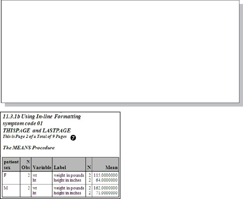
Chapter 11: Output Delivery System 339
MORE INFORMATION
The #BYVAL and #BYVAR title and footnote options are also used in Sections 7.4.3 and are
discussed in Section 15.1.2.
SEE ALSO
Usage note 15727 discusses the use of the BODYTITLE option with the PAGEOF sequence.
The PDF and RTF Destinations - Using THISPAGE and LASTPAGE
The PAGEOF sequence is only available for the RTF destination; however, you can create even
more flexible paging for both the RTF and PDF destinations by using the THISPAGE and
LASTPAGE t formatting sequences. Like the PAGEOF sequence, these are designed to be used
in titles and footnotes, and unanticipated results can be expected when using the BODYTITLE
option with the RTF destination.
The behavior of the LASTPAGE sequence is similar to PAGEOF in the RTF destination. You
may not be able to observe the total number of pages until you either do a print preview or scroll
down a few pages in the table after it has been imported.
ods pdf file="&path\results\E11_3_1b.pdf"
style=printer;
ods rtf file="&path\results\E11_3_1b.rtf"
style=rtf;
title1 '11.3.1b Using In-line Formatting';
title2 '#byvar1 #byval1';
title3 'THISPAGE and LASTPAGE';
title4 h=10pt
'This is Page ~{thispage} of a Total of ~{lastpage} Pages'; t
proc means data=demog n mean;
by symp;
class sex;
var wt ht;
run;
ods _all_ close;
&DUSHQWHU$UW&DUSHQWHU¶V*XLGHWR,QQRYDWLYH6$67HFKQLTXHV&RS\ULJKW6$6,QVWLWXWH,QF&DU\1RUWK&DUROLQD86$
$
//5,*+765(6(59(')RUDGGLWLRQDO6$6UHVRXUFHVYLVLWVXSSRUWVDVFRPSXEOLVKLQJ
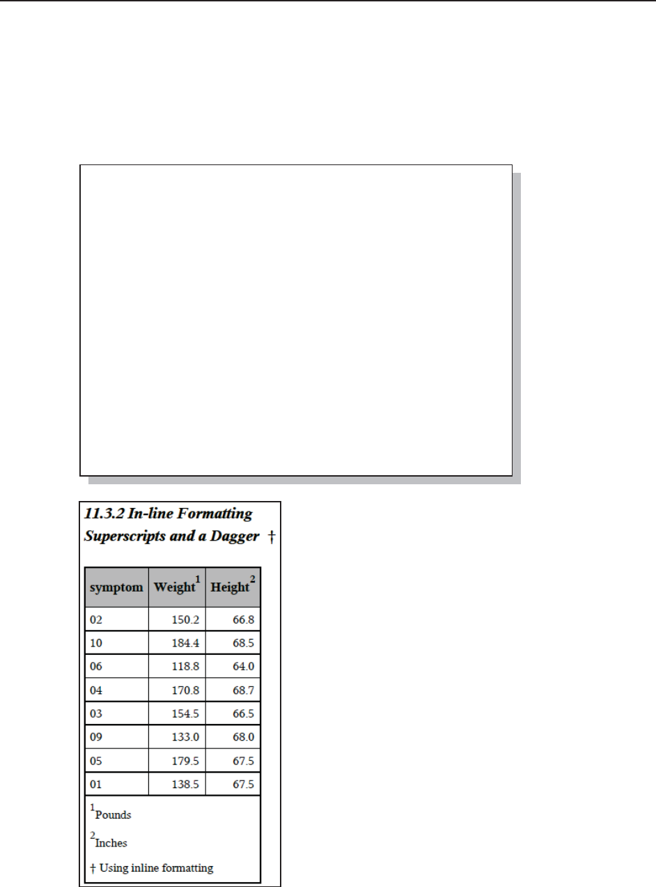
340 Carpenter’s Guide to Innovative SAS Techniques
11.3.2 Superscripts, Subscripts, and a Dagger
In addition to paging information you can also draw attention to specific text by adding
superscripts, subscripts, and a dagger symbol using inline formatting. Inline formatting functions
include:
~{super 1} makes the 1 a superscript
~{sub 14} the number 14 becomes a subscript
~{dagger} the dagger symbol may be used instead of numbers.
n The dagger
symbol is placed in
the title. The
symbol itself does
not have the same
appearance in all
destinations.
o Superscripts are
used to annotate the
units of measure. In
this PROC
REPORT step they
are applied in both
the DEFINE
statement and the
LINE statement.
p The column
placement notation
(@1) is not reliable in most destinations, especially when
using proportional fonts. The @1 will reliably left justify the
text; however, using something like @5 will not necessarily
align text across rows.
title1 '11.3.2 In-line Formatting';
ods escapechar='~';
ods pdf file="&path\results\E11_3_2.pdf"
style=printer;
title2 'Superscripts and a Dagger ~{dagger}'; n
proc report data=advrpt.demog nowd split='*';
column symp wt ht;
define symp / group 'symptom' order=data;
define wt / analysis mean format=6.1
'Weight~{super 1}' o;
define ht / analysis mean format=6.1
'Height~{super 2}' o;
compute after;
line @1p '~{super 1} oPounds';
line @1p '~{super 2} oInches';
line @1p '~{dagger} n Using inline formatting';
endcomp;
run;
ods _all_ close;
&DUSHQWHU$UW&DUSHQWHU¶V*XLGHWR,QQRYDWLYH6$67HFKQLTXHV&RS\ULJKW6$6,QVWLWXWH,QF&DU\1RUWK&DUROLQD86$
$
//5,*+765(6(59(')RUDGGLWLRQDO6$6UHVRXUFHVYLVLWVXSSRUWVDVFRPSXEOLVKLQJ
Chapter 11: Output Delivery System 341
title2 '~{style [font_face="times new roman"]Initial}'
'~{style [font_style=roman] Coded}'
' Symptoms';
MORE INFORMATION
Aligning text across rows can be accomplished using inline formatting sequence codes; see
Section 11.3.4. This same example demonstrates the use of the dagger as well.
11.3.3 Changing Attributes
Attributes associated with text can be changed using the inline style modifier. Most of the
standard attributes that are set by the ODS style can be modified. The style modifier can be used
virtually anywhere that you specify text. This includes not only titles and footnotes, but the labels
of formatted values, and even the data itself. There are two general forms of the style modifier.
Prior to SAS 9.2 the only available form was:
~S={attribute=value}
Notice that an uppercase S= follows the escape character and precedes the curly braces. A typical
use could be to change attributes of the text in a title.
n The default title2 font is changed to Times
New Roman.
o Change the default font style from italics.
p Changes are turned off and the defaults are restored.
Starting with SAS 9.2 a more flexible form of style modifier was introduced. The general form is:
~{style [element=attribute] text}
The style element and its attribute are enclosed within square brackets and together they precede
the text to which the element/attribute pairs are to be applied. Notice that the braces enclose the
text as well as the style elements.
The following TITLE statement generates the same title line as the TITLE statement of the
previous example.
Since modified
attributes apply
only to the text
within the braces, the default attributes are
applied to ‘Symptoms’.
title2 '~S={font_face="times new roman"} nInitial'
'~S={font_style=roman} o Coded'
'~S={} p Symptoms';
&DUSHQWHU$UW&DUSHQWHU¶V*XLGHWR,QQRYDWLYH6$67HFKQLTXHV&RS\ULJKW6$6,QVWLWXWH,QF&DU\1RUWK&DUROLQD86$
$
//5,*+765(6(59(')RUDGGLWLRQDO6$6UHVRXUFHVYLVLWVXSSRUWVDVFRPSXEOLVKLQJ
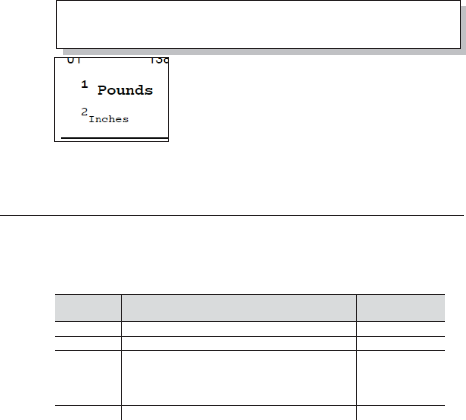
342 Carpenter’s Guide to Innovative SAS Techniques
Either type of style modification sequence can be used outside of the TITLE and FOOTNOTE
statements.
In fact they can be used most places where text is displayed. This
includes data, labels, and formatted values. Here style modification
sequences are applied in a LINE statement within a PROC REPORT
compute block.
SEE ALSO
Haworth, Zender and Burlew (2009, pg 268) creates several style modification sequences based
on data values.
11.3.4 Using Sequence Codes to Control Indentations, Spacing, and
Line Breaks
For some destinations, a series of sequence codes can be used with the escape character to control
line breaks, indentations, and spacing. These codes may not work equally well for each of the
primary destinations, and performance may be dependent on the version of SAS being used.
Code
Sequence
What it does Note
~m Indentation location marker.
~-2n Forces a line break (takes ~m into consideration).
~xn Forces x line breaks (does not take ~m into
consideration).
x= # of line feeds
~w Suggested location for an optional line break.
~_ Creates a non-breaking space. underscore
~xz Inserts one of four error codes. x=1, 2, 3, or 4
compute after;
line @3 '~{style [font_weight=bold font_size=3] ~{super 1} Pounds}';
line @3 '~{style [font_weight=light] ~{super 2}Inches}';
endcomp;
&DUSHQWHU$UW&DUSHQWHU¶V*XLGHWR,QQRYDWLYH6$67HFKQLTXHV&RS\ULJKW6$6,QVWLWXWH,QF&DU\1RUWK&DUROLQD86$
$
//5,*+765(6(59(')RUDGGLWLRQDO6$6UHVRXUFHVYLVLWVXSSRUWVDVFRPSXEOLVKLQJ
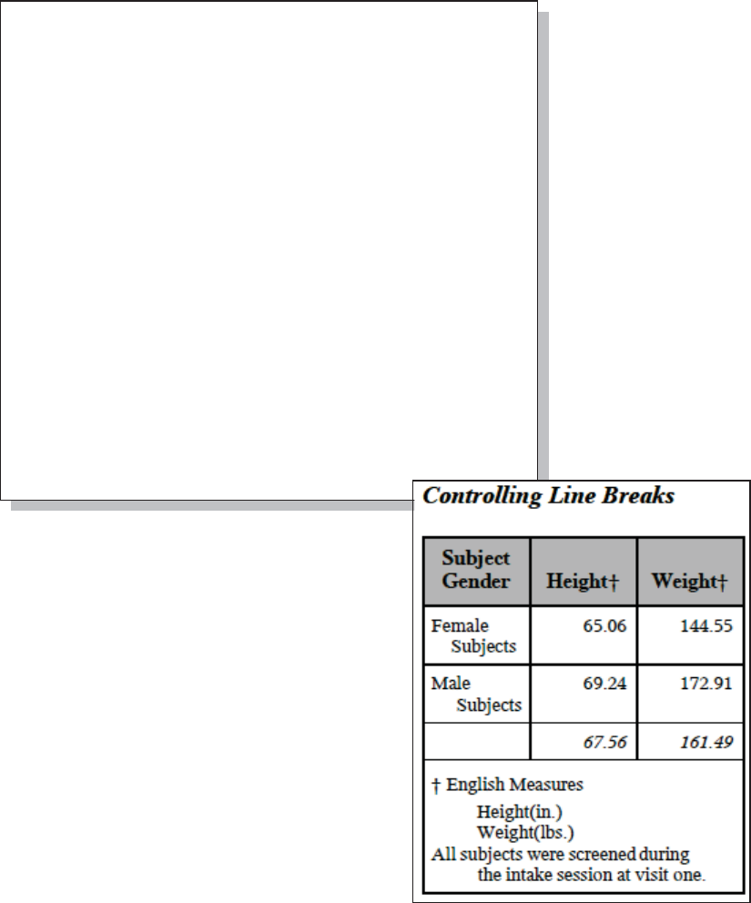
Chapter 11: Output Delivery System 343
proc format;
value $genttl n o
'f','F'='Fe~mmale~-2nSubjects'
'm','M'='Ma~mle~-2nSubjects';
run; no
title1 "Controlling Line Breaks";
proc report data=advrpt.demog nowd;
columns sex ht wt;
define sex / group format=$genttl.
'Subject~w Gender'; p
define ht / analysis mean
format=5.2
'Height~{dagger}q';
define wt / analysis mean
format=6.2
'Weight~{dagger}';
rbreak after / summarize;
compute after;q n
line @1 '~{dagger} Eng~mlish Measures'
'~-2nHeight(in.)~-2nWeight(lbs.)';
line @1 'All su~mbjects were screened during '
'~-2nthe intake session at visit one.';
endcomp; o
run;
n The ~m is used to
mark the alignment
location (indentation)
for the line breaks
specified with the ~-2n
sequence.
o Line breaks are
forced using the ~-2n
notation. Without
forcing these breaks the
width of the table would
be driven by the LINE
statement.
p The ~w indicates an
optional line break. This
means that this will be
the preferred location
for a line break, if one is
needed. In this table the
text will break at the
space with or without using the ~w.
q The dagger symbol is added to associate the
column label with the units footnote.
&DUSHQWHU$UW&DUSHQWHU¶V*XLGHWR,QQRYDWLYH6$67HFKQLTXHV&RS\ULJKW6$6,QVWLWXWH,QF&DU\1RUWK&DUROLQD86$
$
//5,*+765(6(59(')RUDGGLWLRQDO6$6UHVRXUFHVYLVLWVXSSRUWVDVFRPSXEOLVKLQJ

344 Carpenter’s Guide to Innovative SAS Techniques
11.3.5 Issuing Raw RTF Specific Commands
An RTF table or report is generated using a series of commands, control words, and field codes
that are specific to the RTF destination (Section 15.3 goes into more detail on RTF code).
Normally we do not need to know anything about those commands because they are written for us
by ODS. However, when formatting sequences are not available for a specific task and you know
the appropriate underlying command for the destination, you can pass the raw RTF destination-
specific control code from SAS for execution at the destination.
You can issue these raw destination-specific commands using one of the following inline
formatting functions. While the syntax used in SAS 9.1.3 will work in SAS 9.2, the newer
preferred syntax is available starting in SAS 9.2. The escape character (here a tilde is used) must
be declared using the ODS ESCAPECHAR option:
SAS 9.1.3 (and earlier)
~R/destination 'command' especially useful when multiple destinations
are open ~R
'command'
SAS 9.2
~{raw 'command'}
~{dest[destination] 'command'}
In the following example, raw RTF commands are passed both through a format and in TITLE
statements. The commands themselves are preceded by a back slash and followed by a space.
Multiple raw commands can be chained together, and they are turned off by following the control
code with a 0 (zero).
ods escapechar = '~';
proc format;
value $gender
'f','F'='~{raw \b F\b0\i emale}' n
'm','M'='~{raw \b M\b0\i ale}' n;
run;
title1 ~{raw '11.3.5 \i0 Using \b\ul RTF\b0\ul0 Codes'}; o
title2 ~{raw '\i0 Italics off'};
proc report data=advrpt.demog nowd;
columns sex ht wt;
define sex / group format=$gender.;
. . . code not shown . . .
&DUSHQWHU$UW&DUSHQWHU¶V*XLGHWR,QQRYDWLYH6$67HFKQLTXHV&RS\ULJKW6$6,QVWLWXWH,QF&DU\1RUWK&DUROLQD86$
$
//5,*+765(6(59(')RUDGGLWLRQDO6$6UHVRXUFHVYLVLWVXSSRUWVDVFRPSXEOLVKLQJ
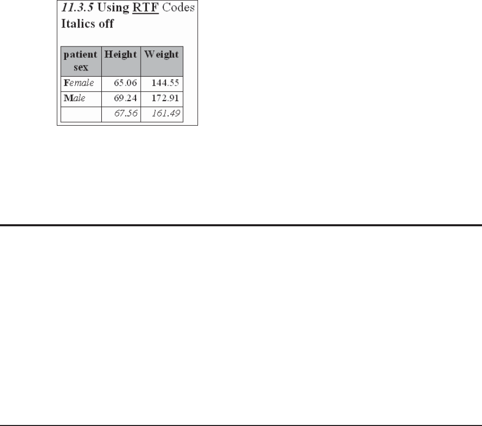
Chapter 11: Output Delivery System 345
n Bolding is turned on and off with the \b and \b0, while
italics are turned on with \i. Notice that the text in this format
has control down to the letter (first letter bolded – remaining
letters in italics).
o The default for the RTF style turns italics on for titles.
These have been turned off (except for the example number;
11.3.5).
SEE ALSO
A few common RTF commands can be found in Haworth, Zender, and Burlew (2009, pg 128).
The same section discusses an alternative approach using a style rather than inline formatting.
11.4 Creating Hyperlinks
Text, reports, graphs, and tables within electronic documents can automatically be connected by
creating hyperlinks. SAS can create these links almost anywhere that text is displayed, as well as
within graphic objects. Links can be established between portions of tables, graphs, other
locations within a table, and between tables of different types. Within a table links can be
established within data values, formats, titles, header text, and graphic symbols.
MORE INFORMATION
Links are created in a PROC PRINT example in Section 8.5.3.
SEE ALSO
A number of the following techniques are presented in PROC REPORT examples by Carpenter
(2007b).
11.4.1 Using Style Overrides to Create Links
In the TABULATE, REPORT, and PRINT procedures the style overrides can be especially useful
for creating links. The application of the style override option (STYLE=) is very similar in all
three procedures; however, in PROC REPORT links can also be generated through the use of the
CALL DEFINE routine.
&DUSHQWHU$UW&DUSHQWHU¶V*XLGHWR,QQRYDWLYH6$67HFKQLTXHV&RS\ULJKW6$6,QVWLWXWH,QF&DU\1RUWK&DUROLQD86$
$
//5,*+765(6(59(')RUDGGLWLRQDO6$6UHVRXUFHVYLVLWVXSSRUWVDVFRPSXEOLVKLQJ

346 Carpenter’s Guide to Innovative SAS Techniques
In this example a report summarizes the data for each of the symptoms (SYMP). It is constructed
so that clicking on the symptom number links to a report for that symptom.
n The primary
HTML file is
named and then
created using
PROC REPORT.
o Each individual
value of SYMP is
associated with a
file that will
contain the
summary for that
symptom. The
CALL DEFINE is
used to associate
the URL with the
symptom.
p An SQL step is
used to assign the
distinct values of
SYMP to macro
variables.
q A macro %DO
loop is used to
cycle through the
individual values of
symptom
(&&SYM&S).
r The macro
variable holding a
specific symptom
(&&SYM&S) is
used to subset the
data.
s The style override option is used to assign the URL attribute to the header, which will now link
back to the primary table.
%macro sympRPT;
title1 '11.4.1 Hyperlinks Using Style Overrides';
ods html file="&path\results\E11_4_1.htm" n
style=journal;
title2 'Symptoms';
proc report data=advrpt.demog nowd split='*';
column symp wt ht;
define symp / group 'Symptom' order=internal
missing;
define wt / analysis mean format=6.1 'Weight';
define ht / analysis mean format=6.1 'Height';
compute symp;
stag = 'E11_4_1_'||trim(left(symp))||'.htm'; o
call define(_col_,'url',stag);
endcomp;
run;
ods _all_ close;
proc sql noprint;
select distinct symp
into: sym1-:sym999 p
from advrpt.demog;
%do s=1 %to &sqlobs; q
ods html file="&path\results\E11_4_1_&&sym&s...htm"
style=journal;
title2 "Symptom &&sym&s";
proc report data=advrpt.demog(where=(symp="&&sym&s"))r
nowd split='*';
column sex wt ht;
define sex / group 'Sex' order=internal
style(header)={url='e11_4_1.htm'}; s
define wt / analysis mean format=6.1 'Weight';
define ht / analysis mean format=6.1 'Height';
run;
ods _all_ close;
%end;
%mend symprpt;
%symprpt
&DUSHQWHU$UW&DUSHQWHU¶V*XLGHWR,QQRYDWLYH6$67HFKQLTXHV&RS\ULJKW6$6,QVWLWXWH,QF&DU\1RUWK&DUROLQD86$
$
//5,*+765(6(59(')RUDGGLWLRQDO6$6UHVRXUFHVYLVLWVXSSRUWVDVFRPSXEOLVKLQJ
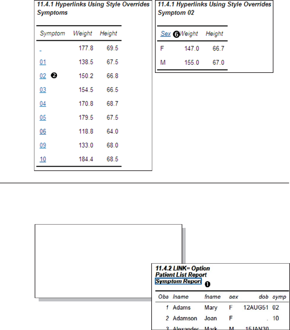
Chapter 11: Output Delivery System 347
title1 '11.4.2 LINK= Option';
ods pdf file="&path\results\E11_4_2.pdf"
style=journal;
title2 'Patient List Report';
title3 link='E11_4_1.htm' n
'Symptom Report';
proc print data=advrpt.demog;
var lname fname sex dob symp;
run;
ods _all_ close;
MORE INFORMATION
Style overrides are introduced and discussed
further in Sections 8.1.3 (TABULATE), 8.4.6
(REPORT), and 8.5.2 (PRINT). The CALL
DEFINE routine is introduced in Section 8.4.7.
11.4.2 Using the LINK= TITLE Statement Option
In the TITLE and FOOTNOTE statements the LINK= option can be used to specify the file to
which you want to link. The option can point to an internal anchor location, a local file, or may
even contain a fully qualified path.
In this example the LINK= option n
is used to point back to the primary
file created in Section 11.4.1.
MORE INFORMATION
Other TITLE and FOOTNOTE statement options are described in Section 9.1.
&DUSHQWHU$UW&DUSHQWHU¶V*XLGHWR,QQRYDWLYH6$67HFKQLTXHV&RS\ULJKW6$6,QVWLWXWH,QF&DU\1RUWK&DUROLQD86$
$
//5,*+765(6(59(')RUDGGLWLRQDO6$6UHVRXUFHVYLVLWVXSSRUWVDVFRPSXEOLVKLQJ

348 Carpenter’s Guide to Innovative SAS Techniques
11.4.3 Linking Graphics Elements
Most graphics elements can be created so that the viewer can click on them and then ‘drill down’
to another graph or report. Linkable graphic elements include, but are not limited to, histogram
bars, scatter plot lines and symbols, maps, pie slices, and legend elements. Linkable elements can
be enabled through the annotate facility as well as the techniques shown here.
While reports can be linked among the three primary destinations (MARKUP, PDF, RTF), linking
from a graphics element requires a file designed for web viewing, such as GIF or PNG, with a
markup overlay, such as HTML. This necessarily means that these techniques will not work for
the LISTING destination.
The key is the generation of a character variable that contains the name of the file to which the
element is to link. The following program creates a vertical histogram. Clicking on any one of the
bars will display a report for the study participants with the selected number of years of education.
n A PNG histogram will
be created by PROC
GCHART. By itself this
file will not contain
linkable elements.
o The variable
DRILLEDU contains the
name of the file to which
we will be linking. In this
example all the reports
are in a single file with
internal anchor point
labels u, therefore, the
paths are all relative to
each other. This variable
could contain a fully
qualified path.
p Create the overlay file
that contains the linkable
elements that are
associated with the
graph n.
q The variable that
contains the ‘link to’
filename o is identified
using the HTML option.
The HTML_LEGEND option can be used when elements of the legend are to be made linkable.
filename e1143 "&path\results\e11_4_3.png"; n
* Initialize graphics options;
goptions reset=all border
ftext=swiss
htext=1;
goptions device=png
gsfname=E1143; n
data demog;
set advrpt.demog(keep=edu wt);
drilledu = catt('href=E11_4_3.pdf#_',
left(put(edu,2.))); o
run;
. . . . code not shown . . . .
* Create a chart that links to the summary report;
ods html path="&path\results" (url=none) p
body='E11_4_3.html';
PROC GCHART DATA=demog;
VBAR edu / type=mean sumvar=wt
discrete
patternid=midpoint
html=drilledu q
raxis=axis1
;
run;
quit;
ods html close;
&DUSHQWHU$UW&DUSHQWHU¶V*XLGHWR,QQRYDWLYH6$67HFKQLTXHV&RS\ULJKW6$6,QVWLWXWH,QF&DU\1RUWK&DUROLQD86$
$
//5,*+765(6(59(')RUDGGLWLRQDO6$6UHVRXUFHVYLVLWVXSSRUWVDVFRPSXEOLVKLQJ

Chapter 11: Output Delivery System 349
The bars of the histogram will link to a series of reports, one for each vertical bar (value of EDU).
r The individual reports, to
which we are linking from the
histogram, are to be stored in
this one PDF file.
s The individual values of
EDU are determined and stored
in a list of macro variables
using an SQL step.
t A macro loop creates a series
of reports – one for each value
of EDU.
u The drill down variable o
contains an anchor label
reference within the PDF file.
This label is created using the
ANCHOR= option. The
ANCHOR points are
coordinated by using the macro
variable reference &&EDU&I.
v The ODS PROCLABEL
statement is used to replace the
procedure name in the PDF
bookmarks with user-specified
text.
w The PDF Bookmark value is changed using the CONTENTS= option.
%macro BldRpt;
ods pdf file="&path\results\e11_4_3.pdf" r
style=journal;
proc sql noprint; s
select distinct edu
into :edu1 - :edu99
from advrpt.demog(keep=edu);
%let educnt=&sqlobs;
quit;
%do i = 1 %to &educnt; t
ods pdf anchor="_&&edu&i"; u
ods proclabel 'Symptom Summary'; v
title3 "&&edu&i Years of Education";
proc report data=advrpt.demog
(where=(edu=&&edu&i t))
contents="_&&edu&i Years" w
nowd;
columns symp sex,wt;
define symp / group;
define sex / across 'Gender';
define wt / analysis mean;
run;
%end;
ods pdf close;
%mend bldrpt;
%bldrpt
&DUSHQWHU$UW&DUSHQWHU¶V*XLGHWR,QQRYDWLYH6$67HFKQLTXHV&RS\ULJKW6$6,QVWLWXWH,QF&DU\1RUWK&DUROLQD86$
$
//5,*+765(6(59(')RUDGGLWLRQDO6$6UHVRXUFHVYLVLWVXSSRUWVDVFRPSXEOLVKLQJ
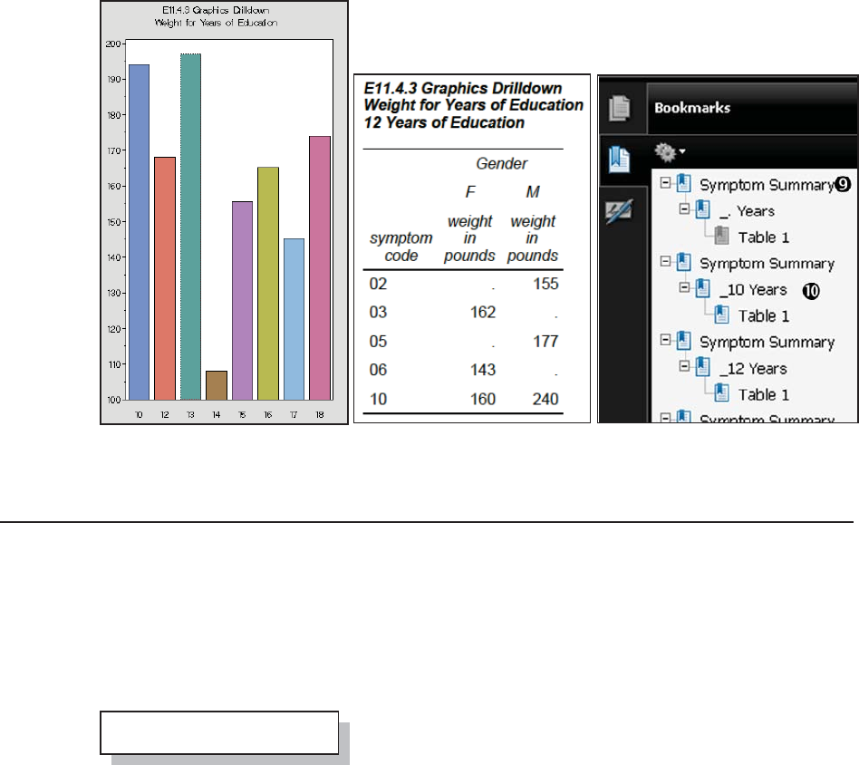
350 Carpenter’s Guide to Innovative SAS Techniques
Clicking on the vertical bar associated with subjects with 12 years of education (second from left),
opens the indicated PDF file at the appropriate anchor point.
MORE INFORMATION
Internal links are discussed further in Section 11.4.4.
11.4.4 Creating Internal Links
While hyperlinks will usually point to the beginning of a file, it is not unusual for the link to point
to a location within a file. This can be a location within a file other than the one being viewed or
to another location within the same file. This is known as an internal link. In the example in
Section 11.4.3 (see o) one of the links formed is a internal link.
Internal links are designated using a pound or hash sign (#). A pointer to an internal location
within a file in the local directory might be named: E11_4_3.pdf#_15. The internal location is
marked using the ANCHOR= option.
In the following example a PDF document is created that contains the output from a PROC
TABULATE and two PRINT procedure steps. The three reports are linked using internal
locations.
ods pdf anchor=_15;
&DUSHQWHU$UW&DUSHQWHU¶V*XLGHWR,QQRYDWLYH6$67HFKQLTXHV&RS\ULJKW6$6,QVWLWXWH,QF&DU\1RUWK&DUROLQD86$
$
//5,*+765(6(59(')RUDGGLWLRQDO6$6UHVRXUFHVYLVLWVXSSRUWVDVFRPSXEOLVKLQJ
Chapter 11: Output Delivery System 351
. . . . code not shown . . . .
proc format;
value $genlnk n
'M' = '#Males'
'F' = '#Females';
run;
ods pdf anchor='Master';
ods proclabel='Overall';
proc tabulate data=tabdat.clinics;
class sex ;
classlev sex/ style={url=$genlnk. o
foreground=blue};
var wt;
table sex=' ',
wt*(n median min max)
/ box='Gender';
run;
ods pdf anchor='Males'; p
ods proclabel='Males'; q
title2 link='#Master' rĨ œŦ ŵ Ŷ ų ů ġ ŵ Ű ġ ŎŢ Ŵ ŵ Ŧ ų Ĩ ļ
title3 c=blue 'Males';
proc print data=tabdat.clinics;
where sex='M'; s
var lname fname ht wt;
run;
. . . . code not shown . . . .
n A format is being used to
assign the link location. The
pound sign (#) identifies the link
location as internal to the current
file. Internal locations are
specified with the ANCHOR=
option p.
o The name of the file or, in this
case, the internal location to
which we will link is assigned
using the URL attribute. Since
this STYLE override option is on
the CLASSLEV statement, the
levels of this classification
variable will form the links.
p The ANCHOR= option marks
an internal location in the current
document to which we can link.
q The ODS PROCLABEL statement changes how the results of this procedure are labeled in the
PDF bookmarks.
r The LINK= option can be used to create links in titles and footnotes. Notice the use of the #
sign to designate the internal link
s A WHERE statement is used to create the table for the males.
CAVEAT
When using SAS 9.2 under Windows, internal link locations and pointers for PDF documents
should all be designated in lowercase. In SAS 9.1.3 mixed case is acceptable. This behavior may
change in future releases of SAS. The problem stems from the conversion of all the anchor
locations to lowercase when the document is rendered.
&DUSHQWHU$UW&DUSHQWHU¶V*XLGHWR,QQRYDWLYH6$67HFKQLTXHV&RS\ULJKW6$6,QVWLWXWH,QF&DU\1RUWK&DUROLQD86$
$
//5,*+765(6(59(')RUDGGLWLRQDO6$6UHVRXUFHVYLVLWVXSSRUWVDVFRPSXEOLVKLQJ

352 Carpenter’s Guide to Innovative SAS Techniques
11.5 Traffic Lighting
Traffic lighting is a technique that allows the programmer to automatically change attributes of a
report based on the values that are presented. Traditionally the background color is changed to
red/yellow/green – hence the name. However any of the attributes can be changed; and most often
a style override is used to change the attribute value. The key to the process is a user-defined
format that is used to map the display value to the attribute that is to be changed.
MORE INFORMATION
Style overrides are introduced and discussed further in Sections 8.1.3 (TABULATE), 8.4.6
(REPORT), and 8.5.2 (PRINT). The CALL DEFINE routine is introduced in Section 8.4.7.
11.5.1 User-Defined Format
A user-defined format is used to associate an ODS attribute value with the values that are to be
displayed in the table. Once established the format can be used by the TABULATE, REPORT, or
PRINT procedures.
Although traditionally traffic lighting techniques are
used to change colors, the extension of the concept
allows us to change multiple attributes, including cell
attributes such as links, font, font size, and bolding.
The VALUE or INVALUE statement is specified as
always, however, the format’s label (text to the right
of the equal sign) is the attribute value. The format is
then used along with the attribute to which it is to be
applied. Generally the association will be created
using a STYLE override option and takes the form of
attribute=format.
proc format;
value $serious_f
'YES','yes' = 'white';
value $serious_b
'YES','yes' = 'red';
value $severity_f
'3' = 'black'
'4','5'= 'white';
value $severity_b
'3' = 'yellow'
'4','5'= 'red';
run;
&DUSHQWHU$UW&DUSHQWHU¶V*XLGHWR,QQRYDWLYH6$67HFKQLTXHV&RS\ULJKW6$6,QVWLWXWH,QF&DU\1RUWK&DUROLQD86$
$
//5,*+765(6(59(')RUDGGLWLRQDO6$6UHVRXUFHVYLVLWVXSSRUWVDVFRPSXEOLVKLQJ
Chapter 11: Output Delivery System 353
11.5.2 PROC TABULATE
Although when using PROC TABULATE the STYLE override options can be applied to all
aspects of the table, for traffic lighting we will generally want to highlight values of statistics or
values derived from the
data. To do this the
STYLE override option
will be nested under the
statistic to which it is to
be applied.
In the protocol for this
study the subject’s initial
weight should be
between 100 and 235
pounds. This table
highlights those clinics
that have enrolled
subjects that are out of
compliance.
n The MAXWT_F.
format will be used to
alter the color of the text
(foreground) o for the
maximum weights. The
color of the background
(red q)is altered by the
MAXWT_B. p format.
The resulting table shows that at least two patients have been
enrolled that do not meet the weight criteria. You will
generally not be pleased with dark text on a dark background,
which is why the foreground color was changed to white,
when the background color was to be changed to red.
SEE ALSO
Carpenter (2010a) has a PROC TABULATE example of
traffic lighting using the STYLE override option.
proc format;
value MaxWT_f n
235-high = 'white'; o
value MaxWT_b p
235-high = 'red'; q
value MinWT_f
low-<100 = 'white';
value MinWT_b
low-<100 = 'red';
run;
title1 '11.5.2 Traffic Lighting: TABULATE';
title2 'Weight Compliance';
ods listing close;
ods pdf file="&path\results\e11_5_2.pdf"
style=journal;
proc tabulate data=advrpt.demog
(where=(clinnum in:('05','06')));
class clinnum;
var wt;
table clinnum,
wt*(min*{style={background=minwt_b.
foreground=minwt_f.}}
max*{style={background=maxwt_b. o
foreground=maxwt_f. n}});
run;
ods pdf close;
&DUSHQWHU$UW&DUSHQWHU¶V*XLGHWR,QQRYDWLYH6$67HFKQLTXHV&RS\ULJKW6$6,QVWLWXWH,QF&DU\1RUWK&DUROLQD86$
$
//5,*+765(6(59(')RUDGGLWLRQDO6$6UHVRXUFHVYLVLWVXSSRUWVDVFRPSXEOLVKLQJ
354 Carpenter’s Guide to Innovative SAS Techniques
11.5.3 PROC REPORT
When using PROC REPORT the style override option can be applied in two ways. First,
statement options such as the ones used in the example in Section 11.5.2 are applied directly.
Second, in PROC REPORT the CALL DEFINE routine allows us to conditionally apply style
overrides.
The examples in this section make use of the formats established in Section 11.5.1. In this report
we would like to highlight adverse events which are either serious (SER=’YES’) or have a
severity level which is greater than 3.
Formats for the foreground and background
colors are applied to the display of the values
of the seriousness (SER n) and severity (SEV
o) of the event.
In the figure for example 11.5.3a (to the left),
the severity codes 3 and greater are
highlighted regardless of the seriousness of the
event. These two formats are independent of
each other and both are applied. Notice that
subject 201 has two events highlighted
(SEV>2), however, neither of the events is
rated as serious (SER=NO).
Because the CALL DEFINE is executable we
can use IF-THEN/ELSE processing to
conditionally assign a format. In this next
example the traffic lighting style override for
the severity is moved to a CALL DEFINE and
is only applied for serious events (SER=YES). p The CALL DEFINE results are applied to the
current column q which is SEV since we are executing the SEV compute block. The style
override is selected r and the style attributes that are to be applied are the same ones as were
applied in the previous example o.
proc report data=advrpt.ae(where=(sev>'1')) nofs;
column subject aestdt ser sev aedesc;
define subject / order;
define aedesc / order;
define aestdt / display;
define ser / display
style(column) ={background=$serious_b. n
foreground=$serious_f.};
define sev / display
style(column) ={background=$severity_b. o
foreground=$severity_f.};
run;
&DUSHQWHU$UW&DUSHQWHU¶V*XLGHWR,QQRYDWLYH6$67HFKQLTXHV&RS\ULJKW6$6,QVWLWXWH,QF&DU\1RUWK&DUROLQD86$
$
//5,*+765(6(59(')RUDGGLWLRQDO6$6UHVRXUFHVYLVLWVXSSRUWVDVFRPSXEOLVKLQJ
Chapter 11: Output Delivery System 355
A portion of the
PROC REPORT
step is shown
here.
p The format
for the severity
has only been
applied when the
event is serious
(SER=’YES’).
SEE ALSO
The use of traffic lighting with PROC REPORT is covered in
detail in Carpenter (2006b).
11.5.4 Traffic Lighting with PROC PRINT
Traffic lighting with PROC PRINT, like with PROC TABULATE and PROC REPORT (see
Sections 11.5.2 and 11.5.3), is applied using the style override option. As was discussed in
Section 8.5.2, which introduced the style override option for the PRINT procedure, the option can
be applied on the VAR statement. The following example utilizes the formats created in Section
11.5.1 and the output mimics the first output generated by the REPORT procedure in Section
11.5.3.
Notice that the style override option is applied as an option on the VAR statement n o. By
splitting the VAR statement into two statements you can apply the traffic lighting formats
differentially.
define ser / display
style(column) ={background=$serious_b. n
foreground=$serious_f.};
define sev / display;
compute sev;
if ser='YES' then p
call define(_col_, q
'style', r
'style ={background=$severity_b. o
foreground=$severity_f.}');
endcomp;
ods pdf style=journal file="&path\results\E11_5_4a.pdf";
proc print data=advrpt.ae(where=(sev>'1'));
by subject;
id subject;
var aestdt ;
var ser / style(column)={background=$serious_b. n
foreground=$serious_f.};
var sev / style(column)={background=$severity_b. o
foreground=$severity_f.};
run;
ods pdf close;
&DUSHQWHU$UW&DUSHQWHU¶V*XLGHWR,QQRYDWLYH6$67HFKQLTXHV&RS\ULJKW6$6,QVWLWXWH,QF&DU\1RUWK&DUROLQD86$
$
//5,*+765(6(59(')RUDGGLWLRQDO6$6UHVRXUFHVYLVLWVXSSRUWVDVFRPSXEOLVKLQJ
356 Carpenter’s Guide to Innovative SAS Techniques
Like the figure in Section 11.5.3a this table applies the
formats on the two variables independently. In PROC
REPORT we were able to use the CALL DEFINE routine to
conditionally apply the format for severity. In PROC
PRINT the CALL DEFINE routine is not available and
formats cannot be conditionally assigned.
SEE ALSO
Carpenter (2006b) discusses traffic lighting in detail for the
PROC REPORT step.
11.6 The ODS LAYOUT Statement
The ODS LAYOUT statement, which is available but was not yet production for SAS 9.2, can be
used to place the results of multiple procedures, including graphics, on one page. The page is
defined in terms of regions with a given procedure’s output being placed into a specific region.
The user gets to define the number, size, and placement of the regions.
There are two basic types of layouts ABSOLUTE and GRIDDED. Absolute layouts, shown
below, have fixed region sizes, while gridded layouts can be more dynamically allocated.
The ability to define and use the output regions is made available by turning on LAYOUT with
the START option on the ODS LAYOUT statement. The general form of a program that utilizes
LAYOUT will be something like the following:
Layout is turned on with the START option and off with
the END option. Between the start and end will be one or
more region definition followed by the procedure that will
write to that region. Regions are rectangular and within the
layout page regions are defined with the ODS REGION
statement.
The primary options are:
X= horizontal position of the upper-left corner (measured from the left).
Y= vertical position of the upper-left corner (measured from the top).
width= width of the region.
height= height of the region.
You get to select the size of the region; however, you do need to be careful. If the region is too
small this warning may appear in the LOG when using layout.
ods layout start;
ods region . . .
proc . . . .
ods region . . .
proc . . . .
ods layout end;
WARNING: THE ABSOLUTE REGION WAS TOO SMALL TO ACCOMMODATE THE TEXT
SUPPLIED. OUTPUT WAS LOST.
&DUSHQWHU$UW&DUSHQWHU¶V*XLGHWR,QQRYDWLYH6$67HFKQLTXHV&RS\ULJKW6$6,QVWLWXWH,QF&DU\1RUWK&DUROLQD86$
$
//5,*+765(6(59(')RUDGGLWLRQDO6$6UHVRXUFHVYLVLWVXSSRUWVDVFRPSXEOLVKLQJ

Chapter 11: Output Delivery System 357
The layout to the left
establishes three
regions. One for a
title written by the
TEXT= option, and
two for side-by-side
PROC REPORT
tables.
n The title for the
page is saved in
macro variables for
use with the ODS
PDF TEXT= option
s. Inline formatting
sequences (~n, ~S)
are described in
Section 11.3.
o The PDF
destination is opened.
p Restrain PDF
from starting a new
page when going to a
new procedure.
q Open the layout space with an overall size definition.
r Define the first region, which will hold the title text stored in the macro variables &TEXT1 and
&TEXT2.
s The text is written to the first region.
t and u The regions used by the two PROC REPORT steps are defined.
v The PDF destination is closed. Actually here all destinations are closed.
w The ODS LAYOUT section is closed.
SEE ALSO
Rob Nelson (2010) creates a
similar, but more complex layout.
Along with a number of other ODS
options, Dan O’Conner and Scott
Huntley (2009) discuss both
absolute and gridded layout options
in detail. Chen (2005) introduces
gridded layout.
%let text1 = ~S={font_face=arial n
font_weight=bold}11.6 Using ODS
LAYOUT~S={font_face=arial}~nMean Weight and Height;
%let text2 = ~nfor Symptom and Years of Education;
title1;
ods pdf file="&path\results\E11_6.pdf" o
style=journal
startpage=never; p
ods escapechar='~';
ods layout start width=7in height=10in; q
ods region x=1in y=1in width=7in height=.5in; r
ods pdf text="&text1&text2"; s
ods region x=0.5in y=1.5in width=7in height=4in; t
proc report data=advrpt.demog nowd;
. . . . REPORT code not shown . . . .
ods region x=1.5in y=1.5in width=3in height=4in; u
proc report data=advrpt.demog nowd;
. . . . REPORT code not shown . . . .
ods _all_ close; v
ods layout end; w
&DUSHQWHU$UW&DUSHQWHU¶V*XLGHWR,QQRYDWLYH6$67HFKQLTXHV&RS\ULJKW6$6,QVWLWXWH,QF&DU\1RUWK&DUROLQD86$
$
//5,*+765(6(59(')RUDGGLWLRQDO6$6UHVRXUFHVYLVLWVXSSRUWVDVFRPSXEOLVKLQJ
358 Carpenter’s Guide to Innovative SAS Techniques
proc print data=advrpt.demog(obs=5);
id lname;
var fname ht wt;
format wt 8.1;
run;
var fname ht;
var wt /style(data)={asis=yes}
style(header)={just=c};
11.7 A Few Other Useful ODS Tidbits
There are just way too many options and statements to fully describe them here. However there
are a couple of which you should be at least aware.
11.7.1 Using the ASIS Style Attribute
The HTML destination removes spacing to give a ‘better’ display. When you want to preserve
spacing surrounding a value, the ASIS option can prevent this behavior.
Although the format used with WT has a width of 8,
the space surrounding the numbers only reflects the
cell margins. We can preserve that space by using
the ASIS style attribute; however, this attribute may
also affect the bottom margin attribute.
The VAR statement has been broken into two
statements so that we can associate STYLE override
options with the variable WT. The header as also
been centered.
Notice that the ASIS attribute has also increased the
bottom margin of the cell.
11.7.2 ODS RESULTS Statement
When we create RTF files under some combinations of operating systems and versions of
Microsoft Office, a prompt is issued when the SAS viewer attempts to open the new RTF file.
This can be especially troublesome when the files are generated as a part of an automated system
or application.
One solution is to turn off the automatic viewing of the results. In the interactive environment this
can be done manually by changing the preference settings. While running the SAS Display
Manager go to:
Tools ĺ Options ĺ Preferencesĺ Results
Uncheck the “View results as they are generated” box.
&DUSHQWHU$UW&DUSHQWHU¶V*XLGHWR,QQRYDWLYH6$67HFKQLTXHV&RS\ULJKW6$6,QVWLWXWH,QF&DU\1RUWK&DUROLQD86$
$
//5,*+765(6(59(')RUDGGLWLRQDO6$6UHVRXUFHVYLVLWVXSSRUWVDVFRPSXEOLVKLQJ

Chapter 11: Output Delivery System 359
The automatic viewing of results can also be controlled through the use of the ODS RESULTS
statement. To override the preference that is selected through the Preferences Dialogue Box, you
may use either:
ods results on; Turn on automatic review of the results (typically the default).
ods results off; Turn off automatic review of the results.
SEE ALSO
Alternative approaches and a deeper statement of the problem were discussed in the SAS Forum
thread http://communities.sas.com/message/42066#42066.
&DUSHQWHU$UW&DUSHQWHU¶V*XLGHWR,QQRYDWLYH6$67HFKQLTXHV&RS\ULJKW6$6,QVWLWXWH,QF&DU\1RUWK&DUROLQD86$
$
//5,*+765(6(59(')RUDGGLWLRQDO6$6UHVRXUFHVYLVLWVXSSRUWVDVFRPSXEOLVKLQJ
360
&DUSHQWHU$UW&DUSHQWHU¶V*XLGHWR,QQRYDWLYH6$67HFKQLTXHV&RS\ULJKW6$6,QVWLWXWH,QF&DU\1RUWK&DUROLQD86$
$
//5,*+765(6(59(')RUDGGLWLRQDO6$6UHVRXUFHVYLVLWVXSSRUWVDVFRPSXEOLVKLQJ

Part 3
Techniques, Tools, and Interfaces
Chapter 12 Taking Advantage of Formats 363
Chapter 13 Interfacing with the Macro Language 397
Chapter 14 Operating System Interface and Environmental Control 437
Chapter 15 Miscellaneous Topics 473
&DUSHQWHU$UW&DUSHQWHU¶V*XLGHWR,QQRYDWLYH6$67HFKQLTXHV&RS\ULJKW6$6,QVWLWXWH,QF&DU\1RUWK&DUROLQD86$
$
//5,*+765(6(59(')RUDGGLWLRQDO6$6UHVRXUFHVYLVLWVXSSRUWVDVFRPSXEOLVKLQJ
362
&DUSHQWHU$UW&DUSHQWHU¶V*XLGHWR,QQRYDWLYH6$67HFKQLTXHV&RS\ULJKW6$6,QVWLWXWH,QF&DU\1RUWK&DUROLQD86$
$
//5,*+765(6(59(')RUDGGLWLRQDO6$6UHVRXUFHVYLVLWVXSSRUWVDVFRPSXEOLVKLQJ

Chapter 12
Taking Advantage of Formats
12.1 Using Preloaded Formats to Modify Report Contents 364
12.1.1 Using Preloaded Formats with PROC REPORT 365
12.1.2 Using Preloaded Formats with PROC TABULATE 367
12.1.3 Using Preloaded Formats with the MEANS and SUMMARY
Procedures 369
12.2 Doing More with Picture Formats 370
12.2.1 Date Directives and the DATATYPE Option 371
12.2.2 Working with Fractional Values 373
12.2.3 Using the MULT and PREFIX Options 374
12.2.4 Display Granularity Based on Value Ranges – Limiting Significant
Digits 376
12.3 Multilabel (MLF) Formats 377
12.3.1 A Simple MLF 377
12.3.2 Calculating Rolling Averages 378
12.4 Controlling Order Using the NOTSORTED Option 381
12.5 Extending the Use of Format Translations 382
12.5.1 Filtering Missing Values 382
12.5.2 Mapping Overlapping Ranges 383
12.5.3 Handling Text within Numeric Values 383
12.5.4 Using Perl Regular Expressions within Format Definitions 384
12.5.5 Passing Values to a Function as a Format Label 384
12.6 ANYDATE Informats 388
12.6.1 Reading in Mixed Dates 389
12.6.2 Converting Mixed DATETIME Values 389
&DUSHQWHU$UW&DUSHQWHU¶V*XLGHWR,QQRYDWLYH6$67HFKQLTXHV&RS\ULJKW6$6,QVWLWXWH,QF&DU\1RUWK&DUROLQD86$
$
//5,*+765(6(59(')RUDGGLWLRQDO6$6UHVRXUFHVYLVLWVXSSRUWVDVFRPSXEOLVKLQJ

364 Carpenter’s Guide to Innovative SAS Techniques
12.7 Building Formats from Data Sets 390
12.8 Using the PVALUE Format 392
12.9 Format Libraries 393
12.9.1 Saving Formats Permanently 393
12.9.2 Searching for Formats 394
12.9.3 Concatenating Format Catalogs and Libraries 394
The use of formats is essential to the process of analysis and reporting of data. The user must be
well grounded not only in the basic application of formats, but the deeper, less commonly known
aspects as well. The power of formats can be taken advantage of in a wide variety of situations. It
is incumbent on the user that these capabilities are fully understood.
MORE INFORMATION
Section 3.5.1 discusses the difference between formats and informats and their uses in the
conversion of character to numeric values.
SEE ALSO
Carpenter (2003a) introduces a number of topics on the use of user-written formats. Ron Cody
(2008a) provides a number of examples of user-written formats which demonstrate a number of
the options and techniques described in this chapter. Bilenas (2005) is a book that is devoted to
the topic of SAS formats.
12.1 Using Preloaded Formats to Modify Report
Contents
Generally when a level of a classification variable is not included in the data, that level will not
appear in any reports or analyses based on that data. Preloaded formats provide a mechanism to
not only force the inclusion of those absent classification levels, they can also be used to filter or
remove unwanted levels.
Preloaded formats can be used with the REPORT, TABULATE, MEANS and SUMMARY
procedures. Preloaded formats are invoked through the use of options, and the available options
and their usage varies for each procedure. For each procedure it is the interaction of these options
that determines the resulting table. For the examples in this section study the results of the various
combinations of the options, then experiment using other combinations.
For each of these procedures the two primary options used are PRELOADFMT and
EXCLUSIVE:
PRELOADFMT Loads the format levels prior to execution. This option will always
be present when using preloaded formats.
EXCLUSIVE Only data levels that are included in the format definition are to
appear in table.
&DUSHQWHU$UW&DUSHQWHU¶V*XLGHWR,QQRYDWLYH6$67HFKQLTXHV&RS\ULJKW6$6,QVWLWXWH,QF&DU\1RUWK&DUROLQD86$
$
//5,*+765(6(59(')RUDGGLWLRQDO6$6UHVRXUFHVYLVLWVXSSRUWVDVFRPSXEOLVKLQJ

Chapter 12: Taking Advantage of Formats 365
As the name implies preloaded formats key off of what
is generally a user-defined format. The formats
$REGX., $GENDERU., and $SYMP., which are
defined here, are used in the examples that follow.
Each contains one level that is not in the data n, and
both $REGX. and $SYMP. exclude levels that are
found in the data. The format $REGX. is used with the
variable REGION, which ranges from ‘1’ through ‘10’.
The format $SYMP. is used with the variable SYMP,
which ranges from ‘01’ through ‘10’. The format
$GENDERU. is used with the variable SEX which
takes on the values of ‘F’ and ‘M’.
12.1.1 Using Preloaded Formats with PROC REPORT
When preloading formats with the REPORT procedure, the PRELOADFMT and, if used, the
EXCLUSIVE options are applied on the DEFINE statement.
In addition to the PRELOADFMT and EXCLUSIVE options, the REPORT procedure can also
take advantage of the options COMPLETEROWS and COMPLETECOLS:
COMPLETEROWS All rows representing format levels are to appear in the report.
COMPLETECOLS All columns representing format levels are to appear in the report.
The following examples show various combinations of these options. Although they do not
discuss the use of COMPLETECOLS, its behavior is similar to COMPLETEROWS, which is
discussed here. This can be easily demonstrated by applying these options to the report item SEX
in these same examples.
Remember that you must apply the PRELOADFMT option on the DEFINE statement for each
report item for which you want to preload a format.
Using PRELOADFMT with EXCLUSIVE
Preloading with the EXCLUSIVE option allows only those levels that are on the format and in the
data. In PROC REPORT these options are applied on the DEFINE statement.
proc format;
value $regx
'1'=' 1'
'2'=' 2'
'X'=' X' ; n
value $genderu
'M'='Male'
'F'='Female'
'U'='Unknown'; n
value $symp
'00'= 'Unspecified' n
'01'= 'Sleepiness'
'02'= 'Coughing'
'03'= 'Limping';
run;
title2 'Using PRELOADFMT with EXCLUSIVE';
proc report data=demog nowd;
column region sex,(wt=n wt);
define region / group
format=$regx6.
preloadfmt exclusive;
define sex / across format=$Genderu. 'Gender';
define n / analysis n format=2.0 'N';
define wt / analysis mean format=6.2 'Weight';
run;
&DUSHQWHU$UW&DUSHQWHU¶V*XLGHWR,QQRYDWLYH6$67HFKQLTXHV&RS\ULJKW6$6,QVWLWXWH,QF&DU\1RUWK&DUROLQD86$
$
//5,*+765(6(59(')RUDGGLWLRQDO6$6UHVRXUFHVYLVLWVXSSRUWVDVFRPSXEOLVKLQJ

366 Carpenter’s Guide to Innovative SAS Techniques
12.1.1 Preloading Formats in PROC REPORT
Using PRELOADFMT with EXCLUSIVE
Gender
Female Male
region N Weight N Weight
1 . . 4 195.00
2 6 109.67 3 105.00
Using the format $REGX. along with
these two options causes only regions 1
and 2 to appear in the report, as these
are the only two regions that are both in
the format and in the data.
Using COMPLETEROWS without EXCLUSIVE
The COMPLETEROWS option, which is used on the PROC statement, forces all levels that
appear either in the data or in the format to appear on the report.
In this example
the
ORDER=DATA
option also
appears on the
DEFINE
statement. Prior
to SAS 9.2 the
ORDER= option
was expected,
although not
always required.
Notice that all
three format
levels appear.
Except for
REGION ‘X’, which does not appear in the data, the output is now in data order (the data has
been sorted by CLINNUM which nominally sorts the regions as well).
The default order for a formatted report item is ORDER=FORMATTED.
Using COMPLETEROWS with EXCLUSIVE
As was shown earlier, using EXCLUSIVE without the COMPLETEROWS option yields only
those levels that are both in the format and in the data. Using the EXCLUSIVE option with the
COMPLETEROWS option creates a report that contains each of the values that are in the format,
regardless of whether or not they are in the data.
12.1.1 Preloading Formats in PROC REPORT
Using COMPLETEROWS with PRELOADFMT and without EXCLUSIVE
Gender
Female Male
region N Weight N Weight
1 0 . 4 195.00
2 6 109.67 3 105.00
X 0 . 0 .
3 5 127.80 5 163.80
4 4 143.00 10 165.60
5 5 146.20 3 177.00
6 3 187.00 6 205.33
7 0 . 4 151.00
8 4 160.00 0 .
9 2 177.00 7 187.00
10 2 163.00 4 177.00
title2 'Using COMPLETEROWS with PRELOADFMT and without EXCLUSIVE';
proc report data=demog nowd completerows;
column region sex,(wt=n wt);
define region / group format=$regx6.
preloadfmt
order=data;
define sex / across format=$Genderu. 'Gender';
define n / analysis n format=2.0 'N';
define wt / analysis mean format=6.2 'Weight';
run;
&DUSHQWHU$UW&DUSHQWHU¶V*XLGHWR,QQRYDWLYH6$67HFKQLTXHV&RS\ULJKW6$6,QVWLWXWH,QF&DU\1RUWK&DUROLQD86$
$
//5,*+765(6(59(')RUDGGLWLRQDO6$6UHVRXUFHVYLVLWVXSSRUWVDVFRPSXEOLVKLQJ

Chapter 12: Taking Advantage of Formats 367
12.1.1 Preloading Formats in PROC REPORT
Using COMPLETEROWS with PRELOADFMT and EXCLUSIVE
Gender
Female Male
region N Weight N Weight
1 0 . 4 195.00
2 6 109.67 3 105.00
X 0 . 0 .
Only those levels in the
format, regardless of
whether or not they are in
the data, are included in the
report.
12.1.2 Using Preloaded Formats with PROC TABULATE
When using preloaded formats with the TABULATE procedure the PRELOADFMT and
EXCLUSIVE options are applied on the CLASS statement. As with the REPORT procedure these
two options interact.
PRELOADFMT with EXCLUSIVE
In each of the examples in this section the user-defined format, $SYMP. is used. This format,
which is defined in Section 12.1, contains only three of the 10 possible values that can occur in
the data, and one additional value that does not occur in the data.
n The
PRELOADFMT and
EXCLUSIVE options
appear on the CLASS
statement associated
with the classification
variable that is to
receive the preloaded
format.
o The appropriate format is assigned to the classification variable.
p The PRINTMISS option allows the display of missing values in a PROC TABULATE table.
Without including this option, levels added by the preloaded format, which would necessarily
always be missing, would not be displayed.
title2 'Using PRINTMISS With the EXCLUSIVE option';
proc tabulate data=advrpt.demog;
class symp /preloadfmt exclusive; n
var ht wt;
table symp,
(ht wt)*(n*f=2. min*f=4.
median*f=7.1 max*f=4.)
/ printmiss; p
format symp $symp.; o
run;
title2 'Using COMPLETEROWS with PRELOADFMT and EXCLUSIVE';
proc report data=demog nowd completerows;
column region sex,(wt=n wt);
define region / group format=$regx6.
preloadfmt exclusive;
define sex / across format=$Genderu. 'Gender';
define n / analysis n format=2.0 'N';
define wt / analysis mean format=6.2 'Weight';
run;
&DUSHQWHU$UW&DUSHQWHU¶V*XLGHWR,QQRYDWLYH6$67HFKQLTXHV&RS\ULJKW6$6,QVWLWXWH,QF&DU\1RUWK&DUROLQD86$
$
//5,*+765(6(59(')RUDGGLWLRQDO6$6UHVRXUFHVYLVLWVXSSRUWVDVFRPSXEOLVKLQJ
368 Carpenter’s Guide to Innovative SAS Techniques
The PRELOADFMT and
EXCLUSIVE options used
together eliminate all values of
SYMP that are not on the
format, while including values
on the format that are not in
the data.
Because the PRINTMISS
option p has been used, the
“Unspecified” row appears in
the table with the appropriate
values for N.
Using PRELOADFMT without EXCLUSIVE
Using the PRELOADFMT option without the EXCLUSIVE option allows you to have all
possible rows, including those without data and those that are not included in the format.
The resulting table shows all values
of SYMP that are either in the data or
in the format. This includes the level
of SYMP that is not found in the data.
MORE INFORMATION
Preloading formats is also
discussed in conjunction with the
REPORT procedure (see Section
12.1.1) and the MEANS and
SUMMARY procedures (see
Section 12.1.3).
The EXCLUSIVE option can also
be used with the CLASSDATA
option; see Section 8.1.4.
SEE ALSO
Carpenter (2010a) discusses the
use of preloaded formats with the
TABULATE procedure.
title2 'Without the EXCLUSIVE option';
proc tabulate data=advrpt.demog;
class symp /preloadfmt;
var ht wt;
table symp,
(ht wt)*(n*f=2. min*f=4.
median*f=7.1 max*f=4.)
/printmiss;
format symp $symp.;
run;
&DUSHQWHU$UW&DUSHQWHU¶V*XLGHWR,QQRYDWLYH6$67HFKQLTXHV&RS\ULJKW6$6,QVWLWXWH,QF&DU\1RUWK&DUROLQD86$
$
//5,*+765(6(59(')RUDGGLWLRQDO6$6UHVRXUFHVYLVLWVXSSRUWVDVFRPSXEOLVKLQJ
Chapter 12: Taking Advantage of Formats 369
title2 'Using the EXCLUSIVE Option';
proc summary data=advrpt.demog;
class symp / preloadfmt n
exclusive o;
var ht;
output out=withexclusive
mean= meanHT;
format symp $symp.;
run;
proc print data=withexclusive;
run;
12.1.3 Using Preloaded Formats with the MEANS and SUMMARY
Procedures
As was the case with PROC TABULATE (see Section 12.1.2) the PRELOADFMT and
EXCLUSIVE options appear on the CLASS statement, when they are used with the MEANS and
SUMMARY procedures.
Using PRELOADFMT with EXCLUSIVE
Preloading with the CLASS statement options PRELOADFMT n and EXCLUSIVE olimits the
levels of the classification variable to those that are both on the format and in the data. Essentially
the format acts as a filter without resorting to either a subsetting IF statement or a WHERE clause.
Notice that unlike PROC TABULATE,
this combination of CLASS statement
options does NOT insert a row for the
formatted value of SYMP that is not in the
data (SYMP=’00’). To add this level using the
MEANS and SUMMARY procedures, the
COMPLETETYPES option must also be
included.
Using COMPLETETYPES with PRELOADFMT and EXCLUSIVE
The PROC statement option COMPLETYPES (this option was introduced in Section 7.10) will
interact with the PRELOADFMT and EXCLUSIVE options. As a result of this interaction, levels
of the classification variable that are not in the data, but are on the format are now included in the
summary. However, levels not on the format are not included in the table.
The ‘Unspecified’ level for SYMP now
appears in the report even though it is not in the
data (_FREQ_=0).
title2 'With EXCLUSIVE and COMPLETETYPES';
proc summary data=advrpt.demog
completetypes;
class symp / preloadfmt
exclusive;
var ht;
. . . code not shown . . . .
&DUSHQWHU$UW&DUSHQWHU¶V*XLGHWR,QQRYDWLYH6$67HFKQLTXHV&RS\ULJKW6$6,QVWLWXWH,QF&DU\1RUWK&DUROLQD86$
$
//5,*+765(6(59(')RUDGGLWLRQDO6$6UHVRXUFHVYLVLWVXSSRUWVDVFRPSXEOLVKLQJ
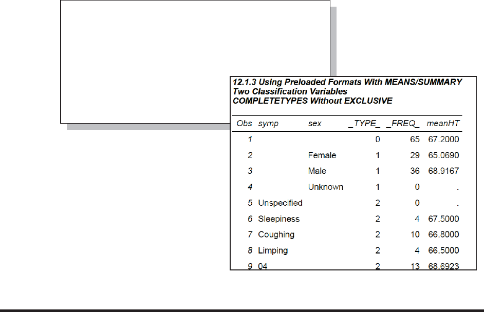
370 Carpenter’s Guide to Innovative SAS Techniques
title2 'Two Classification Variables';
title3 'COMPLETETYPES Without EXCLUSIVE';
proc summary data=advrpt.demog completetypes;
class symp sex / preloadfmt ;
var ht;
output out=twoclass mean= meanHT;
format symp $symp.
sex $genderu.;
run;
proc print data=twoclass;
run;
Using COMPLETETYPES without EXCLUSIVE
When the COMPLETETYPES option is used without the EXCLUSIVE option, all levels of the
classification variable appear whether it is in the data or if it is only in the preloaded format.
A portion of the table
generated by the two
classification variables SYMP
and SEX, which both have
preloaded formats, is shown
here. Notice that each format
level not associated with data appears
as do the unformatted levels (only
SYMP=’04’ is shown in this partial
table).
12.2 Doing More with Picture Formats
Although generally speaking picture formats are only nominally an advanced topic, they are far
underutilized and there are some concepts that are unique to picture formats that are commonly
misunderstood.
The PICTURE statement is used to build what is essentially a template of zeros, nines, and other
characters that are also to be displayed. The zeros and nines are used as placeholders. The nines
indicate that a number must be placed at the location, even if it is a zero. A zero placeholder
indicates that a number is placed at the location if it is non-zero (embedded zeros are displayed).
SEE ALSO
The book The Power of PROC FORMAT (Jonas Bilenas, 2005) is a good source for some of the
more introductory picture format topics.
The documentation for the PICTURE statement gives a clear description of the application of the
format to the value that is to be formatted. The application process should be well understood
before working with fractional values.
&DUSHQWHU$UW&DUSHQWHU¶V*XLGHWR,QQRYDWLYH6$67HFKQLTXHV&RS\ULJKW6$6,QVWLWXWH,QF&DU\1RUWK&DUROLQD86$
$
//5,*+765(6(59(')RUDGGLWLRQDO6$6UHVRXUFHVYLVLWVXSSRUWVDVFRPSXEOLVKLQJ

Chapter 12: Taking Advantage of Formats 371
12.2.1 Date Directives and the DATATYPE Option
The DATATYPE= option on the PICTURE statement can be used to build date-specific formats.
This option allows the use of 'directives', which tell the PICTURE statement how to further
structure or format the value relative to the type of data that is to be interpreted.
The directives are individual case-sensitive letters that indicate a specific portion of the DATE,
TIME, or DATETIME value. There are over 15 directives and the case of the letters used as
directives is important:
Y Year M Minute
m Month S Second
d Day b Month abbreviation
H Hour B Month name
In the PICTURE statement the directive is preceded by a percent sign (%) which acts like an
escape character. Single quotes are used to prevent the interpretation of the % as a macro
language trigger.
The following format is used to display a SAS datetime value in a format that can be used in DB2.
n As in other PICTURE formats a zero may be used as a placeholder.
o The DATATYPE option determines how the incoming value is to be interpreted. Option values
indicate the type of data that the format will be used with. These data types include:
DATE SAS date value
TIME SAS time value
DATETIME SAS datetime value
DATETIME_UTIL SAS datetime value specific for the utilities industry (SAS 9.3)
The LOG shows:
In the DATA step above the macro variable &SELLDATE was created p. Once formatted this
macro variable could be used to write this DATETIME value into SQL code that is to be passed
through to a DB2 server. The %SYSFUNC calls the PUTN function which will render the
formatted value.
proc format;
picture dbdate
other = '%Y-%0m-%0d:%0H:%0M:%0S n' (datatype=datetime)o;
run;
data _null_;
now = '11sep2010:15:05:27'dt;
put now=;
put now= dbdate.;
call symputx('selldate',now); p
run;
now=1599836727
now=2010-09-11:15:05:27
%put %sysfunc(putn(&selldate,dbdate.));
&DUSHQWHU$UW&DUSHQWHU¶V*XLGHWR,QQRYDWLYH6$67HFKQLTXHV&RS\ULJKW6$6,QVWLWXWH,QF&DU\1RUWK&DUROLQD86$
$
//5,*+765(6(59(')RUDGGLWLRQDO6$6UHVRXUFHVYLVLWVXSSRUWVDVFRPSXEOLVKLQJ

372 Carpenter’s Guide to Innovative SAS Techniques
Because of the variety of directives and the availability of the DATATYPE option, there is a great
deal of flexibility as to the
resulting formats. This means
that a format can be
generated for any of the three
datetime data value types.
This flexibility can be
demonstrated by creating
alternate formats for the
MONNAME. format (which
can be used only with DATE
values). The
MONTHNAME. and
MONTHABB. formats
created here are used with
DATETIME values.
q The %B directive returns the month name. When defining the format be sure to leave sufficient
space for the longest month (September), otherwise truncation of the month’s name could take
place.
r The lowercase %b directive returns the first three letters of the
month in uppercase. Again allow three spaces (including the
directive and the escape character).
s If an abbreviated month name is desired in mixed case, a width
value can be included with the format for the full name.
SAS 9.3 Date Directive Enhancements
Prior to SAS 9.3 fractional seconds were truncated (even when the ROUND option was applied to
the PICTURE format). Starting in SAS 9.3 fractional seconds are rounded. Although generally of
minor concern this can change the date for time values within a half second of midnight.
Display Value
DateTime Constant MYDAYT. (prior to SAS 9.3) MYDAYT. (SAS 9.3 and after)
'01apr2011:12:34:56.7'dt 01APR2011:12:34:56 01APR2011:12:34:57
'01apr2011:23:59:59.7'dt 01APR2011:23:59:59 02APR2011:00:00:00
The utility industry often wants to reference a midnight date to be 24:00:00 instead of 00:00:00.
The new DATATYPE= value DATETIME_UTIL allows this.
proc format;
picture monthname
other = '%B q ' (datatype=datetime);
picture monthabb
other = '%b r' (datatype=datetime);
run;
data _null_;
now = '11sep2010:15:05:27'dt;;
put now=;
put now= monthname.;
put now= monthname3.; s
put now= monthabb.;
run;
now=1599836727
now=September q
now=Sep s
now=SEP r
proc format;
picture myDayT (round)
low - high = '%0d%b%0Y:%0H:%0M:%0S'(datatype=datetime)
;
run;
proc format;
picture ymdtime (default=19)
other='%Y-%0m-%0d %0H:%0M:%0S' (datatype=datetime_util);
run;
&DUSHQWHU$UW&DUSHQWHU¶V*XLGHWR,QQRYDWLYH6$67HFKQLTXHV&RS\ULJKW6$6,QVWLWXWH,QF&DU\1RUWK&DUROLQD86$
$
//5,*+765(6(59(')RUDGGLWLRQDO6$6UHVRXUFHVYLVLWVXSSRUWVDVFRPSXEOLVKLQJ

Chapter 12: Taking Advantage of Formats 373
DateTime Constant YMDTIME. Display Value
'01nov2008:00:00:00'dt 2008-10-31 24:00:00
'01nov2008:00:00:01'dt 2008-11-01 00:00:01
The %n directive allows you to count
the number of complete days within an
interval. This allows you to return the
duration in days/hours/minutes/seconds
between two datetime values. The %D
directive cannot be used because it
returns the day of the month.
The LOG shows the result of the PUT
statement.
12.2.2 Working with Fractional Values
Picture formats do not automatically handle fractional values well. This is especially true for
values between zero and 1, and the value of zero itself must also be taken into consideration or it
will not display correctly.
The problem with fractions is demonstrated in the following example. The variable VAL ranges
from 0 to 3 by .25, and three picture formats have been created to display these values.
n The format SHOWVAL. does not contain an explicit decimal point. The displayed values are
only the integer portions. Fractional values are not displayed and the 0 is not displayed.
o The WITHDEC. format contains a decimal point which allows a single decimal value (tenths).
Values below 1 are not displayed correctly, and the 0 is not displayed at all.
p Adding a 9 in the digits place forces the format to write a value in that location. The values less
than 1 are now displayed correctly. The 0 is also now being displayed.
proc format;
picture showval
other = '0000'; n
picture withdec
other = '00.0'; o
picture twodec
other = '09.00'; p
run;
data vallist;
do val = 0 to 3 by .25;
val2 = val;
val3 = val;
val4 = val;
output;
end;
format val2 showval.
val3 withdec.
val4 twodec.;
run;
12.2.2 Picture Formats
Showing Decimals
n o p
Obs val val2 val3 val4
1 0.00 0.00
2 0.25 2 0.25
3 0.50 5 0.50
4 0.75 7 0.75
5 1.00 1 1.0 1.00
6 1.25 1 1.2 1.25
7 1.50 1 1.5 1.50
8 1.75 1 1.7 1.75
9 2.00 2 2.0 2.00
10 2.25 2 2.2 2.25
11 2.50 2 2.5 2.50
12 2.75 2 2.7 2.75
13 3.00 3 3.0 3.00
proc format;
picture durtest(default=27)
other='%n days %H hours %M minutes'
(datatype=time);
run;
data _null_;
start = '01jan2010:12:34'dt;
end = '01feb2010:18:36'dt;
diff = end - start;
put diff=durtest.;
run;
diff=31 days 6 hours 2 minutes
&DUSHQWHU$UW&DUSHQWHU¶V*XLGHWR,QQRYDWLYH6$67HFKQLTXHV&RS\ULJKW6$6,QVWLWXWH,QF&DU\1RUWK&DUROLQD86$
$
//5,*+765(6(59(')RUDGGLWLRQDO6$6UHVRXUFHVYLVLWVXSSRUWVDVFRPSXEOLVKLQJ

374 Carpenter’s Guide to Innovative SAS Techniques
When working with values that are less than one be sure to force at least one significant digit by
using the 9 as the placeholder in the format label.
Truncation is another area that warrants extra consideration when dealing with picture formats.
Values that do not fit into the picture template (the format label) are truncated. The variable X in
this example ranges from a small fraction to a value over one thousand.
p The format is defined with two
decimal places and 9 in the unit’s
digit. Notice that the implied format
used for X does not have sufficient
range to display both the largest and
smallest value. Something like the
format 8.3 would have had the range to show all the
values.
q The value less than .01 (the smallest permitted by
the format) is not surprisingly truncated.
r Only two of the three least significant digits can be
displayed. The display value for X is rounded but for Y the thousandths are truncated.
s We have only allowed for values up to 99.99. Values over 100 have the most significant digits
truncated.
The rounding and truncation issues can be addressed in the format definition. The SHOWDECR.
format shown here allows both rounding and
numbers up to 99999.99.
t The ROUND option causes the format to round
fractional values.
u Be sure to include a sufficient number of
placeholders to accommodate the largest
number.
12.2.3 Using the MULT and PREFIX Options
While text that is to be included, either within or following the formatted value can be included as
part of the picture definition, text that is to precede the display value is ignored. When you want
preceding text to be a part of the displayed value, the PREFIX= option can be used.
proc format;
picture showdec
other = '09.00'; p
run;
data x; q r s
do x = .007,.017,.123,1.234, 12.345, 1234;
y=x;
output;
end;
format y showdec. x 8.3;
run;
proc format;
picture showdecr (round) t
other = '00009.00'; u
run;
12.2.2 Picture Formats
Showing Decimals
Obs x y
1 0.007 0.00 q
2 0.017 0.01
3 0.123 0.12
4 1.234 1.23
5 12.345 12.34 r
6 1234.000 34.00 s
12.2.2 Working with Fractional Values
Showing Decimals
Obs x y
1 0.007 0.01
2 0.017 0.02
3 0.123 0.12
4 1.234 1.23
5 12.345 12.35
6 1234.000 1234.00
&DUSHQWHU$UW&DUSHQWHU¶V*XLGHWR,QQRYDWLYH6$67HFKQLTXHV&RS\ULJKW6$6,QVWLWXWH,QF&DU\1RUWK&DUROLQD86$
$
//5,*+765(6(59(')RUDGGLWLRQDO6$6UHVRXUFHVYLVLWVXSSRUWVDVFRPSXEOLVKLQJ

Chapter 12: Taking Advantage of Formats 375
The MULT= option allows the application of a multiplier. This value is multiplied against the
incoming value and the result is displayed.
A common alternative solution to handling fractional values involves the use of the MULT= and
PREFIX= options.
n The zero is handled
separately.
o Values that are smaller
than .01 add a prefix value
that includes the <.01 text.
p For values from .01 up to
1, multiply the value by 100
and add the ‘0.’ prefix.
q Make sure that there are sufficient significant
digits.
r Since we did not use the (ROUND) option this
value has been truncated.
Since the numbers in this example have two decimal
places, multiplying them by 100 (10n where n is the
number of significant digits to be displayed) turns the number into an integer. The decimal is then
inserted via the picture format.
In the following example dollars are being converted to British pounds (the conversion constant
used for this example is 0.635, which is almost certainly not the current currency conversion
constant).
s The display value
template specifies
two decimal places
(using the European
style with a comma
separating the whole
numbers from the
fractions.
t The multiplication
factor is specified
using the MULT=
opton.
u The PREFIX=
option is used to
designate one or
more leading
symbols. Here the option is applied to each value/label pair; however, it does not need to be
constant, as it is in this example.
title2 'Using The MULT and PREFIX Options';
proc format;
picture pounds
1 - 10 = '9,00's(mult=63.5 tprefix='£'u)
10< - 100 = '09,0'(mult=6.35 vprefix='£')
100<- high= '000.000.000' (mult=.635 prefix='£');
run;
data money;
do dollars = 1.23, 12.3, 123, 1230, 12300;
pounds = dollars;
output;
end;
format dollars dollar10.2 pounds pounds.;
run;
proc print data=money;
run;
proc format;
picture showdec
0 = '9' n
0< - <.01 = '9'(prefix='<.01') o
.01 - <1 = '99'(prefix='0.' mult=100) p
other = '00000.00'; q
run;
data x; r
do x = 0,.001,.012,.123,1.234, 12.345, 1234;
y=x;
output;
end;
format y showdec.;
run;
12.2.3a Picture Formats
Using MULT and PREFIX
Obs x y
1 0.00 0 n
2 0.00 <.010 o
3 0.01 0.01
4 0.12 0.12
5 1.23 1.23
6 12.35 12.34 r
7 1234.00 1234.00 q
&DUSHQWHU$UW&DUSHQWHU¶V*XLGHWR,QQRYDWLYH6$67HFKQLTXHV&RS\ULJKW6$6,QVWLWXWH,QF&DU\1RUWK&DUROLQD86$
$
//5,*+765(6(59(')RUDGGLWLRQDO6$6UHVRXUFHVYLVLWVXSSRUWVDVFRPSXEOLVKLQJ

376 Carpenter’s Guide to Innovative SAS Techniques
v The multiplication factor changes to
accommodate the number of decimal places.
The symbol for pounds, £, which was used in
this example, does not appear on most US
keyboards. Since special characters such as this
one, exist in most fonts, utilizing them in SAS is
fairly straightforward. From your word
processor insert the character or symbol of
choice into a document. From the document
copy it and then paste it into the SAS editor, where it can now be used in your code.
In the following expansion of the POUNDS. format, we allow for the inclusion of negative values
as well as values between 0 and 1.
w Because the
absolute value is
taken on mapped
values, the minus sign
must also be added as
a prefix character.
SEE ALSO
Chapman (2003) has a number of
examples of PICTURE formats that
use the MULT= option.
12.2.4 Display Granularity Based on Value Ranges – Limiting Significant
Digits
Sometimes we want the precision of the displayed value to self-adjust as the size of the numbers
change. This was shown, but not really commented on, in the examples in the previous section. In
the following example we want to limit the displayed value to no more than 6 digits; however, the
values themselves range from 0 to billions.
12.2.3a Picture Formats
Using The MULT and PREFIX Options
Obs dollars pounds
1 $1.23 £0,78
2 $12.30 £7,8
3 $123.00 £78
4 $1,230.00 £781
5 $12,300.00 £7.810
picture pounds
-1 - <0 = '99' (mult=63.5 prefix='£-0,') w
0 = '9' (prefix='£')
0 < - <1 = '99' (mult=63.5 prefix='£0,')
1 - 10 = '9,00'(mult=63.5 prefix='£')
10< - 100 = '99,0'(mult=6.35 prefix='£')
100<- high= '000.000.000' (mult=.635 prefix='£');
12.2.3b Using the PREFIX and MULT Options
Including Negative Values
Obs dollars pounds
1 $-0.12 £-0,07
2 $0.00 £0
3 $0.12 £0,07
4 $1.00 £0,63
5 $1.23 £0,78
6 $12.30 £07,8
7 $123.00 £78
8 $1,230.00 £781
9 $12,300.00 £7.810
&DUSHQWHU$UW&DUSHQWHU¶V*XLGHWR,QQRYDWLYH6$67HFKQLTXHV&RS\ULJKW6$6,QVWLWXWH,QF&DU\1RUWK&DUROLQD86$
$
//5,*+765(6(59(')RUDGGLWLRQDO6$6UHVRXUFHVYLVLWVXSSRUWVDVFRPSXEOLVKLQJ

Chapter 12: Taking Advantage of Formats 377
title2 'Limiting Significant Digits';
proc format;
picture Tons
0 = '9'
0< - <1 = '99' (prefix='0.' mult=100)
1 - <10 = '9.99'
10 - <1000 = '000.9'
1000 - <1e06 = '000,000' n
1e06 - <1e09 = '000.999M' o (mult=1e-03) p
1e09 - <1e12 = '000.999B' (mult=1e-06); q
run;
data imports;
do tons = 0, .15, 1.5,1.5e2, 1.5e4, 1.5e7, 1.5e10;
fmttons = tons;
output;
end;
format fmttons tons.;
run;
proc print data=imports;
run;
n Values between
1000 and 1,000,000
(1e6) are shown
without any decimal
places.
o For values in the
millions, an ‘M’ is
displayed following
the 6 most significant
digits.
p We have shifted
the decimal six
places; however, only
three have been lost.
q The decimal shift is now 9 digits and of these
only three are shown before the decimal point.
The multiplication factor is therefore 1e-06.
This type of format can be especially useful on
graphs where we need to control the width of the
tick mark values on the axis.
12.3 Multilabel (MLF) Formats
When creating formats, overlapping format ranges are generally not allowed. Multilabel formats
overcome this limitation; however, only selected procedures are able to utilize this special type of
format. Multilabel formats are created using the MULTILABEL option on the VALUE statement.
12.3.1 A Simple MLF
In the following example we summarize the years of education into high school and college. At
the same time we want to see the graduate school subset of those attending college. This can
easily be accomplished using a multilabel format.
12.2.4 Picture Formats
Limiting Significant Digits
Obs tons fmttons
1 0.00 0
2 0.15 0.15
3 1.50 1.50
4 150.00 150.0
5 15000.00 15,000
6 15000000.00 15.000M
7 15000000000.00 15.000B
&DUSHQWHU$UW&DUSHQWHU¶V*XLGHWR,QQRYDWLYH6$67HFKQLTXHV&RS\ULJKW6$6,QVWLWXWH,QF&DU\1RUWK&DUROLQD86$
$
//5,*+765(6(59(')RUDGGLWLRQDO6$6UHVRXUFHVYLVLWVXSSRUWVDVFRPSXEOLVKLQJ
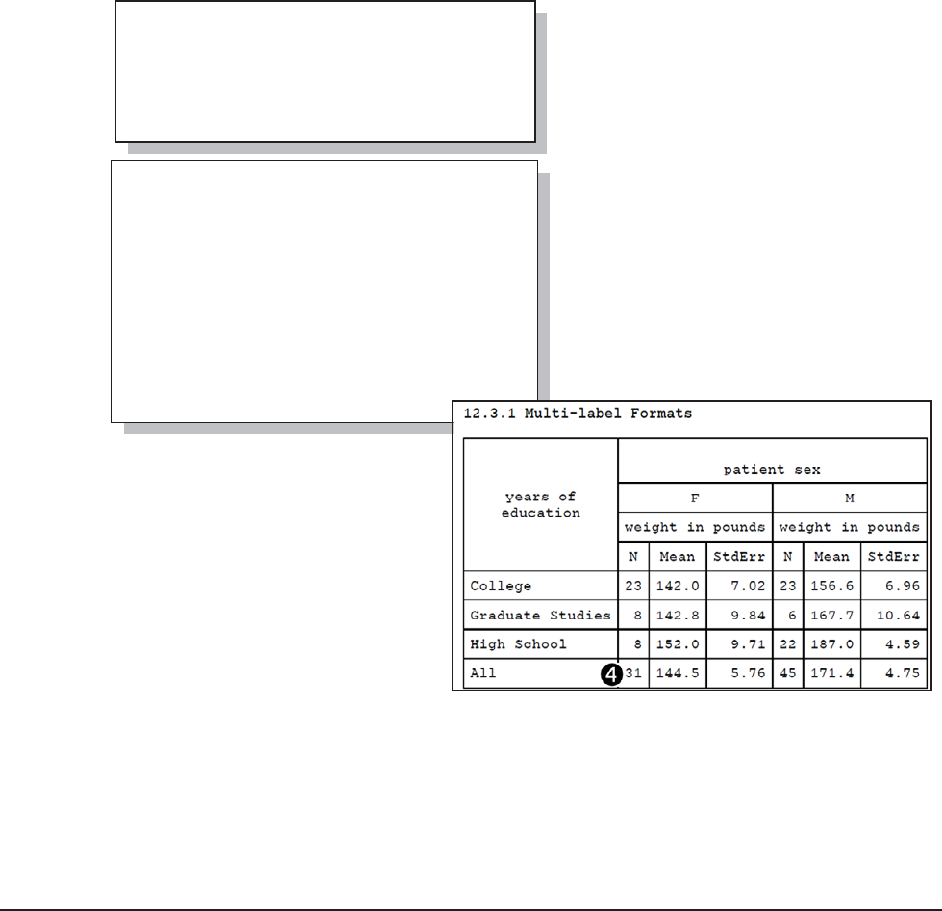
378 Carpenter’s Guide to Innovative SAS Techniques
title1 '12.3.1 Multi-label Formats';
proc tabulate data=advrpt.demog;
class edu / mlf p;
class sex;
var wt;
table edu=' ' all,
sex*wt*(n*f=2.
mean*f=5.1
stderr*f=6.2)
/box=edu;
format edu edlevel.;
run;
n The MULTILABEL option sets up the
format to be used with the MLF option in
PROC TABULATE.
o The ranges for ‘College’ and ‘Graduate
Studies’ overlap (are not distinct). Without
the MULTILABEL option, PROC
FORMAT would generate an error and the
format would not be created.
p The MLF option appears on the CLASS
statement associated with the formatted
variable. Without this option ‘Graduate
Studies’ will not be displayed as a level of
EDU.
q PROC TABULATE correctly counts
and totals the number of persons in
each education category. Notice that
the count for ‘Graduate Studies’ does
not contribute to the overall total.
The MLF option can also be used
with CLASS variables in PROC
MEANS. In future releases of SAS it
may be implemented in other
procedures as well.
Procedures that do not utilize overlapping format values (do not support the MLF option) will
only use the primary range of the format.
MORE INFORMATION
Very often we would like to have better control of the order of the formatted values (in this
example High School comes after College). Section 12.4 discusses the use of the NOTSORTED
option. Multilabel formats are used to calculate a moving average in Section 12.3.2.
12.3.2 Calculating Rolling Averages
There are a number of ways to calculate a rolling or moving average within SAS. The use of
multilabel formats provides a quick and easy programming solution to this often taxing problem.
In this example we would like to calculate a three-visit rolling average of the patient’s potassium
levels. The variable VISIT will take on the values of 1 – 16.
proc format;
value edlevel (multilabel) n
9-12 = 'High School'
13-high='College'
17-high='Graduate Studies'; o
run;
&DUSHQWHU$UW&DUSHQWHU¶V*XLGHWR,QQRYDWLYH6$67HFKQLTXHV&RS\ULJKW6$6,QVWLWXWH,QF&DU\1RUWK&DUROLQD86$
$
//5,*+765(6(59(')RUDGGLWLRQDO6$6UHVRXUFHVYLVLWVXSSRUWVDVFRPSXEOLVKLQJ

Chapter 12: Taking Advantage of Formats 379
data control(keep=fmtname start end label hlo);
retain fmtname 'avg' n
hlo 'M'; o
do start=1 to 14;
end=start+2; p
label=cats('VisitGrp', put(start,z2.)); q
output Control;
end;
hlo='O'; r
label='Unknown';
output;
run;
proc format cntlin=control; s
run;
proc summary data=advrpt.lab_chemistry;
by subject;
class visit / mlf; t
format visit avg.; u
var potassium;
output out=rollingAVG
mean= Avg3Potassium;
run;
n A format control data
set containing the value
pairs, labels, and format
name (AVG.) is created.
o The HLO variable is
used to designate this as a
multilabel format.
p START is the lower
bound of the moving
average and END is the
upper bound. In this
example the width will
contain up to three visits.
q The label is assigned a
value. For the group
starting with visit 4,
LABEL will be
VisitGrp04, which will be
the average of visits 4, 5,
and 6.
r Although not needed here, it is always a good idea to
specify the ‘OTHER’ group.
s PROC FORMAT creates the format using the
CONTROL data set.
t The overlapping ranges of a multilabel format are
ignored unless the MLF option is specified.
u The format is associated with the classification
variable.
The format AVG., which is generated above, is
effectively defined as shown to the right.
proc format;
value avg (multilabel)
1 - 3 = 'VisitGrp01'
2 - 4 = 'VisitGrp02'
3 - 5 = 'VisitGrp03'
4 - 6 = 'VisitGrp04'
5 - 7 = 'VisitGrp05'
6 - 8 = 'VisitGrp06'
7 - 9 = 'VisitGrp07'
8 - 10= 'VisitGrp08'
9 - 11= 'VisitGrp09'
10- 12= 'VisitGrp10'
11- 13= 'VisitGrp11'
12- 14= 'VisitGrp12'
13- 15= 'VisitGrp13'
14- 16= 'VisitGrp14'
other = 'Unknown';
run;
&DUSHQWHU$UW&DUSHQWHU¶V*XLGHWR,QQRYDWLYH6$67HFKQLTXHV&RS\ULJKW6$6,QVWLWXWH,QF&DU\1RUWK&DUROLQD86$
$
//5,*+765(6(59(')RUDGGLWLRQDO6$6UHVRXUFHVYLVLWVXSSRUWVDVFRPSXEOLVKLQJ

380 Carpenter’s Guide to Innovative SAS Techniques
While this technique is a fast and easy way to generate rolling averages, you should be careful to
fully understand how it
will work with your data.
In the portion of the data
shown here for SUBJECT
201, there is no visit 3 and
there is a duplicate
observation for visit 2.
After applying the format
in the PROC SUMMARY
step, we notice in the
portion of the data set
listing for this subject
(201) that there is an
average for visit 3 (it
contains visits 4 & 5
only). Also notice that
because the duplicate
observation (visit 2)
precedes the missing visit
3 the means for the first
two visits have been
distorted.
This subject also did not
have any follow-up visits
after visit 10. This is
reflected in the N
associated with the last two rolling averages.
MORE INFORMATION
Section 3.1.7 uses an ARRAY to calculate a running average. Section 12.7 discusses the process
of creating a format from the data in more detail.
SEE ALSO
The first time that I learned about this technique was from Liang Xie who suggests using a
multilabel format to create a rolling window in a sasCommunity.org tip
http://www.sascommunity.org/wiki/Tips:Summarize_data_in_a_rolling_window.
Moving averages are calculated using PROC EXPAND by Vora (2008).
12.3.2 Using MLF for Calculating Rolling Averages
Obs SUBJECT VISIT LABDT potassium
15 201 1 07/07/2006 3.8
16 201 2 07/14/2006 4.2
17 201 2 07/14/2006 4.2
18 201 4 07/26/2006 4.2
19 201 5 07/21/2006 4.7
20 201 6 07/29/2006 4.5
21 201 7 08/04/2006 4.0
22 201 8 08/11/2006 4.0
23 201 9 09/12/2006 4.2
24 201 10 10/13/2006 3.9
12.3.2 Using MLF for Calculating Rolling Averages
Obs SUBJECT VISIT _FREQ_ Avg3Potassium
12 201 10 4.17000
13 201 VisitGrp01 3 4.06667
14 201 VisitGrp02 3 4.20000
15 201 VisitGrp03 2 4.45000
16 201 VisitGrp04 3 4.46667
17 201 VisitGrp05 3 4.40000
18 201 VisitGrp06 3 4.16667
19 201 VisitGrp07 3 4.06667
20 201 VisitGrp08 3 4.03333
21 201 VisitGrp09 2 4.05000
22 201 VisitGr
p
10 1 3.90000
&DUSHQWHU$UW&DUSHQWHU¶V*XLGHWR,QQRYDWLYH6$67HFKQLTXHV&RS\ULJKW6$6,QVWLWXWH,QF&DU\1RUWK&DUROLQD86$
$
//5,*+765(6(59(')RUDGGLWLRQDO6$6UHVRXUFHVYLVLWVXSSRUWVDVFRPSXEOLVKLQJ
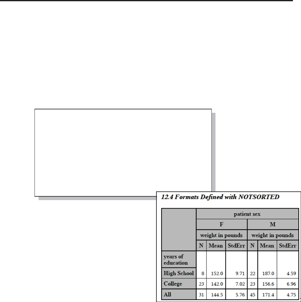
Chapter 12: Taking Advantage of Formats 381
proc format;
value edlevel (notsorted) n
9-12 = 'High School'
13-high='College';
run;
proc tabulate data=advrpt.demog;
class edu sex;
var wt;
table edu all,
sex*wt*(n*f=2. mean*f=5.1 stderr*f=6.2);
format edu edlevel.; o
run;
12.4 Controlling Order Using the NOTSORTED Option
Normally when a user-defined format is created, the format is internally placed into sorted order.
Consequently it does not particularly matter what order the value/label pairings are specified in
the value statement. However, this reordering can be prevented by using the NOTSORTED option
on the VALUE statement n. When applied, the internal order of the format remains as it is
defined. When an ORDER=FORMATTED option is applied to a format that is created using the
NOTSORTED option, the order of the pairings in the format definition is used.
In the PROC TABULATE example in Section 12.3 ‘College’ appears first because it is first
alphabetically. Here the format is created using the NOTSORTED option. Since the level for
‘High School’ is listed first in the following PROC FORMAT, ‘High School’ will appear before
‘College’ in the report.
n When the
NOTSORTED option is
used on the VALUE
statement, the order that
the item pairs are defined
in the VALUE statement
is preserved.
o The format is used as
usual.
CAVEAT
When a format is created it is optimized
internally to make the assignment process
as efficient as possible. Using the
NOTSORTED option negates some of that
optimization; however, for formats with
fewer than a dozen or so value pairs it
generally makes little practical difference.
For very large formats (hundreds or
thousands of items) there may be some
performance access issues when using the
NOTSORTED option. Be sure to
experiment with your data and OS when
using this option for larger formats.
&DUSHQWHU$UW&DUSHQWHU¶V*XLGHWR,QQRYDWLYH6$67HFKQLTXHV&RS\ULJKW6$6,QVWLWXWH,QF&DU\1RUWK&DUROLQD86$
$
//5,*+765(6(59(')RUDGGLWLRQDO6$6UHVRXUFHVYLVLWVXSSRUWVDVFRPSXEOLVKLQJ

382 Carpenter’s Guide to Innovative SAS Techniques
proc format;
value missdate
. = 'Unknown' n
other=[date9.]; o
run;
proc print data=advrpt.demog;
var lname fname dob;
format dob missdate.; p
run;
12.5 Extending the Use of Format Translations
A user-defined format can be used to point to another secondary format or, in SAS 9.3, even a
function. This allows us to create customized formats that retain characteristics of either another
format or a function. The format or function call appears unquoted on the right side of the equal
sign (in the label area) in square brackets.
12.5.1 Filtering Missing Values
We need to create a format that will handle missing
date values differently than non-missing values. In
the MISSDATE. format to the left, missing values
are mapped to the word ‘Unknown’ n, while all
other values are formatted using the DATE9.
format.
o The label for the ‘other’ category is the
secondary or nested format. It is enclosed
in square brackets instead of quotes.
p The nested format is used as is any
other format.
The first few lines of the listing generated by PROC PRINT show that the date of birth has been
formatted. Since Joan Adamson’s date of birth is missing, it has been displayed as ‘Unknown’.
Similar nested formats can be used to check for valid data or data
that can be formatted. This is the case with the PCTZERO. format
which is used to map missing values to special characters for
reporting purposes. Here missing values are mapped to ‘0.00’,
while the non-missing values are displayed using the 6.2 format.
12.5 Nested Formats
Obs lname fname dob
1 Adams Mary 12AUG1951
2 Adamson Joan Unknown
3 Alexander Mark 15JAN1930
4 Antler Peter 15JAN1934
. . . . portions of the listing not shown . . . .
proc format;
value pctzero
.='0.00'
other=[6.2];
run;
&DUSHQWHU$UW&DUSHQWHU¶V*XLGHWR,QQRYDWLYH6$67HFKQLTXHV&RS\ULJKW6$6,QVWLWXWH,QF&DU\1RUWK&DUROLQD86$
$
//5,*+765(6(59(')RUDGGLWLRQDO6$6UHVRXUFHVYLVLWVXSSRUWVDVFRPSXEOLVKLQJ

Chapter 12: Taking Advantage of Formats 383
proc format;
invalue inage
y, yz = .y
s, ss = .s
other = [2.];
run;
data surveyAge;
input patcode $
age inage.;
datalines;
1 45
2 yz
3 36
4 ss
5 y
run;
Obs patcode age
1 1 45
2 2 Y
3 3 36
4 4 S
5 5 Y
12.5.2 Mapping Overlapping Ranges
Another use of nested formats is to define ranges or groups with multiple ranges. Notice here that
the ‘Secondary’ and ‘Out of Range’ groups
span the ‘Primary’ group. A change to one
group definition requires a change to another’s
as well.
Instead we can create a series of nested formats
that call each other. Although potentially more
work to set up initially, these formats offer
more flexibility because the range for each
group is totally self-contained. The format for
the inner most range (PRIMARY.) is called
first, and if the value is outside of the primary
range, the secondary range format (SECOND.)
is called. Notice that the secondary range spans
the primary range. In automated systems this
can be a huge advantage.
In an assignment statement the format is used as
any other format might be used:
12.5.3 Handling Text within Numeric Values
SAS supports up to 28 types of numeric missing values (see Section 2.10.1). These sometimes
need to be associated with codes in the data. When importing data from raw text files, the codes
themselves may be inserted as non-numeric values into the numeric fields. We need the ability to
read the column as a numeric value while differentiating among the various codes.
The informat INAGE. converts selected codes into the specific
missing values .S and .Y. All other non-numeric codes will map
to the standard numeric missing (.). The data set SURVEYAGE
contains the following values. Remember that special numeric
missing values print without the period.
MORE INFORMATION
The use of special numeric
missing values is discussed in
Section 2.10.1. A numeric
informat similar to this one is
created from a data set in
Section 6.7.3.
SEE ALSO
The SAS Forum thread found at http://communities.sas.com/message/48729 discusses various
methods for avoiding errors when reading mixed fields.
proc format;
value agegrps
low - 40 = 'Out of Range'
40 - <48 = 'Secondary'
48 - 52 = 'Primary'
52<- 65 = 'Secondary'
65<- high = 'Out of Range'
other = 'Unknown';
run;
proc format;
value primary
48 - 52 = 'Primary'
other = [second.];
value second
40 - 65 = 'Secondary'
other = [OOR.];
value oor
low - high = 'Out of Range'
other = 'Unknown';
run;
agegroup = put(startage,primary.);
&DUSHQWHU$UW&DUSHQWHU¶V*XLGHWR,QQRYDWLYH6$67HFKQLTXHV&RS\ULJKW6$6,QVWLWXWH,QF&DU\1RUWK&DUROLQD86$
$
//5,*+765(6(59(')RUDGGLWLRQDO6$6UHVRXUFHVYLVLWVXSSRUWVDVFRPSXEOLVKLQJ

384 Carpenter’s Guide to Innovative SAS Techniques
12.5.4 Using Perl Regular Expressions within Format Definitions
Starting in SAS 9.3 the REGEXPE option can appear on the value side of the equal sign for a
value/label pair. This option follows a quoted Perl regular expression and causes the format to
effectively act like the PRXCHANGE function.
The $ABC2DEF. informat shown here has been created to convert the letter combination ‘abc’ to
‘def’.
n The informat $ABC2DEF. is
defined with a default length of 20.
o The PRX string is defined and
followed by the REGEXPE option,
which causes the PRX string to be
interpreted as a Perl Regular
eXpression.
p The special _SAME_ operator is
used to pass the result of the PRX
string to the format’s label.
q The LOG shows that both a stand-alone occurrence and an embedded occurrence of ‘abc’ are
converted to ‘def’.
r Letter combinations other than ‘abc’ are not changed and are
therefore passed through the format ‘as-is’.
12.5.5 Passing Values to a Function as a Format Label
Starting with SAS 9.3 it is possible to pass values into functions via formats. The huge advantage
is that the functions, which are embedded into the format, become available outside the DATA
step, and can be used wherever formats are used.
The function call occurs in the label portion of the
value/label pair and is enclosed in square brackets.
The specifications include:
The function may take no more than one argument.
Numeric functions return numeric values.
Character functions return character values.
The DEFAULT= option should be used to ensure proper widths.
The function can be supplied by SAS or it can be user supplied through the use of PROC
FCMP (see Section 15.2).
proc format;
invalue $abc2def (default=20) n
's/abc/def/' (REGEXPE)o = _same_p;
run;
data _null_;
x=input('abc',$abc2def.); put x=; q
x=input('xabcx',$abc2def.); put x=; q
x=input('xyz',$abc2def.); put x=; r
x=input('def',$abc2def.); put x=; r
run;
x=def q
x=xdefx q
x=xyz r
x=def r
proc format;
value fmtname (default=10)
other=[myfunc()];
run;
&DUSHQWHU$UW&DUSHQWHU¶V*XLGHWR,QQRYDWLYH6$67HFKQLTXHV&RS\ULJKW6$6,QVWLWXWH,QF&DU\1RUWK&DUROLQD86$
$
//5,*+765(6(59(')RUDGGLWLRQDO6$6UHVRXUFHVYLVLWVXSSRUWVDVFRPSXEOLVKLQJ

Chapter 12: Taking Advantage of Formats 385
Using SAS Supplied Functions
The FIPSTATE function can be used to convert a FIPS state code into a two-letter state postal
code abbreviation; however, there is no matching format to perform the same conversion. Here
we use a format to pass the FIPS code to the
FIPSTATE function. As is shown in the LOG, the
FIPSTATE. format returns the 2-character
abbreviation.
The use of functions in formats opens a wide range of possibilities including the use of DATE,
DATETIME, and TIME functions. In this example both numeric and character versions of a
series of formats are created that execute various functions. Notice that conversion between
numeric and character values will occur as needed.
n The DATE function
does not take an
argument, but it can still
be used within a format
label.
o The DATEPART
function will extract the
date portion from a
datetime value.
p The LENGTH
function will provide the
length of the argument.
Although, the LENGTH
function expects a
character argument, a
numeric value will be
converted to a character
value which will subsequently be passed to the LENGTH function.
A DATA _NULL_ step is used to create some numeric and character date and datetime values
which are then used with the formats that were just created.
q X is a numeric value containing the current datetime value in seconds (there are 10 digits in the
number of seconds). The execution shown here took place on day 18,946 (15nov2011).
r Y is a character variable of length 12 containing the number of seconds for the current datetime
value.
s Z is a character variable of length 12 with the current date.
t A is the numeric date portion of the datetime value stored in X.
proc format;
value fipstate
other=[fipstate()];
run;
data _null_;
x=37; put x=fipstate.;
run; x=NC
proc format;
value daten (default=10) other=[date()]; n
value $datec (default=10) other=[date()];
value dpartn (default=10) other=[datepart()]; o
value $dpartc (default=10) other=[datepart()];
value lenn (default=10) other=[length()]; p
value $lenc (default=10) other=[length()];
run;
data _null_;
x=datetime(); q
y=put(datetime(),best12.); r
z=put(date(),best12.); s
a=datepart(x); t
put x= y= z= a=;
u v w
put x=daten. x=dpartn. x=lenn.;
put y=$datec. y=$dpartc. y=$lenc.;
put z=$datec. z=$dpartc. z=$lenc.;
run;
&DUSHQWHU$UW&DUSHQWHU¶V*XLGHWR,QQRYDWLYH6$67HFKQLTXHV&RS\ULJKW6$6,QVWLWXWH,QF&DU\1RUWK&DUROLQD86$
$
//5,*+765(6(59(')RUDGGLWLRQDO6$6UHVRXUFHVYLVLWVXSSRUWVDVFRPSXEOLVKLQJ

386 Carpenter’s Guide to Innovative SAS Techniques
u The DATEN. and $DATEC. formats correctly return the current date value.
v The DPARTN. and DPARTC. formats return the date portion of the datetime value in days.
The variable Z already
contains a date value. The
$DPARTC. format interprets
this value as seconds and
returns the date value of 0
(01jan1960). This shows that
although the value is
character it can be handled by the function as numeric.
w The LENGTH function is applied to the incoming value. Notice that for the variable X the
numeric format (LENN.) is applied and only the number of whole numbers is counted (10). The
character format ($LENC.) returns 12 when applied to the same number.
Using User-Defined Functions
When combined with user-defined functions, the ability to insert a value into a function through a
format can be especially powerful.
In this example the user-defined functions C2FF() and F2CC() are used to convert between
degrees Centigrade and degrees Fahrenheit. These two character functions add the scale symbols
to the resultant value. Similar numeric functions that do not add the scale symbols are created in
Section 15.2.2.
n The OUTLIB= option
specifies the data set and packet
(CONVERSIONS) that will
contain this function definition.
o The FUNCTION statement
names the new function and its
arguments. The $ is used to
specify that this function returns
a character value.
p The RETURN statement
contains the value to be returned
by the function. In this case the
result of the conversion equation
is concatenated to the temperature scale symbol.
q FUNCTION definitions are terminated with the ENDSUB statement.
r The CMPLIB option is used to point to the data set (ADVRPT.FUNCTIONS) that contains the
function definition.
s A constant value (100°C ) is converted using the C2FF() function, and
the converted value is displayed using a PUT statement.
These two functions can be used wherever functions can be used; however, since most procedures
will not accept the use of functions, they are not as generally usable as formats. Below these two
functions are called by formats so that they can be used wherever formats can be used. This
includes in the PUT statement where formats are anticipated and functions are not callable.
proc fcmp
outlib=Advrpt.functions.Conversions; n
function c2ff(c) $; o
return(cats(((9*c)/5)+32,'°F')); p
endsub; q
function f2cc(f) $;
return(cats((f-32)*5/9,'°C'));
endsub;
run;
options cmplib=(advrpt.functions); r
data _null_;
f=c2ff(100); put f=; s
c=f2cc(212); put c=;
run;
f=212°F s
c=100°C
x=1636995477.6 y=1636995477.6 z=18946 a=18946
u v w
x=18946 x=18946 x=10
y=18946 y=18946 y=12
z=18946 z=0 z=12
&DUSHQWHU$UW&DUSHQWHU¶V*XLGHWR,QQRYDWLYH6$67HFKQLTXHV&RS\ULJKW6$6,QVWLWXWH,QF&DU\1RUWK&DUROLQD86$
$
//5,*+765(6(59(')RUDGGLWLRQDO6$6UHVRXUFHVYLVLWVXSSRUWVDVFRPSXEOLVKLQJ
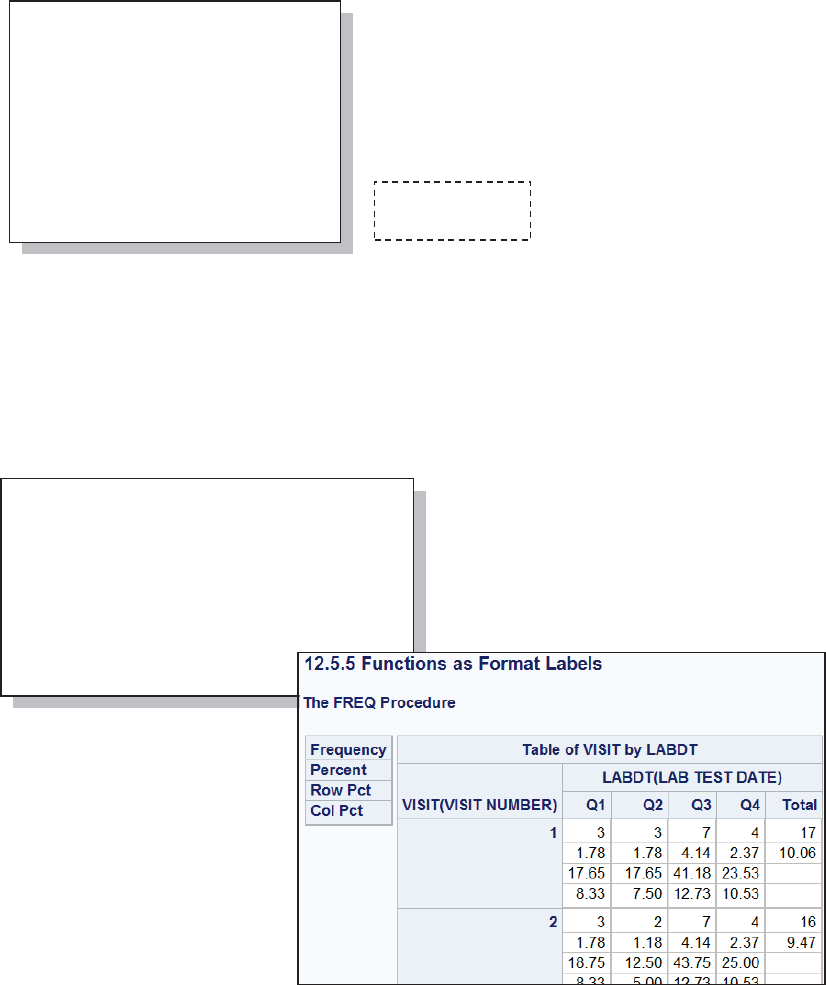
Chapter 12: Taking Advantage of Formats 387
Since the C2FF() and F2CC() functions do not have more than one argument, they can be used
directly in the label portion of a user-defined format. Although in this example the format name
and the function name are the same, this is not in any way a requirement.
t When using a function in the label it is best to set
the default display width.
u The function is called from within the label by
enclosing it in square brackets.
v The format is requested on the PUT statement.
This request results in the execution of the function,
and generates this text in the
LOG.
The initial versions of these functions were written by Rick Langston, senior manager in software
development at SAS.
Return the Quarter without the Year (Qq instead of yyQq)
In Section 15.2.1 the QNUM() function is created to remove the year portion of the value that is
returned by the YYQ. format. In that example a second DATA step was required before we could
use the results of the function in a PROC FREQ step. By using that function in a format, we can
use the format directly in the PROC step and thereby avoid an additional pass of the data.
Here the QNUM() function is used in the
format label. The format is then used in the
PROC FREQ step. The elimination of steps
will almost always improve processing
efficiency.
proc format;
value c2ff (default=10) t
other=[c2ff()]; u
value f2cc (default=10)
other=[f2cc()];
run;
data _null_;
c=100; put c=c2ff.; v
f=212; put f=f2cc.;
run;
c=212°F v
f=100°C
proc format;
value qfmt other=[qnum()];
run;
options cmplib=(advrpt.functions);
proc freq data=advrpt.lab_chemistry
order=formatted;
table visit*labdt;
format labdt qfmt.;
run;
&DUSHQWHU$UW&DUSHQWHU¶V*XLGHWR,QQRYDWLYH6$67HFKQLTXHV&RS\ULJKW6$6,QVWLWXWH,QF&DU\1RUWK&DUROLQD86$
$
//5,*+765(6(59(')RUDGGLWLRQDO6$6UHVRXUFHVYLVLWVXSSRUWVDVFRPSXEOLVKLQJ

388 Carpenter’s Guide to Innovative SAS Techniques
Informats can also be used with functions-as-labels. This is a case where the user wanted the
feature of the TRAILSGN informat, but that informat does not handle implied decimal
specifications. In this example the numbers in the data have been entered without the decimal
point (the value 12 should be .12). The function will use the TRAILSGN informat and then divide
by 100 and return the result.
MORE INFORMATION
Details on the use of PROC FCMP to
create user-defined functions can be
found in Section 15.2.
12.6 ANYDATE Informats
The ANYDATE informats (available starting in SAS 9) are designed to allow you to read in a
variety of mixed date forms including:
DATE, DATETIME, and TIME
DDMMYY, MMDDYY, and YYMMDD
JULIAN, MONYY, and YYQ.
There are various forms of these informats:
ANYDTDTE. extracts the date portion
ANYDTDTM. extracts the datetime portion
ANYDTTME. extracts the time portion
proc fcmp outlib=work.functions.smd;
function tsgn(text $);
put 'in tsgn: ' text=;
x = input(text,trailsgn10.);
x = x/100;
return(x);
endsub;
run;
options cmplib=(work.functions);
proc format;
invalue tsgn(default=10)
other=[tsgn()];
data _null_;
input x: tsgn.;
put x=;
cards;
1
1-
12-
123-
123+
1+
0
run;
1 x=.01
1- x=-0.01
12- x=-0.12
123- x=-1.23
123+ x=1.23
1+ x=0.01
0 x=0
&DUSHQWHU$UW&DUSHQWHU¶V*XLGHWR,QQRYDWLYH6$67HFKQLTXHV&RS\ULJKW6$6,QVWLWXWH,QF&DU\1RUWK&DUROLQD86$
$
//5,*+765(6(59(')RUDGGLWLRQDO6$6UHVRXUFHVYLVLWVXSSRUWVDVFRPSXEOLVKLQJ

Chapter 12: Taking Advantage of Formats 389
12.6.1 Reading in Mixed Dates
This example demonstrates the flexibility of these informats. Here the ANYDTDTE10. informat
is applied to a number of different date forms. The DATESTYLE system option n is used to
resolve some of the possible ambiguities by declaring a default ordering for the month/day/year
portions of the dates.
A PROC PRINT of the
data set shows that these
date values have been
read into the data set as
SAS dates. The
supported date forms are
quite varied and include
DATE9. o. You should
note that the
DATESTYLE= option
cannot fully resolve all
ambiguities and, consequently, some dates may be
misinterpreted. Since 13 is not a valid number for a
month p, the informat assumes that the order of the values has been changed and it guesses that
the correct order is YMD. Since the informats can detect invalid values and make informed
guesses as to the correct order of the date portions, it becomes very important for the user to either
know the data well, or to at the very least, understand exactly how the incoming values can be
converted. In this example it is likely that p should have been read as dd/mm/yy and not
yy/mm/dd.
12.6.2 Converting Mixed DATETIME Values
When the incoming string contains not only dates, but time values as well, the conversion process
becomes even more complicated. For the time portion (and the following applies to SAS time
values as well), the hours can be specified using the 24 hour clock or the 12 hour clock with
AM/PM also included.
Datetime strings might include values such as those
shown to the right. With the exception of the
ambiguous date with a two-digit year n the
ANYDTDTM informat will correctly interpret the date
time portion of these strings. It is unable, however, to
utilize the AM/PM codes, which are ignored.
Fortunately the MDYAMPM. informat is available.
This informat correctly interprets the AM/PM portion of the datetime value; however, it requires
that the date portion be in MDY order.
options datestyle=mdy; n
data new;
input date anydtdte10.;
format date date9.;
datalines;
01/13/2003
13/01/2003
13jan2003 o
13jan03
13/01/03 p
01/02/03
03/02/01
run;
12.6 ANYDATE Informats
Obs date
1 13JAN2003
2 13JAN2003
3 13JAN2003 o
4 13JAN2003
5 03JAN2013 p
6 02JAN2003
7 02MAR2001
10/13/2011:15:45:12
2011-03-01T15:20:45
9/13/2011 11:52:54 AM
9/13/2011 11:52:54 PM
13/09/2011 11:52:54 PM
11/09/12 11:52:54 AM n
2011/09/12 11:52:54 PM
&DUSHQWHU$UW&DUSHQWHU¶V*XLGHWR,QQRYDWLYH6$67HFKQLTXHV&RS\ULJKW6$6,QVWLWXWH,QF&DU\1RUWK&DUROLQD86$
$
//5,*+765(6(59(')RUDGGLWLRQDO6$6UHVRXUFHVYLVLWVXSSRUWVDVFRPSXEOLVKLQJ

390 Carpenter’s Guide to Innovative SAS Techniques
Since there is no informat that will effectively combine the flexibility of the ANYDTDTM.
informat with the ability to interpret the AM/PM, the following adjustment can be used. o The
ANYDTDTM. informat
is used to convert the
datetime string. The
INPUT function returns
the datetime value in
seconds. p If a ‘PM’ is
present we need to add
12 hours worth of
seconds
(43,200=12*60*60) to
the datetime value. q
The INDEX function
searches for an
occurrence of ‘PM’ and
the location is converted
to a binary 0/1 value
which is multiplied by
the number of seconds to
add.
12.7 Building Formats from Data Sets
The VALUE, INVALUE, and PICTURE statements are usually used to create a user-defined
format or informat. As the number of value pairs becomes large, coding these statements becomes
inconvenient (for me large can be less than a dozen). Fortunately you can also define formats and
informats using a data set.
PROC FORMAT accepts a data set to control the definition of the format or informat. The
procedure expects specific variables, and the observations of the data set are used to form the
value pairs. As a minimum the data set used to control the formation of the format must contain
the variables FMTNAME, START, and LABEL n. It may also contain over twenty other
variables that can be used to define the format.
In this example the data set CNTRLFMT will be used create a character format ($CL_REG.) that
will map the clinic number (CLINNUM) into a region (REGION).
n You may keep
variables that will not
be used by PROC
FORMAT.
Extraneous variables
will be ignored.
o The variable
START contains the data value that is to be mapped (left side of the value pair), while LABEL is
the value that will appear as a result of the mapping.
p The character variable FMTNAME contains the name of the format that is to be created.
q The CNTLIN= option is used to specify the data set that contains the format definition.
dt_plus= input(daytime,anydtdtm.) o
+(43200 p
*(^^index(upcase(daytime),'PM')q));
12.6 ANYDATE Informats
Converting Mixed DATETIME Values
Obs daytime dt_plus
1 10/13/2011:15:45:12 13OCT2011:15:45:12
2 2011-03-01T15:20:45 01MAR2011:15:20:45
3 9/13/2011 11:52:54 AM 13SEP2011:11:52:54
4 9/13/2011 11:52:54 PM 13SEP2011:23:52:54
5 13/09/2011 11:52:54 PM 13SEP2011:23:52:54
6 11/09/12 11:52:54 AM 09NOV2012:11:52:54
7 2011/09/12 11:52:54 PM 12SEP2011:23:52:54
data cntrlfmt(keep=fmtname start label)n;
set advrpt.clinicnames(rename=( clinnum=start o
region=label)); o
retain fmtname '$cl_reg'; p
run;
proc format cntlin=cntrlfmt; q
run;
&DUSHQWHU$UW&DUSHQWHU¶V*XLGHWR,QQRYDWLYH6$67HFKQLTXHV&RS\ULJKW6$6,QVWLWXWH,QF&DU\1RUWK&DUROLQD86$
$
//5,*+765(6(59(')RUDGGLWLRQDO6$6UHVRXUFHVYLVLWVXSSRUWVDVFRPSXEOLVKLQJ

Chapter 12: Taking Advantage of Formats 391
data cntrlfmt(keep=fmtname start label);
set advrpt.clinicnames(rename=( clinnum=start));
length fmtname $8 label $40;
fmtname = '$cl_reg';
label = region;
output cntrlfmt;
fmtname = '$cl_name';
label = clinname;
output cntrlfmt;
run;
proc sort data=cntrlfmt;
by fmtname start; r
run;
proc format cntlin=cntrlfmt;
run;
The control data set may define more than one format definition; however, if it does the data set
must be sorted by format name (or at least grouped by format name). In the following example
each incoming
observation is used to
build two formats
($CL_REG. and
$CL_NAME.). r
Notice that the control
data set has been
sorted by the format
name prior to passing
it to the FORMAT
procedure.
The list of potential variables in the control data set that can be utilized by PROC FORMAT is
quite
extensive,
and while
they are well
documented,
you can use
PROC FORMAT and the CNTLOUT= option to surface the format definition by writing it to a
data set. This will reveal the variable names that can be used in a format definition and can give
you a good idea about their usage.
proc format cntlout=control(where=(fmtname='CL_NAME'));
run;
proc print data=control;
run;
12.7 Building Formats from Data
D L
F D D A A
M E L P N D I T N
T S L F E R O S E E G A G
N T A A N F E M F E T E E C 3 T U
O A A E B M M U G U F U I D Y X X H S S Y A
b M R N E I A L T Z I L L I P C C L E E P G
s E T D L N X T H Z X T L T E L L O P P E E
1 CL_NAME 011234 011234 Boston National Medical 1 40 27 27 0 0 0 C N N
2 CL_NAME 014321 014321 Vermont Treatment Center 1 40 27 27 0 0 0 C N N
3 CL_NAME 023910 023910 New York Metro Medical Ctr 1 40 27 27 0 0 0 C N N
4 CL_NAME 024477 024477 New York General Hospital 1 40 27 27 0 0 0 C N N
5 CL_NAME 026789 026789 Geneva Memorial Hospital 1 40 27 27 0 0 0 C N N
&DUSHQWHU$UW&DUSHQWHU¶V*XLGHWR,QQRYDWLYH6$67HFKQLTXHV&RS\ULJKW6$6,QVWLWXWH,QF&DU\1RUWK&DUROLQD86$
$
//5,*+765(6(59(')RUDGGLWLRQDO6$6UHVRXUFHVYLVLWVXSSRUWVDVFRPSXEOLVKLQJ

392 Carpenter’s Guide to Innovative SAS Techniques
The HLO variable can be especially useful because it allows you to specify not only the HIGH
and LOW open ended
ranges, but the keyword
OTHER s as well.
Another less known usage
of HLO is to specify a
nested format (HLO=’F’) t.
The format STUDYDT.,
created here, sets the
acceptable range of dates
for the study. All other
dates will be displayed as
‘Out of Compliance’.
u Although set to
missing in this example,
the START and END
variables do not need to
be cleared for the observation containing HLO=’O’.
MORE INFORMATION
An example in Section 6.5 creates a format from data in order to perform a table lookup. The
example in Section 12.3.2 creates a multilabel format based on data generated in a DATA step.
SEE ALSO
The following SAS Forum thread contains an example of a format built from a data set
http://communities.sas.com/message/39814.
12.8 Using the PVALUE Format
When displaying values between zero and one, especially values close to zero, it is often difficult
to determine the number of decimal values needed. The PVALUE. format was designed to display
small probability values. The number of decimal points (4 in
this table) n designates the smallest number that can be
displayed by the format. Smaller numbers will be displayed with
a < sign. o
This format was designed to work with probability values that
are necessarily constrained to be between 0 and 1, consequently
this format does not handle negative values or even 0 well. All
values less than the minimum specified (for PVALUE6.4 this is
.0001) will be displayed the same (as <.0001). p Even the
minimum (.0001) is displayed as <.0001.
X PVALUE6.4 n
0.000000 <.0001
0.000006 <.0001 o
0.000050 <.0001
0.000100 <.0001 p
0.000400 0.0004
0.003000 0.0030
0.020000 0.0200
0.100000 0.1000
data intervals(keep=fmtname start end label hlo);
retain fmtname 'studydt';
length label $20;
start = '12jan2006:01:01:01'dt;
end = '24nov2007:11:12:13'dt;
label = 'datetime18.';
hlo = 'F'; t
output intervals;
start=.; u
end=.; u
hlo='O';s
label= 'Out of Compliance' ;
output intervals;
run;
proc format cntlin=intervals;
run;
&DUSHQWHU$UW&DUSHQWHU¶V*XLGHWR,QQRYDWLYH6$67HFKQLTXHV&RS\ULJKW6$6,QVWLWXWH,QF&DU\1RUWK&DUROLQD86$
$
//5,*+765(6(59(')RUDGGLWLRQDO6$6UHVRXUFHVYLVLWVXSSRUWVDVFRPSXEOLVKLQJ

Chapter 12: Taking Advantage of Formats 393
proc format;
value range
low - <0 = [best7.]
0 = [1.]
0< - 1 = [pvalue6.4]
1< -high= [best6.];
run;
If you want to take advantage of the capabilities of the PVALUE format, but suspect that some
numbers will be equal to or less than zero or even greater than one, then you may want to create a
format that incorporates, but does not solely
depend on PVALUE.
Here the RANGE. format is created using a
combination of formats.
The table to the right shows how various
values (I) are displayed using the
PVALUE7.4 format (J) and the RANGE. format (K).
12.9 Format Libraries
User-defined formats and informats are saved in a catalog, which by default will have the name
FORMATS. When a format library is not named on the PROC
FORMAT statement, the format definition is written to the
catalog WORK.FORMATS. The entry name is the same as the
format. Here the definition of the TONS. format will be stored in
WORK.FORMATS.TONS.FORMAT.
The catalog entry type will depend on the type of format that is created:
FORMAT Numeric format
FORMATC Character format
INFMT Numeric informat
INFMTC Character informat
Because each of the four types has a different catalog entry type, the same format name can be
used up to four times.
12.9.1 Saving Formats Permanently
Formats are stored permanently by using the LIBRARY= option on the PROC FORMAT
statement. The LIBRARY= option is used to specify the libref that is to contain the FORMATS
catalog. Any formats created by this PROC
FORMAT will be stored in a catalog with the
name of FORMATS in the libref ADVRPT.
12.8 Using the PVALUE Format
Obs i j k
1 -4.1 <.0001 -4.1
2 -0.0001 <.0001 -0.0001
3 -0.00001 <.0001 -1E-5
4 0 <.0001 0
5 0.00001 <.0001 <.0001
6 0.00001 <.0001 <.0001
7 0.0003 0.0003 0.0003
8 0.02 0.0200 0.0200
9 0.1 0.1000 0.1000
10 1 1.0000 1.0000
11 12.34 12.3400 12.34
12 3456.789 3456.79 3456.8
proc format;
picture Tons
0 = '9'
.... code not shown ....
proc format library=advrpt;
.... code not shown ....
&DUSHQWHU$UW&DUSHQWHU¶V*XLGHWR,QQRYDWLYH6$67HFKQLTXHV&RS\ULJKW6$6,QVWLWXWH,QF&DU\1RUWK&DUROLQD86$
$
//5,*+765(6(59(')RUDGGLWLRQDO6$6UHVRXUFHVYLVLWVXSSRUWVDVFRPSXEOLVKLQJ

394 Carpenter’s Guide to Innovative SAS Techniques
Because of the way that SAS searches for format catalogs (see Section 12.9.2), formats that are
stored in a catalog named FORMATS in a libref
named LIBRARY will by default be included in the
search path. The code at first seems a bit odd, but this
FORMAT step will create or add to the catalog
LIBRARY.FORMATS.
Although I find it to be generally a good idea, you are not required to store the format definitions
in a catalog named FORMATS. You can specify the catalog name as a second level on the
LIBRARY= option. Here the
catalog will be named PROJFMT.
12.9.2 Searching for Formats
When requesting a format SAS first checks in WORK.FORMATS and then, if the libref
LIBRARY is defined, SAS will look in LIBRARY.FORMATS. Since format libraries are not
usually conveniently located in these two locations, we need to be able to search for formats in a
variety of places and in catalogs named something other than FORMATS.
The FMTSEARCH= system option is used to identify not only the librefs, but also the order for
the search. In this example SAS will look for the requested format in the catalog
ADVRPT.PROJFMT, and then in catalogs named FORMATS in the librefs WORK and
LIBRARY in that order. Since WORK appears in the FMTSEARCH list, the default catalog is no
longer
WORK.FORMATS, and it
is not searched first.
12.9.3 Concatenating Format Catalogs and Libraries
When your formats are spread among multiple catalogs, the search can be simplified by
concatenating the catalogs.
Catalogs with the same name will be implicitly concatenated when they reside within
concatenated libraries. In the following example formats are being written to two different
libraries (the librefs are OLDFMT and NEWFMT).
libname library 'c:\myfmts';
proc format library=library;
.... code not shown ....
options fmtsearch=(advrpt.projfmt work library);
proc format library=advrpt.projfmt;
.... code not shown ....
&DUSHQWHU$UW&DUSHQWHU¶V*XLGHWR,QQRYDWLYH6$67HFKQLTXHV&RS\ULJKW6$6,QVWLWXWH,QF&DU\1RUWK&DUROLQD86$
$
//5,*+765(6(59(')RUDGGLWLRQDO6$6UHVRXUFHVYLVLWVXSSRUWVDVFRPSXEOLVKLQJ
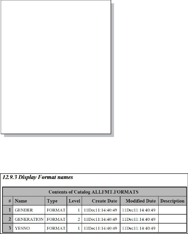
Chapter 12: Taking Advantage of Formats 395
n Any references to the libref ALLFMT
will point to both of the other two
locations.
o The YESNO. format appears in both
format libraries. Notice that the two
definitions are not the same.
p PROC CATALOG is used here to show
the locations of the formats. The column
LEVEL refers to the library containing the
catalog that contains the format.
q Before any of the formats in the
ALLFMT library can be used, the library
must be included on the search path.
Formats in ALLFMT will be found before
any formats with the same name in the
WORK library. Within ALLFMT the
catalogs are searched from left to right.
The version of the YESNO. format in the
NEWFMT library will be used.
The output generated by the CATALOG procedure shows that the various formats can be found in
the concatenated library ALLFMT. It also shows that the YESNO. format, which is defined in
both the OLDFMT and NEWFMT catalogs is being picked up from the first catalog in the list
(NEWFMT – LEVEL=1).
libname oldfmt 'c:\temp1';
libname newfmt 'c:\temp2';
libname allfmt (newfmt oldfmt); n
proc format library=oldfmt;
value yesno 1 = 'Yes' o
0 = 'No';
value generation
low - <1950 = 'Greatest'
1950 - high = 'Boomer';
run;
proc format library=newfmt;
value gender 1 = 'Female'
0 = 'Male';
value yesno 1 = 'No' o
0 = 'Yes';
run;
title1 12.9.3 Display Format names;
proc catalog cat=allfmt.formats; p
contents;
quit;
options fmtsearch=(allfmt work); q
&DUSHQWHU$UW&DUSHQWHU¶V*XLGHWR,QQRYDWLYH6$67HFKQLTXHV&RS\ULJKW6$6,QVWLWXWH,QF&DU\1RUWK&DUROLQD86$
$
//5,*+765(6(59(')RUDGGLWLRQDO6$6UHVRXUFHVYLVLWVXSSRUWVDVFRPSXEOLVKLQJ
396
&DUSHQWHU$UW&DUSHQWHU¶V*XLGHWR,QQRYDWLYH6$67HFKQLTXHV&RS\ULJKW6$6,QVWLWXWH,QF&DU\1RUWK&DUROLQD86$
$
//5,*+765(6(59(')RUDGGLWLRQDO6$6UHVRXUFHVYLVLWVXSSRUWVDVFRPSXEOLVKLQJ

Chapter 13
Interfacing with the Macro Language
13.1 Avoiding Macro Variable Collisions—Make Your Macro Variables
%Local 398
13.2 Using the SYMPUTX Routine 400
13.2.1 Compared to CALL SYMPUT 401
13.2.2 Using SYMPUTX to Save Values of Options 402
13.2.3 Using SYMPUTX to Build a List of Macro Variables 402
13.3 Generalized Programs—Variations on a Theme 403
13.3.1 Steps to the Generalization of a Program 403
13.3.2 Levels of Generalization and Levels of Macro Language
Understanding 405
13.4 Utilizing Macro Libraries 406
13.4.1 Establishing an Autocall Library 406
13.4.2 Tracing Autocall Macro Locations 408
13.4.3 Using Stored Compiled Macro Libraries 408
13.4.4 Macro Library Search Order 409
13.5 Metadata-Driven Programs 409
13.5.1 Processing across Data Sets 409
13.5.2 Controlling Data Validations 410
13.6 Hard Coding — Just Don’t Do It 415
13.7 Writing Macro Functions 417
13.8 Macro Information Sources 420
13.8.1 Using SASHELP and Dictionary tables 420
13.8.2 Retrieving System Options and Settings 422
13.8.3 Accessing the Metadata of a SAS Data Set 424
&DUSHQWHU$UW&DUSHQWHU¶V*XLGHWR,QQRYDWLYH6$67HFKQLTXHV&RS\ULJKW6$6,QVWLWXWH,QF&DU\1RUWK&DUROLQD86$
$
//5,*+765(6(59(')RUDGGLWLRQDO6$6UHVRXUFHVYLVLWVXSSRUWVDVFRPSXEOLVKLQJ

398 Carpenter’s Guide to Innovative SAS Techniques
13.9 Macro Security and Protection 426
13.9.1 Hiding Macro Code 426
13.9.2 Executing a Specific Macro Version 427
13.10 Using the Macro Language IN Operator 430
13.10.1 What Can Go Wrong 430
13.10.2 Using the MINOPERATOR Option 431
13.10.3 Using the MINDELIMITER= Option 432
13.10.4 Compilation vs. Execution for these Options 432
13.11 Making Use of the MFILE System Option 433
13.12 A Bit on Macro Quoting 434
A great deal has been written on the macro language. The documentation provided by SAS
Institute is good and two SAS Press books have been written on the subject, Carpenter’s
Complete Guide to the SAS Macro Language, 2nd Edition (Carpenter, 2004), and SAS Macro
Programming Made Easy, Second Edition (Burlew, 2006). The treatment of the macro language
in this book, therefore, must necessarily be limited to a few topics.
SEE ALSO
Russ Tyndall, a Principal Technical Support Analyst for the DATA Step and Macro Language at
SAS Institute, has written TS739 (Tyndall, 2005), which contains a number of advanced tips as
well as newer features of the macro language.
13.1 Avoiding Macro Variable Collisions—Make Your
Macro Variables %Local
The rule of thumb that a macro variable created within a macro will be local to that macro is a
very dangerous rule simply because it is usually correct. In the world of programming the
problem that only shows up occasionally is one of the worst to detect and fix. Simply knowing the
rules (and there is nothing simple about knowing the rules) for symbol table assignment is not
enough. Most symbol table assignments depend on circumstances that are usually unknown, and
even more often unknowable, to the macro programmer. The rules for table assignment are
described in Carpenter, 2004, Section 13.6, page 395.
Macro variable collisions occur when a macro variable assignment is written to the unintended
symbol table and inadvertently overwrites an existing macro variable’s value. Very often this
happens when the same macro variable name is inadvertently used in more than one of a series of
nested macros.
&DUSHQWHU$UW&DUSHQWHU¶V*XLGHWR,QQRYDWLYH6$67HFKQLTXHV&RS\ULJKW6$6,QVWLWXWH,QF&DU\1RUWK&DUROLQD86$
$
//5,*+765(6(59(')RUDGGLWLRQDO6$6UHVRXUFHVYLVLWVXSSRUWVDVFRPSXEOLVKLQJ

Chapter 13: Interfacing with the Macro Language 399
A subtle example of a macro variable collision, and
one that can cause horrid errors while leaving the
programmer blissfully unaware, is contained in the
program fragments shown here. In this case a
secondary macro (%CHKSURVEY) is called from
within a %DO loop in %PRIMARY.
The %DO loop in %PRIMARY seems to work
without error. But a closer inspection of the inner
macro %CHKSURVEY reveals a hidden problem.
n The %DO loop in %CHKSURVEY uses &I as
the index variable. This variable would usually be
local to %CHKSURVEY; however, since &I
already exists in the higher table of the calling
macro, it will not be local. When %CHKSURVEY
executes, it will modify the value of &I in the higher
table of %PRIMARY. o
In this example, if &DSNCNT o is less than or equal to 6, the loop in %PRIMARY will execute
only once. If the programmer is lucky, &DSNCNT will be greater than 6 and an infinite loop will
be created. This is lucky because then the programmer will at least know to look for the problem!
Unfortunately, we cannot protect the macro variables in a symbol table from being overwritten by
a macro that is called by the outer macro. However, we can protect higher symbol tables by
forcing all of our macro variables onto the LOCAL symbol table. This is done through the use of
the %LOCAL statement. When using nested macro
calls, macros that call macros, ALWAYS use
%LOCAL to prevent collisions!! In the previous
example the collision would have been avoided by
simply adding the %LOCAL statement to
%CHKSURVEY. p As an aside we do not know
for sure that the macro variable &I in %PRIMARY
will not also cause problems to an even higher table,
and a %LOCAL statement should also have been
included in that macro.
In the previous paragraph, I suggest that you ALWAYS use the %LOCAL statement. Others have
suggested that this is too strident, that the %GLOBAL statement and the global symbol table exist
for a reason—so that we can use them. After all, the argument goes, there are situations when you
want to pass a value out of a local symbol table and into the global environment. While I concede
the desire, and might even admit to having used the global symbol table in this way, it is my
admittedly biased opinion that this should not be a first choice, and that it is generally a solution
employed when one of the alternative techniques discussed in this chapter are either not possible
or more likely are not fully understood. That said, there is nothing wrong with using the global
symbol table to pass values as long as the programmer fully understands the risks and has
correctly and successfully mitigated them.
The problem with using the global symbol table is that it does not exist in the parent-child
hierarchy implied by nested macros. The calling macro is the parent and the called macro is the
child macro. We can take advantage of this relationship.
The best way to avoid collisions is to take direct control of symbol table placement. This is what
we did by placing the %LOCAL statement in our macro definitions. Another method of doing
this, without using the global symbol table, is to define your macro variables, and the symbol
%macro primary;
.... code not shown....
%do i = 1 %to &dsncnt; o
%chksurvey(&&dsn&i)
%end;
.... code not shown....
%mend primary;
%macro chksurvey(dset);
.... code not shown....
%do i = 1 %to 5; n
.... code not shown....
%mend chksurvey;
%macro chksurvey(dset);
%local i; p
.... code not shown....
%do i = 1 %to 5;
.... code not shown....
%mend chksurvey;
&DUSHQWHU$UW&DUSHQWHU¶V*XLGHWR,QQRYDWLYH6$67HFKQLTXHV&RS\ULJKW6$6,QVWLWXWH,QF&DU\1RUWK&DUROLQD86$
$
//5,*+765(6(59(')RUDGGLWLRQDO6$6UHVRXUFHVYLVLWVXSSRUWVDVFRPSXEOLVKLQJ

400 Carpenter’s Guide to Innovative SAS Techniques
tables that they use, in such a way as to allow their values to flow to a higher symbol table. This
technique also allows a macro function to return more than one value without resorting to global
macro variables.
While this method is not particularly flexible, it can be useful in some circumstances. The key to
its success is to remember that if a macro variable already exists in a higher symbol table, and
NOT the most local table, a macro variable assignment will be written to the higher table. This
technique is demonstrated in the example that follows.
The name of the analysis data set (&DSN) is determined in the macro %GETDATANAME. In
this case, for some reason, %GETDATANAME cannot be written as a macro function (see
Section 13.7 for more on writing macro functions), and consequently it passes the data set name
out of the macro using the macro variable &DSN. If %GETDATANAME does not explicitly have
a %LOCAL statement for &DSN, the macro variable will be written to the next higher table in
which it already exists; in this case this is the local table for %PRIMARY q.
q The macro variable &DSN is added to the local
symbol table for %PRIMARY (with a null value).
r %GETDATANAME assigns a value to the macro
variable &DSN. Assuming that &DSN does not
already exist on the local symbol table for
%GETDATANAME (there is no %LOCAL
statement), and since it already exists in a higher table
q, its value is written to the higher table (the local
table for %PRIMARY). s The data set name
generated in %GETDATANAME is available during
the execution of the remainder of the macro
%PRIMARY, because it resides on the local table for
%PRIMARY. The value of &DSN flows from the
child macro (%GETDATANAME) to the higher parent macro (%PRIMARY).
MORE INFORMATION
Section 13.6 has another example which purposefully passes a macro variable through a higher
table. The macro in Section 13.2.2 passes macro variables out of a macro by using the global
symbol table.
SEE ALSO
Carpenter (2005) goes into detail on the subject of macro variable collisions and how they can be
avoided. You can also read more about collisions and macro variable referencing scopes in
Carpenter (2004, Section 5.4.2).
13.2 Using the SYMPUTX Routine
Starting in SAS®9 the SYMPUTX routine is offered as alternative to the SYMPUT routine for
building macro variables from within the DATA step. My preference is to always use the
SYMPUTX routine. When I am modifying existing programs that contain a call to SYMPUT, I
will whenever possible, convert it to a SYMPUTX.
%macro primary;
%local dsn; q
%getdataname r
proc print data=&dsn s
.... code not shown....
%mend primary;
%macro getdataname;
.... code not shown....
%let dsn = biomass; r
.... code not shown....
%mend getdataname;
&DUSHQWHU$UW&DUSHQWHU¶V*XLGHWR,QQRYDWLYH6$67HFKQLTXHV&RS\ULJKW6$6,QVWLWXWH,QF&DU\1RUWK&DUROLQD86$
$
//5,*+765(6(59(')RUDGGLWLRQDO6$6UHVRXUFHVYLVLWVXSSRUWVDVFRPSXEOLVKLQJ

Chapter 13: Interfacing with the Macro Language 401
13.2.1 Compared to CALL SYMPUT
The SYMPUTX routine has two major advantages over SYMPUT, and one minor disadvantage.
The only disadvantage of SYMPUTX relative to SYMPUT is that its name has one more letter to
type, and that letter is an x! And actually this is not so much of a disadvantage.
Advantages of SYMPUTX over SYMPUT:
Automatic conversion of numeric input (without a note in the LOG). n
Uses a field width of up to 32 characters when it converts a numeric second argument to
a character value. CALL SYMPUT uses a field width of up to 12 characters.
The value’s leading and trailing blanks are removed prior to assignment. p
Ability to force the macro variable onto the local or global symbol table. q
The advantages of SYMPUTX over SYMPUT are great enough that generally all new coding is
being done using SYMPUTX
in preference to SYMPUT.
The advantages are shown in
this example that writes the
value of the numeric variable
EDU for subject 205 into
three macro variables. n The
use of the numeric variable
EDU generates a conversion note in the LOG as well as the storage of a right justified character
string.
o When using SYMPUT numeric values must be converted using the PUT function to avoid the
note in the LOG. Here a TRIM function could have been used to avoid the storage of the trailing
blank.
p The SYMPUTX routine solves both of the issues shown in n and o.
The LOG shows:
The optional third argument to the SYMPUTX routine can be used to place the macro variable
onto the local (‘l’ or ‘L’) or global (‘g’ or
‘G’) symbol table q. The ability to control
the symbol table assignment is especially
important when attempting to avoid macro variable collisions (see Section 13.1). When the name
of the macro variable is known as it is in this example, it is just as easy to use the %LOCAL (or
%GLOBAL) statement. However, when the macro variable’s name is derived during the
program’s execution, a %LOCAL statement is not always possible.
data _null_;
set advrpt.demog(where=(subject=205));
call symput('EDU205a',edu); n
call symput('EDU205b',left(put(edu,3.))); o
call symputx('EDU205c',edu); p
run;
%put |&edu205a| |&edu205b| |&edu205c|;
NOTE: Numeric values have been converted to character values at the
places given by: n
(Line):(Column).
47:26
NOTE: There were 1 observations read from the data set ADVRPT.DEMOG.
WHERE subject=205;
NOTE: DATA statement used (Total process time):
real time 0.06 seconds
cpu time 0.00 seconds
51 %put |&edu205a| |&edu205b| |&edu205c|;
| 12| |12 |o |12| p
call symputx('EDU205c',edu,'l' q);
&DUSHQWHU$UW&DUSHQWHU¶V*XLGHWR,QQRYDWLYH6$67HFKQLTXHV&RS\ULJKW6$6,QVWLWXWH,QF&DU\1RUWK&DUROLQD86$
$
//5,*+765(6(59(')RUDGGLWLRQDO6$6UHVRXUFHVYLVLWVXSSRUWVDVFRPSXEOLVKLQJ

402 Carpenter’s Guide to Innovative SAS Techniques
MORE INFORMATION
The SYMPUTX examples in Sections 13.2.2 and 13.2.3 use the third argument to make the
symbol table assignment.
13.2.2 Using SYMPUTX to Save Values of Options
The macro %SCALEPOS is used to rescale the SAS/GRAPH VPOS and HPOS graphics options.
The values of these options are stored in macro variables generated by a call to the SYMPUTX
routine.
r The name of the macro
variable to be created is
stored in the variable
OPTNAME, and
consequently the first
argument to the SYMPUTX
routine is not a constant. The
third argument, which can be
either uppercase or
lowercase, allows us to place
these macro variables onto
the global symbol table.
s These macro variables can
be used later to reset the
graphics options back to their
original values.
This technique of passing variables to the global symbol table assumes that we know that the
macro variables &HPOS and &VPOS either do not already exist or that it is OK for the macro
%SCALEPOS to change their values. If this is not the case then we are at risk for having a macro
variable collision (see Section 13.1).
SEE ALSO
Other methods of retrieving, storing, and reestablishing options and their values can be found in
Carpenter (2004, Section 10.3.1).
13.2.3 Using SYMPUTX to Build a List of Macro Variables
It is very common to work with lists of items within the macro language, and there are several
ways to create and process the items in these lists (Fehd and Carpenter, 2007). One common way
of creating a list of macro variables is through the use of SYMPUTX.
The following DATA step is part of a macro that creates a list of all variables within a SAS data
set that are of one type (numeric or character). The name of the macro variables to be created will
take on the values of &VARNAME1, &VARNAME2, etc.
%macro ScalePos(hvscale=2.5);
data _null_;
set sashelp.vgopt(keep=optname setting);
where optname in('HPOS','VPOS');
call symputx(optname,setting,'G'); r
run;
goptions hpos=%sysevalf(&hpos * &hvscale)
vpos=%sysevalf(&vpos * &hvscale);
%mend scalepos;
goptions reset=all dev=win;
%scalepos(hvscale=1.5)
. . . . code not shown . . . .
* Reset the HPOS and VPOS graphics options;
goptions hpos=&hpos vpos=&vpos; s
&DUSHQWHU$UW&DUSHQWHU¶V*XLGHWR,QQRYDWLYH6$67HFKQLTXHV&RS\ULJKW6$6,QVWLWXWH,QF&DU\1RUWK&DUROLQD86$
$
//5,*+765(6(59(')RUDGGLWLRQDO6$6UHVRXUFHVYLVLWVXSSRUWVDVFRPSXEOLVKLQJ

Chapter 13: Interfacing with the Macro Language 403
The CALL SYMPUTX could have been somewhat simplified by using the CATS function to
perform the concatenation.
Using a DATA step is not the only way, nor even necessarily the easiest, to create a list of
numbered macro variables. See the sample code associated with this section for a PROC SQL
example.
MORE INFORMATION
A list of macro variables is created using a PROC SQL step in Section 13.5.
SEE ALSO
In the macro language there are four primary ways of handling lists. These are discussed in Fehd
and Carpenter (2007). Rozhetskin (2010) gives a number of clear and straightforward examples of
the use of list processing for a variety of tasks. Crawford (2006) introduces a macro to simplify
list processing.
13.3 Generalized Programs—Variations on a Theme
The macro language is first and foremost a code generator. As such, one of its strengths is to
create and store reusable code. The next two sections discuss the process of generalization. As
you become stronger in the macro language and more comfortable with the process itself, you
may find that some of the steps shown in this section will become compressed or even eliminated.
13.3.1 Steps to the Generalization of a Program
Because macro programs can be difficult to debug, it is often easier to start with a working (non-
macro) step or program. Then examine your code and modify it using these steps:
Identify those things that change from use to use.
Convert these items to macro language elements.
Use named parameters with reasonable defaults.
data _null_;
set sashelp.vcolumn(where=(libname="%upcase(&lib)" &
memname="%upcase(&mem)" &
type="&type")) end=eof;
call symputx('varname'||left(put(_n_,9.)),name,'L');
if eof then call symputx('varcnt',_n_);
run;
call symputx(cats('varname',_n_),name,'L');
&DUSHQWHU$UW&DUSHQWHU¶V*XLGHWR,QQRYDWLYH6$67HFKQLTXHV&RS\ULJKW6$6,QVWLWXWH,QF&DU\1RUWK&DUROLQD86$
$
//5,*+765(6(59(')RUDGGLWLRQDO6$6UHVRXUFHVYLVLWVXSSRUWVDVFRPSXEOLVKLQJ

404 Carpenter’s Guide to Innovative SAS Techniques
proc means data=&dsn &print;
class &classlst;
var &varlst;
output out=&outdsn
n=
mean=
stderr= / autoname;
run;
%mymeans(outdsn=)
Consider the following simple PROC
MEANS step. We want to generalize the
step to allow processing against any data
set and any list of classification and
analysis variables. We may also want to
allow the user to choose whether or not
the procedure will generate printed
output. The bolded sections of code are
those things that we will need to control
using macro language elements. These
are the items that will be dependent on
run-time conditions.
These dependencies are then converted to
macro language elements, in this case
macro variables. The values of these
macro variables can be supplied in a
number of different ways. For the simple,
most straightforward case, the values can be supplied as parameters in a macro call.
The macro %MYMEANS uses keyword parameters to specify the macro parameters. In addition
the macro also performs some logic checks.
n By default no printed
output will be written;
however, if there is no
summary data set
specified o printed
output is automatically
generated.
p The user can request
both printed output and
a summary data set by
setting &PRINT to
PRINT. The second
semicolon closes the
PROC statement.
q The CLASS and VAR statements are only written if one or more variables have been specified.
The %DO blocks are not really needed here, but they eliminate the need to have a double
semicolon, such as was used on the %ELSE p.
r When the name of a summary data set is provided the OUTPUT statement is written.
The following calls of the %MYMEANS macro demonstrate its flexibility.
This call to %MYMEANS will change the data set and analysis variables, use the default
classification variable, and
will produce no printed
output.
Here only printed output is generated using all the standard defaults
for the macro.
proc means data=advrpt.demog noprint;
class sex;
var ht wt;
output out=stats
n=
mean=
stderr= / autoname;
run;
%macro mymeans(dsn=advrpt.demog,
classlst=sex,
varlst=ht wt,
outdsn=stats,
print=noprint n);
proc means data=&dsn
%if &outdsn = %then print; o
%else &print;; p
%if &classlst ne %then %do;class &classlst;%end; q
%if &varlst ne %then %do; var &varlst; %end; q
%if &outdsn ne %then %do; r
output out=&outdsn n= mean= stderr= / autoname;
%end;
run;
%mend mymeans;
%mymeans(dsn=sashelp.class,varlst=height weight)
&DUSHQWHU$UW&DUSHQWHU¶V*XLGHWR,QQRYDWLYH6$67HFKQLTXHV&RS\ULJKW6$6,QVWLWXWH,QF&DU\1RUWK&DUROLQD86$
$
//5,*+765(6(59(')RUDGGLWLRQDO6$6UHVRXUFHVYLVLWVXSSRUWVDVFRPSXEOLVKLQJ

Chapter 13: Interfacing with the Macro Language 405
SEE ALSO
Carpenter (2009) describes these steps to generalization in more detail.
13.3.2 Levels of Generalization and Levels of Macro Language
Understanding
Another way of looking at the generalization steps described in Section 13.3.1 is to think of the
process that one must go through as they learn the macro language. One could divide the learning
process into three primary steps:
Code substitution
Use of macro statements and macro logic
Creation of dynamic applications using the macro language
As your macro language skills increase, and your understanding of the macro language process
solidifies, you will find that you will be able to write more complex programs.
SEE ALSO
Stroupe (2003) uses the term Text Substitution in a very nice introduction to the macro language.
Code Substitution
Typically programs and macros written at this level expect that the user will supply all the
information needed by the macro. These programs are
characterized by a lack of macro logic, and the use of
macro variables that contain single items of information.
There is only a very short learning curve for these
techniques, which can usually be quickly applied even
by programmers fairly new to SAS.
Macro Statements and Macro Logic
In this stage the user gives more control to the macro, and the macro can determine some
information generalization from its incoming
parameters. At this level the programmer starts
to take advantage of macro logic and utilizes
the macro functions.
This level of learning takes longer to master
and requires a more thorough understanding of
the basic programming aspects of SAS. Many
very good macro programmers never venture
beyond this level of learning.
Dynamic Programming
Characteristics of applications and programs written using dynamic macro programming
techniques include:
A minimum of information is passed to the macro.
A macro is adept at determining what it needs.
Macro logic utilizes information outside of that passed into the macro.
%let dsn = advrpt.demog;
%let vars= subject ht wt;
proc print data=&dsn;
var &vars;
run;
%macro printit;
.... code not shown....
%let dsn = advrpt.demog;
%let vars= subject ht wt;
proc print data=&dsn;
%if &vars ne %then var &vars;;
run;
.... code not shown....
%mend printit;
&DUSHQWHU$UW&DUSHQWHU¶V*XLGHWR,QQRYDWLYH6$67HFKQLTXHV&RS\ULJKW6$6,QVWLWXWH,QF&DU\1RUWK&DUROLQD86$
$
//5,*+765(6(59(')RUDGGLWLRQDO6$6UHVRXUFHVYLVLWVXSSRUWVDVFRPSXEOLVKLQJ

406 Carpenter’s Guide to Innovative SAS Techniques
Macros that call macros are typical.
Utility macros and macro functions are common.
It is common for dynamic macros to build and process lists of values (see Section 13.2.3 for one
method for building a list of macro variables). Remember
the steps to generalization (see Section 13.3.1) as you
begin the process of converting your program from one
that is controlled manually to one that builds its code
dynamically.
13.4 Utilizing Macro Libraries
If you write more than the occasional macro, or if you share macros with colleagues, or if you
ever define the same macro in different programs/places, you should be using macro libraries.
Macro libraries provide the ability to remove the macro definition (%MACRO to %MEND
statements) from your programs. By placing the macro definitions in a library, other programmers
in your group can have access to the same macro definitions. Libraries allow you to effectively
share your macro definitions without copying and storing them in multiple locations.
There are three basic types of macro libraries:
%INCLUDE these are not true macro libraries.
Autocall macro definitions (%MACRO to %MEND) are stored as code.
Stored Compiled compiled macros are stored in permanent catalogs.
Each of the three forms has value and each is worth knowing; however, if you only learn one
type, learn to use the autocall macro library. This library is most often used, and it has a number
of advantages over the other two forms of libraries.
A macro is defined through the use of the %MACRO and %MEND statements. When these
statements are executed, the macro facility performs a macro compilation. This is not really a true
compilation, and is little more than a check on macro syntax. The compiled macro definition is
then written to a SAS catalog with an entry type of MACRO. The default catalog is
WORK.SASMACR and the entry name will be the name of the macro itself.
SEE ALSO
A full treatment of the use of macro libraries can be found in Carpenter (2001a and 2004).
Extensive use is made of Stored Compiled Macro Libraries in Section 13.9 and in Sun and
Carpenter (2011).
13.4.1 Establishing an Autocall Library
By default an autocall macro library is automatically made available. This library contains a fairly
extensive collection of macros that are provided with SAS. These include macros such as
%LEFT, %VERIFY, and %QTRIM.
%let dsn = advrpt.demog;
proc print data=&dsn;
var %varlst(&dsn);
&DUSHQWHU$UW&DUSHQWHU¶V*XLGHWR,QQRYDWLYH6$67HFKQLTXHV&RS\ULJKW6$6,QVWLWXWH,QF&DU\1RUWK&DUROLQD86$
$
//5,*+765(6(59(')RUDGGLWLRQDO6$6UHVRXUFHVYLVLWVXSSRUWVDVFRPSXEOLVKLQJ

Chapter 13: Interfacing with the Macro Language 407
filename mymacs "<phys path to my macro definitions>";
filename prjmacs "<phys path to the project macro definitions>";
filename COmacs "<phys path to the company wide macro definitions>";
options mautosource
nsasautos=(mymacs prjmacs comacs sasautos o);
Two system options, MAUTOSOURCE and SASAUTOS=, are used to control the use of the
autocall library. The ability to access an autocall
library is turned on with the MAUTOSOURCE
system option (by default this option is on). The
physical location of the autocall library is specified
using the SASAUTOS= n system option.
By default the SASAUTOS= option’s value is an automatic composite fileref also named
SASAUTOS o. This fileref points to various locations (which locations and how many depends
to some extent on your release of SAS , and the products that you lease). These locations are used
to house the autocall macro definitions that are supplied by SAS.
You may add your own macro definitions to the autocall library by storing them in one or more
locations and then by adding those locations to the SASAUTOS= option. Notice the use of the
FILENAME statement, not a LIBNAME p statement. Under directory-based systems the fileref
will point to the directory level and under zOS to a partitioned data set.
The only further constraint is that the macro name must match the name of the file that contains
the definition. If you were to create the definition for the macro %ABC, the %MACRO ABC
statement through the %MEND ABC statement, would be stored in a file named ABC.SAS (or
under zOS, an ABC member name). On the UNIX OS, the name of the file that stores the macro
definition must be in all lowercase characters (abc.sas).
When the %ABC macro is called, SAS will search for the program ABC.SAS in the locations
(left to right) specified in the SASAUTOS= option. Once the file is found, the macro definition is
included, the %MACRO to %MEND macro definition is compiled, and then the %ABC macro is
executed.
While it is possible for the file containing the macro definition to contain code other than just the
%MACRO through %MEND statements, it is not a good idea to do so. By segregating the code so
that a given file contains only the definition for the macro for which it is named, macro definitions
become much easier to find, and control.
There are a couple of caveats to be aware of when using autocall libraries. First, be very careful to
include the automatic fileref SASAUTOS o. Failure to do so results in the loss of the ability to
use autocall macros supplied by SAS. Secondly, be sure to specify the library locations using
filerefs and not librefs. Use the FILENAME statement even though you are pointing to a location
and not to a specific file. Although no
error is issued when the SASAUTOS=
option is specified using a libref, the
use of a libref p will cause problems
when the library is accessed.
* Default option settings;
options mautosource
nsasautos=sasautoso;
* WRONG WAY TO SPECIFY THE LIBRARY!!!;
libname p COmacs "c:\temp";
options mautosource
sasautos=(comacs p sasautos o);
%silly
&DUSHQWHU$UW&DUSHQWHU¶V*XLGHWR,QQRYDWLYH6$67HFKQLTXHV&RS\ULJKW6$6,QVWLWXWH,QF&DU\1RUWK&DUROLQD86$
$
//5,*+765(6(59(')RUDGGLWLRQDO6$6UHVRXUFHVYLVLWVXSSRUWVDVFRPSXEOLVKLQJ

408 Carpenter’s Guide to Innovative SAS Techniques
SEE ALSO
Heaton and Woodruff (2009) discuss options for establishing a company-wide autocall library.
SAS Sample Code 24-841, by Peter Crawford, discusses a macro that inserts filerefs into the
SASAUTOS= list of locations http://support.sas.com/kb/24/841.html.
13.4.2 Tracing Autocall Macro Locations
As was discussed in Section 13.4.1, it is not uncommon to have an autocall library point to several
locations. When a macro is called, SAS searches each location in turn and executes the first copy
of the macro that is encountered. You may need to know which location contains the code for the
called macro. The MAUTOLOCDISPLAY system option n, the default is
NOMAUTOLOCDISPLAY, will write the physical location o of the macro’s definition,
whenever a macro is retrieved from an autocall library and is subsequently used.
In this example the definition for the %OBSCNT macro resides in the directory shown for the
fileref MYMACS. Each time the macro is called the LOG shows the path to the program
(OBSCNT.SAS) containing the macro definition.
13.4.3 Using Stored Compiled Macro Libraries
Stored Compiled Macro Libraries are only available when turned on with the MSTORED system
option. The SASMSTORE= option is then used to allocate the stored compiled macro library.
Although the SASMSTORE
option accepts only one libref,
the library associated with that
libref can be a concatenated or
composite library.
If a stored compiled macro library is available, the /STORE option on the %MACRO statement
can be used to direct the compiled
macro to the permanent
COMPLIB.SASMACR catalog.
451 %put There are %obscnt(sashelp.shoes) obs in sashelp.shoes;
MAUTOLOCDISPLAY(OBSCNT): This macro was compiled from the autocall file
C:\AdvTechniques\sascode\sasmacros\obscnt.sas o
There are 395 obs in sashelp.shoes
filename mymacs "&path\sascode\sasmacros";
options mautosource
sasautos=(mymacs sasautos)
mautolocdisplay; n
%put There are %obscnt(sashelp.shoes) obs in sashelp.shoes;
%macro def / store;
%put Stored compiled Version of DEF;
%mend def;
libname complib "&path\sascode\storedmacros";
options mstored
sasmstore=complib;
&DUSHQWHU$UW&DUSHQWHU¶V*XLGHWR,QQRYDWLYH6$67HFKQLTXHV&RS\ULJKW6$6,QVWLWXWH,QF&DU\1RUWK&DUROLQD86$
$
//5,*+765(6(59(')RUDGGLWLRQDO6$6UHVRXUFHVYLVLWVXSSRUWVDVFRPSXEOLVKLQJ

Chapter 13: Interfacing with the Macro Language 409
13.4.4 Macro Library Search Order
Understanding the macro library search order is crucial to understanding which version of a
macro will be executed. When a macro, such as the %ABC macro, is called, SAS must search for
the macro’s definition. SAS first looks for the ABC.MACRO entry in the WORK.SASMACR
catalog. Then, assuming that it is not found in the WORK catalog, and if stored compiled macro
libraries are turned on, a search is made for the ABC.MACRO entry in each SASMACR catalog
in the libref designated by the SASMSTORE= system option. Finally if a compiled entry has not
yet been found, SAS starts a search in the autocall library locations for a program with the name
of ABC.SAS.
In summary the search order is:
1. WORK.SASMACR
2. stored compiled macro libraries (COMPLIB.SASMACR in the above example)
3. autocall macro libraries
13.5 Metadata-Driven Programs
Metadata is data about the data. For the macro language the metadata very often contains the
instructions that will be used to drive the macros. Instead of passing macro parameters the macros
read data to determine the parameters.
13.5.1 Processing across Data Sets
In this example the researcher wants to print the key variables along with the critical variables for
each of several data sets. The %PRINTALL macro has been written to make the listings;
however, the macro obtains the information that it needs (data set name, BY variables, critical
variables) from a SAS data set. This control file, which has one observation for each data set of
interest, contains all the information needed by the %PRINTALL macro.
13.5.1 Using Metadata Across Data Sets
Meta-data Control File
Obs DSN keyvars critvars
1 demog subject dob ht wt
2 Lab_Chemistry subject visit labdt
3 Conmed subject mednumber drug
&DUSHQWHU$UW&DUSHQWHU¶V*XLGHWR,QQRYDWLYH6$67HFKQLTXHV&RS\ULJKW6$6,QVWLWXWH,QF&DU\1RUWK&DUROLQD86$
$
//5,*+765(6(59(')RUDGGLWLRQDO6$6UHVRXUFHVYLVLWVXSSRUWVDVFRPSXEOLVKLQJ

410 Carpenter’s Guide to Innovative SAS Techniques
We can use this table
when we want to process
across all data sets in the
study or when we need
data set specific
information - such as the
BY variables. The
%PRINTALL macro
needs the name of the
data set, it’s BY
variables, and the list of
its critical variables.
n The three variables that contain the metadata values of interest are selected from the control
file.
o A list of macro variables is created. The SQL step does not support the SYMPUTX routine,
instead it uses the INTO : clause to write macro variables to the symbol table.
p The control data set is read into the SQL step.
q The number of data sets, observations in the control data set, is saved in &DSNCOUNT.
r The %DO loop cycles through the &DSNCOUNT data sets with &I as the data set counter.
s The macro variable of the form &&VAR&I refers to the Ith element in the list. For &I=2,
&&CRITVAR&I resolves to LABDT.
Notice the use of an asterisk style comment in the %PRINTALL macro. SAS recommends the use
of the /* */ style of comments. Using asterisk style comments inside a macro to comment out
macro language elements can cause problems (Carpenter, 2004, Section 13.3.5). A minimum rule
should be to use macro comments to comment out or to annotate macro code. See the examples in
Sections 13.5.2 and 13.7.
MORE INFORMATION
In this example and in the example in the following section, the metadata has been manually
generated. Metadata can come from a number of sources, and some of these sources are available
automatically. Section 13.8 discusses some of those sources of information.
13.5.2 Controlling Data Validations
In Section 2.3.3 there is a discussion of the use of a simple data set, which is used to populate the
macro parameters of a data set specific error checking macro. Using similar techniques it is
possible to build the checks themselves based on the data that is to be validated.
%macro printall;
%local i dsncount;
* Build lists of macro vars;
proc sql noprint;
select dsn,keyvars,critvars n
into :dsn1 - :dsn999, o
:keyvar1 - :keyvar999,
:critvar1 - :critvar999
from advrpt.dsncontrol; p
%let dsncount = &sqlobs; q
%do i = 1 %to &dsncount; r
title2 "Critical Variables for &&dsn&i";
proc print data=advrpt.&&dsn&i;
id &&keyvar&i; s
var &&critvar&i;
run;
%end;
%mend printall;
%printall
&DUSHQWHU$UW&DUSHQWHU¶V*XLGHWR,QQRYDWLYH6$67HFKQLTXHV&RS\ULJKW6$6,QVWLWXWH,QF&DU\1RUWK&DUROLQD86$
$
//5,*+765(6(59(')RUDGGLWLRQDO6$6UHVRXUFHVYLVLWVXSSRUWVDVFRPSXEOLVKLQJ

Chapter 13: Interfacing with the Macro Language 411
13.5.2 Metadata Driven Field Checks
Obs dsn var chkrating chktype chktext
1 demog subject 1 notmiss
2 demog RACE 2 list ('1','2','3','4','5','6')
3 conmed medstdt_ 4 datefmt mmddyy10.
4 lab_chemistry potassium 2 maximum 6.7
The metadata shown here contains the data set name and the check information associated with
that check. If the metadata is designed to contain sufficient information, it can easily be expanded
to accommodate any number of checks on any number of data sets, and multiple checks can be
performed on any given variable. The number of checks and the kinds of checks are only limited
by the programmer’s imagination.
In the examples in Section 2.3.3 a data validation and error reporting macro was developed that
utilized metadata to perform simple data checks. We can expand on that macro by making use of
the type of metadata shown here. In this example the checks are performed across all data sets,
and the checks themselves are constructed from the information in the metadata.
Any number of different types of checks is possible; shown here are just a few to give you an idea
of the possibilities (variable CHKTYPE in the metadata):
notmiss the variable may not contain missing values.
list the value must be in the list of values in CHKTEXT.
datefmt the formatted value of the variable (using the format in CHKTEXT) must
not be missing.
maximum the value must be less than or equal to the value in CHKTEXT.
Using this approach any number of checks can be performed against a given variable or data set.
Adding and changing checks does not require coding changes, unless a brand new check is
introduced. Here a slight coding modification would be required if we wanted to introduce a
check for minimum values.
&DUSHQWHU$UW&DUSHQWHU¶V*XLGHWR,QQRYDWLYH6$67HFKQLTXHV&RS\ULJKW6$6,QVWLWXWH,QF&DU\1RUWK&DUROLQD86$
$
//5,*+765(6(59(')RUDGGLWLRQDO6$6UHVRXUFHVYLVLWVXSSRUWVDVFRPSXEOLVKLQJ

412 Carpenter’s Guide to Innovative SAS Techniques
n The
%ERRRPT
macro is passed
the name of the
data set to be
checked and the
key variables for
that data set.
o A DATA
_NULL_ step is
used to read the
error metadata
appropriate for
the data set to be
checked.
p A data set
containing the
data errors is
defined. Here it
is written to the
WORK directory
and its name
includes the
name of the data
set being
checked.
q A macro
%DO loop is
used to cycle
across the checks
that have been
requested in the
metadata for this
data set.
r The
expression used
to detect the data
error will be
written for the
DATA step IF
statement by a
macro %IF and
will be based on
the metadata.
The IF statement terminates with a THEN DO/END at u.
s A %IF statement is used to determine the type of error comparison that is to be written.
t The error condition specified in the metadata is written.
%macro errrpt(dsn=, keyvars=subject); n
%local i;
data _null_; o
set advrpt.fldchk(where=(upcase(dsn)=upcase("&dsn")));
fldcnt+1;
cnt = left(put(fldcnt,6.));
call symputx('errdsn'||cnt,dsn,'l');
call symputx('errvar'||cnt,var,'l');
call symputx('errrating'||cnt,chkrating,'l');
call symputx('errtype'||cnt,chktype,'l');
call symputx('errtext'||cnt,chktext,'l');
call symputx('chkcnt',cnt,'l');
run;
data errrpt&dsn p
(keep=dsn
&keyvars
errvar errval errtxt errrating);
length dsn $25
errvar $15
errval $25
errtxt $25
errrating 8;
set advrpt.&dsn;
%do i = 1 %to &chkcnt; q
%* Write as many error checks as are needed;
if r
%* Determine the error expression;
%if %upcase(&&errtype&i) = NOTMISS %then s
missing(&&errvar&i); t
%else %if %upcase(&&errtype&i) = LIST %then
&&errvar&i not in(&&errtext&i); t
%else %if %upcase(&&errtype&i) = DATEFMT %then
input(&&errvar&i,&&errtext&i) eq .; t
%else %if %upcase(&&errtype&i) = MAXIMUM %then
&&errvar&i gt &&errtext&i; t
then do; u
dsn = "&dsn";
errvar = "&&errvar&i";
errval = &&errvar&i;
errtxt = "&&errtext&i";
errrating= &&errrating&i;
output errrpt&dsn;
end;
%end;
run;
title2 "Data Errors for the &dsn data set";
proc print data=errrpt&dsn;
run;
%mend errrpt;
&DUSHQWHU$UW&DUSHQWHU¶V*XLGHWR,QQRYDWLYH6$67HFKQLTXHV&RS\ULJKW6$6,QVWLWXWH,QF&DU\1RUWK&DUROLQD86$
$
//5,*+765(6(59(')RUDGGLWLRQDO6$6UHVRXUFHVYLVLWVXSSRUWVDVFRPSXEOLVKLQJ

Chapter 13: Interfacing with the Macro Language 413
u The error information is written to the error reporting data set. This THEN DO/END terminates
the IF statement started at r.
The macro %ERRRPT is called once for each data set that is to have its data validated. The list of
data sets used in the study, along with their key variables, can also be placed in metadata. For the
study data being checked in this example, the metadata used to describe the study data sets can be
found in ADVRPT.DSNCONTROL (see Section 13.5.1).
For the checks on the DEMOG data set the following DATA step is written by the %ERRRPT
macro. Notice that only the two checks associated with this data set in the metadata have been
included and that the appropriate variables have been used in the checks.
The ERRRPTDEMOG data set will contain any detected errors (in this case a single error was
found—a missing value for the variable RACE).
data errrptdemog (keep=dsn subject errvar errval errtxt errrating);
length dsn $25 errvar $15 errval $25 errtxt $25 errrating 8;
set advrpt.demog;
if missing(subject) t then do;
dsn = "demog";
errvar = "subject";
errval = subject;
errtxt = "";
errrating= 1;
output errrptdemog;
end;
if RACE not in(('1','2','3','4','5','6')) t then do;
dsn = "demog";
errvar = "RACE";
errval = RACE;
errtxt = "('1','2','3','4','5','6')";
errrating= 2;
output errrptdemog;
end;
run;
13.5.2 Metadata Driven Field Checks
Data Errors for the demog data set
Obs dsn errvar errval errtxt errrating subject
1 demog RACE ('1','2','3','4','5','6') 2 204
&DUSHQWHU$UW&DUSHQWHU¶V*XLGHWR,QQRYDWLYH6$67HFKQLTXHV&RS\ULJKW6$6,QVWLWXWH,QF&DU\1RUWK&DUROLQD86$
$
//5,*+765(6(59(')RUDGGLWLRQDO6$6UHVRXUFHVYLVLWVXSSRUWVDVFRPSXEOLVKLQJ

414 Carpenter’s Guide to Innovative SAS Techniques
The macro %DATAVAL reads the DSNCONTROL metadata and then builds macro variable lists
of data set names and BY
variables. Those macro
variable lists are then used to
call the %ERRRPT macro
(shown above) for each data
set.
v A DATA step is used to
create the lists of macro
variables. This type of list is
generally easier to create
using an SQL step.
w An iterative %DO loop is
used to process across the
list of data sets.
In some instances you may
want to store the validation
formula itself in the
metadata. Although
technically this can be more
challenging, the
methodology is an
expansion of the techniques
shown above.
The DATA _NULL_ step in
the %DATAVAL macro
could have been replaced
with a PROC SQL step. The
end result is the same with
the exception that we cannot
as easily control the symbol
table for the derived macro variables.
The generation of the list of macro variables can be avoided altogether by using the CALL
EXECUTE routine.
%macro dataval;
%local i;
* Determine list of data sets to check;
data _null_; v
set advrpt.dsncontrol;
cnt = left(put(_n_,5.));
call symputx('dsn'||cnt,dsn,'l');
call symputx('keyvars'||cnt,keyvars,'l');
call symputx('dsncnt',cnt,'l');
run;
%* Perform data validation checks on
%* each data set;
%do i = 1 %to &dsncnt;
%errrpt(dsn=&&dsn&i, keyvars=&&keyvars&i) w
%end;
%mend dataval;
%dataval
%macro dataval2;
* Determine list of data sets to check;
proc sql noprint;
select dsn,keyvars
into :dsn1-:dsn999,
:keyvars1-:keyvars999
from advrpt.dsncontrol;
%let dsncnt=&sqlobs;
quit;
%* Perform data validation checks;
%* on each data set;
%do i = 1 %to &dsncnt;
%errrpt(dsn=&&dsn&i, bylst=&&keyvars&i)
%end;
%mend dataval2;
&DUSHQWHU$UW&DUSHQWHU¶V*XLGHWR,QQRYDWLYH6$67HFKQLTXHV&RS\ULJKW6$6,QVWLWXWH,QF&DU\1RUWK&DUROLQD86$
$
//5,*+765(6(59(')RUDGGLWLRQDO6$6UHVRXUFHVYLVLWVXSSRUWVDVFRPSXEOLVKLQJ

Chapter 13: Interfacing with the Macro Language 415
Since CALL EXECUTE is a DATA step routine, the %ERRRPT macro call can be generated
directly for each observation using the DATA step variables. CALL EXECUTE places the macro
call in a stack which executes after the execution of the DATA step.
MORE INFORMATION
Section 2.3.3 introduces an example that uses metadata to drive a data validation macro. Section
13.5.1 introduces the use of the ADVRPT.DSNCONTROL data set.
SEE ALSO
Fehd and Carpenter (2007) and Rozhetskin (2010) discuss several different ways to process a list
of metadata values.
Although not directly applicable to the use of metadata, discussions on how to store a formula as a
data value and have it executed dynamically in a later DATA step can be found in the SAS Forum
threads http://communities.sas.com/message/48498 and
http://communities.sas.com/message/46975#46975.
13.6 Hard Coding—Just Don’t Do It
Hard coding takes place when study or data-specific information is inserted directly as code in our
programs. Unfortunately this is an all too common practice that can cause a number of problems
for the researcher:
Code has embedded data dependencies.
Changes to the dependencies requires coding changes in all programs, which have the
dependency.
Each modified program must be revalidated.
A simple example of a hard coded data dependency is the exclusion of a subject from an analysis.
In this case we need to exclude subject 202 when data is read from ADVRPT.CONMED.
Creating a WHERE
clause through the use of
a WHERE= data set
option to do the exclusion
is quite easy n; however,
for consistency the
exclusion must take place in each program that utilizes data that contains that subject, and it is
likely that the exclusion list will not remain constant. Keeping track of which programs utilize
what data dependent exclusions can become tedious and error prone. By consciously developing
tools for avoiding the use of hard coding, we can avoid the hard coding nightmare.
data conmed;
set advrpt.conmed(where=(subject ne '202')); n
. . . . code not shown . . . .
run;
%macro dataval3;
* Determine list of data sets to check;
data _null_;
set advrpt.dsncontrol;
call execute('%nrstr(%errrpt(dsn='||dsn||', keyvars='||keyvars||'))');
run;
%mend dataval3;
%dataval3
&DUSHQWHU$UW&DUSHQWHU¶V*XLGHWR,QQRYDWLYH6$67HFKQLTXHV&RS\ULJKW6$6,QVWLWXWH,QF&DU\1RUWK&DUROLQD86$
$
//5,*+765(6(59(')RUDGGLWLRQDO6$6UHVRXUFHVYLVLWVXSSRUWVDVFRPSXEOLVKLQJ

416 Carpenter’s Guide to Innovative SAS Techniques
The macro language can be used to replace hard coded exception lists. The simplest solution is to
just move the exception coding to a macro o that can be called from any program that needs to
account for the data exceptions p. While
not very flexible, placing the macro in a
macro library makes the exceptions
available to all programs from a single,
changeable source.
Of course real life is rarely this simple
Exceptions may only be appropriate for
some data sets and there may also need to be data adjustments that need to be applied in only
certain situations. Both of these cases lend themselves well to the creation and use of metadata to
control the process. The use of metadata to drive a process is described in Section 13.5.
A simple extension of the previous example might include a metadata file such as the one shown
here. This data set includes only the data set name and one or more exceptions. Other expressions
are easily
implemented
using this
approach.
In this version of the %EXCEPTIONS macro, the metadata are used to build a WHERE= data set
option that can be used to subset the incoming data. q The data exceptions metadata is read using
an SQL step.
r Observations
associated with
the data set of
interest are
selected, and
the values of
the variable
EXCEPTION
are added to the
macro variable
&EXPLIST s.
s You need to
be careful when
using an ampersand within a macro variable, as was done here. In this macro the individual
clauses are surrounded by parentheses, consequently the & will not be seen as a macro language
trigger.
t The list of data exceptions are stored in the form of a WHERE= data set option. The macro
variable &EXPLIST will NOT be written to the local symbol table for the %EXCEPTIONS
macro, but will be written to the next higher table (where &EXPLIST already has been
established with a null value) u.
data advrpt.DataExceptions;
length dsn $12 exception $35;
dsn='AE'; exception="(subject le '204')"; output;
dsn='conmed'; exception="(subject ne '202')"; output;
dsn='conmed'; exception="(subject ne '208')"; output;
run;
%macro exceptions;
where=(subject ne '202') o
%mend exceptions;
data conmed;
set advrpt.conmed(%exceptions p);
run;
%macro exceptions(dsn=ae);
* Build exception list;
proc sql noprint;
select exception into :explist separated by '&' s
from advrpt.dataexceptions q
where upcase(dsn)=upcase("&dsn"); r
quit;
%if &explist ne %then %let explist=where=(&explist); t
%mend exceptions;
%let explist = ; u
%exceptions(dsn=conmed) v
%put &explist;
proc print data=advrpt.conmed(&explist) w;
run;
&DUSHQWHU$UW&DUSHQWHU¶V*XLGHWR,QQRYDWLYH6$67HFKQLTXHV&RS\ULJKW6$6,QVWLWXWH,QF&DU\1RUWK&DUROLQD86$
$
//5,*+765(6(59(')RUDGGLWLRQDO6$6UHVRXUFHVYLVLWVXSSRUWVDVFRPSXEOLVKLQJ

Chapter 13: Interfacing with the Macro Language 417
u The macro variable is initialized to a null value. This not only ensures that the macro variable
does not contain a value from a previous execution of %EXCEPTIONS, it also adds the macro
variable to the most local symbol table (given the code that we see here, this may be the global
symbol table). The value of &EXPLIST generated within %EXCEPTIONS will, therefore, be
written to this higher symbol table and not to the local table for %EXCEPTIONS. This helps to
control the possibility of a macro variable collision with the value of the macro variable
&EXPLIST in a higher symbol table.
v The %EXCEPTIONS macro is executed and a value is assigned to the macro variable
&EXPLIST. The LOG shows
the resulting WHERE clause.
w The WHERE= data set
option with the exceptions is added when the data set is used. When there are no exceptions for a
given data set, &EXPLIST will have a null value and no observations will be excluded.
MORE INFORMATION
Section 13.1 specifically discusses macro variable collisions.
13.7 Writing Macro Functions
A macro function (Chung and Whitlock (2006) use the terminology Function-Style macros) is a
macro that is written so that it mimics the behavior of a function. Several of the Autocall macros
supplied by SAS (including %LEFT, %QTRIM, and %VERIFY) are actually macro functions. It
is not all that difficult to write a macro function, but there are three rules that you need to follow
to successfully cause the macro to work like a function.
A function returns a specific value of interest, and only that value of interest. Since the macro
language is first and foremost a code generator, we want to make sure that the only code
generated by our function is the value that is to be returned. Of course we would also like our
macro to be robust and to not interfere with any other code that we use in conjunction with our
macro function. The following three rules ensure that your macro will operate like a function and
will not interfere with other code.
Your macro function should:
Use only macro language elements: no DATA steps or PROC steps.
Create no macro variables that are not local to the macro.
Resolve to the value that is to be passed out of the function.
When written following these rules, your macro function can be used in both DATA steps and
with macro language elements. Here is a fairly classic macro function, which is a slightly
modified version of a macro of the same name that appears in Carpenter, 2004 (Section 11.5.1).
This macro function returns the number of observations in a SAS data set by opening and
examining the data set’s metadata.
15 %put &explist;
where=((subject ne '202')&(subject ne '208'))
&DUSHQWHU$UW&DUSHQWHU¶V*XLGHWR,QQRYDWLYH6$67HFKQLTXHV&RS\ULJKW6$6,QVWLWXWH,QF&DU\1RUWK&DUROLQD86$
$
//5,*+765(6(59(')RUDGGLWLRQDO6$6UHVRXUFHVYLVLWVXSSRUWVDVFRPSXEOLVKLQJ

418 Carpenter’s Guide to Innovative SAS Techniques
Notice that the %OBSCNT macro contains only macro statements, that all the macro variables
created in the macro
are forced onto the
local symbol table n,
and that the value of
the number of
observations, &NOBS,
is passed out of the
macro as resolved text
o. As occurs here, it is
quite common that the
value to be passed back
stands alone as a macro
language element–not
as a complete
statement. Here the
macro variable
&NOBS o will
resolve to the number
of observations during
the execution of the macro. This becomes the only non-macro language element in the macro and,
therefore, becomes the resolved value of the macro. If we assume that the data set
WORK.CLINICS has 88 observations, the %IF statement in the code box on the left resolves to
the one in the code box on the right.
The first rule requires all statements to be macro language statements. This includes comments. In
this example macro comments have been used; however, they could have been replaced with the
SAS recommended /* */ style comments. Although the /* */ style comment is not a macro
language element, as is the %* style comment, the /* */ style comment is stripped out even earlier
in the parsing process and, consequently, will not interfere with the macro function as would an
asterisk style comment.
Very often the macro function can be written to contain only a single macro language phrase. This
code segment is executed and the result is passed out of the macro to the calling program. It is
important to remember that code segments are handled differently in the macro language than are
code segments in the DATA step. Macro variables are commonly resolved without being a part of
a complete macro statement o, and a macro function, especially %SYSFUNC, can be a complete
element in and of itself p.
The %WORDCOUNT macro function,
shown here only contains a %SYSFUNC
macro function. Notice that the
%SYSFUNC p is not a part of a
complete statement, and is not followed
by a semicolon. The %SYSFUNC
function call will resolve to the number of
words in &LIST (4 in the example shown here).
%macro obscnt(dsn);
%local nobs dsnid rc; n
%let nobs=.;
%* Open the data set of interest;
%let dsnid = %sysfunc(open(&dsn));
%* If the open was successful get the;
%* number of observations and CLOSE &dsn;
%if &dsnid %then %do;
%let nobs=%sysfunc(attrn(&dsnid,nlobs));
%let rc =%sysfunc(close(&dsnid));
%end;
%else %do;
%put Unable to open &dsn - %sysfunc(sysmsg());
%end;
%* Return the number of observations;
&nobs o
%mend obscnt;
%macro wordcount(list);
%sysfunc(countw(&list,%str( ))) p
%mend wordcount;
%let list = a Bb c d;
%put %wordcount(&list);
%if %obscnt(clinics) > 5 %then %do; %if 88 > 5 %then %do;
&DUSHQWHU$UW&DUSHQWHU¶V*XLGHWR,QQRYDWLYH6$67HFKQLTXHV&RS\ULJKW6$6,QVWLWXWH,QF&DU\1RUWK&DUROLQD86$
$
//5,*+765(6(59(')RUDGGLWLRQDO6$6UHVRXUFHVYLVLWVXSSRUWVDVFRPSXEOLVKLQJ

Chapter 13: Interfacing with the Macro Language 419
The following macro, %AGE, which was written by Ian Whitlock and appears in Chung and
Whitlock (2006), is a macro function that returns a person’s age in years. This macro function is
designed to be used either in a DATA step or in a PROC step WHERE clause. The macro
assumes that &BEGDATE and &ENDDATE are either SAS date values or variables that hold the
date values. Here the %AGE macro is used to list those subjects over 45 as of the specified date.
The value returned by this
function is the expression
itself (not its resolved
value—which is determined
at the time of execution). As
in the previous example,
%WORDCOUNT, the macro contains only an expression and not a complete statement.
MORE INFORMATION
Alternative methods of calculating age can be found in Section 3.2.
Because a macro function can also be used to return a value, the macro call itself can be used as a
part of a macro statement. The macro %NEXTDOG determines the next available macro variable
name that starts with the letters DOG.
q The macro variable &DOG3 has been
defined. The next available name will be
&DOG4.
r The %SYMEXIST function is used to
determine if a given macro variable currently
exists on the global symbol table.
s Increment the counter and check for the
next macro variable.
t When a given macro variable is not
found r the %DO %WHILE loop
terminates and the next available value is
passed out of the macro.
u The next available macro variable is
automatically assigned using the next
available number.
SEE ALSO
Carpenter (2002) and Carpenter (2004: Section 7.5.2) both cover the rules associated with the
creation of macro functions.
The original age formula used by Chung and Whitlock (2006) was devised by Kreuter (2004).
The %NEXTDOG macro was used to demonstrate a concept in a SAS Forum thread
http://communities.sas.com/thread/14805.
%macro age(begdate,enddate);
(floor((intck('month',&begdate,&enddate)-(day(&enddate)<day(&begdate)))/12))
%mend age;
proc print data=advrpt.demog;
* select subjects over 45 as of Feb 18, 1998;
where %age(dob,'18feb1998'd) gt 45;
var fname lname dob;
run;
%let dog=scott;
%let dog1=bill;
%let dog2=george;
%let dog3=notsue; q
%macro nextdog;
%local cnt;
%let cnt=;
%do %while(%symexist(dog&cnt)); r
%let cnt=%eval(&cnt+1); s
%end;
&cnt t
%mend nextdog;
%put nextdog is %nextdog;
%let dog%nextdog=Johnny; u
%put nextdog is %nextdog;
&DUSHQWHU$UW&DUSHQWHU¶V*XLGHWR,QQRYDWLYH6$67HFKQLTXHV&RS\ULJKW6$6,QVWLWXWH,QF&DU\1RUWK&DUROLQD86$
$
//5,*+765(6(59(')RUDGGLWLRQDO6$6UHVRXUFHVYLVLWVXSSRUWVDVFRPSXEOLVKLQJ
420 Carpenter’s Guide to Innovative SAS Techniques
13.8 Macro Information Sources
Macros that are sophisticated enough to seek out and utilize information that they need without
resorting to user input have a great advantage in both flexibility and power. In order for us to
write these macros, we must be aware of these information sources and how and when to use
them.
Fortunately, there is a great deal of information that is easily accessible to the macro language.
13.8.1 Using SASHELP and Dictionary tables
A series of views and on-demand tables have been constructed to provide a great deal of
information about SAS and the environment in which it is running. These come in two basic
flavors:
DICTIONARY tables available only within an SQL step.
SASHELP views can be used anywhere a data set or a view can be used.
The full list of SASHELP views and DICTIONARY tables can be found in the SAS
documentation. The following list is selection of some of these that I have found to be most
helpful.
DICTIONARY Tables and Associated SASHELP Views
DICTIONARY
Table
SASHELP
View Description
CATALOGS VCATALG Contains information about known SAS catalogs.
COLUMNS VCOLUMN Contains information about columns in all known tables.
DICTIONARIES VDCTNRY Contains information about all DICTIONARY tables.
ENGINES VENGINE Contains information about SAS engines.
EXTFILES VEXTFL Contains information about known external files.
FORMATS VFORMAT
VCFORMAT
Contains information about currently accessible formats
and informats.
GOPTIONS VGOPT
VALLOPT
Contains information about currently defined graphics
options (SAS/GRAPH software). SASHELP.VALLOPT
includes SAS system options as well as graphics options.
INDEXES VINDEX Contains information about known indexes.
LIBNAMES VLIBNAM Contains information about currently defined SAS libraries.
MACROS VMACRO Contains information about currently defined macro
variables.
(continued)
&DUSHQWHU$UW&DUSHQWHU¶V*XLGHWR,QQRYDWLYH6$67HFKQLTXHV&RS\ULJKW6$6,QVWLWXWH,QF&DU\1RUWK&DUROLQD86$
$
//5,*+765(6(59(')RUDGGLWLRQDO6$6UHVRXUFHVYLVLWVXSSRUWVDVFRPSXEOLVKLQJ
Chapter 13: Interfacing with the Macro Language 421
DICTIONARY Tables and Associated SASHELP Views (continued)
DICTIONARY
Table
SASHELP
View Description
MEMBERS VMEMBER
VSACCES
VSCATLG
VSLIB
VSTABLE
VSTABVW
VSVIEW
Contains information about all objects that are in currently
defined SAS libraries. SASHELP.VMEMBER contains
information for all member types; the other SASHELP
views are specific to particular member types (such as
tables or views).
OPTIONS VOPTION
VALLOPT
Contains information about SAS system options.
SASHELP.VALLOPT includes graphics options as well as
SAS system options.
STYLES VSTYLE Contains information about known ODS styles.
TABLES VTABLE Contains information about known tables.
TITLES VTITLE Contains information about currently defined titles and
footnotes.
VIEWS VVIEW Contains information about known data views.
To learn more about a given SASHELP view simply explore it like you would any data set. A
quick look at the view with PROC CONTENTS or VIEWTABLE is generally sufficient for you
to understand what the view contains.
The DICTIONARY tables must be explored using an SQL step. The DESCRIBE statement can be
used to write the column names and attributes
to the LOG, while the SELECT statement will
write the contents of the table to any open ODS
destinations.
The information in these tables can then be transferred to macro variables for processing by the
macro language. This can be done in either
the DATA or SQL steps. In this PROC SQL
step a comma-separated list of the names of
all of the data sets in the ADVRPT library is
written to the macro variable
&TABLELIST.
MORE INFORMATION
Examples of the use of SASHELP.VTABLE and DICTIONARY.MEMBERS can be found in
Section 1.1.5.
proc sql;
describe table dictionary.tables;
select * from dictionary.members;
title2 'Build a list of data sets';
proc sql noprint;
select memname
into :tablelist separated by ','
from dictionary.members
where libname='ADVRPT';
%put &tablelist;
quit;
&DUSHQWHU$UW&DUSHQWHU¶V*XLGHWR,QQRYDWLYH6$67HFKQLTXHV&RS\ULJKW6$6,QVWLWXWH,QF&DU\1RUWK&DUROLQD86$
$
//5,*+765(6(59(')RUDGGLWLRQDO6$6UHVRXUFHVYLVLWVXSSRUWVDVFRPSXEOLVKLQJ

422 Carpenter’s Guide to Innovative SAS Techniques
13.8.2 Retrieving System Options and Settings
It is not unusual for a macro to need to adjust the value of a system option or setting during macro
execution. If a macro changes system settings, such as options, during execution, these settings
should be returned to their original values at the completion of the macro’s execution. This means
that the original settings must be captured, saved, and restored.
The SASHELP views and DICTIONARY tables mentioned in Section 13.8.1 are one source of
this type of information. Sources for SAS system option settings include:
SASHELP.VOPTIONS
SASHELP.VALLOPT
SASHELP.VGOPT
DICTIONARY.GOPTIONS
DICTIONARY.OPTIONS
GETOPTION function
The portion of the macro %SECURECODE shown here grabs the current settings for the system
options MPRINT, SYMBOLGEN, and MLOGIC n, saves them in macro variables whose names
start with HOLD o, and then turns these options off p so that the code used in the macro q will
not be revealed in the LOG. At the conclusion of the macro these three options are reset to their
original values r.
It is also possible to collect setting values through the use of functions. There are a great many
functions that can be used to obtain this kind of information and it is essential for an advanced
macro programmer to be well versed in which ones can be useful.
The documentation groups functions by category and some of these categories contain functions
that are especially useful for obtaining information about system settings. These include:
External files
SAS File I/O
Special
%macro securecode;
data _null_;
set sashelp.voption
(where=(optname in('MPRINT','MLOGIC','SYMBOLGEN'))); n
call symputx('hold'||left(optname),optname, 'l'); o
run;
options nomprint nomlogic nosymbolgen; p
/* secure code goes here*/q
options &holdmprint &holdmlogic &holdsymbolgen; r
%mend securecode;
&DUSHQWHU$UW&DUSHQWHU¶V*XLGHWR,QQRYDWLYH6$67HFKQLTXHV&RS\ULJKW6$6,QVWLWXWH,QF&DU\1RUWK&DUROLQD86$
$
//5,*+765(6(59(')RUDGGLWLRQDO6$6UHVRXUFHVYLVLWVXSSRUWVDVFRPSXEOLVKLQJ

Chapter 13: Interfacing with the Macro Language 423
The following example detects the location of a file using the PATHNAME function s (the
assumption being that the macro programmer only knows the fileref—and not the actual physical
location when calling the macro). The macro uses this information to create a new fileref using the
FILENAME t function, which points to a different file (&NEWNAME) in the same location.
Notice that the first argument of the FILENAME function is expected to be a macro variable
when used with %SYSFUNC and that the & is not used.
Once the physical path has been retrieved s, it can be dissected. The filename is extracted from
the end of the string (&ORIGNAME) and its starting location noted (&NAMELOC). Using this
location the new name (&NEWNAME) can then be appended onto the location portion of the
path. Once the new path has been constructed, the new fileref (&NEWLOCREF) can be
established using the FILENAME function t.
The GETOPTION function (in the Special Category of the list of functions), can be used to
retrieve current system option settings. The %FINDAUTOS macro shown here is used to retrieve
the physical locations of the
autocall macro libraries and
to write them to the LOG.
The filerefs associated with
the autocall library are
stored in the SASAUTOS
system option. Because the
%QSCAN is used to parse
the list of locations, this
macro assumes that filerefs,
and not physical names of
files (which could contain
characters that would be interpreted as word delimiters), are used in the definition of the
SASAUTOS system option.
u The value of this option, or any other system option, can be retrieved with the GETOPTION
function.
v The list of filerefs can then be passed, one at a time, through the PATHNAME function.
w In this macro the resulting path, including in this case a composite location, is written to the
LOG.
filename super 'c:\temp\super.pdf';
%macro newref(locref=, newlocref=, newname=);
%local origref origname nameloc newloc rc;
%let origref = %sysfunc(pathname(&locref)); s
%let origname= %scan(&origref,-1,\);
%let nameloc = %sysfunc(indexw(&origref,&origname,\));
%let newloc = %substr(&origref,1,&nameloc-1)&newname;
%let rc = %sysfunc(filename(newlocref,&newloc)); t
%put %sysfunc(fileexist(&newlocref));
%mend newref;
%newref(locref=super,newlocref=silly,newname=freqplot.pdf)
%macro findautos;
%local autoref i ref refpath;
%let autoref = %sysfunc(getoption(sasautos));u
%let i=0;
%do %until(&ref eq);
%let ref = %qscan(&autoref,&i+1);
%if &ref eq %then %return;
%let refpath=%qsysfunc(pathname(&ref)); v
%let i = %eval(&i + 1);
%put &i &ref &refpath; w
%end;
%mend findautos;
&DUSHQWHU$UW&DUSHQWHU¶V*XLGHWR,QQRYDWLYH6$67HFKQLTXHV&RS\ULJKW6$6,QVWLWXWH,QF&DU\1RUWK&DUROLQD86$
$
//5,*+765(6(59(')RUDGGLWLRQDO6$6UHVRXUFHVYLVLWVXSSRUWVDVFRPSXEOLVKLQJ

424 Carpenter’s Guide to Innovative SAS Techniques
MORE INFORMATION
The DATA step SCAN function is used in a related example in Section 3.6.6. Examples related to
determining the location of executing programs can be found in Section 14.6.
SEE ALSO
Carpenter (2008b) demonstrates various ways to retrieve the physical location of a file, even when
it is on a server with a mapped drive.
13.8.3 Accessing the Metadata of a SAS Data Set
Several of the SASHELP views and DICTIONARY tables described in Section 13.8.1 provide
information about the attributes of data sets (e.g., variable names, formats, variable type). Much
of this same information can be obtained through the use of either PROC CONTENTS or DATA
step functions. Depending on what you intend to do there can be decided performance differences
between these approaches. Experiment—results will likely vary from one situation to another.
Using PROC CONTENTS
The OUT= option on the CONTENTS procedure can be used to create a data set that contains the
information of interest. Like
the examples in Section 13.8.1,
once this information is in data
set form it can be harvested
and used by a number of
techniques.
In the macro %VARLIST, the
user may request that a list of
either numeric or character
variables be written to the
LOG. The CONTENTS
procedure returns the column
TYPE as 1 for numeric
variables and 2 for character
variables.
n The OUT= option is used to write a data set containing the metadata. The data set is in the form
of one observation for each variable in the data set.
o The list of space separated variable names that meet the numeric/character attribute is written
to the macro variable &VARLIST.
%macro varlist(dsn=sashelp.class, type=1);
%* TYPE 1=numeric
%* 2=character;
%local varlist;
proc contents data=&dsn
out=cont(keep=name type n
where=(type=&type))
noprint;
run;
proc sql noprint;
select name
into :varlist separated by ' ' o
from cont;
quit;
%put The list of type &type variables is:
&varlist; p
%mend varlist;
%varlist(dsn=advrpt.demog,type=1)
%put %sysfunc(getoption(sasautos));
%findautos
44 %put %sysfunc(getoption(sasautos));
(advmac, sasautos)
45 %findautos
1 advmac C:\AdvTechniques\sascode\sasmacros
2 sasautos (
'C:\Program Files\SAS\SASFoundation\9.2\core\sasmacro'
'C:\Program Files\SAS\SASFoundation\9.2\accelmva\sasmacro'
. . . . portions of the SASAUTOS definition are not shown . . . .
&DUSHQWHU$UW&DUSHQWHU¶V*XLGHWR,QQRYDWLYH6$67HFKQLTXHV&RS\ULJKW6$6,QVWLWXWH,QF&DU\1RUWK&DUROLQD86$
$
//5,*+765(6(59(')RUDGGLWLRQDO6$6UHVRXUFHVYLVLWVXSSRUWVDVFRPSXEOLVKLQJ

Chapter 13: Interfacing with the Macro Language 425
p The list of variable names is then written to the LOG.
If you want to create a summary of all of the data sets in a library the keyword _ALL_ can be
used. This PROC CONTENTS step will create a
table (CONT) that contains one observation for
each variable by data set combination in the
library ADVRPT.
PROC CONTENTS is a fast method for generating a list of metadata attributes. However, there
are limitations. Because of the use of the two PROC steps it is not possible to use this technique in
a macro that will mimic a macro function (see Section 13.7). The use of DATA step functions
along with the %SYSFUNC macro function can eliminate this limitation, improve performance,
and generally simplify the macro coding.
Using DATA Step Functions
The metadata of a SAS data set can be accessed directly using DATA step functions. Although
virtually never used within a DATA step, these functions are extraordinarily helpful when
accessing metadata from within the macro language.
These functions allow us to open and close the data set as well as to query all sorts of things about
the metadata itself. We can even manipulate the data itself; however, that is rarely necessary.
In the %MAKELIST macro shown here, we again need to return a list of either numeric or
character variables. Rather than use either a PROC or DATA step to access the metadata, this
macro goes directly to the source.
q The data set of interest is opened for inspection. The opened data set is assigned a non-zero
identification number (saved here in &DSID), which is used by a number of other functions. Once
opened a series of functions can be applied to the metadata or even to the data itself.
r The ATTRN function is especially useful. It retrieves numeric attributes from the metadata. Its
first argument is the identification number of the opened data set, and the second argument is used
to select the attribute of interest. Here the NVAR argument is used to select the number of
variables stored in the data set. This number becomes the upper bound for the %DO loop which
processes across the variables in the data set.
s The VARTYPE function returns the type (N=numeric, C=character) of the &ith variable. This
value is compared to the requested variable type.
%macro makelist(dsn=sashelp.class, type=N);
%* TYPE = N for numeric
%* C for character;
%local dsid i varlist rc;
%let dsid = %sysfunc(open(&dsn)); q
%do i = 1 %to %sysfunc(attrn(&dsid,nvar)); r
%if %sysfunc(vartype(&dsid,&i))=%upcase(&type) %then s
%let varlist=&varlist %sysfunc(varname(&dsid,&i)); t
%end;
%let rc = %sysfunc(close(&dsid)); u
&varlist v
%mend makelist;
%put Char vars are: %makelist(dsn=advrpt.demog,type=c); w
proc contents data=advrpt._all_
out=cont
noprint;
run;
&DUSHQWHU$UW&DUSHQWHU¶V*XLGHWR,QQRYDWLYH6$67HFKQLTXHV&RS\ULJKW6$6,QVWLWXWH,QF&DU\1RUWK&DUROLQD86$
$
//5,*+765(6(59(')RUDGGLWLRQDO6$6UHVRXUFHVYLVLWVXSSRUWVDVFRPSXEOLVKLQJ
426 Carpenter’s Guide to Innovative SAS Techniques
t The VARNAME function returns the name of the &ith variable.
u After the information has been retrieved from the metadata, the data set is closed.
v This is a macro function and the list of variable names is returned.
w The %MAKELIST macro is called with a request for the names of character variables
(type=c).
MORE INFORMATION
DATA step functions that return variable characteristics can be found in Section 3.6.5.
13.9 Macro Security and Protection
At times, such as when executing macros under a controlled environment or as part of a larger
application, it may be necessary to limit the user’s access to various aspects of the coding of our
macros. Sometimes we need to prevent the dissemination of proprietary code. Other times we
need to force the use of a particular version of a macro.
When control-related issues are discussed by experienced SAS programmers, common topics
include:
What version of a macro is being executed?
How can we control for the correct version?
How do we avoid macro variable collisions and protect our macro variables, compiled
macros, and the source code?
MORE INFORMATION
Sherman and Carpenter (2007) discuss the protection of user IDs and passwords when accessing
external databases from within SAS. This topic is also discussed in less detail in Section 5.4.2.
SEE ALSO
Sun and Carpenter (2011) discuss a number of aspects of the control and protection of macro
code, macro operation, and macro variables.
13.9.1 Hiding Macro Code
When using stored compiled macros, the SOURCE option on the %MACRO statement can be
used to store your macro’s definition, the code itself, in
the catalog along with the compiled macro. This code can
then be reclaimed from the catalog using the %COPY
statement. Of course if your users can see the source code for your macro, they can then re-
engineer your macro. Obviously this is definitely not the best way to hide your macro source
code.
%macro abc/store source;
&DUSHQWHU$UW&DUSHQWHU¶V*XLGHWR,QQRYDWLYH6$67HFKQLTXHV&RS\ULJKW6$6,QVWLWXWH,QF&DU\1RUWK&DUROLQD86$
$
//5,*+765(6(59(')RUDGGLWLRQDO6$6UHVRXUFHVYLVLWVXSSRUWVDVFRPSXEOLVKLQJ

Chapter 13: Interfacing with the Macro Language 427
Regardless of whether or not the SOURCE option was used on the %MACRO statement it is still
to some extent possible
to reclaim some of the
original macro
definition. A DATA
_NULL_ step can be
used to write the hex
codes that are
associated with the macro’s compiled definition to the LOG.
Another technique which has been attributed to Ian Whitlock uses
the %QUOTE function to surface the macro code.
The SECURE option on the %MACRO statement prevents
even this partial recovery of the code by encrypting the
compiled macro definition.
Use of the SECURE option (with or without the STORE option) causes the system option values
of NOMPRINT, NOMLOGIC, and
NOSYMBOLGEN to be temporarily set during
the execution of the macro. The SECURE
option in the example to the left resets the
MPRINT system option to NOMPRINT during
the execution of %DTEST. After %DTEST has
completed execution, the value of MPRINT is
restored as the system option value.
The SECURE option allows us to keep the source code of our validated macro out of the hands of
those who may want to re-engineer our code. However, since one of the primary functions of a
macro is to serve as a code generator any code generated by the macro, even with the SECURE
option in effect, can still be seen by those executing the macro.
13.9.2 Executing a Specific Macro Version
In addition to hiding the macro source code, we may also want to control which version of a given
macro is to be executed. If we have written and validated a given macro, we may need to make
sure that our version is the one executed by our users. Nominally we do this by placing our
version of the macro in the Autocall library and/or in the stored compiled macro library.
The user could still circumvent the use of our version of the macro by writing his/her own macro
from scratch and then force its use in preference to the validated version using any of several
techniques. Each of these techniques results in the compiled version of their macro being written
to the WORK.SASMACR catalog. Since the WORK.SASMACR catalog is always searched first,
their version will then be seen (and executed) in preference to ours.
The user’s version may also be inadvertently written to either the autocall library or to the stored
compiled macro catalog. You can provide some protection by making each of these locations
READ ONLY to all but the developers of the macros. Still the user can compile and execute a
macro from the WORK.SASMACR catalog.
The system options NOMCOMPILE and NOMREPLACE are partial solutions to these
circumventions. However, they are not without side effects, and of course like other system
options, protection of the option’s value itself is outside of our control. NOMCOMPILE prevents
the compilation of new macro definitions and NOMREPLACE restricts the storage of a new
compiled version of a macro that has already been compiled.
filename maccat catalog 'advrpt.sasmacr.abc.macro';
data _null_;
infile maccat;
input;
list;
run;
%macro def/store secure;
options mprint symbolgen mlogic;
%macro dtest/secure;
proc print data=sashelp.class;
run;
%mend dtest;
%dtest
%put %quote(%abc);
&DUSHQWHU$UW&DUSHQWHU¶V*XLGHWR,QQRYDWLYH6$67HFKQLTXHV&RS\ULJKW6$6,QVWLWXWH,QF&DU\1RUWK&DUROLQD86$
$
//5,*+765(6(59(')RUDGGLWLRQDO6$6UHVRXUFHVYLVLWVXSSRUWVDVFRPSXEOLVKLQJ

428 Carpenter’s Guide to Innovative SAS Techniques
NOMCOMPILE prevents the compilation of new macros, but does not prevent the use of macros
that are already stored in
a library. This option is a
solution to the user’s
macro which was written
to replace one of ours n
p. However, it also
prevents the user from
compiling any new macro
definitions. Notice also
that macro definitions
stored in the autocall
library o are not affected
by NOMCOMPILE.
A portion of the LOG
shows that, because of the
NOMCOMPILE option,
the macro %MYGHI was
not compiled, and was
not available for
execution.
The NOMREPLACE system
option is used to prevent the
replacement of a macro definition
that has already been compiled and
resides in WORK.SASMACR. It
has no affect on stored compiled
macro libraries and, therefore,
offers us no protection against a
scenario where the user overwrites
the official version of the macro in
the stored compiled macro library
p.
When used together these two
system options give us some protection for our authorized macro versions from the three cases
shown above. Unfortunately the use of NOMCOMPILE can severely limit the use of user written
macros.
options nomcompile;
%* attempt to compile an autocall macro (%OBSCNT);
%* The macro compiles!!!; o
%put OBS count for DEMOG is %obscnt(advrpt.demog);
* Because of NOMCOMPILE
* macro MYGHI does not compile; n
%macro myghi;
%put compile from within program;
%mend myghi;
%myghi
* Because of NOMCOMPILE
* Included macro definitions do not compile; n
%inc "&path\sascode\Chapter13\frominc13_9_2.sas";
%frominc13_9_2
* Because of NOMCOMPILE
* The macro is not stored or compiled; p
%macro storeghi / store;
%put macro was compiled and stored;
%mend storeghi;
%storeghi
options mcompile nomreplace;
* Compile the autocall macro GHI;
* Definition is stored in WORK.SASMACR; o
* (entry GHI.MACRO does not already exist);
%ghi
* Unauthorized version of GHI
* does not replace version from the
* autocall library;
%macro ghi; n
%put Unauthorized version of GHI;
%mend ghi;
%ghi
1563 %macro myghi;
ERROR: Macro compilation has been disabled by the NOMCOMPILE option. Source code
will be discarded until a corresponding %MEND statement is encountered.
1564 %put compile from within program;
1565 %mend myghi;
1566 %myghi
-
180
WARNING: Apparent invocation of macro MYGHI not resolved.
ERROR: The macro GHI will not be compiled because the NOMREPLACE option is set. Source code
will be discarded until a corresponding %MEND statement is encountered. n
&DUSHQWHU$UW&DUSHQWHU¶V*XLGHWR,QQRYDWLYH6$67HFKQLTXHV&RS\ULJKW6$6,QVWLWXWH,QF&DU\1RUWK&DUROLQD86$
$
//5,*+765(6(59(')RUDGGLWLRQDO6$6UHVRXUFHVYLVLWVXSSRUWVDVFRPSXEOLVKLQJ

Chapter 13: Interfacing with the Macro Language 429
Since one of the biggest issues is that the WORK.SASMACR catalog is searched first, this is the
catalog on which we need to focus. If we were to copy all the macro definitions in our stored
compiled macro library to
WORK.SASMACR at the very start of the
program/application, the NOMREPLACE
option would be protecting our authorized
macro definitions! The macro
%COPYSASMACR can be placed in our
library and then called in the autoexec.sas program, before WORK.SASMACR exists. With the
NOMREPLACE option in effect, but not NOMCOMPILE, users will be free to create their own
macros, but not macros with the same name as any of our validated macros.
The %COPYSASMACR macro will not work if the WORK.SASMACR catalog already exists.
Since compiling any macro, even one that is to be saved as a stored compiled macro creates
WORK.SASMACR, the call to %COPYSASMACR needs to be one of the first things executed
in the AUTOEXEC program.
As an aside, SAS uses an internal pointer to track whether or not WORK.SASMACR exists.
Using the %COPYSASMACR does not reset this pointer. This generally does not matter, because
any macro executed by the user will exist in the stored compiled library as well, and it is the
version (ADVRPT.SASMACR) that will actually be executed (not the version in the
WORK.SASMACR catalog). As soon as the user compiles or attempts to compile any macro, the
pointer is reset and the macro facility will start checking WORK.SASMACR first for macro
definitions.
Another approach is to purge the WORK.SASMACR catalog of any macros with a name of one
of your protected macros prior to running your application. Although the WORK.SASMACR
catalog cannot be deleted its members can
be deleted. The macro %PURGEWORK
deletes one or more entries from the
WORK.SASMACR catalog. The list of
entries to be deleted may contain macros
that are not in the catalog, these generate
an ERROR in the LOG; however, the
remaining macro entries are still deleted.
It should be noted that while this
technique seems to work, deleting macros from the WORK.SASMACR catalog is NOT a
technique that is supported by SAS Institute. Starting in SAS 9.3 there is a new statement called
%SYSMACDELETE that allows you to delete macros from the WORK.SASMACR catalog.
Incorporation of the FORCE option on the PROC CATALOG statement allows you to overwrite
an existing compiled macro in the
WORK.SASMACR catalog. Here the
%COPYSASMACR macro has been enhanced so
that one or more selected macro entries can be
copied from the stored compiled macro library to
the WORK.SASMACR catalog. Unlike
%COPYSASMACR, the %VERCOPY macro
can be executed after the WORK.SASMACR
catalog has been established. If it is called just
before using one of your controlled macros, you can be sure that you will be using your own
version of the macro that is to be called.
%macro copysasmacr/store;
proc catalog catalog=advrpt.sasmacr;
copy out=work.sasmacr;
quit;
%mend copysasmacr;
%macro purgework(macname=);
proc catalog cat=work.sasmacr
entrytype=macro;
delete &macname;
quit;
%mend purgework;
%purgework(macname=abc def ghi myghi)
%macro vercopy(verlist=)/store;
proc catalog c=complib.sasmacr
force
et=macro;
copy out=work.sasmacr ;
select &verlist;
quit;
%mend vercopy;
&DUSHQWHU$UW&DUSHQWHU¶V*XLGHWR,QQRYDWLYH6$67HFKQLTXHV&RS\ULJKW6$6,QVWLWXWH,QF&DU\1RUWK&DUROLQD86$
$
//5,*+765(6(59(')RUDGGLWLRQDO6$6UHVRXUFHVYLVLWVXSSRUWVDVFRPSXEOLVKLQJ

430 Carpenter’s Guide to Innovative SAS Techniques
Here the %BIGSTEP macro will be calling %CLEANUP and %GHI. In order to make sure that
our versions of these two macros exist in the
WORK.SASMACR catalog, we call
%VERCOPY.
SEE ALSO
Sun and Carpenter (2011) offer more detail on a number of additional techniques for the
protection of macros and macro code.
13.10 Using the Macro Language IN Operator
The IN comparison operator can be used in the DATA step to form lists of values that are to be
checked against. For the macro language, the IN operator was briefly available in the initial
release of SAS®9, and has returned with some differences in SAS 9.2.
Although the syntax is a bit different, the macro language IN comparison operator is similar in
function to the IN comparison operator that can be used elsewhere, as in the DATA or SQL steps.
The operator symbol is the pound sign (#), and the mnemonic IN can also be used. By default this
comparison operator is not available in SAS 9.2, but can be made available through the use of the
MINOPERATOR option.
SEE ALSO
Usage Note 35591 http://support.sas.com/kb/35/591.html discusses the IN operator, as does
Usage Note 31322 http://support.sas.com/kb/31322, which shows how to use the IN operator with
a NOT. Examples in the documentation can be found at
http://support.sas.com/documentation/cdl/en/mcrolref/61885/HTML/default/viewer.htm#a003092
012.htm.
Warren Repole has an example of the IN operator as a part of his series of articles titled “Don't Be
a SAS Dinosaur: Modernize Your SAS Programs,”
http://www.repole.com/dinosaur/separatedby.html.
13.10.1 What Can Go Wrong
One of the reasons that the IN operator was unavailable in SAS 9.1 was because of a confusion
between the mnemonic IN and the postal code abbreviation for the state of Indiana, which is also
IN. In the initial release of SAS®9 the
macro %BROKENIN shown here would
fail, because &STATE resolves to IN
before the expression is evaluated. During
the evaluation of the expression the IN is
seen as mnemonic for the IN operator. In
SAS 9.1 there is no confusion, because the
IN operator is not available. In SAS 9.2 the operator returns, but with options that help to remove
the confusion. In SAS 9.2 the IN operator is, by default, not available, and %BROKENIN will
execute correctly.
%macro BrokenIN;
%let state=in;
%if &state=CA %then %put California;
%else %put Not California;
%mend brokenin;
%brokenin
%macro bigstep;
%vercopy(verlist=cleanup ghi)
%cleanup
%* do other things;
%ghi
%mend bigstep;
&DUSHQWHU$UW&DUSHQWHU¶V*XLGHWR,QQRYDWLYH6$67HFKQLTXHV&RS\ULJKW6$6,QVWLWXWH,QF&DU\1RUWK&DUROLQD86$
$
//5,*+765(6(59(')RUDGGLWLRQDO6$6UHVRXUFHVYLVLWVXSSRUWVDVFRPSXEOLVKLQJ

Chapter 13: Interfacing with the Macro Language 431
Regardless of the release of SAS or the status of the MINOPERATOR option, the IN can be
masked from being interpreted
as the mnemonic for the IN
operator by using a quoting
function. Here %BQUOTE is used to mask the resolved value of &STATE until after the
evaluation of the expression when it will not cause a problem. For this particular example the
%BQUOTE will also prevent parsing errors for the states of Oregon (OR) and Nebraska (NE).
13.10.2 Using the MINOPERATOR Option
Starting in SAS 9.2 you can choose whether or not to make the IN operator available. The
selection is done using the MINOPERATOR option (the default is NOMINOPERATOR). This
option can be applied as a system option or, and this is my recommendation, as an option on the
macro statement.
In Section 13.10.1 the macro %BROKENIN was shown to work correctly in SAS 9.2; however, it
will fail in SAS 9.2 when the
MINOPERATOR option is turned on.
Instead of applying the MINOPERATOR at
the system level, if it is applied at the macro
level you gain a finer degree of control. In
the remaining examples in this section this
option will always be set at the macro level
and the assumption will be that the system
option remains turned off (NOMINOPERATOR).
Although we commonly refer to the letters (IN) as the operator symbol, the IN is actually the
mnemonic, and the pound sign (#) is the actual symbol for the operator. Some of the confusion
discussed above would go away if we could turn off the mnemonic and just use the # sign, but
that choice is not currently an option.
The macro %TESTIN can be used to demonstrate the use of the IN operator. Here the
NOMINOPERATOR system option n has been set to mimic the default value (SAS 9.2). Since
we want to use the operator
in the macro it is turned on,
just for the execution of
%TESTIN, through the use
of the MINOPERATOR
option o on the
%MACRO statement. In
this comparison, the
expression checks to see if
the resolved value of
&DSN is in the list of acceptable values p to the right of the operator. The expression is often
easier to read when the list of values is enclosed
in parentheses. The # can be replaced with the
mnemonic. The IN operator resolves to true or
false (1 or 0) and, therefore, uses an implied
%EVAL function.
%if %bquote(&state)=CA %then %put California;
option minoperator;
%macro BrokenIN;
%let state=in;
%if &state=CA %then %put California;
%else %put Not California;
%mend brokenin;
%brokenin
* system option default value;
option nominoperator; n
%macro testIN(dsn=demog)/minoperator; o
%if %upcase(&dsn) # AE CONMED DEMOG p %then %do;
%put &dsn count %obscnt(advrpt.&dsn);
%end;
%mend testin;
%testin(dsn=ae)
%upcase(&dsn) in (AE CONMED DEMOG)
&DUSHQWHU$UW&DUSHQWHU¶V*XLGHWR,QQRYDWLYH6$67HFKQLTXHV&RS\ULJKW6$6,QVWLWXWH,QF&DU\1RUWK&DUROLQD86$
$
//5,*+765(6(59(')RUDGGLWLRQDO6$6UHVRXUFHVYLVLWVXSSRUWVDVFRPSXEOLVKLQJ

432 Carpenter’s Guide to Innovative SAS Techniques
13.10.3 Using the MINDELIMITER= Option
By default the IN operator expects the list of values to be space separated; however, it is possible
to use the MINDELIMITER= option to specify an alternate delimiter for the list. Like the
MINOPERATOR option,
the MINDELIMITER=
option can be specified at
the system option level or
at the macro level, and
again my
recommendation is to
always apply it on the
macro statement and not at the system level. Here the MINDELIMITER= option has been added
to the %MACRO statement q to allow a comma separated list r of values.
By enclosing the list in parentheses and by using the IN mnemonic, as was done here, the macro
expression more closely mimics the syntax used with the DATA step’s IN operator.
13.10.4 Compilation vs. Execution for these Options
When using the system option versions of MINOPERATOR and MINDELIMITER=, it is
important to understand the difference between compilation and execution of the macro. If you
intend to use these options on the %MACRO statement (as I have suggested), rather than as
system options, then the issues discussed below will not affect you, as the values declared on the
%MACRO statement will override the system options during both compilation and execution.
The MINDELIMITER= System Option
The value of the MINDELIMITER= option is set when the macro is compiled. Subsequent
changes to this option
will not affect the
execution of the macro.
s The
MINDELIMITER=
option has been set prior
to the compilation of the
macro %TESTIN.
t Prior to execution, the
value of the
MINDELIMITER=
option has been changed to a blank. Although the value of the MINDELIMITER= option has
been changed t, the %TESTIN macro will still operate correctly. This means that before you
compile a macro that depends on the MINDELIMITER= system option, you must either know the
current value of the option or explicitly set this system option prior to compiling the macro. You
do not, however, need to know the current setting when executing the macro.
%macro testIN(dsn=demog)/minoperator
mindelimiter=','; q
%if %upcase(&dsn) in(AE,CONMED,DEMOG) r %then %do;
%put &dsn count %obscnt(advrpt.&dsn);
%end;
%mend testin;
%testin(dsn=demog)
options minoperator mindelimiter=','; s
%macro testIN(dsn=demog);
%if %upcase(&dsn) in(AE,CONMED,DEMOG) %then %do;
%put &dsn count %obscnt(advrpt.&dsn);
%end;
%else %PUT &DSN not on the list;
%mend testin;
. . . .
* change in mindelimiter does not break the macro;
options minoperator mindelimiter=' '; t
%testin(dsn=conmed)
&DUSHQWHU$UW&DUSHQWHU¶V*XLGHWR,QQRYDWLYH6$67HFKQLTXHV&RS\ULJKW6$6,QVWLWXWH,QF&DU\1RUWK&DUROLQD86$
$
//5,*+765(6(59(')RUDGGLWLRQDO6$6UHVRXUFHVYLVLWVXSSRUWVDVFRPSXEOLVKLQJ

Chapter 13: Interfacing with the Macro Language 433
The MINOPERATOR System Option
For the MINOPERATOR system option, it is the value that is in effect at the time of macro
execution that is applied. It does not matter whether MINOPERATOR or NOMINOPERATOR is
set during the compilation of
the macro; however, if
NOMINOPERATOR is in
effect when the macro is
called, the macro will fail.
The LOG shown here shows
that the macro %TESTIN, which executed successfully in the previous example t, fails with the
MINOPERATOR option turned off u.
Remember you will not need to worry about the current settings of these system options if you
always set their values as options on the %MACRO statement.
13.11 Making Use of the MFILE System Option
Generally when debugging a macro the options MPRINT, SYMBOLGEN, and MLOGIC are
sufficient to find the problem with the code. You can also use the MLOGICNEST and
MPRINTNEST options when the macros are nested. Sometimes, however, you just need a bigger
hammer. The MFILE system option gives us another way of looking at the results of the macro.
The macro language is primarily a code generator, and the MFILE system option allows us to
save the code generated by the macro. This saved code will be completely free from all macro
references. Here for demonstration purposes the macro %PRINTIT performs a simple PROC
PRINT.
n In order to use the MFILE system option, the MPRINT option must also be turned on.
o The resulting SAS code is written to the file associated with the fileref MPRINT (it must be
MPRINT; you do not get to choose the name for this fileref).
The generated SAS code is written to the file (E13_11_mfile.sas p), and contains the PROC
PRINT after all the macro references and
logic have been resolved and executed.
77 options nominoperator; u
78 %testin(dsn=conmed)
ERROR: Required operator not found in expression:
%upcase(&dsn) in(AE,CONMED,DEMOG)
ERROR: The macro TESTIN will stop executing.
%Macro PRINTIT(dsn=,varlist= ,obs=);
proc print data=&dsn
%if &obs ne %then (obs=&obs);;
%if &varlist ne %then var &varlist;;
run;
%mend printit;
options mprint mfile; n
filename mprint o "&path\sascode\Chapter13\E13_11_mfile.sas" p;
%printit(dsn=advrpt.demog,varlist=subject lname fname dob,obs=4)
proc print data=advrpt.demog (obs=4);
var subject lname fname dob;
run;
&DUSHQWHU$UW&DUSHQWHU¶V*XLGHWR,QQRYDWLYH6$67HFKQLTXHV&RS\ULJKW6$6,QVWLWXWH,QF&DU\1RUWK&DUROLQD86$
$
//5,*+765(6(59(')RUDGGLWLRQDO6$6UHVRXUFHVYLVLWVXSSRUWVDVFRPSXEOLVKLQJ

434 Carpenter’s Guide to Innovative SAS Techniques
13.12 A Bit on Macro Quoting
Outside of the macro language quote marks (double and single) are used by the parser to
distinguish character strings from things like options and variable names. In the macro language
quotes are not seen as parsing characters because the & and % characters serve as macro language
triggers. While quote marks are not parsing characters, they and other special characters can have
special meaning in the macro language. As a consequence when we must work with these special
characters; which may also include the comma, semicolon, colon, and Boolean operators, we need
to take precautions to make sure that they are interpreted correctly.
Fortunately the macro language includes a number of functions that mask these special characters.
However, these various functions do not all mask all of the same special characters in the same
way. There are not only several quoting functions that are supplied with the macro language, but
there are also a number of text functions that can be used to return quoted text.
It is not always obvious when macro quoting is going to be required. In this simple example all
we want to do is write the macro variable &LIST to the LOG and we would like to make sure that
the list is left justified.
Here the %LEFT function fails because it has too many positional arguments. The message comes
from the fact that %LEFT is really a macro
with a single positional parameter. But the real
problem is that the commas in &LIST are
being interpreted as parameter separators. The
commas have special meaning to the macro
parser. This meaning can be masked by using a quoting function. Here the %STR function is used
to mask the commas. The %LEFT now
executes as we would expect.
Internally the macro quoting functions insert an invisible character into the text string that allows
the parser to ignore the special characters. Effectively the quoted text stored in &LIST becomes
something like is shown here. Where the
symbol stands for the invisible masking
character. Under Windows it is sometimes
possible to surface this invisible character in the LOG, and it shows up as the symbol.
In the following TITLE statement we would like to insert the run date using the WORDDATE18.
format. Since this numeric format will be right justified we want to left justify it in the title. This
fails for the same
reason as the %PUT
failed in the previous
example. On May 24th
the %SYSFUNC returns a date string
which is to be left justified. The
comma inserted by the
WORDDATE18. format is the culprit.
A quoting function is needed to mask the comma in the date. In this case the %SYSFUNC
function has a quoting
analogue
%QSYSFUNC which
can be used to mask the comma.
%let list = butter, cheese, milk;
%put %left(&list);
%let list = %str(butter, cheese, milk);
%put %left(&list);
%let list =butter, cheese,milk;
title1 "13.12 %left(%sysfunc(date(),worddate18.))";
title1 "13.12 %left(%qsysfunc(date(),worddate18.))";
title1 "13.12 %left( May 24, 2011)";
&DUSHQWHU$UW&DUSHQWHU¶V*XLGHWR,QQRYDWLYH6$67HFKQLTXHV&RS\ULJKW6$6,QVWLWXWH,QF&DU\1RUWK&DUROLQD86$
$
//5,*+765(6(59(')RUDGGLWLRQDO6$6UHVRXUFHVYLVLWVXSSRUWVDVFRPSXEOLVKLQJ
Chapter 13: Interfacing with the Macro Language 435
There are several macro quoting functions. Each is slightly different and the differences are often
quite subtle. Fortunately you do not need a full understanding of each of the various quoting
functions in order to mask special characters. Almost all of your quoting needs can be met with
the %BQUOTE and %NRSTR quoting functions. The following table gives a brief summary of
some of these functions.
Quoting Function This Function’s Super Power
%STR Easy to type—quotes most of the usual suspects.
%BQUOTE Quotes even more characters than %STR.
%NRSTR Masks & and %, and prevents their resolution or execution.
%UNQUOTE Removes macro masking characters.
Each of the macro functions that returns text (such as; %LEFT, %UPCASE, %TRIM,
%SYSFUNC) has a quoting analog (same name preceded by a Q) that returns text with special
characters masked. This includes the macro language triggers & and %. For instance the function
call %LEFT(A&P) would attempt to resolve the &P as a macro variable, whereas the quoting
analog (%QLEFT) will not. Regardless of whether or not characters have been masked before the
use of these functions, they will be unmasked in the returned text, unless a quoting analog is used.
n The %NRSTR allows the
preservation of leading and
trailing blanks and also
masks the &P so that no
attempt is made to resolve it
as a macro variable.
o The value of &STORE
contains leading and trailing
blanks as well as a masked
&P.
p The %LEFT left justifies
the text and allows the
resolution of &P. (&P. is replaced by the letters proc). Notice that the period is seen as a part of
the macro variable name and is also replaced.
q The %QLEFT left justifies the text without removing the masking characters around the A&P.
For my work I usually tend to use the %BQUOTE and %NRSTR quoting functions almost to the
exclusion of the others. For text functions my general rule is to use the Q analogue version unless
there is a reason not to do so.
SEE ALSO
Whitlock (2003) introduces and discusses the ins and outs of macro quoting—start here if you are
new to macro quoting. Rosenbloom and Carpenter (2011b) specifically address issues associated
with macro variables that contain special characters. Macro quoting is discussed in detail in
Carpenter (2004, Section 7.1).
%let p = proc;
%let store=
%nrstr( My favorite store is the A&P. ); n
%put |&store|;o
%put %left(&store); p
%put %qleft(&store); q
7 %put |&store|;
| My favorite store is the A&P. | o
8 %put %left(&store);
My favorite store is the Aproc p
9 %put %qleft(&store);
My favorite store is the A&P. q
&DUSHQWHU$UW&DUSHQWHU¶V*XLGHWR,QQRYDWLYH6$67HFKQLTXHV&RS\ULJKW6$6,QVWLWXWH,QF&DU\1RUWK&DUROLQD86$
$
//5,*+765(6(59(')RUDGGLWLRQDO6$6UHVRXUFHVYLVLWVXSSRUWVDVFRPSXEOLVKLQJ
436
&DUSHQWHU$UW&DUSHQWHU¶V*XLGHWR,QQRYDWLYH6$67HFKQLTXHV&RS\ULJKW6$6,QVWLWXWH,QF&DU\1RUWK&DUROLQD86$
$
//5,*+765(6(59(')RUDGGLWLRQDO6$6UHVRXUFHVYLVLWVXSSRUWVDVFRPSXEOLVKLQJ

Chapter 14
Operating System Interface and Environmental
Control
14.1 System Options 438
14.1.1 Initialization Options 438
14.1.2 Data Processing Options 441
14.1.3 Saving SAS System Options 444
14.2 Using an AUTOEXEC Program 446
14.3 Using the Configuration File 446
14.3.1 Changing the SASAUTOS Location 447
14.3.2 Controlling DM Initialization 449
14.4 In the Display Manager 449
14.4.1 Showing Column Names in ViewTable 450
14.4.2 Using the DM Statement 451
14.4.3 Enhanced Editor Options and Shortcuts 452
14.4.4 Macro Abbreviations for the Enhanced Editor 456
14.4.5 Adding Tools to the Application Tool Bar 461
14.4.6 Adding Tools to Pull-Down and Pop-up Menus 463
14.4.7 Adding Tools to the KEYS List 466
14.5 Using SAS to Write and Send E-mails 467
14.6 Recovering Physical Location Information 468
14.6.1 Using the PATHNAME Function 468
14.6.2 SASHELP VIEWS and DICTIONARY Tables 468
14.6.3 Determining the Executing Program Name and Path 469
14.6.4 Retrieving the UNC (Universal Naming Convention) Path 470
&DUSHQWHU$UW&DUSHQWHU¶V*XLGHWR,QQRYDWLYH6$67HFKQLTXHV&RS\ULJKW6$6,QVWLWXWH,QF&DU\1RUWK&DUROLQD86$
$
//5,*+765(6(59(')RUDGGLWLRQDO6$6UHVRXUFHVYLVLWVXSSRUWVDVFRPSXEOLVKLQJ
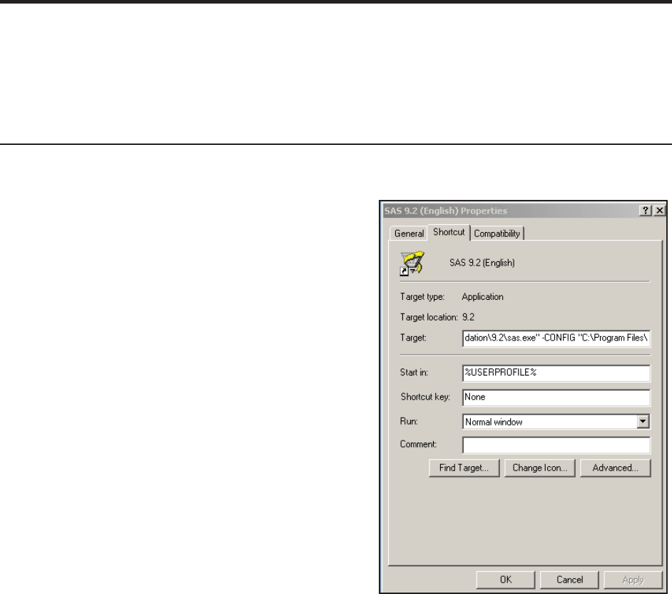
438 Carpenter’s Guide to Innovative SAS Techniques
Very often a significant portion of our use of SAS interfaces with the Operating System, OS.
Fortunately there are a number of tools and techniques that can be used to help us make that
interface smoother. Usually it is a matter of passing information between the OS and SAS. Other
times it is helpful to be able to have SAS execute OS commands directly. Some of the techniques
that I have found to be useful are included in this chapter.
An important interface that is not discussed in this chapter is SAS Enterprise Guide. This topic is
thoroughly covered by Slaughter and Delwiche (2010). Other less frequently used interfaces,
which are also not discussed in this chapter include: SAS/ASSIST, SAS Desktop, and
SAS/INSIGHT.
MORE INFORMATION
A great deal of information on SAS’s interface with the operating system is available in various
forms of metadata (see Section 13.8).
SEE ALSO
Peter Crawford (2006b) discusses a number of Display Manager techniques.
14.1 System Options
Most system options either control the SAS environment or they control the way that SAS
interfaces with the operating system. While most of these options are fairly straightforward to use,
you need to at least be aware of them. In addition some have proven to be especially useful. A few
of the options that fall into one or more of these categories are included here.
14.1.1 Initialization Options
Initialization options are specified when SAS is invoked and usually along with the same script
that calls the SAS execution file. Although
initialization options are available for all
operating systems, the syntax and application
varies by OS. Most of the examples shown
here are for the Windows OS; however, the
implementation with other operating systems
should be fairly straightforward.
Under the Windows OS, when executing
interactively, these options are declared on the
target line of the properties of the SAS
shortcut. The options themselves are preceded
by a dash (-). Here the -CONFIG initialization
option is specified on the TARGET line.
Notice that all paths are enclosed in double
quotes (double quotes are required by
Microsoft for all paths that have any embedded
blanks).
Most of the options shown in this section can
also be specified in the configuration file (see
Section 14.3).
&DUSHQWHU$UW&DUSHQWHU¶V*XLGHWR,QQRYDWLYH6$67HFKQLTXHV&RS\ULJKW6$6,QVWLWXWH,QF&DU\1RUWK&DUROLQD86$
$
//5,*+765(6(59(')RUDGGLWLRQDO6$6UHVRXUFHVYLVLWVXSSRUWVDVFRPSXEOLVKLQJ

Chapter 14: Operating System Interface and Environmental Control 439
SEE ALSO
Hurley (2007) introduces the use of initialization options.
The -SASINITIALFOLDER Option
This initialization option controls the default location that SAS first opens when the Display
Manager brings a SAS program into the editor. Simply follow the option with the path to the
desired folder.
For the sample code associated with this book the -SASINITIALFOLDER option might contain:
The ‘Start In:’ location on the PROPERTIES dialog box has limited utility in this context. It can
be used to designate the base path information, but not necessarily the location of the SAS code of
interest.
The -SYSPARM Option
The -SYSPARM option is used to pass information into a SAS program where it can be accessed
using the automatic macro variable &SYSPARM. Here a
portion of a path is passed into the SAS session when
SAS is initialized n. Within the SAS session the
automatic macro variable &SYSPARM o can be used to access this information. The quotes used
with the initialization
option n are not
stored with
&SYSPARM o.
The -SPLASHLOC Option
This option is more fun than practical. It allows you to point to a bit mapped image, BMP file,
that replaces the normal splash screen shown while SAS is being loaded. Instead of seeing the
SAS logo, you can view a cute picture of your favorite dog, cat, or moose. Of course the image is
not displayed for long. The only practical application that I have seen, other than on April 1, is for
use with a specific tool or program that you want to identify visually.
The -AUTOEXEC Option
The -AUTOEXEC option identifies the path and name of a SAS program that is to be
automatically executed when SAS is started (see Section 14.2). This program executes after the
configuration file and can be extremely useful when setting up a SAS environment that is to be
tailored for a specific application.
The -CONFIG Option
The -CONFIG option identifies the path and name of a SAS configuration file (see Section 14.3).
This is not a SAS program, but is used during the initialization process to set up the base SAS
environment. Many SAS installations restrict the modification of this file.
The -ALTLOG Option
Using this option you can write a separate copy of the LOG to a file of your choice. This becomes
an alternative to using PROC PRINTTO.
The -SYSIN Option
When running SAS programs in batch mode, a specific SAS program can be named to be
executed using the -SYSIN option. When you use this option, it becomes unnecessary to change
-sasinitialfolder "folder location"
-sysparm "c:\temp" n
libname advrpt v9 o "&sysparm\InnovativeTechniques\Data";
-sasinitialfolder "C:\InnovativeTechniques\SASCode"
&DUSHQWHU$UW&DUSHQWHU¶V*XLGHWR,QQRYDWLYH6$67HFKQLTXHV&RS\ULJKW6$6,QVWLWXWH,QF&DU\1RUWK&DUROLQD86$
$
//5,*+765(6(59(')RUDGGLWLRQDO6$6UHVRXUFHVYLVLWVXSSRUWVDVFRPSXEOLVKLQJ

440 Carpenter’s Guide to Innovative SAS Techniques
the location for the launching of SAS. You only need to specify the path to the program that is to
be executed.
SEE ALSO
The sasCommunity.org article by Ron Fehd “Batch processing under Windows” has examples of
the use of -SYSIN and other initialization options
http://www.sascommunity.org/wiki/Batch_processing_under_Windows.
The -RTFCOLOR Option
I do not remember where I heard about this option and I have not found it documented, but it
seems to work under Windows during an interactive session. Using this initialization option
allows you to write your log to a RTF file with preserved colors (notes, warnings, and errors).
During your SAS session or from within your SAS program, issue a DM statement with the
WRTFSAVE option. Alternatively
you could issue the WRTFSAVE
command from the command line
when the LOG window is active.
Even with -RTFCOLOR specified, logs generated with PROC PRINTTO and the -ALTLOG
initialization option do not retain their color.
CAVEAT Use this option with care, do not write applications that depend on it, because this
option is undocumented and there is no guarantee or even likelihood that it will continue to even
exist, let alone be supported in future releases of SAS.
The -INITSTMT and -TERMSTMT Options
The -INITSTMT and -TERMSTMT options are generally used together, and provide a
mechanism to automatically execute a SAS statement at the beginning and end of a SAS session.
The -INITSTMT option designates a statement that is to execute immediately following the
execution of the AUTOEXEC, while the -TERMSTMT option specifies a statement that will
execute just before the session closes. When the SAS statement is a macro call, the entire macro is
executed at the appropriate time.
Since macro variables are stored in memory, their values are not retained from one SAS session to
the next. This example uses the -INITSTMT and -TERMSTMT options to save and restore macro
variable values between SAS sessions. These options designate macro calls to %GETGLOBAL
and %SAVEGLOBAL, both
of which are autocall macros.
The %GETGLOBAL macro recovers the saved values from the data set
ADVRPT.GLOBALVARS and uses the SYMPUTX routine to reestablish them as global macro
variables. Because %GETGLOBAL macro definition is in the autocall library, which was
established by the AUTOEXEC, the macro can be immediately executed by the -INITSTMT
option.
DM 'log; WRTFSAVE "c:\temp\mylog3.rtf"';
-initstmt='%getglobal' -termstmt='%saveglobal'
%macro GetGlobal;
data _null_;
set advrpt.globalvars(where=(name ne 'PATH'));
call symputx(name,value,'g');
run;
%mend getGlobal;
&DUSHQWHU$UW&DUSHQWHU¶V*XLGHWR,QQRYDWLYH6$67HFKQLTXHV&RS\ULJKW6$6,QVWLWXWH,QF&DU\1RUWK&DUROLQD86$
$
//5,*+765(6(59(')RUDGGLWLRQDO6$6UHVRXUFHVYLVLWVXSSRUWVDVFRPSXEOLVKLQJ

Chapter 14: Operating System Interface and Environmental Control 441
options mergenoby=warn; n
data aemed;
merge advrpt.ae
advrpt.conmed;
run;
The %SAVEGLOBAL macro will be executed as the SAS session terminates. All macro
variables currently defined with a scope of global are written to the data set
ADVRPT.GLOBALVARS, where they will be available for the next SAS session. For interactive
sessions the ENDSAS
statement must be executed
in order for the
-TERMSTMT option to be
triggered.
The -NOWORKINIT and -NOWORKTERM Options
By default the WORK location is initialized at the start of the SAS session and is cleared at the
end of the SAS session. Usually this is exactly what you want to have happen; however,
occasionally you may want to maintain the WORK location across SAS sessions. The
-NOWORKINIT option prevents SAS from initializing the WORK location at the start of the
SAS session, and -NOWORKTERM prevents SAS from clearing the WORK location when SAS
terminates.
These two options are independent of each other but will generally be used together, as they allow
you to maintain the WORK space across session boundaries.
14.1.2 Data Processing Options
There are a few SYSTEM options that are either misused or underutilized. This is by no means an
exhaustive list, just a few that I have encountered. Some of these should be used only by the
advanced user who has full knowledge of the ramifications of their use.
The MERGENOBY Option
Unless done in a very deliberate manner, performing a MERGE without a BY statement (one-to-
one merge) can be very risky. When done inadvertently, the result is almost always not what is
desired. Worse, the errors are often not obvious, and these may not produce any warnings, notes,
or error messages in the LOG. The MERGENOBY option can be used to change this behavior.
The MERGENOBY determines what action should be taken when the MERGE statement is used
without a corresponding BY statement.
NOWARN merge takes place without warning (this is the default)
WARN merge takes place and a warning is issued
ERROR merge does not take place and an error is written to the LOG
The MERGENOBY=WARN designation n causes a warning to be issued to the LOG. It is my
opinion that the MERGENOBY option should be set
to ERROR, and only reset to WARN or NOWARN
when a specific compelling need arises. The
MERGENOBY=WARN produces the following
warning in the LOG. Notice that although a warning
is issued, the MERGE still takes place.
WARNING: No BY statement was specified for a MERGE statement.
NOTE: There were 127 observations read from the data set ADVRPT.AE.
NOTE: There were 199 observations read from the data set ADVRPT.CONMED.
NOTE: The data set WORK.AEMED has 199 observations and 13 variables
%macro SaveGlobal;
data advrpt.GlobalVars(keep=name value);
set sashelp.vmacro(where=(scope='GLOBAL'));
run;
%mend saveglobal;
&DUSHQWHU$UW&DUSHQWHU¶V*XLGHWR,QQRYDWLYH6$67HFKQLTXHV&RS\ULJKW6$6,QVWLWXWH,QF&DU\1RUWK&DUROLQD86$
$
//5,*+765(6(59(')RUDGGLWLRQDO6$6UHVRXUFHVYLVLWVXSSRUWVDVFRPSXEOLVKLQJ

442 Carpenter’s Guide to Innovative SAS Techniques
MORE INFORMATION
A MERGE statement without a BY appears in a ‘look-ahead’ example in Section 3.1.4. The code
associated with that example changes and then resets the current setting of the MERGENOBY
option.
The DATASTMTCHK Option
This option protects the user from overwriting data sets due to dropped semicolons by restricting
the use of certain data set names. The default is COREKEYWORDS which prevents you from
naming a data set UPDATE, MERGE, RETAIN, or SET.
COREKEYWORDS data sets may not have a name corresponding to a core
keyword (default)
ALLKEYWORDS also excludes all names that can start SAS DATA step
statements (i.e., ARRAY, DO, OUTPUT)
NONE no restrictions (defacto default prior to V7)
In this DATA step the semicolon has been left off of the DATA statement o. Effectively we are
attempting to create three data sets: WORK.AE, WORK.SET, and
ADVRPT.AE. Fortunately the COREKEYWORDS setting of the
DATASTMTCHK option protects us. In V6 or with the option set
to NONE, all three data sets would have been created with 0
observations and 0 variables – our permanent data set
ADVRPT.AE would have been wiped out!! In my opinion this option should not be reset to match
V6 standards (DATASTMTCHK=NONE).
As an aside, neither the COREKEYWORDS nor the ALLKEYWORDS values will flag a data
set, regardless of its name, which includes a libref. Consequently it would be possible, although of
doubtful utility, to name a data set WORK.UPDATE, when naming it without the libref,
UPDATE, would fail.
The VALIDVARNAME Option
The VALIDVARNAME option is used to determine valid variable naming conventions, and how
the variable names are handled.
V6 variable names must conform to V6 conventions (up to 8 characters). This
option value is no longer documented, but still works for the current versions
of SAS.
V7 allows up to 32 character names, and the case at variable definition is
remembered (the default).
UPCASE case is not remembered or used.
ANY allows non-standard naming conventions. Non-standard naming
conventions have limited utility outside of Base SAS and SAS/STAT.
data ae o
set advrpt.ae;
run;
22 data ae
23 set advrpt.ae;
---
56
ERROR 56-185: SET is not allowed in the DATA statement when option
DATASTMTCHK=COREKEYWORDS.
Check for a missing semicolon in the DATA statement, or use
DATASTMTCHK=NONE
&DUSHQWHU$UW&DUSHQWHU¶V*XLGHWR,QQRYDWLYH6$67HFKQLTXHV&RS\ULJKW6$6,QVWLWXWH,QF&DU\1RUWK&DUROLQD86$
$
//5,*+765(6(59(')RUDGGLWLRQDO6$6UHVRXUFHVYLVLWVXSSRUWVDVFRPSXEOLVKLQJ
Chapter 14: Operating System Interface and Environmental Control 443
The VALIDVARNAME=V6 Option
Useful when you are creating data sets that must conform to
V6 naming conventions. While acceptable for all other
values of VALIDVARNAME, the following DATA step
fails when VALIDVARNAME=v6, because the variable
name has more than 8 characters. This value of the
VALIDVARNAME= option may not be supported in future releases of SAS. In SAS 9.2 it has
not been included in the documentation for the VALIDVARNAME option. Although the V6
value restricts the length of variable names it does not restrict the length of data set names, as was
the case for SAS V6.
The VALIDVARNAME=ANY Option
This setting permits variable names that may come from other sources, such as ORACLE or
EXCEL, that do not use the same naming conventions as SAS. We access these non-standard
variables through the use of named literals that are needed whenever the name contains non-
standard characters. Once the data have been imported into SAS, it is generally recommended that
these variables are renamed to conform to standard SAS naming conventions. When a data set
contains variables defined using named literals, in order to include non-standard characters,
VALIDVARNAME= must always be set to ANY before the data set can be used. Also, whenever
you access any variable containing non-standard characters you must always use named literals to
name the variable.
A named literal is enclosed in quotes and the quoted string is followed by the letter n. Named
literals are used just like any other variable
name. Three variables are included in the
VAR statement to the left.
The application of the use of VALIDVARNAMES=ANY can be shown using the EXCEL file
E14_1_2AE.XLS. This spreadsheet has column headers that do not meet SAS naming standards.
PROC IMPORT can be used to convert this EXCEL table to
a SAS data set. Since the GETNAMES=YES option is used,
SAS will attempt to use the column headers as variable
names. Without first specifying VALIDVARNAME=ANY,
non-standard characters would be converted to underscores.
In this example it would not
have a large impact;
however, naming conflicts
can arise. By using
VALIDVARNAME=ANY,
we know what the columns
will be named in the SAS
data set (WORK.AEXLS).
A look at the properties of
WORK.AEXLS shows that
the non-standard names are
being used by SAS.
option validvarname=v6;
data a;
abcdefghig= 5;
run;
option validvarname=any;
PROC IMPORT OUT= WORK.AeXLS
DATAFILE= "&path\data\E14_1_2AE.xls"
DBMS=EXCEL REPLACE;
SHEET="Sheet1$";
GETNAMES=YES;
MIXED=NO;
SCANTEXT=YES;
USEDATE=YES;
SCANTIME=YES;
RUN;
options validvarnames=any;
proc print data=aexls;
var subject 'ae-date'n 'ae#type'n;
run;
&DUSHQWHU$UW&DUSHQWHU¶V*XLGHWR,QQRYDWLYH6$67HFKQLTXHV&RS\ULJKW6$6,QVWLWXWH,QF&DU\1RUWK&DUROLQD86$
$
//5,*+765(6(59(')RUDGGLWLRQDO6$6UHVRXUFHVYLVLWVXSSRUWVDVFRPSXEOLVKLQJ

444 Carpenter’s Guide to Innovative SAS Techniques
14.1.3 Saving System Options
Options saved using PROC OPTSAVE
Obs OPTNAME OPTVALUE
148 REPLACE 1
149 REUSE NO
150 RIGHTMARGIN 0.000 IN
151 RSASIOTRANSERROR 1
152 S 0
153 S2 0
154 S2V 0
155 SASAUTOS (advmac, sasautos) n
156 SASCMD
…portions of the table not shown…
Non-standard data set names are generally only honored in Base SAS and SAS/STAT, therefore it
is generally a good idea to rename these variables as soon as is convenient. In this case the
variable’s label will reflect the original name.
When using a non-standard name, such as is done in this RENAME option, a named literal is used
- the variable name is surrounded by
quotes, which are immediately
followed by the letter n.
14.1.3 Saving SAS System Options
Typically the settings for SAS System Options persist for the duration of the current job or the
current SAS session. It is possible, however, to save the current system options settings in either
the registry or in a data set. Once saved, they can be retrieved for a future session or job. Saving
the options in a data set is more flexible as it allows other users to acquire the same option
settings, which can include macro and format library controls.
Not all system options can be saved; most notably are initialization options and options that
contain passwords.
The options can be saved and retrieved by the use of either procedures or commands.
MORE INFORMATION
The -INITSTMT and -TERMSTMT system options described in Section 14.1.1 could also be
used to capture and save system options using similar techniques to those shown in that section to
capture and save macro variable values.
SEE ALSO
The SAS Forum thread http://communities.sas.com/message/101546 discusses a number of ways
to gather and reestablish system options.
Using PROCs OPTSAVE and OPTLOAD
The OPTSAVE procedure is used to write the current option settings to a SAS data set. The data
set is like any other and consists of
two columns (OPTNAME and
OPTVALUE). A portion of the
data set ADVRPT.CURRENT_
SETTINGS is shown here. Notice
the SASAUTOS option in line
155 n.
In the code that follows, the
SASAUTOS option is
‘inadvertently’ changed o. We can
observe the change using PROC
OPTIONS p r, and we can
recover the original setting of the
option using PROC OPTLOAD q.
data ae;
set aexls(rename=('ae-date'n=AEDate
'ae#type'n=AEType));
run;
proc optsave out=advrpt.current_settings;
run;
&DUSHQWHU$UW&DUSHQWHU¶V*XLGHWR,QQRYDWLYH6$67HFKQLTXHV&RS\ULJKW6$6,QVWLWXWH,QF&DU\1RUWK&DUROLQD86$
$
//5,*+765(6(59(')RUDGGLWLRQDO6$6UHVRXUFHVYLVLWVXSSRUWVDVFRPSXEOLVKLQJ

Chapter 14: Operating System Interface and Environmental Control 445
r PROC OPTIONS
is used to view the
current setting of the
SASAUTOS option.
Here we have
recovered the setting
of a single option. If
the WHERE clause
had not been used q
all the option settings
in the data set
ADVRPT.
CURRENT_
SETTINGS would
have been used.
Using the DMOPTSAVE and DMOPTLOAD Commands
The DMOPTSAVE and DMOPTLOAD commands are similar to the PROC steps described
above. As commands they are designed to be executed from the command line in the Display
Manager, but this also means that they can either be assigned a key in the KEYS window (see
Section 14.4.7), or that they can be executed from within the DM statement. Since the DM
statement is generally the most flexible, the code is shown here.
s The current system option
settings are saved using the
DMOPTSAVE command.
t The SASAUTOS option is
accidentally changed.
u The new SASAUTOS option
value is ready to be used. All
we do here is demonstrate that it
has been changed.
v The original value for the SASAUTOS option is restored.
MORE INFORMATION
The DM statement is also discussed in Section 14.4.2.
33 proc options option=sasautos; o
34 run;
SAS (r) Proprietary Software Release 9.2 TS2M2
SASAUTOS=adv Search list for autocall macros p
NOTE: PROCEDURE OPTIONS used (Total process time):
real time 0.00 seconds
cpu time 0.00 seconds
35 proc optload data=advrpt.current_settings
(where=(optname='SASAUTOS')); q
36 run;
NOTE: PROCEDURE OPTLOAD used (Total process time):
real time 0.12 seconds
cpu time 0.01 seconds
37 proc options option=sasautos; r
38 run;
SAS (r) Proprietary Software Release 9.2 TS2M2
SASAUTOS=(advmac, sasautos) r
Search list for autocall macros
NOTE: PROCEDURE OPTIONS used (Total process time):
real time 0.00 seconds
cpu time 0.00 seconds
dm 'dmoptsave advrpt.current_settings'; s
options sasautos=adv2; t
proc options option=sasautos; u
run;
dm "dmoptload advrpt.current_settings v
(where=(optname='SASAUTOS'))";
run;
proc options option=sasautos;
run;
&DUSHQWHU$UW&DUSHQWHU¶V*XLGHWR,QQRYDWLYH6$67HFKQLTXHV&RS\ULJKW6$6,QVWLWXWH,QF&DU\1RUWK&DUROLQD86$
$
//5,*+765(6(59(')RUDGGLWLRQDO6$6UHVRXUFHVYLVLWVXSSRUWVDVFRPSXEOLVKLQJ

446 Carpenter’s Guide to Innovative SAS Techniques
14.2 Using an AUTOEXEC Program
When SAS initializes and starts execution, it automatically looks for and executes (if it exists) a
program named AUTOEXEC.SAS. By default the AUTOEXEC.SAS program will only be found
if it is in the !SASROOT directory. Through the use of the -AUTOEXEC initialization option (see
Section 14.1.1), you can point to any SAS program in any location.
The AUTOEXEC.SAS can be any ordinary SAS program. It is commonly used to set up macro
libraries, system options, librefs, and filerefs. Although the program can be named anything
(Fred.jpg), AUTOEXEC.SAS is less obscure.
The AUTOEXEC.SAS shown here could be used to set up the libref used to access the data
associated with this book. It expects that the automatic macro variable &SYSPARM n was
assigned the upper portion of the path structure when SAS was called (see Section 14.1.1 for more
on the use of the -SYSPARM
initialization option). o The
libref is then established and
system options p are declared,
including the establishment of
the autocall library q. This
particular AUTOEXEC is short,
but it could just as easily have contained any number of macro calls or even initiated an
application.
Typically my Windows desktop contains a different SAS icon for each active client/project. Each
has its own unique autoexec program. This ensures that I use the correct data and the correct
programs for each project. If you install and use the AUTOEXEC.SAS program that comes with
the sample code for this book, the libref and autocall macro library used by the sample programs
will automatically be available for your use.
14.3 Using the Configuration File
When SAS initializes, the configuration file is executed before the autoexec program. The
configuration file is not a SAS program, and if you make changes, the editing must be done
carefully. Some companies use the configuration file to provide common setup instructions to all
the site’s SAS installations and consequently do not allow the modification of this file.
If you do want to customize this file, I would suggest that you do not modify the original version,
which can be found in the !SASROOT location. Instead you can copy and then edit the copy. You
then point to the modified configuration file using the -CONFIG initialization option (see Section
14.1.1).
The default name for this file is SASV9.CFG. The location will vary according to OS and
installation. Under a standard Windows setup, you may find it at one of the following locations:
SAS 9.1 C:\Program Files\SAS\SAS 9.1\nls\en
SAS 9.2 C:\Program Files\SAS\SASFoundation\9.2\nls\en
SAS 9.3 C:\Program Files\SASHome\SASFoundation\9.3
* Autoexec.sas *;
%let path = n &sysparm\InnovativeTechniques;
libname advrpt v9 "&path\Data"; o
filename advmac "&path\sascode\sasmacros";
options nodate nonumber nocenter; p
options sasautos=(advmac, sasautos); q
&DUSHQWHU$UW&DUSHQWHU¶V*XLGHWR,QQRYDWLYH6$67HFKQLTXHV&RS\ULJKW6$6,QVWLWXWH,QF&DU\1RUWK&DUROLQD86$
$
//5,*+765(6(59(')RUDGGLWLRQDO6$6UHVRXUFHVYLVLWVXSSRUWVDVFRPSXEOLVKLQJ

Chapter 14: Operating System Interface and Environmental Control 447
Common customizations include:
addition of a macro library location to SASAUTOS
changing the location of the WORK directory
modification of other default values like memory allocation and macro symbol table size
14.3.1 Changing the SASAUTOS Location
The following portion of a configuration file adds a directory n to the list of SASAUTOS
libraries. Adding this
directory to the definition
of SASAUTOS means
that it will automatically
be included in the
autocall library, without
specifying it in the
SASAUTOS= system
option.
In the configuration file
the -SET keyword is
used to establish an
environmental variable,
which will later be
interpreted as a fileref.
Rather than modify the original CONFIG file (or a copy as described above), it is possible to
invoke a second tailored configuration file that will augment or override selected portions of the
original file. The configuration file shown below makes it unnecessary to modify the SASAUTOS
option when defining your autocall library. It does this by inserting the locations directly into the
SASAUTOS system option.
Inserting locations in the autocall library using the INSERT option in the CONFIG.CFG file has
been problematic. Fortunately the following technique was worked out by Peter Crawford of
Crawford Software Consultancy Limited.
o For convenience the
ADVTECH environmental
variable is created and
subsequently used as a path
abbreviation at qr.
p SAS Institute’s autocall library is reestablished using the SASAUTOS option. This step must
be done first, because the original value of the SASAUTOS option is specified without using
parentheses. This definition will replace the default value of SASAUTOS, with one that includes
the parentheses. The parentheses are needed when more than one location is to be specified as is
done at qr.
q The physical path to the production autocall library is inserted into the SASAUTOS option.
The -INSERT option writes the text at the beginning of the list. The APPEND option (which is
not shown) can place the text at the end of the list. Notice the use of the environmental variable
!ADVTECH which is designated as such using the exclamation point.
r A second autocall library is inserted into the SASAUTOS option. Because it is inserted second
it will appear before the PRODMACROS library q.
/* Setup the SAS autocall library definition */
-SET SASAUTOS ("\\groupserver\sascode\macros" n
"!sasroot\core\sasmacro"
"!sasext0\inttech\sasmacro"
"!sasext0\access\sasmacro"
"!sasext0\assist\sasmacro"
"!sasext0\eis\sasmacro"
"!sasext0\ets\sasmacro"
"!sasext0\graph\sasmacro"
"!sasext0\iml\sasmacro"
"!sasext0\or\sasmacro"
"!sasext0\qc\sasmacro"
"!sasext0\share\sasmacro"
"!sasext0\stat\sasmacro"
)
-set advtech "C:\InnovativeTechniques\SASCode" o
-sasautos (sasautos) p
-insert sasautos !advtech\ProdMacros\ q
-insert sasautos !advtech\SASMacros\ r
&DUSHQWHU$UW&DUSHQWHU¶V*XLGHWR,QQRYDWLYH6$67HFKQLTXHV&RS\ULJKW6$6,QVWLWXWH,QF&DU\1RUWK&DUROLQD86$
$
//5,*+765(6(59(')RUDGGLWLRQDO6$6UHVRXUFHVYLVLWVXSSRUWVDVFRPSXEOLVKLQJ

448 Carpenter’s Guide to Innovative SAS Techniques
s The tailored configuration file is pointed to using a second -CONFIG initialization option on
the execution line. This option will generally be in addition to the standard configuration file
which will also use a -CONFIG option.
t We can confirm the values in the
SASAUTOS option by using PROC OPTIONS.
u The value of the ADVTECH environmental
variable can be surfaced using the %SYSGET
macro function.
The LOG shows that the SASAUTOS option has been modified and that the ADVTECH
environmental variable has the anticipated value. Notice that the SASAUTOS fileref is not quoted
t in the LOG. If we had inserted the additional locations without first inserting the parentheses,
this text would have been quoted and that portion of the autocall library would not have been
available.
Other common initialization options that could be declared in this second configuration file could
include:
-SASINITIALFOLDER (see Section 14.1.1)
-AUTOEXEC (see Sections 14.1.1 and 14.2)
-VERBOSE Show option setting in the log at initialization
SEE ALSO
SAS Problem Note 44791 discusses the problem associated with inserting an autocall location,
but does not suggest the solution worked out by Peter Crawford
http://support.sas.com/kb/44/791.html. Sample Code 42360 demonstrates the use of the APPEND
option http://support.sas.com/kb/42/360.html.
-config "C:\InnovativeTechniques\SASCode\Chapter14\E14_3_1.cfg" s
proc options option=sasautos; t
run;
%put %sysget(advtech); u
5 proc options option=sasautos;
6 run;
SAS (r) Proprietary Software Release 9.2 TS2M2
SASAUTOS=( '!advtech\SASMacros\' '!advtech\ProdMacros\' sasautos ) t
Search list for autocall macros
NOTE: PROCEDURE OPTIONS used (Total process time):
real time 0.00 seconds
cpu time 0.00 seconds
7
8 %put %sysget(advtech);
C:\InnovativeTechniques\SASCode u
&DUSHQWHU$UW&DUSHQWHU¶V*XLGHWR,QQRYDWLYH6$67HFKQLTXHV&RS\ULJKW6$6,QVWLWXWH,QF&DU\1RUWK&DUROLQD86$
$
//5,*+765(6(59(')RUDGGLWLRQDO6$6UHVRXUFHVYLVLWVXSSRUWVDVFRPSXEOLVKLQJ
Chapter 14: Operating System Interface and Environmental Control 449
14.3.2 Controlling DM Initialization
When the Display Manager is initialized you can, to a large extent, control the appearance and the
available tools through the use of initialization options. This level of control is most generally of
interest when you are executing an application, perhaps through SAS/AF or SAS/EIS, and you
need to control your user’s ability to access SAS.
n The entire top line can be turned off by using:
-AWSCONTROL NOTITLE
Alternatively you can change the title from the default (SAS) to one of your choosing:
-AWSTITLE "ABC Project"
o The list of drop-down menus can be turned off by using the -NOAWSMENU initialization
option.
The -INITCMD option
allows you to specify
control commands when
executing an application,
such as SAS/AF. The
initialization option
shown here starts a
SAS/AF application and
closes most of the user’s access to the rest of SAS.
14.4 In the Display Manager
The Display Manager is extremely customizable. Many of these possible customizations are a bit
over the top, but there are a number that are very helpful.
SEE ALSO
Richard DeVenezia's Web site has a useful section on "actions" you might consider adding to the
explorer window http://www.devenezia.com/downloads/sas/actions/.
/* Prep for AF start up appliction */
-initcmd "af c=control.Control.wrapper.frame af;
toolclose;
zoom;
command close;
wstatusln off;
wwindowbar off;"
&DUSHQWHU$UW&DUSHQWHU¶V*XLGHWR,QQRYDWLYH6$67HFKQLTXHV&RS\ULJKW6$6,QVWLWXWH,QF&DU\1RUWK&DUROLQD86$
$
//5,*+765(6(59(')RUDGGLWLRQDO6$6UHVRXUFHVYLVLWVXSSRUWVDVFRPSXEOLVKLQJ
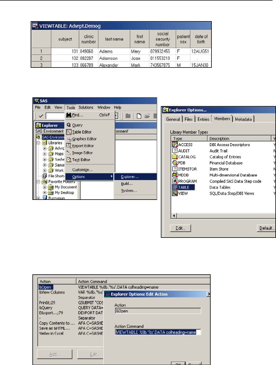
450 Carpenter’s Guide to Innovative SAS Techniques
14.4.1 Showing Column Names in ViewTable
By default the VIEWTABLE window displays variable labels as column headers. I find this to be
very annoying as I
almost always want
to see the variable
name. Fortunately
the default can be
changed to show the
column names
instead of the labels.
Although the following steps will be basically the same, the setup of some of the following dialog
boxes will vary according to OS and version of SAS.
With the SAS Explorer Window active, select:
TOOLS ĺ OPTIONS ĺ EXPLORER.
This brings up the Explorer Options dialog box,
select: MEMBERS ĺ TABLE ĺ EDIT
Edit the line with the ACTION of &OPEN and
add colheading= name. The default for VIEWTABLE will now be to display variable names.
Repeat the process for VIEWS.
&DUSHQWHU$UW&DUSHQWHU¶V*XLGHWR,QQRYDWLYH6$67HFKQLTXHV&RS\ULJKW6$6,QVWLWXWH,QF&DU\1RUWK&DUROLQD86$
$
//5,*+765(6(59(')RUDGGLWLRQDO6$6UHVRXUFHVYLVLWVXSSRUWVDVFRPSXEOLVKLQJ

Chapter 14: Operating System Interface and Environmental Control 451
dm log 'clear';
MORE INFORMATION
Rather than change the default behavior you can also change this setting when the ViewTable is
invoked. Section 14.4.2 shows a DM command that invokes the ViewTable using column names
rather than labels.
14.4.2 Using the DM Statement
The DM statement allows you to execute one or more Display Manager commands from within a
SAS Program. These are the same commands that can be used in the command box, on the
command line, or from the KEYS
window.
If you do not need to designate or change the active window all you need is the action. This is
common when performing a DM task from within a batch program.
The following command can be used to clear the LOG window.
Multiple DM commands can be included in a single DM statement by chaining them together
with semicolons. This DM statement turns off the program editor and executes a SAS/AF
program making
the SAS/AF
window active.
You can also route the LOG much as you can by using PROC PRINTTO.
The POST command can be used to post a message box to the
users screen. This can be a much stronger attention grabber than
just a message to
the LOG.
The enhanced editor is designated using the WEDIT command, and if followed by a filename, a
specific file can be loaded and opened for editing.
The ViewTable can be invoked as well using either the VIEWTABLE or VT command. Here the
data set ADVRPT.DEMOG is opened with the variable names shown as column headings
(COLHEADING=LABELS is
the default).
The DM statement can also be used to assign a specific command to a function key (see Section
14.4.7). The KEYDEF command is used to make the
assignment. Here the F12 key is assigned to clear the
log.
DM <windowname> 'action' <windoname>;
dm af "pgm off; af cat = appls.allproj.passwd.program";
dm 'log; file "&path\logdump1.log"';
dm 'post "this is a message"';
dm 'wedit "C:\InnovativeTechniques\sascode\chapter14\e14_3_1.sas"' ;
dm "viewtable advrpt.demog colheading=names";
dm 'keydef f12 "log;clear"';
&DUSHQWHU$UW&DUSHQWHU¶V*XLGHWR,QQRYDWLYH6$67HFKQLTXHV&RS\ULJKW6$6,QVWLWXWH,QF&DU\1RUWK&DUROLQD86$
$
//5,*+765(6(59(')RUDGGLWLRQDO6$6UHVRXUFHVYLVLWVXSSRUWVDVFRPSXEOLVKLQJ
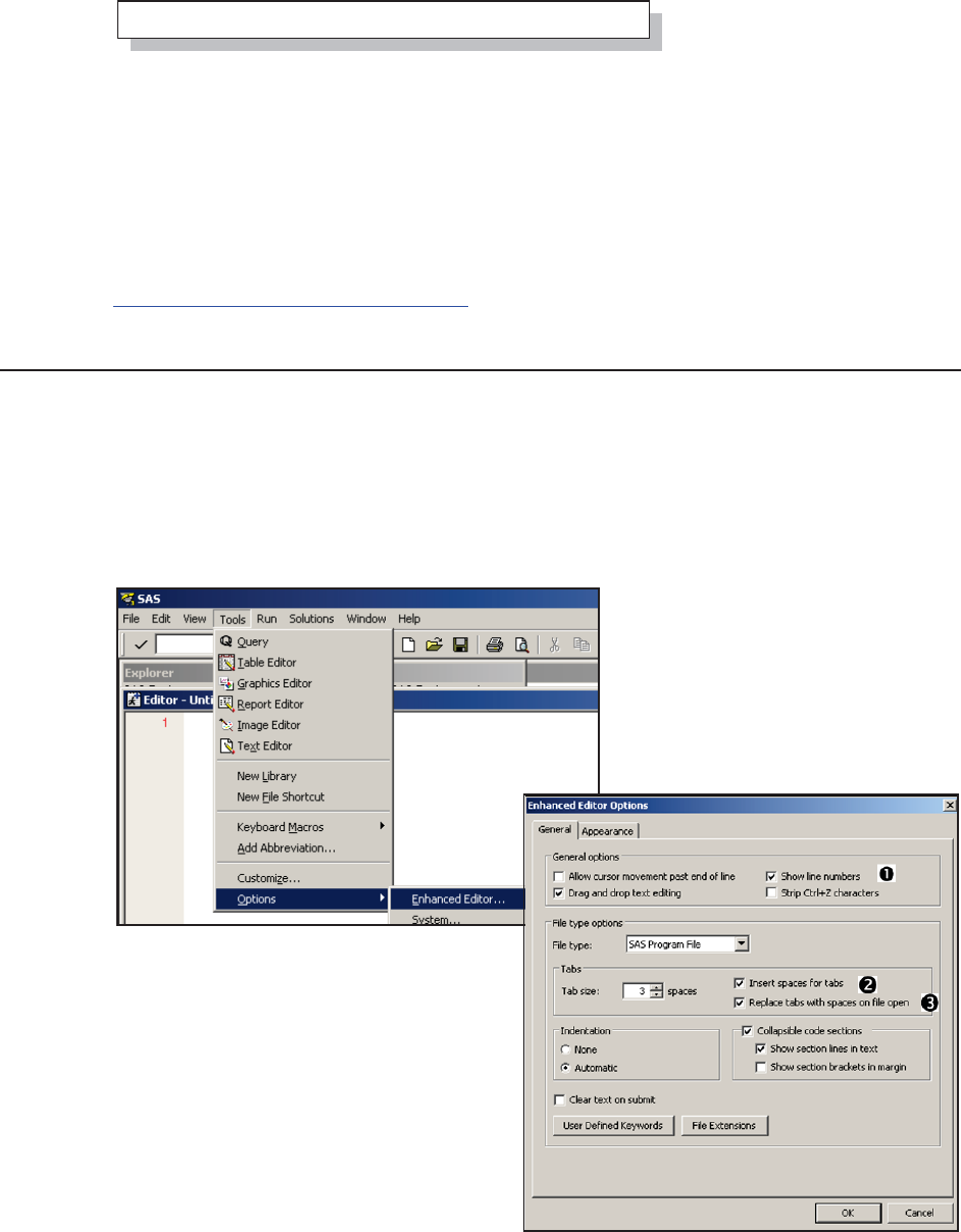
452 Carpenter’s Guide to Innovative SAS Techniques
For combination keystrokes enclose the key definition in quotes as well. The SHIFT F9 key will
now close the next open
ViewTable window. Close a
series of open ViewTable
windows with successive selections.
MORE INFORMATION
The DM statement is used to execute the DMOPTSAVE and DMOPTLOAD commands in
Section 14.1.3. Section 14.4.7 discusses the execution of DM commands through hot key
assignments.
SEE ALSO
The DM statement and the WEDIT command are discussed in the SAS Forum thread
http://communities.sas.com/thread/12520. Rosenbloom and Lafler (2011c) assign a macro call to
a function key.
14.4.3 Enhanced Editor Options and Shortcuts
There are a number of options and shortcuts available for use with the Enhanced Editor. It is also
possible to do a fair amount of customization.
Enhanced Editor Setup
There are only a few set up preferences that I would recommend that you change. Most of the
defaults are fine for typical users. The options for the Enhanced Editor can be found when the
editor is the active window. Use TOOLS ĺ Options ĺ Enhanced Editor. This brings up the
Enhanced Editor Options dialog box.
I like to select ‘Show Line numbers’
n, because it makes life easier for
large programs. More importantly, be
sure to check ‘insert spaces for tabs’ o
and ‘replace tabs with spaces on file
open’ p. Both of these options help to
make it easier to maintain the text
formatting of a SAS program when it is
transferred between programmers.
dm 'keydef "shf f9" "next VIEWTABLE:; end"';
&DUSHQWHU$UW&DUSHQWHU¶V*XLGHWR,QQRYDWLYH6$67HFKQLTXHV&RS\ULJKW6$6,QVWLWXWH,QF&DU\1RUWK&DUROLQD86$
$
//5,*+765(6(59(')RUDGGLWLRQDO6$6UHVRXUFHVYLVLWVXSSRUWVDVFRPSXEOLVKLQJ
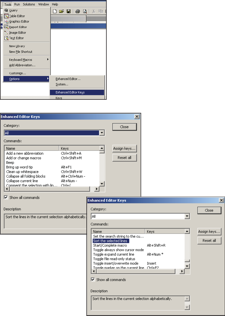
Chapter 14: Operating System Interface and Environmental Control 453
Enhanced Editor Keys
The editor has been set up with a number of shortcut key combinations. Depending on how you
work and what things you tend to do, some of these key combinations can be very useful. You can
see and learn more of these key combinations through the Enhanced Editor Keys pull-down menu.
While the Enhanced Editor is the active window, go to TOOLS ĺ OPTIONS ĺ ENHANCED
EDITOR KEYS.
Explore the resulting dialog box to find the key
combinations that are most useful to you. I
especially like to use:
Ctrl+/ add comments
Ctrl+shift+/ remove comments
Ctrl+F2 mark a line in a program
F2 jump to the next marked line
Shift+F2 jump to the previous marked line
Not only are the defined key combinations very useful, but you can redefine the combinations and
add new keyed operations. Notice
that the BEEP command has no
assigned key combinations and is
therefore not available. While BEEP
is probably not particularly useful,
others can be; you can scroll down
the list of available operations until
you find one of interest. Here “Sort
the selected lines” has been
highlighted. Next press the “Assign
keys…” button.
&DUSHQWHU$UW&DUSHQWHU¶V*XLGHWR,QQRYDWLYH6$67HFKQLTXHV&RS\ULJKW6$6,QVWLWXWH,QF&DU\1RUWK&DUROLQD86$
$
//5,*+765(6(59(')RUDGGLWLRQDO6$6UHVRXUFHVYLVLWVXSSRUWVDVFRPSXEOLVKLQJ
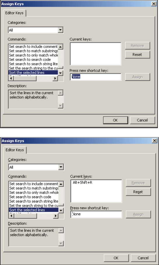
454 Carpenter’s Guide to Innovative SAS Techniques
The ‘Assign Keys’ dialog box
is used to assign a set of key
strokes to this operation.
Highlight the none in the
‘Press new shortcut key:’ box,
and then press the desired
keys. If you select a
combination that is already in
use, the keystroke combination
is changed to be used with the
new operation. In this example
we are choosing to use Alt +
Shift + R (this key
combination will no longer be
used to ‘Start/Complete
macro’).
We can now use this key
combination in the Enhanced
Editor to sort rows.
&DUSHQWHU$UW&DUSHQWHU¶V*XLGHWR,QQRYDWLYH6$67HFKQLTXHV&RS\ULJKW6$6,QVWLWXWH,QF&DU\1RUWK&DUROLQD86$
$
//5,*+765(6(59(')RUDGGLWLRQDO6$6UHVRXUFHVYLVLWVXSSRUWVDVFRPSXEOLVKLQJ
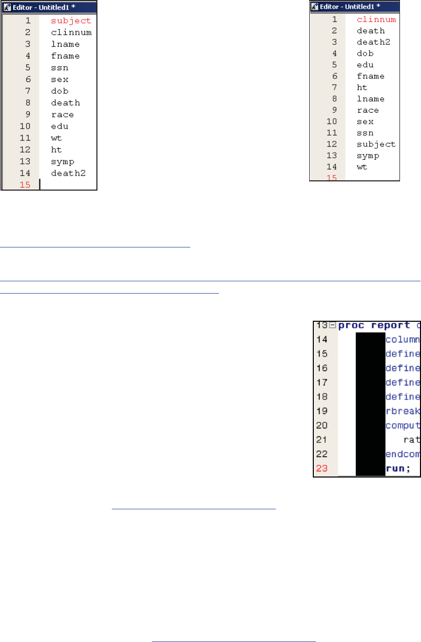
Chapter 14: Operating System Interface and Environmental Control 455
The list of variables on the left, which have
been pasted into the Enhanced Editor, are in
the ADVRPT.DEMOG data set and have
been written in variable number order. If the
first 14 rows are highlighted and we press
the Alt+Shift+R keys the rows are
reordered. And the list becomes the one
shown on the right.
SEE ALSO
A short write-up on select Enhanced Editor keys can be found on the Tek-Tips Forum
http://www.tek-tips.com/faqs.cfm?fid=5140.
The following LinkedIn thread has a number of suggestions
http://www.linkedin.com/groupItem?view=&srchtype=discussedNews&gid=70702&item=63659
611&type=member&trk=eml-anet_dig-b_pd-ttl-cn.
Marking a Block of Text
While most applications allow you to hold the left mouse button
(LMB) while dragging the mouse to highlight entire lines of text, in
the Enhanced Editor you can go a couple of steps further. Dragging
while the cursor is in the gray area (left side of the editor), ensures
that all the text in the first and last lines will be highlighted.
You can highlight, while controlling for columns and lines, by also
pressing the ‘Alt’ key at the same time as dragging with the LMB
depressed. In the image to the right, ‘delete’ would shift lines 14-23
five columns to the left.
SEE ALSO
Under SAS 9.1 there was a problem with the feature to mark blocks
of text on machines for which SAS Enterprise Guide was also
installed. Problem note #30455 shows how to resolve this conflict.
This note can be found at http://support.sas.com/kb/30/455.html.
AUTOSAVE – Finding the Backup File
Files being edited by the Enhanced Editor are automatically saved every few minutes (the
frequency is set in the DM preferences under the TOOLS ĺ OPTIONS ĺ PREFERENCES ĺ
EDIT tab). If you need to recover the saved file the location can be a bit difficult to find and it
varies with OS and version of SAS. Usage Note 12392 states: Enhanced Editor Autosave should
be consulted to find the location of these backup versions of your program. Under Windows the
file extension is .ASV.
SEE ALSO
Usage Note 12392 can be found at http://support.sas.com/kb/12/392.html.
&DUSHQWHU$UW&DUSHQWHU¶V*XLGHWR,QQRYDWLYH6$67HFKQLTXHV&RS\ULJKW6$6,QVWLWXWH,QF&DU\1RUWK&DUROLQD86$
$
//5,*+765(6(59(')RUDGGLWLRQDO6$6UHVRXUFHVYLVLWVXSSRUWVDVFRPSXEOLVKLQJ
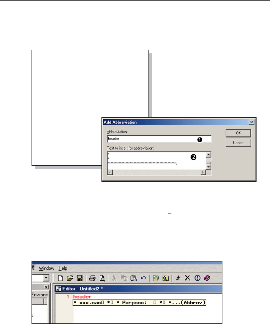
456 Carpenter’s Guide to Innovative SAS Techniques
* xxx.sas
*
* Purpose:
*
* Written by:
* Art Carpenter
* 06Nov2011
* (907)865-9167
*
* Inputs:
*
* Outputs:
*
* Notes:
*
* Modifications:
*
*
*********************************;
14.4.4 Macro Abbreviations for the Enhanced Editor
The Enhanced Editor enables you to build abbreviations for your editor. Much like abbreviations
in other applications, a single word or part of a word can be typed and then other (generally
longer) text can be substituted at a keystroke.
For the purposes of this example assume that you want to type the following header block at the
top of each of your programs. Typing it once
is fine, but more than once becomes tedious.
Let’s make a macro abbreviation that does the
typing for us.
While the Enhanced Editor is the active
window, use the pull-down menus TOOLS
ĺ ADD ABBREVIATION (or the editor
short cut keys CTRL+SHIFT+A). This brings
up the Add Abbreviation dialog box.
In the Add Abbreviation dialog box enter a name for the new abbreviation (header) n. This
becomes a keyboard macro, so you must select a name that has not already been used. Then type
(or more practically paste) the substitution text into the ‘Text to insert for abbreviation’ dialog
space o. Pressing the OK button creates and stores the abbreviation.
To use the abbreviation simply type in the name of the abbreviation while in the Enhanced Editor.
As soon as the last letter of the abbreviation has been entered, a small pop-up ‘tip’ text box
containing the first few characters of the abbreviation is displayed. If at that point you press the
TAB or ENTER key, the name of the abbreviation will be replaced by the text that you stored.
The following
screen shot
shows that the
name of the
HEADER
abbreviation
has been
entered in the
Enhanced
Editor and the
first few characters of the text to be substituted is shown in the pop-up ‘tip’ box. Pressing the
TAB or ENTER key causes the abbreviation name to be replaced by the stored text.
&DUSHQWHU$UW&DUSHQWHU¶V*XLGHWR,QQRYDWLYH6$67HFKQLTXHV&RS\ULJKW6$6,QVWLWXWH,QF&DU\1RUWK&DUROLQD86$
$
//5,*+765(6(59(')RUDGGLWLRQDO6$6UHVRXUFHVYLVLWVXSSRUWVDVFRPSXEOLVKLQJ
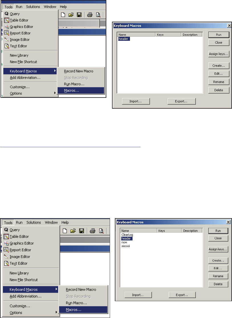
Chapter 14: Operating System Interface and Environmental Control 457
Once created macro abbreviations can be edited or deleted just like any other keyboard macro.
Use the pull-down menus TOOLS ĺ
KEYBOARD MACROS ĺMACROS to bring up
the KEYBOARD MACROS dialog box.
Using this dialog box you may also export/import your macro abbreviations so that they may be
standardized across your work group. Use the EXPORT button to create a file with the KMF
extension. This file can then be imported by another SAS user by using the IMPORT button. A
number of KMF files have been gathered at the sasCommunity.org site
http://www.sascommunity.org/wiki/Abbreviations/Macros.
The date in the HEADER abbreviation shown above is static. There are a number of predefined
edits that we can apply to a keyboard macro (remember that a macro abbreviation is a special
form of a keyboard macro). Several of these predefined edits allow the insertion of date values.
Using these we can automatically insert the current date time stamp from when the abbreviation is
executed. The following steps reestablish the HEADER abbreviation with the current date time
value replacing the static date (06Nov2011).
Edit the HEADER keyboard macro (it has already been established as an abbreviation
(TOOLS ĺKEYBOARD MACROS ĺ MACROS). Select HEADER and the EDIT button.
&DUSHQWHU$UW&DUSHQWHU¶V*XLGHWR,QQRYDWLYH6$67HFKQLTXHV&RS\ULJKW6$6,QVWLWXWH,QF&DU\1RUWK&DUROLQD86$
$
//5,*+765(6(59(')RUDGGLWLRQDO6$6UHVRXUFHVYLVLWVXSSRUWVDVFRPSXEOLVKLQJ

458 Carpenter’s Guide to Innovative SAS Techniques
The original HEADER
definition is going to be
replaced so delete the one
line that starts with “Insert
the string. . .”. This will
completely clear the
abbreviation definition.
That is OK for now. We are
about to insert new text.
The important thing is that
HEADER has already been
established as an
abbreviation.
The commands on the left
of the Edit Keyboard Macro
dialog box can be inserted
into the macro. Once you
have deleted the definition,
scroll down the list of
commands until you find
“Insert the string”. Select it
and press the double arrow
in the middle of the dialog
box to move the command
to the right-hand box.
Paste the portion of the
header text up to, but not
including, the static date
into the Insert String dialog
box and select OK.
&DUSHQWHU$UW&DUSHQWHU¶V*XLGHWR,QQRYDWLYH6$67HFKQLTXHV&RS\ULJKW6$6,QVWLWXWH,QF&DU\1RUWK&DUROLQD86$
$
//5,*+765(6(59(')RUDGGLWLRQDO6$6UHVRXUFHVYLVLWVXSSRUWVDVFRPSXEOLVKLQJ
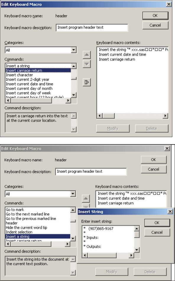
Chapter 14: Operating System Interface and Environmental Control 459
Select the date or date
time values of interest.
Here the “Insert current
date and time” command
has been selected. We
want the subsequent text
to start on the next line so
the command to “Insert a
carriage return” has also
been selected.
The remainder of the
header text can now be
inserted using the ‘Insert
the string’ command.
The “Insert a string”
command is again
selected and the
remainder of the text is
typed or pasted into the
Insert String dialog box.
Specify OK as you exit
from each of the dialog
boxes. The revised
HEADER abbreviation is
now ready to use.
&DUSHQWHU$UW&DUSHQWHU¶V*XLGHWR,QQRYDWLYH6$67HFKQLTXHV&RS\ULJKW6$6,QVWLWXWH,QF&DU\1RUWK&DUROLQD86$
$
//5,*+765(6(59(')RUDGGLWLRQDO6$6UHVRXUFHVYLVLWVXSSRUWVDVFRPSXEOLVKLQJ
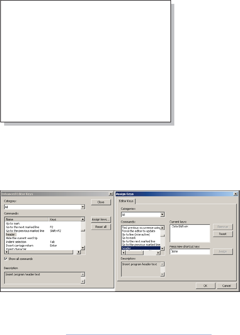
460 Carpenter’s Guide to Innovative SAS Techniques
* xxx.sas
*
* Purpose:
*
* Written by:
* Art Carpenter
* Thursday, November 17, 2011 20:49:54
* (907)865-9167
*
* Inputs:
*
* Outputs:
*
* Notes:
*
* Modifications:
*
*
*********************************;
The HEADER
abbreviation will now
insert the current date
time stamp into the
header text.
The name of the abbreviation will now also appear in the Enhanced Editor Keys dialog box
(introduced in Section 14.4.3). You can use this dialog box to assign a set of keys to execute the
abbreviation.
Select the abbreviation (HEADER) and press the ‘Assign keys. . .’ button. Highlight the text in
the ‘Press new shortcut key:’ box and press the shortcut keys of choice. Here the
CTRL+SHIFT+H keys were chosen. This key combination will now execute the HEADER
abbreviation and will no longer bring up HELP.
SEE ALSO
Carpenter (2003b) introduces this example for the creation of a macro abbreviation. A collection
of abbreviations as well as links to other references with more information can be found on the
sasCommunity.org article http://www.sascommunity.org/wiki/Abbreviations/Macros.
&DUSHQWHU$UW&DUSHQWHU¶V*XLGHWR,QQRYDWLYH6$67HFKQLTXHV&RS\ULJKW6$6,QVWLWXWH,QF&DU\1RUWK&DUROLQD86$
$
//5,*+765(6(59(')RUDGGLWLRQDO6$6UHVRXUFHVYLVLWVXSSRUWVDVFRPSXEOLVKLQJ
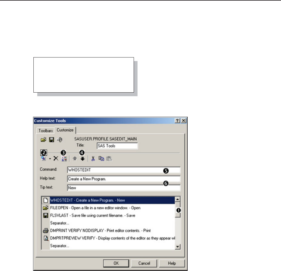
Chapter 14: Operating System Interface and Environmental Control 461
14.4.5 Adding Tools to the Application Tool Bar
Like most applications that have pull-down menus and tool bars, it is possible to modify or
customize the list of available tools. A common usage is when you have a program or code
snippet that you run regularly, and would like to have it readily available. By modifying the tool
bar, you can add an icon that will instantly execute your program.
Consider the following program that will delete all the data sets in the work directory. We would
like to add an icon on the tool bar associated with the
Enhanced Editor that will execute this step. The icon
could be placed on any of the tool bars in the DM, this
one seems most logical.
With the Enhanced Editor in the active window, use the pull-down menus to select TOOLS ĺ
CUSTOMIZE (or right click on the tool bar itself). The CUSTOMIZE TOOLS dialog box for the
tool bar is shown. From here you
can add or remove items on the
tool bar. We would like to add an
icon that will execute our PROC
DATASETS program.
n Move the slider to the
approximate position of the icon
(the final position can be refined
later).
o Add a blank icon (separators
can be useful to make things
clearer).
p Select an icon for your tool.
q Refine the location.
r On the command line enter the
text that is to be executed. In the
example that follows we will be
executing a GSUBMIT command.
s Help and Tip text should be added.
proc datasets library=work
memtype=data
kill
nolist;
quit;
&DUSHQWHU$UW&DUSHQWHU¶V*XLGHWR,QQRYDWLYH6$67HFKQLTXHV&RS\ULJKW6$6,QVWLWXWH,QF&DU\1RUWK&DUROLQD86$
$
//5,*+765(6(59(')RUDGGLWLRQDO6$6UHVRXUFHVYLVLWVXSSRUWVDVFRPSXEOLVKLQJ
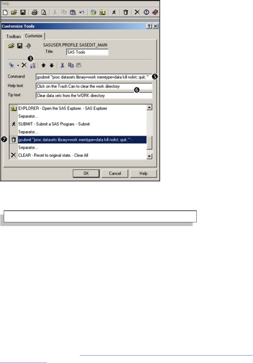
462 Carpenter’s Guide to Innovative SAS Techniques
The tool bar icon used to execute the PROC DATASETS step is shown below. The trash can icon
t has been selected for the tool bar from a list of supplied icons p.
The GSUBMIT command is a
corollary of the DM statement. It
allows you to insert code where a
command is otherwise expected. In
this example the entire step has
been placed in the GSUBMIT
command. This would have been
quite inconvenient if the step had
been any longer. Actually the
GSUBMIT command only allows
500+ characters. For longer steps
consider submitting a macro call or
a %INCLUDE statement.
The %INCLUDE becomes a bit
problematic if the path to the
location of the program contains a
macro variable. This is an issue
because the string associated with
the GSUBMIT command must be
quoted. However, the %INC also
expects either a quoted string or a
fileref. Strings within strings are
often an issue for macro language
elements, because at some point
the macro variable (e.g., &PATH) will be within single quotes. Fortunately in this case, because
of how the line is parsed, the single quotes can be used without masking the macro variable.
The GSUBMIT command is only one of a very long list of commands that can be issued from
within the Display Manager. Other useful commands include those that bring up other DM
windows, such as:
KEYS
LIBNAME
LOG
FILENAME
TITLE
SEE ALSO
Howard (2004) shows this and some similar examples. The PMENU procedure can be used to
design, build, and save customized pull-down menus and tool bars. Charlie Huang’s 9/11/2011
blog entry “Add 10 buttons to enhance SAS 9.3 environment” suggests a number of buttons that
could be added to the tool bar http://www.sasanalysis.com/2011/09/10-buttons-to-tweak-sas-93-
environmnet.html.
gsubmit '%inc "&path\sascode\chapter14\e14_4_5.sas";'
&DUSHQWHU$UW&DUSHQWHU¶V*XLGHWR,QQRYDWLYH6$67HFKQLTXHV&RS\ULJKW6$6,QVWLWXWH,QF&DU\1RUWK&DUROLQD86$
$
//5,*+765(6(59(')RUDGGLWLRQDO6$6UHVRXUFHVYLVLWVXSSRUWVDVFRPSXEOLVKLQJ
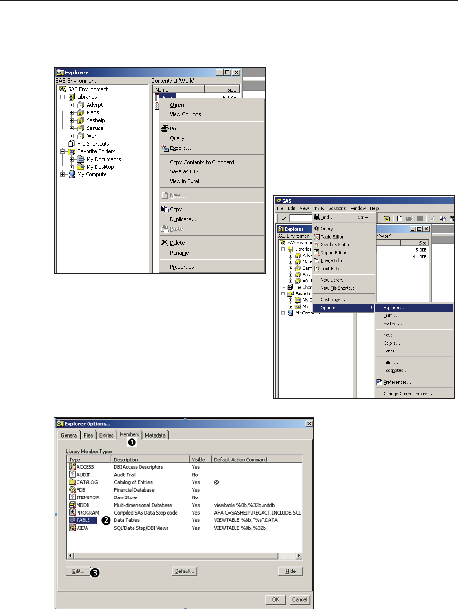
Chapter 14: Operating System Interface and Environmental Control 463
14.4.6 Adding Tools to Pull-Down and Pop-up Menus
Sometimes adding a specialized tool to the pull-down or pop-up menus used in the DM can be
very beneficial. In Section 14.4.5 the GSUBMIT command was used to execute a SAS program
from a tool bar. You can do the same sort of thing from a pull-down or pop-up menu.
Consider the pop-up menu shown on the
left, if you right-click on a data set from
within the Explorer window. We would like
to have the ability to execute a specialized
tool against a SAS data set simply by
clicking on a menu item in this pop-up
menu.
While the Explorer window is active, this
menu is controlled through the TOOLS ĺ
OPTIONS ĺ EXPLORER menus. This
brings up the EXPLORER OPTIONS dialog box.
This box is worth exploring just because it is used
to control access to a variety of objects from
within the SAS Explorer. Since we want to apply
our tool to a SAS data table, we select the
MEMBERS tab n and then highlight the TABLE
(SAS data set) o line. Clicking on the EDIT
button p brings up the EXPLORER OPTIONS:
TABLE OPTIONS dialog box.
&DUSHQWHU$UW&DUSHQWHU¶V*XLGHWR,QQRYDWLYH6$67HFKQLTXHV&RS\ULJKW6$6,QVWLWXWH,QF&DU\1RUWK&DUROLQD86$
$
//5,*+765(6(59(')RUDGGLWLRQDO6$6UHVRXUFHVYLVLWVXSSRUWVDVFRPSXEOLVKLQJ
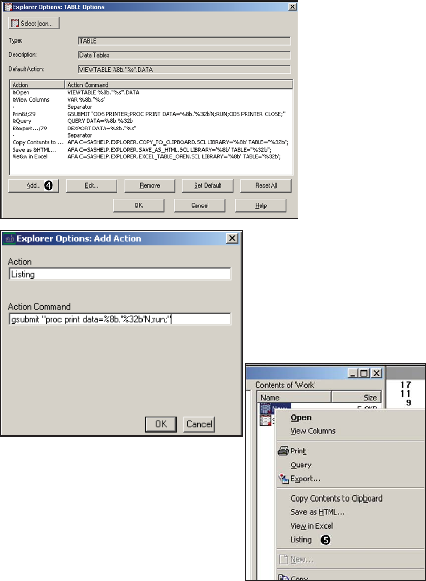
464 Carpenter’s Guide to Innovative SAS Techniques
Notice that the EXPLORER OPTIONS: TABLE OPTIONS dialog box is used to form the
primary pop-up menu that
you see when you right-
click on a SAS data table
(see the first figure in this
section). The items in the
ACTION COMMANDS
section in this dialog box
are worth examining.
Notice the use of the
VIEWTABLE, VAR,
GSUBMIT, and QUERY
commands. The table
name is brought into the
script using %8b for the
libref, and ‘%32b’N for
the data set name.
We are going to add a GSUBMIT item
to this menu by using the ADD action
button q. Highlight the item below,
which you want to insert the new
command, and press the ADD action
button q. This brings up the ADD
ACTION dialog box. Here we enter a
name for the action and the action
(gsubmit "proc print
data=%8b.'%32b'N;run;") that is to
take place. Exit from each of the dialog boxes using
OK. A new entry, titled ‘Listing’ r, will now appear
on the pop-up menu associated with a SAS data set.
Selecting the ‘Listing’ entry will perform a PROC
PRINT on the highlighted data set.
Inserting a PROC PRINT is a bit of a silly thing to do.
If you notice the third item in the ‘table options’ list,
you will see that it already contains a GSUBMIT for a
PROC PRINT which utilizes ODS.
In the following example instead of inserting a
GSUBMIT for a PROC step, we use it to submit
macro language elements.
&DUSHQWHU$UW&DUSHQWHU¶V*XLGHWR,QQRYDWLYH6$67HFKQLTXHV&RS\ULJKW6$6,QVWLWXWH,QF&DU\1RUWK&DUROLQD86$
$
//5,*+765(6(59(')RUDGGLWLRQDO6$6UHVRXUFHVYLVLWVXSSRUWVDVFRPSXEOLVKLQJ
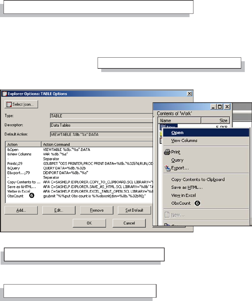
Chapter 14: Operating System Interface and Environmental Control 465
Because the scripting uses the percent sign in the data set name, you must be careful when calling
macro language elements from within the GSUBMIT. This is demonstrated by adding a call to the
%OBSCNT macro which returns the number of observations in a SAS data set. If we use it in a
%PUT statement
the number of
observations is
written to the LOG.
%OBSCNT (see Section 13.4.2) is an autocall macro and is part of the autocall library that comes
with the programs associated with this book. Notice that the percent signs associated with the
macro language are doubled. This delays their interpretation until the macro statement has been
submitted which takes place after the data set name has been inserted. For the data set
WORK.NEW the resultant
submitted %PUT statement will
become:
The TABLE OPTIONS dialog box shows this definition, and the ObsCount entry now appears on
the pop-up menu.
s
The previous
example uses a %PUT statement to write the number of observations to the LOG. You could just
have easily have passed the
name of the data set to a macro
for execution. The GSUBMIT
would be essentially the same. The following GSUBMIT executes the %PRINITIT macro for the
displayed data set. The macro quoting function %NRSTR is used to delay the interpretation of the
macro call and may be required
when the macro resides in a
stored compiled macro library.
For most standard data set names this code can usually be simplified by removing the quotes
around the data set name(%32b).
SEE ALSO
Art Trabachneck et al (2010) demonstrate additional and more extensive techniques.
gsubmit "%%put Obs count is %%obscnt(dsn=%8b.'%32b'N);"
%put Obs count is %obscnt(dsn=work.new);
gsubmit "%%nrstr(%%printit(dsn=%8b.'%32b'N));"
gsubmit "%%nrstr(%%printit(dsn=%8b.%32b));"
&DUSHQWHU$UW&DUSHQWHU¶V*XLGHWR,QQRYDWLYH6$67HFKQLTXHV&RS\ULJKW6$6,QVWLWXWH,QF&DU\1RUWK&DUROLQD86$
$
//5,*+765(6(59(')RUDGGLWLRQDO6$6UHVRXUFHVYLVLWVXSSRUWVDVFRPSXEOLVKLQJ
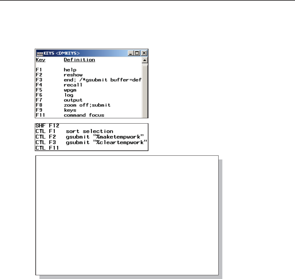
466 Carpenter’s Guide to Innovative SAS Techniques
14.4.7 Adding Tools to the KEYS List
The KEYS window (TOOLS ĺ OPTIONS ĺ KEYS or F9 or KEYS on the command line) lists
DM commands that have been pre-assigned to specific key combinations, including function keys
and mouse buttons. The key assignments can be modified by the user and can include Display
Manager commands and even macro calls.
The first few key definitions of the KEYS window
are shown to the left. Notice that multiple commands
can be concatenated with a semicolon.
You can type in a new command, either by
overwriting an existing command or by typing it in
any available space. Commands can also be inserted
into the key definitions using the KEDYDEF
command on a DM statement (see Section 14.42).
Like in Section 14.4.6, if you want to submit code,
the GSUBMIT command can be used. CTL F2 and
CTL F3 have been designated to submit the
%MAKETEMPWORK and %CLEARTEMPWORK
macro calls. The macro
definitions have been
saved in the autocall
library so that they can
be loaded when the
appropriate key
combinations are
selected.
The
%MAKETEMPWORK
macro creates a
directory and assigns the
libref TEMPWORK to
it. When the library is no
longer needed, perhaps
at the end of the session,
the user can press
CTL+F3, which executes the macro %CLEARTEMPWORK, which in turn clears the contents of
the directory and deletes the directory. Since these macros utilize the %SYSEXEC macro
function, the system option NOXWAIT should be declared to prevent prompts from the OS.
Once modified, the new key definitions can be saved using the SAVE command. Key definitions
are stored as catalog entries with an entry type of keys. Saved definitions can be recovered
through the use of the COPY command.
MORE INFORMATION
Display Manager commands can also be executed through the use of the DM statement (see
Sections 14.1.3 and 14.4.2).
%macro MakeTEMPWORK;
%local rc;
%let rc=%sysfunc(fileexist("c:\tempwork"));
%if &rc=0 %then %do;
%sysexec md "c:\tempwork";
%let rc=%sysfunc(libname(tempwork,c:\tempwork));
%end;
%mend maketempwork;
%macro ClearTEMPWORK;
%local rc;
%let rc=%sysfunc(fileexist("c:\tempwork"));
%if &rc ne 0 %then %do;
%let rc=%sysfunc(libname(tempwork));
%sysexec del /Q "c:\tempwork\*.*";
%sysexec rd /Q "c:\tempwork";
%end;
%mend cleartempwork;
&DUSHQWHU$UW&DUSHQWHU¶V*XLGHWR,QQRYDWLYH6$67HFKQLTXHV&RS\ULJKW6$6,QVWLWXWH,QF&DU\1RUWK&DUROLQD86$
$
//5,*+765(6(59(')RUDGGLWLRQDO6$6UHVRXUFHVYLVLWVXSSRUWVDVFRPSXEOLVKLQJ

Chapter 14: Operating System Interface and Environmental Control 467
SEE ALSO
Rosenbloom and Lafler (2011c) use SUBMIT rather than GSUBMIT in the assignment of several
different macros to KEYS.
14.5 Using SAS to Write and Send E-mails
During or after the processing of a program, you can use SAS to generate e-mails. These can be
notifications of error conditions or the successful termination of the program. The e-mail can even
contain attachments. This simple example will get you started. Read the SEE ALSO references
for details that provide refinements of the technique.
n The attributes of the
e-mail server for this e-mail
ID are specified in options.
These options could also be
specified in the
configuration file. The
EMAILID= and the
EMAILHOST= options will
take on values specific to
your e-mail server.
o The FILENAME
statement is used to define
the e-mail fileref
(GENMAIL). Notice the
use of the EMAIL engine.
p The SUBJECT= option
defines the subject line.
q The recipient’s e-mail
address is specified using
the TO= option.
r The FROM= option designates the sender’s e-mail. This will generally match the
EMAILID n.
s The ATTACH= option designates the file to be attached.
t The file that is to be attached is generated.
u A data _NULL_ step is used to generate the e-mail body. The process of starting to generate
the e-mail takes place when the DATA step is compiled. Conditional execution of statements
within the DATA step can change the body of the e-mail, but remember if the DATA step is
compiled, an e-mail will be generated.
v The FILE statement points to the fileref (GENMAIL) generated using the EMAIL engine.
w The text of the e-mail is generated using a PUT statement.
options emailsys=SMTP emailid="sam@caloxy.com" n
emailhost="caloxy.com" EMAILPORT=25;
* Define the fileref with the email engine;
FILENAME genmail email o
subject="Patient 205 ConMeds" p
to = "Fred@caloxy.com" q
from = "Sam@caloxy.com" r
attach ="&path\results\E14_5.pdf"; s
ods pdf file="&path\results\e14_5.pdf" t
style=journal2;
proc print data=advrpt.conmed
(where=(subject='205'));
id subject;
var medstdt medspdt drug;
run;
ods pdf close;
data _null_; u
file genmail; v
put "Here are the ConMeds for Subject 205"; w
run;
&DUSHQWHU$UW&DUSHQWHU¶V*XLGHWR,QQRYDWLYH6$67HFKQLTXHV&RS\ULJKW6$6,QVWLWXWH,QF&DU\1RUWK&DUROLQD86$
$
//5,*+765(6(59(')RUDGGLWLRQDO6$6UHVRXUFHVYLVLWVXSSRUWVDVFRPSXEOLVKLQJ
468 Carpenter’s Guide to Innovative SAS Techniques
SEE ALSO
A number of papers have been written on using SAS to e-mail results. Hunley (2010) has a
number of extended examples including a discussion of texting. Whitworth (2010) has an
example that includes zipping the file before e-mailing it. Rosenbloom and Lafler(2011d) have a
brief e-mail example.
The SAS Jedi (Mark Jordan) has written a couple of blogs on the use of SAS to e-mail documents
http://blogs.sas.com/sastraining/index.php?/archives/81-Jedi-SAS-Tricks-Email-from-the-Front-
Part-2.html. He has also created a YouTube video on the topic
http://www.youtube.com/watch?v=qPobPZg2osc&feature=related.
Two SAS Forum threads include discussions on the use of e-mail
http://communities.sas.com/thread/10467 and http://communities.sas.com/thread/11086.
14.6 Recovering Physical Location Information
Under the WINDOWS OS there are a number of techniques that you can use to find the physical
location of a data set or file given the information available to SAS.
SEE ALSO
Carpenter (2008b) discusses these and other techniques in more detail.
14.6.1 Using the PATHNAME Function
The PATHNAME function returns the physical path for a given fileref or libref. While rarely used
in the DATA step it has proven to be invaluable in the macro language. Often times we do not
necessarily know the physical path
even though we know a libref or
fileref. Here the physical path is
loaded into a macro variable where
it is displayed in the LOG.
You can even use it on concatenated filerefs such as the autocall library. To gather the current
location of all of the locations in the SASAUTOS fileref you could specify:
MORE INFORMATION
One of the examples in Section 13.8.2 recovers some location information using the PATHNAME
function.
14.6.2 SASHELP VIEWS and DICTIONARY Tables
The path information for existing librefs and filerefs can be gathered by examining the SASHELP
views and SQL DICTIONARY tables. Here you can find not only the path that would be returned
by the PATHNAME function, but other things such as the ENGINE as well.
SASHELP.VLIBNAM and DICTIONARY.LIBNAMES
Each row in the view SASHELP.VLIBNAM (note the spelling) contains the libref and path
information for each libref (more than one row for concatenated librefs). A portion of a listing of
filename saspgm "&path\sascode\e14_6.sas";
%let pgmpath = %sysfunc(pathname(saspgm));
%put &pgmpath;
C:\InnovativeTechniques\sascode\e14_6.sas
%sysfunc(pathname(sasautos))
&DUSHQWHU$UW&DUSHQWHU¶V*XLGHWR,QQRYDWLYH6$67HFKQLTXHV&RS\ULJKW6$6,QVWLWXWH,QF&DU\1RUWK&DUROLQD86$
$
//5,*+765(6(59(')RUDGGLWLRQDO6$6UHVRXUFHVYLVLWVXSSRUWVDVFRPSXEOLVKLQJ

Chapter 14: Operating System Interface and Environmental Control 469
this view shows the primary variables. Notice that the first few locations of the concatenated
SASHELP libref are included as well.
SASHELP.VEXTFL and DICTIONARY.EXTFILES
The location of external files (such as raw data and programs) can also be retrieved from either
the SASHELP.VEXTFL view or the SQL dictionary table DICTIONARY.EXTFILES.
Using the
SASHELP.VEXTFL view,
the path information can be
retrieved through a DATA
step and loaded into a
macro variable. The view
as well as the dictionary
table can be accessed from within an SQL step.
MORE INFORMATION
Section 13.8.1 goes into more detail on the use of
these SASHELP views and SQL DICTIONARY
tables.
14.6.3 Determining the Executing Program Name and Path
Sometimes we need to be able to automatically detect the name or location of an executing
program. This can be especially helpful when we write applications that need to self document,
perhaps by placing the name and location of the executing program in a footnote of the generated
table.
This is fairly straightforward when the executing program is running in batch mode. In batch
mode the name of the executing program is stored in the system option SYSIN, and the value of
system options can be retrieved using the GETOPTION function
Under the Windows OS, the name of the executing program and its path is stored in the
environmental variables SAS_EXECFILENAME and SAS_EXECFILEPATH. Environmental
variables are maintained by the OS; however, SAS can both populate and access their values.
Whenever a SAS program is executed, this includes when it is executed through the Display
Manager from the Enhanced Editor, these environmental variables are updated.
Returning a Physical Location
14.6.2 SASHELP VIEWS and DICTIONARY Tables
Obs libname engine path
1 ADVRPT V9 C:\InnovativeTechniques\Data
2 SASHELP V9 C:\Program Files\SAS\SASFoundation\9.2\nls\en\SASCFG
3 SASHELP V9 C:\Program Files\SAS\SASFoundation\9.2\core\sashelp
4 SASHELP V9 C:\Program Files\SAS\SASFoundation\9.2\inttech\sashelp
5 SASHELP V9 C:\Program Files\SAS\SASFoundation\9.2\mddbserv\sashelp
. . . . portions of the table are not shown . . . .
data _null_;
set sashelp.vextfl(keep=fileref xpath
where=(fileref='SASPGM'));
call symputx('pgmpath2',xpath,'l');
run;
%put &pgmpath2;
proc sql noprint;
select xpath into :pgmsqlpath
from dictionary.extfiles
where fileref='SASPGM';
quit;
%put &pgmsqlpath;
&DUSHQWHU$UW&DUSHQWHU¶V*XLGHWR,QQRYDWLYH6$67HFKQLTXHV&RS\ULJKW6$6,QVWLWXWH,QF&DU\1RUWK&DUROLQD86$
$
//5,*+765(6(59(')RUDGGLWLRQDO6$6UHVRXUFHVYLVLWVXSSRUWVDVFRPSXEOLVKLQJ

470 Carpenter’s Guide to Innovative SAS Techniques
The values of environmental variables are accessed through the use of the %SYSGET macro
function. The returned value can then be loaded into a macro variable or just written to the LOG
as is done here.
When you want the name of the program without the SAS extension it can easily be stripped off
using the %SCAN or %QSCAN function.
When we need to know not just the name, but the location of the SAS program (when executing
from the Enhanced Editor this is the location from where the executing program was retrieved),
we can use the SAS_EXECFILEPATH environmental variable. Here the value is retrieved by the
macro %GRABPATHNAME and then written to the LOG.
14.6.4 Retrieving the UNC (Universal Naming Convention) Path
When a program resides on a network server, the server name is generally mapped to a drive
letter. Since this drive letter can be user specific, knowing that a program resides on the F:\ drive
for one user is not necessarily helpful to someone else. As was shown using all of the previous
methods, it is always the mapped drive that is returned; therefore, a different approach is needed
to retrieve the actual or UNC path. Although the UNC path information is not stored in a location
that is directly available to SAS, it is still possible to get this information - the process is just a bit
more challenging.
Certainly we know that the OS has to know the relationship between the mapped drive letter and
the actual UNC location. Under Windows this information is stored in a Dynamic Link Library,
DLL. Windows has internal tools for accessing the information contained in a DLL and these
tools can be accessed from within SAS using the CALL MODULE routine (the MODULEN and
MODULEC functions can also be used). To make the tools available to the CALL MODULE
routine we must first create a CATALOG SOURCE entry for it to operate against. This entry
contains the arguments that are passed to and from the Windows DLL routine, which for
retrieving the UNC path, is named WNetGetConnectionA (be careful, this name is case sensitive).
The arguments themselves are specific to each routine. The WNetGetConnectionA routine
expects three arguments. Here the SOURCE entry has been written to a catalog in the WORK
directory; however, you will generally make this permanent so that you only have to run this step
once.
%put %sysget(SAS_EXECFILENAME);
%put %qscan(%sysget(SAS_EXECFILENAME),1,.);
E14_6.sas
E14_6
%macro grabpathname;
%sysget(SAS_EXECFILEPATH)
%mend grabpathname;
%put %grabpathname;
114 %put %grabpathname;
C:\InnovativeTechniques\SASCode\Chapter14\E14_6.sas
&DUSHQWHU$UW&DUSHQWHU¶V*XLGHWR,QQRYDWLYH6$67HFKQLTXHV&RS\ULJKW6$6,QVWLWXWH,QF&DU\1RUWK&DUROLQD86$
$
//5,*+765(6(59(')RUDGGLWLRQDO6$6UHVRXUFHVYLVLWVXSSRUWVDVFRPSXEOLVKLQJ

Chapter 14: Operating System Interface and Environmental Control 471
n The attributes needed by the WNetGetConnectionA DLL are specified by writing them to a
SOURCE catalog entry using a DATA _NULL_ step. The fileref must be SASCBTBL, and the
CATALOG engine must be specified.
o The routine attributes are written using PUT statements. The DLL name is case sensitive and
must be specified exactly as written.
The CALL MODULE routine can then be used to access the WNetGetConnectionA routine and
to retrieve the location.
p The %GRABDRIVE macro returns the drive letter alone.
q The %GRABDRIVE macro obtains the mapped drive letter with the colon e.g., F:. This
becomes the input for the DLL. The second argument (OUTPUT_DIR) will contain the returned
UNC path.
filename sascbtbl catalog "work.temp.attrfile.source"; n
data _null_;
file sascbtbl; n
put "routine WNetGetConnectionA module=mpr minarg=3 maxarg=3 o
stackpop=called returns=long;";
put " arg 1 char input byaddr format=$cstr200.;";
put " arg 2 char update byaddr format=$cstr200.;";
put " arg 3 num update byaddr format=pib4.;";
run;
%macro grabdrive; p
%qtrim(%qleft(%qscan(%sysget(SAS_EXECFILEPATH),1,\)))
%mend grabdrive;
%MACRO getUNC;
%local dir path;
%* Determine the UNC path for the SAS program being executed.;
DATA _NULL_;
length input_dir $200 output_dir $200;
* The input directory drive letter: ONLY e.g. j: ;
input_dir = "%grabdrive";q
output_dir = ' ';
output_len = 200;
call module("WNetGetConnectionA",
input_dir, r
output_dir,
output_len);
call symputx('dir',input_dir,'l'); s
call symputx('path',output_dir,'l'); t
RUN;
%* Get the name for the program of execution.;
%put drive letter is &dir; u
%put path is &path; v
%put name is %grabpathname; w
%MEND getunc;
&DUSHQWHU$UW&DUSHQWHU¶V*XLGHWR,QQRYDWLYH6$67HFKQLTXHV&RS\ULJKW6$6,QVWLWXWH,QF&DU\1RUWK&DUROLQD86$
$
//5,*+765(6(59(')RUDGGLWLRQDO6$6UHVRXUFHVYLVLWVXSSRUWVDVFRPSXEOLVKLQJ

472 Carpenter’s Guide to Innovative SAS Techniques
r The MODULE routine is called by passing it the mapped drive letter that is contained in the
variable INPUT_DIR. The UNC path is passed back by WNetGetConnectionA by storing it in
OUTPUT_DIR.
s The input drive letter is stored in the macro variable &DIR.
t The UNC path is placed into the macro variable &PATH. Notice that this is a local macro
variable. Had it been global we would overwrite the &PATH used in most of the examples in this
book.
u Write the mapped drive
letter to the LOG.
v Write the UNC path to the
LOG. This is the portion of the path that has been mapped to the drive letter (F:\ in this example).
w Write the program name to the LOG.
The macro %GETUNC is called by a program
that is not on the C: drive. In this case the
program resides on the F:\ drive. The UNC
path v shows that the F:\ drive letter has been
mapped to the \InnovativeTechniques
directory on the \\CALOXYDELL server.
drive letter is F: u
path is \\CALOXYDELL\InnovativeTechniques v
name is F:\sascode\Chapter14\e14_6_showUNC.sas w
%* Place this program in a mapped
%* drive (NOT the C: drive);
%getunc
&DUSHQWHU$UW&DUSHQWHU¶V*XLGHWR,QQRYDWLYH6$67HFKQLTXHV&RS\ULJKW6$6,QVWLWXWH,QF&DU\1RUWK&DUROLQD86$
$
//5,*+765(6(59(')RUDGGLWLRQDO6$6UHVRXUFHVYLVLWVXSSRUWVDVFRPSXEOLVKLQJ

Chapter 15
Miscellaneous Topics
15.1 A Few Miscellaneous Tips 474
15.1.1 Customizing Your NOTEs, WARNINGs, and ERRORs 474
15.1.2 Enhancing Titles and Footnotes with the #BYVAL and
#BYVAR Options 475
15.1.3 Executing OS Commands 477
15.2 Creating User-defined Functions Using PROC FCMP 479
15.2.1 Building Your Own Functions 479
15.2.2 Storing and Accessing Your Functions 481
15.2.3 Interaction with the Macro Language 482
15.2.4 Viewing Function Definitions 483
15.2.5 Removing Functions 484
15.3 Reading RTF as Data 485
15.3.1 RTF Diagram Completion 486
15.3.2 Template Preparation 486
15.3.3 RTF as Data 487
As if everything in this book was not eclectic enough to be an entire book of miscellaneous topics,
the final chapter is the miscellaneous chapter of this eclectically miscellaneous book.
&DUSHQWHU$UW&DUSHQWHU¶V*XLGHWR,QQRYDWLYH6$67HFKQLTXHV&RS\ULJKW6$6,QVWLWXWH,QF&DU\1RUWK&DUROLQD86$
$
//5,*+765(6(59(')RUDGGLWLRQDO6$6UHVRXUFHVYLVLWVXSSRUWVDVFRPSXEOLVKLQJ

474 Carpenter’s Guide to Innovative SAS Techniques
15.1 A Few Miscellaneous Tips
Here are just a few of many tips.
SEE ALSO
If you want more tips read the ‘Tip of the Day’ on sasCommunity.org. You can even have the tip
tweeted to you.
15.1.1 Customizing Your NOTEs, WARNINGs, and ERRORs
The PUT, PUTLOG, and %PUT statements can be used to generate customized notes, warnings,
and errors in the LOG. Since these statements are executable, logic can be used to conditionally
execute them. The text written to the LOG follows the systems conventions when the statement
keyword is immediately followed by one of the following:
NOTE: The note is written in blue.
WARNING: Warnings are written in green.
ERROR: Errors are written in red and are summarized along with other
errors.
The keyword must be capitalized and must be immediately followed by a colon.
You can also follow the words NOTE, WARNING, or ERROR with a dash instead of a colon.
The customized message will still appear in the LOG with the appropriate color; however, the
word NOTE, WARNING, or ERROR will not appear.
SEE ALSO
Don Henderson wrote a tip on sasCommunity.org that discusses this topic
http://www.sascommunity.org/wiki/Tips:Using_NOTE,_WARNING,_ERROR_in_Your_Progra
m%27s_Generated_Messages.
lock sashelp.class;
%put NOTE: class should be locked;
41 lock sashelp.class;
NOTE: SASHELP.CLASS.DATA is now locked for exclusive access by you.
42 %put NOTE: class should be locked;
NOTE: class should be locked
&DUSHQWHU$UW&DUSHQWHU¶V*XLGHWR,QQRYDWLYH6$67HFKQLTXHV&RS\ULJKW6$6,QVWLWXWH,QF&DU\1RUWK&DUROLQD86$
$
//5,*+765(6(59(')RUDGGLWLRQDO6$6UHVRXUFHVYLVLWVXSSRUWVDVFRPSXEOLVKLQJ
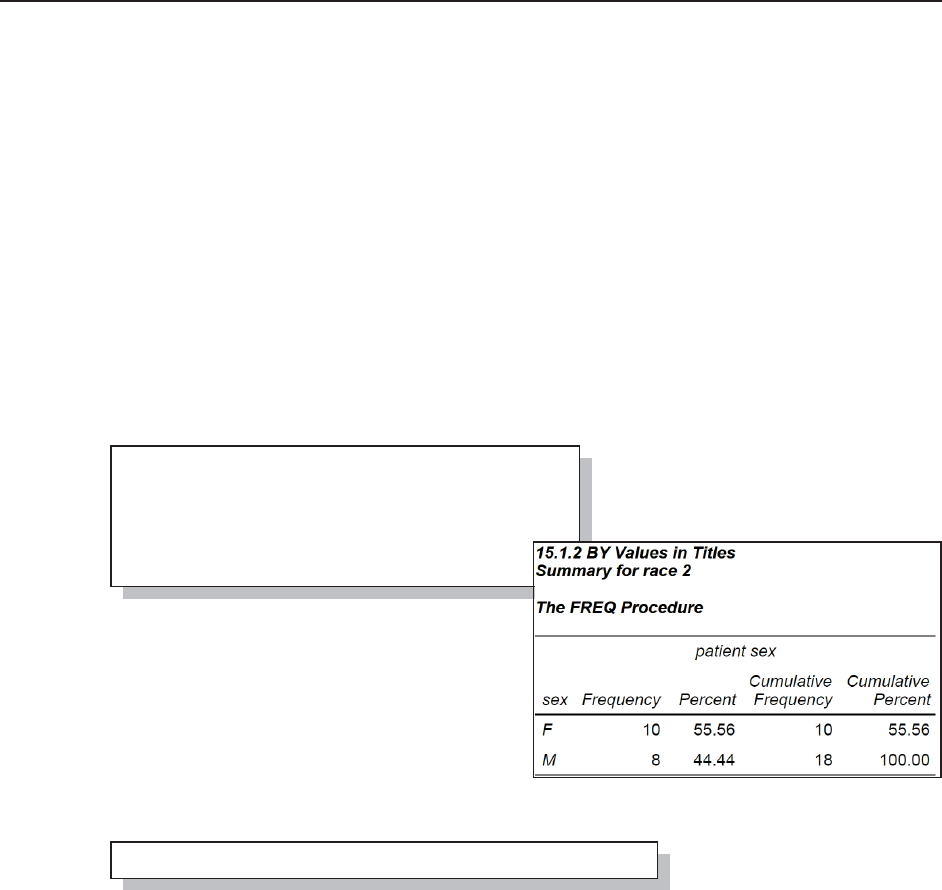
Chapter 15: Miscellaneous Topics 475
15.1.2 Enhancing Titles and Footnotes with the #BYVAL and #BYVAR
Options
When your PROC step uses a BY statement the values of the BY variables or even the variable
names themselves can be inserted into the title or footnote. Although available for use in a few
other locations, the #BYVAL, #BYVAR, and #BYLINE options were designed to be used in the
TITLE and FOOTNOTE statements.
The #BYVAR option is used to place the variable name in the title while the #BYVAL option is
used to place the value of that BY variable. Both the #BYVAL and #BYVAR options have two
ways of addressing a specific BY variable from the list of BY variables. These two forms
(implicit and explicit) can be used interchangeably. Implicit naming uses a number that
corresponds to the list of BY variables (left to right): #BYVAR1 and #BYVAL1 would both refer
to the first variable in the list of variables. Explicit naming uses the variable name in parentheses.
The variable must be on the BY list: #BYVAR(RACE) and #BYVAL(RACE). Only a single
variable may be used within the parentheses.
Here the #BYVAR and #BYVAL options are used to identify the RACE in a PROC FREQ step.
n Since the BY variable information
will appear in the title the procedure’s
BY line is not needed.
o Both the #BYVAR and #BYVAL options
are used and the variables are selected
implicitly. Notice that these options may be
used inside of either single or double quotes.
The same title statement could have been
written using these options with explicit
specifications.
These options work well with the macro language, but make sure that, unlike the titles above, you
use double quotes so that the macro language elements will be resolved correctly.
In the PROC FREQ shown above the procedure automatically creates a separate page for each
combination of the BY variables. This ensures that the titles and the BY variable values for any
given page will be synchronized. Some procedures do not necessarily generate a separate page for
each BY group, when this is the case the titles and the actual BY variable values may appear to be
incorrect.
options nobyline; n
title2 'Summary for #byvar1 #byval1'; o
proc freq data=demog;
by race;
table sex;
run;
title2 'Summary for #byvar(race) #byval(race)';
&DUSHQWHU$UW&DUSHQWHU¶V*XLGHWR,QQRYDWLYH6$67HFKQLTXHV&RS\ULJKW6$6,QVWLWXWH,QF&DU\1RUWK&DUROLQD86$
$
//5,*+765(6(59(')RUDGGLWLRQDO6$6UHVRXUFHVYLVLWVXSSRUWVDVFRPSXEOLVKLQJ

476 Carpenter’s Guide to Innovative SAS Techniques
PROC PRINT will only generate a new page for each BY group when the PAGEBY statement is
used. Without the PAGEBY statement the output will be separated using the BY group
combinations; however, since multiple combinations can appear on the same page, or a given
combination can span pages, it is easy to see how the title would not reflect what is really on the
page. This is demonstrated in the following example.
p The #BYLINE option is used in the title
statement to insert each of the BY variables
and their values.
q The #BYLINE shows both the BY
variables and their values in the title
and mimics the BY line generated by
the procedure.
r This line of text is the BY line
generated by the procedure, and in
this case it has been continued from
the previous page and does not match
the title.
s The BY group that starts on the
current page is reflected in the title q.
MORE INFORMATION
Examples in Section 7.4.3 and also in 11.3.1 use the #BYVAL option on the TITLE statement.
SEE ALSO
Carpenter (1998) discusses these options in detail. A sasCommunity.org tip written by Mary
Rosenbloom demonstrates these options
http://www.sascommunity.org/wiki/Tips:Use_BYVAL_to_Write_Better_Titles.
title2 'BY Information #byline'; p
proc print data=demog;
by race sex;
var lname fname dob;
run; 15.1.2 BY Values in Titles
BY Information race=2 patient sex=F q
race=1 patient sex=M r
(continued)
Obs lname fname dob
42 Thomas Daniel 23MAY38
43 Uno Robert 21MAR44
race=2 patient sex=F s
Obs lname fname dob
44 Adams Mary 12AUG51
45 Adamson Joan .
46 Batell Mary 12JAN37
. . . . portions of the report not shown . . .
&DUSHQWHU$UW&DUSHQWHU¶V*XLGHWR,QQRYDWLYH6$67HFKQLTXHV&RS\ULJKW6$6,QVWLWXWH,QF&DU\1RUWK&DUROLQD86$
$
//5,*+765(6(59(')RUDGGLWLRQDO6$6UHVRXUFHVYLVLWVXSSRUWVDVFRPSXEOLVKLQJ

Chapter 15: Miscellaneous Topics 477
15.1.3 Executing OS Commands
There are several ways to execute operating system commands from within SAS. You can
execute these OS commands from within a DATA step or through the use of global statements or
macro language statements which are essentially global in this context.
Global Execution
The three global statements include:
X
%SYSEXEC
SYSTASK COMMAND
The Windows example that is shown here collects the names of all the SAS controlled files in the
C:\TEMP directory. The names are stored in a text file and then read into a SAS data set. This
type of operation is common when we want to create a list that is to be stored in macro variables.
The full step is first shown using the X statement which is probably the most commonly used
statement for executing OS commands and statements.
n The X statement is used to specify and pass the DIR command to the operating system. Notice
that the command to be passed is enclosed in quotes.
o The DOS DIR command makes a list of files. DOS commands are still available under
Windows even though the current OS is not written using DOS.
p Only SAS controlled entities are to be selected by the DIR command. Microsoft requires that
Windows paths to be enclosed in double quotes.
q Switches are used to limit the results to just the names of the files.
r The > symbol is used to route the results of the DIR command to a file.
s The file containing the list of items is named.
t A FILENAME statement is used to point to the text file containing the list.
The %SYSEXEC statement is a macro language statement that can be executed in open code. As
such it is global in nature. In the macro language quote marks are not used as parsing characters;
consequently, the DIR command is not quoted.
nx 'dir "c:\temp\*.sas7*" /b/o > c:\temp\SASFiles.txt';
o p q r s
filename flist 'c:\temp\SASFiles.txt'; t
data filelist;
infile flist truncover;
input name $20.;
run;
%sysexec(dir "c:\temp\*.sas7*" /b/o > c:\temp\SASFiles.txt);
&DUSHQWHU$UW&DUSHQWHU¶V*XLGHWR,QQRYDWLYH6$67HFKQLTXHV&RS\ULJKW6$6,QVWLWXWH,QF&DU\1RUWK&DUROLQD86$
$
//5,*+765(6(59(')RUDGGLWLRQDO6$6UHVRXUFHVYLVLWVXSSRUWVDVFRPSXEOLVKLQJ

478 Carpenter’s Guide to Innovative SAS Techniques
The SYSTASK COMMAND statement is also a global statement that can be used to execute OS
commands. Its syntax is essentially the same as that used for the X statement.
When the temporary file (C:\temp\sasfiles.txt) is only a means to an end and is of no lasting value,
we can create it virtually and avoid actually creating the physical file. The PIPE device type is
used on the FILENAME statement to essentially route the file to memory. Here the DIR
command is included on the FILENAME statement. Instead of routing the results to a file, they
are directly available to the DATA step.
DATA Step Execution
Within the DATA step the SYSTEM function and the CALL SYSTEM routine can be used to
execute OS commands. One advantage of this technique is that it is executable, which means that
it can be conditionally executed. In this DATA step the CALL SYSTEM routine is used to
generate the same list of files, but only after verifying that the directory exists.
Sub-session Execution Comments
With the exception of the SYSTASK COMMAND statement, when these statements are executed
an OS sub-session command window is by default initiated and opened. Under Windows this is
seen as a DOS command window. This window must then be closed (the DOS command is EXIT)
before SAS can continue with its next statement or operation. This behavior is controlled with the
XWAIT system option. Changing this option to NOXWAIT will automatically close this window
at the completion of the command.
You will probably notice that even with the NOXWAIT option, the black command window still
at least flashes. While this flashing window is not a problem it can be a bit annoying. You can
avoid opening the window altogether with the SYSTASK COMMAND statement, but there are
other subtle differences. The XMIN option can be used to minimize the command box and a brief
command message box. By using the NOXWAIT,
NOXSYNC, and XMIN options, the command box
does not flash.
systask command 'dir "c:\temp\*.sas7*" /b/o > c:\temp\SASFiles.txt';
filename flist pipe 'dir "c:\temp\*.sas7*" /b/o';
data _null_;
if fileexist('c:\temp') then do;
call system('dir "c:\temp\*.sas7*" /b/o > c:\temp\SASFiles.txt');
end;
run;
options noxwait xmin noxsync;
x 'dir *.*';
&DUSHQWHU$UW&DUSHQWHU¶V*XLGHWR,QQRYDWLYH6$67HFKQLTXHV&RS\ULJKW6$6,QVWLWXWH,QF&DU\1RUWK&DUROLQD86$
$
//5,*+765(6(59(')RUDGGLWLRQDO6$6UHVRXUFHVYLVLWVXSSRUWVDVFRPSXEOLVKLQJ

Chapter 15: Miscellaneous Topics 479
The X statement executes synchronously with SAS (XSYNC system option). This means that the
SAS process is suspended until the command generated by the X statement has completed. The
NOXSYNC system option can be used to allow SAS and the sub-session to execute
asynchronously. When operating asynchronously SAS is not suspended while the sub-session
command is completed. This can be an issue if a SAS step that follows the X statement depends
on the result of the command before the command is complete. The SYSTASK COMMAND
statement is by default executed asynchronously.
SEE ALSO
Walsh (2009) goes into more detail on the differences between the X and SYSTASK
COMMAND statements. Varney (2008) discusses a number of DOS commands that can be
accessed using PIPES.
Quoting issues within an X statement are discussed in the SAS Forum thread
http://communities.sas.com/thread/32486?tstart=0. A sasCommunity.org tip discusses the
WAITFOR statement which can be used with the SYSTASK COMMAND statement
http://www.sascommunity.org/wiki/Tips:Schedule_SAS_Programs_with_SYSTASK_and_WAIT
FOR.
15.2 Creating User-defined Functions Using
PROC FCMP
The FCMP procedure allows you to write, compile, and test DATA step functions and CALL
routines that you can then use in the DATA step, with the macro language, and within a number
of procedures that allow the use of functions.
In the simplest sense creating a function is fairly straightforward, as is shown in the examples in
this book. More complex functions are possible. As is the case with so many of the topics in this
book, this section is a teaser. The FCMP procedure is very powerful and the concepts are not that
difficult, but look deeper than the presentations in this section – there is a lot more.
MORE INFORMATION
Several user-defined functions appear in Section 12.5.5
SEE ALSO
The classic introduction to the FCMP procedure was written by Jasson Secosky (2007). Adams
(2010) and Eberhardt (2011) both also provide nice introductions.
15.2.1 Building Your Own Functions
The first version of the QNUM function which is shown here was written by Rick Langston,
senior manager of software development at SAS. It is used to convert a SAS date into a quarter
(Q1, Q2, etc.) without the year portion that is returned by the YYQ. format. This allows us to
consolidate dates into quarters without regard to year.
&DUSHQWHU$UW&DUSHQWHU¶V*XLGHWR,QQRYDWLYH6$67HFKQLTXHV&RS\ULJKW6$6,QVWLWXWH,QF&DU\1RUWK&DUROLQD86$
$
//5,*+765(6(59(')RUDGGLWLRQDO6$6UHVRXUFHVYLVLWVXSSRUWVDVFRPSXEOLVKLQJ
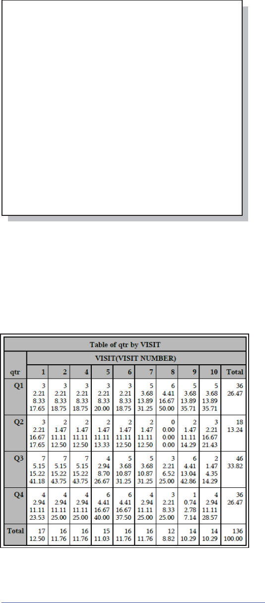
480 Carpenter’s Guide to Innovative SAS Techniques
n The compiled function is saved in
a special data set that includes a
packet, which in this case is named
TMP.
o The FUNCTION statement names
the function, lists its arguments in
parentheses and, if it is to return a
character value, includes the $
before the semicolon.
p Use the YYQ. format to translate
the date into a quarter.
q The third character will be a ‘Q’
if the date was successfully
translated using the YYQ. format.
r Use the RETURN statement to
specify the value to be returned by
the function. The SUBSTR function is used to strip off the year (YY) portion of the formatted
value.
s The date must have been missing or illegal for the YYQ. format.
t The FUNCTION statement always ends with the ENDSUB statement.
u The CMPLIB option is used to point to the data set that contains the TMP ‘packet’ that holds
the function definition.
v A new character variable (QTR)
with a length of $2 is created using
the QNUM function. The lab date is
passed into the function as the single
argument.
w The new variable is used in the
TABLE statement.
MORE INFORMATION
A variation on the QNUM function
is discussed in Section 12.5.5, and a
simplified form can be found in
Section 15.2.2.
SEE ALSO
An example of a function that calls a macro that contains a PROC FREQ can be found at
http://tech.groups.yahoo.com/group/sas_academy/message/438. A FCMP CALL routine is
created at
proc fcmp outlib=work.myfuncs.tmp; n
function qnum(date) $; o
length yyq4 $4;
yyq4=put(date,yyq4.); p
if substr(yyq4,3,1)='Q' q
then return(substr(yyq4,3,2)); r
else return(yyq4); s
endsub; t
run;
options cmplib=(work.myfuncs); u
data qlabs;
set advrpt.lab_chemistry
(keep=subject labdt);
qtr=qnum(labdt); v
run;
title2 'Quarters without years';
proc freq data=advrpt.lab_chemistry;
table qtr*visit; w
run;
&DUSHQWHU$UW&DUSHQWHU¶V*XLGHWR,QQRYDWLYH6$67HFKQLTXHV&RS\ULJKW6$6,QVWLWXWH,QF&DU\1RUWK&DUROLQD86$
$
//5,*+765(6(59(')RUDGGLWLRQDO6$6UHVRXUFHVYLVLWVXSSRUWVDVFRPSXEOLVKLQJ

Chapter 15: Miscellaneous Topics 481
http://tech.groups.yahoo.com/group/sas_academy/message/430. A function is used to calculate a
person’s societal age at http://support.sas.com/kb/36/788.html. PROC FCMP is used to create an
INFORMAT that converts a fraction to a decimal value in a sasCommunity tip by Mike Zdeb
http://www.sascommunity.org/wiki/Tips:Create_an_Informat_from_a_User-Defined_Function.
15.2.2 Storing and Accessing Your Functions
The OUTLIB option on the PROC statement is used to name a storage location for your function.
The function is stored in a special SAS data set. You cannot use this data set to also store data nor
can you store a function in an existing data set.
From an operational perspective it makes sense to organize the storage of your functions. All the
functions associated with the ADVRPT project might be stored in the ADVRPT.FUNCTIONS
data set. Those functions dealing with dates could be stored in the DATES packet.
The OUTLIB option specifies the libref (ADVRPT), data set (FUNCTIONS), and the packet
(DATES). Function names are unique within a packet but not necessarily across packets. A given
packet can contain multiple function
definitions, and a given data set can
contain multiple packets.
When you want to use a compiled function, the CMPLIB system option is used. This option
specifies one or more SAS data sets that contain the packets defined by PROC FCMP. The packet
is not specified, and all packets within the
data set are made available.
In the example in Section 15.2.1 the data set MYFUNCS is written to the non-permanent work
directory. Here we want to create a
more permanent version of this
simplified version of the QNUM
function. The function QNUM is
added to the DATES packet in the
permanent data set
ADVRPT.FUNCTIONS.
We may want to add some other functions to this same data set. Here a new packet
(CONVERSIONS) is added
to the
ADVRPT.FUNCTIONS data
set, and we define two
functions in one call to the
FCMP procedure. These two
functions convert from
degrees centigrade to
Fahrenheit (C2F) and from
Fahrenheit to centigrade
(F2C).
Later we can add more
conversion functions. Here
we add functions to calculate
the Body Mass Index (BMI)
using both Imperial and
Metric units.
proc fcmp outlib=AdvRpt.functions.Dates;
function . . . .
options cmplib=(advrpt.functions);
proc fcmp outlib=advrpt.functions.dates;
function qnum(d) $;
return(cats('Q',qtr(d)));
endsub;
run;
proc fcmp outlib=Advrpt.functions.Conversions;
function c2f(c);
return(((9*c)/5)+32);
endsub;
function f2c(f);
return((f-32)*5/9);
endsub;
run;
proc fcmp outlib=AdvRpt.functions.Conversions;
function E_BMI(h,w);
return((w * 703)/(h*h) );
endsub;
function M_BMI(h,w);
return(w /(h*h));
endsub;
run;
&DUSHQWHU$UW&DUSHQWHU¶V*XLGHWR,QQRYDWLYH6$67HFKQLTXHV&RS\ULJKW6$6,QVWLWXWH,QF&DU\1RUWK&DUROLQD86$
$
//5,*+765(6(59(')RUDGGLWLRQDO6$6UHVRXUFHVYLVLWVXSSRUWVDVFRPSXEOLVKLQJ

482 Carpenter’s Guide to Innovative SAS Techniques
It is likely that you will have a number of functions stored in several data sets. To make all of
these functions available each of the data sets must be listed on the CMPLIB= system option.
Here two data sets are listed.
All the functions in all the
packets in both of these data
sets will be available for use. The exception will be for multiple functions with the same name.
Unlike most library searches, the search order across multiple function libraries is from right to
left. In the example shown here functions in WORK.MYFUNCS will be found first. The packet is
not named in the CMPLIB option; consequently, if the same function name is used in two
different packets within the same data set, it will be harder to anticipate which will be used. I
would recommend that function names be unique within data set.
15.2.3 Interaction with the Macro Language
Functions and routines created using PROC FCMP are typically called from within a DATA step;
however, they may also be called from within the macro language by using the macro function
%SYSFUNC and the macro statement %SYSCALL.
It is also possible to call or execute a macro from within the function or routine by using the
RUN_MACRO function. The following rather silly example demonstrates some of the issues
when calling a macro from within a function or routine.
n The SUBROUTINE
statement declares this as the
routine’s definition. Like with
the FUNCTION statement the
routine is named. Character
argument names are followed by
a $.
o The first argument of the
RUN_MACRO function is the
name of the macro to be called.
The remaining arguments are the
parameters for that macro.
p The positional macro
parameters are not named on the
%MACRO statement. The
parameter names will flow from
the RUN_MACRO function on
through to the macro %PRINTIT
o.
q The values of the macro
parameters arrive quoted. Since
we need them to be unquoted in the application shown here, the DEQUOTE function is called.
r TITLE2 will be displayed when the PROC PRINT executes. Although the TITLE1 statement
will have been executed u, within the domain available to the compiled routine its definition is
not available, and will, therefore, remain undefined.
s The PROC PRINT within the macro %PRINTIT is constructed using the macro parameters.
t The function library is specified.
proc fcmp outlib=advrpt.functions.utilities;
subroutine prntcrit(dsn$,kvar $,cvar $); n
rc=run_macro('printit',dsn,kvar,cvar); o
endsub;
run;
%macro printit(); p
%let dsn = %sysfunc(dequote(&dsn)); q
%let kvar = %sysfunc(dequote(&kvar));
%let cvar = %sysfunc(dequote(&cvar));
title2 "&dsn"; r
proc print data=advrpt.&dsn; s
%if &kvar ne %then id &kvar;;
%if &cvar ne %then var &cvar;;
run;
%mend printit;
options cmplib=(advrpt.functions); t
title1 '15.2.3 Macro Language Interface'; u
data _null_;
set advrpt.dsncontrol;
call prntcrit(dsn,keyvars,critvars); v
put 'Print ' dsn keyvars critvars;
run;
proc print data=advrpt.dsncontrol; w
run;
options cmplib=(advrpt.functions work.myfuncs);
&DUSHQWHU$UW&DUSHQWHU¶V*XLGHWR,QQRYDWLYH6$67HFKQLTXHV&RS\ULJKW6$6,QVWLWXWH,QF&DU\1RUWK&DUROLQD86$
$
//5,*+765(6(59(')RUDGGLWLRQDO6$6UHVRXUFHVYLVLWVXSSRUWVDVFRPSXEOLVKLQJ

Chapter 15: Miscellaneous Topics 483
u TITLE1 is defined before the DATA step that will call the routine; however, this title will not
be available to the macro executed by the PRNTCRIT routine.
v The PRNTCRIT routine is called using three variables from the ADVRPT.DSNCONTROL
data set. The variables in the routine call must be in the same order as they are defined o. The
PRNTCRIT routine is called for each observation on the incoming data set. The routine calls and
executes the macro %PRINTIT. Unlike the CALL EXECUTE routine. which pushes the macro
call to a stack, %PRINTIT will be executed immediately.
w The TITLE1 will be honored, but the TITLE2 will be undefined.
Because functions and routines are compiled, we cannot use a macro call directly within the
function definition. If we had attempted to specify the macro call directly as shown here,
%PRINTIT would have executed while the PRNTCRIT routine was being compiled. Macro calls
such as this one would be used
to generate routine or function
code. Macros that are to be
executed during function
execution should be specified
with the RUN_MACRO function as was shown above.
MORE INFORMATION
The DEQUOTE function is introduced in Section 3.6.7.
SEE ALSO
Chapter 8 in Carpenter’s Complete Guide to the SAS® Macro Language, 2nd Edition (Carpenter,
2004) discusses the use of macros and macro variables within the context of compiled code.
15.2.4 Viewing Function Definitions
User-defined functions do not appear in the SASHELP.VFUNC view or in the
DICTIONARY.FUNCTIONS table. However, under Windows you can see both the list of
available functions and their attributes through the use of the FCMP Function Editor.
To start this editor, go to SOLUTIONS ĺ ANALYSIS ĺ FCMP FUNCTION EDITOR. The
list of available data sets and the functions that they contain is shown in the left pane. Selecting a
function brings up the editor dialog box, which allows you to see the details of the function’s
definition.
proc fcmp outlib=advrpt.functions.utilities;
subroutine prntcrit(dsn$,kvar $,cvar $);
%printit(dsn,kvar,cvar);
. . . . .
&DUSHQWHU$UW&DUSHQWHU¶V*XLGHWR,QQRYDWLYH6$67HFKQLTXHV&RS\ULJKW6$6,QVWLWXWH,QF&DU\1RUWK&DUROLQD86$
$
//5,*+765(6(59(')RUDGGLWLRQDO6$6UHVRXUFHVYLVLWVXSSRUWVDVFRPSXEOLVKLQJ
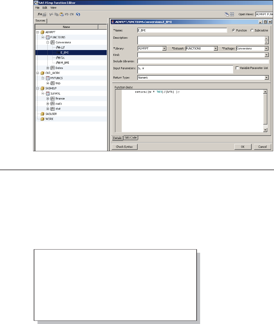
484 Carpenter’s Guide to Innovative SAS Techniques
15.2.5 Removing Functions
Although functions and routines are stored in data sets, you cannot use standard data management
techniques to delete an instance of a function or a routine. Fortunately the FCMP procedure
comes with the DELETEFUNC and DELETESUBR statements that can be used for this purpose.
For the purposes of this example let us assume that a version of the function START has been
stored in two different locations (two different data sets). The search order for multiple data sets is
from right to left (this is the opposite order for searches across libraries, e.g., formats, autocall).
The START function is to be written so that it will return the first date of the specified interval
type.
n A temporary location is
set up to hold the START
function. Unfortunately
this function has been
specified incorrectly using
the INTCK function and
will fail.
o The permanent data set
to collect functions in the
DATES packet is
specified.
p The correct version of START, which uses the INTNX function, is stored in the permanent
location.
proc fcmp outlib=work.funcs.dates; n
function start(int$,date);
return(intck(int,date,0,'b'));
endsub;
run;
proc fcmp outlib=advrpt.functions.dates; o
function start(int$,date);
return(intnx(int,date,0,'b')); p
endsub;
run;
options cmplib=(advrpt.functions work.funcs ); q
&DUSHQWHU$UW&DUSHQWHU¶V*XLGHWR,QQRYDWLYH6$67HFKQLTXHV&RS\ULJKW6$6,QVWLWXWH,QF&DU\1RUWK&DUROLQD86$
$
//5,*+765(6(59(')RUDGGLWLRQDO6$6UHVRXUFHVYLVLWVXSSRUWVDVFRPSXEOLVKLQJ

Chapter 15: Miscellaneous Topics 485
q The CMPLIB option specifies that the WORK.FUNCS data set will be searched first, and this
means that the bad version of the START function n will be found and used.
We need to have the ability to remove the bad definition of START from
WORK.FUNCS.DATES. This can be
done using the DELETEFUNC statement.
r PROC FCMP is called with the
OUTLIB option pointing to the packet
containing the bad definition of START.
s The DELETEFUNC statement can then be used to delete the specific function.
Using the function libraries defined above q, the version of START in
ADVRPT.FUNCTIONS.DATES will now
be the only version available.
t The first day of the year that contains the
date stored in D is returned by the function
START.
u The START function returns the first
day of the month that contains the date in
D.
MORE INFORMATION
You can also delete functions and routines by using the FCMP Function Editor (see Section
15.2.4).
15.3 Reading RTF as Data
RTF is a proprietary document file format developed by Microsoft Corporation in the late 1980s.
Unlike an MS Word .DOC binary file, an RTF file can be read by text editors. This means that if
we treat an RTF file as text, we can use SAS to read and write the RTF file as data, and this opens
the door for the power and flexibility associated with the use of the SAS DATA step and the SAS
macro language.
The example shown in this section modifies a CONsolidated Standards Of Reporting Trials,
CONSORT, flow diagram by filling in the blanks.
SEE ALSO
These specific examples are presented in more detail in Carpenter and Fisher (2011).
proc fcmp outlib=work.funcs.dates; r
deletefunc start; s
run;
data list;
do d = '01jan2010'd to '05feb2010'd;
styr = start('year',d); t
stmo = start('month',d); u
output;
end;
format d styr stmo date9.;
run;
&DUSHQWHU$UW&DUSHQWHU¶V*XLGHWR,QQRYDWLYH6$67HFKQLTXHV&RS\ULJKW6$6,QVWLWXWH,QF&DU\1RUWK&DUROLQD86$
$
//5,*+765(6(59(')RUDGGLWLRQDO6$6UHVRXUFHVYLVLWVXSSRUWVDVFRPSXEOLVKLQJ
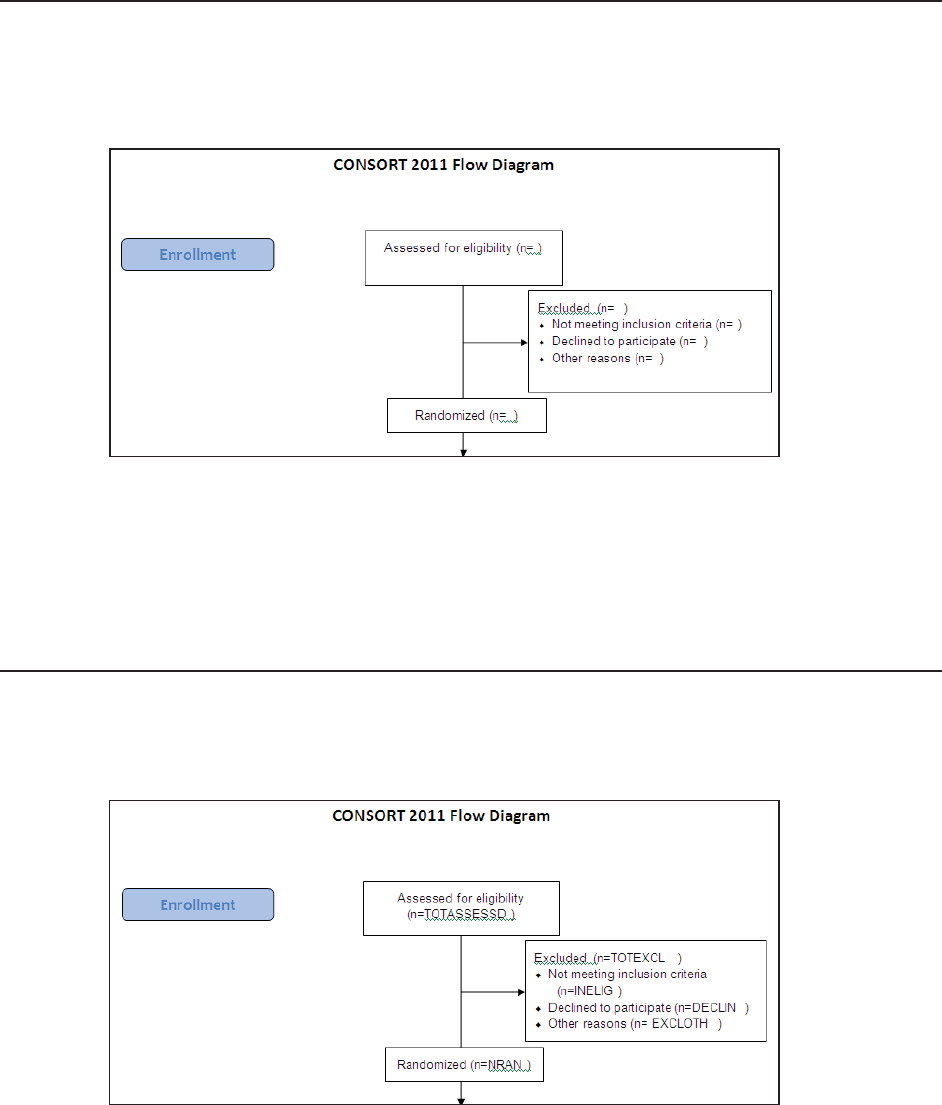
486 Carpenter’s Guide to Innovative SAS Techniques
15.3.1 RTF Diagram Completion
The layout of the CONSORT table depends on the study design. This includes the number of
ARMS and the phases of the study. The techniques discussed in this section, however, are
completely independent of the study design. The first step in this process is to create a template
form of the CONSORT table. This RTF table will contain all the needed information with blank
fields. This
figure shows the
“Enrollment”
portion of a
CONSORT
table, which will
show the
number of
subjects and
their status
relative to the
study. Typically
the N= values
would be filled
in by hand once they had been determined.
The RTF CONSORT table can easily have over a dozen fields that require completion. In the
process described below, each field will be assigned a code unique to the table. The entire table
(RTF file) will then be read as data and the codes will be translated into the final values through
the use of DATA step functions. The resulting modified table will be rewritten, again as an RTF
file, where it will then be available for use by a word processor.
15.3.2 Template Preparation
The template is prepared for use by SAS by filling in each of the individual fields using unique
codes. Here the unique codes for the first six fields are TOTASSESSD, TOTEXCL, INELIG,
DECLIN, EXCLOTH, and NRAN. For our purposes we are assuming that these names never
occur otherwise
in the table.
Other than
being unique,
the code that
you choose is
unimportant, but
for a more
complicated
table the field
code names can
be used to help
make sure that
the values are
inserted in the correct location.
&DUSHQWHU$UW&DUSHQWHU¶V*XLGHWR,QQRYDWLYH6$67HFKQLTXHV&RS\ULJKW6$6,QVWLWXWH,QF&DU\1RUWK&DUROLQD86$
$
//5,*+765(6(59(')RUDGGLWLRQDO6$6UHVRXUFHVYLVLWVXSSRUWVDVFRPSXEOLVKLQJ
Chapter 15: Miscellaneous Topics 487
15.3.3 RTF as Data
Fortunately we need to know very little about RTF code in order to work with it using SAS. A
quick look at a portion of the RTF code that generated the figure shown in the previous section
shows a text language which is mostly not human readable. However, a closer inspection shows
one of our designated keywords (DECLIN).
Our approach will be to have SAS read the RTF text strings, find the appropriate codes, replace
the codes with the values of interest, and then replace the modified RTF text strings. The search
and replace operations will be handled by using the TRANSTRN function, which replaces all
occurrences of the second argument with the third argument. For our purposes there should only
be one occurrence for each of our codes.
The DATA step used to read and write the RTF CONSORT table is fairly straightforward. RTF
does not have a fixed
maximum record length;
however, the length is
generally under 500
characters. Here the
LRECL is set to 3000 –
just in case. The incoming
RTF file is designated by
the fileref CONFFILE1.
The new version of the
CONSORT table is
written to the file named
in the CONFILE2 fileref.
Through the use of the
automatic variable
_INFILE_ we read each RTF line as an entire entity. This string is then searched and the
appropriate codes are replaced. In this example the TRANSTRN function replaces the text
‘TOTASSESSED’ with the appropriate number, which we have provided (345). In the figure to
the left we can
see that the
placeholder
codes that we
used in the
template
version of the
table have
been replaced
with the values
supplied in the
SAS program.
In the paper
cited above,
(Carpenter and Fisher, 2011) macro code is shown that provides an automated metadata driven
coding solution.
\par }{\rtlch\fcs1 \af0\afs16 \ltrch\fcs0 \f3\fs16\lang0\langfe1033\langnp0
\fs16\lang4105\langfe1033\langnp4105\insrsid4260155\charrsid1516310 }{\rt
\f1\fs20\lang4105\langfe1033\langnp4105\insrsid1909421 DECLIN}{\rtlch\fcs1
\par }{\rtlch\fcs1 \af0\afs16 \ltrch\fcs0 \f3\fs16\lang0\langfe1033\langnp0
filename confile1 "C:\temp\CONSORT_Diagram1.rtf";
filename confile2 "C:\temp\CONSORT_Diagram2.rtf";
data _null_;
infile confile1 lrecl=3000;
input;
_infile_ = transtrn(_infile_,'TOTASSESSED','345');
_infile_ = transtrn(_infile_,'TOTEXCL', '56');
_infile_ = transtrn(_infile_,'INELIG', '35');
_infile_ = transtrn(_infile_,'DECLIN', '17');
_infile_ = transtrn(_infile_,'EXCLOTH', '4');
_infile_ = transtrn(_infile_,'NRAN', '289');
file confile2 lrecl=3000;
put _infile_;
run;
&DUSHQWHU$UW&DUSHQWHU¶V*XLGHWR,QQRYDWLYH6$67HFKQLTXHV&RS\ULJKW6$6,QVWLWXWH,QF&DU\1RUWK&DUROLQD86$
$
//5,*+765(6(59(')RUDGGLWLRQDO6$6UHVRXUFHVYLVLWVXSSRUWVDVFRPSXEOLVKLQJ
488
&DUSHQWHU$UW&DUSHQWHU¶V*XLGHWR,QQRYDWLYH6$67HFKQLTXHV&RS\ULJKW6$6,QVWLWXWH,QF&DU\1RUWK&DUROLQD86$
$
//5,*+765(6(59(')RUDGGLWLRQDO6$6UHVRXUFHVYLVLWVXSSRUWVDVFRPSXEOLVKLQJ

Appendix A
Topical Index
Topic Primary Description in: Also appears in:
Across observations, processing 3.1
Age calculation 3.2
Annotate facility introduction 9.4
CSV files; import/export 1.2.4 1.4.2
DATA Step Component Objects (see HASH)
Delimited Files; import/export 1.3, 1.4
Display Manager Customizations 14.3.2
Adding tool bar tools 14.4.5
Adding function keys 14.4.6
DOW loop 3.9.1 2.9.3, 3.3.4, 3.6.2, 3.8.1,
3.9.3, 3.10.3, 6.4, 6.7.2,
6.7.3, 7.4.3
Duplicates, elimination of 2.9
E-mail SAS results 14.5
Engines; on the LIBNAME statement 1.1 1.6.2
Engines: on the FILENAME statement 2.6.3
Enhanced Editor Customizations 14.4.3
Macro Abbreviations 14.4.4
EXCEL 1.1 1.2.5
Named Range 1.2.5
Writing Reports 11.2
FIFO Stack 3.1.7
FIRST. and LAST. Processing 3.1.1 2.9.2, 3.1.7
Format Modifiers 1.3.1
Formats, PRELOADED (see Preloaded)
(continued)
&DUSHQWHU$UW&DUSHQWHU¶V*XLGHWR,QQRYDWLYH6$67HFKQLTXHV&RS\ULJKW6$6,QVWLWXWH,QF&DU\1RUWK&DUROLQD86$
$
//5,*+765(6(59(')RUDGGLWLRQDO6$6UHVRXUFHVYLVLWVXSSRUWVDVFRPSXEOLVKLQJ

490 Carpenter’s Guide to Innovative SAS Techniques
Topic Primary Description in: Also appears in:
Formats, User-defined Chapter 12 2.6.2, 3.6.6, 6.5, 6.7.3,
7.1.2, 8.1.1, 8.1.5
Formats, Building from data 12.7 6.5, 6.7.3, 12.3.2
Functions, user-defined
DATA step 15.2 12.5.5
Macro 13.7
Fuzzy Merge 3.3.1, 3.7.4
Hash Objects 3.3 2.9.5, 6.8
Hyperlinks, creating 11.4
Initializing a SAS Session 14.1.1 14.1.3
Autoexec 14.2 14.1.1
Configuration 14.3 14.1.1
Display Manager 14.3.2
In-line Formatting 11.3 8.4.6
LAST. (see FIRST. Processing)
Libraries, formats 12.9.3
Libraries, functions 15.2.2 12.5.5
Libraries, macro 13.4
Look-ahead, Look-back reads 3.1 3.8.1
MEANS/SUMMARY, using Chapter 7
Understanding _TYPE_ 7.5
Metadata 13.5, 13.8.3
Missing values 2.10
Moving Average calculation 3.1.7, 12.3.2
Password Protection 2.1.2, 5.4.2, 13.9 5.4.1
Preloaded Formats 12.1 2.5.5
Program Generalization 13.3
Quoting 2.6.3 13.12
SET, using double SET statements 3.8.4 3.8.1, 3.1.5, 3.1.6, 3.8.1,
3.10.3, 6.4, 7.4.3
SQL: Generating macro variables 2.3.3, 13.5.1, 13.5.2,
13.6, 13.8.1, 13.8.3
SQL: Joining tables 3.7.4 6.3
SQL: Pass Through 1.5, 5.4.2
Sparse Data, Creating 2.5
Style Overrides 8.1.3
Table Lookup Techniques Chapter 6
Traffic Lighting 11.5
Transposing data 2.4
XML 1.6
&DUSHQWHU$UW&DUSHQWHU¶V*XLGHWR,QQRYDWLYH6$67HFKQLTXHV&RS\ULJKW6$6,QVWLWXWH,QF&DU\1RUWK&DUROLQD86$
$
//5,*+765(6(59(')RUDGGLWLRQDO6$6UHVRXUFHVYLVLWVXSSRUWVDVFRPSXEOLVKLQJ

Appendix B
Usage Index
Of all the procedures, statements, and options discussed in this book, only those that are of note
specifically to the techniques described in this book are listed in this Appendix.
Global Statements and Options 492
Statements, Global 492
Macro Language 493
GOPTIONS, Graphics 493
Options, System 493
Options, Data Set 495
Procedures: Steps, Statements, and Options 495
Procedures 495
DATA Step: Statements and Options 500
Statements, DATA Step 500
Format Modifiers 501
Functions 501
Hash Object 504
Output Delivery System, ODS 504
ODS Destinations and Tagsets 504
ODS Attributes 505
ODS Options 505
ODS Statements 506
SAS Display Manager 506
Display Manager Commands 506
&DUSHQWHU$UW&DUSHQWHU¶V*XLGHWR,QQRYDWLYH6$67HFKQLTXHV&RS\ULJKW6$6,QVWLWXWH,QF&DU\1RUWK&DUROLQD86$
$
//5,*+765(6(59(')RUDGGLWLRQDO6$6UHVRXUFHVYLVLWVXSSRUWVDVFRPSXEOLVKLQJ

492 Carpenter’s Guide to Innovative SAS Techniques
Global Statements and Options
Statements, Global
Statements, Options Primary Description in: Also Appears in:
AXIS 9.3.2 10.1.1, 10.1.2, 10.1.3, 10.2.3
LABEL 9.3.2 10.1.1, 10.1.2, 10.2.3
MAJOR 9.3.2 10.1.1
MINOR 9.3.2 10.1.2, 10.1.3
ORDER 9.3.2 1.2, 10.1.3, 10.2.2
REFLABEL 10.2.2
VALUE 9.3.2 10.1.2, 10.1.3, 10.2.2
DM 14.4.2 2.6.3, 14.1.1, 14.1.3
FILENAME 2.6.3, 5.4.1, 9.2, 11.4.3, 13.9.1,
4.2, 15.3.3
CATALOG 13.9.1 14.6.4
EMAIL 14.5
ATTACH 14.5
FROM 14.5
SUBJECT 14.5
TO 14.5
EXCEL 1.6.2
PIPE 15.1.3 2.6.3
LEGEND 9.3.2
ACROSS 9.3.2
FRAME 9.3.2
LABEL 9.3.2
SHAPE 9.3.2
VALUE 9.3.2
LIBNAME 1.1.1, 1.1.3, 1.2.5, 10.2.1, 14.2
Concatenated libraries 12.9.3
SCAN_TEXT 1.1.3 1.1.4
V9 14.2
SYMBOL 9.3.1 10.1.1, 10.1.2, 10.1.3, 10.2.1,
10.2.2
SYSTASK COMMAND 15.1.3
TITLE 9.1 10.2.2, 10.2.4, 11.3.3, 11.3.5
BOLD 9.1
BCOLOR 9.1
#BYLINE 15.1.2
#BYVAL 15.1.2 7.4.3, 11.3.1
#BYVAR 15.1.2 11.3.1
COLOR 9.1 11.4.4
(continued)
&DUSHQWHU$UW&DUSHQWHU¶V*XLGHWR,QQRYDWLYH6$67HFKQLTXHV&RS\ULJKW6$6,QVWLWXWH,QF&DU\1RUWK&DUROLQD86$
$
//5,*+765(6(59(')RUDGGLWLRQDO6$6UHVRXUFHVYLVLWVXSSRUWVDVFRPSXEOLVKLQJ

Appendix B: Usage Index 493
Statements, Global (continued)
Statements, Options Primary Description in: Also Appears in:
TITLE (continued)
FONT 9.1 10.2.2, 10.2.4
HEIGHT 9.1 10.2.2, 11.3.1
ITALIC 9.1
JUSTIFY 9.1 10.2.2
LINK 11.4.2 11.4.4
UNDERLINE 9.1
X 15.1.3
Macro Language
Statements and Options Primary Description in: Also Appears in:
IN operator (#) 13.10
%LOCAL 13.1 13.7, 13.8.2, 14.6.4
MINDELIMITER 13.10.3
MINOPERATOR 13.10.2
SECURE 13.9.1
SOURCE 13.9.1
STORE 13.9.1
%SYSEXEC 15.1.3 14.4.7
GOPTIONS, Graphics
Graphics option Primary Description in: Also appears in:
BORDER 9.2 10.2.3, 10.2.4, 11.4.3
DEVICE 8.2.1 9.2, 10.2.3, 10.2.4, 11.4.3
FTEXT 9.2 10.2.3, 10.2.4, 11.4.3
GSFNAME 8.2.1 9.2, 11.4.3
GSFMODE 10.2.3
HTEXT 9.2 11.4.3
RESET 9.2 9.3.1, 10.2.3, 10.2.4, 11.4.3
TARGETDEVICE 9.2
XPIXELS 10.2.4
YPIXELS 10.2.4
Options, System
Option Primary Description in: Also Appears in:
in general 14.1
CENTER 14.2
CMPLIB 12.5.5, 15.2.2 15.2.3
CPUCOUNT 4.5
DATASTMTCHK 14.1.2
DATE 14.2
EMAILHOST 14.5
(continued)
&DUSHQWHU$UW&DUSHQWHU¶V*XLGHWR,QQRYDWLYH6$67HFKQLTXHV&RS\ULJKW6$6,QVWLWXWH,QF&DU\1RUWK&DUROLQD86$
$
//5,*+765(6(59(')RUDGGLWLRQDO6$6UHVRXUFHVYLVLWVXSSRUWVDVFRPSXEOLVKLQJ

494 Carpenter’s Guide to Innovative SAS Techniques
Options, System (continued)
Option Primary Description in: Also Appears in:
EMAILID 14.5
EMAILPORT 14.5
EMAILSYS 14.5
FMTERR 2.3.1
FMTSEARCH 12.9.2 12.9.3
initialization 14.1.1
ALTLOG 14.1.1
AUTOEXEC 14.1.1
AWSCONTROL 14.3.2
AWSTITLE 14.3.2
CONFIG 14.1.1 14.3.1
INITCMD 14.3.2
INITSTMT 14.1.1
RTFCOLOR 14.1.1
SASINITIALFOLDER 14.1.1
SPLASHLOC 14.1.1
SYSIN 14.1.1
SYSPARM 14.1.1
TERMSTMT 14.1.1
VERBOSE 14.3.1
MAUTOLOCDISPLAY 13.4.1
MAUTOSOURCE 13.4.1 13.4.2
MCOMPILE 13.9.2
MERGENOBY 14.1.2
MFILE 13.11
MINDELIMITER 13.10.3
MINOPERATOR 13.10.2
MISSING 2.10.2
MLOGIC 13.8.2
MLOGICNEST 13.11
MPRINT 13.8.2, 13.9.1
MPRINTNEST 13.11
MREPLACE 13.9.2
MSGLEVEL 5.3.2
NOWORKINIT 14.1.1
NOWORKTERM 14.1.1
NUMBER 14.2
SASAUTOS 13.4.1 13.4.2, 14.2, 14.3.1
SORTEQUALS 4.1.6
SYMBOLGEN 13.8.2
THREADS 4.5
VALIDVARNAME 14.1.2 1.2.3
XMIN 15.13
XSYNC 15.13
XWAIT 15.13
&DUSHQWHU$UW&DUSHQWHU¶V*XLGHWR,QQRYDWLYH6$67HFKQLTXHV&RS\ULJKW6$6,QVWLWXWH,QF&DU\1RUWK&DUROLQD86$
$
//5,*+765(6(59(')RUDGGLWLRQDO6$6UHVRXUFHVYLVLWVXSSRUWVDVFRPSXEOLVKLQJ

Appendix B: Usage Index 495
Options, Data Set
Option Primary Description in: Also Appears in:
ALTER 2.1.2 5.4.2
DROP 2.1.3 5.1
ENCRYPT 2.1.2 5.4.2
FIRSTOBS 2.1.4 3.1.4, 3.1.5
KEEP 2.1.3 2.1, 2.3.2, 3.1.4, 3.1.5, 4.2, 5.2,
11.1.2, 12.7, 13.5.2
IDXNAME 5.3.4
IDXWHERE 5.3.4
IN 3.8.2, 3.7.1
INDEX 5.3.2
OBS 2.1.4 8.5.2
PW 2.1.2
PWREQ 2.1.2 5.4.2
READ 2.1.2 5.4.2
RENAME 2.1.3 3.1.4, 3.1.5, 3.7.2, 5.1, 6.4, 12.7
REPEMPTY 2.1.1
REPLACE 2.1.1
SORTEDBY 4.4
WHERE 2.1.3, 2.1.4d, 2.2.2, 3.7.2, 5.1,
7.7, 7.8, 11.5.3, 13.2.3, 13.6,
14.1.1
WRITE 2.1.2 5.4.2
Procedures: Steps, Statements, and Options
Procedures
Statements and Options Primary Description in: Also Appears in:
In general (across procedures)
CLASS 7.1 7.1.2, 8.2.2
DESCENDING 7.1.1
GROUPINTERNAL 7.1.2
MISSING 7.1.1
ORDER 7.1.3
EXCLUSIVE 12.1
MISSING 2.10.5, 7.1.1
ORDER 2.6.2, 8.1.5 2.5.5, 8.4.5
PRELOADFMT 12.1 2.5.5
BOXPLOT 10.1.1
(continued)
&DUSHQWHU$UW&DUSHQWHU¶V*XLGHWR,QQRYDWLYH6$67HFKQLTXHV&RS\ULJKW6$6,QVWLWXWH,QF&DU\1RUWK&DUROLQD86$
$
//5,*+765(6(59(')RUDGGLWLRQDO6$6UHVRXUFHVYLVLWVXSSRUWVDVFRPSXEOLVKLQJ

496 Carpenter’s Guide to Innovative SAS Techniques
Procedures (continued)
Statements and Options Primary Description in: Also Appears in:
CATALOG
CONTENTS 12.9.3
COPY 13.9.2
ENTRYTYPE 13.9.2
DELETE 13.9.2
FORCE 13.9.2
SELECT 13.92
COMPARE 5.1
COMPARE 5.1
OUT 5.1
OUTBASE 5.1
OUTCOMP 5.1
OUTNOEQUAL 5.1
CONTENTS 2.6.1, 5.3.1, 13.8.3
_ALL_ 13.8.3
OUT 13.8.3
NOPRINT 13.8.3
VARNUM 2.6.1
DATASETS 2.6.1
AGE 5.6.2
CHANGE 5.6.2
CONTENTS 2.6.1
DELETE 5.5
INDEX CREATE 5.3.2 5.3.3, 6.6
INDEX DELETE 5.3.2 5.3.3
KILL 5.5 14.4.5
MODIFY 5.3.2 2.6.1, 5.3.3, 6.6
NOLIST 5.5 5.6.2, 6.6
DELETE 5.5
EXPORT 1.2 1.4.2, 11.2.2
SHEET 1.2.3 1.2.1, 11.2.2
FCMP 15.2 12.5.5
DELETEFUNC 15.2.5
ENDSUB 15.2.1 12.5.5
FUNCTION 15.2.1 12.5.5
OUTLIB 15.2.2
RETURN 15.2.1 12.5.5
RUN_MACRO 15.2.3
SUBROUTINE 15.2.3
(continued)
&DUSHQWHU$UW&DUSHQWHU¶V*XLGHWR,QQRYDWLYH6$67HFKQLTXHV&RS\ULJKW6$6,QVWLWXWH,QF&DU\1RUWK&DUROLQD86$
$
//5,*+765(6(59(')RUDGGLWLRQDO6$6UHVRXUFHVYLVLWVXSSRUWVDVFRPSXEOLVKLQJ

Appendix B: Usage Index 497
Procedures (continued)
Statements and Options Primary Description in: Also Appears in:
FORMAT 2.6.2, 3.6.6
CNTLIN 12.7 6.5, 6.7.3, 12.3.2
CNTLOUT 12.7
DEFAULT 12.5.4, 12.5.5
formats as labels 12.5.1 12.5.2, 12.5.3, 12.8
functions as labels 12.5.5
INVALUE 12.5.3
LIBRARY 12.9.3
NOTSORTED 12.4
MULTILABEL 12.3
PICTURE 12.2
DATATYPE 12.2.1
directives 12.2.1
MULT 12.2.3
PREFIX 12.2.3
ROUND 12.2.2
REGEXPE 12.5.4
_SAME_ 12.5.4
VALUE 12.7 2.6.2, 3.6.6, 7.1.2, 8.1.1, 8.1.5,
11.3.4, 11.3.5, 11.4.4, 11.5.1,
11.5.2, 12.1, 12.8
FREQ 8.3 2.5.6, 2.9.4, 10.3
NLEVELS 8.3.2
OUTPUT 8.3.1
ALL 8.3.1
SPARSE 2.5.6
TABLE
_ALL_ 8.3.2
CHISQ 8.3.1
PLOTS 10.3
GFONT 10.2.1
GKPI 10.2.4
GPLOT 10.1.2
IMPORT 1.2 14.1.2
DATAROW 1.2.3
DBMS 14.1.2
GETNAMES 1.2.3 1.2.5, 14.1.2
GUESSINGROWS 1.2.3
MIXED 1.2.3 14.1.2
RANGE 1.2.3 1.2.5
SCANTEXT 1.2.3 14.1.2
SCANTIME 14.1.2
SHEET 1.2.3 1.2.1, 14.1.2
(continued)
&DUSHQWHU$UW&DUSHQWHU¶V*XLGHWR,QQRYDWLYH6$67HFKQLTXHV&RS\ULJKW6$6,QVWLWXWH,QF&DU\1RUWK&DUROLQD86$
$
//5,*+765(6(59(')RUDGGLWLRQDO6$6UHVRXUFHVYLVLWVXSSRUWVDVFRPSXEOLVKLQJ

498 Carpenter’s Guide to Innovative SAS Techniques
Procedures (continued)
Statements and Options Primary Description in: Also Appears in:
IMPORT (continued)
TEXTSIZE 1.2.3
USEDATE 14.1.2
MEANS/SUMMARY Chapter 7 2.5.3, 2.5.4, 2.5.5, 13.3.1
CHARTYPE 7.6
CLASS
EXCLUSIVE 12.1.3
MLF 12.3.2
PRELOADFMT 12.1.3
CLASSDATA 7.9 2.5.4
COMPLETETYPES 7.10 2.5.3, 12.1.3
EXCLUSIVE 7.9
MISSING 7.1.1
NWAY 7.6, 7.7
OUTPUT 7.3 7.1
AUTONAME 7.2 5.3.3, 7.4.3
AUTOLABEL 7.2
GROUPID 7.4.2
LEVELS 7.2, 7.11
MAXID 7.4.1
MINID 7.4.1
WAYS 7.2, 7.11
TYPES 7.8
WAYS 7.7
OPTIONS 14.3.1
OPTLOAD 14.1.3
OPTSAVE 14.1.3
PRINT 8.5 11.5.4, 11.7.1
BY 8.5.1 11.5.4
ID 8.5.1 11.5.4
STYLE 8.5.2 11.5.4
PWENCODE 5.4.1
REG 9.3.1, 9.3.2, 9.4
REPORT 8.4 2.5.5, 10.2.4, 11.2.3, 11.3.1,
11.3.2, 11.3.3, 11.3.4, 11.3.5,
11.4.1, 11.5.3
absolute column reference 8.4.2 8.4.3, 8.4.5
alias specification 8.4.3 8.4.2, 8.4.5, 8.4.7, 12.1.1
CALL DEFINE 8.4.7 10.2.4, 11.4.1, 11.5.3
COMPLETECOLS 12.1
COMPLETEROWS 12.1, 12.1.1 2.5.5
(continued)
&DUSHQWHU$UW&DUSHQWHU¶V*XLGHWR,QQRYDWLYH6$67HFKQLTXHV&RS\ULJKW6$6,QVWLWXWH,QF&DU\1RUWK&DUROLQD86$
$
//5,*+765(6(59(')RUDGGLWLRQDO6$6UHVRXUFHVYLVLWVXSSRUWVDVFRPSXEOLVKLQJ

Appendix B: Usage Index 499
Procedures (continued)
Statements and Options Primary Description in: Also Appears in:
REPORT (continued)
compute block 8.4.3
CONTENTS 11.4.3
DEFINE
EXCLUSIVE 12.1.1
NOPRINT 8.4.4 8.4.6
PRELOADFMT 12.1.1
ORDER 8.4.5 8.4.8
NOZERO 8.4.8
LINE 8.4.10 8.4.6, 11.3.2, 11.3.3, 11.3.4
STYLE override 8.4.6 8.4.8, 11.5.3
SHEWHART 10.1.3
SORT 4.1
DUPOUT 4.1.2
EQUALS 4.1.6
FORCE 4.1.5
NODUPKEY 2.5.1, 6.7.1
NODUPLICATES (NODUPREC)4.1.1 2.9.1, 4.1.2, 4.4
SORTSEQ 4.1.4
TAGSORT 4.1.3
SQL 1.5 2.8.1, 2.9.3, 3.7.4, 5.2, 5.4.2,
11.2.2, 11.2.3, 11.4.1, 11.4.3,
13.5.1, 13.5.2
CONNECT 1.5.1 5.4.2
CREATE INDEX 5.3.2 5.3.3
DESCRIBE 13.8.1
DISCONNECT 1.5.1 5.4.2
DISTINCT 2.9.3
DROP TABLE 5.5
ORDER BY 2.9.3
UNION 2.8.1
WHERE 2.2.2
TABULATE 8.1 11.4.4, 11.5.2
CLASS 8.1.1 11.5.2
EXCLUSIVE 12.1.2
MLF 12.3.1
PRELOADFMT 12.1.2
CLASSDATA 8.1.4
CLASSLEV 8.1.3 11.4.4
EXCLUSIVE 8.1.4
KEYLABEL 8.1.1
KEYWORD 8.1.3
ORDER 8.1.5
TABLE 8.1.1 11.5.2
(continued)
&DUSHQWHU$UW&DUSHQWHU¶V*XLGHWR,QQRYDWLYH6$67HFKQLTXHV&RS\ULJKW6$6,QVWLWXWH,QF&DU\1RUWK&DUROLQD86$
$
//5,*+765(6(59(')RUDGGLWLRQDO6$6UHVRXUFHVYLVLWVXSSRUWVDVFRPSXEOLVKLQJ

500 Carpenter’s Guide to Innovative SAS Techniques
Procedures (continued)
Statements and Options Primary Description in: Also Appears in:
TABULATE (continued)
BOX 8.1.1 8.1.3, 12.3.1
MISSTEXT 8.1.1
percentages 8.1.2
PRINTMISS 12.1.2
RTS 8.1.3
VAR 8.1.1 11.5.2
TRANSPOSE 2.4.1 2.5.2, 3.6.5, 5.1
UNIVARIATE 8.2 11.1.1, 11.1.2
CLASS 8.2.2
KEYLEVEL 8.2.2
HISTOGRAM 8.2.1
INSET 8.2.1
OUTPUT 8.2.4
PROBPLOT 8.2.1, 8.2.3
QQPLOT 8.2.1, 8.2.3
DATA Step: Statements and Options
Statements, DATA Step
Statements and Options Primary Description in: Also Appears in:
ARRAY 3.10.1 2.2.3, 2.4.2, 2.10.4, 3.1.7, 3.6.1,
3.6.6, 3.10.3
ARRAY, implicit 3.10.4
ARRAY, temporary 3.10.2 3.1.2, 3.6.2, 3.6.4, 3.6.5, 3.6.6,
3.8.1, 3.10.3, 6.7.1, 6.7.2, 6.7.3
CLASS 2.6.2
DO 3.9
FILE 14.5, 15.3.3
INFILE 1.3.3 5.4.1, 15.3.3
DELIMITER 1.3.3
DLM 1.3.3, 1.4.1
DLMSTR 1.3.3, 1.4.1
DSD 1.3.3, 1.4.1
FLOWOVER 1.3.4
LRECL 15.3.3
MISSOVER 1.3.4
TRUNCOVER 1.3.4 5.4.1
INPUT 1.3 5.4.1
See also informat modifiers
_INFILE_ 15.3.3
(continued)
&DUSHQWHU$UW&DUSHQWHU¶V*XLGHWR,QQRYDWLYH6$67HFKQLTXHV&RS\ULJKW6$6,QVWLWXWH,QF&DU\1RUWK&DUROLQD86$
$
//5,*+765(6(59(')RUDGGLWLRQDO6$6UHVRXUFHVYLVLWVXSSRUWVDVFRPSXEOLVKLQJ

Appendix B: Usage Index 501
Statements, DATA Step (continued)
Statements and Options Primary Description in: Also Appears in:
LENGTH 3.7.1, 3.8.2, 3.10.3, 5.2, 5.4.1…
MERGE, one-to-one 3.1.4
PUT, %PUT 15.1.1
MISSING 2.10.1
RETAIN 5.2, 6.7.3
SET, options and usage 3.8
END 3.8.1, 3.83 2.9.5, 3.1.5, 3.6.2, 3.9.1, 3.9.3,
3.10.3, 6.7.2, 6.7.3, 7.4.3, 13.3.2
INDSNAME 3.8.2
KEY 3.8, 6.6
NOBS 3.8.1 3.9.3
POINT 3.8.1 3.1.6, 3.9.3
SET, double 3.1.5, 3.1.6, 3.6.2, 6.4
sum 3.1.8 3.1.1, 3.1.6, 3.1.7, 3.3.4, 3.8.1
WHERE 2.7 2.3.1
X 2.6.3
Format Modifiers
Format Modifiers Primary Description in: Also Appears in:
? 1.3.1 1.4.5
?? 1.3.1 2.3.1, 2.3.2, 3.6.1
& 1.3.2
: 1.3.2 1.3.3
~ 1.3.2 1.3.3
Functions
Functions Primary Description in: Also Appears in:
ANYALNUM 3.6.1
ANYALPHA 3.6.1 3.6.6
ANYDIGIT 3.6.1 3.6.5
ANYPUNCT 3.6.1
ANYSPACE 3.6.1
ANYUPPER 3.6.1
ANYXDIGIT 3.6.1 3.5.2
ARCOS 3.6.6
ATTRN 13.8.3 13.7
%BQUOTE 13.12 2.6.3, 3.6.7, 13.10.1
CALL DEFINE 2.6.3
CALL EXECUTE 10.2.4, 11.1.2
CALL MISSING 2.10.4 2.9.3, 3.1.2, 3.6.6, 3.10.3
CALL MODULE 14.6.4
CALL SYMPUTX 13.2 6.7.3, 11.2.2, 13.5.2, 13.8.1,
14.1.1, 14.6.4
(continued)
&DUSHQWHU$UW&DUSHQWHU¶V*XLGHWR,QQRYDWLYH6$67HFKQLTXHV&RS\ULJKW6$6,QVWLWXWH,QF&DU\1RUWK&DUROLQD86$
$
//5,*+765(6(59(')RUDGGLWLRQDO6$6UHVRXUFHVYLVLWVXSSRUWVDVFRPSXEOLVKLQJ

502 Carpenter’s Guide to Innovative SAS Techniques
Functions (continued)
Functions Primary Description in: Also Appears in:
CALL SYSTEM 15.1.3
CAT 3.6.3
CATQ 3.6.3
CATS 3.6.3 10.2.4, 11.1.2
CATT 3.6.3
CATX 3.6.3
CEIL 2.2.1, 3.8.1
CLOSE 13.8.3 13.7
COALESCE 3.6.6 2.2.6
COMPARE 3.6.2
COMPLEV 3.6.2
COMPGED 3.6.2
COMPCOST 3.6.2
COMPRESS 3.6.7 3.6.1
CONSTANT 3.6.6
COUNT 3.6.6
COUNTC 3.6.6
COUNTW 3.6.6 13.7
CMISS 2.10.3
DAY 3.2.3
DEQUOTE 3.6.7 15.2.3
DIF 3.1.3
DIM 3.10.3 3.6.6
IFC 3.6.6
IFN 3.6.6 2.2.3, 3.1.4, 3.1.5
INDEX 3.6.6
INDEXC 3.6.6
INDEXW 3.6.6 13.8.2
INPUT 3.5.1 2.3.1, 2.3.2, 3.5.2, 6.7.2
INPUTC 3.5.1
INPUTN 3.5.1 3.4.4
INTCK 3.4 3.2.2, 3.2.3
INTNX 3.4 3.5.1
FILEEXIST 13.8.2, 14.4.7, 15.1.3
FILENAME 13.8.2
FIND 3.6.6
FINDC 3.6.6
FINDW 3.6.6
FLOOR 3.2.3
GEOMEAN 3.6.6
GETOPTION 13.8.2
HBOUND 3.10.3
LAG 3.1.3
LARGEST 3.6.4 3.6.6
LBOUND 3.10.3
LEFT 3.5.1, 3.6.1, 3.7.1, 6.5
%LEFT 13.12 14.6.4
(continued)
&DUSHQWHU$UW&DUSHQWHU¶V*XLGHWR,QQRYDWLYH6$67HFKQLTXHV&RS\ULJKW6$6,QVWLWXWH,QF&DU\1RUWK&DUROLQD86$
$
//5,*+765(6(59(')RUDGGLWLRQDO6$6UHVRXUFHVYLVLWVXSSRUWVDVFRPSXEOLVKLQJ

Appendix B: Usage Index 503
Functions (continued)
Functions Primary Description in: Also Appears in:
LENGTH 3.6.7
LIBNAME 5.4.1, 14.4.7
MAX 3.6.4 2.2.5
MIN 3.6.4 2.2.5, 3.6.6
MISSING 2.10.3 2.2.6, 2.3.1, 13.5.2
MOD 3.1.7
MONTH 2.2.1, 2.2.3
NMISS 2.10.3
NOTDIGIT 3.6.1
NOTXDIGIT 3.5.2
%NRSTR 13.12 11.1.2, 14.4.6
OPEN 13.8.3 13.7
ORDINAL 3.6.4
PATHNAME 14.6.1 13.8.2
PUT 3.5.1 3.5.2, 3.6.3, 6.5, 12.5.2
PUTC 3.5.1
PUTN 3.5.1 3.4.4, 12.2.1
QTR 8.4.8
RANUNI 3.8.1
RENAME 5.6.1
ROUND 3.6.6
SCAN, %SCAN 3.6.6 3.8.2, 13.8.2, 14.6.3
SIGN 2.2.6
SMALLEST 3.6.4
%STR 13.12 2.6.3
STRIP 3.7.6
SUBSTR, %SUBSTR 3.6.6 2.3.1, 3.6.5, 3.6.6, 13.8.2
SUM 2.2.6, 3.1.8
%SYMEXIST 13.7
%SYSFUNC 3.4.4, 3.5.1, 3.6.6, 12.2.1, 13.7,
13.8.2, 13.12, 14.4.7, 14.6.1,
15.2.3
SYMGET 5.4.2
%SYSGET 14.6.3
%SYSRC 6.6.2
SYSMSG 5.4.1
TRANSLATE 3.6.7
TRANSTRN 3.6.7 15.3.3
TRANWRD 3.6.6
TRIM, %TRIM 2.2.2, 3.6.1, 14.6.4
TRIMN 3.6.7
%UNQUOTE 13.12 2.6.3
%UPCASE 13.10.2
VARNAME 13.8.3
VFORMATX 3.6.5
VNAME 3.6.5 3.6.1, 3.10.3
VNAMEX 3.6.5
(continued)
&DUSHQWHU$UW&DUSHQWHU¶V*XLGHWR,QQRYDWLYH6$67HFKQLTXHV&RS\ULJKW6$6,QVWLWXWH,QF&DU\1RUWK&DUROLQD86$
$
//5,*+765(6(59(')RUDGGLWLRQDO6$6UHVRXUFHVYLVLWVXSSRUWVDVFRPSXEOLVKLQJ

504 Carpenter’s Guide to Innovative SAS Techniques
Functions (continued)
Functions Primary Description in: Also Appears in:
VNEXT 3.6.5
VVALUEX 3.6.5
WHICHN 3.6.6 2.2.2, 3.10.3
YEAR 2.2.3, 3.2.1, 3.5.1, 3.6.6, 8.4.8
YRDIF 3.2.2
Hash Object
Statements and Methods Primary Description in: Also Appears in:
ADD 3.3.2 3.3.4, 3.3.5, 3.3.7
CHECK 3.3.6
DECLARE HASH 3.3.1 2.9.5, 3.3.3-3.3.7, 6.8
DECLARE HITER 3.3.4 3.3.5, 3.3.6
DEFINEDATA 3.3.2 2.9.5, 3.3.3-3.3.7, 6.8
DEFINEDONE 3.3.2 2.9.5, 3.3.3-3.3.7, 6.8
DEFINEKEY 3.3.2 2.9.5, 3.3.3-3.3.7, 6.8
DELETE 3.3.5
FIND 3.3.4 3.3.6, 3.3.7, 6.8
FIRST 3.3.4 3.3.5
NEXT 3.3.4 3.3.5, 3.3.6
OUTPUT 3.3.2 2.9.5, 3.3.6
REPLACE 3.3.2 2.9.5, 3.3.4, 3.3.6
Output Delivery System, ODS
ODS Destinations and Tagsets
ODS Destinations and Tagsets Primary Description in: Also Appears in:
CSV 1.4.4
HTML 10.2.4, 11.4.1, 11.4.3
LISTING 11.1.2
MARKUP 1.6.1, 11.2, 11.2.3
OUTPUT 11.1 8.3.2
PDF 2.5.5, 8.4.9, 10.2.4, 10.3, 11.3.1,
11.3.2, 11.4.2, 11.4.3, 11.5.2,
11.5.4, 11.6, 14.5
RTF 8.4.6, 9.1, 11.3.1, 11.3.5, 11.4.4
TAGSET.EXCELXP 11.2, 11.2.1 11.2.2
OPTIONS 11.2.2 11.2.3
&DUSHQWHU$UW&DUSHQWHU¶V*XLGHWR,QQRYDWLYH6$67HFKQLTXHV&RS\ULJKW6$6,QVWLWXWH,QF&DU\1RUWK&DUROLQD86$
$
//5,*+765(6(59(')RUDGGLWLRQDO6$6UHVRXUFHVYLVLWVXSSRUWVDVFRPSXEOLVKLQJ

Appendix B: Usage Index 505
ODS Attributes
Attributes Primary Description in: Also Appears in:
ASIS 11.7.1
BACKGROUND 8.1.3 8.4.7, 8.5.2, 11.5.2, 11.5.3,
11.5.4
CELLWIDTH 8.4.7
FLYOVER 2.6.3
FONT_FACE 8.1.3 8.4.6
FONT_SIZE 8.1.3 8.4.6
FONT_STYLE 8.1.3 8.4.6
FONT_WEIGHT 8.1.3 8.5.2
FONT_WIDTH 8.1.3
FOREGROUND 8.1.3 8.5.2, 11.5.2, 11.5.3, 11.5.4
hyperlinks 11.4
in-line formatting 11.3 8.4.6
attributes 11.3.3, 11.3.4 11.6
DAGGER 11.3.2
LASTPAGE 11.3.1
PAGEOF 11.3.1
raw commands 11.3.5
subscript 11.3.2
superscript 11.3.2
THISPAGE 11.3.1
JUST 8.1.3, 8.4.6, 8.4.8, 8.4.9, 11.7.1
links, forming 11.4 8.5.3
URL 11.4.4
ODS Options
Options Primary Description in: Also Appears in:
ANCHOR 11.4.3, 11.4.4
BODYTITLE 9.1
DELIMITER 1.4.4
PROCLABEL 11.4.3 11.4.4
STARTPAGE 11.6
STYLE override 2.6.3
TABULATE 8.1.3 11.4.4, 11.5.2
PRINT 8.5.2 11.5.4, 11.7.1
REPORT 8.4.6 11.4.1
&DUSHQWHU$UW&DUSHQWHU¶V*XLGHWR,QQRYDWLYH6$67HFKQLTXHV&RS\ULJKW6$6,QVWLWXWH,QF&DU\1RUWK&DUROLQD86$
$
//5,*+765(6(59(')RUDGGLWLRQDO6$6UHVRXUFHVYLVLWVXSSRUWVDVFRPSXEOLVKLQJ

506 Carpenter’s Guide to Innovative SAS Techniques
ODS Statements
Statements Primary Description in: Also Appears in:
ODS _ALL_ CLOSE 11.4.2, 11.6
ODS ESCAPECHAR 11.3
ODS GRAPHICS 10.3
ODS LAYOUT 11.6
ODS REGION 11.6
ODS RESULTS 11.7.2
ODS TRACE 11.1.1
SAS Display Manager
Display Manager Commands
Command Primary Description in: Also Appears in:
AF 14.3.2
CLEAR 14.4.2
COMMAND 14.3.2
DMOPTLOAD 14.1.3
DMOPTSAVE 14.1.3
GSUBMIT 14.4.5 14.4.6, 14.4.7
KEYDEF 14.4.2
POST 14.4.2
TOOLCLOSE 14.3.2
VIEWTABLE 14.4.2
WEDIT 14.4.2
WSTATUSLN 14.3.2
window name 14.42
WWINDOWBAR 14.3.2
ZOOM 14.3.2
&DUSHQWHU$UW&DUSHQWHU¶V*XLGHWR,QQRYDWLYH6$67HFKQLTXHV&RS\ULJKW6$6,QVWLWXWH,QF&DU\1RUWK&DUROLQD86$
$
//5,*+765(6(59(')RUDGGLWLRQDO6$6UHVRXUFHVYLVLWVXSSRUWVDVFRPSXEOLVKLQJ

References
The links shown in this section are intended to be live links; however, if you are reading this book
on the traditional paper, the links of course cannot be live. The links shown below, along with the
links shown throughout the book, are available in electronic form on sasCommunity.org, where
the links can be live. Look for the category associated with this book’s title.
User Publications
Adams, John H., 2010, “The new SAS 9.2 FCMP Procedure, what functions are in your future?”,
Proceedings of the Pharmaceutical SAS User Group Conference (PharmaSUG), 2010, Cary,
NC: SAS Institute Inc., paper AD02. http://www.lexjansen.com/pharmasug/2010/ad/ad02.pdf
Adams, Sara, and Chris Colby, 2009, “Age Is Just a Number: Accurately Calculating Integer and
Continuous Age”, published in the Proceedings of the Western Users of SAS Software
Conference (WUSS), Cary, NC: SAS Institute Inc., paper COD-Adams.
http://www.wuss.org/proceedings09/09WUSSProceedings/papers/cod/COD-Adams.pdf
Aker, Sandra Lynn, 2000, “Using KEY= to Perform Table Look-up”, published in the conference
Proceedings of the Twenty-Fifth Annual SAS Users Group International Conference, SUGI,
Cary, NC: SAS Institute Inc., paper 234-25.
http://www2.sas.com/proceedings/sugi25/25/po/25p234.pdf
Aker, Sandra Lynn, 2002, “Table Look-up Using Techniques Other Than the Matched Merge DATA
Step”, published in the conference Proceedings of the Twenty-Seventh Annual SAS Users
Group International Conference, SUGI, Cary, NC: SAS Institute Inc., paper 195-27.
http://www2.sas.com/proceedings/sugi27/p195-27.pdf
Andrews, Rick, 2006, “SAS® to Excel® and Back Again”, published on sasCommunity.org.
http://www.sascommunity.org/mwiki/images/9/93/CMSSUG-0603-Excel.pdf.
Andrews, Rick and Tom Kress, 2006, “SQL vs SAS®: Clash of the Titans”, published on
sasCommunity.org.
http://www.sascommunity.org/mwiki/images/5/52/CMSSUG-0506-SQL.pdf
Andrews, Rick, 2008, “Printable Spreadsheets Made Easy: Utilizing the SAS® Excel XP Tagset”,
Proceedings of the 21st Annual NorthEast SAS Users Group Conference, NESUG, Cary, NC:
SAS Institute Inc. paper AP06. http://www.nesug.org/Proceedings/nesug08/ap/ap06.pdf
Bahler, Caroline, 2001, “Data Cleaning and Base SAS Functions”, published in the Proceedings of the
Twenty-Sixth Annual SAS Users Group International Conference (SUGI), Cary, NC: SAS
Institute Inc., paper 56-26. http://www2.sas.com/proceedings/sugi26/p056-26.pdf
Benjamin, Jr., William E., 2007, “Hurry!!!, Hurry!!! Step Right UP. Use The ‘Magical Compound
Where Clause’ to Eliminate Data Steps, Reduce Processing Steps, Speed Job Turnaround, and
Mystify Your Friends.”, Proceedings of the SAS Global Forum 2007 Conference, Cary, NC:
SAS Institute Inc., paper 034-2007.
http://www2.sas.com/proceedings/forum2007/034-2007.pdf
Bilenas, Jonas V. 2005, The Power of PROC FORMAT, Cary, NC: SAS Institute Inc.
http://www.sas.com/apps/pubscat/bookdetails.jsp?catid=1&pc=59498
&DUSHQWHU$UW&DUSHQWHU¶V*XLGHWR,QQRYDWLYH6$67HFKQLTXHV&RS\ULJKW6$6,QVWLWXWH,QF&DU\1RUWK&DUROLQD86$
$
//5,*+765(6(59(')RUDGGLWLRQDO6$6UHVRXUFHVYLVLWVXSSRUWVDVFRPSXEOLVKLQJ

508 Carpenter’s Guide to Innovative SAS Techniques
Bryant, Lara, Sally Muller, and Ray Pass, 2000,“ ODS, YES! Odious, NO! – An Introduction to the
SAS Output Delivery System”, published in the conference Proceedings of the Twenty-Fifth
Annual SAS Users Group International Conference, SUGI, Cary, NC: SAS Institute Inc.,
paper 149-25. http://www2.sas.com/proceedings/sugi25/25/hands/25p149.pdf
Burlew, Michele, 2006, SAS Macro Programming Made Easy, Second Edition, Cary, NC: SAS
Institute Inc., 426 pp. https://support.sas.com/pubscat/bookdetails.jsp?pc=60560
Carpenter, Arthur L., 1994, “Techniques to Avoid: What Momma Should Have Told You About
SAS/GRAPH”, published in the Proceedings of the Nineteenth Annual SAS Users Group
International Conference (SUGI), Cary, NC: SAS Institute Inc. Also published in the
Proceedings of the Second Annual Western Users of SAS Software Conference (WUSS),
1994, Cary, NC: SAS Institute Inc.
http://www.sascommunity.org/sugi/SUGI94/Sugi-94-222%20Carpenter.pdf
Carpenter Arthur L. and Charles E. Shipp, 1995, Quick Results with SAS/GRAPH® Software, Cary,
NC: SAS Institute Inc., 249 pp.
http://www.sas.com/apps/pubscat/bookdetails.jsp?catid=1&pc=55127
Carpenter, Arthur L., 1998, “Better Titles: Using The #BYVAR and #BYVAL Title Options”,
published in the Proceedings of the Twenty-Third Annual SAS Users Group International
Conference (SUGI), Cary, NC: SAS Institute Inc.
http://www2.sas.com/proceedings/sugi23/Coders/p75.pdf
Carpenter, Arthur L., 1999, Annotate: Simply the Basics, SAS Institute, Inc., Cary, NC., 94 pp.
http://www.sas.com/apps/pubscat/bookdetails.jsp?catid=1&pc=57320
Carpenter, Arthur L., 2001a, “Building and Using Macro Libraries”, Proceedings of the Ninth Annual
Western Users of SAS Software Conference, Cary, NC: SAS Institute Inc. Also in the
Proceedings of the Twenty-Seventh Annual SAS Users Group International Conference
(SUGI), 2002, Cary, NC: SAS Institute Inc. as well as in the proceedings of MWSUG 2001,
PharmaSUG 2002, and PNWSUG 2002 and 2005. http://caloxy.com/papers/45-p17-27.pdf
Carpenter, Arthur L., 2001b, “Table Lookups: From IF-THEN to Key-Indexing,” presented at the
Ninth Western Users of SAS Software Conference (September, 2001) and the Twenty-Sixth
Annual SAS Users Group International Conference, SUGI, (April, 2001), and the Pacific
Northwest SAS Users Group Conference (November, 2005). The paper was published in the
proceedings for each of these conferences.
http://www2.sas.com/proceedings/sugi26/p158-26.pdf
Carpenter, Arthur L., 2002, “Macro Functions: How to Make Them - How to Use Them”,
Proceedings of the Twenty-Seventh Annual SAS® Users Group International Conference,
Cary, NC: SAS Institute Inc., paper 100-27. Also in the Proceedings of the Pharmaceutical
SAS® Users Group Conference, Cary, NC: SAS Institute Inc. 2002, paper CC06, pp. 87-91,
and in the Proceedings of the MidWest SAS Users Group Conference (MWSUG), 2005, Cary,
NC: SAS Institute Inc. http://caloxy.com/papers/46-ts200.pdf
Carpenter, Arthur L., 2003a, “Building and Using User Defined Formats”, Proceedings of the
Eleventh Annual Western Users of SAS Software Conference, Cary, NC: SAS Institute Inc.
Also in the Proceedings of the Twenty-Ninth Annual SAS Users Group International
Conference (SUGI), 2004, Cary, NC: SAS Institute Inc., paper 236-29.
http://caloxy.com/papers/53-TU02.pdf
Carpenter, Arthur L., 2003b, “Creating Display Manager Abbreviations and Keyboard Macros for the
Enhanced Editor”, Proceedings of the Twenty-Eighth Annual SAS® Users Group
International Conference, Cary, NC: SAS Institute Inc., paper 108-28. Also in the
Proceedings of the Pharmaceutical SAS® Users Group Conference (PharmaSUG), Cary, NC:
SAS Institute Inc. (2003), paper CC025, pp. 127-130.
http://www2.sas.com/proceedings/sugi28/108-28.pdf
&DUSHQWHU$UW&DUSHQWHU¶V*XLGHWR,QQRYDWLYH6$67HFKQLTXHV&RS\ULJKW6$6,QVWLWXWH,QF&DU\1RUWK&DUROLQD86$
$
//5,*+765(6(59(')RUDGGLWLRQDO6$6UHVRXUFHVYLVLWVXSSRUWVDVFRPSXEOLVKLQJ

References 509
Carpenter, Arthur L., 2004, Carpenter’s Complete Guide to the SAS® Macro Language, 2nd Edition,
Cary, NC: SAS Institute Inc., 476 pp.
http://www.sas.com/apps/pubscat/bookdetails.jsp?catid=1&pc=59224
Carpenter, Arthur L., 2005, “Make ‘em %LOCAL: Avoiding Macro Variable Collisions”, published
in the Proceedings of the Thirteenth Annual Western Users of SAS Software Conference
(WUSS), Cary, NC: SAS Institute Inc., paper sol_make_em_local_avoiding. Also published
in the Proceedings of the Pharmaceutical SAS Users Group Conference (PharmaSUG), 2005,
Cary, NC: SAS Institute Inc., paper TT04. http://caloxy.com/papers/62_TT04.pdf
Carpenter, Arthur L., 2006a, “In The Compute Block: Issues Associated with Using and Naming
Variables”, published in the Proceedings of the Fourteenth Annual Western Users of SAS
Software Conference (WUSS), Cary, NC: SAS Institute Inc., paper DPR_Carpenter. Also
published in the Proceedings of the SAS Global Forum 2007 Conference, Cary, NC: SAS
Institute Inc., paper 025-2007 and in the Proceedings of the Pharmaceutical SAS Users
Group Conference (PharmaSUG), 2007, Cary, NC: SAS Institute Inc., paper CC05.
http://caloxy.com/papers/70-DPR.pdf
Carpenter, Arthur L., 2006b, “Advanced PROC REPORT: Traffic Lighting - Controlling Cell
Attributes With Your Data”, published in the Proceedings of the Fourteenth Annual Western
Users of SAS Software, Conference (WUSS), Cary, NC: SAS Institute Inc., paper
TUT_Carpenter. http://www.caloxy.com/papers/69-TUT.pdf
Carpenter Arthur L., 2007a, Carpenter’s Complete Guide to the SAS® REPORT Procedure, Cary, NC:
SAS Institute Inc., 463 pp.
http://www.sas.com/apps/pubscat/bookdetails.jsp?catid=1&pc=60966
Carpenter, Arthur L., 2007b, “Advanced PROC REPORT: Getting Your Tables Connected Using
Links”, Proceedings of the Pharmaceutical SAS Users Group Conference (PharmaSUG),
2007, Cary, NC: SAS Institute Inc., paper HW04. Also presented in 2007 at the Fifteenth
Annual Western Users of SAS Software Conference (WUSS), San Francisco, CA, in 2008 at
MWSUG, and in 2009 at WUSS, SESUG, SCSUG, and PNWSUG.
http://caloxy.com/papers/75LinksDrillDown.pdf
Carpenter, Arthur L., 2008, “The MEANS/SUMMARY Procedure: Getting Started and Doing More”,
presented at the Sixteenth Annual Western Users of SAS Software Conference (WUSS),
Universal City, CA. Also presented at the PharmaSUG conference, 2009, papers TT05 and
TT06. http://caloxy.com/papers/79MeansSummary.pdf
Carpenter, Arthur L., 2008b, “The Path, The Whole Path, And Nothing But the Path, So Help Me
Windows”, Proceedings of the SAS Global Forum Conference, 2008, NC: SAS Institute Inc.,
paper 023-2008. http://www2.sas.com/proceedings/forum2008/023-2008.pdf
Carpenter, Arthur L., 2009, “Manual to Automatic: Changing Your Program’s Transmission”.
Presented at the Seventeenth Annual Western Users of SAS Software Conference, WUSS,
Cary, NC: SAS Institute Inc., paper APP-Carpenter. Also presented at the Vancouver SAS
Users Group, 2010, and the PharmaSUG conference, 2010, paper AD25.
http://www.sas.com/offices/NA/canada/downloads/presentations/Van10/Manual.pdf
Carpenter, Arthur L., 2010a, “PROC TABULATE: Getting Started and Doing More”, presented at the
2010 Pharmaceutical SAS Users Group Conference, PharmaSUG, Cary, NC: SAS Institute
Inc., papers HW03 and HW04. http://www.pharmasug.org/cd/papers/HW/HW03.pdf
Carpenter, Arthur L., 2010b, “SAS/GRAPH® Elements You Should Know –Even If You Don’t Use
SAS/GRAPH”, Presented in 2010 at the Western Users of SAS Software Conference ,
WUSS, and also in 2010 at the Southeast SAS Users Group, SESUG, SAS Global Forum
2010 Conference , and at the 2011 Pharmaceutical SAS Users Group Conference,
PharmaSUG. http://analytics.ncsu.edu/sesug/2010/HOW04.Carpenter.pdf
&DUSHQWHU$UW&DUSHQWHU¶V*XLGHWR,QQRYDWLYH6$67HFKQLTXHV&RS\ULJKW6$6,QVWLWXWH,QF&DU\1RUWK&DUROLQD86$
$
//5,*+765(6(59(')RUDGGLWLRQDO6$6UHVRXUFHVYLVLWVXSSRUWVDVFRPSXEOLVKLQJ

510 Carpenter’s Guide to Innovative SAS Techniques
Carpenter, Arthur L. and Dennis G. Fisher, 2011, “Reading and Writing RTF Documents as Data:
Automatic Completion of CONSORT Flow Diagrams”, presented at the Western Users of
SAS Software Conference, WUSS.
http://www.wuss.org/proceedings11/Papers_Carpenter_A_74920.pdf
Cassidy, Deb, 2005, “How Old Am I?”, published in the Proceedings of the Thirtieth Annual SAS
Users Group International Conference, SUGI, 2005, Cary, NC: SAS Institute Inc.,
Paper 060-30. http://www2.sas.com/proceedings/sugi30/060-30.pdf
Cates, Randall, 2001, “MISSOVER, TRUNCOVER, and PAD, OH MY!! or Making Sense of the
INFILE and INPUT Statements.”, published in the Proceedings of the Twenty-Sixth Annual
SAS Users Group International Conference, SUGI, 2001, Cary, NC: SAS Institute Inc.,
Paper 009-26. http://www2.sas.com/proceedings/sugi26/p009-26.pdf
Chapal, Scott E., 2003, “Using SAS® and Other XML Tools Effectively”, published in the
Proceedings of the Southeast SAS Users Group Conference, SESUG, 2003, Cary, NC: SAS
Institute Inc., paper TU11-Chapal. http://analytics.ncsu.edu/sesug/2003/TU11-Chapal.pdf
Chapman, David D., 2003, “Using Formats and Other Techniques to Complete PROC REPORT
Tables”, Proceedings of the Twenty-Eighth Annual SAS® Users Group International
Conference, Cary, NC: SAS Institute Inc., paper 132-28.
http://www2.sas.com/proceedings/sugi28/132-28.pdf
Chen, Ling Y., 2005, “Using V9 ODS LAYOUT to Simplify Generation of Individual Case
Summaries”, presented at the 2005 Pharmaceutical SAS Users Group Conference,
PharmaSUG, Cary, NC: SAS Institute Inc., papers PO02.
http://www.lexjansen.com/pharmasug/2005/posters/po02.pdf
Cheng, Alice M., 2011, “Hunting for Columbus’ Eggs in the SAS® Programming World: A Guidance
to Creative Thinking for SAS® Programmers”, published in the Proceedings of the Western
Users of SAS Software Conference (WUSS), Cary, NC: SAS Institute Inc., paper 74930.
http://www.lexjansen.com/wuss/2011/coders/Papers_Cheng_A_74930.pdf
Choate, Paul A. and Carol A. Martell, 2006, “De-Mystifying the SAS® LIBNAME Engine in
Microsoft Excel: A Practical Guide”, published in the Proceedings of the Thirty-first Annual
SAS Users Group International Conference, SUGI, 2006, Cary, NC: SAS Institute Inc., Paper
024-31. http://www2.sas.com/proceedings/sugi31/024-31.pdf
Chung, Chang Y. and Ian Whitlock, 2006, “%IFN – A Macro Function”, published in the Proceedings
of the Thirty-first Annual SAS Users Group International Conference, SUGI, 2006, Cary, NC:
SAS Institute Inc., Paper 042-31. http://www2.sas.com/proceedings/sugi31/042-31.pdf .
Clifford, Billy, 2005, “Frequently Asked Questions about SAS® Indexes”, published in the
Proceedings of the Thirtieth Annual SAS Users Group International Conference, SUGI, 2005,
Cary, NC: SAS Institute Inc., Paper 008-30.
http://www2.sas.com/proceedings/sugi30/008-30.pdf
Cody, Ron, 2004, “An Introduction to Perl Regular Expressions in SAS 9”, published in the
Proceedings of the Twenty-Ninth Annual SAS Users Group International Conference,
SUGI,2004, Cary, NC: SAS Institute Inc., paper 265-29.
http://www2.sas.com/proceedings/sugi29/265-29.pdf
Cody, Ron, 2008a, “Using Advanced Features of User-defined Formats and Informats”, published in
the Proceedings of the SAS Global Forum Conference, 2008, Cary, NC: SAS Institute Inc.,
paper 041-2008. http://www2.sas.com/proceedings/forum2008/041-2008.pdf
Cody, Ron, 2008b, Cody’s Data Cleaning Techniques Using SAS, Second Edition, Cary, NC: SAS
Institute Inc., 248 pp. https://support.sas.com/pubscat/bookdetails.jsp?catid=1&pc=61703
Cody, Ron, 2010, SAS Functions by Example, 2nd Edition, Cary, NC: SAS Institute Inc., 445 pp.
https://support.sas.com/pubscat/bookdetails.jsp?catid=1&pc=62857
&DUSHQWHU$UW&DUSHQWHU¶V*XLGHWR,QQRYDWLYH6$67HFKQLTXHV&RS\ULJKW6$6,QVWLWXWH,QF&DU\1RUWK&DUROLQD86$
$
//5,*+765(6(59(')RUDGGLWLRQDO6$6UHVRXUFHVYLVLWVXSSRUWVDVFRPSXEOLVKLQJ

References 511
Crawford, Peter, 2006a, “List Processing - Make Light Work of List Processing in SAS®”, published
in the Proceedings of the Thirty-first Annual SAS Users Group International Conference,
SUGI, 2006, Cary, NC: SAS Institute Inc., Paper 012-31.
http://www2.sas.com/proceedings/sugi31/012-31.pdf
Crawford, Peter, 2006b, “The Personal Touch: Control Your Environment as a SAS® User”, published
in the Proceedings of the Thirty-first Annual SAS Users Group International Conference,
SUGI, 2006, Cary, NC: SAS Institute Inc., Paper 237-31.
http://www2.sas.com/proceedings/sugi31/237-31.pdf
Davison, John W. Jr., 2006, “SAS® by Design – A Disciplined Approach”, published in the
Proceedings of the Thirty-first Annual SAS Users Group International Conference, SUGI,
2006, Cary, NC: SAS Institute Inc., paper 003-31.
http://www2.sas.com/proceedings/sugi31/003-31.pdf
DelGobbo, Vincent, 2007, “Creating Multi-Sheet Excel Workbooks the Easy Way with SAS®”,
Proceedings of the SAS Global Forum Conference, 2007, Cary, NC: SAS Institute Inc., paper
120-2007. http://support.sas.com/rnd/papers/sgf07/sgf2007-excel.pdf
DeVenezia, Richard A., 2004, SAS programs originally presented on SAS-L.
http://www.devenezia.com/downloads/sas/samples/hash-6.sas
Dorfman, Paul M., 2000a, “Private Detectives In a Data Warehouse: Key-Indexing, Bitmapping, And
Hashing”, published in Proceedings of the Twenty-Fifth Annual SAS Users Group
International Conference, SUGI, Cary, NC: SAS Institute Inc, paper 129-25.
http://www2.sas.com/proceedings/sugi25/25/dw/25p129.pdf
Dorfman, Paul M., 2000b, “Table Lookup via Direct Addressing: Key-Indexing, Bitmapping,
Hashing”, published in the Proceedings of the Southeast SAS Users Group Conference,
SESUG, June, 2000. http://analytics.ncsu.edu/sesug/2000/p-105.pdf
Dorfman, Paul M., 2002, “The Magnificant DO”, published in the Proceedings of the Southeast SAS
Users Group Conference, SESUG, 2002, Cary, NC: SAS Institute Inc., paper TU05.
http://www.devenezia.com/papers/other-authors/sesug-2002/TheMagnificentDO.pdf
Dorfman, Paul M. and Gregg P. Snell, 2002, “Hashing Rehashed”, published in the Proceedings of the
Twenty-Seventh Annual SAS Users Group International Conference, SUGI, 2002, Cary, NC:
SAS Institute Inc., paper 12-27. http://www2.sas.com/proceedings/sugi27/p012-27.pdf
Dorfman, Paul M. and Gregg P. Snell, 2003, “Hashing: Generations”, published in the Proceedings of
the Twenty-Eighth Annual SAS Users Group International Conference, SUGI, 2003, Cary,
NC: SAS Institute Inc., paper 004-28. http://www2.sas.com/proceedings/sugi28/004-28.pdf
Dorfman, Paul M. and Lessia S. Shajenko, 2004a, “Data Step Programming Using the Hash Objects”,
published in the Proceedings of the Seventeenth Annual NorthEast SAS Users Group
Conference, NESUG, 2004, Cary, NC: SAS Institute Inc., paper PM06.
http://www.nesug.org/Proceedings/nesug04/pm/pm06.pdf
Dorfman, Paul M. and Koen Vyverman, 2004b, “Hash Component Objects: Dynamic Data Storage
and Table Look-Up” published in the Proceedings of the Twenty-Ninth Annual SAS Users
Group International Conference, SUGI, 2004, Cary, NC: SAS Institute Inc., paper 238-29.
http://www2.sas.com/proceedings/sugi29/238-29.pdf
Dorfman, Paul M. and Koen Vyverman, 2005, “Data Step Hash Objects as Programming Tools”,
published in the Proceedings of the Thirtieth Annual SAS Users Group International
Conference, SUGI, 2005, Cary, NC: SAS Institute Inc., paper 236-30.
http://www2.sas.com/proceedings/sugi30/236-30.pdf
Dorfman, Paul M. and Koen Vyverman, 2009, “The DOW-Loop Unrolled”, published in the
Proceedings of the SAS Global Forum Conference, 2009, Cary, NC: SAS Institute Inc., paper
038-2009. http://support.sas.com/resources/papers/proceedings09/038-2009.pdf
&DUSHQWHU$UW&DUSHQWHU¶V*XLGHWR,QQRYDWLYH6$67HFKQLTXHV&RS\ULJKW6$6,QVWLWXWH,QF&DU\1RUWK&DUROLQD86$
$
//5,*+765(6(59(')RUDGGLWLRQDO6$6UHVRXUFHVYLVLWVXSSRUWVDVFRPSXEOLVKLQJ

512 Carpenter’s Guide to Innovative SAS Techniques
Dunn, Toby and Chang Y. Chung, 2005, “Retaining, Lagging, Leading, and Interleaving Data”,
published in the Proceedings of the Pharmaceutical SAS Users Group Conference,
PharmaSUG, Cary, NC: SAS Institute Inc., paper TU09.
http://www.pharmasug.org/2005/TU09.pdf
Dunn, Toby, 2010, “Efficiency: How Your Data Structure Can Help or Hurt!!!” published in the
Proceedings of the South-Central SAS Users Group Conference, SCSUG, Cary, NC: SAS
Institute Inc. http://www.scsug.org/SCSUGProceedings/2010/Dunn_3/Efficiency-
How_Your_Data_Structure.pdf
Eberhardt, Peter, 2010, “The SAS Hash Object: It’s Time To .find() Your Way Around”, published in
the Proceedings of the Pharmaceutical SAS Users Group Conference, PharmaSUG, Cary,
NC: SAS Institute Inc., paper HW01. http://www.pharmasug.org/cd/papers/HW/HW01.pdf
Eberhardt, Peter, 2011, “A Cup of Coffee and Proc FCMP: I Cannot Function Without Them”,
published in the Proceedings of the Pharmaceutical SAS Users Group Conference,
PharmaSUG, Cary, NC: SAS Institute Inc., paper TU07.
http://www.pharmasug.org/proceedings/2011/TU/PharmaSUG-2011-TU07.pdf
Edney, Shawn, 2009, “Creating Common Information Structures Using List’s Stored in Data Step
Hash Objects”, Proceedings of the SAS Global Forum Conference, 2009, Cary, NC: SAS
Institute Inc., paper 011-2009.
http://support.sas.com/resources/papers/proceedings09/011-2009.pdf
Fehd, Ronald J., 2007, “Do Which? Loop, Until or While? A Review Of Data Step And Macro
Algorithms”, Proceedings of the SAS Global Forum Conference, 2007, Cary, NC: SAS
Institute Inc., paper 067-2007. http://www2.sas.com/proceedings/forum2007/067-2007.pdf
Fehd, Ronald J. and Arthur L. Carpenter, 2007, “List Processing Basics: Creating and Using Lists of
Macro Variables”, Proceedings of the SAS Global Forum Conference, 2007, Cary, NC: SAS
Institute Inc., paper 113-2007. http://caloxy.com/papers/72Lists.pdf
Fehd, Ronald J., 2009, “Using Functions SYSFUNC and IFC to Conditionally Execute Statements in
Open Code”, Proceedings of the SAS Global Forum Conference, 2009, Cary, NC: SAS
Institute Inc., paper 054-2009.
http://support.sas.com/resources/papers/proceedings09/054-2009.pdf
A supporting article can be found on sasCommunity.org
http://www.sascommunity.org/wiki/Conditionally_Executing_Global_Statements
First, Steven, 2008, “The SAS INFILE and FILE Statements”, Proceedings of the SAS Global Forum
Conference, 2008, Cary, NC: SAS Institute Inc., paper 166-2008.
http://www2.sas.com/proceedings/forum2008/166-2008.pdf
Frey, Gerald, 2004, “SAS Excels”, Presented at MWSUG in 2004, http://www.sys-
seminar.com/pdfs/sas_excels.pdf.
Friendly, Michael, 1991, SAS® System for Statistical Graphics, Cary, NC: SAS Institute Inc., 697 pp.
http://www.sas.com/apps/pubscat/bookdetails.jsp?catid=1&pc=56143
Gebhart, Eric, 2010,” ODS ExcelXP: Tag Attr Is It! Using and Understanding the TAGATTR= Style
Attribute with the ExcelXP Tagset”, Proceedings of the SAS Global Forum Conference,
2010, Cary, NC: SAS Institute Inc., paper 031-2010.
http://support.sas.com/resources/papers/proceedings10/031-2010.pdf
Hamilton, Jack, 2001, “How Many Observations Are In My Data Set?”, published in the Proceedings
of the Twenty-Sixth Annual SAS Users Group International Conference, SUGI, 2001, Cary,
NC: SAS Institute Inc., paper 095-26. http://www2.sas.com/proceedings/sugi26/p095-26.pdf
Hamilton, Jack, 2007, “Creating Data-Driven Data Set Names in a Single Pass Using Hash Objects”,
published in the Proceedings of the SouthEast SAS Users Group Conference, SESUG, Cary,
NC: SAS Institute Inc., paper SD04. http://analytics.ncsu.edu/sesug/2007/SD04.pdf
&DUSHQWHU$UW&DUSHQWHU¶V*XLGHWR,QQRYDWLYH6$67HFKQLTXHV&RS\ULJKW6$6,QVWLWXWH,QF&DU\1RUWK&DUROLQD86$
$
//5,*+765(6(59(')RUDGGLWLRQDO6$6UHVRXUFHVYLVLWVXSSRUWVDVFRPSXEOLVKLQJ

References 513
Haworth, Lauren E., 1999, PROC TABULATE by Example, Cary, NC: SAS Institute Inc., 374 pp.
http://www.sas.com/apps/pubscat/bookdetails.jsp?catid=1&pc=56514
Haworth, Lauren E., Cynthia L. Zender, and Michele M. Burlew, 2009, Output Delivery System: The
Basics and Beyond, Cary, NC: SAS Institute Inc., 610 pp.
http://www.sas.com/apps/pubscat/bookdetails.jsp?catid=1&pc=61686
Heaton, Ed, 2008, “Many-to-Many Merges in the DATA Step”, Proceedings of the SAS Global
Forum Conference, 2008, NC: SAS Institute Inc., paper 81-2008.
http://www2.sas.com/proceedings/forum2008/081-2008.pdf
Heaton, Ed and Sarah Woodruff, 2009, “Implementing User-Friendly Macro Systems”, Proceedings
of the SouthEast SAS Users Group Conference, SESUG, 2009, NC: SAS Institute Inc., paper
FF-006. http://analytics.ncsu.edu/sesug/2009/FF006.Heaton.pdf
Hemedinger, Chris, Susan Slaughter, 2011, “Social Networking and SAS®: Running PROCs on Your
Facebook Friends”, Proceedings of the SAS Global Forum Conference, 2011, NC: SAS
Institute Inc., paper 315-2011.
http://support.sas.com/resources/papers/proceedings11/315-2011.pdf
Howard, Rob, 2004, “GSUBMIT: Simple Customization of your SAS® Application Toolbar in SAS
for Windows® “, published in the Proceedings of the Pharmaceutical SAS Users Group
Conference, PharmaSUG, Cary, NC: SAS Institute Inc., paper CC19.
http://www.lexjansen.com/pharmasug/2004/coderscorner/cc19.pdf
Humphreys, Suzanne M., 2006, “MISSING! - Understanding and Making the Most of Missing Data”,
Proceedings of the Thirty-first Annual SAS Users Group International Conference, 2006, NC:
SAS Institute Inc., paper 025-31. http://www2.sas.com/proceedings/sugi31/025-31.pdf
Hunley, Chuck, 2010, “SMTP E-Mail Access Method: Hints, Tips, and Tricks”, Proceedings of the
SAS Global Forum Conference, 2010, NC: SAS Institute Inc., paper 060-2010.
http://support.sas.com/resources/papers/proceedings10/060-2010.pdf
Hunt, Stephen, 2010, “SAS 1-Liners”, Proceedings of the SAS Global Forum Conference, 2010, NC:
SAS Institute Inc., paper 054-2010.
http://support.sas.com/resources/papers/proceedings10/054-2010.pdf
Hurley, George J., 2007, “Customizing Your SAS Initialization”, Proceedings of the SAS Global
Forum Conference, 2007, NC: SAS Institute Inc., paper 063-2007.
http://www2.sas.com/proceedings/forum2007/063-2007.pdf
Jolley, Linda and Jane Stroupe, 2007, “Dear Miss SASAnswers: A Guide to SAS® Efficiency”,
published in the Proceedings of the SAS Global Forum 2007 Conference, Cary, NC: SAS
Institute Inc., paper 042-2007. http://www2.sas.com/proceedings/forum2007/042-2007.pdf
Keelan, Stephen, 2002, “Off and Running with Arrays in SAS®”, published in the Proceedings of the
Twenty-Seventh Annual SAS Users Group International Conference, SUGI, 2002, Cary, NC:
SAS Institute Inc., paper 66-27. http://www2.sas.com/proceedings/sugi27/p066-27.pdf
King, John and Mike Zdeb, 2010, “Transposing Data Using PROC SUMMARY'S IDGROUP
Option”, Proceedings of the SAS Global Forum Conference, 2010, NC: SAS Institute Inc.,
paper 102-2010. http://support.sas.com/resources/papers/proceedings10/102-2010.pdf
King, John Henry, 2011,”Using a HASH Table to Reference Variables in an Array by Name”
published in the Proceedings of the Pharmaceutical SAS Users Group Conference,
PharmaSUG, Cary, NC: SAS Institute Inc., paper TT04.
http://www.pharmasug.org/proceedings/2011/TT/PharmaSUG-2011-TT04.pdf
Kohli, Monal, 2006, “Project Duplication: Eradication Techniques”, published in the Proceedings of
the Thirty-first Annual SAS Users Group International Conference, SUGI, 2006, Cary, NC:
SAS Institute Inc., paper 031-31. http://www2.sas.com/proceedings/sugi31/031-31.pdf
&DUSHQWHU$UW&DUSHQWHU¶V*XLGHWR,QQRYDWLYH6$67HFKQLTXHV&RS\ULJKW6$6,QVWLWXWH,QF&DU\1RUWK&DUROLQD86$
$
//5,*+765(6(59(')RUDGGLWLRQDO6$6UHVRXUFHVYLVLWVXSSRUWVDVFRPSXEOLVKLQJ

514 Carpenter’s Guide to Innovative SAS Techniques
Kreuter, William, 2004, “Sample 24808: Accurately Calculating Age with Only One Line of Code”,
Cary, NC: SAS Institute Inc. http://staff.washington.edu/billyk/TechTips_SC4Q98.pdf and
also at http://support.sas.com/kb/24/808.html.
Kuhfeld, Warren F., 2010, Statistical Graphics in SAS: An Introduction to the Graph Template
Language and the Statistical Graphics Procedures, Cary, NC: SAS Institute Inc., 211 pp.
https://support.sas.com/pubscat/bookdetails.jsp?catid=1&pc=63120
Lavery, Russ, 2005, “The SQL Optimizer Project: _Method and _Tree in SAS®9.1”, published in the
Proceedings of the Thirtieth Annual SAS Users Group International Conference, SUGI, 2005,
Cary, NC: SAS Institute Inc., Paper 101-30. http://www2.sas.com/proceedings/sugi30/101-
30.pdf
Levin, Lois, 2004, “Methods of Storing SAS® Data into Oracle Tables”, published in the Proceedings
of the Twenty-Ninth Annual SAS Users Group International Conference, SUGI, 2004, Cary,
NC: SAS Institute Inc., Paper 106-29. http://www2.sas.com/proceedings/sugi29/106-29.pdf
Li, Arthur, 2011, “The Many Ways to Effectively Utilize Array Processing”, published in the
Proceedings of the SAS Global Forum Conference, 2011, Cary, NC: SAS Institute Inc., paper
244-2011. http://support.sas.com/resources/papers/proceedings11/244-2011.pdf
Liu, Ying, 2008, “SAS® Hash Objects: An Efficient Table Look-Up in the Decision Tree”,
published in the Proceedings of the SouthEast SAS Users Group Conference, SESUG, Cary,
NC: SAS Institute Inc., paper CS-057.
http://analytics.ncsu.edu/sesug/2008/CS-057.pdf
Lund, Pete, 2006, "PDF Can be Pretty Darn Fancy -Tips and Tricks for the ODS PDF Destination",
Proceedings of the Thirty-first Annual SAS Users Group International Conference, SUGI,
2006, Cary, NC: SAS Institute Inc., Paper 092-31.
http://www2.sas.com/proceedings/sugi31/092-31.pdf
Matange, Sanjay and Dan Heath, 2011, Statistical Graphics Procedures by Example: Effective Graphs
Using SAS, Cary, NC: SAS Institute Inc., 357 pp.
https://support.sas.com/pubscat/bookdetails.jsp?catid=1&pc=63855
McQuown, Gary, 2005, “PROC IMPORT with a Twist”, Proceedings of the Thirtieth Annual SAS
Users Group International Conference, SUGI, 2005, Cary, NC: SAS Institute Inc., Paper
038-30. http://www2.sas.com/proceedings/sugi30/038-30.pdf
Miron, Thomas, 1995, The How-To Book for SAS/GRAPH Software, Cary, NC: SAS Institute Inc.,
286 pp. http://www.sas.com/apps/pubscat/bookdetails.jsp?catid=1&pc=55203
Murphy, William C. , 2006, “Squeezing Information out of Data” Proceedings of the Thirty-first
Annual SAS Users Group International Conference, SUGI, 2006, Cary, NC: SAS Institute
Inc., Paper 028-31. http://www2.sas.com/proceedings/sugi31/028-31.pdf
Nelson, Greg Barnes, Danny Grasse, and Jeff Wright. 2004a. “Automated Testing and Real-time
Event Management: An Enterprise Notification System” Proceedings of the Twenty-ninth
Annual SAS Users Group International Conference, SUGI, 2004, Cary, NC: SAS Institute
Inc., Paper 228-29. http://www2.sas.com/proceedings/sugi29/228-29.pdf
Nelson, Greg Barnes. 2004b. “SASUnit: Automated Testing for SAS.” Proceedings of the
Pharmaceutical SAS Users Group, PharmaSUG, Cary, NC: SAS Institute Inc, Paper DM10.
http://www.lexjansen.com/pharmasug/2004/datamanagement/dm10.pdf
Nelson, Rob, 2010, “ODS LAYOUT to Create Publication-Quality PDF Reports of STD Surveillance
Data”, published in the Proceedings of the SAS Global Forum Conference,2010, Cary, NC:
SAS Institute Inc., paper 216-2010.
http://support.sas.com/resources/papers/proceedings10/216-2010.pdf
&DUSHQWHU$UW&DUSHQWHU¶V*XLGHWR,QQRYDWLYH6$67HFKQLTXHV&RS\ULJKW6$6,QVWLWXWH,QF&DU\1RUWK&DUROLQD86$
$
//5,*+765(6(59(')RUDGGLWLRQDO6$6UHVRXUFHVYLVLWVXSSRUWVDVFRPSXEOLVKLQJ

References 515
O’Connor, Daniel and Scott Huntley, 2009, “Breaking New Ground with SAS® 9.2 ODS Layout
Enhancements”, published in the Proceedings of the Western Users of SAS Software
Conference, 2009, Cary, NC: SAS Institute Inc., paper DPR-OCONNOR.
http://www.lexjansen.com/wuss/2009/dpr/DPR-OConnor.pdf. An excellent related
PowerPoint presentation can be found at:
http://support.sas.com/rnd/base/early-access/layout.ppt
Palmer, Michael, 2003, “XML in the DATA Step”, published in the Proceedings of the Twenty-Eighth
Annual SAS Users Group International Conference, SUGI, 2003, Cary, NC: SAS Institute
Inc., Paper 025-28.
http://www2.sas.com/proceedings/sugi28/025-28.pdf
Palmer, Michael, 2004, “XML in the DATA Step”, published in the Proceedings of the Twenty-Ninth
Annual SAS Users Group International Conference, SUGI, 2004, Cary, NC: SAS Institute
Inc., Paper 036-29.
http://www2.sas.com/proceedings/sugi29/036-29.pdf
Pratter, Frederick, 2008, “XML for SAS® Programmers”, published in the Proceedings of the SAS
Global Forum Conference, 2008, Cary, NC: SAS Institute Inc., paper 042-2008.
http://www2.sas.com/proceedings/forum2008/042-2008.pdf
Raithel, Michael A., 2004, “Creating and Exploiting SAS® Indexes”, published in the Proceedings of
the Twenty-Ninth Annual SAS Users Group International Conference, SUGI, 2004, Cary, NC:
SAS Institute Inc., Paper 123-29.
http://www2.sas.com/proceedings/sugi29/123-29.pdf
Raithel, Michael A., 2006, The Complete Guide to SAS Indexes, Cary, NC: SAS Institute Inc., 324 pp.
http://www.sas.com/apps/pubscat/bookdetails.jsp?catid=1&pc=60409
Raithel, Michael A., 2009, “Tips:Create_a_PROC_IMPORT_or_PROC_EXPORT_Template_
Program_for_Ease_of_Use”, article appearing on sasCommunity.org,
http://www.sascommunity.org/wiki/Tips:Create_a_PROC_IMPORT_or_PROC_EXPORT_T
emplate_Program_for_Ease_of_Use
Ray, Robert and Jason Secosky, 2008, “Better Hashing in SAS® 9.2”, published in the Proceedings of
the SAS Global Forum Conference, 2008, Cary, NC: SAS Institute Inc., paper 306-2008.
http://support.sas.com/rnd/base/datastep/dot/better-hashing-sas92.pdf.
Rhodes, Dianne Louise, 2005, “Speaking Klingon: A Translators guide to PROC TABULATE”,
published in the Proceedings of the Thirtieth Annual SAS Users Group International
Conference, SUGI, 2005, Cary, NC: SAS Institute Inc., paper 258-30.
http://www2.sas.com/proceedings/sugi30/258-30.pdf
Rosenbloom, Mary F.O., 2011a, “Using PROC CONTENTS and a Macro to Convert Internal Data
Values to their Associated Format Values”, published in the Proceedings of the Nineteenth
Annual Western Users of SAS Software Conference, WUSS, Cary, NC, SAS Institute Inc.,
Paper 74974.
http://www.wuss.org/proceedings11/Papers_Rosenbloom_M_74974.pdf
Rosenbloom, Mary F.O., and Art Carpenter, 2011b, “Macro Quoting to the Rescue: Passing Special
Characters”, published in the Proceedings of the Nineteenth Annual Western Users of SAS
Software Conference, WUSS, Cary, NC, SAS Institute Inc., Paper 74973.
http://www.wuss.org/proceedings11/Papers_Rosenbloom_M_74973.pdf
Rosenbloom, Mary, and Kirk Paul Lafler, 2011c, “Assigning a User-defined Macro to a Function
Key”, published in the Proceedings of the Nineteenth Annual Western Users of SAS Software
Conference, WUSS, Cary, NC, SAS Institute Inc., Paper 76113.
http://www.wuss.org/proceedings11/Papers_Rosenbloom_M_76113.pdf
&DUSHQWHU$UW&DUSHQWHU¶V*XLGHWR,QQRYDWLYH6$67HFKQLTXHV&RS\ULJKW6$6,QVWLWXWH,QF&DU\1RUWK&DUROLQD86$
$
//5,*+765(6(59(')RUDGGLWLRQDO6$6UHVRXUFHVYLVLWVXSSRUWVDVFRPSXEOLVKLQJ

516 Carpenter’s Guide to Innovative SAS Techniques
Rosenbloom, Mary F.O., and Kirk Paul Lafler, 2011d, “Best Practices: Clean House to Avoid
Hangovers”, published in the Proceedings of the Nineteenth Annual Western Users of SAS
Software Conference, WUSS, Cary, NC, SAS Institute Inc., Paper 76114.
http://www.wuss.org/proceedings11/Papers_Rosenbloom_M_76114.pdf
Rozhetskin, Dmitry, 2010, “Choosing the Best Way to Store and Manipulate Lists in SAS®” published
in the Proceedings of the Fourteenth Western Users of SAS Software Conference, WUSS,
Cary, NC, SAS Institute Inc., Paper COD-Rozhetskin.
http://www.wuss.org/proceedings10/coders/2972_9_COD-Rozhetskin.pdf
Scerbo, Marge, Craig Dickstein, and Alan C. Wilson, 2001, Health Care Data and the SAS® System,
Cary, NC: SAS Institute Inc., 274 pp.
http://www.sas.com/apps/pubscat/bookdetails.jsp?catid=1&pc=57638
Schreier, Howard, 2001, “Now _INFILE_ is an AXWRPDWLF9DULDEOHí6R:KDW"´SXEOLVKHG in the
Proceedings of the Fourteenth Annual NorthEast SAS Users Group Conference, Cary, NC:
SAS Institute Inc., paper cc4018bw.
http://www.nesug.org/proceedings/nesug01/cc/cc4018bw.pdf
Schreier, Howard, (2003), “Interleaving a Dataset with Itself: How and Why?” Proceedings of the
Sixteenth Annual NorthEast SAS Users Group (NESUG) Conference, 2003.
www.nesug.org/proceedings/nesug03/cc/cc002.pdf
Schreier, Howard, 2007, “Conditional Lags Don't Have to be Treacherous”, Proceedings of the
Twentieth Annual NorthEast SAS Users Group Conference, NESUG, Cary, NC: SAS Institute
Inc. paper CC33.
http://www.howles.com/saspapers/CC33.pdf
Secosky, Jason and Janice Bloom, 2007, “Getting Started with the DATA Step Hash Object”,
published in the Proceedings of the SAS Global Forum 2007 Conference, Cary, NC: SAS
Institute Inc., paper 271-2007.
http://www2.sas.com/proceedings/forum2007/271-2007.pdf
Secosky, Jason, 2007, “User-Written DATA Step Functions”, published in the Proceedings of the SAS
Global Forum 2007 Conference, Cary, NC: SAS Institute Inc., paper 008-2007.
http://www2.sas.com/proceedings/forum2007/008-2007.pdf
Sherman, Paul D. and Arthur L. Carpenter, 2007, “Secret Sequel: Keeping Your Password Away
From the LOG”, Proceedings of the Pharmaceutical SAS Users Group Conference
(PharmaSUG), 2007, Cary, NC: SAS Institute Inc., paper TT07. Also in the Proceedings of
the SAS Global Forum 2009 Conference, Cary, NC: SAS Institute Inc., Paper 013-2009.
http://caloxy.com/papers/74Secret.pdf
Shostak, Jack, 2005, SAS® Programming in the Pharmaceutical Industry, Cary, NC: SAS Institute
Inc., 332 pp. https://support.sas.com/pubscat/bookdetails.jsp?catid=1&pc=59827
Slaughter, Susan J. and Lora D. Delwiche, The Little SAS Book for Enterprise Guide 4.2, Cary, NC:
SAS Institute Inc., 371 pp.
https://support.sas.com/pubscat/bookdetails.jsp?catid=1&pc=61861
Steven, David C., 2007,”Keep your database passwords out of the clear: Quick and easy tips to protect
yourself”, published in the Proceedings of the Pacific Northwest SAS Users Group
Conference, PNWSUG, 2007, Cary, NC: SAS Institute Inc.
http://www.lexjansen.com/pnwsug/2007/Dave%20Steven%20-
%20Keep%20your%20database%20passwords%20out%20of%20the%20clear.pdf
Stroupe, Jane, 2003,”Nine Steps to Get Started using SAS® Macros”, published in the Proceedings of
the Twenty-Eighth Annual SAS Users Group International Conference, SUGI, 2003, Cary,
NC: SAS Institute Inc., paper 56-28.
http://www2.sas.com/proceedings/sugi28/056-28.pdf
&DUSHQWHU$UW&DUSHQWHU¶V*XLGHWR,QQRYDWLYH6$67HFKQLTXHV&RS\ULJKW6$6,QVWLWXWH,QF&DU\1RUWK&DUROLQD86$
$
//5,*+765(6(59(')RUDGGLWLRQDO6$6UHVRXUFHVYLVLWVXSSRUWVDVFRPSXEOLVKLQJ

References 517
Stroupe, Jane, 2007, “Adventures in Arrays: A Beginning Tutorial”, published in the Proceedings of
the SAS Global Forum 2007 Conference, Cary, NC: SAS Institute Inc., paper 1780-2007.
http://support.sas.com/rnd/papers/sgf07/arrays1780.pdf
Stroupe, Jane and Linda Jolley, 2008, “Using Table Lookup Techniques Efficiently”, published in the
Proceedings of the SAS Global Forum 2008 Conference, Cary, NC: SAS Institute Inc., paper
095-2008. http://www2.sas.com/proceedings/forum2008/095-2008.pdf
Sun, Eric and Arthur L. Carpenter, 2011, “Protecting Macros and Macro Variables: It Is All About
Control”. Presented in 2011 at the Pharmaceutical SAS Users Group Conference,
PharmaSUG, paper AD17. http://www.pharmasug.org/proceedings/2011/AD/PharmaSUG-
2011-AD17.pdf
Tabachneck, Arthur S., Randy Herbison, Andrew Clapson, John King, Roger DeAngelis, Tom
Abernathy, 2010, “Automagically Copying and Pasting Variable Names”, published in the
Proceedings of the SAS Global Forum 2010 Conference, Cary, NC: SAS Institute Inc., paper
046-2010. http://support.sas.com/resources/papers/proceedings10/046-2010.pdf
Tyndall, Russ, 2005,”Give Your Macro Code an Extreme Makeover: Tips for even the most seasoned
macro programmer”, Technical Support Tip 739, Cary, NC: SAS Institute Inc.
http://support.sas.com/techsup/technote/ts739.pdf
Varney, Brian, 2008, “Check out These Pipes: Using Microsoft Windows Commands from SAS®”,
published in the Proceedings of the SAS Global Forum 2008 Conference, Cary, NC: SAS
Institute Inc., paper 092-2008. http://www2.sas.com/proceedings/forum2008/092-2008.pdf
Virgile, Robert, 1998, Efficiency: Improving the Performance of Your SAS Applications, Cary, NC:
SAS Institute Inc., 232 pp.
https://support.sas.com/pubscat/bookdetails.jsp?catid=1&pc=55960
Vora, Premal P., 2008, “Easy Rolling Statistics with PROC EXPAND”, published in the Proceedings
of the SAS Global Forum 2008 Conference, Cary, NC: SAS Institute Inc., paper 093-2008.
http://www2.sas.com/proceedings/forum2008/093-2008.pdf
Waller, Jennifer L., 2010, “How to Use ARRAYs and DO Loops: Do I DO OVER or Do I DO i?”,
Proceedings of the SAS Global Forum 2010 Conference, Cary, NC: SAS Institute Inc., Paper
158-2010. http://support.sas.com/resources/papers/proceedings10/158-2010.pdf
Walsh, Irina, 2009, “Pros and Cons of X command vs. SYSTASK command”, published in the
Proceedings of the Western Users of SAS Software Conference (WUSS), Cary, NC: SAS
Institute Inc., paper COD-Walsh.
http://www.wuss.org/proceedings09/09WUSSProceedings/papers/cod/COD-Walsh.pdf
Whitlock, Ian, 2003,” A Serious Look Macro Quoting”, published in the Proceedings of the Twenty-
Eighth Annual SAS Users Group International Conference, SUGI, 2003, Cary, NC: SAS
Institute Inc., paper 11-28. http://www2.sas.com/proceedings/sugi28/011-28.pdf
Whitlock, Ian, 2008, “The Art of Debugging”, Proceedings of the SAS Global Forum 2009
Conference, Cary, NC: SAS Institute Inc., Paper 165-2008.
http://www2.sas.com/proceedings/forum2008/165-2008.pdf
Whitworth, Ryan, 2010, “Zip and Email Files Using SAS® To Reduce Errors and Make
Documentation Easy”, Proceedings of the SAS Global Forum Conference, 2010, NC: SAS
Institute Inc., paper 084-2010. http://support.sas.com/resources/papers/proceedings10/084-
2010.pdf
Wright, Jeff, 2006, “Drawkcab Gnimmargorp: Test-Driven Development with FUTS”, published in
the Proceedings of the Thirty-first Annual SAS Users Group International Conference, SUGI,
2006, Cary, NC: SAS Institute Inc, Paper 004-31.
http://www2.sas.com/proceedings/sugi31/004-31.pdf
&DUSHQWHU$UW&DUSHQWHU¶V*XLGHWR,QQRYDWLYH6$67HFKQLTXHV&RS\ULJKW6$6,QVWLWXWH,QF&DU\1RUWK&DUROLQD86$
$
//5,*+765(6(59(')RUDGGLWLRQDO6$6UHVRXUFHVYLVLWVXSSRUWVDVFRPSXEOLVKLQJ

518 Carpenter’s Guide to Innovative SAS Techniques
Zender, Cynthia L., 2007, “Funny ^Stuff~ in My Code: Using ODS ESCAPECHAR”, Proceedings of
the SAS Global Forum 2007 Conference, Cary, NC: SAS Institute Inc., Paper 099-2007.
http://www2.sas.com/proceedings/forum2007/099-2007.pdf
Zender, Cynthia L., 2008, “Creating Complex Reports”, Proceedings of the SAS Global Forum 2008
Conference, Cary, NC: SAS Institute Inc., Paper 173-2008.
http://www2.sas.com/proceedings/forum2008/173-2008.pdf
Generally Good Reading – Lots More to Learn
Where can you go to get more information? There are a number of sites and opportunities
available that have a great variety of types of information. A few of these are collected here.
Certainly there are many others including those that have come into being since the publication of
this book. These links and others will be published on sasCommunity.org (search for this book’s
title). There you can add your own favorite links to share with others.
A number of interesting articles can be found under the sasCommunity.org category ‘SAS Traps’.
http://www.sascommunity.org/wiki/Category:SAS_Traps
A Tips and Tricks thread on SAS-L contains a number of items that are definitely worth knowing.
http://listserv.uga.edu/cgi-bin/wa?A2=ind1001d&L=sas-l&F=&S=&P=5105
SAS Documentation
“XML Engine with DATA Step or PROC COPY”
http://support.sas.com/documentation/cdl/en/movefile/59598/HTML/default/xmlchap.htm
SAS Usage Notes
Usage Note 15727: Writing PAGE X OF Y in RTF does not work with BODYTITLE
http://support.sas.com/kb/15/727.html
Discussion Forums
Discussion forums allow you to not only receive information, but post questions as well. It is this
give and take that makes these sites so valuable.
SAS-L is arguably the longest running online help forum. You can participate or just observe
http://listserv.uga.edu/archives/sas-l.html.
The SAS sponsored SAS Forums allow you to ask and answer questions
http://communities.sas.com.
LinkedIn has over 600 groups that include SAS in their description and a number of these
encourage forum-style discussions
http://www.linkedin.com/groupsDirectory.
SAS Professionals offers a forum discussion site
http://www.sasprofessionals.net/.
Stack Overflow includes discussion forums on virtually all topics related to computing. This
includes a number related to SAS http://stackoverflow.com/questions/tagged/sas.
On Google Groups the group comp.soft-sys.sas http://groups.google.com/group/comp.soft-
sys.sas/topics?hl=en has a large number of SAS related entries and a large following.
&DUSHQWHU$UW&DUSHQWHU¶V*XLGHWR,QQRYDWLYH6$67HFKQLTXHV&RS\ULJKW6$6,QVWLWXWH,QF&DU\1RUWK&DUROLQD86$
$
//5,*+765(6(59(')RUDGGLWLRQDO6$6UHVRXUFHVYLVLWVXSSRUWVDVFRPSXEOLVKLQJ

References 519
Newsletters, Corporate and Private Sites
Newsletters and corporate sites that regularly include tips and ‘how-to’ information include:
Amadeus Software Ltd.
http://www.amadeus.co.uk/sas-technical-services/tips-and-techniques/. You can sign up for their
newsletter at: http://www.amadeus.co.uk/about-us/newsletter-signup/.
Richard DeVenezia
This Website has links to downloads, papers and other useful information about SAS
http://www.devenezia.com/downloads/sas/actions/.
San Diego SAS Users Group
The SANDS Newsletter contains at least one tip in each issue http://sandsug.org/.
System Seminar Consultants, Inc.
The Missing Semicolon newsletter is loaded with tips and coding techniques
http://www.sys-seminar.com/newsletter.
VIEWS User Group
The newsletter contains tips in addition to information on the use of SAS
http://www.sascommunity.org/wiki/VIEWS_News.
User Communities
Sponsored by the SAS Global User Group the wiki site sasCommunity.org contains thousands of
user-supplied articles on all aspects pertaining to SAS http://www.sascommunity.org. This site
publishes a daily tip, and current and past tips can be reviewed at
http://www.sascommunity.org/wiki/Tip_of_the_Day. This site can also be searched using a
Google appliance.
http://www.sascommunity.org/wiki/Tips:You_can_use_Google_to_search_sascommunity.org_for
_tips_and_articles
Publications
Lex Jansen
While user conference proceedings can be found on numerous sites, most of these papers have
been indexed at this site http://www.lexjansen.com/.
Blogs about SAS
A number of active SAS blogs can be found on sasCommunity.org
http://www.sascommunity.org/planet/.
SAS Press
Books written about SAS by those who use SAS can be found in the SAS Press catalog
https://support.sas.com/pubscat/complete.jsp. Most of these books include sample programs and
data which can be downloaded even if you do not buy the book.
&DUSHQWHU$UW&DUSHQWHU¶V*XLGHWR,QQRYDWLYH6$67HFKQLTXHV&RS\ULJKW6$6,QVWLWXWH,QF&DU\1RUWK&DUROLQD86$
$
//5,*+765(6(59(')RUDGGLWLRQDO6$6UHVRXUFHVYLVLWVXSSRUWVDVFRPSXEOLVKLQJ

520 Carpenter’s Guide to Innovative SAS Techniques
Learning SAS
SAS Institute offers a variety of types of learning opportunities, from instructor led to computer
based, and are available here: http://support.sas.com/training/
University at Albany School of Public Health
A collection of links put together by Mike Zdeb can be found here
http://www.albany.edu/~msz03/.
&DUSHQWHU$UW&DUSHQWHU¶V*XLGHWR,QQRYDWLYH6$67HFKQLTXHV&RS\ULJKW6$6,QVWLWXWH,QF&DU\1RUWK&DUROLQD86$
$
//5,*+765(6(59(')RUDGGLWLRQDO6$6UHVRXUFHVYLVLWVXSSRUWVDVFRPSXEOLVKLQJ
Index
A
absolute column references 281
ACROSS option
DEFINE statement (REPORT) 281–282, 284
LEGEND statement 308
ACTUAL= option, HBULLET statement (GKPI) 321
Add Abbreviation dialog box 456
Add Action dialog box 464
ADD method 120, 123
age calculations
about 114–115
functions for 116–117, 419
simple formula for 115–116
society measuring age 117
%AGE macro function 419
AGE statement, DATASETS procedure 212
aliases, report items and 281
aligning
decimal points 289–290
texting across rows 341
ALL keyword 89, 261–262, 278
_ALL_ list abbreviation
DATASETS procedure and 76
inserting separators manually 31–32
SORT procedure and 187
ALTER data set option 41
-ALTLOG initialization option 439–440
ampersand (&) 19–20, 434–435
ANALYSIS option, DEFINE statement (REPORT) 281
ANCHOR= option, ODS PDF statement 349–351
anchor tags (HTML) 295
AND operator 85
ANGLE= option, AXIS statement 307
ANNO= option 273, 309–311
annotate facility 273, 309–311
ANNOTATE= option 309
ANYALNUM function 144
ANYALPHA function 144–145, 161
ANYDATE informats 388–390
ANYDIGIT function 144
ANYDTDTE. informat 388
ANYDTDTE10. informat 389
ANYDTDTM. informat 388–390
ANYDTTME. informat 388
ANYPUNCT function 144
ANYSPACE function 144
ANYUPPER function 144
ANYXDIGIT function 143–144
APPEND option, CONFIG.CFG file 447
APPEND statement, DATASETS procedure 90
Appender object 118
appending data sets 88–90
application tool bar, adding tools to 461–462
ARCOS function 154
ARRAY statement
key indexing and 224
reordering variables on PDV and 202
shorthand variable naming and 73–74
syntax for 180–181
temporary arrays and 181
transposing data example 64
arrays
about 180
functions used within 182–183
implicit 183–184
key indexing and 223–227
shorthand variable naming and 73–74
syntax for 180–181
table lookup techniques 214
temporary 181
transposing data to 64, 107–108
ASCENDING option
CLASS statement (MEANS) 234
CLASS statement (SUMMARY) 234
ASCII collating sequence 188
ASIS style attribute 358
Assign Keys dialog box 454, 460
assignment statements, logical and comparison operators in
47–49
asterisk (*) 202, 410
at sign (@) 26, 340
ATTACH= option, FILENAME statement 467
ATTRIB statement
DATASETS procedure 76
reordering variables on PDV and 202
ATTRN function 425
autocall macro libraries 406–408
-AUTOEXEC initialization option 439, 448
AUTOEXEC.SAS program 446
AUTOLABEL option, OUTPUT statement 239–240
automatic dates 136–138
automatic variables
See specific automatic variables
automating processes 198–200, 329
AUTONAME option, OUTPUT statement 239–240
AutoSave feature (Enhanced Editor) 455
AVG. format 379
AXIS statement
about 306
ANGLE= option 307
COLOR= option 307
FONT= option 307
generating box plots 315, 317
HEIGHT= option 307
LABEL= option 307
MAJOR= option 307
MINOR= option 307
ORDER= option 307
ROTATE= option 308
UNIVARIATE procedure and 273
VALUE= option 307
B
%B directive 372
%b directive 372
BACKGROUND= attribute 266
BCOLOR= option
FOOTNOTE statement 298–299
TITLE statement 298–299
BEEP command 453
BEST. format 139
BEST32. format 169
BETWEEN operator 83
BINARY. format 143
binary number conversions 143
BMI (Body Mass Index) 310–311, 321, 481
BMP files 439
Body Mass Index (BMI) 310–311, 321, 481
BODYTITLE option, ODS RTF statement 299, 338–339
&DUSHQWHU$UW&DUSHQWHU¶V*XLGHWR,QQRYDWLYH6$67HFKQLTXHV&RS\ULJKW6$6,QVWLWXWH,QF&DU\1RUWK&DUROLQD86$
$
//5,*+765(6(59(')RUDGGLWLRQDO6$6UHVRXUFHVYLVLWVXSSRUWVDVFRPSXEOLVKLQJ
522 Index
BOLD option
FOOTNOTE statement 298
TITLE statement 298
Boolean transformations 51–52
BORDER graphics option 300
BOX= option, TABLE statement (TABULATE) 261, 265
box plots, generating 314–317
BOXPLOT procedure
about 314–315
high-resolution graphs and 303
PLOT statement 314–315
BOXSTYLE option, PLOT statement (BOXPLOT) 314
BOXWIDTH option, PLOT statement (BOXPLOT) 314
BOXWIDTHSCALE option, PLOT statement (BOXPLOT)
314
%BQUOTE macro function 435
_BREAK_ automatic variable 281
BWIDTH= option, SYMBOL statement 316
BY-group processing
eliminating duplicate observations 92–93
FIRST. processing and 92–93, 105–107, 123
indexes and 203
LAST. processing and 92–93, 105–107
WHERE statement and 86–88
BY statement
CLASS statement and 255
ID statement and 291–292
indexes and 222
MERGENOBY= system option and 441
percentile statistics example 245
PRINT procedure 291–292
SORT procedure 121
table lookup techniques 216, 222
TRANSPOSE procedure 199
UNIVARIATE procedure 328
BY variables
attribute consistency 166–169
common to data sets 169–170
FREQ procedure and 475
repeating 170–171
UNIVARIATE procedure and 328
#BYLINE option, TITLE statement 476
#BYVAL option
FOOTNOTE statement 475–476
TITLE statement 245, 338–339, 475–476
#BYVAR option
FOOTNOTE statement 475–476
TITLE statement 245, 338–339, 475–476
C
calculations
moving averages 107, 113–114, 378–380
person's age 114–117, 419
CALL DEFINE routine
REPORT procedure and 79
style attributes and 287–288
style overrides and 345–346
traffic lighting and 354–356
CALL EXECUTE routine 414–415, 483
CALL MISSING routine
about 100, 148
arrays and 183
building FIFO stacks 113
eliminating duplicate observations 96
transposing data to arrays 108
CALL MODULE routine 470–472
CALL PRNTCRIT routine 483
CALL SYMPUT routine 401–402
CALL SYMPUTX routine
about 400
building list of macro variables 402–403
CALL SYMPUT routine and 401–402
%GETGLOBAL macro and 440
IF statement processing and 163, 179–180
saving values of options 402
CALL SYSTEM routine 478
CAPABILITY procedure 303, 317
CARDS statement 21
CARDS4 statement 21
Cartesian product 171
case-sensitive reordering 189
CASE statement, SQL procedure 215
CASE_FIRST keyword 189
CAT function 147
CATALOG procedure 211, 395
catalogs
concatenating 394–395
deleting 211
renaming 212
saving formats 393
saving informats 393
CATQ function 147
CATS function 147, 163, 403
CATT function 147, 163, 295
CATX function 147, 163
CEIL function 46
CELLWIDTH= attribute 287
C2F function 481
C2FF function 386–387
CHANGE statement, DATASETS procedure 212
CHARACTER list modifier 75
_CHARACTER_ variable name list 76, 99
character variables
CMISS function and 99–100
shorthand naming 75–76
variable conversions and 138–142
CHARTYPE option
MEANS procedure 247–248
SUMMARY procedure 247–248
CHECK method 130
CHISQ option, TABLE statement (FREQ) 278, 323
CLASS statement, GLM procedure 100
CLASS statement, MEANS procedure
ASCENDING option 234
BY statement and 255
DESCENDING option 234
EXCLUSIVE option 235, 369–370
generalizing programs example 404
GROUPINTERNAL option 235, 237
missing classification variables and 100
MISSING option 100, 234–236
MLF option 235
ORDER= option 78, 235, 237–238
ordered data and 191–192
PRELOADFMT option 235, 369
sort considerations 191–193
CLASS statement, SUMMARY procedure
ASCENDING option 234
BY statement and 255
DESCENDING option 234, 236
EXCLUSIVE option 235, 369–370
GROUPINTERNAL option 235, 237
MISSING option 100, 234–236
MLF option 235
ORDER= option 78, 192, 235, 237–238
ordered data and 191–192
PRELOADFMT option 235, 369
&DUSHQWHU$UW&DUSHQWHU¶V*XLGHWR,QQRYDWLYH6$67HFKQLTXHV&RS\ULJKW6$6,QVWLWXWH,QF&DU\1RUWK&DUROLQD86$
$
//5,*+765(6(59(')RUDGGLWLRQDO6$6UHVRXUFHVYLVLWVXSSRUWVDVFRPSXEOLVKLQJ
Index 523
CLASS statement, TABULATE procedure
about 258
EXCLUSIVE option 367–368
MLF option 378
PRELOADFMT option 367–368
splitting statements 235
STYLE= option 265
CLASS statement, UNIVARIATE procedure
about 328
KEYLEVEL= option 274
CLASSDATA= option
MEANS procedure 70–71, 251–252
SUMMARY procedure 70, 251–252
TABULATE procedure 70, 252, 267–268
classification variables 100, 236
CLASSLEV statement, TABULATE procedure 265–266, 351
CLEAR method 126, 128
CLEAR option
LIBNAME statement 8
ODS LISTING statement 331
%CLEARTEMPWORK macro 466
$CL_NAME. format 391
CLOSE option, ODS LISTING statement 331
$CL_REG. format 391
CMISS function 99–100
CMPLIB system option
accessing functions 481–482
pointing to function definitions 386, 480
removing functions 485
$CNAME. format 220–221
$CNAME20. format 221
CNTLIN= option, FORMAT procedure 220, 227, 390
CNTLOUT= option, FORMAT procedure 391
COALESCE function 51, 154
code generation, macro language 403–406
code substitution 405
Cody, Ron 169
collapsing dates 136–137
colon (:)
as comparison modifier 46–47
as format modifier 18, 22
in constructors 119
shorthand variable naming and 75–76
COLOR= option
AXIS statement 307
FOOTNOTE statement 298
SYMBOL statement 304, 316
TITLE statement 298
column names in VIEWTABLE 450–451
COLUMN statement, REPORT procedure 281–284
columns in reports
absolute column references 281
column placement notation and 340
consolidating 284–285
dummy 283–284
COLUMNS window (Display Manager) 200
comma (,) 21
COMMA7. format 264
comma-slash (,,/) 23
comments in macros 410, 418
COMPARE function 145
COMPARE= option, COMPARE procedure 198–199
COMPARE procedure
about 198
automating process 198–200
COMPARE= option 198–199
DATA= option 198–199
OUT= option 198
OUTBASE option 198
OUTCOMP option 198
OUTNOEQUAL option 198
comparison functions 145–147
comparison operators
colon modifier in 46–47
in assignment statements 47–49
COMPBL function 147, 163
COMPCOST function 145
COMPGED function 145–146
COMPLETECOLS option, REPORT procedure 365
COMPLETEROWS option, REPORT procedure 72, 365–367
COMPLETETYPES option
MEANS procedure 70, 253, 369–370
SUMMARY procedure 70, 253, 369–370
COMPLEV function 145
composite indexes 203, 206
COMPOUND function 147
compound inequalities 49–50
compound variable names 281
COMPRESS function 143, 147, 163–165
%COMPRESS macro function 163
compute blocks
about 280
dummy columns to consolidate 283–284
execution overview 281–283
naming report items in 280–281
COMPUTED option, DEFINE statement (REPORT) 281
concatenating
format catalogs 394–395
tables 260
concatenation functions 147
concatenation operator (||) 147
-CONFIG initialization option 438–439, 446, 448
CONFIG.CFG file 447
configuration file
about 446–447
changing SASAUTOS location 447–448
common customizations of 447
controlling DM initialization 449
default name 446
location of 446
CONNECT statement, SQL procedure 32, 210
CONSORT flow diagram 485–487
CONSTANT function 154
constructors
about 119
colon in 119
DATASET: 95, 119, 121
HASHEXP: 119
ORDERED: 119, 126
CONTAINS operator 83–84
CONTENTS= option, REPORT procedure 349
CONTENTS procedure
indexes and 203–204
macro information sources and 421
metadata sort information and 193–194
OUT= option 424–425
reordering variables on PDV 200
VARNUM option 74, 200
COPY procedure 207
%COPYSASMACR macro 429
CORR keyword 89
COUNT function 155
COUNTC function 155
counting functions 155
COUNTW function 155
CPUCOUNT system option 195
Crawford, Peter 408, 447–448
CREATE INDEX statement, SQL procedure 204
CREATE option, INDEX statement (DATASETS) 204
CSV destination 31
&DUSHQWHU$UW&DUSHQWHU¶V*XLGHWR,QQRYDWLYH6$67HFKQLTXHV&RS\ULJKW6$6,QVWLWXWH,QF&DU\1RUWK&DUROLQD86$
$
//5,*+765(6(59(')RUDGGLWLRQDO6$6UHVRXUFHVYLVLWVXSSRUWVDVFRPSXEOLVKLQJ
524 Index
CSV files
additional information 15
importing/exporting 12–15
writing 29–32
CTEXT= graphics option 302
CTITLE= graphics option 302
CTONUM. informat 141
Customize Tools dialog box 461–462
D
%D directive 373
dagger symbol 340–341
dash (-) 438–441
data engines
additional information 5
clearing librefs and 5
determining availability of 4
LIBNAME statement and 4–8
options associated with 6–7
reading and writing data with 5
replacing Excel sheets with 7–8
viewing data 6
data normalization
about 60–61
TRANSPOSE procedure and 61–63
transposing in DATA steps 63–64
DATA= option
COMPARE procedure 198–199
DELETE procedure 211
EXPORT procedure 9
TRANSPOSE procedure 61
data processing options 441–444
data set options
about 38–39
controlling observations 42–45
controlling replacement conditions 40–41
DATA step statements and 41–42, 206–207
ODS OUTPUT statement and 328
password protection 41
SORT procedure and 190–191
data sets
accessing metadata for 424–426
appending 88–90
automating processes and 198–200, 329
breaking up 126–128
building and maintaining indexes 202–207
building formats from 390–392
creating 327–329
deleting 211
indexes and 207
processing metadata across 409–410
protecting passwords 208–210
recovering physical location information 468–472
renaming 211–212
reordering variables on PDV 200–202
updating with hash tables 130–131
data source statements 10–12
Data Step Component Interface
See DSCI (Data Step Component Interface)
DATA steps
See also specific DO loops
See also specific statements and functions
accessing metadata of data sets 424–426
alternative functions 154–163
ANY family of functions 144–145
appending data sets 88–90
arrays in 180–184
building 12–14
calculating person's age 114–117, 419
comparison functions 145–147
component objects in 117–131
concatenation functions 147
counting functions 155
creating indexes 203–205, 221
data set options 39, 206–207
determining unique keys 94–95
eliminating duplicate observations 95–96
executing OS commands 478
finding minimum/maximum values 50–51, 147–148
generating e-mails 467
HASH objects and 227–229
IN comparison operator and 47, 430
joins and merges in 165–171, 216–218
NOT family of functions 144–145
powerful and flexible functions 154–163
processing across observations 105–114
transposing data in 63–64
underutilized functions 143–165
variable conversions 138–143
variable information functions 148–154
WHERE usage in 82–83
data validation
about 52
checking date strings 53–54
in metadata-driven programs 410–415
database passwords 209–210
DATALINES statement 20–21
DATA_NULL step 120–121, 126–127
DATAROW statement, IMPORT procedure 10
DATASET: constructor 95, 119, 121
DATASETS procedure
AGE statement 212
APPEND statement 90
ATTRIB statement 76
CHANGE statement 212
copying index files 207
creating indexes 203–205, 221
DELETE statement 211
deleting data sets 211
deleting sheets 7
INDEX statement 205, 222
KILL option 211
MEMTYPE= option 211
MODIFY statement 76, 222
NOLIST option 211, 222
DATASTMTCHK system option 40–41, 442
%DATATYP macro function 145
DATATYPE= option, PICTURE statement (FORMAT)
371–373
%DATAVAL macro 414
date directives 371–373
DATE function 385
date manipulation
intervals and ranges 137
nested dates 288–289
date values 371–373, 385–386
$DATEC. format 386
DATEN. format 386
DATEPART function 385
dates
automatic 136–138
building date-specific formats 371–373
checking strings with formats 53–55
collapsing 136–137
expanding 137
intervals/ranges for 137
previous month by name 137–138
reading in mixed dates 389
DATESTYLE system option 389
&DUSHQWHU$UW&DUSHQWHU¶V*XLGHWR,QQRYDWLYH6$67HFKQLTXHV&RS\ULJKW6$6,QVWLWXWH,QF&DU\1RUWK&DUROLQD86$
$
//5,*+765(6(59(')RUDGGLWLRQDO6$6UHVRXUFHVYLVLWVXSSRUWVDVFRPSXEOLVKLQJ
Index 525
DATETIME function 385
datetime values 371–373, 385–386, 389–390
DAY function 117
DBMS= option
EXPORT procedure 10, 29
IMPORT procedure 10, 12
debugging macro programs 210, 403–405, 433
decimal number conversions 143
decimal points, aligning 289–290
DECLARE statement
about 119–120
eliminating duplicate observations 95
HASH objects and 228
hash tables referencing hash tables 129
simple sort example 121
DEFAULT= option, VALUE statement (FORMAT) 384
DEFINE routine
See CALL DEFINE routine
DEFINE statement, REPORT procedure
ACROSS option 281–282, 284
ANALYSIS option 281
COMPUTED option 281
DISPLAY option 281
GROUP option 281
JUST= style attribute 289
MISSING option 100
NOPRINT option 284
NOZERO option 288–289
ORDER= option 281, 366
PRELOADFMT option 365–366
superscripts and 340
DEFINEDATA method 120, 228
DEFINEDONE method 120, 228
DEFINEKEY method 120–121, 228
DELETE method 127–128
DELETE option, INDEX statement (DATASETS) 205
DELETE procedure 211
DELETE statement, DATASETS procedure 211
DELETEFUNC statement, FCMP procedure 484–485
DELETESUBR statement, FCMP procedure 484
deleting
catalogs 211
data sets 211
Excel sheets 7
DelGobbo, Vince 333, 335
DELIMITER= option
CSV tagset 31
EXPORT procedure 29
FILE statement 28–29
INFILE statement 21, 23–24
delimiters
controlling input 20–24
inserting manually 31–32
multiple 23
writing delimited files 28–32
DEQUOTE function 163, 165, 482
DESCENDING option
CLASS statement (MEANS) 234
CLASS statement (SUMMARY) 234, 236
SORT procedure 234
DESCRIBE statement, SQL procedure 421
DeVenezia, Richard 118, 130, 449
DEVICE= graphics option 271, 300–301
DICTIONARY tables
additional information 8
attributes of data sets and 424
list of 420–421
recovering physical location information 468–469
SQL procedure and 8, 421
DICTIONARY.CATALOGS table 420
DICTIONARY.COLUMNS table 151, 420
DICTIONARY.DICTIONARIES table 420
DICTIONARY.ENGINES table 420
DICTIONARY.EXTFILES table 420, 469
DICTIONARY.FORMATS table 420
DICTIONARY.FUNCTIONS table 483
DICTIONARY.GOPTIONS table 420, 422
DICTIONARY.INDEXES table 420
DICTIONARY.LIBNAMES table 420, 468–469
DICTIONARY.MACROS table 420
DICTIONARY.MEMBERS table 8, 421
DICTIONARY.OPTIONS table 421–422
DICTIONARY.STYLES table 421
DICTIONARY.TABLES table 421
DICTIONARY.TITLES table 421
DICTIONARY.VIEWS table 421
DIF function 109
DIM function 155–156, 182
DIR command 477–478
direct addressing (key indexing) 214, 223–227
DISCONNECT statement, SQL procedure 32
Display Manager
about 449
adding to pull-down and pop-up menus 463–465
adding tools to application tool bar 461–462
adding tools to KEYS list 466–467
bringing up windows 462
COLUMNS window 200
controlling initialization 449
Enhanced Editor 452–460
executing commands 445
VIEWTABLE window 6, 200, 421, 450–451
DISPLAY option, DEFINE statement (REPORT) 281
DISTINCT function 93
DLL (Dynamic Link Library) 470–471
DLM= option
FILE statement 28–29
INFILE statement 21, 23–24
DLMOPT option, INFILE statement 21
DLMSTR= option
FILE statement 28
INFILE statement 21, 23–24, 28–29
DM statement
about 466
additional information 452
executing commands 445, 451–452
quotation marks and 79
WRTFSAVE option 440
DMOPTLOAD command 445, 452
DMOPTSAVE command 445, 452
%DO loop
EXPORT procedure and 335
semicolons and 404
usage example 16
DO loops
compound 178
key index lookups 225
LAG function in 109
MIDPOINTS option and 272
OUTPUT statement in 64
principles of 176–180
special forms 178–180
DO UNTIL loop
breaking up data sets 127
eliminating duplicate observations 95
FINDC function and 159
HASH object example 228–229
key index lookups 224
stepping through hash tables 123, 126
variable information functions example 153
&DUSHQWHU$UW&DUSHQWHU¶V*XLGHWR,QQRYDWLYH6$67HFKQLTXHV&RS\ULJKW6$6,QVWLWXWH,QF&DU\1RUWK&DUROLQD86$
$
//5,*+765(6(59(')RUDGGLWLRQDO6$6UHVRXUFHVYLVLWVXSSRUWVDVFRPSXEOLVKLQJ
526 Index
DO WHILE loop 123
DOC files 485
dollar sign ($) 6, 386
%DOPROCESS macro 329
Dorfman, Paul 118
DOS command window 477–478
dot notation 120
DOT symbol 317–318
double negation 51
double SET statements
about 175–176
look-ahead technique and 111
MERGE statement and 111, 176, 218–219
table lookup techniques 214
double transpose 67–69
DOW (Do-Whitlock) loop 94–95, 176–177
DPARTC. format 386
$DPARTC. format 386
DPARTN. format 386
DROP= data set option 42, 201
DROP statement
DROP= data set option and 42
reordering variables on PDV 201–202
shorthand variable naming and 73
DROP TABLE statement, SQL procedure 211
DSCI (Data Step Component Interface)
about 117–119
accessing methods within objects 119–120
additional information 118–119
breaking up data sets 126–128
declaring objects 119
hash tables referencing hash tables 128–130
hash tables updating master data sets 130–131
simple sort using HASH object 120–121
stepping through hash tables 121–126
%DS2CSV macro 30
DSD option
FILE statement 28–29, 32
INFILE statement 21
%DTEST macro 427
dummy columns 283–284
duplicate observations
about 90–91
eliminating 90–96
FIRST. processing 92–93
FREQ procedure and 93
HASH objects and 94–96
LAST. processing 92–93
SORT procedure and 91–92
SQL procedure and 93
DUPOUT= option, SORT procedure 187–188
Dynamic Link Library (DLL) 470–471
dynamic macro programming 405–406
E
e-mails, writing and sending 467–468
EBCDIC collating sequence 188
Edit Keyboard Macro dialog box 458–459
ELSE statement
DLM option and 23
logical and comparison operators in 48–49
OUTPUT statement and 55
EMAIL engine 467
EMAILHOST= system option 467
EMAILID= system option 467
ENCRYPT data set option 41
END option, ODS LAYOUT statement 356
END= option, SET statement
about 172, 175, 245
breaking up data sets example 128
DO loop examples 177, 180
look-ahead example 111
ENDSAS statement 441
ENDSUB statement, FCMP procedure 480
Enhanced Editor (Display Manager)
adding tools to application tool bar 461–462
additional information 455
AutoSave feature 455
macro abbreviations for 456–460
options and shortcuts 452–455
Enhanced Editor Keys dialog box 453
Enhanced Editor Options dialog box 452
environmental variables 447, 469–470
EQT operator 47
EQUALS option, SORT procedure 190
_ERROR_ automatic variable 18, 151, 180
error handling
controlling data validations 410–415
controlling with macros 58–60
customizing 474
writing to error data sets 55–58
%ERRRPT macro 58–60, 412–415
escape character sequences
changing text attributes 341–342
controlling indentations 342–343
controlling line breaks 342–343
controlling spacing 342–343
dagger symbol 340–341
inline formatting and 286, 337–345
page X of Y 338–339
subscripts 340–341
superscripts 340–341
%EVAL macro function 431
evaluating expressions
about 45
additional information 49
Boolean transformations 51–52
colon in comparison operators 47–49
comparison operators in assignment statements 47–49
compound inequalities 49–50
data validation 52–55
exception reporting 52, 55–60
MIN and MAX operators 50–51
numeric expressions 51–52
operator hierarchy 45–46
EXCEL engine
about 5
additional information 5
replacing Excel sheets with 7–8
working with named ranges 16–17
Excel sheets and workbooks
deleting 7
generating multisheet 334–335
naming considerations 6
preventing export of blank 15–16
recovering names of 8
replacing with data engines 7–8
working with named ranges 16–17
writing reports to tables 332–336
EXCELXP destination 332
EXCELXP tagset
about 332–333
additional information 333–334
documentation and options 333–334
generating multisheet workbooks 334–335
OPTIONS option 333
SHEET_INTERVAL option 334
EXCEPT operator (SQL) 93
&DUSHQWHU$UW&DUSHQWHU¶V*XLGHWR,QQRYDWLYH6$67HFKQLTXHV&RS\ULJKW6$6,QVWLWXWH,QF&DU\1RUWK&DUROLQD86$
$
//5,*+765(6(59(')RUDGGLWLRQDO6$6UHVRXUFHVYLVLWVXSSRUWVDVFRPSXEOLVKLQJ
Index 527
exception reporting
controlling data validations 410–415
controlling with macros 58–60
customizing 474
writing to error data sets 55–58
%EXCEPTIONS macro 416–417
EXCLUSIVE option
CLASS statement (MEANS) 235, 369–370
CLASS statement (SUMMARY) 235, 369–370
CLASS statement (TABULATE) 367–368
MEANS procedure 71, 251–252, 364
REPORT procedure 364–367
SUMMARY procedure 70, 251–252, 364
TABULATE procedure 252, 267–268, 364
EXIT command (DOS) 478
EXPAND procedure 101, 380
expanding dates 137
Explorer Options: Table Options dialog box 464–465
Explorer Options dialog box 463
Explorer window 463
EXPORT procedure
about 9
additional information 335
DATA= option 9
DBMS= option 10, 29
DELIMITER= option 29
EXCELXP tagset and 335
exporting CSV files 12–15
OUTFILE= option 9, 29
preventing export of blank sheets 15–16
reordering variables on PDV 200
REPLACE option 9–10
SHEET= statement 9
writing delimited files 29–30
exporting CSV files 12–15
expressions, evaluating
See evaluating expressions
Extensible Markup Language (XML)
EXCELXP tagset and 332
MARKUP destination 34
reading and writing to 33
XML engine 34–35
F
F= option
See FONT= option
F2C function 481
F2CC function 386–387
FCMP Function Editor 483–485
FCMP procedure
about 479
additional information 480–481
age measurement formula and 117
DELETEFUNC statement 484–485
DELETESUBR statement 484
ENDSUB statement 480
FUNCTION statement 386, 480, 482
interacting with macro language 482–483
OUTLIB= option 386, 481, 485
passing values to functions and 384
RETURN statement 386, 480
SUBROUTINE statement 482
FIFO stacks 113–114
FILE= option
ODS CSV statement 31
ODS MARKUP statement 34
FILE statement
DLM= option 28–29
DLMSTR= option 28
DSD option 28–29, 32
EMAIL engine and 467
LRECL= option 487
FILENAME function 423
FILENAME statement
ATTACH= option 467
executing OS commands 477
FROM= option 467
PIPE device type and 478
SUBJECT= option 467
TO= option 467
FILENAME window 462
filtering missing values 382
FIND function 157
FIND method
about 120
hash tables referencing hash tables 130
stepping through hash tables 122–125
table lookup techniques 228–229
%FINDAUTOS macro 423
FINDC function 157, 159
FINDW function 157
FIPSTATE function 385
FIRST. processing
BY-group processing and 92–93, 105–107, 123
eliminating duplicate observations 92–93
transposing data to arrays 108
FIRST method 125, 127
FIRSTOBS= data set option 42–45, 110–111
FLOOR function 117
FLOWOVER option, INFILE statement 25
FLYOVER= attribute 79–80
FMTSEARCH= system option 394
FONT catalog 318
FONT= option
AXIS statement 307
FOOTNOTE statement 298
TITLE statement 298
FONT_FACE= attribute 266
fonts
building 317–318
default selections 273
FONT catalog and 318
TrueType 319–320
FONT_SIZE= attribute 266
FONT_STYLE= attribute 266
FONT_WEIGHT= attribute 266
FONT_WIDTH= attribute 266
FOOTNOTE statement
BCOLOR= option 298–299
BOLD option 298
#BYVAL option 475–476
#BYVAR option 475–476
COLOR= option 298
FONT= option 298
HEIGHT= option 298
ITALIC option 298
JUSTIFY= option 298
LINK= option 347
ODS supported options 298
PAGEOF formatting sequence 338
UNDERLINE option 298
FORCE option
APPEND statement (DATASETS) 90
SORT procedure 190
FOREGROUND= attribute 266
FORMAT catalog entry type 393
format libraries
about 393
concatenating format catalogs 394–395
&DUSHQWHU$UW&DUSHQWHU¶V*XLGHWR,QQRYDWLYH6$67HFKQLTXHV&RS\ULJKW6$6,QVWLWXWH,QF&DU\1RUWK&DUROLQD86$
$
//5,*+765(6(59(')RUDGGLWLRQDO6$6UHVRXUFHVYLVLWVXSSRUWVDVFRPSXEOLVKLQJ
528 Index
format libraries (continued)
saving formats permanently 393–394
searching for formats 394
format modifiers
about 18
checking date strings 53
for INPUT statement 18–20, 22
FORMAT procedure
CNTLIN= option 220, 227, 390
CNTLOUT= option 391
INVALUE statement 141, 352, 390
LIBRARY= option 393–394
PICTURE statement 370–377, 390
REGEXPE option 384
table lookup techniques 219–221
VALUE statement 270, 352, 377–378, 381, 384, 390
FORMAT statement
in DATA steps 20
reordering variables on PDV and 202
SUMMARY procedure 237
TABULATE procedure 381
variable information functions and 152
format translations
about 382
filtering missing values 382
handling text with numeric values 383–384
mapping overlapping ranges 383
passing values into function 384–388
FORMATC catalog entry type 393
formats
See also inline formatting
ANYDATE informats and 388–390
building from data sets 390–392
checking date strings with 53–54
conditionally assigning 354
controlling order with NOTSORTED option 381
displaying small probability values 392–393
multilabel 377–380
passing values into 384–388
picture 370–377
preloaded 72, 364–370
saving in catalogs 393
saving permanently 393–394
searching for 394
table lookup techniques 214, 219–221
formulas, storing as data values 415
fractional values, picture formats 373–374
FRAME option, LEGEND statement 308
FREQ procedure
about 277
BY variables and 475
%DOPROCESS macro and 329
duplicate observations and 93
graphics and 323
NLEVELS option 278
ODS OUTPUT statement 329
OUTPUT statement 277–278
QNUM function and 387
SPARSE option 73
TABLE statement 73, 93, 100, 236, 277–279, 323
Friendly, Michael 156, 314
FROM CONNECTION phrase (SQL) 32
FROM= option, FILENAME statement 467
FROM statement, SQL procedure 93
FTEXT= graphics option
migrating text 273
setting fonts 274, 300–301, 319
UNIVARIATE procedure and 302
FTITLE= graphics option 302
Function Editor (FCMP) 483–484
FUNCTION statement, FCMP procedure 386, 480, 482
functions
See also specific functions
alternative 154–163
ANY family of 144–145
collecting setting values through 422–424
comparison 145–147
concatenation 147
counting 155
for age calculations 116–117, 419
interacting with macro language 482–483
macro 417–419
NOT family of 144–145
passing values into 384–388
powerful and flexible 154–163
removing 484–485
storing and accessing 481–482
underutilized 143–165
user-defined 386–387, 479–485
variable information 148–154
viewing definitions 483–484
fuzzy merges 171
G
GCHART procedure 272, 348
Gebhart, Eric 333
$GENDERU. format 365
GEOMEAN function 156
GET operator 47
%GETDATANAME macro 400
%GETFUNC macro 472
%GETGLOBAL macro 440
GETNAMES option, LIBNAME statement 7
GETNAMES= statement, IMPORT procedure 10–11, 13, 443
GETOPTION function 110, 422–423, 469
GFONT procedure 317–318
GIF files 348
GKPI procedure 320–322
GLM procedure 100
%GLOBAL statement 399, 401
GOPTIONS procedure 300–302, 319
GPLOT procedure 314–316
%GRABDRIVE macro 471
%GRABPATHNAME macro function 470
graphics elements, linking 348–350
graphics fonts, building 317–318
Graphics Stream File (GSF) 301
GROUP option, DEFINE statement (REPORT) 281
GROUPINTERNAL option
CLASS statement (MEANS) 235, 237
CLASS statement (SUMMARY) 235, 237
GSF (Graphics Stream File) 301
GSFMODE= graphics option 301
GSFNAME= graphics option 271, 300–301
GSUBMIT command 461–466
GUESSINGROWS= statement, IMPORT procedure 10–12
H
hard coding issues 415–417
HASH object
about 94, 118
additional information 118–119
defining and loading 120–121
determining unique keys 94–95
eliminating duplicate observations 94–96
many-to-many merges and 171
&DUSHQWHU$UW&DUSHQWHU¶V*XLGHWR,QQRYDWLYH6$67HFKQLTXHV&RS\ULJKW6$6,QVWLWXWH,QF&DU\1RUWK&DUROLQD86$
$
//5,*+765(6(59(')RUDGGLWLRQDO6$6UHVRXUFHVYLVLWVXSSRUWVDVFRPSXEOLVKLQJ
Index 529
simple sorts using 120–121
table lookup techniques 227–229
hash sign (#) 350–351, 430–431
hash tables
about 118
creating 119
key indexing and 223–227
referencing hash tables 128–130
stepping through 121–126
table lookup techniques 214, 227–229
updating master data sets 130–131
HASHEXP: constructor 119
Haworth, Lauren 258
HAXIS= option, PLOT statement (BOXPLOT) 315
HBOUND function 182–183
HBULLET statement, GKPI procedure 320–321
HEADER option, LIBNAME statement 7
HEIGHT= option
AXIS statement 307
FOOTNOTE statement 298
SYMBOL statement 304
TITLE statement 298
Henderson, Don 176, 474
HEX. format 143
HEX16. format 169
hexadecimal number conversions 143
hiding macro code 426–427
hierarchy of operators 45–46
HISTOGRAM statement, UNIVARIATE procedure
about 270
MIDPOINTS option 272
OUTHISTOGRAM= option 273
histograms
linking to reports 348–349
UNIVARIATE procedure and 270, 272–273
HITER object
about 118
accessing hash tables 119
stepping through hash tables 122, 125–126
HPOS graphics option 402
HTEXT= graphics option 300, 302
HTITLE= graphics option 302
HTML anchor tags 295
HTML destination
about 332
ASIS style attribute and 358
linking graphics elements 348
HTML3 destination 332
HTML option, VBAR statement (GCHART) 348
HTML4 tagset 332
HTML_LEGEND option, VBAR statement (GCHART) 348
Huang, Charlie 462
Huntley, Scott 357
hyperlinks
about 345
creating internal links 350–351
linking graphics elements 348–350
style overrides and 345–347
hyphen (-) 438–441
I
I= option, SYMBOL statement 315–316
ID statement
PRINT procedure 291–292
TRANSPOSE procedure 62, 153, 199
UNIVARIATE procedure 327
IDGROUP option, OUTPUT statement 61, 243–244
IDXNAME data set option 206–207
IDXWHERE data set option 206–207
IF statement
CALL SYMPUTX routine comparison 163, 179–180
conditionally assigning formats 354
DLM option and 23
logical and comparison operators in 48–49
MIN and MAX operator and 50–51
negative values and 51
table lookup techniques 214–216
IFC function 156–158
IFN function 156–157
implicit arrays 183–184
IMPORT procedure
about 9
data source statements 10–12
DATAROW statement 10
DBMS= option 10, 12
GETNAMES statement 10–11, 13, 443
GUESSINGROWS= statement 10–12
importing CSV files 12–15
MIXED= statement 11–12
NAMEROW= statement 12
RANGE= statement 10, 17
REPLACE option 10
SCANTEXT statement 10
SHEET= statement 10
STARTROW= statement 12
TEXTSIZE statement 10
working with named ranges 16–17
importing CSV files 12–15
IN comparison operator
DATA steps and 47, 430
in macro language 430–433
SQL procedure and 47, 430
INAGE. informat 383
%INCLUDE statement 406, 462
indentations 342–343
INDEX function
about 157, 159
ANY family of functions and 144
mixed dates example 390
semicolons and 163
INDEX statement, DATASETS procedure
about 222
CREATE option 204
DELETE option 205
INDEXC function 157
indexes
about 193, 202–204
BY statement 222
caveats and considerations 207
composite 203, 206
KEY= option, SET statement 203, 222–223
simple 203–205
table lookup techniques 214, 221–223
INDEXW function 157
indicator bars and dials 320–322
INDSNAME= option, SET statement 172, 174–175
inequalities, compound 49–50
_INFILE_ automatic variable 17
INFILE statement
DELIMITER option 21
DLM= option 21, 23–24
DLMOPT option 21
DLMSTR= option 21, 23–24, 28–29
DSD option 21
FLOWOVER option 25
LENGTH= option 26
MISSOVER option 25, 27–28
TRUNCOVER option 25–28
INFMT catalog entry type 393
&DUSHQWHU$UW&DUSHQWHU¶V*XLGHWR,QQRYDWLYH6$67HFKQLTXHV&RS\ULJKW6$6,QVWLWXWH,QF&DU\1RUWK&DUROLQD86$
$
//5,*+765(6(59(')RUDGGLWLRQDO6$6UHVRXUFHVYLVLWVXSSRUWVDVFRPSXEOLVKLQJ
530 Index
INFMTC catalog entry type 393
INFORMAT statement
in DATA steps 20
reordering variables on PDV and 202
information sources (macro)
about 420
accessing metadata for data sets 424–426
DICTIONARY tables 420–421
SASHELP views 420–421
informats
saving in catalogs 393
user-defined 140–141
initialization options 438–441
-INITSTMT initialization option 440–441, 444
inline formatting
changing text attributes 341–342
controlling indentations 342–343
controlling line breaks 342–343
controlling spacing 342–343
dagger symbol 340–341
escape character sequences and 286, 337–345
page X of Y 338–339
subscripts 340–341
superscripts 340–341
inline style modifiers 341–342
INPUT function
about 139
checking date strings with formats 53–54
datetime values and 390
key indexing and 224, 226
%SYSFUNC function and 138
table lookup techniques 221
variable conversions 138–142
INPUT statement
about 17
additional information 17
controlling delimited input 20–24
format modifiers for 18–20, 22
reading variable-length records 24–28
INPUTC function 141
INPUTN function
additional information 142
automatic dates and 138
execution considerations 141
%SYSFUNC function and 139
INSERT option, CONFIG.CFG file 447
Insert String dialog box 458–459
INSET statement, UNIVARIATE procedure 270–271, 273
INSIDE option, LEGEND statement 308
INTCK function
about 116, 132
additional information 132
alignment options 134–136
automatic dates 137
shift operators 132–134
START function and 484
internal links, creating 350–351
INTERPOL= option, SYMBOL statement 304, 315–316
INTERSECT operator (SQL) 93
interval multipliers 132–133
INTNX function
about 132
additional information 132
alignment options 133–135
automatic dates 136–138
interval multipliers 132–133
shift operators 132–134
START function and 484
variable conversion example 142
INTO : clause, SELECT statement (SQL) 410
INVALUE statement, FORMAT procedure
creating formats 390
creating informats 141, 390
traffic lighting and 352
IS MISSING operator 83–84
IS NULL operator 84
ITALIC option
FOOTNOTE statement 298
TITLE statement 298
J
J= option
See JUSTIFY= option
Java object 118
JAVAIMG device 321
joins and merges
about 165
BY variable attribute consistency and 166–169
fuzzy 171
in DATA steps 165–171, 216–218
repeating BY variables 170–171
table lookup techniques 214
variables in common 169–170
Jordan, Mark 468
JUST= style attribute 289
JUSTIFY= option
about 319
FOOTNOTE statement 298
TITLE statement 298
K
KEDYDEF command 466
KEEP= data set option
about 39, 42–43
duplicate observations and 93
KEEP statement and 8, 42
reordering variables on PDV 201
SORT procedure and 191
variable values and 30
KEEP statement
KEEP= data set option and 8, 42
reordering variables on PDV 201–202
shorthand variable naming and 73–74
key indexing (direct addressing) 214, 223–227
KEY= option, SET statement 172, 203, 222–223
Key Performance Indicator (KPI) 320–322
Keyboard Macros dialog box 457
KEYDEF command 451
KEYLABEL statement, TABULATE procedure 262
KEYLEVEL= option, CLASS statement (UNIVARIATE) 274
KEYS window 445, 462, 466–467
KEYWORD statement, TABULATE procedure 265
KILL option, DATASETS procedure 211
King, John 179
KMF files 457
KPI (Key Performance Indicator) 320–322
L
LABEL= option
AXIS statement 307
LEGEND statement 308
TABLE statement (TABULATE) 266
LAG function 108–109
Langston, Rick 479
LARGEST function 147–148
LAST. processing
BY-group processing and 92–93, 105–107
&DUSHQWHU$UW&DUSHQWHU¶V*XLGHWR,QQRYDWLYH6$67HFKQLTXHV&RS\ULJKW6$6,QVWLWXWH,QF&DU\1RUWK&DUROLQD86$
$
//5,*+765(6(59(')RUDGGLWLRQDO6$6UHVRXUFHVYLVLWVXSSRUWVDVFRPSXEOLVKLQJ
Index 531
eliminating duplicate observations 92–93
transposing data to arrays 108
%LASTMY macro function 142
LASTPAGE formatting sequence 339
LBOUND function 182–183
leading blanks 163
LEFT function 140, 167
%LEFT macro function
autocall libraries and 406, 417
quotation marks and 435
removing characters from text strings 163
LEGEND= option, LEGEND statement 308
LEGEND statement
about 306
ACROSS option 308
FRAME option 308
generating box plots 315
INSIDE option 308
LABEL= option 308
LEGEND= option 308
NOLEGEND option 308
OUTSIDE option 308
SHAPE= option 309
VALUE= option 308
$LENC. format 386
length, numeric variables 81
LENGTH function 163, 385
%LENGTH macro function 101
LENGTH= option, INFILE statement 26
LENGTH statement
about 27
in joins and merges 168
reordering variables on PDV 201
RETAIN statement and 202
setting variable attributes 96
usage example 162
LENN. format 386
LET operator 47
LEVELS option, OUTPUT statement 254
LIBNAME function 208
LIBNAME statement
CLEAR option 8
data access engines and 4–8
GETNAMES option 7
HEADER option 7
MIXED option 7
PASSWORD option 6
SCAN_TEXT option 7
USER option 6
VER option 7
working with named ranges 16–17
XMLFILEREF= option 34
LIBNAME window 462
LIBRARY= option, FORMAT procedure 393–394
LIFO stacks 113
LIKE operator 83–85
line breaks 342–343
LINE= option, SYMBOL statement 304
LINE statement, REPORT procedure
aliases in 281
changing text attributes 342
conditionally executing 290–291
STYLE= option 285–287
superscripts and 340
LINK= option
FOOTNOTE statement 347
TITLE statement 347, 351
LIST style input 18, 20
LISTING destination
format considerations 264
HTML anchor tags and 295
linking graphic elements and 348
RTS= option and 265
STYLE= option and 285
%LOCAL statement 398–401
LOG window 462
Logger object 118
logical operators in assignment statements 47–49
logo symbol 318
look-ahead technique
additional information 105, 110
double SET statement and 111
MERGE statement and 110
SET statement and 174
look-back technique
additional information 105
LAG function and 108–109
SET statement and 111–113, 174
LRECL= option, FILE statement 487
M
~m sequence code 342–343
macro abbreviations for Enhanced Editor 456–460
macro functions 417–419
See also specific macro functions
macro information sources
about 420
accessing metadata for data sets 424–426
DICTIONARY tables 420–421
SASHELP views 420–421
macro language
avoiding macro variable collisions 398–400
building macro variables 400–403
#BYVAL option and 475
#BYVAR option and 475
comments and 410, 418
controlling exception reporting with macros 58–60
debugging considerations 210, 403–405, 433
executing specific versions 427–430
functions interacting with 482–483
generalized programs and 403–406
IN operator 430–433
macro information sources 420–429
macro libraries and 406–409
metadata-driven programs and 409–415
MFILE system option and 433
missing values and 101
quotation marks and 434–435, 475
replacing hard coding with 415–417
security and protection considerations 426–430
writing macro functions 417–419
macro libraries 406–409
%MACRO statement
MINDELIMITER= system option and 431
processing overview 407
SECURE option 427
SOURCE option 426–427
/STORE option 408
macro variables
avoiding collisions 398–400
building 400–403
building list of 402–403
missing values and 101
quotation marks and 80
resetting graphics options 402
MAJOR= option, AXIS statement 307
%MAKELIST macro 425–426
%MAKETEMPWORK macro 466
%MAKEXLS macro 16
&DUSHQWHU$UW&DUSHQWHU¶V*XLGHWR,QQRYDWLYH6$67HFKQLTXHV&RS\ULJKW6$6,QVWLWXWH,QF&DU\1RUWK&DUROLQD86$
$
//5,*+765(6(59(')RUDGGLWLRQDO6$6UHVRXUFHVYLVLWVXSSRUWVDVFRPSXEOLVKLQJ
532 Index
mapping overlapping ranges 383
MARKUP destination
about 33–34
EXCELXP tagset 333
linking reports from 348
MATCH_ALL option, ODS OUTPUT statement 330–332
MAUTOLOCDISPLAY system option 408
MAUTOSOURCE system option 407
MAX function 50, 147–148
MAX operator 50–51, 86
MAX statistic 241–243
MAXID option, OUTPUT statement 241–243
maximum values
finding 147–148
MAX function 50, 147–148
MAX operator 50–51, 86
MAXWT_B. format 353
MAXWT_F. format 353
MDYAMPM. informat 389
MEAN= option, OUTPUT statement 240–241
MEANS procedure
about 233–234
CHARTYPE option 247–248
CLASS statement 78, 100, 191–192, 234–238, 255, 404
CLASSDATA= option 70–71, 251–252
COMPLETETYPES option 70, 253, 369–370
EXCLUSIVE option 71, 251–252, 364
generalizing programs example 404
identifying extremes 241–245
naming output variables 238–240
NWAY option 247, 276
ORDER= option 77–79
OUTPUT statement 238–245, 254
preloaded formats and 72, 364, 369–370
THREADS system option and 195
transposing data and 61
_TYPE_ automatic variable and 246–248
TYPES statement 250–251
VAR statement 404
WAYS statement 249–250
MEMTYPE= option, DATASETS procedure 211
%MEND statement 407
MERGE statement
double SET statement and 111, 176, 218–219
in joins and merges 168
look-ahead technique and 110
MERGENOBY= system option and 441
repeating BY variables and 170
table lookup techniques 216–218
MERGENOBY= system option 110, 441–442
merges and joins
See joins and merges
metadata
about 409
accessing for data sets 424–426
controlling data validations 410–415
macro language and 409–415
processing across data sets 409–410
sort considerations 193–194
sources of information for 410
methods
about 119
accessing within objects 119–120
dot notation and 120
return codes 121, 126
MFILE system option 433
MI procedure 101
MIDPOINTS option, HISTOGRAM statement (UNIVARIATE)
272
MIN function 50, 147–148
MIN operator 50–51, 86
MIN statistic 241–243
MINDELIMITER= system option 431–432
MINID option, OUTPUT statement 241–243
minimum values
finding 147–148
MIN function 50, 147–148
MIN operator 50–51, 86
MINOPERATOR system option 430–433
MINOR= option, AXIS statement 307
MISSDATE. format 382
MISSING function
about 99–100
checking for missing date values 55
negation of 51
MISSING method 120
MISSING option
CLASS statement (MEANS) 100, 234–236
CLASS statement (SUMMARY) 100, 234–236
DEFINE statement (REPORT) 100
TABLE statement (FREQ) 100
MISSING routine
See CALL MISSING routine
MISSING statement 97
MISSING system option 98
missing values
additional information 97
CALL MISSING routine 96, 100
checking for missing dates 54–55
classification variables 100
CMISS function and 99–100
filtering 382
imputing 101
macro variables and 101
MISSING function and 51, 55, 99–100
MISSING system option 98
NMISS function and 99–100
numeric 383–384
replacing with zero 51
special 97–98
SUM function and 114
MISSOVER option, INFILE statement 25, 27–28
MISSTEXT= option, TABLE statement (TABULATE) 262
MIXED option, LIBNAME statement 7
MIXED procedure 314
MIXED= statement, IMPORT procedure 11–12
MLF (multilabel) formats 377–380
MLF option
CLASS statement (MEANS) 235
CLASS statement (SUMMARY) 235
MLF option, CLASS statement (TABULATE) 378
MLOGIC system option 422, 433
MLOGICNEST system option 433
MMDDY. format 53
MOD function 113–114
MODIFY statement
DATASETS procedure 76, 222
hash tables updating master data sets 130
MODULEC function 470
MODULEN function 470
MONNAME. format 142, 372
MONTH function 46–47
MONTHABB. format 372
MONTHNAME. format 372
moving average calculation 107, 113–114, 378–380
MPRINT system option 422, 427, 433
MPRINTNEST system option 433
MSGLEVEL= system option 203, 205
MSOFFICE2k destination 332
MSTORED system option 408
&DUSHQWHU$UW&DUSHQWHU¶V*XLGHWR,QQRYDWLYH6$67HFKQLTXHV&RS\ULJKW6$6,QVWLWXWH,QF&DU\1RUWK&DUROLQD86$
$
//5,*+765(6(59(')RUDGGLWLRQDO6$6UHVRXUFHVYLVLWVXSSRUWVDVFRPSXEOLVKLQJ
Index 533
MULT= option, PICTURE statement (FORMAT) 374–377
multilabel (MLF) formats 377–380
MULTILABEL option, VALUE statement (FORMAT) 377–
378
MYDATT. format 372
%MYMEANS macro 404
MZERO. format 262
N
_N_ automatic variable 112, 151
%n directive 373
N= option, OUTPUT statement 240–241
N statistic 240–241, 288
NAME= option, HBULLET statement (GKPI) 321
named ranges 16–17, 74–75
NAMEROW= statement, IMPORT procedure 12
naming
compound variable names 281
output variables 238–240
report items in compute block 280–281
shorthand variables 75–76
negation, double 51
negative values, determining 52
Nelson, Rob 357
nesting
dates 288–289
formats 383
macros 398–400
tables 260–261
_NEW_ keyword 128
NEW LIBRARY window 4
NEXT method 126–130
%NEXTDOG macro function 419
NLEVELS option, FREQ procedure 278
NMISS function 99–100
-NOAWSMENU initialization option 449
NOBS= option, SET statement 172–174, 180
NOBYLINE system option 245
NODUPKEY option, SORT procedure
eliminating duplicates example 92
filling sparse data example 66
joins and merges example 169–170
key indexing and 223
NODUPREC option and 187
simple sort example 121
NODUPLICATES option, SORT procedure 91
NODUPREC option, SORT procedure 186–187, 190
NOEQUALS option, SORT procedure 190
NOFMTERR system option 53
NOLEGEND option, LEGEND statement 308
NOLIST option, DATASETS procedure 211, 222
NOMAUTOLOCDISPLAY system option 408
NOMCOMPILE system option 427–428
NOMINOPERATOR system option 431
NOMLOGIC system option 427
NOMPRINT system option 427
NOMREPLACE system option 427–429
NOOBS option, PRINT procedure 31
NOPRINT option, DEFINE statement (REPORT) 284
NOPRINT option, TABLE statement (FREQ) 279
normalizing data 60–64
NOSORTEQUALS system option 190
NOSYMBOLGEN system option 427
NOT operator 83–84
NOTALPHA function 145
NOTCHES option, PLOT statement (BOXPLOT) 314
NOTDIGIT function 145, 164
notes, customizing 474
NOTHREADS system option 195
NOTSORTED option, VALUE statement (FORMAT) 270,
381
NOTXDIGIT function 143
-NOWORKINIT initialization option 441
-NOWORKTERM initialization option 441
NOXSYNC system option 478
NOXWAIT system option 478
NOZERO option, DEFINE statement (REPORT) 288–289
%NRSTR macro function 435, 465
numbered range variable lists 73–74
numeric expressions, evaluating 51–52
NUMERIC list modifier 75
numeric missing values 383–384
_NUMERIC_ variable name list 76, 99, 182
numeric variables
FIRST. and LAST. processing 92–93, 105–107
NMISS function and 99–100
setting length of 81
shorthand naming 75–76
variable conversions and 138–142
NWAY option
MEANS procedure 247, 276
SUMMARY procedure 247, 276
O
objects
accessing methods within 119–120
creating and naming 119
determining names of 326–327
dot notation and 120
labels and ODS OUTPUT statement 328
OBS= data set option 42–45
%OBSCNT macro 408, 418, 465
observations
additional information 105
building FIFO stacks 113–114
BY-group processing 105–107
eliminating duplicate 90–96
identifying extremes 241–245
LAG function and 108–109
look-ahead and MERGE statement 110
look-ahead and SET statement 111
look-back and SET statement 111–113
processing across 105–114
SUM statement and 114
transposing to arrays 64, 107–108
O'Conner, Dan 357
OCTAL. format 143
ODS (Output Delivery System)
about 297, 326
additional information 326
creating hyperlinks 345–351
escape character sequences and 337–345
graphics options and settings 300–302
inline formatting and 337–345
reading and writing to XML 34
STYLE= option and 266
title and footnote options 298–300
traffic lighting 352–356
useful tidbits 358–359
writing delimited files 31
writing reports to Excel 332–336
ODS CSV statement 31
ODS ESCAPECHAR option 337, 344
ODS GRAPHICS statement 323
ODS LAYOUT statement 356–357
ODS LISTING statement 331
&DUSHQWHU$UW&DUSHQWHU¶V*XLGHWR,QQRYDWLYH6$67HFKQLTXHV&RS\ULJKW6$6,QVWLWXWH,QF&DU\1RUWK&DUROLQD86$
$
//5,*+765(6(59(')RUDGGLWLRQDO6$6UHVRXUFHVYLVLWVXSSRUWVDVFRPSXEOLVKLQJ
534 Index
ODS MARKUP statement
EXCELXP tagset and 333
FILE= option 34
STYLE= option 336
ODS NOUSEGOPT statement 302
ODS OUTPUT statement
creating data sets 329
data set options and 326
MATCH_ALL option 330–332
object labels and 328
PERSIST= option 330–332
ODS PDF statement 349–351, 357
ODS PROCLABEL statement 349, 351
ODS REGION statement 356
ODS RESULTS statement 358–359
ODS RTF statement 299, 338–339
ODS TRACE statement 327
ODS USEGOPT statement 302
OPEN= option, SET statement 172
operator hierarchy 45–46
OPTIONS option
EXCELXP tagset 333
ODS CSV statement 31
OPTIONS procedure 300, 444–445
OPTLOAD procedure 444–445
OPTSAVE procedure 444–445
ORDER BY statement, SQL procedure 93
ORDER= option
about 77–79
AXIS statement 307
CLASS statement 192, 235, 237–238
CLASS statement (MEANS) 78, 235, 237–238
CLASS statement (SUMMARY) 78, 192, 235, 237–238
DEFINE statement (REPORT) 281, 366
MEANS procedure 77–79
TABULATE procedure 269–270
TITLE statement 77
ORDERED: constructor 119, 126
ORDINAL function 147–148
OS commands
additional information 479
data step execution 478
global execution 477–478
sub-session execution comments 478–479
OUT= option
COMPARE procedure 198
CONTENTS procedure 424–425
OUTPUT statement (SUMMARY) 239
SORT procedure 5
TRANSPOSE procedure 61
OUTBASE option, COMPARE procedure 198
OUTCOMP option, COMPARE procedure 198
OUTFILE= option, EXPORT procedure 9, 29
OUTHISTOGRAM= option, HISTOGRAM statement
(UNIVARIATE) 273
OUTLIB= option, FCMP procedure 386, 481, 485
OUTNOEQUAL option, COMPARE procedure 198
Output Delivery System
See ODS (Output Delivery System)
OUTPUT destination
about 326
creating data sets 327–329
determining object names 326–327
MATCH_ALL option 330–332
NLEVELS option and 279
PERSIST= option 330–332
OUTPUT method
breaking up data sets 126–128
hash tables referencing hash tables 128–130
simple sort example 120–121
OUTPUT statement
See also ODS OUTPUT statement
AUTOLABEL option 239–240
AUTONAME option 239–240
conditionally executing 151
ELSE statement and 55
FREQ procedure 277–278
IDGROUP option 61, 243–244
in DO loops 64
LEVELS option 254
MAXID option 241–243
MEAN= option 240–241
MEANS procedure 238–245, 254
MINID option 241–243
N= option 240–241
naming output variables 238–240
PCTLPRE= option 277
PCTLPTS= option 277
statistic specification 240–241
SUMMARY procedure 238–245, 254
UNIVARIATE procedure 276–277
WAYS option 254
output variables, naming 238–240
OUTSIDE option, LEGEND statement 308
overlapping ranges, mapping 383
P
PAGEBY statement, PRINT procedure 476
PAGEOF formatting sequence 338–339
parentheses () 119
pass-through (SQL) 32–33, 208–210
passing values as format labels 384–388
PASSWORD option, LIBNAME statement 6
password protection 41, 208–210
PATHNAME function 423, 468
PATTERN statement 317
PCTLPRE= option, OUTPUT statement (UNIVARIATE) 277
PCTLPTS= option, OUTPUT statement (UNIVARIATE) 277
PCTZERO. format 382
PDF destination 339, 348
percent sign (%) 84–85, 434–435
percentages, calculating 262–264, 276–277
percentile statistics 245
period (.) 97–98
Perl regular expressions 384
PERSIST= option, ODS OUTPUT statement 330–332
physical location information 468–472
picture formats
about 370
additional information 370
date directives and 370–372
display granularity and 376–377
fractional values and 373–374
preceding text and 374–376
truncating 374
PICTURE statement, FORMAT procedure
about 370, 390
DATATYPE= option 371–373
fractional values and 373–374
MULT= option 374–377
PREFIX= option 374–376
ROUND option 372, 374
PLOT statement
BOXPLOT procedure 314
REG procedure 305
plot symbols 303, 318
See also SYMBOL statement
PLOTS= option, TABLE statement (FREQ) 323
PMENU procedure 462
&DUSHQWHU$UW&DUSHQWHU¶V*XLGHWR,QQRYDWLYH6$67HFKQLTXHV&RS\ULJKW6$6,QVWLWXWH,QF&DU\1RUWK&DUROLQD86$
$
//5,*+765(6(59(')RUDGGLWLRQDO6$6UHVRXUFHVYLVLWVXSSRUWVDVFRPSXEOLVKLQJ
Index 535
PNG files 348
POINT= option, SET statement
about 172–174
DO loops and 180
look-ahead technique and 111–113
POINTLABEL option, SYMBOL statement 311
pop-up menus, adding tools to 463–465
positive values, determining 52
pound sign (#) 350–351, 430–431
POUNDS. format 376
PREFIX= option
PICTURE statement (FORMAT) 374–376
TRANSPOSE procedure 61, 67
prefix variable lists 73–74
preloaded formats
about 72, 364
MEANS procedure 72, 364, 369–370
modifying report contents with 364–370
REPORT procedure and 72, 364–367
SUMMARY procedure 72, 364, 369–370
TABULATE procedure and 72, 364, 367–368
PRELOADFMT option
CLASS statement (MEANS) 235, 369
CLASS statement (SUMMARY) 235, 369
CLASS statement (TABULATE) 367–368
%PRIMARY statement 399–400
PRINT procedure
about 291
BY statement 291–292
filtering missing values 382
generating table of contents 295
ID statement 291–292
NOOBS option 31
PAGEBY statement 476
reordering variables on PDV 200
STYLE= option 292–294
style overrides and 345–347
TITLE statement 245
traffic lighting and 352, 355–356
VAR statement 31, 294, 355
WHERE statement 351
%PRINTALL macro 409–410
%PRINTIT macro 465, 483
PRINTMISS option, TABLE statement (TABULATE) 367–
368
PRINTTO procedure 439–440
probability plots 275, 303
probability values, displaying 392–393
PROBIT procedure 303
PROBPLOT statement, UNIVARIATE procedure 270, 275
process automation 198–200, 329
process control charts, generating 316–317
%PROCESS macro 329
PRXCHANGE function 384
PTCN option, TABLE statement (TABULATE) 263–264
PTCSUM option, TABLE statement (TABULATE) 263–264
pull-down menus, adding tools to 463–465
%PURGEWORK macro 429
PUT function
about 139
CALL SYMPUT routine and 401
execution considerations 141
in joins and merges 167
%SYSFUNC function and 138
table lookup techniques 221
variable conversions 138–142
PUT statement
conditional 29
customizing text written to logs 474
generating e-mails 467
inserting separators manually 31
variable conversions 143
%PUT statement 465, 474
PUTC function 141
PUTLOG statement 474
PUTN function
automatic dates and 138
execution considerations 141
%SYSFUNC function and 139, 142, 371
PVALUE. format 392–393
PW data set option 41
PWENCODE procedure 208–210
PWREQ data set option 41
Q
%QLEFT macro function 163, 435
QNUM function 387, 479–481
QQPLOT statement, UNIVARIATE procedure 270, 276
%QSCAN macro function 423, 470
%QSYSFUNC macro function 434
QTR function 288
%QTRIM macro function 163, 406, 417
quantile plots (QQplots) 276, 303
QUERY command 464
question mark (?)
as format modifier 18
CONTAINS operator and 84
quotation marks (")
about 79–81
DSD option and 21
macro language and 434–435, 475
%QUOTE macro function 427
R
%RAND_WO macro 173
RANGE. format 393
RANGE= statement, IMPORT procedure 10, 17
RANUNI function 173
READ data set option 41
reading data
in variable-length records 24–28
look-ahead technique 105, 110–111
look-back technique 105, 108–109, 111–113
mixed dates and 389
to XML 33–35
with data access engines 5
REG procedure
NOLEGEND option and 308
PLOT statement 305
SAS/GRAPH support 303
REGEXPE option, FORMAT procedure 384
regular expressions (Perl) 384
$REGX. format 365–366
RENAME= data set option
about 42–43, 444
appending data sets 89
RENAME statement and 42
table lookup techniques 220
RENAME function 209, 212
RENAME statement 42, 202
renaming
catalogs 212
data sets 211–212
reordering
case-sensitive 189
numeric strings 188–189
variables on PDV 200–202
REPEMPTY data set option 40–41
&DUSHQWHU$UW&DUSHQWHU¶V*XLGHWR,QQRYDWLYH6$67HFKQLTXHV&RS\ULJKW6$6,QVWLWXWH,QF&DU\1RUWK&DUROLQD86$
$
//5,*+765(6(59(')RUDGGLWLRQDO6$6UHVRXUFHVYLVLWVXSSRUWVDVFRPSXEOLVKLQJ
536 Index
REPLACE data set option 40–41
REPLACE method 94–95, 120, 124
REPLACE option
EXPORT procedure 9–10
IMPORT procedure 10
Repole, Warren 430
report items 280–281
REPORT procedure
about 280
aligning decimal points 289–290
CALL DEFINE routine 287–288
COLUMN statement 281–284
COMPLETECOLS option 365
COMPLETEROWS option 72, 365–367
compute block and 280–291
consolidating columns 284–285
CONTENTS= option 349
DEFINE statement 100, 281–282, 288–289, 340, 365–
366
EXCLUSIVE option 364–367
indicator bars and dials 321–322
LINE statement 281, 285–287, 290–291, 340, 342
nested dates 288–289
preloaded formats and 72, 364–367
style overrides and 345–347
TABULATE procedure and 280
THREADS system option and 195
traffic lighting and 352, 354–355
reports
modifying contents with preloaded formats 364–370
writing to Excel tables 332–336
RESET= graphics option 301, 304
RETAIN statement
reordering variables on PDV and 202
SUM statement and 114
table lookup techniques 220
return codes (methods) 121, 126
RETURN statement, FCMP procedure 386, 480
Rhodes, Dianne 258
Rhodes, Mike 110
rolling average calculation 107, 113–114, 378–380
Rosenbloom, Mary 476
ROTATE= option, AXIS statement 308
ROUND function 159–160
ROUND option, PICTURE statement (FORMAT) 372, 374
RTF destination
issuing raw RTF specific commands 344–345
LASTPAGE formatting sequence 339
linking reports from 348
PAGEOF formatting sequence 338–339
THISPAGE formatting sequence 339
RTF file format 485–487
-RTFCOLOR initialization option 440
RTS= option, TABLE statement (TABULATE) 265–266
RUN statement 20
RUN_MACRO function 482
S
SAME operator 83, 85
_SAME_ operator 384
SAS/ACCESS engine 4, 6
SAS/AF application 449
SAS/GRAPH application
about 297, 303, 313–314
annotate facility 273, 309–311
building indicator bars and dials 320–322
changing plot symbols with SYMBOL statement 303–
306
controlling axes and legends 306–309
FREQ procedure and 323
generating box plots 314–317
graphics options and settings 300–302
specialty techniques and procedures 317–322
splitting text lines 319
title/footnote options 298–300
UNIVARIATE procedure and 270, 273
SAS/QC application 303, 314, 316–317
SAS/STAT application 303, 314
SASAUTOS= system option
autocall libraries and 407, 423
changing SASAUTOS location 447–448
saving system options and 444–445
SAS_EXECFILENAME environmental variable 469
SAS_EXECFILEPATH environmental variable 469–470
SASHELP views
additional information 8
attributes of data sets and 424
list of 420–421
recovering physical location information 468–469
SASHELP.VALLOPT view 420–422
SASHELP.VCATALG view 420
SASHELP.VCFORMAT view 420
SASHELP.VCOLUMNS view 151, 420
SASHELP.VDCTNRY view 420
SASHELP.VENGINE view 420
SASHELP.VEXTFL view 420, 469
SASHELP.VFORMAT view 420
SASHELP.VFUNC view 483
SASHELP.VGOPT view 420, 422
SASHELP.VINDEX view 420
SASHELP.VLIBNAM view 420, 468–469
SASHELP.VMACRO view 420
SASHELP.VMEMBER view 421
SASHELP.VOPTIONS view 421–422
SASHELP.VSACCES view 421
SASHELP.VSCATLG view 421
SASHELP.VSLIB view 421
SASHELP.VSTABLE view 421
SASHELP.VSTABVW view 421
SASHELP.VSTYLE view 421
SASHELP.VSVIEW view 421
SASHELP.VTABLE view 8, 421
SASHELP.VTITLE view 421
SASHELP.VVIEW view 421
-SASINITIALFOLDER initialization option 439, 448
SASMSTORE= system option 408–409
!SASROOT directory 446
SASV9.CFG file 446
SAVE command 466
%SAVEGLOBAL macro 440–441
%SCALEPOS macro 402
SCAN function 160, 424
%SCAN macro function 16, 470
SCAN_TEXT option, LIBNAME statement 7
SCANTEXT statement, IMPORT procedure 10
Schreier, Howard 52, 105
search order for macro libraries 409
searching for formats 394
Secosky, Jasson 479
%SECRETSQL macro 209–210
SECURE option, %MACRO statement 427
%SECURECODE macro 422
security considerations
macro language and 426–430
password protection 41, 208–210
SELECT statement
DATA steps 215, 421
SQL procedure 202, 410, 421
&DUSHQWHU$UW&DUSHQWHU¶V*XLGHWR,QQRYDWLYH6$67HFKQLTXHV&RS\ULJKW6$6,QVWLWXWH,QF&DU\1RUWK&DUROLQD86$
$
//5,*+765(6(59(')RUDGGLWLRQDO6$6UHVRXUFHVYLVLWVXSSRUWVDVFRPSXEOLVKLQJ
Index 537
semicolon (;)
%DO blocks and 404
INDEX function and 163
troubleshooting missing 40
sending e-mails 467–468
-SET keyword 447
SET statement
about 172
breaking up data sets example 127
double 111, 175–176, 214, 218–219
END= option 111, 128, 172, 175, 177, 245
HASH objects and 228–229
INDSNAME= option 172, 174–175
KEEP= data set option and 42
key index lookups 225
KEY= option 172, 203, 222
look-ahead technique and 111
look-back technique and 111–113
NOBS= option 172–174, 180
OPEN= option 172
POINT= option 111–113, 172–174, 180
reordering variables on PDV and 201
simple sort example 120–121
UNIQUE option 172
SETINIT procedure 5
SHAPE= option, LEGEND statement 309
SHEET= statement
EXPORT procedure 9
IMPORT procedure 10
SHEET_INTERVAL option, EXCELXP tagset 334
sheets
See Excel sheets and workbooks
SHEWART procedure 303, 314, 316–317
shift operators 132–134
shorthand variable lists 73–76
SHOWDECR. format 374
%SHOWSTYLES macro 336
SHOWVAL. format 373
SIGN function 52
slash (/) 239
%SLIDER macro 322
SMALLEST function 147–148
SORT procedure
BY statement 121
data set options and 190–191
DESCENDING option 234
duplicate observations and 91–92
DUPOUT= option 187–188
EQUALS option 190
FORCE option 190
metadata sort information 193–194
NODUPKEY option 66, 92, 121, 169–170, 187, 223
NODUPLICATES option 91
NODUPREC option 186–187, 190
NOEQUALS option 190
OUT= option 5
simple sort example 120–121
sort order considerations 191–193
SORTSEQ option 188–189
table lookup techniques 217
TAGSORT option 121, 188
THREADS system option and 195
SORTEDBY data set option 194
SORTEQUALS system option 190
SORTSEQ option, SORT procedure 188–189
SOUNDEX function 85–86, 145
sounds like operator 85–86
SOURCE catalog entry 470–471
SOURCE option, %MACRO statement 426–427
spacing 342–343
sparse data
about 65
CLASSDATA= option and 70–71
COMPLETETYPES option and 70
double transpose 67–69
known template of rows 65–66
preloaded formats and 72
SPARSE option and 73
SPARSE option, TABLE statement (FREQ) 73
SPEDIST function 145
-SPLASHLOC initialization option 439
SQL procedure
CASE statement 215
CONNECT statement 32, 210
CREATE INDEX statement 204
creating indexes 203–205, 221
DESCRIBE statement 421
DICTIONARY tables and 8, 421
DISCONNECT statement 32
DROP TABLE statement 211
duplicate observations and 93
FROM statement 93
IN comparison operator and 47, 430
join operations 218
ORDER BY statement 93
pass-throughs and 32–33, 208–210
SELECT statement 202, 410, 421
sort considerations 193
THREADS system option and 195
WHERE clause 82–83
START function 484–485
START option, ODS LAYOUT statement 356
STARTROW= statement, IMPORT procedure 12
STDIZE procedure 101
STOP statement 121, 131
/STORE option, %MACRO statement 408
stored compiled macro libraries 406, 408
storing
formulas as data values 415
functions 481–482
%STR macro function 101, 435
strings
See text strings
STRIP function 163–164
STUDYDT. format 392
style attributes
about 335–336
CALL DEFINE routine and 287–288
changing for text 341–342
PRINT procedure and 292–294
style modifiers 341–342
STYLE= option
CLASS statement (TABULATE) 265
CLASSLEV statement (TABULATE) 266, 351
creating links 345–347
LINE statement (REPORT) 285–287
ODS MARKUP statement 336
PRINT procedure 292–294
TABLE statement (TABULATE) 265–266, 353
VAR statement (PRINT) 355
VAR statement (TABULATE) 267
SUBJECT= option, FILENAME statement 467
SUBROUTINE statement, FCMP procedure 482
subscripts 340–341
subsets
CLASSDATA= option and 251–252
EXCLUSIVE option and 251–252
LEVELS option and 254
percentiles creating 245
TYPES statement and 250–251
&DUSHQWHU$UW&DUSHQWHU¶V*XLGHWR,QQRYDWLYH6$67HFKQLTXHV&RS\ULJKW6$6,QVWLWXWH,QF&DU\1RUWK&DUROLQD86$
$
//5,*+765(6(59(')RUDGGLWLRQDO6$6UHVRXUFHVYLVLWVXSSRUWVDVFRPSXEOLVKLQJ
538 Index
subsets (continued)
WAYS option and 254
WAYS statement and 249
subsetting IF statements 87
SUBSTR function
about 161
checking date strings example 54
conditionally executing 158
manipulating dates 480
variable information functions and 154
SUM function 114
SUM statement 114
SUMMARY procedure
about 233–234
CHARTYPE option 247–248
CLASS statement 78, 100, 191–192, 234–238, 255
CLASSDATA= option 70, 251–252
COMPLETETYPES option 70, 253, 369–370
EXCLUSIVE option 70, 251–252, 364
FORMAT statement 237
identifying extremes 241–245
naming output variables 238–240
NWAY option 247, 276
OUTPUT statement 238–245, 254
preloaded formats and 72, 364, 369–370
shorthand variable naming and 75–76
THREADS system option and 195
transposing date and 61
_TYPE_ automatic variable and 246–248
TYPES statement 250–251
VAR statement 76
WAYS statement 249–250
sunflower symbol 318
%SUPERQ macro function 210
superscripts 340–341
SYMBOL statement
BWIDTH= option 316
changing plot symbols with 303–306
COLOR= option 304, 316
generating box plots 314–315
GPLOT procedure and 315–316
HEIGHT= option 304
I= option 315–316
INTERPOL= option 304, 315–316
LINE= option 304
POINTLABEL option 311
probability plots and 275, 303
quantile plots and 303
UNIVARIATE procedure and 273
VALUE= option 304, 316
WIDTH= option 304
SYMBOLGEN system option 210, 422, 433
SYMBOLLEGEND option, PLOT statement (BOXPLOT) 314
%SYMEXIST macro function 419
SYMGET function 210
$SYMP. format 365, 367
SYMPUT routine 401–402
SYMPUTX routine
See CALL SYMPUTX routine
%SYSCALL statement 482
%SYSEXEC macro function 466, 477
%SYSFUNC macro function
about 418, 482
accessing metadata of data sets 425
COUNTW function and 155
FILENAME function and 423
IFC function and 157
IFN function and 157
INPUT function and 138
INPUTN function and 139
INTNX function and 137–138
PUT function and 138
PUTN function and 139, 142, 371
quotation marks and 434–435
%SYSGET macro function 448, 470
-SYSIN initialization option 439–440
SYSIN system option 469
%SYSMACDELETE statement 429
SYSMSG function 209
&SYSPARM automatic macro variable 439
-SYSPARM initialization option 439
%SYSRC macro function 223
SYSTASK COMMAND statement 477–479
SYSTEM function 478
system options
See also specific options
about 39, 438
additional information 444
data processing options 441–444
initialization options 438–441
macro language and 422–424
saving 444–445
T
table lookup techniques
about 213–214
array processing 214
BY statement 216, 222
direct addressing 214, 223–227
double SET statements 214, 218–219
format-driven 214, 219–221
hash tables 214, 227–229
IF statements 214–216
indexes and 214, 221–223
joins and merges 214, 216–218
key indexing 214, 223–227
table of contents, generating 295
TABLE statement, FREQ procedure
about 93, 277–278
CHISQ option 278, 323
classification variables and 236
MISSING option 100
NOPRINT option 279
PLOTS= option 323
SPARSE option 73
TABLE statement, TABULATE procedure
about 258–259
BOX= option 261, 265
combination of elements 261–262
concatenated elements 260
LABEL= option 266
MISSTEXT= option 262
nested elements 260–261
PCTN option 263–264
PRINTMISS option 367–368
PTCSUM option 263–264
RTS= option 265–266
singular elements 259–260
STYLE= option 265–266, 353
tables
building from CSV files 13–15
concatenated 260
dimension components of 259
hash 118–119
nested 260–261
writing reports to 332–336
TABULATE procedure
about 258–262
additional information 258, 270
&DUSHQWHU$UW&DUSHQWHU¶V*XLGHWR,QQRYDWLYH6$67HFKQLTXHV&RS\ULJKW6$6,QVWLWXWH,QF&DU\1RUWK&DUROLQD86$
$
//5,*+765(6(59(')RUDGGLWLRQDO6$6UHVRXUFHVYLVLWVXSSRUWVDVFRPSXEOLVKLQJ
Index 539
calculating percentages 262–264
CLASS statement 235, 258, 265, 367–368, 378
CLASSDATA= option 70, 252, 267–268
CLASSLEV statement 265–266, 351
EXCLUSIVE option 252, 267–268, 364
FORMAT statement 381
KEYLABEL statement 262
KEYWORD statement 265
ORDER= option 269–270
preloaded formats and 72, 364, 367–368
REPORT procedure and 280
style overrides and 345–347
TABLE statement 258–266, 353, 367–368
THREADS system option and 195
traffic lighting and 352–353
VAR statement 235, 258, 265, 267
TAGSORT option, SORT procedure 121, 188
TARGET= option, HBULLET statement (GKPI) 321
TARGETDEVICE= graphics option 301
temporary arrays 181
_TEMPORARY_ keyword 107, 181
temporary variables
FIRST. and LAST. processing 92–93, 105–107
indexes and 222–223
-TERMSTMT initialization option 440–441, 444
TEXT= option, ODS PDF statement 357
text strings
aligning across rows 341
changing attributes of 341–342
checking date strings with formats 53–54
handling with numeric values 383–384
marking blocks of in Enhanced Editor 455
migrating 273
removing characters from 163–165
reordering numeric 188–189
splitting lines of 319
text substitution (term) 405
TEXTSIZE statement, IMPORT procedure 10
THISPAGE formatting sequence 339
THREADS system option 194–195
tilde (~)
as escape character 337
as format modifier 18, 22
TIME function 385
time values 371–373
TITLE statement
BCOLOR= option 298–299
BOLD option 298
#BYLINE option 476
#BYVAL option 245, 338–339, 475–476
#BYVAR option 245, 338–339, 475–476
changing text attributes 341
COLOR= option 298
FONT= option 298
font selections in 273, 320
HEIGHT= option 298
ITALIC option 298
JUSTIFY= option 298
%LASTMY function and 142
LINK= option 347, 351
ODS supported options 298
ORDER= option 77
PAGEOF formatting sequence 338
raw RTF commands and 344
SAS/GRAPH support 305
UNDERLINE option 298
TITLE window 462
TO= option, FILENAME statement 467
TONS. format 393
tools
adding to application tool bar 461–462
adding to KEYS window 466–467
adding to pull-down and pop-up menus 463–465
TOXLS libref 5, 8
Trabachneck, Art 465
traffic lighting
about 352
PRINT procedure and 352, 355–356
REPORT procedure and 352, 354–355
TABULATE procedure and 352–353
user-defined format 352
trailing @ 26
trailing blanks 163, 401
TRAILSGN informat 388
TRANSLATE function 163–164
TRANSPOSE procedure
about 61–63
BY statement 199
DATA= option 61
double transpose 67–69
ID statement 62, 153, 199
OUT= option 61
PREFIX= option 61, 67
VAR statement 69, 199
transposing data
about 60–61
double transpose 67–69
in DATA steps 63–64
to arrays 107–108
TRANSPOSE procedure and 61–63
TRANSTRN function 163, 165, 487
TRANWRD function 161–163
TRIM function 47, 163–164, 401
%TRIM macro function 163, 435
TRIMN function 163–165
TrueType fonts 319–320
truncating picture formats 374
TRUNCOVER option, INFILE statement 25–28
~2n sequence code 342–343
_TYPE_ automatic variable
about 246–247
CHARTYPE option and 248
TYPES statement and 250–251
WAYS statement and 249–250
TYPES statement
MEANS procedure 250–251
SUMMARY procedure 250–251
U
UNC (Universal Naming Convention) 470–472
UNDERLINE option
FOOTNOTE statement 298
TITLE statement 298
underscore (_) 10, 84–85
UNION operator (SQL) 88–90, 93
UNIQUE option, SET statement 172
UNIVARIATE procedure
about 270
ANNO= option 273
BY statement 328
CLASS statement 274, 328
FTEXT= graphics option and 302
generating presentation-quality plots 270–273
HISTOGRAM statement 270, 272
ID statement 327
identifying extremes 241
INSET statement 270–271, 273
ODS TRACE statement and 326–327
&DUSHQWHU$UW&DUSHQWHU¶V*XLGHWR,QQRYDWLYH6$67HFKQLTXHV&RS\ULJKW6$6,QVWLWXWH,QF&DU\1RUWK&DUROLQD86$
$
//5,*+765(6(59(')RUDGGLWLRQDO6$6UHVRXUFHVYLVLWVXSSRUWVDVFRPSXEOLVKLQJ
540 Index
UNIVARIATE procedure (continued)
OUTPUT destination and 327–332
OUTPUT statement 276–277
probability plots and 275
PROBPLOT statement 270, 275
QQPLOT statement 270, 276
quantile plots and 276
SAS/GRAPH support and 303
Universal Naming Convention (UNC) 470–472
%UNQUOTE macro function 80, 435
%UPCASE macro function 435
UPDATE statement 130
URL= style attribute 346
USER option, LIBNAME statement 6
V
validating data
about 52
checking date strings 53–54
in metadata-driven programs 410–415
VALIDVARNAME= system option 10, 442–444
VALUE= option
AXIS statement 307
LEGEND statement 308
SYMBOL statement 304, 316
VALUE statement, FORMAT procedure
about 390
DEFAULT= option 384
MULTILABEL option 377–378
NOTSORTED option 270, 381
traffic lighting and 352
VAR command 464
VAR statement
MEANS procedure 404
PRINT procedure 31, 294, 355
shorthand variable lists and 73, 76
SUMMARY procedure 76
TABULATE procedure 235, 258, 265, 267
TRANSPOSE procedure 69, 199
variable information functions 148–154
variable-length records, reading 24–28
variable names, shorthand lists 73–76
variables
See also numeric variables
character 75–76, 99–100, 138–142
classification 100, 236
converting 138–142
environmental 447, 469–470
macro 80, 101, 398–403
naming in compute block 280–281
output 238–240
shorthand 73–76
temporary 92–93, 105–107, 222–223
VARNAME function 426
VARNUM option, CONTENTS procedure 74, 200
VARRAY function 149
VARRAYX function 149
VARTYPE function 425
$VARYING15. informat 27
$VARYING informat 26–28
VAXIS= option, PLOT statement (BOXPLOT) 315
VBAR statement, GCHART procedure 348
VER option, LIBNAME statement 7
-VERBOSE initialization option 448
%VERIFY macro function 406, 417
versions, macro 427–430
VFORMAT function 149
VFORMATD function 149
VFORMATDX function 149
VFORMATN function 149
VFORMATNX function 149
VFORMATW function 149
VFORMATWX function 149
VFORMATX function 149, 154
View Columns tool 6
VIEWTABLE command 451, 464
VIEWTABLE window (Display Manager)
about 6, 200
closing 452
SASHELP views and 421
showing column names in 450–451
VINARRAY function 149
VINARRAYX function 149
VINFORMAT function 149
VINFORMATD function 149
VINFORMATDX function 149
VINFORMATN function 149
VINFORMATNX function 149
VINFORMATW function 149
VINFORMATWX function 149
VINFORMATX function 149
VLABEL function 149
VLABELX function 149
VLENGTH function 149
VLENGTHX function 150
VNAME function
about 150, 183
additional information 163
usage example 153
VNAMEX function 150, 153
VNEXT function 149–154
VPOS graphics option 402
VT command 451
VTYPE function 150, 154
VTYPEX function 150
VVALUE function 150
VVALUEX function 150, 153
W
~w sequence code 342–343
WAITFOR statement 479
warnings, customizing 474
WAYS option, OUTPUT statement 254
WAYS statement
MEANS procedure 249–250
SUMMARY procedure 249–250
WEDIT command 452
WHERE= data set option
colon operator and 47
creating WHERE clause 415–417
in DATA steps 82–83
SORT procedure and 191
WHERE statement
about 82–83
BY-group processing and 86–88
checking date strings 53
colon comparison operator modifier in 47
compound inequalities and 49
creating 415–417
data set options and 45
MIN and MAX operators 50–51
negative values and 51
operators supported 83–86
PRINT procedure 351
reordering variables on PDV and 201
WHICHN function 49, 162–163, 183
Whitlock, Ian 95, 176, 419, 427
WIDTH= option, SYMBOL statement 304
&DUSHQWHU$UW&DUSHQWHU¶V*XLGHWR,QQRYDWLYH6$67HFKQLTXHV&RS\ULJKW6$6,QVWLWXWH,QF&DU\1RUWK&DUROLQD86$
$
//5,*+765(6(59(')RUDGGLWLRQDO6$6UHVRXUFHVYLVLWVXSSRUWVDVFRPSXEOLVKLQJ
Index 541
Windows fonts 319–320
WITHDEC. format 373
WNetGetConnectionA routine 470–472
%WORDCOUNT macro function 418–419
WORDDATE18. format 434
workbooks
See Excel sheets and workbooks
WORK.FORMATS catalog 393–394
WORK.SASMACR catalog 427–430
WRITE data set option 41
writing data
in delimited files 28–32
in e-mails 467–468
reports to Excel tables 332–336
to XML 33–35
with data access engines 5
writing macro functions 417–419
WRTFSAVE option, DM statement 440
X
X statement 79, 477–479
Xie, Liang 380
XMIN system option 478
XML (Extensible Markup Language)
EXCELXP tagset and 332
MARKUP destination 34
reading and writing to 33
XML engine 33–35
XML destination 33
XML engine 33–35
XMLFILEREF= option, LIBNAME statement 34
~xn sequence code 342–343
XPIXELS graphics option 321
XSYNC system option 479
XWAIT system option 478
~xz sequence code 342–343
Y
YEAR function 48, 116, 157
YESNO. format 395
YMDTIME. format 373
YPIXELS graphics option 321
YRDIF function 116–117
YYQ. format 387, 479–480
Z
.z missing value 98
Zdeb, Mike 154, 481
Zender, Cynthia 258
Symbols and Numbers
* (asterisk) 202, 410
@ (at sign) 26, 340
- (hyphen) 438–441
/ (slash) 239
~_ sequence code 342–343
" (quotation marks)
about 79–81
DSD option and 21
macro language and 434–435, 475
# (pound sign) 350–351, 430–431
$ (dollar sign) 6, 386
% (percent sign) 84–85, 434–435
& (ampersand) 19–20, 434–435
& format modifier 18
() (parentheses) 119
, (comma) 21
,,/ (comma-slash) 23
. (period) 97–98
._ missing value 98
: (colon)
as comparison modifier 46–47
as format modifier 18, 22
in constructors 119
shorthand variable naming and 75–76
; (semicolon)
%DO blocks and 404
INDEX function and 163
troubleshooting missing 40
=* operator 83
> symbol 477
? (question mark)
as format modifier 18
CONTAINS operator and 84
?? format modifier
about 18
checking date string example 53
INPUT function and 145
SUBSTR function and 161
_ (underscore) 10, 84–85
|| (concatenation operator) 147
~ (tilde)
as escape character 337
as format modifier 18, 22
~2n sequence code 342–343
&DUSHQWHU$UW&DUSHQWHU¶V*XLGHWR,QQRYDWLYH6$67HFKQLTXHV&RS\ULJKW6$6,QVWLWXWH,QF&DU\1RUWK&DUROLQD86$
$
//5,*+765(6(59(')RUDGGLWLRQDO6$6UHVRXUFHVYLVLWVXSSRUWVDVFRPSXEOLVKLQJ
&DUSHQWHU$UW&DUSHQWHU¶V*XLGHWR,QQRYDWLYH6$67HFKQLTXHV&RS\ULJKW6$6,QVWLWXWH,QF&DU\1RUWK&DUROLQD86$
$
//5,*+765(6(59(')RUDGGLWLRQDO6$6UHVRXUFHVYLVLWVXSSRUWVDVFRPSXEOLVKLQJ
