Cassandra: The Definitive Guide Cassandra.The.Definitive.Guide
Cassandra%20-%20The%20Definitive%20Guide
Cassandra.The.Definitive.Guide-www.gocit.vn
Cassandra.The.Definitive.Guide
Cassandra.The.Definitive.Guide-www.gocit.vn
Cassandra.The.Definitive.Guide-www.gocit.vn
User Manual: Pdf
Open the PDF directly: View PDF ![]() .
.
Page Count: 330 [warning: Documents this large are best viewed by clicking the View PDF Link!]
- Table of Contents
- Foreword
- Preface
- Chapter 1. Introducing Cassandra
- Chapter 2. Installing Cassandra
- Chapter 3. The Cassandra Data Model
- Chapter 4. Sample Application
- Chapter 5. The Cassandra Architecture
- Chapter 6. Configuring Cassandra
- Chapter 7. Reading and Writing Data
- Query Differences Between RDBMS and Cassandra
- Basic Write Properties
- Consistency Levels
- Basic Read Properties
- The API
- Setup and Inserting Data
- Using a Simple Get
- Seeding Some Values
- Slice Predicate
- Get Range Slices
- Multiget Slice
- Deleting
- Batch Mutates
- Programmatically Defining Keyspaces and Column Families
- Summary
- Chapter 8. Clients
- Chapter 9. Monitoring
- Chapter 10. Maintenance
- Chapter 11. Performance Tuning
- Chapter 12. Integrating Hadoop
- Appendix. The Nonrelational Landscape
- Glossary
- Index

Cassandra: The Definitive Guide

Cassandra: The Definitive Guide
Eben Hewitt
Beijing
•
Cambridge
•
Farnham
•
Köln
•
Sebastopol
•
Tokyo

Cassandra: The Definitive Guide
by Eben Hewitt
Copyright © 2011 Eben Hewitt. All rights reserved.
Printed in the United States of America.
Published by O’Reilly Media, Inc., 1005 Gravenstein Highway North, Sebastopol, CA 95472.
O’Reilly books may be purchased for educational, business, or sales promotional use. Online editions
are also available for most titles (http://my.safaribooksonline.com). For more information, contact our
corporate/institutional sales department: (800) 998-9938 or corporate@oreilly.com.
Editor: Mike Loukides
Production Editor: Holly Bauer
Copyeditor: Genevieve d’Entremont
Proofreader: Emily Quill
Indexer: Ellen Troutman Zaig
Cover Designer: Karen Montgomery
Interior Designer: David Futato
Illustrator: Robert Romano
Printing History:
November 2010: First Edition.
Nutshell Handbook, the Nutshell Handbook logo, and the O’Reilly logo are registered trademarks of
O’Reilly Media, Inc. Cassandra: The Definitive Guide, the image of a Paradise flycatcher, and related
trade dress are trademarks of O’Reilly Media, Inc.
Many of the designations used by manufacturers and sellers to distinguish their products are claimed as
trademarks. Where those designations appear in this book, and O’Reilly Media, Inc. was aware of a
trademark claim, the designations have been printed in caps or initial caps.
While every precaution has been taken in the preparation of this book, the publisher and author assume
no responsibility for errors or omissions, or for damages resulting from the use of the information con-
tained herein.
TM
This book uses RepKover™, a durable and flexible lay-flat binding.
ISBN: 978-1-449-39041-9
[M]
1289577822
This book is dedicated to my sweetheart,
Alison Brown. I can hear the sound of violins,
long before it begins.

Table of Contents
Foreword . .................................................................. xv
Preface .................................................................... xvii
1. Introducing Cassandra ................................................... 1
What’s Wrong with Relational Databases? 1
A Quick Review of Relational Databases 6
RDBMS: The Awesome and the Not-So-Much 6
Web Scale 12
The Cassandra Elevator Pitch 14
Cassandra in 50 Words or Less 14
Distributed and Decentralized 14
Elastic Scalability 16
High Availability and Fault Tolerance 16
Tuneable Consistency 17
Brewer’s CAP Theorem 19
Row-Oriented 23
Schema-Free 24
High Performance 24
Where Did Cassandra Come From? 24
Use Cases for Cassandra 25
Large Deployments 25
Lots of Writes, Statistics, and Analysis 26
Geographical Distribution 26
Evolving Applications 26
Who Is Using Cassandra? 26
Summary 28
2. Installing Cassandra . ................................................... 29
Installing the Binary 29
Extracting the Download 29
vii

What’s In There? 29
Building from Source 30
Additional Build Targets 32
Building with Maven 32
Running Cassandra 33
On Windows 33
On Linux 33
Starting the Server 34
Running the Command-Line Client Interface 35
Basic CLI Commands 36
Help 36
Connecting to a Server 36
Describing the Environment 37
Creating a Keyspace and Column Family 38
Writing and Reading Data 39
Summary 40
3. The Cassandra Data Model . . ............................................. 41
The Relational Data Model 41
A Simple Introduction 42
Clusters 45
Keyspaces 46
Column Families 47
Column Family Options 49
Columns 49
Wide Rows, Skinny Rows 51
Column Sorting 52
Super Columns 53
Composite Keys 55
Design Differences Between RDBMS and Cassandra 56
No Query Language 56
No Referential Integrity 56
Secondary Indexes 56
Sorting Is a Design Decision 57
Denormalization 57
Design Patterns 58
Materialized View 59
Valueless Column 59
Aggregate Key 59
Some Things to Keep in Mind 60
Summary 60
viii | Table of Contents

4. Sample Application .................................................... 61
Data Design 61
Hotel App RDBMS Design 62
Hotel App Cassandra Design 63
Hotel Application Code 64
Creating the Database 65
Data Structures 66
Getting a Connection 67
Prepopulating the Database 68
The Search Application 80
Twissandra 85
Summary 85
5. The Cassandra Architecture .............................................. 87
System Keyspace 87
Peer-to-Peer 88
Gossip and Failure Detection 88
Anti-Entropy and Read Repair 90
Memtables, SSTables, and Commit Logs 91
Hinted Handoff 93
Compaction 94
Bloom Filters 95
Tombstones 95
Staged Event-Driven Architecture (SEDA) 96
Managers and Services 97
Cassandra Daemon 97
Storage Service 97
Messaging Service 97
Hinted Handoff Manager 98
Summary 98
6. Configuring Cassandra .................................................. 99
Keyspaces 99
Creating a Column Family 102
Transitioning from 0.6 to 0.7 103
Replicas 103
Replica Placement Strategies 104
Simple Strategy 105
Old Network Topology Strategy 106
Network Topology Strategy 107
Replication Factor 107
Increasing the Replication Factor 108
Partitioners 110
Table of Contents | ix

Random Partitioner 110
Order-Preserving Partitioner 110
Collating Order-Preserving Partitioner 111
Byte-Ordered Partitioner 111
Snitches 111
Simple Snitch 111
PropertyFileSnitch 112
Creating a Cluster 113
Changing the Cluster Name 113
Adding Nodes to a Cluster 114
Multiple Seed Nodes 116
Dynamic Ring Participation 117
Security 118
Using SimpleAuthenticator 118
Programmatic Authentication 121
Using MD5 Encryption 122
Providing Your Own Authentication 122
Miscellaneous Settings 123
Additional Tools 124
Viewing Keys 124
Importing Previous Configurations 125
Summary 127
7. Reading and Writing Data . ............................................. 129
Query Differences Between RDBMS and Cassandra 129
No Update Query 129
Record-Level Atomicity on Writes 129
No Server-Side Transaction Support 129
No Duplicate Keys 130
Basic Write Properties 130
Consistency Levels 130
Basic Read Properties 132
The API 133
Ranges and Slices 133
Setup and Inserting Data 134
Using a Simple Get 140
Seeding Some Values 142
Slice Predicate 142
Getting Particular Column Names with Get Slice 142
Getting a Set of Columns with Slice Range 144
Getting All Columns in a Row 145
Get Range Slices 145
Multiget Slice 147
x | Table of Contents

Deleting 149
Batch Mutates 150
Batch Deletes 151
Range Ghosts 152
Programmatically Defining Keyspaces and Column Families 152
Summary 153
8. Clients .............................................................. 155
Basic Client API 156
Thrift 156
Thrift Support for Java 159
Exceptions 159
Thrift Summary 160
Avro 160
Avro Ant Targets 162
Avro Specification 163
Avro Summary 164
A Bit of Git 164
Connecting Client Nodes 165
Client List 165
Round-Robin DNS 165
Load Balancer 165
Cassandra Web Console 165
Hector (Java) 168
Features 169
The Hector API 170
HectorSharp (C#) 170
Chirper 175
Chiton (Python) 175
Pelops (Java) 176
Kundera (Java ORM) 176
Fauna (Ruby) 177
Summary 177
9. Monitoring . ......................................................... 179
Logging 179
Tailing 181
General Tips 182
Overview of JMX and MBeans 183
MBeans 185
Integrating JMX 187
Interacting with Cassandra via JMX 188
Cassandra’s MBeans 190
Table of Contents | xi

org.apache.cassandra.concurrent 193
org.apache.cassandra.db 193
org.apache.cassandra.gms 194
org.apache.cassandra.service 194
Custom Cassandra MBeans 196
Runtime Analysis Tools 199
Heap Analysis with JMX and JHAT 199
Detecting Thread Problems 203
Health Check 204
Summary 204
10. Maintenance ......................................................... 207
Getting Ring Information 208
Info 208
Ring 208
Getting Statistics 209
Using cfstats 209
Using tpstats 210
Basic Maintenance 211
Repair 211
Flush 213
Cleanup 213
Snapshots 213
Taking a Snapshot 213
Clearing a Snapshot 214
Load-Balancing the Cluster 215
loadbalance and streams 215
Decommissioning a Node 218
Updating Nodes 220
Removing Tokens 220
Compaction Threshold 220
Changing Column Families in a Working Cluster 220
Summary 221
11. Performance Tuning . .................................................. 223
Data Storage 223
Reply Timeout 225
Commit Logs 225
Memtables 226
Concurrency 226
Caching 227
Buffer Sizes 228
Using the Python Stress Test 228
xii | Table of Contents

Generating the Python Thrift Interfaces 229
Running the Python Stress Test 230
Startup and JVM Settings 232
Tuning the JVM 232
Summary 234
12. Integrating Hadoop ................................................... 235
What Is Hadoop? 235
Working with MapReduce 236
Cassandra Hadoop Source Package 236
Running the Word Count Example 237
Outputting Data to Cassandra 239
Hadoop Streaming 239
Tools Above MapReduce 239
Pig 240
Hive 241
Cluster Configuration 241
Use Cases 242
Raptr.com: Keith Thornhill 243
Imagini: Dave Gardner 243
Summary 244
Appendix: The Nonrelational Landscape . . . . . . . . . . . . . . . . . . . . . . . . . . . . . . . . . . . . . . . . 245
Glossary ................................................................... 271
Index ..................................................................... 285
Table of Contents | xiii

Foreword
Cassandra was open-sourced by Facebook in July 2008. This original version of
Cassandra was written primarily by an ex-employee from Amazon and one from Mi-
crosoft. It was strongly influenced by Dynamo, Amazon’s pioneering distributed key/
value database. Cassandra implements a Dynamo-style replication model with no sin-
gle point of failure, but adds a more powerful “column family” data model.
I became involved in December of that year, when Rackspace asked me to build them
a scalable database. This was good timing, because all of today’s important open source
scalable databases were available for evaluation. Despite initially having only a single
major use case, Cassandra’s underlying architecture was the strongest, and I directed
my efforts toward improving the code and building a community.
Cassandra was accepted into the Apache Incubator, and by the time it graduated in
March 2010, it had become a true open source success story, with committers from
Rackspace, Digg, Twitter, and other companies that wouldn’t have written their own
database from scratch, but together built something important.
Today’s Cassandra is much more than the early system that powered (and still powers)
Facebook’s inbox search; it has become “the hands down winner for transaction pro-
cessing performance,” to quote Tony Bain, with a deserved reputation for reliability
and performance at scale.
As Cassandra matured and began attracting more mainstream users, it became clear
that there was a need for commercial support; thus, Matt Pfeil and I cofounded Riptano
in April 2010. Helping drive Cassandra adoption has been very rewarding, especially
seeing the uses that don’t get discussed in public.
Another need has been a book like this one. Like many open source projects, Cassan-
dra’s documentation has historically been weak. And even when the documentation
ultimately improves, a book-length treatment like this will remain useful.
xv

Thanks to Eben for tackling the difficult task of distilling the art and science of devel-
oping against and deploying Cassandra. You, the reader, have the opportunity to learn
these new concepts in an organized fashion.
—Jonathan Ellis
Project Chair, Apache Cassandra, and Cofounder, Riptano
xvi | Foreword

Preface
Why Apache Cassandra?
Apache Cassandra is a free, open source, distributed data storage system that differs
sharply from relational database management systems.
Cassandra first started as an incubation project at Apache in January of 2009. Shortly
thereafter, the committers, led by Apache Cassandra Project Chair Jonathan Ellis, re-
leased version 0.3 of Cassandra, and have steadily made minor releases since that time.
Though as of this writing it has not yet reached a 1.0 release, Cassandra is being used
in production by some of the biggest properties on the Web, including Facebook,
Twitter, Cisco, Rackspace, Digg, Cloudkick, Reddit, and more.
Cassandra has become so popular because of its outstanding technical features. It is
durable, seamlessly scalable, and tuneably consistent. It performs blazingly fast writes,
can store hundreds of terabytes of data, and is decentralized and symmetrical so there’s
no single point of failure. It is highly available and offers a schema-free data model.
Is This Book for You?
This book is intended for a variety of audiences. It should be useful to you if you are:
• A developer working with large-scale, high-volume websites, such as Web 2.0 so-
cial applications
• An application architect or data architect who needs to understand the available
options for high-performance, decentralized, elastic data stores
• A database administrator or database developer currently working with standard
relational database systems who needs to understand how to implement a fault-
tolerant, eventually consistent data store
xvii

• A manager who wants to understand the advantages (and disadvantages) of Cas-
sandra and related columnar databases to help make decisions about technology
strategy
• A student, analyst, or researcher who is designing a project related to Cassandra
or other non-relational data store options
This book is a technical guide. In many ways, Cassandra represents a new way of
thinking about data. Many developers who gained their professional chops in the last
15–20 years have become well-versed in thinking about data in purely relational or
object-oriented terms. Cassandra’s data model is very different and can be difficult to
wrap your mind around at first, especially for those of us with entrenched ideas about
what a database is (and should be).
Using Cassandra does not mean that you have to be a Java developer. However, Cas-
sandra is written in Java, so if you’re going to dive into the source code, a solid under-
standing of Java is crucial. Although it’s not strictly necessary to know Java, it can help
you to better understand exceptions, how to build the source code, and how to use
some of the popular clients. Many of the examples in this book are in Java. But because
of the interface used to access Cassandra, you can use Cassandra from a wide variety
of languages, including C#, Scala, Python, and Ruby.
Finally, it is assumed that you have a good understanding of how the Web works, can
use an integrated development environment (IDE), and are somewhat familiar with the
typical concerns of data-driven applications. You might be a well-seasoned developer
or administrator but still, on occasion, encounter tools used in the Cassandra world
that you’re not familiar with. For example, Apache Ivy is used to build Cassandra, and
a popular client (Hector) is available via Git. In cases where I speculate that you’ll need
to do a little setup of your own in order to work with the examples, I try to support that.
What’s in This Book?
This book is designed with the chapters acting, to a reasonable extent, as standalone
guides. This is important for a book on Cassandra, which has a variety of audiences
and is changing rapidly. To borrow from the software world, I wanted the book to be
“modular”—sort of. If you’re new to Cassandra, it makes sense to read the book in
order; if you’ve passed the introductory stages, you will still find value in later chapters,
which you can read as standalone guides.
Here is how the book is organized:
Chapter 1, Introducing Cassandra
This chapter introduces Cassandra and discusses what’s exciting and different
about it, who is using it, and what its advantages are.
Chapter 2, Installing Cassandra
This chapter walks you through installing Cassandra on a variety of platforms.
xviii | Preface

Chapter 3, The Cassandra Data Model
Here we look at Cassandra’s data model to understand what columns, super col-
umns, and rows are. Special care is taken to bridge the gap between the relational
database world and Cassandra’s world.
Chapter 4, Sample Application
This chapter presents a complete working application that translates from a rela-
tional model in a well-understood domain to Cassandra’s data model.
Chapter 5, The Cassandra Architecture
This chapter helps you understand what happens during read and write operations
and how the database accomplishes some of its notable aspects, such as durability
and high availability. We go under the hood to understand some of the more com-
plex inner workings, such as the gossip protocol, hinted handoffs, read repairs,
Merkle trees, and more.
Chapter 6, Configuring Cassandra
This chapter shows you how to specify partitioners, replica placement strategies,
and snitches. We set up a cluster and see the implications of different configuration
choices.
Chapter 7, Reading and Writing Data
This is the moment we’ve been waiting for. We present an overview of what’s
different about Cassandra’s model for querying and updating data, and then get
to work using the API.
Chapter 8, Clients
There are a variety of clients that third-party developers have created for many
different languages, including Java, C#, Ruby, and Python, in order to abstract
Cassandra’s lower-level API. We help you understand this landscape so you can
choose one that’s right for you.
Chapter 9, Monitoring
Once your cluster is up and running, you’ll want to monitor its usage, memory
patterns, and thread patterns, and understand its general activity. Cassandra has
a rich Java Management Extensions (JMX) interface baked in, which we put to use
to monitor all of these and more.
Chapter 10, Maintenance
The ongoing maintenance of a Cassandra cluster is made somewhat easier by some
tools that ship with the server. We see how to decommission a node, load-balance
the cluster, get statistics, and perform other routine operational tasks.
Chapter 11, Performance Tuning
One of Cassandra’s most notable features is its speed—it’s very fast. But there are
a number of things, including memory settings, data storage, hardware choices,
caching, and buffer sizes, that you can tune to squeeze out even more performance.
Preface | xix

Chapter 12, Integrating Hadoop
In this chapter, written by Jeremy Hanna, we put Cassandra in a larger context and
see how to integrate it with the popular implementation of Google’s Map/Reduce
algorithm, Hadoop.
Appendix
Many new databases have cropped up in response to the need to scale at Big Data
levels, or to take advantage of a “schema-free” model, or to support more recent
initiatives such as the Semantic Web. Here we contextualize Cassandra against a
variety of the more popular nonrelational databases, examining document-
oriented databases, distributed hashtables, and graph databases, to better
understand Cassandra’s offerings.
Glossary
It can be difficult to understand something that’s really new, and Cassandra has
many terms that might be unfamiliar to developers or DBAs coming from the re-
lational application development world, so I’ve included this glossary to make it
easier to read the rest of the book. If you’re stuck on a certain concept, you can flip
to the glossary to help clarify things such as Merkle trees, vector clocks, hinted
handoffs, read repairs, and other exotic terms.
This book is developed against Cassandra 0.6 and 0.7. The project team
is working hard on Cassandra, and new minor releases and bug fix re-
leases come out frequently. Where possible, I have tried to call out rel-
evant differences, but you might be using a different version by the time
you read this, and the implementation may have changed.
Finding Out More
If you’d like to find out more about Cassandra, and to get the latest updates, visit this
book’s companion website at http://www.cassandraguide.com.
It’s also an excellent idea to follow me on Twitter at @ebenhewitt.
Conventions Used in This Book
The following typographical conventions are used in this book:
Italic
Indicates new terms, URLs, email addresses, filenames, and file extensions.
Constant width
Used for program listings, as well as within paragraphs to refer to program elements
such as variable or function names, databases, data types, environment variables,
statements, and keywords.
xx | Preface
Constant width bold
Shows commands or other text that should be typed literally by the user.
Constant width italic
Shows text that should be replaced with user-supplied values or by values deter-
mined by context.
This icon signifies a tip, suggestion, or general note.
This icon indicates a warning or caution.
Using Code Examples
This book is here to help you get your job done. In general, you may use the code in
this book in your programs and documentation. You do not need to contact us for
permission unless you’re reproducing a significant portion of the code. For example,
writing a program that uses several chunks of code from this book does not require
permission. Selling or distributing a CD-ROM of examples from O’Reilly books does
require permission. Answering a question by citing this book and quoting example
code does not require permission. Incorporating a significant amount of example code
from this book into your product’s documentation does require permission.
We appreciate, but do not require, attribution. An attribution usually includes the title,
author, publisher, and ISBN. For example: “Cassandra: The Definitive Guide by Eben
Hewitt. Copyright 2011 Eben Hewitt, 978-1-449-39041-9.”
If you feel your use of code examples falls outside fair use or the permission given here,
feel free to contact us at permissions@oreilly.com.
Safari® Enabled
Safari Books Online is an on-demand digital library that lets you easily
search over 7,500 technology and creative reference books and videos to
find the answers you need quickly.
With a subscription, you can read any page and watch any video from our library online.
Read books on your cell phone and mobile devices. Access new titles before they are
available for print, and get exclusive access to manuscripts in development and post
feedback for the authors. Copy and paste code samples, organize your favorites,
Preface | xxi

download chapters, bookmark key sections, create notes, print out pages, and benefit
from tons of other time-saving features.
O’Reilly Media has uploaded this book to the Safari Books Online service. To have full
digital access to this book and others on similar topics from O’Reilly and other pub-
lishers, sign up for free at http://my.safaribooksonline.com
How to Contact Us
Please address comments and questions concerning this book to the publisher:
O’Reilly Media, Inc.
1005 Gravenstein Highway North
Sebastopol, CA 95472
800-998-9938 (in the United States or Canada)
707-829-0515 (international or local)
707 829-0104 (fax)
We have a web page for this book, where we list errata, examples, and any additional
information. You can access this page at:
http://oreilly.com/catalog/0636920010852/
To comment or ask technical questions about this book, send email to:
bookquestions@oreilly.com
For more information about our books, conferences, Resource Centers, and the
O’Reilly Network, see our website at:
http://www.oreilly.com
Acknowledgments
There are many wonderful people to whom I am grateful for helping bring this book
to life.
Thanks to Jeremy Hanna, for writing the Hadoop chapter, and for being so easy to
work with.
Thank you to my technical reviewers. Stu Hood’s insightful comments in particular
really improved the book. Robert Schneider and Gary Dusbabek contributed thought-
ful reviews.
Thank you to Jonathan Ellis for writing the foreword.
Thanks to my editor, Mike Loukides, for being a charming conversationalist at dinner
in San Francisco.
Thank you to Rain Fletcher for supporting and encouraging this book.
xxii | Preface

I’m inspired by the many terrific developers who have contributed to Cassandra. Hats
off for making such a pretty and powerful database.
As always, thank you to Alison Brown, who read drafts, gave me notes, and made sure
that I had time to work; this book would not have happened without you.
Preface | xxiii

CHAPTER 1
Introducing Cassandra
If at first the idea is not absurd,
then there is no hope for it.
—Albert Einstein
Welcome to Cassandra: The Definitive Guide. The aim of this book is to help developers
and database administrators understand this important new database, explore how it
compares to the relational database management systems we’re used to, and help you
put it to work in your own environment.
What’s Wrong with Relational Databases?
If I had asked people what they wanted, they
would have said faster horses.
—Henry Ford
I ask you to consider a certain model for data, invented by a small team at a company
with thousands of employees. It is accessible over a TCP/IP interface and is available
from a variety of languages, including Java and web services. This model was difficult
at first for all but the most advanced computer scientists to understand, until broader
adoption helped make the concepts clearer. Using the database built around this model
required learning new terms and thinking about data storage in a different way. But as
products sprang up around it, more businesses and government agencies put it to use,
in no small part because it was fast—capable of processing thousands of operations a
second. The revenue it generated was tremendous.
And then a new model came along.
The new model was threatening, chiefly for two reasons. First, the new model was very
different from the old model, which it pointedly controverted. It was threatening be-
cause it can be hard to understand something different and new. Ensuing debates can
help entrench people stubbornly further in their views—views that might have been
1

largely inherited from the climate in which they learned their craft and the circumstan-
ces in which they work. Second, and perhaps more importantly, as a barrier, the new
model was threatening because businesses had made considerable investments in the
old model and were making lots of money with it. Changing course seemed ridiculous,
even impossible.
Of course I’m talking about the Information Management System (IMS) hierarchical
database, invented in 1966 at IBM.
IMS was built for use in the Saturn V moon rocket. Its architect was Vern Watts, who
dedicated his career to it. Many of us are familiar with IBM’s database DB2. IBM’s
wildly popular DB2 database gets its name as the successor to DB1—the product built
around the hierarchical data model IMS. IMS was released in 1968, and subsequently
enjoyed success in Customer Information Control System (CICS) and other applica-
tions. It is still used today.
But in the years following the invention of IMS, the new model, the disruptive model,
the threatening model, was the relational database.
In his 1970 paper “A Relational Model of Data for Large Shared Data Banks,” Dr.
Edgar F. Codd, also at IBM, advanced his theory of the relational model for data while
working at IBM’s San Jose research laboratory. This paper, still available at http://www
.seas.upenn.edu/~zives/03f/cis550/codd.pdf, became the foundational work for rela-
tional database management systems.
Codd’s work was antithetical to the hierarchical structure of IMS. Understanding and
working with a relational database required learning new terms that must have sounded
very strange indeed to users of IMS. It presented certain advantages over its predecessor,
in part because giants are almost always standing on the shoulders of other giants.
While these ideas and their application have evolved in four decades, the relational
database still is clearly one of the most successful software applications in history. It’s
used in the form of Microsoft Access in sole proprietorships, and in giant multinational
corporations with clusters of hundreds of finely tuned instances representing multi-
terabyte data warehouses. Relational databases store invoices, customer records, prod-
uct catalogues, accounting ledgers, user authentication schemes—the very world, it
might appear. There is no question that the relational database is a key facet of the
modern technology and business landscape, and one that will be with us in its various
forms for many years to come, as will IMS in its various forms. The relational model
presented an alternative to IMS, and each has its uses.
So the short answer to the question, “What’s wrong with relational databases?” is
“Nothing.”
There is, however, a rather longer answer that I gently encourage you to consider. This
answer takes the long view, which says that every once in a while an idea is born that
ostensibly changes things, and engenders a revolution of sorts. And yet, in another way,
such revolutions, viewed structurally, are simply history’s business as usual. IMS,
2 | Chapter 1: Introducing Cassandra

RDBMS, NoSQL. The horse, the car, the plane. They each build on prior art, they each
attempt to solve certain problems, and so they’re each good at certain things—and less
good at others. They each coexist, even now.
So let’s examine for a moment why, at this point, we might consider an alternative to
the relational database, just as Codd himself four decades ago looked at the Information
Management System and thought that maybe it wasn’t the only legitimate way of or-
ganizing information and solving data problems, and that maybe, for certain problems,
it might prove fruitful to consider an alternative.
We encounter scalability problems when our relational applications become successful
and usage goes up. Joins are inherent in any relatively normalized relational database
of even modest size, and joins can be slow. The way that databases gain consistency is
typically through the use of transactions, which require locking some portion of the
database so it’s not available to other clients. This can become untenable under very
heavy loads, as the locks mean that competing users start queuing up, waiting for their
turn to read or write the data.
We typically address these problems in one or more of the following ways, sometimes
in this order:
• Throw hardware at the problem by adding more memory, adding faster processors,
and upgrading disks. This is known as vertical scaling. This can relieve you for a
time.
• When the problems arise again, the answer appears to be similar: now that one
box is maxed out, you add hardware in the form of additional boxes in a database
cluster. Now you have the problem of data replication and consistency during
regular usage and in failover scenarios. You didn’t have that problem before.
• Now we need to update the configuration of the database management system.
This might mean optimizing the channels the database uses to write to the under-
lying filesystem. We turn off logging or journaling, which frequently is not a
desirable (or, depending on your situation, legal) option.
• Having put what attention we could into the database system, we turn to our ap-
plication. We try to improve our indexes. We optimize the queries. But presumably
at this scale we weren’t wholly ignorant of index and query optimization, and
already had them in pretty good shape. So this becomes a painful process of picking
through the data access code to find any opportunities for fine tuning. This might
include reducing or reorganizing joins, throwing out resource-intensive features
such as XML processing within a stored procedure, and so forth. Of course, pre-
sumably we were doing that XML processing for a reason, so if we have to do it
somewhere, we move that problem to the application layer, hoping to solve it there
and crossing our fingers that we don’t break something else in the meantime.
What’s Wrong with Relational Databases? | 3

• We employ a caching layer. For larger systems, this might include distributed
caches such as memcached, EHCache, Oracle Coherence, or other related prod-
ucts. Now we have a consistency problem between updates in the cache and
updates in the database, which is exacerbated over a cluster.
• We turn our attention to the database again and decide that, now that the appli-
cation is built and we understand the primary query paths, we can duplicate some
of the data to make it look more like the queries that access it. This process, called
denormalization, is antithetical to the five normal forms that characterize the re-
lational model, and violate Codd’s 12 Commandments for relational data. We
remind ourselves that we live in this world, and not in some theoretical cloud, and
then undertake to do what we must to make the application start responding at
acceptable levels again, even if it’s no longer “pure.”
I imagine that this sounds familiar to you. At web scale, engineers have started to won-
der whether this situation isn’t similar to Henry Ford’s assertion that at a certain point,
it’s not simply a faster horse that you want. And they’ve done some impressive, inter-
esting work.
We must therefore begin here in recognition that the relational model is simply a
model. That is, it’s intended to be a useful way of looking at the world, applicable to
certain problems. It does not purport to be exhaustive, closing the case on all other
ways of representing data, never again to be examined, leaving no room for alternatives.
If we take the long view of history, Dr. Codd’s model was a rather disruptive one in its
time. It was new, with strange new vocabulary and terms such as “tuples”—familiar
words used in a new and different manner. The relational model was held up to sus-
picion, and doubtless suffered its vehement detractors. It encountered opposition even
in the form of Dr. Codd’s own employer, IBM, which had a very lucrative product set
around IMS and didn’t need a young upstart cutting into its pie.
But the relational model now arguably enjoys the best seat in the house within the data
world. SQL is widely supported and well understood. It is taught in introductory uni-
versity courses. There are free databases that come installed and ready to use with a
$4.95 monthly web hosting plan. Often the database we end up using is dictated to us
by architectural standards within our organization. Even absent such standards, it’s
prudent to learn whatever your organization already has for a database platform. Our
colleagues in development and infrastructure have considerable hard-won knowledge.
If by nothing more than osmosis—or inertia—we have learned over the years that a
relational database is a one-size-fits-all solution.
So perhaps the real question is not, “What’s wrong with relational databases?” but
rather, “What problem do you have?”
That is, you want to ensure that your solution matches the problem that you have.
There are certain problems that relational databases solve very well.
4 | Chapter 1: Introducing Cassandra

If massive, elastic scalability is not an issue for you, the trade-offs in relative complexity
of a system such as Cassandra may simply not be worth it. No proponent of Cassandra
that I know of is asking anyone to throw out everything they’ve learned about relational
databases, surrender their years of hard-won knowledge around such systems, and
unnecessarily jeopardize their employer’s carefully constructed systems in favor of the
flavor of the month.
Relational data has served all of us developers and DBAs well. But the explosion of the
Web, and in particular social networks, means a corresponding explosion in the sheer
volume of data we must deal with. When Tim Berners-Lee first worked on the Web in
the early 1990s, it was for the purpose of exchanging scientific documents between
PhDs at a physics laboratory. Now, of course, the Web has become so ubiquitous that
it’s used by everyone, from those same scientists to legions of five-year-olds exchanging
emoticons about kittens. That means in part that it must support enormous volumes
of data; the fact that it does stands as a monument to the ingenious architecture of the
Web.
But some of this infrastructure is starting to bend under the weight.
In 1966, a company like IBM was in a position to really make people listen to their
innovations. They had the problems, and they had the brain power to solve them.
As we enter the second decade of the 21st century, we’re starting to see similar inno-
vations, even from young companies such as Facebook and Twitter.
So perhaps the real question, then, is not “What problem do I have?” but rather, “What
kinds of things would I do with data if it wasn’t a problem?” What if you could easily
achieve fault tolerance, availability across multiple data centers, consistency that you
tune, and massive scalability even to the hundreds of terabytes, all from a client lan-
guage of your choosing? Perhaps, you say, you don’t need that kind of availability or
that level of scalability. And you know best. You’re certainly right, in fact, because if
your current database didn’t suit your current database needs, you’d have a nonfunc-
tioning system.
It is not my intention to convince you by clever argument to adopt a non-relational
database such as Apache Cassandra. It is only my intention to present what Cassandra
can do and how it does it so that you can make an informed decision and get started
working with it in practical ways if you find it applies. Only you know what your data
needs are. I do not ask you to reconsider your database—unless you’re miserable with
your current database, or you can’t scale how you need to already, or your data model
isn’t mapping to your application in a way that’s flexible enough for you. I don’t ask
you to consider your database, but rather to consider your organization, its dreams for
the future, and its emerging problems. Would you collect more information about your
business objects if you could?
Don’t ask how to make Cassandra fit into your existing environment. Ask what kinds
of data problems you’d like to have instead of the ones you have today. Ask what new
What’s Wrong with Relational Databases? | 5

kinds of data you would like. What understanding of your organization would you like
to have, if only you could enable it?
A Quick Review of Relational Databases
Though you are likely familiar with them, let’s briefly turn our attention to some of the
foundational concepts in relational databases. This will give us a basis on which to
consider more recent advances in thought around the trade-offs inherent in distributed
data systems, especially very large distributed data systems, such as those that are
required at web scale.
RDBMS: The Awesome and the Not-So-Much
There are many reasons that the relational database has become so overwhelmingly
popular over the last four decades. An important one is the Structured Query Language
(SQL), which is feature-rich and uses a simple, declarative syntax. SQL was first offi-
cially adopted as an ANSI standard in 1986; since that time it’s gone through several
revisions and has also been extended with vendor proprietary syntax such as Micro-
soft’s T-SQL and Oracle’s PL/SQL to provide additional implementation-specific
features.
SQL is powerful for a variety of reasons. It allows the user to represent complex rela-
tionships with the data, using statements that form the Data Manipulation Language
(DML) to insert, select, update, delete, truncate, and merge data. You can perform a
rich variety of operations using functions based on relational algebra to find a maximum
or minimum value in a set, for example, or to filter and order results. SQL statements
support grouping aggregate values and executing summary functions. SQL provides a
means of directly creating, altering, and dropping schema structures at runtime using
Data Definition Language (DDL). SQL also allows you to grant and revoke rights for
users and groups of users using the same syntax.
SQL is easy to use. The basic syntax can be learned quickly, and conceptually SQL and
RDBMS offer a low barrier to entry. Junior developers can become proficient readily,
and as is often the case in an industry beset by rapid changes, tight deadlines, and
exploding budgets, ease of use can be very important. And it’s not just the syntax that’s
easy to use; there are many robust tools that include intuitive graphical interfaces for
viewing and working with your database.
In part because it’s a standard, SQL allows you to easily integrate your RDBMS with a
wide variety of systems. All you need is a driver for your application language, and
you’re off to the races in a very portable way. If you decide to change your application
implementation language (or your RDBMS vendor), you can often do that painlessly,
assuming you haven’t backed yourself into a corner using lots of proprietary extensions.
6 | Chapter 1: Introducing Cassandra

Transactions, ACID-ity, and two-phase commit
In addition to the features mentioned already, RDBMS and SQL also support transac-
tions. A database transaction is, as Jim Gray puts it, “a transformation of state” that
has the ACID properties (see http://research.microsoft.com/en-us/um/people/gray/pa
pers/theTransactionConcept.pdf). A key feature of transactions is that they execute vir-
tually at first, allowing the programmer to undo (using ROLLBACK) any changes that
may have gone awry during execution; if all has gone well, the transaction can be reli-
ably committed. The debate about support for transactions comes up very quickly as
a sore spot in conversations around non-relational data stores, so let’s take a moment
to revisit what this really means.
ACID is an acronym for Atomic, Consistent, Isolated, Durable, which are the gauges
we can use to assess that a transaction has executed properly and that it was successful:
Atomic
Atomic means “all or nothing”; that is, when a statement is executed, every update within the
transaction must succeed in order to be called successful. There is no partial failure where one
update was successful and another related update failed. The common example here is with
monetary transfers at an ATM: the transfer requires subtracting money from one account and
adding it to another account. This operation cannot be subdivided; they must both succeed.
Consistent
Consistent means that data moves from one correct state to another correct state, with no
possibility that readers could view different values that don’t make sense together. For example,
if a transaction attempts to delete a Customer and her Order history, it cannot leave Order rows
that reference the deleted customer’s primary key; this is an inconsistent state that would cause
errors if someone tried to read those Order records.
Isolated
Isolated means that transactions executing concurrently will not become entangled with each
other; they each execute in their own space. That is, if two different transactions attempt to
modify the same data at the same time, then one of them will have to wait for the other to
complete.
Durable
Once a transaction has succeeded, the changes will not be lost. This doesn’t imply another
transaction won’t later modify the same data; it just means that writers can be confident that
the changes are available for the next transaction to work with as necessary.
On the surface, these properties seem so obviously desirable as to not even merit con-
versation. Presumably no one who runs a database would suggest that data updates
don’t have to endure for some length of time; that’s the very point of making updates—
that they’re there for others to read. However, a more subtle examination might lead
us to want to find a way to tune these properties a bit and control them slightly. There
is, as they say, no free lunch on the Internet, and once we see how we’re paying for our
transactions, we may start to wonder whether there’s an alternative.
Transactions become difficult under heavy load. When you first attempt to horizontally
scale a relational database, making it distributed, you must now account for distributed
A Quick Review of Relational Databases | 7
transactions, where the transaction isn’t simply operating inside a single table or a single
database, but is spread across multiple systems. In order to continue to honor the ACID
properties of transactions, you now need a transaction manager to orchestrate across
the multiple nodes.
In order to account for successful completion across multiple hosts, the idea of a two-
phase commit (sometimes referred to as “2PC”) is introduced. But then, because
two-phase commit locks all associate resources, it is useful only for operations that can
complete very quickly. Although it may often be the case that your distributed opera-
tions can complete in sub-second time, it is certainly not always the case. Some use
cases require coordination between multiple hosts that you may not control yourself.
Operations coordinating several different but related activities can take hours to
update.
Two-phase commit blocks; that is, clients (“competing consumers”) must wait for a
prior transaction to finish before they can access the blocked resource. The protocol
will wait for a node to respond, even if it has died. It’s possible to avoid waiting forever
in this event, because a timeout can be set that allows the transaction coordinator node
to decide that the node isn’t going to respond and that it should abort the transaction.
However, an infinite loop is still possible with 2PC; that’s because a node can send a
message to the transaction coordinator node agreeing that it’s OK for the coordinator
to commit the entire transaction. The node will then wait for the coordinator to send
a commit response (or a rollback response if, say, a different node can’t commit); if the
coordinator is down in this scenario, that node conceivably will wait forever.
So in order to account for these shortcomings in two-phase commit of distributed
transactions, the database world turned to the idea of compensation. Compensation,
often used in web services, means in simple terms that the operation is immediately
committed, and then in the event that some error is reported, a new operation is invoked
to restore proper state.
There are a few basic, well-known patterns for compensatory action that architects
frequently have to consider as an alternative to two-phase commit. These include writ-
ing off the transaction if it fails, deciding to discard erroneous transactions and
reconciling later. Another alternative is to retry failed operations later on notification.
In a reservation system or a stock sales ticker, these are not likely to meet your require-
ments. For other kinds of applications, such as billing or ticketing applications, this
can be acceptable.
Gregor Hohpe, a Google architect, wrote a wonderful and often-cited
blog entry called “Starbucks Does Not Use Two-Phase Commit.” It
shows in real-world terms how difficult it is to scale two-phase commit
and highlights some of the alternatives that are mentioned here. Check
it out at http://www.eaipatterns.com/ramblings/18_starbucks.html. It’s
an easy, fun, and enlightening read.
8 | Chapter 1: Introducing Cassandra

The problems that 2PC introduces for application developers include loss of availability
and higher latency during partial failures. Neither of these is desirable. So once you’ve
had the good fortune of being successful enough to necessitate scaling your database
past a single machine, you now have to figure out how to handle transactions across
multiple machines and still make the ACID properties apply. Whether you have 10 or
100 or 1,000 database machines, atomicity is still required in transactions as if you were
working on a single node. But it’s now a much, much bigger pill to swallow.
Schema
One often-lauded feature of relational database systems is the rich schemas they afford.
You can represent your domain objects in a relational model. A whole industry has
sprung up around (expensive) tools such as the CA ERWin Data Modeler to support
this effort. In order to create a properly normalized schema, however, you are forced
to create tables that don’t exist as business objects in your domain. For example, a
schema for a university database might require a Student table and a Course table. But
because of the “many-to-many” relationship here (one student can take many courses
at the same time, and one course has many students at the same time), you have to
create a join table. This pollutes a pristine data model, where we’d prefer to just have
students and courses. It also forces us to create more complex SQL statements to join
these tables together. The join statements, in turn, can be slow.
Again, in a system of modest size, this isn’t much of a problem. But complex queries
and multiple joins can become burdensomely slow once you have a large number of
rows in many tables to handle.
Finally, not all schemas map well to the relational model. One type of system that has
risen in popularity in the last decade is the complex event processing system, which
represents state changes in a very fast stream. It’s often useful to contextualize events
at runtime against other events that might be related in order to infer some conclusion
to support business decision making. Although event streams could be represented in
terms of a relational database, it is an uncomfortable stretch.
And if you’re an application developer, you’ll no doubt be familiar with the many
object-relational mapping (ORM) frameworks that have sprung up in recent years to
help ease the difficulty in mapping application objects to a relational model. Again, for
small systems, ORM can be a relief. But it also introduces new problems of its own,
such as extended memory requirements, and it often pollutes the application code with
increasingly unwieldy mapping code. Here’s an example of a Java method using
Hibernate to “ease the burden” of having to write the SQL code:
A Quick Review of Relational Databases | 9

@CollectionOfElements
@JoinTable(name="store_description",
joinColumns = @JoinColumn(name="store_code"))
@MapKey(columns={@Column(name="for_store",length=3)})
@Column(name="description")
private Map<String, String> getMap() {
return this.map;
}
//... etc.
Is it certain that we’ve done anything but move the problem here? Of course, with some
systems, such as those that make extensive use of document exchange, as with services
or XML-based applications, there are not always clear mappings to a relational data-
base. This exacerbates the problem.
Sharding and shared-nothing architecture
If you can’t split it, you can’t scale it.
—Randy Shoup, Distinguished Architect, eBay
Another way to attempt to scale a relational database is to introduce sharding to your
architecture. This has been used to good effect at large websites such as eBay, which
supports billions of SQL queries a day, and in other Web 2.0 applications. The idea
here is that you split the data so that instead of hosting all of it on a single server or
replicating all of the data on all of the servers in a cluster, you divide up portions of the
data horizontally and host them each separately.
For example, consider a large customer table in a relational database. The least dis-
ruptive thing (for the programming staff, anyway) is to vertically scale by adding CPU,
adding memory, and getting faster hard drives, but if you continue to be successful and
add more customers, at some point (perhaps into the tens of millions of rows), you’ll
likely have to start thinking about how you can add more machines. When you do so,
do you just copy the data so that all of the machines have it? Or do you instead divide
up that single customer table so that each database has only some of the records, with
their order preserved? Then, when clients execute queries, they put load only on the
machine that has the record they’re looking for, with no load on the other machines.
It seems clear that in order to shard, you need to find a good key by which to order
your records. For example, you could divide your customer records across 26 machines,
one for each letter of the alphabet, with each hosting only the records for customers
whose last names start with that particular letter. It’s likely this is not a good strategy,
however—there probably aren’t many last names that begin with “Q” or “Z,” so those
machines will sit idle while the “J,” “M,” and “S” machines spike. You could shard
according to something numeric, like phone number, “member since” date, or the
name of the customer’s state. It all depends on how your specific data is likely to be
distributed.
10 | Chapter 1: Introducing Cassandra

There are three basic strategies for determining shard structure:
Feature-based shard or functional segmentation
This is the approach taken by Randy Shoup, Distinguished Architect at eBay, who
in 2006 helped bring their architecture into maturity to support many billions of
queries per day. Using this strategy, the data is split not by dividing records in a
single table (as in the customer example discussed earlier), but rather by splitting
into separate databases the features that don’t overlap with each other very much.
For example, at eBay, the users are in one shard, and the items for sale are in
another. At Flixster, movie ratings are in one shard and comments are in another.
This approach depends on understanding your domain so that you can segment
data cleanly.
Key-based sharding
In this approach, you find a key in your data that will evenly distribute it across
shards. So instead of simply storing one letter of the alphabet for each server as in
the (naive and improper) earlier example, you use a one-way hash on a key data
element and distribute data across machines according to the hash. It is common
in this strategy to find time-based or numeric keys to hash on.
Lookup table
In this approach, one of the nodes in the cluster acts as a “yellow pages” directory
and looks up which node has the data you’re trying to access. This has two obvious
disadvantages. The first is that you’ll take a performance hit every time you have
to go through the lookup table as an additional hop. The second is that the lookup
table not only becomes a bottleneck, but a single point of failure.
To read about how they used data sharding strategies to improve per-
formance at Flixster, see http://lsvp.wordpress.com/2008/06/20.
Sharding can minimize contention depending on your strategy and allows you not just
to scale horizontally, but then to scale more precisely, as you can add power to the
particular shards that need it.
Sharding could be termed a kind of “shared-nothing” architecture that’s specific to
databases. A shared-nothing architecture is one in which there is no centralized (shared)
state, but each node in a distributed system is independent, so there is no client con-
tention for shared resources. The term was first coined by Michael Stonebraker at
University of California at Berkeley in his 1986 paper “The Case for Shared Nothing.”
Shared Nothing was more recently popularized by Google, which has written systems
such as its Bigtable database and its MapReduce implementation that do not share
state, and are therefore capable of near-infinite scaling. The Cassandra database is a
shared-nothing architecture, as it has no central controller and no notion of master/
slave; all of its nodes are the same.
A Quick Review of Relational Databases | 11

You can read the 1986 paper “The Case for Shared Nothing” online at
http://db.cs.berkeley.edu/papers/hpts85-nothing.pdf. It’s only a few pa-
ges. If you take a look, you’ll see that many of the features of shared-
nothing distributed data architecture, such as ease of high availability
and the ability to scale to a very large number of machines, are the very
things that Cassandra excels at.
MongoDB also provides auto-sharding capabilities to manage failover and node bal-
ancing. That many nonrelational databases offer this automatically and out of the box
is very handy; creating and maintaining custom data shards by hand is a wicked prop-
osition. It’s good to understand sharding in terms of data architecture in general, but
especially in terms of Cassandra more specifically, as it can take an approach similar
to key-based sharding to distribute data across nodes, but does so automatically.
Summary
In summary, relational databases are very good at solving certain data storage problems,
but because of their focus, they also can create problems of their own when it’s time
to scale. Then, you often need to find a way to get rid of your joins, which means
denormalizing the data, which means maintaining multiple copies of data and seriously
disrupting your design, both in the database and in your application. Further, you
almost certainly need to find a way around distributed transactions, which will quickly
become a bottleneck. These compensatory actions are not directly supported in any
but the most expensive RDBMS. And even if you can write such a huge check, you still
need to carefully choose partitioning keys to the point where you can never entirely
ignore the limitation.
Perhaps more importantly, as we see some of the limitations of RDBMS and conse-
quently some of the strategies that architects have used to mitigate their scaling issues,
a picture slowly starts to emerge. It’s a picture that makes some NoSQL solutions seem
perhaps less radical and less scary than we may have thought at first, and more like a
natural expression and encapsulation of some of the work that was already being done
to manage very large databases.
Web Scale
An invention has to make sense in the world in which it
is finished, not the world in which it is started.
—Ray Kurzweil
Because of some of the inherent design decisions in RDBMS, it is not always as easy to
scale as some other, more recent possibilities that take the structure of the Web into
consideration. But it’s not only the structure of the Web we need to consider, but also
its phenomenal growth, because as more and more data becomes available, we need
12 | Chapter 1: Introducing Cassandra
architectures that allow our organizations to take advantage of this data in near-time
to support decision making and to offer new and more powerful features and
capabilities to our customers.
It has been said, though it is hard to verify, that the 17th-century English
poet John Milton had actually read every published book on the face of
the earth. Milton knew many languages (he was even learning Navajo
at the time of his death), and given that the total number of published
books at that time was in the thousands, this would have been possible.
The size of the world’s data stores have grown somewhat since then.
We all know the Web is growing. But let’s take a moment to consider some numbers
from the IDC research paper “The Expanding Digital Universe.” (The complete
paper is available at http://www.emc.com/collateral/analyst-reports/expanding-digital
-idc-white-paper.pdf.)
• YouTube serves 100 million videos every day.
• Chevron accumulates 2TB of data every day.
• In 2006, the amount of data on the Internet was approximately 166 exabytes
(166EB). In 2010, that number reached nearly 1,000 exabytes. An exabyte is one
quintillion bytes, or 1.1 million terabytes. To put this statistic in perspective, 1EB
is roughly the equivalent of 50,000 years of DVD-quality video. 166EB is approx-
imately three million times the amount of information contained in all the books
ever written.
• Wal-Mart’s database of customer transactions is reputed to have stored 110 tera-
bytes in 2000, recording tens of millions of transactions per day. By 2004, it had
grown to half a petabyte.
• The movie Avatar required 1PB storage space, or the equivalent of a single MP3
song—if that MP3 were 32 years long (source: http://bit.ly/736XCz).
• As of May 2010, Google was provisioning 100,000 Android phones every day, all
of which have Internet access as a foundational service.
• In 1998, the number of email accounts was approximately 253 million. By 2010,
that number is closer to 2 billion.
As you can see, there is great variety to the kinds of data that need to be stored, pro-
cessed, and queried, and some variety to the businesses that use such data. Consider
not only customer data at familiar retailers or suppliers, and not only digital video
content, but also the required move to digital television and the explosive growth of
email, messaging, mobile phones, RFID, Voice Over IP (VoIP) usage, and more. We
now have Blu-ray players that stream movies and music. As we begin departing from
physical consumer media storage, the companies that provide that content—and the
third-party value-add businesses built around them—will require very scalable data
solutions. Consider too that as a typical business application developer or database
A Quick Review of Relational Databases | 13

administrator, we may be used to thinking of relational databases as the center of our
universe. You might then be surprised to learn that within corporations, around 80%
of data is unstructured.
Or perhaps you think the kind of scale afforded by NoSQL solutions such as Cassandra
don’t apply to you. And maybe they don’t. It’s very possible that you simply don’t have
a problem that Cassandra can help you with. But I’m not asking you to envision your
database and its data as they exist today and figure out ways to migrate to Cassandra.
That would be a very difficult exercise, with a payoff that might be hard to see. It’s
almost analytic that the database you have today is exactly the right one for your ap-
plication of today. But if you could incorporate a wider array of rich data sets to help
improve your applications, what kinds of qualities would you then be looking for in a
database? The question becomes what kind of application would you want to have if
durability, elastic scalability, vast storage, and blazing-fast writes weren’t a problem?
In a world now working at web scale and looking to the future, Apache Cassandra
might be one part of the answer.
The Cassandra Elevator Pitch
Hollywood screenwriters and software startups are often advised to have their “elevator
pitch” ready. This is a summary of exactly what their product is all about—concise,
clear, and brief enough to deliver in just a minute or two, in the lucky event that they
find themselves sharing an elevator with an executive or agent or investor who might
consider funding their project. Cassandra has a compelling story, so let's boil it down
to an elevator pitch that you can present to your manager or colleagues should the
occasion arise.
Cassandra in 50 Words or Less
“Apache Cassandra is an open source, distributed, decentralized, elastically scalable,
highly available, fault-tolerant, tuneably consistent, column-oriented database that
bases its distribution design on Amazon’s Dynamo and its data model on Google’s
Bigtable. Created at Facebook, it is now used at some of the most popular sites on the
Web.” That’s exactly 50 words.
Of course, if you were to recite that to your boss in the elevator, you'd probably get a
blank look in return. So let's break down the key points in the following sections.
Distributed and Decentralized
Cassandra is distributed, which means that it is capable of running on multiple
machines while appearing to users as a unified whole. In fact, there is little point in
running a single Cassandra node. Although you can do it, and that’s acceptable for
getting up to speed on how it works, you quickly realize that you’ll need multiple
14 | Chapter 1: Introducing Cassandra

machines to really realize any benefit from running Cassandra. Much of its design and
code base is specifically engineered toward not only making it work across many dif-
ferent machines, but also for optimizing performance across multiple data center racks,
and even for a single Cassandra cluster running across geographically dispersed data
centers. You can confidently write data to anywhere in the cluster and Cassandra will
get it.
Once you start to scale many other data stores (MySQL, Bigtable), some nodes need
to be set up as masters in order to organize other nodes, which are set up as slaves.
Cassandra, however, is decentralized, meaning that every node is identical; no Cas-
sandra node performs certain organizing operations distinct from any other node.
Instead, Cassandra features a peer-to-peer protocol and uses gossip to maintain and
keep in sync a list of nodes that are alive or dead.
The fact that Cassandra is decentralized means that there is no single point of failure.
All of the nodes in a Cassandra cluster function exactly the same. This is sometimes
referred to as “server symmetry.” Because they are all doing the same thing, by defini-
tion there can’t be a special host that is coordinating activities, as with the master/slave
setup that you see in MySQL, Bigtable, and so many others.
In many distributed data solutions (such as RDBMS clusters), you set up multiple cop-
ies of data on different servers in a process called replication, which copies the data to
multiple machines so that they can all serve simultaneous requests and improve per-
formance. Typically this process is not decentralized, as in Cassandra, but is rather
performed by defining a master/slave relationship. That is, all of the servers in this kind
of cluster don’t function in the same way. You configure your cluster by designating
one server as the master and others as slaves. The master acts as the authoritative
source of the data, and operates in a unidirectional relationship with the slave nodes,
which must synchronize their copies. If the master node fails, the whole database is in
jeopardy. The decentralized design is therefore one of the keys to Cassandra’s high
availability. Note that while we frequently understand master/slave replication in the
RDBMS world, there are NoSQL databases such as MongoDB that follow the master/
slave scheme as well.
Decentralization, therefore, has two key advantages: it’s simpler to use than master/
slave, and it helps you avoid outages. It can be easier to operate and maintain a decen-
tralized store than a master/slave store because all nodes are the same. That means that
you don’t need any special knowledge to scale; setting up 50 nodes isn’t much different
from setting up one. There’s next to no configuration required to support it. Moreover,
in a master/slave setup, the master can become a single point of failure (SPOF). To
avoid this, you often need to add some complexity to the environment in the form of
multiple masters. Because all of the replicas in Cassandra are identical, failures of a
node won’t disrupt service.
In short, because Cassandra is distributed and decentralized, there is no single point
of failure, which supports high availability.
The Cassandra Elevator Pitch | 15

Elastic Scalability
Scalability is an architectural feature of a system that can continue serving a greater
number of requests with little degradation in performance. Vertical scaling—simply
adding more hardware capacity and memory to your existing machine—is the easiest
way to achieve this. Horizontal scaling means adding more machines that have all or
some of the data on them so that no one machine has to bear the entire burden of
serving requests. But then the software itself must have an internal mechanism for
keeping its data in sync with the other nodes in the cluster.
Elastic scalability refers to a special property of horizontal scalability. It means that
your cluster can seamlessly scale up and scale back down. To do this, the cluster must
be able to accept new nodes that can begin participating by getting a copy of some or
all of the data and start serving new user requests without major disruption or recon-
figuration of the entire cluster. You don’t have to restart your process. You don’t have
to change your application queries. You don’t have to manually rebalance the data
yourself. Just add another machine—Cassandra will find it and start sending it work.
Scaling down, of course, means removing some of the processing capacity from your
cluster. You might have to do this if you move parts of your application to another
platform, or if your application loses users and you need to start selling off hardware.
Let’s hope that doesn’t happen. But if it does, you won’t need to upset the entire apple
cart to scale back.
High Availability and Fault Tolerance
In general architecture terms, the availability of a system is measured according to its
ability to fulfill requests. But computers can experience all manner of failure, from
hardware component failure to network disruption to corruption. Any computer is
susceptible to these kinds of failure. There are of course very sophisticated (and often
prohibitively expensive) computers that can themselves mitigate many of these cir-
cumstances, as they include internal hardware redundancies and facilities to send
notification of failure events and hot swap components. But anyone can accidentally
break an Ethernet cable, and catastrophic events can beset a single data center. So for
a system to be highly available, it must typically include multiple networked computers,
and the software they’re running must then be capable of operating in a cluster and
have some facility for recognizing node failures and failing over requests to another part
of the system.
Cassandra is highly available. You can replace failed nodes in the cluster with no
downtime, and you can replicate data to multiple data centers to offer improved local
performance and prevent downtime if one data center experiences a catastrophe such
as fire or flood.
16 | Chapter 1: Introducing Cassandra

Tuneable Consistency
Consistency essentially means that a read always returns the most recently written
value. Consider two customers are attempting to put the same item into their shopping
carts on an ecommerce site. If I place the last item in stock into my cart an instant after
you do, you should get the item added to your cart, and I should be informed that the
item is no longer available for purchase. This is guaranteed to happen when the state
of a write is consistent among all nodes that have that data.
But there’s no free lunch, and as we’ll see later, scaling data stores means making certain
trade-offs between data consistency, node availability, and partition tolerance. Cas-
sandra is frequently called “eventually consistent,” which is a bit misleading. Out of
the box, Cassandra trades some consistency in order to achieve total availability. But
Cassandra is more accurately termed “tuneably consistent,” which means it allows
you to easily decide the level of consistency you require, in balance with the level of
availability.
Let’s take a moment to unpack this, as the term “eventual consistency” has caused
some uproar in the industry. Some practitioners hesitate to use a system that is descri-
bed as “eventually consistent.”
For detractors of eventual consistency, the broad argument goes something like this:
eventual consistency is maybe OK for social web applications where data doesn’t
really matter. After all, you’re just posting to mom what little Billy ate for breakfast,
and if it gets lost, it doesn’t really matter. But the data I have is actually really
important, and it’s ridiculous to think that I could allow eventual consistency in my
model.
Set aside the fact that all of the most popular web applications (Amazon, Facebook,
Google, Twitter) are using this model, and that perhaps there’s something to it. Pre-
sumably such data is very important indeed to the companies running these
applications, because that data is their primary product, and they are multibillion-
dollar companies with billions of users to satisfy in a sharply competitive world. It may
be possible to gain guaranteed, immediate, and perfect consistency throughout a highly
trafficked system running in parallel on a variety of networks, but if you want clients
to get their results sometime this year, it’s a very tricky proposition.
The detractors claim that some Big Data databases such as Cassandra have merely
eventual consistency, and that all other distributed systems have strict consistency. As
with so many things in the world, however, the reality is not so black and white, and
the binary opposition between consistent and not-consistent is not truly reflected in
practice. There are instead degrees of consistency, and in the real world they are very
susceptible to external circumstance.
Eventual consistency is one of several consistency models available to architects. Let’s
take a look at these models so we can understand the trade-offs:
The Cassandra Elevator Pitch | 17

Strict consistency
This is sometimes called sequential consistency, and is the most stringent level of
consistency. It requires that any read will always return the most recently written
value. That sounds perfect, and it’s exactly what I’m looking for. I’ll take it! How-
ever, upon closer examination, what do we find? What precisely is meant by “most
recently written”? Most recently to whom? In one single-processor machine, this
is no problem to observe, as the sequence of operations is known to the one clock.
But in a system executing across a variety of geographically dispersed data centers,
it becomes much more slippery. Achieving this implies some sort of global clock
that is capable of timestamping all operations, regardless of the location of the data
or the user requesting it or how many (possibly disparate) services are required to
determine the response.
Causal consistency
This is a slightly weaker form of strict consistency. It does away with the fantasy
of the single global clock that can magically synchronize all operations without
creating an unbearable bottleneck. Instead of relying on timestamps, causal con-
sistency instead takes a more semantic approach, attempting to determine the
cause of events to create some consistency in their order. It means that writes that
are potentially related must be read in sequence. If two different, unrelated oper-
ations suddenly write to the same field, then those writes are inferred not to be
causally related. But if one write occurs after another, we might infer that they
are causally related. Causal consistency dictates that causal writes must be read in
sequence.
Weak (eventual) consistency
Eventual consistency means on the surface that all updates will propagate through-
out all of the replicas in a distributed system, but that this may take some time.
Eventually, all replicas will be consistent.
Eventual consistency becomes suddenly very attractive when you consider what is re-
quired to achieve stronger forms of consistency.
When considering consistency, availability, and partition tolerance, we can achieve
only two of these goals in a given distributed system (we explore the CAP Theorem in
the section “Brewer’s CAP Theorem” on page 19). At the center of the problem is
data update replication. To achieve a strict consistency, all update operations will be
performed synchronously, meaning that they must block, locking all replicas until the
operation is complete, and forcing competing clients to wait. A side effect of such a
design is that during a failure, some of the data will be entirely unavailable. As
Amazon CTO Werner Vogels puts it, “rather than dealing with the uncertainty of the
correctness of an answer, the data is made unavailable until it is absolutely certain that
it is correct” ("Dynamo: Amazon’s Highly Distributed Key-Value Store”: [http://www
.allthingsdistributed.com/2007/10/amazons_dynamo.html], 207).
18 | Chapter 1: Introducing Cassandra

We could alternatively take an optimistic approach to replication, propagating updates
to all replicas in the background in order to avoid blowing up on the client. The diffi-
culty this approach presents is that now we are forced into the situation of detecting
and resolving conflicts. A design approach must decide whether to resolve these con-
flicts at one of two possible times: during reads or during writes. That is, a distributed
database designer must choose to make the system either always readable or always
writable.
Dynamo and Cassandra choose to be always writable, opting to defer the complexity
of reconciliation to read operations, and realize tremendous performance gains. The
alternative is to reject updates amidst network and server failures.
In Cassandra, consistency is not an all-or-nothing proposition, so we might more ac-
curately term it “tuneable consistency” because the client can control the number of
replicas to block on for all updates. This is done by setting the consistency level against
the replication factor.
The replication factor lets you decide how much you want to pay in performance to
gain more consistency. You set the replication factor to the number of nodes in the
cluster you want the updates to propagate to (remember that an update means any
add, update, or delete operation).
The consistency level is a setting that clients must specify on every operation and that
allows you to decide how many replicas in the cluster must acknowledge a write op-
eration or respond to a read operation in order to be considered successful. That’s the
part where Cassandra has pushed the decision for determining consistency out to the
client.
So if you like, you could set the consistency level to a number equal to the replication
factor, and gain stronger consistency at the cost of synchronous blocking operations
that wait for all nodes to be updated and declare success before returning. This is not
often done in practice with Cassandra, however, for reasons that should be clear (it
defeats the availability goal, would impact performance, and generally goes against the
grain of why you’d want to use Cassandra in the first place). So if the client sets
the consistency level to a value less than the replication factor, the update is considered
successful even if some nodes are down.
Brewer’s CAP Theorem
In order to understand Cassandra’s design and its label as an “eventually consistent”
database, we need to understand the CAP theorem. The CAP theorem is sometimes
called Brewer’s theorem after its author, Eric Brewer.
While working at University of California at Berkeley, Eric Brewer posited his CAP
theorem in 2000 at the ACM Symposium on the Principles of Distributed Computing.
The theorem states that within a large-scale distributed data system, there are three
The Cassandra Elevator Pitch | 19
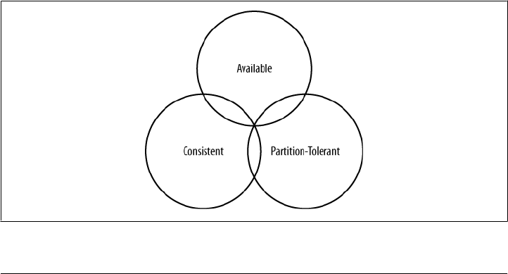
requirements that have a relationship of sliding dependency: Consistency, Availability,
and Partition Tolerance.
Consistency
All database clients will read the same value for the same query, even given con-
current updates.
Availability
All database clients will always be able to read and write data.
Partition Tolerance
The database can be split into multiple machines; it can continue functioning in
the face of network segmentation breaks.
Brewer’s theorem is that in any given system, you can strongly support only two of the
three. This is analogous to the saying you may have heard in software development:
“You can have it good, you can have it fast, you can have it cheap: pick two.”
We have to choose between them because of this sliding mutual dependency. The more
consistency you demand from your system, for example, the less partition-tolerant
you’re likely to be able to make it, unless you make some concessions around
availability.
The CAP theorem was formally proved to be true by Seth Gilbert and Nancy Lynch of
MIT in 2002. In distributed systems, however, it is very likely that you will have network
partitioning, and that at some point, machines will fail and cause others to become
unreachable. Packet loss, too, is nearly inevitable. This leads us to the conclusion that
a distributed system must do its best to continue operating in the face of network
partitions (to be Partition-Tolerant), leaving us with only two real options to choose
from: Availability and Consistency.
Figure 1-1 illustrates visually that there is no overlapping segment where all three are
obtainable.
Figure 1-1. CAP Theorem indicates that you can realize only two of these properties at once
20 | Chapter 1: Introducing Cassandra
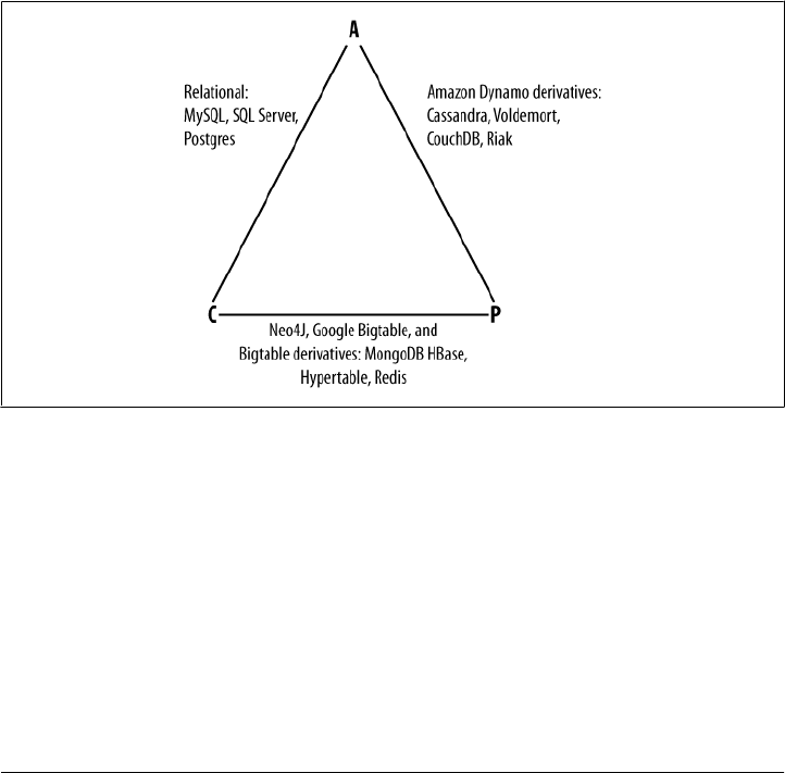
It might prove useful at this point to see a graphical depiction of where each of the
nonrelational data stores we’ll look at falls within the CAP spectrum. The graphic in
Figure 1-2 was inspired by a slide in a 2009 talk given by Dwight Merriman, CEO and
founder of MongoDB, to the MySQL User Group in New York City (you can watch it
online at http://bit.ly/7r6kRg). However, I have modified the placement of some systems
based on my research.
Figure 1-2 shows the general focus of some of the different databases we discuss in this
chapter. Note that placement of the databases in this chart could change based on
configuration. As Stu Hood points out, a distributed MySQL database can count as a
consistent system only if you’re using Google’s synchronous replication patches; oth-
erwise, it can only be Available and Partition-Tolerant (AP).
It’s interesting to note that the design of the system around CAP placement is inde-
pendent of the orientation of the data storage mechanism; for example, the CP edge is
populated by graph databases and document-oriented databases alike.
Figure 1-2. Where different databases appear on the CAP continuum
In this depiction, relational databases are on the line between Consistency and Avail-
ability, which means that they can fail in the event of a network failure (including a
cable breaking). This is typically achieved by defining a single master server, which
could itself go down, or an array of servers that simply don’t have sufficient mechanisms
built in to continue functioning in the case of network partitions.
Graph databases such as Neo4J and the set of databases derived at least in part from
the design of Google’s Bigtable database (such as MongoDB, HBase, Hypertable, and
Redis) all are focused slightly less on Availability and more on ensuring Consistency
and Partition Tolerance.
The Cassandra Elevator Pitch | 21

If you’re interested in the properties of other Big Data or NoSQL data-
bases, see this book’s Appendix.
Finally, the databases derived from Amazon’s Dynamo design include Cassandra,
Project Voldemort, CouchDB, and Riak. These are more focused on Availability and
Partition-Tolerance. However, this does not mean that they dismiss Consistency as
unimportant, any more than Bigtable dismisses Availability. According to the Bigtable
paper, the average percentage of server hours that “some data” was unavailable is
0.0047% (section 4), so this is relative, as we’re talking about very robust systems
already. If you think of each of these letters (C, A, P) as knobs you can tune to arrive
at the system you want, Dynamo derivatives are intended for employment in the many
use cases where “eventual consistency” is tolerable and where “eventual” is a matter
of milliseconds, read repairs mean that reads will return consistent values, and you can
achieve strong consistency if you want to.
So what does it mean in practical terms to support only two of the three facets of CAP?
CA
To primarily support Consistency and Availability means that you’re likely using
two-phase commit for distributed transactions. It means that the system will block
when a network partition occurs, so it may be that your system is limited to a single
data center cluster in an attempt to mitigate this. If your application needs only
this level of scale, this is easy to manage and allows you to rely on familiar, simple
structures.
CP
To primarily support Consistency and Partition Tolerance, you may try to
advance your architecture by setting up data shards in order to scale. Your data
will be consistent, but you still run the risk of some data becoming unavailable if
nodes fail.
AP
To primarily support Availability and Partition Tolerance, your system may return
inaccurate data, but the system will always be available, even in the face of network
partitioning. DNS is perhaps the most popular example of a system that is mas-
sively scalable, highly available, and partition-tolerant.
22 | Chapter 1: Introducing Cassandra

Note that this depiction is intended to offer an overview that helps draw
distinctions between the broader contours in these systems; it is not
strictly precise. For example, it’s not entirely clear where Google’s
Bigtable should be placed on such a continuum. The Google paper de-
scribes Bigtable as “highly available,” but later goes on to say that if
Chubby (the Bigtable persistent lock service) “becomes unavailable for
an extended period of time [caused by Chubby outages or network is-
sues], Bigtable becomes unavailable” (section 4). On the matter of data
reads, the paper says that “we do not consider the possibility of multiple
copies of the same data, possibly in alternate forms due to views or
indices.” Finally, the paper indicates that “centralized control and By-
zantine fault tolerance are not Bigtable goals” (section 10). Given such
variable information, you can see that determining where a database
falls on this sliding scale is not an exact science.
Row-Oriented
Cassandra is frequently referred to as a “column-oriented” database, which is not in-
correct. It’s not relational, and it does represent its data structures in sparse
multidimensional hashtables. “Sparse” means that for any given row you can have one
or more columns, but each row doesn’t need to have all the same columns as other
rows like it (as in a relational model). Each row has a unique key, which makes its data
accessible. So although it’s not wrong to say that Cassandra is columnar or column-
oriented, it might be more helpful to think of it as an indexed, row-oriented store, as
we examine more thoroughly in Chapter 3. I list the data orientation as a feature, be-
cause there are several data models that are easy to visualize and use in a nonrelational
model; it’s a weird mixture of laziness and possibly inviting far more work than nec-
essary to just assume that the relational model is always best, regardless of your
application.
Cassandra stores data in what can be thought of for now as a multidimensional hash
table. That means you don’t have to decide ahead of time precisely what your data
structure must look like, or what fields your records will need. This can be useful if
you’re in startup mode and are adding or changing features with some frequency. It is
also attractive if you need to support an Agile development methodology and aren’t
free to take months for up-front analysis. If your business changes and you later need
to add or remove new fields on the fly without disrupting service, go ahead; Cassandra
lets you.
That’s not to say that you don’t have to think about your data, though. On the contrary,
Cassandra requires a shift in how you think about it. Instead of designing a pristine
data model and then designing queries around the model as in RDBMS, you are free
to think of your queries first, and then provide the data that answers them.
The Cassandra Elevator Pitch | 23

Schema-Free
Cassandra requires you to define an outer container, called a keyspace, that contains
column families. The keyspace is essentially just a logical namespace to hold column
families and certain configuration properties. The column families are names for asso-
ciated data and a sort order. Beyond that, the data tables are sparse, so you can just
start adding data to it, using the columns that you want; there’s no need to define your
columns ahead of time. Instead of modeling data up front using expensive data mod-
eling tools and then writing queries with complex join statements, Cassandra asks you
to model the queries you want, and then provide the data around them.
High Performance
Cassandra was designed specifically from the ground up to take full advantage of
multiprocessor/multicore machines, and to run across many dozens of these machines
housed in multiple data centers. It scales consistently and seamlessly to hundreds of
terabytes. Cassandra has been shown to perform exceptionally well under heavy load.
It consistently can show very fast throughput for writes per second on a basic com-
modity workstation. As you add more servers, you can maintain all of Cassandra’s
desirable properties without sacrificing performance.
Where Did Cassandra Come From?
The Cassandra data store is an open source Apache project available at http://cassandra
.apache.org. Cassandra originated at Facebook in 2007 to solve that company’s inbox
search problem, in which they had to deal with large volumes of data in a way that was
difficult to scale with traditional methods. Specifically, the team had requirements to
handle huge volumes of data in the form of message copies, reverse indices of messages,
and many random reads and many simultaneous random writes.
The team was led by Jeff Hammerbacher, with Avinash Lakshman, Karthik Rangana-
than, and Facebook engineer on the Search Team Prashant Malik as key engineers.
The code was released as an open source Google Code project in July 2008. During its
tenure as a Google Code project in 2008, the code was updateable only by Facebook
engineers, and little community was built around it as a result. So in March 2009 it was
moved to an Apache Incubator project, and on February 17, 2010 it was voted into a
top-level project.
A central paper on Cassandra by Facebook’s Lakshman and Malik
called “A Decentralized Structured Storage System” is available at: http:
//www.cs.cornell.edu/projects/ladis2009/papers/lakshman-ladis2009
.pdf.
24 | Chapter 1: Introducing Cassandra

Cassandra today presents a kind of paradox: it feels new and radical, and yet it’s solidly
rooted in many standard, traditional computer science concepts and maxims that suc-
cessful predecessors have already institutionalized. Cassandra is a realist’s kind of
database; it doesn’t depart from the relational model to be a fun art project or experi-
ment for smart developers. It was created specifically to solve a real-world problem that
existing tools weren’t able to solve. It acknowledges the limitations of prior methods
and faces our new world of big data head-on.
How Did Cassandra Get Its Name?
I’m a little surprised how often people ask me where the database got its name. It’s not
the first thing I think of when I hear about a project. But it is interesting, and in the case
of this database, it’s felicitously meaningful.
In Greek mythology, Cassandra was the daughter of King Priam and Queen Hecuba of
Troy. Cassandra was so beautiful that the god Apollo gave her the ability to see the
future. But when she refused his amorous advances, he cursed her such that she would
still be able to accurately predict everything that would happen—but no one would
believe her. Cassandra foresaw the destruction of her city of Troy, but was powerless
to stop it. The Cassandra distributed database is named for her. I speculate that it is
also named as kind of a joke on the Oracle at Delphi, another seer for whom a database
is named.
Use Cases for Cassandra
We have now unpacked the elevator pitch and have an understanding of Cassandra’s
advantages. Despite Cassandra’s sophisticated design and smart features, it is not the
right tool for every job. So in this section let’s take a quick look at what kind of projects
Cassandra is a good fit for.
Large Deployments
You probably don’t drive a semi truck to pick up your dry cleaning; semis aren’t well
suited for that sort of task. Lots of careful engineering has gone into Cassandra’s high
availability, tuneable consistency, peer-to-peer protocol, and seamless scaling, which
are its main selling points. None of these qualities is even meaningful in a single-node
deployment, let alone allowed to realize its full potential.
There are, however, a wide variety of situations where a single-node relational database
is all we may need. So do some measuring. Consider your expected traffic, throughput
needs, and SLAs. There are no hard and fast rules here, but if you expect that you can
reliably serve traffic with an acceptable level of performance with just a few relational
databases, it might be a better choice to do so, simply because RDBMS are easier to
run on a single machine and are more familiar.
Use Cases for Cassandra | 25

If you think you’ll need at least several nodes to support your efforts, however, Cas-
sandra might be a good fit. If your application is expected to require dozens of nodes,
Cassandra might be a great fit.
Lots of Writes, Statistics, and Analysis
Consider your application from the perspective of the ratio of reads to writes. Cassandra
is optimized for excellent throughput on writes.
Many of the early production deployments of Cassandra involve storing user activity
updates, social network usage, recommendations/reviews, and application statistics.
These are strong use cases for Cassandra because they involve lots of writing with less
predictable read operations, and because updates can occur unevenly with sudden
spikes. In fact, the ability to handle application workloads that require high perform-
ance at significant write volumes with many concurrent client threads is one of the
primary features of Cassandra.
According to the project wiki, Cassandra has been used to create a variety of applica-
tions, including a windowed time-series store, an inverted index for document
searching, and a distributed job priority queue.
Geographical Distribution
Cassandra has out-of-the-box support for geographical distribution of data. You can
easily configure Cassandra to replicate data across multiple data centers. If you have a
globally deployed application that could see a performance benefit from putting the
data near the user, Cassandra could be a great fit.
Evolving Applications
If your application is evolving rapidly and you’re in “startup mode,” Cassandra might
be a good fit given its schema-free data model. This makes it easy to keep your
database in step with application changes as you rapidly deploy.
Who Is Using Cassandra?
Cassandra is still in its early stages in many ways, not yet seeing its 1.0 release at the
time of this writing. There are few easy, graphical tools to help manage it, and the
community has not settled on certain key internal and external design questions that
have been revisited. But what does it say about the promise, usefulness, and stability
of a data store that even in its early stages is being used in production by many large,
well-known companies?
26 | Chapter 1: Introducing Cassandra

It is a logical fallacy, informally called the Bandwagon Fallacy, to argue
that just because something is growing in popularity means that it is
“true.” Cassandra is without a doubt enjoying skyrocketing growth in
popularity, especially over the past year or so. Still, my point here is
that the many successful production deployments at a variety of com-
panies for a variety of purposes is sufficient to suggest its usefulness and
readiness.
The list of companies using Cassandra is growing. These companies include:
• Twitter is using Cassandra for analytics. In a much-publicized blog post (at http://
engineering.twitter.com/2010/07/cassandra-at-twitter-today.html), Twitter’s pri-
mary Cassandra engineer, Ryan King, explained that Twitter had decided against
using Cassandra as its primary store for tweets, as originally planned, but would
instead use it in production for several different things: for real-time analytics, for
geolocation and places of interest data, and for data mining over the entire user
store.
• Mahalo uses it for its primary near-time data store.
• Facebook still uses it for inbox search, though they are using a proprietary fork.
• Digg uses it for its primary near-time data store.
• Rackspace uses it for its cloud service, monitoring, and logging.
• Reddit uses it as a persistent cache.
• Cloudkick uses it for monitoring statistics and analytics.
• Ooyala uses it to store and serve near real-time video analytics data.
• SimpleGeo uses it as the main data store for its real-time location infrastructure.
• Onespot uses it for a subset of its main data store.
Cassandra is also being used by Cisco and Platform64, and is starting to see use at
Comcast and bee.tv for personalized television streaming to the Web and to mobile
devices. There are others. The bottom line is that the uses are real. A wide variety of
companies are finding use cases for Cassandra and seeing success with it. As of this
writing, the largest known Cassandra installation is at Facebook, where they have more
than 150TB of data on more than 100 machines.
Many more companies are currently evaluating Cassandra for production use in dif-
ferent projects, and a services company called Riptano, cofounded by Jonathan Ellis,
the Apache Project Chair for Cassandra, was started in April of 2010. As more features
are added and better tooling and support options are rolled out, anticipate even broader
adoption.
Who Is Using Cassandra? | 27

Summary
In this chapter, we’ve taken an introductory look at Cassandra’s defining characteris-
tics, history, and major features. We have seen which major companies are using it
and what they’re using it for. We also examined a bit of history of the evolution of
important contributions to the database field in order to gain a historical view of Cas-
sandra’s value proposition.
28 | Chapter 1: Introducing Cassandra

CHAPTER 2
Installing Cassandra
For those among us who like instant gratification, we’ll start by installing Cassandra.
Because Cassandra introduces a lot of new vocabulary, there might be some unfamiliar
terms as we walk through this. That’s OK; the idea here is to get set up quickly in a
simple configuration to make sure everything is running properly. This will serve as an
orientation. Then, we’ll take a step back and understand Cassandra in its larger context.
Installing the Binary
Cassandra is available for download from the Web at http://cassandra.apache.org. Just
click the link on the home page to download the latest release version as a gzipped
tarball. The prebuilt binary is named apache-cassandra-x.x.x-bin.tar.gz, where x.x.x
represents the version number. The download is around 10MB.
Extracting the Download
The simplest way to get started is to download the prebuilt binary. You can unpack the
compressed file using any regular ZIP utility. On Linux, GZip extraction utilities should
be preinstalled; on Windows, you’ll need to get a program such as WinZip, which is
commercial, or something like 7-Zip, which is freeware. You can download the freeware
program 7-Zip from http://www.7-zip.org.
Open your extracting program. You might have to extract the ZIP file and the TAR file
in separate steps. Once you have a folder on your filesystem called apache-cassandra-
x.x.x, you’re ready to run Cassandra.
What’s In There?
Once you decompress the tarball, you’ll see that the Cassandra binary distribution
includes several directories. Let’s take a moment to look around and see what we have.
29

bin
This directory contains the executables to run Cassandra and the command-line
interface (CLI) client. It also has scripts to run the nodetool, which is a utility for
inspecting a cluster to determine whether it is properly configured, and to perform
a variety of maintenance operations. We look at nodetool in depth later. It also has
scripts for converting SSTables (the datafiles) to JSON and back.
conf
This directory, which is present in the source version at this location under the
package root, contains the files for configuring your Cassandra instance. There are
three basic functions: the storage-conf.xml file allows you to create your data store
by configuring your keyspace and column families; there are files related to setting
up authentication; and finally, the log4j properties let you change the logging levels
to suit your needs. We see how to use all of these when we discuss configuration
in Chapter 6.
interface
For versions 0.6 and earlier, this directory contains a single file, called
cassandra.thrift. This file represents the Remote Procedure Call (RPC) client API
that Cassandra makes available. The interface is defined using the Thrift syntax
and provides an easy means to generate clients. For a quick way to see all of the
operations that Cassandra supports, open this file in a regular text editor. You can
see that Cassandra supports clients for Java, C++, PHP, Ruby, Python, Perl, and
C# through this interface.
javadoc
This directory contains a documentation website generated using Java’s JavaDoc
tool. Note that JavaDoc reflects only the comments that are stored directly in the
Java code, and as such does not represent comprehensive documentation. It’s
helpful if you want to see how the code is laid out. Moreover, Cassandra is a
wonderful project, but the code contains precious few comments, so you might
find the JavaDoc’s usefulness limited. It may be more fruitful to simply read the
class files directly if you’re familiar with Java. Nonetheless, to read the JavaDoc,
open the javadoc/index.html file in a browser.
lib
This directory contains all of the external libraries that Cassandra needs to run.
For example, it uses two different JSON serialization libraries, the Google collec-
tions project, and several Apache Commons libraries. This directory includes the
Thrift and Avro RPC libraries for interacting with Cassandra.
Building from Source
Cassandra uses Apache Ant for its build scripting language and the Ivy plug-in for
dependency management.
30 | Chapter 2: Installing Cassandra
You can download Ant from http://ant.apache.org. You don’t need to
download Ivy separately just to build Cassandra.
Ivy requires Ant, and building from source requires the complete JDK, version 1.6.0_20
or better, not just the JRE. If you see a message about how Ant is missing tools.jar,
either you don’t have the full JDK or you’re pointing to the wrong path in your envi-
ronment variables.
If you want to download the most cutting-edge builds, you can get the
source from Hudson, which the Cassandra project uses as its Continu-
ous Integration tool. See http://hudson.zones.apache.org/hudson/job/Cas
sandra/ for the latest builds and test coverage information.
If you are a Git fan, you can get a read-only trunk version of the Cassandra source using
this command:
>git clone git://git.apache.org/cassandra.git
Git is a source code management system created by Linus Torvalds to
manage development of the Linux kernel. It’s increasingly popular and
is used by projects such as Android, Fedora, Ruby on Rails, Perl, and
many Cassandra clients (as we’ll see in Chapter 8). If you’re on a Linux
distribution such as Ubuntu, it couldn’t be easier to get Git. At a
console, just type >apt-get install git and it will be installed and ready
for commands. For more information, visit http://git-scm.com/.
Because Ivy takes care of all the dependencies, it’s easy to build Cassandra once you
have the source. Just make sure you’re in the root directory of your source download
and execute the ant program, which will look for a file called build.xml in the current
directory and execute the default build target. Ant and Ivy take care of the rest. To
execute the Ant program and start compiling the source, just type:
>ant
That’s it. Ivy will retrieve all of the necessary dependencies, and Ant will build the nearly
350 source files and execute the tests. If all went well, you should see a BUILD SUCCESS
FUL message. If all did not go well, make sure that your path settings are all correct,
that you have the most recent versions of the required programs, and that you down-
loaded a stable Cassandra build. You can check the Hudson report to make sure that
the source you downloaded actually can compile.
Building from Source | 31
If you want to see detailed information on what is happening during the
build, you can pass Ant the -v option to cause it to output verbose details
regarding each operation it performs.
Additional Build Targets
To compile the server, you can simply execute ant as shown previously. But there are
a couple of other targets in the build file that you might be interested in:
test
Users will probably find this the most helpful, as it executes the battery of unit
tests. You can also check out the unit test sources themselves for some useful
examples of how to interact with Cassandra.
gen-thrift-java
This target generates the Apache Thrift client interface for interacting with the
database in Java.
gen-thrift-py
This target generates the Thrift client interface for Python users.
build-jar
To create a Java Archive (JAR) file for distribution, execute the command >ant
jar. This will perform a complete build and output a file into the build directory
called apache-cassandra-x.x.x.jar.
Building with Maven
The original authors of Cassandra apparently didn’t care much for Maven, so the early
releases did not include any Maven POM file. But because so many Java developers
have begun to favor Maven over Ant, and the tooling support in IDEs for Maven has
become so strong, there’s a pom.xml contribution to the project so you can build from
Maven if you prefer.
To build the source from Maven, navigate to <cassandra-home>/contrib/maven and
execute this command:
$ mvn clean install
If you have any difficulties building with Maven, you may have to get some of the
required JARs manually. As of version 0.6.3, the Maven POM doesn’t work out of
the box because some dependencies, such as the libthrift.jar file, are unavailable in a
repository.
Few developers are using Maven with Cassandra, so Maven lacks strong
support. Which is to say, use caution, because the Maven POM is often
broken.
32 | Chapter 2: Installing Cassandra

Running Cassandra
In earlier versions of Cassandra, before you could start the server there was a bit of
fiddling to be done with Ivy and setting environment variables. But the developers have
done a terrific job of making it very easy to start using Cassandra immediately.
Cassandra requires Java Standard Edition JDK 6. Preferably, use
1.6.0_20 or greater. It has been tested on both the Open JDK and Sun’s
JDK. You can check your installed Java version by opening a command
prompt and executing >java -version. If you need a JDK, you can get
one at http://java.sun.com/javase/downloads.
On Windows
Once you have the binary or the source downloaded and compiled, you’re ready to
start the database server.
You also might need to set your JAVA_HOME environment variable. To do this on
Windows 7, click the Start button and then right-click on Computer. Click Advanced
System Settings, and then click the Environment Variables... button. Click New... to
create a new system variable. In the Variable Name field, type JAVA_HOME. In the Variable
Value field, type the path to your JDK installation. This is probably something like C:
\Program Files\Java\jdk1.6.0_20. Remember that if you create a new environment var-
iable, you’ll need to reopen any currently open terminals in order for the system to
become aware of the new variable. To make sure your environment variable is set
correctly and that Cassandra can subsequently find Java on Windows, execute this
command in a new terminal: >echo %JAVA_HOME%. This prints the value of your
environment variable.
Once you’ve started the server for the first time, Cassandra will add two directories to
your system. The first is C:\var\lib\cassandra, which is where it will store its data in files
called commitlog. The other is C:\var\log\cassandra; logs will be written to a file called
system.log. If you encounter any difficulties, consult the files in these directories to see
what might have happened. If you’ve been trying different versions of the database and
aren’t worried about losing data, you can delete these directories and restart the server
as a last resort.
On Linux
The process on Linux is similar to that on Windows. Make sure that your JAVA_HOME
variable is properly set to version 1.6.0_20 or better. Then, you need to extract the
Cassandra gzipped tarball using gunzip. Finally, create a couple of directories for Cas-
sandra to store its data and logs, and give them the proper permissions, as shown here:
Running Cassandra | 33

ehewitt@morpheus$ cd /home/eben/books/cassandra/dist/apache-cassandra-0.7.0-beta1
ehewitt@morpheus$ sudo mkdir -p /var/log/cassandra
ehewitt@morpheus$ sudo chown -R ehewitt /var/log/cassandra
ehewitt@morpheus$ sudo mkdir -p /var/lib/cassandra
ehewitt@morpheus$ sudo chown -R ehewitt /var/lib/cassandra
Instead of ehewitt, of course, substitute your own username.
Starting the Server
To start the Cassandra server on any OS, open a command prompt or terminal window,
navigate to the <cassandra-directory>/bin where you unpacked Cassandra, and run the
following command to start your server. In a clean installation, you should see some
log statements like this:
eben@morpheus$ bin/cassandra -f
INFO 13:23:22,367 DiskAccessMode 'auto' determined to be standard, indexAccessMode
is standard
INFO 13:23:22,475 Couldn't detect any schema definitions in local storage.
INFO 13:23:22,476 Found table data in data directories.
Consider using JMX to call org.apache.cassandra.service.StorageService
.loadSchemaFromYaml().
INFO 13:23:22,497 Cassandra version: 0.7.0-beta1
INFO 13:23:22,497 Thrift API version: 10.0.0
INFO 13:23:22,498 Saved Token not found. Using qFABQw5XJMvs47lg
INFO 13:23:22,498 Saved ClusterName not found. Using Test Cluster
INFO 13:23:22,502 Creating new commitlog segment /var/lib/cassandra/commitlog/
CommitLog-1282508602502.log
INFO 13:23:22,507 switching in a fresh Memtable for LocationInfo at CommitLogContext(
file='/var/lib/cassandra/commitlog/CommitLog-1282508602502.log', position=276)
INFO 13:23:22,510 Enqueuing flush of Memtable-LocationInfo@29857804(178 bytes,
4 operations)
INFO 13:23:22,511 Writing Memtable-LocationInfo@29857804(178 bytes, 4 operations)
INFO 13:23:22,691 Completed flushing /var/lib/cassandra/data/system/
LocationInfo-e-1-Data.db
INFO 13:23:22,701 Starting up server gossip
INFO 13:23:22,750 Binding thrift service to localhost/127.0.0.1:9160
INFO 13:23:22,752 Using TFramedTransport with a max frame size of 15728640 bytes.
INFO 13:23:22,753 Listening for thrift clients...
INFO 13:23:22,792 mx4j successfuly loaded
HttpAdaptor version 3.0.2 started on port 8081
Using the -f switch tells Cassandra to stay in the foreground instead of
running as a background process, so that all of the server logs will print
to standard out and you can see them in your terminal window, which
is useful for testing.
Congratulations! Now your Cassandra server should be up and running with a new
single node cluster called Test Cluster listening on port 9160.
34 | Chapter 2: Installing Cassandra
The committers work hard to ensure that data is readable from one
minor dot release to the next and from one major version to the next.
The commit log, however, needs to be completely cleared out from ver-
sion to version (even minor versions).
If you have any previous versions of Cassandra installed, you may want
to clear out the data directories for now, just to get up and running. If
you’ve messed up your Cassandra installation and want to get started
cleanly again, you can delete the folders in /var/lib/cassandra and /var/
log/cassandra.
Running the Command-Line Client Interface
Now that you have a Cassandra installation up and running, let’s give it a quick try to
make sure everything is set up properly. On Linux, running the command-line interface
just works. On Windows, you might have to do a little additional work.
On Windows, navigate to the Cassandra home directory and open a new terminal in
which to run our client process:
>bin\cassandra-cli
It’s possible that on Windows you will see an error like this when starting the client:
Starting Cassandra Client
Exception in thread "main" java.lang.NoClassDefFoundError:
org/apache/cassandra/cli/CliMain
This probably means that you started Cassandra directly from within the bin directory,
and it therefore sets up its Java classpath incorrectly and can’t find the CliMain file to
start the client. You can define an environment variable called CASSANDRA_HOME that
points to the top-level directory where you have placed or built Cassandra, so you don’t
have to pay as much attention to where you’re starting Cassandra from.
For a little reminder on setting environment variables on Windows, see
the section “On Windows” on page 33.
To run the command-line interface program on Linux, navigate to the Cassandra home
directory and run the cassandra-cli program in the bin directory:
>bin/cassandra-cli
The Cassandra client will start:
eben@morpheus$ bin/cassandra-cli
Welcome to cassandra CLI.
Type 'help' or '?' for help. Type 'quit' or 'exit' to quit.
[default@unknown]
Running the Command-Line Client Interface | 35

You now have an interactive shell at which you can issue commands.
Note, however, that if you’re used to Oracle’s SQL*Plus or similar command-line
database clients, you may become frustrated. The Cassandra CLI is not intended to be
used as a full-blown client, as it’s really for development. That makes it a good way to
get started using Cassandra, because you don’t have to write lots of code to test inter-
actions with your database and get used to the environment.
Basic CLI Commands
Before we get too deep into how Cassandra works, let’s get an overview of the client
API so that you can see what kinds of commands you can send to the server. We’ll see
how to use the basic environment commands and how to do a round trip of inserting
and retrieving some data.
Help
To get help for the command-line interface, type help or ? to see the list of available
commands. The following list shows only the commands related to metadata and con-
figuration; there are other commands for getting and setting values that we explore
later.
[default@Keyspace1] help
List of all CLI commands:
? Display this message.
help Display this help.
help <command> Display detailed, command-specific help.
connect <hostname>/<port> Connect to thrift service.
use <keyspace> [<username> 'password'] Switch to a keyspace.
describe keyspace <keyspacename> Describe keyspace.
exit Exit CLI.
quit Exit CLI.
show cluster name Display cluster name.
show keyspaces Show list of keyspaces.
show api version Show server API version.
create keyspace <keyspace> [with <att1>=<value1> [and <att2>=<value2> ...]]
Add a new keyspace with the specified attribute and value(s).
create column family <cf> [with <att1>=<value1> [and <att2>=<value2> ...]]
Create a new column family with the specified attribute and value(s).
drop keyspace <keyspace> Delete a keyspace.
drop column family <cf> Delete a column family.
rename keyspace <keyspace> <keyspace_new_name> Rename a keyspace.
rename column family <cf> <new_name> Rename a column family.
Connecting to a Server
Starting the client this way does not automatically connect to a Cassandra server in-
stance. So to connect to a particular server after you have started Cassandra this way,
use the connect command:
36 | Chapter 2: Installing Cassandra
eben@morpheus:~/books/cassandra/dist/apache-cassandra-0.7.0-beta1$ bin/cassandra-cli
Welcome to cassandra CLI.
Type 'help' or '?' for help. Type 'quit' or 'exit' to quit.
[default@unknown] connect localhost/9160
Connected to: "Test Cluster" on localhost/9160
[default@unknown]
As a shortcut, you can start the client and connect to a particular server instance by
passing the host and port parameters at startup, like this:
eben@morpheus:~/books/cassandra/dist/apache-cassandra-0.7.0-beta1$ bin/
cassandra-cli localhost/9160
Welcome to cassandra CLI.
Type 'help' or '?' for help. Type 'quit' or 'exit' to quit.
[default@unknown]
If you see this error while trying to connect to a server:
Exception connecting to localhost/9160 - java.net.ConnectException:
Connection refused: connect
make sure that a Cassandra instance is started at that host and port and
that you can ping the host you’re trying to reach. There may be firewall
rules preventing you from connecting. Also make sure that you’re using
the new 0.7 syntax as described earlier, as it has changed from previous
versions.
The CLI indicates that you’re connected to a Cassandra server cluster called “Test
Cluster”. That’s because this cluster of one node at localhost is set up for you by
default.
In a production environment, be sure to remove the Test Cluster from
the configuration.
Describing the Environment
After connecting to your Cassandra instance Test Cluster, if you’re using the binary
distribution, an empty keyspace, or Cassandra database, is set up for you to test with.
To see the name of the current cluster you’re working in, type:
[default@unknown] show cluster name
Test Cluster
To see which keyspaces are available in the cluster, issue this command:
[default@unknown] show keyspaces
system
Basic CLI Commands | 37

If you have created any of your own keyspaces, they will be shown as well. The
system keyspace is used internally by Cassandra, and isn’t for us to put data into. In
this way, it’s similar to the master and temp databases in Microsoft SQL Server. This
keyspace contains the schema definitions and is aware of any modifications to the
schema made at runtime. It can propagate any changes made in one node to the rest
of the cluster based on timestamps.
To see the version of the API you’re using, type:
[default@Keyspace1] show api version
10.0.0
There are a variety of other commands with which you can experiment. For now, let’s
add some data to the database and get it back out again.
Creating a Keyspace and Column Family
A Cassandra keyspace is sort of like a relational database. It defines one or more column
families, which are very roughly analogous to tables in the relational world. When you
start the CLI client without specifying a keyspace, the output will look like this:
>bin/cassandra-cli --host localhost --port 9160
Starting Cassandra Client
Connected to: "Test Cluster" on localhost/9160
Welcome to cassandra CLI.
Type 'help' or '?' for help. Type 'quit' or 'exit' to quit.
[default@unknown]
Your shell prompt is for default@unknown because you haven’t authenticated as a par-
ticular user (which we’ll see how to do in Chapter 6) and you didn’t specify a keyspace.
This authentication scheme is familiar if you’ve used MySQL before.
Authentication and authorization are very much works in progress at
the time of this writing. The recommended deployment is to put a fire-
wall around your cluster.
Let’s create our own keyspace so we have something to write data to:
[default@unknown] create keyspace MyKeyspace with replication_factor=1
ab67bad0-ae2c-11df-b642-e700f669bcfc
Don’t worry about the replication_factor for now. That’s a setting we’ll look at in
detail later. After you have created your own keyspace, you can switch to it in the shell
by typing:
[default@unknown] use MyKeyspace
Authenticated to keyspace: MyKeyspace
[default@MyKeyspace]
We’re “authorized” to the keyspace because MyKeyspace doesn’t require credentials.
38 | Chapter 2: Installing Cassandra

Now we can create a column family in our keyspace. To do this on the CLI, use the
following command:
[default@MyKeyspace] create column family User
991590d3-ae2e-11df-b642-e700f669bcfc
[default@MyKeyspace]
This creates a new column family called “User” in our current keyspace, and takes the
defaults for column family settings. We can use the CLI to get a description of a key-
space using the describe keyspace command, and make sure it has our column family
definition, as shown here:
[default@MyKeyspace] describe keyspace MyKeyspace
Keyspace: MyKeyspace
Column Family Name: User
Column Family Type: Standard
Column Sorted By: org.apache.cassandra.db.marshal.BytesType
flush period: null minutes
------
[default@MyKeyspace]
We’ll worry about the Type, Sorted By, and flush period settings later. For now, we
have enough to get started.
Writing and Reading Data
Now that we have a keyspace and a column family, we’ll write some data to the database
and read it back out again. It’s OK at this point not to know quite what’s going on.
We’ll come to understand Cassandra’s data model in depth later. For now, you have
a keyspace (database), which has a column family. For our purposes here, it’s enough
to think of a column family as a multidimensional ordered map that you don’t have to
define further ahead of time. Column families hold columns, and columns are the
atomic unit of data storage.
To write a value, use the set command:
[default@MyKeyspace] set User['ehewitt']['fname']='Eben'
Value inserted.
[default@MyKeyspace] set User['ehewitt']['email']='me@example.com'
Value inserted.
[default@MyKeyspace]
Here we have created two columns for the key ehewitt, to store a set of related values.
The column names are fname and email. We can use the count command to make sure
that we have written two columns for our single key:
[default@MyKeyspace] count User['ehewitt']
2 columns
Now that we know the data is there, let’s read it, using the get command:
Basic CLI Commands | 39

[default@MyKeyspace] get User['ehewitt']
=> (column=666e616d65, value=Eben, timestamp=1282510290343000)
=> (column=656d61696c, value=me@example.com, timestamp=1282510313429000)
Returned 2 results.
You can delete a column using the del command. Here we will delete the email column
for the ehewitt row key:
[default@MyKeyspace] del User['ehewitt']['email']
column removed.
Now we’ll clean up after ourselves by deleting the entire row. It’s the same command,
but we don’t specify a column name:
[default@MyKeyspace] del User['ehewitt']
row removed.
To make sure that it’s removed, we can query again:
[default@Keyspace1] get User['ehewitt']
Returned 0 results.
Summary
Now you should have a Cassandra installation up and running. You’ve worked with
the CLI client to insert and retrieve some data, and you’re ready to take a step back and
get the big picture on Cassandra before really diving into the details.
40 | Chapter 2: Installing Cassandra

CHAPTER 3
The Cassandra Data Model
In this chapter, we’ll gain an understanding of Cassandra’s design goals, data model,
and some general behavior characteristics.
For developers and administrators coming from the relational world, the Cassandra
data model can be very difficult to understand initially. Some terms, such as
“keyspace,” are completely new, and some, such as “column,” exist in both worlds but
have different meanings. It can also be confusing if you’re trying to sort through the
Dynamo or Bigtable source papers, because although Cassandra may be based on them,
it has its own model.
So in this chapter we start from common ground and then work through the unfamiliar
terms. Then, we do some actual modeling to help understand how to bridge the gap
between the relational world and the world of Cassandra.
The Relational Data Model
In a relational database, we have the database itself, which is the outermost container
that might correspond to a single application. The database contains tables. Tables
have names and contain one or more columns, which also have names. When we add
data to a table, we specify a value for every column defined; if we don’t have a value
for a particular column, we use null. This new entry adds a row to the table, which we
can later read if we know the row’s unique identifier (primary key), or by using a SQL
statement that expresses some criteria that row might meet. If we want to update values
in the table, we can update all of the rows or just some of them, depending on the filter
we use in a “where” clause of our SQL statement.
For the purposes of learning Cassandra, it may be useful to suspend for a moment what
you know from the relational world.
41
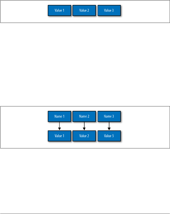
A Simple Introduction
In this section, we’ll take a bottom-up approach to understanding Cassandra’s data
model.
The simplest data store you would conceivably want to work with might be an array
or list. It would look like Figure 3-1.
Figure 3-1. A list of values
If you persisted this list, you could query it later, but you would have to either examine
each value in order to know what it represented, or always store each value in the same
place in the list and then externally maintain documentation about which cell in the
array holds which values. That would mean you might have to supply empty place-
holder values (nulls) in order to keep the uniform size in case you didn’t have a value
for an optional attribute (such as a fax number or apartment number). An array is a
clearly useful data structure, but not semantically rich.
So we’d like to add a second dimension to this list: names to match the values. We’ll
give names to each cell, and now we have a map structure, as shown in Figure 3-2.
Figure 3-2. A map of name/value pairs
This is an improvement because we can know the names of our values. So if we decided
that our map would hold User information, we could have column names like first
Name, lastName, phone, email, and so on. This is a somewhat richer structure to work
with.
42 | Chapter 3: The Cassandra Data Model

But the structure we’ve built so far works only if we have one instance of a given entity,
such as a single Person or User or Hotel or Tweet. It doesn’t give us much if we want
to store multiple entities with the same structure, which is certainly what we want to
do. There’s nothing to unify some collection of name/value pairs, and no way to repeat
the same column names. So we need something that will group some of the column
values together in a distinctly addressable group. We need a key to reference a group
of columns that should be treated together as a set. We need rows. Then, if we get a
single row, we can get all of the name/value pairs for a single entity at once, or just get
the values for the names we’re interested in. We could call these name/value pairs
columns. We could call each separate entity that holds some set of columns rows. And
the unique identifier for each row could be called a row key.
Cassandra defines a column family to be a logical division that associates similar data.
For example, we might have a User column family, a Hotel column family, an
AddressBook column family, and so on. In this way, a column family is somewhat
analogous to a table in the relational world.
Putting this all together, we have the basic Cassandra data structures: the column,
which is a name/value pair (and a client-supplied timestamp of when it was last upda-
ted), and a column family, which is a container for rows that have similar, but not
identical, column sets.
In relational databases, we’re used to storing column names as strings only—that’s all
we’re allowed. But in Cassandra, we don’t have that limitation. Both row keys and
column names can be strings, like relational column names, but they can also be long
integers, UUIDs, or any kind of byte array. So there’s some variety to how your key
names can be set.
This reveals another interesting quality to Cassandra’s columns: they don’t have to be
as simple as predefined name/value pairs; you can store useful data in the key itself,
not only in the value. This is somewhat common when creating indexes in Cassandra.
But let’s not get ahead of ourselves.
Now we don’t need to store a value for every column every time we store a new entity.
Maybe we don’t know the values for every column for a given entity. For example,
some people have a second phone number and some don’t, and in an online form
backed by Cassandra, there may be some fields that are optional and some that are
required. That’s OK. Instead of storing null for those values we don’t know, which
would waste space, we just won’t store that column at all for that row. So now we have
a sparse, multidimensional array structure that looks like Figure 3-3.
A Simple Introduction | 43
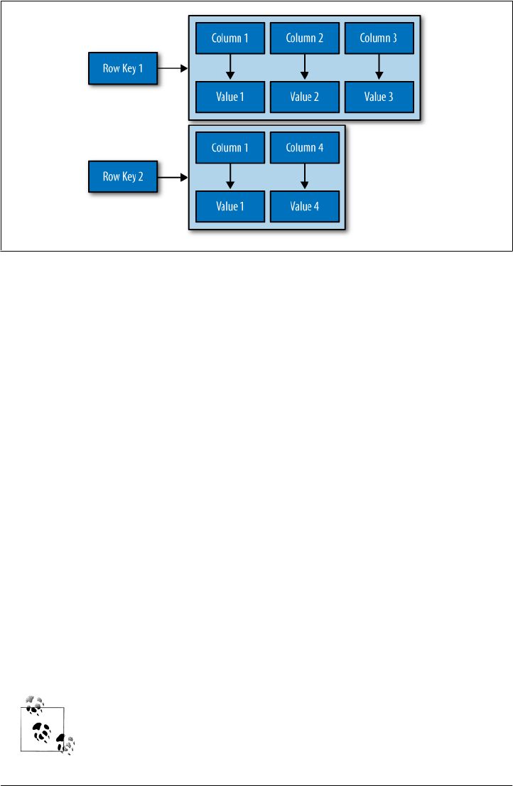
Figure 3-3. A column family
It may help to think of it in terms of JavaScript Object Notation (JSON) instead of a
picture:
Musician: ColumnFamily 1
bootsy: RowKey
email: bootsy@pfunk.com, ColumnName:Value
instrument: bass ColumnName:Value
george: RowKey
email: george@pfunk.com ColumnName:Value
Band: ColumnFamily 2
george: RowKey
pfunk: 1968-2010 ColumnName:Value
Here we have two column families, Musician and Band. The Musician column family
has two rows, “bootsy” and “george”. These two rows have a ragged set of columns
associated with them: the bootsy record has two columns (email and instrument), and
the george record has only one column. That’s fine in Cassandra. The second column
family is Band, and it also has a “george” row, with a column named “pfunk”.
Columns in Cassandra actually have a third aspect: the timestamp, which records the
last time the column was updated. This is not an automatic metadata property, how-
ever; clients have to provide the timestamp along with the value when they perform
writes. You cannot query by the timestamp; it is used purely for conflict resolution on
the server side.
Rows do not have timestamps. Only each individual column has a
timestamp.
44 | Chapter 3: The Cassandra Data Model
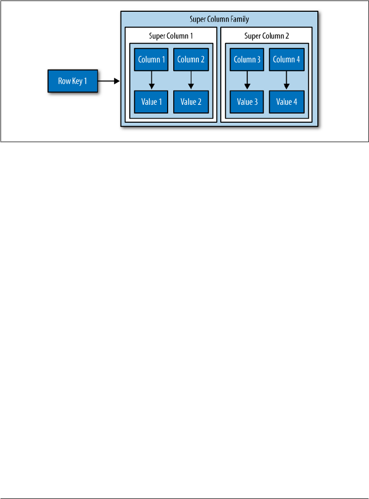
And what if we wanted to create a group of related columns, that is, add another di-
mension on top of this? Cassandra allows us to do this with something called a super
column family. A super column family can be thought of as a map of maps. The super
column family is shown in Figure 3-4.
Figure 3-4. A super column family
Where a row in a column family holds a collection of name/value pairs, the super
column family holds subcolumns, where subcolumns are named groups of columns.
So the address of a value in a regular column family is a row key pointing to a column
name pointing to a value, while the address of a value in a column family of type
“super” is a row key pointing to a column name pointing to a subcolumn name
pointing to a value. Put slightly differently, a row in a super column family still contains
columns, each of which then contains subcolumns.
So that’s the bottom-up approach to looking at Cassandra’s data model. Now that we
have this basic understanding, let’s switch gears and zoom out to a higher level, in order
to take a top-down approach. There is so much confusion on this topic that it’s worth
it to restate things in a different way in order to thoroughly understand the data model.
Clusters
Cassandra is probably not the best choice if you only need to run a single node. As
previously mentioned, the Cassandra database is specifically designed to be distributed
over several machines operating together that appear as a single instance to the end
user. So the outermost structure in Cassandra is the cluster, sometimes called the
ring, because Cassandra assigns data to nodes in the cluster by arranging them in
a ring.
A node holds a replica for different ranges of data. If the first node goes down, a replica
can respond to queries. The peer-to-peer protocol allows the data to replicate across
nodes in a manner transparent to the user, and the replication factor is the number of
Clusters | 45

machines in your cluster that will receive copies of the same data. We’ll examine this
in greater detail in Chapter 6.
Keyspaces
A cluster is a container for keyspaces—typically a single keyspace. A keyspace is the
outermost container for data in Cassandra, corresponding closely to a relational data-
base. Like a relational database, a keyspace has a name and a set of attributes that define
keyspace-wide behavior. Although people frequently advise that it’s a good idea to
create a single keyspace per application, this doesn’t appear to have much practical
basis. It’s certainly an acceptable practice, but it’s perfectly fine to create as many key-
spaces as your application needs. Note, however, that you will probably run into trou-
ble creating thousands of keyspaces per application.
Depending on your security constraints and partitioner, it’s fine to run multiple key-
spaces on the same cluster. For example, if your application is called Twitter, you
would probably have a cluster called Twitter-Cluster and a keyspace called Twitter.
To my knowledge, there are currently no naming conventions in Cassandra for such
items.
In Cassandra, the basic attributes that you can set per keyspace are:
Replication factor
In simplest terms, the replication factor refers to the number of nodes that will act
as copies (replicas) of each row of data. If your replication factor is 3, then three
nodes in the ring will have copies of each row, and this replication is transparent
to clients.
The replication factor essentially allows you to decide how much you want to pay
in performance to gain more consistency. That is, your consistency level for reading
and writing data is based on the replication factor.
Replica placement strategy
The replica placement refers to how the replicas will be placed in the ring. There
are different strategies that ship with Cassandra for determining which nodes
will get copies of which keys. These are SimpleStrategy (formerly known as
RackUnawareStrategy), OldNetworkTopologyStrategy (formerly known as Rack-
AwareStrategy), and NetworkTopologyStrategy (formerly known as Datacenter-
ShardStrategy).
Column families
In the same way that a database is a container for tables, a keyspace is a container
for a list of one or more column families. A column family is roughly analagous to
a table in the relational model, and is a container for a collection of rows. Each row
contains ordered columns. Column families represent the structure of your data.
Each keyspace has at least one and often many column families.
46 | Chapter 3: The Cassandra Data Model

I mention the replication factor and replica placement strategy here because they are
set per keyspace. However, they don’t have an immediate impact on your data model
per se.
It is possible, but generally not recommended, to create multiple keyspaces per appli-
cation. The only time you would want to split your application into multiple keyspaces
is if you wanted a different replication factor or replica placement strategy for some of
the column families. For example, if you have some data that is of lower priority,
you could put it in its own keyspace with a lower replication factor so that Cassandra
doesn’t have to work as hard to replicate it. But this may be more complicated than it’s
worth. It’s probably a better idea to start with one keyspace and see whether you really
need to tune at that level.
Column Families
A column family is a container for an ordered collection of rows, each of which is itself
an ordered collection of columns. In the relational world, when you are physically
creating your database from a model, you specify the name of the database (keyspace),
the names of the tables (remotely similar to column families, but don’t get stuck on the
idea that column families equal tables—they don’t), and then you define the names of
the columns that will be in each table.
There are a few good reasons not to go too far with the idea that a column family is like
a relational table. First, Cassandra is considered schema-free because although the
column families are defined, the columns are not. You can freely add any column to
any column family at any time, depending on your needs. Second, a column family has
two attributes: a name and a comparator. The comparator value indicates how columns
will be sorted when they are returned to you in a query—according to long, byte, UTF8,
or other ordering.
In a relational database, it is frequently transparent to the user how tables are stored
on disk, and it is rare to hear of recommendations about data modeling based on how
the RDBMS might store tables on disk. That’s another reason to keep in mind that a
column family is not a table. Because column families are each stored in separate files
on disk, it’s important to keep related columns defined together in the same column
family.
Another way that column families differ from relational tables is that relational tables
define only columns, and the user supplies the values, which are the rows. But in Cas-
sandra, a table can hold columns, or it can be defined as a super column family. The
benefit of using a super column family is to allow for nesting.
For standard column families, which is the default, you set the type to Standard; for a
super column family, you set the type to Super.
Column Families | 47
When you write data to a column family in Cassandra, you specify values for one or
more columns. That collection of values together with a unique identifier is called a
row. That row has a unique key, called the row key, which acts like the primary key
unique identifier for that row. So while it’s not incorrect to call it column-oriented, or
columnar, it might be easier to understand the model if you think of rows as containers
for columns. This is also why some people refer to Cassandra column families as similar
to a four-dimensional hash:
[Keyspace][ColumnFamily][Key][Column]
We can use a JSON-like notation to represent a Hotel column family, as shown here:
Hotel {
key: AZC_043 { name: Cambria Suites Hayden, phone: 480-444-4444,
address: 400 N. Hayden Rd., city: Scottsdale, state: AZ, zip: 85255}
key: AZS_011 { name: Clarion Scottsdale Peak, phone: 480-333-3333,
address: 3000 N. Scottsdale Rd, city: Scottsdale, state: AZ, zip: 85255}
key: CAS_021 { name: W Hotel, phone: 415-222-2222,
address: 181 3rd Street, city: San Francisco, state: CA, zip: 94103}
key: NYN_042 { name: Waldorf Hotel, phone: 212-555-5555,
address: 301 Park Ave, city: New York, state: NY, zip: 10019}
}
I’m leaving out the timestamp attribute of the columns here for sim-
plicity, but just remember that every column has a timestamp.
In this example, the row key is a unique primary key for the hotel, and the columns are
name, phone, address, city, state, and zip. Although these rows happen to define values
for all of the same columns, you could easily have one row with 4 columns and another
row in the same column family with 400 columns, and none of them would have to
overlap.
It’s an inherent part of Cassandra’s replica design that all data for a single
row must fit on a single machine in the cluster. The reason for this
limitation is that rows have an associated row key, which is used to
determine the nodes that will act as replicas for that row. Further, the
value of a single column cannot exceed 2GB. Keep these things in mind
as you design your data model.
We can query a column family such as this one using the CLI, like this:
cassandra> get Hotelier.Hotel['NYN_042']
=> (column=zip, value=10019, timestamp=3894166157031651)
=> (column=state, value=NY, timestamp=3894166157031651)
=> (column=phone, value=212-555-5555, timestamp=3894166157031651)
=> (column=name, value=The Waldorf=Astoria, timestamp=3894166157031651)
=> (column=city, value=New York, timestamp=3894166157031651)
48 | Chapter 3: The Cassandra Data Model

=> (column=address, value=301 Park Ave, timestamp=3894166157031651)
Returned 6 results.
This indicates that we have one hotel in New York, New York, but we see six results
because the results are column-oriented, and there are six columns for that row in the
column family. Note that while there are six columns for that row, other rows might
have more or fewer columns.
Column Family Options
There are a few additional parameters that you can define for each column family. These
are:
keys_cached
The number of locations to keep cached per SSTable. This doesn’t refer to
column name/values at all, but to the number of keys, as locations of rows per
column family, to keep in memory in least-recently-used order.
rows_cached
The number of rows whose entire contents (the complete list of name/value pairs
for that unique row key) will be cached in memory.
comment
This is just a standard comment that helps you remember important things about
your column family definitions.
read_repair_chance
This is a value between 0 and 1 that represents the probability that read repair
operations will be performed when a query is performed without a specified quo-
rum, and it returns the same row from two or more replicas and at least one of the
replicas appears to be out of date. You may want to lower this value if you are
performing a much larger number of reads than writes.
preload_row_cache
Specifies whether you want to prepopulate the row cache on server startup.
I have simplified these definitions somewhat, as they are really more about configura-
tion and server behavior than they are about the data model. They are covered in detail
in Chapter 6.
Columns
A column is the most basic unit of data structure in the Cassandra data model. A column
is a triplet of a name, a value, and a clock, which you can think of as a timestamp for
now. Again, although we’re familiar with the term “columns” from the relational
world, it’s confusing to think of them in the same way in Cassandra. First of all, when
designing a relational database, you specify the structure of the tables up front by
Columns | 49
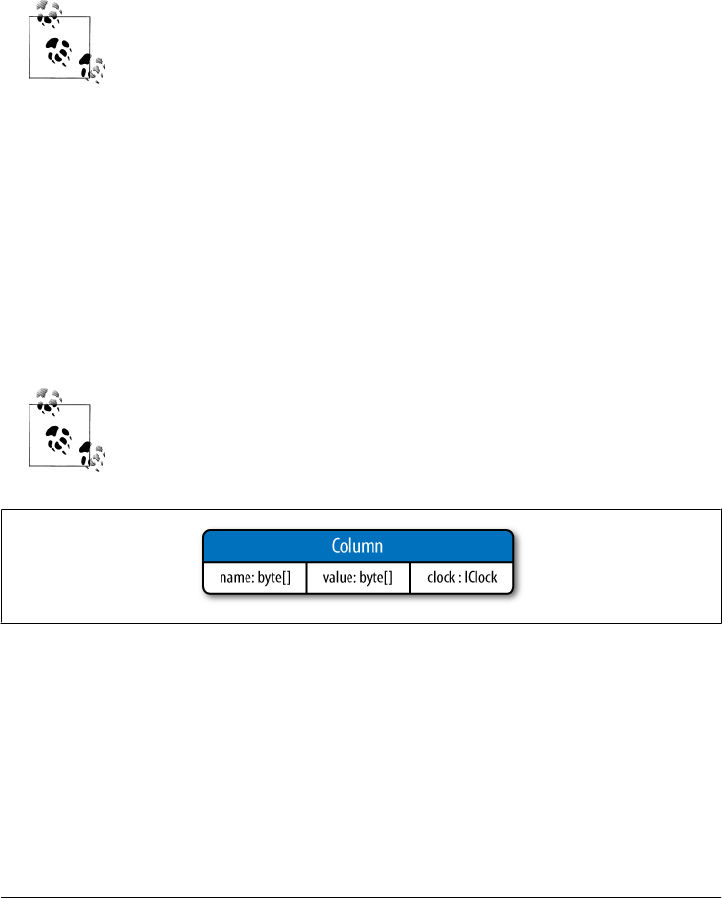
assigning all of the columns in the table a name; later, when you write data, you’re
simply supplying values for the predefined structure.
But in Cassandra, you don’t define the columns up front; you just define the column
families you want in the keyspace, and then you can start writing data without defining
the columns anywhere. That’s because in Cassandra, all of a column’s names are
supplied by the client. This adds considerable flexibility to how your application works
with data, and can allow it to evolve organically over time.
Cassandra’s clock was introduced in version 0.7, but its fate is uncertain.
Prior to 0.7, it was called a timestamp, and was simply a Java long type.
It was changed to support Vector Clocks, which are a popular mecha-
nism for replica conflict resolution in distributed systems, and it’s how
Amazon Dynamo implements conflict resolution. That’s why you’ll
hear the third aspect of the column referred to both as a timestamp and
a clock. Vector Clocks may or may not ultimately become how time-
stamps are represented in Cassandra 0.7, which is in beta at the time of
this writing.
The data types for the name and value are Java byte arrays, frequently supplied as
strings. Because the name and value are binary types, they can be of any length. The
data type for the clock is an org.apache.cassandra.db.IClock, but for the 0.7 release, a
timestamp still works to keep backward compatibility. This column structure is illus-
trated in Figure 3-5.
Cassandra 0.7 introduced an optional time to live (TTL) value, which
allows columns to expire a certain amount of time after creation. This
can potentially prove very useful.
Figure 3-5. The structure of a column
Here’s an example of a column you might define, represented with JSON notation just
for clarity of structure:
{
"name": "email",
"value: "me@example.com",
"timestamp": 1274654183103300
}
50 | Chapter 3: The Cassandra Data Model
In this example, this column is named “email”; more precisely, the value of its name
attribute is “email”. But recall that a single column family will have multiple keys (or
row keys) representing different rows that might also contain this column. This is why
moving from the relational model is hard: we think of a relational table as holding the
same set of columns for every row. But in Cassandra, a column family holds many rows,
each of which may hold the same, or different, sets of columns.
On the server side, columns are immutable in order to prevent multithreading
issues. The column is defined in Cassandra by the org.apache.cassandra.db.IColumn
interface, which allows a variety of operations, including getting the value of the column
as a byte array or, in the case of a super column, getting its subcolumns as a
Collection<IColumn> and finding the time of the most recent change.
In a relational database, rows are stored together. This wasn’t the case for early versions
of Cassandra, but as of version 0.6, rows for the same column family are stored together
on disk.
You cannot perform joins in Cassandra. If you have designed a data
model and find that you need something like a join, you’ll have to either
do the work on the client side, or create a denormalized second column
family that represents the join results for you. This is common among
Cassandra users. Performing joins on the client should be a very rare
case; you really want to duplicate (denormalize) the data instead.
Wide Rows, Skinny Rows
When designing a table in a traditional relational database, you’re typically dealing
with “entities,” or the set of attributes that describe a particular noun (Hotel, User,
Product, etc.). Not much thought is given to the size of the rows themselves, because
row size isn’t negotiable once you’ve decided what noun your table represents. How-
ever, when you’re working with Cassandra, you actually have a decision to make about
the size of your rows: they can be wide or skinny, depending on the number of columns
the row contains.
A wide row means a row that has lots and lots (perhaps tens of thousands or even
millions) of columns. Typically there is a small number of rows that go along with so
many columns. Conversely, you could have something closer to a relational model,
where you define a smaller number of columns and use many different rows—that’s
the skinny model.
Wide rows typically contain automatically generated names (like UUIDs or time-
stamps) and are used to store lists of things. Consider a monitoring application as an
example: you might have a row that represents a time slice of an hour by using a modi-
fied timestamp as a row key, and then store columns representing IP addresses that
accessed your application within that interval. You can then create a new row key after
an hour elapses.
Columns | 51

Skinny rows are slightly more like traditional RDBMS rows, in that each row will con-
tain similar sets of column names. They differ from RDBMS rows, however, because
all columns are essentially optional.
Another difference between wide and skinny rows is that only wide rows will typically
be concerned about sorting order of column names. Which brings us to the next section.
Column Sorting
Columns have another aspect to their definition. In Cassandra, you specify how column
names will be compared for sort order when results are returned to the client. Columns
are sorted by the “Compare With” type defined on their enclosing column family, and
you can choose from the following: AsciiType, BytesType, LexicalUUIDType, Integer
Type, LongType, TimeUUIDType, or UTF8Type.
AsciiType
This sorts by directly comparing the bytes, validating that the input can be parsed
as US-ASCII. US-ASCII is a character encoding mechanism based on the lexical
order of the English alphabet. It defines 128 characters, 94 of which are printable.
BytesType
This is the default, and sorts by directly comparing the bytes, skipping the valida-
tion step. BytesType is the default for a reason: it provides the correct sorting for
most types of data (UTF-8 and ASCII included).
LexicalUUIDType
A 16-byte (128-bit) Universally Unique Identifier (UUID), compared lexically (by
byte value).
LongType
This sorts by an 8-byte (64-bit) long numeric type.
IntegerType
Introduced in 0.7, this is faster than LongType and allows integers of both fewer and
more bits than the 64 bits provided by LongType.
TimeUUIDType
This sorts by a 16-byte (128-bit) timestamp. There are five common versions of
generating timestamp UUIDs. The scheme Cassandra uses is a version one UUID,
which means that it is generated based on conflating the computer’s MAC address
and the number of 100-nanosecond intervals since the beginning of the Gregorian
calendar.
UTF8Type
A string using UTF-8 as the character encoder. Although this may seem like a
good default type, that’s probably because it’s comfortable to programmers who
are used to using XML or other data exchange mechanism that requires common
encoding. In Cassandra, however, you should use UTF8Type only if you want your
data validated.
52 | Chapter 3: The Cassandra Data Model
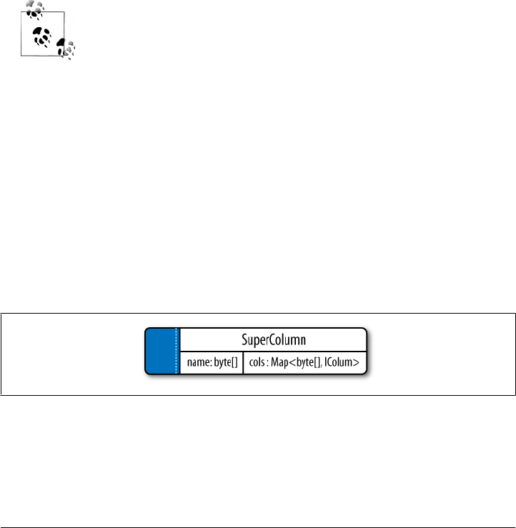
Custom
You can create your own column sorting mechanism if you like. This, like many
things in Cassandra, is pluggable. All you have to do is extend the org.apache
.cassandra.db.marshal.AbstractType and specify your class name.
Column names are stored in sorted order according to the value of compare_with. Rows,
on the other hand, are stored in an order defined by the partitioner (for example,
with RandomPartitioner, they are in random order, etc.). We examine partitioners in
Chapter 6.
It is not possible in Cassandra to sort by value, as we’re used to doing in relational
databases. This may seem like an odd limitation, but Cassandra has to sort by column
name in order to allow fetching individual columns from very large rows without
pulling the entire row into memory. Performance is an important selling point of Cas-
sandra, and sorting at read time would harm performance.
Column sorting is controllable, but key sorting isn’t; row keys always
sort in byte order.
Super Columns
A super column is a special kind of column. Both kinds of columns are name/value
pairs, but a regular column stores a byte array value, and the value of a super column
is a map of subcolumns (which store byte array values). Note that they store only a
map of columns; you cannot define a super column that stores a map of other super
columns. So the super column idea goes only one level deep, but it can have an
unbounded number of columns.
The basic structure of a super column is its name, which is a byte array (just as with a
regular column), and the columns it stores (see Figure 3-6). Its columns are held as a
map whose keys are the column names and whose values are the columns.
Figure 3-6. The basic structure of a super column
Each column family is stored on disk in its own separate file. So to optimize perform-
ance, it’s important to keep columns that you are likely to query together in the same
column family, and a super column can be helpful for this.
Super Columns | 53

The SuperColumn class implements both the IColumn and the IColumnContainer classes,
both from the org.apache.cassandra.db package. The Thrift API is the underlying RPC
serialization mechanism for performing remote operations on Cassandra. Because the
Thrift API has no notion of inheritance, you will sometimes see the API refer to a
ColumnOrSupercolumn type; when data structures use this type, you are expected to
know whether your underlying column family is of type Super or Standard.
Fun fact: super columns were one of the updates that Facebook added
to Google’s Bigtable data model.
Here we see some more of the richness of the data model. When using regular columns,
as we saw earlier, Cassandra looks like a four-dimensional hashtable. But for super
columns, it becomes more like a five-dimensional hash:
[Keyspace][ColumnFamily][Key][SuperColumn][SubColumn]
To use a super column, you define your column family as type Super. Then, you still
have row keys as you do in a regular column family, but you also reference the super
column, which is simply a name that points to a list or map of regular columns (some-
times called the subcolumns).
Here is an example of a super column family definition called PointOfInterest. In the
hotelier domain, a “point of interest” is a location near a hotel that travelers might like
to visit, such as a park, museum, zoo, or tourist attraction:
PointOfInterest (SCF)
SCkey: Cambria Suites Hayden
{
key: Phoenix Zoo
{
phone: 480-555-9999,
desc: They have animals here.
},
key: Spring Training
{
phone: 623-333-3333,
desc: Fun for baseball fans.
},
}, //end of Cambria row
SCkey: (UTF8) Waldorf=Astoria
{
key: Central Park
desc: Walk around. It's pretty.
},
key: Empire State Building
{
phone: 212-777-7777,
desc: Great view from the 102nd floor.
54 | Chapter 3: The Cassandra Data Model

}
}
}
The PointOfInterest super column family has two super columns, each named for a
different hotel (Cambria Suites Hayden and Waldorf=Astoria). The row keys are names
of different points of interest, such as “Phoenix Zoo” and “Central Park”. Each row
has columns for a description (the “desc” column); some of the rows have a phone
number, and some don’t. Unlike relational tables, which group rows of identical struc-
ture, column families and super column families group merely similar records.
Using the CLI, we could query a super column family like this:
cassandra> get PointOfInterest['Central Park']['The Waldorf=Astoria']['desc']
=> (column=desc, value=Walk around in the park. It's pretty., timestamp=1281301988847)
This query is asking: in the PointOfInterest column family (which happens to be de-
fined as type Super), use the row key “Central Park”; for the super column named
“Waldorf=Astoria”, get me the value of the “desc” column (which is the plain language
text describing the point of interest).
Composite Keys
There is an important consideration when modeling with super columns: Cassandra
does not index subcolumns, so when you load a super column into memory, all of its
columns are loaded as well.
This limitation was discovered by Ryan King, the Cassandra lead at
Twitter. It might be fixed in a future release, but the change is pending
an update to the underlying storage file (the SSTable).
You can use a composite key of your own design to help you with queries. A composite
key might be something like <userid:lastupdate>.
This could just be something that you consider when modeling, and then check back
on later when you come to a hardware sizing exercise. But if your data model anticipates
more than several thousand subcolumns, you might want to take a different approach
and not use super columns. The alternative involves creating a composite key. Instead
of representing columns within a super column, the composite key approach means
that you use a regular column family with regular columns, and then employ a custom
delimiter in your key name and parse it on client retrieval.
Here’s an example of a composite key pattern, used in combination with an example
of a Cassandra design pattern I call Materialized View, as well as a common Cassandra
design pattern I call Valueless Column:
Super Columns | 55

HotelByCity (CF) Key: city:state {
key: Phoenix:AZ {AZC_043: -, AZS_011: -}
key: San Francisco:CA {CAS_021: -}
key: New York:NY {NYN_042: -}
}
There are three things happening here. First, we already have defined hotel information
in another column family called Hotel. But we can create a second column family called
HotelByCity that denormalizes the hotel data. We repeat the same information we
already have, but store it in a way that acts similarly to a view in RDBMS, because it
allows us a quick and direct way to write queries. When we know that we’re going to
look up hotels by city (because that’s how people tend to search for them), we can
create a table that defines a row key for that search. However, there are many states
that have cities with the same name (Springfield comes to mind), so we can’t just name
the row key after the city; we need to combine it with the state.
We then use another pattern called Valueless Column. All we need to know is what
hotels are in the city, and we don’t need to denormalize further. So we use the column’s
name as the value, and the column has no corresponding value. That is, when the
column is inserted, we just store an empty byte array with it.
Design Differences Between RDBMS and Cassandra
There are several differences between Cassandra’s model and query methods compared
to what’s available in RDBMS, and these are important to keep in mind.
No Query Language
SQL is the standard query language used in relational databases. Cassandra has no
query language. It does have an API that you access through its RPC serialization
mechanism, Thrift.
No Referential Integrity
Cassandra has no concept of referential integrity, and therefore has no concept of joins.
In a relational database, you could specify foreign keys in a table to reference the pri-
mary key of a record in another table. But Cassandra does not enforce this. It is still a
common design requirement to store IDs related to other entities in your tables, but
operations such as cascading deletes are not available.
Secondary Indexes
Here’s why secondary indexes are a feature: say that you want to find the unique ID
for a hotel property. In a relational database, you might use a query like this:
SELECT hotelID FROM Hotel WHERE name = 'Clarion Midtown';
56 | Chapter 3: The Cassandra Data Model
This is the query you’d have to use if you knew the name of the hotel you were looking
for but not the unique ID. When handed a query like this, a relational database will
perform a full table scan, inspecting each row’s name column to find the value you’re
looking for. But this can become very slow once your table grows very large. So the
relational answer to this is to create an index on the name column, which acts as a copy
of the data that the relational database can look up very quickly. Because the hotelID
is already a unique primary key constraint, it is automatically indexed, and that is the
primary index; for us to create another index on the name column would constitute a
secondary index, and Cassandra does not currently support this.
To achieve the same thing in Cassandra, you create a second column family that holds
the lookup data. You create one column family to store the hotel names, and map them
to their IDs. The second column family acts as an explicit secondary index.
Support for secondary indexes is currently being added to Cassandra
0.7. This allows you to create indexes on column values. So, if you want
to see all the users who live in a given city, for example, secondary index
support will save you from doing it from scratch.
Sorting Is a Design Decision
In RDBMS, you can easily change the order in which records are returned to you by
using ORDER BY in your query. The default sort order is not configurable; by default,
records are returned in the order in which they are written. If you want to change the
order, you just modify your query, and you can sort by any list of columns. In Cassan-
dra, however, sorting is treated differently; it is a design decision. Column family
definitions include a CompareWith element, which dictates the order in which your rows
will be sorted on reads, but this is not configurable per query.
Where RDBMS constrains you to sorting based on the data type stored in the column,
Cassandra only stores byte arrays, so that approach doesn’t make sense. What you can
do, however, is sort as if the column were one of several different types (ASCII, Long
integer, TimestampUUID, lexicographically, etc.). You can also use your own pluggable
comparator for sorting if you wish.
Otherwise, there is no support for ORDER BY and GROUP BY statements in Cassandra
as there is in SQL. There is a query type called a SliceRange, which we examine in
Chapter 4; it is similar to ORDER BY in that it allows a reversal.
Denormalization
In relational database design, we are often taught the importance of normalization.
This is not an advantage when working with Cassandra because it performs best when
the data model is denormalized. It is often the case that companies end up denormal-
izing data in a relational database. There are two common reasons for this. One is
Design Differences Between RDBMS and Cassandra | 57

performance. Companies simply can’t get the performance they need when they have
to do so many joins on years’ worth of data, so they denormalize along the lines of
known queries. This ends up working, but goes against the grain of how relational
databases are intended to be designed, and ultimately makes one question whether
using a relational database is the best approach in these circumstances.
A second reason that relational databases get denormalized on purpose is a business
document structure that requires retention. That is, you have an enclosing table that
refers to a lot of external tables whose data could change over time, but you need to
preserve the enclosing document as a snapshot in history. The common example here
is with invoices. You already have Customer and Product tables, and you’d think that
you could just make an invoice that refers to those tables. But this should never be done
in practice. Customer or price information could change, and then you would lose the
integrity of the Invoice document as it was on the invoice date, which could violate
audits, reports, or laws, and cause other problems.
In the relational world, denormalization violates Codd's normal forms, and we try to
avoid it. But in Cassandra, denormalization is, well, perfectly normal. It's not required
if your data model is simple. But don't be afraid of it.
The important point is that instead of modeling the data first and then writing queries,
with Cassandra you model the queries and let the data be organized around them.
Think of the most common query paths your application will use, and then create the
column families that you need to support them.
Detractors have suggested that this is a problem. But it is perfectly reasonable to expect
that you should think hard about the queries in your application, just as you would,
presumably, think hard about your relational domain. You may get it wrong, and then
you’ll have problems in either world. Or your query needs might change over time, and
then you’ll have to work to update your data set. But this is no different from defining
the wrong tables, or needing additional tables, in RDBMS.
For an interesting article on how Cloudkick is using Cassandra to store
metrics and monitoring data, see https://www.cloudkick.com/blog/2010/
mar/02/4_months_with_cassandra.
Design Patterns
There are a few ways that people commonly use Cassandra that might be described
as design patterns. I’ve given names to these common patterns: Materialized View,
Valueless Column, and Aggregate Key.
58 | Chapter 3: The Cassandra Data Model

Materialized View
It is common to create a secondary index that represents additional queries. Because
you don’t have a SQL WHERE clause, you can recreate this effect by writing your data to
a second column family that is created specifically to represent that query.
For example, if you have a User column family and you want to find users in a
particular city, you might create a second column family called UserCity that stores
user data with the city as keys (instead of the username) and that has columns named
for the users who live in that city. This is a denormalization technique that will speed
queries and is an example of specifically designing your data around your queries (and
not the other way around). This usage is common in the Cassandra world. When you
want to query for users in a city, you just query the UserCity column family, instead of
querying the User column family and doing a bunch of pruning work on the client across
a potentially large data set.
Note that in this context, “materialized” means storing a full copy of the original data
so that everything you need to answer a query is right there, without forcing you to
look up the original data. If you are performing a second query because you’re only
storing column names that you use, like foreign keys in the second column family, that’s
a secondary index.
As of 0.7, Cassandra has native support for secondary indexes.
Valueless Column
Let’s build on our User/UserCity example. Because we’re storing the reference data in
the User column family, two things arise: one, you need to have unique and thoughtful
keys that can enforce referential integrity; and two, the columns in the UserCity
column family don’t necessarily need values. If you have a row key of Boise, then the
column names can be the names of the users in that city. Because your reference data
is in the User column family, the columns don’t really have any meaningful value; you’re
just using it as a prefabricated list, but you’ll likely want to use values in that list to get
additional data from the reference column family.
Aggregate Key
When you use the Valueless Column pattern, you may also need to employ the
Aggregate Key pattern. This pattern fuses together two scalar values with a separator
to create an aggregate. To extend our example further, city names typically aren’t
unique; many states in the US have a city called Springfield, and there’s a Paris, Texas,
and a Paris, Tennessee. So what will work better here is to fuse together the state name
Design Patterns | 59

and the city name to create an Aggregate Key to use in our Materialized View. This key
would look something like: TX:Paris or TN:Paris. By convention, many Cassandra users
employ the colon as the separator, but it could be a pipe character or any other character
that is not otherwise meaningful in your keys.
Some Things to Keep in Mind
Let’s look briefly at a few things to keep in mind when you’re trying to move from a
relational mindset to Cassandra’s data model. I’ll just say it: if you have been working
with relational databases for a long time, it’s not always easy. Here are a few pointers:
• Start with your queries. Ask what queries your application will need, and model
the data around that instead of modeling the data first, as you would in the rela-
tional world. This can be shocking to some people. Some very smart people have
told me that this approach will cause trouble for the Cassandra practitioner down
the line when new queries come up, as they tend to in business. Fair enough. My
response is to ask why they assume their data types would be more static than their
queries.
• You have to supply a timestamp (or clock) with each query, so you need a strategy
to synchronize those with multiple clients. This is crucial in order for Cassandra
to use the timestamps to determine the most recent write value. One good strategy
here is the use of a Network Time Protocol (NTP) server. Again, some smart people
have asked me, why not let the server take care of the clock? My response is that
in a symmetrical distributed database, the server side actually has the same
problem.
Summary
In this chapter we took a gentle approach to understanding Cassandra’s data model of
keyspaces, column families, columns, and super columns. We also explored a few of
the contrasts between RDBMS and Cassandra.
60 | Chapter 3: The Cassandra Data Model
CHAPTER 4
Sample Application
In this chapter, we create a complete sample application so we can see how all the parts
fit together. We will use various parts of the API to see how to insert data, perform
batch updates, and search column families and super column families.
To create the example, we want to use something that is complex enough to show the
various data structures and basic API operations, but not something that will bog you
down with details. In order to get enough data in the database to make our searches
work right (by finding stuff we’re looking for and leaving out stuff we’re not looking
for), there’s a little redundancy in the prepopulation of the database. Also, I wanted to
use a domain that’s familiar to everyone so we can concentrate on how to work with
Cassandra, not on what the application domain is all about.
The code in this chapter has been tested against the 0.7 beta 1 release,
and works as shown. It is possible that API changes may necessitate
minor tuning on your part, depending on your version.
Data Design
When you set out to build a new data-driven application that will use a relational
database, you might start by modeling the domain as a set of properly normalized tables
and use foreign keys to reference related data in other tables. Now that we have an
understanding of how Cassandra stores data, let’s create a little domain model that is
easy to understand in the relational world, and then see how we might map it from a
relational to a distributed hashtable model in Cassandra.
Relational modeling, in simple terms, means that you start from the conceptual domain
and then represent the nouns in the domain in tables. You then assign primary keys
and foreign keys to model relationships. When you have a many-to-many relationship,
you create the join tables that represent just those keys. The join tables don’t exist in
the real world, and are a necessary side effect of the way relational models work. After
you have all your tables laid out, you can start writing queries that pull together
61

disparate data using the relationships defined by the keys. The queries in the relational
world are very much secondary. It is assumed that you can always get the data you want
as long as you have your tables modeled properly. Even if you have to use several
complex subqueries or join statements, this is usually true.
By contrast, in Cassandra you don’t start with the data model; you start with the query
model.
For this example, let’s use a domain that is easily understood and that everyone can
relate to: a hotel that wants to allow guests to book a reservation.
Our conceptual domain includes hotels, guests that stay in the hotels, a collection of
rooms for each hotel, and a record of the reservation, which is a certain guest in a certain
room for a certain period of time (called the “stay”). Hotels typically also maintain a
collection of “points of interest,” which are parks, museums, shopping galleries,
monuments, or other places near the hotel that guests might want to visit during their
stay. Both hotels and points of interest need to maintain geolocation data so that they
can be found on maps for mashups, and to calculate distances.
Obviously, in the real world there would be many more considerations
and much more complexity. For example, hotel rates are notoriously
dynamic, and calculating them involves a wide array of factors. Here
we’re defining something complex enough to be interesting and touch
on the important points, but simple enough to maintain the focus on
learning Cassandra.
Here’s how we would start this application design with Cassandra. First, determine
your queries. We’ll likely have something like the following:
• Find hotels in a given area.
• Find information about a given hotel, such as its name and location.
• Find points of interest near a given hotel.
• Find an available room in a given date range.
• Find the rate and amenities for a room.
• Book the selected room by entering guest information.
Hotel App RDBMS Design
Figure 4-1 shows how we might represent this simple hotel reservation system using a
relational database model. The relational model includes a couple of “join” tables in
order to resolve the many-to-many relationships of hotels-to-points of interest, and for
rooms-to-amenities.
62 | Chapter 4: Sample Application
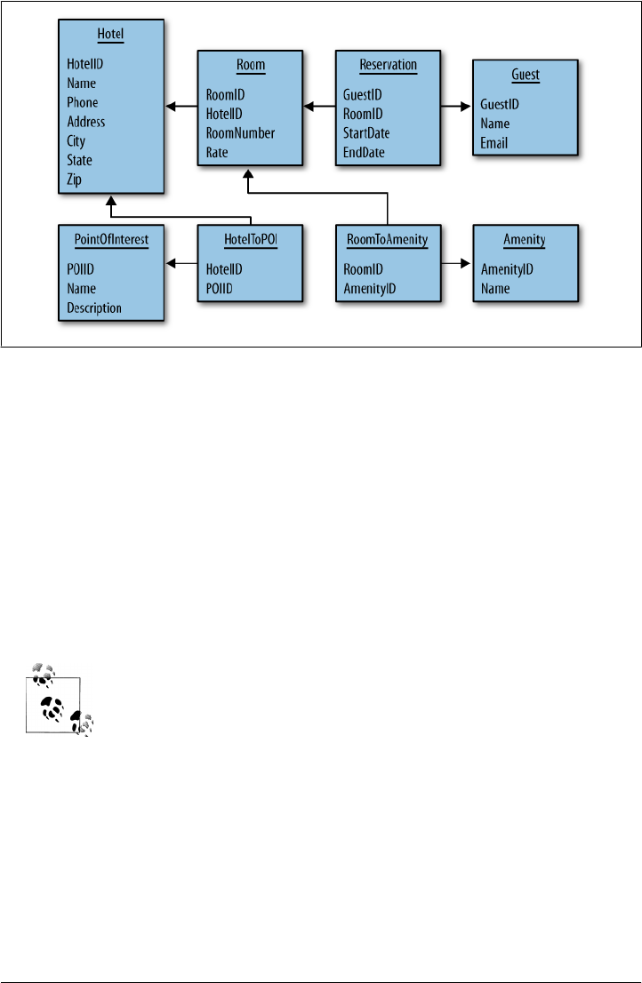
Figure 4-1. A simple hotel search system using RDBMS
Hotel App Cassandra Design
Although there are many possible ways to do it, we could represent the same logical
data model using a Cassandra physical model such as that shown in Figure 4-2.
In this design, we’re doing all the same things as in the relational design. We have
transferred some of the tables, such as Hotel and Guest, to column families. Other
tables, such as PointOfInterest, have been denormalized into a super column family.
In the relational model, you can look up hotels by the city they’re in using a SQL
statement. But because we don’t have SQL in Cassandra, we’ve created an index in the
form of the HotelByCity column family.
I’m using a stereotype notation here, so <<CF>> refers to a column family,
<<SCF>> refers to a super column family, and so on.
We have combined room and amenities into a single column family, Room. The columns
such as type and rate will have corresponding values; other columns, such as
hot tub, will just use the presence of the column name itself as the value, and be oth-
erwise empty.
Hotel App Cassandra Design | 63
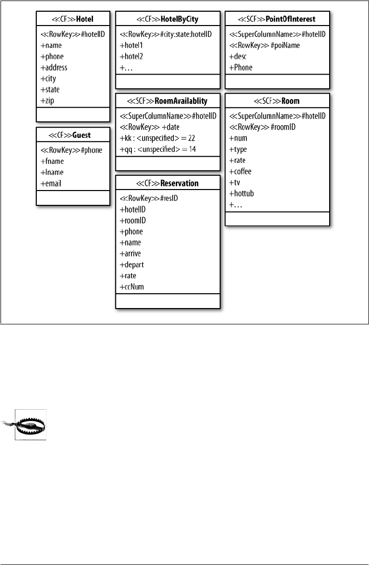
Hotel Application Code
In this section we walk through the code and show how to implement the given design.
This is useful because it illustrates several different API functions in action.
The purpose of this sample application is to show how different ideas
in Cassandra can be combined. It is by no means the only way to
transfer the relational design into this model. There is a lot of low-level
plumbing here that uses the Thrift API. Thrift is (probably) changing to
Avro, so although the basic ideas here work, you don’t want to follow
this example in a real application. Instead, check out Chapter 8 and use
one of the many available third-party clients for Cassandra, depending
on the language that your application uses and other needs that you
have.
Figure 4-2. The hotel search represented with Cassandra’s model
64 | Chapter 4: Sample Application

The application we’re building will do the following things:
1. Create the database structure.
2. Prepopulate the database with hotel and point of interest data. The hotels are
stored in standard column families, and the points of interest are in super column
families.
3. Search for a list of hotels in a given city. This uses a secondary index.
4. Select one of the hotels returned in the search, and then search for a list of points
of interest near the chosen hotel.
5. Booking the hotel by doing an insert into the Reservation column family should
be straightforward at this point, and is left to the reader.
Space doesn’t permit implementing the entire application. But we’ll walk through the
major parts, and finishing the implementation is just a matter of creating a variation of
what is shown.
Creating the Database
The first step is creating the schema definition. For this example, we’ll define the
schema in YAML and then load it, although you could also use client code to define it.
The YAML file shown in Example 4-1 defines the necessary keyspace and column
families.
Example 4-1. Schema definition in cassandra.yaml
keyspaces:
- name: Hotelier
replica_placement_strategy: org.apache.cassandra.locator.RackUnawareStrategy
replication_factor: 1
column_families:
- name: Hotel
compare_with: UTF8Type
- name: HotelByCity
compare_with: UTF8Type
- name: Guest
compare_with: BytesType
- name: Reservation
compare_with: TimeUUIDType
- name: PointOfInterest
column_type: Super
compare_with: UTF8Type
compare_subcolumns_with: UTF8Type
- name: Room
Hotel Application Code | 65

column_type: Super
compare_with: BytesType
compare_subcolumns_with: BytesType
- name: RoomAvailability
column_type: Super
compare_with: BytesType
compare_subcolumns_with: BytesType
This definition provides all of the column families to run the example, and a couple
more that we don’t directly reference in the application code, because it rounds out the
design as transferred from RDBMS.
Loading the schema
Once you have the schema defined in YAML, you need to load it. To do this, open a
console, start the jconsole application, and connect to Cassandra via JMX. Then,
execute the operation loadSchemaFromYAML, which is part of the org.apache
.cassandra.service.StorageService MBean. Now Cassandra knows about your
schema and you can start using it. You can also use the API itself to create keyspaces
and column families.
Data Structures
The application requires some standard data structures that will just act as transfer
objects for us. These aren’t particularly interesting, but are required to keep things
organized. We’ll use a Hotel data structure to hold all of the information about a hotel,
shown in Example 4-2.
Example 4-2. Hotel.java
package com.cassandraguide.hotel;
//data transfer object
public class Hotel {
public String id;
public String name;
public String phone;
public String address;
public String city;
public String state;
public String zip;
}
This structure just holds the column information for convenience in the application.
We also have a POI data structure to hold information about points of interest. This is
shown in Example 4-3.
66 | Chapter 4: Sample Application

Example 4-3. POI.java
package com.cassandraguide.hotel;
//data transfer object for a Point of Interest
public class POI {
public String name;
public String desc;
public String phone;
}
We also have a Constants class, which keeps commonly used strings in one easy-to-
change place, shown in Example 4-4.
Example 4-4. Constants.java
package com.cassandraguide.hotel;
import org.apache.cassandra.thrift.ConsistencyLevel;
public class Constants {
public static final String CAMBRIA_NAME = "Cambria Suites Hayden";
public static final String CLARION_NAME= "Clarion Scottsdale Peak";
public static final String W_NAME = "The W SF";
public static final String WALDORF_NAME = "The Waldorf=Astoria";
public static final String UTF8 = "UTF8";
public static final String KEYSPACE = "Hotelier";
public static final ConsistencyLevel CL = ConsistencyLevel.ONE;
public static final String HOST = "localhost";
public static final int PORT = 9160;
}
Holding these commonly used strings make the code clearer and more concise, and
you can easily change these values to reflect what makes sense in your environment.
Getting a Connection
For convenience, and to save repeating a bunch of boilerplate code, let’s put the con-
nection code into one class, called Connector, shown in Example 4-5.
Example 4-5. A connection client convenience class, Connector.java
package com.cassandraguide.hotel;
import static com.cassandraguide.hotel.Constants.KEYSPACE;
import org.apache.cassandra.thrift.Cassandra;
import org.apache.cassandra.thrift.InvalidRequestException;
import org.apache.thrift.TException;
import org.apache.thrift.protocol.TBinaryProtocol;
import org.apache.thrift.protocol.TProtocol;
import org.apache.thrift.transport.TFramedTransport;
Hotel Application Code | 67

import org.apache.thrift.transport.TSocket;
import org.apache.thrift.transport.TTransport;
import org.apache.thrift.transport.TTransportException;
//simple convenience class to wrap connections, just to reduce repeat code
public class Connector {
TTransport tr = new TSocket("localhost", 9160);
// returns a new connection to our keyspace
public Cassandra.Client connect() throws TTransportException,
TException, InvalidRequestException {
TFramedTransport tf = new TFramedTransport(tr);
TProtocol proto = new TBinaryProtocol(tf);
Cassandra.Client client = new Cassandra.Client(proto);
tr.open();
client.set_keyspace(KEYSPACE);
return client;
}
public void close() {
tr.close();
}
}
When we need to execute a database operation, we can use this class to open a con-
nection and then close the connection once we’re done.
Prepopulating the Database
The Prepopulate class, shown in Example 4-6, does a bunch of inserts and batch_
mutates in order to prepopulate the database with the hotel information and points of
interest information that users will search for.
Example 4-6. Prepopulate.java
package com.cassandraguide.hotel;
import static com.cassandraguide.hotel.Constants.CAMBRIA_NAME;
import static com.cassandraguide.hotel.Constants.CL;
import static com.cassandraguide.hotel.Constants.CLARION_NAME;
import static com.cassandraguide.hotel.Constants.UTF8;
import static com.cassandraguide.hotel.Constants.WALDORF_NAME;
import static com.cassandraguide.hotel.Constants.W_NAME;
import java.io.UnsupportedEncodingException;
import java.util.ArrayList;
import java.util.HashMap;
import java.util.List;
import java.util.Map;
import org.apache.cassandra.thrift.Cassandra;
import org.apache.cassandra.thrift.Clock;
68 | Chapter 4: Sample Application

import org.apache.cassandra.thrift.Column;
import org.apache.cassandra.thrift.ColumnOrSuperColumn;
import org.apache.cassandra.thrift.ColumnParent;
import org.apache.cassandra.thrift.ColumnPath;
import org.apache.cassandra.thrift.Mutation;
import org.apache.cassandra.thrift.SuperColumn;
import org.apache.log4j.Logger;
/**
* Performs the initial population of the database.
* Fills the CFs and SCFs with Hotel, Point of Interest, and index data.
* Shows batch_mutate and insert for Column Families and Super Column Families.
*
* I am totally ignoring exceptions to save space.
*/
public class Prepopulate {
private static final Logger LOG = Logger.getLogger(Prepopulate.class);
private Cassandra.Client client;
private Connector connector;
//constructor opens a connection so we don't have to
//constantly recreate it
public Prepopulate() throws Exception {
connector = new Connector();
client = connector.connect();
}
void prepopulate() throws Exception {
//pre-populate the DB with Hotels
insertAllHotels();
//also add all hotels to index to help searches
insertByCityIndexes();
//pre-populate the DB with POIs
insertAllPointsOfInterest();
connector.close();
}
//also add hotels to lookup by city index
public void insertByCityIndexes() throws Exception {
String scottsdaleKey = "Scottsdale:AZ";
String sfKey = "San Francisco:CA";
String newYorkKey = "New York:NY";
insertByCityIndex(scottsdaleKey, CAMBRIA_NAME);
insertByCityIndex(scottsdaleKey, CLARION_NAME);
insertByCityIndex(sfKey, W_NAME);
insertByCityIndex(newYorkKey, WALDORF_NAME);
}
//use Valueless Column pattern
Hotel Application Code | 69

private void insertByCityIndex(String rowKey, String hotelName)
throws Exception {
Clock clock = new Clock(System.nanoTime());
Column nameCol = new Column(hotelName.getBytes(UTF8),
new byte[0], clock);
ColumnOrSuperColumn nameCosc = new ColumnOrSuperColumn();
nameCosc.column = nameCol;
Mutation nameMut = new Mutation();
nameMut.column_or_supercolumn = nameCosc;
//set up the batch
Map<String, Map<String, List<Mutation>>> mutationMap =
new HashMap<String, Map<String, List<Mutation>>>();
Map<String, List<Mutation>> muts =
new HashMap<String, List<Mutation>>();
List<Mutation> cols = new ArrayList<Mutation>();
cols.add(nameMut);
String columnFamily = "HotelByCity";
muts.put(columnFamily, cols);
//outer map key is a row key
//inner map key is the column family name
mutationMap.put(rowKey, muts);
//create representation of the column
ColumnPath cp = new ColumnPath(columnFamily);
cp.setColumn(hotelName.getBytes(UTF8));
ColumnParent parent = new ColumnParent(columnFamily);
//here, the column name IS the value (there's no value)
Column col = new Column(hotelName.getBytes(UTF8), new byte[0], clock);
client.insert(rowKey.getBytes(), parent, col, CL);
LOG.debug("Inserted HotelByCity index for " + hotelName);
} //end inserting ByCity index
//POI
public void insertAllPointsOfInterest() throws Exception {
LOG.debug("Inserting POIs.");
insertPOIEmpireState();
insertPOICentralPark();
insertPOIPhoenixZoo();
insertPOISpringTraining();
70 | Chapter 4: Sample Application

LOG.debug("Done inserting POIs.");
}
private void insertPOISpringTraining() throws Exception {
//Map<byte[],Map<String,List<Mutation>>>
Map<byte[], Map<String, List<Mutation>>> outerMap =
new HashMap<byte[], Map<String, List<Mutation>>>();
List<Mutation> columnsToAdd = new ArrayList<Mutation>();
Clock clock = new Clock(System.nanoTime());
String keyName = "Spring Training";
Column descCol = new Column("desc".getBytes(UTF8),
"Fun for baseball fans.".getBytes("UTF-8"), clock);
Column phoneCol = new Column("phone".getBytes(UTF8),
"623-333-3333".getBytes(UTF8), clock);
List<Column> cols = new ArrayList<Column>();
cols.add(descCol);
cols.add(phoneCol);
Map<String, List<Mutation>> innerMap =
new HashMap<String, List<Mutation>>();
Mutation columns = new Mutation();
ColumnOrSuperColumn descCosc = new ColumnOrSuperColumn();
SuperColumn sc = new SuperColumn();
sc.name = CAMBRIA_NAME.getBytes();
sc.columns = cols;
descCosc.super_column = sc;
columns.setColumn_or_supercolumn(descCosc);
columnsToAdd.add(columns);
String superCFName = "PointOfInterest";
ColumnPath cp = new ColumnPath();
cp.column_family = superCFName;
cp.setSuper_column(CAMBRIA_NAME.getBytes());
cp.setSuper_columnIsSet(true);
innerMap.put(superCFName, columnsToAdd);
outerMap.put(keyName.getBytes(), innerMap);
client.batch_mutate(outerMap, CL);
LOG.debug("Done inserting Spring Training.");
}
private void insertPOIPhoenixZoo() throws Exception {
Map<byte[], Map<String, List<Mutation>>> outerMap =
new HashMap<byte[], Map<String, List<Mutation>>>();
List<Mutation> columnsToAdd = new ArrayList<Mutation>();
Hotel Application Code | 71

long ts = System.currentTimeMillis();
String keyName = "Phoenix Zoo";
Column descCol = new Column("desc".getBytes(UTF8),
"They have animals here.".getBytes("UTF-8"), new Clock(ts));
Column phoneCol = new Column("phone".getBytes(UTF8),
"480-555-9999".getBytes(UTF8), new Clock(ts));
List<Column> cols = new ArrayList<Column>();
cols.add(descCol);
cols.add(phoneCol);
Map<String, List<Mutation>> innerMap =
new HashMap<String, List<Mutation>>();
String cambriaName = "Cambria Suites Hayden";
Mutation columns = new Mutation();
ColumnOrSuperColumn descCosc = new ColumnOrSuperColumn();
SuperColumn sc = new SuperColumn();
sc.name = cambriaName.getBytes();
sc.columns = cols;
descCosc.super_column = sc;
columns.setColumn_or_supercolumn(descCosc);
columnsToAdd.add(columns);
String superCFName = "PointOfInterest";
ColumnPath cp = new ColumnPath();
cp.column_family = superCFName;
cp.setSuper_column(cambriaName.getBytes());
cp.setSuper_columnIsSet(true);
innerMap.put(superCFName, columnsToAdd);
outerMap.put(keyName.getBytes(), innerMap);
client.batch_mutate(outerMap, CL);
LOG.debug("Done inserting Phoenix Zoo.");
}
private void insertPOICentralPark() throws Exception {
Map<byte[], Map<String, List<Mutation>>> outerMap =
new HashMap<byte[], Map<String, List<Mutation>>>();
List<Mutation> columnsToAdd = new ArrayList<Mutation>();
Clock clock = new Clock(System.nanoTime());
String keyName = "Central Park";
Column descCol = new Column("desc".getBytes(UTF8),
"Walk around in the park. It's pretty.".getBytes("UTF-8"), clock);
//no phone column for park
72 | Chapter 4: Sample Application

List<Column> cols = new ArrayList<Column>();
cols.add(descCol);
Map<String, List<Mutation>> innerMap =
new HashMap<String, List<Mutation>>();
Mutation columns = new Mutation();
ColumnOrSuperColumn descCosc = new ColumnOrSuperColumn();
SuperColumn waldorfSC = new SuperColumn();
waldorfSC.name = WALDORF_NAME.getBytes();
waldorfSC.columns = cols;
descCosc.super_column = waldorfSC;
columns.setColumn_or_supercolumn(descCosc);
columnsToAdd.add(columns);
String superCFName = "PointOfInterest";
ColumnPath cp = new ColumnPath();
cp.column_family = superCFName;
cp.setSuper_column(WALDORF_NAME.getBytes());
cp.setSuper_columnIsSet(true);
innerMap.put(superCFName, columnsToAdd);
outerMap.put(keyName.getBytes(), innerMap);
client.batch_mutate(outerMap, CL);
LOG.debug("Done inserting Central Park.");
}
private void insertPOIEmpireState() throws Exception {
Map<byte[], Map<String, List<Mutation>>> outerMap =
new HashMap<byte[], Map<String, List<Mutation>>>();
List<Mutation> columnsToAdd = new ArrayList<Mutation>();
Clock clock = new Clock(System.nanoTime());
String esbName = "Empire State Building";
Column descCol = new Column("desc".getBytes(UTF8),
"Great view from 102nd floor.".getBytes("UTF-8"), clock);
Column phoneCol = new Column("phone".getBytes(UTF8),
"212-777-7777".getBytes(UTF8), clock);
List<Column> esbCols = new ArrayList<Column>();
esbCols.add(descCol);
esbCols.add(phoneCol);
Map<String, List<Mutation>> innerMap = new HashMap<String, List<Mutation>>();
Mutation columns = new Mutation();
ColumnOrSuperColumn descCosc = new ColumnOrSuperColumn();
SuperColumn waldorfSC = new SuperColumn();
Hotel Application Code | 73

waldorfSC.name = WALDORF_NAME.getBytes();
waldorfSC.columns = esbCols;
descCosc.super_column = waldorfSC;
columns.setColumn_or_supercolumn(descCosc);
columnsToAdd.add(columns);
String superCFName = "PointOfInterest";
ColumnPath cp = new ColumnPath();
cp.column_family = superCFName;
cp.setSuper_column(WALDORF_NAME.getBytes());
cp.setSuper_columnIsSet(true);
innerMap.put(superCFName, columnsToAdd);
outerMap.put(esbName.getBytes(), innerMap);
client.batch_mutate(outerMap, CL);
LOG.debug("Done inserting Empire State.");
}
//convenience method runs all of the individual inserts
public void insertAllHotels() throws Exception {
String columnFamily = "Hotel";
//row keys
String cambriaKey = "AZC_043";
String clarionKey = "AZS_011";
String wKey = "CAS_021";
String waldorfKey = "NYN_042";
//conveniences
Map<byte[], Map<String, List<Mutation>>> cambriaMutationMap =
createCambriaMutation(columnFamily, cambriaKey);
Map<byte[], Map<String, List<Mutation>>> clarionMutationMap =
createClarionMutation(columnFamily, clarionKey);
Map<byte[], Map<String, List<Mutation>>> waldorfMutationMap =
createWaldorfMutation(columnFamily, waldorfKey);
Map<byte[], Map<String, List<Mutation>>> wMutationMap =
createWMutation(columnFamily, wKey);
client.batch_mutate(cambriaMutationMap, CL);
LOG.debug("Inserted " + cambriaKey);
client.batch_mutate(clarionMutationMap, CL);
LOG.debug("Inserted " + clarionKey);
client.batch_mutate(wMutationMap, CL);
LOG.debug("Inserted " + wKey);
client.batch_mutate(waldorfMutationMap, CL);
LOG.debug("Inserted " + waldorfKey);
74 | Chapter 4: Sample Application

LOG.debug("Done inserting at " + System.nanoTime());
}
//set up columns to insert for W
private Map<byte[], Map<String, List<Mutation>>> createWMutation(
String columnFamily, String rowKey)
throws UnsupportedEncodingException {
Clock clock = new Clock(System.nanoTime());
Column nameCol = new Column("name".getBytes(UTF8),
W_NAME.getBytes("UTF-8"), clock);
Column phoneCol = new Column("phone".getBytes(UTF8),
"415-222-2222".getBytes(UTF8), clock);
Column addressCol = new Column("address".getBytes(UTF8),
"181 3rd Street".getBytes(UTF8), clock);
Column cityCol = new Column("city".getBytes(UTF8),
"San Francisco".getBytes(UTF8), clock);
Column stateCol = new Column("state".getBytes(UTF8),
"CA".getBytes("UTF-8"), clock);
Column zipCol = new Column("zip".getBytes(UTF8),
"94103".getBytes(UTF8), clock);
ColumnOrSuperColumn nameCosc = new ColumnOrSuperColumn();
nameCosc.column = nameCol;
ColumnOrSuperColumn phoneCosc = new ColumnOrSuperColumn();
phoneCosc.column = phoneCol;
ColumnOrSuperColumn addressCosc = new ColumnOrSuperColumn();
addressCosc.column = addressCol;
ColumnOrSuperColumn cityCosc = new ColumnOrSuperColumn();
cityCosc.column = cityCol;
ColumnOrSuperColumn stateCosc = new ColumnOrSuperColumn();
stateCosc.column = stateCol;
ColumnOrSuperColumn zipCosc = new ColumnOrSuperColumn();
zipCosc.column = zipCol;
Mutation nameMut = new Mutation();
nameMut.column_or_supercolumn = nameCosc;
Mutation phoneMut = new Mutation();
phoneMut.column_or_supercolumn = phoneCosc;
Mutation addressMut = new Mutation();
addressMut.column_or_supercolumn = addressCosc;
Mutation cityMut = new Mutation();
cityMut.column_or_supercolumn = cityCosc;
Mutation stateMut = new Mutation();
stateMut.column_or_supercolumn = stateCosc;
Mutation zipMut = new Mutation();
zipMut.column_or_supercolumn = zipCosc;
//set up the batch
Hotel Application Code | 75

Map<byte[], Map<String, List<Mutation>>> mutationMap =
new HashMap<byte[], Map<String, List<Mutation>>>();
Map<String, List<Mutation>> muts =
new HashMap<String, List<Mutation>>();
List<Mutation> cols = new ArrayList<Mutation>();
cols.add(nameMut);
cols.add(phoneMut);
cols.add(addressMut);
cols.add(cityMut);
cols.add(stateMut);
cols.add(zipMut);
muts.put(columnFamily, cols);
//outer map key is a row key
//inner map key is the column family name
mutationMap.put(rowKey.getBytes(), muts);
return mutationMap;
}
//add Waldorf hotel to Hotel CF
private Map<byte[], Map<String, List<Mutation>>> createWaldorfMutation(
String columnFamily, String rowKey)
throws UnsupportedEncodingException {
Clock clock = new Clock(System.nanoTime());
Column nameCol = new Column("name".getBytes(UTF8),
WALDORF_NAME.getBytes("UTF-8"), clock);
Column phoneCol = new Column("phone".getBytes(UTF8),
"212-555-5555".getBytes(UTF8), clock);
Column addressCol = new Column("address".getBytes(UTF8),
"301 Park Ave".getBytes(UTF8), clock);
Column cityCol = new Column("city".getBytes(UTF8),
"New York".getBytes(UTF8), clock);
Column stateCol = new Column("state".getBytes(UTF8),
"NY".getBytes("UTF-8"), clock);
Column zipCol = new Column("zip".getBytes(UTF8),
"10019".getBytes(UTF8), clock);
ColumnOrSuperColumn nameCosc = new ColumnOrSuperColumn();
nameCosc.column = nameCol;
ColumnOrSuperColumn phoneCosc = new ColumnOrSuperColumn();
phoneCosc.column = phoneCol;
ColumnOrSuperColumn addressCosc = new ColumnOrSuperColumn();
addressCosc.column = addressCol;
ColumnOrSuperColumn cityCosc = new ColumnOrSuperColumn();
cityCosc.column = cityCol;
ColumnOrSuperColumn stateCosc = new ColumnOrSuperColumn();
stateCosc.column = stateCol;
76 | Chapter 4: Sample Application

ColumnOrSuperColumn zipCosc = new ColumnOrSuperColumn();
zipCosc.column = zipCol;
Mutation nameMut = new Mutation();
nameMut.column_or_supercolumn = nameCosc;
Mutation phoneMut = new Mutation();
phoneMut.column_or_supercolumn = phoneCosc;
Mutation addressMut = new Mutation();
addressMut.column_or_supercolumn = addressCosc;
Mutation cityMut = new Mutation();
cityMut.column_or_supercolumn = cityCosc;
Mutation stateMut = new Mutation();
stateMut.column_or_supercolumn = stateCosc;
Mutation zipMut = new Mutation();
zipMut.column_or_supercolumn = zipCosc;
//set up the batch
Map<byte[], Map<String, List<Mutation>>> mutationMap =
new HashMap<byte[], Map<String, List<Mutation>>>();
Map<String, List<Mutation>> muts =
new HashMap<String, List<Mutation>>();
List<Mutation> cols = new ArrayList<Mutation>();
cols.add(nameMut);
cols.add(phoneMut);
cols.add(addressMut);
cols.add(cityMut);
cols.add(stateMut);
cols.add(zipMut);
muts.put(columnFamily, cols);
//outer map key is a row key
//inner map key is the column family name
mutationMap.put(rowKey.getBytes(), muts);
return mutationMap;
}
//set up columns to insert for Clarion
private Map<byte[], Map<String, List<Mutation>>> createClarionMutation(
String columnFamily, String rowKey)
throws UnsupportedEncodingException {
Clock clock = new Clock(System.nanoTime());
Column nameCol = new Column("name".getBytes(UTF8),
CLARION_NAME.getBytes("UTF-8"), clock);
Column phoneCol = new Column("phone".getBytes(UTF8),
"480-333-3333".getBytes(UTF8), clock);
Column addressCol = new Column("address".getBytes(UTF8),
"3000 N. Scottsdale Rd".getBytes(UTF8), clock);
Column cityCol = new Column("city".getBytes(UTF8),
"Scottsdale".getBytes(UTF8), clock);
Column stateCol = new Column("state".getBytes(UTF8),
Hotel Application Code | 77

"AZ".getBytes("UTF-8"), clock);
Column zipCol = new Column("zip".getBytes(UTF8),
"85255".getBytes(UTF8), clock);
ColumnOrSuperColumn nameCosc = new ColumnOrSuperColumn();
nameCosc.column = nameCol;
ColumnOrSuperColumn phoneCosc = new ColumnOrSuperColumn();
phoneCosc.column = phoneCol;
ColumnOrSuperColumn addressCosc = new ColumnOrSuperColumn();
addressCosc.column = addressCol;
ColumnOrSuperColumn cityCosc = new ColumnOrSuperColumn();
cityCosc.column = cityCol;
ColumnOrSuperColumn stateCosc = new ColumnOrSuperColumn();
stateCosc.column = stateCol;
ColumnOrSuperColumn zipCosc = new ColumnOrSuperColumn();
zipCosc.column = zipCol;
Mutation nameMut = new Mutation();
nameMut.column_or_supercolumn = nameCosc;
Mutation phoneMut = new Mutation();
phoneMut.column_or_supercolumn = phoneCosc;
Mutation addressMut = new Mutation();
addressMut.column_or_supercolumn = addressCosc;
Mutation cityMut = new Mutation();
cityMut.column_or_supercolumn = cityCosc;
Mutation stateMut = new Mutation();
stateMut.column_or_supercolumn = stateCosc;
Mutation zipMut = new Mutation();
zipMut.column_or_supercolumn = zipCosc;
//set up the batch
Map<byte[], Map<String, List<Mutation>>> mutationMap =
new HashMap<byte[], Map<String, List<Mutation>>>();
Map<String, List<Mutation>> muts =
new HashMap<String, List<Mutation>>();
List<Mutation> cols = new ArrayList<Mutation>();
cols.add(nameMut);
cols.add(phoneMut);
cols.add(addressMut);
cols.add(cityMut);
cols.add(stateMut);
cols.add(zipMut);
muts.put(columnFamily, cols);
//outer map key is a row key
//inner map key is the column family name
mutationMap.put(rowKey.getBytes(), muts);
return mutationMap;
78 | Chapter 4: Sample Application

}
//set up columns to insert for Cambria
private Map<byte[], Map<String, List<Mutation>>> createCambriaMutation(
String columnFamily, String cambriaKey)
throws UnsupportedEncodingException {
//set up columns for Cambria
Clock clock = new Clock(System.nanoTime());
Column cambriaNameCol = new Column("name".getBytes(UTF8),
"Cambria Suites Hayden".getBytes("UTF-8"), clock);
Column cambriaPhoneCol = new Column("phone".getBytes(UTF8),
"480-444-4444".getBytes(UTF8), clock);
Column cambriaAddressCol = new Column("address".getBytes(UTF8),
"400 N. Hayden".getBytes(UTF8), clock);
Column cambriaCityCol = new Column("city".getBytes(UTF8),
"Scottsdale".getBytes(UTF8), clock);
Column cambriaStateCol = new Column("state".getBytes(UTF8),
"AZ".getBytes("UTF-8"), clock);
Column cambriaZipCol = new Column("zip".getBytes(UTF8),
"85255".getBytes(UTF8), clock);
ColumnOrSuperColumn nameCosc = new ColumnOrSuperColumn();
nameCosc.column = cambriaNameCol;
ColumnOrSuperColumn phoneCosc = new ColumnOrSuperColumn();
phoneCosc.column = cambriaPhoneCol;
ColumnOrSuperColumn addressCosc = new ColumnOrSuperColumn();
addressCosc.column = cambriaAddressCol;
ColumnOrSuperColumn cityCosc = new ColumnOrSuperColumn();
cityCosc.column = cambriaCityCol;
ColumnOrSuperColumn stateCosc = new ColumnOrSuperColumn();
stateCosc.column = cambriaStateCol;
ColumnOrSuperColumn zipCosc = new ColumnOrSuperColumn();
zipCosc.column = cambriaZipCol;
Mutation nameMut = new Mutation();
nameMut.column_or_supercolumn = nameCosc;
Mutation phoneMut = new Mutation();
phoneMut.column_or_supercolumn = phoneCosc;
Mutation addressMut = new Mutation();
addressMut.column_or_supercolumn = addressCosc;
Mutation cityMut = new Mutation();
cityMut.column_or_supercolumn = cityCosc;
Mutation stateMut = new Mutation();
stateMut.column_or_supercolumn = stateCosc;
Mutation zipMut = new Mutation();
zipMut.column_or_supercolumn = zipCosc;
//set up the batch
Hotel Application Code | 79

Map<byte[], Map<String, List<Mutation>>> cambriaMutationMap =
new HashMap<byte[], Map<String, List<Mutation>>>();
Map<String, List<Mutation>> cambriaMuts =
new HashMap<String, List<Mutation>>();
List<Mutation> cambriaCols = new ArrayList<Mutation>();
cambriaCols.add(nameMut);
cambriaCols.add(phoneMut);
cambriaCols.add(addressMut);
cambriaCols.add(cityMut);
cambriaCols.add(stateMut);
cambriaCols.add(zipMut);
cambriaMuts.put(columnFamily, cambriaCols);
//outer map key is a row key
//inner map key is the column family name
cambriaMutationMap.put(cambriaKey.getBytes(), cambriaMuts);
return cambriaMutationMap;
}
}
This is a rather long example, but it attempts to show something more than “hello,
world”—there are a number of insert and batch_mutate operations shown with
standard column families and super column families. I have also included multiple rows
for each type so that more sophisticated queries are required.
This class is the first to execute in our sample application, and once the prepopulate
method is complete, your database will have all the data that the search functions need
to work with.
The Search Application
Example 4-7 is the Java class with the main method that you should execute. It relies
on Log4J, so you’ll want to point to your log4j.properties file when you run it. All you
have to do is run this class, and the database gets prepopulated with all of the hotel and
point of interest information; then, it allows the user to search for hotels in a given city.
The user picks one hotel, and the application fetches the nearby points of interest. You
can then implement the remaining parts of the application to book a reservation if you
like.
Example 4-7. HotelApp.java
package com.cassandraguide.hotel;
import static com.cassandraguide.hotel.Constants.CL;
import static com.cassandraguide.hotel.Constants.UTF8;
import java.util.ArrayList;
import java.util.List;
import org.apache.cassandra.thrift.Cassandra;
80 | Chapter 4: Sample Application

import org.apache.cassandra.thrift.Column;
import org.apache.cassandra.thrift.ColumnOrSuperColumn;
import org.apache.cassandra.thrift.ColumnParent;
import org.apache.cassandra.thrift.KeyRange;
import org.apache.cassandra.thrift.KeySlice;
import org.apache.cassandra.thrift.SlicePredicate;
import org.apache.cassandra.thrift.SliceRange;
import org.apache.cassandra.thrift.SuperColumn;
import org.apache.log4j.Logger;
/**
* Runs the hotel application. After the database is pre-populated,
* this class mocks a user interaction to perform a hotel search based on
* city, selects one, then looks at some surrounding points of interest for
* that hotel.
*
* Shows using Materialized View pattern, get, get_range_slices, key slices.
*
* These exceptions are thrown out of main to reduce code size:
* UnsupportedEncodingException,
InvalidRequestException, UnavailableException, TimedOutException,
TException, NotFoundException, InterruptedException
Uses the Constants class for some commonly used strings.
*/
public class HotelApp {
private static final Logger LOG = Logger.getLogger(HotelApp.class);
public static void main(String[] args) throws Exception {
//first put all of the data in the database
new Prepopulate().prepopulate();
LOG.debug("** Database filled. **");
//now run our client
LOG.debug("** Starting hotel reservation app. **");
HotelApp app = new HotelApp();
//find a hotel by city--try Scottsdale or New York...
List<Hotel> hotels = app.findHotelByCity("Scottsdale", "AZ");
//List<Hotel> hotels = app.findHotelByCity("New York", "NY");
LOG.debug("Found hotels in city. Results: " + hotels.size());
//choose one
Hotel h = hotels.get(0);
LOG.debug("You picked " + h.name);
//find Points of Interest for selected hotel
LOG.debug("Finding Points of Interest near " + h.name);
List<POI> points = app.findPOIByHotel(h.name);
//choose one
POI poi = points.get(0);
LOG.debug("Hm... " + poi.name + ". " + poi.desc + "--Sounds fun!");
Hotel Application Code | 81

LOG.debug("Now to book a room...");
//show availability for a date
//left as an exercise...
//create reservation
//left as an exercise...
LOG.debug("All done.");
}
//use column slice to get from Super Column
public List<POI> findPOIByHotel(String hotel) throws Exception {
///query
SlicePredicate predicate = new SlicePredicate();
SliceRange sliceRange = new SliceRange();
sliceRange.setStart(hotel.getBytes());
sliceRange.setFinish(hotel.getBytes());
predicate.setSlice_range(sliceRange);
// read all columns in the row
String scFamily = "PointOfInterest";
ColumnParent parent = new ColumnParent(scFamily);
KeyRange keyRange = new KeyRange();
keyRange.start_key = "".getBytes();
keyRange.end_key = "".getBytes();
List<POI> pois = new ArrayList<POI>();
//instead of a simple list, we get a map whose keys are row keys
//and the values the list of columns returned for each
//only row key + first column are indexed
Connector cl = new Connector();
Cassandra.Client client = cl.connect();
List<KeySlice> slices = client.get_range_slices(
parent, predicate, keyRange, CL);
for (KeySlice slice : slices) {
List<ColumnOrSuperColumn> cols = slice.columns;
POI poi = new POI();
poi.name = new String(slice.key);
for (ColumnOrSuperColumn cosc : cols) {
SuperColumn sc = cosc.super_column;
List<Column> colsInSc = sc.columns;
for (Column c : colsInSc) {
String colName = new String(c.name, UTF8);
if (colName.equals("desc")) {
poi.desc = new String(c.value, UTF8);
82 | Chapter 4: Sample Application

}
if (colName.equals("phone")) {
poi.phone = new String(c.value, UTF8);
}
}
LOG.debug("Found something neat nearby: " + poi.name +
". \nDesc: " + poi.desc +
". \nPhone: " + poi.phone);
pois.add(poi);
}
}
cl.close();
return pois;
}
//uses key range
public List<Hotel> findHotelByCity(String city, String state)
throws Exception {
LOG.debug("Seaching for hotels in " + city + ", " + state);
String key = city + ":" + state.toUpperCase();
///query
SlicePredicate predicate = new SlicePredicate();
SliceRange sliceRange = new SliceRange();
sliceRange.setStart(new byte[0]);
sliceRange.setFinish(new byte[0]);
predicate.setSlice_range(sliceRange);
// read all columns in the row
String columnFamily = "HotelByCity";
ColumnParent parent = new ColumnParent(columnFamily);
KeyRange keyRange = new KeyRange();
keyRange.setStart_key(key.getBytes());
keyRange.setEnd_key((key+1).getBytes()); //just outside lexical range
keyRange.count = 5;
Connector cl = new Connector();
Cassandra.Client client = cl.connect();
List<KeySlice> keySlices =
client.get_range_slices(parent, predicate, keyRange, CL);
List<Hotel> results = new ArrayList<Hotel>();
for (KeySlice ks : keySlices) {
List<ColumnOrSuperColumn> coscs = ks.columns;
LOG.debug(new String("Using key " + ks.key));
for (ColumnOrSuperColumn cs : coscs) {
Hotel hotel = new Hotel();
Hotel Application Code | 83

hotel.name = new String(cs.column.name, UTF8);
hotel.city = city;
hotel.state = state;
results.add(hotel);
LOG.debug("Found hotel result for " + hotel.name);
}
}
///end query
cl.close();
return results;
}
}
I interspersed the code with comments to illustrate the purpose of the different
statements.
The output of running the application is shown in Example 4-8.
Example 4-8. Output of running the hotel application
DEBUG 09:49:50,858 Inserted AZC_043
DEBUG 09:49:50,861 Inserted AZS_011
DEBUG 09:49:50,863 Inserted CAS_021
DEBUG 09:49:50,864 Inserted NYN_042
DEBUG 09:49:50,864 Done inserting at 6902368219815217
DEBUG 09:49:50,873 Inserted HotelByCity index for Cambria Suites Hayden
DEBUG 09:49:50,874 Inserted HotelByCity index for Clarion Scottsdale Peak
DEBUG 09:49:50,875 Inserted HotelByCity index for The W SF
DEBUG 09:49:50,877 Inserted HotelByCity index for The Waldorf=Astoria
DEBUG 09:49:50,877 Inserting POIs.
DEBUG 09:49:50,880 Done inserting Empire State.
DEBUG 09:49:50,881 Done inserting Central Park.
DEBUG 09:49:50,885 Done inserting Phoenix Zoo.
DEBUG 09:49:50,887 Done inserting Spring Training.
DEBUG 09:49:50,887 Done inserting POIs.
DEBUG 09:49:50,887 ** Database filled. **
DEBUG 09:49:50,889 ** Starting hotel reservation app. **
DEBUG 09:49:50,889 Seaching for hotels in Scottsdale, AZ
DEBUG 09:49:50,902 Using key [B@15e9756
DEBUG 09:49:50,903 Found hotel result for Cambria Suites Hayden
DEBUG 09:49:50,903 Found hotel result for Clarion Scottsdale Peak
DEBUG 09:49:50,904 Found hotels in city. Results: 2
DEBUG 09:49:50,904 You picked Cambria Suites Hayden
DEBUG 09:49:50,904 Finding Points of Interest near Cambria Suites Hayden
DEBUG 09:49:50,911 Found something neat nearby: Phoenix Zoo.
Desc: They have animals here..
Phone: 480-555-9999
DEBUG 09:49:50,911 Found something neat nearby: Spring Training.
Desc: Fun for baseball fans..
Phone: 623-333-3333
DEBUG 09:49:50,911 Hm... Phoenix Zoo. They have animals here.--Sounds fun!
DEBUG 09:49:50,911 Now to book a room...
DEBUG 09:49:50,912 All done.
84 | Chapter 4: Sample Application

Again, you typically don’t want to write against Thrift or Avro yourself, but instead
should use one of the clients listed in Chapter 8. The purpose here is to give you an
idea of how the plumbing works, and to show a complete, working application that
performs inserts and various searches and that resembles real-world usage.
Twissandra
When you start thinking about how to design for Cassandra, take a look at Twissandra,
written by Eric Florenzano. Visit http://www.twissandra.com to see a fully working
Twitter clone that you can download and try out. The source is all in Python, and it
has a few dependencies on Django and a JSON library to sort out, but it’s a great place
to start. You can use what’s likely a familiar data model (Twitter’s) and see how users,
time lines, and tweets all fit into a simple Cassandra data model.
There is also a helpful post by Eric Evans explaining how to use Twissandra, which is
available at http://www.rackspacecloud.com/blog/2010/05/12/cassandra-by-example.
Summary
In this chapter we saw how to create a complete, working Cassandra application. We
also illustrated a typical relational model compared with how you might represent that
model in Cassandra, and introduced a variety of commands for interacting with the
database.
Summary | 85

CHAPTER 5
The Cassandra Architecture
In this chapter, we examine several aspects of Cassandra’s internal design in order to
understand how it does its job. We consider the peer-to-peer design and its corre-
sponding gossip protocol, as well as what Cassandra does on read and write requests,
and examine how these choices affect architectural considerations such as scalability,
durability, availability, manageability, and more. We also discuss Cassandra’s
adoption of a Staged Event-Driven Architecture, which acts as the platform for request
delegation.
The Cassandra architecture is very sophisticated and relies on the use of several
different theoretical constructs. It is hard to discuss any one new term without refer-
encing other terms we probably also haven’t met yet. This can be frustrating, which is
why I’ve included the Glossary in the back of the book for you to refer to.
System Keyspace
Cassandra has an internal keyspace called system that it uses to store metadata about
the cluster to aid in operations. In Microsoft SQL Server, two meta-databases are main-
tained: master and tempdb. The master is used to keep information about disk space,
usage, system settings, and general server installation notes; the tempdb is used as a
workspace to store intermediate results and perform general tasks. The Oracle database
always has a tablespace called SYSTEM, used for similar purposes. The Cassandra system
keyspace is used much like these.
Specifically, the system keyspace stores metadata for the local node, as well as hinted
handoff information. The metadata includes:
• The node’s token
• The cluster name
• Keyspace and schema definitions to support dynamic loading
• Migration data
• Whether or not the node is bootstrapped
87

The schema definitions are stored in two column families: the Schema column family
holds user keyspace and schema definitions, and the Migrations column family records
the changes made to a keyspace.
You cannot modify the system keyspace.
Peer-to-Peer
In traditional databases that can be deployed on multiple machines (such as MySQL),
and even in newer models such as Google’s Bigtable, some nodes are designated masters
and some slaves. They have different roles in the overall cluster: the master acts as the
authoritative source for data, and slaves synchronize their data to the master. Any
changes written to the master are passed on to slaves. This model is optimized for
reading data, as it allows data to be read from any slave. But the replication is one-way,
from master to slave. This has an important ramification: all writes must be sent to the
master, which means that it is a potential single point of failure. In a master/slave setup,
the master node can have far-reaching effects if it goes offline.
By contrast, Cassandra has a peer-to-peer distribution model, such that any given node
is structurally identical to any other node—that is, there is no “master” node that acts
differently than a “slave” node. The aim of Cassandra’s design is overall system avail-
ability and ease of scaling. The peer-to-peer design can improve general database
availability, because while taking any given Cassandra node offline may have a potential
impact on overall throughput, it is a graceful degradation that does not interrupt serv-
ice. Assuming that you are using a reasonable replication strategy, the data on a failed
node will still be available for reads and writes.
This design also makes it easier to scale Cassandra by adding new nodes. Because the
behavior of each node is identical, in order to add a new server, you simply need to add
it to the cluster. The new node will not immediately accept requests so that it has
time to learn the topology of the ring and accept data that it may also be responsible
for. After it does this, it can join the ring as a full member and begin accepting requests.
This is largely automatic and requires minimal configuration. For this reason, the P2P
design makes both scaling up and scaling down an easier task than in master/slave
replication.
Gossip and Failure Detection
To support decentralization and partition tolerance, Cassandra uses a gossip protocol
for intra-ring communication so that each node can have state information about other
nodes. The gossiper runs every second on a timer. Hinted handoff is triggered by gossip,
when a node notices that a node it has hints for has just come back online. Anti-entropy,
on the other hand, is a manual process; it is not triggered by gossip.
88 | Chapter 5: The Cassandra Architecture

Gossip protocols (sometimes called “epidemic protocols”) generally assume a faulty
network, are commonly employed in very large, decentralized network systems, and
are often used as an automatic mechanism for replication in distributed databases. They
take their name from the concept of human gossip, a form of communication in which
peers can choose with whom they want to exchange information.
The term “gossip protocol” was originally coined in 1987 by Alan
Demers, a researcher at Xerox’s Palo Alto Research Center, who was
studying ways to route information through unreliable networks.
The gossip protocol in Cassandra is primarily implemented by the org.apache
.cassandra.gms.Gossiper class, which is responsible for managing gossip for the local
node. When a server node is started, it registers itself with the gossiper to receive end-
point state information.
Because Cassandra gossip is used for failure detection, the Gossiper class maintains a
list of nodes that are alive and dead.
Here is how the gossiper works:
1. Periodically (according to the settings in its TimerTask), the G=gossiper will choose
a random node in the ring and initialize a gossip session with it. Each round of
gossip requires three messages.
2. The gossip initiator sends its chosen friend a GossipDigestSynMessage.
3. When the friend receives this message, it returns a GossipDigestAckMessage.
4. When the initiator receives the ack message from the friend, it sends the friend a
GossipDigestAck2Message to complete the round of gossip.
When the gossiper determines that another endpoint is dead, it “convicts” that end-
point by marking it as dead in its local list and logging that fact.
Cassandra has robust support for failure detection, as specified by a popular algorithm
for distributed computing called Phi Accrual Failure Detection. This manner of failure
detection originated at the Advanced Institute of Science and Technology in Japan in
2004.
Accrual failure detection is based on two primary ideas. The first general idea is that
failure detection should be flexible, which is achieved by decoupling it from the appli-
cation being monitored. The second and more novel idea challenges the notion of tra-
ditional failure detectors, which are implemented by simple “heartbeats” and decide
whether a node is dead or not dead based on whether a heartbeat is received or not.
But accrual failure detection decides that this approach is naive, and finds a place in
between the extremes of dead and alive—a suspicion level.
Therefore, the failure monitoring system outputs a continuous level of “suspicion”
regarding how confident it is that a node has failed. This is desirable because it can take
Gossip and Failure Detection | 89

into account fluctuations in the network environment. For example, just because one
connection gets caught up doesn’t necessarily mean that the whole node is dead. So
suspicion offers a more fluid and proactive indication of the weaker or stronger possi-
bility of failure based on interpretation (the sampling of heartbeats), as opposed to a
simple binary assessment.
You can read the original Phi Accrual Failure Detection paper by
Naohiro Hayashibara et al. at http://ddg.jaist.ac.jp/pub/HDY+04.pdf.
Failure detection is implemented in Cassandra by the org.apache.cassandra.gms
.FailureDetector class, which implements the org.apache.cassandra.gms.IFailure
Detector interface. Together, they allow the following operations:
isAlive(InetAddress)
What the detector will report about a given node’s alive-ness.
interpret(InetAddress)
Used by the gossiper to help it decide whether a node is alive or not based on
suspicion level reached by calculating Phi (as described in the Hayashibara paper).
report(InetAddress)
When a node receives a heartbeat, it invokes this method.
Anti-Entropy and Read Repair
Where you find gossip protocols, you will often find their counterpart, anti-entropy,
which is also based on an epidemic theory of computing. Anti-entropy is the replica
synchronization mechanism in Cassandra for ensuring that data on different nodes is
updated to the newest version.
Here’s how it works. During a major compaction, the server initiates a TreeRequest/
TreeReponse conversation to exchange Merkle trees with neighboring nodes. The
Merkle tree is a hash representing the data in that column family. If the trees from the
different nodes don’t match, they have to be reconciled (or “repaired”) in order to
determine the latest data values they should all be set to. This tree comparison valida-
tion is the responsibility of the org.apache.cassandra.service.AntiEntropyService
class. AntiEntropyService implements the Singleton pattern and defines the static Dif
ferencer class as well, which is used to compare two trees; if it finds any differences, it
launches a repair for the ranges that don’t agree.
Anti-entropy is used in Amazon’s Dynamo, and Cassandra’s implementation is mod-
eled on that (see Section 4.7 of the Dynamo paper).
Dynamo uses a Merkle tree for anti-entropy (see the definition of Merkle tree in the
Glossary). Cassandra uses them too, but the implementation is a little different. In
90 | Chapter 5: The Cassandra Architecture

Cassandra, each column family has its own Merkle tree; the tree is created as a snapshot
during a major compaction operation (see “Compaction” in the Glossary), and is kept
only as long as is required to send it to the neighboring nodes on the ring. The advantage
of this implementation is that it reduces disk I/O.
After each update, the anti-entropy algorithm kicks in. This performs a checksum
against the database and compares checksums of peers; if the checksums differ, then
the data is exchanged. This requires using a time window to ensure that peers have had
a chance to receive the most recent update so that the system is not constantly and
unnecessarily executing anti-entropy. To keep the operation fast, nodes internally
maintain an inverted index keyed by timestamp and only exchange the most recent
updates.
In Cassandra, you have multiple nodes that make up your cluster, and one or more of
the nodes act as replicas for a given piece of data. To read data, a client connects to any
node in the cluster and, based on the consistency level specified by the client, a number
of nodes are read. The read operation blocks until the client-specified consistency level
is met. If it is detected that some of the nodes responded with an out-of-date value,
Cassandra will return the most recent value to the client. After returning, Cassandra
will perform what’s called a read repair in the background. This operation brings the
replicas with stale values up to date.
This design is observed by Cassandra as well as by straight key/value stores such as
Project Voldemort and Riak. It acts as a performance improvement because the client
does not block until all nodes are read, but the read repair stage manages the task of
keeping the data fresh in the background. If you have lots of clients, it’s important to
read from a quorum of nodes in order to ensure that at least one will have the most
recent value.
If the client specifies a weak consistency level (such as ONE), then the read repair is
performed in the background after returning to the client. If you are using one of the
two stronger consistency levels (QUORUM or ALL), then the read repair happens before data
is returned to the client.
If a read operation shows different values stored for the same timestamp, Cassandra
will compare the values directly as a tie-breaking mechanism to ensure that read re-
pairing doesn’t enter an infinite loop. This case should be exceedingly rare.
Memtables, SSTables, and Commit Logs
When you perform a write operation, it’s immediately written to the commit log. The
commit log is a crash-recovery mechanism that supports Cassandra’s durability goals.
A write will not count as successful until it’s written to the commit log, to ensure that
if a write operation does not make it to the in-memory store (the memtable, discussed
in a moment), it will still be possible to recover the data.
Memtables, SSTables, and Commit Logs | 91
After it’s written to the commit log, the value is written to a memory-resident data
structure called the memtable. When the number of objects stored in the memtable
reaches a threshold, the contents of the memtable are flushed to disk in a file called an
SSTable. A new memtable is then created. This flushing is a nonblocking operation;
multiple memtables may exist for a single column family, one current and the rest
waiting to be flushed. They typically should not have to wait very long, as the node
should flush them very quickly unless it is overloaded.
Each commit log maintains an internal bit flag to indicate whether it needs flushing.
When a write operation is first received, it is written to the commit log and its bit flag
is set to 1. There is only one bit flag per column family, because only one commit log
is ever being written to across the entire server. All writes to all column families will go
into the same commit log, so the bit flag indicates whether a particular commit log
contains anything that hasn’t been flushed for a particular column family. Once the
memtable has been properly flushed to disk, the corresponding commit log’s bit flag
is set to 0, indicating that the commit log no longer has to maintain that data for
durability purposes. Like regular logfiles, commit logs have a configurable rollover
threshold, and once this file size threshold is reached, the log will roll over, carrying
with it any extant dirty bit flags.
The SSTable is a concept borrowed from Google’s Bigtable. Once a memtable is flushed
to disk as an SSTable, it is immutable and cannot be changed by the application. Despite
the fact that SSTables are compacted, this compaction changes only their on-disk
representation; it essentially performs the “merge” step of a mergesort into new files
and removes the old files on success.
The idea that “SSTable” is a compaction of “Sorted String Table” is
somewhat of a misnomer for Cassandra, because the data is not stored
as strings on disk.
Each SSTable also has an associated Bloom filter, which is used as an additional per-
formance enhancer (see “Bloom Filters” on page 95).
All writes are sequential, which is the primary reason that writes perform so well in
Cassandra. No reads or seeks of any kind are required for writing a value to Cassandra
because all writes are append operations. This makes one key limitation on perform-
ance the speed of your disk. Compaction is intended to amortize the reorganization
of data, but it uses sequential IO to do so. So the performance benefit is gained by
splitting; the write operation is just an immediate append, and then compaction helps
to organize for better future read performance. If Cassandra naively inserted values
where they ultimately belonged, writing clients would pay for seeks up front.
On reads, Cassandra will check the memtable first to find the value. Memtables are
implemented by the org.apache.cassandra.db.Memtable class.
92 | Chapter 5: The Cassandra Architecture

Hinted Handoff
Consider the following scenario. A write request is sent to Cassandra, but the node
where the write properly belongs is not available due to network partition, hardware
failure, or some other reason. In order to ensure general availability of the ring in such
a situation, Cassandra implements a feature called hinted handoff. You might think of
a hint as a little post-it note that contains the information from the write request. If the
node where the write belongs has failed, the Cassandra node that receives the write will
create a hint, which is a small reminder that says, “I have the write information that is
intended for node B. I’m going to hang onto this write, and I’ll notice when node B
comes back online; when it does, I’ll send it the write request.” That is, node A will
“hand off” to node B the “hint” regarding the write.
This allows Cassandra to be always available for writes, and reduces the time that a
failed node will be inconsistent after it does come back online. We discussed consis-
tency levels previously, and you may recall that consistency level ANY, which was added
in 0.6, means that a hinted handoff alone will count as sufficient toward the success of
a write operation. That is, even if only a hint was able to be recorded, the write still
counts as successful.
Some concern about hinted handoffs has been voiced by members of the Cassandra
community. At first, it seems like a thoughtful and elegant design to ensure overall
durability of the database, and appears unproblematic because it is familiar from many
distributed computing paradigms, such as Java Message Service (JMS). In a durable
guaranteed-delivery JMS queue, if a message cannot be delivered to a receiver, JMS will
wait for a given interval and then resend the request until the message is received. But
there is a practical problem with both guaranteed delivery in JMS and Cassandra’s
hinted handoffs: if a node is offline for some time, the hints can build up considerably
on other nodes. Then, when the other nodes notice that the failed node has come back
online, they tend to flood that node with requests, just at the moment it is most vul-
nerable (when it is struggling to come back into play after a failure).
In response to these concerns, it is now possible to disable hinted handoff entirely, or,
as a less extreme measure, reduce the priority of hinted handoff messages against new
write requests.
In Cassandra 0.6 and earlier, HintedHandoffManager.sendMessage would
read an entire row into memory, and then send the row back to the client
in a single message. As of version 0.7, Cassandra will now page within
a single hinted row instead. This can improve performance against very
wide rows.
Hinted Handoff | 93

Compaction
A compaction operation in Cassandra is performed in order to merge SSTables. During
compaction, the data in SSTables is merged: the keys are merged, columns are com-
bined, tombstones are discarded, and a new index is created.
Compaction is the process of freeing up space by merging large accumulated datafiles.
This is roughly analogous to rebuilding a table in the relational world. But as Stu Hood
points out, the primary difference in Cassandra is that it is intended as a transparent
operation that is amortized across the life of the server.
On compaction, the merged data is sorted, a new index is created over the sorted data,
and the freshly merged, sorted, and indexed data is written to a single new SSTable
(each SSTable consists of three files: Data, Index, and Filter). This process is managed
by the class org.apache.cassandra.db.CompactionManager. CompactionManager imple-
ments an MBean interface so it can be introspected.
Another important function of compaction is to improve performance by reducing the
number of required seeks. There are a bounded number of SSTables to inspect to find
the column data for a given key. If a key is frequently mutated, it’s very likely that the
mutations will all end up in flushed SSTables. Compacting them prevents the database
from having to perform a seek to pull the data from each SSTable.
There are different types of compaction in Cassandra. A major compaction is triggered
one of two ways: via a node probe or automatically. A node probe sends a TreeRequest
message to the nodes that neighbor the target. When a node receives a TreeRequest, it
immediately performs a read-only compaction in order to validate the column family.
A read-only compaction has the following steps:
1. Get the key distribution from the column family.
2. Once the rows have been added to the validator, if the column family needs to be
validated, it will create the Merkle tree and broadcast it to the neighboring nodes.
3. The Merkle trees are brought together in a “rendezvous” as a list of Differencers
(trees that need validating or comparison).
4. The comparison is executed by the StageManager class, which is responsible for
handling concurrency issues in executing jobs. In this case, the StageManager uses
an Anti-Entropy Stage. This uses the org.apache.cassandra.concurrent.JMXEnabled
ThreadPoolExecutor class, which executes the compaction within a single thread
and makes the operation available as an MBean for inspection.
You can increase overall performance by reducing the priority of compaction threads.
To do so, use the following flag:
-Dcassandra.compaction.priority=1
This will affect CPU usage, not IO.
94 | Chapter 5: The Cassandra Architecture
Bloom Filters
Bloom filters are used as a performance booster. They are named for their inventor,
Burton Bloom. Bloom filters are very fast, nondeterministic algorithms for testing
whether an element is a member of a set. They are nondeterministic because it is pos-
sible to get a false-positive read from a Bloom filter, but not a false-negative. Bloom
filters work by mapping the values in a data set into a bit array and condensing a larger
data set into a digest string. The digest, by definition, uses a much smaller amount of
memory than the original data would. The filters are stored in memory and are used to
improve performance by reducing disk access on key lookups. Disk access is typically
much slower than memory access. So, in a way, a Bloom filter is a special kind of cache.
When a query is performed, the Bloom filter is checked first before accessing disk.
Because false-negatives are not possible, if the filter indicates that the element does not
exist in the set, it certainly doesn’t; but if the filter thinks that the element is in the set,
the disk is accessed to make sure.
A new JMX MBean feature will be added to Nodetool that allows you to check the
number of false-positives that your Bloom filters are returning; this operation is called
getBloomFilterFalsePositives.
Apache Hadoop, Google Bigtable, and Squid Proxy Cache also employ
Bloom filters.
Tombstones
In the relational world, you might be used to the idea of a “soft delete.” Instead of
actually executing a delete SQL statement, the application will issue an update state-
ment that changes a value in a column called something like “deleted”. Programmers
sometimes do this to support audit trails, for example.
There’s a similar concept in Cassandra called a tombstone. This is how all deletes work
and is therefore automatically handled for you. When you execute a delete operation,
the data is not immediately deleted. Instead, it’s treated as an update operation that
places a tombstone on the value. A tombstone is a deletion marker that is required to
suppress older data in SSTables until compaction can run.
There’s a related setting called Garbage Collection Grace Seconds. This is the amount
of time that the server will wait to garbage-collect a tombstone. By default, it’s set to
864,000 seconds, the equivalent of 10 days. Cassandra keeps track of tombstone age,
and once a tombstone is older than GCGraceSeconds, it will be garbage-collected. The
purpose of this delay is to give a node that is unavailable time to recover; if a node is
down longer than this value, then it is treated as failed and replaced.
Tombstones | 95
As of 0.7, this setting is configurable per column family (it used to be for the whole
keyspace).
Staged Event-Driven Architecture (SEDA)
Cassandra implements a Staged Event-Driven Architecture (SEDA). SEDA is a general
architecture for highly concurrent Internet services, originally proposed in a 2001 paper
called “SEDA: An Architecture for Well-Conditioned, Scalable Internet Services” by
Matt Welsh, David Culler, and Eric Brewer (who you might recall from our discussion
of the CAP theorem).
You can read the original SEDA paper at http://www.eecs.harvard.edu/
~mdw/proj/seda.
In a typical application, a single unit of work is often performed within the confines of
a single thread. A write operation, for example, will start and end within the same
thread. Cassandra, however, is different: its concurrency model is based on SEDA, so
a single operation may start with one thread, which then hands off the work to another
thread, which may hand it off to other threads. But it’s not up to the current thread to
hand off the work to another thread. Instead, work is subdivided into what are called
stages, and the thread pool (really, a java.util.concurrent.ExecutorService) associ-
ated with the stage determines execution. A stage is a basic unit of work, and a single
operation may internally state-transition from one stage to the next. Because each stage
can be handled by a different thread pool, Cassandra experiences a massive perform-
ance improvement. This SEDA design also means that Cassandra is better able to
manage its own resources internally because different operations might require disk
IO, or they might be CPU-bound, or they might be network operations, and so on, so
the pools can manage their work according to the availability of these resources.
A stage consists of an incoming event queue, an event handler, and an associated
thread pool. Stages are managed by a controller that determines scheduling and thread
allocation; Cassandra implements this kind of concurrency model using the thread pool
java.util.concurrent.ExecutorService. To see specifically how this works, check out
the org.apache.cassandra.concurrent.StageManager class.
The following operations are represented as stages in Cassandra:
• Read
• Mutation
• Gossip
• Response
• Anti-Entropy
96 | Chapter 5: The Cassandra Architecture

• Load Balance
• Migration
• Streaming
A few additional operations are also implemented as stages. There are stages for units
of work performed on memtables (in the ColumnFamilyStore class), and the Consistency
Manager is a stage in the StorageService.
The stages implement the IVerbHandler interface to support the functionality for a
given verb. Because the idea of mutation is represented as a stage, it can play a role in
both insert and delete operations.
SEDA is a powerful architecture. Because it is event-driven, as its name states, work
can be performed with exceptional concurrency and minimal coupling.
Managers and Services
There is a set of classes that form Cassandra’s basic internal control mechanisms. I’ll
present a brief overview of these here so that you can become familiar with some of the
more important ones. The first one to consider is probably the org.apache.cassandra
.thrift.CassandraServer class. This class implements the calls to the Thrift interface,
and delegates most of the efforts of performing queries to org.apache.cassandra
.service.StorageProxy.
Cassandra Daemon
The org.apache.cassandra.service.CassandraDaemon interface represents the life cycle
of the Cassandra service running on a single node. It includes the typical life cycle
operations that you might expect: start, stop, activate, deactivate, and destroy.
Storage Service
The Cassandra database service is represented by org.apache.cassandra.service
.StorageService. The storage service contains the node’s token, which is a marker
indicating the range of data that the node is responsible for.
The server starts up with a call to the initServer method of this class, upon which the
server registers the SEDA verb handlers, makes some determinations about its state
(such as whether it was bootstrapped or not, and what its partitioner is), and registers
itself as an MBean with the JMX server.
Messaging Service
The purpose of org.apache.cassandra.net.MessagingService is to create socket listen-
ers for message exchange; inbound and outbound messages from this node come
Managers and Services | 97

through this service. The MessagingService.listen method creates a thread. Each
incoming connection then dips into the ExecutorService thread pool using
org.apache.cassandra.net.IncomingTcpConnection (a class that extends Thread) to de-
serialize the message. The message is validated, and then it’s determined whether this
is a streaming message or not. Message streaming is Cassandra’s optimized way of
sending sections of SSTable files from one node to another; all other communication
between nodes occurs via serialized messages. If it’s streaming, the message is passed
to an IncomingStreamReader; if it’s not streaming, the message is handled by Messaging
Service’s deserialization executor, which is handed the message in the form of a task
that implements Runnable. Because this service also makes heavy use of stages and the
pool it maintains is wrapped with an MBean, you can find out a lot about how this
service is working (whether reads are getting backed up and so forth) through JMX.
Hinted Handoff Manager
As its name suggests, org.apache.cassandra.db.HintedHandoffManager is the class that
manages hinted handoffs internally. To do so it maintains a thread pool, which is
available for JMX monitoring as HINTED-HANDOFF-POOL.
Summary
In this chapter, we examined the main pillars of Cassandra’s construction, including
gossip, anti-entropy, accrual failure detection, and how the use of a Staged Event-
Driven Architecture maximizes performance. We also looked at how Cassandra
internally executes various operations, such as tombstones and read repair. Finally, we
surveyed some of the major classes and interfaces, pointing out key points of interest
in case you want to dive deeper into the code base.
98 | Chapter 5: The Cassandra Architecture

CHAPTER 6
Configuring Cassandra
In this chapter, we look at how to configure Cassandra. We walk through creating
keyspaces, setting up replication, and using a proper replica placement strategy.
Cassandra works out of the box with no configuration at all; you can simply download
and decompress, and then execute the program to start the server with its default
configuration.
We will focus on aspects of Cassandra that affect node behavior in a cluster, perform-
ance, and meta-operations such as replication, partitioning, and snitches. Performance
tuning is considered a separate topic and gets its own treatment in Chapter 11.
Cassandra development is moving quickly, and there have been many
inveterate changes. I’ve tried my best to keep up with them here.
Keyspaces
Keyspaces used to be defined statically in an XML configuration file, but as of 0.7, you
can use the API to create keyspaces and column families.
In Cassandra version 0.6 and prior, configuration for your cluster and column families
was stored in a file called storage-conf.xml. Then there was a transitional conversion
from XML to YAML, so you will see references to storage-conf.xml and cassandra
.yaml. But version 0.7 introduced dynamic loading, so all creation and modification of
keyspace and column family definition is done through the Thrift API or the command-
line interface (CLI).
Starting with version 0.7 of Cassandra, you can use API operations to make changes
to your schemas, much like you would in SQL by issuing Data Definition Language
(DDL) statements, such as CREATE TABLE or ALTER TABLE.
99

Once your schema has been loaded into the system keyspace (Cassandra’s internal
keyspace for cluster metadata), any changes to your schema must be done using the
Thrift interface. These methods are all prefixed with “system”, presumably in order to
remind you that they are highly impactful schema modification operations that modify
the system keyspace:
system_add_keyspace
Creates a keyspace.
system_rename_keyspace
Changes the name of a keyspace after taking a snapshot of it. Note that this method
blocks until its work is done.
system_drop_keyspace
Deletes an entire keyspace after taking a snapshot of it.
system_add_column_family
Creates a column family.
system_drop_column_family
Deletes a column family after taking a snapshot of it.
system_rename_column_family
Changes the name of a column family after taking a snapshot of it. Note that this
method blocks until its work is done.
For example, to create a new keyspace using the CLI in 0.7, you can launch the
command-line client as shown here:
[default@unknown] connect 127.0.0.1/9160
Connected to: "Test Cluster" on 127.0.0.1/9160
[default@unknown] create keyspace Test1 with replication_factor=0
610d06ed-a8d8-11df-93db-e700f669bcfc
[default@unknown] describe keyspace Test1
Keyspace: Test1
The convention default@unknown is similar to MySQL, where the authenticated user-
name (if one is required) and the keyspace name you’re currently using act as the
prompt. So we can switch to a different keyspace using the use keyspace command:
use <keyspace> [<username> 'password']
Now that we’ve switched to our new keyspace on the CLI, we can add a column family
to it:
[default@Test1] create column family MyCF
4105a82f-ad51-11df-93db-e700f669bcfc
You can specify additional settings as you like when creating the keyspace or column
family using the with flag, and more settings using the and flag:
[default@MyKeyspace] create keyspace NewKs with replication_factor=1
100 | Chapter 6: Configuring Cassandra

There are other keyspace-related CLI commands you can invoke as necessary:
drop keyspace <keyspace>
drop column family <cf>
rename keyspace <keyspace> <keyspace_new_name>
rename column family <cf> <new_name>
It’s also possible to use the API to do this, as shown in Example 6-1.
Example 6-1. Using the API to dynamically create a keyspace and column family
package com.cassandraguide.config;
import java.util.ArrayList;
import java.util.List;
import org.apache.cassandra.thrift.Cassandra;
import org.apache.cassandra.thrift.CfDef;
import org.apache.cassandra.thrift.KsDef;
import org.apache.thrift.protocol.TBinaryProtocol;
import org.apache.thrift.protocol.TProtocol;
import org.apache.thrift.transport.TFramedTransport;
import org.apache.thrift.transport.TSocket;
import org.apache.thrift.transport.TTransport;
public class ConfigAPI {
private static final String HOST = "localhost";
private static final int PORT = 9160;
/**
* Creates a new keyspace and CF.
*/
public static void main(String... args) throws Exception {
String keyspaceName = "DynamicKeyspace";
System.out.println("Creating new keyspace: "+ keyspaceName);
//Create Keyspace
KsDef k = new KsDef();
k.setName(keyspaceName);
k.setReplication_factor(1);
k.setStrategy_class("org.apache.cassandra.locator.RackUnawareStrategy");
List<CfDef> cfDefs = new ArrayList<CfDef>();
k.setCf_defs(cfDefs);
//Connect to Server
TTransport tr = new TSocket(HOST, PORT);
TFramedTransport tf = new TFramedTransport(tr);
TProtocol proto = new TBinaryProtocol(tf);
Cassandra.Client client = new Cassandra.Client(proto);
tr.open();
//Add the new keyspace
client.system_add_keyspace(k);
Keyspaces | 101

System.out.println("Added keyspace: "+ keyspaceName);
}
}
So all you need to do to create a new keyspace is give it a name, a replica placement
strategy (see “Replica Placement Strategies” on page 104), and a replication factor,
then define any column families you want that keyspace to hold, and you’re set. Now
you are ready to start inserting values into your new MyCF column family.
Cassandra will provide the default replication strategy if you don’t name
one; I’m just trying to be explicit in this example to show the syntax.
Creating a Column Family
To create a column family, you also use the CLI or the API. Here are the options avail-
able when creating a column family:
column_type
Either Super or Standard.
clock_type
The only valid value is Timestamp.
comparator
Valid options include AsciiType, BytesType, LexicalUUIDType, LongType, TimeUUID
Type, and UTF8Type.
subcomparator
Name of comparator used for subcolumns when the column_type is Super. Valid
options are the same as comparator.
reconciler
Name of the class that will reconcile conflicting column versions. The only valid
value at this time is Timestamp.
comment
Any human-readable comment in the form of a string.
rows_cached
The number of rows to cache.
preload_row_cache
Set this to true to automatically load the row cache.
key_cache_size
The number of keys to pull into the cache.
read_repair_chance
Valid values are a number between 0.0 and 1.0.
102 | Chapter 6: Configuring Cassandra

Here’s an example:
[default@Keyspace1] create column family MyRadCF with
column_type='Standard' and comparator='UTF8Type' and rows_cached=40000
3ae948aa-ae14-11df-a254-e700f669bcfc
Transitioning from 0.6 to 0.7
The cassandra.yaml file in the conf directory appears to be the replacement for storage-
conf.xml, the configuration file from version 0.6 and earlier. But this YAML file is
intended only for users upgrading their config files from XML to YAML. Instead, use
the Thrift API calls prefixed with system_ to configure your keyspaces and column
families, as shown previously.
If you do have an existing storage-conf.xml file from using version 0.6, you will first
need to convert it to YAML using the bin/config-converter tool, which can generate a
cassandra.yaml file from a storage-conf.xml. There is an operation exposed through
JMX in the org.apache.cassandra.service.StorageServiceMBean called loadSchema
FromYAML, which you can invoke to force Cassandra to load your schema changes from the
cassandra.yaml file in your seed node. New nodes in your cluster will get schema up-
dates as they are started. The seed node is not special here. You can run this method
against any one node (though running it against more than one node is not recom-
mended), and all nodes will receive the schema changes and gossip about changes to
the schema. This is a one-time operation that stores the definition in Cassandra’s system
keyspace, and you don’t want to modify the YAML file after running this. For any
subsequent changes, you’ll need to use the API or CLI. This operation will be depre-
cated once the transition is complete.
Although it’s simple enough for testing to just use the defaults, let’s examine how to
configure the replica placement strategy, replication factor, and end point snitch. These
settings are configurable within a keyspace, so that different keyspaces can have dif-
ferent settings for each.
Replicas
The replica placement strategy becomes more important the more nodes you add to
your cluster. In Cassandra, the term node refers to the most general case; it means a
server running the Cassandra software, participating in a ring of one or more Cassandra
servers.
Every Cassandra node is a replica for something. For a given key range, there may be
some Cassandra nodes that are not replicas for that range. If the replication factor is
set to 1, writes are written only to a single node. If that node goes down, the values
stored on that node are not accessible. If the replication factor is set to 2, two of the
nodes in your cluster will get the value written to them on every write, and they will be
Replicas | 103

replicas for each other. So if your replication factor is set to N, then each node will act
as a replica for N ranges, even if N is set to 1.
A Cassandra cluster, or collection of hosts, is typically referred to as a ring, for
reasons we’ll see now. Each node in the ring is assigned a single, unique token. Each
node claims ownership of the range of values from its token to the token of the previous
node. This is captured in the org.apache.cassandra.dht.Range class. Exactly how a
token is represented is dependent on the partitioner you’re using. (For more informa-
tion on partitioners, see “Partitioners” on page 110 later in this chapter.)
When creating a replica, the first replica is always placed in the node claiming the key
range of its token. All remaining replicas are distributed according to a configurable
replication strategy, which we’ll look at now.
Replica Placement Strategies
In its simplest terms, to satisfy the replica placement strategy for the configuration file,
you just need to provide the name of a Java class that extends the org.apache
.cassandra.locator.AbstractReplicationStrategy class. The purpose of this setting is to
configure the way that the node picker works.
For determining replica placement, Cassandra implements the Gang of
Four Strategy pattern. The strategy is outlined in the common abstract
class, allowing different implementations of an algorithm (different
strategies for accomplishing the same work). Each algorithm imple-
mentation is encapsulated inside a single class that adheres to the
interface. So you can provide the strategy framework a variety of differ-
ent implementations of the algorithm, all of which are interchangeable
to the runtime. Clients do not have to be concerned about which strategy
is used. A common use of the Strategy pattern is for sorting. Imagine a
SortStrategy interface with a single sort operation and different imple-
mentations for Quicksort, Mergesort, and so on. Each sorts in different
ways, depending on your needs.
The interface provides 11 public methods that require implementation; if your strategy
can make use of some of the method implementations provided in the abstract parent,
then you can override only the methods you want. Of course, you don’t have to im-
plement this yourself. Out of the box, Cassandra provides three implementations of
this interface (extensions of the abstract class): Rack-Aware Strategy, Rack-Unaware
Strategy, and Data Center Shard Strategy.
Choosing the right replication strategy is important because the strategy determines
which nodes are responsible for which key ranges. The implication is that you’re also
determining which nodes should receive which write operations, which can have a big
impact on efficiency in different scenarios. If you set up your cluster such that all writes
104 | Chapter 6: Configuring Cassandra
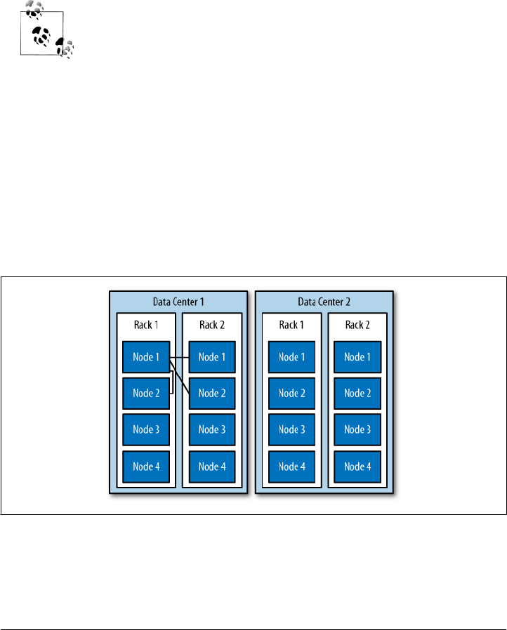
are going to two data centers—one in Australia and one in Reston, Virginia—you will
see a matching performance degradation. The variety of pluggable strategies allows
you greater flexibility, so that you can tune Cassandra according to your network top-
ology and needs.
The first replica will always be the node that claims the range in which the token falls,
but the remainder of the replicas are placed according to the replica placement strategy
you use.
As I write this chapter, the names of the strategies are changing. The
new names in 0.7 will be SimpleStrategy (formerly known as RackUnaware
Strategy), OldNetworkTopologyStrategy (formerly known as RackAwareS
trategy), and NetworkTopologyStrategy (formerly known as Datacen
terShardStrategy).
Simple Strategy
Simple Strategy is the new name for Rack-Unaware Strategy.
The strategy used by default in the configuration file is org.apache.cassandra
.locator.RackUnawareStrategy. This strategy only overrides the calculateNatural
Endpoints method from the abstract parent implementation. This strategy places rep-
licas in a single data center, in a manner that is not aware of their placement on a data
center rack. This means that the implementation is theoretically fast, but not if the next
node that has the given key is in a different rack than others. This is shown in Figure 6-1.
Figure 6-1. The Simple Strategy places replicas in a single data center, without respect to topology
What’s happening here is that the next N nodes on the ring are chosen to hold replicas,
and the strategy has no notion of data centers. A second data center is shown in the
diagram to highlight the fact that the strategy is unaware of it.
Replica Placement Strategies | 105
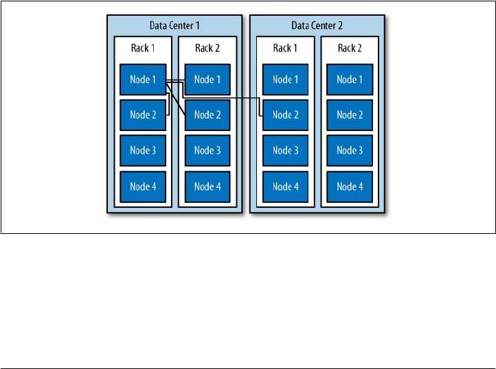
Old Network Topology Strategy
The second strategy for replica placement that Cassandra provides out of the box is
org.apache.cassandra.locator.RackAwareStrategy, now called Old Network Topology
Strategy. It’s mainly used to distribute data across different racks in the same data
center. Like RackUnawareStrategy, this strategy only overrides the calculateNaturalEnd
points method from the abstract parent implementation. This class, as the original
name suggests, is indeed aware of the placement in data center racks.
Say you have two data centers, DC1 and DC2, and a set of Cassandra servers. This
strategy will place some replicas in DC1, putting each in a different available rack. It
will also ensure that another replica is placed in DC2. The Rack-Aware Strategy is
specifically for when you have nodes in the same Cassandra cluster spread over two
data centers and you are using a replication factor of 3. This strategy is depicted in
Figure 6-2.
Use this strategy when you want to ensure higher availability at the potential cost of
some additional latency while the third node in the alternate data center is contacted.
There is no point in using Rack-Aware Strategy if you are only running Cassandra in a
single data center. Cassandra is optimized for running in different data centers, how-
ever, and taking advantage of its high availability may be an important consideration
for you. If your Cassandra cluster does span multiple data centers, consider using this
strategy.
Figure 6-2. The Old Network Topology Strategy places the second replica in a different data center
and others on different racks in the same data center
If you use the Rack-Aware Strategy, you must also use the Rack-Aware Snitch. Snitches
are described in “Snitches” on page 111.
106 | Chapter 6: Configuring Cassandra
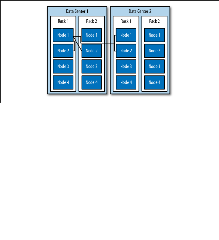
Network Topology Strategy
This strategy, included with the 0.7 release of Cassandra, allows you to specify more
evenly than the RackAwareStrategy how replicas should be placed across data centers.
To use it, you supply parameters in which you indicate the desired replication strategy
for each data center. This file is read and executed by the org.apache.cassandra
.locator.DataCenterShardStrategy class, so the implementation is somewhat flexible.
The data center shard strategy is depicted in Figure 6-3.
This strategy used to employ a file called datacenter.properties. But as of 0.7, this
metadata is attached directly to the keyspace and strategy as a map of configuration
options.
Figure 6-3. The Network Topology Strategy places some replicas in another data center and the
remainder in other racks in the first data center, as specified
Replication Factor
The replication factor specifies how many copies of each piece of data will be stored
and distributed throughout the Cassandra cluster. It is specified by the replication_
factor setting.
It may seem intuitive that the more nodes you have in your cluster, the more you want
to increase the replication factor. However, you don’t want to follow this rule of thumb
alone; instead, increase the replication factor in order to satisfy your required service
level.
With a replication factor of one, your data will exist only in a single node in the cluster.
Losing that node means that data becomes unavailable. It also means that Cassandra
will have to do more work as coordinator among nodes; if all the data for a given key
Replication Factor | 107

is on node B, every client request for that key that enters through node A will need to
be forwarded.
You must not set this value higher than the number of nodes in your cluster, as this
wouldn’t make any sense. But you also don’t want to use this setting to tune Cassandra.
Cassandra will achieve high consistency when the read replica count plus the write
replica count is greater than the replication factor.
So if you have 10 nodes in your cluster, you could set the replication factor to 10 as the
maximum. But you might not want to do that, as it robs Cassandra of what it’s good
at and stymies its availability, because if a single node goes down, you won’t be able to
have high consistency. Instead, set the replication factor to a reasonable number and
then tune the consistency level up or down. The consistency level never allows you to
write to more than the number of nodes specified by the replication factor. A “reason-
able number” here is probably fairly low. ONE seems like the lowest number; however,
ANY is similar to ONE but even less consistent, since you might not see the written value
until a long time after you wrote it. If any node in the cluster is alive, ANY should succeed.
If you’re new to Cassandra, the replication factor can sometimes be
confused with the consistency level. The replication factor is set per
keyspace, and is specified in the server’s config file. The consistency level
is specified per query, by the client. The replication factor indicates how
many nodes you want to use to store a value during each write operation.
The consistency level specifies how many nodes the client has decided
must respond in order to feel confident of a successful read or write
operation. The confusion arises because the consistency level is based
on the replication factor, not on the number of nodes in the system.
Increasing the Replication Factor
The replication factor is not a setting that is intended to be changed on a live cluster
and should be determined ahead of time. But as your application grows and you need
to add nodes, you can increase the replication factor. There are some simple guidelines
to follow when you do this. First, keep in mind that you’ll have to restart the nodes
after a simple increase in the replication factor value. A repair will then be performed
after you restart the nodes, as Cassandra will have to redistribute some data in order
to account for the increased replication factor. For as long as the repair takes, it is
possible that some clients will receive a notice that data does not exist if they connect
to a replica that doesn’t have the data yet.
A faster way of increasing the replication factor from 1 to 2 is to use the node tool. First,
execute a drain on the original node to ensure that all the data is flushed to the SSTables.
Then, stop that node so it doesn’t accept any more writes. Next, copy the datafiles from
your keyspaces (the files under the directory that is your value for the DataFile
Directory element in the config). Make sure not to copy the values in the internal
Cassandra keyspace. Paste those datafiles to the new node. Change the settings in the
108 | Chapter 6: Configuring Cassandra

configuration of both nodes so that the replication factor is set to 2. Make sure that
autobootstrap is set to false in both nodes. Then, restart both nodes and run node tool
repair. These steps will ensure that clients will not have to endure the potential of false
empty reads for as long.
To illustrate this, I have three nodes with IP addresses ending in 1.5, 1.7, and 1.8, and
their replication factor is set to 1. I will connect to node 1.5 and perform a write to a
column that hasn’t previously existed anywhere:
cassandra> connect 192.168.1.5/9160
Connected to: "TDG Cluster" on 192.168.1.5/9160
cassandra> set Keyspace1.Standard2['mykey']['rf']='1'
Value inserted.
Now I shut down node 1.5 and connect to the other node, 1.7, and try to get the value
I just set:
cassandra> connect 192.168.1.7/9160
Connected to: "TDG Cluster" on 192.168.1.7/9160
cassandra> get Keyspace1.Standard2['mykey']['rf']
Exception null
Because my replication factor was 1, the value was written only to the 1.5 node, so
when I lost that node, the other node in the cluster didn’t have the value. No client will
be able to read the value of the rf column until 1.5 comes back online.
But let’s see the effect of updating the replication factor. We change it from 1 to 2 in
the 1.5 and 1.7 nodes and restart. Let’s insert a new value to our rf column on node 1.7:
cassandra> connect 192.168.1.7/9160
Connected to: "TDG Cluster" on 192.168.1.7/9160
cassandra> get Keyspace1.Standard2['mykey']['rf']
Exception null
cassandra> set Keyspace1.Standard2['mykey']['rf']='2'
Value inserted.
The Exception null response in the preceding example proves that the value didn’t
exist on node 1.7 beforehand. Now we shut down node 1.7 and connect to 1.5, and
we see the value because it was replicated to 1.5 on our write to 1.7, due to our repli-
cation factor:
cassandra> connect 192.168.1.5/9160
Connected to: "TDG Cluster" on 192.168.1.5/9160
cassandra> get Keyspace1.Standard2['mykey']['rf']
=> (column=rf, value=2, timestamp=1279491483449000)
As a general guideline, you can anticipate that your write throughput capacity will be
the number of nodes divided by your replication factor. So in a 10-node cluster that
typically does 10,000 writes per second with a replication factor of 1, if you increase
the replication factor to 2, you can expect to do around 5,000 writes per second.
Replication Factor | 109
Partitioners
The future is already here; it’s just not
evenly distributed yet.
—William Gibson
The purpose of the partitioner is to allow you to specify how row keys should be
sorted, which has a significant impact on how data will be distributed across your
nodes. It also has an effect on the options available for querying ranges of rows. There
are a few different partitioners you can use, which we look at now.
The choice of partitioner does not apply to column sorting, only row
key sorting.
You set the partitioner by updating the value of the Partitioner element in the config
file or in the API. It takes as a value the name of a class that implements the
org.apache.cassandra.dht.IPartitioner interface. Out of the box, Cassandra provides
three of these: the random partitioner, which is the default; the order-preserving
partitioner; and collating order-preserving partitioner. Because of Cassandra’s gener-
ally pluggable design, you can also create your own partitioner by implementing the
org.apache.cassandra.dht.IPartitioner class and placing it on Cassandra’s classpath.
Keep in mind that the partitioner can modify the on-disk SSTable rep-
resentations. So if you change the partitioner type, you will have to
delete your data directories.
Random Partitioner
The random partitioner is implemented by org.apache.cassandra.dht.Random
Partitioner and is Cassandra’s default. It uses a BigIntegerToken with an MD5 hash
applied to it to determine where to place the keys on the node ring. This has the ad-
vantage of spreading your keys evenly across your cluster, because the distribution is
random. It has the disadvantage of causing inefficient range queries, because keys
within a specified range might be placed in a variety of disparate locations in the ring,
and key range queries will return data in an essentially random order.
Order-Preserving Partitioner
The order-preserving partitioner is implemented by org.apache.cassandra.dht.Order
PreservingPartitioner, which implements IPartitioner<StringToken>. Using this type
of partitioner, the token is a UTF-8 string, based on a key. Rows are therefore stored
by key order, aligning the physical structure of the data with your sort order.
110 | Chapter 6: Configuring Cassandra

Configuring your column family to use order-preserving partitioning (OPP) allows you
to perform range slices.
It’s worth noting that OPP isn’t more efficient for range queries than random parti-
tioning—it just provides ordering. It has the disadvantage of creating a ring that is
potentially very lopsided, because real-world data typically is not written to evenly. As
an example, consider the value assigned to letters in a Scrabble game. Q and Z are rarely
used, so they get a high value. With OPP, you’ll likely eventually end up with lots
of data on some nodes and much less data on other nodes. The nodes on which lots of
data is stored, making the ring lopsided, are often referred to as “hot spots.” Because
of the ordering aspect, users are commonly attracted to OPP early on. However, using
OPP means that your operations team will need to manually rebalance nodes periodi-
cally using Nodetool’s loadbalance or move operations.
If you want to perform range queries from your clients, you must use an order-
preserving partitioner or a collating order-preserving partitioner.
Collating Order-Preserving Partitioner
This partitioner orders keys according to a United States English locale (EN_US). Like
OPP, it requires that the keys are UTF-8 strings. Although its name might imply that
it extends the OPP, it doesn’t. Instead, this class extends AbstractByteOrdered
Partitioner. This partitioner is rarely employed, as its usefulness is limited.
Byte-Ordered Partitioner
New for 0.7, the team added ByteOrderedPartitioner, which is an order-preserving
partitioner that treats the data as raw bytes, instead of converting them to strings the
way the order-preserving partitioner and collating order-preserving partitioner do. If
you need an order-preserving partitioner that doesn’t validate your keys as being
strings, BOP is recommended for the performance improvement.
Snitches
The job of a snitch is simply to determine relative host proximity. Snitches gather some
information about your network topology so that Cassandra can efficiently route re-
quests. The snitch will figure out where nodes are in relation to other nodes. Inferring
data centers is the job of the replication strategy.
Simple Snitch
By default, Cassandra uses org.apache.cassandra.locator.EndPointSnitch. It operates
by simply comparing different octets in the IP addresses of each node. If two hosts
have the same value in the second octet of their IP addresses, then they are determined
Snitches | 111

to be in the same data center. If two hosts have the same value in the third octet of their
IP addresses, then they are determined to be in the same rack. “Determined to be” really
means that Cassandra has to guess based on an assumption of how your servers are
located in different VLANs or subnets.
Simple Snitch was renamed in 0.7; prior to that it was called endpoint
snitch.
You configure which endpoint snitch implementation to use by updating the value for
the <EndPointSnitch> element in the configuration file. The other choice is the
PropertyFileSnitch.
PropertyFileSnitch
The org.apache.cassandra.locator.PropertyFileSnitch used to be in contrib, but was
moved into the main code base in 0.7. This snitch allows you more control when using
a Rack-Aware Strategy by specifying node locations in a standard key/value properties
file called cassandra-rack.properties.
This snitch was contributed by Digg, which uses Cassandra and regularly contributes
to its development. This snitch helps Cassandra know for certain if two IPs are in the
same data center or on the same rack—because you tell it that they are. This is perhaps
most useful if you move servers a lot, as operations often need to, or if you have inherited
an unwieldy IP scheme.
The default configuration of cassandra-rack.properties looks like this:
# Cassandra Node IP=Data Center:Rack
10.0.0.10=DC1:RAC1
10.0.0.11=DC1:RAC1
10.0.0.12=DC1:RAC2
10.20.114.10=DC2:RAC1
10.20.114.11=DC2:RAC1
10.20.114.15=DC2:RAC2
# default for unknown nodes
default=DC1:r1
Here we see that there are two data centers, each with two racks. Cassandra can
determine an even distribution with good performance.
Update the values in this file to record each node in your cluster to specify which rack
contains the node with that IP and which data center it’s in. Although this may seem
difficult to maintain if you expect to add or remove nodes with some frequency, re-
member that it’s one alternative, and it trades away a little flexibility and ease of
maintenance in order to give you more control and better runtime performance, as
112 | Chapter 6: Configuring Cassandra
Cassandra doesn’t have to figure out where nodes are. Instead, you just tell it where
they are.
The PropertyFileSnitch used to be called PropertyFileEndPoint
Snitch and was in the contrib directory before being promoted to part
of the standard distribution, in case you see references to that online.
Creating a Cluster
You can run Cassandra on a single machine, which is fine for getting started as you
learn how to read and write data. But Cassandra is specifically engineered to be used
in a cluster of many machines that can share the load in very high-volume situations.
In this section, we see what you have to do to get multiple Cassandra instances to talk
to each other in a ring.
During the writing of this book, the entire configuration mechanism
was changing dramatically. This section covers how to create a cluster
using version 0.6.
What we want to do here is just use the sample keyspace that ships with Cassandra to
make sure that we can get multiple machines in a ring together. So we’ll start with the
default configuration file and keyspace definition, and change only those settings
required to create a simple cluster.
For this exercise, let’s say that we have two boxes we want to set up as a Cassandra
cluster, with the IP addresses 192.168.1.5 and 192.168.1.7. When you start Cassandra,
it reads the configuration file to determine how you want the current node to broadcast
—that is, what host or IP address and what port to use. You need to tell the current
node about the other nodes with which it should participate in a ring. Doing this is a
simple matter of opening the config file in a text editor and updating a few values, as
we’ll examine here.
A new node in a cluster needs what’s called a seed node. If node A acts as a seed for
node B, when node B comes online, it will use node A as a reference point from which
to get data. Seed nodes will ignore the AutoBootstrap setting because it is assumed that
they will be the first nodes in the cluster.
Changing the Cluster Name
Cassandra clusters are given names in order to prevent machines in one cluster from
joining another that you don’t want them to be a part of. The name of the default
cluster in the config file is “Test Cluster”. You can change the name of the cluster by
Creating a Cluster | 113

updating the <ClusterName> element—just make sure that you have done this on all
nodes that you want to participate in this cluster.
If you have written data to an existing Cassandra cluster and then change
the cluster name, Cassandra will warn you with a cluster name mis-
match error as it tries to read the datafiles on startup, and then it will
shut down.
Adding Nodes to a Cluster
The configuration file has an element that is set to false by default. Say that you have
been running a cluster or a single node and added data to it, and now you want to
introduce more nodes to the cluster. You can do this using the autobootstrap element.
I have a single Cassandra server running on an IP ending in 1.5, as shown by NodeTool:
$ bin/nodetool -h 192.168.1.5 ring
Address Status Load Range Ring
192.168.1.5 Up 433.43 MB 126804671661649450065809810549633334036 |<--|
This server has its own address as a seed. We leave autobootstrap set to false, because
this node is acting as a seed. If you want to add a new seed node, then you should
autobootstrap it first, and then change it to a seed afterward. For node B to use node
A as a seed, node B needs to reference node A as its seed in its configuration file. But
node A does not have to declare itself as a seed.
Now I’d like to add another node to share the load. This node’s address ends in 1.7.
First, make sure that the nodes in the cluster all have the same name and the same
keyspace definitions so that the new node can accept data. Edit the config file on the
second node to indicate that the first one will act as the seed. Then, set autobootstrap
to true.
When the second node is started up, it immediately recognizes the first node, but then
sleeps for 90 seconds to allow time for nodes to gossip information about how much
data they are storing locally. It then gets the bootstrap token from the first node, so it
knows what section of the data it should accept. The bootstrap token is a token that
splits the load of the most-loaded node in half. Again, the second node sleeps for 30
seconds and then starts bootstrapping.
INFO 11:45:43,652 Starting up server gossip
INFO 11:45:43,886 Joining: getting load information
INFO 11:45:43,901 Sleeping 90000 ms to wait for load information...
INFO 11:45:45,742 Node /192.168.1.5 is now part of the cluster
INFO 11:45:46,818 InetAddress /192.168.1.5 is now UP
INFO 11:45:46,818 Started hinted handoff for endPoint /192.168.1.5
INFO 11:45:46,865 Finished hinted handoff of 0 rows to endpoint /192.168.1.5
INFO 11:47:13,913 Joining: getting bootstrap token
INFO 11:47:16,004 New token will be 41707658470746813056713124104091156313 to a
ssume load from /192.168.1.5
114 | Chapter 6: Configuring Cassandra

INFO 11:47:16,019 Joining: sleeping 30000 ms for pending range setup
INFO 11:47:46,034 Bootstrapping
Depending on how much data you have, you could see your new node in this state for
some time. You can use Nodetool’s streams command to watch the data being trans-
ferred for bootstrap. Watching the logfile is a good way to determine that the node is
finished bootstrapping, but to watch for progress while it’s happening, use nodetool
streams. Eventually, the new node will accept the load from the first node, and you’ll
see a successful indication that the new node has started up:
INFO 11:52:29,361 Sampling index for /var/lib/cassandra/data\Keyspace1\Standard
1-1-Data.db
INFO 11:52:34,073 Streaming added /var/lib/cassandra/data\Keyspace1\Standard1-1
-Data.db
INFO 11:52:34,088 Bootstrap/move completed! Now serving reads.
INFO 11:52:34,354 Binding thrift service to /192.168.1.7:9160
INFO 11:52:34,432 Cassandra starting up...
As you can see, it took around four minutes to transfer data.
During bootstrapping, the first (seed) node at 1.5 looks like this:
INFO 11:48:12,955 Sending a stream initiate message to /192.168.1.7 ...
INFO 11:48:12,955 Waiting for transfer to /192.168.1.7 to complete
INFO 11:52:28,903 Done with transfer to /192.168.1.7
Now we can run node tool again to make sure that everything is set up properly:
$ bin/nodetool -h 192.168.1.5 ring
Address Status Load Range Ring
126804671661649450065809810549633334036
192.168.1.7 Up 229.56 MB 41707658470746813056713124104091156313 |<--|
192.168.1.5 Up 459.26 MB 126804671661649450065809810549633334036 |-->|
Cassandra has automatically bootstrapped the 1.7 node by sending it half of the data
from the previous node (1.5). So now we have a two-node cluster. To ensure that it
works, let’s add a value to the 1.5 node:
cassandra> connect 192.168.1.5/9160
Connected to: "TDG Cluster" on 192.168.1.5/9160
cassandra> set Keyspace1.Standard2['mykey']['col0']='value0'
Value inserted.
Now let’s open a second CLI client and read that value from the 1.7 node:
cassandra> connect 192.168.1.7/9160
Connected to: "TDG Cluster" on 192.168.1.7/9160
cassandra> get Keyspace1.Standard2['mykey']['col0']
=> (column=col0, value=value0, timestamp=1278878907805000
You can repeat these steps to add additional nodes to your cluster.
If there’s something wrong with one of the nodes in your cluster (perhaps it’s offline,
but Cassandra is not sure), you may see a question mark when you run node tool:
Creating a Cluster | 115
$ bin/nodetool -h 192.168.1.5 ring
Address Status Load Range Ring
112711146095673746066359353163476425700
192.168.1.5 Up 459.26 MB 27647275353297313886547808446514704912 |<--|
192.168.1.7 ? 229.53 MB 112711146095673746066359353163476425700 |-->|
Multiple Seed Nodes
Cassandra allows you to specify multiple seed nodes. A seed node is used as a contact
point for other nodes, so Cassandra can learn the topology of the cluster, that is, what
hosts have what ranges.
By default, the configuration file will have only a single seed entry:
seeds:
- 127.0.0.1
To add more seed nodes to your ring, just add another seed element. We can set two
servers to be seeds just by indicating the IP address or hostname of this node and then
adding our second instance:
seeds:
- 192.168.1.5
- 192.168.1.7
Make sure that the autobootstrap element is set to false if you’re using
a node’s own IP address as a seed. One approach is to make the first
three or five nodes in a cluster seeds, without autobootstrap—that is,
by manually choosing tokens or by allowing Cassandra to pick random
tokens. The rest of your nodes will not be seeds, so they can be added
using autobootstrap.
Next, we need to update the listen address for this machine so it’s not just on loopback.
Listen address is how nodes identify each other, and it’s used for all internal commu-
nication.
listen_address: 192.168.1.5
Finally, we need to change the address on which our RPC client will broadcast because
this is how other nodes will see this one. By default, the configuration file will have an
rpc_address entry that uses localhost. We’ll change this value to the actual IP address
of each machine:
rpc_address: 192.168.1.5
The rpc_address setting is used only for connections made directly from clients to Cas-
sandra nodes.
116 | Chapter 6: Configuring Cassandra

rpc_address used to be called ThriftAddress, but because of the up-
coming possible change to Avro instead of Thrift as the RPC mecha-
nism, it has been changed to a more general name.
Now you can restart Cassandra and start the installations on the other machines. If you
have successfully added multiple nodes to your cluster, you will see output similar to
this (yours might be a little less verbose, as I’m showing debug-level output here):
INFO 15:45:15,629 Starting up server gossip
INFO 15:45:15,677 Binding thrift service to /192.168.1.5:9160
INFO 15:45:15,681 Cassandra starting up...
DEBUG 15:45:16,636 GC for ParNew: 13 ms, 12879912 reclaimed leaving 11233080 used;
max is 1177812992
DEBUG 15:45:16,647 attempting to connect to /192.168.1.7
DEBUG 15:45:17,638 Disseminating load info ...
INFO 15:45:19,744 Node /192.168.1.7 is now part of the cluster
DEBUG 15:45:19,746 Node /192.168.1.7 state normal, token
41654880048427970483049687892424207188
DEBUG 15:45:19,746 No bootstrapping or leaving nodes -> empty pending ranges
for Keyspace1
INFO 15:45:20,789 InetAddress /192.168.1.7 is now UP
DEBUG 15:45:20,789 Started hinted handoff for endPoint /192.168.1.7
DEBUG 15:45:20,800 Finished hinted handoff for endpoint /192.168.1.7
DEBUG 15:46:17,638 Disseminating load info ...
This output shows that I have two nodes in my cluster: the node I just started, which
is listening on 192.168.1.5, and the node that was already up and running, which is
listening on 192.168.1.7.
Dynamic Ring Participation
Nodes in a Cassandra cluster can be brought down and brought back up without
disruption to the rest of the cluster (assuming a reasonable replication factor and con-
sistency level). Say that we have started a two-node cluster as described earlier in
“Creating a Cluster” on page 113. We can cause an error to occur that will take down
one of the nodes, and then make sure that the rest of the cluster is still OK:
INFO 15:34:18,953 Starting up server gossip
INFO 15:34:19,281 Binding thrift service to /192.168.1.7:9160
INFO 15:34:19,343 Cassandra starting up...
INFO 15:45:19,396 Node /192.168.1.5 is now part of the cluster
INFO 15:45:20,176 InetAddress /192.168.1.5 is now UP
INFO 16:13:36,476 error writing to /192.168.1.5
INFO 16:13:40,517 InetAddress /192.168.1.5 is now dead.
INFO 16:21:02,466 error writing to /192.168.1.5
INFO 16:21:02,497 error writing to /192.168.1.5
The error message will repeat until the 1.5 node comes back up. Running Nodetool
will indicate that it’s down now, while the other node is still up.
Dynamic Ring Participation | 117

So we bring it back up and check the logs at 1.7. Sure enough, Cassandra has auto-
matically detected that the other participant has returned to the cluster and is again
open for business:
INFO 16:33:48,193 error writing to /192.168.1.5
INFO 16:33:51,235 error writing to /192.168.1.5
INFO 16:34:20,126 Standard2 has reached its threshold; switching in a fresh Mem
table at CommitLogContext(file='/var/lib/cassandra/commitlog\CommitLog-127759165
782.log', position=752)
INFO 16:34:20,173 Enqueuing flush of Memtable(Standard2)@7481705
INFO 16:34:20,251 Writing Memtable(Standard2)@7481705
INFO 16:34:20,282 LocationInfo has reached its threshold; switching in a fresh
Memtable at CommitLogContext(file='/var/lib/cassandra/commitlog\CommitLog-127759
658782.log', position=752)
INFO 16:34:20,298 Enqueuing flush of Memtable(LocationInfo)@24804063
INFO 16:34:20,579 Completed flushing c:\var\lib\cassandra\data\Keyspace1\Standa
d2-1-Data.db
INFO 16:34:20,594 Writing Memtable(LocationInfo)@24804063
INFO 16:34:20,797 Completed flushing c:\var\lib\cassandra\data\system\LocationI
fo-2-Data.db
INFO 16:34:58,159 Node /192.168.1.5 has restarted, now UP again
INFO 16:34:58,159 Node /192.168.1.5 state jump to normal
The state jump to normal for the 1.5 node indicates that it’s part of the cluster again:
eben@morpheus$ bin/nodetool -host 192.168.1.5 ring
Address Status Load Range Ring
41654880048427970483049687892424207188
192.168.1.5 Up 1.71 KB 20846671262289044293293447172905883342 |<--|
192.168.1.7 Up 2 KB 41654880048427970483049687892424207188 |-->|
Security
By default, Cassandra allows any client on your network to connect to your cluster.
This does not mean that no security is set up out of the box, but rather that Cassandra
is configured to use an authentication mechanism that allows all clients, without re-
quiring that they provide credentials. The security mechanism is pluggable, which
means that you can easily swap out one authentication method for another, or write
your own.
The authenticator that’s plugged in by default is the org.apache.cassandra.auth.Allow
AllAuthenticator. If you want to force clients to provide credentials, another alternative
ships with Cassandra, the org.apache.cassandra.auth.SimpleAuthenticator. In this
section, we see how to use this second authenticator.
Using SimpleAuthenticator
There are two files included in the config directory: access.properties and passwd
.properties. The access file uses a key/value pair to specify which users are allowed access
118 | Chapter 6: Configuring Cassandra

to which keyspaces, specified by a comma-separated list. The example provided looks
like this:
Keyspace1=jsmith,Elvis Presley,dilbert
This indicates that there are three users allowed to access Keyspace1, and spaces are
allowed in the usernames.
The file passwd.properties must contain a list of these users and specify the password
for each of them. Here is the example passwd.properties file:
jsmith=havebadpass
Elvis\ Presley=graceland4evar
dilbert=nomoovertime
Note that because the user Elvis Presley has a space in his username, a backslash must
be used to escape the space.
To use the Simple Authenticator, replace the value for the authenticator element in
cassandra.yaml. Change it from org.apache.cassandra.auth.AllowAllAuthenticator to
the name of the implementing class that requires a login: org.apache.cassan
dra.auth.SimpleAuthenticator.
If you haven’t configured the authentication files properly, you’ll see an error like this:
ERROR 10:44:27,928 Fatal error: When using org.apache.cassandra.auth.SimpleAuth
enticator
access.properties and passwd.properties properties must be defined.
That’s because there is one more step: we have to tell Cassandra the location of the
access and passwords files, using the bin/cassandra.in.sh include script. We pass the
file locations to the JVM by pasting the following code at the bottom of this file. My
include file now looks like the snippet here, indicating the full path to the files:
JVM_OPTS="
-Dpasswd.properties=/home/eben/books/cassandra/dist/
apache-cassandra-0.7.0-beta1/
conf/passwd.properties
-Daccess.properties=/home/eben/books/cassandra/dist/
apache-cassandra-0.7.0-beta1/
conf/access.properties"
If you have specified an incorrect location or name for either of these files, the server
log will let you know:
ERROR 11:13:55,755 Internal error processing login
java.lang.RuntimeException: Authentication table file given by property
passwd.properties
could not be found: /somebadpath/my.properties (No such file or directory)
Now we can log into the command-line interface with a username and password
combination:
[default@unknown] connect localhost/9160
Connected to: "Test Cluster" on localhost/9160
[default@unknown] use Keyspace1 jsmith 'havebadpass'
Security | 119
Authenticated to keyspace: Keyspace1
[jsmith@Keyspace1]
If you enter an incorrect password, the CLI tells you:
[default@unknown] use Keyspace1 jsmith 'havebadpassfdfdfd'
Exception during authentication to the cassandra node: verify keyspace exists,
and you are using correct credentials.
If you enter a username that doesn’t exist or try to authenticate to a keyspace that the
user doesn’t have access to, you’ll see something like this:
[default@unknown] use Keyspace1 dude 'dude'
Login failure. Did you specify 'keyspace', 'username' and 'password'?
[default@unknown]
Somewhat confusingly, if you just try to use a keyspace that you don’t have access to,
you’ll see an authentication message, but then you won’t be able to perform operations.
In the following example, we switch to a keyspace that requires authentication. The
CLI appears to let us do that, but then we can’t read a column:
[default@Keyspace1] get Standard1['user123']['name']
Your credentials are not sufficient to perform READONLY operations
[default@Keyspace1]
Assuming we have set the 'name' value for this user, if we supply the proper credentials,
we can perform the operation:
[default@Keyspace1] use Keyspace1 eben 'pass'
Authenticated to keyspace: Keyspace1
[eben@Keyspace1] get Standard1['user123']['name']
=> (column=6e616d65, value=bootsy, timestamp=1284316537496000)
[eben@Keyspace1]
We can also specify the username and password combination when we connect on the
CLI:
eben@morpheus:~/books/cassandra/dist/apache-cassandra-0.7.0-beta1$
bin/cassandra-cli --host localhost --port 9160
--username jsmith --password havebadpass --keyspace Keyspace1
Connected to: "Test Cluster" on localhost/9160
Welcome to cassandra CLI.
Type 'help' or '?' for help. Type 'quit' or 'exit' to quit.
[jsmith@Keyspace1] get Standard1['user123']['name']
=> (column=6e616d65, value=bootsy, timestamp=1284316537496000)
[jsmith@Keyspace1]
Executing a query now returns us a result.
In 0.6, there was no login operation provided by the Thrift API, so if
you’ve gotten used to starting the CLI and then connecting in a separate
operation, that won’t work if you are requiring authentication. A login
operation was added in 0.7.
120 | Chapter 6: Configuring Cassandra
In 0.7, authenticators have been split into an IAuthenticator (which
handles authentication) and IAuthority (which handles authorization).
The SimpleAuthenticator class has had authorization split out into
SimpleAuthority. SimpleAuthenticator reads only passwd.properties,
and SimpleAuthority reads only access.properties.
Programmatic Authentication
If you have set up authentication on your keyspace, your client application code will
need to log in. You can use Example 6-2 as a guide.
Example 6-2. Programmatic authentication to a keyspace
package com.cassandraguide.config;
import java.util.HashMap;
import java.util.Map;
import org.apache.cassandra.thrift.AccessLevel;
import org.apache.cassandra.thrift.AuthenticationRequest;
import org.apache.cassandra.thrift.Cassandra;
import org.apache.thrift.protocol.TBinaryProtocol;
import org.apache.thrift.protocol.TProtocol;
import org.apache.thrift.transport.TFramedTransport;
import org.apache.thrift.transport.TSocket;
import org.apache.thrift.transport.TTransport;
/**
* How to connect if you've set up SimpleAuthenticator
*/
public class AuthExample {
public static void main(String[] args) throws Exception {
TTransport tr = new TSocket("localhost", 9160);
TFramedTransport tf = new TFramedTransport(tr);
TProtocol proto = new TBinaryProtocol(tf);
Cassandra.Client client = new Cassandra.Client(proto);
tr.open();
AuthenticationRequest authRequest = new AuthenticationRequest();
Map<String, String> credentials = new HashMap<String, String>();
credentials.put("username", "jsmith");
credentials.put("password", "havebadpass");
authRequest.setCredentials(credentials);
client.set_keyspace("Keyspace1");
AccessLevel access = client.login(authRequest);
System.out.println("ACCESS LEVEL: " + access);
tr.close();
}
}
Security | 121

In this case, the program just prints out FULL because that’s this user’s access level.
There are a couple of things to note here. First, the credentials map uses username and
password as keys; it’s not username as the key and password as the value. Second, you
need to call set_keyspace separately, to indicate what keyspace you’re trying to
authenticate to.
Using MD5 Encryption
The SimpleAuthenticator class has two modes for specifying passwords: plain text and
MD5 encrypted. So far, we’ve used the default, plain text. Let’s look at how to improve
security a bit by using MD5. MD5 is a cryptographical algorithm that stands for
“Message-Digest algorithm version 5” (the “5” indicates an improvement in strength
over version 4). It’s a widely used one-way hash function that generates a 128-bit hash
value from an input. It’s also worth noting that MD5 is not going to be radically secure
for you; it's just a little harder to break in.
You enable MD5 in the cassandra.in.sh file by passing the passwd.mode switch to the
JVM:
JVM_OPTS=" \
-da \
//other stuff...
-Dpasswd.mode=MD5"
Now if you try to authenticate using an unencrypted password, you’ll see an error like
this:
Exception during authentication to the cassandra node, verify you are using correct
credentials.
You can use a variety of tools to generate an MD5-encrypted version of the plain-text
username and password as a one-way hash. Here’s a short Python program to create
an MD5 hash from a plain string:
$ python
Python 2.6.5 ...
>>> from hashlib import md5
>>> p = "havebadpass"
>>> h = md5(p).hexdigest()
>>> print h
e1a31eee2136eb73e8e47f9e9d13ab0d
Now you can replace the password for jsmith in the passwd.properties file with the
encrypted value.
Providing Your Own Authentication
You can provide your own method of authenticating to Cassandra if you want to make
special requirements, such as a Kerberos ticket or encryption, or if you want to store
passwords in a different location, such as an LDAP directory. To create your own
122 | Chapter 6: Configuring Cassandra

authentication scheme, simply implement the IAuthenticator interface. This interface
requires two methods, as shown here:
public AccessLevel login(String keyspace, AuthenticationRequest authRequest)
throws AuthenticationException, AuthorizationException;
public void validateConfiguration() throws ConfigurationException;
The login method must return a Thrift AccessLevel instance, indicating what degree
of access the authenticating user is allowed. The validateConfiguration method
simply allows a check to ensure that the authentication mechanism is properly set up.
For example, with the SimpleAuthenticator, it just checks that the required access and
passwd files have been specified.
Miscellaneous Settings
There are a few settings related to general configuration that don’t quite seem to belong
in any other category, so I’ve grouped them together here.
column_index_size_in_kb
This indicates the size in kilobytes that a row is allowed to grow to before its col-
umns will be indexed. If you have very large column values, you’ll want to increase
this value. Super columns are not indexed, so this setting refers only to column
indexes. You do not want this setting to be very large because all the index data is
read for each read access, so you could slow Cassandra down if you make it read
more than is necessary. This becomes especially important if you frequently read
partial rows.
in_memory_compaction_limit_in_mb
This value represents the size limit for rows being compacted in memory. If a row
is larger than this, it will be staged onto disk and compacted in a slower, two-step
process. The setting’s value is set to 64MB by default. Prior to Cassandra version
0.7, this was called the row_warning_threshold_in_mb.
gc_grace_seconds
This indicates the amount of time in seconds to wait before garbage-collecting
tombstones. Tombstones are markers indicating that a value was deleted, but they
persist until this threshold is met. By default it is set to 864,000, which is 10 days.
This might seem like an inordinately long time, but you have to allow enough time
for tombstones to propagate through the entire cluster to any replicas. That may
still seem like a long time, but the idea is that you could have hardware failures,
and you’ll need time to get those nodes back up and operational so that tombstones
can replicate to them too. If a downed node that did not receive tombstone noti-
fications comes back up after the tombstones have been truly deleted, read repair
will allow the untombstoned, undeleted data to slowly be introduced back into the
cluster.
Miscellaneous Settings | 123

Of course, if you do a lot of deleting, you could tune this setting back for the sake
of tidiness, but it’s probably not going to make a huge difference.
phi_convict_threshold
This marks the Phi value that must be reached in order for Cassandra to conclude
that the server is down. By default, this is set to 8, and in general you will not want
to change this setting. However, if your network is not performing optimally or
you have other reasons to suspect that Cassandra could get a false read on this,
you can increase this setting to allow more leniency in determining whether a node
is actually down.
Phi Threshold and Accrual Failure Detectors
Since its inception at Facebook, Cassandra has employed what is called an Accrual
Failure Detector. This is a failure detector that outputs a value associated with each
process (or node). This value is called Phi. The value is output in a manner that is
designed from the ground up to be adaptive in the face of volatile network conditions,
so it’s not a binary condition that simply checks whether a server is up or down.
The Phi convict threshold in the configuration adjusts the sensitivity of the failure de-
tector. Lower values increase the sensitivity and higher values decrease it, but not in a
linear fashion.
The Phi value refers to a level of suspicion that a server might be down. Applications
such as Cassandra that employ an AFD can specify variable conditions for the Phi value
they emit. Cassandra can generally detect a failed node in about 10 seconds using this
mechanism.
You can read the original Phi Accrual Failure Detection paper on which Cassandra’s
design is based at http://ddg.jaist.ac.jp/pub/HDY+04.pdf.
Additional Tools
This section discusses miscellaneous tools that ship with Cassandra to help you
configure it.
Viewing Keys
You can see which keys are in your SSTables using a script called sstablekeys. To run
it, just use the location of the SSTable for which you want to see keys, as shown here:
eben@morpheus$ bin/sstablekeys /var/lib/cassandra/data/Hotelier/Hotel-1-Data.db
WARN 10:56:05,928 Schema definitions were defined both locally and in cassandra.yaml.
Definitions in cassandra.yaml were ignored.
415a435f303433
415a535f303131
4341535f303231
4e594e5f303432
124 | Chapter 6: Configuring Cassandra

Importing Previous Configurations
If you had a keyspace defined in 0.6 using the configuration file that you’d like to
import into Cassandra 0.7 or higher, you can use a special JMX operation, Storage
Service.loadSchemaFromYaml(). Note that this method has two important caveats: first,
it is intended to be used only once; second, it will probably be removed by version 0.8.
Starting with version 0.7, the user keyspaces defined in cassandra.yaml are not loaded
by default when the server starts. So you might see a message like this as your Cassandra
server starts up for the first time:
INFO config.DatabaseDescriptor: Found table data in data directories.
Consider using JMX to call org.apache.cassandra.service.StorageService.
loadSchemaFromYaml().
In order to load them, you need to invoke the loadSchemaFromYaml JMX operation. But
in order to invoke this command, you need to do a couple of things. First, get mx4j-
tools.jar from Sourceforge.net. Download and extract the ZIP file into any directory.
Then, copy the JAR named mx4j-tools.jar in its lib directory into Cassandra’s lib
directory. This will allow you to make JMX connections to interact with Cassandra in
really rich ways. We’ll see more about using JMX with Cassandra later, but for now
we just want to get a keyspace up for testing. Restart Cassandra after adding the JAR.
Next, open a new terminal and issue the command jconsole. A GUI will start and load
the JConsole tool that ships with Java. This tool can introspect the Java Virtual Machine
and allow you to view runtime data and invoke operations that are exposed via JMX.
To load the keyspaces defined in cassandra.yaml, click the MBeans tab in the JConsole
GUI. Expand the org.apache.cassandra.service bean, then StorageService, then
Operations. Click the loadSchemaFromYAML operation and click the button. This will
execute the command on the Cassandra service and load your schemas in the cassan-
dra.yaml file.
To perform the once-only operation to import a 0.6 configuration into 0.7, use the
loadSchemaFromYaml operation on the StorageService MBean. This is shown in Fig-
ure 6-4.
Now you should see output similar to the following in your logs:
17:35:47 INFO thrift.CassandraDaemon: Cassandra starting up...
17:35:48 INFO utils.Mx4jTool: mx4j successfuly loaded
HttpAdaptor version 3.0.2 started on port 8081
17:40:43 INFO config.DatabaseDescriptor: UTF8Type
17:40:43 INFO config.DatabaseDescriptor: BytesType
17:40:43 INFO config.DatabaseDescriptor: UTF8Type
17:40:43 INFO config.DatabaseDescriptor: TimeUUIDType
17:40:43 INFO config.DatabaseDescriptor: BytesType
17:40:43 INFO config.DatabaseDescriptor: BytesType
17:40:43 INFO config.DatabaseDescriptor:
The database descriptor logs are a good thing, as this indicates that the operation loaded
your schemas.
Additional Tools | 125
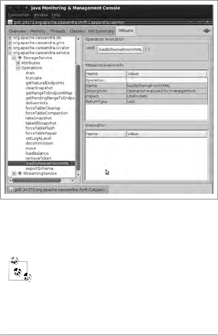
You can also use the org.apache.cassandra.config.Converter class to assist you in
converting from storage-conf.xml to a cassandra.yaml file. If you are upgrading from
0.6 to 0.7, this should be your first step. To run the converter, use the config-
converter script in the bin directory. It will read in the old file, convert it, and dump the
contents.
If you need to import and export data, Cassandra comes with two scripts
for working with JSON: one that imports JSON into Cassandra
SSTables, and another that exports existing SSTables into JSON.
Figure 6-4. Using the jconsole tool to load old keyspaces defined in cassandra.yaml
126 | Chapter 6: Configuring Cassandra

Summary
In this chapter we looked at how to configure Cassandra, including using the new
dynamic configuration ability in the API and some of the utilities that ship with the
server to dig into your raw datafiles. We saw how to set the replication factor and
the snitch, and how to use a good replica placement strategy.
If you prefer to use a graphical interface instead of the CLI, you can get information
regarding your Cassandra setup using Chiton, which is a Python GTK-based Cassandra
browser written by Brandon Williams. You can find it at http://github.com/driftx/chiton.
Summary | 127

CHAPTER 7
Reading and Writing Data
Now that we understand the data model, we’ll look at the different kinds of queries
you can perform in Cassandra to read and write data. In this chapter, we use Cassandra
0.6.7-beta1, which is the most recent release version at the time of this writing.
Query Differences Between RDBMS and Cassandra
There are several differences between Cassandra’s model and query methods and
what’s available in RDBMS, and these are important to keep in mind.
No Update Query
There is no first-order concept of an update in Cassandra, meaning that there is no
client query called an “update.” You can readily achieve the same effect, however, by
simply performing an insert using an existing row key. If you issue an insert statement
for a key that already exists, Cassandra will overwrite the values for any matching
columns; if your query contains additional columns that don’t already exist for that
row key, then the additional columns will be inserted. This is all seamless.
Record-Level Atomicity on Writes
Cassandra automatically gives you record-level atomicity on every write operation. In
RDBMS, you would have to specify row-level locking. Although Cassandra offers
atomicity at the column family level, it does not guarantee isolation.
No Server-Side Transaction Support
Because you need to denormalize tables to create secondary indexes, you might need
to insert data into two or more tables (one for your primary table and one for your
inverted or secondary index). This means issuing two insert statements. So if it is
129
applicable for your use case, you’ll need to manually “roll back” writes by issuing a
delete if one of the insert operations fails.
More to the point, perhaps, is that Cassandra doesn’t have transactions, because it just
wasn’t built with that goal in mind.
No Duplicate Keys
It is possible in SQL databases to insert more than one row with identical values if you
have not defined a unique primary key constraint on one of the columns. This is not
possible in Cassandra. If you write a new record with a key that already exists in a
column family, the values for any existing columns will be overwritten, and any col-
umns that previously were not present for that row will be added to the row.
Basic Write Properties
There are a few basic properties of Cassandra’s write ability that are worth noting. First,
writing data is very fast in Cassandra, because its design does not require performing
disk reads or seeks. The memtables and SSTables save Cassandra from having to
perform these operations on writes, which slow down many databases. All writes in
Cassandra are append-only.
Because of the database commit log and hinted handoff design, the database is always
writeable, and within a column family, writes are always atomic.
Consistency Levels
Cassandra’s tuneable consistency levels mean that you can specify in your queries how
much consistency you require. A higher consistency level means that more nodes need
to respond to the query, giving you more assurance that the values present on each
replica are the same. If two nodes respond with different timestamps, the newest value
wins, and that’s what will be returned to the client. In the background, Cassandra will
then perform what’s called a read repair: it takes notice of the fact that one or more
replicas responded to a query with an outdated value, and updates those replicas with
the most current value so that they are all consistent.
There are several consistency levels that you can specify, and they mean something
different for read operations than for write operations. The possible consistency levels,
and the implications of specifying each one for read queries, are shown in Table 7-1.
The consistency levels are based on the replication factor specified in
the configuration file, not on the total number of nodes in the system.
130 | Chapter 7: Reading and Writing Data
Table 7-1. Read consistency levels
Consistency level Implication
ZERO Unsupported. You cannot specify CL.ZERO for read operations because it doesn’t make sense. This
would amount to saying “give me the data from no nodes.”
ANY Unsupported. Use CL.ONE instead.
ONE Immediately return the record held by the first node that responds to the query. A background thread
is created to check that record against the same record on other replicas. If any are out of date, a read
repair is then performed to sync them all to the most recent value.
QUORUM Query all nodes. Once a majority of replicas ((replication factor / 2) + 1) respond, return to
the client the value with the most recent timestamp. Then, if necessary, perform a read repair in the
background on all remaining replicas.
ALL Query all nodes. Wait for all nodes to respond, and return to the client the record with the most recent
timestamp. Then, if necessary, perform a read repair in the background. If any nodes fail to respond,
fail the read operation.
As you can see from the table, there are certain consistency levels that are not supported
for read operations: ZERO and ANY. Notice that the implication of consistency level ONE
is that the first node to respond to the read operation is the value that the client will
get—even if it is out of date. The read repair operation is performed after the record is
returned, so any subsequent reads will all have a consistent value, regardless of the
responding node.
Another item worth noting is in the case of consistency level ALL. If you specify
CL.ALL, then you’re saying that you require all replicas to respond, so if any node with
that record is down or otherwise fails to respond before the timeout, the read operation
fails.
A node is considered unresponsive if it does not respond to a query
before the value specified by rpc_timeout_in_ms in the configuration file.
The default is 10 seconds.
You can specify these consistency levels for write operations as well, though their
meanings are very different. The implications of using the different consistency levels
on writes are shown in Table 7-2.
Table 7-2. Write consistency levels
Consistency level Implication
ZERO The write operation will return immediately to the client before the write is recorded; the write will
happen asynchronously in a background thread, and there are no guarantees of success.
ANY Ensure that the value is written to a minimum of one node, allowing hints to count as a write.
ONE Ensure that the value is written to the commit log and memtable of at least one node before
returning to the client.
Consistency Levels | 131

Consistency level Implication
QUORUM Ensure that the write was received by at least a majority of replicas ((replication factor / 2)
+ 1).
ALL Ensure that the number of nodes specified by replication factor received the write before
returning to the client. If even one replica is unresponsive to the write operation, fail the operation.
The most notable consistency level for writes is the ANY level. This level means that the
write is guaranteed to reach at least one node, but it allows a hint to count as a successful
write. That is, if you perform a write operation and the node that the operation targets
for that value is down, the server will make a note to itself, called a hint, which it will
store until that node comes back up. Once the node is up, the server will detect this,
look to see whether it has any writes that it saved for later in the form of a hint, and
then write the value to the revived node. In many cases, the node that makes the hint
actually isn’t the node that stores it; instead, it sends it off to one of the nonreplica
neighbors of the node that is down.
Using the consistency level of ONE on writes means that the write operation will be
written to both the commit log and the memtable. That means that writes at CL.ONE are
durable, so this level is the minimum level to use to achieve fast performance and du-
rability. If this node goes down immediately after the write operation, the value will
have been written to the commit log, which can be replayed when the server is brought
back up to ensure that it still has the value.
For both reads and writes, the consistency levels of ZERO, ANY, and ONE are considered
weak, whereas QUORUM and ALL are considered strong. Consistency is tuneable in Cas-
sandra because clients can specify the desired consistency level on both reads and
writes. There is an equation that is popularly used to represent the way to achieve
strong consistency in Cassandra: R + W > N = strong consistency. In this equation, R,
W, and N are the read replica count, the write replica count, and the replication factor,
respectively; all client reads will see the most recent write in this scenario, and you will
have strong consistency.
Basic Read Properties
There are a few basic properties of reading data from Cassandra that are worth noting.
First, it’s easy to read data because clients can connect to any node in the cluster to
perform reads, without having to know whether a particular node acts as a replica for
that data. If a client connects to a node that doesn’t have the data it’s trying to read,
the node it’s connected to will act as coordinator node to read the data from a node
that does have it, identified by token ranges.
To fulfill read operations, Cassandra does have to perform seeks, but you can speed
these up by adding RAM. Adding RAM will help you if you find the OS doing a lot of
paging on reads (in general, it is better to enable the various caches Cassandra has).
132 | Chapter 7: Reading and Writing Data
Cassandra has to wait for a number of responses synchronously (based on consistency
level and replication factor), and then perform read repairs as necessary.
So reads are clearly slower than writes, for these various reasons. The partitioner doesn’t
influence the speed of reads. In the case of range queries, using OPP is significantly
faster because it allows you to easily determine which nodes don’t have your data. The
partitioner’s responsibility is to perform the consistent hash operation that maps keys
to nodes. In addition, you can choose row caching and key caching strategies to give
you a performance boost (see Chapter 11).
The API
This section presents an overview of the basic Cassandra API so that once we start
reading and writing data, some of these exotic terms won’t seem quite so difficult. We
already know what a column, super column, and column family are: a column family
contains columns or super columns; a super column contains only columns (you can’t
nest one super column inside another); and columns contain a name/value pair and a
timestamp.
In a relational database, the terms SELECT, INSERT, UPDATE, and DELETE mean
just what they mean colloquially, in regular life. But working with Cassandra’s API
structures is not exactly straightforward, and can be somewhat daunting to newcomers;
after all, there’s no such thing as a “slice range” in regular life, so these terms may take
some getting used to.
There are two basic concepts that you’ll want to learn quickly: ranges and slices. Many
queries are defined using these terms, and they can be a bit confusing at first.
Columns are sorted by their type (as specified by CompareWith), and rows
are sorted by their partitioner.
Ranges and Slices
A range basically refers to a mathematical range, where you have a set of ordered ele-
ments and you want to specify some subset of those elements by defining a start element
and a finish element. The range is the representation of all the elements between start
and finish, inclusive.
Ranges typically refer to ranges of keys (rows). The term slice is used to refer to a range
of columns within a row.
The range works according to the column family’s comparator. That is, given columns
a, b, c, d, and e, the range of (a,c) includes columns a, b, and c. So, if you have 1,000
columns with names that are long integers, you can see how you could easily specify a
The API | 133

range of columns between 35 and 45. By using ranges, you can retrieve all of the col-
umns in a range that you define (called a range slice), or you can perform the same
update to the items in the range using a batch.
You may have many hundreds of columns defined on a row, but you might not want
to retrieve all of them in a given query. Columns are stored in sorted order, so the range
query is provided so that you can fetch columns within a range of column names.
Range queries require using an OrderPreservingPartitioner, so that
keys are returned in the order defined by the collation used by the
partitioner.
When specifying a range query and using Random Partitioner, there’s really no way to
specify a range more narrow than “all”. This is obviously an expensive proposition,
because you might incur additional network operations. It can also potentially result
in missed keys. That’s because it’s possible that an update happening at the same time
as your row scan will miss the updates made earlier in the index than what you are
currently processing.
There is another thing that can be confusing at first. When you are using Random
Partitioner, you must recall that range queries first hash the keys. So if you are using a
range of “Alice” to “Alison”, the query will first run a hash on each of those keys and
return not simply the natural values between Alice and Alison, but rather the values
between the hashes of those values.
Here is the basic flow of a read operation that looks for a specific key when using
Random Partitioner. First, the key is hashed, and then the client connects to any node
in the cluster. That node will route the request to the node with that key. The memtable
is consulted to see whether your key is present; if it’s not found, then a scan is performed
on the Bloom filter for each file, starting with the newest one. Once the key is found in
the Bloom filter, it is used to consult the corresponding datafile and find the column
values.
Setup and Inserting Data
We’ll look at inserts first, because you need to have something in the database to query.
In this section we set up a Java project and walk through a complete example that does
an insert and then reads the data back.
First, download Cassandra from http://cassandra.apache.org. It’s easiest to get started
with the binary version. See Chapter 2 if you’re having any trouble.
Now let’s create a new project to test some of our work. For now, we’ll use a Java
project in Eclipse. First, create a new project, and then add a few JARs to your classpath:
a Log4J JAR to output log statements (don’t forget to set the properties file for your
134 | Chapter 7: Reading and Writing Data

own classes); the Thrift library called libthrift-r917130.jar, which contains the
org.apache.thrift classes; and the Cassandra JAR apache-cassandra-x.x.x.jar, which
contains the org.apache.cassandra classes. We also need to add the SLF4J logger (both
the API and the implementation JAR), which Cassandra requires. Finally, add an ar-
gument to your JVM to add the log4j.properties file to your classpath:
-Dlog4j.configuration=file:///home/eben/books/cassandra/log4j.properties
In Eclipse, you can add the log4j.properties file by creating a new Run
Configuration. Click the Arguments tab, and then in the VM Arguments
text field, enter the parameter specified in the previous code sample—
of course using the actual path to your properties file.
My log4j.properties file looks like this:
# output messages into a rolling log file as well as stdout
log4j.rootLogger=DEBUG,stdout,R
# stdout
log4j.appender.stdout=org.apache.log4j.ConsoleAppender
log4j.appender.stdout.layout=org.apache.log4j.PatternLayout
log4j.appender.stdout.layout.ConversionPattern=%5p %d{HH:mm:ss,SSS} %m%n
# rolling log file
log4j.appender.R=org.apache.log4j.RollingFileAppender
log4j.appender.file.maxFileSize=5MB
log4j.appender.file.maxBackupIndex=5
log4j.appender.R.layout=org.apache.log4j.PatternLayout
log4j.appender.R.layout.ConversionPattern=%5p [%t] %d{ISO8601} %C %F (line %L) %m%n
# This points to your logs directory
log4j.appender.R.File=cass-client.log
To keep this simple, we’ll use the default keyspace and configuration. Now start the
server, and create a class that looks like the one shown in Example 7-1. This example
will open a connection to Cassandra and write a new row with two columns: name and
age. We then read back a single column value for that row, and then read the entire row.
Example 7-1. SimpleWriteRead.java
package com.cassandraguide.rw;
import java.io.UnsupportedEncodingException;
import java.util.List;
import org.apache.cassandra.thrift.Cassandra;
import org.apache.cassandra.thrift.Clock;
import org.apache.cassandra.thrift.Column;
import org.apache.cassandra.thrift.ColumnOrSuperColumn;
import org.apache.cassandra.thrift.ColumnParent;
import org.apache.cassandra.thrift.ColumnPath;
import org.apache.cassandra.thrift.ConsistencyLevel;
Setup and Inserting Data | 135

import org.apache.cassandra.thrift.InvalidRequestException;
import org.apache.cassandra.thrift.NotFoundException;
import org.apache.cassandra.thrift.SlicePredicate;
import org.apache.cassandra.thrift.SliceRange;
import org.apache.cassandra.thrift.TimedOutException;
import org.apache.cassandra.thrift.UnavailableException;
import org.apache.log4j.Logger;
import org.apache.thrift.TException;
import org.apache.thrift.protocol.TBinaryProtocol;
import org.apache.thrift.protocol.TProtocol;
import org.apache.thrift.transport.TFramedTransport;
import org.apache.thrift.transport.TSocket;
import org.apache.thrift.transport.TTransport;
public class SimpleWriteRead {
private static final Logger LOG = Logger.getLogger(SimpleWriteRead.class);
//set up some constants
private static final String UTF8 = "UTF8";
private static final String HOST = "localhost";
private static final int PORT = 9160;
private static final ConsistencyLevel CL = ConsistencyLevel.ONE;
//not paying attention to exceptions here
public static void main(String[] args) throws UnsupportedEncodingException,
InvalidRequestException, UnavailableException, TimedOutException,
TException, NotFoundException {
TTransport tr = new TSocket(HOST, PORT);
//new default in 0.7 is framed transport
TFramedTransport tf = new TFramedTransport(tr);
TProtocol proto = new TBinaryProtocol(tf);
Cassandra.Client client = new Cassandra.Client(proto);
tf.open();
client.set_keyspace("Keyspace1");
String cfName = "Standard1";
byte[] userIDKey = "1".getBytes(); //this is a row key
Clock clock = new Clock(System.currentTimeMillis());
//create a representation of the Name column
ColumnPath colPathName = new ColumnPath(cfName);
colPathName.setColumn("name".getBytes(UTF8));
ColumnParent cp = new ColumnParent(cfName);
//insert the name column
LOG.debug("Inserting row for key " + new String(userIDKey));
client.insert(userIDKey, cp,
new Column("name".getBytes(UTF8),
"George Clinton".getBytes(), clock), CL);
//insert the Age column
136 | Chapter 7: Reading and Writing Data

client.insert(userIDKey, cp,
new Column("age".getBytes(UTF8),
"69".getBytes(), clock), CL);
LOG.debug("Row insert done.");
// read just the Name column
LOG.debug("Reading Name Column:");
Column col = client.get(userIDKey, colPathName,
CL).getColumn();
LOG.debug("Column name: " + new String(col.name, UTF8));
LOG.debug("Column value: " + new String(col.value, UTF8));
LOG.debug("Column timestamp: " + col.clock.timestamp);
//create a slice predicate representing the columns to read
//start and finish are the range of columns--here, all
SlicePredicate predicate = new SlicePredicate();
SliceRange sliceRange = new SliceRange();
sliceRange.setStart(new byte[0]);
sliceRange.setFinish(new byte[0]);
predicate.setSlice_range(sliceRange);
LOG.debug("Complete Row:");
// read all columns in the row
ColumnParent parent = new ColumnParent(cfName);
List<ColumnOrSuperColumn> results =
client.get_slice(userIDKey,
parent, predicate, CL);
//loop over columns, outputting values
for (ColumnOrSuperColumn result : results) {
Column column = result.column;
LOG.debug(new String(column.name, UTF8) + " : "
+ new String(column.value, UTF8));
}
tf.close();
LOG.debug("All done.");
}
}
Running this example will output the following:
DEBUG 14:02:09,572 Inserting row for key 1
DEBUG 14:02:09,580 Row insert done.
DEBUG 14:02:09,580 Reading Name Column:
DEBUG 14:02:09,585 Column name: name
DEBUG 14:02:09,586 Column value: George Clinton
DEBUG 14:02:09,586 Column timestamp: 1284325329569
DEBUG 14:02:09,589 Complete Row:
DEBUG 14:02:09,594 age : 69
DEBUG 14:02:09,594 name : George Clinton
DEBUG 14:02:09,594 All done.
Setup and Inserting Data | 137

This isn’t Cassandra-specific, but in Java you can easily get a more user-
friendly representation of a date by wrapping the long timestamp output
with a new Date object, like this: new Date(col.timestamp);.
Let’s unpack what we’ve done here. First, we create a connection to the Cassandra
server:
TTransport tr = new TSocket(HOST, PORT);
//new default in 0.7 is framed transport
TFramedTransport tf = new TFramedTransport(tr);
TProtocol proto = new TBinaryProtocol(tf);
Cassandra.Client client = new Cassandra.Client(proto);
tf.open();
client.set_keyspace("Keyspace1");
Here we’re using the framed transport, which is the new default in Cassandra 0.7. This
code connects to Cassandra at the specified keyspace.
Then, we create representations for the column family we’ll use, and convenience
values for the row key and clock that indicate when this insert was performed:
String cfName = "Standard1";
byte[] userIDKey = "1".getBytes(); //this is a row key
Clock clock = new Clock(System.currentTimeMillis());
Next, we use the client object with the column path to insert a new value:
ColumnParent cp = new ColumnParent(cfName);
//insert the name column
LOG.debug("Inserting row for key " + new String(userIDKey));
client.insert(userIDKey, cp,
new Column("name".getBytes(UTF8),
"George Clinton".getBytes(), clock), CL);
The insert operation requires a row key, as well as the column object that includes the
column name and the value we want to assign to it for this row key. We also specify
the clock representing when this insert was performed, and the consistency level to
apply.
We then basically repeat this operation to write to the same row, but now to the age
column, giving it a value of 69:
client.insert(userIDKey, cp,
new Column("age".getBytes(UTF8),
"69".getBytes(), clock), CL);
So at this point we have inserted two columns into a single row and are ready to read
it back to verify.
138 | Chapter 7: Reading and Writing Data

To ensure our insert went well by reading it back, we use the client get method, passing
the row key and the path to the column we want to read (the name column below), and
then specify the consistency level we require for this operation:
ColumnPath colPathName = new ColumnPath(cfName);
colPathName.setColumn("name".getBytes(UTF8));
Column col = client.get(userIDKey, colPathName,
CL).getColumn();
LOG.debug("Column name: " + new String(col.name, UTF8));
LOG.debug("Column value: " + new String(col.value, UTF8));
LOG.debug("Column timestamp: " + col.clock.timestamp);
So each column value has its own timestamp (wrapped in a clock) because it’s the
column, not the row, that is the atomic unit. This can be confusing when you first come
to Cassandra if you’re used to adding a timestamp column to a relational table to in-
dicate when it was last updated. But there’s no such thing in Cassandra as the last time
a row was updated; it’s granular at the column level.
Because Cassandra returns a byte array for column names and values, we create a
String object around the byte array so we can do application stuff with it (like write it
to a log here). The clock is stored as a long (representing the milliseconds since the
Unix epoch), so we could wrap this in a new java.util.Date object if we wanted to.
So using the get method and specifying the column path and other parameters, we read
a single column’s value. But now we want to get a “range” of columns for a single row
(called a slice). So we use a slice predicate:
SlicePredicate predicate = new SlicePredicate();
SliceRange sliceRange = new SliceRange();
sliceRange.setStart(new byte[0]);
sliceRange.setFinish(new byte[0]);
predicate.setSlice_range(sliceRange);
The slice predicate is a container object that allows us to specify the range of columns
that we want to read between a start and a finish. By specifying new byte[0] as the start
and finish positions of the range, we’re saying that we want all of the columns.
Now that our predicate is set up, we can execute the range slice query that will get all
of the columns for our row, so we can loop over them one by one:
ColumnParent parent = new ColumnParent(cfName);
List<ColumnOrSuperColumn> results =
client.get_slice(userIDKey, parent, predicate, CL);
This get_slice query uses the predicate we created as well as two new things: the
ColumnOrSuperColumn class and a column parent. The ColumnOrSuperColumn class is just
what it says: it represents either a column or a super column returned by Thrift. Thrift
does not have support for inheritance, so this class is used to pack up both columns
and super columns in this one object (depending on what you’re querying). The client
just reads the values if a column is returned; if a super column is returned, the client
gets a column out of the super column and reads that.
Setup and Inserting Data | 139

The column parent is the path to the parent of a set of columns. Because we’re retrieving
a set of columns in a get_slice by definition, we need to specify the column family that
is the parent of the columns we’re looking up. Now we can loop over columns for this
row, printing out each column’s three attributes, and then close the connection:
for (ColumnOrSuperColumn result : results) {
Column column = result.column;
LOG.debug(new String(column.name, UTF8) + " : "
+ new String(column.value, UTF8));
}
tf.close();
You use the insert operation to add values or to overwrite existing values. So to update
a value, use the insert operation with the new column values you want for the
same key.
You can also insert many values at once, which we see how to do later in this chapter
in “Batch Mutates” on page 150.
Using a Simple Get
Use the get operation to retrieve columns or super columns, using a column path to
access them:
ColumnOrSuperColumn get(byte[] key, ColumnPath column_path,
ConsistencyLevel consistency_level)
Example 7-2 shows how to do this.
Example 7-2. Using the get operation
package com.cassandraguide.rw;
//imports left out
public class GetExample {
private static final Logger LOG = Logger.getLogger(GetExample.class);
private static final String UTF8 = "UTF8";
private static final String HOST = "localhost";
private static final int PORT = 9160;
private static final ConsistencyLevel CL = ConsistencyLevel.ONE;
public static void main(String[] args) throws UnsupportedEncodingException,
InvalidRequestException, UnavailableException, TimedOutException,
TException, NotFoundException {
TTransport tr = new TSocket(HOST, PORT);
//new default in 0.7 is framed transport
TFramedTransport tf = new TFramedTransport(tr);
TProtocol proto = new TBinaryProtocol(tf);
140 | Chapter 7: Reading and Writing Data

Cassandra.Client client = new Cassandra.Client(proto);
tf.open();
client.set_keyspace("Keyspace1");
String cfName = "Standard1";
byte[] userIDKey = "1".getBytes(); //this is the row key
Clock clock = new Clock(System.currentTimeMillis());
//create a representation of the Name column
ColumnParent cp = new ColumnParent(cfName);
//insert the name column
LOG.debug("Inserting row for key " + new String(userIDKey));
client.insert(userIDKey, cp,
new Column("name".getBytes(UTF8),
"George Clinton".getBytes(), clock), CL);
LOG.debug("Row insert done.");
/** Do the GET */
LOG.debug("Get result:");
// read all columns in the row
ColumnPath path = new ColumnPath();
path.column_family = cfName;
path.column = "name".getBytes();
ColumnOrSuperColumn cosc = client.get(userIDKey, path, CL);
Column column = cosc.column;
LOG.debug(new String(column.name, UTF8) + " : "
+ new String(column.value, UTF8));
//END GET
tr.close();
LOG.debug("All done.");
}
}
Here, we perform an insert so that we have something to get. We create a client object
and then call its get method, which takes the row key, a column path, and a consistency
level as arguments. The column path sets the name of the column that we’re looking
for. Remember that the column names and values are binary (in a Java client they’re
byte arrays), so we have to convert the string column name to a byte array for the query.
Then when we get the column’s value, it’s a byte array too, so we convert it to a string
to work with the result.
In this example, we add values for both the name and the age columns, but because
our column path represents only the single column we’re interested in querying, we
just get the age. The output is shown here:
DEBUG 14:36:42,265 Inserting row for key 1
DEBUG 14:36:42,273 Row insert done.
Using a Simple Get | 141

DEBUG 14:36:42,273 Get result:
DEBUG 14:36:42,282 name : George Clinton
DEBUG 14:36:42,282 All done.
Seeding Some Values
Here we’ll just use the command-line interface to quickly create a couple of keys with
some different columns to serve as data for the following queries:
[default@Keyspace1] set Standard1['k1']['a']='1'
Value inserted.
[default@Keyspace1] set Standard1['k1']['b']='2'
Value inserted.
[default@Keyspace1] set Standard1['k1']['c']='3'
Value inserted.
[default@Keyspace1] set Standard1['k2']['a']='2.1'
Value inserted.
[default@Keyspace1] set Standard1['k2']['b']='2.2'
So we have two rows; the first has three columns and the second has two columns.
Slice Predicate
A slice predicate is used in both read and write operations, acting as a limiting factor
for specifying a set of columns. You can specify the predicate one of two ways: with a
list of column names or with a slice range. If you know the names of a few columns
that you want to retrieve, then you can specify them explicitly by name. If you don’t
know their names, or for another reason want to retrieve a range of columns, you use
a slice range object to specify the range.
I’m using contained examples to be concise. But it is not uncommon to
see many, many columns defined per row in Cassandra, so don’t let
these examples mislead you. It’s a big data store and can hold two billion
columns per row in version 0.7.
To use the slice predicate, you create a predicate object populated with the column
names you want, and pass it to your read operation.
Getting Particular Column Names with Get Slice
If you want to get just the columns called “a” and “b” in a single row, you can use the
predicate with the column names specified.
You can get a set of columns contained in a column parent using a get_slice operation.
It will retrieve values by column name or a range of names, and will return either col-
umns or super columns. The get_slice operation has this signature:
142 | Chapter 7: Reading and Writing Data

List<ColumnOrSuperColumn> get_slice(byte[] key,
ColumnParent column_parent, SlicePredicate predicate, ConsistencyLevel cl)
This is shown in Example 7-3.
Example 7-3. SlicePredicate.java
package com.cassandraguide.rw;
// imports omitted
public class SlicePredicateExample {
public static void main(String[] args) throws Exception {
Connector conn = new Connector();
Cassandra.Client client = conn.connect();
SlicePredicate predicate = new SlicePredicate();
List<byte[]> colNames = new ArrayList<byte[]>();
colNames.add("a".getBytes());
colNames.add("b".getBytes());
predicate.column_names = colNames;
ColumnParent parent = new ColumnParent("Standard1");
byte[] key = "k1".getBytes();
List<ColumnOrSuperColumn> results =
client.get_slice(key, parent, predicate, ConsistencyLevel.ONE);
for (ColumnOrSuperColumn cosc : results) {
Column c = cosc.column;
System.out.println(new String(c.name, "UTF-8") + " : "
+ new String(c.value, "UTF-8"));
}
conn.close();
System.out.println("All done.");
}
}
In this example, only the specified columns will be retrieved, and the other columns
will be ignored. The query returns a list of ColumnOrSuperColumn objects. Because we
know that we’re querying a regular column family, we get the column out of the
ColumnOrSuperColumn data structure returned by the underlying RPC mechanism
(Thrift), and finally retrieve the names and values from it in a loop.
The output is as follows:
a : 1
b : 2
All done.
Slice Predicate | 143

Getting a Set of Columns with Slice Range
Sometimes you don’t want to specify each and every column you want to retrieve,
perhaps because you have a lot of columns to retrieve or because you don’t know all
of their names.
To read a range of the columns in a row, you can specify the start and finish columns,
and Cassandra will give you the start and finish columns as well as any columns in
between, according to the sorting order based on the comparator for that column fam-
ily. Create your slice predicate, then create your range, and then set the range into the
predicate before passing the predicate to your read operation. Here’s an example:
SlicePredicate predicate = new SlicePredicate();
SliceRange sliceRange = new SliceRange();
sliceRange.setStart("age".getBytes());
sliceRange.setFinish("name".getBytes());
predicate.setSlice_range(sliceRange);
When executed with a get_slice operation, this query will return the two columns
specified, as well as any columns that a comparison operation would sort within that
range (between them lexicographically, numerically, or whatever). For example, if this
row also had an “email” column, it would be returned in the results as well.
You must consider the column names according to their comparator, and specify start
and finish in the proper order. For example, trying to set a start of name and a finish of
age will throw an exception like this:
InvalidRequestException(why:range finish must come after start in the order of
traversal)
Recall that “returning a column” doesn’t mean that you get the value,
as in SQL; it means that you get the complete column data structure,
which is the name, the value, and the timestamp.
Counts
You can limit the number of columns returned by your slice range by using the count
attribute of the Slice Range structure. Let’s say we have a row with hundreds of
columns. We could specify a range that might include many of these columns, but limit
our result set to only the first 10 columns like this:
SliceRange sliceRange = new SliceRange();
sliceRange.setStart("a".getBytes());
sliceRange.setFinish("d".getBytes());
sliceRange.count = 10;
Again, the “first” columns are those according to the order dictated by the column
family’s comparator.
144 | Chapter 7: Reading and Writing Data

Reversed
You can also reverse the order in which the columns are fetched by setting the reversed
= true attribute on the slice range. If you have columns age, email, and name, then setting
reversed to true returns them in the order name, email, age.
Getting All Columns in a Row
To read all of the columns in a row, you still need the predicate using a slice range, but
you pass it empty byte arrays for the start and finish parameters, like this:
SlicePredicate predicate = new SlicePredicate();
SliceRange sliceRange = new SliceRange();
sliceRange.setStart(new byte[0]);
sliceRange.setFinish(new byte[0]);
predicate.setSlice_range(sliceRange);
Then, you can pass this populated predicate object to your get_slice operation along
with the other necessary parameters (such as consistency level and so on).
Get Range Slices
In the same way that you access a set of columns by using a range, you can also access
a range of keys or tokens. Using the get_range_slices operation, you can pass it a
KeyRange object that defines the range of keys you want.
One major distinction here is that you can get either keys or tokens in a range using
the same KeyRange data structure as the parameter to get_range_slices. Key ranges are
start-inclusive, whereas token ranges are start-exclusive; because of ring distribution,
tokens can wrap around so that the end token is less than the start token.
The API defines the operation get_range_slices for you to use. The operation is struc-
tured like this:
List<KeySlice> results = client.get_range_slices(parent, predicate, keyRange,
ConsistencyLevel);
For a complete listing that shows using a range slice, see Example 7-4.
Example 7-4. GetRangeSliceExample.java
package com.cassandraguide.rw;
//imports omitted
public class GetRangeSliceExample {
public static void main(String[] args) throws Exception {
Connector conn = new Connector();
Cassandra.Client client = conn.connect();
System.out.println("Getting Range Slices.");
Get Range Slices | 145
SlicePredicate predicate = new SlicePredicate();
List<byte[]> colNames = new ArrayList<byte[]>();
colNames.add("a".getBytes());
colNames.add("b".getBytes());
predicate.column_names = colNames;
ColumnParent parent = new ColumnParent("Standard1");
KeyRange keyRange = new KeyRange();
keyRange.start_key = "k1".getBytes();
keyRange.end_key = "k2".getBytes();
//a key slice is returned
List<KeySlice> results =
client.get_range_slices(parent, predicate, keyRange,
ConsistencyLevel.ONE);
for (KeySlice keySlice : results) {
List<ColumnOrSuperColumn> cosc = keySlice.getColumns();
System.out.println("Current row: " +
new String(keySlice.getKey()));
for (int i = 0; i < cosc.size(); i++) {
Column c = cosc.get(i).getColumn();
System.out.println(new String(c.name, "UTF-8") + " : "
+ new String(c.value, "UTF-8"));
}
}
conn.close();
System.out.println("All done.");
}
}
This program assumes that you’ve added a few values for a few
different row keys to work with, as shown in “Seeding Some Val-
ues” on page 142.
The program outputs the following:
Getting Range Slices.
Current row: k1
a : 1
b : 2
Current row: k2
a : 2.1
b : 2.2
All done.
146 | Chapter 7: Reading and Writing Data

Though the names involving “slice” and “range” may seem unusual at first, they turn
out to be innocuous. Just remember that slices mean sets of columns and ranges mean
sets of keys. So in this example, we’re getting multiple columns for multiple row keys.
Multiget Slice
With get_slice, we saw how to get a set of column names for a single specified row
key. multiget_slice lets you retrieve a subset of columns for a set of row keys based
on a column parent and a predicate. That is, given more than one row key, retrieve the
value of the named columns for each key. So a multiget slice is more than one named
column for more than one row.
There used to be a method called multiget, but it is now deprecated in
favor of multiget_slice.
The operation looks like this:
Map<byte[],List<ColumnOrSuperColumn>> results =
client.multiget_slice(rowKeys, parent, predicate, CL);
You specify the parent and the predicate as usual, and also provide the operation with
the set of row keys you want to query. The row keys are just specified as a list of byte
arrays, which are the key names.
The results come back to us as a Map<byte[],List<ColumnOrSuperColumn>>. This may
seem like a complicated data structure, but it’s actually simple. A map is a key/value
pair, and in this case the byte array key is the row key, so in this example there will be
two keys: one for each row key we get. Each byte[] key in the results map points to a
list containing one or more ColumnOrSuperColumn objects. This structure is used because
Thrift does not support inheritance. You have to know whether your column family is
of type Standard or Super, and then you just get the right one from the data structure.
From the ColumnOrSuperColumn, you extract the column (in this case, the super_
column will be empty), and then use the column object to get the name and value. You
could also get the timestamp from it if you wanted to.
An example of using multiget slice is shown in Example 7-5.
Example 7-5. MultigetSliceExample.java
package com.cassandraguide.rw;
//imports omitted
public class MultigetSliceExample {
private static final ConsistencyLevel CL = ConsistencyLevel.ONE;
Multiget Slice | 147

private static final String columnFamily = "Standard1";
public static void main(String[] args) throws UnsupportedEncodingException,
InvalidRequestException, UnavailableException, TimedOutException,
TException, NotFoundException {
Connector conn = new Connector();
Cassandra.Client client = conn.connect();
System.out.println("Running Multiget Slice.");
SlicePredicate predicate = new SlicePredicate();
List<byte[]> colNames = new ArrayList<byte[]>();
colNames.add("a".getBytes());
colNames.add("c".getBytes());
predicate.column_names = colNames;
ColumnParent parent = new ColumnParent(columnFamily);
//instead of one row key, we specify many
List<byte[]> rowKeys = new ArrayList<byte[]>();
rowKeys.add("k1".getBytes());
rowKeys.add("k2".getBytes());
//instead of a simple list, we get a map, where the keys are row keys
//and the values the list of columns returned for each
Map<byte[],List<ColumnOrSuperColumn>> results =
client.multiget_slice(rowKeys, parent, predicate, CL);
for (byte[] key : results.keySet()) {
List<ColumnOrSuperColumn> row = results.get(key);
System.out.println("Row " + new String(key) + " --> ");
for (ColumnOrSuperColumn cosc : row) {
Column c = cosc.column;
System.out.println(new String(c.name, "UTF-8") + " : "
+ new String(c.value, "UTF-8"));
}
}
conn.close();
System.out.println("All done.");
}
}
So we have a couple of row keys in the database, with identifiers I’ve kept purposefully
short and clear in order to help you visualize the structure. We have a variety of column
sets between the two rows but we’re only interested in retrieving the a and c columns,
so we use a slice predicate and specify the column_names to limit the results. We also
want to specify more than one row, so we use a list of byte arrays to indicate which row
keys we’re after.
148 | Chapter 7: Reading and Writing Data

Running this code elicits the following result:
Running Multiget Slice.
Row k2 -->
a : 2.1
Row k1 -->
a : 1
c : 3
All done.
As you can see, there was no column named “b” defined for the row with key “k2”,
and Cassandra didn’t return anything for it. There was a value for column “b” in row
“k1”, but we didn’t ask for it in our slice, so we didn’t get it.
Because we’re using Thrift as the underlying RPC mechanism to com-
municate with Cassandra, the results will come back to you unordered
and you’ll have to sort them on the client. That’s because Thrift can’t
preserve order. A multiget is actually just a wrapper over a series of get
requests.
Deleting
Deleting data is not the same in Cassandra as it is in a relational database. In RDBMS,
you simply issue a delete statement that identifies the row or rows you want to delete.
In Cassandra, a delete does not actually remove the data immediately. There’s a simple
reason for this: Cassandra’s durable, eventually consistent, distributed design. If Cas-
sandra had a straightforward design for deletes and a node goes down, that node would
therefore not receive the delete. Once that node comes back online, it would mistakenly
think that all of the nodes that had received the delete had actually missed a write (the
data that it still has because it missed the delete), and it would start repairing all of the
other nodes. So Cassandra needs a more sophisticated mechanism to support deletes.
That mechanism is called a tombstone.
A tombstone is a special marker issued in a delete that overwrites the deleted values,
acting as a placeholder. If any replica did not receive the delete operation, the tombstone
can later be propagated to those replicas when they are available again. The net effect
of this design is that your data store will not immediately shrink in size following a
delete. Each node keeps track of the age of all its tombstones. Once they reach the age
as configured in gc_grace_seconds (which is 10 days by default), then a compaction is
run, the tombstones are garbage-collected, and the corresponding disk space is
recovered.
Remember that SSTables are immutable, so the data is not deleted from
the SSTable. On compaction, tombstones are accounted for, merged
data is sorted, a new index is created over the sorted data, and the freshly
merged, sorted, and indexed data is written to a single new file.
Deleting | 149
The assumption is that 10 days is plenty of time for you to bring a failed node back
online before compaction runs. If you feel comfortable doing so, you can reduce that
grace period to reclaim disk space more quickly.
Let’s run an example that will delete some data that we previously inserted. Note that
there is no “delete” operation in Cassandra, it’s remove, and there’s really no “remove,”
it’s just a write (of a tombstone flag). Because a remove operation is really a tombstone
write, you still have to supply a timestamp with the operation, because if there are
multiple clients writing, the highest timestamp wins—and those writes might include
a tombstone or a new value. Cassandra doesn’t discriminate here; whichever operation
has the highest timestamp will win.
A simple delete looks like this:
Connector conn = new Connector();
Cassandra.Client client = conn.connect();
String columnFamily = "Standard1";
byte[] key = "k2".getBytes(); //this is the row key
Clock clock = new Clock(System.currentTimeMillis());
ColumnPath colPath = new ColumnPath();
colPath.column_family = columnFamily;
colPath.column = "b".getBytes();
client.remove(key, colPath, clock, ConsistencyLevel.ALL);
System.out.println("Remove done.");
conn.close();
Batch Mutates
There were many examples of using batch mutate to perform multiple inserts in Chap-
ter 4, so I won’t rehash that here. I’ll just present an overview.
To perform many insert or update operations at once, use the batch_mutate method
instead of the insert method. Like a batch update in the relational world, the
batch_mutate operation allows grouping calls on many keys into a single call in order
to save on the cost of network round trips. If batch_mutate fails in the middle of its list
of mutations, there will be no rollback, so any updates that have already occured up to
this point will remain intact. In the case of such a failure, the client can retry the
batch_mutate operation.
There used to be an operation called batch_insert, but it is deprecated.
150 | Chapter 7: Reading and Writing Data

Batch Deletes
The sample application doesn’t include any delete operations, so let’s look at that in a
little more depth.
You use remove to delete a single column, but you can use a Deletion structure with a
batch_mutate operation to perform a set of complex delete operations at once.
You can create a list of column names that you want to delete, and then indirectly pass
it to batch_mutate. I say “indirectly” because there are several data structures that you
need to create in order to run a deletion.
First, create the list of column names to delete. Pass that list to a SlicePredicate, pass
the SlicePredicate to a Deletion object, pass that to a Mutation object, and finally,
pass that to a batch_mutate.
The following code snippet shows how to do this. First, you create a SlicePredicate
object to hold the names of the columns you want to delete. Here we just want to delete
the “b” column. Then, you create a Deletion object that sets this predicate, and create
a Mutation that sets this Deletion.
Once you have the Deletion object set up, you can create your mutation map. This map
uses a byte array key to point to the deletions you want to make, so you can use different
keys with the same or different mutation objects to perform the batch delete. These
keys point to another map, which itself uses a string as the key to name the column
family to modify. That map key points to a list of mutations that should be performed.
String columnFamily = "Standard1";
byte[] key = "k2".getBytes(); //this is the row key
Clock clock = new Clock(System.currentTimeMillis());
SlicePredicate delPred = new SlicePredicate();
List<byte[]> delCols = new ArrayList<byte[]>();
//let's delete the column named 'b', though we could add more
delCols.add("b".getBytes());
delPred.column_names = delCols;
Deletion deletion = new Deletion();
deletion.predicate = delPred;
deletion.clock = clock;
Mutation mutation = new Mutation();
mutation.deletion = deletion;
Map<byte[], Map<String, List<Mutation>>> mutationMap =
new HashMap<byte[], Map<String, List<Mutation>>>();
List<Mutation> mutationList = new ArrayList<Mutation>();
mutationList.add(mutation);
Map<String, List<Mutation>> m = new HashMap<String, List<Mutation>>();
m.put(columnFamily, mutationList);
Batch Mutates | 151

//just for this row key, though we could add more
mutationMap.put(key, m);
client.batch_mutate(mutationMap, ConsistencyLevel.ALL);
There is a second way to specify items to delete using the Deletion structure: you can
use a SliceRange instead of a List of columns, so you can delete by range instead of
explicitly listing column names.
Range Ghosts
You may sometimes hear people refer to “range ghosts” in Cassandra. This means that
even if you have deleted all of the columns for a given row, you will still see a result
returned for that row in a range slice, but the column data will be empty. This is valid,
and is just something to keep in mind as you iterate result sets on the client.
Programmatically Defining Keyspaces and Column Families
You can create keyspaces and column families through the API as well. Example 7-6
shows you how.
Example 7-6. DefineKeyspaceExample.java
package com.cassandraguide.rw;
//imports omitted
/**
* Shows how to define a keyspace and CF programmatically.
*/
public class DefineKeyspaceExample {
public static void main(String[] args) throws UnsupportedEncodingException,
InvalidRequestException, UnavailableException, TimedOutException,
TException, NotFoundException, InterruptedException {
Connector conn = new Connector();
Cassandra.Client client = conn.connect();
System.out.println("Defining new keyspace.");
KsDef ksdef = new KsDef();
ksdef.name = "ProgKS";
ksdef.replication_factor = 1;
ksdef.strategy_class =
"org.apache.cassandra.locator.RackUnawareStrategy";
List<CfDef> cfdefs = new ArrayList<CfDef>();
CfDef cfdef1 = new CfDef();
cfdef1.name = "ProgCF1";
cfdef1.keyspace = ksdef.name;
cfdefs.add(cfdef1);
152 | Chapter 7: Reading and Writing Data

ksdef.cf_defs = cfdefs;
client.system_add_keyspace(ksdef);
System.out.println("Defining new cf.");
CfDef cfdef2 = new CfDef();
cfdef2.keyspace = ksdef.name;
cfdef2.column_type = "Standard";
cfdef2.name = "ProgCF";
client.system_add_column_family(cfdef2);
conn.close();
System.out.println("All done.");
}
}
Summary
In this chapter we saw how to read and write data using a variety of operations offered
by Cassandra’s rich API.
Summary | 153
CHAPTER 8
Clients
We’re used to connecting to relational databases using drivers. For example, in Java,
JDBC is an API that abstracts the vendor implementation of the relational database to
present a consistent way of storing and retrieving data using Statements, Prepared-
Statements, ResultSets, and so forth. To interact with the database you get a driver that
works with the particular database you’re using, such as Oracle, SQL Server, or MySQL;
the implementation details of this interaction are hidden from the developer. Given
the right driver, you can use a wide variety of programming languages to connect to a
wide variety of databases.
Cassandra is somewhat different in that there are no drivers for it. If you’ve decided to
use Python to interact with Cassandra, you don’t go out and find a Cassandra driver
for Python; there is no such thing. Instead of just abstracting the database interactions
from the developer’s point of view, the way JDBC does, an entirely different mechanism
is used. This is a client generation layer, provided by the Thrift API and the Avro project.
But there are also high-level Cassandra clients for Java, Scala, Ruby, C#, Python, Perl,
PHP, C++, and other languages, written as conveniences by third-party developers.
There are benefits to these clients, in that you can easily embed them in your own
applications (which we’ll see how to do) and that they frequently offer more features
than the basic Thrift interface does, including connection pooling and JMX integration
and monitoring.
In the following sections, we see how Thrift and Avro work and how they’re used with
Cassandra. Then, we move on to examine more robust client projects that independent
developers have written in various languages to offer different options for working with
the database.
If you’re going to write a Cassandra application, use one of these clients
instead of writing all of that plumbing code yourself. The only difficulty
is in choosing a client that will continue to stay in lockstep with updates
to Cassandra itself.
155
Basic Client API
In Cassandra version 0.6 and earlier, Thrift served as the foundation for the entire client
API. With version 0.7, Avro started being supported due to certain limitations of the
Thrift interface and the fact that Thrift development is no longer particularly active.
For example, there are a number of bugs in Thrift that have remained open for over a
year, and the Cassandra committers wanted to provide a client layer that is more active
and receives more attention. Thrift is currently in version 0.2, with no release since
2009, and there is precious little documentation.
It is not clear at the time of this writing how long Thrift will be supported in addition
to Avro; they’re both in the now-current tree. Because it is currently unclear which will
ultimately be supported, I’ve included a little about them both here.
Thrift
Thrift is the driver-level interface; it provides the API for client implementations in a
wide variety of languages. Thrift was developed at Facebook and donated as an Apache
project with Incubator status in 2008. It’s available at http://incubator.apache.org/
thrift, though you don’t need to download it separately to use Cassandra.
Thrift is a code generation library for clients in C++, C#, Erlang, Haskell, Java, Ob-
jective C/Cocoa, OCaml, Perl, PHP, Python, Ruby, Smalltalk, and Squeak. Its goal is
to provide an easy way to support efficient RPC calls in a wide variety of popular lan-
guages, without requiring the overhead of something like SOAP.
To use it, you create a language-neutral service definition file that describes your data
types and service interface. This file is then used as input into the engine that generates
RPC client code libraries for each of the supported languages. The effect of the static
generation design choice is that it is very easy for the developer to use, and the code
can perform efficiently because validation happens at compile time instead of runtime.
You can read the full paper that describes the Thrift implementation,
written by its creators, at http://incubator.apache.org/thrift/static/thrift
-20070401.pdf.
The design of Thrift offers the following features:
Language-independent types
Because types are defined in a language-neutral manner using the definition file,
they can be shared between different languages. For example, a C++ struct can be
exchanged with a Python dictionary.
156 | Chapter 8: Clients

Common transport interface
The same application code can be used whether you are using disk files, in-memory
data, or a streaming socket.
Protocol independence
Thrift encodes and decodes the data types for use across protocols.
Versioning support
The data types are capable of being versioned to support updates to the client API.
The data definitions are created using a file ending with a .thrift extension. Under
your Cassandra source folder, there’s a folder called interface. In it is a file called
cassandra.thrift. This file holds the data definitions for Cassandra. I won’t include the
whole file contents here, but it looks like this:
//data structures
struct Column {
1: required binary name,
2: required binary value,
3: required i64 timestamp,
}
struct SuperColumn {
1: required binary name,
2: required list<Column> columns,
}
//exceptions
exception NotFoundException {
}
//etc...
//service API structures
enum ConsistencyLevel {
ZERO = 0,
ONE = 1,
QUORUM = 2,
DCQUORUM = 3,
DCQUORUMSYNC = 4,
ALL = 5,
ANY = 6,
}
struct SliceRange {
1: required binary start,
2: required binary finish,
3: required bool reversed=0,
4: required i32 count=100,
}
struct SlicePredicate {
1: optional list<binary> column_names,
2: optional SliceRange slice_range,
}
struct KeyRange {
1: optional string start_key,
2: optional string end_key,
3: optional string start_token,
Thrift | 157

4: optional string end_token,
5: required i32 count=100
}
//service operations
service Cassandra {
# auth methods
void login(1: required string keyspace, 2:required AuthenticationRequest
auth_request)
throws (1:AuthenticationException authnx, 2:AuthorizationException
authzx),
i32 get_count(1:required string keyspace,
2:required string key,
3:required ColumnParent column_parent,
4:required ConsistencyLevel consistency_level=ONE)
throws (1:InvalidRequestException ire, 2:UnavailableException ue,
3:TimedOutException te),
//etc...
//meta-APIs
/** list the defined keyspaces in this cluster */
set<string> describe_keyspaces(),
//etc...
Here I have shown a representative sample of what’s in the Thrift definition source
file that makes up the Cassandra API. By looking at this file you can understand how
Thrift definitions are made, what types of operations are available from the Cassandra
client interface, and what kind of data structures they use.
In the Cassandra distribution, the same interface folder that has this .thrift file also
has a folder called thrift. This folder contains subfolders, one for each language that
has bindings generated from Thrift based on the definitions.
When Cassandra is built, here’s what happens. The Ant build executes the following
targets to create bindings for Java, Python, and Perl:
<target name="gen-thrift-java">
<echo>Generating Thrift Java code from ${basedir}/interface/cassandra.thrift
....</echo>
<exec executable="thrift" dir="${basedir}
/interface">
<arg line="--gen java" />
<arg line="-o ${interface.thrift.dir}" />
<arg line="cassandra.thrift" />
</exec>
</target>
<target name="gen-thrift-py">
<echo>Generating Thrift Python code from ${basedir}
/interface/cassandra.thrift ....</echo>
<exec executable="thrift" dir="${basedir}/interface">
<arg line="--gen py" />
<arg line="-o ${interface.thrift.dir}" />
<arg line="cassandra.thrift" />
158 | Chapter 8: Clients

</exec>
</target>
//etc...
These Ant targets call the Thrift program directly, passing arguments to it for each of
the different languages. Note that the distribution ships with generated Java API; these
targets are not called during a regular build. So if you want to get a Perl or Python
interface, you need to execute these targets directly (or modify the build file to include
these targets).
To generate Thrift bindings for other languages, pass it to the --gen
switch (for example, thrift --gen php).
The Ant targets use the libthrift-r917130.jar located in Cassandra’s lib directory. Note
that the Thrift JAR version number changes as Cassandra is updated.
Thrift Support for Java
To build Thrift for Java, navigate to the directory <thrift-home>/lib/java. Execute the
build.xml script by typing >ant in a terminal.
Exceptions
There are several exceptions that can be thrown from the client interface that you might
see on occasion. The following is a list of basic exceptions and explanations of why you
might see them, though a couple of them are not in the Thrift definition:
AuthenticationException
The user has invalid credentials or does not exist.
AuthorizationException
The user exists but has not been granted access to this keyspace.
ConfigurationException
This is thrown when the class that loads the database descriptor can’t find the
configuration file, or if the configuration is invalid. This can happen if you forgot
to specify a partitioner or endpoint snitch for your keyspace, used a negative integer
for a value that only accepts a positive integer, and so forth. This exception is not
thrown from the Thrift interface.
InvalidRequestException
The user request is improperly formed. This might mean that you’ve asked for data
from a keyspace or column family that doesn’t exist, or that you haven’t included
all required parameters for the given request.
Thrift | 159

NotFoundException
The user requested a column that does not exist.
TException
You might get this when invoking a Thrift method that is no longer valid for the
server. This can occur if you mix and match different Thrift versions with server
versions. This exception is not thrown from the Thrift interface, but is part of
Thrift itself. TExceptions are uncaught, unexpected exceptions that bubble up
from the server and terminate the current Thrift call. They are not used as appli-
cation exceptions, which you must define yourself.
TimedOutException
The response is taking longer than the configured limit, which by default is 10
seconds. This typically happens because the server is overloaded with requests, the
node has failed but this failure has not yet been detected, or a very large amount
of data has been requested.
UnavailableException
Not all of the Cassandra replicas that are required to meet the quorum for a read
or write are available. This exception is not thrown from the Thrift interface.
Thrift Summary
If you want to use Thrift directly for your project, there are numerous prerequisites for
working on Windows (see http://wiki.apache.org/thrift/ThriftInstallationWin32) and
many things that can go wrong. Partly because the Thrift project is still nascent, has
limitations with transport implementations, and has not received a lot of direct atten-
tion since its open source inception, Cassandra is probably switching to Avro.
Avro
The Apache Avro project is a data serialization and RPC system targeted as the re-
placement for Thrift in Cassandra, starting with version 0.7. Avro was created by Doug
Cutting, most famous perhaps for creating Apache Hadoop, the implementation of
Google’s MapReduce algorithm.
Avro provides many features similar to those of Thrift and other data serialization and
RPC mechanisms such as Google’s Protocol Buffer, including:
• Robust data structures
• An efficient, small binary format for RPC calls
• Easy integration with dynamically typed languages such as Python, Ruby, Small-
talk, Perl, PHP, and Objective-C
Avro has certain advantages that Thrift doesn’t, in particular the fact that static code
generation is not required to use RPC for your application, though you can use it for
160 | Chapter 8: Clients

performance optimization for statically typed languages. The project is somewhat
more mature (the current release version is 1.3.2) and more active.
When you execute the Cassandra Ant file, the build target calls, among other things,
the avro-generate target, which generates the Avro interfaces. These files are in the
same interface directory where Thrift-generated files are. To find the complete defini-
tion of the Avro interface for Cassandra, look in the cassandra.avpr file, which contains
the JSON defining all the messages and operations that Cassandra clients can use.
{
"namespace": "org.apache.cassandra.avro",
"protocol": "Cassandra",
"types": [
{"name": "ColumnPath", "type": "record",
"fields": [
{"name": "column_family", "type": "string"},
{"name": "super_column", "type": ["bytes", "null"]},
{"name": "column", "type": ["bytes", "null"]}
]
},
{"name": "Column", "type": "record",
"fields": [
{"name": "name", "type": "bytes"},
{"name": "value", "type": "bytes"},
{"name": "timestamp", "type": "long"}
]
},
{"name": "SuperColumn", "type": "record",
"fields": [
{"name": "name", "type": "bytes"},
{"name": "columns", "type": {"type": "array", "items": "Column"}}
]
},
//etc..
}
],
"messages": {
"get": {
"request": [
{"name": "keyspace", "type": "string"},
{"name": "key", "type": "string"},
{"name": "column_path", "type": "ColumnPath"},
{"name": "consistency_level", "type": "ConsistencyLevel"}
],
"response": "ColumnOrSuperColumn",
"errors": ["InvalidRequestException", "NotFoundException",
"UnavailableException", "TimedOutException"]
},
"insert": {
"request": [
{"name": "keyspace", "type": "string"},
{"name": "key", "type": "string"},
Avro | 161

{"name": "column_path", "type": "ColumnPath"},
{"name": "value", "type": "bytes"},
{"name": "timestamp", "type": "long"},
{"name": "consistency_level", "type": "ConsistencyLevel"}
],
"response": "null",
"errors": ["InvalidRequestException", "UnavailableException",
"TimedOutException"]
},
//etc...
The JSON format is concise and easy to read. You can see, for example, that there are
at least two kinds of messages, one representing a get request and the other representing
an insert request. The exceptions possible for each type are packaged with their
messages.
The meaning of each exception is discussed earlier in
“Thrift” on page 156.
Avro Ant Targets
The Cassandra build.xml file defines two Ant targets that are executed when
Cassandra is compiled from source, which is made possible by avro-1.2.0-dev.jar in the
Cassandra lib directory. These targets are shown in the following listing:
<!--
Generate avro code
-->
<target name="check-avro-generate">
<uptodate property="avroUpToDate"
srcfile="${interface.dir}/cassandra.avpr"
targetfile="${interface.avro.dir}/org/apache/cassandra/avro/
Cassandra.java" />
<taskdef name="protocol"
classname="org.apache.avro.specific.ProtocolTask">
<classpath refid="cassandra.classpath" />
</taskdef>
<taskdef name="schema" classname="org.apache.avro.specific.SchemaTask">
<classpath refid="cassandra.classpath" />
</taskdef>
<taskdef name="paranamer"
classname="com.thoughtworks.paranamer.ant.ParanamerGeneratorTask">
<classpath refid="cassandra.classpath" />
</taskdef>
</target>
<target name="avro-generate" unless="avroUpToDate"
depends="init,check-avro-generate">
<echo>Generating avro code...</echo>
<protocol destdir="${interface.avro.dir}">
162 | Chapter 8: Clients
<fileset dir="${interface.dir}">
<include name="**/*.avpr" />
</fileset>
</protocol>
<schema destdir="${interface.avro.dir}">
<fileset dir="${interface.dir}">
<include name="**/*.avsc" />
</fileset>
</schema>
</target>
The Ant tasks for Thrift generation directly ran the Thrift executable (as you would on
the command line). But the Avro targets are more complex. The check-avro-generate
target uses a custom property called avroUpToDate. The avro-generate target does not
run if it is determined by the check-avro-generate task that all of the files are up to date
already. If the generated client API files are not up to date with the current schema,
then the cassandra.avpr file will be reread and will generate the sources again under
<CASSANDRA_HOME>/interface/avro. The org.apache.cassandra.avro.Cassandra
.java file represents the runtime Java Avro interface.
The Ant <taskdef> tag defines custom extension tasks that subsequent targets can ex-
ecute. Here we see two: the SchemaTask and the ParanamerGeneratorTask. The Schema
Task is part of Avro itself, and is used to generate a Java interface and classes for the
described protocol. The ParaNamer library (paranamer-generator-2.1.jar) is used to
allow the parameter names of nonprivate methods and constructors—which are typi-
cally dropped by the compiler—to be accessed at runtime. It reads the source directory
of Avro-generated Java classes and outputs to the build directory Java classes that
maintain the names defined in the source.
Avro Specification
The Avro project defines a specification, so you could theoretically write your own
implementation of the Avro spec. Avro supports six kinds of complex types: records,
enums, arrays, maps, unions, and fixed.
If you’re interested, you can read the complete Avro specification at
http://avro.apache.org/docs/current/spec.html, though it is definitely not
required to work with Cassandra.
Avro definitions are written as schemas, using JavaScript Object Notation (JSON). This
is different from in Thrift, however, because the schemas are always present along
with the data when it is read. This is an advantage because it means that less type
information needs to be sent with the data, so the serialization is compact and efficient.
Avro stores data with its schema, which means that any program can process it later,
independently of the RPC mechanism.
Avro | 163

Avro Summary
As of Cassandra version 0.7, Avro is the RPC and data serialization mechanism for
Cassandra. It generates code that remote clients can use to interact with the database.
It’s well-supported in the community and has the strength of growing out of the larger
and very well-known Hadoop project. It should serve Cassandra well for the foreseeable
future.
You can read more about Avro at its Apache project page: http://avro.apache.org.
A Bit of Git
Cassandra doesn’t use Git directly, but understanding at least a bit about Git will help
you use a variety of client projects that do use Git. (If you’re already familiar with Git,
feel free to skip this section.) Many open source projects have started moving to GitHub
recently. Git is a relatively new, free source code revision system, written by Linus
Torvalds to help him develop the Linux kernel. It includes social features. GitHub is a
Git project hosting site, written in Ruby on Rails, that offers free and commercial
options.
The following client libraries, which we’ll look at individually, all use Git: the Web
Console, Hector, Pelops, and other Cassandra-related satellite projects such as Twis-
sandra (as discussed in the example of Twitter implementation using Cassandra).
The simplest way to get the code for a Git project is to find the project’s home page on
GitHub and click the Download Source button to get either a .tar or .zip file of the
project’s trunk.
If you’re on a Linux distribution such as Ubuntu, it couldn’t be easier
to get Git. At a console, just type >apt-get install git and it will be
installed and ready for commands.
If you want to work with the source itself (i.e., to fork it), you’ll need a Git client. If
you’re on Windows, you’ll first have to get the Cygwin POSIX emulator and then
install Git. Next, go to the GitHub page hosting the project you’re interested in and
find the project’s Git URL. Open a terminal in the directory you want to put the source
code into and use the clone command. This will produce output like this:
.../gitrep>git clone http://github.com/suguru/cassandra-webconsole.git
Initialized empty Git repository in C:/git/cassandra-webconsole/.git
remote: Counting objects: 604, done.
remote: Compressing objects: 100% (463/463), done.
remote: Total 604 (delta 248), reused 103 (delta 9)
Receiving objects: 100% (604/604), 6.24 MiB | 228 KiB/s, done.
Resolving deltas: 100% (248/248), done.
164 | Chapter 8: Clients

Now we have a subdirectory named after the Git project so that we can build the project
and start using it. This is enough to get you started so that you can run the clients. A
full discussion of Git is outside the scope of this book, but you can read more about it
at GitHub.com. There’s a good help section on how to get set up at http://help.github
.com, and the site http://gitref.org offers a really good reference for beginners.
Connecting Client Nodes
Once your cluster is set up, it does not matter which node in the cluster your client
connects to. That’s because Cassandra nodes are symmetrical, and any node will act
as a proxy to a given request, forwarding the request to the node that handles the desired
range.
There are a few options here to keep things organized and efficient.
Client List
The most straightforward way to connect to a cluster is to maintain a list of the ad-
dresses or hostnames of the servers in the cluster and cycle through them on the client
side. You allow clients to choose among them according to some algorithm of your
choosing, such as random or sequential. In this way, you’re setting up a sort of poor-
man’s client balancer.
This has the advantage of being the simplest to set up, and requires no intervention
from operations. For testing, this is fine, but it ultimately will become difficult to
manage.
Round-Robin DNS
Another option is to create a record in DNS that represents the set of servers in the
cluster. Using round-robin DNS allows clients to connect simply and cleanly. This has
the significant advantage of not requiring any maintenance or logic on the client side
for connecting to different nodes, and is the recommended approach.
Load Balancer
The third option is to have operations deploy a load balancer in front of the Cassandra
cluster, and then configure clients to connect to it. The load balancer will act as the
configuration point.
Cassandra Web Console
There’s a web console available from Suguru Namura, who contributed the code as a
GitHub project. The console makes it easy to interact with Cassandra to perform a
Cassandra Web Console | 165
variety of tasks and view information about your cluster. I’m starting with this console
before getting into the real clients you will use to interact with the database because it
gives you a very user-friendly view into the configuration of your Cassandra instance.
You can download the console, which runs as a WAR, at http://github.com/suguru/
cassandra-webconsole. If you want to modify the source code, either fork it with Git or
just grab one of the binaries from the Downloads page of the project. The console
requires Java 6 and Tomcat 6. If you want to compile the project, you’ll need Maven 2.
Let’s take a brief look at its features:
Keyspaces
The console allows you to view keyspace properties and add, rename, and drop a
keyspace. You can view the configuration information about each keyspace as well,
including the column families.
Column families
You can add or drop column families and view their keys.
Ring
You can view system information such as uptime and heap usage.
You will likely need to modify the port on which you start Tomcat if
you also have Cassandra running on the same box, because Cassandra
will use ports 8080 and 8084 for JMX.
I’ve started up the console on my local machine at http://localhost:9999/cassandra
-webconsole. The first time you start the console, you’ll be presented with a screen that
lets you enter the information required to connect to a particular Cassandra server.
Framed Transport and Buffered Transport
There are two choices for which transport type you want to use to connect to
Cassandra: Framed Transport and Buffered Transport. Framed Transport was added
to Thrift in order to support asynchronous servers. There’s not necessarily a perform-
ance difference between the two, but your choice of client language might dictate which
one you need to enable. For example, Twisted Python requires using Framed Transport,
whereas Haskell, Ocaml, Cocoa, and Smalltalk (as of this writing) do not support
Framed Transport.
Because you need to enable this on the Cassandra server, the console asks you to in-
dicate which one you’re using.
Once you’ve connected to a Cassandra server, the web console reads its configuration
information and brings you to a screen to start interacting with Cassandra.
Figure 8-1 shows the configuration screen for the console itself. Figure 8-2 shows a
screenshot of the keyspace and column family configuration information that the web
166 | Chapter 8: Clients
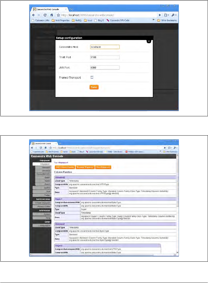
console lets you view. You can see here that I have four keyspaces. Keyspace1 has
been selected to show the column family definitions; the others are system, Test, and
Twitter. Using this screen, you can add a column family to the keyspace, rename a
keyspace, drop a keyspace entirely, or create a new keyspace.
Figure 8-1. The Setup configuration screen for a Cassandra web console
Figure 8-2. Keyspace and column family information in the web console
Cassandra Web Console | 167

Adding a column family or super column family is easy, as shown in Figure 8-3. How-
ever, the web console doesn’t let you add data to your column families, as you might
expect.
Figure 8-3. Adding a super column family in the web console
You can determine how long your server has been up, how much memory it’s using,
and the load by viewing the Ring screen, as shown in Figure 8-4.
Overall, the web console presents an intuitive, attractive interface that makes it easy to
perform basic administration tasks for your Cassandra setup.
Hector (Java)
Hector is an open source project written in Java using the MIT license. It was created
by Ran Tavory of Outbrain (previously of Google) and is hosted at GitHub. It was one
of the early Cassandra clients and is used in production at Outbrain. It wraps Thrift
and offers JMX, connection pooling, and failover.
168 | Chapter 8: Clients
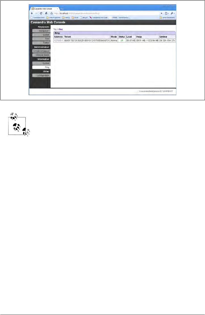
In Greek mythology, Hector was the builder of the city of Troy and was
known as an outstanding warrior. He was also Cassandra’s brother.
Because Hector was one of the first Cassandra client projects, and because it is used by
a wide variety of developers and even has other client projects based on it (see “Hec-
torSharp (C#)” on page 170), we’ll write a complete but simple example application
using it.
To get Hector, clone it from its GitHub site at http://github.com/rantav/hector. Use
the git command if you want the source, or just download the binary from the Down-
loads tab.
Features
Hector is a well-supported and full-featured Cassandra client, with many users and an
active community. It offers the following:
High-level object-oriented API
Java developers should find the interfaces that Hector offers, such as Keyspace and
Column, very natural to use.
Fail over support
Thrift does not provide support for failed clients. This is because Cassandra is
intended to be used in a highly distributed fashion and has good support for failed
nodes in the database ring. But if your client connects to a node that has gone
down, it would be nice to have your client fail over—to automatically search for
another node to use to complete your request. Happily, Hector provides this.
Figure 8-4. The Ring screen shows system usage
Hector (Java) | 169

Connection pooling
Cassandra is specifically built for very high scalability, and it therefore also becomes
a requirement on the client side to support connection pools so that your applica-
tion doesn’t become a bottleneck that robs you of Cassandra’s speed. It’s expensive
to open and close connections, just as it is in JDBC. Hector’s connection pooling
uses Apache’s GenericObjectPool.
JMX support
Cassandra makes liberal use of JMX, which comes in very handy for monitoring.
Hector directly supports JMX by exposing metrics such as bad connections, avail-
able connections, idle connections, and more.
The Hector API
The following is an example from Ran Tavory’s blog (http://prettyprint.me) illustrating
how Hector simplifies working with Cassandra:
// Create a cluster
Cluster c = HFactory.getOrCreateCluster("MyCluster", "cassandra1:9160");
// Choose a keyspace
KeyspaceOperator ko = HFactory.createKeyspaceOperator("Keyspace1", c);
// create an string extractor.
StringExtractor se = StringExtractor.get();
// insert value
Mutator m = HFactory.createMutator(keyspaceOperator);
m.insert("key1", "ColumnFamily1", createColumn("column1", "value1", se, se));
// Now read a value
// Create a query
ColumnQuery<String, String> q = HFactory.createColumnQuery(keyspaceOperator, se, se);
// set key, name, cf and execute
Result<HColumn<String, String>> r = q.setKey("key1").
setName("column1").
setColumnFamily("ColumnFamily1").
execute();
// read value from the result
HColumn<String, String> c = r.get();
String value = c.getValue();
System.out.println(value);
HectorSharp (C#)
HectorSharp is a C# port of Ran Tavory’s Hector Java client (Tavory is also a committer
on the HectorSharp project). Its features are similar to Hector:
• A high-level client with an intuitive, object-oriented interface
• Client-side failover
• Connection pooling
• Load balancing
170 | Chapter 8: Clients
Let’s walk through creating an application using HectorSharp as our interface to Cas-
sandra. This is probably the best way to see how to incorporate it into your projects.
We’ll create a simple C# console project that reads and writes some data to Cassandra
so you can see how it’s used.
As of this writing, HectorSharp works with version 0.6 of Cassandra,
but not 0.7.
Using Git, download HectorSharp from http://github.com/mattvv/hectorsharp.
Remember, to easily get source code from Git, open a terminal in the directory you
want as the parent, and use the git clone command with the .git URL, like this:
>git clone http://github.com/mattvv/hectorsharp.git
Once you have the source, make sure you also have the .NET framework, version 3.5
or better, which you can download for free from Microsoft.com. You can also use the
Visual Studio .NET 2010 Express IDE, which is free, uses the .NET 4.0 framework,
and makes it very easy to work with C# projects. Download Visual Studio C# Express
from http://www.microsoft.com/express/Downloads. This may take a while and will
require you to restart your computer.
Once Visual Studio is installed, open the HectorSharp project so you can view the
source code and add it as a reference to our own project. To open the project, choose
File > Open Project... and then select the file HectorSharp.sln. The Express version of
Visual Studio may complain about not doing Solution files, but don’t worry about that.
Build the HectorSharp source by right-clicking the HectorSharp project name in the
Solution Explorer window. You should see a notice in the bottom-left corner saying
“Build Succeeded”. This will produce the HectorSharp .dll client that we can use in our
own application.
To create our application that wraps HectorSharp, choose File > New Project... >
Console Application. Call your new project ExecuteHector. You’ll be presented with a
shell class called Program.cs with a main method.
Now let’s reference the HectorSharp DLL so we can use its classes. To do this, choose
Project > Add Reference. When the dialog window comes up, pick the Browse tab,
then navigate to the location where you unpacked HectorSharp. Go to the bin\
Release directory and pick the HectorSharp.dll file. You should see HectorSharp added
as a reference in your Solution Explorer.
I have changed the name of my application to CassandraProgram.cs. If
you do this too, you’ll need to change the executable in the project by
choosing Project > ExecuteHector Properties. Choose the Application
tab, and then enter your program name in the Startup Object field.
HectorSharp (C#) | 171

Let’s take a quick look at some of the high-level constructs that HectorSharp makes
available:
ICassandraClient
This is the interface used by HectorSharp client objects, whose implementation
type is typically a KeyedCassandraClientFactory object.
Pool
HectorSharp pools its connections to Cassandra, so you use a factory method
to create a pool, like this: Pool = new CassandraClientPoolFactory().Create();.
Then, using the pool, you can create a client.
Client
From the connection pool, you can get a Client that is used to connect with Cas-
sandra. This is neat:
Client = new KeyedCassandraClientFactory(
Pool,
new KeyedCassandraClientFactory.Config { Timeout = 10 })
.Make( new Endpoint("localhost", 9160) );
You pass the pool into your client factory, then you can specify additional config-
uration details (such as timeout in seconds), and finally build an endpoint using
the host and port you want to connect to. In the preceding example, we specified
a new timeout value of 10 (the default is 20).
Keyspace
This represents a Cassandra keyspace, which you obtain from the Client object.
It allows you to specify the name of the keyspace to connect to and a consistency
level to use:
Keyspace = Client.GetKeyspace(
"Keyspace1",
ConsistencyLevel.ONE,
new FailoverPolicy(0) { Strategy = FailoverStrategy.FAIL_FAST });
The FailoverPolicy class allows you to indicate what HectorSharp should do if
it encounters an error in communication (not an application error); that is, if it
thinks that a node it’s trying to connect to is down. You can retry, retry on incre-
ments, or just decide to quit, which is what I’ve specified here.
ColumnPath
A ColumnPath is a simple wrapper that allows you to easily reference an entire col-
umn family, a super column within a particular column family, or a single column
within a column family. It consists of nothing but C# properties for each of those
three items, plus constructors.
HectorSharp uses the Gang of Four Command pattern for Data Access Objects (DAOs),
because that’s how Hector works. So you could create a DAO with a get method as
shown here:
172 | Chapter 8: Clients

/**
* Get a string value.
* @return The string value; null if no value exists for the given key.
*/
public String get(String key) {
return execute(new Command<String>(){
public String execute(Keyspace ks) {
try {
return string(ks.getColumn(key, createColumnPath(COLUMN_NAME)).getValue());
} catch (NotFoundException e) {
return null;
}
}
});
}
protected static <T> T execute(Command<T> command) {
return command.execute(CASSANDRA_HOST, CASSANDRA_PORT, CASSANDRA_KEYSPACE);
}
The get command is using the parameterized execute method, as are other sibling
commands for insert and delete (not shown in the example). For our sample appli-
cation, we’ll just keep it simple, but this is a reasonable pattern to follow for such a use
case.
We’re finally ready to write some code. Your application should look like the listing in
Example 8-1.
Example 8-1. CassandraProgram.cs
using System;
using HectorSharp;
using HectorSharp.Utils;
using HectorSharp.Utils.ObjectPool;
/**
* Stands in for some C# application that would use HectorSharp
* as a high-level Cassandra client.
*/
namespace ExecuteHector
{
class CassandraProgram
{
internal ICassandraClient Client;
internal IKeyspace Keyspace;
internal IKeyedObjectPool<Endpoint, ICassandraClient> Pool;
static void Main(string[] args)
{
CassandraProgram app = new CassandraProgram();
Console.WriteLine("Starting HectorSharp...");
app.Pool = new CassandraClientPoolFactory().Create();
Console.WriteLine("Set up Pool.");
HectorSharp (C#) | 173

app.Client = new KeyedCassandraClientFactory(app.Pool,
new KeyedCassandraClientFactory.Config { Timeout = 10 })
.Make(new Endpoint("localhost", 9160));
Console.WriteLine("Created client.");
app.Keyspace = app.Client.GetKeyspace(
"Keyspace1",
ConsistencyLevel.ONE,
new FailoverPolicy(0) { Strategy = FailoverStrategy.FAIL_FAST });
Console.WriteLine("Found keyspace " + app.Keyspace.Name);
//set up column path to use
var cp = new ColumnPath("Standard1", null, "MyColumn");
// write values
Console.WriteLine("\nPerforming write using " + cp.ToString());
for (int i = 0; i < 5; i++)
{
String keyname = "key" + i;
String value = "value" + i;
app.Keyspace.Insert(keyname, cp, value);
Console.WriteLine("wrote to key: " + keyname + " with value: " + value);
}
// read values
Console.WriteLine("\nPerforming read.");
for (int i = 0; i < 5; i++)
{
String keyname = "key" + i;
var column = app.Keyspace.GetColumn(keyname, cp);
Console.WriteLine("got value for " + keyname + " = " + column.Value);
}
Console.WriteLine("All done.");
}
}
}
Compile this code into a console application by choosing Debug > Build Solution.
Now we’re ready to test it out. Open a console and start Cassandra as usual: >bin
\cassandra -f. Now open a second console and navigate to the directory where you
have your “ExecuteHector” project, then switch into the bin\Release directory. This
directory has our executable in it; to run our program, just enter ExecuteHector.exe
at the prompt. You should see output similar to the following:
C:\git\ExecuteHector\bin\Release>ExecuteHector.exe
Starting HectorSharp...
Set up Pool.
Created client.
Found keyspace Keyspace1
Performing write using ColumnPath(family: 'Standard1', super: '', column: 'MyColumn'
wrote to key: key0 with value: value0
174 | Chapter 8: Clients

wrote to key: key1 with value: value1
wrote to key: key2 with value: value2
wrote to key: key3 with value: value3
wrote to key: key4 with value: value4
Performing read.
got value for key0 = value0
got value for key1 = value1
got value for key2 = value2
got value for key3 = value3
got value for key4 = value4
All done.
C:\git\ExecuteHector\bin\Release>
As you can see, if you’re creating a C# application and want to use Cassandra as the
backing database, it is very easy to get started with HectorSharp, and its object model
is very high-level, intuitive, and easy to use. Just be aware that as of this writing,
HectorSharp is still in the nascent stages, so make sure that your requirements are
supported before going too far.
You can find out more about HectorSharp at http://hectorsharp.com.
Chirper
If you’re a .NET developer, you might be interested in Chirper. Chirper is a port of
Twissandra to .NET, written by Chaker Nakhli. It’s available under the Apache 2.0
license, and the source code is on GitHub at http://github.com/nakhli/Chirper. You can
read a blog post introducing Chirper at http://www.javageneration.com/?p=318.
Chiton (Python)
Chiton is a Cassandra browser written by Brandon Williams that uses the Python GTK
framework. You can get it from http://github.com/driftx/chiton. It has several prerequi-
sites, so a little setup is required. Before you can use it, make sure you have the following
setup:
• Python 2.5 or better.
• Twisted Python (an event-driven networking interface for Python), available at
http://twistedmatrix.com/trac.
• Thrift (0.2).
• PyGTK 2.14 or later (a graphical user interface kit for Python), available at http://
www.pygtk.org. This in turn requires GTK+. You likely already have it if you’re on
Linux; you can download the binary if you’re on Windows. Just uncompress
the download into a directory and manually add the bin subfolder to the system’s
path environment variable.
Chiton (Python) | 175

Pelops (Java)
Pelops is a free, open source Java client written by Dominic Williams. It is similar to
Hector in that it’s Java-based, but it was started more recently. This has become a very
popular client. Its goals include the following:
• To create a simple, easy-to-use client
• To completely separate concerns for data processing from lower-level items such
as connection pooling
• To act as a close follower to Cassandra so that it’s readily up to date
And the API is much simpler than using the low-level stuff exposed by Thrift and Avro.
To write data, you just need a Mutator class; to read data, just use a Selector. Here’s
a brief sample from Williams’ website that creates a connection pool to a list of Cas-
sandra servers, then writes multiple subcolumn values to a super column:
Pelops.addPool(
"Main",
new String[] { "cass1.database.com", "cass2.database.com", "cass3.database.com"},
9160,
new Policy());
Mutator mutator = Pelops.createMutator("Main", "SupportTickets");
UuidHelper.newTimeUuidBytes(), // using a UUID value that sorts by time
mutator.newColumnList(
mutator.newColumn("category", "videoPhone"),
mutator.newColumn("reportType", "POOR_PICTURE"),
mutator.newColumn("createdDate", NumberHelper.toBytes(System.currentTimeMillis())),
mutator.newColumn("capture", jpegBytes),
mutator.newColumn("comment") ));
mutator.execute(ConsistencyLevel.ONE);
Consider how much easier that is than using the API provided out of the box.
You can get the source code from http://code.google.com/p/pelops, and you can read
some samples and explanations of how to use Pelops at Dominic Williams’ site, http:
//ria101.wordpress.com.
If you’re using Cassandra from a Java application, I encourage you to give Pelops a try.
Kundera (Java ORM)
Kundera is an object-relational mapping (ORM) implementation for Cassandra written
using Java annotations. It’s available at http://kundera.googlecode.com under an Apache
2.0 license. According to its author, Impetus Labs, the aim of Kundera is:
176 | Chapter 8: Clients

...to make working with Cassandra drop-dead simple and fun. Kundera does not reinvent
the wheel by making another client library; rather it leverages the existing libraries and
builds—on top of them—a wrap-around API to help developers do away with unnec-
essary boiler plate codes, and program a neater-and-cleaner code that reduces code-
complexity and improves quality. And above all, improves productivity.
Kundera uses Pelops under the hood. A sample Java entity bean looks like this:
@Entity
@ColumnFamily(keyspace = "Keyspace1", family = "Band")
public class Band {
@Id
private String id;
@Column(name = "name")
private String name;
@Column(name = "instrument")
private String instrument;
You can perform a JPA query like this:
Query query = entityManager.createQuery("SELECT m from Band c where name='george'");
List<SimpleComment> list = query.getResultList();
This library is quite new at the time of this writing, so it has yet to be seen how readily
it will be adopted. Still, it does appear promising, and it speaks to burgeoning interest
in Cassandra among general application developers.
Fauna (Ruby)
Ryan King of Twitter and Evan Weaver created a Ruby client for the Cassandra database
called Fauna. If you envision using Cassandra from Ruby, this might fit the bill. To find
out more about Fauna, see http://github.com/fauna/cassandra/blob/master/README
.rdoc.
Summary
You should now have an understanding of the variety of client interfaces available for
Cassandra and how to install and use them. There are many Cassandra clients, each
with its own strengths and limitations, in different languages and varying degrees of
production-readiness. It’s not possible to cover all of them here, so I’ve taken a repre-
sentative sample from a few different languages. To see a variety of other options that
might fit your needs better, see the Cassandra project wiki Client Options page at http:
//wiki.apache.org/cassandra/ClientOptions.
Summary | 177

CHAPTER 9
Monitoring
This chapter is about using a variety of tools to monitor and understand important
events in the life cycle of your Cassandra cluster. We’ll look at some simple ways to see
what’s going on, such as changing the logging levels and understanding the output.
But Cassandra also features built-in support for Java Management Extensions (JMX),
which offers a rich way to monitor your Cassandra nodes and their underlying Java
environment. With just a little integration work, we can see the health of the database
and ongoing events, and even interact with it remotely to tune certain values. JMX is
an important part of Cassandra, and we’ll spend some time to make sure we know how
it works and what exactly Cassandra makes available for monitoring and management
with JMX, and we’ll even write our own custom MBean to expose a new Cassandra
feature. Let’s get started!
Logging
The simplest way to get a picture of what’s happening in your database is to just change
the logging level to make the output more verbose. This is great for development and
for learning what Cassandra is doing under the hood.
Cassandra uses Log4J for its logging utility. By default, the Cassandra server log level
is set at INFO, which doesn’t give you much detail about what work Cassandra is doing
at any given time. It just outputs basic status updates, such as the following:
INFO 08:49:17,614 Saved Token found: 94408749511599155261361719888434486550
INFO 08:49:17,614 Saved ClusterName found: Test Cluster
INFO 08:49:17,620 Starting up server gossip
INFO 08:49:17,655 Binding thrift service to morpheus/192.168.1.5:9160
INFO 08:49:17,659 Cassandra starting up...
When you start Cassandra in a terminal, you keep this output running in the terminal
window by passing the program the -f flag (to keep output visible in the foreground
of the terminal window). But Cassandra is also writing these logs to physical files for
you to examine later.
179

By changing the logging level to DEBUG, we can see much more clearly what activity the
server is working on, instead of seeing only these stage updates.
To change the logging level, open the file <cassandra-home>/conf/log4j-server
.properties and find the line that looks like this:
log4j.rootLogger=INFO,stdout,R
Change this line so it looks like this:
log4j.rootLogger=DEBUG,stdout,R
Of course, in production you’ll want to tune the logging level back up
to WARN or ERROR, as the verbose output will slow things down
considerably.
Now we can see a lot more activity as Cassandra does its work:
INFO 09:41:54,936 Completed flushing /var/lib/cassandra/data/system/
LocationInfo-8-Data.db
DEBUG 09:41:54,942 Checking to see if compaction of LocationInfo would be useful
DEBUG 09:41:54,942 discard completed log segments for CommitLogContext(file='/var/
lib/cassandra/commitlog/CommitLog-1277397714697.log',...
INFO 09:41:54,943 Compacting [org.apache.cassandra.io.SSTableReader(path='/var/
lib/cassandra
DEBUG 09:41:54,943 Marking replay position 121 on commit log CommitLogSegment(/var/
lib/cassandra/commitlog/CommitLog-1277397714697.log)...
DEBUG 09:41:54,943 index size for bloom filter calc for file
: /var/lib/cassandra/data/system/LocationInfo-5-Data.db : 256
DEBUG 09:41:54,944 index size for bloom filter calc for file
: /var/lib/cassandra/data/system/LocationInfo-6-Data.db : 512
DEBUG 09:41:54,944 index size for bloom filter calc for file
: /var/lib/cassandra/data/system/LocationInfo-7-Data.db : 768
INFO 09:41:54,985 Log replay complete
INFO 09:41:55,009 Saved Token found: 94408749511599155261361719888434486550
INFO 09:41:55,010 Saved ClusterName found: Test Cluster
INFO 09:41:55,016 Starting up server gossip
INFO 09:41:55,048 Binding thrift service to morpheus/192.168.1.5:9160
INFO 09:41:55,051 Cassandra starting up...
DEBUG 09:41:55,112 Marking /var/lib/cassandra/data/system/LocationInfo-5-Data.db
compacted
//...
DEBUG 09:41:55,117 Estimating compactions for Super1
DEBUG 09:41:55,117 Estimating compactions for Standard2
DEBUG 09:41:55,117 Estimating compactions for Super2
DEBUG 09:41:55,118 Estimating compactions for Standard1
DEBUG 09:41:55,118 Estimating compactions for StandardByUUID1
DEBUG 09:41:55,118 Estimating compactions for LocationInfo
DEBUG 09:41:55,118 Estimating compactions for HintsColumnFamily
DEBUG 09:41:55,118 Checking to see if compaction of Super1 would be useful
DEBUG 09:41:55,119 Checking to see if compaction of Standard2 would be useful
DEBUG 09:41:55,119 Checking to see if compaction of Super2 would be useful
//...
180 | Chapter 9: Monitoring

DEBUG 09:41:56,023 GC for ParNew: 1 ms, 14643776 reclaimed leaving 80756296 used;
max is 1177812992
DEBUG 09:41:56,035 attempting to connect to lucky/192.168.1.2
DEBUG 09:41:57,025 Disseminating load info ...
This allows you to see exactly what Cassandra is doing and when, which is very helpful
in troubleshooting. But it’s also helpful in simply understanding what Cassandra does
to maintain itself.
If you want to change the location of the logs directory, just find the following entry in
the same log4j.properties file and chose a different filename:
log4j.appender.R.File=/var/log/cassandra/system.log
There’s not a different entry for Windows; on Windows systems this will automatically
resolve to C:\\var\log\cassandra\system.log.
If you don’t see any logfiles in this location, make sure that you are the
owner of the directories, or at least that proper read and write permis-
sions are set. Cassandra won’t tell you if it can’t write the log; it just
won’t. Same for the datafiles.
Note that this is the location for the log of the activity of the database, and not for
Cassandra’s internal datafiles. Those are stored in /var/lib/cassandra.
Tailing
You don’t need to start Cassandra using the foreground switch in order to see the
rolling log. You can also simply start it without the -f option and then tail the logs.
Tailing is not specific to Cassandra; it’s a small program available in Linux distributions
to see new values printed to a console as they are appended to a file.
To tail the logs, start Cassandra like this:
>bin/cassandra
Then open a second console, enter the tail command, and pass it the location of the
particular file you want to tail, like this:
>tail -f /var/log/cassandra/system.log
The -f option means “follow,” and as Cassandra outputs information to the physical
logfile, tail will output it to the screen. To stop tailing, just type Ctrl-C.
You can do the same thing if you’re using Windows, but Windows doesn’t include a
tail program natively. So to achieve this, you’ll need to download and install Cygwin,
which is a Bash shell emulator. Cygwin allows you to have a Linux-style interface and
use a variety of Linux tools on Windows. You can get Cygwin for free from http://www
.cygwin.com.
Then you can start Cassandra regularly and tail the logfile using this command:
Logging | 181

eben@lucky~$ tail -f C:\\var\\log\\cassandra\\system.log
This will show the output in the console in the same way as if it were foregrounded.
General Tips
Following along
Once you’re running the server with debug logging enabled, you can see a lot more
happening that can help during debugging. For example, here we can see the output
when writing and then reading a simple value to the database:
DEBUG 12:55:09,778 insert
DEBUG 12:55:09,779 insert writing local key mycol
DEBUG 12:55:36,387 get
DEBUG 12:55:36,390 weakreadlocal reading SliceByNamesReadCommand(
table='Keyspace1', key='mycol',
columnParent='QueryPath(columnFamilyName='Standard1',
superColumnName='null', columnName='null')',
columns=[6b6579393939,])
That’s the server output generated by executing this command in the CLI:
cassandra> set Keyspace1.Standard1['mycol']['key999']='value999'
Value inserted.
cassandra> get Keyspace1.Standard1['mycol']['key999']
=> (column=6b6579393939, value=value999, timestamp=1277409309778000
Notice what’s happened here. We’ve inserted a value in the column family named
Standard1. When we perform a get request, the column key key999 is translated to
6b6579393939, because the Standard1 column family is defined as using BytesType as a
CompareWith value.
However, if we use the Standard2 column family, we’ll see the key column name on the
get request as we typed it because that column family is defined as using a Compare
With of UTF-8. So again we’ll do a set and then a get request for the same value. The
CLI output is shown here:
cassandra> set Keyspace1.Standard2['mycol']['key888']='value888'
Value inserted.
cassandra> get Keyspace1.Standard2['mycol']['key888']
=> (column=key888, value=value888, timestamp=1277409950795000)
The server log records this query as follows:
DEBUG 13:06:03,291 get
DEBUG 13:06:03,292 weakreadlocal reading SliceByNamesReadCommand(
table='Keyspace1', key='mycol',
columnParent='QueryPath(columnFamilyName='Standard2',
superColumnName='null', columnName='null')',
columns=[key888,])
This should give you enough information to follow along with what the server’s doing
as you work.
182 | Chapter 9: Monitoring

Warning signs
There are a few things to look out for as you run Cassandra. For example, if you see
something like this in the logs with no further update, there’s something wrong with
the nodes in your ring:
DEBUG 12:39:56,312 attempting to connect to mywinbox/192.168.1.3
It’s OK to attempt to connect, but then it should actually connect. It’s possible for this
to happen when you mix Windows and Linux boxes in a Cassandra cluster, which is
definitely not recommended. If your Linux and Windows boxes can see each other,
share resources such as printers, read and write files between them, view web pages the
other is serving, and so forth, this might give you the impression that this should work.
Don’t be tempted to mix and match in a production environment.
Overview of JMX and MBeans
In this section, we explore how Cassandra makes use of Java Management Extensions
(JMX) to enable remote management of your servers. JMX started as Java Specification
Request (JSR) 160 and has been a core part of Java since version 5.0.
You can read more about the JMX implementation in Java by examining
the java.lang.management package.
JMX is a Java API that provides management of applications in two key ways. First,
JMX allows you to understand your application’s health and overall performance in
terms of memory, threads, and CPU usage—things that are generally applicable to any
Java application. Second, JMX allows you to work with specific aspects of your appli-
cation that you have instrumented.
Instrumentation refers to putting a wrapper around application code that provides
hooks from the application to the JVM in order to allow the JVM to gather data that
external tools can use. Such tools include monitoring agents, data analysis tools, pro-
filers, and more. JMX allows you not only to view such data but also, if the application
enables it, to manage your application at runtime by updating values.
JMX is commonly used for a variety of application control operations, including:
• Low available memory detection, including the size of each graduation space on
the heap
• Thread information such as deadlock detection, peak number of threads, and
current live threads
• Verbose classloader tracing
Overview of JMX and MBeans | 183
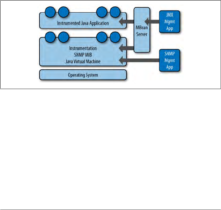
• Log level control
• General information such as application uptime and the active classpath
Many popular Java applications are instrumented using JMX, including the JVM itself,
HP Open View, Oracle WebLogic Server, the Glassfish application server, and Cas-
sandra. In these applications, JMX is simply one way of managing the container; JBoss
Application Server, on the other hand, uses JMX as the primary way of interacting with
the container.
For example, the WebLogic server provides a very wide range of activities via JMX.
You can, for example, monitor the number of available JDBC connections in a pool or
see the number of stateless session beans loaded in the container in a given state. Not
only can you monitor these things, but you can use a graphical console that ships with
the Sun (now Oracle) JDK to change their values. Want to increase the size of the pool
of message-driven beans? A JMX-enabled container could allow you to manage your
resources in this way.
A depiction of the JMX architecture is shown in Figure 9-1.
Figure 9-1. The JMX architecture
The JMX architecture is simple. The JVM collects information from the underlying
operating system. The JVM itself is instrumented, so many of its features are exposed
for management as described earlier. An instrumented Java application (such as Cas-
sandra) runs on top of this, also exposing some of its features as manageable objects.
The JDK includes an MBean server that makes the instrumented features available over
a remote protocol to a JMX Management Application. The JVM also offers manage-
ment capabilities to Simple Network Monitoring Protocol (SNMP) agents and works
in a similar manner.
But within a given application, you can manage only what the application developers
have made available for you to manage. Luckily, the Cassandra developers have
instrumented large parts of the database, making management via JMX fairly straight-
forward.
184 | Chapter 9: Monitoring
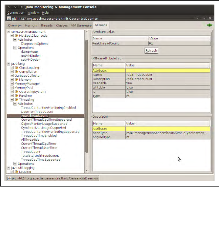
This instrumentation of a Java application is performed by wrapping the application
code that you want JMX to hook into with managed beans.
MBeans
A managed bean, or MBean, is a special type of Java bean that represents a single man-
ageable resource inside the JVM. MBeans interact with an MBean server to make their
functions remotely available.
The jconsole tool ships with the standard Java Development Kit. It provides a graphical
user interface client for working with MBeans and can be used for local or remote
management. A view of JConsole is shown in Figure 9-2.
Figure 9-2. JConsole showing the peak thread count for a Cassandra daemon
In this figure, you can see the two kinds of views into your application that JMX offers:
the general view about threads, memory, and CPU that every application will have,
and a more detailed view that exposes the peak thread count value. You can see that
many other instrumented aspects of the application are also available.
Overview of JMX and MBeans | 185
JConsole is popular because it’s easy to use and ships with the JDK. But
this is only one possible JMX client. The JBoss Application Server web
console, for example, is itself a JMX client of the JBoss server.
There are many aspects of an application or the JVM that can be instrumented but
that may be disabled. Thread Contention is one example of a potentially useful MBean
that is turned off by default in the JVM. These aspects can be very useful for debugging,
so if you see an MBean that you think might help you hunt down a problem, go ahead
and enable it. But keep in mind that nothing comes for free, and it’s a good idea to read
the JavaDoc on the MBean you want to enable in order to understand the potential
impact on performance. ThreadCPUTime is another example of a useful, but expensive,
MBean.
Some simple values in the application are exposed as attributes. An example of this is
Threading > PeakThreadCount, which just reports the value that the MBean has stored
for the greatest number of threads the application used at a single point in time. You
can refresh to see the most recent value, but that’s pretty much all you can do with it.
Because such a value is maintained internally in the JVM, it doesn’t make sense to set
it externally (it’s derived from actual events, and not configurable).
But other MBeans are configurable. They make operations available to the JMX agent
that let you get and set values. You can tell whether the MBean will let you set a value
by looking at the value for writable. If it’s false, you will see a label indicating the read-
only value; if it’s true, you will see a set of one or more fields to add your new value
and a button to update it. An example of this is the java.util.logging.Logger bean,
as shown in Figure 9-3.
Note that the parameter names are not available to the JMX agent; they’re just labeled
as p0, p1, etc. That’s because the Java compiler “forgot” the parameter names during
compilation. So in order to know what parameters to set, you’ll need to look at the
JavaDoc for the particular MBean you’re working with. In the case of java.util
.logging.Logger, this class implements an interface called java.util.logging
.LoggingMXBean, which wraps it for instrumentation. To find out what the right pa-
rameters are, we examine the JavaDoc for this class and see that p0 is the name of the
logger you want to change, and p1 is the logging level you want to set that logger to.
If it’s not obvious, setting the logging level for java.util.logging won’t
help you much if that’s not what your application is using for logging.
It’s just used here as a general example because it’s easy to understand
and serves as a gentle introduction. But Cassandra does not use that
logging package.
Some MBeans return an attribute value of javax.management.openmbean.CompositeData
Support. That means that these are not simple values that can be displayed in a single
186 | Chapter 9: Monitoring
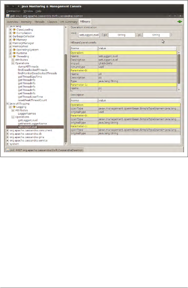
field, such as LoadedClassCount, but are instead multivalued. One example is Memory >
HeapMemoryUsage, which offers several data points and therefore has its own view.
Another type of MBean operation is one that doesn’t simply show a value or allow you
to set a value, but instead lets you execute some useful action. dumpAllThreads and
resetPeakThreadCount are two such operations.
Now we’ll quickly get set up to start monitoring and managing Cassandra specifically.
Integrating JMX
Enabling Cassandra to use JMX is easy, but there are a couple of dependencies. Go to
http://mx4j.sourceforge.net and download version 3.0.1 of the library MX4J. You can
probably use a newer version if one’s available, but this version is known to work.
After you’ve downloaded the library, unzip it and navigate to the lib directory. Copy
two JARs from this directory: mx4j.jar and mx4j-tools.jar. Paste them into your
<cassandra-home>/lib directory and restart Cassandra. Now other Cassandra nodes
Figure 9-3. The java.util.logging.Logger MBean allows you to set a logger’s log level
Overview of JMX and MBeans | 187
can connect via JMX to monitor its health and even to set values for the functions that
are exposed as MBeans.
If you’ve downloaded Cassandra’s source code, just drop the two necessary JARs into
the lib directory and rebuild the source. The next time you start Cassandra, you should
see output similar to the following:
INFO 13:37:28,473 Cassandra starting up...
DEBUG 13:37:28,474 Will try to load mx4j now, if it's in the classpath
INFO 13:37:28,508 mx4j successfuly loaded
HttpAdaptor version 3.0.2 started on port 8081
Here, MX4J will act as our JMX server agent, and now we’re ready to start getting some
benefit from JMX.
Interacting with Cassandra via JMX
Now that JMX is enabled, let’s connect to Cassandra on its JMX port. To do so, open
a new terminal and type the following:
>jconsole
When you run jconsole, you’ll see a login screen similar to that in Figure 9-4.
From here, you can simply double-click on the value org.apache.cassandra.thrift
.CassandraDaemon under the Local Process section if you’re monitoring a node on the
same machine. If you want to monitor a node on a different machine, check the Remote
Process radio button, then enter the host and port you want to connect to. Cassandra
JMX by default broadcasts on port 8080, so you can enter a value like the one shown
here and then hit Connect:
>lucky:8080
If you have trouble with this, make sure that you don’t have something
else running on port 8080, as that’s a popular port for tools such as
Apache Tomcat.
Once you’ve connected to a server, the default view includes four major categories
about your server’s state, which are updated constantly:
Heap Memory Usage
This shows the total memory available to the Cassandra program, as well as how
much it’s using right now.
Threads
This is the number of live threads Cassandra is using.
188 | Chapter 9: Monitoring
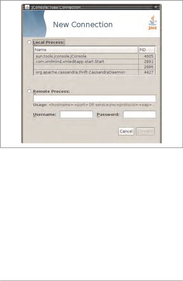
Classes
The number of classes that Cassandra has loaded. This number is relatively small
for such a powerful program; Cassandra typically requires around 2,300 classes
out of the box. Compare this to a program such as Oracle WebLogic, which typ-
ically loads around 24,000 classes.
CPU Usage
This shows the percentage of the processor that the Cassandra program is currently
using.
You can use the selector to adjust the time range shown in the charts.
If you want to see a more detailed view of how Cassandra is using the Java heap and
nonheap memory, click the Memory tab. By changing the chart value in the drop-
down, you can see in detail the graduations in which Cassandra is using its memory.
You can also (try to) force a garbage collection if you think it’s necessary.
You can connect to more than one JMX agent at once. Just choose File > New Con-
nection... and repeat the steps to connect to another running Cassandra node to view
multiple servers at once.
Figure 9-4. The jconsole login
Interacting with Cassandra via JMX | 189

Cassandra’s MBeans
Once you’ve connected with a JMX agent such as JConsole, you can manage Cassandra
using the MBeans it exposes. To do so, click the MBeans tab. Other than the standard
Java items available to every agent, there are several Cassandra packages that contain
manageable beans, organized by their package names, which start with
org.apache.cassandra. We won’t go into detail on all of them here, but there are several
of interest that we’ll take a look at.
Many classes in Cassandra are exposed as MBeans, which means in practical terms that
they implement a custom interface that describes the operations that need to be im-
plemented and for which the JMX agent will provide hooks. The steps are basically the
same for getting any MBean to work; I’ll use a single key class as an example. If you’d
like to JMX-enable something that isn’t already enabled, modify the source code
following this general outline and you’ll be in business.
For this example, we look at Cassandra’s StorageService and how it uses MBeans.
Here’s the partial definition of the StorageServiceMBean class, with some operations
omitted for brevity:
public interface StorageServiceMBean
{
public Set<String> getLiveNodes();
public Set<String> getUnreachableNodes();
public void forceTableFlush(String tableName, String... columnFamilies)
throws IOException;
public void removeToken(String token);
//...
}
As you can see by this MBean interface definition, there’s no magic going on. This is
just a regular interface defining the set of operations that will be exposed to JMX that
the StorageService implementation must support. This typically means maintaining
additional metadata as the regular operations do their work.
The StorageService class implements this interface and must do the work of directly
supporting JMX. The consistency manager field has a reference type of java.util
.concurrent.ExecutorService, but the actual implementation is of type org.apache
.cassandra.concurrent.JMXEnabledThreadPoolExecutor.
private ExecutorService consistencyManager_ =
new JMXEnabledThreadPoolExecutor(DatabaseDescriptor.getConsistencyThreads(),
DatabaseDescriptor.getConsistencyThreads(),
StageManager.KEEPALIVE,
TimeUnit.SECONDS,
new LinkedBlockingQueue<Runnable>(),
new NamedThreadFactory("CONSISTENCY-MANAGER"));
190 | Chapter 9: Monitoring

The JMXEnabledThreadPoolExecutor implements the JMXEnabledThreadPoolExecutorM
Bean and, by association, org.apache.cassandra.concurrent.IExecutorMBean, so that all
the Cassandra classes that use thread pools can expose the same operations to JMX.
It’s in the JMXEnabledThreadPoolExecutor that we see how Cassandra becomes JMX-
enabled.
The executor pool registers with the platform MBean server in its constructor, as
shown here:
public JMXEnabledThreadPoolExecutor(int corePoolSize,
int maximumPoolSize,
long keepAliveTime,
TimeUnit unit,
BlockingQueue<Runnable> workQueue,
NamedThreadFactory threadFactory)
{
super(corePoolSize, maximumPoolSize, keepAliveTime, unit, workQueue,
threadFactory);
super.prestartAllCoreThreads();
MBeanServer mbs = ManagementFactory.getPlatformMBeanServer();
mbeanName = "org.apache.cassandra.concurrent:type=" + threadFactory.id;
try
{
mbs.registerMBean(this, new ObjectName(mbeanName));
}
catch (Exception e)
{
throw new RuntimeException(e);
}
}
The platform server here is simply the default one embedded in the JDK. The MBean
is named and registered so that the MBean server knows to monitor it and make it
manageable via the agent.
In order to do proper cleanup, when the JMXEnabledThreadPoolExecutor is shut down,
the class will also unregister itself from the MBean server:
private void unregisterMBean()
{
try
{
ManagementFactory.getPlatformMBeanServer().unregisterMBean
(new ObjectName(mbeanName));
}
catch (Exception e)
{
throw new RuntimeException(e);
}
}
Likewise, the StorageService class itself registers and unregisters with the MBean
server for the JMX properties that it maintains locally. So this implementation does all
Cassandra’s MBeans | 191
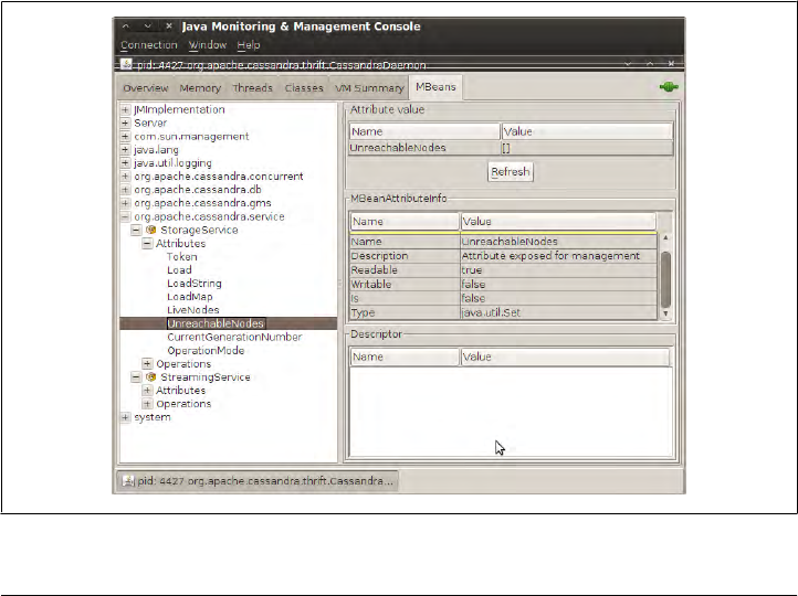
of the work that it is intended to do, and then has implementations of the methods that
are only necessary for talking to the MBean server. For example, here is the Storage
Service implementation of the of the getUnreachableNodes operation:
public Set<String> getUnreachableNodes()
{
return stringify(Gossiper.instance.getUnreachableMembers());
}
The Gossiper class is a Singleton that maintains lists of IP addresses of the nodes it has
sent and received heartbeat messages from, so when you call the getUnreachable
Nodes operation in the JMX agent, it calls the MBean method in StorageService, which
delegates the call to the Gossiper, which returns the set of unreachable IP addresses,
wrapped in a new set so it can’t be modified directly by the caller:
/* unreachable member set */
private Set<InetAddress> unreachableEndpoints_ =
new ConcurrentSkipListSet<InetAddress>(inetcomparator);
//...
public Set<InetAddress> getUnreachableMembers()
{
return new HashSet<InetAddress>(unreachableEndpoints_);
}
So when we open it up in the JMX agent JConsole, we see, happily, that we have no
unreachable nodes because the set is empty. If there were unreachable nodes, their IP
addresses would appear in the Value field, as shown in Figure 9-5.
Figure 9-5. The StorageService unreachable nodes attribute
192 | Chapter 9: Monitoring

In the following sections, we see what features are available for monitoring and
management in this way via JMX, by package.
org.apache.cassandra.concurrent
This package houses Cassandra’s threading and streaming functionality. As such, it is
the home of the Staged Event-Driven Architecture (SEDA) classes, the gossiper, the
balancers, and the classes that flush data in memtables.
Most of these MBeans allow you to view only attributes. If you are suspicious of data
writing problems or unbalanced node problems in your Cassandra ring, start here.
Because of the SEDA architecture, each stage in Cassandra is exposed as its own
MBean. This means you’re able to quickly determine exactly how many objects are in
a given stage at a given time. The stages include:
• Anti-Entropy Stage
• Migration Stage
• Response Stage
• Row Mutation Stage (for deletes and updates)
• Row Read Stage
• Stream Stage
For each of these stages you can see the counts for active, completed, and pending
tasks. Some of the stages, such as for reading and writing data, maintain their own
thread pools, and the MBeans allow you to see the pool size. All of the stage objects
expose only attributes and don’t allow you to perform any operations.
org.apache.cassandra.db
These are the Cassandra classes related to the core database itself that are exposed as
MBeans. They include Caches, Column Family Stores, the Commit Log, and the
Compaction Manager.
You can view information about a variety of caches that Cassandra maintains—
including the caches for column family key and row hints—for location information
of keys, rows, and migrations. The cache information contains attributes for the cache’s
current size, capacity, number of cache requests, cache hits, and recent cache activity.
Column Family Stores is another set of MBeans, but these give you a richer variety of
attribute values, and also allow you to perform some operations. These give you a view
into your memtables, SSTables, and Bloom filter usage. You can use the operations
provided to force a flush of the memtables, initiate a major compaction by calling the
forceMajorCompaction method of the CompactionManager class, or invalidate a row cache.
Cassandra’s MBeans | 193

One useful set of statistics here relates to reading and writing data, included in the
ColumnFamilyStores > system > Schema bean:
Total Read Count
This is the number of reads Cassandra has performed, available from the Read
Count attribute.
Recent Read Latency
You get this number (in microseconds) from the RecentReadLatencyMicros attrib-
ute. You can also see the TotalReadLatencyMicros; the total reads multiplied by the
read latency gives you that number.
These statistics come in very handy if you are concerned that performance is degrading.
But they also are great for showing how fast Cassandra can be. For example, on my
eight-core machine, I’ve recorded write latency at 92 microseconds for simple values
in a small database.
This set of MBeans also makes data regarding the Compaction Manager availa-
ble, including the total bytes that are in the process of being compacted and the total
bytes that have been compacted.
org.apache.cassandra.gms
This package has one MBean with three operations: you can dump arrival times or get
and set the conviction threshold, which by default is 8.
org.apache.cassandra.service
The service package offers two beans: StorageService and StreamingService. Because
these classes are central to Cassandra’s operations, they expose the greatest number of
operations and give you considerable external control. Let’s take a moment to survey
some of the key elements.
StorageService
Because Cassandra is a database, it’s essentially a very sophisticated storage program;
therefore, one of the first places you’ll want to look when you encounter problems is
the StorageService MBean. This allows you to inspect your OperationMode, which re-
ports normal if everything is going smoothly (other possible states are leaving, joining,
decommissioned, and client).
You can also view the current set of live nodes, as well as the set of unreachable nodes
in the cluster. If any nodes are unreachable, Cassandra will tell you their IP addresses
in the UnreachableNodes attribute. But there are many other standard maintenance
operations that this bean affords you, and understanding the operations available here
is important to keeping your cluster in good health. I encourage you to check out the
194 | Chapter 9: Monitoring

bean for yourself, of course, and here I highlight some of the key maintenance
operations.
If you want to change Cassandra’s log level at runtime without interrupting service (as
we saw earlier in the general example), you can invoke the setLog4jLevel(String class
Qualifier, String level) method. For example, say that you have set Cassandra’s log
level to debug because you’re troubleshooting an issue. You can use some of the meth-
ods described here to try to help fix your problem, then you might want to change the
log level to something less trying on the system. To do this, navigate to the StorageSer
vice MBean in JConsole. We’ll change the value for a particularly chatty class: the
LoadDisseminator. The first parameter to this operation is the name of the class you
want to set the log level for, and the second parameter is the level you want to set it to.
Enter org.apache.cassandra.service.LoadDisseminator and INFO, and click the button
labeled setLog4jLevel. You should see the following output in your logs (assuming your
level was already debug):
DEBUG 17:17:30,515 Disseminating load info ...
INFO 17:17:42,001 set log level to INFO for classes under
'org.apache.cassandra.service.LoadDisseminator'
(if the level doesn't look like 'INFO' then log4j couldn't parse 'INFO')
As you can see from this output, Cassandra was logging a load info statement because
the logger was set to debug. After invoking the setLog4jLevel operation, we get the
INFO output and no more debug level statements.
To get an understanding of each node’s load, you can use the getLoadMap() method,
which will return to you a Java Map with keys of IP addresses with values of their
corresponding loads.
If you’re looking for a certain key, you can use the getNaturalEndpoints(String table,
byte[] key) operation. Pass it the table name and the key for which you want to find
the endpoint value, and it will return a list of IP addresses that are responsible for storing
this key.
You can also use the getRangeToEndpointMap operation to get a map of range to end
points describing your ring topology.
If you wish to decommission a server, you can also do that with this MBean. Invoke
the decommission() operation, and the current node’s data will automatically transfer
to another machine and take this node out of service.
If you’re feeling brave, you can invoke the truncate operation for a given column family
in a given keyspace. If all of the nodes are available, this operation will delete all data
from the column family but leave its definition intact.
A good idea for general maintenance is to use the loadBalance() operation if you dis-
cover through other MBeans that your nodes have become very unbalanced. This can
happen from time to time, where some nodes have an inordinate share of the data. This
operation will cause the current node to unload its data onto one of its neighboring
Cassandra’s MBeans | 195

nodes, and then it will bootstrap to receive the data of the node in the ring burdened
with the most data.
StreamingService
The org.cassandra.streaming.StreamingServiceMBean defines the following interface:
public interface StreamingServiceMBean
{
public Set<InetAddress> getStreamDestinations();
public List<String> getOutgoingFiles(String host) throws IOException;
public Set<InetAddress> getStreamSources();
public List<String> getIncomingFiles(String host) throws IOException;
public String getStatus();
}
There are two basic ideas here: a stream source and a stream destination. Each node
can stream its data to another node in order to perform load balancing, and this class
supports these operations. The MBean methods give you a necessary view into the data
that is moving between nodes in the cluster.
The getStatus operation is not an enumeration with some set list of possible statuses.
It rather returns a string in the form of ReceivingFrom: [node] SendingTo: [node].
So in conjunction with the Storage-Service MBean, if you’re concerned that a node is
not receiving data as it should, or that a node is unbalanced or even down, these two
services working together can give you very rich insight into exactly what’s happening
in your cluster during a snapshot in time.
Custom Cassandra MBeans
Let’s quickly write a very simple MBean so that you can do this kind of work yourself
if there’s a new feature you’d like to JMX-enable. There’s nothing to it.
First, we get the source code and create our MBean interface next to the Cassandra
source file it wraps. Our MBean will return the current version of the Cassandra API,
which is not currently available in Cassandra. Our MBean looks like this:
package org.apache.cassandra.thrift;
public interface CassandraServerMBean {
public String getVersion();
}
Now we need to open up the source of CassandraServer.java and make it implement
our MBean interface and hook into the JMX server. Finally, we’ll actually implement
196 | Chapter 9: Monitoring

the method. Thrift generates a version number that is accessible from the CLI, so we’ll
just reuse that. Our new CassandraServer.java class looks like this:
package org.apache.cassandra.thrift;
import javax.management.MBeanServer;
import javax.management.ObjectName;
import org.apache.cassandra.auth.AllowAllAuthenticator;
import org.apache.cassandra.concurrent.StageManager;
//rest of imports...
public class CassandraServer implements Cassandra.Iface, CassandraServerMBean
{
public static final String MBEAN_OBJECT_NAME =
"org.apache.cassandra.service:type=CassandraService";
public CassandraServer()
{
storageService = StorageService.instance;
final MBeanServer mbs = ManagementFactory.getPlatformMBeanServer();
try
{
mbs.registerMBean(this, new ObjectName(MBEAN_OBJECT_NAME));
}
catch (Exception e)
{
throw new RuntimeException(e);
}
}
//rest of server implementation...
//our mbean hook method
public String getVersion() {
String version = null;
try {
version = describe_version();
} catch(TException e) {
logger.warn("Cassandra server version unavailable: ", e.getMessage());
version = "unavailable";
}
return version;
}
}
So we have implemented the interface and connected the Cassandra server with the
management platform. Now all we need to do is open a terminal, navigate to our
<cassandra-home> directory using the $ ant command, and start the server. Then, run
jconsole and connect to your server instance. You should see your attribute available,
as shown in Figure 9-6.
Custom Cassandra MBeans | 197
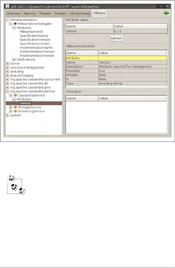
Figure 9-6. Our custom MBean exposing the Cassandra version
Here, version 8.1.0 is the API version information generated as a Thrift constant; it
doesn’t necessarily correspond to the release version.
If you are modifying the source and are unsure about what you’ve
changed, you can always use Subversion to check the changes in your
local repository against what you checked out. Use the svn diff com-
mand to see the changes between the two files and dump the result to
a new file:
eben@morpheus:~$ svn diff
/home/eben/cassandra/dist/trunk-svn-1/src/java/org/apache/cassandra/thrift/
CassandraServer.java
/home/eben/cassandra/dist/trunk-svn-2/src/java/org/apache/cassandra/thrift/
CassandraServer.java
>> /home/eben/CassandraServer.patch
198 | Chapter 9: Monitoring

Runtime Analysis Tools
We don’t need to go into too much more detail about JMX in general here, but to
understand Cassandra and manage it, it’s good to know what features are exposed with
JMX. It’s also useful to know what tools Java makes available out of the box to detect
and spot the source of a memory leak, analyze a hung process, and so on. Because
Cassandra is a Java application, and because it is relatively young, there are no third-
party tools specific to Cassandra at this point.
If you are debugging and you’re not sure what commands have been
executed against Cassandra with the CLI, look in your home directory
for a hidden file called .cassandra.history. This acts like your Bash shell
history, listing the commands in a plain-text file in the order Cassandra
executed them. Nice!
Heap Analysis with JMX and JHAT
As you’re debugging your Cassandra application, it’s often useful to understand what’s
happening in your heap. If you’re working off of the trunk or are otherwise unsure of
your Cassandra build, there are some native Java tools available to you.
Cassandra can use a lot of memory, and garbage collection and major compactions can
have a big impact on performance. One helpful program here is called Java Heap
Analysis Tool (JHAT). JHAT uses the HPROF binary format to create web pages that
allow you to browse all the objects in the heap and see all the references to and from
heap objects. You can combine this tool, which ships with the JDK, with some data
made available through JMX.
To gain a better understanding of our heap, we’ll use the com.sun.management.HotSpot
Diagnostic bean. It has an operation called dumpHeap. Because that’s the name of the
operation in the MBean, that’s the label on the button in the JMX agent. This bean
allows you to specify a filename where you want to dump the heap to; then you click
the button and it writes the heap information into the file you specified. But the dump
Heap operation writes the heap’s current state to a file that’s encoded in the HPROF
binary format for heap and CPU profiling. So we can’t read it in a text file and will need
to use JHAT to view the data.
To get a heap dump, run JConsole and navigate to the com.sun.management.HotSpot
Diagnostic bean, expand the Operations tree, and click the dumpHeap operation. Enter
a relative or absolute path naming the file you want to write the heap dump to, as shown
in Figure 9-7.
Open a new terminal and start up jconsole. You should see a pop-up box indicating
that the method was successfully invoked.
Runtime Analysis Tools | 199
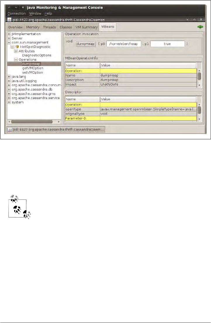
You can also get a heap dump file on a running process without the graphical interface
using the jmap tool that ships with the JDK. First, get your Cassandra instance’s process
ID. To get the process IDs on a Linux system for programs, use the ps command and
look for ‘java’. Or, if you have many Java processes running, you can find Cassandra
more specifically by grepping for the Cassandra daemon.
You can find Cassandra’s process ID on a Linux system by opening a
terminal and using the ps command as follows:
$ ps -ef | grep 'CassandraDaemon'
Once you have the Cassandra process ID, we can use it to specify the heap we want to
get a snapshot of with the jmap tool. This is useful for finding out what’s going on in a
hung process, locating the source of a memory leak, and so on.
eben@morpheus:~$ jmap -dump:live,format=b,file=/home/eben/jmapdump.bin 4427
Dumping heap to /home/eben/jmapdump.bin ...
Heap dump file created
Now that we have captured our heap data, let’s use JHAT to check it out. To run JHAT,
open a terminal and type something like the following, replacing my heap dump file
location with yours:
$jhat /home/eben/jmapdump.bin
Figure 9-7. Invoking the dumpHeap operation on our Cassandra node
200 | Chapter 9: Monitoring

This command will run for a moment and then output something like the following:
Chasing references, expect 63 dots..............................................
.................
Eliminating duplicate references................................................
...............
Snapshot resolved.
Started HTTP server on port 7000
Server is ready.
Now that the server is started, you can open a browser to http://localhost:7000 to view
the file. The heap dump file is also portable, so you can move it to another box after
you generate it and view it there in JHAT.
JHAT will run for a moment and then launch a web server (there’s a
small HTTP server built into the JDK since version 6) on port 7000, so
you might need to close JConsole or some other program to ensure that
port can be used, because it’s not configurable. To make sure it’s open,
type >netstat -o -a on Windows or >netstat -o -a | less on Linux.
For more information on how to use JHAT, consult http://java.sun.com/
javase/6/docs/technotes/tools/share/jhat.html or just type jhat -h for help
options.
The generated website offers a variety of options, including limiting your view to only:
• All classes, including Java platform classes
• All classes, excluding Java platform classes
• All members of the rootset
• Instance counts for all classes
• Heap histogram, showing all classes with the number of instances that have been
created and their total size
• Classes awaiting finalizer execution
If there’s a problem with Cassandra, an hprof file will be created, as we can see in the
following output:
DEBUG 16:13:17,640 Disseminating load info ...
java.lang.OutOfMemoryError: Java heap space
Dumping heap to java_pid21279.hprof ...
Heap dump file created [2766589 bytes in 0.032 secs]
ERROR 16:13:34,369 Fatal exception in thread Thread[pool-1-thread-1,5,main]
java.lang.OutOfMemoryError: Java heap space
at org.apache.thrift.protocol.TBinaryProtocol.readStringBody(TBinaryProtocol
.java:296)
at org.apache.thrift.protocol.TBinaryProtocol.readMessageBegin(TBinaryProtocol
.java:203)
at org.apache.cassandra.thrift.Cassandra$Processor.process(Cassandra.java:1113)
The file will be created in <cassandra-home>, and you can open it like this:
Runtime Analysis Tools | 201

$ jhat java_pid21279.hprof
The file will be analyzed, the server will be created, and you can open a browser to see
what the state of your objects were at the time of the crash.
Alternatively, you can create your own custom view by executing a query of the
heap data in an HTML form. Object Query Language (OQL) is a simple SQL-like
syntax for querying the heap dump file to find only objects that meet certain specified
properties. The query in Figure 9-8 allows us to filter on only objects that are in Cas-
sandra’s org.apache.cassandra.db package.
Figure 9-8. Using Object Query Language in JHAT to filter only Cassandra’s classes in the db package
Once the query result returns, you can click on the class name to see additional detail
about it.
You can execute queries about more specific properties of objects as well. For example,
you may want to filter for only objects that have a string longer than 200 characters.
Using OQL, you could issue a statement such as this:
select s from java.lang.String s where s.count >= 200
202 | Chapter 9: Monitoring

More detail on the Object Query Language is beyond the scope of this
book, but it’s not hard to use. There are a few examples included with
the tool, and its syntax is very similar to SQL. There are also some
good blogs describing how to use it; in particular, check out A. Sun-
dararajan’s blog at http://blogs.sun.com/sundararajan/entry/querying
_java_heap_with_oql.
In this case, we can use the results of the query to see the classpath information held
in a string:
Object at 0x3a272e0
instance of -ea -Xdebug
-Xrunjdwp:transport=dt_socket,server=y,address=8888,suspend=n
-Xms128m -Xmx1G -XX:TargetSurvivorRatio=90 -XX:+AggressiveOpts
-XX:+UseParNewGC -XX:+UseConcMarkSweepGC -XX:+CMSParallelRemarkEnabled
-XX:+HeapDumpOnOutOfMemoryError
-XX:SurvivorRatio=128 -XX:MaxTenuringThreshold=0
-Dcom.sun.management.jmxremote.port=8080
-Dcom.sun.management.jmxremote.ssl=false
-Dcom.sun.management.jmxremote.authenticate=false -Dcassandra
-Dstorage-config=/opt/apache-cassandra-0.6.2/0.6.2-source/conf
-Dcassandra-foreground=yes (24 bytes)
This is a roundabout way to see your classpath switches, but it does give you an idea
of how JMap and JHAT can help you find interesting information about your runtime
state.
Detecting Thread Problems
If you are seeing slowness or uncontrollable growth in the JConsole, you might want
to inspect the current thread behavior. Cassandra makes heavy use of thread pools and
the Java concurrency libraries, so understanding their state can be important to
debugging efforts.
In the console, click the Threads tab. The window on the left will show you a list of
threads and pools, and you can click any of them to see a stack. This view will also
show you their current state. If you see any threads in a stuck state, that’s a sign that
your server is not releasing resources as it should, and you will start to see performance
bottlenecks around this thread. If many stuck threads begin to queue up in a stuck
state, your server will eventually crash. If you’re seeing unusual growth in heap usage
where garbage collection is not reclaiming space, you might have an issue with stuck
threads, and you can check this area of the console to determine thread state.
Runtime Analysis Tools | 203

In Java, a “stuck” thread is a thread that the application has transitioned
to the “stuck” state following a timeout period; that is, the application
has decided that after a certain amount of time during which work is
not being completed, the thread will never complete its work. This can
prevent it from getting returned to the thread pool, which means fewer
threads will be available for new work, which means performance will
start crumbling.
Finally, you can click the Detect Deadlock button if you’re concerned that you might
have internal deadlocked threads.
Health Check
There are a few basic things that you’ll want to look for to ensure that nodes in your
cluster are healthy:
• Check the MBean for org.apache.cassandra.concurrent.ROW_MUTATION_STAGE.
You’re looking to see that the completed task counts are increasing, which means
that writes (inserts, updates, and deletes) are coming through and are completing
successfully.
• Check the MBean for org.apache.cassandra.concurrent.ROW_READ_STAGE. For
this, you’re also ensuring that the completed task counts are increasing, which
means that read operations are coming through and are completing successfully.
• Make sure for both of these MBeans that the number in the PendingTasks attribute
is not growing too much. Even if it’s not a very low number, it should be relatively
stable. A growing set of pending tasks means that Cassandra is having trouble
keeping up with the load. As is usual with databases, once this problem starts, it
will only continue in a downward spiral. Three things that can improve this
situation are a decreased load, scaling up (adding more hardware), or scaling out
(adding another node and rebalancing).
• As usual, check the logs to make sure that nothing is reporting at ERROR level.
Summary
In this chapter we looked at ways you can monitor and manage your Cassandra
cluster. In particular, we went into some detail on JMX and learned the rich variety of
operations Cassandra makes available to the MBean server. We saw how to use JCon-
sole to view what’s happening in your Cassandra cluster, and we performed basic
maintenance tasks. Using just a little Java code, we saw how you could easily use
MBeans yourself to JMX-enable a new aspect of the source code if you wish.
We also gained some insight into how to use tools that come with the Java Development
Kit to help us understand the runtime object graph within Cassandra. Using JMap and
204 | Chapter 9: Monitoring

the Java Heap Analysis Tool, we took a snapshot of the program’s memory and then
queried it using Object Query Language to find objects with properties we might be
concerned about.
There are a variety of other operations monitoring tools that are more robust, but this
will get you started. Your organization might use one already that you can hook into,
such as OpenNMS (see http://www.opennms.org), which has JMX hooks. Nagios, for
example, is open source, free, and rather straightforward. It also has the advantage of
readily connecting to JMX, and it’s what they use at Mahalo to monitor their Cassandra
ring.
There’s an article on Mahalo about how to integrate Nagios with JMX.
See http://www.mahalo.com/how-to-monitor-cassandra-with-nagios.
You should now be ready to perform routine maintenance, understand your Cassandra
cluster better, and know how to perform some general and fine-grained tuning tasks
to keep Cassandra healthy.
Summary | 205
CHAPTER 10
Maintenance
In this chapter, we look at some things you can do to keep Cassandra healthy. So put
your operations hat on, and let’s get started.
The Nodetool ships with Cassandra and can be found in <cassandra-home>/bin. This
is a command-line program that offers a rich array of ways to look at your cluster,
understand its activity, and modify it. Nodetool lets you get limited statistics about the
cluster, see the ranges each node maintains, move data from one node to another,
decommission a node, and even repair a node that’s having trouble.
Many of the tasks in Nodetool overlap with functions available in the
JMX interface. This is because, behind the scenes, Nodetool is invoking
JMX using a helper class called NodeProbe. So JMX is doing the real work,
the NodeProbe class is used to connect to the JMX agent and sort out the
data, and the NodeCmd class is used to present it in an interactive
command-line interface.
To use Nodetool, you need to have the same environment as Cassandra itself; that is,
it requires the same classpath and logging files.
The command-line Nodetool is a wrapper around org.apache.cassandra
.tools.NodeCmd. Take a look at the source for that class if you need to
know more about exactly what it’s doing.
Starting Nodetool is a breeze. Just open a terminal, navigate to <cassandra-home>, and
enter the following command:
$bin/nodetool
Running it this way will error out, but you also cause the program to print a list of
available commands, which are covered next.
207

Getting Ring Information
There is a variety of information you can get about the ring and its nodes, which we
look at in this section. You can get basic information on an individual node or on all
the nodes participating in a ring.
Info
The most straightforward command to issue is the info command. It tells Nodetool to
connect with a single node and get some basic data about its current state. Just pass it
the address of the node you want info for:
$ bin/nodetool -h 192.168.1.5 info
134439585115453215112331952664863163581
Load : 3.93 MB
Generation No : 1277663698
Uptime (seconds) : 19639
Heap Memory (MB) : 36.60 / 1011.25
The only item here that might not be entirely obvious is the “Generation No” field.
This is a heartbeat state associated with every endpoint. It’s maintained by the
Gossiper using a timestamp.
Ring
To determine what nodes are in your ring and what state they’re in, use the host and
ring switches on Nodetool, like this:
$ bin/nodetool -host 192.168.1.5 ring
This will give you a result like this one:
Address Status Load Range Ring
41654880048427970483049687892424207188
192.168.1.5 Up 1.71 KB 20846671262289044293293447172905883342 |<--|
192.168.1.7 Up 2.93 KB 41654880048427970483049687892424207188 |-->|
Here we see the IP addresses of all the nodes in the ring. In this case we have two nodes,
one at 1.5 and one at 1.7, both of which are up (currently available and ready for
queries). The load column represents the byte count of the data each node is holding.
Range Tokens
Keyspaces divide their data into ranges. Cassandra assigns each node in the cluster a
unique token, called the Range Token, which determines what keys that node will be
the primary replica for. The range column shown using the ring switch indicates the
token each node is responsible for.
208 | Chapter 10: Maintenance

There is a special range called the “wrapping range.” The node with the lowest token
value gets assigned all the keys that are less than that token, as well as all the keys
greater than the range of the largest token; i.e., it wraps from the largest back around
to the lowest.
Getting Statistics
Nodetool also lets you gather statistics about the state of your server down to the data
level. This is much more detailed information about your data than is gathered by the
info switch. There are two basic commands: cfstats and tpstats, both of which we
examine now.
Using cfstats
To see an overview of each column family, you can use the cfstats switch. This gives
you cluster metrics. To view column family statistics, execute Nodetool as follows
(replacing the IP address with one in your cluster, of course):
$ bin/nodetool -host 192.168.1.5 cfstats
This will generate output like the following:
Keyspace: Keyspace1
Read Count: 13
Read Latency: 0.3252307692307692 ms.
Write Count: 3
Write Latency: 0.13266666666666665 ms.
Pending Tasks: 0
Column Family: StandardByUUID1
SSTable count: 0
Space used (live): 0
Space used (total): 0
Memtable Columns Count: 0
Memtable Data Size: 0
Memtable Switch Count: 0
Read Count: 0
Read Latency: NaN ms.
Write Count: 0
Write Latency: NaN ms.
Pending Tasks: 0
Key cache capacity: 200000
Key cache size: 0
Key cache hit rate: NaN
Row cache: disabled
Compacted row minimum size: 0
Compacted row maximum size: 0
Compacted row mean size: 0
Column Family: Standard2
SSTable count: 1
Space used (live): 379
Getting Statistics | 209

Space used (total): 379
Memtable Columns Count: 0
Memtable Data Size: 0
Memtable Switch Count: 1
Read Count: 13
Read Latency: 0.325 ms.
Write Count: 3
Write Latency: 0.133 ms.
Pending Tasks: 0
Key cache capacity: 1
Key cache size: 0
Key cache hit rate: NaN
Row cache: disabled
Compacted row minimum size: 0
Compacted row maximum size: 0
Compacted row mean size: 0
Here I have omitted lots of the output for brevity; the same statistics are generated for
each column family. We can see the latency on reads and writes, the total number of
reads and writes, the cache hit ratio, and the number of tasks that are not yet complete
in the Pending Tasks count.
Look out for a large number of pending tasks, and especially a growing
number of pending tasks. This could mean that Cassandra is running
out of resources and cannot keep up. If Nodetool reveals a large number
of pending tasks, check with JMX (as shown in Chapter 9) or execute
the tpstats command (as we’ll see next) to see what stage different tasks
are in. For example, a large number of tasks in the ROW-MUTATION-
STAGE (writes) might mean that inserts, updates, or deletes are coming
in faster than Cassandra can execute them.
One thing that the statistics here show is how fast Cassandra is. Admittedly, there’s
very little load on this box, but writes are executed in 1/10 of a millisecond.
Using tpstats
The tpstats tool gives us information on the thread pools that Cassandra maintains.
Cassandra is highly concurrent, and optimized for multiprocessor/multicore machines.
Moreover, Cassandra employs a Staged Event-Driven Architecture (SEDA) internally,
so understanding the behavior and health of the thread pools is important to good
Cassandra maintenance.
To find statistics on the thread pools, execute Nodetool with the tpstats switch, like
this:
$ bin/nodetool -host 192.168.1.5 tpstats
This will generate ASCII output representing the thread pool data on the specified node:
210 | Chapter 10: Maintenance

Pool Name Active Pending Completed
FILEUTILS-DELETE-POOL 0 0 101
MESSAGING-SERVICE-POOL 2 4 71594081
STREAM-STAGE 0 0 2
RESPONSE-STAGE 0 0 38154433
ROW-READ-STAGE 0 0 12542
LB-OPERATIONS 0 0 0
COMMITLOG 1 0 65070187
GMFD 0 0 1002891
MESSAGE-DESERIALIZER-POOL 0 0 105025414
LB-TARGET 0 0 0
CONSISTENCY-MANAGER 0 0 2079
ROW-MUTATION-STAGE 1 1 52419722
MESSAGE-STREAMING-POOL 0 0 121
LOAD-BALANCER-STAGE 0 0 0
FLUSH-SORTER-POOL 0 0 115
MEMTABLE-POST-FLUSHER 0 0 115
COMPACTION-POOL 0 0 364
FLUSH-WRITER-POOL 0 0 115
HINTED-HANDOFF-POOL 0 0 154
You can see directly how many operations are in what stage, and whether they are
active, pending, or completed. This output was captured during a write operation, and
therefore shows that there is an active task in the ROW-MUTATION-STAGE.
Seeing lots of zeroes in the output means that you either have very little activity on the
server or that Cassandra is doing an exceptional job of keeping up with the load.
Basic Maintenance
There are a few tasks that you’ll need to perform before or after more impactful tasks.
For example, it makes sense to take a snapshot only after you’ve performed a flush. So
in this section we look at some of these basic maintenance tasks: repair, snapshot, and
cleanup.
Repair
Running nodetool repair causes Cassandra to execute a major compaction. A Merkle
tree of the data on the target node is computed, and the Merkle tree is compared with
those of other replicas. This step makes sure that any data that might be out of sync
with other nodes isn’t forgotten.
During a major compaction (see “Compaction” in the Glossary), the server initiates a
TreeRequest/TreeReponse conversation to exchange Merkle trees with neighboring
nodes. The Merkle tree is a hash representing the data in that column family. If the
trees from the different nodes don’t match, they have to be reconciled (or “repaired”)
in order to determine the latest data values they should all be set to. This tree compar-
ison validation is the responsibility of the org.apache.cassandra.service.AntiEntropy
Service class. AntiEntropyService implements the Singleton pattern and defines the
Basic Maintenance | 211
static Differencer class as well, which is used to compare two trees. If it finds any
differences, it launches a repair for the ranges that don’t agree.
So although Cassandra takes care of such matters automatically on occasion, you can
run it yourself as well.
Anti-entropy is used in Amazon’s Dynamo, and Cassandra’s imple-
mentation is modeled on that (see Section 4.7 of the Dynamo paper if
you have an academic interest).
The repair command, unlike other Nodetool commands, requires passing the name
of the particular keyspace you want to repair:
$ bin/nodetool repair Keyspace1 -h 192.168.1.7
After running the tool, you’ll see some moderate output in your server logs, similar to
this:
DEBUG 13:34:59,683 Started deliverAllHints
INFO 13:34:59,684 Compacting []
DEBUG 13:34:59,684 Expected bloom filter size : 128
DEBUG 13:34:59,685 Finished deliverAllHints
What’s a Merkle tree?
A Merkle tree, named for its inventor, Ralph Merkle, is also known as a “hash tree.”
It’s a data structure represented as a binary tree, and it’s useful because it summarizes
in short form the data in a larger data set. In a hash tree, the leaves are the data blocks
(typically files on a filesystem) to be summarized. Every parent node in the tree is a hash
of its direct child node, which tightly compacts the summary.
In Cassandra, the Merkle tree is implemented in the org.apache.cassandra.utils
.MerkleTree class.
Merkle trees are used in Cassandra to ensure that the peer-to-peer network of nodes
receives data blocks unaltered and unharmed. They are also used in cryptography to
verify the contents of files and transmissions, and are used in the Google Wave product
as well.
Because major compaction is a complex and sensitive operation, it’s a
good idea to run it only infrequently (not every day) and during low-
traffic periods.
212 | Chapter 10: Maintenance

Flush
Data is stored in a memtable. To force a write of the data from the memtable to the
SSTable on the filesystem, you can use the flush command on Nodetool, like this:
bin/nodetool flush -h 192.168.1.1 -p 9160
If you check the server logs, you’ll see output similar to this:
DEBUG 15:16:33,945 Forcing binary flush on keyspace Keyspace1, CF Standard2
DEBUG 15:16:33,945 Forcing flush on keyspace Keyspace1, CF Standard2
INFO 15:16:33,945 Standard2 has reached its threshold;
switching in a fresh Memtable at
CommitLogContext(file='/var/lib/cassandra/commitlog/CommitLog-1277663698134.log',
position=1390)
//etc
INFO 15:16:34,104 Completed flushing /var/lib/cassandra/data/Keyspace1/
Standard2-3-Data.db
Cleanup
Say that you’ve had a cluster running for some time, and you want to change the rep-
lication factor or the replication strategy. That’s possible, but with two caveats. First,
these are not intended to be performed on a live cluster, and therefore will likely require
you to bring nodes down and then back up, even if you’ve reloaded the configuration
dynamically. Second, you will want to run a Nodetool cleanup afterward to make sure
that everything is OK.
You can execute Nodetool with the cleanup argument and the node you want to clean:
$ bin/nodetool cleanup -h 192.168.1.7
This will execute and then immediately return control to the terminal. Essentially this
will run an anti-compaction on the specified node.
Snapshots
The purpose of a snapshot is to make a copy of some or all of the keyspaces in a node
and save it to what is essentially a separate database file. This means that you can back
up the keyspaces elsewhere or leave them where they are in case you need to restore
them later.
Taking a Snapshot
When you take a snapshot of one or more keyspaces, Cassandra delegates the call to
the Table class, which then calls the snapshot method on every column family. This
just uses Java’s file facilities to create a copy of the SSTables. Note the implication here:
if data exists only in the commit log, it will not be part of the snapshot. Only data that
Snapshots | 213
has been previously flushed will be part of the snapshot, because the storage service
basically performs a direct file copy.
To perform a flush before taking a snapshot, see “Flush” on page 213.
Taking a snapshot is straightforward:
$ bin/nodetool -h 192.168.1.5 snapshot
This will print out in the server logs an indication that a snapshot has been taken:
DEBUG 14:25:15,385 Snapshot for Keyspace1 table data file
/var/lib/cassandra/data/Keyspace1/Standard2-1-Filter.db
created as /var/lib/cassandra/data/Keyspace1/snapshots/1277673915365/
Standard2-1-Filter.db
DEBUG 14:25:15,424 Snapshot for system table data file
/var/lib/cassandra/data/system/LocationInfo-9-Filter.db
created as /var/lib/cassandra/data/system/snapshots/1277673915389/
LocationInfo-9-Filter.d
Notice that the snapshot has been placed in a folder named for the timestamp at which
it was taken, in its own datafile ending with a .db extension, like Cassandra’s regular
data tables. Here, a snapshot has been taken for all of the keyspaces on the server,
including Cassandra’s internal keyspace system.
If you want to specify only a single keyspace to take a snapshot of, you can pass it as
an additional argument:
$ bin/nodetool -h 192.168.1.5 snapshot Keyspace1
You don’t have to move the snapshots somewhere else for backups. In
case a node’s datafile gets corrupted, it will be much easier to restore if
you leave them where Cassandra writes them.
If you want to restore a snapshot that you have previously taken, there are a few
simple steps to follow. Simply shut down the node and remove the old SSTables and
commit logs. Then, copy all the files from the snapshot directory into the regular data
directory.
Clearing a Snapshot
You can also delete any snapshots you’ve made, say, after you’ve backed them up to
permanent storage elsewhere. To clear your snapshots, use the clearsnapshot switch
on Nodetool.
214 | Chapter 10: Maintenance

You’ll see output on the server like this:
DEBUG 14:45:00,490 Disseminating load info ...
DEBUG 14:45:11,797 Removing snapshot directory
/var/lib/cassandra/data/Keyspace1/snapshots
DEBUG 14:45:11,798 Deleting Standard2-1-Index.db
DEBUG 14:54:45,727 Deleting 1277675283388-Keyspace1
//...clearing out other data files
DEBUG 14:54:45,728 Deleting snapshots
DEBUG 14:45:11,806 Cleared out all snapshot directories
Note the behavior here: all snapshots are cleared, including those stored with the
system table for this keyspace.
Load-Balancing the Cluster
If you find that your cluster is becoming unbalanced, perhaps because many keys were
inserted within a certain range, you can redistribute data in order to balance out your
cluster.
loadbalance and streams
Executing Nodetool with the loadbalance switch will decommission a node, sending
its tokens to other nodes, and then bootstrap it again. The loadbalance command is
essentially a convenience wrapper around performing two separate tasks: decommis
sion and boostrap.
You can monitor your load-balancing operation, which can take some time if you have
a lot of data, by issuing the stream switch to Nodetool.
Here we issue the loadbalance argument to Nodetool to start sending data from 1.5 to
other nodes:
$ bin/nodetool -host 192.168.1.5 loadbalance
This will begin the load-balancing process. While that’s happening, we can check the
status by using the streams argument with the host we want to check out, and then
make sure that our other node is still OK:
eben@morpheus$ bin/nodetool streams -h 192.168.1.5
Mode: Leaving: streaming data to other nodes
Not sending any streams.
Not receiving any streams.
eben@morpheus$ bin/nodetool streams -h 192.168.1.7
Mode: Normal
Not sending any streams.
Not receiving any streams.
Load-Balancing the Cluster | 215

Once the load balancing is complete, we can check the logs to see what happened during
the balancing.
Here we can see that the node on 1.5 started leaving the cluster after we load balanced,
sending its data to the other node, then bootstrapped itself, and then started accepting
data again. This has the effect of load balancing.
DEBUG 10:46:58,727 Leaving: old token was 20846671262289044293293447172905883342
DEBUG 10:46:58,746 Pending ranges:
/192.168.1.7:
(41654880048427970483049687892424207188,
20846671262289044293293447172905883342]
INFO 10:46:58,746 Leaving: sleeping 30000 for pending range setup
DEBUG 10:46:59,323 Disseminating load info ...
DEBUG 10:47:28,748 Node /192.168.1.5 ranges
[(41654880048427970483049687892424207188,20846671262289044293293447172905883342]]
DEBUG 10:47:28,749 Range
(41654880048427970483049687892424207188,20846671262289044293293447172905883342]
will be responsibility of /192.168.1.7
DEBUG 10:47:28,750 Ranges needing transfer are
[(41654880048427970483049687892424207188,20846671262289044293293447172905883342]]
INFO 10:47:28,750 Leaving: streaming data to other nodes
DEBUG 10:47:28,753 Beginning transfer process to /192.168.1.7 for ranges
(41654880048427970483049687892424207188,20846671262289044293293447172905883342]
INFO 10:47:28,753 Flushing memtables for Keyspace1...
INFO 10:47:28,753 Performing anticompaction ...
DEBUG 10:47:28,754 waiting for stream aks.
INFO 10:47:28,754 AntiCompacting [org.apache.cassandra.io.SSTableReader(
path='/var/lib/cassandra/data/Keyspace1/Standard2-1-Data.db')]
DEBUG 10:47:28,755 index size for bloom filter calc for file :
/var/lib/cassandra/data/Keyspace1/Standard2-1-Data.db : 256
DEBUG 10:47:28,755 Expected bloom filter size : 128
INFO 10:47:28,886 AntiCompacted to /var/lib/cassandra/data/Keyspace1/stream/
Standard2-2-Data.db.
239/239 bytes for 1 keys. Time: 131ms.
INFO 10:47:28,887 AntiCompacting []
DEBUG 10:47:28,887 Expected bloom filter size : 128
INFO 10:47:28,888 AntiCompacting []
INFO 10:47:28,892 Stream context metadata /var/lib/cassandra/data/Keyspace1/stream/
Standard2-2-Index.db:55,
1 sstables./var/lib/cassandra/data/Keyspace1/stream/Standard2-2-Filter.db:325,
1 sstables./var/lib/cassandra/data/Keyspace1/stream/Standard2-2-Data.db:239
DEBUG 10:47:28,893 Adding file /var/lib/cassandra/data/Keyspace1/stream/
Standard2-2-Index.db to be streamed.
DEBUG 10:47:28,893 Adding file /var/lib/cassandra/data/Keyspace1/stream/
Standard2-2-Filter.db to be streamed.
DEBUG 10:47:28,893 Adding file /var/lib/cassandra/data/Keyspace1/stream/
Standard2-2-Data.db to be streamed.
INFO 10:47:28,895 Sending a stream initiate message to /192.168.1.7 ...
DEBUG 10:47:28,895 attempting to connect to /192.168.1.7
INFO 10:47:28,895 Waiting for transfer to /192.168.1.7 to complete
DEBUG 10:47:29,309 Running on default stage
DEBUG 10:47:29,310 Received a stream initiate done message ...
DEBUG 10:47:29,310 Streaming 55 length file /var/lib/cassandra/data/Keyspace1/stream/
216 | Chapter 10: Maintenance

Standard2-2-Index.db ...
DEBUG 10:47:29,316 Bytes transferred 55
DEBUG 10:47:29,316 Done streaming /var/lib/cassandra/data/Keyspace1/stream/
Standard2-2-Index.db
DEBUG 10:47:29,331 Running on default stage
DEBUG 10:47:29,332 Deleting file /var/lib/cassandra/data/Keyspace1/stream/
Standard2-2-Index.db after streaming
55/619 bytes.
DEBUG 10:47:29,332 Streaming 325 length file /var/lib/cassandra/data/Keyspace1/stream/
Standard2-2-Filter.db ...
DEBUG 10:47:29,335 Bytes transferred 325
DEBUG 10:47:29,335 Done streaming /var/lib/cassandra/data/Keyspace1/stream/
Standard2-2-Filter.db
DEBUG 10:47:29,345 Running on default stage
DEBUG 10:47:29,345 Deleting file /var/lib/cassandra/data/Keyspace1/stream/
Standard2-2-Filter.db after streaming
325/619 bytes.
DEBUG 10:47:29,345 Streaming 239 length file /var/lib/cassandra/data/Keyspace1/
stream/Standard2-2-Data.db ...
DEBUG 10:47:29,347 Bytes transferred 239
DEBUG 10:47:29,347 Done streaming /var/lib/cassandra/data/Keyspace1/stream/
Standard2-2-Data.db
DEBUG 10:47:29,389 Running on default stage
DEBUG 10:47:29,390 Deleting file /var/lib/cassandra/data/Keyspace1/stream/
Standard2-2-Data.db after streaming
239/619 bytes.
DEBUG 10:47:29,390 Signalling that streaming is done for /192.168.1.7
INFO 10:47:29,390 Done with transfer to /192.168.1.7
DEBUG 10:47:29,391 stream acks all received.
DEBUG 10:47:29,392 No bootstrapping or leaving nodes -> empty pending ranges
for Keyspace1
DEBUG 10:48:59,322 Disseminating load info ...
DEBUG 10:49:01,406 Processing response on a callback from 191997@/192.168.1.7
INFO 10:49:01,406 New token will be 134439585115453215112331952664863163581 to
assume load from /192.168.1.7
INFO 10:49:01,407 re-bootstrapping to new token
134439585115453215112331952664863163581
INFO 10:49:01,407 Joining: sleeping 30000 for pending range setup
INFO 10:49:31,408 Bootstrapping
DEBUG 10:49:31,408 Beginning bootstrap process
DEBUG 10:49:31,413 Added /192.168.1.7/Keyspace1 as a bootstrap source
DEBUG 10:49:31,414 Requesting from /192.168.1.7 ranges
(41654880048427970483049687892424207188,134439585115453215112331952664863163581]
DEBUG 10:49:32,097 Running on default stage
DEBUG 10:49:32,098 StreamInitiateVerbeHandler.doVerb STREAM_INITIATE 10579
Let’s look a little more closely at the steps Cassandra goes through to achieve the load
balancing. We see several things happen in this output. First, Cassandra inspects the
cluster nodes available and the token ranges on each. It then creates a list of the database
files on the 1.5 server that need to be streamed. Because the Standard2 column family
has data, it will move its Index, Data, and Filter file values to another node (in this case,
the 1.7 node). The 1.5 node then sends a stream initiate message to the 1.7 node to
indicate that it’s going to start streaming its data to that node. The bytes are then
transferred, and once 1.7 acknowledges receipt of the data, the local files are deleted
Load-Balancing the Cluster | 217

from 1.5 and the server is decommissioned for a moment. Immediately, the 1.5 node
returns, and gossip indicates to the cluster that it’s available to start receiving data. New
range tokens are assigned, and the 1.5 node starts assuming some of the load from the
1.7 server.
If we now execute Nodetool with the ring argument, we see that new ranges have been
assigned to the nodes, and they both have roughly the same amount of data:
Address Status Load Range Ring
134439585115453215112331952664863163581
192.168.1.7 Up 3.53 KB 41654880048427970483049687892424207188 |<--|
192.168.1.5 Up 2.95 KB 134439585115453215112331952664863163581 |-->|
Decommissioning a Node
Decommissioning a node means pulling it out of service. When you call decommission
on Nodetool, you’re calling the decommission operation on Cassandra’s Storage
Service class.
Say that we have two nodes in the ring:
eben@morpheus$ bin/nodetool -host 192.168.1.5 ring
Address Status Load Range Ring
134439585115453215112331952664863163581
192.168.1.7 Up 4.17 KB 41654880048427970483049687892424207188 |<--|
192.168.1.5 Up 3.59 KB 134439585115453215112331952664863163581 |-->|
Now we want to decommission the 1.7 node. You can issue the decommission argument
to Nodetool to pull one of the nodes out of service, as shown here:
$ bin/nodetool decommission -h 192.168.1.7
After issuing this command, it will wait for some time, as configured. By default, this
is 30 seconds. Nodetool won’t print anything further, but the server logs will. On our
1.5 node—the node that we’re keeping—we see the following output after issuing the
decommission command:
DEBUG 13:59:00,488 Disseminating load info ...
DEBUG 13:59:40,010 Node /192.168.1.7 state leaving, token
41654880048427970483049687892424207188
DEBUG 13:59:40,022 Pending ranges:
/192.168.1.5:
(134439585115453215112331952664863163581,41654880048427970483049687892424207188]
DEBUG 14:00:00,488 Disseminating load info ...
DEBUG 14:00:10,184 Running on default stage
DEBUG 14:00:10,184 StreamInitiateVerbeHandler.doVerb STREAM_INITIATE 4084
DEBUG 14:00:10,187 no data needed from /192.168.1.7
DEBUG 14:00:10,551 Node /192.168.1.7 state left, token
41654880048427970483049687892424207188
DEBUG 14:00:10,552 No bootstrapping or leaving nodes -> empty pending ranges for
Keyspace1
INFO 14:00:18,049 InetAddress /192.168.1.7 is now dead.
218 | Chapter 10: Maintenance
The gossiper tells 1.5 that it’s in a leaving state. In this particular case, it didn’t need to
stream data from 1.7 because it was already balanced, and then 1.5 is given the news:
1.7 is dead. If we run nodetool -h <ip> ring at this point, our 1.7 node has indeed
fallen off the list.
Meanwhile, in the server logs for the node we decommissioned, we see the following
output:
INFO 13:37:36,299 InetAddress /192.168.1.5 is now UP
INFO 13:59:40,929 Leaving: sleeping 30000 for pending range setup
INFO 14:00:11,286 Leaving: streaming data to other nodes
INFO 14:00:11,318 Flushing memtables for Keyspace1...
INFO 14:00:11,318 Performing anticompaction ...
INFO 14:00:11,333 AntiCompacting [org.apache.cassandra.io.SSTableReader(path='c
:\var\lib\cassandra\data\Keyspace1\Standard2-2-Data.db'),org.apache.cassandra.io
.SSTableReader(path='c:\var\lib\cassandra\data\Keyspace1\Standard2-1-Data.db')]
INFO 14:00:11,349 AntiCompacting []
INFO 14:00:11,364 AntiCompacting []
INFO 14:00:11,411 Stream context metadata
INFO 14:00:11,427 Sending a stream initiate message to /192.168.1.5 ...
INFO 14:00:13,455 Shutting down MessageService...
INFO 14:00:13,455 Shutdown complete (no further commands will be processed)
INFO 14:00:13,470 Decommissioned
INFO 14:00:13,470 MessagingService shutting down server thread.
The node starts out aware of 1.5, then receives the decommission command. It enters
the leaving state and sleeps for 30 seconds to make sure it has enough time to gather
all the necessary range information. The memtables are flushed from memory to disk
in the SSTables, and an anti-compaction is performed on the data. It then initiates a
stream to transfer its data to the 1.5 node as necessary. Finally, it shuts down.
If you call decommission on a node that can’t be decommissioned (i.e., one that isn’t
part of the ring yet, or on the only node available), you’ll see an error message to that
effect. The basic steps that are executed during a decommission are:
1. The gossiper is shut down so it doesn’t receive more data.
2. The messaging service is shut down for this node.
3. The SEDA stage manager is shut down, because it won’t accept more work to move
through a stage.
4. The mode is set to “decommissioned”.
5. The storage service determines what available nodes can receive data appropriate
for the ranges that need transferring. The data is streamed to other nodes.
6. Once the receiving node acknowledges successful transfer of the data and has no
more to transfer, the server can leave the ring.
Be warned that data is not automatically removed from a decommis-
sioned node. If you decide that you want to reintroduce a previously
decommissioned node into the ring with a different range, you’ll need
to manually delete its data first.
Decommissioning a Node | 219

Updating Nodes
Removing Tokens
If you wish to remove a token, you can do so with Nodetool.
Simply execute the command like this, where the argument to the removetoken com-
mand is the actual token you want to remove:
$ bin/nodetool -h 127.0.0.1 removetoken 42218023250148343019074760608074740927
The client will return without comment on success. Note that you cannot remove a
node’s own token, as that would destroy the node’s integrity. You can connect to node
1 and use it to remove a given token, wherever it is on the ring.
Compaction Threshold
The compaction threshold refers to the number of SSTables that are in the queue to be
compacted before a minor compaction is actually kicked off. By default, the minimum
number is 4 and the maximum is 32. You don’t want this number to be too small, or
Cassandra will spend time fighting with clients for resources to perform many frequent,
unnecessary compactions. You also don’t want this number to be too large, or Cas-
sandra could spend a lot of resources performing many compactions at once, and
therefore will have fewer resources available for clients.
To find out the compaction threshold on a given node, invoke Nodetool with the
getcompactionthreshold command:
eben@morpheus$ bin/nodetool -h 192.168.1.5 getcompactionthreshold
Current compaction threshold: Min=4, Max=32
Changing Column Families in a Working Cluster
If you need to, you can add, remove, or rename column families in a live Cassandra
cluster. Here are the steps to follow:
1. Using Nodetool, run drain to empty the commit log.
2. Shut down Cassandra and make sure that there’s no remaining data in the commit
log.
3. Delete the SSTable files. These files are in your data directory and are named <cf>-
Data.db, <cf>-Index.db, and <cf>-Filter.db, looking only for the files prefixed with
the name of the column family you want to change. Rename these files in a
corresponding fashion.
220 | Chapter 10: Maintenance

Summary
In this chapter we looked at some of the ways you can interact with Cassandra to
perform routine operational maintenance tasks. We saw how to get statistics, how to
rebalance lopsided nodes, how to take a snapshot of your database for backup purpo-
ses, how to decommission nodes, and more.
Summary | 221

CHAPTER 11
Performance Tuning
In this chapter, we look at how to tune Cassandra to improve performance. A variety
of settings in the configuration file help us do this, and we present a few pointers on
hardware selection and configuration. There are several isolated settings that you can
update in Cassandra’s configuration file; although the defaults are often appropriate,
there might be circumstances in which you need to change them. In this chapter, we
look at several of those settings.
As a general rule, it’s important to note that simply adding nodes to a cluster will not
improve performance on its own. You need to replicate the data appropriately, then
send traffic to all the nodes from your clients. If you aren’t distributing client requests,
the new nodes could just stand by somewhat idle.
We also see how to use the Python stress test tool that ships with Cassandra to run a
reasonable load against Cassandra and quickly see how it behaves under stress test
circumstances. We can then tune Cassandra appropriately and feel confident that we’re
ready to launch in a staging environment.
Data Storage
There are two sets of files that Cassandra writes to as part of handling update opera-
tions: the commit log and the datafile. Their different purposes need to be considered
in order to understand how to treat them during configuration.
The commit log can be thought of as short-term storage. As Cassandra receives updates,
every write value is written immediately to the commit log in the form of raw sequential
file appends. If you shut down the database or it crashes unexpectedly, the commit log
can ensure that data is not lost. That’s because the next time you start the node, the
commit log gets replayed. In fact, that’s the only time the commit log is read; clients
never read from it. But the normal write operation to the commit log blocks, so it would
damage performance to require clients to wait for the write to finish.
223

The datafile represents the Sorted String Tables (SSTables). Unlike the commit log, data
is written to this file asynchronously. The SSTables are periodically merged during
major compactions to free up space. To do this, Cassandra will merge keys, combine
columns, and delete tombstones.
Read operations can refer to the in-memory cache and in this case don’t need to go
directly to the datafiles on disk. If you can allow Cassandra a few gigabytes of memory,
you can improve performance dramatically when the row cache and the key cache are
hit.
The commit logs are periodically removed, following a successful flush of all their ap-
pended data to the dedicated datafiles. For this reason, the commit logs will not grow
to anywhere near the size of the datafiles, so the disks don’t need to be as large; this is
something to consider during hardware selection. For example, if Cassandra runs a
flush, you’ll see something in the server logs like this:
INFO 18:26:11,497 Enqueuing flush of Memtable-LocationInfo@26830618(52 bytes, 2
operations)
INFO 18:26:11,497 Writing Memtable-LocationInfo@26830618(52 bytes, 2 operations)
INFO 18:26:11,732 Completed flushing /var/lib/cassandra/data/system/
LocationInfo-2-Data.db
INFO 18:26:11,732 Discarding obsolete commit log:
CommitLogSegment(/var/lib/cassandra/commitlog/CommitLog-1278894011530.log)
Then, if you check the commit log directory, that file has been deleted.
By default, the commit log and the datafile are stored in the following locations:
<CommitLogDirectory>/var/lib/cassandra/commitlog</CommitLogDirectory>
<DataFileDirectories>
<DataFileDirectory>/var/lib/cassandra/data</DataFileDirectory>
</DataFileDirectories>
You can change these values to store the datafiles or commit log in different locations.
You can specify multiple datafile directories if you wish.
You don’t need to update these values for Windows, even if you leave
them in the default location, because Windows will automatically adjust
the path separator and place them under C:\. Of course, in a real envi-
ronment, it’s a good idea to specify them separately, as indicated.
For testing, you might not see a need to change these locations. However, it’s recom-
mended that you store the datafiles and the commit logs on separate hard disks for
maximum performance. Cassandra, like many databases, is particularly dependent on
the speed of the hard disk and the speed of the CPUs (it’s best to have four or eight
cores, to take advantage of Cassandra’s highly concurrent construction). So make sure
for QA and production environments to get the fastest disks you can, and get at least
two separate ones so that the commit logfiles and the datafiles are not competing for
224 | Chapter 11: Performance Tuning

I/O time. It’s more important to have several processing cores than one or two very fast
ones.
Reply Timeout
The reply timeout is a setting that indicates how long Cassandra will wait for other
nodes to respond before deciding that the request is a failure. This is a common setting
in relational databases and messaging systems. This value is set by the RpcTimeoutIn
Millis element (rpc_timeout_in_ms in YAML). By default, this is 5,000, or five seconds.
Commit Logs
You can set the value for how large the commit log is allowed to grow before it stops
appending new writes to a file and creates a new one. This is similar to setting log
rotation on Log4J.
This value is set with the CommitLogRotationThresholdInMB element (commitlog_rota
tion_threshold_in_mb in YAML). By default, the value is 128MB.
Another setting related to commit logs is the sync operation, represented by the
commitlog_sync element. There are two possible settings for this: periodic and batch.
periodic is the default, and it means that the server will make writes durable only at
specified intervals. When the server is set to make writes durable periodically, you can
potentially lose the data that has not yet been synced to disk from the write-behind
cache.
In order to guarantee durability for your Cassandra cluster, you may want to examine
this setting.
If your commit log is set to batch, it will block until the write is synced to disk
(Cassandra will not acknowledge write operations until the commit log has been com-
pletely synced to disk). This clearly will have a negative impact on performance.
You can change the value of the configuration attribute from periodic to batch to spec-
ify that Cassandra must flush to disk before it acknowledges a write. Changing this
value will require taking some performance metrics, as there is a necessary trade-off
here: forcing Cassandra to write more immediately constrains its freedom to manage
its own resources. If you do set commitlog_sync to batch, you need to provide a suitable
value for CommitLogSyncBatchWindowInMS, where MS is the number of milliseconds
between each sync effort. Moreover, this is not generally needed in a multinode cluster
when using write replication, because replication by definition means that the write
isn’t acknowledged until another node has it.
If you decide to use batch mode, you will probably want to split the commit log onto
a separate device to mitigate the performance impact. It’s a good idea to split it out
onto a separate disk from the SSTables (data) anyway, even if you don’t do this.
Commit Logs | 225

Memtables
Each column family has a single memtable associated with it. There are a few settings
around the treatment of memtables. The size that the memtable can grow to before it
is flushed to disk as an SSTable is specified with the MemtableSizeInMB element
(binary_memtable_throughput_in_mb in YAML). Note that this value is based on the size
of the memtable itself in memory, and not heap usage, which will be larger because of
the overhead associated with column indexing.
You’ll want to balance this setting with MemtableObjectCountInMillions, which sets a
threshold for the number of column values that will be stored in a memtable before it
is flushed.
A related configurable setting is memtable_throughput_in_mb. This refers to the maxi-
mum number of columns that will be stored in a single memtable before the memtable
is flushed to disk as an SSTable. The default value is 0.3, which is approximately
333,000 columns.
You can also configure how long to keep memtables in memory after they’ve been
flushed to disk. This value can be set with the memtable_flush_after_mins element.
When the flush is performed, it will write to a flush buffer, and you can configure the
size of that buffer with flush_data_buffer_size_in_mb.
Another element related to tuning the memtables is memtable_flush_writers. This set-
ting, which is 1 by default, indicates the number of threads used to write out the
memtables when it becomes necessary. If you have a very large heap, it can improve
performance to set this count higher, as these threads are blocked during disk I/O.
Concurrency
Cassandra differs from many data stores in that it offers much faster write performance
than read performance. There are two settings related to how many threads can perform
read and write operations: concurrent_reads and concurrent_writes. In general, the
defaults provided by Cassandra out of the box are very good. But you might want to
update the concurrent_reads setting immediately before you start your server. That’s
because the concurrent_reads setting is optimal at two threads per processor core. By
default, this setting is 8, assuming a four-core box. If that’s what you have, you’re in
business. If you have an eight-core box, tune it up to 16.
The concurrent_writes setting behaves somewhat differently. This should match the
number of clients that will write concurrently to the server. If Cassandra is backing a
web application server, you can tune this setting from its default of 32 to match the
number of threads the application server has available to connect to Cassandra. It is
common in Java application servers such as WebLogic to prefer database connection
pools no larger than 20 or 30, but if you’re using several application servers in a cluster,
you’ll need to factor that in as well.
226 | Chapter 11: Performance Tuning
Caching
There are several settings related to caching, both within Cassandra and at the operating
system level. Caches can use considerable memory, and it’s a good idea to tune them
carefully once you understand your usage patterns.
There are two primary caches built into Cassandra: a row cache and a key cache. The
row cache caches complete rows (all of their columns), so it is a superset of the key
cache. If you are using a row cache for a given column family, you will not need to use
a key cache on it as well.
Your caching strategy should therefore be tuned in accordance with a few factors:
• Consider your queries, and use the cache type that best fits your queries.
• Consider the ratio of your heap size to your cache size, and do not allow the cache
to overwhelm your heap.
• Consider the size of your rows against the size of your keys. Typically keys will be
much smaller than entire rows.
The keys_cached setting indicates the number of key locations—not key values—that
will be saved in memory. This can be specified as a fractional value (a number between
0 and 1) or as an integer. If you use a fraction, you’re indicating a percentage of keys
to cache, and an integer value indicates an absolute number of keys whose locations
will be cached.
The keys_cached setting is a per-column family setting, so different col-
umn families can have different numbers of key locations cached if some
are used more frequently than others.
This setting will consume considerable memory, but can be a good trade-off if your
locations are not hot already.
The purpose of disk_access_mode is to enable memory mapped files so that the oper-
ating system can cache reads, thus reducing the load on Cassandra’s internal caches.
This sounds great, but in practice, disk_access_mode is one of the less-useful settings,
and at this point doesn’t work exactly as was originally envisioned. This may be im-
proved in the future, but it is just as likely that the setting will be removed. Certainly
feel free to play around with it, but you might not see much difference.
You can also populate the row cache when the server starts up. To do this, use the
preload_row_cache element. The default setting for this is false, but you will want to set
it to true to improve performance. The cost is that bootstrapping can take longer if
there is considerable data in the column family to preload.
The rows_cached setting specifies the number of rows that will be cached. By default,
this value is set to 0, meaning that no rows will be cached, so it’s a good idea to turn
Caching | 227

this on. If you use a fraction, you’re indicating a percentage of everything to cache, and
an integer value indicates an absolute number of rows whose locations will be cached.
You’ll want to use this setting carefully, however, as this can easily get out of hand. If
your column family gets far more reads than writes, then setting this number very high
will needlessly consume considerable server resources. If your column family has a
lower ratio of reads to writes, but has rows with lots of data in them (hundreds of
columns), then you’ll need to do some math before setting this number very high. And
unless you have certain rows that get hit a lot and others that get hit very little, you’re
not going to see much of a boost here.
Buffer Sizes
The buffer sizes represent the memory allocation when performing certain operations.
The following is a quick overview of these settings:
flush_data_buffer_size_in_mb
By default, this is set to 32 megabytes and indicates the size of the buffer to use
when memtables get flushed to disk.
flush_index_buffer_size_in_mb
By default, this is set to 8 megabytes. If each key defines only a few columns, then
it’s a good idea to increase the index buffer size. Alternatively, if your rows have
many columns, then you’ll want to decrease the size of the buffer.
sliced_buffer_size_in_kb
Depending on how variable your queries are, this setting is unlikely to be very
useful. It allows you to specify the size, in kilobytes, of the buffer to use when
executing slices of adjacent columns. If there is a certain slice query that you per-
form far more than others, or if your data is laid out with a relatively consistent
number of columns per family, then this setting could be moderately helpful on
read operations. But note that this setting is defined globally.
Using the Python Stress Test
Cassandra ships with a popular utility called py_stress that you can use to run a stress
test on your Cassandra cluster. To run py_stress, navigate to the <cassandra-home>/
contrib directory. You might want to check out the README.txt file, as it will have the
list of dependencies required to run the tool.
There are a few steps we need to go through before we can run the tool. First, make
sure that you still have the default keyspace (Keyspace1) in your configuration and
have it loaded, as the tool will run against the default column family definitions.
Then, you need to build the Python Thrift interface, which may require a few steps.
228 | Chapter 11: Performance Tuning

Generating the Python Thrift Interfaces
Before we can run the stress tool, we need to make sure that we have the Thrift interfaces
for Python available to it (because it’s a Python script). You’ll know that you haven’t
done this step yet, or have done it incorrectly, if you see an error like this after running
the command:
No module named thrift.transport
Make sure that you have Python installed on your system. To do this, open a terminal
and type $python; you should see output similar to this:
eben@morpheus$ python
Python 2.6.5 (r265:79063, Apr 16 2010, 13:09:56)
[GCC 4.4.3] on linux2
Type "help", "copyright", "credits" or "license" for more information
Make sure that you have Python 2.6 or better installed so that you can take advantage
of the newest multithreading capabilities it offers, which come in handy with the stress
test.
Getting Thrift
To get Thrift, download it from http://incubator.apache.org/thrift. This will give you
a file like thrift-0.2.0-incubating.tar.gz, which you can decompress. Then, in the direc-
tory where you decompressed it, execute the following command on Linux to establish
some dependencies:
$ sudo apt-get install -y libboost-dev libevent-dev python-dev automake pkg-config
libtool flex bison
Thrift might not run on your system if you don’t have the C++ Boost libraries properly
installed. Get Boost from http://www.boost.org. Then, in the Boost home directory, run
these commands:
$ ./bootstrap.sh
$ ./bjam
This should compile and install Boost. Now, to build Thrift, run a series of commands
as root from the Thrift home directory:
$ ./bootstrap.sh
$ ./configure
$ ./make
$ ./make install
$ cd lib/py
$ ./make
Now run the command $which thrift. This will tell you where Thrift installed. On my
system, this is /usr/local/bin/thrift.
Using the Python Stress Test | 229
On Ubuntu Linux, you might see an error such as “autoscan: not found”
when trying to install Thrift. Autoscan is also not available via yum or
apt-get. In order to get autoscan, which the Thrift bootstrap needs,
you’ll have to run this command: $ sudo apt-get install automake.
You can tell whether you have autoscan installed by executing the
command $which autoscan. If it returns nothing, you don’t have it.
If Thrift is installed properly, you should be able to run the Thrift program and see help
output:
$ thrift -version
Thrift version 0.2.0-exported
Put your site-packages directory on the Python path:
$ export PYTHONPATH=/usr/lib/python2.6/site-packages/
Now you can navigate to the <cassandra-home> directory. Run the following command
to generate the Thrift interfaces for Python:
$ ant gen-thrift-py
You should see a successful build message. Now you’ll have the Cassandra Thrift
interfaces for Python generated in the directory <cassandra-home>/interfaces/thrift/
gen-py. Copy this directory to <cassandra-home>/contrib/py_stress. Now just make
sure that your Cassandra server is started, and you’re ready to run the Python stress test.
Running the Python Stress Test
Now that we’re all set up, we can run the stress test. Navigate to the <cassandra-home>/
contrib/py_stress directory. In a terminal, type stress.py to run the test against local
host.
If you see a message indicating that the stress test cannot connect to localhost:9160,
you have a couple of options. First, make sure that your Cassandra server is actually
started and listening on that address and port. If you configured Cassandra to listen
on your IP or hostname instead of localhost, you can change the script to point where
your server is, change your config to listen on localhost, or, probably best, just pass the
script the -d option to indicate which node you want to connect to. Here we go:
$ stress.py -d 192.168.1.5
You can execute stress.py -h to get usage on the stress test script.
230 | Chapter 11: Performance Tuning

The test will run until it inserts one million values, and then stop. I ran this test on a
single regular workstation with an Intel I7 processor (which is similar to eight cores)
with 4GB of RAM available and a lot of other processes running. Here was my output:
eben@morpheus$ ./stress.py -d 192.168.1.5 -o insert
total,interval_op_rate,avg_latency,elapsed_time
196499,19649,0.0024959407711,10
370589,17409,0.00282591440216,20
510076,13948,0.00295883878841,30
640813,13073,0.00438663874102,40
798070,15725,0.00312562838215,50
950489,15241,0.0029109908417,60
1000000,4951,0.00444872583334,70
Let’s unpack this a bit. What we’ve done is generated and inserted one million values
into a completely untuned single node Cassandra server in about 70 seconds. You can
see that in the first 10 seconds we inserted 196,499 randomly generated values. The
average latency per operation is 0.0025 seconds, or 2.5 milliseconds. But this is using
the defaults, and is on a Cassandra server that already has 1GB of data in the database
to manage before running the test. Let’s give the test more threads to see if we can
squeeze a little better performance out of it:
eben@morpheus$ ./stress.py -d 192.168.1.5 -o insert -t 10
total,interval_op_rate,avg_latency,elapsed_time
219217,21921,0.000410911544945,10
427199,20798,0.000430060066223,20
629062,20186,0.000443717396772,30
832964,20390,0.000437958271074,40
1000000,16703,0.000463042383339,50
What we’ve done here is used the -t flag to use 10 threads at once. This means that in
50 seconds, we wrote 1,000,000 records—about 2 milliseconds latency per write, with
a totally untuned database that is already managing 1.5GB of data.
You should run the test several times to get an idea of the right number of threads given
your hardware setup. Depending on the number of cores on your system, you’re going
to see worse—not better—performance if you set the number of threads arbitrarily
high, because the processor will devote more time to managing the threads than doing
your work. You want this to be a rough match between the number of threads and the
number of cores available to get a reasonable test.
Now that we have all of this data in the database, let’s use the test to read some values
too:
$ ./stress.py -d 192.168.1.5 -o read
total,interval_op_rate,avg_latency,elapsed_time
103960,10396,0.00478858081549,10
225999,12203,0.00406984714627,20
355129,12913,0.00384438665076,30
485728,13059,0.00379976526221,40
617036,13130,0.00378045491559,50
749154,13211,0.00375620621777,60
Using the Python Stress Test | 231

880605,13145,0.00377542658007,70
1000000,11939,0.00374060139004,80
As you can see, Cassandra doesn’t read nearly as fast as it writes; it takes about 80
seconds to read one million values. Remember, though, that this is out of the box,
untuned, single-threaded, on a regular workstation running other programs, and the
database is 2GB in size. Regardless, this is a great tool to help you do performance
tuning for your environment and to get a set of numbers that indicates what to expect
in your cluster.
Startup and JVM Settings
Cassandra allows you to configure a variety of options for how the server should start
up, how much Java memory should be allocated, and so forth. In this section we look
at how to tune the startup.
If you’re using Windows, the startup script is called cassandra.bat, and on Linux it’s
cassandra.sh. You can start the server by simply executing this file, which sets several
defaults. But there’s another file in the bin directory that allows you to configure a
variety of settings related to how Cassandra starts. This file is called cassandra.in.sh
and it separates certain options, such as the JVM settings, into a different file to make
it easier to update.
Tuning the JVM
Try tuning the options passed to the JVM at startup for better performance. The key
JVM options included in cassandra.in.sh and guidelines for how you might tweak them
are illustrated in Table 11-1. If you want to change any of these values, simply open
the cassandra.in.sh file in a text editor, change the values, and restart.
Table 11-1. Java performance tuning options
Java option Setting guidelines
Heap Min and Max By default, these are set to 256MB and 1GB, respectively. To tune these, set them higher (see following
note) and to the same value.
Assertions By default, the JVM is passed the -ea option to enable assertions. Changing this option from -ea to
-da (disable assertions) can have a positive effect on performance.
Survivor Ratio The Java heap is broadly divided into two object spaces: young and old. The young space is subdivided
into one for new object allocation (called “eden space”) and another for new objects that are still in
use. Older objects still have some reference, and have therefore survived a few garbage collections, so
the Survivor Ratio is the ratio of eden space to survivor space in the young object part of the heap.
Increasing the ratio makes sense for applications with lots of new object creation and low object
preservation; decreasing it makes sense for applications with longer-living objects. Cassandra sets this
value to 8 by default, meaning that the ratio of eden to survivor space is 1:8 (each survivor space will
be 1/8 the size of eden). This is fairly low, because the objects are living longer in the memtables. Tune
this setting along with MaxTenuringThreshold.
232 | Chapter 11: Performance Tuning
Java option Setting guidelines
MaxTenuring
Threshold
Every Java object has an age field in its header, indicating how many times it has been copied within
the young generation space. They’re copied (into a new space) when they survive a young generation
garbage collection, and this copying has a cost. Because long-living objects may be copied many times,
tuning this value can improve performance. By default, Cassandra has this value set at 1. Set it to 0 to
immediately move an object that survives a young generation collection to the tenured generation.
UseConcMarkS
weepGC
This instructs the JVM on what garbage collection (GC) strategy to use; specifically, it enables the
ConcurrentMarkSweep algorithm. This setting uses more RAM, and uses more CPU power to do
frequent garbage collections while the application is running in order to keep the GC pause time to a
minimum. When using this strategy, it’s important to set the heap min and max values to the same
value, in order to prevent the JVM from having to spend a lot of time growing the heap initially. It is
possible to tune this to -XX:+UseParallelGC, which also takes advantage of multiprocessor
machines; this will give you peak application performance, but with occasional pauses. Do not use the
Serial GC with Cassandra.
The majority of options in the include configuration file surround the Java settings. For
example, the default setting for the maximum size of the Java heap memory usage is
1GB. If you’re on a machine capable of using more, you may want to tune this setting.
Try setting the -Xmx and -Xms options to the same value to keep Java from having to
manage heap growth.
The maximum theoretical heap size for a 32-bit JVM is 4GB. However,
do not simply set your JVM to use as much memory as you have available
up to 4GB. There are many factors involved here, such as the amount
of swap space and memory fragmentation. Simply increasing the size of
the heap using -Xmx will not help if you don’t have any swap available.
Typically it is possible to get approximately 1.6GB of heap on a 32-bit
JVM on Windows and closer to 2GB on Solaris. Using a 64-bit JVM on
a 64-bit system will allow more space. See http://java.sun.com/docs/hot
spot/HotSpotFAQ.html for more information.
Tuning some of these options will make stress tests perform better. For example, I saw
a 15% performance improvement using the following settings over the defaults:
JVM_OPTS=" \
-da \
-Xms1024M \
-Xmx1024M \
-XX:+UseParallelGC \
-XX:+CMSParallelRemarkEnabled \
-XX:SurvivorRatio=4 \
-XX:MaxTenuringThreshold=0
When performance tuning, it’s a good idea to set only the heap min and max options,
and nothing else at first. Only after real-world usage in your environment and some
performance benchmarking with the aid of heap analysis tools and observation of your
specific application’s behavior should you dive into tuning the more advanced JVM
Startup and JVM Settings | 233

settings. If you tune your JVM options and see some success using a load-testing tool
or something like the Python stress test in contrib, don’t get too excited. You need to
test under real-world conditions; don’t simply copy these settings.
For more information on Java 6 performance tuning (Java 6 operates
differently than previous versions), see http://java.sun.com/javase/tech
nologies/hotspot/gc/gc_tuning_6.html.
In general, you’ll probably want to make sure that you’ve instructed the heap to
dump its state if it hits an out of memory error. This is just good practice if you’ve been
getting out of memory errors. You can also instruct the heap to print garbage-collection
details. Also, if you have a lot of data in Cassandra and you’re noticing that garbage
collection is causing long pauses, you can attempt to cause garbage collection to run
when the heap has filled up less memory than it otherwise would take as a threshold
to initialize a garbage collection. All of these parameters are shown here:
-XX:CMSInitiatingOccupancyFraction=88 \
-XX:+HeapDumpOnOutOfMemoryError \
-XX:+PrintGCDetails -XX:+PrintGCTimeStamps -verbose:gc \
Summary
In this chapter we looked at the settings available in Cassandra to aid in performance
tuning, including caching settings, memory settings, and hardware concerns. We also
set up and used the Python stress test tool to write and then read one million rows of
data.
If you’re somewhat new to Linux systems and you want to run Cassandra on Linux
(which is recommended), you may want to check out Jonathan Ellis’s blog entry on
using a variety of Linux performance monitoring tools to help you understand the
performance of your underlying platform so that you can troubleshoot in the right
place. You can find that entry at http://spyced.blogspot.com/2010/01/linux-performance
-basics.html.
Ultimately, you want to have lots of memory available, and as many processors and
cores as you can afford.
234 | Chapter 11: Performance Tuning

CHAPTER 12
Integrating Hadoop
Jeremy Hanna
As companies and organizations adopt technologies like Cassandra, they look for tools
that can be used to perform analytics and queries against their data. The built-in ways
to query can do much, along with custom layers atop that. However, there are distrib-
uted tools in the community that can be fitted to work with Cassandra as well.
Hadoop seems to be the elephant in the room when it comes to open source big data
frameworks. There we find tools such as an open source MapReduce implementation
and higher-level analytics engines built on top of that, such as Pig and Hive. Thanks to
members of both the Cassandra and Hadoop communities, Cassandra has gained some
significant integration points with Hadoop and its analytics tools.
In this chapter, we explore how Cassandra and Hadoop fit together. First, we give a
brief history of the Apache Hadoop project and go into how one can write MapReduce
programs against data in Cassandra. From there, we cover integration with higher-level
tools built on top of Hadoop: Pig and Hive. Once we have an understanding of these
tools, we cover how a Cassandra cluster can be configured to run these analytics in a
distributed way. Finally, we share a couple of use cases where Cassandra is being used
alongside Hadoop to solve real-world problems.
What Is Hadoop?
If you’re already familiar with Hadoop, you can safely skip this section. If you haven’t
had the pleasure, Hadoop (http://hadoop.apache.org) is a set of open source projects
that deal with large amounts of data in a distributed way. Its Hadoop distributed file-
system (HDFS) and MapReduce subprojects are open source implementations of
Google’s GFS and MapReduce.
Google found that several internal groups had been implementing similar functionality
in order to solve problems in a distributed way. They saw that it was common to have
two phases of operations over distributed data: a map phase and a reduce phase. A map
function operates over raw data and produces intermediate values. A reduce function
235

distills those intermediate values in some way, producing the final output for that
MapReduce computation. By standardizing on a common framework, they could build
more solutions to problems rather than new models of the same wheel.
Doug Cutting decided to write open source implementations of the Google File
System (http://labs.google.com/papers/gfs.html) and MapReduce (http://labs.google
.com/papers/mapreduce.html), and thus, Hadoop was born. Since then, it has bloss-
omed into myriad tools, all dealing with solutions for big data problems. Today, Ha-
doop is widely used, by Yahoo!, Facebook, LinkedIn, Twitter, IBM, Rackspace, and
many other companies. There is a vibrant community and a growing ecosystem.
Cassandra has built-in support for the Hadoop implementation of MapReduce (http:
//hadoop.apache.org/mapreduce).
Working with MapReduce
This section covers details on how to write a simple MapReduce job over data stored
in Cassandra using the Java language. We also briefly cover how to output data into
Cassandra and discuss ongoing progress with using Cassandra with Hadoop Streaming
for languages beyond Java.
The word count example given in this section is also found in the Cas-
sandra source download in its contrib module. It can be compiled and
run using instructions found there. It is best to run with that code, as
the current version might have minor modifications. However, the
principles remain the same.
For convenience, the word count MapReduce example can be run locally against a
single Cassandra node. However, for more information on how to configure Cassandra
and Hadoop to run MapReduce in a more distributed fashion, see the section “Cluster
Configuration” on page 241.
Cassandra Hadoop Source Package
Cassandra has a Java source package for Hadoop integration code, called org
.apache.cassandra.hadoop. There we find:
ColumnFamilyInputFormat
The main class we’ll use to interact with data stored in Cassandra from Hadoop.
It’s an extension of Hadoop’s InputFormat abstract class.
ConfigHelper
A helper class to configure Cassandra-specific information such as the server node
to point to, the port, and information specific to your MapReduce job.
236 | Chapter 12: Integrating Hadoop

ColumnFamilySplit
The extension of Hadoop’s InputSplit abstract class that creates splits over our
Cassandra data. It also provides Hadoop with the location of the data, so that it
may prefer running tasks on nodes where the data is stored.
ColumnFamilyRecordReader
The layer at which individual records from Cassandra are read. It’s an extension
of Hadoop’s RecordReader abstract class.
There are similar classes for outputting data to Cassandra in the Hadoop package, but
at the time of this writing, those classes are still being finalized.
Running the Word Count Example
Word count is one of the examples given in the MapReduce paper and is the starting
point for many who are new to the framework. It takes a body of text and counts the
occurrences of each distinct word. Here we provide some code to perform a word count
over data contained in Cassandra. A working example of word count is also included
in the Cassandra source download.
First we need a Mapper class, shown in Example 12-1.
Example 12-1. The TokenizerMapper.java class
public static class TokenizerMapper extends Mapper<byte[],
SortedMap<byte[], IColumn>, Text, IntWritable> {
private final static IntWritable one = new IntWritable(1);
private Text word = new Text();
private String columnName;
public void map(byte[] key, SortedMap<byte[], IColumn> columns, Context context)
throws IOException, InterruptedException {
IColumn column = columns.get(columnName.getBytes());
String value = new String(column.value());
StringTokenizer itr = new StringTokenizer(value);
while (itr.hasMoreTokens()) {
word.set(itr.nextToken());
context.write(word, one);
}
}
protected void setup(Context context)
throws IOException, InterruptedException {
this.columnName = context.getConfiguration().get(“column_name”);
}
}
Running the Word Count Example | 237
Readers familiar with MapReduce programs will notice how familiar this mapper looks.
In this case, the inputs to the mapper are row keys and associated row values from
Cassandra. Row values in the world of Cassandra are simply maps containing the col-
umn information. In addition to the word count code itself, we override the setup
method to set the column name we are looking for. The rest of the mapper code is
generic to any word count implementation.
When iterating over super columns in your mapper, each IColumn would
need to be cast to a SuperColumn, and it would contain nested column
information.
Next, let’s look at a Reducer implementation for our word count, shown in Exam-
ple 12-2.
Example 12-2. The Reducer implementation
public static class IntSumReducer extends
Reducer<Text, IntWritable, Text, IntWritable> {
private IntWritable result = new IntWritable();
public void reduce(Text key, Iterable<IntWritable> values, Context context)
throws IOException, InterruptedException {
int sum = 0;
for (IntWritable val : values) {
sum += val.get();
}
result.set(sum);
context.write(key, result);
}
}
There should be nothing surprising in this reducer; nothing is Cassandra-specific.
Finally, we get to the class that runs our MapReduce program, shown in Example 12-3.
Example 12-3. The WordCount class runs the MapReduce program
public class WordCount extends Configured implements Tool {
public int run(String[] args) throws Exception {
Job job = new Job(getConf(), “wordcount”);
job.setJarByClass(WordCount.class);
job.setMapperClass(TokenizerMapper.class);
job.setCombinerClass(IntSumReducer.class);
job.setReducerClass(IntSumReducer.class);
job.setOutputKeyClass(Text.class);
job.setOutputValueClass(IntWritable.class);
job.setInputFormatClass(ColumnFamilyInputFormat.class);
238 | Chapter 12: Integrating Hadoop

FileOutputFormat.setOutputPath(job, new Path(“/tmp/word_count”));
ConfigHelper.setThriftContact(job.getConfiguration(), “localhost”, 9160);
ConfigHelper.setInputColumnFamily(
job.getConfiguration(), “Keyspace1”, “Standard1”);
SlicePredicate predicate = new SlicePredicate().setColumn_names(
Arrays.asList(columnName.getBytes()));
ConfigHelper.setInputSlicePredicate(job.getConfiguration(), predicate);
job.waitForCompletion(true);
return 0;
}
}
There are a few things to note about the WordCount class that go beyond a boilerplate
word count. We need to set the InputFormat to Cassandra’s ColumnFamilyInputFormat,
along with the column name that our mapper is looking for. Cassandra includes some-
thing called a ConfigHelper that provides a way to set properties we’ll need, such as the
Thrift contact information (server and port), the keyspace, and the column family. It
also allows us to set our slice predicate.
Outputting Data to Cassandra
Our example reducer used a FileOutputFormat to output its results. As its name sug-
gests, FileOutputFormat writes the results out to a filesystem. As of 0.7, there will be a
Cassandra-based OutputFormat implementation. As of this writing, some of the imple-
mentation details are still being finalized. For updates on the built-in output format,
see http://wiki.apache.org/cassandra/HadoopSupport.
It is possible, however, to write directly to Cassandra via Thrift (or a higher-level client)
in the Reducer step. In the previous example, this means that instead of writing to the
context, one could write its key and value to Cassandra directly.
Hadoop Streaming
Our word count MapReduce example was written in Java. Hadoop Streaming is the
Hadoop way to allow languages besides Java to run MapReduce jobs using Standard
In and Standard Out. As of this writing, Hadoop Streaming is not supported in Cas-
sandra’s MapReduce integration. However, work is being done to support it in the near
future. For details about the current status, see the wiki.
Tools Above MapReduce
MapReduce is a great abstraction for developers so that they can worry less about the
details of distributed computing and more about the problems they are trying to solve.
Over time, an even more abstracted toolset has emerged. Pig and Hive operate at a level
Tools Above MapReduce | 239
above MapReduce and allow developers to perform more complex analytics more
easily. Both of these frameworks can operate against data in Cassandra.
Pig
Pig (http://hadoop.apache.org/pig) is a platform for data analytics developed at Yahoo!.
Included in the platform is a high-level language called Pig Latin and a compiler that
translates programs written in Pig Latin into sequences of MapReduce jobs.
Along with the direct Hadoop integration for running MapReduce jobs over data in
Cassandra, there has also been work done to provide integration for Pig. With its grunt
shell prompt and the Pig Latin scripting language, Pig provides a way to simplify writing
analytics code. To write our word count example using Pig Latin:
LOAD 'cassandra://Keyspace1/Standard1' USING CassandraStorage() \
as (key:chararray, cols:bag{col:tuple(name:bytearray, value:bytearray)});
cols = FOREACH rows GENERATE flatten(cols) as (name, value);
words = FOREACH cols GENERATE flatten(TOKENIZE((chararray) value)) as word;
grouped = GROUP words BY word;
counts = FOREACH grouped GENERATE group, COUNT(words) as count;
ordered = ORDER counts BY count DESC;
topten = LIMIT ordered 10;
dump topten;
This alternative word count is only eight lines long. Line 1 gets all the data in the
Standard1 column family, describing that data with aliases and data types. We extract
the name/value pairs in each of the rows. In line 3, we have to cast the value to a
character array in order to tokenize it with the built-in TOKENIZE function. We next
group by and count each word instance. Finally, we order our data by count and output
the top 10 words found.
It is trivial to operate over super columns with Pig. It is simply another
nested level of data that we can flatten in order to get its values.
To some, coding MapReduce programs is tedious and filled with boilerplate code. Pig
provides an abstraction that makes our code significantly more concise. Pig also allows
programmers to express operations such as joins much more simply than by using
MapReduce alone.
The Pig integration code (a LoadFunc implementation) is found in the contrib section of
Cassandra’s source download. It can be compiled and run using instructions found
there, and it also includes instructions on how to configure Cassandra-specific
configuration options. In a moment, we’ll see how to configure a Cassandra cluster to
run Pig jobs (compiled down to MapReduce) in a distributed way.
240 | Chapter 12: Integrating Hadoop

Hive
Like Pig, Hive (http://hadoop.apache.org/hive) is a platform for data analytics. Instead
of a scripting language, queries are written in a query language similar to the familiar
SQL called Hive-QL. Hive was developed by Facebook to allow large data sets to be
abstracted into a common structure.
As of this writing, work on a Hive storage handler for Cassandra is being finalized. For
updates and documentation on its usage with Cassandra, see the wiki.
Cluster Configuration
MapReduce and other tools can run in a nondistributed way for trying things out or
troubleshooting a problem. However, in order to run in a production environment,
you’ll want to install Hadoop in your Cassandra cluster as well. Although a compre-
hensive discussion of Hadoop installation and configuration is outside the scope of this
chapter, we do go over how to configure Cassandra alongside Hadoop for best per-
formance. Readers can find more about Hadoop configuration at http://hadoop.apache
.org or in Tom White’s excellent reference, Hadoop: The Definitive Guide (O’Reilly).
Because Hadoop has some unfamiliar terminology, here are some useful definitions:
HDFS
Hadoop distributed filesystem.
Namenode
The master node for HDFS. It has locations of data blocks stored in several datanodes and often
runs on the same server as the jobtracker in smaller clusters.
Datanode
Nodes for storing data blocks for HDFS. Datanodes run on the same servers as tasktrackers.
Jobtracker
The master process for scheduling MapReduce jobs. The jobtracker accepts new jobs, breaks
them into map and reduce tasks, and assigns those tasks to tasktrackers in the cluster. It is
responsible for job completion. It often runs on the same server as the namenode in smaller
clusters.
Tasktracker
The process responsible for running map or reduce tasks from the jobtracker. Tasktrackers run
on the same servers as datanodes.
Like Cassandra, Hadoop is a distributed system. The MapReduce jobtracker spreads
tasks across the cluster, preferably near the data it needs. When a jobtracker initiates
tasks, it looks to HDFS to provide it with information about where that data is stored.
Similarly, Cassandra’s built-in Hadoop integration provides the jobtracker with data
locality information so that tasks can be close to the data.
In order to achieve this data locality, Cassandra nodes must also be part of a Hadoop
cluster. The namenode and jobtracker can reside on a server outside your Cassandra
Cluster Configuration | 241
cluster. Cassandra nodes will need to be part of the cluster by running a tasktracker
process on each node. Then, when a MapReduce job is initiated, the jobtracker can
query Cassandra for locality of the data when it splits up the map and reduce tasks.
A four-node Cassandra cluster with tasktracker processes running on each Cassandra
node is shown in Figure 12-1. At least one node in the cluster needs to be running the
datanode process. There is a light dependency on HDFS for small amounts of data
(the distributed cache), and a single datanode should suffice. External to the cluster is
the server running the Hadoop namenode and jobtracker.
Figure 12-1. Four-node Cassandra cluster with an external namenode/jobtracker
When a job is initiated from a client machine, it goes to the jobtracker. The jobtracker
receives information about the data source from when the job is submitted, via the
configuration options mentioned earlier. At that point, it can use Cassandra’s Column
FamilyRecordReader and ColumnFamilySplit to get the physical locations of different
segments of data in the cluster. Then, it can use that location to split up the tasks among
the nodes in the cluster, preferring to run tasks on nodes where the associated data
resides.
Finally, when creating jobs for MapReduce to execute (either directly or via Pig), the
Hadoop configuration needs to point to the namenode/jobtracker (in the Hadoop con-
figuration files) and the Cassandra configuration options. The cluster will be able to
handle the integration from there.
Use Cases
To help you understand why Cassandra/Hadoop integration is interesting and useful,
here we include a couple of use cases from out in the Cassandra community.
242 | Chapter 12: Integrating Hadoop

Raptr.com: Keith Thornhill
Raptr is a service that allows gamers to communicate and share their gaming statistics
and achievements. Keith Thornhill works as a Senior Software Engineer at Raptr and
saw a need to take their storage and analytics backend to the next level. Their legacy
storage solution and analytics were home grown, and they were outgrowing them.
Doing queries across the entire dataset was tedious and could take hours to run.
Keith saw Cassandra as a promising storage solution for the following reasons:
• Built-in scaling instead of scaffolded on
• Single view of read/write access (no masters or slaves)
• A hands-off style of operations that under normal cases (node failures, adding new
nodes, etc.) “just works” and requires very little micromanagement
Keith also watched as the Cassandra/Hadoop integration evolved and saw Pig as an
analytics solution he could use. Initially he wanted to look for ways to use PHP or
Python to use MapReduce. However, after becoming familiar with Pig, he didn’t see a
need. He noted that the turnaround time from idea to execution with Pig was very
quick. The query runtime was also a nice surprise. He could traverse all of the data in
10–15, minutes rather than hours. As a result, Raptr is able to explore new possibilities
in analyzing their data.
As far as configuration, Keith has a separate namenode/jobtracker and installed the
datanode/tasktracker on each of his Cassandra nodes. He notes that a nice side effect
of this is that the analytics engine scales with the data.
Imagini: Dave Gardner
Imagini provides publishers with tools to profile all their site visitors through “visual
quizzes” and an inference engine. Behind the scenes, this involves processing large
amounts of behavioral data and then making the results available for real-time access.
After looking at several alternatives, Imagini went with Cassandra because of its fault
tolerance, decentralized architecture (no single point of failure), and large write
capacity.
Dave Gardner, a senior Imagini developer, writes, “We use Cassandra to store our real-
time data, including information on roughly 100 million users, which is expected to
grow substantially over the coming year. This is nearly all accessed via simple key
lookup.”
Currently Imagini aggregates data from a variety of sources into Hadoop’s distributed
filesystem, HDFS. Using Hadoop Streaming, they use PHP to MapReduce over their
data and output directly to Cassandra via Thrift in their reducers. The results reside in
Cassandra to provide real-time access to the data.
Use Cases | 243

Looking forward, Imagini hopes to simplify their workflow once Hadoop Streaming
becomes available with Cassandra. They’re planning on storing even raw data in Cas-
sandra, MapReduce over that data, and then output the result into Cassandra.
Summary
In this chapter, we examined Hadoop, the open source implementation of the Google
MapReduce algorithm. We took a brief look at Hadoop basics and how to integrate it
with Cassandra by running the word count example that ships with Cassandra, and
also saw how to use Pig, a simple and concise language to express MapReduce jobs.
Finally, we got a picture of how a few different companies are using Hadoop and
Cassandra together.
244 | Chapter 12: Integrating Hadoop

APPENDIX
The Nonrelational Landscape
Cassandra is one of many new nonrelational database projects that have sprung up
recently, and in order to understand their goals and the designs that have been shaped
by those goals, it may prove useful to take a step back and understand what these
different projects are about.
We’ve lately become familiar with the term “NoSQL” to describe a set
of databases that don’t use SQL. I have been using the term “nonrela-
tional” in acknowledgment that these databases are frequently grouped
together in the popular imagination. But part of the point of this ap-
pendix is to illustrate that we probably should stop talking this way. It
is specious to compare NoSQL databases to relational databases; as
you’ll see, none of the so-called “NoSQL” databases have the same
implementation, goals, features, advantages, and disadvantages. So
comparing “NoSQL” to “relational” is really a shell game.
So in this appendix we review a variety of popular nonrelational databases. Cassandra
does certain things very, very well. It does other things less well. So my aim here is to
help you understand Cassandra’s place in the constellation of competing nonrelational
databases so that you are best armed to make the right choice of database for your
needs. If you already know that you want to employ Cassandra, this survey should still
prove useful in understanding some of the design decisions and trade-offs made in
Cassandra.
Nonrelational Databases
Of course the world is full of popular databases that have never employed anything like
a relational model. These include object databases, XML native databases, document-
oriented databases, graph databases, and key-value stores. Some of these represent
products that have been around for many years, and some are just starting to see pro-
duction use. I examine a few of these nonrelational databases here.
245

There are several other nonrelational databases that I don’t discuss,
generally because they are less popular, are specialized projects, or are
not yet very far along in their implementation and production use. One
of these is the “semi-relational” database Drizzle, which is based on
MySQL. Microsoft’s cloud database platform based on SQL Server is
called SQL Server Data Services (SDS). Yahoo!’s PNUTS is definitely
worth taking a look at. You can read the PNUTS paper at http://research
.yahoo.com/files/pnuts.pdf. For a more comprehensive list, visit Alex
Popescu’s wonderful site MyNoSQL at http://nosql.mypopescu.com.
You might be reading this book because you have already selected Cassandra for a
database project. But perhaps you’ve simply heard of its use at popular web properties
such as Twitter and Facebook and want to gain a better understanding of what it is. If
that’s the case, it may prove helpful to understand some of the competing products so
you can see what they emphasize, where they differ, and how Cassandra compares in
this context.
So let’s take a brief look at some of these alternatives to help you see how they differ
from what you might already be familiar with. I have tried to characterize each database
in terms of the same general categories in order to make the comparison clear.
In general, these databases are distributed, which means that their design allows for
more than one node of the database that contains copies of the data, and they handle
the replication automatically for you. (There are some exceptions, however, such as
Amazon’s SimpleDB.) They have a variety of features to help handle massive scale,
which is important for many new web applications.
On the negative side, however, what these databases generally share is a lack of great
tooling and framework support. Many of the solutions here are new, which means that
the developers are focusing on the core product and that you’ll have to forego, at least
for the time being, tools such as graphical consoles, which we’ve become used to in the
RDBMS world. To employ any of these solutions, including Cassandra, you’ll need to
feel comfortable working with a command-line interface, simple shell tools, and getting
your hands dirty with some plumbing. Because many of these databases are becoming
more popular and widely understood, you can expect such conveniences to be available
in the near future.
Object Databases
The purpose of an object database is to avoid the object-relational impedance mismatch
that occurs when trying to use a relational database under an application written in an
object-oriented programming language. Object databases store data not in terms of
relations and columns and rows, but in terms of the objects themselves, making it
straightforward to use the database from an object-oriented application. This allows
you to avoid writing extensive SQL code or stored procedures to map from application
246 | Appendix: The Nonrelational Landscape

objects to database tables and avoid having to use an object-relational mapping (ORM)
layer. ORM layers can be cumbersome, add complexity to your overall application,
and slow down data operations.
Because you don’t have to translate data from application objects into the relational
model, applications with object databases can be very fast. You also don’t need rela-
tional keys to help you join data to fulfill queries, because data is findable in the database
as it is in your application: by following pointers.
Object databases have been with us since the mid-1970s and 1980s. They never really
caught on for widespread business application use, but have found some success in
niche areas such as computer-aided design (CAD) applications, spatial applications,
telecommunications, and embedded systems.
InterSystems’ object database Caché is probably the best known commercial product,
though Persistent Objects and Extended database Technology (POET), which is now
the Versant Object Database, is also used for Java, .NET, and C++ applications.
There are some disadvantages to using object-oriented (OO) databases. Although there
is often a performance boost to be realized from using an OO database, typically it also
tightly couples your data store to your application, but the trade-off may be worth it,
depending on your needs. Also, object databases typically will only deserialize objects
into the same programming language used to serialize them, which can severely limit
your architecture’s flexibility by introducing even tighter coupling.
In recent years, there has been less interest and movement in object databases than the
other types of data stores discussed here, so I won’t go into more detail.
XML Databases
XML databases are a special form of document databases, optimized specifically for
working with XML. The first working draft of XML was developed in 1996, and version
1.0 was published as a W3C standard in February of 1998. XML quickly enjoyed wide-
spread use, as web applications found it expressive and easy to use as a transfer format
across a wide variety of languages. So-called “XML native” databases soon sprang up,
one of the first being Tamino from Software AG. They are now employed in a variety
of use cases, such as content management and supply chain systems, document man-
agement, publishing, and support of SOA initiatives.
XRX Architecture
In addition to the other uses just mentioned, XML databases are central to what is
termed an “XRX Web Application Architecture,” which has grown in popularity in
recent years. This architecture is called “symmetrical” or sometimes “zero-translation”
because it uses XML in every tier of an application. “XRX” stands for XForms, REST,
and XQuery.
XML Databases | 247

On the client side, XRX uses XForms, which is a W3C-recommendation XML format
distinct from HTML forms; XForms is capable of expressing the kinds of controls re-
quired in forms, but it does not dictate the final presentation form. That is, XForms
can be rendered in web pages, but also in other applications, such as Open Office and
Lotus documents. It accomplishes this flexibility by using a Model View Controller
(MVC) design, which allows advanced features such as form validation against an XML
schema document, and in-page data refreshes. Currently, no browser natively supports
XForms, though plug-ins are available for Firefox, and libraries exist to allow server-
side translation of XForms into XHTML.
In the middle tier, XRX uses RESTful services, sometimes only as a facade around the
database; on the backend, XRX employs a native XML database to store and query
documents using XQuery, and frequently these databases expose a RESTful interface.
XML databases have proven useful in part because they allow developers to work with
XML using specifications aimed at XML documents. Working directly with XML in
the data tier can be a relief to developers facing the notorious “impedance mismatch”
between object-oriented application languages and relational databases.
XML databases have one core function: to allow you to store and query XML docu-
ments. Although they are often not stored directly in their “native” format, developers
can work with the documents using APIs as if they were. These include:
• Use of XML-friendly query mechanisms such as XPath and XQuery. XPath is the
mechanism to address the variety of data items in a document, such as elements
and attributes. XQuery affords a robust querying mechanism in the form of
FLOWR queries (so named because they allow you to use statements such as
“For”, “Let”, “Where”, “Order,” and “Return”).
• Performance improvements when you’re using XML directly within your applica-
tion. Some applications that work with XML will map these documents to a
relational database, but there are a variety of advantages to skipping this step and
using an XML database instead. For example, XML documents typically represent
hierarchical data structures, which may map poorly to a relational model.
• Flexibility for accessing your data. XML databases frequently allow you to work
with data in DOM, JDOM, SAX APIs, and SOAP. Each of these has its own
strengths, and you’re not limited to the single query mechanism of SQL.
• Responsive full-text searches.
• Features that are familiar from working with relational databases, such as joins
across document collections, user-defined functions, search support for metadata
as well as data, and more.
• Flexible use of XML throughout the stack, such as when using XForms in the
presentation tier.
• Other features, such as storage of non-XML documents (for example, full plain-
text [unstructured] documents).
248 | Appendix: The Nonrelational Landscape

If you’re not familiar with XPath as a means to find data in an XML document, consider
the following example XML document:
<catalog>
<plays>
<play name='Hamlet'><price>5.95</price></play>
<play name='King Lear'><price>6.95</price></play>
</plays>
</catalog>
Given this XML document, the following XPath expression will give us the value “6.95”,
which is the result of navigating to the value of the price element inside the play
element whose value for the name attribute is “King Lear”:
//catalog/plays/play/[@name='King Lear']/price
There are a variety of XML databases in open source projects and commercial offerings.
They typically employ one of two data storage mechanisms: text-based or model-based.
Text-based XML databases typically will store their data as large text files, character
large objects (CLOBs), or even as a binary large object (BLOB) in an underlying rela-
tional database, performing the translation for you. Model-based XML databases don’t
directly store the text of the XML document; instead, they parse documents into an
internal proprietary object model that appears to the developer as an XML docu-
ment. Often this boils down to breaking down the various parts of an XML document
(elements, attributes, etc.) and storing them as fragments within a relational database.
The following sections offer a quick overview of some of the popular XML databases.
SoftwareAG Tamino
Tamino was one of the earliest XML-native databases. It’s a mature commercial offering
that supports a wide variety of the kinds of functions you’d expect in an “enterprise-
ready” database, such as high availability.
eXist
The eXist XML database started as a personal project of Wolfgang Meier in 2000 and
continues to be actively developed today. It is an open source XML database written
in Java. It features rich support for XPath and XQuery, as well as XInclude, WebDAV
(Distributed Authoring and Versioning), XML Access Control Markup Language
(XACML) for security, SOAP, REST, and XML-RPC. It also comes with an easy-to-use,
web-based console to execute queries.
Oracle Berkeley XML DB
Berkeley XML DB is an open source database written in Java that started as a research
project at Harvard and is now supported by Oracle. Berkeley XML DB is embeddable,
so it can run as a JAR within your application. It supports C++, Java, XQuery, high
XML Databases | 249

availability, and transactions. The Berkeley database is specifically geared toward de-
velopers rather than DBAs, as the only way to interact with the database is to write
code; it has no standalone server and no graphical tool such as SQL Server Management
Studio. You can use Berkeley XML DB to store a mixture of XML documents and less-
structured documents.
MarkLogic Server
MarkLogic is a server backed by an XML database that supports XQuery for Create,
Read, Update, and Delete (CRUD) operations; full-text searching; XML searching; and
transactions. It supports REST using XML or JavaScript Object Notation (JSON).
Although MarkLogic is a commercial product, there is a free community license avail-
able for small projects and nonprofit organizations.
Apache Xindice
The Apache Xindice project was one of the early XML databases, with work beginning
in 2001. It was designed for working only with small and medium-sized documents.
Since its last release—version 1.1—in 2007, it has not been actively maintained, and
version 1.2 has been a work in progress for years now.
Summary
There are many other XML databases, including TigerLogic, MonetDB, Sedna, and
more. The importance of XML databases in this context is that some of this work serves
as a predecessor to the more recent document-oriented databases, which we explore
in a moment. More to the point, however, is that these databases highlight some of the
advantages that can be realized by considering how your database maps to the specific
needs of your application architecture, rather than simply assuming that a relational
database is a one-size-fits-all solution.
Of course, if you are storing only small XML documents and your application doesn’t
require document collections, then you are not likely to find any performance benefit
in an XML database.
Document-Oriented Databases
In a relational database, data is stored in terms of tables, requiring data that might
otherwise be repeated to be “broken apart” in order to use relational keys. You then
can employ complex queries written to pull your relational data back together for a
single query result that captures the data in a two-dimensional grid of rows and
columns.
There are several advantages to document-oriented databases in general:
250 | Appendix: The Nonrelational Landscape

• The basic unit of storage in a document database is a complete document itself. A
document can store any number of fields of any length, and each field can store
multiple values. This differs from a relational database, which requires all fields to
be present for every record.
• In a document-oriented database, you don’t need to store “empty” fields for which
you have no data, as is required in RDBMS. This can save space in the database.
• They are very free-form in that they do not require a schema.
• Security can be assigned at the individual document level.
• They typically include full-text search capabilities. This is sometimes provided as
a special feature of RDBMS and is common in XML databases.
So what is meant by a “document”? It could be text, written and stored as JSON (see
“What’s JSON?”); it could be XML, though there is a separate discussion around that
specialized form of document database; it could be a YAML document (most JSON
documents can be parsed by a YAML parser); and it could also be a different format,
as there are a variety of alternatives. The technical implementations from one document
database to another are not the same. For instance, CouchDB stores data as JSON, and
Lotus Notes, which has been around much longer, uses its own internal format.
What’s JSON?
JSON, which stands for JavaScript Object Notation, is a data exchange format that
serves as an alternative to XML. A basic JSON document for a contact in an address
book might look like this:
{
"contact": {
"fname": "Alison",
"lname": "Brown",
"address": {"street": "301 Park Ave", "city": "New York", "state": "NY",
"zip": "10022"},
"phone": [
{ "type": "mobile", "number": "480-555-5555" },
{ "type": "home", "number": "212-444-4444" }
]
}
}
That JSON data would likely be expressed in XML like this:
<contact>
<fname>Alison</fname><lname>Brown</lname>
<address>
<street>301 Park Ave</street><city>New York</city>
<state>NY</state><zip>10022</zip>
</address>
<phone type="mobile">480-555-5555</phone>
<phone type="home">212-444-4444</phone>
</contact>
JSON supports just a few data types, as opposed to the many offered by XML. These
are number, Unicode string, boolean, array, object, and null.
Document-Oriented Databases | 251

In the preceding JSON document, you can see we have a contact object with a few
attributes. The first and last name are defined as strings. The address attribute has an
object value, as the address defines its own set of attributes. Finally the phone attribute
has an array value, which is denoted by the surrounding square brackets and the fact
that the type attribute is repeated. JSON documents have an associated Internet media
type of application/json.
JSON has been around since 1999, but has grown dramatically in popularity in recent
years as developers have become tired of what is perceived as bloated XML documents
and difficult tooling and APIs. The simple facts that a typical JSON document contains
around 30% fewer characters than the corresponding XML document and that Google
started offering JSON as a format for its GData protocol in 2006 probably have had a
lot to do with the surge in popularity.
JSON documents are leaner and lighter than XML documents capturing the same data,
and although XML enjoys widespread tooling support on a variety of platforms, JSON
documents are very simple and require less tooling to interact with in the first place.
One potential disadvantage to JSON, depending on your use case, is that JSON can’t
be validated directly against a schema as XML can.
JSON is highlighted here because of its frequent use in representing data directly or in
examples for document databases and distributed hash tables; we see a lot more of it
throughout this book.
You can think of document-oriented databases as collections of key-value collections,
making them a kind of predecessor to the key-value stores discussed later in “Key-Value
Stores and Distributed Hashtables” on page 261. Although that’s easy to envision,
consider a JSON document such as the one shown here:
{
"title": "I Heart LolCatz",
"author: "Inigo Montoya",
"ts": Date("31-Dec-99 11:59"),
"comments": [{
"author": "Robert Zimmerman",
"comment: "I'm just a song and dance man"}, {
"author": "Rogers Nelson",
"comment: "I'm just a song and dance man"}
]
}
Consider the tables that might be required to represent even this very simple data
structure in a relational database and what the queries might look like. With a
document-oriented database, you store exactly that document, and queries are simple
one-liners.
IBM Lotus
Lotus, first released in 1989, was perhaps the inspiration for all the other kinds of
document-oriented databases, such as CouchDB and MongoDB. Lotus represents a
252 | Appendix: The Nonrelational Landscape
family of products for collaboration, including Lotus Notes and Domino for email,
discussion, and calendar; Lotus Sametime for messaging; and others.
•Website: http://www.ibm.com/software/lotus
•Orientation: Document
•Created: Lotus was first released in 1989. The most recent version as of this writing
is version 8.5, released in March 2010.
•Schema: There is no required schema. Documents (“notes”) are stored in a native
format called a Notes Storage File (NSF), but can be thought of for modeling
purposes as JSON documents.
•Client: The most recent versions of the Lotus client for end users have been created
around Eclipse. To interact with a Domino database, you can access APIs provided
in C, C++, or Java. Notes databases are not relational, but you can use a SQL driver
with them, and the Domino XML Language provides XML views of all data so you
can use these processing tools.
•CAP: Lotus can be clustered and performs replication.
•Production use: Lotus is used as an end-user collaboration tool throughout many
enterprises.
Apache CouchDB
As a database, CouchDB is perhaps most similar to Lotus Notes. This is not entirely
surprising, as its creator, Damien Katz, worked on Lotus Notes at IBM before deciding
to embark on this project, with the idea that it would be a database ”of the Web.” The
documents stored by CouchDB do not need to share the same schema, and query
capabilities are made available via views, which are constructed as JavaScript functions.
CouchDB is interesting in part for what it terms Multi-Version Concurrency Control
(MVCC). MVCC means that readers will not block writers and writers will not block
readers. In order to support this, all writes occur as appends to the document store,
making it much harder to corrupt datafiles. This implementation is somewhat similar
to Cassandra; using an append-only model means that files can grow very large very
quickly, requiring a background process to run compactions.
If you’d like to read more about CouchDB, check out the O’Reilly book
CouchDB: The Definitive Guide, by J. Chris Anderson, Jan Lehnardt,
and Noah Slater.
•Website: http://couchdb.apache.org
•Orientation: Document
•Created: Work was begun in 2005. In 2008, it became an Apache Incubator
project.
Document-Oriented Databases | 253

•Implementation language: Erlang
•Distributed: Yes. Data can be read and updated by users and the server while
disconnected, and any changes can then be replicated bidirectionally later.
•Schema: There is no required schema. Documents are stored in their entirety using
JSON. Each document is assigned a unique ID.
•Client: RESTful JSON API that allows access from any language capable of making
HTTP requests.
•CAP: Eventually consistent. Replication is used to synchronize multiple copies of
data on different nodes. CouchDB features ACID semantics similar to many rela-
tional database systems.
•Production use: CouchDB is not yet in a 1.0 release as of this writing, but it is
used in production in a variety of social websites and software applications. See
http://bit.ly/dn73DY for a list of specific production instances.
•Additional features: MapReduce, incremental replication, and fault-tolerance are
all supported. Comes with a web console.
MongoDB
MongoDB is perhaps most similar to CouchDB. It purports to combine the best of key-
value stores, document databases, object databases, and RDBMS. That is, it shards
automatically as with a key-value store, allows JSON-based dynamic schema docu-
ments, and offers a rich query language in the manner of a relational database.
If you’d like to read more about MongoDB, check out the O’Reilly book
MongoDB: The Definitive Guide, by Kristina Chodorow and Michael
Dirolf.
•Website: http://www.mongodb.org
•Orientation: Document
•Created: Developed at 10gen by Geir Magnusson and Dwight Merriman
•Implementation language: C++
•Distributed: Yes
•Schema: JSON-style documents are stored, and you can use dynamic schemas.
•CAP: MongoDB uses a single master for any shard, making it completely
consistent.
•Production use: MongoDB is used in production at SourceForge, Bit.ly, Four-
square, GitHub, Shutterfly, Evite, The New York Times, Etsy, and many more.
254 | Appendix: The Nonrelational Landscape

•Additional features: MapReduce is supported. There’s a very neat web interface
that lets you try MongoDB in your browser using a JavaScript shell. Check it out
at http://try.mongodb.org.
Riak
Riak is a hybrid database based on Amazon Dynamo that acts as a document-oriented
database and also a distributed key-value store. It’s fault-tolerant and scales linearly,
and it’s intended for use in web applications. It is similar to Cassandra in that it does
not have a central controller, and therefore no single point of failure.
The design of Riak includes three basic elements: buckets, keys, and values. Data is
organized into buckets, which are little more than flat namespaces for logically group-
ing key-value pairs. This much is similar in design and terminology to the Google
Storage system.
Basho Technologies, the maker of Riak, offers both a commercial version and an open
source version.
Riak runs on most Unix-based systems, but is not supported on Windows.
•Website: http://wiki.basho.com
•Orientation: Document and key-value store
•Created: Basho Technologies in Cambridge, Massachusetts. This company was
formed in 2008 by architects from Akamai.
•Implementation language: Primarily Erlang, with some C and JavaScript
•Distributed: Yes
•Replication: Replication can be set at the bucket level.
•Schema: Riak is schema-less and doesn’t use specific data types. The values asso-
ciated with keys are objects. All data is stored as opaque BLOBs, so you can store
just about any kind of data in Riak.
•Client: Riak offers three primary ways of interacting with it: via a JSON over
HTTP interface; drivers for Erlang, Python, Java, PHP, JavaScript, and Ruby; and,
finally, a Protocol Buffers client interface. Protocol Buffers is a Google project that
they use internally for very fast RPC, and is available at http://code.google.com/p/
protobuf/.
•CAP: Riak is similar to Cassandra in that the database allows for “tuneability” for
desired levels of consistency, availability, and partition tolerance.
Document-Oriented Databases | 255

•Production use: Customers include Comcast and Mochi Media.
•Additional features: Easy integration with MapReduce/Hadoop. The commer-
cial version, called Enterprise DS, also supports replication across data centers (the
open source version supports replication only within a single data center), a web
console, and Simple Network Management Protocol (SNMP) support.
Graph Databases
Graph databases present another alternative to the relational data model. You can think
of a graph as a network. Instead of storing data in tables or columns, graph databases
use three basic constructs to represent data: nodes, edges, and properties. In the graph
database world, a node is a standalone, independent object that doesn’t depend on
anything else. An edge is an object that depends on the existence of two nodes. Prop-
erties are straightforward: they’re the attributes of a node. For example, a person node
might have a name property and an email property. Both nodes and edges can have
associated properties.
Figure A-1 shows a graph database with five nodes and five edges. The edges describe
a variety of relationships, but in this example, each has only a single property of the
edge name. We can see that one of the edges is bidirectional. Each node in this example
has a single property (“name”), but they could all have a variety of additional properties.
One nice thing about a graph database is that it’s “whiteboard friendly”; that is, the
data model looks like how we often think when mapping things out at the whiteboard,
and we don’t need additional translation steps to make the data fit our database’s
constraints.
Graph databases differ from other nonrelational offerings such as key-value stores in
that they represent the edges as first-class citizens, and not just the nodes. That is to
say that whereas many programming languages and databases we’re used to allow us
to infer a relationship, the relationship itself is only indirectly represented (say, via a
foreign key relation or a pointer). In graph databases, the relationships are given equal
status with the nodes, as the relationship between the nodes is considered central to
certain use cases. For example, graph databases have become more popular in recent
years because they readily map to the social web domain and perform very well for the
kinds of queries required in Web 2.0 social networking applications, where the rela-
tionships are really the point of the whole endeavor. A second important and growing
use case for graph databases is the Semantic Web, where predicates are given equal
status to subjects and objects in a triple.
256 | Appendix: The Nonrelational Landscape
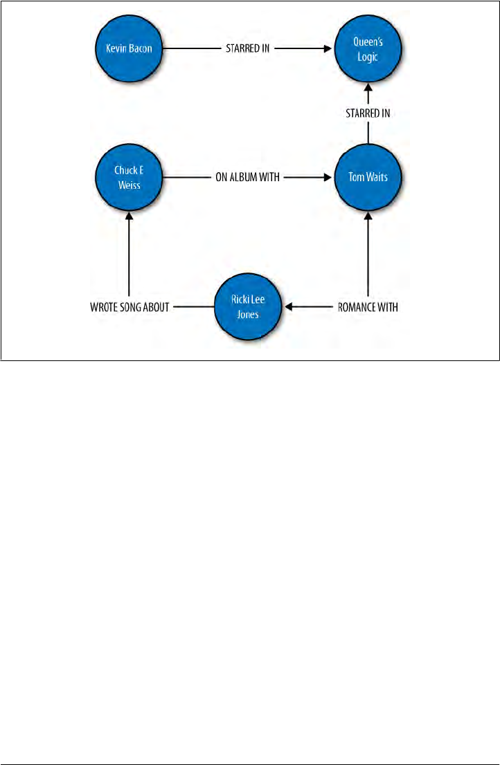
Figure A-1. A graph modeling relationships
Two key trends over the last 15 years have precipitated the rise of graph databases as
an important form of data store. The first is a rise in the sheer volume of data, and the
second is a rise in the interconnectedness of that data; both of these trends make graph
databases an attractive choice.
Consider for example the rough time line shown in Figure A-2. Starting in the early
1990s, text documents and basic linked hypermedia represented the bulk of content
on the Web. Such documents were straightforward to store and easy to generate using
relational databases. Then, in the early part of this century, RSS feeds, blogs, and wikis
started cropping up, adding automation and linking of reference data in new ways that
stretched the relational model. As 2005 gave rise to the idea of Web 2.0 (or the Age
of Participation, as it was termed by Jonathan Schwartz at Sun), we began to see folk-
sonomies, tag clouds, and taxonomies, all optimized for machine consumption and
inference as much as for direct human consumption. We started to shift away from
thinking of the Web as a bunch of “pages” like those in a magazine whose content can
be dynamically generated by pulling together entries in a relational database; we started
thinking instead in terms of ways to represent that data so that it can be linked in terms
of the ideas represented. The large-scale availability of the high-speed Internet infra-
structure allowed social networking sites to blossom. Many more people were suddenly
connected, and the Web was offering new ways for them to interact, rather than just
read.
Graph Databases | 257

Figure A-2. The need to manage data on a very large scale is increasing, and will continue to do so
It is at this point where the Web starts to employ that important second layer of se-
mantics, accompanied by the explosion in volume of data, and where the largest web
properties are forced to start looking at alternatives to the relational database. Some
semantic web researchers and enthusiasts have recently suggested that we are entering
a new era, Web 3.0, where RDF, microformats, and ontologies will support a super-
connected “web of data” culminating in a gigantic graph of the world’s knowledge base
some years from now. As such, the usefulness of graph databases, which directly sup-
port the idea of a semantic relationship between two nodes, becomes more immediately
apparent.
Like many document-oriented databases, graph databases typically allow for free-form
schemas, allowing your application to evolve easily as your data set grows and changes.
Because there is no relational model, joins are not necessary, which can offer more
efficient queries as your data set grows.
The primary advantage of a graph database over RDBMS is that there’s no impedance
mismatch; you can store your objects just as you would use them in your application
and just as you would draw them on a whiteboard, which makes for straightforward,
readily understandable, and quick modeling. As with key-value stores and document-
oriented databases, graph databases allow you to represent semistructured data and
naturally evolve your schemas according to newfound relationships and properties.
If you’re interested in exploring graph databases for a social web or Semantic Web
application, you might want to check out the variety of other graph databases not
explored here, including Dex, HypergraphDB, Infogrid, and VertexDB. I encourage
you also to take a look at the Gremlin project at http://wiki.github.com/tinkerpop/grem
lin. Gremlin is an open source programming language designed specifically for per-
forming queries, graph analysis, and manipulation in graph databases. Gremlin can be
258 | Appendix: The Nonrelational Landscape

invoked from a Java Virtual Machine via its implementation in accordance with JSR
223.
We look at only a couple of graph databases here, but if you’re a regular Hadoop user
you might also check out the Hama project, which is in Incubator status as of this
writing. Hama is a package on top of Hadoop that adds support for massive matrix and
graph data. See http://incubator.apache.org/hama. There is also a Google project called
Pregel, which they’ve been using internally for a couple of years and which they might
open source. You can read Google’s announcement on Pregel at http://googleresearch
.blogspot.com/2009/06/large-scale-graph-computing-at-google.html.
FlockDB
In April 2010, Twitter announced that they were open-sourcing to GitHub their new
graph database called FlockDB. They created FlockDB to store the adjacency lists for
followers on Twitter, so they could readily understand who follows whom and who
blocks whom. It scales horizontally and is designed for online, low-latency, high-
throughput environments. The Twitter FlockDB cluster stores 13+ billion edges and
sustains peak traffic of 20,000 writes per second and 100,000 reads per second.
•Website: http://github.com/twitter/flockdb
•Orientation: Graph
•Created: Created in 2010 by Twitter
•Implementation language: Scala
•License: Apache License v2
•Distributed: Yes
•Schema: The schema is very straightforward, as FlockDB does not attempt to solve
every database problem, but only those relating to the set of problems Twitter faces
with their relationship graphs and the size of their dataset. The graph contains
entries with four attributes: a source ID, a destination ID, a position, and a state.
•Client: FlockDB uses the Thrift 0.2 client, and Twitter has also written a Ruby
frontend that offers a richer interface.
•Replication: Yes
•Storage: MySQL
•Production use: Twitter
•Additional features: FlockDB allows you to quickly page through result sets that
contain millions of entries and to archive and later restore previously archived
graph edges. It uses Kestrel as a loosely coupled, reliable message queue that picks
a server at random to write to, so there is no cross-server communication (no clus-
tering, no multicast, etc.).
Graph Databases | 259

Neo4J
Neo4J is an ACID-compliant graph database optimized for very fast graph traversals.
It’s transactional, supporting JTA/JTS, two-phase commit, deadlock detection, and
MVCC. It has been in production use since 2003, making it one of the older data stores
presented here, and is capable of scaling to billions of entities (nodes, edges, properties)
in a single JVM.
Neo4J can be embedded as a small JAR file, so it’s easy to get up and running and use
in a flexible way in your applications.
•Website: http://neo4j.org
•Orientation: Graph
•Created: Created and used in production since 2003 by Neo Technologies. Ver-
sion 1.0 was released in February 2010.
•Implementation language: Java
•License: Apache GPLv3, with commercial licensing available for advanced
features.
•Distributed: Neo4J is partially distributed using RMI. Note that the free version
of Neo4J is not distributable to multiple machines.
•Schema: Schema-less graph of nodes, edges, and optional properties
•Client: There are a few options here. You can run Neo4J as a REST server so that
you can use simple HTTP operations with JSON; Neo4J has a shell client interface
as well. There are language bindings available for Java, Python, Ruby, Clojure,
Scala, and PHP. See Neo4j.py for the Jython and CPython interfaces, and Neo4jrb
for the JRuby bindings. Neoclipse is a plug-in to the Eclipse IDE that offers a
graphical representation of your graph and an interface with Grails.
•Replication: As of this writing, Neo4J replication is still in the works. It uses a
master/slave replication design based on the one used in MySQL, where you can
write to any slave instance, and lock coordination and change distribution are
handled by the master. You can tune the consistency level desired, so you can
achieve strong consistency by having Neo4J write synchronously to the write
master and slave, or you can improve performance using eventual consistency by
propagating writes to slaves asynchronously.
•Storage: Custom disk-based storage
•Production use: Box.net, ThoughtWorks
•Additional features: Because it is a graph database, Neo4J can be used to good
advantage with semantic web applications. It allows you to execute SPARQL Pro-
tocol and RDF Query Language (SPARQL) queries for interacting with Resource
Description Framework (RDF) and acts as a partial Web Ontology Language
(OWL) store.
260 | Appendix: The Nonrelational Landscape

Integration with Apache Lucene/Solr is available to store external indexes and perform
fast global searches. An index in distributed databases can be thought of like a dic-
tionary—a direct pointer from a key to a value.
As of version 1.1, Neo4J features an event framework.
Key-Value Stores and Distributed Hashtables
In a relational model, we tend to first consider the tables that our domain requires, then
think of how we can normalize the tables to avoid duplicate data. The tables with their
defined columns and the relationships between the tables become our schema.
In a key-value store, however, typically you don’t define a schema as such. Your domain
rather becomes a bucket into which you can drop data items; the data items are keys
that have a set of attributes. All data relevant to that key is therefore stored with the
key, resulting in a sharp contrast to the normalized model prized in relational databases:
data is frequently duplicated. There are some variations here, though, and some con-
ceptual overlap results with the columnar databases.
Another contrast is one of modeling. When working with relational databases, we tend
to think hard about the schema, trusting that any question we want to ask the database
will be answerable. Because the questions—the queries—are secondary in this model,
they can become very complex. You’ve surely seen elaborate SQL statements that use
several joins, subqueries, aggregate functions, temporary tables, and so forth. In the
columnar model, however, we tend to think of the query first, and the queries we’ll
execute help dictate the design of the buckets we’ll need. The assumption in columnar
databases that supports this is that we want replication in order for the database to be
available, and that data duplication is OK because disk space is inexpensive.
Data integrity is another point of difference. Data integrity is the extent to which the
data in an application is complete and consistent. Relational databases have some built-
in capabilities to help ensure data integrity, such as primary keys (which ensure entity
integrity) and foreign key constraints (which ensure referential integrity). In a key-value
store, however, the responsibility for data integrity resides entirely with the application.
Consider an example: your database might include Customers and Orders. In a rela-
tional database, referential keys must be defined in the database to allow you to join
these tables and see, for example, all the orders a particular customer has placed. Al-
though you could do this in a key-value store, typically you don’t define any relation-
ships in the data model itself; your application is responsible for maintaining data in-
tegrity if, for example, you decide to delete a customer record.
One criticism of key-value stores is that they are terrific if you need to scale to billions
of records, but that this use case is a concern only for very large, social-based web
properties. The suggestion is that key-value stores mean by definition that your
Key-Value Stores and Distributed Hashtables | 261

application will see the database as a single, enormous, globally accessible hashtable,
which is difficult to maintain and hard on programmer productivity.
There are many key-value stores in the wild today, including Tokyo Cabinet, Amazon’s
SimpleDB, and Microsoft’s Dynomite.
Amazon Dynamo
Dynamo is Amazon’s proprietary key-value storage system. Though it’s not usable by
developers, it’s still important to discuss because it, along with Google Bigtable, in-
spired many of the design decisions in Apache Cassandra.
In October of 2007, Werner Vogels, CTO of Amazon, published a white paper for the
Association of Computing Machinery (ACM) called “Dynamo: Amazon’s Highly Avail-
able Key-value Store.” This paper continues to be publicly available on his blog
“All Things Distributed” at http://www.allthingsdistributed.com/files/amazon-dynamo
-sosp2007.pdf. The paper is rather technical, but it is clear, concise, and very well writ-
ten. I will just summarize the main points here.
Dynamo was born, as were many of the systems described in this chapter, from the
need to honor strict requirements for realizing high performance under continuous
growth, meeting service-level agreements (SLAs), remaining available under strenuous
load and failures, gracefully handling those failures, and allowing horizontal scale.
Therefore, with respect to the CAP theorem, Dynamo, like Cassandra, is highly avail-
able and eventually consistent. Failure handling in both of these systems is regarded as
a “normal case without impacting availability or performance.” This is achievable be-
cause of the trade-off Dynamo makes with consistency.
Dynamo is used for Amazon’s shopping cart, and of course consistency is important
to Amazon. For a service such as a web-based shopping cart, which does not have
competing readers, it is more than worth the trade-offs and will not be problematic.
Although consistency is not the main focus of this system, it is a “tuneable” property,
such that “eventual” is perhaps a misnomer.
As in Cassandra, consistency in Dynamo works where a configurable property allows
the user to decide what number of replicas must successfully respond before it can be
determined that an operation was successful. To achieve this, communication between
replicas is based on a peer-to-peer (P2P) communication protocol called “gossip,”
which we’ll examine further in terms of Cassandra inherits.
The requirements for the Dynamo architecture were clear. In order to support a highly
available model, the team decided to tune down the consistency “knob.” Again, this is
perfectly acceptable for their given use case. They also wanted a very easy-to-use query
model, so the data is referenced using unique keys and stored simply as byte arrays.
This eliminates the need for any sophisticated schema design and allows Amazon to
put effort toward low-latency and high-throughput performance optimizations and
their other primary goals.
262 | Appendix: The Nonrelational Landscape

To achieve an acceptable level of consistency, Dynamo must support some sort of
versioning mechanism so that replicas can know which node has the most recent (valid)
copy of written data. So it employs something called a vector clock, in which each
process maintains a numeric reference to the most recent event it’s aware of. Another
facet of the architecture that Cassandra shares with Dynamo is the hinted handoff.
This section has summarized the basic points of the Amazon Dynamo paper in order
to help you understand its architectural goals and features. Although I very much en-
courage you to read the Dynamo paper, be aware that Cassandra does diverge in its
own ways, so don’t take for granted that something described there will necessarily
apply to Cassandra. In short, Cassandra derives its design around consistency and par-
tition tolerance from Dynamo, and its data model is based on Bigtable.
Project Voldemort
Voldemort was started as a project within LinkedIn when they encountered problems
with simple data partitioning to meet their scalability needs, similar to how Cassandra
was started within Facebook. Voldemort is a distributed, very simple key-value store,
based on Amazon’s Dynamo and Memcached.
Performance numbers suggested by Jay Kreps of LinkedIn indicate approximately
20,000 reads and 17,000 writes per second with one client and one server.
•Website: http://project-voldemort.com
•Orientation: Key-value store
•Created: Created in 2008 by LinkedIn’s Data and Analytics team for application
to real-time problems
•Implementation language: Java
•Distributed: Yes
•Schema: The primary aims of Voldemort are high performance and availability.
As a result, the database supports only the most minimal schema. The following
are essentially the only supported queries: value = store.get(key), store.put(key,
value), and store.delete(key). Because Voldemort allows you to specify your
schema with JSON, it supports all the data types that JSON supports.
•Client: Like Cassandra, Voldemort allows for pluggable interfaces. According to
the Voldemort website, it supports pluggable serialization and integrates with
Thrift, Avro, and Google Protocol Buffers.
•Replication: Data is automatically replicated over multiple servers; this is
configurable.
•Storage: Voldemort allows for pluggable storage on disk using BerkeleyDB or
MySQL.
•Production use: LinkedIn
•Additional features: Can be used in conjunction with Hadoop.
Key-Value Stores and Distributed Hashtables | 263

Redis
Redis is not a “plain” key-value store, as it supports a variety of values in different data
structures such as binary-safe strings (strings that don’t contain a space or newline
character), lists and sets of binary-safe strings, and sorted sets, which contain a floating-
number score.
In March of 2010, VMWare took over as project sponsor of Redis.
•Website: http://code.google.com/p/redis
•Orientation: Key-value store
•Created: Created in 2009
•Implementation language: ANSI C
•Distributed: No distribution or fault tolerance.
•Schema: Key-value store, using server:key-name to store and retrieve values.
•Clients: Redis supports a wide array of clients, typically through contributed li-
braries, including Ruby, Python, Twisted Python, Erlang, Tcl, Perl, Lua, Java,
Scala, Clojure, C#, C, Haskell, and Google’s new Go language.
•CAP: Eventually consistent
•Open source: Yes. Hosted in Google projects. There’s a neat web page that offers
a Redis tutorial (based on the MongoDB tutorial) that allows you to try Redis
directly from your browser using JavaScript. Give it a try at http://try.redis-db.com.
Columnar Databases
A columnar database simply means a data store that organizes data around columns
instead of rows. This slight shift in focus optimizes the workload for certain kinds of
problems—in particular, data warehouses and analytics applications that require
computing aggregate values over very large sets of similar data. Columnar (or “column-
oriented”) databases are well-suited to online analytical processing (OLAP) work,
where queries are executed over a broad dataset.
Data storage works a little differently with columnar databases, in order to optimize
disk space and the amount of time spent in IO. For example, columnar databases allow
you to write a record containing a value for only one out of a large number of possible
columns, and only that single column value will be stored and take up space. This is
different from RDBMS, in which nulls are not stored for free. It can be useful to think
of RDBMS tables like spreadsheets, in which all columns are of the same size for each
row, and null values are maintained to keep the grid-like shape of the data structure.
This model doesn’t work for columnar databases, though, because null values are not
present. It’s more helpful to think of columnar data as tags: values can be of arbitrary
length, and the names and widths of columns are not preset.
264 | Appendix: The Nonrelational Landscape

Columnar databases often require the data to be of a uniform type, which presents an
opportunity for data compression.
Columnar databases have been around since the early 1970s. Sybase IQ, for example,
is one of these, and was for many years the only commercial columnar database.
But of the recent (mostly open source) projects that are part of the NoSQL conversation,
there are a few databases that are an evolution of basic key-value stores in that they
feature a richer data model. You can think of these columnar databases as multidi-
mensional key-value stores or distributed hash tables that, instead of supporting merely
straight key-value pairs, allow for arrangements called column families to help organize
columns and provide a richer model. These are Google’s Bigtable, HBase, Hypertable,
and Cassandra.
Google’s Bigtable is really the parent of the modern columnar databases. It is propri-
etary, but there are a few published papers on its design, and each of the other columnar
databases discussed are implementations that closely follow Bigtable’s design or, as in
the case of Cassandra, take certain key ideas from Bigtable.
Google Bigtable
Bigtable is Google’s internally used custom database, designed to scale into the petabyte
range. Bigtable is described in the paper published by Google in 2006 called “Bigtable:
A Distributed Storage System for Structured Data.” The goals of the project are stated
in that paper: “wide applicability, scalability, high performance, and high availability.”
Bigtable is used extensively within Google as the underlying data store, supporting
more than 60 projects, including Gmail, YouTube, Google Analytics, Google Finance,
Orkut, Personalized Search, and Google Earth. Bigtable runs on top of the Google File
System (GFS).
It is useful to understand Bigtable, at least to a certain degree, because many of its
attributes and design decisions are explicitly copied in Cassandra. Although Cassandra
gets its design for consistency and partition tolerance from Amazon Dynamo, Cassan-
dra’s data model is based more closely on Bigtable’s. For example, Cassandra borrows
from Bigtable (sometimes with modification) the implementation of SSTables, memt-
ables, Bloom filters, and compactions (see the Glossary for definitions of these terms;
they are explored in detail elsewhere in this book as appropriate). In this way, Cassandra
supports a somewhat richer data model than Dynamo, something more flexible and
layered than a simple key-value store, as it supports sparse, semistructured data.
Columnar Databases | 265

I very much encourage you to read the Google Bigtable paper; it’s an
excellent read. However, keep in mind that although Cassandra
borrows many key ideas from Bigtable, it is not generally a 1:1 corre-
spondence in ideas or implementation. For example, Bigtable defines
master and slave nodes, and while Cassandra’s data model and storage
mechanism are based on Bigtable and use the same terminology in many
places, it’s not always the case. For example, Bigtable reads and writes
are close but not identical to their Cassandra implementations; Bigtable
defines a Tablet structure that is not strictly present in Cassandra; and
so on. You can read the paper at http://labs.google.com/papers/bigtable
.html.
Cassandra does contrast with Bigtable in several areas, however, not least of which is
that Cassandra maintains a decentralized model. In Bigtable there is a master server
that controls operations using the Chubby persistent distributed locking mechanism;
in Cassandra, all the nodes are on even par with no centralized control, and they com-
municate using a gossip model.
Bigtable relies on a distributed lock service called Chubby for several different things:
ensuring that there is at most a single master replica at any given time; managing server
bootstrapping, discovery, and death; and storing the schema information.
•Website: None, but you might be interested in a related project called Google
Fusion Tables, which is available at http://tables.googlelabs.com.
•Orientation: Columnar
•Created: By Google, Inc. Development started in 2004, with the paper published
in 2006.
•Implementation language: C++
•Distributed: Yes
•Storage: Google File System (GFS). Files are divided into 64-megabyte chunks,
and a typical write operation will only ever append to the files in order to provide
maximum throughput. GFS has as a driving principle that the filesystem must run
on banks of inexpensive commodity servers, which can be prone to failure, and
therefore it must be able to manage availability in such a scenario. Bigtable features
two server types: one master node and many chunkservers. The chunkservers store
the data chunk files, and the master node stores all of the metadata about the
chunks, such as the location of some particular piece of data. This is a clear point
where Cassandra diverges from Bigtable’s design, as Cassandra nodes are all the
same and there is no master server centrally controlling the ring.
•Schema: The data model in Bigtable is a sparse, distributed, multidimensional
sorted map. It allows you to store data in a richer way than, say, Amazon SimpleDB,
as you can use list types. The map is indexed using a row key, a column key, and
a timestamp; the values themselves are uninterpreted byte arrays.
266 | Appendix: The Nonrelational Landscape

•Client: C++. Queries are also sometimes written in a scripting language developed
at Google called Sawzall. Initially, the Sawzall API did not support writing values
to the database, but did allow data filtering, transformation, and summarizing.
MapReduce is typically used as both an input source and an output source.
•Open source: No
•Additional features: While Bigtable itself is not directly available for your own
use, you can use it indirectly if you build an application with Google App Engine.
Bigtable was designed with use of the MapReduce algorithm in mind. There are a
few clones of Bigtable, and Hadoop is an open source implementation of
MapReduce.
HBase
HBase is a clone of Google’s Bigtable, originally created for use with Hadoop (it’s ac-
tually a subproject of the Apache Hadoop project). In the way that Google’s Bigtable
uses the Google File System (GFS), HBase provides database capabilities for Hadoop,
allowing you to use it as a source or sink for MapReduce jobs. Unlike some other
columnar databases that provide eventual consistency, HBase is strongly consistent.
Perhaps it is interesting to note that Microsoft is a contributor to HBase, following their
acquisition of Powerset.
•Website: http://hbase.apache.org
•Orientation: Columnar
•Created: HBase was created at Powerset in 2007 and later donated to Apache.
•Implementation language: Java
•Distributed: Yes. You can run HBase in standalone, pseudodistributed, or fully
distributed mode. Pseudodistributed mode means that you have several instances
of HBase, but they’re all running on the same host.
•Storage: HBase provides Bigtable-like capabilities on top of the Hadoop File
System.
•Schema: HBase supports unstructured and partially structured data. To do so,
data is organized into column families (a term that appears in discussions of Apache
Cassandra). You address an individual record, called a “cell” in HBase, with a
combination of row key, column family, cell qualifier, and timestamp. As opposed
to RDBMS, in which you must define your table well in advance, with HBase
you can simply name a column family and then allow the cell qualifiers to be de-
termined at runtime. This lets you be very flexible and supports an agile approach
to development.
•Client: You can interact with HBase via Thrift, a RESTful service gateway, Proto-
buf (see “Additional Features” below), or an extensible JRuby shell.
•Open source: Yes (Apache License)
Columnar Databases | 267

•Production use: HBase has been used at Adobe since 2008. It is also used at Twit-
ter, Mahalo, StumbleUpon, Ning, Hulu, World Lingo, Detikcom in Indonesia, and
Yahoo!.
•Additional features: Because HBase is part of the Hadoop project, it features tight
integration with Hadoop. There is a set of convenience classes that allow you to
easily execute MapReduce jobs using HBase as the backing data store.
HBase requires Zookeeper to run. Zookeeper, also part of the Hadoop project, is a
centralized service for maintaining configuration information and distributed synchro-
nization across nodes in a cluster. Although this does add an external dependency, it
makes maintaining the cluster easier and helps simplify the HBase core.
HBase allows you to use Google’s Protobuf (Protocol Buffer) API as an alternative to
XML. Protobuf is a very efficient way of serializing data. It has the advantage of com-
pacting the same data two to three times smaller than XML, and of being 20–100 times
faster to parse than XML because of the way the protocol buffer encodes bytes on the
wire. This can make working with HBase very fast. Protobuf is used extensively within
Google; they incorporate nearly 50,000 different message types into Protobuf across a
wide variety of systems. Check out the Protobuf Google code project at http://code
.google.com/p/protobuf.
The database comes with a web console user interface to monitor and manage region
servers and master servers.
Hypertable
Hypertable is a Google Bigtable clone, very similar to HBase. It is used at Zvents, where
the project originated, to write more than one billion cells per day. It can run on a
distributed filesystem such as HFS or the Kosmos File System. Hypertable uses Multi-
Version Concurrency Control (MVCC) to allow user transactions to execute in a private
memory space, which are readable by other clients only once the transaction has
committed.
Like Cassandra and other Bigtable derivatives, it uses Bloom filters and commit logs to
minimize disk access and improve performance.
Hypertable is well-suited for analytics applications and processing. Unlike many of the
other nonrelational solutions, it is not used frequently to back websites.
•Website: http://www.hypertable.org
•Orientation: Columnar
•Created: Hypertable was started in February of 2007 at Zvents.
•Implementation language: C
•Distributed: Yes
•Open Source: Yes
268 | Appendix: The Nonrelational Landscape

•Schema: Hypertable stores data as a multidimensional table represented as a flat,
sorted list of key-value pairs. The key is essentially the concatenation of four
dimension keys (row, column family, column qualifier, and timestamp).
•Clients: The primary Thrift API (also used by Cassandra before being replaced by
Avro) is C++, with bindings for Java, Python, Ruby, PHP, Perl, Erlang, Haskell,
C#, Perl, and Ocaml.
•Additional features: Hypertable has its own query language called Hypertable
Query Language (HQL). HQL is modeled on SQL, so you can express queries in
a familiar manner, such as select * from QueryLogByTimestamp WHERE ROW =^
'2010-03-27 17:05';. The query here looks a lot like SQL, but includes a modified
syntax. For example, the ^= operator means “starts with.”
Like Voldemort and Cassandra (before Avro, at least), Hypertable uses the Thrift API
for client serialization.
Polyglot Persistence
The different styles of persistence that we’ve toured in this chapter highlight one fact:
each of them is good at solving a particular problem, or has particular strengths where
the others don’t. You may have heard the term “polyglot programming,” which is
largely credited to Neal Ford. The idea with polyglot programming is that different
programming languages are good at different things, and that you can combine pro-
gramming languages in a single solution in order to realize the maximum benefit. Dean
Wampler of http://polyglotprogramming.com offers the overwhelming success of Emacs
as an example of how polyglot programming can be helpful: Emacs uses C for its kernel,
which made it fast, and a scripting dialect of Lisp called Emacs Lisp (ELisp), which
made it easy to extend. Polyglot programming as a concept has been enabled by a variety
of advances in the last few years, including the ability of the Java Virtual Machine to
run a variety of languages. We more frequently hear of large web applications that have
parts that are implemented in Scala, Ruby, and PHP. For example, the most recent
iteration of the eBay architecture is mostly Java, but the search engine is in C++.
I submit that we may see a similar trend in persistence. The NoSQL conversation has
challenged the status quo—that RDBMS is the right tool for every job because it’s the
tool we have. Some proponents of NoSQL suggest that RDBMS will be replaced with
one or more of these solutions. I rather think it’s more likely that we’ll see polyglot
persistence, or the use of a variety of data stores performing different tasks within an
application. In this vision, relational databases will live side by side with nonrelational
databases, and they will operate together within modular, service-oriented applica-
tions, each optimized to perform the tasks they do best.
Columnar Databases | 269

Summary
In the previous sections, we took a whirlwind tour of a variety of nonrelational data-
bases in order to properly contextualize Cassandra in light of the overall NoSQL move-
ment. The purpose was to shed some light on how the industry has been thinking about
data over the last few years and to compare and contrast some of these systems in order
to understand their broader theoretical underpinnings.
We also took a tour of the many so-called NoSQL offerings in order to understand the
alternatives to relational databases that have sprung up in recent years. These databa-
ses, in their variety of forms, are different ways of trying to respond to the growing need
for handling data at massive “web scale.” Another purpose of this tour was to illustrate
that NoSQL databases exist for a reason, though some pundits and industry experts
may object. They are being used by many large companies with strenuous data re-
quirements and cannot be dismissed as newfangled “art projects.” They are strongly
rooted in important ideas surrounding data scalability from some of the best minds in
the industry, sometimes going back decades. And, though it’s true that they have (very
public) problems at times, that’s also the case with relational databases.
So my purpose in this book has not been to convince you to throw away all your rela-
tional databases and replace them with the new flavor of the month. It’s been to help
you understand the advantages and disadvantages of alternatives to relational databa-
ses, and to understand Cassandra in-depth, so that when you’re presented with your
next data problem, you’re ready to take a step back and select not just the default tool,
but the best tool for the job.
270 | Appendix: The Nonrelational Landscape

Glossary
I can’t believe what a bunch of nerds we are. We’re
looking up “money laundering” in a dictionary.
—Peter, Office Space
This glossary provides definitions of some of the terms that are important to understand
when working with Apache Cassandra. There’s some really good material at http://wiki
.apache.org/cassandra, but reading it for the first time can be tricky, as each new term
seems to be explained only with other new terms. Many of these concepts are daunting
to beginning or even intermediate web developers or database administrators, so
they’re presented here in an easy reference. Much of the information in this glossary is
repeated and expanded upon in relevant sections throughout this book.
Anti-Entropy
Anti-entropy, or replica synchronization, is
the mechanism in Cassandra for ensuring
that data on different nodes is updated to
the newest version.
Here’s how it works. During a major com-
paction (see Compaction), the server initiates a
TreeRequest/TreeResponse conversation to
exchange Merkle trees with neighboring no-
des. The Merkle tree is a hash representing
the data in that column family. If the trees
from the different nodes don’t match, then
they have to be reconciled (or “repaired”) in
order to determine the latest data values
they should all be set to. This tree compari-
son validation is the responsibility of
the
org.apache.cassandra.service.AntiEntropy
Service class. AntiEntropyService imple-
ments the Singleton pattern and defines the
static Differencer class as well. This class is
used to compare two trees, and if it finds
any differences, it launches a repair for the
ranges that don’t agree.
Anti-entropy is used in Amazon’s Dynamo,
and Cassandra’s implementation is mod-
eled on that (see Section 4.7 of the Dynamo
paper).
In Dynamo, they use a Merkle tree for anti-
entropy (see Merkle Tree). Cassandra does too,
but the implementation is a little different.
In Cassandra, each column family has its
own Merkle tree; the tree is created as a
snapshot during a major compaction oper-
ation, and it is kept only as long as is re-
quired to send it to the neighboring nodes
on the ring. The advantage of this imple-
mentation is that it reduces disk I/O.
See Read Repair for more information on how
these repairs occur.
271

Async Write
Sometimes called “async writes” in docu-
mentation and user lists, this simply means
“asynchronous writes” and refers to the fact
that Cassandra makes heavy use of
java.util.concurrent library components
such as ExecutorService and Future<T> for
writing data to buffers.
Avro
Avro is (probably) replacing Thrift as the
RPC client for interacting with Cassandra.
Avro is a subproject of the Apache Hadoop
project, created by Doug Cutting (creator of
Hadoop and Lucene). It provides function-
ality similar to Thrift, but is a dynamic data
serialization library that has an advantage
over Thrift in that it does not require static
code generation. Another reason that the
project is migrating to Avro is that Thrift
was originally created by Facebook and then
donated to Apache, but since that time has
received little active development attention.
This means that the Cassandra server will be
ported from org.apache.cassandra.thrift.
CassandraServer to org.apache.cassan
dra.avro.CassandraServer. As of this writ-
ing, this is underway but not yet complete.
You can find out more about Avro at its
project page, http://avro.apache.org.
Bigtable
Bigtable is a distributed database created at
Google in 2006 as a high-performance col-
umnar database on top of Google File Sys-
tem (GFS). Bigtable and Amazon’s Dynamo
database are the direct parents of Cassan-
dra. Cassandra inherits these aspects from
Bigtable: sparse array data and disk storage
using an SSTable.
Yahoo!’s HBase is a Bigtable clone.
You can read the complete Google Bigtable
paper at http://labs.google.com/papers/bigta
ble.html.
Bloom Filter
In simple terms, a Bloom filter is a very fast,
nondeterministic algorithm for testing
whether an element is a member of a set.
These algorithms are nondeterministic be-
cause it is possible to get a false-positive read
but not a false-negative. Bloom filters work
by mapping the values in a dataset into a bit
array and condensing a larger dataset into a
digest string. The digest, by definition, uses
a much smaller amount of memory than the
original data would.
Cassandra uses Bloom filters to reduce disk
access, which can be expensive, on key look-
ups. Every SSTable has an associated Bloom
filter; when a query is performed, the Bloom
filter is checked first before accessing disk.
Because false-negatives are not possible, if
the filter indicates that the element does not
exist in the set, it certainly doesn’t; if the fil-
ter thinks that the element is in the set, the
disk is accessed to make sure.
Although it is a disadvantage that false-
positives are possible with Bloom filters,
their advantage is that they can be very fast
because they use space efficiently, due to the
fact that (unlike simple arrays, hashtables,
or linked lists) they do not store their ele-
ments completely. Instead, Bloom filters
make heavy use of memory and reduce disk
access. One result is that the number of
false-positives increases as the number of
elements increases.
Bloom filters are used by Apache Hadoop,
Google Bigtable, and Squid Proxy Cache.
They are named for their inventor, Burton
Bloom.
Cassandra
In Greek mythology, Cassandra was the
daughter of King Priam and Queen Hecuba
of Troy. She was so beautiful that the god
Apollo gave her the ability to see the future.
But when she refused his amorous advances,
he cursed her such that she would accurately
predict everything that would happen, yet
no one would believe her. Cassandra fore-
saw the destruction of her city of Troy, but
was powerless to stop it. The Cassandra dis-
tributed database is named for her.
Async Write
272 | Glossary

The data store itself is an Apache project
available at http://cassandra.apache.org. It
started in incubator status in January of
2009. It has the following key properties: it
is decentralized, elastic, fault-tolerant,
tuneably consistent, highly available, and
designed to massively scale on commodity
servers spread across different data centers.
It is in use at companies such as Digg, Face-
book, Twitter, Cloudkick, Cisco, IBM,
Reddit, Rackspace, SimpleGeo, Ooyala,
and OpenX.
Cassandra was originally written at Face-
book to solve their Inbox Search problem.
The team was led by Jeff Hammerbacher,
with Avinash Lakshman, Karthik Rangana-
than, and Facebook engineer on the Search
Team Prashant Malik as key engineers. The
code was released as an open source Google
Code project in July of 2008. In March of
2009, it was moved to an Apache Incubator
project, and on February 17 of that year, it
was voted into a top-level project.
A central paper on Cassandra by
Facebook’s Lakshman and Malik called “A
Decentralized Structured Storage System”
is available at http://www.cs.cornell.edu/
projects/ladis2009/papers/lakshman-la
dis2009.pdf.
A blog post from 2008 by Avinash Laksh-
man describes how they were using Cassan-
dra at Facebook: http://www.facebook.com/
note.php?note_id=24413138919&id=
9445547199&index=9.
It is easy to see why the Cassandra database
is aptly named: its community asserts that
Cassandra and other related NoSQL data-
bases are the future. Despite widespread use
of eventually consistent databases at com-
panies such as Amazon, Google, Facebook,
and Twitter, there remain many skeptics
(“nonbelievers”) of such a model. It is fur-
ther speculated that by naming the database
Cassandra, after the Greek seer of the future,
its creators are making a kind of joking ref-
erence to the Oracle database.
The Java client Hector by Ran Tavory is
named for Cassandra’s brother.
Chiton
In ancient Greece, a chiton was a cloth gar-
ment, typically sleeveless, worn by both
men and women. It is the namesake for the
open source project Chiton by Brandon
Williams, which is a Python GTK-based
browser for Apache Cassandra. It is cur-
rently hosted at http://github.com/driftx/chi
ton.
A related project is Telephus, a low-level
client API for Cassandra written in Twisted
Python. It is currently hosted at http://github
.com/driftx/Telephus.
Cluster
A cluster is two or more Cassandra instances
acting in concert. These instances commu-
nicate with one another using Gossip.
When you configure a new instance to in-
troduce to your cluster, you’ll need to do a
few things. First, indicate a Seed Node. Next,
indicate the ports on which Cassandra
should listen for two things: Gossip and the
Thrift interface. Once your cluster is config-
ured, use the Node Tool to verify that it is set
up correctly.
Column
A column is the most basic unit of represen-
tation in the Cassandra data model. A col-
umn is a triplet of a name (sometimes refer-
red to as a “key”), a value, and a timestamp.
A column’s values, including the time-
stamp, are all supplied by the client. The
data type for the name and value are Java
byte arrays. The data type for the timestamp
is a long primitive. Columns are immutable
in order to prevent multithreading issues.
Columns are organized into column
families.
The column is defined in Cassandra by
the org.apache.cassandra.db.IColumn inter-
face, which allows a variety of operations,
including getting the value of the column as
a byte[] or getting its subcolumns as a
Column
Glossary | 273

Collection<IColumn>, and finding the time
of the most recent change.
Columns are sorted by their type, which is
one of AsciiType, BytesType, LexicalUUID
Type, LongType, TimeUUIDType, UTF8Type.
See also Column Family.
Column Family
A column family is roughly analogous to a
table in a relational model. It is a container
for an ordered collection of columns.
Because each column family is stored in a
separate file, be sure to define columns that
you are likely to access together in the same
column family.
You define your application’s column fam-
ilies in the Cassandra configuration file. You
can supply global (per-keyspace) values for
the size of the row cache, the size of the key
cache, and the “read repair chance.” Col-
umn families can be one of two types:
standard or super.
See also Column, Keyspace, Super Column.
Column Name
The name part of the name/value pair stored
within a Row.
Column Value
The value part of the name/value pair stored
within a Row. The size of a column value is
limited by machine memory.
Commit Log
The commit log is responsible for all of the
write operations in Cassandra. When you
perform a write, it first enters the commit
log so the data won’t be lost in the event of
failure; then the value is populated in the
memtable so it’s available in memory for
performance. Once the Memtable fills up, the
data is flushed to the SSTable.
It is represented by the org.apache.cassan
dra.db.commitlog.CommitLog class. On every
write or delete, an entry in the form of a
RowMutation object is serialized and appen-
ded to the commit log. These objects are or-
ganized into commit log segments. By
default, commit logs roll once they reach a
size threshold of 128MB; when a new com-
mit log is created, it accepts writes in transit.
This setting is configurable.
Compaction
Compaction is the process of freeing up
space by merging large accumulated data-
files. This is roughly analogous to rebuilding
a table in the relational world. On compac-
tion, the merged data is sorted, a new index
is created over the sorted data, and the
freshly merged, sorted, and indexed data is
written to a single new file.
The operations that are performed during
compaction to free up space include merg-
ing keys, combining columns, and deleting
tombstones. This process is managed by the
class org.apache.cassandra.db.Compaction
Manager. CompactionManager implements an
MBean interface so it can be introspected.
There are different types of compaction in
Cassandra.
A major compaction is triggered in one of
two ways: via a node probe or automatically.
A node probe sends a TreeRequest message
to the nodes that neighbor the target. When
a node receives a TreeRequest, it immedi-
ately performs a read-only compaction in or-
der to validate the column family.
A read-only compaction has the following
steps:
1. Get the key distribution from the col-
umn family.
2. Once the rows have been added to the
validator, if the column family needs to
be validated, it will create the Merkle
tree and broadcast it to the neighboring
nodes.
3. The Merkle trees are brought together
in a “rendezvous” as a list of Differenc
ers (trees that need validating or com-
parison).
4. The comparison is executed by the
StageManager class, which is responsi-
ble for handling concurrency issues in
Column Family
274 | Glossary

executing jobs. In this case, the Stage
Manager uses an anti-entropy stage.
This uses the org.apache.cassandra.co
ncurrent.JMXEnabledThreadPoolExecu
tor class, which executes the compac-
tion within a single thread and makes
the operation available as an MBean for
inspection.
Compression
Data compression on return is on the road
map for future versions, but as of 0.6 it is not
yet supported.
Consistency
Consistency means that a transaction does
not leave the database in an illegal state, and
that no integrity constraints are violated.
This is considered a crucial aspect of trans-
actions in relational databases and is one of
the ACID properties (Atomic, Consistent,
Isolated, Durable). In Cassandra, the rela-
tive degree of consistency can be calculated
by the following:
N = the number of nodes that store replicas
of the data
W = the number of replicas that must ac-
knowledge receipt of a write before it can be
said to be successful
R = the number of replicas that are contac-
ted when a data object is accessed in a read
operation
W + R > N = strong consistency
W + R <= N = eventual consistency
Consistency Level
This configurable setting allows you to de-
cide how many replicas in the cluster must
acknowledge a write operation or respond
to a read operation in order to be considered
successful. The consistency level is set ac-
cording to your stated Replication Factor, not the
raw number of nodes in the cluster.
There are multiple levels of consistency that
you can tune for performance. The best-
performing level has the lowest consistency
level. They mean different things for writing
and reading. This is covered in Chapter 7.
For write operations:
• ZERO: Write operations will be han-
dled in the background, asynchro-
nously. This is the fastest way to write
data, and the one that offers the least
confidence that your operations will
succeed.
• ANY: This level was introduced in Cas-
sandra 0.6 and means that you can be
assured that your write operation was
successful on at least one node, even if
the acknowledgment is only for a hint
(see Hinted Handoff). This is a relatively
weak level of consistency.
• ONE: Ensures that the write operation
was written to at least one node, in-
cluding its commit log and memtable.
If a single node responds, the operation
is considered successful.
• QUORUM: A quorum is a number of
nodes that represents consensus on an
operation. It is determined by <Replica
tionFactor> / 2 + 1. So if you have a
replication factor of 10, then 6 replicas
would have to acknowledge the opera-
tion to gain a quorum.
• DCQUORUM: A version of quorum
that prefers replicas in the same data
center in order to balance the high con-
sistency level of quorum with the lower
latency of preferring to perform opera-
tions on replicas in the same data
center.
• ALL: Every node as specified in your
<ReplicationFactor> configuration en-
try must successfully acknowledge the
write operation. If any nodes do not
acknowledge the write operation, the
write fails. This has the highest level of
consistency and the lowest level of per-
formance.
For read operations:
Consistency Level
Glossary | 275

• ONE: This returns the value on the first
node that responds. Performs a read re-
pair in the background.
• QUORUM: Queries all nodes and re-
turns the record with the most recent
timestamp after a quorum of nodes
have responded, where a "quorum" is
(n /2) + 1.
• DCQUORUM: Ensures that only no-
des in the same data center are queried.
Applicable when using Rack-Aware
placement strategy.
• ALL: Queries all nodes and returns the
value with the most recent timestamp.
This level waits for all nodes to re-
spond, and if one doesn’t, it fails the
read operation.
Note that there is no such thing as READ
ZERO, as it doesn’t make sense to specify
that you want to read some data and don’t
need any node to respond.
Data Center Shard Strategy
See Replication Strategy.
Decentralized
Cassandra is considered decentralized be-
cause it defines no master server, and in-
stead uses a peer-to-peer approach in order
to prevent bottlenecks and single points of
failure. Decentralization is important in
Cassandra because it is what allows it to
scale up and also to scale down; peers can
enter or exit the cluster as they like, with
minimal disruption.
Denormalization
In relational databases, denormalization, or
the creation of redundant data, is sometimes
applied in order to improve performance of
read-mostly applications, such as in online
analytical processing (OLAP). In Cassan-
dra, it is typical to see denormalized data, as
this improves performance and helps ac-
count for the fact that data is structured
according to the queries you’ll need, in dis-
tinction to standard relational databases
where the data is typically structured
around the object model independently.
Durability
When a database is durable, it means that
writes will permanently survive, even in the
event of a server crash or sudden power
failure.
Cassandra accomplishes durability by ap-
pending writes to the end of the commit log,
allowing the server to avoid having to seek
the location in the data file. Only the com-
mit log needs to be synced with the file sys-
tem, and this happens either periodically or
in a specified batch window.
When working in a single server node, Cas-
sandra does not immediately synchronize a
file’s in-core state with the storage device.
That can mean that if the server is shut down
immediately after a write is performed, the
write may not be present on restart. Note
that a single server node is not recommen-
ded for production.
See also Commit Log.
Dynamo
Created in 2006 by Amazon and, along with
Google’s Bigtable, a primary basis for Cas-
sandra. From Dynamo, Cassandra gets the
following: a key-value store, a symmetric
peer-to-peer architecture, gossip-based
discovery, eventual consistency, and tuna-
bility per operation.
You can read the complete paper
“Dynamo: Amazon’s Highly Available Key-
Value Store” at http://www.allthingsdistrib
uted.com/2007/10/amazons_dynamo.html.
Elastic
Read and write throughput can increase lin-
early as more machines are added to the
cluster.
Eventual Consistency
Consistency is the property that describes
the internal integrity of the data following
an operation. In practical terms for a
strongly consistent database, this means
that once a client has performed a write op-
eration, all readers will immediately see the
new value. In eventual consistency, the
Data Center Shard Strategy
276 | Glossary

database will not generally be consistent im-
mediately, but rather eventually (where
“eventually” is typically a matter of the small
number of milliseconds it takes to send the
new value to all replicas, relative to the
amount of data, the number of nodes, and
the geographical distribution of those no-
des). DNS is an example of a popular
eventually consistent architecture. Eventual
consistency is sometimes called “weak con-
sistency.”
Eventual consistency has become popular in
the last few years because it offers the ability
to support massive scalability. Although it
is possible to achieve high scalability in tra-
ditional fully consistent databases, the man-
agement overhead can become a burden. Of
course, eventual consistency presents cer-
tain disadvantages, such as additional
complexity in the programming model.
Though the design of eventual consistency
in Cassandra is based on how it is used in
Amazon’s Dynamo, Cassandra is probably
better characterized as “tuneably” consis-
tent, rather than eventually consistent. That
is, Cassandra allows you to configure the
Consistency Level across the spectrum—includ-
ing ensuring that Cassandra blocks until all
replicas are readable (which is equivalent to
full consistency).
Riak, Voldemort, MongoDB, Yahoo!’s
HBase, CouchDB, Microsoft’s Dynomite,
and Amazon’s SimpleDB/Dynamo are other
eventually consistent data stores.
Failure Detection
Failure detection is the process of determin-
ing which nodes in a distributed fault-
tolerant system have failed. Cassandra’s im-
plementation is based on the idea of Accrual
Failure Detection, first advanced by the Ad-
vanced Institute of Science and Technology
in Japan in 2004. Accrual failure detection
is based on two primary ideas: that failure
detection should be flexible by being decou-
pled from the application being monitored,
and outputting a continuous level of “sus-
picion” regarding how confident the moni-
tor is that a node has failed. This is desirable
because it can take into account fluctuations
in the network environment. Suspicion of-
fers a more fluid and proactive indication of
the weaker or stronger possibility of failure
based on interpretation (the sampling of
heartbeats), as opposed to a simple binary
assessment.
Failure detection is implemented in Cassan-
dra by the org.apache.cassandra.gms.Fail
ureDetector class.
You can read the original Phi Accrual Failure
Detection paper at http://ddg.jaist.ac.jp/pub/
HDY+04.pdf.
Fault Tolerance
Fault tolerance is the system’s ability to con-
tinue operating in the event of a failure of
one or more of its components. Fault toler-
ance is also referred to as graceful degrada-
tion, meaning that if the system operation
degrades following a failure, the degraded
performance is relative only to the failed
component(s).
Gossip
The gossiper is responsible for ensuring that
all of the nodes in a cluster are aware of the
important state information in the other
nodes. The gossiper runs every second to
ensure that even nodes that have failed or
are not yet online are able to receive node
states. It is designed to perform predictably,
even at sharply increased loads. The gossip
protocol supports rebalancing of keys
across the nodes and supports Failure Detec-
tion. Gossip is an important part of the anti-
entropy strategy.
The state information that the gossiper
shares is structured as key/value pairs. In
Cassandra, the gossip protocol continues to
gossip state information to other nodes until
it is made obsolete by newer data.
When a server node is started, it registers
itself with the gossiper. For more in-
forma
tion, check out the org.apache.cassandra.s
ervice.StorageService class.
Gossip
Glossary | 277

Also see the Amazon paper on gossip at http:
//www.cs.cornell.edu/home/rvr/papers/flow
gossip.pdf.
Hector
An open source project created by Ran Ta-
vory of Outbrain and hosted at GitHub,
Hector is a Cassandra client written in Java.
It wraps Thrift and offers JMX, connection
pooling, and failover.
Hinted Handoff
This is a mechanism to ensure availability,
fault tolerance, and graceful degradation. If
a write operation occurs and a node that is
intended to receive that write goes down, a
note (the “hint”) is given (“handed off”) to
a different live node to indicate that it should
replay the write operation to the unavailable
node when it comes back online. This does
two things: it reduces the amount of time
that it takes for a node to get all the data it
missed once it comes back online, and it im-
proves write performance in lower consis-
tency levels. That is, a hinted handoff does
not count as a sufficient acknowledgment
for a write operation if the consistency level
is set to ONE, QUORUM, or ALL. A hint
does count as a write for consistency level
ANY, however. Another way of putting this
is that hinted writes are not readable in and
of themselves.
The node that received the hint will know
very quickly when the unavailable node
comes back online again, because of Gossip.
If, for some reason, the hinted handoff
doesn’t work, the system can still perform a
read repair.
Key
See Row Key.
Keyspace
A keyspace is a container for column fami-
lies. It is roughly analogous to the database
in the relational model, used in Cassandra
to separate applications. Where a relational
database is a collection of tables, a keyspace
is an ordered collection of column families.
You define your application’s keyspace in
the Cassandra configuration file or by using
the definition methods in the API. When
you define a keyspace, you can also define
its replication factor and its replica place-
ment strategy. Within a given Cassandra
cluster, you can have one or more keyspa-
ces, typically one for each application.
See also Column Family.
Lexicographic Ordering
Lexicographic ordering is the natural (al-
phabetic) ordering of the product of two
ordered Cartesian sets.
Memtable
An in-memory representation of data that
has been recently written. Once the memt-
able is full, it is flushed to disk as an SSTable.
Merkle Tree
Perhaps better known as a “hash tree,” a
Merkle tree is a binary tree data structure
that summarizes in short form the data in a
larger dataset. In a hash tree, the leaves are
the data blocks (typically files on a filesys-
tem) to be summarized. Every parent node
in the tree is a hash of its direct child node,
which tightly compacts the summary.
In Cassandra, the Merkle tree is implemen-
ted in the org.apache.cassandra.utils.Mer
kleTree class.
Merkle trees are used in Cassandra to ensure
that the peer-to-peer network of nodes re-
ceives data blocks unaltered and unharmed.
They are used in cryptography as well to
verify the contents of files and transmis-
sions, and are used in the Google Wave
product. They are named for their inventor,
Ralph Merkle.
Multiget
Query by column name for a set of keys.
Multiget Slice
Query to get a subset of columns for a set of
keys.
Node
An instance of Cassandra. Typically a Cas-
sandra cluster will have many nodes,
Hector
278 | Glossary

sometimes collectively called the node ring,
or just “the ring.” A node refers to any Cas-
sandra server in a cluster, whereas “replica”
refers to a node that specifically has a copy
of some data from another node.
Node Tool
This is an executable file with the path bin/
nodetool that inspects a cluster to determine
whether it is properly configured and per-
forms a variety of maintenance operations.
The commands available on nodetool are
cleanup, clearsnapshot, compact, cfstats,
decommission, drain, flush, info, loadba
lance, move, repair, ring, snapshot [snap
shotname], removetoken, and tpstats.
For example, you can use nodetool drain to
prevent the commit log from accepting any
new writes.
NoSQL
“NoSQL” is a general name for the collec-
tion of databases that do not use Structured
Query Language (SQL) or a relational data
model. It is sometimes used to mean “Not
Only SQL” to indicate that the proponents
of various nonrelational databases do not
suggest that relational databases are a bad
choice—but rather that they are not the only
choice for data storage. This term was
coined by Cassandra committer Eric Evans
of Rackspace, but he has since distanced
himself from the term in preference of the
term “Big Data” to highlight the fact that
this family of nonrelational databases is de-
fined not by what they’re not (implementa-
tions of SQL), but rather by what they do
(handle huge data loads). This term, in my
view, has reached the end of its useful life,
because it’s confusing. It has proven too
tempting to discuss a set of databases to-
gether that really have few goals, design
decisions, or features in common. Let Cas-
sandra be Cassandra, let CouchDB be
CouchDB, and let Riak be Riak.
Order-Preserving Partitioner
This is a kind of Partitioner that stores rows by
key order, aligning the physical structure of
the data with your sort order. Configuring
your column family to use order-preserving
partitioning allows you to perform range sli-
ces, meaning that Cassandra knows which
nodes have which keys.
This partitioner is somewhat the opposite of
the Random Partitioner; it has the advantage of
allowing for efficient range queries, but the
disadvantage of unevenly distributing keys.
The order-preserving partitioner (OPP) is
implemented by the org.apache.cassandra
.dht.OrderPreservingPartitionerclass.
There is a special kind of OPP called
the collating order-preserving partitioner
(COPP). This acts like a regular OPP, but
sorts the data in a collated manner accord-
ing to English/US lexicography instead of
byte ordering. For this reason, it is useful for
locale-aware applications. The COPP is
implemented by the org.apache.cassandra
.dht.CollatingOrderPreservingParti
tioner class.
This is implemented in Cassandra by
org.apache.cassandra.dht.OrderPreser
vingPartitioner.
See also Token.
Partition
In general terms, a partition refers to a net-
work partition, which is a break in the net-
work that prevents one machine from inter-
acting directly with another. A partition can
be caused by failed switches, routers, or net-
work interfaces. Consider a cluster of five
machines {A, B, C, D, E} where {A, B} are
on one subnet and {C, D, E} are on a second
subnet. If the switch to which {C, D, E} are
connected fails, then you have a network
partition that isolates the two subclusters
{A, B} and {C, D, E}.
Cassandra is a fault-tolerant database, and
network partitions are one such fault. As
such, it is able to continue operating in the
face of a network partition and merge data
in replication once the partition is healed
again.
Partition
Glossary | 279

Partitioner
The partitioner controls how your data is
distributed over your nodes. In order to find
a set of keys, Cassandra must know what
nodes have the range of values you’re look-
ing for. There are three types of partitioner:
random partitioner, which is the default;
order-preserving partitioner; and collating
order-preserving partitioner. You configure
this in storage-conf.xml or cassandra.yaml
(for 0.7) using the <Partitioner> element:
<Partitioner>org.apache.cassan
dra.dht.RandomPartitioner</Partitioner>.
Note that partitioning applies to the sorting
of row keys, not columns.
Once you have chosen a partitioner type,
you cannot change it without destroying
your data (because an SSTable is immutable).
See also Order-Preserving Partitioner and Random Par-
titioner.
Quorum
A majority of nodes that respond to an op-
eration. This is a configurable consistency
level. In a quorum read, the proxy waits for
a majority of nodes to respond with the
same value. This makes for a slower read
operation, but also helps ensure that you
don’t get returned stale data.
Rack-Aware Strategy
See Replication Strategy.
Random Partitioner
This is a kind of Partitioner that uses a BigIn
tegerToken with an MD5 hash to determine
where to place the keys on the node ring.
This has the advantage of spreading your
keys evenly across your cluster, but the dis-
advantage of causing inefficient range quer-
ies. This is the default partitioner.
See also Partitioner and Order-Preserving Partitioner.
Range Slice
Query to get a subset of columns for a range
of keys.
Read Repair
This is another mechanism to ensure con-
sistency throughout the node ring. In a read
operation, if Cassandra detects that some
nodes have responded with data that is in-
consistent with the response of other, newer
nodes, it makes a note to perform a read re-
pair on the old nodes. The read repair means
that Cassandra will send a write request to
the nodes with stale data to get them up to
date with the newer data returned from the
original read operation. It does this by pull-
ing all the data from the node, performing a
merge, and writing the merged data back to
the nodes that were out of sync. The detec-
tion of inconsistent data is made by com-
paring timestamps and checksums.
The method for reconciliation is the
org.apache.cassandra.streaming package.
Replication
In general distributed systems terms, repli-
cation refers to storing multiple copies of
data on multiple machines so that if one
machine fails or becomes unavailable due to
a Partition, the cluster can still make data
available. Caching is a simple form of repli-
cation. In Cassandra, replication is a means
of providing high performance and availa-
bility/fault-tolerance.
Replication Factor
Cassandra offers a configurable replication
factor, which allows you essentially to de-
cide how much you want to pay in perform-
ance to gain more consistency. That is, your
consistency level for reading and writing
data is based on the replication factor, as it
refers to the number of nodes across which
you have replicated data. The replication
factor is set in the configuration file or the
API.
See also Consistency Level.
Replication Strategy
The replication strategy, sometimes referred
to as the placement strategy, determines
how replicas will be distributed. The first
replica is always placed in the node claiming
the key range of its Token. All remaining rep-
licas are distributed according to a configu-
rable replication strategy.
Partitioner
280 | Glossary

The Gang of Four Strategy pattern is em-
ployed to allow a pluggable means of repli-
cation, but Cassandra comes with three out
of the box. Choosing the right replication
strategy is important because in determin-
ing which nodes are responsible for which
key ranges, you’re also determining which
nodes should receive write operations; this
has a big impact on efficiency in different
scenarios. The variety of pluggable strat-
egies allows you greater flexibility, so that
you can tune Cassandra according to your
network topology and needs.
Replication strategies are an extension of the
org.apache.cassandra.locator.AbstractRe
plicationStrategy class. You can write your
own replication strategy if you like by ex-
tending that class.
The replication placement strategy is con-
figured per keyspace using the <ReplicaPla
cementStrategy> element. They are dis-
cussed in depth in Chapter 6.
Row
In a column family, a row is a sorted map
that matches column names to column val-
ues. In a super column, a row is a sorted map
that matches super column names to maps
matching column names to column values.
The Row Key defines the individual row, and
the row defines the name/value pairs of the
columns. The size of a single row cannot ex-
ceed the amount of space on disk.
Rows are sorted by their Partitioner, which is
one of these types: RandomPartitioner, Order
PreservingPartitioner, or CollatingOrder
PreservingPartitioner.
Rows are defined by the class org.apache.c
assandra.db.Row.
See also Row Key.
Row Key
Sometimes called simply “key,” a row key is
analogous to a primary key for an object in
the relational model. It represents a way to
identify a single row of columns and is an
arbitrary length string.
In the Thrift interface, the Java client always
assumes that row keys are encoded as
UTF-8, but this is not the case for clients in
other languages, where you may need to
manually encode ASCII strings as UTF-8.
SEDA (Staged Event-Driven Architecture)
Cassandra employs a Staged Event-Driven
Architecture to gain massive throughput un-
der highly concurrent conditions. SEDA at-
tempts to overcome the overhead associated
with threads. This overhead is due to sched-
uling, lock contention, and cache misses.
The effect of SEDA is that work is not started
and completed by the same thread; this can
make a more complex code base, but also
yield better performance. Therefore, much
of the key work in Cassandra—such as
reading, mutation, gossiping, memtable
flushing, and compaction—are performed
as stages (the “S” in SEDA). A stage is es-
sentially a separated event queue.
As events enter the incoming queue, the
event handler supplied by the application is
invoked. The controller is capable of dy-
namically tuning the number of threads al-
located to each stage as demand dictates.
The advantages of SEDA are higher concur-
rency and better management of CPU, disk,
and network resources.
You can read more about SEDA as it was
originally proposed by Matt Welsh, David
Culler, and Eric Brewer at http://www.eecs
.harvard.edu/~mdw/proj/seda.
See also Stage.
Seed Node
A seed is a node that already exists in a Cas-
sandra cluster and is used by newly added
nodes to get up and running. The newly
added node can start gossiping with the seed
node to get state information and learn the
topology of the node ring. There may be
many seeds in a cluster.
Slice
This is a type of read query. Use get_
slice() to query by a single column name
Slice
Glossary | 281

or a range of column names. Use
get_range_slice() to return a subset of
columns for a range of keys.
Snitch
A snitch is Cassandra’s way of mapping a
node to a physical location in the network.
It helps determine the location of a node rel-
ative to another node in order to assist with
discovery and ensure efficient request rout-
ing. There are different kinds of snitches.
The EndpointSnitch (or RackInferringSnitc
h), for instance, determines whether two no-
des are in the same data center or the same
rack. Its strategy for doing so is essentially
to guess at the relative distance of two nodes
in a data center and rack based on reading
the second and third octets of their IP ad-
dresses.
The DataCenterEndpointSnitch allows you
to specify IP subnets for racks, grouped by
which data center the racks are in.
The PropertyFileSnitch allows you to map
IP addresses to rack and data centers in a
properties file called cassandra-rack.proper-
ties.
The snitch strategy classes can be found in
the org.apache.cassandra.locator package.
Sparse
In the relational model, every data type (ta-
ble) must have a value for every column,
even if that value is sometimes null. Cas-
sandra, on the other hand, represents a
sparse or “schema-free” data model, which
means that rows may have values for as
many or as few of the defined columns as
you like. This allows for a degree of effi-
ciency. For example, consider a 1000 × 1000
cell spreadsheet, similar to a relational table.
If many of the cells have empty values, the
storage model is inefficient.
SSTable
SSTable stands for Sorted String Table. In-
herited from Google’s Bigtable, an SSTable
is how data is stored on disk in Cassandra.
It is a log that allows only appending. In-
memory tables (memtables) are used in
front of SSTables for buffering and sorting
data. SSTables allow for high performance
on writes and can be compacted.
SSTables are immutable. Once a memtable
is flushed to disk as an SSTable, it cannot be
changed by the application; Compaction
changes only their on-disk representation.
To import or export data from JavaScript
Object Notation (JSON), check out the
classes org.apache.cassandra.tools.SSTable
Importer and SSTableExporter.
Stage
Part of Cassandra’s Staged Event-Driven
Architecture (SEDA), a stage wraps a basic
unit of work. A single operation can flow
between various stages to complete, rather
than getting completed in the same thread
that started the work.
A stage consists of an incoming event queue,
an event handler, and an associated thread
pool. Stages are managed by a controller
that determines scheduling and thread allo-
cation; Cassandra implements this kind of
concurrency model using the thread pool
java.util.concurrent.ExecutorService. To
see specifically how this works, check out
the org.apache.cassandra.concurrent.Stage
Manager class.
A few additional operations are implemen-
ted as stages too, including working with
memtables in the ColumnFamilyStore class,
and the consistency manager is a stage in the
StorageService.
An operation may start with one thread,
which then hands off the work to another
thread, which may hand it off to other
threads. This handing-off is not directly be-
tween threads, however; it occurs between
stages.
See also SEDA (Staged Event-Driven Architecture).
Strong Consistency
For reads, strong consistency means that if
it is detected that a repair needs to be made,
first perform the read repair, then return the
result.
Snitch
282 | Glossary

Super Column
A super column is a column whose value is
not a string, but instead a named list of other
columns, which in this context are called
subcolumns. The subcolumns are ordered,
and the number of columns you can define
is unbounded. Super columns also differ
from regular columns in that they do not
have an associated timestamp.
Super columns are not recursive; that is,
they go only one level deep. A super column
can hold a map only of other columns, and
not a map of more super columns.
They are defined in SuperColumn.java,
which implements both the IColumn and
IColumnContainer interfaces. The interface
allows you to perform a variety of opera-
tions, including the following: get all of the
subcolumns in a super column, get a single
subcolumn by name, add a subcolumn, re-
move a subcolumn, check the number of
subcolumns in the super column, and check
when a subcolumn was last modified.
super columns were one of the updates
added by Facebook to the original data
model of Google’s Bigtable.
See also Column Family.
Thrift
Thrift is the name of the RPC client used to
communicate with the Cassandra server. It
statically generates an interface for seriali-
zation in a variety of languages, including C
++, Java, Python, PHP, Ruby, Erlang, Perl,
Haskell, C#, Cocoa, Smalltalk, and OCaml.
It is this mechanism that allows you to in-
teract with Cassandra from any of these
client languages.
It was created in April 2007 at Facebook and
donated to Apache as an incubator project
in May 2008. At the time of this writing, the
Thrift interface is most likely being replaced
by the newer and more active Apache
project Avro. Another advantage of Avro is
that it does not require static code genera-
tion.
You can read more about Thrift on its
project page at http://incubator.apache.org/
thrift.
Timestamp
In Cassandra, timestamps for column values
are supplied by the client, so it is important
to synchronize client clocks. The timestamp
is by convention the number of microsec-
onds since the Unix epoch (midnight,
January 1, 1970).
Token
Each node in the node ring has a single token
that is used to claim a range of keys, based
on the value of the token in the previous
node in the ring. You can specify your own
token or let Cassandra generate one for you.
The representation of the token is depend-
ent on the kind of partitioner used.
With a Random Partitioner, the token is an inte-
ger in the range 0-2127, generated by apply-
ing an MD5 hash on keys. This is represen-
ted by the org.apache.cassandra.dht.BigIn
tegerToken class.
With an Order-Preserving Partitioner, the token is
a UTF-8 string, based on the key. This is
represented by the org.apache.cassandra
.dht.StringToken class.
Tokens are represented in Cassandra by the
org.apache.cassandra.dht.Token class.
Tombstone
Cassandra does not immediately delete data
following a delete operation. Instead, it
marks the data with a “tombstone,” an in-
dicator that the column has been deleted but
not removed entirely yet. The tombstone
can then be propagated to other replicas.
Tombstones are discarded on major Compac-
tion.
Vector Clock
Vector clocks allow for partial, causal or-
dering of events in a distributed system. A
vector clock maintains an array of logical
clocks, one for each process, and each proc-
ess contains a local copy of the clock.
Vector Clock
Glossary | 283

In order to keep the entire set of processes
in a consistent logical state, one process will
send its clock to another process, which is
then updated. In order to ensure
consistency, some version of the following
steps are typically followed.
All clocks start at 0. Each time a process ex-
periences an event, its clock is incremented
by 1. Each time a process prepares to send a
message, this too counts as an event, so it
increments its clock by 1 and then sends its
entire vector to the external process along
with the message. Each time a process re-
ceives a message, this too counts as an event,
so it updates its own clock by 1 and then
compares its vector to the vector wrapped in
the incoming message from the external
process. It updates its own clock with the
maximum value from the comparison.
A vector clock event synchronization strat-
egy will likely be introduced in a future ver-
sion of Cassandra.
Weak Consistency
For reads, weak consistency improves per-
formance by first returning results, and af-
terward performing any necessary Read Repair.
Weak Consistency
284 | Glossary

Index
Symbols
2PC (see two-phase commit)
? (help) command, 36
A
AbstractReplicationStrategy class, 104
AbstractType class, 53
access.properties file, 119
AccessLevel objects, 123
accrual failure detection, 89
Accrual Failure Detector, 124
ACID transactions, 7
Aggregate Key design pattern, 60
ALL (consistency level)
reads, 130
writes, 131
AllowAllAuthenticator class, 118
Amazon
Dynamo (see Dynamo)
use of eventual consistency, 17
analytics, use of Cassandra for, 26
Ant, 30
additional build targets for ant command,
32
Avro targets, 162
build executing targets to create language
bindings, 158
custom extension task definitions for
subsequent targets, 163
anti-entropy, 90
defined, 271
AntiEntropyService class, 90, 212
ANY (consistency level), 93
reads, 130
writes, 131
AP, primarily supporting Availability and
Partition Tolerance, 22
Apache Cassandra Project, xvii
Apache Commons libraries, 30
Apache CouchDB, 253
Apache Xindice, 250
API version, displaying, 38
application example (Hotel), 61–85
Cassandra design, 63
code, 64–85
creating the database, 65
data structures, 66
getting a connection, 67
operations performed by, 65
pre-populating database, 68–80
data design, 61
RDBMS design, 62
search application, 80–85
applications, evolving, use of Cassandra for,
26
architecture (Cassandra), 87–98
anti-entropy and read repair, 90
Bloom Filters, 95
compaction, 94
gossip protocol and failure detection, 88
hinted handoff, 93
managers and services, 97
memtables, SSTables, and commit logs, 91
peer-to-peer distribution model, 88
Staged Event-Driven Architecture (SEDA),
96
system keyspace, 87
tombstones, 95
AsciiType sorts, 52
We’d like to hear your suggestions for improving our indexes. Send email to index@oreilly.com.
285

async writes, 272
atomic transactions, 7
authentication, 118–123
MD5 encryption for passwords with
SimpleAuthenticator, 122
programmatic, 121
providing your own, 123
SimpleAuthenticator, changes in version
0.7, 121
using SimpleAuthenticator, 119–121
authorization, 121
autobootstrap setting
adding nodes to cluster, 114
for changing replication factor, 109
seed nodes ignoring, 113
availability
CAP theorem, 20
Cassandra's high availability, 15
high availability and fault tolerance, 16
improvement with peer-to-peer design, 88
tradeoffs with consistency and partiton
tolerance, 18
Avro, 30, 160–164, 272
Ant targets, 162
cassandra.avro file, 161
specification, 163
avro-generate target, 161, 163
B
batch and periodic settings for commit log sync
operation, 225
batch mutates, 150
deletes, 151
pre-populating database in Hotel
application (example), 68
batch_mutate operation, 150
Bigtable, 11, 14, 23, 265
databases derived from, place on CAP
continuum, 21
defined, 272
bin directory, 30
bin/cassandra.in.sh include script, 119
binary installation, Cassandra, 29
blocking in synchronous updates, 18
Bloom Filter, 95, 272
use in read operations with Random
Partitioner, 134
Boost, 229
bootstrapping, 116
(see also autobootstrap setting)
adding nodes to cluster, 114
Brewer's Theorem, 19
(see also CAP Theorem)
buffer sizes, 228
Buffered Transport, 166
build targets for ant, 32
Byte-Ordered Partitioner, 111
BytesType sorts, 52
C
C# clients, 156, 170
(see also HectorSharp)
C++
Boost libraries, 229
clients, 156
CA, primarily supporting Consistency and
Availability, 22
caches, viewing information on, 193
caching layer, 4
caching, performance tuning, 227
calculateNaturalEndpoints method, 105
CAP Theorem, 19
“The Case for Shared Nothing”, 11
Cassandra
architecture (see architecture)
building from source, 30
clients supported, 30
defined, 272
design differences from RDBMS, 56
download site, 29
focus on availability and partiton tolerance,
22
in Greek mythology, 25
Hadoop source package, 236
installing the binary, 29
list of large companies using it, 26
origins of, 24
queries, differences from RDBMS, 129
releases, xvii
running, 33
use cases, 25
Cassandra API, 133
ranges, 133
cassandra-rack.properties file, default
configuration, 112
cassandra.avro file, 161
cassandra.thrift file, 30, 157
cassandra.yaml file
286 | Index

keyspaces defined in, loading, 125
users upgrading config files from XML to
YAML, 103
CassandraDaemon class, 97, 188
CassandraServer class, 97
CASSANDRA_HOME environment variable,
35
causal consistency, 18
cfstats command, 209
check-avro-generate target, 163
Chirper, 175
Chiton, 175, 273
cleanup command, 213
CLI (command line interface)
commands, basic, 36–40
connect, 36
creating keyspace and column family,
38
describing the environment, 37
help, 36
writing and reading data, 39
creating keys with different columns, 142
creating keyspace in version 0.7, 100
executables for, 30
logging into, with username and password,
119
modifications to schemas, 99
other keyspace-related commands, 101
querying a column family, 48
querying super column family, 55
running, 35
specifying username and password during
connection, 120
clients, 155–177
Avro, 160–164
basic client API, 156
Chirper, 175
Chiton (Python), 175
connecting client nodes, 165
Fauna (Ruby), 177
Git, 164
Hector, 168
HectorSharp (C#), 170–175
Kundera, 176
Pelops (Java), 176
simple client to write values and then read
them, 135–140
Thrift API, 156
web console, 166
clock, 50
clock_type, 102
CloudKick, use of Cassandra, 58
clusters, 113–117
adding nodes, 114
changing name of, 114
configuration for integration with Hadoop,
241
defined, 45, 273
dynamic participation of nodes, 117
load balancing, 215–218
rings, 104
showing name of current cluster, 37
specifying multiple seed nodes, 116
Codd, Edgar F., 2
Collating Order-Preserving Partitioner, 111
column families, 39, 47–49
adding, dropping, and renaming, 100
changing in working cluster, 220
CompareWith element in definitions, 57
creating using CLI, 38
creating using Thrift API, 101
creating, options available, 102
defined, 43, 274
defining programmatically, 152
Garbage Collection Grace Seconds, 96
Merkle Trees representing data in, 90
name and comparator attributes, 47
options, 49
querying using the CLI, 48
representing in JSON-like notation, 48
setting for keyspaces, 46
Standard or Super type, 47
super, 45
super column family definition (example),
54
column name, 274
column value, 274
column-oriented, 23
columnar databases, 264–269
Bigtable, 265
HBase, 267
Hypertable, 268
ColumnFamilyInputFormat class, 236
ColumnFamilyRecordReader class, 237
ColumnFamilySplit class, 237
ColumnFamilyStore class, 97
ColumnOrSuperColumn class, 139
ColumnOrSupercolumn type, 54
Index | 287

ColumnPath object (HectorSharp), 172
columns, 43, 50
clock attribute, 50
defined, 273
defining (example), 50
IColumn interface, 51
specifying how names will be compared for
sort order, 52
structure of Cassandra columns, 50
SuperColumn class, 53
timestamp attribute, 44
wide rows or skinny rows, 51
writing data to and reading from, 39
column_index_size_in_kb setting, 123
column_type, 102
com.sun.management.HotSpotDiagnostic
bean, 199
command line interface (see CKU)
comment option (column families), 49, 102
commit logs, 92, 130
defined, 274
emptying, 220
flushing data to datafiles, 224
purpose of, 223
setting rotation threshold, 225
storage on separate hard disk from datafiles,
224
sync operation settings, 225
CommitLogRotationThresholdInMB element,
225
compaction, 94
defined, 274
im_memory_compaction_limit_in_mb
setting, 123
Merkle Tree created as snapshot during, 91
reducing priority of compaction threads,
94
compaction threshold, finding for a node, 220
CompactionManager class, 94
comparators
options for, 102
ranges and, 134
Compare With type (column families), 52
compare_with attribute, 53
compensation, 8
composite keys, 55
compression, 275
concurent package, 193
concurrency model, Cassandra, 96
concurrent_reads setting, tuning, 226
concurrent_writes setting, tuning, 226
conf directory, 30
config-converter script, 125
ConfigHelper class, 236, 239
configuration, 99–127
clusters, 113–117
dynamic ring participation, 117
keyspaces, 99–103
miscellaneous settings, 123
partitioners, 110–111
replica placement strategies, 104–107
replicas, 103
replication factor, 107
security, 118–123
snitches, 111
tools for, 124
importing previous configurations, 125
connect command, 36
connection client convenience class
(Connector.java example), 67
consistency
CAP Theorem, 20
defined, 275
gained through transactions, 3
models of, 17
tradeoffs with availability and partition
tolerance, 18
in transactions, 7
tuneable, 17
Consistency Level
ANY, 93
specified by client, 91
consistency levels, 130
defined, 19, 275
reads, 130
replication factor versus, 108
writes, 131
Consistency Manager, 97
Constants class (Hotel application example),
67
contrib module, 236
Converter class, 126
CouchDB, 253
count attribute of slice range, 144
CP, primarily supporting Consistency and
Partition Tolerance, 22
create column family command, 100
Custom sorts, 53
288 | Index

Cygwin, 181
D
DAOs (data access objects), creating in
HectorSharp, 172
Data Center Shard Strategy, 104, 107
data consistency, 17
Data Definition Language (DDL), 6
creating and altering tables, 99
data design, Cassandra application (example),
61
data integrity, 261
Data Manipulation Language (see DML)
data model
Cassandra
clusters, 45
column families, 43, 47–49
columns, 50
introduction to, 42
keyspaces, 46
super columns, 54
Google Bigtable, 14
relational databases, 41
data serialization and RPC systems, 160
data structures, defining for Hotel application
(example), 66–67
data update replication, 18
database transactions (see transactions)
databases
Cassandra db package, 193
creating for Hotel application (example),
65
how different databases appear on CAP
continuum, 21
pre-populating database in Hotel
application (example), 68–80
DataFileDirectory element, 109
datafiles, 224
storage on separate hard disks from commit
logs, 224
datanode (Hadoop), 241
DB2, 2
DDL (Data Definition Language), 6
creating and altering tables, 99
DEBUG logging level, 180
decentralized, 15, 276
“A Decentralized Structured Storage System”,
24
decommissioning a node, 218
deletes, 149
batch deletes, 151
del command, 40
range ghosts, 152
tombstones, 95
Deletion object, 151
denormalization, 4, 12
RDBMS versus Cassandra, 58
dependency management plug-in, Ivy, 30
describe keyspace command, 39
Deserialization Executor, MessagingService,
98
design patterns, 58
Aggregate Key, 60
Materialized View, 59
Valueless Column, 59
Differencer class, 90, 212
Digg, 27
Property File Snitch, 112
disk access on key lookups, reduction of, 95
disk_access_mode setting, 227
distributed transactions, 8
distributed, defined, 15
distribution design, based on Amazon
Dynamo, 14
DML (Data Manipulation Language), 6
DNS, round-robin, connecting client nodes,
165
document-oriented databases, 250–256
Apache CouchDB, 253
IBM Lotus, 253
JSON (JavaScript Object Notation), 251
MongoDB, 254
Risk, 255
documentation, javadoc directory, 30
dumpHeap operation on Cassandra node, 199
duplicate keys, not possible in Cassandra, 130
durability, 276
durable transactions, 7
dynamic loading, 99
Dynamo, 14, 262
anti-entropy, 90
databases derived from, focus on availability
and partition tolerance, 22
defined, 276
E
eBay, use of sharding in relational database,
10
Index | 289

Eclipse, creating Java project in, 135
elastic, 276
elastic scalability, 5
defined, 16
elevator pitch for Cassandra, 14
End Point Snitch, 112
epidemic protocols (see gossip protocols)
Erlang clients, 156
event-driven architecture, SEDA, 96
eventual consistency, 17
defined, 277
exceptions, Thrift, 159
ExecutorService class (Java), 96, 190
eXist XML database, 249
“The Expanding Digital Universe”, 13
extracting downloaded Cassandra binary, 29
F
Facebook, 14
origins of Cassandra, 24
Thrift, 156
use of Cassandra for inbox search, 27
use of eventual consistency, 17
FailoverPolicy class (HectorSharp), 172
failure detection, 277
robust support as specified by Phi Accrual
Failure Detection, 89
use of gossip protocol, 88
FailureDetector class, 90
fault tolerance, 16
fault-tolerant, 277
Fauna (Ruby), 177
feature-based shards (functional
segmentation), 11
FileOutputFormat class, 239
Flixter, data sharding strategies, 11
FlockDB, 259
Florenzano, Eric, 85
flush command, 213
flush_data_buffer_size_in_mb setting, 226,
228
flush_index_buffer_size_in_mb setting, 228
Framed Transport, 166
functional segmentation (shards), 11
G
Gang of Four Command pattern for Data
Access Objects (DAOs), 172
Gang of Four Strategy pattern, 104
Garbage Collection Grace Seconds setting, 95
gc_grace_seconds setting, 123, 149
geographical distribution of data, Cassandra
support for, 26
geolocation data, Hotel application (example),
62
get command, 39
get operation, 140–142
getBloomFilterFalsePositives method, 95
get_range_slices operation, 145
get_slice operation, 142
Git
client projects using Git, 164
read-only trunk version of Cassandra
source, 31
Google
Bigtable, 14, 265, 272
collections project, 30
MapReduce, 236
use of eventual consistency, 17
use of Shared Nothing architecture, 11
gossip protocols, 277
use for intra-ring communication, 88
GossipDigestAck2Message, 89
GossipDigestAckMessage, 89
GossipDigestSynMessage, 89
Gossiper class, 89
getUnreachableMembers method, 192
graph databases, 256–261
FlockDB, 259
Neo4J, 260
place on CAP continuum, 21
guaranteed delivery in JMS, 93
H
Hadoop, 160
configuration, information on, 241
Hadoop distributed filesystem (HDFS), 235,
241
Hadoop, integrating with Cassandra, 235–244
brief history of Hadoop, 235
cluster configuration, 241
Hive, 241
Pig, 240
running word count example, 237
class running MapReduce program, 238
Hadoop Streaming, 239
Mapper implementation, 237
290 | Index

outputting data to Cassandra, 239
Reducer implementation, 238
use cases, 242
Imagini, 243
Raptr.com, 243
working with MapReduce, 236
Haskell clients, 156
HBase database, 267
HDFS (Hadoop distributed filesystem), 235,
241
health check for nodes in cluster, 204
heap analysis, using JMX and JHAT, 199–203
heap size setting for JVM, 233
heap, instructing to dump its state on out of
memory error, 234
Hector, 168, 278
API, 170
features, 169
HectorSharp (C#), 170–175
Cassandra application, 173
console project reading and writing data to
Cassandra, 171
Gang of Four Command pattern for Data
Access Objects (DAOs), 172
high-level constructs, 172
help command, 36
high availability (see availability)
high performance, Cassandra, 24
hinted handoffs, 93
defined, 278
hints counting as writes, 132
information in system keyspace, 87
HintedHandoffManager class, 98
Hive, 241
Hohpe, Gregor, 8
horizontal scaling, 16
hot spots, 111
Hotel application (see application example)
HotSpotDiagnostic bean, dumpHeap
operation, 199
HPROF binary format, 199
Hypertable, 268
I
IAuthenticator interface, 123
IBM
databases developed by, 2
Lotus, 253
ICassandraClient interface (HectorSharp), 172
IColumn interface, 54
IColumnContainer interface, 54
IExecutorMBean interface, 191
IFailureDetector interface, 90
Imagini, Cassandra/Hadoop integration, 243
include script, 119
IncomingStreamReader class, 98
IncomingTcpConnection class, 98
indexed, row-oriented store, 23
indexes
created over sorted data during compaction,
94
secondary, RDBMS versus Cassandra, 56
info command, 208
INFO logging level, 179
Information Management System (IMS), IBM,
2
initServer method, 97
inserts, 134–140
pre-polutatiing database in Hotel
application (example), 68
instrumentation, 183
IntegerType sorts, 52
interface directory, 30
interface folder, 157
Avro interfaces, 161
thrift folder and subfolders, 158
interpret method, 90
InterSystems’ object database, Caché, 247
in_memory_compaction_limit_in_mb setting,
123
IP address or hostname of node as seed, 114,
116
IPartitioner interface, 110
isAlive method, 90
isolation (transactions), 7
IVerbHandler interface, 97
Ivy plug-in for dependency management, 30
J
JAR (Java Archive) files
Avro, 162
creating for distribution, 32
Thrift, 159
Java
clients, 156
generating Apache Thrift client interface for
Java database, 32
Hector, 168
Index | 291

Pelops client, 176
use by Kundera, 177
performance tuning on Java 6, 234
runtime Avro interface, 163
source package for Hadoop integration
code, 236
Thrift support for, 159
Java classpath on Windows, 35
Java Heap Analysis Tool (see JHAT)
Java Management Extension (see JMX)
Java Message Service (JMS), durable
guaranteed-delivery JMS queues, 93
Java Runtime Environment (JRE), 31
java.util.concurrent.ExecutorService class, 96,
190
java.util.logging.Logger MBean, 186
java.util.logging.LoggingMXBean class, 186
javadoc directory, 30
JavaScript Object Notation (see JSON)
JConsole tool, 185, 199
login, 188
looking for unreachable nodes, 192
using to load old keyspaces defined in
cassandra.yaml, 125
JDK (Java Development Kit), 31, 184
JHAT (Java Heap Analysis Tool), 199–203
using Object Query Language (OOL) to
query heap dump file, 202
jmap tool, 200
JMS (Java Message Service), durable
guaranteed-delivery JMS queues, 93
JMX (Java Management Extension), 179
enabling with custom Cassandra MBeans,
196
heap analysis using, 199
integrating with Cassandra, 187
interacting with Cassandra, 188
JConsole client, 185
managing Cassandra using its MBeans, 190
MBeans (see MBeans)
overview, 183
JMXEnabledThreadPoolExecutor class, 94,
190
registering with MBean server, 191
unregistering with MBean server, 191
JMXEnabledThreadPoolExecutorMBean class,
191
jobtracker (Hadoop), 241
joins, inability to perform in Cassandra, 51
JRE (Java Runtime Environment), 31
JSON (JavaScript Object Notation), 44
Avro definitions written as schemas, 163
cassandra.avro file, 161
defined, 251
definition of Cassandra column, 50
importing and exporting, scripts for, 126
representing column family in JSON-like
notation, 48
serialization libraries, 30
JVM (Java virtual machine), 183
tuning, 232
K
key cache, 227
key-based sharding, 11
key-value stores, 261–264
Amazon Dynamo, 262
Project Voldemort, 263
Redis, 264
KeyRange objects, 145
keys, 43
(see also row keys)
Aggregate Key design pattern, 60
ranges of, 133
keyspaces, 24, 99–103
authenticating to, using
SimpleAuthenticator, 119
basic attributes, 46
configuration file, transitioning from 0.6 to
0.7, 103
creating, 99
creating column families, options for, 102
creating keyspace and column family, 38
creating keyspace and column family using
Thrift API, 101
defined, 278
defining programmatically, 152
HectorSharp (C#) client, 172
loading old keyspace defined in
cassandra.yaml, 125
modifying system keyspace, 100
programmatic authentication to, 121
showing available keyspaces for cluster, 37
system, 87
users in, 119
keys_cached setting, 49, 227
key_cache_size, 102
Kundera, 176
292 | Index

L
large deployments, use of Cassandra, 25
LexicalUUIDType sorts, 52
lib directory, 30
Linux
getting process IDs, 200
installing Thrift on Ubuntu Linux, 230
mixing with Windows boxes in cluster,
183
running Cassandra, 33
running Command Line interface on, 35
startup script, 232
listen_address setting, 116
load balancer, connecting client nodes, 165
load balancing a cluster, 215–218
nodetool, loadbalance and streams
switches, 215
LoadDisseminator class, 195
loadSchemaFromYAML method, 66, 125
loadSchemasFromYAML method, 103
Log4J, 179
JAR file, 135
log4j.properties file, 80
log4j.properties file, 135
changing location of logs directory, 181
Logger MBean, 186
logging, 179–183
changing location of logs directory, 181
examining debug-level output, 182
logging levels, 179
output at DEBUG logging level, 180
tailing the logs, 181
warning signs to take note of, 183
LoggingMXBean class, 186
login method, 123
LongType sorts, 52
lookup tables, sharding approach, 11
Lotus, 253
M
maintenance, basic, 211
causing Cassandra to run major
compaction, 211
forcing write of data from memtables to
SSTables, 213
running nodetool cleanup, 213
major compaction, 94
running using nodetool repair, 211
managed beans (see MBeans)
managers, 97
Mapper implementation, word count example,
237
mapping application objects to relational
model, 9
MapReduce
Cassandra's built-in support for Hadoop
implementation, 236
Google Bigtable implementation, 11
Hadoop implementation, 235
working with, 236
Hadoop Streaming, 239
jobtracker, 241
Mapper implementation, word count
example, 237
Reducer implementation, word count
example, 238
tools operating at level above, Pig and Hive,
240
WordCount class running MapReduce
program, 238
MarkLogic server, XML database, 250
master/slave design, 88
master/slave relationship, 15
Materialized View design pattern, 55, 59
Maven, building with, 32
MBeans
attributes, 186
Cassandra, 190–193
org.apache.cassandra.concurrent
package, 193
org.apache.cassandra.db package, 193
org.apache.cassandra.gms package, 194
org.apache.cassandra.service package,
194–196
compaction operations, 94
CompactionManager, 94
custom Cassandra MBeans, 196
exposing Cassandra version (example),
197
getBloomFilterFalsePositives operation, 95
overview, 185
StorageServiceMBean, 103
MD5 encryption for passwords, 122
Memtable class, 92
MemtableObjectCountInMillions setting, 226
memtables, 92
defined, 278
Index | 293

forcing write of data to SSTables, 213
settings, performance tuning, 226
stages for units of work performed on, 97
usage information, 193
MemtableSizeInMB element, 226
memtable_flush_after_mins element, 226
memtable_flush_writers element, 226
memtable_throughput_in_mb setting, 226
Merkle Trees, 90, 212
defined, 278
MessagingService class, 98
metadata in system keyspace, 87
model-based XML databases, 249
MongoDB, 254
auto-sharding capabilities, 12
Multi-Version Concurrency Control (MVCC),
253
multidimensional hashtables, Cassandra data
storage in, 23
multiget, 278
multiget slice, 147–149, 278
multiget_slice operation, 147
Mutation object for batch deletes, 151
MX4J library, 187
mx4j-tools.jar file, 125
MySQL
distributed, place on CAP continuum, 21
master/slave design, 15
N
Nagios, use with JMX, 205
namenode (Hadoop), 241
Neo4J database, 260
.NET framework, version 3.5 or better (for
HectorSharp), 171
network partitions, 279
in distributed systems, 20
Network Time Protocol (NTP) server, use of,
60
Network Topology Strategy, 107
node availability, 17
NodeCmd class, 207
NodeProbe class, 207
nodes
adding to a cluster, 114
connecting client nodes, 165
decommissioning, 218
defined, 279
dynamic ring participation, 117
multiple seed nodes, 116
in ring, token assigned to, 104
updating, 220
changing column families in working
cluster, 220
compaction threshold, 220
removing tokens, 220
Nodetool, 207
cfstats switch, 209
cleanup command, 213
clearsnapshot switch, 214
decommission command, 218
defined, 279
drain command, 220
flush command, 213
getcompactionthreshold command, 220
host switch and ring command, 208
increasing replication factor, 109
info command, 208
load balance or move operations, 111
loadbalance and streams, 215
question mark (?) for uncertain nodes, 115
removetoken command, 220
repair, 211
snapshot command, 214
streams command, 115
tpstats, 210
nonrelational databases, 245
columnar, 264–269
document-oriented, 250–256
graph, 256–261
key-value stores and distributed hashtables,
261–264
object, 247
XML, 247–250
NoSQL, 3, 245, 270
(see also nonrelational databases)
auto-sharding capabilities, 12
defined, 279
information on databases, 22
master/slave scheme, 15
NTP (Network Time Protocol) server, use of,
60
O
object databases, 247
Object Query Language (OQL), using in JHAT,
202
Object Relational Mapping (ORM), 9
294 | Index

implementation for Cassandra, 176
Objective C/Cocoa clients, 156
Old Network Topology Strategy, 106
ONE (consistency level)
reads, 130
writes, 131
ONE (replication factor), 108
Online Analytical Processing (OLAP), 264
OpenNMS, 205
operations monitoring tools, 205
OPP (see Order-Preserving Partitioner)
Oracle Berkeley XML DB, 250
Order-Preserving Partitioner (OPP), 111
Collating Order-Preserving Partitioner, 111
defined, 279
use for range queries, 133
org.apache.cassandra classes, 135
org.apache.cassandra.auth.AllowAllAuthentic
ator, 118
org.apache.cassandra.auth.SimpleAuthenticat
or, 118–121, 122
org.apache.cassandra.avro.Cassandra.java file,
163
org.apache.cassandra.concurrent package,
193
org.apache.cassandra.concurrent.IExecutorM
Bean interface, 191
org.apache.cassandra.concurrent.JMXEnabled
ThreadPoolExecutor class, 190
org.apache.cassandra.concurrent.StageManag
er class, 96
org.apache.cassandra.config.Converter class,
125
org.apache.cassandra.db package, 193
org.apache.cassandra.db.CompactionManage
r class, 94
org.apache.cassandra.db.IColumn interface,
51
org.apache.cassandra.db.marshal.AbstractTyp
e, 53
org.apache.cassandra.db.Memtable class, 92
org.apache.cassandra.dbt.Range class, 104
org.apache.cassandra.dht.IPartitioner
interface, 110
org.apache.cassandra.dht.RandomPartitioner
class, 110
org.apache.cassandra.gms package, 194
org.apache.cassandra.gms.FailureDetector
class, 90
org.apache.cassandra.gms.Gossiper class, 89
org.apache.cassandra.gms.IFailureDetector
interface, 90
org.apache.cassandra.hadoop package, 236
org.apache.cassandra.locator.AbstractReplicat
ionStrategy class, 104
org.apache.cassandra.locator.DataCenterShar
dStrategy class, 107
org.apache.cassandra.locator.EndPointSnitch
class, 112
org.apache.cassandra.locator.PropertyFileSnit
ch, 112
org.apache.cassandra.locator.RackUnawareStr
ategy class, 105
org.apache.cassandra.net.IncomingTcpConne
ction class, 98
org.apache.cassandra.net.MessagingService
class, 98
org.apache.cassandra.service package, 194
org.apache.cassandra.service.AntiEntropyServ
ice class, 90, 212
org.apache.cassandra.service.CassandraDaem
on class, 97
org.apache.cassandra.service.LoadDisseminat
or class, 195
org.apache.cassandra.service.StorageProxy
class, 97
org.apache.cassandra.service.StorageService
class, 97
org.apache.cassandra.thrift.CassandraDaemo
n class, 188
org.apache.cassandra.thrift.CassandraServer
class, 97
org.apache.cassandra.tools.NodeCmd class,
207
org.apache.thrift classes, 135
ORM (Object Relational Mapping), 9
implementation for Cassandra, 176
OutputFormat implementation for Cassandra,
239
P
ParameterGeneratorTask, 163
ParaNamer library, 163
partition tolerance, 17
CAP Theorem, 20
tradeoffs with consistency and availability,
18
Partitioner element, 110
Index | 295

partitioners, 110–111
Byte-Ordered Partitioner, 111
Collating Order-Preserving Partitioner, 111
defined, 280
Order-Preserving Partitioner, 111
Random Partitioner, 110
use with range queries, 133
partitions, defined, 279
passwd.mode, 122
passwd.properties file, 119
passwords, 119
(see also authenticstion)
plain text and MD5 mode for
SimpleAuthenticator, 122
peer-to-peer distribution model, 88
Pelops (Java), 176
use by Kundera, 177
PendingTasks attribute, 204
performance tuning, 223–234
buffer sizes, 228
caching, 227
commit logs, 225
concurrency, 226
data storage, 223
memtables, 226
reply timeout, 225
startup and JVM settings, 232
using Python stress test (py_stress), 228–
232
performance, high performance from
Cassandra, 24
periodic and batch settings for commit log sync
operation, 225
Perl clients, 156
Persistent Objects and Extended database
Technology (POET), 247
Phi Accrual Failure Detection algorithm, 89
PHI threshold and Accrual Failure Detectors,
124
phi_convict_threshold setting, 124
PHP clients, 156
Pig, 240
Pig Latin, 240
points of interest (POI) data structure (Hotel
application example), 66
Polyglot programming, 269
preload_row_cache setting, 49, 102, 227
Prepopulate class (example), 68–80
priority of compaction threads, reducing, 94
process ID for Cassandra instance, 200
Property File Snitch, 112
Python, 155
Chiton, 175
clients, Thrift code generation library for,
156
Thrift client interface for, 32
Python stress test (py_stress), 228–232
generating Thrift interfaces for Python, 229
running, 230
Q
queries, differences between RDBMS and
Cassandra, 129
query language, RDBMS versus Cassandra, 56
query model, determining for Cassandra
application, 62
quorum, 280
QUORUM (consistency level)
reads, 130
writes, 131
R
Rack-Aware Snitch, 106
Rack-Aware Strategy, 104
renamed Old Network Topology Strategy,
106
Rack-Unaware Strategy, 104
RAM, adding to speed up reads, 133
Random Partitioner, 110
defined, 280
read operations using, 134
Range class, 104
range ghosts, 152
range queries, use of OPP, 133
range slices
defined, 280
get range slices, 145
range tokens (see tokens)
ranges, 133
slice (see slice ranges)
Raptr.com, Cassandra/Hadoop integration,
243
RDBMS (relational database management
systems), 1–14
design differences from Cassandra, 56
Hotel application design (example), 62
296 | Index

moving to Cassandra data model, pointers
for, 60
queries, differences from Cassandra, 129
reasons for popularity, 6
schema, 9
sharding and shared-nothing architecture,
10
soft deletes, 95
summary of strengths and weaknesses, 12
transactions, ACID-ity, and two-phase
commits, 7
read repair, 91, 280
read-only compaction, 94
reading and writing data, 39, 129–153
basic read properties, 132
basic write properties, 130
batch mutates, 150
Cassandra API, 133
Cassandra's high performance on writes,
24
checking memtable before reads, 92
concurrent_reads and concurrent_writes
settings, 226
consistency levels, 130
deleting data, 149
get range slices, 145–147
multiget slice, 147–149
programmatically defining keyspaces and
column families, 152
query differences, RDBMS and Cassandra,
129
setup and inserting data, 134–140
simple client to write, then read data,
135
slice predicate, 142–145
getting all columns in a row, 145
getting particular column names with
get_slice, 142
getting set of columns with slice range,
144
statistics on, 194
using a simple get, 140–142
read_repair_chance option (column families),
102
read_repair_change option (column families),
49
reconciler for conflicting column versions, 102
Redis, 264
Reducer implementation, word count example,
238
referential integrity, RDBMS versus Cassandra,
56
relational databases, 1, 6
(see also RDBMS)
on CAP continuum, 21
data model, 41
one-size-fits-all solution, 4
problems with, 3
tables, similarity and differences of column
families, 47
remote procedure calls (see RPC)
remove operations, 150
repair command, 211
replica placement strategies, 104–107
Network Topology Strategy, 107
Old Network Topology Strategy, 106
Simple Strategy, 105
Replica Placement Strategy, 46
replica synchronization, 271
replicas, 46
anti-entropy synchronization method, 90
configuring, 103
replication
achieving consistency in, 18
defined, 280
replication factor, 46, 107, 280
ANY, 108
consistency level versus, 108
defined, 19
increasing, 108
ONE, 108
setting, 46
replication strategy, 280
reply timeout, 225
report method, 90
REST, 247
reversed attribute on slice range, 145
ring, 45
(see also clusters)
defined, 104
dynamic participation by nodes, 117
getting information about, 208
host switch and ring command on
nodetool, 208
info command, 208
ring command, 208
Risk database, 255
Index | 297

rotation threshold for commit logs, 225
round-robin DNS, 165
row cache, 227
row keys, 43, 48
defined, 281
sorting of, specified by partitioners, 110
row-oriented databases, 23
rows, 43
Cassandra, as containers for columns, 48
collection of, in column families, 46
defined, 281
reading all columns in a row, 145
in same column family, stored together, 51
size of, 123
wide or skinny, 51
rows_cached setting, 49, 102, 228
RPC (remote procedure calls)
Avro, 160
client API, 30
Thrift support of, 156
RpcTimeoutInMillis element, 225
rpc_address setting, 116
rpc_timeout_in_ms setting, 225
Ruby clients, 156
Fauna, 177
running Cassandra, 33
on Lunux, 33
on Windows, 33
starting the server, 34
runtime analysis tools, 199–204
detecting thread problems, 203
heap analysis with JMX and JHAT, 199–
203
S
scalability
aided by peer-to-peer design, 88
defined, 16
problems with relational database
applications, 3
scaling down, 16
schema definition, 38
schema-free, 24
schemas
Avro definitions written as, 163
defining for Cassandra database (example),
65
loading database schema, 66
relational database, 9
SchemaTask, 163
search application, HotelApp (example), 80–
85
output from, 84
secondary indexes, RDBMS versus Cassandra,
56
security, 118–123
programmatic authentication, 121
providing your own authentication, 123
using MD5 encryption for passwords with
SimpleAuthenticator, 122
using SimpleAuthenticator, 119–121
SEDA (Staged Event-Driven Architecture), 96,
281
Cassandra classes, 193
seed nodes, 113
defined, 281
multiple, 116
seeks
none required for writing data, 92
reducing number of through compaction,
94
sequential consistency, 18
server
connecting to, 36
starting, 34
server symmetry, 15
service package, MBeans, 194
services, 97
set command, 39
sharding and shared-nothing architecture, 10
Shared Nothing architecture, 11
Shoup, Randy, 11
show api version command, 38
show cluster name command, 37
Simple Network Monitoring Protocol (SNMP)
agents, 184
Simple Snitch, 112
Simple Strategy, 105
SimpleAuthenticator class, 118–121
MD5 encryptiion for passwords, 122
single point of failure (SPOF), 15
skinny rows, 52
SLF4J logger, 135
slice, 133, 282
slice predicate, 139, 142–145
getting particular column names with
get_slice, 142
getting set of columns with slice range, 144
298 | Index

getting all columns in a row, 145
using in batch deletes, 151
slice query, 139
slice ranges, 142
getting set of columns with, 144
limiting number of columns returned by,
144
SliceRange type, 57
using for batch deletes, 152
sliced_buffer_size_in_mb setting, 228
Smalltalk clients, 156
snapshots, 213
clearing, 214
taking, 214
snitches, 111
defined, 282
Property File Snitch, 112
Simple Snitch, 112
social networks, explosion in data volume from,
5
SoftwareAG, Tamino database, 249
sorting
columns, 52
RDBMS versus Cassandra, 57
source files, building Cassandra from, 30
additional build targets for ant, 32
building with Maven, 32
sparse, 23, 282
Spring web console, 166
SQL (Structured Query Language), 3, 6
(see also NoSQL)
WHERE clause, recreating effect of, 59
Squeak clients, 156
sstablekeys tool, 124
SSTables, 92
copying in snapshot, 214
Data, Index, and Filter files, 94
defined, 282
deleting during column family modification,
220
forcing write of data from memtables to
SSTables, 213
usage information, 193
Staged Event-Driven Architecture (see SEDA)
StageManager class, 94, 96
stages, 96
defined, 282
listed, 193
Standard type (column families), 47
“Starbucks Does not Use Two-Phase Commit”,
8
startup, tuning, 232
statistics
gathering for server, 209
using cfstats, 209
using nodetool tpstats switch, 210
use of Cassandra for, 26
Stonebraker, Michael, 11
storage-conf.xml file, 99
converting to cassandra.yaml file, 103
StorageProxy class, 97
StorageService class, 97, 190
Consistency Manager stage, 97
loadSchemaFromYaml method, 125
MBean, 194
registering and unregistering with MBean
server, 192
StorageServiceMBean class, 66, 190
loadSchemasFromYAML method, 103
StreamingServiceMBean class, 194, 196
streams command (Nodetool), 115, 215
strict consistency, 18
strong consistency, 132, 282
stuck threads, 203
subcolumns, 45, 54
subcomparator, 102
super column families, 45
super columns, 53
ColumnOrSuperColumn class, 139
composite keys, 55
defined, 283
definition, example, 54
SuperColumn class, 54
Super type (column families), 47, 54
SuperColumn class, 54
suspicion level, 89, 124
sync operation for commit logs, 225
system keyspace, 38, 87
modifying, 100
storing, 103
system_add_column_family operation, 100
system_add_keyspace operation, 100
system_drop_column_family operation, 100
system_drop_keyspace operation, 100
system_rename_column_family operation,
100
system_rename_keyspace operation, 100
Index | 299

T
Table class, taking snapshots, 214
tables
in relational databases, 41
similarity and differences of column
families, 47
tailing logs, 181
Tamino, 249
tasktracker (Hadoop), 241
text-based XML databases, 249
thread pools
associated with stages, 96
ExecurtorService, 98
information on, getting with tpstats, 210
thread problems, detecting, 203
ThreadContention MBean, 186
threading and streaming functionality, 193
Thrift, 30, 156
Ant build target, gen-thrift-jave, 32
Ant build target, gen-thrift-py, 32
Ant build to executing targets to create
language bindings, 158
building, 229
cassandra.thrift file, 157
CassandraServer class, 97
defined, 283
downloading, 229
exceptions, 159
features, 156
generating interfaces for Python, 229
modifications to schemas, 99
subfolders with bindings for languages,
158
support for Java, 159
using to write data to Cassandra from
Hadoop, 239
Thrift API, 54
AccessLevel objects, 123
creating keyspaces and column families,
101
JAR file containing, 135
thrift command, --gem switch, 159
timestamps
Cassandra column attribute, 44
clock, 50
for columns, 139
defined, 283
UUIDs for, 52
TimeUUIDType sorts, 52
token assigned to each node in a ring, 104
tokens, 208
defined, 283
removing, 220
tombstones, 95, 149
defined, 283
tpstats command, 210
transactions
ACID-ity and two-phase commit, 7
differences between Cassandra and
RDBMS, 130
transport types for Cassandra connections,
166
Twissandra, 85
port to .NET (Chirper), 175
Twitter
use of Cassandra, 27
use of eventual consistency, 17
two-phase commit, 8
U
updates
no update query in Cassandra, 129
synchronous blocking operations, 18
writes to commit log and datafile, 223
use keyspace command, 100
UTF8Type sorts, 52
UUIDs (Universally Unique Identifiers)
LexicalUUIDType, 52
TimeUUIDType, 52
V
validateConfiguration method, 123
Valueless Column design pattern, 55, 59
vector clocks, 283
Versant Object Database, 247
vertical scaling, 3, 16
views in RDBMS, 56
Visual Studio .NET 2010 Express IDE, 171
Voldemort, 263
W
weak (eventual) consistency, 18
weak consistency, 132, 284
web console (Spring), 166
web page for this book, xxii
Web scale, 13
wide rows, 51
300 | Index

Windows
Cygwin, 181
Git andCygwin POSIX emulator, 164
mixing with Linux boxes in cluster, 183
running Cassandra command line client
interface, 35
running Cassandra on, 33
startup script, 232
Thrift on, 160
with flag, creating keyspace or column family,
100
wrapping range, 209
write throughput capacity, 109
writes, 14
(see also reading and writing data)
append operations in Cassandra, 92
Cassandra's throughput on, 26
hinted handoff information, 93
record-level atomicity on, 129
set command, 39
X
XForms, 247
XML databases, 247–250
Apache Xindice, 250
eXist, 249
MarkLogic server, 250
Oracle Berkeley XML DB, 250
SoftwareAG Tamino, 249
XML, JSON data expressed in, 251
XPath, 249
XQuery, 247
XRX Web Application Architecture, 247
Y
YAML
schema definition in cassandra.yaml file,
65
upgrading from storage-conf.xml file to
cassandra.yaml file, 103
Z
ZERO (consistency level)
reads, 130
writes, 131
Index | 301

About the Author
Eben Hewitt is the Director of Application Architecture for a global corporation, where
he is responsible for system strategy and design. He has contributed documentation to
the Apache Cassandra project and is the author of several technology books, including
Java SOA Cookbook (O'Reilly). He contributed to 97 Things Every Software Architect
Should Know (O'Reilly) and has served as technical reviewer for several software books.
Eben has been in IT for 12 years and has designed and implemented large-scale dis-
tributed systems across several domains, including retail, travel, government, and ISPs.
He has been an invited speaker on Cassandra, SOA, REST, and event-driven architec-
ture at many industry conferences in Asia and throughout the US and has been inter-
viewed about these topics on leading industry sites. You can follow Eben on Twitter at
@ebenhewitt.
Colophon
The bird on the cover of Cassandra: The Definitive Guide is a Paradise flycatcher. Part
of the family of monarch flycatchers (Monarchidae), Paradise flycatchers are passerine
(perching) insectivores. They’re the most widely distributed of the monarch flycatchers
and can be found from sub-Saharan Africa to Southeast Asia and on many Pacific is-
lands. While most species are resident, others, including the Japanese Paradise fly-
catcher and the Satin flycatcher, are migratory.
Most species of Paradise flycatcher are sexually dimorphic, meaning that males and
females look different. Females of most species tend to be less brilliantly colored than
their male counterparts, which are also characterized by long tail feathers that vary in
length according to species. For example, the male Asian Paradise flycatcher’s tail
streamers can be approximately 15 inches long. Female flycatchers are believed to select
their mate based on tail length. Paradise flycatchers are monogamous, which makes
their distinctive coloring and plumage unusual, as this form of sexual display is usually
reserved for nonmonogamous species.
Because they’re so widely distributed, Paradise flycatchers can be found in a variety of
habitats, including savannas, bamboo groves, rain forests, deciduous forests, and even
cultivated gardens. Most species catch their food on the wing, thanks in part to their
quick reflexes and sharp eyesight.
The cover image is from Cassell’s Natural History, Vol. IV. The cover font is Adobe ITC
Garamond. The text font is Linotype Birka; the heading font is Adobe Myriad Con-
densed; and the code font is LucasFont’s TheSansMonoCondensed.
