D Flow Flexible Mesh Technical Reference Manual Flow_FM_Technical_Reference_Manual FM
User Manual: Pdf D-Flow_FM_Technical_Reference_Manual
Open the PDF directly: View PDF ![]() .
.
Page Count: 166 [warning: Documents this large are best viewed by clicking the View PDF Link!]
- List of Figures
- List of Tables
- List of Symbols
- 1 Problem specification
- 2 Data structures
- 3 Unstructured grid generation
- 4 Numerical schemes
- 5 Conceptual description
- 5.1 Introduction
- 5.2 General background
- 5.3 Governing equations
- 5.4 Boundary conditions
- 5.5 Turbulence
- 5.6 Secondary flow
- 5.7 Wave-current interaction
- 5.8 Heat flux models
- 5.9 Tide generating forces
- 5.10 Hydraulic structures
- 5.11 Flow resistance: bedforms and vegetation
- 6 Numerical approach
- 6.1 Topology of the mesh
- 6.2 Spatial discretization
- 6.3 Temporal discretization
- 6.4 Boundary Conditions
- 6.4.1 Virtual boundary "cells": izbndpos
- 6.4.2 Discretization of the boundary conditions
- 6.4.3 Imposing the discrete boundary conditions: jacstbnd
- 6.4.4 Relaxation of the boundary conditions: Tlfsmo
- 6.4.5 Atmospheric pressure: PavBnd, rhomean
- 6.4.6 Adjustments of numerical parameters at and near the boundary
- 6.4.7 Viscous fluxes: irov
- 6.5 Summing up: the whole computational time step
- 6.6 Flooding and drying
- 6.7 Fixed Weirs
- 6.7.1 Adjustments to the geometry: oblique weirs and FixedWeirContraction
- 6.7.2 Adjustment to momentum advection near, but not on the weir
- 6.7.3 Adjustments to the momentum advection on the weir: FixedWeirScheme
- 6.7.4 Supercritical discharge
- 6.7.5 Empirical formulas for subgrid modelling of weirs
- 6.7.6 Villemonte model for weirs
- 6.7.7 Grid snapping of fixed weirs and thin dams
- 7 Numerical schemes for three-dimensional flows
- 8 Parallelization
- A Analytical conveyance
- References
Delft3D flexible Mesh suite
1D/2D/3D Modelling suite for integral water solutions
Technical Reference Manual
D-Flow Flexible Mesh
DRAFT
DRAFT
DRAFT
D-Flow Flexible Mesh
Technical Reference Manual
Released for:
Delft3D FM Suite 2018
D-HYDRO Suite 2018
Version: 1.1.0
SVN Revision: 54909
April 18, 2018
DRAFT
D-Flow Flexible Mesh, Technical Reference Manual
Published and printed by:
Deltares
Boussinesqweg 1
2629 HV Delft
P.O. 177
2600 MH Delft
The Netherlands
telephone: +31 88 335 82 73
fax: +31 88 335 85 82
e-mail: info@deltares.nl
www: https://www.deltares.nl
For sales contact:
telephone: +31 88 335 81 88
fax: +31 88 335 81 11
e-mail: software@deltares.nl
www: https://www.deltares.nl/software
For support contact:
telephone: +31 88 335 81 00
fax: +31 88 335 81 11
e-mail: software.support@deltares.nl
www: https://www.deltares.nl/software
Copyright © 2018 Deltares
All rights reserved. No part of this document may be reproduced in any form by print, photo
print, photo copy, microfilm or any other means, without written permission from the publisher:
Deltares.

DRAFT
Contents
Contents
List of Figures vii
List of Tables ix
List of Symbols xi
1 Problem specification 1
1.1 The master definition file ........................... 1
2 Data structures 3
2.1 Hierarchy of unstructured nets ........................ 3
2.2 Implementation details of unstructured nets .................. 3
2.3 Improve use of cache ............................. 3
2.3.1 Improved cache use by node renumbering . . . . . . . . . . . . . . 3
3 Unstructured grid generation 5
3.1 Curvilinear grids ............................... 5
3.2 Triangular grids ................................ 5
3.3 2D networks ................................. 5
3.4 Grid optimizations ............................... 5
3.5 Grid orthogonalization ............................ 5
3.5.1 Discretization ............................. 6
3.5.2 Curvilinear-like discretization . . . . . . . . . . . . . . . . . . . . . 8
3.6 Grid smoothing ................................ 8
3.6.1 Assigning the node coordinates in computational space . . . . . . . . 9
3.6.1.1 Determining the true cell angles . . . . . . . . . . . . . . 12
3.6.1.2 Assigning the node coordinates . . . . . . . . . . . . . . 13
3.6.2 Computing the operators . . . . . . . . . . . . . . . . . . . . . . . 15
3.6.2.1 Node-to-edge operator . . . . . . . . . . . . . . . . . . . 16
3.6.2.2 Edge-to-node operator . . . . . . . . . . . . . . . . . . . 19
3.6.2.3 Node-to-node operator . . . . . . . . . . . . . . . . . . . 19
3.6.3 Computing the mesh monitor matrix . . . . . . . . . . . . . . . . . 20
3.6.4 Composing the discretization . . . . . . . . . . . . . . . . . . . . . 20
4 Numerical schemes 21
4.1 Time integration ................................ 21
4.2 Matrix solver: Gauss and CG ......................... 21
4.2.1 Preparation .............................. 21
4.2.2 Solving the matrix . . . . . . . . . . . . . . . . . . . . . . . . . . 21
4.2.3 Example ............................... 22
5 Conceptual description 25
5.1 Introduction .................................. 25
5.2 General background ............................. 25
5.3 Governing equations ............................. 25
5.4 Boundary conditions ............................. 25
5.5 Turbulence .................................. 25
5.6 Secondary flow ................................ 26
5.6.1 Governing equations ......................... 26
5.6.1.1 Streamline curvature . . . . . . . . . . . . . . . . . . . . 26
5.6.1.2 Spiral flow intensity . . . . . . . . . . . . . . . . . . . . . 27
5.6.1.3 Bedload transport direction . . . . . . . . . . . . . . . . . 27
5.6.1.4 Dispersion stresses . . . . . . . . . . . . . . . . . . . . 28
Deltares iii

DRAFT
D-Flow Flexible Mesh, Technical Reference Manual
5.6.2 Numerical schemes . . . . . . . . . . . . . . . . . . . . . . . . . . 29
5.6.2.1 Calculation of streamline curvature . . . . . . . . . . . . . 29
5.6.2.2 Calculation of spiral flow intensity . . . . . . . . . . . . . . 31
5.6.2.3 Calculation of bedload sediment direction . . . . . . . . . 31
5.6.2.4 Calculation of dispersion stresses . . . . . . . . . . . . . 31
5.7 Wave-current interaction ........................... 31
5.8 Heat flux models ............................... 32
5.9 Tide generating forces . . . . . . . . . . . . . . . . . . . . . . . . . . . . 32
5.10 Hydraulic structures .............................. 32
5.11 Flow resistance: bedforms and vegetation . . . . . . . . . . . . . . . . . . 32
6 Numerical approach 33
6.1 Topology of the mesh ............................. 33
6.1.1 Connectivity ............................. 33
6.1.2 Bed geometry: bed level types . . . . . . . . . . . . . . . . . . . . 35
6.2 Spatial discretization ............................. 36
6.2.1 Continuity equation . . . . . . . . . . . . . . . . . . . . . . . . . . 37
6.2.2 Momentum equation ......................... 39
6.3 Temporal discretization . . . . . . . . . . . . . . . . . . . . . . . . . . . . 56
6.3.1 Solving the water level equation . . . . . . . . . . . . . . . . . . . 62
6.4 Boundary Conditions ............................. 62
6.4.1 Virtual boundary "cells": izbndpos . . . . . . . . . . . . . . . . . . 65
6.4.2 Discretization of the boundary conditions . . . . . . . . . . . . . . . 66
6.4.3 Imposing the discrete boundary conditions: jacstbnd . . . . . . . . . 69
6.4.4 Relaxation of the boundary conditions: Tlfsmo . . . . . . . . . . . . 73
6.4.5 Atmospheric pressure: PavBnd, rhomean . . . . . . . . . . . . . . . 73
6.4.6 Adjustments of numerical parameters at and near the boundary . . . 73
6.4.7 Viscous fluxes: irov . . . . . . . . . . . . . . . . . . . . . . . . . . 74
6.5 Summing up: the whole computational time step . . . . . . . . . . . . . . . 74
6.6 Flooding and drying .............................. 77
6.6.1 Wet cells and faces: epshu . . . . . . . . . . . . . . . . . . . . . . 77
6.6.2 Spatial discretization near the wet/dry boundary . . . . . . . . . . . 77
6.6.3 Spatial discretization of the momentum equation for small water depths:
chkadv, trshcorio ........................... 79
6.6.4 Temporal discretization of the momentum equation near the wet/dry
boundary ............................... 79
6.7 Fixed Weirs .................................. 80
6.7.1 Adjustments to the geometry: oblique weirs and FixedWeirContraction 81
6.7.2 Adjustment to momentum advection near, but not on the weir . . . . . 81
6.7.3 Adjustments to the momentum advection on the weir: FixedWeirScheme 82
6.7.4 Supercritical discharge . . . . . . . . . . . . . . . . . . . . . . . . 86
6.7.5 Empirical formulas for subgrid modelling of weirs . . . . . . . . . . . 86
6.7.6 Villemonte model for weirs . . . . . . . . . . . . . . . . . . . . . . 87
6.7.7 Grid snapping of fixed weirs and thin dams . . . . . . . . . . . . . . 89
7 Numerical schemes for three-dimensional flows 93
7.1 Governing equations ............................. 93
7.2 Three-dimensional layers ........................... 94
7.2.1 sigma-grid .............................. 94
7.2.2 z-layers ................................ 94
7.3 Connectivity ................................. 95
7.4 Spatial discretization ............................. 95
7.4.1 Continuity equation . . . . . . . . . . . . . . . . . . . . . . . . . . 96
7.4.2 Momentum equation ......................... 96
iv Deltares

DRAFT
Contents
7.5 Temporal discretization . . . . . . . . . . . . . . . . . . . . . . . . . . . . 97
7.6 Vertical fluxes . . . . . . . . . . . . . . . . . . . . . . . . . . . . . . . . . 101
7.7 Turbulence closure models . . . . . . . . . . . . . . . . . . . . . . . . . . 102
7.7.1 Constant coefficient model . . . . . . . . . . . . . . . . . . . . . . 103
7.7.2 Algebraic eddy viscosity closure model . . . . . . . . . . . . . . . . 103
7.7.3 k-epsilon turbulence model . . . . . . . . . . . . . . . . . . . . . . 103
7.7.4 k-tau turbulence model . . . . . . . . . . . . . . . . . . . . . . . . 108
7.8 Baroclinic pressure ..............................110
7.9 Artificial mixing due to sigma-coordinates . . . . . . . . . . . . . . . . . . . 113
7.9.1 A finite volume method for a sigma-grid . . . . . . . . . . . . . . . . 113
7.9.2 Approximation of the pressure term . . . . . . . . . . . . . . . . . . 114
8 Parallelization 115
8.1 Parallel implementation . . . . . . . . . . . . . . . . . . . . . . . . . . . . 115
8.1.1 Ghost cells ..............................115
8.1.2 Mesh partitioning with METIS . . . . . . . . . . . . . . . . . . . . . 117
8.1.3 Communication . . . . . . . . . . . . . . . . . . . . . . . . . . . . 118
8.1.4 Parallel computations . . . . . . . . . . . . . . . . . . . . . . . . . 119
8.1.5 Parallel Krylov solver . . . . . . . . . . . . . . . . . . . . . . . . . 119
8.1.5.1 parallelized Krylov solver . . . . . . . . . . . . . . . . . . 121
8.1.5.2 PETSc solver . . . . . . . . . . . . . . . . . . . . . . . . 122
8.2 Test-cases ..................................122
8.2.1 Schematic Waal model . . . . . . . . . . . . . . . . . . . . . . . . 124
8.2.2 esk-model ..............................124
8.2.3 San Fransisco Delta-Bay model . . . . . . . . . . . . . . . . . . . . 137
8.3 Governing equations . . . . . . . . . . . . . . . . . . . . . . . . . . . . . 141
8.4 Spatial discretization . . . . . . . . . . . . . . . . . . . . . . . . . . . . . 141
A Analytical conveyance 145
A.1 Conveyance type 2 ..............................145
A.2 Conveyance type 3 ..............................146
References 149
Deltares v

DRAFT
D-Flow Flexible Mesh, Technical Reference Manual
vi Deltares

DRAFT
List of Figures
List of Figures
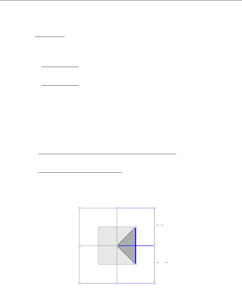
3.1 Local grid mapping x(ξ, η)around a node for orthogonalization; ξ-lines are
dashed; the dual cell is shaded ........................ 6
3.2 Part of the control volume that surrounds edge j(dark shading) and the nodes
involved .................................... 7
3.3 Part of the control volume that surrounds edge j(dark shading) and the nodes
involved; quadrilateral grid cells; edges used in Equation (3.12) are coloured
blue ...................................... 8
3.4 Curvilinear coordinate mapping on a planar domain. The tangent and normal
vectors are not necessarily up to scale (Van Dam, 2009). . . . . . . . . . . . 9
3.5 Geometric meaning of the singular value decomposition of Jacobian matrix J
(Huang, 2005, fig. 2.2) . . . . . . . . . . . . . . . . . . . . . . . . . . . . 10
3.6 non-rectangular triangular cell; the dashed cell is an optimal equiangular poly-
gon, while the shaded cell is the resulting cell after scaling in η0direction; Φ0
is the angle of the ξ0-axis in the (ξ, η)-frame . . . . . . . . . . . . . . . . . 10
3.7 The stencil for node iformed by the nodes A, ..., K. Node Dand Hare
rectangular nodes. The node angle is between two subsequent blue edges. . . 11
3.8 Rectangular triangle cell; additional node angles θrect1and θrect2and edge
j12 are used to determine optimal angle Φopt . . . . . . . . . . . . . . . . . 12
3.9 Computational coordinates for one quadrilateral and five triangular cells, one
of which is a rectangular (shaded) before transformation to (ξ, η)-coordinates.
α=1
2π,β=1
4πand γ=5
4π/4.. . . . . . . . . . . . . . . . . . . . . . 14
3.10 The circle in Figure 3.10a is squeezed in vertical direction (i.e. ⊥OM) to
obtain the ellipse in Figure 3.10b. Blue: d(M, 0) = d(M, 1) = d(M, 4) =
R0; Green: d(0,1) = d(0,4) = 1.. . . . . . . . . . . . . . . . . . . . . . 14
3.11 Control volume for computing the node-to-edge gradient at edge jdiscrete for
the discrete operators Gξ,Gξ......................... 16
3.12 Sketch for the computation of the cirumcentre of a triangle . . . . . . . . . . 17
3.13 Control volume for computing the edge-to-node gradient at the central node
for the discrete operators Dξand Dη, where ξ=ξ0=0. . . . . . . . . . 19
5.1 The flow streamline path and the direction of dispersion stresses. . . . . . . . 28
6.1 Definition of the variables on the staggered mesh . . . . . . . . . . . . . . . 34
6.2 Numbering of cells, faces and nodes, with their orientation to each other. . . . 34
6.3 Connectivity of cells, faces and nodes . . . . . . . . . . . . . . . . . . . . . 34
6.4 Flow area Aujand face-based water depth huj. . . . . . . . . . . . . . . . 38
6.5 Area computation for cell Ω1......................... 39
6.6 Computational cells L(j)and R(j)neighboring face j; water levels are stored
at the cell circumcenters, indicated with the +-sign . . . . . . . . . . . . . . 40
6.7 Nodal interpolation from cell-centered values; contribution from face jto node
r(j); the shaded area indicates the control volume Ωn.. . . . . . . . . . . . 46
6.8 Higher-order reconstruction of face-based velocity uuj, from the left . . . . . 49
6.9 Cross sectional bed bathemetry perpendicular to the flow direction. . . . . . . 63
6.10 Virtual boundary "cells" near the shaded boundary; xLjis the virtual "cell"
center near boundary face j;xR(j)is the inner-cell center; bjis the point on
face jthat is nearest to the inner-cell center ................. 65
6.11 Examples of grid snapping for fixed weirs and thin dams. . . . . . . . . . . . 90
6.12 Examples of computation of crest heights. . . . . . . . . . . . . . . . . . . 91
7.1 A schematic view of σ- and z-layers. ..................... 94
7.2 Layer distribution in 3D. . . . . . . . . . . . . . . . . . . . . . . . . . . . . 95
7.3 Turbulence figure . . . . . . . . . . . . . . . . . . . . . . . . . . . . . . . 105
Deltares vii

DRAFT
D-Flow Flexible Mesh, Technical Reference Manual
8.1 Stencil for momentum advection and diffusion; the numbers indicate the level
of the neighboring cells . . . . . . . . . . . . . . . . . . . . . . . . . . . . 116
8.2 Ghost cells ..................................116
8.3 Partitioning of the schematic Waal model with METIS . . . . . . . . . . . . . 125
8.4 Speed-up of the schematic Waal model; Lisa . . . . . . . . . . . . . . . . . 130
8.5 Speed-up of the schematic Waal model; h4 . . . . . . . . . . . . . . . . . . 131
8.6 Speed-up of the schematic Waal model; SDSC’s Gordon; PETSc . . . . . . . 132
8.7 Speed-up of the schematic Waal model; SDSC’s Gordon; CG+MILUD . . . . 132
8.8 Partitioning of the ’esk-model’ with METIS . . . . . . . . . . . . . . . . . . . 133
8.9 Speed-up of the ’esk-model’; Lisa . . . . . . . . . . . . . . . . . . . . . . . 134
8.10 Speed-up of the schematic Waal model; Gordon . . . . . . . . . . . . . . . 136
8.11 Speed-up of the San Fransisco Delta-Bay model; Gordon . . . . . . . . . . . 138
8.12 Stencil for momentum advection and diffusion; the numbers indicate the level
of the neighboring cells . . . . . . . . . . . . . . . . . . . . . . . . . . . . 143
A.1 A schematic view of cross sectional bed bathemetry perpendicular to the flow
direction. . . . . . . . . . . . . . . . . . . . . . . . . . . . . . . . . . . . 146
A.2 A schematic view of flow nodes and the velocity components in two-dimensional
case. .....................................146
viii Deltares

DRAFT
List of Tables
List of Tables
6.1 Definition of the variables used in Algorithm (4) . . . . . . . . . . . . . . . . 44
6.2 Various limiters available in D-Flow FM for the reconstruction of face-based
velocities in momentum advection . . . . . . . . . . . . . . . . . . . . . . . 51
6.3 Data during a computational time step from tnto tn+1 with Algorithm (32); the
translation to D-Flow FM nomenclature is shown in the last column . . . . . . 75
8.1 METIS settings ................................117
8.2 time-step averaged wall-clock times of the Schematic Waal model; Lisa; note:
MPI communication times are not measured for the PETSc solver . . . . . . . 125
8.3 time-step averaged wall-clock times of the Schematic Waal model; h4; note:
MPI communication times are not measured for the PETSc solver . . . . . . . 126
8.4 time-step averaged wall-clock times of the Schematic Waal model; SDSC’s
Gordon; note: MPI communication times are not measured for the PETSc solver127
8.5 time-step averaged wall-clock times of the Schematic Waal model; SDSC’s
Gordon; CG+MILUD . . . . . . . . . . . . . . . . . . . . . . . . . . . . . 128
8.6 time-step averaged wall-clock times of the ’esk-model’; Lisa; note: MPI com-
munication times are not measured for the PETSc solver . . . . . . . . . . . 129
8.7 time-step averaged wall-clock times of the Schematic Waal model; Gordon;
note: MPI communication times are not measured for the PETSc solver . . . . 135
8.8 time-step averaged wall-clock times of the San Fransisco Delta-Bay model;
Gordon; note: MPI communication times are not measured for the PETSc solver139
8.9 time-step averaged wall-clock times of the San Fransisco Delta-Bay model;
Gordon; non-solver MPI communication times . . . . . . . . . . . . . . . . . 140
Deltares ix

DRAFT
D-Flow Flexible Mesh, Technical Reference Manual
x Deltares

DRAFT
List of Symbols
List of Symbols
Symbol Unit Description
ˆ
hjmHydraulic radius at face j
J(k)−Set of faces jof cell k
N(k)−Set of nodes iof cell k
~nj−Normal vector on face jof an cell, outward direction is positive
~ujm/s Complete velocity vector at the velocity point on edge j
~xζk- the coordinates of cell-center k
ζkmWater level at circumcenter of cell k
ζujmWater level at the velocity point uj
Aujm2Flow area at face j
blkmBed level at cell k
hkmWater depth at cell k(hk=ζk−blk)
i−Node counter
j−Face counter
k−Cell counter
L(j)−Left cell of face j, giving some orentation to the face
l(j)−Left node of face j, giving some orentation to the face
R(j)−Right cell of face j, giving some orentation to the face
r(j)−Right node of face j, giving some orentation to the face
sj,k −Orientation of face jto cell k
ujm/s Face-normal velocity
vjm/s Tangential velocity component at cell face j
Vkm3Volume of water column at cell k
wujmWidth of face j
zimBed level at node i
Aej−Explict part of the discretization of the advection and diffusion
Aij−Implict part of the discretization of the advection and diffusion
bl1jmBed level at left node of face j
bl2jmBed level at right node of face j
Deltares xi

DRAFT
D-Flow Flexible Mesh, Technical Reference Manual
xii Deltares

DRAFT
1 Problem specification
The specification of a problem to be run should resemble the procedure for Delft3D-FLOW,
i.e., through a Master Definition Flow file. The Master Definition Unstructured (MDU) file
standards are evidently not equal to those for Delft3D (yet?).
1.1 The master definition file
Deltares 1 of 152

DRAFT
D-Flow Flexible Mesh, Technical Reference Manual
2 of 152 Deltares
DRAFT
2 Data structures
The data structures used for flow simulations on unstructured meshes are fundamentally dif-
ferent from those on curvilinear meshes, which fit in standard rank-2 arrays. Section 2.1 con-
tains the conceptual hierarchy of mesh and flow data. Section 2.2 contains implementation
details of the variables and IO-routines available.
2.1 Hierarchy of unstructured nets
net node
net link (2D)
net link (1D)
pressure points: 2D flow node circumcenter/1D flow node
flow link
netcell/flow node (2D)
netcell/flow node (1D)
1. Net (domain discretization)
2. Flow data (1D+2D)
(1..NUMK)
(1..NUML1D)
(NUML1D+1..NUML)
(1..NDX2D=NUMP)
(NDX2D+1..NDXI)
boundary flow node (NDXI+1..NDX)
(1..LNX1D)
(LNX1D..LNXI)
(LNXI+1..LNX1DBND)
(LNX1DBND+1..LNX)
1D internal
2D internal
1D open bnd
2D open bnd
2.2 Implementation details of unstructured nets
2.3 Improve use of cache
2.3.1 Improved cache use by node renumbering
The order of nodes in unstructured nets can be arbitrary, as opposed to structured nets, where
neighbouring grid points generally lie at offsets ±1and ±Nxin computer memory.
The order of net nodes in memory should not affect the numerical outcomes in any way, so it
is safe to apply any permutation to the net- and/or flow nodes. A permutation that puts nodes
that are close to each other in the net also close to each other in memory likely improves
cache effiency.
The basic problem is: given a set of nodes and their adjacency matrix, find a permutation for
the nodes such that, when applied, the new adjacency matrix has a smaller bandwidth. The
Reverse Cuthill–McKee (RCM) algorithm is a possible way to achieve this.
Net nodes can be renumbered, with the net links used as adjacency information. This is only
done upon the user’s request (Operations >Renumber net nodes), since net node ordering
does not affect the flow simulation times very much. For flow nodes it is done automatically, as
part of flow_geominit(). It can be switched off in Various >Change geometry settings.
Technical detail: for true efficiency the flow links should be ordered approximately in the same
pace as the flow nodes. Specifically: lne is reordered, based on its first node lne(1,:).
Other code parts require (assume) that net links are indexed identical to flow links, so kn is
Deltares 3 of 152

DRAFT
D-Flow Flexible Mesh, Technical Reference Manual
reordered in the same way as lne was.
4 of 152 Deltares

DRAFT
3 Unstructured grid generation
The grid generation parts in D-Flow FM are standard grid generation techniques for either
curvilinear grids, triangular grids or 2D networks. D-Flow FM does not generate a hybrid
unstructured net of arbitrary polygons at once, but facilitates easy combination of beforemen-
tioned grids and nets in subdomains. It does offer grid optimization over the entire hybrid net,
such as orthogonalization, automated removal of small cells and more.
Most of this functionality will be moved to RGFGRID.
3.1 Curvilinear grids
Curvilinear grid generation is done by (old) code from RGFGRID, within polygons of splines.
3.2 Triangular grids
Unstructured triangular grid generation is done with the Triangle code by J.R. Shewchuk from
Berkely. This is an implementation of Delaunay triangulation. In RGFGRID, this will be re-
placed by SEPRAN routines.
3.3 2D networks
Two-dimensional (SOBEK-like) networks are interactively clicked by the user.
3.4 Grid optimizations
There are two grid optimization procedures: orthogonalization and smoothing. They will be
explained in the following sections.
3.5 Grid orthogonalization
D-Flow FM adopts a staggered scheme for the discretization of the two-dimensional shallow
water equations. Due to our implementation of the staggered scheme, the computational grid
needs to be orthogonal.
Definition 3.5.1. We say that a grid is orthogonal if its edges are perpendicular to the edges
of the dual grid.
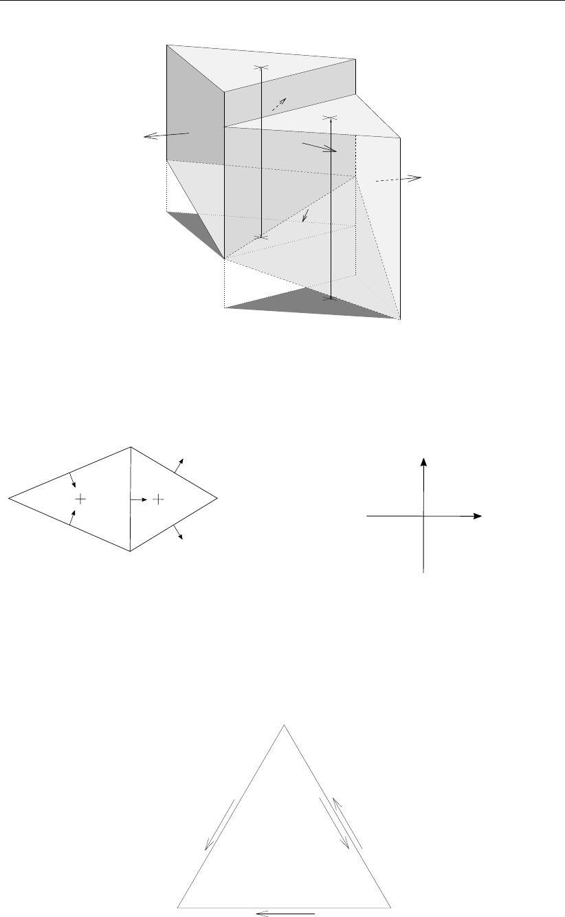
To this end, we will firstly construct a local grid mapping x(ξ, η)attached to some node i, see
Figure 3.1. Since the ξand ηgrid lines are aligned with the primary and dual edges, the grid
will be orthogonal if the grid mapping satisfies the relation
∂x
∂ξ •∂x
∂η = 0,(3.1)
A grid mapping that satisfies Equation (3.1), also satisfies the scaled Laplace equation
∂
∂ξ a∂x
∂ξ +∂
∂η 1
a
∂x
∂η = 0,(3.2)
∇•a∂x
∂ξ ,1
a
∂x
∂η T
= 0 (3.3)
Deltares 5 of 152
DRAFT
D-Flow Flexible Mesh, Technical Reference Manual
η
ξ
Figure 3.1: Local grid mapping x(ξ, η)around a node for orthogonalization; ξ-lines are
dashed; the dual cell is shaded
where ais the aspect ratio defined by:
a=
∂x
∂η
∂x
∂ξ
.(3.4)
Equation (3.2) can be written in the following form, after integration over the controle volume
Ωand applying the Divergence theorem:
ISa∂x
∂ξ ,1
a
∂x
∂η T
•ndS=ISa∂x
∂ξ nξ+1
a
∂x
∂η nηdS= 0,(3.5)
where Sis the boundary of the control volume Ωin (ξ, η)space and n= (nξ, nη)Tis the
outward orthonormal vector.
3.5.1 Discretization
For the description of the discretization of Equation (3.4) and Equation (3.5) the following
nomenclature is used:
Definition 3.5.2. Jint is the set of internal primary edges connected to node iand x0and
x1jare the coordinates of that node and of the neighboring node connected through edge j,
respectively. Furthermore, xLjand xRjare the left and right neighboring cell-circumcentre
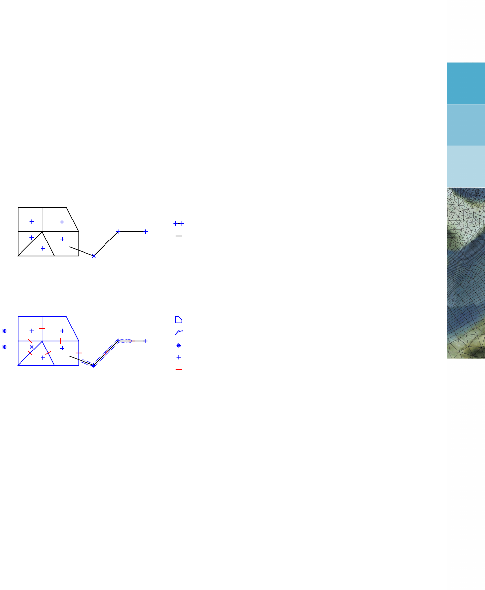
coordinates, see Figure 3.2a.
Definition 3.5.3. Jbnd is the set of boundary edges (nonempty if node iis on the grid bound-
ary only), xR∗
jare the coordinates of a virtual node and xbcjare boundary node coordinates,
see Figure 3.2b.
6 of 152 Deltares
DRAFT
Unstructured grid generation
xLj=x(1
2,1
2)
x0=x(0,0)
x1j=x(1,0)
xRj=x(1
2,−1
2)
(a) Internal edge
xLj
x1j
x0
xR∗
j
xbcj
(b) Boundary edge; xbcjare the coordinates
of a node projected onto the grid boundary,
xR∗
jare virtual node coordinates
Figure 3.2: Part of the control volume that surrounds edge j(dark shading) and the nodes
involved
The discretizations of the aspect ratio for edge j,Equation (3.4), with ∆ξ= ∆η= 1 yields
aj≈
xLj−xRj
∆η
∆ξ
kx1j−x0k=
xLj−xRj
kx1j−x0k, j ∈ Jint (3.6)
and the discretization of Equation (3.5) yields
X
j∈Ji
kxRj−xLjk
kx1j−x0k(x1j−x0) +
X
j∈Je(1
2kxR∗
j−xLjk
kx1j−x0k(x1j−x0) + 1
2kx1j−x0k
kxR∗
j−xLjk(xR∗
j−xLj))= 0,
(3.7)
where the second summation in Equation (3.7) accounts for boundary edges.
The virtual node xR∗
jis constructed by extrapolation from the circumcenter and boundary
nodes, using Equation (3.8) to project the left cell-circumcenter orthogonally onto the grid
boundary xbcj:
xbcj=x0+(x1j−x0)•(xLj−x0)
kx1j−x0k2(x1j−x0).(3.8)
xR∗
j= 2xbcj−xLj,(3.9)
Remark 3.5.4.We will always assume that the grid is on the left-hand side of a boundary
edge.
Finally, Equation (3.7) can be put in the following form
X
j∈Ji
aj(x1j−x0) + X
l∈Le1
2aj(x1j−x0) + 1
2kx1j−x0knj,= 0,
Deltares 7 of 152
DRAFT
D-Flow Flexible Mesh, Technical Reference Manual
(3.10)
where nj=xR∗
j−xLj
kxR∗
j−xLjkis the outward normal at edge jand ajis the aspect ratio of edge
j, i.e.
aj=
kxRj−xLjk
kx1j−x0k, j ∈ Ji,
kxR∗
j−xLjk
kx1j−x0k, j ∈ Je.
(3.11)
3.5.2 Curvilinear-like discretization
The previous formulation may lead to distorted quadrilateral grids. This is remedied by mim-
icking a curvilinear formulation in the quadrilateral parts of the grid. Then, in Equation (3.10)
the aspect ratio of Equation (3.11) is replaced by
aj=
4kxRj−xLjk
2kx1j−x0k+kx2Rj−x1Rjk+kx2Lj−x1Ljk, j ∈ Jint,
2kxR∗
j−xLjk
kx1j−x0k+kx2Lj−x1Ljk, j ∈ Jbnd,
(3.12)
where the nodes involved are depicted in Figure 3.3.
x1Rj =x(0,−1)
x1Rj =x(0,1)
x0=x(0,0)
xLj=x(1
2,1
2)
xRj=x(1
2,−1
2)
x1j=x(1,0)
x2Rj =x(1,−1)
x2Lj =x(1,1)
Figure 3.3: Part of the control volume that surrounds edge j(dark shading) and the nodes
involved; quadrilateral grid cells; edges used in Equation (3.12) are coloured
blue
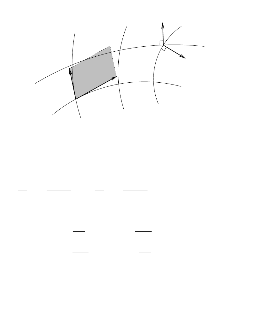
3.6 Grid smoothing
Enhancing the smoothness of the grid is performed by means of an elliptic smoother. This
work is based on Huang (2001,2005). In order to prevent grid folds in non-convex domains,
the smoother is formulated in terms of a so-called inverse map, i.e. ξ(x, y), and leads to
∇•G−1∇ξi= 0, i ∈ {1,2},(3.13)
where Gis the monitor function for grid adaptivity which will be explained later (section 3.6.3)
and ξ1≡ξ,ξ2≡η.
Remark 3.6.1.Although the method is based on an inverse mapping ξ(x, y), it is more
convenient to work with the direct mapping x(ξ, η).
8 of 152 Deltares
DRAFT
Unstructured grid generation
ξ=c1ξ=c2ξ=c3
η=d1
η=d2
∇η=a2
∇ξ=a1
xξ=a1
xη=a2
det(J)
Figure 3.4: Curvilinear coordinate mapping on a planar domain. The tangent and normal
vectors are not necessarily up to scale (Van Dam,2009).
By interchanging the role of dependent and independent variables, Equation (3.13) can be
transformed into an expression for the direct grid mapping x(ξ, η):
∂x
∂ξ a1,∂(G−1)
∂ξ a1+∂x
∂η a1,∂(G−1)
∂ξ a2+
∂x
∂ξ a2,∂(G−1)
∂η a1+∂x
∂η a2,∂(G−1)
∂η a2
−a1, G−1a1∂2x
∂ξ2+a1, G−1a2∂2x
∂ξ∂η +
a2, G−1a1∂2x
∂η∂ξ +a2, G−1a2∂2x
∂η2= 0,(3.14)
where by h•,•ian inner product is meant and a1=∇ξand a2=∇ηare the contravariant
base vectors (Figure 3.4), by definition:
aα•aβ=δβ
α, α, β ∈ {1,2}(3.15)
and thus
kaγk=1
kaγk, γ ∈ {1,2}(3.16)
Obviously we need to start by defining the node coordinates in (ξ, η)-space based on their
connectivity with neighboring grid nodes.
3.6.1 Assigning the node coordinates in computational space
By assigning the node coordinates in computational (ξ, η)-space, we postulate the optimal
smooth grid. Compare with a curvi-linear grid in this respect. To see how we have to choose
the (ξ, η)coordinates, first consider a linearization of the grid mapping around a node:
x=x0+J(ξ−ξ0) + Okξk2,(3.17)
where x0and ξ0are the node coordinates in physical and computational space respectively
and Jis the Jacobian matrix of the transformation. Following Huang (2005), the Jacobian
Deltares 9 of 152
DRAFT
D-Flow Flexible Mesh, Technical Reference Manual
matrix Jcan be decomposed into (singular value decomposition):
J=UΣVT,(3.18)
where VTis a rotation in (ξ, η)-space, Σa compression/expansion and Ua rotation in
(x, y)-space, see Figure 3.5.
ξ-space ξ-space
x-space x-space
VT
U
Σ
J=UΣVT
Figure 3.5: Geometric meaning of the singular value decomposition of Jacobian matrix J
(Huang,2005, fig. 2.2)
Since Equation (3.14) is invariant to rotation of the (ξ, η)-axis, rotation Vis irrelevant and we
may start by assigning ξ= (0,0)Tto the center node iand ξ= (1,0)Tto an arbitrary
neighboring node.
We now proceed by considering a cell attached to a node iin coordinate frame (ξ0, η0),
see Figure 3.6, and define an optimal angle Φopt between two subsequent edges that are
connected to node i.
η0
ξ
η
Φ
Φ0
Φopt
ξ0
Figure 3.6: non-rectangular triangular cell; the dashed cell is an optimal equiangular poly-
gon, while the shaded cell is the resulting cell after scaling in η0direction; Φ0
is the angle of the ξ0-axis in the (ξ, η)-frame
Definition 3.6.2. The optimal angle Φopt is the angle between two subsequent edges of a
cell, both connected to node i, that would lead to the desired optimal smooth grid cell.
10 of 152 Deltares
DRAFT
Unstructured grid generation
Remark 3.6.3.In general, the optimal smooth cell is an equiangular polygon, with the excep-
tion for rectangular triangles. The optimal angle at a node of a rectangular triangle is either
1
4πor 1
2π, depending on the grid connectivity.
For a non-rectangular triangle this optimal angle would be 1
3π. However, by considering a
node with five non-rectangular triangles attached, one can easily understand that this angle
is unsuitable in general, as five of such angles do not sum up to 2π. Therefore, we define a
true angle as follows:
Definition 3.6.4. The true angle Φis the angle between two subsequent edges of a cell, both
connected to node i, such that sum of all cell true-angles equals its prescribed value of either
2π(internal nodes), π(boundary nodes) or 1
2π(corner nodes).
The true cell is obtained from the optimal cell by scaling the cell, as will be explained later
(section 3.6.1.2).
Returning to the optimal angle, we first discriminate between rectangular cells and non-
rectangular cells to account for (partly) quadrilateral grids.
iA
B
C
D
E
F
G
H
I
JK
Figure 3.7: The stencil for node iformed by the nodes A, ..., K. Node Dand Hare
rectangular nodes. The node angle is between two subsequent blue edges.
Definition 3.6.5. The stencil is the set of cells that are connected to node i. A node angle
is the angle between two subsequent stencil-boundary edges connected to node i. A rect-
angular node, not being node iitself, is a node that is connected to three or less non-stencil
quadrilateral cells and no other non-stencil nodes. A rectangular cell is a quadrilateral cell or
a triangular cell which contains at least one right angle.
Note: Each node of a rectangular cell will be called a rectangular node. So one of the optimal
angles Φopt of such a cell is rectangular. Rectangular nodes have optimal node angles as
indicated in Figure 3.8, which can be 1
4π,1
2π,πor 3
2π. It will be indicated with the sub-script
rect.
Deltares 11 of 152
DRAFT
D-Flow Flexible Mesh, Technical Reference Manual
θrect1
Φopt
j12
θrect2
Figure 3.8: Rectangular triangle cell; additional node angles θrect1and θrect2and edge
j12 are used to determine optimal angle Φopt
The rectangular node angles are computed by
θrecti=
(2 −1
2Nnsq)π, node iis a rectangular internal node,
(1 −1
2Nnsq)π, node iis a rectangular boundary node,
1
2π, node iis a rectangular corner node,
(3.19)
where Nnsq is the number of non-stencil quadrilaterals connected to node i. The optimal
angle Φopt for rectangular nodes is finally determined by (see Figure 3.8)
Φopt =
(1 −2
N)π, N ≥4∨non-rectangular cell,
1
2π, N = 3 ∧rectangular cell with two rectangular nodes ’1’ and ’2’
∧θrect1+θrect2=π
∧j12 is not a boundary edge,
1
4π, other,
(3.20)
where Nis the number of nodes that comprise the cell. In the example of Figure 3.8, nodes
1and 2are rectangular nodes with angles of πand 1
2πrespectively and the shaded cell is a
rectangular triangle with optimal angle 1
4π.
3.6.1.1 Determining the true cell angles
Having defined the optimal angles for all cells, we can derive the true angles by demanding
that the cells fit in the stencil. To this end, we consider the number and type of cells connected
to node i.
Definition 3.6.6. The sum of all cell-optimal and true angles are called ΣΦopt and ΣΦ re-
spectively. Furthermore, the sum of all optimal and true angles of quadrilateral cells are called
ΣΦopt
quad and ΣΦquad respectively. The number of quadrilateral cells is Nquad. The same def-
initions hold for the rectangular triangular cells: ΣΦopt
trirect ,ΣΦtrirect and Ntrirect respectively
and for the remaining cells: ΣΦopt
rem,ΣΦrem and Nrem respectively.
Remark 3.6.7.The remaining cells are not necessarily non-rectangular triangles only, but can
also be pentagons and/or hexagons, et cetera.
12 of 152 Deltares

DRAFT
Unstructured grid generation
Of course holds
ΣΦopt = ΣΦopt
quad + ΣΦopt
trirect + ΣΦopt
rem,(3.21)
N=Nquad +Ntrirect +Nrem.(3.22)
In a similar fashion, the sum of all true angles should sum up to 2πf, where
f=
1,internal node,
1
2,boundary node,
1
4,corner node.
(3.23)
In other words, we seek true angles ΣΦquad ,ΣΦtrirect and ΣΦrem such that:
ΣΦquad + ΣΦtrirect + ΣΦrem = 2πf. (3.24)
This is achieved by setting
ΣΦquad =µΣΦopt
quad,(3.25)
ΣΦtrirect =µ µtrirect ΣΦopt
trirect ,(3.26)
ΣΦrem =µ µremΣΦopt
rem.(3.27)
We give highest precedence to the optimal angles of quadrilateral cells, followed by rectan-
gular triangular cells and lowest precedence to the remaining cells. From the angle left for
the remaining cells (non-rectangular triangles, pentagons and hexagons) the coefficient µrem
can be determined (with a lower band):
µrem = max 2π f −ΣΦopt
quad + ΣΦopt
trirect
ΣΦopt
rem
,NtriΦmin
ΣΦopt
rem !,(3.28)
If there are remaining cells (Nrem >0) then µtrirect = 1 and if there are no remaining
cells µrem = 1 and ΣΦopt
rem = 0 and does not influence the angles available for quads and
rectangular triangles. So:
µtrirect =
1Nrem >0
max 2π f −ΣΦopt
quad
ΣΦopt
trirect
,Ntrirect Φmin
ΣΦopt
trirect !, Nrem = 0,(3.29)
At last µis determined by taken all cells into account
µ=2π f
ΣΦopt
quad +µtrirect ΣΦopt
trirect +µremΣΦopt
rem
.(3.30)
Φmin =1
12 πis the minimum cell angle, determining a lower band for the factors µtrirect and
µrem.
3.6.1.2 Assigning the node coordinates
With the the optimal angles of the cell defined, the (ξ0, η0)coordinates can be assigned to the
cell nodes. We require that all edges connected to node ihave unit length in computational
(ξ, η)-space, which has its consequences for rectangular triangles.
Deltares 13 of 152
DRAFT
D-Flow Flexible Mesh, Technical Reference Manual
η0
ξ0
η
ξ
γ
αβ
γ
γ
γ
Figure 3.9: Computational coordinates for one quadrilateral and five triangular cells, one
of which is a rectangular (shaded) before transformation to (ξ, η)-coordinates.
α=1
2π,β=1
4πand γ=5
4π/4.
Remark 3.6.8.Since all edges connected to node iare required to have unit length, rectan-
gular triangles may be transformed into non-rectangular triangles, but maintain their cell angle
Φopt, see Figure 3.9 for an example.
0
1
2
3
4
R0
X
π−θ
θ
M
(a) Nodes on circle.
0
1
2
3
4
R0
XM
Φ
(b) Nodes on ellipse.
Figure 3.10: The circle in Figure 3.10a is squeezed in vertical direction (i.e. ⊥OM) to
obtain the ellipse in Figure 3.10b. Blue: d(M, 0) = d(M, 1) = d(M, 4) =
R0; Green: d(0,1) = d(0,4) = 1.
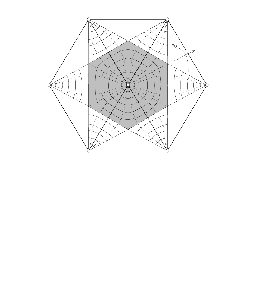
Since the cell in (ξ0, η0)coordinates is an equiangular polygon in (ξ0, η0)-space (Figure 3.10a),
the coordinates of the ith node is
ξ0=R0(1 −cos(i θ)),(3.31)
η0=−R0sin(i θ),(3.32)
θ=2π
N(3.33)
14 of 152 Deltares
DRAFT
Unstructured grid generation
where i= 0 corresponds to the center node iand counting counterclockwise, Nis the
number of nodes that comprise the cell and R0the radius of the circumcircle, see Fig-
ure 3.10a (node ξi−1=i−1and i= 1, . . . , N). The circle in Figure 3.10a is squeezed
in such a way that the edge from node 0to node 1and node 0to node 4has length 1(dis-
tance: d(0,1) = d(0,4) = 1) and Φis the true angle, also d(0, X)remains the same
R0(1 −cos θ) = cos(1
2Φ)because the squeezing is perpendicular to the OM-axis (i.e.
the ξ0-axis). The other edges of the polygon does not have, in general, a length of 1 after
squeezing. The radius of the circumcircle read:
R0=cos(1
2Φ)
(1 −cos θ)(3.34)
The cell aspect ratio Ais defined as the ratio between the distance d(1, N)in Figure 3.10b
and the distance d(1, N)in Figure 3.10a, yielding:
A=(1 −cos θ) tan(1
2Φ)
sin θ,(3.35)
where θ=2π
N, with Nbeing the number of nodes that comprise the cell.
The coordinates (ξ, η)of the cell nodes are obtained by scaling and rotating the cell in such
a way that it fits in the stencil, see Figure 3.6. The transformation from (ξ0, η0)to (ξ, η)
coordinates read:
ξ= cos (Φ0)ξ0−Asin (Φ0)η0,(3.36)
η= sin (Φ0)ξ0+Acos (Φ0)η0,(3.37)
3.6.2 Computing the operators
For the solution of Equation (3.14), we approximate ∂2x
∂ξ∂η at node ξ0
∂2x
∂ξ∂η ξ0≈X
j∈J
Dξ X
i∈N
Gηxi!j
,(3.38)
and similar for the other derivatives ∂2x
∂ξ2,∂2x
∂η2and ∂2x
∂η∂ξ , where:
Definition 3.6.9. Jis the set of edges attached to node ξ0and Nis the set of nodes in the
stencil of node ξ0. Furthermore, Gξand Gηare the node-to-edge approximations and Dξ
and Dηthe edge-to-node approximations of the ξand ηderivatives respectively.
The discretization is as follows. For some quantity Φ, its gradient can be approximated in the
usual finite-volume way
∇ξΦ≈1
vol(Ωξ)I∂Ωξ
ΦnξdSξ.(3.39)
Deltares 15 of 152
DRAFT
D-Flow Flexible Mesh, Technical Reference Manual
3.6.2.1 Node-to-edge operator
ξ1j
ξ0
j
ξRj
ξ1j+1
ξLj
Figure 3.11: Control volume for computing the node-to-edge gradient at edge jdiscrete
for the discrete operators Gξ,Gξ
For the node-to-edge gradient (Gξ, Gη)Twe take the control volume as indicated in Fig-
ure 3.11 and obtain for some node-based quantity Φ
(Gξ, Gη)TΦj=
(ξRj−ξLj)⊥(Φ1j−Φ0)−(ξ1j−ξ0)⊥(ΦRj−ΦLj)
k(ξ1j−ξ0)×(ξRj−ξLj)k, j ∈ Jint,
(ξR∗
j−ξLj)⊥(Φ1j−Φ0)−(ξ1j−ξ0)⊥(ΦR∗
j−ΦLj)
k(ξ1j−ξ0)×(ξRj−ξLj)k, j ∈ Jbnd,
(3.40)
where we use similar definitions as Definitions 3.5.2 and 3.5.3, and Remark 3.5.4 also holds.
Furthermore, ξ•ξ⊥= 0 ⇒ξ⊥= (−η, ξ)T, so ξ⊥is parallel to the contravariant vector a2
(ξ=a1and a1•a2= 0) and ξ0=0by construction. Because the values ξLjand ξRjare
not node based, the value at the circumcentres need to be determined from the node values
of that cell.
Determine the value at circumcenters
The cell circumcenters ξLjand ξRjcan be expressed in general form as
ξLj=X
i∈N
Ai
Ljξi,(3.41)
ξRj=ξLj−1,(3.42)
Definition 3.6.10. ALjis the left node-to-cell mapping for the cell left from edge j.
The above summation is over all nodes, the coefficient Ai
Lj= 0 if the node idoes not belong
to the left cell of edge j.
16 of 152 Deltares
DRAFT
Unstructured grid generation
Circumcenter of non triangle
For a non-triangle cell kthe centroid is taken as an approximation of the circumcenter. So:
ALj=1
N, L(j) = k(3.43)
where Nis the number of vertices of the cell k.
Circumcenter of a triangle
For triangular cells on the other hand, the circumcenter is used and computed as follows:
ξLj=ξ0+α(ξ1j−ξ0) + β(ξ1j+1 −ξ0),(3.44)
ξRj=ξLj−1,(3.45)
ξLj
ξ0ξ1j
ξ1j+1
θ
Figure 3.12: Sketch for the computation of the cirumcentre of a triangle
where
α=1−1
γc
2(1 −c2),(3.46)
β=1−γc
2(1 −c2),(3.47)
and
γ=kξ1j−ξ0k
kξ1j+1 −ξ0k,(3.48)
c=(ξ1j−ξ0)•(ξ1j+1 −ξ0)
kξ1j−ξ0kkξ1j+1 −ξ0k(= cos θ).(3.49)
Remark 3.6.11.The edges jaround node iare arranged in counterclockwise order.
The circumcenter of a triangle expressed in the vertex coordinates (Equation (3.41)) read:
ξLj= (1 −α−β)ξ0+αξ1j+βξ1j+1 ,(3.50)
ξRj=ξLj−1,(3.51)
The cell center values Φin Equation (3.40) are computed in the same manner, i.e.:
ΦLj=X
i∈N
Ai
LjΦi,(3.52)
ΦRj= ΦLj−1.(3.53)
Deltares 17 of 152

DRAFT
D-Flow Flexible Mesh, Technical Reference Manual
Operator Gξand Gη
Combining Equation (3.40),Equation (3.52) and Equation (3.53) yields for each internal edges
j
GξΦ|j=−(ηRj−ηLj)(Φ1j−Φ0)+(η1j−η0)P
i∈N
(Ai
Lj−1Φi−Ai
LjΦi)
k(ξ1j−ξ0)×(ξRj−ξLj)k, j ∈ Jint,
(3.54)
and
GηΦ|j=
(ξRj−ξLj)(Φ1j−Φ0)−(ξ1j−ξ0)P
i∈N
(Ai
Lj−1Φi−Ai
LjΦi)
k(ξ1j−ξ0)×(ξRj−ξLj)k, j ∈ Jint,
(3.55)
Boundary edges are treated in a similar fashion as before, see Equation (3.9), by creating a
virtual node:
ξR∗
j= 2ξbcj−ξLj,(3.56)
ΦR∗
j= 2Φbcj−ΦLj,(3.57)
and
ξbcj=ξ0+αξ(ξ1j−ξ0),(3.58)
Φbcj= Φ0+αx(Φ1j−Φ0),(3.59)
with
αξ= (ξLj−ξ0)•
ξ1j−ξ0
kξ1j−ξ0k,(3.60)
αx=αξ.(3.61)
Remark 3.6.12.Note that αξ=1
2for triangular and quadrilateral cells. The boundary condi-
tions are non-orthogonal, in contrast to Equation (3.8). This maintains the linearity of opera-
tors Gξand Gη.
Substitution in Equation (3.40) yields for each boundary edge j
GξΦ|j=−(ηR∗
j−ξLj)(Φ1j−Φ0)+(η1j−η0)(ΦR∗
j−P
i∈N
Ai
LjΦi)
k(ξ1j−ξ0)×(ξR∗
j−ξLj)k, j ∈ Jbnd,
(3.62)
and
GηΦ|j=
(ξR∗
j−ξLj)(Φ1j−Φ0)−(ξ1j−ξ0)(ΦR∗
j−P
i∈N
Ai
LjΦi)
k(ξ1j−ξ0)×(ξR∗
j−ξLj)k, j ∈ Jbnd,(3.63)
18 of 152 Deltares
DRAFT
Unstructured grid generation
3.6.2.2 Edge-to-node operator
For the edge-to-node gradient we take the control volume as indicated in Figure 3.13
j
ξ0
ξ1j
ξ1j+1
ξRj
ξLj
Figure 3.13: Control volume for computing the edge-to-node gradient at the central node
for the discrete operators Dξand Dη, where ξ=ξ0=0
and obtain
(Dξ, Dη)T=1
Vdj,(3.64)
where
dj=(ξRj−ξLj)⊥, j ∈ Jint,
(ξbcj−ξLj)⊥−(ξbcj−ξ0)⊥, j ∈ Jbnd,(3.65)
and with ξ∈IR2
V=ZΩ
dΩ = 1
2ZΩ∇•ξdΩ = 1
2I∂Ω
ξ•ndΓ⇒(3.66)
V=1
2X
j∈Jint
ξLj+ξRj
2•dj+1
2X
j∈Jbnd
ξLj+ξR∗
j
2•dj.(3.67)
3.6.2.3 Node-to-node operator
The computation of the Jacobian requires the node-to-node gradient.
Definition 3.6.13. Jξand Jηare the node-to-node approximations of the ξand ηderivatives
respectively.
They can be constructed as
Jξ|i=X
j∈Jint
Dξ 1
2X
i∈Iint
(Ai
LjJi+Ai
Lj−1Ji)!j
+X
j∈Jbnd
Dξ1
2(J0j+J1j)j
,
(3.68)
Deltares 19 of 152

DRAFT
D-Flow Flexible Mesh, Technical Reference Manual
and
Jη|i=X
j∈Jint
Dη 1
2X
i∈Iint
(Ai
LjJi+Ai
Lj−1Ji)!j
+X
j∈Jbnd
Dη1
2(J0j+J1j)j
.
(3.69)
3.6.3 Computing the mesh monitor matrix
In the discretization of Equation (3.14), we approximate the contravariant base vectors by
firstly computing the Jacobian by applying Equation (3.68) and Equation (3.69), and using
a1=∇ξand a2=∇η:
a1= ( J22,−J12)T/det J, (3.70)
a2= (−J21, J11)T/det J. (3.71)
The mesh monitor matrix Gis computed as explained in Huang (2001). It is based on a
solution value at grid nodes, that determines the mesh refinement direction v:
v=∇u, (3.72)
which is approximated by firstly smoothing u, and computing
v=X
i∈N
a1Jξui+a2Jηui.(3.73)
This direction vector is directly inserted in the mesh monitor matrix, see Huang (2001) for
details. The obtained mesh monitor matrix is smoothed, after which the inverse G−1is calcu-
lated.
3.6.4 Composing the discretization
With the operators Dξ,Dη,Gξand Gηavailable, and the contravariant base vectors a1and
a2and the inverse mesh monitor matrix G−1computed, the discretization of Equation (3.14)
is a straightforward task. We obtain
X
i∈N
wixi=0,(3.74)
where
wi=a1,∂(G−1)
∂ξ a1Jξ+a1,∂(G−1)
∂ξ a2Jη+
a2,∂(G−1)
∂η a1Jξ+a2,∂(G−1)
∂η a2Jη
− a1, G−1a1X
j∈J
DξGξ|j+a1, G−1a2X
j∈J
DξGη|j+
a2, G−1a1X
j∈J
DηGξ|j+a2, G−1a2X
j∈J
DηGη|j!= 0,(3.75)
20 of 152 Deltares
DRAFT
4 Numerical schemes
4.1 Time integration
...
4.2 Matrix solver: Gauss and CG
The implicit part of the discretized PDEs is solved by a combination of Gauss elimination,
based on minimum degree, and CG.1The procedure solves an equation As1=b, where A
is a sparse, diagonally dominant and symmetric matrix. The array s1(1:nodtot) contains
the unknown values to be solved. The value of nodtot describes the number of nodal points.
The sample program calls two routines:
1 the routine prepare
2 the routine solve_matrix
4.2.1 Preparation
prepare determines which rows of matrix A, i.e., which nodes, are solved by Gauss elimina-
tion and which by CG, based on the nodes’ degree. It need to be applied just once, thereafter
solve_matrix can be called as many times as needed. The inputs of prepare are the
following arrays and variables:
nodtot the total number of nodes or unknowns
lintot the total number of initial upper-diagonal non-zero entries of the orig-
inal equation not affected by Gaussian elimination, or the total num-
ber of lines between two nodes.
maxdgr the maximum degree of a node that is eliminated by Gaussian elimi-
nation
line(1:lintot,1:2) the adjacency graph of Aor the list of the indices of non-zero
entries.
The outputs of prepare are the following arrays and variables:
nogauss the number of nodes that will be eliminated by Gaussian elimination
nocg the number of unknowns of the remaining equation to be solved by
CG.
ijtot the total number of upper-diagonal non-zero entries including the fill-
ins due to Gaussian elimination.
ijl(1:lintot) contains the addresses of aij(1:ijtot) (lintot<=ijtot)
where the non-zero entries of the original equation are to be stored.
noel(1:nogauss) numbers of the nodes that will be eliminated by Gaussian elimi-
nation in the order given by noel(1:nogauss). The remaining
unknowns, given by
noel(nogauss+1:nogauss+nocg), are solved by CG.
row(1:nodtot) sparse matrix administration used by solve_matrix (see pro-
gram listing)
4.2.2 Solving the matrix
The output of prepare is input to solve_matrix. Other input to solve_matrix is
given by:
1The Gauss+CG solver was designed and implemented by Guus Stelling. This section is largely a copy of his
original Word document accompanying a test program.
Deltares 21 of 152
DRAFT
D-Flow Flexible Mesh, Technical Reference Manual
aii(1:nodtot) the main diagonal elements of A
aij(ijl(1:lintot)) the non-zero upper-diagonal elements of A
bi(1:nodtot) the components of the right hand side vector b
s0(1:nodtot) initial estimate of the final solution
ipre if ipre=1 then point Jacobi preconditioning is applied otherwise
LUD preconditioning will be applied
The subroutine does the following steps:
1 call gauss_elimination
2 call cg(ipre)
3 call gauss_substitution
After this the unknown vector s1(1:nodtot) has been found.
4.2.3 Example
To illustrate the solve_matrix routine the following example is given:
01 02 03 04 05 06
07 08 09 10 11 12
13 14 15 16 17 18
19 20 21 22 23 24
25 26 27 28 29 30
31 32 33 34 35 36
This is the adjacency graph of a 36×36 matrix A. For this graph nodtot=36 and lintot=60.
The graph is described by the following set of lines:
(01,02) (07,08) (13,14) (19,20) (25,26) (31,32) (02,03) (08,09) (14,15) (20,21) (26,27) (32,33)
(03,04) (09,10) (15,16) (21,22) (27,28) (33,34) (04,05) (10,11) (16,17) (22,23) (28,29) (34,35)
(05,06) (11,12) (17,18) (23,24) (29,30) (35,36) (01,07) (07,13) (13,19) (19,25) (25,31) (02,08)
(08,14) (14,20) (20,26) (26,32) (03,09) (09,15) (15,21) (21,27) (27,33) (04,10) (10,16) (16,22)
(22,28) (28,34) (05,11) (11,17) (17,23) (23,29) (29,35) (06,12) (12,18) (18,24) (24,30) (30,36),
as can be verified in the picture. The degree of each node and its connecting node numbers
are given by the following table:
node 1 : 2 2 7
node 2 : 3 1 3 8
node 3 : 3 2 4 9
node 4 : 3 3 5 10
node 5 : 3 4 6 11
node 6 : 2 5 12
node 7 : 3 8 1 13
node 8 : 4 7 9 2 14
node 9 : 4 8 10 3 15
node 10 : 4 9 11 4 16
node 11 : 4 10 12 5 17
node 12 : 3 11 6 18
22 of 152 Deltares

DRAFT
Numerical schemes
node 13 : 3 14 7 19
node 14 : 4 13 15 8 20
node 15 : 4 14 16 9 21
node 16 : 4 15 17 10 22
node 17 : 4 16 18 11 23
node 18 : 3 17 12 24
node 19 : 3 20 13 25
node 20 : 4 19 21 14 26
node 21 : 4 20 22 15 27
node 22 : 4 21 23 16 28
node 23 : 4 22 24 17 29
node 24 : 3 23 18 30
node 25 : 3 26 19 31
node 26 : 4 25 27 20 32
node 27 : 4 26 28 21 33
node 28 : 4 27 29 22 34
node 29 : 4 28 30 23 35
node 30 : 3 29 24 36
node 31 : 2 32 25
node 32 : 3 31 33 26
node 33 : 3 32 34 27
node 34 : 3 33 35 28
node 35 : 3 34 36 29
node 36 : 2 35 30
If no Gaussian elimination is is applied, but if the equation is solved entirely by CG then
this administration is used by the cg subroutine. However if every point up to degree 4 (i.e.
maxdgr=5) is eliminated by Gauss then the following table might result:
gauss 1 : 2 2 7
gauss 6 : 2 5 12
gauss 31 : 2 32 25
gauss 36 : 2 35 30
gauss 2 : 3 3 8 7
gauss 4 : 3 3 5 10
gauss 7 : 3 8 13 3
gauss 12 : 3 11 18 5
gauss 19 : 3 20 13 25
gauss 24 : 3 23 18 30
gauss 32 : 3 33 26 25
gauss 34 : 3 33 35 28
gauss 5 : 4 11 3 10 18
gauss 8 : 4 9 14 3 13
gauss 11 : 4 10 17 18 3
gauss 15 : 4 14 16 9 21
gauss 22 : 4 21 23 16 28
gauss 25 : 4 26 20 13 33
gauss 26 : 4 27 20 33 13
gauss 29 : 4 28 30 23 35
gauss 30 : 4 35 23 18 28
gauss 35 : 4 33 28 23 18
cg 3 : 6 9 10 13 18 14 17
cg 9 : 6 10 3 14 13 16 21
Deltares 23 of 152

DRAFT
D-Flow Flexible Mesh, Technical Reference Manual
cg 10 : 5 9 16 3 18 17
cg 13 : 6 14 3 20 9 33 27
cg 14 : 6 13 20 9 3 16 21
cg 16 : 7 17 10 14 9 21 23 28
cg 17 : 5 16 18 23 10 3
cg 18 : 6 17 23 3 10 28 33
cg 20 : 5 21 14 13 33 27
cg 21 : 7 20 27 14 16 9 23 28
cg 23 : 6 17 18 21 16 28 33
cg 27 : 5 28 21 33 20 13
cg 28 : 6 27 33 21 23 16 18
cg 33 : 6 27 28 20 13 23 18
The corner nodes have the lowest degree so they are eliminated first as the table shows.
These are followed by other nodes on the boundary before internal nodes are eliminated.
After each elimination step the degree of neighboring points, due to fill-in, might be increased,
so minimum degree automatically imposes some kind of colored ordering of the nodal points.
Elimination of such points is known to improve the convergence properties of CG, see e.g. ?.
The nodes, which are left over for CG, clearly show the increased degree due to fill in.
In general the fastest convergence, in terms of number of iterations, is obtained by choosing
maxdgr as large as memory allows in combination with LUD pre-conditioning. However in
terms of computational time the fastest convergence is obtained by a moderate choice of
maxdgr, such that approximately 50 % of the total number of grid points is eliminated by
Gauss in combination with point Jacobi preconditioning.
24 of 152 Deltares

DRAFT
5 Conceptual description
5.1 Introduction
[yet empty]
5.2 General background
[yet empty]
5.3 Governing equations
[yet empty]
5.4 Boundary conditions
[yet empty]
5.5 Turbulence
Reynold’s stresses
The Reynolds stresses in the horizontal momentum equation are modelled using the eddy
viscosity concept, (for details e.g. Rodi (1984)). This concept expresses the Reynolds stress
component as the product between a flow as well as grid-dependent eddy viscosity coefficient
and the corresponding components of the mean rate-of-deformation tensor. The meaning and
the order of the eddy viscosity coefficients differ for 2D and 3D, for different horizontal and
vertical turbulence length scales and fine or coarse grids. In general the eddy viscosity is a
function of space and time.
For 3D shallow water flow the stress tensor is an-isotropic. The horizontal eddy viscosity
coefficient, νH, is much larger than the vertical eddy viscosity νV(νHνV). The horizontal
viscosity coefficient may be a superposition of three parts:
1 a part due to “sub-grid scale turbulence”,
2 a part due to “3D-turbulence” see Uittenbogaard et al. (1992) and
3 a part due to dispersion for depth-averaged simulations.
In simulations with the depth-averaged momentum and transport equations, the redistribution
of momentum and matter due to the vertical variation of the horizontal velocity is denoted as
dispersion. In 2D simulations this effect is not simulated as the vertical profile of the horizontal
velocity is not resolved. This dispersive effect may be modelled as the product of a viscosity
coefficient and a velocity gradient. The dispersive viscosity coefficient may be estimated by
the Elder formulation.
If the vertical profile of the horizontal velocity is not close to a logarithmic profile (e.g. due to
stratification or due to forcing by wind) then a 3D-model for the transport of matter is recom-
mended instead of 2D modelling with Elder approximation.
The horizontal eddy viscosity is mostly associated with the contribution of horizontal turbulent
motions and forcing that are not resolved by the horizontal grid (“sub-grid scale turbulence”)
or by (a priori) the Reynolds-averaged shallow-water equations. For the former we introduce
the sub-grid scale (SGS) horizontal eddy viscosity νSGS and for the latter the horizontal eddy
viscosity νV. D-Flow FM simulates the larger scale horizontal turbulent motions through a
Deltares 25 of 152
DRAFT
D-Flow Flexible Mesh, Technical Reference Manual
sub-grid scale method (SGS), eg. Elder. The user may add a background horizontal viscosity,
νback
H, as a constant or spatially dependent. Consequently, in D-Flow FM the horizontal eddy
viscosity coefficient is defined by
νH=νSGS +νV+νback
H.(5.1)
The 3D part νVis referred to as the three-dimensional turbulence and in 3D simulations it is
computed following a 3D-turbulence closure model.
For turbulence closure models responding to shear production only, it may be convenient to
specify a background or “ambient” vertical mixing coefficient in order to account for all other
forms of unresolved mixing, νback
V. Therefore, in addition to all turbulence closure models in
D-Flow FM a constant (space and time) background mixing coefficient may be specified by the
user, which is a background value for the vertical eddy viscosity in the momentum equations.
Consequently, the vertical eddy viscosity coefficient is defined by:
νV=νmol + max(νV, νback
V),(5.2)
with νmol the kinematic viscosity of water. The 3D part ν3Dis computed by a 3D-turbulence
closure model, see section 7.7.
5.6 Secondary flow
This section presents developments regarding to the secondary flow by means of radius of
flow curvature and the spiral intensity equation. Then the spiral flow intensity is used to calcu-
late the deviation angle of shear stress, and the effect of secondary flow on depth averaged
equations. The governing equations are first explained, then, the numerical techniques for
reconstruction of velocity gradients are described.
5.6.1 Governing equations
5.6.1.1 Streamline curvature
The curvature of flow streamlines, 1/Rs, can be defined by
1
Rs
=
dx
dt
d2y
dt2−dy
dt
d2x
dt2
hdx
dt 2+dy
dt 2i3/2(5.3)
where xand yare the coordinate components of flow element and tis time. Substituting
u=dx/dt and v=dy/dt gives
1
Rs
=udv
dt −vdu
dt
(u2+v2)3/2(5.4)
Expanding the material derivatives du/dt and dv/dt gives,
1
Rs
=
u∂v
∂t +u∂v
∂x +v∂v
∂y −vdu
dt +u∂u
∂x +v∂u
∂y
(u2+v2)3/2(5.5)
Under the assumption of a steady flow, Equation (5.5) changes to,
1
Rs
=u2∂v
∂x +uv ∂v
∂y −uv ∂u
∂x −v2∂u
∂y
(u2+v2)3/2(5.6)
26 of 152 Deltares
DRAFT
Conceptual description
Equation (5.6) describes the curvature of flow streamlines by means of the velocity field. The
sign of the streamline curvature indicates the direction in which the velocity vector rotates
along the curve. If the velocity vector rotates clockwise, then 1/R > 0and if it rotates
counterclockwise, then 1/R < 0. Following this convention, the spiral flow intensity will be
negative for bends with flows from left to right, and positive for bends with flows from right to
the left.
5.6.1.2 Spiral flow intensity
As the curvature is calculated, it can be contributed in the solution of spiral flow intensity. The
spiral flow intensity, I, is calculated by
∂hI
∂t +∂uhI
∂x +∂vhI
∂y =h∂
∂x DH
∂I
∂x+h∂
∂x DH
∂I
∂y +hS (5.7)
where his the water depth and
S=−I−Ie
Ta
(5.8)
Ie=Ibe −Ice (5.9)
Ibe =h
Rs|u|(5.10)
Ice =fh
2(5.11)
|u|=√u2+v2(5.12)
Ta=La
|u|(5.13)
La=(1 −2α)h
2κ2α(5.14)
As the spiral motion intensity is found, it can be used in calculating the bedload transport
direction and the dispersion stresses (and the effect on the momentum equations).
5.6.1.3 Bedload transport direction
In the case of depth-averaged simulation (two-dimension shallow water), the spiral motion
intensity is used to calculate the bedload transport direction φτ, which is given by
tan φτ=v−αIu
|u|I
u+αIv
|u|I(5.15)
in which
αI=2
κ2Es1−√g
κC (5.16)
Here gis the gravity, κis the von Kármán constant and Cis the Chézy coefficient. Esis a
coefficient specified by the user to control the effect of the spiral motion on bedlead transport.
Value 0implies that the effect of the spiral motion is not included in the bedload transport
direction.
Deltares 27 of 152
DRAFT
D-Flow Flexible Mesh, Technical Reference Manual
5.6.1.4 Dispersion stresses
The momentum equations for shallow water are given as (without the Coriolis force)
∂uh
∂t +∂uuh
∂x +∂vuh
∂y =−gh∂zs
∂x −Cfu|u| − ∂hTxx
∂x −∂hTyx
∂y −∂hSxx
∂x −∂hSyx
∂y
(5.17)
∂vh
∂t +∂vuh
∂x +∂vvh
∂y =gh∂zs
∂y −Cfv|u| − ∂hTyx
∂x −∂hTyy
∂y −∂hSyx
∂x −∂hSyy
∂y
(5.18)
The 3D velocity, can be decomposed into three components
U=u+u∗+u0(5.19)
where uis the depth-averaged velocity component, u∗is the depth-varying and u0is the
time varying component. The depth-averaged Reynolds stresses are represented as Sxx,
Sxy,Syx and Syy following from an averaging operations in time and depth. The so-called
dispersion terms are found on the right hand side
Txx =hu∗u∗i, Txy =hu∗v∗i
Tyx =hv∗u∗i, Tyy =hv∗v∗i(5.20)
The dispersion stresses need closure, similar to the Reynolds stresses. The used approach
is to consider a fully developed flow in the streamwise direction (i.e. primary flow = logarith-
mic), and from a 1DV model it is possible to reconstruct the secondary flow profile. The time
Figure 5.1: The flow streamline path and the direction of dispersion stresses.
averaged velocity can be written as:
u=u+u∗=us(1 + fs) cos θ−us
H
Rs
fnsin θ(5.21)
v=v+v∗=us
H
Rs
fncos θ+us(1 + fs) sin θ(5.22)
The depth varying component can subsequently be written as:
u∗=ufs−vH
Rs
fn(5.23)
v∗=uH
Rs
fn+vfs(5.24)
28 of 152 Deltares
DRAFT
Conceptual description
Which can subsequently be rewritten as:
u∗=ufs−v
|u|Ifn(5.25)
v∗=u
|u|Ifn+vfs(5.26)
The dispersion terms can be evaluated as:
hu∗u∗i=u2f2
s−2uv
|u|Ihfsfni+v2
|u|2I2f2
n(5.27)
hu∗v∗i=uv f2
s+ 2u2−v2
|u|Ihfsfni − uv
|u|2I2f2
n(5.28)
hv∗v∗i=v2f2
s+ 2 uv
|u|Ihfsfni+u2
|u|2I2f2
n(5.29)
Here, we applied Delft3D approach. In Delft3D approach, the following propositions are ap-
plied:
hf2
siis O(1) but hardly varies (Olesen,1987, p. 9)
I2hf2
niis small for mildly curving, shallow water flow
hfsfni= 5α−15.6α2+ 37.5α3(cf. Delft3D-FLOW UM (2013, eq. 9.155))
Under these assumptions the dispersion stresses can be simplified to:
Txx =hu∗u∗i=−2uv
|u|Ihfsfni(5.30)
Txy =Tyx =hu∗v∗i=u2−v2
|u|Ihfsfni(5.31)
Tyy =hv∗v∗i= 2 uv
|u|Ihfsfni(5.32)
5.6.2 Numerical schemes
In this section, the numerical techniques, implemented for calculation of secondary flow, are
described. It contains the calculation of the streamline curvature, spiral motion intensity, di-
rection of bedload transport and the effect on the momentum equations.
5.6.2.1 Calculation of streamline curvature
It is known that Perot reconstruction leads to inaccuracies in calculation of the streamlines
curvature for the case with unstructured non-uniform grids. In general it is only first order
accurate on unstructured meshes (Perot,2000) and the velocity gradients derived from these
reconstructed fields are inconsistent (Shashkov et al.,1998) and can result in erroneous es-
timates of the streamline curvature, leading to non-physical solutions. However, on uniform
meshes, owing to fortunate cancellations on account of grid uniformity, this methodology leads
to second order accurate velocities and consistent gradients (Shashkov et al.,1998;Natarajan
and Sotiropoulos,2011).
In order to avoid the inaccuracy leading from Perot reconstruction on non-uniform grids, we
reconstructed the velocity gradients by a higher order reconstruction method. There are two
popular methods, namely Green-Gauss and least square reconstructions, which are widely
used in the previous studies (Mavriplis,2003) and they are also widely implemented in the
Deltares 29 of 152
DRAFT
D-Flow Flexible Mesh, Technical Reference Manual
existing commercial software (i.e. ANSYS Fluent). The least-squares constructions represent
a linear function exactly for vertex and cell-centered discretizations on arbitrary mesh types,
unrelated to mesh topology, while the Green-Gauss construction represents a linear function
exactly only for a vertex-based discretization on simple elements, such as triangles or tetra-
hedra (Mavriplis,2003). Hence, we used least square reconstruction for its ability in handling
with all type of grid structures.
The least-squares gradient construction is obtained by solving for the values of the gradients
which minimize the sum of the squares of the differences between neighboring values and
values extrapolated from the point iunder consideration to the neighboring locations. The
objective to be minimized is given as
N
X
k=1
w2
ikE2
ik (5.33)
where wis a weighting function and Erepresents the error. Considering a linear reconstruc-
tion, and using Taylor series, we have
uk=ui+∂u
∂xi
(xk−xi) + ∂u
∂y i
(yk−yi) + E∆x2,∆y2(5.34)
Considering ∆xik =xk−xi,∆yik =yk−yiand ∆uik =uk−ui, it yields
E2
ik =−∆uik +∂u
∂xi
∆xik +∂u
∂y i
∆yik2
(5.35)
A system of two equations for the two gradients ∂u/∂x and ∂u/∂y is obtained by solving the
minimization problem
∂PN
k=1 w2
ikE2
ik
∂ux
= 0 (5.36)
∂PN
k=1 w2
ikE2
ik
∂uy
= 0 (5.37)
Equations (5.36) and (5.37) lead to the following set of equations
ai
∂u
∂x +bi
∂u
∂y =di(5.38)
bi
∂u
∂x +ci
∂u
∂y =ei(5.39)
30 of 152 Deltares

DRAFT
Conceptual description
where
ai=
N
X
k=1
w2
ik∆x2
ik (5.40)
bi=
N
X
k=1
w2
ik∆xik∆yik (5.41)
ci=
N
X
k=1
w2
ik∆y2
ik (5.42)
di=
N
X
k=1
w2
ik∆uik∆xik (5.43)
ei=
N
X
k=1
w2
ik∆uik∆yik (5.44)
The above system of equations for the gradients is then easily solved using Cramer’s rule.
This method is shown to have a second order accuracy (Mavriplis,2003).
For the unweighted case (wik = 1), the determinant corresponds to a difference in quantities
of the order O(∆x4), which may lead to ill-conditioned systems. This may be the motivation
for investigations into alternate solution techniques for the least-squares construction, such
as the QR factorization method advocated in Haselbacher and Blazek (1999) and Anderson
and Bonhaus (1994). Note that when inverse distance weighting is used (wik =1
√dx2
ik+dy2
ik
),
the determinant scales as O(1), and the system is much better conditioned.
5.6.2.2 Calculation of spiral flow intensity
As the spiral flow intensity is in the form of transport equation, it is calculated using the ex-
isting transport function in D-Flow FM. This is achieved by calculating the source term of
Equation (5.7) and linking it to the existing code.
5.6.2.3 Calculation of bedload sediment direction
The direction of bedload sediment is calculated by implementing Equation (5.15) in D-Flow FM.
The calculated spiral intensity and velocity field is used to find the final angle of the acting
shear stress.
5.6.2.4 Calculation of dispersion stresses
The dispersion stresses Txx,Txy(= Tyx)and Tyy are calculated parametrically by Equa-
tion (5.27) to Equation (5.29). In order to calculate the effect of these stresses on the momen-
tum equations, calculation of derivatives, and hence a reconstruction technique, is necessary.
This is achieved by implementing the same reconstruction technique used in section 5.6.2.
5.7 Wave-current interaction
[yet empty]
Deltares 31 of 152

DRAFT
D-Flow Flexible Mesh, Technical Reference Manual
5.8 Heat flux models
[yet empty]
5.9 Tide generating forces
[yet empty]
5.10 Hydraulic structures
[yet empty]
5.11 Flow resistance: bedforms and vegetation
[yet empty]
32 of 152 Deltares
DRAFT
6 Numerical approach
D-Flow FM solves the two- and three-dimensional shallow-water equations. We will focus
on two dimensions first. The shallow-water equations express conservation of mass and
momentum
∂h
∂t +∇•(hu)=0,(6.1)
∂hu
∂t +∇•(huu) = −gh∇ζ+∇•(νh(∇u+∇uT)) + τ
ρ.(6.2)
where ∇=∂
∂x,∂
∂y T
(i.e. two dimensional), ζis the water level, hthe water depth, u
the velocity vector, gthe gravitational acceleration, νthe viscosity, ρthe water mass density
and τis the bottom friction:
τ=−ρg
C2kuku,(6.3)
with Cbeing the Chézy coefficient.
Rewrite the time derivative of the momentum equation (Equation (6.2)) as:
∂hu
∂t =h∂u
∂t +u∂h
∂t (6.4)
The shallow water equations can then be written as:
∂h
∂t +∇•(hu)=0,(6.5)
∂u
∂t +1
h(∇•(huu)−u∇•(hu)) = −g∇ζ+1
h∇•(νh(∇u+∇uT)) + 1
h
τ
ρ,
(6.6)
The equations are complemented with appropriate initial conditions and water level and/or
velocity boundary conditions. The boundary conditions are explained in section 6.4. The
initial conditions will not be discussed further.
6.1 Topology of the mesh
In this section the connectivity between cells, faces and nodes is defined (topology) and how
the bed level is interpreted.
6.1.1 Connectivity
We will firstly introduce some notation that expresses the connectivity of computational cells,
faces and mesh nodes, see Figure 6.2b.
We say that
cell kcontains vertical faces jthat are in the set J(k),
cell kcontains mesh nodes ithat are in the set I(k),
face jcontains mesh nodes l(j)and r(j), given some orientation of face j,
face jcontains neighbors cells L(j)and R(j), given some orientation of face j.
Deltares 33 of 152
DRAFT
D-Flow Flexible Mesh, Technical Reference Manual
u1
u2
u4
z1
z3
z4
ζ2
u3
u5
z2
bl1
bl2
ζ1
hs1
hs2
Figure 6.1: Discretization of the water level ζk(at cell circumcenter), bed-levels zi(at
nodes) and blk(at cell circumcenter), water depth hk(=ζk−blk; at cell
circumcenter) and face-normal velocities uj(at faces).
1
2
34
1
2
34
5
12
(a) Top-view on Figure 6.1. Numbering
of cells, faces and nodes. The flow
direction through the face is positive
from the left to the right cell as de-
fined by n.
j
L(j)R(j)
r(j)
l(j)
(b) Orientation of face jto the neighboring cells
and nodes.
Figure 6.2: Numbering of cells, faces and nodes, with their orientation to each other.
k
facenode
i∈ I(k)j∈ J(k)k∈ {L(j),R(j)}
i∈ {l(j),r(j)}
i j
cell
Figure 6.3: Connectivity of cells, faces and nodes
34 of 152 Deltares

DRAFT
Numerical approach
Thus, in the example of Figure 6.2:
J(1) = {1,2,3},
J(2) = {4,1,5},
I(1) = {1,2,3},
I(2) = {2,4,1},
l(1) = 2 and r(1) = 1,
l(2) = 2 and r(2) = 3,
. . . ,
l(5) = 2 and r(5) = 4,
L(1) = 1 and R(1) = 2,
L(2) = ∗and R(2) = 1,
. . . ,
L(5) = 2 and R(5) = ∗
The orientation of face jwith respect to cell k∈ {L(j),R(j)}is accounted for by sj,k in the
following manner:
sj,k =1,L(j) = k(njis outward normal of cell k),
−1,R(j) = k(njis inward normal of cell k), (6.7)
where njis the normal vector of face j, defined positive in the direction from cell L(j)to
R(j). In the example of Figure 6.2a s1,1= 1 and s1,2=−1.
The connectivity translates directly to administration in the D-Flow FM code as follows:
J(k):nd(k)%ln,
I(k):nd(k)%nod,
l(j):lncn(2,j),r(j):lncn(1,j),
L(j):ln(1,j),R(j):ln(2,j).
6.1.2 Bed geometry: bed level types
The bed geometry is user defined by specifying the cell-centered values (bed level type
= 1), by its face-based values (bed level type = 2), or by the values at the mesh
nodes (other bed level types). In the first two cases, the bed is assumed piecewise constant.
In the other cases, the bed is assumed piecewise linear or piecewise constant, depending on
the "bed level type" and the term to be discretized at hand.
The bed geometry appears in the discretization of the governing equations by means of its
cell-centered value blkand its face-based values bl1jand bl2j. Given some orientation,
bl1jrepresents the left-hand side bed level at face jand bl2jthe right-hand side bed level,
respectively. In such a manner a linear representation of the bed from bl1jto bl2jis obtained
at face j. It is used, for example, in the computation of the flow area Aujas we will see in
Section Face-based water depth huj.
Note: that for the sake of clarity we will not discuss one-dimensional modelling at this occa-
sion.
In case of bed level type "1", the cell-centered levels are (user) defined in blkand the node-
based levels zifrom the mesh are disregarded. Similarly, for bed level type "2" the face-based
Deltares 35 of 152

DRAFT
D-Flow Flexible Mesh, Technical Reference Manual
bed levels are defined in bluj. In the other cases the bed levels ziare defined at the mesh
nodes. The cell-based bed levels blkare then derived from the nodal values as shown in
Algorithm (1). Refer to section 6.1.1 for the definitions of sets of nodes I(k)and faces J(k),
respectively.
How the face-based bed levels bl1jand bl2jare determined is shown in Algorithm (1). Refer
to section 6.1.1 for the definitions of L(j),R(j),r(j)and l(j)respectively.
Algorithm 1 setbobs: compute face-based bed-levels bl1jand bl2jand cell-based bed-level
blk
blk=
user specified,bed level type = 1,
min
j∈J (k)(bluj),bed level type = 2,
min
j∈J (k)min(bl1j, bl2j),bed level type ∈ {3,4,5},
P
i∈I(k)
zi/P
i∈I(k)
1,bed level type = 6
zkuni,otherwise (this value is supplied to cells without
specified bed level).
(6.8)
bl1j=
max(blL(j), blR(j)),bed level type = 1,
bluj,bed level type = 2,
zl(j),bed level type ∈ {3,4,5} ∧ conveyance type ≥1,
1
2(zl(j)+zr(j)),bed level type = 3 ∧conveyance type <1,
min(zl(j), zr(j)),bed level type = 4 ∧conveyance type <1,
max(zl(j), zr(j)),bed level type = 5 ∧conveyance type <1,
max(blL(j), blR(j)),bed level type = 6.
(6.9)
bl2j=zr(j),bed level type ∈ {3,4,5} ∧ conveyance type ≥1,
bl1j,otherwise.(6.10)
The notation translates directly to administration in the D-Flow FM code as follows:
bl1j: bob(1,j),
bl2j: bob(2,j).
6.2 Spatial discretization
The spatial discretization is performed in a staggered manner, i.e. velocity normal components
ujare defined at the cell faces j, with face normal vector nj, and the water levels ζkat
cell centers k. See Figure 6.2 for an example. Note that in this example k∈ {1,2}and
j∈ {1,2,...,5}.
36 of 152 Deltares

DRAFT
Numerical approach
6.2.1 Continuity equation
The continuity eqaution read::
∂h
∂t +∇•(hu)=0,(6.11)
and is is spatially discretized as, see (Equation (6.5)):
dVk
dt=−X
j∈J (k)
Aujujsj,k,(6.12)
. Where J(k)is the set of vertical faces that bound cell kand sj,k accounts for the orientation
of face jwith respect to cell k, see section 6.1.1.
Furthermore, Vkis the volume of the water column at cell kcomputed with Algorithm (20),
not discussed here, Aujapproximates the flow area of face j, computed with Algorithm (3),
and hujis the water depth at face j, computed with Algorithm (2). Algorithms (3) and (2) will
be discussed momentarily.
Face-based water depth huj
In contrast to the bed, which may vary linearly for bed level types 3, 4 and 5 and conveyance
types ≥1, the water level is assumed constant within a face. The water level at the faces are
reconstructed from the cell-centered water levels with an upwind approximation. The face-
based water depth hujis then defined as the maximum water depth in face j, see Figure 6.4.
It is computed with Algorithm (2).
Algorithm 2 sethu: approximate the face-based water depth hujwith an upwind reconstruc-
tion of the water level at the faces
huj=ζL(j)−min(bl1j, bl2j), uj>0∨uj= 0 ∧ζL(j)> ζR(j),
ζR(j)−min(bl1j, bl2j), uj<0∨uj= 0 ∧ζL(j)≤ζR(j).(6.13)
Example
In the example of Figure 6.1, the water level at face j, assumed constant in the face as
indicated in the figure, is approximated by:
ζuj=
ζ2if u1<0
max(ζ1, ζ2)if u1= 0
ζ1if u1>0
(6.14)
Remark 6.2.1.We will see later in Equation (6.97) that the time-integration of the continuity
equation is implicit/explicit. Nonetheless, the upwind direction of hujis based on the velocity
at the beginning of the time-step only.
Remark 6.2.2.The upwind reconstruction of hujfrom the cell-centered water levels is a
first-order approximation (possibly based on the incorrect upwind direction, see previous re-
mark). Higher-order reconstruction is not available at this moment, regardless of the option
limtyphu.
Deltares 37 of 152
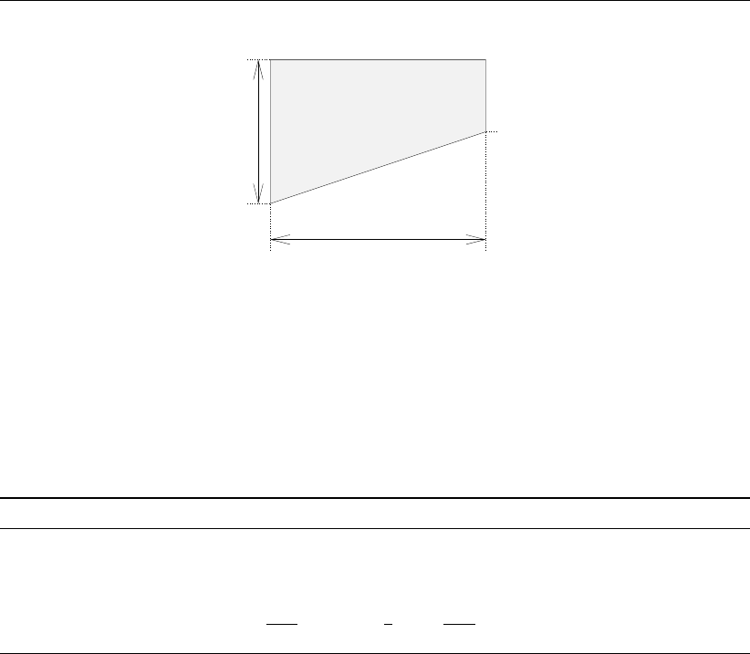
DRAFT
D-Flow Flexible Mesh, Technical Reference Manual
Auj
huj
min(bl1j, bl2j)
wuj
max(bl1j, bl2j)
ζiup(j)
l(j)
r(j)
Figure 6.4: Flow area Aujand face-based water depth huj
Wet cross-sectional area Auj
By the flow area Aujthe wet cross-sectional area of the face jis meant. Since the bed level
in face jis linearly varying from bl1jto bl2j, and the water in the face is assumed at constant
level min(bl1j, bl2j) + huj, the wet area can be computed with Algorithm (3). Note that wuj
Algorithm 3 setau: compute the flow area Auj
∆blj= max(bl1j, bl2j)−min(bl1j, bl2j),(6.15)
Auj=(wujhuj,if ∆blj< δwuj,
wujhujmin( huj
∆blj,1) 1−1
2min(∆blj
huj,1),otherwise.(6.16)
is the width of face j, see Figure 6.4, and ∆bljis the cross-sectional bed variation.
Remark 6.2.3.The exception for the case ∆blj< δwujwith δ= 10−3in Equation (6.16)
should maybe be reconsidered.
Remark 6.2.4.In case of bed level type 3and conveyance types ≥1, the bed is assumed
lineary varying within a face, see Algorithm (1). This is accounted for in the computation
of the wet cross-sectional areas of the vertical faces, see Algorithm (3). A linearly varying
bed, on the other hand, is not accounted for in the computation water column volumes Vkin
Algorithm (20), without non-linear iterations (explained later). This seems inconsistent when
we are employing a finite volume approximation as in e.g. Equation (6.12).
Total area of a cell
The definition of variables to determined the total area of a computational cell are depicted in
Figure 6.5.
38 of 152 Deltares
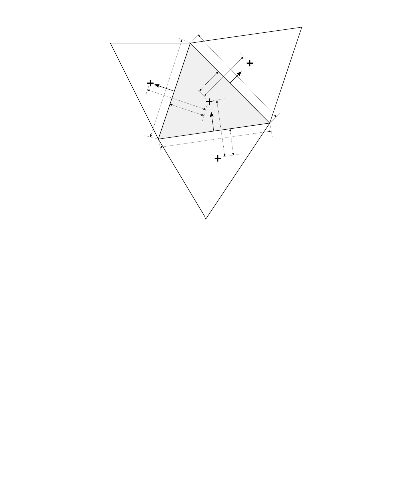
DRAFT
Numerical approach
α1
α2
α3
∆x2
∆x3
∆x1
21
3
wu2
wu3
wu1
Ω1
Figure 6.5: Area computation for cell Ω1
The total area Aof cell Ωkis determined as follows:
A(Ωk) = X
j∈J (Ωk)|L(j)=k
αj∆xjwuj +X
j∈J (Ωk)|L(j)6=k
(1 −αj)∆xjwuj (6.17)
An example for area Ω1is:
A(Ω1) = 1
2α1∆x1wu1+1
2α2∆x2wu2+1
2(1 −α3)∆x3wu3(6.18)
6.2.2 Momentum equation
The momentum equation read
∂u
∂t +1
h(∇•(huu)−u∇•(hu)) = −g∇ζ+1
h∇•(νh(∇u+∇uT)) + 1
h
τ
ρ,
(6.19)
and is discretized at the faces and in face-normal direction, see Figure 6.6.
Deltares 39 of 152
DRAFT
D-Flow Flexible Mesh, Technical Reference Manual
αj∆xj
∆xj
wuj
L(j)R(j)
nj
Figure 6.6: Computational cells L(j)and R(j)neighboring face j; water levels are stored
at the cell circumcenters, indicated with the +-sign
In this figure ∆xjis the distance between the two neigboring cell centers, i.e. ∆xj=
kxR(j)−xL(j)k, and wujis, as explained before, the width of face j.
Making use of the properties of an orthogonal mesh, the water level-gradient term projected
in the face-normal direction is discretized as
g∇ζ|j•nj≈g
∆xj
(ζR(j)−ζL(j)).(6.20)
The bed friction term is discretized as
1
h
τ
ρj
•nj≈ −gkujk
C2ˆ
hj
uj,(6.21)
where ˆ
hjacts as an hydraulic radius whose computation depends on the "conveyance type".
Its precise discretization is discussed later (see Algorithm (12) and Algorithm (13)). The mag-
nitude of the velocity is computed by: kujk=qu2
j+v2
j. Furthermore, advection and
diffusion are discretized as
1
h(∇•(huu)−u∇•(hu)) −1
h∇•(νh(∇u+∇uT))j
•nj≈ Aijuj+Aej.(6.22)
The terms Aij(implicit part) and Aej(explicit part) will be discussed in more detail hereafter.
These terms play an important role in the D-Flow FM code and are called advi and adve,
respectively.
Summing up, the spatial discretization of Equation (6.6) reads
duj
dt=−g
∆xjζR(j)−ζL(j)− Aijuj− Aej−gkujk
C2ˆ
hj
uj.(6.23)
40 of 152 Deltares

DRAFT
Numerical approach
Momentum advection
It would be a clear advantage if the momentum equation was discretized conservatively, es-
pecially for flows with discontinuities such as hydraulic jumps. This is not easily achieved in
case of staggered, unstructured meshes. Nonetheless, Perot (2000) shows how to achieve
momentum conservation in similar circumstances for the incompressible Navier Stokes equa-
tions. This approach is applied to the shallow water equations in Kramer and Stelling (2008)
and Kleptsova et al. (2010). However, subtleties exist in the formulations as pointed out in
Borsboom (2013). The various advection schemes in D-Flow FM differ on these subtleties.
The difficulty with the staggered layout on unstructured meshes is that we only solve the
momentum equation in face-normal direction. We could, in principle, formulate a control vol-
ume for each face-normal velocity, but are unable to define conservative fluxes, as we do
not solve for the whole momentum vector, as we would do with a collocated arrangement of
the unknowns. To this end, Perot (2000) pursues conservation of the full reconstructed cell-
centered momentum vector. The advection operator is firstly discretized at cell centers, as
if we were dealing with a collocated layout of our unknowns, and subsequently interpolated
back to the faces and projected in face-normal direction.
Remark 6.2.5.Perot (2000) shows that the reconstruction from face-normal quantities to
cell-centered vectors and the interpolation from cell-centered vector to face-normal quanti-
ties need to satisfy certain demands. We are not free to choose a reconstruction to our liking
and the accuracy may even be compromised on irregular meshes.
The application of this approach to the shallow-water equations as in Kramer and Stelling
(2008) and Kleptsova et al. (2010) is non-trivial. Complicating matters significantly is that we
are not solving in conservative, but in primitive variables. As pointed out in Borsboom (2013),
the discretization of advection is subject to many subtleties. In D-Flow FM various advection
schemes exist that vary on these subtleties.
Remark 6.2.6.It’s fair to say that, formally speaking, none of the momentum advection
schemes in D-Flow FM is conservative in the sense of Perot (2000).
The approach in Perot (2000) is as follows. Given some cell k, assume that cell-centered
conservative advection is approximated by
∇•(huu)|Ωk≈ak.(6.24)
Face-normal advection at face jis then interpolated from its neighboring cells L(j)and R(j)
as
∇•(huu)|Γj•nj≈αjaL(j)+ (1 −αj)aR(j)•nj,(6.25)
where αjis the non-dimensional distance from the left cell center to the face, see Figure 6.6.
Note that the terms −u∇•(hu)and 1
hin Equation (6.22) are due to our non-conservative
formulation and do not appear in Equation (6.25). In the non-conservative formulation of
Equation (6.22), their discretization contributes significantly to the subtle differences in the
various schemes. See Borsboom (2013) for more details.
The cell-centered advection is discretized as
ak=1
A(Ωk)X
j∈J (k)
uujqjsj,k,(6.26)
where uujis the reconstructed full velocity at the faces and A(Ωk)the area of the control
volume Ωk, i.e. the cell. It is reconstructed from the cell-centered velocities ucwith an upwind
Deltares 41 of 152

DRAFT
D-Flow Flexible Mesh, Technical Reference Manual
scheme, e.g.
uuj=uL(j), uj≥0,
uR(j), uj<0.,(6.27)
or with a higher-order limited version, discussed later. The cell-centered velocities in turn are
reconstructed from the (primitive) face-normal velocities with Algorithm (6), also discussed
later. Furthermore, flux qjis derived from the face-normal velocity as
qj=Aujuj,(6.28)
see also Algorithm (21), explained later when we will discuss the time discretization.
The term −u∇•(hu)is the so-called "storage term" and is due to our non-conservative for-
mulation of the momentum equation. It originates from the substitution of the continuity equa-
tion in the conservatively formulated momentum equation. Glancing ahead at our temporal
discretization, we observe the following. If we want our discretization to be discretely conser-
vative, we need to substitute the continuity equation after spatial and temporal discretization,
see Equation (6.108) (explained later). This means that we require the fluxes in the storage
term to be identical to the fluxes in the discrete continuity equation, Equation (6.97), i.e. qn+1
j,
where ndenotes the time level:
−u∇•(hu)|n
k≈ − u
A(Ωk)X
j∈J (k)
qn+1
jsj,k,(6.29)
where we do not mention at which time level term u
A(Ωk)is to be evaluated. Equation (6.29)
leads to an implicit contribution to the discrete advection for θ > 0. However, in D-Flow FM
the storage term is always discretized explicitly in time. It is based on explicit fluxes qn
jor on
qan
j, depending on the advection scheme.
Remark 6.2.7.Since the fluxes in the storage term are at the old time level, in contrast to
the fluxes in the continuity equation, advection in D-Flow FM is non-conservative for non-
stationary flows and θ > 0.
Given the discretization of the conservatively formulated advection of Eqns. ((6.25)) and
((6.26)) and the storage term of Equation (6.29), the advection can now be composed in
general form as
Aej=ALjP
l∈J ∗(L(j))
q∗
lsl,L(j)uul•nj−q∗∗
lsl,L(j)(1 −θl,L(j))u∗
Lj+
ARjP
l∈J ∗(R(j))
q∗
lsl,R(j)uul•nj−q∗∗
lsl,R(j)(1 −θl,R(j))u∗
Rj,(6.30)
and
Aij=−ALjX
l∈J ∗(L(j))
q∗∗
lsl,L(j)θl,L(j)−ARjX
l∈J ∗(R(j))
q∗∗
lsl,R(j)θl,R(j),(6.31)
where J∗,q∗
l,q∗∗
l,θl,{L,R}(j),u∗
{L,R}j,ALj,ARjvary for the different advection schemes as
described in Algorithm (4) and Jiis the set of faces with inward fluxes, i.e.
Ji(k) = {j∈ J(k)|ujsj,k <0}(6.32)
and
huvj= max(αjhζL(j)+ (1 −αj)hζR(j), εhζ),(6.33)
42 of 152 Deltares

DRAFT
Numerical approach
where εhζis a threshold. θl,L(j)and θl,R(j)are determined by their face-based Courant
numbers σj,L(j)and σj,R(j)as follows
θl,{L,R}(j)=1
1−σj,{L,R}(j)
(6.34)
where σj,L(j)and σj,R(j)are computed as:
σj,L(j)=
1.4∆t|qaj|
αjVL(j)+(1−αj)VR(j),P
j∈J (L(j))
1 = 3,
∆t|qaj|
αjVL(j)+(1−αj)VR(j),other,
(6.35)
and
σj,R(j)=
1.4∆t|qaj|
αjVL(j)+(1−αj)VR(j),P
j∈J (R(j))
1=3,
∆t|qaj|
αjVL(j)+(1−αj)VR(j),other,
(6.36)
respectively.
Algorithm 4 advec: compute advection terms of the form
1
h(∇•(huu)−u∇•(hu))j•nj≈ Aijuj+Aej
compute higher-order accurate reconstructions of face-based velocity vector uufrom cell-
centered velocity vectors ucwith Algorithm (10)
compute Aeand Ai:
Aej=ALjX
l∈J ∗(L(j))
q∗
lsl,L(j)uul•nj−q∗∗
lsl,L(j)(1 −θl,L(j))u∗
Lj+
ARjX
l∈J ∗(R(j))
q∗
lsl,R(j)uul•nj−q∗∗
lsl,R(j)(1 −θl,R(j))u∗
Rj(6.37)
Aij=−ALjX
l∈J ∗(L(j))
q∗∗
lsl,L(j)θl,L(j)−ARjX
l∈J ∗(R(j))
q∗∗
lsl,R(j)θl,R(j)
(6.38)
See Table 6.1 for the definition of the variables used in this algorithm.
Where Note that VAuL(j)and VAuR(j)are undefined.
Cell center interpolation
We saw in the previous section that the cell-centered reconstructed full velocity vector ucplays
an important role in the discretization of the momentum advection. This section elaborates on
its computation.
Following Perot (2000), and taking a cell kas a control volume, the full cell-centered veloc-
ity vector can be reconstructed from the face-normal components ujby using the following
approximation
uck≈1
A(Ωk)Z
Ωk
∇•(u(x−xck)) dΩ = 1
A(Ωk)Z
∂Ωk
(x−xck)u•ndΓ,(6.39)
where Ωkis the control volume, i.e. the cell k,∂Ωkthe boundary of the control volume,
A(Ωk)its area and nis an outward orthonormal vector.
Deltares 43 of 152

DRAFT
D-Flow Flexible Mesh, Technical Reference Manual
Table 6.1: Definition of the variables used in Algorithm (4)
iadv J∗q∗
lq∗∗
lθl,{L,R}(j)u∗
{L,R}jALjARj
0 - - - - 0 0
1Jqalql0uj1
VL(j)+VR(j)
1
VL(j)+VR(j)
2Jqalqal0uj1
VL(j)+VR(j)
1
VL(j)+VR(j)
3, 33 Jqalqal0ujαj
αjVL(j)+(1−αj)VR(j)
1−αj
αjVL(j)+(1−αj)VR(j)
4Jiqalqal0ujαj
αjVL(j)+(1−αj)VR(j)
1−αj
αjVL(j)+(1−αj)VR(j)
5Jqalqalmax(1 −1
σl,{L,R}(j),0) ujαj
αjVL(j)+(1−αj)VR(j)
1−αj
αjVL(j)+(1−αj)VR(j)
6Jiqalqalmax(1 −1
σl,{L,R}(j),0) ujαj
αjVL(j)+(1−αj)VR(j)
1−αj
αjVL(j)+(1−αj)VR(j)
7,9,11 Jqalqal1ujαj
αjVL(j)+(1−αj)VR(j)
1−αj
αjVL(j)+(1−αj)VR(j)
8,10,12 Jiqalqal1ujαj
αjVL(j)+(1−αj)VR(j)
1−αj
αjVL(j)+(1−αj)VR(j)
30 Jqalqal0uj1
VL(j)+VR(j)
1
VL(j)+VR(j)
31 Jqalqal0uc{L,R}(j)•njαj
VL(j)
1−αj
VR(j)
34 Jqalqal0ujαj
huvjbAL(j)
1−αj
huvjbAR(j)
36 Jqlql0ujαj
VL(j)
1−αj
VR(j)
37 Jqlql0ujαj
huvjbAL(j)
1−αj
huvjbAR(j)
38 Jqlql0uc{L,R}(j)•njαj
VAuL(j)
1−αj
VAuR(j)
333 Jqalqal0ujαj
VAuL(j)
1−αj
VAuR(j)
Remark 6.2.8.We will not discuss whether uckrepresents a cell-averaged or nodal value.
Nevertheless, Equation (6.39) is a second order approximation if the center point is sufficiently
close to the mass center of the control volume. Note: that in our case the center point is the
cell circumcenter, which can deviate considerably from the mass center for irregular meshes.
The discretization of Equation (6.39) in cell kis
uck=X
j∈{l∈J (k)|sl,k=1}
wcLjuj+X
j∈{l∈J (k)|sl,k=−1}
wcRjuj(6.40)
44 of 152 Deltares

DRAFT
Numerical approach
with weight vectors wcLjand wcRjare computed with Algorithm (5), where bAkis the bed
area of cell k.
Algorithm 5 setlinktocenterweights: compute weight vectors wcLjand wcRjin the cell-
center reconstruction of Equation (6.40)
wcLj=αj∆xjnjwuj
A(ΩL(j))(6.41)
wcRj=(1 −αj)∆xjnjwuj
A(ΩR(j))(6.42)
Remark 6.2.9.Cells that are cut by a dry-wet interface do not get any special treatment,
i.e. dry faces (with formally undefined velocities) still appear in the reconstruction, with as-
sumed zero velocity. Hence, cell centered velocity vectors near the dry-wet interface may be
inconsistent with the local flow.
The cell centered velocities are computed with Algorithm (6), where hζkis the cell centered
water depth at cell k, defined as hζk=ζk−blζ. Note that uqis a ‘discharge-averaged’
Algorithm 6 setucxucyucxuucyu: reconstruct cell centered velocity vectors ucand uq, and
set first-order upwind fluxes uL
u
uqk=1
hζk
X
j∈J (k)|L(j)=k
hujwcLjuj+X
j∈J (k)|R(j)=k
hujwcRjuj
(6.43)
if iPerot = 2 then
uck=uqk(6.44)
else
uck=X
j∈J (k)|L(j)=k
wcLjuj+X
j∈J (k)|R(j)=k
wcRjuj(6.45)
end if
uuj=
ucL(j), qaj>0
ucR(j), qaj<0
0, qaj= 0
(6.46)
reconstructed velocity vector. It is used for the tangential velocity vjcomponent at the faces:
vj=αjuqL(j)+ (1 −αj)uqR(j)×nj(6.47)
Remark 6.2.10.It is not hard to see that the interpolation of uqmay be inconsistent, depend-
ing on the "bed level type", see Algorithms (1) and (2), and the bed geometry itself.
Note that Algorithm (6) also sets a first-order upwind approximation of uu, necessary in mo-
mentum advection, see Equation (6.26). Higher order corrections are added in Algorithm (10),
explained later.
Deltares 45 of 152
DRAFT
D-Flow Flexible Mesh, Technical Reference Manual
wuj
R(j)
∆xj
L(j)
αnRjwuj
r(j)
l(j)
Figure 6.7: Nodal interpolation from cell-centered values; contribution from face jto node
r(j); the shaded area indicates the control volume Ωn.
Nodal interpolation
In the discretization of horizontal momentum diffusion and in the bed friction for "conveyance
type" ≥3, node-based velocity vectors unappear. This section elaborates on their compu-
tation.
The nodal velocity vectors are interpolated from the cell-centered velocity vectors uc, which
were, in turn, interpolated from the face-normal velocities u•n, see the previous section.
Given some available cell-centered data, say Φc(e.g. one of the components of the velocity
vector), we can define a control volume as indicated in Figure 6.7 and interpolate to the nodes,
say Φn, as follows:
Φn≈1
2A(Ωn)Z
Ωn
∇•(Φ(x−xn)) dΩ = 1
2A(Ωn)Z
∂Ωn
Φ(x−xn)•ndΓ,(6.48)
where
Ωnis the node-based control volume,
∂Ωnthe boundary of the control volume,
dΓits boundary,
A(Ωn)the area of the control volume,
nthe outward normal vector and
xnare the node coordinates.
Remark 6.2.11.Equation (6.48) is a second order approximation if the node is located suf-
ficiently close to the mass center of the control volume. In the example of Figure 6.7 this is
indeed the case, but not necessarily for general meshes.
The discretization of Equation (6.48) at node iis
Φi=X
j∈{l|l(l)=i}
wLj
1
2(ΦcL(j)+ ΦR(j)) + X
j∈{l|r(l)=i}
wRj
1
2(ΦL(j)+ ΦR(j)),(6.49)
46 of 152 Deltares
DRAFT
Numerical approach
with weights wiLjand wiRjcomputed as
wiLj=
1
2αiLj∆xjwuj
P
l∈{m|l(m)=l(j)}
1
2αiLj∆xlwul+P
l∈{l|r(m)=l(j)}
1
2αiRl∆xlwul
(6.50)
wiRj=
1
2αnRj∆xjwuj
P
l∈{m|l(m)=r(j)}
1
2αiLl∆xlwul+P
l∈{m|r(m)=r(j)}
1
2αiRl∆xlwul
(6.51)
Note that αiLj∆xjand αiRj∆xjapproximate the components of (x−xi)•nin Equa-
tion (6.50) and Equation (6.51) for node iand face j, which in D-Flow FM are computed
as
αiLj=k1
2(xζL(j)+xζR(j))−xil(j)k
k1
2(xζL(j)+xζR(j))−xil(j)k+k1
2(xζL(j)+xζR(j))−xir(j)k,(6.52)
αiRj= 1 −αnLj,(6.53)
where
xζkare the coordinates of cell-center kand
xiare the coordinates of mesh node i, respectively.
Remark 6.2.12.A more straightforward approach, employing the properties of an orthogonal
mesh and using wuj:= kxir(j)−xil(j)k, would be:
αiLj=1
2(xζL(j)+xζR(j))−xil(j)•(xir(j)−xil(j))
wu2
j
.(6.54)
In D-Flow FM the interpolation of cell-centered velocity vectors to nodal velocity vectors is as
in Equation (6.48). That is, when "jacomp" 6= 1 and we do not consider mesh boundaries.
The quantity Φis to be replaced by both components of the velocity vector, respectively, i.e.
ui=X
j∈{l|l(l)=i}
wiLj
1
2(ucL(j)+ucR(j)) + X
j∈{l|r(l)=i}
wiRj
1
2(ucL(j)+ucR(j))
(6.55)
When "jacomp" = 1, however, the two components of the velocity vector (ux, uy), get dif-
ferent weights. If we say uc=: (ucx, ucy)Tand un=: (unx, uny)T, then the interpolation
becomes as performed by Algorithm (7). The weights wnxL,wnxR,wnyLand wnyRare
computed with Algorithm (8), where exand eyare the unit vectors in x- and y-direction re-
spectively. The exceptions at mesh boundaries remain unmentioned.
Remark 6.2.13.For nodes not on the mesh boundary, it is unclear why the weights in Al-
gorithm (7) for vector interpolation should differ from Equation (6.50) and Equation (6.51) for
scalar interpolation, which is the case if "jacomp" = 1 in Algorithm (8). The option "jacomp"
= 1 may need to be reconsidered.
The various variables used in the nodal interpolation have the following names in the D-
Flow FM code:
xζk•ex:xz(k),xζk•ey:yz(k),
xni•ex:xk(i),xni•ey:yk(i),
unxi:ucnx(i),unyi:ucny(i),
αnLj:acn(2,j),αnRj:acn(1,j),
wnxLj:wcnx4(j),wnyLj:wcny4(j),
wnxRj:wcnx3(j),wnyRj:wcny3(j).
Deltares 47 of 152

DRAFT
D-Flow Flexible Mesh, Technical Reference Manual
Algorithm 7 setcornervelocities: interpolate nodal velocity vectors un= (unx, uny)Tfrom
cell-centered velocity vectors uc= (ucx, ucy)T
unxi=X
j∈{l|l(l)=i}
wnxLj
1
2(ucxL(j)+ucxR(j)) +
X
j∈{l|r(l)=i}
wnxRj
1
2(ucxL(j)+ucxR(j))(6.56)
unyi=X
j∈{l|l(l)=i}
wnyLj
1
2(ucyL(j)+ucyR(j)) +
X
j∈{l|r(l)=i}
wnyRj
1
2(ucyL(j)+ucyR(j))(6.57)
Algorithm 8 setlinktocornerweights: compute weights wnxLj,wnxRj,wnyLjand wnyRjin
the nodal interpolation of Algorithm (7), Equation (6.56) and Equation (6.57)
χxj=2 max(10−6,|nj•ex|),jacomp = 1
1,otherwise (6.58)
χyj=2 max(10−6,|nj•ey|),jacomp = 1
1,otherwise (6.59)
if r(j)and l(j)are not boundary nodes then
wnxLj=
1
2αnLj∆xjwujχxj
P
l∈{m|l(m)=l(j)}
1
2αnLj∆xlwulχxj+P
j∈{l|r(m)=l(j)}
1
2αnRl∆xlwulχxj
wnyLj=
1
2αnLj∆xjwujχyj
P
l∈{m|l(m)=l(j)}
1
2αnLj∆xlwulχyj+P
l∈{m|r(m)=l(j)}
1
2αnRl∆xlwulχyj
wnxRj=
1
2αnRj∆xjwujχxj
P
l∈{m|l(m)=r(j)}
1
2αnLl∆xlwulχxj+P
l∈{m|r(m)=r(j)}
1
2αnRl∆xlwulχxj
wnyRj=
1
2αnRj∆xjwujχyj
P
l∈{m|l(m)=r(j)}
1
2αnLl∆xlwulχyj+P
l∈{m|r(m)=r(j)}
1
2αnRl∆xlwulχyj
else
unmentioned, at least one of the nodes is a boundary node
end if
Higher-order reconstruction: limtypmom
A higher-order accurate discretization of advection may be achieved by higher-order accurate
reconstruction of the face-based full velocity vectors uuin Equation (6.26). A first-order ap-
proximation is already available from Algorithm (6), Equation (6.46). This section elaborates
on the higher-order corrections added to uu.
The reconstruction at the faces is a one-dimensional reconstruction on a line through both
neighboring cells L(j)and R(j). Besides the neighboring cell-centered values, a third value
is sought on the line, which is interpolated from cells connected to the left-hand side neigh-
48 of 152 Deltares

DRAFT
Numerical approach
RL2j
L(j)R(j)
nj
CLj
kL2j
kL1j
RL1j
Figure 6.8: Higher-order reconstruction of face-based velocity uuj, from the left
boring cell L(j)for reconstruction from the left, and cells connected to the right-hand side
neighboring cell R(j)for reconstruction from the right, respectively. We will refer the these
third locations on the line as CLjand CRjrespectively. For the reconstruction along the line
a one-dimensional limiter is used with the purpose to obtain a TVD scheme. In D-Flow FM
various limiters are available by means of the option limtypmom.
Remark 6.2.14.It is not immediately clear why a TVD limiter based on interpolated values
would guarantee TVD properties of the primitive variables.
We will firstly consider the stencil for the reconstruction. Assume that we want to reconstruct
at face jfrom the left, then the cells in the stencil are {R(j),L(j), kL1j, kL2j}. An example
is shown in Figure 6.8. If we let RL1jmeasure the distance from the cell center kL1jto the
line through L(j)and R(j), and similarly for RL2j, then the cells kL1jand kL2jare chosen
according to the rules stated in Algorithm (9). These cells are the cells whose circumcenters
are closest to the line through L(j)and R(j).
The values in cells kL1jand kL2jare used to interpolate a value at CLj, which is located on
the line trough the left and right cell centers L(j)and R(j). The higher-order reconstruction
is then performed based on the values of cells CLj,L(j)and R(j)in a one-dimensional
fashion.
A value, say Φ, at CLj, i.e. ΦCLj(being one of the two cell-centered velocity vector compo-
nents as we will see later), is interpolated as follows:
ΦCLj=sL1jΦkL1j+sL2jΦkL2j.(6.60)
The weights are computed with Algorithm (9). Note that the exception for RL1j<0.1∆xj
only adds one cell to the stencil for higher-order reconstruction, mimicking stencils on e.g.
curvilinear meshes. Note also the exception for the (face-specified) advection types 6and 8,
not discussed further.
The interpolation of Equation (6.60) is applied to the Cartesian components of the velocity
vector. In such a manner values at uxCLjand uyCLjare obtained. The reconstruction is
Deltares 49 of 152

DRAFT
D-Flow Flexible Mesh, Technical Reference Manual
Algorithm 9 setupwslopes: determine the cells kL1and kL2, and compute weights sL1and
sL2in Equation (6.60) for the higher-order reconstruction from the left at the faces, and similar
for reconstruction from the right to obtain kR1,kR2,sR1and sR2
if reconstruction from the left then
determine the cells kL1jand kL2jaccording to the following rules
cells kL1jand kL2jeach share a face with cell L(j)
the cell center is at the left-hand side from cell center L(j), i.e. (xζk•nj<0for
k∈ {kL1j, kL2j}
cell center kL1jis closer to the line through cell centers L(j)and R(j)than, or as
close as, any other cell that obeys the two rules above
cell center kL2jis closer to the line through cell centers L(j)and R(j)than, or as
close as, any other cell that is not kL1jand obeys the first two rules above and results
in a intersection point CLjthat is sufficiently far from cell center L(j), as expressed
by (xCLj−xζR(j))•(xζL(j)−xζR(j))>1.2
if RL1j<0.1∆xjand the "advection type" of face between kL1jand L(j)/∈ {6,8}
then
sL1j= 1,sL2j= 0,γLj=∆xj
kxζL(j)−xζkL1jk
else if cell kL2jfound and the "advection type" of faces between kL1jand L(j), and
between kL2jand L(j)/∈ {6,8}then
sL1j=kxCLj−xζkL2jk
kxζkL1j−xζkL2jk,sL2j= 1 −sL1j,γLj=∆xj
kxζL(j)−xCLjk
else
sL1j= 0,sL2j= 0,γLj= 0 (no higher-order reconstruction)
end if
else
similar as reconstruction from the left by replacing Lwith R, vice versa, and taking the
reversed orientation into account
end if
then performed with Algorithm (10). Note that in Algorithm (10), Equation (6.63) and Equa-
tion (6.64),γLjaccounts for the non-uniform spacing along the line through cell centers L(j)
and R(j). It is computed along with the stencil and weights in Algorithm (9) and similarly for
γRj.
In D-Flow FM various limiters (Ψin Algorithm (10)) are available. They are set with the
keyword limtypmom, see Table 6.2.
Remark 6.2.15.In the D-Flow FM limiters 1to 4are formulated using the property Ψ(r) =
rΨ(1
r)for symmetric limiters. Since the Koren limiter is not symmetric, its implementation is
incorrect. Limiters 11,12 and 13 are also incorrect implementations.
Remark 6.2.16.Since the limiter functions are non-linear in general, and the velocity field
is represented by face-normal components, the component-wise reconstruction is orientation
dependent. Hence, the discretization is not invariant for a rotation of the coordinate frame.
This may be circumvented by reconstructing face-normal and tangential components instead.
The translation of the various variables introduced here to the D-Flow FM code is as follows:
50 of 152 Deltares
DRAFT
Numerical approach
Algorithm 10 sethigherorderadvectionvelocities: higher-order accurate reconstructions of
face-based velocity vector uufrom cell-centered velocity vectors uc
interpolate velocity vectors on a line through cell centers L(j)and R(j), from the left and
from the right:
uCLj=sL1juckL1j+sL2juckL2j(6.61)
uCRj=sR1juckR1j+sR2juckR2j(6.62)
if qaj>0then
compute slope ratio in limiter, for each velocity component
rx=ucR(j)x−ucL(j)x
ucL(j)x−uCLjx
1
γLj
(6.63)
ry=ucR(j)y−ucL(j)y
ucL(j)y−uCLjy
1
γLj
(6.64)
apply limiter Ψto each velocity component and reconstruct the velocity vector at the face
uuj=ucL(j)+αjmax(1−∆t|uj|
∆xj
,0) Ψ(rx) 0
0 Ψ(ry)(ucR(j)−ucL(j))(6.65)
else
reconstruction from the right similar as reconstruction from the left by replacing Lwith
R, vice versa, αjby 1−αjand taking the reversed orientation into account
end if
Table 6.2: Various limiters available in D-Flow FM for the reconstruction of face-based
velocities in momentum advection
limtypmom limiter Ψ(r)
0first-order upwind 0
1,5,15 minmod max(min(r, 1),0)
2Van Leer r+|r|
1+|r|
3incorrect Koren rmax(min(min(2/r, 1+2/r
3),2),0)
4,14 monotonized central max(min(min(2r, 1+r
2),2),0)
11 incorrect minmod 1
rmax(min(r, 1),0)
12 incorrect Van Leer 1
r
r+|r|
1+|r|
13 another incorrect Koren max(min(min(2/r, 1+2/r
3),2),0)
20 Beam-Warming r
21 Lax-Wendroff 1
kL1j:klnup(1,j),kR1j:klnup(4,j),
kL2j:klnup(2,j),kR2j:klnup(5,j),
sL1j:slnup(1,j),sR1j:slnup(4,j),
sL2j:slnup(2,j),sR2j:slnup(5,j),
γLj:slnup(3,j),γRj:slnup(6,j).
Deltares 51 of 152
DRAFT
D-Flow Flexible Mesh, Technical Reference Manual
Momentum diffusion
The momentum diffusion term in Equation (6.6) is
1
h∇•(νh(∇u+∇uT)).
In D-Flow FM, this term is modified as
1
hp∇•(νhp(∇u+∇uT)),
where
p=(1,istresstype = 3,
1,istresstype = 5,
0,otherwise.
(6.66)
Remark 6.2.17.It is unclear why, for istresstype 6= 3 ∧istresstype 6= 5, a
modified, incorrect form of momentum diffusion, i.e. p6= 1, is employed in D-Flow FM.
Obviously, the momentum diffusion term needs to be discretized at the faces and projected in
face normal direction. The approach undertaken is similar to the discretization of momentum
advection. First a cell-centered conservative discretization of ∇•(νh(∇u+∇uT)) is for-
mulated which is subsequently interpolated to the faces, projected in the face normal direction
and divided by a water level hto bring it in non-conservative form.
If we call the cell-centered discretization dk, or more precisely
∇•νhp(∇u+∇uT)Ωk≈dk,(6.67)
then the face-normal momentum diffusion at face jis interpolated from its neighboring cells
L(j)and R(j)as
∇•(νhp(∇u+∇uT))Γj•nj≈αjdL(j)+ (1 −αj)dR(j)•nj,(6.68)
where again αjis the non-dimensional distance from the left cell center to the face, see
Figure 6.6.
The cell-averaged diffusion in cell kcan be written in the usual manner as
∇•νhp(∇u+∇uT)Ωk=1
A(Ω) Z
∂Ωk
νhp(∂u
∂n +∇u•n)dΓ,(6.69)
where A(Ωk) = bAkis the bed area of cell k. This expression is discretized as
∇•νhp(∇u+∇uT)Ωk≈dk=
1
bAkP
j∈J (k)
tujwujsj,k, p = 0,
1
bAkP
j∈J (k)
tujwujmin(hζL(j), hζR(j))sj,k, p = 1,istresstype = 3,
1
bAkP
j∈J (k)
tujAujsj,k, p = 1,istresstype = 5.
(6.70)
52 of 152 Deltares
DRAFT
Numerical approach
Note that tjis the viscous stress at face j. By using n= (nx, ny)T, setting s=n⊥=
(−ny, nx)Tand noting that
∇u•n=nx−ny
nynx
n•∂u
∂n
n•∂u
∂s
=nx2nxny
nxnyny2∂u
∂n +−nxny−ny2
nx2nxny∂u
∂s ,
the viscous stresses tujfor istresstype 6= 6 are computed as
tuj=νj 1 + nx2
jnxjnyj
nxjnyj1 + ny2
jucR(j)−ucL(j)
∆xj
+
−nxjnyj−ny2
j
nx2
jnxjnyjunl(j)−unr(j)
wuj.
(6.71)
For istresstype = 6 the viscous stresses are completely expressed in normal and tan-
gential components and essentially the same expression as Equation (6.71) is obtained.
Note that uck(here with k∈ {L(j),R(j)}) and uni(here with i∈ {l(j),r(j)}) are cell-
centered and node-based velocity vectors, respectively. Their reconstruction from the face-
normal velocity components and interpolation has been discussed in the foregoing sections,
see Algorithms (6) and (7) respectively.
The contribution of the horizontal momentum diffusion term to the discrete momentum equa-
tion Equation (6.23) is finally obtained by bringing it in non-conservative form and interpolation
at the faces
Aej=−αjdL(j)
HLp
j
+(1 −αj)dR(j)
HRp
j•nj,(6.72)
as performed by Algorithm (11). It shows that the choice for HLjand HRjdepends on
istresstype.
Algorithm 11 setumod|momentum diffusion: compute momentum diffusion terms of the form
nj•−1
hpνhp(∇u+∇uT)j≈ Aej
compute viscous stresses
tl=νl 1 + nx2
lnxlnyl
nxlnyl1 + ny2
lucR(l)−ucL(l)
∆xl
+−nxlnyl−ny2
l
nx2
lnxlnylunl(l)−unr(l)
wul
Aej=−
αj
bAL(j)HLjX
l∈J (L(j))
νlAltl•njsl,L(j)+1−αj
bAR(j)HRjX
l∈J (R(j))
νlAltl•njsl,R(j)
with Al,HLj,HRjdefined by:
istresstype AlHLjHRj
2, 4, 6 wul1 1
3wulmin(hζL(l), hζR(l))1
2(hζL(j)+hζR(j))1
2(hζL(j)+hζR(j))
5AulhζL(j)hζR(j)
Remark 6.2.18.Momentum diffusion is discretized in a similar fashion as momentum advec-
tion, namely based on a cell-centered expression of the conservative formulation, interpolation
to the faces and bringing it into a non-conservative form, i.e. dividing it by the water depth.
Deltares 53 of 152
DRAFT
D-Flow Flexible Mesh, Technical Reference Manual
Consequently, the discretizations of the terms 1
HLjand 1
HRj, due to the non-conservative for-
mulation, are expected to equal their counterparts in momentum advection. However, they do
not, as can be seen by comparing Algorithm (11) with Algorithm (4).
Remark 6.2.19.In the discretization of the diffusive fluxes, the area of face jis approximated
by wujmin(hζL(j), hζR(j))for istresstype ’3’. It is unclear why the actual cross-sectional
area Aujdoes not suffice. For the other istresstypes, see Remark 6.2.17.
Turbulence modelling: Smagorinsky, Elder
For istresstype 2and 3, the viscosity coefficient νjcan be computed with Elder’s formula
or a Smagorinsky model. Note that the background viscosity is added, not mentioned here
further for simplicity. In the first case, it is
νj=Eκ
6huj
√g
Cqu2
j+v2
j,(6.73)
where Eis the user-specified Elder coefficient and Cis the (time- and space varying) Chézy
coefficient. And in case of the Smagorinsky model
νj=CSp∆xjwuj2s2∂un
∂n
2
+∂un
∂t +∂ut
∂n 2
+ 2∂ut
∂t
2j
,(6.74)
where CSis a user-specified Smagorinsky coefficient and the velocity derivatives at face j
are approximated with finite differences similarly to Equation (6.71).
Limitation of viscosity coefficient
The explicit time integration of momentum diffusion is subject to a time-step limitation for
numerical stability. We however maintain our time step and limit the eddy viscosity coefficient
instead. We assume that it is sufficient to consider the model equation
∂u
∂t =∇•(ν∇u)⇒ZΩ
∂u
∂t dv=IS
ν∇udS(6.75)
We also assume that it is sufficient to only consider a cell-based discretization, for cell kit
would be
ucn+1
k−ucn
k
∆t=1
Vn
kX
j∈J (k)
νjAun
j
un
R(j)−un
L(j)
∆xj
sj,k.(6.76)
Remark 6.2.20.If we disregard the differences due the interpolation to the faces, and the
missing terms ∇•(hν∇uT), the discretization of the model equation only conforms to the
form of the momentum diffusion term if istresstype=5, and if Vk=bAkhζk(no non-linear
iterations, see Algorithm (20)), as can be seen by comparing with Algorithm (11).
Equation (6.76) can be rewritten as
ucn+1
k=
1−∆t
Vn
kX
j∈J (k)
νjAun
j
∆xj
ucn
k+∆t
Vn
kX
j∈J (k)
νjAun
j
∆xj
un
O(k,j),(6.77)
where O(k, j) = is the cell that shares face jwith cell k, i.e.
O(k, j) = L(j) + R(j)−k. (6.78)
54 of 152 Deltares
DRAFT
Numerical approach
We require that
0≤∆t
Vn
kX
j∈J (k)
νjAun
j
∆xj≤1,(6.79)
which is satisfied if we limit the viscosity coefficient by
νj≤1
N
∆xj
Aun
j∆tmin(Vn
L(j), V n
R(j)),(6.80)
where Nis the maximum number of faces in a cell. It is set to N= 5, although cells with
more than five faces may occasionally be encountered.
Boundary stresses: irov
The viscous stress in Equation (6.70) at the closed boundaries need special attention, where
three conditions that may be applied:
irov=0: full slip,
irov=1: partial slip,
irov=2: no slip.
The boundary conditions are further explained in Section 6.4.7.
Bed friction
The bottom friction can be expressed on the flow links as follows,
1
h
τ
ρj
•nj≈ −gkujk
C2ˆ
hj
uj,(6.81)
where ˆ
hj=Aj/Pjand Aj=hjdyj, as shown in Figure 6.9 The Chézy formula for deter-
mining the velocity is:
uj=Cqˆ
hji(6.82)
qj=AjCqˆ
hji=Ajˆ
h2/3
j
n√i(6.83)
Q=X
j
qj=PAjˆ
h2/3
j
n√i=K√i(6.84)
U=Q
A=K
A√i=
1
nPAjˆ
h2/3
j
PAj
√i(6.85)
Cfu =g
C2ˆ
hj
=g PAj
1
nPAjˆ
h2/3
j!2
=gA
K2
(6.86)
where ˆ
hjand Kvary for different conveyance schemes. The differences in the various
schemes are in the way of defining the hydraulic radius ˆ
hjand Kin Equation (6.86).
In D-Flow FM we have as a default setting of Ibedlevtype=3. This is applied for estimation
of the bedlevel at flow links. It assumes variation in cross flow direction of the local waterdepth,
Deltares 55 of 152
DRAFT
D-Flow Flexible Mesh, Technical Reference Manual
flow velocity and friction coefficient. This is called the analytic 2D conveyance method (type
3). This method shows good grid convergence. A more simple variant is 1D conveyance
(type 2). Another method is only by taking the variation of the waterdepth into account across
flow links, which leads to a hydraulic radius equal to the cross-sectional area divided by the
wet perimeter (type 1). These methods are described in Algorithm (12). For derivation of
formulations in Algorithm (12) we refer the reader to Appendix A.
When assuming a constant bedlevel at a flow link, one can either average between bedlevels
at waterlevel points (type 0), or between the levels of two cornerpoints (type -1). The former
one leads to lower bed friction in general, because the bedlevel at a waterlevelpoint is taken
as the lowest connect link level. Formulations for conveyance types -1 and 0 are shown in
Algorithm (13).
Algorithm 12 getprof2D: compute conveyance types 1, 2 and 3.
ˆ
hj=Aj/Pj(6.87)
γi=nαi1 + α2
i1/4(6.88)
γ0
i=nαi1 + α2
i+α02
i1/4
(6.89)
K2=3
8h8/3
i−h8/3
i+1/γi(6.90)
K3=βi−hi
δ
αiK2+3
11
δ
αiγ0
ih11/3
i−h11/3
i+1 (6.91)
Cfu =
g/C2ˆ
hj,conveyance type = 1,
g(Aj/K2)2,conveyance type = 2,
g(Aj/K3)2,conveyance type = 3,
(6.92)
Algorithm 13 setcfuhi: compute conveyance types 0 and -1.
Cfu =g
C2ˆ
hj
(6.93)
where
ˆ
hj=max (εh, huj),conveyance type =−1,
max (εh, huvj),conveyance type = 0,(6.94)
Coriolis forces
[yet empty]
6.3 Temporal discretization
The spatial discretization is, as explained in section 6.2, performed in a staggered manner,
i.e. velocity normal components ujare defined at the cell faces j, with face normal vector nj,
and the water levels ζkat cell centers k. If advection and diffusion are spatially discretized as
in Equation (6.22)
1
h(∇•(huu)−u∇•(hu)) −1
h∇•(νh(∇u+∇uT))j
•nj≈ Aijuj+Aej,
56 of 152 Deltares
DRAFT
Numerical approach
then the temporal discretization of Equation (6.6) is
1
∆t+Ain
j+gkˆ
ujk
C2hun+1
j=1
∆tun
j−gθj
∆xjζn+1
R(j)−ζn+1
L(j)
− Aen
j−g(1 −θj)
∆xjζn
R(j)−ζn
L(j),(6.95)
where superscript ndenotes the time level, ˆ
ujis obtained by substituting ˆ
uj= (ˆuj,un
j•
n⊥
j)T,un+1
j= ˆuj,θj= 0 in Equation (6.95) and solving for ˆuj, and ∆xj=kxR(j)−xL(j)k
measures the distance between the two water level points of cells L(j)and R(j)of face j.
Note that we have assumed that the face normal njis in the direction from cell L(j)to R(j).
The velocity update of Equation (6.95) is summarized as
un+1
j=−fun
j(ζn+1
R(j)−ζn+1
L(j)) + run
j,(6.96)
where fun
jand run
jare determined iteratively by Algorithm (14).
Algorithm 14 furu: compute fun
jand run
jin un+1
j=−fun
j(ζn+1
R(j)−ζn+1
L(j)) + run
j
ˆu(0)
j=ujn
p= 0
while p < MAXITER ∧ |ˆu(p)
j−ˆu(p−1)
j|> ε∨i= 0 do
p=p+ 1
frj=g
C2hq(ˆu(p−1)
j)2+ (vjn)2
Bu=1
∆t+Aij+frj
fun
j=1
Bu
gθj
∆xj
run
j=1
Bu1
∆tun
j− Aej−g(1 −θj)
∆xjζn
R(j)−ζn
L(j)
ˆu(p)
j=−fun
j(ζn
R(j)−ζn
L(j)) + run
j
end while
Here MAXITER = 4,ε= 10−2is a tolerance and vjis the tangential velocity component at
face jwhose computation is discussed on a different occasion.
The continuity equation is discretized as
Vn+1
k−Vn
k
∆t=−X
j∈J (k)
Aujnθjujn+1 + (1 −θj)ujnsj,k,(6.97)
where J(k)is the set of faces that bound cell kand sj,k accounts for the orientation of face
jwith respect to cell k, i.e.
sj,k =1,L(j) = k(njis outward normal of cell k),
−1,R(j) = k(njis inward normal of cell k). (6.98)
Deltares 57 of 152

DRAFT
D-Flow Flexible Mesh, Technical Reference Manual
Furthermore, Vn+1
kis the volume of the water column at cell kand Aujapproximates the
flow area of face j, i.e.
Auj=hujwj,(6.99)
with hujthe water level at face j(details not discussed here) and wjthe width of face j.
Substitution of Equation (6.96) in Equation (6.97) yields the following system for the water
column volume at the next time instant:
Vn+1
k−Vn
k
∆t+X
j∈J (k)
Aun
jθjfun
jζn+1
k−X
j∈J (k)
Aun
jθjfun
jζn+1
O(k,j)=
−X
j∈J (k)
Aun
j(1 −θj)un
j+θjrun
jsj,k,(6.100)
where O(k, j) = is the cell that shares face jwith cell k, i.e.
O(k, j) = L(j) + R(j)−k. (6.101)
Remark 6.3.1.The flow area of face j,Auj, always appears explicitly in the continuity equa-
tion, Equation (6.97).
The water level equation, Equation (6.100), is summarized as
Vn+1
k−Vn
k
∆t+Bn
kζn+1
k+X
j∈J (k)
Cn
jζn+1
O(k,j)=dn
k,(6.102)
where the coefficients Bn
k(diagonal entries), Cn
j(off-diagonal entries) and dn
k(right-hand
side) are computed by Algorithm (15).
Algorithm 15 s1ini: compute the matrix entries and right-hand side in the water level equation
Vn+1
k−Vn
k
∆t+Bn
kζn+1
k+P
j∈J (k)
Cn
jζn+1
O(k,j)=dn
k,Equation (6.102)
Cn
j=−Aun
jθjfun
j
Bn
k=−X
j∈J (k)
Cn
j
dn
k=−X
j∈J (k)
Aun
j(1 −θj)un
j+θjrun
jsj,k
The continuity equation is only applied at water level cells that are or may become (partially)
wet at the next time level. These cells are marked with kfs(k) = 1 and is based on the water
level of the surrounding faces, see Algorithm (16).
Algorithm 16 setkfs: mark the water level cells that are or may become (partially) wet with
kfs(k)=1
kfs(k) = 0,huj= 0 ∀j∈ J(k),
1, otherwise.
58 of 152 Deltares

DRAFT
Numerical approach
Algorithm 17 pack_matrix: determine the set Kof water level cells for which the continuity
equation is solved
mark wet/dry cells, Algorithm (16)
K={k:kfs(k)=1}
The resulting set of water level cells is called K, see Algorithm (17). The continuity equation
is only applied at cells kfor k∈ K.
In order to solve Equation (6.102), we need to express the Vn+1
kvolume of the water column
at cell kat time level n+ 1 in terms of the water level ζn+1. Since this relation is non-linear
in general, Equation (6.102) is solved iteratively by means of Newton iterations. We firstly
linearize the expression for the volume of the water column and obtain for some iteration p.
Vn+1(p+1)
k=Vn+1(p)
k+An+1(p)
kζn+1(p+1)
k−ζn+1(p)
k,(6.103)
where An+1(p)
kis the wet bed area of cell kat (iterative) time level n+ 1(p). Substitution in
Equation (6.102) yields
1
∆tAn+1(p)
k+Bn
kζn+1(p+1)
k+X
j∈J (k)
Cn
jζn+1(p+1)
O(k,j)=
dn
k−1
∆tVn+1(p)
k−Vn
k−An+1(p)
kζn+1(p)
k,
(6.104)
which is summarized as
Brn+1(p)
kζn+1(p+1)
k+X
j∈J (k)
Crn
jζn+1(p+1)
O(k,j)=drn+1(p)
k,(6.105)
where the coefficients Brn
k(diagonal entries), Crn
j(off-diagonal entries) and drn
k(right-hand
side) are computed by Algorithm (18).
Algorithm 18 s1nod: compute the matrix entries and right-hand side in the water level equa-
tion Brn+1(p)
kζn+1(p+1)
k+P
j∈J (k)
Crn
jζn+1(p+1)
O(k,j)=drn+1(p)
k,Equation (6.105)
Brn+1(p)
k=Bn
k+1
∆tAn+1(p)
k
Crn
j=Cn
j
drn+1(p)
k=dn
k−1
∆tVn+1(p)
k−Vn
k−An+1(p)
kζn+1(p)
k.
Note that we did not describe the water level boundary conditions in Algorithm (18).
The unknown water levels k∈ K in Equation (6.105) are solved with a Krylov solver as will
be explained in section 6.3.1.
During the iterative process, the water level ζn+1(p+1)
kmay have dropped below the bed level
blkresulting in a negative water level. In these cases the time step is repeated with either a
reduced time step with factor f= 0.7(type 1), or the water level cell kis eliminated from
Deltares 59 of 152

DRAFT
D-Flow Flexible Mesh, Technical Reference Manual
Algorithm 19 poshcheck: check positivity of water level
if ζn+1(p+1)
k< blkthen
if type 1 then
∆t=f∆t,
repeat time-step
else if type 2 (default) then
hun
j= 0, j ∈ J(k).
repeat time-step
end if
end if
the system by setting the water levels of its bounding faces to zero (type 2, default), see
Algorithm (19).
Having computed a new iterate of the water level, the water column volume Vn+1(p+1)
kand
wet bed area An+1(p+1)
kof cell kare computed with Algorithm (20). Note that if no non-linear
iterations are performed, the wet bed area is set equal to the cell bed area bAk.
Algorithm 20 volsur: compute water-column volume Vn+1(p+1)
kand wet bed area An+1(p+1)
k
if no non-linear iterations then
Vn+1(p+1)
k=bAkmax(ζn+1(p+1)
k−blk,0)
An+1(p+1)
k=bAk
else
compute actual wet bed area and water column volume of cell kbased on a constant
water level in a cell and linearly varying bed levels at the faces
not elaborated further
end if
The time-step is finalized by employing Equation (6.96), see Algorithm (21). Two discharges
are computed at the next time level, namely
qn+1
j=Aun
jθjun+1
j+ (1 −θj)un
j,(6.106)
qan+1
j=Aun
jun+1
j.(6.107)
Discharge qn+1
jsatisfies the continuity equation Equation (6.97)
Vn+1
k−Vn
k
∆t=−X
j∈J (k)
qn+1
jsj,k,(6.108)
and appears for example in the discretization of advection in Equation (6.6). The use of qan+1
j
is not discussed here, but it is important to note that it does not satisfy the continuity equation.
60 of 152 Deltares

DRAFT
Numerical approach
Algorithm 21 u1q1: update velocity un+1
jand discharges qn+1
jand qan+1
j
if hun
j>0then
un+1
j=−fun
j(ζn+1
R(j)−ζn+1
L(j)) + run
j(6.109)
qn+1
j=Aun
jθjun+1
j+ (1 −θj)un
j(6.110)
qan+1
j=Aun
jun+1 (6.111)
else
un+1
j=0 (6.112)
qn+1
j=0 (6.113)
qan+1
j=0 (6.114)
end if
The time-step is summed up in Algorithm (22).
Algorithm 22 step_reduce: perform a time step
while first iteration or repeat time-step (type 1) do
tn+1 =tn+ ∆t
compute fun
jand run
jwith Algorithm (14)
while first iteration or repeat time-step (type 2) do
compute the matrix entries Bn
k,Cn
jand right-hand side dn
kin the water level equation
with Algorithm (15)
determine the set of water levels that need to be solved, Algorithm (17)
p= 0
ζn+1(0)
k=ζn
k
while max
kζn+1(p)
k−ζn+1(p−1)
k> ε ∧not repeat time-step∨p= 0 do
p=p+ 1
compute the matrix entries Brn
k,Crn
jand right-hand side drn
kin the water level
equation with Algorithm (18)
solve the unknown water levels and obtain ζn+1(p+1)
k, Algorithm (23)
check positivity of water level with Algorithm (19) and repeat time-step if necessary
with modified ∆t(type 1) or hun
j(type 2, default)
if not repeat time-step then
compute water-column volume Vn+1(p+1)
kand wet bed area An+1(p+1)
kwith Al-
gorithm (20)
end if
end while
end while
end while
ζn+1
k=ζn+1(p+1)
k
compute velocities un+1
jand discharges qn+1
jand qan+1
jare defined at the next time level,
Algorithm (21)
Deltares 61 of 152
DRAFT
D-Flow Flexible Mesh, Technical Reference Manual
6.3.1 Solving the water level equation
The unknown water levels k∈ K in Equation (6.105) are solved with a Krylov solver, Algo-
rithm (23).
Algorithm 23 solve_matrix: solve the unknown water levels in Equation (6.105)
perform Gauss elimination to reduce the number of unknowns in the system
solve system with Algorithm (24)
perform the Gauss substitution and obtain ζn+1(p+1)
k, k ∈ K
set ζn+1(p+1)
k=ζn+1(p)
k, k /∈ K
However, prior to solving the system, a Minimum Degree algorithm is applied to reduce the
system size. The somewhat misleading terms Gauss elimination and substitution in Algo-
rithm (23) are due to the minimum degree algorithm. The permutation order is only computed
during the initialization of the computations. It will not be discussed further.
The (reduced) water level equation to be solved has the form of
As=d,(6.115)
where according to Equation (6.105)
As=
Br1ζ1+P
j∈J (1)
CrjζO(1,j)
Br2ζ2+P
j∈J (2)
CrjζO(2,j)
.
.
.
(6.116)
and d= (dr1, dr2, . . . )T. Note that we have omitted the superscripts for the sake of brevity.
Note also that for simplicity, we assumed all unknowns ζ1, ζ2, . . . appear in the solution vec-
tor, although due to the minimum degree algorithm and possible dry cells, they do not.
The system is solved by a preconditioned Conjugate Gradient method as shown in Algo-
rithm (24). The preconditioner Pcan either be diagonal scaling, or an incomplete Cholesky
decomposition.
Remark 6.3.2.The iterations in Algorithm (24) could be stopped after the computation of
the absolute error. However, we want the possibility to base our stopping criterion on the
preconditioned residual kz(p)
rk∞. For now, we will base our stopping criterion only on the
residual r(p).
6.4 Boundary Conditions
We can identify three types of boundary conditions in D-Flow FM. These are:
1 Boundary conditions that complement the governing equations, Equation (6.5) and Equa-
tion (6.6).
2 Supplementary boundary conditions that impose additional constraints at the boundaries.
3 Boundary conditions for constituents, such as salinity.
We will not discuss the last category. The following boundary conditions in the first category
may be imposed:
0 default: full-slip,
62 of 152 Deltares
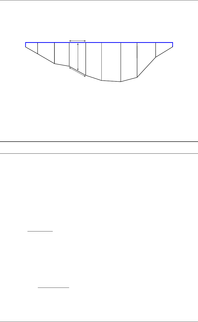
DRAFT
Numerical approach
dyj
Pj
hj
Figure 6.9: Cross sectional bed bathemetry perpendicular to the flow direction.
Algorithm 24 conjugategradient: solve water level equation with a preconditioned Conjugate
Gradient method
compute preconditioner P
compute initial residual r(0) =d−As(0)
compute maximum error ε=kr(0)k∞
apply preconditioner Pz(0)
r=r(0)
set p(0) =z(0)
r
compute inner product Dr(0),z(0)
rE
i= 0
while ε > tol do
compute Ap(p)
compute p(p), Ap(p)
α(p)=Dr(p),z(p)
rE
hp(p),Ap(p)i
s(p+1) =s(p)+α(p)p(p)
r(p+1) =r(p)−α(p)Ap(p)
compute maximum error ε=kr(p+1)k∞
apply preconditioner Pz(p+1)
r=r(p+1)
if ε > tol then
compute Dr(p+1),z(p+1)
rE
β(p+1) =Dr(p+1),z(p+1)
rE
Dr(p),z(p)
rE
p(p+1) =z(p+1)
r+β(p+1)p(p)
p=p+ 1
end if
end while
Deltares 63 of 152

DRAFT
D-Flow Flexible Mesh, Technical Reference Manual
1 "waterlevel",
2 "Neumann",
3 "velocity",
4 "discharge",
5 "Riemann",
6 "outflow"
7 "Qh",
where, except for the default full-slip condition, we have adopted the terminology and num-
bering of D-Flow FM. Additionally, the following boundary conditions in the second category
may be imposed:
8 "tangentialvelocity",
9 "ucxucyadvectionvelocity",
10 "normalvelocity",
were again we have used D-Flow FM terminology, but extended the numbering for our con-
venience. We will use the numbering for the identification of the (parts of) the boundary, at
which these conditions are implied. i.e. Γ1is the part of the boundary with water level bound-
ary conditions, et cetera. Since the boundary conditions 8to 10 are supplemental, they may
be combined with conditions 1to 9.
Disregarding the effects of atmospheric pressure and time relaxation (discussed later), the
boundary conditions may be summarized as:
u•n= 0,x∈Γ0,default,(6.117)
ζ=ζb,x∈Γ1,"waterlevel",(6.118)
∂ζ
∂n =sb,x∈Γ2,"Neumann",(6.119)
u•n=ub,x∈Γ3,"velocity",(6.120)
Z
Γ4
hu•ndΓ = Qb,x∈Γ4,"discharge",(6.121)
ζ+sh
gu•n= 2ζb−ζ0,x∈Γ5,"Riemann",(6.122)
∂ζ
∂n = 0,u•n>0,x∈Γ6,"outflow",(6.123)
∂ζ
∂t −pgh ∂ζ
∂n +sb= 0,u•n≤0,x∈Γ6,"outflow",(6.124)
ζ=hb
Z
Γ7
hu•ndΓ
,x∈Γ7,"Qh",(6.125)
and
u•t=vb,x∈Γ8,"tangentialvelocity",(6.126)
u=ub,x∈Γ9,"ucxucyadvectionvelocity",(6.127)
u•n=ub,x∈Γ10,"normalvelocity",(6.128)
64 of 152 Deltares
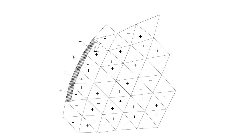
DRAFT
Numerical approach
xR(j)
bj
xL(j)dj
Figure 6.10: Virtual boundary "cells" near the shaded boundary; xLjis the virtual "cell"
center near boundary face j;xR(j)is the inner-cell center; bjis the point on
face jthat is nearest to the inner-cell center
where ζb,sb,ub,vb,ub,Qband hbare user prescribed at the boundary where appropriate,
nis the inward-positive normal vector, tis a unit tangential vector and ζ0is the initial water
level.
Remark 6.4.1.The condition u•n>0in Equation (6.123) is satisfied at inflow only.
Remark 6.4.2.At the "Qh" boundary ζis a function hbof Qand Q−ζcondition is imposed.
6.4.1 Virtual boundary "cells": izbndpos
We firstly introduce some notation. B0is the set of faces that are at the full-slip boundary, B1
is the set of faces at the "waterlevel" boundary Γ1and so on.
There is no administration in D-Flow FM for B0. The default boundary conditions are satisfied
by effectively setting the face-normal velocity component to zero, i.e.
uj= 0, j ∈ B0.(6.129)
The non-default boundary conditions are imposed by using virtual boundary cells, see Fig-
ure 6.10. Note that the term "cell" is ambiguous as it is only defined by means of its cir-
cumcenter. For boundary conditions of the first category (1 to 7), we discriminate between
boundaries where, roughly speaking, the water level is imposed (1, 2, 5 and 7) and where
velocities are imposed (6 and 7), i.e.
Γζ= Γ1∪Γ2∪Γ5∪Γ6∪Γ7,(6.130)
Γu= Γ3∪Γ4,(6.131)
Γ = Γζ∪Γu(6.132)
and similarly for the sets Bζ,Buand B. The second category of boundaries are supplemental
and are a subset of the first. Hence, for the definition of the virtual boundary "cell" centers we
only need to consider water level and velocity boundaries, Γζand Γurespectively.
Let djmeasure the shortest distance from the cell circumcenter to the boundary face, see Fig-
ure 6.10, and let bjbe the corresponding nearest point on the boundary face. Then the virtual
Deltares 65 of 152

DRAFT
D-Flow Flexible Mesh, Technical Reference Manual
"cell" centers are computed with Algorithm (25). Note that xnare mesh node coordinates and
remember that the face normal njis inward positive.
Algorithm 25 addexternalboundarypoints: compute centers of virtual boundary "cells"
xL(j)=
bj−max(dj,1
2pbAR(j))nj, j ∈ Bζ∧izbndpos = 0
1
2(xnl(j)+xnr(j)), j ∈ Bζ∧izbndpos = 1,
bj−max(dj,1
2pbAR(j))nj, j ∈ Bu.
(6.133)
Remark 6.4.3.Option izbndpos = 2 is not documented here.
Algorithm (25) shows that the virtual cell centers are on the boundary for izbndpos=1 and
at a distance dj(or 1
2pbAR(j)) from the boundary otherwise.
Besides a center, the virtual boundary "cells" also have a bed area bAand bed level bl defined
as
bAL(j)=bAL(j),
blL(j)=blR(j).j∈ B.(6.134)
6.4.2 Discretization of the boundary conditions
The boundary conditions are accounted for by modification of the discretization near the
boundaries. Assume that we are at time-level nand advance to time-level n+ 1, then the
discretization of Eqns. ((6.117)) to ((6.125)) is:
un+1
j= 0, j ∈ B0,default,(6.135)
ζn+1
L(j)=ζb(bj,ˆ
tn+1), j ∈ B1,"waterlevel",(6.136)
ζn+1
R(j)−ζn+1
L(j)
∆xj
=sb(bj,ˆ
tn+1), j ∈ B2,"Neumann",(6.137)
un+1
j=ub(bj,ˆ
tn+1), j ∈ B3,"velocity",(6.138)
un+1
j=Qb(ˆ
tn+1)(hun
j)2/3
P
l∈B4
Aun
l(hun
l)2/3, j ∈ B4"discharge",(6.139)
ζn+1
L(j)= 2ζb(bj,ˆ
tn+1)−ζ0
R(j)+. . .
. . . −s1
2(hζn
L(j)+hζn
R(j))
gun
j, j ∈ B5,"Riemann",(6.140)
ζn+1
L(j)=ζn
R(j), un
j>0j∈ B6,"outflow",(6.141)
ζn+1
L(j)−ζn
L(j)
∆tn=rg1
2(hζn
L(j)+hζn
R(j)). . .
. . . (ζn
R(j)−ζn
L(j)
∆xj
+sb(bj,ˆ
tn+1)), uj≤0, j ∈ B6,"outflow",(6.142)
ζn+1
L(j)=hb(X
l∈B7
qn
l), j ∈ B7,"Qh",(6.143)
where hζkis the cell-centered water depth, i.e.
hζk=ζk−blk,(6.144)
66 of 152 Deltares

DRAFT
Numerical approach
ζb(x, t)is a user-prescribed time-varying water level at boundary Γ1, similar for normal slope
sb(x, t)and normal velocity ub(bj,ˆ
tn+1), and Qb(t)is a user-prescribed time-varying dis-
charge at boundary Γ4. Furthermore, ˆ
tn+1 is an estimate of the next time level tn+1.
Note that at "Qh" boundaries the discharge qn
jis used, which is according to Algorithm (21)
qn
j=Aun−1
jθjun
j+ (1 −θj)un−1
j.(6.145)
The function hb(Q)is user-provided by means of a table. It will not be discussed further.
We do neither mention the threshold on hun
jfor the discharge boundaries under outflow con-
ditions Qb(t)<0, nor a threshold on 1
2(hζn
L(j)+hζn
R(j))at the Neumann boundaries.
The second category boundary conditions only affect the reconstruction of the cell-centered
full velocity vectors ucnear the boundary:
uc
n
L(j)=un
jnj+vb(bj,ˆ
tn+1)tj, j ∈ B8,"tangentialvelocity",(6.146)
uc
n
L(j)=ub(bj,ˆ
tn+1), j ∈ B9,"ucxucyadvectionvelocity",(6.147)
uc
n
L(j)=ub(bj,ˆ
tn+1)nj, j ∈ B10,"normalvelocity",(6.148)
where vb(x, t),ub(x, t)and ub(x, t)are user-prescribed and time-varying at the boundary.
Remark 6.4.4.During the time-step from tnto tn+1, the cell center reconstructed is based
on un
j(fully explicit). The boundary conditions are at the new time-level, on the other hand.
This seems inconsistent.
Note that the "ucxucyadvectionvelocity" and "normalvelocity" conditions allow a supercritical
inflow at the boundary. All three boundary conditions types are only relevant for inflow condi-
tions.
Discharge boundaries: jbasqbnddownwindhs, qbndhutrs
For simplicity we only consider one discharge boundary and mention that there may be more
than one. The face-based water depth in the evaluation of the flow area can optionally
be set to a downwind approximation (for an inflowing discharge boundary) with the option
jbasqbnddownwindhs, i.e.
huj=ζR(j)−blR(j), j ∈ B4∧jbasqbnddownwindhs = 1,"discharge".(6.149)
Compare with Algorithm (2) where the face-based water depths hujare computed. They are
overwritten in Algorithm (26) at the discharge boundary.
Remark 6.4.5.Since for some cases the water depth at the discharge boundaries are mod-
ified after the volumes Vkand cross-sectional wetted areas Aujare computed, the water
depth now seems inconsistent with the aforementioned quantities.
Riemann boundaries
At a Riemann boundary we do not allow any outgoing perturbation with respect to some
reference boundary state to reflect back from the boundary. This is achieved by prescribing
the incoming Riemann invariant. Note that we disregard directional effects. Using the D-
Flow FM convention of a positive inward normal at the boundary, this can be put as
u•n+ 2pgh =ub+ 2pghb(6.150)
Deltares 67 of 152

DRAFT
D-Flow Flexible Mesh, Technical Reference Manual
Algorithm 26 setau | discharge boundaries: adjustment to Algorithm (3) to overwrite water
depths at the discharge boundaries
if jbasqbnddownwindhs=0 then
B∗={l∈ B4|hul>0}
huj= max(0,P
l∈B∗ζR(l)wul
P
l∈B∗wul)−min(bl1j, bl2j), j ∈ B∗
end if
if jbasqbnddownwindhs=1 then
huj=ζR(j)−blR(j), j ∈ B4
compute Auj,j∈ B5as in Algorithm (3)
end if
ˆ
B={l∈ B4|hul≥qbndhutrs ∨Qb≥0}
huj= 0, j ∈ B4\ˆ
B
Auj= 0, j ∈ B4\ˆ
B
zuj=Qb(huj)2/3
P
l∈ˆ
B
(hul)2/3Aul, j ∈ B4
where we take boundary values (ζb, ub)as the reference boundary state. By using hb=
h+ζb−ζ, the term √ghbcan be linearized in ζaround ζ=ζbas
pghb=pg(h+ζb−ζ)≈pgh +1
2rg
h(ζb−ζ).(6.151)
Substitution yields
rg
hζ+u•n=ub+rg
hζb.(6.152)
Instead of prescribing a combination of velocity and water level, we prefer to prescribe the
water level at the boundary, i.e. ζb. For the necessary, but unknown velocity ubwe use linear
theory with respect to the initial state (ζ, u) = (ζ0, u0) = (ζ0,0).
Remark 6.4.6.We assume that the initial velocity field is zero in any case.
Note: Assumed is that there is no residual flow in the model.
By assuming small perturbations with respect to the initial conditions and considering conser-
vation of mass at the boundary, we have:
ubh=pgh(ζb−ζ0),(6.153)
or
ub=rg
h(ζb−ζ0).(6.154)
Substitution of this expression in Equation (6.152) yields
rg
hζ+u•n=rg
h(2ζb−ζ0).(6.155)
Note that a similar approach is taken in ?
68 of 152 Deltares

DRAFT
Numerical approach
The discretization in D-Flow FM is then as shown in Equation (6.140):
ζn+1
L(j)= 2ζb(bj,ˆ
tn+1)−ζ0
R(j)−s1
2(hζn
L(j)+hζn
R(j))
gun
j, j ∈ B5,"Riemann".
Qh boundaries: qhrelax
Again, for simplicity we will only consider one Qh boundary. The applied water level ζbjis
relaxed with a user-specified parameter αQh (qhrelax) that turns Equation (6.143) into
ζn+1
j=αQh hb(X
l∈B7
qn
l) + (1 −αQh)ζn
j, j ∈ B7
By hb(P
l∈B7
qn
l)we in fact always refer to this relaxed expression and will not mention the
relaxation explicitly.
6.4.3 Imposing the discrete boundary conditions: jacstbnd
During a time-step from tnto tn+1, the discrete boundary conditions, i.e. Equation (6.136)
to Equation (6.143) and Equation (6.146) to Equation (6.148), are imposed in the following
manner:
the reconstruction of the full velocity vectors ucn
jis modified with Algorithm (27) to account
for the boundary conditions at the new time level ˆ
tn+1,
the water level boundary conditions at the new time level ˆ
tn+1 are applied to the water
level at the old time level tnwith Algorithm (28),
the velocity boundary conditions are imposed on un+1
j, j ∈ Buin Algorithm (30),
the system of equations, referred to as the "water level equations", to obtain ζn+1 is
adjusted in Algorithm (29) near the boundaries,
having computed the water levels ζn+1 from the "water level equation" with Algorithm (23),
the water levels in the virtual boundary "cells" ζn+1
Lj ,j∈ Bζare computed with Algo-
rithm (28),
the velocities at the new time level un+1
jare computed with Algorithm (21) which requires
no modifications since fuand ruwere properly adjusted in Algorithm (30).
Remark 6.4.7.The boundary conditions at the new time level ˆ
tn+1 are applied to the cell-
center reconstruction of the full velocity vectors un
cat the old time level tn.
Remark 6.4.8.It is unclear why boundary conditions need to be applied again to the water
level at the old time level tnat the beginning of the time step. They where applied at the end of
the previous time step. Furthermore, conditions from the new time level ˆ
tn+1 are now applied
to the water level at the previous time level tn.
Remark 6.4.9.It is unclear why boundary conditions need to be applied to the water level
at the new time level ˆ
tn+1 right after solving the "water level equation" with Algorithm (28),
since the virtual boundary "cells" are included in the solution vector s= (ζ1, ζ2, . . . )Tand
the discrete system of Equation (6.105) is augmented with the discrete boundary conditions
of Equation (6.118) to Equation (6.125) in Algorithm (29).
Remark 6.4.10.The discretization of the "outflowboundary" condition, Γ6, in Algorithm (28)
is different from the one in Algorithm (29) and seems incomplete. The condition for uj≤0is
missing.
Remark 6.4.11.The "Qh" boundary condition is ineffective in Algorithm (28), since it is miss-
ing from Equation (6.156) and Equation (6.157).
Deltares 69 of 152

DRAFT
D-Flow Flexible Mesh, Technical Reference Manual
Algorithm 27 setucxucyucxuucyu | boundary conditions: adjustment to Algorithm (6) to sat-
isfy the boundary conditions
ucn
L(j)=
ucn
R(j), j ∈ B2∨(j∈ B ∧ jacstbnd = 1)
(ucn
R(j)•nj)nj, j ∈ B \ B2∧jacstbnd = 0
un
jnj+vb(bj,ˆ
tn+1)tj, j ∈ B8
ub(bj,ˆ
tn+1)j∈ B9
ub(bj,ˆ
tn+1)nj, j ∈ B10
Algorithm 28 sets01zbnd: apply boundary conditions to water levels ζnor ζn+1
zb=
(1 −αsmo)ζ0
j+αsmoζb(bj,ˆ
tn+1), j ∈ B1
ζn+1
j, j ∈ B2
2ζb(bj,ˆ
tn+1)−rmax( 1
2(hζn
L(j)+hζn
R(j)),εhs)
gun
j, j ∈ B5
(1 −αsmo)ζ0
L(j)+αsmo hb(P
l∈B7
qn
l), j ∈ B7
zb= max(zb −patmL(j)−pav
ρmean g, blL(j)+δ), j ∈ Bζ\ B6
δ= 10−3
if apply to ζnthen
ζn
L(j)=zb, j ∈ B1∪ B2∪ B5
max(ζn
R(j), blR(j)), un
j>0, j ∈ B6(6.156)
else {apply to ζn+1}
ζn+1
L(j)=zb, j ∈ B1∪ B2∪ B5
max(ζn
R(j), blR(j)), un
j>0, j ∈ B6(6.157)
end if
The water level boundary conditions are inserted into the system of equations as follows.
Firstly, Equation (6.136) to Equation (6.143) show that for some zbthe boundary conditions
can be put as
ζn+1
L(j)=zb, j ∈ Bζ\ B2,(6.158)
ζn+1
R(j)−ζn+1
L(j)
∆xj
=sb(b,ˆ
tn+1), j ∈ B2.(6.159)
The rows in the system that are affected by these boundary conditions are the rows that
correspond to the virtual boundary "cell" L(j)and the neighboring internal cell R(j). The
latter may come as a surprise, but is due to our constraint that the system should remain
symmetric. The general form of the system for these rows is obtained by substituting k=L(j)
and k=R(j), j ∈ Bζin Equation (6.105) respectively, and using O(L(j), j) = R(j)and
O(R(j), j) = L(j), i.e.
Brn+1(p)
L(j)ζn+1(p+1)
L(j)+Crn
jζn+1(p+1)
R(j)=drn+1(p)
L(j),
Brn+1(p)
R(j)ζn+1(p+1)
R(j)+P
l∈J (R(l))\j
Crn
lζn+1(p+1)
O(R(j),l)+Crn
jζn+1(p+1)
L(j)=drn+1(p)
R(j),
j∈ Bζ.
Combining these expressions yields for the non-Neumann boundary conditions
ζn+1(p+1)
L(j)=zb,
Brn+1(p)
R(j)ζn+1(p+1)
R(j)+P
l∈J (R(l))\j
Crn
lζn+1(p+1)
O(R(j),l)=drn+1(p)
R(j)−Crn
jzb,
j∈ Bζ\B2
70 of 152 Deltares

DRAFT
Numerical approach
Algorithm 29 s1nod | boundary conditions: adjustments to Algorithm (18) to satisfy the
boundary conditions in the water level equation
Brn+1(p)
kζn+1(p+1)
k+P
j∈J (k)
Crn
jζn+1(p+1)
O(k,j)=drn+1(p)
k,Equation (6.105)
Brn+1(p)
L(j)= 1, j ∈ Bζ
zb=
(1 −αsmo)ζ0
j+αsmoζb(bj,ˆ
tn+1), j ∈ B1
−sb(bj,ˆ
tn+1)∆xjCrn
j, j ∈ B2
2ζb(bj,ˆ
tn+1)−rmax( 1
2(hζn
L(j)+hζn
R(j)),εhs)
gun
j, j ∈ B5
ζn
R(j), un
j>0, j ∈ B6
ζn
L(j)+ ∆tnqg1
2(hζn
L(j)+hζn
R(j))(ζn
R(j)−ζn
L(j)+sb(bj,ˆ
tn+1)), uj≤0, j ∈ B6
(1 −αsmo)ζ0
L(j)+αsmo hb(P
l∈B7
qn
l), j ∈ B7
zb= max(zb −patmL(j)−pav
ρmean g, blL(j)+ 10−3), j ∈ Bζ
drn+1(p)
R(j)=drn+1(p)
R(j)−Crn
jzb,
Brn+1(p)
L(j)= 1,
Crn
j= 0,
drn+1(p)
L(j)=zb,
j∈ Bζ\ B2
Brn+1(p)
L(j)=−Crn
j,
drn+1(p)
L(j)=−Crn
j∆xjsb(bj,ˆ
tn+1),)j∈ B2
Crn
j=−Brn+1(p)
R(j),
Brn+1(p)
L(j)=−Crn
j,
drn+1(p)
L(j)= 0,
Brn+1(p)
R(j)=Brn+1(p)
R(j)−Crn
j,
j∈ Bu
Deltares 71 of 152

DRAFT
D-Flow Flexible Mesh, Technical Reference Manual
and for the Neumann boundary condition
−Crn
jζn+1(p+1)
L(j)+Crn
jζn+1(p+1)
R(j)=
−Crn
j∆xjsb(bj,ˆ
tn+1),
Brn+1(p)
R(j)ζn+1(p+1)
R(j)+P
l∈J (R(l))\j
Crn
lζn+1(p+1)
O(R(j),l)+Crn
jζn+1(p+1)
L(j)=,
drn+1(p)
R(j),
j∈ B2.
The consequences for the matrix elements are shown in Algorithm (29).
The velocity boundary conditions appear in the system in the following manner. The condition
for the face-normal velocity components can be expressed as
un+1
j=zuj, j ∈ Bu=B3∪ B4,(6.160)
where according to Equation (6.138)
zuj=ub(bj,ˆ
tn+1), j ∈ B3(6.161)
and zujis computed with Algorithm (26) for the discharge boundaries j∈ B4. Since the
velocity at the next time level with Equation (6.96) in Algorithm (14)
un+1
j=−fun
j(ζn+1
R(j)−ζn+1
L(j)) + run
j,
the adjustments to Algorithm (14) are obvious and presented in Algorithm (30). Note that the
velocity boundary conditions are relaxed with a parameter αsmo from the initial conditions,
assumed zero. This will be explained in the next section.
Algorithm 30 furu | boundary conditions: adjustments to Algorithm (14) to satisfy the bound-
ary conditions of the form un+1
j=zuj, j ∈ Buin un+1
j=−fun
j(ζn+1
R(j)−ζn+1
L(j)) + run
j
fun
j= 0,
run
j=αsmozuj,j∈ Bu
Returning to the system of water level equations, the consequence of the velocity boundary
conditions for the matrix element Crn
jcan be seen in Algorithm (15), i.e.
Crn
j= 0, j ∈ Bu.(6.162)
However, we want to apply a homogeneous Neumann condition to the water level at the
velocity boundary:
ζn+1
R(j)−ζn+1
L(j)= 0 ∈ Bu.(6.163)
This can for arbitrary non-zero Crn
jbe formulated as
−Crn
jζn+1(p+1)
L(j)+Crn
jζn+1(p+1)
R(j)=
0,
(Brn+1(p)
R(j)−Crn
j)ζn+1(p+1)
R(j)+P
l∈J (R(l))\j
Crn
lζn+1(p+1)
O(R(j),l)+Crn
jζn+1(p+1)
L(j)=,
drn+1(p)
R(j),
j∈ Bu.
To obtain a sensible order of magnitude, we set, as shown in Algorithm (29),
Crn
j=−Brn+1(p)
R(j), j ∈ Bu.(6.164)
72 of 152 Deltares

DRAFT
Numerical approach
6.4.4 Relaxation of the boundary conditions: Tlfsmo
In Algorithms (28), (30) and (29) the boundary conditions are relaxed from the initial values
with a parameter αsmo that turns the discrete boundary conditions into
ζn+1
L(j)= (1 −αsmo)ζ0
L(j)+αsmo ζb(bj,ˆ
tn+1), j ∈ B1,"waterlevel",(6.165)
un+1
j=αsmo ub(bj,ˆ
tn+1), j ∈ B3,"velocity",(6.166)
un+1
j=αsmo
Qb(ˆ
tn+1)(hun
j)2/3
P
l∈B4
Aun
l(hun
l)2/3, j ∈ B4"discharge",(6.167)
ζn+1
L(j)= (1 −αsmo)ζ0
L(j)+αsmo hb(X
l∈B7
qn
l), j ∈ B7,"Qh" (6.168)
and similar for the continuous formulation. The parameter αsmo is computed from the user-
prescribed parameter Tsmo (Tlfsmo) as
αsmo = min ˆ
tn+1 −t0
Tsmo
,1.(6.169)
Remark 6.4.12.The second category velocity boundary conditions are not being relaxed in
the same way as the first category, but maybe they should.
Remark 6.4.13.A zero initial velocity field is assumed in the relaxation of the boundary con-
ditions.
6.4.5 Atmospheric pressure: PavBnd, rhomean
Local changes in atmospheric pressure at the boundaries, except for the outflow boundary,
are accounted for by correcting the water level with
−patmL(j)−pav
ρmean g(6.170)
as shown in Algorithms (28) and (29), where patmk,pav (called PavBnd in D-Flow FM) and
ρmean (called rhomean in D-Flow FM) are the user-supplied atmospheric pressure in cell k,
average pressure and average density, respectively.
6.4.6 Adjustments of numerical parameters at and near the boundary
At and near the boundary, the advection scheme and time-integration method are adjusted
with Algorithm (31). The time-integration parameter θjis set to 1and the advection scheme
is set to ’6’ at and near the water level boundary. See Algorithm (4) for an overview of the
advection schemes. These settings are not only applied to the water level boundary faces,
but also to all faces of internal cells that are adjacent to the water level boundary.
For the velocity boundary conditions, the time integration parameter θjis set to 1at and near
the boundary. Advection is turned off by setting the advection scheme to −1, but only for the
faces at the boundary that is.
Deltares 73 of 152

DRAFT
D-Flow Flexible Mesh, Technical Reference Manual
Algorithm 31 flow_initexternalforcings: adjust numerical settings near the boundaries
θl= 1, l ∈ J(R(j))
iadvl= 6, l ∈ J(R(j)) j∈ Bζ
θl= 1, l ∈ J(R(j))
iadvj=−1j∈ Bu
6.4.7 Viscous fluxes: irov
Momentum diffusion is elaborated in Theorem 6.2.2 and in particular Algorithm (11). It will
be clear that we can not evaluate the viscous stresses tujat closed boundaries as in Equa-
tion (6.71). Instead, boundary conditions need to be imposed. These are:
tuj=
0,irov=0, free slip,
−u∗
j|u∗
j|sj,irov=1, partial slip,
−νjUj
∆yjsj,irov=2, no slip,
(6.171)
where u∗
jis the friction velocity, sj=n⊥
ja unit tangential boundary vector whose orientation
we will not discuss and, if R(j)is the boundary cell (note that L(j)does not exist),
∆yj=1
2
bAR(j)
wuj
.(6.172)
The friction velocity is computed as
u∗
j=Ujκ
C+d/z0
,(6.173)
with
Uj=ucR(j)•sj,(6.174)
z0the user specified roughness height, κthe Von Karman contanst, da distance from the
cell centroid perpendicular to the boundary face and Ceither 1or 9.
The boundary cell-based momentum diffusion term then becomes
1
hp∇•νhp(∇u+∇uT)ΩR(j)
≈1
Hp
R(j)
dR(j)+P
l∈{m∈B0|R(m)=R(j)}
tulwulsl,R(j)
bAR(j)
, j ∈ J0,(6.175)
where dR(j)represents the contribution from the non-boundary faces of boundary cell R(j)
as given by Equation (6.70) for k=R(j).
Remark 6.4.14.Comparing the contribution of the viscous boundary stress with the ex-
pression for the contribution of the internal faces dkin Equation (6.70) reveals that the
istresstype does not apply to the contribution of the boundary stresses. Apparently
p= 0 is applied here. See Remark 6.2.17 in this respect.
6.5 Summing up: the whole computational time step
With the discretization explained in the previous sections, we are now able to sum up the com-
putational time step. It is shown in Algorithms (32), (33) and (34). The data being computed
and updated are shown in Table 6.3.
74 of 152 Deltares

DRAFT
Numerical approach
Table 6.3: Data during a computational time step from tnto tn+1 with Algorithm (32); the
translation to D-Flow FM nomenclature is shown in the last column
input D-Flow FM
time instant tntime0
water level ζn
ks0
face-normal velocity components un
ju0
fluxes qn
j,qan
jq1,qa
water column volumes Vn
kvol1
wet bed areas An
kA1
time step ∆tn−1dts
during the time step (a selection)
estimate for next time instant ˆ
tn+1 time0+dts
the face based water level hun
jhu
wetted cross-sectional areas Aun
jAu
the water column thickness hsn
khs
the cell-centered full velocity vectors ucn
k,uqn
kucx,ucy,ucxq,ucyq
node-based full velocity vectors unn
iucnx,ucny
momentum equation terms Aej,Aijadve,advi
output
time instant tn+1 time1
water level ζn+1
ks1
face-normal velocity components un+1
ju1
fluxes qn+1
j,qan+1
jq1,qa
water column volumes Vn+1
kvol1
wet bed areas An+1
kA1
time step ∆tndts
Algorithm 32 flow_single_timestep: perform a computational time step from tnto tn+1 and
obtain ζn+1
k,un+1
j,qn1
j,qan+1
jand Vkn+1,∀kand ∀j
flow_initimestep: compute derived data hujn,Aun
j, et cetera and perform the predictor
phase of the fractional time step to obtain Aijand Aej,∀jwith Algorithm (33)
step_reduce: compose system of water-level equations, solve the system to obtain ζn+1
k,
compute volumes and wetted areas Vn+1
k,An+1
k, set hun
jto zero (old time-level) for dis-
abled faces during solve and perform the corrector phase to obtain un+1
j,qn+1
jand qan+1
j
with Algorithm (22)
Deltares 75 of 152

DRAFT
D-Flow Flexible Mesh, Technical Reference Manual
Algorithm 33 flow_initimestep: compute derived data and perform the predictor phase of the
fractional time step
hζn
k=ζn
k−blk,∀k
ˆ
tn+1 =tn+ ∆tn
flow_setexternalboundaries: update boundary values at time instant ˆ
tn+1
sethu: compute face-based water levels hun
jwith Algorithm (2) and Algorithm (41) ex-
plained later
setau: compute the flow area Aun
jwith Algorithms (3) and (26)
setumod: compute cell-based full velocity vectors ucn
k,uqn
k, first-order upwind velocity
uL
u
n
jand add Coriolis forces and viscous fluxes to Aejwith Algorithm (34)
compute bed friction coefficients
compute time step ∆tn+1
advec: add advection terms to Aijand Aejwith Algorithms (4) and (42)
setextforcechkadvec: add external forces to Aijand Aejand make adjustments for small
water depths, Algorithm (37) explained later
Algorithm 34 setumod: compute cell-based full velocity vectors uck,uqk, first-order upwind
velocity uL
ujand add Coriolis forces and viscous fluxes to Aej
setucxucyucxuucyu: reconstruct cell centered velocity vectors uckand uqk, and set first-
order upwind fluxes uL
ujwith Algorithms (6) and (27)
compute tangential velocities vjfrom the cell-centered velocities uqkwith Eqn. ((6.47))
compute Coriolis forces
setcornervelocities: interpolate nodal velocity vectors unfrom cell-centered velocity vec-
tors ucwith Algorithm (7)
compute viscous momentum fluxes, except at the default boundaries, i.e. j /∈ J0, and add
to Aejwith Algorithm (11)
compute viscous momentum fluxes near the default boundaries j∈ J0and add to Aej
76 of 152 Deltares

DRAFT
Numerical approach
6.6 Flooding and drying
The governing equations, Equation (6.5) and Equation (6.6), can only be formulated for posi-
tive water levels, i.e. the "wet" part of the whole domain where h > 0. However, our domain
may also contain areas that are dry. If we let Ωdenote the whole domain, then we can define
the wet part ¯
Ω(t)as
¯
Ω(t) = {x∈Ω|h(x, t)>0}.(6.176)
In other words, when we are faced with flooding and drying we are actually attempting to solve
a moving boundary problem, where ∂¯
Ω(x, t)is the moving boundary.
In D-Flow FM the governing equations are discretized on a stationary mesh (in two dimen-
sions). Looking at the governing equations, Equation (6.5) and Equation (6.6), we can imme-
diately identify two difficulties in the numerical treatment of the wet/dry boundary:
the spatial discretization near the moving wet/dry boundary, and
the temporal discretization at cells that become wet or dry during a time-step.
One may think of two possible approaches to overcome the difficulties with the spatial opera-
tors near the moving boundary: the stencil could be adapted such that it does not extend to
the dry part of the domain, or, alternatively, the spatial operators could be left unmodified and
the flow variables in the dry part could be given values that comply with the (moving) boundary
conditions. We leave it up to the reader to decide which approach is taken in D-Flow FM and
restrict ourselves by describing the measures taken in D-Flow FM to account for the wet/dry
boundary.
6.6.1 Wet cells and faces: epshu
We can distinguish between wet (or dry) cells and wet (or dry) faces, which are the discrete
counterpart of ¯
Ω(or Ω\¯
Ω). Dry faces are identified by setting their face-based water level to
zero, i.e. huj= 0. In D-Flow FM this occurs at two occasions during a time-step:
at the beginning of the time step, and based on the water level ζn
k, faces for which hu≤
εhu are disabled by setting them to zero with Algorithm (35). Note that εhu is a threshold
which is called epshu in D-Flow FM and is user specified,
during the time step, the water level ζn+1(p)
kmay have dropped below the bedlevel. De-
pending on poshcheck , the time-step is repeated with a smaller time step (type 1) or
all faces of the cell are deactivated by setting their hun
jto zero, see Algorithm (19), and
the water level equation is solved again.
Algorithm 35 sethu | drying and wetting: adjustment to Algorithm (2) to account for drying
and wetting
compute hun
jwith Algorithm (2)
disable dry faces by setting hun
j= 0 if hun
j≤εhu
6.6.2 Spatial discretization near the wet/dry boundary
In D-Flow FM, dry faces affect the discretization of:
the wet bed areas An
kand water-column volumes Vn
k,
momentum advection: set to zero in Algorithm (4) (not mentioned there),
bed friction forces: set to zero, and
viscous fluxes: set to zero for hun
jin Algorithm (34).
Deltares 77 of 152

DRAFT
D-Flow Flexible Mesh, Technical Reference Manual
The computation of the wet bed areas and water-columns was already presented in Algo-
rithm (20). As can been seen in Algorithm (20), the bed is assumed constant in case of no
non-linear iterations. That is, as far as the water-column volumes and wet bed areas are con-
cerned. See Remark 6.2.4 in that respect. With a constant bed level, no modifications are
necessary for the computation of the wet bed area. The bed is either completely wet, or it
isn’t. In case of non-linear computations, however, the bed is assumed non-constant in a cell.
The expressions for Vkand Akare then
Vk=Z
Ωk∩¯
Ω
hdΩ(6.177)
and
Ak=Z
Ωk∩¯
Ω
dΩ(6.178)
respectively, where we have used that Ωk∩¯
Ωindicates the wet part op the cell. These
integrals are discretized as indicated in Algorithm (36).
Remark 6.6.1.Applying Gauss’s theorem to Equation (6.178) yields
Ak=Z
∂Ωk∩¯
Ω
1
2(x−xk)•ndl+Z
Ωk∩∂¯
Ω
1
2(x−xk)•ndl, (6.179)
where we have assumed outward positive normal vectors n. It shows that we do not only
need to integrate along (a part of) the edges of Ωk, but also along the wet/dry boundary in cell
∂¯
Ω∩Ωk. Since this term is missing in the expression for Ak, the wet bed area of a partially
wet cell is incorrectly computed.
Algorithm 36 volsur | non-linear iterations: compute water-column volume Vn+1(i+1)
kand
wet bed area An+1(i+1)
k
if no non-linear iterations then
use Algorithm (20)
else
compute ∆bj= max(bl1j, bl2j)−min(bl1j, bl2j)and wet cross-sectional area Auj
as in Algorithm (3)
Ak=P
j∈{l∈J (k)|sk,l=1}
1
2∆xjαjmin( huj
∆bj,1)wuj+
P
j∈{l∈J (k)|sk,l=−1}
1
2∆xj(1 −αj) min( huj
∆bj,1)wuj
Vk=P
j∈{l∈J (k)|sk,l=1}
1
2∆xjαjAuj+
P
j∈{l∈J (k)|sk,l=−1}
1
2∆xj(1 −αj)Auj
end if
78 of 152 Deltares
DRAFT
Numerical approach
6.6.3 Spatial discretization of the momentum equation for small water depths: chkadv,
trshcorio
Recall that Eqn. ((6.23)) summarizes the spatial discretization of the momentum equation:
duj
dt=−g
∆xjζR(j)−ζL(j)− Aijuj− Aej−g|uj|
C2huj,
where Aejand Aijrepresent the contributions of momentum advection, diffusion, Coriolis
forces and external forces not being bed friction. These contribution are computed with Algo-
rithm (4) for advection and Algorithm (34) for diffusion and Coriolis forces, respectively. The
contributions to Aejby external forces not being the bed friction are added by Algorithm (37).
It shows that for small water depths hujthe term Aejis limited to zero from a user-specified
threshold hchkadv, called chkadv in D-Flow FM.
Algorithm 37 setextforcechkadvec: add external forces not being the bed friction forces to
Aejand Aij, and limit for vanishing water depths, in the expression:
duj
dt=−g
∆xjζR(j)−ζL(j)− Aijuj− Aej−g|uj|
C2huj
add external forces to Aej
if huj>0then
if hsL(j)<1
2hζR(j)∧ Aej<0∧hζR(j)< hchkadv then
Aej= min( hζL(j)
hchkadv ,1)Aej
else if hζR(j)<1
2hζL(j)∧ Aej>0∧hζL(j)< hchkadv then
Aej= min(hζR(j)
hchkadv ,1)Aej
end if
end if
Remark 6.6.2.It is unclear why the term Aejneeds to be limited to zero for vanishing water
depths.
Remark 6.6.3.It is unclear why only the term Aejis limited, and not the other terms. In the
first place Aij, but also the remaining terms in Eqn. ((6.23)).
Coriolis forces are computed and added to Aejin Algorithm (34). Besides the limitation
described above, an additional limitation is performed. If fcjis the Coriolis normal force
at face j, then it is limited as indicated in Algorithm (38) with a threshold htrshcorio called
|trshcorio | in D-Flow FM.
Algorithm 38 setumod | limitation of Coriolis forces: adjustment to Algorithm (34) to account
for vanishing water depths
htrshcorio = 1
hminj= min(hζL(j), hζR(j))
limit Coriolis forces fcjto fcjmin( hmin
htrshcorio ,1)
Remark 6.6.4.The Coriolis forces are limited by Algorithm (38)and by Algorithm (37).
6.6.4 Temporal discretization of the momentum equation near the wet/dry boundary
If the face is dry at the beginning of the time step, then it is assumed that during a time-step
from tnto tn+1 no water is fluxed through it. The face-normal velocity un
jis set to zero in such
circumstances.
Deltares 79 of 152

DRAFT
D-Flow Flexible Mesh, Technical Reference Manual
Remark 6.6.5.The assumption that during a time step no water is fluxed through a dry face
that is dry at the old time instant imposes a time step limitation.
Remark 6.6.6.Setting the face-normal velocities in the dry area to zero does not seem to
obey a moving wet/dry boundary condition. Hence, the spatial operators and temporal dis-
cretization are not allowed to be applied without modification. However, they are.
Setting hun
j= 0 during the time step does not affect the computation of momentum advection
and diffusion et cetera, as the terms Aeand Aeremain untouched. It only affects the water-
column volumes Vn+1
kand wet bed areas An+1
k, face-normal velocities un+1
jand fluxes qn+1
j
and qan+1
jat the new time instant as can be seen from Algorithm (22), which do not appear
in the discretization of the momentum equation.
Recall that the temporal discretization of the momentum equation is expressed by Eqn. ((6.96))
for huj>0, or
un+1
j=−fun
j(ζn+1
R(j)−ζn+1
L(j)) + run
j, hun
j>0.
Extended for the situation when the face becomes wet or dry, it becomes
un+1
j=
0,face is dry at beginning of the time step,
0,face is wet and becomes dry during the time step,
−fun
j(ζn+1
R(j)−ζn+1
L(j)) + run
j,face remains wet.
(6.180)
If the face is still wet at the end of the time step from tnto tn+1, but becomes dry at the
beginning of the new time step from tn+1 to tn+2 due to Algorithm (35), then its normal
velocity component is left unmodified, since the velocities are only set at the end of the time
step by Algorithm (21).
Remark 6.6.7.A face that was still wet at the end of the previous time-step, but becomes dry
during the current time-step can have a non-zero normal-velocity at the old time level. It is
being used in the evaluation of advection terms, diffusion terms et cetera at the beginning of
the next time step, although the face is dry. In contrast, faces that were already dry from the
end of the previous time step have zero normal-velocity.
6.7 Fixed Weirs
This section elaborates on the numerical treatment of the fixed weirs. They are commonly
used to model sudden changes in depth (roads, summer dikes) and groynes in numerical
simulations of rivers. In D-Flow FM, a fixed weir is a fixed non-movable construction gener-
ating energy losses due to constriction of the flow. Weirs are discretely represented along
mesh lines. In such a manner, faces can be identified that are located exactly on top of the
weirs, and no computational cells are cut by a weir. A cell is either on one side of a fixed
weir, or on the other side. Provided that the cross-sectional wet areas of the faces Aujhave
been properly modified to account for the fixed weir (if present), no modifications have to be
made to the discretization of the continuity equation. The momentum equation, on the other
hand, has to be modified such that we obtain our desired subgrid model. The flow over a fixed
weir can not be modeled in D-Flow FM as is, but is based on an alternative approach which
is called ’subgrid’ modelling, which means that a weir is not ’modelled on the grid’, but that a
parametrization is applied.
Two different subgrid approaches are available to simulate the energy losses by fixed weirs.
First of all, a numerical approach has been implemented. Then, a special discretization of
the advective terms before and after the fixed weir is applied. This option is switched on
80 of 152 Deltares

DRAFT
Numerical approach
via keyword fixedweirtype=6. This numerical approach is described in detail in sec-
tion 6.7.1 to section 6.7.4. Next to the numerical approach, there is an empirical approach
to determine the energy losses by weirs, for which two options are availabe in D-Flow FM,
namely the so-called ’Tabellenboek’ and ’Villemonte’ approaches. The Tabellenboek option
is switched on via keyword fixedweirtype=8, while the Villemonte approach coincides
with keyword fixedweirtype=9. The two corresponding empirical formulas have been
taken from the Simona software, see the website http://www.helpdeskwater.nl/
onderwerpen/applicaties-model/applicaties-per/watermanagement/watermanagement/
simona. Based on many flume measurements formulas have been derived to fit the mea-
surements as well as possible. This empirical approach is described in section 6.7.5.
6.7.1 Adjustments to the geometry: oblique weirs and FixedWeirContraction
Recall that the bed geometry is represented by the face-based bed-levels bl1and bl2, see
section 6.1.2 and Algorithm (1). The wet cross-sectional area Auis derived from it with
Algorithm (3). In other words, the fixed weirs are properly represented by adjusting bl1and
bl2. Also appearing in the expression for Auis the face width wu. Weirs that are not aligned
with the mesh, called oblique weirs for shortness, are projected to the (non-aligned) weir, i.e.
wuj=ckxr(j)−xl(j)k |nj•nwj|,(6.181)
where nwjis a unit vector normal to the part of the fixed weir that is associated with face
j. The cross-sectional wetted area is decreased by the same amount as wuby means of
Algorithm (3).
Remark 6.7.1.Oblique weirs are not fully understood at this moment. We do not attempt to
explain Equation (6.181) further.
In Equation (6.181) cis a user-specified contraction coefficient that accounts for obstacles in
the flow that accompanied with the weir, such as pillars. It is called FixedWeirContraction
in D-Flow FM.
The adjustments of bl1,bl2and wuare performed with Algorithm (39).
Algorithm 39 setfixedweirs: change geometry bl1,bl2and wuand advection type for fixed
weirs
bl1j= max(zcj, bl1j)
bl2j= max(zcj, bl2j)
if left and right weir sill levels are prescribed and conveyance type >0then
set bl1jand bl2jof adjacent faces, not described further
end if
adjust advection type of adjacent faces with Algorithm (40)
wuj=ckxr(j)−xl(j)k |nj•nwj|
6.7.2 Adjustment to momentum advection near, but not on the weir
Due to our subgrid modelling,the flow over a weir is discontinuous. In principle, this has is
consequences for the discretization of all spatial operators near the weir and to this end the
advection type near the weir is also adjusted by Algorithm (39). More precisely, all faces
belonging to cells that are adjacent to weirs, except for the faces that are associated with a
weir themselves, with Algorithm (40) have their advection type set to 4. As can be seen in
Algorithm (4), only inflowing cell-centered velocities are used in the expression for momentum
advection for scheme 4. Doing so, the advection at faces adjacent to and upstream of the
weir are not affected by the cell-centered velocities near the weir.
Deltares 81 of 152

DRAFT
D-Flow Flexible Mesh, Technical Reference Manual
Remark 6.7.2.Since the flow over a weir is discontinuous due to our subgrid modelling, one
may need to discretize the spatial operators near the weir more rigorously.
Algorithm 40 setfixedweirscheme3onlink: set advection type to 4of faces near the weir
if face jis associated with a fixed weir then
iadvj= 21
θj= 1
for l∈ {m∈ J(L(j)) ∪ J(R(j)) |iadvm6= 21}do
iadvl= 4
θl= 1
end for
end if
6.7.3 Adjustments to the momentum advection on the weir: FixedWeirScheme
We assume that a face jis located exactly on top of a fixed weir or not at all. Upstream of a
fixed weir, a contraction zone exists. The cell-centered water level upstream of the face (L(j)
if uj>0) represents the far-field water level before the contraction zone. The water level at
the cell-centered water level downstream of the face (R(j)if uj>0) is used as a downwind
approximation of the water level on top of the fixed weir. In other words, the discretization at a
face jrepresents the flow upstream of the weir at face j. This is the contraction zone, which is
governed by energy conservation. The expansion zone downstream of the weir, is governed
by momentum conservation and is directly resolved in the mesh without, in principle, further
adjustments.
Assume that at face jis on top of a weir and that the flow is from the left L(j)to the right
neighboring cell R(j). We require that:
1 Energy is conserved from cell L(j)to R(j).
2 The downstream water level ζR(j)should have no effect on the fixed weir in supercritical
conditions. In this case the water level on top of the weir reached its minimum value of
2
3Ej, where Ejis the far-field energy head above crest. Its computation will be discussed
later.
Energy conservation is expressed by means of Bernoulli’s equation, i.e.
1
2uin2
j+gζL(j)=1
2u2
j+g(zCj+huj),(6.182)
where uinjis a far-field velocity component in face-normal direction njand zCjis the crest
level. For the water level at the weir huja downwind approximation is used that obeys our
second requirement:
huj= max(ζR(j)−zCj,2
3Ej),(6.183)
where Ejis the far-field energy head above the crest. It is computed as
Ej=ζL(j)−zCj+1
2guin2
j.(6.184)
Remark 6.7.3.Equation (6.184) is only valid along streamlines and consequently we may
only consider flows that are perpendicular to the weir (1D flows) or are uniform along both
sides of the weir.
82 of 152 Deltares
DRAFT
Numerical approach
Substitution of Equation (6.186) in Equation (6.182), some rearrangement of terms and divi-
sion by ∆xjyields
1
2∆xju2
j−uin2
j=−g
∆xζR(j)−ζL(j)−g
∆xmax(0,2
3Ej−(ζR(j)−zCj)) (6.185)
This equation if brought into the form that is solved in D-Flow FM by adding the acceleration
term, which only serves to relax to our stationary subgrid expression of Equation (6.185)
duj
dt+1
2∆xju2
j−uin2
j=−g
∆xζR(j)−ζL(j)−g
∆xmax(0,2
3Ej−(ζR(j)−zCj))
(6.186)
Remark 6.7.4.Although momentum diffusion over the wear is missing in Equation (6.186), it
is actually included in D-Flow FM.
Recall that the spatial discretization is summarized as shown in Equation (6.23):
duj
dt=−g
∆xjζR(j)−ζL(j)− Aijuj− Aej−gkujk
C2huj.
For the temporal discretization, see Equation (6.95). The terms for fixed weirs can then be
put as, assuming uj>0:
Aij=1
2∆xj
uj,(6.187)
Aej=−1
2∆xj
uin2
j+g
∆xmax(0,2
3Ej−(ζR(j)−zCj)).(6.188)
Remark 6.7.5.Although bed friction is not included in Equation (6.185), it is included in D-
Flow FM by means of Equation (6.23). Its actual computation will not be discussed at this
occasion.
The terms of Equation (6.183), and Equation (6.187) and Equation (6.188) are prescribed
partly with Algorithm (41) and partly with Algorithm (42). Note that the latter also adjusts the
cell-centered velocity vectors uc.
In Algorithms (41) and (42) a far-field velocity uin is computed. For FixedWeirScheme 4,
the far-field velocity is projected in weir-normal, instead of face-normal direction. For Fixed-
WeirScheme 5the kinetic energy is not used in the determination of the far-field energy head.
Remark 6.7.6.Starting from Bernoulli’s equation to derive the weir subgrid model, it seems
inconsistent to project the far-field velocity in weir-normal direction for scheme 4, while using
the face-normal velocity as the weir crest velocity.
Remark 6.7.7.Starting from Bernoulli’s equation to derive the weir subgrid model, it seems
inconsistent not to include the far-field velocity for scheme 5.
The far-field velocity is based on the cell-centered velocity vector in the adjacent, upstream
cell. The cell-centered velocity vectors are reconstructed from the face-normal velocity com-
ponents with Algorithm (6). However, the upstream cell-centered velocity is reconstructed
from a set of face-normal velocity components that includes the weir itself. Since we are
seeking for a far-field velocity, we have to exclude the increased crest velocity ujfrom the re-
construction. See Remark 6.7.2 in this respect. This is achieved by estimating an unperturbed
Deltares 83 of 152

DRAFT
D-Flow Flexible Mesh, Technical Reference Manual
Algorithm 41 sethu | fixed weir: adjustment to Algorithm (2); set huand part (one of two) to
Ae
if uj>0then
compute far-field velocity ˆucL(j)with Algorithm (43)
uinj=(ˆucL(j)•nwj,fixed weir scheme 4
0fixed weir scheme 5
ˆucL(j)•nj,otherwise
Ej=ζL(j)−zcj+1
2guin2
j
if ζR(j)< ζL(j)then
huj= max(ζR(j)−zcj,2
3Ej)
Aej=−g
∆xjmin(0, ζR(j)−zcj−2
3Ej)
end if
else
as above by interchanging L(j)and R(j)and taking reversed orientation into account
end if
Algorithm 42 advec | fixed weir: adjustment to Algorithm (4) for fixed weir; set Aiand add
part (two of two) to Ae; overwrite cell-center velocity vectors ucof adjacent cells
if fixed weir scheme ∈ {3,4,5}then
compute and overwrite cell-centered weir-velocities ucL(j)and ucR(j)with Algorithm (44)
end if
if uj>0then
compute far-field velocity ˆucL(j)with Algorithm (43)
uinj=ˆucL(j)•nwj,fixed weir scheme 4
ˆucL(j)•nj,otherwise
Aij=uj
2∆xj
Aej=Aej−uin2
j
2∆xj
else
as above by interchanging L(j)and R(j)and taking reversed orientation into account
end if
84 of 152 Deltares

DRAFT
Numerical approach
velocity ˆujas if no weir was present and using that velocity in the reconstruction instead. The
unperturbed velocity is estimated by using continuity, i.e.
ˆuj=huj
ˆ
hj
uj,(6.189)
where ˆ
hjis a typical water depth for the upstream cell (L(j)if uj>0). The reconstruction
of the upstream cell-centered velocity vector is then performed as shown in Algorithm (43).
Note that the faces that are associated with a weir are identified with iadvj= 21, see
Algorithm (40), so ˆ
J(k)is the set of faces of cell kwithout the faces that are associated to a
fixed weir.
Algorithm 43 getucxucynoweirs: reconstruct a cell-centered velocity vector near a fixed wear
without the weir itself
ˆ
R(k) = {j∈R(k)|iadvj6= 21}(6.190)
ˆ
hk=(1
P
j∈ˆ
R(k)
wujP
j∈R(k)
wujhuj,ˆ
R(k)6=∅
0,otherwise
(6.191)
uck=1
bAk
(X
j∈{l∈ˆ
R(k)|sl,k=1}
αj∆xjwujnjuj+
X
j∈{l∈R(k)\ˆ
R(k)|sl,k=1}
αj∆xjwujnjujmin(1,huj
ˆ
hk
) +
X
j∈{l∈ˆ
R(k)|sl,k=−1}
(1 −αj)∆xjwujnjuj+
X
j∈{l∈R(k)\ˆ
R(k)|sl,k=−1}
(1 −αj)∆xjwujnjujmin(1,huj
ˆ
hk
))(6.192)
For the advection downstream of the wear the cell-centered velocity vectors get the opposite
treatment with Algorithm (44).
Deltares 85 of 152
DRAFT
D-Flow Flexible Mesh, Technical Reference Manual
Algorithm 44 getucxucyweironly: reconstruct a cell-centered velocity vector near a fixed wear
with the weir itself
¯
J(k) = {j∈ J(k)|iadvj= 21}(6.193)
¯
hk=(1
P
j∈¯
J(k)
wujP
j∈¯
J(k)
wujhuj,¯
R(k)6=∅
0,otherwise
(6.194)
uck=1
bAk
(X
j∈{l∈¯
J(k)|sl,k=1}
αj∆xjwujnjuj+
X
j∈{l∈J (k)\¯
R(k)|sl,k=1}
αj∆xjwujnjujmax(1,huj
¯
hk
) +
X
j∈{l∈¯
J(k)|sl,k=−1}
(1 −αj)∆xjwujnjuj+
X
j∈{l∈J (k)\¯
R(k)|sl,k=−1}
(1 −αj)∆xjwujnjujmax(1,huj
¯
hk
))(6.195)
6.7.4 Supercritical discharge
Supercritical conditions are defined by
ζ∗
R(j)≤zc+2
3Ej,(6.196)
where we let superscript ∗indicate supercritical and stationary conditions. The water level at
the crest is then according to Equation (6.183)
hu∗
j=2
3Ej.(6.197)
and the crest velocity according to Equation (6.185)
u∗
j=r2
3gEj.(6.198)
The face-based discharge under stationary and supercritical conditions is then by definition
q∗
j:= Au∗
ju∗
j=wujhu∗
ju∗
j=wuj
2
3Ejr2
3gEj,(6.199)
where we have used Equation (6.28) and Algorithm (3).
6.7.5 Empirical formulas for subgrid modelling of weirs
The energy loss due to a weir described by the loss of energy height ([m]). The energy loss
in the direction perpendicular to the weir is denoted as ∆E. This energy loss is added as an
opposing force in the momentum equation by adding a term −g∆E/∆xto the right hand
side of the momentum equation, resulting in a jump in the water levels by ∆Eat the location
of the weir.
86 of 152 Deltares

DRAFT
Numerical approach
The computation of the energy loss depends on the flow condition. There is a distinction
between a subcritical flow condition and a supercritical flow condition. Furthermore, there are
two different empirical formulations for the energy loss in use in D-Flow FM:
1Tabellenboek
Then, the energy loss is computed according to the following principles, see Wijbenga
(1990):
In critical flow conditions
To match the theoretical critical flow condition on the crest (flow velocity and wave
propagation speed are the same on the crest).
In subcritical flow conditions
Based on the so-called "Tabellenboek"’ approach, see Vermaas (1987) and the for-
mula according to Carnot. The formulation was fitted to match laboratory measure-
ments with hydraulically smooth weirs and with the ramp factors m1=m2both equal
to 4.0: see (Equation (6.207)) for the definitions of m1and m2.
Whether Carnot’s formula or the Tabellenboek is used depends on the flow velocity
above the weir: if the flow velocity at the weir is less than 0.25 m/s, the energy
loss is calculated according to the Carnot equation for the energy loss in a sudden
expansion. If the flow velocity above the weir is more than 0.50 m/s, the energy loss is
determined by interpolation of measured data which are collected in the Tabellenboek.
When the flow velocity is between 0.25 and 0.50 m/s, a weighted average is taken
between the energy loss following Carnot and the measurements.
For velocities at the weir less than 0.25 m/s the energy loss is calculated according
to Carnot’s law:
∆E=1
2gUweir −Qweir
ζ2+d22
(6.200)
with Uweir the flow velocity on the weir and ζ2the downstream water level and U2the
downstream flow velocity.
2Villemonte
The second available formulation is the formulation proposed by Villemonte (1947). The
formula has terms for different aspects of the weir’s geometry and for the vegetation on it,
more than the Tabellenboek-formulation. This formulation involves a number of parame-
ters, for which realistic values need to be found.
The default values produce an energy loss which is very close to the energy loss found by
the Tabellenboek formula. Alternative values for the tuning parameters were calculated by
Sieben (2011).
Depending on the flow condition, the empirical discharge is processed into the model in
one of the following two ways:
2.1 In critical flow, a loss of energy height is prescribed which causes the discharge to
converge to the empirical discharge over a small period of time.
2.2 In subcritical flow, a loss of energy height is prescribed which is the same as the
loss of energy height in a one-dimensional, steady flow with the given discharge.
Under the influence of (wind-)forces or two-dimensional effects, the discharge may
not converge to the empirical value, even though the energy loss will be the same
as in the one-dimensional, steady case.
3 In section 6.7.6 the Villemonte approach is described in detail.
6.7.6 Villemonte model for weirs
The Villemonte model is based on the analysis of a large number of measurements, which
were fitted for a formula which expresses the discharge across the weir as a function of the
Deltares 87 of 152
DRAFT
D-Flow Flexible Mesh, Technical Reference Manual
energy heights E1upstream and E2downstream of the weir:
Q=Q(E1, E2).(6.201)
The energy heights E1and E2are given by:
E1=ζ1+U2
1
2g, E2=ζ2+U2
2
2g,(6.202)
where the following notations are introduced:
ζ1upstream water level, measured from weir crest [m]
ζ2downstream water level, measured from weir crest [m]
ggravitational acceleration [m/s2]
U1upstream flow velocity component in direction towards the weir [m/s]
U2downstream flow velocity component in direction from the weir [m/s]
Apart from the energy heights, the discharge in the empirical formula ((6.201)) depends on
the properties of the weir. The formula proposed by Villemonte is
Q=Cd0Qc(E1)s1−max 0,min 1,E2
E1p,(6.203)
where the following notations are introduced:
Qdischarge per unit width across the weir [m2/s]
Cd0resistance coefficient of the weir [−]
Qc(E1)theoretical value for discharge across the weir in case of critical flow [m2/s]
ppower coefficient in discharge formula [−]
Determination of Cd0,Qth and p
The determination of Cd0,Qth and pis as described in the following three sections.
Theoretical critical discharge
The theoretical value Qcfor the discharge in case of critical flow is given by
Qc=2
3E1r2g
3E1.(6.204)
Note: that, even in critical flow conditions, the discharge has the form ((6.203)), and therefore
differs from the theoretical critical discharge Qc.
Resistence coefficient of the weir
The resistance coefficient Cd0depends on the weir’s vegetation in the following way:
Cd0= (1 + ξ1/3)−3/2Cd0,ref ,(6.205)
where Cd0,ref is the resistance coefficient the weir would have if it had no vegetation, and
where ξ1is the dimensionless vegetation coefficient, given by
ξ1= (1 −Armin(hv, h1)) Cdrag (6.206)
where the following notations are introduced:
88 of 152 Deltares
DRAFT
Numerical approach
Cdrag user-specified drag coefficient [−]
Aruser-specified vegetation density per linear meter [1/m]
hvuser-specified vegetation height [m]
h1upstream water level measured from the crest [m]
The effects of the weir’s geometry, vegetation and flow conditions on the resistance coefficient
Cd0,ref is modeled in the following way:
Cd0,ref =c1w1−1
4e−m1/2+ (1 −w)4
5+13
20e−m2/10,(6.207)
where the following notations were introduced:
c1user-specified calibration coefficient [−], default [.0
Note: the Tabellenboek measurements correspond to the default value c1=
1.0.
m1user-specified ramp of the upwind slope toward the weir
(ratio of ramp length and height, [−], default 4.0
m2user-specified ramp of the downwind slope from the weir [−], default 4.0
winterpolation weight [−]
The interpolation weight wis given by
w=e−E1/Lcrest ,(6.208)
where Lcrest is the length of the weir’s crest [m] in the direction across the weir.
Power coefficient p
The effect of the vegetation on the power-coefficient pis modeled in the following way:
p=(1 + ξ1/3)3
1+2ξ1
pref ,(6.209)
where pref is the power coefficient found in absence of vegetation:
pref =27
4C2
d0 1 + d1
E11−e−m2/c2−2
−1 + d1
E1−2!−1
.(6.210)
The user-specified calibration coefficient c2has a default value c2= 10. This is the correct
value for hydraulically smooth weirs. For hydraulically rough weirs, the value should be 50.
6.7.7 Grid snapping of fixed weirs and thin dams
All geographical features of a model that are described by x-, and y-coordinates, like fixed
weirs, thin dams and cross-sections, have to be interpolated to the computational grid when
running a model. The computational core of D-Flow FM automatically assigns these features
to the corresponding net links of the grid. This is called grid snapping. In this section is
explained how the grid snapping is implemented in the computational core of D-Flow FM.
This can be checked with the graphical user interface via the grid snapping feature.
In Figure 6.11 eight examples are shown how grid snapping of fixed weirs and thin dams
has been implemented. The upper four examples are for thin dams (in red), while the lower
four examples involve fixed weirs (in blue). In all eight examples one computational cell is
Deltares 89 of 152
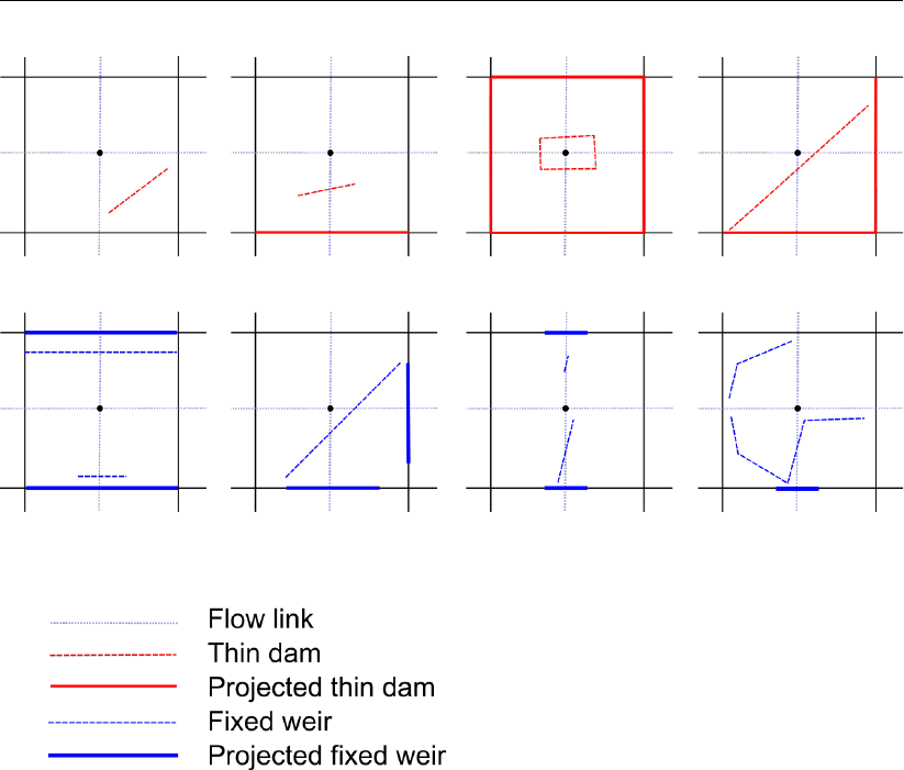
DRAFT
D-Flow Flexible Mesh, Technical Reference Manual
Figure 6.11: Examples of grid snapping for fixed weirs and thin dams.
shown with the water level point at the centre and four flow links that are connected to this
water level point. If a thin dam or fixed weir intersects with a flow link, then this object will
be snapped to the corresponding net link. In the left top example there is no intersection and
thus no grid snapping to a net link. In the second example, there is one intersection with one
flow link, in the third example four intersections and in the fourth example two intersections.
This corresponds to the number of net links to which grid snapping have been applied. In the
lower four examples of Figure 6.11 grid snapping of fixed weirs is explained. The algorithm
for determining whether or not a fixed weir is snapped on a net link is the same as for thin
dams and is explained above. The extra aspects for fixed weirs are its width and its height.
The width of a fixed weir is illustrated in Figure 6.11, while the computation fo the height is
illustrated in Figure 6.12. The following algorithm is applied for the computation of the height
of a fixed weir:
the height is the weighted average of the heights at the ends of the polyline of a fixed weir,
if multiple fixed weirs intersect a flow link, then the maximum of the interpolated values is
taken,
The width (wu) of a fixed weir is determined by the corner (α) between the fixed weir and the
net link and is computed according to
wu = cos (90 −α)×width, (6.211)
with width the width of a net link. If multiple fixed weirs intersect a flow link, then the maximum
of the interpolated values is taken for the width.
90 of 152 Deltares
DRAFT
Numerical approach
Figure 6.12: Examples of computation of crest heights.
Deltares 91 of 152

DRAFT
D-Flow Flexible Mesh, Technical Reference Manual
92 of 152 Deltares
DRAFT
7 Numerical schemes for three-dimensional flows
7.1 Governing equations
In D-Flow FM transport is formulated as,
d
dt ZV(t)
ϕ dV +Z∂V (t)
ϕ(u−v)•ndS =Z∂V (t)K˜
∇ϕ•ndS +ZV(t)
s dV (7.1)
where V(t)is a three-dimensional control volume, ϕis a transport variable, uthe flow ve-
locity field, vthe velocity of the (vertically) moving control volume, Kis a diagonal matrix
K=diag (νH, νH, νV),˜
∇is the gradient operator in 3D, with diffusion coefficients and s
a source term. In case of three-dimensional (layer-averaged) flow, with ∆za layer thickness
from z1(x, y, t)to z2(x, y, t), we obtain
∂∆zϕ
∂t +∇•(∆zuϕ) + ωz2[ϕ]z=z2−ωz1[ϕ]z=z1=∇•(∆zνH∇ϕ)
+νV
∂ϕ
∂z −νH∇z2•∇ϕz=z2−νV
∂ϕ
∂z −νH∇z1•∇ϕz=z1
+ ∆zs (7.2)
where uand ∇still the horizontal components are meant, i.e. u= (u, v)Tand ∇=
∂
∂x ,∂
∂y T
and νVis the vertical diffusion coefficient. Furthermore, ωz1and ωz2are the
velocity components normal, relative to the moving z=z1and z=z2layer interfaces,
respectively.
The continuity equation is derived by setting ϕ= 1 and s= 0,
∂∆z
∂t +∇•(∆zu) + ωz2−ωz1= 0 (7.3)
Summing up all equations along the layers, and setting zero flux condition at the bed and the
free surface, it yields:
∂h
∂t +∇•(hu) = hs (7.4)
In a similar way, the horizontal momentum equation can be obtained by setting ϕ=u. Unlike
the continuity equation, the momentum equation is not integrated over the depth.
∂∆zu
∂t +∇•(∆zuu) + ωz2uz2−ωz1uz1=∇•(∆zνH∇u)
+νV
∂u
∂z −νH∇z2•∇uz2−νV
∂u
∂z −νH∇z1•∇uz1
+ ∆zs (7.5)
subtracting Equation (7.3) from Equation (7.5) yields,
∂u
∂t +1
∆z[∇•(∆zuu)− ∇ •(∆zu)− ∇ •(∆zνH∇u)]
+1
∆z[ωz2(uz2−u)−ωz1(uz1−u)] =
+1
∆zνV∂u
∂z −νH∇z2•∇uz2−1
∆zνV∂u
∂z −νH∇z1•∇uz1+s(7.6)
The last term in the right-hand side of Equation (7.6) includes the source terms, namely
pressure. It can be described by s=sp. The pressure term is imposed on all flow cells as
sp=−g∂ζ
∂x (7.7)
Deltares 93 of 152
DRAFT
D-Flow Flexible Mesh, Technical Reference Manual
The bed friction acts as surface force and it affects the flow in the first layer close to the bed.
νV
∂u
∂z z=0
=τb
ρ(7.8)
The wind force also acts as a surface force on the free surface, and hence it affects the top
layer of the flow.
νV
∂u
∂z z=zmax
=Cd
ρa
ρw
W2(7.9)
where Wis the speed of the wind, ρais the air density, ρwis the density of water and Cdis
air-water friction coefficient.
7.2 Three-dimensional layers
In D-Flow FM two type of grid topologies in the vertical direction are applied, σand zgrids. σ-
layers are layers which divide the computational regions between the bed and the free surface.
These layers are adaptive and the interfaces of the layers may change in time associates with
the deformation of the bed and free surface, see Figure 7.1a.
x
z
σ= 0
σ= 1
(a) σ-layers
x
z
(b) z-layers
Figure 7.1: A schematic view of σ- and z-layers.
Unlike the σ-layers, z-layers are strictly horizontal and they don’t adapt the temporal variation
of the bed and free surface, see Figure 7.1b.
7.2.1 σ-layers
In σ-grid the vertical distribution of the grid form layers which can adapt the geometry of the
bed and free surface. In D-Flow FM the thickness of sigma-layers can be uniform (equidistant
in the vertical direction), user specified, or stretched around a user defined level γwith stretch-
ing factor of α(Algorithm (45)). For stretching around a user defined level, Equation (7.10)
and Equation (7.11) are applied for both bottom and top parts.
Algorithm 45 flow_allocflow:
∆zi,1=
user specified,stretching type = 1, i = 1
1−αi
1−αm
i×γ, stretching type = 2, i = 1,2
1
m,otherwise i= 1
(7.10)
∆zi,k =(user specified,stretching type = 1, i = 1
∆zi,k−1×αi,stretching type = 2, i = 1,2
∆zi,k−1,otherwise, i = 1
(7.11)
7.2.2 z-layers
94 of 152 Deltares
DRAFT
Numerical schemes for three-dimensional flows
7.3 Connectivity
In D-Flow FM the horizontal connectivity of the computational cells in three-dimensional are
defined identical with that of 2D case.
z
y
xi
j
l
Vk,l
Ak
∆zi,l
Figure 7.2: Layer distribution in 3D.
Ak, projected area of cell k.
Vk,l, volume in layer lof cell k.
∆zi,l thickness of layer labove node i.
However, in order to take the vertical distribution into account, a structured type of bookkeep-
ing is applied. The data is stored in an one-dimensional array, and for each base node (2D
flow node on the bed), two pointers are defined associated to the bottom and top cells in the
vertical direction, defined by Kb(k)and Kt(k), respectively. Similar type of connectivity is
also applied for the flow links in the vertical direction. Each base link (2D flow link on the bed),
similar to flow nodes, consists of two pointers associated to the links in the bottom and top
levels in the vertical direction, defined by Lb(j)and Lt(j).
The connectivity translates directly to administration in the D-Flow FM code as follows:
Kb(k):kbot(k),
Kt(k):ktop(k),
Lb(j):Lbot(j),
Lt(j):Ltop(j),
where jis the link index for the base flow nodes k.
Note: In D-Flow FM the layers are defined by one-dimensional array. For each cell column
the layers change from Kb(k)to Kt(k)and for each flow-link column they change from Lb(j)
to Lt(j). However for the reason of clarity, we define it by two-dimensional indices at which
the first index specifies the base cell k(or flow link j) and the second index specifies the layer
number l.
7.4 Spatial discretization
Deltares 95 of 152

DRAFT
D-Flow Flexible Mesh, Technical Reference Manual
Algorithm 46 sethu: compute the layer depths at flow-link location j
zuj,l =zL(j),l, uj,l >0∨uj,l = 0 ∧ζL(j)> ζR(j)
zR(j),l, uj,l <0∨uj,l = 0 ∧ζL(j)≤ζR(j)
σ=zuj,l −zuj,0
zuj,M(j)−zuj,0
˜
huj,l =σhuj
Auj,l =˜
huj,l −˜
huj,l−1wuj
7.4.1 Continuity equation
The continuity equation Equation (7.4) is spatially discretized on the water column as
dVk
dt =−X
j∈J (k)
M(j)
X
l=1
Auj,luj,lsj,k (7.12)
where M(j)is the maximum layers number at the location of link j,Vkis the volume of water
column for base cell kcomputed with Algorithm (20), Auj,l approximates the flow area of face
jat layer lcomputed with Algorithm (3), uj,l is the normal velocity component associated to
face (j, l)and sj,k accounts for the orientation of face jwith respect to cell k.
Face based layer depth
The face-based layer depths reconstructed from the cell-centered layer depths with an up-
wind approximation. The face-based layer depth, ˜
hu, is then applied to calculate the cross-
sectional area, Auj,l at layer j(see Algorithm (46)).
7.4.2 Momentum equation
Unlike the two-dimensional case, the discretization of the momentum equation in 3D occurs
on all flow faces associated with the layers (Horizontally). However, the discretization of the
advection and diffusion terms are identical with that of the two-dimensional case, except it is
applied along the layers. Hence, the advection and diffusion terms can be expressed by
advec =1
∆z∇•(∆zuu)−u∇•(∆zu)− ∇ •(ν∆z(∇u+∇uT))j,l •nj
≈ Aij,luj,l +Aej,l (7.13)
where Aij,l and Aej,l are the implicit and explicit parts, respectively. Because of similarity
with the two-dimensional case, the derivation of the equations is not discussed here. The
advection term is discretized in Algorithm (4) and the diffusion term in Algorithm (11) for each
layer. Similar to the two-dimensional case, the limiters, used for the advection, is described in
Algorithm (9) and Algorithm (10) on each layer.
The water level-gradient term projected in the face-normal direction is discretized along the
water column as
∇ζ|j•nj≈g
∆xjζR(j)−ζL(j)(7.14)
The is discretized as The contribution of the bed friction term into the momentum equation
occurs only on the flow faces associated with the first σ-layer. However, unlike the 2D case,
96 of 152 Deltares
DRAFT
Numerical schemes for three-dimensional flows
Algorithm 47 getustbcfuhi: compute the bed shear stress for the first σ-layer
S= ln ∆zuj,1/2 + µz0
z0, m = 0
S= ln ∆zuj,1+µz0
ez0, m = 1
S= ln ∆zuj,1/e +µz0
z0, m = 2
S= ln ∆zuj,1/2 + z0
z0, m = 3
√cf=κ
S
u∗
j=un+1
j,1√cf
this term is not discretized in its original form. The discretization of this term is done by fitting
a logarithmic-law for rough beds. The merely of this approach is in finding the shear velocity
by means of integration of the log-law wall function. The log-law wall-function for rough beds
reads
u
u∗≈1
κln z+µz0
z0(7.15)
where κis von Kármán constant and z0id the roughness height and µis a constant equals
to 1or 9. Integration of Equation (7.15) for the first layer at flow link jgives
uj,1=u∗
j
κ1 + µz0
∆zuj,1ln ∆zuj,1+µz0
z0−z0
∆zuj,1
µln(µ)−1(7.16)
Considering z0/∆zuj,1to be small, the bed shear velocity will be
uj,1≈u∗
κln ∆zuj,1+µz0
ez0(7.17)
Then the shear velocity is derived as
u∗
j=κ
ln ∆zuj,1+µz0
ez0uj,1=uj,1√cf(7.18)
The bed shear stress is defines as τ=ρu∗2. However, different forms of log-law functions
are used in D-Flow FM. The calculation of the bed shear stress is given in Algorithm (47).
Remark 7.4.1.The log-law wall function is valid for fully developed flow. The bed shear stress
under fully developed flow is lower than that of non-developed flow. Therefore, Equation (7.18)
underestimates the bed friction for unstationary flows.
7.5 Temporal discretization
Similar to the 2D part, the spatial discretization in 3D is also performed in a staggered manner.
The velocity normal components uj,l are defined at the cell faces (j, l), with face normal
vector nj,l, and the water levels ζkat cell centers k. If advection and diffusion are spatially
Deltares 97 of 152
DRAFT
D-Flow Flexible Mesh, Technical Reference Manual
discretized as in Equation (7.13) then the temporal discretization of Equation (7.5) is
∂u
∂t +Advec +1
∆z[ωz2(uz2−u)−ωz1(uz1−u)]
=−g∂ζ
∂x +1
∆zνV
∂u
∂z z2−1
∆zνV
∂u
∂z z1
(7.19)
Remark 7.5.1.Note that in D-Flow FM the second term in the vertical diffusion term, namely
νHδz •∇uis neglected in. It is done for simplification of the discretization. However, this
term becomes important in when the layer-level gradient is large, and neglecting this term
may cause large error.
After substitution of Advec from Equation (7.13) and discretize the other terms implicitly, it
yields the following discretized form of equation
1
∆tun+1
j,l +Aij,lun+1
j,l +Aej,l +ω0
2un+1
z2−ω0
1un+1
z1−(ω0
2−ω0
1)un+1
j,l
=1
∆tun
j,l −gθj
∆xjζn+1
R(j)−ζn+1
L(j)−g(1 −θj)
∆xjζn
R(j)−ζn
L(j)
+ν0
2un+1
j,l+1 −un+1
j,l −ν0
1un+1
j,l −un+1
j,l−1(7.20)
where uz1and uz2are the upwinded velocities, ω0
1=ωz1/∆zj,l,ω0
2=ωz2/∆zj,l,ν0
1=
ν1/zj,l∆z1and ν0
2=ν2/zj,l∆z2,∆z1= (zj,l +zj,l−1)/2and ∆z2= (zj,l +zj,l+1)/2.
ν1and ν2are the vertical eddy diffusivity at the top and the bottom of the velocity control
volume, respectively. Applying a first order upwind scheme, Equation (7.20) can be reformed
as follows
gθj
∆xjζn+1
R(j)−ζn+1
L(j)+alun+1
j,l−1+blun+1
j,l +clun+1
j,l+1 =dl(7.21)
where
al=−max (ω0
1,0) −ν0
1(7.22)
bl=1
∆t+Aij,l + max (ω0
2,0) −min (ω0
1,0) −(ω0
2−ω0
1) + ν0
2+ν0
1(7.23)
cl= min (ω0
2,0) −ν0
2(7.24)
dl=1
∆tun
j,l −g(1 −θj)
∆xjζn
R(j)−ζn
L(j)(7.25)
Remark 7.5.2.in D-Flow FM the discretization of vertical convection is also done by central
scheme (javau = 4). It is found that the central scheme may lead to instabilities.
Remark 7.5.3.In D-Flow FM the vertical advection can be switched off by using javau = 0.
However, switching off the vertical advection may lead to non-physical results.
We write Equation (7.20) in a general form as
un+1
j,l =−fun
j,l ζn+1
R(j)−ζn+1
L(j)+run
j,l (7.26)
Substituting Equation (7.26) in Equation (7.21) leads to the following relation for fuand ru
gθj
∆xjζn+1
R(j)−ζn+1
L(j)+alhruj,l−1−fuj,l−1ζn+1
R(j)−ζn+1
L(j)i
+blhruj,l −fuj,l ζn+1
R(j)−ζn+1
L(j)i
+clhruj,l+1 −fuj,l+1 ζn+1
R(j)−ζn+1
L(j)i=dl(7.27)
98 of 152 Deltares

DRAFT
Numerical schemes for three-dimensional flows
Equation (7.27) needs to be satisfied for any given initial water level (e.g. ζR(j)=ζL(j)) .
Hence, this equation can be splitted to two equations.
by making a homogeneous field and dropping the pressure terms,
by substituting the derived equation from the previous step, and derive a second equation.
Dropping the pressure terms in Equation (7.27) gives
alruj,l−1+blruj,l +clruj,l+1 =dl(7.28)
Substituting Equation (7.28) in Equation (7.27), leads to the following equation for fu
alfuj,l−1+blfuj,l +clfuj,l+1 =d0
l(7.29)
where
d0
l=−gθj
∆xjζn+1
R(j)−ζn+1
L(j)(7.30)
This procedure is presented in Algorithm (48).
Equation (7.28) and Equation (7.29) are tri-diagonal matrices for ruand fu, respectively. They
are solved by Thomas Algorithm for tri-diagonal matrices (See Algorithm (49))
Algorithm 48 vertical_profile_u0: compute fun
j,l and run
j,l in un+1
j,l =−fun
j,l(ζn+1
R(j,l)−ζn+1
L(j))+
run
j
For each j:
a= 0, b = 1/∆t, c = 0, d1=un
j,Lb(j)/∆t
for l= 1 to M(j)−1do
adv1= max (ω0
l,0)
adv =−min (ω0
l,0)
T1= (νt+adv1)/∆zl+1
T2= (νt+adv)/∆zl
bl+1 =bl+1 +T1
al+1 =al+1 −T1
bl=bl+T2
cl=cl−T2
dl+1 =un
j,l+1/∆t
end for
for l= 1 to M(j)do
bl=bl+Aij,k
dl=dl− Aej,k −g(1 −θj)
∆xjζn
R(j)−ζn
L(j)
d0
l=gθj
∆xj
end for
Solve alruj,l−1+blruj,l +clruj,l+1 =dlby Algorithm (49)
Solve alfuj,l−1+blfuj,l +clfuj,l+1 =d0
lby Algorithm (49)
Deltares 99 of 152

DRAFT
D-Flow Flexible Mesh, Technical Reference Manual
Algorithm 49 tridag: compute tridiagonal matrix of aiui−1+biui+ciui+1 =di
β=b1
u1=d1/β
for i= 2 to nstep 1do
ei=ci−1
β
β=bi−aiei
ui=di−aiui−1
β
end for
ui=ui−ei+1ui+1 , i =n−1, n −2, ..., 1
The continuity equation is discretized as
Vn+1
k−Vn
k
∆t=−X
j∈J (k)
M(j)
X
l=1
Aun
j,l θjun+1
j,l + (1 −θj)un
j,lsj,k (7.31)
where Vn+1
kis the volume of the water column at base cell kand Auj,l approximates the flow
area of face j, l
Auj,l = ∆zj,lwj(7.32)
with ∆zj,l is the distance between two layers land l−1related to base link j,wjis the width
of base link j. Subsitution of Equation (7.26) in Equation (7.31) yields the following equation.
Vn+1
k−Vn
k
∆t+X
j∈J (k)
M(j)
X
l=1
Aun
j,lθjfun
j,lζn+1
k−X
j∈J (k)
M(j)
X
l=1
Aun
j,lθjfun
j,lζn+1
O(k,j)
=−X
j∈J (k)
M(j)
X
l=1
Aun
j,l (1 −θj)un
j,l +θjrun
j,lsj,k (7.33)
Equation (7.31) can be summarized as
Vn+1
k−Vn
k
∆t+Bn
kζn+1
k+X
j∈J (k)
M(j)
X
l=1
Cn
jζn+1
O(k,j)=dn
k(7.34)
where Bn
k(diagonal entries), Cn
j(off-diagonal entry) and dn
k(right-hand side) are computed
by Algorithm (50).
In order to solve Equation (7.34), we need to express Vn+1
kin the terms of ζn+1
k. Since this
relation is non-linear, Equation (7.34) is solved iteratively by means of Newton iterations. After
linearizion of the volume, we have
Vn+1(p+1)
k=Vn+1(p)
k+An+1(p)
kζn+1(p+1)
k−ζn+1(p)
k(7.35)
100 of 152 Deltares

DRAFT
Numerical schemes for three-dimensional flows
Algorithm 50 s1ini: compute the matrix entries and right-hand side in the water level equation
Vn+1
k−Vn
k
∆t+Bn
kζn+1
k+P
j∈J (k)
Cn
jζn+1
O(k,j)=dn
k,Equation (7.34)
Cn
j=−
M(j)
X
l=1
Aun
j,lθjfun
j,l
Bn
k=−X
j∈J (k)
Cn
j
dn
k=−X
j∈J (k)
M(j)
X
l=1
Aun
j(1 −θj)un
j+θjrun
jsj,k
where An+1(p)
kis the wet bed area of cell kat (iterative) time level n+ 1(p). Substituting
Equation (7.35) into Equation (7.34), yields
Brn+1(p)
kζn+1(p+1)
k+X
j∈J (k)
Cn
rjζn+1(p+1)
O(k,j)=dn+1(p)
rk(7.36)
the form of Equation (7.36) is identical with that of Equation (6.105) in 2D. Hence, the coeffi-
cients Bn
rk,Cn
rkand dn
rkare computed at the same way of 2D, shown in Algorithm (18). Similar
to 2D, the unknown water levels k∈ K are solved with Krylov solver (see section 6.3.1).
The time step is finalized by employing Equation (7.26) back for un+1 as it is shown in Algo-
rithm (51). Moreover, the velocities and the discharge are integrated over depth.
Algorithm 51 u1q1: update velocity un+1
j,k and discharges qn+1
jand qan+1
j
if hun
j>0then
un+1
j,l =−fun
j,l(ζn+1
R(j)−ζn+1
L(j)) + run
j,l
qn+1
j,l =Aun
j,l θjun+1
j,l + (1 −θj)un
j,l
qan+1
j,l =Aun
j,lun+1
qn+1
j,0=
M(j)
X
l=1
qn+1
j,l
qan+1
j,0=
M(j)
X
l=1
qan+1
j,l
Aun+1
j,0=
M(j)
X
l=1
Aun+1
j,l
un+1
j,0=qn+1
j,0/Aun+1
j,0
end if
7.6 Vertical fluxes
In order to solve the vertical advection in Equation (7.19), the values of ωz1and ωz2needs
to be calculated. In D-Flow FM the vertical fluxes are evaluated as the superposition of two
effects.
Deltares 101 of 152

DRAFT
D-Flow Flexible Mesh, Technical Reference Manual
1 Mass balance for each cell
2 The vertical motion of the water surface.
If qHdescribes the sum of horizontal fluxes, then
δqHk,l =−X
j∈J (k)
qj,lsj,k +δqzk,l (7.37)
where δqHk,l =qHk,l −qHk,l−1is the vertical flux passing through the interface (k, l), and
δqzk,l is the vertical flux from cell (k, l)under effect of vertical motion of the free surface.
The difference in the horizontal fluxes has to be compensated via the vertical fluxes by
δqHk,l =−δqVk,l (first under assumption δqzk,l = 0). As there is no vertical flux through
the bed (zero flux), the calculation of the flux starts from the first layer, and is advanced to the
upper layers.
The change of the water level (and the vertical location of layers) induces extra vertical fluxes
through layer interfaces. This flux is equal to the rate of volume which passes through the
interface, because of its motion. This flux is equal to
qσ=A(Ωk)zn+1
k,l −zn
k,l
∆t(7.38)
where zk,l is the vertical position of the interface (k, l). Note that this flux does not effect the
value of the vertical velocity of the flow. The calculation of the vertical fluxes and velocities is
described in Algorithm (52).
Algorithm 52 u1q1: calculate the vertical fluxes qH
if hun
j>0then
qHk,0= 0
for l= 1 to N(k)do
δqVk,l =−X
j∈J (k)
qj,lsj,k
δqHk,l =−δqVk,l
qHk,l =qHk,l−1+δqHk,l
ωk,l =ωk,l−1+δqHk,l/A (Ωk)
qHk,l =qHk,l −A(Ωk)zn+1
k,l −zn
k,l
∆t
end for
end if
Remark 7.6.1.In the calculation of the fluxes, by marching, along the water column from the
bottom to the top, the fluxes on the water surface will not be equal to zero. The error in the
vertical flux on the water surface is supposed to be small, and it is neglected. Hence, the
procedure is not fully mass conservative.
7.7 Turbulence closure models
In D-Flow FM four types of turbulence closure models are employed.
1 Constant coefficient model
102 of 152 Deltares

DRAFT
Numerical schemes for three-dimensional flows
2 Algebraic eddy viscosity closure model
3k-εturbulence model
4k-τturbulence model
At the first model, the eddy viscosity is a user defined constant. The three last models are
based on the so-called eddy viscosity concept of Kolmogorov and Prandtl. The eddy viscosity
is related to a characteristic length scale and velocity scale. The common target of this models
is to find the eddy viscosity νV.
7.7.1 Constant coefficient model
This model is the simplest closure based on a constant value which has to be specified by the
user. We remark that a constant eddy viscosity will lead to parabolic vertical velocity profile
as laminar flow.
7.7.2 Algebraic eddy viscosity closure model
The algebraic eddy viscosity model does not involve transport equations for the turbulent
quantities. This so-called zero order closure scheme consists of algebraic formulation. This
model uses analytical formulas to determine Land νV.
L=zuj 1−zuj
huj (7.39)
νV=Lu∗bκ(7.40)
with κthe von Kármán constant. For homogeneous flow this leads to a logarithmic velocity
profile. The computation of νVis given in Algorithm (53).
Algorithm 53 update_verticalprofiles: compute the vertical turbulent viscosity νV
L=˜
huj,l
Compute √cffrom Algorithm (47)
u∗j=√cfun+1
j,l
νV=κLu∗j
7.7.3 k-εturbulence model
In the k-εturbulence model, transport equations have to be solved for both the turbulent
kinetic energy kand for the energy dissipation ε. The mixing length Lis then determined
from εand kaccording to:
L=cD
k√k
ε.(7.41)
The transport equations for kand εare non-linearly coupled by means of their eddy diffusivity
Dk,Dεand dissipation terms. The transport equations for kand εare given by:
∂k
∂t +u∂k
∂x +v∂k
∂y +ω∂k
∂z =∂
∂z Dk
∂k
∂z +Pk+Bk−ε(7.42)
∂ε
∂t +u∂ε
∂x +v∂ε
∂y +ω∂ε
∂z =∂
∂z Dε
∂ε
∂z +Pε+Bε−c2ε
ε2
k(7.43)
Deltares 103 of 152
DRAFT
D-Flow Flexible Mesh, Technical Reference Manual
with
Dk=νmol
σmol
+νV
σk
(7.44)
Dε=νV
σε
(7.45)
In the production term Pkof turbulent kinetic energy, the horizontal gradients of the horizontal
velocity and all the gradients of the vertical velocities are neglected. The production term is
given by:
Pk=νV"∂u
∂z 2
+∂v
∂z 2#(7.46)
In stratified flows, turbulent kinetic energy is converted into potential energy. This is repre-
sented by a buoyancy flux Bkdefined by:
Bk=gνV
ρσρ
∂ρ
∂z (7.47)
with the Prandtl-Schmidt number σρ= 0.7for salinity and temperature and σρ= 1.0for
suspended sediments. The production term Pεand the buoyancy flux Bεare defined by:
Pε=c1ε
ε
kPk(7.48)
Bε=c1ε
ε
k(1 −c3ε)Bk(7.49)
with the calibration constants given by (Rodi,1984):
c1ε= 1.44,(7.50)
c2ε= 1.92,(7.51)
c3ε=0.0unstable stratification
1.0stable stratification (7.52)
The vertical eddy viscosity νVis determined, with Lprescribed by Equation (7.41), by:
νV=c0
µL√k=cµ
k2
ε(7.53)
with cµ=cDc0
µ.
The k-εequations are discretized explicitly in the horizontal direction and implicitly in the
vertical direction. The variables kand εare located at the base flow-link and on the interface
of the layers. Figure 7.3 shows an schematic view of the control volume for kand ε.
104 of 152 Deltares
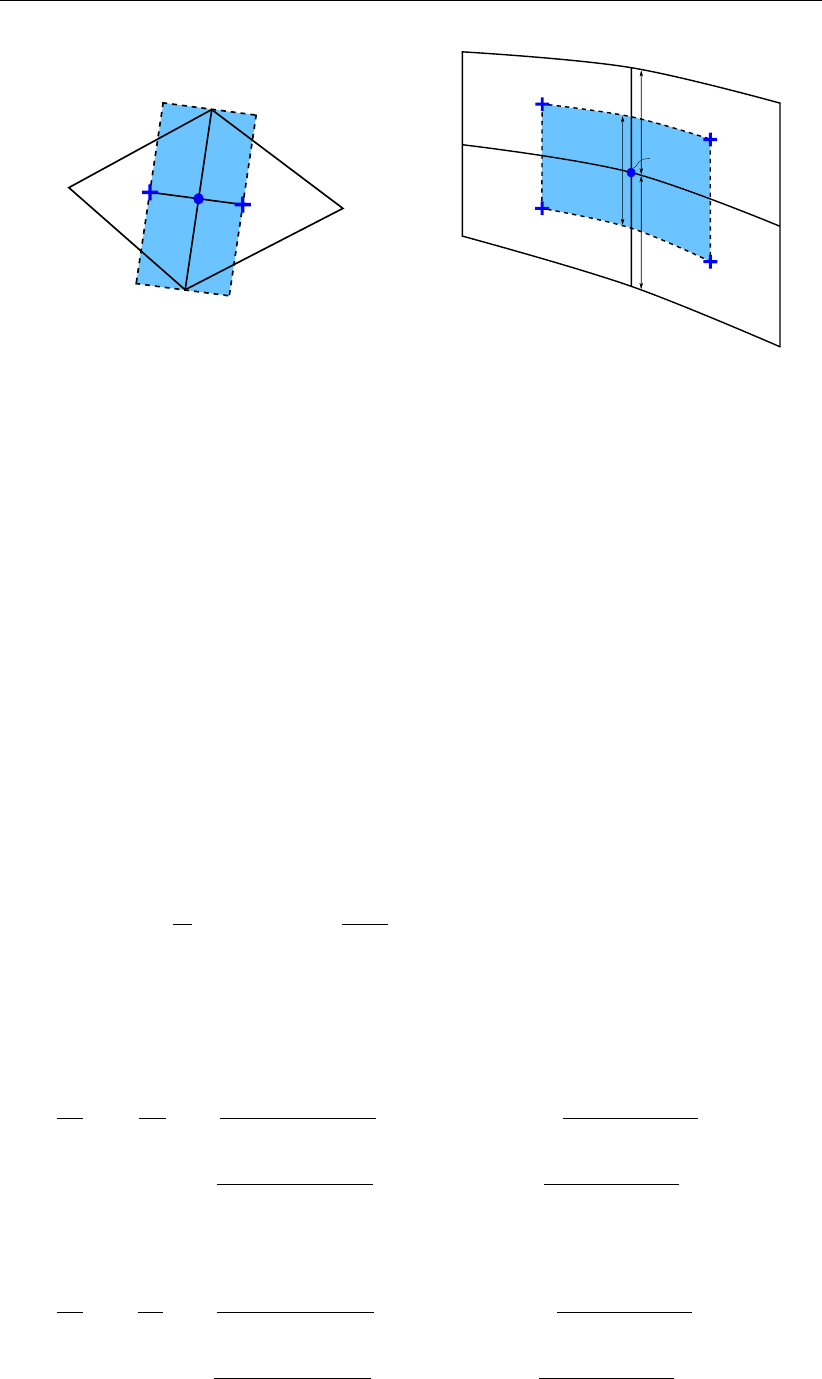
DRAFT
Numerical schemes for three-dimensional flows
j
k1k2
(a) Top view
kj,l, εj,l
∆zj,l
∆zj,l+1
∆zj,l+1/2
(b) Side view
Figure 7.3: The top view (a) and the side view (b) of the location of the turbulence vari-
ables on the computational grid.
Advection
The horizontal advection term is discretized explicitly by means of first order upwind. The
horizontal advection can be written in non-conservative form as
u•(∇k) = ∇•(uk)−k(∇•u)(7.54)
Integration of this term yields,
ZV
u•(∇k)dV =ZV∇•(uk)dV −ZV
k(∇•u)dV (7.55)
ZV
u•(∇k)dV =ZA
(uk)•ndA −ZA
k(u•n)dA (7.56)
u•(∇k) = 1
VXqn+1
j,l kn
j,l −kn+1
j,l
VXqn+1
j,l (7.57)
Diffusion
The diffusion terms in equations Equation (7.42) and Equation (7.43) are discretized implicitly
as,
∂
∂z Dk
∂τ
∂z ≈θDk2
∆zj,l+1∆zj,l+1/2kn+1
j,l+1 −kn+1
j,l −θDk1
∆zj,l∆zj,l+1/2kn+1
j,l −kn+1
j,l−1
+(1 −θ)Dk2
∆zj,l+1∆zj,l+1/2kn
j,l+1 −kn
j,l−(1 −θ)Dk1
∆zj,l∆zj,l+1/2kn
j,l −kn
j,l−1
(7.58)
∂
∂z Dε
∂ε
∂z ≈θDε2
∆zj,l+1∆zj,l+1/2εn+1
j,l+1 −εn+1
j,l −θDε1
∆zj,l∆zj,l+1/2εn+1
j,l −εn+1
j,l−1
+(1 −θ)Dε2
∆zj,l+1∆zj,l+1/2εn
j,l+1 −εn
j,l−(1 −θ)Dε1
∆zj,l∆zj,l+1/2εn
j,l −εn
j,l−1
(7.59)
Deltares 105 of 152
DRAFT
D-Flow Flexible Mesh, Technical Reference Manual
where indices 1and 2refer to the values on the bottom and the top of control volume, respec-
tively. The production terms for kequation is then discretized as
Pk≈νVun+1
j,l+1 −un+1
j,l 2+vn+1
j,l+1 −vn+1
j,l 2
∆zj,l+1/2
(7.60)
The dissipation term is a sink and the buoyancy term may act as a sink and can destabilize the
system. In order to conserve a diagonal dominant matrix, a semi-implicit method (Patankar
trick) is used to guarantee positivity of the numerical solutions. The discretized terms read
Bk≈(2Bkn
j,l
kn+1
j,l
kn
j,l −Bkn
j,l if B < 0
Bkn
j,l if B≥0
(7.61)
εn
j,l ≈
2εn
j,l
kn+1
j,l
kn
j,l −εn
j,l if k−ε
kn+1
j,l
τn
j,l
if k−τ
(7.62)
The production in the εequation is reformed by substituting Equation (7.53) in Equation (7.48).
Pε=c1εcµ
νV
kn
j,lPk(7.63)
The discretization of the buoyancy term for the εequation is similar to that of kequation:
ensuring positivity by using Patankar trick as
Bε=c3εcµBkkn
j,l (7.64)
collecting all above-mentioned terms, in their discretized forms, leads to tridiagonal matrices
for kand εin the form of
alkn+1
j,l−1+blkn+1
j,l +clkn+1
j,l+1 =dl(7.65)
and
alεn+1
j,l−1+blεn+1
j,l +clεn+1
j,l+1 =dl(7.66)
which are solved by Thomas algorithm, with the following boundary conditions. The boundary
conditions use the bed friction velocity, u∗b, and surface friction velocity, u∗t(caused by wind).
kj,0=u2
∗b
√cµ
, kj,M(j)=u2
∗t
√cµ
(7.67)
∂ε
∂z j,1/2
=−|u∗b|3
κ1
2∆zj,1+µz02,∂ε
∂z j,M(j)−1/2
=|u∗t|3
κ1
2∆zj,M(j)2(7.68)
where µtakes values of 1(based on theoretical analysis) or 9(based on measurements).
Algorithm (54) and Algorithm (55) represent algorithms for kand εequations, respectively.
106 of 152 Deltares

DRAFT
Numerical schemes for three-dimensional flows
Algorithm 54 update_verticalprofiles: compute the kinetic energy k
for l= 1 to M(j)do
D1=Dkj,l−1/2/∆zj,l+1/2∆zj,l, D2=Dkj,l+1/2/∆zj,l+1/2∆zj,l+1
ν0
V= min (νv, νmin)
ρz1=ρR(j),l+1−ρR(j),l
∆zR(j),l+1/2, ρz2=ρL(j),l+1−ρL(j),l
∆zL(j),l+1/2
ρz=1
2(ρz1+ρz2)
Bk=−gν0
V
ρσρρz
Pk=ν0
Vuj,l+1−uj,l
∆zj,l+1/22+ν0
Vvj,l+1−vj,l
∆zj,l+1/22
if k−εthen
Sk=εn
j,l/kn
l,j
β= 2
else if k−τthen
Sk= 1/τn
j,l
β= 1
end if
al=−D1θ−max (ω1,0)/∆zj,l+1/2
bl= 1/∆t+ (D1+D2)θ+ 2 max(Bk,0)/kn
j,l +βSk
+ max (ω2,0)/∆zj,l+1/2−min (ω1,0)/∆zj,l+1/2
cl=−D2θ+ min (ω2,0)/∆zj,l+1/2
dl=kn
j,l/∆t−D2kn
j,l −kn
j,l+1(1 −θ) + D1kn
j,l−1−kn
j,l(1 −θ)
+ max(Bk,0) −min(Bk,0) + Pk+ (β−1)Skkn
j,l − Akj,l
end for
Calculate u∗bby Algorithm (47)
a0= 0, b0= 1, c0= 0, d0=u2
∗b/√cµ
aM(j)= 0, bM(j)= 1, cM(j)= 0, dM(j)=u2
∗t/√cµ
Solve alkl−1+blkl+clkl+1 =dlby Algorithm (49)
Algorithm 55 update_verticalprofiles: compute the energy dissipation ε
for l= 1 to M(j)do
D1=Dεj,l−1/2/∆zj,l+1/2∆zj,l, D2=Dεj,l+1/2/∆zj,l+1/2∆zj,l+1
ν0
V= min (νv, νmin)
Pε=c1εcµkn
j,lPk/ν0
V
Bε=cµc1εkn+1
j,l min(Bk,0)
Sε=c2εεn
j,l/kn+1
j,l
al=−D1θ−max (ω1,0)/∆zj,l+1/2
bl= 1/∆t+ (D1+D2)θ+ 2Sε+ max (ω2,0)/∆zj,l+1/2−min (ω1,0)/∆zj,l+1/2
cl=−D2θ+ min (ω2,0)/∆zj,l+1/2
dl=εn
j,l/∆t−D2εn
j,l −εn
j,l+1(1 −θ) + D1εn
j,l−1−εn
j,l(1 −θ)
−Bε+Pε+Sεεn
j,l − Aεj,l
end for
a0= 0, b0= 1, c0=−1, d0= ∆zj,1max(u∗b,0)3/(κ∆(1
2zj,1+µz0)2)
aM(j)=−1, bM(j)= 1, cM(j)= 0, dM(j)= 4 |u∗t|3/(κ∆zj,M(j))
Solve alεl−1+blεl+clεl+1 =dlby Algorithm (49)
Deltares 107 of 152
DRAFT
D-Flow Flexible Mesh, Technical Reference Manual
7.7.4 k-τturbulence model
The time-scale of turbulence, τ, is defined by
τ=k
ε(7.69)
The eddy viscosity then equals
νV=cµ
k2
ε=cµkτ (7.70)
where cµ= 0.09. The variable τmodels a typical time-scale of turbulent eddies. The k−τ
equations read
∂k
∂t +u∂k
∂x +v∂k
∂y +ω∂k
∂z =∂
∂z Dk
∂k
∂z +Pk+Bk−k
τ(7.71)
∂τ
∂t +u∂τ
∂x +v∂τ
∂y +ω∂τ
∂z =∂
∂z Dτ
∂τ
∂z +Pτ+Bτ−(1 −c2ε)(7.72)
+Dkτ +Dτ τ +Dkk
where
Dτ=νmol
σmol
+νV
στ
(7.73)
Pτ=τ
k(1 −c1ε)Pk(7.74)
Bτ=τ
k(1 −c3ε)Bk(7.75)
Dkτ =1
h2
2
kDτ
∂τ
∂σ
∂k
∂σ (7.76)
Dττ =−1
h2
2
τDτ
∂τ
∂σ
∂τ
∂σ (7.77)
Dkk =−1
h2
τ
k
∂
∂σ 1
σε−1
σkνV
∂k
∂σ (7.78)
The signs of the coefficients are so that the production term Pτactually acts as sink of τ. This
can be explained by realizing that production of dissipation εresults in a faster dissipation of
turbulent eddies and therefore a smaller time-scale τof turbulence. Even though Pτacts as
a sink, it will still be called a production term because of the parallels with the ε-equation.
Likewise the dissipation term ετis a source of τ.
By substituting Equation (7.70) in Equation (7.74) for k, it changes to the following form
Pτ=cµ
νt
c1τPkτ2(7.79)
where c1τ= 1 −c1εis a constant. This equation is linearized by Picard method as
Pτ=cµ
νt
c1τPkτnτn+1 (7.80)
Similar to the above expression, by substituting Equation (7.70) in Equation (7.75), the buoy-
ancy term is changed to the following form
Bτ=c3τ
cµ
νt
Bkτ2(7.81)
108 of 152 Deltares
DRAFT
Numerical schemes for three-dimensional flows
where c3τ= 1 is for stable stratification and c=−0.44 is for unstable stratification. After
linearization by Picard method, it yields
Bτ=c3τ
cµ
νt
Bkτn
j,lτn+1
j,l (7.82)
or
Bτ=c3τ
cµ
στ
N2τn
j,lτn+1
j,l (7.83)
and
N2=−g
ρ0
∂ρ
∂z (7.84)
The currently used values of c3τfor stable and unstable stratification guarantee that c3τN2is
positive under all conditions, hence c3τ<0if N2<0and c3τ>0if N2>0.
The diffusion terms Dττ and Dkτ are simplified by neglecting νfrom the viscosity, as it is
small compared with the eddy viscosity. By inserting Equation (7.70) into the equations for
Dττ and Dkτ , it leads to the following form of equations
Dττ =−2cµ
στ
k∂τ
∂z ∂τ
∂z (7.85)
Dkτ =2cµ
στ
τ∂k
∂z ∂τ
∂z (7.86)
By summing Equation (7.85) and Equation (7.85) we have,
Dkτ +Dτ τ =2cµ
σττ∂k
∂z −k∂τ
∂z ∂τ
∂z =A∂τ
∂z (7.87)
Equation (7.87) is an advection equation. This equation is discretized by means of first order
upwind as follows.
Dkτ +Dτ τ = max(A,0)τn+1
j,l −τn+1
j,l−1
∆zj,l
+ min(A,0)τn+1
j,l+1 −τn+1
j,l
∆zj,l+1
(7.88)
where Ais discretized as,
A ≈ cµ
σττj,l−1+τj,l
2
kj,l −kj,l−1
∆zj,l
+τj,l+1 +τj,l
2
kj,l+1 −kj,l
∆zj,l+1
−kj,l−1+kj,l
2
τj,l −τj,l−1
∆zj,l −kj,l+1 +kj,l
2
τj,l+1 −τj,l
∆zj,l+1 (7.89)
In this analysis, the term of Dkk in Equation (7.73) is neglected.
The vertical diffusion term (the first term in the right hand side of Equation (7.73)) is discretized
implicitly by means of θmethod.
∂
∂z Dτ
∂τ
∂z ≈θDτ2
∆zj,l+1∆zj,l+1/2τn+1
j,l+1 −τn+1
j,l −θDτ1
∆zj,l∆zj,l+1/2τn+1
j,l −τn+1
j,l−1
+(1 −θ)Dτ2
∆zj,l+1∆zj,l+1/2τn
j,l+1 −τn
j,l−(1 −θ)Dτ1
∆zj,l∆zj,l+1/2τn
j,l −τn
j,l−1
(7.90)
Deltares 109 of 152

DRAFT
D-Flow Flexible Mesh, Technical Reference Manual
Combining all equations together, it leads to the following equation for each computational cell
alτn+1
j,l−1+blτn+1
j,l +clτn+1
l+1 =dl(7.91)
Marching in the vertical direction for each jlocation, it leads to a tridiagonal matrix (for each
j) which is solved by Thomas algorithm (see Algorithm (56)). The boundary conditions at the
bed and water surface are applied as,
a0= 0, b1= 1, c0= 0, d0=9κz0
max(u∗b,10−6)√cµ
aM(j)= 0, bM(j)= 1, cM(j)= 0, dM(j)= 0
Remark 7.7.1.The Dkk term is neglected because it may cause numerical instabilities. If k
goes to zero, then it follows from the positivity of kthat ∂k/∂z also goes to zero. However,
numerically ∂k/∂z is not necessarily small when kgoes to zero, especially on coarse grids,
and this term can grow to infinity. It is expected that this term is generally rather small because
the factor 1/σε−1/σkin front of the term is only 0.2 with the current parameter settings.
Remark 7.7.2.The k-τturbulence model is applied for the first time in Delft3D package and
it still needs intensive verifications.
Algorithm 56 update_verticalprofiles: compute the energy dissipation τ
for l= 1 to M(j)do
D1=Dεj,l−1/2/∆zj,l+1/2∆zj,l, D2=Dεj,l+1/2/∆zj,l+1/2∆zj,l+1
ν0
V= min (νv, νmin)
Pτ= (1 −c1ε)cµτn
j,lPk/ν0
V
Bτ=c3τcµBkτn
j,l
α1=kn
j,l−1+kn
j,lτn
j,l −τn
j,l−1/(2∆zj,l)
α2=kn
j,l+1 +kn
j,lτn
j,l+1 −τn
j,l/(2∆zj,l+1)
Dττ =cµ(α1+α2)/στ
β1=τn
j,l−1+τn
j,lkn
j,l −kn
j,l−1/(2∆zj,l)
β2=τn
j,l+1 +τn
j,lkn
j,l+1 −kn
j,l/(2∆zj,l+1)
Dkτ =cµ(β1+β2)/στ
D= (Dττ −Dkτ )/∆zj,l+1/2
al=−D1θ−max(D, 0) −max (ω1,0)/∆zj,l+1/2
bl= 1/∆t+ (D1+D2)θ−Bτ−Pτ+ max(D, 0) −min(D, 0)
+ max (ω2,0)/∆zj,l+1/2−min (ω1,0)/∆zj,l+1/2
cl=−D2θ+ min(D, 0) + min (ω2,0)/∆zj,l+1/2
dl=τn
j,l/∆t−D2τn
j,l −τn
j,l+1(1 −θ) + D1τn
j,l−1−τn
j,l(1 −θ)
−(1 −c2ε)− Aεj,l
end for
Calculate u∗by Algorithm (47)
a0= 0, b1= 1, c0= 0, d0= 9κz0/max(u∗b,10−6)√cµ
aM(j)= 0, bM(j)= 1, cM(j)= 0, dM(j)= 0
Solve alτl−1+blτl+clτl+1 =dlby Algorithm (49)
7.8 Baroclinic pressure
Under the shallow-water assumption, the vertical momentum equation is reduced to a hydro-
static pressure equation. Vertical accelerations due to buoyancy effects and due to sudden
variations in the bottom topography are not taken into account. So:
∂P
∂z =−gρ (7.92)
110 of 152 Deltares

DRAFT
Numerical schemes for three-dimensional flows
After integration between two successive layers, in the vertical direction, the hydrostatic pres-
sure is
P(z) = P2+gZ∆zl
0
ρ(z)dz (7.93)
where P2is the pressure on the upper layer level. The local density is related to the values of
temperature and salinity by the equation of state. The density is assumed to change linearly
at each flow cell, along the layer in the vertical direction. The density can be described as
ρ(z) = ρ2+αz, with α= (ρ1−ρ2)/∆zl, where ρ1and ρ2are the densities on the top
and bottom of the flow cell, respectively. After substitution of this relation in Equation (7.93)
and integration , it gives,
P(z) = P2+gρ2∆zl+1
2α∆z2
l(7.94)
The force on the flow is derived by integration of the pressure in the vertical direction.
F(z) = Z∆zl
0
P(z)dz (7.95)
Subsituting Equation (7.95) in Equation (7.94) gives,
F(z) = P2∆zl+1
2gρ2∆z2
l+1
6gα∆z3
l(7.96)
Remark 7.8.1.For integration of Equation (7.94) and Equation (7.95), the vertical coordinate
is locally set starting from the top of the cell (on the layer) toward downward.
The merely of this method is to calculate F(z)at the cells between the layers, and integrate
the force from the water surface to the cell levels. Once it is done, the forces around the
control volume are integrate. This method is applied in Algorithm (57).
Deltares 111 of 152

DRAFT
D-Flow Flexible Mesh, Technical Reference Manual
Algorithm 57 addbaroc2: compute the baroclinic pressure along σ-layers
First, extrapolate the density on the water surface
βL=∆zL(j),M(j)−1
∆zL(j),M(j)+ ∆zL(j),M(j)−1
βR=∆zR(j),M(j)−1
∆zR(j),M(j)+ ∆zR(j),M(j)−1
˜ρL,M(j)= (1 + βL)ρL(j),M(j)−βLρL(j),M(j)−1
˜ρR,M(j)= (1 + βR)ρR(j),M(j)−βRρR(j),M(j)−1
for l=M(j)−1to 1step −1do
βL=∆zL(j),l
∆zL(j),l + ∆zL(j),l+1
βR=∆zR(j),l
∆zR(j),l + ∆zR(j),l+1
˜ρL,l =βLρL(j),l + (1 −βL)ρL(j),l+1
˜ρR,l =βRρR(j),l + (1 −βR)ρR(j),l+1
end for
for l=M(j)to 1step −1do
αL=˜ρL,l−1−˜ρL,l
∆zL(j),l
, αR=˜ρR,l−1−˜ρR,l
∆zR(j),l
PL=g
M(j)
X
l0=l
1
2˜ρL,l0∆zL(j),l0+1
6αL∆z2
L(j),l0
PR=g
M(j)
X
l0=l
1
2˜ρR,l0∆zR(j),l0+1
6αR∆z2
R(j),l0
GL=PL∆zL(j),l +1
2˜ρL,l∆z2
L(j),l +1
6αL∆z3
L(j),l
GR=PR∆zR(j),l +1
2˜ρR,l∆z2
R(j),l +1
6αR∆z3
R(j),l
˜ρj,l =1
4˜ρL(j),l + ˜ρL(j),l−1+ ˜ρR(j),l + ˜ρR(j),l−1
GB=zL(j),l−1−zR(j),l−1
M(j)
X
l0=l
˜ρj,l0∆zj,l0
GT=zL(j),l −zR(j),l
M(j)
X
l0=l+1
˜ρj,l0∆zj,l0
δPl=GL−GR+GB−GT
Vρ=1
4∆zL(j),l (˜ρL,l + ˜ρL,l−1)+∆zR(j),l (˜ρR,l + ˜ρR,l−1)
∆P=δPl/Vρ
end for
112 of 152 Deltares
DRAFT
Numerical schemes for three-dimensional flows
7.9 Artificial mixing due to σ-coordinates
The fluxes of the transport equations consist of both advective and diffusive fluxes. In sigma
co-ordinates the approximation of the advective fluxes does not introduce large truncation
errors. Therefore in this section we consider only diffusive fluxes given by
Fi=DH
∂c
∂xi
, i = 1,2; F3=DV
∂c
∂x3
(7.97)
where DH, denotes the horizontal eddy diffusion coefficient and DVdenotes the vertical
eddy diffusion coefficient.
It is difficult to find a numerical approximation that is stable and positive. Near steep bottom
slopes or near tidal flats where the total depth becomes very small, truncations errors in the
approximation of the horizontal diffusive fluxes in σ-coordinates are likely to become very
large, similarly to the horizontal pressure gradient. Thus a complete transformation must be
included. However, in that case numerical problems are encountered concerning accuracy,
stability and monotonicity. In D-Flow FM a method is applied which gives a consistent, sta-
ble and monotonic approximation of the horizontal diffusion terms even when the hydrostatic
consistency condition is violated. For details we refer the user to Stelling and Van Kester
(1994)
7.9.1 A finite volume method for a σ-grid
Applying the Gauss theorem to the transport equation yields
∂
∂t Zv
c dv +Is
F•nds = 0 (7.98)
Instead of transforming the transport equation to σ-co-ordinates, we generate a sigma grid
by choosing a distribution of the vertical co-ordinate sigma. The vertical diffusive fluxes are
straightforward to implement. The only difficulty is the approximation of the horizontal diffusive
fluxes. To explain this method, it is sufficient to consider a simplified one-dimensional heat
equation (i.e. a transport equation without advection in one dimension)
∂c (x, z, t)
∂t −∂
∂x DH
∂c (x, z, t)
∂x = 0 (7.99)
For this equation a finite volume method has to be constructed that meets the following re-
quirements:
1 consistent approximation of the horizontal diffusive fluxes
2 fulfilment of the min-max principle
3 minimal artificial vertical diffusion
A non-linear approach is chosen which consists of the following steps.
Step 1
First, diffusive fluxes fi+1
2,l+1
2, l = 0,...,2K(Kis the σ-layer number), are defined
according to
fi+1
2,l+1
2=
DHmin (∆mc, ∆nc)zi+1
2,l+1−zi+1
2,l
xi+1−xi,if ∆mc > 0∧∆nc > 0
DHmax (∆mc, ∆nc)zi+1
2,l+1−zi+1
2,l
xi+1−xi,if ∆mc≤0∧∆nc≤0
0,if ∆mc∆nc < 0
(7.100)
Deltares 113 of 152
DRAFT
D-Flow Flexible Mesh, Technical Reference Manual
The differences ∆m/nc= ∆m/nci+1
2,l+1
2are given by (l= 0,...,2K)
fi+1
2,l+1
2=(∆mci+1
2,l+1
2=ci+1 zi,m(l)−ci,m(l)
∆nci+1
2,l+1
2=ci+1,n(l)−cizi+1,n(l)(7.101)
where ci(z)is a simple linear interpolation formula given by
ci(z) =
ci,1,if z≤zi,1
z−zi,k
zi,k+1−zi,k ci,k+1 +zi,k+1−z
zi,k+1−zi,k ci,k,if zi,k < z ≤zi,k+1
ci,K ,if z≥zi,K
(7.102)
Step 2
In this step the diffusive fluxes are added to the appropriate control volumes according to
Vn+1
i,k cn+1
i,k =Vn
i,kcn
i,k −∆tX
∀l|m(l)=k
fn
i+1
2,l+1
2+ ∆tX
∀l|n(l)=k
fn
i−1
2,l+1
2
(7.103)
where nis the time index, t=n∆tand Vndenotes the size of the control volume. The
absence of advection implies Vn=Vn+1
7.9.2 Approximation of the pressure term
The horizontal gradients of the pressure must be approximated for the horizontal momen-
tum equations. The pressure gradient must be computed along the same verticals as the
horizontal concentration gradients. The pressure pin Cartesian coordinates is given by
p(x, z) = Zζ
z
ρ(x, z0, t)gdz0(7.104)
From the Leibniz rule it follows that ∂p/∂x is given by
∂p
∂x =∂
∂x Zζ(x)
z
ρ(x, z0)gdz0=Zζ(x)
z
g∂
∂xρ(x, z0)dz0+gρ (ζ)∂ζ
∂x (7.105)
The relation between the density ρand the salinity sand temperature Tis given by the equa-
tion of state, namely ρ=ρ(s(x, t), T (x, t)). The integral in Equation (7.105) is replaced
by a summation over the intervals which are in the water column above the velocity point with
vertical co-ordinate z.
∂p
∂xxi+1
2,z=g
2K+1
X
l=K+1 ∂ρ
∂sf(s)
DH
+∂ρ
∂T f(T)
DHi+1
2,l+1
2
+gzi+1
2,k+1 −z
zi+1
2,k+1 −zi+1
2,k ∂ρ
∂sf(s)
DH
+∂ρ
∂T f(T)
DHi+1
2,k+1
2
+gρζi+1 −ζi
∆x(7.106)
where k= max l|zi+1
2,l < z
114 of 152 Deltares

DRAFT
8 Parallelization
This chapter elaborates on the parallelization of D-Flow FM, which enables the simulation
on 1D and 2D network. The sequential time loop is described in section 6.3. This chapter
emphasises on the modifications needed for parallelization.
8.1 Parallel implementation
The goal of parallelization of D-Flow FM is twofold. We aim for faster computations on shared-
or distributed-memory machines and the ability to model problems that do not fit on a single
machine. To this end we decompose the computational domain into subdomains and apply
the "single program, multiple data" (SPDM) technique for parallelization. Since we apply
SPDM, we want each subdomain (process) to be as autonomous as can be and require that
each subdomain has its own unique computational mesh,
the subdomain interfaces act as boundaries where data is communicated,
only primitive variables uand ζare communicated,
the parallel and sequential algorithm yield the same results, except for round-off errors
that is,
the modelling in all subdomains is identical, has the same time-step, et cetera. Note this
this requirement compromises our aim for autonomous subdomain modelling.
8.1.1 Ghost cells
Keeping our design choices in mind, it is apparent from Equation (6.22) to Equation (6.95)
that during a time-step we need to compute advection, diffusion and the water-level gradient
in the momentum equation anywhere in the subdomain. Similarly, we need to compute the
discharge divergence in the continuity equation, Equation (6.97) anywhere in our subdomains.
The stencil used for computing momentum advection and diffusion is depicted in Figure 8.12.
It will be clear that the stencil can not be applied near the subdomain interfaces. Since we
choose not to modify the stencil as explained in the foregoing, the subdomains need to be
augmented with ghost cells that only serve to compute the time-step update for the "inter-
nal" water-levels and velocities. No valid velocity- and water-level update are computed for
the "external", ghost water-levels and velocities. Instead, values at the next time-level are
copied from the corresponding neighboring subdomains, where valid time-step updates were
computed, see Figure 8.2.
The question remains how many ghost cells need to be supplied. The stencil for the momen-
tum advection and diffusion is depicted in Figure 8.12. To be able to count the number of
cells in the stencil, we firstly define the level of a neighboring cell. Cells adjacent to a face are
level 1. Their neighboring cells, i.e. cells that share at least one common face, are level 2, et
cetera, see Figure 8.12. We say that a cell is in the stencil, if at least one of it’s face-normal
velocity components is required in the stencil, since in D-Flow FM a face-normal velocity can
only exist if both its neighboring cells exist.
It will not be hard to see that one level of ghost cells suffices for the water-level gradients in
the momentum equation and divergence in the continuity equation. The spatial discretization
of momentum advection and diffusion will not be explained in detail here, but it is important
to understand that advection and diffusion are in fact computed at cell centers, based on
reconstructed cell-centered data, and interpolated back to the faces. So we have
one level of neighbors for the interpolation from cell-centered to face-normal advection
and diffusion,
Deltares 115 of 152
DRAFT
D-Flow Flexible Mesh, Technical Reference Manual
4
3
4
3
4
4
3
2
1
2
3
4
4
3
2
1
2
3
4
3
4
3
4
4
Figure 8.1: Stencil for momentum advection and diffusion; the numbers indicate the level
of the neighboring cells
subdomain 1
subdomain 0
subdomain 1
subdomain 0
sequential
parallel
communication
Figure 8.2: Ghost cells
116 of 152 Deltares

DRAFT
Parallelization
Table 8.1: METIS settings
parameter/option value meaning
routine METIS_PartGraphRecursive
or METIS_PartGraphKway
mesh partitioning method
NITER 100 Number of iterations for the refine-
ment algorithms at each stage of the
uncoarsening process
UFACTOR 1.001 allowed load imbalance
CONTIG 0 or 1 enforce contiguous subdomains (1)
or not (0), only available when using
K-way method
one additional level for a higher order cell-centered (collocated) discretization, and
one additional level for the reconstruction of the cell-centered velocity vector from the
edge-normal data.
This sums up to four levels of neighbors, as can be seen in Figure 8.12. Consequently, four
levels of ghosts cells are required for momentum advection and diffusion.
The ghost level of cell kis called gs(k)and of face j gu(j). They are related by
gu(j) = (min(gs(L(j)), gs(R(j))),face jis a ghost face, not on the subdomain interface,
max(gs(L(j)), gs(R(j))),face jis a ghost face, on the subdomain interface,
0face jis not a ghost face.
(8.1)
If face jis on the subdomain interface, it can only be a ghost face of subdomain id if the
neighboring ghost cell has a lower subdomain number than id, since we say that it is owned
by the subdomain with the lowest number, explained hereafter, see Equation (8.2). If face jis
not on the subdomain interface, it can only be a ghost face of subdomain id if both adjacent
cells have subdomain numbers other than id.
8.1.2 Mesh partitioning with METIS
The METIS software package,see Karypis (2013), is used for partitioning the mesh. A dual
graph of the mesh is firstly generated, and then partitioned. METIS produces a cell coloring
of the unpartitioned mesh, that we will refer to as the cell subdomain number ids(k), where k
is the cell number. Two partition methods are available in METIS: Recursive Bisection (default
method in D-Flow FM) and multilevle K-way. The latter enables to enforce contiguous subdo-
mains, and it is observed that this comes at the cost of a reduced homogeneous distribution
of cells over the subdomains, however.
The non-default METIS settings employed are listed in Table 8.1.
Any cell in the unpartitioned mesh uniquely belongs to a subdomain, so the water-level un-
knowns can uniquely be assigned a subdomain number. The face-normal velocity unknowns,
on the other hand, can not, since the velocities on the subdomain interfaces can belong to
either of the two adjacent subdomains. We choose to uniquely assign a subdomain number
idu(j)to face jby taking the minimum subdomain number of its two adjacent cells:
idu(j) = min (ids(L(j)), ids(R(j))) .(8.2)
Data will be communicated from the subdomain that owns the data to the subdomains that
require the data.
Deltares 117 of 152

DRAFT
D-Flow Flexible Mesh, Technical Reference Manual
With the cell coloring available, the subdomain meshes are augmented with four layers of
ghost cells and written to partition mesh files. There, the cell coloring is also written and then
read during the initialization of the parallel computation.
Remark 8.1.1.Level 5ghost cells are not included in the subdomain meshes, except when
all its neighboring cells have level 4or lower, or are non-ghost cells. In that case all faces of
the level 5 ghost cell are present in the subdomain mesh. Since in D-Flow FM cells with all
its faces being defined in the mesh can not be disregarded, the level 5ghost cells itself are
included in the subdomain mesh.
8.1.3 Communication
The whole domain mesh was partitioned as described in the foregoing. It is not used during
the parallel computations and we will only consider the subdomains from now on.
During the computations we need to update the ghost values from the other subdomains.
However, we do not need to communicate all variables at all instances in the time step. It
depends on the operator under consideration. To this end, three sets of ghost values are
defined:
Gs={k:gs(k)=1},(8.3)
Gsall ={k: 1 ≤gs(k)≤N+ 1},(8.4)
Gu={j: 1 ≤gu(j)≤N+ 1},(8.5)
where N= 4 is the number of ghost levels. It may come as a surprise that we include ghost
levels up to N+1, however see Remark 8.1.1 in this respect. Gsrefers to an update of the first
level of ghost water-levels, needed in the continuity equation, Gsall to all ghost water-levels
and Guto all face-normal velocity components respectively.
Communication information is not stored to any subdomain specific file. Instead, coordinates
of the ghost cells and ghost faces are communicated with the other subdomains in the initial-
ization phase of the computations and, doing so, send lists Ss,Ssall and Suare constructed,
see Algorithm (58).
Remark 8.1.2.We have a one-to-one mapping of task (or ranks) to subdomain number, i.e.
task iwill correspond to subdomain i,i∈ {0, N −1}, with Nbeing the number of subdo-
mains.
Algorithm 58 partition_init: initialize the parallel communication
generate subdomain numbers based on the partitioning polygon (cells with subdomain
numbers other than the own subdomain number will correspond to ghost cells)
set the ghost levels
make the ghost lists Gs,Gsall and Gu
make the send lists Ss,Ssall and Su
The update of the ghost water-levels is performed by MPI communication, see Algorithm (59).
The other ghost types are updated similarly.
Algorithm 59 update_ghosts: update the ghost water-levels by means of MPI communication
non-blocking MPI-send ζk,k∈ Ssto other subdomains
MPI-receive ζk,k∈ Gsfrom other subdomains
wait for send to terminate
118 of 152 Deltares

DRAFT
Parallelization
8.1.4 Parallel computations
In the parallel run, each task will
prepare the subdomain model, i.e.
read the subdomain mesh,
read the boundary conditions,
read external forcings,
et cetera,
initialize the parallel communication, Algorithm (58),
perform the time stepping, as in Algorithm (22),
update ghost values during the time stepping,
output flow variables.
Note that the boundary conditions, external forcing files, et cetera are shared by the subdo-
mains. In fact, they are just the sequential files and do not need to be partitioned. Only the
mesh and the model definition file need to be partitioned. The partitioned model definition
files will contain references to the subdomain mesh, all other information equals its sequential
counterpart.
The parallel time-step is shown in Algorithm (60). The parallel extension of Algorithm (21)
is trivial and listed in Algorithm (61). The parallel solver for the water-level equation Algo-
rithm (23) is described in the next section.
Remark 8.1.3.It is sufficient for the parallel water-level solver to update only level-1 ghost
water-levels Gs. It is therefore necessary that all ghost water-levels Gsall are updated right
after the solve, as shown in Algorithm (60).
The parallel extensions of the following will remain unmentioned:
discharge boundary conditions,
cross sections and observation stations (for post-processing).
8.1.5 Parallel Krylov solver
The unknown water levels k∈ K in Equation (6.105) are solved in the same manner as in
case of the sequential computations, Algorithm (23), except for the solver itself, which now is
a parallel Krylov solver. We have two solvers available:
1 the parallelized version of the sequential algorithm (Algorithm (24)), and
2 a solver from the Portable, Extensible Toolkit for Scientific Computation (PETSc), Balay
et al. (2013).
Deltares 119 of 152

DRAFT
D-Flow Flexible Mesh, Technical Reference Manual
Algorithm 60 parallel step_reduce: perform a time step; parallel-specific statements are out-
lined
while first iteration or repeat time-step (type 1) do
tn+1 =tn+ ∆t
compute fun
jand run
jwith Algorithm (14)
while first iteration or repeat time-step (type 2) do
compute the matrix entries Bn
k,Cn
jand right-hand side dn
kin the water-level equation
with Algorithm (15)
determine the set of water-levels that need to be solved, Algorithm (17)
i= 0
ζn+1(0)
k=ζn
k
while max
kζn+1(i)
k−ζn+1(i−1)
k> ε ∧not repeat time-step∨i= 0 do
i=i+ 1
compute the matrix entries Brn
k,Crn
jand right-hand side drn
kin the water-level
equation with Algorithm (18)
parallel solve the unknown water-levels and obtain ζn+1(i+1)
k, see section 8.1.5
update all ghost water-levels ζn+1(i−1)
k,k∈ Gsall
check positivity of water level with Algorithm (19) and repeat time-step if necessary
with modified ∆t(type 1) or hun
j(type 2, default)
reduce ’repeat time-step’
if not repeat time-step then
compute water-column volume Vn+1(i+1)
kand wet bed area An+1(i+1)
kwith Algo-
rithm (20)
reduce max
kζn+1(i)
k−ζn+1(i−1)
k
end if
end while
end while
end while
ζn+1
k=ζn+1(i+1)
k
compute velocities un+1
j, update ghost velocities un+1
j,k∈ Guand compute dis-
charges qn+1
jand qan+1
jat the next time level, Algorithm (61)
120 of 152 Deltares
DRAFT
Parallelization
Algorithm 61 parallel u1q1: update velocity un+1
j, update ghost velocities un+1
j, and com-
pute discharges qn+1
jand qan+1
j; parallel-specific statements are outlined
if hun
j>0then
un+1
j=−fun
j(ζn+1
R(j)−ζn+1
L(j)) + run
j
else
un+1
j= 0
end if
update ghost velocities un+1
j,j∈ Gu
if hun
j>0then
qn+1
j=Aun
jθjun+1
j+ (1 −θj)un
j(8.6)
qan+1
j=Aun
jun+1 (8.7)
else
qn+1
j=0 (8.8)
qan+1
j=0 (8.9)
end if
8.1.5.1 parallelized Krylov solver
The (reduced) global system to be solved has the form of
A[0,0] ··· A[0,N−1]
.
.
.....
.
.
A[N−1,0] . . . A[N−1,N −1]
s[0]
.
.
.
s[N−1]
=
d[0]
.
.
.
d[N−1]
,(8.10)
where the superscript [id]indicates the domain number. A matrix-vector multiplication can be
written as
.
.
.
A[id,id]s[id]+P
jd6=id
A[id,jd]s[jd]
.
.
.
,
where the diagonal diagonal contribution is computed as in the sequential case, see Equa-
tion (6.116), however for the internal unknowns only
A[id,id]s[id]=
.
.
.
Br[id]
ks[id]
k+P
j∈J [id](k)\G[id]
s
Cr[id]
js[id]
O(k,j)
.
.
.
(8.11)
and the off-diagonal contributions are computed by means of the ghost values G[id]
s
X
jd6=id
A[id,jd]s[jd]=
.
.
.
P
j∈J [id](k)∩G[id]
s
Cr[id]
js[id]
O(k,j)
.
.
.
,(8.12)
provided that the ghost values G[id]
sare up-to-date .
Deltares 121 of 152

DRAFT
D-Flow Flexible Mesh, Technical Reference Manual
Remark 8.1.4.Equation (8.10) shows that water-level unknowns in Ssare required for the
global matrix-vector multiplication. For that reason, they are disregarded in the Maximum
Degree algorithm and will never be eliminated from the solution vector s.
The system is solved by a parallelized preconditioned Conjugate Gradient method of Algo-
rithm (24), as shown in Algorithm (62), where we consider one subdomain id only and have
dropped the superscript [id]. The parallel extensions are trivial, except for the preconditioner
Pthat is. We apply a non-overlapping Additive Schwarz MILU factorization and precondition-
ing Pz(i+1)
r=r(i+1) can then be expressed as
P[id]z(i+1)[id]
r=r[id]−X
jd6=id
A[id,jd]z(i)[id]
r,(8.13)
where P[id]approximates A[id,id]. We use a MILU factorization available from SPARSKIT,
Saad (1994).
8.1.5.2 PETSc solver
As an alternative to the parallelized sequential Krylov solver, as explained in the foregoing, we
can apply a solver from the Portable, Extensible Toolkit for Scientific Computation (PETSc),
Balay et al. (2013). We use default settings.
8.2 Test-cases
In this section two test-cases are considered. To assess the scalability of the parallel im-
plementation, the computing time is measured for decompositions with varying number of
subdomains.
We measure the wall-clock times spent in the time-steps. This does not include file output
for post-processing. At prescribed modelling-time instances, computing times are measured
and summed (in time) by each subdomain. The maximum computing times over all the sub-
domains are used to determine a time-step average during a measurement interval, i.e.
Ttime-stepk=
max
d
nk
P
i=1
∆Td
i−max
d
nk−1
P
i=1
∆Td
i
nk−nk−1
,(8.14)
where ∆Td
iis the wall-clock computing time of time-step iand subdomain d,kis a mea-
surement index and nis the number of time steps. We will refer to this time as the time-step
averaged wall-clock time of a "time-step". The time-step wall-clock time is further divided into
MPInon-sol: MPI-communication time not related to the Krylov solver. These are the up-
date of the ghost-values Gsall and Gu, respectively and the reduction of the variables as
indicated in Algorithm (60),
solver: total Krylov solve time. This is the time spent by the Krylov solver, including MPI-
communication,
MPIsol: MPI-communication time in the Krylov solver. Unfortunately, no such times are
available for the PETSc solver,
#Krylov iterations: the time-step averaged number of iterations needed for the Krylov
solver to converge.
We expect that the non-communication times will show nearly linear scalability and foresee
that the communication times behave much worse. Furthermore, if the precondition becomes
122 of 152 Deltares

DRAFT
Parallelization
Algorithm 62 conjugategradient_MPI: solve water-level equation with a preconditioned Con-
jugate Gradient method; parallel specific statements are outlined
compute preconditioner P
update ghost values ζk,k∈ Gs
compute initial residual r(0) =d−As(0)
compute maximum error ε=kr(0)k∞
update ghost residuals rk,k∈ Gs
apply preconditioner Pz(0)
r=r(0)
set p(0) =z(0)
r
compute inner product Dr(0),z(0)
rE
reduce inner product Dr(0),z(0)
rE
reduce maximum error ε=kr(0)k∞
i= 0
while ε > tol do
update ghost values pk,k∈ Gs
compute Ap(i)
compute p(i), Ap(i)
reduce p(i), Ap(i)
α(i)=Dr(i),z(i)
rE
hp(i),Ap(i)i
s(i+1) =s(i)+α(i)p(i)
r(i+1) =r(i)−α(i)Ap(i)
compute maximum error ε=kr(i+1)k∞ε=kr(0)k∞
reduce maximum error ε=kr(0)k∞
update ghost values r(i+1),k∈ Gs
apply preconditioner Pz(i+1)
r=r(i+1)
if ε > tol then
compute Dr(i+1),z(i+1)
rE
reduce Dr(i+1),z(i+1)
rE
β(i+1) =Dr(i+1),z(i+1)
rE
Dr(i),z(i)
rE
p(i+1) =z(i+1)
r+β(i+1)p(i)
i=i+ 1
end if
end while
Deltares 123 of 152

DRAFT
D-Flow Flexible Mesh, Technical Reference Manual
less effective when the number of subdomains increases, the number of iterations will in-
crease.
The speed-up factor fcan now be defined as:
fk(N) = Ttime-stepkN
Ttime-stepkref
N, (8.15)
where Nis the number of subdomains and ref refers to a reference domain decomposition,
for which we take the decomposition with the smallest number of subdomains available. Note
that we do not compare with the single-domain, sequential simulations.
The simulations were conducted on the Deltares h4 cluster and the Lisa cluster at SURFsara,
see Lisa. For all our simulations, we took four cores per node.
Remark 8.2.1.Wall-clock times on Lisa were limited to 2.5hours, so, depending on the
number of subdomains, some simulations advanced further in modelling time than others.
For our comparison, we will always compare time-step averaged computing times at the same
modelling times.
8.2.1 Schematic Waal model
The first test-case under considerations is the schematic Waal model, see Yossef and Zagonjoli
(2010). The model has a rectangular domain of length 30 km and width 1800 m. It has a deep
center section of width 600 m and bottom levels varying from 0.795 (left) to −2.205 m (right).
The shallow outer part has a bottom level varying from 6.988 (left) to 3.988 m (right).
The mesh size in the deep, center part is 2×2m2and in the shallow outer part 2×4m2.
The total number of cells is 9 000 000. The maximum time step is 0.45 sec. The domain is
decomposed in 8,16,32,64 and 128 subdomains, respectively. The partitioning is depicted
in Figure 8.3.
Timing results on the SURFsara Lisa cluster are presented in Table 8.2 and the corresponding
speed-up factor in Figure 8.4. The results on the Deltares h4 cluster are shown in Table 8.3
and Figure 8.5 respectively. Recall that the wall-clock computing time on Lisa was limited to
2.5h, see Remark 8.2.1.
The results show that the speed-up factor with 128 subdomains is 108.66 on the Lisa cluster
and 85.1on the Deltares h4 cluster. This is a factor of 0.84, respectively 0.67 away from their
theoretical maximum. The reduced scaling on the h4 may be attributed to the poorer scaling
of the Krylov solver on the h4, due to communication overhead. It is interesting to see that
the number of iterations of the Krylov solver does not increase significantly when the number
of subdomain is increased. We do therefore not expect the preconditioner to have lost its
effectiveness. On the other hand, a more advanced preconditioner should reduce the number
of iterations in all cases and consequently the communication overhead, especially for large
numbers of subdomains.
8.2.2 esk-model
124 of 152 Deltares
DRAFT
Parallelization
(a) 8 subdomains
(b) 16 subdomains
(c) 32 subdomains
(d) 64 subdomains
(e) 128 subdomains
Figure 8.3: Partitioning of the schematic Waal model with METIS
Table 8.2: time-step averaged wall-clock times of the Schematic Waal model; Lisa; note:
MPI communication times are not measured for the PETSc solver
#dmns t [h] time step [s] MPInon-sol [s] solver [s] MPIsol [s] #Krylov-iters
8 0.33 3.24200 0.07037 1.29400 0.00000 15.06000
0.65
1.25
2.57
3.00
16 0.33 1.64950 0.03644 0.64200 0.00000 16.01500
0.65 1.62100 0.02498 0.62600 0.00000 15.00000
1.25
2.57
3.00
32 0.33 0.87400 0.03441 0.34975 0.00000 16.84500
0.65 0.87000 0.03687 0.34800 0.00000 16.00000
1.25 0.84851 0.03394 0.32426 0.00000 14.14356
2.57
3.00
64 0.33 0.44050 0.01904 0.18345 0.00000 17.22000
0.65 0.44950 0.01983 0.17100 0.00000 16.00000
1.25 0.42673 0.01962 0.16139 0.00000 14.25248
2.57 0.41782 0.01906 0.15347 0.00000 13.20792
3.00
128 0.33 0.23870 0.01792 0.09415 0.00000 17.03000
0.65 0.22450 0.01344 0.09075 0.00000 16.00000
1.25 0.21733 0.01334 0.08361 0.00000 14.17327
2.57 0.21436 0.01332 0.08069 0.00000 13.09901
3.00 0.21733 0.01352 0.08020 0.00000 13.00000
Deltares 125 of 152

DRAFT
D-Flow Flexible Mesh, Technical Reference Manual
Table 8.3: time-step averaged wall-clock times of the Schematic Waal model; h4; note:
MPI communication times are not measured for the PETSc solver
#dmns t [h] time step [s] MPInon-sol [s] solver [s] MPIsol [s] #Krylov-iters
8 0.33 3.74800 0.05160 1.31350 0.00000 15.06000
0.65 3.74000 0.05333 1.31050 0.00000 15.00000
1.25 3.62376 0.05163 1.19802 0.00000 13.00000
2.57 3.56436 0.05029 1.13861 0.00000 12.00990
3.00 3.56931 0.05019 1.13861 0.00000 12.06436
16 0.33 1.91550 0.04459 0.69650 0.00000 16.01500
0.65 1.88450 0.04294 0.66700 0.00000 15.00000
1.25 1.84158 0.04365 0.61881 0.00000 13.43564
2.57 1.81188 0.04255 0.59406 0.00000 12.63861
3.00 1.79703 0.04414 0.57426 0.00000 12.03960
32 0.33 1.01650 0.05025 0.39900 0.00000 16.84500
0.65 1.01300 0.06046 0.38300 0.00000 16.00000
1.25 0.96535 0.04963 0.34703 0.00000 14.10396
2.57 0.95050 0.04990 0.33020 0.00000 13.00990
3.00 0.95050 0.04960 0.33416 0.00000 13.00000
64 0.33 0.56200 0.03892 0.23580 0.00000 17.41000
0.65 0.54450 0.03161 0.22550 0.00000 16.61000
1.25 0.53465 0.03145 0.21634 0.00000 14.88614
2.57 0.50990 0.03226 0.19158 0.00000 13.14851
3.00 0.51485 0.03446 0.19307 0.00000 13.20297
128 0.33 0.35225 0.03553 0.17490 0.00000 17.03000
0.65 0.34550 0.03375 0.17005 0.00000 16.00000
1.25 0.32228 0.03249 0.14703 0.00000 14.18317
2.57 0.30941 0.03199 0.13465 0.00000 13.04950
3.00 0.31040 0.03188 0.13812 0.00000 13.0099
126 of 152 Deltares

DRAFT
Parallelization
Table 8.4: time-step averaged wall-clock times of the Schematic Waal model; SDSC’s
Gordon; note: MPI communication times are not measured for the PETSc
solver
#dmns t [h] time step [s] MPInon-sol [s] solver [s] MPIsol [s] #Krylov-iters
8 0.33 2.85100 0.03012 1.15250 0.00000 15.06000
0.65 2.85000 0.03273 1.14950 0.00000 15.00000
1.25 2.73762 0.02946 1.04455 0.00000 13.00000
2.57 2.68317 0.03151 0.99505 0.00000 12.00000
3.00 2.68812 0.03118 0.99505 0.00000 12.03960
16 0.33 1.49700 0.01458 0.63950 0.00000 16.00500
0.65 1.47000 0.01882 0.61200 0.00000 15.00000
1.25 1.41584 0.01454 0.56238 0.00000 13.20792
2.57 1.39604 0.01439 0.54455 0.00000 12.49505
3.00 1.38614 0.01494 0.52970 0.00000 12.04455
32 0.33 0.75100 0.02350 0.32120 0.00000 16.84500
0.65 0.73850 0.02326 0.31000 0.00000 16.00000
1.25 0.71535 0.02308 0.28564 0.00000 14.11386
2.57 0.69802 0.02249 0.27129 0.00000 13.00000
3.00 0.70297 0.02239 0.27129 0.00000 13.00000
64 0.33 0.38245 0.01719 0.16115 0.00000 17.41000
0.65 0.37900 0.01764 0.15610 0.00000 16.59500
1.25 0.35941 0.01667 0.14059 0.00000 14.90594
2.57 0.36386 0.02118 0.13960 0.00000 13.28218
3.00 0.34851 0.01580 0.13020 0.00000 13.22277
128 0.33 0.19340 0.01688 0.07790 0.00000 17.03000
0.65 0.18550 0.01454 0.07245 0.00000 16.00000
1.25 0.18119 0.01455 0.06812 0.00000 14.16832
2.57 0.17723 0.01499 0.06436 0.00000 13.05446
3.00 0.17673 0.01435 0.06337 0.00000 13.00000
Deltares 127 of 152

DRAFT
D-Flow Flexible Mesh, Technical Reference Manual
Table 8.5: time-step averaged wall-clock times of the Schematic Waal model; SDSC’s
Gordon; CG+MILUD
#dmns t [h] time step [s] MPInon-sol [s] solver [s] MPIsol [s] #Krylov-iters
8 0.33 5.73000 0.02977 4.04400 0.06205 22.86000
0.65 5.64500 0.03029 3.96000 0.07000 22.24500
1.25 5.44554 0.02777 3.76238 0.03337 20.89109
2.57
3.00
16 0.33 3.13550 0.02596 2.27150 0.05955 24.54500
0.65 3.02000 0.02771 2.16000 0.06665 23.00000
1.25 2.89604 0.02547 2.03465 0.06297 21.40594
2.57
3.00
32 0.33 1.65000 0.02941 1.21550 0.08840 25.00000
0.65 1.61900 0.03393 1.18350 0.08590 24.00000
1.25 1.53960 0.02714 1.10396 0.07139 22.19802
2.57
3.00
64 0.33 0.88850 0.02410 0.66200 0.07745 26.20000
0.65 0.85700 0.02364 0.62950 0.06110 24.99000
1.25 0.82970 0.01814 0.60792 0.06282 23.75248
2.57
3.00
128 0.33 0.46550 0.01583 0.35070 0.06740 25.48500
0.65 0.44900 0.01584 0.33450 0.06505 24.01500
1.25 0.43465 0.01655 0.31980 0.05683 22.79703
2.57 0.42327 0.01655 0.30891 0.05990 21.89604
3.00 0.42079 0.01568 0.30446 0.05743 21.77228
128 of 152 Deltares

DRAFT
Parallelization
Table 8.6: time-step averaged wall-clock times of the ’esk-model’; Lisa; note: MPI com-
munication times are not measured for the PETSc solver
#dmns t [h] time step [s] MPInon-sol [s] solver [s] MPIsol [s] #Krylov-iters
4 0.35 0.33152 0.00314 0.09406 0.00000 3.11984
0.45
0.63
0.75
0.85
1.10
8 0.35 0.16979 0.00355 0.05513 0.00000 3.30041
0.45 0.17875 0.00451 0.05752 0.00000 4.06024
0.63
0.75
0.85
1.10
16 0.35 0.09284 0.00271 0.03237 0.00000 3.09976
0.45 0.10073 0.00637 0.03337 0.00000 3.86932
0.63 0.10140 0.00341 0.03565 0.00000 3.75257
0.75
0.85
1.10
32 0.35 0.04625 0.00171 0.01493 0.00000 3.36052
0.45 0.04792 0.00200 0.01844 0.00000 4.34007
0.63 0.04908 0.00202 0.01608 0.00000 3.97418
0.75 0.04865 0.00209 0.01487 0.00000 3.09526
0.85
1.10
64 0.35 0.02323 0.00122 0.00999 0.00000 3.22176
0.45 0.02508 0.00148 0.01139 0.00000 4.30026
0.63 0.02567 0.00111 0.00915 0.00000 3.74654
0.75 0.02543 0.00120 0.00894 0.00000 3.00078
0.85 0.02545 0.00182 0.00846 0.00000 2.99741
1.10
128 0.35 0.01341 0.00087 0.00681 0.00000 3.89344
0.45 0.01514 0.00119 0.00782 0.00000 3.00000
0.63 0.01489 0.00125 0.00803 0.00000 4.00273
0.75 0.01496 0.00101 0.00614 0.00000 3.06459
0.85 0.01415 0.00090 0.00566 0.00000 3.00109
1.10 0.01414 0.00100 0.00554 0.00000 3.00715
Deltares 129 of 152
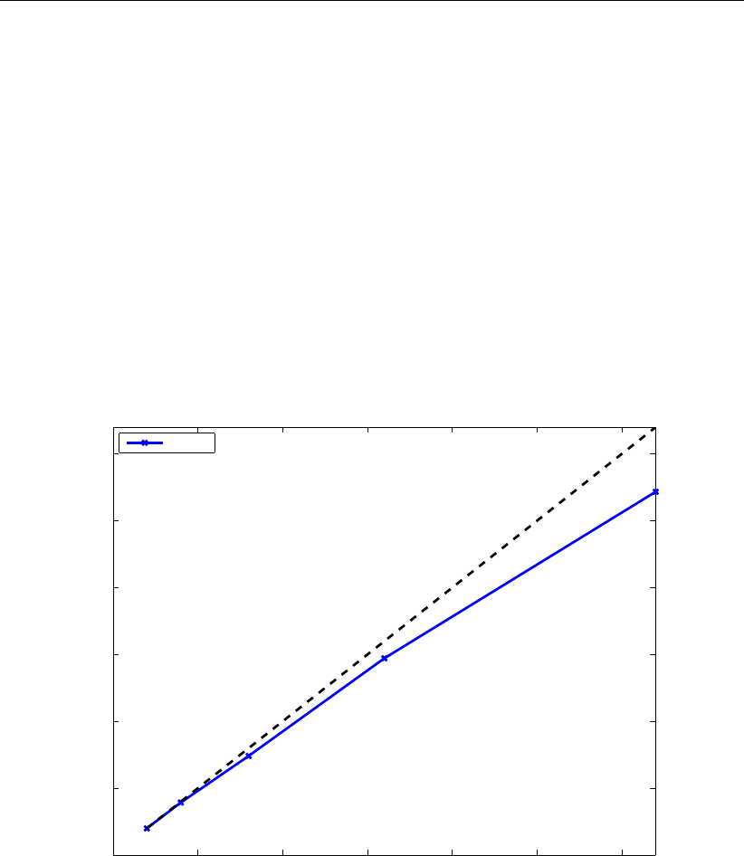
DRAFT
D-Flow Flexible Mesh, Technical Reference Manual
0 20 40 60 80 100 120
0
20
40
60
80
100
120
#subdomains
speed−up
Schematic Waal model; lisa
t=0.33 h
Figure 8.4: Speed-up of the schematic Waal model; Lisa
130 of 152 Deltares
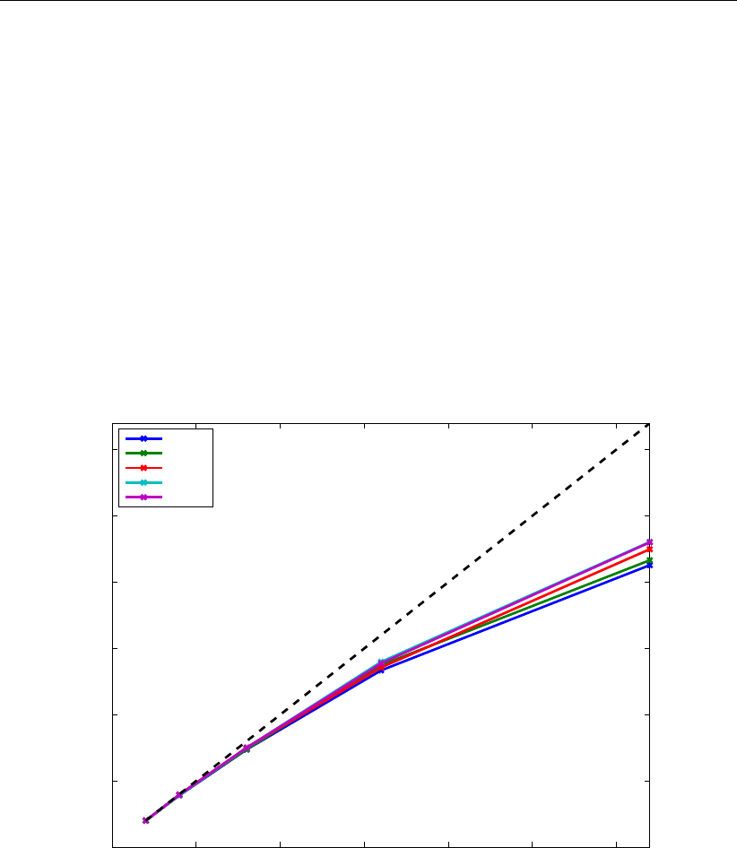
DRAFT
Parallelization
0 20 40 60 80 100 120
0
20
40
60
80
100
120
#subdomains
speed−up
Schematic Waal model; h4
t=0.33 h
0.65
1.25
2.57
3.00
Figure 8.5: Speed-up of the schematic Waal model; h4
Deltares 131 of 152
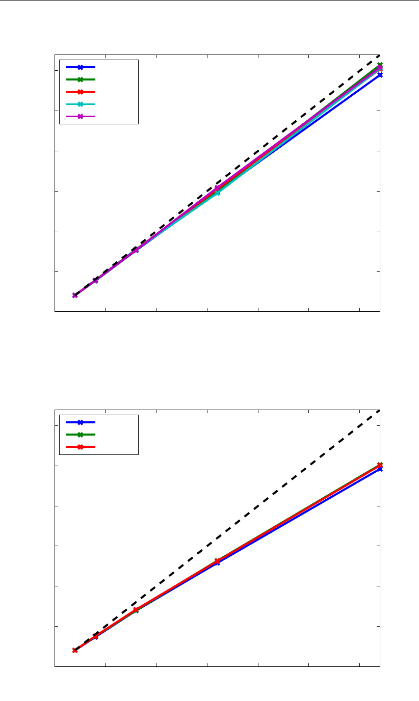
DRAFT
D-Flow Flexible Mesh, Technical Reference Manual
0 20 40 60 80 100 120
0
20
40
60
80
100
120
#subdomains
speed−up
Schematic Waal model; Gordon
t=0.33 h
0.65
1.25
2.57
3.00
Figure 8.6: Speed-up of the schematic Waal model; SDSC’s Gordon; PETSc
0 20 40 60 80 100 120
0
20
40
60
80
100
120
#subdomains
speed−up
Schematic Waal model; Gordon
t=0.33 h
0.65
1.25
Figure 8.7: Speed-up of the schematic Waal model; SDSC’s Gordon; CG+MILUD
132 of 152 Deltares
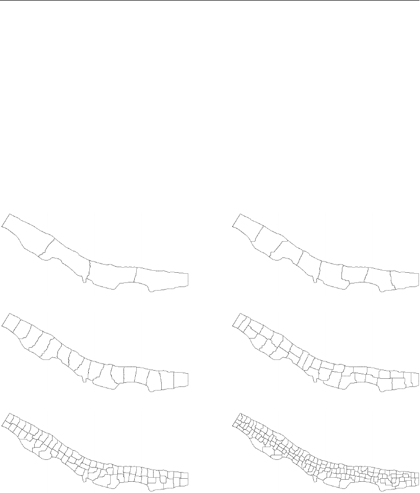
DRAFT
Parallelization
(a) 4 subdomains (b) 8 subdomains
(c) 16 subdomains (d) 32 subdomains
(e) 64 subdomains (f) 128 subdomains
Figure 8.8: Partitioning of the ’esk-model’ with METIS
Deltares 133 of 152
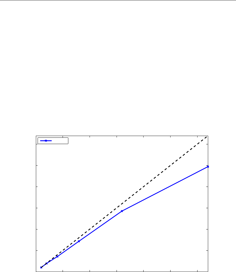
DRAFT
D-Flow Flexible Mesh, Technical Reference Manual
0 20 40 60 80 100 120
0
20
40
60
80
100
120
#subdomains
speed−up
esk_model; lisa
t=0.35 h
Figure 8.9: Speed-up of the ’esk-model’; Lisa
134 of 152 Deltares
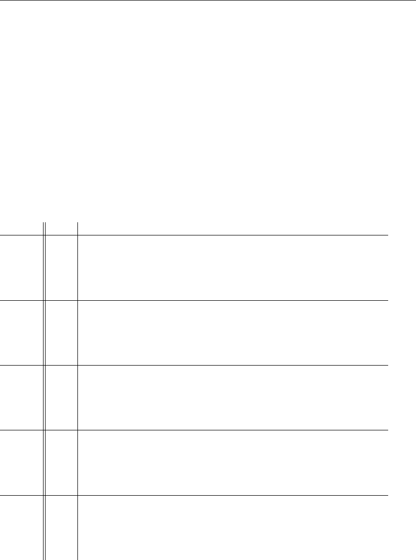
DRAFT
Parallelization
Table 8.7: time-step averaged wall-clock times of the Schematic Waal model; Gordon;
note: MPI communication times are not measured for the PETSc solver
#dmns t [h] time step [s] MPInon-sol [s] solver [s] MPIsol [s] #Krylov-iters
8 0.33 2.85100 0.03012 1.15250 0.00000 15.06000
0.65 2.85000 0.03273 1.14950 0.00000 15.00000
1.25
2.57
3.00
16 0.33 1.02900 0.02056 0.20595 0.00000 0.00000
0.65 1.01950 0.01502 0.20350 0.00000 0.00000
1.25 1.02277 0.01663 0.20297 0.00000 0.00000
2.57 1.01980 0.01624 0.20396 0.00000 0.00000
3.00
32 0.33 0.74950 0.02224 0.32080 0.00000 16.84500
0.65 0.73900 0.02293 0.31000 0.00000 16.00000
1.25 0.71634 0.02423 0.28614 0.00000 14.11386
2.57
3.00
64 0.33 0.37265 0.01499 0.15550 0.00000 17.41000
0.65 0.36750 0.01483 0.15075 0.00000 16.59500
1.25 0.35792 0.01431 0.14059 0.00000 14.90594
2.57 0.34802 0.01390 0.13119 0.00000 13.28218
3.00 0.34802 0.01353 0.13069 0.00000 13.22277
128 0.33 0.23665 0.03332 0.10325 0.00000 17.03000
0.65 0.23350 0.03431 0.09945 0.00000 16.00000
1.25 0.22624 0.03432 0.09287 0.00000 14.16832
2.57 0.22228 0.03386 0.08861 0.00000 13.05446
3.00 0.22129 0.03327 0.08812 0.00000 13.00000
Deltares 135 of 152
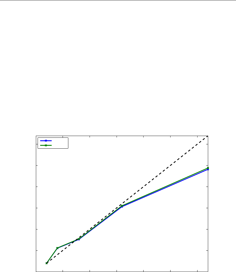
DRAFT
D-Flow Flexible Mesh, Technical Reference Manual
0 20 40 60 80 100 120
0
20
40
60
80
100
120
#subdomains
speed−up
Schematic Waal model; gordon
t=0.33 h
0.65
Figure 8.10: Speed-up of the schematic Waal model; Gordon
136 of 152 Deltares

DRAFT
Parallelization
8.2.3 San Fransisco Delta-Bay model
Deltares 137 of 152
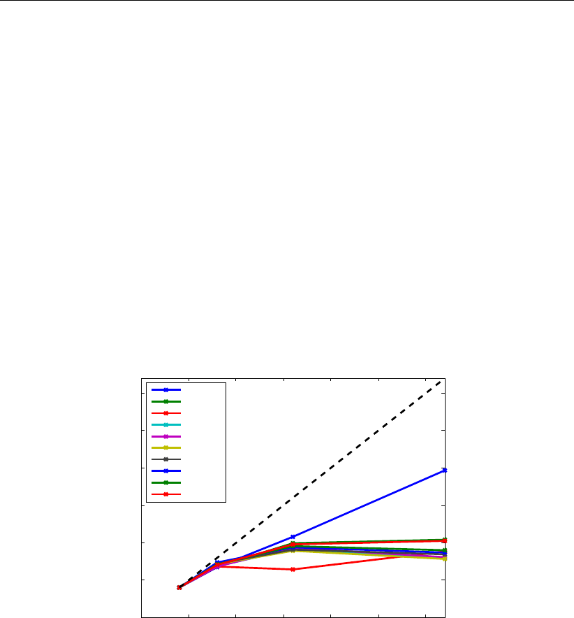
DRAFT
D-Flow Flexible Mesh, Technical Reference Manual
0 10 20 30 40 50 60
0
10
20
30
40
50
60
#subdomains
speed−up
San Fransisco Delta−Bay model
t=12.00 h
24.00
36.00
48.00
60.00
72.00
84.00
96.00
108.00
120.00
Figure 8.11: Speed-up of the San Fransisco Delta-Bay model; Gordon
138 of 152 Deltares

DRAFT
Parallelization
Table 8.8: time-step averaged wall-clock times of the San Fransisco Delta-Bay model;
Gordon; note: MPI communication times are not measured for the PETSc
solver
#dmns t [h] time step [s] MPInon-sol [s] solver [s] MPIsol [s] #Krylov-iters
8 12.00 0.14902 0.03099 0.01477 0.00000 16.25754
24.00 0.14889 0.02928 0.01528 0.00000 17.40124
36.00 0.14595 0.02592 0.01490 0.00000 15.49879
48.00 0.14759 0.02715 0.01527 0.00000 16.83857
60.00 0.14408 0.02398 0.01498 0.00000 15.99481
72.00 0.14509 0.02441 0.01519 0.00000 16.30267
84.00 0.14399 0.02353 0.01504 0.00000 16.12262
96.00 0.14880 0.02593 0.01518 0.00000 16.15620
108.00 0.14632 0.02445 0.01512 0.00000 16.01746
120.00 0.15038 0.02918 0.01510 0.00000 15.54151
16 12.00 0.08892 0.02771 0.00958 0.00000 13.72882
24.00 0.08726 0.02380 0.00981 0.00000 15.03835
36.00 0.08581 0.02293 0.00973 0.00000 12.97420
48.00 0.08607 0.02290 0.00991 0.00000 14.47656
60.00 0.08461 0.02147 0.00993 0.00000 13.58980
72.00 0.08183 0.01859 0.01005 0.00000 14.13277
84.00 0.08015 0.01716 0.00999 0.00000 13.80952
96.00 0.08123 0.01806 0.00998 0.00000 13.95845
108.00 0.08180 0.01852 0.00989 0.00000 13.77271
120.00 0.08547 0.02227 0.00985 0.00000 13.07582
32 12.00 0.05542 0.02316 0.00776 0.00000 18.51036
24.00 0.06021 0.02928 0.00791 0.00000 20.00691
36.00 0.09062 0.05868 0.00775 0.00000 17.71882
48.00 0.06466 0.03252 0.00790 0.00000 19.38103
60.00 0.06179 0.02975 0.00779 0.00000 18.33746
72.00 0.06537 0.03326 0.00785 0.00000 18.83925
84.00 0.06325 0.03124 0.00780 0.00000 18.64772
96.00 0.06352 0.03145 0.00782 0.00000 18.54788
108.00 0.06137 0.02929 0.00787 0.00000 18.57109
120.00 0.06140 0.02937 0.00775 0.00000 17.73242
64 12.00 0.03032 0.01249 0.00593 0.00000 19.85593
24.00 0.05749 0.03969 0.00612 0.00000 22.02080
36.00 0.06610 0.04823 0.00595 0.00000 18.88561
48.00 0.07463 0.05664 0.00613 0.00000 21.21491
60.00 0.07151 0.05354 0.00605 0.00000 19.72320
72.00 0.07442 0.05639 0.00611 0.00000 20.56026
84.00 0.06798 0.05006 0.00607 0.00000 20.07916
96.00 0.06844 0.05042 0.00611 0.00000 20.40540
108.00 0.06524 0.04724 0.00609 0.00000 20.24993
120.00 0.05862 0.04063 0.00606 0.00000 19.43446
Deltares 139 of 152
DRAFT
D-Flow Flexible Mesh, Technical Reference Manual
Table 8.9: time-step averaged wall-clock times of the San Fransisco Delta-Bay model;
Gordon; non-solver MPI communication times
#dmns t [h] MPIu[s] MPIsall [s] MPIreduce
8 12.00 0.00028 0.02238 0.00833
24.00 0.00029 0.01985 0.00914
36.00 0.00028 0.01609 0.00956
48.00 0.00028 0.01600 0.01086
60.00 0.00029 0.01268 0.01101
72.00 0.00027 0.01284 0.01130
84.00 0.00028 0.01227 0.01098
96.00 0.00027 0.01346 0.01220
108.00 0.00028 0.01249 0.01168
120.00 0.00028 0.01756 0.01133
16 12.00 0.00030 0.02184 0.00557
24.00 0.00030 0.01594 0.00756
36.00 0.00031 0.01250 0.01012
48.00 0.00030 0.01202 0.01058
60.00 0.00031 0.00982 0.01134
72.00 0.00030 0.00866 0.00963
84.00 0.00031 0.00795 0.00890
96.00 0.00031 0.00869 0.00907
108.00 0.00032 0.00807 0.01013
120.00 0.00030 0.01173 0.01024
32 12.00 0.00032 0.01859 0.00424
24.00 0.00033 0.01228 0.01667
36.00 0.00033 0.00884 0.04951
48.00 0.00032 0.00736 0.02484
60.00 0.00034 0.00595 0.02347
72.00 0.00031 0.00582 0.02713
84.00 0.00033 0.00574 0.02517
96.00 0.00033 0.00669 0.02442
108.00 0.00033 0.00588 0.02307
120.00 0.00032 0.00809 0.02096
64 12.00 0.00021 0.00902 0.00326
24.00 0.00022 0.00886 0.03060
36.00 0.00023 0.00696 0.04103
48.00 0.00023 0.00676 0.04966
60.00 0.00022 0.00437 0.04895
72.00 0.00024 0.00395 0.05220
84.00 0.00024 0.00375 0.04607
96.00 0.00023 0.00423 0.04597
108.00 0.00021 0.00374 0.04329
120.00 0.00020 0.00517 0.03526
140 of 152 Deltares
DRAFT
Parallelization
8.3 Governing equations
D-Flow FM solves the two- and three-dimensional shallow-water equations. We will focus
on two dimensions first. The shallow-water equations express conservation of mass and
momentum and can be put into the following form:
d
dtZ
Ω
hdΩ + Z
∂Ω
hu•ndΓ =0,(8.16)
d
dtZ
Ω
hudΩ + Z
∂Ω
huu •ndΓ = −Z
∂Ω
1
2h2ndΓ−Z
Ω
h∇ddΩ(8.17)
+Z
∂Ω
(νh(∇u+∇uT)) •ndΓ + Z
Ω
τdΩ,
(8.18)
where ζis the water level, hthe water level, d=ζ−hthe bed level, uthe velocity vector, g
the gravitational acceleration, νthe viscosity and τis the bottom friction:
τ=g
C2kuku,(8.19)
with Cbeing the Chézy coefficient.
8.4 Spatial discretization
The spatial discretization is performed in a staggered manner, i.e. velocity normal components
ujare defined at the cell faces j, with face normal vector nj, and the water levels skat cell
centers k.
We define volume Vkassociated with cell Ωkas
Vk=Z
Ω
hdΩ(8.20)
and the discharge through face jas
qj=Z
Γj
hu•ndΓ,(8.21)
which is discretized as
qj=hupwind(j)uj.(8.22)
The upwind cell associated with face jis
upwind(j) = L(j), uj≥0,
R(j), uj<0.(8.23)
We define the water-column volume Vkas
Vk=Z
Ωk
hdΩ(8.24)
Deltares 141 of 152
DRAFT
D-Flow Flexible Mesh, Technical Reference Manual
and for simplicity assume that it can be expressed as
Vk=bAkhk,(8.25)
where Ωkis the (two-dimensional) grid cell and bAkis the area of its horizontal projection.
Note that this relation does not hold in case of (partially) dry cells.
Borsboom et al. show that Equation (8.16) and Equation (8.18) can be discretized conserva-
tively as:
d
dthk=1
bAkX
j∈J (k)
qj1j,k,(8.26)
d
dt(˜
hjuj) = −g¯
hj
(sR(j)−sL(j))
∆xj−αLjAL(j)+αRjAR(j)•nj
+αLjDL(j)+αRjDR(j)•nj+τj,(8.27)
where ∆xj=kxR(j)−xL(j)k,˜
hjis the weighted average face water level
˜
hj=αL(j)hL(j)+αR(j)hR(j),(8.28)
¯
hjis the average face water level
¯
hj=1
2hL(j)+1
2hR(j),(8.29)
Akis the cell-centered conservative advection of hu, discretized as
Ak=1
bAkX
l∈J (k)
ucupwind(l)ql1l,k.(8.30)
and Dkis the cell-centered diffusion, not discussed further. The cell-center based velocity
vectors are reconstructed from the face-normal velocity components with
uck=1
bAkX
j∈J (k)
(xuj−xck)uj∆Γj1j,k.(8.31)
Using
d
dt(˜
hjuj) = ˜
hj
duj
dt+uj
d˜
hj
dt=˜
hj
duj
dt+αL
dhL(j)
dt+αR
dhR(j)
dt(8.32)
and substituting Equation (8.26) we obtain
duj
dt=−g¯
hj
˜
hj
(sR(j)−sL(j))
∆xj
−1
˜
hjαLj
1
bAL(j)X
l∈J (L(j))
(ucupwind(l)•nj−uj)ql1l,k+
αRj
1
bAR(j)X
l∈J (R(j))
(ucupwind(l)•nj−uj)ql1l,k
+1
˜
hjαLjDL(j)+αRjDR(j)•nj+τj
˜
hj
.(8.33)
142 of 152 Deltares
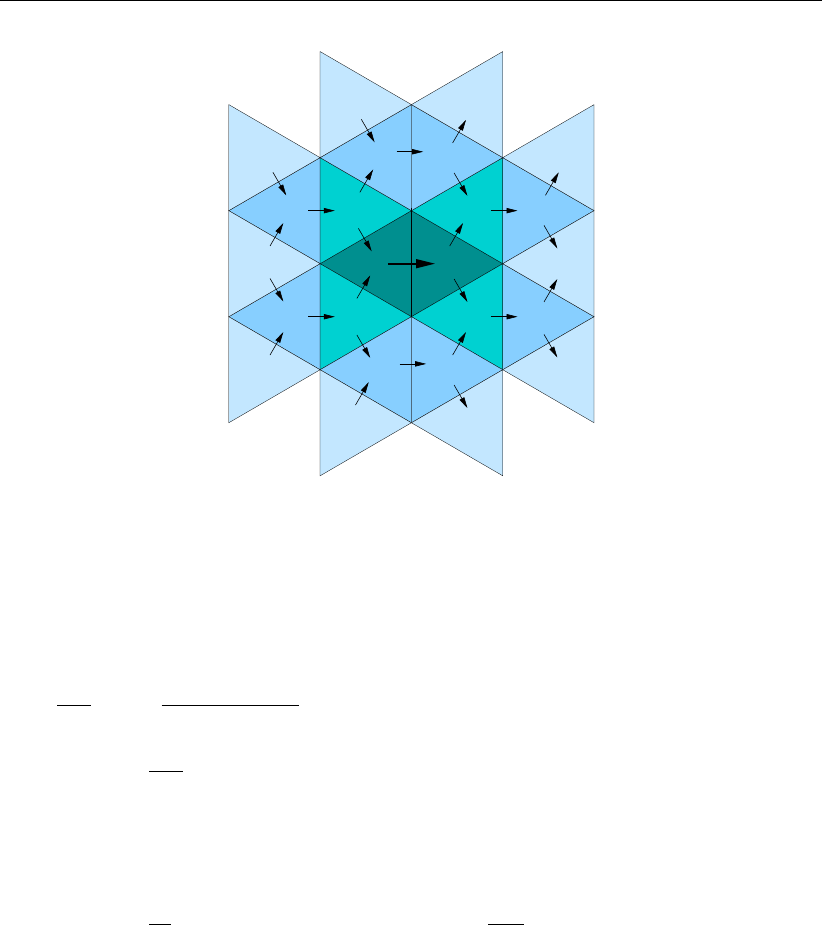
DRAFT
Parallelization
4
3
4
3
4
4
3
2
1
2
3
4
4
3
2
1
2
3
4
3
4
3
4
4
Figure 8.12: Stencil for momentum advection and diffusion; the numbers indicate the level
of the neighboring cells
The advection and pressure-gradient terms are conform Kramer and Stelling. In D-Flow FM,
however, the following form is implemented:
duj
dt=−g(sR(j)−sL(j))
∆xj
−1
VujαLjX
l∈J (L(j))
(ucupwind(l)•nj−uj)ql1l,k+
αRjX
l∈J (R(j))
(ucupwind(l)•nj−uj)ql1l,k
+1
¯
hjαLjDL(j)+αRjDR(j)•nj+τj
hRj
,(8.34)
where Vujis a face-based volume
Vuj=αLjVL(j)+αRjVR(j)(8.35)
and hRjis the hydraulic radius of face j.
The stencil used for computing momentum advection and diffusion is depicted in Fig. 8.12.
Issues:
orthogonal meshes hard to achieve, compromises mesh smoothness,
non-conservative advection and different pressure gradient term implemented, but gives
best results for shock problems,
higher-order implementation gives satisfactory results for swirling flows,
shear-dominated flow suffers from wide advection stencil, see Poiseuille test-case.
Deltares 143 of 152

DRAFT
D-Flow Flexible Mesh, Technical Reference Manual
144 of 152 Deltares
DRAFT
A Analytical conveyance
A.1 Conveyance type 2
In conveyance type 2, we consider the flow is one dimensional, and we calculate the bed
friction based on intersection perpendicular to the flow direction(Figure A.1). Parameter K2
can be derived as follows.
αi=zi+1 −zi
yi+1 −yi
=hi−hi+1
yi+1 −yi
(A.1)
K2=Z
A
C√RdA , or K2=Z
A
CrdA
dP dA (A.2)
Where Ris hydraulic radius, Cis Chézy coefficient, Ais the cross sectional area and Pis
the wet area.
dA =h(y)dy , h(y) = hi−αi(y−yi)(A.3)
dP =qdy2+ (αidy)2=q1 + α2
idy (A.4)
K2=Zyi+1
yi
C
(1 + α2
i)1
4
h(y)3
2dy , (C=h(y)1
6
n)(A.5)
K2=Zyi+1
yi
1
n(1 + α2
i)1
4
h(y)5
3dy (A.6)
K2=Zyi+1
yi
1
n(1 + α2
i)1
4
(hi−αi(y−yi))5
3dy (A.7)
K2=−1
nαi(1 + α2
i)1
4
3
8{hi−αi(y−yi)}8
3
yi+1
yi
(A.8)
K2=1
nαi(1 + α2
i)1
4
3
8h
8
3
i−h
8
3
i+1(A.9)
Deltares 145 of 152

DRAFT
D-Flow Flexible Mesh, Technical Reference Manual
yiyi+1
hi+1
hiAi
Pi
z
y
Figure A.1: A schematic view of cross sectional bed bathemetry perpendicular to the flow
direction.
yi
yi+1
Figure A.2: A schematic view of flow nodes and the velocity components in two-
dimensional case.
A.2 Conveyance type 3
Conveyance type 3 is similar to type 2, except it is extended to consider the second velocity
component. Considering a two-dimensional case as illustrated in Figure A.2, we can derive
K3as follows,
uU
C2R=i, U =u
β2(A.10)
uj=βCpRj√i, K3=βAjR
2
3
j
n(A.11)
β=βi−δ(y−yi), δ =βi−βi+1
yi+1 −yi
(A.12)
If αiand α0
iare the slopes in the streamwise and transverse directions respectively, we have,
K3=Zyi+1
yi
βi−δ(y−yi)
n1 + α2
i+α02
i1
4
(hi−αi(y−yi))5
3dy (A.13)
K3=T
n1 + α2
i+α02
i1
4
(A.14)
146 of 152 Deltares

DRAFT
Analytical conveyance
T=Zyi+1
yi
(βi−δ(y−yi)) (hi−αi(y−yi))5
3dy (A.15)
T=Zyi+1
yi
(βi−δ(y−yi)) (hi−αi(y−yi))5
3dy (A.16)
T=δ
αiZyi+1
yiβi
αi
δ−αi(y−yi)(hi−αi(y−yi))5
3dy (A.17)
T=δ
αiZyi+1
yiβi
αi
δ−hi+ (hi−αi(y−yi))(hi−αi(y−yi))5
3dy (A.18)
T=δ
αiZyi+1
yiβi
αi
δ−hi(hi−αi(y−yi))5
3+ (hi−αi(y−yi))8
3dy (A.19)
T=−δ
αiαiβi
αi
δ−hi3
8(hi−αi(y−yi))8
3
yi+1
yi
+−δ
αiαi
3
11 (hi−αi(y−yi))11
3
yi+1
yi
(A.20)
T=δ
αiαiβi
αi
δ−hi3
8h
8
3
i−h
8
3
i+1+3
11 h
11
3
i−h
11
3
i+1(A.21)
T=1
αβi−hi
δ
αi3
8h
8
3
i−h
8
3
i+1+δ
αi
3
11 h
11
3
i−h
11
3
i+1(A.22)
K3=T
n1 + α2
i+α02
i1
4
=βi−hi
δ
αiKα+1
n(1 + α2
si +α2
ni)1
4
δ
αiαi
3
11 h
11
3
i−h
11
3
i+1
(A.23)
Deltares 147 of 152

DRAFT
D-Flow Flexible Mesh, Technical Reference Manual
148 of 152 Deltares

DRAFT
References
Anderson, W. K. and D. L. Bonhaus, 1994. “An implicit upwind algorithm for computing turbu-
lent flows on unstructured grids.” Computers Fluids 23 (1): 1–21.
Balay, S., J. Brown, K. Buschelman, V. Eijkhout, W. D. Gropp, D. Kaushik, M. G. Knepley, L. C.
McInnes, B. F. Smith and H. Zhang, 2013. PETSc Users Manual. Tech. Rep. ANL-95/11 -
Revision 3.4, Argonne National Laboratory.
Borsboom, M., 2013. Construction and analysis of D-FLOW FM-type discretizations. Tech.
rep., Deltares memorandum.
Dam, A. van, 2009. Go with the Flow. Ph.D. thesis, University of Utrecht. Moving meshes
and solution monitoring for compressible flow simulation.
Delft3D-FLOW UM, 2013. Delft3D-FLOW User Manual. Deltares, 3.14 ed.
Haselbacher, A. and J. Blazek, 1999. “On the accurate and efficient discretization of the
Navier-Stokes equations on mixed grids.” In Proceedings of the 14th AIAA CFD Confer-
ence, AIAA Paper 99-3363-CP, pages 946–956. Snowmass,CO.
Huang, W., 2001. “Practical Aspects of Formulation and Solution of Moving Mesh Partial
Differential Equations.” Journal of Computational Physics 171: 753–775.
Huang, W., 2005. “Anisotropic Mesh Adaptation and Movement.” lecture notes for the work-
shop on Adaptive Method, Theory and Application.
Karypis, G., 2013. METIS - A Software Package for Partitioning Unstructured Graph, Parti-
tioning Meshes, and Computing Fill-Reducing Orderings of Sparse Matrices, Version 5.1.0.
Tech. rep., Department of Computer Science and Engineering, University of Minnesota.
Kleptsova, O., G. S. Stelling and J. D. Pietrzak, 2010. “An accurate momentum advec-
tion scheme for a z-level coordinate models.” Ocean Dyn. 60 (6): 1447–1461. DOI:
10.1007/s10236-010-0350-y.
Kramer, S. C. and G. S. Stelling, 2008. “A conservative unstructured scheme for rapidly varied
flows.” Int. J. Numer. Methods Fluids 58 (2): 183–212. DOI: 10.1002/fld.1722.
Lisa. https://www.surfsara.nl/systems/lisa.
Mavriplis, D. J., 2003. Revisiting the least-squares procedure for gradient reconstruction on
unstructured meshes. Report NASA/CR-2003-212683, NASA.
Natarajan, G. and F. Sotiropoulos, 2011. “IDeC(k): A new velocity reconstruction algorithm
on arbitrarily polygonal staggered meshes.” Journal of Computational Physics 230: 6583–
6604.
Olesen, K. W., 1987. Bed topography in shallow river bends. Tech. rep., Delft University of
Technology. Communications on Hydraulic and Geotechnical Engineering.
Perot, B., 2000. “Conservation properties of unstructured staggered mesh schemes.” J.
Comput. Phys. 159 (1): 58–89. DOI: 10.1006/jcph.2000.6424.
Rodi, W., 1984. “Turbulence models and their application in Hydraulics, State-of-the-art paper
article sur l’etat de connaissance.” IAHR Paper presented by the IAHR-Section on Funda-
mentals of Division II: Experimental and Mathematical Fluid Dynamics, The Netherlands.
Saad, Y., 1994. “SPARSKIT: a basic tool kit for sparse matrix computations - Version 2.”
Deltares 149 of 152

DRAFT
D-Flow Flexible Mesh, Technical Reference Manual
Shashkov, M., B. Swartz and W. B., 1998. “Local reconstruction of a vector field from its
normal components on the faces of grid cells.” Journal of Computational Physics 139:
406–409.
Sieben, J., 2011. Overzicht en synthese beschikbare data overlaatproeven, Update 2011.
Tech. rep., Rijkswaterstaat.
Stelling, G. S. and J. A. T. M. van Kester, 1994. “On the approximation of horizontal gradi-
ents in sigma co-ordinates for bathymetry with steep bottom slopes.” International Journal
Numerical Methods In Fluids 18: 915–955.
Uittenbogaard, R. E., J. A. T. M. van Kester and G. S. Stelling, 1992. Implementation of
three turbulence models in 3D-TRISULA for rectangular grids. Tech. Rep. Z81, WL | Delft
Hydraulics, Delft, The Netherlands.
Vermaas, H., 1987. Energylosses due to weirs. Tech. Rep. Q92, WL | Delft Hydraulics, Delft,
The Netherlands. In Dutch (Energieverliezen door overlaten: Een gewijzigde berekenings-
procedure voor WAQUA-rivieren versie).
Villemonte, J., 1947. “Submerged Weir Discharge Studies.” Engineering News Record pages
866–869.
Wijbenga, J. H. A., 1990. Representation of extra energy losses in RIVCUR. Tech. Rep. Q910,
WL | Delft Hydraulics, Delft, The Netherlands. In Dutch (Weergave van extra energieverlies
in RIVCUR), research for Rijkswaterstaat, Dienst Binnenwateren/RIZA.
Yossef, M. and M. Zagonjoli, 2010. Modelling the hydraulic effect of lowering the groynes on
design flood level. Tech. Rep. 1002524-000, Deltares.
150 of 152 Deltares
DRAFT

PO Box 177
2600 MH Del
Boussinesqweg 1
2629 VH Del
The Netehrlands
+31 (0)88 335 81 88
sales@deltaressystems.nl
www.deltaressystems.nl
DRAFT
