D Flow Flexible Mesh User Manual Flow_FM_User_Manual FM
User Manual: Pdf D-Flow_FM_User_Manual
Open the PDF directly: View PDF ![]() .
.
Page Count: 436 [warning: Documents this large are best viewed by clicking the View PDF Link!]
- List of Figures
- List of Tables
- 1 A guide to this manual
- 2 Introduction to D-Flow Flexible Mesh
- 3 Getting started
- 3.1 Introduction
- 3.2 Overview of D-Flow FM GUI
- 3.3 Dockable views
- 3.4 Ribbons and toolbars
- 3.5 Basic steps to set up a D-Flow FM model
- 3.5.1 Add a D-Flow FM model
- 3.5.2 Set up a D-Flow FM model
- 3.5.3 Multiple input files
- 3.5.4 Converting a Delft3D-FLOW model into D-Flow FM
- 3.5.5 Validate D-Flow FM model
- 3.5.6 File tree
- 3.5.7 Run D-Flow FM model
- 3.5.8 Inspect model output
- 3.5.9 Import/export or delete a D-Flow FM model
- 3.5.10 Save project
- 3.5.11 Exit DeltaShell
- 3.6 Important differences compared to Delft3D-FLOW GUI
- 4 All about the modelling process
- 4.1 Introduction
- 4.2 mdu-file and attribute files
- 4.3 Filenames and conventions
- 4.4 Setting up a D-Flow FM model
- 4.5 Save project, MDU file and attribute files
- 5 Running a model
- 5.1 Running a simulation
- 5.2 Parallel calculations using MPI
- 5.3 Running a scenario using DeltaShell
- 5.4 Running a scenario using a batch script
- 5.5 Run time
- 5.6 Files and file sizes
- 5.7 Command-line arguments
- 5.8 Restart a simulation
- 5.9 Frequently asked questions
- 6 Visualize results
- 7 Hydrodynamics
- 7.1 Introduction
- 7.2 General background
- 7.3 Hydrodynamic processes
- 7.4 Hydrodynamics boundary conditions
- 7.5 Artificial mixing due to sigma-coordinates
- 7.6 Secondary flow
- 7.7 Drying and flooding
- 7.8 Intakes, outfalls and coupled intake-outfalls
- 7.9 Equations of state for the density
- 7.10 Tide generating forces
- 8 Transport of matter
- 9 Turbulence
- 10 Heat transport
- 11 Wind
- 11.1 Definitions
- 11.2 File formats
- 11.3 Masking of points in the wind grid from interpolation (`land-sea mask')
- 12 Hydraulic structures
- 13 Bedforms and vegetation
- 14 Calibration factor
- 15 Coupling with D-Waves (SWAN)
- 16 Coupling with D-RTC (RTC-Tools)
- 17 Coupling with D-Water Quality (Delwaq)
- 18 Sediment transport and morphology
- 18.1 General formulations
- 18.2 Cohesive sediment
- 18.2.1 Cohesive sediment settling velocity
- 18.2.2 Cohesive sediment dispersion
- 18.2.3 Cohesive sediment erosion and deposition
- 18.2.4 Interaction of sediment fractions
- 18.2.5 Influence of waves on cohesive sediment transport
- 18.2.6 Inclusion of a fixed layer
- 18.2.7 Inflow boundary conditions cohesive sediment
- 18.3 Non-cohesive sediment
- 18.4 Bedload sediment transport of non-cohesive sediment
- 18.4.1 Basic formulation
- 18.4.2 Suspended sediment correction vector
- 18.4.3 Interaction of sediment fractions
- 18.4.4 Inclusion of a fixed layer
- 18.4.5 Calculation of bedload transport at open boundaries
- 18.4.6 Bedload transport at velocity points
- 18.4.7 Adjustment of bedload transport for bed-slope effects
- 18.5 Transport formulations for non-cohesive sediment
- 18.5.1 Van Rijn (1993)
- 18.5.2 Engelund-Hansen (1967)
- 18.5.3 Meyer-Peter-Muller (1948)
- 18.5.4 General formula
- 18.5.5 Bijker (1971)
- 18.5.6 Van Rijn (1984)
- 18.5.7 Soulsby/Van Rijn
- 18.5.8 Soulsby
- 18.5.9 Ashida-Michiue (1974)
- 18.5.10 Wilcock-Crowe (2003)
- 18.5.11 Gaeuman et al. (2009) laboratory calibration
- 18.5.12 Gaeuman et al. (2009) Trinity River calibration
- 18.6 Morphological updating
- 18.7 Specific implementation aspects
- 19 Tutorial
- 19.1 Introduction
- 19.2 Tutorial 1: Creating a curvilinear grid
- 19.3 Tutorial 2: Creating a triangular grid
- 19.4 Tutorial 3: Coupling multiple separate grids
- 19.5 Tutorial 4: Inserting a bed level
- 19.6 Tutorial 5: Imposing boundary conditions
- 19.7 Tutorial 6: Defining output locations
- 19.8 Tutorial 7: Defining computational parameters
- 19.9 Tutorial 8: Running a model simulation
- 19.10 Tutorial 9: Viewing the output of a model simulation
- 20 Calibration and data assimilation
- 20.1 Introduction
- 20.2 Getting started with OpenDA
- 20.3 The OpenDA black box model wrapper for D-Flow FM
- 20.4 OpenDA configuration
- 20.4.1 Main configuration file and the directory structure
- 20.4.2 The algorithm configuration
- 20.4.3 The stochObserver configuration
- 20.4.4 The stochModel configuration
- 20.4.5 D-Flow FM files and the OpenDA dataObjects configuration
- 20.4.5.1 Start and end time in the model definition file (.mdu)
- 20.4.5.2 External forcings (.xyz)
- 20.4.5.3 Boundary time series (.tim)
- 20.4.5.4 Meteorological boundary conditions (<.amu>, <.amv>, <.amp>)
- 20.4.5.5 Result time series (<_his.nc>)
- 20.4.5.6 Restart file (<_map.nc>)
- 20.4.5.7 Calibration factor definition file (<.cld>)
- 20.4.5.8 Trachytopes roughness definition file (<.ttd>)
- 20.5 Generating noise
- 20.6 Examples of the application of OpenDA for D-Flow FM
- 20.6.1 Example 1: Calibration of the roughness parameter
- 20.6.2 Example 2: EnKF with uncertainty in the tidal components
- 20.6.3 Example 3: EnKF with uncertainty in the inflow velocity
- 20.6.4 Example 4: EnKF with uncertainty in the inflow condition for salt
- 20.6.5 Example 5: EnKF with uncertainty on the wind direction
- 20.6.6 Example 6: EnKF with the DCSM v5 model and uncertainty on the wind direction
- References
- A The master definition file
- B Attribute files
- B.1 Introduction
- B.2 Polyline/polygon file
- B.3 Sample file
- B.4 Time series file (ASCII)
- B.5 The external forcings file
- B.6 Trachytopes
- B.7 Weirs
- B.8 Calibration Factors
- B.9 Sources and sinks
- B.10 Dry points and areas
- B.11 Structure INI file
- B.12 Space varying wind and pressure
- C Initial conditions and spatially varying input
- D Boundary conditions specification
- E Output files
- F Spatial editor
- Index

Delft3D flexible Mesh suite
1D/2D/3D Modelling suite for integral water solutions
User Manual
D-Flow Flexible Mesh
DRAFT
DRAFT
DRAFT
D-Flow Flexible Mesh
D-Flow FM in Delta Shell
User Manual
Released for:
Delft3D FM Suite 2018
D-HYDRO Suite 2018
Version: 1.2.1
SVN Revision: 55248
April 18, 2018
DRAFT
D-Flow Flexible Mesh, User Manual
Published and printed by:
Deltares
Boussinesqweg 1
2629 HV Delft
P.O. 177
2600 MH Delft
The Netherlands
telephone: +31 88 335 82 73
fax: +31 88 335 85 82
e-mail: info@deltares.nl
www: https://www.deltares.nl
For sales contact:
telephone: +31 88 335 81 88
fax: +31 88 335 81 11
e-mail: software@deltares.nl
www: https://www.deltares.nl/software
For support contact:
telephone: +31 88 335 81 00
fax: +31 88 335 81 11
e-mail: software.support@deltares.nl
www: https://www.deltares.nl/software
Copyright © 2018 Deltares
All rights reserved. No part of this document may be reproduced in any form by print, photo
print, photo copy, microfilm or any other means, without written permission from the publisher:
Deltares.

DRAFT
Contents
Contents
List of Figures xiii
List of Tables xxi
1 A guide to this manual 1
1.1 Introduction .................................. 1
1.2 Overview ................................... 1
1.3 Manual version and revisions ......................... 2
1.4 Typographical conventions .......................... 2
1.5 Changes with respect to previous versions .................. 3
2 Introduction to D-Flow Flexible Mesh 5
2.1 Areas of application .............................. 5
2.2 Standard features ............................... 5
2.3 Special features ................................ 6
2.4 Important differences compared to Delft3D-FLOW . . . . . . . . . . . . . . 6
2.5 Coupling to other modules .......................... 7
2.6 Installation .................................. 7
2.6.1 Installation of DeltaShell . . . . . . . . . . . . . . . . . . . . . . . 7
2.6.2 Installation of the computational core . . . . . . . . . . . . . . . . . 7
2.7 Examples ................................... 8
3 Getting started 9
3.1 Introduction .................................. 9
3.2 Overview of D-Flow FM GUI ......................... 9
3.2.1 Project window . . . . . . . . . . . . . . . . . . . . . . . . . . . . 10
3.2.2 Central (map) window . . . . . . . . . . . . . . . . . . . . . . . . 11
3.2.3 Map window ............................. 12
3.2.4 Messages window . . . . . . . . . . . . . . . . . . . . . . . . . . 13
3.2.5 Time navigator window . . . . . . . . . . . . . . . . . . . . . . . . 13
3.3 Dockable views ................................ 13
3.3.1 Docking tabs separately . . . . . . . . . . . . . . . . . . . . . . . 13
3.3.2 Multiple tabs ............................. 14
3.4 Ribbons and toolbars ............................. 15
3.4.1 Ribbons (shortcut keys) . . . . . . . . . . . . . . . . . . . . . . . . 15
3.4.2 File .................................. 15
3.4.3 Home ................................. 17
3.4.4 View ................................. 17
3.4.5 Tools ................................. 18
3.4.6 Map ................................. 18
3.4.7 Scripting ............................... 19
3.4.8 Shortcuts ............................... 19
3.4.9 Quick access toolbar ......................... 20
3.5 Basic steps to set up a D-Flow FM model . . . . . . . . . . . . . . . . . . . 20
3.5.1 Add a D-Flow FM model . . . . . . . . . . . . . . . . . . . . . . . 20
3.5.2 Set up a D-Flow FM model . . . . . . . . . . . . . . . . . . . . . . 21
3.5.3 Multiple input files . . . . . . . . . . . . . . . . . . . . . . . . . . 21
3.5.4 Converting a Delft3D-FLOW model into D-Flow FM . . . . . . . . . . 22
3.5.5 Validate D-Flow FM model . . . . . . . . . . . . . . . . . . . . . . 22
3.5.6 File tree ............................... 24
3.5.7 Run D-Flow FM model . . . . . . . . . . . . . . . . . . . . . . . . 24
3.5.8 Inspect model output ......................... 24
3.5.9 Import/export or delete a D-Flow FM model . . . . . . . . . . . . . . 25
Deltares iii

DRAFT
D-Flow Flexible Mesh, User Manual
3.5.10 Save project ............................. 26
3.5.11 Exit Delta Shell . . . . . . . . . . . . . . . . . . . . . . . . . . . . 26
3.6 Important differences compared to Delft3D-FLOW GUI . . . . . . . . . . . . 27
3.6.1 Project vs model ........................... 27
3.6.2 Load/save vs import/export . . . . . . . . . . . . . . . . . . . . . . 27
3.6.3 Working from the map . . . . . . . . . . . . . . . . . . . . . . . . 27
3.6.4 Coordinate conversion . . . . . . . . . . . . . . . . . . . . . . . . 27
3.6.5 Model area .............................. 28
3.6.6 Integrated models (model couplings) . . . . . . . . . . . . . . . . . 29
3.6.7 Ribbons (shortcut keys) . . . . . . . . . . . . . . . . . . . . . . . . 29
3.6.8 Context menus . . . . . . . . . . . . . . . . . . . . . . . . . . . . 29
3.6.9 Scripting ............................... 29
4 All about the modelling process 31
4.1 Introduction .................................. 31
4.2 mdu-file and attribute files ........................... 31
4.3 Filenames and conventions . . . . . . . . . . . . . . . . . . . . . . . . . . 32
4.4 Setting up a D-Flow FM model . . . . . . . . . . . . . . . . . . . . . . . . 32
4.4.1 General ................................ 33
4.4.1.1 Vertical layer specification . . . . . . . . . . . . . . . . . 33
4.4.1.2 Model coordinate system . . . . . . . . . . . . . . . . . . 34
4.4.1.3 Angle of latitude . . . . . . . . . . . . . . . . . . . . . . 35
4.4.2 Area ................................. 35
4.4.2.1 Grid snapped features . . . . . . . . . . . . . . . . . . . 36
4.4.2.2 Observation points . . . . . . . . . . . . . . . . . . . . . 37
4.4.2.3 Observation cross-sections . . . . . . . . . . . . . . . . . 38
4.4.2.4 Thin dams ......................... 39
4.4.2.5 Fixed weirs ......................... 40
4.4.2.6 Land boundaries . . . . . . . . . . . . . . . . . . . . . . 42
4.4.2.7 Dry points and dry areas . . . . . . . . . . . . . . . . . . 43
4.4.2.8 Pumps ........................... 45
4.4.2.9 Weirs . . . . . . . . . . . . . . . . . . . . . . . . . . . . 46
4.4.2.10 Gates ........................... 48
4.4.3 Computational grid . . . . . . . . . . . . . . . . . . . . . . . . . . 49
4.4.4 Bed Level ............................... 49
4.4.5 Time frame .............................. 50
4.4.6 Processes .............................. 51
4.4.7 Initial conditions ........................... 52
4.4.8 Boundary conditions ......................... 54
4.4.8.1 Specification of boundary locations (support points) . . . . 54
4.4.8.2 Boundary data editor (forcing) . . . . . . . . . . . . . . . 57
4.4.8.3 Import/export boundary conditions from the Project window 71
4.4.8.4 Overview of boundary conditions in attribute table (non-editable) 73
4.4.9 Physical parameters ......................... 74
4.4.9.1 Constants ......................... 74
4.4.9.2 Roughness ......................... 74
4.4.9.3 Viscosity . . . . . . . . . . . . . . . . . . . . . . . . . . 75
4.4.9.4 Wind . . . . . . . . . . . . . . . . . . . . . . . . . . . . 76
4.4.9.5 Heat Flux model . . . . . . . . . . . . . . . . . . . . . . 76
4.4.9.6 Tidal forces ......................... 77
4.4.10 Sources and sinks . . . . . . . . . . . . . . . . . . . . . . . . . . 77
4.4.11 Numerical parameters . . . . . . . . . . . . . . . . . . . . . . . . 79
4.4.12 Output parameters . . . . . . . . . . . . . . . . . . . . . . . . . . 79
4.4.13 Miscellaneous . . . . . . . . . . . . . . . . . . . . . . . . . . . . 83
iv Deltares

DRAFT
Contents
4.4.14 Sediment ............................... 83
4.4.15 Morphology .............................. 86
4.5 Save project, MDU file and attribute files . . . . . . . . . . . . . . . . . . . 89
5 Running a model 91
5.1 Running a simulation ............................. 91
5.2 Parallel calculations using MPI . . . . . . . . . . . . . . . . . . . . . . . . 91
5.2.1 Introduction .............................. 91
5.2.2 Partitioning the model ......................... 92
5.2.2.1 More about the mesh partitioning . . . . . . . . . . . . . . 93
5.2.3 Partitioning the MDU file . . . . . . . . . . . . . . . . . . . . . . . 95
5.2.3.1 Remaining model input . . . . . . . . . . . . . . . . . . . 95
5.2.4 Running a parallel job ......................... 96
5.2.5 Visualizing the results of a parallel run . . . . . . . . . . . . . . . . 96
5.2.5.1 Plotting all partitioned map files with Delft3D-QUICKPLOT . 97
5.2.5.2 Merging multiple map files into one . . . . . . . . . . . . . 97
5.3 Running a scenario using Delta Shell . . . . . . . . . . . . . . . . . . . . . 98
5.4 Running a scenario using a batch script . . . . . . . . . . . . . . . . . . . . 99
5.5 Run time ................................... 99
5.5.1 Multi-core performance improvements by OpenMP . . . . . . . . . . 100
5.6 Files and file sizes ..............................100
5.6.1 History file ..............................101
5.6.2 Map file ................................101
5.6.3 Restart file ..............................102
5.7 Command-line arguments . . . . . . . . . . . . . . . . . . . . . . . . . . . 102
5.8 Restart a simulation ..............................103
5.9 Frequently asked questions . . . . . . . . . . . . . . . . . . . . . . . . . . 104
6 Visualize results 105
6.1 Introduction ..................................105
6.2 Visualization with Delta Shell . . . . . . . . . . . . . . . . . . . . . . . . . 105
6.3 Visualization with Quickplot . . . . . . . . . . . . . . . . . . . . . . . . . . 106
6.4 Visualization with Muppet . . . . . . . . . . . . . . . . . . . . . . . . . . . 107
6.5 Visualization with Matlab . . . . . . . . . . . . . . . . . . . . . . . . . . . 107
6.6 Visualization with Python . . . . . . . . . . . . . . . . . . . . . . . . . . . 107
7 Hydrodynamics 109
7.1 Introduction ..................................109
7.2 General background . . . . . . . . . . . . . . . . . . . . . . . . . . . . . 109
7.2.1 Range of applications of D-Flow FM . . . . . . . . . . . . . . . . . 109
7.2.2 Physical processes . . . . . . . . . . . . . . . . . . . . . . . . . . 110
7.2.3 Assumptions underlying D-Flow FM . . . . . . . . . . . . . . . . . . 111
7.3 Hydrodynamic processes . . . . . . . . . . . . . . . . . . . . . . . . . . . 112
7.3.1 Topological conventions . . . . . . . . . . . . . . . . . . . . . . . 113
7.3.2 Conservation of mass and momentum . . . . . . . . . . . . . . . . 116
7.3.2.1 Continuity equation . . . . . . . . . . . . . . . . . . . . . 116
7.3.2.2 Momentum equations in horizontal direction . . . . . . . . 117
7.3.2.3 Vertical velocities . . . . . . . . . . . . . . . . . . . . . . 117
7.3.3 The hydrostatic pressure assumption . . . . . . . . . . . . . . . . . 117
7.3.4 The Coriolis force . . . . . . . . . . . . . . . . . . . . . . . . . . . 118
7.3.5 Diffusion of momentum . . . . . . . . . . . . . . . . . . . . . . . . 118
7.3.6 Conveyance in 2D . . . . . . . . . . . . . . . . . . . . . . . . . . 119
7.4 Hydrodynamics boundary conditions . . . . . . . . . . . . . . . . . . . . . 120
7.4.1 Open boundary conditions . . . . . . . . . . . . . . . . . . . . . . 121
Deltares v

DRAFT
D-Flow Flexible Mesh, User Manual
7.4.1.1 The location of support points . . . . . . . . . . . . . . . 121
7.4.1.2 Physical information . . . . . . . . . . . . . . . . . . . . 123
7.4.1.3 Example . . . . . . . . . . . . . . . . . . . . . . . . . . 128
7.4.1.4 Miscellaneous . . . . . . . . . . . . . . . . . . . . . . . 130
7.4.2 Vertical boundary conditions . . . . . . . . . . . . . . . . . . . . . 131
7.4.3 Shear-stresses at closed boundaries . . . . . . . . . . . . . . . . . 131
7.5 Artificial mixing due to sigma-coordinates . . . . . . . . . . . . . . . . . . . 132
7.6 Secondary flow ................................136
7.6.1 Definition . . . . . . . . . . . . . . . . . . . . . . . . . . . . . . . 137
7.6.2 Depth-averaged continuity equation . . . . . . . . . . . . . . . . . . 137
7.6.3 Momentum equations in horizontal direction . . . . . . . . . . . . . 137
7.6.4 Effect of secondary flow on depth-averaged momentum equations . . 138
7.6.5 The depth averaged transport equation for the spiral motion intensity . 139
7.7 Drying and flooding ..............................139
7.7.1 Definitions ..............................140
7.7.1.1 Piecewise constant approach for the bed level . . . . . . . 141
7.7.1.2 Piecewise linear approach for the bed levels . . . . . . . . 142
7.7.1.3 Hybrid bed level approach . . . . . . . . . . . . . . . . . 143
7.7.2 Specification in Delta Shell . . . . . . . . . . . . . . . . . . . . . . 143
7.8 Intakes, outfalls and coupled intake-outfalls . . . . . . . . . . . . . . . . . . 144
7.9 Equations of state for the density . . . . . . . . . . . . . . . . . . . . . . . 146
7.10 Tide generating forces . . . . . . . . . . . . . . . . . . . . . . . . . . . . 148
8 Transport of matter 151
8.1 Introduction ..................................151
8.2 Some words about suspended sediment transport . . . . . . . . . . . . . . 152
8.3 Transport processes . . . . . . . . . . . . . . . . . . . . . . . . . . . . . 152
8.3.1 Advection . . . . . . . . . . . . . . . . . . . . . . . . . . . . . . . 152
8.3.2 Diffusion . . . . . . . . . . . . . . . . . . . . . . . . . . . . . . . 153
8.3.3 Sources and sinks . . . . . . . . . . . . . . . . . . . . . . . . . . 154
8.3.4 Forester filter . . . . . . . . . . . . . . . . . . . . . . . . . . . . . 155
8.4 Transport boundary and initial conditions . . . . . . . . . . . . . . . . . . . 155
8.4.1 Open boundary conditions . . . . . . . . . . . . . . . . . . . . . . 155
8.4.2 Closed boundary conditions . . . . . . . . . . . . . . . . . . . . . 156
8.4.3 Vertical boundary conditions . . . . . . . . . . . . . . . . . . . . . 156
8.4.4 Thatcher-Harleman boundary conditions . . . . . . . . . . . . . . . 156
8.4.5 Initial conditions . . . . . . . . . . . . . . . . . . . . . . . . . . . 156
9 Turbulence 159
9.1 k-epsilon turbulence model . . . . . . . . . . . . . . . . . . . . . . . . . . 161
9.2 k-tau turbulence model . . . . . . . . . . . . . . . . . . . . . . . . . . . . 164
10 Heat transport 165
10.1 Heat balance . . . . . . . . . . . . . . . . . . . . . . . . . . . . . . . . . 168
10.2 Solar radiation ................................168
10.3 Atmospheric radiation (long wave radiation) . . . . . . . . . . . . . . . . . . 170
10.4 Back radiation (long wave radiation) . . . . . . . . . . . . . . . . . . . . . . 171
10.5 Effective back radiation . . . . . . . . . . . . . . . . . . . . . . . . . . . . 171
10.6 Evaporative heat flux . . . . . . . . . . . . . . . . . . . . . . . . . . . . . 171
10.7 Convective heat flux . . . . . . . . . . . . . . . . . . . . . . . . . . . . . 173
11 Wind 175
11.1 Definitions ..................................175
11.1.1 Nautical convention . . . . . . . . . . . . . . . . . . . . . . . . . . 175
11.1.2 Drag coefficient . . . . . . . . . . . . . . . . . . . . . . . . . . . . 175
vi Deltares

DRAFT
Contents
11.2 File formats ..................................178
11.2.1 Defined on the computational grid . . . . . . . . . . . . . . . . . . 179
11.2.1.1 Specification of uniform wind through velocity components . 179
11.2.1.2 Specification of uniform wind through magnitude and direction180
11.2.2 Defined on an equidistant grid . . . . . . . . . . . . . . . . . . . . 180
11.2.3 Defined on a curvilinear grid . . . . . . . . . . . . . . . . . . . . . 182
11.2.4 Space and time varying Charnock coefficients . . . . . . . . . . . . 183
11.2.5 Defined on a spiderweb grid . . . . . . . . . . . . . . . . . . . . . 184
11.2.6 Combination of several wind specifications . . . . . . . . . . . . . . 186
11.3 Masking of points in the wind grid from interpolation (‘land-sea mask’) . . . . . 188
12 Hydraulic structures 189
12.1 Introduction ..................................189
12.2 Structures ..................................189
12.2.1 Fixed weirs ..............................190
12.2.2 (adjustable) Weirs . . . . . . . . . . . . . . . . . . . . . . . . . . 190
12.2.3 Gates . . . . . . . . . . . . . . . . . . . . . . . . . . . . . . . . . 192
12.2.4 Pumps ................................193
12.2.5 Thin dams ..............................194
13 Bedforms and vegetation 195
13.1 Bedform heights . . . . . . . . . . . . . . . . . . . . . . . . . . . . . . . 195
13.2 Trachytopes ..................................195
13.2.1 Trachytope classes . . . . . . . . . . . . . . . . . . . . . . . . . . 195
13.2.2 Averaging and accumulation of trachytopes . . . . . . . . . . . . . . 202
13.3 (Rigid) three-dimensional vegetation model . . . . . . . . . . . . . . . . . . 203
14 Calibration factor 205
15 Coupling with D-Waves (SWAN) 207
15.1 Getting started ................................207
15.1.1 Input D-Flow FM . . . . . . . . . . . . . . . . . . . . . . . . . . . 208
15.1.2 Input D-Waves . . . . . . . . . . . . . . . . . . . . . . . . . . . . 208
15.1.3 Input dimr ..............................209
15.1.4 Online process order . . . . . . . . . . . . . . . . . . . . . . . . . 211
15.1.5 Related files . . . . . . . . . . . . . . . . . . . . . . . . . . . . . 212
15.2 Forcing by radiation stress gradients . . . . . . . . . . . . . . . . . . . . . 213
15.3 Stokes drift and mass flux . . . . . . . . . . . . . . . . . . . . . . . . . . . 214
15.4 Streaming ..................................215
15.5 Enhancement of the bed shear-stress by waves . . . . . . . . . . . . . . . . 215
16 Coupling with D-RTC (RTC-Tools) 221
16.1 Introduction ..................................221
16.2 Getting started ................................221
16.2.1 User interface: the first steps . . . . . . . . . . . . . . . . . . . . . 221
16.2.2 Input D-Flow FM . . . . . . . . . . . . . . . . . . . . . . . . . . . 222
16.2.3 Input D-RTC . . . . . . . . . . . . . . . . . . . . . . . . . . . . . 223
16.2.4 Input d_hydro . . . . . . . . . . . . . . . . . . . . . . . . . . . . . 223
16.2.5 Online process order . . . . . . . . . . . . . . . . . . . . . . . . . 223
17 Coupling with D-Water Quality (Delwaq) 225
17.1 Introduction ..................................225
17.2 Offline versus online coupling . . . . . . . . . . . . . . . . . . . . . . . . . 225
17.3 Creating output for D-Water Quality . . . . . . . . . . . . . . . . . . . . . . 225
17.4 Current limitations ..............................226
Deltares vii

DRAFT
D-Flow Flexible Mesh, User Manual
18 Sediment transport and morphology 227
18.1 General formulations . . . . . . . . . . . . . . . . . . . . . . . . . . . . . 227
18.1.1 Introduction ..............................227
18.1.2 Suspended transport . . . . . . . . . . . . . . . . . . . . . . . . . 227
18.1.3 Effect of sediment on fluid density . . . . . . . . . . . . . . . . . . 228
18.1.4 Sediment settling velocity . . . . . . . . . . . . . . . . . . . . . . . 228
18.1.5 Dispersive transport . . . . . . . . . . . . . . . . . . . . . . . . . 229
18.1.6 Three-dimensional wave effects . . . . . . . . . . . . . . . . . . . . 230
18.1.7 Initial and boundary conditions . . . . . . . . . . . . . . . . . . . . 230
18.1.7.1 Initial condition . . . . . . . . . . . . . . . . . . . . . . . 230
18.1.7.2 Boundary conditions . . . . . . . . . . . . . . . . . . . . 230
18.2 Cohesive sediment ..............................231
18.2.1 Cohesive sediment settling velocity . . . . . . . . . . . . . . . . . . 231
18.2.2 Cohesive sediment dispersion . . . . . . . . . . . . . . . . . . . . 232
18.2.3 Cohesive sediment erosion and deposition . . . . . . . . . . . . . . 232
18.2.4 Interaction of sediment fractions . . . . . . . . . . . . . . . . . . . 233
18.2.5 Influence of waves on cohesive sediment transport . . . . . . . . . . 233
18.2.6 Inclusion of a fixed layer . . . . . . . . . . . . . . . . . . . . . . . 234
18.2.7 Inflow boundary conditions cohesive sediment . . . . . . . . . . . . 234
18.3 Non-cohesive sediment . . . . . . . . . . . . . . . . . . . . . . . . . . . . 234
18.3.1 Non-cohesive sediment settling velocity . . . . . . . . . . . . . . . . 234
18.3.2 Non-cohesive sediment dispersion . . . . . . . . . . . . . . . . . . 235
18.3.2.1 Using the k-epsilon turbulence model . . . . . . . . . . . . 235
18.3.2.2 Using the k-tau turbulence model . . . . . . . . . . . . . . 236
18.3.3 Reference concentration . . . . . . . . . . . . . . . . . . . . . . . 236
18.3.4 Non-cohesive sediment erosion and deposition . . . . . . . . . . . . 237
18.3.5 Inclusion of a fixed layer . . . . . . . . . . . . . . . . . . . . . . . 240
18.3.6 Inflow boundary conditions non-cohesive sediment . . . . . . . . . . 240
18.4 Bedload sediment transport of non-cohesive sediment . . . . . . . . . . . . 241
18.4.1 Basic formulation . . . . . . . . . . . . . . . . . . . . . . . . . . . 241
18.4.2 Suspended sediment correction vector . . . . . . . . . . . . . . . . 242
18.4.3 Interaction of sediment fractions . . . . . . . . . . . . . . . . . . . 242
18.4.4 Inclusion of a fixed layer . . . . . . . . . . . . . . . . . . . . . . . 243
18.4.5 Calculation of bedload transport at open boundaries . . . . . . . . . 243
18.4.6 Bedload transport at velocity points . . . . . . . . . . . . . . . . . . 244
18.4.7 Adjustment of bedload transport for bed-slope effects . . . . . . . . . 244
18.5 Transport formulations for non-cohesive sediment . . . . . . . . . . . . . . . 247
18.5.1 Van Rijn (1993) . . . . . . . . . . . . . . . . . . . . . . . . . . . . 247
18.5.2 Engelund-Hansen (1967) . . . . . . . . . . . . . . . . . . . . . . . 252
18.5.3 Meyer-Peter-Muller (1948) . . . . . . . . . . . . . . . . . . . . . . 252
18.5.4 General formula . . . . . . . . . . . . . . . . . . . . . . . . . . . 253
18.5.5 Bijker (1971) . . . . . . . . . . . . . . . . . . . . . . . . . . . . . 253
18.5.5.1 Basic formulation . . . . . . . . . . . . . . . . . . . . . . 253
18.5.5.2 Transport in wave propagation direction (Bailard-approach) . 255
18.5.6 Van Rijn (1984) . . . . . . . . . . . . . . . . . . . . . . . . . . . . 257
18.5.7 Soulsby/Van Rijn . . . . . . . . . . . . . . . . . . . . . . . . . . . 258
18.5.8 Soulsby ................................260
18.5.9 Ashida-Michiue (1974) . . . . . . . . . . . . . . . . . . . . . . . . 262
18.5.10 Wilcock-Crowe (2003) . . . . . . . . . . . . . . . . . . . . . . . . 263
18.5.11 Gaeuman et al. (2009) laboratory calibration . . . . . . . . . . . . . 264
18.5.12 Gaeuman et al. (2009) Trinity River calibration . . . . . . . . . . . . 264
18.6 Morphological updating . . . . . . . . . . . . . . . . . . . . . . . . . . . . 265
18.6.1 Bathymetry updating including bedload transport . . . . . . . . . . . 267
18.6.2 Erosion of (temporarily) dry points . . . . . . . . . . . . . . . . . . 268
viii Deltares

DRAFT
Contents
18.6.3 Dredging and dumping . . . . . . . . . . . . . . . . . . . . . . . . 268
18.6.4 Bed composition models and sediment availability . . . . . . . . . . 269
18.7 Specific implementation aspects . . . . . . . . . . . . . . . . . . . . . . . 270
19 Tutorial 273
19.1 Introduction ..................................273
19.1.1 Setup of the tutorial . . . . . . . . . . . . . . . . . . . . . . . . . . 273
19.1.2 Basic grid concepts . . . . . . . . . . . . . . . . . . . . . . . . . . 273
19.2 Tutorial 1: Creating a curvilinear grid . . . . . . . . . . . . . . . . . . . . . 275
19.3 Tutorial 2: Creating a triangular grid . . . . . . . . . . . . . . . . . . . . . . 280
19.4 Tutorial 3: Coupling multiple separate grids . . . . . . . . . . . . . . . . . . 282
19.5 Tutorial 4: Inserting a bed level . . . . . . . . . . . . . . . . . . . . . . . . 284
19.6 Tutorial 5: Imposing boundary conditions . . . . . . . . . . . . . . . . . . . 287
19.7 Tutorial 6: Defining output locations . . . . . . . . . . . . . . . . . . . . . . 290
19.8 Tutorial 7: Defining computational parameters . . . . . . . . . . . . . . . . . 291
19.9 Tutorial 8: Running a model simulation . . . . . . . . . . . . . . . . . . . . 293
19.10 Tutorial 9: Viewing the output of a model simulation . . . . . . . . . . . . . . 294
20 Calibration and data assimilation 297
20.1 Introduction ..................................297
20.2 Getting started with OpenDA . . . . . . . . . . . . . . . . . . . . . . . . . 297
20.3 The OpenDA black box model wrapper for D-Flow FM . . . . . . . . . . . . . 298
20.4 OpenDA configuration . . . . . . . . . . . . . . . . . . . . . . . . . . . . 298
20.4.1 Main configuration file and the directory structure . . . . . . . . . . . 298
20.4.2 The algorithm configuration . . . . . . . . . . . . . . . . . . . . 300
20.4.3 The stochObserver configuration . . . . . . . . . . . . . . . . . 300
20.4.3.1 NoosTimeSeriesStochObserver . . . . . . . . . . . . . . 300
20.4.3.2 IoObjectStochObserver . . . . . . . . . . . . . . . . . . . 301
20.4.4 The stochModel configuration . . . . . . . . . . . . . . . . . . . 302
20.4.5 D-Flow FM files and the OpenDA dataObjects configuration . . . . . . 303
20.4.5.1 Start and end time in the model definition file (.mdu). . . . 303
20.4.5.2 External forcings (.xyz). . . . . . . . . . . . . . . . . . 303
20.4.5.3 Boundary time series (.tim). . . . . . . . . . . . . . . . 305
20.4.5.4 Meteorological boundary conditions (<∗.amu>,<∗.amv>,
<∗.amp>). . . . . . . . . . . . . . . . . . . . . . . . 305
20.4.5.5 Result time series (<∗_his.nc>). . . . . . . . . . . . . . 306
20.4.5.6 Restart file (<∗_map.nc>). . . . . . . . . . . . . . . . . 306
20.4.5.7 Calibration factor definition file (<∗.cld>). . . . . . . . . . 306
20.4.5.8 Trachytopes roughness definition file (<∗.ttd>). . . . . . . 308
20.5 Generating noise . . . . . . . . . . . . . . . . . . . . . . . . . . . . . . . 309
20.6 Examples of the application of OpenDA for D-Flow FM . . . . . . . . . . . . 311
20.6.1 Example 1: Calibration of the roughness parameter . . . . . . . . . . 311
20.6.2 Example 2: EnKF with uncertainty in the tidal components . . . . . . 313
20.6.3 Example 3: EnKF with uncertainty in the inflow velocity . . . . . . . . 314
20.6.4 Example 4: EnKF with uncertainty in the inflow condition for salt . . . 314
20.6.5 Example 5: EnKF with uncertainty on the wind direction . . . . . . . 315
20.6.6 Example 6: EnKF with the DCSM v5 model and uncertainty on the
wind direction . . . . . . . . . . . . . . . . . . . . . . . . . . . . . 315
References 317
A The master definition file 323
B Attribute files 329
B.1 Introduction ..................................329
Deltares ix

DRAFT
D-Flow Flexible Mesh, User Manual
B.2 Polyline/polygon file ..............................329
B.3 Sample file ..................................330
B.4 Time series file (ASCII) . . . . . . . . . . . . . . . . . . . . . . . . . . . . 331
B.5 The external forcings file . . . . . . . . . . . . . . . . . . . . . . . . . . . 331
B.5.1 Old style external forcings . . . . . . . . . . . . . . . . . . . . . . 331
B.5.2 New style external forcing (boundary conditions only) . . . . . . . . . 332
B.5.3 Accepted quantity names . . . . . . . . . . . . . . . . . . . . . . . 333
B.6 Trachytopes ..................................334
B.6.1 Area Roughness on Links (ARL-file) . . . . . . . . . . . . . . . . . 335
B.6.1.1 Example . . . . . . . . . . . . . . . . . . . . . . . . . . 335
B.6.1.2 Conversion from Delft3D input files . . . . . . . . . . . . . 335
B.6.2 Trachytope Definition file (TTD-file) . . . . . . . . . . . . . . . . . . 336
B.6.2.1 General format . . . . . . . . . . . . . . . . . . . . . . . 336
B.6.2.2 Example . . . . . . . . . . . . . . . . . . . . . . . . . . 336
B.6.2.3 Discharge dependent format . . . . . . . . . . . . . . . . 336
B.6.2.4 Water level dependent format . . . . . . . . . . . . . . . . 337
B.6.2.5 Supported roughness formulations . . . . . . . . . . . . . 338
B.7 Weirs .....................................339
B.7.0.1 Example . . . . . . . . . . . . . . . . . . . . . . . . . . 339
B.8 Calibration Factors ..............................340
B.8.1 Calibration factor definition file (CLD-file) . . . . . . . . . . . . . . . 340
B.8.1.1 Header of the CLD-file . . . . . . . . . . . . . . . . . . . 340
B.8.1.2 Constant values . . . . . . . . . . . . . . . . . . . . . . 340
B.8.1.3 Discharge dependent format . . . . . . . . . . . . . . . . 340
B.8.1.4 Water level dependent format . . . . . . . . . . . . . . . . 341
B.8.1.5 Example . . . . . . . . . . . . . . . . . . . . . . . . . . 341
B.8.2 Calibration Class Area on Links (CLL-file) . . . . . . . . . . . . . . . 341
B.8.2.1 Header of the CLL-file . . . . . . . . . . . . . . . . . . . 342
B.8.2.2 Body of the CLL-file . . . . . . . . . . . . . . . . . . . . 342
B.8.2.3 Example . . . . . . . . . . . . . . . . . . . . . . . . . . 342
B.9 Sources and sinks ..............................342
B.10 Dry points and areas . . . . . . . . . . . . . . . . . . . . . . . . . . . . . 343
B.11 Structure INI file . . . . . . . . . . . . . . . . . . . . . . . . . . . . . . . 343
B.12 Space varying wind and pressure . . . . . . . . . . . . . . . . . . . . . . . 343
B.12.1 Meteo on equidistant grids . . . . . . . . . . . . . . . . . . . . . . 344
B.12.2 Curvilinear data . . . . . . . . . . . . . . . . . . . . . . . . . . . . 347
B.12.3 Spiderweb data . . . . . . . . . . . . . . . . . . . . . . . . . . . . 350
B.12.4 Fourier analysis . . . . . . . . . . . . . . . . . . . . . . . . . . . . 354
C Initial conditions and spatially varying input 357
C.1 Introduction ..................................357
C.2 Supported quantities . . . . . . . . . . . . . . . . . . . . . . . . . . . . . 357
C.2.1 Water levels . . . . . . . . . . . . . . . . . . . . . . . . . . . . . 357
C.2.2 Initial velocities . . . . . . . . . . . . . . . . . . . . . . . . . . . . 357
C.2.3 Salinity ................................357
C.2.4 Temperature . . . . . . . . . . . . . . . . . . . . . . . . . . . . . 357
C.2.5 Tracers ................................357
C.2.6 Sediment . . . . . . . . . . . . . . . . . . . . . . . . . . . . . . . 358
C.2.7 Physical coefficients . . . . . . . . . . . . . . . . . . . . . . . . . 358
C.3 Supported file formats . . . . . . . . . . . . . . . . . . . . . . . . . . . . 358
C.3.1 Inside-polygon option . . . . . . . . . . . . . . . . . . . . . . . . . 358
C.3.2 Sample file ..............................359
C.3.3 Vertical profile file . . . . . . . . . . . . . . . . . . . . . . . . . . . 359
C.3.4 Map file ................................359
x Deltares

DRAFT
Contents
C.3.5 Restart file ..............................359
D Boundary conditions specification 361
D.1 Supported boundary types . . . . . . . . . . . . . . . . . . . . . . . . . . 361
D.1.1 Astronomic boundary conditions . . . . . . . . . . . . . . . . . . . 361
D.1.2 Astronomic correction factors . . . . . . . . . . . . . . . . . . . . . 361
D.1.3 Harmonic flow boundary conditions . . . . . . . . . . . . . . . . . . 361
D.1.4 QH-relation flow boundary conditions . . . . . . . . . . . . . . . . . 361
D.1.5 Time-series flow boundary conditions . . . . . . . . . . . . . . . . . 362
D.1.6 Time-series transport boundary conditions . . . . . . . . . . . . . . 362
D.1.7 Time-series for the heat model parameters . . . . . . . . . . . . . . 362
D.2 Boundary signal file formats . . . . . . . . . . . . . . . . . . . . . . . . . . 362
D.2.1 The <cmp>format . . . . . . . . . . . . . . . . . . . . . . . . . 362
D.2.2 The <qh>format ..........................363
D.2.3 The <bc>format ..........................363
D.2.4 The NetCDF-format for boundary condition time-series . . . . . . . . 365
E Output files 367
E.1 Diagnostics file ................................367
E.2 Demanding output ..............................368
E.2.1 The MDU-file . . . . . . . . . . . . . . . . . . . . . . . . . . . . . 368
E.2.2 Observation points . . . . . . . . . . . . . . . . . . . . . . . . . . 368
E.2.3 Moving observation points . . . . . . . . . . . . . . . . . . . . . . 368
E.2.4 Cross-sections . . . . . . . . . . . . . . . . . . . . . . . . . . . . 369
E.3 NetCDF output files ..............................369
E.3.1 Timeseries as NetCDF his-file . . . . . . . . . . . . . . . . . . . . 369
E.3.2 Spatial fields as NetCDF map-file . . . . . . . . . . . . . . . . . . . 372
E.3.3 Restart files as NetCDF rst-file . . . . . . . . . . . . . . . . . . . . 374
E.4 Shapefiles ..................................374
F Spatial editor 375
F.1 Introduction ..................................375
F.2 General ....................................375
F.2.1 Overview of spatial editor . . . . . . . . . . . . . . . . . . . . . . . 375
F.2.2 Import/export dataset . . . . . . . . . . . . . . . . . . . . . . . . . 376
F.2.3 Activate (spatial) model quantity . . . . . . . . . . . . . . . . . . . 377
F.2.4 Colorscale ..............................377
F.2.5 Render mode . . . . . . . . . . . . . . . . . . . . . . . . . . . . . 378
F.2.6 Context menu . . . . . . . . . . . . . . . . . . . . . . . . . . . . 380
F.3 Quantity selection . . . . . . . . . . . . . . . . . . . . . . . . . . . . . . . 381
F.4 Geometry operations . . . . . . . . . . . . . . . . . . . . . . . . . . . . . 382
F.4.1 Polygons . . . . . . . . . . . . . . . . . . . . . . . . . . . . . . . 383
F.4.2 Lines . . . . . . . . . . . . . . . . . . . . . . . . . . . . . . . . . 383
F.4.3 Points ................................384
F.5 Spatial operations . . . . . . . . . . . . . . . . . . . . . . . . . . . . . . . 385
F.5.1 Import point cloud . . . . . . . . . . . . . . . . . . . . . . . . . . 386
F.5.2 Crop . . . . . . . . . . . . . . . . . . . . . . . . . . . . . . . . . 387
F.5.3 Erase . . . . . . . . . . . . . . . . . . . . . . . . . . . . . . . . . 388
F.5.4 Set value . . . . . . . . . . . . . . . . . . . . . . . . . . . . . . . 388
F.5.5 Contour . . . . . . . . . . . . . . . . . . . . . . . . . . . . . . . 389
F.5.6 Copy to samples . . . . . . . . . . . . . . . . . . . . . . . . . . . 391
F.5.7 Copy to spatial data . . . . . . . . . . . . . . . . . . . . . . . . . 393
F.5.8 Merge spatial data . . . . . . . . . . . . . . . . . . . . . . . . . . 393
F.5.9 Gradient . . . . . . . . . . . . . . . . . . . . . . . . . . . . . . . 395
Deltares xi

DRAFT
D-Flow Flexible Mesh, User Manual
F.5.10 Interpolate ..............................396
F.5.11 Smoothing ..............................399
F.5.12 Overwrite (single) value . . . . . . . . . . . . . . . . . . . . . . . . 401
F.6 Operation stack ................................401
F.6.1 Stack workflow . . . . . . . . . . . . . . . . . . . . . . . . . . . . 402
F.6.2 Edit operation properties . . . . . . . . . . . . . . . . . . . . . . . 402
F.6.3 Enable/disable operations . . . . . . . . . . . . . . . . . . . . . . 405
F.6.4 Delete operations . . . . . . . . . . . . . . . . . . . . . . . . . . . 405
F.6.5 Refresh stack . . . . . . . . . . . . . . . . . . . . . . . . . . . . . 406
F.6.6 Quick links ..............................407
F.6.7 Import/export . . . . . . . . . . . . . . . . . . . . . . . . . . . . . 407
Index 409
xii Deltares

DRAFT
List of Figures
List of Figures
3.1 Start-up lay-out Delta Shell .......................... 9
3.2 Project window of D-Flow FM plugin . . . . . . . . . . . . . . . . . . . . . 11
3.3 Central map with contents of the D-Flow FM plug-in . . . . . . . . . . . . . . 12
3.4 Map tree controlling map contents . . . . . . . . . . . . . . . . . . . . . . 12
3.5 Log of messages, warnings and errors in message window . . . . . . . . . . 13
3.6 Time navigator in Delta Shell ......................... 13
3.7 Docking windows on two screens within the Delta Shell framework. . . . . . . 13
3.8 Bringing the Time Navigator window to the front . . . . . . . . . . . . . . . 14
3.9 Docking the Time Navigator window. . . . . . . . . . . . . . . . . . . . . . 14
3.10 Auto hide the Properties window . . . . . . . . . . . . . . . . . . . . . . . 14
3.11 Perform operations using the shortcut keys . . . . . . . . . . . . . . . . . . 15
3.12 The File ribbon. ................................ 16
3.13 The Delta Shell options dialog. . . . . . . . . . . . . . . . . . . . . . . . . 17
3.14 The Home ribbon. ............................... 17
3.15 The View ribbon. ............................... 17
3.16 The Tools ribbon contains just the Data item. . . . . . . . . . . . . . . . . . 18
3.17 The Map ribbon. ............................... 18
3.18 The scripting ribbon within Delta Shell. . . . . . . . . . . . . . . . . . . . . 19
3.19 The quick access toolbar. ........................... 20
3.20 Adding a new model from the ribbon . . . . . . . . . . . . . . . . . . . . . 21
3.21 Adding a new model using the Right Mouse Button on “project1” in the Project
window .................................... 21
3.22 Select “D-Flow FM model” . . . . . . . . . . . . . . . . . . . . . . . . . . 21
3.23 Illustration of multiple input files for observation points . . . . . . . . . . . . . 22
3.24 Validate model ................................ 23
3.25 Validation report ............................... 23
3.26 Run model .................................. 24
3.27 Output of wave model in Project window . . . . . . . . . . . . . . . . . . . 24
3.28 Import wave model from Project window . . . . . . . . . . . . . . . . . . . 25
3.29 Import wave model from file ribbon . . . . . . . . . . . . . . . . . . . . . . 26
3.30 Set map coordinate system using right mouse button . . . . . . . . . . . . . 28
3.31 Select a coordinate system using the quick search bar . . . . . . . . . . . . 28
3.32 Perform operations using the shortcut keys . . . . . . . . . . . . . . . . . . 29
4.1 The Select model ... window ......................... 32
4.2 Overview of general tab . . . . . . . . . . . . . . . . . . . . . . . . . . . . 33
4.3 Vertical layer specification window (σ-model is β-functionality) . . . . . . . . 34
4.4 Coordinate system wizard ........................... 35
4.5 Overview of geographical features . . . . . . . . . . . . . . . . . . . . . . 35
4.6 Overview of map ribbon . . . . . . . . . . . . . . . . . . . . . . . . . . . . 36
4.7 Example of expanded grid snapped features attribute in map tree . . . . . . . 36
4.8 Example of grid snapped features displayed on the central map . . . . . . . . 37
4.9 Geographical and grid snapped representation of an observation point . . . . 37
4.10 Attribute table with observation points . . . . . . . . . . . . . . . . . . . . . 38
4.11 Geographical and grid snapped representation of a cross section . . . . . . . 38
4.12 Attribute table with observation cross sections . . . . . . . . . . . . . . . . 39
4.13 Geographical and grid snapped representation of a thin dam . . . . . . . . . 39
4.14 Attribute table with thin dams ......................... 40
4.15 Geographical and grid snapped representation of a fixed weir . . . . . . . . . 40
4.16 Schematic representation of a fixed weir . . . . . . . . . . . . . . . . . . . 40
4.17 Attribute table with fixed weirs ......................... 41
4.18 Fixed weir editor ............................... 41
Deltares xiii

DRAFT
D-Flow Flexible Mesh, User Manual
4.19 Geographical representation of a land boundary . . . . . . . . . . . . . . . 42
4.20 Attribute table with land boundaries . . . . . . . . . . . . . . . . . . . . . . 42
4.21 Geographical and grid snapped representation of several dry points . . . . . . 43
4.22 Attribute table with dry points ......................... 44
4.23 Geographical and grid snapped representation of a dry area . . . . . . . . . 44
4.24 Attribute table with dry areas ......................... 45
4.25 Polygon for pump (a) and adjustment of physical properties (b). . . . . . . . . 46
4.26 Selection of the pumps . . . . . . . . . . . . . . . . . . . . . . . . . . . . 46
4.27 Polygon for adjustable weir (a) and adjustment of geometrical and temporal
conditions (b). ................................. 47
4.28 Time series for crest level. . . . . . . . . . . . . . . . . . . . . . . . . . . 47
4.29 Time series for crest level. . . . . . . . . . . . . . . . . . . . . . . . . . . 48
4.30 Polygon for gate (a) and adjustment of geometrical and temporal conditions (b). 48
4.31 Bed level activated in the spatial editor . . . . . . . . . . . . . . . . . . . . 49
4.32 Overview time frame tab ........................... 50
4.33 Relation between Reference Date and the simulation start and stop time for
astronomic- and harmonic-series as used in the simulation. Time-series should
cover the simulation time. ........................... 51
4.34 Overview processes tab ........................... 52
4.35 Initial conditions in the Project window . . . . . . . . . . . . . . . . . . . . 52
4.36 The ‘Initial Conditions’ tab where you can specify the uniform values and the
layer distributions of the active physical quantities. . . . . . . . . . . . . . . 53
4.37 Initial water levels activated in the spatial editor . . . . . . . . . . . . . . . . 53
4.38 Selecting 3 dimensional initial fields from the dropdown box in the ‘Map’ ribbon
to edit them in the spatial editor . . . . . . . . . . . . . . . . . . . . . . . . 53
4.39 Restart files in output states folder . . . . . . . . . . . . . . . . . . . . . . 54
4.40 Restart file in initial conditions attribute . . . . . . . . . . . . . . . . . . . . 54
4.41 Adding a boundary support point on a polyline in the central map . . . . . . . 55
4.42 Polyline added in Project window under ‘Boundary Conditions’ . . . . . . . . 56
4.43 Geometry edit options in Map ribbon . . . . . . . . . . . . . . . . . . . . . 56
4.44 Edit name of polyline/boundary in Boundaries tab . . . . . . . . . . . . . . . 57
4.45 Overview of the boundary data editor . . . . . . . . . . . . . . . . . . . . . 58
4.46 Process and quantity selection in the boundary data editor . . . . . . . . . . 59
4.47 Activate a support point . . . . . . . . . . . . . . . . . . . . . . . . . . . . 60
4.48 Specification of time series in the boundary data editor (left panel) . . . . . . 60
4.49 Window for generating series of time points . . . . . . . . . . . . . . . . . . 61
4.50 Csv import wizard: csv file selection . . . . . . . . . . . . . . . . . . . . . . 62
4.51 Clipboard/csv import wizard: specification of how data should be parsed into
columns ................................... 63
4.52 Clipboard/csv import wizard: specification of how values should be parsed and
columns should be mapped . . . . . . . . . . . . . . . . . . . . . . . . . . 64
4.53 Window for entering input to download boundary data from WPS . . . . . . . 65
4.54 Specification of harmonic components in boundary data editor . . . . . . . . 66
4.55 Selection of astronomical components from list (after pressing ‘select compo-
nents’) .................................... 67
4.56 Suggestions for astronomical components in list . . . . . . . . . . . . . . . 68
4.57 Editing harmonic/astronomic components and their corrections . . . . . . . . 68
4.58 Specification of a Q-h relationship . . . . . . . . . . . . . . . . . . . . . . . 69
4.59 Selection of vertically uniform or varying boundary conditions in case of a 3D
model ..................................... 69
4.60 Overview of the layer view component of the boudary conditions editor . . . . 70
4.61 Specification of boundary forcing data (in this example for salinity) at 3 posi-
tions in the vertical .............................. 70
xiv Deltares

DRAFT
List of Figures
4.62 Example of active and total signal for multiple water level data series on one
support point ................................. 71
4.63 Importing or exporting boundary features — both polylines <∗.pli>and forc-
ing <∗.bc>— from the Project window using the right mouse button . . . . . 71
4.64 Import or export a <∗.pli>-file as is or with coordinate transformation. . . . . 72
4.65 Import or export a <∗.pli>-file as is or with coordinate transformation. . . . . 72
4.66 Import or export a *.pli file as is or with coordinate transformation. . . . . . . . 73
4.67 Overview of all boundary conditions in attribute table . . . . . . . . . . . . . 73
4.68 The physical parameters in the Project window . . . . . . . . . . . . . . . . 74
4.69 The section of the ‘Physical Parameters’ tab where you can specify roughness
related parameters and formulations. . . . . . . . . . . . . . . . . . . . . . 74
4.70 Roughness activated in the spatial editor to create/edit a spatially varying field 75
4.71 The section of the‘Physical Parameters’ tab where you can specify (uniform)
values for the horizontal and vertical eddy viscosity and diffusivity. . . . . . . . 75
4.72 Viscosity activated in the spatial editor to create/edit a spatially varying field . . 76
4.73 Overview of parameters in sub-tab Wind . . . . . . . . . . . . . . . . . . . 76
4.74 Activate the sources and sinks editing icon in the Map ribbon . . . . . . . . . 77
4.75 Add sources and sinks in the central map using the ‘Sources and sinks’ icon. . 78
4.76 Sources and sinks appearing in the Project window . . . . . . . . . . . . . . 78
4.77 Specifying time series for sources and sinks in the sources and sinks editor . . 79
4.78 Output parameters tab . . . . . . . . . . . . . . . . . . . . . . . . . . . . 79
4.79 Overview output parameters tab . . . . . . . . . . . . . . . . . . . . . . . 81
4.80 Overview of the Sediment tab, showing a sediment of type ‘sand’. . . . . . . . 84
4.81 Default view of the Morphology tab. . . . . . . . . . . . . . . . . . . . . . . 86
4.82 Model/data import wizard ........................... 90
5.1 Partioning exporter dialog ........................... 93
5.2 Domain selector in Delft3D-QUICKPLOT for partitioned map files. . . . . . . . 97
5.3 Selecting the model you want to run in the Project window . . . . . . . . . . 98
5.4 Group Run in Home ribbon . . . . . . . . . . . . . . . . . . . . . . . . . . 98
5.5 Run console Delta Shell ........................... 99
6.1 Example of setting output (in)visible in the Map window . . . . . . . . . . . . 105
6.2 Useful map visualization options in the Delft3D-QUICKPLOT . . . . . . . . . 106
6.3 Example of the Muppet visualization of the D-Flow FM map output file . . . . 107
7.1 Example of σ-model (left) and Z-model (right). . . . . . . . . . . . . . . . . 113
7.2 Flexible mesh topology . . . . . . . . . . . . . . . . . . . . . . . . . . . . 114
7.3 Two conventional definitions of the cell center of a triangle: the circumcenter
and the mass center.. . . . . . . . . . . . . . . . . . . . . . . . . . . . . 115
7.4 Perfect orthogonality and nearly perfect smoothness along the edge connect-
ing two triangles. Black lines/dots are network links/nodes, blue lines/dots are
flow links/nodes. . . . . . . . . . . . . . . . . . . . . . . . . . . . . . . . 115
7.5 Poor mesh properties due to violating either the smoothness or the orthogo-
nality at the edge connecting two triangles . . . . . . . . . . . . . . . . . . 116
7.6 Input for map projection for specifying Coriolis parameter on the grid. . . . . . 118
7.7 Input parameters for horizontal and vertical eddy viscosities. . . . . . . . . . 119
7.8 Bed representation with uniform depth levels (a), and locally sloping bed (b). . 119
7.9 A shematic view of the linear variation over the width for calculating the flow
parameters. ..................................121
7.10 Virtual boundary ’cells’ near the shaded boundary . . . . . . . . . . . . . . 122
7.11 Delta-Shell view of a simple channel covered by a straightforward Cartesian
grid. Boundary conditions are prescribed at the left hand side and the right
hand size of the domain. . . . . . . . . . . . . . . . . . . . . . . . . . . . 128
Deltares xv

DRAFT
D-Flow Flexible Mesh, User Manual
7.12 Example of a hydrostatic consistent and inconsistent grid; (a) Hδσ > σ ∂H
∂x δx,
(b) Hδσ < σ ∂H
∂x δx ..............................133
7.13 Finite Volume for diffusive fluxes and pressure gradients . . . . . . . . . . . 133
7.14 Left and right approximation of a strict horizontal gradient . . . . . . . . . . . 134
7.15 Vertical profile secondary flow (v) in river bend and direction bed stress . . . . 136
7.16 Definition of the water levels, the bed levels and the velocities in case of two
adjacent triangular cells. . . . . . . . . . . . . . . . . . . . . . . . . . . . 141
7.17 Specification of the conveyance option in Delta Shell. . . . . . . . . . . . . . 143
7.18 Specification of the bed level treatment type in Delta Shell. . . . . . . . . . . 143
7.19 Specification of the hybrid bed options (with keywords blminabove and
blmeanbelow). . . . . . . . . . . . . . . . . . . . . . . . . . . . . . . . 144
10.1 Overview of the heat exchange mechanisms at the surface . . . . . . . . . . 165
10.2 Co-ordinate system position Sun
δ: declination; θ: latitude; ωt: angular speed . . . . . . . . . . . . . . . . . 170
11.1 Nautical conventions for the wind. . . . . . . . . . . . . . . . . . . . . . . 175
11.2 Prescription of the dependency of the wind drag coefficient Cdon the wind
speed is achieved by means of at least 1 point, with a maximum of 3 points. . 176
11.3 Grid definition of the spiderweb grid for cyclone winds. . . . . . . . . . . . . 184
12.1 Selection of structures (and other items) in the toolbar. . . . . . . . . . . . . 189
12.2 Input for simple weir . . . . . . . . . . . . . . . . . . . . . . . . . . . . . 190
12.3 General structure, side view . . . . . . . . . . . . . . . . . . . . . . . . . . 191
12.4 General structure, top view . . . . . . . . . . . . . . . . . . . . . . . . . . 191
12.5 Input for a general structure . . . . . . . . . . . . . . . . . . . . . . . . . . 192
12.6 Input for a gate ................................193
15.1 Schematic view of non-linear interaction of wave and current bed shear-stresses
(from Soulsby et al. (1993b, Figure 16, p. 89)) . . . . . . . . . . . . . . . . . 216
15.2 Inter-comparison of eight models for prediction of mean and maximum bed
shear-stress due to waves and currents (from Soulsby et al. (1993b, Figure 17,
p. 90)) ....................................218
16.1 An Integrated model in the Project window . . . . . . . . . . . . . . . . . . 222
16.2 Example of a Control flow in D-RTC . . . . . . . . . . . . . . . . . . . . . 222
18.1 Selection of the kmx layer; where ais Van Rijn’s reference level . . . . . . . . 237
18.2 Schematic arrangement of flux bottom boundary condition . . . . . . . . . . 237
18.3 Approximation of concentration and concentration gradient at bottom of kmx
layer .....................................238
18.4 Setting of bedload transport components at velocity points . . . . . . . . . . 244
18.5 Morphological control volume and bedload transport components . . . . . . . 267
19.1 Topology and definitions for a grid as used in D-Flow FM. . . . . . . . . . . . 274
19.2 Perfect orthogonality and nearly perfect smoothness along the edge connect-
ing two triangles. Black lines/dots are network links/nodes, blue lines/dots are
flow links/nodes. . . . . . . . . . . . . . . . . . . . . . . . . . . . . . . . 274
19.3 Poor grid properties due to violating either the smoothness or the orthogonality
at the edge connecting two triangles . . . . . . . . . . . . . . . . . . . . . 275
19.4 Start RGFGRID by a double-click on Grid.. . . . . . . . . . . . . . . . . . 275
19.5 Splines in Tutorial01 . . . . . . . . . . . . . . . . . . . . . . . . . . . . . 276
19.6 Settings for the Grow Grid from Splines procedure. . . . . . . . . . . . . . . 277
19.7 Generated curvilinear grid after the new Grow Grid from Splines procedure. . 278
xvi Deltares

DRAFT
List of Figures
19.8 Orthogonality of the generated curvilinear grid after the Grow Grid from Splines
procedure. ..................................279
19.9 Importing a land boundary . . . . . . . . . . . . . . . . . . . . . . . . . . 280
19.10 After closing RGFGRID the grid is visible in the Delta Shell GUI. . . . . . . . 280
19.11 Polygon that envelopes the area in which an unstructured grid is aimed to be
established. . . . . . . . . . . . . . . . . . . . . . . . . . . . . . . . . . 281
19.12 Unstructured grid, after having refined the polygon. . . . . . . . . . . . . . . 282
19.13 Connection of the river grid and the unstructured grid. The red lines show the
inserted grid lines used to couple the two grids manually. . . . . . . . . . . . 283
19.14 Orthogonality of the integrated grid, containing the curvilinear part, the trian-
gular part and the coupling between the two grids. . . . . . . . . . . . . . . 284
19.15 Project tree. . . . . . . . . . . . . . . . . . . . . . . . . . . . . . . . . . 285
19.16 Map-ribbon with the Spatial Operations menu. . . . . . . . . . . . . . . . . 285
19.17 Interpolated bed levels values at the grid (estuary). . . . . . . . . . . . . . . 286
19.18 Interpolated bed levels values at the grid (harbour). . . . . . . . . . . . . . 286
19.19 Location of the two open boundaries at the sea and river side. . . . . . . . . 288
19.20 Selection of Boundary01. . . . . . . . . . . . . . . . . . . . . . . . . . . 288
19.21 Boundary conditions seaside. . . . . . . . . . . . . . . . . . . . . . . . . 289
19.22 Boundary condition riverside. . . . . . . . . . . . . . . . . . . . . . . . . . 289
19.23 Overview cross sections and observation points. . . . . . . . . . . . . . . . 291
19.24 The time frame of the simulation. . . . . . . . . . . . . . . . . . . . . . . . 292
19.25 Imposed initial conditions for the simulation. . . . . . . . . . . . . . . . . . 292
19.26 Optional output parameters for the computation. . . . . . . . . . . . . . . . 292
19.27 Menu for saving a project. . . . . . . . . . . . . . . . . . . . . . . . . . . 293
19.28 View of Delta Shell when running a model. . . . . . . . . . . . . . . . . . . 294
19.29 View of Delta Shell, available to select a location for timeseries in. . . . . . . 295
19.30 View of Delta Shell, time-series for observation point ”Obs03”. . . . . . . . . 295
19.31 WMS layer icon at the top of the map-tree viewer. . . . . . . . . . . . . . . 296
19.32 View of Delta Shell in combination with OpenStreetMap. . . . . . . . . . . . 296
19.33 Select waterlevel(s1) from the map tree . . . . . . . . . . . . . . . . . . . . 296
20.1 Visualisation of the EnKF computation results from OpenDA for a certain ob-
servation point ................................314
B.1 Illustration of the data to grid conversion for meteo input on a separate curvi-
linear grid . . . . . . . . . . . . . . . . . . . . . . . . . . . . . . . . . . . 349
B.2 Wind definition according to Nautical convention . . . . . . . . . . . . . . . 351
B.3 Spiderweb grid definition . . . . . . . . . . . . . . . . . . . . . . . . . . . 352
F.1 Overview of spatial editor functionality in Map ribbon . . . . . . . . . . . . . 375
F.2 Importing a point cloud into the project using the context menu on “project” in
the project tree ................................376
F.3 Activate the imported point cloud in the spatial editor by double clicking it in
the project tree ................................376
F.4 Activate the imported point cloud in the spatial editor by selecting it from the
dropdown box in the Map ribbon . . . . . . . . . . . . . . . . . . . . . . . 377
F.5 Activate the colorscale using the button in the map ribbon . . . . . . . . . . . 377
F.6 Edit the colorscale properties using the context menu on the active layer in the
Map Tree . . . . . . . . . . . . . . . . . . . . . . . . . . . . . . . . . . . 378
F.7 Select the rendermode for the active layer in the property grid. . . . . . . . . 379
F.8 Example of a coverage rendered as colored numbers. . . . . . . . . . . . . 380
F.9 Selecting a smoothing operation for a polygon geometry from the context
menu (using context menu) . . . . . . . . . . . . . . . . . . . . . . . . . . 381
Deltares xvii

DRAFT
D-Flow Flexible Mesh, User Manual
F.10 Activating a spatial quantity by double clicking it in the project tree (in this
example ‘Initial Water Level’) . . . . . . . . . . . . . . . . . . . . . . . . . 382
F.11 Activating a spatial quantity by selecting it from the dropdown box in the ‘Map’
ribbon .....................................382
F.12 Overview of the available geometry operations in the ‘Map’ ribbon . . . . . . . 382
F.13 Activating the polygon operation and drawing polygons in the central map. . . 383
F.14 Activating the line operation and drawing lines in the central map. . . . . . . . 384
F.15 Activating the ‘Add points’ operation, drawing them in the central map and
assigning a value to them. . . . . . . . . . . . . . . . . . . . . . . . . . . 385
F.16 Overview of the available spatial operations in the ‘Map’ ribbon . . . . . . . . 385
F.17 Importing a point cloud using the ‘Import’ operation from the ‘Map’ ribbon . . . 386
F.18 Option to perform a coordinate transformation on the imported point cloud . . 386
F.19 Appearance of import point cloud operation in the operations stack . . . . . . 387
F.20 Performing a crop operation on a point cloud with a polygon using ‘Crop’ from
the ‘Map’ ribbon ................................387
F.21 Appearance of crop operation in the operations stack . . . . . . . . . . . . . 387
F.22 Performing an erase operation on a point cloud with a polygon using ‘Erase’
from the ‘Map’ ribbon . . . . . . . . . . . . . . . . . . . . . . . . . . . . . 388
F.23 Appearance of erase operation in the operations stack . . . . . . . . . . . . 388
F.24 Performing a set value operation (e.g. overwrite) on a point cloud with a poly-
gon using ‘Set Value’ from the ‘Map’ ribbon . . . . . . . . . . . . . . . . . . 389
F.25 Appearance of set value operation in the operations stack . . . . . . . . . . . 389
F.26 Import a nautical chart as a georeferenced tiff file . . . . . . . . . . . . . . . 390
F.27 Set the right map coordinate system for the geotiff . . . . . . . . . . . . . . 390
F.28 Performing a contour operation on a nautical chart using lines to define the
contours and ‘Contour’ from the ‘Map’ ribbon . . . . . . . . . . . . . . . . . 390
F.29 Bring the sample set to the front if it appears behind the nautical chart . . . . 391
F.30 Appearance of contour operation in the operations stack . . . . . . . . . . . 391
F.31 Applying the copy to samples operation . . . . . . . . . . . . . . . . . . . . 392
F.32 Copy to samples operation result . . . . . . . . . . . . . . . . . . . . . . . 392
F.33 Applying the copy spatial data operation . . . . . . . . . . . . . . . . . . . 393
F.34 Copy spatial data operation result . . . . . . . . . . . . . . . . . . . . . . . 393
F.35 Activating the merge spatial data tool from the ribbon . . . . . . . . . . . . . 394
F.36 The merge operation requests a pointwise combination method . . . . . . . . 394
F.37 Resulting grid coverage . . . . . . . . . . . . . . . . . . . . . . . . . . . . 395
F.38 Performing a gradient operation on a point cloud with a polygon using ‘Gradi-
ent’ from the ‘Map’ ribbon . . . . . . . . . . . . . . . . . . . . . . . . . . . 395
F.39 Appearance of gradient operation in the operations stack . . . . . . . . . . . 396
F.40 Interpolation Operation options . . . . . . . . . . . . . . . . . . . . . . . . 396
F.41 Averaging options . . . . . . . . . . . . . . . . . . . . . . . . . . . . . . . 397
F.42 Performing an interpolation operation on a single sample set (without using a
polygon) using ‘Interpolate’ from the ‘Map’ ribbon . . . . . . . . . . . . . . . 397
F.43 Appearance of interpolation of ‘set1’ to the coverage ’bed level’ in the opera-
tions stack ..................................398
F.44 Performing an interpolation operation on multiple sample sets (without using a
polygon) using ‘Interpolate’ from the ‘Map’ ribbon . . . . . . . . . . . . . . . 398
F.45 Appearance of interpolation of ‘set1’ and ‘set2’ to the coverage ’bed level’ in
the operations stack . . . . . . . . . . . . . . . . . . . . . . . . . . . . . 399
F.46 Performing a smoothing operation on a point cloud with a polygon using ‘Smooth-
ing’ from the ‘Map’ ribbon . . . . . . . . . . . . . . . . . . . . . . . . . . . 399
F.47 Appearance of smoothing operation in the operations stack . . . . . . . . . . 400
F.48 The cursor for the overwrite operation showing the value of the closest cover-
age point . . . . . . . . . . . . . . . . . . . . . . . . . . . . . . . . . . . 400
xviii Deltares

DRAFT
List of Figures
F.49 Performing an overwrite operation on a coverage point using ‘Single Value’
from the ‘Map’ ribbon . . . . . . . . . . . . . . . . . . . . . . . . . . . . . 401
F.50 Appearance of overwrite operation in the operations stack . . . . . . . . . . . 401
F.51 The ‘Operations’ panel with the operations stack. In this example ‘bed level’
is the coverage (e.g. trunk) that is edited. The point clouds ‘set 1’ and ‘set 2’
(e.g. branches) are used to construct the ‘bed level’ coverage. . . . . . . . . 402
F.52 Input for the operation (top panel), mask for the operation (middle panel) and
output of the operation (bottom panel) . . . . . . . . . . . . . . . . . . . . . 403
F.53 Editing the value or ‘Pointwise operation’ of a ‘Set Value’ operation using the
properties panel . . . . . . . . . . . . . . . . . . . . . . . . . . . . . . . 404
F.54 Disabling an operation using the boxed cross icon in the stack menu. The
operation will become grey. Note the exlamation marks marking the stack ‘out
of sync’. . . . . . . . . . . . . . . . . . . . . . . . . . . . . . . . . . . . 405
F.55 Removing an operation from the stack using the cross icon in the stack menu . 405
F.56 Removing an operation from the stack using the context menu on the selected
operation . . . . . . . . . . . . . . . . . . . . . . . . . . . . . . . . . . . 406
F.57 Refresh the stack using the ‘Refresh’ button so that all operation are (re-)
evaluated . . . . . . . . . . . . . . . . . . . . . . . . . . . . . . . . . . . 406
F.58 Quick link to the original dataset before performing any spatial operations . . . 407
F.59 Quick link to the output after performing all (enabled) operations . . . . . . . 407
Deltares xix

DRAFT
D-Flow Flexible Mesh, User Manual
xx Deltares
DRAFT
List of Tables
List of Tables
3.1 Functions and their descriptions within the scripting ribbon of Delta Shell. . . 19
3.2 Shortcut keys within the scripting editor of Delta Shell. . . . . . . . . . . . . 19
3.2 Shortcut keys within the scripting editor of Delta Shell. . . . . . . . . . . . . 20
4.1 Overview and description of numerical parameters . . . . . . . . . . . . . . 80
4.2 Input and output parameters of the example . . . . . . . . . . . . . . . . . . 83
4.3 Time (after Reference Date in seconds) of output files . . . . . . . . . . . . . 83
4.4 Overview and description miscellaneous parameters . . . . . . . . . . . . . 83
15.1 Fitting coefficients for wave/current boundary layer model . . . . . . . . . . . 217
18.1 Additional transport relations . . . . . . . . . . . . . . . . . . . . . . . . . 247
18.2 Overview of the coefficients used in the various regression models (Soulsby
et al., 1993a) . . . . . . . . . . . . . . . . . . . . . . . . . . . . . . . . . 261
18.3 Overview of the coefficients used in the various regression models, continued
(Soulsby et al., 1993a) . . . . . . . . . . . . . . . . . . . . . . . . . . . . 262
20.1 Directory structure of the OpenDA Ensemble Kalman filtering configuration for
the simple Waal D-Flow FM model. . . . . . . . . . . . . . . . . . . . . . . 299
20.2 D-Flow FM files that can be manipulated and the corresponding OpenDA class
names to be used in the dflowfmWrapper.xml file. . . . . . . . . . . . . 303
A.1 Standard MDU-file with default settings. . . . . . . . . . . . . . . . . . . . . 323
B.1 List of accepted external forcing quantity names. . . . . . . . . . . . . . . . 333
E.1 Features and MDU settings for generating shapefiles . . . . . . . . . . . . . 374
Deltares xxi

DRAFT
D-Flow Flexible Mesh, User Manual
xxii Deltares

DRAFT
1 A guide to this manual
1.1 Introduction
This User Manual describes the hydrodynamic module D-Flow Flexible Mesh (D-Flow FM)
which is part of the Delft3D Flexible Mesh Model Suite.
This module is part of several Modelling suites, released by Deltares as Deltares Systems
or Dutch Delta Systems. These modelling suites are based on the Delta Shell framework.
The framework enables to develop a range of modeling suites, each distinguished by the
components and — most significantly — the (numerical) modules, which are plugged in. The
modules which are compliant with the Delta Shell framework are released as D-Name of the
module, for example: D-Flow Flexible Mesh, D-Waves, D-Water Quality, D-Real Time Control,
D-Rainfall Run-off.
Therefore, this user manual is shipped with several modelling suites. In the start-up screen
links are provided to all relevant User Manuals (and Technical Reference Manuals) for that
modelling suite. It will be clear that the Delta Shell User Manual is shipped with all these
modelling suites. Other user manuals can be referenced. In that case, you need to open the
specific user manual from the start-up screen in the central window. Some texts are shared
in different user manuals, in order to improve the readability.
1.2 Overview
To make this manual more accessible we will briefly describe the contents of each chapter.
If this is your first time to start working with D-Flow FM we suggest you to read Chapter 3,Get-
ting started and practice the tutorial of Chapter 19. These chapters explain the user interface
and guide you through the modelling process resulting in your first simulation.
Chapter 2:Introduction to D-Flow Flexible Mesh, provides specifications of D-Flow FM, such
as the areas of application, the standard and specific features provided, coupling to other
modules and utilities.
Chapter 3:Getting started, gives an overview of the basic features of the D-Flow FM GUI and
will guide you through the main steps to set up a D-Flow FM model.
Chapter 4:All about the modelling process, provides practical information on the GUI, setting
up a model with all its parameters and tuning the model.
Chapter 5:Running a model, discusses how to validate and execute a model run. Either in
the GUI, or in batch mode and/or in parallel using MPI. It also provides some information on
run times and file sizes.
Chapter 6:Visualize results, explains in short the visualization of results within the GUI. It
introduces the programs Quickplot and Muppet to visualize or animate the simulation results,
and Matlab for general post-processing.
Chapter 7:Hydrodynamics, gives some background information on the conceptual model of
the D-Flow FM module.
Chapter 8:Transport of matter, discusses the modeled tranport processes, their governing
equations, boundary and initial conditions and user-relevant numerical and physical settings.
Deltares 1 of 412

DRAFT
D-Flow Flexible Mesh, User Manual
Chapter 9:Turbulence provides a detailed insight into the modelling of turbulence.
Chapter 10:Heat transport, provides a detailed insight into (the modelling of) heat transport.
Chapter 11:Wind, gives background information of how wind fields should be imposed, the
relevant definitions and the supported file formats.
Chapter 12:Hydraulic structures, gives background information of the available hydraulic
structures in D-Flow FM, the relevant definitions and the supported file formats.
Chapter 15:Coupling with D-Waves (SWAN), provides guidance on the integrated modelling
of hydrodynamics (D-Flow FM) and waves (D-Waves).
Chapter 16:Coupling with D-RTC (RTC-Tools), provides guidance on the integrated modelling
of hydrodynamics (D-Flow FM) and real time control of hydraulic structures (D-RTC).
Chapter 17:Coupling with D-Water Quality (Delwaq), provides guidance on the integrated
modelling of hydrodynamics (D-Flow FM) and water quality (D-Water Quality).
Chapter 18:Sediment transport and morphology, describes the three-dimensional transport
of suspended sediment, bedload transport and morphological updating of the bottom.
Chapter 19:Tutorial, gives you some first hands-on experience in using the D-Flow FM GUI
to define the input of a simple problem, in validating this input, in executing the simulation and
in inspecting the results.
Chapter 20:Calibration and data assimilation, describes how the OpenDA toolbox could be
deployed to apply calibration and data assimilation.
1.3 Manual version and revisions
This manual applies to:
the D-HYDRO Suite, version 2016.2
the Delft3D Flexible Mesh Suite, version 2017
SOBEK 3, version 3.6.1 (and higher)
1.4 Typographical conventions
Throughout this manual, the following conventions help you to distinguish between different
elements of text.
Example Description
Module
Project
Title of a window or a sub-window are in given in bold.
Sub-windows are displayed in the Module window and
cannot be moved.
Windows can be moved independently from the Mod-
ule window, such as the Visualisation Area window.
2 of 412 Deltares

DRAFT
A guide to this manual
Example Description
Save Item from a menu, title of a push button or the name of
a user interface input field.
Upon selecting this item (click or in some cases double
click with the left mouse button on it) a related action
will be executed; in most cases it will result in displaying
some other (sub-)window.
In case of an input field you are supposed to enter input
data of the required format and in the required domain.
<\tutorial\wave\swan-curvi>
<siu.mdw>
Directory names, filenames, and path names are ex-
pressed between angle brackets, <>. For the Linux
and UNIX environment a forward slash (/) is used in-
stead of the backward slash (\) for PCs.
“27 08 1999” Data to be typed by you into the input fields are dis-
played between double quotes.
Selections of menu items, option boxes etc. are de-
scribed as such: for instance ‘select Save and go to
the next window’.
delft3d-menu Commands to be typed by you are given in the font
Courier New, 10 points.
In this User manual, user actions are indicated with this
arrow.
[m s−1] [−] Units are given between square brackets when used
next to the formulae. Leaving them out might result in
misinterpretation.
Command prompts and terminal output are shown in framed boxes with typewriter font:
> ./dflowfm --version
Deltares, D-Flow FM Version 1.1.149.41663, Sep 02 2015, 10:40:42
Compiled with support for:
IntGUI: no
OpenGL: no
OpenMP: yes
MPI : yes
PETSc : yes
METIS : yes
1.5 Changes with respect to previous versions
Several descriptions of β-functionality are added or marked as β-functionality.
Deltares 3 of 412

DRAFT
D-Flow Flexible Mesh, User Manual
4 of 412 Deltares

DRAFT
2 Introduction to D-Flow Flexible Mesh
Note: The 3D modelling is a β-functionality.
D-Flow Flexible Mesh (D-Flow FM) is a hydrodynamic simulation program developed by Deltares.
It is part of Deltares’ unique, fully integrated computer software suite for a multi-disciplinary
approach and 1D, 2D and 3D computations for coastal, river and estuarine areas. It can carry
out simulations of flows, waves, water quality and ecology.
It has been designed for experts and non-experts alike. The Delft3D Flexible Mesh Suite is
composed of several modules, grouped around a mutual interface, while being capable to
interact with one another. D-Flow FM, which this manual is about, is one of these modules.
D-Flow FM is a multi-dimensional (1D, 2D and 3D) hydrodynamic (and transport) simulation
program which calculates non-steady flow and transport phenomena that result from tidal
and meteorological forcing on structured and unstructured, boundary fitted grids. The term
Flexible Mesh in the name refers to the flexible combination of unstructured grids consisting of
triangles, quadrangles, pentagons and hexagons. In 3D simulations the vertical grid is using
the σco-ordinate approach. As an alternative a fixed zlayers approach is also possible. The
2D functionality in D-Flow FM has been released, while the functionality for 3D and 1D is in
development.
2.1 Areas of application
Tide and wind-driven flows (i.e., storm surges).
Stratified and density driven flows.
River flow simulations.
Rural channel networks.
Rainfall runoff in urban environments.
Simulation of tsunamis, hydraulic jumps, bores and flood waves.
Fresh-water river discharges in bays.
Salt intrusion.
Cooling water intakes and waste water outlets.
Transport of dissolved material and pollutants.
2.2 Standard features
Tidal forcing.
The effect of the Earth’s rotation (Coriolis force).
Density driven flows (pressure gradients terms in the momentum equations).
Advection-diffusion solver included to compute density gradients.
Space and time varying wind and atmospheric pressure.
Advanced turbulence models to account for the vertical turbulent viscosity and diffusivity
based on the eddy viscosity concept. Four options are provided: 1) constant, 2) algebraic,
3) k-εand 4) k-τmodel.
Time varying sources and sinks (e.g., river discharges).
Simulation of the thermal discharge, effluent discharge and the intake of cooling water at
any location and any depth.
Robust simulation of drying and flooding of inter-tidal flats and river winter beds.
Deltares 5 of 412

DRAFT
D-Flow Flexible Mesh, User Manual
2.3 Special features
Built-in automatic switch converting 2D bottom-stress coefficient to 3D coefficient.
Built-in anti-creep correction to suppress artificial vertical diffusion and artificial flow due
to σ-grids.
Heat exchange through the free water surface.
Wave induced stresses and mass fluxes.
Influence of waves on the bed shear stress.
Optional facility to calculate the intensity of the spiral motion phenomenon in the flow
(e.g., in river bends) which is especially important in sedimentation and erosion studies
(for depth averaged — 2DH — computations only).
Non-linear iterations in the solver can be enabled for accurate flooding results.
Optional facility for tidal analysis of output parameters.
Optional facility for special structures such as pumping stations, fixed weirs, controllable
barriers (1D, 2D and 3D)
Default advection scheme suitable for various flow regimes, from bore propagation to eddy
shedding.
Domain partitioning for parallellized runs on MPI-based High Performance Computing
clusters.
2.4 Important differences compared to Delft3D-FLOW
The most noticeable difference between Delft3D-FLOW and D-Flow FM is the use of unstruc-
tured grids. Large regions with quadrangles can be coupled with much greater freedom than
before, using triangles, pentagons and hexagons. Grid refinement (and coarsening) without
DD-coupling is now possible in one and the same model grid. In future, 1D networks will be
coupled to 2D grids, either adjacent to each other or the 1D network overlying the 2D grid.
Finally, many of Delft3D-FLOW’s grid restrictions are now gone: since there are no true grid
’rows’ and ’columns’ anymore, rows of grid cells may be coupled to columns, in any direction
and at any position.
In addition to the unstructured grid files, all geometric model input is now specified in geo-
graphical coordinates, either in Cartesian or spherical coordinates (x,yor longtitude, lati-
tude). This is different from Delft3D-FLOW which required model input in grid indices. This
so-called model-independent coordinates input allows for easy change of a model grid, after
which the remaining model input can remain the same.
The new Delta Shell graphical user interface provides a much more powerful and integrated
environment for setting up D-Flow FM models and inspecting model input such as time-
dependent forcings (boundary conditions and barrier control). Another improvement within
Delta Shell is the use of scripting for running and live interaction with a model.
Coupled running of D-Flow FM with other modules has been extended with real time control
of hydraulic structures, as listed in the following section.
Like Delft3D-FLOW, D-Flow FM implements a finite volume solver on a staggered grid. How-
ever, since there is no concept of grid ’rows’ and ’columns’, there is also no ADI-solver pos-
sible. The continuity equation is solved implicitly for all points in a single combined system.
Time integration is done explicitly for part of the advection term, and the resulting dynamic
time-step limitation is automatically set based on the Courant criterium. The possible per-
formance penalty that may result from this approach can often be remedied by refining and
coarsening the computational grid at the right locations.
In D-Flow FM, the advection scheme is suitable for both subcritical and critical flows. The
scheme is ’shock proof’, is capable of reproducing correct bore propagation velocities.
6 of 412 Deltares
DRAFT
Introduction to D-Flow Flexible Mesh
2.5 Coupling to other modules
The hydrodynamic conditions (velocities, water elevations, density, salinity, vertical eddy vis-
cosity and vertical eddy diffusivity) calculated in the D-Flow FM module are used as input to
the other modules of the Delft3D Flexible Mesh Suite, which are:
Module Description
D-Waves (SWAN) short wave propagation, see also chapter 15
D-Water Quality (Delwaq) far-field water quality, see also chapter 17
D-Real Time Control flow-triggered control of hydrodynamic structures
Module couplings that are not yet available are summarized below:
Module Description
D-Waq PART mid-field water quality and particle tracking
Delft3D-SED cohesive and non-cohesive sediment transport
For using D-Flow FM the following utilities are important:
Module Description
Delta Shell for complete model set-up and model runs, see chapter 3 and
chapter 4
RGFGRID for generating curvilinear and unstructured grids
Delft3D-QUICKPLOT for visualisation and animation of simulation results
OpenEarthTools set of MATLAB scripts for postprocessing of output files, see
http://www.openearth.eu
DFMOUTPUT for merging partitioned map files into one, see Section 5.2.5.
For details on using these utility programs you are referred to the respective User Manuals.
2.6 Installation
Separate installation are provided for DeltaShell and the computational core.
2.6.1 Installation of DeltaShell
Delta Shell is only available for Windows operating systems. You can either install the msi-
version or copy the zip-version. For the msi-version first follow the steps in the installation
programme. Consequently, start the application from Start →All Programs →Deltares or by
double-clicking the short-cut on your desktop. For the zip-version you don’t have to install any-
thing. First unpack the zip, consequently go to bin and double-click <DeltaShell.Gui.x64.exe>
to start the application.
2.6.2 Installation of the computational core
For the installation of the computational core a separate Installation Manual is provided.
Deltares 7 of 412

DRAFT
D-Flow Flexible Mesh, User Manual
2.7 Examples
An extensive set of example models is available as part of this D-Flow FM release. Throughout
this User Manual, references to these testcases are made via the directory names as follows:
<f05_boundary_conditions/c019_waterlevel_bc_cmp_varying/>
<f17_sources_sinks/c020_sourcesink_3D/>
8 of 412 Deltares

DRAFT
3 Getting started
3.1 Introduction
The D-Flow FM plugin is part of the Delta Shell framework. For an introduction to the gen-
eral look-and-feel and functionalities of the Delta Shell framework you are referred to the
Delta Shell User Manual. This chapter gives an overview of the basic features of the D-
Flow FM plugin and will guide you through the main steps to set up a D-Flow FM model. For
a more detailed description of the GUI features you are referred to chapter 4. For technical
documentation you are referred to D-Flow FM TRM (2015).
3.2 Overview of D-Flow FM GUI
When you start the application for the first time the lay-out will look like Figure 3.1. The basic
lay-out consists of the following items:
Ribbon - top
Project window - up left
Map window - down left
central (map) window - up centre
Messages window - down centre
Toolbox,Chart,Region and Operations window - up right
Properties window - down right
Figure 3.1: Start-up lay-out Delta Shell
All the windows can be customized/hidden according to your own preferences.
These settings will be automatically saved for the next time you the application.
The most important windows for the D-Flow FM plugin are the Project, central (map), Map,
Messages and Time navigator windows.
The contents of these windows are briefly discussed in the subsections below.
Deltares 9 of 412

DRAFT
D-Flow Flexible Mesh, User Manual
3.2.1 Project window
After adding or importing a D-Flow FM model (see section 3.5.1 and section 3.5.9), the Project
window will be extended with D-Flow FM specific features (see Figure 3.2). The Project
window provides you with the basic steps to set up a D-Flow FM model.
The Project window consists of the following features:
General general model information such as depth layer specification, model
coordinate system and angle of latitude
Area geographical (GIS based) features, such as observation points, struc-
tures, dry points and land boundaries
Domain computational grid (Note: still to be implemented, for now under
general)
Bed Level model bed level
Time Frame model time frame and time step
Processes active physical processes in the model such as salinity, temperature,
wind and tide generating forces
Initial conditions initial conditions for water levels and other physical processes
Boundary conditions model boundaries and boundary condition specification
Physical parameters physical settings for processes such as roughness, viscosity, wind
and temperature
Sources and sinks location and time series specification for point sources and sinks
Numerical parameters numerical simulation settings
Output parameters output specification
Output output after running the simulation
Upon clicking the items in the Project window the corresponding tab (in case of non-geographic
model settings), attribute table (in case of geographic model settings) or editor view (in case
of advanced editing options) will open. Using the right mouse button gives options such as
importing/exporting model data.
10 of 412 Deltares
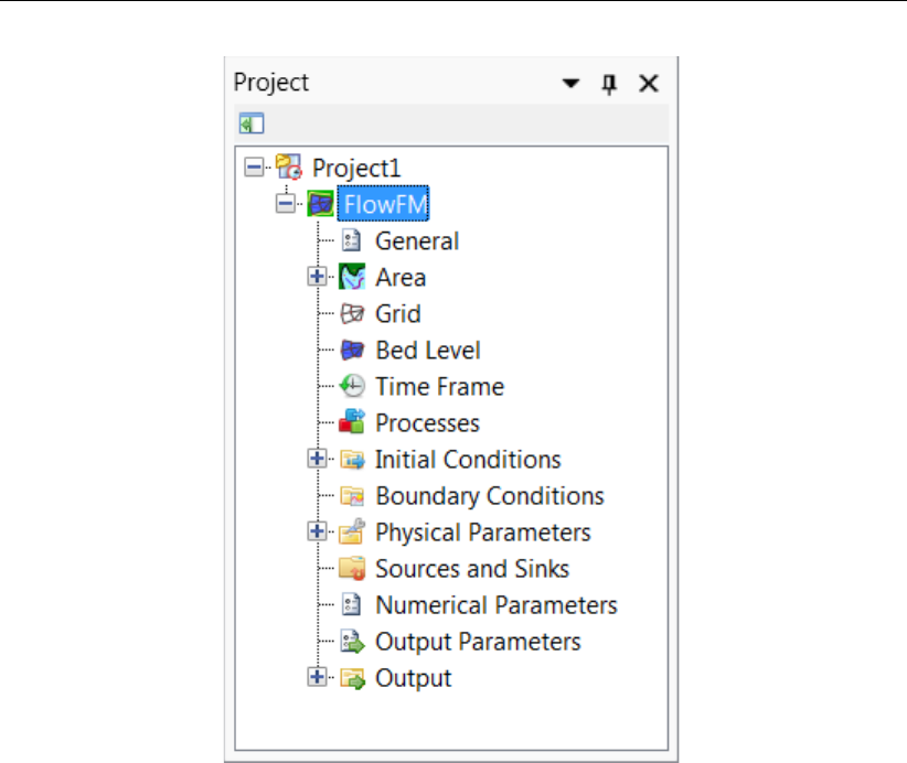
DRAFT
Getting started
Figure 3.2: Project window of D-Flow FM plugin
3.2.2 Central (map) window
The central window shows the contents of the main editor you are working with. In most cases
this will be the central map with tabulated input fields (see Figure 3.3). The map is used to
edit geographic model data, the tabulated input fields to edit overall model settings. Moreover,
the contents of the central window can also be a specific editor such as the time point editor
or the boundary condition editor. Each of these editors will open as a separate view.
Deltares 11 of 412
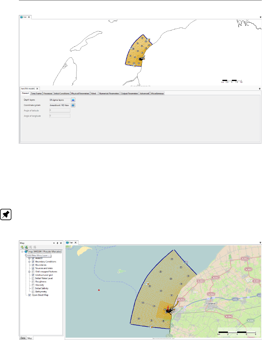
DRAFT
D-Flow Flexible Mesh, User Manual
Figure 3.3: Central map with contents of the D-Flow FM plug-in
3.2.3 Map window
The map tree allows the user to control the visibility of the contents of the central map using
checkboxes. Furthermore, the user can add (wms) layers, such as satellite imagery or open
street maps (see Figure 3.4).
Note: Please note that the map usually has a different coordinate system than the model. In
rendering the model attributes they are transformed to the map coordinate system (for visual
inspection on the map), but the model will be saved in the model coordinate system.
Figure 3.4: Map tree controlling map contents
12 of 412 Deltares
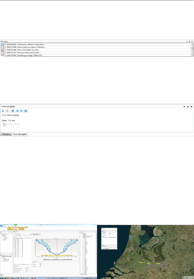
DRAFT
Getting started
3.2.4 Messages window
The message window (Figure 3.5) provides a log of information on the recent activities in
Delta Shell. It also provides warning and error messages.
Figure 3.5: Log of messages, warnings and errors in message window
3.2.5 Time navigator window
The time navigator (Figure 3.6) can be used to step through time dependent model output
and other time dependent geographic features on the map.
Figure 3.6: Time navigator in Delta Shell
3.3 Dockable views
The Delta Shell framework offers lots of freedom to customize dockable views, which are
discussed in this section.
3.3.1 Docking tabs separately
Within the Delta Shell framework the user can dock the separate windows according to per-
sonal preferences. These preferences are then saved for future use of the framework. An
example of such preferences is presented in Figure 3.7, where windows have been docked
on two screens.
Figure 3.7: Docking windows on two screens within the Delta Shell framework.
Deltares 13 of 412
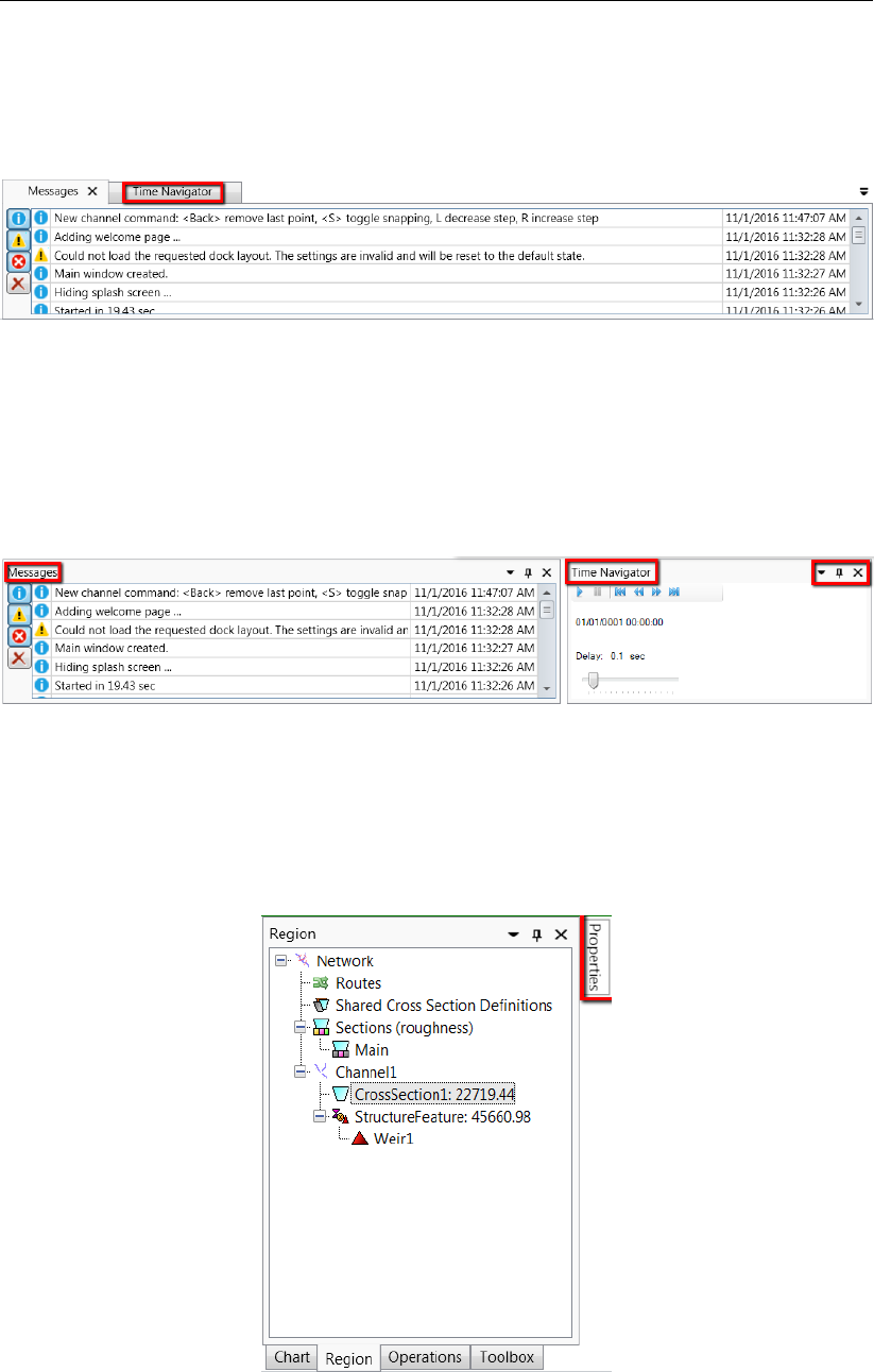
DRAFT
D-Flow Flexible Mesh, User Manual
3.3.2 Multiple tabs
In case two windows are docked in one view, the underlying window (tab) can be brought to
the front by simply selecting the tab, as is shown here.
Figure 3.8: Bringing the Time Navigator window to the front
By dragging dockable windows with the left mouse button and dropping the window left, right,
above or below another one the graphical user interface can be customized according to
personal preferences. Here an example of the Time Navigator window being docked above
the Properties window.
Figure 3.9: Docking the Time Navigator window.
Additional features are the possibility to remove or (auto) hide the window (top right in Fig-
ure 3.9). In case of removal, the window can be retrieved by a mouse-click on Time Navigator
in the View ribbon. Hiding the Time Navigator window results in:
Figure 3.10: Auto hide the Properties window
14 of 412 Deltares
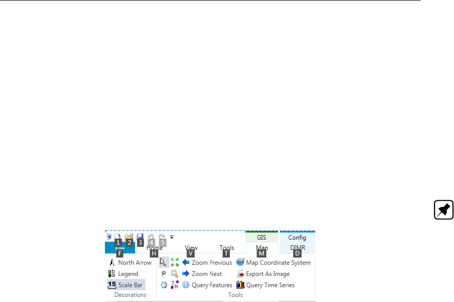
DRAFT
Getting started
3.4 Ribbons and toolbars
The user can access the toolbars arranged in ribbons. Model plug-ins can have their own
model specific ribbon. The ribbon may be auto collapsed by activating the Collapse the Ribbon
button when right-mouse-clicking on the ribbon.
3.4.1 Ribbons (shortcut keys)
Delta Shell makes use of ribbons, just like Microsoft Office. You can use these ribbons for
most of the operations. With the ribbons comes shortcut key functionality, providing shortcuts
to perform operations. If you press Alt, you will see the letters and numbers to access the
ribbons and the ribbon contents (i.e. operations). For example, Alt + H will lead you to the
Home-ribbon (Figure 3.11).
Note: Implementation of the shortcut key functionality is still work in progress.
Figure 3.11: Perform operations using the shortcut keys
3.4.2 File
The left-most ribbon is the File ribbon. It has menu-items comparable to most Microsoft
applications. Furthermore, it offers users import and export functionality, as well as the Help
and Options dialogs, as shown in Figure 3.12 and Figure 3.13.
Deltares 15 of 412
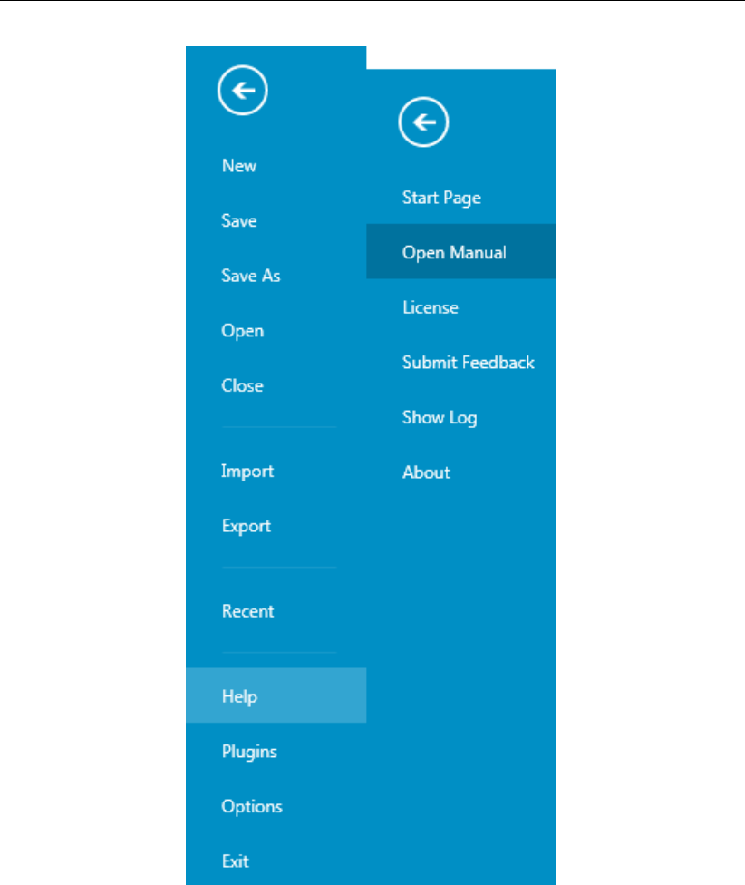
DRAFT
D-Flow Flexible Mesh, User Manual
Figure 3.12: The File ribbon.
16 of 412 Deltares

DRAFT
Getting started
Figure 3.13: The Delta Shell options dialog.
3.4.3 Home
The second ribbon is the Home ribbon (Figure 3.14). It harbours some general features for
clipboard actions, addition of items, running models, finding items within projects or views,
and help functionality.
Figure 3.14: The Home ribbon.
3.4.4 View
The third ribbon is the View ribbon (Figure 3.15). Here, the user can show or hide windows.
Figure 3.15: The View ribbon.
Deltares 17 of 412
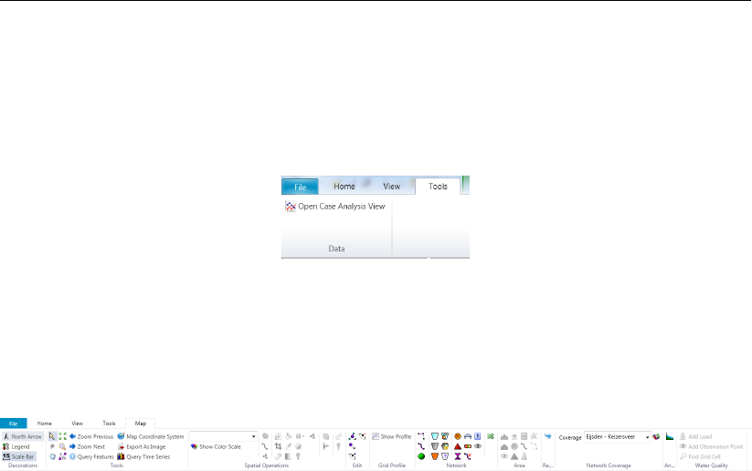
DRAFT
D-Flow Flexible Mesh, User Manual
3.4.5 Tools
The fourth ribbon is the Tools ribbon (Figure 3.16). By default, it contains only the Open
Case Analysis View tool. Some model plug-ins offer the installation of extra tools that may be
installed. These are documented within the user documentation of those model plug-ins.
Figure 3.16: The Tools ribbon contains just the Data item.
3.4.6 Map
The last ribbon is the Map ribbon (Figure 3.17).
Figure 3.17: The Map ribbon.
This will be used heavily, while it harbours all Geospatial functions, like:
Decorations for the map
North arrow
Scale bar
Legend
...
Tools to customize the map view
Select a single item
Select multiple items by drawing a curve
Pan
Zoom to Extents
Zoom by drawing a rectangle
Zoom to Measure distance
...
Edit polygons, for example within a network, basin, or waterbody
Move geometry point(s)
Add geometry point(s)
Remove geometry point(s)
Creation of a model Network, for example for D-Flow 1D
Add new Branch
Split Branch
Add Cross section
Add Weir
Add Pump
...
Still, all functions of the category can be activated as they will appear in the drop-down panel.
18 of 412 Deltares
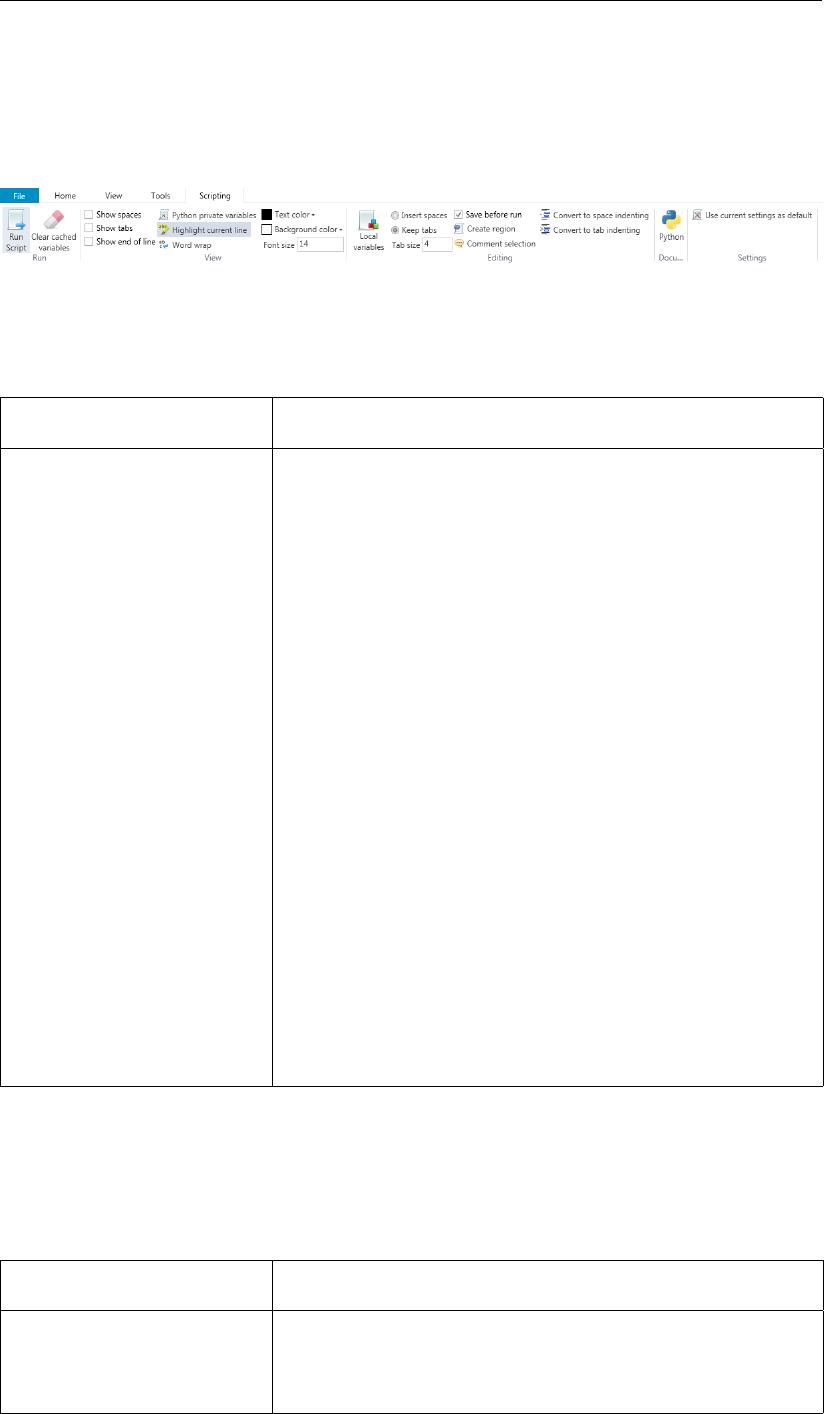
DRAFT
Getting started
3.4.7 Scripting
When you open the scripting editor in Delta Shell, a Scripting ribbon category will appear.
This ribbon has the following additional options (see also Figure 3.18), which are described in
Table 3.1:
Figure 3.18: The scripting ribbon within Delta Shell.
Table 3.1: Functions and their descriptions within the scripting ribbon of Delta Shell.
Function Description
Run script Executes the selected text. If no text is selected then it will
execute the entire script
Clear cached variables Clears all variables and loaded libraries from memory
Debugging Enables/Disables the debug option. When enabled you can
add breakpoint to the code (using F9 or clicking in the mar-
gin) and the code will stop at this point before executing the
statement (use F10 (step over) or F11 (step into) for a more
step by step approach)
Python variables Show or hide python variables (like _var_) in code comple-
tion
Insert spaces/tabs Determines if spaces or tab characters are added when
pressing tab
Tab size Sets the number of spaces that are considered equal to a
tab character
Save before run Saves the changes to the file before running
Create region Creates a new region surrounding the selected text
Comment selection Comments out the selected text
Convert to space indenting Converts all tab characters in the script to spaces. The num-
ber of spaces is determined by Tab size
Convert to tab indenting Converts all x number of space characters (determined by
Tab size) in the script to tabs
Python (documentation) Opens a link to the python website, showing you the python
syntax and standard libraries
Delta Shell (documentation) Opens a link to the Delta Shell documentation website (gen-
erated documentation of the Delta Shell api)
3.4.8 Shortcuts
The shortcut keys of the scripting editor within Delta Shell are documented in Table 3.2.
Table 3.2: Shortcut keys within the scripting editor of Delta Shell.
Shortcut Function
Ctrl + Enter Run selection (or entire script with no selection)
Ctrl + Shift +
Enter
Run current region (region where the cursor is in)
Ctrl + X Cut selection
Deltares 19 of 412
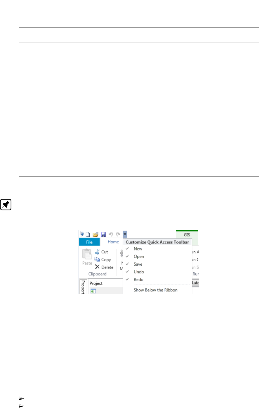
DRAFT
D-Flow Flexible Mesh, User Manual
Table 3.2: Shortcut keys within the scripting editor of Delta Shell.
Shortcut Function
Ctrl + C Copy selection
Ctrl + V Paste selection
Ctrl + S Save script
Ctrl + - Collapse all regions
Ctrl + + Expand all regions
Ctrl + " Comment or Uncomment current selection
Ctrl + W Add selection as watch variable
Ctrl + H Highlight current selection in script (press esc to cancel)
F9 Add/remove breakpoint (In debug mode only)
F5 Continue running (In debug mode only — when on break-
point)
Shift + F5 Stop running (In debug mode only — when on breakpoint)
F10 Step over current line and break on next line (In debug mode
only - when on breakpoint)
F11 Step into current line if possible, otherwise go to next line
(In debug mode only — when on breakpoint). This is used
to debug functions declared in the same script (that have
already runned)
3.4.9 Quick access toolbar
Note: The user can make frequently used functions available by a single mouse-click in the
Quick Access Toolbar, the top-most part of the application-window. Do this by right-mouse-
clicking a ribbon item and selecting Add to Quick Access Toolbar.
Figure 3.19: The quick access toolbar.
3.5 Basic steps to set up a D-Flow FM model
This section shows the basic steps to set up a D-Flow FM model. For a more detailed de-
scription of the steps and GUI features you are referred to chapter 4.
3.5.1 Add a D-Flow FM model
After starting the application for the first time, the start page will open with a default project (i.e.
“project1”, see Figure 3.1). To add a D-Flow FM model to the project you have the following
options:
click “New Model” in the “Home”-ribbon (Figure 3.20)
use the Right Mouse Button on “project1” in the Project window, go to “Add” and “New
Model” (Figure 3.21)
20 of 412 Deltares
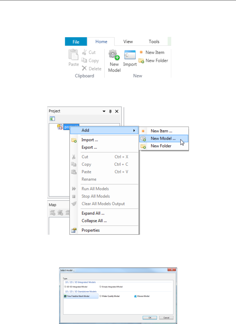
DRAFT
Getting started
From the list of available models (which can vary depending on your installation), select “D-
Flow FM model” (Figure 3.22).
Figure 3.20: Adding a new model from the ribbon
Figure 3.21: Adding a new model using the Right Mouse Button on “project1” in the
Project window
Figure 3.22: Select “D-Flow FM model”
3.5.2 Set up a D-Flow FM model
To set up the D-Flow FM model follow the steps in the Project window. For a more detailed
description, see chapter 4.
3.5.3 Multiple input files
The input of a D-Flow FM model is stored in a MDU file and in a number of attribute files,
which are explained in section 4.5. In general, all items of a certain quantity are stored in one
Deltares 21 of 412
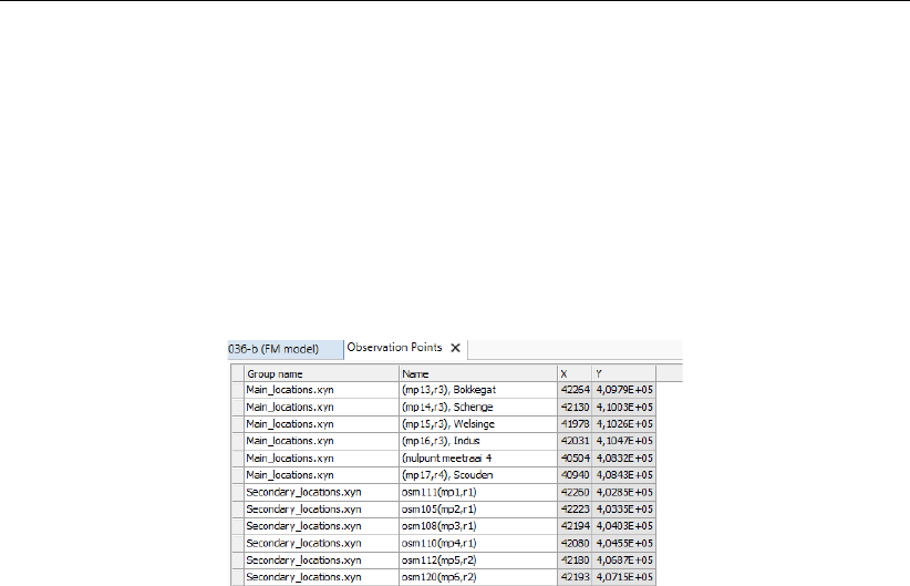
DRAFT
D-Flow Flexible Mesh, User Manual
attribute file. This is the standard approach. However, D-Flow FM also allows to have more
input files for all quantities, such as thin dams, dry points, cross sections and fixed weirs,
gates.
In the MDU file multiple input files per quantity can be specified. These input files have to be
separated by a " " (whitespace) in the MDU file. For a description of the MDU file we refer
to Appendix A. In Figure 3.23 this is illustrated by using two files for the observation points,
namely main_locations.xyn and secondary_locations.xyn. In a similar way the other quantities
like fixed weirs and thin dams can be stored in multiple files.
Figure 3.23: Illustration of multiple input files for observation points
3.5.4 Converting a Delft3D-FLOW model into D-Flow FM
Existing Delft3D-FLOW models can be converted into a set of input files suitable for D-
Flow FM (to a large extent). The conversion can be done by some Matlab utitilies, which
are described in section B.6.1.2.
3.5.5 Validate D-Flow FM model
You can check whether your model setup is valid by using the right mouse button in the Project
window and select “Validate” (Figure 3.24). This will produce a validation report (Figure 3.25).
Red exclamation marks indicate the parts of the model that are still invalid. By clicking the
hyperlink you will be automatically redirected to the invalid step in the model setup, so that
you can correct it.
22 of 412 Deltares
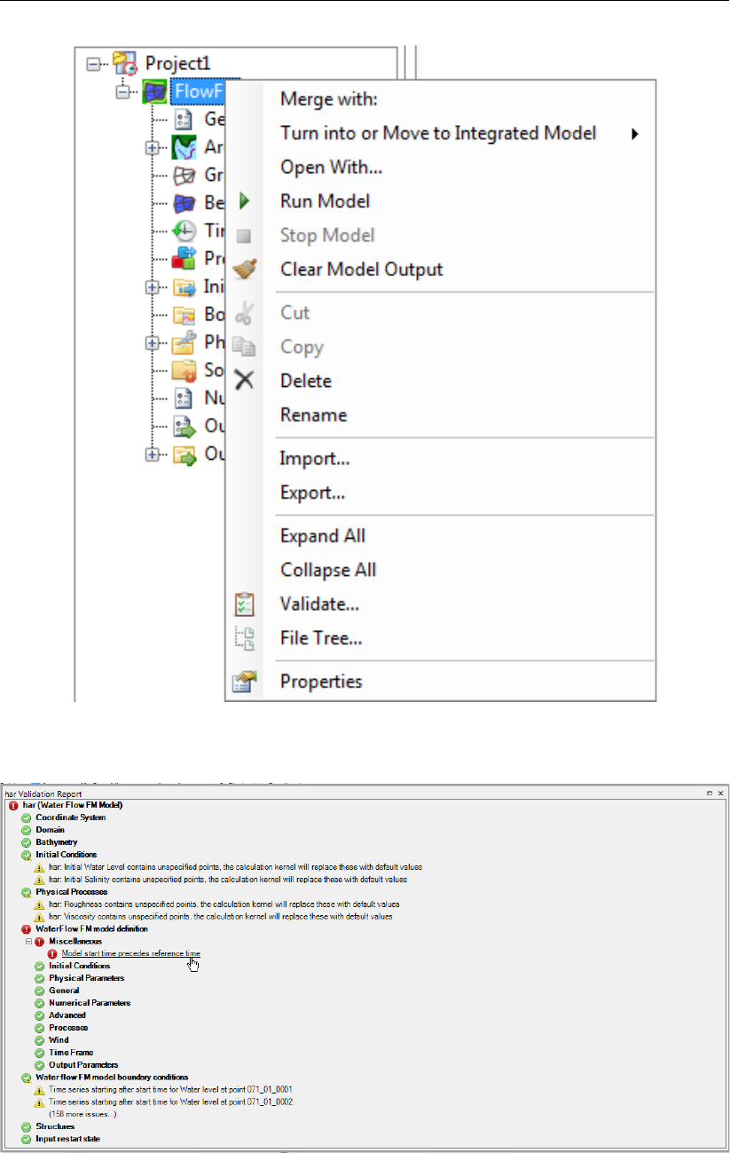
DRAFT
Getting started
Figure 3.24: Validate model
Figure 3.25: Validation report
Deltares 23 of 412
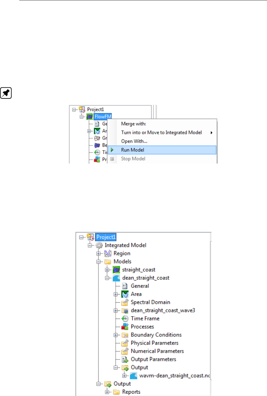
DRAFT
D-Flow Flexible Mesh, User Manual
3.5.6 File tree
To check the file paths and names of the attribute files which are linked to your model, you
can select “File tree” using the right mouse button on your model in the Project window.
3.5.7 Run D-Flow FM model
If you are satisfied with the model setup, you can run it from Delta Shell using the right mouse
button on model and select “Run model” (Figure 3.26).
Note: it is also possible to run D-Flow FM outside Delta Shell using the command line.
Figure 3.26: Run model
3.5.8 Inspect model output
The simulation will start and the output will be stored in the output folder in the Project window
(Figure 3.27). Delta Shell provides some basic tools to inspect the model output. For more
extensive and advanced options you are referred to Quickplot and Muppet.
Figure 3.27: Output of wave model in Project window
24 of 412 Deltares
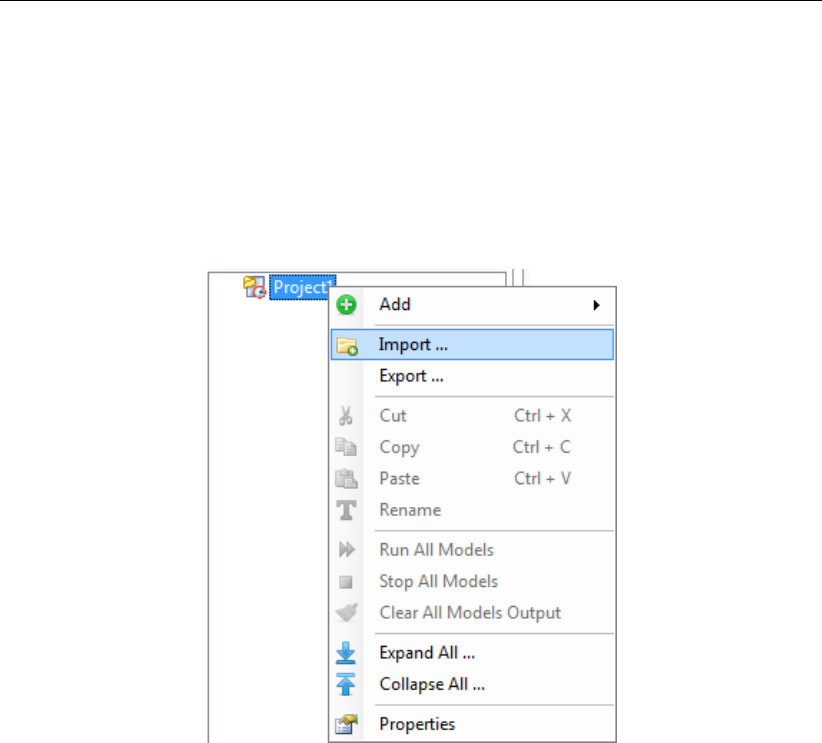
DRAFT
Getting started
3.5.9 Import/export or delete a D-Flow FM model
To import an existing D-Flow FM model either use the right mouse button on the project level
in the Project window (Figure 3.28) or go to the File-ribbon and press Import (Figure 3.29).
Likewise you can export a model or delete a model.
For the steps in the Project window that are linked to attribute files (observation points, grid,
bed level, etc.) you can use the right mouse button to import or export these attribute files.
Figure 3.28: Import wave model from Project window
Deltares 25 of 412
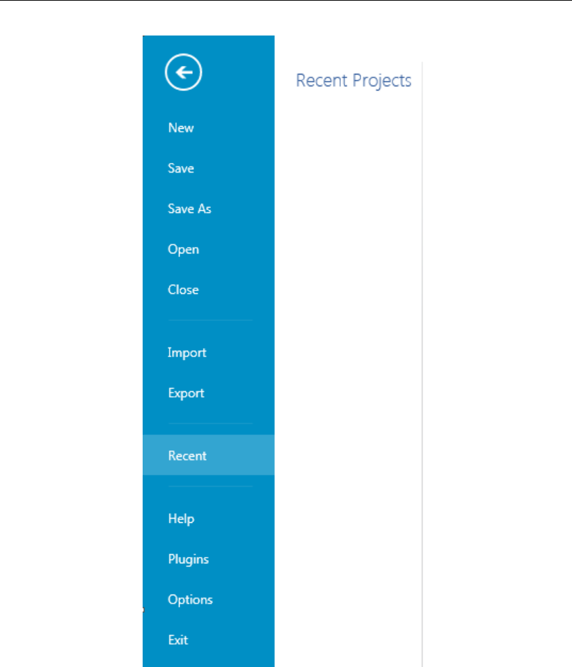
DRAFT
D-Flow Flexible Mesh, User Manual
Figure 3.29: Import wave model from file ribbon
3.5.10 Save project
To save the project (and, hence, the model) use the disk-icon on the Quick Access Toolbar or
the File-ribbon (Figure 3.29). If you would like to save the project under a different name use
Save As.
3.5.11 Exit Delta Shell
If you are finished you can exit Delta Shell using the red cross or pressing the Exit button in
the File-ribbon (Figure 3.29).
26 of 412 Deltares

DRAFT
Getting started
3.6 Important differences compared to Delft3D-FLOW GUI
The differences between the former Delft3D-FLOW GUI and the D-Flow FM plugin in Delta Shell
in lay-out and functionality are numerous. Here, we address only the most important differ-
ences in the workflow.
3.6.1 Project vs model
The entity “project” is new in the Delta Shell GUI. In the hierarchy the entity“project” is on a
higher level than the entity “model”. A project can contain multiple models, which can either
run standalone or coupled. The user can run all models in the project at once (on project level)
or each model separately (on model level). When the user saves the project, the project set-
tings will be saved in a <∗.dsproj>configuration file and the project data in a <*.dsproj_data
folder>. The <*.dsproj_data>folder contains folders with all input and output files for the
models within the project. There is no model intelligence in the <∗.dsproj>configuration file,
meaning that the models can also be run outside the GUI from the <*.dsproj_data>folder.
3.6.2 Load/save vs import/export
The user can load an existing Delta Shell project, make changes in the GUI and, consequently,
save all the project data. Loading and saving means working on the original project data, i.e.
the changes made by the user overwrite the original project data. Alternatively, use Save As
to keep the original project data and save the changes project data at another location (or with
another name).
Import/export functionality can be used to copy data from another location into the project
(import) or, vice versa, to copy data from the project to another location (export). Import/export
is literally copying, e.g.:
import: changes on the imported data will only affect the data in the project and not the
source data (upon saving the project)
export: the model data is copied to another location “as is”, changes made afterwards will
only affect the data in the project not the exported data (upon saving the project)
3.6.3 Working from the map
One of the most important differences with the former GUI is the central map. The central
map is comparable with the former “visualization area”, but with much more functionality and
flexibility. The map helps you to see what you are doing and inspect the model at all times.
You can use the Region and Map ribbons to add/edit model features in the map.
3.6.4 Coordinate conversion
With the map as a central feature, functionality to convert model and map coordinates is an
indispensable feature. In the General tab you can set the model coordinate system. In the
map tree you can set the map coordinate system using the right mouse button (Figure 3.30).
The coordinate systems are subdivided in geographic and projected systems. Use the quick
search bar to find the coordinate system you need either by name or EPSG code (Figure 3.31).
Deltares 27 of 412
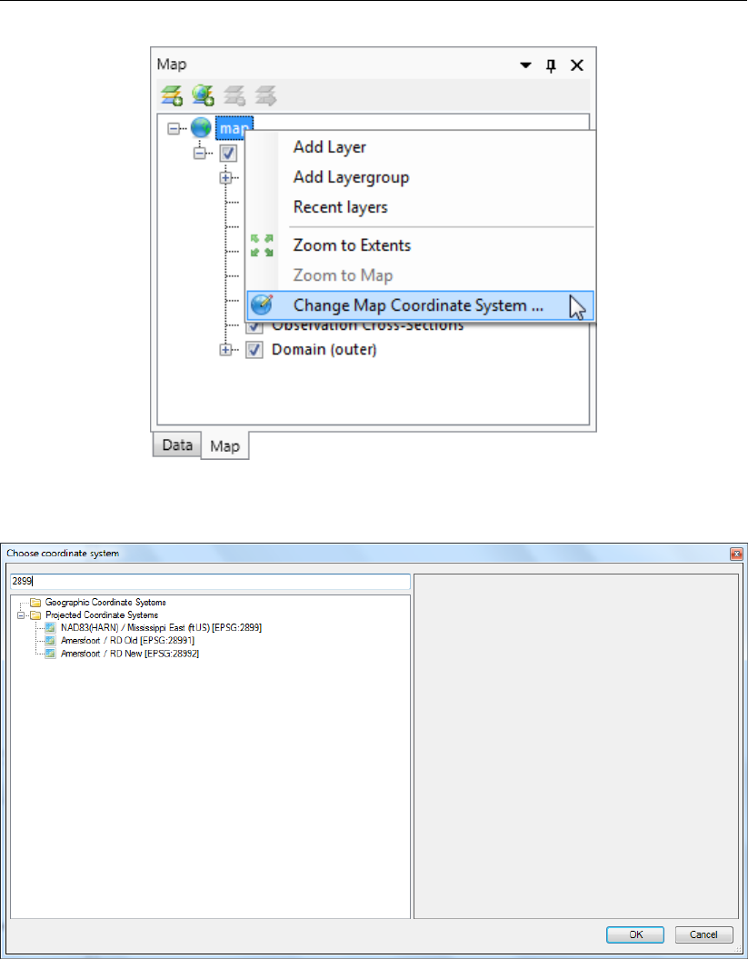
DRAFT
D-Flow Flexible Mesh, User Manual
Figure 3.30: Set map coordinate system using right mouse button
Figure 3.31: Select a coordinate system using the quick search bar
3.6.5 Model area
The model area contains geographical features, such as observation points & curves and
obstacles. In contrast to the former GUI, these features can even exist without a grid or outside
the grid and they are not based on grid coordinates, implying that their location remains the
same when the grid is changed (for example by (de-)refining).
Finally, for the computations, the SWAN computational core interpolates the features to the
grid. In the future we would like to show to which grid points the features are snapped before
running the computation. However, this requires some updates in the SWAN computational
core.
28 of 412 Deltares
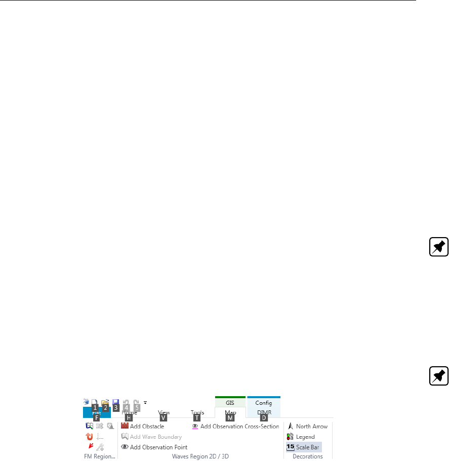
DRAFT
Getting started
3.6.6 Integrated models (model couplings)
The Delta Shell framework implements the concept of an Integrated model in order to couple
different models, such as: hydrodynamics coupled with the controlling of structures, waves,
morphology and/or water quality.
Two types of coupling are distinguished: offline and online coupling. In case of an Integrated
model with offline coupling, the entire hydrodynamic simulation is done first, i.e., separately
from the second simulation. The file-based hydrodynamic output serves as input for the sec-
ond simulation. As such, the hydrodynamic flow drives the controlling of structures or the
simulation of waves or water quality. In this case there is no feedback on the hydrodynamic
simulation. For many applications, this is good practice.
An online coupling, on the other hand, exchanges data every time after computing a specified
time interval. This tight coupling allows for direct feedback of the various processes on one
another. This is crucial for controlling structures.
Note: Offline is also referred to as sequential coupling and online as parallel coupling.
3.6.7 Ribbons (shortcut keys)
Delta Shell makes use of ribbons, just like Microsoft Office. You can use these ribbons for
most of the operations. With the ribbons comes shortcut key functionality, providing shortcuts
to perform operations. If you press Alt, you will see the letters and numbers to access the
ribbons and the ribbon contents (i.e. operations). For example, Alt + H will lead you to the
Home-ribbon (Figure 3.32).
Note: Implementation of the shortcut key functionality is still work in progress.
Figure 3.32: Perform operations using the shortcut keys
3.6.8 Context menus
Context menus are the menus that pop up using the right mouse button. These context menus
provide you with some handy functionality and shortcuts specific for the selected item. The
functionality is available in all Delta Shell windows and context dependent. You can best try it
yourself to explore the possibilities.
3.6.9 Scripting
Delta Shell has a direct link with scripting in Iron Python (NB: this is not the same as C-Python).
This means that you can get and set data, views and model files by means of scripting instead
of having to do it all manually. Scripting can be a very powerful tool to automate certain steps
of your model setup or to add new functionality to the GUI. You can add a new script by adding
a new item, either in the Home-ribbon or through the right mouse button.
Deltares 29 of 412

DRAFT
D-Flow Flexible Mesh, User Manual
30 of 412 Deltares

DRAFT
4 All about the modelling process
4.1 Introduction
In order to set up a hydrodynamic model you must prepare an input file. All parameters to
be used originate from the physical phenomena being modelled. Also from the numerical
techniques being used to solve the equations that describe these phenomena, and finally,
from decisions being made to control the simulation and to store its results. Within the range
of realistic values, it is likely that the solution is sensitive to the selected parameter values, so
a concise description of all parameters is required. This input data is collected into the Master
Definition Unstructured file, called a mdu-file.
In section 4.2 we discuss some general aspects of the mdu-file and its attribute files. The
sections thereafter describe how the actual modelling process can be done in the GUI.
4.2 mdu-file and attribute files
The Master Definition Unstructured file (mdu-file) is the input file for the hydrodynamic simu-
lation program. It contains all the necessary data required for defining a model and running
the simulation program. In the mdu-file you can define attribute files in which relevant data
(for some parameters) is stored. This will be particularly the case when parameters contain
a large number of data (e.g., time-dependent or space varying data). The mdu-file and all
possible user-definable attribute files are listed and described in Appendix A.
Although you are not supposed to work directly on the mdu-file it is useful to have some ideas
on it as it reflects the idea of the designer on how to handle large amounts of input data and
it might help you to gain a better idea on how to work with this file.
The basic characteristics of an mdu-file are:
It is an ASCII file.
Each line contains a maximum of 256 characters.
Each (set of) input parameter(s) is preceded by a (set of) keyword(s).
The results of all modules are written to platform independent binary (NetCDF-)files, so also
these result files you can transfer across hardware platforms without any conversion.
The mdu-file contains several sections, denoted by square brackets, below are the most rele-
vant ones:
[model] this section contains the program name and its version.
[geometry] in this section, the main entry comprises the specification of the grid (i.e.
the netcdf network file). In addition, thin dams and thin dykes can be specified.
[numerics] this section contains the settings of specific parts of the flow solver, such
as limiters and the iterative solver type.
[physics] in this field, physical model parameters can be inserted, for instance related
to friction modelling and turbulence modelling.
[wind] the wind section prescribed the dependency of the wind drag coefficient to the
wind velocity through 2 or 3 breakpoints. This field also contains pressure infor-
mation.
[time] in this section, the start time and the stop time of the simulation are specified in
hours, minutes or seconds. The other times specified are specified in seconds.
[restart] in this section, the restart file can be specified, either as a <∗_map.nc>-file
or as an <∗_rst.nc>file.
Deltares 31 of 412
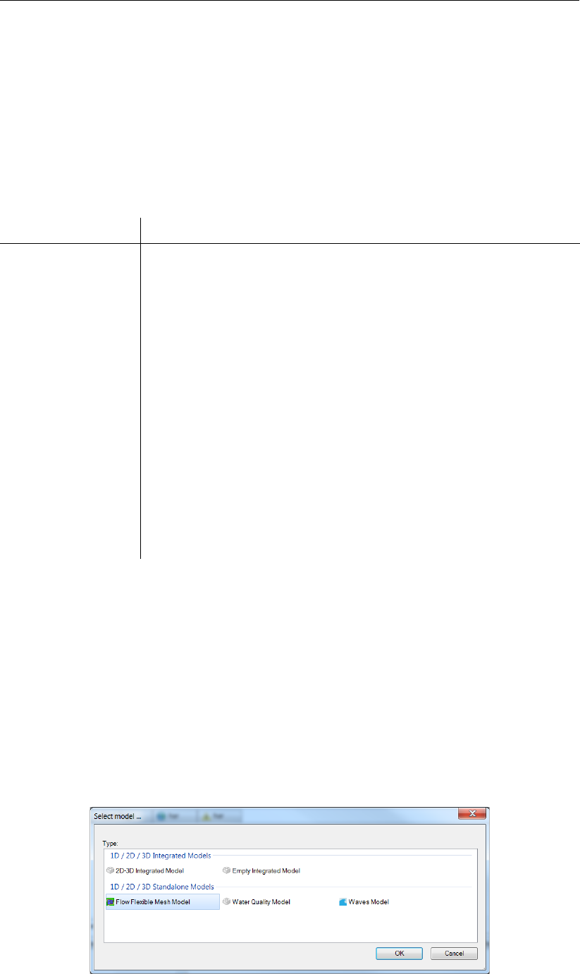
DRAFT
D-Flow Flexible Mesh, User Manual
[external forcing] this section only contains the name of the external forcings file.
[output] in this section, the writing frequency of output data can be prescribed.
Appendix A contains the full list of MDU sections and keywords.
4.3 Filenames and conventions
Filenames and file extensions hardly have any strict requirements in D-Flow FM, but we do
advise to use the suggested file naming patterns below:
file pattern description
mdu_name.mdu mdu-file
∗_net.nc Unstructured grid (network) file
∗.xyz Sample file (for spatial fields)
∗.ldb Landboundary file (polyline file format)
∗_thd.pli Thin dam file (polyline file format)
∗_fxw.pliz Fixed weir file (polyline file format with zvalues)
∗_part.pol Partitioning polygon file (polyline file format)
∗.ext External forcings file
pli_name.pli Boundary condition location file (polyline file format)
pli_name_000X.tim Timeseries boundary data file at point #X
pli_name_000X.cmp Astronomic/harmonical component boundary data file at point #X
∗.bc BC-format boundary data file with polyline and point labels in file
∗.xyn Observation station file
∗_crs.pli Observation cross-sections file
mdu_name_map.nc Output map file
mdu_name_his.nc Output his file
mdu_name.dia Output diagnostics (log) file
4.4 Setting up a D-Flow FM model
This chapter describes how to set up a D-Flow FM model in an empty Delta Shell project.
When you open the GUI, an empty project is automatically created. Starting from scratch,
you have to create an empty D-Flow FM model in a Delta Shell project:
In the ribbon menu items, go to Home and click on New Model. The Select model ...
window appears (Figure 4.1). Click on D-Flow FM model and click OK. Alternatively, you
can also double click on D-Flow FM model to open it directly.
Or use the right mouse button on the name of your project (project1 by default). In the
context menu that appears, select Add and click New Model. Again, the Select model ...
window appears allowing you to add an empty D-Flow FM model.
Figure 4.1: The Select model ... window
32 of 412 Deltares
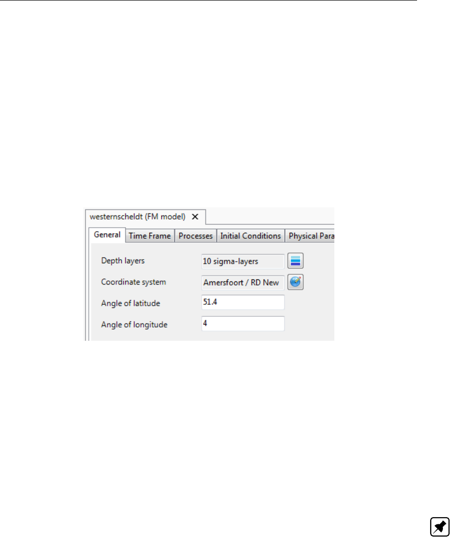
DRAFT
All about the modelling process
In the Project window, an empty model has appeared (Water Flow FM Model (1) by default).
Click the plus sign (+) before the name of the model to expand all model attributes in the
Project window: General, Area, Grid, Bed Level, Time Frame, Processes, Initial Conditions,
Boundary Conditions, Physical Parameters, Sources and Sinks, Numerical Parameters, Out-
put Parameters and Output. In the following paragraphs, all model attributes are treated
separately.
4.4.1 General
When you double click on General in the Project window, tabulated input fields appear under-
neath the central map (Figure 4.2). The general tab contains general model information such
as the model grid (will be moved to domain in later release), the number of vertical layers and
vertical model, the model coordinate system and the angle of latitude.
Figure 4.2: Overview of general tab
4.4.1.1 Vertical layer specification
When you click on the blue striped icon next to the vertical layers text box (depth layers), the
Edit depth layers window appears (Figure 4.3). This window allows you to choose the type of
layering and the corresponding number of layers. The drop down menu contains two distinct
layering types:
1 Single
2 Z
3 Sigma (β-functionality)
Note: Currently, only the Single and Sigma type layering are presented.
Deltares 33 of 412
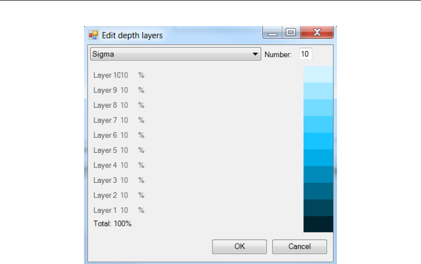
DRAFT
D-Flow Flexible Mesh, User Manual
Figure 4.3: Vertical layer specification window (σ-model is β-functionality)
The recommended type of vertical layering differs depending on the model application and the
processes that you are interested in. Layers in the σ-model increase or decrease in thickness
as the water depth in the model increases or decreases. The relative thickness distribution
of the different layers however remains fixed. Layers in the Z-model have a fixed thickness,
which does not change as the water depth in the model varies. If the water depth drops below
the cumulative thickness of all z-layers, layer(s) will fall dry. When Single is chosen, the model
contains only 1 vertical layer. (An extensive description of σ- and z-type layering is found in
section 7.3).
If your model contains more than 1 layer, the thickness distribution of the vertical layers can be
specified. In Delta Shell, user can specify the number of layers and then automatically obtain
uniformly distributed layer thicknesses (The total percentage is 100 %). As shown in Figure
Figure 4.3, setting 10 layers results in 10 % thickness distribution for each layer. Specifying
non-uniformly distributed layer thickness is β-functionality and can be done through the MDU
file.
4.4.1.2 Model coordinate system
A very important property of your model is the coordinate system in which it is specified.
Within the interface, there is a clear distinction between the coordinate system of your model
and all of its attributes and the coordinate system of the central map and all of its items. Both
coordinate systems can be set independent from each other. Keep in mind, that the coordinate
system of your model is saved and used when you run your model. Only coordinate systems
supported by the computational core are supported.
The model coordinate system can be set using the globe icon next to the Coordinate system
text box. After clicking this button, the coordinate system wizard is opened (Figure 4.4). This
wizard allows you to choose one of many possible coordinate systems and apply it to your
model. You can use the search bar to browse the various coordinate systems (searching
possible by name and EPSG code). If your model is specified in a certain coordinate system
already, it is possible to convert the model coordinate system using the same button. After
clicking OK, all model attributes are converted to the system of choice. Note that you have to
34 of 412 Deltares

DRAFT
All about the modelling process
close and re-open all map views for the changes to take effect in these views.
Figure 4.4: Coordinate system wizard
The map coordinate system applies to all items in the map Project window. To change the map
coordinate system, navigate the menu ribbons to Map and click on Map coordinate system.
Alternatively, right mouse click on map in the map Project window and select Change Map
Coordinate System. The coordinate system wizard appears, allowing you to set the map
coordinate system of your choice. When the original model coordinate system differs from the
selected map coordinate system, all map items are automatically converted to the specified
map coordinate system.
4.4.1.3 Angle of latitude
For a Cartesian grid you have to specify the latitude of the model area; this is used to calculate
a fixed Coriolis force for the entire area. For a spherical grid the Coriolis force is calculated
from the latitude coordinates in the grid file and thus varies in the latitude direction. Typically,
you use spherical co-ordinates for large areas, such as a regional model. When a value of 0
is entered, the Coriolis force is not taken into account.
4.4.2 Area
The model area contains all geographical features, such as the observation points, structures
and land boundaries. These features can exist without a grid or outside the grid as they are not
based on grid coordinates but xy-coordinates. This means that the location of the model area
features remains the same when the grid is changed (for example by (de-)refining). When you
expand the model attribute Area in the Project window, a list of possible geographical features
is displayed (Figure 4.5).
Figure 4.5: Overview of geographical features
Figure 4.6 displays an overview of the map ribbon. The left red box indicates the FM Region
Deltares 35 of 412
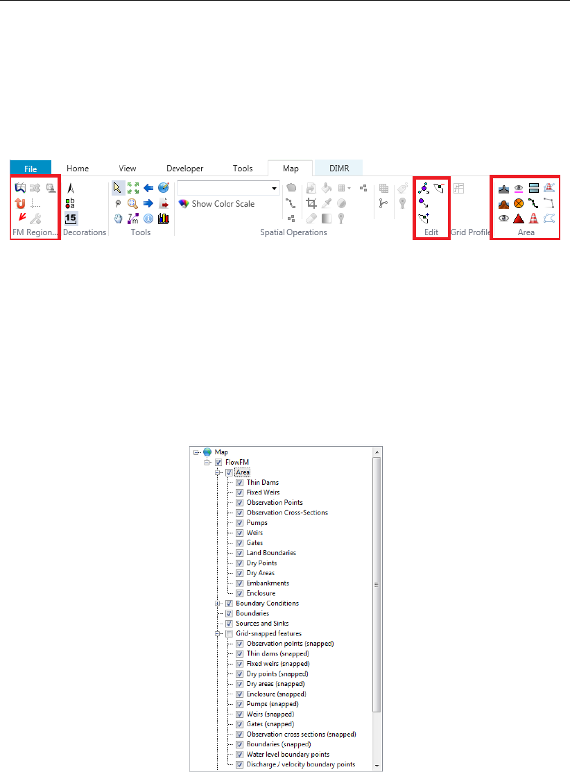
DRAFT
D-Flow Flexible Mesh, User Manual
2D / 3D of the map ribbon. To add a geographical feature, click the corresponding item in this
box and use your mouse to indicate the location of the desired feature on the central map.
Importing and exporting of all model features is done via the context menu by using your right
mouse button on the different features. The red box on the right highlights the various editing
buttons available to edit the locations of the geographical features. The specifics for each
feature are discussed separately in the following sections.
Figure 4.6: Overview of map ribbon. Left red box highlights FM Region 2D / 3D menu
containing icons used to add features. Right red box highlights Edit menu
which contains icons used to edit geographical features (move/add)
4.4.2.1 Grid snapped features
All geographical features of your model that are described by x-, and y-coordinates have to
be interpolated to your computational grid when you run your model. The computational core
of D-Flow FM automatically assigns these features to the corresponding parts of your grid.
The graphical user interface allows you to inspect the interpolated locations of these features.
Figure 4.7: Example of expanded grid snapped features attribute in map tree
Figure 4.7 shows a part of the map tree, showing the Area2D and Grid-snapped features
attributes. The x- and y-locations of all spatial model features are shown within the Area2D
attribute. You can hide or show any of these attributes by means of clicking the check boxes
in front of the attributes. When you enable the Grid-snapped features, all items within the
Area2D attribute, as well as all boundaries are interpolated to their corresponding locations on
the computational grid. The interpolation is performed instantaneously by the computational
core of D-Flow FM, which enables you to directly inspect the numerical interpretation of all
features on the computational grid. Figure 4.8 shows an example of four observation points
36 of 412 Deltares
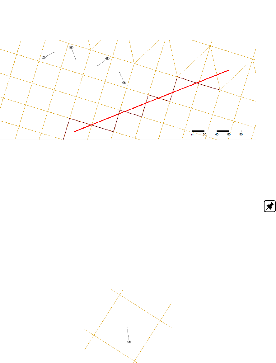
DRAFT
All about the modelling process
and one thin dam in the central map, showing both the x- and y-locations of these features
as well as their representation on the computational grid.
Figure 4.8: Example of grid snapped features displayed on the central map
4.4.2.2 Observation points
Observation points are used to monitor the time-dependent behaviour of one or all computed
quantities as a function of time at a specific location, i.e. water elevations, velocities, fluxes,
salinity, temperature and concentration of the constituents . Observation points represent an
Eulerian viewpoint at the results. (Note: Sediment transport is a β-functionality)
To add an observation point, click the corresponding icon from the FM Region 2D / 3D menu
in the map ribbon (Figure 4.6). By clicking in the central map, observation points are placed
in your model. Selected observation points (first click the Select icon from the “Tools” menu
in the map ribbon) can be deleted using backspace or directly from the attribute table (ex-
plained below). The grid snapped representation (Figure 4.9) is indicated by a line linking the
observation points to the closest cell center, indicating that output will be stored of this cell.
Importing and exporting of observation points is possible via the context menu of “Observation
points” in the Project window (right mouse button).
Figure 4.9: Geographical and grid snapped representation of an observation point
When you double click the Observation points attribute in the Project window, the observation
points tab is displayed underneath the central map (Figure 4.10). This tab shows an attribute
table with the names, x- and y-locations (in the model coordinate system) of the various
observation points within the model. When one of the entries is selected, the corresponding
observation point is highlighted in the central map.
Deltares 37 of 412
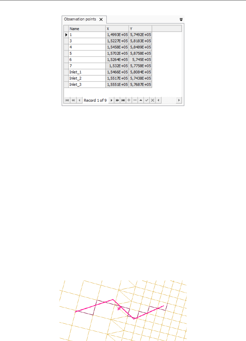
DRAFT
D-Flow Flexible Mesh, User Manual
Figure 4.10: Attribute table with observation points
4.4.2.3 Observation cross-sections
Cross-sections (Figure 4.11) are used to store the sum of computed fluxes (hydrodynamic),
flux rates (hydrodynamic), fluxes of matter (if existing) and transport rates of matter (if existing)
sequentially in time at a prescribed interval.
To add a cross section, click the corresponding icon from the FM Region 2D / 3D menu in
the map ribbon (Figure 4.6). By clicking in the central map, cross section points are added.
Note that a cross section consists of a minimum of two points, but an arbitrary amount of
intermediate points can be added. The last point is indicated by double clicking the left mouse
button. The distance in meters (independent of the local coordinate system) in between the
last point and the mouse pointer is indicated in pink; in case more than two points are used,
the cumulative length of the entire cross section is shown in black. Once highlighted in the
central map, a cross section is deleted with backspace or directly from the attribute table
described below. The positive direction through the cross section is indicated by a pink arrow.
The direction of this arrow is dependent on the order in which the cross section points are
drawn (to change the direction, flip the start and end points). Importing and exporting of
cross sections is possible via the context menu of “Observation cross-sections” in the Project
window (right mouse button).
Figure 4.11: Geographical and grid snapped representation of a cross section
Double clicking the Observation cross-sections attribute in the Project window enables the
Observation cross-sections tab in the central map view (Figure 4.12). Alternatively, you can
double click on any cross section in the map. The attribute table displayed in the tab contains
the names of the various cross sections of your model. When one of the entries is selected,
the corresponding cross section is highlighted in the central map. A cross section entry can
be deleted from the table via the context menu (right mouse button).
38 of 412 Deltares
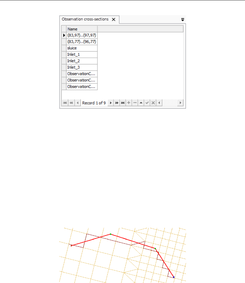
DRAFT
All about the modelling process
Figure 4.12: Attribute table with observation cross sections
4.4.2.4 Thin dams
Thin dams (Figure 4.13) are infinitely thin objects defined at the velocity points which prohibit
flow exchange between the two adjacent computational cells without reducing the total wet
surface and the volume of the model. The purpose of a thin dam is to represent small obsta-
cles (e.g. breakwaters, dams) in the model which have sub-grid dimensions, but large enough
to influence the local flow pattern. A thin dam is assumed to have an infinite level in the model;
no water will ever overflow a thin dam.
To add a thin dam, click the corresponding icon from the FM Region 2D / 3D menu in the map
ribbon (Figure 4.6). Adding, deleting, importing and exporting of a line feature such as a thin
dam is discussed in more detail in section 4.4.2.3 on cross sections.
Figure 4.13: Geographical and grid snapped representation of a thin dam
When you double click the Thin dams attribute in the Project window, the corresponding Thin
dams tab appears underneath the central map (Figure 4.14). Alternatively, you can also
double click on any thin dam in the central map. Within this tab, an attribute table is shown
which displays the names of all thin dams within your model. When one of the entries is
selected, the corresponding item is highlighted in the central map. A thin dam entry can be
deleted from the table via the context menu (right mouse button).
Deltares 39 of 412
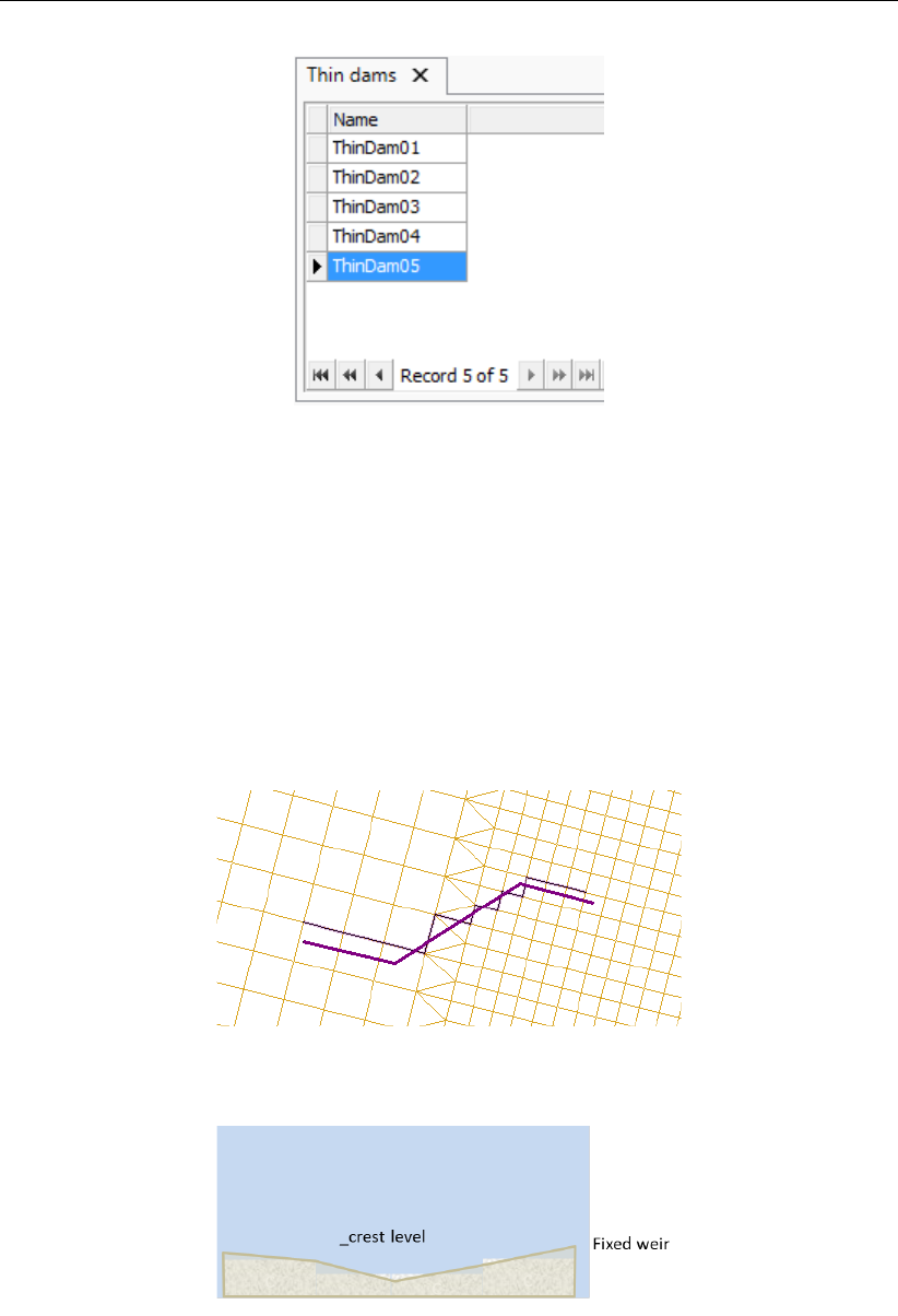
DRAFT
D-Flow Flexible Mesh, User Manual
Figure 4.14: Attribute table with thin dams
4.4.2.5 Fixed weirs
A fixed weir (Figure 4.15) has the same function as a thin dam (section 4.4.2.4). However,
unlike a thin dam, a fixed weir can be assigned both xy- and z-values. Furthermore, a fixed
weir can be assigned a crest length (a thin dam is infinitely thin). The z-values correspond
to the crest level of the fixed weir at the corresponding x- and y-locations; the level can vary
in space, but is constant in time (Figure 4.16). Consequently, a fixed weir can overflow if the
water level exceeds the crest level of the fixed weir. The level is specified with regard to the
same vertical reference level as all other model items with level specifications (e.g. bed level
values and initial water levels).
Figure 4.15: Geographical and grid snapped representation of a fixed weir
Figure 4.16: Schematic representation of a fixed weir
To add a fixed weir, click the corresponding icon from the FM Region 2D / 3D menu in the
map ribbon (Figure 4.6). Adding, deleting, importing and exporting of a line feature such as a
fixed weir is discussed in more detail in section 4.4.2.3 on cross sections.
When you double click the Fixed weirs attribute in the Project window, the corresponding
40 of 412 Deltares
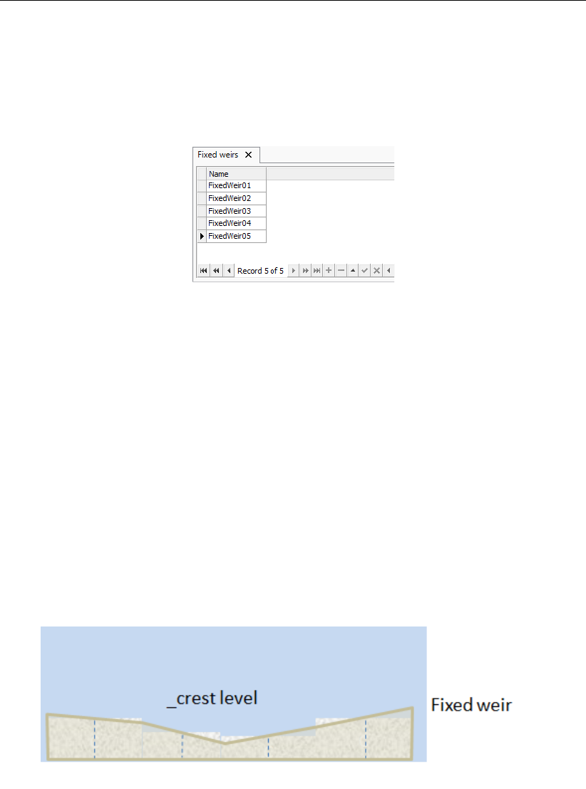
DRAFT
All about the modelling process
Fixed weirs tab appears underneath the central map (Figure 4.17). Alternatively, you can also
double click on any fixed weir in the central map. Within this tab, an attribute table is shown
which displays the names of all fixed weirs within your model. When one of the entries is
selected, the corresponding item is highlighted in the central map. A fixed weir entry can be
deleted from the table via the context menu (right mouse button).
Figure 4.17: Attribute table with fixed weirs
When you double click on a fixed weir in the central map, the fixed weir editor opens in a
separate view (Figure 4.18). On the right, a graphic representation (top view) of the fixed weir
is displayed. The support point that is selected in the table is highlighted by means of a blue
circle. On the left, a table is displayed showing the following properties of each support point
of the fixed weir under consideration:
X: x-location of the support point
Y: y-location of the support point
Crest level: level of fixed weir (spatially varying but fixed in time)
Crest length: length of the crest (instead of an infinitely thin crest)
Left ground level: ground level to the left of the crest; together with crest level determines
slope of crest on the left side
Right ground level: ground level to the right of the crest; together with crest level deter-
mines slope of crest on the right side
Figure 4.18: Fixed weir editor
Deltares 41 of 412
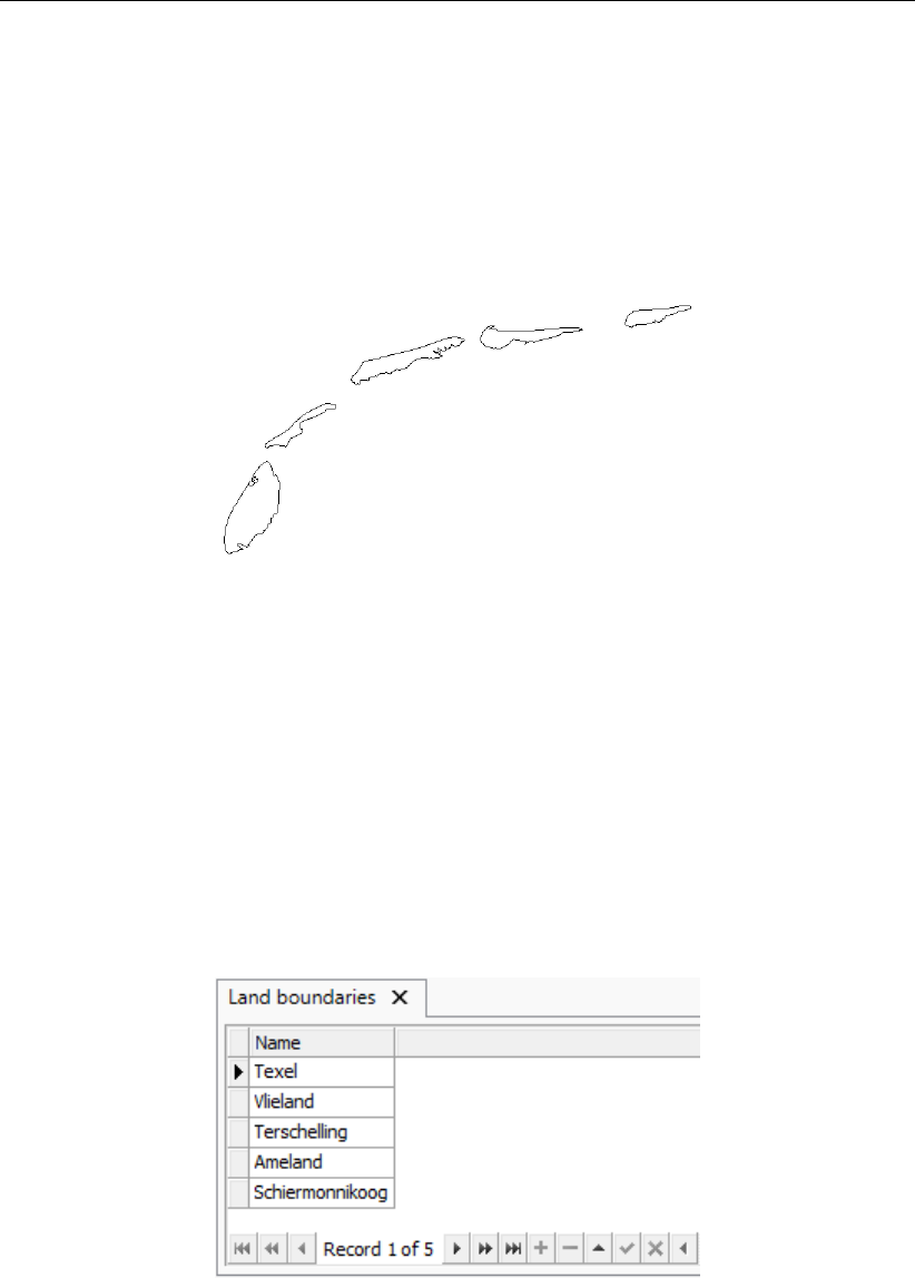
DRAFT
D-Flow Flexible Mesh, User Manual
4.4.2.6 Land boundaries
A land boundary (Figure 4.19) encloses the main geographic features surrounding your model
and indicates the intersection of the water and land masses. When you set up your computa-
tional grid in RGFGRID, a land boundary determines the onshore extent of your model. When
you open RGFGRID to edit your grid, the land boundary is automatically transferred and dis-
played. For more details on grid generation, you are referred to the User Manual of RGFGRID
(RGFGRID UM,2016).
Figure 4.19: Geographical representation of a land boundary
To add a land boundary, click the corresponding icon from the FM Region 2D / 3D menu in
the map ribbon (Figure 4.6). Adding, deleting, importing and exporting of a line feature such
as a land boundary is discussed in more detail in section 4.4.2.3 on cross sections.
When you double click the Land boundaries attribute in the Project window, the corresponding
land boundaries tab appears underneath the central map (Figure 4.20). Alternatively, you can
also double click on any land boundary in the central map. Within this tab, an attribute table is
shown which displays the names of all land boundaries within your model. When one of the
entries is selected, the corresponding item is highlighted in the central map. A land boundary
entry can be deleted from the table via the context menu (right mouse button).
Figure 4.20: Attribute table with land boundaries
42 of 412 Deltares
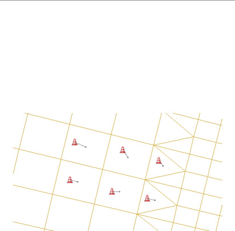
DRAFT
All about the modelling process
4.4.2.7 Dry points and dry areas
Dry points are grid cells centred around a water level point that are permanently dry during
a computation, irrespective of the local water depth and without changing the water depth as
seen from the wet points. Dry areas are the same, but provide an easy way of defining many
grid points as a single dry area at once.
Note that the flexibility of unstructured grids makes the use of dry points less necessary than
with structured grid models, such as Delft3D-FLOW. In the interior of unstructured grids, some
or more grid cells can easily be deleted during grid manipulation, e.g., in RGFGRID. Still, a
dry points file can be used to explicitly mark locations or regions inside the grid as dry cells.
Dry points in the GUI
Figure 4.21: Geographical and grid snapped representation of several dry points
To add a dry point, click the corresponding icon from the FM Region 2D / 3D menu in the map
ribbon (Figure 4.6). Adding, deleting, importing and exporting of a point feature such as a dry
point is discussed in more detail in section 4.4.2.2 on observation points. The grid snapped
representation of a dry point (Figure 4.21) is indicated by a line linking the dry point to the
closest cell center.
When you double click the “Dry points” attribute in the Project window, the corresponding
Dry points tab appears underneath the central map (Figure 4.22). Alternatively, you can also
double click on any dry point in the central map. Within this tab, an attribute table is shown
which displays the names of all dry points within your model. When one of the entries is
selected, the corresponding item is highlighted in the central map. A dry point entry can be
deleted from the table via the context menu (right mouse button).
Deltares 43 of 412
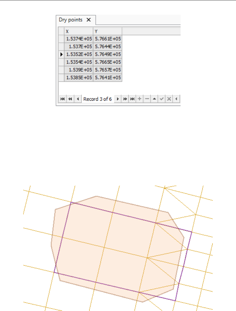
DRAFT
D-Flow Flexible Mesh, User Manual
Figure 4.22: Attribute table with dry points
Dry areas in the GUI
Dry areas (Figure 4.23), like dry points, indicate areas that permanently dry during a com-
putation. Instead of adding many separate dry points, you can draw a polygon that encloses
all required computational cells. Only cells which centers are strictly inside the polygon are
taken into account. The grid snapped representation of the dry area clearly indicates which
cells are considered within the dry area.
Figure 4.23: Geographical and grid snapped representation of a dry area
When you double click the Dry areas attribute in the Project window, the corresponding Dry
areas tab appears underneath the central map (Figure 4.24). Alternatively, you can also
double click on any dry area in the central map. Within this tab, an attribute table is shown
which displays the names of all dry areas within your model. When one of the entries is
selected, the corresponding item is highlighted in the central map. A dry area entry can be
deleted from the table via the context menu (right mouse button).
44 of 412 Deltares
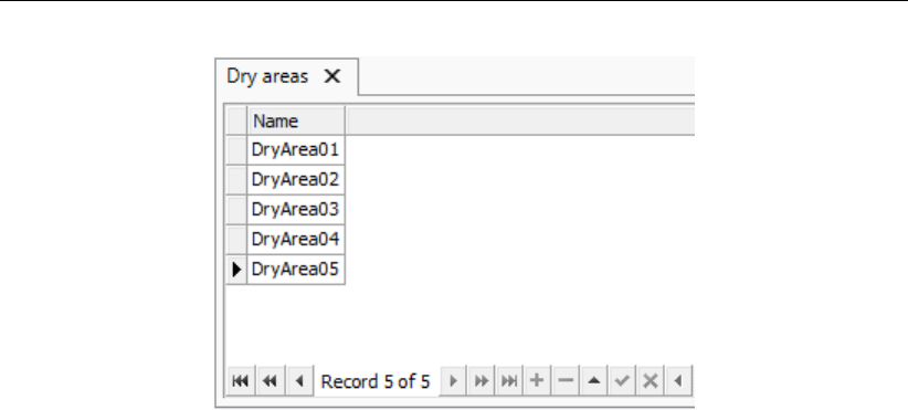
DRAFT
All about the modelling process
Figure 4.24: Attribute table with dry areas
Dry points file input
Dry points are defined by a sample file <∗.xyz>, dry areas are defined by a polygon file
<∗.pol>. Add the filename to the MDU as below:
[geometry]
# ...
DryPointsFile = <filename.xyz> # Dry points file *.xyz, third column dummy z values,
# or polygon file *.pol.
The format of the sample file is defined in section B.3. The format of the polygon file is defined
in section B.2. All grid cells that contain a sample point are removed from the model grid, and
as a result do not appear in any of the output files. Alternatively, for a polygon file, all grid cells
whose mass center lies within the polygon will be removed from the model grid.
Finally, an optional flag can be set in the polygon file to invert the masking behavior of the poly-
gon. That is: all points outside of the polygon will be marked as dry and therefore removed.
To realize this, the polygon block should have three columns, and the first point should have
az-value of -1 in the third column.
4.4.2.8 Pumps
Pumps are a type of structures in D-Flow FM. Unlike the other structures, pumps can force the
flow only on one direction. This direction is determined by arrow in D-Flow FM. The direction
of pump can be reverted by mouse right-click and selecting "Reverse line(s)".
Like all other structures in D-Flow FM, the pump can be defined by a polygon. The input data
of the pumps can be given by selecting and editing the pump polygon (see Figure 4.25). Right
click on the pump polygon and selecting "Delete Selection" leads to deletion of the selected
pump. Double clicking the pump polygons (or right click the pump in the list and select "Open
view"), it opens a tab for editing the pump properties. The tab includes pump capacity. If the
pump capacity is time dependent, it can be given by time series data (Figure 4.25).
Deltares 45 of 412
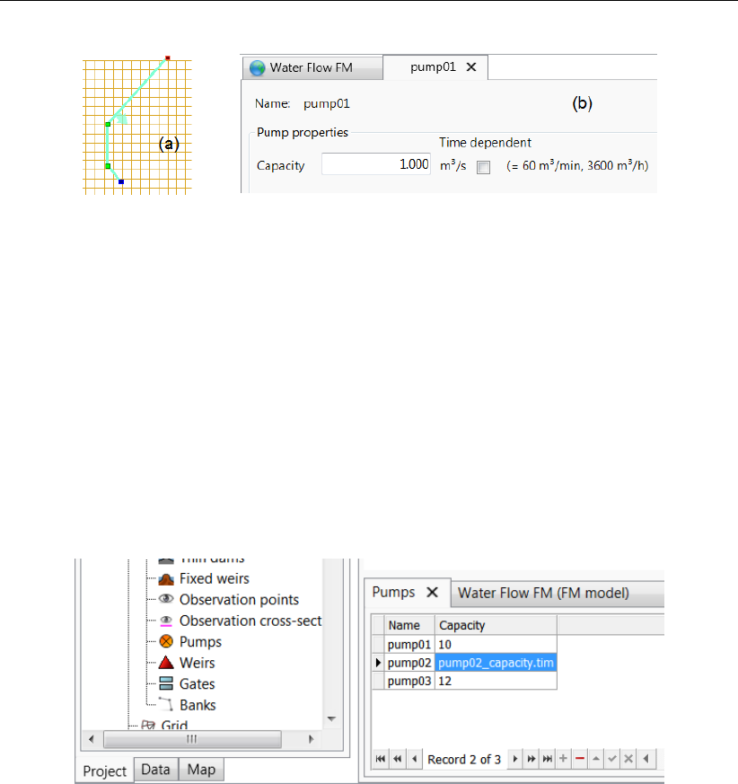
DRAFT
D-Flow Flexible Mesh, User Manual
Figure 4.25: Polygon for pump (a) and adjustment of physical properties (b).
Right clicking the pumps attribute in the Project window opens a pop-down window on which
you can select to import or export pumps. The pumps can be imported as polyline by a
<∗.pli>file or by a structure file, and they can be exported as a <∗.pli>file, structure file, or
<shapefile>.
Double clicking the pumps attribute in the Project window opens the pumps tab underneath
the central map. The attribute table in this tab shows all pumps with their corresponding
properties. When one of the pumps is selected, the corresponding item is highlighted in the
central map. Double clicking any of the pumps in the central map opens the Structure Editor
as a new map view in which all parameters related to the pump can be set (Figure 4.26).
Figure 4.26: Selection of the pumps
4.4.2.9 Weirs
Unlike the fixed weir, weir (or adjustable weir) can be adjusted based on the user require-
ments. To set an adjustable weir in the computational domain, you can select the icon weir
from the toolbar, and draw a line by mouse. This line includes direction, which defines the
sign of total flux passing above the weir (positive flux in the direction of weir, otherwise neg-
ative). This direction can be inverted by mouse right-click and selecting Reverse line(s). By
double-click on the weir, you can add the geometrical and time-dependent parameters such
as Crest level,Crest width,Crest level time series and Lateral concentration coefficient (See
Figure 4.27).
46 of 412 Deltares
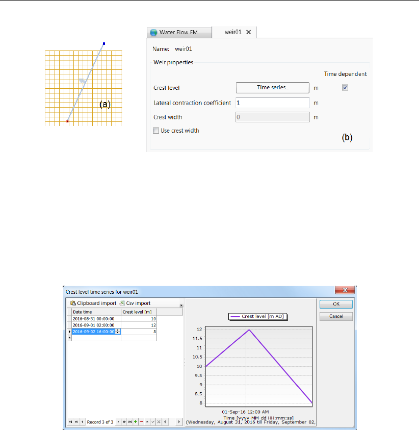
DRAFT
All about the modelling process
Figure 4.27: Polygon for adjustable weir (a) and adjustment of geometrical and temporal
conditions (b).
Moreover, the time series of the crest level can be set in the case the crest level is time
dependent. The time dependency diagram can be defined by the help of time series diagram
as shown in Figure 4.28. The time series can also be imported (and exported) from external
<csv>-file.
Figure 4.28: Time series for crest level.
The weirs can be deleted, imported and exported. By right clicking on the weir polygon, and
selecting "Delete Selection" from the pop-down window, you can delete the selected weir.
Right clicking the "Weirs" attribute in the Project window opens the "Weirs" tab opens the
options for import and export. You can import weirs as polygon (<∗.pli>file) or as a structure
by structure file. The weirs can also be exported to a polygon file, to a structure data file, or
by be the help of shapefile.
Double clicking the "Weirs" attribute in the Project window opens the "Weirs" tab underneath
the central map. The attribute table in this tab shows all weirs with their corresponding prop-
erties. When one of the weirs is selected, the corresponding item is highlighted in the central
map. Double clicking any of the weirs in the central map opens the Structure Editor as a new
map view in which all parameters related to the weir can be set (Figure 4.29).
Deltares 47 of 412
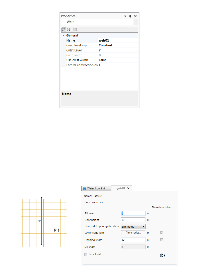
DRAFT
D-Flow Flexible Mesh, User Manual
Figure 4.29: Time series for crest level.
4.4.2.10 Gates
In D-Flow FM the gates can be imposed by polygon, and can be edited in a similar way as the
other structures (see Figure 4.30). Like the other structures, mentioned above, the gates can
be imported and exported by means of structure file or <∗.pli>file.
Figure 4.30 shows the edit tab of the gate properties. The gate can be opened horizontally,
as well as vertically.
Figure 4.30: Polygon for gate (a) and adjustment of geometrical and temporal conditions
(b).
48 of 412 Deltares
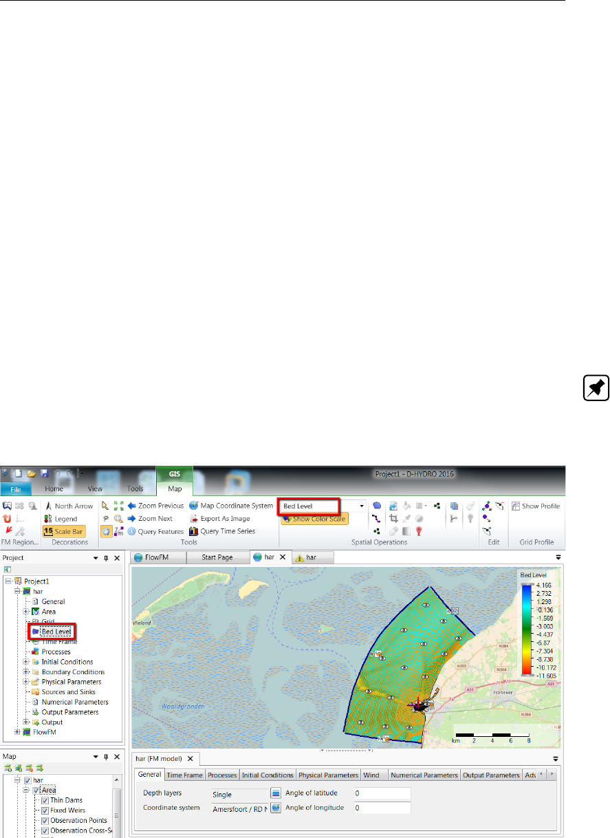
DRAFT
All about the modelling process
4.4.3 Computational grid
To set up your grid, click on the Edit grid button which opens the program RGFGRID. All
features of grid setup in RGFGRID are treated separately in RGFGRID UM (2016). If a land
boundary is present in your project, this is exported to RGFGRID automatically. Once you
have setup your grid in RGFGRID, click File →Save Project and close the program. The grid
will now be visible within the central map. Editing of the grid remains possible at any point in
time during the setup of your model by means of clicking the edit grid button. Any changes
you make are always saved after clicking File →Save Project and loaded back into the central
map.
4.4.4 Bed Level
When you double click on Bed level in the Project window or select Bed level from the drop-
down box in the spatial editor section of the Map ribbon, the spatial editor is activated (Fig-
ure 4.31). This editor can be used to generate a bathymetry for your computational grid. How
to work with the spatial editor is described in Appendix F. Be aware that the bathymetry in
D-Flow FM is defined as the bed level (e.g. positive upward), implying that all bed levels below
the reference plane are negative. By default the bed levels are defined on the net nodes.
Note: Please note that, currently, other bed level definition types (e.g. BedlevTypes) are not
visually supported by the GUI. If you would like to switch the bed level defintions to another
type, you have to set the BedlevType in the Physical Parameters tab. However, the bed level
locations will not be updated accordingly in the central map.
Figure 4.31: Bed level activated in the spatial editor
Deltares 49 of 412
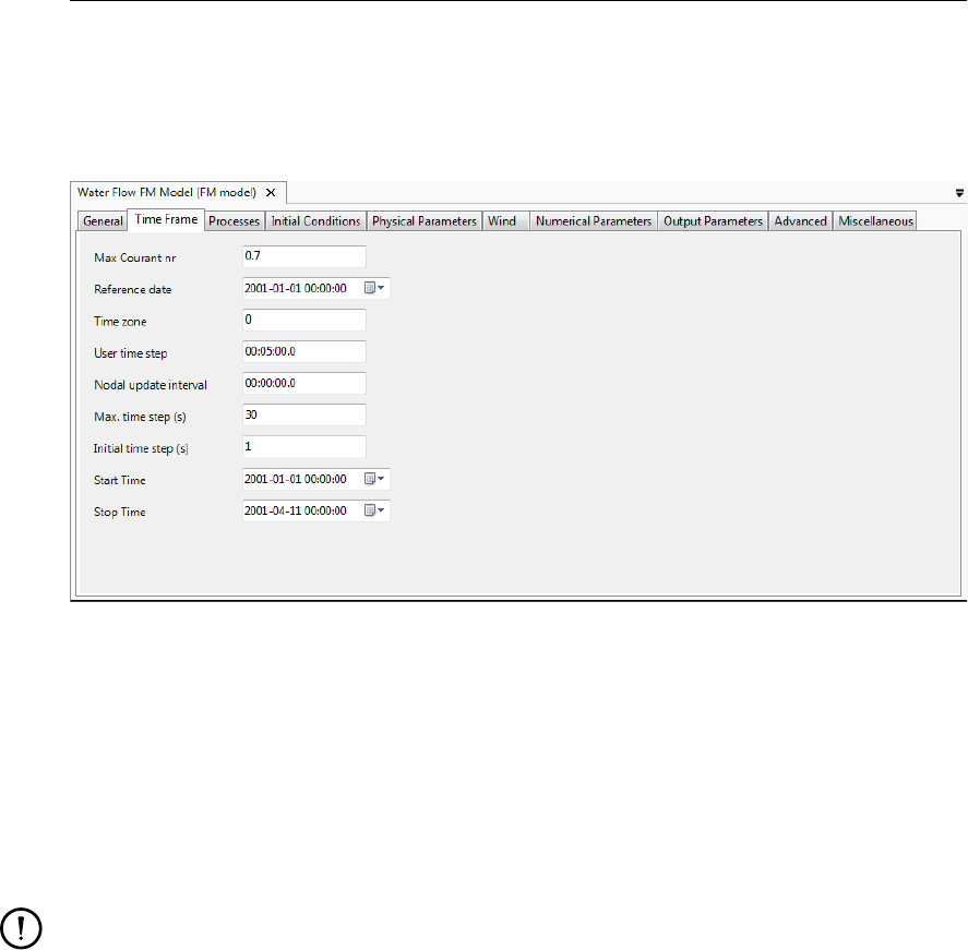
DRAFT
D-Flow Flexible Mesh, User Manual
4.4.5 Time frame
In the settings tab, in the sub-tab time frame (Figure 4.32), you can specify everything related
to the time frame in which your model will run.
Figure 4.32: Overview time frame tab
In general, the time frame is defined by a reference date and a start and stop time. The
time step size of your model is automatically limited (every time step) based on a Courant
condition. In more detail, you must define the following input data:
Max Courant nr The maximum allowed Courant number, which is used to compute
the time step size from the CFL criterium. D-Flow FM uses an ex-
plicit advection scheme, therefore a value of 0.7or lower is advised.
Remark:
You should check the influence of the time step on your results
at least once.
Reference date The reference date and time of the simulation. It defines the (arbi-
trary) t= 0 point for all time-series as used in the simulation. In the
GUI, time-specifications are always absolute, but in the underlying
model input files, these are stored as time values relative to the ref-
erence date. Typically, input time-series files are specified in minutes
after this t= 0 point. See for an illustration Figure 4.33.
Time zone The time difference between local time and UTC.
The time zone is defined as the time difference (in hours) between
the local time (normally used as the time frame for D-Flow FM) and
Coordinated universal time (UTC). The local Time Zone is used for
for two processes:
To determine the phases in local time of the tidal components
when tide generating forces are included in the simulation, see
section 7.10.
To compare the local time of the simulation with the times at
which meteo input is specified, e.g., wind velocities and atmo-
spheric pressure. These can be specified in a different time zone.
If the Time Zone = 0 then the simulation time frame will refer to UTC.
User time step The interval that is highest in the hierarchy. It specifies the inter-
val with which the meteorological forcings are updated. The Max.
50 of 412 Deltares
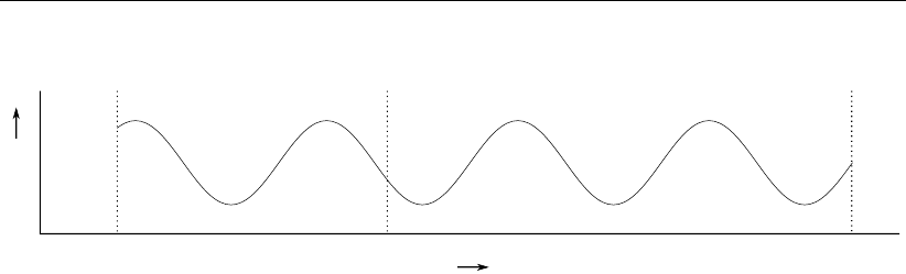
DRAFT
All about the modelling process
Reference Date Start Time Stop Time
Time
ζ
Figure 4.33: Relation between Reference Date and the simulation start and stop time
for astronomic- and harmonic-series as used in the simulation. Time-series
should cover the simulation time.
time step cannot be larger than the User time step, and it will auto-
matically be set back if it is. Also, the output intervals should be a
multiple of this User time step, see Appendix E. Finally the compu-
tational time steps will be fitted to end up exactly at each User time
step, such that proper equidistant output time series are produced.
Nodal update interval When using astronomic boundary conditions, the nodal factors can
be updated with certain intervals, see section 7.10.
Max. time step The Max. time step is the upper limit for the computational time
step. The automatic time step can not be switched off explicitly.
(If you want to enforce a fixed time step anyway, set the parame-
ter Max. time step (s) to the desired step size, and the parameter
Max. Courant nr. to an arbitrary high value.)
Initial time step the initial time step of the model; there is no data available yet during
the first time step to compute the time step automatically based on
a Courant condition. The computational time step then gradually
increases from Initial time step to the CFL-number limited time step
(assuming that Initial time step is relatively small).
Start Time The start date and time of the simulation.
Stop Time The stop date and time of the simulation. Always make sure that the
model Stop Time is larger than the model Start Time to avoid errors
during your calculation.
4.4.6 Processes
In the processes tab (Figure 4.34) you can specify which processes you want to incorporate
into your model. You can choose whether or not to include tidal forcing, salinity, temperature
and sediment/morphology by means of check boxes. In addition, you can specify which Wave
model you want to use. Note that when ticking the sediment/morphology check box, two tabs
for setting sediment and morphology parameters appear.
Deltares 51 of 412
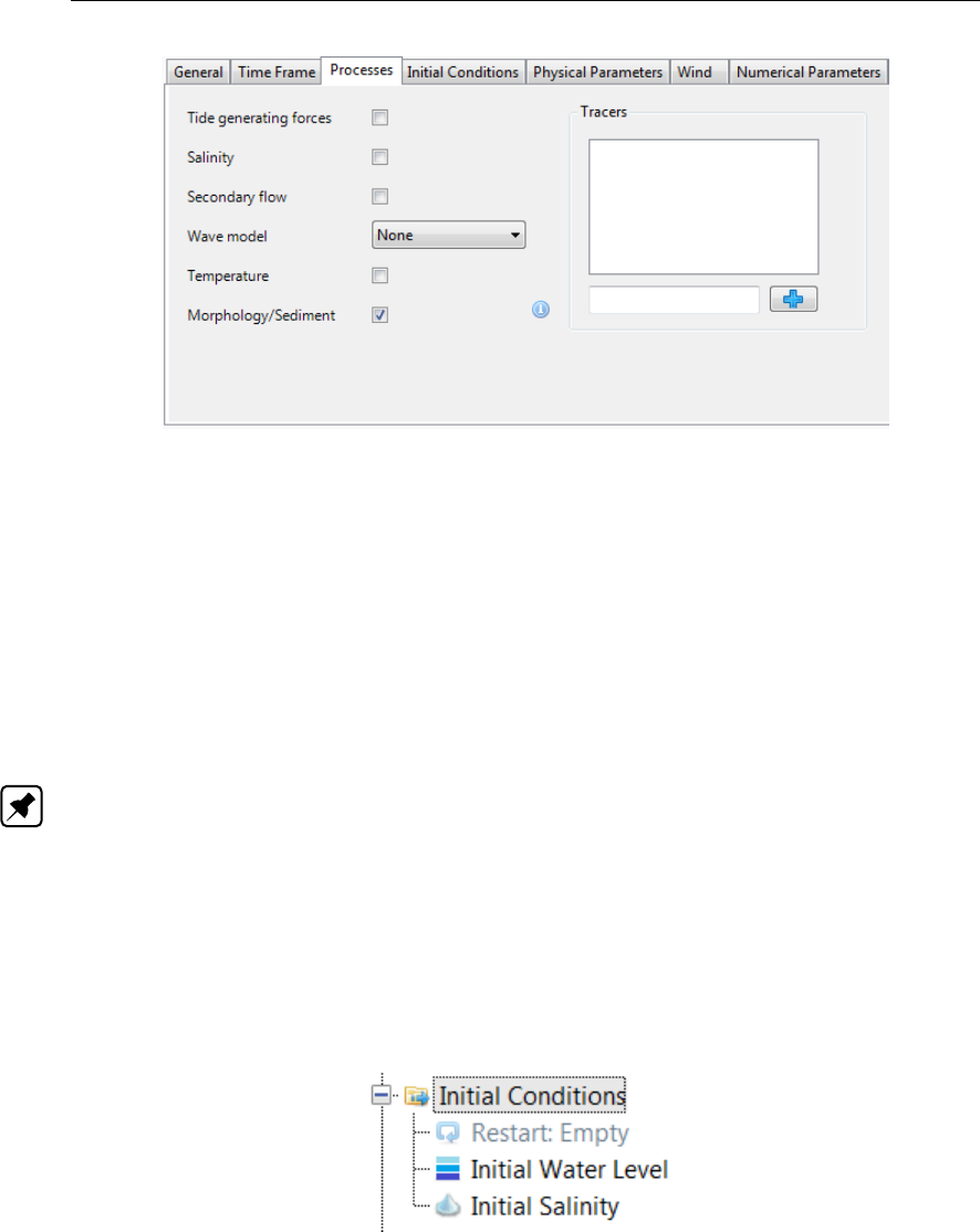
DRAFT
D-Flow Flexible Mesh, User Manual
Figure 4.34: Overview processes tab
4.4.7 Initial conditions
When expanding the initial conditions in the Project window, all quantities requiring an initial
state are shown (Figure 4.35). The number of quantities depends on the activated physical
processes in the ‘Processes’ tab (see section 4.4.6). The initial conditions for each quantity
can be specified as a uniform value or as a coverage (e.g. a spatially varying field).
The uniform values can edited in the ‘Initial Conditions’ tab, which opens upon double clicking
‘Initial Conditions’ in the Project window (Figure 4.36). In this tab you can also specify the
layer distribution for the initial condition specification in case of a 3 dimensional quantity (i.e.
salinity). Note: Please note that for 3 dimensional initial conditions currently only the option
‘top-bottom’ is supported.
In case of spatially varying initial conditions you can double click the quantity in the Project
window or select it from the dropdown box in the spatial editor section of the /emphSpecial
Operations ribbon (Figure 4.37). Then the spatial editor is activated, which you can use to edit
spatially varying fields. For more information on how to use the spatial editor you are referred
to Appendix F. In case of 3 dimensional initial conditions, you can select the layer from the
quantity dropdown box in the ‘Map’ ribbon (Figure 4.38).
Figure 4.35: Initial conditions in the Project window
52 of 412 Deltares

DRAFT
All about the modelling process
Figure 4.36: The ‘Initial Conditions’ tab where you can specify the uniform values and the
layer distributions of the active physical quantities.
Figure 4.37: Initial water levels activated in the spatial editor
Figure 4.38: Selecting 3 dimensional initial fields from the dropdown box in the ‘Map’
ribbon to edit them in the spatial editor
Instead of defining initial conditions from scratch you can also import fields from a previous
computation (using restart files). When you run a model using the Delta Shell GUI which is
writing restart files, the restart states will appear in the “Output” folder in the Project window
(Figure 4.39). For a description of the specification of restart files, please refer to paragraph
Deltares 53 of 412
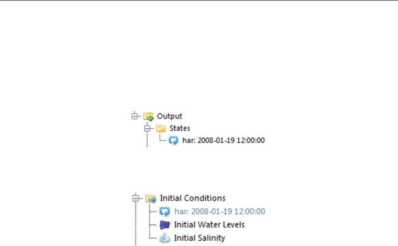
DRAFT
D-Flow Flexible Mesh, User Manual
section 4.4.12. To use a restart file as initial conditions, apply the right mouse button and
select “Use as initial state”. The file will now appear under “Initial Conditions” in the Project
window (Figure 4.40). To activate the restart file utilize the right mouse button and select “Use
restart”. The file will no longer be grey, but is now highlighted in black. The model will now
restart from this file. Notice that the simulation still starts at the original User Start Time, rather
than the time of the restart file. (The restart file only provides initial conditions.)
Figure 4.39: Restart files in output states folder
Figure 4.40: Restart file in initial conditions attribute
4.4.8 Boundary conditions
Boundary conditions consist of a location specification (‘support points’) and a forcing for that
location.
Section 4.4.8.1 describes how support points can be specified in Delta Shell. The boundary
forcing can be specified in the boundary data editor.
Section 4.4.8.2 describes the functionality of the boundary data editor. Finally, section 4.4.8.4
describes how the user can get an overview of the boundary locations and forcing in the
attribute table.
4.4.8.1 Specification of boundary locations (support points)
In D-Flow FM the boundary locations are defined as ‘support points’ on a polyline (<∗.pli>).
The user can add a boundary polyline (<∗.pli>) in the central map by selecting the ‘Add
Boundary’ icon in ’FM Region 2D / 3D’ of the ‘Map’ ribbon (see Figure 4.41). The number of
individual mouse clicks determines the number of support points on the polyline. The polyline
is closed by a double click. Once the polyline is added it becomes visible in the Project
window under ‘Boundary Conditions’ (see Figure 4.42). The polyline can be edited by the
general edit operations in the ‘Map’ ribbon (i.e. add/delete/move individual geometry points
or the complete geometry, see Figure 4.43). The name of the polyline (or ‘boundary’) can be
edited in the Boundaries tab, which can be opened by double clicking ‘Boundaries’ in the ‘Map
Tree’ (see Figure 4.44).
54 of 412 Deltares
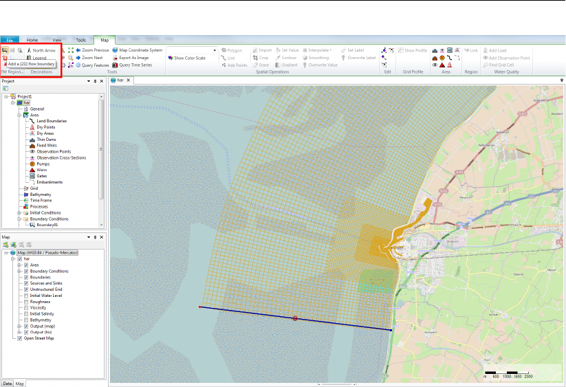
DRAFT
All about the modelling process
Figure 4.41: Adding a boundary support point on a polyline in the central map. By double
clicking on the polyline in the map, the boundary condition editor will open to
edit the forcing data on the polyline.
Deltares 55 of 412
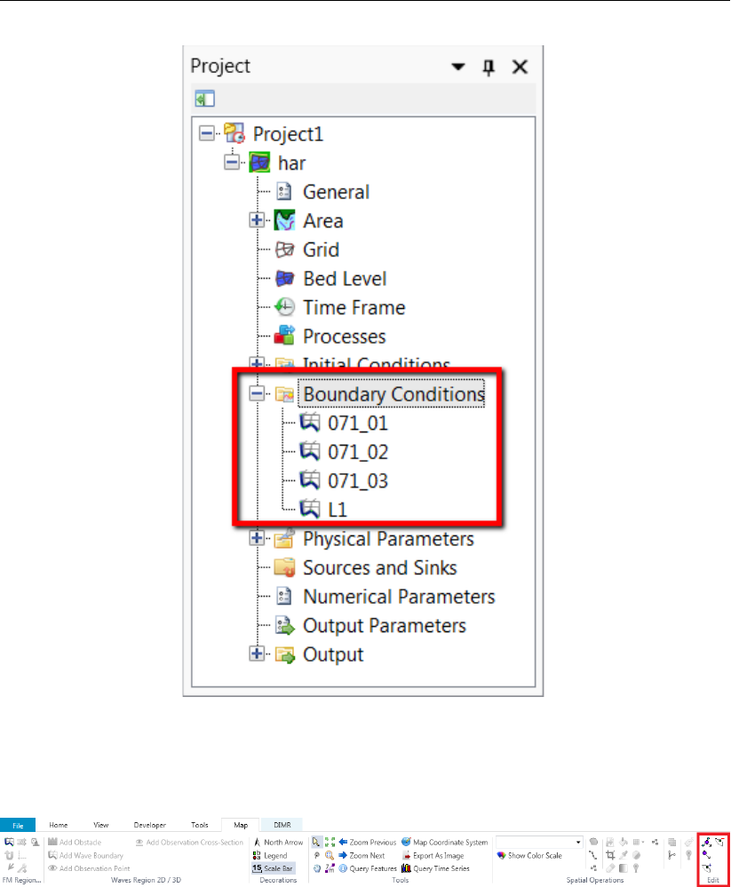
DRAFT
D-Flow Flexible Mesh, User Manual
Figure 4.42: Polyline added in Project window under ‘Boundary Conditions’. By double
clicking on the name of the polyline, the boundary condition editor will open
to edit the forcing data on the polyline.
Figure 4.43: Geometry edit options in Map ribbon
56 of 412 Deltares
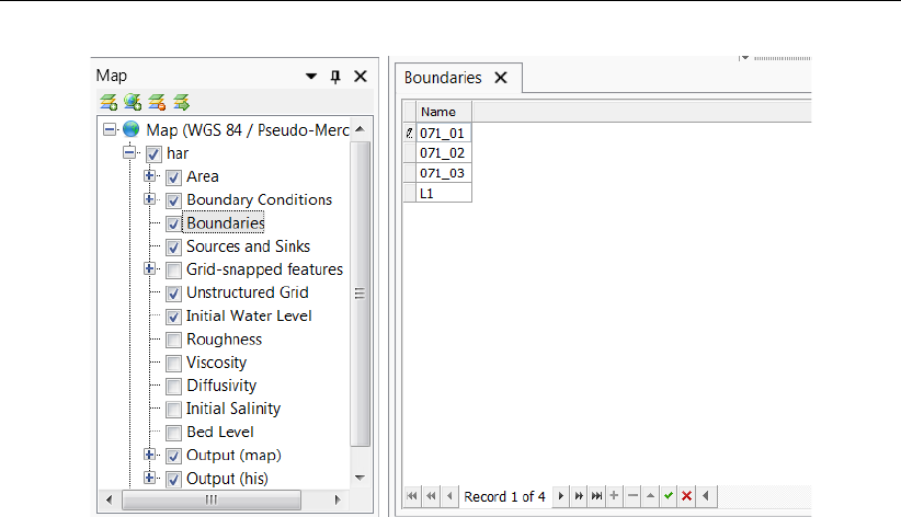
DRAFT
All about the modelling process
Figure 4.44: Edit name of polyline/boundary in Boundaries tab
4.4.8.2 Boundary data editor (forcing)
The boundary condition editor can be opened either by double clicking on the boundary name
in the Project window (Figure 4.42) or by double clicking the boundary polyline in the map win-
dow (Figure 4.41). An overview of the boundary data editor is given in Figure 4.45. This editor
can be used to specify the boundary forcing for different quantities (i.e. water level, velocity,
discharge, salinity, etc.) corresponding to different processes (i.e. flow, salinity, temperature,
tracers). The user can select the processes and quantities in the upper left corner. In the
upper centre panel the user can select the forcing function for the selected quantity (i.e. time
series, harmonic components, astronomical components or Q-h relation). The upper right
corner contains a list of the support points on the polyline. The geometry view shows the
location of the selected support point on the polyline (<∗.pli>). In the middle panel are some
handy buttons to generate, import and export forcing data. In the lower left panel the user
can specify the boundary data for the selected support point. The lower right corner shows
the signal of the boundary data. The following sections describe the features of the boundary
data editor in more detail.
Deltares 57 of 412
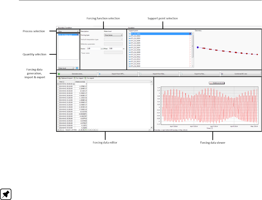
DRAFT
D-Flow Flexible Mesh, User Manual
Figure 4.45: Overview of the boundary data editor
Process and quantity selection:
Currently, D-Flow FM supports the processes flow, salinity, temperature and tracers (Note:
tracers are not yet fully editable). The processes available in the boundary condition editor
depend on the selected processes in the processes tab (see section 4.4.6). After selecting
the process from the dropdown box the user can select one of the corresponding quanti-
ties, as illustrated in Figure 4.46. For the process flow the user can choose from five principal
quantities: water level, velocity, Riemann invariant, Neuman gradient and discharge. All quan-
tities are specified per support point, except for discharges which are specified per polyline
(<∗.pli>). A support point can have multiple forcing quantities of the same type (i.e. water
level, velocity, Riemann, Neumann or discharge). These quantities are added up. This can be
relevant to add a surge level to an astronomical water level for example. Furthermore, the user
can apply normal and tangential velocities as ‘add on’ quantities. The following combinations
of quantities are allowed:
Water level + normal velocity
Water level + tangential velocity
Water level + normal velocity + tangential velocity
Velocity (= normal) + tangential velocity
Riemann + tangential velocity
58 of 412 Deltares

DRAFT
All about the modelling process
Figure 4.46: Process and quantity selection in the boundary data editor
Forcing function selection:
The user can select one of the following forcing functions:
Time series
Harmonic components
Harmonic components + correction
Astronomic components
Astronomic components + correction
Q-h relation (only for water levels)
The next section describes how data can be added for these types of forcing functions.
Add forcing data to a support point or polyline:
By default all support points on the polyline are deactivated. To add forcing data to a support
point the user first needs to activate it by pressing the green ‘add’-symbol in the list of support
points (see Figure 4.47). Consequently, the user can specify the forcing data in the lower left
panel based on the selected forcing function. Of which a preview is shown in the lower right
panel. Note: Please note that once a support point containing forcing data is made
inactive, all data on the support point is lost!
The user can choose from the forcing functions time series, harmonic components (+ correc-
tion), astronomic components (+ correction) and Q-h relation. Examples of the boundary data
specifications for these different forcing functions are given below. Note: Please note that
once the user changes the forcing function of a polyline, all data on the polyline is lost!
Deltares 59 of 412

DRAFT
D-Flow Flexible Mesh, User Manual
Figure 4.47: Activate a support point
Time series
The time format for time series is yyyy-mm-dd HH:MM:SS. There are multiple ways to specify
time series for the selected quantity:
Specify the time series step by step in the table (Figure 4.48): the user can add or delete
rows with the “plus”- and “minus”-signs below the table.
Figure 4.48: Specification of time series in the boundary data editor (left panel)
Generate time series using the ‘Generate time series’ button (Figure 4.49): the user can
specify start time, stop time and time step.
60 of 412 Deltares
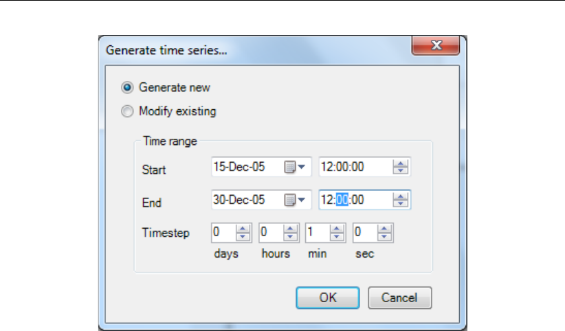
DRAFT
All about the modelling process
Figure 4.49: Window for generating series of time points
Import from csv using the ‘Csv import’ button: a wizard will open in which the user can
(1) select a csv-file (Figure 4.50), (2) specify how data should be parsed into columns
(Figure 4.51) and (3) how the values should be parsed and mapped into columns (Fig-
ure 4.52).
Deltares 61 of 412
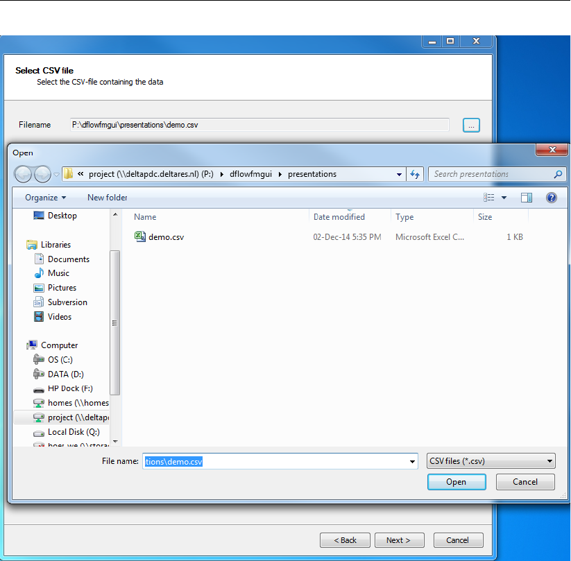
DRAFT
D-Flow Flexible Mesh, User Manual
Figure 4.50: Csv import wizard: csv file selection
62 of 412 Deltares
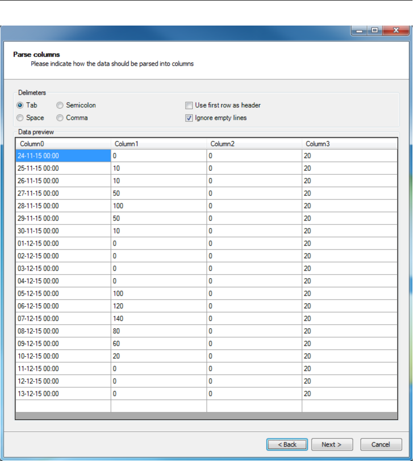
DRAFT
All about the modelling process
Figure 4.51: Clipboard/csv import wizard: specification of how data should be parsed into
columns
Deltares 63 of 412
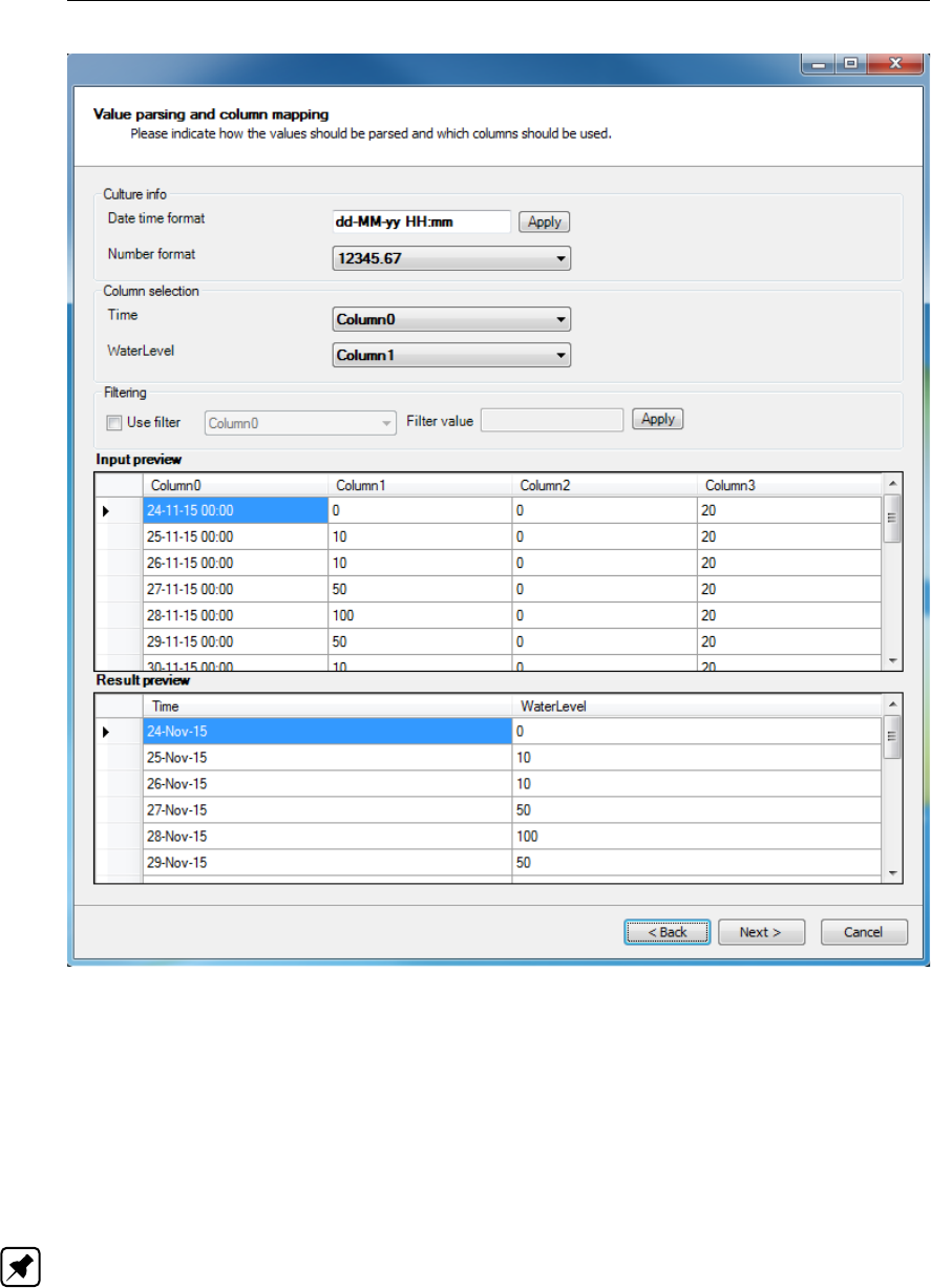
DRAFT
D-Flow Flexible Mesh, User Manual
Figure 4.52: Clipboard/csv import wizard: specification of how values should be parsed
and columns should be mapped
Import from clipboard using the ‘Clipboard import’ button: a wizard will open in which the
user can specify (1) how data should be parsed into columns (Figure 4.51) and (2) how
the values should be parsed and mapped into columns (Figure 4.52).
Import from Web Processing Service (WPS): with this service the user can download
boundary forcing data (for now only water level time series) for a selected support point
from an online database (TOPEX/Poseidon 7.2). Upon pressing the button ‘Import from
WPS ’ a window will pop up as depicted in Figure 4.53. Here, the user can specify the time
interval and time step for downloading the data. (Note: Please note that this service is
only available with an internet connection!)
64 of 412 Deltares
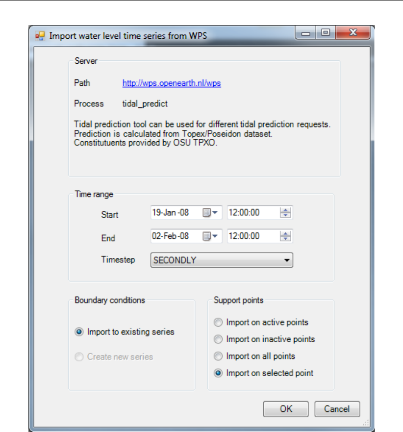
DRAFT
All about the modelling process
Figure 4.53: Window for entering input to download boundary data from WPS
Import from attribute file <∗.bc>: with this button the user can import data from existing
boundary conditions <∗.bc>file. The user has three options for importing:
Overwrite where matching (replace): only overwrites the forcing data for matching
support points in the <∗.bc>-file and GUI input.
Overwrite where missing (extend): only overwrites the forcing data for matching sup-
port points in the <∗.bc>-file and in the GUI input that did not contain data.
Overwrite all: overwrites the forcing data for all support points in the GUI (meaning
that the forcing data for non-matching support points is emptied).
Deltares 65 of 412
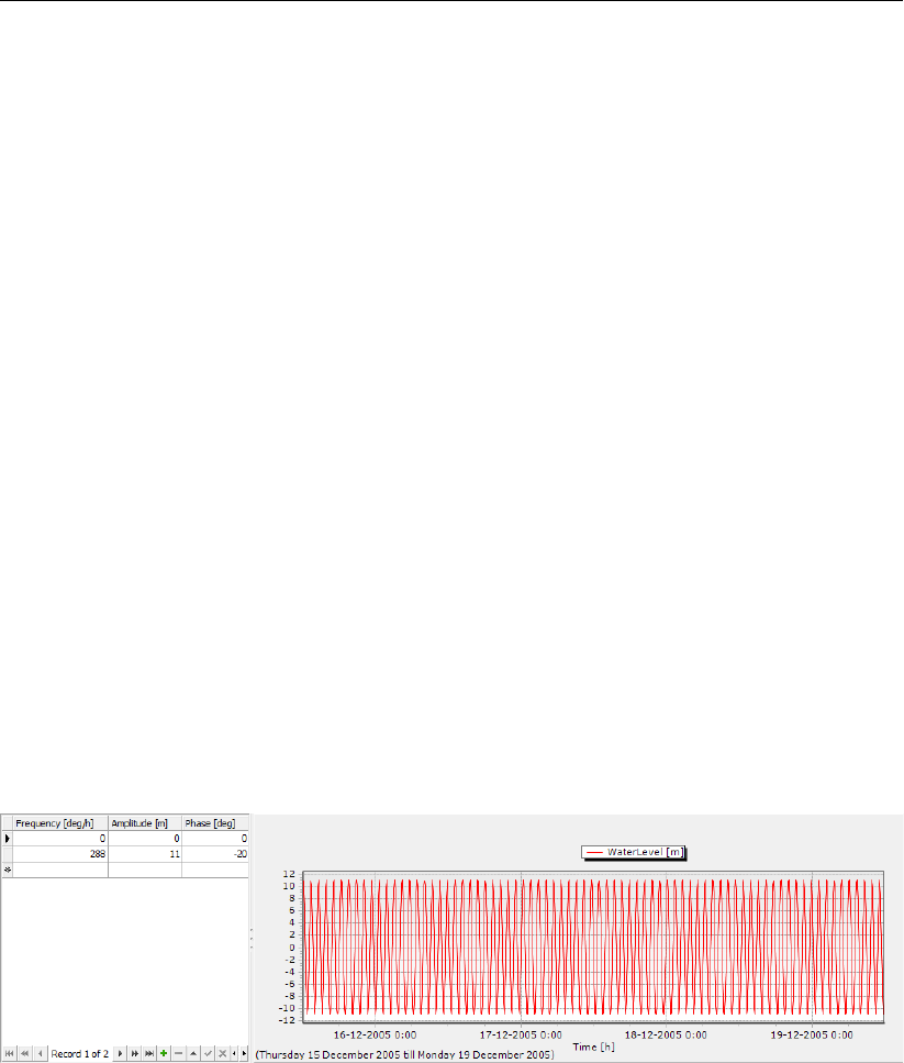
DRAFT
D-Flow Flexible Mesh, User Manual
Harmonic components
The harmonic components are defined by a frequency, amplitude and phase (see Figure 4.54).
By default the forcing data viewer shows the harmonic component for the time frame specified
for the model simulation. The options to define the harmonic components are similar to the
options for time series:
Specify components step by step: the user can add or delete rows with the “plus”- and
“minus”-signs below the table.
Select (astronomical) components using the ‘Select components’ button (Figure 4.55): the
user can select astronomical components which will be transformed in the corresponding
frequencies.
Import from csv using the ‘Csv import’ button: a wizard will open in which the user can
(1) select a csv-file, (2) specify how data should be parsed into columns and (3) how the
values should be parsed and mapped into columns.
Import from clipboard using the ‘Clipboard import’ button: a wizard will open in which the
user can specify (1) how data should be parsed into columns and (2) how the values
should be parsed and mapped into columns.
Import from attribute file <∗.bc>: with this button the user can import data from existing
boundary conditions <∗.bc>file. The user has three options for importing:
Overwrite where matching (replace): only overwrites the forcing data for matching
support points in the bc-file and GUI input.
Overwrite where missing (extend): only overwrites the forcing data for matching sup-
port points in the bc-file and in the GUI input that did not contain data.
Overwrite all: overwrites the forcing data for all support points in the GUI (meaning
that the forcing data for non-matching support points is emptied).
Figure 4.54: Specification of harmonic components in boundary data editor
66 of 412 Deltares
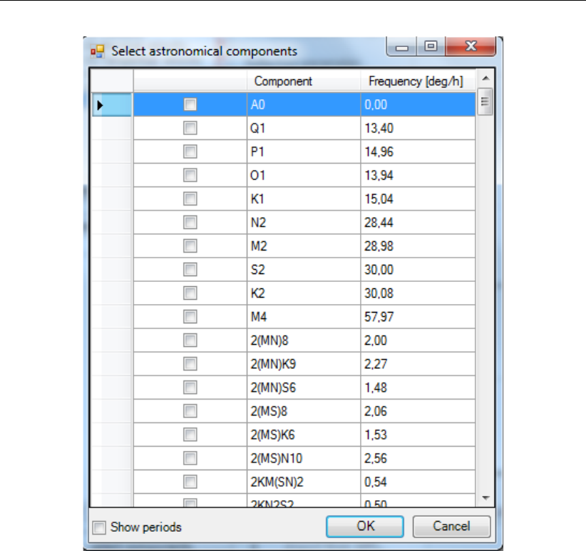
DRAFT
All about the modelling process
Figure 4.55: Selection of astronomical components from list (after pressing ‘select com-
ponents’)
Astronomic components
Astronomical components are similar to harmonic components, with the exception that the
frequency is prescribed. Instead of specifying the frequency the user can select astronomical
components by name. Upon editing the component field in the table the user will get sugges-
tions for components in a list (Figure 4.56). The most frequently used components (A0, Q1,
P1, O1, K1, N2, M2, S2, K2 and M4) are put on top of the list, the other components are listed
in alphabetic order. Instead of defining each component individually, the user can also make
a selection of components by pressing the button ‘select components’ (Figure 4.55).
Deltares 67 of 412
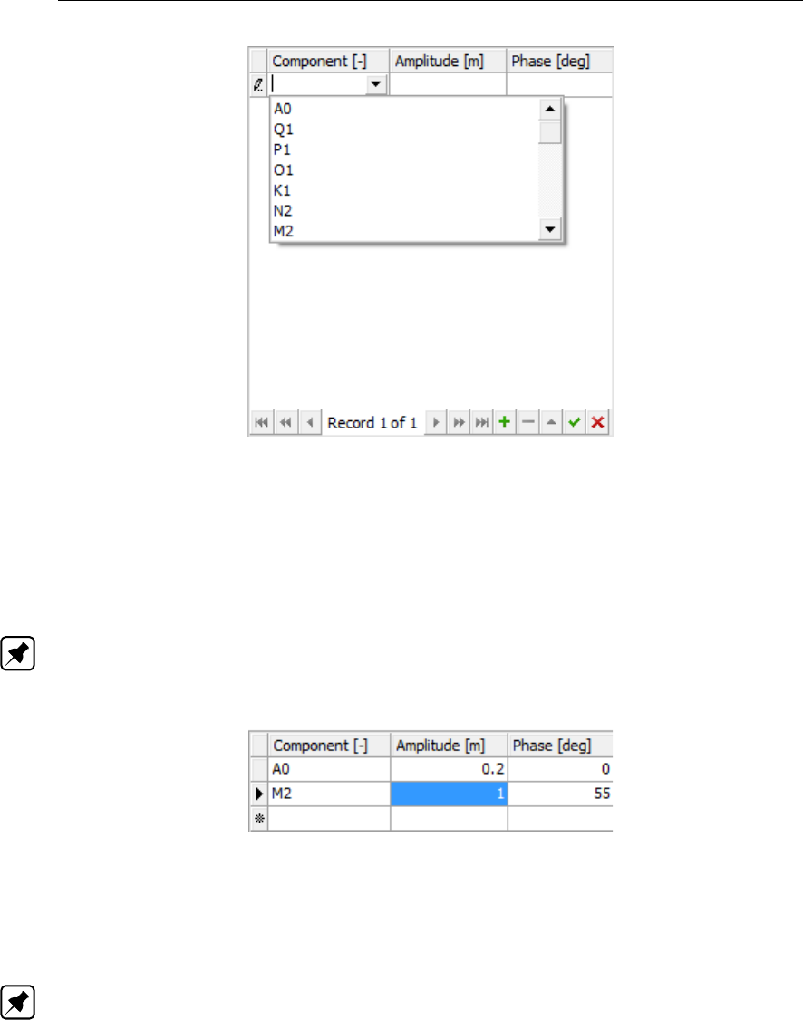
DRAFT
D-Flow Flexible Mesh, User Manual
Figure 4.56: Suggestions for astronomical components in list
Harmonic or astronomic components with corrections
For calibration purposes the user can combine harmonic or astronomic components with cor-
rections. The corrections are defined in terms of an amplitude (multiplication) factor and a
phase difference (see Figure 4.57). This allows the user to keep track of both the original sig-
nal and the calibration coefficients. The effects of the corrections on the resulting signal are
directly visualized in the forcing data viewer. Note: Please note that the import function-
ality is not (yet) working properly for astronomic/harmonic boundary conditions with
corrections.
Figure 4.57: Editing harmonic/astronomic components and their corrections
Q-h relation (only for water level)
The user can force the boundary with a Q-h relationship, but only for the quantity water level.
This is a relationship between discharge and water level (see Figure 4.58). The relationship
can only be prescribed per polyline, not per support point. (Note: this functionality has not
been tested extensively yet)
68 of 412 Deltares

DRAFT
All about the modelling process
Figure 4.58: Specification of a Q-h relationship
Exporting boundary conditions
With the Export to files button the user can export all boundary forcing data for the given
polyline to a <∗.bc>-file.
4.4.8.2.1 3D boundary conditions
Note: The 3D-implementation is a β-functionality.
When the model is 3D (i.e. the number of layers is larger than 1), the user can specifiy 3
dimensional boundary conditions for relevant quantities such as velocity, salinity, temperature
and tracer concentration. The user can choose from vertically uniform or vertically varying
boundary conditions (Figure 4.59), where the latter are defined as a percentage from the bed.
In the boundary condition editor the layer view will appear (Figure 4.60). Here, the user can
specify the vertical positions of the boundary conditions and view their position relative to
the model layers. Please note that the number and position of vertical boundary conditions
does not necessarily have to match the number and/or the exact position of the model layers.
The computational core will interpolate the boundary forcing position to the number of model
layers.
In case of non-uniform boundary conditions over the vertical, the number of columns in the
boundary forcing data editor will increase correspondingly (see Figure 4.61). In this way the
user can specify the conditions for all vertical positions in the same table and view the resulting
signals in the forcing data viewer.
Figure 4.59: Selection of vertically uniform or varying boundary conditions in case of a
3D model
Deltares 69 of 412
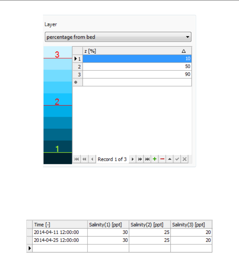
DRAFT
D-Flow Flexible Mesh, User Manual
Figure 4.60: Overview of the layer view component of the boudary conditions editor. In
the table the user can edit the vertical positions of the boundary conditions
as a percentage from the bed. In the view left of the table, the user can
see the vertical positions of the boundary conditions (indicated by number
corresponding to the table) relative to the model layers.
Figure 4.61: Specification of boundary forcing data (in this example for salinity) at 3 posi-
tions in the vertical
View boundary data
All boundary data of the same quantity on a support point can be (pre-)viewed in the boundary
data view in the lower-right panel. If multiple signals of the same quantity have been entered,
the viewer will show the active signal in red and the total signal of all datasets in grey (see
Figure 4.62). In the view the user can zoom-in by dragging a box from top-left to bottom-right
and zoom-out by dragging a box from bottom-right to top-left.
70 of 412 Deltares
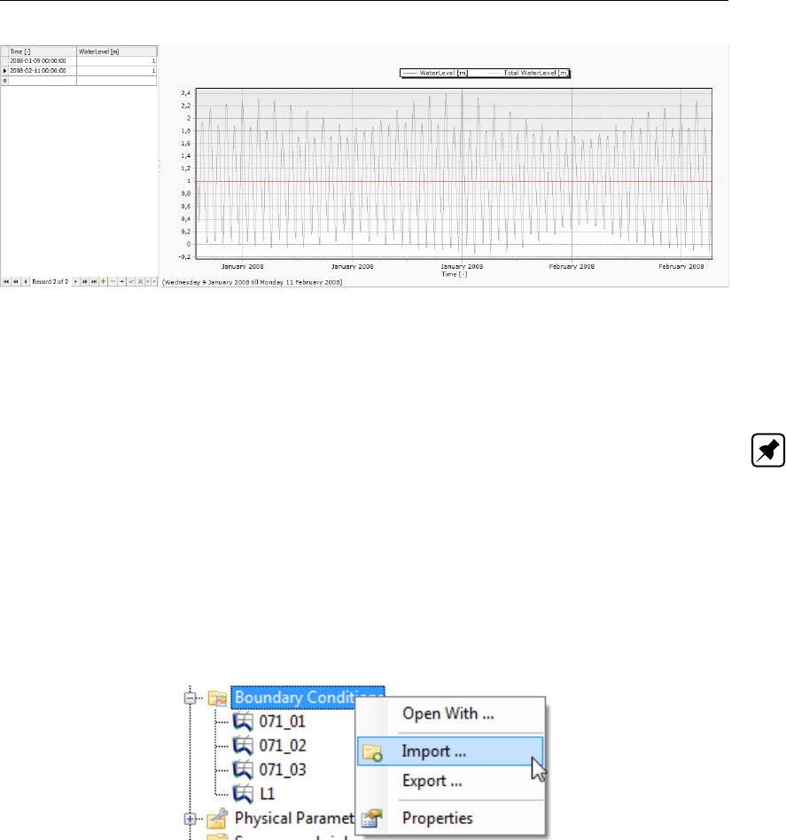
DRAFT
All about the modelling process
Figure 4.62: Example of active and total signal for multiple water level data series on one
support point
To inspect multiple quantities at a support point at the same time (for example water level
and salinity) the user can use the combined boundary data viewer by pressing the button
‘combined BC view’. Note: This does not work properly yet.
4.4.8.3 Import/export boundary conditions from the Project window
Apart from import and export functionality per individual boundary polyline in the bound-
ary condition editor, the GUI offers the opportunity to import and export boundary locations
(<∗.pli>) and forcing (<∗.bc>) on a higher level. Hereto, you have to click the right mouse
button on “Boundary Conditions” in the Project window and select “import” or “export” (Fig-
ure 4.63). Imports and exports on “Boundary Conditions” apply to all the boundary conditions
whereas import and exports on a boundary polyline apply only to that boundary condition.
Figure 4.63: Importing or exporting boundary features — both polylines <∗.pli>and forc-
ing <∗.bc>— from the Project window using the right mouse button
Import and export polylines
Upon importing a <∗.pli>-file with the same filename and the same polyline name(s) as the
existing polyline names in the GUI, the existing polyline(s) will be replaced and all forcing data
thereon will be deleted. Upon importing a polyline(s) with a different name(s), the polyline(s)
will be added to the Project window without any forcing data on it/them. The user will be
asked to import the data “as is” or to perform a coordinate transformation before the import
(see Figure 4.64).
Alternatively, the user can exported created polylines to a <∗.pli>-file. Upon export the user
will be asked to export the data “as is” or to perform a coordinate transformation before the
export (see Figure 4.64).
Deltares 71 of 412
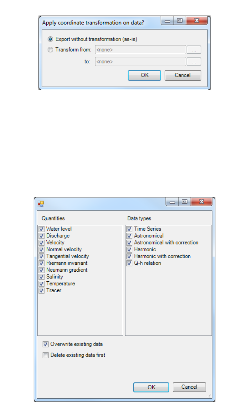
DRAFT
D-Flow Flexible Mesh, User Manual
Figure 4.64: Import or export a <∗.pli>-file as is or with coordinate transformation.
Import and export boundary forcing data
Similar to the polylines, you can import and export boundary forcing data from/to a <∗.bc>-
file. To import forcing data the existence of a polyline with at least one matching support
point is a prerequisite. Upon importing <∗.bc>data you can select which quantities and
forcing types from the <∗.bc>-file should be imported and with which overrwrite options (see
Figure 4.65). Similarly,you can export boundary forcing data. As an additional exporting
feature you can select whether you would like to export: 1) all forcing data into one file, 2) as
separate files per boundary, 3) as separate files per process or 4) as separate files per quantity
(see Figure 4.66).
Figure 4.65: Import or export a <∗.pli>-file as is or with coordinate transformation.
72 of 412 Deltares
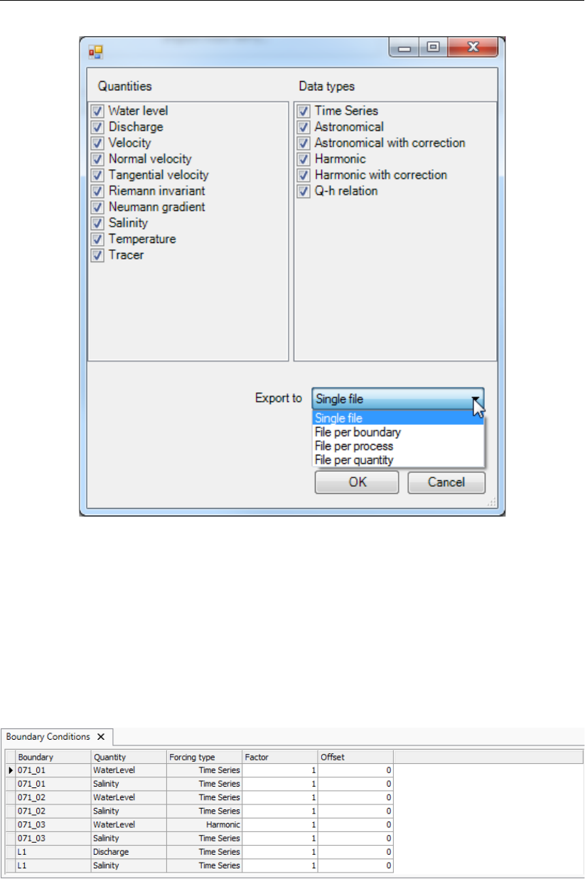
DRAFT
All about the modelling process
Figure 4.66: Import or export a *.pli file as is or with coordinate transformation.
4.4.8.4 Overview of boundary conditions in attribute table (non-editable)
The attribute table of the boundary conditions gives an overview of all specified boundary
polylines and corresponding forcing (see Figure 4.67). This attribute table can be opened by
double clicking ‘Boundary Conditions’ from the project or map tree. Most of the features in
the attribute table are non-editable, except for the optional (multiplication) factor and offset per
quantity per polyline. With these settings you can integrally multiply all data on a polyline with
a factor and/or add an offset to it.
Figure 4.67: Overview of all boundary conditions in attribute table
Deltares 73 of 412
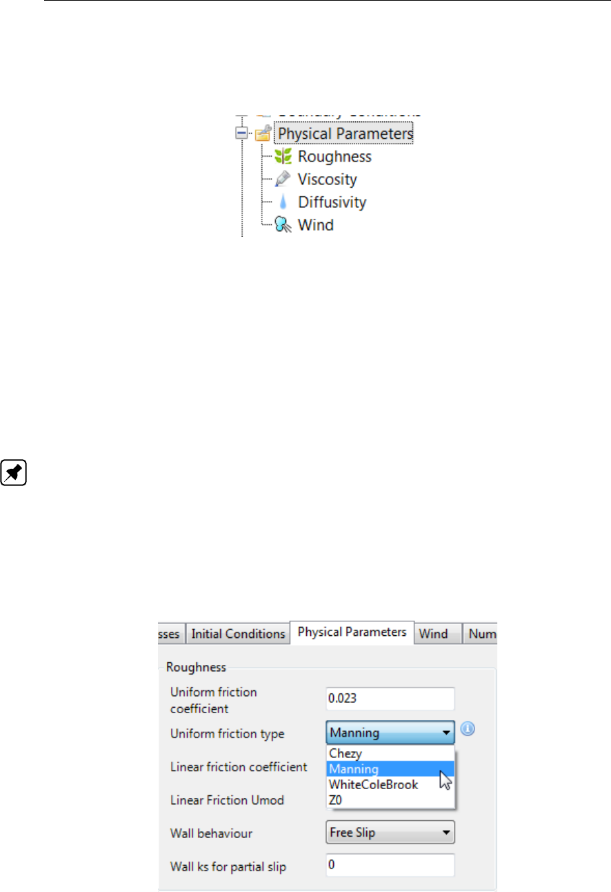
DRAFT
D-Flow Flexible Mesh, User Manual
4.4.9 Physical parameters
The physical parameters attribute is used to set all physical parameters of your model. When
it is expanded in the Project window, it shows three attributes; roughness, viscosity and wind.
Figure 4.68: The physical parameters in the Project window
4.4.9.1 Constants
In the Physical Parameters tab, under Constants, the user can adjust the value of Gravity
[m/s2] and Default water density [kg/m3].
4.4.9.2 Roughness
Bed roughness can be specified as a uniform value or as a coverage (e.g. a spatially varying
field). The uniform values as well as the roughness formulation (i.e. Chézy, Manning, White-
ColeBrook or Z0) can be edited in the ‘Physical Parameters’ tab, which opens upon double
clicking ‘Roughness’ in the Project window (Figure 4.69). Note: The latter is not yet work-
ing. In this tab you can also specify the linear friction coefficient, linear friction Umod, wall
behaviour (free slip or partial slip) and wall ks for partial slip.
In case of spatially varying bed roughness you can double click the quantity in the Project
window or select it from the dropdown box in the Spatial Operations ribbon (Figure 4.70).
Then the spatial editor is activated, which you can use to edit spatially varying fields. For
more information on how to use the spatial editor you are referred to Appendix F.
Figure 4.69: The section of the ‘Physical Parameters’ tab where you can specify rough-
ness related parameters and formulations.
74 of 412 Deltares
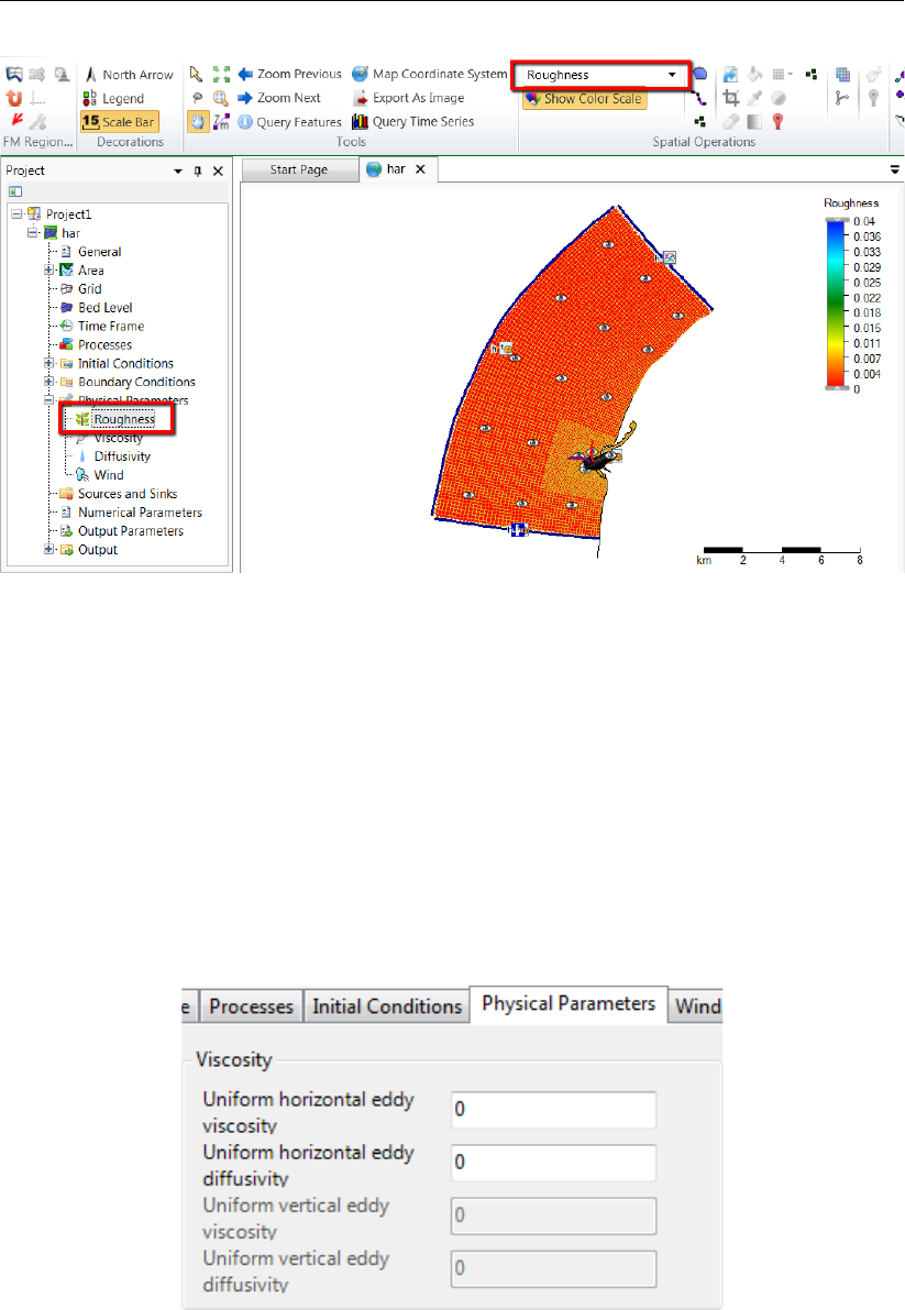
DRAFT
All about the modelling process
Figure 4.70: Roughness activated in the spatial editor to create/edit a spatially varying
field
4.4.9.3 Viscosity
The eddy viscosity can be specified as a uniform value or as a coverage (e.g. a spatially
varying field). In the ‘Physical parameters’ tab you can specify the uniform values for the
horizontal and vertical (in case of 3D simulations) eddy viscosity and diffusivity (Figure 4.71).
In case of spatially varying viscosity you can double click the quantity in the Project window or
select it from the dropdown box in the Spatial Operations ribbon (Figure 4.72). Then the spatial
editor is activated, which you can use to edit spatially varying fields. For more information on
how to use the spatial editor you are referred to Appendix F.
Figure 4.71: The section of the‘Physical Parameters’ tab where you can specify (uniform)
values for the horizontal and vertical eddy viscosity and diffusivity.
Deltares 75 of 412
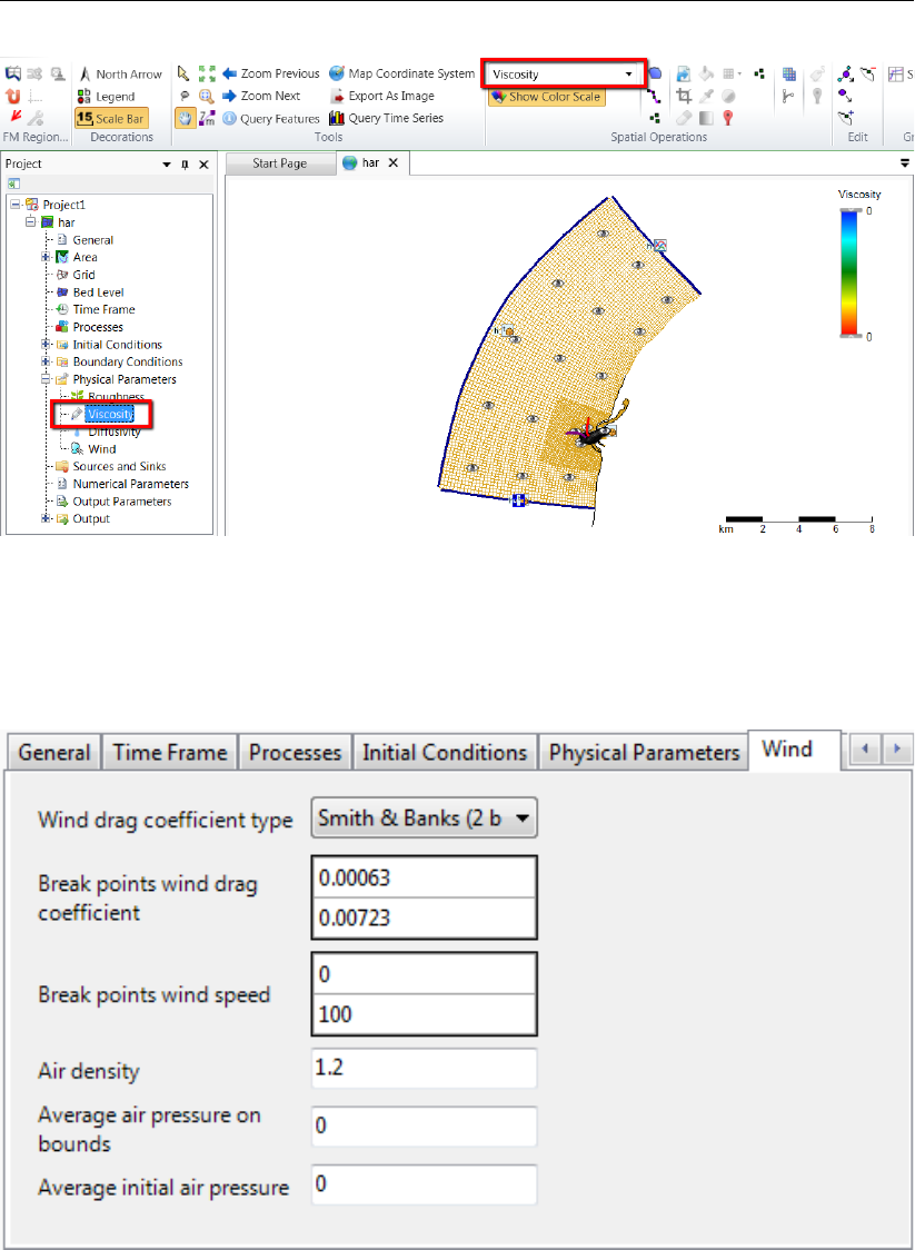
DRAFT
D-Flow Flexible Mesh, User Manual
Figure 4.72: Viscosity activated in the spatial editor to create/edit a spatially varying field
4.4.9.4 Wind
All relevant parameters, described in chapter 11 can be adjusted in the following sub-tab.
Figure 4.73: Overview of parameters in sub-tab Wind
4.4.9.5 Heat Flux model
The Heat flux model, described in chapter 10, needs only specification of which model to use.
See the drop-down selection in Figure 4.34.
76 of 412 Deltares
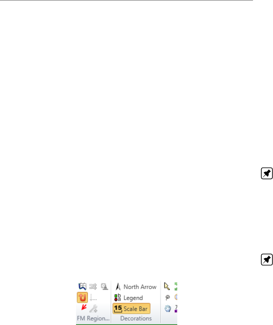
DRAFT
All about the modelling process
4.4.9.6 Tidal forces
The Tide generating forces, described in section 7.10, can be enabled in the Processes tab,
see Figure 4.34.
4.4.10 Sources and sinks
Sources and sinks (or: intake/outfall facilities) can be used to add/extract a discharge to/from
the model or to redistribute water and constituents (such as temperature and salinity) within
the model. Sources and sinks consists of a location (defined by a <∗.pli>-file) and time series
describing the discharges (defined by a <∗.tim>-file). All the hydrodynamical considerations
behind sources and sinks are discussed in section 7.8.
Sources and sinks locations
Sources and sinks can be added to the model using the corresponding icon from the Map
ribbon (Figure 4.74). When the sources/sinks icon is active you can add them as polyline
elements in the central map using the left mouse button. Each polyline element is closed by
double clicking the left mouse button.
Note: Please note that the length of the ployline elements is not taken into account in the
handling of sources and sinks (e.g. it is modeled as an instant redistribution of water and
constituents without delays and friction losses).
Polyline elements starting outside the model domain and going inward are sources and,
vice versa, polyline elements starting inside the model domain and going outward are sinks.
Polyline elements starting and ending within the model are intake/outfall type of discharges.
The drawing direction determines the direction of the discharge indicated by an arrow (Fig-
ure 4.75). In case of a source the direction of the last polyline element determines the direction
of flow momentum into the model.
Note: The ‘reverse’ line option — to switch the discharge direction without having to redraw
the source/sink — is not implemented.
Figure 4.74: Activate the sources and sinks editing icon in the Map ribbon
Deltares 77 of 412
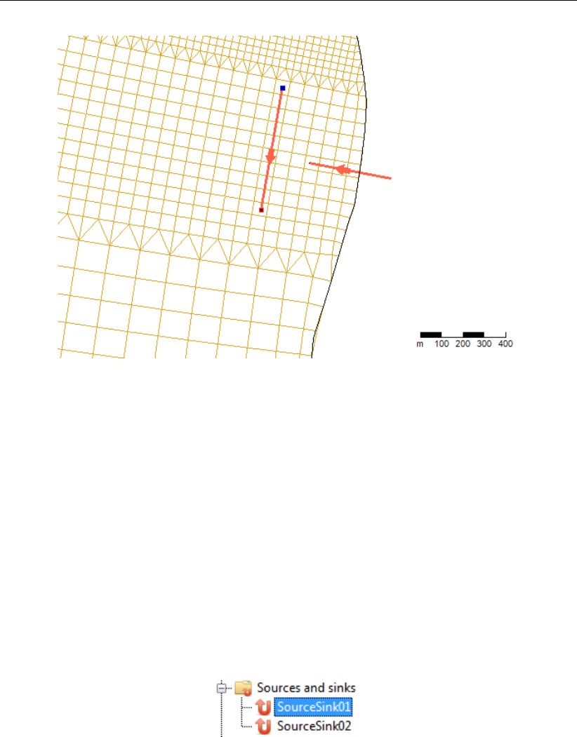
DRAFT
D-Flow Flexible Mesh, User Manual
Figure 4.75: Add sources and sinks in the central map using the ‘Sources and sinks’ icon.
Sources and sinks time series
After drawing the sources/sinks locations in the central map, they appear under ‘Sources and
sinks’ in the Project window (Figure 4.76). Either by double clicking the sources/sinks in the
Project window or the line element in the central map, you can open the sources and sinks
editor (Figure 4.77). In this editor you can specify the discharge time series as well as the
corresponding constituents (for example salinity and temperature, depending on the active
physical processes). The time series of water discharges are always defined as absolute
values. For the time series of constituents the following applies:
For sources the constituent time series are absolute values
For sinks the constituent time series are determined by the modeled values
For sources and sinks (intake/outfall relationships) the constituent time series are the ex-
cess values (e.g. on top of the modeled values)
Figure 4.76: Sources and sinks appearing in the Project window
78 of 412 Deltares
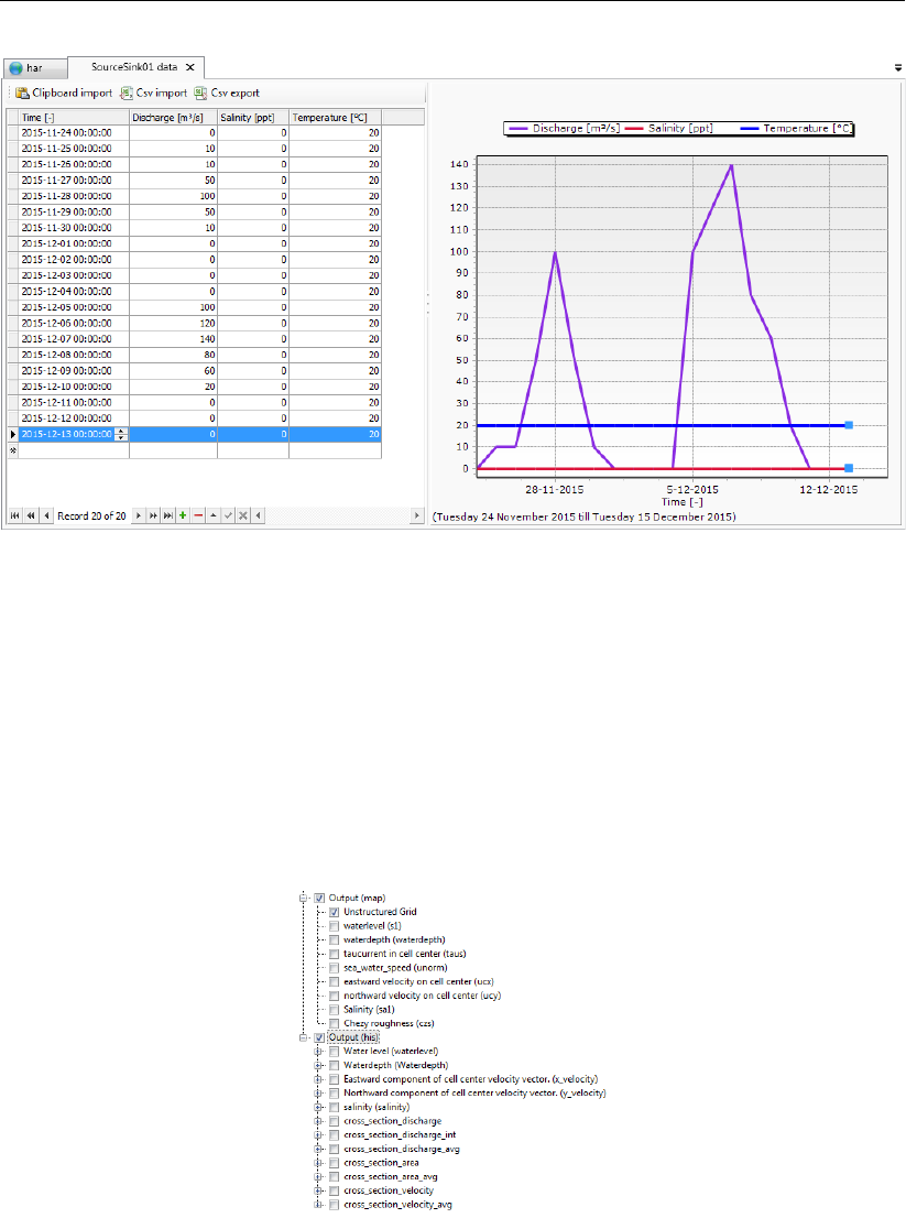
DRAFT
All about the modelling process
Figure 4.77: Specifying time series for sources and sinks in the sources and sinks editor
4.4.11 Numerical parameters
In the numerical parameters tab, all numerical parameters related to your computation can be
set. The parameters that can be set are described in Table 4.1.
4.4.12 Output parameters
Model runs can produce various types of output files. The Map window shows the two most-
used types: map output and his(tory) output (Figure 4.78).
Figure 4.78: Output parameters tab
The history file contains output on specific locations: time series data on observation points
(section 4.4.2.2), cross-sections (section 4.4.2.3) and structures (Sections 4.4.2.8 –4.4.2.10).
The map file contains flow quantities on the entire grid at specified time intervals, and can later
be used for 2D and 3D visualizations of entire flow fields. The map file can typically turn out
much larger than the history file, and it is therefore advised to use larger time intervals for map
files than for his files.
Additionally, three more types of output can be requested: restart files, WAQ output, and
timing statistics. Restart files are a special type of map file that can later be used as initial
Deltares 79 of 412

DRAFT
D-Flow Flexible Mesh, User Manual
Table 4.1: Overview and description of numerical parameters
Parameter Description
Max Courant number The size of the time step, ∆t, is computed by the
computational kernel automatically, each time step
by means of the maximum tolerable Courant num-
ber. By default, this value is 0.7.
Wave velocity fraction The wave velocity fraction is related to stability of
the computation. By using this fraction, the velocity
of the flow is enlarged with the wave velocity times
this fraction. The value of this fraction is 0.1 by de-
fault.
Advection type This key depicts the ID of the advection scheme. By
default this value is 33.
Water depth limiter type The limiter type for waterdepth in continuity equa-
tion: 0 means no limiter (default), 1 is the min-
mod method, 2 the Van Leer method, 3 the Koren
method and 4 the monotone central method.
Advection velocity limiter type The limiter type for the cell center advection veloc-
ity: 0 means no limiter, 1 the minmod method, 2 the
Van Leer method, 3 the Koren method and 4 the
monotone central method (default).
Salinity transport limiter type The limiter type for salinity transport: 0 means
no limiter, 1 the minmod method, 2 the Van Leer
method, 3 the Koren method and 4 the monotone
central method (default).
Solver type Specification of the Poisson equation type solver
for the pressure: 1 = sobekGS_OMP, 2 =
sobekGS_OMPthreadsafe, 3 = sobekGS, 4 =
sobekGS + Saadilud (default), 5 = parallel/global
Saad, 6 = parallel/Petsc, 7 = parallel/GS.
Max degree in Gaussian elimination The maximum degree in the Gauss elimination, part
of the pressure solver. This key has the value 6 by
default.
Thin dike scheme Or: fixed weir scheme. 0: none, 1: compact stencil,
2: whole tile lifted, full subgrid weir + factor.
Thin dike contraction Or: fixed weir contraction. This is the fixed weir flow
width contraction factor, being the flow width = flow
width times the fixed weir contraction.
Boundary smoothing time Fourier smoothing time on waterlevel boundaries
(s).
Linear continuity Default 0; Set to 1 for linearizing d(Hu)/dx; link to
AdvecType.
Threshold for drop losses Apply droplosses only if local bed slope is larger
than this specific value.
Theta of time integration Compromise in explicit/implicit time integration.
Downwind cell H on Q boundaries Specifies the way of the upstream discharge bound-
ary: 0 is original hu on qbnd, 1 is downwind hs on
qbnd
80 of 412 Deltares
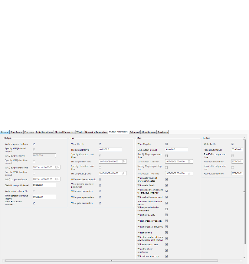
DRAFT
All about the modelling process
states in other runs. Restart files contain several additional flow quantities and are written
at specified intervals into one file per each restart time. Typically, one selects a large restart
interval in order not to waste disk space. WAQ output files are written by D-Flow FM and are
intended to be used as input files to subsequent D-Water Quality runs. More details on water
quality modelling can be found in chapter 17. Timing statistics can be produced both in the
diagnostics file (via Statistics output interval, for viewing basic simulation progress), and in
a separate detailed timings file (via Timing statistics output interval, for detailed performance
analysis).
When double clicking the output parameters tab in the Project window, the output parameters
sub-tab of the settings tab is highlighted in the central map. All parameters related to the out-
put of your model run are specified here (Figure 4.79). The most common output parameters
to set are the parameters related to the water quality files, history files, map files and restart
files.
Figure 4.79: Overview output parameters tab
For each of the three files (water quality, history, map and restart) the input parameters are
specified in the same manner (Figure 4.79). Taking his output as an example: when Write
His File is checked, the output of history file is enabled. His Output Interval determines the
interval at which the output data is stored in the file; the smaller the interval, the more detailed
the output and the larger the file. By default, history output is written from the start until the
end of the simulation. Optionally, output can be restricted to a certain time window: to specify
different output start and/or stop times, check the box next to Specify His Output Start Time
and/or Specify His Output Stop Time and enter the desired times next to the parameters His
Output Start Time and His Output Stop Time.
When Write Snapped Features is activated, then shape files with snapped data will be gen-
erated for all quantities, such as fixed weirs and thin dams. For example, for fixed weirs a
crest height is specified at both end of a fixed weir polyline. In between linear interpolation is
applied, which can be checked via these shape files.
Below, the various output options are described in greater detail. There is a special require-
ment on the output parameters for His and Restart files that the Output Interval,Output Start
Time and Output Stop Time must be integer multiples of User Time Step. Optionally, the
Deltares 81 of 412

DRAFT
D-Flow Flexible Mesh, User Manual
interval ( Output Stop Time−Output Start Time) should be an integer multiple of User Time
Step.
Write his file
His Output Interval Time interval for history time series.
His Output Start/Stop
time
Restrict history output to a specified time window.
Write mass balance
totals
Enable detailed mass balance time series output in the his file.
Write (misc.) structure
parameters
Enable time series output across general structures, pumps, weirs
and gates in the his file.
Write map file
Map Output Interval Time interval for map field time series.
Map Output Start/Stop
time
Restrict map output to a specified time window.
Specific Map Output
Times
File containing specific time values at which to produce additional
map output snapshots. It the value is not integer, it is firstly set to the
least integer larger than or equal to this value. If the computational
time does not hit the specified time value, the output snapshot is
chosen to be at the time closest to the specified time value.
Write water levels, etc. Several optionals for enabling/disabling certain quantities output in
the map file.
Write restart file
Restart interval Time interval for restart files.
Rst Output Start/Stop
time
Restrict restart output to a specified time window.
Other output options
WAQ Output Interval Time interval for D-Water Quality files in <DFM_DELWAQ_mdu_name\*.hyd>,
etc.
Simulation statistics
output interval
Interval for simulation progress output (on standard out and diagnos-
tics file).
Timing statistics output
interval
Interval for detailed timings output into <mdu_name_timings.txt>
for expert performance analysis.
Example
One example of input and output parameters (in seconds) is given in Table 4.2.Table 4.3
shows the time (after Reference Date in seconds) when output files are generated. We explain
this example as follows.
The history ile has output interval 18 seconds. No parameters are specified for His Output
Start Time and His Output Stop Time, which means that they are automatically set equal
to Start Time and Stop Time of the simulation, respectively.
The Map Output Interval is 6 seconds, and Map Output Start Time is 15 seconds. Since
the Map Output Stop Time is not given, it is set to equal to Stop Time. Moreover, we hope
to have output at time given in Specified Map Output as 30.5 and 42.1 seconds. These
two values are firstly set to 31 and 43 seconds, respectively, in the simulation. Then there
will be output snapshots if the computational time hit these two integers. Otherwise, as
in this example, the output snapshots will be provided when the computational time hits
82 of 412 Deltares
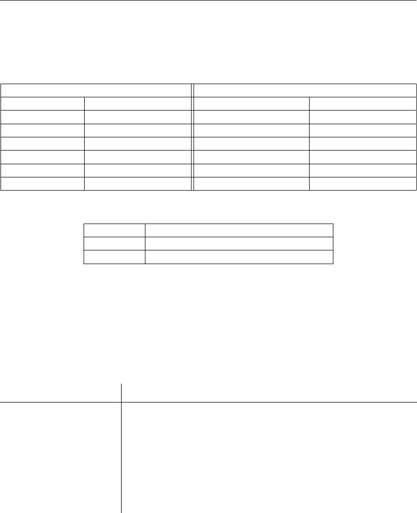
DRAFT
All about the modelling process
the time that is greater and the closest to these integers, i.e. at 31.2 and 43.2 (as seen in
Table 4.3).
Three parameters are set for the output of the Rst files: the interval, start and stop time.
Input parameters Output parameters
Reference Date 2007-11-19 00:00:00 His Output Interval 00:00:18
User Time Step 00:00:00.3 Map Output Interval 00:00:06
Start Time 2007-11-19 00:00:03 Map Output Start Time 2007-11-19 00:00:15
Stop Time 2007-11-19 00:00:51 Specific Map Output 30.5, 42.1
Rst Output Interval 00:00:09
Rst Output Start Time 2007-11-19 00:00:12
Rst Output Stop Time 2007-11-19 00:00:45
Table 4.2: Input and output parameters of the example
His file 3, 21, 39, 51
Map file 3, 15, 21, 27, 31.2, 33, 39, 43.2, 45, 51
Restart file 3, 12, 21, 30, 39, 45
Table 4.3: Time (after Reference Date in seconds) of output files
4.4.13 Miscellaneous
Within the miscellaneous sub-tab, various parameters in relation to waves and equatorial
settings can be adjusted. Table 4.4 gives an overview and description of these parameters.
Table 4.4: Overview and description miscellaneous parameters
Parameter Description
Time step type Leave at default.
Turbulence model See chapter 9.
Turbulence advection Leave at default.
Water level threshold Max allowed water level difference between old and new time
step in any cell. Run will abort if exceeded. (0 means disabled)
Velocity threshold Max allowed velocity difference between old and new time step
in any cell. Run will abort if exceeded. (0 means disabled)
Dry cell threshold Flooding threshold at velocity points. Used in wetting and drying.
4.4.14 Sediment
If you have activated the process sediment/morphology in the Processes tab (section 4.4.6),
the tab Sediment appears. In this tab, you can add, delete and modify parameters and settings
that are related to individual sediment fractions. In order to add and define a sediment fraction,
the following steps can be taken:
1 Create and name a sediment fraction.
2 If needed, adjust the reference density for hindered settling calculations.
3 Select the type of fraction (either Sand, Mud or Bed-load).
4 Specify the parameters associated with the selected type of fraction.
5 Select a transport formula to be used with the sediment fraction.
6 Specify the parameters associated with the selected transport formula.
Deltares 83 of 412
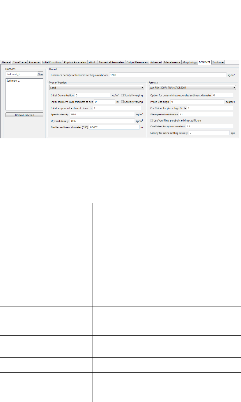
DRAFT
D-Flow Flexible Mesh, User Manual
You can repeat these steps in case you want to incorporate multiple fractions within your
model.
After selection of the Sediment tab and adding a new sediment fraction, the window given by
(Figure 4.80) is shown.
Figure 4.80: Overview of the Sediment tab, showing a sediment of type ‘sand’.
A sediment fraction can be deleted by first selecting the fraction you wish to remove, and then
clicking the Remove Fraction button.
Below, an overview of keywords that are associated to different types of sediment is provided
Parameter Lower
limit
Upper
limit
Default Unit Type of
sediment
Reference density hindered set-
tling
100 10000 1600 kg/m3Uniform for
all fractions
Initial sediment layer at bed 0 ∞0 m Sand,
mud and
bed-load
Specific density 100 4000 2650 kg/m3Sand,
mud and
bed-load
Dry bed density 0 10000 1600 kg/m3Sand
0 10000 500 kg/m3Mud
Initial concentration 0 Inf 0 kg/m3Sand and
mud
Median sediment diameter D50 0.000063 0.002 0.0002 m Sand
Salinity for saline settling velocity 0 391 0 ppt Mud
Settling velocity fresh water 0 1 0.00025 m/s Mud
(continued on next page)
84 of 412 Deltares

DRAFT
All about the modelling process
Table 4.4 – continued from previous page
Parameter Lower
limit
Upper
limit
Default Unit Type of
sediment
Settling velocity saline water 0 1 0.00025 m/s Mud
Critical shear stress erosion 0 100 0.5 N/m2Mud
Critical shear stress sedimenta-
tion
0 1000 1000 N/m2Mud
Reference density for
hindered settling
In high concentration mixtures, the settling velocity of a single par-
ticle is reduced due to the presence of other particles. In order to
account for this hindered settling effect Richardson and Zaki (1954)
are followed. The reference density is a parameter in their formula-
tion. See section 18.1.4.
Specific density For sediment transport the Eckart relation is extended to include the
density effect of sediment fractions in the fluid mixture, see sec-
tion 18.1.3. The specific density of each sediment fraction is part
of this formulation.
Dry bed density The thickness of the sediment above the fixed layer is calculated
by dividing the mass of sediment available at the bed by the user
specified dry bed density.
Initial concentration Option to specify the initial concentration of the sediment fraction,
can be specified as uniform or spatially varying.
Median sediment
diameter (D50)
The settling velocity of a non-cohesive (“sand”) sediment fraction is
computed following the method of Van Rijn (1993). The formulation
used depends on the diameter of the sediment in suspension: See
section 18.3.1
Settling velocity The settling velocity of the cohesive sediment, note that this is spec-
ified in m/s
Critical bed shear
stress for erosion
If the bed shear stress is smaller than the critical stress, no ero-
sion takes place. If the bed shear stress is larger than the flux is
calculated following Partheniades-Krone, see section 18.2.3, can be
specified as uniform or spatially varying.
Critical bed shear
stress for
sedimentation
If the bed shear stress is larger than the critical stress, no sedimen-
tation takes place. If the bed shear stress is smaller than the flux is
calculated following Partheniades-Krone, see section 18.2.3, can be
specified as uniform or spatially varying.
Sediment erosion rate Erosion parameter Min the formulation of Partheniades-Krone, see
section 18.2.3.
Initial sediment layer
thickness at bed
The initial sediment layer thickness at the bed in metre, can be spec-
ified as uniform or spatially varying.
Remark:
When adding multiple sediment fractions with an initial sediment layer thickness, the
layers are completely mixed by default. E.g. a uniform layer of 4 m present for one
sediment fraction, and a uniform layer of 6 m for another fraction, results in an initial
sediment layer of 10 m, in which 40 % and 60 % of the respective sediment fractions is
present. If you wish to have the model behave differently, options for bed stratigraphy
are available, refer to section 18.6.4.
Deltares 85 of 412
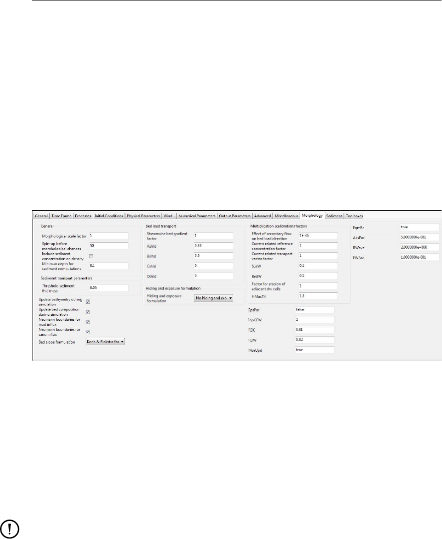
DRAFT
D-Flow Flexible Mesh, User Manual
Spatially varying variables
As indicated above, some variables can be defined as spatially varying. Note that when
activating a variable as spatially varying, the selected variable is added to the list of spatially
varying variables in the spatial editor. In Appendix F, a detailed description on how to work
with this spatial editor is provided. Note that you can no longer specify a uniform value for a
variable that is selected as spatially varying.
4.4.15 Morphology
If you have activated the process sediment/morphology in the Processes tab (section 4.4.6),
the tab Morphology appears. In this tab, you can modify parameters and settings that are
related to individual sediment fractions. After selection of the Morphology tab, the window
given by (Figure 4.81) is shown.
Figure 4.81: Default view of the Morphology tab.
With the feedback of bottom changes to the hydrodynamic computation you can execute a
full morphodynamic computation. You can also include the influence of waves by running this
version of D-Flow FM in combination with the D-Waves module. See section 18.6 for details.
General
Update bathymetry
during FLOW
simulation
If you want to take into account the feedback of bottom changes on
the hydrodynamics, tick off this option.
Remark:
The use of this update option only affects the updating of the
depth values (at ζand velocity points) used by flow calculations
at subsequent time-steps; the quantity of sediment available at
the bed will still be updated, regardless of the state of this flag.
Include effect of
sediment on fluid
density
You can include or neglect the effect of sediment on the fluid density
by setting this option accordingly.
For coarser non-cohesive material you can specify that, at all open inflow boundaries, the flow
should enter carrying all “sand” or “mud” sediment fractions at their equilibrium concentration
profiles. This means that the sediment load entering through the boundaries will be near-
perfectly adapted to the local flow conditions, and very little accretion or erosion should be
experienced near the model boundaries.
Equilibrium sand
concentration profile at
inflow boundary
Tick off to use this option. When not activated the inflow concen-
86 of 412 Deltares

DRAFT
All about the modelling process
trations specified in Data Group Boundaries →Transport conditions
will be used.
One of the complications inherent in carrying out morphological projections on the basis of
hydrodynamic flows is that morphological developments take place on a time scale several
times longer than typical flow changes (for example, tidal flows change significantly in a period
of hours, whereas the morphology of a coastline will usually take weeks, months, or years to
change significantly). One technique for approaching this problem is to use a Morphological
time scale factor whereby the speed of the changes in the morphology is scaled up to a rate
that it begins to have a significant impact on the hydrodynamic flows.
Morphological scale
factor
The above can be achieved by specifying a non-unity value.
The implementation of the Morphological time scale factor is achieved by simply multiplying
the erosion and deposition fluxes from the bed to the flow and vice-versa by this scale factor, at
each computational time-step. This allows accelerated bed-level changes to be incorporated
dynamically into the hydrodynamic flow calculations.
Frequently, a hydrodynamic simulation will take some time to stabilise after transitioning from
the initial conditions to the (dynamic) boundary conditions. It is likely that during this stabilisa-
tion period the patterns of erosion and accretion that take place do not accurately reflect the
true morphological development and should be ignored.
Spin-up interval before
morphological changes
Specify a time interval (in minutes after the start time) after which the
morphological bottom updating will begin. During this time interval all
other calculations will proceed as normal (sediment will be available
for suspension for example) however the effect of the sediment fluxes
on the available bottom sediments will not be taken into account.
Minimum depth for
sediment calculation
In the case of erosion near dry points a threshold depth for comput-
ing sediment transport can be used, see section 18.6.2.
Sediment transport parameters
The following parameters are only relevant for non-cohesive sediments.
van Rijn’s reference
level factor
For non-cohesive sediment (e.g. sand), we follow the method of Van
Rijn (1993) for the combined effect of waves and currents, see sec-
tion 18.3. The reference height formulation contains a proportionality
factor called van Rijn’s reference level factor.
Because of the more complex, partly explicit — partly implicit, erosive flux terms used for
“sand” type sediments it is not possible to use the simple source limitation technique used for
cohesive sediments. Instead, you must specify a Threshold sediment thickness.
Threshold sediment
thickness
At each time-step the thickness of the bottom sediments is calcu-
lated. If the remaining sediment thickness is less than the user-
specified threshold and erosive conditions are expected then the
source and sink sediment flux terms, see Eq. ((18.25)), are reduced
in the following manner:
Estimated ripple height
factor
In case of waves, the wave related roughness is related to the esti-
mated ripple height, see section 18.3.3.
Deltares 87 of 412

DRAFT
D-Flow Flexible Mesh, User Manual
Multiplication (calibration) factors
The following parameters are only relevant for non-cohesive sediments.
In the case of erosion near a dry beach or bank, the standard scheme will not allow erosion
of the adjacent cells, even when a steep scour hole would develop right next to the beach.
Therefore a scheme has been implemented, where for each wet cell, if there are dry points
adjacent to it; the erosion volume is distributed over the wet cell and the adjacent dry cells.
Factor for erosion of
adjacent dry cells
The distribution is governed by a user-specified factor for erosion
of adjacent dry cells, which determines the fraction of the erosion
to assign (evenly) to the adjacent cells; if this factor equals zero,
the standard scheme is used; if this factor equals 1, all erosion that
would occur in the wet cell is assigned to the adjacent dry cells.
Current-related
reference
concentration factor
The reference concentration is calculated in accordance with Van
Rijn et al. (2000), see section 18.3.3.
Only Van Rijn (1993) and Van Rijn et al. (2004) compute explicitly a wave-related transport
component.
Stotal =BED ·Sbedload current +BEDW ·Sbedload waves +SUSW ·Ssuspended waves (4.1)
dDP S
dt =Stotal out −Stotal in +SUS ·(Entrainment −Deposition)(4.2)
where Sbedload current,Sbedload waves,Ssuspended waves, Entrainment, and Deposition depend on
the sediment transport formula used. In most cases it holds Sbedload waves = 0 and Ssuspended waves =
0.
Current-related transport vector magnitude factor: —
Wave-related suspended transport factor: The wave-related suspended sediment trans-
port is modelled using an approximation method proposed by Van Rijn (2001), see sec-
tion 18.5.1.
Wave-related bedload transport factor: —
88 of 412 Deltares

DRAFT
All about the modelling process
Domain:
Parameter Lower limit Upper limit Default Unit
Include sediment concentra-
tion on density
yes or no no none
Update bathymetry during sim-
ulation
yes or no yes none
Update bed composition dur-
ing simulation
yes or no no none
Neumann boundaries for
sand/mud influx
yes or no yes none
Morphological scale factor 0.0 10000.0 1.0 -
Spin-up interval 0.0 50.0 min
Minimum depth for sediment
calculation
0.1 10.0 0.1 m
Threshold sediment thickness 0.005 10.0 0.05 m
Van Rijn’s reference level 0.4 2.0 1.0 -
Estimated ripple height factor 1.0 5.0 2.0 -
Factor for erosion of adjacent
dry cells
0.0 1.0 0.0 -
Current-related reference con-
centration factor
0.0 100.0 1.0 -
Current-related transport vec-
tor magnitude factor
0.0 100.0 1.0 -
Wave-related suspended
transport factor
0.0 100.0 1.0 -
Wave-related bedload trans-
port factor
0.0 100.0 1.0 -
4.5 Save project, MDU file and attribute files
To save your Delta Shell project, navigate the menu ribbons to File and click Save as. Choose
a location, specify a name and click Save. Your project will now be saved in a folder called
<name.dsproj_data>and a <name.dsproj>file is written. Within this folder you will find all
input ASCII input files of your model, output files of your model (if the model was run using
the GUI) and zip folders containing your restart files. Be aware that the output files are stored
within a separate folder in which the input files of your model are stored. The output folder on
the same level as the folder containing model input files is empty.
To open a project, navigate the menu ribbons to File and click Open. Select the <∗.dsproj>-
file of choice and click Open.
Importing model or data within a Delta Shell project can be achieved in two ways. Navigate
the menu ribbons to File and click Import. The import wizard appears, allowing you to select
what you want to import (Figure 4.82).
Deltares 89 of 412
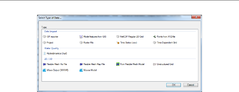
DRAFT
D-Flow Flexible Mesh, User Manual
Figure 4.82: Model/data import wizard
Alternatively, you can also right mouse click on the name of your project in the Project window
and select Import.
Exporting your model can be achieved in the same fashion as importing your model. All model
input files will be written to the folder you select. Be aware that model files exported to a folder
in which other model files with the same names are present will be overwritten.
90 of 412 Deltares

DRAFT
5 Running a model
5.1 Running a simulation
After defining the input for the D-Flow FM hydrodynamic simulation, the computation can
be executed either via Delta Shell or using batch scripts. Via Delta Shell, the status of the
computation and possible messages are displayed in a separate window. When using a batch
script, all messages are written to the diagnostics file (section E.1) and you can continue
working in the current window. Not all functionality is available when using Delta Shell to start
a calculation. Use a batch script (see section 5.4) in the following cases:
1 Using MPI to run in parallel
2 Using some queueing mechanism on a cluster
3 Running some unattended simulations, while continuing to work in Delta Shell.
Note that currently we have two different names of the D-Flow FM executables, for Windows
dflowfm-cli.exe and for Linux dflowfm.
5.2 Parallel calculations using MPI
5.2.1 Introduction
This section describes parallel computing with D-Flow FM based on the Message Passing
Interface system (MPI). This can be run both on computing clusters with distributed memory
as well as shared memory machines with multiple processors and/or multiple CPU cores.
The goal of parallelization of D-Flow FM is twofold. We aim for much faster computations on
shared- or distributed-memory machines and the ability to model problems that do not fit on a
single machine. A less powerful, yet possibly attractive performance improvement is offered
by D-Flow FM’s OpenMP-based parallelization (section 5.5.1).
Technical backgrounds on the parallel algorithms in D-Flow FM are described in the Technical
Reference Manual D-Flow FM TRM (2015).
Workflow of a parallel run
A parallel run divides the work between multiple processes. To this end we partition the model
and let separate processes solve the submodels and generate partitioned output. Given a
whole model, the workflow is as follows:
1 partition the model (mesh and model definition file),
2 submit the parallel job to a queue on a computing cluster, and
3 visualize the results from partitioned output files.
Deltares 91 of 412

DRAFT
D-Flow Flexible Mesh, User Manual
5.2.2 Partitioning the model
In D-Flow FM a model is defined by the model definition file, the mesh file and external forc-
ing/boundary condition files, et cetera. The latter are shared by all submodels and do not
need to be partitioned, they should only be available to all processes. So, partitioning the
model concerns partitioning of:
the mesh. This is achieved through the graphical user interface or by a command line
option. Mesh files for every subdomain will be created;
the model definition file. The partitioned model definition files will contain references to
the subdomain mesh, and all other information equals its sequential counterpart.
An efficient approach to partition both the mesh and MDU files is via the command line, using
> dflowfm --partition:ndomains=n:icgsolver=i <mdu-file>
This command reads the name of the mesh file from mdu-file, and generates nsubdomain
mesh files by the METIS software package (See D-Flow FM TRM (2015) and references
mentioned therein). Then, it creates nsubdomain MDU files where the parallel Krylov solver
icgsolver is set to i. Here, ican be 6, the PETSc solver(recommended for Linux), or, 7,
the parallel CG with MILU block preconditioning (recommended for Windows).
For example, to partition the MDU file <example.mdu>, which specifies the mesh file as
<exampel_net.nc>, to eight subdomain files on a Windows machine, one can use:
> dflowfm --partition:ndomains=8:icgsolver=7 example.mdu
The mesh file is partitioned into eight subdomain mesh files, with names <example_000j_net.nc>,
j=0,1,...,7. In other words, they are:
example_0000_net.nc example_0003_net.nc example_0006_net.nc
example_0001_net.nc example_0004_net.nc example_0007_net.nc
example_0002_net.nc example_0005_net.nc
Then, eight subdomain mdu-files are also created, with names <example_0000.mdu>to
<exampel_0007.mdu>. The different items in, e.g. <example_0000.mdu>with respect to
the original mdu-file are:
[geometry]
NetFile = example_0000_net.nc
[numerics]
Icgsolver = 7
92 of 412 Deltares
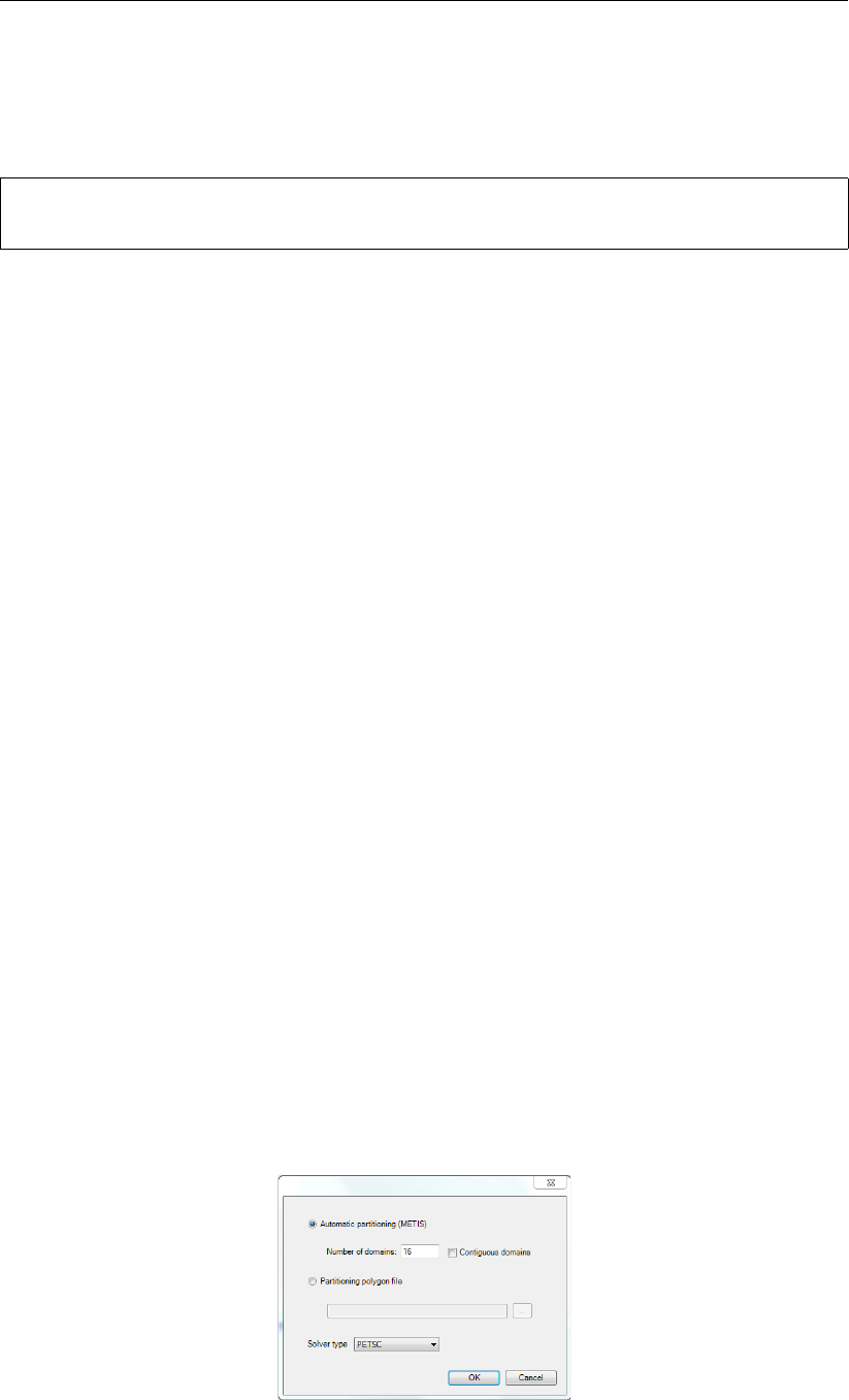
DRAFT
Running a model
If the user wants to manually partition the mesh instead of applying METIS, then he has to
provide a polygon file <userpol.pol> which determines the mesh partition. In this situation,
following command can partition both the MDU and mesh files:
> dflowfm --partition:icgsolver=i <mdu-file> <userpol.pol>
5.2.2.1 More about the mesh partitioning
The mesh can be automatically partitioned with the METIS software package, or manually
by supplying polygons that define the subdomains. They both produce a cell coloring of
the unpartitioned mesh. In each subdomain, the cells are assigned the same color, and
augmented with ghost cells. These information are saved in the resulting partitioning mesh
file, e.g. <example_NNNN_net.nc>, where _NNNN is a subdomain index.
Regarding partitioning manually with user-supplied partitioning polygons, the partitioning obeys
the following rules:
if the polygons have a z-value specified, it is considered a subdomain number,
if the polygons have no z-value specified, its order determines the corresponding subdo-
main number,
if a cell is not inside at least one polygon, it is assigned to subdomain 0,
if a cell is inside only one polygon, it is assigned to the subdomain defined by that polygon,
if a cell is inside more than one polygon, it is assigned to the subdomain with the highest
number.
In other words, the polygons may be overlapping and the largest subdomain number is taken
in the overlapping regions. If the polygons have no z-value, the polygon order determines the
corresponding subdomain number, i.e. the first polygon corresponds to subdomain 1 et cetera
and there is no polygon defining subdomain 0.
Both types of mesh partitioning are available through Delta Shell or on the command line.
Partitioning the mesh with METIS via Delta Shell
We will firstly focus on the METIS partitioner. Partitioning the mesh from within Delta Shell is
achieved by the following steps. In the Project window, select the model you want to run by
means of clicking on the desired model (Figure 6.1). A right-mouse click will open the context
menu, then select Export.... In the window Select Type of Data..., choose Partition exporter
and the partitioning dialog will appear (Figure 5.1).
Figure 5.1: Partioning exporter dialog
Deltares 93 of 412

DRAFT
D-Flow Flexible Mesh, User Manual
Enter the desired amount of subdomains, and typically leave the contiguous option switched
off and the solver type at its default. After pressing OK, a file dialog will appear. Enter the
name of the MDU file, without any trailing ’_000x’ partition numbers: these will be added
automatically.
Partitioning the mesh with the graphical user interface is achieved by the following steps:
You are prompted for Contiguous domains are not necessary for parallel computations in D-
Flow FM and often METIS produces contiguous subdomains without enforcing it. Still, some
users may want to explicitly enforce contiguous domains. If you want to do so, make sure
that your unpartitioned mesh is contiguous. Not being so may cause errors, Note that there
is no polygon defining subdomain 0. Parts of the mesh not confined by any polygon are
assumed to be in subdomain 0. In other words, there are at least N−1polygons defining
Nsubdomains. In that case, regenerate the cell colors/domain numbers again by selecting
Operations →Generate domain numbers (polygon or METIS). Note that you will not be asked
to specify the number of subdomains. The cell coloring/domain numbering is now based on
the (modified) polygons and not produced by the METIS partitioner. Manual partitioning with
user-specified polygons will be explained in the next section, The entered mesh filename is a
basename that will be used to derive the partitioning filenames, e.g. <example_net.nc>will
produce:
Partitioning the mesh from the command line
Apart from using the graphical user interface, it is possible to perform the partitioning on the
command line. The two types of partitioning can be carried out via the following commands.
The command that uses METIS partitioner reads:
> dflowfm --partition:ndomains=n <meshfile>
where ndomains=n specifies that nsubdomains are to be generated. For example, parti-
tioning <example_net.nc>results in subdomain mesh files <example_000j_net.nc>,j=0,1,...,n-1.
An advanced command, which enables more options, is:
> dflowfm --partition:ndomains=n[:method=0|1][:genpolygon=0|1][:contiguous=0|1]
<meshfile>
where the partition method can be chosen via setting method=0, the Recursive Bisection
method (default), or method=1, the multilevel K-Way method. We refer to Karypis (2013) for
more details about these two methods. Option genpolygon specifies if the command gen-
erates a partition polygon file (genpolygon=1), or not (genpolygon=0, default). Option
contiguous enforces the contiguous partition when specifying both contiguous=1 and
method=1. (Only the K-Way method enables the contiguous partition.) It is not switched
on by default. Comparing to the previous command, this advanced command additionally
generates a partition polygon file <example_part.pol>when genpolygon=1 is specified.
Note: Backwards compatibility: when using the legacy partitioning script generate_parallel_mdu.sh
make sure to include the non-default option genpolygon=1 in the above command, such
that the required polygon file is produced.
94 of 412 Deltares
DRAFT
Running a model
Note: When partition a mesh file, e.g. <example_net.nc>, by default a separate file
<DFM_interpreted_idomain_example_net.nc>is generated, which includes partition domain
information and cell information. One can switch off generating this file by adding in the MDU
file ->[output]-> Writepart_domain = 0.
To manually partition a mesh, a user-specified polygon file <userpols.pol>has to be pro-
vided. The corresponding command reads:
> dflowfm --partition <meshfile> <userpol.pol>
This generates files the same as before.
5.2.3 Partitioning the MDU file
Having partitioned the mesh, the model definition file needs to be partitioned, as every sub-
model requires its own definition file with references to
the partitioned mesh file, e.g. <example_0000_net.nc>,
an appropriate parallel Krylov solver, can be
6: PETSc solver, recommended (for Linux), or
7: parallel CG with MILU block preconditioning (for Windows),
a unique snapshot directory,
optionally, a partitioned restart file, and
optionally, a partitioning polygon file, e.g. <example_part.pol>.
The generate_parallel_mdu.sh script partitions a sequential model definition file au-
tomatically:
> generate_parallel_mdu.sh <mdu-file> <nprocs> [partpol-file] <Icgsolver>
with
mdu-file sequential model definition file,
nprocs number of subdomains/parallel processes,
partpol-file partitioning polygon file (optionally),
Icgsolver parallel Krylov solver, can be 6 or 7.
Note that the partitioned mesh filenames (and partitioned restart filenames) are derived from
the mesh filename (and the restart filename) specified in the sequential model definition file.
5.2.3.1 Remaining model input
A parallel run of a D-Flow FM model needs only partitioned <.mdu>and <_net.nc>files.
All other model input is the same as for a standalone run, e.g., meteo forcings, boundary con-
ditions, observation stations and more. These are generally copied to the working directory
by the parallel job submission script.
Deltares 95 of 412

DRAFT
D-Flow Flexible Mesh, User Manual
5.2.4 Running a parallel job
To run a parallel job with D-Flow FM model on a cluster you have to prepare the submission
script. The submission script should be prepared with respect to the specific options that job
scheduler on your cluster requires.
The simple example of the D-Flow FM submission script on the cluster with the Grid Engine:
#!/bin/bash
#$ -V
#$ -q test
#$ -cwd
#$ -N My_DflowFM_JOB
#$ -m bea
#$ -M my.email@provider.net
export LD_LIBRARY_PATH=$DFLOWFM/lib:$LD_LIBRARY_PATH
export PATH=$DFLOWFM/bin:$PATH
mpiexec -np 4 dflowfm --autostartstop YOUR_MDU_FILE.mdu > out.txt 2> err.txt
In this simplify example above we submit the D-Flow FM simulation that was partitioned into
4 domains and is going to use only 1 node. The options used above are:
-V Specify that all environment variables active within the qsub utility be exported to
the context of the job.
-q Specify the queue ’test’ to be used for this job, if absent default queue is used.
-cwd Execute the job from the current working directory.
-N Specify the name of the job.
-m Specifies which message type should be emailed (b=beginning of job, e=end of
job, a=abort of job.
-M Specifies the email address to send the notification.
In order to submit more complicated, e.g. multi-node simulations, additional options that are
scheduler depended have to be added.
5.2.5 Visualizing the results of a parallel run
The map and history output files (as introduced in section 4.4.12) deserve special attention in
parallel runs.
The history file — with time series for observation points, structures and more — is written
only by process #0, and all model-global data has already been aggregated into that single
file: <mdu_name_0000_his.nc>.
The map file — with full-grid output of flow fields — is written for each domain separately as
<mdu_name_000X_map.nc>. This saves communication overhead during the parallel run.
The partitioned map files contain duplicate points, since each file also contains the domain’s
ghost nodes. For postprocessing these map files, two options are now available:
1 Direct plotting of the set of all map files in Delft3D-QUICKPLOT: the partitioned file series
will be recognized automatically, and the partion results will be drawn on top of each other.
For water levels this gives good results.
96 of 412 Deltares
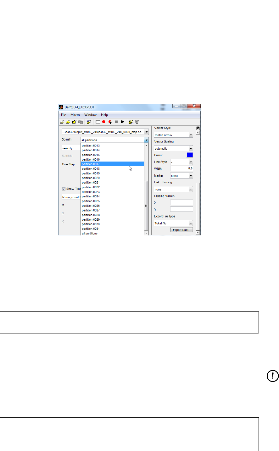
DRAFT
Running a model
2 Merging the partioned map files into a single global map file with the DFMOUTPUT tool.
The resulting map file can then be loaded again in Delft3D-QUICKPLOT and other post-
processing utilities.
5.2.5.1 Plotting all partitioned map files with Delft3D-QUICKPLOT
When opening one of the partitioned map files into Delft3D-QUICKPLOT, it will automatically
detect that the map file is part of a series. An additional select list Domain appears, see
Figure 5.2. Select either “all partitions”, or a partition of your choice, and proceed with the
plotting as normal (section 6.3).
Figure 5.2: Domain selector in Delft3D-QUICKPLOT for partitioned map files.
5.2.5.2 Merging multiple map files into one
The partitioned map files of a parallel model run can be merged into a single global map file
with the DFMOUTPUT tool. It cuts off ghost nodes, and concatenates all grid points, taking
care of correct global renumbering. Usage:
> dfmoutput mapmerge [--infile FILE1 [FILE2 FILE3...]] [--outfile DSTFILE]
where FILE1/2/3 are the input files, e.g., <mdu_name_0000_map.nc>,...,<mdu_name_0031_map.nc>
and DSTFILE is an optional output file name (the default is <mdu_name_merged_map.nc>).
Remark:
Since a restart file is a special type of map file, partitioned restart files can also be
merged using the above command.
The built-in help gives a list of more advanced options:
> dfmoutput mapmerge --help
Merge multiple map files from parallel run into one.
Optional switches:
Deltares 97 of 412

DRAFT
D-Flow Flexible Mesh, User Manual
--infile FILE1 [FILE2...], -i FILE1 [FILE2...]
default value
One or more input files.
--listfile LISTFILE, -F LISTFILE
Pass contents of LISTFILE as input files.
--outfile DSTFILE, -o DSTFILE
Write output to file DSTFILE.
Default: <model>_merged_map.nc
--force, -f
default value .false.
Force overwriting of existing output file.
--help, -h
Print this help message
--version, -v
Print version
Examples:
dfmoutput mapmerge --infile model_0000_map.nc model_0001_map.nc
5.3 Running a scenario using Delta Shell
In the Project window, select the model you want to run by means of clicking the first attribute
of the desired model (Figure 6.1).
Figure 5.3: Selecting the model you want to run in the Project window
Starting the calculation can be achieved in two ways. You can navigate the menu ribbons; go
to “Home” and in the group Run click on the button “Run Current”. To run all models that are
opened in the Project window, click on “Run All” (Figure 5.4).
Figure 5.4: Group Run in Home ribbon
Alternatively, you can right mouse click the first attribute in the Project window of the model
you want to run. Next, click “Run Model” to start the calculation. When you select the first of
the model you want to run, the properties window (“View” “Properties”) shows several prop-
erties of the model you selected. If you set “ShowModelRunConsole” on true, the model run
console of the computational core will be showed during the calculation, providing you with
additional information during the model run (Figure 5.5).
98 of 412 Deltares
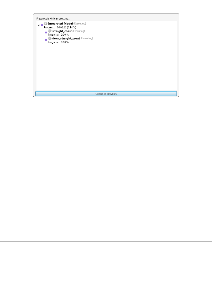
DRAFT
Running a model
Figure 5.5: Run console Delta Shell
When you cancel the run by clicking “Cancel all activities”, model results are stored up to the
point where you cancel the run.
5.4 Running a scenario using a batch script
Separate scripts are needed for Windows (with the extension <∗.bat>) and Linux (with the
extension <∗.sh>). See section 5.7 for the command-line arguments.
In this section we refer to the variable %DFLOWFM% for Windows and $DFLOWFM for Linux as
a variable that stores path to the directory that contains the dflowfm-cli package.
The easiest Windows script (assuming you have downloaded the Windows dflowfm-cli pack-
age, assuming you are in the directory of a configured test-case):
set PATH=%DFLOWFM%\bin;%PATH%
dflowfm-cli.exe --autostartstop YOUR_MDU_FILE.mdu
The easiest Linux script (assuming you have downloaded the Linux dflowfm-cli package, as-
suming you are in the directory of a configured test-case):
export LD_LIBRARY_PATH=$DFLOWFM/lib:$LD_LIBRARY_PATH
export PATH=$DFLOWFM/bin:$PATH
dflowfm --autostartstop YOUR_MDU_FILE.mdu
5.5 Run time
The actual run time of a model can vary considerably depending on a variety of factors such
as:
The problem being solved, characterised by the number of active grid points, the number
of layers in the vertical or the number of processes taken into account.
The length of the simulation in time and the time step being used.
The hardware configuration that is used and the work load of the processor.
Deltares 99 of 412

DRAFT
D-Flow Flexible Mesh, User Manual
For this reason, only some general considerations are given to determine the run time of a
hydrodynamic simulation. On a PC or a workstation without separate I/O-processors the CPU
time is the sum of the processor time and the I/O time.
The processor time required for a simulation is primarily determined by:
The model definition, i.e., the number of active grid points and the number and type of the
processes taken into account.
The length of the simulated period in terms of the number of time steps executed.
The I/O time is determined by:
The number of times the computed data are written to history, map, restart files and other
communication files for water quality or wave model couplings.
The number of observation points, cross-sections and the number of output parameters.
The simulation performance is defined as the CPU time per grid point per time step per con-
stituent:
simulation performance =CPU time
Dnt ·Ndx [system seconds]
where:
Dnt is the number of time steps executed
Ndx is the number of flow nodes
The simulation performance is written to the diagnostic file at the end of the simulation.
5.5.1 Multi-core performance improvements by OpenMP
D-Flow FM has built-in support for multi-core parallellism using OpenMP1. This speeds up
calculations by employing multiple processor cores in a single (shared-memory) computer,
e.g., a modern-day notebook. OpenMP-parallellism in D-Flow FM does not scale as well as
MPI-parallellism (section 5.2), but it comes for free (not any change to model input necessary)
and can give a welcome performance improvement (approximately double speed on an Intel
quadcore CPU). It is strongly advised to limit the number of OpenMP-threads to one less than
the number of physical cores in your machine, thus also ignoring any hyperthreading. An
example on Linux for an i7 quadcore CPU machine:
export OMP_NUM_THREADS=3
dflowfm --autostartstop YOUR_MDU_FILE.mdu
5.6 Files and file sizes
For estimating the required disk space the following files are important:
history file
map file
restart file
1http://www.openmp.org
100 of 412 Deltares

DRAFT
Running a model
5.6.1 History file
The size of the history file is determined by:
The number of monitoring points (observation points + cross-sections): H1.
The number of quantities stored: H2.
The number of additional process parameters, such as salinity, temperature, constituents
and turbulence quantities, taken into account in the simulation: H3.
The number of time the history data is written to the history file: H4.
You can estimate the size of a history file (in bytes) from the following equation:
size history file = H1 ·(H2 + H3) ·H4 ·8 bytes.
As a first approximation you can use H2 = 8.
Example
For a 2D simulation with density driven currents (salinity and temperature), a simulated period
of 12 hrs 30 min, a time integration step of 5 minutes, 30 monitoring points and each time
step being stored, the size of the history file will be of the order of 384 kBytes. For the same
model but now with 10 layers in the vertical the file size will increase to about 4 MBytes. These
estimates show that history files are rather small. Unless the number of monitoring points is
excessively large the history files are typically much smaller than the map output files.
5.6.2 Map file
The size of the map file is determined by:
The size of the model, i.e. the number of grid cells multiplied by the number of layers (Ndxi
·Kmax): M1n, and the number of flow links (open grid cell edges) multiplied by the number
of layers (Lnx ·Kmax): M1l.
The number of quantities stored on grid cells and flow links: M2n, M2l, respectively.
The number of process parameters taken into account, such as salinity, temperature,
constituents and turbulence quantities: M3.
The number of time steps for which the map file is written: M4.
Remark:
For a more refined estimate you should distinguish between parameters that depend
or not on the number of layers used (such as the water level). For a 3D simulation the
latter quantities can be neglected, for a 2D simulation they must be accounted for. As a
first estimate we double the number of quantities M2 in a 2D simulation.
As a first approximation you can use M2n = 5, M2l = 5 for a 3D simulation and M2n = 8, M2l
= 5 for a 2D simulation.
You can estimate the size of a map file (in bytes) from the following equation:
size map file =[M1n ·(M2n + M3) + M1l ·M2l] ·M4 ·8 bytes.
Deltares 101 of 412

DRAFT
D-Flow Flexible Mesh , User Manual
Example
For a 2D simulation with 6800 grid cells and 13000 flow links, simulation results stored for
a period of 7 days, and the file is written with an interval of 60 minutes the size of the map
file will be about 161 MBytes. For larger models the map file can easily become excessively
large, as result the map file is less frequently written, for instance every 2 or 3 hours.
5.6.3 Restart file
A restart file is a special type of map file, where only one time snapshot per file is saved (i.e,
M4 = 1). No grid or flow geometry information is stored in a restart file, except for the flow
cell/link information (denoted by M5). Moreover, the restart files obtained after a parallel run
contain some necessary information about parallelization (denoted by M6). Similarly to the
equation of size map file above, one can write the estimating equation as follows:
size rst file = [M1n ·(M2n + M3) + M1l ·M2l + M5 + M6] ·8 bytes,
where M6 = 0 for a sequential run.
5.7 Command-line arguments
A complete model schematisation can be run from the command line using the D-Flow FM
Command Line Interface (CLI), dflowfm-cli.exe (dflowfm on Linux). A basic non-
interactive run is started by:
> dflowfm-cli --autostartstop \emph{mdu\_name}.mdu
In the box below, a full list of command-line options and arguments is shown:
> dflowfm-cli --help
Usage: dflowfm-cli [OPTIONS] [FILE]...
Options:
--autostart MDUFILE
Auto-start the model run, and wait upon completion.
--autostartstop MDUFILE
Auto-start the model run, and exit upon completion.
--noautostart MDUFILE
Disable any AutoStart option in the MDU file (if any).
--partition:OPTS [POLFILE] NETFILE
Partitions the unstructured grid in NETFILE into multiple files.
POLFILE is an optional polygon file which defines the partitions.
Only used when ndomain in OPTS is undefined or 0.
OPTS is a colon-separated list opt1=val1:opt2=val2:...
ndomains = N Number of partitions.
method = [01] Partition method: Recursive Bisection(0), K-Way(1).
genpolygon= [01] Generate partition polygon(1) or not(0).
contiguous= [01] Enforce contiguous grid cells in each domain.
Only available when K-Way is enabled (method=1).
102 of 412 Deltares

DRAFT
Running a model
-t N, --threads N
Set maximum number of OpenMP threads.
N must be a positive integer.
--refine:OPTS NETFILE
Refine the unstructured grid in NETFILE from commandline.
OPTS is a colon-separated list opt1=val1:opt2=val2:...
hmin=VAL
dtmax=VAL
maxlevel=M
connect=[01]
directional=[01]
outsidecell=[01]
-q, --quiet
Minimal output: Only (fatal) errors are shown.
--verbose:[level_stdout[:level_dia]], e.g., --verbose:INFO:DEBUG
Set verbosity level of output on standard out and in diagnostics file.
where level is in: {DEBUG|INFO|WARNING|ERROR|FATAL}
Levels are optional, default is INFO on screen, DEBUG in dia file.
-h, --help
Display this help information and exit.
-v, --version
Output version information and exit.
5.8 Restart a simulation
D-Flow FM allows to restart a simulation, not from the original starting time, but from a user-
specified time with all the information at that time. In other words, for a model which has a long
spinup time from tstart, instead of restarting from tstart, one can restart another simulation of
the same model from a later time trst, where tstart ≤trst < tstop. And the results for times
trst ≤t≤tstop are the same as in the original simulation run.
This can be achieved by following steps:
1 In order to obtain restart files <_rst.nc>, this needs to be enabled in the output parame-
ters (see section 4.4.12 for more details about how to set output parameters).
2 Run the original model from tstart to tstop, resulting in restart files.
3 To restart the simulation from time trst, in the MDU file modify TStart to trst,and fill
in the name of corresponding restart file in RestartFile of the [restart]-section.
Moreover, place the corresponding restart file relative to the directory of this MDU file.
To restart a parallel simulation, one can use any of the following methods:
Method 1 On each subdomain use its own restart file.
Method 2 Merge all the subdomain restart files into a single global restart file (see section 5.2.5.2),
and then use it for all the subdomains. This means to put the name of this merged file as
RestartFile in all subdomain MDU files. This method is supported when restarting
with the same, or a different domain partitioning. Moreover, such a merged restart file can
also be used to restart a sequential run.
The above two methods require taking care of the name of the restart file in subdomain MDU
files. D-Flow FM automatically fills in the correct names, when partition an MDU file to subdo-
main MDU files (see section 5.2.2), in the following way:
Deltares 103 of 412

DRAFT
D-Flow Flexible Mesh, User Manual
For Method 1 When <mduname_YYMMDD_HHMMSS_rst.nc>is filled in RestartFile of the orig-
inal MDU file, partition this MDU file gives subdomain MDU files with RestartFile as
<mduname_000X_YYMMDD_HHMMSS_rst.nc>for each subdomain <000X>.
For Method 2 If the string word "merged" is contained in the name of RestartFile in the original
MDU file, then this file name is kept to all the subdomain MDU files after partitioning.
It is also possible to use a map file as a restart file, following the above approaches. Notice
that in this case, one needs to specify the RestartDateTime in MDU file as well. However,
we strongly recommend to use <_rst.nc>file instead of a map file.
D-Flow FM also supports restarting a 3D model simulation with σ-layers. Note: The 3D-
implementation is a beta functionality.
5.9 Frequently asked questions
This chapter aims to help you with common questions that may arise while using D-Flow FM.
1Question
My model does not run/crashes. What’s wrong?
Answer
The diagnostics file is the starting point for finding out what went wrong. See section E.1
for a detailed description of the contents of this file, and the order of model run output.
Globally, ask yourself the following questions:
Was the MDU file found?
If yes, was the model successfully loaded? Common mistakes are missing boundary
or meteorological forcings file.
If yes, was the time loop successfully started? Possible errors are non-writable output
files.
If yes, does the dia file contain any messages from during the time loop? Possible
errors are solver convergence errors.
If not, did the run end successfully?
2Question
I get a warning that my network is non-orthogonal. Can I loosen the orthogonality tresh-
old?
Answer
Unfortunately, no. Orthogonality is very important for accuracy: advised orthogonality val-
ues for your grid are around 0.01, preferrably lower. The current treshold is already very
high at a value of 0.5. Use RGFGRID to improve your grid orthogonality (and smooth-
ness).
104 of 412 Deltares
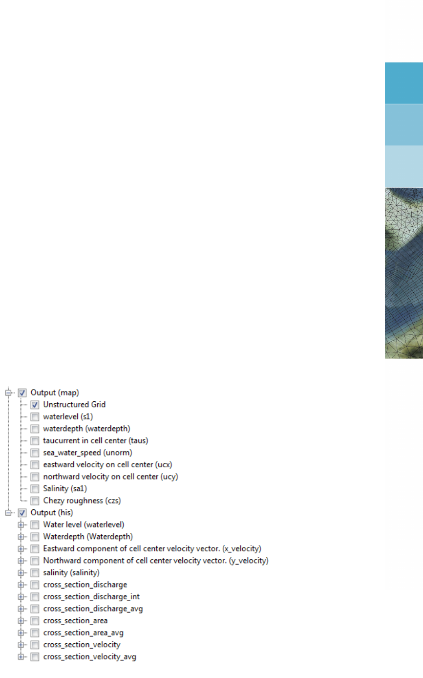
DRAFT
6 Visualize results
6.1 Introduction
A model run will produce two types of output:
1 a graph or history (<∗.his>-file) for a specific quantity on a location
2 a map (<∗.map>-file) for a specific quantity
Both are stored in files within the project, as described in section 5.6.
D-Flow FM provides basic visualization of the model and the model results. Advanced and
tailor-made visualization is possible by the export of the his- and/or map-files, and inspection
with dedicated visualization applications. Some are provided and described below.
6.2 Visualization with Delta Shell
When your model run has finished, a new folder called “Output” has appeared at the bottom
of the attributes of your model in the Map window. Inside this folder, all output quantities of
the his-, and map-files can be found, as well as a folder called “States”, in which you find
all restart files written during the model run. Output folders have also appeared in the Map
window; “Output (map)” and “Output (his)”. Both the results of your map and his files can be
viewed in the central map by means of enabling the desired quantities from the Map window
(Figure 6.1).
Figure 6.1: Example of setting output (in)visible in the Map window
The time navigator can be used to slide through the different time steps in the output files.
If your model is relatively large, the drawing performance of the interface can be improved
Deltares 105 of 412
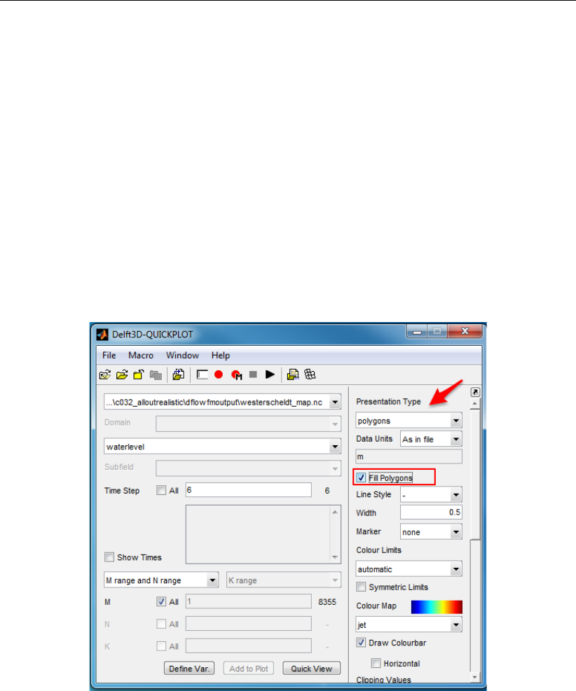
DRAFT
D-Flow Flexible Mesh, User Manual
dramatically by enabling QuadTree visualizations in the properties window of the layer you
want to visualize. To this end, select the layer you want to visualize in the ...
6.3 Visualization with Quickplot
The interface of the Delft3D-QUICKPLOT allows to open the NetCDF output files from a D-
Flow FM simulation. In the interface you can select data fields, make a selection of time
steps, stations or specify a preferred figure presentation options. After selection of a certain
options you can visualize your data by using the “Quick View” button. To add another plot to
an existing figure the “Add to Plot” button should be used.
When plotting the map output files from a D-Flow FM simulation, by default the presentation
type “markers” will be selected. To smoothly visualize your results it is recommended to
change presentation type into “polygons” and then select the option “Fill Polygons” (see the
example on the Figure 6.2).
Figure 6.2: Useful map visualization options in the Delft3D-QUICKPLOT
See the Delft3D-QUICKPLOT User Manual for full details and a description of the routines
and their use.
106 of 412 Deltares
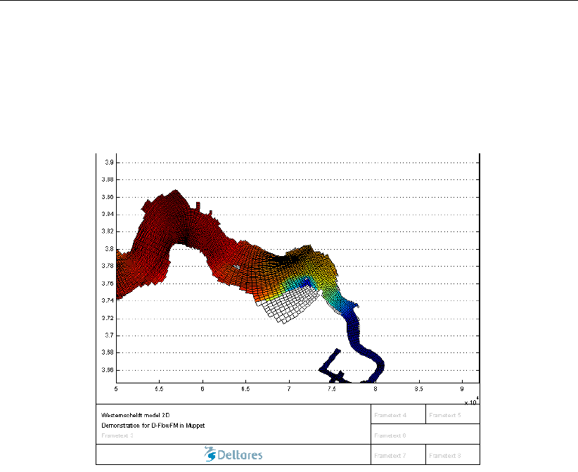
DRAFT
Visualize results
6.4 Visualization with Muppet
The interface of the Muppet allows to “Add Dataset” from a NetCDF output file from a D-
Flow FM simulation. It is possible to create a timeseries for a selected variable in from the
history files. Additionally Muppet offers the option to visualize the map output files from a
D-Flow FM simulation (see Figure 6.3).
Figure 6.3: Example of the Muppet visualization of the D-Flow FM map output file
In the Muppet interface it is possible to specify figure settings, plot descriptions, labels and
many more.
6.5 Visualization with Matlab
In the OpenEarthTools you can find two example scripts that allow you to load and visualize
the D-Flow FM output. Note that in the Matlab scripts for the D-Flow FM the UGRID notation
is used.
The <plotMap.m>script plots a D-Flow FM unstructured map and optionally the handles h
are returned. By modifying the script you can change the plotted variable, layout or the plot
style options.
The <plotNet.m>script plots a D-Flow FM unstructured net, optionally the handles h are
returned. This script can visualize nodes, links and cell circumcenters of a network. By
modifying the script you can choose the preferred plotting settings and variables to plot (by
default nodes, edges and faces are plotted).
6.6 Visualization with Python
Currently there are no examples of Python scripts for the D-Flow FM output visualization in the
OpenEarthTools. However, if such a need arises it is possible to load netcdf Python libraries,
and create your own simple visualization of the variables present in the NetCDF output files.
Deltares 107 of 412

DRAFT
D-Flow Flexible Mesh, User Manual
108 of 412 Deltares

DRAFT
7 Hydrodynamics
7.1 Introduction
Increasing awareness of environmental issues has focused the attention of scientists and en-
gineers on the problem of predicting the flow and dispersion of contaminants in water systems.
Reliable information on water flow, waves, water quality, sediment transport and morphology
can be obtained from appropriate mathematical models. In general the first step in such mod-
elling activities concerns the simulation of the flow itself. Whether the problem is related, for
example, to the stability of a hydraulic structure, to salt intrusion, to the dispersion of pollu-
tants or to the transport of silt and sediment, flow simulations usually form the basis of the
investigations to be carried out.
The Delft3D Flexible Mesh Suite is the integrated modelling system of Deltares for the aquatic
environment. D-Flow Flexible Mesh, the flow module of this system, provides the hydrody-
namic basis for other modules such as water quality, ecology, waves and morphology. For
steady and non-steady modelling of the far-field water quality and ecology, it is coupled with
the far-field water quality module D-Water Quality. For the interaction between waves and
currents the flow module may be coupled with the short-waves model D-Waves. To control
structures, the flow module is coupled to the D-Real Time Control module.
D-Flow FM is flexible by using an unstructured grid in the horizontal plane. In the vertical di-
rection D-Flow FM offers two different vertical grid systems: a so-called σco-ordinate system
(σ-model) introduced by Phillips (1957) for ocean models and the Cartesian z-co-ordinate
system (Z-model).
This section gives some background information on the conceptual model of the D-Flow FM
module. Most of the concepts and algorithms are applicable to both the σ-model and Z-
model.
Note: The 3D-implementation is a β-functionality.
7.2 General background
7.2.1 Range of applications of D-Flow FM
The hydrodynamic module D-Flow FM simulates two-dimensional (2DH, depth-averaged) or
three-dimensional (3D) unsteady flow and transport phenomena resulting from tidal and/or
meteorological forcing, including the effect of density differences due to a non-uniform tem-
perature and salinity distribution (density-driven flow). The flow model can be used to predict
the flow in shallow seas, coastal areas, estuaries, lagoons, rivers and lakes. It aims to model
flow phenomena of which the horizontal length and time scales are significantly larger than
the vertical scales.
If the fluid is vertically homogeneous, a depth-averaged approach is appropriate. D-Flow FM
is able to run in two-dimensional mode (one computational layer), which corresponds to solv-
ing the depth-averaged equations. Examples in which the two-dimensional, depth-averaged
flow equations can be applied are tidal waves, storm surges, tsunamis, harbor oscillations
(seiches) and transport of pollutants in vertically well-mixed flow regimes.
Three-dimensional modelling is of particular interest in transport problems where the hori-
zontal flow field shows significant variation in the vertical direction. This variation may be
generated by wind forcing, bed stress, Coriolis force, bed topography or density differences.
Examples are dispersion of waste or cooling water in lakes and coastal areas, upwelling and
Deltares 109 of 412

DRAFT
D-Flow Flexible Mesh, User Manual
downwelling of nutrients, salt intrusion in estuaries, fresh water river discharges in bays and
thermal stratification in lakes and seas.
7.2.2 Physical processes
The numerical hydrodynamic modelling system D-Flow FM solves the unsteady shallow water
equations in two (depth-averaged) or in three dimensions. The system of equations consists
of the horizontal equations of motion, the continuity equation, and the transport equations
for conservative constituents. The equations are formulated in orthogonal curvilinear co-
ordinates or in spherical co-ordinates on the globe. In D-Flow FM models with structured grid
are considered as a simplified form of an unstructured grid. In Cartesian co-ordinates, the
free surface level and bathymetry are related to a flat horizontal plane of reference, whereas
in spherical co-ordinates the reference plane follows the Earth curvature.
The flow is forced by tide at the open boundaries, wind stress at the free surface, pressure
gradients due to free surface gradients (barotropic) or density gradients (baroclinic). Source
and sink terms are included in the equations to model the discharge and withdrawal of water.
The D-Flow FM model includes mathematical formulations that take into account the following
physical phenomena:
Free surface gradients (barotropic effects).
The effect of the Earth rotation (Coriolis force).
Water with variable density (equation of state).
Horizontal density gradients in the pressure (baroclinic effects).
Turbulence induced mass and momentum fluxes (turbulence closure models).
Transport of salt, heat and other conservative constituents.
Tidal forcing at the open boundaries.
Space and time varying wind shear-stress at the water surface.
Space varying shear-stress at the bed.
Space and time varying atmospheric pressure on the water surface.
Time varying sources and sinks (e.g. river discharges).
Drying and flooding of tidal flats.
Heat exchange through the free surface.
Evaporation and precipitation.
Tide generating forces.
Effect of secondary flow on depth-averaged momentum equations.
Lateral shear-stress at wall.
Vertical exchange of momentum due to internal waves.
Influence of waves on the bed shear-stress (2D and 3D).
Wave induced stresses (radiation stress) and mass fluxes.
Flow through hydraulic structures.
Wind driven flows including tropical cyclone winds.
110 of 412 Deltares

DRAFT
Hydrodynamics
7.2.3 Assumptions underlying D-Flow FM
In D-Flow FM the 2D (depth-averaged) or 3D non-linear shallow water equations are solved.
These equations are derived from the three dimensional Navier-Stokes equations for incom-
pressible free surface flow. The following assumptions and approximations are applied:
In the σco-ordinate system the depth is assumed to be much smaller than the horizontal
length scale. For such a small aspect ratio the shallow water assumption is valid, which
means that the vertical momentum equation is reduced to the hydrostatic pressure rela-
tion. Thus, vertical accelerations are assumed to be small compared to the gravitational
acceleration and are therefore not taken into account.
The effect of variable density is only taken into account in the pressure term (Boussinesq
approximation).
In the σco-ordinate system, the immediate effect of buoyancy on the vertical flow is
not considered. In D-Flow FM vertical density differences are taken into account in the
horizontal pressure gradients and in the vertical turbulent exchange coefficients. So the
application of D-Flow FM is restricted to mid-field and far-field dispersion simulations of
discharged water.
For a dynamic online coupling between morphological changes and flow the 2D sediment
and morphology feature is available.
In a Cartesian frame of reference, the effect of the Earth curvature is not taken into ac-
count. Furthermore, the Coriolis parameter is assumed to be uniform unless specifically
specified otherwise.
In spherical co-ordinates the inertial frequency depends on the latitude.
At the bed a slip boundary condition is assumed, a quadratic bed stress formulation is
applied.
The formulation for the enhanced bed shear-stress due to the combination of waves and
currents is based on a 2D flow field, generated from the velocity near the bed using a
logarithmic approximation.
The equations of D-Flow FM are capable of resolving the turbulent scales (large eddy
simulation), but usually the hydrodynamic grids are too coarse to resolve the fluctuations.
Therefore, the basic equations are Reynolds-averaged introducing so-called Reynolds
stresses. These stresses are related to the Reynolds-averaged flow quantities by a turbu-
lence closure model.
In D-Flow FM the 3D turbulent eddies are bounded by the water depth. Their contribution
to the vertical exchange of horizontal momentum and mass is modelled through a vertical
eddy viscosity and eddy diffusivity coefficient (eddy viscosity concept). The coefficients
are assumed to be proportional to a velocity scale and a length scale. The coefficients
may be specified (constant) or computed by means of an algebraic, k-τor k-εturbulence
model, where kis the turbulent kinetic energy, τis the turbulent time scale and εis the
dissipation rate of turbulent kinetic energy.
In agreement with the aspect ratio for shallow water flow, the production of turbulence is
based on the vertical (and not the horizontal) gradients of the horizontal flow. In case
of small-scale flow (partial slip along closed boundaries), the horizontal gradients are in-
cluded in the production term.
The boundary conditions for the turbulent kinetic energy and energy dissipation at the free
surface and bed assume a logarithmic law of the wall (local equilibrium).
The eddy viscosity is an-isotropic. The horizontal eddy viscosity and diffusivity coefficients
should combine both the effect of the 3D turbulent eddies and the horizontal motions that
cannot be resolved by the horizontal grid. The horizontal eddy viscosity is generally much
larger than the vertical eddy viscosity.
For large-scale flow simulations, the tangential shear-stress at lateral closed boundaries
can be neglected (free slip). In case of small-scale flow partial slip is applied along closed
boundaries.
For large-scale flow simulations, the horizontal viscosity terms are reduced to a bi-harmonic
Deltares 111 of 412

DRAFT
D-Flow Flexible Mesh, User Manual
operator along co-ordinate lines. In case of small-scale flow the complete Reynold’s stress
tensor is computed. The shear-stress at the side walls is calculated using a logarithmic
law of the wall.
In the σco-ordinate system, D-Flow FM solves the so-called long wave equation.
The pressure is hydrostatic and the model is not capable of resolving the scales of short
waves. Therefore, the basic equations are averaged in analogy with turbulence introducing
so called radiation stresses. These stresses are related to the wave quantities of Delft3D-
WAVE.
It is assumed that a velocity point is set dry when the actual water depth is below half of a
user-defined threshold. If the point is set dry, then the velocity at that point is set to zero.
The velocity point is set wet again when the local water depth is above the threshold. The
hysteresis between drying and flooding is introduced to prevent drying and flooding in two
consecutive time steps.
The drying and flooding procedure leads to a discontinuous movement of the closed
boundaries at tidal flats.
A continuity cell is set dry when all surrounding velocity points at the grid cell faces are
dry or when the actual water depth at the cell centre is below zero (negative volume).
The flux of matter through a closed wall and through the bed is zero.
Without specification of a temperature model, the heat exchange through the free surface
is zero. The heat loss through the bed is always zero.
If the total heat flux through the water surface is computed using a temperature excess
model the exchange coefficient is a function of temperature and wind speed and is de-
termined according to Sweers (1976). The natural background temperature is assumed
constant in space and may vary in time. In the more advanced heat flux formulation the
fluxes due to solar radiation, atmospheric and back radiation, convection, and heat loss
due to evaporation are modeled separately.
The effect of precipitation on the water temperature is accounted for.
7.3 Hydrodynamic processes
D-Flow FM solves the Navier Stokes equations for an incompressible fluid, under the shal-
low water and the Boussinesq assumptions. In the vertical momentum equation the vertical
accelerations are neglected, which leads to the hydrostatic pressure equation. In 3D models
the vertical velocities are computed from the continuity equation. The set of partial differential
equations in combination with an appropriate set of initial and boundary conditions is solved
on an ustructured finite volume grid.
In the horizontal direction D-Flow FM uses orthogonal unstructured grids. Two coordinate
references are supported:
1 Cartesian co-ordinates
2 Spherical co-ordinates
The boundaries of a river, an estuary or a coastal sea are in general curved and are not
smoothly represented on a structured grid. The boundary becomes irregular and may intro-
duce significant discretization errors. To reduce these errors unstructured grids are used. The
unstructured grids also allow local grid refinement in areas with large horizontal gradients.
In the vertical direction D-Flow FM offers two different vertical grid systems: the σcoordinate
system (σ-model) and the Cartesian z-co-ordinate system (Z-model). In the σmodel, the
vertical grid consists of layers bounded by two σplanes, which are not strictly horizontal
but follow the bed topography and the free surface. Because the σ-model is boundary fitted
both to the bed and to the moving free surface, a smooth representation of the topography
is obtained. The number of layers over the entire horizontal computational area is constant,
112 of 412 Deltares
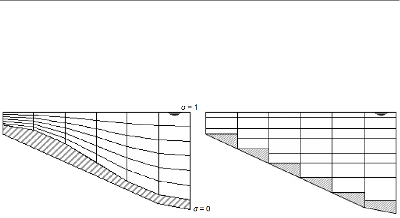
DRAFT
Hydrodynamics
irrespective of the local water depth. The distribution of the relative layer thickness is usually
non-uniform. This allows for more resolution in the zones of interest such as the near surface
area (important for e.g. wind-driven flows, heat exchange with the atmosphere) and the near
bed area (sediment transport). Please note that in D-Flow FM, unlike Delft3D, the σcoordinate
is equal to zero on the bed is 1on the water surface.
Figure 7.1: Example of σ-model (left) and Z-model (right).
Although the σ-grid is boundary fitted (in the vertical), it will not always have enough reso-
lution around the pycnocline. The co-ordinate lines intersect the density interfaces that may
give significant errors in the approximation of strictly horizontal density gradients (Leendertse,
1990;Stelling and Van Kester,1994). Therefore, Z-model was introduced in D-Flow FM for 3D
simulations of weakly forced stratified water systems. The Z-model has horizontal co-ordinate
lines that are (nearly) parallel with density interfaces (isopycnals) in regions with steep bed
slopes. This is important to reduce artificial mixing of scalar properties such as salinity and
temperature. The Z-model is not boundary-fitted in the vertical. The bed (and free surface) is
usually not a co-ordinate line and is represented as a staircase (zig-zag boundary).
7.3.1 Topological conventions
A computational cell in a D-Flow FM grid (sometimes referred to as a ’network’) consists of
corner nodes and edges connecting the corner nodes. Such a grid cell should contain at least
three corner nodes and at most six corner nodes. The following topological conventions are
used:
netnodes: corners of a cell (triangles, quadrangles, ...),
netlinks: edges of a cell, connecting netnodes,
flownodes: the cell circumcentre, in case of triangles the exact intersection of the three
perpendicular bisectors and hence also the centre of the circumscribing circle,
flowlinks: a line segment connecting two flownodes.
Deltares 113 of 412
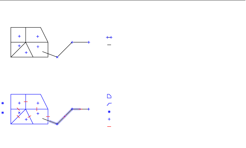
DRAFT
D-Flow Flexible Mesh, User Manual
net node
net link (2D)
net link (1D)
pressure points: 2D flow node circumcenter/1D flow node
flow link
netcell/flow node (2D)
netcell/flow node (1D)
1. Net (domain discretization)
2. Flow data (1D+2D)
(1..NUMK)
(1..NUML1D)
(NUML1D+1..NUML)
(1..NDX2D=NUMP)
(NDX2D+1..NDXI)
boundary flow node (NDXI+1..NDX)
(1..LNX1D)
(LNX1D..LNXI)
(LNXI+1..LNX1DBND)
(LNX1DBND+1..LNX)
1D internal
2D internal
1D open bnd
2D open bnd
Figure 7.2: Flexible mesh topology
This mesh topology is illustrated in Figure 7.2. The ’center’ of a cell can be defined in multiple
ways. To illustrate this, two conventional cell center definitions for a triangle are highlighted in
Figure 7.3. The two displayed cell centers have different properties:
1 the circumcenter is the location within the triangle which is the center point of a circle
that intersects the triangle at each corner node of the triangle; as a consequence, the
orthogonal projection of the center point to each face of the triangle divides each face into
two exactly equidistant pieces,
2 the mass center (or centroid) is the center of gravity; as a consequence, a line through a
corner node and the mass center divides a face into two exactly equidistant pieces under
an angle not necessarily equal to 90◦.
114 of 412 Deltares

DRAFT
Hydrodynamics
Figure 7.3: Two conventional definitions of the cell center of a triangle: the circumcenter
and the mass center.
D-Flow FM utilizes the circumcenter as the basis of the definition of the elementary flow vari-
ables ’water level’ and ’flow velocity’. The water level is defined at the circumcenter, whereas
the face normal flow velocity is defined at the orthogonal projection of the circumcenter onto
the cell face, i.e., the midpoint of the cell face.
Important properties of the mesh are the orthogonality and smoothness. The orthogonality
is defined as the cosine of the angle ϕbetween a flowlink and a netlink. Ideally 0, angle
ϕ= 90◦. The smoothness of a mesh is defined as the ratio of the areas of two adjacent
cells. Ideally 1, the areas of the cells are equal to each other. A nearly ideal setup is shown
in Figure 7.4.
Figure 7.4: Perfect orthogonality and nearly perfect smoothness along the edge connect-
ing two triangles. Black lines/dots are network links/nodes, blue lines/dots are
flow links/nodes.
It is quite easy (and therefore dangerous) to generate meshes that violate the orthogonality
Deltares 115 of 412
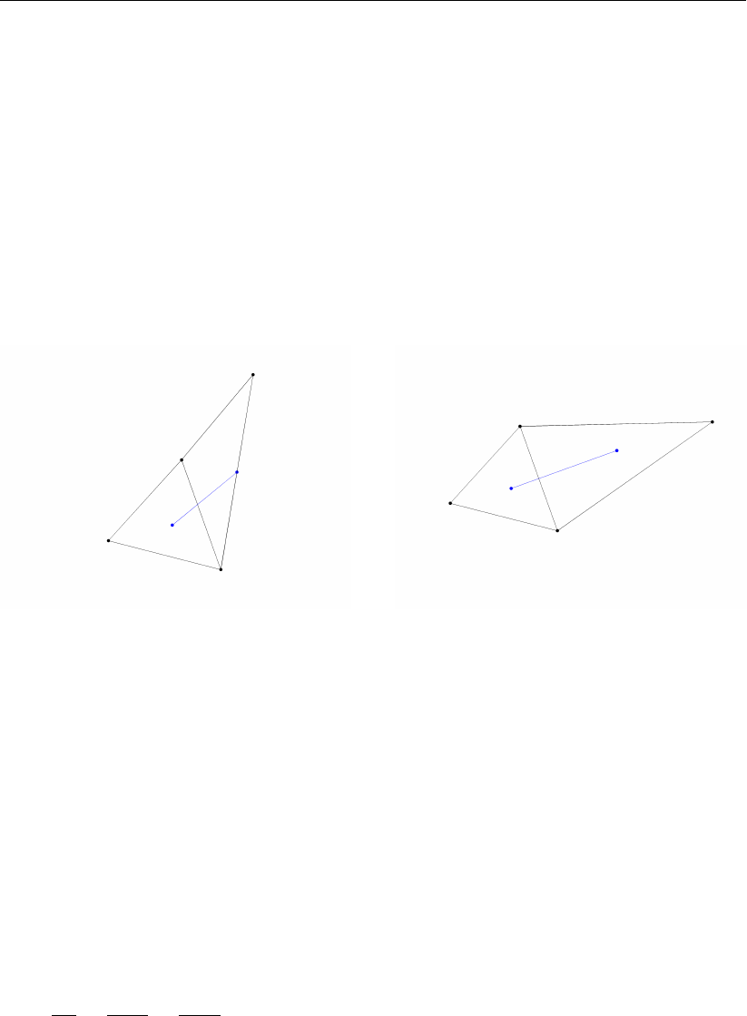
DRAFT
D-Flow Flexible Mesh, User Manual
and smoothness requirements. In Figure 7.5, two different setups of two gridcells are shown
with different mesh properties.
The left picture of Figure 7.5 shows how orthogonality can be detoriated by skewing the right
triangle with respect to the left triangle. While having the same area (perfect smoothness),
the mutually oblique orientation results in poor orthogonality. In this particular case, the centre
of the circumscribing circle is in principle located outside the right triangle. Such a triangle is
denoted as an ’open’ triangle, which is bad for computations.
The opposite is shown in the right picture of Figure 7.5 in which the right triangle has strongly
been elongated, disturbing the smoothness property. However, the orthogonality is nearly
perfect. Nonetheless, both meshes need to be improved to assure accurate model results.
(a) Perfect smoothness, but poor orthogonality. (b) Perfect orthogonality, but poor smoothness
Figure 7.5: Poor mesh properties due to violating either the smoothness or the orthog-
onality at the edge connecting two triangles. Black lines/dots are network
links/nodes, blue lines/dots are flow links/nodes.
7.3.2 Conservation of mass and momentum
In this section, we will present in detail the governing equations for mass and momentum con-
servation. These equations are indicated by a continuity equation and momentum equations.
7.3.2.1 Continuity equation
D-Flow FM solves the depth-averaged continuity equation, derived by integration the continu-
ity equation, for incompressible fluids (∇•u= 0) over the total depth, taken into account the
kinematic boundary conditions at water surface and bed level, and is given by:
∂h
∂t +∂Uh
∂x +∂V h
∂y =Q(7.1)
with Uand Vthe depth averaged velocities. Qis representing the contributions per unit area
due to the discharge or withdrawal of water, precipitation and evaporation:
Q=Zh
0
(qin −qout)dz +P−E(7.2)
with qin and qout the local sources and sinks of water per unit of volume [1/s], respectively, P
the non-local source term of precipitation and Enon-local sink term due to evaporation. We
remark that the intake of, for example, a power plant is a withdrawal of water and should be
modelled as a sink. At the free surface there may be a source due to precipitation or a sink
due to evaporation.
116 of 412 Deltares

DRAFT
Hydrodynamics
7.3.2.2 Momentum equations in horizontal direction
The momentum equations in x- and y-direction are given by:
∂u
∂t +u∂u
∂x +v∂u
∂y +w∂u
∂z −fv =−1
ρ0
∂P
∂x +Fx+∂
∂z νV
∂u
∂z +Mx(7.3)
∂v
∂t +u∂v
∂x +v∂v
∂y +w∂v
∂z +fu =−1
ρ0
∂P
∂y +Fy+∂
∂z νV
∂v
∂z +My(7.4)
Where νVis the vertical eddy viscosity coefficient. Density variations are neglected, except
in the baroclinic pressure terms, ∂P/∂x and ∂P/∂y represent the pressure gradients.
The forces Fxand Fyin the momentum equations represent the unbalance of horizontal
Reynolds stresses.
Mxand Myrepresent the contributions due to external sources or sinks of momentum (ex-
ternal forces by hydraulic structures, discharge or withdrawal of water, wave stresses, etc.).
The effects of surface waves on the flow as modelled in D-Flow FM are described in sec-
tion 15.2.
7.3.2.3 Vertical velocities
The vertical velocity win the adapting σco-ordinate system is computed from the continuity
equation:
∂h
∂t +∂uh
∂x +∂vh
∂y +∂w
∂z =h(qin −qout)(7.5)
At the surface the effect of precipitation and evaporation is taken into account. The vertical
velocity wis defined at the iso σ-surfaces. wis the vertical velocity relative to the moving
σ-plane. It may be interpreted as the velocity associated with up- or downwelling motions.
7.3.3 The hydrostatic pressure assumption
Under the shallow water assumption, the vertical momentum equation is reduced to a hydro-
static pressure equation. Vertical accelerations due to buoyancy effects and due to sudden
variations in the bed topography are not taken into account. So:
∂P
∂z =−ρgh (7.6)
For water of constant density and taking into account the atmospheric pressure, it includes
gradients of the free surface level, called barotropic pressure gradients. The atmospheric
pressure is included in the system for storm surge simulations. The atmospheric pressure
gradients dominate the external forcing at peak winds during storm events. Space and time
varying wind and pressure fields are especially important when simulating storm surges.
In case of a non-uniform density the pressure gradients includes not only barotropic pressure
gradient, but also vertical pressure gradient, the so called baroclinic pressure gradient. The
baroclinic pressure gradient is the result of variable distribution of density and temperature in
the vertical direction.
In the horizontal gradient a vertical derivative is introduced by the σco-ordinate transforma-
tion. In estuaries and coastal seas the vertical grid may deteriorate strongly in case of steep
Deltares 117 of 412
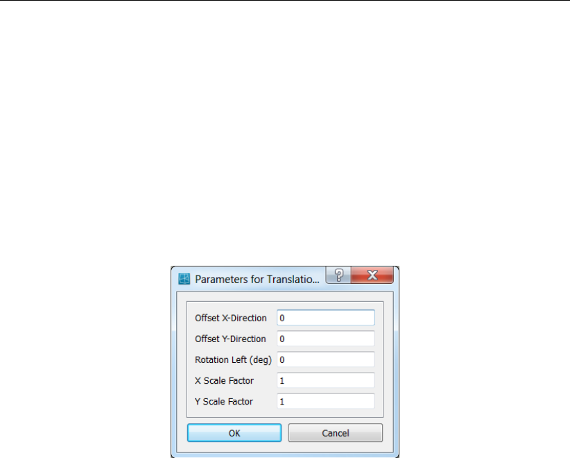
DRAFT
D-Flow Flexible Mesh, User Manual
bed slopes. In order to avoid artificial flow the numerical approximation of the baroclinic pres-
sure terms requires a special numerical approach. The treatment of D-Flow FM to avoid the
artificial mixing due to σco-ordinates are discussed in section 7.5, see also Stelling and Van
Kester (1994).
7.3.4 The Coriolis force
The Coriolis parameter fdepends on the geographic latitude φand the angular speed of
rotation of the earth, Ω(f= 2Ω sin φ). For a grid the user should specify the space varying
Coriolis parameter, using a suitable projection. This can be done by selecting Coordinate
System in RGFGRID, and selection of the option for Spherical Coordinate. The parameters
for translation and rotation can be given as shown in Figure 7.6.
Figure 7.6: Input for map projection for specifying Coriolis parameter on the grid.
7.3.5 Diffusion of momentum
The forces Fxand Fyin the horizontal momentum equations represent the unbalance of
horizontal Reynolds stresses. The Reynolds stresses are modelled using the eddy viscosity
concept, (for details e.g. Rodi (1984)). This concept expresses the Reynolds stress compo-
nent as the product between a flow as well as grid-dependent eddy viscosity coefficient and
the corresponding components of the mean rate-of-deformation tensor. The meaning and the
order of the eddy viscosity coefficients differ for 2D and 3D, for different horizontal and vertical
turbulence length scales and fine or coarse grids. In general the eddy viscosity is a function
of space and time.
For 3D shallow water flow the stress tensor is an-isotropic. The horizontal eddy viscosity
coefficient, νH, is much larger than the vertical eddy viscosity νV(νHνV). The horizontal
viscosity coefficient may be a superposition of three parts:
1 a part due to "sub-grid scale turbulence",
2 a part due to "3D-turbulence" see Uittenbogaard et al. (1992) and
3 a part due to dispersion for depth-averaged simulations.
In simulations with the depth-averaged momentum and transport equations, the redistribution
of momentum and matter due to the vertical variation of the horizontal velocity is denoted
as dispersion. In 2D simulations this dispersion is not simulated as the vertical profile of the
horizontal velocity is not resolved. Then this dispersive effect may be modelled as the product
of a viscosity coefficient and a velocity gradient. The dispersion term may be estimated by the
Elder formulation.
118 of 412 Deltares
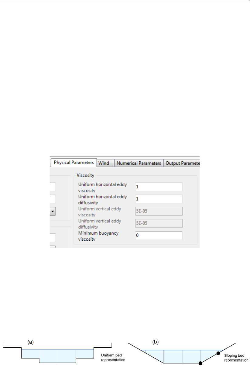
DRAFT
Hydrodynamics
If the vertical profile of the horizontal velocity is not close to a logarithmic profile (e.g. due to
stratification or due to forcing by wind) then a 3D-model for the transport of matter is recom-
mended.
The horizontal eddy viscosity is mostly associated with the contribution of horizontal turbulent
motions and forcing that are not resolved by the horizontal grid ("sub-grid scale turbulence") or
by (a priori) the Reynolds-averaged shallow-water equations. in 3D, in the vertical direction,
νVis referred to as the three-dimensional turbulence and in it is computed following a 3D-
turbulence closure model.
Therefore, in addition to all turbulence closure models in D-Flow FM a constant (space and
time) background mixing coefficient may be specified by the user, which is a background
value for the vertical eddy viscosity in the momentum Equation (7.3) and Equation (7.4) con-
sequently.
The horizontal and vertical eddy viscosities can be set by user defined value under Physical
Parameters shown in Figure 7.7.
Figure 7.7: Input parameters for horizontal and vertical eddy viscosities.
7.3.6 Conveyance in 2D
Bed friction often plays a major role in the discharge capacity and expected maximum water
levels of channels and gullies. If we model a trapezoidal channel with sloping sidewalls on a
grid with 6 grid cells across the width of the channel, a typical cross section using the standard
bed representation with uniform depth appears per cell (Figure 7.8a). In D-Flow FM, we allow
for representation of a locally sloping bed as shown in Figure 7.8b.
Figure 7.8: Bed representation with uniform depth levels (a), and locally sloping bed (b).
The most left and the most right cell are not yet wet in the uniform bed representation. In
the sloping bed representation, these outer cells are partly wet, yielding a more accurate
description of the total wet cross sectional area. The user can select whether to apply this
Deltares 119 of 412

DRAFT
D-Flow Flexible Mesh, User Manual
more accurate description or not. This can only be done only in combination with a net-node
based bathymetry description, i.e. using the keyword Ibedlevtype = 3 in the .mdu file.
For the bed friction in 2D models, one implicitly assumes a fully developed vertical velocity
profile, using a logarithmic function of the water depth for the White-Colebrook bed friction
formulation, or a one-sixth power function of the water depth for the Manning formulation. In a
sloping cell, the local water depth is varying over the width of the cell. In the deeper part flow
velocities will be higher than in the shallower part. Bed stresses will vary over the width of a
cell with water depth and with the velocity. Integrating the stresses over the width of a cell one
can derive the resulting total stress.
The bed friction term is not only a function of the normal velocity component in the direction
of the flow link itself, but also depends on the tangential velocity component and with that on
the total velocity. For each of the four components water depth, normal velocity, total velocity
and Chézy parameter, we assume a linear variation over the width (Figure 7.9).
If we have in the .mdu file Conveyance2D = 3, the 2D analytic conveyance description
using these four linearly varying components is applied. This option shows best grid conver-
gence behaviour. Good grid convergence implies that the converged answer can be achieved
on a coarser grid, thus saving computational costs.
If one sets Conveyance2D = 2, the tangential velocity component is assumed zero. This
method is only applicable on curvilinear grids that are aligned with the flow direction.
If one sets Conveyance2D = 1, both the normal and tangential velocity component are
assumed constant over the width. Effectively one obtains the so called ’lumped’ bed friction
approach, with hydraulic radius R=A/P ,Abeing the wet cross sectional area and Pthe
wet perimeter. This method works equally well as methods 2 and 1, provided that there is
sufficient resolution of a gully in the grid. It is found that when a gully is resolved by more than
about 10 or 12 cells, it provides almost identical answers as method 2, while saving some
10 % computational overhead compared to method 2.
Setting Conveyance2D = -1, the hydraulic radius is based on a uniform bed level at the
velocity point taken as the average bed level of the two surrounding net nodes (depth points
in WAQUA terms). This option is identical to the combination of WAQUA option dpuopt =
mean i.c.m. dpsopt = max.
Setting Conveyance2D = 0, the hydraulic radius is based on a uniform bed level at the
velocity point taken as the average bed level of the two surrounding water level points. This
option is not advisable because cell bed levels are taken as the minimum value of the bed
levels of attached link. So a min-max operator is invoked, which is not suitable for accuracy.
7.4 Hydrodynamics boundary conditions
In section 4.4.8, the boundary conditions are discussed from the viewpoint of the user inter-
face. In the user interface, the user can specify the locations at which particular boundary
conditions are to be imposed. Using section 4.4.8 as a backdrop, the present section dis-
cusses the underlying files and fileformats and the way these are interpreted by the computa-
tional kernel. Three types of boundary conditions are discussed in this section, namely open
boundaries (in section 7.4.1), vertical boundaries (in section 7.4.2) and closed boundaries (in
section 7.4.3).
120 of 412 Deltares
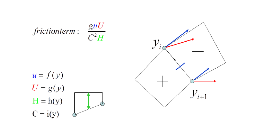
DRAFT
Hydrodynamics
Figure 7.9: A shematic view of the linear variation over the width for calculating the flow
parameters.
7.4.1 Open boundary conditions
The proper prescription of an open boundary condition along a certain (part of the) rim of the
grid can be achieved by considering four elements of the model:
1 a polyline file (extension .pli), containing the locations at which the boundary conditions
should be imposed,
2 a boundary conditions file (extension .bc), containing the key physical information, such
the time dependent information of the quantity under consideration and the physical nature
of the quantity itself,
3 an external forcing file (extension .ext), in which the connection is laid between the
polyline file and the boundary conditons file,
4 the prescription of the single external forcing file, containing the connection between loca-
tion and physical information, in the master definition file (extension .mdu).
These four elements are subsequently discussed in the following.
7.4.1.1 The location of support points
The flow engine needs the specification of support points for the boundary conditions (also
see section 4.4.8.1). By default, these support points are a means to construct a series of
virtual cell centers along the boundary rim of the grid. Figure 7.10 provides an image of this
concept.
Deltares 121 of 412
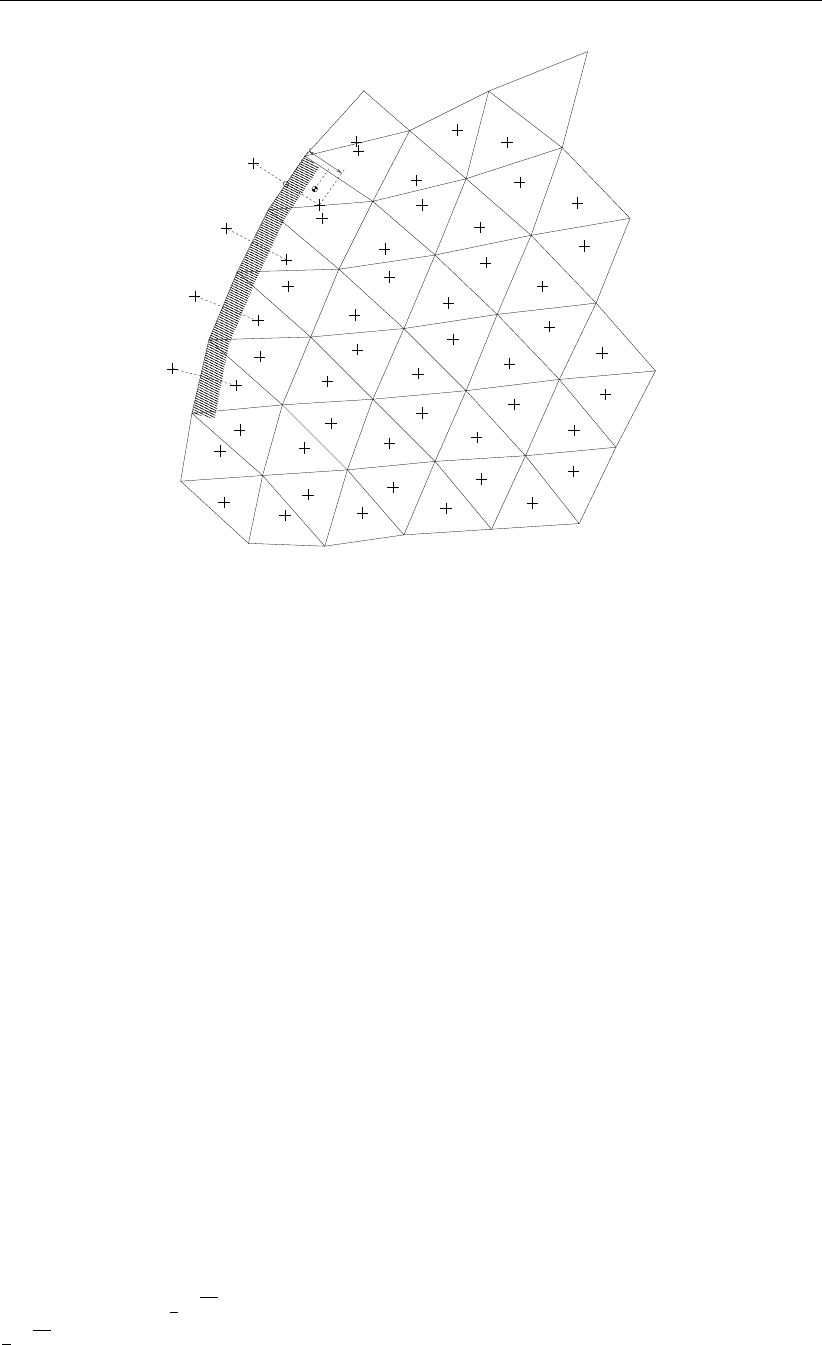
DRAFT
D-Flow Flexible Mesh, User Manual
xR(j)
bj
xL(j)dj
Figure 7.10: Virtual boundary ’cells’ near the shaded boundary; xLj is the virtual ’cell’
center near boundary face j;xR(j)is the inner-cell center; bjis the point on
face jthat is nearest to the inner-cell center
The support points are stored as one single polyline per boundary condition, marking the rim
along which the boundary conditions should hold. The polyline should be drawn in the vicinity
of the rim. The user can specify the size of this ‘vinicity’ by means of the MDU-file keyword
OpenBoundaryTolerance. The keyword specifies the search tolerance factor between
the boundary polyline and the grid cells. The unit of this keyword is the cell size unit (i.e., not
metres). By default, this value is 3, which loosely means that in the vinicity of 3∆xof the grid
rim is searched of a boundary condition polyline.
The actual location of a specific boundary location point can be computed in three different
ways, dependent on the user’s choice for the keyword izbndpos in the MDU-file:
1izbndpos = 0: construction of the boundary condition point by means of orthogonal
mirroring of the closest cell center,
2izbndpos = 1: construction of the boundary condition point as the orthogonal projec-
tion of the closest cell center onto the grid rim,
3izbndpos = 2: construction of the boundary condition point as the actual location of
the support points spanning the polyline.
Only the option izbndpos = 0 is discussed; the other two options are not yet fully opera-
tional. The mirroring of the closest cell center is conducted as follows. First, the orthogonal
distance from the boundary cell center to the actual rim of the grid is computed: djin Fig-
ure 7.10. Second, the cell center of the outside virtual cell is defined at a distance djoutside
of the grid. However, the flat area of the cell, say A, at the rim can give rise to an adaptation
of this distance. If 1
2√A > dj, then the center of the virtual cell is located at the a distance
1
2√Aaway from the grid.
122 of 412 Deltares

DRAFT
Hydrodynamics
7.4.1.2 Physical information
In the bc-file, multiple types of boundary conditions can be prescribed. In this section, the
boundary conditions for the flow motion are briefly reflected on.
Water level
A water level signal is applied at the cell center of the virtual cell outside the grid (ghost cells
or mirror cells). Water levels can be imposed as a timeseries or as a harmonic signal. In
case of a harmonic signal, the period of the signal can be given as an astronomic component
acronym.
If a timeseries is applied to a the first support point of a polyline named arbitraryname,
prescribed in some polyline file, then the header of the bc-file is:
[forcing]
Name = arbitraryname_0001
Function = timeseries
Time-interpolation = linear
Quantity = time
Unit = minutes since YYYY-MM-DD
Quantity = waterlevelbnd
Unit = m
[two-column data]
The data is to be inserted as a two-column array containing the time (in minutes) and the
water level itself (in meters w.r.t. the reference level). In case of harmonic components, the
header of the bc-file is:
[forcing]
Name = arbitraryname_0001
Function = harmonic
Quantity = harmonic component
Unit = minutes
Quantity = waterlevelbnd amplitude
Unit = m
Quantity = waterlevelbnd phase
Unit = degrees
[three-column data]
The data is to be inserted as a three-column array containing the period (in minutes), the
amplitude (in meters) and the phase (in degrees). If the period is Tminutes, the amplitude is
Ameters and the phase is ϕdegrees, then the signal that is applied reads
h(t) = B+Acos(2πt/T −ϕ).(7.7)
The parameter Bcan be prescribed by an additional signal with a period specified equal to
0 minutes. As an example, the data series:
0.0 0.5 0.0
745.0 2.0 0.0
Deltares 123 of 412

DRAFT
D-Flow Flexible Mesh, User Manual
represents the signal h(t)=0.5+2.0 cos(2πt/745), with the time tin minutes.
Discharge
A discharge boundary condition is applied at the face-center of the virtual boundary cell. For
this, the face-normal velocity is used in combination with the face-center water depth. The
face-based water depth in the evaluation of the flow area can optionally be set to a downwind
approximation (for an inflowing discharge boundary) with the option jbasqbnddownwindhs
= 1 (default value).
Discharges can be imposed as a timeseries or as a harmonic signal. In case of a harmonic
signal, the period of the signal can be given as an astronomic component acronym.
If a timeseries is applied to a the first support point of a polyline named arbitraryname,
prescribed in some polyline file, then the header of the bc-file is:
[forcing]
Name = arbitraryname_0001
Function = timeseries
Time-interpolation = linear
Quantity = time
Unit = minutes since YYYY-MM-DD
Quantity = dischargebnd
Unit = m3/s
[two-column data]
The data is to be inserted as a two-column array containing the time (in minutes) and the
water level itself (in meters w.r.t. the reference level). In case of harmonic components, the
header of the bc-file is:
[forcing]
Name = arbitraryname_0001
Function = harmonic
Quantity = harmonic component
Unit = minutes
Quantity = dischargebnd amplitude
Unit = m3/s
Quantity = dischargebnd phase
Unit = degrees
[three-column data]
The data is to be inserted as a three-column array containing the period (in minutes), the
amplitude (in cubic meters per second) and the phase (in degrees).
Velocity
A velocity boundary condition is applied at the face-center of the virtual boundary cell. Values
provided are interpreted as face-normal velocities. Velocities can be imposed as a timeseries
or as a harmonic signal. In case of a harmonic signal, the period of the signal can be given
as an astronomic component acronym.
124 of 412 Deltares

DRAFT
Hydrodynamics
If a timeseries is applied to a the first support point of a polyline named arbitraryname,
prescribed in some polyline file, then the header of the bc-file is:
[forcing]
Name = arbitraryname_0001
Function = timeseries
Time-interpolation = linear
Quantity = time
Unit = minutes since YYYY-MM-DD
Quantity = velocitybnd
Unit = m/s
[two-column data]
The data is to be inserted as a two-column array containing the time (in minutes) and the
water level itself (in meters w.r.t. the reference level). In case of harmonic components, the
header of the bc-file is:
[forcing]
Name = arbitraryname_0001
Function = harmonic
Quantity = harmonic component
Unit = minutes
Quantity = velocitybnd amplitude
Unit = m/s
Quantity = velocitybnd phase
Unit = degrees
[three-column data]
The data is to be inserted as a three-column array containing the period (in minutes), the
amplitude (in meters per second) and the phase (in degrees).
Water level gradient
Besides the option to prescribe actual water levels as a boundary condition, D-Flow FM facil-
itates the prescription of water level gradients. Such a Neumann-type boundary condition for
the water level can be assigned through the keyword neumannbnd. The value of the water
level gradient is applied at the face-center.
Water level gradients can be imposed as a timeseries or as a harmonic signal. In case of a
harmonic signal, the period of the signal can be given as an astronomic component acronym.
If a timeseries is applied to a the first support point of a polyline named arbitraryname,
prescribed in some polyline file, then the header of the bc-file is:
[forcing]
Name = arbitraryname_0001
Function = timeseries
Time-interpolation = linear
Quantity = time
Unit = minutes since YYYY-MM-DD
Quantity = neumannbnd
Deltares 125 of 412

DRAFT
D-Flow Flexible Mesh , User Manual
Unit = -
[two-column data]
The data is to be inserted as a two-column array containing the time (in minutes) and the
water level itself (in meters w.r.t. the reference level). In case of harmonic components, the
header of the bc-file is:
[forcing]
Name = arbitraryname_0001
Function = harmonic
Quantity = harmonic component
Unit = minutes
Quantity = neumannbnd amplitude
Unit = -
Quantity = neumannbnd phase
Unit = degrees
[three-column data]
The data is to be inserted as a three-column array containing the period (in minutes), the
amplitude (in meters per second) and the phase (in degrees). The water level gradient is
interpreted positive in the outward-normal direction.
Riemann invariant
At a Riemann boundary we do not allow any outgoing perturbation with respect to some
reference boundary state to reflect back from the boundary. This is achieved by prescribing
the incoming Riemann invariant. Using the convention of a positive inward normal at the
boundary, this can be put as ub+ 2√gHb, with ubthe velocity at the boundary and Hbthe
total water depth at the boundary. In this expression, we take the boundary values uband Hb
as the reference boundary state. While applying Riemann boundaries, directional effects are
disregarded.
Using linearization and the assumption of a flow field that is initially at rest, the Riemann
boundary is rewritten such that is takes the form:
ζ= 2ζb−sH
gu−ζ0(7.8)
with ζthe surface level elevation, Hthe total water depth, gthe gravitational acceleration, u
the velocity (positive inward) and ζ0the initial surface level elevation. Instead of prescribing
a combination of the velocity and the water level, we prefer to prescribe only the water level
at the boundary, i.e. ζb. The value for ζbis supposed to be provided by the user (as well as,
obviously, the initial surface level elevation ζ0).
A water level for Riemann boundary can be imposed as a timeseries or as a harmonic sig-
nal. In case of a harmonic signal, the period of the signal can be given as an astronomic
component acronym. If a timeseries is applied to a the first support point of a polyline named
arbitraryname, prescribed in some polyline file, then the header of the bc-file is:
[forcing]
Name = arbitraryname_0001
126 of 412 Deltares

DRAFT
Hydrodynamics
Function = timeseries
Time-interpolation = linear
Quantity = time
Unit = minutes since YYYY-MM-DD
Quantity = riemannbnd
Unit = m
[two-column data]
The data is to be inserted as a two-column array containing the time (in minutes) and the
water level for Riemann boundary (in meters). In case of harmonic components, the header
of the bc-file is:
[forcing]
Name = arbitraryname_0001
Function = harmonic
Quantity = harmonic component
Unit = minutes
Quantity = riemannbnd amplitude
Unit = m
Quantity = riemannbnd phase
Unit = degrees
[three-column data]
The data is to be inserted as a three-column array containing the period (in minutes), the
amplitude (in meters per second) and the phase (in degrees).
Suppose, as an example, that we have:
a flow domain with a bathymetry at a bed level equal to 0 m w.r.t. the reference level,
an initial water level equal to 10 m w.r.t. the reference level,
a local initial disturbance of the initial water level,
and an initial flow field at rest,
and that we aim to prevent reflections at the boundary. In that case, it follows from Equa-
tion (7.8) that ζb= 10 m w.r.t. the reference level is to be prescribed. Remark that this
application only holds for small disturbances of ζfrom ζb.
Discharge-water level dependency
If a relation between the discharge and the local water level is known on beforehand, then
this relation can be provided to the flow model as a table by means of the keyword qhtable.
This table, provides the water level ζas a function of the computed discharge Q.
If a Qh-table is applied to a the first support point of a polyline named arbitraryname,
prescribed in some polyline file, then the header of the bc-file is:
[forcing]
Name = arbitraryname_0001
Function = qhtable
Quantity = qhbnd discharge
Unit = m3/s
Quantity = qhbnd waterlevel
Deltares 127 of 412
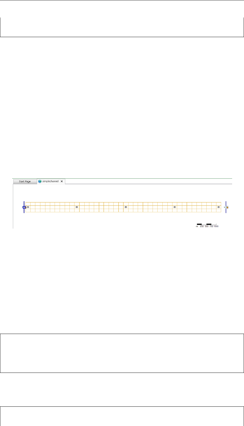
DRAFT
D-Flow Flexible Mesh , User Manual
Unit = m
[two-column data]
The data is to be inserted as a two-column array containing the discharge (in cubic meters
per second) and the water level (in meters w.r.t. the reference level).
The user is able to apply a weighting parameter to compromise between the water level com-
puted by the Qh-relation and the water level computed at the previous time step level. This
parameter is accessible as the keyword Qhrelax in the MDU-file. By default, this parameter
is 0.01. As a consequence, the newly computed water level consists of the Qh-relation result
for 1 % and for 99 % of the previous time step water level.
7.4.1.3 Example
Recalling the four elementary actions from the beginning of section 7.4.1, the administration
in files can be illustrated by means of an example. Suppose, we have a channel that is
geometrically modelled by means of the grid shown in Figure 7.11. The domain is 10000 m
long and 500 m wide. The bottom left corner coincides with the origin of the geometrical frame
of reference.
Figure 7.11: Delta-Shell view of a simple channel covered by a straightforward Cartesian
grid. Boundary conditions are prescribed at the left hand side and the right
hand size of the domain.
The domain shown in Figure 7.11 contains two boundaries: on the left hand, a discharge
boundary condition is present to present flow entering the domain, on the right hand, a water
level boundary condition is set. Having two boundaries, we have two polyline files, in this
example: left.pli and right.pli.
The contents of left.pli are:
boundaryleft
2 2
-80 -50
-80 550
whereas the contents of right.pli are:
boundaryright
2 2
128 of 412 Deltares

DRAFT
Hydrodynamics
10250 -50
10250 550
Notice that both polyline files contain the name of the polyline, namely boundaryleft
and boundaryright, respectively. In this example, both the polylines contain two support
points. For each of these support points, timeseries can be prescribed. In this example,
we restrict ourselves to homogeneous boundary conditions. This means that we have to
prescribe physical information for the first support points, i.e. for boundaryleft_0001
and boundaryright_0001.
The physical information should be provided in the bc-file. In this example, we use the follow-
ing bc-file:
[forcing]
Name = boundaryleft_0001
Function = timeseries
Time-interpolation = linear
Quantity = time
Unit = minutes since 2001-01-01
Quantity = dischargebnd
Unit = m3/s
0.000000 2500.0
120.000000 3000.0
240.000000 2500.0
360.000000 2000.0
480.000000 2500.0
600.000000 3000.0
720.000000 2500.0
840.000000 2000.0
960.000000 2500.0
1080.000000 3000.0
1200.000000 2500.0
1320.000000 2000.0
1440.000000 2500.0
[forcing]
Name = boundaryright_0001
Function = timeseries
Time-interpolation = linear
Quantity = time
Unit = minutes since 2001-01-01
Quantity = waterlevelbnd
Unit = m
0.000000 2.50
1440.000000 2.50
This file couples the timeseries for the discharge to the support point named boundaryleft_0001.
Likewise, the water level boundary, being constant in time, is coupled to the support point
named boundaryright_0001.
The final specification of the boundary conditions is wrapped up in the external forcing file,
with extension .ext. In this file, the connection is laid between the quantity of the bound-
ary condition, the name of the polyline file (in which the name of the polyline itself is given)
and the forcing file (in which the physical information is provided). In our example, the file
simplechannel.ext has the following contents:
Deltares 129 of 412

DRAFT
D-Flow Flexible Mesh, User Manual
[boundary]
quantity = dischargebnd
locationfile = left.pli
forcingfile = simplechannel.bc
[boundary]
quantity = waterlevelbnd
locationfile = right.pli
forcingfile = simplechannel.bc
The final step is to let the model know that the external forcings file simplechannel.ext
is the one that should be used. This is to be achieved in the MDU-file:
[external forcing]
ExtForceFile =
ExtForceFileNew = simplechannel.ext
Notice that the name is specified at the keyword ExtForceFileNew. The other keyword,
ExtForceFile, should be kept empty, unless deprecated .tim-files and/or .cmp-files are
used to prescribe the physical information for the boundaries.
7.4.1.4 Miscellaneous
In the previous sections, the most essential information on the application of boundary condi-
tions is described. Some remaining aspects are discussed in this section.
Artificial boundary layers
Advection terms at the offshore boundary may generate an artificial boundary layer along the
boundary. The advection terms containing normal gradients have to be switched off. This is
done by utilizing the keyword jacstbnd in the MDU-file. By default this keyword jacstbnd
= 0, keeping the functionality inactive. The keyword can be set to jacstbnd = 1 to do
otherwise.
Smoothing parameter boundary conditions
The solution of the shallow water equations is uniquely determined by a set of initial and
boundary conditions. The boundary conditions represent the external forcing and determine
the steady state solution. The deviation between the initial condition and the steady state
solution generates a transient (mass spring system analogy).
In D-Flow FM, the initial conditions for the water level and velocities are obtained from:
The results of a previous run (warm start).
User-prescribed (space varying or uniform) input fields (cold start).
The initial values are usually inconsistent with the boundary conditions at the start time of the
simulation. This will generate a transient solution consisting of waves with eigen frequencies
of the model domain. These waves may be reflected at the boundaries and generate a stand-
ing wave system. The waves should be dissipated completely by bottom friction and viscosity
130 of 412 Deltares

DRAFT
Hydrodynamics
terms or leave the domain through the open boundaries. The damping of the transient solution
determines the spin-up time of the numerical model.
To reduce the amplitude of the transient wave and the spin-up time of a model, D-Flow FM has
an option to switch on the boundary forcing gradually by use of a smoothing period (parameter
Tsmo). With Fi(t)the initial value at the boundary, Fb(t)the boundary condition signal and
Fsmo
b(t)the boundary conditiona fter smoothing, the boundary forcing is given by:
Fsmo
b(t) = αFi(t) + (1 −α)Fb(t),(7.9)
with:
α=Tsmo −t
Tsmo
(7.10)
if t < Tsmo. In case t≥Tsmo, then the smoothing parameter is set to zero: α= 0.
Smoothing is possible both for a warm and a cold start. If the initial conditions are consistent
with the boundary conditions at the start time of the simulation then the smoothing time should
be set to zero.
Secondary boundary conditions
In section 7.4.1.2, several types of boundary conditions are discussed. In addition, two
types of boundary conditions can be applied on top of the canonical types: normal veloc-
ities and tangential velocities. The associated keyword are normalvelocitybnd and
tangentialvelocitybnd, respectively.
7.4.2 Vertical boundary conditions
Vertical boundary conditions close the system of shallow water equations at the bed level and
the free surface level. Please refer to the Delft3D-FLOW User Manual, Section 9.4.1.1.
7.4.3 Shear-stresses at closed boundaries
A closed boundary is situated at the transition between land and water. At a closed boundary,
two boundary conditions have to be prescribed. One boundary condition has to do with the
flow normal to the boundary and the other one with the shear-stress along the boundary.
A closed sidewalls is always considered as impermeable. For the shear stress along the
boundary, the possible conditions to be prescribed are free-slip (zero tangential shear-stress),
partial-slip and full-slip.
For large-scale simulations, the influence of the shear-stresses along closed boundaries can
be neglected. Free slip is then applied for all closed boundaries. For simulations of smallscale
flow (e.g. laboratory scale), the influence of the side walls on the flow may no longer be
neglected. This option has been implemented for closed boundaries and dry points but not for
thin dams. The reason is that the shear stress at a thin dam is dependent on the side (double
valued).
Along the side walls, the tangential shear stress is calculated based on a logarithmic law of
the wal. The friction velocity u∗is determined by the logarithmic law for a rough wall, with side
wall roughness y0and the velocity in the first grid point near the side wall. Let ∆ysbe the
grid size normal to the sidwall, then:
|→
usidewall|=u∗
κln 1 + ∆ys
2y0(7.11)
Deltares 131 of 412

DRAFT
D-Flow Flexible Mesh, User Manual
The choice for the way tangial shear stress are computed can be inserted through the key
irov in the MDU-file (under [physics]):
the case irov = 0 treats the side walls as free-slip walls (default),
the case irov = 1 treats the side walls as partial-slip walls,
the case irov = 2 treats the side walls as no-slip walls.
If the choice for partial-slip walls is made, then a specific wall roughness value should be pre-
scribed in the MDU-file. For this, the keyword wall_ks should be used (under [physics]
in the MDU-file). The computational engine interpretes this value as Nikuradse roughness ks.
The value for y0is computed as y0=ks/30.
7.5 Artificial mixing due to sigma-coordinates
The σ-transformation is boundary-fitted in the vertical. The bottom boundary and free surface
are represented smoothly. The water column is divided into the same number of layers inde-
pendent of the water depth. In a σ-model, the vertical resolution increases automatically in
shallow areas.
For steep bottom slopes combined with vertical stratification, σ-transformed grids introduce
numerical problems for the accurate approximation of horizontal gradients both in the baro-
clinic pressure term and in the horizontal diffusion term. Due to truncation errors artificial
vertical mixing and artificial flow may occur, Leendertse (1990) and Stelling and Van Kester
(1994). This artificial vertical transport is sometimes called "creep".
Let zbbe the position of the bed and Hthe total water depth. If we consider the transformation
from Cartesian co-ordinates to σco-ordinates, defined by:
x=x∗, y =y∗, σ =z−zb
H(H=ζ−zb)(7.12)
as result σ= 0 at the bed level and σ= 1 at the free surface. The horizontal pressure
gradient reads:
∂p
∂x =∂p∗
∂x∗
∂x∗
∂x +∂p∗
∂σ
∂σ
∂x =∂p∗
∂x∗−1
H∂zb
∂x +σ∂H
∂x ∂p∗
∂σ .(7.13)
In case of vertical stratification near steep bottom slopes, small pressure gradients at the
left-hand side may be the sum of relatively large terms with opposite sign at the right-hand
side.
Small truncation errors in the approximation of both terms result in a relatively large error in
the pressure gradient.
This artificial forcing produces artificial flow.
The truncation errors depend on the grid sizes ∆xand ∆z.
Observations of this kind has led to the notion of "hydrostatic consistency", see also Fig-
ure 7.12. In the notation used by Haney (1991) this consistency relation is given by:
σ
H
∂H
∂x <
∂σ
∂x(7.14)
132 of 412 Deltares
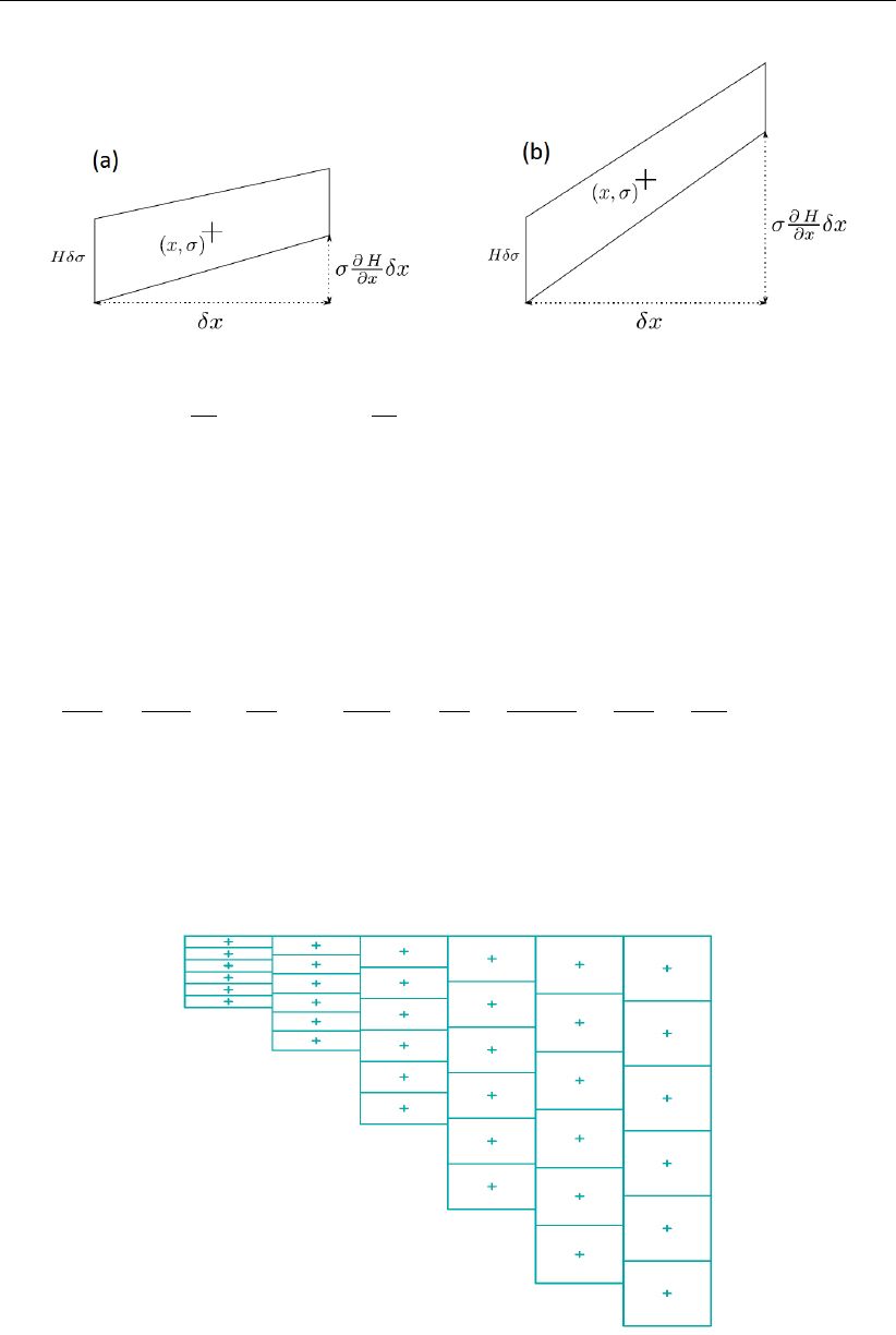
DRAFT
Hydrodynamics
Figure 7.12: Example of a hydrostatic consistent and inconsistent grid; (a) Hδσ >
σ∂H
∂x δx, (b) Hδσ < σ ∂H
∂x δx
From this equation, it can be seen that by increasing the number of σ-levels the consistency
condition will eventually be violated.
Similarly, for the horizontal diffusion term, the transformation from Cartesian co-ordinates to
σco-ordinates leads to various cross derivatives. For example, the transformation of a simple
second order derivative leads to:
∂2c
∂x2=∂2c∗
∂x∗2+∂σ
∂x2
−∂2c∗
∂σ2+ 2∂σ
∂x −∂2c∗
∂x∗∂σ +∂2σ
∂x2−∂c∗
∂σ (7.15)
For such a combination of terms it is difficult to find a numerical approximation that is stable
and positive, see Huang and Spaulding (1996). Near steep bottom slopes or near tidal flats
where the total depth becomes very small, truncations errors in the approximation of the
horizontal diffusive fluxes in σ-co-ordinates are likely to become very large, similar to the
horizontal pressure gradient.
Figure 7.13: Finite Volume for diffusive fluxes and pressure gradients
Deltares 133 of 412
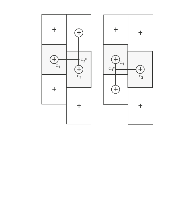
DRAFT
D-Flow Flexible Mesh, User Manual
Figure 7.14: Left and right approximation of a strict horizontal gradient
In D-Flow FM the stress tensor is redefined in the σco-ordinate system assuming that the
horizontal length scale is much larger than the water depth (Blumberg and Mellor,1985) and
that the flow is of boundary-layer type. The horizontal gradients are taken along σ-planes.
This approach guarantees a positive definite operator, also on the numerical grid (Beckers
et al.,1998).
If the same approach is used for the horizontal diffusion operator in the transport equation:
∂2c
∂x2≈∂2c∗
∂x∗2(7.16)
Horizontal diffusion will lead to vertical transport of matter through vertical stratification inter-
faces (pycnocline) which is nonphysical. A more accurate, strict horizontal discretization is
needed.
In D-Flow FM an option is available that minimises artificial vertical diffusion and artificial flow
due to truncation errors. A method has been implemented which gives a consistent, stable and
monotonic approximation of both the horizontal pressure gradient and the horizontal diffusion
term, even when the hydrostatic consistency condition equation is not fulfilled. This "anti-
creep" option is based upon a Finite Volume approach; see Figure 7.13. The horizontal
diffusive fluxes and baroclinic pressure gradients are approximated in Cartesian co-ordinates
by defining rectangular finite volumes around the σ-co-ordinate grid points. Since these boxes
are not nicely connected to each other, see Figure 7.14, an interpolation in zco-ordinates is
required to compute the fluxes at the interfaces.
Since the centres of the finite volumes on the left-hand side and right-hand side of a vertical
interval are not at the same vertical level, a z-interpolation of the scalar concentration cis
needed to compute strictly horizontal derivatives. The values obtained from this interpolation
are indicated by c∗
1and c∗
2respectively in Figure 7.14. (Stelling and Van Kester,1994) apply
134 of 412 Deltares

DRAFT
Hydrodynamics
a non-linear filter to combine the two consistent approximations of the horizontal gradient,
s1= (c∗
2−c1)/∆xand s2= (c2−c∗
1)/∆x
If s1×s2<0Then
∆c
∆x= 0
Else
∆c
∆x=sign (s1)×min (|s1|,|s2|)
Endif
(7.17)
If an interval has only grid boxes at one side, the derivative is directly set to zero. The hor-
izontal fluxes are summed for each control volume to compute the diffusive transport. The
integration of the horizontal diffusion term is explicit with time step limitation:
∆t≤1
DH1
∆x2+1
∆y2(7.18)
The derivatives are used in the integral for the baroclinic pressure force in the momentum
equation:
Px(x, z) = 1
ρ0Zζ
z
g∂ρ (x, s)
∂x ds (7.19)
Originally, this approach was implemented in Delft3D-FLOW. Slørdal (1997) stated that the
above approximation may sometimes produce errors of the same sign which leads to a sys-
tematic underestimation of the baroclinic pressure term. This underestimation can be ascribed
to the non-linear filter, which selects the minimum of the two gradients under consideration.
This limiter is fully analogous to the min-mod limiter used for the construction of monotone
advection schemes (Hirsch,1990). Since the same approximation of the horizontal gradient
is used for the horizontal diffusion flux, it is important to ensure that the difference operator
is positive definite in order to get physically realistic solutions. The maximum and minimum
of a variable being transported by diffusion do not increase or decrease (min-max principle).
By taking the minimum of the gradients, Stelling and Van Kester (1994) show that, the min-
max principle is fulfilled. Beckers et al. (1998) show that any nine-point consistent linear dis-
cretization of the horizontal diffusion on the σ-grid does not fulfil the min-max principle. From
numerical tests Slørdal (1997) concluded that the underestimation is reduced by increasing
the vertical resolution, but is sometimes enhanced by increasing the horizontal resolution.
Let s4be a consistent approximation of the horizontal gradient s4= (s1+s2)/2.Slørdal
(1997) suggested to take s4as approximation of the horizontal gradient. He calls his approach
the "modified Stelling and Van Kester scheme". It is equivalent to linear interpolation at a
certain z-level before taking the gradient. It is more accurate than taking the minimum of
the absolute value of the two slopes s1and s2but it does not fulfil the min-max principle
for the diffusion operator. It may introduce wiggles and a small persistent artificial vertical
diffusion (except for linear vertical density distributions). Due to the related artificial mixing,
stratification may disappear entirely for long term simulations, unless the flow is dominated by
the open boundary conditions.
By introducing an additional approximation of the horizontal gradient in the filter algorithm
defined by s3= (c2−c1)/∆x, the stringent conditions of the minimum operator can be re-
laxed somewhat. The drawback of underestimation of the baroclinic pressure force reported
by Slørdal (1997) can be minimised without loosing that the method fulfils the min-max princi-
ple. This third gradient s3, which is consistent for min(|s1|,|s2|)< s3<max(|s1|,|s2|),
has point-to-point transfer properties and therefore leads to a positive scheme for sufficiently
small time steps. The following non-linear approach presently available in D-Flow FM is both
Deltares 135 of 412
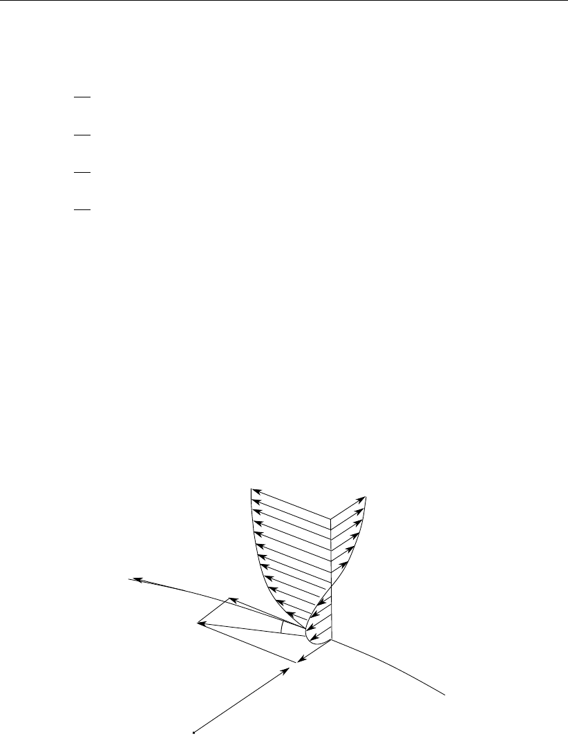
DRAFT
D-Flow Flexible Mesh, User Manual
consistent and assures the min-max principle:
If s1×s2<0Then
∆c
∆x= 0
Elseif |s4|<|s3|Then
∆c
∆x=s4
Elseif min (|s1|,|s2|)<|s3|<max (|s1|,|s2|)Then
∆c
∆x=s3
Else
∆c
∆x=sign (s1) min (|s1|,|s2|)
Endif
(7.20)
The method requires a binary search to find the indices of neighbouring grid boxes, which is
time consuming. The increase in computation time is about 30 %.
If the streamlines are strictly horizontal, transport of matter discretised on a σco-ordinate
grid may still generate some numerical vertical diffusion by the discretisation of the advection
terms.
7.6 Secondary flow
The flow in a river bend is basically three-dimensional. The velocity has a component in the
plane perpendicular to the river axis. This component is directed to the inner bend near the
riverbed and directed to the outer bend near the water surface, see Figure 7.15.
+sτbs
τb
τbn
+r
M
δ
uv
Figure 7.15: Vertical profile secondary flow (v) in river bend and direction bed stress
This so-called "secondary flow" (spiral motion) is of importance for the calculation of changes
of the riverbed in morphological models and the dispersion of matter. In a 3D model the
secondary flow is resolved on the vertical grid, but in 2D depth-averaged simulations the
secondary flow has to be determined indirectly using a secondary flow model. It strongly
varies over the vertical but its magnitude is small compared to the characteristic horizontal
flow velocity.
136 of 412 Deltares

DRAFT
Hydrodynamics
7.6.1 Definition
The secondary flow will be defined here as the velocity component v(σ)normal to the depth-
averaged main flow. The spiral motion intensity of the secondary flow Iis a measure for the
magnitude of this velocity component along the vertical:
I=Z1
0|v(σ)|dσ (7.21)
A vertical distribution for a river bend is given in Figure 7.15. The spiral motion intensity I
leads to a deviation of the direction of the bed shear stress from the direction of the depth-
averaged flow and thus affects the bedload transport direction. This effect can be taken into
account in morphological simulations.
The component of the bed shear stress normal to the depth-averaged flow direction τbr reads:
τbr =−2ρα21−α
2|u|I(7.22)
where αis defined in Equation (7.33) and |u|is the magnitude of the depth-averaged velocity.
To take into account the effect of the secondary flow on the depth-averaged flow, the depth-
averaged shallow water equations have to be extended with:
An additional advection-diffusion equation to account for the generation and adaptation of
the spiral motion intensity.
Additional terms in the momentum equations to account for the horizontal effective shear
stresses originating from the secondary flow.
7.6.2 Depth-averaged continuity equation
The depth-averaged continuity equation is given by:
∂h
∂t +∂hu
∂x +∂hv
∂y =Q(7.23)
where uand vindicate the depth-averaged velocities along Cartesian axis.
7.6.3 Momentum equations in horizontal direction
The momentum equations in x- and y-direction are given by:
∂u
∂t +u∂u
∂x +v∂u
∂y −fu =−1
ρ0
Px−gu√u2+v2
C2
2Dh+Fx+Fsx +Mx(7.24)
∂v
∂t +u∂v
∂x +v∂v
∂y +fv =−1
ρ0
Pv−gv√u2+v2
C2
2Dh+Fy+Fsy +My(7.25)
The fourth term in the right-hand side represents the effect of the secondary flow on the depth-
averaged velocities (shear stresses by depth-averaging the non-linear acceleration terms).
Deltares 137 of 412

DRAFT
D-Flow Flexible Mesh, User Manual
7.6.4 Effect of secondary flow on depth-averaged momentum equations
To account for the effect of the secondary flow on the depth-averaged flow, the momentum
equations have to be extended with additional shear stresses. To close the equations these
stresses are coupled to parameters of the depth-averaged flow field. The main flow is as-
sumed to have a logarithmic velocity profile and the secondary flow originates from a multipli-
cation of a universal function with the spiral motion intensity, see Kalkwijk and Booij (1986).
Depth averaging of the 3D equations leads to correction terms in the depth-averaged momen-
tum equations for the effect of spiral motion:
Fsx =1
h∂hTxx
∂x +∂hTxy
∂y (7.26)
Fsy =1
h∂hTxy
∂x +∂hTyy
∂y (7.27)
with the shear-stresses, resulting from the secondary flow, modelled as:
Txx =−2βuv (7.28)
Txy =Tyx =β(u2−v2)(7.29)
Tyy = 2βuv (7.30)
and:
β=β∗h
R∗
s
(7.31)
β∗=βc5α−15.6α2+ 37.5α3(7.32)
βc∈[0,1], correction coefficient specified by you,
α=√g
κC2D
<1
2(7.33)
with R∗
sthe effective radius of curvature of a 2D streamline to be derived from the intensity of
the spiral motion and κthe Von Kármán constant. The spiral motion intensity is computed by
Equation (7.34). The limitation on α,Equation (7.33), is set to ensure that the length scale La
in Equation (7.41) is always positive. For βc= 0, the depth-averaged flow is not influenced
by the secondary flow.
Remark:
Equation (7.33) effectively means a lower limit on C2D.
138 of 412 Deltares

DRAFT
Hydrodynamics
7.6.5 The depth averaged transport equation for the spiral motion intensity
The variation of the spiral motion intensity Iin space and time, is described by a depth-
averaged advection-diffusion equation:
∂hI
∂t +∂uhI
∂x +∂vhI
∂y =h∂
∂x DH
∂I
∂x+h∂
∂x DH
∂I
∂y +hS (7.34)
with:
S=−I−Ie
Ta
(7.35)
Ie=Ibe −Ice (7.36)
Ibe =h
Rs|u|(7.37)
Ice =fh
2(7.38)
|u|=√u2+v2(7.39)
Ta=La
|u|(7.40)
La=(1 −2α)h
2κ2α(7.41)
and Rsthe radius of curvature of the stream-line defined by:
us
Rs
=−∂ur
∂s (7.42)
with usand urthe components along and perpendicular to the streamline. The effective
radius of curvature to be used for the evaluation of the coefficient β,Equation (7.32), reads:
R∗
s=h|u|
I(7.43)
To guarantee stability the effective radius of curvature is bounded by the following empirical
relation:
R∗
s≥10h(7.44)
The above formulas account for two sources of secondary flow:
The centrifugal force in case of curved streamlines, Ibe.
The effect of the Coriolis force, Ice.
7.7 Drying and flooding
Estuaries and coastal embayments contain large, shallow, and relatively flat areas separated
and interleaved by deeper channels and creeks. When water levels are high, the entire area
is covered by water. But as tide falls, the shallow areas are exposed, and ultimately the flow
is confined only to the deeper channels. The dry tidal flats may occupy a substantial fraction
of the total surface area. The accurate reproduction of covering or uncovering of the tidal flats
is an important feature of numerical flow models based on the shallow water equations.
Many rivers have compound channels, consisting of a main channel that always carries flow
(the summer bed) and one or two flood plains which only convey flow during extreme river
Deltares 139 of 412

DRAFT
D-Flow Flexible Mesh, User Manual
discharges (the winter bed). The summer bed is surrounded by low dykes, which could be
overtopped if the river discharge increases. The winter-bed is surrounded by much higher
dykes, which are designed to protect the polders against water levels due extreme river dis-
charges. The flooding of the flood plains increases the drainage capacity of the river and
reduces the local water level gradients.
In a numerical model, the process of drying and flooding is represented by removing grid
points from the flow domain that become dry when the tide falls and by adding grid points
that become wet when the tide rises. Drying and flooding is constrained to follow the sides of
grid cells. In this section, we specify the algorithms which have been used to determine the
moment when a grid cell (water level point) or cell boundary (velocity point) becomes dry or
wet. Drying and flooding gives a discontinuous movement of the closed boundaries and may
generate small oscillations in water levels and velocities. The oscillations introduced by the
drying and flooding algorithm are small if the grid sizes are small and the bottom has smooth
gradients.
Essential elements of the wetting and drying algorithm are the definition of the water level, the
definition of the bed level and the criteria for setting a velocity and/or water level point wet or
dry. In the following subsections, these three items will be discussed.
7.7.1 Definitions
In section 7.3.1, the locations of the primary flow variables (water level and flow velocity) have
been described. Through Figure 7.3 it has been clarified that the water level is computed at the
location of the circumcenter (cell center), whereas the face normal flow velocity is computed
at the midpoint of each cell face (face center).
For the computation of these two primary variables, the level of the bed must be known both
at the cell center and at the face center. The user can specify the way these values are inter-
preted from the available bathymetry by means of the MDU-file keywords bedlevtyp and
conveyance2D. For a proper understanding of the possibilities of D-Flow FM, Figure 7.16
is provided with a three-dimensional representation of two adjacent triangular cells.
140 of 412 Deltares
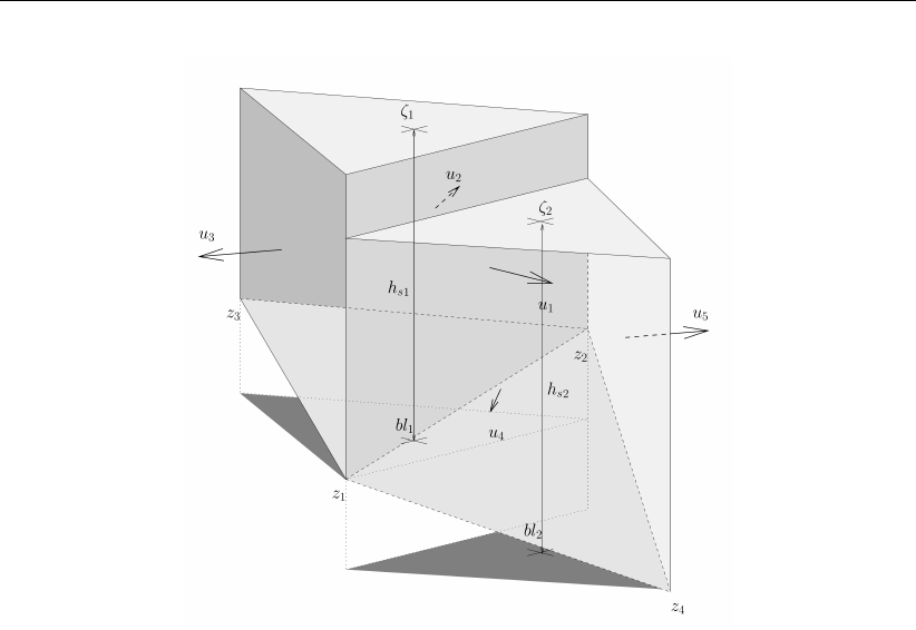
DRAFT
Hydrodynamics
Figure 7.16: Definition of the water levels, the bed levels and the velocities in case of two
adjacent triangular cells.
To the keyword bedlevtyp, the values 1,2,3,4,5and 6can be assigned. For the keyword
conveyance2D, the values -1,0,1,2and 3are available.
The most common case is the definition of the bed levels at the corner nodes of the cell and
a choice for the keyword bedlevtyp = 3. Depending on the choice for conveyance2D,
the face center bed levels and cell center bed levels are computed.
7.7.1.1 Piecewise constant approach for the bed level
In principle, the bed levels are considered as piecewise constant in space. This approach
is followed if conveyance2D <1. The keyword bedlevtyp can be used in combination
with the piecewise constant approach as highlighted in the table below. Note that the bed level
is defined with respect to the reference level (not to be confused with a water depth given as
a positive value downwards). With conveyance2D <1, we have:
Deltares 141 of 412

DRAFT
D-Flow Flexible Mesh, User Manual
Keyword Value Cell center bed level Face center bed level
bedlevtyp 1 user specified the highest cell center bed
level considering the two
cells next to the face
bedlevtyp 2 the lowest face center bed
level considering all the
faces of the cell
user specified
bedlevtyp 3 the lowest face center bed
level considering all the
faces of the cell
the mean corner bed level
considering the two corner
nodes the face is connecting
bedlevtyp 4 the lowest face center bed
level considering all the
faces of the cell
the minimum corner bed
level considering the two
corner nodes the face is
connecting
bedlevtyp 5 the lowest face center bed
level considering all the
faces of the cell
the maximum corner bed
level considering the two
corner nodes the face is
connecting
bedlevtyp 6 the mean corner bed level
considering all the corners of
the cell
the highest cell center bed
level considering the two
cells next to the face
The former Delft3D-FLOW version, running on curvilinear meshes, has utilized the piecewise
constant approach for bed levels as well. The treatment of the bed level itself is, however,
different from D-Flow FM. In Delft3D, the user can distinctly specify the treatment type for
the cell center bed level and the face center bed level. In D-Flow FM, the choice for the one
implies the choice for the other. A strict, exact match of settings for which Delft3D-FLOW and
D-Flow FM treat the bed similarly, is not facilitated. Hence, the user himself should take care
in comparing the Delft3D-FLOW results and D-Flow FM results when it comes to the bed level
treatment settings.
7.7.1.2 Piecewise linear approach for the bed levels
A piecewise linear bed level approach can be chosen for through setting conveyance2D
≥1. In this case, only the approach for bedlevtyp equal to 3,4and 5is affected. With
conveyance2D ≥1, we have:
Keyword Value Cell center bed level Face center bed level
bedlevtyp 3,4,5the lowest corner node bed
level considering all the
nodes of the cell
linearly varying from the bed
level at the one corner node
to the bed level at the other
corner node
Notice that the choice for either bedlevtyp equal to 3,4or 5does not imply different
bed level treatment approaches. For the case conveyance2D ≥1, the bed is assumed
linearly varying within a face only to compute the wet cross-sectional area of the vertical fase;
142 of 412 Deltares
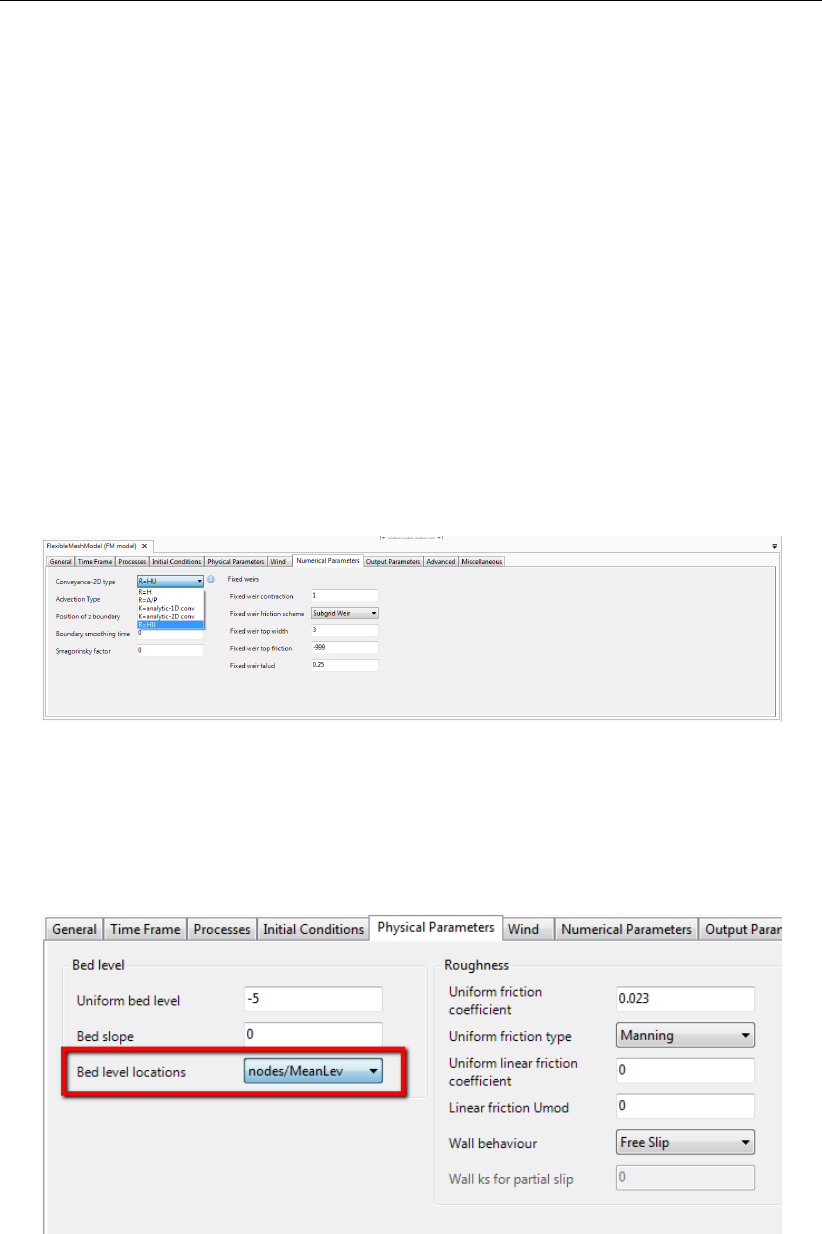
DRAFT
Hydrodynamics
it should, however, be remarked that for the computation of the water column volume in a cell,
this linear variation of the bed is not taken into account.
7.7.1.3 Hybrid bed level approach
In addition to the previously described bed level treatment approaches, D-Flow FM facilitates
a hybrid approach for the computation of the cell center bed level by means of the keywords
blminabove and blmeanbelow. In this approach, the cell center bed level is computed
as the mean of the associated face center bed levels, be it only below the user specified level
blmeanbelow. For levels above the user specified level blminabove, the minimum value
of the associated face center bed levels is used. In between these two user specified levels,
the bed levels are constructed by means of a linear interpolation between the two approaches’
results.
7.7.2 Specification in Delta Shell
The specification of the treatment of the bed level locations can be achieved through the tab
fields ‘Numerical Parameters’ and ‘Physical Parameters’.
Figure 7.17: Specification of the conveyance option in Delta Shell.
The tab field ‘Numerical Parameters’ contains the choice for the conveyance options: see
Figure 7.17).
Figure 7.18: Specification of the bed level treatment type in Delta Shell.
The tab field ‘Physical Parameters’ contains the choice for the Bed level locations. Five options
are facilitated: bedlevtyp numbers 1up to 5; the option 6is not facilitated in the user
interface.
Deltares 143 of 412
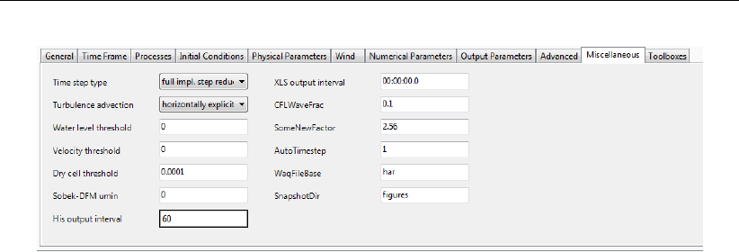
DRAFT
D-Flow Flexible Mesh, User Manual
Figure 7.19: Specification of the hybrid bed options (with keywords blminabove and
blmeanbelow).
By means of the tab field ‘Miscellaneous’, the hybrid options with the keywords blminabove
and blmeanbelow can be enabled.
7.8 Intakes, outfalls and coupled intake-outfalls
Many engineering studies concern the design of intakes and outfalls. For instance, studies
about positioning of waste water diffusers or coupled intake-outfall design for cooling water
at power plants. Intakes and outfalls can be modeled using sinks and sources. A source is
a point in the model where a discharge Qin [m3/s] is prescribed by a time series ASCII file
(section D.2.1) with at least two and maximum four columns.
1 When salinity and temperature are not used in the computation:
Model expects two columns, where the first column is the time in minutes, the second is
the discharge in [m3/s].
2 When either salinity or temperature is used in the computation:
Model expects three columns, where the first column is the time in minutes, the second is
the discharge in [m3/s], the third column contains either the salinity in [ppt] or the temper-
ature in [◦C]. Note that third column can be either salinity or temperature depending which
constituent is used in the model and which is not.
3 When salinity and temperature are present in the model:
Model expects four columns, where the first column is the time in minutes, the second
is the discharge in [m3/s], the third column contains the salinity in [ppt] and the fourth
contains the temperature in [◦C].
The location of the source or sink is specified in a polyline file (section B.2), containing a
polyline with either multiple points or just one point. If two or more points are specified, a
coupled source sink pair is made, the first point is the FROM (or sink) point, the last point is
the TO (or source) point. Three variants may occur:
1 Sink point side lies inside a grid cell A, source point also lies inside a grid cell B (A may
equal B, but that is rarely useful): water is extracted from cell A and transported to B.
2 Sink point lies outside of the grid, source point lies in a grid cell B: water is discharged into
B, a bit like an inflow discharge boundary condition.
3 Sink side lies inside a grid cell A, source side lies outside of the grid: water is extracted
from A, a bit like an outflow discharge boundary condition.
Specifying a negative discharge value effectively interchanges the role of the source and sink
points. If only one point is in the <∗.pli>file, it is assumed to be a source point. Specifying a
negative discharge turns the source into a sink.
144 of 412 Deltares

DRAFT
Hydrodynamics
For 3D computations, the polyline file should have a third column with z-values. It is good
practice to change the <∗.pli>file into a <∗.pliz>file. The z-values are used to determine
in which vertical grid cell the source and/or sink lie. The layer number can vary in time in
sigma models.
In the case of a coupled pair of sink source points (variant 1), the third and fourth column with
the salinity and temperature specification are interpreted as delta salinity and delta tempera-
ture. So the values at the source point become the values at the sink point plus the specified
delta values.
The sources and sinks are specified in the <∗.ext>file in a way similar to the boundary
conditions:
QUANTITY=discharge_salinity_temperature_sorsin
FILENAME=chan1_westeast.pli # A file ’chan1_westeast.tim’, with same basename
# as the polyline should be present
FILETYPE=9
METHOD =1
OPERAND =O
AREA =1.5
The specified area in the last line of this file determines (together with the specified discharge)
the amount of momentum uQ that is released at the source point. This is currently only
implemented in advection scheme 33 (cf. D-Flow FM TRM (2015) on Momentum advection).
Omitting this line or specifying a zero area switches off the release of momentum at the source
point. The direction of the discharged momentum is in direction of the last two points of the
polyline. So a one point polyline is momentumless. Both in 2D and 3D, the momentum can
only be directed in horizontal direction.
Sources and sinks are treated explicity in the numerical scheme. This implies that the ac-
tual discharged or extracted amounts of water are limited by the velocity Courant condition
Q∆t/V < 1. Not doing so could lead to severe timestep restrictions. Consider for instance
a specified extraction in case the extraction point has fallen dry. In that case, a real pump
would not be able to extract water and the specified extraction is more likely an input error
than an actual description of a physically feasible situation. So, we limit the specified dis-
charges to the local velocity Courant restriction. By specifying observation cross-sections
(section 4.4.2.3), one can compare prescribed discharges to the discharges that were ac-
tually realised in the model. In case of large differences, the discharge should probably be
distributed over a larger number of gridcells, or the extraction channel that feeds the extraction
point should be dredged.
When outfalls are adjacent to a closed model boundary, one might consider specifying a dis-
charge boundary instead of a point source. These are treated more implicitly in the numerical
scheme and are preferable for that reason.
When modelling freshwater inflow from a river into a sea, the vertical distribution of the dis-
charge that one should specify depends on the amount of detail available for modelling the
saline water - fresh water interface. If the river is modeled with sufficient detail, and the river
is well mixed at the upstream model boundary, the mixing process can be part of the mod-
elling and the river can be discharged over the whole vertical. If the mixing process cannot be
resolved in the model, for instance if the river is modeled as a point discharge adjacent to a
closed boundary, make sure that the whole river is discharged into the top layer or in the top
Deltares 145 of 412

DRAFT
D-Flow Flexible Mesh, User Manual
layers, depending on the estimated thickness of the fresh water plume at the discharge cell.
If one would have distributed the river discharge over the whole vertical, the size of the fresh
water plume would be underestimated because of too much mixing at the river discharge cell.
For example input files see example directories:
f17_sources_sinks/c010_sourcesink_2D/
f17_sources_sinks/c020_sourcesink_3D/
7.9 Equations of state for the density
The density of water ρis a function of salinity (s) and temperature (t).
In D-Flow FM we copied the implementation from Delft3D of the formulation derived by Eckart
(1958) that is based on a limited number of measurements dating from 1910 (only two salini-
ties at 5 temperatures). In the original equation the pressure is present, but at low pressures
the effect on density can be neglected.
Eckart formulation
The Eckart formulation is given by (Eckart,1958):
Range: 0< T < 40 ◦C, 0<s<40 ppt
ρ=1 000P0
λ+α0P0
,(7.45)
where:
λ= 1 779.5 + 11.25T−0.074 5T2−(3.80 + 0.01T)s, (7.46)
α0= 0.698 0,(7.47)
P0= 5 890 + 38T−0.375T2+ 3s. (7.48)
with the salinity sin [ppt] and the water temperature Tin [◦C].
The keyword that selects the equation of state in the mdu file is called Idensform. The influ-
ence of salinity and or temperature on water motion through the baroclinic pressure can be
switched off by setting Idensform=0
146 of 412 Deltares

DRAFT
Hydrodynamics
UNESCO formulation
The UNESCO formulation is given by (UNESCO,1981a):
Range: 0< T < 40 ◦C, 0.5< s < 43 ppt
ρ=ρ0+As +Bs3/2+Cs2(7.49)
where
ρ0= 999.842 594 + 6.793 952 ×10−2T−9.095 290 ×10−3T2+
+ 1.001 685 ×10−4T3−1.120 083 ×10−6T4+ 6.536 332 ×10−9T5
(7.50)
A= 8.244 93 ×10−1−4.089 9 ×10⁻³T+ 7.643 8 ×10⁻⁵T2+
−8.246 7 ×10⁻⁷T3+ 5.387 5 ×10⁻⁹T4(7.51)
B=−5.724 66 ×10−3+ 1.022 7 ×10⁻⁴T−1.654 6 ×10⁻⁶T2(7.52)
C= 4.831 4 ×10⁻⁴(7.53)
with the salinity sin [ppt] and the water temperature Tin [◦C].
Note: The UNESCO formulation is set as default.
Remarks:
Equation (7.51) is known as the International Equation of State for Seawater (EOS80)
and is based on 467 data points. The standard error of the equation is 3.6×10⁻³
kg/m3(Millero and Poisson,1981).
The Practical Salinity Scale (UNESCO,1981b, Par. 3.2) and the International Equation
of State are meant for use in all oceanic waters. However, these equations should be
used with caution in waters that have a chemical composition different from standard
seawater. In such waters, densities derived with the methods based on practical salinity
measurements and the International Equation of State may deviate measurably from
the true densities. However, in water masses different in composition from standard
seawater the differences in densities derived by the new equations involve only very
small errors.
Recommendation
The UNESCO formulae serve as an international standard. Further, the UNESCO formulae
show the correct temperature of 4 degrees Celsius where fresh water has its maximum den-
sity. The latter is of importance for thermal stratification in deep lakes in moderate climate
zones. Therefore we recommend the application of the UNESCO formulae and to select the
Eckart formulation only for consistence with previous projects in which it has been used. At
this moment the default is UNESCO.
Nevertheless, the UNESCO formulae have their limitations as they are based on the general
properties of seawater mixed with fresh water. Particularly in cases where marginal density
differences play a role, typically lakes, a variable mineral content of the water may create den-
sity differences not detected by just temperature and salinity. For such dedicated cases, you
are warranted to check the accuracy of the UNESCO formulae against experimental density-
relations derived from the (lake) water. In case of deviations or other constituents determining
the water density, we then recommend to contact the Helpdesk for further assistance such as
the implementation of a more dedicated density formulation.
Deltares 147 of 412

DRAFT
D-Flow Flexible Mesh, User Manual
7.10 Tide generating forces
Numerical models of tidal motion in coastal seas generally do not account for the direct local
influence of the tide generating forces. The amount of water mass in these models is relatively
small and the effect of these forces on the flow can be neglected. In that case, tidal motion
can often be reproduced with sufficient accuracy just by prescribing the tidal forcing along
open model boundaries.
In models covering larger seas or oceans, the contribution of the gravitational forces on the
water motion increases considerably and can no longer be neglected. In a global model, open
boundaries are absent and the tidal motion can only be induced by including tide generating
forces. Because tidal forces only play a significant role in the larger models, and because the
exact position of each computational point on earth must be known, we have implemented
these forces only in combination with spherical coordinates. By default, tide generating forces
is switched on in spherical models. You can switch it off by setting in the mdu file: Tidalforc-
ing=0
The tide generating forces originate from the Newtonian gravitational forces of the terrestrial
system (Sun, Moon and Earth) on the water mass. The equilibrium tide is the tide that would
result from the gravitational forces if a solid earth would be completely covered by an ocean
of about 21.5 km deep, such that the wave propagation speed would match the speed of the
celestial forces over the ocean surface. The interacting frequencies that result can be grouped
as diurnal, semi diurnal and long periodic. The total number of tide generating frequencies that
is evaluated in the computation is a tradeoff between required accuracy and computational
cost. Per default, we use a set of 60 frequencies, similar to TRIWAQ.
A smaller set of 11 main frequencies as used in Delft3D can also be selected by setting in the
MDU file :
Doodsonstart = 57.555
Doodsonstop = 275.555
Doodsoneps = 0.030
The full set of 484 components can be selected by specifying:
Doodsonstart = 55.565
Doodsonstop = 375.575
Doodsoneps = 0.000
For the set of 60 components these numbers are:
Doodsonstart = 55.565
Doodsonstop = 375.575
Doodsoneps = 0.030
The earth itself is deformed by the celestial forces, this is called the solid earth tide. An
estimate of this influence is based on the work of Love (1927), is included in the total tide
generating potential.
148 of 412 Deltares

DRAFT
Hydrodynamics
We have gratefully applied the Fortran subroutines written by E.J.O. Schrama. Details on the
implementation of tide generating forces can be found in his lecture notes Schrama (2007).
In order to save computation cost, the tidal potential is not computed for each computational
point, but on a grid with a resolution of 1 degree in both the South-North and West-East
direction.
The tidal and surge motions of the seas and ocean also deform the earth , which is called
tidal loading. Next to that, the water at some point is attracted by all moving water elsewhere
on the globe. This is called self attraction. The combined influence of these two processes is
implemented in a beta version.
Deltares 149 of 412

DRAFT
D-Flow Flexible Mesh, User Manual
150 of 412 Deltares
DRAFT
8 Transport of matter
8.1 Introduction
In D-Flow FM, transport is formulated as
d
dtZ
V(t)
cdV+Z
∂V (t)
c(u−v)•ndS=Z
∂V (t)
(K∇c)•ndS+Z
V(t)
sdV, (8.1)
where V(t)is a three-dimensional control volume, cis a concentration, uthe flow velocity
field, vthe velocity of the (vertically) moving control volume, Kis a diagonal matrix K=
diag(κ, κ, κz)with diffusion coefficients and sa source term. For two-dimensional (depth-
averaged) flow, we obtain
∂hc
∂t +∇•(huc) = ∇•(hκ∇c) + hs, (8.2)
where his the water depth. In case of three-dimensional (layer-averaged) flow, with ∆za
layer thickness from z0(x, y, t)to z1(x, y, t), we obtain
∂∆z c
∂t +∇•(∆zuc)+[ωz1c]z=z1−[ωz0c]z=z0=∇•(∆z κ∇c)+
κz
∂c
∂z −κ∇z1•∇cz=z1−κz
∂c
∂z −κ∇z0•∇cz=z0
+ ∆z s, (8.3)
where by uand ∇still the horizontal components are meant, i.e. u= (u, v)Tand ∇=
∂
∂x,∂
∂y T
and κzis the vertical diffusion coefficient. Furthermore ωz0and ωz1are the
velocity component normal and relative to the moving z=z0and z=z1layer interfaces
respectively. Note that taking c= 1 yields
ωz1+∂z1
∂t =ωz0− ∇ •(∆zu) + ∂z0
∂t ,(8.4)
which, combined with a zero-flux condition at the bed, recursively defines ωz0and ωz1for all
layers.
We apply Equation (8.2) and Equation (8.3) to transport of
salinity,
temperature,
suspended sediment,
tracers,
other, intentionally not mentioned,
and ultimately to the water itself (the continuity equation) to obtain the relative layer interface
velocities as expressed by Equation (8.4).
In the following we will highlight various physical and numerical settings in D-Flow FM. First
and foremost, it is important to understand that there are two numerical implementations
available, that differ slightly. These are selected with the keyword transportmethod in
the mdu-file:
transportmethod = 0
Deltares 151 of 412

DRAFT
D-Flow Flexible Mesh, User Manual
or
transportmethod = 1 # default.
The difference mainly concerns the treatment of vertical advection as explained in the next
section. Note that tracers are only available with transportmethod ’1’.
8.2 Some words about suspended sediment transport
In D-Flow FM two sediment models are available.
The first is a genuine D-Flow FM implementation, while the second is adopted from Delft3D-
SED and is only available in combination with transportmethod ’1’.
For a description of the latter, see chapter 18 in this manual.
We will not discuss the specifics of either of the two sediment models further and confine
ourselves to mentioning the relevant settings that concern suspended sediment transport of
the one of chapter 18.
8.3 Transport processes
Looking at the equations that govern transport of matter, we can identify three processes,
namely advection, diffusion and sources/sinks. The next sections will describe the relevant
user settings.
8.3.1 Advection
Advection of matter is expressed by the term ∇•(huc)in Equation (8.2) in the case of
two-dimensional modelling.
In three dimensions, we make a distinction between horizontal advection ∇•(∆zuc)and
vertical advection [ωz1c]z=z1−[ωz0c]z=z0in Equation (8.3). A higher-order numerical approx-
imation of these terms can be obtained by setting their "limiter type" to an appropriate value.
Setting the limiter type to "0" reduces the numerical approximation to a low-order upwind
method (i.e. severe limiting).
Although not restricted to the advection of salinity only, the choices for all matter are set with
keyword limtypsa in the mdu-file, for example
[numerics]
limtypsa = 0 # first-order upwind, or
or
[numerics]
limtypsa = 4 # MC limiter
For transportmethod=1, only the monotonized central (MC) limiter is available and used
when limtypsa>0, for example 1 or 2 or 6, but not -1. For transportmethod=0 other
limiters are available as well and the MC limiter is selected by setting limtypsa to ’4’, which
is its default value. We will not discuss the non-default limiters.
152 of 412 Deltares

DRAFT
Transport of matter
In three-dimensional modelling horizontal advection is similarly as in two dimension, but now
vertical advection can be selected with the keyword Vertadvtypsal in the mdu-file, i.e.
[numerics]
Vertadvtypsal = 0 # no vertical advection
or
[numerics]
Vertadvtypsal = 5 # default
The various combinations of transportmethod and Vertadvtypsal have the follow-
ing meaning:
Vertadv-
typsal
transport method
0 1
space time space time
0 none none none none
11st order upwind forward Euler
salt and temper-
ature: central,
other: higher-
order limited up-
wind
salt and tem-
perature: θ-
method, other:
forward Euler
2 central forward Euler
31st order upwind θ-method
4 central θ-method
5 neg. stratification
or water depth <
chkadvd:1st or-
der upwind, other-
wise: central
θ-method
6 as 5 as 5 temperature: cen-
tral, other: higher-
order limited up-
wind
temperature: θ-
method, other:
forward Euler
For the limited higher-order upwind discretization the MC limiter is used if transportmethod=1
if limtypsa>0, regardless of its specific value, and 1st-order upwind if limtypsa=0.
8.3.2 Diffusion
Diffusion of matter is expressed by the term ∇•(hκ∇c)for two-dimensional modelling and
a similar and additional terms in three dimensions, see Equation (8.3).
Clearly, we have horizontal diffusivity κand vertical diffusivity κz. The horizontal diffusivity κ
is a summation of
the molecular diffusivity κl, only for transportmethod=1. We use the following values:
κl=
1
700 νl,salt,
1
6.7νl,temperature,
0νl,sediment,
0νl,tracers,
(8.5)
where νl= 10−6m2/s is the kinematic viscosity,
a background diffusivity, user-specified as
spatially varying values by horizontaleddydiffusivitycoefficient in the
ext-file, or
Deltares 153 of 412

DRAFT
D-Flow Flexible Mesh, User Manual
a uniform value Dicouv in the mdu-file,
in that order of precedence, and
a contribution from turbulent transport expressed as νt/σt, where νtis the eddy viscosity
coefficient and σtis the turbulent Prandtl-Schmidt number for which the following values
are used:
σt=
0.7,salt,
0.7,temperature,
1.0,sediment,
1.0,tracers.
(8.6)
Horizontal diffusion is turned off when Dicouv=0.
The user has to be aware of the following. The explicit nature of the horizontal diffusion terms
in the time-integration method imposes a condition on the time step for numerical stability.
Recall that we have a similar condition due to explicit horizontal advection. Although we
always decrease the time step to satisfy the advection-related time step criterion, we do not
do so for diffusion. Instead, diffusion is limited such that our time step is restricted by advection
only, or by a user-specified maximum time step if it is smaller. For further details, consult D-
Flow FM TRM (2015).
Be aware that the modelled diffusion may be be smaller than anticipated. However, the ac-
tual effective diffusion encountered may be (much) larger than anticipated due to numerical
diffusion of the advection scheme.
Not considering suspended sediment, and similar to the horizontal diffusivity, the vertical dif-
fusivity κzis a summation of
the molecular diffusivity κl(for both transport methods), see Equation (8.5), not added for
transport method ’1’ if Dicoww=0,
a background vertical diffusivity, user-specified as a uniform value Dicoww in the mdu-file,
and
a contribution from turbulent transport, similar to its horizontal counterpart, but with the
horizontal viscosity coefficient now replaced by the vertical (eddy) viscosity coefficient.
Time integration is performed with a method that does not impose an additional constraint on
the time step. Unlike horizontal diffusion which is limited to ensure numerical stability while
maintaining the time-step size, vertical diffusion is not limited.
Vertical diffusion is turned off when, again not considering suspended sediment:
for transport method ’0’: Dicoww=0 or Vertadvtypsal=1 or Vertadvtypsal=2,
for both transport methods: the water depth is smaller than a threshold 10−2m.
For the vertical diffusivity of suspended sediment, see chapter 18.
8.3.3 Sources and sinks
Sources and sinks may be provided by an entry in the ext-file as follows:
quantity=discharge_salinity_temperature_sorsin
This simultaneously prescribes sources and sinks of
154 of 412 Deltares

DRAFT
Transport of matter
water volume itself (i.e. discharge),
salinity, and
temperature.
See section 7.8 for more details.
8.3.4 Forester filter
The central vertical advection schemes of transport method ’0’ may cause nonphysical os-
cillations, or wiggles, especially near regions of large gradients. The user has the option to
suppress salt and temperature wiggles with a filter inspired by the so-called Forester filter.
This filter also penalizes physically unstable stratification. The maximum number of iterations
in the filter is controlled with keywords Maxitverticalforestersal for salt (default
100) and Maxitverticalforestertem for temperature (default 0, i.e. no filtering). Note
that the filter is unavailable when using transport method ’1’.
8.4 Transport boundary and initial conditions
The equations that govern transport of matter are complemented with boundary and initial
conditions. We make the distinction between "horizontal" boundaries, that are either "open"
or "closed", and vertical boundaries, only relevant for three-dimensional modelling.
8.4.1 Open boundary conditions
At "horizontal" open boundaries the following boundary conditions are applied:
salt, temperature and tracers:
inflow: user-specified Dirichlet condition,
outflow: homogeneous Neumann condition,
suspended sediment: see chapter 18.
The user-specified Dirichlet conditions are supplied in the usual manner through the ext-file,
i.e.
quantity=salinitybnd
for salt and
quantity=temperaturebnd
for temperature. Boundaries conditions for multiple tracers may be defined by appending their
name to the tracerbnd keyword, for example
quantity=tracerbndMY_FIRST_TRACER
and
quantity=tracerbndMY_SECOND_TRACER
Deltares 155 of 412

DRAFT
D-Flow Flexible Mesh, User Manual
8.4.2 Closed boundary conditions
At "horizontal" closed boundaries zero-flux conditions are applied.
8.4.3 Vertical boundary conditions
At the "vertical" boundaries, i.e. at the bed and at the water surface, zero-flux conditions are
applied, except for temperature that is, see chapter 10 for further details on that matter.
8.4.4 Thatcher-Harleman boundary conditions
Consider (a part of) an open boundary where the flow reverts from outflowing to inflowing.
According to section 8.4.1, at that very moment a Dirichlet condition becomes effective and
a user-specified boundary value is prescribed. This value does in general not reflect the true
condition at the boundary and causes a discontinuous temporal behaviour. The so-called
Thatcher-Harleman boundary condition is intended to regularize this behaviour. The actual
value applied at the boundary is smoothly transformed from the last value under outflow con-
ditions to the user-specified value under inflow conditions within a user-specified return time.
This return time is prescribed with the keyword return_time in the “new style” external
forcings file for boundary condition, for example
[boundary]
quantity = salinitybnd
locationfile = tfl_01.pli
forcingfile = tfl.bc
return_time = 250
See section B.5 for more details on this format. Note that the Thatcher-Harleman boundary
conditions are only available currently for two-dimensional modelling.
8.4.5 Initial conditions
We will only consider intitial conditions for salinity, temperature and tracers. For initial sediment
concentrations, see chapter 18.
Initial conditions are specified in three possible ways, namely
a horizontally spatially varying field in the usual way through the ext-file,
a vertical profile in three dimensions, horizontally uniformly distributed, for salinity and
temperature only in the ext-file, and
uniform values for salinity and temperature in the mdu-file.
In the ext-file we have
quantity = initialsalinity
for the intial salinity, and
quantity = initialsalinitytop
for the initial salinity in the top layer in case of three-dimensional modelling. When specified,
the initial salinity field is linearly distributed from the "initialsalinity" in the lowest layer to the
156 of 412 Deltares

DRAFT
Transport of matter
"initialsalinitytop" in the top layer. When not specified, the initial salinity field is vertically
uniformly distributed.
The initial temperature field is prescribed with
quantity = initialtemperature
which in three dimensions is vertically uniformly distributed.
A horizontally uniformly distributed vertical profile of salinity and temperature can be pre-
scribed with initialverticalsalinityprofile and initialverticaltemperatureprofile
respectively, for example for salinity
QUANTITY=initialverticalsalinityprofile
FILENAME=inisal.pol
FILETYPE=10
METHOD=4
OPERAND=O
The polygon file contains (z, salinity) value pairs, where zis the vertical coordinate in meters.
For example for linearly varying salinity from 30 to 20 ppt from −10 to 0m:
L1
2 2
-10 30
0 20
The initial field of an arbitrary number of tracers are prescribed in the same way, except for
the user-specified tracername that is added to the keyword initialtracer, similar to the
tracer boundary conditions, for example
quantity=initialtracerMY_FIRST_TRACER
and
quantity=initialtracerMY_SECOND_TRACER
Default values for salinity and temperature are defined in the mdu-file with Initialsalinity
and Initialtemperature respectively.
Deltares 157 of 412

DRAFT
D-Flow Flexible Mesh, User Manual
158 of 412 Deltares

DRAFT
9 Turbulence
Note: The 3D-implementation is a β-functionality.
D-Flow FM solves the Navier-Stokes equations for an incompressible fluid. Usually the grid
(horizontal and/or vertical) is too coarse and the time step too large to resolve the turbulent
scales of motion. The turbulent processes are “sub-grid”. The primitive variables are space-
and time-averaged quantities. Filtering the equations leads to the need for appropriate closure
assumptions.
For 3D shallow water flow the stress and diffusion tensor are an-isotropic. The horizontal eddy
viscosity coefficient νHand eddy diffusivity coefficient DHare much larger than the vertical
coefficients νVand DV, i.e. νHνVand DHDV. The horizontal coefficients are
assumed to be a superposition of three parts:
1 a part due to molecular viscosity.
2 a part due to “2D-turbulence”,
3 a part due to “3D-turbulence” see Uittenbogaard et al. (1992) and
The 2D part is associated with the contribution of horizontal motions and forcings that cannot
be resolved (“sub-grid scale turbulence”) by the horizontal grid (Reynolds averaged or eddy
resolving computations). The 3D part is referred to as the three-dimensional turbulence and
is computed following one of the turbulence closure models, described in this section. For
2D depth-averaged simulations, the horizontal eddy viscosity and eddy diffusivity coefficient
should also contain a contribution due to the vertical variation of the horizontal flow (Taylor
shear dispersion).
The background horizontal viscosity coefficient νback
Hand eddy diffusivity coefficient Dback
H
(constant or space-varying) can be specified in the Delta Shell GUI and D-Flow FM’s MDU
file. In Delft3D-FLOW a sub-grid scale model, HLES for 2D-turbulence is implemented. (see
Delft3D-FLOW User Manual). In D-Flow FM we have not yet achieved this, but we imple-
mented a simple horizontal model, the so called Smagorinsky model, so that we can at least
cope with possibly very large grid size variations.
The horizontal eddy coefficients are typically an order of magnitude larger than the vertical
coefficients determined by the turbulence closure model.
In D-Flow FM, two two-equation turbulence closure models have been implemented to deter-
mine the vertical eddy viscosity (νV) and vertical eddy diffusivity (DV):
1k-εturbulence closure model.
2k-τturbulence closure model(in β-version).
The k-τmodel is a mathematical variant of the k-εmodel. Both models solve equations for
production, dissipation and transport of turbulent kinetic energy k. In the k-εmodel the dissi-
pation rate of turbulent kinetic energy ε, is modeled, whereas in the k-τmodel the dissipation
timescale τis modeled.
Both models are based on the so-called eddy viscosity concept of Kolmogorov (1942) and
Prandtl (1945).
A brief description of each of these turbulence closure model will be given further on in this
section, for more details we refer to Uittenbogaard et al. (1992). The k-εmodel has been
used in tidal simulations by Baumert and Radach (1992) and Davies and Gerritsen (1994), for
Deltares 159 of 412

DRAFT
D-Flow Flexible Mesh, User Manual
stratified flow of a river plume by Postma et al. (1999) and for the evolution of a thermocline
by Burchard and Baumert (1995).
For strongly stratified flows it is important to introduce suitably chosen constant ambient (back-
ground) mixing coefficients, because the mixing coefficients computed by turbulence models
with shear production only, reduce to zero. In the latter situation the vertical layers are com-
pletely de-coupled (frictionless). Disturbances are hardly damped and also the erosion of the
vertical stratification is reduced to molecular diffusion.
Based on our experience with highly stratified flows we suggest applying an ambient or back-
ground vertical eddy viscosity in the order of 10−4m2/s for the vertical exchange of mo-
mentum. This value corresponds with field measurements in the Rotterdam Waterway, The
Netherlands.
Eddy diffusivity
The vertical eddy diffusivity is a scaled form of the eddy viscosity according to:
D3D=ν3D
σc
.(9.1)
Parameter σcis the Prandtl-Schmidt number. Its numerical value depends on the substance
c.
In Delft3D-FLOW the following settings of σcare used:
In all cases, regardless the turbulence closure model, σc= 0.7for the transport of heat,
salinity, and tracer concentrations. For suspended sediment concentrations in online sed-
iment transport computations, σc= 1.0.
For the transport of turbulent kinetic energy kin the k-Lmodel and k-εmodel σc= 1.0,
and for the transport of turbulent kinetic energy dissipation εin the k-εmodel σc= 1.3.
In the mathematical formulation, the fluxes are instantaneously influenced by changes in the
vertical gradients of velocity and density. A physical adjustment time of the turbulence to the
variations of the vertical gradients, is not taken into account. The fluxes are not a monotone
function of the gradients. For the transport equation of heat, for small temperature gradients
the heat flux increases when the temperature gradient increases but for large temperature
gradients the heat flux decreases because the vertical eddy diffusivity is damped. For large
values of the density gradients and small values of the velocity gradients, the vertical diffusion
equation becomes mathematically ill-posed Barenblatt et al. (1993), and the computed vertical
profiles may become discontinuous (stepwise). The number of “steps” is dependent on the
vertical grid.
The numerical scheme for the vertical advection of heat and salt (central differences) may
introduce small vertical oscillations. This computational noise may enhance the turbulent
mixing. D-Flow FM has a vertical filtering technique to remove this noise and to reduce the
undesirable mixing. For more details, see section 8.3.4.
In strongly-stratified flows, the turbulent eddy viscosity at the interface reduces to zero and
the vertical mixing reduces to molecular diffusion. To account for the vertical mixing induced
by shearing and breaking of short and random internal gravity waves, we suggest to apply an
ambient eddy diffusivity in the order of 10−4to 10−5m2/s dependent on the Prandtl-Schmidt
number. In Delft3D-FLOW for stable stratified flows, the minimal eddy diffusivity may be based
on the Ozmidov length scale Loz, specified by you and the Brunt-Väisälä frequency of internal
160 of 412 Deltares

DRAFT
Turbulence
waves:
DV= max D3D,0.2L2
ozs−g
ρ
∂ρ
∂z !.(9.2)
This feature is still to be implemented in D-Flow FM
For a detailed description of the turbulence closure models of Delft3D-FLOW we refer to Rodi
(1984) and Uittenbogaard et al. (1992).
9.1 k-εturbulence model
In the k-εturbulence model, transport equations must be solved for both the turbulent kinetic
energy kand for the energy dissipation ε. The mixing length Lis then determined from εand
kaccording to:
L=cD
k√k
ε.(9.3)
In the transport equations, the following two assumptions are made:
The production, buoyancy, and dissipation terms are the dominating terms.
The horizontal length scales are larger than the vertical ones (shallow water, boundary
layer type of flows).
Because of the first assumption, the conservation of the turbulent quantities is less important
and the transport equation is implemented in a non-conservation form.
The transport equations for kand εare non-linearly coupled by means of their eddy diffusivity
Dk, Dεand the dissipation terms. The transport equations for kand εare given by:
∂k
∂t +u∂k
∂x +v∂k
∂y +ω
ζ−zb
∂k
∂σ =
+1
(ζ−zb)2
∂
∂σ Dk
∂k
∂σ +Pk+Pkw +Bk−ε, (9.4)
∂ε
∂t +u∂ε
∂x +v∂ε
∂y +ω
ζ−zb
∂ε
∂σ =
1
(ζ−zb)2
∂
∂σ Dε
∂ε
∂σ +Pε+Pεw +Bε−c2ε
ε2
k.(9.5)
with
Dk=νmol
σmol
+ν3D
σk
and Dε=ν3D
σε
(9.6)
In the production term Pkof turbulent kinetic energy, the horizontal gradients of the horizontal
velocity and all the gradients of the vertical velocities are neglected. The production term is
given by:
Pk=ν3D
1
(ζ−zb)2"∂u
∂σ 2
+∂v
∂σ 2#.(9.7)
Deltares 161 of 412

DRAFT
D-Flow Flexible Mesh, User Manual
For small-scale applications (e.g. simulation of laboratory flume), you can switch on a more
extended production term Pkof turbulent kinetic energy (option “partial slip”, rough side wall)
given by:
Pk= 2ν3D"1
2 (ζ−zb)2(∂u
∂σ 2
+∂v
∂σ 2)#+
+ 2ν3D"∂u
∂x2
+1
2∂u
∂y +∂v
∂x2
+∂v
∂y 2#.(9.8)
In this expression, ν3Dis the vertical eddy viscosity, prescribed by Equation (9.16). In Equa-
tion (9.7) and Equation (9.8) it has been assumed that the gradients of the vertical velocity w
can be neglected with respect to the gradients of the horizontal velocity components uand v.
The horizontal and vertical (σ-grid) curvature of the grid has also been neglected.
The turbulent energy production due to wave action is given by Pkw, but has not been im-
plemented yet in D-Flow FM: Wave forcing in 3D models is being prepared for an upcoming
release.
Near the closed walls the normal derivative of the tangential velocity is determined with the
law of the wall:
∂u
∂y =u∗
κy .(9.9)
In stratified flows, turbulent kinetic energy is converted into potential energy. This is repre-
sented by a buoyancy flux Bkdefined by:
Bk=ν3D
ρσρ
g
h
∂ρ
∂σ (9.10)
with the Prandtl-Schmidt number σρ= 0.7for salinity and temperature and σρ= 1.0for
suspended sediments.
The production term Pεand the buoyancy flux Bεare defined by:
Pε=c1ε
ε
kPk,(9.11)
Bε=c1ε
ε
k(1 −c3ε)Bk,(9.12)
with Lprescribed by Equation (9.3) and the calibration constants by (Rodi,1984):
c1ε= 1.44,(9.13)
c2ε= 1.92,(9.14)
c3ε=0.0unstable stratification
1.0stable stratification (9.15)
In D-Flow FM in the ε-equation for stable stratification the buoyancy flux is switched off, so
c3ε= 1.0and for unstable stratification the buoyancy flux is switched on c3ε= 0.0.
162 of 412 Deltares

DRAFT
Turbulence
The energy production and energy dissipation due to waves, the terms Pkw and Pεw in Equa-
tion (9.4) and Equation (9.5), have not been implemented yet in D-Flow FM: Wave forcing in
3D models is being prepared for an upcoming release.
The coefficients of the 3D k-εturbulence closure model as implemented in D-Flow FM are
not the same as in the depth-averaged k-εturbulence closure model (Rodi,1984), therefore
for depth-averaged simulations, the k-εturbulence closure model is not available for you.
The vertical eddy viscosity ν3Dis determined by:
ν3D=c0
µL√k=cµ
k2
ε,(9.16)
with:
cµ=cDc0
µ.(9.17)
To solve the transport equation, boundary conditions must be specified. A local equilibrium of
production and dissipation of kinetic energy is assumed at the bed which leads to the following
Dirichlet boundary condition:
k|σ=−1=u2
∗b
√cµ
.(9.18)
The friction velocity u∗bat the bed is determined from the magnitude of the velocity in the
grid point nearest to the bed, under the assumption of a logarithmic velocity profile. The bed
roughness (roughness length) may be enhanced by the presence of wind generated short
crested waves.
In case of wind forcing, a similar Dirichlet boundary condition is prescribed for the turbulent
kinetic energy kat the free surface:
k|σ=0 =u2
∗s
√cµ
.(9.19)
In the absence of wind, the turbulent kinetic energy kat the surface is set to zero.
At open boundaries, the turbulent energy kis computed using the equation for kwithout hor-
izontal advection. For a logarithmic velocity profile this will approximately lead to the following
linear distribution based on the shear-stress at the bed and at the free surface:
k(z) = 1
√cµu2
∗b1−z−zb
ζ−zb+u2
∗s
z−zb
ζ−zb.(9.20)
For εthe bed boundary condition reads:
∂ε
∂z =(εb+1 −εb)
∆zb
=u3
∗
κ∆zb
2+ 9z02(9.21)
The k-εturbulence model was successfully applied for the simulation of stratified flow in the
Hong Kong waters (Postma et al.,1999) and verified for the seasonal evolution of the thermo-
cline (Burchard and Baumert,1995).
Deltares 163 of 412

DRAFT
D-Flow Flexible Mesh, User Manual
9.2 k-τturbulence model
The k-τturbulence model is derived by Speziale et al. (1992) as a transformation of the
ε-equation of the k-εturbulence model where the variable τmodels a typical time-scale of
turbulent eddies.
The k-τturbulence model used in D-Flow FM deviates from the equation of Speziale et al.
(1992) at a few points, to derive their k-τmodel they used a different version of the k-εmodel
and the most important difference is that they do not include buoyancy in their model.
The transport equations for kand τused in D-Flow FM read (see for a derivation Dijkstra
(2014)):
∂k
∂t +u∂k
∂x +v∂k
∂y +ω
ζ−zb
∂k
∂σ =
1
(ζ−zb)2
∂
∂σ Dk
∂k
∂σ +Pk+Pkw +Bk−kτ, (9.22)
∂τ
∂t +u∂τ
∂x +v∂τ
∂y +ω
ζ−zb
∂τ
∂σ =
1
(ζ−zb)2∂
∂σ Dτ
∂τ
∂σ +2
kDτ
∂τ
∂σ
∂k
∂σ −2
τDτ
∂τ
∂σ
∂τ
∂σ −τ
k
∂
∂σ 1
σε−1
σk∂k
∂σ
−τ
k(cε1−1)Pk−τ
k(cε3−1)Bk+cε2−1(9.23)
with
Dk=νmol
σmol
+ν3D
σk
and Dτ=ν3D
στ
.(9.24)
164 of 412 Deltares
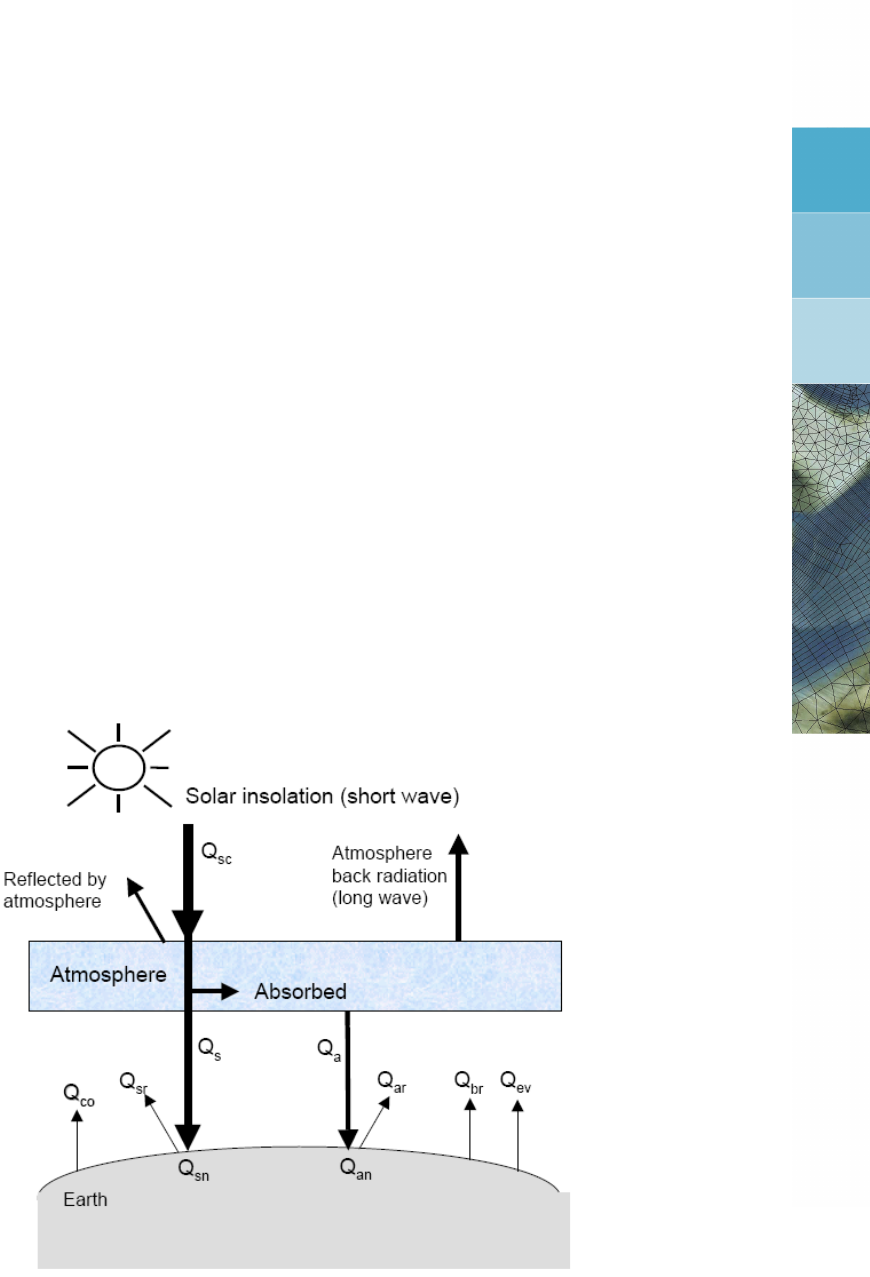
DRAFT
10 Heat transport
This chapter is an almost integral copy of the Delft3D-FLOW manual. The difference is that in
Delft3D-FLOW five heat flux models are implemented, whereas in D-Flow FM only two models
are implemented. These are the most complete heat flux model, the so called Composite heat
flux model (i.e. the Ocean heat flux model nr 5 in Delft3D-FLOW) and the most simple model,
the Excess temperature model (model nr 3 in Delft3D-FLOW). In D-Flow FM, the parameter
that sets the temperature model is called Temperaturemodel in the mdu-file. We kept the
numbering of Delft3D. When specifying Temperaturemodel=1, the temperature is taken
into account in the transport solver and in the equation of state, but heat fluxes though the
water surface are not taken into account. This may be useful when mixing is the primary factor
that determines the temperature distribution.
The heat radiation emitted by the sun reaches the earth in the form of electromagnetic waves
with wavelengths in the range of 0.15 to 4 µm. In the atmosphere the radiation undergoes
scattering, reflection and absorption by air, cloud, dust and particles. On average neither the
atmosphere nor the earth accumulates heat, which implies that the absorbed heat is emitted
back again. The wavelengths of these emitted radiations are longer (between 4 and 50 µm)
due to the lower prevailing temperature in the atmosphere and on Earth. Schematically the
radiation process, along with the heat flux mechanisms at the water surface, is shown in
Figure 10.1.
Figure 10.1: Overview of the heat exchange mechanisms at the surface
Legend for Figure 10.1:
Qsc radiation (flux) for clear sky condition in [J/m2s]
Qco heat loss due to convection (sensible) in [J/m2s]
Qsr reflected solar radiation in [J/m2s]
Qssolar radiation (short wave radiation) in [J/m2s]
Qsn net incident solar radiation (short wave), =Qs−Qsr
Deltares 165 of 412

DRAFT
D-Flow Flexible Mesh, User Manual
Qaatmospheric radiation (long wave radiation) in [J/m2s]
Qan net incident atmospheric radiation (long wave)
Qar reflected atmospheric radiation in [J/m2s]
Qbr back radiation (long wave radiation) in [J/m2s]
Qev heat loss due to evaporation (latent) in [J/m2s]
In D-Flow FM the heat exchange at the free surface is modeled by taking into account the sep-
arate effects of solar (short wave) and atmospheric (long wave) radiation, and heat loss due to
back radiation, evaporation and convection. The heat losses due to evaporation and convec-
tion are functions of the wind speed. In absence of wind, these terms become zero. However,
since water vapor is lighter than air, water may be cooled by evaporation and convection even
in a no wind situation. The terms are called Qevfree and Qcofree respectively.
Excess temperature model - heat flux model 3
In the Excess temperature model the heat exchange flux at the air-water interface is computed
based upon the prescribed background air temperature, the computed water temperature of
the top layer and the prescribed wind speed. This relatively simple model is sometimes used
in intake–outfall design studies. It can be applied when the temperature mixing process itself
is more relevant than the actual heat loss through the air water interface. The applied heat
exchange coefficient is mainly a function of the windspeed and water surface temperature.
The excess temperature model 3 is based on Sweers (1976), the heat exchange flux is rep-
resented by a bulk exchange formula:
Qtot =−λ(Ts−Tback),(10.1)
with Tsthe water temperature at the free surface and Tback the natural background tempera-
ture, both in ◦C.
The heat exchange coefficient λis a function of the surface temperature Tsand the wind
speed U10. It is derived by linearization of the exchange fluxes for back radiation, evaporation
and convection. The following relation was derived by Sweers (1976):
λ= 4.48 + 0.049Ts+f(U10)1.12 + 0.018Ts+ 0.00158T2
s.(10.2)
Composite - heat flux model 5
The heat flux model 5 following Gill (1982) and Lane (1989) was calibrated for the North Sea
and successfully applied for great lakes.
In the Composite heat flux model, the relative humidity in [%], air temperature in [◦C] and
cloudiness in [%] are prescribed.
These quantities may be either uniform or specially varying. In the external forcingsfile one
may have:
QUANTITY =humidity_airtemperature_cloudiness
FILENAME =meteo.hac
FILETYPE =6
METHOD =3
OPERAND =O
166 of 412 Deltares

DRAFT
Heat transport
For example input files see example directories:
f20_heat_flux/**/
The effective back radiation and the heat losses due to evaporation and convection are com-
puted by the model. Additionally, when air and water densities and/or temperatures are such
that free convection occurs, free convection of latent and sensible heat is computed by the
model.
Normally, solar radiation is computed based upon time of day, position on earth and cloudi-
ness. However, if solar radiation was measured, it can also be prescribed (in [W/m2]), e.g.:
QUANTITY =humidity_airtemperature_cloudiness_solarradiation
FILENAME =meteo.hacs
FILETYPE =6
METHOD =3
OPERAND =O
In both heat flux models, the wind forcing may be uniform or spatially varying.
If wind is uniform, the wind speed and direction are prescribed, wind speed is in m/s, and
direction follows nautical convention: 0 means wind coming from North, 90 means wind is
coming from East. In the external forcings file specify, e.g.:
QUANTITY=windxy
FILENAME=zeg99-10.wnd
FILETYPE=2
METHOD=1
OPERAND=O
If wind is spatially varying, the air pressure is also prescribed:
QUANTITY =airpressure_windx_windy
FILENAME =CSM_2015.apwxwy
FILETYPE =6
METHOD =3
OPERAND =O
Air pressure is in [Pa], wind x- and y-components are given [m/s].
For the physical background of the heat exchange at the air-water interface and the definitions,
we refer to Sweers (1976) for the Excess temperature model (Temperaturemodel=3), and to
Gill (1982) and Lane (1989) for the Ocean heat flux model (Temperaturemodel=5).
Deltares 167 of 412

DRAFT
D-Flow Flexible Mesh, User Manual
10.1 Heat balance
The total heat flux through the free surface reads:
Qtot =Qsn +Qan −Qbr −Qev −Qco −Qevfree −Qcofree,(10.3)
with:
Qsn net incident solar radiation (short wave)
Qan net incident atmospheric radiation (long wave)
Qbr back radiation (long wave)
Qev evaporative heat flux (latent heat)
Qco convective heat flux (sensible heat)
Qevfree evaporative heat flux (free convection latent heat)
Qcofree convective heat flux (free convection sensible heat).
The subscript nrefers to a net contribution. Each of the heat fluxes in Equation (10.3) will be
discussed in detail.
The change in temperature in the top layer Ts[◦C] is given by:
∂Ts
∂t =Qtot
ρwcp∆zs
,(10.4)
where Qtot [J/m2s] is the total heat flux through the air-water surface, cp(= 3930 J kg−1 K) is
the specific heat capacity of sea water, ρwis the specific density of water [kg/m3] and ∆zs
[m] is the thickness of the top layer. As in Delft3D-FLOW, the heat exchange at the bed is
assumed to be zero. This may lead to over-prediction of the water temperature in shallow
areas. Also the effect of precipitation on the water temperature is not taken into account.
Remarks:
The temperature Tis by default expressed in ◦C. However, in some formulas the abso-
lute temperature ¯
Tin K is used. They are related by:
¯
T=T+ 273.15.(10.5)
In Equation (10.4) the total incoming heat flux is absorbed with exponential decay as a
function of depth. See the parameter Secchi-depth in the mdu-file.
10.2 Solar radiation
The short-wave radiation emitted by the sun that reaches the earth surface under a clear sky
condition can be evaluated by means of:
Applying Stefan-Boltzmann’s law for radiation from a black-body:
Q=σ¯
T4(10.6)
with σ= Stefan-Boltzmann’s constant = 5.67 ×10⁻⁸J/(m2s K4) and ¯
Tthe (absolute)
temperature in K.
Direct measurements.
Not all of the radiation is absorbed at the water surface. A part is transmitted to deeper water.
Short waves can penetrate over a distance of 3 to 30 meters, depending on the clarity of the
water, while the relatively longer waves are absorbed at the surface. Therefore, it is convenient
to separate the incoming solar insolation into two portions:
168 of 412 Deltares

DRAFT
Heat transport
1βQsn, the longer wave portion, which is absorbed at the surface and
2(1 −β)Qsn, the remainder part, which is absorbed in deeper water.
The absorption of heat in the water column is an exponential function of the distance Hfrom
the water surface:
(1 −β)Qsn =ZH
0
e−γz dz ⇒(10.7)
Qsn (h) = γe−γh
1−e−γH (1 −β)Qsn,(10.8)
with:
βpart of Qsn absorbed at the water surface which is a function of the wavelength.
The default value of βin D-Flow FM is 0.06.
γextinction coefficient (measured) in m−1, also related to the so-called Secchi-
depth γ=1.7
HSecchi
hdistance to the water surface in meters.
Htotal water depth.
The incoming energy flux at the water surface depends on the angle (declination) between
the incoming radiation and the Earth’s surface. This declination depends on the geographical
position on the Earth and the local time. The Earth axis is not perpendicular to the line
connecting the Sun with Earth. This tilting (angle δ) varies with the time of the year and it
leads to a seasonal variation of the radiation flux. At June 21, the declination is maximal,
23.5 degrees. Of course, by the rotation of the Earth the solar radiation also varies during the
day. Near twelve o’clock local time, the sun elevation above the horizon is maximal. For an
overview of the angles used to determine the solar elevation angle γ, see Figure 10.2.
The temporal and latitude-dependent solar elevation angle γis estimated by:
sin (γ) = sin (δ) sin πφ
180−cos (δ) cos πφ
180cos (ω1t)(10.9)
with:
δ=23.5π
180 cos(ω0t−2.95),(10.10)
where ω0is the frequency of the annual variation and ω1the frequency of the diurnal variation;
φis the latitude.
The incoming short-wave solar radiation through a clear sky at ground level Qsc is about 0.76
of the flux incident at the top of the atmosphere (Gill,1982):
Qsc =0.76Ssin(γ),sin(γ)≥0,
0.0,sin(γ)<0.(10.11)
The solar constant S= 1 368 J/(m2s) or W/m2. This is the average energy flux at the mean
radius of the Earth.
A part of the radiation that reaches the water surface is reflected. The fraction reflected or
scattered (surface albedo) is dependent on latitude and season. Cloud cover will reduce the
magnitude of the radiation flux that reaches the sea surface. The cloudiness is expressed by
Deltares 169 of 412
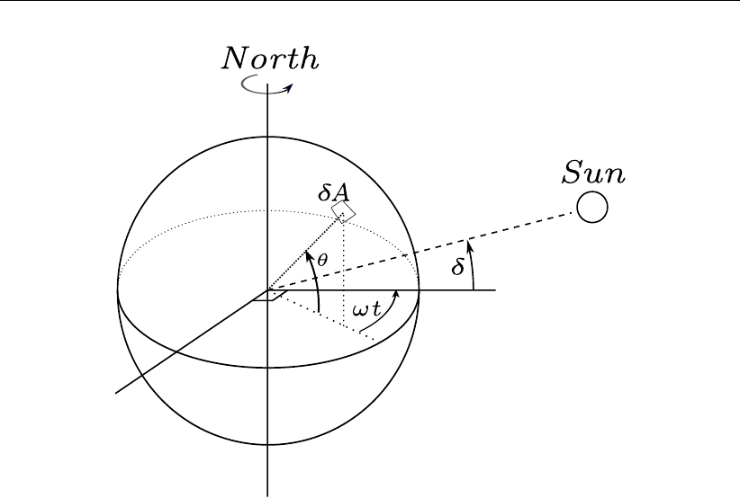
DRAFT
D-Flow Flexible Mesh, User Manual
Figure 10.2: Co-ordinate system position Sun
δ: declination; θ: latitude; ωt: angular speed
a cloud cover fraction Fc, the fraction of the sky covered by clouds. The correction factor for
cloud cover is an empirical formula. The absorption of solar radiation is calculated (Gill,1982)
as the product of the net downward flux of short wave-radiation in cloudless conditions and
factors correcting for reflection and cloud cover:
Qsn =Qs−Qsr = (1 −α)Qsc(1.0−0.4Fc−0.38F2
c),(10.12)
with:
Qsn net heat radiation (flux) from the Sun
Qssolar radiation (short wave radiation) in [J/m2s]
Qsr reflected solar radiation in [J/m2s]
Qsc radiation (flux) for clear sky condition
αalbedo (reflection) coefficient (=0.06)
Fcfraction of sky covered by clouds (user-defined input)
10.3 Atmospheric radiation (long wave radiation)
Atmospheric radiation is primarily due to emission of absorbed solar radiation by water vapour,
carbon dioxide and ozone in the atmosphere. The emission spectrum of the atmosphere is
highly irregular. The amount of atmospheric radiation that reaches the earth is determined by
applying the Stefan-Boltzmann’s law that includes the emissivity coefficient of the atmosphere
ε. Taking into account the effect of reflection by the surface and reflection and absorption by
clouds, the relation for the net atmospheric radiation Qan reads (Octavio et al.,1977):
Qan = (1 −r)εσ ¯
T4
ag(Fc),(10.13)
where ¯
Tais the air temperature (in K) and the reflection coefficient r= 0.03. The emissivity
factor of the atmosphere εmay depend both on vapour pressure and air temperature. The
emissivity of the atmosphere varies between 0.7 for clear sky and low temperature and 1.0.
The presence of clouds increases the atmospheric radiation. This is expressed in the cloud
function g(Fc).
170 of 412 Deltares

DRAFT
Heat transport
with Tathe air temperature (in ◦C). The cloud function g(Fc)in Equation (10.13) is given by:
g(Fc)=1.0+0.17F2
c.2−9(10.14)
The linearisation of Equation (10.13) is carried out around Ta= 15 ◦C.
Remark:
The atmospheric radiation is part of the total long-wave radiation flux, the so-called
effective back radiation, see section 10.5.
10.4 Back radiation (long wave radiation)
Water radiates as a near black body, so the heat radiated back by the water can be described
by Stefan-Boltzmann’s law of radiation, corrected by an emissivity factor ε= 0.985 of water
(Sweers,1976;Octavio et al.,1977) and the reflection coefficient for the air-water interface
r= 0.03:
Qbr = (1 −r)εσ ¯
T4
s,(10.15)
with ¯
Tsthe (absolute) water surface temperature in K.
10.5 Effective back radiation
The total net long wave radiation flux is computed. This is called the effective back radiation:
Qeb =Qbr −Qan.(10.16)
The atmospheric radiation depends on the vapour pressure ea, see section 10.6, the air tem-
perature Taand the cloud cover Fc. The back radiation depends on the surface temperature
Ts.
The effective back radiation Qeb is computed following:
Qeb =εσ ¯
T4
s(0.39 −0.05√ea)1.0−0.6F2
c,(10.17)
with the actual vapour pressure eagiven by Equation (10.22).
10.6 Evaporative heat flux
Evaporation is an exchange process that takes place at the interface between water and air
and depends on the conditions both in the water near the surface and the air above it. The
evaporation depends on meteorological factors (wind-driven convection) and vapour pres-
sures.
Forced convection of latent heat
The latent heat flux due to forced convection for the ocean heat flux model reads:
Qev,forced =LVρaf(U10){qs(Ts)−qa(Ta)},(10.18)
with qsand qathe specific humidity of respectively saturated air and remote air (10 m above
water level):
qs(Ts) = 0.62es
Patm −0.38es
,(10.19)
qa(Ta) = 0.62ea
Patm −0.38ea
.(10.20)
Deltares 171 of 412

DRAFT
D-Flow Flexible Mesh, User Manual
The saturated and remote vapour pressures esand eaare given by:
es= 100.7859+0.03477Ts
1.0+0.00412Ts,(10.21)
ea=rhum100.7859+0.03477Ta
1.0+0.00412Ta.(10.22)
With Lvthe latent heat of vaporisation in J/kg water:
Lv= 2.5 106−2.3 103Ts.(10.23)
The wind function in Equation (10.18) is defined as:
f(U10) = ceU10,(10.24)
Without the influence of free convection, the Dalton number cein the Composite heat flux
model was calibrated for the North Sea to be ce= 0.0015. This value should be close to the
Cdcoefficient that is used in the computation of wind stresses. The exchange coefficients of
latent heat and momentum transfer are closely related. Specifying a negative Dalton number
in the mdu file forces the use of the specified Cdcoefficient, thus taking into account the
specified dependency between windspeed and the Cdcoefficient.
Here rhum is the relative humidity in [-].
Remarks:
The relative humidity rhum is specified in the input files in percentages.
When the computed Eis negative, it is replaced by zero, assuming that it is caused by
modelling misfit and not by the actual physical process of water condensation out of the
air into the water. The same applies to the part associated with free convection.
For the excess temperature model, the wind speed function f(U10)following Sweers (1976)
is used:
f(U10) = (3.5+2.0U10)5.0×10⁶
Sarea 0.05
,(10.25)
where Sarea is the exposed water surface in m2, defined in the input and fixed for the whole
simulation. The coefficients calibrated by Sweers were based on the wind speed at 3 meter
above the free surface; the coefficients in Equation (10.25) are based on the wind speed 10
meter above the water level.
Free convection of latent heat
Loss of heat due to evaporation occurs not only by forced convection, wind driven, but also
by free convection. Free convection is driven by buoyant forces due to density differences
(by temperature and/or water vapour content) creating unstable conditions in the atmospheric
boundary layer. Evaporation due to free convection is important in circumstances where in-
verse temperature/density gradients are present and wind speeds are almost negligible so
that the amount of forced convection is small. Neglecting free convection in this situation will
lead to underestimating the heat loss. (Ryan et al.,1974) developed a correction to the wind
function, accounting for free convection. The derivation of evaporation by just free convection
is based on the analogy of heat and mass transfer.
172 of 412 Deltares

DRAFT
Heat transport
The latent heat flux due to free convection reads:
Qev,free =ksLVρa(qs−qa),(10.26)
with the average air density:
ρa=ρa0+ρa10
2,(10.27)
and with the heat transfer coefficient defined as:
ks=(0if ρa10 −ρa0≤0
cfr.conv ngα2
νair ρa(ρa10 −ρa0)o1/3if ρa10 −ρa0>0(10.28)
where the coefficient of free convection cf r.conv was calibrated to be 0.14, see (Ryan et al.,
1974). The viscosity of air νair is assumed to have the constant value 16.0×10⁻⁶m2/s. The
molecular diffusivity of air αm2/s is defined as
α=νair
σ,(10.29)
with σ= 0.7(for air) the Prandtl number. In Equation (10.26), the saturated air density is
given by:
ρa0=
100Patm−100es
Rdry +100es
Rvap
Ts+ 273.15 ,(10.30)
the remote air density (10 m above the water level):
ρa10 =
100Patm−100ea
Rdry +100ea
Rvap
Tair + 273.15 ,(10.31)
where Rdry is the gas constant for dry air: 287.05 J/(kg K) and Rvap is the gas constant for
water vapour: 461.495 J/(kg K). The specific humidity of respectively saturated air and remote
air (10 m above the water level), qsand qaare given by Equation (10.19) and Equation (10.20).
The saturated and remote vapour pressure esand eaare defined in Equation (10.21) and
Equation (10.22).
The total heat flux due to evaporation then results from adding the forced convection of latent
heat in Equation (10.18) and the free convection of latent heat in Equation (10.26):
Qev =Qev,forced +Qev,free.(10.32)
10.7 Convective heat flux
In the Ocean heat flux model, the convective heat flux is split into two parts, just as the evap-
orative heat flux. The convective heat flux is divided into a contribution by forced convection
and a contribution by free convection.
Forced convection of sensible heat
The sensible heat flux due to forced convection is computed by:
Qco,forced =ρacpg(U10) (Ts−Ta),(10.33)
with cpthe specific heat of air. It is considered constant and taken to be 1 004.0J/(kg K). The
wind-speed function g(U10)is defined following Gill (1982):
g(U10) = cHU10,(10.34)
with cHthe so-called Stanton number. Without the influence of free convection, the Stanton
number was calibrated for the North Sea to be cH= 0.00145.
Deltares 173 of 412

DRAFT
D-Flow Flexible Mesh, User Manual
Free convection of sensible heat
Qco,free =ksρacp(Ts−Ta),(10.35)
with the heat transfer coefficient ksgiven by Equation (10.28).
The total heat flux due to convection then results from adding the forced convection of sensible
heat in Equation (10.33) and the free convection of sensible heat in Equation (10.35):
Qco =Qco,forced +Qco,free.(10.36)
174 of 412 Deltares
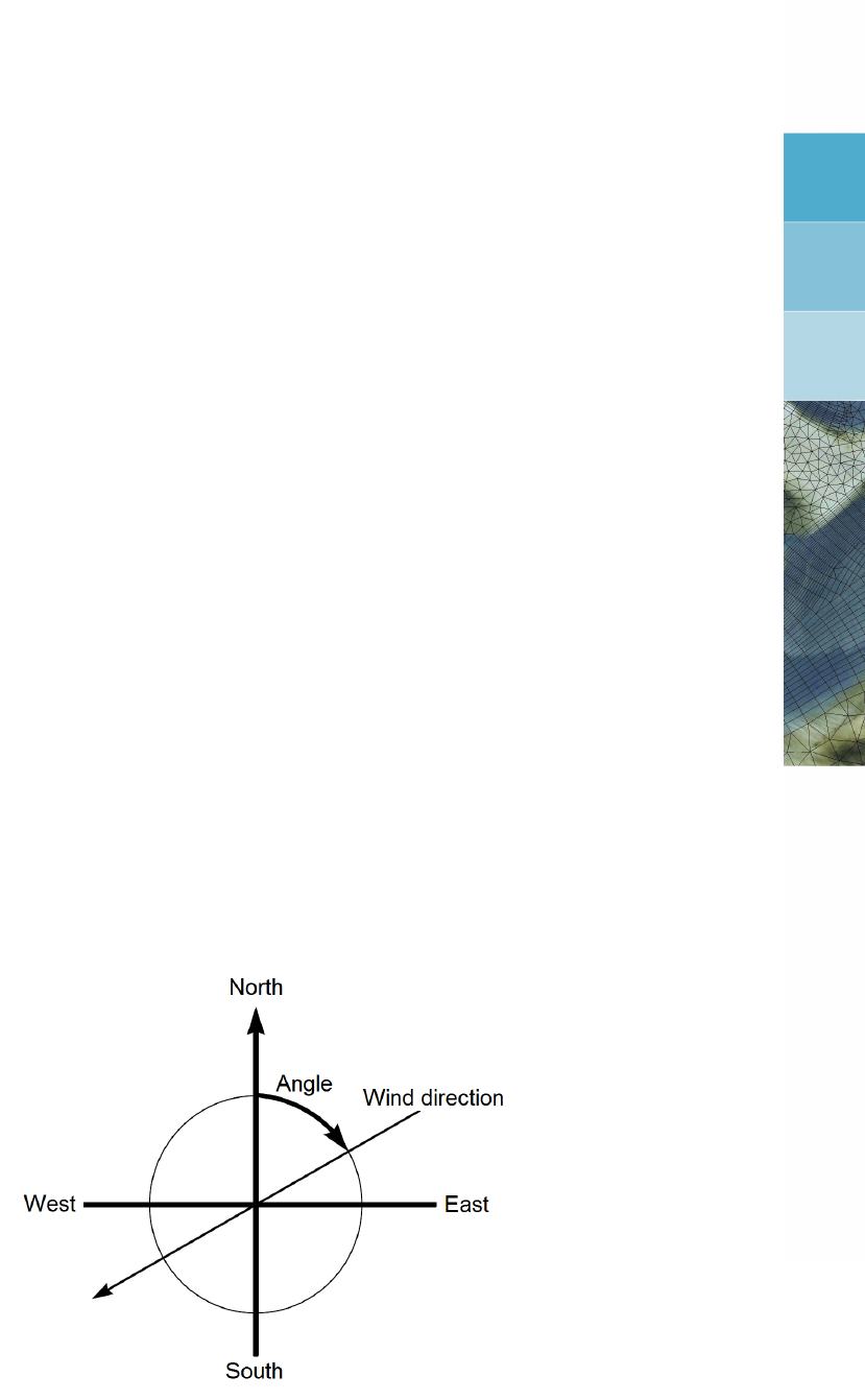
DRAFT
11 Wind
Various external influences can exert a force on the flow field. One of these influences is the
wind. The force exerted by the wind is coupled to the flow equations as a shear stress. The
magnitude is determined by the following widely used quadratic expression:
|τs|=ρaCdU2
10 (11.1)
where:
ρathe density of air.
U10 the wind speed 10 meter above the free surface (time and space dependent).
Cdthe wind drag coefficient, dependent on U10.
In order to specify the wind shear stress, a drag coefficient is required as well as the wind
field in terms of velocity magnitude and wind direction. In this chapter, the backgrounds
are provided of how wind fields should be imposed, in addition to section 4.4.9.4. Relevant
definitions are addressed in section 11.1, whereas supported file formats are addressed in
section 11.2.
11.1 Definitions
When imposing wind conditions, two definitions are respected: a definition for the wind direc-
tion (see section 11.1.1) and a definition regarding the drag coefficient (see section 11.1.2).
11.1.1 Nautical convention
The wind direction is defined according to the nautical definition, i.e. relative to true North and
positive measured clockwise. In Figure 11.1 the wind direction is about +60 degrees, i.e. an
East-North-East wind.
Figure 11.1: Nautical conventions for the wind.
11.1.2 Drag coefficient
The dependency of the drag coefficient on the wind speed should be specified by the user.
The user can choose between the following concepts:
Deltares 175 of 412
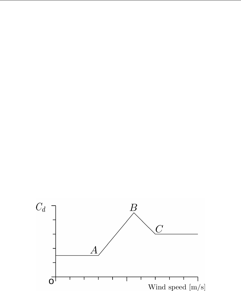
DRAFT
D-Flow Flexible Mesh, User Manual
a constant drag coefficient,
a dependency according to Smith and Banke (1975),
a dependency according to Charnock (1955),
a dependency according to Hwang (2005a) and Hwang (2005b).
The specification of the type of wind drag formulation should be accomplished in the MDU-
file. For this purpose, the keyword ICdtyp can be utilized. For this keyword ICdtyp, five
options could be demanded for:
ICdtyp = 1 – constant drag coefficient,
ICdtyp = 2 – linearly varying drag coefficient (cf. Smith and Banke (1975)),
ICdtyp = 3 – piecewise linearly varying drag coefficient (cf. Smith and Banke (1975)),
ICdtyp = 4 –Charnock (1955) formulation (no breakpoints),
ICdtyp = 5 –Hwang (2005a) and Hwang (2005b) formulation (no breakpoints).
If a Smith & Banke type dependency is chosen for, the additional entries Cdbreakpoints
and Windspeedbreakpoints come into play. In the following sections, the specification
of either of these options are depicted.
Smith & Banke type formulation
When specifying a Smith & Banke type dependency, the definition as sketched in Figure 11.2
should be kept in mind.
Figure 11.2: Prescription of the dependency of the wind drag coefficient Cdon the wind
speed is achieved by means of at least 1 point, with a maximum of 3 points.
From this sketch, it can be seen that the wind drag is considered as dependent on the wind
speed in a piecewise linear way. The options, that are facilitated in this respect, are:
define one set of coordinates (breakpoint A), specifying a constant drag coefficient, valid
for all wind speeds,
define two sets of coordinates (breakpoints A and B), specifying a linearly varying depen-
dency for one range of wind speeds,
define three sets of coordinates (breakpoints A, B and C), specifying a piecewise linear
dependency for two ranges of wind speeds.
Remark that for the latter two options, the drag coefficient is taken constant for wind speeds
176 of 412 Deltares

DRAFT
Wind
lower/higher than the lowest/highest specified wind speed, with a drag coefficient equal to the
drag coefficient associated with the lowest/highest specified lowest/highest wind speed. In
case of three breakpoints, the expression reads:
Cd(U10) =
CA
d, U10 ≤UA
10,
CA
d+CB
d−CA
dU10 −UA
10
UB
10 −UA
10
, UA
10 ≤U10 ≤UB
10,
CB
d+CC
d−CB
dU10 −UB
10
UC
10 −UB
10
, UB
10 ≤U10 ≤UC
10,
CC
d, UC
10 ≤U10,
(11.2)
By means of the entries Cdbreakpoints and Windspeedbreakpoints, the coor-
dinates of the breakpoints (see Figure 11.2) can be specified. Typical values associated
with the Smith and Banke (1975) formulation are Cd= 6.3×10⁻⁴for U= 0 m/s and
Cd= 7.23 ×10⁻³for U= 100 m/s. In this case, the entries in the MDU-file should be
specified as follows:
[wind]
ICdtyp = 2
Cdbreakpoints = 0.00063 0.00723
Windspeedbreakpoints = 0.00000 100.00000
Charnock formulation
The Charnock formulation (see Charnock (1955)) is based on the assumption of a fully devel-
oped turbulent boundary layer of the wind flow over the water surface. The associated wind
speed profile follows a logithmic shape. In the Charnock formulation, the wind speed is con-
sidered at 10 meters above the free water surface, hence yielding the following expression:
U10
u∗
=1
κln z10
z0(11.3)
with κthe Von Kármán constant, z10 the distance to the water surface (equal to 10 m), u∗the
friction velocity and U10 the wind speed at 10 m above the water surface. The drag coefficient
Cdis defined as:
Cd=u2
∗
U2
10
.(11.4)
Charnock (1955) has proposed to represent the friction of the water surface as z0according
to:
z0=b u2
∗
g,(11.5)
with gthe gravitation acceleration and ba specific constant. Charnock (1955) has proposed
b= 0.012. The value of the constant bcan be specified in the MDU-file by the user by means
of one single value for Cdbreakpoints. Since the above relation yields an implicit relation
for u∗, the system is solved for iteratively. The user should be aware of interpretation of the
specified wind field as the wind field at 10 m above the water surface. See paragraph 11.2.4
for a space and time varying Charnock coefficient b.
Deltares 177 of 412

DRAFT
D-Flow Flexible Mesh, User Manual
Hwang formulation
The dynamic roughness could also be related to the steady state wave conditions of the flow
field under consideration. The connection of the wave parameters with the drag coefficient
as elaborated by Hwang (2005a) is available within D-Flow FM through ICdtyp = 5, given
a wave field. The Hwang-formulation interpretes the user defined wind speed as the wind
speed at 10 m above the water surface.
The drag coefficient is computed as:
Cd=1
κln kpz10
kpz0−2
(11.6)
with z10 = 10 m, κthe Von Kármán constant. With wavelength scaling, kpz0is the natural
expression of the dimensionless roughness, where kpis the wave number of the spectral
peak, computed on the basis of the actual water depth and the provided peak period Tpas
wave field. Further following Hwang (2005a),
kpz0=πexp −κC−0.5
λ/2(11.7)
in which Cλ/2is the drag coefficient at half the wavelength above surface. This parameter
Cλ/2is computed as:
Cλ/2=A10 ωpU10
ga10
(11.8)
in which A10 = 1.289 ×10⁻³,a10 = 0.815,U10 the wind speed at 10 m above the water
surface and ωpthe wave peak frequency (ωp= 2π/Tp). Thus, the drag coefficient Cdis
defined.
11.2 File formats
The wind field should be provided by means of an ascii-type file. This file should contain the
grid on which the wind field is defined as well as the wind velocity vector(s).
D-Flow FM currently supports four types of wind field prescriptions, i.e. four grid types on
which the wind field can be given. This wind grid does not need to be the same as the
computational grid. The grid options to provide the wind data on are:
1 the computational grid — in this case, no specific wind grid is provided. The provided wind
field is considered to be uniform over the entire model area. The wind field can be time
dependent.
2 an equidistant grid — in this case, a wind field can be prescribed that varies both in space
and in time. A Cartesian arcinfo-type grid should be provided on which the wind field is
defined.
3 a curvilinear grid — this case is conceptually similar to the previous type (the equidistant
grid) in the sense that a wind field can be imposed that both varies in space and time.
However, a separate file should be provided in which a curvilinear grid is defined (a classic
<∗.grd>-type file as known from Delft3D) on which the wind field is defined.
4 a spiderweb grid — this type of wind specification is specially devoted to cyclone winds
and is only available in combination with computational grids that are of spherical type.
In this case, a cyclone wind field is given on a polar grid with the center (’eye’) of the
cyclone being the origin of the polar coordinate system. The location of this eye and the
associated wind field usually varies in time.
178 of 412 Deltares

DRAFT
Wind
Each of these filetypes can be assigned through the entry in the external forcings file (the
<∗.ext>-file) named FILETYPE. In this chapter, the various types of wind field specifications
are highlighted subsequently. Each of the options is illustrated by means of an example.
11.2.1 Defined on the computational grid
In D-Flow FM, the specification of the wind on the computational grid is equivalent to the
specification of a uniform wind, since no separate wind grid is provided to the model. The
specification of a uniform wind field can be done in two ways:
1 componentwise: as velocity in the longitudinal x-direction [m/s] and in the latitudal y-
direction [m/s] — the associated FILETYPE in the external forcings file is depicted as
uniform, which has FILETYPE=1.
2 by magnitude [m/s] and direction [degN] (see Figure 11.1) — the associated FILETYPE
in the external forcings file is depicted as unimagdir, which has FILETYPE=2.
These two types are treated below separately.
11.2.1.1 Specification of uniform wind through velocity components
Since no particular wind grid is used, only timeseries for the x-component and the y-compo-
nent of the wind need to be specified. The specification of these timeseries can be done
separately (one single file for the x-component and one single file for the y-component) or
jointly (one single file containing the x-component and the y-component of the wind).
Uniform wind should be provided as an <∗.wnd>-file containing either 2 colums (in case
of separate specification of the x-component and y-component of the wind) or 3 columns (in
case of joint specification of the velocity components). In either case, the first column contains
the time in minutes with respect to the overall reference time.
Example
As an example, a uniform wind field is applied to a certain model. The uniform wind is provided
in a file named windxdirydir.wnd. The contents of this wind file are:
0.00000 10.00000 10.00000
60.00000 -10.00000 -10.00000
The first column denotes the time in minutes with respect to the reference date (specified in
the mdu-file). The second column denotes the wind velocity in x-direction, whereas the third
column denotes the wind velocity in y-direction; both wind components are provided in one
single file.
The connection with the flow model itself is laid through the external forcings file. The actual
specification of the wind is in this case:
QUANTITY =windxy
FILENAME =windxdirydir.wnd
FILETYPE =1
Deltares 179 of 412

DRAFT
D-Flow Flexible Mesh, User Manual
METHOD =1
OPERAND =O
Since the two components are given in one single file, the QUANTITY is set to windxy. If
two separate files would have been provided, the QUANTITY would have been set to windx
and windy over two separate datablocks in the external forcings file.
11.2.1.2 Specification of uniform wind through magnitude and direction
Instead of specifying the separate components of the wind field, the uniform wind vector can
also be prescribed through its magnitude and direction (see Figure 11.1).
This kind of specification should be done by means of one single file, containing three columns,
representing the time (in minutes with respect to the reference date), the velocity magnitude
[m/s], not necessarily positive, and the direction (nautical convention).
Example
As an example, the previous uniform wind case is reformulated as a case with magnitude
and direction of the wind field prescribed. The unimagdir wind is provided in a file named
<windinput.wnd>. The contents of this file are:
0.00000 14.14213562373095 225.00000
60.00000 -14.14213562373095 225.00000
The first column denotes the time in minutes with respect to the reference date (specified in
the mdu-file). The second column denotes the wind velocity magnitude, whereas the third
column denotes the wind direction. Note that there is a clear difference between the above
case and a case in which the magnitude is kept positive (14.1421 m/s) and the direction varies
(and hence rotates!) from 225 degN to 45 degN.
The connection with the flow model itself is laid through the external forcings file. The actual
specification of the wind is in this case:
QUANTITY =windxy
FILENAME =windinput.wnd
FILETYPE =2
METHOD =1
OPERAND =O
11.2.2 Defined on an equidistant grid
The vector components of the velocity vectors can also be specified on a distinct grid, either of
equidistant type or of curvilinear type. In both cases, the characteristics of the grid should be
provided. In case of an equidistant grid, the grid is specified in arcinfo-style. That means, the
constant grid sizes ∆xand ∆yshould be specified such that a grid is spanned with respect
to the location of the lower left corner of the grid (either the center of the lower left cel or the
lower left corner of the lower left cell).
180 of 412 Deltares

DRAFT
Wind
Example
As an example, a grid with ∆x= ∆y= 100 m is spanned, based on the center of the
lower left cell, located at x=y= 60 m with respect to the origin. The input data for the x-
component and the y-component should be specified separately, in two distinct files. The input
of the x-component data should be given in an <∗.amu>-type file, such as <windxdir.amu>
as an example:
### START OF HEADER
### This file is created by Deltares
### Additional commments
FileVersion = 1.03
filetype = meteo_on_equidistant_grid
NODATA_value = -9999.0
n_cols = 5
n_rows = 4
grid_unit = m
x_llcenter = 60
y_llcenter = 60
dx = 110
dy = 110
n_quantity = 1
quantity1 = x_wind
unit1 = m s-1
### END OF HEADER
TIME = 0 hours since 2006-01-01 00:00:00 +00:00
10 10 10 10 10
10 10 10 10 10
10 10 10 10 10
10 10 10 10 10
TIME = 1 hours since 2006-01-01 00:00:00 +00:00
-10 -10 -10 -10 -10
-10 -10 -10 -10 -10
-10 -10 -10 -10 -10
-10 -10 -10 -10 -10
For the y-component data, a similar file (e.g. <windydir.amv>) should be provided. In ad-
dition, the pressure could be specified in a similar file (e.g. <pressure.amp>). Note that
x_llcorner and y_llcorner, instead of x_llcenter and y_llcenter, are also
supported.
Wind on an equidistant grid has been provided a filetype specification as FILETYPE=4. The
connection with the flow model itself is laid through the external forcings file. The actual
specification of the wind is in this case:
QUANTITY =windx
FILENAME =windxdir.amu
FILETYPE =4
METHOD =2
OPERAND =O
QUANTITY =windy
FILENAME =windydir.amv
FILETYPE =4
METHOD =2
OPERAND =O
Deltares 181 of 412

DRAFT
D-Flow Flexible Mesh , User Manual
QUANTITY =atmosphericpressure
FILENAME =pressure.amp
FILETYPE =4
METHOD =2
OPERAND =O
11.2.3 Defined on a curvilinear grid
In analogy with the wind specification on an equidistant grid, the wind can be specified on a
curvilinear grid. This curvilinear grid should be provided as a classic <∗.grd>-file as known
from Delft3D. A difference with the equidistant grid wind is the necessity to compile all data
blocks (i.e. pressure, x-component and y-component) in one single file. This file should have
the extension <∗.apwxwy>. The sequence of this datablock is: 1) pressure, 2) x-velocity
component, 3) y-velocity component.
Example
As an example, a curvilinear grid named <meteo.grd>is present, providing the underlying
coordinates of the wind data field. The input data, comprising the atmospheric pressure,
the x-velocity component and the y-velocity component, are given in one single file (as is
compulsory). The contents of the example <meteo.apwxwy>-file is:
### START OF HEADER
### This file is created by Deltares
### Additional commments
FileVersion = 1.03
filetype = meteo_on_curvilinear_grid
NODATA_value = -9999.0
grid_file = meteo.grd
first_data_value = grid_llcorner
data_row = grid_row
n_quantity = 3
quantity1 = apwxwy
unit1 = Pa
### END OF HEADER
TIME = 0.0 hours since 2006-01-01 00:00:00 +00:00
101325 101325 101325 101325 101325
101325 101325 101325 101325 101325
101325 101325 101325 101325 101325
101325 101325 101325 101325 101325
10 10 10 10 10
10 10 10 10 10
10 10 10 10 10
10 10 10 10 10
10 10 10 10 10
10 10 10 10 10
10 10 10 10 10
10 10 10 10 10
TIME = 1.0 hours since 2006-01-01 00:00:00 +00:00
101325 101325 101325 101325 101325
101325 101325 101325 101325 101325
101325 101325 101325 101325 101325
101325 101325 101325 101325 101325
-10 -10 -10 -10 -10
-10 -10 -10 -10 -10
-10 -10 -10 -10 -10
-10 -10 -10 -10 -10
-10 -10 -10 -10 -10
-10 -10 -10 -10 -10
182 of 412 Deltares

DRAFT
Wind
-10 -10 -10 -10 -10
-10 -10 -10 -10 -10
Note that grid_llcenter, instead of grid_llcorner, is also supported. On the con-
trary, grid_column is not supported instead of grid_row.
Wind on a curvilinear grid has been provided a filetype specification as FILETYPE=6. The
connection with the flow model itself is laid through the external forcings file. The actual
specification of the wind is in this case:
QUANTITY =airpressure_windx_windy
FILENAME =meteo.apwxwy
FILETYPE =6
METHOD =3
OPERAND =O
Notice that METHOD=3 is chosen for wind on a curvilinear grid, instead of METHOD=2 in case
of wind on an equidistant grid.
11.2.4 Space and time varying Charnock coefficients
The value for the Charnock coefficient bin Eq. ((11.5)) can be a constant given in the MDU-
file, but also be given as a space and time varying field.
For a space and time varying Charnock coefficient, the user should provide a NetCDF-file
with meteorological forcing, including Charnock coefficients, and use the file specification
FILETYPE=11.
The specification is in this case:
QUANTITY =airpressure_windx_windy_charnock
FILENAME =meteo.nc
FILETYPE =11
METHOD =3
OPERAND =O
Deltares 183 of 412
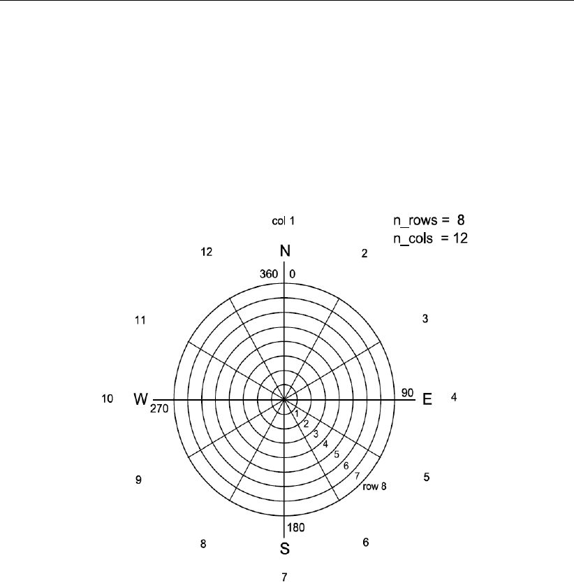
DRAFT
D-Flow Flexible Mesh, User Manual
11.2.5 Defined on a spiderweb grid
Cyclone winds can be imposed by means of a ‘spiderweb’-like polar grid. The origin typi-
cally coincides with the cyclone eye and can move in time. Spiderwebs can only be used in
combination with a spherical computational grid. The origin of the spiderweb should be given
as longitude (for xeye) and latitude (for yeye). The number of rows (discretisation in radial
direction) and the number of columns (discretisation in angular direction) should be given, as
well as the radius of the grid (in meters). The definition of the spiderweb grid is illustrated in
Figure 11.3.
Figure 11.3: Grid definition of the spiderweb grid for cyclone winds.
The files containing the spiderweb data and metadata have the extension <∗.spw>. They
consist of a global header containing properties that are not varying in time, followed by blocks
of data for subsequent time levels. Each of these data blocks is headed by a set of properties
for the corresponding time level. A detailed description of the spiderweb file format can be
found in section B.12.3.
Through the specified unit for atmospheric pressure in the file, it can be specified whether the
values should be interpreted as mbar (=hPa), instead of Pa, which is the default. Specifying
the spiderweb merge fraction βin spw_merge_frac allows for linear fading of wind speed
and pressure drop towards the outer rim. For a spiderweb with radius R, the weigth assigned
to the spiderweb wind and pressure at a radius ris given by (R−r)/βR for rbetween
(1 −β)Rand R. The weight equals unity within the inner circle and zero beyond the outer
rim.
184 of 412 Deltares

DRAFT
Wind
Example
As an example, a spiderweb grid named <spwsimple.spw>is present, providing the under-
lying coordinates of the wind data field. The input data, comprising the atmospheric pressure
drops, the wind velocity magnitudes (in [m/s]) and the wind directions (in [degN]), are given in
one single file (as is compulsory). The contents of the example <spwsimple.spw>-file is:
### Spiders web derived from TRACK file: gonu.trk
### This file is created by Deltares
### All text on a line behind the first # is parsed as commentary
### Additional commments
FileVersion = 1.03
filetype = meteo_on_spiderweb_grid
### Spiders web derived from TRACK file: gonu.trk
### This file is created by Deltares
### All text on a line behind the first # is parsed as commentary
### Additional commments
NODATA_value = -1001
n_cols = 4
n_rows = 4
spw_radius = 600000.0
spw_merge_frac = 0.75
spw_rad_unit = m
### END OF HEADER
TIME = 340000.00 minutes since 2005-01-01 00:00:00 +00:00
x_spw_eye = 265.00
y_spw_eye = 33.00
p_drop_spw_eye = 7000.000
5.000000 5.000000 5.000000 5.000000
10.000000 10.000000 10.000000 10.000000
15.000000 15.000000 15.000000 15.000000
20.000000 20.000000 20.000000 20.000000
270.00 0.00 90.00 180.00
270.00 0.00 90.00 180.00
270.00 0.00 90.00 180.00
270.00 0.00 90.00 180.00
4000.00 4000.00 4000.00 4000.00
3000.00 3000.00 3000.00 3000.00
2000.00 2000.00 2000.00 2000.00
1000.00 1000.00 1000.00 1000.00
TIME = 380000.00 minutes since 2005-01-01 00:00:00 +00:00
x_spw_eye = 275.00
y_spw_eye = 18.00
p_drop_spw_eye = 8000.000
5.000000 5.000000 5.000000 5.000000
10.000000 10.000000 10.000000 10.000000
15.000000 15.000000 15.000000 15.000000
20.000000 20.000000 20.000000 20.000000
270.00 0.00 90.00 180.00
270.00 0.00 90.00 180.00
270.00 0.00 90.00 180.00
270.00 0.00 90.00 180.00
4000.00 4000.00 4000.00 4000.00
3000.00 3000.00 3000.00 3000.00
2000.00 2000.00 2000.00 2000.00
1000.00 1000.00 1000.00 1000.00
Wind on a spiderweb grid has been provided a filetype specification as FILETYPE=5. The
connection with the flow model itself is laid through the external forcings file. The actual
specification of the wind is in this case:
Deltares 185 of 412

DRAFT
D-Flow Flexible Mesh , User Manual
QUANTITY =airpressure_windx_windy
FILENAME =spwsimple.spw
FILETYPE =5
METHOD =1
OPERAND =O
Notice that METHOD=1 is chosen for wind on a spiderweb grid, instead of METHOD=2 in case
of wind on an equidistant grid and METHOD=3 in case of wind on a curvilinear grid.
Alternatively, the spiderweb wind and pressure can be specified in the external forcings file as
separate quantities referring to the same file (or specify one and omit the other):
QUANTITY =windxy
FILENAME =spwsimple.spw
FILETYPE =5
METHOD =1
OPERAND =O
QUANTITY =airpressure
FILENAME =spwsimple.spw
FILETYPE =5
METHOD =1
OPERAND =O
(NB. There is a slight difference between both specifications regarding their effect on the flow.
The first approach requires an additional interpolation of wind on the velocity points, which in
some cases of coarse computational grids and small scale wind could introduce smoothing.)
11.2.6 Combination of several wind specifications
The combination of the various wind specification types can only be achieved if the QUANTITY
of the winds to be combined is the same, for instance QUANTITY=windx. The option
OPERAND=+ can be used to add a wind field to an existing wind field.
Example
If the uniform wind is to be combined with a wind specified on an equidistant grid, then the
wind field could be assigned in the external forcings file as follows:
QUANTITY =windx
FILENAME =windxdir.wnd
FILETYPE =1
METHOD =1
OPERAND =O
QUANTITY =windy
FILENAME =windydir.wnd
FILETYPE =1
METHOD =1
OPERAND =O
186 of 412 Deltares

DRAFT
Wind
QUANTITY =windx
FILENAME =windxdir.amu
FILETYPE =4
METHOD =2
OPERAND =+
QUANTITY =windy
FILENAME =windydir.amv
FILETYPE =4
METHOD =2
OPERAND =+
The same is possible for e.g. a uniform wind and two spiderweb cyclones:
QUANTITY=windxy
FILENAME=uni.tim
FILETYPE=2
METHOD=1
OPERAND=O
QUANTITY =windxy
FILENAME =spwsimple.spw
FILETYPE =5
METHOD =1
OPERAND =+
QUANTITY =windxy
FILENAME =spwsimple2.spw
FILETYPE =5
METHOD =1
OPERAND =+
QUANTITY =atmosphericpressure
FILENAME =spwsimple.spw
FILETYPE =5
METHOD =1
OPERAND =+
QUANTITY =atmosphericpressure
FILENAME =spwsimple2.spw
FILETYPE =5
METHOD =1
OPERAND =+
In the above example, the wind is first prescribed as a spatially uniform time-varying field,
onto which the spiderweb winds are added Note that the uniform wind has the ‘O’ operand,
which means that it overrides rather than adds. However, since the default wind is zero, one
might just as well have used the ‘+’ operand. If the spiderweb merge fraction is specified
in the spiderweb file, a gradual transition between the spiderweb wind and the background
wind is applied using the linearly varying weight as described above. The same is done for
atmospheric pressure, if specified except that pressure is added to, whereas wind is averaged
with the background values. Without any input, the background atmospheric pressure is set
to PavBnd in the section [wind] in the MDU-file, if present and zero otherwise.
Deltares 187 of 412

DRAFT
D-Flow Flexible Mesh, User Manual
11.3 Masking of points in the wind grid from interpolation (‘land-sea mask’)
A mask can be supplied by the user to prevent selected points in the wind grid from contribut-
ing to the wind interpolation on velocity points, e.g. to exclude land points. This feature was
included to conform to SIMONA and therefore implemented in the same way.
For each individual grid point for which to interpolate from the wind grid:
Masked wind points are excluded from the interpolation.
The total of the weight factors for the remaining wind points is determined.
If this total falls below 1E-03, the mask is ignored and the original bilinear weights are
used.
Otherwise, the weights for the remaining wind points are normalised again.
The effect of the mask, when applied as a land-sea mask, is that for velocity points close
to shore the interpolated wind is no longer influenced by the wind over land (which would
otherwise yield a zone of points with reduced wind near the shore).
Specification and format of the mask file
The name of the mask file, if any, is specified in the <.ext>file, labelled SOURCEMASK,
directly following the FILENAME specification, e.g.:
QUANTITY =windxy
FILENAME =meteo.wxwy
SOURCEMASK =meteo_mask.asc
FILETYPE =6
METHOD =3
OPERAND =O
The mask file itself has the same layout as the wind file, though the number of required header
fields is reduced, e.g.:
FileVersion = 1.03
.
.
unit1 = Pa
### END OF HEADER
11111
11100
11100
11000
The lines in the header are ignored. The number of columns and rows in the matrix of ones
and zeros should match those of a block (for a single variable and a single timestep) in the
meteo files. Zeros signify the position of rejected points (and ones those of the accepted
points) in the wind grid.
188 of 412 Deltares
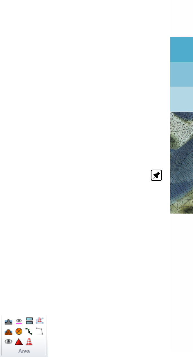
DRAFT
12 Hydraulic structures
12.1 Introduction
Obstacles in the flow may generate sudden transitions from flow contraction to flow expansion.
The grid resolution is often low compared to the gradients of the water level, the velocity
and the bathymetry. The hydrostatic pressure assumption may locally be invalid. Examples
of these obstacles in civil engineering are: gates, barriers, dams, groynes and weirs. The
obstacles generate energy losses and may change the direction of the flow.
The forces due to obstacles in the flow which are not resolved (sub-grid) on the horizontal grid,
should be parameterised. The obstacles are denoted in D-Flow FM as hydraulic structures.
In the numerical model the hydraulic structures should be located at velocity points of the
grid. The direction of the forces should be specified at input. To model the force on the flow
generated by a hydraulic structure, a quadratic energy or linear loss term is added to the
momentum equation.
Note: Structure definitions can be made in Delta Shell, and will then be saved into a struc-
tures <∗.ini>-file (section B.11).
12.2 Structures
The user can insert the hydraulic structures by the means of polygons on the grid. By select-
ing the required structure and drawing a polygon on the computational grid, the location of
structure can be defined (see Figure 12.1). The supported structures in D-Flow FM are
Fixed Weirs
(Adjustable) weirs
Gates
Pumps
Thin dams
In practice, the word ’barrier’ is often used for structures. However, in D-Flow FM such struc-
tures are modelled as a gate or a weir in combination with a so-called Control Group (D-Real
Time Control model).
Figure 12.1: Selection of structures (and other items) in the toolbar.
Deltares 189 of 412
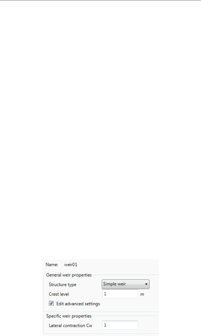
DRAFT
D-Flow Flexible Mesh, User Manual
12.2.1 Fixed weirs
In D-Flow FM, a fixed weir is a fixed non-movable construction generating energy losses due
to constriction of the flow. They are commonly used to model sudden changes in depth (roads,
summer dikes) and groynes in numerical simulations of rivers. Such structures are applied
to keep the river in its bed for navigation purposes. Others are built, for instance, to protect
an area behind a tidal weir from salt intrusion. Upstream of a weir the flow is accelerated
due to contraction and downstream the flow is decelerated due to expansion. The expansion
introduces an important energy loss due to turbulence. The energy loss is dependent on the
shape of the weir and its crest level.
Weirs are located in D-Flow FM on the velocity points of the computational grids. For a
description of the input of weirs, we refer you to section 4.4.2.9.
In D-Flow FM, two different approaches are applied to simulate the energy losses by fixed
weirs. First of all, a numerical approach has been implemented. Then, a special discretization
of the advective terms around the fixed weir is applied. For a detailed description we refer to
D-Flow FM TRM (2015,section 6.7.1–6.7.4). Next to the numerical approach, there is an
emperical approach. Based on measurements in flume laboratories empirical formulae can
be derived in order to match the measurements as accurately as possible. In this empirical
approach, the energy loss due to a weir is described by the loss of energy height ([m]). The
energy loss in the direction perpendicular to the weir is denoted as ∆E. This energy loss is
added as an opposing force in the momentum equation by adding a term −g∆E/∆xto the
right hand side of the momentum equation, resulting in a jump in the water levels by ∆Eat
the location of the weir. For the computation fo the energy loss ∆Etwo options are availabe
in D-Flow FM, namely the so-called ’Tabellenboek’ and ’Villemonte’ approaches. The two
corresponding empirical formulas have been taken from the Simona software suite. For a
detailed description of both formulas we refer to D-Flow FM TRM (2015,section 6.7.5–6.7.6).
In this empirical approach the discretization of the advective terms does not change, unlike
the numerical approach in D-Flow FM for modelling fixed weirs.
12.2.2 (adjustable) Weirs
Unlike the fixed weir (with fixed crest level), an adjustable weir has geometric parameters that
can be adjusted in time. The controllable weirs, which are called weirs or gates in D-Flow FM,
are weirs which can be controlled with a predefined time series or get controlled based on
the water level or other conditions. Two type of weirs are possible in D-Flow FM, namely a
so-called simple weir and a general structure. In case of a simple weir only a crest level and
a contraction coefficient can be specified, which is shown in Figure 12.2.
Figure 12.2: Input for simple weir
190 of 412 Deltares
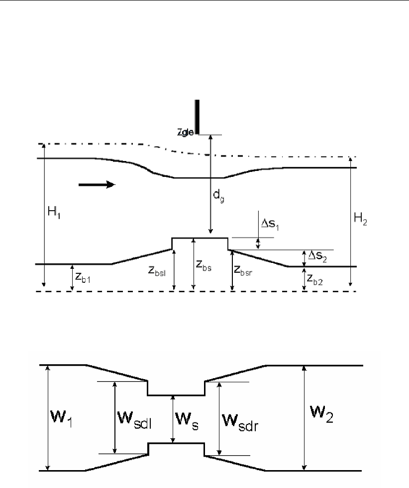
DRAFT
Hydraulic structures
The general structure gives more freedom in defining the dimensions and the geometry of
the hydraulic structure. The geometrical shape is given in Figure 12.3 and Figure 12.4. The
discharge through a general structure is computed on basis of upstream and downstream
energy levels.
Figure 12.3: General structure, side view
Figure 12.4: General structure, top view
In the GUI of D-Flow FM the coefficients of a general structure can be set as shown in Fig-
ure 12.5. Flow across the general structure can be of the following types: drowned weir flow,
free weir flow, drowned gate flow, and free gate flow, depending on the dimensions of the
structure and the flow conditions. Whether or not the gate is in the flow or above the flow
yields either submerged or free flow. Furthermore, the flow can be either subcritical or criti-
cal. Both for incoming flow ("Flow") which represents flood and for outgoing flow ("Reverse")
which represents ebb, contraction coefficients can be specified. This can be seen as tuning
parameters for the user.
In Figure 12.5 the geometric parameters of a weir can be specified. The five values for the
width (Upstream 1, Upstream 2, Crest, Downstream 1 and Downstream 2) coincide with the
five width parameters in Figure 12.4, which are W1,Wsdl,Ws,Wsdr and W2, respectively.
Similarly, the five values for the level correspond with Zb1,Zbsl,Zbs,Zbsr and Zb2in Fig-
ure 12.3.
Deltares 191 of 412

DRAFT
D-Flow Flexible Mesh, User Manual
Figure 12.5: Input for a general structure
The structure parameters for a (adjustable) weir can be defined via the <structures.ini>file:
type = weir
id = weir02
polylinefile = weir02.pli
crest_level = weir02_crest_level.tim
lat_cont_coeff = 1
12.2.3 Gates
Constructions which partially block the horizontal flow can be modelled as so-called "gates".
Its horizontal and vertical position can be specified. Upstream of the gate the flow is ac-
celerated due to contraction and downstream the flow is decelerated due to expansion. A
gate may include two type of openings, namely, in horizontal and in vertical directions. In
two-dimensional simulations, the vertical effect is parameterized by a quadratic energy loss
term.
The horizontal effect are mimicked by setting the velocities of the computational faces (at posi-
tion of the gate) to zero. This generates structure of the horizontal flow around the gate which
is more realistic. There is no transport of salt or sediment through the blocked computational
faces of a gate. The width of a gate is assumed to be zero, so it has no influence on the water
volume.
In D-Flow FM the gates can be imposed by polygons, and can be edited in a similar way as
the other structures. For more details on gates in Delta Shell, we refer you to section 4.4.2.10.
In Figure 12.6 the geometric parameters of a gate are shown.
192 of 412 Deltares

DRAFT
Hydraulic structures
Figure 12.6: Input for a gate
The structure of the input file for the gates is as follows:
type = gate
id = gate01
polylinefile = gate01.pli
lower_edge_level = 15
opening_width = gate01_opening_width.tim
sill_level = 7
door_height = 5
horizontal_opening_direction = symmetric
12.2.4 Pumps
Pumps are another type of structures in D-Flow FM. Unlike the other structures, a pump can
force the flow only on one direction. However, pumps can be defined by polygons, like all
other structures in D-Flow FM.
The pump includes specific capacity, and pumps the water by its capacity, as long as the
water level is sufficient. In the case, the water level is lower than a required value, pump will
not pump any flow, despite of their capacity. The structure of the input file for the pumps is as
follows:
type = pump
id = pump01
polylinefile = pump01.pli
capacity = pump01_capacity.tim
start_level_delivery_side = 0
stop_level_delivery_side = 0
start_level_suction_side = 3
stop_level_suction_side = 2
reduction_factor_no_levels = 0
Deltares 193 of 412

DRAFT
D-Flow Flexible Mesh, User Manual
12.2.5 Thin dams
Thin dams are similar to fixed weirs. The only difference between the thin dams and fixed
weirs are in their crest levels. Thin dams, in principle, include infinitely high crest levels and
hence, they do not allow water flux. Similar to the other structures, the thin dams can be
selected from the toolbar and drawn by a polygon. D-Flow FM adjusts the polygon to the
nearest velocity points. The input data for a thin dam is identical to those for fixed-weir, except
for the crest level.
194 of 412 Deltares

DRAFT
13 Bedforms and vegetation
The terrain and vegetation exert shear stresses on the passing flow. The magnitude of the
shear stress of the bed is often characterised by means of roughness coefficient of type
Chézy, Manning or White-Colebrook. Within the main stream flow the shear stresses are
largely determined by the local conditions of the alluvial bed (bed composition and bedform
characteristics). In other areas, such the floodplains of rivers and in the intertidal areas of
estuaries, the flow resistance is determined by a combination of vegetation and an alluvial
bedforms or even a non-alluvial bed. To accurately represent such conditions in the numerical
model, D-Flow FM has been extended with a vegetation model. Another related feature known
from Delft3D-FLOW is the bedform roughness predictors; these are not available in D-Flow FM
yet. These types of flow resistance may be resolved in a 2D numerical model using the
trachytope approach (see section 13.2).
13.1 Bedform heights
The dune height and Van Rijn (2007) bedform roughness predictors, known from Delft3D-
FLOW, are not available yet in D-Flow FM. They will be in an upcoming release.
13.2 Trachytopes
This functionality allows you to specify the bed roughness and flow resistance on a sub-grid
level by defining and using various land use or roughness/resistance classes, further referred
to as trachytopes after the Greek word τραχ´υτης for roughness. The input parameters and
files to use the trachytopes functionality are described in section B.6.
At every time step (or less frequent as requested by the user) the trachytopes are converted
into a representative bed roughness C,kor nand optional linear flow resistance coefficient
λper velocity point with index j.
M=−1
2λjuj|uj|(13.1)
To save computational time the user may choose to update the computed bed roughness and
resistance coefficients less frequently than every time step. See section B.6 for a description
of the keywords and input files associated with this feature.
The following two sections describe the various classes of trachytopes distinguished and the
way in which they are combined, respectively.
13.2.1 Trachytope classes
Three base classes of trachytopes are distinguished: area classes, line classes and point
classes. The area classes (type range 51–200) basically cover the whole area, therefore,
they are generally the dominant roughness factor. The line classes (type range 201–250)
may be used to represent hedges and similar flow resistance elements; it will add anisotropy
to the roughness field. The point class (type range 251–300) represents a set of point flow
resistance elements. The next six sections provide an overview of the various trachytope
formulae implemented.
Special classes (1–50)
In addition to the three base classes two special trachytope classes have been defined: a flood
protected area and a composite trachytope class. The first class represents a sub-grid area
Deltares 195 of 412

DRAFT
D-Flow Flexible Mesh, User Manual
that is protected from flooding and thus does not contribute to the bed roughness; however,
the effect on the flow resistance should be taken into account. The second class can be used
to make derived trachytope classes that are a combination of two other trachytopes: an area
fraction αof trachytope type T1and an area fraction β(often equal to 1−α) of trachytope
type T2.
FormNr Name Formula
Special classes (1–50)
1 flood protected area area fraction shows up as fbin Eqs. (13.53)
and (13.56)
2 composite trachytope fraction αof type T1and fraction β(generally
β= 1 −α) of type T2
Area trachytope classes (51–200)
The class of area trachytopes is subdivided into three types: simple (51–100), alluvial (101–
150) and vegetation (151–200). Four simple area trachytopes have been implemented repre-
senting the four standard roughness types of flow module.
FormNr Name Formula
51 White-Colebrook value k
52 Chézy value C
53 Manning value C=6
√h/n
54 z0value k= 30z0
Six alluvial trachytopes have been implemented.
FormNr Name Formula
101 simplified Van Rijn Equation (13.2)
102 power relation Equation (13.3)
103 Van Rijn (1984c) Equations (13.4) to (13.12)
104 Struiksma Equations (13.13) to (13.16)
105 bedforms quadratic Equation (13.17)
106 bedforms linear Equation (13.18)
The first alluvial roughness formula is a simplified version of the Van Rijn (1984c) alluvial
roughness predictor
k=Ah0.7h1−e−Bh−0.3i(13.2)
it is obtained from Equation (13.4) by noting that hb∝h0.7and Lb∝hand ignoring the
grain related roughness. The parameters Aand Bcan be calibrated by the user. The second
formula implemented is a straightforward general power law
C=AhB(13.3)
196 of 412 Deltares

DRAFT
Bedforms and vegetation
where Aand Bare calibration coefficients. The Van Rijn (1984c) alluvial roughness predictor
reads
k=k90 + 1.1hb1−e−25hb/Lb(13.4)
where the bedform height hband length Lbare given by
hb= 0.11hD50
h0.31−e−T/2(25 −T)(13.5)
Lb= 7.3h(13.6)
where his the local water depth and the transport stage parameter Tis given by
T=u02
∗−u2
∗,cr
u2
∗,cr
(13.7)
where u0∗is the bed shear velocity given by
u02
∗=gu2/C2
g,90 (13.8)
where
Cg,90 = 18 10log(12h/k90)and k90 = 3D90 (13.9)
and u∗,cr is the critical bed shear velocity according Shields given by
u2
∗,cr =g∆D50θc(13.10)
given
θc=
0.24/D∗if D∗≤4
0.14D−0.64
∗if 4< D∗≤10
0.04D−0.10
∗if 10 < D∗≤20
0.013D0.29
∗if 20 < D∗≤150
0.055 if 150 < D∗
(13.11)
where
D∗=D50 g∆
ν21/3
(13.12)
This predictor does not contain any calibration coefficients but requires D50 and D90 data
from the morphology module. It does not include the advective and relaxation behaviour that
is available by explicitly simulating the dune height as described in section 13.1 combined with
trachytope number 106.
The second alluvial roughness predictor proposed by (Struiksma, pers. comm.) allows for a
lot of adjustments, it reads
1
C2= (1 −ξ)1
C2
90
+ξ1
C2
min
(13.13)
where
C90 =A110log(A2h/D90)(13.14)
Deltares 197 of 412
DRAFT
D-Flow Flexible Mesh, User Manual
and
ξ=max(0, θg−θc)
θm−θc
θ2
m−θcθg
(θm−θc)θg
(13.15)
which varies from 0at θg≤θcto 1at θg=θmwhere
θg=u2
C2
90∆D50
(13.16)
and A1,A2,θc,θm,Cmin are coefficients that the user needs to specify. This formula requires
also D50 and D90 data from the morphology module. The fifth formula is based on Van Rijn
(2007) and reads
k= min(qk2
s,r +k2
s,mr +k2
s,d,h
2)(13.17)
It uses the roughness heights of ripples kr, mega-ripples kmr and dunes kd. These formulae
depend on sediment properties D50 and D90 data which may be either specified as part of
the roughness type or obtained from the morphology module. The sixth formula is similar, but
uses a linear addition
k= min(ks,r +ks,mr +ks,d,h
2)(13.18)
Four vegetation based area trachytopes have been implemented. Two formulae (referred to
as ‘Barneveld’) are based on the work by Klopstra et al. (1996,1997) and two on the work by
Baptist (2005).
FormNr Name Formula
151 Barneveld 1 Eqs. (13.19) –(13.28),CD= 1.65
152 Barneveld 2 Eqs. (13.19) –(13.25),(13.29) –(13.31)
153 Baptist 1 Eqs. (13.32) and (13.33)
154 Baptist 2 Eqs. (13.34),(13.36) and (13.37)
The formula by Klopstra et al. (1997) reads
C=1
h3/2
2
√2AqC3ehv√2A+u2
v0−pC3+u2
v0+
uv0
√2Aln (√C3ehv√2A+u2
v0−uv0)(√C3+u2
v0+uv0)
(√C3ehv√2A+u2
v0+uv0)(√C3+u2
v0−uv0)+
√g(h−(hv−a))
κ(h−(hv−a)) ln h−(hv−a)
z0−aln a
z0−(h−hv)
(13.19)
where
A=nCD
2α(13.20)
C3=2g(h−hv)
α√2A(ehv√2A+e−hv√2A)(13.21)
198 of 412 Deltares

DRAFT
Bedforms and vegetation
a=1 + q1 + 4E2
1κ2(h−hv)
g
2E2
1κ2
g
(13.22)
and
z0=ae−F(13.23)
where
E1=√2AC3ehv√2A
2qC3ehv√2A+u2
v0
(13.24)
and
F=κqC3ehv√2A+u2
v0
pg(h−(hv−a)) (13.25)
Here, his the water depth, hvis the vegetation height, and n=mD where mis the number
of stems per square metre and Dis the stem diameter. For the first implementation the
parameter αin Equation (13.21) is given by
α= max(0.001,0.01phhv)(13.26)
and the velocity within the vegetation is approximated by uv0√iwhere
u2
v0=2g
CDn(13.27)
and iis the water level gradient. For emerged vegetation the first implementation reads
1
C2=CDnh
2g(13.28)
The second implementation of Klopstra et al. (1996) is based on a modification by Van Velzen
et al. (2003); it is identical except for the following modifications to Eqs. (13.26) –(13.28). The
main difference between the two implementations is the inclusion of the roughness Cbof the
bed itself (without vegetation). The parameter αin Equation (13.21) is now given by
α= 0.0227h0.7
v(13.29)
and the velocity within the vegetation is approximated by uv0√iwhere
u2
v0=hv
CDhvn
2g+1
C2
b
(13.30)
and iis the water level gradient. For emerged vegetation the second implementation reads
1
C2=CDnh
2g+1
C2
b
(13.31)
Deltares 199 of 412

DRAFT
D-Flow Flexible Mesh, User Manual
For large values of Cbthe latter two equations simplify to the corresponding equations of the
first implementation. The first implementation requires vegetation height hvand density n
as input parameters (the drag coefficient CDis equal to 1.65); for second implementation
you’ll also need to specify the drag coefficient CDand the alluvial bed roughness kb(Cbin
Equation (13.31) is computed as 18 10log(12h/kb)).
The first implementation of the roughness predictor by Baptist (Baptist,2005) reads for the
case of submerged vegetation
C=1
q1
C2
b+CDnhv
2g
+√g
κln( h
hv
)(13.32)
where nis the vegetation density (n=mD where mis the number of stems per square
metre and Dis the stem diameter). The second term goes to zero at the transition from
submerged to emerged vegetation. At that transition the formula changes into the formula for
non-submerged vegetation which reads
C=1
q1
C2
b+CDnh
2g
(13.33)
which is identical to the non-submerged case of the second implementation of the work by
Klopstra et al. (1996) (see Equation (13.31)).
The drawback of the three vegetation based formulations above is that they parameterize the
flow resistance by means of the bed roughness. Consequently, the presence of vegetation
will lead to a higher bed roughness and thus to a higher bed shear stress and larger sediment
transport rates in case of morphological computations. Therefore, we have included a −λ
2u2
term in the momentum equation where λrepresents the flow resistance of the vegetation. For
the case of non-submerged vegetation h<hvthe flow resistance and bed roughness are
strictly separated
C=Cband λ=CDn(13.34)
In the case of submerged vegetation h>hvthe two terms can’t be split in an equally clean
manner. However, we can split the terms such that the bed shear stress computed using
the depth averaged velocity uand the net bed roughness Cequals the bed shear stress
computed using the velocity uvwithin the vegetation layer and the real bed roughness Cb.
u2
C2=u2
v
C2
b
(13.35)
With this additional requirement we can rewrite Equation (13.32) as
C=Cb+√g
κln( h
hv
)s1 + CDnhvC2
b
2g(13.36)
and
λ=CDnhv
h
C2
b
C2(13.37)
which simplify to Equation (13.34) for h=hv. Both formulae by Baptist require vegetation
height hv, density n, drag coefficient CDand alluvial bed roughness Cbas input parameters.
200 of 412 Deltares

DRAFT
Bedforms and vegetation
Linear trachytope classes (201–250)
Two formulae have been implemented for linear trachytopes such as hedges or bridge piers.
FormNr Name Formula
201 hedges 1 Eqs. (13.38) to (13.40)
202 hedges 2 Eqs. (13.41) to (13.43)
The first implementation reads
1
C2=h
2g
Lhedge
Wcell Lcell
1−µ2
µ2(13.38)
where Lhedge is the projected length of the hedge, Wcell and Lcell are the width and length
of the grid cell. The ratio Lhedge /Wcell may be interpreted as the number of hedges that the
flow encounters per unit width. The second ratio is thus the inverse of the average distance
between these hedges within the grid cell. The last term may be loosely referred to as the
drag of the hedge, which is determined by the hedge pass factor µgiven by
µ= 1 + 0.175nh
hv−2(13.39)
if the hedge extends above the water level (hv> h) and is given by
µ= 1 −0.175nh
hv(13.40)
if the hedge is fully submerged (h>hv) where nis a dimensionless hedge density. The
second implementation reads
1
C2=CDnLhedge h
2gLcell Wcell
(13.41)
or equivalently
C=s2gLcell Wcell
hLhedge r1
CDn(13.42)
for non-submerged conditions and
C=s2gLcell Wcell
hLhedge
hv
hr1
CDn+m0v
u
u
th−hv
h2
1−h−hv
h2
(13.43)
for submerged conditions. We recognize the same ratio Lcell Wcell /Lhedge that represents
the average distance between hedges. Equation (13.41) can be directly compared to similar
equations for area trachytopes (Equation (13.28)), point trachytopes (Equation (13.44)). Note
that the formula for computing the loss coefficient for a bridge explicitly includes the reduction
in the flow area and the resulting increase in the effective flow velocity, whereas the above
mentioned trachytope formulae don’t.
Deltares 201 of 412
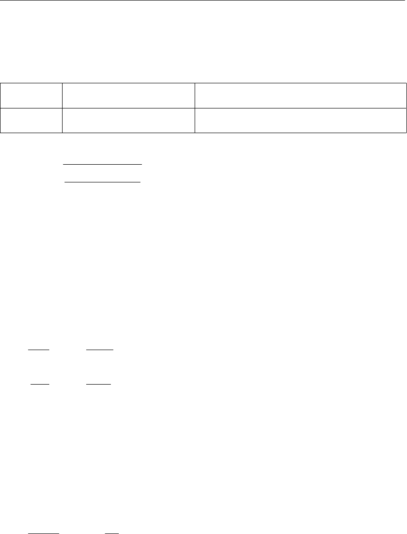
DRAFT
D-Flow Flexible Mesh, User Manual
Point trachytope classes: various (251–300)
One formula for point trachytopes has been implemented. It may be used to represent groups
of individual trees or on a smaller scale plants.
FormNr Name Formula
251 trees Eqn. (13.44)
The implemented formula reads
C=s2g
CDnmin(hv, h)(13.44)
where n=mD with mthe number of trees per unit area and Dthe characteristic tree
diameter, hvis the vegetation height and his the local water depth. The formula is identical
to Equation (13.33) except for the fact that the point trachytope formula has no bed roughness
and area associated with it. The generalization of Equation (13.44) to the submerged case
(h > hv) lacks the extra term in Equation (13.32).
13.2.2 Averaging and accumulation of trachytopes
Point and linear roughnesses are accumulated by summing the inverse of the squared Chézy
values Ci.
1
C2
pnt
=X
i
1
C2
pnt,i
(13.45)
1
C2
lin
=X
i
1
C2
lin,i
(13.46)
The area roughnesses are accumulated weighted by the surface area fraction fi. These
roughnesses are accumulated as White-Colebrook roughness values and as Chézy values;
for the latter values both the linear sum (“parallel”) and the sum of inverse of squared values
(“serial”) are computed. Roughness values are converted into each other as needed based
on the local water depth.
karea =X
i
fiki(13.47)
1
C2
area,s
=X
i
fi
1
C2
i
(13.48)
Carea,p=X
i
fiCi(13.49)
For the fraction of the grid cell area for which no roughness class is specified the default
roughness is used.
The flow resistance coefficients are also accumulated proportionally to the surface area frac-
tion fiassociated with the trachytope considered. For the fraction of the grid cell area for
which no flow resistance is specified, obviously none is used.
λ=X
i
fiλi(13.50)
202 of 412 Deltares

DRAFT
Bedforms and vegetation
The final effective bed roughness of the grid cell may be computed by either one of the follow-
ing two methods.
Method 1
The total mean roughness is computed by summing the White-Colebrook values for the areas
and line and point resistance features.
km=karea +klin +kpnt (13.51)
where klin = 12h10−Clin /18 and kpnt = 12h10−Cpnt /18. The effect of the water free
area fraction fbis taken into account by means of the following empirical relation in which
Cm= 18 10log(12h/km)is the mean Chézy value corresponding to the total mean White-
Colebrook roughness value obtained from Equation (13.51).
fb= max(min(0.843, fb),0.014) (13.52)
Ctotal =Cm1.12 −0.25fb−0.99pfb(13.53)
The resulting Ctotal value is used in the computation. This method together with trachytope
classes 1, 51, 101, 151 and 201 corresponds to the NIKURADSE option of the WAQUA/TRI-
WAQ flow solver.
Method 2
The total roughness is computed by first averaging over the serial and parallel averages of the
Chézy values according
Carea =αsCarea,s+ (1 −αs)Carea,p(13.54)
where αs= 0.6by default. Subsequenty the effect of the water free area fraction fbis
taken into account by means of the following empirical relation (identical to Equation (13.53)
of method 1).
fb= max(min(0.843, fb),0.014) (13.55)
Carea,corr =Carea 1.12 −0.25fb−0.99pfb(13.56)
Finally the Chézy value representing the total bed roughness is computed by accumulating
the inverses of the squared Chézy values.
1
C2
total
=1
C2
area,corr
+1
C2
lin
+1
C2
pnt
(13.57)
The resulting Ctotal value is used in the computation. This method together with trachytope
classes 1, 51, 52, 53, 101, 152, 202 and 251 corresponds to the ROUGHCOMBINATION
option of the WAQUA/TRIWAQ flow solver.
13.3 (Rigid) three-dimensional vegetation model
The (rigid) 3D Vegetation model (Winterwerp and Uittenbogaard (1997)), as known from
Delft3D-FLOW, is not available yet in D-Flow FM.
Deltares 203 of 412

DRAFT
D-Flow Flexible Mesh, User Manual
204 of 412 Deltares

DRAFT
14 Calibration factor
The current chapter explains the effect of the calibration factor. The calibration factor is mul-
tiplier of the roughness. The calibration factor may be constant, discharge- or water-level-
dependent. By assigning different areas to different calibration classes, each region can be
independently calibrated. Calibration roughness definitions can also be combined by assign-
ing multiple field definitions and a weighting for each gridcell edge (net link). This approach
allows thus both abrupt and gradual transitions and the modeller can control how the calibra-
tion factor is going to be used. The approach is similar to the roughness and link definitions
used in the trachytopes module for alluivial- and bedform-roughness (see chapter 13).
The calibration factor is defined by means of two files (see section B.8):
Calibration factor definition file (CLD-file). This file defines the calibration factor (e.g. con-
stant, water-level- or discharge dependent).
Calibration factor area file (CLL-file). This file associates calibration factor defintions with
the edges of the model grid and include a relative weighting.
The resulting weighted calibration factor is multiplied by the roughness type as expressed by
the UnifFrictCoef keyword in the [physics] section in the .mdu file (see Appendix A).
This implies that the effect of the calibration will be different depending on the definition of
UnifFrictCoef. For example, if the UnifFrictCoef=0 (i.e. Chézy) a local calibration
factor of 0.5 will imply an increase of the bed shear stress, whereas if UnifFrictCoef=2
(i.e. White-Colebrook) a reduction of the bed shear stress may be expected. A background
calibration factor equal to one is applied if the sum of the weights at a single link is lower than
one.
The calibration factor approach cannot be combined with multiple roughness types as speci-
fied through the external forcing file. This will lead to an error. Such a spatial variation in the
roughness can be achieved by defining these areas through the trachytopes module.
It is good to be aware of the following known differences with the trachytopes module:
The weighting of the calibration factors is done for all entries in the calibration area defin-
tion file. Averaging for the trachytopes area file is only done for the last sequence of
trachytope area defintions at one and the same location.
When a calibration factor definition is imposed at a location outside of the grid, and this
calibration factor definition depends on a water level station or cross-section which is also
outside of the domain, the model crashes, however the trachytopes module allows this.
Deltares 205 of 412

DRAFT
D-Flow Flexible Mesh, User Manual
206 of 412 Deltares

DRAFT
15 Coupling with D-Waves (SWAN)
This chapter is on the coupling of hydrodynamics and waves. Full documentation on D-Waves
is available in its own User Manual; this chapter is limited to the details of running coupled
flow-wave models, and the physical interaction processes between the two of them.
15.1 Getting started
The Delta Shell framework implements the concept of an Integrated model in order to couple
different models, such as: hydrodynamics coupled with the controlling of structures, waves,
morphology and/or water quality.
Two types of coupling are distinguished: offline and online coupling. In case of an Integrated
model with offline coupling, the entire hydrodynamic simulation is done first, i.e., separately
from the second simulation. The file-based hydrodynamic output serves as input for the sec-
ond simulation. As such, the hydrodynamic flow drives the controlling of structures or the
simulation of waves or water quality. In this case there is no feedback on the hydrodynamic
simulation. For many applications, this is good practice.
An online coupling, on the other hand, exchanges data every time after computing a specified
time interval. This tight coupling allows for direct feedback of the various processes on one
another. This is crucial for controlling structures.
Note: Offline is also referred to as sequential coupling and online as parallel coupling.
With respect to waves, offline and online results into:
1offline: First, a separate D-Waves computation is executed, resulting in a communication
file (com-file) containing wave data. Then a D-Flow FM computation is executed, using
the wave data from the com-file.
2online: D-Flow FM computations are alternated with D-Waves calculations. D-Flow FM
writes flow data to the com-file, D-Waves uses this flow data for the wave calculation and
writes wave data to the com-file. D-Flow FM uses the updated wave data.
Both modes are started by executing DIMR with a <dimr_config.xml>file as argument. This
file prescribes the mode and when the D-Flow FM computation should be paused to perform
a D-Waves calculation. From within the working directory, the following run-scripts in the
installation directory can be called:
On Windows:
<win64\scripts\run_dimr.bat>
On Linux:
<lnx64/scripts/run_dimr.sh>
On Windows, a computation with D-Flow FM in parallel using MPI:
<win64\scripts\run_dimr_parallel.bat>
On Linux, submitting a job on the Deltares cluster (sequential and parallel):
<lnx64/scripts/submit_dimr.sh>
This script can be used for clusters outside Deltares too, but system specific modifications
will be needed.
See the DIMR documentation for more information.
Deltares 207 of 412

DRAFT
D-Flow Flexible Mesh, User Manual
15.1.1 Input D-Flow FM
Optionally add the following lines to the .mdu file:
[numerics]
Epshu = 0.05 # Input for threshold water depth for wet and dry cells
[waves]
Wavemodelnr = 3 # Wave model nr, 0=no, 1=fetch/depth limited hurdlestive,
2=youngverhagen, 3 = D-Waves, 4=wave group forcing
Rouwav = FR84
Gammax = 0.5 # Maximum wave height/water depth ratio
[output]
EulerVelocities = 1 # 0 (default): GLM, 1: Euler.
Only relevant when using waves
Description:
Wavemodelnr Key switch to enable wave modelling. Use “3” for wave data from
D-Waves (online or offline) and passing hydrodynamic data to D-
Waves (online only). A file will be generated automatically named
<”runid”_com.nc>to exchange data.
Rouwav Necessary to include bed shear-stress enhancement by waves. See
also Delft3D-FLOW manual.
EulerVelocities Optional flag to write Eulerian velocities to the D-Flow FM map file.
Currently, only Eulerian values will be written for the cell centre veloc-
ity x-component and y-component (parameters ucx and ucy). Check
that the ”long_name” contains the word ”Eulerian”.
Epshu Optionally overwrite the default value of “1.0e-4”. Depending on your
model, the default value of Epshu in combination with modelling
waves may lead to huge local velocities near (almost) dry points.
This will result in very small time steps. Increasing Epshu might be
a reasonable workaround.
Gammax Optionally overwrite the default value of “1.0”. Depending on your
model, the default value of Gammax may lead to huge local veloc-
ities in shallow water. Decreasing Gammax might be a reasonable
workaround.
15.1.2 Input D-Waves
Optionally add the following lines to the .mdw file:
[Output]
MapWriteNetCDF = true
COMFile = ../fm/dflowfmoutput/fff_com.nc
NetCDFSinglePrecision = false
locationFile = ../fm/loo_obs.xyn
writeTable = true
Description:
208 of 412 Deltares

DRAFT
Coupling with D-Waves (SWAN)
MapWriteNetCDF Default value “false”, resulting in no output written in NetCDF for-
mat. The coupling with D-Flow FM is only implemented for NetCDF
format, so this flag must be set to “true” when being coupled with
D-Flow FM.
COMFile Necessary reference to the file being used to communicate data to
and from D-Flow FM. The name must exactly match with the name
of the com-file being generated by D-Flow FM.
NetCDFSinglePrecision Optional flag to write data in single precision instead of double
precision. Default value is “false”. Might be useful to decrease the
size of the com-file or to compare with a Delft3D-FLOW computation.
locationFile Optional reference to observation points in D-Flow FM. When in
combination with the “writeTable” flag, D-Waves will produce a his-
tory file in NetCDF format for these observation points.
writeTable Optional flag to force SWAN to produce an output file in table format
for each set of locations specified in a locationFile. Default value is
“false”.
15.1.3 Input dimr
Both D-Flow FM and D-Waves are used as dynamic libraries (DLL’s on Windows, so’s on
Linux). DIMR is a small executable steering both dynamic libraries. Its input file, usually
called “dimr_config.xml”, looks like this:
<?xml version="1.0" encoding="iso-8859-1"?>
<dimrConfig xmlns="http://schemas.deltares.nl/dimrConfig"
xmlns:xsi="http://www.w3.org/2001/XMLSchema-instance"
xsi:schemaLocation="http://schemas.deltares.nl/dimrConfig
http://content.oss.deltares.nl/schemas/d_hydro-1.00.xsd">
<documentation>
<fileVersion>1.00</fileVersion>
<createdBy>Deltares, Coupling team</createdBy>
<creationDate>2015-05-20T07:56:32+01</creationDate>
</documentation>
<control>
<parallel>
<startGroup>
<time>0.0 60.0 99999999.0</time>
<coupler name="flow2rtc"/>
<start name="myNameRTC"/>
<coupler name="rtc2flow"/>
</startGroup>
<startGroup>
<time>0.0 3600.0 99999999.0</time>
<start name="myNameWave"/>
</startGroup>
<start name="myNameDFlowFM"/>
</parallel>
</control>
<component name="myNameDFlowFM">
<library>dflowfm</library>
<process>0 1 2</process>
<mpiCommunicator>DFM_COMM_DFMWORLD</mpiCommunicator>
<workingDir>fm</workingDir>
<inputFile>weirtimeseries.mdu</inputFile>
</component>
<component name="myNameWave">
<library>wave</library>
<process>0</process>
<workingDir>wave</workingDir>
<!-- component specific -->
Deltares 209 of 412

DRAFT
D-Flow Flexible Mesh, User Manual
<inputFile>weir.mdw</inputFile>
</component>
<component name="myNameRTC">
<library>RTCTools_BMI</library>
<process>0</process>
<workingDir>rtc</workingDir>
<!-- component specific -->
<inputFile>.</inputFile>
</component>
<coupler name="flow2rtc">
<sourceComponent>myNameDFlowFM</sourceComponent>
<targetComponent>myNameRTC</targetComponent>
<item>
<sourceName>observations/Upstream/water_level</sourceName>
<targetName>input_ObservationPoint01_water_level</targetName>
</item>
</coupler>
<coupler name="rtc2flow">
<sourceComponent>myNameRTC</sourceComponent>
<targetComponent>myNameDFlowFM</targetComponent>
<item>
<sourceName>output_weir_crest_level</sourceName>
<targetName>weirs/weir01/crest_level</targetName>
</item>
</coupler>
</dimrConfig>
Description:
<control> Specifies the workflow of the deltaresHydro executable. It indicates which com-
ponents are started in which order. If the data transfer is to be arranged by
the main program dimr, then a coupler should be included. The main <con-
trol> block is a sequential block; this means that each component is initialized,
time stepped, and finalized before the next component starts. For each com-
ponent/coupler listed inside the <control> block there will be a corresponding
component/ coupler specification block defined below.
<parallel> Within a <parallel> tag the components are started concurrently (if the mpi pro-
cess ids listed per component don’t overlap) or executed synchronously in se-
quence (first all initialize, then time stepping, and to conclude all finalization
calls). The order of the components is retained.
<start/> A <parallel> block contains exactly one <start/> component, defining the start
and end time of the simulation. This is the component inside the <parallel> block
with the smallest time step and can be denoted as the ”master-component”. All
other components must be defined with a <startGroup> and can be denoted as
a ”slave-component”.
<startGroup> A <startGroup> should be used if a component (possibly including couplers)
should only be executed at a subset of simulation time steps.
<time> Start-, step- and stop-time (in seconds) at which this slave-component should
be executed. The times are relative to the times of the master-component. Thus
a start-time of 0.0 always refers to the start time of the master-component and
a stop-time of ”infinity” always refers to the end time of the master-component.
<component name="myComponentName"> Component specification block. ”myCompo-
nentName” is free to be defined by the user. It must match exactly with the
reference in the <control> block above. The name of a component must be
unique.
<library> Reference to the component to be executed. Currently ”flowfm”, ”wave” and
”RTCTools_BMI” are supported. The name must match exactly the name of
the related dll/so (excluding prefixes (e.g. “lib”) and suffixes (e.g. “.dll” or “.so”)).
210 of 412 Deltares

DRAFT
Coupling with D-Waves (SWAN)
The library should be located in the search path, or it may include an absolute or
relative path. Multiple <component> blocks may refer to the same component
to be executed.
<process> Optional list of the ids of the mpi processes that should be used to run the
component. If not specified, then the component will run only in process “0”
(i.e. non-parallel). The processes may be specified as a space separated list
with series compressed using colons e.g. “16:31” represents processes “16 17
18” up to “31”.
<mpiCommunicator> D-Flow FM specific flag. Mandatory only when this D-Flow FM com-
ponent should run a parallel (partitioned) model. Note that this is unrelated to
the <parallel> tag as introduced above.
<workingDir> Specification of the working directory of this <component>, relative to the
location of the “dimr_config.xml” file. The workingDir is the base/root directory
of all input and output files for the component. All other files will be located
RELATIVE TO this folder. If not specified, then workingDir will be equal to the
folder of the configuration file.
<inputFile> Specification of the input file of this <component>, relative to <workingDir>:
D-Flow FM: mdu-file, D-Waves: mdw-file, D-RTC: .
<coupler name="myCouplerName"> Coupler specification block. ”myCouplerName” is free
to be defined by the user. It must match exactly with the reference in the <con-
trol> block above. The name of a coupler must be unique.
<sourceComponent> Identifies which component provides the data.
<targetComponent> Identifies which component needs to receive the data. The coupler
runs on the superset of the processes configured for the source and target
components.
<item> For each quantity to be exchanged, the name in the source component and the
name in the target component are specified. To support recursive components,
a directory syntax is used with forward slashes. If a name includes a forward
slash, then it needs to be escaped using a backward slash, like \/; if a name
includes a backward slash, then it needs to be escaped with a backward slash,
like \\.
<sourceName> Identifies which parameter will be sent at the source component side.
<targetName> Identifies which parameter will be received at the target component side.
15.1.4 Online process order
When D-Flow FM runs online in alternation with D-Waves and D-RTC, process steps can
be identified, where the order as prescribed in “dimr_config.xml” is respected as much as
possible. The process order of the example “dimr_config.xml” file in the section above is:
1 D-Flow FM::Init
D-Flow FM is initialized. Grid- and Flow-data is written to the NetCDF com-file.
Even though D-Flow FM is not the first component in the example config-file, it must be
the first component to be initialized, because the initialization results may be needed when
other components are initialized. This is implemented as an exceptional rule: The master-
component is always the first component to be initialized.
2D-RTC::Init
D-RTC is initialized using (only) D-RTC input. Data from other components is not initialized
yet; default values are used.
3D-Waves::Init
D-Waves is initialized. Grid- and Flow-data created by D-Flow FM::Init is read from the
com-file. Grid conversion factors are generated. The factors for the conversion from the
(structured!) wave grid to the (unstructured) flow grid are calculated inside D-Waves.
The factors for the conversion from the (unstructured) flow grid to the (structured) wave
Deltares 211 of 412

DRAFT
D-Flow Flexible Mesh, User Manual
grid are calculated by ”ESMF_RegridWeightGen” via the execution of script <ESMF_-
RegridWeightGen_in_Delft3D-WAVE.bat>(Windows) or <ESMF_RegridWeightGen_in_-
Delft3D-WAVE.sh>(Linux).
4D-RTC::Step
A D-RTC computation is performed at time “0.0”: Data is communicated (by DIMR) from
D-Flow FM to D-RTC, the actual D-RTC computation is executed, data is communicated
(by DIMR) from D-RTC to D-Flow FM.
5D-Waves::Step
A D-Waves calculation is performed at time “0.0”: Flow data is read (by D-Waves) from
the com-file and converted to the wave grid(s). SWAN input files are written, a SWAN
calculation is started by executing script <swan.bat>(Windows) or <swan.sh>(Linux),
SWAN output files are read, wave-data is converted to the flow grid and written to the
com-file (by D-Waves).
6 D-Flow FM::Step
A D-Flow FM calculation is performed: The com-file is checked for wave data to be
used/updated. The simulation time will proceed from “0.0” to “60.0” (next time that another
component should be executed). Flow-data is written to the com-file (by D-Flow FM).
7D-RTC::Step, D-Flow FM::Step
A D-RTC computation is performed after every “60.0” seconds. Then a D-Flow FM com-
putation is performed and the simulation time will proceed another “60.0” seconds. This
continues untile the simulation time has progressed for “3600.0” seconds.
8D-RTC::Step, D-Waves::Step, D-Flow FM::Step
A D-RTC computation is performed, then a D-Waves computation, then a D-Flow FM
computation. The simulation time will proceed another “60.0” seconds and the next D-
RTC computation can start.
9D-RTC::Finish
D-RTC is finished at the end of the simulation.
10 D-Waves::Finish
D-Waves is finished at the end of the simulation.
11 D-Flow FM::Finish
D-Flow FM is finished at the end of the simulation.
15.1.5 Related files
Below is an overview of the related files in the default directory structure. In this example the
runid is set to foo.
<testcaseroot>
dimr_config.xml Configuration file, input for DIMR
<fm>Work directory for D-Flow FM
foo.mdu D-Flow FM input file
<dflowfmoutput>D-Flow FM output directory
foo_com.nc Communication file, written/read by both D-Flow FM and D-Waves
<rtc>Work directory for D-RTC
settings.json D-RTC input file (must have exactly this name)
<xml_dir>D-RTC directory containing xml input/output files and csv output file
<xsd_dir>D-RTC directory containing xsd input files
<wave>Work directory for D-Waves
foo.mdw D-Waves input file
TMP_ESMF*_source.nc Temporary input file for ESMF_Regridder, created by D-
Waves
TMP_ESMF*_destination.nc Temporary input file for ESMF_Regridder, created
212 of 412 Deltares

DRAFT
Coupling with D-Waves (SWAN)
by D-Waves
TMP_ESMF*_weights.nc Resulting weights file, created by ESMF_Regridder, read
by D-Waves
PET0.RegridWeightGen.Log ESMF_Regridder log file
swn-diag.foo SWAN log file
15.2 Forcing by radiation stress gradients
The momentum equation in x-direction, averaged over the wave motion and expressed in
GLM co-ordinates is given by (GLM: Generalized Lagrangian Mean):
∂¯uL
j
∂t + ¯uL
i
∂¯uL
j
∂xj
+... +g∂¯
ζ
∂xj−1
ρ
∂¯τL
ij
∂xi
=FL
j,(15.1)
where for iand jthe summation rule applies, i, j ={1,2,3}. As shown by Groeneweg
(1999) the right-hand side of Equation (15.1) contains a term related to a Stokes correction of
the shear stresses. In the current implementation this term is neglected.
The wave-induced force, i.e. the right-hand side of Equation (15.1), can be expressed in the
wave parameters of the wave model that is being applied. For linear current refraction the
expression can be derived analytically. To account for wave dissipation due to for instance
bottom friction, wave breaking and whitecapping and wave growth due to wind one can rely
on mild slope formulations with dissipation terms.
As shown by Dingemans et al. (1987), using the gradients of the radiation stresses in numer-
ical models can result in spurious currents. Dingemans et al. (1987) showed that the diver-
gence free part of the radiation stress is not capable of driving currents and can therefore
be neglected if one is primarily interested in wave-driven currents. The remaining part of the
radiation stress gradients is closely related to the wave energy dissipation, i.e. the right-hand
side of Equation (15.1) can be written as:
Fi=Dki
ω,(15.2)
where Dis the total energy dissipation due to waves, kiis the wave number in i-direction
and ωis the wave frequency; see Dingemans (1997) for many details and discussions on this
subject.
2D implementation
For a depth averaged model the momentum equations in x- and y-direction, leaving out most
of the terms, can be written as:
∂U
∂t +. . . +gU√U2+V2
C2
2Dh+. . . =. . . +Fx,(15.3)
∂V
∂t +. . . +gV √U2+V2
C2
2Dh+. . . =. . . +Fy,(15.4)
where Fxand Fyare the depth averaged wave-induced forcings and given by the gradients
of the radiation stress tensor S, or following Dingemans et al. (1987) approximated by wave
energy dissipation:
Fx=−∂Sxx
∂x −∂Syx
∂y =Dkx
ω,(15.5)
Fy=−∂Sxy
∂x −∂Syy
∂y =Dky
ω.(15.6)
Deltares 213 of 412

DRAFT
D-Flow Flexible Mesh, User Manual
The dissipation rate D(a negative quantity) is computed by the wave model and read from the
communication file. In SWAN, the dissipation rate may be computed from the bottom friction
(orbital motion), depth-induced breaking and whitecapping.
You can choose to apply the radiation stress or the dissipation rate to determine the wave-
induced forces.
3D implementation
There is no coupling available yet for 3D D-Flow FM models and D-Waves. The effect of the
divergence free part of the radiation stresses is (the remaining part of the radiation stress gra-
dients, after the wave dissipation has been subtracted) is added to the momentum equations
in D-Flow FM (effect spread over the water column). This provides most adequate results,
e.g. in situations with undertow.
15.3 Stokes drift and mass flux
In surface waves, fluid particles describe an orbital motion. The net horizontal displacement
for a fluid particle is not zero. This wave induced drift velocity, the so-called Stokes-drift,
is always in the direction of wave propagation. A particle at the top of the orbit beneath a
wave crest moves slightly faster in the forward direction than it does in the backward direction
beneath a wave trough. The mean drift velocity is a second order quantity in the wave height.
The drift leads to additional fluxes in the wave averaged mass continuity equation.
The wave-induced mass fluxes MS
xand MS
yare found by integration of the components of
the Stokes drift uSand vSover the wave-averaged total water depth:
MS
x=Zh
0
ρouSdz =E
ωkx(15.7)
MS
y=Zh
0
ρ0vSdz =E
ωky(15.8)
with Ethe wave energy defined as:
E=1
8ρ0gH2
rms.(15.9)
The mass fluxes MS
xand MS
yare computed by an interface program and are written to the
communication file.
Remarks:
The mass flux effect is only taken into account when D-Flow FM is used from within
Delft3D-MOR.
The velocities written to the communication file for use in Delft3D-MOR, D-Waves, and
D-Water Quality are based on the total flux velocities.
The Eulerian velocities, which may be used in comparisons with measurements at a
fixed location, are written to the hydrodynamic map and history files.
214 of 412 Deltares

DRAFT
Coupling with D-Waves (SWAN)
2D implementation
The depth-averaged Stokes drift is given by:
US=MS
x
ρ0h,(15.10)
VS=MS
y
ρ0h.(15.11)
3D implementation
There is no coupling available yet for 3D D-Flow FM models and D-Waves.
15.4 Streaming
Streaming is a 3D feature. There is still no coupling available for 3D D-Flow FM models and
D-Waves.
15.5 Enhancement of the bed shear-stress by waves
The boundary layers at the bed associated with the waves and the current interact non-linearly.
This has the effect of enhancing both the mean and oscillatory bed shear-stresses. In addition
the current profile is modified, because the extra turbulence generated close to the bed by the
waves appears to the current as being equivalent to an enhanced bottom roughness. The
bed shear-stress due to the combination of waves and current is enhanced beyond the value
which would result from a linear addition of the bed shear-stress due to waves, τw, and the
bed shear-stress due to current τc. For sediment transport modelling it is important to predict
the maximum bed shear-stress, τmax, while the current velocity and the turbulent diffusion
are determined by the combined wave-current bed shear-stress τm.
Various, often very complex, methods exist to describe the bottom boundary layer under com-
bined current and wave action and the resulting virtual roughness. Soulsby et al. (1993a)
developed a parameterisation of these methods allowing a simple implementation and com-
parison of various wave-current interaction models: Fredsøe (1984); Myrhaug and Slaattelid
(1990); Grant and Madsen (1979); Huynh-Thanh and Temperville (1991); Davies et al. (1988);
Bijker (1967); Christoffersen and Jonsson (1985); O’ Connor and Yoo (1988); Van Rijn et al.
(2004). All these methods have all been implemented in D-Flow FM and can be applied in
2D and 3D modelling. However, as there are minor, but specific differences in determining
certain quantities, such as determining the shear-stress at the bottom, we prefer to discuss
the 2D and 3D implementation separately.
2D implementation
Following Soulsby et al. (1993b), Figure 15.1 gives a schematic overview of the bed shear-
stresses for wave current interaction.
Soulsby et al. (1993b) fitted one standard formula to all of the models, each model having its
own fitting coefficients. The parameterisation of Soulsby for the time-mean bed shear-stress
is of the form:
|τm|=Y(|τc|+|τw|),(15.12)
with
Y=X{1 + bXp(1 −X)q},(15.13)
Deltares 215 of 412
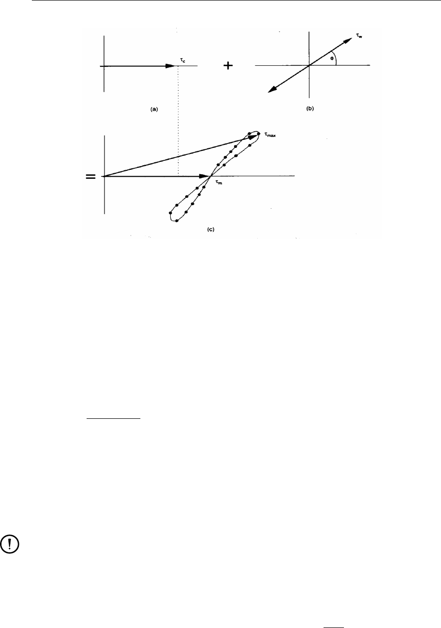
DRAFT
D-Flow Flexible Mesh, User Manual
Figure 15.1: Schematic view of non-linear interaction of wave and current bed shear-
stresses (from Soulsby et al. (1993b, Figure 16, p. 89))
and for the maximum bed shear-stress:
|τmax|=Z(|τc|+|τw|),(15.14)
with
Z= 1 + aXm(1 −X)n.(15.15)
and:
X=|τc|
|τc|+|τw|,(15.16)
The value of the parameters a,b,p,q,mand ndepends on the friction model which is
parameterised, and:
|τc|magnitude of the bed stress due to current alone
|τw|magnitude of the bed stress for waves alone
|τm|magnitude of the mean bed stress for combined waves and current
|τmax|magnitude of the maximum bed stress for combined waves and current.
Remark:
The stresses τmand τmax are assumed to have the same direction as τc.
Following Soulsby et al. (1993b) the expressions for the parameters χ(=a, b, p, q, m, n)
and J(=I, J; also depending on the friction model) have the form:
χ=χ1+χ2|cos φ|J+χ3+χ4|cos φ|J10log fw
C2D,(15.17)
in which:
C2Ddrag coefficient due to current
fwwave friction factor
φthe angle between the current direction and the direction of wave propagation.
216 of 412 Deltares

DRAFT
Coupling with D-Waves (SWAN)
Table 15.1: Fitting coefficients for wave/current boundary layer model
Model1a1a2a3a4m1m2m3m4n1n2n3n4I
FR84 -0.06 1.70 -0.29 0.29 0.67 -0.29 0.09 0.42 0.75 -0.27 0.11 -0.02 0.80
MS90 -0.01 1.84 -0.58 -0.22 0.63 -0.09 0.23 -0.02 0.82 -0.30 0.19 -0.21 0.67
HT91 -0.07 1.87 -0.34 -0.12 0.72 -0.33 0.08 0.34 0.78 -0.23 0.12 -0.12 0.82
GM79 0.11 1.95 -0.49 -0.28 0.65 -0.22 0.15 0.06 0.71 -0.19 0.17 -0.15 0.67
DS88 0.05 1.62 -0.38 0.25 1.05 -0.75 -0.08 0.59 0.66 -0.25 0.19 -0.03 0.82
BK67 0.00 2.00 0.00 0.00 0.00 0.50 0.00 0.00 0.00 0.50 0.00 0.00 1.00
CJ85 -0.01 1.58 -0.52 0.09 0.65 -0.17 0.18 0.05 0.47 -0.03 0.59 -0.50 0.64
OY88 -0.45 2.24 0.16 -0.09 0.71 0.27 -0.15 0.03 1.19 -0.66 -0.13 0.12 0.77
b1b2b3b4p1p2p3p4q1q2q3q4J
FR84 0.29 0.55 -0.10 -0.14 -0.77 0.10 0.27 0.14 0.91 0.25 0.50 0.45 3.00
MS90 0.65 0.29 -0.30 -0.21 -0.60 0.10 0.27 -0.06 1.19 -0.68 0.22 -0.21 0.50
HT91 0.27 0.51 -0.10 -0.24 -0.75 0.13 0.12 0.02 0.89 0.40 0.50 -0.28 2.70
GM79 0.73 0.40 -0.23 -0.24 -0.68 0.13 0.24 -0.07 1.04 -0.56 0.34 -0.27 0.50
DS88 0.22 0.73 -0.05 -0.35 -0.86 0.26 0.34 -0.07 -0.89 2.33 2.60 -2.50 2.70
BK67 0.32 0.55 0.00 0.00 -0.63 0.05 0.00 0.00 1.14 0.18 0.00 0.00 3.00
CJ85 0.47 0.29 -0.09 -0.12 -0.70 0.13 0.28 -0.04 1.65 -1.19 -0.42 0.49 0.60
OY88 -0.06 0.26 0.08 -0.03 -1.00 0.31 0.25 -0.26 0.38 1.19 0.25 -0.66 1.50
VR04 Y= 0.0and Z= 1.0
1FR84=Fredsøe (1984), MS90=Myrhaug and Slaattelid (1990),
HT91=Huynh-Thanh and Temperville (1991), GM79=Grant and Madsen (1979), DS88=Davies et al. (1988),
BK67=Bijker (1967), CJ85=Christoffersen and Jonsson (1985), OY88=O’ Connor and Yoo (1988),
VR04=Van Rijn et al. (2004)
As the radiation stress is always in the wave direction, we can derive φfrom:
|cos φ|=|UFx+V Fy|
|U||F|.(15.18)
Values of the parameters a,b,p,qand Jin Equation (15.17) have been optimised by Soulsby
et al. (1993b), see Table 15.1 and Figure 15.2.
The bed shear-stress due to flow alone may be computed using various types of formulations
like Chézy, Manning or White-Colebrook. The bed shear-stress due to current alone can be
written in the form:
τc=gρ0U|U|
C2
2D
.(15.19)
The magnitude of the wave-averaged bed shear-stress due to waves alone is related to the
wave orbital velocity near the bottom uorb and the friction coefficient fw:
|τw|=1
2ρ0fwu2
orb.(15.20)
The orbital velocity is computed from the linear wave theory and is given by:
uorb =1
4√πHrmsω
sinh (kH),(15.21)
Deltares 217 of 412
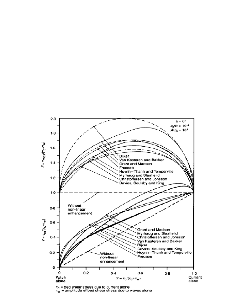
DRAFT
Coupling with D-Waves (SWAN)
where the root-mean-square wave height Hrms and the wave period T(= 2π/ω)are read
from the communication file. The variation of the wave friction factor with relative orbital excur-
sion at the bed under purely oscillatory flow is given by Swart (1974) (≡Equations (18.70),
(18.109) and (18.150)):
fw=
0.00251 exp 5.21 A
ks−0.19,A
ks>π
2,
0.3,A
ks≤π
2,
(15.22)
with:
A=uorb
ω,(15.23)
ksis the Nikuradse roughness length-scale and ωis the wave angular frequency.
As the bed is in rest and the equations are formulated in GLM co-ordinates, we must cor-
rect the bed shear-stress used in the momentum equations for the Stokes drift. The total or
effective bed shear stress is given by:
τb=|τm|
|U|U−US,(15.24)
where the components of the depth-averaged Stokes drift USare given by Eqs. (15.10) and
(15.11).
3D implementation
There is no coupling available yet for 3D D-Flow FM models and D-Waves.
Deltares 219 of 412

DRAFT
D-Flow Flexible Mesh, User Manual
220 of 412 Deltares

DRAFT
16 Coupling with D-RTC (RTC-Tools)
This chapter is on the coupling of hydrodynamics and real-time control of hydraulic structures.
16.1 Introduction
parallel/sequential coupling, which is shared
The Delta Shell framework implements the concept of an Integrated model in order to couple
different models, such as: hydrodynamics coupled with the controlling of structures, waves,
morphology and/or water quality.
Two types of coupling are distinguished: offline and online coupling. In case of an Integrated
model with offline coupling, the entire hydrodynamic simulation is done first, i.e., separately
from the second simulation. The file-based hydrodynamic output serves as input for the sec-
ond simulation. As such, the hydrodynamic flow drives the controlling of structures or the
simulation of waves or water quality. In this case there is no feedback on the hydrodynamic
simulation. For many applications, this is good practice.
An online coupling, on the other hand, exchanges data every time after computing a specified
time interval. This tight coupling allows for direct feedback of the various processes on one
another. This is crucial for controlling structures.
Note: Offline is also referred to as sequential coupling and online as parallel coupling.
A coupled flow-rtc model can be run either as an Integrated Model from within Delta Shell, or
from the commandline using the d_hydro program.
In case of a flow-rtc coupling
the flow model will exchange for example Water levels
subsequently, the rtc model will evaluate for example the Crest level of a controlled struc-
ture, based on the exchanged water levels
in case of an online coupling this Crest level will influence the simulation of the flow of
water
16.2 Getting started
16.2.1 User interface: the first steps
First, the user must add a real-time control model to the flow-fm model. The Project window
will look like this.
Deltares 221 of 412
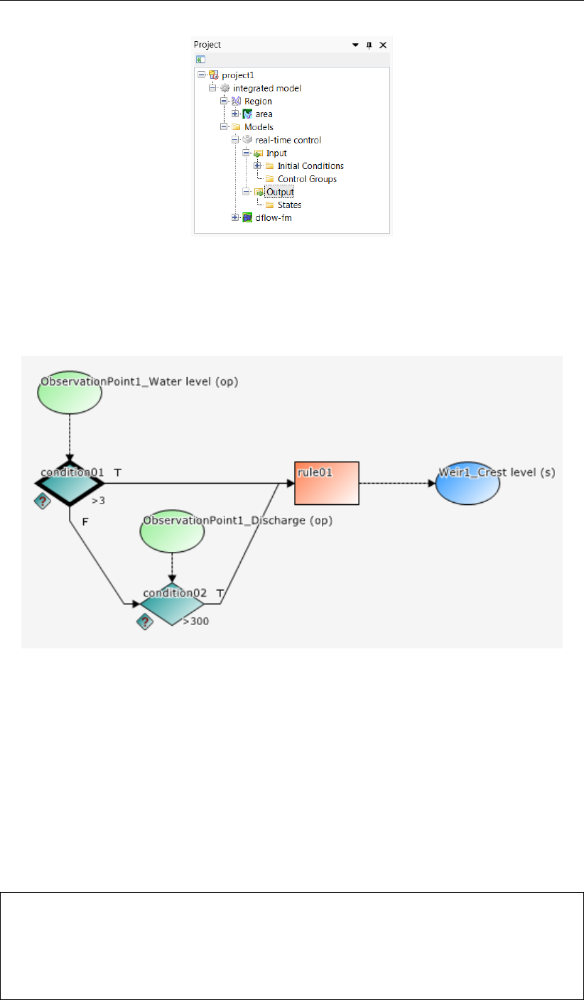
DRAFT
D-Flow Flexible Mesh, User Manual
Figure 16.1: An Integrated model in the Project window
Secondly, the user will model the control flow for an hydraulic structure. This may look like
this.
Figure 16.2: Example of a Control flow in D-RTC
Full documentation on D-RTC is available in its own User Manual. This chapter is limited to
the details of running coupled flow-rtc models.
16.2.2 Input D-Flow FM
The hydraulic structures that are normally driven by time series in <∗.tim>files, will now be
fed by D-RTC. Replace the timeseries file name by the REALTIME keyword in the <structures.ini>
file (section B.11):
[structure]
type = weir # Type of structure
id = weir01 # Name of the structure
polylinefile = weir01.pli # *.pli; Polyline geometry definition for 2D structure
crest_level = REALTIME # Crest level in [m]
222 of 412 Deltares
DRAFT
Coupling with D-RTC (RTC-Tools)
Also, the MDU file may optionally contain an observation file and/or a cross section file, such
that D-RTC’s triggers can be set to the observed time series at these locations.
[output]
ObsFile = obs.xyn
CrsFile = river_crs.pli
16.2.3 Input D-RTC
The input of D-RTC consists of several <∗.xml>files and a toplevel <settings.json>. We
refer to the D-RTC User Manual for further details.
16.2.4 Input d_hydro
In ??, details on a coupled flow-rtc-wave model are presented.
16.2.5 Online process order
This is discussed in Section 15.1.4.
Deltares 223 of 412

DRAFT
D-Flow Flexible Mesh, User Manual
224 of 412 Deltares

DRAFT
17 Coupling with D-Water Quality (Delwaq)
17.1 Introduction
D-Water Quality is a multi-dimensional water quality model framework developed by Deltares
over the past decades. It solves the advection-diffusion-reaction equation on a predefined
computational grid and for a wide range of model substances. D-Water Quality offers flexible
configuration of the substances to be included, as well as the processes to be evaluated.
D-Water Quality is not a hydrodynamic model, so information on flow fields is obtained from
hydraulic models such as D-Flow 1D (SOBEK 3) and D-Flow FM.
Here, only the coupling is discussed. Full documentation on D-Water Quality is available.
17.2 Offline versus online coupling
parallel/sequential coupling, which is shared
The Delta Shell framework implements the concept of an Integrated model in order to couple
different models, such as: hydrodynamics coupled with the controlling of structures, waves,
morphology and/or water quality.
Two types of coupling are distinguished: offline and online coupling. In case of an Integrated
model with offline coupling, the entire hydrodynamic simulation is done first, i.e., separately
from the second simulation. The file-based hydrodynamic output serves as input for the sec-
ond simulation. As such, the hydrodynamic flow drives the controlling of structures or the
simulation of waves or water quality. In this case there is no feedback on the hydrodynamic
simulation. For many applications, this is good practice.
An online coupling, on the other hand, exchanges data every time after computing a specified
time interval. This tight coupling allows for direct feedback of the various processes on one
another. This is crucial for controlling structures.
Note: Offline is also referred to as sequential coupling and online as parallel coupling.
The online coupling is scheduled for a future release.
17.3 Creating output for D-Water Quality
Creating output for D-Water Quality by D-Flow FM can be enabled in Delta Shell in the main
window under the tab ‘Output Parameters’. Change the “WAQ output interval” to a nonzero
value. The MDU-equivalent is the keyword [output],WaqInterval, where three num-
bers can be put and they are in the order of "WAQinterval, WAQ output-start-time, WAQ
output-end-time". Each number should be a whole number of seconds, and must be a multi-
ple of the “User time step” (see tab “Time frame”). Moreover, if the start and end output time
is not explicitly specified, they are automatically set to start and end time of the simulation,
respectively.
D-Flow FM will create a special output folder named <DFM_DELWAQ_mdu_name>. In this
folder a <.hyd>-file will be created that gives an overview of the coupling with references to
the files containing the hydrodynamic exchange data.
Load the <.hyd>-file in the D-Water Quality GUI to prepare the input for a water quality
calculation. For further information on how to run D-Water Quality please consult its user
manual.
Deltares 225 of 412

DRAFT
D-Flow Flexible Mesh, User Manual
The coupling between D-Flow FM and D-Water Quality has currently been tested with good
results for 2D and 3D (sigma-layer) meshes.
The D-Water Quality GUI fully supports coupling with results from D-Flow FM. Postprocessing
can be done in Delft3D-QUICKPLOT.
17.4 Current limitations
When using domain decomposition, D-Flow FM will create a special output folder per domain
named <DFM_DELWAQ_mdu_name_nnnn>. Since D-Water Quality can accept results for
a single domain only, you have to merge the results into one domain using a tool called
ddcouplefm, which can be obtained by contacting support.
It can be useful to model the water quality processes on a coarser mesh than the hydrody-
namic grid, and for this grid aggregation would be usefull. This is however not yet available
for the coupling between D-Flow FM and D-Water Quality.
226 of 412 Deltares

DRAFT
18 Sediment transport and morphology
Note: The implementation of sediment transport and morphological processes is currently a
β-functionality of D-Flow FM.
18.1 General formulations
18.1.1 Introduction
The sediment transport and morphology module supports both bedload and suspended load
transport of non-cohesive sediments and suspended load of cohesive sediments.
For schematisation we distinguish "mud" (cohesive suspended load transport), "sand" (non-
cohesive bedload and suspended load transport) and "bedload" (non-cohesive bedload only
or total load transport) fractions.
A model may contain a mixture of up to 99 suspended (i.e. "sand" and "mud") fraction and an
arbitrary amount of "bedload" fractions if computer memory and simulation time allows.
The only difference between "bedload" and "sand" fractions lies in the fact that the suspended
load advection-diffusion equation is not solved for the "bedload" fraction.
If the suspended load is known to be negligible (either due to sediment diameter or sediment
transport formula chosen), the "bedload" approach is more efficient.
Sediment interactions are taken into account although especially in the field of sand-mud
interactions still a couple of processes are lacking.
18.1.2 Suspended transport
Three-dimensional transport of suspended sediment is calculated by solving the three-dimensional
advection-diffusion (mass-balance) equation for the suspended sediment:
∂c(`)
∂t +∂uc(`)
∂x +∂vc(`)
∂y +
∂w−w(`)
sc(`)
∂z +
−∂
∂x ε(`)
s,x
∂c(`)
∂x −∂
∂y ε(`)
s,y
∂c(`)
∂y −∂
∂z ε(`)
s,z
∂c(`)
∂z = 0,(18.1)
where:
c(`)mass concentration of sediment fraction (`)[kg/m3]
u,vand wflow velocity components [m/s]
ε(`)
s,x,ε(`)
s,y and ε(`)
s,z eddy diffusivities of sediment fraction (`)[m2/s]
w(`)
s(hindered) sediment settling velocity of sediment fraction (`)[m/s]
The local flow velocities and eddy diffusivities are based on the results of the hydrodynamic
computations. Computationally, the three-dimensional transport of sediment is computed in
exactly the same way as the transport of any other conservative constituent, such as salinity,
heat, and constituents. There are, however, a number of important differences between sed-
iment and other constituents, for example, the exchange of sediment between the bed and
the flow, and the settling velocity of sediment under the action of gravity. These additional
processes for sediment are obviously of critical importance. Other processes such as the
effect that sediment has on the local mixture density, and hence on turbulence damping, can
Deltares 227 of 412

DRAFT
D-Flow Flexible Mesh, User Manual
also be taken into account. In addition, if a net flux of sediment from the bed to the flow, or
vice versa, occurs then the resulting change in the bathymetry should influence subsequent
hydrodynamic calculations. The formulation of several of these processes (such as, settling
velocity, sediment deposition and pickup) are sediment-type specific, this especially applies
for sand and mud. Furthermore, the interaction of sediment fractions is important for many
processes, for instance the simultaneous presence of multiple suspended sediment fractions
has implications for the calculation of the local hindered settling velocity of any one sediment
fraction as well as for the resulting mixture density.
The following sections describe, at a conceptual level, the differences between the suspended
transport of sediments and the transport of other conservative constituents. At the same
time we discuss some of the differences in general terms and refer for the details of the
mathematical formulations to section 18.2 and section 18.3.
Remarks:
The presence of multiple sediment fractions considerably complicates the calculation of
the density of the bed and the availability of a particular class of sediment at the bed.
See the sections on sediment interaction (section 18.4.3) and bed composition models
(section 18.6.4).
Small negative sediment concentrations (−1×10⁻³kg/m3) can be found in a compu-
tation.
These negative concentrations can be suppressed by applying a horizontal Forester
filter.
However, this can result in a substantially larger computing time.
It is suggested to accept small negative concentrations and to apply a Forester filter
only when the negative concentrations become unacceptably large.
Avertical Forester filter applied in a sediment transport computation will not affect the
sediments. Since this filter smoothes the vertical profile and thus can have a strong
influence on the vertical mixing processes, this vertical filter has been de-activated for
sediments.
18.1.3 Effect of sediment on fluid density
The effect of sediment on fluid density is not implemented in D-Flow FM yet.
18.1.4 Sediment settling velocity
The settling velocity w(`)
sfor sand and mud are strongly different in formulation; see Sections
18.2.1 and 18.3.1 for details. In high concentration mixtures, the settling velocity of a single
particle is reduced due to the presence of other particles. In order to account for this hindered
settling effect we follow Richardson and Zaki (1954) and determine the settling velocity in
a fluid-sediment mixture as a function of the sediment concentration and the non-hindered
settling fall velocity:
w(`)
s=1−ctot
s
Csoil 5
w(`)
s,0.(18.2)
where Csoil is the reference density (input parameter), ws,0is the ‘basic’ sediment fraction
specific settling velocity. The total mass concentration ctot
mis the sum of the mass concentra-
tions of the sediment fractions:
ctot
m=
lsed
X
`=1
c(`)
s.(18.3)
228 of 412 Deltares

DRAFT
Sediment transport and morphology
As the fall velocity is now a function of the sediment fractions concentration, this implies that
each sediment fraction has a fall velocity which is a function of location and time.
Remark:
The process of sediment settling is computed with a first-order upwind numerical scheme.
While use of the upwind settling formulation does slightly under-predict the mass of sed-
iment settling, the magnitude of this error has been shown to be rather small (Lesser
et al.,2000).
18.1.5 Dispersive transport
The eddy diffusivities ε(`)
s,x,ε(`)
s,y and ε(`)
s,z depend on the flow characteristics (turbulence level,
taking into account the effect of high sediment concentrations on damping turbulent exchange
processes) and the influence of waves (due to wave induced currents and enhanced bottom
shear stresses). D-Flow FM supports four so-called “turbulence closure models”:
1 Constant coefficient.
2 Algebraic eddy viscosity closure model.
3k-εturbulence closure model.
4k-τturbulence closure model (β-functionality.
The first is a simple constant value which is specified by you. A constant eddy viscosity will
lead to parabolic vertical velocity profiles (laminar flow). The other three turbulence closure
models are based on the eddy viscosity concept of Kolmogorov (1942) and Prandtl (1945)
and offer zero, first, and second order closures for the turbulent kinetic energy (k) and for the
mixing length (L). All three of the more advanced turbulence closure models take into account
the effect that a vertical density gradient has on damping the amount of vertical turbulent
mixing. See chapter 9 for a full description of the available turbulence closure models.
The output of a turbulence closure model is the eddy viscosity at each layer interface; from
this the vertical sediment mixing coefficient is calculated:
ε(`)
s=βεf,(18.4)
where:
ε(`)
svertical sediment mixing coefficient for the sediment fraction (`)
βnon-cohesive sediment: Van Rijn’s ‘beta’ factor or effective ‘beta’ factor.
cohesive sediment fractions and fine sand (<150 µm): 1.0.
εfvertical fluid mixing coefficient calculated by the selected turbulence model.
Remarks:
For cohesive sediment fractions the extra turbulent mixing due to waves is not yet in-
cluded in the eddy diffusivity. This is a limitation of the present implementation. See
also section 18.2.2.
For non-cohesive sediment the effect of waves is accounted for by using a modified or
effective ‘beta’ factor of Van Rijn (k-εmodel) or by using a separate formula to compute
εf(algebraic or k-L) model. See also section 18.3.2.
Deltares 229 of 412

DRAFT
D-Flow Flexible Mesh, User Manual
18.1.6 Three-dimensional wave effects
Note: The three-dimensional sediment transport is not implemented in D-Flow FM yet.
These effects are important when computing the transport of sediment in wave and current
situations; see Sections 18.2.5 and 18.3.4 for full details regarding their effect on cohesive
and non-cohesive sediments respectively.
18.1.7 Initial and boundary conditions
To solve Equation (18.1) you need to prescribe initial and boundary conditions for each sus-
pended sediment fraction.
18.1.7.1 Initial condition
The initial conditions for the sediment fractions are handled in exactly the same manner as
those for any other conservative constituent, i.e. you can specify:
One global initial concentration for each sediment fraction.
Space-varying initial concentrations read from a restart file generated by a previous run.
Space-varying initial concentrations read from a user-defined input file.
In these options cohesive and non-cohesive sediment fractions are treated in the same way.
In many practical applications the non-cohesive sediment concentrations adapt very rapidly to
equilibrium conditions, so in the case of a cold start where the hydrodynamic model also takes
some time to stabilise, a uniform zero concentration for the non-cohesive sediment fractions
is usually adequate.
18.1.7.2 Boundary conditions
For each of the model boundaries you must prescribe the boundary condition for each sedi-
ment fraction. We discuss in short the general type of conditions and refer for the details to
the sections to follow.
Water surface boundary
The vertical diffusive flux through the free surface is set to zero for all conservative constituents
(except heat, which can cross this boundary). This is left unchanged for suspended sediment.
−w(`)
sc(`)−ε(`)
s,z
∂c(`)
∂z = 0,at z=ζ(18.5)
where z=ζis the location of the free surface.
Bed boundary condition
The exchange of material in suspension and the bed is modelled by calculating the sediment
fluxes from the bottom computational layer to the bed, and vice versa. These fluxes are then
applied to the bottom computational layer by means of a sediment source and/or sink term in
each computational cell. The calculated fluxes are also applied to the bed in order to update
the bed level. The boundary condition at the bed is given by:
−w(`)
sc(`)−ε(`)
s,z
∂c(`)
∂z =D(`)−E(`),at z=zb(18.6)
230 of 412 Deltares

DRAFT
Sediment transport and morphology
where:
D(`)sediment deposition rate of sediment fraction (`).
E(`)sediment erosion rate of sediment fraction (`).
The formulations of D(`)and E(`)strongly differ for cohesive and non-cohesive sediment; for
the details you are referred to Sections 18.2.3 and 18.3.4 respectively.
Open inflow boundaries
D-Flow FM requires you to specify boundary conditions for all conservative constituents at
all open inflow boundaries. When modelling in three dimensions you may choose to specify
boundary concentrations that have a uniform, linear, or step distribution over the vertical. You
may also choose to specify a “Thatcher-Harleman” return time to simulate the re-entry of
material that flowed out of the model after the flow reverses direction.
All of these options are also available for sediment constituents, although they are probably
more appropriate for fine, cohesive sediment than for sand-sized particles. To assist with
modelling coarser material an additional option has been included. This option allows you to
specify that, at all open inflow boundaries, the flow should enter carrying all “sand” sediment
fractions at their “equilibrium” concentration profiles. This feature has been implemented as
a Neumann boundary condition, that is, zero concentration gradient at the boundary. By set-
ting the sediment concentrations at the boundary equal to those just inside model domain, a
near-perfectly adapted flow will enter the domain and very little accretion or erosion should
be experienced near the model boundaries. This will generally be the desired situation if the
model boundaries are well chosen. This feature can be activated for sand and mud frac-
tion separately by setting NeuBcSand (previously, EqmBc) and/or NeuBcMud to true in the
morphology input file.
Open outflow boundaries
No boundary condition is prescribed at outflow boundaries; effectively this means that the dis-
persive transport of sediment at the outflow boundary is neglected compared to the advective
transport.
18.2 Cohesive sediment
Note: The cohesive sediment is not yet implemented in D-Flow FM.
18.2.1 Cohesive sediment settling velocity
In salt water cohesive sediment tends to flocculate to form sediment "flocs", with the degree
of flocculation depending on the salinity of the water. These flocs are much larger than the
individual sediment particles and settle at a faster rate. In order to model this salinity depen-
dency you must supply two settling velocities and a maximum salinity. The first velocity, WS0,
is taken to be the settling velocity of the sediment fraction in fresh water (salinity = 0). The
second velocity, WSM, is the settling velocity of the fraction in water having a salinity equal to
SALMAX. The settling velocity of the sediment flocs is calculated as follows:
w(`)
s,0=
w(`)
s,max
21−cos( πS
Smax )+w(`)
s,f
21 + cos( πS
Smax ),when S≤Smax
w(`)
s,max,when S > Smax
(18.7)
where:
Deltares 231 of 412

DRAFT
D-Flow Flexible Mesh, User Manual
w(`)
s,0the (non-hindered) settling velocity of sediment fraction (`)
w(`)
s,max WSM, settling velocity of sediment fraction (`)at salinity concentration SALMAX
w(`)
s,f WS0, fresh water settling velocity of sediment fraction (`)
Ssalinity
Smax SALMAX, maximal salinity at which WSM is specified
Remarks:
Modelling turbulence induced flocculation or the break-up of sediment flocs is not yet
implemented.
The influence of flocculation is disregarded by setting WSM = WS0.
18.2.2 Cohesive sediment dispersion
The vertical mixing coefficient for sediment is equal to the vertical fluid mixing coefficient
calculated by the selected turbulence closure model, i.e.:
ε(`)
s=εf,(18.8)
where:
ε(`)
svertical sediment mixing coefficient for sediment fraction (`)
εfvertical fluid mixing coefficient calculated by the selected turbulence closure
model
18.2.3 Cohesive sediment erosion and deposition
For cohesive sediment fractions the fluxes between the water phase and the bed are calcu-
lated with the well-known Partheniades-Krone formulations (Partheniades,1965):
E(`)=M(`)Sτcw, τ(`)
cr,e,(18.9)
D(`)=w(`)
sc`
bSτcw, τ(`)
cr,d,(18.10)
c(`)
b=c(`)z=∆zb
2, t,(18.11)
where:
E(`)erosion flux [kg m−2s−1]
M(`)user-defined erosion parameter EROUNI [kg m−2s−1]
Sτcw, τ(`)
cr,eerosion step function:
Sτcw, τ(`)
cr,e=
τcw
τ(`)
cr,e −1!,when τcw > τ(`)
cr,e,
0,when τcw ≤τ(`)
cr,e.
(18.12)
D(`)deposition flux [kg m−2s−1]
w(`)
sfall velocity (hindered) [m/s]
c(`)
baverage sediment concentration in the near bottom computational
layer
232 of 412 Deltares

DRAFT
Sediment transport and morphology
Sτcw, τ(`)
cr,ddeposition step function:
Sτcw, τ(`)
cr,d=
1−τcw
τ(`)
cr,d !,when τcw < τ(`)
cr,d,
0,when τcw ≥τ(`)
cr,d.
(18.13)
τcw maximum bed shear stress due to current and waves as calculated
by the wave-current interaction model selected by the user.
τ(`)
cr,e user-defined critical erosion shear stress TCEUNI [N/m2]
τ(`)
cr,d user-defined critical deposition shear stress TCDUNI [N/m2]
Remark:
Superscript (`)implies that this quantity applies to sediment fraction (`).
The calculated erosion or deposition flux is applied to the near bottom computational cell by
setting the appropriate sink and source terms for that cell. Advection, particle settling, and
diffusion through the bottom of the near bottom computational cell are all set to zero to prevent
double counting these fluxes.
18.2.4 Interaction of sediment fractions
The following notes hold only in case of multiple sediment fractions. The formulations given
in the previous section have been formulated for uniform cohesive sediment beds. However,
often the bed will be made up of a range of sediment types and sizes. In such cases the
erosion rate will be affected. If the bed stratigraphy is modelled in detail, it may be assumed
that the erosion rate is proportional to the availability of the sediment fraction considered
in the top-most layer of the bed stratigraphy. On the other hand if the bed stratigraphy is not
explicitly included in the model and only the overall characteristics of the local bed composition
is known, one must assume either that the bed composition is almost uniform (in which case
the erosion rate can again be assumed to be proportional to the bed composition) or that the
cohesive sediment fraction considered forms a layer that covers the other sediment fractions
(in this case the erosion rate of the cohesive sediment will not be reduced). The former
approach is nowadays the default approach for the online-morphology module, but the latter
behaviour may be activated by setting the OldMudFrac keyword tot true in the morphology
input file.
Remarks:
Assuming an erosion rate proportional to the availability of the sediment fraction consid-
ered may result in a significant underestimation of the erosion rate if the bed is modelled
as a single uniformly mixed layer (default setting) and the mud contents is low.
Assuming that the erosion rate is independent of the availability of the sediment fraction
considered will lead to an overestimation of the erosion rate. For instance, if the model
includes two equal cohesive sediment fractions their total transport rate will be double
that of the rate observed in an identical simulation carried out using the total amount of
the two sediment fractions in the former simulation.
18.2.5 Influence of waves on cohesive sediment transport
The influence of wave on cohesive sediment is not implemented in D-Flow FM yet.
Deltares 233 of 412

DRAFT
D-Flow Flexible Mesh, User Manual
18.2.6 Inclusion of a fixed layer
If the thickness of the sediment layer becomes small then the erosion flux is reduced by a
factor fFIXFAC as defined in section 18.4.4. This reduction factor is related to the formula-
tions implemented for non cohesive sediment transport (see Sections 18.3.5 and 18.4.4 for
suspended and bedload transport respectively).
18.2.7 Inflow boundary conditions cohesive sediment
Although it is general good advice to locate the open boundaries sufficiently far away from
the area of interest, this is not always possible in long-term simulations. In such cases it is
desirable to impose some kind of equilibrium boundary conditions. The mud concentrations
are in general more loosely coupled to local morphology than the concentrations of coarser
non-cohesive sediment fractions; a unique "equilibrium" concentration (profile) does often
not exist due to differences in critical shear stresses for erosion and sedimentation. So, D-
Flow FM allows for a different approach. For cohesive material you can specify that, at all open
inflow boundaries, the flow should enter carrying the same mud concentration as computed
in the interior of the model. This feature is enabled by setting NeuBcMud in the morphology
input file to true (Neumann boundary condition: concentration gradient perpendicular to open
boundary equal to zero). Although this option may sometimes be very useful, one must be
careful when applying it: the sediment concentration of the incoming flow may take on any
value that does not lead to significant deposition in the first grid cell.
By setting NeuBcMud = false, the concentrations to be applied at the inflow boundaries
are read from the <∗.bcc>file, which has to be created with the FLOW User Interface. If the
parameter is set to true, the values specified in the <∗.bcc>file are overruled.
18.3 Non-cohesive sediment
For the transport of non-cohesive sediment, Van Rijn et al. (2000) approach is followed by
default. You can also specify a number of other transport formulations (see section 18.5)
18.3.1 Non-cohesive sediment settling velocity
The settling velocity of a non-cohesive (“sand”) sediment fraction is computed following the
method of Van Rijn (1993). The formulation used depends on the diameter of the sediment in
suspension:
w(`)
s,0=
(s(`)−1)gD(`)2
s
18ν,65 µm< Ds≤100 µm
10ν
Ds
s1 + 0.01(s(`)−1)gD(`)3
s
ν2−1
,100 µm< Ds≤1000 µm
1.1q(s(`)−1)gD(`)
s,1000 µm< Ds
(18.14)
where:
s(`)relative density ρ(`)
s/ρwof sediment fraction(`)
D(`)
srepresentative diameter of sediment fraction (`)
νkinematic viscosity coefficient of water [m2/s]
D(`)
sis the representative diameter of the suspended sediment given by the user-defined sed-
iment diameter SEDDIA (D50 of bed material) multiplied by the user-defined factor FACDSS
234 of 412 Deltares

DRAFT
Sediment transport and morphology
(see also remarks). This value of D(`)
swill be overruled if IOPSUS=1 and the transport for-
mula of Van Rijn (1993) has been selected, see section 18.5.1 for details.
Remark:
In the case of non-uniform bed material Van Rijn (1993) concluded that, on the basis of
measurements, D(`)
sshould be in the range of 60 to 100 % of D50 of the bed material.
If the bed material is very widely graded (well sorted) consideration should be given to
using several sediment fractions to model its behaviour more accurately.
18.3.2 Non-cohesive sediment dispersion
The output of a turbulence closure model is the eddy viscosity at each layer interface; from
this the vertical sediment mixing coefficient is calculated using the following expressions:
18.3.2.1 Using the k-εturbulence model
In the case of the k-εturbulence closure model the vertical sediment mixing coefficient can
be calculated directly from the vertical fluid mixing coefficient calculated by the turbulence
closure model, using the following expression:
ε(`)
s=β(`)
eff εf,(18.15)
where:
ε(`)
svertical sediment mixing coefficient of sediment fraction (`)
β(`)
eff the effective Van Rijn’s ‘beta’ factor of sediment fraction (`)As the beta factor
should only be applied to the current-related mixing this is estimated as:
β(`)
eff = 1 + β(`)−1τc
τw+τc
,(18.16)
for non-cohesive sediment fractions
β(`)Van Rijn’s ‘beta’ factor of the sediment fraction (`),Equation (18.17)
τcbed shear stress due to currents
τwbed shear stress due to waves
εfvertical fluid mixing coefficient calculated by the k-εturbulence closure model
Van Rijn’s ’beta’ factor is calculated from (Van Rijn,1984b):
β(`)= 1 + 2 w(`)
s
u∗,c !2
.(18.17)
Where w(`)
sis the settling velocity of the non-cohesive sediment fraction, and u∗,c is the local
bed shear stress due to currents.
This implies that the value of β(`)is space (and time) varying, however it is constant over the
depth of the flow. In addition, due to the limited knowledge of the physical processes involved,
we follow Van Rijn (1993) and limit β(`)to the range 1< β(`)<1.5.
Remarks:
In a wave and current situation Van Rijn (1993) applies the β-factor to only the current-
related turbulent mixing, whereas we apply it to the total turbulent mixing calculated by
the selected turbulence closure model. However, little is known about the dependence
of the β-factor on flow conditions; this discrepancy is expected to be of little importance
in practical situations.
Deltares 235 of 412

DRAFT
D-Flow Flexible Mesh, User Manual
The k-εturbulence closure model has been extended by Walstra et al. (2000) to include
the three-dimensional effects of waves. However the effect of wave asymmetry on the
bedload transport is not yet included.
18.3.2.2 Using the k-τturbulence model
The k-τmodel in combination with sediment transport is not supported in D-Flow FM yet.
18.3.3 Reference concentration
For non-cohesive sediment (e.g. sand), we follow the method of Van Rijn (1993) for the com-
bined effect of waves and currents. The reference level is given by:
a= min max AKSFAC ·ks,∆r
2,0.01h,0.20h,(18.18)
where:
aVan Rijn’s reference level
AksFac user-defined proportionality factor (morphology input file)
ksuser-defined current-related effective roughness height (see options below)
∆rwave-induced ripple height, set to a constant value of 0.025 m
hwater depth
Remark:
Van Rijn’s reference level ais limited to a maximum of 20 % of the water depth. This
precaution is only likely to come into effect in very shallow areas.
With the keyword IOPKCW you have two options to calculate ks(and kw):
ksderived from current-related effective roughness height as determined in the D-Flow FM
module (spatially varying) and kw=RWAVE ·∆r .
ksand kwspecified by you (constant in space).
Calculation of the reference concentration
The reference concentration cais calculated directly by the sediment transport formula or
it is derived from the suspended sediment transport rate given by the sediment transport
formula as ca=Ss/Hu. The default transport formula (Van Rijn,1993) includes a formula
for the reference concentration (see section 18.5.1). The reference concentration is adjusted
proportional to the relative availability of the sediment fraction in the top-layer of the bed (see
section 18.6.4 on bed composition models).
Remark:
The reference concentration and therefore the suspended load can be calibrated using
the keyword Sus in the morphology input file.
236 of 412 Deltares
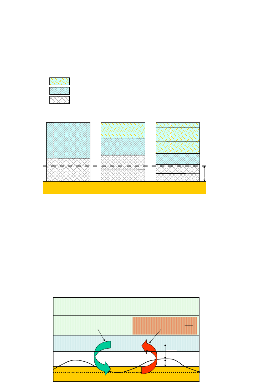
DRAFT
Sediment transport and morphology
18.3.4 Non-cohesive sediment erosion and deposition
The transfer of sediment between the bed and the flow is modelled using sink and source
terms acting on the near-bottom layer that is entirely above Van Rijn’s reference level. This
layer is identified as the reference layer and for brevity is referred to as the kmx-layer; see
Figure 18.1.
BED
a
BED
Layer
kmx
BED
kmx
kmx
kmx
Coarse Grid Medium Grid Fine Grid
Standard computational cell
Reference cell for “sand” sediment
Concentration set equal to concentration of reference layer for
‘sand’ sediment calculations
KEY
Figure 18.1: Selection of the kmx layer; where ais Van Rijn’s reference level
The sediment concentrations in the layer(s) that lie below the kmx layer are assumed to rapidly
adjust to the same concentration as the reference layer.
Each half time-step the source and sink terms model the quantity of sediment entering the flow
due to upward diffusion from the reference level and the quantity of sediment dropping out of
the flow due to sediment settling. A sink term is solved implicitly in the advection-diffusion
equation, whereas a source term is solved explicitly. The required sink and source terms for
the kmx layer are calculated as follows.
cwFluxDeposition
s
=
a
z
∆
dz
dc
FluxErosion
s
ε
=
kmx
layer
BED
Figure 18.2: Schematic arrangement of flux bottom boundary condition
In order to determine the required sink and source terms for the kmx layer, the concentration
and concentration gradient at the bottom of the kmx layer need to be approximated. We
assume a standard Rouse profile between the reference level aand the centre of the kmx
Deltares 237 of 412
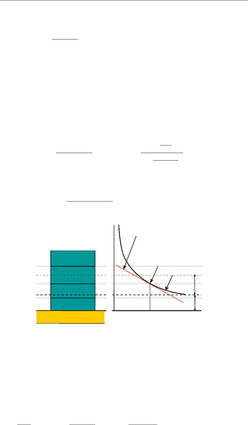
DRAFT
D-Flow Flexible Mesh, User Manual
layer (see Figure 18.3).
c(`)=c(`)
aa(h−z)
z(h−a)A(`)
,(18.19)
where:
c(`)concentration of sediment fraction (`)
c(`)
areference concentration of sediment fraction (`)
aVan Rijn’s reference level
hwater depth
zelevation above the bed
A(`)Rouse number
As the reference concentration and the concentration in the centre of the kmx layer ckmx are
known, the exponent A(`)can be determined.
c(`)
kmx =c(`)
aa(h−zkmx)
zkmx(h−a)A(`)
⇒A(`)=
ln ckmx
ca
ln a(h−zkmx)
zkmx(h−a)(18.20)
The concentration at the bottom of the kmx layer is:
c(`)
kmx(bot)=c(`)
aa(h−zkmx(bot))
zkmx(bot)(h−a)A(`)
(18.21)
a
BED
kmx +
+
∆z
c
kmx
c
a
Concentration
Approximation to concentration
gradient at bottom of kmx layer
Approximation to
concentration at
bottom of kmx layer
H e i g h t a b o v e b e d
c
kmxbot
Rouse profile
a
BED
kmx +
+
∆z
c
kmx
c
a
Concentration
Approximation to concentration
gradient at bottom of kmx layer
Approximation to
concentration at
bottom of kmx layer
H e i g h t a b o v e b e d
c
kmxbot
Rouse profile
a
BED
kmx +
+
∆z
c
kmx
c
a
Concentration
Approximation to concentration
gradient at bottom of kmx layer
Approximation to
concentration at
bottom of kmx layer
H e i g h t a b o v e b e d
c
kmxbot
Rouse profile
a
BED
kmx +
+
∆z
c
kmx
c
a
Concentration
Approximation to concentration
gradient at bottom of kmx layer
Approximation to
concentration at
bottom of kmx layer
H e i g h t a b o v e b e d
a
BED
kmx +
+
∆z
c
kmx
c
a
Concentration
Approximation to concentration
gradient at bottom of kmx layer
Approximation to
concentration at
bottom of kmx layer
H e i g h t a b o v e b e d
a
BED
kmx
a
BED
kmx +
+
∆z
c
kmx
c
a
Concentration
Approximation to concentration
gradient at bottom of kmx layer
Approximation to
concentration at
bottom of kmx layer
H e i g h t a b o v e b e d
c
kmxbot
Rouse profile
Figure 18.3: Approximation of concentration and concentration gradient at bottom of kmx
layer
We express this concentration as a function of the known concentration ckmx by introducing
a correction factor α1:
c(`)
kmx(bot)=α(`)
1c(`)
kmx (18.22)
The concentration gradient of the Rouse profile is given by:
∂c(`)
∂z =A(`)c(`)
aa(h−z)
z(h−a)A(`)−1
·−ah
z2(h−a)(18.23)
238 of 412 Deltares

DRAFT
Sediment transport and morphology
The concentration gradient at the bottom of the kmx layer is:
c0(`)
kmx(bot)=A(`)c(`)
aa(h−zkmx(bot))
zkmx(bot)(h−a)A(`)−1
· −ah
z2
kmx(bot)(h−a)!(18.24)
We express this gradient as a function of the known concentrations caand ckmx by introducing
another correction factor α2:
c0(`)
kmx(bot)=α(`)
2 c(`)
kmx −c(`)
a
∆z!(18.25)
Erosive flux due to upward diffusion
The upward diffusion of sediment through the bottom of the kmx layer is given by the expres-
sion:
E(`)=ε(`)
s
∂c(`)
∂z ,(18.26)
where ε(`)
sand ∂c(`)
∂z are evaluated at the bottom of the kmx layer.
We approximate this expression by:
E(`)≈α(`)
2ε(`)
s c(`)
a−c(`)
kmx
∆z!,(18.27)
where:
α(`)
2correction factor for sediment concentration
ε(`)
ssediment diffusion coefficient evaluated at the bottom of the kmx cell of sedi-
ment fraction(`)
c(`)
areference concentration of sediment fraction(`)
c(`)
kmx average concentration of the kmx cell of sediment fraction(`)
∆zdifference in elevation between the centre of the kmx cell and Van Rijn’s refer-
ence level: ∆z=zkmx −a
The erosion flux is split in a source and sink term:
E(`)≈α(`)
2ε(`)
sc(`)
a
∆z−α(`)
2ε(`)
sc(`)
kmx
∆z.(18.28)
The first of these terms can be evaluated explicitly and is implemented as a sediment source
term. The second can only be evaluated implicitly and is implemented as a (positive) sink
term. Thus:
Source(`)
erosion =α(`)
2ε(`)
sc(`)
a
∆z(18.29)
Sink(`)
erosion =α(`)
2ε(`)
sc(`)
kmx
∆z(18.30)
Deltares 239 of 412

DRAFT
D-Flow Flexible Mesh, User Manual
Deposition flux due to sediment settling
The settling of sediment through the bottom of the kmx cell is given by the expression:
D(`)=w(`)
sc(`)
kmx(bot),(18.31)
where w(`)
sand c(`)
kmx(bot)are evaluated at the bottom of the kmx layer.
We set:
c(`)
kmx(bot)=α(`)
1c(`)
kmx.(18.32)
The deposition flux is approximated by:
D(`)≈α(`)
1c(`)
kmxw(`)
s.(18.33)
This results in a simple deposition sink term:
Sink(`)
deposition =α(`)
1c(`)
kmxw(`)
s.(18.34)
The total source and sink terms is given by:
Source(`)=α(`)
2c(`)
a ε(`)
s
∆z!,(18.35)
Sink(`)="α(`)
2 ε(`)
s
∆z!+α(`)
1w(`)
s#c(`)
kmx.(18.36)
These source and sink terms are both guaranteed to be positive.
18.3.5 Inclusion of a fixed layer
The bedload transport is reduced if the thickness of the sediment layer becomes small (see
section 18.4.4). The same effect has been implemented as a reduction for the entrainment
and deposition terms as well as the equilibrium concentration by a factor fFIXFAC if erosion is
expected to occur.
18.3.6 Inflow boundary conditions non-cohesive sediment
Although it is general good advice to locate the open boundaries sufficiently far away from
the area of interest, this is not always possible in long-term simulations. In such cases it
is desirable to impose some kind of equilibrium boundary conditions. Although equilibrium
boundary conditions may be better defined for non-cohesive sediments than for cohesive
sediments, we have implemented the open boundary condition in a consistent manner. For
non-cohesive suspended material you can specify that, at all open inflow boundaries, the
flow should enter carrying the same concentration of sediment as computed in the interior
of the model. This feature is enabled by setting NeuBcSand in the morphology input file to
true (Neumann boundary condition: concentration gradient perpendicular to open boundary
equal to zero). This means that the sediment load entering through the boundaries will be
near-perfectly adapted to the local flow conditions and very little accretion or erosion should
240 of 412 Deltares

DRAFT
Sediment transport and morphology
be experienced near the model boundaries. This will generally be the desired situation if
the model boundaries are well chosen. This method gives the correct results even when the
turbulent mixing profile is clearly non-parabolic.
By setting NeuBcSand = false, the concentrations to be applied at the inflow boundaries
are read from the <∗.bcc>file, which has to be created with the FLOW User Interface. If the
parameter is set to true, the values specified in the <∗.bcc>file are overruled. This parameter
used to be called EqmBc.
18.4 Bedload sediment transport of non-cohesive sediment
Bedload (or, for the simpler transport formulae, total load) transport is calculated for all “sand”
and “bedload” sediment fractions by broadly according to the following approach: first, the
magnitude and direction of the bedload transport at the cell centres is computed using the
transport formula selected (See section 18.5), subsequently the transport rates at the cell
interfaces are determined, corrected for bed-slope effect and upwind bed composition and
sediment availability.
18.4.1 Basic formulation
For simulations including waves the magnitude and direction of the bedload transport on a
horizontal bed are calculated using the transport formula selected assuming sufficient sedi-
ment and ignoring bed composition except for e.g. hiding and exposure effects on the critical
shear stresses. The default sediment transport formula is Van Rijn (1993) as documented in
section 18.5.1.
Some of the sediment transport formulae prescribe the bedload transport direction whereas
others predict just the magnitude of the sediment transport. In the latter case the initial trans-
port direction will be assumed to be equal to the direction of the characteristic (near-bed) flow
direction. In the case of a depth-averaged simulation, the secondary flow/spiral flow intensity
Isoptionally computed by the flow module may be taken into account; the bedload transport
direction ϕτis given by the following formula:
tan(ϕτ) = v−αIu
UIs
u−αIv
UIs
(18.37)
in which
αI=2
κ2Es1−1
2
√g
κC (18.38)
where:
ggravitational acceleration
κVon Kármán constant
CChézy roughness
Uthe depth-averaged velocity
Escoefficient to be specified by you as Espir keyword in the morphology input
file
The default value of Esis 0, which implies that the spiral flow effect on the bedload transport
direction is not included. The spiral flow effect is of crucial importance in a depth-averaged
simulation to get pointbar formation in river bends. This effect is only included for transport
formulae that return the bedload transport rate but not its direction, i.e. Engelund & Hansen,
Meyer-Peter & Muller, General formula, Van Rijn (1984), Ashida & Michiue and optionally the
user-defined formula.
Deltares 241 of 412

DRAFT
D-Flow Flexible Mesh, User Manual
The Van Rijn (1993) formula distinguishes the following transport components that are all
treated like bed or total load, i.e without relaxation effects of an advection diffusion equation:
bedload due to currents, Sbc
bedload due to waves, Sbw
suspended load due to waves, Ssw.
These three transport components can be calibrated independently by using the respective
keywords Bed,BedW and SusW in the morphology input file.
18.4.2 Suspended sediment correction vector
The Suspended sediment correction vector is not implemented yet in D-Flow FM.
18.4.3 Interaction of sediment fractions
The following notes hold only in case of multiple sediment fractions. Sediment fractions may
interacted in several ways:
reference concentrations, erosion rates and sediment transport rates will be reduced pro-
portional to the availability of sediment fraction considered in the bed (less of the fraction
available for transport)
sediment fractions of different sizes influence each other by means of hiding and exposure:
fine sediments hide among coarse sediments and are thereby partly shielded from the
main flow while the coarser sediments are more exposed than they would be among
other sediments of the same size. This effect is taken into account by increasing the
effective critical shear stress for fine sediments while lowering it for coarse sediments.
This adjustment is carried out using a multiplicative factor ξ. The following formulations
have been implemented:
No hiding and exposure correction (ξ= 1)
Egiazaroff formulation
ξ=10log 19
10log 19 + 10log (Di/Dm)2
.(18.39)
Ashida & Michiue formulation
ξ=
0.8429Dm
Diif Di/Dm<0.38889
10log 19
10log 19 + 10log (Di/Dm)2
otherwise .(18.40)
Parker, Klingeman & McLean or Soehngen, Kellermann & Loy formulation
ξ=Dm
Diα
.(18.41)
where αis given by the ASKLHE keyword in the morphology input file.
Wu, Wang & Jia formulation
ϕ(`)=X
i
η(i)D(i)
D(`)−D(i)(18.42)
ξ(`)=1−ϕ(`)
ϕ(`)m
(18.43)
242 of 412 Deltares

DRAFT
Sediment transport and morphology
where mis given by the MWWJHE keyword in the morphology input file.
The hiding and exposure effect has been implemented for the following transport formulae
containing a critical shear stress: Meyer-Peter & Muller, general formula, Ashida-Michiue and
optionally the user-defined formula.
18.4.4 Inclusion of a fixed layer
Inclusion of a fixed layer implies that the quantity of sediment at the bed is finite and may, if
excessive erosion occurs, become exhausted and be unavailable to supply sediment to sus-
pended and bedload transport modes. In case the bed is covered by bedforms, the troughs of
the bedforms will start to expose the non-erodible layer before sediment runs out completely.
This results in a gradual reduction of the transport capacity over a certain sediment thickness
indicated by THRESH. This effect is taken into account in the bedload formulations by com-
paring the thickness of the sediment layer available at the bed with a user-defined threshold
value. If the quantity of sediment available is less than the threshold then the magnitude of
the calculated bedload transport vector is reduced as follows:
S00
b=fFIXFACS00
b,(18.44)
where:
S00
bmagnitude of the bedload transport vector (before correction for bed slope ef-
fects)
fFIXFAC upwind fixed layer proximity factor: fFIXFAC =DPSED
THRESH , limited to the range
0≤fFIXFAC ≤1.
DPSED depth of sediment available at the bed
THRESH user-defined erosion threshold
The equilibrium suspended load concentration in the sediment pickup term is reduced by the
same fixed layer proximity factor (in this case of course the local value and not some upwind
value is used since suspended sediment pickup has no associated horizontal direction).
In effect, because of the upwind approach used to transfer the bedload transport components
to the velocity points, this method limits the sediment that can leave a computational cell, if the
quantity of the sediment at the bed is limited. One implication of the use of this rather simple
approach is that a finite (although always less than the user-defined threshold) thickness of
sediment is required at the bed if a non-zero magnitude of the bedload transport vector is
required.
Remarks:
Areas may be initially specified as containing zero bottom sediment if non-erodible ar-
eas are required. It is likely that these areas will accrete a little sediment in order to
allow an equilibrium bedload transport pattern to develop.
This effect has also been included for cohesive and non cohesive suspended sediment
as indicated in section 18.2 and section 18.3.5.
18.4.5 Calculation of bedload transport at open boundaries
Bedload transport at open boundaries is not implemented yet.
Deltares 243 of 412
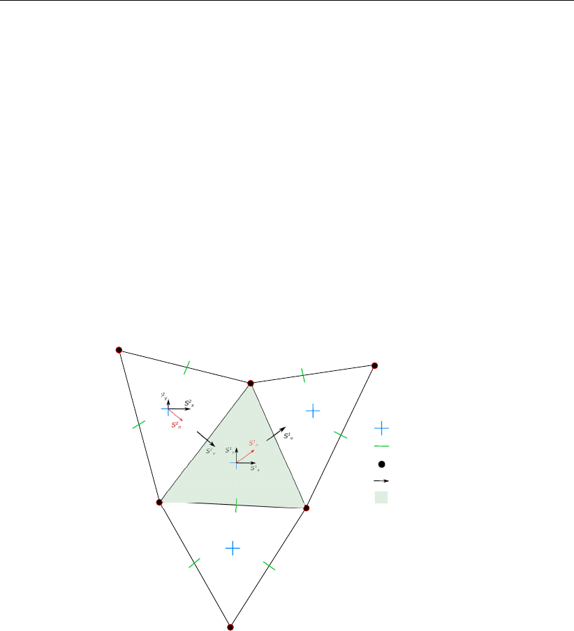
DRAFT
D-Flow Flexible Mesh, User Manual
18.4.6 Bedload transport at velocity points
As the control volume for bed level change calculations is centred on the water level points,
see Figure 18.4, the bedload transport vector components are actually required at the velocity
points, rather than at the water level points where Sxand Syare calculated. By default, we
use a simple “upwind” numerical scheme to set the bedload transport components at the
velocity points as this ensures that the bed will remain stable. For each active velocity point
the upwind direction is determined by summing the bedload transport components at the
water level points on either side of the velocity point and taking the upwind direction relative to
the resulting net transport direction. The bedload transport component at the velocity point is
then set equal to the component computed at the water level point immediately "upwind" (see
Figure 18.4). In the example shown in Figure 18.4 the bedload transport normal component
on the velocity point, S1
u, is set equal to S1
n, where S1
nis the projection of bedload flux vector at
point 1 in the normal direction of the corresponding velocity face. Based on the same method,
the component S2
uis set equal to S2
n. It is possible to switch from upwind to central approach
by setting the UpwindBedload keyword in the morphology input file to false; although the
central approach is more accurate, it is less stable (less damping).
S1x
S1u
S2x
S1y
S2y
S1n
S2n
S2u
Water level point
Velocity point
Depth point
Bedload transport
Control volume
Figure 18.4: Setting of bedload transport components at velocity points
18.4.7 Adjustment of bedload transport for bed-slope effects
Bedload transport is affected by bed level gradients. Two bed slope directions are distin-
guished: the slope in the initial direction of the transport (referred to as the longitudinal bed
slope) and the slope in the direction perpendicular to that (referred to as the transverse bed
slope). The longitudinal bed slope results in a change in the sediment transport rate as given
by:
S0
b=αsS00,(18.45)
or, in vector component form:
S0
b,x =αsS00
b,x,(18.46)
S0
b,y =αsS00
b,y,(18.47)
whereas the primary effect of the transverse bed slope is a change in transport towards the
downslope direction (this may be accomplished by either a pure rotation of the transport vec-
tor or by adding a transverse transport component). You may choose one of the following
formulations for these effects.
244 of 412 Deltares
DRAFT
Sediment transport and morphology
1 no effect of bed slope on bedload transport
2Bagnold (1966) for longitudinal slope and Ikeda (1982,1988) as presented by Van Rijn
(1993) for transverse slope. This is the default option for the bedload transport of all
sediment transport formulae. In this case αsis given by
αs= 1 + αbs tan (φ)
cos tan−1∂z
∂s tan (φ) + ∂z
∂s −1!,(18.48)
where αbs is a user-defined tuning parameter, ALFABS keyword in the morphology in-
put file (default = 1.0). An additional bedload transport vector is subsequently calculated,
perpendicular to the main bedload transport vector. The magnitude of this vector is calcu-
lated using a formulation based on the work of Ikeda (1982,1988) as presented by Van
Rijn (1993). Van Rijn’s equation (7.2.52) is modified to Equation (18.49) by setting the ref-
erence co-ordinates sand naligned with and perpendicular to the local characteristic flow
direction respectively. This implies that there is no flow in the ndirection: i.e. ub,n = 0:
Sb,n =|S0
b|αbn
ub,cr
|ub|
∂zb
∂n ,(18.49)
where:
Sb,n additional bedload transport vector. The direction of this vector is normal to
the unadjusted bedload transport vector, in the down slope direction
|S0
b|magnitude of the unadjusted bedload transport vector (adjusted for longitu-
dinal bed slope only): |S0
b|=qS0
b,x2+S0
b,y2.
αbn user-defined coefficient, ALFABN (default = 1.5)
ub,cr critical (threshold) near-bed fluid velocity
ubnear-bed fluid velocity vector
∂zb
∂n bed slope in the direction normal to the unadjusted bedload transport vector
To evaluate Equation (18.49) we substitute:
ub,cr
|ub|=rτb,cr
|τb|,(18.50)
where:
τb,cr critical bed shear stress
τbbed shear stress due to current and waves: τb=µcτb,cw +µwτb,w.
resulting in:
Sb,n =|S0
b|fnorm,(18.51)
where:
fnorm =αbnrτb,cr
|τb|
∂zb
∂n .(18.52)
The two components of this vector are then added to the two components of the bedload
transport vector as follows:
Sb,x =S0
b,x −S0
b,yfnorm
Sb,y =S0
b,y +S0
b,xfnorm (18.53)
where Sb,x and Sb,y are the components of the required bedload transport vector, calcu-
lated at the water level points
Deltares 245 of 412

DRAFT
D-Flow Flexible Mesh, User Manual
3Koch and Flokstra (1980) as extended by Talmon et al. (1995). In this case αsis given by
αs= 1 −αbs
∂z
∂s,(18.54)
where αbs is a user-defined tuning parameter, ALFABS keyword in the morphology input
file (default = 1.0). The direction of the bedload is adjusted according to the following
formulation:
tan(ϕs) = sin(ϕτ) + 1
f(θ)
∂zb
∂y
cos(ϕτ) + 1
f(θ)
∂zb
∂x
,(18.55)
in which ϕτis the original direction of the sediment transport and ϕsis the final direction
and where f(θ)equals:
f(θ) = AshθBsh
iDi
HCsh Di
DmDsh
,(18.56)
where Ash,Bsh,Csh and Dsh are tuning coefficients specified by you in the morphology
input file as keywords Ashld,Bshld,Cshld and Dshld.
4Parker and Andrews (1985). The same formulae for αsand ϕshold as in the previous
case except for f(θ)which now equals:
f(θ) = cL
1 + µcLsθ
max 1
10 θ, ξθcr,(18.57)
where Coulomb friction parameter cL, lift-drag ratio µand critical shields parameter θcr
should be specified by you in the morphology input file as keywords CoulFri,FlFdRat
and ThetaCr. Note that this formula includes the hiding and exposure factor ξ.
This completes the calculation of the bedload transport field. The transports at the velocity
points are then stored for use in the computation of bed level changes, as described in the
section 18.6. In all cases the bed slope has been defined as follows.
Longitudinal bed slope
This bed slope is calculated as:
∂zb
∂s =∂z(u)
∂x
S00
b,x
|S00
b|+∂z(v)
∂y
S00
b,y
|S00
b|,(18.58)
∂zb
∂s max
= 0.9 tan (φ),(18.59)
where:
∂zb
∂s bed slope in the direction of bedload transport
∂z(u)
∂x bed slope in the positive x-direction
∂z(v)
∂y bed slope in the positive y-direction
φinternal angle of friction of bed material (assumed to be 30◦)
Remarks:
zbis the depth down to the bed from a reference level (positive down), a downward bed
slope returns a positive value).
246 of 412 Deltares
DRAFT
Sediment transport and morphology
Table 18.1: Additional transport relations
Formula Bedload Waves
18.5.1,Van Rijn (1993) Bedload + suspended Yes
18.5.2,Engelund-Hansen (1967) Total transport No
18.5.3,Meyer-Peter-Muller (1948) Total transport No
18.5.4,General formula Total transport No
18.5.5,Bijker (1971) Bedload + suspended Yes
18.5.6,Van Rijn (1984) Bedload + suspended No
18.5.7,Soulsby/Van Rijn Bedload + suspended Yes
18.5.8,Soulsby Bedload + suspended Yes
18.5.9,Ashida-Michiue (1974) Total transport No
18.5.10,Wilcock-Crowe (2003) Bedload No
18.5.11,Gaeuman et al. (2009) laboratory calibration Bedload No
18.5.12,Gaeuman et al. (2009) Trinity River calibration Bedload No
The bed slope is calculated at the velocity points as these are the locations at which the
bedload transport vector components will finally be applied.
Transverse bed slope
This bed slope is calculated as:
∂zb
∂n =−∂z(u)
∂x
S00
b,y
|S00
b|+∂z(v)
∂y
S00
b,x
|S00
b|.(18.60)
18.5 Transport formulations for non-cohesive sediment
This special feature offers a number of standard sediment transport formulations for non-
cohesive sediment. Table 18.1 gives a summary of the available additional formulae.
Additionally, you can implement your own sediment transport formula in a shared library
(<dll>or <so>) and call it from D-Flow FM. Now, let us continue with a general descrip-
tion of the sediment transport formulae included by default.
18.5.1 Van Rijn (1993)
Van Rijn (1993) distinguishes between sediment transport below the reference level a which is
treated as bedload transport and that above the reference level which is treated as suspended-
load. Sediment is entrained in the water column by imposing a reference concentration at the
reference level.
Reference concentration
The reference concentration is calculated in accordance with Van Rijn et al. (2000) as:
c(`)
a= 0.015ρ(`)
s
D(`)
50 T(`)
a1.5
aD(`)
∗0.3(18.61)
where:
c(`)
amass concentration at reference level a
In order to evaluate this expression the following quantities must be calculated:
Deltares 247 of 412

DRAFT
D-Flow Flexible Mesh, User Manual
D(`)
∗non-dimensional particle diameter:
D(`)
∗=D(`)
50 (s(`)−1)g
ν21/3
(18.62)
T(`)
anon-dimensional bed-shear stress:
T(`)
a=(µ(`)
cτb,cw +µ(`)
wτb,w)−τ(`)
cr
τ(`)
cr
(18.63)
µ(`)
cefficiency factor current:
µ(`)
c=f0(`)
c
fc
(18.64)
f0(`)
cgain related friction factor:
f0(`)
c= 0.24 "10log 12h
3D(`)
90 !#−2
(18.65)
f(`)
ctotal current-related friction factor:
f(`)
c= 0.24 10log 12h
ks−2
(18.66)
τb,cw bed shear stress due to current in the presence of waves. Note that the bed
shear velocity u∗is calculated in such a way that Van Rijn’s wave-current inter-
action factor αcw is not required.
τb,cw =ρwu2
∗(18.67)
µ(`)
wefficiency factor waves:
µ(`)
w= max 0.063,1
81.5−Hs
h2!(18.68)
τb,w bed shear stress due to waves:
τb,w =1
4ρwfwb
Uδ2(18.69)
fwtotal wave-related friction factor:
fw= exp
−6+5.2 ˆ
Aδ
ks,w !−0.19
(18.70)
To avoid the need for excessive user input, the wave related roughness ks,w is related to the
estimated ripple height, using the relationship:
ks,w =RWAVE ·∆r, with ∆r= 0.025 and 0.01 m≤ks,w ≤0.1m (18.71)
where:
248 of 412 Deltares
DRAFT
Sediment transport and morphology
RWAVE the user-defined wave roughness adjustment factor. Recommended to be in
the range 1–3, default = 2.
τ(`)
cr critical bed shear stress:
τ(`)
cr = (ρ(`)
s−ρw)gD(`)
50 θ(`)
cr (18.72)
θ(`)
cr threshold parameter θ(`)
cr is calculated according to the classical Shields curve
as modelled by Van Rijn (1993) as a function of the non-dimensional grain size
D∗. This avoids the need for iteration.
Note: for clarity, in this expression the symbol D∗has been used where D(`)
∗
would be more correct:
θ(`)
cr =
0.24D−1
∗,1< D∗≤4
0.14D−0.64
∗,4< D∗≤10
0.04D−0.1
∗,10 < D∗≤20
0.013D0.29
∗,20 < D∗≤150
0.055,150 < D∗
(18.73)
aVan Rijn’s reference level
ˆ
Aδpeak orbital excursion at the bed: ˆ
Aδ=Tpˆ
Uδ
2π.
D(`)
50 median sediment diameter
D(`)
90 90 % sediment passing size: D(`)
90 = 1.5D(`)
50
hwater depth
kaapparent bed roughness felt by the flow when waves are present. Calculated by
D-Flow FM using the wave-current interaction formulation selected: ka≤10ks
ksuser-defined current-related effective roughness height (space varying)
ks,w wave-related roughness, calculated from ripple height, see Equation (18.71)
uzvelocity magnitude taken from a near-bed computational layer. In a current-only
situation the velocity in the bottom computational layer is used. Otherwise, if
waves are active, the velocity is taken from the layer closest to the height of the
top of the wave mixing layer δ.
b
Uδpeak orbital velocity at the bed: √2RMS orbital velocity at bed, taken from the
wave module.
zuheight above bed of the near-bed velocity (uz)used in the calculation of bottom
shear stress due to current
∆restimated ripple height, see Equation (18.71)
δmthickness of wave boundary mixing layer following Van Rijn (1993): 3δw(and
δm≥ka)
δwwave boundary layer thickness:
δw= 0.072 ˆ
Aδˆ
Aδ
ks,w −0.25.
We emphasise the following points regarding this implementation:
The bottom shear stress due to currents is based on a near-bed velocity taken from the
hydrodynamic calculations, rather than the depth-averaged velocity used by Van Rijn.
All sediment calculations are based on hydrodynamic calculations from the previous half
time-step. We find that this is necessary to prevent unstable oscillations developing.
The apparent roughness felt by the flow (ka) is dependent on the hydrodynamic wave-current
interaction model applied. At this time, Van Rijn’s wave-current interaction model is not avail-
able in D-Flow FM. This means that it is not possible for a user to exactly reproduce results
obtained using Van Rijn’s full formulations for waves and currents.
Deltares 249 of 412

DRAFT
D-Flow Flexible Mesh, User Manual
Adjustment of the representative diameter of suspended sediment
The representative diameter of the suspended sediment D(`)
sgenerally given by the user-
defined sediment diameter SEDDIA (D50 of bed material) multiplied by the user-defined factor
FACDSS (see also remarks) can be overruled in case the Van Rijn (1993) transport formula is
selected. This achieved by setting IOPSUS=1 the representative diameter of the suspended
sediment will then be set to:
D(`)
s=
0.64D(`)
50 for T(`)
A≤1
D(`)
50 1+0.015 T(`)
A−25 for 1< T (`)
A≤25
D(`)
50 for 25 < T (`)
A
(18.74)
where T(`)
ais given by equation (18.63).
Bedload transport rate
For simulations including waves the magnitude and direction of the bedload transport on a
horizontal bed are calculated using an approximation method developed by Van Rijn et al.
(2003). The method computes the magnitude of the bedload transport as:
|Sb|= 0.006ρswsD(`)
50 M0.5M0.7
e(18.75)
where:
Sbbedload transport [kg m-1 s-1]
Msediment mobility number due to waves and currents [-]
Meexcess sediment mobility number [-]
M=v2
eff
(s−1) gD50
(18.76)
Me=(veff −vcr)2
(s−1) gD50
(18.77)
veff =qv2
R+U2
on (18.78)
in which:
vcr critical depth averaged velocity for initiation of motion (based on a parameteri-
sation of the Shields curve) [m/s]
vRmagnitude of an equivalent depth-averaged velocity computed from the velocity
in the bottom computational layer, assuming a logarithmic velocity profile [m/s]
Uon near-bed peak orbital velocity [m/s] in onshore direction (in the direction on
wave propagation) based on the significant wave height
Uon (and Uoff used below) are the high frequency near-bed orbital velocities due to short
waves and are computed using a modification of the method of Isobe and Horikawa (1982).
This method is a parameterisation of fifth-order Stokes wave theory and third-order cnoidal
wave theory which can be used over a wide range of wave conditions and takes into ac-
count the non-linear effects that occur as waves propagate in shallow water (Grasmeijer and
Van Rijn,1998).
The direction of the bedload transport vector is determined by assuming that it is composed
of two parts: part due to current (Sb,c) which acts in the direction of the near-bed current, and
250 of 412 Deltares

DRAFT
Sediment transport and morphology
part due to waves (Sb,w) which acts in the direction of wave propagation. These components
are determined as follows:
Sb,c =Sb
p1 + r2+ 2 |r|cos ϕ(18.79)
|Sb,w|=r|Sb,c|(18.80)
where:
r=(|Uon| − vcr)3
(|vR| − vcr)3(18.81)
Sb,w = 0 if r < 0.01,Sb,c = 0 if r > 100, and ϕ= angle between current and wave
direction for which Van Rijn (2003) suggests a constant value of 90◦.
Also included in the “bedload” transport vector is an estimation of the suspended sediment
transport due to wave asymmetry effects. This is intended to model the effect of asymmetric
wave orbital velocities on the transport of suspended material within about 0.5 m of the bed
(the bulk of the suspended transport affected by high frequency wave oscillations).
This wave-related suspended sediment transport is again modelled using an approximation
method proposed by Van Rijn (2001):
Ss,w =fSUSWγUALT(18.82)
where:
Ss,w wave-related suspended transport [kg/(ms)]
fSUSW user-defined tuning parameter
γphase lag coefficient (= 0.2)
UAvelocity asymmetry value [m/s] = U4
on−U4
of f
U3
on+U3
of f
LTsuspended sediment load [kg/m2] = 0.007ρsD50Me
The three separate transport modes are imposed separately. The direction of the bedload
due to currents Sb,c is assumed to be equal to the direction of the current, whereas the two
wave related transport components Sb,w and Ss,w take on the wave propagation direction.
This results in the following transport components:
Sbc,u =ub,u
|ub||Sb,c|(18.83)
Sbc,v =ub,v
|ub||Sb,c|(18.84)
Sbw,u =Sb,w cos φ(18.85)
Sbw,v =Sb,w sin φ(18.86)
Ssw,u =Ss,w cos φ(18.87)
Ssw,v =Ss,w sin φ(18.88)
where φis the local angle between the direction of wave propagation and the computational
grid. The different transport components can be calibrated independently by using the Bed,
BedW and SusW keywords in the morphology input file.
Deltares 251 of 412

DRAFT
D-Flow Flexible Mesh, User Manual
18.5.2 Engelund-Hansen (1967)
The Engelund-Hansen sediment transport relation has frequently been used in rivers and
estuaries. It reads:
S=Sb+Ss,eq =0.05αq5
√gC3∆2D50
(18.89)
where:
qmagnitude of flow velocity
∆the relative density (ρs−ρw)/ρw
CChézy friction coefficient
αcalibration coefficient (O(1))
The transport rate is imposed as bedload transport due to currents Sbc. The following formula
specific parameters have to be specified in the input files of the Transport module: calibration
coefficient αand roughness height rk.
Remarks:
The D50 grain size diameter is based on the sediment fraction considered.
A second formula specific input parameter (rk) is required for the Engelund-Hansen
formula. This parameter, which represents the roughness height for currents alone in
[m], is only used to determine the Cvalue when the Chézy friction in the flow has not
been defined. Generally, this parameter can thus be treated as a dummy parameter.
18.5.3 Meyer-Peter-Muller (1948)
The Meyer-Peter-Muller sediment transport relation is slightly more advanced than the Engelund-
Hansen formula, as it includes a critical shear stress for transport. It reads:
S= 8αD50p∆gD50(µθ −ξθcr)3/2(18.90)
where:
αcalibration coefficient (O(1))
∆the relative density (ρs−ρw)/ρw
µripple factor or efficiency factor
θcr critical mobility parameter (= 0.047)
ξhiding and exposure factor for the sediment fraction considered
and the Shields mobility parameter θgiven by
θ=q
C21
∆D50
(18.91)
in which qis the magnitude of the flow velocity [m/s]. The ripple factor µreads:
µ= min C
Cg,90 1.5
,1.0!(18.92)
where Cg,90 is the Chézy coefficient related to grains, given by:
Cg,90 = 18 10log 12(d+ζ)
D90 (18.93)
252 of 412 Deltares

DRAFT
Sediment transport and morphology
with D90 specified in [m]. The transport rate is imposed as bedload transport due to currents
Sbc. The following formula specific parameters have to be specified in the input files of the
Transport module: calibration coefficient αand a dummy value.
Remark:
The D50 is based on the sediment fraction considered, the D90 grain size diameters is
based on the composition of the local sediment mixture.
18.5.4 General formula
The general sediment transport relation has the structure of the Meyer-Peter-Muller formula,
but all coefficients and powers can be adjusted to fit your requirements. This formula is aimed
at experienced users that want to investigate certain parameters settings. In general this
formula should not be used. It reads:
S=αD50p∆gD50θb(µθ −ξθcr)c(18.94)
where ξis the hiding and exposure factor for the sediment fraction considered and
θ=q
C21
∆D50
(18.95)
in which qis the magnitude of the flow velocity.
The transport rate is imposed as bedload transport due to currents Sbc. The following param-
eters have to be specified in the input files of the Transport module: calibration coefficient α,
powers band c, ripple factor or efficiency factor µ, critical mobility parameter θcr.
18.5.5 Bijker (1971)
The Bijker formula sediment transport relation is a popular formula which is often used in
coastal areas. It is robust and generally produces sediment transport of the right order of
magnitude under the combined action of currents and waves. Bedload and suspended load
are treated separately. The near-bed sediment transport (Sb) and the suspended sediment
transport (Ss) are given by the formulations in the first sub-section. It is possible to include
sediment transport in the wave direction due to wave asymmetry and bed slope following
the Bailard approach, see Bailard (1981), Stive (1986). Separate expressions for the wave
asymmetry and bed slope components are included:
Sb=Sb0+Sb,asymm +Ss,asymm +Sb,slope +Ss,slope (18.96)
Ss=Ss0(18.97)
where Sb0and Ss0are the sediment transport in flow direction as computed according to the
formulations of Bijker in the first sub-section, and the asymmetry and bed slope components
for bedload and suspended transport are defined in the second sub-section. Both bedload and
suspended load terms are incorporated in the bedload transport for further processing. The
transport vectors are imposed as bedload transport vector due to currents Sbc and suspended
load transport magnitude Ss, from which the equilibrium concentration is derived, respectively.
18.5.5.1 Basic formulation
The basic formulation of the sediment transport formula according to Bijker is given by:
Sb=bD50
q
C√g(1 −φ) exp (Ar)(18.98)
Ss= 1.83SbI1ln 33.0h
rc+I2(18.99)
Deltares 253 of 412
DRAFT
D-Flow Flexible Mesh, User Manual
where
CChézy coefficient (as specified in input of D-Flow FM module)
hwater depth
qflow velocity magnitude
φporosity
and
Ar= max (−50,min (100, Ara)) (18.100)
b=BD + max 0,min 1,(hw/h)−Cd
Cs−Cd(BS −BD)(18.101)
I1= 0.216 rc
hz∗−1
1−rc
hz∗
1
Z
rc/h 1−y
yz∗dy (18.102)
I2= 0.216 rc
hz∗−1
1−rc
hz∗
1
Z
rc/h
ln y1−y
yz∗dy (18.103)
where
BS Coefficient bfor shallow water (default value 5)
BD Coefficient bfor deep water (default value 2)
CsShallow water criterion (Hs/h) (default value 0.05)
CdDeep water criterion (default value 0.4)
rcRoughness height for currents [m]
and
Ara =−0.27∆D50C2
µq21+0.5ψUb
q2(18.104)
µ=C
18 10log(12h/D90)1.5
(18.105)
z∗=w
κq√g
Cr1+0.5ψUb
q2(18.106)
Ub=ωhw
2 sinh (kwh)(18.107)
ω=2π
T(18.108)
254 of 412 Deltares

DRAFT
Sediment transport and morphology
fw= exp −5.977 + 5.123
a0.194
0(18.109)
a0= max 2,Ub
ωrc(18.110)
ψ=(Cqfw
2gif wave effects are included (T > 0)
0otherwise (18.111)
where
CChézy coefficient (as specified in input of D-Flow FM module)
hwwave height (Hrms)
kwwave number
Twave period computed by the waves model or specified by you as Tuser.
Ubwave velocity
wsediment fall velocity [m/s]
∆relative density (ρs−ρw)/ρw
κVon Kármán constant (0.41)
The following formula specific parameters have to be specified in the input files of the Trans-
port module: BS,BD,Cs,Cd, dummy argument, rc,w,εand Tuser.
18.5.5.2 Transport in wave propagation direction (Bailard-approach)
If the Bijker formula is selected it is possible to include sediment transport in the wave direction
due to wave asymmetry following the Bailard approach, see Bailard (1981) and Stive (1986).
For a detailed description of the implementation you are referred to Nipius (1998).
Separate expressions for the wave asymmetry and bed slope components are included for
both bedload and suspended load. Both extra bedload and suspended load transport vectors
are added to the bedload transport as computed in the previous sub-section:
Sb=Sb0+Sb,asymm +Ss,asymm +Sb,slope +Ss,slope (18.112)
where the asymmetry components for respectively the bedload and suspended transport in
wave direction are written as:
Sb;asymm(t) = ρcfεb
(ρs−ρ)g(1 −φ) tan ϕ|u(t)|2u(t)(18.113)
Ss;asymm(t) = ρcfεs
(ρs−ρ)g(1 −φ)w|u(t)|3u(t)(18.114)
from which the components in directions tangential and normal to flow links are obtained by
multiplying with the cosine and sine of the wave angle θwand the bed slope components as:
Sb;slope,ξ (t) = ρcfεb
(ρs−ρ)g(1 −φ) tan ϕ
1
tan ϕ|u(t)|3∂zb
∂ξ (18.115)
Ss;slope,ξ (t) = ρcfεs
(ρs−ρ)g(1 −φ)w
εs
w|u(t)|5∂zb
∂ξ (18.116)
and similar for the ηdirection, where:
Deltares 255 of 412

DRAFT
D-Flow Flexible Mesh, User Manual
u(t)near bed velocity signal [m/s]
ρdensity of water [kg/m3]
ρsdensity of the sediment [kg/m3]
cfcoefficient of the bottom shear stress [-] (constant value of 0.005)
φporosity [-] (constant value of 0.4)
ϕnatural angle of repose [-] (constant value of tan ϕ= 0.63)
wsediment fall velocity [m/s]
εbefficiency factor of bedload transport [-] (constant value of 0.10)
εsefficiency factor of suspended transport [-] (constant value of 0.02, but in imple-
mented expression for suspended bed slope transport the second εsis replaced
by a user-defined calibration factor; see Equation (18.119)).
These transports are determined by generating velocity signals of the orbital velocities near
the bed by using the Rienecker and Fenton (1981) method, see also Roelvink and Stive
(1989).
The (short wave) averaged sediment transport due to wave asymmetry, Equations (18.113)
and (18.114), is determined by using the following averaging expressions of the near bed
velocity signal (calibration coefficients included):
u|u|2=F acA ˜u|˜u|2+ 3F acU ¯u|˜u|2(18.117)
u|u|3=F acA ˜u|˜u|3+ 4F acU ¯u|˜u|3(18.118)
in which:
˜uorbital velocity signal
¯uaveraged flow velocity (due to tide, undertow, wind, etc.)
F acA user-defined calibration coefficient for the wave asymmetry
F acU user-defined calibration coefficient for the averaged flow
The suspended transport relation due to the bed slope according to Equation (18.116) is
implemented as:
Ss;slope,ξ(t) = ρcfεs
(ρs−ρ)g(1 −φ)w
εsl
w|u(t)|5∂zb
∂ξ (18.119)
where:
εsl user-defined calibration coefficient EpsSL
To activate this transport option, you have to create a separate file named <coef.inp>which
contains on three separate lines the calibration coefficients: FacA,FacU and EpsSL. The
other parameters are read from the transport input file or are specified as general sediment
characteristics.
Note: the user-defined FacU value is currently treated as a dummy value, FacU = 0.0 will
always be used.
A validation study (Nipius,1998) showed that the following coefficient settings yielded the best
results for the Dutch coast:
FacA = 0.4
FacU = 0.0
EpsSL = 0.11
If a relatively straight coast is considered the effect of the parameters is:
256 of 412 Deltares

DRAFT
Sediment transport and morphology
The wave asymmetry causes onshore directed sediment transport (i.e. in the wave propa-
gation direction). An increased FacA results in an increased onshore transport and hence
steepening of the cross-shore bottom profile.
The bed slope transport is in general offshore directed. By increasing EpsSL an in-
creased flattening of the bottom profile occurs (i.e. increased offshore transports).
The ratio between these parameters determines the balance between onshore and off-
shore transport and hence the shape and slope of the cross-shore bottom profile. The
associated response time of the cross-shore morphology can be influenced by modifying
the values of the two parameters, but maintaining a constant ratio. Increased values result
in increased gross transports and consequently a reduced morphological response time
(and vice versa).
18.5.6 Van Rijn (1984)
The Van Rijn (1984a,b,c) sediment transport relation is a transport formula commonly used for
fine sediments in situations without waves. Separate expressions for bedload and suspended
load are given. The bedload transport rate is given by:
Sb=
0.053q∆gD3
50D−0.3
∗T2.1for T < 3.0
0.1q∆gD3
50D−0.3
∗T1.5for T≥3.0
(18.120)
where Tis a dimensionless bed shear parameter, written as:
T=µcτbc −τbcr
τbcr
(18.121)
It is normalised with the critical bed shear stress according to Shields (τbcr), the term µcτbc is
the effective shear stress. The formulas of the shear stresses are
τbc =1
8ρwfcbq2(18.122)
fcb =0.24
(10log (12h/ξc))2(18.123)
µc=18 10log (12h/ξc)
Cg,90 2
(18.124)
where Cg,90 is the grain related Chézy coefficient
Cg,90 = 18 10log 12h
3D90 (18.125)
The critical shear stress is written according to Shields:
τbcr =ρw∆gD50θcr (18.126)
in which θcr is the Shields parameter which is a function of the dimensionless particle param-
eter D∗:
D∗=D50 ∆g
ν21
3
(18.127)
Deltares 257 of 412

DRAFT
D-Flow Flexible Mesh, User Manual
The suspended transport formulation reads:
Ss=fcsqhCa(18.128)
In which Cais the reference concentration, qdepth averaged velocity, hthe water depth and
fcs is a shape factor of which only an approximate solution exists:
fcs =f0(zc)if zc6= 1.2
f1(zc)if zc= 1.2(18.129)
f0(zc) = (ξc/h)zc−(ξc/h)1.2
(1 −ξc/h)zc(1.2−zc)(18.130)
f1(zc) = ξc/h
1−ξc/h1.2
ln (ξc/h)(18.131)
where ξcis the reference level or roughness height (can be interpreted as the bedload layer
thickness) and zcthe suspension number:
zc= min 20,ws
βκu∗
+φ(18.132)
u∗=qrfcb
8(18.133)
β= min 1.5,1+2ws
u∗2!(18.134)
φ= 2.5ws
u∗0.8Ca
0.650.4
(18.135)
The reference concentration is written as:
Ca= 0.015α1
D50
ξc
T1.5
D0.3
∗
(18.136)
The bedload transport rate is imposed as bedload transport due to currents Sbc,while the
computed suspended load transport rate is converted into a reference concentration equal to
fcsCa. The following formula specific parameters have to be specified in the input files of the
Transport module: calibration coefficient α1, dummy argument, reference level (bedload layer
thickness) or roughness height ξc[m] and settling velocity ws[m/s].
18.5.7 Soulsby/Van Rijn
The sediment transport relation has been implemented based on the formulations provided in
Soulsby (1997). References in the following text refer to this book.
If the wave period Tpis smaller than 10−6s, the wave period Tpis set to 5 s and the root-
mean-square wave height is set to 1 cm. Furthermore, the wave period is limited to values
larger than 1 s. The root-mean-square wave height is limited to values smaller than 0.4 H,
where His the water depth.
258 of 412 Deltares

DRAFT
Sediment transport and morphology
The sediment transport is set to zero in case of velocities smaller than 10−6m/s, water depth
larger than 200 m or smaller than 1 cm.
The root-mean-square orbital velocity is computed as:
Urms =√2πHrms
Tpsinh (kH)(18.137)
Furthermore, D∗is defined as (Soulsby,1997, p.104):
D∗=g∆
ν21/3
D50 (18.138)
Using the critical bed shear velocity according to Van Rijn (Soulsby,1997, p.176):
Ucr =0.19D0.1
50 10log (4H/D90)if D50 ≤0.5mm
8.5D0.6
50 10log (4H/D90)if 0.5mm < D50 ≤2mm (18.139)
larger values of D50 lead to an error and to the halting of the program.
The sediment transport is split into a bedload and suspended load fraction. The direction of
the bedload transport is assumed to be equal to the direction of the depth-averaged velocity
in a 2D simulation and equal to the direction of the velocity at the reference level a(see
section 18.3.3) in a 3D simulation (Soulsby,1997, p.183):
Sbx =AcalAsbuξ (18.140)
Sby =AcalAsbvξ (18.141)
and the suspended transport magnitude is given by the following formula (this quantity is
lateron converted to a reference concentration to feed the advection-diffusion equation for the
suspended sediment transport as indicated in section 18.3.3):
Ss=AcalAssξ√u2+v2(18.142)
where
Acal a user-defined calibration factor
Asb bedload multiplication factor
Asb = 0.005HD50/H
∆gD50 1.2
(18.143)
Ass suspended load multiplication factor
Ass = 0.012D50
D−0.6
∗
(∆gD50)1.2(18.144)
ξa general multiplication factor
ξ=rU2+0.018
CD
U2
rms −Ucr2.4
(18.145)
where Uis the total depth-averaged velocity and CDis the drag coefficient due
to currents, defined by:
CD=κ
ln (H/z0)−12
(18.146)
where z0equals 6 mm and the Von Kármán constant κis set to 0.4.
Deltares 259 of 412

DRAFT
D-Flow Flexible Mesh, User Manual
The bedslope correction factor is not explicitly included in this formula as it is a standard
correction factor available in the online morphology module. The method is intended for con-
ditions in which the bed is rippled.
The following formula specific parameters have to be specified in the input files of the Trans-
port module: the calibration factor Acal, the ratio of the two characteristic grain sizes D90/D50
and the z0roughness height.
18.5.8 Soulsby
The sediment transport relation has been implemented based on the formulations provided in
Soulsby (1997). References in the following text refer to this book.
If the wave period Tpis smaller than 10−6s, the wave period Tpis set to 5 s and the root-
mean-square wave height is set to 1 cm. Furthermore, the wave period is limited to values
larger than 1 s. The root-mean-square wave height is limited to values smaller than 0.4 H,
where His the water depth.
The sediment transport is set to zero in case of velocities smaller than 10−6m/s, water depth
larger than 200 m or smaller than 1 cm.
The root-mean-square orbital velocity Urms and the orbital velocity Uorb are computed as
Urms =√2Uorb =√2πHrms
Tpsinh (kH)(18.147)
For a flat, non-rippled bed of sand the z0roughness length is related to the grain size as
(Soulsby,1997, eq.25, p.48) where χis a user-defined constant:
z0=D50
χ(18.148)
The relative roughness is characterised using a∗:
a∗=UorbTp
z0
(18.149)
which is subsequently used to determine the friction factor of the rough bed according to
Swart (1974):
fw=0.3if a∗≤30π2
0.00251 exp (14.1a−0.19
∗)if a∗>30π2(18.150)
which corresponds to formulae 60a/b of Soulsby (p.77) using r=a∗/(60π)where ris the
relative roughness used by Soulsby. The friction factor is used to compute the amplitude of
the bed shear-stress due to waves as:
τw= 0.5ρfwU2
orb (18.151)
Furthermore, the shear stress due to currents is computed as:
τc=ρCDU2(18.152)
260 of 412 Deltares

DRAFT
Sediment transport and morphology
Table 18.2: Overview of the coefficients used in the various regression models (Soulsby
et al.,1993a)
Model b1 b2 b3 b4 p1 p2 p3 p4
1 (FR84) 0.29 0.55 -0.10 -0.14 -0.77 0.10 0.27 0.14
2 (MS90) 0.65 0.29 -0.30 -0.21 -0.60 0.10 0.27 -0.06
3 (HT91) 0.27 0.51 -0.10 -0.24 -0.75 0.13 0.12 0.02
4 (GM79) 0.73 0.40 -0.23 -0.24 -0.68 0.13 0.24 -0.07
5 (DS88) 0.22 0.73 -0.05 -0.35 -0.86 0.26 0.34 -0.07
6 (BK67) 0.32 0.55 0.00 0.00 -0.63 0.05 0.00 0.00
7 (CJ85) 0.47 0.29 -0.09 -0.12 -0.70 0.13 0.28 -0.04
8 (OY88) -0.06 0.26 0.08 -0.03 -1.00 0.31 0.25 -0.26
where
CD=κ
1 + ln (z0/H)2
(18.153)
as defined on Soulsby (1997, p.53–55). The interaction of the currents and waves is taken
into account using the factor Y in the following formula for mean bed shear stress during a
wave cycle under combined waves and currents (Soulsby,1997, p.94):
τm=Y(τw+τc)(18.154)
The formula for Yis given by:
Y=X[1 + bXp(1 −X)q](18.155)
where:
X=τc
τc+τw
(18.156)
and bis computed using:
b=b1+b2|cos φ|J+b3+b4|cos φ|J10log (fw/CD)(18.157)
and pand qare determined using similar equations. In this formula φequals the angle
between the wave angle and the current angle, and the coefficients are determined by the
model index modind and tables 18.2 and 18.3 (related to Soulsby (1997, Table 9, p.91)):
Using the shear stresses given above, the following two Shields parameters are computed:
θm=τm
ρg∆D50
and θw=τw
ρg∆D50
(18.158)
Furthermore, D∗is defined as (Soulsby,1997, p.104):
D∗=g∆
ν21/3
D50 (18.159)
Deltares 261 of 412
DRAFT
D-Flow Flexible Mesh, User Manual
Table 18.3: Overview of the coefficients used in the various regression models, continued
(Soulsby et al.,1993a)
Model q1 q2 q3 q4 J
1 (FR84) 0.91 0.25 0.50 0.45 3.0
2 (MS90) 1.19 -0.68 0.22 -0.21 0.50
3 (HT91) 0.89 0.40 0.50 -0.28 2.7
4 (GM79) 1.04 -0.56 0.34 -0.27 0.50
5 (DS88) -0.89 2.33 2.60 -2.50 2.7
6 (BK67) 1.14 0.18 0.00 0.00 3.0
7 (CJ85) 1.65 -1.19 -0.42 0.49 0.60
8 (OY88) 0.38 1.19 0.25 -0.66 1.50
with which a critical Shields parameter is computed (Soulsby,1997, eq.77, p.106):
θcr =0.30
1+1.2D∗
+ 0.055 (1 −exp (−0.02D∗)) (18.160)
The sediment transport rates are computed using the following formulations for normalised
transport in current direction and normal direction (Soulsby,1997, eq.129, p.166/167):
Φx1= 12 (θm−θcr)pθm+ε(18.161)
Φx2= 12 (0.95 + 0.19 cos (2φ)) θmpθw+ε(18.162)
Φx= max (Φx1,Φx2)(18.163)
Φy=12 (0.19θmθ2
wsin (2φ))
(θw+ε)1.5+ 1.5 (θm+ε)1.5(18.164)
where εis a small constant (10−4) to prevent numerical complications. From these expression
are finally the actual bedload transport rates obtained:
Sb,x =pg∆D3
50
U(Φxu−Φyv)(18.165)
Sb,y =pg∆D3
50
U(Φxv−Φyu)(18.166)
The transport vector is imposed as bedload transport due to currents. The following formula
specific parameters have to be specified in the input files of the Transport module: calibration
coefficient Acal, the model index for the interaction of wave and current forces modind (integer
number 1 to 8) and the D50/z0ratio χ(about 12).
18.5.9 Ashida-Michiue (1974)
The transport rate is given by a generalised version of the Ashida-Michiue formulation:
Sbc =αq∆gD3
50θm1−ξθc
θp 1−rξθc
θ!q
(18.167)
262 of 412 Deltares
DRAFT
Sediment transport and morphology
where ξis the hiding and exposure factor for the sediment fraction considered and:
θ=q
C21
∆D50
(18.168)
in which qis the magnitude of the flow velocity. The transport rate is imposed as bedload
transport due to currents Sbc. The following formula specific parameters have to be specified
in the input files of the Transport module: α,θc,m,pand q.
18.5.10 Wilcock-Crowe (2003)
The Wilcock-Crowe transport model is a fractional surface based transport model for calcu-
lating bedload transport of mixed sand and gravel sediment. The equations and their devel-
opment are described in Wilcock and Crowe (2003). The bedload transport rate of each size
fraction is given by:
Sbi =W∗
iFiU3
∗
∆g(18.169)
W∗
i=(0.002φ7.5for φ < 1.35
14 1−0.894
φ0.54.5for φ≥1.35 (18.170)
φ=τ
τri
(18.171)
τri
τrm
=Di
Dmb
(18.172)
τrm = (0.021 + 0.015 exp (−20Fs)) (ρs−ρw)gDg(18.173)
b=0.67
1 + exp 1.5−Di
Dg(18.174)
where:
DiD50 of size fraction i
Dggeometric mean grain size of whole grain size distribution
Fiproportion of size fraction ion the bed surface
Fsproportion of sand on the bed surface
Sbi bedload transort rate of size fraction i
W∗
idimensionless bedload transport rate of size fraction i
∆the relative density of the sediment (ρs−ρw)/ρw
τri reference shear stress of grains of size Di
τrm reference shear stress of grains of size Dg
Remarks:
The Wilcock-Crowe model incorporates its own hiding function so no external formula-
tion should be applied.
The roughness height used for the calculation of grain shear stress during the develop-
ment of the Wilcock-Crowe transport model was ks= 2D65.
This sediment transport formula does not have any input parameters that can be, or
need to be, tuned.
Deltares 263 of 412
DRAFT
D-Flow Flexible Mesh, User Manual
18.5.11 Gaeuman et al. (2009) laboratory calibration
The Gaeuman et al. sediment transport model is a modified form of the Wilcock-Crowe model
which uses the variance of grain size distribution on the phi scale (σ2
φ) rather than the frac-
tion of sand on the bed surface (Fs) as a measure of the bed surface condition for use in
the calculation of reference shear stress. The ’laboratory calibration’ implementation of the
Gaeuman et al. transport model is calibrated to the experimental data used in the derivation
of the Wilcock-Crowe transport model. The model, it’s derivation and calibration is described
in Gaeuman et al. (2009).
The formulae for the calculation of Sbi,W∗
i,φand τri are the same as for the Wilcock-Crowe
transport model (Equations (18.169),(18.170),(18.171) and (18.172)) but the calculation of
τrm and bdiffers.
τrm = θc0+0.015
1 + exp 10.1σ2
φ−14.14!(ρs−ρw)gDg(18.175)
b=1−α0
1 + exp 1.5−Di
Dg(18.176)
σ2
φ=
n
X
i=1 2log Di
Dg2
Fi(18.177)
where θc0and α0are user specified parameters. If the values θc0= 0.021 and α0= 0.33
are specified the original relation calibrated to the Wilcock-Crowe laboratory data is recovered.
Remark:
The Gaeuman et al. model incorporates its own hiding function so no external formula-
tion should be applied.
18.5.12 Gaeuman et al. (2009) Trinity River calibration
The ’Trinity River calibration’ implementation of the Gaeuman et al. transport model is cali-
brated to observed bedload transport rates in the Trinity River, USA and is described in Gaeu-
man et al. (2009). It differs from the ’laboratory calibration’ implementation in the calculation
of τrm and b.
τrm = θc0+0.022
1 + exp 7.1σ2
φ−11.786!(ρs−ρw)gDg(18.178)
b=1−α0
1 + exp 1.9−Di
3Dg(18.179)
where θc0and α0are user specified parameters. If the values θc0= 0.03 and α0= 0.3are
specified the original Gaeuman et al. formulation calibrated to the Trinity River is recovered.
Remark:
The Gaeuman et al. model incorporates its own hiding function so no external formula-
tion should be applied.
264 of 412 Deltares

DRAFT
Sediment transport and morphology
18.6 Morphological updating
The elevation of the bed is dynamically updated at each computational time-step. This is
one of the distinct advantages over an offline morphological computation as it means that the
hydrodynamic flow calculations are always carried out using the correct bathymetry.
At each time-step, the change in the mass of bed material that has occurred as a result of the
sediment sink and source terms and transport gradients is calculated. This change in mass is
then translated into a bed level change based on the dry bed densities of the various sediment
fractions. Both the bed levels at the cell centres and cell interfaces are updated.
Remark:
The depths stored at the depth points (which are read directly from the bathymetry
specified as input) are only updated for writing to the communication file and the result
files.
A number of additional features have been included in the morphological updating routine in
order to increase the flexibility. These are discussed below.
Morphological “switch”
You can specify whether or not to update the calculated depths to the bed by setting the
MorUpd (or equivalently BedUpd) flag in the morphology input file. It may be useful to turn
bottom updating off if only the initial patterns of erosion and deposition are required, or an
investigation of sediment transport patterns with a constant bathymetry is required.
Remark:
The use of MorUpd or BedUpd only affects the updating of the depth values (at ζand
velocity points); the amount of sediment available in the bed will still be updated. Use
the CmpUpd flag to switch off the updating of the bed composition. If you wish to prevent
any change in both the bottom sediments and flow depths from the initial condition then
this may also be achieved by either setting the morphological delay interval MorStt to
a value larger than the simulation period, or by setting the morphological factor MorFac
to 0. See below for a description of these two user variables.
Morphological delay
Frequently, a hydrodynamic simulation will take some time to stabilise after transitioning from
the initial conditions to the (dynamic) boundary conditions. It is likely that during this stabil-
isation period the patterns of erosion and accretion that take place do not accurately reflect
the true morphological development and should be ignored. This is made possible by use of
MorStt whereby you can specify a time interval (in minutes after the start time) after which
the morphological bottom updating will begin. During the MorStt time interval all other
calculations will proceed as normal (sediment will be available for suspension for example)
however the effect of the sediment fluxes on the available bottom sediments will not be taken
into account.
Deltares 265 of 412

DRAFT
D-Flow Flexible Mesh, User Manual
Morphological time scale factor
One of the complications inherent in carrying out morphological projections on the basis of
hydrodynamic flows is that morphological developments take place on a time scale several
times longer than typical flow changes (for example, tidal flows change significantly in a period
of hours, whereas the morphology of a coastline will usually take weeks, months, or years to
change significantly). One technique for approaching this problem is to use a “morphological
time scale factor” whereby the speed of the changes in the morphology is scaled up to a rate
that it begins to have a significant impact on the hydrodynamic flows. This can be achieved
by specifying a non-unity value for the variable MorFac in the morphology input file.
Remark:
The Morphological scale factor can also be time-varying. This feature is not yet sup-
ported by the GUI. You have to edit the <∗.mor>file manually.
The implementation of the morphological time scale factor is achieved by simply multiplying
the erosion and deposition fluxes from the bed to the flow and vice-versa by the MorFac-
factor, at each computational time-step. This allows accelerated bed-level changes to be
incorporated dynamically into the hydrodynamic flow calculations.
While the maximum morphological time scale factor that can be included in a morphodynamic
model without affecting the accuracy of the model will depend on the particular situation being
modelled, and will remain a matter of judgement, tests have shown that the computations
remain stable in moderately morphologically active situations even with MorFac-factors in
excess of 1 000. We also note that setting MorFac=0 is often a convenient method of pre-
venting both the flow depth and the quantity of sediment available at the bottom from updating,
if an investigation of a steady state solution is required.
Remarks:
Verify that the morphological factor that you use in your simulation is appropriate by
varying it (e.g. reducing it by a factor of 2) and verify that such changes do not affect
the overall simulation results.
The interpretation of the morphological factor differs for coastal and river applications.
For coastal applications with tidal motion, the morphological variations during a tidal cy-
cle are often small and the hydrodynamics is not significantly affected by the bed level
changes. By increasing the morphological factor to for instance 10, the morphological
changes during one simulated tidal cycle are increased by this factor. From a hydrody-
namical point of view this increase in morphological development rate is allowed if the
hydrodynamics is not significantly influenced. In that case the morphological develop-
ment after one tidal cycle can be assumed to represent the morphological development
that would in real life only have occurred after 10 tidal cycles. In this example the num-
ber of hydrodynamic time steps required to simulate a certain period is reduced by a
factor of 10 compared to a full 1:1 simulation. This leads to a significant reduction in
simulation time. However, one should note that by following this approach the order
of events is changed, possible conflicts may arise in combination with limited sediment
availability and bed stratigraphy simulations. In river applications there is no such pe-
riodicity as a tidal cycle. For such applications, the morphological factor should be
interpreted as a speed-up factor for morphological development without changing the
order of events. Effectively, it means that the morphological development is simulated
using a, for instance 10 times, larger time step than the hydrodynamics, or phrased
more correctly the hydrodynamics is simulated at a 10 times faster rate. This means
that in case of time-varying boundary conditions (e.g. river hydrograph) the time-scale
of these forcings should be sped up: a 20 day flood peak will be compressed in 2 days.
However, one should take care that by speeding up the hydrodynamic forcings one
266 of 412 Deltares
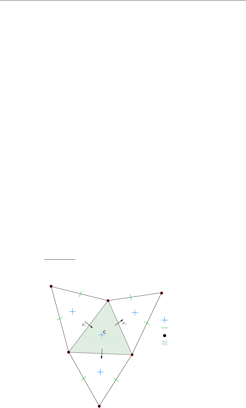
DRAFT
Sediment transport and morphology
does not substantially change the nature of the overall hydrodynamic and morphologi-
cal development: a quasi-steady flood period should not become a short, dynamic flash
flood. For river applications, changing the morphological factor must be associated with
changing all external time-varying forcings. For coastal applications only the overall
simulation time should be adjusted. Note that the combination of a river-like flood peak
and a tidal motion will cause problems when interpreting morphological factor not equal
to 1.
The effect of the morphological factor is different for bed and suspended load. At each
time step bedload is picked-up from the bed and deposited on the bed: only the trans-
ports are increased by the morphological factor used for the time step considered. How-
ever, in case of suspended load there is a time-delay between the time of erosion and
the time of deposition. The erosion and deposition fluxes are increased by the morpho-
logical factor, but the suspended concentrations are not (since that would influence the
density effects). It is possible to vary the morphological factor during a simulation to
speed up relatively quiet periods more than relatively active periods. Such changes in
the morphological factor will not influence the mass balance of a bed or total load sim-
ulation since pickup and deposition are combined into one time step. However, in case
of suspended load the entrainment and deposition may occur at time-steps governed
by different morphological factors. In such cases the entrainment flux that generated a
certain suspended sediment concentration will differ from the deposition flux that was
caused by the settling of the same suspended sediment. A change in morphological
factor during a period of non-zero suspended sediment concentrations, will thus lead to
a mass-balance error in the order of the suspended sediment volume times the change
in morphological factor. The error may kept to a minimum by appropriately choosing the
transition times.
18.6.1 Bathymetry updating including bedload transport
The change in the quantity of bottom sediments caused by the bedload transport is calculated
using the expression:
∆c
SED =∆tfMORFAC
AcX
i
Si
uWi
u(18.180)
S1
u
S2
u
Water level point
Velocity point
Depth point
Control volume
S3
u
Figure 18.5: Morphological control volume and bedload transport components
Deltares 267 of 412

DRAFT
D-Flow Flexible Mesh, User Manual
where:
∆c
SED change in quantity of bottom sediment at location c[kg/m2]
∆tcomputational time-step [s]
fMORFAC user-defined morphological acceleration factor, MORFAC
Acarea of computational cell at location c[m2]
Si
ucomputed bedload sediment transport vector in udirection (direction
normal to face i), held at the velocity point [kg/(m s)]
Wi
uwidth of the face i[m]
This calculation is repeated for all ‘sand’ and ‘bedload’ sediment fractions, if more than one is
present, and the resulting change in the bottom sediment mass is added to the change due
to the suspended sediment sources and sinks and included in the bed composition and bed
level updating scheme.
18.6.2 Erosion of (temporarily) dry points
In the case of erosion near a dry beach or bank, the standard scheme will not allow erosion
of the adjacent cells, even when a steep scour hole would develop right next to the beach.
Therefore a scheme has been implemented that allows the (partial) redistribution of an erosion
flux from a wet cell to the adjacent dry cells. The distribution is governed by a user-defined
factor ThetSD, which determines the fraction of the erosion to assign (evenly) to the adjacent
cells. If ThetSD equals zero the standard scheme is used, i.e. all erosion occurs at the wet
cell. If ThetSD equals 1 all erosion that would occur in the wet cell is assigned to the adjacent
dry cells. The ‘wet’ and ‘dry’ cells in the paragraph above are defined as cells at which the
water depth is, respectively, more and less than the threshold depth SedThr for computing
sediment transport.
A modification to this method may be activated by specifying a parameter HMaxTH larger
than the threshold depth SedThr for computing sediment transport. In this case, the factor
ThetSD is used as upper limit for the fraction of the erosion to be transferred to adjacent dry
cells. The actual factor to be transferred is equal to Thet , which is computed as:
Thet = (h1−SedThr )/(HMaxTH −SedThr )×ThetSD
where Thet = min(Thet ,ThetSD )(18.181)
Here, h1is the local water depth. The purpose of this formulation is to allow erosion of parts
that are inactive in terms of transport but still wet, while limiting the erosion of the dry beach.
If erosion of the dry beach is desired, this option is not recommended, so HMaxTH should be
set less than SedThr.
Remark:
The overall erosion flux is redistributed to the adjacent cells. Depending on the avail-
ability of individual sediment fractions at the central ‘wet’ cell and the surrounding ‘dry’
cells, the erosion from the adjacent cells will replenish the eroded cell with different
sediment fractions than those that were eroded.
18.6.3 Dredging and dumping
If the bed levels are updated, you may also include some dredging and dumping activities at
the end of each half time step. This feature can also be used for sand mining (only dredging,
no associated dumping within the model domain) and sediment nourishment (only dumping,
no associated dredging within the model domain). Dredging and dumping is performed at this
stage in the following order:
268 of 412 Deltares
DRAFT
Sediment transport and morphology
For each dredge area: if the bed level exceeds a threshold level (or the water depth drops
below a certain level) then the bed level is lowered based on the dredging option and the
corresponding volume of sediment is removed. If the dredging capacity is less than the
volume to be dredged, the sequence of dredging (e.g. top first or uniform) determines
which grid cells are dredging at the current point in time.
The volume of dredged material is summed over all cells in a dredge area and distributed
over the dump areas, using the link percentages or the link order (up to the dump capacity).
In simulations with multiple sediment fractions the sediment composition is tracked.
For each dump area: the bed level is raised and the bed composition is adjusted based on
the volume and characteristics of material to be dumped. The sediment may be distributed
equally or non-uniformly (e.g. deepest points first) over the grid cells in the dump area.
Remark:
Dredging and dumping may also performed during initialization, before the first time-
step.
Warning:
Dredging large amounts of material may harm the stability of the calculation.
The dredging and dumping feature allows you to specify dredging and dumping areas as
x,ypolygons. Within each dredging polygon the bed levels are lowered to a user-defined
depth; by default grid cells are considered to lie within a polygon if their centre lies within
the polygon. It is possible to distribute the dredged material over multiple dumping locations.
You may also decide to not dump the sediment back into the model (feature referred to as
sand mining); this can be implemented by defining a dump polygon outside the grid, or by
not specifying any dump polygon at all. This option cannot be combined with the option to
dredge only as much as dump capacity is available. For sediment nourishment one should
use a [nourishment] block specifying the amount (and, if applicable, the composition)
of the nourished sediment. The dredging and dumping activities should be specified in a
<∗.dad>file. The <mdu>file should contain a keyword Fildad referring to the file used.
The <∗.dad>file refers to the file containing the polygons.
18.6.4 Bed composition models and sediment availability
The morphology module currently implements two bed composition models:
A uniformly mixed bed (one sediment layer). There is no bookkeeping of the order in which
sediments are deposited and all sediments are available for erosion.
A layered bed stratigraphy (multiple sediment layers). A user-defined number of bed com-
position bookkeeping layers may be included to keep track of sediment deposits. When
sediments are deposited, they are initially added to the top-most layer. After mixing in
the top layer, sediments are pushed towards the bookkeeping layers beneath it. The
bookkeeping layers are filled up to a user-defined maximum thickness, if this threshold is
exceeded a new layer is created. If the creation of a new layer would exceed the maxi-
mum number of layers specified by you, layers at the bottom of the stratigraphy stack will
be merged. Only sediments in the top-most layer are available for erosion. After erosion,
the top-most layer is replenished from below.
The default bed composition model is the uniformly mixed one. Currently only the default bed
composition model is supported by the user interface.
At input you must specify the amount of sediment available at the bed as the total (dry) mass
of all sediment fractions in [kg/m2]. This may be a constant value for the entire model or,
Deltares 269 of 412

DRAFT
D-Flow Flexible Mesh, User Manual
alternatively, a space-varying initial sediment file (values to be specified at cell centres). The
initial bed composition is assumed to be uniformly mixed.1The thickness of the total sediment
layer is calculated from the sediment mass by dividing by the user-defined dry bed density
CDryB. Currently, CDryB is constant in time and space for each individual sediment fraction.
The top of these sediment deposits will coincide with the initial bed level. Below the bottom
of these deposits the model assumes a non-erodible bed (sometimes referred to as a fixed
layer).
When the model almost runs out of sediment at a particular location, the sediment flux terms
will be reduced. The reduction starts when the available sediment thickness drops below a
user-defined threshold Thresh. The flux terms affected are slightly different for cohesive and
non-cohesive sediments, as described below.
Cohesive sediment fractions
In the case of cohesive sediment, the erosive sediment source term is reduced proportion-
ally to the ratio of available sediment thickness over Thresh. The deposition term is never
reduced. However, the cohesive sediment is still not included in D-Flow FM.
Non-cohesive sediment fractions
In the case of non-cohesive sediments all bedload transport rates out of a grid cell are reduced
by the upwind ratio of available sediment thickness over Thresh. The source and sink terms
of the advection-diffusion equation are not reduced unless the erosive sediment source term
is predicted to be larger than the deposition (sink) term, in that case both terms are reduced by
the ratio of available sediment thickness over Thresh as shown by the following equations:
Sourcetotal =frSourcetotal,(18.182)
Sinktotal =frSinktotal,(18.183)
where fris a reduction factor determined by:
fr= min ∆sed
Thresh ,1,(18.184)
where ∆sed is the thickness of sediment at the bed.
The likelihood of erosive conditions occurring is assessed by calculating the total sediment
source and sink terms using the concentration from the previous time-step to evaluate the
implicit sink term. If the sink term is greater than the source term, then deposition is expected,
and fris set to 1.0 so that deposition close to the fixed layer is not hindered.
18.7 Specific implementation aspects
Negative water depth check
In rare situations (with high morphological acceleration factors) it is possible that, in one time-
step, the bed accretes more than the water depth. If this occurs the water depth will become
negative (water surface level is below the bed level). This situation is checked for and, if it
occurs, the water surface level for the cell is set equal to the new bed level. The cell will then
be set dry.
1The uniformly mixed bed can be used as input for both bed composition models. If you have more detailed
information on the bed stratigraphy, you may use the bed stratigraphy model and specify an initial layering of the
bed composition by means of the IniComp keyword and associated initial bed composition file. In that case the
bed composition given in the <∗.sed>file will overruled, you have to specify dummy values though.
270 of 412 Deltares

DRAFT
Sediment transport and morphology
Threshold depth for sediment calculations introduced
If the water depth in a cell is less than SedThr, specified in the morphology input file, then
the sediment source and sink terms and bedload transport are not calculated for ‘sand’ and
‘bedload’ sediment fractions. This restriction has been included in order to prevent numerical
problems during the computation of the reference concentration, e.g. to prevent sudden bursts
of sediment from occurring when computational cells are flooded.
Remark:
In areas with very shallow water depths and sediment sources and sinks, you must
ensure that the user-defined threshold depth for drying and flooding is not set too large.
Calculation of bed shear in wave and current situations altered
The calculation of the bed shear velocity u∗has been simplified in situations with waves and
currents. The bed shear is always calculated using the velocities computed in the bottom
computational layer, rather than using the computational layer closest to the top of the sedi-
ment mixing layer. The reference velocity in the bottom computational layer is adjusted to the
top of the sediment mixing layer using the apparent bed roughness kabefore being used to
compute the bed shear velocity using the physical bed roughness ks.
Depth at grid cell faces (velocity points)
During a morphological simulation the depth stored at the Uand Vvelocity points must be
updated to reflect the bed level changes calculated in the water level points. This used to be
performed by setting the new depth for the velocity point by copying the new depth held at the
water level point, using a simple upwind numerical scheme. As this may introduce instabili-
ties in the flow computation, especially near drying and flooding and in tidal simulations, this
method has been replaced by setting the depth at Uand Vpoints equal to the minimum of
the adjacent depths in water level points. This change significantly improves the smoothness
of flooding dry cells.
Remarks:
The setting of depths at velocity points as the minimum of the adjacent water level
points only comes into effect if sediment is present and the user-defined flag MORUPD
is .true. (i.e. bathymetrical changes are expected to occur at some point during the
simulation period). If this condition is not met then the depths at the velocity points do
not need to be updated during the course of the simulation.
The program still requires the depth at velocity points to be set to MOR for morphological
simulations. This anticipated that this restriction is lifted in a coming release.
Since the MOR and MIN procedures for computing the depth at cell interfaces are equiv-
alent, we advise you to use the MIN procedure during the calibration of a hydronamic
model that will later on be converted into a morphological model.
Deltares 271 of 412

DRAFT
D-Flow Flexible Mesh, User Manual
272 of 412 Deltares

DRAFT
19 Tutorial
19.1 Introduction
In this brief introduction, basic information is provided on either the setup of the tutorial and
some basic grid concepts.
19.1.1 Setup of the tutorial
In this three-hours tutorial you will experience the basic functionality of D-Flow FM. On the
one hand you will learn how to capture a certain area with a computational grid. On the other
hand you will set up and run a computation yourself. This involves for example inserting a bed
level, imposing boundary conditions, running a D-Flow FM model and postprocessing with a
D-Flow FM output file. This manual contains nine tutorials (with indication of the estimated
time):
Tutorial 1 (section 19.2): Creating a curvilinear grid (25 minutes).
Tutorial 2 (section 19.3): Creating a triangular grid (20 minutes).
Tutorial 3 (section 19.4): Coupling multiple distinct grids (15 minutes).
Tutorial 4 (section 19.5): Inserting a bed level (15 minutes).
Tutorial 5 (section 19.6): Imposing boundary conditions (25 minutes).
Tutorial 6 (section 19.7): Defining output locations (15 minutes).
Tutorial 7 (section 19.8): Defining computational parameters (10 minutes).
Tutorial 8 (section 19.9): Running a model simulation (20 minutes).
Tutorial 9 (section 19.10): Viewing the output of a model simulation (15 minutes).
This estimated times leave room for a 5 minutes introduction and a 15 minutes break after
tutorial 4. The necessary input files for a tutorial can be found in the directories tutorial01 till
tutorial09. You can put your output files in a separate directory, e.g. finished.
19.1.2 Basic grid concepts
In D-Flow FM, grids (sometimes denoted as ’networks’) consist of net cells and are described
by net nodes (corners of a cell), net links (edges of a cell, connecting net nodes), flow
nodes (the cell circumcentre) and flow links (a line segment connecting two flow nodes).
This grid topology is illustrated in Figure 19.1. Important properties of the mesh are the
orthogonality and smoothness. The orthogonality is defined as the cosine of the angle ϕ
between a flowlink and a netlink. Ideally 0, angle ϕ= 90◦. The smoothness of a mesh is
defined as the ratio of the areas of two adjacent cells. Ideally 1, the areas of the cells are
equal to each other. A nearly ideal setup is shown in Figure 19.2.
Deltares 273 of 412
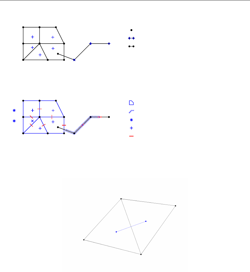
DRAFT
D-Flow Flexible Mesh, User Manual
net node
net link (2D)
net link (1D)
netcell circumcenter
netcell link
netcell/flow node (2D)
netcell/flow node (1D)
1. Net (domain discretization)
2. Flow data (2D)
(1..NUMK)
(1..NUML1D)
(NUML1D+1..NUML)
(1..NDX2D=NUMP)
(NDX2D+1..NDXI)
boundary flow node (NDXI+1..NDX)
(1..LNX1D)
(LNX1D..LNXI)
(LNXI+1..LNX)
Figure 19.1: Topology and definitions for a grid as used in D-Flow FM.
Figure 19.2: Perfect orthogonality and nearly perfect smoothness along the edge con-
necting two triangles. Black lines/dots are network links/nodes, blue lines/-
dots are flow links/nodes.
It is rather easy to generate grids that violate the orthogonality and smoothness requirements.
In Figure 19.3, two different setups of two grid cells are shown with different grid properties.
Figure 19.3a shows how orthogonality can be detoriated by skewing the right triangle with
respect to the left triangle. While having the same area (perfect smoothness), the mutually
oblique orientation results in poor orthogonality. In this particular case the circumcentre of
the right triangle is outside the area of the triangle because it is an obtuse triangle, which is
bad for computations with D-Flow FM. The opposite is shown in Figure 19.3b in which the
right triangle has strongly been elongated, disturbing the smoothness property. However, the
orthogonality is perfect (both triangle are acute). Nonetheless, both grids need to be improved
to assure accurate model results.
274 of 412 Deltares
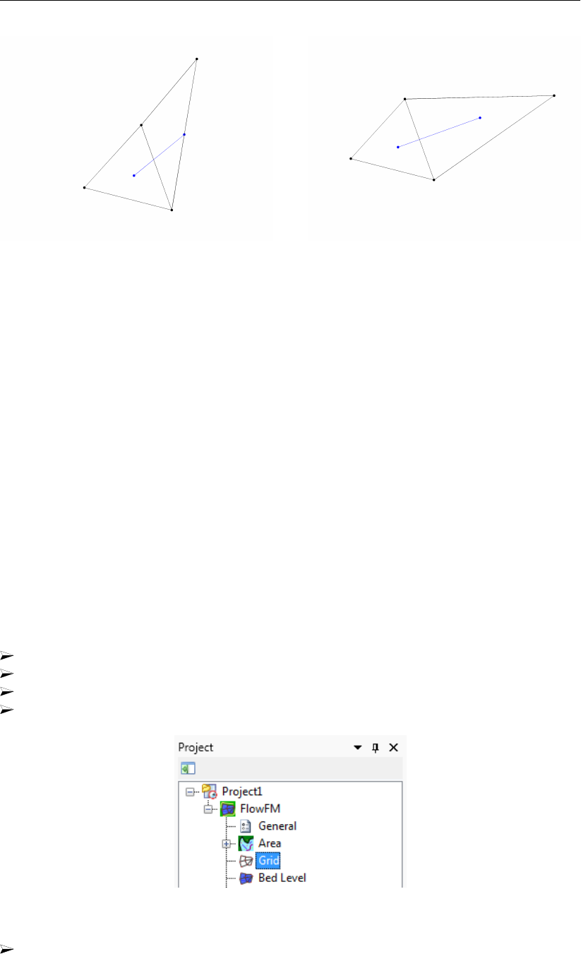
DRAFT
Tutorial
(a) Perfect smoothness, but poor orthogonality. (b) Perfect orthogonality, but poor smoothness
Figure 19.3: Poor grid properties due to violating either the smoothness or the orthog-
onality at the edge connecting two triangles. Black lines/dots are network
links/nodes, blue lines/dots are flow links/nodes.
19.2 Tutorial 1: Creating a curvilinear grid
In the upcoming tutorials, the Westernscheldt and the harbour of Antwerp will be used as an
example case for generating a grid and setting up a computation.
With D-Flow FM both structured grids and unstructured grids are possible. In practice, a large
part of a model domain might be based on a structured grid. Therefore, it is important that a
D-Flow FM user also has sufficiently expertise in generating structured grids. In this exercise
we therefore will apply D-Flow FM for the generation of a curvilinear grid.
The generation of a grid is an iterative process. However, the Undo functionality is limited in
RGFGRID. By clicking on Esc it is sometimes possible to undo the last action. Therefore, it is
important to frequently save intermediate results in RGFGRID.
To start RGFGRID in the Delta Shell Graphical User Interface the following steps have to be
carried out:
Double click on the Delta Shell icon on the desktop of your computer.
Click on New Model in the main toolbar at the top of the Delta Shell GUI.
A new window pops up in which you have to select Flow Flexible Mesh Model →OK.
Double click on Grid, see Figure 19.4. RGFGRID will now start.
Figure 19.4: Start RGFGRID by a double-click on Grid.
Choose from the main menubar Coordinate System →Cartesian Coordinates. This is
the default setting, which means that you do not have to change anything.
To generate a curvilinear grid from splines, a grid is iteratively developed. The approach is as
Deltares 275 of 412
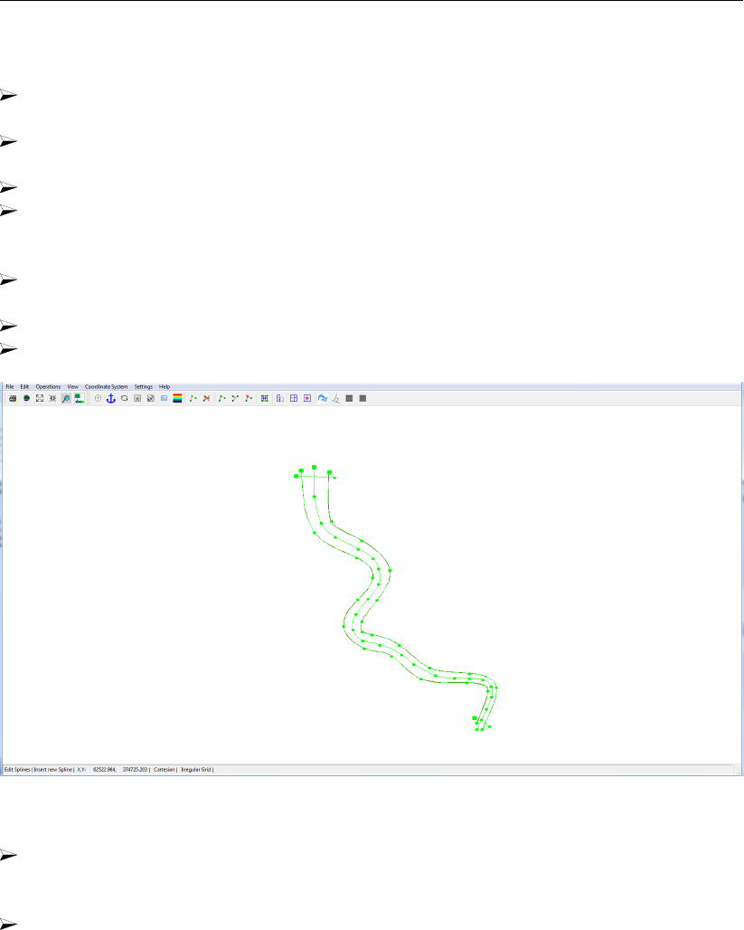
DRAFT
D-Flow Flexible Mesh, User Manual
follows:
Import a land boundary via File →Attribute Files →Open Land Boundary and select the
file <tutorial01\scheldtriver.ldb>
Select Edit →Splines →New and draw a spline at the left boundary of the river (use the
leftmousebutton) with at least three vertices. Finalise the spline by one rightmouseclick.
Select the lefthandside spline through choosing Edit →Splines →Select.
Choose the option Edit →Splines →Attach to Land Boundary. Select the the two outer
points delimiting the spline to be snapped. The vertices which will be snapped are now
marked by a square. Press the rightmousebutton to perform the snapping.
A window appears for extra snapping: Press Yes several times. You will see the spline
evolve towards the land boundary. Press No when you are satisfied with the result.
Repeat the previous three steps for the righthandside spline.
Draw a third spline along the river axis; see Figure 19.5.
Figure 19.5: Splines in Tutorial01
Draw two cross-splines, each containing exact two vertices: one spline at the North side
and one spline at the South side of the river (see Figure 19.7). The channel is now
enveloped by four splines and there is an extra spline along the river axis.
Choose Settings →Grow Grid from Splines. . . . You will be able to set several settings
of the operator. The first seven entries should be changed into the values shown in Fig-
ure 19.6.
276 of 412 Deltares
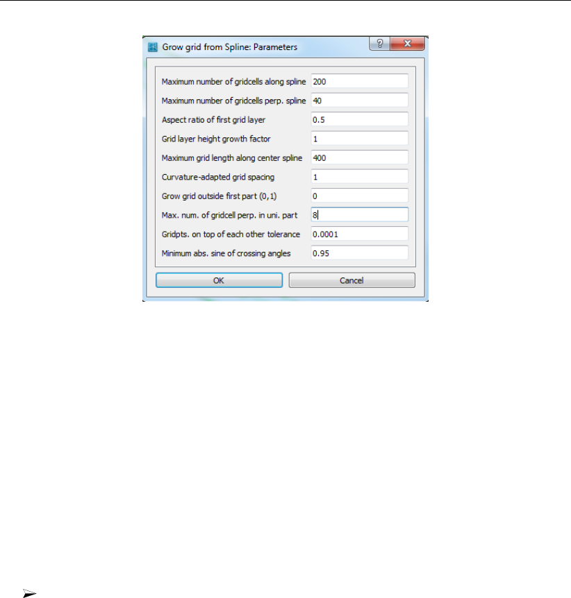
DRAFT
Tutorial
Figure 19.6: Settings for the Grow Grid from Splines procedure.
A brief explanation:
Using the parameter Max. num. of gridcells perp. in uni. part, the user can give an
indication of the number of cells across the width between the longitudinal splines.
By using the parameters Maximum grid length along center spline, the user can give
an indication of the length of the cells in longitudinal direction. Based on the value
of the parameter Aspect ratio of first grid layer, the algorithm establishes a suitable
grid, under the restrictions of the prevailing maximum numbers of gridcells (first two
entries).
The option Grid layer height growth factor enables the user to demand for a non-
equidistant grid in cross-sectional direction. The value represents the width-ratio of
two adjacent cells. Using the option Grow grid outside first part (0/1), one can extend
a grid outside the longitudinal splines, for instance to capture winterbed regions.
After entering the values of Figure 19.6, choose Operations →Grow Grid from Splines.
This will deliver the grid as shown in Figure 19.7.
Deltares 277 of 412
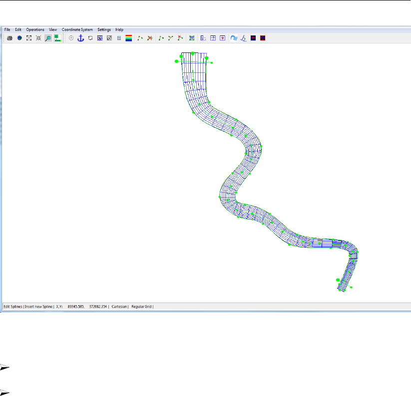
DRAFT
D-Flow Flexible Mesh, User Manual
Figure 19.7: Generated curvilinear grid after the new Grow Grid from Splines procedure.
To be able to further improve the grid, choose Operations →Convert grid →Regular to
Irregular. Strictly, the grid is now not curvilinear anymore, but unstructured.
Choose View →Grid Property Style →Coloured Edge and then View →Grid Properties
→Orthogonality. The result is shown in Figure 19.8. We remark that no orthogonalisation
iterations have been performed yet. Try to reach the level of orthogonality as shown in
Figure 19.8.
278 of 412 Deltares
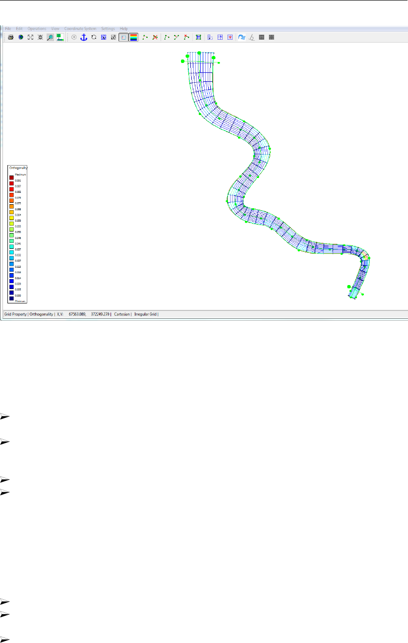
DRAFT
Tutorial
Figure 19.8: Orthogonality of the generated curvilinear grid after the Grow Grid from
Splines procedure.
To save the grid and close RGFGRID the following steps have to be carried out:
Choose from the menubar File →Export →UGRID (D-Flow FM). . . and save the grid
with name <scheldt01_net.nc>in the folder <tutorial01>.The grid has now been saved.
Choose File →Attribute Files →Save splines with Intermediate Points and save the
splines with the name<scheldt01.spl>in folder tutorial01. The splines and the grid have
now been saved.
Choose File →Save Project.
Close RGFGRID by choosing File →Exit
Folder <tutorial01\finished>contains splines and a grid for this tutorial exercise that has been
prepared by Deltares.
Now your are back in the Delta Shell GUI. It appears that the land boundary is not visible
anymore, because it was selected in RGFGRID. However, also in the Delta Shell GUI a land
boundary can be activated via:
Open Area under Project1 →FlowFM →Area.
Import the land boundary from <tutorial01\scheldtriver.ldb>by choosing Import via the
right mouse button on Project1 →FlowFM →Area →Land Boundaries (see Figure 19.9).
Do not apply a coordinate transformation by pressing OK.
Deltares 279 of 412
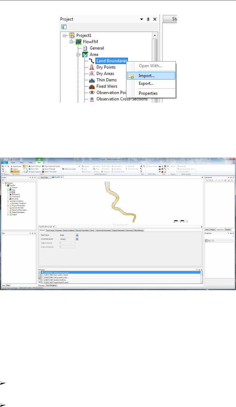
DRAFT
D-Flow Flexible Mesh, User Manual
Figure 19.9: Importing a land boundary
Now the grid and land boundary are visible in the central map of the Delta Shell GUI, see
Figure 19.10.
Figure 19.10: After closing RGFGRID the grid is visible in the Delta Shell GUI.
19.3 Tutorial 2: Creating a triangular grid
We will continue with the grid created in the previous tutorial for the Scheldt river. The river is
separated from the harbour, west of the river, by a sluice. The small area between the sluice
and the Scheldt will benefit from an unstructured grid because of its irregular geometry. The
unstructured grid for this irregular geometry is created first in this section.
The following steps have to be carried out:
Import the land boundary from <tutorial02\scheldtharbour.ldb>by choosing Import via
the right mouse button on Project1 →FlowFM →Area →Land Boundaries (see Fig-
ure 19.9). Do not apply a coordinate transformation, press OK.
Import the grid file by choosing Import via the right mouse button on Project1 →FlowFM
280 of 412 Deltares
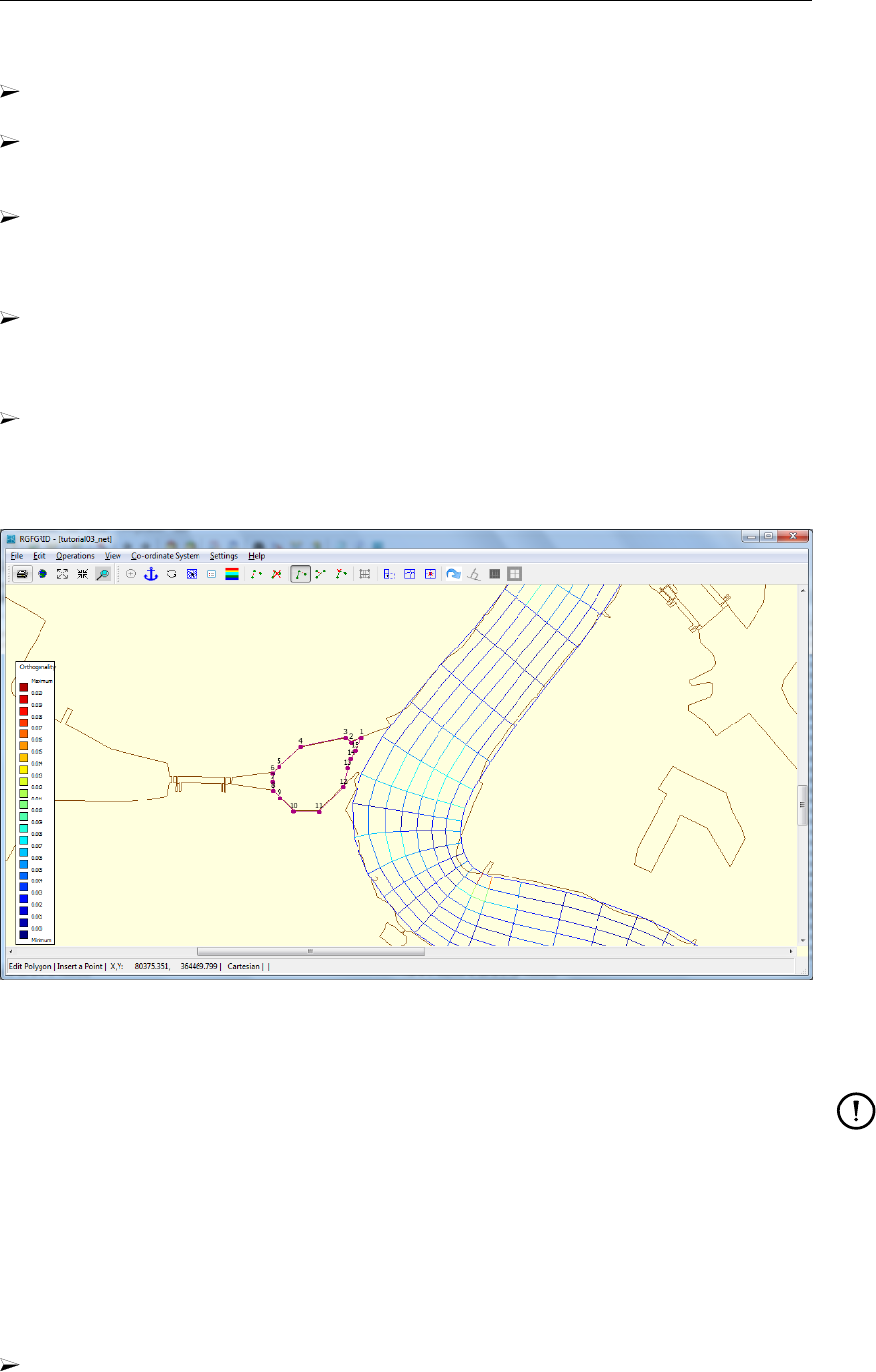
DRAFT
Tutorial
→Grid. Choose the grid file <scheldt01_net.nc>in the folder <tutorial02>.
Start RGFGRID by double clicking on Grid, see Figure 19.4. Set the Coordinate System
(if necessary), as has been explained in section 19.2 (Figure 19.4).
Choose from the menubar Edit →Polygons →New. The intention is to mark the area of
interest (i.e. the area for which we want to generate the grid) by means of a polygon, see
Figure 19.11.
Start drawing the polygon at a distance from the curvilinear grid that is similar to the width
of the curvilinear grid cells (since we want to have a smooth transition in grid resolution).
Specify the second point at a relatively small distance from the first one.This distance is
later used as the first indication of the size of the triangular gridcells to be placed.
Mark the characteristic locations of the area (follow the landboundary) and place the final
points at the same distance away from the river grid as the first point. The distance
between the last two points should be similar to the distance between the first two points.
The result is shown in Figure 19.11.
Choose Edit →Polygons →Refine (linear) and click on the first and last points of the
polyline (in Figure 19.11 we would select point 1 first and then point 15). Now, the polygon
is divided into a finer set of line elements (based on the length of the first and last segment
of the polyline).
Figure 19.11: Polygon that envelopes the area in which an unstructured grid is aimed to
be established.
Remarks:
The distance between the points of the polygon is derived from the distance of the
two polyline segments at both sides of the selected segment. The length of the poly-
line segments varies linearly from the segment length at the one side of the selected
segment towards the segment length at the other side of the selected segment.
You can play around to see how this works. If needed, you can add extra polyline
points by choosing Edit →Polygon →Insert point. Choose Edit →Polygon →
Move point if a point move would make sense.
You can snap the refined polygon to the landboundary through Edit →Polygons →
Attach to Land Boundary. Select two points for this.
Now we continue with this tutorial by carried out the following steps:
Choose Operations →Domain →New to indicate that the new grid to be generated grid
should be created next to the already existing one (and not replace it).
Deltares 281 of 412
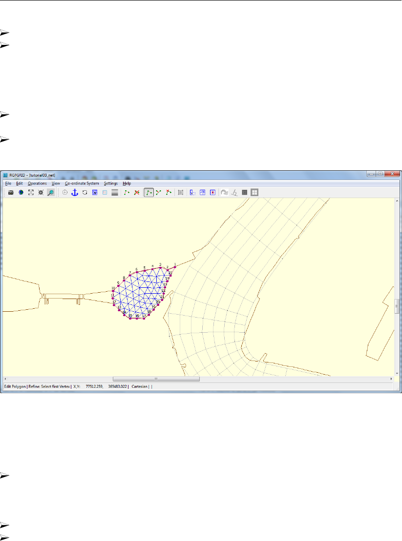
DRAFT
D-Flow Flexible Mesh, User Manual
Choose Operations →Grow Grid from Polygons. The result is shown in Figure 19.12.
Improve the orthogonality through Operations →Orthogonalise grid. With the default
settings also the smoothness is improved.
Since the solver only supports one grid, we need to merge the newly created grid with the
original grid of the river. The newly created grid is currently selected. Next:
Choose Edit →Multi Select and click on the river Scheldt grid to select it as well. After
selection both grids should be coloured blue with black dots on the nodes.
Choose Operations →Grid →Merge Grids to merge the nodes of the (two) highlighted
grids. Now, the grids have been merged. However, nothing will visually change.
Figure 19.12: Unstructured grid, after having refined the polygon.
To save the grid and go back to the Delta Shell GUI:
Choose from the menubar File →Export →UGRID (D-Flow FM). . . and save it with
name <scheldt02_net.nc>in the folder <tutorial02>. The grid has now been saved. We
remark that folder <tutorial02\finished>contains a grid for this tutorial exercise that has
been prepared by Deltares.
Choose File →Save Project.
Close RGFGRID by clicking on File →Exit.
19.4 Tutorial 3: Coupling multiple separate grids
From the previous tutorial we have ended up with two separate grids that are not connected
yet. Obviously, these two grids should properly be integrated into one single grid. Before we
can couple the two grids, we should first make sure that the typical grid size is of the same
order of magnitude for both grids at the location where the connection is to be laid. Hence,
basically two operations are to be done:
Split the grid cells in the Scheldt river grid over the full width. Hence, the grid cell size in
the river will match the gridcell size of the unstructured grid.
Merge the two grids and put connections in between.
282 of 412 Deltares
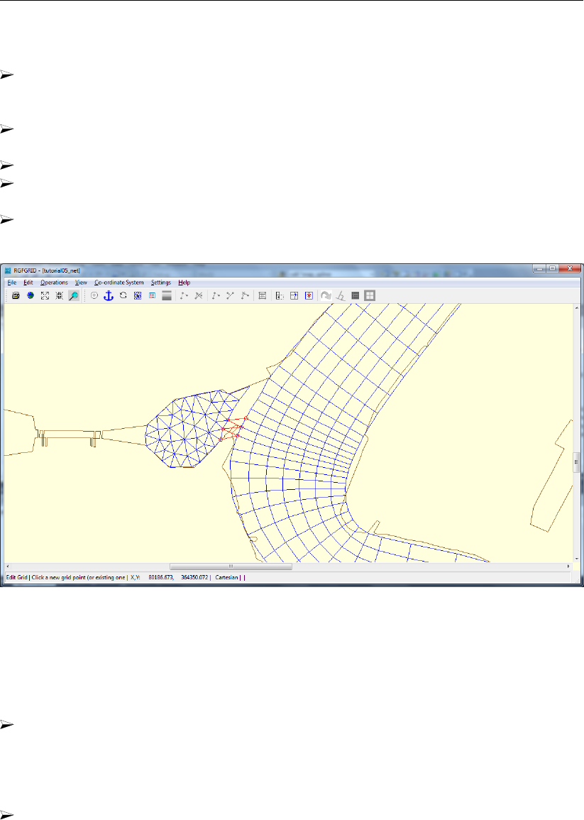
DRAFT
Tutorial
The splitting can be established as follows:
Import the land boundary file <scheldtharbour.ldb>and the grid file <scheldt02_net.nc>
from the folder <tutorial03>in DeltaShell under Project1 →FlowFM →Area and Project1
→FlowFM →Grid, respectively.
Start RGFGRID and set the Coordinate System (if necessary), as has been explained in
section 19.2 (Figure 19.4).
Choose Edit →Irregular Grid →Split Row or Column.
Select the locations where the grid lines should be split by clicking on the left boundary of
the Scheldt river.
Try to achieve the picture shown in Figure 19.13, in particular the typical grid size in the
curved area. N.B. Ignore the red lines in this picture for now!
Figure 19.13: Connection of the river grid and the unstructured grid. The red lines show
the inserted grid lines used to couple the two grids manually.
Connecting edges between the two parts of the grid can be created as follows:
Since the two visually separate grid parts have already been merged into one logical grid in
the previous tutorial, we can now physically connect them by laying new gridlines between
them. Therefore, select Edit →Irregular Grid →Insert Node. Insert new gridlines in a
zigzag-like style: see the red grid lines in Figure 19.13. Now, you will benefit from the
(more or less) equal resolutions in the river and unstructured regions.
Finally, you will end up with a picture like shown in Figure 19.14. You can visualize the
orthogonality through View →Grid Property Style →Coloured Edge and View →Grid
property →Orthogonality.
Deltares 283 of 412
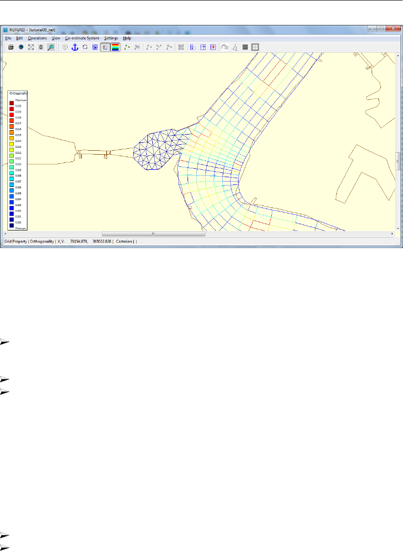
DRAFT
D-Flow Flexible Mesh, User Manual
Figure 19.14: Orthogonality of the integrated grid, containing the curvilinear part, the tri-
angular part and the coupling between the two grids.
To save the grid and close RGFGRID is done as follows:
File →Export →UGRID (D-Flow FM). . . and save the it with name <scheldt03_net.nc>
in folder <tutorial03_result>.
The grid has now been saved.
Choose File →Save Project.
Close RGFGRID by clicking on Exit.
19.5 Tutorial 4: Inserting a bed level
In previous tutorial exercises we focused on the grid generation. The next step is to couple the
bed level data to the grid. The grid for this tutorial exercise is available in file <westernscheldt03_net.nc>
in the directory <tutorial04>. A harbour has been added to the grid, as well as the Western-
scheldt part at the North side. Bed levels are available in the file <westernscheldt_bed_level.xyz>.
The file with bed levels should first be projected onto the unstructured grid by means of inter-
polation. To this purpose, the following actions should be carried out:
Start Delta Shell as already explained in previous tutorial exercises.
Create a D-Flow FM model by choosing New Model →Flow Flexible Mesh model →OK.
The project tree of a D-Flow FM model is shown in Figure 19.15.
284 of 412 Deltares
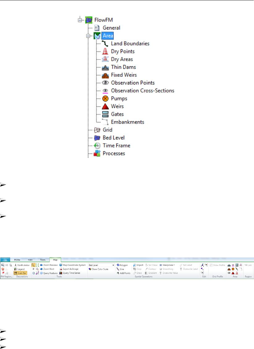
DRAFT
Tutorial
Figure 19.15: Project tree.
Import the grid file by rightmouseclicking on Grid →Import (see Figure 19.15) and choose
the available grid file <westernscheldt03_net.nc>from folder <tutorial04>,
Import the land boundary file: Area by rightmouseclicking on Land boundaries →Import
and import the land boundary file <sealand.ldb>,Grid transformation →OK,
Import a sample file containing the measured bed levels: in the drop down menu at the
top of the screen (See Figure 19.16), choose Bed Level. Then choose Import from the
Spatial Operators menu, and select the file <westernscheldt_bed_level.xyz>which con-
tains measured bed level data for the Westernscheldt, from the North Sea up to Antwerp,
Grid transformation →OK.
Figure 19.16: Map-ribbon with the Spatial Operations menu.
Now we are going to project the bed level data onto the nodes:
Choose Interpolate (see Figure 19.16).
Choose interpolate selected set.
The window Interpolation operation appear. Select the Overwrite option for Pointwise
operation, then press OK. The result will look like Figure 19.17. If you do not see a
colorbar, click Show Color Scale (see Figure 19.16).
Deltares 285 of 412
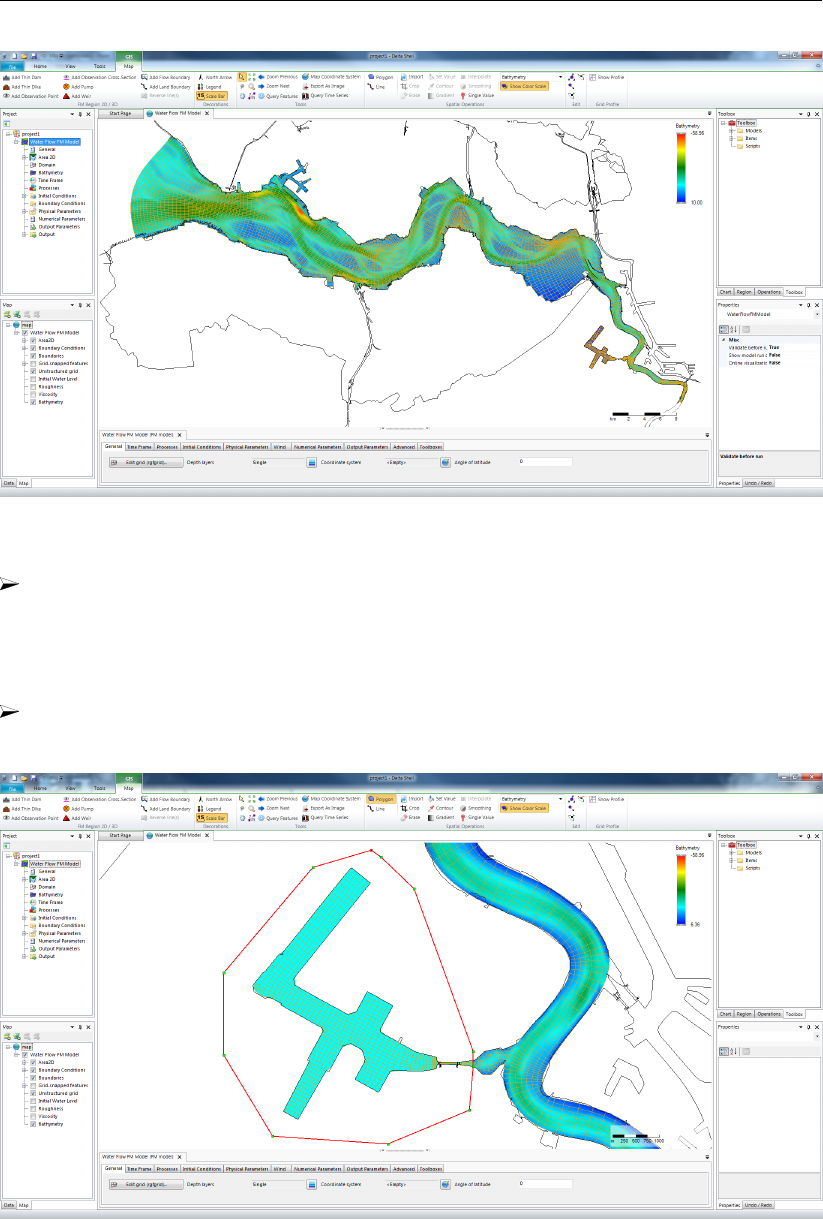
DRAFT
D-Flow Flexible Mesh, User Manual
Figure 19.17: Interpolated bed levels values at the grid (estuary).
Have a look at the sluice and the docks of the harbour. You can see that the bed level
in this area is unrealistically high. This unrealistic value has been assigned because of
undesired extrapolation, since no bed level data has been available in this area. To repair
this, first draw a polygon that envelops the sluice and the docks. Do this by clicking
Polygon (see Figure 19.16). The resulting polygon can be observed in Figure 19.18.
Choose Set value (see Figure 19.16): specify an appropriate value, for instance “-10” m.
The result will look like as shown in Figure 19.18.
Figure 19.18: Interpolated bed levels values at the grid (harbour).
N.B. The mesh file (<∗_net.nc>) will contain the grid together with the bed level data in the
nodes.
To save the mesh and bed level, and save the model within the Delta Shell GUI the following
should be done:
286 of 412 Deltares
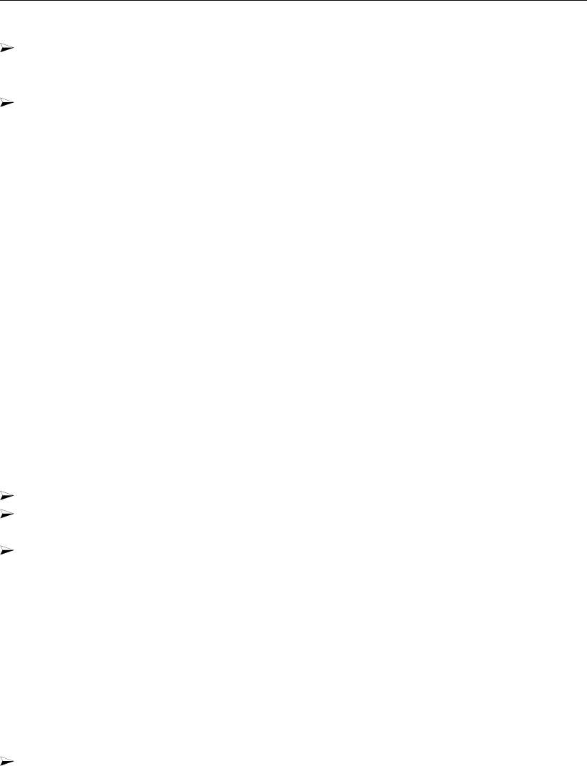
DRAFT
Tutorial
To save the mesh file you have to rightmouseclick on Grid →Export in the project bar.
Choose Grid exporter and save the file as <westernscheldt04_net.nc>in folder tuto-
rial04.The grid including the bed level has now been saved.
To close Delta Shell click on File →Exit. Then, the following question arises: "Save
changes to the project: Project?" Click on No. Now, the current D-Flow FM model has
now been closed.
Folder <tutorial04\finished>contains a bed level for this tutorial exercise that has been pre-
pared by Deltares.
19.6 Tutorial 5: Imposing boundary conditions
Along both the sea boundary and the Scheldt river boundary, appropriate boundary conditions
have to be imposed. The boundary conditions can be prescribed in many ways, for instance
as water levels, velocities (tangential and normal direction), discharge and Riemann. In this
tutorial exercise we will impose boundary conditions for the Western Scheldt in the following
way:
At the sea boundary: a periodic water level boundary, described as a harmonic signal with
a mean 0.5 m+NAP, an amplitude 2.5 m and a frequency of 28.984 ° h−1,
At the river boundary: a constant discharge boundary, described by a constant 2500 m3s−1.
Let us start with a new D-Flow FM model and import the network and land boundaries, which
is done as follows:
Click on New Model →Delft3D Flexible Mesh Model →OK.
Load the grid file from the folder <tutorial05>by rightmouseclicking on Grid →Import
(see Figure 19.15) and select file <westernscheldt04_net.nc>.
Import the land boundary file via Project1 →FlowFM →Area (see Figure 19.15) by right-
mouseclicking on Land boundaries →Import and import the land boundary file <sealand.ldb>,
Grid transformation →OK.
In order to define boundary conditions one has to follow this strategy:
1 draw a polyline along the boundary;
2 fill a file with essential information;
3 link the boundary files with the model setup.
The boundary conditions can be imposed as follows:
Choose Add (2D) Flow Boundary (top of screen, see Figure 19.19) and insert a polyline
along the sea boundary. To close the polyline, doubleclick. In the Project bar at the left,
under Boundary Conditions, this boundary has now been added. Figure 19.19 shows how
this will look like.
Tip: to remove a wrongly placed point in the polyline, use Remove point from geometry
(top of screen, above Edit, see Figure 19.16). It is also possible to replace or add a point.
Deltares 287 of 412
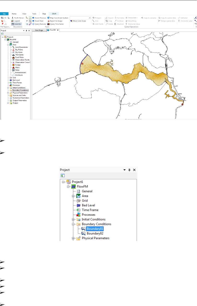
DRAFT
D-Flow Flexible Mesh, User Manual
Figure 19.19: Location of the two open boundaries at the sea and river side.
Draw another polyline at the river entrance south of Antwerp, see the right bottom corner
of Figure 19.19).
To impose boundary conditions at the seaboundary, double click at Boundary01, see Fig-
ure 19.20.
Figure 19.20: Selection of Boundary01.
Choose Water level, press +and choose Forcing type: Astronomical.
Selected the first boundary support point Boundary01_0001 by clicking on the plus-sign
behind it, repeat this for the last boundary support point.
Choose Select components. . . (at the lefthandside of the screen).
Choose the components A0 and M2, and press OK,
Select All support points and press OK. All support points will now have components A0
and M2 defined.
Fill in the amplitudes of the components in the table, see Figure 19.21.
288 of 412 Deltares

DRAFT
Tutorial
Figure 19.21: Boundary conditions seaside.
We have now prescribed an astronomical water level signal, consisting of two components.
The first component has an amplitude equal to 0.5 m with a frequency of 0 degrees/hour,
i.e. a constant value of 0.5 m+NAP. The second component has an amplitude of 2.5 m with
a frequency of 28.984 degrees/hour. Basically, the signal h(t)=0.5+2.5 cos(28.984 t)
has been prescribed now, with hin meters w.r.t. the reference level (in case: NAP) and t
in hours.
To impose boundary conditions at the riverboundary, double click at Boundary02, Choose
Discharge and press +. Choose Forcing type: Time Series.
To impose a contant discharge of 2500 m3s−1, fill in the table like Figure 19.22. Make sure
you insert the same times!
Figure 19.22: Boundary condition riverside.
Deltares 289 of 412
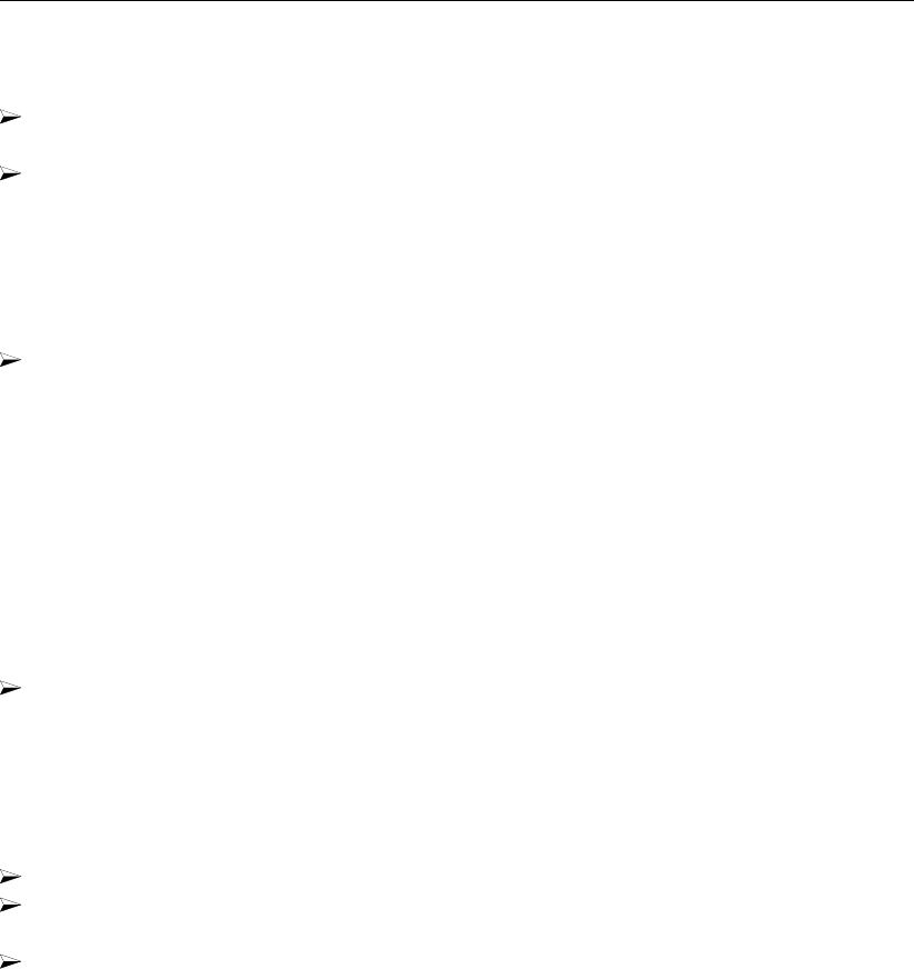
DRAFT
D-Flow Flexible Mesh, User Manual
To be able to load this D-Flow FM model in the future, it is necessary to save the model:
In the project tree, rightclick on FlowFM and select Rename. Rename the model to “west-
ernscheldt05”.
Save the model in folder <tutorial05_result>. In the project tree rightclick on western-
scheldt05. Choose Export select Flow Flexible Mesh model, press OK and save the
model as <westernscheldt05>.
The model might now be loaded in the next tutorial exercise, without inserting all network files
or land and flow boundaries individually again.
Now close the D-Flow FM model by rightmouseclicking In the project bar on western-
scheldt05 →Delete →OK.
19.7 Tutorial 6: Defining output locations
Often one would like to monitor computational results at certain specific cross-sections or
locations (i.e. ’observation points’). In this tutorial exercise we will add cross-sections and
observation points in a D-Flow FM model.
We will start with importing an existing D-Flow FM model without cross-sections and obser-
vation points:
Import the D-Flow FM Model from the folder <tutorial06>by choosing (in the top ribbon)
Import →Flow Flexible Mesh Model and press OK. Then choose <westernscheldt05.mdu>
and click on Open.
Inserting cross-sections and observation points is rather straightforward. The following actions
are necessary, in which we start with inserting cross sections:
Choose Add Observation Cross-Section (2D) (see item Area in the ribbon).
Draw as many cross-sections as you like. Finalize each cross-section by doubleclicking
the left mouse button.
To view how many cross sections have been made, double click on Area →Observation
Cross-Sections, see Figure 19.23.
290 of 412 Deltares
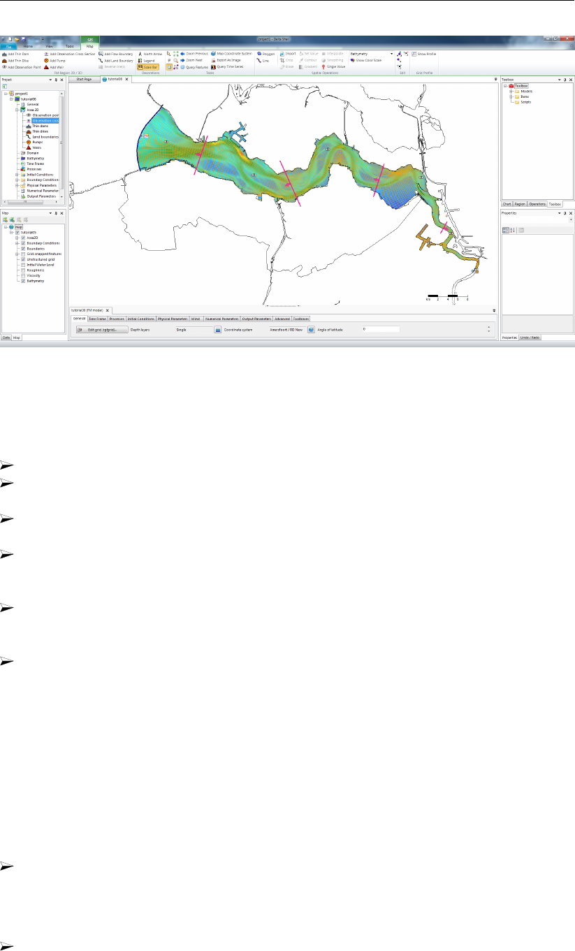
DRAFT
Tutorial
Figure 19.23: Overview cross sections and observation points.
Now we will add observation points:
Choose Add Observation Point. Draw as many observation points as you like.
To view how many observation points have been made, double click on Area →Observa-
tion points.
Save the current FM model in the folder <tutorial06>by rightmouseclicking in the project
tree on westernscheldt05.
Choose Export, choose Flow Flexible Mesh Model and press OK, then save the model
with name “westernscheldt06”). The observation points and cross sections have now
been saved in the new <mdu>-file.
Tip: It is also possible to save only the observations points for instance to a certain folder.
To try this, rightmouseclick on Observation points →Export →Observation points to
<xyn>-file. Then, choose a filename and a folder.
Close the current Flexible Mesh model by rightmouseclicking In the project bar on west-
ernscheldt05 →Delete →OK.
19.8 Tutorial 7: Defining computational parameters
Before we can run the model, all computational parameters need to be set. For example,
this involves the Time Frame,Initial Conditions and the Output Parameters. These can be
specified in the grey box at the bottom of Delta Shell. All other parameters are set by default,
and will not be consider in this tutorial exercise.
We will start with importing an existing D-Flow FM model:
Import the D-Flow FM Model from the folder <tutorial07>, by choosing Home →Import
→Flow Flexible Mesh Model →OK. Choose <westernscheldt06.mdu>and press Open.
Several parameters will be set. We will start with the Time Frame, see Figure 19.24:
At the Time Frame section: fill in the parameters of Figure 19.24.
Deltares 291 of 412
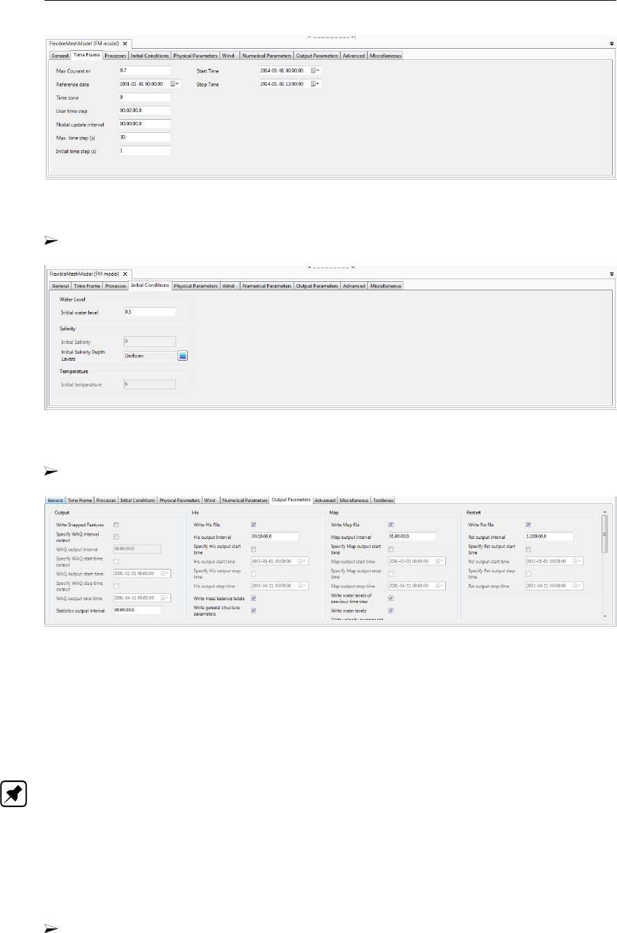
DRAFT
D-Flow Flexible Mesh, User Manual
Figure 19.24: The time frame of the simulation.
At the Initial Conditions section: fill in “0.5” m for the Initial water level, see Figure 19.25.
Figure 19.25: Imposed initial conditions for the simulation.
At the Output Parameters section: fill in the parameters of Figure 19.26.
Figure 19.26: Optional output parameters for the computation.
As an explanation, the computation will generate history-files and map-files:
In history-files, timeseries are stored at the cross-sections and observation locations, at a
frequency specified via the parameter His Output Interval.
The map-files collect data over the entire domain, at a frequency specified via the param-
eter Map Output Interval.
Note: Be aware that these periods are clipped by the parameter User time step, which has
been specified under Time Frame. That means, if User time step >His Output Interval,
then the period with which his-files are written is given by User time step.
Restart files will be written when Write Rst File is selected.
The period with which these files are written can then be specified at Rst Output Interval.
This period is not clipped by User time step. To start a computation with a restart file is
not part of this tutorial.
Save the current D-Flow FM model in the folder <tutorial07>by rightmouseclicking in the
project tree on westernscheldt06, choose Export and save the model as <westernscheldt07>.
The computational parameters have now been saved in the <mdu>-file.
292 of 412 Deltares
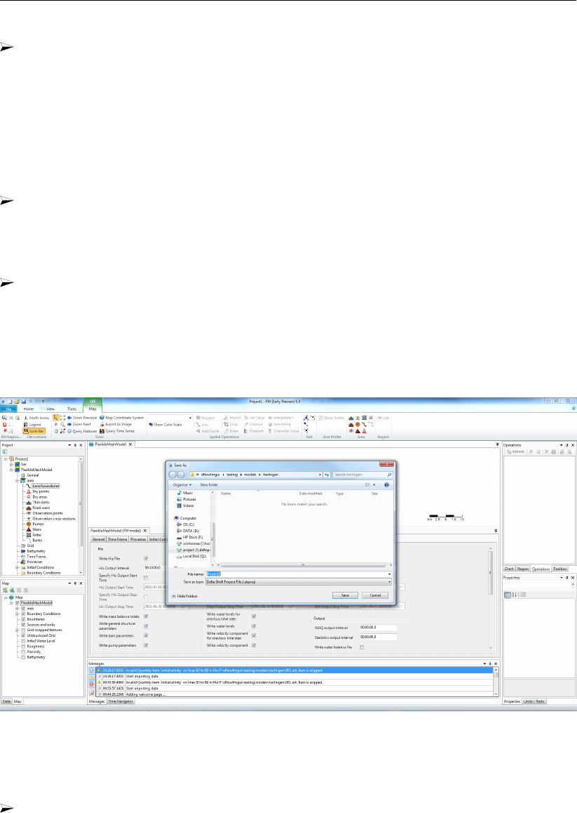
DRAFT
Tutorial
Now close the current FM model (In the project bar, rightmouseclick on westernscheldt06
→Delete →OK ).
19.9 Tutorial 8: Running a model simulation
Up till now we have saved the D-Flow FM model by means of a <mdu>-file. For running
computations, it is necessary to save the entire project, which will be done in this tutorial
exercise:
Import the D-Flow FM Model from the folder <tutorial08>, by choosing Import →Flow
Flexible Mesh Model →OK. Choose <westernscheldt07.mdu>and Open.
For saving the entire project, the following should be done:
Choose File →Save As to save <tutorial08.dsproj>in the folder <tutorial08>and click
Save.
The project has now been saved in a folder called <tutorial08\tutorial08.dsproj_data>
and a project file <tutorial08\tutorial08.dsproj>has been created (See Figure 19.27).
Within this folder you will find all input files of the model (some are ASCII), output files of
the model (when it has been run) and, if applicable, zip-folders containing the restart files.
Figure 19.27: Menu for saving a project.
To start a computation, the following needs to be done:
In the project tree select the model you want to run by means of clicking the first attribute
of the desired model (which has been named westernscheldt07, see Figure 19.28).
Choose Run Model. Now, the simulation will start running.
Deltares 293 of 412
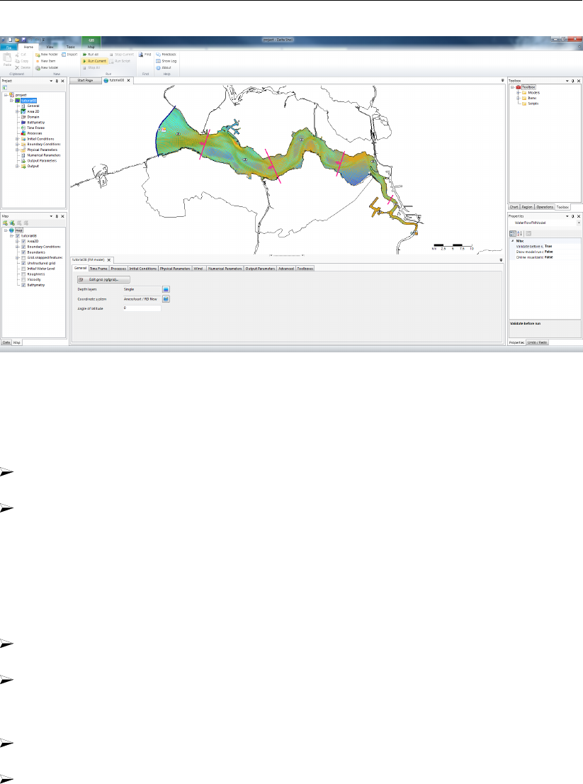
DRAFT
D-Flow Flexible Mesh, User Manual
Figure 19.28: View of Delta Shell when running a model.
The output of the run is being stored in the folder tutorial07\finished. Now:
Save the project with generated output in the folder <tutorial08>(File →Save As and
save the project with name “tutorial08.dsproj”). Press Yes to overwrite the project.
Now close the current D-Flow FM model (In the project bar, rightmouseclick on western-
scheldt07 →Delete →OK ).
19.10 Tutorial 9: Viewing the output of a model simulation
The output of the model can be observed within Delta Shell. At first a project has to be
imported:
Choose File →Open. Select the file <tutorial9.dsproj>from the folder <tutorial09>and
choose Open. The project is now activated.
Doubleclick on westernscheldt07.
To view the output of the history files (observation points and cross-sections):
Click with leftmousebutton on an observation point (while being in select mode. Your
mouse looks like an arrow in this mode).
Choose at the top part of the screen Query Time Series, see Figure 19.29 (option available
within the Map-ribbon).
294 of 412 Deltares
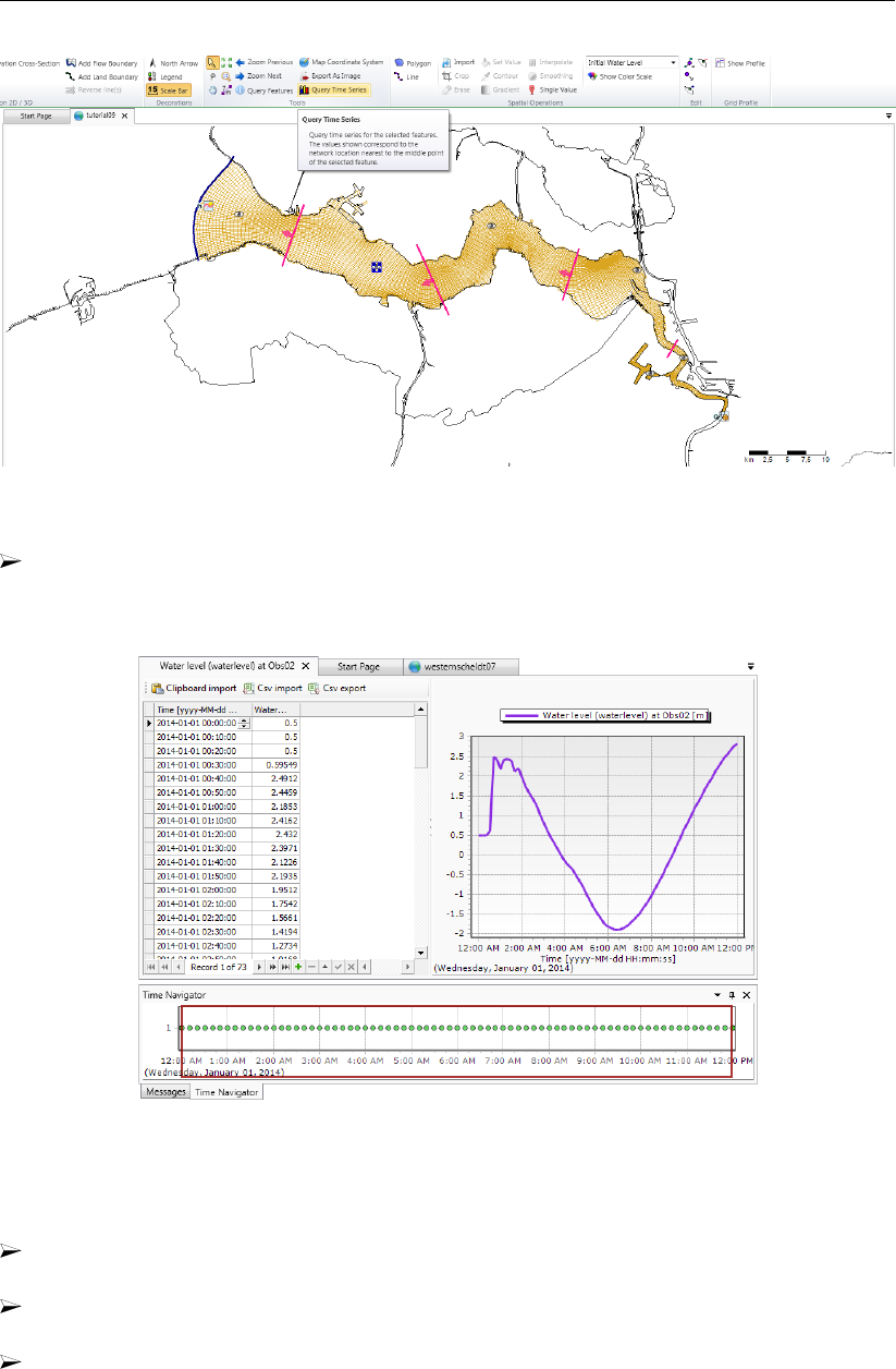
DRAFT
Tutorial
Figure 19.29: View of Delta Shell, available to select a location for timeseries in.
Choose Water level (waterlevel) →OK. You can now observe the water levels in the
observation point you selected, see Figure 19.30. You can choose other parameters as
well to observe. Also cross-sections can be observed this way.
Figure 19.30: View of Delta Shell, time-series for observation point ”Obs03”.
To view the output of the map files:
Open the Time Navigator, by choosing from the ribbon Time Navigator. The Time Naviga-
tor will appear at the bottom of Delta Shell.
If necessary; select, below the Data window, the tab Map (lower left corner of the main
window).
Choose in the Map-tree Add New Wms Layer (see Figure 19.31) and choose http://openstreetmap.org.
Deltares 295 of 412
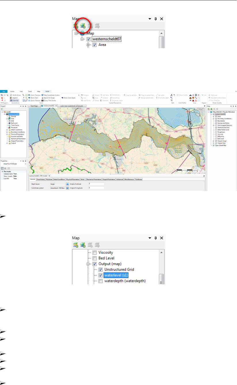
DRAFT
D-Flow Flexible Mesh, User Manual
Figure 19.31: WMS layer icon at the top of the map-tree viewer.
Now, the model can be observed with OpenStreetMap in the background. See Fig-
ure 19.32.
Figure 19.32: View of Delta Shell in combination with OpenStreetMap.
Open Output in the map tree to the left. Choose waterlevel(s1) to observe water levels,
see Figure 19.33.
Figure 19.33: Select waterlevel(s1) from the map tree
To adjust the legend, rightmouseclick on Output(map) →waterlevel (s1) and select Prop-
erties. Now the window Layer Properties Editor appears in which the legend can be
adjusted.
Set classes to “11”
Select Custom range and set the legend values for minimum and maximum value to “-2.5”
to “-0.5”.
Press Generate
Press OK, see Figure 19.33.
Click the play button in the Time Navigator to check whether the water levels change in
time. Choose another parameter, e.g. water depth, to observe afterwards too.
Now close the current D-Flow FM model (In the project bar, rightmouseclick on western-
scheldt07 →Delete →OK ).
296 of 412 Deltares

DRAFT
20 Calibration and data assimilation
Note: Calibration of D-Flow FM with OpenDA is a β-functionality.
20.1 Introduction
A flow model in D-Flow FM will generally benefit from parameter calibration to closer match
observation data. When the model runs in an operational system data assimilation can be
used to into the running model. For the automatic calibration and data assimilation, the open
source toolbox OpenDA is available.
OpenDA basically provides three types of building blocks: an optimisation algorithm that per-
forms the calibration or data assimilation, communication routines for passing information
between OpenDA and D-Flow FM, and methods for handling observation data. The commu-
nication between OpenDA and D-Flow FM is realised using a Black Box approach. A number
of wrapper objects (so called dataObjects) are available for reading and writing D-Flow FM
input and output files.
This chapter contains a description of how the OpenDA toolbox could be deployed to apply
calibration and data assimilation. The OpenDA tools can run D-Flow FM models and ana-
lyze the model results. A more extensive design description of the D-Flow FM wrappers for
OpenDA can be found in the D-Flow FM TRM (2015).
More information on OpenDA can be found on the website http://www.openda.org.
General information on the installation of OpenDA to get started is provided in section 20.2.
section 20.4 gives an overview of the black box wrapper for D-Flow FM. section 20.4 de-
scribes the OpenDA configuration and the related D-Flow FM files. The generation of noise
and how this noise is added to forcings and boundaries is given in section 20.5. Examples
case for calibration and data assimilation using the ensemble Kalman filter are described in
section 20.6.
20.2 Getting started with OpenDA
The required D-Flow FM wrapper is enclosed in the official OpenDA release since version
2.2.2. The following three elements are needed for a calibration or data assimilation run with
D-Flow FM:
1 The D-Flow FM Command Line Interface (CLI) installation. All OpenDA algorithms start D-
Flow FM with a shell script start_dflowfm.sh or a batch script start_dflowfm.bat.
Both scripts assume that D-Flow FM executable is available on the search path (i.e. it
should be executable from the command line). If this is not the case change the environ-
ment variable PATH to include the installation path of the D-Flow FM executable.
2 An OpenDA installation including the OpenDA core, the D-Flow FM specific wrapper code
and examples.
3 A Java Runtime Environment (JRE) version 7 (or higher) is needed to run OpenDA (2.2.2).
OpenDA can use one of the system installed JREs or alternatively an JRE can be installed
directly in the OpenDA directory at the same level as the <bin>directory.
For Linux it is required to run source settings_local.sh to setup OpenDA. The
OpenDA GUI can be started from the <bin>directory using oda_run_gui.bat (Win-
dows) or oda_run.sh with the -gui command line option (Linux).
Deltares 297 of 412

DRAFT
D-Flow Flexible Mesh, User Manual
20.3 The OpenDA black box model wrapper for D-Flow FM
For a D-Flow FM model to function within the OpenDA toolbox we need to establish two things:
1 the control to propagate the model over time and
2 access to the model state, physical parameters, boundary conditions and external forc-
ings.
In the black box approach the standard D-Flow FM command line executable is used to prop-
agate the model over time. Access to the model state, physical parameters, boundary con-
ditions and external forcings is obtained by reading from and writing to the D-Flow FM input
and output files. Inside OpenDA all data is available in the form of exchange items which all
have an unique identifier.
Calibration and data assimilation typically need multiple model evaluations with altered pa-
rameters, forcings, boundary conditions or the initial model state. In the black box approach
this is achieved by creating multiple work directories containing altered model input files and
starting the D-Flow FM executable in each work directory. D-Flow FM model results are than
read from the work directories and compared to observation data.
For calibration this is an iterative process. Results from model evaluations 1, . . . , n are re-
quired to obtain a better estimate for parameter values, which are then evaluated in run n+1.
In case of an ensemble Kalman filter (EnKF) run, the D-Flow FM computations (one run for
each ensemble member) is stopped each time an observation is available, the input files for
each ensemble member are modified according to the ensemble Kalman filter algorithm, after
which the D-Flow FM run is restarted.
Next to the D-Flow FM model configuration OpenDA has its own configuration for selecting
the algorithm, observations and interfacing with the D-Flow FM input an output files.
20.4 OpenDA configuration
20.4.1 Main configuration file and the directory structure
The OpenDA main configuration file has the .oda extension. All OpenDA configuration files
use the xml format. It is advised to use a schema aware xml editor, when making changes to
the OpenDA configuration. These editors provide direct access to the documentation that is
stored in the schema and can validate the correctness of the xml files.
All other xml config file names and directories are configurable. However, there is a commonly
used directory layout and naming convention. All the examples are configured using this
convention. For example, the directory structure for the simple_waal_kalman example is given
in Table 20.1.
All the work directories are available in the <stochModel>directory, after performing a run
with OpenDA they contain the D-Flow FM results.
It is a good practice to name the main configuration file corresponding to the algorithms exe-
cuted by OpenDA. The following files are used in the provided examples:
<Simulation.oda>: performs a regular D-Flow FM simulation run, only the executable is
started by OpenDA. This algorithm is useful to check the configuration.
<Dud.oda>: Dud (Doesn’t Use Derivative) is one of the optimisation algorithms available
for calibration purposes.
298 of 412 Deltares
DRAFT
Calibration and data assimilation
<simple_waal_kalman>
<algorithm>..................calibration method or data-assimilation algorithm
<enkfAlgorithm.xml>....................algorithm specific configuration
...
<stochModel>...........................model and its uncertainty description
<bin>............................bat and .sh scripts for calling D-Flow FM
<input_dflowfm>.......................D-Flow FM template configuration
...
<work0/>...............................work directory for propagated mean
<work1/>..........................work directory for first ensemble member
...
<dflowfmModel.xml>.......................exchange items configuration
<dflowfmStochModel.xml>............... predictor, state and parameter
<dflowfmWrapper.xml>............actions and data objects configuration
...
<stochObserver>.............................. observations and uncertainty
<noosObservations.xml>..................observations and uncertainty
<waterlevel_Obs01.noos>.........................raw observation file
...
<Enkf.oda>............................................main configuration file
...
Table 20.1: Directory structure of the OpenDA Ensemble Kalman filtering configuration
for the simple Waal D-Flow FM model.
<SequentialSimulation.oda>: performs a D-Flow FM simulation run through which the
executable is stopped and restarted by OpenDA at the moments for which observed data
are available.
<Enkf.oda>: performs an ensemble Kalman filtering.
The main configuration for an OpenDA application has three mandatory components, which
make up an OpenDA application: stochModelFactory,stochObserver and algorithm.
Each component is configured by specifying its className attribute, workingDirectory
and configFile/configString. There are optional components to enable writing
OpenDA results, to define OpenDA restart input and output files and to enable timings. The
resultwriter is typically useful for writing stochastic properties that are only available to
OpenDA and not in D-Flow FM.
The main configuration file <Enkf.oda>for the simple_waal example:
<?xml version="1.0" encoding="UTF-8"?>
<openDaApplication
xmlns="http://www.openda.org"
xmlns:xsi="http://www.w3.org/2001/XMLSchema-instance"
xsi:schemaLocation
="http://www.openda.org http://schemas.openda.org/openDaApplication.xsd">
<stochObserver className="org.openda.observers.NoosTimeSeriesStochObserver">
<workingDirectory>./stochObserver</workingDirectory>
<configFile>noosObservations.xml</configFile>
</stochObserver>
<stochModelFactory className="org.openda.blackbox.wrapper.BBStochModelFactory">
<workingDirectory>./stochModel</workingDirectory>
<configFile>dflowfmStochModel.xml</configFile>
</stochModelFactory>
<algorithm className="org.openda.algorithms.kalmanFilter.EnKF">
<workingDirectory>./algorithm</workingDirectory>
<configString>EnkfAlgorithm.xml</configString>
Deltares 299 of 412

DRAFT
D-Flow Flexible Mesh, User Manual
</algorithm>
<resultWriter className="org.openda.resultwriters.MatlabResultWriter">
<workingDirectory>.</workingDirectory>
<configFile>Enkf_results.m</configFile>
<selection>
<resultItem id="pred_f"/>
<resultItem id="pred_f_0"/>
<resultItem id="pred_f_1"/>
<resultItem id="pred_f_std"/>
<resultItem id="pred_f_central"/>
<resultItem id="pred_a_linear"/>
<resultItem id="analysis_time"/>
<resultItem id="obs"/>
</selection>
</resultWriter>
</openDaApplication>
Note that the directory layout in this section is created by setting the workingDirectory
elements in stochModelFactory,stochObserver and algorithm parts of the con-
figuration. Each of these components have their own configuration, which are described in
the following sections.
20.4.2 The algorithm configuration
All provided methods for calibration and data assimilation are configurable through an xml file.
The convention is to include the algorithm name in the fila name e.g <EnkfAlgorithm.xml>.
For data assimilation algorithms the configuration typically specifies the ensemble size and
the option to use stochastic parameters, forcing and initialisation. For calibration algorithms
the configuration typically contains definition of the cost function and tolerances and stop-
ping criteria. For a list of algorithms and their configuration options see the general OpenDA
documentation.
20.4.3 The stochObserver configuration
The access to observations is standardized in OpenDA using a stochObserver object.
The configuration and the observation data are placed in the <stochObserver>directory.
OpenDA contains a number of different stochObserver objects that can handle different
types of data files. In this manual, we discuss the NoosTimeSeriesStochObserver
and the more generic IoObjectStochObserver. For a more complete list of available
stochObservers see the OpenDA web site.
20.4.3.1 NoosTimeSeriesStochObserver
The NOOS file format is used to store time series. The format is created for use by the
members of the North West European Shelf Operational Oceanographic System http://
www.noos.cc/. An example of (a part of) a NOOS file is:
#------------------------------------------------------
#------------------------------------------------------
# Location : station01
# Position : (0.0,0.0)
# Source : twin experiment DFlowFM
# Unit : waterlevel
# Analyse time: null
# Timezone : null
#------------------------------------------------------
199101010000 1.0000
199101010100 0.8944
199101010200 0.6862
300 of 412 Deltares

DRAFT
Calibration and data assimilation
199101010300 0.5956
199101010400 0.3794
199101010500 0.1372
199101010600 -0.1300
199101010700 -0.3044
199101010800 -0.3963
199101010900 -0.3739
199101011000 -0.1930
...
The file contains a header with meta data specifying among others the location name (Location)
and the quantity (Unit). The data is written in two columns, the first gives the time of the
observation using the ‘YYYYMMDDhhmm’ format and the second column gives the measured
value.
The file <noosObserver.xml>defines a number of time series, each coupled to a NOOS file
containing the measurements.
<?xml version="1.0" encoding="UTF-8"?>
<noosObserver
xmlns="http://www.openda.org"
xmlns:xsi="http://www.w3.org/2001/XMLSchema-instance"
xsi:schemaLocation
="http://www.openda.org http://schemas.openda.org/schemas/noosObservations.xsd">
<timeSeries status="use" standardDeviation="0.05">
den_helder_waterlevel_astro.noos
</timeSeries>
<timeSeries status="use" standardDeviation="0.05">
aberdeen_waterlevel_astro.noos
</timeSeries>
</noosObserver>
OpenDA creates an exchange item for each observation time series. The default exchange
item id (identifier) is created using the location (Location) and the quantity (Unit). The
standard deviation (measurement error) is specified with standDeviation attribute.
20.4.3.2 IoObjectStochObserver
This observer uses a dataObject for handling the file IO. All exchange items that are provided
by dataObject can be used by the observer. For instance the NetcdfDataObject can read and
write to NetCDF files, and has an exchange item for each variable in the NetCDF file. The
lake_kalman example uses this approach to use the *.his file from a D-Flow FM run as
synthetic observations for a ensemble Kalman filter run. The <dflowfmStochObsConfig.xml>
file reads:
<?xml version="1.0" encoding="UTF-8"?>
<ioObjectStochObserver
xmlns="http://www.openda.org"
xmlns:xsi="http://www.w3.org/2001/XMLSchema-instance"
xsi:schemaLocation
="http://www.openda.org http://schemas.openda.org/openDaStochObserver.xsd">
<uncertaintyModule
workingDirectory="."
className="org.openda.uncertainties.UncertaintyEngine">
<arg>stochObsUncertainties.xml</arg>
</uncertaintyModule>
<ioObject
workingDirectory="."
className="org.openda.exchange.dataobjects.NetcdfDataObject">
<fileName>lake2d_his.nc</fileName>
</ioObject>
Deltares 301 of 412

DRAFT
D-Flow Flexible Mesh, User Manual
</ioObjectStochObserver>
In the configuration of UncertaintyEngine OpenDA object, a selection of these ex-
change items id’s is made and a standard deviation is specified.
<?xml version="1.0" encoding="UTF-8"?>
<uncertainties
xmlns="http://www.wldelft.nl"
xmlns:xsi="http://www.w3.org/2001/XMLSchema-instance"
xsi:schemaLocation
="http://www.wldelft.nl http://schemas.openda.org/uncertainties.xsd"
version="1.0">
<uncertaintyType>ProbabilityDistributionFunction</uncertaintyType>
<probabilityDistributionFunction id="S1.waterlevel" isActive="true">
<normal mean="0" stdv="0.05" stdvIsFactor="false"/>
</probabilityDistributionFunction>
<probabilityDistributionFunction id="S2.waterlevel" isActive="true">
<normal mean="0" stdv="0.05" stdvIsFactor="false"/>
</probabilityDistributionFunction>
<probabilityDistributionFunction id="S3.waterlevel" isActive="true">
<normal mean="0" stdv="0.05" stdvIsFactor="false"/>
</probabilityDistributionFunction>
<probabilityDistributionFunction id="S4.waterlevel" isActive="true">
<normal mean="0" stdv="0.05" stdvIsFactor="false"/>
</probabilityDistributionFunction>
</uncertainties>
20.4.4 The stochModel configuration
The stochModel configuration usually consists of three <∗.xml>files in the <stochModel>
directory. These are called:
<dflowfmWrapper.xml>: This file specifies the actions to perform in order to run a D-
Flow FM simulation and list the D-Flow FM input and output files that can be used to let
OpenDA interact with the model. For each file the dataObject is specified which is used
for handling the specified file.
<dflowfmModel.xml>: This file contains a list of the exchange items which are provided
by the configured dataObject. The model time information is constructed by the time-
InfoExchangeItems element. It also contains a number of alias values which can be
used in three stochModel configuration files.
<dflowfmStochModel.xml>: In this file defines the predictor, the selection of observations
which are compared to the model results. For calibration this file also specifies which
parameters can be changed. For data assimilation this files contains the definition of the
model state and the noise (uncertainty) specification for the boundaries and forcings.
302 of 412 Deltares

DRAFT
Calibration and data assimilation
20.4.5 D-Flow FM files and the OpenDA dataObjects configuration
The dataObjects for reading and writing provide so-called exchange items that allow OpenDA
to manipulate specific parts of the files of D-Flow FM. The D-Flow FM files that can be manip-
ulated by OpenDA and the corresponding OpenDA class names are given in Table 20.2.
Table 20.2: D-Flow FM files that can be manipulated and the corresponding OpenDA
class names to be used in the dflowfmWrapper.xml file.
D-Flow FM filetype OpenDA dataObject & exchange items
<∗.mdu>org.openda.model_dflowfm.DFlowFMTimeInfo
IDs: start_time, end_time
<∗.amu>org.openda.model_dflowfm.DFlowFMMeteoFile
ID: x_wind
<∗.amv>org.openda.model_dflowfm.DFlowFMMeteoFile
IDs: y_wind
<∗.amp>org.openda.model_dflowfm.DFlowFMMeteoFile
ID: air_pressure
<∗.tim>org.openda.model_dflowfm.DFlowFMTimeSeriesDataObject
IDs: BOUNDARY_ID.#:QUANTITY
<∗.xyz>org.openda.model_dflowfm.DFlowFMXyzFile
IDs: FILENAME_#
<∗_his.nc>org.openda.exchange.dataobjects.NetcdfDataObject
IDs: STATION_ID.VARIABLE_NAME
<∗_map.nc>org.openda.model_dflowfm.DFlowFMRestartFileWrapper
IDs: VARIABLE_NAME
<∗.cld>org.openda.model_dflowfm.DFlowFMCalibrationFactorFile
IDs: CalFactor-CALIBRATION_DEFINTION_NUMBER,
CalFactor-CALIBRATION_DEFINTION_NUMBER-q{DISCHARGE},
CalFactor-CALIBRATION_DEFINTION_NUMBER-h{WATERLEVEL}
<∗.ttd>org.openda.model_dflowfm.DFlowFMTrachytopeFile
IDs: RoughNr_{ROUGHNESSNR}_FormulaNr{FORMULANR}_{FORMULAPARAMETER},
RoughNr_{ROUGHNESSNR}_DISCHARGE{DISCHARGE}_FormulaNr{FORMULANR}_{FORMULAPARAMETER},
RoughNr_{ROUGHNESSNR}_WATERLEVEL{WATERLEVEL}_FormulaNr{FORMULANR}_{FORMULAPARAMETER}
All the dataObjects and their configuration are described tn the following sections.
20.4.5.1 Start and end time in the model definition file (.mdu)
The start and end time are set in <∗.mdu>-file the by OpenDA using the start_time and
end_time exchange items. These are provided by the DFlowFMTimeInfo data object.
D-Flow FM reference Exchange Item Id Remark
TStart start_time RefDate and Tunit needed for interpretation
TStop end_time RefDate and Tunit needed for interpretation
20.4.5.2 External forcings (.xyz)
All D-Flow FM external forcings are specified via the <∗.ext>forcings file. Here a spatial
forcing can be defined by using a .xyz-file (e.g. the bed friction coefficients). For instance
the file <nikuradse.xyz>contains:
Deltares 303 of 412

DRAFT
D-Flow Flexible Mesh , User Manual
x1 y1 0.9994357525438934
x2 y2 0.9994357525438934
x3 y3 2.0021214673505600
x4 y4 2.0021214673505600
x5 y5 2.0021214673505600
x6 y6 2.0021214673505600
When performing calibration of a spatial field it is often required to group points in a select
number of regions. The calibration then does not change the individual values but applies
a factor to all values in the group. The best approach is to create a file with multipliers (e.g
<friction_multiplier.xyz>) which are initially all equal to one.
x1 y1 1.0
x2 y2 1.0
x3 y3 1.0
x4 y4 1.0
x5 y5 1.0
x6 y6 1.0
The multiplication (or addition) with the values in nikuradse.xyz should be configured in
the *.ext file.
Group from keywords in file
One option to construct groups is to use keywords directly in the <friction_multiplier.xyz>file:
x1 y1 1.0 #friction_3
x2 y2 1.0 #friction_3
x3 y3 1.0 #friction_1
x4 y4 1.0 #friction_1
x5 y5 1.0 #friction_4
x6 y6 1.0 #friction_4
In the OpenDA wrapper config the dataObject is than configured as:
<ioObject className="org.openda.model_dflowfm.DFlowFMXyzFile">
<file>friction_multiplier.xyz</file>
<id>frictionCoefFile</id>
<arg>idsFromKeywordsInFile</arg>
</ioObject>
This will create exchange items with identifier friction_3,friction_1 and friction_4.
Group from template file
An other options is to use a template file (<friction_multiplier_template.xyz>) with exactly the
same (x,y) coordinates as in (<friction_multiplier.xyz>). The third column is used to define
groups by using these values as group numbers:
304 of 412 Deltares

DRAFT
Calibration and data assimilation
x1 y1 3.0
x2 y2 3.0
x3 y3 4.0
x4 y4 4.0
x5 y5 1.0
x6 y6 1.0
In the OpenDA wrapper config the dataObject must be configured as:
<ioObject className="org.openda.model_dflowfm.DFlowFMXyzFile">
<file>friction_multiplier.xyz</file>
<id>frictionCoefFile</id>
<arg>idsFromTemplateFile=friction_multiplier_template.xyz</arg>
</ioObject>
This will create an exchange item for each group with identifier ‘FILE_BASENAME + _ + num-
ber from template file’, e.g. friction_multiplier_3,friction_multiplier_4
and friction_multiplier_1.
20.4.5.3 Boundary time series (.tim)
Boundary conditions are specified as a combination of a <∗.pli>file and one or more .tim
files. The DFlowFMTimeSeriesDataObject dataObject creates exchange items for all
boundary conditions. It starts with reading the name of the external forcing file name from
the <.mdu>-file (key ExtForceFile). The <∗.ext>-file contains formatted blocks, one
for each forcing. Forcings are defined along polylines, given in .pli-files. A <∗.pli>-file is
accompanied by a <∗.cmp>- or a (number of) <∗.tim>-file(s).
Noise can be added by means of an extra block in the .ext-file. As an example, noise is
added to a boundary with a discharge imposed as:
QUANTITY =dischargebnd
FILENAME =sw_east_dis.pli
FILETYPE =9
METHOD =3
OPERAND =O
QUANTITY =dischargebnd
FILENAME =sw_east_dis_noise.pli
FILETYPE =9
METHOD =3
OPERAND =+
The discharge is set by the first block (operand=O), the information in the <∗.pli>-files is
identical and noise is added as a time series: the <_noise.pli>file is always accompanied by
a (number of) <∗.tim>file(s). The location-information on the first line of the .pli-file
combined with the quantity is used to construct the exchange item identifier: location.1.-
dischargebnd. The numbering is used to discern between multiple <∗.tim>-files possibly
linked to a single <∗.pli>-file.
20.4.5.4 Meteorological boundary conditions (<∗.amu>,<∗.amv>,<∗.amp>)
OpenDA can read and write to the D-Flow FM <∗.amu>,<∗.amv>and <∗.amp>files using
the org.openda.model_dflowfm.DFlowFMMeteoFile dataObject. These contain
the x- and ycomponents of the wind and the air pressure at the free surface on an equidistant
Deltares 305 of 412

DRAFT
D-Flow Flexible Mesh , User Manual
grid. In a typical data assimilation use noise fields are added to the wind. For the this purpose
OpenDA can generate a spatial noise field on an equidistant grid (see section 20.5). D-
Flow FM can combine fields defined in files on different to single field on the computational
grid.
20.4.5.5 Result time series (<∗_his.nc>)
The <∗_his.nc>-file contains time series with D-Flow FM model results for a number of sta-
tions. The generic org.openda.exchange.dataobjects.NetcdfDataObject is
used for handling this type of files. The NetcdfDataObject expects a NetCDF-file that
contains dimensions time and stations plus a variable station_id of type string and
dimension stations. For each variable in this NetCDF-file with dimensions (time,stations)
an exchange item is created, that can be referred to as station_id(i).variablename.
For instance:
dimensions:
time = UNLIMITED ; // (2882 currently)
stations = 3 ;
station_name_len = 40 ;
variables:
char station_id(stations, station_name_len) ;
(containing strings Obs1, Obs2, Obs3)
double waterlevel(time, stations) ;
(containing the computed values of the waterlevel)
results in three exchange items (a 1D vector in this case) with identifiers: Obs1.waterlevel,
Obs2.waterlevel and Obs3.waterlevel.
20.4.5.6 Restart file (<∗_map.nc>)
OpenDA provides the org.openda.model_dflowfm.DFlowFMRestartFileWrapper
for reading and writing the <∗_map.nc>-file. This file contains all information needed to
restart a D-Flow FM computation. Not all variables are relevant for manipulation by OpenDA:
variable names that start with ‘time’, ‘NetLink’, ‘BndLink’, ‘FlowLink’, ‘NetElem’, ‘FlowElem’,
‘NetNode’, ‘wgs84’ and ‘projected_coordinate_system’ are ignored. Variables of other types
than float or double are also ignored. For all other variables an exchange item is created,
where the name of the variable in the NetCDF is used as the exchange item id.
Note: for Kalman filtering it is essential that the model starts from the <∗_map.nc>file. It is
not possible to specify an initial field by setting the initialwaterlevel or initialsalinity
quantities in the <∗.ext>file. If you want to set an initial field using these settings, make a
custom D-Flow FM run where TStop is equal to TStart and use the created <∗_map.nc>
file for the starting point of the Kalman filtering.
20.4.5.7 Calibration factor definition file (<∗.cld>)
The calibraction factor definition file has the following layout. This file includes examples of
the three different types of calibration definition factors and in comments the resulting names
of the exchange items for OpenDA.
# [FileInformation]
# FileType = CalibrationFactorsDefinitionFile
306 of 412 Deltares

DRAFT
Calibration and data assimilation
# FileVersion = 1.0
# [CalibrationFactors]
# Non-Q-or-h-dependent
#
# calibration-class-nr calibration-factor
#
34 0.9
#
# (will lead to exchange item CalFactor-34)
# Q-dependent calibration factors
#
# calibration-class-nr DISCHARGE "Cross-section name"
# calibration-class-nr Q1 ConstantValueAtQ1
# calibration-class-nr Q2 ConstantValueAtQ2
# calibration-class-nr Q3 ConstantValueAtQ3
# calibration-class-nr Q4 ConstantValueAtQ4
#
601 DISCHARGE "cross-section name"
601 0100 1.0
601 1000 1.0
601 5500 1.0
# (will lead to exchange items:
# CalFactor-601-q0100, CalFactor-601-q1000, CalFactor-601-q5500) etc.
# Waterlevel dependent calibration factor
# calibration-class-nr WATERLEVEL "Observation station name"
# calibration-class-nr H1 ConstantValueAtH1
# calibration-class-nr H2 ConstantValueAtH2
# calibration-class-nr H3 ConstantValueAtH3
# calibration-class-nr H4 ConstantValueAtH4
#
3 WATERLEVEL "water-level station name"
3 0.45 1.0
3 0.9 1.0
# (will lead to exchange items:
# CalFactor-3-h0.45 and CalFactor-3-h0.9)
OpenDA provides the org.openda.model_dflowfm.DFlowFMCalibrationFactorFile
for reading and writing the <∗.cld>-file. In the OpenDA wrapper config <dflowfmWrapper.xml>
the dataObject can be configured as:
<ioObject className="org.openda.model_dflowfm.DFlowFMCalibrationFactorFile">
<file>FlowFM.cld</file>
<id>calibFactorFileID</id>
</ioObject>
In the dflowfmModel.xml a listing of the exchange items which are to be used can be
found. To select all of the available exchange items from the calibration factor definition file,
the following code can be used:
<exchangeItems>
<vector id="allElementsFromIoObject" ioObjectId="calibFactorFileID"/>
</exchangeItems>
To select just a few of the exchange items, these can also be selected individually:
<exchangeItems>
<vector id="CalFactor-601-q0100" ioObjectId="calibFactorFileID"
elementId="CalFactor-601-q0100"/>
Deltares 307 of 412

DRAFT
D-Flow Flexible Mesh, User Manual
<vector id="CalFactor-601-q1000" ioObjectId="calibFactorFileID"
elementId="CalFactor-601-q1000"/>
<vector id="CalFactor-601-h0.45" ioObjectId="calibFactorFileID"
elementId="CalFactor-601-h0.45"/>
<vector id="CalFactor-601-q0.9" ioObjectId="calibFactorFileID"
elementId="CalFactor-601-h0.9"/>
</exchangeItems>
20.4.5.8 Trachytopes roughness definition file (<∗.ttd>)
The trachytopes definition file has the following layout. This file includes examples of the
three different types of calibration definition factors and in comments the resulting names of
the exchange items for OpenDA.
# [FileInformation]
# FileType = TrachytopesRoughnessDefinitionFile
# FileVersion = 1.0
# [RoughnessDefinitions]
#
# Constant roughness definitions
# roughness-definition-code formula-number formula-parameters
# Nikuradse 0.2
7 51 0.2
# (Leads to exchange-item RoughNr_7_FormulaNr_51_A)
# Linear trachytopes: wooden barrier
9 201 5.0 1.25
# (Leads to exchange-items RoughNr_9_FormulaNr_201_A
# and RoughNr_9_FormulaNr_201_B})
# Uniform chezy value 25
10 52 25
# (Leads to exchange-item RoughNr_10_FormulaNr_52_A)
# Discharge dependent trachytopes
# roughness-definition-code DISCHARGE cross-section-name
# roughness-definition-code Q1 formula-number formula-parametersatQ1
# roughness-definition-code Q2 formula-number formula-parametersatQ2
11 DISCHARGE "m=1"
11 0.0 51 0.2
11 200.0 51 0.18
11 1000.0 51 0.1
%# (Leads to exchange-items RoughNr_11_DISCHARGE0.0_FormulaNr_51_A,
# RoughNr_11_DISCHARGE200.0_FormulaNr_51_A,
# RoughNr_11_DISCHARGE1000.0_FormulaNr_51_A)
# Water-level dependent trachytopes
# roughness-definition-code WATERLEVEL observation-station-name
# roughness-definition-code ZS1 formula-number formula-parametersatZS1
# roughness-definition-code ZS2 formula-number formula-parametersatZS2
11 WATERLEVEL "obs1"
16 -1.2 151 4.0 0.1
16 -1 151 4.0 0.3
16 2 151 5.0 0.1
# (Leads to exchange-items RoughNr_16_WATERLEVEL-1.2_FormulaNr_151_A,
# RoughNr_16_WATERLEVEL-1.2_FormulaNr_151_B,
# RoughNr_16_WATERLEVEL-1_FormulaNr_151_A,
# RoughNr_16_WATERLEVEL-1_FormulaNr_151_B,
# RoughNr_16_WATERLEVEL2_FormulaNr_151_A,
# RoughNr_16_WATERLEVEL2_FormulaNr_151_B)
308 of 412 Deltares

DRAFT
Calibration and data assimilation
OpenDA provides the org.openda.model_dflowfm.dflowfm.DFlowFMTrachytopeFile
for reading and writing the <∗.cld>-file. In the OpenDA wrapper config <dflowfmWrapper.xml>
the dataObject can be configured as:
<ioObject className="org.openda.model_dflowfm.dflowfm.DFlowFMTrachytopeFile">
<file>FlowFM.ttd</file>
<id>trachytopesFileID</id>
</ioObject>
In the dflowfmModel.xml a listing of the exchange items which are to be used can be
found. To select all of the available exchange items from the calibration factor definition file,
the following code can be used:
<exchangeItems>
<vector id="allElementsFromIoObject" ioObjectId="trachytopesFileID"/>
</exchangeItems>
To select just a few of the exchange items, these can also be selected individually:
<exchangeItems>
<vector id="RoughNr_7_FormulaNr_51_A" ioObjectId="trachytopesFileID"
elementId="RoughNr_7_FormulaNr_51_A"/>
<vector id="RoughNr_11_DISCHARGE0.0_FormulaNr_51_A" ioObjectId="trachytopesFileID"
elementId="RoughNr_11_DISCHARGE0.0_FormulaNr_51_A"/>
<vector id="RoughNr_16_WATERLEVEL-1.2_FormulaNr_151_A" ioObjectId="trachytopesFileID"
elementId="RoughNr_16_WATERLEVEL-1.2_FormulaNr_151_A"/>
<vector id="RoughNr_16_WATERLEVEL-1.2_FormulaNr_151_B" ioObjectId="trachytopesFileID"
elementId="RoughNr_16_WATERLEVEL-1.2_FormulaNr_151_B"/>
</exchangeItems>
20.5 Generating noise
To add uncertainty to the external forcings and the boundary conditions, OpenDA has func-
tionality for generating noise time series and spatial fields. The noise generation can be spec-
ified within the state definition in <dflowfmStochModel.xml>. For instance in the example
simple_waal_kalman, a noise time series is created (ID dischargenoise), which is
added to the inflow discharge (ID eastboundary.1:dischargebnd).
<?xml version="1.0" encoding="UTF-8"?>
<blackBoxStochModel
xmlns:xsi="http://www.w3.org/2001/XMLSchema-instance"
xsi:schemaLocation
="http://www.openda.org http://schemas.openda.org/blackBoxStochModelConfig.xsd"
xmlns="http://www.openda.org">
<modelConfig>
<file>./dflowfmModel.xml</file>
</modelConfig>
<vectorSpecification>
<state>
<noiseModel
id="boundaryNoiseModel"
className="org.openda.noiseModels.TimeSeriesNoiseModelFactory"
workingDirectory=".">
<configFile>BoundaryNoise.xml</configFile>
<exchangeItems>
<exchangeItem
id="dischargenoise"
operation="add"
modelExchangeItemId="eastboundary.1:dischargebnd"/>
</exchangeItems>
</noiseModel>
<vector id="s1"/>
<vector id="unorm"/>
Deltares 309 of 412

DRAFT
D-Flow Flexible Mesh, User Manual
</state>
</vectorSpecification>
</blackBoxStochModel>
The config file <BoundaryNoise.xml>contains the details of the noise:
<?xml version="1.0" encoding="UTF-8"?>
<mapsNoiseModelConfig>
<simulationTimespan timeFormat="dateTimeString">
199208311200,199209010000,...,199212090000
</simulationTimespan>
<timeSeries
id="dischargenoise"
location="eastboundary"
quantity="discharge"
standardDeviation="0.2"
timeCorrelationScale="6.0"
timeCorrelationScaleUnit="hours"/>"
</mapsNoiseModelConfig>
A noise time series is created (ID dischargenoise) with a correlation time of 6 hours
and a standard deviation of 0.2.Note: currently OpenDA does not support the creation of
D-Flow FM files, all files should exist in the <input_dflowfm>. In this case the boundary is
defined in <sw_east_dis.pli>, but the noise is in a separate file <sw_east_dis_noise.pli>.
Initially it contains zeros, but is filled with the noise values at run time. The time points in the
file need to match the simulationTimespan in the OpenDA config. The total discharge
at the boundary is constructed by D-Flow FM where the noise is added to original boundary
values (see <simple_waal.ext>).
To generate a spatial correlation field the same approach can be used. In the lake_kalman
example a noise field is added the wind. Instead of timeSeries anoiseItem is specified
which contains the grid definition.
<?xml version="1.0" encoding="UTF-8"?>
<mapsNoiseModelConfig>
<simulationTimespan timeFormat="dateTimeString">
200106240000,200106240100,...,200106270000
</simulationTimespan>
<noiseItem id="2DNoise" quantity="wind-x" unit="m/s" height="10.0"
standardDeviation="20.0"
timeCorrelationScale="12.0" timeCorrelationScaleUnit="hours"
initialValue="0.0"
horizontalCorrelationScale="10" horizontalCorrelationScaleUnit="km">
<grid type="cartesian" coordinates="XY">
<x>0,3000,...,63000</x>
<y>0,3000,...,63000</y>
</grid>
</noiseItem>
</mapsNoiseModelConfig>
The calculation of spatially correlated noise on a cartesian grid is quite fast as the xand
y-direction are independent. The interpolation from an equidistant grid to the computa-
tional grid is performed within D-Flow FM. Again, note that an zero valued wind files should
be present <input_dflowfm>folder, where the time stamps match with the ones given in
simulationTimespan in the OpenDA configuration.
310 of 412 Deltares

DRAFT
Calibration and data assimilation
20.6 Examples of the application of OpenDA for D-Flow FM
In this section, some examples are elaborated for both the calibration of a model and the
ensemble Kalman filtering (abbreviated as ‘EnKF’) of a model. All the examples can be found
in the directory <examples/model_dflowfm_blackbox>.
20.6.1 Example 1: Calibration of the roughness parameter
The automatic calibration of a model needs two main choices from the user:
1 Which model parameters may be modified during the calibration process?
2 Which model results need to be compared to observations, to judge the model quality?
The remainder of this section will be in the form of a tutorial, to directly illustrate all steps in
an example model. In this example you will use a small river model ‘simple_waal’ and use the
bed roughness to calibrate this model for its three water level observation stations.
Step 1: Inspect the model
All the required model files can be found in the directory <simple_waal_calibration_roughness>.
Consider the following steps:
1 Start D-Flow FM (standalone) in directory <input_dflowfm/>.
2 Select Files →Load MDU-file.
3 Load the model: select <simple_waal.mdu>.
4 You can run the model if you like (right mouse button).
The basic model is built to simulate a simple two-dimensional river with a spatially varying
bed friction coefficient. It is driven by two boundary conditions: an upstream discharge inflow
at the eastern boundary and a downstream water level at the western boundary. Inspect the
model forcing in the following way:
1 Open the external forcings file <simple_waal.ext>in a text editor.
2 Notice how, in addition to the two boundaries, there are two blocks for the friction coeffi-
cient. The first one is a spatially varying roughness field in the <sw_nikuradse.xyz>file.
The second refers to the <sw_frcfact_all.xyz>file that contains multipliers for the original
friction coefficients. A third file <sw_frcfact_template.xyz>is present, which is used to
define a number of subdomains.
3 In D-Flow FM, select Files →Load sample file and select <sw_frcfact_template.xyz>.
4 Notice how the loaded samples have three distinct values 1, 2 and 3, which act as iden-
tifiers: they approximately define the corner points of three subdomains of the entire river
stretch. For each subdomain, a different roughness can be calibrated.
Step 2: Select the model parameters
Currently, the only calibratable parameters are the time-independent parameters in the exter-
nal forcings file that use the .xyz sample file format. The most obvious parameter is the bed
friction coefficient.
Deltares 311 of 412

DRAFT
D-Flow Flexible Mesh, User Manual
Step 3: Select the model results
The example directory <simple_waal>contains all the necessary configuration files for the
so-called Black Box model wrapper for D-Flow FM to run a ‘twin experiment’. In a twin ex-
periment a model setup with given solution (the synthetic observations) is perturbed after
which OpenDA is applied to re-estimate the original settings. The effects of the parame-
ter variations may be judged by comparing time series output in the <∗_his.nc>history file
to observed data in NOOS time series format. The model output and observation data are
compared by calculating a cost function. Which cost function is used is configured in the
<dudAlgorithm.xml>in the <algorithm>directory. See the OpenDA documentation for the
available options for the cost function.
The D-Flow FM model simulates a 1D river flow. The input files for D-Flow FM are located in
the directory <simple_waal/stochModel/input>. D-Flow FM allows the user to specify regions
with a different bed friction coefficient (constant for each region) and is able to handle the
interpolation of the coefficients between these regions. In the experiment we try to re-estimate
the values of the bed friction coefficients of an earlier run. As observations, the waterlevel at
three locations (stations) along the river is used. These results are written to the main output
file (<∗_his.nc>) as time series.
In the directory <simple_waal>, there are two main configuration files of OpenDA present:
Simulation.oda: runs a single run of the model, this configuration is mainly used to
test the black box configuration files.
Dud.oda runs a calibration experiment with algorithm DUD (Doesn’t Use Derivative).
These files configure the main ingredients of an OpenDA run:
1 the stochObserver (org.openda.observers.NoosTimeSeriesStochObserver).
Observations for this experiment were created by extracting the timeseries for all stations
from the netcdf-file and convert them to NOOS format (script nchis2noos.sh) het script
schrijft nog tijd sinds begin situatie.
2 the stochObserver (org.openda.observers.NoosTimeSeriesStochObserver).
Observations for this experiment were created by extracting the time series for all stations
from the netcdf-file and convert them to NOOS format (script nchis2noos.sh)
3 the stochModelFactory (org.openda.blackbox.wrapper.BBStochModelFactory). A black
box model configuration consist of three configuration files that are described in more
detail below.
4 the algorithm (org.openda.algorithms.Dud). Dud is a well known algorithm in calibration
experiments, more information about it can be found on the OpenDA website or in the
literature.
The configuration files for these 3 components are located in different sub directories to reflect
the Object Oriented architecture of OpenDA. The fourth block in the configuration file specifies
the result writer (org.openda.resultwriters.MatlabResultWriter). The resulting m-file may be
loaded in Matlab to visualize results of the OpenDA run.
In this example, the data exchange between OpenDA and D-Flow FM is limited to the bed
friction coefficients and the computed waterlevel at observation locations. The waterlevel at a
observation location is expected to be written to NetCDF-file with the following features
1 dimension ‘time’ and ‘stations’ are defined
2 there exists a variable ‘station_id(stations)’ defined that contains strings with the station_id
312 of 412 Deltares

DRAFT
Calibration and data assimilation
For NetCDF-files that satisfy these two conditions OpenDA creates an ‘exchange item’ for
each variable that has the dimensions (time, stations). The exchange item is referred to as
‘station id(nr)’.’name of variable’.
20.6.2 Example 2: EnKF with uncertainty in the tidal components
The geometry for this test case is the same as used in the Delft3D model example for calibra-
tion that was presented in a Deltares webinar (recording, slides and all configuration files for
this example are available at the OpenDA website).
Regularly, D-Flow FM uses 1 component file to specify all tidal component (one component
at a line). In order to add different noise models to different components, you must split the
component file and add one <∗.tim>-files for noise for each component.
Again, all configuration files are available, but not much effort has been put into the exact
configuration of the EnKF algorithm or the noise model specifications. The results of the
SequentialSimulation show that this test case suffers much less from the inexact restart. The
whole workflow is highlighted in more detail below.
A few remarks are made:
the directories <bin>and <jre>should be on the same level,
the computation is started through running the file oda_run_gui.bat,
the bare D-Flow FM model is located in the directory <input_dflowfm>,
the observations are in .noos-format, and are located in the directory <stochObserver>.
Step 2: Start the EnKF computation
The OpenDA run is launched through the core oda_run_gui.bat file. Once having
opened this file, a user interface appears. Within the user interface, an <∗.oda>-file can
be opened from a certain case directory (in this case, we have <estuary_kalman>). One
can choose Enkf.oda,SequentialSimulation.oda or Simulation.oda. In this
case, we choose for Enkf.oda.
Step 3: Examine the applied noise
The basic necessary component of an EnKF computation comprises the noise applied to
some variable. In this case, the noise is applied to the waterlevel boundary representing the
tidal motion. Within the directory <input_dflowfm>, this noise is explicitly declared through a
separate polyline and a separate data file for the boundary. The configuration of the noise is
accomplished through two <∗.xml>-files in the directory <stoch_model>.
Step 4: Run the EnKF computation
By means of the user interface, the EnKF computation can be launched. After having opened
the file <EnKF.oda>, the Run-button can be pressed. The computation is being performed.
Along the computation’s duration, multiple <work>directories are generated in the directory
<stochModel>, i.e. <work0>,<work1>,<work2>, etc.
Deltares 313 of 412
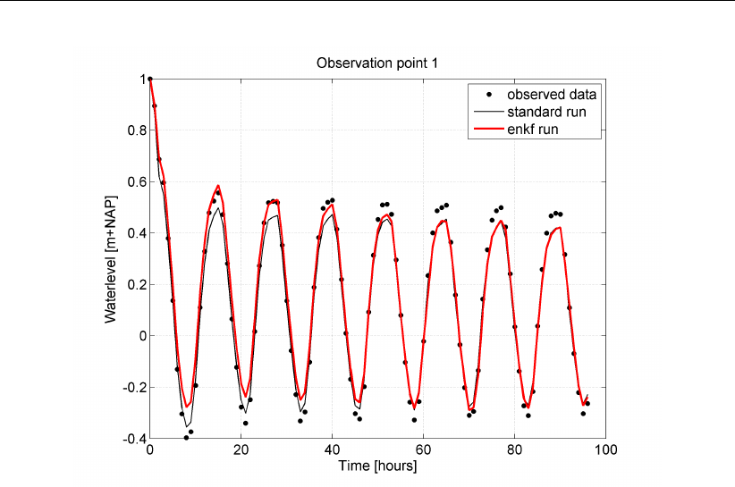
DRAFT
D-Flow Flexible Mesh, User Manual
Figure 20.1: Visualisation of the EnKF computation results from OpenDA for a certain
observation point. The dots represent the observed data, the black line rep-
resents the original computation with D-Flow FM (without Kalman filtering)
and the red line represents the D-Flow FM computation with Kalman filtering.
Step 5: Evaluate the outcomes
After having run the computation, output files have been generated in Matlab-format. The
relevant files are placed in the directory <estuary_kalman>. The data are stored in the
Matlab file <Enkf_results.m>. Visualisation could be accomplished like shown in Figure 20.1.
20.6.3 Example 3: EnKF with uncertainty in the inflow velocity
The geometry in this example is the same as for the calibration example: a two-dimensional
river model, the initial waterlevel is zero, the river bed is filled gradually due to the bound-
ary conditions. At the inflow boundary, a constant discharge is prescribed (along the line
<sw_east_dis_0001.pli>), whereas at the outflow boundary, a constant water level is pre-
scribed (along the line <sw_west_wlev_0001.cmp>).
There are 3 observation locations along the river (Obs01, Obs02 and Obs03). The mat-
lab script <plot_results_hisfile.m>is available to plot the water level as a function of time for
these 3 stations. Simulation time span is 100 days (Start: 199208310000, End: 199212090000).
The noise contribution is found in file <sw_east_dis_noise.pli>. Initially, no noise is present,
so the file contains zeroes in directory <input_dflowfm>.
20.6.4 Example 4: EnKF with uncertainty in the inflow condition for salt
The geometry in this example and the boundary conditions for waterlevel and velocity are
exactly the same as in simple_waal_kalman. The transport of salt is added to the com-
putation by a discharge boundary condition sw_east_dis_sal_001.pli and a noise
component added to this boundary.
314 of 412 Deltares

DRAFT
Calibration and data assimilation
20.6.5 Example 5: EnKF with uncertainty on the wind direction
This example is also converted from a Delft3D test case (d3d_lake_2d): a lake forced
by an uniform wind field. This example is a twin experiment with spatially correlated 2D-
noise added to the wind field. The noise is created on cartesian (equidistant grid), the noise
realisations are written by OpenDA to the <lake2d_windx_noise.amu>. The 2D noise field
is interpolated at computational grid by D-Flow FM and added to the uniform wind field. The
<SequentialSimulationNoise.oda>can be used to perform a single D-Flow FM run where
wind with noise is used as forcing. The resulting <lake2d_his.nc>file can be is used as
syntethic observations by the <stochObserver>.
20.6.6 Example 6: EnKF with the DCSM v5 model and uncertainty on the wind direction
This example is converted from the SIMONA DCSM v5 model with spatially correlated 2D-
noise added to the wind field.
Deltares 315 of 412

DRAFT
D-Flow Flexible Mesh, User Manual
316 of 412 Deltares

DRAFT
References
Bagnold, R. A., 1966. An approach to the sediment transport problem from general physics.
US government Print Office.
Bailard, J. A., 1981. “An Energetics Total Load Sediment Transport Model for Plane Sloping
Beaches.” Journal of Geophysical Research 86 (C11): 10938–10954.
Baptist, M. J., 2005. Modelling floodplain biogeomorphology. Ph.D. thesis, Delft University of
Technology.
Barenblatt, G. I., M. Bertsch, R. Dal Passo, V. M. Prostokishen and M. Ughi, 1993. “A mathe-
matical model of turbulent heat and mass transfer in stably stratified shear flow.” Journal of
Fluid Mechanics 253: 341–358.
Baumert, H. and G. Radach, 1992. “Hysteresis of Turbulent Kinetic Energy in Non-rotational
Tidal Flows: A Model Study.” Journal of Geophysical Research 97 (C3): 3669–3677.
Beckers, J. M., H. Burchard, J. M. Campin, E. Deleersnijder and P. P. Mathieu, 1998. “Another
reason why simple discretizations of rotated diffusion operators cause problems in ocean
models: comments on “isoneutral diffusion in a z co-ordinate ocean model”.” American
Meteorological Society 28: 1552–1559.
Bijker, E. W., 1967. Some considerations about scales for coastal models with moveable bed.
Tech. Rep. 50, WL | Delft Hydraulics, Delft, The Netherlands.
Blumberg, A. F. and G. L. Mellor, 1985. “Modelling vertical and horizontal diffusivities with the
sigma co-ordinate system.” Monthly Weather Review 113 (8): 1379.
Burchard, H. and H. Baumert, 1995. “On the performance of a mixed-large model based on
the k-epsilon turbulence closure.” Journal of Geophysical Research 100 (C5): 8523–8540.
Charnock, H., 1955. “Wind-stress on a water surface.” Q. J. Royal Meteorol. Soc. 81: 639–
640.
Christoffersen, J. B. and I. G. Jonsson, 1985. “Bed friction and dissipation in a combined
current and wave motion.” Ocean Engineering 12 (5): 387–423.
D-Flow FM TRM, 2015. D-Flow Flexible Mesh Technical Reference Manual. Deltares, Delft,
1.1.124 ed.
Davies, A. G., R. L. Soulsby and H. L. King, 1988. “A numerical model of the combined wave
and current bottom boundary layer.” Journal of Geophysical Research 93 (C1): 491–508.
Davies, A. M. and H. Gerritsen, 1994. “An intercomparison of three-dimensional tidal hydro-
dynamic models of the Irish Sea.” Tellus 46A: 200–221.
Dijkstra, Y. M., 2014. Turbulence modelling in environmental flows. Improving the accuracy
of the k-εmodel by a mathematical transformation. Master’s thesis, Delft University of
Technology. Faculty of Civil Engineering and Geosciences, Department of Environmental
Fluid Mechanics.
Dingemans, M. W., 1997. Water Wave Propagation over Uneven Bottoms, Vol. 1 and 2.
Advanced Series on Ocean Engineering, Vol. 13. World Scientific, London.
Dingemans, M. W., A. C. Radder and H. J. de Vriend, 1987. “Computation of the driving forces
of wave-induced currents.” Coastal Engineering 11: 539–563.
Eckart, C., 1958. “Properties of water, Part II. The equation of state of water and sea water at
low temperatures and pressures.” American Journal of Science 256: 225–240.
Deltares 317 of 412

DRAFT
D-Flow Flexible Mesh, User Manual
Fredsøe, J., 1984. “Turbulent boundary layer in wave-current interaction.” Journal of Hydraulic
Engineering 110: 1103–1120.
Gaeuman, D., E. Andrews, A. Krause and W. Smith, 2009. “Predicting fractional bed load
transport rates: Application of the Wilcock-Crowe equations to a regulated gravel bed river.”
Water Resources Research 45.
Gill, A. E., 1982. Atmosphere-Ocean dynamics, vol. 30 of International Geophysics Series.
Academic Press.
Grant, W. D. and O. S. Madsen, 1979. “Combined wave and current interaction with a rough
bottom.” Journal of Geophysical Research 84 (C1): 1797–1808.
Grasmeijer, B. and L. Van Rijn, 1998. “Breaker bar formation and migration.” Coastal Engi-
neering pages 2750–2758. Virginia, USA.
Groeneweg, J., 1999. Wave-current interactions in a generalized Lagrangian mean formula-
tion. Delft University of Technology, Delft, The Netherlands. Ph.D. thesis.
Haney, R. L., 1991. “On the pressure gradient force over steep topography in sigma co-
ordinate models.” Journal of Physical Oceanography 21: 610–619.
Hirsch, C., 1990. Numerical computation of internal and external flows. John Wiley & Sons,
New York.
Huang, W. and M. Spaulding, 1996. “Modelling horizontal diffusion with sigma coordinate
system.” Journal of Hydraulic Engineering 122 (6): 349–352.
Huynh-Thanh, S. and A. Temperville, 1991. “A numerical model of the rough turbulent bound-
ary layer in combined wave and current interaction.” In R. L. Soulsby and R. Bettes, eds.,
Sand transport in rivers, estuaries and the sea, pages 93–100. Balkema Rotterdam.
Hwang, P., 2005a. “Comparison of the ocean surface wind stress computed with different
parameterization functions of the drag coefficient.” J. Oceanogr. 61: 91–107.
Hwang, P., 2005b. “Drag coefficient, dynamic roughness and reference wind speed.” J.
Oceanogr. 61: 399–413.
Ikeda, S., 1982. “Incipient Motion of Sand Particles on Side Slopes.” Journal of the Hydraulics
Division, ASCE 108 (1): 95–114.
Ikeda, S., 1988. Not yet known.
Isobe, M. and K. Horikawa, 1982. “Study on water particle velocities of shoaling and breaking
waves.” Coastal Engineering in Japan 25: 109–123.
Kalkwijk, J. P. T. and R. Booij, 1986. “Adaptation of secondary flow in nearly horizontal flow.”
Journal of Hydraulic Research 24 (1): 19–37.
Karypis, G., 2013. METIS - A Software Package for Partitioning Unstructured Graph, Parti-
tioning Meshes, and Computing Fill-Reducing Orderings of Sparse Matrices, Version 5.1.0.
Tech. rep., Department of Computer Science and Engineering, University of Minnesota.
Klopstra, D., H. J. Barneveld and J. M. Van Noortwijk, 1996. Analytisch model hydraulis-
che ruwheid van overstroomde moerasvegetatie. Tech. Rep. PR051, HKV consultants,
Lelystad, The Netherlands. Commissioned by Rijkswaterstaat/RIZA, The Netherlands.
Klopstra, D., H. J. Barneveld, J. M. Van Noortwijk and E. H. van Velzen, 1997. “Analytical
model for hydraulic roughness of submerged vegetation.” In The 27th IAHR Congress, San
Francisco, 1997; Proceedings of Theme A, Managing Water: Coping with Scarcity and
Abundance, pages 775–780. American Society of Civil Engineers (ASCE), New York.
318 of 412 Deltares

DRAFT
References
Koch, F. G. and C. Flokstra, 1980. “Bed level computations for curved alluvial channels.” In
Proceedings of the XIXth congress of the International Association for Hydraulic Research,
2-7 Feb. 1981, New Delhi, India, vol. 2, pages 357–364.
Kolmogorov, A. N., 1942. “Equations of turbulent motion in incompressible fluid.” Izv. Akad.
Nauk. SSR, Seria fizicheska Vi No.1 2 (1-2): 56–58. English translation: 1968 Imperial
College, Mech. Eng. Dept. Rept. ON/6.
Lane, A., 1989. The heat balance of the North Sea. Tech. Rep. 8, Proudman Oceanographic
Laboratory.
Leendertse, J. J., 1990. “Turbulence modelling of surface water flow and transport: part IVa.”
Journal of Hydraulic Engineering 114 (4): 603–606.
Lesser, G., J. van Kester and J. A. Roelvink, 2000. On-line sediment transport within Delft3D-
FLOW. Tech. Rep. Z2899, wl.
Love, A. E. H., 1927. A Treatise on the Mathematical Theory of Elasticity. Cambridge Univer-
sity Press, 4th ed.
Millero, F. J. and A. Poisson, 1981. “International one-atmosphere equation of state of sea
water.” Deep-Sea Research 28A (6): 625–629.
Myrhaug, D. and O. H. Slaattelid, 1990. “A rational approach to wave-current friction coeffi-
cients for rough, smooth and transitional turbulent flow.” Coastal Engineering 14: 265–293.
Nipius, K. G., 1998. Transverse transport modelling using Bailard applied to Grevelingen-
mouth delta. Delft University of Technology, Delft, The Netherlands. M.Sc. thesis, in
Dutch (Dwarstransportmodellering m.b.v. Bailard toegepast op de Voordelta Grevelingen-
monding).
O’ Connor, B. A. and D. Yoo, 1988. “Mean bed friction of combined wave-current flow.” Coastal
Engineering 12: 1–21.
Octavio, K. A. H., G. H. Jirka and D. R. F. Harleman, 1977. Vertical Heat Transport Mecha-
nisms in Lakes and Reservoirs. Tech. Rep. 22, Massachusetts Institute of Technology.
Parker, G. and E. D. Andrews, 1985. “Sorting of bed load sediment by flow in meander bends.”
Water Resources Research 21: 1361–1373.
Partheniades, E., 1965. “Erosion and Deposition of Cohesive Soils.” Journal of the Hydraulics
Division, ASCE 91 (HY 1): 105–139. January.
Phillips, N. A., 1957. “A co-ordinate system having some special advantages for numerical
forecasting.” Journal of Meteorology 14: 184–185.
Postma, L., G. S. Stelling and J. Boon, 1999. “Three-dimensional water quality and hydro-
dynamic modelling in Hong Kong. Stratification and water quality.” In Proceedings of the
2nd International Symp. on Environmental Hydraulics, Hong Kong, December 1998, pages
43–49. Balkema, Rotterdam.
Prandtl, L., 1945. “Über ein neues Formelsystem für die ausgebildete Turbulenz.” Nachrichten
von der Akademie der Wissenschaften in Gottingen. Mathematisch-Physikalische Klasse
pages 6–19.
RGFGRID UM, 2016. Delft3D-RGFGRID User Manual. Deltares, 5.00 ed.
Richardson, J. F. and W. N. Zaki, 1954. “Sedimentation and fluidization: Part I.” I. Trans.
Institution of Chemical Engineers 32: 35–53.
Deltares 319 of 412

DRAFT
D-Flow Flexible Mesh, User Manual
Rienecker, M. M. and J. D. Fenton, 1981. “A Fourier approximation method for steady water
waves.” Journal of Fluid Mechanics 104: 119–137.
Rijn, L. C. van, 1984a. “Sediment transport, Part I: bed load transport.” Journal of Hydraulic
Engineering 110 (10): 1431–1456.
Rijn, L. C. van, 1984b. “Sediment transport, Part II: suspended load transport.” Journal of
Hydraulic Engineering 110 (11): 1613–1640.
Rijn, L. C. van, 1984c. “Sediment transport, Part III: bed form and alluvial roughness.” Journal
of Hydraulic Engineering 110 (12): 1733–1754.
Rijn, L. C. van, 1993. Principles of Sediment Transport in Rivers, Estuaries and Coastal Seas.
Aqua Publications, The Netherlands.
Rijn, L. C. van, 2001. General view on sand transport by currents and waves : data analysis
and engineering modelling for uniform and graded sand (TRANSPOR 2000 and CROS-
MOR 2000 models). Z2899.20 / Z2099.30 / Z2824.30. WL | Delft Hydraulics, Delft, The
Netherlands.
Rijn, L. C. van, 2003. “Sediment transport by currents and waves; general approximation
formulae Coastal Sediments.” In Corpus Christi, USA.
Rijn, L. C. van, 2007. “Unified View of Sediment Transport by Currents and Waves. I: Initiation
of Motion, Bed Roughness, and Bed-Load Transport.” Journal of Hydraulic Engineering
133 (6): 649–667.
Rijn, L. C. van, J. A. Roelvink and W. T. Horst, 2000. Approximation formulae for sand transport
by currents and waves and implementation in DELFT-MOR. Tech. Rep. Z3054.40, WL |
Delft Hydraulics, Delft, The Netherlands.
Rijn, L. C. van, D. R. Walstra and M. v. Ormondt, 2004. Description of TRANSPOR2004 and
implementation in Delft3D-ONLINE. Tech. Rep. Z3748.10, WL | Delft Hydraulics, Delft, The
Netherlands.
Rijn, L. van, D. Walstra, B. Grasmeijer, J. Sutherland, S. Pan and J. Sierra, 2003. “The
predictability of cross-shore bed evolution of sandy beaches at the time scale of storms
and seasons using process-based profile models.” Coastal Engineering 47: 295–327.
Rodi, W., 1984. “Turbulence models and their application in Hydraulics, State-of-the-art paper
article sur l’etat de connaissance.” IAHR Paper presented by the IAHR-Section on Funda-
mentals of Division II: Experimental and Mathematical Fluid Dynamics, The Netherlands.
Roelvink, J. A. and M. J. F. Stive, 1989. “Bar-generating cross-shore flow mechanisms on a
beach.” Journal of Geophysical Research 94 (C4): 4785–4800.
Ryan, P. J., D. R. F. Harleman and K. D. Stolzenbach, 1974. “Surface Heat Loss From Cooling
Ponds.” Water Resources Research 10 (5): 930–938.
Schrama, E., 2007. “Tides. Lecture Notes AE4-876.”
Slørdal, L. H., 1997. “The pressure gradient force in sigma-co-ordinate ocean models.” Inter-
national Journal Numerical Methods In Fluids 24: 987–1017.
Smith, S. D. and E. G. Banke, 1975. “Variation of the sea surface drag coefficient with wind
speed.” Quarterly Joournal of the Royal Meteorological Society 101: 665–673.
Soulsby, R., 1997. Dynamics of marine sands, a manual for practical applications. Thomas
Telford, London.
320 of 412 Deltares

DRAFT
References
Soulsby, R. L., A. G. Davies, J. Fredsøe, D. A. Huntley, I. G. Jonnson, D. Myrhaug, R. R.
Simons, A. Temperville and T. J. Zitman, 1993a. “Bed shear stresses due to combined
waves and currents.” In Abstracts-in-depth of the Marine Science and Technology G8-M
overall workshop, Grenoble., pages 2.1-1/2.1–4.
Soulsby, R. L., L. Hamm, G. Klopman, D. Myrhaug, R. R. Simons and G. P. Thomas, 1993b.
“Wave-current interaction within and outside the bottom boundary layer.” Coastal Engineer-
ing 21: 41–69.
Speziale, C. G., R. Abid and E. C. Anderson, 1992. “Critical evaluation of two-equation models
for near-wall turbulence.” AIAA Journal 30: 324–331.
Stelling, G. S. and J. A. T. M. van Kester, 1994. “On the approximation of horizontal gradi-
ents in sigma co-ordinates for bathymetry with steep bottom slopes.” International Journal
Numerical Methods In Fluids 18: 915–955.
Stive, M. J. F., 1986. “A model for cross-shore sediment transport.” In Proceedings 20th
International Coastal Engineering Conference, pages 1550–1564. American Society of Civil
Engineers, New York.
Swart, 1974. Offshore sediment transport and equilibrium beach profiles. Ph.D. thesis, Delft
University of Technology, Delft, The Netherlands. Delft Hydraulics Publ. 131.
Sweers, H. E., 1976. “A nomogram to estimate the heat exchange coefficient at the air-water
interface as a function of windspeed and temperature; a critical survey of some literature.”
Journal of Hydrology 30: –.
Talmon, A. M., N. Struiksma and M. C. L. M. van Mierlo, 1995. “Laboratory measurements of
the direction of sediment transport on transverse alluvial-bed slopes.” Journal of Hydraulic
Research 33 (4): 495–517.
Uittenbogaard, R. E., J. A. T. M. van Kester and G. S. Stelling, 1992. Implementation of
three turbulence models in 3D-TRISULA for rectangular grids. Tech. Rep. Z81, WL | Delft
Hydraulics, Delft, The Netherlands.
UNESCO, 1981a. Background papers and supporting data on the international equation of
state 1980. Tech. Rep. 38, UNESCO.
UNESCO, 1981b. The practical salinity scale 1978 and the international equation of state of
seawater 1980. Tech. Rep. 36, UNESCO. Tenth report of the Joint Panel on Oceanographic
Tables and Standards (1981), (JPOTS), Sidney, B.C., Canada.
Velzen, E. H. van, P. Jesse, P. Cornelissen and H. Coops, 2003. Stromingsweerstand vege-
tatie in uiterwaarden. Tech. Rep. 2003.029, Rijkswaterstaat/RIZA.
Walstra, D. J. R., J. A. Roelvink and J. Groeneweg, 2000. “Calculation of Wave-Driven Cur-
rents in a 3D Mean Flow Model.” In Proceedings 27th International Conference on Coastal
Engineering, Sydney, Australia, July 16-21, 2000.
Wilcock, P. and J. Crowe, 2003. “Surface-based transport model for mixed-size sediment.”
Journal of Hydraulic Engineering 129 (2): 120–128.
Winterwerp, J. C. and R. E. Uittenbogaard, 1997. Sediment transport and fluid mud flow.
Tech. Rep. Z2005, WL | Delft Hydraulics, Delft, The Netherlands.
Deltares 321 of 412

DRAFT
D-Flow Flexible Mesh, User Manual
322 of 412 Deltares

DRAFT
A The master definition file
The mdu-file contains the key information of the flow model. Besides the names of the relevant
user specified files, such as the grid file and the external forcings file, the values of various
model parameters should be specified in the MDU-file. The most important model parameter
settings are given in Table A.1 as well as the associated default setting for these parameters.
The basename of the mdu-file, without .mdu, is also used as the model identification string,
and is often denoted as mdu_name throughout this User Manual. It is equivalent to Delft3D-
FLOW’s runid concept.
Table A.1: Standard MDU-file with default settings.
Keyword Default setting Description
[model]
Program D-Flow FM Program
Version 1.1.134.38754Version
MDUFormatVersion 1.02 File format version. Do not edit this.
AutoStart 0 Autostart simulation after loading MDU or not
(0=no, 1=autostart, 2=autostartstop).
[geometry]
NetFile *_net.nc
BathymetryFile *.xyb
DryPointsFile Dry points file *.xyz, third column dummy z values,
or polygon file *.pol.
WaterLevIniFile Initial water levels sample file *.xyz
LandBoundaryFile Only for plotting
ThinDamFile *_thd.pli, Polyline(s) for tracing thin dams.
FixedWeirFile *_fxw.pliz, Polyline(s) x,y,z, z = fixed weir top lev-
els (formerly fixed weir)
VertplizFile *_vlay.pliz), = pliz with x,y, Z, first Z =nr of layers,
second Z = laytyp
ProflocFile *_proflocation.xyz) x,y,z, z = profile refnumber
ProfdefFile *_profdefinition.def) definition for all profile nrs
ProfdefxyzFile *_profdefinition.def) definition for all profile nrs
ManholeFile File containing manholes (e.g. *.dat)
PartitionFile *_part.pol, polyline(s) x,y
Uniformwidth1D 2. Uniform width for 1D profiles not specified bij
profloc
WaterLevIni 0. Initial water level
Bedlevuni -5. Uniform bed level, (only if bedlevtype>=3, used at
missing z values in netfile
Bedslope 0. bedslopeinclination, sets zk = bedlevuni +
x*bedslope ans sets zbndz = xbndz*bedslope
BedlevType 3 1: at cell center (tiles xz,yz,bl,bob=max(bl)), 2: at
face (tiles xu,yu,blu,bob=blu), 3: at face (using
mean node values), 4: at face (using min node
values), 5: at face (using max node values), 6:
with bl based on node values
Blmeanbelow -999. if not -999d0, below this level the cell centre
bedlevel is the mean of surrouding netnodes
Blminabove -999. if not -999d0, above this level the cell centre
bedlevel is the min of surrouding netnodes
AngLat 0. Angle of latitude S-N (deg), 0=no Coriolis
AngLon 0. Angle of longitude E-W (deg), 0=Greenwich
Conveyance2D -1 -1:R=HU,0:R=H, 1:R=A/P, 2:K=analytic-1D conv,
3:K=analytic-2D conv
(continued on next page)
Deltares 323 of 412

DRAFT
D-Flow Flexible Mesh, User Manual
Keyword Default setting Description
(continued from previous page)
Nonlin2D 0 Non-linear 2D volumes, only icm ibedlevtype = 3
and Conveyance2D>=1
Sillheightmin 0.0 Weir treatment only if both sills larger than this
value (m)
Makeorthocenters 0 1=yes, 0=no switch from circumcentres to ortho-
centres in geominit
Dcenterinside 1. limit cell center; 1.0:in cell <-> 0.0:on c/g
Bamin 1.d-6 Minimum gridcell area , icm cutcells
OpenBoundaryTolerance 3. Search tolerance factor between boundary poly-
line and grid cells. Unit: in cell size units (i.e., not
metres).
Kmx 0 Max nr of vertical layers
Layertype 1 1= all sigma, 2 = all z, 3 = use VertplizFile
Numtopsig 0 Nr of sigmalayers in top of Zlayer model
SigmaGrowthFactor 1. layer thickness growth factor from bed up
[numerics]
CFLMax 0.7 Max. Courant nr.
CFLWaveFrac 0.1 Wave velocity fraction, total courant vel = u +
cflw*wavevelocity
AdvecType 33 Adv type, 0=no, 1= Wenneker, qu-udzt, 2=1,
q(uio-u), 3=Perot q(uio-u), 4=Perot q(ui-u),
5=Perot q(ui-u) without itself
Lincontin 0 Default 0; Set to 1 for linearizing d(Hu)/dx; link to
AdvecType
TimeStepType 2 0=only transport, 1=transport + velocity update,
2=full implicit step_reduce, 3=step_jacobi, 4=ex-
plicit
Limtyphu 0 Limiter type for waterdepth in continuity eq., 0=no,
1=minmod,2=vanLeer,3=Kooren,4=Monotone
Central
Limtypmom 4 Limiter type for cell center ad-
vection velocity, 0=no, 1=min-
mod,2=vanLeer,3=Kooren,4=Monotone Central
Limtypsa 4 Limiter type for salinity transport, 0=no, 1=min-
mod,2=vanLeer,3=Kooren,4=Monotone Central
Maxdegree 6 Maximum degree in Gauss elimination
Vertadvtypsal 5 Vertical advection type for salinity, 0=No, 1=Up-
wexpL, 2=Centralexpl, 3=UpwimpL, 4=Cen-
traLimpL, 5=4 but 3 for neg. stratif., 6=higher
order expl, no forester
Icgsolver 4 Solver type , 1 = sobekGS_OMP, 2 =
sobekGS_OMPthreadsafe, 3 = sobekGS, 4
= sobekGS + Saadilud, 5 = parallel/global Saad,
6 = parallel/Petsc, 7 = parallel/GS
FixedWeirScheme 9 6 = semi-subgrid scheme, 8 = Tabellenboek, 9 =
Villemonte
FixedWeirContraction 1. flow width = flow width*FixedWeirContraction
Jbasqbnddownwindhs 0 0 : original hu on qbnd, 1 = downwind hs on qbnd
Izbndpos 0 Position of z boundary, 0=D3Dflow, 1=on net
boundary, 2 = on specifiend polyline
Tlfsmo 0. Fourier smoothing time on waterlevel boundaries
(s)
Slopedrop2D 0. Apply droplosses only if local bottom slope >
Slopedrop2D, <=0 =no droplosses
Chkadvd 0.1 Check advection terms if depth < chkadvdp, =>
less setbacks
Teta0 0.55 Teta of time integration, 0.5 < Teta < 1d0
(continued on next page)
324 of 412 Deltares

DRAFT
The master definition file
Keyword Default setting Description
(continued from previous page)
Qhrelax 1.d-2 Relaxation qhbnd ( )
cstbnd 0 Delft-3D type velocity treatment near boundaries
for small coastal models (1) or not (0)
Maxitverticalforestersal100 0 : no vertical filter, > 0 = Max nr of iterations
Maxitverticalforestertem0 0 : no vertical filter for temp, > 0 = Max nr of itera-
tions
Jaorgsethu 1 0 : setumod, sethu, setau sequence, 1 : sethu,
setau, setumod sequence (standard)
ilutype 0 0: parms-default
nlevel 0 0: parms-default
dtol 0. 0d0: parms-default
Epshu 1.d-4 Input for threshold water depth for wet and dry
cells
Maxwaterleveldiff 0. upper bound (in m) on water level changes, <= 0:
no bounds
Maxvelocitydiff 0. upper bound (in m/s) on velocity changes, <= 0:
no bounds
TransportMethod 1 Transport method
Turbulencemodel 3 0=no, 1 = constant, 2 = algebraic, 3 = k-eps, 4 =
k-tau
Turbulenceadvection 3 0=no, 3 = hor. expl., vert. impl.
[physics]
UnifFrictCoef 2.3d-2 Uniform friction coefficient, 0=no friction
UnifFrictType 1 0=Chezy, 1=Manning, 2=White-Colebrook,
3=idem, WAQUA style
UnifFrictCoef1D 2.3d-2 Uniform friction coefficient in 1D links, 0=no fric-
tion
UnifFrictCoefLin 0. Uniform linear friction coefficient for ocean models
(m/s), 0=no
Umodlin 0 linear friction umod , ifrctyp 4,5,6
Vicouv 1. Uniform horizontal eddy viscosity (m2/s)
Dicouv 1. Uniform horizontal eddy diffusivity (m2/s)
Vicoww 5.d-5 Uniform vertical eddy viscosity (m2/s)
Dicoww 5.d-5 Uniform vertical eddy diffusivity (m2/s)
Vicwminb 0. Minimum visc in prod and buoyancy term (m2/s)
Smagorinsky 0. Add Smagorinsky horizontal turbulence : vicu =
vicu + ( (Smagorinsky*dx)**2)*S, e.g. 0.1
Elder 0. Add Elder contribution : vicu = vicu + El-
der*kappa*ustar*H/6), e.g. 1.0
irov 0 0=free slip, 1 = partial slip using wall_ks
wall_ks 0. Nikuradse roughness for side walls,
wall_z0=wall_ks/30
Rhomean 1000. Average water density (kg/m3)
Idensform 0 1=Eckart, 2=UNESCO, 3=barocin case
Ag 9.813 Gravitational acceleration
TidalForcing 0 Tidal forcing (0=no, 1=yes) (only for jsferic == 1)
Doodsonstart 55.565 TRIWAQ = 55.565D0 , D3D = 57.555D0
Doodsonstop 375.575 TRIWAQ = 375.575D0 , D3D = 275.555D0
Doodsoneps 0.0 TRIWAQ = 0.0 400 cmps , D3D = 0.03 60 cmps
Salinity 0 Include salinity, (0=no, 1=yes)
InitialSalinity 0. Inital salinity concentration (ppt)
Sal0abovezlev -999. Salinity 0 above level (m)
DeltaSalinity -999. for testcases
Temperature 0 Include temperature, (0=no, 1=only transport,
5=heat flux model (5) of D3D), 3=excess model
of D3D
InitialTemperature 6. Inital temperature (degC)
(continued on next page)
Deltares 325 of 412

DRAFT
D-Flow Flexible Mesh, User Manual
Keyword Default setting Description
(continued from previous page)
Secchidepth 2. Water clarity parameter (m)
Stanton 0.0013 Coefficient for convective heat flux ( ), if negative,
use Cd wind
Dalton 0.0013 Coefficient for evaporative heat flux ( ), if negative,
use Cd wind
SecondaryFlow 0 Secondary flow (0=no, 1=yes)
[wind]
ICdtyp 2 ( ),1=const, 2=S&B 2 breakpoints, 3= S&B 3
breakpoints, 4=Charnock constant
Cdbreakpoints 6.3d-4
7.23d-3
( ), e.g. 0.00063 0.00723
Windspeedbreakpoints 0. 100. (m/s), e.g. 0.0 100.0
Rhoair 1.205 Air density (kg/m3)
PavBnd 0. Average air Pressure on open boundaries,
(N/m2), only applied if value > 0
[time]
RefDate 20010101 Reference date (yyyymmdd)
Tzone 0. Data Sources in GMT are interrogated with time
in minutes since refdat-Tzone*60
Tunit S Time units in MDU (H, M or S)
DtUser 300. User timestep in seconds (interval for external
forcing update & his/map output)
DtMax 30. Max timestep in seconds
DtInit 1. Initial timestep in seconds
TStart 0. Start time w.r.t. RefDate (in TUnit)
TStop 8640000. Stop time w.r.t. RefDate (in TUnit)
[restart]
RestartFile Restart file, only from netcdf-file, hence: either
*_rst.nc or *_map.nc
RestartDateTime Restart time (YYYYMMDDHHMMSS), only rele-
vant in case of restart from *_map.nc
[externalforcing]
ExtForceFile Old format for external forcings file *.ext, link with
tim/cmp-format boundary conditions specification
ExtForceFileNew New format for external forcings file *.ext, link with
bc -format boundary conditions specification
[output]
OutputDir Output directory of map-, his-, rst-
, dat- and timings-files, default:
DFM_OUTPUT_<modelname>. Set to . for
no dir/current dir.
ObsFile *.xyn Coords+name of observation stations.
CrsFile *_crs.pli Polyline(s) definining cross section(s).
HisFile *_his.nc History file in NetCDF format.
HisInterval 120. History output, given as ’interval’ ’start period’
’end period’ (s)
XLSInterval 0. Interval (s) between XLS history
FlowGeomFile *_flowgeom.nc Flow geometry file in NetCDF for-
mat.
MapFile *_map.nc Map file in NetCDF format.
MapInterval 1200. Map file output, given as ’interval’ ’start period’
’end period’ (s)
(continued on next page)
326 of 412 Deltares

DRAFT
The master definition file
Keyword Default setting Description
(continued from previous page)
MapFormat 1 Map file format, 1: netCDF, 2: Tecplot, 3: netCFD
and Tecplot
Heatfluxesonoutput 0 1=yes,0=no
Richardsononoutput 0 1=yes,0=no
RstInterval 86400. Restart file output, given as ’interval’ ’start period’
’end period’ (s)
S1incinterval 0. Interval (m) in incremental file for waterlevels S1
WaqFileBase Basename (without extension) for all Delwaq files
to be written.
WaqInterval 0. Interval (in s) between Delwaq file outputs
StatsInterval 0. Interval (in s) between simulation statistics output.
Writebalancefile 0 Write Balancefile, 1=yes, 0=no
TimingsInterval 0. Timings output interval
TimeSplitInterval 0X Time splitting interval, after which a new output
file is started. value+unit, e.g. ’1 M’, valid units:
Y,M,D,h,m,s.
MapOutputTimeVector File (.mpt) containing fixed map output times (s)
w.r.t. RefDate
FullGridOutput 0 0:compact, 1:full time-varying grid data
SnapshotDir figures Directory where snapshots/screendumps are
saved.
Deltares 327 of 412

DRAFT
D-Flow Flexible Mesh, User Manual
328 of 412 Deltares

DRAFT
B Attribute files
B.1 Introduction
In the following sections we describe the attribute files used in the input file (MDU-file) of D-
Flow FM. Most of these files contain the quantities that describe one specific item, such as
the location of open boundaries, or time dependent data of fluxes discharged in the model
area by discharge stations. Most of the attribute files can be generated by the Delta Shell GUI
after defining an input scenario. Some files can almost only be generated by utility programs
such as the unstructured grid generated by RGFGRID. Still, we describe both type of files as
it might be useful to know how the input data is structured to be able to generate (large) files,
such as astronomic boundary conditions, or time-series for wind speed and direction by client
specific tools.
B.2 Polyline/polygon file
D-Flow FM uses the same format for polylines and (closed) polygons. When used as a poly-
gon file, there is not the requirement that the first and last point should be identical. It is
good modelling practice to name files containing polygons with the extension .pol, and files
containing polylines with the extension .pli. When the polylines have a third column with
z-coordinates, the extension .pliz is advised.
File contents The coordinates of one or more polylines. Each polyline (piecewise
linear) is written in a single block of data.
Filetype ASCII
File format Free formatted
Filename <name.pol>
Generated RGFGRID, QUICKIN, Delta Shell, etc
Record description:
Record Record description
Preceding description records, starting with an asterisk (∗), and will
be ignored.
1 A non blank character string, starting in column one.
2 Two integers Nr, Ncrepresenting the numbers of rows and number
of columns for this block of data.
Two reals representing the x, y or λ, φ-coordinate, followed by re-
maining data values at that location (if Nc>2).
Example:
*
*Polyline L007
*
L007
6 2
132400.0 549045.0
132345.0 549030.0
132165.0 549285.0
131940.0 549550.0
Deltares 329 of 412

DRAFT
D-Flow Flexible Mesh, User Manual
131820.0 549670.0
131585.0 549520.0
*
*Polyline L008
*
L008
4 2
131595.0 549685.0
131750.0 549865.0
131595.0 550025.0
131415.0 550175.0
*
*Polyline L009
*
L009
6 2
131595.0 549655.0
148975.0 564595.0
150000.0 564935.0
152105.0 565500.0
153150.0 566375.0
154565.0 567735.0
B.3 Sample file
Sample file are used for several of D-Flow FM’s input files.
File contents The location and value of samples.
Filetype ASCII
File format Free formatted
Filename <name.xyz>
Generated Manually or Offline with QUICKIN or Delta Shell and data from digi-
tised charts or GIS-database.
Record description:
Filetype Record description
Free formatted Location and sample value per row
Two reals representing the x, y or λ, φ-coordinate and one real rep-
resenting the sample value
Example:
Sample file with 12 sample values with their location (free formatted file).
213813.2 603732.1 -4.053000
214686.0 607226.1 -4.522000
214891.7 610751.2 -5.000000
210330.8 601424.1 -2.169000
211798.0 604444.8 -2.499000
212460.0 607475.7 -2.760000
212436.9 610362.5 -2.865000
185535.4 606607.9 1.360000
186353.0 603789.4 1.122000
187959.2 601197.6 0.9050000
190193.0 599101.5 0.7050000
208578.7 602513.7 -0.7990000
330 of 412 Deltares

DRAFT
Attribute files
B.4 Time series file (ASCII)
Time series files are used for several of D-Flow FM’s input files. There is no header, except for
optional comment lines. There should be two or more columns: the first column contains time
in minutes since the model’s reference date, all remaining columns contain the data values.
Each line contains a single time with its (space-uniform) values.
B.5 The external forcings file
Two definition files for the external forcings are supported, each with their own format.
B.5.1 Old style external forcings
The name of the file is specified in the MDU-file as "ExtForceFile". External forcings
are specified in in blocks key-value pairs, e.g.
*comments
*comments
QUANTITY =waterlevelbnd
FILENAME =tfl_01.pli
FILETYPE =9
METHOD =3
OPERAND =O
QUANTITY = ...
FILENAME = ...
...
The format is not case-sensitive, but key-value pairs are expected in the particular order
shown below. Accepted keywords are:
Deltares 331 of 412

DRAFT
D-Flow Flexible Mesh, User Manual
quantity character Name of the quantity, see the list below
filename character File associated with this forcing
sourcemask∗character File containing a mask
filetype integer Indication of the filetype:
1. Time series (D.2.1)
2. Time series magnitude and direction
3. Spatially varying weather
4. ArcInfo
5. Spiderweb data (cyclones) (B.12.3)
6. Curvilinear data (B.12.2)
7. Samples (B.3)
8. Triangulation magnitude and direction
9. Polyline (<∗.pli>-file, B.2)
11. NetCDF grid data (e.g. meteo fields)
14. NetCDF wave data
method integer Method of interpolation:
1. Pass through (no interpolation)
2. Interpolate time and space
3. Interpolate time and space,
save weights
4. Interpolate space
5. Interpolate time
7. Interpolate/Extrapolate time
operand integer
value∗float custom coefficients for transformation
factor∗float
ifrctyp∗float
averagingtype∗float
relativesearchcellsize∗float
extrapoltol∗float
area∗float Area for source/sink
Note: Keywords marked with ∗are optional
B.5.2 New style external forcing (boundary conditions only)
The name of the file is specified in the MDU-file as "ExtForceFileNew". External forcings
are specified in the ini-file format in blocks headed by [boundary], followed by a list of key-
value pairs in random order, e.g.
*comments
[boundary]
quantity=waterlevelbnd
locationfile=tfl_01.pli
forcingfile=tfl_01.bc
[boundary]
quantity= ...
...
Accepted keywords are:
332 of 412 Deltares
DRAFT
Attribute files
quantity character Name of the quantity, see the list below (boundaries only)
locationfile character Boundary polyline <∗.pli>
forcingfile character BC-file with boundary data <∗.bc>
character NetCDF-file with boundary time series <∗.nc>
return_time∗float Thatcher-Harleman (section 8.4.4) return time
(default=0, meaning Thatcher-Harleman disabled).
Note: Keywords marked with ∗are optional
B.5.3 Accepted quantity names
Most members on the list of accepted quantity names can be sorted in either of five categories:
Boundary conditions
Meteorological fields
Structure parameters
Initial fields
Spatial physical properties
Table B.1: List of accepted external forcing quantity names.
Quantity pg. Description
Boundary conditions:
waterlevelbnd 123 Water level
neumannbnd 125 Water level gradient
riemannbnd 126 Riemann invariant
outflowbnd
velocitybnd 124 Velocity
dischargebnd 124 Discharge
riemann_velocitybnd Riemann invariant velocity
salinitybnd 155 Salinity
temperaturebnd 155 Temperature
sedimentbnd 227 Suspended sediment
uxuyadvectionvelocitybnd
normalvelocitybnd,
tangentialvelocitybnd
131 Normal and tangential velocity
qhbnd 127 Discharge-water level dependency
tracerbnd<tracername>155 User-defined tracer
Meteorological fields:
windx, windy, windxy 180 Wind components, wind vector
airpressure_windx_windy 180 Atmospheric pressure and wind components
atmosphericpressure 180 Atmospheric pressure
rainfall Precipitation
humidity_airtemperature...
..._cloudiness
humidity_airtemperature...
..._cloudiness_solarradiation
discharge_salinity...
..._temperature_sorsin
154 Discharge, salinity and heat sources
Structure parameters:
pump 45 Pump capacity
damlevel
gateloweredgelevel
generalstructure
Initial fields:
Deltares 333 of 412

DRAFT
D-Flow Flexible Mesh, User Manual
Quantity pg. Description
initialwaterlevel 357
initialsalinity 357
initialsalinitytop 357
initialtemperature 357
initialverticaltemperatureprofile357
initialverticalsalinityprofile 357
initialtracer<tracername>357
Spatial physical properties: 358
frictioncoefficient
horizontaleddyviscositycoefficient
horizontaleddydiffusivitycoefficient
advectiontype
ibotlevtype
Miscelaneous:
shiptxy
movingstationxy 368 Moving observation point for output (time,x,y)
B.6 Trachytopes
The trachytope functionality allows for the usage of different types of roughness formulations at different
locations within the computational domain. Multiple formulation may be active in the same grid cell.
Several keywords in the MDU file influence the functioning. All keywords below should be placed
underneath the [trachytopes] section in the MDU file.
Keyword Value Description Default
TrtRou Y or N Trachytope option activated N
TrtDef <name.ttd>Definition file trachytopes
Trtl <name.arl>Area Roughness on Link file trachy-
topes
DtTrt pos. real Time step in seconds for updat-
ing roughness and resistance coef-
ficients based on trachytopes. Must
be a multiple of DtUser.
1DtUser
TrtMnH pos. real Minimum water depth in roughness
computation
.2 Epshu
TrtMth 1 or 2 Area averaging method 1
TrtAsr real ∈[0,1] Serial factor in averaging of area
roughnesses
0.6
TrtMxR integer Maximum recursion depth for mixed
trachytope definitions
8
334 of 412 Deltares

DRAFT
Attribute files
B.6.1 Area Roughness on Links (ARL-file)
File contents The Area Roughness on Links file (ARL-file) is the input file for the spatial
distribution of the alluvial and vegetation roughness which are handled by
the trachytopes module.
Filetype ASCII
File format Space separated file format
Filename <name.arl>
Generated At present: Conversion possible from structured Delft3D-FLOW input files
with matlab conversion tool from Open Earth Tools (http://www.openearth.
info/), see example below ( section B.6.1.2).
The ARL file has the following properties:
A single line comment, starts with a hash tag “#” or an asterisk “*”.
Each line has the format
“xu yu zu TrachytopesNr Fraction”,
where xu,yu,zu is the coordinate of the midpoint of the netlink,
TrachytopeNr is an integer corresponding to the number as described in the TrachyTopes
Definition File (cf. section B.6.2),
and Fraction is a Fraction between 0.0 and 1.0
A line with a midpoint-netlink-coordinate which is the same as the preceding line (comments not
considered) allows multiple types of trachytopes roughness definitions, provided the sum of the
Fraction keywords does not add to a value greater than 1.0.
If the sum is less than 1.0 the background roughness prescribed in the [physics] chapter in
the MDU file is prescribed for the remaining Fraction, cf. Appendix A. Only a single roughness
type is allowed in combination with the Trachytopes module.
If a midpoint-netlink-coordinate is repeated in the .arl file with the midpoint-netlink-coordinate xu,
yu,zu in the preceding line being different, all previous instances of the specific xu,yu,zu are
ignored.
B.6.1.1 Example
An example of the <arl>file is given below based on the <ttd>file given in section B.6.2. In this case
the netlink with u point located at xu= 10.542 and yu= 11.6, which is covered for 30 %, 30 % 20 %
and 20 % for TrachytopeNr = 1, 2, 4 and 3 respectively.
(continued)
...
10.542 11.6 0 1 0.3
10.542 11.6 0 2 0.3
10.542 11.6 0 4 0.2
10.542 11.6 0 3 0.2
...
(continued)
B.6.1.2 Conversion from Delft3D input files
Open Earth Tools has different matlab tools available for the conversion of Delft3D models to D-
Flow FM models (e.g. dflowfmConverter.m and d3d2dflowfm.m).
An extra Matlab conversion script has been added to convert Delft3D’s <∗.aru>and <∗.arv>files to
<∗.arl>files for D-Flow FM:
d3d2dflowfm_friction_trachytopes.m.
It can be called as follows:
oetsettings
d3d2dflowfm_friction_trachytopes(filgrd,filaru,filarv,filnet,filarl)
Deltares 335 of 412

DRAFT
D-Flow Flexible Mesh, User Manual
where the variables are defined as follows:
filgrd delft3d grid filename (*.grd)
filaru delft3d area definition file in u-direction (*.aru)
filarv delft3d area definition file in v-direction (*.arv)
filnet name of the dflowfm network file (*_net.nc)
filarl name of the dflowfm trachytope file (*.arl))
B.6.2 Trachytope Definition file (TTD-file)
The trachytope definition file contains lines of the following format defining the different types of trachy-
topes. The types which are supported are general, discharge dependent and water-level dependent
formats.
B.6.2.1 General format
The general format is formatted as follows:
TrachytopeNr FormulaNr ...Parameters...
where ...Parameters... indicates a space separated list of formula specific parameters; the
parameters required and their order are specified in section B.6.2.5. The user must specify for each
trachytope (combination of formula number and parameters) a unique positive trachytope number. This
trachytope number is used in the area files (see section B.6.1) to indicate the roughness types on a
net link.
B.6.2.2 Example
An example of such a file where the first three codes 1–3 with a Nikuradse roughness height are
defined, and the fourth (code 4) is Chézy roughness height.
1 51 0.1
2 51 0.2
3 51 0.3
4 52 35
B.6.2.3 Discharge dependent format
The discharge dependent format is formatted as follows:
TrachytopeNr DISCHARGE "Cross-section name"
TrachytopeNr Q1 FormulaNr ...Parameters...
TrachytopeNr Q2 FormulaNr ...Parameters...
TrachytopeNr Q3 FormulaNr ...Parameters...
TrachytopeNr Q4 FormulaNr ...Parameters...
...
which again expects a user defined TrachytopeNr. The first row contains the keyword “DIS-
CHARGE” and subsequently a cross-section name occuring in CrsFile in the mdu-file.
The cross-section name can be enclosed by quotation marks, for instance when the cross-section
name is made up of more than one word. The subsequent rows all have the same TrachytopeNr
as the first row and furthermore every FormulaNr should be the same. The list of discharges Q1,
Q2, Q3, Q4 should be monotonically increasing.
The ...Parameters... for each formula type are specified in section B.6.2.5.
336 of 412 Deltares

DRAFT
Attribute files
B.6.2.4 Water level dependent format
The water-level dependent format is similar to the discharge dependent format and is formatted as
follows:
TrachytopeNr WATERLEVEL "Observation-station name"
TrachytopeNr ZS1 FormulaNr ...Parameters...
TrachytopeNr ZS2 FormulaNr ...Parameters...
TrachytopeNr ZS3 FormulaNr ...Parameters...
TrachytopeNr ZS4 FormulaNr ...Parameters...
...
which again expects a user defined TrachytopeNr. The first row contains the keyword “WA-
TERLEVEL” and subsequently an observation-station name occuring in ObsFile in the mdu-file. The
observation-statopm name can be enclosed by quotation marks, for instance when the observation-
station name is made up of more than one word. The subsequent rows all have the same TrachytopeNr
as the first row and furthermore every FormulaNr should be the same. The list of waterlevels ZS1,
ZS2, ZS3, ZS4 should be monotonically increasing.
The ...Parameters... for each formula type are specified in section B.6.2.5.
Deltares 337 of 412

DRAFT
D-Flow Flexible Mesh, User Manual
B.6.2.5 Supported roughness formulations
The roughness formulations specified in the table below are supported by D-Flow FM. These formula-
tions are specified in the .ttd by FormulaNr and ...Parameters... in the order in which they
appear in the table below. The related formulae are presented in the Technical Reference Manual
FormulaNr Description Parameters
Special classes (1–50)
1 flood protected area, reduces the effective area
of the grid cell. It has no influence on the continu-
ity equation (i.e. it does not decrease the surface
area of the grid cell).
–
2 composite trachytope: fraction αof type T1and
fraction β(generally β= 1 −α) of type T2
T1,T2,α,β
Area trachytope classes: simple type (51–100)
51 constant White-Colebrook/Nikuradse value k[m]
52 constant Chézy value C[m1/2/s]
53 constant Manning value n[s/m1/3]
54 constant z0value z0[m]
61 constant White-Colebrook/Nikuradse values for
ebb and flood
kebb [m], kflood [m]
62 constant Chézy values for ebb and flood Cebb [m1/2/s], Cflood [m1/2/s]
63 constant Manning values for ebb and flood nebb [s/m1/3], nflood [s/m1/3]
64 constant z0values for ebb and flood z0,ebb [m], z0,flood [m]
Area trachytope classes: alluvial type (101–150)
101 simplified Van Rijn A[m0.3], B[m0.3]
102 power relation A[m1/2/s], B[-]
1031Van Rijn predictor -
1041Struiksma predictor A1[m1/2/s], A2[-], θc[-], θm
[-], Cmin [m1/2/s]
1051bedforms quadratic -
1061bedforms linear -
Area trachytope classes: vegetation type (151–200)
151 Barneveld 1 hv[m], n[1/m]
152 Barneveld 2 hv[m], n[1/m], CD[-], kb[m]
153 Baptist 1 hv[m], n[1/m], CD[-], Cb
[m1/2/s]
154 Baptist 2 hv[m], n[1/m], CD[-], Cb
[m1/2/s]
Linear trachytope classes: various (201–250)
201 hedges 1 hv[m], n[1/m]
202 hedges 2 hv[m], n[1/m]
Linear trachytope classes: various (251–300)
251 trees hv[-], CD[-]
1The alluvial roughness predictors 103, 104, 105 and 106 are not yet supported, because the coupling with
the morphology module is not yet available.
338 of 412 Deltares

DRAFT
Attribute files
B.7 Weirs
A fixed weir has many quantitites. On a polyline several quantitites has to be specified. In the table
below an overview is given of all these quantities.
Keyword Description Default value
X-coordinate X-coordinate of polyline point -
y-coordinate Y-coordinate of polyline point -
Crest level crest height - [m]
Sill up Sill height at left/bottom side 0.0 [m]
Sill down Sill height at right/top 0.0 [m]
Crest length length of weir in perpendicular direc-
tion
3.0 [m]
Talud up Slope of weir at left/bottom side 4.0 [-]
Talud down Slope of weir at right/top 4.0 [-]
Vegetation
coefficient
Friction due to vegetation on weir 0.0 [-]
Weir type (v)illemonte or (t)abellenboek v [-]
The last column with the weir type (Villemonte or Tabellenboek) is optional. In this way, individual poly-
line can be given another weir type. For example, if FixedweirType=9 (Villemonte) has been specified
in the MDU-file, then individual polylines can be set to Tabellenboek by adding a "t" to all points in the
polyline; see the example below.
B.7.0.1 Example
An example of a polyline with fixed weir input is given below. It consists of a polyline with two points
(continued)
...
weir
2 10
399.999420 99.997688 2.0 0.2 0.8 3.0 4.0 4.0 0 t
399.999420 100.999542 2.1 0.3 0.9 3.0 4.0 4.0 0 t
...
(continued)
In general, fixed weir polylines do not coincide with the computational grid. The polylines are snapped
to flow links, which is illustrated in Figure 4.15. This is computed by the computational kernel of D-
Flow FM.
In practice, it is possible that a certain flow link contains multiple snapped fixed weirs. This is for
example the case when polylines with fixed weirs cross each other. Then, the fixed weir with the
highest crest level is taken, because the crest level is used in the drying-flooding algorithm. In this way,
overtopping of a weir the water level only occurs if the water level is above the weir with the highest
crest level.
Deltares 339 of 412

DRAFT
D-Flow Flexible Mesh, User Manual
B.8 Calibration Factors
The calibration factor functionality is a multiplier for the rouhgness at different locations within the com-
putational domain. Multiple formulation may be active in the same grid cell. Several keywords in the
MDU file influence the functioning. All keywords below should be placed under the [calibration]
section in the MDU file.
Keyword Value Description Default
UseCalibration1 or 0 Calibration factor option activated N
DefinitionFile<name.cld>Calibration factor definition file
AreaFile <name.cll>Calibration factor area file
B.8.1 Calibration factor definition file (CLD-file)
The calibration class definition file contains lines of the following format defining the different calibration
classes. It supports constant values and values that depend on the discharge at a named cross section
or the water level at a named location.
B.8.1.1 Header of the CLD-file
The file starts with the following header
# [FileInformation]
# FileType = CalibrationFactorsDefinitionFile
# FileVersion = 1.0
# [CalibrationFactors]
B.8.1.2 Constant values
The format for constant values is as follows:
CalibrationClassNr ConstantValue
where ConstantValue indicates the calibration value to be used (use 1.0 to use the uncalibrated
roughness). The user must specify for each calibration class (line in this file) a unique calibration class
number CalibrationClassNr. This calibration class number is used in the calibration area <.cll>
file to indicate the area of influence of this class.
B.8.1.3 Discharge dependent format
The discharge dependent line is formatted as follows:
CalibrationClassNr DISCHARGE "Cross-section name"
CalibrationClassNr Q1 ConstantValueAtQ1
CalibrationClassNr Q2 ConstantValueAtQ2
CalibrationClassNr Q3 ConstantValueAtQ3
CalibrationClassNr Q4 ConstantValueAtQ4
...
which again expects a user defined calibration class number CalibrationClassNr. The first line
contains the keyword DISCHARGE and subsequently a cross-section name occurring in the CrsFile in
the mdu-file. The cross-section name can be enclosed by quotation marks, for instance when the name
340 of 412 Deltares

DRAFT
Attribute files
contains spaces. The subsequent lines all start with the same calibration class number as the first line.
The list of discharges Q1,Q2,Q3, and Q4 should be monotonically increasing. For each discharge
value a calibration value should be specified. Between the discharges specified, the calibration values
are linearly interpolated. Below the minimum and above the maximum discharge the first and last
values are used respectively.
B.8.1.4 Water level dependent format
The water-level dependent format is similar to the discharge dependent format and is formatted as
follows:
CalibrationClassNr WATERLEVEL "Observation-station name"
CalibrationClassNr ZS1 ConstantValueAtZS1
CalibrationClassNr ZS2 ConstantValueAtZS2
CalibrationClassNr ZS3 ConstantValueAtZS3
CalibrationClassNr ZS4 ConstantValueAtZS4
...
which again expects a user defined calibration class number CalibrationClassNr. The first
line contains the keyword WATERLEVEL and subsequently an observation-station name occurring
in ObsFile in the mdu-file. The observation-station name can be enclosed by quotation marks, for
instance when the name contains spaces. The subsequent lines all start with the same calibration
class number as the first line. The list of water levels ZS1,ZS2,ZS3, and ZS4 should be monotonically
increasing. For each water level value a calibration value should be specified. Between the water levels
specified, the calibration values are linearly interpolated. Below the minimum and above the maximum
water level the first and last values are used respectively.
B.8.1.5 Example
The example file given below defines three calibration classes. In the area associated with the first
class, the roughness values are used without any adjustment. In the area associated with the second
class, the roughness value is decreased by 20%. In the area associated with the third and final class,
the increase in the roughness value varies between 0% and 30% depending on the discharge at a
specific location.
# [FileInformation]
# FileType = CalibrationFactorsDefinitionFile
# FileVersion = 1.0
# [CalibrationFactors]
# areas without any calibration adjustment
1 1.0
# areas with 20% decreased roughness value
2 0.8
# area with calibration depending on discharge at crsX
10 DISCHARGE ’crsX’
10 500 1.0
10 1000 1.1
10 3000 1.3
B.8.2 Calibration Class Area on Links (CLL-file)
Deltares 341 of 412

DRAFT
D-Flow Flexible Mesh, User Manual
B.8.2.1 Header of the CLL-file
The file starts with the following header
# [FileInformation]
# FileType = CalibrationAreasFile
# FileVersion = 1.0
# [CalibrationAreas]
B.8.2.2 Body of the CLL-file
The body of the CLL-file consists of comment lines (any line starting with # or *) or data lines of the
following format:
xu yu zu CalibrationClassNr AreaFraction
where xu,yu,zu is the coordinate of the midpoint of the netlink, CalibrationClassNr is an inte-
ger corresponding to the number as described in the Calibration Class Definition File (cf. section B.8.1),
and AreaFraction is an area fraction between 0.0 and 1.0.
All lines that list the same xu,yu,zu coordinates are combined to a weighted average of multiple
calibration classes, provided the sum of the fractions does not add to a value greater than 1.0.
If the sum of the areas specified for a certain netlink is less than 1.0, then the a constant calibration
factor of 1.0 is assumed for the remaining area (i.e. no calibration effect). The result is that if for a
specific netlink no line is specified at all, then the roughness of this netlink will be unaffected by the
calibration process.
B.8.2.3 Example
The example of the <CLL>-file is given below based on the <CLD>-file given in section B.8.1. In
this case the roughness at netlink with midpoint located at xu = 10.542 and yu = 11.6 is completely
affected by calibration class 1, the netlink with midpoint at xu = 11.120 and yu = 12.1 is affected for
60% by calibration class 1 and 40% by calibration class 10, and the final location listed uses only the
value resulting from calibration class 10.
...
10.542 11.6 0 1 1.0
11.120 12.1 0 1 0.6
11.120 12.1 0 10 0.4
12.635 12.6 0 10 1.0
...
B.9 Sources and sinks
Sources and sinks (section 7.8) are defined as part of the <∗.ext>file, as follows:
QUANTITY=discharge_salinity_temperature_sorsin
FILENAME=chan1_westeast.pli # A file ’chan1_westeast.tim’, with same basename
# as the polyline should be present
FILETYPE=9
METHOD =1
OPERAND =O
AREA =1.5
342 of 412 Deltares

DRAFT
Attribute files
The <∗.pli>file is a polyline file (section B.2) with two or three columns (for 2D or 3D models, re-
spectively). Along with the <∗.pli>-file, there has to be a time series file (section D.2.1) with the same
basename as the <∗.pli>-file, and extension <.tim>. The columns in the <∗.tim>are as follows:
time in minutes, discharge Qin [m3/s], and all constituents in the model. The order of consituents is:
salinity in [ppt], temperature Tin [◦C], sediment concentrations, spiral flow intensity and tracers. For
example, if we only have temperature and two tracers we get 5 columns: time, discharge, temperature,
tracer 1, tracer 2.
B.10 Dry points and areas
Dry points can either be defined by a basic sample file (see section B.3), or a polygon file (see sec-
tion B.2).
Special attention must be given to the optional third column of a polygon file: when the first point has
az-value of −1, the polygon mask is inverted, i.e., all points outside the polygon are set as dry points.
More details can be found in section 4.4.2.7.
B.11 Structure INI file
Hydraulic structures are defined in a <structures.ini>file. Each structures is defined in its own
[structure] section, followed by a set of key-value parameters that depend on the type of struc-
ture:
[structure]
type = weir # Type of structure
id = weir01 # Name of the structure
polylinefile = weir01.pli # *.pli; Polyline location for structure
crest_level = weir01_crest.tim # Crest level in [m]
[structure]
type = gate # Type of structure
id = gate01 # Name of the structure
polylinefile = gate01.pli # *.pli; Polyline location for structure
sill_level = gate01_crest.tim # Sill (crest) level in [m]
sill_width = 39.5 # (Optional) sill width in [m], between
# the fixed side walls.
door_height = 8.54 # Gate door height in [m], used for
# detecting flow across door.
lower_edge_level = gate01_ledge.tim # Position of gate’s lower edge in [m],
# used for flow underneath door.
opening_width = gate01_opening.tim # (Optional) opening width between two
# sideways closing gate doors.
horizontal_opening_direction = from_left/from_right/symmetric # (Optional) Opening
# direction of the gate door(s).
[structure]
type = pump # Type of structure
id = pump01 # Name of the structure
polylinefile = pump01.pli # *.pli; Polyline location for structure
capacity = pump01_cap.tim # Pumping capacity in [m3/s]
B.12 Space varying wind and pressure
In many cases the space varying wind data is provided by a meteorological station. This data is often
defined on a different grid than the computational grid used in D-Flow FM. Translating these files into
files defined on the grid of the computational engine is often a lengthy process and can result in huge
files. This feature facilitates the reading of the meteorological data on its own grid and interpolates the
data internally to the grid of D-Flow FM. D-Flow FM can handle three types of meteorological input:
Deltares 343 of 412

DRAFT
D-Flow Flexible Mesh, User Manual
1 Time- and space-varying wind on an equistant grid
2 Time- and space-varying wind on a curvilinear grid
3 Time- and space-varying wind on a Spiderweb grid
B.12.1 Meteo on equidistant grids
File contents Time-series of a space varying wind and atmospheric pressure defined on
an equidistant (Cartesian or spherical) grid.
File format Free formatted or unformatted, keyword based.
Generated Some offline program.
Remark:
The keywords are case insensitive.
Header description for the wind velocity files:
Keywords Value Description
FileVersion 1.03 version of file format
Filetype meteo_on_equidistant_grid meteo input on equidistant grid
NODATA_value free value used for input that is to be
neglected
n_cols free number of columns used for wind
datafield
n_rows free number of rows used for wind
datafield
grid_unit mor unit of distances on the grid
degree in both x- and y-direction
x_llcorner free x-coordinate of lower left corner of
lower left grid cell (in units specified
in grid_unit
y_llcorner free y-coordinate of lower left corner of
lower left grid cell (in units specified
in grid_unit
x_llcenter free x-coordinate of centre of lower
left grid cell (in units specified in
grid_unit
y_llcenter free y-coordinate of centre of lower
left grid cell (in units specified in
grid_unit
dx free gridsize in x-direction in units speci-
fied in grid_unit
dy free gridsize in y-direction in units speci-
fied in grid_unit
n_quantity 1 number of quantities specified in the
file
quantity1 x_wind or the velocity component given in
y_wind unit unit1
344 of 412 Deltares
DRAFT
Attribute files
Keywords Value Description
unit1 m s-1 unit of quantity1: metre/second
The user must specify the location of the equidistant grid on which the meteorological data is specified.
If one has the location of the lower left corner of the lower left grid cell, one can specify the starting
point of the grid using keywords x_llcorner and y_llcorner. If one has the location of the
cell centre of the lower left grid cell, one should use the keywords x_llcenter and y_llcenter.
Using the first option, the first data value is placed at (x_llcorner+1
2dx, y_llcorner+1
2dy), which is the
cell centre of cell (1,1). Using the latter option, the first data value is placed at (x_llcenter, y_llcenter),
which is again the cell centre of cell (1,1), i.e. the data values are always placed at the cell centres of
the meteorological grid. Note that the lower left grid cell is defined to be the grid cell with index (1,1).
When using the option of meteorological data on a separate curvilinear grid, the origin and orientation
of the data set can be chosen freely with respect to the grid on which it is specified, see section B.12.2
for details.
Time definition and data block description for the wind velocity files
Keywords Value Description
Time fixed format described below time definition string
The time definition string has a fixed format, used to completely determine the time at which a dataset
is valid. The time definition string has the following format:
TIME minutes/hours since YYYY-MM-DD HH:MM:SS TIME ZONE, e.g.
360 minutes since 2008-07-28 10:55:00 +01:00
The format of the string is completely fixed. No extra spaces or tabs can be added between the different
parts of the definition. The time definition is followed by the datablock of input values corresponding to
the specified time. The data block contains values for the wind velocity in x- or y-direction for n_cols
by n_rows points, starting at the top left point. The time definition and the data block are repeated for
each time instance of the time-series.
The atmospheric pressure file
The header for the atmospheric pressure is similar to that of the wind velocity files, except for the
following differences.
Keywords Value Description
quantity1 air_pressure air pressure
unit1 Pa or mbar unit of quantity1: Pascal or
millibar
The specification of the time definition and the data block is fully conform the wind velocity files.
File version and conversion
The current description holds for FileVersion 1.03. The table below shows the latest modifications
in the file format (and version number).
Deltares 345 of 412
DRAFT
D-Flow Flexible Mesh , User Manual
FileVersion Modifications
1.03 Use of keyword Value_pos to indicate the position of the lower left corner of
the grid replaced by use of the combination of keywords:
x_llcorner and y_llcorner or
x_llcenter and y_llcenter
1.02 No changes for this meteo input type, but for the meteo type me-
teo_on_spiderweb_grid
1.01 Changed keyword MeteoType to FileType
Changed fixed value of input type (Keyword Filetype) from ArcInfo to me-
teo_on_equidistant_grid
Restrictions:
The contents of the file will not be checked on its domain.
Keywords are followed by an equal sign ’=’ and the value of the keyword.
When a keyword has value free, the value of this keyword is free to choose by the user. When
only one value is given for a keyword, this keyword has a fixed value and when 2 or more options
are shown, the user can choose between those values.
Times must be specified exactly according to the time definition. See the examples shown in
this section.
The atmospheric pressure file must use the same grid definition and time frame as the files for
the wind velocity components.
The unit of the meteo grid must be the same as the computational grid, i.e. both with grid_unit
= [m] or both with grid_unit = [degree].
Input items in a data block are separated by one or more blanks.
The wind components are specified at the cell centres (water level points) of the numerical grid.
The wind components are specified in the west-east (x_wind) and south-north directions
(y_wind).
Remarks:
The time definition in the meteo files contains the number of minutes or hours since a reference
date and time in a certain time zone. The reference time and time zone may differ from those
of the simulation. During a simulation the computational engine will search in the meteo file for
the current simulation time and interpolate between neighbouring times if necessary. Possible
differences in time zone will be accounted for by shifting the meteo input data. The reference
times within the time definition string may vary in a meteo file, i.e. it is possible to attach new
input with a different reference time, behind the last data block. Consecutive times must always
be increasing in the input file.
Comments can be added after pound signs (#). These are not read.
Example of a file containing wind in x-direction (west-east)
The data blocks in this example are the result of the following FORTRAN statements:
do j = nrows,1,-1
write(out,*) (xwind(i,j),i=1,ncols)
enddo
The x-wind velocity file for a 3 (n_cols) by 4 (n_rows) grid has the following layout:
FileVersion = 1.03
filetype = meteo_on_equidistant_grid
NODATA_value = -999.000
n_cols = 3
n_rows = 4
grid_unit = degree
x_llcenter = -12.000
346 of 412 Deltares

DRAFT
Attribute files
y_llcenter = 48.000
dx = 0.12500
dy = 0.083333333
n_quantity = 1
quantity1 = x_wind
unit1 = m s-1
TIME = 0.0 hours since 2008-01-15 04:35:00 +00:00
2 3.0 3.6
3 4.5 2
2.2 1 2.3
1.2 0.7 -0.4
TIME = 6.0 hours since 2008-01-15 04:35:00 +00:00
-1.1 -2.3 -3.6
-3.2 0.8 1.1
2.2 -1 -1.6
1.2 -0.7 -0.4
This results in an x-component of wind velocity given - in [m/s] - on a spherical, 3 by 4, equidistant
grid, with grid sizes given by dx and dy (in degrees) and where the centre point of the lower left cell of
the grid lies in (longitude, latitude) (-12.0, 48.0) on the globe. Data is given at two times: 0 and 6 hours
since January 15th, 2008, 4:35 AM, in UTC+0.
Remark:
The layout of the data blocks is from north to south (whereas most of the other files in Delft3D-
FLOW, such as the curvilinear grid file, are ordered from south to north).
Usually the signal corresponds to Mean Sea Level. One actually wants to prescribe an input
signal corresponding to the local pressure prescribed by the space varying meteo input. To this
end, it is possible to specify an average pressure - which should correspond to your input signal
on the open boundaries - which is then used to determine local pressure gradients that need to
be applied along the open boundaries to obtain an input signal that is consistent with the local
atmospheric pressure. Using this keyword one can specify an average pressure that is used on
all open boundaries, independent of the type of wind input. The pressure must be specified in
N/m2. An example:
B.12.2 Curvilinear data
File contents Time-series of a space varying wind and atmospheric pressure defined on
a curvilinear (Cartesian or spherical) grid.
File format Free formatted or unformatted, keyword based.
Generated Some offline program.
Remark:
The keywords are case insensitive.
Header description for the wind velocity files:
Keywords Value Description
FileVersion 1.03 version of file format
Filetype meteo_on_curvilinear_grid meteo input on curvilinear grid
NODATA_value free value used for input that is to be
neglected
grid_file free.grd name of the curvilinear grid file on
which the data is specified
first_data_value grid_llcorner or see example below
grid_ulcorner or
grid_lrcorner or
Deltares 347 of 412

DRAFT
D-Flow Flexible Mesh, User Manual
Keywords Value Description
grid_urcorner
data_row grid_row or see example below
grid_column
n_quantity 1 number of quantities specified in the
file
quantity1 x_wind or the velocity component given in
y_wind unit unit1
unit1 m s-1 unit of quantity1: metres/second
Time definition and data block description for the wind velocity files
For a description of the time definition and data block see section B.12.1.
The atmospheric pressure file
For a description of the atmospheric file see section B.12.1.
File version and conversion
The current description holds for FileVersion 1.03. The table below shows the latest modifications
in the file format (and version number).
FileVersion Modifications
1.03 Fixed bug in interpolation of data from meteo grid to computational grid: Con-
version script mirrored data set erroneously. This was treated correctly by me-
teo module. Fixed both the conversion script and the meteo module together:
Required modification in meteo input file:
Change first_data_value = grid_llcorner into grid_ulcorner or vice versa
or
Change first_data_value = grid_lrcorner into grid_urcorner or vice
versa
1.02 No changes for this meteo input type, but for the meteo type me-
teo_on_spiderweb_grid
1.01 Changed keyword MeteoType to FileType
Changed keyword Curvi_grid_file to Grid_file
Changed fixed value of input type (Keyword Filetype) from Curvi to me-
teo_on_curvilinear_grid
Restrictions:
The restrictions for space varying wind and pressure on a separate curvilinear grid are the same
as for space varying wind and pressure on an equidistant grid, described in section B.12.1. A
differerence is that the data values on the curvilinear grid are not specified in the cell centres,
but in the grid points (cell corners).
The unit of the meteo grid must be the same as the computational grid, i.e. both with grid_unit
= [m] or both with grid_unit = [degree].
Remark:
348 of 412 Deltares

DRAFT
Attribute files
The remarks for space varying wind and pressure on a separate curvilinear grid are the same
as for space varying wind and pressure on an equidistant grid, described in section B.12.1.
Figure B.1: Illustration of the data to grid conversion for meteo input on a separate curvi-
linear grid
Example:
A file for input of x-velocity (in west-east direction) on a 4 (n_rows) by 5 (n_cols) curvilinear grid, where
the meteorogical data is mirrored vertically with respect to the grid, has the following layout:
FileVersion = 1.03
filetype = meteo_on_curvilinear_grid
NODATA_value = -999.000
grid_file = curviwind.grd
first_data_value = grid_llcorner
data_row = grid_row
n_quantity = 1
quantity1 = x_wind
unit1 = m s-1
TIME = 0.0 minutes since 1993-06-28 14:50:00 -02:00
12345
6 7 8 9 10
11 12 13 14 15
16 17 18 19 20
TIME = 600.0 minutes since 1993-06-28 14:50:00 -02:00
12345
6 7 8 9 10
11 12 13 14 15
16 17 18 19 20
This results in an x-component of velocity given - in [m/s] - on the curvilinear grid specified in file
<curviwind.grd>. The data set will be mirrored such that the first value of the data (upper left corner,
in the example ’1’) corresponds to the lower left corner of the grid (point (1,1)) and a row of data
corresponds to a row on the grid, see Figure B.1. Data is given at two times: 0 and 600 minutes since
June 28th, 1993, 14:50 PM, in UTC-2.
Deltares 349 of 412

DRAFT
D-Flow Flexible Mesh, User Manual
B.12.3 Spiderweb data
Remarks:
The spiderweb file format used in D-Flow FM forms a subset of the the format described be-
low. The extensive format is accepted by D-Flow FM, but not all keywords are required and/or
meaningful.
The keywords grid_unit and air_pressure_reference are ignored.
The keyword n_quantity is ignored; the number of quantities is always 3.
The keywords quantity1,quantity1 and quantity1 are ignored, the order of the vari-
ables in the file is assumed to be wind speed, wind direction and pressure drop.
The keywords unit1 and unit2 are ignored.
The keyword unit3 is optional; if omitted or different from ‘mbar’, Pa is silently assumed
Cyclone winds are governed by a circular motion, combined with a cyclone track. This type of wind
is generally very difficult to implement on a curvilinear grid. This feature facilitates the reading of the
so-called Spiderweb files and interpolates the wind and pressure data internally to the computational
grid. A special feature of the space varying wind and pressure on the Spiderweb grid is that it can
be combined with one of the other meteorological input options described in this manual, i.e. to either
uniform wind and pressure, or to one of the space varying wind and pressure options, see section B.12.
File contents Time-series of a space varying wind and atmospheric pressure defined on
a Spiderweb grid. This grid may be specified in Cartesian or spherical
coordinates.
File format Free formatted or unformatted, keyword based.
Generated Some offline program.
Remarks:
The keywords are case insensitive.
Space varying wind and pressure on a Spiderweb grid is added to other wind input and the wind
fields are interpolated and combined in and around the cyclone.
Header description of the Spiderweb wind and pressure file:
Keywords Value Description
FileVersion 1.03 version of file format
Filetype meteo_on_spiderweb_grid meteo input on Spiderweb grid
NODATA_value free value used for input that is to be
neglected
n_cols free number of gridpoints in angular
direction
n_rows free number of gridpoints in radial
direction
grid_unit mor unit of the Spiderweb grid
degree
spw_radius free radius of the spiderweb given in units
given by spw_rad_unit
spw_rad_unit m unit of the Spiderweb radius
spw_merge_frac [0.0,1.0] fraction of the Spiderweb radius
where merging starts of the back-
ground wind with the Spiderweb
wind. Default is 0.5
air_pressure air_pressure_default_from Both keyword and value are too
350 of 412 Deltares
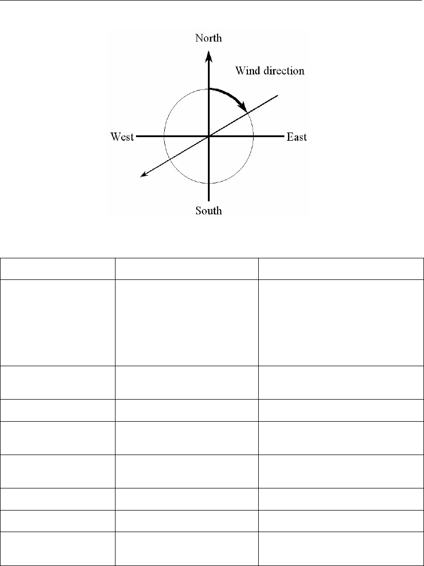
DRAFT
Attribute files
Figure B.2: Wind definition according to Nautical convention
Keywords Value Description
_reference _computational_engine long to fit on one line.
Reference value related to p_drop is
the default air pressure of the com-
putional engine
or free or the value specified.
If missing, p_drop is extracted from
the actual atmospheric pressure.
n_quantity 3 number of quantities specified in the
file
quantity1 wind_speed wind speed given in unit unit1
quantity2 wind_from_direction direction where the wind is coming
from given in unit unit2
quantity3 p_drop drop in atmospheric pressure given
in unit unit3
unit1 m s-1 unit of quantity1: metres/second
unit2 degree unit of quantity2: degrees
unit3 Pa or unit of quantity3: Pascal or
mbar millibar
Time definition and data block description
For a description of the time definition see section B.12.1.
Cyclone track information:
For each time in the time series of space varying wind and pressure on a Spiderweb grid, the position
of the cyclone eye (and thus also the spiderweb grid) must be given, as well as the drop of atmospheric
pressure in the cyclone eye.
Deltares 351 of 412
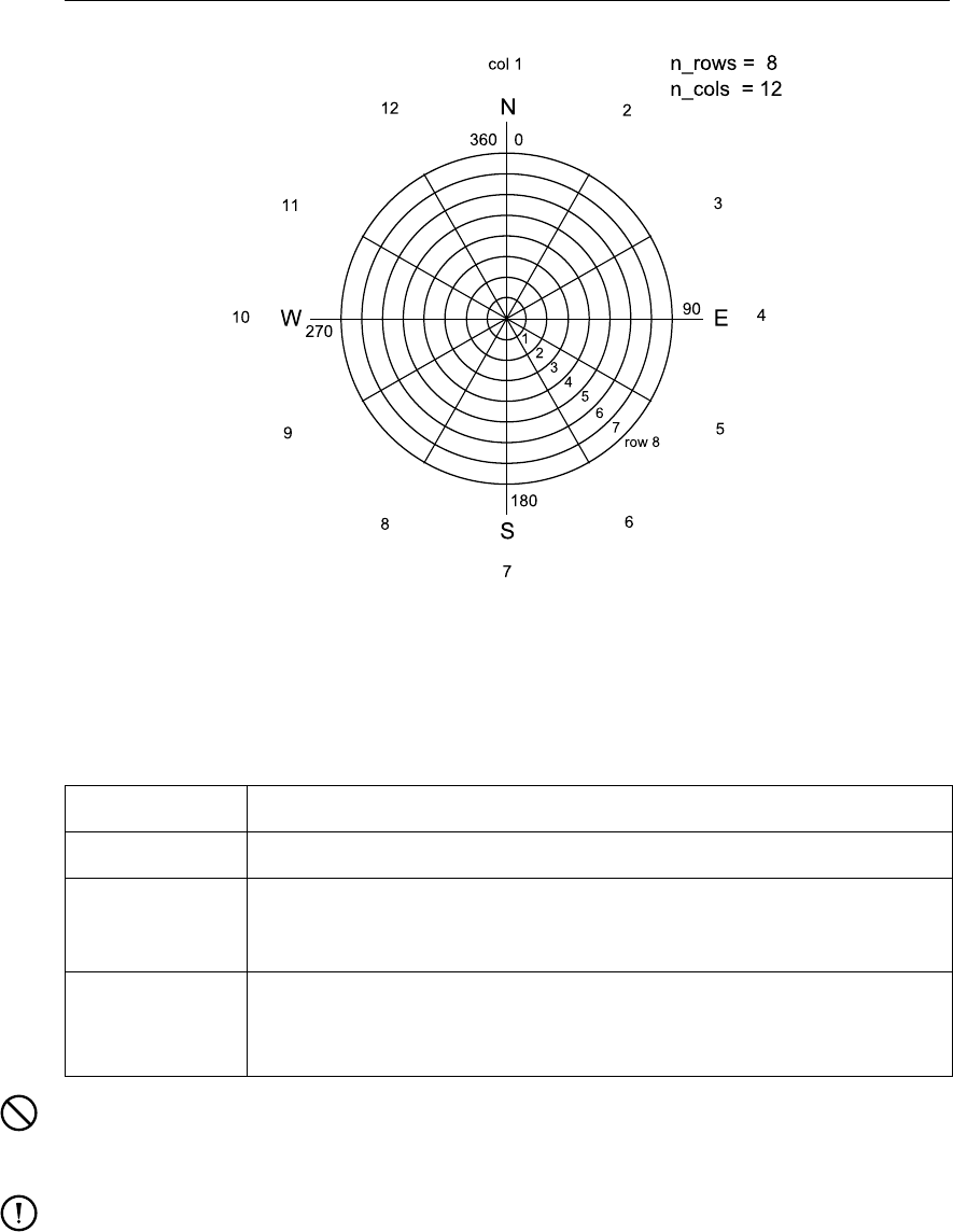
DRAFT
D-Flow Flexible Mesh , User Manual
Figure B.3: Spiderweb grid definition
File version and conversion
The current description holds for FileVersion 1.03. The table below shows the latest modifications
in the file format (and version number).
FileVersion Modifications
1.03 No changes for this meteo input type
1.02 Changed the use of keyword n_rows and n_cols. The radius of the cyclone
is divided in n_rows rings of width: spw_radius/n_rows [m] and the circle is
divided in n_cols parts of 2π/n_cols [rad].
1.01 Changed keyword MeteoType to FileType
Changed fixed value of input type (Keyword Filetype) from Spiderweb to
meteo_on_spiderweb_grid
Restriction:
The restrictions for space varying wind and pressure on a Spiderweb grid are the same as for
space varying wind and pressure on an equidistant grid, described in section B.12.1.
Remarks:
The remarks for space varying wind and pressure on a separate curvilinear grid are the same
as for space varying wind and pressure on an equidistant grid, described in section B.12.1.
The Spiderweb grid is circular and the definitions of the number of rows n_rows and the num-
ber of columns n_cols is therefore different then for the other meteo input formats. For the
Spiderweb grid, the number of rows determines the grid size in radial direction. The number of
columns defines the grid size in angular direction. See Figure B.3.
The wind is specified according to the nautical convention, i.e. wind from the true North has
direction zero and the wind turns clockwise with an increasing angle. See Figure B.2.
352 of 412 Deltares

DRAFT
Attribute files
Example:
A file for input of space varying wind and pressure on a 5x3 Spiderweb grid, has the following layout:
FileVersion = 1.03
filetype = meteo_on_spiderweb_grid
NODATA_value = -999.000
n_cols = 3
n_rows = 5
grid_unit = degree
spw_radius = 600000.0
spw_rad_unit = m
air_pressure_reference = air_pressure_default_from_computational_engine
n_quantity = 3
quantity1 = wind_speed
quantity2 = wind_from_direction
quantity3 = p_drop
unit1 = m s-1
unit2 = degree
unit3 = Pa
TIME = 0.0 hours since 1997-07-14 03:00:00 -06:00
x_spw_eye = 115.1
y_spw_eye = 18.9
p_drop_spw_eye = 5300.0
1.38999 1.38261 1.38315
1.28251 1.34931 1.22571
1.27215 1.31214 1.32451
1.38999 1.86592 2.87732
1.43899 1.24912 2.21519
60.0000 180.0000 270.0000
28.7500 20.0000 31.2500
42.5000 53.7500 65.0000
49.3400 60.2400 81.5200
51.4100 62.0000 43.1200
5301.280 5294.490 5156.240
5043.460 5112.040 5264.020
5140.020 5202.520 5411.210
5294.730 5285.760 5235.250
5242.530 5156.190 5124.240
TIME = 1.0 hours since 1997-07-14 03:00:00 -06:00
x_spw_eye = 114.8
y_spw_eye = 18.8
p_drop_spw_eye = 5250.0
1.35763 1.35763 1.35763
1.35763 1.87273 2.24784
1.92214 2.47836 2.17266
1.87662 2.72116 2.82375
1.26585 2.24146 2.38722
159.0000 346.5200 290.6400
342.3200 282.1400 20.2400
10.7500 25.5300 36.4500
61.8400 81.6200 45.5100
49.5250 56.7500 75.1300
5314.520 5104.490 5287.240
5124.240 5285.760 5252.420
5152.460 5247.040 5222.020
5242.020 5223.520 5475.210
5244.270 5211.210 4998.110
This results in the following set of meteo data. Velocities given in [m/s] and pressure drops in [Pa] on
a Spiderweb grid which is given in spherical coordinates (grid_unit = degree). The cyclone and
spiderweb grid have a radius of 600 km. The grid is 5x3, which means the radius is divided in five
parts of 120 km and the 360 degrees are divided in 3 parts of 120 degrees each. Wind speeds, wind
directions and pressure drops are given at two times: 0 and 1.0 hour since July 14th, 1997, 03:00 AM,
in UTC-6. Between these two times the cyclone eye moves from (longitude, latitude) (115.1, 18.9) to
Deltares 353 of 412

DRAFT
D-Flow Flexible Mesh, User Manual
(114.8, 18.8) on the globe and the pressure drop in the cylcone eye decreases from 5300.0 [Pa] to
5250.0 [Pa].
B.12.4 Fourier analysis
File contents All parameters required to execute an online Fourier analysis for specified
quantities, a specified period and for specified frequencies (Data Group
Output - Storage).
Filetype ASCII
File format Fix formatted for text variables, free formatted for real and integer values.
Filename <name.fou>
Generated Manually offline
Record description:
Record Record description
each record Variable on which the Fourier analysis is to be performed (2 characters):
wl water levels
uv velocities
qf mass fluxes of water
ct temperature
cs salinity
cn n-th constituent in the MDF-file
bs bed stress
Analysis start time in minutes after 00:00:00 on the Reference Date,
Analysis stop time in minutes after 00:00:00 on the Reference Date,
Number of cycles within the analysis time frame,
Nodal amplification factor,
Astronomical argument,
Layer number for the Fourier analysis,
Flag for the computation of elliptic parameters:
y/n (default no) if number of cycles >0,
min/max if number of cycles = 0.
Remarks:
If the number of cycles is set equal to 0, the mean level of the variable over the interval specified
by the start and stop time is determined.
If, in addition, the flag for the computation of elliptic parameters is set to “max” or “min” the max-
imal or minimal value is determined of the selected variable as it occured during the simulation.
Computed Fourier amplitudes slightly differ from the amplitude of the corresponding tidal com-
ponent. When comparisons with co-tidal maps have to be made, this factor can be determined
using the subsystem ASCON of Delft3D-TIDE, the tidal analysis package of Deltares.
Computed Fourier phases are related to the reference date of the FLOW computation. For
comparisons with co-tidal maps a phase shift equal to the astronomical argument has to be
applied.
The layer number is not relevant for water levels.
For computational cells which are dry during all Fourier cycles, no values are associated, and
hence they contain missing value.
Restrictions:
Times specified must be a multiple of the computational time step.
Times specified must be a valid time, i.e. must fit in the simulation time frame of the FLOW
computation.
Items in a record must be separated by one or more blanks.
The variable’s name must start in position one.
354 of 412 Deltares

DRAFT
Attribute files
Example:
A Fourier analysis is requested for:
Water level: mean value and the first two harmonics.
U- and V-velocity: first harmonic, in the top layer (1).
Mass fluxes of water: first harmonic, in the top layer (1).
Temperature: first harmonic, in the third layer.
Salinity: mean value of the third layer.
Four constituents: mean value for a slightly shifted time period in the top layer for 3 constituents;
and the maximum for the fourth constituent.
wl 720. 1440. 2 1.000 0.000
wl 720. 1440. 1 1.000 0.000
wl 720 1440. 0 1.000 0.000
uv 720. 1440. 1 1.000 0.000 1
qf 720. 1440. 1 1.000 0.000 1
ct 720. 1440. 1 1.000 0.000 3
cs 720. 1440. 0 1.000 0.000 3
c1 710. 1430. 0 1.000 0.000 1
c2 710. 1430. 0 1.000 0.000 1
c3 710. 1430. 0 1.000 0.000 1
c4 710. 1430. 0 1.000 0.000 1 max
Remark:
A layer value of 0 in a 3D model is not allowed; i.e. this will NOT result in a depth-averaged
value.
Deltares 355 of 412

DRAFT
D-Flow Flexible Mesh, User Manual
356 of 412 Deltares

DRAFT
C Initial conditions and spatially varying input
C.1 Introduction
Spatially varying input is input data that varies in space, not in time, such as initial conditions (water
levels, etc.), or spatially varying model parameters (friction coefficients, etc.). D-Flow FM uses input
data in model-independent coordinates, that is, the input files should contain their own spatial coor-
dinates, and do not correspond with the D-Flow FM grid cell numbering. As a result, the model grid
can always be changed, without the need to change all other spatial input. The spatial input will be
interpolated onto the active model grid. Spatial input has to be specified in the ext-file (section B.5). All
supported quantities are listed in Table B.1 under “Initial fields” and “Spatial physical properties”.
Initial conditions can also be set using a restart-file, which assigns the exact values in the file to the
current model grid. No interpolation is performed, and the restart file should correspond exactly with
the current model.
C.2 Supported quantities
C.2.1 Water levels
Water levels can come from both all file types listed below. The restart file sets the water level both at
the old and new time step. Non-restart files should be specified using QUANTITY=initialwaterlevel.
C.2.2 Initial velocities
Initial velocities should come from restart files, such that they exactly correspond with the model’s
waterdepths. They can also come from non-restart files using QUANTITY=initialvelocityx/y,
but this is not advised.
C.2.3 Salinity
Salinity concentrations from non-restart files are possible as spatially varying, depth-averaged values,
or (for 3D models) as linearly interpolated values between a top layer concentration and a bottom layer
concentration. The latter is achieved by specifying two QUANTITY blocks: initialsalinity and
initialsalinitytop. For 3D models, alternatively, spatially constant, but depth-varying salinities
can be set using the QUANTITY=initialverticalsalinityprofile, and a vertical profile
file (see section C.3.3).
C.2.4 Temperature
Temperature values from non-restart files are possible as depth-averaged values, using
QUANTITY=initialtemperature.
For 3D models, alternatively, spatially constant, but depth-varying temperatures can be set using
the QUANTITY=initialverticaltemperatureprofile, and a vertical profile file (see sec-
tion C.3.3).
C.2.5 Tracers
Initial tracer concentrations from non-restart files are similar to temperature values, now specified using
QUANTITY=initialtracer<tracername>. The set of tracer name(s) is not listed in the MDU-file
explicitly, they are inferred from all supplied initial tracer definitions and the tracer boundary conditions
(see also section D.1.6). The <tracername>postfix can uniquely associate an initialtracer
quantity with a tracerbnd quantity.
Deltares 357 of 412

DRAFT
D-Flow Flexible Mesh, User Manual
C.2.6 Sediment
Initial sediment concentrations for the Delft3D-SED-based sediment transport module (see section 8.2
for an explanation) is via the <∗.sed>file. See the Delft3D-SED User Manual for further details.
C.2.7 Physical coefficients
A second group of spatially varying input are the physical and numerical coefficients listed below. They
allow changing model parameters in space or in certain sub-regions of the domain, and as such these
values override the uniform values from the MDU file. The input data can come from the in-polygon file
type (section C.3.1 or the sample file type (section C.3.2).
quantity name MDU uniform equivalent description
frictioncoefficient UnifFrictCoef Friction coefficient (use IFRCTYP and
UnifFrictType, resp. to set the fric-
tion type.
horizontaleddy...
...viscositycoefficient
Vicouv Horizontal eddy viscosity coefficient
(m2/s).
horizontaleddy...
...diffusivitycoefficient
Dicouv Horizontal eddy diffusivity coefficient
(m2/s).
advectiontype AdvecType Type of advection scheme.
ibotlevtype BedlevType Type of bed-level handling.
C.3 Supported file formats
All file formats below, except for restart files, are in model-independent coordinates and will be cropped
and/or interpolated onto the model grid.
C.3.1 Inside-polygon option
A spatially constant value in a restricted part of the domain can be set by specifying a polygon file
(section B.2) in the ext-file as follows:
QUANTITY=frictioncoefficient
FILENAME=winterbed.pol
FILETYPE=10
METHOD =4
VALUE =55
IFRCTYP =1 # Optional, override uniform [physics] UnifFrictType=..
The interpolation option METHOD=4 simply specifies the no-interpolation is to be performed, only
inside-polygon cropping. For QUANTITY=frictioncoefficient the default friction type may be
overridden with the keyword IFRCTYP.
358 of 412 Deltares

DRAFT
Initial conditions and spatially varying input
C.3.2 Sample file
Spatial data from sample files (<∗.xyz>, see section B.3) is interpolated by triangle interpolation or
sample averaging. The following options control the type of interpolation:
interpolation method options description
METHOD=5 Triangle interpolation
EXTRAPOLTOL=20 Allow extrapolation from convex hull of samples
up to . . . meters (default: 0).
METHOD=6 Sample averaging inside control volumes:
AVERAGINGTYPE=1 Normal (unweighted) averaging
AVERAGINGTYPE=2 Nearest neighbour
AVERAGINGTYPE=3 Maximal value
AVERAGINGTYPE=4 Minimal value
AVERAGINGTYPE=5 Inverse weighted distance averaging
AVERAGINGTYPE=6 Minimal absolute value
RELATIVESEARCHCELLSIZE
=...
Control size of search volume: 1=actual cell,
1.5=50 % larger in all directions.
C.3.3 Vertical profile file
Initial values that are constant in 2D space, but vary in depth can be specified using vertical profile
files, which are basic polyline files (section B.2). For example for a linearly varying salinity from 30 to
20 ppt from -10 to 0 m :
L1
2 2
-10 30
0 20
The METHOD keyword must be specified, but is further ignored: linear interpolation is always used.
C.3.4 Map file
Initial field data from a map file may be used as non-restart input. Values are read in from the map files
as if they were samples, and further treated and interpolated as such. All interpolation options from
section C.3.2 can be used here. This option may be used as a non-exact restart state when the model
grid has been changed (e.g., locally refined or cropped to a subdomain).
C.3.5 Restart file
Restart files are discussed in section E.3.3. They should be included in your model in the mdu-file as
follows:
[restart]
RestartFile = mdu_name_yyyymmdd_HHMMSS_rst.nc
RestartDateTime = # Restart time (YYYYMMDDHHMMSS), only relevant
# in case of restart from *_map.nc
Deltares 359 of 412

DRAFT
D-Flow Flexible Mesh, User Manual
Concerning parallel runs, each subdomain can generate its own restart/map file. To restart a parallel
run, one can use any of the following approaches:
On each subdomain use its own restart/map file, provided that the partition does not change. (This
means that in each partition MDU file specify its own restart/map file.)
Merge the subdomain restart/map files to one global file (see 5.2.5.2). This file enables to restart
a parallel run with a different or the same partition. (This means that specify the merged file for
all the partition MDU files.) One can also run a sequential simulation with this merged restart/map
file.
360 of 412 Deltares

DRAFT
D Boundary conditions specification
Boundary conditions are part of the external forcing of a model and and as such declared in the
external-forcings file (section B.5).
D.1 Supported boundary types
D.1.1 Astronomic boundary conditions
Boundary values can be specified for any location in terms of astronomical components in attribute files
with extension <cmp>(the BC-format, discussed furtheron, is supported as an alternative). Tidal mo-
tion are described as a series of simple harmonic constituent motions, each with its own characteristic
period:
H(t) = A0+
k
X
i=1
AiF(ci) cos 2π
T(ci)t+ (V0+u) (ci)−Gi(D.1)
in which:
cii-th component, specified by label (name)
Aiamplitude of the i-th component
Giphase of the i-th component
T(ci)period
H(t)boundary value at time t
A0constant offset value
knumber of relevant components
F(ci)nodal amplitude factor
(V0+u)(ci)astronomical argument
The component (by label) ci, amplitude Aiand phase Gifor each component iare required in the
<cmp>-file In addition to the primary constituents, compound and higher harmonic constituents may
have to be used. This is the case in shallow water areas for example, where advection, large amplitude
to depth ratio, and bottom friction give rise to non-linear interactions.
F,V0and uare also time-dependent. For a given period, their values are easily calculated or obtained
various tidal year books. V0is a frequency dependent phase correction factor relating the local time
frame of the observations to an internationally agreed celestial time frame. Fiand uiare slowly varying
amplitude and phase corrections, The variations depend on the frequency, often with a cyclic period
of 18.6 years. By default, the nodal amplitude factors and astronomical arguments are re-calculated
every 6 hours.
D.1.2 Astronomic correction factors
For individual astronomic components, correcting factor αifor amplitude and offset δimay be specified
by the user so that the effective amplitude for that component becomes αiAiand the effective phase
becomes Gi+δi.
D.1.3 Harmonic flow boundary conditions
Harmonic boundary conditions are specifies in a manner similar their astronomical counterpart, except
that the periods (first column of a .cmp file) are declared explicitly, rather than using component names.
Equation ((D.1)) applies with T(ci) = Tiand furthermore F= 1 and (V0+u) = 0.
D.1.4 QH-relation flow boundary conditions
In this type of boundary condition, a waterlevel is prescribed as a function of the integrated discharge
through a crossection defined by the polyline of the boundary.
Deltares 361 of 412

DRAFT
D-Flow Flexible Mesh, User Manual
The relation between waterlevel and discharge is specified in a lookup-table.
Within this table linear interpolation is applied.
Note that only one waterlevel is set for the entire QH-boundary, and that its behaviour is specified by a
single QH-table for the entire boundary.
D.1.5 Time-series flow boundary conditions
Time-series in the general time-series file format (section D.2.1) can be used to specify values on
boundaries.
Boundary values are provided at discrete points in time, which are then used for interpolation at times
in between.
Extrapolation beyond the range of specified times is not supported, Time-series are also supported at
multiple vertical levels for quantities that are defined on layers (tracers, salinity, temperature, velocity).
These need to be specified in the BC-format (section D.2.3).
D.1.6 Time-series transport boundary conditions
The boundary conditions of tracers, salinity and temperature are specified similar to any other quantity
already mentioned. The quantity name should be in the form tracerbnd<name>, where name is
the user-defined tracer name.
D.1.7 Time-series for the heat model parameters
In order to conduct a heat flux simulation (if in the MDU-file “Temperature” under [physics]
was set to 5), then four time-varying meteorological fields become relevant:
humidity
airtemperature
cloudiness
solar radiation
These are read as a three- or four-column vector (the first three variables of this list, either with or
without solar radiation). The corresponding quantity names in the <ext>-file are:
humidity_airtemperature_cloudiness
humidity_airtemperature_cloudiness_solarradiation
As for filetype, currently only the curvilinear format (B.12.2) and the multicolumn time series (D.2.1) are
supported.
D.2 Boundary signal file formats
D.2.1 The <cmp>format
*comments
*...
c[0] amplitude[0] phase[0]
c[1] amplitude[1] phase[1]
...
where crepresents a period in minutes or the name of a valid astronomic component. Amplitudes are
assumed to be in the unit of the quantity.
362 of 412 Deltares

DRAFT
Boundary conditions specification
D.2.2 The <qh>format
*comments
*...
discharge[0] waterlevel[0]
discharge[1] waterlevel[1]
...
D.2.3 The <bc>format
The BC-format for boundary signal data was introduced to combine multiple quantities for multiple
locations in a single (ASCII) file. Each location will be defined in a separate ‘BC block’, which consists
of a column-wise table, (the data), and a header specifiying how this table should be interpreted.
The BC-format is pseudo-formally defined below, using EBNF1-notation. Though all BC keywords
in this description are uppercase, nothing in the BC-format is case-sensitive, not even user-defined
names. Whitespace is optional, except for the new lines as in the definitions below.
BC-file = { BC-block }
BC-block = "[FORCING]" ,
"FUNCTION = " , function ,
"NAME = ",location ,
["OFFSET = " , offset ] ,
["FACTOR = " , factor ] ,
["VERTICAL POSITION SPECIFICATION = " , {vertical-position} ,
"VERTICAL INTERPOLATION = " , vertical-interpolation ,
"VERTICAL POSITION TYPE = " , vertical-position-type] ,
"MISSING VALUE DEFINITION = " , float ,
"TIME INTERPOLATION = " , time-interpolation,
{ quantity-block | vector-block },
{ data-block }
function = "TIMESERIES" | "HARMONIC" | "ASTRONOMIC" | "HARMONIC-CORRECTION" |
"ASTRONOMIC-CORRECTION" | "T3D" | "QHTABLE"
The FUNCTION attribute specifies how the BC-block should be interpreted. The options are:
"TIMESERIES" Value(s) as a function of time
"HARMONIC" Period, amplitude, phase
"ASTRONOMIC" Component-name, amplitude, phase
"HARMONIC-CORRECTION" Period, amplitude-factor, phase-offset
"ASTRONOMIC-CORRECTION" Component-name, amplitude-factor, phase-offset
"T3D" Values on multiple vertical positions versus time
"QHTABLE" Discharge as a function of waterlevel
A single BC-block is uniquely tied to a single boundary location by the location value:
location = pli-name , ["_" , pointnumber]
The pli-name pointnumber combination identifies the BC-block (when searched). The pointnumber
should be omitted for blocks providing valies for an entire polyline. Currently this is only the case for
blocks with the function "QHTABLE", which apply to all points on a polyline,
1https://en.wikipedia.org/wiki/Extended_Backus%E2%80%93Naur_Form
Deltares 363 of 412

DRAFT
D-Flow Flexible Mesh, User Manual
vertical-interpolation = "LINEAR" | "LOG" | "BLOCK"
time-interpolation = "LINEAR" | "BLOCK-TO" | "BLOCK-FROM"
"LINEAR" linear interpolation between times or vertical positions.
"LOG" logarithmic interpolation between vertical positions (e.g. vertical
velocity profiles).
"BLOCK" equal to the value at the directly lower specified vertical position.
"BLOCK-FROM" equal to that at the start of the time interval (latest specified time
value).
"BLOCK-TO" equal to that at the end of the time interval (upcoming specified time
value) .
vertical-position-type = "PERCBED" | "ZBED"
"PERCBED" Percentage wrt. waterdepth from the bed upward (sigma layers).
"ZBED" Absolute distance from the bed upward (z-layers).
vertical-position
The vertical position is specified as a space- or comma-separated list of floats, the interpretation of
which varies according to the vertical position type. The order of the positions in the list becomes rele-
vant when referring to them from the quantity blocks. However, no specific ordering of these positions
(ascending or descending) is assumed.
quantity-block = "QUANTITY = ",quantity-name
{quantity-property}
quantity-property = |"VERTICAL POSITION = ", vertical-position-index |
"UNIT = " unit |
vector block = vectorname,":",[{quantity-name}","],quantity-name
data-block = {column-data}
quantity-name (character string)
The quantity name, in conjunction with the BC-block name (representing location) serves as a search-
ing key in the BC-file to find the BC-block and column within that block. These names can be chosen
freely, except that some names and combinations have a special meaning.
1. a quantity bndname in a block with function "HARMONIC" or "HARMONIC-CORRECTION" should
have the quantities
HARMONIC COMPONENT
bndname AMPLITUDE
bndname PHASE
2. a quantity bndname in a block with function "ASTRONOMIC" or "ASTRONOMIC-CORRECTION"
should have the quantities
ASTRONOMIC COMPONENT
bndname AMPLITUDE
bndname PHASE
3. Blocks with function "TIMESERIES" or "T3D" require a quantity
TIME
364 of 412 Deltares

DRAFT
Boundary conditions specification
This also implies that the component-quantity in harmonic and astronomic BC-blocks applies to any
quantity in that block. The same holds for the time-quantity in timeseries and T3D blocks.
vertical-position-index (integer)
This is a (one-based) index into the vertical-position-specification, assigning a vertical position to the
quantity (T3D-blocks only)
offset, factor (floating points)
These are set for the complete BC-block. In the case of timeseries (function is "TIMESERIES"
or "T3D"), all values in the table are multiplied with the factor and increased by the offset. In the
case of astronomic or harmonic components (function is "HARMONIC" or "ASTRONOMIC"), only
the amplitude column is multiplied by the given factor.
datablock
This block holds the actual data in columns. The interpretation of the columns is fully determined by
the order of the quantity-blocks in the header, i.e. the n-th quantity-block in the header refers to the
n-th column. Therefore, The columns should contain valid floating point numbers (scientific notation is
also allowed).
The only exception is the column associated with astronomic component names, which is expected to
contain strings.
D.2.4 The NetCDF-format for boundary condition time-series
Time series data for 2D boundaries can also be ingested from NetCDF files.
These files should meet the following structure:
To look up boundary signal locations with a certain label, a character variable should be defined
with attribute cf_role = ‘timeseries_id’. This variable should have two dimensions. The
first dimension corresponds with the different boundary signal locations in the file.
The contents are interpreted as location identifiers of support points of the boundaries.
The variables containing the timeseries for the support points should have the attribute standard_name
= <quantity-name>, so as to associate the variable with a requested quantity. The first di-
mension corresponds with the different boundary signal locations in the file.
The second dimension corresponds with time and is the only dimension that can be ’UNLIMITED’.
So, similar to the (ASCII) BC-format, location name and quantity name together determine the time-
series to be read, only now
the quantity name is sought among the variables standard-name attributes.
the location name is sought in a separate list of timeseries IDs, of which
the first dimension matches the first dimension of the ‘data’-variables.
the role as ‘timeseries_id’ is signified through the cf_role attribute.
Deltares 365 of 412

DRAFT
D-Flow Flexible Mesh, User Manual
366 of 412 Deltares

DRAFT
E Output files
D-Flow FM can produce several types of output into several different files. This chapter summarizes
the types of output and how to configure them in them model definition. We distinguish five types of
output here:
1 The diagnostics file, a log file with live details of a single model run.
2 NetCDF output files for history, map and restart data.
3 Tecplot.
4 Timings file with performance statistics.
5 Shapefiles.
E.1 Diagnostics file
The diagnostics (dia) file is the log file of a single model simulation run. It is an important file to
check for warning or error messages, when suspecting a faulty model run. The filename is auto-
matically chosen as <mdu_name.dia>. For parallel model runs, each process writes its own file
<mdu_name_000X.dia>. The dia file has the following global structure:
Various INFO/DEBUG messages:
** INFO : Opened file : unstruc.hlp
[..]
The version of D-Flow FM used for this calculation:
*Deltares, D-Flow FM Version 1.1.145.41271M, Aug 11 2015, 18:05:31
Date and time of model run start:
File creation date: 18:27:44, 06-09-2015
[..]
Check for possible model initialization errors:
** WARNING: readMDUFile: [numerics] cflwavefrac=0.1 was in file, but not used.
[..]
Upon successful initialization, a full printout of the effective model settings is given:
** INFO : ** Model initialization was successful **
** INFO : *Active Model definition:
# Generated on 18:27:45, 06-09-2015
# Deltares, D-Flow FM Version 1.1.145.41271M, Aug 11 2015, 18:05:31
[model]
[..]
Next, the time loop is started:
** INFO : **
** INFO : Writing initial output to file(s)...
** DEBUG : Opened NetCDF file ’DFM_OUTPUT_035hammen/035hammen_his.nc’ as #3.
** DEBUG : Opened NetCDF file ’DFM_OUTPUT_035hammen/035hammen_map.nc’ as #4.
** INFO : Done writing initial output to file(s).
[..]
Finishing summary of model run:
** INFO : simulation period (s) : 6400.0000000000
** INFO : nr of timesteps ( ) : 771.0000000000
** INFO : average timestep (s) : 8.3009079118
[..]
Some basic run time statistics
** INFO : time steps (s) : 76.2840000003
** INFO : Computation started at: 18:27:45, 06-09-2015
** INFO : Computation finished at: 18:29:04, 06-09-2015
** INFO :
Which parallellization options have been active in this run:
** INFO : MPI : no.
** INFO : OpenMP : yes.
Deltares 367 of 412

DRAFT
D-Flow Flexible Mesh, User Manual
#threads max : 8
E.2 Demanding output
The configuration of what output should be produced during a model run is via the MDU file, and
several attribute files for history files.
E.2.1 The MDU-file
The MDU-file has an aptly named [output]-section, with a range of key-value-pair options. See
Table A.1 on page 326 for all available output options.
E.2.2 Observation points
Observation points in a single observation point file <∗.xyn>define the locations for time series output
for single grid cells. The observation point file is basically like a sample file (section B.3), but now with
station id strings in the third column:
-2.06250000e+00 5.71583333e+01 ABDN
-2.73750000e+00 5.15083334e+01 AVMH
-2.11250000e+00 4.91750000e+01 ’St Helier Jersey’
Remarks:
The observation points are stationary by default.
The x,y-locations are snapped to the grid cell in which they lie. When an observation point lies
on a grid cell edge, snapping results are unpredictable.
Time series are reported for the cell-centered solution data, that is: no interpolation to the exact
x,y-location takes place.
Observation points may have non-unique names (also together with moving observation points),
but the results can only be distinguished by the column number in the output file, and this
practice is not advised.
The station id/name may contain spaces, in which case it should be surrounded by single
quotes.
E.2.3 Moving observation points
Moving observation points are specified via the <∗.ext>-file:
QUANTITY=movingstationtxy
FILENAME=movingstation1.tim
FILETYPE=1
METHOD=1
OPERAND=O
The <∗.tim>file (one for each moving observation point) is a standard time series file (section D.2.1)
with three columns, containing the time in minutes since the reference data, the x- and y-position of
the moving station at that time.
Remarks:
Stationary and moving observation points form one large set of observation points in the output
his file.
368 of 412 Deltares

DRAFT
Output files
No space, nor time interpolation is done: the reported values are instantaneous values for the
grid cell in which the moving observation point lies at that each output time.
E.2.4 Cross-sections
Cross-sections are polylines in a single <_crs.pli>polyline file (section B.2). Cross section polylines
are snapped to the grid cell edges, and cumulative, space-integrated discharges and constituent trans-
port are reported as time series.
Remarks:
The first header line of each polyline block contains the name of each cross section.
The cross section polyline is snapped to all grid cell edges (i.e., velocity points), whose flow link
is intersected by the polyline.
The flow data on velocity points is integrated along the polyline and across all vertical layers,
resulting in a single time series per cross section and flow quantity.
E.3 NetCDF output files
All flow data output produced by D-Flow FM is written in the NetCDF format. This cross-platform
storage format is widely used in the world. The contents of a file can be documented using variable
attributes and standardized meta data. For this purpose the D-Flow FM output files aim to satisfy the
CF-conventions.
E.3.1 Timeseries as NetCDF his-file
The history file <mdu_name_his.nc>contains the dimensions and variable definitions in its header,
followed by the actual data. For parallel runs, all data is gathered by domain #0 into <mdu_name_0000_his.nc>
(section 5.2.5).
Dimensions
The following dimensions are defined in a his file header:
netcdf weirfree_his {
dimensions:
time = UNLIMITED ; // (64 currently)
name_len = 64 ;
stations = 18 ;
cross_section = 4 ;
cross_section_name_len = 64 ;
cross_section_pts = 3 ;
npumps = 2 ;
// and possibly nweirgens, nweirs, ngategens, ngates, nsources/sinks
Location variables
The original location and IDs for stations, cross sections and sources/sinks are also included in the his
file:
variables:
double station_x_coordinate(stations) ;
station_x_coordinate:units = "m" ;
station_x_coordinate:standard_name = "projection_x_coordinate" ;
station_x_coordinate:long_name = "x-coordinate" ;
double station_y_coordinate(stations) ;
station_y_coordinate:units = "m" ;
Deltares 369 of 412

DRAFT
D-Flow Flexible Mesh, User Manual
station_y_coordinate:standard_name = "projection_y_coordinate" ;
station_y_coordinate:long_name = "x-coordinate" ;
char station_name(stations, name_len) ;
station_name:cf_role = "timeseries_id" ;
station_name:long_name = "Observation station name" ;
double cross_section_x_coordinate(cross_section, cross_section_pts) ;
cross_section_x_coordinate:units = "m" ;
cross_section_x_coordinate:standard_name = "projection_x_coordinate" ;
cross_section_x_coordinate:long_name = "x-coordinate" ;
double cross_section_y_coordinate(cross_section, cross_section_pts) ;
cross_section_y_coordinate:units = "m" ;
cross_section_y_coordinate:standard_name = "projection_y_coordinate" ;
cross_section_y_coordinate:long_name = "y-coordinate" ;
char cross_section_name(cross_section, cross_section_name_len) ;
double source_sink_x_coordinate(source_sink, source_sink_pts) ;
source_sink_x_coordinate:units = "m" ;
source_sink_x_coordinate:standard_name = "projection_x_coordinate" ;
source_sink_x_coordinate:long_name = "x-coordinate" ;
double source_sink_y_coordinate(source_sink, source_sink_pts) ;
source_sink_y_coordinate:units = "m" ;
source_sink_y_coordinate:standard_name = "projection_y_coordinate" ;
source_sink_y_coordinate:long_name = "y-coordinate" ;
char source_sink_name(source_sink, source_sink_name_len) ;
Variables on stations
Variables on observations station are typically defiend as follows:
double waterlevel(time, stations) ;
waterlevel:standard_name = "sea_surface_level" ;
waterlevel:long_name = "Water level" ;
waterlevel:units = "m" ;
waterlevel:coordinates = "station_x_coordinate station_y_coordinate station_name" ;
waterlevel:_FillValue = -999.
;
Other quantities that can be written are:
Water depth
Flow velocity (xand y)
Salinity, temperature and other transported quantities, such as tracers
Variables on cross sections
Variables on cross sections are typically defined as follows:
double cross_section_discharge(time, cross_section) ;
cross_section_discharge:units = "m^3/s" ;
cross_section_discharge:coordinates = "cross_section_name" ;
Other quantities that can be written are:
Cross section flow area at current time;
370 of 412 Deltares

DRAFT
Output files
Cross section average velocity at current time;
Mass balance output
The history file may also contain model-global, time-integrated mass balance output, for example:
double WaterBalance_total_volume(time) ;
WaterBalance_total_volume:units = "m3" ;
Other quantities that can be written are:
Net storage since Tstart;
Volume error since Tstart;
Cumulative inflow through boundaries since Tstart;
Cumulative outflow through boundaries since Tstart;
Net inflow through boundaries since Tstart;
Cumulative inflow via SOBEK–D-Flow FM 1D–2D boundaries since Tstart;
Cumulative outflow via SOBEK–D-Flow FM 1D–2D boundaries since Tstart;
Net inflow via SOBEK–D-Flow FM 1D–2D boundaries since Tstart;
Total precipitation volume since Tstart;
Net inflow via source–sink elements since Tstart;
Variables on sources/sinks
Variables on sources/sinks are typically defined as follows:
double source_sink_prescribed_discharge(time, source_sink) ;
source_sink_prescribed_discharge:units = "m^3/s" ;
source_sink_prescribed_discharge:coordinates = "source_sink_name" ;
Other quantities that can be written are:
source sink prescribed salinity increment;
source sink prescribed temperature increment;
source sink current discharge;
source sink cumulative volume;
source sink discharge average.
These variables are automatically written to his-file if any source/sink exists. One can switch it off by
setting in MDU-file that [output] Wrihis_sourcesink = 0.
Hydraulic structure output
A history file can also contain automatic output for hydraulic structures, without the need to add an
explicit cross section at the same location. An example variable is:
double weirgen_discharge(time, weirgens) ;
weirgen_discharge:long_name = "Weir accumulated discharge (via general structure)" ;
Other quantities that can be written are:
Deltares 371 of 412

DRAFT
D-Flow Flexible Mesh, User Manual
weir crest level at current time;
Total discharge through gate at current time;
gate sill level at current time;
gate sill width at current time;
gate door lower edge level at current time;
gate door opening width at current time;
Total pump discharge at current time;
Max. pump capacity at current time;
E.3.2 Spatial fields as NetCDF map-file
The map file <mdu_name_map.nc>contains data on the entire model grid in 1D, 2D and 3D. Three
formats are currently supported, selected by the MapFormat keyword in the MDU:
[output]
MapFormat = 1 # Map file format, 1: NetCDF, 2: Tecplot, 3: NetCFD and Tecplot, 4: NetCDF-UGRID
D-Flow FM is using the more standardized UGRID1format. This is the default option. Delta Shell and
Delft3D-QUICKPLOT also support this format. In this section only the conventional NetCDF format (1)
is further discussed.
For parallel runs, each process writes a separate file for each partition as <mdu_name_000X_map.nc>.
The map file contains the dimensions and variable definitions in its header, followed by the actual data.
Dimensions
The following dimensions are defined in a map file header:
netcdf weirfree_map {
dimensions:
nNetNode = 310 ;
nNetLink = 486 ;
nNetLinkPts = 2 ;
nBndLink = 252 ;
nNetElem = 180 ;
nNetElemMaxNode = 4 ;
nNetLinkContourPts = 4 ;
nFlowElem = 180 ; // Nr.
of grid cells
nFlowElemMaxNode = 4 ;
nFlowElemContourPts = 4 ;
nFlowLink = 246 ; // Nr.
of flow links (open cell edges)
nFlowLinkPts = 2 ;
time = UNLIMITED ; // (64 currently)
For plotting solution data, the grid cells (flow nodes) are important, and the flow links (open cell edges).
All Net*dimensions relate the flow grid tot the original unstructured network. More explanation of
these topological naming conventions can be found in section 7.3.1.
1https://github.com/ugrid-conventions/ugrid-conventions
372 of 412 Deltares

DRAFT
Output files
Location variables
The location and shape of grid cells is stored in several x,y variables:
double FlowElem_xcc(nFlowElem) ;
FlowElem_xcc:units = "m" ;
FlowElem_xcc:standard_name = "projection_x_coordinate" ;
FlowElem_xcc:long_name = "Flow element circumcenter x" ;
FlowElem_xcc:bounds = "FlowElemContour_x" ;
double FlowElem_ycc(nFlowElem) ;
FlowElem_ycc:units = "m" ;
FlowElem_ycc:standard_name = "projection_y_coordinate" ;
FlowElem_ycc:long_name = "Flow element circumcenter y" ;
FlowElem_ycc:bounds = "FlowElemContour_y" ;
// [..]
double FlowElemContour_x(nFlowElem, nFlowElemContourPts) ;
FlowElemContour_x:units = "m" ;
FlowElemContour_x:standard_name = "projection_x_coordinate" ;
FlowElemContour_x:long_name = "List of x-points forming flow element" ;
FlowElemContour_x:_FillValue = -999.
;
// [..]
double FlowElem_bl(nFlowElem) ;
FlowElem_bl:units = "m" ;
FlowElem_bl:positive = "up" ;
FlowElem_bl:standard_name = "sea_floor_depth" ;
FlowElem_bl:long_name = "Bottom level at flow element\’s circumcenter." ;
Variables on grid cells/pressure points
Variables on grid cells (represented by the pressure point/cell circumcenter) are typically defined as
follows:
double s1(time, nFlowElem) ;
s1:coordinates = "FlowElem_xcc FlowElem_ycc" ;
s1:standard_name = "sea_surface_level" ;
s1:long_name = "waterlevel" ;
s1:units = "m" ;
s1:grid_mapping = "projected_coordinate_system" ;
Other quantities that can be written are:
Water level at beginning of time step;
Water depth;
Numlimdt: number of times each cell was limiting the time step;
Bed shear stress;
Cell-centered velocity components;
Effective Chézy roughness;
Salinity;
Temperature;
Tracers and other constituents;
Heat flux quantities, air temperature, relative humidity, cloudiness, and more detailed fluxes (chap-
ter 10);
Streamline curvature and spiral flow intensity (section 7.6);
Suspended sediment concentrations and erodable layer thicknesses (chapter 18);
Cell-centered wind speed components and atmospheric pressure;
Deltares 373 of 412

DRAFT
D-Flow Flexible Mesh, User Manual
Variables on flow links/velocity points
Variables on grid cell edges (represented by the velocity point) are typically defined as follows:
double q1(time, nFlowLink) ;
q1:coordinates = "FlowLink_xu FlowLink_yu" ;
q1:long_name = "Flow flux" ;
q1:units = "m3/s" ;
Other quantities that can be written are:
Normal velocities at the old and new time level;
Horizontal viscosity and diffusivity;
Edge-centered wind speed components;
Effective roughness values from trachytopes/vegetation (section 13.2)
E.3.3 Restart files as NetCDF rst-file
Restart files <mdu_name_yyyymmdd_HHMMSS_rst.nc>are almost identical to map files, except
that they contain all data for just a single time. The grid and flow geometry information is not present,
except for the flow cell/link coordinates. Moreover, restart files resulted from a parallel run contains
parallelization information. For this reason, restart files are less suitable for plotting, but efficient for
restarting a computation.
E.4 Shapefiles
Shapefiles2are widely used for visualization in geographic information system (GIS) software. A
shapefile stores geometric locations and corresponding attributes information for the spatial features.
D-Flow FM can generate shapefiles by setting keyword in the MDU file. Table E.1 shows what features
can be written to a shapefile by D-Flow FM, and the corresponding MDU settings. (By default these
keywords are zero, which disables writing the shapefile.) Moreover, this function is also valid in parallel
simulation.
Table E.1: Features and MDU settings for generating shapefiles
Features for shapefiles MDU setting
Cross sections [output] Wrishp_crs = 1
Weirs [output] Wrishp_weir= 1
Gates [output] Wrishp_gate= 1
Fixed weirs [output] Wrishp_fxw = 1
Thin dams [output] Wrishp_thd = 1
Embankments [output] Wrishp_ebm = 1
Observation stations [output] Wrishp_obs = 1
Source-sinks [output] Wrishp_src = 1
2https://www.esri.com/library/whitepapers/pdfs/shapefile.pdf
374 of 412 Deltares
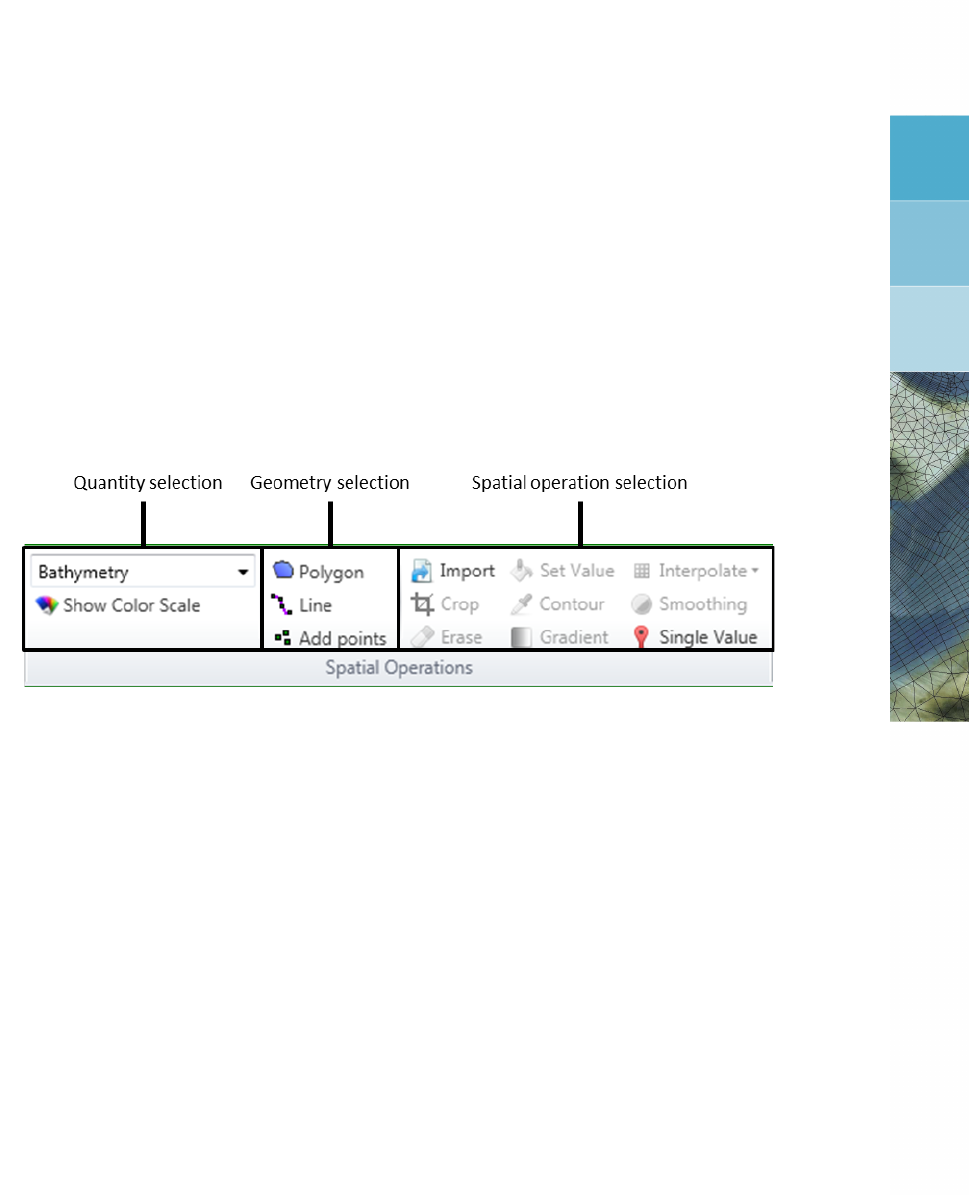
DRAFT
F Spatial editor
F.1 Introduction
The spatial editor is a generic feature of the Delta Shell framework for editing spatial data (e.g. bed
level, roughness, viscosity, initial conditions, sediment availability). The spatial editor supports both
point clouds and coverages (e.g. data on a grid or network). Therefore, you can use the spatial editor
both to edit spatial data in general and to prepare model input. This Chapter describes the general
features of the spatial editor (section F.2), (spatial) quantity selection (section F.3), geometry operations
(section F.4), spatial operations (section F.5) and the operation stack (section F.6). The examples given
below are typically focusing on use of the spatial editor in the D-Flow FM plugin, but are in principal
applicable to any Delta Shell plugin.
Figure F.1: Overview of spatial editor functionality in Map ribbon
F.2 General
F.2.1 Overview of spatial editor
The spatial editor functionality can be accessed from the “Spatial Operations” section of the “Map
Ribbon” (Figure F.1). Typically, you first select which dataset or quantity (either a point cloud or a
coverage) to work on (e.g. bed level, roughness, viscosity, initial conditions, sediment availability), then
a geometry (e.g. point, line, polygon) and finally which spatial operation to perform (e.g. crop, erase,
set value, contour, interpolate, smoothing). Typical workflows are as follows:
Working on a point cloud dataset:
1 Import the dataset as point cloud (section F.2.2)
2 Activate/select the dataset (quantity) in the spatial editor (section F.3)
3 Select a geometry to perform an operation on (section F.4)
4 Select the spatial operation for this geometry (section F.5)
5 Repeat steps 3 and 4 until you are satisfied with the data
6 Export the dataset (section F.6.7)
Working on a coverage (e.g. model input):
1 Activate/select the spatial quantity to work on in the spatial editor (section F.3)
2 Optional: import a dataset as point cloud (section F.5.1)
3 Select a geometry to perform an operation on (section F.4)
4 Select the spatial operation for this geometry (section F.5)
5 Repeat steps 3 and 4 until you are satisfied with the data
6 Interpolate the point cloud to the grid or network ((section F.5.10))
7 Optional: export the dataset (section F.6.7)
Upon performing a spatial operation, the ‘Operations’ panel will open (see Figure F.51) with the op-
erations stack. This stack keeps track of the workflow of spatial operations that you performed. This
helps you to make transparent how you arrived at your ‘final’ dataset without having to save all the in-
termediate datasets (steps) separately. Moreover, the stack is reproducible and easily editable without
Deltares 375 of 412
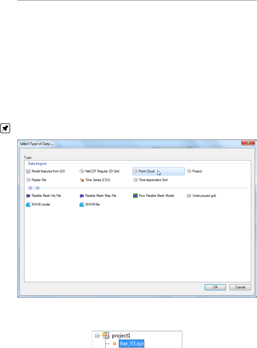
DRAFT
D-Flow Flexible Mesh, User Manual
having to start all over again. When working on a coverage (e.g. the second workflow), point clouds
can be used to construct the coverage. In this case the coverage (for example ‘Bed level’) is the ‘trunk’
of the workflow and the point clouds (appearing as sets in the stack) are ‘branches’ or subsets of this
trunk (see Figure F.51). By selecting the set or coverage in the ‘Operations’ panel you determine on
which dataset you are working. The interpolate operation (section F.5.10) allows you to bring data from
the point cloud (branch) to the coverage (trunk). For more information on the stack you are referred to
section section F.6.
F.2.2 Import/export dataset
To import a (point cloud) dataset use the context menu on “project” in the “Project Tree”, select “import”
from the context menu and select the point cloud importer (Figure F.2). After the import the point cloud
will be added to the project tree. To activate the point cloud in the spatial editor either double click the
dataset in the project tree (Figure F.3) or select it from the drop down box in the spatial editor ribbon
(Figure F.4).
Note: Exporter still to be implemented
Figure F.2: Importing a point cloud into the project using the context menu on “project” in
the project tree
Figure F.3: Activate the imported point cloud in the spatial editor by double clicking it in
the project tree
376 of 412 Deltares
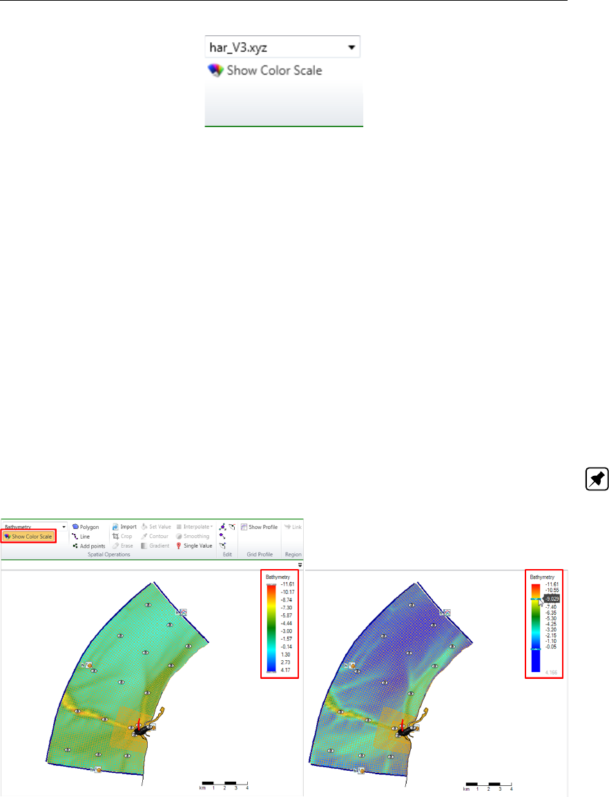
DRAFT
Spatial editor
Figure F.4: Activate the imported point cloud in the spatial editor by selecting it from the
dropdown box in the Map ribbon
F.2.3 Activate (spatial) model quantity
Similar to activating an imported dataset in the spatial editor, you can also activate a (spatial) model
quantity (e.g. bed level, initial conditions, roughness, viscosity) in the spatial editor by double clicking
the quantity in the project tree or selecting it from the dropdown box in the “Map” ribbon.
F.2.4 Colorscale
Upon activating a spatial quantity in the spatial editor it becomes visible in the map window with a
corresponding colorscale (Figure F.5 top). You can (de-)activate the colorscale by clicking on the
“Show Color Scale” button in the “Map” ribbon (Figure F.5 left panel). By default the colorscale is
ranging from the minimum value of the active dataset. You can adjust/decrease this range using the
sliders at the top and bottom sliders of the colorbar (Figure F.5 right panel).
You can also adjust the colormap and classes of the colorscale using the context menu on the spatial
quantity in the “Map tree” and selecting “Properties” (Figure F.6 left panel). A layer properties editor
will open in which you can set the colormap to your own preferences (Figure F.6 right panel). Note:
Please note that currently you can only edit the properties of the colorscale before you perform spatial
operations. Once you have performed a spatial operation this functionality will be disabled.
Figure F.5: Activate the colorscale using the button in the map ribbon (top) and the col-
orscale will become visible in the map window (left). You can adjust/decrease
the range of the colorscale using the sliders at the top and bottom of the
colorbar (right).
Deltares 377 of 412
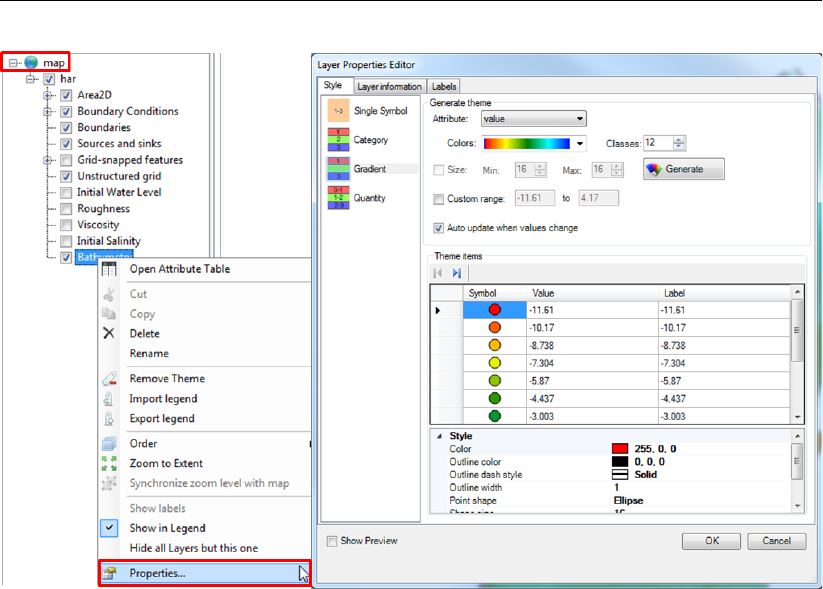
DRAFT
D-Flow Flexible Mesh, User Manual
Figure F.6: Edit the colorscale properties using the context menu on the active layer in
the Map Tree
F.2.5 Render mode
By default point clouds are rendered as (colored) points and coverages as shades (e.g. ‘FillSmooth’).
The render mode can be edited using the properties of the active layer Figure F.7. Delta Shell offers
the following render modes:
Points
Lines (only for coverages)
Shades or ‘FillSmooth’ (only for coverages)
Colored numbers
Mono colored numbers
An example of a coverage rendered as colored numbers is given in Figure F.8.
378 of 412 Deltares
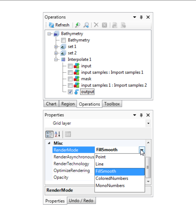
DRAFT
Spatial editor
Figure F.7: Select the rendermode for the active layer in the property grid.
Deltares 379 of 412
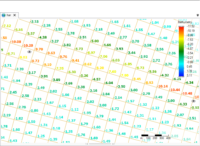
DRAFT
D-Flow Flexible Mesh, User Manual
Figure F.8: Example of a coverage rendered as colored numbers.
F.2.6 Context menu
In addition to the selection of spatial operation from the ‘Map’ ribbon (see section F.5), you can also
select spatial operations using the context menu (e.g. context menu). After drawing a geometry and
clicking the context menu all spatial operation available for the geometry will pop-up (see Figure F.9).
The spatial operation will become active upon selecting it from the context menu.
380 of 412 Deltares
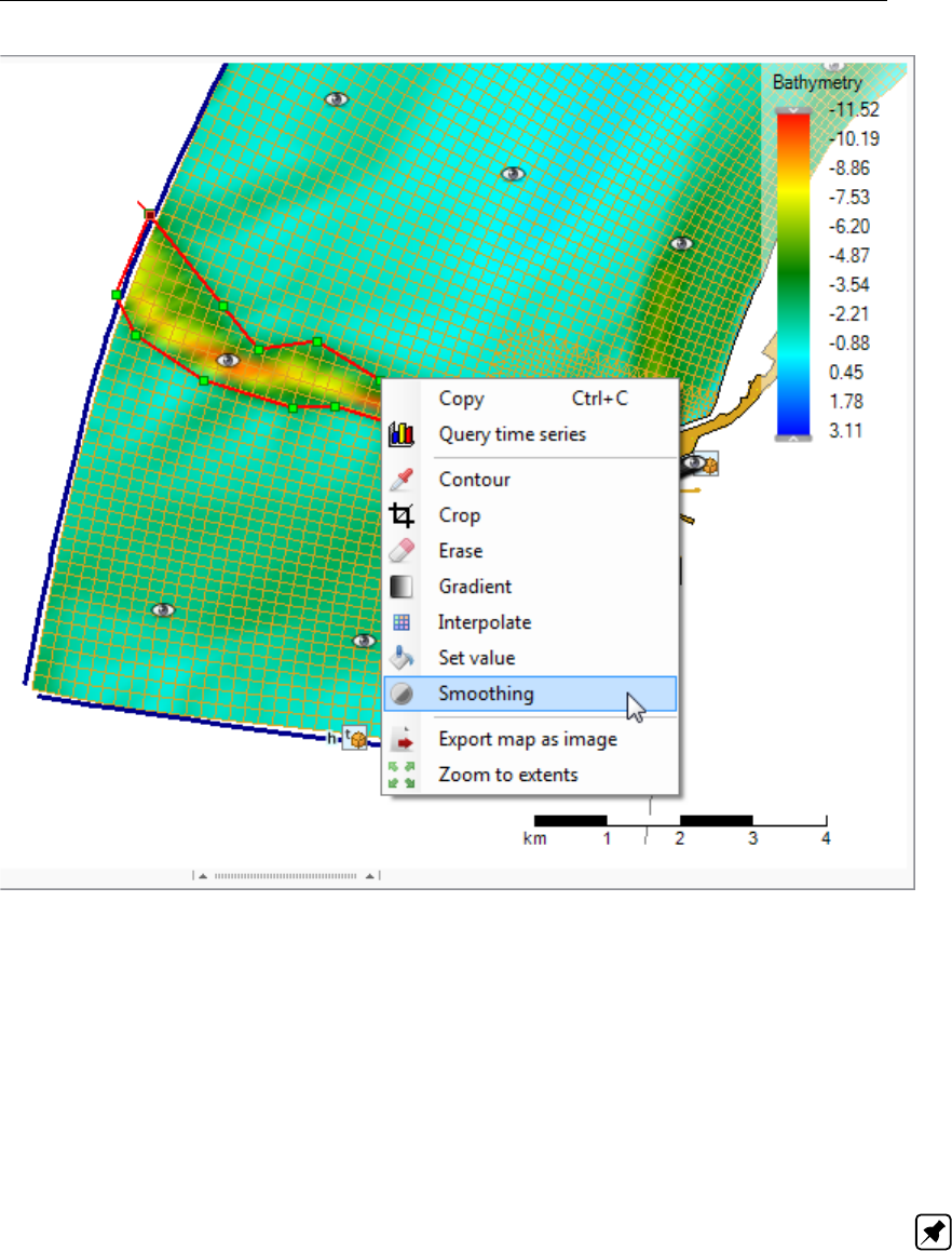
DRAFT
Spatial editor
Figure F.9: Selecting a smoothing operation for a polygon geometry from the context
menu (using context menu)
F.3 Quantity selection
A spatial quantity can be activated/selected either by double clicking it in the project tree (Figure F.10)
or by selecting it from the dropdown box in the “Map” ribbon (Figure F.11). Upon selecting the spatial
quantity it will be shown as a point cloud (for a dataset) or coverage (for model input) on the central
map. Typically, you start from a point cloud (either obtained from import or by generating samples
yourself) which will eventually be interpolated to a grid or network (e.g. coverage). The spatial editor
will keep track of both the changes made to the point cloud(s) and coverage of the selected spatial
quantity. The information will be saved in the Delta Shell project and available the next time you open
the project. Note: The operations are not yet saved in a human-readable/editable file
Deltares 381 of 412
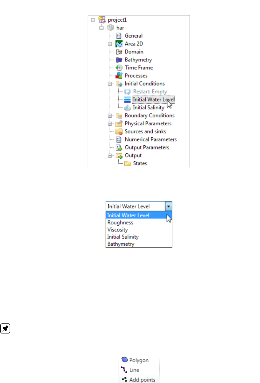
DRAFT
D-Flow Flexible Mesh, User Manual
Figure F.10: Activating a spatial quantity by double clicking it in the project tree (in this
example ‘Initial Water Level’)
Figure F.11: Activating a spatial quantity by selecting it from the dropdown box in the
‘Map’ ribbon
F.4 Geometry operations
The spatial editor supports three types of geometry operations: (1) polygons, (2) lines and (3) points
(see also Figure F.12). The following sub-sections subsequently describe how these geometries can be
selected and edited. If you do not select any of these three geometry operations, the spatial operation
automatically applies to all the data.
Note: Please note that the drawn geometries are not yet persistent, implying that the geome-
tries once drawn cannot be edited yet. Upon pressing the “Esc” button while in editing mode
all drawn geometries will dissapear.
Figure F.12: Overview of the available geometry operations in the ‘Map’ ribbon
382 of 412 Deltares
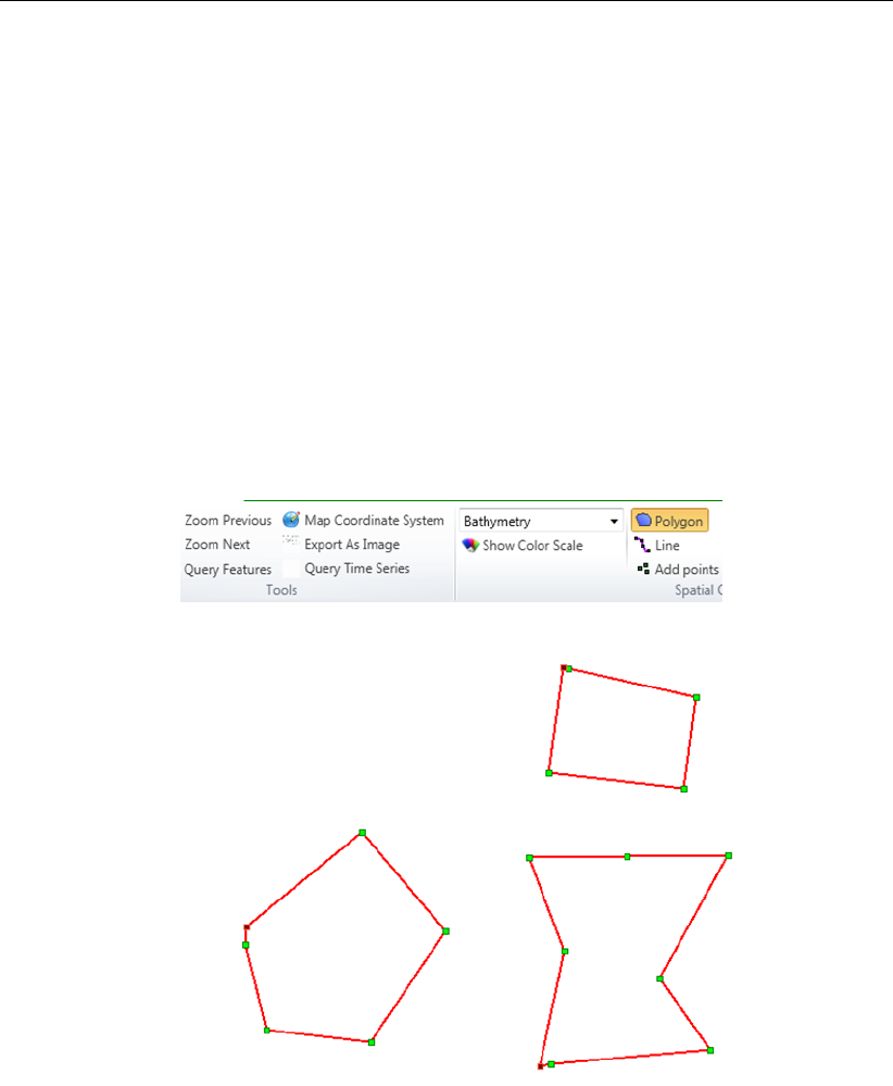
DRAFT
Spatial editor
F.4.1 Polygons
Upon selecting “Polygon” from the “Map” ribbon you can draw one or multiple polygons (Figure F.13).
Each polygon point is defined by a single click with the LMB. The polygon is closed by double clicking
the LMB. After drawing the (first) polygon, the available spatial operations for polygons are enabled in
the “Map” ribbon. The following spatial operations are available for polygons:
Crop (section F.5.2)
Erase (section F.5.3)
Set Value (section F.5.4)
Contour (section F.5.5)
Gradient (section F.5.9)
Smoothing (section F.5.11)
Interpolate - only in case samples and a grid/network are available (section F.5.10)
Copy to samples (section F.5.6)
The selected spatial operation applies to all the drawn polygons.
Figure F.13: Activating the polygon operation and drawing polygons in the central map.
F.4.2 Lines
Upon selecting “Line” from the “Map” ribbon you can draw one or multiple lines (Figure F.14). Each
line point is defined by a single click with the LMB. The line is completed by double clicking the LMB.
After drawing the (first) line, the available spatial operations for lines are enabled in the “Map” ribbon.
The following spatial operations are available for lines:
Contour (section F.5.5)
The selected spatial operation applies to all the drawn lines.
Deltares 383 of 412
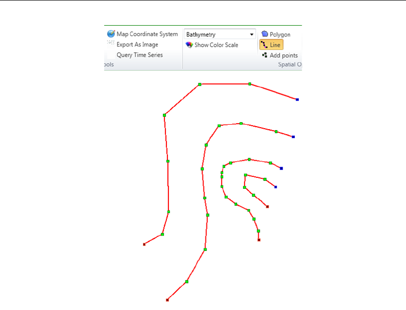
DRAFT
D-Flow Flexible Mesh, User Manual
Figure F.14: Activating the line operation and drawing lines in the central map.
F.4.3 Points
Upon selecting “Add points” from the “Map” ribbon you can draw one or multiple points and assign a
uniform value to them (Figure F.15). Each point is defined by a single click with the LMB. The group
of points is completed by double clicking the LMB. Upon double clicking a popup appears in which you
can assign a value to the points.
384 of 412 Deltares
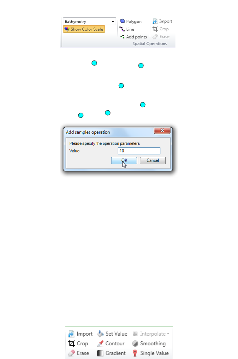
DRAFT
Spatial editor
Figure F.15: Activating the ‘Add points’ operation, drawing them in the central map and
assigning a value to them.
F.5 Spatial operations
The spatial editor supports the following spatial operations (see also Figure F.16):
Import (section F.5.1) - only for point clouds
Crop (section F.5.2)
Erase (section F.5.3)
Set Value (section F.5.4)
Contour (section F.5.5) - only for point clouds
Gradient (section F.5.9)
Interpolate (section F.5.10) - only for point clouds
Smoothing (section F.5.11)
Change single value (section F.5.12) - only for grid coverages
Merge spatial data (section F.5.8) - only for grid coverages
Copy to samples (section F.5.6) - only for grid coverages
Copy to spatial data (section F.5.7) - only for grid coverages
Figure F.16: Overview of the available spatial operations in the ‘Map’ ribbon
The sections below provide a description of each operation.
Deltares 385 of 412
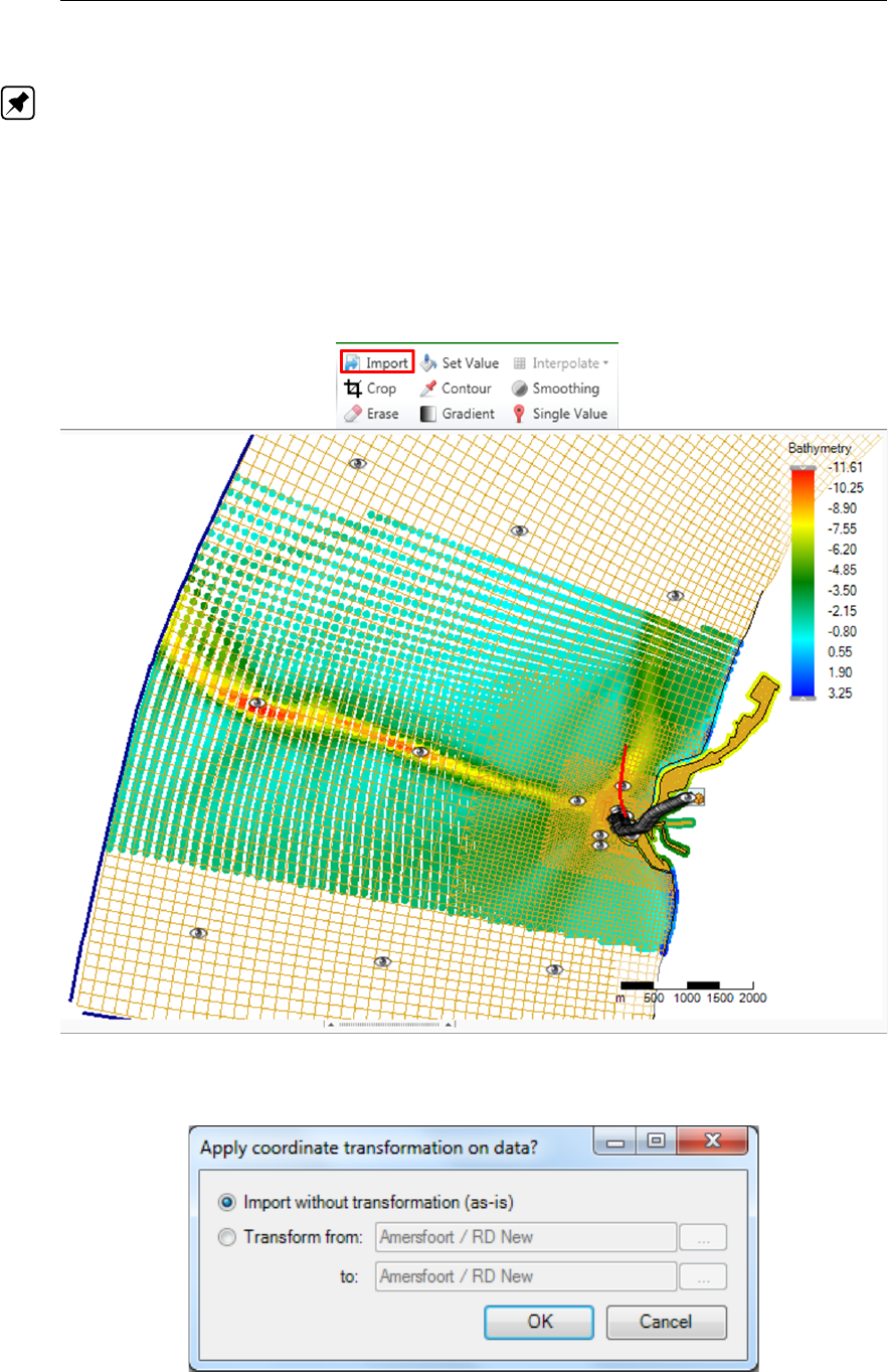
DRAFT
D-Flow Flexible Mesh, User Manual
F.5.1 Import point cloud
With the import operation you can import a point cloud for the selected spatial quantity (Note: To
import a coverage select ‘Import’ from the context menu of the spatial quantity in the project tree).
For this operation no geometry is required. The import operation is activated from the ‘Map’ ribbon
(Figure F.17). Upon importing a point cloud you are asked whether a coordinate transformation should
be applied to the imported dataset (Figure F.18). By default it will be assumed that the imported data
is in the same coordinate system as the model. If not, you can indicate from which to which coordinate
system the data should be transformed. After import the point cloud is added to the operations stack
(Figure F.19). The difference between this importer and importing a point cloud on the project or model
level in the project tree (section F.2.2) is that for this importer the point cloud is directly assigned to the
selected spatial quantity (e.g. model input) instead of being treated as a separate dataset.
Figure F.17: Importing a point cloud using the ‘Import’ operation from the ‘Map’ ribbon
Figure F.18: Option to perform a coordinate transformation on the imported point cloud
386 of 412 Deltares

DRAFT
Spatial editor
Figure F.19: Appearance of import point cloud operation in the operations stack
F.5.2 Crop
The crop operation crops a point cloud or coverage (depending on which one is active). The crop
operation is activated from the ‘Map’ ribbon. and only available for polygon geometries. You can
control which part of the data should be erased by using polygons. If you provide a polygon outside
the point cloud or coverage, all data will be erased. For an example see Figure F.20. After cropping
(part of) the point cloud of coverage the operation is added to the operations stack (Figure F.21).
Figure F.20: Performing a crop operation on a point cloud with a polygon using ‘Crop’
from the ‘Map’ ribbon
Figure F.21: Appearance of crop operation in the operations stack
Deltares 387 of 412
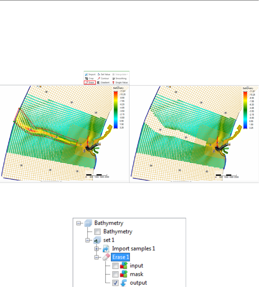
DRAFT
D-Flow Flexible Mesh, User Manual
F.5.3 Erase
The erase operation erases (part of) a point cloud or coverage (depending on which one is active).
The erase operation is activated from the ‘Map’ ribbon. You can control which part of the data should
be erased by using polygons. If no polygons are provided, the total dataset will be erased. For an
example see Figure F.22. After erasing (part of) the point cloud or coverage the operation is added to
the operations stack (Figure F.23).
Figure F.22: Performing an erase operation on a point cloud with a polygon using ‘Erase’
from the ‘Map’ ribbon
Figure F.23: Appearance of erase operation in the operations stack
F.5.4 Set value
The set value operation assigns a value to a point cloud or coverage (depending on which one is
active). The set value operation is activated from the ‘Map’ ribbon and only available for polygon
geometries or for the total data set if no polygon is provided. By assigning a value can choose from
the following operations:
Overwrite : overwrites all existing points within the polygon (excluding no data values) with the
uniform value
Overwrite where missing (only for coverages) : overwrites all missing values within the polygon
with the uniform value
Add : Adds the uniform value to all existing points within the polygon (excluding no data values)
Subtract : Subtracts the uniform value from all existing points within the polygon (excluding no
data values)
Multiply : Multiplies all existing points within the polygon (excluding no data values) with the uni-
form value
Divide : Divides all existing points within the polygon (excluding no data values) by the uniform
value
Maximum : Sets all existing points within the polygon (excluding no data values) to the maximum
of its current value and the uniform value
388 of 412 Deltares
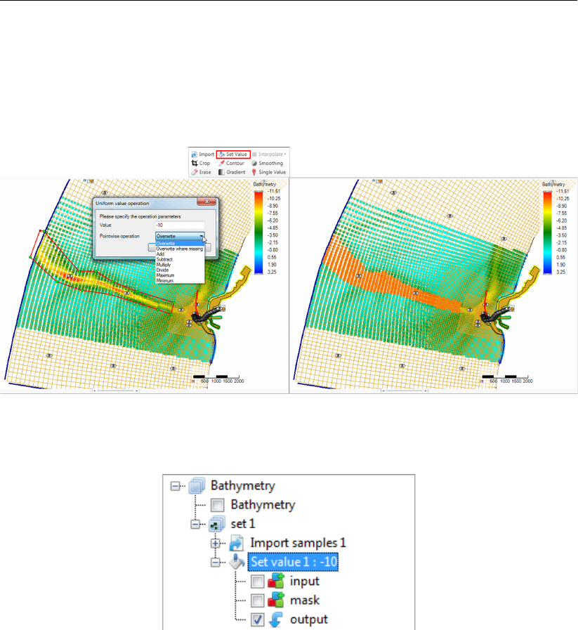
DRAFT
Spatial editor
Minimum : Sets all existing points within the polygon (excluding no data values) to the minimum
of its current value and the uniform value
For an example see Figure F.24. After performing a set value operation to (part of) the point cloud or
coverage the operation is added to the operations stack (Figure F.25).
Figure F.24: Performing a set value operation (e.g. overwrite) on a point cloud with a
polygon using ‘Set Value’ from the ‘Map’ ribbon
Figure F.25: Appearance of set value operation in the operations stack
F.5.5 Contour
The contour operation creates a point cloud with a uniform value along a line or polygon (depending
on which one is active). The contour operation is activated from the ‘Map’ ribbon. After drawing the
lines or polygons you have to assign the uniform value (argument) and the sampling interval in m.
This spatial operation can be useful to digitalize information from nautical charts for example. In this
case you first have to import the nautical chart as a geotiff (Figure F.26), set the right map coordinate
system (Figure F.27) and then use the contour operation Figure F.28. Sometimes the samples are
created behind the geotiff. Then you can use the context menu on the samples layer in the Map tree
to bring the samples to the front (Figure F.29). After applying the contour operation it is added to the
stack (Figure F.30).
Deltares 389 of 412
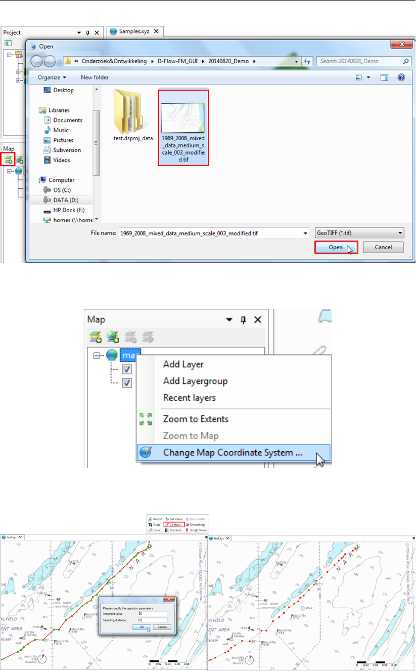
DRAFT
D-Flow Flexible Mesh, User Manual
Figure F.26: Import a nautical chart as a georeferenced tiff file
Figure F.27: Set the right map coordinate system for the geotiff
Figure F.28: Performing a contour operation on a nautical chart using lines to define the
contours and ‘Contour’ from the ‘Map’ ribbon
390 of 412 Deltares
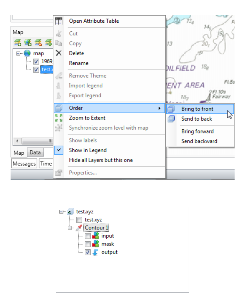
DRAFT
Spatial editor
Figure F.29: Bring the sample set to the front if it appears behind the nautical chart
Figure F.30: Appearance of contour operation in the operations stack
F.5.6 Copy to samples
This operation converts the currently selected grid coverage to a sample set, which becomes that
starting point of a new subset. If polygons have been drawn, the operation will confine the copy to the
interiors. The operation will not convert missing values to samples. Note that the operation does keep
a reference to the original copied grid coverage; if it is changes by a re-evaluation of the stack, the
changes will affect the output point cloud.
Deltares 391 of 412
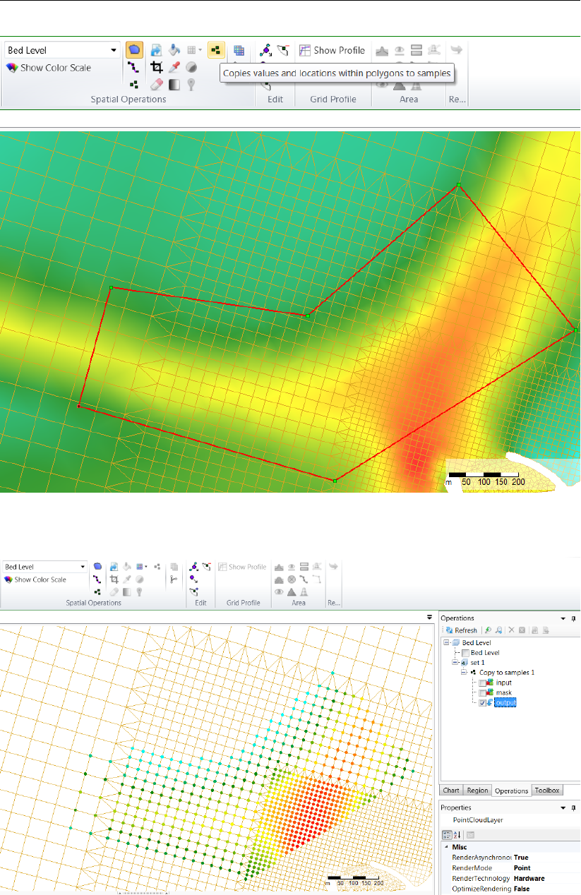
DRAFT
D-Flow Flexible Mesh, User Manual
Figure F.31: Applying the copy to samples operation
Figure F.32: Copy to samples operation result
392 of 412 Deltares
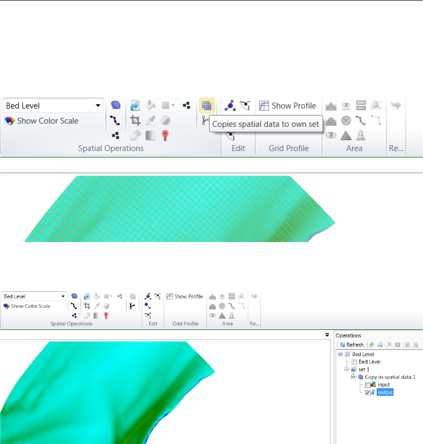
DRAFT
Spatial editor
F.5.7 Copy to spatial data
This operation simply clones the grid coverage, starting a new subset with a snapshot of the currently
selected operation output. Similarly to F.5.6, it keeps a reference to the input data and will perform the
clone again upon re-evaluation.
Figure F.33: Applying the copy spatial data operation
Figure F.34: Copy spatial data operation result
F.5.8 Merge spatial data
Whenever a subset contains a grid coverage as its editing data (after applying e.g. F.5.7) on the same
grid as the main operation set, its result can be combined with the main set by applying this operation,
similarly to the interpolation operation for sample sets, discussed below. Combing the grid coverages
can be achieved with the usual pointwise methods.
Deltares 393 of 412
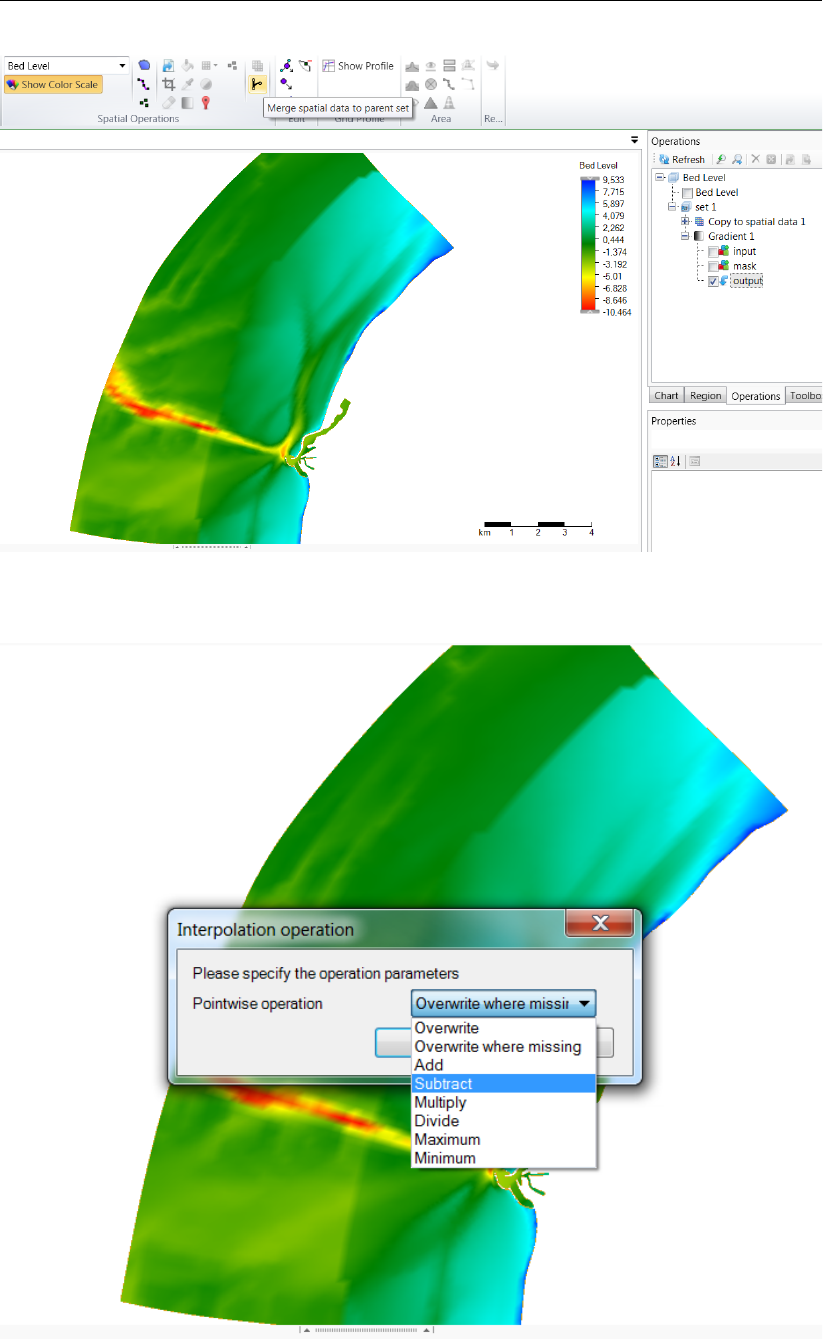
DRAFT
D-Flow Flexible Mesh, User Manual
Figure F.35: Activating the merge spatial data tool from the ribbon
Figure F.36: The merge operation requests a pointwise combination method
394 of 412 Deltares

DRAFT
Spatial editor
Figure F.37: Resulting grid coverage
F.5.9 Gradient
The gradient operation applies a gradient to a point cloud or grid coverage (depending on which one
is active). The gradient operation is activated from the ‘Map’ ribbon and only available for polygon
geometries or for the total data set if no polygon is provided. You have to assign the initial (start) value,
the final (end) value and the going to angle (according to the Cartesian convention with 0 degrees is
East, 90 degrees is North, etc Note: This is not working properly yet). For an example see Figure F.38.
After applying a gradient to (part of) the point cloud or coverage the operation is added to the operations
stack (Figure F.39).
Figure F.38: Performing a gradient operation on a point cloud with a polygon using ‘Gra-
dient’ from the ‘Map’ ribbon
Deltares 395 of 412
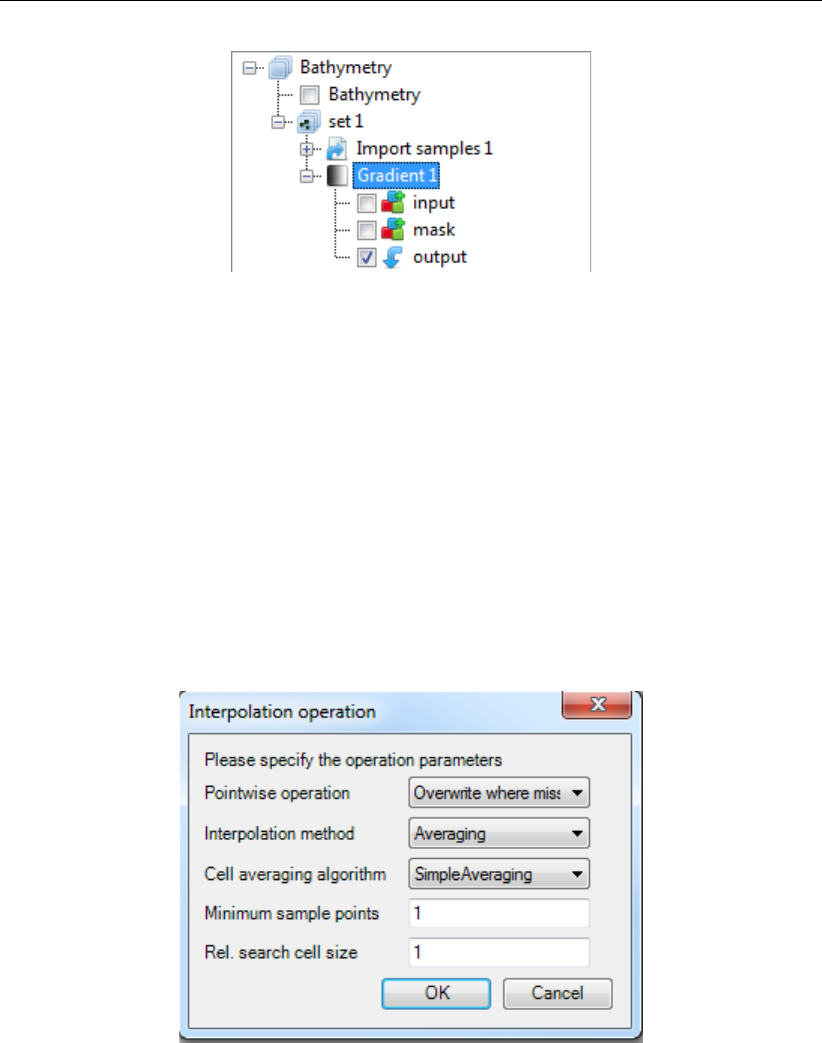
DRAFT
D-Flow Flexible Mesh, User Manual
Figure F.39: Appearance of gradient operation in the operations stack
F.5.10 Interpolate
The interpolate operation is the way to get sample set(s) to a grid or network (e.g. coverage). In the
operation stack this means that we are actively switching from working on a point cloud (helping to
construct the coverage) to working on the selected coverage (or spatial quantity). The interpolation
is performed on the data within a polygon or polygons (if provided) or all the data (if no polygons are
provided). The interpolate operation can be performed on a single (selected) sample set or on multiple
sample sets. Both methods are discussed below. The methods for interpolation are either
Triangulation: performs a Delauney triangulation on the sample point set before projecting onto the
grid.
Averaging: combines sample points within a possible enlarged cell according an algorithm of
choice. The user can set the search cell expansion factor (rel. search cell size) and a thresh-
old for the number of sample points within a cell (minimum sample points), see Figure F.40.
Figure F.40: Interpolation Operation options
Seven Cell averaging algorithms can be chosen by the user; see Figure F.41. These algorithms are
explained below:
SimpleAveraging: bilinear interpolation is applied, which uses a distanceweighted average of the
surrounding samples. The closer the sample point the larger the weighted value.
ClosestPoint: the value of the closest sample inside the search area is taken.
MaximumValue: the maximum value of the samples inside the search area is taken.
MinimumValue: the minimum value of the samples inside the search area is taken.
InverseWeightedDistance: Instead of a distanceweighted average (w) in case of the inverse of
SimpleAveraging, the distanceweighted average (1/w) is taken. The closer the sample point the
smaller the weighted value.
MinAbs: the minimum of the absolute values of the samples inside the search area is taken.
KdTree: This is an obsolete option, which will be removed in a future release.
396 of 412 Deltares
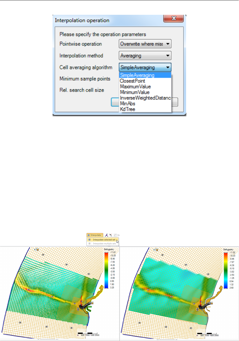
DRAFT
Spatial editor
Figure F.41: Averaging options
By default, the interpolation will only overwrite missing values in the gridded data set. However, if the
grid coverage already contains values, the user may choose to overwrite or combine the data by a
pointwise arithmetic operation.
Interpolate single (selected) set
To perform interpolation on a single sample set, select the sample set (i.e. ‘set1’) in the operation stack
and press ‘Interpolate’ in the ‘Map’ ribbon (Figure F.42). Since no polygon is provided in this example,
all the samples will be interpolated to the grid. Use polygons if you would like to have more control over
the interpolation. After the interpolation the operation is added to the operations stack (Figure F.43).
Please note that after performing the interpolation the workflow in the stack is shifting from the sample
set (i.e. ‘set1’ - which was a side step to construct the coverage) to the coverage (i.e. ‘bed level’).
Figure F.42: Performing an interpolation operation on a single sample set (without using
a polygon) using ‘Interpolate’ from the ‘Map’ ribbon
Deltares 397 of 412
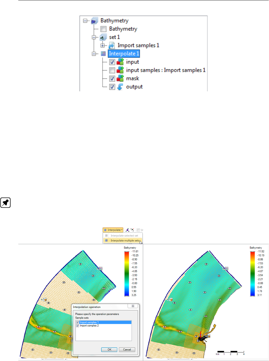
DRAFT
D-Flow Flexible Mesh, User Manual
Figure F.43: Appearance of interpolation of ‘set1’ to the coverage ’bed level’ in the oper-
ations stack
Interpolate multiple sets
To perform interpolation on multiple sample sets, select the active coverage (i.e. ‘bed level’) in the
operation stack and press ‘Interpolate’ in the ‘Map’ ribbon (Figure F.44). In the popup you can select
which sample sets to include in the interpolation (in this example both). Since no polygon is provided,
all the samples (from the two sets) will be interpolated to the grid. Use polygons if you would like to
have more control over the interpolation. After the interpolation the operation is added to the operations
stack (Figure F.45). Again note that after performing the interpolation the workflow in the stack is
shifting from the sample set (which was a side path to construct the coverage) to the coverage (i.e. bed
level).
Note: Please note that interpolation of multiple sample sets can also be achieved by importing/com-
bining different sample sets into the same set in the stack instead of using two separate sets. In this
case you can just interpolate the single (selected) set.
Figure F.44: Performing an interpolation operation on multiple sample sets (without using
a polygon) using ‘Interpolate’ from the ‘Map’ ribbon
398 of 412 Deltares
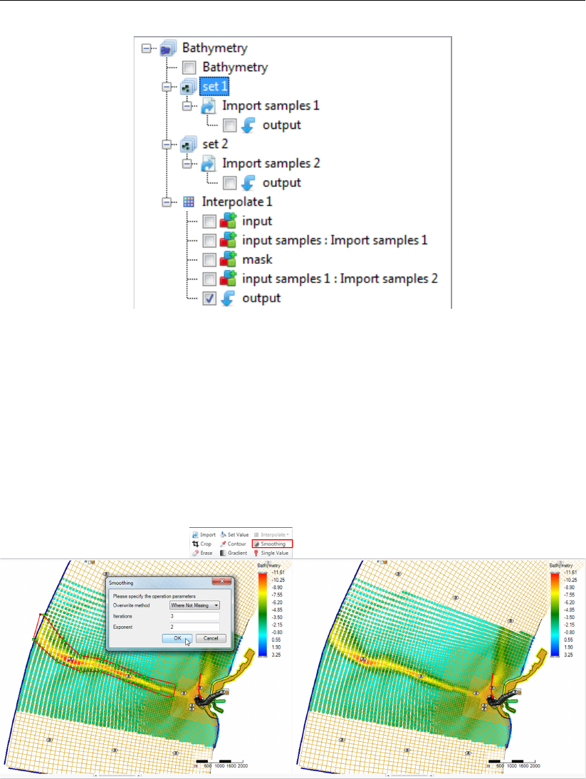
DRAFT
Spatial editor
Figure F.45: Appearance of interpolation of ‘set1’ and ‘set2’ to the coverage ’bed level’ in
the operations stack
F.5.11 Smoothing
The smoothing operation smooths out (steep) gradients in a point cloud or coverage (depending on
which one is active). The smoothing operation is activated from the ‘Map’ ribbon and only available for
polygon geometries or for the total data set if no polygon is provided. You have to assign the smoothing
exponent and number of smoothing steps. The higher the exponent and the number of smoothing
steps, the heavier the smoothing. For an example see Figure F.46. After applying smoothing to (part
of) the point cloud or coverage the operation is added to the operations stack (Figure F.47).
Figure F.46: Performing a smoothing operation on a point cloud with a polygon using
‘Smoothing’ from the ‘Map’ ribbon
Deltares 399 of 412
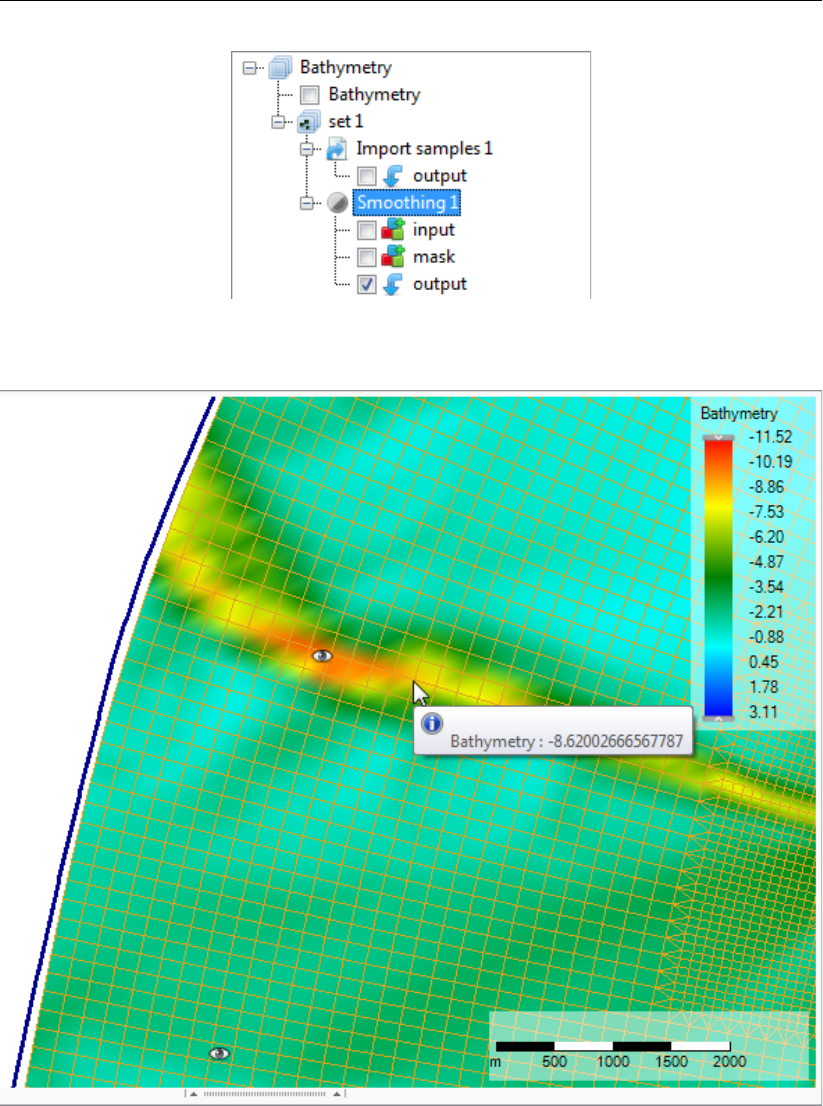
DRAFT
D-Flow Flexible Mesh, User Manual
Figure F.47: Appearance of smoothing operation in the operations stack
Figure F.48: The cursor for the overwrite operation showing the value of the closest cov-
erage point
400 of 412 Deltares
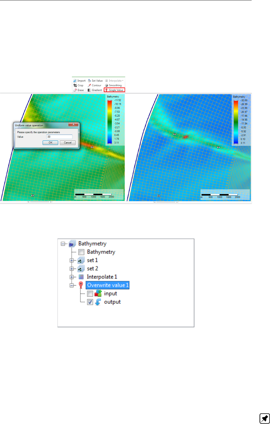
DRAFT
Spatial editor
F.5.12 Overwrite (single) value
The ‘overwrite (single) value’ operation allows you to edit single values on the active coverage after
the interpolation. The ‘overwrite (single) value’ operation is activated from the ‘Map’ ribbon. There is
no geometry required for this operation. Upon selecting the operation from the ribbon a cursor will
become active showing the coverage value closest to the cursor in a tooltipstring (Figure F.48). Upon
clicking LMB a popup appears in which you can overwrite the value of this coverage point Figure F.49.
After applying the overwrite operation it is added to the operations stack (Figure F.50).
Figure F.49: Performing an overwrite operation on a coverage point using ‘Single Value’
from the ‘Map’ ribbon
Figure F.50: Appearance of overwrite operation in the operations stack
F.6 Operation stack
The operation stack keeps track of the workflow of spatial operations that you performed. This helps
you to make transparent how you arrived at your ‘final’ dataset without having to save all the inter-
mediate datasets (steps) separately. Moreover, the stack is reproducible and easily editable without
having to start all over again. This section describes the stack workflow (section F.6.1), how to edit
operation properties (section F.6.2), how to enable/disable (section F.6.3), delete (section F.6.4), re-
fresh(section F.6.5) operations, quick links (section F.6.6) and import/export functionality (section F.6.7).
Note: Currently, the stack is saved in the Delta Shell project upon saving the project. The next time
you open the project, the stack will reappear. The stack is not (yet) saved in a human readable/editable
file.
Deltares 401 of 412

DRAFT
D-Flow Flexible Mesh, User Manual
F.6.1 Stack workflow
Upon performing a spatial operation, the ‘Operations’ panel will open (see Figure F.51) with the oper-
ations stack (tree). The stack first shows on which point cloud or coverage you are working (in this
example ‘bed level’). Subesquently, all the operations on this dataset are listed. For each operation
you can inspect what the input, mask (e.g. the geometry used for the operation) and output are for the
operation (Figure F.52). By default the stack continues from the last operation that you performed. If
you wish to work on a different dataset or operation within a dataset, you have to select that dataset or
operation in the ‘Operations’ panel with the LMB.
When working on a coverage, point clouds (or sets) can be used to construct the coverage. In that
case the stack jumps from the ‘trunk’ to a ‘branch’ and the subsequent operations are performed on the
point cloud (see Figure F.51). By selecting the set or coverage in the ‘Operations’ panel you determine
on which dataset you are working. The interpolate operation (section F.5.10) allows you to bring data
from the point cloud (branch) to the coverage (trunk). See also Figure F.51.
Figure F.51: The ‘Operations’ panel with the operations stack. In this example ‘bed level’
is the coverage (e.g. trunk) that is edited. The point clouds ‘set 1’ and ‘set 2’
(e.g. branches) are used to construct the ‘bed level’ coverage.
F.6.2 Edit operation properties
For each operation that you performed the properties (such as the value or ‘Pointwise operation’ of
a ‘Set Value’ operation) can be edited using the ‘Properties’ window (Figure F.53). Note: Please
note that the mask of an operation cannot (yet) be edited. By editing the operation properties the
operation stack becomes ‘out of sync’ and has to be refreshed for the changes to become active (see
section F.6.5).
402 of 412 Deltares
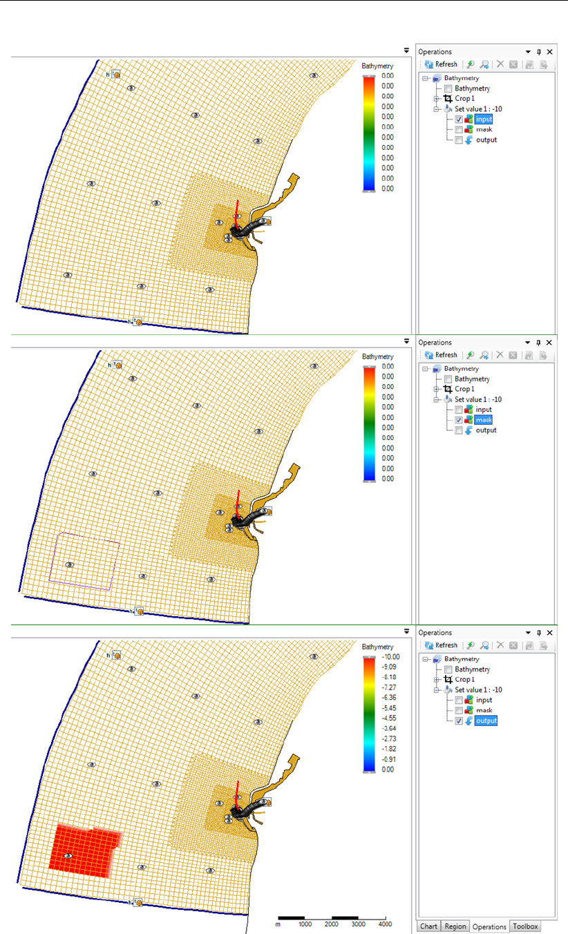
DRAFT
Spatial editor
Figure F.52: Input for the operation (top panel), mask for the operation (middle panel) and
output of the operation (bottom panel)
Deltares 403 of 412
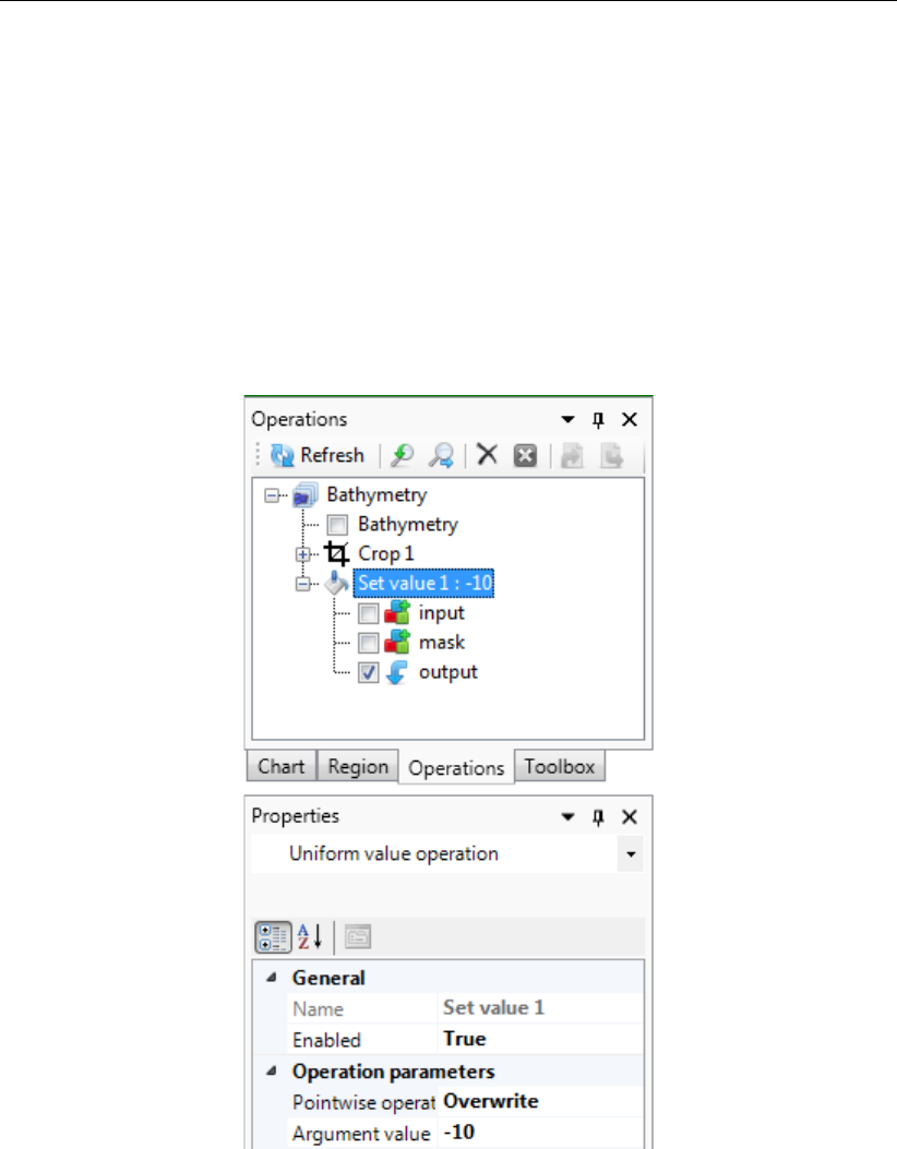
DRAFT
D-Flow Flexible Mesh, User Manual
Figure F.53: Editing the value or ‘Pointwise operation’ of a ‘Set Value’ operation using the
properties panel
404 of 412 Deltares
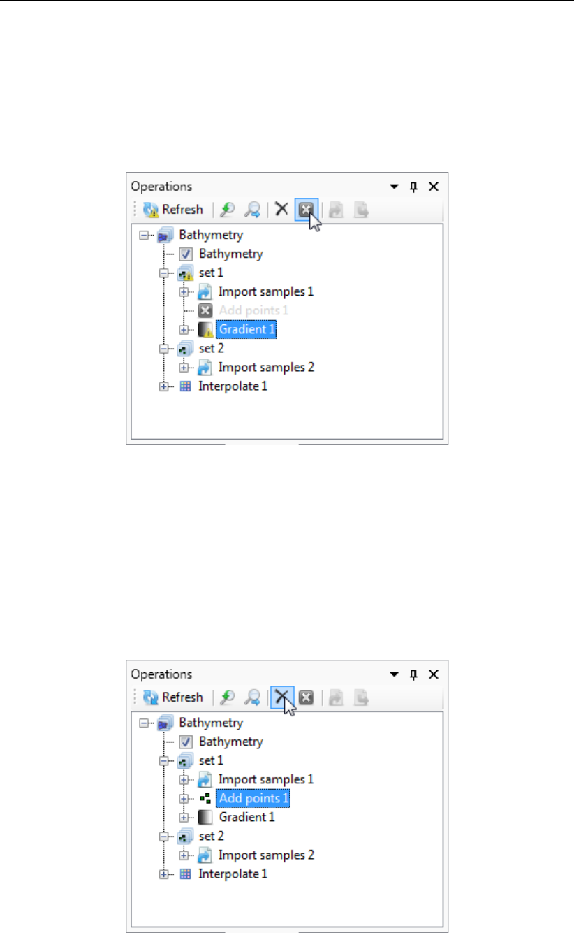
DRAFT
Spatial editor
F.6.3 Enable/disable operations
You can (temporarily) enable/disable operations by selecting the operation and pressing boxed cross
icon in the stack menu (Figure F.54). Upon disabling an operation the operation will be made grey in
the stack and the operation is not taken into account anymore upon evaluation of the overall result. The
result of disabling an operation is not directly activated. This is indicated in the stack with the ’out of
sync’ exlamation mark (Figure F.54). You need to refresh the stack (see section F.6.5) for the changes
to become active.
Figure F.54: Disabling an operation using the boxed cross icon in the stack menu. The
operation will become grey. Note the exlamation marks marking the stack
‘out of sync’.
F.6.4 Delete operations
To delete an operation permanently you have to select the operation and either press the cross icon
(Figure F.55) or use the context menu and select delete (Figure F.56). The operation will be removed
from the stack. The result of deleting an operation is not directly activated. This is indicated in the
stack with the ’out of sync’ exlamation mark. You need to refresh the stack (see section F.6.5) for the
changes to become active.
Figure F.55: Removing an operation from the stack using the cross icon in the stack menu
Deltares 405 of 412

DRAFT
D-Flow Flexible Mesh, User Manual
Figure F.56: Removing an operation from the stack using the context menu on the se-
lected operation
F.6.5 Refresh stack
When the stack is marked ‘out of sync’ by exclamation marks, you can refresh the stack by pressing
the ‘Refresh’ button for the changes to become active (Figure F.57). Upon refreshing the stack all the
(enabled) operations in the stack will be (re-)evaluated. Note: Please note that refreshing the stack
can take some time when large datasets are (re-)evaluated!
Figure F.57: Refresh the stack using the ‘Refresh’ button so that all operation are (re-)
evaluated
406 of 412 Deltares
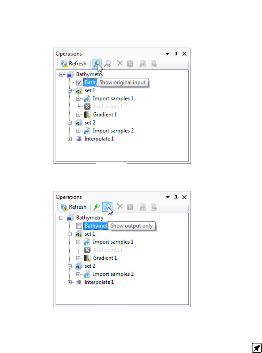
DRAFT
Spatial editor
F.6.6 Quick links
The stack menu contains two quick links to quickly show the original dataset (e.g. where you started
from, Figure F.58) and the end result of the spatial operations (Figure F.59).
Figure F.58: Quick link to the original dataset before performing any spatial operations
Figure F.59: Quick link to the output after performing all (enabled) operations
F.6.7 Import/export
Note: Importing and exporting data into or from the stack is still under construction
Deltares 407 of 412

DRAFT
D-Flow Flexible Mesh, User Manual
408 of 412 Deltares


DRAFT
D-Flow Flexible Mesh, User Manual
410 of 412 Deltares
DRAFT

PO Box 177
2600 MH Del
Boussinesqweg 1
2629 VH Del
The Netehrlands
+31 (0)88 335 81 88
sales@deltaressystems.nl
www.deltaressystems.nl
DRAFT
